Contents
Instructor's Preface vii
Student's Preface xi
Dependence Chart xiii
0 Sets and Relations 1
I
Groups and Subgroups
1 Introduction and Examples 11
2 Binary Operations 20
3 Isomorphic Binary Structures 28
. 4 Groups 36
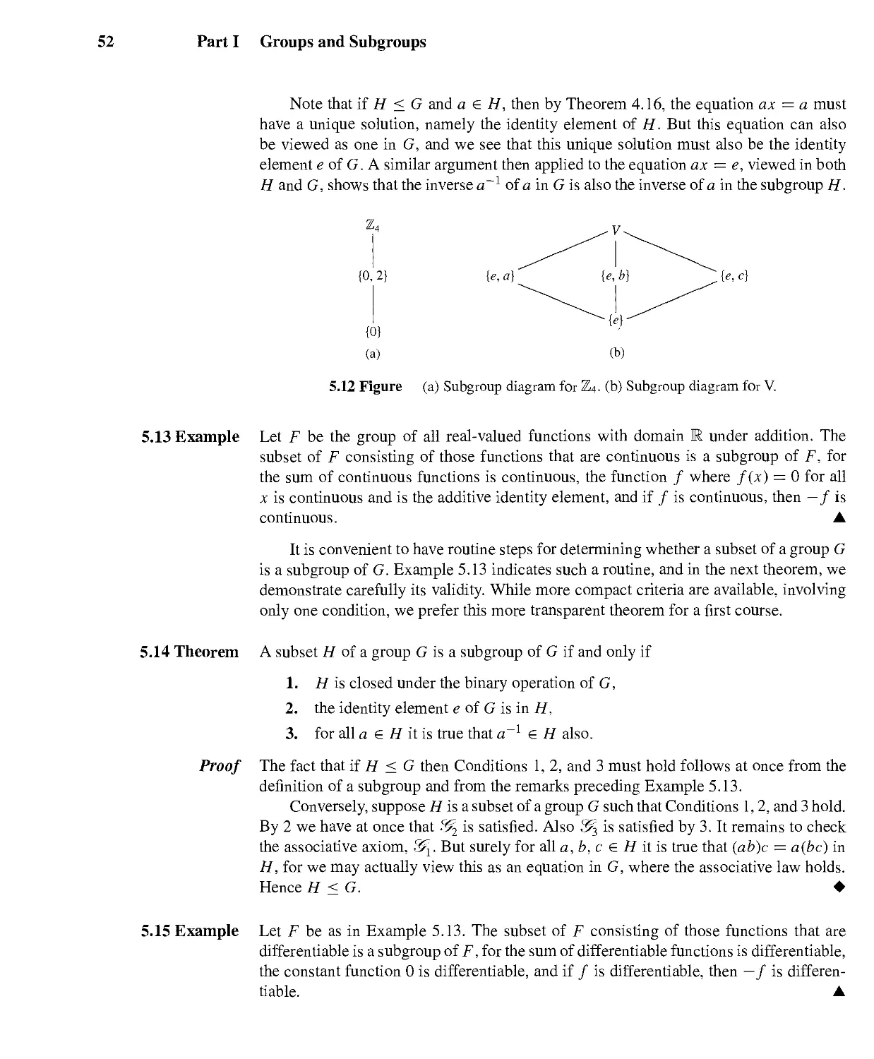
5 Subgroups 49
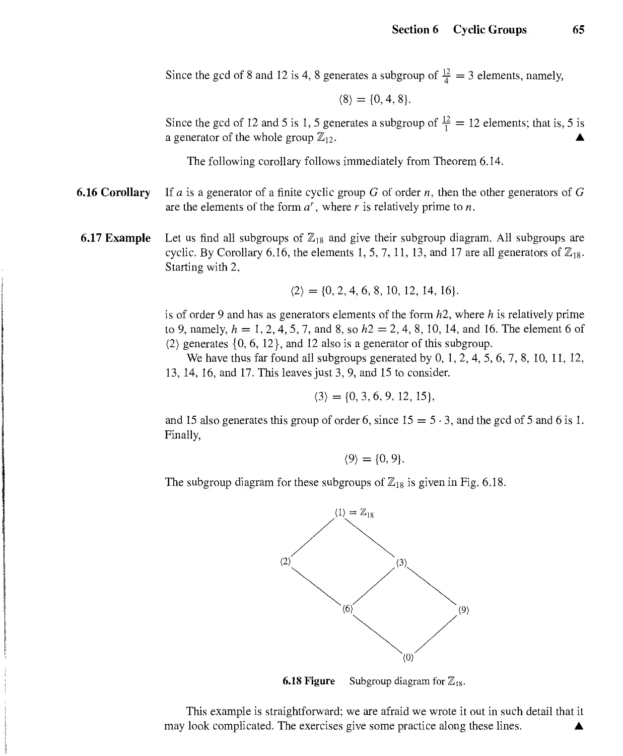
• 6 Cyclic Groups 59
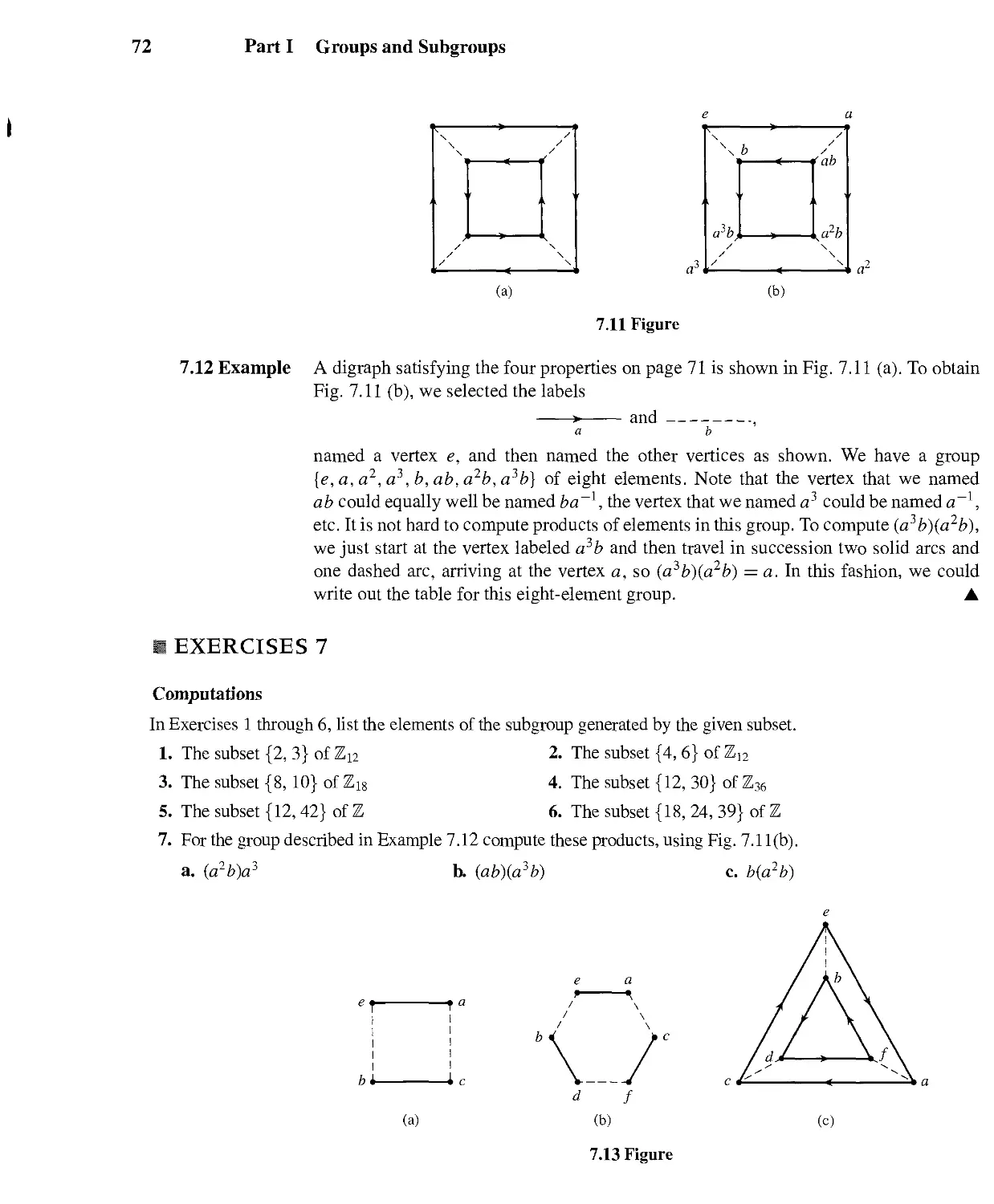
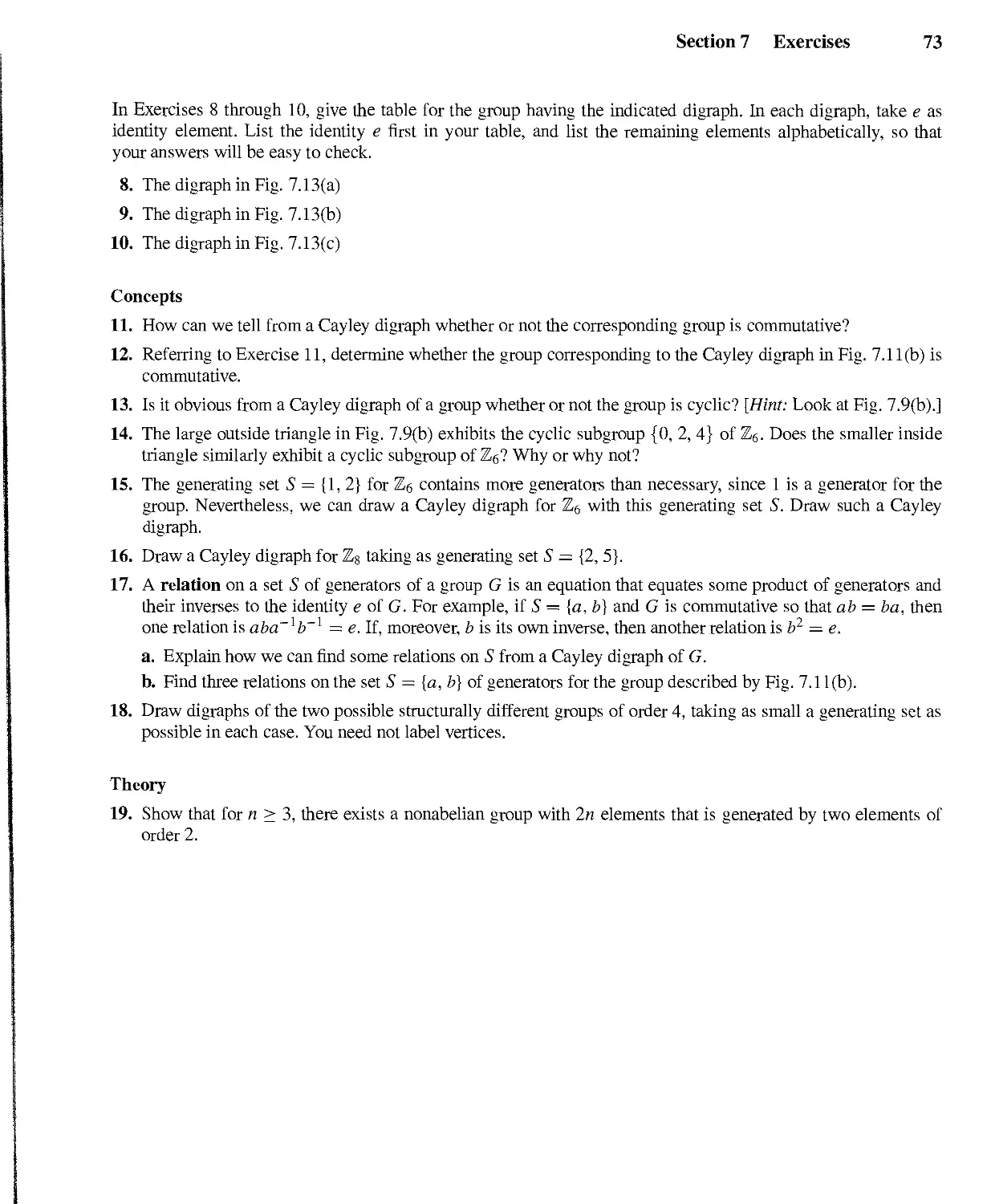
7 Generating Sets and Cayley Digraphs 68
IT
11
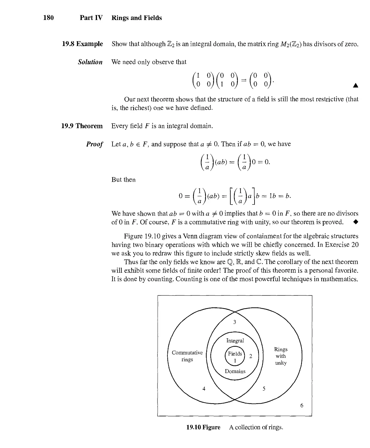
Permutations, Cosets, and Direct Products
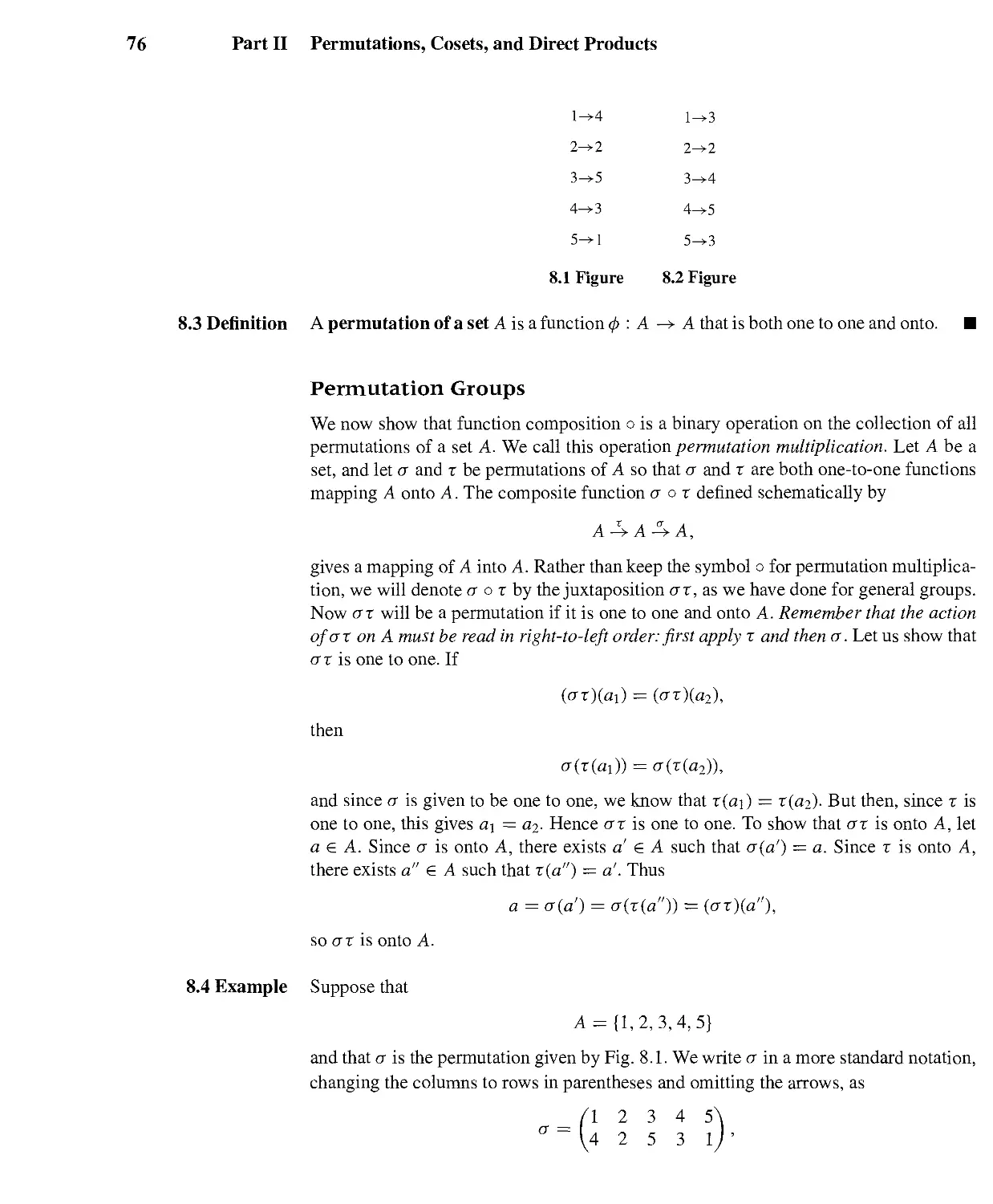
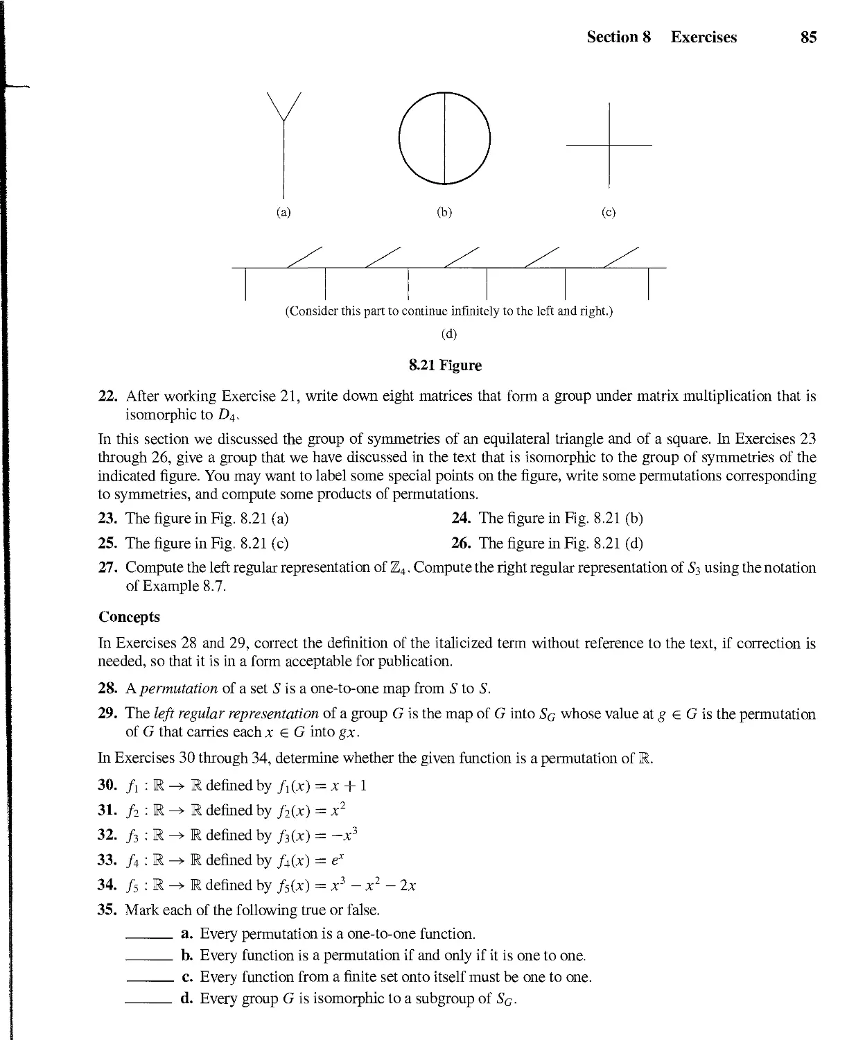
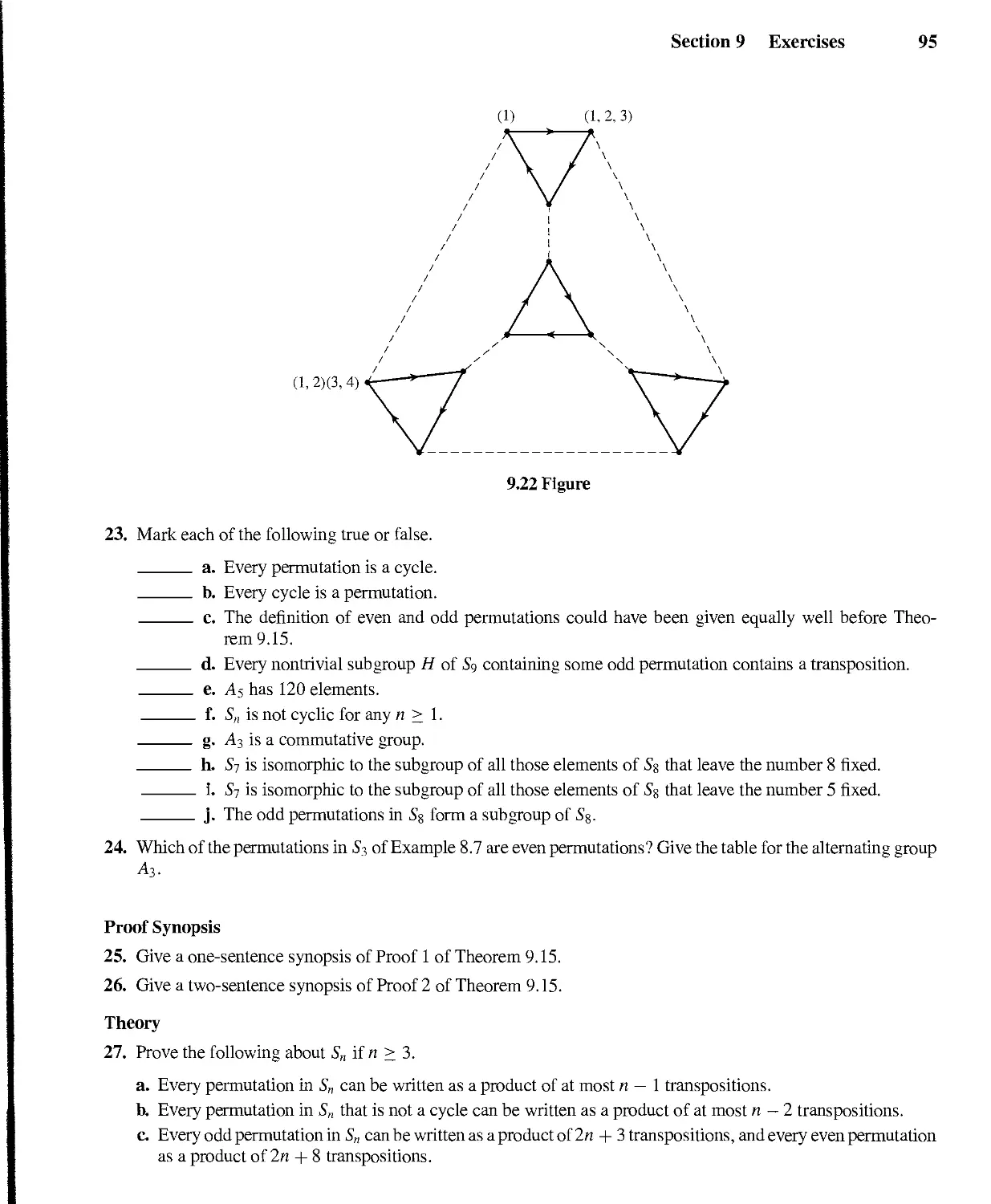
8 Groups of Permutations 75
9 Orbits, Cycles, and the Alternating Groups 87
10 Cosets and the Theorem of Lagrange 96
11 Direct Products and Finitely Generated Abelian Groups 104
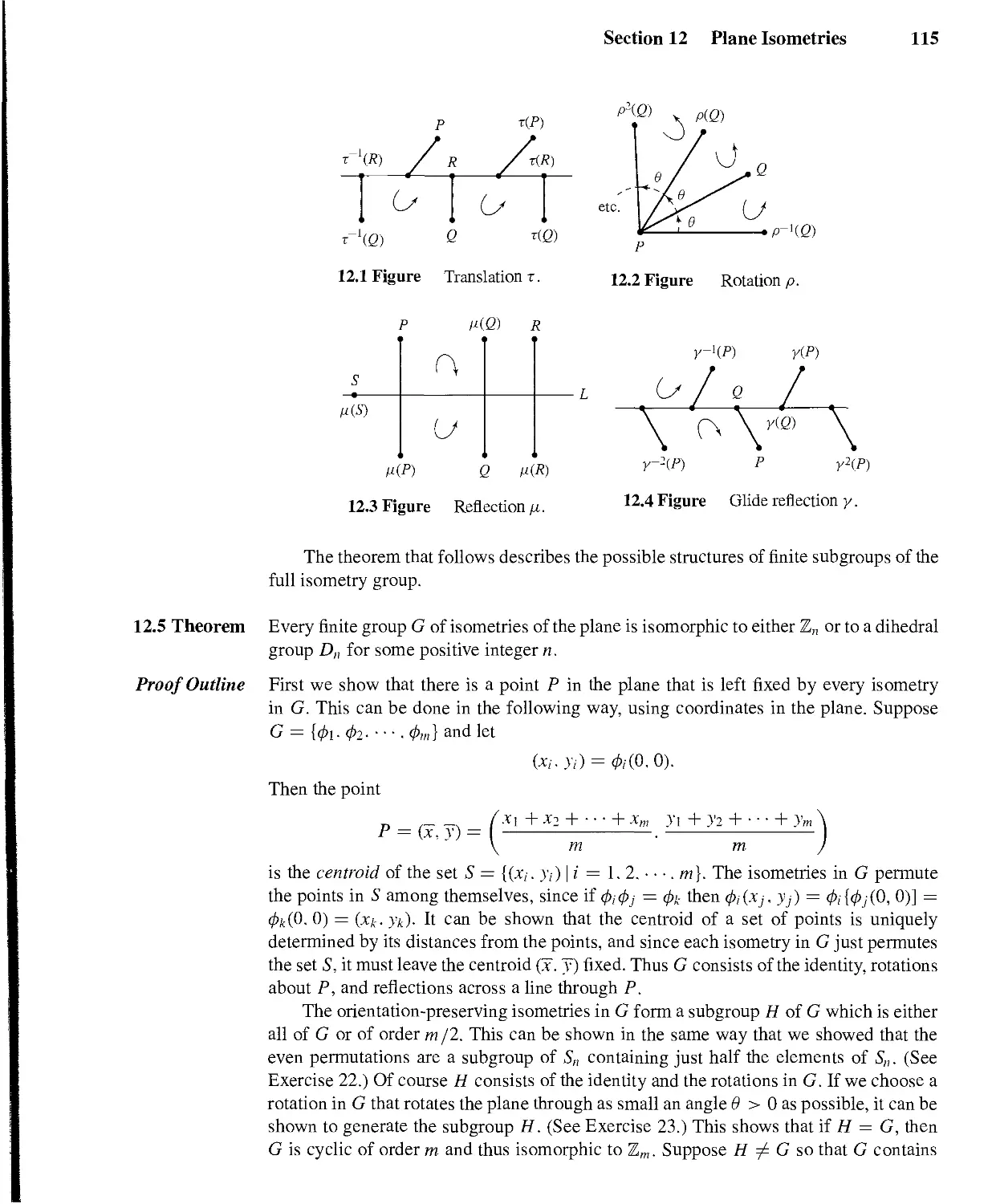
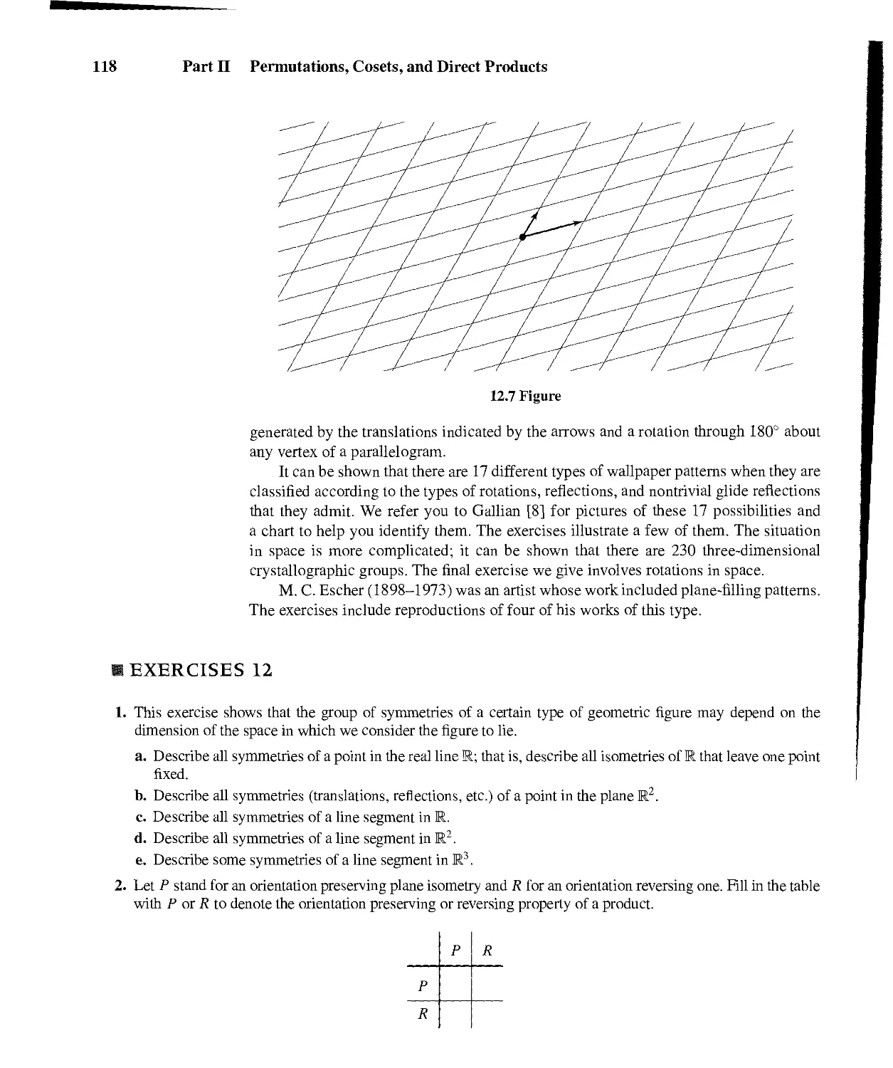
tl2 Plane Isometries 114

Contents
III
HOMOMORPHISMS AND FACTOR GROUPS 125
13 Homomorphisms 125
14 Factor Groups 135
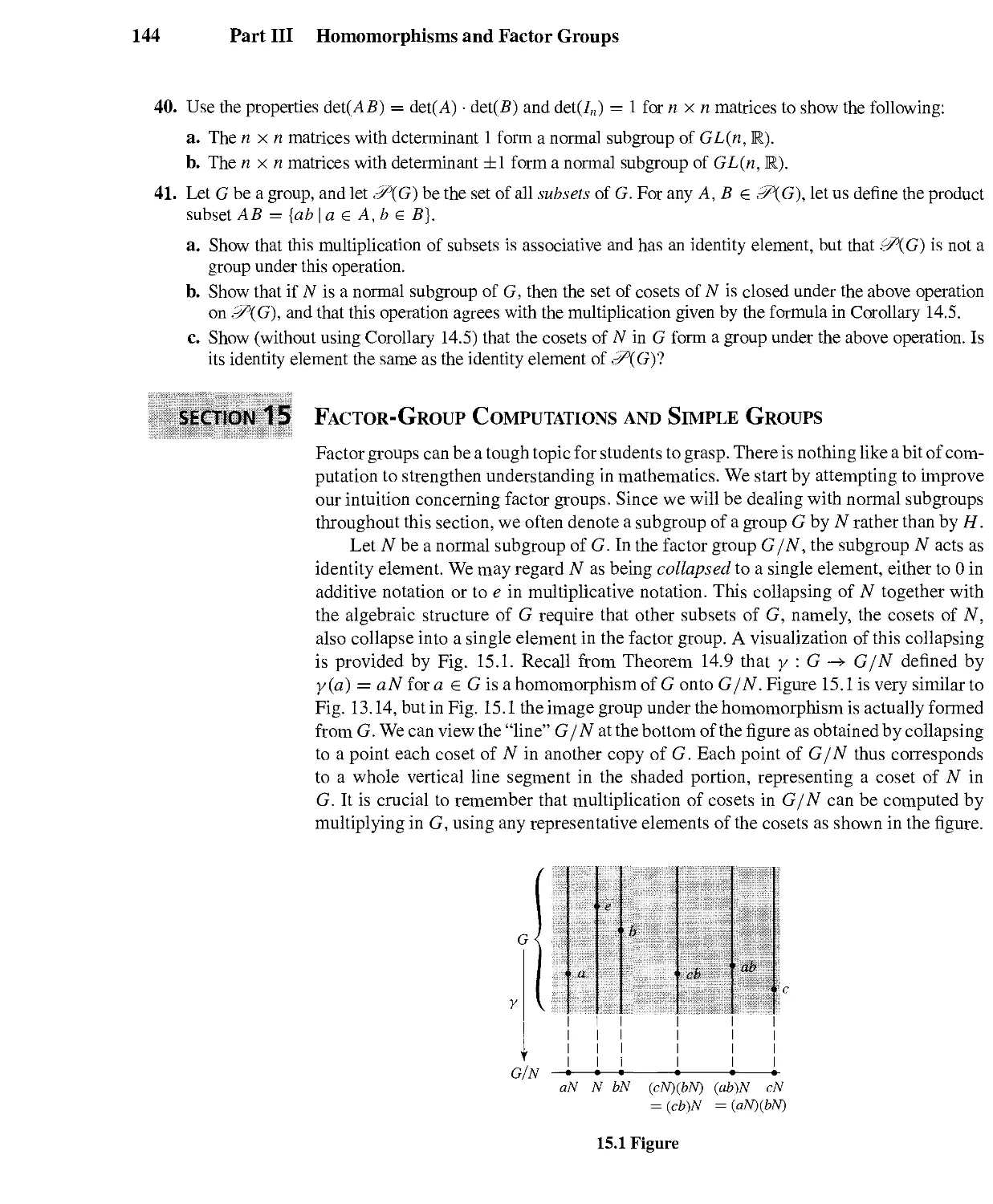
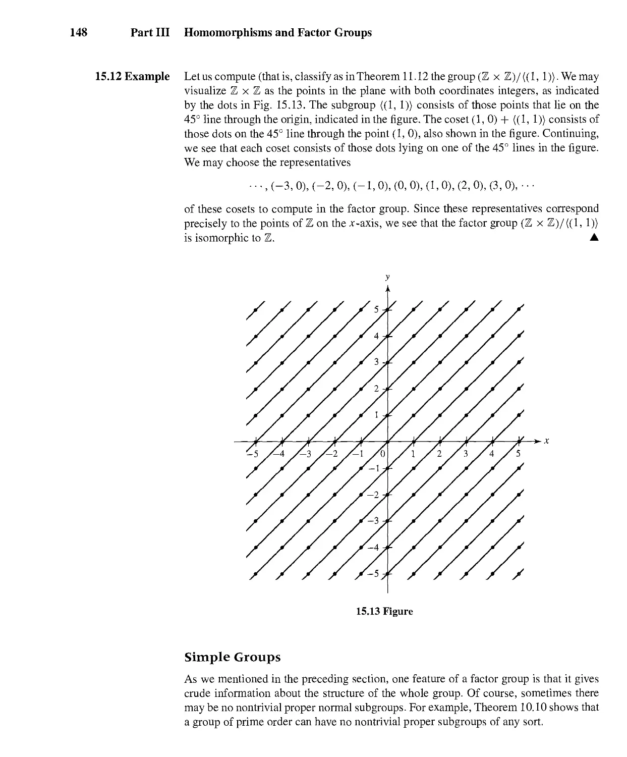
15 Factor-Group Computations and Simple Groups 144
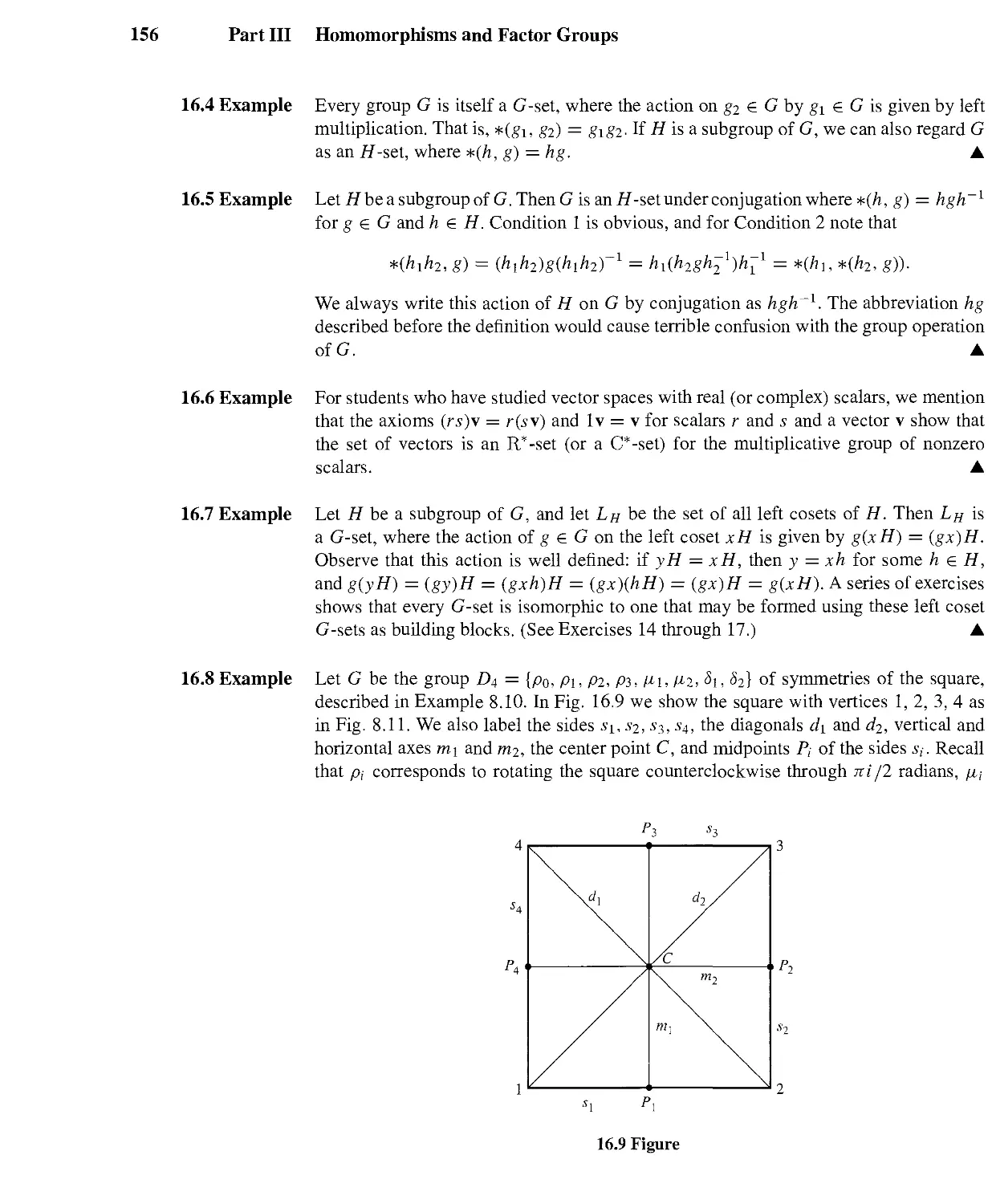
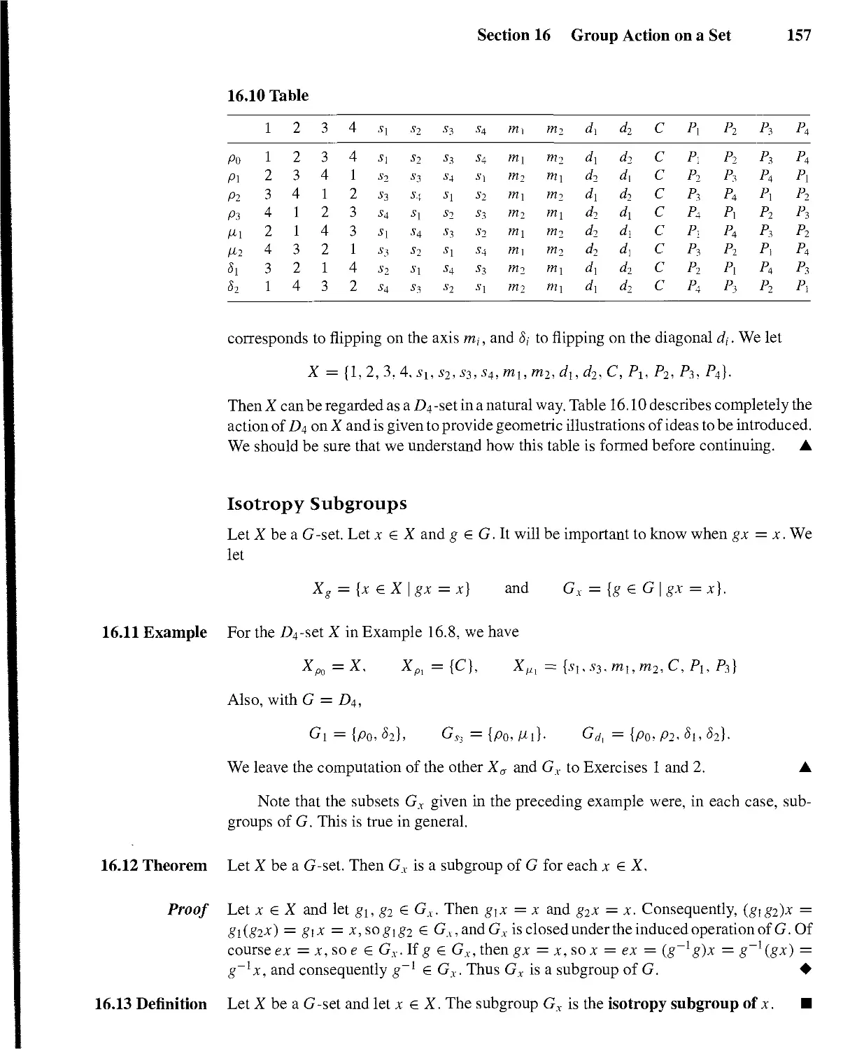
*16 Group Action on a Set 154
Tl7 Applications of G-Sets to Counting 161
Rings and Fields 167
18 Rings and Fields 167
19 Integral Domains 177
20 Fermat's and Euler's Theorems 184
21 The Field of Quotients of an Integral Domain 190
22 Rings of Polynomials 198
23 Factorization of Polynomials over a Field 209
i"24 Noncommutative Examples 220
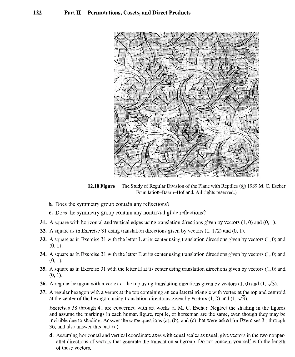
+25 Ordered Rings and Fields 227
Ideals and Factor Rings 237
26 Homomorphisms and Factor Rings 237
27 Prime and Maximal Ideals 245
+28 Grobner Bases for Ideals 254
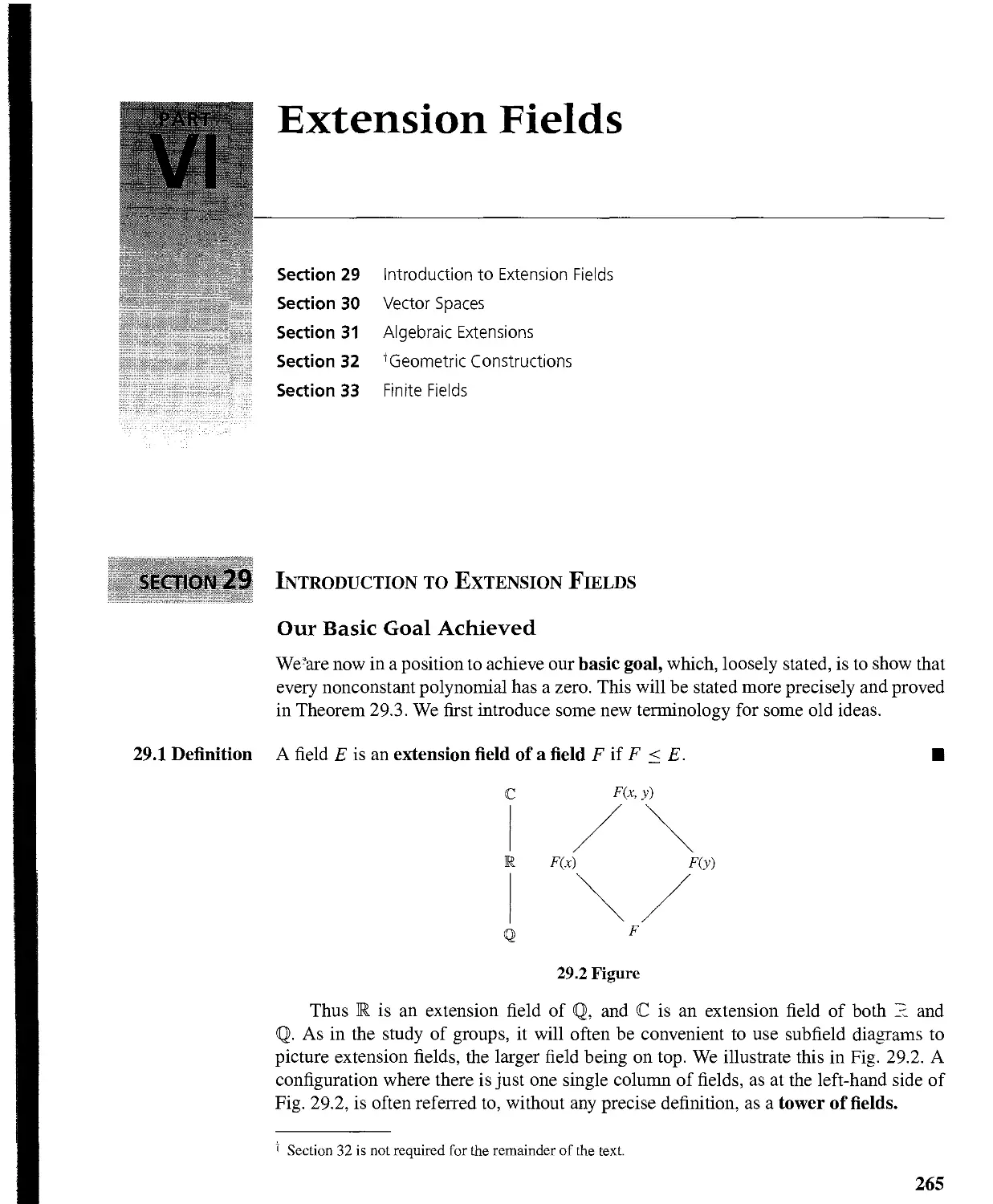
Extension Fields 265
29 Introduction to Extension Fields 265
30 Vector Spaces 274
31 Algebraic Extensions 283
^32 Geometric Constructions 293
33 Finite Fields 300
VII
Advanced Group Theory 307
34 Isomorphism Theorems 307
35 Series of Groups 311
36 Sylow Theorems 321
37 Applications of the Sylow Theory 327

Contents v
38 Free Abelian Groups 333
39 Free Groups 341
40 Group Presentations 346
'VIII
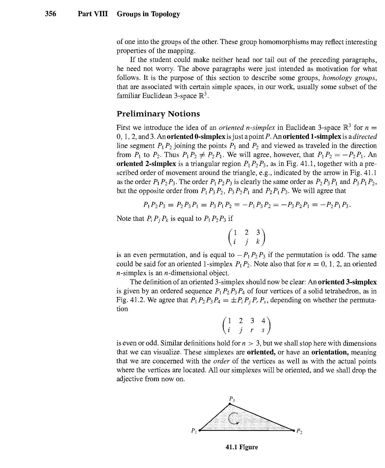
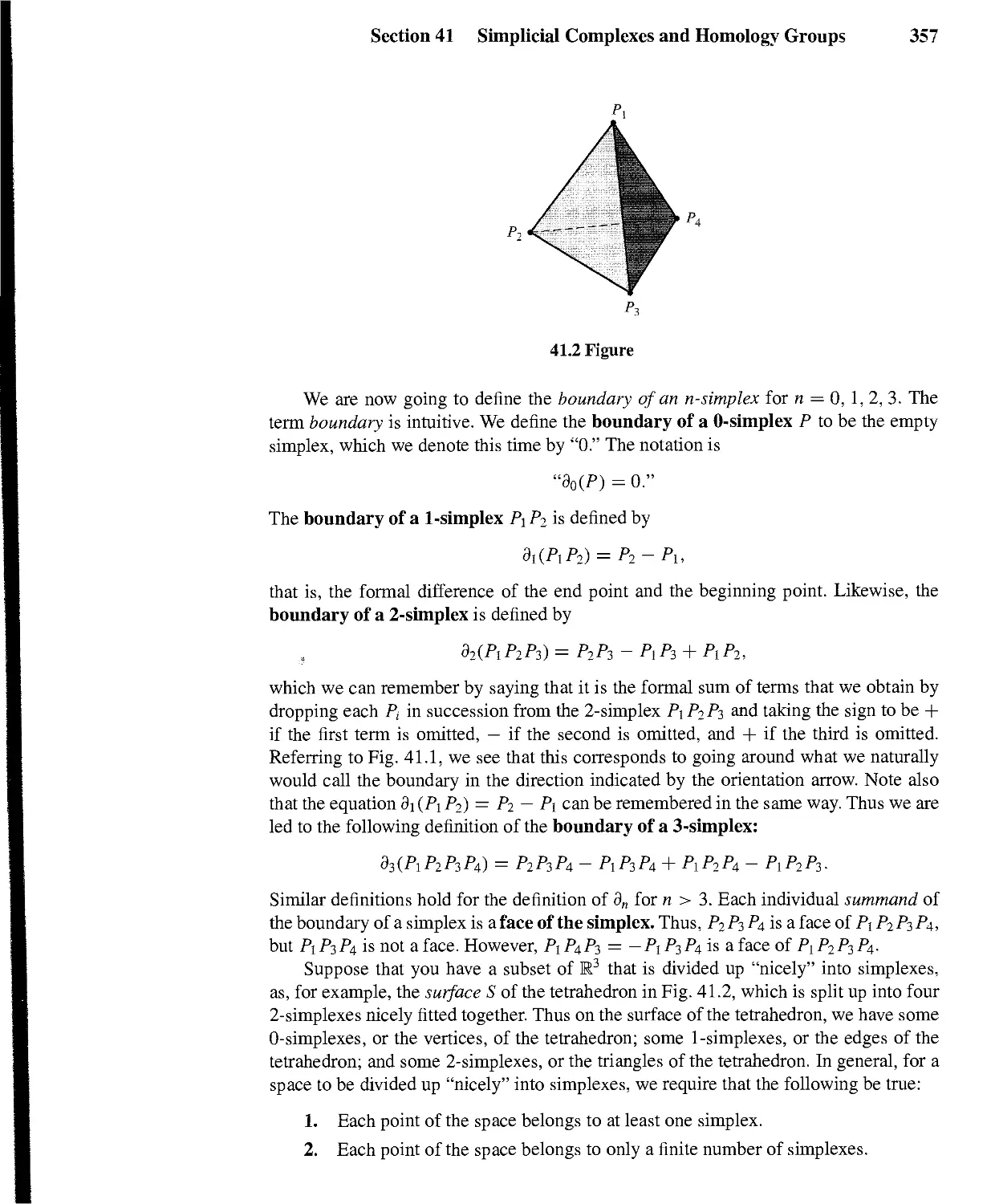
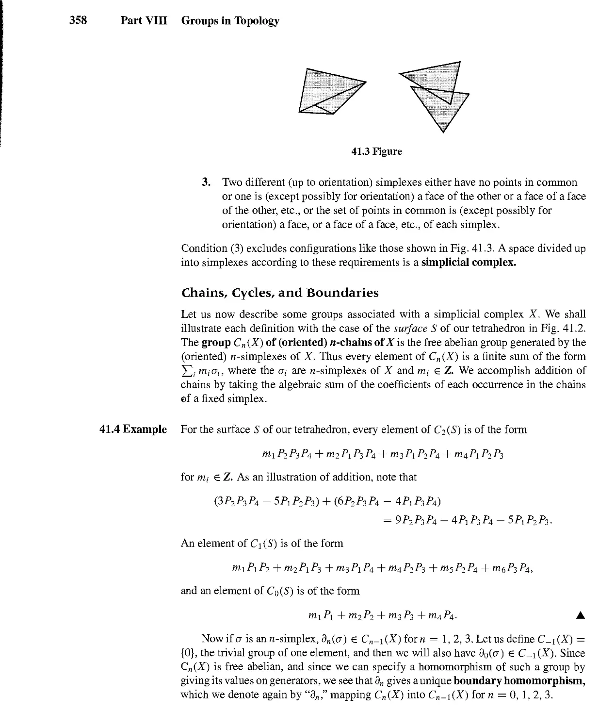
Groups in Topology 355
41 Simplicial Complexes and Homology Groups 355
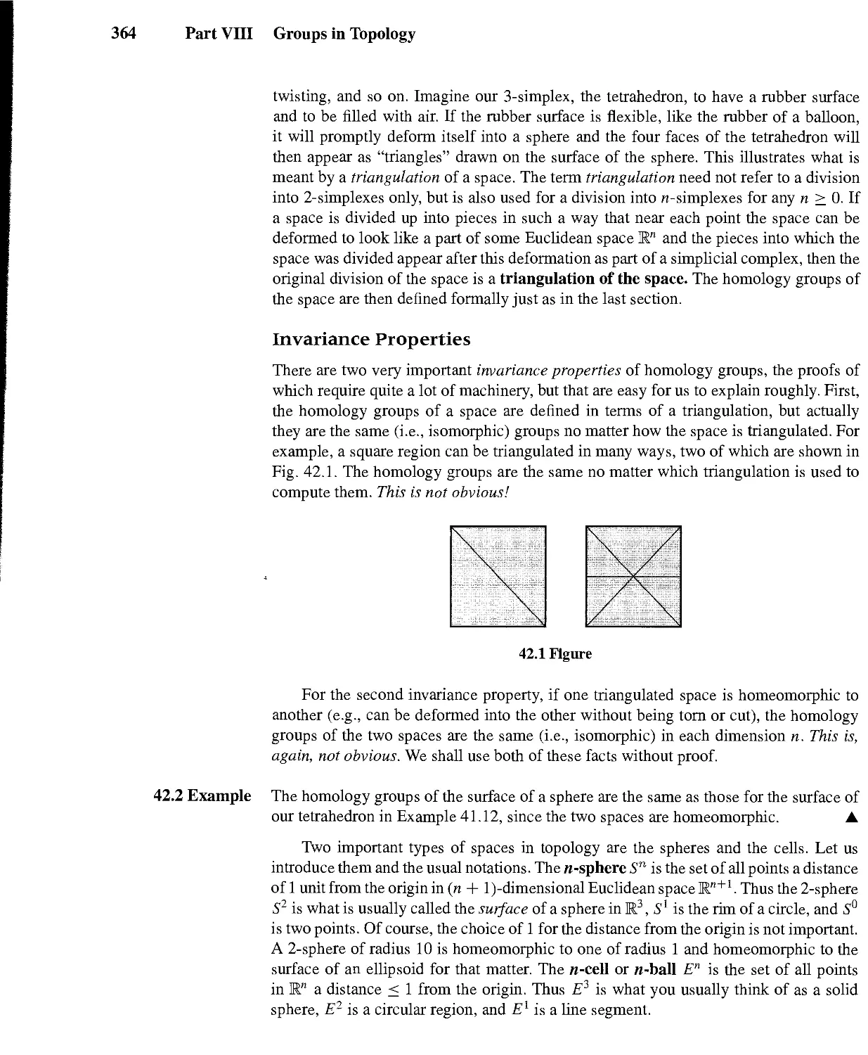
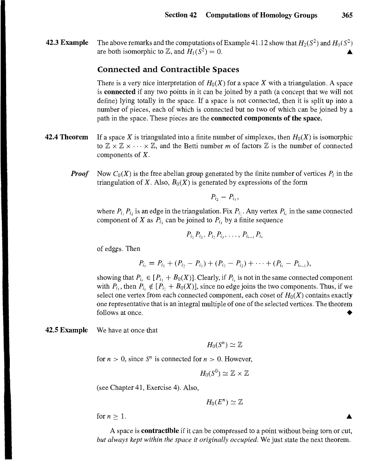
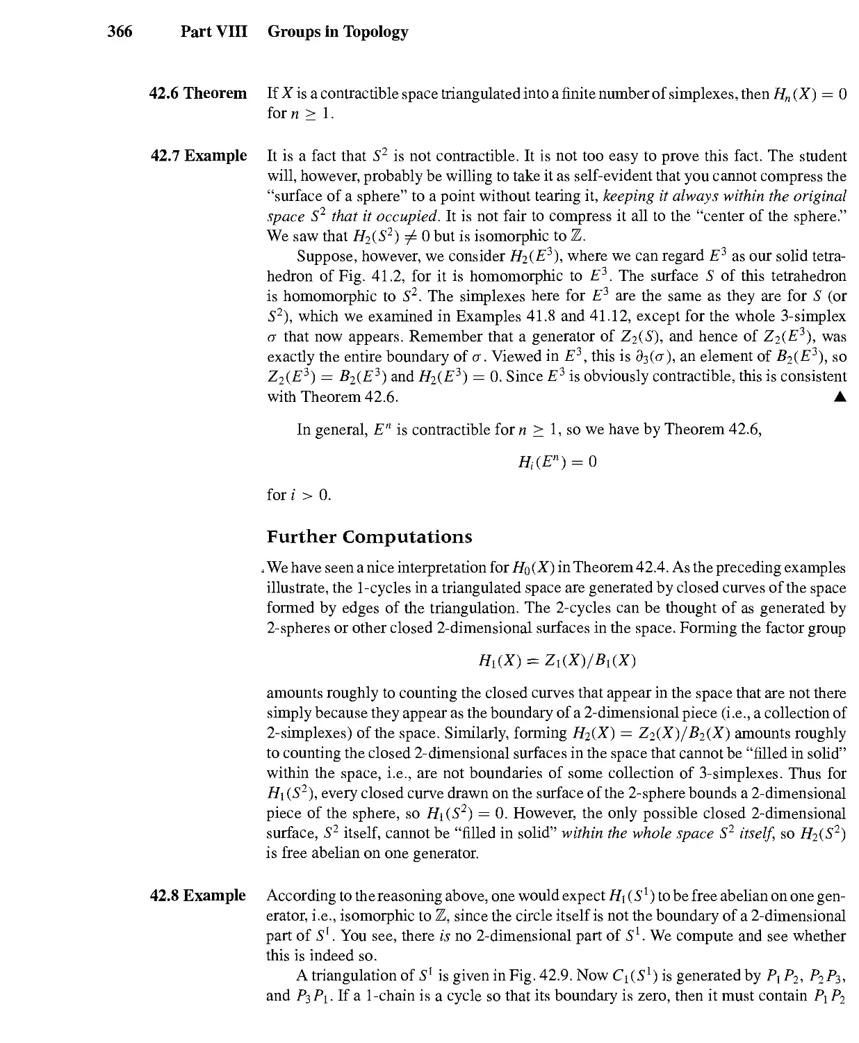
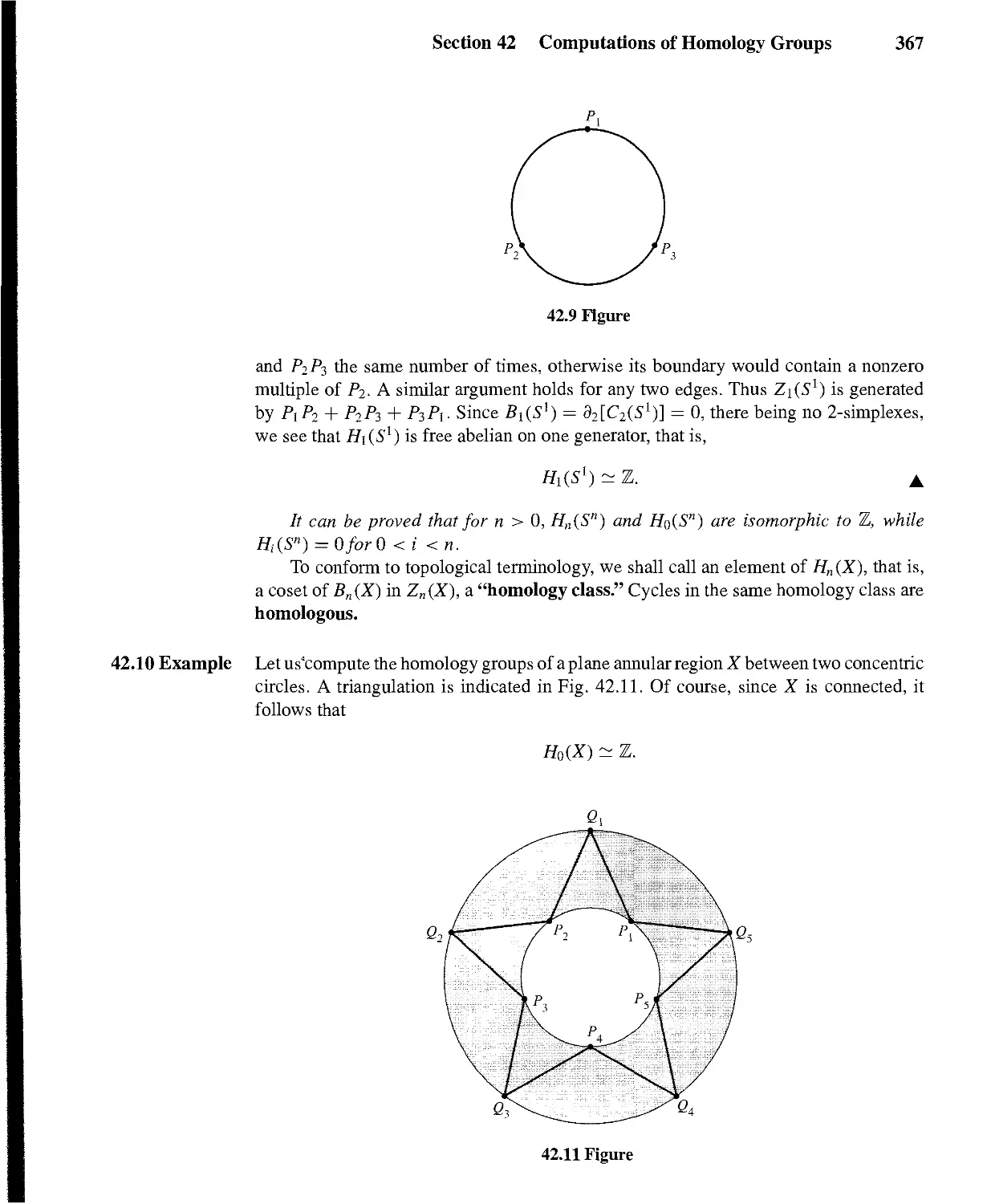
42 Computations of Homology Groups 363
43 More Homology Computations and Applications 371
44 Homological Algebra 379
ix
Factorization 389
45 Unique Factorization Domains 389
46 Euclidean Domains 401
47 Gaussian Integers and Multiplicative Norms 407
X
Automorphisms and Galois Theory 415
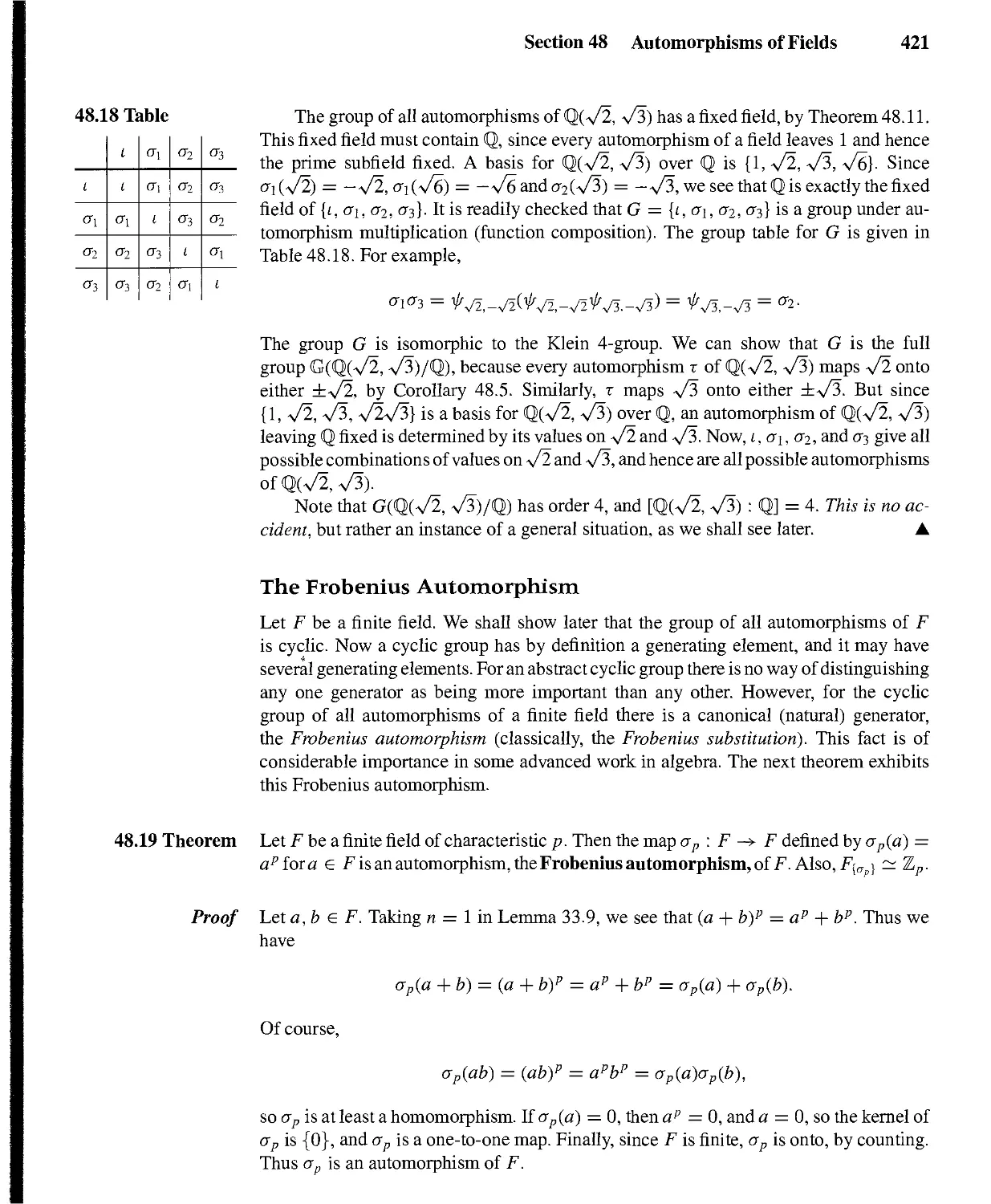
48 Automorphisms of Fields 415
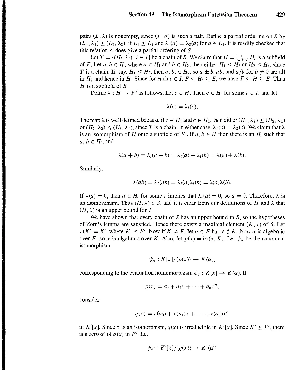
49 The Isomorphism Extension Theorem 424
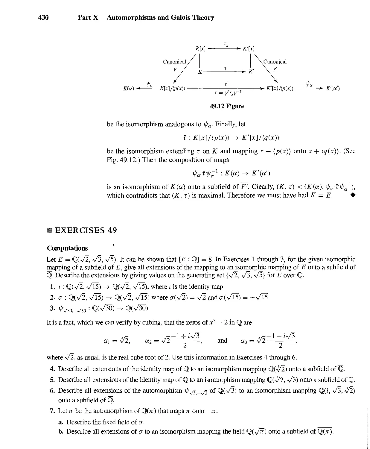
50 Splitting Fields 431
51 Separable Extensions 436
T52 Totally Inseparable Extensions 444
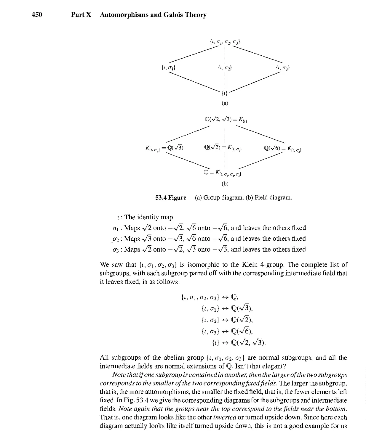
53 Galois Theory 448
54 Illustrations of Galois Theory 457
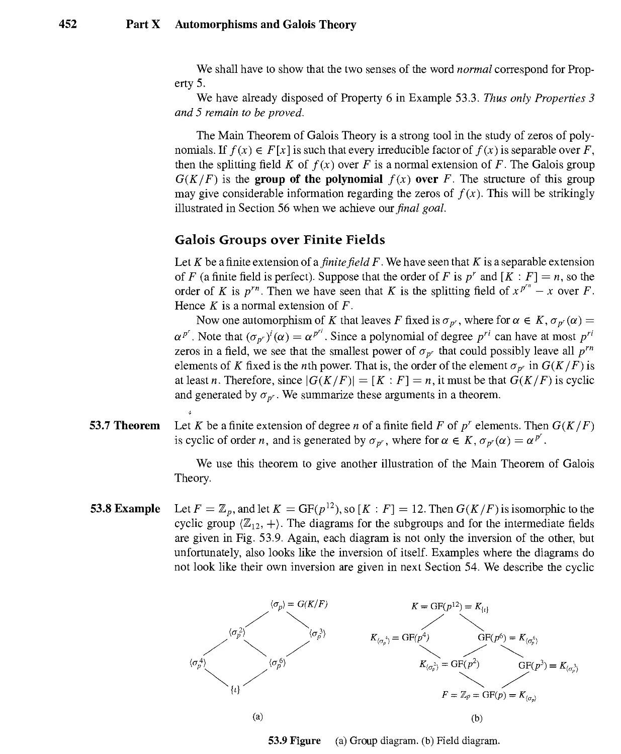
55 Cyclotomic Extensions 464
56 Insolvability of the Quintic 470
Appendix: Matrix Algebra 477
Bibliography 483
Notations 487
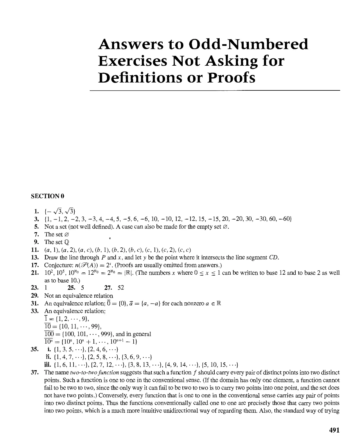
Answers to Odd-Numbered Exercises Not Asking for Definitions or Proofs 491
Index 513
' Not required for the remainder of the text.
■ This section is a prerequisite for Sections 17 and 36 only.

Instructor's Preface
This is an introduction to abstract algebra. It is anticipated that the students have studied
calculus and probably linear algebra. However, these are primarily mathematical
maturity prerequisites; subject matter from calculus and linear algebra appears mostly in
illustrative examples and exercises.
As in previous editions of the text, my aim remains to teach students as much about
groups, rings, and fields as I can in a first course. For many students, abstract algebra is
their first extended exposure to an axiomatic treatment of mathematics. Recognizing this,
I have included extensive explanations concerning what we are trying to accomplish,
how we are trying to do it, and why we choose these methods. Mastery of this text
constitutes a firm foundation for more specialized work in algebra, and also provides
valuable experience for any further axiomatic study of mathematics.
Changes from the Sixth Edition
The amount of preliminary material had increased from one lesson in the first edition
to four lessons in the sixth edition. My personal preference is to spend less time before
getting to algebra; therefore, I spend little time on preliminaries. Much of it is review for
many students, and spending four lessons on it may result in their not allowing sufficient
time in their schedules to handle the course when new material arises. Accordingly, in
this edition, I have reverted to just one preliminary lesson on sets and relations, leaving
other topics to be reviewed when needed. A summary of matrices now appears in the
Appendix.
The first two editions consisted of short, consecutively numbered sections, many of
which could be covered in a single lesson. I have reverted to that design to avoid the
cumbersome and intimidating triple numbering of definitions, theorems examples, etc.
In response to suggestions by reviewers, the order of presentation has been changed so
vii

Instructor's Preface
that the basic material on groups, rings, and fields that would normally be covered in a
one-semester course appears first, before the more-advanced group theory. Section 1 is
a new introduction, attempting to provide some feeling for the nature of the study.
In response to several requests, I have included the material on homology groups
in topology that appeared in the first two editions. Computation of homology groups
strengthens students' understanding of factor groups. The material is easily accessible;
after Sections 0 through 15, one need only read about free abelian groups, in Section 38
through Theorem 38.5, as preparation. To make room for the homology groups, I have
omitted the discussion of automata, binary linear codes, and additional algebraic
structures that appeared in the sixth edition.
I have also included a few exercises asking students to give a one- or two-sentence
synopsis of a proof in the text. Before the first such exercise, I give an example to show
what I expect.
Some Features Retained
I continue to break down most exercise sets into parts consisting of computations,
concepts, and theory. Answers to odd-numbered exercises not requesting a proof again
appear at the back of the text. However, in response to suggestions, I am supplying the
answers to parts a), c), e), g), and i) only of my 10-part true-false exercises.
The excellent historical notes by Victor Katz are, of course, retained. Also, a manual
containing complete solutions for all the exercises, including solutions asking for proofs,
is available for the instructor from the publisher.
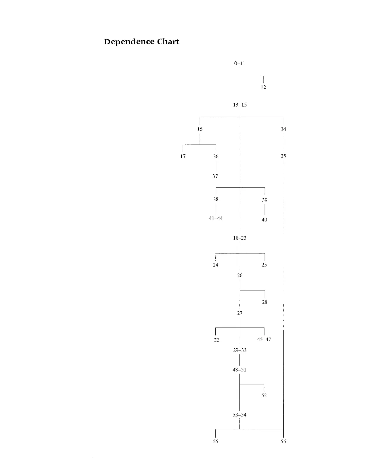
A dependence chart with section numbers appears in the front matter as an aid in
making a syllabus.
Acknowledgments
I am very grateful to those who have reviewed the text or who have sent me suggestions
and corrections. I am especially indebted to George M. Bergman, who used the sixth
edition and made note of typographical and other errors, which he sent to me along
with a great many other valuable suggestions for improvement. I really appreciate this
voluntary review, which must have involved a large expenditure of time on his part.
I also wish to express my appreciation to William Hoffman, Julie LaChance, and
Cindy Cody of Addison-Wesley for their help with this project. Finally, I was most
fortunate to have John Probst and the staff at TechBooks handling the production of the
text from my manuscript. They produced the most error-free pages I have experienced,
and courteously helped me with a technical problem I had while preparing the solutions
manual.
Suggestions for New Instructors of Algebra
Those who have taught algebra several times have discovered the difficulties and
developed their own solutions. The comments I make here are not for them.
This course is an abrupt change from the typical undergraduate calculus for the
students. A graduate-style lecture presentation, writing out definitions and proofs on the
board for most of the class time, will not work with most students. I have found it best

Instructor's Preface ix
to spend at least the first half of each class period answering questions on homework,
trying to get a volunteer to give a proof requested in an exercise, and generally checking
to see if they seem to understand the material assigned for that class. Typically, I spent
only about the last 20 minutes of my 50-minute time talking about new ideas for the next
class, and giving at least one proof. From a practical point of view, it is a waste of time
to try to write on the board all the definitions and proofs. They are in the text.
I suggest that at least half of the assigned exercises consist of the computational
ones. Students are used to doing computations in calculus. Although there are many
exercises asking for proofs that we would love to assign, I recommend that you assign
at most two or three such exercises, and try to get someone to explain how each proof is
performed in the next class. I do think students should be asked to do at least one proof
in each assignment.
Students face a barrage of definitions and theorems, something they have never
encountered before. They are not used to mastering this type of material. Grades on tests
that seem reasonable to us, requesting a few definitions and proofs, are apt to be low and
depressing for most students. My recommendation for handling this problem appears in
my article, Happy Abstract Algebra Classes, in the November 2001 issue of the MAA
FOCUS.
At URI, we have only a single semester undergraduate course in abstract algebra.
Our semesters are quite short, consisting of about 42 50-minute classes. When I taught
the course, I gave three 50-minute tests in class, leaving about 38 classes for which the
student was given an assignment. I always covered the material in Sections 0-11, 13-15,
18-23, 26, 27, and 29-32, which is a total of 27 sections. Of course, I spent more than
one class on several of the sections, but I usually had time to cover about two more;
sometimes I included Sections 16 and 17. (There is no point in doing Section 16 unless
you do Section 17, or will be doing Section 36 later.) I often covered Section 25, and
sometimes Section 12 (see the Dependence Chart). The job is to keep students from
becoming discouraged in the first few weeks of the course.

Student's Preface
This course may well require a different approach than those you used in previous
mathematics courses. You may have become accustomed to working a homework problem by
turning back in the text to find a similar problem, and then just changing some numbers.
That may work with a few problems in this text, but it will not work for most of them.
This is a subject in which understanding becomes all important, and where problems
should not be tackled without first studying the text.
Let me make some suggestions on studying the text. Notice that the text bristles
with definitions, theorems, corollaries, and examples. The definitions are crucial. We
must agree on terminology to make any progress. Sometimes a defimtion is followed
by an example that illustrates the concept. Examples are probably the most important
aids in studying the text. Pay attention to the examples. I suggest you skip the proofs
of the theorems on your first reading of a section, unless you are really "gung-ho" on
proofs. You should read the statement of the theorem and try to understand just what it
means. Often, a theorem is followed by an example that illustrates it, a great aid in really
understanding what the theorem says.
In summary, on your first reading of a section, I suggest you concentrate on what
information the section gives, and on gaining a real understanding of it. If you do not
understand what the statement of a theorem means, it will probably be meaningless for
you to read the proof.
Proofs are very basic to mathematics. After you feel you understand the information
given in a section, you should read and try to understand at least some of the proofs.
Proofs of corollaries are usually the easiest ones, for they often follow very directly from
the theorem. Quite a lot of the exercises under the "Theory" heading ask for a proof. Try
not to be discouraged at the outset. It takes a bit of practice and experience. Proofs in
algebra can be more difficult than proofs in geometry and calculus, for there are usually
no suggestive pictures that you can draw. Often, a proof falls out easily if you happen to
xi

Student's Preface
look at just the right expression. Of course, it is hopeless to devise a proof if you do not
really understand what it is that you are trying to prove. For example, if an exercise asks
you to show that given thing is a member of a certain set, you must know the defining
criterion to be a member of that set, and then show that your given thing satisfies that
criterion.
There are several aids for your study at the back of the text. Of course, you will
discover the answers to odd-numbered problems not requesting a proof. If you run into a
notation such as Z„ that you do not understand, look in the list of notations that appears
after the bibliography. If you run into terminology like inner automorphism that you do
not understand, look in the Index for the first page where the term occurs.
In summary, although an understanding of the subject is important in every
mathematics course, it is really crucial to your performance in this course. May you find it a
rewarding experience.
Narragansett, RI
J.B.F.

Dependence Chart
0-11
12
13-15
16
I I
17 36
37
38
41-44
34
35
39
40
18-23
24 25
26
32
27
29-33
48-51
28
45-47
52
53-54
55
56

section 0 Sets and Relations
On Definitions, and the Notion of a Set
Many students do not realize the great importance of definitions to mathematics. This
importance stems from the need for mathematicians to communicate with each other.
If two people are trying to communicate about some subject, they must have the same
understanding of its technical terms. However, there is an important structural weakness.
It is impossible to define every concept.
Suppose, for example, we define the term set as "A set is a well-defined collection of
objects." One naturally asks what is meant by a collection. We could define it as "A
collection is an aggregate of things." What, then, is an aggregate? Now our language
is finite, so after some time we will run out of new words to use and have to repeat
some words already examined. The definition is then circular and obviously worthless.
Mathematicians realize that there must be some undefined or primitive concept with
which to start. At the moment, they have agreed that set shall be such a primitive concept.
We shall not define set, but shall just hope that when such expressions as "the set of all
real numbers" or "the set of all members of the United States Senate" are used, people's
various ideas of what is meant are sufficiently similar to make communication feasible.
We summarize briefly some of the things we shall simply assume about sets.
1. A set S is made up of elements, and if a is one of these elements, we shall
denote this fact by a e S.
2. There is exactly one set with no elements. It is the empty set and is denoted
by 0.
3. We may describe a set either by giving a characterizing property of the
elements, such as "the set of all members of the United States Senate," or by
listing the elements. The standard way to describe a set by listing elements is
to enclose the designations of the elements, separated by commas, in braces,
for example, {1, 2, 15}. If a set is described by a characterizing property P(x)
of its elements x, the brace notation {x \ P(x)} is also often used, and is read
"the set of all x such that the statement P(x) about x is true." Thus
{2,4, 6, 8} = {x | x is an even whole positive number < 8}
= {2x\x = 1,2,3,4}.
The notation {x \ P(x)} is often called "set-builder notation."
4. A set is well defined, meaning that if S is a set and a is some object, then
either a is definitely in S, denoted by a e S, or a is definitely not in S, denoted
by a ¢ S. Thus, we should never say, "Consider the set S of some positive
numbers," for it is not definite whether 2 e S or 2 ¢. S. On the other hand, we
1

2 Section 0 Sets and Relations
can consider the set T of all prime positive integers. Every positive integer is
definitely either prime or not prime. Thus 5 e T and 14 ¢. T. It may be hard to
actually determine whether an object is in a set. For example, as this book
goes to press it is probably unknown whether 2(2") + 1 is in T. However,
2(2 ) + 1 is certainly either prime or not prime.
It is not feasible for this text to push the definition of everything we use all the way
back to the concept of a set. For example, we will never define the number n in terms of
a set.
Every definition is an if and only if'type of statement.
With this understanding, definitions are often stated with the only if suppressed, but it
is always to be understood as part of the definition. Thus we may define an isosceles
triangle as follows: "A triangle is isosceles if it has two sides of equal length," when we
really mean that a triangle is isosceles if and only if it has two sides of equal length.
In our text, we have to define many terms. We use specifically labeled and numbered
definitions for the main algebraic concepts with which we are concerned. To avoid an
overwhelming quantity of such labels and numberings, we define many terms within the
body of the text and exercises using boldface type.
Boldface Convention
A term printed in boldface in a sentence is being defined by that sentence.
Do not feel that you have to memorize a definition word for word. The important
thing is to understand the concept, so that you can define precisely the same concept
in your own words. Thus the definition "An isosceles triangle is one having two equal
sides" is perfectly correct. Of course, we had to delay stating our boldface convention
until we had finished using boldface in the preceding discussion of sets, because we do
not define a set!
In this section, we do define some familiar concepts as sets, both for illustration and
for review of the concepts. First we give a few definitions and some notation.
0.1 Definition A set B is a subset of a set A, denoted by B c A or A Z> B, if every element of B is in
A. The notations B C A or A D B will be used for B C A but B / A. ■
• Note that according to this definition, for any set A, A itself and 0 are both subsets of A.
0.2 Definition If A is any set, then A is the improper subset of A. Any other subset of A is a proper
subset of A. ■

Sets and Relations 3
0.3 Example Let S = {1, 2, 3}. This set S has a total of eight subsets, namely 0, {1}, {2}, {3},
{1,2}, {1, 3}, {2, 3}, and {1,2, 3}. A
0.4 Definition Let A and B be sets. The set A x B = {(a, b) \ a e A and b e B) is the Cartesian
product of A and B. ■
0.5 Example If A = {1, 2, 3} and B = {3, 4}, then we have
A x B = {(1, 3), (1, 4), (2, 3), (2, 4), (3, 3), (3, 4)}. A
Throughout this text, much work will be done involving familiar sets of numbers.
Let us take care of notation for these sets once and for all.
Z is the set of all integers (that is, whole numbers: positive, negative, and zero).
Q is the set of all rational numbers (that is, numbers that can be expressed as quotients
m/n of integers, where n / 0).
E is the set of all real numbers.
Z+, Q+, and E+ are the sets of positive members of Z, Q, and E, respectively.
C is the set of all complex numbers.
Z*, Q*, E*, and C* are the sets of nonzero members of Z, Q, E, and C, respectively.
0.6 Example The set E x E is the familiar Euclidean plane that we use in first-semester calculus to
draw graphs of functions. A
Relations Between Sets
We introduce the notion of an element a of set A being related to an element b of set B,
which we might denote by a .^¾ b. The notation a .y£ b exhibits the elements a and b in
left-to-right order, just as the notation (a, b) for an element in A x B. This leads us to
the following definition of a relation .^¾ as a set.
0.7 Definition A relation between sets A and B is a subset J? of A x B. We read (a, b) e J? as "a is
related to b" and write a ,yH,b. ■
0.8 Example (Equality Relation) There is one familiar relation between a set and itself that we
consider every set S mentioned in this text to possess: namely, the equality relation =
defined on a set S by
= is the subset {(x, x)\x e S] of S x S.
Thus for any x e S, we have x = x, but if x and y are different elements of S, then
(x, y) ¢. = and we write x ^ y. A
We will refer to any relation between a set S and itself, as in the preceding example,
as a relation on S.
0.9 Example The graph of the function/ where f(x) = x3 for all x e E, isthesqbset{(x,x3) \x e E}
of E x E. Thus it is a relation on E. The function is completely determined by its graph.
A

4 Section 0 Sets and Relations
The preceding example suggests that rather than define a "function" y = f(x) to
be a "rule" that assigns to each x e E exactly one y e E, we can easily describe it as a
certain type of subset of E x E, that is, as a type of relation. We free ourselves from E
and deal with any sets X and Y.
0.10 Definition A function ¢) mapping X into Y is a relation between X and Y with the property that
each x & X appears as the first member of exactly one ordered pair (x, y) in ¢. Such a
function is also called a map or mapping of X into Y. We write § : X —>• Y and express
(x, y) € 0 by 4>{x) = y. The domain of 4> is the set X and the set Y is the codomain of
¢. The range of ¢) is 0[X] = {<j>(x) \x e X}. ■
0.11 Example We can view the addition of real numbers as a function + : (E x E) —>• E, that is, as a
mapping of E x E into E. For example, the action of + on (2, 3) e E x E is given in
function notation by +((2, 3)) = 5. In set notation we write ((2, 3), 5) e +. Of course
our familiar notation is 2 + 3 = 5. ▲
Cardinality
The number of elements in a set X is the cardinality of X and is often denoted by \X\.
For example, we have |{2, 5,7} | = 3. It will be important for us to know whether two sets
have the same cardinality. If both sets are finite there is no problem; we can simply count
the elements in each set. But do Z, Q, and E have the same cardinality? To convince
ourselves that two sets X and Y have the same cardinality, we try to exhibit a pairing of
each x in X with only one )' in Y in such a way that each element of Y is also used only
once in this pairing. For the sets X = {2, 5, 7} and Y = {?, !, #}, the pairing
2<*V?, 5o#, 7o!
shows they have the same cardinality. Notice that we could also exhibit this pairing as
{(2, ?), (5, #), (7, !)} which, as a subset of X x F, is a relation between X and F. The
pairing
1 23 45 67 89 10---
0-11-22-33-44 -5
shows that the sets Z and Z+ have the same cardinality. Such a pairing, showing that
sets X and F have the same cardinality, is a special type of relation <-> between X and
F called a one-to-one correspondence. Since each element x of X appears precisely
once in this relation, we can regard this one-to-one correspondence as a function with
domain X. The range of the function is F because each y in F also appears in some
pairing x ■*+ y. We formalize this discussion in a definition.
0.12 Definition *A function ¢) : X —>• F is one to one if 4>{x\) = 0(¾) only when x\ = X2 (see
Exercise 37). The function § is onto F if the range of 0 is F. ■
* We should mention another terminology, used by the disciples of N. Bourbaki, in case you encounter it
elsewhere. In Bourbaki's terminology, a one-to-one map is an injection, an onto map is a surjection, and a
map that is both one to one and onto is a bijection.

Sets and Relations 5
If a subset of X x Y is a one-to-one function <p mapping X onto Y, then each x & X
appears as the first member of exactly one ordered pair in ¢) and also each y e Y appears
as the second member of exactly one ordered pair in ¢. Thus if we interchange the first
and second members of all ordered pairs (x, y) in <p to obtain a set of ordered pairs (y, x),
we get a subset of Y x X, which gives a one-to-one function mapping Y onto X. This
function is called the inverse function of ¢, and is denoted by <j>~1. Summarizing, if
§ maps X one to one onto Y and <j>(x) = y, then 0"1 maps Y one to one onto X, and
4>-\y) = x.
0.13 Definition Two sets X and Y have the same cardinality if there exists a one-to-one function mapping
X onto F, that is, if there exists a one-to-one correspondence between X and Y. ■
0.14 Example The function / : E ->• E where f(x) = x2 is not one to one because /(2) = /(-2) = 4
but 2 ^ —2. Also, it is not onto E because the range is the proper subset of all nonnegative
numbers in E. However, g : E —>• E defined by g(x) = x3 is both one to one and onto
E. A
We showed that Z and Z+ have the same cardinality. We denote this cardinal number
by Ko, so that |Z| = |Z+| = Ko. It is fascinating that a proper subset of an infinite set
may have the same number of elements as the whole set; an infinite set can be defined
as a set having this property.
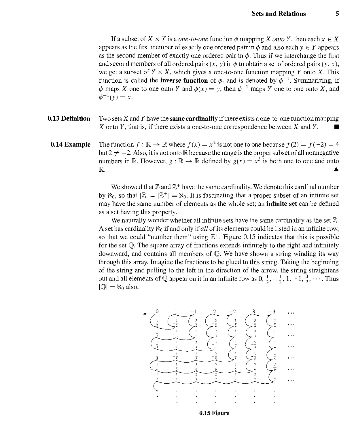
We naturally wonder whether all infinite sets have the same cardinality as the set Z.
A set has cardinality Ko if and only if all of its elements could be listed in an infinite row,
so that we could "number them" using Z+. Figure 0.15 indicates that this is possible
for the set Q. The square array of fractions extends infinitely to the right and infinitely
downward, and contains all members of Q. We have shown a string winding its way
through this array. Imagine the fractions to be glued to this string. Taking the beginning
of the string and pulling to the left in the direction of the arrow, the string straightens
out and all elements of Q appear on it in an infinite row as 0, \,— ^,1,-1, |, • • •. Thus
|Q| = K0 also.
0.15 Figure

6 Section 0 Sets and Relations
If the set S = {x e E | 0 < x < 1} has cardinality Ko, all its elements could be listed
as unending decimals in a column extending infinitely downward, perhaps as
0.3659663426 • ■ •
0.7103958453 • • •
0.0358493553 • • •
0.9968452214---
We now argue that any such array must omit some number in S. Surely S contains a
number r having as its nth digit after the decimal point a number different from 0, from 9,
and from the nth digit of the nth number in this list. For example, r might start .5637- • •.
The 5 rather than 3 after the decimal point shows r cannot be the first number in S
listed in the array shown. The 6 rather than 1 in the second digit shows r cannot be the
second number listed, and so on. Because we could make this argument with any list,
we see that S has too many elements to be paired with those in Z+. Exercise 15 indicates
that E has the same number of elements as S. We just denote the cardinality of E by
|E|. Exercise 19 indicates that there are infinitely many different cardinal numbers even
greater than |E|.
Partitions and Equivalence Relations
Sets are disjoint if no two of them have any element in common. Later we will have
occasion to break up a set having an algebraic structure (e.g., a notion of addition) into
disjoint subsets that become elements in a related algebraic structure. We conclude this
section with a study of such breakups, or partitions of sets.
0.16 Definition A partition of a set S is a collection of nonempty subsets of S such that every element
of S is in exactly one of the subsets. The subsets are the cells of the partition. ■
When discussing a partition of a set S, we denote by x the cell containing the element
x of S.
0.17 Example Splitting Z+ into the subset of even positive integers (those divisible by 2) and the subset
of odd positive integers (those leaving a remainder of 1 when divided by 2), we obtain
a partition of Z+ into two cells. For example, we can write
14 = (2,4,6.8,10,12, 14, 16. 18, •••}.
We could also partition Z+ into three cells, one consisting of the positive integers
divisible by 3, another containing all positive integers leaving a remainder of 1 when
divided by 3, and the last containing positive integers leaving a remainder of 2 when
divided by 3.
Generalizing, for each positive integer n, we can partition Z+ into n cells according
to whether the remainder is 0, 1, 2, • • • , n — 1 when a positive integer is divided by n.
These cells are the residue classes modulo n in Z+. Exercise 35 asks us to display these
partitions for the cases n =2,3, and 5. ▲

Sets and Relations 7
Each partition of a set S yields a relation .M on S in a natural way: namely, for
x, y e S, let x .M y if and only if x and y are in the same cell of the partition. In set
notation, we would write x ■>€ y as (x, y) e ,^¾ (see Definition 0.7). A bit of thought
shows that this relation .^¾ on S satisfies the three properties of an equivalence relation
in the following definition.
0.18 Definition An equivalence relation .^¾ on a set S is one that satisfies these three properties for all
x, y, z e S.
1. (Reflexive) x .Mx.
2. (Symmetric) If x -jfcy, then y .^ x.
3. (Transitive) If x .^¾ y and y ,3% z then x.J?z. ■
To illustrate why the relation ,>? corresponding to a partition of S satisfies the
symmetric condition in the definition, we need only observe that if y is in the same cell
as x (that is, if x .>? y), then x is in the same cell as y (that is, y ..M x). We leave the
similar observations to verify the reflexive and transitive properties to Exercise 28.
0.19 Example For any nonempty set S, the equality relation = defined by the subset {(x, x) \ x e S] of
S x S is an equivalence relation. ▲
0.20 Example (Congruence Modulo n) Let n e Z+. The equivalence relation on Z+ corresponding
to the partition of Z+ into residue classes modulo n, discussed in Example 0.17, is
congruence modulo n. It is sometimes denoted by =„. Rather than write a=„b, we
usually write a = b (mod n), read, "a is congruent to b modulo n." For example, we
have 15 = 27 (mod 4) because both 15 and 27 have remainder 3 when divided by 4. ▲
0.21 Example Let a relation ,^/B on the set Z be defined by n .^¾ m if and only if nm > 0, and let us
determine whether ^¾ is an equivalence relation.
Reflexive a .M a, because a2 > 0 for all a e Z.
Symmetric If a .M b, then ab > 0, so ba > 0 and b .Ma.
Transitive \ia.yib and b .M c, then ab > 0 and be > 0. Thus ab2c = acb2 > 0.
If we knew b2 > 0, we could deduce ac > 0 whence a ,M c. We have to examine the
case b = 0 separately. A moment of thought shows that —3,^0 and 0 .M 5, but we do
not have —3 ,^2 5. Thus the relation c/Z, is not transitive, and hence is not an equivalence
relation. ▲
We observed above that a partition yields a natural equivalence relation. We now
show that an equivalence relation on a set yields a natural partition of the set. The theorem
that follows states both results for reference.
0.22 Theorem (Equivalence Relations and Partitions) Let S be a nonempty set and let ~ be an
equivalence relation on S. Then ~ yields a partition of S, where
a = \x e S \x ~ a}.

8 Section 0 Sets and Relations
Also, each partition of S gives rise to an equivalence relation ~ on S where a ~ b if and
only if a and b are in the same cell of the partition.
Proof We must show that the different cells a = {x eSU~a)fora eSdo give a partition
of S, so that every element of S is in some cell and so that if a e b, then a =b. Let
a e S. Then a e a by the reflexive condition (1), so a is in at least one cell.
Suppose now that a were in a cell b also. We need to show that a = b as sets; this
will show that a cannot be in more than one cell. There is a standard way to show that
two sets are the same:
Show that each set is a subset of the other.
We show that a c.b. Let x e a. Then x ~ a. But aefc,soa~i>. Then, by the transitive
condition (3), x ~ b, so x € b. Thus ocj. Now we show that £ c a. Let y e £. Then
y ~ fc. But aefc,sofl~fc and, by symmetry (2), b ~- a. Then by transitivity (3), y ~ a,
so >' e a. Hence Kq also, so £ = a and our proof is complete. ♦
Each cell in the partition arising from an equivalence relation is an equivalence
class.
■ EXERCISES 0
In Exercises 1 through 4, describe the set by listing its elements.
1. {x e M \x2 = 3} 2. {m e Z | m2 = 3}
3. {m e Z | mn = 60 for some n e Z} 4. {m e Z | m2 - m < 115}
In Exercises 5 through 10, decide whether the object described is indeed a set (is well defined). Give an alternate
description of each set.
5. {n e Z+ | n is a large number}
6. {n e Z | n2 < 0}
7. {n e Z | 39 < n3 < 57}
8. {x e Q | x is almost an integer}
9. {x &Q\x may be written with denominator greater than 100}
10. {x e Q | x may be written with positive denominator less than 4}
11. List the elements in {a, b, c} x {1, 2, c}.
12. Let A = {1, 2, 3} and B = {2, 4, 6}. For each relation between A and B given as a subset of A x S, decide
whether it is a function mapping A into S. If it is a function, decide whether it is one to one and whether it is
onto B.
a. {(1,4), (2,4), (3, 6)} b. {(1,4), (2, 6), (3,4)}
c. {(1, 6), (1, 2), (1,4)} d. {(2, 2), (1, 6), (3,4)}
e. {(1, 6), (2, 6), (3, 6)} f. {(1,2), (2, 6), (2,4)}
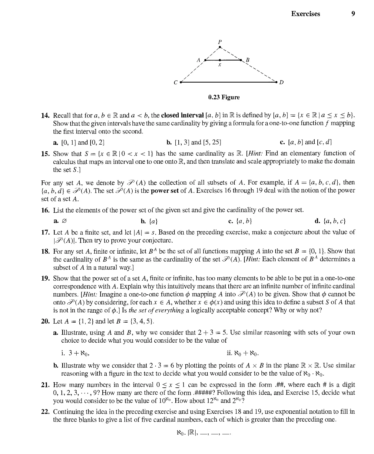
13. Illustrate geometrically that two line segments AB and CD of different length have the same number of points
by indicating in Fig. 0.23 what point y of CD might be paired with point x of AB.

Exercises
9
A
/
p
X
-
,B
c*-
0.23 Figure
14. Recall that for a, b e R and a < b, the closed interval [a, fc] in R is denned by [a, fc] = {* e R | a < * < £>}.
Show that the given intervals have the same cardinality by giving a formula for a one-to-one function / mapping
the first interval onto the second.
a. [0, 1] and [0, 2] b. [1, 3] and [5, 25] c. [a, b] and [c, d]
15. Show that S = {x €'R\0 < x < 1} has the same cardinality as R. [Hint: Find an elementary function of
calculus that maps an interval one to one onto R, and then translate and scale appropriately to make the domain
the set S.]
For any set A, we denote by SP (A) the collection of all subsets of A. For example, if A = {a, b, c, d}, then
{a, b, d] e -5^(A). The set SP(A) is the power set of A. Exercises 16 through 19 deal with the notion of the power
set of a set A.
16. List the elements of the power set of the given set and give the cardinality of the power set.
a. 0 b. {a} c. {a,b} d. {a, b, c}
17. Let A be a finite set, and let \A\ = s. Based oh the preceding exercise, make a conjecture about the value of
\.3^(A)\. Then try to prove your conjecture.
18. For any set A, finite or infinite, let BA be the set of all functions mapping A into the set B = {0, 1}. Show that
the cardinality of BA is the same as the cardinality of the set d^(A). [Hint: Each element of BA determines a
subset of A in a natural way.]
19. Show that the power set of a set A, finite or infinite, has too many elements to be able to be put in a one-to-one
correspondence with A. Explain why this intuitively means that there are an infinite number of infinite cardinal
numbers. [Hint: Imagine a one-to-one function ¢) mapping A into .5s(A) to be given. Show that § cannot be
onto d?(A) by considering, for each x & A, whether x e (j>(x) and using this idea to define a subset S of A that
is not in the range of ¢.] Is the set of everything a logically acceptable concept? Why or why not?
20. LetA = {1,2} and lets = {3,4,5}.
a. Illustrate, using A and B, why we consider that 2 + 3 = 5. Use similar reasoning with sets of your own
choice to decide what you would consider to be the value of
i. 3 + K0, ii. K0 + K0.
b. Illustrate why we consider that 2 • 3 = 6 by plotting the points of A x B in the plane R x R. Use similar
reasoning with a figure in the text to decide what you would consider to be the value of Ko • Ko.
21. How many numbers in the interval 0 < x < 1 can be expressed in the form .##, where each # is a digit
0, 1, 2, 3, • • •, 9? How many are there of the form .#####? Following this idea, and Exercise 15, decide what
you would consider to be the value of 10K°. How about 12N" and 2N'°?
22. Continuing the idea in the preceding exercise and using Exercises 18 and 19, use exponential notation to fill in
the three blanks to give a list of five cardinal numbers, each of which is greater than the preceding one.
K0.|R|, _,_,_.

10 Section 0 Sets and Relations
In Exercises 23 through 27, find the number of different partitions of a set having the given number of elements.
23. 1 element 24. 2 elements 25. 3 elements
26. 4 elements 27. 5 elements
28. Consider a partition of a set S. The paragraph following Definition 0.18 explained why the relation
x .^¾ y if and only if x and y are in the same cell
satisfies the symmetric condition for an equivalence relation. Write similar explanations of why the reflexive
and transitive properties are also satisifed.
In Exercises 29 through 34, determine whether the given relation is an equivalence relation on the set. Describe the
partition arising from each equivalence relation.
29. n M m in Z if nm > 0 30. x .M y in M if x > y
31. x.rfymRif\x\ = \y\ 32. x JZ y inMif \x - y\ < 3
33. n J% m in Z+ if n and m have the same number of digits in the usual base ten notation
34. n ,>8 m in Z+ if n and m have the same final digit in the usual base ten notation
35. Using set notation of the form {#,#. #. • • •} for an infinite set, write the residue classes modulo n in Z+ discussed
in Example 0.17 for the indicated value of n.
a. n = 2 b. n = 3 c. n = 5
36. Let n e Z+ and let ~ be defined on Z by r ~ s if and only if r - s is divisible by n, that is, if and only if
r — s = nq for some q e Z.
a. Show that ~ is an equivalence relation on Z. (It is called "congruence modulo n" just as it was for Z+. See
part b.)
b. Show that, when restricted to the subset Z+ of Z, this ~ is vhe equivalence relation, congruence modulo n,
of Example 0.20.
c. The cells of this partition of Z are residue classes modulo n in Z. Repeat Exercise 35 for the residue classes
modulo in Z rather than in Z+ using the notation {■ • •, #. #, #. • ■ •} for these infinite sets.
37. Students often misunderstand the concept of a one-to-one function (mapping). I think I know the reason. You
see, a mapping <p : A—> B has a direction associated with it, from A to B. It seems reasonable to expect a
one-to-one mapping simply to be a mapping that carries one point of A into one point of B, in the direction
indicated by the arrow. But of course, every mapping of A into B does this, and Definition 0.12 did not say
that at all. With this unfortunate situation in mind, make as good a pedagogical case as you can for calling the
functions described in Definition 0.12 two-to-two functions instead. (Unfortunately, it is almost impossible to
get widely used terminology changed.)

part Groups and Subgroups
Section 1 Introduction and Examples
Section 2 Binary Operations
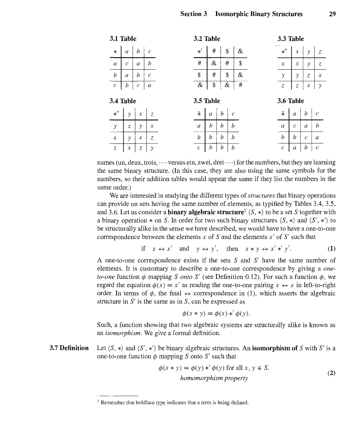
Section 3 Isomorphic Binary Structures
Section 4 Groups
Section 5 Subgroups
Section 6 Cyclic Groups
Section 7 Generating Sets and Cayley Digraphs
section 1 Introduction and Examples
In this section, we attempt to give you a little idea of the nature of abstract algebra.
We are all familiar with addition and multiplication of real numbers. Both addition
and multiplication combine two numbers to obtain one number. For example, addition
combines 2 and 3 to obtain 5. We consider addition and multiplication to be binary
operations. In this text, we abstract this notion, and examine sets in which we have one
or more binary operations. We think of a binary operation on a set as giving an algebra
on the set, and we are interested in the structural properties of that algebra. To illustrate
what we mean by a structural property with our familiar set E of real numbers, note
that the equation x + x = a has a solution x in E for each a e E, namely, x = a/2.
However, the corresponding multiplicative equation x ■ x = a does not have a solution
in E if a < 0. Thus, E with addition has a different algebraic structure than E with
multiplication.
Sometimes two different sets with what we naturally regard as very different binary
operations turn out to have the same algebraic structure. For example, we will see in
Section 3 that the set E with addition has the same algebraic structure as the set E+ of
positive real numbers with multiplication!
This section is designed to get you thinking about such things informally. We will
make everything precise in Sections 2 and 3. We now turn to some examples.
Multiplication of complex numbers of magnitude 1 provides us with several examples that will
be useful and illuminating in our work. We start with a review of complex numbers and
their multiplication.
11

Groups and Subgroups
i
i
(
-4
-3 -2 -1 0
—i
-2i
bi
a + bi
■—T
I
I
\a
1.1 Figure
Complex Numbers
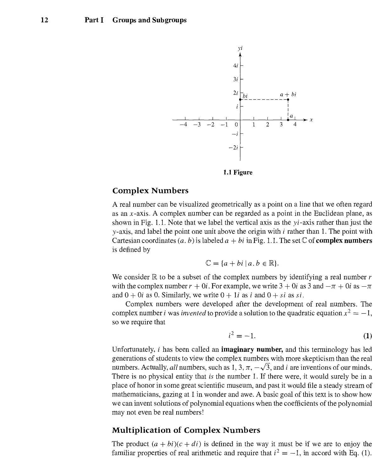
A real number can be visualized geometrically as a point on a line that we often regard
as an x-axis. A complex number can be regarded as a point in the Euclidean plane, as
shown in Fig. 1.1. Note that we label the vertical axis as the yi-axis rather than just the
>'-axis, and label the point one unit above the origin with i rather than 1. The point with
Cartesian coordinates (a. b) is labeled a + bi in Fig. 1.1. The set C of complex numbers
is defined by
C:
{a + bi I a. b e
We consider ffi to be a subset of the complex numbers by identifying a real number r
with the complex number r + Qi. For example, we write 3 + Oz' as 3 and — it + Qi as — it
and 0 + 0; as 0. Similarly, we write 0 + \i as i and 0 + si as si.
Complex numbers were developed after the development of real numbers. The
complex number i was invented to provide a solution to the quadratic equation x2 = -1,
so we require that
(1)
Unfortunately, i has been called an imaginary number, and this terminology has led
generations of students to view the complex numbers with more skepticism than the real
numbers. Actually, all numbers, such as 1, 3, it, — a/3, and i are inventions of our minds.
There is no physical entity that is the number 1. If there were, it would surely be in a
place of honor in some great scientific museum, and past it would file a steady stream of
mathematicians, gazing at 1 in wonder and awe. A basic goal of this text is to show how
we can invent solutions of polynomial equations when the coefficients of the polynomial
may not even be real numbers!
Multiplication of Complex Numbers
The product {a + bi){c + di) is defined in the way it must be if we are to enjoy the
familiar properties of real arithmetic and require that i2 = — 1, in accord with Eq. (1).

Section 1 Introduction and Examples 13
Namely, we see that we want to have
(a + bi){c + di) = ac + adi + bci + bdi2
= ac + adi + bci + bd(—l)
= (ac — bd) + (ad + bc)i.
Consequently, we define multiplication of z\ — a + be and zi = c + di as
Z\zi = (a + bi)(c + di) = (ac — bd) + (ad + bc)i,
(2)
which is of the form r + si with r = ac — bd and s = ad + be. It is routine to check
that the usual properties z\Zi = ZiZ\. Zifez3) = (z\Z2)z3 andz!(z2 + Z3) = Z1Z2 + Z1Z3
all hold for all z\. Z2, Z3 e C
1.2 Example Compute (2 - 50(8 + 30-
Solution We don't memorize Eq. (2), but rather we compute the product as we did to motivate
that equation. We have
(2 - 5i)(8 + 30 = 16 + 6; - 40/ + 15 = 31 — 34r. ▲
To establish the geometric meaning of complex multiplication, we first define the
absolute value \a + bi\ of a + bi by
\a + bi\ = -Ja1 + b2.
(3)
This absolute value is a nonnegative real number and is the distance from a + bi to the
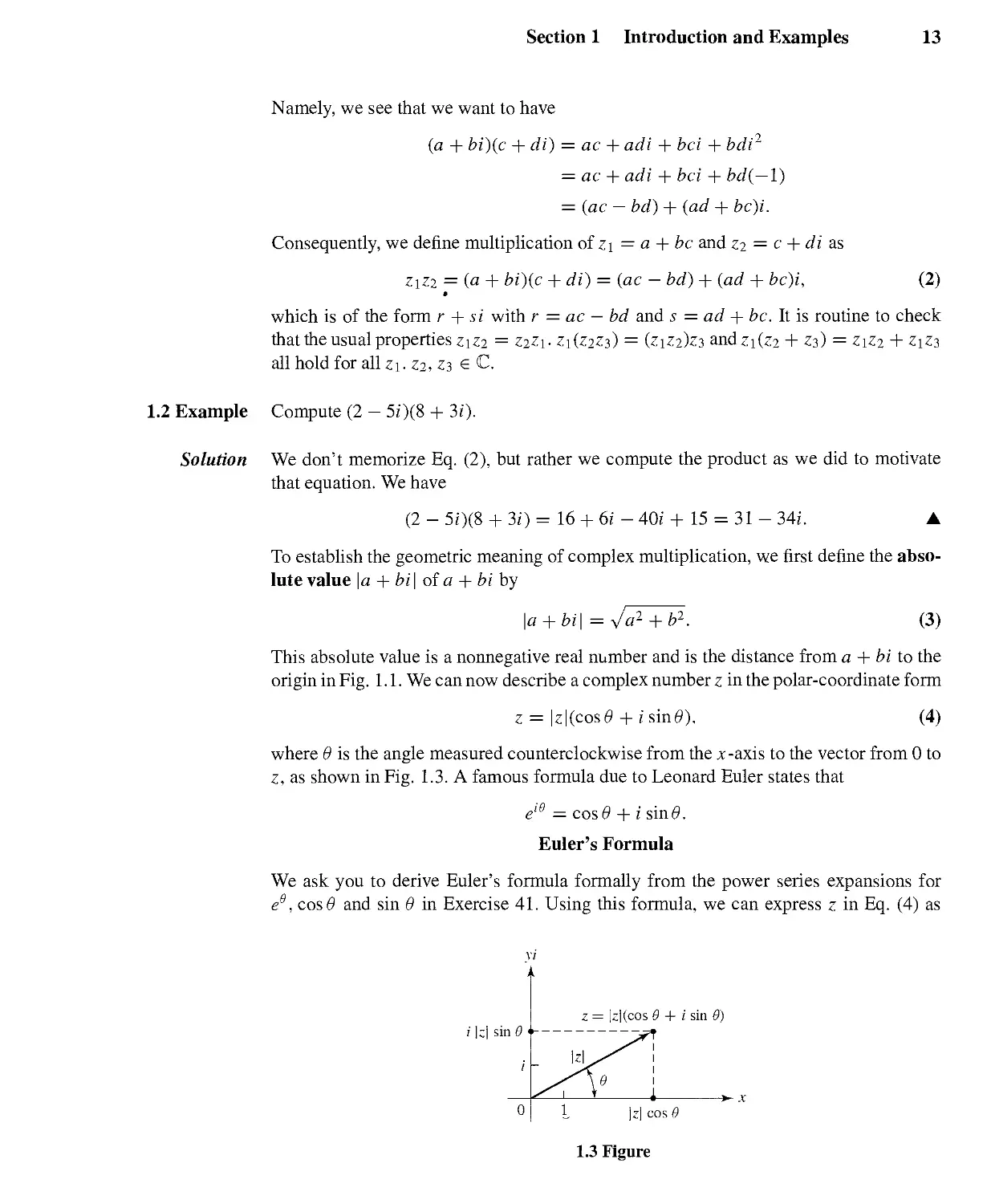
origin in Fig. 1.1. We can now describe a complex number z in the polar-coordinate form
z = |z|(cos# + i sin#).
(4)
where 6 is the angle measured counterclockwise from the ;t-axis to the vector from 0 to
z, as shown in Fig. 1.3. A famous formula due to Leonard Euler states that
e'6 — cosO + i sin#.
Euler's Formula
We ask you to derive Euler's formula formally from the power series expansions for
e6, cos 6 and sin 6 in Exercise 41. Using this formula, we can express z in Eq. (4) as
y
,
;' |c| sin 9
i
0
,
1
I
z
Z\
= |z|(cos0 + 1 sin 9)
^r^ 1
y^ 1
1
9 1
V 1 > ,
|z| cos 9
1.3 Figure

14 Part I Groups and Subgroups
z = Me .Letus set
zi = \zi\e'
i6\
and
Zl
\z2\e"
and compute their product in this form, assuming that the usual laws of exponentiation
hold with complex number exponents. We obtain
\z,\e^ = |z,
,,1(01+02)
Z\Zi = \Zi\e '\z2\e'"' = |Zi||Z2|e"
= |zil|z2|[cos(0i + 82) + i sin(0! + 82)].
(5)
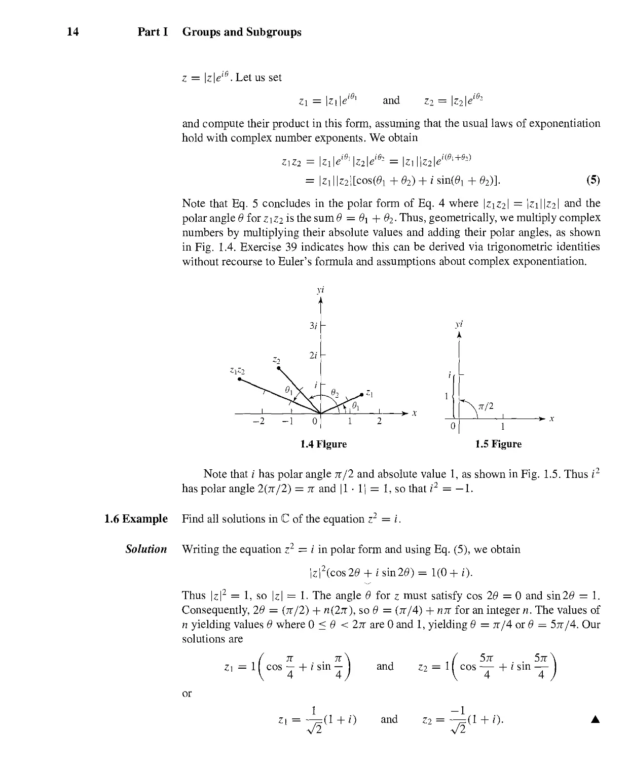
Note that Eq. 5 concludes in the polar form of Eq. 4 where \z\Zi\ = \zi\\z2\ and the
polar angle 8 for ziz2 is the sum 8 = 8\ + 82. Thus, geometrically, we multiply complex
numbers by multiplying their absolute values and adding their polar angles, as shown
in Fig. 1.4. Exercise 39 indicates how this can be derived via trigonometric identities
without recourse to Euler's formula and assumptions about complex exponentiation.
1.4 Figure
N7T/2
1.5 Figure
Note that i has polar angle n/2 and absolute value 1, as shown in Fig. 1.5. Thus i2
has polar angle 2(n/2) = u and |1 • 1| = 1, so that i2 = — 1.
1.6 Example Find all solutions in C of the equation z2 = i.
Solution Writing the equation z2 = i in polar form and using Eq. (5), we obtain
|z|2(cos2<9 + ;sin2<9)= 1(0+0-
Thus |z|2 = 1, so \z\ ~ 1. The angle 8 for z must satisfy cos 28 = 0 and sin2# — 1.
Consequently, 28 = (n/2) + n(2n), so 8 = (tt/4) + rnt for an integer n. The values of
n yielding values 8 where 0 < 8 < 2tt are 0 and 1, yielding 8 = tt/4 or 8 = 5n/4. Our
solutions are
TC . . It
Z\ — 1 cos —l-1 sin —
4 4
. 5tt 5rt
and £2 = 1 cos 1- i sin —
4 4
or
z\ = -7=(1 + 0
V2
and Z2 = —p(l + 0-
V2

Section 1 Introduction and Examples 15
1.7 Example Find all solutions of z = —16.
Solution As in Example 1.6 we write the equation in polar form, obtaining
|z|4(cos4<9 + i sin46») = 16(-1 + Or).
Consequently, |z|4 = 16, so \z\ = 2 while cos 46 = -I and sin46» = 0. We find that
40 = n + n(2n), so 6 = (n/4) + n(7t/2) for integers n. The different values of 6
obtained where 0 < 6 < 2tt are tt/4, 3tt/4, 5tt/4, and In/4. Thus one solution of z4 =
-16 is
2(cos^ + isin^=2(-L + -L;-)=V2(l + i).
In a similar way, we find three more solutions,
72(-1 + 0, 72(-1-0- and 72(1-0- A
The last two examples illustrate that we can find solutions of an equation z" = a + bi
by writing the equation in polar form. There will always be n solutions, provided that
a + bi / 0. Exercises 16 through 21 ask you to solve equations of this type.
We will not use addition or division of complex numbers, but we probably should
mention that addition is given by
(a + bi) + (c + di) = (a + c) + (b + d)i. (6)
and division of a + bi by nonzero c + di can be performed using the device
a + bi a + bi c — di (ac + bd) + (be — ad)i
c + di c + di c — di c2 + d2
ac + bd be — ad
+ -^^TL (7)
c2 + d2 c2 + d2
Algebra on Circles
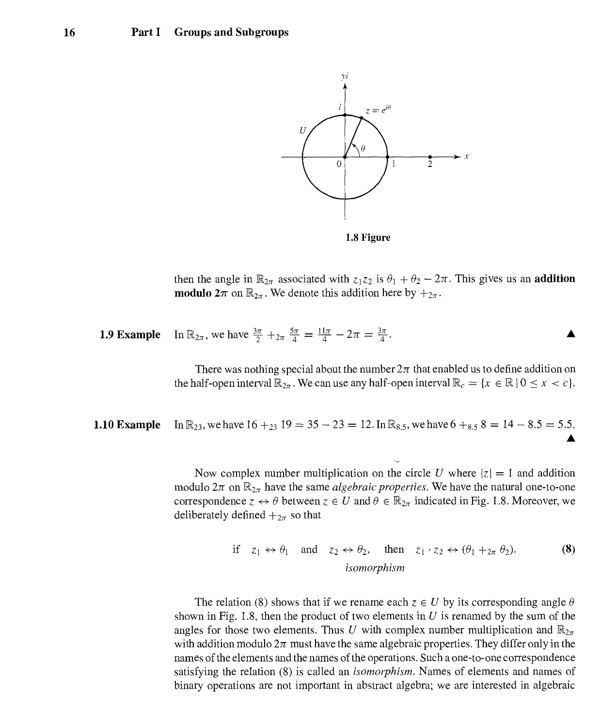
Let U = {z € C \ \z\ = 1], so that U is the circle in the Euclidean plane with center at
the origin and radius 1, as shown in Fig. 1.8. The relation \z\Zi\ = IZ1IIZ2I shows that
the product of two numbers in U is again a number in U; we say that U is closed under
multiplication. Thus, we can view multiplication in U as providing algebra on the circle
in Fig. 1.8.
As illustrated in Fig. 1.8, we associate with each z = cos 9 + i sin# in U a real
number 6 e R that lies in the half-open interval where 0 < 0 < 2n. This half-open
interval is usually denoted by [0, 2tt), but we prefer to denote it by 11¾^ for reasons
that will be apparent later. Recall that the angle associated with the product Z1Z2 of two
complex numbers is the sum 6\ + 62 of the associated angles. Of course if 6\ + 62 > 2it

16 Part I Groups and Subgroups
1.8 Figure
then the angle in R2jr associated with z\Z2 is 8\ + 62 — 2it. This gives us an addition
modulo 2-7T on E2jr. We denote this addition here by +2n ■
1.9 Example In R2w, we have 3-f +2n 5-f = lJ£- - 2n = 3f. A
There was nothing special about the number 2tc that enabled us to define addition on
the half-open interval R2ir • We can use any half-open interval Rc = {x e ffi|0 < * < c}.
1.10 Example InR23,wehave 16 +23 19 = 35 - 23 = 12.InE8.5,wehave6+8.5 8 = 14-8.5
5.5.
▲
Now complex number multiplication on the circle U where |z| = 1 and addition
modulo 2tt on ffi2.T have the same algebraic properties. We have the natural one-to-one
correspondence z *> 0 between z e U and 6 e ffi2^ indicated in Fig. 1.8. Moreover, we
deliberately defined +2n so that
if z\ <+ 0\ and zi +> 02, then z\- zi±* (0\ +2n 02).
isomorphism
(8)
The relation (8) shows that if we rename each z e U by its corresponding angle 0
shown in Fig. 1.8, then the product of two elements in U is renamed by the sum of the
angles for those two elements. Thus U with complex number multiplication and ffi2ir
with addition modulo 2it must have the same algebraic properties. They differ only in the
names of the elements and the names of the operations. Such a one-to-one correspondence
satisfying the relation (8) is called an isomorphism. Names of elements and names of
binary operations are not important in abstract algebra; we are interested in algebraic

Section 1 Introduction and Examples 17
properties. We illustrate what we mean by saying that the algebraic properties of U and
of R2;r are the same.
1.11 Example In U there is exactly one element e such that e ■ z = z for all z e U, namely, e = 1.
The element 0 in R2;r that corresponds to 1 e U is the only element e in R2;r such that
e +2n x = x for all x e R23r. ^
1.12 Example The equation z ■ z ■ z ■ z= lint/ has exactly four solutions, namely, 1, i, —1, and —i.
Now let/ and 0 e ffi2;r correspond, and the equation x +2jT x +2;r * +2jr x = 0 in R2;r
has exactly four solutions, namely, 0. tt/2, tt, and 3tt/2, which, of course, correspond
to 1, i, — 1, and —i, respectively. ▲
Because our circle U has radius 1, it has circumference 2it and the radian measure of
an angle 6 is equal to the length of the arc the angle subtends. If we pick up our half-open
interval ffi2jT, put the 0 in the interval down on the 1 on the *-axis and wind it around the
circle U counterclockwise, it will reach all the way back to 1. Moreover, each number
in the interval will fall on the point of the circle having that number as the value of the
central angle 6 shown in Fig. 1.8. This shows that we could also think of addition on
ffi2;r as being computed by adding lengths of subtended arcs counterclockwise, starting
at z = 1, and subtracting 2it if the sum of the lengths is lit or greater.
If we think of addition on a circle in terms of adding lengths of arcs from a starting
point P on the circle and proceeding counterclockwise, we can use a circle of radius
2, which has circumference 4tt, just as well as a circle of radius 1. We can take our
half-open interval BL^ and wrap it around counterclockwise, starting at P; it will just
cover the whole circle. Addition of arcs lengths gives us a notion of algebra for points on
this circle of radius 2, which is surely isomorphic to ~M^n with addition +4^. However,
if we take as the circle \z\ = 2 in Fig. 1.8, multiplication of complex numbers does not
give us an algebra on this circle. The relation \z\Z2\ = \z\\|z21 shows that the product of
two such complex numbers has absolute value 4 rather than 2. Thus complex number
multiplication is not closed on this circle.
The preceding paragraphs indicate that a little geometry can sometimes be of help
in abstract algebra. We can use geometry to convince ourselves that ffi2;r and BL^ are
isomorphic. Simply stretch out the interval R2;r uniformly to cover the interval E4^, or,
if you prefer, use a magnifier of power 2. Thus we set up the one-to-one correspondence
a *> 2a between a e E2t and 2a e E4JT. The relation (8) for isomorphism becomes
if a ±+ 2a and b ±* 2b then {a +¾ b) ±* (2a +4^ 2b). (9)
isomorphism
This is obvious if a + b < 2tt. If a + b = 2jt + c, then 2a + 2b = An + 2c, and the
final pairing in the displayed relation becomes c *> 2c, which is true.
1.13 Example x +4^ x +4^ x +4^ x = 0 in 1¾^ has exactly four solutions, namely, 0, n, 2jt, and 3tt,
which are two times the solutions found for the analogous equation in ffi2jr in
Example 1.12. ▲

18 Part I Groups and Subgroups
There is nothing special about the numbers 2n and An in the previous argument.
Surely, Ec with +c is isomorphic to E^ with +j for all c, d e E+. We need only pair
* e Ec with (d/c)x e Erf.
Roots of Unity
The elements of the set Un = {z e C | z" = 1} are called the nth roots of unity. Using the
technique of Examples 1.6 and 1.7, we see that the elements of this set are the numbers
( 2jt\ . ( 2n\ r „ , „
cos m— + i sin m— for m = 0. 1, 2, • • •, n — 1.
\ n J \ n J
They all have absolute value 1, so U„ C U. If we let £ = cos ^ + i sin ^-, then these
nth roots of unity can be written as
1 = ^,^,^,^,---,^-1. do)
Because £" = 1, these n powers of £ are closed under multiplication. For example, with
n — 10, we have
t6ts = tH = tl0t4 = 1 • t4 = t4 -^
Thus we see that we can compute £' £-7 by computing i +,, j, viewing i and j as elements
ofE„.
Let Z„ = {0, 1. 2, 3. • • •. n — 1}. We see that Z„ c E„ and clearly addition modulo
n is closed on Z„.
1.14 Example The solution of the equation x + 5 = 3 in Zg is x = 6, because 5+86 = 11 — 8 = 3.
▲
If we rename each of thenth roots of unity in (10) by its exponent, we use for names
all the elements of Z„. This gives a one-to-one correspondence between U„ and Z„.
Clearly,
if £' ±± i and CJ *+ J- *en (f' • ^) ±> (i +„ j). (11)
isomorphism
Thus [/„ with complex number multiplication and Z„ with addition +„ have the same
algebraic properties.
1.15 Example It can be shown that there is an isomorphism of U% with Z8 in which £ = ei2ir/8 ^> 5,
Under this isomorphism, we must then have £2 = t; ■ £ *> 5 +8 5 = 2. ▲
Exercise 35 asks you to continue the computation in Example 1.15, finding the
elements of Z8 to which each of the remaining six elements of U% correspond.

Section 1 Exercises 19
■ EXERCISES 1
In Exercises 1 through 9 compute the given arithmetic expression and give the answer in the form a + bi for
a,b€R.
1. /3 2. /4 3. /23
4. (-035 5. (4 - r)(5 + 3r) 6. (8 + 2/)(3 - /)
7. (2 - 30(4 + /) + (6- 5/) 8. (1 + /)3 9. (1 - /)5 (Use the binomial theorem.)
10. Find |3-4/|. 11. Find |6 + 4/|.
In Exercises 12 through 15 write the given complex number z in the polar form \z\(p + qi) where \p + qi\ — 1.
12.3-4/ 13.-1 + / 14.12 + 5/ 15.-3 + 5/
In Exercises 16 through 21, find all solutions in C of the given equation.
16.z4=l 17. z4 = -1 18. z3 =-8 19. z3 = -27/
20. z6 = 1 21. z6 = -64
In Exercises 22 through 27, compute the given expression using the indicated modular addition.
22. 10+17 16 23- 8 +io 6 24- 20-5 +25 19-3
25. | +i | 26. 3f +2, ^ 27. 2V2+^32 3V2
28. Explain why the expression 5 +6 8 in R6 makes no sense.
In Exercises 29 through 34, find all solutions x of the given equation.
29. x +15 7 = 3 in Zi5 30. x +2jT t = T in R^
31. * +7 * = 3 in Z7 32. x +7 * +7 * = 5 in Z7
33. x +12 * = 2 in Z12 34. * +4 x +4 * +4 * = 0 in Z4
35. Example 1.15 asserts that there is an isomorphism of £/g with Zg in which f = e'(n/4) ^> 5 and f2 ^> 2. Find
the element of Z$ that corresponds to each of the remaining six elements f'" in [/¾ for m = 0, 3, 4, 5, 6,
and 7.
36. There is an isomorphism of C/7 with Z7 in which t, = e'(2-T/7) ^> 4. Find the element in Z7 to which t,m must
correspond for m = 0,2, 3, 4, 5, and 6.
37. Why can there be no isomorphism of U& with Z6 in which f = e'(T/3) corresponds to 4?
38. Derive the formulas
sin(a + b) = sin a cos b + cos a sin b
and
cos(a + b) = cos a cos b — sin a sin b
by using Euler's formula and computing e'"e'b.
39. Letzi = |zi|(cos0i+/sinSi) andz2 = |z2l(cos6>2 + / sin02). Use the trigonometric identities in Exercise 38
toderiveziZ2 = |zi||z2|[cos(0i + 92) + / sin(0i +92)].
40. a. Derive a formula for cos 30 in terms of sin 9 and cos 9 using Euler's formula.
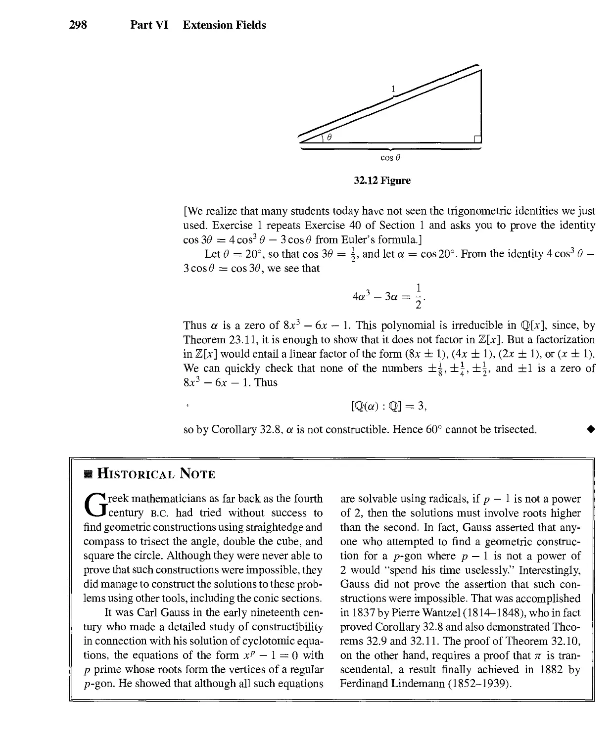
b. Derive the formula cos 30 = 4 cos3 0-3 cos 0 from part (a) and the identity sin2 0 + cos2 0 = 1. (We will
have use for this identity in Section 32.)

20 Part I Groups and Subgroups
41. Recall the power series expansions
X2 X3 X4 xn
e =1+*+2! + 3!+4!+"- + ^ + --<
x3 x0 x1 _ iN„_, x2"~]
sin, =,-- + --- + .-. + (-1)-^-^ + ..., and
x2 xA xb r s„ x2n
COSX = l-V.+^.-6i + -- + {~1)(2ny.+-
from calculus. Derive Euler's formula e'e = cosS + ;' sinS formally from these three series expansions.
section 2 Binary Operations
Suppose that we are visitors to a strange civilization in a strange world and are observing
one of the creatures of this world drilling a class of fellow creatures in addition of
numbers. Suppose also that we have not been told that the class is learning to add, but
were just placed as observers in the room where this was going on. We are asked to give a
report on exactly what happens. The teacher makes noises that sound to us approximately
like gloop, poyt. The class responds with bimt. The teacher then gives ompt, gaft, and the
class responds with poyt. What are they doing? We cannot report that they are adding
numbers, for we do not even know that the sounds are representing numbers. Of course,
we do realize that there is communication going on. All we can say with any certainty is
that these creatures know some rule, so that when certain pairs of things are designated
in their language, one after another, like gloop, poyt, they are able to agree on a response,
bimt. This same procedure goes on in addition drill in our first grade classes where a
teacher may say four, seven, and the class responds with eleven.
In our attempt to analyze addition and multiplication of numbers, we are thus led to
the idea that addition is basically just a rule that people learn, enabling them to associate,
with two numbers in a given order, some number as the answer. Multiplication is also
such a rule, but a different rule. Note finally that in playing this game with students,
teachers have to be a little careful of what two things they give to the class. If a first
grade teacher suddenly inserts ten, sky, the class will be very confused. The rule is only
defined for pairs of things from some specified set.
Definitions and Examples
As mathematicians, let us attempt to collect the core of these basic ideas in a useful
definition, generalizing the notions of addition and multiplication of numbers. As we
remarked in Section 0, we do not attempt to define a set. However, we can attempt to
be somewhat mathematically precise, and we describe our generalizations as functions
(see Definition 0.10 and Example 0.11) rather than as rules. Recall from Definition 0.4
that for any set S, the set S x S consists of all ordered pairs (a, b) for elements a and b
of S.
2.1 Definition A binary operation * on a set S is a function mapping S x S into S. For each (a, b) e
S x S, we will denote the element *((a, b)) of S by a * b. ■

Section 2 Binary Operations 21
Intuitively, we may regard a binary operation * on S as assigning, to each ordered
pair (a, b) of elements of S, an element a * b of S. We proceed with examples.
2.2 Example Our usual addition + is a binary operation on the set E. Our usual multiplication • is a
different binary operation on E. In this example, we could replace E by any of the sets
C, Z,E+,orZ+. ▲
Note that we require a binary operation on a set S to be defined for every ordered
pair (a, b) of elements from S.
2.3 Example Let M(E) be the set of all matrices^ with real entries. The usual matrix addition + is not
a binary operation on this set since A + B is not defined for an ordered pair (A, B) of
matrices having different numbers of rows or of columns. ▲
Sometimes a binary operation on S provides a binary operation on a subset H of S
also. We make a formal definition. ~
2.4 Definition Let * be a binary operation on S and let H be a subset of S. The subset H is closed
under * if for alla,b e //we also have a * b e H. In this case, the binary operation on
H given by restricting * to H is the induced operation of * on H. ■
By our very definition of a binary operation * on S, the set S is closed under *, but
a subset may not be, as the following example shows.
2.5 Example Our usual addition + on the set E of real numbers does not induce a binary operation
on the set E* of nonzero real numbers because 2 e E* and —2 e E*, but 2 + (—2) = 0
and 0 ¢. E*. Thus E* is not closed under *. ▲
In our text, we will often have occasion to decide whether a subset H of S is closed
under a binary operation * on S. To arrive at a correct conclusion, we have to know what
it means for an element to be in H, and to use this fact. Students have trouble here. Be
sure you understand the next example.
2.6 Example Let + and • be the usual binary operations of addition and multiplication on the set
Z, and let H = {n2\n e Z+}. Determine whether H is closed under (a) addition and
(b) multiplication.
Forpart (a), we need only observe that 12 = 1 and 22 = 4 are in H, but that 1 + 4 = 5
and 5 ¢. H. Thus H is not closed under addition.
For part (b), suppose that r e H and s e H. Using what it means for r and s to be
in H, we see that there must be integers n and m in Z+ such that r = n2 and s = m2.
Consequently, rs = n2m2 = (nm)2. By the characterization of elements in H and the
fact that nm e Z+, this means that rs e H, so H is closed under multiplication. ▲
T Most students of abstract algebra have studied linear algebra and are familiar with matrices and matrix
operations. For the benefit of those students, examples involving matrices are often given. The reader who is
not familiar with matrices can either skip all references to them or turn to the Appendix at the back of the text
where there is a short summary.

Parti
Groups and Subgroups
2.7 Example Let F be the set of all real-valued functions f having as domain the set E of real numbers.
We are familiar from calculus with the binary operations +, —, ■, and oonF. Namely,
for each ordered pair (/, g) of functions in F, we define for each x e E
f + 8 by {f + g)(x) = f{x) + g(x) addition,
/ - £ by (/ - g)(x) = f(x) - g(x) subtraction,
/ • 8 by (/ • g)(x) = f(x)g(x) multiplication,
and
/ o g by (/ o g)(x) = f(g(x))
composition.
All four of these functions are again real valued with domain E, so F is closed under all
four operations +, —, ■, and o. ▲
The binary operations described in the examples above are very familiar to you.
In this text, we want to abstract basic structural concepts from our familiar algebra.
To emphasize this concept of abstraction from the familiar, we should illustrate these
structural concepts with unfamiliar examples. We presented the binary operations of
complex number multiplication on U and U„, addition +„ on Z„, and addition +c on Ec
in Section 1.
The most important method of describing a particular binary operation * on a given
set is to characterize the element a * b assigned to each pair (a, b) by some property
defined in terms of a and b.
2.8 Example
On Z+, we define a binary operation * by a * b equals the smaller of a and b, or the
common value ifa = b. Thus 2 * 11 = 2; 15 * 10 = 10; and 3*3 = 3. ▲
2.9 Example On Z+, we define a binary operation *' by a *' b ■
and 5 *' 5 = 5.
a. Thus 2 *' 3 = 2, 25 *' 10 = 25,
2.10 Example On Z+, we define a binary operation *" by a *" b = (a * b) + 2, where * is defined in
Example 2.8. Thus 4 *" 7 = 6;25 *" 9 = 11; and 6 *" 6 = 8. ▲
It may seem that these examples are of no importance, but consider for a moment.
Suppose we go into a store to buy a large, delicious chocolate bar. Suppose we see two
identical bars side by side, the wrapper of one stamped $1.67 and the wrapper of the
other stamped $1.79. Of course we pick up the one stamped $1.67. Our knowledge of
which one we want depends on the fact that at some time we learned the binary operation
* of Example 2.8. It is a very important operation. Likewise, the binary operation *' of
Example 2.9 is defined using our ability to distinguish order. Think what a problem we
would have if we tried to put on our shoes first, and then our socks! Thus we should
not be hasty about dismissing some binary operation as being of little significance. Of
course, our usual operations of addition and multiplication of numbers have a practical
importance well known to us.
Examples 2.8 and 2.9 were chosen to demonstrate that a binary operation may or
may not depend on the order of the given pair. Thus in Example 2.8, a * b = b * a for
alla,b e Z+ , and in Example 2.9 this is not the case, for 5 *' 7 = 5 but 7 *' 5 = 7.

Section 2 Binary Operations 23
2.11 Definition A binary operation * on a set S is commutative if (and only if) a * b = b * a for all
a,b&S. ■
As was pointed out in Section 0, it is customary in mathematics to omit the words
and only if from a definition. Definitions are always understood to be if and only if
statements. Theorems are not always if and only if statements, and no such convention
is ever used for theorems.
Now suppose we wish to consider an expression of the form a * b * c. A binary
operation * enables us to combine only two elements, and here we have three. The obvious
attempts to combine the three elements are to form either (a * b) * c or a * (b * c). With
* defined as in Example 2.8, (2 * 5) * 9 is computed by 2 * 5 = 2 and then 2*9 = 2.
Likewise, 2 * (5 * 9) is computed by 5 * 9 = 5 and then 2*5 = 2. Hence (2 * 5) * 9 =
2 * (5 * 9), and it is not hard to see that for this *,
(a * b) * c = a * {b * c),
so there is no ambiguity in writing a * b * c. But for *" of Example 2.10,
(2 *" 5) *" 9 = 4 *" 9 = 6,
while
2 *" (5 *" 9) = 2 *" 7 = 4.
Thus {a *" b) *" c need not equal a *" {b *" c), and an expression a *" b *" c may be
ambiguous.
2.12 Definition A binary operation on a set S is associative if (a * b) * c = a * (b * c) for all a, b, c e S.
■
It can be shown that if * is associative, then longer expressions such as a * b *
c * d are not ambiguous. Parentheses may be inserted in any fashion for purposes of
computation; the final results of two such computations will be the same.
Composition of functions mapping E into E was reviewed in Example 2.7. For any
set S and any functions f and g mapping S into S, we similarly define the composition
f o g of g followed by /as the function mapping S into S such that (f o g)(x) = f{g{x))
for all x & S. Some of the most important binary operations we consider are defined
using composition of functions. It is important to know that this composition is always
associative whenever it is defined.
(Associativity of Composition) Let S be a set and let /, g, and h be functions mapping
S into S. Then / o (g o h) = (/ o g) o h.
To show these two functions are equal, we must show that they give the same assignment
to each x & S. Computing we find that
(/ o {g o h))(x) = f((g o h)(x)) = f(g(h(x)))
and
((/ O g) o h)(x) = {f o g)(h(x)) = f(g(h(x))),
so the same element f(g(h(x))) of S is indeed obtained. ♦
2.13 Theorem
Proof

24
Part I Groups and Subgroups
As an example of using Theorem 2.13 to save work, recall that it is a fairly painful
exercise in summation notation to show that multiplication of n x n matrices is an
associative binary operation. If, in a linear algebra course, we first show that there
is a one-to-one correspondence between matrices and linear transformations and that
multiplication of matrices corresponds to the composition of the linear transformations
(functions), we obtain this associativity at once from Theorem 2.13.
Tables
For a finite set, a binary operation on the set can be defined by means of a table in which
the elements of the set are listed across the top as heads of columns and at the left side
as heads of rows. We always require that the elements of the set be listed as heads across
the top in the same order as heads down the left side. The next example illustrates the
use of a table to define a binary operation.
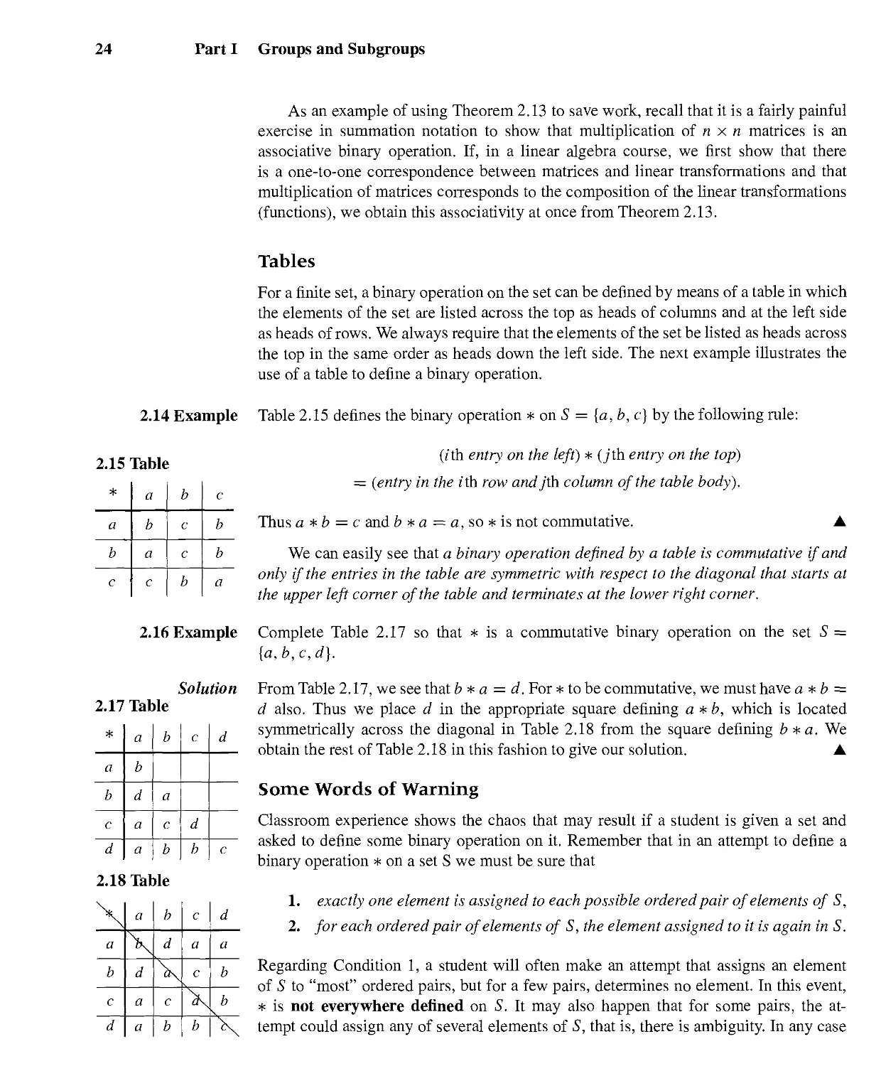
2.14 Example Table 2.15 defines the binary operation * on S = {a, b, c] by the following rule:
2.15 Table
(i th entry on the left) * (jth entry on the top)
= {entry in the i\h row and jth column of the table body).
Thus a * b = c and b * a = a, so * is not commutative. ▲
We can easily see that a binary operation defined by a table is commutative if and
only if the entries in the table are symmetric with respect to the diagonal that starts at
the upper left corner of the table and terminates at the lower right corner.
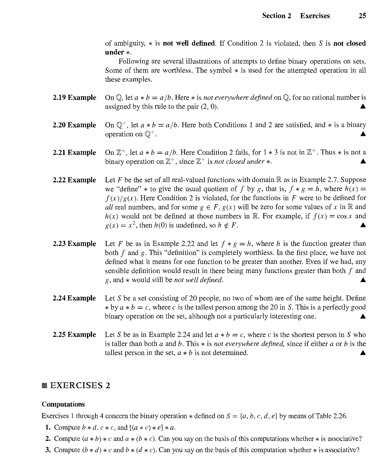
2.16 Example Complete Table 2.17 so that * is a commutative binary operation on the set S =
{a, b, c, d).
*
a
b
c
a
b
a
c
b
c
c
b
c
b
b
a
Solution
2.17 Table
*
a
b
c
d
a
b
d
a
a
b
a
c
b
c
d
b
d
c
2.18 Table
\l
a
b
c
d
a
\
d
a
a
b
d
\
c
b
c
a
c
X
b
d
a
b
b
\
From Table 2.17, we see that b *a = d. For * to be commutative, we must have a * b =
d also. Thus we place d in the appropriate square defining a * b, which is located
symmetrically across the diagonal in Table 2.18 from the square defining b*a. We
obtain the rest of Table 2.18 in this fashion to give our solution. ▲
Some Words of Warning
Classroom experience shows the chaos that may result if a student is given a set and
asked to define some binary operation on it. Remember that in an attempt to define a
binary operation * on a set S we must be sure that
1. exactly one element is assigned to each possible ordered pair of elements of S,
2. for each ordered pair of elements of S, the element assigned to it is again in S.
Regarding Condition 1, a student will often make an attempt that assigns an element
of S to "most" ordered pairs, but for a few pairs, determines no element. In this event,
* is not everywhere defined on S. It may also happen that for some pairs, the
attempt could assign any of several elements of S, that is, there is ambiguity. In any case

Section 2 Exercises 25
of ambiguity, * is not well defined. If Condition 2 is violated, then S is not closed
under *.
Following are several illustrations of attempts to define binary operations on sets.
Some of them are worthless. The symbol * is used for the attempted operation in all
these examples.
2.19 Example On Q, let a * b = a/b. Here * is not everywhere defined on Q, for no rational number is
assigned by this rule to the pair (2, 0). ▲
2.20 Example On Q+, let a * b = a/b. Here both Conditions 1 and 2 are satisfied, and * is a binary
operation on Q+. ▲
2.21 Example On Z+, let a * b = a/b. Here Condition 2 fails, for 1 * 3 is not in Z+. Thus * is not a
binary operation on Z+, since Z+ is not closed under *. A
2.22 Example Let F be the set of all real-valued functions with domain E as in Example 2.7. Suppose
we "define" * to give the usual quotient of f by g, that is, f * g = h, where h(x) =
f(x)/g(x). Here Condition 2 is violated, for the functions in F were to be defined for
all real numbers, and for some g e F, g(x) will be zero for some values of x in E and
h{x) would not be defined at those numbers in E. For example, if f{x) = cos* and
g(x) = x2, then h(0) is undefined, soh £ F. ▲
2.23 Example Let F be as in Example 2.22 and let f * g = h, where h is the function greater than
both f and g. This "definition" is completely worthless. In the first place, we have not
defined what it means for one function to be greater than another. Even if we had, any
sensible definition would result in there being many functions greater than both f and
g, and * would still be not well defined. ▲
2.24 Example Let S be a set consisting of 20 people, no two of whom are of the same height. Define
* by a * b = c, where c is the tallest person among the 20 in S. This is a perfectly good
binary operation on the set, although not a particularly interesting one. ▲
2.25 Example Let S be as in Example 2.24 and let a * b = c, where c is the shortest person in S who
is taller than both a and b. This * is not everywhere defined, since if either a or b is the
tallest person in the set, a * b is not determined. ▲
■ EXERCISES 2
Computations
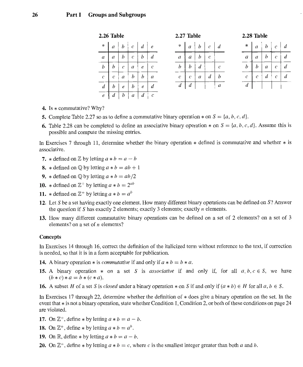
Exercises 1 through 4 concern the binary operation * denned on S = {a, b, c, d, e] by means of Table 2.26.
1. Compute b *d, c *c, and [(a * c) * e] * a.
2. Compute (a * b) * c and a * (b * c). Can you say on the basis of this computations whether * is associative?
3. Compute (b * d) * c and b * (d * c). Can you say on the basis of this computation whether * is associative?

26 Part I Groups and Subgroups
2.26 Table 2.27 Table 2.28 Table
*
a
b
c
d
e
a
a
b
c
b
d
b
b
c
a
e
b
C
c
a
b
b
a
d
b
e
b
e
d
e
d
c
a
d
c
*
a
b
c
d
a
a
b
c
d
b
b
d
a
c
c
d
d
c
b
a
*
a
b
c
d
a
a
b
c
b
b
a
d
c
c
c
c
d
d
d
d
4. Is * commutative? Why?
5. Complete Table 2.27 so as to define a commutative binary operation * on S = {a, b, c, d).
6. Table 2.28 can be completed to define an associative binary operation * on S = {a, b, c, d). Assume this is
possible and compute the missing entries.
In Exercises 7 through 11, determine whether the binary operation * defined is commutative and whether * is
associative.
7. * defined on Z by letting a*b = a — b
8. * defined on Q by letting a * b = ab + 1
9. * defined on Q by letting a * b = ab/2
10. * defined on Z+ by letting a*b-2ah
11. * defined on Z+ by letting a *b = ab
12. Let S be a set having exactly one element. How many different binary operations can be defined on SI Answer
the question if S has exactly 2 elements; exactly 3 elements; exactly n elements.
13. How many different commutative binary operations can be defined on a set of 2 elements? on a set of 3
elements? on a set of n elements?
Concepts
In Exercises 14 through 16, correct the definition of the italicized term without reference to the text, if correction
is needed, so that it is in a form acceptable for publication.
14. A binary operation * is commutative if and only if a * b = b * a.
15. A binary operation * on a set S is associative if and only if, for all a,b,c e S, we have
(b * c) * a = b * (c * a).
16. A subset H of a set S is closed under a binary operation * on S if and only if (a * b) e H for all a,b e S.
In Exercises 17 through 22, determine whether the definition of * does give a binary operation on the set. In the
event that * is not a binary operation, state whether Condition 1, Condition 2, or both of these conditions on page 24
are violated.
17. On Z+, define * by letting a *b = a — b.
18. On Z+, define * by letting a *b = ab.
19. On R, define * by letting a *b = a - b.
20. On Z+, define * by letting a * b = c, where c is the smallest integer greater than both a and b.

Section 2 Exercises 27
21. On Z+, define * by letting a * b = c, where c is at least 5 more than a + b.
22. On Z+, define * by letting a * b = c, where c is the largest integer less than the product of a and b.
23. Let H be the subset of M2(M) consisting of all matrices of the form for a, b e ffi. Is H closed under
a matrix addition? b matrix multiplication?
24. Mark each of the following true or false.
a. If * is any binary operation on any set S, then a * a = a for all a e S.
b. If * is any commutative binary operation on any set S, then a * (b * c) = (b * c) * a for all a, b,
c e S.
c. If * is any associative binary operation onanyset S, thena * (b * c) = (b * c) *aforalla, b, c e S.
d. The only binary operations of any importance are those defined on sets of numbers.
e. A binary operation * on a set S is commutative if there exist a,b e S such that a * b = b *a.
f. Every binary operation defined on a set having exactly one element is both commutative and
associative.
g. A binary operation on a set S assigns at least one element of S to each ordered pair of elements
of S.
h. A binary operation on a set S assigns at most one element of S to each ordered pair of elements of
S.
i. A binary operation on a set S assigns exactly one element of S to each ordered pair of elements
of S.
j. A binary operation on a set S may assign more than one element of S to some ordered pair of
elements of S.
25. Give a set different from any of those described in the examples of the text and not a set of numbers. Define
two different binary operations * and *' on this set. Be sure that your set is well defined.
Theory
26. Prove that if * is an associative and commutative binary operation on a set S, then
(a * b) * (c * d) = [(d * c) * a] * b
for all a, b, c, d e S. Assume the associative law only for triples as in the definition, that is, assume only
(x * y) * z = x * (y * z)
for all x, y,z e S.
In Exercises 27 and 28, either prove the statement or give a counterexample.
27. Every binary operation on a set consisting of a single element in both commutative and associative.
28. Every commutative binary operation on a set having just two elements is associative.
Let F be the set of all real-valued functions having as domain the set ffi of all real numbers. Example 2.7 defined
the binary operations +, —, •, and o on F. In Exercises 29 through 35, either prove the given statement or give a
counterexample.
29. Function addition + on F is associative.
30. Function subtraction — on F is commutative

28
Part I Groups and Subgroups
31. Function subtraction — on F is associative.
32. Function multiplication • on F is commutative.
33. Function multiplication • on F is associative.
34. Function composition o on F is commutative.
35. If * and *' are any two binary operations on a set S, then
a *(b *' c) = (a * b) *' (a * c) for all a, b, c e S.
36. Suppose that * is an associative binary operation on a set S. Let H = {a e S \ a * x = x * a for all x e S}.
Show that H is closed under *. (We think of H as consisting of all elements of S that commute with every
element in S.)
37. Supposethat*isanassociativeandcommutativebinaryoperationonaset5'.ShowthatH = {a e S\a*a = a)
is closed under *. (The elements of H are idempotents of the binary operation *.)
section 3 Isomorphic Binary Structures
Compare Table 3.1 for the binary operation * on the set S = {a, b, c] with Table 3.2 for
the binary operation *' on the set T = {#, $, &}.
Notice that if, in Table 3.1, we replace all occurrences of a by #, every b by $, and
every c by & using the one-to-one correspondence
a -o- # fc -o- $ c -o- &
we obtain precisely Table 3.2. The two tables differ only in the symbols (or names)
denoting the elements and the symbols * and *' for the operations. If we rewrite Table 3.3
with elements in the order y, x, z, we obtain Table 3.4. (Here we did not set up any one-
one-correpondence; we just listed the same elements in different order outside the heavy
bars of the table.) Replacing, in Table 3.1, all occurrences of a by y, every b by x, and
every c by z using the one-to-one correspondence
a -o- >' b -o- x c -o- z
we obtain Table 3.4. We think of Tables 3.1, 3.2, 3.3, and 3.4 as being structurally alike.
These four tables differ only in the names (or symbols) for their elements and in the
order that those elements are listed as heads in the tables. However, Table 3.5 for binary
operation * and Table 3.6 for binary operation * on the set S = {a, b, c] are structurally
different from each other and from Table 3.1. In Table 3.1, each element appears three
times in the body of the table, while the body of Table 3.5 contains the single element b.
In Table 3.6, for all 5 eS we get the same value c for 5 * s along the upper-left to lower-
right diagonal, while we get three different values in Table 3.1. Thus Tables 3.1 through
3.6 give just three structurally different binary operations on a set of three elements,
provided we disregard the names of the elements and the order in which they appear as
heads in the tables.
The situation we have just discussed is somewhat akin to children in France and in
Germany learning the operation of addition on the set Z+. The children have different

Section 3 Isomorphic Binary Structures 29
3.1 Table 3.2 Table 3.3 Table
*
a
b
c
a
c
a
b
b
a
b
c
c
b
c
a
*"
X
y
z
X
X
y
z
y
y
z
X
z
z
X
y
*'
#
$
&
#
&
#
$
$
#
$
&
&
$
&
#
3.4 Table 3.5 Table 3.6 Table
*
a
b
c
a
c
b
a
b
a
c
b
c
b
a
c
*"
y
X
z
y
z
y
X
X
y
X
z
z
X
z
y
*
a
b
c
a
b
b
b
b
b
b
b
c
b
b
b
names (un, deux, trois, • • • versus ein, zwei, drei ■ • •) for the numbers, but they are learning
the same binary structure. (In this case, they are also using the same symbols for the
numbers, so their addition tables would appear the same if they list the numbers in the
same order.)
We are interested in studying the different types of structures that binary operations
can provide on sets having the same number of elements, as typified by Tables 3.4, 3.5,
and 3.6. Let us consider a binary algebraic structure^ {S, *) to be a set S together with
a binary operation * on S. In order for two such binary structures {S, *) and (S', *') to
be structurally alike in the sense we have described, we would have to have a one-to-one
correspondence between the elements x of S and the elements x' of S' such that
if x -«► x and y ^> y', then x * y ^> x *' y'. (1)
A one-to-one correspondence exists if the sets S and S' have the same number of
elements. It is customary to describe a one-to-one correspondence by giving a one-
to-one function 0 mapping S onto S' (see Definition 0.12). For such a function ¢, we
regard the equation 4>{x) = x' as reading the one-to-one pairing x ^> x in left-to-right
order. In terms of ¢, the final ^> correspondence in (1), which asserts the algebraic
structure in S' is the same as in S, can be expressed as
4>(x*y) = 0(x)*'0(y).
Such, a function showing that two algebraic systems are structurally alike is known as
an isomorphism. We give a formal definition.
3.7 Definition Let (S, *) and {S', *') be binary algebraic structures. An isomorphism of S with S' is a
one-to-one function 0 mapping S onto S' such that
(f>{x * y) = 4>{y) *' (f>{y) for all x, y e S.
homomorphism property
1 Remember that boldface type indicates that a term is being defined.

30 Part I Groups and Subgroups
If such a map § exists, then S and S' are isomorphic binary structures, which we
denote by S ~ S', omitting the * and *' from the notation. ■
You may wonder why we labeled the displayed condition in Definition 3.7 the
homomorphism property rather than the isomorphism property. The notion of isomorphism
includes the idea of one-to-one correspondence, which appeared in the definition via the
words one-to-one and onto before the display. In Chapter 13, we will discuss the
relation between S and S' when 0:5-^5' satisfies the displayed homomorphism property,
but ¢) is not necessarily one to one; § is then called a homomorphism rather than an
isomorphism.
It is apparent that in Section 1, we showed that the binary structures {U, ■) and
(Ec, +c) are isomorphic for all c e E+. Also, {U„, ■) and (Z„, +„} are isomorphic for
eachn e Z+.
Exercise 27 asks us to show that for a collection of binary algebraic structures, the
relation ~ in Definition 3.7 is an equivalence relation on the collection. Our discussion
leading to the preceding definition shows that the binary structures defined by Tables 3.1
through 3.4 are in the same equivalence class, while those given by Tables 3.5 and 3.6 are
in different equivalence classes. We proceed to discuss how to try to determine whether
binary structures are isomorphic.
How to Show That Binary Structures Are Isomorphic
We now give an outline showing how to proceed from Definition 3.7 to show that two
binary structures {S, *} and {S', *') are isomorphic.
Step 1 Define the function 0 that gives the isomorphism of S with S'. Now this
means that we have to describe, in some fashion, what 0(s) is to be for every s & S.
Step 2 Show that 0 is a one-to-one function. That is, suppose that <j)(x) = 4>{y)
in S' and deduce from this that x = y in S.
Step 3 Show that 0 is onto S'. That is, suppose that s' e S' is given and show that
there does exist s & S such that 0(s) = s'.
Step 4 Show that 4>{x * y) = 4>{x) *' 4>{y)for all x,y e S. This is just a question
of computation. Compute both sides of the equation and see whether they are the
same.
3.8 Example Let us show that the binary structure (E, +} with operation the usual addition is
isomorphic to the structure (R+, •} where • is the usual multiplication.
Step 1 We have to somehow convert an operation of addition to multiplication.
Recall from ab+c = (ab)(a€) that addition of exponents corresponds to
multiplication of two quantities. Thus we try defining <f> : E —>• E+ by
(j){x) = ex for x e E. Note that ex > 0 for all x e E, so indeed,
4>{x) e E+.
Step 2 If (j>(x) = 4>{y), then ex = ey. Taking the natural logarithm, we see that
x = y, so 0 is indeed one to one.

Section 3 Isomorphic Binary Structures 31
Step 3 If r e E+, then ln(r) e E and 0(lnr) = eln r = r. Thus 0 is onto E+.
Step 4 For x, y e E, we have 0(x + y) = ex+y = ex ■ ey = 0(x) ■ 0(y). Thus we
see that § is indeed an isomorphism. ▲
3.9 Example Let 2Z = {2n \ n e Z}, so that 2Z is the set of all even integers, positive, negative, and
zero. We claim that (Z, +} is isomorphic to (2Z, +}, where + is the usual addition. This
will give an example of a binary structure (Z, +} that is actually isomorphic to a structure
consisting of a proper subset under the induced operation, in contrast to Example 3.8,
where the operations were totally different.
Step 1 The obvious function ¢) : Z —>• 2Z to try is given by <j>{n) = 2n for n € Z.
Step 2 If (j>{m) = <p{ri), then 2m = 2n so m = n. Thus § is one to one.
Step 3 If n e 2Z, then n is even so n = 2m for m = n/2 e Z. Hence
(j>{m) = 2(n/2) = n so 0 is onto 2Z.
Step 4 Let m,n e Z. The equation
4>{m + n) = 2(m + n) = 2m + 2n = (f>{m) + 0(n)
then shows that 0 is an isomorphism. A
How to Show That Binary Structures Are Not Isomorphic
We now turn to the reverse question, namely:
How do we demonstrate that two binary structures (S, *) and {S', *'} are not
isomorphic, if this is the case?
This would mean that there is no one-to-one function <f> from S onto S' with the property
4>{x * >') = 4>{x) *' <j>(y) for all x, y € S. In general, it is clearly not feasible to try every
possible one-to-one function mapping S onto S' and test whether it has this property,
except in the case where there are no such functions. This is the case precisely when S
and S' do not have the same cardinality. (See Definition 0.13.)
3.10 Example The binary structures (Q, +} and(E, +} are not isomorphic because Q has cardinality K0
while |E| ^ K0. (See the discussion following Example 0.13.) Note that it is not enough
to say that Q is a proper subset of E. Example 3.9 shows that a proper subset with the
induced operation can indeed be isomorphic to the entire binary structure. ▲
A structural property of a binary structure is one that must be shared by any
isomorphic structure. It is not concerned with names or some other nonstructural
characteristics of the elements. For example, the binary structures defined by Tables 3.1 and
3.2 are isomorphic, although the elements are totally different. Also, a structural
property is not concerned with what we consider to be the "name" of the binary operation.
Example 3.8 showed that a binary structure whose operation is our usual addition can be
isomorphic to one whose operation is our usual multiplication. The number of elements
in the set S is a structural property of (S, *}.

32
Part I Groups and Subgroups
In the event that there are one-to-one mappings of S onto S', we usually show that
(S, *) is not isomorphic to (S', *'} (if this is the case) by showing that one has
some structural property that the other does not possess.
3.11 Example The sets Z and Z+ both have cardinality X0, and there are lots of one-to-one functions
mapping Z onto Z+. However, the binary structures (Z, •) and (Z+, •), where • is the
usual multiplication, are not isomorphic. In (Z, •) there are two elements x such that
x • x = x, namely, 0 and 1. However, in (Z+, •), there is only the single element 1. ▲
We list a few examples of possible structural properties and nonstructural properties
of a binary structure (S, *) to get you thinking along the right line.
Possible Structural Properties
1. The set has 4 elements.
2. The operation is commutative.
3. x * x = x for all x e S.
4. The equation a * x = b has a
solution x in S for all a, b e S.
Possible Nonstructural Properties
a. The number 4 is an element.
b. The operation is called "addition.'
c. The elements of S are matrices.
d. S is a subset of C.
We introduced the algebraic notions of commutativity and associativity in Section 2.
One other structural notion that will be of interest to us is illustrated by Table 3.3,
where for the binary operation *" on the set {x,y, z], we have x *" u = u *" x = u
for all choices possible choices, x, y, and z for u. Thus x plays the same role as 0 in
(E, +) where 0 + u = u + 0 = u for all u e E, and the same role as 1 in (E, •) where
1 • u = u ■ 1 = u for all u e E. Because Tables 3.1 and 3.2 give structures isomorphic
to the one in Table 3.3, they must exhibit an element with a similar property. We see that
b * u = u * b = u for all elements u appearing in Table 3.1 and that $*'u = u*'$ = u
for all elements u in Table 3.2. We give a formal definition of this structural notion and
prove a little theorem.
3.12 Definition Let {S, *} be a binary structure. An element e of S is an identity element for * if
e*s = s*e = s for all s € S. ■
3.13 Theorem (Uniqueness of Identity Element) A binary structure {S, *) has at most one identity
element. That is, if there is an identity element, it is unique.
Proof Proceeding in the standard way to show uniqueness, suppose that both e and e are
elements of S serving as identity elements. We let them compete with each other. Regarding
e as an identity element, we must have e * e = e. However, regarding e as an identity
element, we must have e * e = e. We thus obtain e = e, showing that an identity element
must be unique. ♦

Section 3 Isomorphic Binary Structures 33
If you now have a good grasp of the notion of isomorphic binary structures, it
should be evident that having an identity element for * is indeed a structural property of
a structure {S, *}. However, we know from experience that many readers will be unable
to see the forest because of all the trees that have appeared. For them, we now supply a
careful proof, skipping along to touch those trees that are involved.
3.14Theorem Suppose {S, *} has an identity elements for*. If 0 : S —>• S' is an isomorphism of {S, *}
with {S', *'}, then 0(e) is an identity element for the binary operation *' on S'.
Proof Lets' e S'. We must show that 0(e) *' s' = s' *' 0(e) = s'. Because 0 is an isomorphism,
it is a one-to-one map of S onto S'. In particular, there exists s & S such that 0(s) = s'.
Now e is an identity element for * so that we know that e * s = s * e = s. Because 0 is
a function, we then obtain
(p{e * s) = 0(s * e) = <p(s).
Using Definition 3.7 of an isomorphism, we can rewrite this as
0(e) *' 4>{s) = 0(5) *' 0(e) = 0(5).
Remembering that we chose s € S such that 0(5) = s', we obtain the desired relation
0(e) *' s' = s' *' 0(e) = s'. ♦
We conclude with three more examples showing via structural properties that
certain binary structures are not isomorphic. In the exercises we ask you to show, as in
Theorem 3.14, that the properties we use to distinguish the structures in these examples
are indeed structural. That is, they must be shared by any isomorphic structure.
3.15 Example We show that the binary structures (Q, +} and (Z, +} under the usual addition are not
isomorphic. (Both Q and Z have cardinality Ko, so there are lots of one-to-one functions
mapping Q onto Z.) The equation x + x = c has a solution x for all c e Q, but this is
not the case in Z. For example, the equation x + x = 3 has no solution in Z. We have
exhibited a structural property that distinguishes these two structures. ▲
3.16 Example The binary structures (C, •} and (E, •} under the usual multiplication are not isomorphic.
(It can be shown that C and ffi have the same cardinality.) The equation x ■ x = c has a
solution x for all c e C, but x • x =-1 has no solution in ffi. ▲
3.17 Example The binary structure (M2(E), •} of 2 x 2 real matrices with the usual matrix multiplication
is not isomorphic to (E, •} with the usual number multiplication. (It can be shown that both
sets have cardinality |E|.) Multiplication of numbers is commutative, but multiplication
of matrices is not. ▲

34 Part I Groups and Subgroups
■ EXERCISES 3
In all the exercises, + is the usual addition on the set where it is specified, and • is the usual multiplication.
Computations
1. What three things must we check to determine whether a function ¢: S —>• 5" is an isomorphism of a binary
structure (S, *) with (S", *')?
In Exercises 2 through 10, determine whether the given map 0 is an isomorphism of the first binary structure with
the second. (See Exercise 1.) If it is not an isomorphism, why not?
2.
3.
4.
5.
6.
7.
8.
9.
10.
Z, +) with (Z, +) where <j>(ri) = —n for n e Z
Z, +) with (Z, +) where <j>(n) = 2n for n e Z
Z, +) with (Z, +) where 0(n) = n + 1 for n e Z
Q, +) with (Q, +) where <j>(x) = x/2 for x e Q
Q, •) with (Q, •) where 0(x) = x2 for * € Q
E, •) with (E, •) where 0(x) = *3 for* e E
M2(E), •) with (E, •) where 0(A) is the determinant of matrix A
Mi(E), •) with (E, •) where 0(A) is the determinant of matrix A
E, +) with (E+, •) where 0(r) = 0.5'" for r e E
In Exercises 11 through 15, let F be the set of all functions / mapping E into E that have derivatives of all orders.
Follow the instructions for Exercises 2 through 10.
11. (F, +) with {F, +} where ¢(/) = /', the derivative of /
12. (F, +) with (E, +) where ¢(/) = /'(0)
13. (F, +) with (F, +) where 0(/)(*) = ft /(t)dt
14. (F, +) with (F, +) where 0(/)(*) = £[£ /(f)A]
15. (F, •) with (F, •) where 0(/)(x) = x • /(x)
16. The map 0 : Z -* Z defined by 0(n) = n + 1 for n e Z is one to one and onto Z. Give the definition of a
binary operation * on Z such that ¢ is an isomorphism mapping
a. (Z, +) onto (Z, *), b. (Z, *) onto (Z, +).
In each case, give the identity element for * on Z.
17. The map 0 : Z -^ Z defined by 0(n) = n + 1 for n e Z is one to one and onto Z. Give the definition of a
binary operation * on Z such that ¢ is an isomorphism mapping
a. (Z, •) onto (Z, *), b. (Z, *) onto (Z, •).
In each case, give the identity element for * on Z.
18. The map ¢ : Q-+ Q defined by <j>(x) = 3x — 1 for x e Q is one to one and onto Q. Give the definition of a
binary operation * on Q such that 0 is an isomorphism mapping
a. (Q, +) onto (Q, *), b. (Q, *) onto (Q, +).
In each case, give the identity element for * on Q.

Section 3 Exercises 35
19. The map <p : Q -» Q defined by <j>{x) = 3x — 1 for x e Q is one to one and onto Q. Give the definition of a
binary operation * on Q such that 0 is an isomorphism mapping
a. (Q, •) onto (Q, *), b. (Q, *) onto (Q, •).
In each case, give the identity element for * on Q.
Concepts
20. The displayed homomorphism condition for an isomorphism ¢) in Definition 3.7 is sometimes summarized
by saying, "0 must commute with the binary operation(s)." Explain how that condition can be viewed in this
manner.
In Exercises 21 and 22, correct the definition of the italicized term without reference to the text, if correction is
needed, so that it is in a form acceptable for publication.
21. A function 0 : S —>- 5" is an isomorphism if and only if 0(a * b) = 0(a) *' 0(&)-
22. Let * be a binary operation on a set S. An element e of S with the property 5*e = 5 = e*5isan identity
element for * for all s e S.
Proof Synopsis
A good test of your understanding of a proof is your ability to give a one or two sentence synopsis of it, explaining
the idea of the proof without all the details and computations. Note that we said "sentence" and not "equation."
From now on, some of our exercise sets may contain one or two problems asking for a synopsis of a proof in the
text. It should rarely exceed three sentences. We should illustrate for you what we mean by a synopsis. Here is our
one-sentence synopsis of Theorem 3.14. Read the statement of the theorem now, and then our synopsis.
Representing an element of S' as 0(5) for some s e S, use the homomorphism property
of 0 to carry the computation of 0(e) *' 0(5) back to a computation in S.
That is the kind of explanation that one mathematician might give another if asked, "How does the proof go?"
We did not make the computation or explain why we could represent an element of S' as 0(5). To supply every
detail would result in a completely written proof. We just gave the guts of the argument in our synopsis.
23. Give a proof synopsis of Theorem 3.13.
Theory
24. An identity element for a binary operation * as described by Definition 3.12 is sometimes referred to as "a
two-sided identity element." Using complete sentences, give analogous definitions for
a. a left identity element ei for *, and b. a right identity element en for *.
Theorem 3.13 shows that if a two-sided identity element for * exists, it is unique. Is the same true for a one-sided
identity element you just defined? If so, prove it. If not, give a counterexample (S, *) for a finite set S and find
the first place where the proof of Theorem 3.13 breaks down.
25. Continuing the ideas of Exercise 24 can a binary structure have a left identity element ei and a right identity
element en where eL / eRl If so, give an example, using an operation on a finite set S. If not, prove that it is
impossible.

36 Part I Groups and Subgroups
26. Recall that if / : A —>- B is a one-to-one function mapping A onto S, then / ' (fc) is the unique a e A such that
f(a) = fc. Prove that if <p : S —>- 5" is an isomorphism of (5, *) with (5", *'), then ¢^ is an isomorphism of
(5",*') with (S,*).
27. Prove that if 0 : S -» 5" is an isomorphism of (S, *) with (5", *')andy/- : 5" -» 5"' is an isomorphism of (S", *')
with (5"', *"), then the composite function i\r o 0 is an isomorphism of (5, *) with (5"', *").
28. Prove that the relation ~ of being isomorphic, described in Definition 3.7, is an equivalence relation on any set
of binary structures. You may simply quote the results you were asked to prove in the preceding two exercises at
appropriate places in your proof.
In Exercises 29 through 32, give a careful proof for a skeptic that the indicated property of a binary structure (S, *)
is indeed a structural property. (In Theorem 3.14, we did this for the property, "There is an identity element for *.")
29. The operation * is commutative.
30. The operation * is associative.
31. For each c e S, the equation x * x = c has a solution x in S.
32. There exists an element b in S such that b*b = b. ~
33. Let H be the subset of M2(E) consisting of all matrices of the form for a, b e ffi. Exercise 23 of
Section 2 shows that H is closed under both matrix addition and matrix multiplication.
a. Show that (C, +) is isomorphic to (H, +}.
b. Show that (C, •) is isomorphic to (H, •).
(We say that H is a matrix representation of the complex numbers C.)
34. There are 16 possible binary structures on the set {a, b} of two elements. How many nonisomorphic (that is,
structurally different) structures are there among these 16? Phrased more precisely in terms of the isomorphism
equivalence relation ~ on this set of 16 structures, how many equivalence classes are there? Write down one
structure from each equivalence class. [Hint: Interchanging a and b everywhere in a table and then rewriting
the table with elements listed in the original order does not always yield a table different from the one we
started with.]
section 4 Groups
Let us continue the analysis of our past experience with algebra. Once we had mastered
the computational problems of addition and multiplication of numbers, we were ready
to apply these binary operations to the solution of problems. Often problems lead to
equations involving some unknown number x, which is to be determined. The simplest
equations are the linear ones of the forms a + x = b for the operation of addition, and
ax =b for multiplication. The additive linear equation always has a numerical solution,
and so has the multiplicative one, provided a/0. Indeed, the need for solutions of
additive linear equations such as 5 + x = 2 is a very good motivation for the negative
numbers. Similarly, the need for rational numbers is shown by equations such as 2x = 3.
It is desirable for us to be able to solve linear equations involving our binary
operations. This is not possible for every binary operation, however. For example, the equation
a * x = a has no solution in S = {a, b, c] for the operation * of Example 2.14. Let us
abstract from familiar algebra those properties of addition that enable us to solve the
equation 5 + * = 2 in Z. We must not refer to subtraction, for we are concerned with the
solution phrased in terms of a single binary operation, in this case addition. The steps in

Section 4 Groups 37
the solution are as follows:
5 + * = 2, given,
-5+ (5+ *) =-5+ 2, adding-5,
(-5 + 5) + x = -5 + 2, associative law,
0 + * = —5 + 2, computing — 5 + 5,
* = -5 + 2, property of 0,
x = —3, computing — 5 + 2.
Strictly speaking, we have not shownhere that —3 is a solution, but rather that it is the only
possibility for a solution. To show that —3 is a solution, one merely computes 5 + (—3).
A similar analysis could be made for the equation 2x = 3 in the rational numbers with
the operation of multiplication:
2x = 3, given,
\{2x) = \(i), multiplying by i, ^
{\ ■ 2)x = ^3, associative law,
1 • x = ^3, computing ^2,
43, property of 1,
2
3 computing 13.
We can now see what properties a set S and a binary operation * on S would have to
have to permit imitation of this procedure for an equation a * x = b for a, b € S. Basic
to the procedure is the existence of an element e in S with the property that e * x = x
for all x € S. For our additive example, 0 played the role of e, and 1 played the role for
our multiplicative example. Then we need an element a' in S that has the property that
a! * a = e. For our additive example with a = 5, —5 played the role of a', and \ played
the role for our multiplicative example with a = 2. Finally we need the associative law.
The remainder is just computation. A similar analysis shows that in order to solve the
equation x * a = b (remember that a * x need not equal x * a), we would like to have an
element e in S such that x * e = x for all x e S and an a' in S such that a * a! = e. With
all of these properties of * on S, we could be sure of being able to solve linear equations.
Thus we need an associative binary structure (S, *) with an identity element e such that
for each a e S, there exists a! e S such that a * a' = a' * a = e. This is precisely the
notion of a group, which we now define.
Definition and Examples
Rather than describe a group using terms defined in Sections 2 and 3 as we did at the end
of the preceding paragraph, we give a self-contained definition. This enables a person
who picks up this text to discover what a group is without having to look up more terms.
4.1 Definition A group (G, *) is a set G, closed under a binary operation *, such that the following
axioms are satisfied:
Sfx: For all a,b,c e G, we have
(a * b) * c = a * (b * c). associativity of *

38 Part I Groups and Subgroups
3^: There is an element e in G such that for all x e G,
e * x = x *e = x. identity element e for *
3¾-. Corresponding to each a e G, there is an element a' in G such that
a * a = a * a = e. inverse a' of a ■
4.2 Example We easily see that (U, •} and (£/„, •} are groups. Multiplication of complex numbers is
associative and both U and U„ contain 1, which is an identity for multiplication. For
e'e e U, the computation
ew ■ ei{2^e) = e2"1 = 1
shows that every element of U has an inverse. For z e £/„, the computation
z ■ z"'1 =zn = l
shows that every element of Un has an inverse. Thus (U, ■) and (£/„, •} are groups.
Because (Rc, +c) is isomorphic to (£/, •}, we see that (Ec, +c) is a group for all c e M+.
Similarly, the fact that (Z„, +„} is isomorphic to ([/„, •} shows that (Z„, +„} is a group
forallneZ+. A
We point out now that we will sometimes be sloppy in notation. Rather than use
the binary structure notation (G, *} constantly, we often refer to a group G, with the
understanding that there is of course a binary operation on the set G. In the event that
clarity demands that we specify an operation * on G, we use the phrase "the group G
Historical Note
There are three historical roots of the
development of abstract group theory evident in the
mathematical literature of the nineteenth century:
the theory of algebraic equations, number theory,
and geometry. All three of these areas used group-
theoretic methods of reasoning, although the
methods were considerably more explicit in the first area
than in the other two.
One of the central themes of geometry in the
nineteenth century was the search for invariants
under various types of geometric transformations.
Gradually attention became focused on the
transformations themselves, which in many cases can be
[ thought of as elements of groups.
In number theory, already in the eighteenth
century Leonhard Euler had considered the remainders
on division of powers a" by a fixed prime p. These
remainders have "group" properties. Similarly,
Carl F Gauss, in his Disquisitiones Arithmeti-
cae (1800), dealt extensively with quadratic forms
ax2 + 2bxy + cy2, and in particular showed that
equivalence classes of these forms under
composition possessed what amounted to group
properties.
Finally, the theory of algebraic equations
provided the most explicit prefiguring of the group
concept. Joseph-Louis Lagrange (1736-1813) in fact
initiated the study of permutations of the roots of an
equation as a tool for solving it. These permutations,
of course, were ultimately considered as elements
of a group.
It was Walter von Dyck (1856-1934) and i
Heinrich Weber (1842-1913) who in 1882 were
able independently to combine the three historical
roots and give clear definitions of the notion of an
abstract group.

Section 4 Groups 39
under *." For example, we may refer to the groups Z, (
than write the more tedious (Z, +), (Q, +), and (ffi, +).
to the group Zg without specifying the operation.
i>, and ffi under addition rather
However, we feel free to refer
4.3 Definition A group G is abelian if its binary operation is commutative.
■ Historical Note
Commutative groups are called abelian in honor
of the Norwegian mathematician Niels Henrik
Abel (1802-1829). Abel was interested in the
question of solvability of polynomial equations. In a
paper written in 1828, he proved that if all the roots
of such an equation can be expressed as rational
functions f, g,... ,h of one of them, say x, and
if for any two of these roots, f{x) and g{x), the
relation f{g{x)) = g{f{x)) always holds, then the
equation is solvable by radicals. Abel showed that
each of these functions in fact permutes the roots of
the equation; hence, these functions are elements
of the group of permutations of the roots. It was
this property of commutativity in these
permutation groups associated with solvable equations that
led Camille Jordan in his 1870 treatise on
algebra to name such groups abelian; the name since
then has been applied to commutative groups in
general.
Abel was attracted to mathematics as a teenager
and soon surpassed all his teachers in Norway. He
finally received a government travel grant to study
elsewhere in 1825 and proceeded to Berlin, where
he befriended August Crelle, the founder of the most
influential German mathematical journal. Abel
contributed numerous papers to Crelle's Journal during
the next several years, including many in the field
of elliptic functions, whose theory he created
virtually single-handedly. Abel returned to Norway in
1827 with no position and an abundance of debts.
He nevertheless continued to write brilliant papers,
but died of tuberculosis at the age of 26, two days
before Crelle succeeded in finding a university
position for him in Berlin.
Let us give some examples of some sets with binary operations that give groups and
also of some that do not give groups.
4.4 Example The set Z+ under addition is not a group. There is no identity element for + in Z+. ▲
4.5 Example The set of all nonnegative integers (including 0) under addition is still not a group. There
is an identity element 0, but no inverse for 2. ▲
4.6 Example The familiar additive properties of integers and of rational, real, and complex numbers
show that Z, Q, E, and C under addition are abelian groups. ▲
4.7 Example The set Z+ under multiplication is not a group. There is an identity 1, but no inverse
of 3. A
4.8 Example The familiar multiplicative properties of rational, real, and complex numbers show that
the sets Q+ and E+ of positive numbers and the sets Q*, ffi*, and C* of nonzero numbers
under multiplication are abelian groups. ▲

40
Part I Groups and Subgroups
4.9 Example The set of all real-valued functions with domain E under function addition is a group.
This group is abelian. ▲
4.10 Example (Linear Algebra) Those who have studied vector spaces should note that the axioms
for a vector space V pertaining just to vector addition can be summarized by asserting
that V under vector addition is an abelian group. ▲
4.11 Example The set Mmx„(E) of all m x n matrices under matrix addition is a group. The m x n
matrix with all entries 0 is the identity matrix. This group is abelian. ▲
4.12 Example The set M„(E) of all n x n matrices under matrix multiplication is not a group. The
n x n matrix with all entries 0 has no inverse. ▲
4.13 Example Show that the subset S of Mn (E) consisting of all invertible n x n matrices under matrix
multiplication is a group.
Solution We start by showing that S is closed under matrix multiplication. Let A and B be in S,
so that both A^1 and B'1 exist and AA'1 = BB'1 = In. Then
(AB)(B'1A~1) = A{BB~l)A~l = AlnA'x =. I„,
so that AB is invertible and consequently is also in S.
Since matrix multiplication is associative and /„ acts as the identity element, and
since each element of S has an inverse by definition of S, we see that S is indeed a group.
This group is not commutative. It is our first example of a nonabelian group. a
The group of invertible n x n matrices described in the preceding example is of
fundamental importance in linear algebra. It is the general linear group of degree n,
and is usually denoted by GL(n, E). Those of you who have studied linear algebra know
that a matrix A in GL(n, E) gives rise to an invertible linear transformation T : E" —>•
E", defined by 7\x) = Ax, and that conversely, every invertible linear transformation
of E" into itself is defined in this fashion by some matrix in GL(n, E). Also, matrix
multiplication corresponds to composition of linear transformations. Thus all invertible
linear transformations of E" into itself form a group under function composition; this
group is usually denoted by GL(W). Of course, GL(n, E) ~ GL(W).
4.14 Example Let * be defined on Q+ by a * b = ab/2. Then
and likewise
ab abc
(a *b) *c = — *c= ,
' 2 4
be abc
a * (b * c) = a * — = .
2 4
Thus * is associative. Computation shows that
2* a = a *2 = a
for all a e Q+, so 2 is an identity element for *. Finally,
a*- = -*a=2,
a a
so a! = A/a is an inverse for a. Hence Q+ with the operation * is a group.

Section 4 Groups 41
Elementary Properties of Groups
As we proceed to prove our first theorem about groups, we must use Definition 4.1, which
is the only thing we know about groups at the moment. The proof of a second theorem
can employ both Definition 4.1 and the first theorem; the proof of a third theorem can
use the definition and the first two theorems, and so on.
Our first theorem will establish cancellation laws. In real arithmetic, we know that
2a = 2b implies that a = b. We need only divide both sides of the equation 2a = 2b
by 2, or equivalently, multiply both sides by |, which is the multiplicative inverse of 2.
We parrot this proof to establish cancellation laws for any group. Note that we will also
use the associative law.
4.15 Theorem If G is a group with binary operation *, then the left and right cancellation laws
hold in G, that is, a * b = a * c implies b = c, and b * a = c * a implies b = c for all
a, b, c e G.
Proof Suppose a * b = a * c. Then by 3¾. there exists a', and
a * (a * b) = a' * (a * c).
By the associative law,
(a' * a) * b = (a' * a) * c.
By the definition of a' in 3¾, a' * a = e, so
e * b = e * c.
By the definition of e in .¾
b = c.
Similarly, from b * a = c * a one can deduce that b = c upon multiplication on the right
by a! and use of the axioms for a group. ♦
Our next proof can make use of Theorem 4.15. We show that a "linear equation" in
a group has a unique solution. Recall that we chose our group properties to allow us to
find solutions of such equations.
4.16 Theorem If G is a group with binary operation *, and if a and b are any elements of G, then the
linear equations a * x = b and y * a = b have unique solutions x and y in G.
Proof First we show the existence of at least one solution by just computing that a! * b is a
solution of a * x = b. Note that
a * (a' * b) = (a * a') * b, associative law,
= e * b, definition of a',
= b, property of e.
Thus x = a' * b is a solution of a * x = b- In a similar fashion, y = b * a' is a solution
of y * a = b.

42 Part I Groups and Subgroups
To show uniqueness of y, we use the standard method of assuming that we have
two solutions, y\ and yi, so that y\ * a = b and yi * a = b. Then y\ * a = )¾ * a, and
by Theorem 4.15, y\ = )¾. The uniqueness of x follows similarly. ♦
Of course, to prove the uniqueness in the last theorem, we could have followed the
procedure we used in motivating the definition of a group, showing that if a * x = b,
then x = a! * b. However, we chose to illustrate the standard way to prove an object is
unique; namely, suppose you have two such objects, and then prove they must be the
same. Note that the solutions x — a' * b and y = b * a! need not be the same unless * is
commutative.
Because a group is a special type of binary structure, we know from Theorem 3.13
that the identity e in a group is unique. We state this again as part of the next theorem
for easy reference.
In a group G with binary operation *, there is only one element e in G such that
e * x = x * e = x
for all x e G. Likewise for each aeC, there is only one element a' in G such that
a * a = a * a = e.
In summary, the identity element and inverse of each element are unique in a group.
Theorem 3.13 shows that an identity element for any binary structure is unique. No use
of the group axioms was required to show this.
Turning to the uniqueness of an inverse, suppose that aeG has inverses a' and a"
so that a'*a = a*a' = e and a" * a = a * a" = e. Then
a * a" = a * a' — e
and, by Theorem 4.15,
a i
a = a ,
so the inverse of a in a group is unique. ♦
Note that in a group G, we have
(a * b) * {b' * a') = a * (b * b') * a = (a * e) * a' = a * a = e.
This equation and Theorem 4.17 show that b' * a' is the unique inverse of a * b.
That is, (a * b)' = b' * a'. We state this as a corollary.
4.18 Corollary Let G be a group. For all a,b e G, we have (a * b)' = V * a'.
For your information, we remark that binary algebraic structures with weaker axioms
than those for a group have also been studied quite extensively. Of these weaker structures,
the semigroup, a set with an associative binary operation, has perhaps had the most
attention. A monoid is a semigroup that has an identity element for the binary operation.
Note that every group is both a semigroup and a monoid.
4.17 Theorem
Proof

Section 4 Groups 43
Finally, it is possible to give axioms for a group (G, *} that seem at first glance to
be weaker, namely:
1. The binary operation * on G is associative.
2. There exists a left identity element e in G such that e * x = x for all x e G.
3. For each a e G, there exists a left inverse a! in G such that a' * a = e.
From this one-sided definition, one can prove that the left identity element is also a right
identity element, and a left inverse is also a right inverse for the same element. Thus
these axioms should not be called weaker, since they result in exactly the same structures
being called groups. It is conceivable that it might be easier in some cases to check these
left axioms than to check our two-sided axioms. Of course, by symmetry it is clear that
there are also right axioms for a group.
Finite Groups and Group Tables
All our examples after Example 4.2 have been of infinite groups, that is, groups where
the set G has an infinite number of elements. We turn to finite groups, starting with the
smallest finite sets.
Since a group has to have at least one element, namely, the identity, a minimal set that
might give rise to a group is a one-element set {e}. The only possible binary operation *
on {e} is defined by e * e = e. The three group axioms hold. The identity element is
always its own inverse in every group.
Let us try to put a group structure on a set of two elements. Since one of the elements
must play the role of identity element, we may as well let the set be {e, a}. Let us attempt
to find a table for a binary operation * on {e, a} that gives a group structure on {e, a}.
When giving a table for a group operation, we shall always list the identity first, as in
the following table.
*
e
a
e
a
Since e is to be the identity, so
e * x = x * e = x
for all x e {e, a], we are forced to fill in the table as follows, if * is to give a group:
*
e
a
e
e
a
a
a
Also, a must have an inverse a' such that
a * a = a * a = e.

Groups and Subgroups
In our case, a! must be either e or a. Since a! = e obviously does not work, we must
have a! = a, so we have to complete the table as follows:
*
e
a
e
e
a
a
a
e
All the group axioms are now satisfied, except possibly the associative property.
Checking associativity on a case-by-case basis from a table defining an operation can be a
very tedious process. However, we know that Z2 = {0, 1} under addition modulo 2 is
a group, and by our arguments, its table must be the one above with e replaced by 0
and a by 1. Thus the associative property must be satisfied for our table containing e
and a.
With this example as background, we should be able to list some necessary conditions
that a table giving a binary operation on a finite set must satisfy for the operation to give
a group structure on the set. There must be one element of the set, which we may as well
denote by e, that acts as the identity element. The condition e * x = x means that the row
of the table opposite e at the extreme left must contain exactly the elements appearing
across the very top of the table in the same order. Similarly, the condition x * e = x
means that the column of the table under e at the very top must contain exactly the
elements appearing at the extreme left in the same order. The fact that every element a
has a right and a left inverse means that in the row having a at the extreme left, the
element e must appear, and in the column under a at the very top, the e must appear.
Thus e must appear in each row and in each column. We can do even better than this,
however. By Theorem 4.16, not only the equations a * x = e and y * a = e have unique
solutions, but also the equations a * x = b and y * a = b. By a similar argument, this
means that each element b of the group must appear once and only once in each row and
each column of the table.
Suppose conversely that a table for a binary operation on a finite set is such that
there is an element acting as identity and that in each row and each column, each element
of the set appears exactly once. Then it can be seen that the structure is a group structure
if and only if the associative law holds. If a binary operation * is given by a table,
the associative law is usually messy to check. If the operation * is defined by some
characterizing property of a * b, the associative law is often easy to check. Fortunately,
this second case turns out to be the one usually encountered. '
We saw that there was essentially only one group of two elements in the sense that
if the elements are denoted by e and a with the identity element e appearing first, the
table must be shown in Table 4.19. Suppose that a set has three elements. As before, we
may as well let the set be {e, a, b). For e to be an identity element, a binary operation
* on this set has to have a table of the form shown in Table 4.20. This leaves four
places to be filled in. You can quickly see that Table 4.20 must be completed as shown
in Table 4.21 if each row and each column are to contain each element exactly once.
Because there was only one way to complete the table and Z3 = {0, 1, 2} under addition
modulo 3 is a group, the associative property must hold for our table containing e, a,
andfo.

Section 4 Exercises 45
Now suppose that G' is any other group of three elements and imagine a table for G'
with identity element appearing first. Since our filling out of the table for G = {e, a, b)
could be done in only one way, we see that if we take the table for G' and rename the
identity e, the next element listed a, and the last element b, the resulting table for G'
must be the same as the one we had for G. As explained in Section 3, this renaming
gives an isomorphism of the group G' with the group G. Definition 3.7 denned the
notion of isomorphism and of isomorphic binary structures. Groups are just certain
types of binary structures, so the same definition pertains to them. Thus our work above
can be summarized by saying that all groups with a single element are isomorphic, all
groups with just two elements are isomorphic, and all groups with just three elements are
isomorphic. We use the phrase up to isomorphism to express this identification using the
equivalence relation ~. Thus we may say, "There is only one group of three elements,
up to isomorphism."
4.19 Table 4.20 Table 4.21 Table
*
e
a
e
e
a
a
a
e
*
e
a
b
e
e
a
b
a
a
b
e
b
b
e
a
*
e
a
b
e
e
a
b
a
a
b
b
■ EXERCISES 4
Computations
In Exercises 1 through 6, determine whether the binary operation * gives a group structure on the given set. If no
group results, give the first axiom in the order 3^, 3¾, 3¾ from Definition 4.1 that does not hold.
1. Let * be defined on Z by letting a *b = ab.
2. Let * be defined on 2Z = {2« | n e Z} by letting a * b = a + b.
3. Let * be defined on R+ by letting a * b = ~Jab.
4. Let * be defined on Q by letting a * b = ab.
5. Let * be defined on the set R* of nonzero real numbers by letting a * b = a/b.
6. Let * be defined on C by letting a *b = \ab\.
7. Give an example of an abelian group G where G has exactly 1000 elements.
8. We can also consider multiplication •„ modulo n in Z„. For example, 5 -7 6 = 2 in Z7 because 5 • 6 — 30 =
4(7) + 2. The set {1, 3, 5, 7} with multiplication -8 modulo 8 is a group. Give the table for this group.
9. Show that the group (£/, •) is not isomorphic to either (R, +) or (R*, •). (All three groups have cardinality |R|.)
10. Let n be a positive integer and let nL = {nm \ m e Z}.
a. Show that («Z, +) is a group.
b. Show that («Z, +) ~ (Z, +).

46 Part I Groups and Subgroups
In Exercises 11 through 18, determine whether the given set of matrices under the specified operation, matrix
addition or multiplication, is a group. Recall that a diagonal matrix is a square matrix whose only nonzero entries
lie on the main diagonal, from the upper left to the lower right corner. An upper-triangular matrix is a square
matrix with only zero entries below the main diagonal. Associated with each n x n matrix A is a number called
the determinant of A, denoted by det(A). If A and B are both n x n matrices, then det(AS) = det(A) det(S). Also,
det(7„) = 1 and A is invertible if and only if det(A) ^ 0.
11. All n x n diagonal matrices under matrix addition.
12. All n x n diagonal matrices under matrix multiplication.
13. All n x n diagonal matrices with no zero diagonal entry under matrix multiplication.
14. All n x n diagonal matrices with all diagonal entries 1 or — 1 under matrix multiplication.
15. All n x n upper-triangular matrices under matrix multiplication.
16. All n x n upper-triangular matrices under matrix addition.
17. All n x n upper-triangular matrices with determinant 1 under matrix multiplication.
18. All n x n matrices with determinant either 1 or — 1 under matrix multiplication.
19. Let S be the set of all real numbers except — 1. Define * on S by
a *b = a + b + ab.
a. Show that * gives a binary operation on S.
b. Show that (S, *) is a group.
c. Find the solution of the equation 2***3 = 7 in S.
20. This exercise shows that there are two nonisomorphic group structures on a set of 4 elements.
Let the set be [e, a, b, c}, with e the identity element for the group operation. A group table would then have
to start in the manner shown in Table 4.22. The square indicated by the question mark cannot be filled in with
a. It must be filled in either with the identity element e or with an element different from both e and a. In this
latter case, it is no loss of generality to assume that this element is b. If this square is filled in with e, the table
can then be completed in two ways to give a group. Find these two tables. (You need not check the associative
law.) If this square is filled in with b, then the table can only be completed in one way to give a group. Find this
table. (Again, you need not check the associative law.) Of the three tables you now have, two give isomorphic
groups. Determine which two tables these are, and give the one-to-one onto renaming function which is an
isomorphism.
a. Are all groups of 4 elements commutative?
b. Which table gives a group isomorphic to the group £/4, so that we know the binary operation defined by the
table is associative?
c. Show that the group given by one of the other tables is structurally the same as the group in Exercise 14 for
one particular value of n, so that we know that the operation defined by that table is associative also.
21. According to Exercise 12 of Section 2, there are 16 possible binary operations on a set of 2 elements. How
many of these give a structure of a group? How many of the 19,683 possible binary operations on a set of
3 elements give a group structure?
Concepts
22. Consider our axioms .^, .¾ and .¾ for a group. We gave them in the order 5^.¾.¾¾. Conceivable other
orders to state the axioms are -^5¾¾¾. .¾¾¾¾¾. 3¾¾¾^ .¾.^.¾ and ^.¾¾^. Of these six possible

Section 4 Exercises 47
orders, exactly three are acceptable for a definition. Which orders are not acceptable, and why? (Remember
this. Most instructors ask the student to define a group on at least one test.)
4.22 Table
*
e
a
b
c
•
e
a
b
c
a
a
?
b
b
c
c
23. The following "definitions" of a group are taken verbatim, including spelling and punctuation, from papers of
students who wrote a bit too quickly and carelessly. Criticize them.
a. A group G is a set of elements together with a binary operation * such that the following conditions are
satisfied
* is associative
There exists e e G such that
e*x=x*e = x= identity.
For every a e G there exists an a' (inverse) such that
a ■ a = a ■ a = e
b. A group is a set G such that
The operation on G is associative.
there is an identity element (e) in G.
for every a e G, there is an a' (inverse for each element)
c. A group is a set with a binary operation such
the binary operation is defined
an inverse exists
an identity element exists
d. A set G is called a group over the binery operation * such that for all a, b e G
Binary operation * is associative under addition
there exist an element {e} such that
a*e = e*a = e
Fore every element a there exists an element a' such that
a*a' = a'*a = e
24. Give a table for a binary operation on the set {e, a, b} of three elements satisfying axioms ,¾ and ,^ for a
group but not axiom Wx.
25. Mark each of the following true or false.
a. A group may have more than one identity element.
b. Any two groups of three elements are isomorphic.
c. In a group, each linear equation has a solution.

48 Part I Groups and Subgroups
d. The proper attitude toward a definition is to memorize it so that you can reproduce it word for word
as in the text.
e. Any definition a person gives for a group is correct provided that everything that is a group by that
person's definition is also a group by the definition in the text.
f. Any definition a person gives for a group is correct provided he or she can show that everything
that satisfies the definition satisfies the one in the text and conversely.
g. Every finite group of at most three elements is abelian.
h. An equation of the form a * x * b = c always has a unique solution in a group.
i. The empty set can be considered a group.
j. Every group is a binary algebraic structure.
Proof synopsis
We give an example of a proof synopsis. Here is a one-sentence synopsis of the proof that the inverse of an element
a in a group (G, *) is unique.
Assuming that a * a' = e and a * a" = e, apply the left cancellation law to the equation a * a' = a * a".
Note that we said "the left cancellation law" and not "Theorem 4.15." We always suppose that our synopsis was
given as an explanation given during a conversation at lunch, with no reference to text numbering and as little
notation as is practical.
26. Give a one-sentence synopsis of the proof of the left cancellation law in Theorem 4.15.
27. Give at most a two-sentence synopsis of the proof in Theorem 4.16 that an equation ax = b has a unique
solution in a group.
Theory
28. From our intuitive grasp of the notion of isomorphic groups, it should be clear that if cp : G -» G' is a group
isomorphism, then 4>{e) is the identity e' of G'. Recall that Theorem 3.14 gave a proof of this for isomorphic
binary structures (S, *) and (5", *'). Of course, this covers the case of groups.
It should also be intuitively clear that if a and a' are inverse pairs in G, then 0(a) and <j>{a') are inverse pairs
in G', that is, that 4>{a)' = <p(a'). Give a careful proof of this for a skeptic who can't see the forest for all the
trees.
29. Show that if G is a finite group with identity e and with an even number of elements, then there is a ^ e in G
such that a * a = e.
30. Let R* be the set of all real numbers except 0. Define * on R* by letting a * b = \a\b.
a. Show that * gives an associative binary operation on R*.
b. Show that there is a left identity for * and a right inverse for each element in R*.
c. Is R* with this binary operation a group?
d. Explain the significance of this exercise.
31. If * is a binary operation on a set S, an element x of S is an idempotent for * if x * x = x. Prove that a group
has exactly one idempotent element. (You may use any theorems proved so far in the text.)
32. Show that every group G with identity e and such that x * x = e for all x e G is abeliaa [Hint: Consider
(a * b) * (a * b).]

Section 5 Subgroups 49
33. Let G be an abelian group and let c" = c *c *■ ■■ *c for n factors c, where c & G and n e Z+. Give a
mathematical induction proof that (a * b)" = (a")* (b") for all a, b e G.
34. Let G be a group with a finite number of elements. Show that for any a e G, there exists an n e Z+ such that
a" = e. See Exercise 33 for the meaning of a". [Hint: Consider e, a, a2, a3,..., a'", where m is the number
of elements in G, and use the cancellation laws.]
35. Show that if (a * b)2 = a2 * b2 for a and b in a group G, then a *b = b* a. See Exercise 33 for the meaning
of a2.
36. Let G be a group and let a,b e G. Show that (a * b)' = a' *b' if and only if a * b = b * a.
37. Let G be a group and suppose that a * b * c = e for a, b, c e G. Show that b * c * a = e also.
38. Prove that a set G, together with a binary operation * on G satisfying the left axioms 1, 2, and 3 given on
page 43, is a group.
39. Prove that a nonempty set G, together with an associative binary operation * on G such that
a * x = b and y * a = b have solutions in G for all a, b e G,
is a group. [Hint: Use Exercise 38.]
40. Let (G, •) be a group. Consider the binary operation * on the set G defined by
a * b = b ■ a
for a,b e G. Show that (G, *) is a group and that (G, *) is actually isomorphic to (G, •). [Hint: Consider the
map 4> with <p{a) = a' for a e G.]
41. Let G be a group and let g be one fixed element of G. Show that the map ig, such that ig(x) = gxg' for* e G,
is an isomorphism of G with itself.
section 5 Subgroups
Notation and Terminology
It is time to explain some conventional notation and terminology used in group theory.
Algebraists as a rule do not use a special symbol * to denote a binary operation different
from the usual addition and multiplication. They stick with the conventional additive or
multiplicative notation and even call the operation addition or multiplication, depending
on the symbol used. The symbol for addition is, of course, +, and usually multiplication
is denoted by juxtaposition without a dot, if no confusion results. Thus in place of the
notation a * b, we shall be using either a + b to be read "the sum of a and b," or ab
to be read "the product of a and bV There is a sort of unwritten agreement that the
symbol + should be used only to designate commutative operations. Algebraists feel
very uncomfortable when they see a + b / b + a. For this reason, when developing our
theory in a general situation where the operation may or may not be commutative, we
shall always use multiplicative notation.
Algebraists frequently use the symbol 0 to denote an additive identity element and
the symbol 1 to denote a multiplicative identity element, even though they may not be
actually denoting the integers 0 and 1. Of course, if they are also talking about numbers
at the same time, so that confusion would result, symbols such as e or u are used as

50
Part I Groups and Subgroups
5.1 Table
1
a
b
1
1
a
b
a
a
b
1
b
b
1
a
5.2 Table
+
0
a
b
0
0
a
b
a
a
b
0
b
b
0
a
identity elements. Thus a table for a group of three elements might be one like Table 5.1
or, since such a group is commutative, the table might look like Table 5.2. In general
situations we shall continue to use e to denote the identity element of a group.
It is customary to denote the inverse of an element a in a group by a-1 in
multiplicative notation and by —a in additive notation. From now on, we shall be using these
notations in place of the symbol a'.
Let n be a positive integer. If a is an element of a group G, written multiplicatively,
we denote the product aaa ... a for n factors a by a". We let a0 be the identity element
e, and denote the product a~1a~1a~1.. .a-1 for n factors by a~n. It is easy to see that
our usual law of exponents, aman = am+n form, n e Z, holds. Form, n e Z+, it is clear.
We illustrate another type of case by an example:
-V = a
aaaaa = a (a a)aaaa = a eaaaa = a (ea)aaa
a aaaa = (a
a)aaa = eaaa = (ea)aa = aaa = a
In additive notation, we denote a + a +a + ■ ■ ■ +a for n summands by na, denote
(—a) + (—a) + (—a) + ■ ■ ■ + (—a) for n summands by —na, and let 0a be the identity
element. Be careful: In the notation na, the number n is in Z, not in G. One reason
we prefer to present group theory using multiplicative notation, even if G is abelian,
is the confusion caused by regarding n as being in G in this notation na. No one ever
misinterprets the n when it appears in an exponent.
Let us explain one more term that is used so often it merits a special definition.
5.3 Definition If G is a group, then the order \G\ of G is the number of elements in G. (Recall from
Section 0 that, for any set S, \S\ is the cardinality of S.) ■
Subsets and Subgroups
You may have noticed that we sometimes have had groups contained within larger
groups. For example, the group Z under addition is contained within the group Q under
addition, which in turn is contained in the group ffi under addition. When we view the
group (Z, +} as contained in the group (ffi, +}, it is very important to notice that the
operation + on integers n and m as elements of (Z, +} produces the same element n + m
as would result if you were to think of n and m as elements in (E, +}. Thus we should
not regard the group (Q+, •} as contained in (ffi, +}, even though Q+ is contained in ffi as
a set. In this instance, 2 • 3 = 6 in (Q+, •}, while 2 + 3 = 5 in (E, +}. We are requiring
not only that the set of one group be a subset of the set of the other, but also that the
group operation on the subset be the induced operation that assigns the same element
to each ordered pair from this subset as is assigned by the group operation on the whole
set.
5.4 Definition If a subset H of a group G is closed under the binary operation of G and if H with the
induced operation from G is itself a group, then H is a subgroup of G. We shall let
H < G or G > H denote that H is a subgroup of G, and H < G or G > H shall mean
H < G but H / G. ■

Section 5 Subgroups 51
Thus (Z, +} < (E, +} but (Q+, •} is not a subgroup of (E, +}, even though as sets,
Q+ C E. Every group G has as subgroups G itself and [e], where e is the identity element
of G.
5.5 Definition If G is a group, then the subgroup consisting of G itself is the improper subgroup of G.
All other subgroups are proper subgroups. The subgroup {e} is the trivial subgroup
of G. All other subgroups are nontrivial. ■
We turn to some illustrations.
5.6 Example Let E" be the additive group of all n-component row vectors with real number entries.
The subset consisting of all of these vectors having 0 as entry in the first component is
a subgroup of E". ▲
5.7 Example Q+ under multiplication is a proper subgroup of E+ under multiplication. ▲
5.8 Example The nth roots of unity in C form a subgroup Un of the group C* of nonzero complex
numbers under multiplication. ▲
5.9 Example There are two different types of group structures of order 4 (see Exercise 20 of Section 4).
We describe them by their group tables (Tables 5.10 and 5.11). The group V is the Klein
4-group, and the notation V comes from the German word Vier for four. The group
Z4 is isomorphic to the group £/4 = {1, i, — 1, — i} of fourth roots of unity under
multiplication.
The only nontrivial proper subgroup of Z4 is {0,2}. Note that {0,3 } is not a subgroup
of Z4, since {0, 3} is not closed under +. For example, 3 + 3=2, and 2 ¢ {0, 3}.
However, the group V has three nontrivial proper subgroups, {e, a), [e, b], and [e, c).
Here {e, a, b] is not a subgroup, since {e, a, b] is not closed under the operation of V
because ab = c, and c ¢ [e, a, b). A
5.10 Table
5.11 Table
Z4:
+
0
1
2
3
0
0
1
2
3
1
1
2
3
0
2
2
3
0
1
3
3
0
1
2
e
a
b
c
e
e
a
b
c
a
a
e
c
b
b
b
c
e
a
c
c
b
a
e
It is often useful to draw a subgroup diagram of the subgroups of a group. In such
a diagram, a line running downward from a group G to a group H means that H is a
subgroup of G. Thus the larger group is placed nearer the top of the diagram. Figure 5.12
contains the subgroup diagrams for the groups Z4 and V of Example 5.9.

52
Part I Groups and Subgroups
Note that if H < G and a e H, then by Theorem 4.16, the equation ax — a must
have a unique solution, namely the identity element of H. But this equation can also
be viewed as one in G, and we see that this unique solution must also be the identity
element e of G. A similar argument then applied to the equation ax = e, viewed in both
H and G, shows that the inverse a~1 of a in G is also the inverse of a in the subgroup H.
{0,2}
{0}
(a)
le,a)
(b)
5.12 Figure (a) Subgroup diagram for Z4. (b) Subgroup diagram for V.
5.13 Example Let F be the group of all real-valued functions with domain E under addition. The
subset of F consisting of those functions that are continuous is a subgroup of F, for
the sum of continuous functions is continuous, the function f where f(x) = 0 for all
x is continuous and is the additive identity element, and if f is continuous, then — f is
continuous. ▲
It is convenient to have routine steps for determining whether a subset of a group G
is a subgroup of G. Example 5.13 indicates such a routine, and in the next theorem, we
demonstrate carefully its validity. While more compact criteria are available, involving
only one condition, we prefer this more transparent theorem for a first course.
5.14 Theorem A subset H of a group G is a subgroup of G if and only if
1. H is closed under the binary operation of G,
2. the identity element e of G is in H,
3. for all a e H it is true that a^1 e H also.
Proof The fact that if H < G then Conditions 1, 2, and 3 must hold follows at once from the
definition of a subgroup and from the remarks preceding Example 5.13.
Conversely, suppose H is a subset of a group G such that Conditions 1,2, and 3 hold.
By 2 we have at once that .^ is satisfied. Also 5¾ is satisfied by 3. It remains to check
the associative axiom, 8¾. But surely for all a, b, c e H it is true that (ab)c = a(bc) in
H, for we may actually view this as an equation in G, where the associative law holds.
Hence H < G. ♦
5.15 Example Let F be as in Example 5.13. The subset of F consisting of those functions that are
differentiable is a subgroup of F, for the sum of differentiable functions is differentiable,
the constant function 0 is differentiable, and if f is differentiable, then — f is
differentiable. ▲

Section 5 Subgroups 53
5.16 Example Recall from linear algebra that every square matrix A has associated with it a number
det( A) called its determinant, and that A is invertible if and only if det( A) / 0. If A and B
are square matrices of the same size, thenit can be shown that det(AB) — det(A) • det(B).
Let G be the multiplicative group of all invertible n x n matrices with entries in C and
let T be the subset of G consisting of those matrices with determinant 1. The equation
det(AB) = det(A) • det(B) shows that T is closed under matrix multiplication. Recall
that the identity matrix /„ has determinant 1. From the equation det(A) • det(A_1) =
det(AA_1) = det(7„) = 1, we see that if det(A) = 1, then det(A_1) = 1. Theorem 5.14
then shows that T is a subgroup of G. ▲
Cyclic Subgroups
Let us see how large a subgroup H of Z12 would have to be if it contains 3. It would have
to contain the identity element 0 and 3 + 3, which is 6. Then it has to contain 6+3,
which is 9. Note that the inverse of 3 is 9 and the inverse of 6 is 6. It is easily checked
that H = {0, 3, 6, 9} is a subgroup of Z]2, and it is the smallest subgroup containing 3.
Let us imitate this reasoning in a general situation. As we remarked before, for
a general argument we always use multiplicative notation. Let G be a group and let
a e G. A subgroup of G containing a must, by Theorem 5.14, contain an, the result
of computing products of a and itself for n factors for every positive integer n. These
positive integral powers of a do give a set closed under multiplication. It is possible,
however, that the inverse of a is not in this set. Of course, a subgroup containing a must
also contain a-1, and, in general, it must contain a~m for all m e Z+. It must contain the
identity element e = a0. Summarizing, a subgroup of G containing the element a must
contain all elements an {or nafor additive groups) for all n e Z. That is, a subgroup
containing a must contain {a" \n e Z}. Observe that these powers an of a need not be
distinct. For example, in the group V of Example 5.9,
a = e, a =a, a — e, a~ = a, and so on.
We have almost proved the next theorem.
5.17 Theorem Let G be a group and let a e G. Then
ff = K|neZ)
is a subgroup of G and is the smallest' subgroup of G that contains a, that is, every
subgroup containing a contains H.
1 We may find occasion to distinguish between the terms minimal and smallest as applied to subsets of a set S
that have some property. A subset H of S is minimal with respect to the property if H has the property, and
no subset K C H,K ^ H, has the property. If H has the property and H c K for every subset K with the
property, then H is the smallest subset with the property. There may be many minimal subsets, but there can
be only one smallest subset. To illustrate, {e,a}, {e, b], and {e, c} are all minimal nontrivial subgroups of the
group V. (See Fig. 5.12.) However, V contains no smallest nontrivial subgroup.

54 Part I
Groups and Subgroups
Proof We check the three conditions given in Theorem 5.14 for a subset of a group to give a
subgroup. Since aras = ar+s for r, 5 g Z, we see that the product in G of two elements
of H is again in H. Thus H is closed under the group operation of G. Also a0 = e, so
e e H, and for ar e H, a~r e H and a~rar = e. Hence all the conditions are satisfied,
and H < G.
Our arguments prior to the statement of the theorem showed that any subgroup of
G containing a must contain H, so H is the smallest subgroup of G containing a. ♦
5.18Definition Let G be a group and let a e G. Then the subgroup {a" \n e Z} of G, characterized
in Theorem 5.17, is called the cyclic subgroup of G generated by a, and denoted
by(a>. ■
5.19 Definition An element a of a group G generates G and is a generator for G if {a} = G. A group
G is cyclic if there is some element a in G that generates G. ■
5.20 Example Let Z4 and 7 be the groups of Example 5.9. Then Z4 is cyclic and both 1 and 3 are
generators, that is,
(1) = (3)=24-
However, V is not cyclic, for {a}, {b}, and (c) are proper subgroups of two elements. Of
course, {e) is the trivial subgroup of one element. ▲
5.21 Example The group Z under addition is a cyclic group. Both 1 and —1 are generators for this
group, and they are the only generators. Also, for n e Z+, the group Z„ under addition
modulo n is cyclic. If n > 1, then both 1 and n — 1 are generators, but there may be
others. ▲
5.22 Example Consider the group Z under addition. Let us find (3). Here the notation is additive, and
(3) must contain
0,
3. 3 + 3=6, 3 + 3 + 3 = 9, and so on,
-3 + -3 = —6, -3+- —3 H—3 = —9, and so on.
In other words, the cyclic subgroup generated by 3 consists of all multiples of 3, positive,
negative, and zero. We denote this subgroup by 3Z as well as (3). In a similar way, we
shall let «Z be the cyclic subgroup («} of Z. Note that 6Z < 3Z. ▲
5.23 Example For each positive integer n, let U„ be the multiplicative group of the nth roots of unity
in C. These elements of U„ can be represented geometrically by equally spaced points
on a circle about the origin, as illustrated in Fig. 5.24. The heavy point represents the
number
2tt 2tc
i; = cos \- i sin —.
n n

Section 5 Exercises 55
The geometric interpretation of multiplication of complex numbers, explained in
Section 1, shows at once that as £ is raised to powers, it works its way counterclockwise
around the circle, landing on each of the elements of Un in turn. Thus Un under
multiplication is a cyclic group, and £ is a generator. The group U„ is the cyclic subgroup (£)
of the group U of all complex numbers z, where \z\ = 1, under multiplication. ▲
5.24 Figure
EXERCISES 5
Computations
In Exercises 1 through 6, determine whether the given subset of the complex numbers is a subgroup of the group
C of complex numbers under addition.
1. M 2. Q+ 3. 7Z
4. The set CR of pure imaginary numbers including 0
5. The set 7rQ of rational multiples of n 6. The set [it" ]«eZ}
7. Which of the sets in Exercises 1 through 6 are subgroups of the group C* of nonzero complex numbers under
multiplication?
In Exercises 8 through 13, determine whether the given set of invertible n x n matrices with real number entries is
a subgroup of GL(n, M).
8. The n x n matrices with determinant 2
9. The diagonal n x n matrices with no zeros on the diagonal
10. The upper-triangular n x n matrices with no zeros on the diagonal
11. The n x n matrices with determinant — 1
12. The n x n matrices with determinant — 1 or 1
13. The set of all n x n matrices A such that (AT)A = 7,,. [These matrices are called orthogonal. Recall that AT,
the transpose of A, is the matrix whose j'th column is the /th row of A for 1 < j < n, and that the transpose
operation has the property (AB)T = (BT)(AT).]

56 Part I Groups and Subgroups
Let F be the set of all real-valued functions with domain R and let F be the subset of F consisting of those functions
that have a nonzero value at every point in R. In Exercises 14 through 19, determine whether the given subset of F
with the induced operation is (a) a subgroup of the group F under addition, (b) a subgroup of the group F under
multiplication.
14. The subset F
15. The subset of all / e F such that /(1) = 0
16. The subset of all / e F such that /(1) = 1
17. The subset of all / e F such that /(0) = 1
18. The subset of all / e F such that /(0) = -1
19. The subset of all constant functions in F.
20. Nine groups are given below. Give a complete list of all subgroup relations, of the form G, < Gj, that exist
between these given groups G\, G?, • • •, Gg.
G\ = Z under addition
G2 = 12Z under addition
G3 = Q+ under multiplication
G4 = R under addition
G5 = R+ under multiplication
G6 = {jr" I « e Z} under multiplication
G7 = 3Z under addition
Gg = the set of all integral multiples of 6 under addition
Gg = {6" I n e Z} under multiplication
21. Write at least 5 elements of each of the following cyclic groups.
a. 25 Z under addition
b. {(1)" I n e Z} under multiplication
c. {tt" I n e Z} under multiplication
In Exercises 22 through 25, describe all the elements in the cyclic subgroup of GL(2, R) generated by the given
2x2 matrix.
0 -2"
-2 0
26. Which of the following groups are cyclic? For each cyclic group, list all the generators of the group.
G, = (Z, +) G2 = (Q, +) G3 = (Q+, •) G4 = (6Z, +)
G5 = {6" I n e Z} under multiplication
Gg = {a + fcV21 a, b e Z} under addition
In Exercises 27 through 35, find the order of the cyclic subgroup of the given group generated by the indicated
element.
27. The subgroup of Z4 generated by 3
28. The subgroup of V generated by c (see Table 5.11)
29. The subgroup of U(, generated by cos ^f + i sin ^f
30. The subgroup of Us generated by cos ^f- + i sin ^-
31. The subgroup of U% generated by cos =y + i sin =y
22.
0
-1
23.
1 1
0 1
24.
3 0
0 2
25.

Section 5 Exercises 57
32. The subgroup of U% generated by cos ^f + i sin ^f
33. The subgroup of the multiplicative group G of invertible 4x4 matrices generated by
0 0 1 o"
0 0 0 1
10 0 0
0 10 0
34. The subgroup of the multiplicative group G of invertible 4x4 matrices generated by
"0 0 0 l"
0 0 10
10 0 0
_0 1 0 0^
35. The subgroup of the multiplicative group G of invertible 4x4 matrices generated by
0 1 o o"
0 0 0 1
0 0 10
10 0 0
36. a. Complete Table 5.25 to give the group X(, of 6 elements.
b. Compute the subgroups (0), (1), (2), (3), (4), and (5) of the group Z6 given in part (a).
c. Which elements are generators for the group X(, of part (a)?
d. Give the subgroup diagram for the part (b) subgroups of X(,. (We will see later that these are all the subgroups
ofZ6.)
5.25 Table
+
0
1
2
3
4
5
0
0
1
2
3
4
5
1
1
2
2
2
3
3
3
4
4
4
5
5
5
0
Concepts
In Exercises 37 and 38, correct the definition of the italicized term without reference to the text, if correction is
needed, so that it is in a form acceptable for publication.
37. A subgroup of a group G is a subset H of G that contains the identity element e of G and also contains the
inverse of each of its elements.
38. A group G is cyclic if and only if there exists a e G such that G = {an | n € Z}.
39. Mark each of the following true or false.
a. The associative law holds in every group.
b. There may be a group in which the cancellation law fails.

58 Part I Groups and Subgroups
c. Every group is a subgroup of itself.
d. Every group has exactly two improper subgroups.
e. In every cyclic group, every element is a generator.
f. A cyclic group has a unique generator.
g. Every set of numbers that is a group under addition is also a group under multiplication.
h. A subgroup may be defined as a subset of a group.
i. Z4 is a cyclic group.
j. Every subset of every group is a subgroup under the induced operation.
40. Show by means of an example that it is possible for the quadratic equation x1 = e to have more than two
solutions in some group G with identity e.
Theory
In Exercises 41 and 42, let 0 : G ^ G' be an isomorphism of a group (G, *) with a group (G', *'). Write out a
proof to convince a skeptic of the intuitively clear statement.
41. If J? is a subgroup of G, then 0[ff] = {0(¾) | h e H} is a subgroup of G'. That is, an isomorphism carries
subgroups into subgroups.
42. If G is cyclic, then G' is cyclic.
43. Show that if H and K are subgroups of an abelian group G, then
{hk I h € H and k € K]
is a subgroup of G.
44. Find the flaw in the following argument: "Condition 2 of Theorem 5.14 is redundant, since it can be derived
from 1 and 3, for let a e H. Then a~] e H by 3, and by 1, aa~] = e is an element of H, proving 2."
45. Show that a nonempty subset H of a group G is a subgroup of G if and only if ab^1 € H for all a, b € H.
(This is one of the more compact criteria referred to prior to Theorem 5.14)
46. Prove that a cyclic group with only one generator can have at most 2 elements.
47. Prove that if G is an abelian group, written multiplicatively, with identity element e, then all elements x of G
satisfying the equation x1 = e form a subgroup H of G.
48. Repeat Exercise 47 for the general situation of the set H of all solutions x of the equation x" = e for a fixed
integer n > 1 in an abelian group G with identity e.
49. Show that if a e G, where G is a finite group with identity e, then there exists n e Z+ such that a" = e.
50. Let a nonempty finite subset H of a group G be closed under the binary operation of G. Show that H is a
subgroup of G.
51. Let G be a group and let a be one fixed element of G. Show that
Ha = {x e G I xa = ax}
is a subgroup of G.
52. Generalizing Exercise 51, let S be any subset of a group G.
a. Show that H$ = {x e G | xs = sx for all 5 e S} is a subgroup of G.
b. In reference to part (a), the subgroup HG is the center of G. Show that HG is an abelian group.
53. Let H be a subgroup of a group G. For a, b e G, let a ~ b if and only if ab~] e H. Show that ~ is an
equivalence relation on G.

Section 6 Cyclic Groups 59
54. For sets H and K, we define the intersection H n K by
flni[ = {i|xeflandie^).
Show that if H < G and K < G, then H Pi K < G. (Remember: < denotes "is a subgroup of," not "is a subset
of")
55. Prove that every cyclic group is abelian.
56. Let G be a group and let Gn = {gn | g e G}. Under what hypothesis about G can we show that G„ is a subgroup
ofG?
57. Show that a group with no proper nontrivial subgroups is cyclic.
section 6 Cyclic Groups
Recall the following facts and notations from Section 5. If G is a group and a e G, then
H = {an\n &Z}
is a subgroup of G (Theorem 5.17). This group is the cyclic subgroup (a) of G generated
by a. Also, given a group G and an element a in G, if
G = {an | n e Z},
then a is a generator of G and the group G = {a) is cyclic. We introduce one new bit of
terminology. Let a be an element of a group G. If the cyclic subgroup (a) of G is finite,
then the order of a is the order \(a) | of this cyclic subgroup. Otherwise, we say that a
is of infinite order. We will see in this section that if a e G is of finite order m, then m
is the smallest positive integer such that am = e.
The first goal of this section is to describe all cyclic groups and all subgroups of
cyclic groups. This is not an idle exercise. We will see later that cyclic groups serve
as building blocks for all sufficiently small abelian groups, in particular, for all finite
abelian groups. Cyclic groups are fundamental to the understanding of groups.
Elementary Properties of Cyclic Groups
We start with a demonstration that cyclic groups are abelian.
6.1 Theorem Every cyclic group is abelian.
Proof Let G be a cyclic group and let a be a generator of G so that
G = (a) = {an | n e Z}.
If gi and g2 are any two elements of G, there exist integers r and 5 such that gi = ar
and g2 = as. Then
glg2 = aras = ar+s = as+r = asar = g2gu
so G is abelian. ♦
We shall continue to use multiplicative notation for our general work on cyclic
groups, even though they are abelian.

60 Part I Groups and Subgroups
The division algorithm that follows is a seemingly trivial, but very fundamental tool
for the study of cyclic groups.
n > 0, q > 0 —|-
2m
-\ A—
<I>n (q + \)m
n < 0, q < 0 —|-
qm (q + \)m
2m
6.2 Figure
6.3 Division Algorithm for Z If m is a positive integer and n is any integer, then there exist unique integers q
and r such that
and
0 < r <
n = mq + r
Proof We give an intuitive diagrammatic explanation, using Fig. 6.2. On the real x-axis of
analytic geometry, mark off the multiples of m and the position of n. Now n falls either
on a multiple qm of m and r can be taken as 0, or n falls between two multiples of m.
If the latter is the case, let qm be the first multiple of m to the left of n. Then r is as
shown in Fig. 6.2. Note that 0 < r < m. Uniqueness of q and r follows since if n is not
a multiple of m so that we can take r = 0, then there is a unique multiple qm of m to the
left of n and at distance less than m from n, as illustrated in Fig. 6.2. ♦
In the notation of the division algorithm, we regard q as the quotient and r as the
nonnegative remainder when n is divided by m.
6.4 Example Find the quotient q and remainder r when 38 is divided by 7 according to the division
algorithm.
Solution The positive multiples of 7 are 7, 14, 21, 28, 35, 42,---. Choosing the multiple to leave
a nonnegative remainder less than 7, we write
38 = 35 + 3 = 7(5) + 3
so the quotient is q = 5 and the remainder is r = 3. ▲
6.5 Example Find the quotient q and remainder r when —38 is divided by 7 according to the division
algorithm.
Solution The negative multiples of 7 are -7, -14, -21, -28, -35, -42,
tiple to leave a nonnegative remainder less than 7, we write
. Choosing the mul-
so the quotient is q
-38 = -42 + 4 = 7(-6) + 4
-6 and the remainder is r = 4.
We will use the division algorithm to show that a subgroup Hofa cyclic group G
is also cyclic. Think for a moment what we will have to do to prove this. We will have to

Section 6 Cyclic Groups 61
use the definition of a cyclic group since we have proved little about cyclic groups yet.
That is, we will have to use the fact that G has a generating element a. We must then
exhibit, in terms of this generator a, some generator c = am for H in order to show that
H is cyclic. There is really only one natural choice for the power m of a to try. Can you
guess what it is before you read the proof of the theorem?
6.6 Theorem A subgroup of a cyclic group is cyclic.
Proof Let G be a cyclic group generated by a and let H be a subgroup of G. If H = {e}, then
H = (e) is cyclic. If H ^ {e}, then a" e H for some n € Z+. Let m be the smallest
integer in Z+ such that am e H.
We claim that c = am generates H; that is,
H = (am) = (c).
We must show that every b e H is a power of c. Since b & H and H < G, we have
b = a" for some n. Find g and r such that
n = mq + r for 0 < r < m
in accord with the division algorithm. Then
an = amq+r = {am)qar,
so
ar = {amyqan.
Now since a" & H.am & H, and H is a group, both (am)~q and a" are in H. Thus
(am)"V e ff; that is, ar e ff.
Since m was the smallest positive integer such that am e H and 0 < r < m, we must
have r = 0. Thus n = ^m and
b = a» = (am)i =cq,
so fc is a power of c. ♦
As noted in Examples 5.21 and 5.22, Z under addition is cyclic and for a positive
integer ft, the set nL of all multiples of ft is a subgroup of Z under addition, the cyclic
subgroup generated by ft. Theorem 6.6 shows that these cyclic subgroups are the only
subgroups of Z under addition. We state this as a corollary.
6.7 Corollary The subgroups of Z under addition are precisely the groups ftZ under addition for n e Z.
This corollary gives us an elegant way to define the greatest common divisor of
two positive integers r and s. Exercise 45 shows that H = {nr + ms | n,m e Z} is a
subgroup of the group Z under addition. Thus H must be cyclic and have a generator d,
which we may choose to be positive.

62 Part I Groups and Subgroups
6.8 Definition Let r and 5 be two positive integers. The positive generator d of the cyclic group
H = {nr + ms \ n,m e Z}
under addition is the greatest common divisor (abbreviated gcd) of r and s. We write
d = gcd(r, s). ■
Note from the definition that d is a divisor of both r and 5 since both r = \r + Os
and 5 = Or + Is are in H. Since d e H, we can write
d = nr + ms
for some integers n and m. We see that every integer dividing both r and 5 divides the
right-hand side of the equation, and hence must be a divisor of d also. Thus d must
be the largest number dividing both r and s; this accounts for the name given to d in
Definition 6.8.
6.9 Example Find the gcd of 42 and 72.
Solution The positive divisors of 42 are 1, 2, 3, 6, 7, 14, 21, and 42. The positive divisors of 72
are 1, 2, 3, 4, 6, 8, 9, 12, 18, 24, 36, and 72. The greatest common divisor is 6. Note
that 6 = (3)(72) + (-5)(42). There is an algorithm for expressing the greatest common
divisor d of r and 5 in the form d = nr + ms, but we will not need to make use of it
here. ▲
Two positive integers are relatively prime if their gcd is 1. For example, 12 and 25
are relatively prime. Note that they have no prime factors in common. In our discussion
of subgroups of cyclic groups, we will need to know the following:
If r ands are relatively prime andifr divides sm, then r must divide m.
(1)
Let's prove this. If r and 5 are relatively prime, then we may write
1 = ar + bs for some a, b e Z.
Multiplying by m, we obtain
m = arm + bsm.
Nowr divides both arm and bsm since r divides sm. Thus r is a divisor of the right-hand
side of this equation, so r must divide m.
The Structure of Cyclic Groups
We can now describe all cyclic groups, up to an isomorphism.

Section 6 Cyclic Groups 63
6.10 Theorem Let G be a cyclic group with generator a. If the order of G is infinite, then G is isomorphic
to (Z, +}. If G has finite order ft, then G is isomorphic to (Z„, +„).
Proof Case I For all positive integers m,am / e. In this case we claim that no two
distinct exponents h and k can give equal elements ah and ak of G.
Suppose that aA = a* and say h > k. Then
„h-k h-k
a a = a = e,
contrary to our Case I assumption. Hence every element of G can be
expressed as am for a unique meZ. The map ¢) : G —> Z given by
(j>(a') = i is thus well defined, one to one, and onto Z. Also,
0(a!V) = 4>{ai+i) = i + j= ¢(0.1) + 0(aJ'),
so the homomorphism property is satisfied and 0 is an isomorphism.
Case II am = efor some positive integer m. Let n be the smallest positive
integer such that a" = e.lf s e Z and 5 = nq + r for 0 < r < ft, then
</ = a"<7+r = (a")<V = e<7ar = ar. AsinCase 1, if 0 < k < h < n and
aA = a*, then aA_* = e and 0 < h - fc < n, contradicting our choice of
n. Thus the elements
a0 = e, a, a ,a ,
are all distinct and comprise all elements of G. The map \j/ : G —>• Z„
given by i/f(a') = i for *' = 0, 1, 2, • • •, n - 1 is thus well defined, one to
one, and onto Z„. Because a" = e, we see that a1 a' = ak where
k = i +n j- Thus
f(alaj) = i +„ j = f(a') +„ f(aJ),
so the homomorphism property is satisfied and \j/ is an isomorphism.
n- 1
6.11 Figure
6.12 Figure
6.13 Example
Motivated by our work with Un, it is nice to visualize the elements e= a0, a1, a2, ■ ■ ■,
an~' of a cyclic group of order n as being distributed evenly on a circle (see Fig. 6.11). The
element ah is located h of these equal units counterclockwise along the circle, measured
from the bottom where e = a0 is located. To multiply ah and ak diagrammatically, we
start from ah and go k additional units around counterclockwise. To see arithmetically

64 Part I Groups and Subgroups
6.14 Theorem
Proof
where we end up, find q and r such that
h + k = nq + r for 0 < r < n.
The nq takes us all the way around the circle q times, and we then wind up at ar. A
Figure 6.12 is essentially the same as Fig. 6.11 but with the points labeled with the
exponents on the generator. The operation on these exponents is addition modulo n.
Subgroups of Finite Cyclic Groups
We have completed our description of cyclic groups and turn to their subgroups. Corollary
6.7 gives us complete information about subgroups of infinite cyclic groups. Let us give
the basic theorem regarding generators of subgroups for the finite cyclic groups.
Let G be a cyclic group with n elements and generated by a. Let b e G and let b = as.
Then b generates a cyclic subgroup H of G containing n/d elements, where d is the
greatest common divisor ofnands. Also, (as) = (ar)ifandonlyifgcd(5, n) = gcd(t,n).
That b generates a cyclic subgroup H of G is known from Theorem 5.17. We need show
only that H has n/d elements. Following the argument of Case II of Theorem 6.10, we
see that H has as many elements as the smallest positive power m of b that gives the
identity. Now b = as, and bm = e if and only if (as)m = e, or if and only if n divides
ms. What is the smallest positive integer m such that n divides ms? Let d be the gcd of
n and s. Then there exists integers u and v such that
d = un + vs.
Since d divides both n and s, we may write
1 = u(n/d) + v(s/d)
where both n/d and s/d are integers. This last equation shows that n/d and s/d are
relatively prime, for any integer dividing both of them must also divide 1. We wish to
find the smallest positive m such that
m(s/d) .
(n/d)
is an integer.
From the boxed division property (1), we conclude that n/d must divide m, so the
smallest such m is n/d. Thus the order of H is n/d.
Taking for the moment Z„ as a model for a cyclic group of order n, we see that if d is
a divisor of n, then the cyclic subgroup (d) of Z„ had n/d elements, and contains all the
positive integers m less than n such that gcd(m, n) = d. Thus there is only one subgroup
of Z„ of order n/d. Taken with the preceding paragraph, this shows at once that if
a is a generator of the cyclic group G, then (as) = (a'} if and only if gcd(s, n) =
gcd(f.n). ♦
6.15 Example For an example using additive notation, consider Z^, with the generator a = 1. Since
the greatest comm
elements, namely
the greatest common divisor of 3 and 12 is 3, 3 = 3 • 1 generates a subgroup of y = 4
(3) = {0,3,6,9}.

Section 6 Cyclic Groups 65
Since the gcd of 8 and 12 is 4, 8 generates a subgroup of -j = 3 elements, namely,
(8} = {0,4, 8}.
Since the gcd of 12 and 5 is 1, 5 generates a subgroup of y = 12 elements; that is, 5 is
a generator of the whole group Z^. A
The following corollary follows immediately from Theorem 6.14.
6.16 Corollary If a is a generator of a finite cyclic group G of order n, then the other generators of G
are the elements of the form ar, where r is relatively prime to n.
6.17 Example Let us find all subgroups of "L\% and give their subgroup diagram. All subgroups are
cyclic. By Corollary 6.16, the elements 1, 5, 7, 11, 13, and 17 are all generators of 7L\%.
Starting with 2,
(2) = {0,2,4,6,8, 10, 12, 14, 16}.
is of order 9 and has as generators elements of the form h2, where h is relatively prime
to 9, namely, h = 1, 2, 4, 5, 7, and 8, so h2 = 2,4, 8, 10, 14, and 16. The element 6 of
(2) generates {0, 6, 12}, and 12 also is a generator of this subgroup.
We have thus far found all subgroups generated by 0, 1, 2, 4, 5, 6, 7, 8, 10, 11, 12,
13, 14, 16, and 17. This leaves just 3, 9, and 15 to consider.
(3) ={0,3,6,9, 12,15},
and 15 also generates this group of order 6, since 15 = 5 • 3, and the gcd of 5 and 6 is 1.
Finally,
(9} = {0, 9}.
The subgroup diagram for these subgroups of Zig is given in Fig. 6.18.
(1) = zlg
6.18 Figure Subgroup diagram for Z18.
This example is straightforward; we are afraid we wrote it out in such detail that it
may look complicated. The exercises give some practice along these lines. ▲

66 Part I Groups and Subgroups
■ EXERCISES 6
Computations
In Exercises 1 through 4, find the quotient and remainder, according to the division algorithm, when n is divided
by m.
1. n = 42, m = 9 2. n = -42, m = 9
3. n = -50, m = 8 4. n = 50, m = 8
In Exercises 5 through 7, find the greatest common divisor of the two integers.
5. 32 and 24 6. 48 and 88 7. 360 and 420
In Exercises 8 through 11, find the number of generators of a cyclic group having the given order.
8. 5 9. 8 10. 12 11. 60
An isomorphism of a group with itself is an automorphism of the group. In Exercises 12 through 16, find the
number of automorphisms of the given group.
[Hint: Make use of Exercise 44. What must be the image of a generator under an automorphism?]
12. Z2 13. Z6 14. Z8 15. Z 16. Z12
In Exercises 17 through 21, find the number of elements in the indicated cyclic group.
17. The cyclic subgroup of Z30 generated by 25
18. The cyclic subgroup of Z42 generated by 30
19. The cyclic subgroup (;') of the group C* of nonzero complex numbers under multiplication
20. The cyclic subgroup of the group C* of Exercise 19 generated by (1 + i)/V2
21. The cyclic subgroup of the group C* of Exercise 19 generated by 1 + ;'
In Exercises 22 through 24, find all subgroups of the given group, and draw the subgroup diagram for the subgroups.
22. Z,2 23. Z36 24. Z8
In Exercises 25 through 29, find all orders of subgroups of the given group.
25. Z6 26. Z8 27. Z12 28. Z20 29. Z,7
Concepts
In Exercises 30 and 31, correct the definition of the italicized term without reference to the text, if correction is
needed, so that it is in a form acceptable for publication.
30. An element a of a group G has order n e Z+ if and only if a" = e.
31. The greatest common divisor of two positive integers is the largest positive integer that divides both of them.
32. Mark each of the following true or false.
a. Every cyclic group is abelian.
b. Every abelian group is cyclic.
c. Q under addition is a cyclic group.
d. Every element of every cyclic group generates the group.
e. There is at least one abelian group of every finite order >0.
f. Every group of order <4 is cyclic.

Section 6 Exercises 67
g. All generators of Z20 are prime numbers.
h. If G and G' are groups, then G n G' is a group.
i. If H and ^f are subgroups of a group G, then H D K isa group.
j. Every cyclic group of order >2 has at least two distinct generators.
In Exercises 33 through 37, either give an example of a group with the property described, or explain why no
example exists.
33. A finite group that is not cyclic
34. An infinite group that is not cyclic
35. A cyclic group having only one generator
36. An infinite cyclic group having four generators
37. A finite cyclic group having four generators
The generators of the cyclic multiplicative group U„ of all nth roots of unity in C are the primitive nth roots of
unity. In Exercises 38 through 41, find the primitive nth roots of unity for the given value of n.
38. n = 4
39. n = 6
40. n = 8
41. n = 12
Proof Synopsis
42. Give a one-sentence synopsis of the proof of Theorem 6.1.
43. Give at most a three-sentence synopsis of the proof of Theorem 6.6.
Theory
44. Let G be a cyclic group with generator a, and let G' be a group isomorphic to G. If <f>: G —>• G' is an
isomorphism, show that, for every x € G, <j){x) is completely determined by the value 4>{a). That is, if ¢):
G —> G' and xff : G —>• G' are two isomophisms such that 0(a) = if (a), then (f>{x) = ir{x) for all x & G.
45. Let r and 5 be positive integers. Show that {nr + ms \ n, m e Z} is a subgroup of Z.
46. Let a and b be elements of a group G. Show that if ab has finite order n, then ba also has order n.
47. Let r and s be positive integers.
a. Define the least common multiple of r and 5 as a generator of a certain cyclic group.
b. Under what condition is the least common multiple of r and 5 their product, rsi
c. Generalizing part (b), show that the product of the greatest common divisor and of the least common multiple
of r and 5 is rs.
48. Show that a group that has only a finite number of subgroups must be a finite group.
49. Show by a counterexample that the following "converse" of Theorem 6.6 is not a theorem: "If a group G is
such that every proper subgroup is cyclic, then G is cyclic."
50. Let G be a group and suppose a e G generates a cyclic subgroup of order 2 and is the unique such element.
Show that ax = xa for all x e G. [Hint: Consider (xax'])2.]
51. Let p and q be distinct prime numbers. Find the number of generators of the cyclic group 7Lpq.

68 Part I Groups and Subgroups
52. Let p be a prime number. Find the number of generators of the cyclic group Zpr, where r is an integer > 1.
53. Show that in a finite cyclic group G of order n, written multiplicatively, the equation xm = e has exactly m
solutions x in G for each positive integer m that divides n.
54. With reference to Exercise 53, what is the situation if 1 < m < n and m does not divide n?
55. Show that 1p has no proper nontrivial subgroups if p is a prime number.
56. Let G be an abelian group and let H and K be finite cyclic subgroups with \H\ = r and \K\ = s.
a. Show that if r and 5 are relatively prime, then G contains a cyclic subgroup of order rs.
b. Generalizing part (a), show that G contains a cyclic subgroup of order the least common multiple of r and s.
section 7 Generating Sets And Cayley Digraphs
Let G be a group, and let a e G. We have described the cyclic subgroup (a) of G, which
is the smallest subgroup of G that contains the element a. Suppose we want to find as
small a subgroup as possible that contains both a and b for another element b in G. By
Theorem 5.17, we see that any subgroup containing a and b must contain a" and bm for
all m, n e Z, and consequently must contain all finite products of such powers of a and b.
For example, such an expression might be a2b4a~3b2a5. Note that we cannot "simplify"
this expression by writing first all powers of a followed by the powers of b, since G may
not be abelian. However, products of such expressions are again expressions of the same
type. Furthermore, e = a0 and the inverse of such an expression is again of the same
type. For example, the inverse of a2fo4a~3fo2a5 is a~5b~2a3b~4a~2. By Theorem 5.14,
this shows that all such products of integral powers of a and b form a subgroup of G,
which surely must be the smallest subgroup containing both a and b. We call a and b
generators of this subgroup. If this subgroup should be all of G, then we say that {a, b)
generates G. Of course, there is nothing sacred about taking just two elements a, b e G.
We could have made similar arguments for three, four, or any number of elements of G,
as long as we take only finite products of their integral powers.
7.1 Example The Klein 4-group V = {e, a, b, c] of Example 5.9 is generated by {a, b] since ab = c.
It is also generated by {a, c], {b, c], and {a, b, c}. If a group G is generated by a subset S,
then every subset of G containing S generates G. ▲
7.2Example The group Z6 is generated by {1} and {5}. It is also generated by {2,3}since2 + 3 = 5,
so that any subgroup containing 2 and 3 must contain 5 and must therefore be Z6- It is
also generated by {3, 4}, {2, 3, 4}, {1, 3}, and {3, 5}, but it is not generated by {2, 4}
since (2) = {0, 2, 4} contains 2 and 4. ▲
We have given an intuitive explanation of the subgroup of a group G generated by
a subset of G. What follows is a detailed exposition of the same idea approached in
another way, namely via intersections of subgroups. After we get an intuitive grasp of
a concept, it is nice to try to write it up as neatly as possible. We give a set-theoretic
definition and generalize a theorem that was in Exercise 54 of Section 5.

Section 7 Generating Sets and Cayley Digraphs 69
7.3 Definition Let {5,- | i e 1} be a collection of sets. Here I may be any set of indices. The intersection
DieISi of the sets St is the set of all elements that are in all the sets St; that is,
n S{ = {x\x e Si for all; e /}.
iel
If I is finite, I = {1, 2, ..., n], we may denote n,-e/S,- by
Si ns2n---0¾. ■
7.4 Theorem The intersection of some subgroups //, of a group G for 2 e / is again a subgroup of G.
Proof Let us show closure. Let a e n,-e///, and fo e n,-e///,-, so that a e //, for all 2 e I and
fo e //, for all; e /. Thenafo e //,- for all 2 e /, since //, is a group. Thus afo e n,-e///,-.
Since //, is a subgroup for all i e /, we have e e //, for all 2 e /, and hence
e e n,-e///,-.
Finally, for a e n,-e///,-, we have a e //, for all 2 e /, so a-1 e //,■ for all 2 e /,
which implies that a-1 e n,e///,-. ♦
Let G be a group and let a,- e G for i e /. There is at least one subgroup of G
containing all the elements at for i e /, namely G is itself. Theorem 7.4 assures us that
if we take the intersection of all subgroups of G containing all a,- for z' e /, we will obtain
a subgroup // of G. This subgroup H is the smallest subgroup of G containing all the
a,- for 2' e /.
7.5 Definition Let G be a group and let a,- e G for 2 e /. The smallest subgroup of G containing
{a,- 12 e /} is the subgroup generated by {a,- 12 e /}. If this subgroup is all of G, then
{a,- 12 e /} generates G and the a,- are generators of G. If there is a finite set {a,- 12 e /}
that generates G, then G is finitely generated. ■
Note that this definition is consistent with our previous definition of a generator for
a cyclic group. Note also that the statement a is a generator of G may mean either that
G = {a} or that a is a member of a subset of G that generates G. The context in which
the statement is made should indicate which is intended. Our next theorem gives the
structural insight into the subgroup of G generated by {a,- 12 e /} that we discussed for
two generators before Example 7.1.
7.6 Theorem If G is a group and a,- e G for 2 e /, then the subgroup // of G generated by {a,- 12 e /}
has as elements precisely those elements of G that are finite products of integral powers
of the a,-, where powers of a fixed a,- may occur several times in the product.
Proof Let K denote the set of all finite products of integral powers of the a,-. Then K c H.
We need only observe that K is a subgroup and then, since H is the smallest subgroup
containing at for 2 e /, we will be done. Observe that a product of elements in K is
again in K. Since (a,-)0 = e, we have e & K. For every element fc in ^T, if we form from
the product giving k a new product with the order of the a,- reversed and the opposite

Part I Groups and Subgroups
sign on all exponents, we have k 1, which is thus in K. For example,
which is again in K. ♦
Cayley Digraphs
For each generating set S of a finite group G, there is a directed graph representing the
group in terms of the generators in S. The term directed graph is usually abbreviated as
digraph. These visual representations of groups were devised by Cayley, and are also
referred to as Cayley diagrams in the literature.
Intuitively, a digraph consists of a finite number of points, called vertices of the
digraph, and some arcs (each with a direction denoted by an arrowhead) joining vertices.
In a digraph for a group G using a generating set S we have one vertex, represented by
a dot, for each element of G. Each generator in S is denoted by one type of arc. We
could use different colors for different arc types in pencil and paperwork. Since different
colors are not available in our text, we use different style arcs, like solid, dashed, and
dotted, to denote different generators. Thus if S = {a, b, c] we might denote
a by ■
bby---*
and
cby •
With this notation, an occurrence of x»-
*y in a Cayley digraph means that
xa = y. That is, traveling an arc in the direction of the arrow indicates that multiplication
of the group element at the start of the arc on the right by the generator corresponding
to that type of arc yields the group element at the end of the arc. Of course, since
we are in a group, we know immediately that ya~l = x. Thus traveling an arc in the
direction opposite to the arrow corresponds to multiplication on the right by the inverse
of the corresponding generator. If a generator in S is its own inverse, it is customary to
denote this by omitting the arrowhead from the arc, rather than using a double arrow.
For example, if b2 = e, we might denote b by
7.7Example BothofthedigraphsshowninFig.7.8representthegroupZ6withgeneratingset5 = {1}
Neither the length and shape of an arc nor the angle between arcs has any significance
(b)
7.8 Figure Two digraphs for Ze with S = (1} using ■

Section 7 Generating Sets and Cayley Digraphs 71
(a) (b)
7.9 Figure Two digraphs for Z6 with S = (2, 3} using *—
■ and-
7.10 Example Both of the digraphs shown in Fig. 7.9 represent the group Z& with generating set S =
{2,3}. Since 3 is its own inverse, there is no arrowhead on the dashed arcs representing 3.
Notice how different these Cayley diagrams look from those in Fig. 7.8 for the same
group. The difference is due to the different choice for the set of generators. ▲
Every digraph for a group must satisfy these four properties for the reasons indicated.
Reason
Every equation gx = h has a solution
in a group.
Property
1. The digraph is connected, that is,
we can get from any vertex g to
any vertex h by traveling along
consecutive arcs, starting at g and
ending at h.
2. At most one arc goes from a vertex
g to a vertex h.
3. Each vertex g has exactly one arc
of each type starting at g, and one
of each type ending at g.
4. If two different sequences of arc
types starting from vertex g lead
to the same vertex h, then those
same sequences of arc types starting
from any vertex u will lead to
the same vertex v.
It can be shown that, conversely, every digraph satisfying these four properties is a Cayley
digraph for some group. Due to the symmetry of such a digraph, we can choose labels
like a, b, c for the various arc types, name any vertex e to represent the identity, and
name each other vertex by a product of arc labels and their inverses that we can travel
to attain that vertex starting from the one that we named e. Some finite groups were first
constructed (found) using digraphs.
The solution of gx = h is unique.
For g e G and each generator b we
can compute gb, and {gb~l)b = g.
If gq = h and gr = h, then uq =
ug~lh = ur.

72 Part I Groups and Subgroups
;
/
/
/
,, ■
\
\
\
(a)
7.11 Figure
7.12 Example A digraph satisfying the four properties on page 71 is shown in Fig. 7.11 (a). To obtain
Fig. 7.11 (b), we selected the labels
> and ,
a b
named a vertex e, and then named the other vertices as shown. We have a group
{e,a,a2,a3,b,ab,a2b,a3b} of eight elements. Note that the vertex that we named
ab could equally well be named ba~l, the vertex that we named a3 could be named a~l,
etc. It is not hard to compute products of elements in this group. To compute (a3b)(a2b),
we just start at the vertex labeled a3b and then travel in succession two solid arcs and
one dashed arc, arriving at the vertex a, so (a3b)(a2b) = a. In this fashion, we could
write out the table for this eight-element group. ▲
EXERCISES 7
Computations
In Exercises 1 through 6, list the elements of the subgroup generated by the given subset.
1. The subset {2, 3} of Z12 2. The subset {4, 6} of Z]2
3. The subset {8, 10} of Zi8 4. The subset {12, 30} of Z36
5. The subset {12, 42} of Z 6. The subset {18, 24, 39} of Z
7. For the group described in Example 7.12 compute these products, using Fig. 7.11(b).
a. (a2b)a3
b. (ab)(a3b)
c. b(a2b)
bi-
(a)
-Ta
' *
d f
(b)
(c)
7.13 Figure

Section 7 Exercises 73
In Exercises 8 through 10, give the table for the group having the indicated digraph. In each digraph, take e as
identity element. List the identity e first in your table, and list the remaining elements alphabetically, so that
your answers will be easy to check.
8. The digraph in Fig. 7.13(a)
9. The digraph in Fig. 7.13(b)
10. The digraph in Fig. 7.13(c)
Concepts
11. How can we tell from a Cayley digraph whether or not the corresponding group is commutative?
12. Referring to Exercise 11, determine whether the group corresponding to the Cayley digraph in Fig. 7.11(b) is
commutative.
13. Is it obvious from a Cayley digraph of a group whether or not the group is cyclic? [Hint: Look at Fig. 7.9(b).]
14. The large outside triangle in Fig. 7.9(b) exhibits the cyclic subgroup {0, 2, 4} of Z6. Does the smaller inside
triangle similarly exhibit a cyclic subgroup of Zg? Why or why not?
15. The generating set S = {1, 2} for Zg contains more generators than necessary, since 1 is a generator for the
group. Nevertheless, we can draw a Cayley digraph for Z6 with this generating set S. Draw such a Cayley
digraph.
16. Draw a Cayley digraph for Z8 taking as generating set S = {2, 5}.
17. A relation on a set S of generators of a group G is an equation that equates some product of generators and
their inverses to the identity e of G. For example, if S = {a, b} and G is commutative so that ab = ba, then
one relationis aba~lb~l = e. If, moreover, b is its own inverse, then another relation is b2 = e.
a. Explain how we can find some relations on S from a Cayley digraph of G.
b. Find three relations on the set S = {a, b} of generators for the group described by Fig. 7.11 (b).
18. Draw digraphs of the two possible structurally different groups of order 4, taking as small a generating set as
possible in each case. You need not label vertices.
Theory
19. Show that for n > 3, there exists a nonabelian group with 2n elements that is generated by two elements of
order 2.

part Permutations, Cosets,
IJ and Direct Products
Section 8 Groups of Permutations
Section 9 Orbits, Cycles, and the Alternating Groups
Section 10 Cosets and the Theorem of Lagrange
Section 11 Direct Products and Finitely Generated Abelian Groups
Section 12 fPlane Isometries
section 8 Groups of Permutations
We have seen examples of groups of numbers, like the groups Z, Q, and E under
addition. We have also introduced groups of matrices, like the group GL(2, E). Each
element A of GL(2, E) yields a transformation of the plane E2 into itself; namely, if we
regard x as a 2-component column vector, then Ax is also a 2-component column vector.
The group GL(2, E) is typical of many of the most useful groups in that its elements
act on things to transform them. Often, an action produced by a group element can be
regarded as a function, and the binary operation of the group can be regarded ^function
composition. In this section, we construct some finite groups whose elements, called
permutations, act on finite sets. These groups will provide us with examples of finite
nonabelian groups. We shall show that any finite group is structurally the same as some
group of permutations. Unfortunately, this result, which sounds very powerful, does not
turn out to be particularly useful to us.
You may be familiar with the notion of a permutation of a set as a rearrangement of the
elements of the set. Thus for the set {1,2,3,4,5}, a rearrangement of the elements could
be given schematically as in Fig. 8.1, resulting in the new arrangement {4, 2, 5, 3, 1}.
Let us think of this schematic diagram in Fig. 8.1 as a function mapping of each element
listed in the left column into a single (not necessarily different) element from the same
set listed at the right. Thus 1 is carried into 4,2 is mapped into 2, and so on. Furthermore,
to be a permutation of the set, this mapping must be such that each element appears in
the right column once and only once. For example, the diagram in Fig. 8.2 does not give
a permutation, for 3 appears twice while 1 does not appear at all in the right column. We
now define a permutation to be such a mapping.
' Section 12 is not used in the remainder of the text.
75

76 Part II Permutations, Cosets, and Direct Products
l->4
2^2
3^5
4^3
5->l
l->3
2^2
3^4
4^5
5^3
8.1 Figure
8.3 Definition A permutation of a set A is a function § :
A
8.2 Figure
—>• A that is both one to one and onto.
Permutation Groups
We now show that function composition o is a binary operation on the collection of all
permutations of a set A. We call this operation permutation multiplication. Let A be a
set, and let a and x be permutations of A so that a and x are both one-to-one functions
mapping A onto A. The composite function a ox defined schematically by
A\A^A,
gives a mapping of A into A. Rather than keep the symbol o for permutation
multiplication, we will denote a o x by the juxtaposition ax, as we have done for general groups.
Now ax will be a permutation if it is one to one and onto A. Remember that the action
of ax on A must be read in right-to-left order: first apply x and then a. Let us show that
ax is one to one. If
then
(ax)(ai) = (ax)(a2),
a(x(ai)) = a(x(a2)),
and since a is given to be one to one, we know that x{a\) = x{a2). But then, since x is
one to one, this gives a\ — a2. Hence ax is one to one. To show that ax is onto A, let
a e A. Since a is onto A, there exists a' & A such that a(a') = a. Since x is onto A,
there exists a" e A such that x(a") = a'. Thus
a = a{a') = a{x{a")) = (ax)(a"),
so ax is onto A.
8.4 Example Suppose that
A = {1,2, 3,4, 5}
and that a is the permutation given by Fig. 8.1. We write a in a more standard notation,
changing the columns to rows in parentheses and omitting the arrows, as

Section 8 Groups of Permutations 77
■ Historical Note
One of the earliest recorded studies of
permutations occurs in the Sefer Yetsirah, or Book
of Creation, written by an unknown Jewish author
sometime before the eighth century. The author was
interested in counting the various ways in which
the letters of the Hebrew alphabet can be arranged.
The question was in some sense a mystical one.
It was believed that the letters had magical
powers; therefore, suitable arrangements could
subjugate the forces of nature. The actual text of the
Sefer Yetsirah is very sparse: "Two letters build
two words, three build six words, four build 24
words, five build 120, six build 720, seven build
5040." Interestingly enough, the idea of counting
the arrangements of the letters of the alphabet also
occurred in Islamic mathematics in the eighth and
ninth centuries. By the thirteenth century, in both
the Islamic and Hebrew cultures, the abstract idea
of a permutation had taken root so that both Abu-1-'
Abbas ibn al-Banna (1256-1321), a mathematician
from Marrakech in what is now Morocco, and Levi
ben Gerson, a French rabbi, philosopher, and
mathematician, were able to give rigorous proofs that the
number of permutations of any set of n elements is
n!, as well as prove various results about counting
combinations.
Levi and his predecessors, however, were
concerned with permutations as simply arrangements of
a given finite set. It was the search for solutions of
polynomial equations that led Lagrange and others
in the late eighteenth century to think of
permutations as functions from a finite set to itself, the set
being that of the roots of a given equation. And it
was Augustin-Louis Cauchy (1789-1857) who
developed in detail the basic theorems of permutation
theory and who introduced the standard notation
used in this text.
so that a (I) = 4, cr(2) = 2, and so on. Let
'12 3 4 5
,3 5 4 2 1
T =
Then
ax
1 2
4 2
3 4 5
5 3 1
12 3 4 5
3 5 4 2 1
For example, multiplying in right-to-left order,
(crr)(l) = cr(T(l)) = cr(3) = 5. A
We now show that the collection of all permutations of a nonempty set A forms a
group under this permutation multiplication.
8.5 Theorem Let A be a nonempty set, and let SA be the collection of all permutations of A. Then Sa
is a group under permutation multiplication.
Proof We have shown that composition of two permutations of A yields a permutation of A,
so Sa is closed under permutation multiplication.
Now permutation multiplication is defined as function composition, and in Section 2,
we showed that function composition is associative. Hence S^J is satisfied.
The permutation i such that i(a) — a, for all a e A acts as identity. Therefore ^ is
satisfied.

78 Part II Permutations, Cosets, and Direct Products
For a permutation a, the inverse function, a~l, is the permutation that reverses the
direction of the mapping a, that is, a -1 (a) is the element a' of A such that a = a (a'). The
existence of exactly one such element a' is a consequence of the fact that, as a function,
a is both one to one and onto. For each a e A we have
i(a) = a = cr(a') = cr(a~l(a)) = (crcr~l)(a)
and also
L(a') =a' = a~\a) = a~\a{a')) = (CT_1o-)(a'),
so that <7_1<7 and crcr-1 are both the permutation i. Thus (¾ is satisfied. ♦
Warning: Some texts compute a product a \± of permutations in left-to-right order, so
that {o\L){a) = /x(cr(a)). Thus the permutation they get for a\i is the one we would get
by computing \±o. Exercise 51 asks us to check in two ways that we still get a group.
If you refer to another text on this material, be sure to check its order for permutation
multiplication.
There was nothing in our definition of a permutation to require that the set A be
finite. However, most of our examples of permutation groups will be concerned with
permutations of finite sets. Note that the structure of the group Sa is concerned only
with the number of elements in the set A, and not what the elements in A are. If sets A and
B have the same cardinality, then Sa — Sb- To define an isomorphism ¢: Sa —>• Sb , we
let f : A —> B be a one-to-one function mapping A onto B, which establishes that A and
B have the same cardinality. For a e Sa, we let 4>{a) be the permutation a e Sb such that
a(f(a)) = f(a(a)) for all a e A. To illustrate this for A = {1, 2, 3} and B = {#, $, %}
and the function / : A —>• B defined as
/(1) =#, /(2) = $, /(3) = %,
¢) maps
/1 2 3\ . /# $ %\
(,3 2 ij11110^ $ #J-
We simply rename the elements of A in our two-row notation by elements in B using
the renaming function f, thus renaming elements of Sa to be those of Sb- We can take
{1, 2, 3, • • •, n} to be a prototype for a finite set A of n elements.
8.6Deflnition Let A be the finite set {1,2, • • • ,n}. The group of all permutations of A is the symmetric
group on n letters, and is denoted by Sn. ■
Note that Sn has n\ elements, where
nl=n(n- \){n -2)--- (3)(2)(1).
Two Important Examples
8.7 Example An interesting example for us is the group 63 of 3! — 6 elements. Let the set A be {1,2,3}.
We list the permutations of A and assign to each a subscripted Greek letter for a name.

Section 8 Groups of Permutations 79
The reasons for the choice of names will be clear later. Let
Mo
Mi
92 =
1
1
1
2
3
2
2
2
3
2
1
3
3
3
1
3
2
Ml
M2
M3
1
3
2
2
3
2
2
2
1
3
2
3
1
3
3
8.8 Table
8.9 Figure
Pa
Pi
Pi
Mi
M2
M3
Po
Po
Pi
Pi
Mi
M2
M3
Pi
Pi
Pi
Po
M2
/U-3
Mi
P2
P2
Po
Pi
M3
Mi
M2
Mi
Mi
M3
M2
Po
P2
Pi
M2
M2
Mi
M3
Pi
Po
P2
M3
M3
M2
Mi
P2
Pi
Po
The multiplication table for 53 is shown in Table 8.8. Note that this group is not abelian!
We have seen that any group of at most 4 elements is abelian. Later we will see that
a group of 5 elements is also abelian. Thus S3 has minimum order for any nonabelian
group. ▲
There is a natural correspondence between the elements of S3 in Example 8.7 and the
ways in which two copies of an equilateral triangle with vertices 1,2, and 3 (see Fig. 8.9
can be placed, one covering the other with vertices on top of vertices. For this reason,
53 is also the group D3 of symmetries of an equilateral triangle. Naively, we used p,
for rotations and jxt for mirror images in bisectors of angles. The notation D3 stands for
the third dihedral group. The nth dihedral group Dn is the group of symmetries of the
regular n-gon. See Exercise 44.'
Note that we can consider the elements of S3 to act on the triangle in Fig. 8.9. See
the discussion at the start of this section.
8.10 Example Let us form the dihedral group D4 of permutations corresponding to the ways that two
copies of a square with vertices 1, 2, 3, and 4 can be placed, one covering the other with
vertices on top of vertices (see Fig. 8.11). D4 will then be the group of symmetries
of the square. It is also called the octic group. Again, we choose seemingly arbitrary
Many people denote the nth dihedral group by D2,, rather than by D„ since the order of the group is 2n.

80 Part II Permutations, Cosets, and Direct Products
notation that we shall explain later. Naively, we are using pt for rotations, /x,- for mirror
images in perpendicular bisectors of sides, and <5, for diagonal flips. There are eight
permutations involved here. Let
Po
12 3 4
12 3 4
Mi
12 3 4
2 14 3
8.11 Figure
Pi
12 3 4
2 3 4 1
pi 2
12 3 4
4 3 2 1
P2 =
12 3 4
3 4 12
Si =
12 3 4
3 2 14
Pi
12 3 4
4 12 3
12 3 4
14 3 2
8.12'
Po
Pi
Pi
Pi
Mi
M2
«i
Si
Table
Po
Po
Pi
Pi
Pi
Mi
M2
«i
Si
P\
Pi
Pi
Pi
Po
Si
Si
Mi
M2
Pi
Pi
Pi
Po
Pi
M2
Mi
Si
«i
Pi
Pi
Po
P\
Pi
«i
Si
M2
Mi
Mi
Mi
«i
M2
Si
Po
Pl
Pi
Pi
M2
M2
Si
Mi
s,
Pi
Po
Pi
Pi
«i
«i
M2
Si
Mi
Pi
P\
Po
Pi
Si
Si
Mi
s,
M2
Pi
Pi
Pi
Po
{PO'^ll
{Po- h
8.13 Figure Subgroup diagram for D4.

Section 8 Groups of Permutations 81
The table for D4 is given in Table 8.12. Note that D4 is again nonabelian. This group
is simply beautiful. It will provide us with nice examples for many concepts we will
introduce in group theory. Look at the lovely symmetries in that table! Finally, we give
in Fig. 8.13 the subgroup diagram for the subgroups of D4. Look at the lovely symmetries
in that diagram! ▲
Cayley's Theorem
Look at any group table in the text. Note how each row of the table gives a permutation
of the set of elements of the group, as listed at the top of the table. Similarly, each column
of the table gives a permutation of the group set, as listed at the left of the table. In view
of these observations, it is not surprising that at least every finite group G is isomorphic
to a subgroup of the group So of all permutations of G. The same is true for infinite
groups; Cayley's theorem states that every group is isomorphic to some group consisting
of permutations under permutation multiplication. This is a nice and intriguing result,
and is a classic of group theory. At first glance, the theorem might seem to be a tool to
answer all questions about groups. What it really shows is the generality of groups of
permutations. Examining subgroups of all permutation groups Sa for sets A of all sizes
would be a tremendous task. Cayley's theorem does show that if a counterexample exists
to some conjecture we have made about groups, then some group of permutations will
provide the counterexample.
We now proceed to the proof of Cayley's theorem, starting with a definition and
then a lemma that is important in its own right.
* Historical Note
Arthur Cayley (1821-1895) gave an abstract-
sounding definition of a group in a paper of
1854: "A set of symbols, 1, a, f), ■ ■ ■, all of them
different and such that the product of any two of
them (no matter in what order) or the product of
any one of them into itself, belongs to the set, is
said to be a group." He then proceeded to define a
group table and note that every line and column of
the table "will contain all the symbols 1, a, /3, ■ ■ ■. "
Cayley's symbols, however, always represented
operations on sets; it does not seem that he was aware
of any other kind of group. He noted, for instance,
that the four matrix operations 1, a = inversion,
/S = transposition, and y = a/S, form, abstractly,
the non-cyclic group of four elements. In any case,
his definition went unnoticed for a quarter of a
century.
This paper of 1854 was one of about 300 written
during the 14 years Cayley was practicing law, being
unable to find a suitable teaching post. In 1863, he
finally became a professor at Cambridge. In 1878,
he returned to the theory of groups by publishing
four papers, in one of which he stated Theorem 8.16
of this text; his "proof was simply to notice from
the group table that multiplication by any group
element permuted the group elements. However, he
wrote, "this does not in any wise show that the best
or the easiest mode of treating the general problem
[of finding all groups of a given order] is thus to
regard it as a problem of [permutations]. It seems
clear that the better course is to consider the general
problem in itself."
The papers of 1878, unlike the earlier one,
found a receptive audience; in fact, they were an
important influence on Walter Van Dyck's 1882
axiomatic definition of an abstract group, the
definition that led to the development of abstract group
theory.

82
Part II Permutations, Cosets, and Direct Products
8.14 Definition Let f : A -> B be a function and let H be a subset of A. The image of H under f is
{f(h) | h e //} and is denoted by /[#]. ■
8.15 Lemma Let G and G' be groups and let <f> : G -> G' be a one-to-one function such that 0(xy) =
0(x)0(y)forallx, y e G. Then0[G] is asubgroup of G'and^provides an isomorphism
of G with0[G].
Proof We show the conditions for a subgroup given in Theorem 8.14 are satisfied by 0[G].
Let x', y' e 0[G]. Then there exist ijeG such that ¢^) = x and 4>{y) = y'. By
hypothesis, <j>(xy) = <j>(x)<j>(y) = x'y', showing that x'y' e 0[G]. We have shown that
0[G] is closed under the operation of G'.
Let e' be the identity of G'. Then
e'$(e) = 0(e) = 0(ee) = 4>{e)$(e).
Cancellation in G' shows that e' = 0(e) so e' e 0[G].
For x' e 0[G] where x' = 0(x), we have
e' = 4>{e) = 4>{xx~l) = <j>(x)(j>(x~ ) = x'$(x~l),
which shows that x'_1 = 4>{x~l) e 0[G]. This completes the demonstration that 0[G]
is a subgroup of G'.
That 0 provides an isomorphism of G with 0[G] now follows at once because <f>
provides a one-to-one map of G onto 0[G] such that 4>{xy) = 4>{x)4>{y) for all x, y e G.
♦
8.16 Theorem (Cayley's Theorem) Every group is isomorphic to a group of permutations.
Proof Let G be a group. We show that G is isomorphic to a subgroup of SG. By Lemma 8.15, we
need only to define a one-to-one function 0 : G —>• So such that <j>(xy) = 4>{x)4>{y) for all
ije G.Forx e GJetA^ : G ->• G be defined by kx(g) = xgforallg e G.(Wethink
of Xx as performing left multiplication by x.) The equation Xx(x~1c) = x(x~lc) = c for
all c e G shows that Ax maps G onto G. If kx(a) = kx(b), then xa = xb so a = b by
cancellation. Thus AA- is also one to one, and is a permutation of G. We now define
4> : G —>• Sg by defining 0(x) = Ax for all x e G.
To show that § is one to one, suppose that <j>(x) = 4>{y)- Then Xx = Xy as functions
mapping G into G. In particular Ax(e)
one. It only remains to show that (j>(xy) ■
g e G,wehaveAX},(g):
(XxXy)(g) = Xx(Xy(g))
Xy(e), so xe ~ ye and x -
4>{x)4>{y), that is, that Xxy
y. Thus 0 is one to
- XxXy. Now for any
(xy)g. Permutation multiplication is function composition, so
: ^x(yg) = x(yg). Thus by associativity, A
■xy
XyXV
For the proof of the theorem, we could have considered equally well the permutations
px of G defined by
P.Ag) = gx
for g e G. (We can think of px as meaning right multiplication by x.) Exercise 52 shows
that these permutations form a subgroup of SG, again isomorphic to G, but provided by

Section 8 Exercises 83
a map /x : G -> So defined by
M(*) = Px-> ■
8.17 Definition The map <f> in the proof of Theorem 8.16 is the left regular representation of G, and
the map /x in the preceding comment is the right regular representation of G. ■
8.18 Example Let us compute the left regular representation of the group given by the group table,
Table 8.19. By "compute" we mean give the elements for the left regular representation
and the group table. Here the elements are
Xe=(e a f), K = (e I b), and Xb = (l a b\.
\e a b) \a b e) \b e a)
The table for this representation is just like the original table with x renamed Xx, as seen
in Table 8.20. For example,
Kh = (e I b)(l a b) = (e a ?W. A
\a b e) \b e a) \e a b) A
8.19 Table 8.20 Table
e
a
b
e
e
a
b
a
a
b
e
b
b
e
a
K
K
h
K
K
K
h
K
K
K
K
K
K
K
K
For a finite group given by a group table, pa is the permutation of the elements
corresponding to their order in the column under a at the very top, and ka is the
permutation corresponding to the order of the elements in the row opposite a at the extreme
left. The notations pa and Xa were chosen to suggest right and left multiplication by a,
respectively.
■ EXERCISES 8
Computation
In Exercises 1 through 5, compute the indicated product involving the following permutations in S(,:
/12345 6\ /12345 6\ /12345 6\
CT~V3 1456 2j' r~l2 4136 5J' ^(5 2 4 3 1 6J'
1. xa 2. x2a 3. /x<72 4. a~2x 5. a'ha
In Exercises 6 through 9, compute the expressions shown for the permutations a, x and /x defined prior to Exercise 1.
6. |(cr)| 7. |(r2)i 8. ct100 9. /x100

84 Part II Permutations, Cosets, and Direct Products
10. Partition the following collection of groups into subcoUections of isomorphic groups. Here a * superscript means
all nonzero elements of the set.
Z under addition
Z6
Z2
S6
17Z under addition
O under addition
S2
R* under multiplication
R+ under multiplication
Q* under multiplication
C* under multiplication
The subgroup {it) of R* under multiplication
12 3
3 5 4
3Z under addition The subgroup G of S$ generated by
R under addition
Let A be a set and let a & SA. For a fixed a e A, the set
Oa.a = {a"(a)\n&Z}
is the orbit of a under a. In Exercises 11 through 13, find the orbit of 1 under the permutation defined prior to
Exercise 1.
11. a 12. r 13. /x
14. In Table 8.8, we used po: Pi. P2, Mi, M2, M3 as the names of the 6 elements of S3. Some authors use the notations
e, p, p2, 4>, p4>, p24> for these elements, where their e is our identity po, their P is our pi, and their 0 is our/^.
Verify geometrically that their six expressions do give all of S3.
15. With reference to Exercise 14, give a similar alternative labeling for the 8 elements of D4 in Table 8.12.
16. Find the number of elements in the set {a e S4 | cr(3) = 3}.
17. Find the number of elements in the set {a e S51 a{2) = 5}.
18. Consider the group S3 of Example 8.7
a. Find the cyclic subgroups (pi), (p2), and (/xi) of S3.
b. Find all subgroups, proper and improper, of S3 and give the subgroup diagram for them.
19. Verify that the subgroup diagram for D4 shown in Fig. 8.13 is correct by finding all (cyclic) subgroups generated
by one element, then all subgroups generated by two elements, etc.
20. Give the multiplication table for the cyclic subgroup of S5 generated by
P =
12 3 4 5
2 4 5 13
There will be six elements. Let them be p, p2, p3, p4, p3
21. a. Verify that the six matrices
1 0 0"
0 1 0
0 0 1
,
"0 1 0"
0 0 1
1 0 0
"0 0 f
1 0 0
0 1 0
"1 0 0"
0 0 1
0 1 0
"0 0 f
0 1 0
1 0 0
,
and p° = p6. Is this group isomorphic to S3?
0 1 0
1 0 0
0 0 1
form a group under matrix multiplication. [Hint: Don't try to compute all products of these matrices. Instead,
is transformed by multiplying it on the left by each of the matrices."
think how the column vector
b. What group discussed in this section is isomorphic to this group of six matrices?

Section 8 Exercises
85
(a)
(b)
(c)
(Consider this part to continue infinitely to the left and right.)
(d)
8.21 Figure
22. After working Exercise 21, write down eight matrices that form a group under matrix multiplication that is
isomorphic to D4.
In this section we discussed the group of symmetries of an equilateral triangle and of a square. In Exercises 23
through 26, give a group that we have discussed in the text that is isomorphic to the group of symmetries of the
indicated figure. You may want to label some special points on the figure, write some permutations corresponding
to symmetries, and compute some products of permutations.
23. The figure in Fig. 8.21 (a) 24. The figure in Fig. 8.21 (b)
25. The figure in Fig. 8.21 (c) 26. The figure in Fig. 8.21 (d)
27. Compute the left regular representation of Z4. Compute the right regular representation of S3 using the notation
of Example 8.7.
Concepts
In Exercises 28 and 29, correct the definition of the italicized term without reference to the text, if correction is
needed, so that it is in a form acceptable for publication.
28. A permutation of a set S is a one-to-one map from S to S.
29. The left regular representation of a group G is the map of G into So whose value at g e G is the permutation
of G that carries each ieG into gx.
In Exercises 30 through 34, determine whether the given function is a permutation of R.
30. /1 : R -> R defined by fl(x) = x + l
31. /2 : R -> R defined by f2(x) = x2
32. /3 : R -> R defined by f2(x) = -x3
33. /4 : R -> R defined by fA{x) = ex
34. /5 : R -> R defined by f5(x) = x3 - x2 - 2x
35. Mark each of the following true or false.
a. Every permutation is a one-to-one function.
b. Every function is a permutation if and only if it is one to one.
c. Every function from a finite set onto itself must be one to one.
d. Every group G is isomorphic to a subgroup of Sq ■

86 Part II Permutations, Cosets, and Direct Products
e. Every subgroup of an abelian group is abelian.
f. Every element of a group generates a cyclic subgroup of the group.
g. The symmetric group S10 has 10 elements.
h. The symmetric group S3 is cyclic.
i. Sn is not cyclic for any n.
j. Every group is isomorphic to some group of permutations.
36. Show by an example that every proper subgroup of a nonabelian group may be abelian.
37. Let A be a nonempty set. What type of algebraic structure mentioned previously in the text is given by the set
of all functions mapping A into itself under function composition?
38. Indicate schematically a Cay ley digraph for Dn using a generating set consisting of a rotation through 2jt/n
radians and a reflection (mirror image). See Exercise 44.
Proof Synopsis
39. Give a two-sentence synopsis of the proof of Cayley's theorem.
Theory
In Exercises 40 through 43, let A be a set, B a subset of A, and let b be one particular element of B. Determine
whether the given set is sure to be a subgroup of SA under the induced operation. Here cr[B] = {a{x) \x e B}.
40. {a e SA | a(b) = b} 41. {a e SA | a{b) e B}
42. {a e SA | a[B] c B} 43. {a e SA | a[B] = B}
44. In analogy with Examples 8.7 and 8.10, consider a regular plane n-gon for n > 3. Each way that two copies of
such an n-gon can be placed, with one covering the other, corresponds to a certain permutation of the vertices.
The set of these permutations in a group, the nth dihedral group Dn, under permutation multiplication. Find
the order of this group Dn. Argue geometrically that this group has a subgroup having just half as many elements
as the whole group has.
45. Consider a cube that exactly fills a certain cubical box. As in Examples 8.7 and 8.10, the ways in which the
cube can be placed into the box correspond to a certain group of permutations of the vertices of the cube. This
group is the group of rigid motions (or rotations) of the cube. (It should not be confused with the group of
symmetries of the figure, which will be discussed in the exercises of Section 12.) How many elements does this
group have? Argue geometrically that this group has at least three different subgroups of order 4 and at least
four different subgroups of order 3.
46. Show that Sn is a nonabelian group for n > 3.
47. Strengthening Exercise 46, show that if n > 3, then the only element of a of S„ satisfying cry = ycr for all
y e 5,, is cr = 1, the identity permutation.
48. Orbits were defined before Exercise 11. Let a, b e A and a e SA ■ Show that ifOaM and Ob.a have an element
in common, then OaM = Ob.a-
49. If A is a set, then a subgroup H of SA is transitive on A if for each a, b e A there exists a e H such that
cr(a) = b. Show that if A is a nonempty finite set, then there exists a finite cyclic subgroup H of SA with
IHI = \A\ that is transitive on A.
50. Referring to the definition before Exercise 11 and to Exercise 49, show that for a e Sa, (o) is transitive on A
if and only if Oa,a = A for some a € A.
51. (See the warning on page 78). Let G be a group with binary operation *. Let G' be the same set as G, and
define a binary operation *' on G' by x *' y = y * x for all x, y e G'.
a. (Intuitive argument that G' under *' is a group.) Suppose the front wall of your class room were made
of transparent glass, and that all possible products a * b = c and all possible instances a * (b * c) =

Section 9 Orbits, Cycles, and the Alternating Groups 87
(a * b) * c of the associative property for G under * were written on the wall with a magic marker. What
would a person see when looking at the other side of the wall from the next room in front of yours?
b. Show from the mathematical definition of *' that G' is a group under *'.
52. Let G be a group. Prove that the permutations pa:G -> G, where pa{x) = iaforaeG and x e G, do form
a group isomorphic to G.
53. A permutation matrix is one that can be obtained from an identity matrix by reordering its rows. If P is an
n x n permutation matrix and A is any n x n matrix and C = PA, then C can be obtained from A by making
precisely the same reordering of the rows of A as the reordering of the rows which produced P from /„.
a. Show that every finite group of order n is isomorphic to a group consisting ofnxn permutation matrices
under matrix multiplication.
b. For each of the four elements e,a,b, and c in the Table 5.11 for the group V, give a specific 4x4 matrix
that corresponds to it under such an isomorphism.
section 9 Orbits, Cycles, and the Alternating Groups
Orbits
Each permutation a of a set A determines a natural partition of A into cells with the
property that a, b e A are in the same cell if and only if b = an{a) for some n e Z. We
establish this partition using an appropriate equivalence relation:
For a, b e A, let a ~ b if and only if b = cr"(a) for some n e Z. (1)
We now check that ~ defined by Condition (1) is indeed an equivalence relation.
Reflexive Clearly a ~ a since a = i(a) = cr°(a).
Symmetric If a ~ b, then b = an{a) for some n e Z. But then a = a~n(b)
and — n e Z, so b ~ a.
Transitive Supposes ~ foandfo ~ c, thenfo = an(a) and c = crm(b) for some
n, m e Z. Substituting, we find that c = am(a"(a)) = a"+m(a),
so a ~ c.
Let cr be a permutation of a set A. The equivalence classes in A determined by the
equivalence relation (1) are the orbits of a. ■
Since the identity permutation i of A leaves each element of A fixed, the orbits of i are
the one-element subsets of A. ▲
Find the orbits of the permutation
_/l 234567 8\
° ~ \h 867415 2)
inS8.
To find the orbit containing 1, we apply a repeatedly, obtaining symbolically
1—> i —> o —> L —> i —> o —> L —> i —> ■ ■ ■ .
9.1 Definition
9.2 Example
9.3 Example
Solution

88 Part II Permutations, Cosets, and Direct Products
Since a'1 would simply reverse the directions of the arrows in this chain, we see that
the orbit containing 1 is {1, 3, 6}. We now choose an integer from 1 to 8 not in {1, 3, 6},
say 2, and similarly find that the orbit containing 2 is {2, 8}. Finally, we find that the
orbit containing 4 is {4, 7, 5}. Since these three orbits include all integers from 1 to 8,
we see that the complete list of orbits of a is
{1,3,6}, {2,8}, {4,5,7}.
Cycles
For the remainder of this section, we consider just permutations of a finite set A of n
elements. We may as well suppose that A = {1, 2, 3, ■ • •, n) and that we are dealing with
elements of the symmetric group Sn.
Refer back to Example 9.3. The orbits of
12 3 4 5 6 7 8
3 8 6 7 4 15 2
(2)
are indicated graphically in Fig. 9.4. That is, a acts on each integer from 1 to 8 on
one of the circles by carrying it into the next integer on the circle traveled
counterclockwise, in the direction of the arrows. For example, the leftmost circle indicates that
cr(l) = 3, (7(3) = 6, and cr(6) = 1. Figure 9.4 is a nice way to visualize the structure of
the permutation a.
9.4 Figure
9.5 Figure
Each individual circle in Fig. 9.4 also defines, by itself, a permutation in S%
example, the leftmost circle corresponds to the permutation
M
12 3 4 5 6 7 8
3 2 6 4 5 17 8
For
(3)
that acts on 1, 3, and 6 just as a does, but leaves the remaining integers 2, 4, 5, 7, and 8
fixed. In summary, /x has one three-element orbit {1, 3, 6} and five one-element orbits
{2}, {4}, {5}, {7},and {8}. Such a permutation, described graphically by a single circle,
is called a cycle (for circle). We consider the identity permutation to be a cycle since it
can be represented by a circle having only the integer 1, as shown in Fig. 9.5. We now
define the term cycle in a mathematically precise way.

Section 9 Orbits, Cycles, and the Alternating Groups 89
9.6 Definition A permutation a e S„ is a cycle if it has at most one orbit containing more than one
element. The length of a cycle is the number of elements in its largest orbit. ■
To avoid the cumbersome notation, as in Eq. (3), for a cycle, we introduce a single-row
cyclic notation. In cyclic notation, the cycle in Eq. (3) becomes
/x = (1,3,6).
We understand by this notation that /x carries the first number 1 into the second number 3,
the second number 3 into the next number 6, etc., until finally the last number 6 is carried
into the first number 1. An integer not appearing in this notation for /x is understood to
be left fixed by /x. Of course, the set on which /x acts, which is {1, 2, 3, 4, 5, 6, 7, 8} in
our example, must be made clear by the context.
9.7 Example Working within S5, we see that
(1,3,5,4)
9.8 Theorem
Proof
12 3 4 5
3 2 5 14
Observe that
(1, 3, 5, 4) = (3, 5, 4, 1) = (5, 4, 1, 3) = (4, 1, 3, 5).
Of course, since cycles are special types of permutations, they can be multiplied just
as any two permutations. The product of two cycles need not again be a cycle, however.
Using cyclic notation, we see that the permutation a in Eq. (2) can be written as a
product of cycles:
12 3 4 5 6 7 8
3 8 6 7 4 15 2
(1,3,6)(2,8)(4,7,5).
(4)
These cycles are disjoint, meaning that any integer is moved by at most one of these
cycles; thus no one number appears in the notations of two different cycles. Equation (4)
exhibits a in terms of its orbits, and is a one-line description of Fig. 9.4. Every
permutation in Sn can be expressed in a similar fashion as a product of the disjoint cycles
corresponding to its orbits. We state this as a theorem and write out the proof.
Every permutation a of a finite set is a product of disjoint cycles.
Let B\, B?, ■ ■ ■, Br be the orbits of a, and let /x,- be the cycle defined by
/x,(x)
a{x)
x
for* e S,
otherwise.
Clearly a = mm • • • Mr- Since the equivalence-class orbits B\, B2, ■ ■ ■, B, being
distinct equivalence classes, are disjoint, the cycles /xj, /x2, • ■ •, /xr are disjoint also. ♦
While permutation multiplication in general is not commutative, it is readily seen
that multiplication of disjoint cycles is commutative. Since the orbits of a permutation
are unique, the representation of a permutation as a product of disjoint cycles, none of
which is the identity permutation, is unique up to the order of the factors.

90 Part II Permutations, Cosets, and Direct Products
9.9 Example Consider the permutation
12 3 4 5 6
6 5 2 4 3 1
Let us write it as a product of disjoint cycles. First, 1 is moved to 6 and then 6 to 1, giving
the cycle (1, 6). Then 2 is moved to 5, which is moved to 3, which is moved to 2, or
(2, 5, 3). This takes care of all elements but 4, which is left fixed. Thus
12 3 4 5 6
6 5 2 4 3 1
(1,6)(2,5,3).
Multiplication of disjoint cycles is commutative, so the order of the factors (1,6) and
(2, 5, 3) is not important. ▲
You should practice multiplying permutations in cyclic notation where the cycles
may or may not be disjoint. We give an example and provide further practice in Exercises
7 through 9.
9.10 Example Consider the cycles (1,4,5,6) and (2,1,5) in S6. Multiplying, we find that
(1,4,5,6)(2, 1,5) =
and
(2, 1,5)(1,4,5,6) =
Neither of these permutations is a cycle.
12 3 4 5 6
6 4 3 5 2 1
12 3 4 5 6
4 13 2 6 5
Even and Odd Permutations
It seems reasonable that every reordering of the sequence 1, 2,..., n can be achieved
by repeated interchange of positions of pairs of numbers. We discuss this a bit more
formally.
9.11 Definition A cycle of length 2 is a transposition. ■
Thus a transposition leaves all elements but two fixed, and maps each of these onto
the other. A computation shows that
{a\,a2, ••-,«„) = (ai,a„)(ai,a„_i)- • ■ (a\, a3)(ai, a2).
Therefore any cycle is a product of transpositions. We then have the following as a
corollary to Theorem 9.8.
9.12 Corollary Any permutation of a finite set of at least two elements is a product of transpositions.
Naively, this corollary just states that any rearrangement of n objects canbe achieved
by successively interchanging pairs of them.

Section 9 Orbits, Cycles, and the Alternating Groups 91
9.13 Example Following the remarks prior to the corollary, we see that (1, 6) (2, 5, 3) is the product
(1, 6) (2, 3) (2, 5) of transpositions. ▲
9.14 Example In Sn for n > 2, the identity permutation is the product (1, 2) (1, 2) of transpositions.
▲
We have seen that every permutation of a finite set with at least two elements is a
product of transpositions. The transpositions may not be disjoint, and a representation
of the permutation in this way is not unique. For example, we can always insert at the
beginning the transposition (1,2) twice, because (1, 2) (1, 2) is the identity permutation.
What is true is that the number of transpositions used to represent a given permutation
must either always be even or always be odd. This is an important fact. We will give
two proofs. The first uses a property of determinants from linear algebra. The second
involves counting orbits and was suggested by David M. Bloom.
9.15 Theorem No permutation in S„ can be expressed both as a product of an even number of
transpositions and as a product of an odd number of transpositions.
Proof 1 (From We remarked in Section 8 that SA ~ SB if A and B have the same cardinality. We
linear algebra) work with permutations of the n rows of the n x n identity matrix /„, rather than of the
numbers 1, 2, ..., n. Theidentity matrix has determinant 1. Interchanging any two rows
of a square matrix changes the sign of the determinant. Let C be a matrix obtained by a
permutation a of the rows of I„.lfC could be obtained from /„ by both an even number
and an odd number of transpositions of rows, its determinant would have to be both 1
and — 1, which is impossible. Thus a cannot be expressed both as a product of an even
number and an odd number of transpositions.
Proof 2 Let a e Sn and let r = (z, j) be a transposition in Sn. We claim that the number of orbits
(Counting orbits) of a and of xa differ by 1.
Case I Suppose i and j are in different orbits of a. Write a as a product of
disjoint cycles, the first of which contains j and the second of which
contains i, symbolized by the two circles in Fig. 9.16. We may write the
product of these two cycles symbolically as
(b, j, x, x, x)(a, i, x, x)
where the symbols x denote possible other elements in these orbits.
9.16 Figure

92 Part II Permutations, Cosets, and Direct Products
Computing the product of the first three cycles in xa = (2, j)a, we
obtain
(2, j)(b, j, x, x, x)(a, i, x, x) = (a, j, x, x, x,b,i, x, x).
The original 2 orbits have been joined to form just one in xa as
symbolized in Fig. 9.16. Exercise 28 asks us to repeat the computation
to show that the same thing happens if either one or both of i and j
should be only element of their orbit in a.
Case II Suppose 2 and j are in the same orbit of a. We can then write a as a
product of disjoint cycles with the first cycle of the form
(a, i, x, x, x, b, j, x, x)
shown symbolically by the circle in Fig. 9.17. Computing the product of
the first two cycles in xa = (2, j)a, we obtain
(2, j)(a, 2, x, x, x, b, j, x, x) = (a, j, x, x)(b, i, x, x, x).
The original single orbit has been split into two as symbolized in
Fig. 9.17.
We have shown that the number of orbits of xa differs from the number of
orbits of a by 1. The identity permutation 1 has n orbits, because each element is
the only member of its orbit. Now the number of orbits of a given permutation
a e Sn differs from n by either an even or an odd number, but not both. Thus it is
impossible to write
a = X\X2xi ■ ■ ■ xmL
where the 7¾ are transpositions in two ways, once with m even and once with m
odd. ♦
9.18 Definition A permutation of a finite set is even or odd according to whether it can be expressed
as a product of an even number of transpositions or the product of an odd number of
transpositions, respectively. ■
9.19 Example The identity permutation 1 in Sn is an even permutation since we have 1 = (1,2)(1, 2).
If n = 1 so that we cannot form this product, we define 1 to be even. On the other hand,
the permutation (1, 4, 5, 6) (2, 1, 5) in S6 can be written as
(1, 4, 5, 6)(2, 1, 5) = (1, 6)(1, 5)(1, 4)(2, 5)(2, 1)
which has five transpositions, so this is an odd permutation. ▲
The Alternating Groups
We claim that for n > 2, the number of even permutations in Sn is the same as the number
of odd permutation; that is, S„ is split equally and both numbers are (n !)/2. To show this,
let A„ be the set of even permutations in S„ and let B„ be the set of odd permutations
for n > 2. We proceed to define a one-to-one function from A„ onto Bn. This is exactly
what is needed to show that A„ and Bn have the same number of elements.

Section 9 Orbits, Cycles, and the Alternating Groups 93
Let x be any fixed transposition in S„; it exists since n > 2. We may as well suppose
that x = (1,2). We define a function
XT : An ->• Bn
by
XT{a) = xa,
thatis, a e A„ is mapped into (1, 2)<7 by XT. Observe that since a is even, the permutation
(1, 2)cT can be expressed as a product of a (1 + even number), or odd number, of
transpositions, so (1, 2)<7 is indeed in Bn. If for a and /x in A„ it is true that X T{a) = Ar(/x),
then
(1,2)ct = (1.2)//,
and since Sn is a group, we have a = /x. Thus XT is a one-to-one function. Finally,
T = (1,2) = T_1,
so if p e B„, then
and
A.r(T"V) = x{x~lp) = p.
Thus Ar is onto B„. Hence the number of elements in A„ is the same as the number in
Bn since there is a one-to-one correspondence between the elements of the sets.
Note that the product of two even permutations is again even. Also since n > 2, S„
has the transposition (1,2) and i = (1, 2)(1, 2) is an even permutation. Finally, note that
if a is expressed as a product of transpositions, the product of the same transpositions
taken in just the opposite order is a _1. Thus if a is an even permutation, a^1 must also
be even. Referring to Theorem 5.14, we see that we have proved the following statement.
9.20 Theorem If n > 2, then the collection of all even permutations of {1,2,3,•■-,«} forms a subgroup
of order nl/2 of the symmetric group S„.
9.21 Definition The subgroup of Sn consisting of the even permutations of n letters is the alternating
group A„ on n letters. ■
Both S„ and A„ are very important groups. Cayley's theorem shows that every finite
group G is structurally identical to some subgroup of S„ for n = \G\. It can be shown
that there are no formulas involving just radicals for solution of polynomial equations
of degree n for n > 5. This fact is actually due to the structure of A„, surprising as that
may seem!

94 Part II Permutations, Cosets, and Direct Products
■ EXERCISES 9
Computations
In Exercises 1 through 6, find all orbits of the given permutation.
12 3 4 5 6\ /1234567 8
5 13 6 2 A) \5 6 2 4 8 3 17
3- (2 3 5 1 4 6 8 7) 4.CT:Z-.ZwhereCT(n) = n + l
5. a : Z -» Z where a(n) = n + 2 6. <r : Z -^ Z where a(n) = n — 3
In Exercises 7 through 9, compute the indicated product of cycles that are permutations of {1,2, 3,4, 5, 6, 7, 8}.
7. (1, 4, 5)(7, 8)(2, 5,7) 8. (1, 3, 2, 7)(4, 8, 6)
9. (1,2)(4,7,8)(2,1)(7,2,8,1,5)
In Exercises 10 through 12, express the permutation of {1, 2, 3, 4, 5, 6, 7, 8} as a product of disjoint cycles, and
then as a product of transpositions.
1ft /1 2 3 4 5 6 7 8\ /12 3 4 5 6 7 8
10- (,8 2 6 3 7 4 5 l) V 6 4 1 8 2 5 7
./12345678
* ^3 14 7 2 5 8 6
13. Recall that element a of a group G with identity element e has order r > 0 if ar = e and no smaller positive
power of a is the identity. Consider the group S&.
a. What is the order of the cycle (1,4, 5, 7)?
b. State a theorem suggested by part (a).
c. What is the order of a = (4, 5)(2, 3, 7)? of x = (1,4)(3, 5,7, 8)?
d. Find the order of each of the permutations given in Exercises 10 through 12 by looking at its decomposition
into a product of disjoint cycles.
e. State a theorem suggested by parts (c) and (d). [Hint: The important words you are looking for are least
common multiple.]
In Exercises 14 through 18, find the maximum possible order for an element of Sn for the given value of n.
14. n = 5 15. n = 6 16. n = 7 17. n = 10 18. n = 15
19. Figure 9.22 shows a Cayley digraph for the alternating group A4 using the generating set S = {(1,2, 3),
(1,2)(3,4)}. Continue labeling the other nine vertices with the elements of A4, expressed as a product of
disjoint cycles.
Concepts
In Exercises 20 through 22, correct the definition of the italicized term without reference to the text, if correction
is needed, so that it is in a form acceptable for publication.
20. For a permutation a of a set A, an orbit of a is a nonempty minimal subset of A that is mapped onto itself by a.
21. A cycle is a permutation having only one orbit.
22. The alternating group is the group of all even permutations.

Section 9 Exercises 95
(1,2,3)
(1, 2)(3, 4) ■
9.22 Figure
23. Mark each of the following true or false.
a. Every permutation is a cycle.
b. Every cycle is a permutation.
c. The definition of even and odd permutations could have been given equally well before
Theorem 9.15.
d. Every nontrivial subgroup H of Sg containing some odd permutation contains a transposition.
e. A 5 has 120 elements.
f. S„ is not cyclic for any n > 1.
g. A3 is a commutative group.
h. SV is isomorphic to the subgroup of all those elements of S% that leave the number 8 fixed.
i. SV is isomorphic to the subgroup of all those elements of S% that leave the number 5 fixed.
j. The odd permutations in S$ form a subgroup of S%.
24. Which of the permutations in S3 of Example 8.7 are even permutations? Give the table for the alternating group
A3.
Proof Synopsis
25. Give a one-sentence synopsis of Proof 1 of Theorem 9.15.
26. Give a two-sentence synopsis of Proof 2 of Theorem 9.15.
Theory
27. Prove the following about S„ if n > 3.
a. Every permutation in S„ can be written as a product of at most n—\ transpositions.
b. Every permutation in Sn that is not a cycle can be written as a product of at most n — 2 transpositions.
c. Every odd permutation in S„ can be written as a product of 2n + 3 transpositions, and every even permutation
as a product of 2n + 8 transpositions.

Part II Permutations, Cosets, and Direct Products
28. a. Draw a figure like Fig. 9.16 to illustrate that if i and j are in different orbits of a and a(i) = i, then the
number of orbits of (i, j)o is one less than the number of orbits of a.
b. Repeat part (a) if o(j) = j also.
29. Show that for every subgroup H of Sn for n > 2, either all the permutations in H are even or exactly half of
them are even.
30. Let a be a permutation of a set A. We shall say "a moves a e A" if a (a) ^ a. If A is a finite set, how many
elements are moved by a cycle cr e 5/1 of length n?
31. Let A be an infinite set. Let H be the set of all a e SA such that the number of elements moved by a (see
Exercise 30) is finite. Show that H is a subgroup of S„.
32. Let A be an infinite set. Let K be the set of all a e SA that move (see Exercise 30) at most 50 elements of A.
Is K a subgroup of SA1 Why?
33. Consider S„ for a fixed n > 2 and let cr be a fixed odd permutation. Show that every odd permutation in Sn is
a product of a and some permutation in A„.
34. Show that if a is a cycle of odd length, then a2 is a cycle.
35. Following the line of thought opened by Exercise 34, complete the following with a condition involving n and
r so that the resulting statement is a theorem:
If a is a cycle of length n, then cr'' is also a cycle if and only if...
36. Let G be a group and let a be a fixed element of G. Show that the map Xa : G -+ G, given by Afl(g) = ag for
g e G, is a permutation of the set G.
37. Referring to Exercise 36, show that H = {Afl | a e G} is a subgroup of So, the group of all permutations of G.
38. Referring to Exercise 49 of Section 8, show that H of Exercise 37 is transitive on the set G. [Hint: This is an
immediate corollary of one of the theorems in Section 4.]
39. Show that Sn is generated by {(1,2), (1,2, 3, • • •, n)}. [Hint: Show that as r varies, (1,2, 3, • • •, nj{\, 2)
(1, 2, 3, • • •, n)"~r gives all the transpositions (1,2), (2, 3), (3, 4), • • •, (n - 1, n), (n, 1). Then show that any
transposition is a product of some of these transpositions and use Corollary 9.12]
section 10 Cosets and the Theorem of Lagrange
You may have noticed that the order of a subgroup H of a finite group G seems always
to be a divisor of the order of G. This is the theorem of Lagrange. We shall prove it by
exhibiting a partition of G into cells, all having the same size as H. Thus if there are r
such cells, we will have
r(order of H) = (order of G)
from which the theorem follows immediately. The cells in the partition will be called
cosets of H, and they are important in their own right. In Section 14, we will see that if
H satisfies a certain property, then each coset can be regarded as an element of a group
in a very natural way. We give some indication of such coset groups in this section to
help you develop a feel for the topic.
Cosets
Let H be a subgroup of a group G, which may be of finite or infinite order. We exhibil
two partitions of G by defining two equivalence relations, ~L and ~8onG.

Section 10 Cosets and the Theorem of Lagrange 97
10.1 Theorem Let H be a subgroup of G. Let the relation ~L be defined on G by
a ~L b if and only if a~lb e H.
Let ~jj be defined by
a ~# b if and only if ab~x e H.
Then ~l and ~j? are both equivalence relations on G.
Proof We show that ~l is an equivalence relation, and leave the proof for ~« to Exercise 26.
When reading the proof, notice how we must constantly make use of the fact that H is
a subgroup of G.
Reflexive Let a e G. Then a~la = e and e e H since H is a subgroup. Thus
a ~L a.
Symmetric Supposes ~L fe.Thena-1^ e H. Since His a subgroup, (a~1b)~l
is in H and {a~xb)~l = b~la, so fc_1a is in H and fe ~l «•
Transitive Let a ~-Lb and fe ~l c. Then a~lb e H and fe_1c e H. Since H
is a subgroup, {a~xb){b^c) = a~lc is in H, so a ~l c. ♦
The equivalence relation ~l in Theorem 10.1 defines a partition of G, as described
in Theorem 0.22. Let's see what the cells in this partition look like. Suppose a e G. The
cell containing a consists of all x e G such that a ~~l x, which means all x e G such that
a~xx e H. Now a~lx e H if and only if a-1* = h for some h & H, or equivalently, if
andonlyif;t = a/jforsome/j e //.Therefore the cell containing a is {ah \h e H], which
we denote by aH. If we go through the same reasoning for the equivalence relation ~j?
defined by H, we find the cell in this partition containing a e G is Ha = {ha \h e H}.
Since G need not be abelian, we have no reason to expect aH and Ha to be the same
subset of G. We give a formal definition.
10.2 Definition Let H be a subgroup of a group G. The subset aH = {ah | h e H] of G is the left
coset of H containing a, while the subset Ha = {ha | /j e H] is the right coset of H
containing a. ■
10.3 Example Exhibit the left cosets and the right cosets of the subgroup 3Z of Z.
Solution Our notation here is additive, so the left coset of 3Z containing m is m + 3Z. Taking
m = 0, we see that
3Z= {---,-9,-6, -3,0,3,6,9,---}
is itself one of its left cosets, the coset containing 0. To find another left coset, we select
an element of Z not in 3Z, say 1, and find the left coset containing it. We have
1 + 3Z = {• • •, -8, -5, -2, 1, 4, 7,10, • • •}.
These two left cosets, 3Z and 1 + 3Z, do not yet exhaust Z. For example, 2 is in neither
of them. The left coset containing 2 is
2 + 3Z = {• • •, -7, -4, -1, 2, 5, 8, 11, • • •}.

98 Part II Permutations, Cosets, and Direct Products
It is clear that these three left cosets we have found do exhaust Z, so they constitute the
partition of Z into left cosets of 3Z.
Since Z is abelian, the left coset m + 3Z and the right coset 3Z + m are the same,
so the partition of Z into right cosets is the same. ▲
We observe two things from Example 10.3.
For a subgroup H of an abelian group G, the partition of G into left cosets of H
and the partition into right cosets are the same.
Also, looking back at Examples 0.17 and 0.20, we see that the equivalence relation ~j?
for the subgroup nZ of Z is the same as the relation of congruence modulo n. Recall that
h = k (mod n) in Z if h — k is divisible by n. This is the same as saying that h + (—k) is
in nZ, which is relation ~# of Theorem 10.1 in additive notation. Thus the partition of
Z into cosets of nZ is the partition of Z into residue classes modulo n. For that reason,
we often refer to the cells of this partition as cosets modulo nL. Note that we do not have
to specify left or right cosets since they are the same for this abelian group Z.
10.4 Example The group Z6 is abelian. Find the partition of X(, into cosets of the subgroup H = {0, 3}.
Solution One coset is {0, 3} itself. The coset containing 1 is 1 + {0, 3} = {1, 4}. The coset
containing 2 is 2 + {0, 3} = {2, 5}. Since {0, 3}, {1, 4}, and {2, 5} exhaust all of Z6, these
are all the cosets. ▲
We point out a fascinating thing that we will develop in detail in Section 14. Referring
back to Example 10.4, Table 10.5 gives the binary operation for 2,(, but with elements
listed in the order they appear in the cosets {0, 3}, {1, 4}, (2, 5}. We shaded the table
according to these cosets.
Suppose we denote these cosets by LT(light), MD(medium), and DK(dark)
according to their shading. Table 10.5 then defines a binary operation on these shadings, as
shownin Table 10.6. Note that if we replace LT by 0,MD by 1, and DK by 2 in Table 10.6,
we obtain the table for Z3. Thus the table of shadings forms a group! We will see in
10.5 Table 10.6 Table
+6
0
3
1
4
2
5
0
0
3
1
4
2
.1
3
3
0
4
1
—
■ 5
2~
1
1
4
1
0
4
4
1
0
1
"1
2
5
^
0
4
'
5
5
2
0
3
1
4
LT
MD
DK
LT
LT
MD
DK
MD
MD
DK
LT
DK
DK
LT
MD

Section 10 Cosets and the Theorem of Lagrange 99
10.7 Example
Section 14 that for a partition of an abelian group into cosets of a subgroup, reordering
the group table according to the elements in the cosets always gives rise to such a coset
group.
Table 10.8 again shows Table 8.8 for the symmetric group S3 on three letters. Let H be
the subgroup (mi) = {p0, /xj} of S3. Find the partitions of S3 into left cosets of H, and
the partition into right cosets of H.
Solution For the partition into left cosets, we have
H = {po, Ml),
P\H = {P1P0, M1M1} = {pi, /x3},
p2H = {p2po, M2M1} = {P2, M2l-
The partition into right cosets is
H = {Mo,Mil,
Hpi = {poPu MiMi) = {Pi, M2},
Hpl = {A)P2, M1M2} = {/02, M3l-
The partition into left cosets of H is different from the partition into right cosets. For
example, the left coset containing p\ is {p\, /13}, while the right coset containing px is
{pi, Mil- This does not surprise us since the group S3 is not abelian. ▲
Referring to Example 10.7, Table 10.9 gives permutation multiplication in S3. The
elements are listed in the order they appear in the left cosets {po, Mil, {p\, /13}, {/¾. M2}
found in that example. Again, we have shaded the table light, medium, and dark according
to the coset to which the element belongs. Note the difference between this table and
Table 10.5. This time, the body of the table does not split up into 2x2 blocks opposite
and under the shaded cosets at the left and the top, as in Table 10.5 and we don't get a
coset group. The product of a light element and a dark one may be either dark or medium.
Table 10.8 is shaded according to the two left cosets of the subgroup {p\) =
{po, p\, /¾} °f ^3- These are also the two right cosets, even though S3 is not abelian.
10.8 Table
10.9 Table
Po
Pi
Pl
>1
M2
Ms
PO
Po
Pi
Pi
Ml
M2
Ms
Pi
Pi
Pi
Po
M2
M3
Mr
Pi
Pi
Po
Pi
M.i
Mi
M2
Mi
Mi
M3
M2
PO
Pi
P\
M2
M2
Mi
MJ
Pi
Po
P2
M3
M3
Mz
Mi
P2
Pi
Po
Po
Mi
Pi
M3
mi
*1
Po
Po
Mi
Pi
M3
jjjl
iigsij
Mi
Mi
Po
m
Mi
Mi
Mi
Po
M3
M3
Ms
Po
Mi
Pi
^3
A"
Ml
Ml
Mi
P\
11 '
fli
M3
Po

Part II Permutations, Cosets, and Direct Products
From Table 10.8 it is clear that we do have a coset group isomorphic to Z2 in this case.
We will see in Section 14 that the left cosets of a subgroup H of a group G give rise to
a coset group precisely when the partition of G into left cosets of H is the same as the
partition into right cosets of H. In such a case, we may simply speak of the cosets of H,
omitting the adjective left or right. We discuss coset groups in detail in Section 14, but
we think it will be easier for you to understand them then if you experiment a bit with
them now. Some of the exercises in this section are designed for such experimentation.
The Theorem of Lagrange
Let H be a subgroup of a group G. We claim that every left coset and every right coset
of H have the same number of elements as H. We show this by exhibiting a one-to-one
map of H onto a left coset gH of H for a fixed element g of G. If H is of finite order, this
will show that gH has the same number of elements as H. If H is infinite, the existence
of such a map is taken as the definition for equality of the size of H and the size of gH.
(See Definition 0.13.)
Our choice for a one-to-one map 0:7/^ gH is the natural one. Let <j>(h) = gh
for each h e H. This map is onto gH by the definition of gH as {gh \ h e H}. To show
that it is one to one, suppose that <j>{h\) = 4>{h2) for h\ and h2 in H. Then gh\ = gh2
and by the cancellation law in the group G, we have h\ =/12. Thus 0 is one to one.
Of course, a similar one-to-one map of H onto the right coset Hg can be constructed.
(See Exercise 27.) We summarize as follows:
Every coset (left or right) of a subgroup H of a group G has the same number of
elements as H.
We can now prove the theorem of Lagrange.
10.10 Theorem (Theorem of Lagrange) Let H be a subgroup of a finite group G. Then the order of
H is a divisor of the order of G.
Proof Let n be the order of G, and let H have order m. The preceding boxed statement shows
that every coset of H also has m elements. Let r be the number of cells in the partition
of G into left cosets of H. Then n = rm, so m is indeed a divisor of n. ♦
Note that this elegant and important theorem comes from the simple counting of
cosets and the number of elements in each coset. Never underestimate results that count
somethingl We continue to derive consequences of Theorem 10.10, which should be
regarded as a counting theorem.
10.11 Corollary Every group of prime order is cyclic.
Proof Let G be of prime order p, and let a be an element of G different from the identity. Then
the cyclic subgroup {a) of G generated by a has at least two elements, a and e. But by

Section 10 Exercises 101
Theorem 10.10, the order m > 2 of (a) must divide the prime p. Thus we must have
m = p and {a) = G, so G is cyclic. ♦
Since every cyclic group of order p is isomorphic to Zp, we see that there is only
one group structure, up to isomorphism, of a given prime order p. Now doesn't this
elegant result follow easily from the theorem of Lagrange, a counting theorem? Never
underestimate a theorem that counts something. Proving the preceding corollary is a
favorite examination question.
10.12 Theorem The order of an element of a finite group divides the order of the group.
Proof Remembering that the order of an element is the same as the order of the cyclic subgroup
generated by the element, we see that this theorem follows directly from Theorem 10.10.
♦
10.13 Definition Let H be a subgroup of a group G. The number of left cosets of H in G is the index
(G :7/) of HinG. ■
The index (G : H) just defined may be finite or infinite. If G is finite, then obviously
(G : H) is finite and (G : H) = \G\/\H\, since every coset of H contains \H\ elements.
Exercise 35 shows the index (G : 77) could be equally well defined as the number of right
cosets of 77 in G. We state a basic theorem concerning indices of subgroups, and leave
the proof to the exercises (see Exercise 38).
10.14 Theorem Suppose 77 and K are subgroups of a group G such that K < 77 < G, and suppose
(77: K) and (G : 77) are both finite. Then (G : K) is finite, and (G : K) = (G : 77)(77: K).
Theorem 10.10 shows that if there is a subgroup 77 of a finite group G, then the
order of 77 divides the order of G. Is the converse true? That is, if G is a group of order
n, andm divides n, is there always a subgroup of order ml We will see in the next section
that this is true for abelian groups. However, A4 can be shown to have no subgroup of
order 6, which gives a counterexample for nonabelian groups.
■ EXERCISES 10
Computations
1. Find all cosets of the subgroup 4Z of Z.
2. Find all cosets of the subgroup 4Z of 2Z.
3. Find all cosets of the subgroup (2) of Z12.
4. Find all cosets of the subgroup (4) of Z^.
5. Find all cosets of the subgroup (18) of Z36.
6. Find all left cosets of the subgroup {po, M2} of the group D4 given by Table 8.12.
7. Repeat the preceding exercise, but find the right cosets this time. Are they the same as the left cosets?

102
Part II Permutations, Cosets, and Direct Products
8. Rewrite Table 8.12 in the order exhibited by the left cosets in Exercise 6. Do you seem to get a coset group of
order 4? If so, is it isomorphic to Z4 or to the Klein 4-group V?
9. Repeat Exercise 6 for the subgroup {po, Pi\ of -D4.
10. Repeat the preceding exercise, but find the right cosets this time. Are they the same as the left coset?
11. Rewrite Table 8.12 in the order exhibited by the left cosets in Exercise 9. Do you seem to get a coset group of
order 4? If so, is it isomorphic to Z4 or to the Klein 4-group VI
12. Find the index of (3) in the group Z24-
13. Find the index of (/^) in the group S3, using the notation of Example 10.7
14. Find the index of (/x2) in the group D4 given in Table 8.12
15. Let a = (1, 2, 5, 4)(2, 3) in S5. Find the index of (a) in S5.
16. Let (1 = (1,2,4, 5)(3, 6) in S6. Find the index of (/x) in S6.
Concepts
In Exercises 17 and 18, correct the definition of the italicized term without reference to the text, if correction is
needed, so that it is in a form acceptable for publication.
17. Let G be a group and let H c G. The left coset of H containing a is aH = {ah \h e H}.
18. Let G be a group and let H < G. The index of H in G is the number of right cosets of H in G.
19. Mark each of the following true or false.
a. Every subgroup of every group has left cosets.
b. The number of left cosets of a subgroup of a finite group divides the order of the group.
c. Every group of prime order is abelian.
. d. One cannot have left cosets of a finite subgroup of an infinite group.
e. A subgroup of a group is a left coset of itself.
f. Only subgroups of finite groups can have left cosets.
g. An is of index 2 in S„ for n > 1.
. h. The theorem of Lagrange is a nice result.
i. Every finite group contains an element of every order that divides the order of the group.
j. Every finite cyclic group contains an element of every order that divides the order of the group.
In Exercises 20 through 24, give an example of the desired subgroup and group if possible. If impossible, say why
it is impossible.
20. A subgroup of an abelian group G whose left cosets and right cosets give different partitions of G
21. A subgroup of a group G whose left cosets give a partition of G into just one cell
22. A subgroup of a group of order 6 whose left cosets give a partition of the group into 6 cells
23. A subgroup of a group of order 6 whose left cosets give a partition of the group into 12 cells
24. A subgroup of a group of order 6 whose left cosets give a partition of the group into 4 cells
Proof Synopsis
25. Give a one-sentence synopsis of the proof of Theorem 10.10.
Theory
26. Prove that the relation ~/? of Theorem 10.1 is an equivalence relation.
27. Let H be a subgroup of a group G and let g e G. Define a one-to-one map of H onto Hg. Prove that your map
is one to one and is onto Hg.

Section 10 Exercises 103
28. Let H be a subgroup of a group G such that g lhg e H for all g e G and all /j e ff. Show that every left coset
gH is the same as the right coset Hg.
29. Let H be a subgroup of a group G. Prove that if the partition of G into left cosets of H is the same as the
partition into right cosets of H, then g~lhg e H for all g e G and all /j e H. (Note that this is the converse of
Exercise 28.)
Let H be a subgroup of a group G and let a, b e G. In Exercises 30 through 33 prove the statement or give a
counterexample.
30. If aH = bH, then Ha = Hb.
31. If Ha = Hb, then b e Ha.
32. If aH = fcff, then Ha~l = Hb'1.
33. If aH = bH, then a2ff = b2H.
34. Let G be a group of order pq, where p and q are prime numbers. Show that every proper subgroup of G is
cyclic.
35. Show that there are the same number of left as right cosets of a subgroup H of a group G; that is, exhibit
a one-to-one map of the collection of left cosets onto the collection of right cosets. (Note that this result is
obvious by counting for finite groups. Your proof must hold for any group.)
36. Exercise 29 of Section 4 showed that every finite group of even order 2n contains an element of order 2. Using
the theorem of Lagrange, show that if n is odd, then an abelian group of order 2n contains precisely one element
of order 2.
37. Show that a group with at least two elements but with no proper nontrivial subgroups must be finite and of
prime order.
38. Prove Theorem 10.14 [Hint: Let {atH | i — 1, • • •, r} be the collection of distinct left cosets of H in G and
{bjK | j = 1, • • •, s} be the collection of distinct left cosets of K in H. Show that
{(aibj)K\i = 1,---,rj = l,---,s}
is the collection of distinct left cosets of K in G.]
39. Show that if H is a subgroup of index 2 in a finite group G, then every left coset of H is also a right coset of H.
40. Show that if a group G with identity e has finite order n, then a'1 = e for all a e G.
41. Show that every left coset of the subgroup Z of the additive group of real numbers contains exactly one element
x such that 0 < x < 1.
42. Show that the function sine assigns the same value to each element of any fixed left coset of the subgroup (2jt)
of the additive group M of real numbers. (Thus sine induces a well-defined function on the set of cosets; the
value of the function on a coset is obtained when we choose an element x of the coset and compute sin x.)
43. Let H and K be subgroups of a group G. Define ~ on G by a ~ b if and only if a = hbk for some h e H and
some k e K.
a. Prove that ~ is an equivalence relation on G.
b. Describe the elements in the equivalence class containing a e G. (These equivalence classes are called
double cosets.)
44. Let SA be the group of all permutations of the set A, and let c be one particular element of A.
a. Show that {a e SA \ a{c) = c} is a subgroup Sc.c ofSA.
b. Let d ^ c be another particular element of A. Is Sc_d = {a e SA I a (c) = d} a subgroup of SA ? Why or why
not?
c. Characterize the set Sc,d of part (b) in terms of the subgroup Scx of part (a).

104 Part II Permutations, Cosets, and Direct Products
45. Show that a finite cyclic group of order n has exactly one subgroup of each order d dividing n, and that these
are all the subgroups it has.
46. The Euler phi-function is defined for positive integers n by ip(n) = s, where s is the number of positive integers
less than or equal to n that are relatively prime to n. Use Exercise 45 to show that
d\n
the sum being taken over all positive integers d dividing n. [Hint: Note that the number of generators of Zj is
<p(d) by Corollary 6.16.]
47. Let G be a finite group. Show that if for each positive integer m the number of solutions x of the equation
xm = e in G is at most m, then G is cyclic. [Hint: Use Theorem 10.12 and Exercise 46 to show that G must
contain an element of order n = | G |.]
section 11 Direct Products and Finitely Generated Abelian Groups
Direct Products
Let us take a moment to review our present stockpile of groups. Starting with finite
groups, we have the cyclic group Z„, the symmetric group S„, and the alternating group
A„ for each positive integer n. We also have the dihedral groups Dn of Section 8, and the
Klein 4-group V. Of course we know that subgroups of these groups exist. Turning to
infinite groups, we have groups consisting of sets of numbers under the usual addition or
multiplication, as, for example, Z, ffi, and C under addition, and their nonzero elements
under multiplication. We have the group U of complex numbers of magnitude 1 under
multiplication, which is isomorphic to each of the groups Ec under addition modulo c,
where c e ffi+. We also have the group Sa of all permutations of an infinite set A, as
well as various groups formed from matrices.
One purpose of this section is to show a way to use known groups as building blocks
to form more groups. The Klein 4-group will be recovered in this way from the cyclic
groups. Employing this procedure with the cyclic groups gives us a large class of abelian
groups that can be shown to include all possible structure types for a finite abelian group.
We start by generalizing Definition 0.4.
11.1 Definition The Cartesian product of sets Si,S2,---.Sn is the set of all ordered n-tuples
(«i, 02,---, an), where a,- e S,- for i = 1, 2, ■ ■ ■, n. The Cartesian product is denoted
by either
Si x S2 x • • • x S„
or by
n
s, ■
1=1
We could also define the Cartesian product of an infinite number of sets, but the
definition is considerably more sophisticated and we shall not need it.
Now let G\, G%, ■ ■ ■, Gn be groups, and let us use multiplicative notation for all
the group operations. Regarding the G,- as sets, we can form Y["=i ^,- Let us show that
we can make J~["=1 Gt into a group by means of a binary operation of multiplication by

Section 11 Direct Products and Finitely Generated Abelian Groups 105
components. Note again that we are being sloppy when we use the same notation for a
group as for the set of elements of the group.
11.2 Theorem Let Gl5 G2, ■ ■ ■ ,G„ be groups. For (^, a2, ■ ■ ■, a„) and (b\, b2, ■ ■ •, b„) in YYi=i ^/,
define {a\, a2, ■ ■ ■, a„)(bi, b2, ■ ■ ■, b„) to be the element (a\b\, a2b2, ■ ■ ■, a„b„). Then
Yi"=i Gi is a group, the direct product of the groups G;, under this binary operation.
Proof Note that since a,- e G,, bt e G,, and G,- is a group, we have a,-fc,- e G,. Thus the
definition of the binary operation on ]~~[;=i Gt given in the statement of the theorem makes
sense; that is, Yl'-=i Gi is closed under the binary operation.
The associative law in \Yl=i Gt is thrown back onto the associative law in each
component as follows:
{ax,a2, ■■■ ,a„)[(bi,b2,--- ,b„)(cuc2, •••,(:„)]
— (a\,a2, ■■ ■, an)(bicu b2c2, • • •, b„c„)
= (aiihci), a2(b2c2), ■■■, a„(b„c„))
= {{a\bi)ci, (a2b2)c2, ■■■, (anb„)cn)
= (aibua2b2, •••, anbn)(cu c2, ■ ■ ■, c„)
= [(«1,02, " - " , a„)(i>l, fc-2, " • " , fc"n)](Cl, C2, ---,0,,).
If a is the identity element in G,-, then clearly, with multiplication by components,
{e\, e2, ■ ■ ■, e„) is an identity in YYI=i Gi- Finally, an inverse of {a\, a2, ■ ■ ■, an) is
(aj-1, a^1, ■ ■ ■, a~l); compute the product by components. Hence n?=i Gj is a group.
♦
In the event that the operation of each G, is commutative, we sometimes use additive
notation in J-["=1 G, and refer to ]~["=1 G, as the direct sum of the groups G,. The
notation @"=1 G,- is sometimes used in this case in place of YYi=i Gi, especially with
abelian groups with operation +. The direct sum of abelian groups Gj, G2, ■ ■ ■ ,G„ may
be written G\ @ G2 @ ■ ■ • @ G„. We leave to Exercise 46 the proof that a direct product
of abelian groups is again abelian.
It is quickly seen that if the 5; has r,- elements for i = 1, • • •, n, then F]"=1 5,- has
r\ri • • • rn elements, for in an n-tuple, there are r± choices for the first component from
Si, and for each of these there are r2 choices for the next component from S2, and so on.
11.3 Example Consider the group Z2 x Z3, which has 2 • 3 = 6 elements, namely (0, 0), (0, 1), (0, 2),
(1, 0), (1, 1), and (1, 2). We claim that Z2 x Z3 is cyclic. It is only necessary to find a
generator. Let us try (1, 1). Here the operations in Z2 and Z3 are written additively, so
we do the same in the direct product Z2 x Z3.
(1,1) = (1,1)
2(1,1) = (1,1) + (1,1) = (0,2)
3(1,1) = (1,1) + (1,1) + (1,1) = (1,0)
4(1, 1) = 3(1, 1) + (1. 1) = (1, 0) + (1, 1) = (0, 1)
5(1, 1) = 4(1, 1) + (1, 1) = (0, 1) + (1, 1) = (1, 2)
6(1, 1) = 5(1, 1) + (1, 1) = (1, 2) + (1, 1) = (0, 0)

106 Part II
Permutations, Cosets, and Direct Products
Thus (1, 1) generates all of Z2 x Z3. Since there is, up to isomorphism, only one cyclic
group structure of a given order, we see that Z2 x Z3 is isomorphic to Zg. ▲
11.4 Example Consider Z3 x Z3. This is a group ofnine elements. We claim that Z3 x Z3 is not cyclic.
Since the addition is by components, and since in Z3 every element added to itself three
times gives the identity, the same is true in Z3 x Z3. Thus no element can generate the
group, for a generator added to itself successively could only give the identity after nine
summands. We have found another group structure of order 9. A similar argument shows
that Z2 x Z2 is not cyclic. Thus Z2 x Z2 must be isomorphic to the Klein 4-group. ▲
The preceding examples illustrate the following theorem:
11.5 Theorem ThegroupZm x Z„ is cyclic and is isomorphic to Zm„ if and only if m and n are relatively
prime, that is, the gcd of m and n is 1.
Proof Consider the cyclic subgroup of Zm x Z„ generated by (1, 1) as described by Theorem
5.17. As our previous work has shown, the order of this cyclic subgroup is the smallest
power of (1, 1) that gives the identity (0, 0). Here taking a power of (1, 1) in our additive
notation will involve adding (1, 1) to itself repeatedly. Under addition by components,
the first component 1 e Zm yields 0 only after m summands, 2m summands, and so on,
and the second component 1 e Z„ yields 0 only after n summands, 2n summands, and
so on. For them to yield 0 simultaneously, the number of summands must be a multiple
of both m and n. The smallest number that is a multiple of both m and n will be mn if
and only if the gcd of m and n is 1; in this case, (1, 1) generates a cyclic subgroup of
order mn, which is the order of the whole group. This shows that Zm x Z„ is cyclic of
order mn, and hence isomorphic to Zm„ if m and n are relatively prime.
For the converse, suppose that the gcd of m and n is d > 1. The mn/d is divisible
by both m and n. Consequently, for any (r, s) in Zm x Z„, we have
(r, s) + (r, s) + ■ ■ ■ + (r, s) = (0, 0).
* , '
mn/d summands
Hence no element (r, s) in Zm x Z„ can generate the entire group, so Zm x Z„ is
not cyclic and therefore not isomorphic to Zm„. ♦
This theorem can be extended to a product of more than two factors by similar
arguments. We state this as a corollary without going through the details of the proof.
11.6 Corollary The group Y[l=i ^m, is cyclic and isomorphic to Zmim2...m;i if and only if the numbers mt
for i = 1, • • •, n are such that the gcd of any two of them is 1.
11.7 Example The preceding corollary shows that if n is written as a product of powers of distinct prime
numbers, as in
n = (Pir(P2)n2---(Pr)nr,
then Z„ is isomorphic to
^(f>l)"' X ^(Pl)"2 X • • • X ^{prf ■
In particular, Z72 is isomorphic to 7L% x Z9. ▲

Section 11 Direct Products and Finitely Generated Abelian Groups 107
We remark that changing the order of the factors in a direct product yields a group
isomorphic to the original one. The names of elements have simply been changed via a
permutation of the components in the n-tuples.
Exercise 47 of Section 6 asked you to define the least common multiple of two
positive integers r and 5 as a generator of a certain cyclic group. It is straightforward to
prove that the subset of Z consisting of all integers that are multiples of both r and 5 is
a subgroup of Z, and hence is a cyclic group. Likewise, the set of all common multiples
of n positive integers r1; r2, ■ ■ ■, rn is a subgroup of Z, and hence is cyclic.
11.8 Definition Let rl, r2, ■ ■ ■, rn be positive integers. Their least common multiple (abbreviated 1cm)
is the positive generator of the cyclic group of all common multiples of the r;, that is,
the cyclic group of all integers divisible by each rt for i = 1, 2, • • •, n. ■
FromDefinition 11.8andourwork on cyclic groups,we see that the 1cm ofr1; r2, ■ ■ ■,
r„ is the smallest positive integer that is a multiple of each r,- for i = 1, 2, • • •, n, hence
the name least common multiple.
11.9 Theorem Let (ax, a2, ■ ■ ■, a„) e YYi=i Gi- ^ a< *s °f fimte order r,- in G,, then the order of
(a\, a2, ■ ■ ■, an) in n?=i ^/ is e(3ual t° the least common multiple of all the rt.
Proof This follows by a repetition of the argument used in the proof of Theorem 11.5. For a
power of (flj, a2, ■ ■ ■, an) to give {e\, e2, ■ ■ ■, en), the power must simultaneously be a
multiple of r\ so that this power of the first component a\ will yield e\, a multiple of r2,
so that this power of the second component a2 will yield e2, and so on. ♦
11.10 Example Find the order of (8, 4, 10) in the group Z12 x Z60 x Z24.
Solution Since the gcd of 8andl2is4, we see that 8 is of order ^ = 3 in Zj2. (See Theorem 6.14.)
Similarly, we find that 4 is of order 15 in Z60 and 10 is of order 12 in Z24. The 1cm
of 3, 15, and 12 is 3 • 5 • 4 = 60, so (8, 4, 10) is of order 60 in the group Zj2 x Z60 x
Zm. A
11.11 Example The group Z x Z2 is generated by the elements (1, 0) and (0, 1). More generally, the
direct product of n cyclic groups, each of which is either Z or Zm for some positive
integer m, is generated by the n n-tuples
(1,0,0,---,0), (0,1,0,---,0), (0,0,1,---,0), ••-, (0,0,0,---,1).
Such a direct product might also be generated by fewer elements. For example, Z3 x
Z4 x Z35 is generated by the single element (1, 1, 1). ▲
Note that if Yil-i Gi is the direct product of groups G,, then the subset
Gi = {(<?i, e2, ■ ■ ■, <?,_!, at, ei+i, ■ ■ ■, en) \ at e G,},
that is, the set of all n-tuples with the identity elements in all places but the /th, is a
subgroup of n^i Gt. It is also clear that this subgroup G,- is naturally isomorphic to G,-;
just rename
(eue2, --/,-1,^,^1, • ■-,£„) by a,-.

108 Part II Permutations, Cosets, and Direct Products
The group G,- is mirrored in the /th component of the elements of G,, and the e,- in
the other components just ride along. We consider Yl1=i Gi to be the internal direct
product of these subgroups G,. The direct product given by Theorem 11.2 is called the
external direct product of the groups G,-. The terms internal and external, as applied to
a direct product of groups, just reflect whether or not (respectively) we are regarding the
component groups as subgroups of the product group. We shall usually omit the words
external and internal and just say direct product. Which term we mean will be clear from
the context.
= Historical Note
In his Disquisitiones Arithmeticae, Carl Gauss
demonstrated various results in what is today the
theory of abelian groups in the context of
number theory. Not only did he deal extensively with
equivalence classes of quadratic forms, but he also
considered residue classes modulo a given integer.
Although he noted that results in these two areas
were similar, he did not attempt to develop an
abstract theory of abelian groups.
In the 1840s, Ernst Kummer in dealing with
ideal complex numbers noted that his results were in
many respects analogous to those of Gauss. (See the
Historical Note in Section 26.) But it was Kummer's
student Leopold Kronecker (see the Historical Note
in Section 29) who finally realized that an abstract
theory could be developed out of the analogies. As
he wrote in 1870, "these principles [from the work
of Gauss and Kummer] belong to a more general,
abstract realm of ideas. It is therefore appropriate
to free their development from all unimportant
restrictions, so that one can spare oneself from the
necessity of repeating the same argument in
different cases. This advantage already appears in the
development itself, and the presentation gains in
simplicity, if it is given in the most general admissible
manner, since the most important features stand out
with clarity." Kronecker then proceeded to develop
the basic principles of the theory of finite abelian
groups and was able to state and prove a version of
Theorem 11.12 restricted to finite groups.
The Structure of Finitely Generated Abelian Groups
Some theorems of abstract algebra are easy to understand and use, although their proofs
may be quite technical and time-consuming to present. This is one section in the text
where we explain the meaning and significance of a theorem but omit its proof. The
meaning of any theorem whose proof we omit is well within our understanding, and
we feel we should be acquainted with it. It would be impossible for us to meet some of
these fascinating facts in a one-semester course if we were to insist on wading through
complete proofs of all theorems. The theorem that we now state gives us complete
structural information about all sufficiently small abelian groups, in particular, about all
finite abelian groups.
11.12 Theorem (Fundamental Theorem of Finitely Generated Abelian Groups) Every finitely
generated abelian group G is isomorphic to a direct product of cyclic groups in the form
Z(piyi X Z(p,)-2 X • • • X Z(P(|)r„ X Z X Z X • • • X Z,

Section 11 Direct Products and Finitely Generated Abelian Groups 109
where the pt are primes, not necessarily distinct, and the r,- are positive integers. The
direct product is unique except for possible rearrangement of the factors; that is, the
number (Betti number of G) of factors Z is unique and the prime powers {pif are
unique.
Proof The proof is omitted here. ♦
11.13 Example Find all abelian groups, up to isomorphism, of order 360. The phrase up to isomorphism
signifies that any abelian group of order 360 should be structurally identical (isomorphic)
to one of the groups of order 360 exhibited.
Solution We make use of Theorem 11.12. Since our groups are to be of the finite order 360, no
factors Z will appear in the direct product shown in the statement of the theorem.
First we express 360 as a product of prime powers 23 325. Then using Theorem 11.12,
we get as possibilities
1. Z2 x Z2 x Z2 x Z3 x Z3 x Z5
2. Z2 x Z4 x Z3 x Z3 x Z5
3. Z2 x Z2 x Z2 x Z9 x Z5
4. Z2 x Z4 x Z9 x Z5
5. Z8 x Z3 x Z3 x Z5
6. Z8 x Z9 x Z5
Thus there are six different abelian groups (up to isomorphism) of order 360. ▲
Applications
We conclude this section with a sampling of the many theorems we could now prove
regarding abelian groups.
11.14 Definition A group G is decomposable if it is isomorphic to a direct product of two proper nontrivial
subgroups. Otherwise G is indecomposable. ■
11.15 Theorem The finite indecomposable abelian groups are exactly the cyclic groups with order a
power of a prime.
Proof Let G be a finite indecomposable abelian group. Thenby Theorem 11.12, G is isomorphic
to a direct product of cyclic groups of prime power order. Since G is indecomposable,
this direct product must consist of just one cyclic group whose order is a power of a
prime number.
Conversely, let p be a prime. Then Zpr is indecomposable, for if Zp>- were
isomorphic to Zpi x ZpJ, where i + j = r, then every element would have an order at most
„max(rj) < r ^
11.16 Theorem If m divides the order of a finite abelian group G, then G has a subgroup of order m.
Proof By Theorem 11.12, we can think of G as being
Z0>,)"> xZ(kP *■■• xZ0>„)''">

110 Part II Permutations, Cosets, and Direct Products
where not all primes pt need be distinct. Since {piY^iPiY1 ■ ■ ■ (pnY" is the order of G,
then m must be of the form (piY1 (P2)Sl ■ ■ ■ (PnY", where 0 < st < r,-. By Theorem 6.14,
{Pi)r'~s> generates a cyclic subgroup of Z^.y,- of order equal to the quotient of (Pi)ri by
the gcd of (pi f- and (p, )r> ~s'. But the gcd of (pt f' and (pt f- ~s- is (pt f- ~s>. Thus (pt f ~s>
generates a cyclic subgroup Z(Piy, of order
[(pi)r'i/[(piY'-Sii = (piyi-
Recalling that {a) denotes the cyclic subgroup generated by a, we see that
tors,)x((ftr-)x-xten
is the required subgroup of order m. ♦
11.17 Theorem If m is a square free integer, that is, m is not divisible by the square of any prime, then
every abelian group of order m is cyclic.
Proof Let G be an abelian group of square free order m. Then by Theorem 11.12, G is
isomorphic to
Z(piyi X Z(p2yi X • • • X Z(pn)r„ ,
where m = {p\)ri (P2Y2 ■ • • (PnY" ■ Since m is square free, we must have all r,- = 1 and
all pi distinct primes. Corollary 11.6 then shows that G is isomorphic to ZpiP2...Pa, so G
is cyclic. ♦
EXERCISES 11
Computations
1. List the elements of Z2 x Z4. Find the order of each of the elements. Is this group cyclic?
2. Repeat Exercise 1 for the group Z3 x Z4.
In Exercises 3 through 7, find the order of the given element of the direct product.
3. (2, 6) in Z4 x Zi2 4- (2* 3)in Z6 x Z15 5. (8, 10) in Z12 x Z18
6. (3, 10, 9) in Z4 x Z12 x Zi5 7. (3, 6, 12, 16) in Z4 x Z,2 x Z20 x Z24
8. What is the largest order among the orders of all the cyclic subgroups of Z& x 7L%>. of Zj2 x Z15?
9. Find all proper nontrivial subgroups of Z2 x Z2.
10. Find all proper nontrivial subgroups of Z2 x Z2 x Z2.
11. Find all subgroups of Z2 x Z4 of order 4.
12. Find all subgroups of Z2 x Z2 x Z4 that are isomorphic to the Klein 4-group.
13. Disregarding the order of the factors, write direct products of two or more groups of the form Z„ so that the
resulting product is isomorphic to Z60 in as many ways as possible.
14. Fill in the blanks.
a. The cyclic subgroup of Z24 generated by 18 has order
b. Z3 x Z4 is of order

Section 11 Exercises 111
c. The element (4, 2) of Z12 x Z8 has order
d. The Klein 4-group is isomorphic to Z x Z
e. Z2 x Z x Z4 has elements of finite order.
15. Find the maximum possible order for some element of Z4 x Z6.
16. Are the groups Z2 x Zl2 and Z4 x %& isomorphic? Why or why not?
17. Find the maximum possible order for some element of Z8 x Z10 x Z24.
18. Are the groups Z8 x Z10 x Z24 and Z4 x Zi2 x Z40 isomorphic? Why or why not?
19. Find the maximum possible order for some element of Z4 x Z18 x Z15.
20. Are the groups Z4 x Z18 x Z]5 and Z3 x 1^ x Z10 isomorphic? Why or why not?
In Exercises 21 through 25, proceed as in Example 11.13 to find all abelian groups, up to isomorphism, of the given
order.
21. Order 8 22- 0rder 16 23- 0rder 32
24. Order 720 25. Order 1089
26. How many abelian groups (up to isomorphism) are there of order 24? of order 25? of order (24)(25)?
27. Following the idea suggested in Exercise 26, let m and n be relatively prime positive integers. Show that if
there are (up to isomorphism) r abelian groups of order m and 5 of order n, then there are (up to isomorphism)
rs abelian groups of order mn.
28. Use Exercise 27 to determine the number of abelian groups (up to isomorphism) of order (10)5.
29. a. Let p be a prime number. Fill in the second row of the table to give the number of abelian groups of order p",
up to isomorphism.
n
number of groups
2
3
4
5
6
7
8
b. Let p, q, and r be distinct prime numbers. Use the table you created to find the number of abelian groups,
up to isomorphism, of the given order.
i. p3q4r7 ii. (qr)1 iii. q5r4q3
30. Indicate schematically a Cayley digraph for Zm x Z„ for the generating set S = {(1, 0), (0, 1)}.
31. Consider Cayley digraphs with two arc types, a solid one with an arrow and a dashed one with no arrow,
and consisting of two regular n-gons, for n > 3, with solid arc sides, one inside the other, with dashed arcs
joining the vertices of the outer n-gon to the inner one. Figure 7.9(b) shows such a Cayley digraph with n = 3,
and Figure 7.11(b) shows one with n = 4. The arrows on the outer n-gon may have the same (clockwise or
counterclockwise) direction as those on the inner n-gon, or they may have the opposite direction. Let G be a
group with such a Cayley digraph.
a. Under what circumstances will G be abelian?
b. If G is abelian, to what familiar group is it isomorphic?
c. If G is abelian, under what circumstances is it cyclic?
d. If G is not abelian, to what group we have discussed is it isomorphic?

112 Part II Permutations, Cosets, and Direct Products
Concepts
32. Mark each of the following true or false.
a. If Gi and Gj are any groups, then G\ x G2 is always isomorphic to G2 x G].
b. Computation in an external direct product of groups is easy if you know how to compute in each
component group.
c. Groups of finite order must be used to form an external direct product.
d. A group of prime order could not be the internal direct product of two proper nontrivial subgroups.
e. Z2 x Z4 is isomorphic to Zg.
f. Z2 x Z4 is isomorphic to S%.
g. Z3 x Zg is isomorphic to S4.
h. Every element in Z4 x Zg has order 8.
i. The order of Z12 x Zj5 is 60.
j. Zm x Z„ has mn elements whether m and n are relatively prime or not.
33. Give an example illustrating that not every nontrivial abelian group is the internal direct product of two proper
nontrivial subgroups.
34. a. How many subgroups of Z5 x Zg are isomorphic to Z5 x Z6?
b. How many subgroups of Z x Z are isomorphic to Z x Z?
35. Give an example of a nontrivial group that is not of prime order and is not the internal direct product of two
nontrivial subgroups.
36. Mark each of the following true or false.
a. Every abelian group of prime order is cyclic.
b. Every abelian group of prime power order is cyclic.
c. Z8 is generated by {4, 6}.
d. Zg is generated by {4, 5, 6}.
e. All finite abelian groups are classified up to isomorphism by Theorem 11.12.
f. Any two finitely generated abelian groups with the same Betti number are isomorphic.
g. Every abelian group of order divisible by 5 contains a cyclic subgroup of order 5.
h. Every abelian group of order divisible by 4 contains a cyclic subgroup of order 4.
i. Every abelian group of order divisible by 6 contains a cyclic subgroup of order 6.
j. Every finite abelian group has a Betti number of 0.
37. Let p and q be distinct prime numbers. How does the number (up to isomorphism) of abelian groups of order pr
compare with the number (up to isomorphism) of abelian groups of order qr ?
38. Let G be an abelian group of order 72.
a. Can you say how many subgroups of order 8 G has? Why, or why not?
b. Can you say how many subgroups of order 4 G has? Why, or why not?
39. Let G be an abelian group. Show that the elements of finite order in G form a subgroup. This subgroup is called
the torsion subgroup of G.
Exercises 40 through 43 deal with the concept of the torsion subgroup just defined.
40. Find the order of the torsion subgroup of Z4 x Z x Z3; of Zn x Z x Z12.

Section 11 Exercises 113
41. Find the torsion subgroup of the multiplicative group E* of nonzero real numbers.
42. Find the torsion subgroup T of the multiplicative group C* of nonzero complex numbers.
43. An abelian group is torsion free if e is the only element of finite order. Use Theorem 11.12 to show that
every finitely generated abelian group is the internal direct product of its torsion subgroup and of a torsion-free
subgroup. (Note that {e} may be the torsion subgroup, and is also torsion free.)
44. The part of the decomposition of G in Theorem 11.12 corresponding to the subgroups of prime-power order
can also be written in the form Zm, x Zm, x • • • x Zmr, where m, divides mi+\ f or / = 1, 2, • • •, r — 1. The
numbers m; can be shown to be unique, and are the torsion coefficients of G.
a. Find the torsion coefficients of Z4 x Z9.
b. Find the torsion coefficients of Z6 x Z12 x Z20
c. Describe an algorithm to find the torsion coefficients of a direct product of cyclic groups.
Proof Synopsis
45. Give a two-sentence synopsis of the proof of Theorem 11.5.
Theory
46. Prove that a direct product of abelian groups is abelian.
47. Let G be an abelian group. Let H be the subset of G consisting of the identity e together with all elements of
G of order 2. Show that H is a subgroup of G.
48. Following up the idea of Exercise 47 determine whether H will always be a subgroup for every abelian group
G if H consists of the identity e together with all elements of G of order 3; of order 4. For what positive
integers n will H always be a subgroup for every abelian group G, if H consists of the identity e together with
all elements of G of order n? Compare with Exercise 48 of Section 5.
49. Find a counterexample of Exercise 47 with the hypothesis that G is abelian omitted.
Let H and K be subgroups of a group G. Exercises 50 and 51 ask you to establish necessary and sufficient criteria
for G to appear as the internal direct product of H and K.
50. Let H and K be groups and let G = H x K. Recall that both H and K appear as subgroups of G in a natural
way. Show that these subgroups H (actually H x {e}) and K (actually {e} x K) have the following properties.
a. Every element of G is of the form hk for some h e H and k e K.
b. hk = kh for all h e H and k e K. c. H n K = {<?}.
51. Let H and K be subgroups of a group G satisfying the three properties listed in the preceding exercise. Show
that for each g € G, the expression g = hk for h e H and k e K is unique. Then let each g be renamed (h, k).
Show that, under this renaming, G becomes structurally identical (isomorphic) to H x K.
52. Show that a finite abelian group is not cyclic if and only if it contains a subgroup isomorphic to Zp x Zp for
some prime p.
53. Prove that if a finite abelian group has order a power of a prime p, then the order of every element in the group
is a power of p. Can the hypothesis of commutativity be dropped? Why, or why not?
54. Let G, H, and K be finitely generated abelian groups. Show that if G x K is isomorphic to H x K, then

114 Part II Permutations, Cosets, and Direct Products
SECTION 12 ^PlANE IsOMETRIES
Consider the Euclidean plane E2. An isometry of E2 is a permutation ¢) : E2 —> E2
that preserves distance, so that the distance between points P and Q is the same as
the distance between the points (f>(P) and 4>(Q) for all points P and Q in E2. If ij/ is
also an isometry of E2, then the distance between i/f(0(P)) and VWK2)) must be the
same as the distance between (f>(P) and ¢(0), which in turn is the distance between P
and Q, showing that the composition of two isometries is again an isometry. Since the
identity map is an isometry and the inverse of an isometry is an isometry, we see that the
isometries of E2 form a subgroup of the group of all permutations of E2.
Given any subset S of E2, the isometries of E2 that carry S onto itself form a
subgroup of the group of isometries. This subgroup is the group of symmetries of S in
E2. In Section 8 we gave tables for the group of symmetries of an equilateral triangle
and for the group of symmetries of a square in E2.
Everything we have defined in the two preceding paragraphs could equally well
have been done for n-dimensional Euclidean space E", but we will concern ourselves
chiefly with plane isometries here.
It can be proved that every isometry of the plane is one of just four types (see Artin
[5]). We will list the types and show, for each type, a labeled figure that can be carried
into itself by an isometry of that type. In each of Figs. 12.1, 12.3, and 12.4, consider the
line with spikes shown to be extended infinitely to the left and to the right. We also give
an example of each type in terms of coordinates.
translation r: Slide every point the same distance in the same direction. See
Fig. 12.1. (Example: r(x, y) = (x, y) + (2, -3) = (x + 2,y- 3).)
rotation p: Rotate the plane about a point P through an angle 6. See Fig. 12.2.
(Example: p(x, y) = (—y, x) is a rotation through 90° counterclockwise about the
origin (0, 0).)
reflection /x: Map each point into its mirror image (/x for mirror) across a line
L, each point of which is left fixed by /x. See Fig. 12.3. The line L is the axis of
reflection. (Example: n(x, y) = (y,x) is a reflection across the line y = x.)
glide reflection y: The product of a translation and a reflection across a line mapped
into itself by the translation. See Fig. 12.4. (Example: y(x, y) = (x + 4, —y) is a
glide reflection along the a:-axis.)
Notice the little curved arrow that is carried into another curved arrow in each of
Figs. 12.1 through 12.4. For the translation and rotation, the counterclockwise directions
of the curved arrows remain the same, but for the reflection and glide reflection, the
counterclockwise arrow is mapped into a clockwise arrow. We say that translations and
rotations preserve orientation, while the reflection and glide reflection reverse
orientation. We do not classify the identity isometry as any definite one of the four types
listed; it could equally well be considered to be a translation by the zero vector or a
rotation about any point through an angle of 0°. We always consider a glide reflection to
be the product of a reflection and a translation that is different from the identity isometry.
This section is not used in the remainder of the text.

Section 12 Plane Isometries 115
r(R)
T(P)
r(R)
r-\Q) Q <G)
12.1 Figure Translation x.
P lAQ) R
P-KQ)
12.2 Figure Rotation p.
>
s
i
i
■
■
y-HP)
Y(P)
IMP) Q n(K>
12.3 Figure Reflection /x.
y l g /
\ o. \KG) \
y-2(P) P y2(P)
12.4 Figure Glide reflection y.
The theorem that follows describes the possible structures of finite subgroups of the
full isometry group.
12.5 Theorem Every finite group G of isometries of the plane is isomorphic to either Z„ or to a dihedral
group D„ for some positive integer n.
Proof Outline First we show that there is a point P in the plane that is left fixed by every isometry
in G. This can be done in the following way, using coordinates in the plane. Suppose
G = {0i. 02- • • •. 0m} and let
(*;.)';) = 0/(0.0).
Then the point
'xi +x2-\ h x„, Ji + )'2 H H )'„
Cc, J) ^
m
is the centroid of the set S = {(Xj. }'i)\i = 1. 2. • • •. m}. The isometries in G permute
the points in S among themselves, since if 0,0j = fa then fa(Xj, >'j) = 0,-(0,-(0, 0)] =
0,(.(0. 0) = (¾. yk). It can be shown that the centroid of a set of points is uniquely
determined by its distances from the points, and since each isometry in G just permutes
the set S, it must leave the centroid (x. y) fixed. Thus G consists of the identity, rotations
about P, and reflections across a line through P.
The orientation-preserving isometries in G form a subgroup H of G which is either
all of G or of order m /2. This can be shown in the same way that we showed that the
even permutations are a subgroup of S„ containing just half the elements of S„. (See
Exercise 22.) Of course H consists of the identity and the rotations in G. If we choose a
rotation in G that rotates the plane through as small an angle 0 > 0 as possible, it can be
shown to generate the subgroup H. (See Exercise 23.) This shows that if H = G, then
G is cyclic of order m and thus isomorphic to Z„,. Suppose H =£ G so that G contains

116 Part II Permutations, Cosets, and Direct Products
some reflections. Let H = {i, p\, ■ ■ ■, p„_i} with n = m /2. If /x is a reflection in G, then
the coset Hfi consists of all n of the reflections in G.
Consider now a regular n-gon in the plane having P as its center and with a vertex
lying on the line through P left fixed by /x. The elements of H rotate this n-gon through
all positions, and the elements of H/x first reflect in an axis through a vertex, effectively
turning the n-gon over, and then rotate through all positions. Thus the action of G on
this n-gon is the action of Dn, so G is isomorphic to D„. ♦
The preceding theorem gives the complete story about finite plane isometry groups.
We turn now to some infinite groups of plane isometries that arise naturally in decorating
and art. Among these are the discrete frieze groups. A discrete frieze consists of a pattern
of finite width and height that is repeated endlessly in both directions along its baseline
to form a strip of infinite length but finite height; think of it as a decorative border strip
that goes around a room next to the ceiling on wallpaper. We consider those isometries
that carry each basic pattern onto itself or onto another instance of the pattern in the
frieze. The set of all such isometries is called the "frieze group." All discrete frieze
groups are infinite and have a subgroup isomorphic to Z generated by the translation
that slides the frieze lengthwise until the basic pattern is superimposed on the position
of its next neighbor pattern in that direction. As a simple example of a discrete frieze,
consider integral signs spaced equal distances apart and continuing infinitely to the left
and right, indicated schematically like this.
■■///////////////////////////////////-
Let us consider the integral signs to be one unit apart. The symmetry group of this frieze
is generated by a translation x sliding the plane one unit to the right, and by a rotation p
of 180° about a point in the center of some integral sign. There are no horizontal or
vertical reflections, and no glide reflections. This frieze group is nonabelian; we can
check that xp = px~l. The n-th dihedral group Dn is generated by two elements that
do not commute, a rotation p\ through 360/n° of order n and a reflection /x of order
2 satisfying /?i/x = /xp^1. Thus it is natural to use the notation D^ for this nonabelian
frieze group generated by x of infinite order and p of order 2.
As another example, consider the frieze given by an infinite string of D's.
DDDDDDDDDDD
Its group is generated by a translation x one step to the right and by a vertical reflection /x
across a horizontal line cutting through the middle of all the D's. We can check that these
group generators commute this time, that is, t/x = /xt, so this frieze group is abelian
and is isomorphic to Z x Z2.
It can be shown that if we classify such discrete friezes only by whether or not their
groups contain a
rotation horizontal axis reflection
vertical axis reflection nontrivial glide reflection
then there are a total of seven possibilities. A nontrivial glide reflection in a symmetry
group is one that is not equal to a product of a translation in that group and a reflection
in that group. The group for the string of D's above contains glide reflections across

Section 12 Plane Isometries 117
the horizontal line through the centers of the D's, but the translation component of each
glide reflection is also in the group so they are all considered trivial glide reflections in
that group. The frieze group for
D D D D D
D D D D D
contains a nontrivial glide reflection whose translation component is not an element of
the group. The exercises exhibit the seven possible cases, and ask you to tell, for each
case, which of the four types of isometries displayed above appear in the symmetry
group. We do not obtain seven different group structures. Each of the groups obtained
can be shown to be isomorphic to one of
Z, £>oo, Z x Z2, or Doo x Z2.
Equally interesting is the study of symmetries when a pattern in the shape of a square,
parallelogram, rhombus, or hexagon is repeated by translations along two nonparallel
vector directions to fill the entire plane, like patterns that appear on wallpaper. These
groups are called the wallpaper groups or the plane crystallographic groups. While a
frieze could not be carried into itself by a rotation through a positive angle less than
180°, it is possible to have rotations of 60°, 90°, 120°, and 180° for some of these
plane-filling patterns. Figure 12.6 provides an illustration where the pattern consists of
a square. We are interested in the group of plane isometries that carry this square onto
itself or onto another square. Generators for this group are given by two translations
(one sliding a square to the next neighbor to the right and one to the next above), by a
rotation through 90° about the center of a square, and by a reflection in a vertical (or
horizontal) line along the edges of the square. The one reflection is all that is needed to
"turn the plane over"; a diagonal reflection can also be used. After being turned over,
the translations and rotations can be used again. The isometry group for this periodic
pattern in the plane surely contains a subgroup isomorphic to Z x Z generated by the
unit translations to the right and upward, and a subgroup isomorphic to £)4 generated by
those isometries that carry one square (it can be any square) into itself.
If we consider the plane to be filled with parallelograms as in Fig. 12.7, we do not
get all the types of isometries that we did for Fig. 12.6. The symmetry group this time is
12.6 Figure

118 Part II Permutations, Cosets, and Direct Products
12.7 Figure
generated by the translations indicated by the arrows and a rotation through 180° about
any vertex of a parallelogram.
It can be shown that there are 17 different types of wallpaper patterns when they are
classified according to the types of rotations, reflections, and nontrivial glide reflections
that they admit. We refer you to Gallian [8] for pictures of these 17 possibilities and
a chart to help you identify them. The exercises illustrate a few of them. The situation
in space is more complicated; it can be shown that there are 230 three-dimensional
crystallographic groups. The final exercise we give involves rotations in space.
M. C. Escher (1898-1973) was an artist whose work included plane-filling patterns.
The exercises include reproductions of four of his works of this type.
■ EXERCISES 12
1. This exercise shows that the group of symmetries of a certain type of geometric figure may depend on the
dimension of the space in which we consider the figure to lie.
a. Describe all symmetries of a point in the real line R; that is, describe all isometries of R that leave one point
fixed.
b. Describe all symmetries (translations, reflections, etc.) of a point in the plane R2.
c. Describe all symmetries of a line segment in R.
d. Describe all symmetries of a line segment in R2.
e. Describe some symmetries of a line segment in R3.
2. Let P stand for an orientation preserving plane isometry and R for an orientation reversing one. Fill in the table
with P or R to denote the orientation preserving or reversing property of a product.
p
R
P
R

Section 12 Exercises 119
3. Fill in the table to give all possible types of plane isometries given by a product of two types. For example, a
product of two rotations may be a rotation, or it may be another type. Fill in the box corresponding to pp with
both letters. Use your answer to Exercise 2 to eliminate some types. Eliminate the identity from consideration.
T
P
M
y
X
p
M
y
4. Draw a plane figure that has a one-element group as its group of symmetries in R2.
5. Draw a plane figure that has a two-element group as its group of symmetries in R2.
6. Draw a plane figure that has a three-element group as its group of symmetries in R2.
7. Draw a plane figure that has a four-element group isomorphic to Z4 as its group of symmetries in R2.
8. Draw a plane figure that has a four-element group isomorphic to the Klein 4-group V as its group of symmetries
inR2.
9. For each of the four types of plane isometries (other than the identity), give the possibilities for the order of an
isometry of that type in the group of plane isometries.
10. A plane isometry cp has a fixed point if there exists a point P in the plane such that 4>{P) = P. Which of the
four types of plane isometries (other than the identity) can have a fixed point?
11. Referring to Exercise 10, which types of plane isometries, if any, have exactly one fixed point?
12. Referring to Exercise 10, which types of plane isometries, if any, have exactly two fixed points?
13. Referring to Exercise 10, which types of plane isometries, if any, have an infinite number of fixed points?
14. Argue geometrically that a plane isometry that leaves three noncolinear points fixed must be the identity map.
15. Using Exercise 14, show algebraically that if two plane isometries cp and t/t agree on three noncolinear points,
that is, if cj>(Pj) = if (Pi) for noncolinear points Pi, P2, and P3, thcncp and ^ are the same map.
16. Do the rotations, together with the identity map, form a subgroup of the group of plane isometries? Why or why
not?
17. Do the translations, together with the identity map, form a subgroup of the group of plane isometries? Why or
why not?
18. Do the rotations about one particular point P, together with the identity map, form a subgroup of the group of
plane isometries? Why or why not?
19. Does the reflection across one particular line L, together with the identity map, form a subgroup of the group
of plane isometries? Why or why not?
20. Do the glide reflections, together with the identity map, form a subgroup of the group of plane isometries? Why
or why not?
21. Which of the four types of plane isometries can be elements of a finite subgroup of the group of plane isometries?
22. Completing a detail of the proof of Theorem 12.5, let G be a finite group of plane isometries. Show that
the rotations in G, together with the identity isometry, form a subgroup H of G, and that either H = G or
IGI =2\H\. [Hint: Use the same method that we used to show that \S„\ =2\A„\.]

120 Part II Permutations, Cosets, and Direct Products
23. Completing a detail in the proof of Theorem 12.5, let G be a finite group consisting of the identity isometry
and rotations about one point P in the plane. Show that G is cyclic, generated by the rotation in G that turns
the plane counterclockwise about P through the smallest angle 9 > 0. [Hint: Follow the idea of the proof that
a subgroup of a cyclic group is cyclic]
Exercises 24 through 30 illustrate the seven different types of friezes when they are classified according to their
symmetries. Imagine the figure shown to be continued infinitely to the right and left. The symmetry group of a
frieze always contains translations. For each of these exercises answer these questions about the symmetry group
of the frieze.
a. Does the group contain a rotation?
b. Does the group contain a reflection across a horizontal line?
c. Does the group contain a reflection across a vertical line?
d. Does the group contain a nontrivial glide reflection?
e. To which of the possible groups Z, D^, Z x Z2, or D^, x Z2 do you think the symmetry group of the
frieze is isomorphic?
24. FFFFFFFFFFFFFFF
25. TTTTTTTTTT
26. EEEEEEEEEEEE
12.8 Figure The Study of Regular Division of the Plane with Horsemen (© 1946 M. C.
Escher Foundation-Baarn-Holland. All rights reserved.)

Section 12 Exercises
121
27zzzzzzzzzzzz
28HHHHHHHHHH
J J J J J
11111
n n n n
u u u u
Exercises 31 through 37 describe a pattern to be used to fill the plane by translation in the two directions given by
the specified vectors. Answer these questions in each case.
a. Does the symmetry group contain any rotations? If so, through what possible angles 6» where 0 < 6 <
180°?
29.
30.
r-.^su
i~m.
/i- --
'#
■■A ■
ft
■-"i i.', .'' '-— "V-'"~- ;*tT,-- . ji-
12.9 Figure The Study of Regular Division of the Plane with Imaginary Human Figures (©
1936 M. C. Escher Foundation-Baarn-Holland. All rights reserved.)

122 Part II Permutations, Cosets, and Direct Products
12.10 Figure The Study of Regular Division of the Plane with Reptiles (© 1939 M. C. Escher
Foundation-Baarn-Holland. All rights reserved.)
b. Does the symmetry group contain any reflections?
c. Does the symmetry group contain any nontrivial glide reflections?
31. A square with horizontal and vertical edges using translation directions given by vectors (1, 0) and (0, 1).
32. A square as in Exercise 31 using translation directions given by vectors (1, 1/2) and (0, 1).
33. A square as in Exercise 31 with the letter L at its center using translation directions given by vectors (1,0) and
(0, 1).
34. A square as in Exercise 31 with the letter E at its center using translation directions given by vectors (1,0) and
(0, 1).
35. A square as in Exercise 31 with the letter H at its center using translation directions given by vectors (1,0) and
(0, 1).
36. A regular hexagon with a vertex at the top using translation directions given by vectors (1,0) and (1, V3).
37. A regular hexagon with a vertex at the top containing an equilateral triangle with vertex at the top and centroid
at the center of the hexagon, using translation directions given by vectors (1, 0) and (1, V3).
Exercises 38 through 41 are concerned with art works of M. C. Escher. Neglect the shading in the figures
and assume the markings in each human figure, reptile, or horseman are the same, even though they may be
invisible due to shading. Answer the same questions (a), (b), and (c) that were asked for Exercises 31 through
36, and also answer this part (d).
d. Assuming horizontal and vertical coordinate axes with equal scales as usual, give vectors in the two nonpar-
allel directions of vectors that generate the translation subgroup. Do not concern yourself with the length
of these vectors.

Section 12 Exercises 123
12.11 Figure The Study of Regular Division of the Plane with Human Figures (© 1936 M. C.
Escher Foundation-Baarn-Holland. All rights reserved.)
38. The Study of Regular Division of the Plane with Horsemen in Fig. 12.8.
39. The Study of Regular Division of the Plane with Imaginary Human Figures in Fig. 12.9.
40. The Study of Regular Division of the Plane with Reptiles in Fig. 12.10.
41. The Study of Regular Division of the Plane with Human Figures in Fig. 12.11.
42. Show that the rotations of a cube in space form a group isomorphic to S4. [Hint: A rotation of the cube permutes
the diagonals through the center of the cube.]

Homomorphisms and
Factor Groups
Section 13 Homomorphisms
Section 14 Factor Groups
Section 15 Factor-Group Computations and Simple Groups
Section 16 -Group Action on a Set
Section 17 ^Applications of G-Sets to Counting
section 13 Homomorphisms
Structure-Relating Maps
Let G and G' be groups. We are interested in maps from G to G' that relate the group
structure of G to the group structure of G'. Such a map often gives us information
about one of the groups from known structural properties of the other. An isomorphism
§ '■ G -*- G', if one exists, is an example of such a structure-relating map. Ifwe know all
about the group G and know that 0 is an isomorphism, we immediately know all about
the group structure of G', for it is structurally just a copy of G. We now consider more
general structure-relating maps, weakening the conditions from those of an isomorphism
by no longer requiring that the maps be one to one and onto. You see, those conditions are
the purely set-theoretic portion of our definition of an isomorphism, and have nothing to
do with the binary operations of G and of G'. The binary operations are what give us the
algebra which is the focus of our study in this text. We keep just the homomorphism
property of an isomorphism related to the binary operations for the definition we now make.
13.1 Definition A map 0 of a group G into a group G' is a homomorphism if the homomorphism
property
4>{ab) = 4>{a)(j>{b) (1)
holds for all a, b e G. B
1 Section 16 is a prerequisite only for Sections 17 and 36.
Section 17 is not required for the remainder of the text.
PART
III
125

Part III Homomorphisms and Factor Groups
Let us now examine the idea behind the requirement (1) for a homomorphism
¢) : G —>■ G'. In Eq. (1), the product ab on the left-hand side takes place in G, while the
product 4>{a)4>{b) on the right-hand side takes place in G'. Thus Eq. (1) gives a relation
between these binary operations, and hence between the two group structures.
For any groups G and G', there is always at least one homomorphism <f> : G —>■ G'',
namely the trivial homomorphism denned by 0(g) = e' for all g e G, where e' is the
identity in G'. Equation (1) then reduces to the true equation e' = e'e'. No information
about the structure of G or G' can be gained from the other group using this trivial
homomorphism. We give an example illustrating how a homomorphism <f> mapping G
onto G' may give structural information about G'.
13.2 Example Let § : G —>■ G' be a group homomorphism of G onto G'. We claim that if G is abelian,
then G' must be abelian. Let a! ,b' e G'. We must show that a'b' = b'a!. Since ¢ is
onto G', there exist a,b e G such that 4>{a) = a' and <j>{b) = b'. Since G is abelian,
we have ab = ba. Using property (1), we have a'b' = <j>{d)<j>{b) = 4>{ab) = 4>{ba) =
4>{b)4>{a) = b'a', so G' is indeed abelian? ▲
Example 13.16 will give an illustration showing how information about G' may
give information about G via a homomorphism ¢ : G —>■ G''. We now give examples of
homomorphisms for specific groups.
13.3 Example Let S„ be the symmetric group on n letters, and let ¢ : Sn —>■ Z2 be denned by
_ JO if a is an even permutation,
11 if a is an odd permutation.
Show that 0 is a homomorphism.
Solution We must show that ¢(0(/) = ¢(0) + ¢((/,) for all choices of a, (i e S„. Note that the
operation on the right-hand side of this equation is written additively since it takes place
in the group Z2. Verifying this equation amounts to checking just four cases:
a odd and (i odd,
a odd and (i even,
a even and (i odd,
a even and (i even.
Checking the first case, if a and /x can both be written as a product of an odd number of
transpositions, then cr/x can be written as the product of an even number of transpositions.
Thus ¢(0(1) = 0 and ¢(0) + ¢((/) = 1 + 1 = 0 in Z2. The other cases can be checked
similarly. ▲
13.4 Example (Evaluation Homomorphism) Let F be the additive group of all functions mapping
ffi into ffi, let ffi be the additive group of real numbers, and let c be any real number. Let
0C : F ^- ffi be the evaluation homomorphism defined by 0C(/) = f(c) for f e F.
Recall that, by definition, the sum of two functions f and g is the function f + g whose
value at x is f(x) + g(x). Thus we have
4>c(f + 8) = (/ + 8)(c) = f(c) + g(c) = ¢,(/) + $c{g),
and Eq. (1) is satisfied, so we have a homomorphism. ▲

Section 13 Homomorphisms 127
13.5 Example Let E" be the additive group of column vectors with n real-number components. (This
group is of course isomorphic to the direct product of E under addition with itself for
n factors.) Let A be an m x n matrix of real numbers. Let ¢) : E" —>■ Em be denned by
0(v) = Av for each column vector v e E". Then 0 is a homomorphism, since for v, w e
E", matrix algebra shows that 0(v + w) = A(v + w) = Av + Aw = 0(v) + 0(w). In
linear algebra, such a map computed by multiplying a column vector on the left by a
matrix A is known as a linear transformation. ▲
13.6 Example Let GL(n, E) be the multiplicative group of all invertible n x n matrices. Recall that a
matrix A is invertible if and only if its determinant, det(A), is nonzero. Recall also that
for matrices A, B e GL(n. E) we have
det(AB) = det(A) det(fi).
This means that det is a homomorphism mapping GL(n, E) into the multiplicative group
E* of nonzero real numbers. ▲
Homomorphisms of a group G into itself are often useful for studying the structure
of G. Our next example gives a nontrivial homomorphism of a group into itself.
13.7 Example Let r e Z and let §r : Z ->■ Z be denned by ¢r(n) = rn for all n e Z. For all m, n e Z,
wehave0r(m + n) = r(m + n) = rm + rn = 4>T(m) + 4>r{n) so0, is a homomorphism.
Note that 0O is the trivial homomorphism, <j>\ is the identity map, and 0_i maps Z onto
Z. For all other r in Z, the map ¢,. is not onto Z. ▲
13.8 Example Let G = G i x G2 x • • ■ x G,■ x • • • x G„ be a direct product of groups. The projection
map Ttj : G —>■ G, where 7tj(gi. gi. ■ ■ ■ ■ gi- ■ ■ ■, gn) = gi is a homomorphism for each
i = 1, 2. • ■ •. n. This follows immediately from the fact that the binary operation of G
coincides in the i\h component with the binary operation in G,■. ▲
13.9 Example Let F be the additive group of continuous functions with domain [0, 1] and let E be the
additive group of real numbers. The map a : F —>■ E defined by a{f) = fQ f(x)dx for
f efisa homomorphism, for
°U + 8)= f (f + 8){x)dx = I [f{x) + g(x)]dx
Jo Jo
/ f(x)dx + / g(x)dx = o(f) + o(g)
Jo Jo
for all f, g e F.
13.10 Example (Reduction Modulo n) Let y be the natural map of Z into Z„ given by y(m) = r,
where r is the remainder given by the division algorithm when m is divided by n. Show
that y is a homomorphism.
Solution We need to show that
y(s+t) = y(s) + y(t)
for s, t e Z. Using the division algorithm, we let
5 = qxn + ri
(2)

128 Part III Homomorphisms and Factor Groups
and
t = q2n + r2 (3)
where 0 < r, < n for i = 1, 2. If
n + r2 = qin + r3 (4)
for 0 < r3 < n, then adding Eqs. (2) and (3) we see that
5 + t = (qi + q2 + qi)« + r3,
so that y(s + t) = r3.
From Eqs. (2) and (3) we see that y(s) = r\ and y(t) = r2. Equation (4) shows that
the sum r\ + r2 in Z„ is equal to r3 also.
Consequently y(s + t) = y(s) + y(t), so we do indeed have a homomorphism. ▲
Each of the homomorphisms in the preceding three examples is a many-to-one map.
That is, different points of the domain of the map may be carried into the same point.
Consider, for illustration, the homomorphism it\ : "L2 x Z4 ->■ Z2 in Example 13.8 We
have
7^(0, 0) = 7Tl(0, 1) = 7^(0, 2) = 7Ti(0, 3) = 0,
so four elements in Z2 x Z4 are mapped into 0 in X2 by Tt\.
Composition of group homomorphisms is again a group homomorphism. That is, if
¢) : G —>■ G' and y : G' —>■ G" are both group homomorphisms then their composition
(y 0 ¢) : G —>■ G", where (y 0 0)(^) = y{4>{g)) for g e G, is also a homomorphism.
(See Exercise 49.)
Properties of Homomorphisms
We turn to some structural features of G and G' that axe preserved by a homomorphism
¢) : G —>• G''. First we review set-theoretic definitions. Note the use of square brackets
when we apply a function to a subset of its domain.
13.11 Definition Let 0 be a mapping of a set X into a set Y, and let A c X and BcF. The image 0[A]
of A in Y under 0 is {0(a) | a e A}. The set 0[X] is the range of 0. The inverse image
0_1[B] ofBinX is {.x e X | 0(*) e B}. ■
The first three properties of a homomorphism stated in the theorem that follows have
already been encountered for the special case of an isomorphism; namely, in Theorem
3.14, Exercise 28 of Section 4, and Exercise 41 of Section 5. There they were really
obvious because the structures of G and G' were identical. We will now see that they
hold for structure-relating maps of groups, even if the maps are not one to one and onto.
We do not consider them obvious in this new context.
13.12 Theorem Let 0 be a homomorphism of a group G into a group G'.
1. If e is the identity element in G, then 0(e) is the identity element e' in G''.
2. If a e G,then0(a_1) = 0(a)"1.

Section 13 Homomorphisms 129
3. If H is a subgroup of G, then 0[H] is a subgroup of G'.
4. If K' is a subgroup of G', then 0_1 [K'] is a subgroup of G.
Loosely speaking, 0 preserves the identity element, inverses, and subgroups.
Proof Let 0 be a homomorphism of G into G'. Then
0(a) = 0(ae) = 0(a)0(e).
Multiplying on the left by 0(a)-1, we see that e' = 0(e). Thus 0(e) must be the identity
element e' in G'. The equation
e' = 0(e) = 0(aa_1) = 0(a)0(a_1)
shows that 0(a_1) = 4>{a)~x.
Turning to Statement (3), let H be a subgroup of G, and let 0(a) and 0(fo) be any
two elements in 4>[H]. Then <j>(a)<j>(b) = <j>(ab), so we see that 0(a)0(fo) e 0[H]; thus,
0[H] is closed under the operation of G'. The fact that e' = 0(e) and 0(a_1) = 0(a)-1
completes the proof that 0[H] is a subgroup of G'.
Going the other way for Statement (4), let K' be a subgroup of G'. Suppose a and b are
in0_1[.Sr'].Then0(a)0(fo) e K' since K' is a subgroup. The equation <j>{ab) = 0(a)0(fo)
shows that ab e 0~' [£']. Thus 0~' [.ST'] is closed under the binary operation in G. Also,
K' must contain the identity element e' = 0(e), so e e 0_1[^']. If a e 0_1[.Sr'], then
0(a) e 7T, so 0(a)-1 e Z'. But 0(a)-1 = 0(a_1), so we must have a-1 e 0_1[^'].
Hence 0_1 [K1] is a subgroup of G. ♦
Let 0 : G —>■ G' be a homomorphism and let e' be the identity element of G'. Now
{e'} is a subgroup of G', so 0_1 [{e'}] is a subgroup H of G by Statement (4) in Theorem
13.12. This subgroup is critical to the study of homomorphisms.
13.13 Definition Let (f> : G ^ G' be a homomorphism of groups. The subgroup 0_1[{e'}] =
{x e G | (j){x) = e'} is the kernel of 0, denoted by Ker(0). ■
Example 13.5 discussed the homomorphism 0 : E" —>■ Em given by 0(v) = A\
where A is an m x n matrix. In this context, Ker(0) is called the null space of A. It
consists of all v e ffi" such that Av = 0, the zero vector.
Let H = Ker(0) for a homomorphism 0 : G ->• G''. We think of 0 as "collapsing"
H down onto e'. Theorem 13.15 that follows shows that for g e G, the cosets gH
and Hg are the same, and are collapsed onto the single element 0(g) by 0. That is
4>~l [{0(g)}] = ,?# = Hg. (Be sure that you understand the reason for the uses of (), [],
and {} in 0_1[{0fe)}]-) We have attempted to symbolize this collapsing in Fig. 13.14,
where the shaded rectangle represents G, the solid vertical line segments represent the
cosets of H = Ker(0), and the horizontal line at the bottom represents G'. We view
0 as projecting the elements of G, which are in the shaded rectangle, straight down
onto elements of G', which are on the horizontal line segment at the bottom. Notice
the downward arrow labeled 0 at the left, starting at G and ending at G'. Elements of
H = Ker(0) thus lie on the solid vertical line segment in the shaded box lying over e',
as labeled at the top of the figure.

130
Part III Homomorphisms and Factor Groups
13.15 Theorem Let 0 : G
set
-'[("'ll l,H H Hx <*>-%'}]
G'
a' ¢(6) e' ftx) y'
13.14 Figure Cosets of H collapsed by ¢.
G' be a group homomorphism, and let H — Ker(0). Let a e G. Then the
0-1[{0(a)}] = {*eG|0(x) = 0(fl)}
is the left coset aH of H, and is also the right coset Ha of H. Consequently, the two
partitions of G into left cosets and into right cosets of H are the same.
Proof We want to show that
{x e G | <f>{x) = 0(a)} = aH.
There is a standard way to show that two sets are equal; show that each is a subset
of the other.
Suppose that <j>(x) — 4>{a). Then
0(a)~V(*) = e',
where e' is the identity of G'. By Theorem 13.12, we know that 4>{a)~x — 4>{a~x),
so we have
0(0-1)^) = e.
Since 0 is a homomorphism, we have
4>{a~l)(p{x) = 4>{a~lx), so 4>{a~lx) = e'.
But this shows that a~lx is in H = Ker(0), so a~lx = h for some h e H, and x —
ah e aH. This shows that
{x &G\ 00) = 0(a)} c aH.

Section 13 Homomorphisms 131
To show containment in the other direction, let y e aH, so that y = ah for some
h & H. Then
(p(y) — (p(ah) = 0(a)0(/j) = 4>{a)e' = 4>{a),
so that y e {x e G | ¢^) = 0(a)}.
We leave the similar demonstration that {ieG 4>{x) = 4>{a)} = Ha to Exercise
52. ♦
13.16 Example Equation 5 of Section 1 shows that \z\Z2\ = IZ1HZ2I f°r complex numbers z\ and z2.
This means that the absolute value function | | is a homomorphism of the group C*
of nonzero complex numbers under multiplication onto the group M+ of positive real
numbers under multiplication. Since {1} is a subgroup of M+, Theorem 13.12 shows
again that the complex numbers of magnitude 1 form a subgroup U of C*. Recall that the
complex numbers can be viewed as filling the coordinate plane, and that the magnitude
of a complex number is its distance from the origin. Consequently, the cosets of U are
circles with center at the origin. Each circle is collapsed by this homomorphism onto its
point of intersection with the positive real axis. ▲
We give an illustration of Theorem 13.15 from calculus.
13.17 Example Let D be the additive group of all differentiable functions mapping M into R, and let F
be the additive group of all functions mapping M into M. Then differentiation gives us a
map ¢) : D —*- F, where ¢(/) — /'for / e F. We easily see that 0 is a homomorphism,
for ¢(/ + g) — (/ + g)' — /' + g' = ¢(/) + 0(g); the derivative of a sum is the sum
of the derivatives.
Now Ker(0) consists of all functions / such that /' = 0, the zero constant function.
Thus Ker(0) consists of all constant functions, which form a subgroup C of F. Let us
find all functions in G mapped into x2 by ¢, that is, all functions whose derivative is
x2. Now we know that x3/3 is one such function. By Theorem 13.15, all such functions
form the coset x^/3 + C. Doesn't this look familiar? ▲
We will often use the following corollary of Theorem 13.15.
13.18 Corollary A group homomorphism 0 : G ^- G' is a one-to-one map if and only if Ker(0) — {e}.
Proof If Ker(0) = {e}, then for every a e G, the elements mapped into ¢(0) are precisely the
elements of the left coset a{e] = {a}, which shows that ¢ is one to one.
Conversely, suppose ¢ is one to one. Now by Theorem 13.12, we know that 0(e) = e',
the identity element of G'. Since ¢ is one to one, we see that e is the only element mapped
into e' by ¢, so Ker(0) = {e}. ♦
In view of Corollary 13.18, we modify the outline given prior to Example 3.8 for
showing that a map 0 is an isomorphism of binary structures when the structures are
groups G and G'.

132
Part III Homomorphisms and Factor Groups
Stepl
Step 2
Step 3
To Show <f>: G ->
Show 0 is a homomorphism.
Show Ker(0) = {<?}.
Show ¢) maps G onto G'.
G'
Is
an Isomorphism
Theorem 13.15 shows that the kernel of a group homomorphism § : G —*- G' is a
subgroup H of G whose left and right cosets coincide, so that gH = Hg for all g e G.
We will see in Section 14 that when left and right cosets coincide, we can form a coset
group, as discussed intuitively in Section 10. Furthermore, we will see that H then
appears as the kernel of a homomorphism of G onto this coset group in a very natural
way. Such subgroups H whose left and right cosets coincide are very useful in studying
a group, and are given a special name. We will work with them a lot in Section 14.
■ Historical Note
Normal subgroups were introduced by Evariste
Galois in 1831 as a tool for deciding whether
a given polynomial equation was solvable by
radicals. Galois noted that a subgroup H of a group
G of permutations induced two decompositions of
G into what we call left cosets and right cosets.
If the two decompositions coincide, that is, if the
left cosets are the same as the right cosets, Galois
called the decomposition proper. Thus a subgroup
giving a proper decomposition is what we call a
normal subgroup. Galois stated that if the group
of permutations of the roots of an equation has a
proper decomposition, then one can solve the given
equation if one can first solve an equation
corresponding to the subgroup H and then an equation
corresponding to the cosets.
Camille Jordan, in his commentaries on
Galois's workin 1865 and 1869, elaborated on these
ideas considerably. He also defined normal
subgroups, although without using the term, essentially
as on this page and likewise gave the first definition
of a simple group (page 149).
13.19 Definition A subgroup H of a group G is normal if its left and right cosets coincide, that is, if
gH = tfgforallg eG. ■
Note that all subgroups of abelian groups are normal.
13.20 Corollary If ¢) : G ->• G' is a group homomorphism, then Ker(0) is a normal subgroup of G.
Proof This follows immediately from the last sentence in the statement of Theorem 13.15 and
Definition 13.19. ♦
For any group homomorphism <f> : G —>• G'', two things are of primary importance:
the kernel of ¢, and the image 0[G] of G in G'. We have indicated the importance of

Section 13 Exercises 133
Ker(0). Section 14 will indicate the importance of the image 0[G]. Exercise 44 asks us
to show that if \G\ is finite, then |0[G]| is finite and is a divisor of \G\.
EXERCISES 13
Computations
In Exercises 1 through 15, determine whether the given map 0 is a homomorphism. [Hint: The straightforward
way to proceed is to check whether <p{ab) = <p{a)cp{b) for all a and b in the domain of 0. However, if we should
happen to notice that 0_1 [{e'}] is not a subgroup whose left and right cosets coincide, or that 0 does not satisfy the
properties given in Exercise 44 or 45 for finite groups, then we can say at once that 0 is not a homomorphism.]
Z —y R under addition be given by cp(ri) = n.
R —>• Z under addition be given by <p(x) = the greatest integer < x.
R* —>• R* under multiplication be given by cp{x) = \x\.
"Lb —y 1j be given by cp{x) = the remainder of x when divided by 2, as in the division algorithm.
Zg —y 7Li be given by <p(x) = the remainder of x when divided by 2, as in the division algorithm.
R —y R*, where R is additive and R* is multiplicative, be given by <p{x) = 2J'.
G; ^* Gt x Gi x • • • x G, x • • • x G, be given by 0;(g,) = (ex. ei...., gi,..., er), where gt e G,
and ej is the identity element of Gj. This is an injection map. Compare with Example 13.8.
8. Let G be any group and let <f> : G ->• G be given by <f>{g) = g~' for g &G,
9. Let F be the additive group of functions mapping R into R having derivatives of all orders. Let cp : F —>• F be
given by ¢(/) = f", the second derivative of /.
10. Let F be the additive group of all continuous functions mapping R into R. Let R be the additive group of real
numbers, and let cp : F —y R be given by
1. Let0
2. Let0
3. Let0
4. Let0
5. Let0
6. Let0
7. Let0;
f
Jo
¢(/) = / f(x)dx.
/o
11. Let F be the additive group of all functions mapping R into R, and let <p : F —>• F be given by ¢(/) = 3/.
12. Let M„ be the additive group of all n x n matrices with real entries, and let R be the additive group of real
numbers. Let 0(A) = det(A), the determinant of A, for A e M„.
13. Let M„ and R be as in Exercise 12. Let <p{A) = tr(A) for A & Mn, where the trace tr(A) is the sum of the
elements on the main diagonal of A, from the upper-left to the lower-right corner.
14. Let GL(n, R) be the multiplicative group of invertible n x n matrices, and let R be the additive group of real
numbers. Let cp : GL(n, R) —y R be given by cp{A) = tr(A), where tr(A) is defined in Exercise 13.
15. Let F be the multiplicative group of all continuous functions mapping R into R that are nonzero at every x &R.
Let R* be the multiplicative group of nonzero real numbers. Let cp : F —y R* be given by ¢(/) = f0 f(x)dx.
In Exercises 16 through 24, compute the indicated quantities for the given homomorphism cp. (See Exercise 46.)
16. Ker(0) for0 : S3 -+ Z2 in Example 13.3
17. Ker(0) and 0(25) for <j> : Z -+ Z7 such that 0(1) = 4
18. Ker(0) and 0(18) for 0 : Z -+ Zi0 such that 0(1) = 6

134 Part III Homomorphisms and Factor Groups
19. Ker(0) and 0(20) for 0 : Z -+ S& such that 0(1) = (1, 4,2, 6)(2, 5, 7)
20. Ker(0) and 0(3) for 0 : Zl0 -► Z20 such that 0(1) = 8
21. Ker(0) and 0(14) for 0 : Z24 -► Sg where 0(1) = (2, 5)(1, 4, 6, 7)
22. Ker(0) and 0(-3, 2) for 0 : Z x Z -* Z where 0(1, 0) = 3 and 0(0,1) = -5
23. Ker(0) and 0(4, 6) for 0 : Z x Z -* Z x Z where 0(1, 0) = (2, -3) and 0(0, 1) = (—1,5)
24. Ker(0) and 0(3, 10) for 0 : Z x Z ^ Sw where 0(1, 0) = (3, 5)(2,4) and 0(0,1) = (1, 7)(6, 10, 8,9)
25. How many homomorphisms are there of Z onto Z?
26. How many homomorphisms are there of Z into Z?
27. How many homomorphisms are there of Z into Z2 ?
28. Let G be a group, and let g € G. Let 0g : G —>• G be defined by <pg(x) = gx for x e G. For which g e G is
0g a homomorphism?
29. Let G be a group, and let g & G. Let 0g : G ->• G be defined by <j)g{x) = gxg~l for x e G. For which geG
is 0g a homomorphism?
Concepts
In Exercises 30 and 31, correct the definition of the italicized term without reference to the text, if correction is
needed, so that it is in a form acceptable for publication.
30. A homomorphism is a map such that <p(xy) = 0(*)0(;y).
31. Let 0 : G —y G' be a homomorphism of groups. The kernel o/ 0 is {* e G\ <j>{x) = e'} where e' is the identity
inG'.
32. Mark each of the following true or false.
a. A„ is a normal subgroup of S„.
b. For any two groups G and G', there exists a homomorphism of G into G'.
c. Every homomorphism is a one-to-one map.
d. A homomorphism is one to one if and only if the kernel consists of the identity element alone.
e. The image of a group of 6 elements under some homomorphism may have 4 elements. (See Exercise
44.)
f. The image of a group of 6 elements under a homomorphism may have 12 elements.
g. There is a homomorphism of some group of 6 elements into some group of 12 elements.
h. There is a homomorphism of some groups of 6 elements into some group of 10 elements.
i. A homomorphism may have an empty kernel.
j. It is not possible to have a nontrivial homomorphism of some finite group into some infinite group.
In Exercises 33 through 43, give an example of a nontrivial homomorphism 0 for the given groups, if an example
exists. If no such homomorphism exists, explain why that is so. You may use Exercises 44 and 45.
Z2 xZ,
33.
35.
37.
39.
41.
43.
<j>
<P
<P
<P
<P
<P
Z12 ->• Z5
Z2 x Z4 ->•
Z3^S3
Z x Z^ 2
D4^-S3
S4 -+ S3
34.
36.
38.
40.
42.
<P
<P
0
<P
<P
Z12
z3-
z^
2Z-
S3-
-+ z4
* z
S3
■* Z x
+ s4

Section 14 Factor Groups 135
Theory
44. Let <p : G -+ G' be a group homomorphism. Show that if \G\ is finite, then |0[G]| is finite and is a divisor
of|G|.
45. Let <f> : G -+ G' be a group homomorphism. Show that if |G'| is finite, then, \cp[G]\ is finite and is a divisor
of|G'|.
46. Let a group G be generated by {a,- \i e /}, where/is some indexing set and a,- e Gforalh' e /.Let</> : G —y G'
and /x : G —>• G' be two homomorphisms from G into a group G', such that </>(«,) = /x(a,) for every i € I. Prove
that cp = /x. [Thus, for example, a homomorphism of a cyclic group is completely determined by its value on a
generator of the group.] [Hint: Use Theorem7.6 and, of course, Definition 13.1.]
47. Show that any group homomorphism cp : G -+ G' where | G | is a prime must either be the trivial homomorphism
or a one-to-one map.
48. The sign of an even permutation is +1 and the sign of an odd permutation is — 1. Observe that the map
sgn„ : 5„ —>• {1, —1} defined by
sgnn(ff) = sign of a
is a homomorphism of S„ onto the multiplicative group {1, —1}. What is the kernel? Compare with Example
13.3.
49. Show that if G, G', and G" are groups and if <f> : G -+ G' and y : G' -+ G" are homomorphisms, then the
composite map y<p : G -+ G" is a homomorphism.
50. Let cp : G —>• H be a group homomorphism. Show that 0[G] is abelian if and only if for all x, y e G, we have
*)a_1;y_1 e Ker(0).
51. Let G be any group and let a be any element of G. Let <f> : Z -+ G be defined by 0(«) = a". Show that 0 is a
homomorphism. Describe the image and the possibilities for the kernel of ¢.
52. Let (j) : G -+ G' be a homomorphism with kernel H and let a e G. Prove the set equality {x e G | (j>{x) =
<t>{a)} = Ha.
53. Let G be a group, Let h,k e G and let <f> : Z x Z ->• G be defined by 0(m, n) = /jmfc". Give a necessary and
sufficient condition, involving h and k, for 0 to be a homomorphism. Prove your condition.
54. Find a necessary and sufficient condition on G such that the map ¢) described in the preceding exercise is a
homomorphism for all choices of h, k e G.
55. Let G be a group, h an element of G, and n a positive integer. Let § : Z„ -+ G be defined by 0(i) = h' for
0 < i < n. Give a necessary and sufficient condition (in terms of h and n) for 0 to be a homomorphism. Prove
your assertion.
section 14 Factor Groups
Let H be a subgroup of a finite group G. Suppose we write a table for the group operation
of G, listing element heads at the top and at the left as they occur in the left cosets of
H. We illustrated this in Section 10. The body of the table may break up into blocks
corresponding to the cosets (Table 10.5), giving a group operation on the cosets, or they
may not break up that way (Table 10.9). We start this section by showing that if H is the
kernel of a group homomorphism 0 : G ->• G', then the cosets of H (remember that left
and right cosets then coincide) are indeed elements of a group whose binary operation
is derived from the group operation of G.

136 Part III Homomorphisms and Factor Groups
Factor Groups from Homomorphisms
Let G be a group and let S be a set having the same cardinality as G. Then there is a one-
to-one correspondence *> between S and G. We can use *> to define a binary operation
on S, making S into a group isomorphic to G. Naively, we simply use the correspondence
to rename each element of G by the name of its corresponding (under «») element in S.
We can describe explicitly the computation of xy for x,y e S as follows:
if x ±* gi and y *> g2 and z *> g\g2, then xy = z. (1)
The direction —»• of the one-to-one correspondence s -^ g between s & S and g e G
gives us a one-to-one function /x mapping S onto G. (Of course, the direction ^- of *>
gives us the inverse function /x_1). Expressed in terms of /x, the computation (1) of xy
for ijei becomes
if/i(x) = gi and /x(;y) = g2 and (i(z) = gig2, then *;y = z. (2)
The map /x : S —*- G now becomes an isomorphism mapping the group S onto the
groupG. Notice thatfrom (2), we obtain ^{xy) = /x(z) = g\g2 = /x(*)/x(;y), the required
homomorphism property.
Let G and G' be groups, let <j> : G ->• G' be a homomorphism, and let H = Ker(0).
Theorem 13.15 shows that for a e G, we have 0_1[{0(a)}] = aH = Ha. We have a
one-to-one correspondence aH *> 0(a) between cosets of H in G and elements of the
subgroup 0[G] of G'. Remember that if x e aH, so that x = ah for some h & H, then
0(;t) = 0(a/j) = 0(a)0(/j) = 0(a)e' = 0(a), so the computation of the element of 0[G]
corresponding to the coset aH = xH is the same whether we compute it as 0(a) or as
(j>{x). Let us denote the set of all cosets of H by G/H. (We read G/H as "G over H" or
as "G modulo H" or as "G mod H" but never as "G divided by H")
In the preceding paragraph, we started with a homomorphism ¢) : G —*- G' having
kernel H, and we finished with the set G/H of cosets in one-to-one correspondence with
the elements of the group 0[G]. In our work above that, we had a set S with elements
in one-to-one correspondence with a those of a group G, and we made S into a group
isomorphic to G with an isomorphism /x. Replacing S by G/H and replacing G by
0[G] in that construction, we can consider G/H to be a group isomorphic to 0[G] with
that isomorphism /x. In terms of G/H and 0[G], the computation (2) of the product
(xH)(yH) for xH, yH e G/H becomes
if fi(xH) = (j>(x) and ix(y H) = (j>(y) and fi(zH) = (j>(x)(j>(y),
then (xH)(yH) = zH. (3)
But because 0 is a homomorphism, we can easily find z e G such that ii{zH) =
4>(x)4>(y)\ namely, we take z = xy in G, and find that
fiizH) = n(xyH) = ftxy) = 0W0(y).
This shows that the product (xH)(yH) of two cosets is the coset (xy)H that contains
the product xy of x and y in G. While this computation of (xH)(yH) may seem to
depend on our choices x from xH and y from yH, our work above shows it does not.
We demonstrate it again here because it is such an important point. lfhi,h2 e H so that
xh\ is an element of xH and yh2 is an element of yH, then there exists hj, e H such

Section 14 Factor Groups 137
that h\y = yh3 because Hy = yH by Theorem 13.15. Thus we have
(xhl)(yh2) = x(Iny)h2 = x(yh3)h2 = (xy)(h3h2) € (xy)H,
so we obtain the same coset. Computation of the product of two cosets is accomplished
by choosing an element from each coset and taking, as product of the cosets, the coset
that contains the product in G of the choices. Any time we define something (like a
product) in terms of choices, it is important to show that it is well defined, which means
that it is independent of the choices made. This is precisely what we have just done. We
summarize this work in a theorem.
14.1 Theorem
14.2 Example
14.3 Example
Let ¢) : G —*- G' be a group homomorphism with kernel H. Then the cosets of H form
a factor group, G/H. where (aH)(bH) = {ab)H. Also, the map /x : G/H -*- 0[G]
defined by /i(aH) = 4>{a) is an isomorphism. Both coset multiplication and /x are well
defined, independent of the choices a and b from the cosets.
Example 13.10 considered the map y : Z —>■ Z„, where y{m) is the remainder when
m is divided by n in accordance with the division algorithm. We know that y is a
homomorphism. Of course, Ker(y) = nZ. By Theorem 14.1, we see that the factor
group Z/nZ is isomorphic to Z„. The cosets of nL are the residue classes modulo n. For
example, taking n = 5, we see the cosets of 5Z are
5Z= {•••
1+5Z={---
2 + 5Z= {•••
3+5Z= {•••
4 + 5Z= {•••
-10,-5,0,5, 10
-9,-4, 1,6, 11,
-8,-3,2,7, 12,
-7,-2,3,8, 13,
-6,-1,4,9,14,
Note that the isomorphism /x : Z/5Z —*- Zg of Theorem 14.1 assigns to each coset of
5Z its smallest nonnegative element. That is, /x(5Z) = 0, /x(l + 5Z) = 1, etc. ▲
It is very important that we learn how to compute in a factor group. We can multiply
(add) two cosets by choosing any two representative elements, multiplying (adding)
them and finding the coset in which the resulting product (sum) lies.
Consider the factor group Z/5Z with the cosets shown above. We can add (2 + 5Z) +
(4 + 5Z) by choosing 2 and 4, finding 2+4 = 6, and noticing that 6 is in the coset
1 + 5Z. We could equally well add these two cosets by choosing 27 in 2 + 5Z and —16
in 4 + 5Z; the sum 27 + (-16) = 11 is also in the coset 1 + 5Z. ▲
The factor groups L/nL in the preceding example are classics. Recall that we refer
to the cosets of nL as residue classes modulo n. Two integers in the same coset are
congruent modulo n. This terminology is carried over to other factor groups. A factor
group G/H is often called the factor group of G modulo H. Elements in the same
coset of H are often said to be congruent modulo H. By abuse of notation, we may
sometimes write Z/nZ = Z„ and think of Z„ as the additive group of residue classes of
Z modulo (n), or abusing notation further, modulo n.

138 Part III Homomorphisms and Factor Groups
Factor Groups from Normal Subgroups
So far, we have obtained factor groups only from homomorphisms. Let G be a group and
let H be a subgroup of G. Now H has both left cosets and right cosets, and in general,
a left coset aH need not be the same set as the right coset Ha. Suppose we try to define
a binary operation on left cosets by defining
(aH)(bH) = (ab)H (4)
as in the statement of Theorem 14.1 Equation 4 attempts to define left coset multiplication
by choosing representatives a and b from the cosets. Equation 4 is meaningless unless
it gives a well-defined operation, independent of the representative elements a and b
chosen from the cosets. The theorem that follows shows that Eq. 4 gives a well-defined
binary operation if and only if H is a normal subgroup of G.
14A Theorem Let H be a subgroup of a group G. Then left coset multiplication is well defined by the
equation
(aH)(bH) = (ab)H
if and only if H is a normal subgroup of G.
Proof Suppose first that (aH)(bH) = (ab)H does give a well-defined binary operation on left
cosets. Let a e G. We want to show that aH and Ha are the same set. We use the
standard technique of showing that each is a subset of the other.
Let x&aH. Choosing representatives x e aH and a^&a^H, we have
(xH)(a~lH) = (xa~1)H. On the other hand, choosing representatives a e aH and
a'1 e a~lH, we see that (aHXa^H) = eH = H. Using our assumption that left coset
multiplication by representatives is well defined, we must have xa~l = h e H. Then
x = ha, so x & Ha and aH c Ha. We leave the symmetric proof that Ha c aH to
Exercise 25.
We turn now to the converse: If H is a normal subgroup, then left coset multiplication
by representatives is well-defined. Due to our hypothesis, we can simply say cosets,
omitting left and right. Suppose we wish to compute (aH)(bH). Choosing a e aH and
b e bH, we obtain the coset {ab)H. Choosing different representatives ah\ e aH and
bh2 € bH, we obtain the coset ahibh2H. We must show that these are the same coset.
Now h\b € Hb = bH, so h\b = bhj, for some hj, e H. Thus
(ahi)(bh2) = a(h\V)hi = a(bh3)h2 = {ab){h^hi)
and (ab)(h3h2) € (ab)H. Therefore, ah\bh2 is in (ab)H. ♦
Theorem 14.4 shows that if left and right cosets of H coincide, then Eq. 4 gives a
well-defined binary operation on cosets. We wonder whether the cosets do form a group
with such coset multiplication. This is indeed true.
14.5 Corollary Let H be a normal subgroup of G. Then the cosets of H form a group G/H under the
binary operation (aH)(bH) = (ab)H. ▲

Section 14 Factor Groups 139
Proof Computing, (aH)[(bH)(cH)] = (aH)[(bc)H] = [a(bc)]H, and similarly, we have
[(aH)(bH)](cH) = [(ab)c]H, so associativity in G/H follows from associativity in
G. Because (aH)(eH) = (ae)H = aH = (ea)H = (eH)(aH), we see that eH = H is
the identity element in G/H. Finally, (a~lH)(aH) = (a~la)H = eH = (aa^)H =
(aH)(a~lH) shows thata^H = {aHTx. ♦
14.6 Definition The group G/H in the preceding corollary is the factor group (or quotient group) of
G by H. ■
14.7 Example Since Z is an abelian group, nZ is a normal subgroup. Corollary 14.5 allows us to
construct the factor group Z/nZ with no reference to a homomorphism. As we observed
in Example 14.2, Z/nZ is isomorphic to Z„. ▲
14.8 Example
Consider the abelian group
of E contains as elements
under addition, and let c e E+. The cyclic subgroup (c)
• • • — 3c, —2c, —c, 0, c, 2c, 3c, • • •.
Every coset of (c) contains just one element of x such that 0 < x < c. If we choose these
elements as representatives of the cosets when computing in E/(c), we find that we are
computing their sum modulo c as discussed for the computation in Ec in Section 1.
For example, if c = 5.37, then the sum of the cosets 4.65 + (5.37) and 3.42 + (5.37)
is the coset 8.07 + (5.37), which contains 8.07 - 5.37 = 2.7, which is 4.65 +5.37 3.42.
Working with these coset elements x where 0 < x < c, we thus see that the group Ec of
Example 4.2 is isomorphic to E/ (c) under an isomorphism -f where -fy (x) = x + (c) for
all x e Ec. Of course, E/(c) is then also isomorphic to the circle group U of complex
numbers of magnitude 1 under multiplication. ▲
We have seen that the group Z/(«) is isomorphic to the group Z„, and as a set,
Z„ = {0, 1, 3, 4, • • •, n — 1}, the set of nonnegative integers less than n. Example 14.8
shows that the group E/(c) is isomorphic to the group Ec. In Section 1, we choose the
notation Ec rather than the conventional [0, c) for the half-open interval of nonnegative
real numbers less than c. We did that to bring out now the comparison of these factor
groups of Z with these factor groups of E.
The Fundamental Homomorphism Theorem
We have seen that every homomorphism ¢) : G —*- G' gives rise to a natural factor group
(Theorem 14.1), namely, G/Ker(0). We now show that each factor group G/H gives rise
to a natural homomorphism having H as kernel.
14.9 Theorem Let H be a normal subgroup of G. Then y : G
homomorphism with kernel H.
Proof Let x, y e G. Then
G/H given by y(x) = xH is a
y(xy) = (xy)H = (xH)(yH) = y(x)y(y),

Part III Homomorphisms and Factor Groups
14.11 Theorem
G/H
14.10 Figure
so y is a homomorphism. Since xH = H if an only if x € H, we see that the kernel of
y is indeed H. ♦
We have seen in Theorem 14.1 that if 0 : G —>■ G' is a homomorphism with kernel H,
then /j,: G/H —>■ 0[G] where n(gH) = 4>{g) is an isomorphism. Theorem 14.9 shows
that y : G -*- G/H defined by y{g) = gH is a homomorphism. Figure 14.10 shows
these groups and maps. We see that the homomorphism § can be factored, 0 = fiy,
where y is a homomorphism and jx is an isomorphism of G/H with 0[G]. We state this
as a theorem.
(The Fundamental Homomorphism Theorem) Let <f> : G —*- G' be a group
homomorphism with kernel H. Then 0[G] is a group, and /x : G/H —>■ 0[G] given by
/i(gH) = 0(g) is an isomorphism. If y : G —*- G/H is the homomorphism given by
y(g) = gH, then 0(g) = /xy(g) for each g e G.
The isomorphism /x in Theorem 14.11 is referred to as a natural or canonical
isomorphism, and the same adjectives are used to describe the homomorphism y. There
may be other isomorphisms and homomorphisms for these same groups, but the maps
/x and y have a special status with <f> and are uniquely determined by Theorem 14.11.
In summary, every homomorphism with domain G gives rise to a factor group G/H,
and every factor group G/H gives rise to a homomorphism mapping G into G/H.
Homomorphisms and factor groups are closely related. We give an example indicating
how useful this relationship can be.
14.12 Example Classify the group (Z4 x Z2)/({0} x Z2) according to the fundamental theorem of finitely
generated abelian groups (Theorem 11.12).
Solution The projection map it\ : Z4 x Z2 —>• Z4 given by it\{x, y) = x is a homomorphism of
Z4 x Z2 onto Z4 with kernel {0} x Z2. By Theorem 14.11, we know that the given factor
group is isomorphic to Z4. ▲
Normal Subgroups and Inner Automorphisms
We derive some alternative characterizations of normal subgroups, which often provide
us with an easier way to check normality than finding both the left and the right coset
decompositions.

Section 14 Factor Groups 141
Suppose that H is a subgroup of G such that ghg~l e H for all g e G and all
heH. Then gHg~l = {ghg~l \ h e H} c H for all g e G. We claim that actually
gHg~l = H. We must show that H c gHg~l for all g e G. Let h & H. Replacing g by
g-1 in the relation ghg~l e H, we obtain g-'/iC?-1)-1 = g~lhg = hi where hi e H.
Consequently, /i = ghig~l e gHg~l, and we are done.
Suppose that gH = Hg for all g e G. Theng/j = /ii g, so ghg^1 e H for all g e G
and all A e //. By the preceding paragraph, this means that gHg^1 = H for all g & G.
Conversely, if gHg~1 = H for all g & G, then ghg~1 = hi so g/j = h\g e Hg, and
gH c Hg. But also, g~lHg = H giving g~'/jg = h2, so that /jg = gh2 and Hg c
gH.
We summarize our work as a theorem.
14.13 Theorem The following are three equivalent conditions for a subgroup H of a group G to be a
normal subgroup of G.
1. ghg~l e H for all g e G and A e H.
2. gHg'1 = H for all g & G.
3. gH = Hg for all geG.
Condition (2) of Theorem 14.13 is often taken as the definition of a normal subgroup
H of a group G.
14.14 Example Every subgroup H of an abelian group G is normal. We need only note that gh = hg
for all h e H and all g & G, so, of course, ghg^1 = h e H for all g e G and all h & H.
▲
Exercise 29 of Section 13 shows that the map ^ : G ^- G denned by ^(x) = gxg-1
is a homomorphism of G into itself. We see that gag~l = gbg^1 if and only ifa = b, so
ig is one to one. Since g(g~lyg)g~1 = y, we see that ig is onto G, so it is an isomorphism
of G with itself.
14.15 Definition An isomorphism 0 : G —*- G of a group G with itself is an automorphism of G. The
automorphism ig : G —*- G, where ^(x) = gxg-1 for all x e G, is the inner
automorphism of G by g. Performing ^ on x is called conjugation of x by g. ■
The equivalence of conditions (1) and (2) in Theorem 14.13 shows that gH = Hg
for all g e G if andonly if ig[H] = Hforallg e G, that is, if and only if His invariant
under all inner automorphisms of G. It is important to realize that ig[H] = H is an
equation in sets; we need not have ig{h) = h for all h e H. That is ^ may perform a
nontrivial permutation of the set H. We see that the normal subgroups of a group G are
precisely those that are invariant under all inner automorphisms. A subgroup K of G is
a conjugate subgroup of H if K = ig[H] for some g & G.

142 Part III Homomorphisms and Factor Groups
■ EXERCISES 14
Computations
In Exercises 1 through 8, find the order of the given factor group.
1. Zfi/<3) 2. (Z4 x Z12)/«2) x <2»
3. (Z4 x Z2)/<(2, 1)) 4. (Z3 x Z5)/({0} x Z5)
5. (Z2 x Z4)/((l, 1)) 6. (Z12 x Z18)/((4, 3))
7. (Z2 x 53)/<(l, A)) 8- (Zn x Z15)/<(1, 1))
In Exercises 9 through 15, give the order of the element in the factor group.
9. 5 + (4) in Z12/(4) 10. 26 + (12) in Z60/(12)
11. (2, 1) + ((1,1)) in (Z3 x Z6)/((l, 1)) 12. (3,1) + ((1, 1)) in (Z4 x Z4)/((l, 1))
13. (3, 1) + ((0, 2)) in (Z4 x Z8)/((0, 2)) 14. (3, 3) + ((1, 2)) in (Z4 x Z8)/((l, 2))
15. (2, 0) + ((4,4)) in (Z6 x Z8)/((4,4))
16. Compute iP] [H] for the subgroup H = {po, /xi} of the group S3 of Example 8.7.
Concepts
In Exercises 17 through 19, correct the definition of the italicized term without reference to the text, if correction
is needed, so that it is in a form acceptable for publication.
17. A normal subgroup H of G is one satisfying hG = Gh for all h e H.
18. A normal subgroup H of G is one satisfying g~lhg e H for all h e H and all g e G.
19. An automorphism of a group G is a homomorphism mapping G into G.
20. What is the importance of a normal subgroup of a group G?
Students often write nonsense when first proving theorems about factor groups. The next two exercises are designed
to call attention to one basic type of error.
21. A student is asked to show that if H is a normal subgroup of an abelian group G, then G/H is abelian. The
student's proof starts as follows:
We must show that G/H is abelian. Let a and b be two elements of G/H.
a. Why does the instructor reading this proof expect to find nonsense from here on in the student's paper?
b. What should the student have written?
c. Complete the proof.
22. A torsion group is a group all of whose elements have finite order. A group is torsion free if the identity is
the only element of finite order. A student is asked to prove that if G is a torsion group, then so is G/H for
every normal subgroup H of G. The student writes
We must show that each element of G/H is of finite order. Let x e G/H.
Answer the same questions as in Exercise 21.
23. Mark each of the following true or false.
a. It makes sense to speak of the factor group G/N if and only if N is a normal subgroup of the group
G.
b. Every subgroup of an abelian group G is a normal subgroup of G.
c. An inner automorphism of an abelian group must be just the identity map.

Section 14 Exercises 143
d. Every factor group of a finite group is again of finite order.
e. Every factor group of a torsion group is a torsion group. (See Exercise 22.)
f. Every factor group of a torsion-free group is torsion free. (See Exercise 22.)
g. Every factor group of an abelian group is abelian.
h. Every factor group of a nonabelian group is nonabelian.
i. Z/nZ is cyclic of order n.
j. R/nR is cyclic of order n, where nR = {nr | r e R] and R is under addition.
Theory
24. Show that A„ is a normal subgroup of S„ and compute S„/A„; that is, find a known group to which S„/A„ is
isomorphic.
25. Complete the proof of Theorem 14.4 by showing that if if is a subgroup of a group G and if left coset
multiplication (aH)(bH) = (ab)H is well defined, then Ha c aH.
26. Prove that the torsion subgroup T of an abelian group G is a normal subgroup of G, and that G/ T is torsion
free. (See Exercise 22.)
27. A subgroup H is conjugate to a subgroup K of a group G if there exists an inner automorphism ig of G such
that ig[H] = K. Show that conjugacy is an equivalence relation on the collection of subgroups of G.
28. Characterize the normal subgroups of a group G in terms of the cells where they appear in the partition given
by the conjugacy relation in the preceding exercise.
29. Referring to Exercise 27, find all subgroups of 53 (Example 8.7) that are conjugate to {p0, /x2}-
30. Let H be a normal subgroup of a group G, and let m = (G : H). Show that am e H for every a e G.
31. Show that an intersection of normal subgroups of a group G is again a normal subgroup of G.
32. Given any subset S of a group G, show that it makes sense to speak of the smallest normal subgroup that
contains S. [Hint: Use Exercise 31.]
33. Let G be a group. An element of G that can be expressed in the form aba~lb~l for some a, b e G is a
commutator in G. The preceding exercise shows that there is a smallest normal subgroup C of a group G
containing all commutators in G; the subgroup C is the commutator subgroup of G. Show that G/C is an
abelian group.
34. Show that if a finite group G has exactly one subgroup H of a given order, then H is a normal subgroup of G.
35. Show that if H and N are subgroups of a group G, and N is normal in G, then H n N is normal in H. Show
by an example that HON need not be normal in G.
36. Let G be a group containing at least one subgroup of a fixed finite order s. Show that the intersection of all
subgroups of G of order 5 is a normal subgroup of G. [Hint: Use the fact that if H has order s, then so does
x~lHx for all x e G.]
37. a. Show that all automorphisms of a group G form a group under function composition.
b. Show that the inner automorphisms of a group G form a normal subgroup of the group of all automorphisms
of G under function composition. [Warning: Be sure to show that the inner automorphisms do form a
subgroup.]
38. Show that the set of all g e G such that ig : G —*- G is the identity inner automorphism ie is a normal subgroup
of a group G.
39. Let G and G' be groups, and let H and H' be normal subgroups of G and G', respectively. Let 0 be a
homomorphism of G into G'. Show that 0 induces a natural homomorphism 0„ : (G/H) —»• {G1 /H')\i(j)[H] c
H'. (This fact is used constantly in algebraic topology.)

Part III Homomorphisms and Factor Groups
Use the properties det(AB) = det(A) • det(S) and det(7„) = 1 for n x n matrices to show the following:
a. The n x n matrices with determinant 1 form a normal subgroup of GL(n, W).
b. The n x n matrices with determinant ±1 form a normal subgroup of GL(n, W).
Let G be a group, and let dP{G) be the set of all subsets of G. For any A, B e 3?{G), let us define the product
subset AB = \ab\a e A,b e B}.
a. Show that this multiplication of subsets is associative and has an identity element, but that i/\ G) is not a
group under this operation.
b. Show that if N is a normal subgroup of G, then the set of cosets of N is closed under the above operation
on 2P(G), and that this operation agrees with the multiplication given by the formula in Corollary 14.5.
c. Show (without using Corollary 14.5) that the cosets of N in G form a group under the above operation. Is
its identity element the same as the identity element of 3\ G)?
section 15 Factor-Group Computations and Simple Groups
Factor groups can be a tough topic for students to grasp. There is nothing like a bit of
computation to strengthen understanding in mathematics. We start by attempting to improve
our intuition concerning factor groups. Since we will be dealing with normal subgroups
throughout this section, we often denote a subgroup of a group G by N rather than by H.
Let N be a normal subgroup of G. In the factor group G/N, the subgroup N acts as
identity element. We may regard N as being collapsed to a single element, either to 0 in
additive notation or to e in multiplicative notation. This collapsing of N together with
the algebraic structure of G require that other subsets of G, namely, the cosets of N,
also collapse into a single element in the factor group. A visualization of this collapsing
is provided by Fig. 15.1. Recall from Theorem 14.9 that y : G —>■ G/N defined by
y(a) = aN for a e G is a homomorphism of G onto G/N. Figure 15.1 is very similar to
Fig. 13.14, but in Fig. 15.1 the image group under the homomorphism is actually formed
from G. We can view the "line" G/N at the bottom of the figure as obtained by collapsing
to a point each coset of N in another copy of G. Each point of G/N thus corresponds
to a whole vertical line segment in the shaded portion, representing a coset of N in
G. It is crucial to remember that multiplication of cosets in G/N can be computed by
multiplying in G, using any representative elements of the cosets as shown in the figure.
i' c
I
I
aN N bN (cN)(bN) (ab)N cN
= (cb)N =(aN)(bN)
/~< /\T
I I
I I
15.1 Figure

Section 15 Factor-Group Computations and Simple Groups 145
Additively, two elements of G will collapse into the same element of G/N if they
differ by an element of N. Multiplicatively, a and b collapse together if ab~v is in N.
The degree of collapsing can vary from nonexistent to catastrophic. We illustrate the two
extreme cases by examples.
15.2 Example The trivial subgroup N = {0} of Z is, of course, a normal subgroup. Compute Z/{0}.
Solution
15.3 Example
Solution
Since N = {0} has only one element, every coset of N has only one element. That is,
the cosets are of the form {m} for m e Z. There is no collapsing at all, and consequently,
Z/{0} ~ Z. Each m e Z is simply renamed {m} in Z/{0}. ▲
Let n be a positive integer. The set nE = {nr \ r e .
and it is normal since E is abelian. Compute E/nl
is a subgroup of E under addition,
A bit of thought shows that actually nE = E, because each x e E is of the form n{x/n)
and x/n e E. Thus E/nE has only one element, the subgroup nE. The factor group is
a trivial group consisting only of the identity element. ▲
As illustrated in Examples 15.2 and 15.3 for any group G, we have G/{e] ~ G
and G/ G ~ {e}, where {e} is the trivial group consisting only of the identity element e.
These two extremes of factor groups are of little importance. We would like knowledge
of a factor group G/N to give some information about the structure of G. If N = {e},
the factor group has the same structure as G and we might as well have tried to study G
directly. If N = G, the factor group has no significant structure to supply information
about G. If G is a finite group and N / {e} is a normal subgroup of G, then G/N is a
smaller group than G, and consequently may have a more simple structure than G. The
multiplication of cosets in G/N reflects the multiplication in G, since products of cosets
can be computed by multiplying in G representative elements of the cosets.
We give two examples showing that even when G/N has order 2, we may be able to
deduce some useful results. If G is a finite group and G/N has just two elements, then
we must have \G\ =2\N\. Note that every subgroup H containing just half the elements
of a finite group G must be a normal subgroup, since for each element a in G but not in
H, both the left coset aH and the right coset Ha must consist of all elements in G that
are not in H. Thus the left and right cosets of H coincide and H is a normal subgroup
of G.
15.4 Example Because \Sn\ = 2 \ A„ |, we see that An is a normal subgroup of Sn, and Sn/An has order 2.
Let a be an odd permutation in S„, so that S„/A„ = {An, a A„}. Renaming the element
An "even" and the element a A„ "odd," the multiplication in S„/A„ shown in Table 15.5
becomes
15.5 Table
An
aAn
An
An
oAn
aAn
oAn
An
(even)(even) = even
(even)(odd) = odd
(odd)(even) = odd
(odd)(odd) = even.
Thus the factor group reflects these multiplicative properties for all the permutations in
Sn. A

146 Part III Homomorphisms and Factor Groups
Example 15.4 illustrates that while knowing the product of two cosets in G/N does
not tell us what the product of two elements of G is, it may tell us that the product in G
of two types of elements is itself of a certain type.
15.6 Example (Falsity of the Converse of the Theorem of Lagrange) The theorem of Lagrange
states if 77 is a subgroup of a finite group G, then the order of 77 divides the order of G.
We show that it is false that if d divides the order of G, then there must exist a subgroup
H of G having order d. Namely, we show that A4, which has order 12, contains no
subgroup of order 6.
Suppose that 77 were a subgroup of A4 having order 6. As observed before in
Example 15.4, it would follow that H would be a normal subgroup of A4. Then A4/H
would have only two elements, H and crH for some a e A4 not in H. Since in a group
of order 2, the square of each element is the identity, we would have 7777 = 77 and
(crH)(crH) = H. Now computation in a factor group can be achieved by computing
with representatives in the original group. Thus, computing in A4, we find that for each
a e H we must have a2 e H and for each P e oH we must have P2 e H. That is, the
square of every element in A4 must be in H. But in A4, we have
(1,2,3) = (1,3.2)2 and (1,3,2) = (1,2,3)2
so (1, 2, 3) and (1, 3, 2) are in H. A similar computation shows that (1, 2, 4), (1, 4, 2),
(1, 3, 4), (1, 4, 3), (2, 3, 4), and (2, 4, 3) are all in H. This shows that there must be at
least 8 elements in H, contradicting the fact that H was supposed to have order 6. ▲
We now turn to several examples that compute factor groups. If the group we start
with is finitely generated and abelian, then its factor group will be also. Computing such a
factor group means classifying it according to the fundamental theorem (Theorem 11.12).
15.7 Example Let us compute the factor group (Z4 x Zg)/((0, 1)). Here ((0, 1)) is the cyclic subgroup
H of Z4 x Z(, generated by (0, 1). Thus
H = {(0. 0), (0, 1), (0. 2), (0, 3), (0, 4), (0, 5)}.
Since Z4 x Zg has 24 elements and H has 6 elements, all cosets of H must have
6 elements, and (Z4 x Z(,)/H must have order 4. Since Z4 x Zg is abelian, so is
(Z4 x Zg)/7/ (remember, we compute in a factor group by means of representatives
from the original group). In additive notation, the cosets are
// = (0,0) + 7/, (1,0) + 7/, (2,0) + 7/, (3,0) + 7/.
Since we can compute by choosing the representatives (0, 0), (1, 0), (2, 0), and (3, 0), it
is clear that (Z4 x Zg)/7/ is isomorphic to Z4. Note that this is what we would expect,
since in a factor group modulo 7/, everything in 7/ becomes the identity element; that is,
we are essentially setting everything in 7/ equal to zero. Thus the whole second factor
Zg of Z4 x Zg is collapsed, leaving just the first factor Z4. ▲
Example 15.7 is a special case of a general theorem that we now state and prove.
We should acquire an intuitive feeling for this theorem in terms of collapsing one of the
factors to the identity element.

Section 15 Factor-Group Computations and Simple Groups 147
15.8 Theorem Let G = H x K be the direct product of groups H and K. Then H = {{h, e)\h e 7/}
is a normal subgroup of G. Also G/H is isomorphic to K in a natural way. Similarly,
G/K ~ H in a natural way.
Proof Consider the homomorphism 7t2 : H x K ->• K, where Jt2(h, k) = k. (See Example
13.8). Because Ker(7T2) = H, we see that H is a normal subgroup of H x K. Because
n2 is onto K, Theorem 14.11 tells us that (H x K)/H ~ K. ♦
We continue with additional computations of abelian factor groups. To illustrate
how easy it is to compute in a factor group if we can compute in the whole group, we
prove the following theorem.
15.9 Theorem A factor group of a cyclic group is cyclic.
Proof Let G be cyclic with generator a, and let N be a normal subgroup of G. We claim
the coset aN generates G/N. We must compute all powers of aN. But this amounts to
computing, in G, all powers of the representative a and all these powers give all elements
in G. Hence the powers of aN certainly give all cosets of N and G/N is cyclic. ♦
15.10 Example Let us compute the factor group (Z4 x Z6)/((0, 2)). Now (0, 2) generates the subgroup
7/ = ((0,0),(0,2),(0,4)}
of Z4 x Z(, of order 3. Here the first factor Z4 of Z4 x Z(, is left alone. The Z(, factor,
on the other hand, is essentially collapsed by a subgroup of order 3, giving a factor group
in the second factor of order 2 that must be isomorphic to Z2. Thus (Z4 x Zg)/((0, 2))
is isomorphic to Z4 x Z2. ▲
15.11 Example Let us compute the factor group (Z4 x Z6)/((2. 3)). Be carefull There is a great
temptation to say that we are setting the 2 of Z4 and the 3 of Zg both equal to zero, so that
Z4 is collapsed to a factor group isomorphic to Z2 and Zg to one isomorphic to Z3, giving
a total factor group isomorphic to Z2 x Z3. This is wrong] Note that
7/ = ((2, 3)) = {(0, 0), (2, 3)}
is of order 2, so (Z4 x Z6)/((2. 3)) has order 12, not 6. Setting (2, 3) equal to zero
does not make (2, 0) and (0, 3) equal to zero individually, so the factors do not collapse
separately.
The possible abelian groups of order 12 are Z4 x Z3 and Z2 x Z2 x Z3, and we
must decide to which one our factor group is isomorphic. These two groups are most
easily distinguished in that Z4 x Z3 has an element of order 4, and Z2 x Z2 x Z3 does
not. We claim that the coset (1. 0) + 7/ is of order 4 in the factor group (Z4 x Ze)/H.
To find the smallest power of a coset giving the identity in a factor group modulo 7/, we
must, by choosing representatives, find the smallest power of a representative that is in
the subgroup 7/. Now,
4(1. 0) = (1, 0) + (1, 0) + (1, 0) + (1, 0) = (0, 0)
is the first time that (1, 0) added to itself gives an element of 7/. Thus (Z4 x Z6)/((2, 3))
has an element of order 4 and is isomorphic to Z4 x Z3 or Zj2. ▲

148 Part III Homomorphisms and Factor Groups
15.12 Example Letus compute (that is, classify as in Theorem 11.12 the group (Z x Z)/((l, 1)). We may
visualize Z x Z as the points in the plane with both coordinates integers, as indicated
by the dots in Fig. 15.13. The subgroup ((1, 1)) consists of those points that lie on the
45° line through the origin, indicated in the figure. The coset (1, 0) + ((1, 1)) consists of
those dots on the 45° line through the point (1, 0), also shown in the figure. Continuing,
we see that each coset consists of those dots lying on one of the 45° lines in the figure.
We may choose the representatives
• • •, (-3, 0), (-2, 0), (-1,0), (0, 0), (1, 0), (2, 0), (3, 0),---
of these cosets to compute in the factor group. Since these representatives correspond
precisely to the points of Z on the *-axis, we see that the factor group (Z x Z)/((l, 1))
is isomorphic to Z. A
15.13 Figure
Simple Groups
As we mentioned in the preceding section, one feature of a factor group is that it gives
crude information about the structure of the whole group. Of course, sometimes there
may be no nontrivial proper normal subgroups. For example, Theorem 10.10 shows that
a group of prime order can have no nontrivial proper subgroups of any sort.

Section 15 Factor-Group Computations and Simple Groups 149
15,14 Definition A group is simple if it is nontrivial and has no proper nontrivial normal subgroups. ■
15.15 Theorem The alternating group An is simple for n > 5.
Proof See Exercise 39. ♦
There are many simple groups other than those given above. For example, Ag is of
order 60 and A& is of order 360, and there is a simple group of nonprime order, namely
168, between these orders.
The complete determination and classification of all finite simple groups were
recently completed. Hundreds of mathematicians worked on this task from 1950 to 1980.
It can be shown that a finite group has a sort of factorization into simple groups, where
the factors are unique up to order. The situation is similar to the factorization of positive
integers into primes. The new knowledge of all finite simple groups can now be used to
solve some problems of finite group theory.
We have seen in this text that a finite simple abelian group is isomorphic to %p for
some prime p. In 1963, Thompson and Feit [21] published their proof of a longstanding
conjecture of Burnside, showing that every finite nonabelian simple group is of even
order. Further great strides toward the complete classification were made by Aschbacher
in the 1970s. Early in 1980, Griess announced that he had constructed a predicted
"monster" simple group of order
808, 017,424, 794, 512, 875, 886, 459, 904, 961, 710, 757, 005, 754, 368,
000, 000, 000.
Aschbacher added the final details of the classification in August 1980. The research
papers contributing to the entire classification fill roughly 5000 journal pages.
We turn to the characterization of those normal subgroups Nofa group G for which
G/N is a simple group. First we state an addendum to Theorem 13.12 on properties of
a group homomorphism. The proof is left to Exercises 35 and 36.
15.16 Theorem Let § : G ->• G' be a group homomorphism. If N is a normal subgroup of G, then 0LV]
is a normal subgroup of 0[G]. Also, if N' is a normal subgroup of 0[G], then 0_1 [N']
is a normal subgroup of G.
Theorem 15.16 should be viewed as saying that a homomorphism § : G —*- G'
preserves normal subgroups between G and 0[G]. It is important to note that 0[iV] may
not be normal in G', even though N is normal in G. For example, ¢) : Z2 —*- S3, where
0(0) = po and ¢(1) = /xi is a homomorphism, and Z2 is a normal subgroup of itself,
but {p0, /xi} is not a normal subgroup of 53.
We can now characterize when G/N is a simple group.
15.17 Definition A maximal normal subgroup of a group G is a normal subgroup M not equal to G
such that there is no proper normal subgroup N of G properly containing M. ■

150 Part III Homomorphisms and Factor Groups
15.18 Theorem M is a maximal normal subgroup of G if and only if G/M is simple.
Proof Let M be a maximal normal subgroup of G. Consider the canonical homomorphism
y : G —*- G/M given by Theorem 14.9. Now y~l of any nontrivial proper normal
subgroup of G/M is a proper normal subgroup of G properly containing M. But M is
maximal, so this can not happen. Thus G/M is simple.
Conversely, Theorem 15.16 shows that if N is a normal subgroup of G properly
containing M, then y [N] is normal in G/M. If also N / G, then
y[N] / G/M and y|W] / {M}.
Thus, if G/M is simple so that no such y[N] can exist, no such N can exist, and M is
maximal. ♦
The Center and Commutator Subgroups
Every nonabelian group G has two important normal subgroups, the center Z(G) of
G and the commutator subgroup C of G. (The letter Z comes from the German word
zentrum, meaning center.) The center Z(G) is denned by
Z(G) = {z&G\zg = gz for all g e G}.
Exercise 52 of Section 5 shows that Z(G) is an abelian subgroup of G. Since for each g e
Gandz e Z(G) we have gzg-1 = zgg-1 = ze = z, we see at once that Z(G) is a normal
subgroup of G. If G is abelian, then Z(G) = G; in this case, the center is not useful.
15.19 Example The center of a group G always contains the identity elements. It may be that Z(G) = {e},
in which case we say that the center of G is trivial. For example, examination of Table 8.8
for the group ,¾ shows us that Z(&) = {/?oK so the center of ,¾ is trivial. (This is a special
case of Exercise 38, which shows that the center of every nonabelian group of order pq
for primes p and q is trivial.) Consequently, the center of S3 x Zg must be {/¾} x ^5,
which is isomorphic to Z5. ▲
Turning to the commutator subgroup, recall that in forming a factor group of G
modulo a normal subgroup N, we are essentially putting every element in G that is in N
equal to e, for N forms our new identity in the factor group. This indicates another use for
factor groups. Suppose, for example, that we are studying the structure of a nonabelian
group G. Since Theorem 11.12 gives complete information about the structure of all
sufficiently small abelian groups, it might be of interest to try to form an abelian group
as much like G as possible, an abelianized version of G, by starting with G and then
requiring that ab = ba for all a and b in our new group structure. To require that ab = ba
is to say that aba~lb~l = e in our new group. An element aba~lb~l in a group is a
commutator of the group. Thus we wish to attempt to form an abelianized version of G
by replacing every commutator of G by e. By the first observation of this paragraph, we
should then attempt to form the factor group of G modulo the smallest normal subgroup
we can find that contains all commutators of G.
15.20 Theorem LetGbeagroup.Thesetofallcomrnutatorsafca-1^1 fora, b e G generates a subgroup
C (the commutator subgroup) of G. This subgroup C is a normal subgroup of G.
Furthermore, if N is a normal subgroup of G, then G/N is abelian if and only if C < N.

Section 15 Exercises 151
Proof The commutators certainly generate a subgroup C; we must show that it is normal in
G. Note that the inverse (aba~lb~l)~l of a commutator is again a commutator, namely,
bab~la~l. Also e = eee~1e~l is a commutator. Theorem 7.6 then shows that C consists
precisely of all finite products of commutators. For x e C, we must show that g~lxg e C
for all g e G, or that if x is a product of commutators, so is g~lxg for all g e G. By
inserting e = gg~l between each product of commutators occurring in x, we see that it
is sufficient to show for each commutator cdc~ld~l that g~1(cdc~1d~l)g is in C. But
g-\cdc-ld-l)g = (g-lcdc-l)(e)(d-lg)
= (g-lcdc-l)(gd-ldg-l)(d-lg)
= [(g-1c)d(g-lc)-ld~l][dg-1d-1g],
which is in C. Thus C is normal in G.
The rest of the theorem is obvious if we have acquired the proper feeling for factor
groups. One doesn't visualize in this way, but writing out that G/ C is abelian follows from
(aC){bC) = abC = ab{b~la~lba)C
= (abb~l cTl)baC = baC = (bC){aC).
Furthermore, if N is a normal subgroup of G and G/N is abelian, then (a~1N)(b~lN) =
(b-lN)(a-lN); that is, aba~lb~lN = N, so aba~lb~l e N, and C < N. Finally, if
C < N, then
(aN)(bN) = abN = ab{b~laTlba)N
= (abb~la~l)baN = baN = (bN)(aN).
15.21 Example For the group S3 in Table 8.8, we find that one commutator is /?i/xi/?j~' /x^' = Pi^iPi^i
= M3M2 = /?2-We similarly find that paMiP^Vi"1 = P2M1P1M1 = M2M3 = Pi- Thus the
commutator subgroup C of S3 contains A3. Since A3 is a normal subgroup of S3 and
S3/A3 is abelian, Theorem 15.20 shows that C = A3. ▲
■ EXERCISES 15
Computations
In Exercises 1 through 12, classify the given group according to the fundamental theorem of finitely generated
abelian groups.
1. (¾ x Z4)/((0,1)) 2. (Z2 x 24)/((0, 2))
3. (¾ x Z4)/((l, 2)) 4. (Z4 x Z8)/((l, 2))
5. (Z4 x Z4 x Z8)/((l, 2,4)) 6. (Z x Z)/((0, 1))
7. (Z x Z)/((l, 2)) 8. (Z x Z x Z)/((l, 1, 1))
9. (Z x Z x Z4)/((3, 0, 0)) 10. (Z x Z x Z8)/((0,4, 0))
11. (Z x Z)/((2, 2)) 12. (Z x Z x Z)/((3, 3, 3))

152
Part III Homomorphisms and Factor Groups
13. Find both the center Z{D^) and the commutator subgroup C of the group D4 of symmetries of the square in
Table 8.12.
14. Find both the center and the commutator subgroup of Z3 x 53.
15. Find both the center and the commutator subgroup of S3 x D4.
16. Describe all subgroups of order < 4 of Z4 x Z4, and in each case classify the factor group of Z4 x Z4 modulo
the subgroup by Theorem 11.12. That is, describe the subgroup and say that the factor group of Z4 x Z4 modulo
the subgroup is isomorphic to Z2 x Z4, or whatever the case may be. [Hint: Z4 x Z4 has six different cyclic
subgroups of order 4. Describe them by giving a generator, such as the subgroup ((1, 0)). There is one subgroup
of order 4 that is isomorphic to the Klein 4-group. There are three subgroups of order 2.]
Concepts
In Exercises 17 and 18, correct the definition of the italicized term without reference to the text, if correction is
needed, so that it is in a form acceptable for publication.
17. The center of a group G contains all elements of G that commute with every element of G.
18. The commutator subgroup of a group G is {a~lb~lab \a,b e G}.
19. Mark each of the following true or false.
a. Every factor group of a cyclic group is cyclic.
b. A factor group of a noncyclic group is again noncyclic.
c. R/Z under addition has no element of order 2.
d. R/Z under addition has elements of order n for all n e Z+.
e. M/Z under addition has an infinite number of elements of order 4.
f. If the commutator subgroup C of a group G is {e}, then G is abelian.
g. If G/H is abelian, then the commutator subgroup of C of G contains H.
h. The commutator subgroup of a simple group G must be G itself.
i. The commutator subgroup of a nonabelian simple group G must be G itself.
j. All nontrivial finite simple groups have prime order.
In Exercises 20 through 23, let F be the additive group of all functions mapping R into R, and let F* be the
multiplicative group of all elements of F that do not assume the value 0 at any point of R.
20. Let K be the subgroup of F consisting of the constant functions. Find a subgroup of F to which F/K is
isomorphic.
21. Let K* be the subgroup of F* consisting of the nonzero constant functions. Find a subgroup of F* to which
F*/K* is isomorphic.
22. Let K be the subgroup of continuous functions in F. Can you find an element of F/K having order 2? Why
or why not?
23. Let K* be the subgroup of F* consisting of the continuous functions in F*. Can you find an element of F*/K*
having order 2? Why or why not?
In Exercises 24 through 26, let U be the multiplicative group {z € C | \z\ = 1}.
24. Let zo € U. Show that zqU = {zqz \ z € U) is a subgroup of U, and compute U/zoU.
25. To what group we have mentioned in the text is U/{— 1) isomorphic?
26. Let f„ = cos(2jr/n) + i sin(2jr/n) where n e Z+. To what group we have mentioned is U/{!;„} isomorphic?
27. To what group mentioned in the text is the additive group R/Z isomorphic?

Section 15 Exercises 153
28. Give an example of a group G having no elements of finite order > 1 but having a factor group G/H, all of
whose elements are of finite order.
29. Let H and K be normal subgroups of a group G. Give an example showing that we may have H ~ K while
G/H is not isomorphic to G/K.
30. Describe the center of every simple
a. abelian group
b. nonabelian group.
31. Describe the commutator subgroup of every simple
a. abelian group
b. nonabelian group.
Proof Synopsis
32. Give a one-sentence synopsis of the proof of Theorem 15.9.
33. Give at most a two-sentence synopsis of the proof of Theorem 15.18.
Theory
34. Show that if a finite group G contains a nontrivial subgroup of index 2 in G, then G is not simple.
35. Let cj> : G -> G' be a group homomorphism, and let N be a normal subgroup of G. Show that cj>[N] is normal
subgroup of 0[G].
36. Let <f> : G -> G' be a group homomorphism, and let N' be a normal subgroup of G'. Show that <j>"1 [N1] is a
normal subgroup of G.
37. Show that if G is nonabelian, then the factor group G/Z{G) is not cyclic. [Hint: Show the equivalent contra-
positive, namely, that if G/Z{G) is cyclic then G is abelian (and hence Z(G) = G).]
38. Using Exercise 37, show that a nonabelian group G of order pq where p and q are primes has a trivial center.
39. Prove that A„ is simple for n > 5, following the steps and hints given.
a. Show A„ contains every 3-cycle if n > 3.
b. Show A„ is generated by the 3-cycles for n > 3. [Hint: Note that {a, b)(c, d) = (a, c, b){a, c, d) and
{a, c){a, b) = {a, b, c).]
c. Let r and 5 be fixed elements of {1, 2, • • •, n} for n > 3. Show that A„ is generated by the n "special"
3-cycles of the form (r, s, i) for 1 < i < n [Hint: Show every 3-cycle is the product of "special" 3-cycles
by computing
and
(r, s,if, (r,s, j)(r,s,i)2, (r. s, jf(r, s,i),
(r, 5. i)2{r, s, k)(r, s, j)2(r, s, i).
Observe that these products give all possible types of 3-cycles.]
d. Let N be a normal subgroup of A„ for n > 3. Show that if N contains a 3-cycle, then N = A„. [Hint: Show
that (r, s, i) e N implies that (r, s, j) e N for j = 1, 2, • • •, n by computing
((r,s)(i,mr,s,i)2((r,s)(ij))-1.]
e. Let N be a nontrivial normal subgroup of A„ for n > 5. Show that one of the following cases must hold,
and conclude in each case that N = A„.

154 Part III Homomorphisms and Factor Groups
Case I N contains a 3-cycle.
Casell Af containsaproductofdisjointcycles,atleastoneofwhichhaslengthgreaterthan3. [Hint: Suppose
N contains the disjoint product a = /x(«i, 02,---,0.,.). ShowCT-1(ai, 02, a3)o{a\,a.2, 03)-1 isin Af,
and compute it.]
Caselll N contains a disjoint product of the former = (1(04,0$, 0^)(01,02, a3). [Hint: Show o~l(a\, 02, aA)
a(a\, a.2, a4)_1 is in N, and compute it.]
CaselV N contains a disjoint product of the former = (i(a\, a2, a3) where (i is a product of disjoint 2-cycles.
[Hint: Show a2 e N and compute it.]
Case V N contains a disjoint product a of the former = (i(a3, 04)(01,02), where /x is a product of an even
number of disjoint 2-cycles. [Hint: Show that o~Y(ai, C12, a3)a(a\, ai, a3)~l is in N, and compute
it to deduce that a = (02, 04)(01, a3) is in N. Using n > 5 for the first time, find i ^ a\, a.2, a3, a4
in {1, 2, • • •, «}. Let /J = (ai,a3, 0- Show that j}~xafia e A7, and compute it.]
40. Let N be a normal subgroup of G and let H be any subgroup of G. Let HN = {hn \h e H,n & N}. Show that
HN is a subgroup of G, and is the smallest subgroup containing both N and H.
41. With reference to the preceding exercise, let M also be a normal subgroup of G. Show that NM is again a
normal subgroup of G.
42. Show that if H and ^f are normal subgroups of a group G such that H n K = {e}, then M = kh for all /z e ff
and fc e K. [Hint: Consider the commutator hkh~lk~x = (hkh~l)k~l = h{kh'lk~1).]
section 16 tGROup Action on a Set
We have seen examples of how groups may act on things, like the group of symmetries
of a triangle or of a square, the group of rotations of a cube, the general linear group
acting on ffi", and so on. In this section, we give the general notion of group action on a
set. The next section will give an application to counting.
The Notion of a Group Action
Definition 2.1 defines a binary operation * on a set S to be a function mapping S x S
into S. The function * gives us a rule for "multiplying" an element si in S and an element
52 in S to yield an element si * 52 in S.
More generally, for any sets A, B, and C, we can view a map * : A x B —>• C as
defining a "multiplication," where any element a of A times any element b of B has as
value some element c of C. Of course, we write a * b = c, or simply ab = c. In this
section, we will be concerned with the case where X is a set, G is a group, and we have
a map *:GxX->I We shall write *(g, x) as g * x or gx.
16.1 Definition Let X be a set and G a group. An action of G on X is a map *:GxI^I such that
■
1. ex = x for all x e X,
2. (gig2)(x) = gi(g2x) for all x € X and all gu g2 e G.
Under these conditions, X is a G-set.
t This section is a prerequisite only for Sections 17 and 36.

Section 16 Group Action on a Set 155
16.2 Example Let X be any set, and let H be a subgroup of the group Sx of all permutations of X.
Then X is an //-set, where the action of a e H on X is its action as an element of
Sx, so that ax = o{x) for all x e X. Condition 2 is a consequence of the definition of
permutation multiplication as function composition, and Condition 1 is immediate from
the definition of the identity permutation as the identity function. Note that, in particular,
{1, 2, 3, • • •, n} is an Sn set. ▲
Our next theorem will show that for every G-set X and each g e G, the map
ag : X -+ X defined by ag{x) = gx is a permutation of X, and that there is a homomor-
phism ¢) : G -+ Sx such that the action of G on X is essentially the Example 16.2 action
of the image subgroup H = 0[G] of Sx on X. So actions of subgroups of Sx on X
describe all possible group actions on X. When studying the set X, actions using subgroups
of Sx suffice. However, sometimes a set X is used to study G via a group action of G on X.
Thus we need the more general concept given by Definition 16.1.
16.3 Theorem Let X be a G-set. For each g e G, the function ag : X -+ X defined by og{x) = gx
for x € X is a permutation of X. Also, the map 0 : G -+ Sx defined by 0(g) = crg is a
homomorphism with the property that <j>{g){x) = gx.
Proof To show that ag is a permutation of X, we must show that it is a one-to-one map
of X onto itself. Suppose that ag{x\) = ag(xi) for x\, X2 € X. Then gx\ = gX2-
Consequently, g~l(gx\) = g~1(gX2)- Using Condition 2 in Definition 16.1, we see that
(g_1g)xi = (g~1g)x2, so ex\ = ex2- Condition 1 of the definition then yields x\ — xi,
so ag is one to one. The two conditions of the definition show that for x e X, we have
ag(g~Xx) = g(g~l)x = (gg~l)x = ex = x, so ag maps X onto X. Thus ag is indeed a
permutation.
To show that $ : G -+ Sx defined by 4>{g) = ag is a homomorphism, we must
show that 4>{g\g2) = 4>{g\)4>{gi) for all gi, g2 & G. We show the equality of these two
permutations in Sx by showing they both carry anieX into the same element.
Using the two conditions in Definition 16.1 and the rule for function composition, we
obtain
0(gig2)(*) = agig2(x) = (gig2)x = gi(g2x) = gi(Tg2(x) = agt(ag2(x))
= (¾0¾)^) = (¾¾)¾ = (0(£l)0(,g2))(*).
Thus 0 is a homomorphism. The stated property of ¢) follows at once since by our
definitions, we have 4>{g){x) = og{x) = gx. ♦
It follows from the preceding theorem and Theorem 13.15 that if X is G-set, then
the subset of G leaving every element of X fixed is a normal subgroup NofG, and we
can regard X as a G/N-set where the action of a coset gN on X is given by (gN)x = gx
for each x e X. If N = {e}, then the identity element of G is the only element that leaves
every x & X fixed; we then say that G acts faithfully on X. A group G is transitive on
a G-set X if for each x\,X2 € X, there exists g & G such that gx\ = X2- Note that G is
transitive on X if and only if the subgroup 0[G] of Sx is transitive on X, as defined in
Exercise 49 of Section 8.
We continue with more examples of G-sets.

Part III Homomorphisms and Factor Groups
16.4 Example Every group G is itself a G-set, where the action on g2 e G by gi e G is given by left
multiplication. That is, *(gi, g2) = gig2- If H is a subgroup of G, we can also regard G
as an //-set, where *(/i, g) = hg. A
16.5 Example Let//be a subgroup of G. Then G is an //-set under conjugation where *(h, g) = hgh~x
for g e G and /j e //. Condition 1 is obvious, and for Condition 2 note that
*(hih2, g) = (hih2)g(hih2r1 = hx{h2gh~^)h~x = *(hu*(h2, g)).
We always write this action of H on G by conjugation as hgh"x. The abbreviation hg
described before the definition would cause terrible confusion with the group operation
ofG. ▲
16.6 Example For students who have studied vector spaces with real (or complex) scalars, we mention
that the axioms (rs)\ = r(s\) and lv = v for scalars r and 5 and a vector v show that
the set of vectors is an R*-set (or a C*-set) for the multiplicative group of nonzero
scalars. ▲
16.7 Example Let H be a subgroup of G, and let L# be the set of all left cosets of H. Then LH is
a G-set, where the action of g e G on the left coset xH is given by g(xH) = (gx)H.
Observe that this action is well defined: if yH = xH, then y = xh for some h e //,
and g{yH) = (gy)H = (gxh)H = (gx)(hH) = (gx)H = g(xH). A series of exercises
shows that every G-set is isomorphic to one that may be formed using these left coset
G-sets as building blocks. (See Exercises 14 through 17.) ▲
16.8 Example Let G be the group Z)4 = {p0, p\, p2, pi, /xi, [i2, h\, S2] of symmetries of the square,
described in Example 8.10. In Fig. 16.9 we show the square with vertices 1, 2, 3, 4 as
in Fig. 8.11. We also label the sides si, 52, s3, s4, the diagonals d\ and d2, vertical and
horizontal axes m\ and m2, the center point C, and midpoints P,- of the sides 5,-. Recall
that pi corresponds to rotating the square counterclockwise through ni/2 radians, /x,-
16.9 Figure

Section 16 Group Action on a Set 157
16.10 Table
Po
Pi
Pi
P-i
Mi
M2
Si
S2
1
1
2
3
4
2
4
3
1
2
2
3
4
1
1
3
2
4
3
3
4
1
2
4
2
1
3
4
4
1
2
3
3
1
4
2
•51
S\
Si
S3
S4
Si
s3
Si
S4
Si
S2
S3
S4
Si
S4
Si
Si
S3
S3
S3
■54
•Si
•52
•S3
•51
S4
Si
•54
S4
S\
S2
•S3
Si
•S4
•S3
•51
m\
mi
m2
mi
mi
mi
m\
ffjT
mi
m2
tn2
mi
m2
mi
mi
m2
mi
nil
di
di
d2
di
di
di
di
di
di
di
di
di
d2
di
di
dx
di
di
C
C
c
c
c
c
c
c
c
Pi
Pi
Pi
P3
P4
Pi
P3
Pi
P4
Pi
Pi
P3
P4
Pi
P4
Pi
Pi
p3
P3
p3
P4
Pi
Pi
P3
Pi
P4
Pi
P4
P4
Pi
Pi
P3
Pi
P4
P3
Pi
corresponds to flipping on the axis m,, and 5,- to flipping on the diagonal di. We let
X = {1, 2, 3, 4, si, 52, 53, 54, mi, mi, d\, di. C, P\, P2, P3, Pn).
Then X can be regarded as a £>4-set in a natural way. Table 16.10 describes completely the
action of D4 on X and is given to provide geometric illustrations of ideas to be introduced.
We should be sure that we understand how this table is formed before continuing. ▲
Isotropy Subgroups
Let X be a G-set. Let x & X and g e G. It will be important to know when gx = x.We
let
{x e X I gx = x]
and
GA = {g e G I gx = x}.
16.11 Example For the Z)4-set X in Example 16.8, we have
Xpo=X, XPI={C], XIM={sl,S3,mum2,C,PuP3}
Also, with G = D4,
Gi = lp0,S2}, GJ3={po, Mi}- Gdl = {p0,p2,Si,S2}.
We leave the computation of the other Xa and Gx to Exercises 1 and 2. ▲
Note that the subsets Gx given in the preceding example were, in each case,
subgroups of G. This is true in general.
16.12 Theorem Let X be a G-set. Then Gx is a subgroup of G for each ieX,
Proof Let x & X and let g\, g2 e Gx. Then g\x = x and g2x = x. Consequently, (gig2)* =
g\{g2x) = g\x = x,sogig2 e Gx, and Gx is closed under the induced operation of G. Of
course ex = x, so e e Gx. If g e Gx,then gx = x, sox = ex = (g~lg)x = g~l(gx) =
g~lx, and consequently g~l e Gx. Thus Gx is a subgroup of G. ♦
16.13 Definition Let X be a G-set and let x & X. The subgroup Gx is the isotropy subgroup of x. ■

158 Part III Homomorphisms and Factor Groups
Orbits
For the ZVset X of Example 16.8 with action table in Table 16.10, the elements in the
subset {1, 2, 3, 4} are carried into elements of this same subset under action by Z)4.
Furthermore, each of the elements 1, 2, 3, and 4 is carried into all the other elements of
the subset by the various elements of D4. We proceed to show that every G-set X can
be partitioned into subsets of this type.
16.14 Theorem Let X be a G-set. For x\, X2 & X, let x\ ~ xi if and only if there exists geG such that
gX\ = X2- Then ~ is an equivalence relation on X.
Proof For each x e X, we have ex = x, so x ~ x and ~ is reflexive.
Suppose x\ ~ X2, so gx\=X2 for some g&G. Then g~lX2 = g~~l(gxi) =
(g~lg)xl = ex\ = x\, so X2 ~ x\, and ~ is symmetric.
Finally, if* 1 ~ X2 and ^2 ~ X3, thengi*i = X2 and g2X2 ~ xi for some g{, g2 € G.
Then (g2gi)xi = g2(gixi) = £2*2 = *3, so *i ~ X3 and ~ is transitive. ♦
16.15 Definition Let X be a G-set. Each cell in the partition of the equivalence relation described in
Theorem 16.14 is an orbit in X under G. If x e X, the cell containing x is the orbit
of x. We let this cell be Gx. ■
The relationship between the orbits in X and the group structure of G lies at the
heart of the applications that appear in Section 17. The following theorem gives this
relationship. Recall that for a set X, we use |X| for the number of elements in X, and
(G : H) is the index of a subgroup H in a group G,
16.16 Theorem Let X be a G-set and let leX. Then \Gx\ = (G : Gx). If \G\ is finite, then \Gx\ is a
divisor of \G\.
Proof We define a one-to-one map -f from Gx onto the collection of left cosets of Gx in G,
Let x\ e Gx. Then there exists g\ e G such that gi* = *i. We define i/{x\) to be the
left coset g\ Gx of Gx. We must show that this map ty is well defined, independent of the
choice of g\ e G such that g\x = xi. Suppose also that g\x = xi.Then, g\x = g\x, so
8i\gix) = gil(gi'x), from which we deduce x = (gilgi')x. Therefore g^x g{ e Gx,
so g\ e giG.r, and giGA = g\'Gx. Thus the map ^ is well defined.
To show the map -f is one to one, suppose x\,X2 & Gx, and \jr(x\) = ^(¾). Then
there exist g\, g2 e G such that x 1 = gi x. *2 = ft^, and ,¾ e gi Gx. Then ,¾ = ^1 g for
some g e Gx, so ^2 = ^2-^ = gi(gx) = g\x = x\. Thus ■f is one to one.
Finally, we show that each left coset of Gx in G is of the form ^f(^i) for some
a'i e Gx. Let giG* be a left coset. Then if g\x = x\, we have g\Gx = i/r(xi). Thus ^
maps Ga: one to one onto the collection of right cosets so \Gx\ = (G : Gx).
If \G\ is finite, then the equation \G\ = \GX\(G : Gx) shows that \Gx\ = (G : Gx)
is a divisor of IGI. ♦

Section 16 Exercises 159
16.17 Example Let X be the Z)4-set in Example 16.8, with action table given by Table 16.10. With
G = Z)4,wehaveGl = {1, 2, 3, 4}andG[ = {p0, S2}. Since \G\ = 8, we have |G1| =
(G : GO = 4. A
We should remember not only the cardinality equation in Theorem 16.16 but also
that the elements of G carrying x into g\X are precisely the elements of the left coset
g\ Gx. Namely, if g e G^then^g)* = gi(gx) = g\x. On the other hand, if g2x = g\x,
then gi\g2x) = x so (gil g2)x = x. Thus g~lg2 e Gx so g2 e g^Gx.
■ EXERCISES 16
Computations
In Exercises 1 through 3, let
X = {1, 2, 3, 4, S]. s2, s3, s4, m\,m2, dud2, C, Pu P2, P3, P4)
be the ZVset of Example 16.8 with action table in Table 16.10. Find the following, where G = D4.
1. The fixed sets Xa for each a e D4, that is, X^ ,XPi,---,X^
2. The isotropy subgroups Gv for each x &X, that is, Gj, G2, • • •, GP,, Gpt
3. The orbits in X under D4
Concepts
In Exercises 4 and 5, correct the definition of the italicized term without reference to the text, if correction is needed,
so that it is in a form acceptable for publication.
4. A group G acts faithfully on X if and only if gx = x implies that g = e.
5. A group G is transitive on a G-set X if and only if, for some g e G, gx can be every other x.
6. Let X be a G-set and let S c X. If Gs c S for all s eS, then S is a sub-G-set. Characterize a sub-G-set of a
G-set X in terms of orbits in X and G.
7. Characterize a transitive G-set in terms of its orbits.
8. Mark each of the following true or false.
a. Every G-set is also a group.
b. Each element of a G-set is left fixed by the identity of G.
c. If every element of a G-set is left fixed by the same element g of G, then g must be the identity e.
d. Let X be a G-set with x\,x2 & X and g e G. If gxi = gx2, thenx\ = x2.
e. Let X be a G-set with jel and g\, g2 e G. If g\x = g2x, then gi = g2.
f. Each orbit of a G-set X is a transitive sub-G-set.
g. Let X be a G-set and let H < G. Then X can be regarded in a natural way as an ff-set.
h. With reference to (g), the orbits in X under H are the same as the orbits in X under G.
i. If X is a G-set, then each element of G acts as a permutation of X.
j. Let X be a G-set and let x e X. If G is finite, then \G\ = \Gx\ ■ |G.V |.
9. Let X and Y be G-sets with the same group G. An isomorphism between G-sets X and 7 is a map cj> : X —>• 7
that is one to one, onto 7, and satisfies g0(.x) = cpigx) for all * e X and geG. Two G-sets are isomorphic
if such an isomorphism between them exists. Let X be the ZVset of Example 16.8.

160
Part III Homomorphisms and Factor Groups
a. Find two distinct orbits of X that are isomorphic sub-Z)4-sets.
b. Show that the orbits {1, 2, 3, 4} and {s\ ,«21*31 *4} are n°t isomorphic sub-Z)4-sets. [Hint: Find an element
of G that acts in an essentially different fashion on the two orbits.]
c. Are the orbits you gave for your answer to part (a) the only two different isomorphic sub-Z)4-sets of XI
10. Let X be the Z)4-set in Example 16.8.
a. Does Z)4 act faithfully on XI
b. Find all orbits in X on which Z)4 acts faithfully as a sub-Z)4-set.
Theory
11. Let X be a G-set. Show that G acts faithfully on X if and only if no two distinct elements of G have the same
action on each element of X.
12. Let X be a G-set and let Y c X. Let GY = {g e G | gy = y for all y e Y}. Show GY is a subgroup of G,
generalizing Theorem 16.12.
13. Let G be the additive group of real numbers. Let the action of 9 e G on the real plane M2 be given by rotating
the plane counterclockwise about the origin through 9 radians. Let P be a point other than the origin in the
plane.
a. Show R2 is a G-set.
b. Describe geometrically the orbit containing P.
c. Find the group Gp.
Exercises 14 through 17 show how all possible G-sets, up to isomorphism (see Exercise 9), can be formed from
the group G.
14. Let {Xt \i e 7} be a disjoint collection of sets, so Xj fl Xj = 0 for i ^ j. Let each Xt be a G-set for the same
group G.
a. Show that \Ji€lXj can be viewed in a natural way as a G-set, the union of the G-sets Xt.
b. Show that every G-set X is the union of its orbits.
15. Let X be a transitive G-set, and let xo € X. Show that X is isomorphic (see Exercise 9) to the G-set L of all
left cosets of GXo, described in Example 16.7. [Hint: For igl, suppose x = gxo, and define <f> : X -> L by
<f>{x) = gGXo. Be sure to show <f> is well defined!]
16. Let Xt for i e 7 be G-sets for the same group G, and suppose the sets X-, are not necessarily disjoint. Let
X'i = {{x, i)\x e Xj] for each ;' e 7. Then the sets X\ are disjoint, and each can still be regarded as a G-set in
an obvious way. (The elements of Xj have simply been tagged by i to distinguish them from the elements of
Xj for; 7^ j.) The G-set 1J.£/Z- is the disjoint union of the G-sets Xt. Using Exercises 14 and 15, show that
every G-set is isomorphic to a disjoint union of left coset G-sets, as described in Example 16.7.
17. The preceding exercises show that every G-set X is isomorphic to a disjoint union of left coset G-sets. The
question then arises whether left coset G-sets of distinct subgroups H and KoiG can themselves be isomorphic.
Note that the map defined in the hint of Exercise 15 depends on the choice of xq as "base point." If xq is replaced
by goXQ and if GXo ^ Gffii0,thenthecollectionsL^ofleftcosetsofi? — GXo and L% of left cosets of K — GgoXo
form distinct G-sets that must be isomorphic, since both LH and Lk are isomorphic to X.
a. Let X be a transitive G-set and let xq & X and go e G. If H = GXo describe K = GgQXo in terms of H
and go-
b. Based on part (a), conjecture conditions on subgroups H and K of G such that the left coset G-sets of H
and K are isomorphic.
c. Prove your conjecture in part (b).

Section 17 Applications of G-Sets to Counting 161
18. Up to isomorphism, how many transitive Z4 sets X are there? (Use the preceding exercises.) Give an example
of each isomorphism type, listing an action table of each as in Table 16.10. Take lowercase names a, b, c, and
so on for the elements in the set X.
19. Repeat Exercise 18 for the group 1,(,.
20. Repeat Exercise 18 for the group &. List the elements of & in the order (, (1, 2, 3), (1, 3, 2), (2, 3), (1, 3),
(1,2).
section 17 Applications of G-Sets to Counting
This section presents an application of our work with G-sets to counting. Suppose, for
example, we wish to count how many distinguishable ways the six faces of a cube can
be marked with from one to six dots to form a die. The standard die is marked so that
when placed on a table with the 1 on the bottom and the 2 toward the front, the 6 is on
top, the 3 on the left, the 4 on the right, and the 5 on the back. Of course, other ways of
marking the cube to give a distinguishably different die are possible.
Let us distinguish between the faces of the cube for the moment and call them the
bottom, top, left, right, front, and back. Then the bottom can have any one of six marks
from one dot to six dots, the top any one of the five remaining marks, and so on. There
are 6! = 720 ways the cube faces can be marked in all. Some markings yield the same
die as others, in the sense that one marking can be carried into another by a rotation
of the marked cube. For example, if the standard die described above is rotated 90°
counterclockwise as we look down on it, then 3 will be on the front face rather than 2,
but it is the same die.
There are 24 possible positions of a cube on a table, for any one of six faces can be
placed down, and then any one of four to the front, giving 6 • 4 = 24 possible positions.
Any position can be achieved from any other by a rotation of the die. These rotations
form a group G, which is isomorphic to a subgroup of S% (see Exercise 45 of Section 8).
We let X be the 720 possible ways of marking the cube and let G act on X by rotation of
the cube. We consider two markings to give the same die if one can be carried into the
other under action by an element of G, that is, by rotating the cube. In other words, we
consider each orbit in X under G to correspond to a single die, and different orbits to
give different dice. The determination of the number of distinguishable dice thus leads
to the question of determining the number of orbits under G in a G-set X.
The following theorem gives a tool for determining the number of orbits in a G-
set X under G. Recall that for each jeGwe let Xg be the set of elements of X left
fixed by g, so that Xg = {x e X | gx = x}. Recall also that for each x e X, we let
Gx = {g € G | gx = x], and Gx is the orbit of x under G.
17.1 Theorem (Burnside's Formula) Let G be a finite group and X a finite G-set. If r is the number
of orbits in X under G, then
r-\G\ = J2\Xg\- (1)
g€G
i This section is not used in the remainder of the text.

162 Part III Homomorphisms and Factor Groups
Proof We consider all pairs (g, x) where gx = x, and let N be the number of such pairs. For
each g e G there are \Xg\ pairs having g as first member. Thus,
N = J2\Xg\- (2)
?eG
On the other hand, for each x e X there are | Gx | pairs having x as second member. Thus
we also have
n = Y,\°*
x&X
By Theorem 16.16 we have \Gx\ = (G : Gx). But we know that (G : Gx) = \G\/\GX\,
so we obtain \GX\ = \G\/\Gx\. Then
k\G*\ \k\Gx\)
Now l/\Gx\ has the same value for all x in the same orbit, and if we let O be any orbit,
then
y — = y — = i- (4)
z_^ Irj-v-1 £-j \n\ w
xeO I X] x<=0 ^1
Substituting (4) in (3), we obtain
N = | G | (number of orbits in X under G) = | G \ ■ r. (5)
Comparison of Eq. 2 and Eq. 5 gives Eq. 1. ♦
17.2 Corollary If G is a finite group and X is a finite G-set, then
(number of orbits in X under G) = —— • T^ IX,,I.
Proof The proof of this corollary follows immediately from the preceding theorem. ♦
Let us continue our computation of the number of distinguishable dice as our first
example.
17.3 Example We let X be the set of 720 different markings of faces of a cube using from one to six
dots. Let G be the group of 24 rotations of the cube as discussed above. We saw that the
number of distinguishable dice is the number of orbits in X under G. Now \G\ = 24.
For g e G where g ^= e, we have \Xg\ = 0, because any rotation other than the identity
element changes any one of the 720 markings into a different one. However, | Xe | = 720
since the identity element leaves all 720 markings fixed. Then by Corollary 17.2,
(number of orbits) = — • 720 = 30,
so there are 30 distinguishable dice.
▲

Section 17 Applications of G-Sets to Counting 163
Of course the number of distinguishable dice could be counted without using the
machinery of the preceding corollary, but by using elementary combinatorics as often
taught in a freshman finite math course. In marking a cube to make a die, we can,
by rotation if necessary, assume the face marked 1 is down. There are five choices
for the top (opposite) face. By rotating the die as we look down on it, any one of
the remaining four faces could be brought to the front position, so there are no different
choices involved for the front face. But with respect to the number on the front face, there
are 3 • 2 ■ 1 possibilities forthe remaining three side faces. Thus there are 5 • 3 • 2 • 1 = 30
possibilities in all.
The next two examples appear in some finite math texts and are easy to solve by
elementary means. We use Corollary 17.2 so that we have more practice thinking in
terms of orbits.
17.4 Example How many distinguishable ways can seven people be seated at a round table, where
there is no distinguishable "head" to the table? Of course there are 7! ways to assign
people to the different chairs. We take X to be the 7! possible assignments. A rotation of
people achieved by asking each person to move one place to the right results in the same
arrangement. Such a rotation generates a cyclic group G of order 7, which we consider
to act on X in the obvious way. Again, only the identity e leaves any arrangement fixed,
and it leaves all 7! arrangements fixed. By Corollary 17.2
(number of orbits) = - • 7! = 6! = 720. ▲
17.5 Example How many distinguishable necklaces (with no clasp) can be made using seven different-
colored beads of the same size? Unlike the table in Example 17.4, the necklace can be
turned over as well as rotated. Thus we consider the full dihedral group Dq of order
2 • 7 = 14 as acting on the set X of 7! possibilities. Then the number of distinguishable
necklaces is
(number of orbits) = — • 7! = 360, ▲
In using Corollary 17.2, we have to compute \G\ and \Xg\ for each g e G. In the
examples and the exercises, | G | will pose no real problem. Let us give an example where
\Xg | is not as trivial to compute as in the preceding examples. We will continue to assume
knowledge of very elementary combinatorics.
17.6 Example Let us find the number of distinguishable ways the edges of an equilateral triangle can
be painted if four different colors of paint are available, assuming only one color is used
on each edge, and the same color may be used on different edges.
Of course there are 43 = 64 ways of painting the edges in all, since each of the
three edges may be any one of four colors. We consider X to be the set of these 64
possible painted triangles. The group G acting on X is the group of symmetries of the
triangle, which is isomorphic to .¾ and which we consider to be .¾. We use the notation for

164 Part III Homomorphisms and Factor Groups
elements in 53 given in Section 8. We need to compute \Xg | for each of the six elements (
inS3.
Every painted triangle is left fixed by p0.
To be invariant under p\, all edges must be the
same color, and there are 4 possible colors.
Same reason as for p\.
The edges that are interchanged must be the same
color (4 possibilities) and the other edge may
also be any of the colors (times 4 possibilities).
= 16 Same reason as for \i\.
-^ Pol
xPl\
Xpi\
xM,l
xMJ
= 64
= 4
= 4
= 16
= \x,
Then
Thus
^2\Xg\ = 64 + 4 + 4+16+16+16= 120.
g€S3
(number of orbits) = - ■ 120 = 20,
6
and there are 20 distinguishable painted triangles.
17.7 Example We repeat Example 17.6 with the assumption that a different color is used on each edge.
The number of possible ways of painting the edges is then 4 • 3 • 2 = 24, and we let X be
the set of 24 possible painted triangles. Again, the group acting on X can be considered
to be 53. Since all edges are a different color, we see |ZW| = 24 while \Xg\ = 0 for
g / p0. Thus
(number of orbits) = - • 24 = 4,
6
so there are four distinguishable triangles. ▲
- EXERCISES 17
Computations
In each of the following exercises use Corollary 17.2 to work the problem, even though the answer might be obtained
by more elementary methods.
1. Find the number of orbits in {1,2, 3,4, 5, 6, 7, 8} under the cyclic subgroup ((1,3,5,6)) of 58.
2. Find the number of orbits in {1, 2, 3,4, 5,6, 7, 8} under the subgroup of 58 generated by (1, 3) and (2,4,7).
3. Find the number of distinguishable tetrahedral dice that can be made using one, two, three, and four dots on the
faces of a regular tetrahedron, rather than a cube.
4. Wooden cubes of the same size are to be painted a different color on each face to make children's blocks. How
many distinguishable blocks can be made if eight colors of paint are available?

Section 17 Exercises 165
5. Answer Exercise 4 if colors may be repeated on different faces at will. [Hint: The 24 rotations of a cube consist
of the identity, 9 that leave a pair of opposite faces invariant, 8 that leave a pair of opposite vertices invariant,
and 6 leaving a pair of opposite edges invariant.]
6. Each of the eight corners of a cube is to be tipped with one of four colors, each of which may be used on from
one to all eight corners. Find the number of distinguishable markings possible. (See the hint in Exercise 5.)
7. Find the number of distinguishable ways the edges of a square of cardboard can be painted if six colors of paint
are available and
a. no color is used more than once.
b. the same color can be used on any number of edges.
8. Consider six straight wires of equal lengths with ends soldered together to form edges of a regular tetrahedron.
Either a 50-ohm or 100-ohm resistor is to be inserted in the middle of each wire. Assume there are at least six
of each type of resistor available. How many essentially different wirings are possible?
9. A rectangular prism 2 ft long with 1-ft square ends is to have each of its six faces painted with one of six possible
colors. How many distinguishable painted prisms are possible if
a. no color is to be repeated on different faces,
b. each color may be used on any number of faces?

Rings and Fields
Section 18
Section 19
Section 20
Section 21
Section 22
Section 23
Section 24
Section 25
Rings and Fields
Integral Domains
Fermat's and Euler's Theorems
The Field of Quotients of an Integral Domain
Rings of Polynomials
Factorization of Polynomials over a Field
!Noncommutative Examples
fOrdered Rings and Fields
section 18 Rings and Fields
All our work thus far has been concerned with sets on which a single binary operation
has been defined. Our years of work with the integers and real numbers show that a study
of sets on which two binary operations have been defined should be of great importance.
Algebraic structures of this type are introduced in this section. In one sense, this section
seems more intutive than those that precede it, for the structures studied are closely
related to those we have worked with for many years. However, we will be continuing
with our axiomatic approach. So, from another viewpoint this study is more complicated
than group theory, for we now have two binary operations and more axioms to deal with.
Definitions and Basic Properties
The most general algebraic structure with two binary operations that we shall study is
called a ring. As Example 18.2 following Definition 18.1 indicates, we have all worked
with rings since grade school.
18.1 Definition A ring {R. +, ■} is a set R together with two binary operations + and •, which we call
addition and multiplication, defined on R such that the following axioms are satisfied:
^¾). {R, +} is an abelian group.
J%2. Multiplication is associative.
■M3. For all a, b, c e R, the left distributive law, a ■ (b + c) = (a ■ b) + (a ■ c) and
the right distributive law (a + b) ■ c = (a ■ c) + (b ■ c) hold. ■
Sections 24 and 25 are not required for the remainder of the text.
PART
IV
167

168 Part IV Rings and Fields
18.2 Example We are well aware that axioms ^gj, Jl?2, and «^83 for a ring hold in any subset of the
complex numbers that is a group under addition and that is closed under multiplication.
For example, (Z, +, •>, (Q, +, •>, (ffi, +, •>, and (C, +, •} are rings. ▲
■ Historical Note
The theory of rings grew out of the study of two
particular classes of rings, polynomial rings in
n variables over the real or complex numbers
(Section 22) and the "integers" of an algebraic number
field. It was David Hilbert (1862-1943) who first
introduced the term ring, in connection with the
latter example, but it was not until the second decade
of the twentieth century that a fully abstract
definition appeared. The theory of commutative rings
was given a firm axiomatic foundation by Emmy
Noether (1882-1935) in her monumental paper
"Ideal Theory in Rings," which appeared in 1921. A
major concept of this paper is the ascending chain
condition for ideals. Noether proved that in any ring
in which every ascending chain of ideals has a
maximal element, every ideal is finitely generated.
Emmy Noether received her doctorate from the
University of Erlangen, Germany, in 1907. Hilbert
invited her to Gottingen in 1915, but his efforts to
secure her a paid position were blocked because
of her sex. Hilbert complained, "I do not see that
the sex of the candidate is an argument against her
admission [to the faculty]. After all, we are a
university, not a bathing establishment." Noether was,
however, able to lecture under Hilbert's name.
Ultimately, after the political changes accompanying
the end of the First World War reached Gottingen,
she was given in 1923 a paid position at the
University. For the next decade, she was very influential
in the development of the basic concepts of modern
algebra. Along with other lewish faculty members,
however, she was forced to leave Gottingen in 1933.
She spent the final two years of her life at Bryn Mawr
College near Philadelphia.
It is customary to denote multiplication in a ring by juxtaposition, using ab in place
of a ■ b. We shall also observe the usual convention that multiplication is performed
before addition in the absence of parentheses, so the left distributive law, for example,
becomes
a(b + c) = ab + ac,
without the parentheses on the right side of the equation. Also, as a convenience analogous
to our notation in group theory, we shall somewhat incorrectly refer to a ring R in place
of a ring {R, +, •}, provided that no confusion will result. In particular, from now on Z
will always be (Z, +, •}, and Q, ffi, and C will also be the rings in Example 18.2. We
may on occasion refer to (/?,+) as the additive group of the ring R.
18.3 Example Let R be any ring and let M„(R) be the collection of all n x n matrices having elements
of R as entries. The operations of addition and multiplication in R allow us to add
and multiply matrices in the usual fashion, explained in the appendix. We can quickly
check that {Mn(R), +} is an abelian group. The associativity of matrix multiplication
and the two distributive laws in Mn{R) are more tedious to demonstrate, but
straightforward calculations indicate that they follow from the same properties in R. We will

Section 18 Rings and Fields 169
assume from now on that we know that Mn{R) is a ring. In particular, we have the
rings Af„(Z), Af„(Q), Af„(R), and M„(£). Note that multiplication is not a commutative
operation in any of these rings for n > 2. ▲
18.4 Example Let F be the set of all functions f : E —*- E. We know that {F, +} is an abelian group
under the usual function addition,
if + 8)(x) = f(x) + g(x).
We define multiplication on F by
(fg){x) = f{x)g{x).
That is,/g is the function whose value at x is f(x)g(x). It is readily checked that F is a
ring; we leave the demonstration to Exercise 34. We have used this juxtaposition notation
a/x for the composite function cr(p,(x)) when discussing permutation multiplication. If
we were to use both function multiplication and function composition in F, we would
use the notation f o g for the composite function. However, we will be using
composition of functions almost exclusively with homomorphisms, which we will denote by
Greek letters, and the usual product defined in this example chiefly when multiplying
polynomial function f{x)g{x), so no confusion should result. ▲
18.5 Example Recall that in group theory, nZ is the cyclic subgroup of Z under addition consisting of
all integer multiples of the integer n. Since {nr){ns) = n{nrs), we see that nL, is closed
under multiplication. The associative and distributive laws which hold in Z then assure
us that {nL, +, •} is as ring. From now on in the text, we will consider nL to be this ring.
▲
18.6 Example Consider the cyclic group (Z„, +}. If we define for a,b e Ln the product ab as the
remainder of the usual product of integers when divided by n, it can be shown that
(Z„, +, •} is a ring. We shall feel free to use this fact. For example, in L\q we have
(3)(7) = 1. This operation on Z„ is multiplication modulo n. We do not check the ring
axioms here, for they will follow in Section 26 from some of the theory we develop
there. From now on, Z„ will always be the ring (Z„ ,+,•}. ▲
18.7 Example If Rx, R2, ■ ■ •. R n are rings, we can form the set R\ x R2 x • • • x Rn of all ordered
n-tuples (rj, r2. • • •, r„), where rt e Rt. Defining addition and multiplication of n-tuples
by components (just as for groups), we see at once from the ring axioms in each
component that the set of all these n -tuples forms a ring under addition and multiplication by
components. The ring R\ x R2 x • • • x R„ is the direct product of the rings /?,-. ▲
Continuing matters of notation, we shall always let 0 be the additive identity of a
ring. The additive inverse of an element a of a ring is —a. We shall frequently have
occasion to refer to a sum
a + a + • ■ • + a
having n summands. We shall let this sum be n ■ a, always using the dot. However, n ■ a
is not to be constructed as a multiplication ofn and a in the ring, for the integer n may
not be in the ring at all. If n < 0, we let
n ■ a = (-a) + (-a) + \- (-a)

170 Part IV Rings and Fields
for \n\ summands. Finally, we define
Q-a = 0
for 0 e Z on the left side of the equations and 0 e R on the right side. Actually, the
equation 0a = 0 holds also for 0 e R on both sides. The following theorem proves this
and various other elementary but important facts. Note the strong use of the distributive
laws in the proof of this theorem. Axiom c%j for a ring concerns only addition, and
axiom ^%2 concerns only multiplication. This shows that in order to prove anything that
gives a relationship between these two operations, we are going to have to use axiom
,^B3. For example, the first thing that we will show in Theorem 18.8 is that 0a = 0 for
any element a in a ring R. Now this relation involves both addition and multiplication.
The multiplication 0a stares us in the face, and 0 is an additive concept. Thus we will
have to come up with an argument that uses a distributive law to prove this.
18.8 Theorem If R is a ring with additive identity 0, then for any a,b e R we have
1. 0a = aO = 0,
2. a(-b) = (-a)b = -(ab),
3. (-a)(-b) = ab.
Proof For Property 1, note that by axioms &x and «>g2,
aO + aO = a(0 + 0) = aO = 0 + aO.
Then by the cancellation law for the additive group (/?,+}, we have aO = 0. Likewise,
0a + 0a = (0 + 0)a = 0a = 0 + 0a
implies that 0a = 0. This proves Property 1.
In order to understand the proof of Property 2, we must remember that, by definition,
—(ab) is the element that when added to ab gives 0. Thus to show that a(—b) = —(ab),
we must show precisely that a(—b) + ab = 0. By the left distributive law,
a(-b) + ab = a(-b + b) = aO = 0,
since aO = 0 by Property 1. Likewise,
(-a)b + ab = (-a + a)b = 0b = 0.
For Property 3, note that
(-a)(-b) = -(a(-b))
by Property 2. Again by Property 2,
-(a(-b)) = -(-(ab)),
and —(—(ab)) is the element that when added to —(ab) gives 0. This is ab by definition
of —(ab) and by the uniqueness of an inverse in a group. Thus, (—a)(—b) = ab. ♦
It is important that you understand the preceding proof. The theorem allows us to
use our usual rules for signs.

Section 18 Rings and Fields 171
Homomorphisms and Isomorphisms
From our work in group theory, it is quite clear how a structure-relating map of a ring R
into a ring R' should be defined.
18.9 Definition For rings R and R', a map ¢) : R ->■ R' is a homomorphism if the following two
conditions are satisfied for alla,b e R:
1. <t>(a + b) = <t>(a) + 0(fe),
2. <j>{ab) = (p(a)(f>{b). ■
In the preceding definition, Condition 1 is the statement that 0 is a
homomorphism mapping the abelian group {R, +} into (/?', +}. Condition 2 requires that ¢) relate
the multiplicative structures of the rings R and R' in the same way. Since ¢) is also
a group homomorphism, all the results concerning group homomorphisms are valid
for the additive structure of the rings. In particular, § is one to one if and only if its
kernel Ker(0) = {a e R | 0(a) = 0'} is just the subset {0} of R. The homomorphism
¢) of the group {R, +} gives rise to a factor group. We expect that a ring
homomorphism will give rise to a factor ring. This is indeed the case. We delay discussion of
this to Section 26, where the treatment will parallel our treatment of factor groups in
Section 14.
18.10 Example Let F be the ring of all functions mapping E into E defined in Example 18.4. For each
a e E, we have the evaluation homomorphism §a : F ->• E, where 0a(/) = /(«) for
f e F. We defined this homomorphism for the group (F, +) in Example 13.4, but we
did not do much with it in group theory. We will be working a great deal with it in the
rest of this text, for finding a real solution of a polynomial equation p(x) = 0 amounts
precisely to finding ael such that 4>a{p) = 0. Much of the remainder of this text deals
with solving polynomial equations. We leave the demonstration of the multiplicative
homomorphism property 2 for 4>a to Exercise 35. ▲
18.11 Example The map ¢) : Z —>■ Z„ where 4>{a) is the remainder of a modulo n is a ring
homomorphism for each positive integer n. We know <j>(a + b) = 4>{a) + <j>{b) by group theory.
To show the multiplicative property, write a =qxn + r\ and b = qin + r2 according
to the division algorithm. Then ab = n(qiq2n + r\q2 + q\ri) + r\r2. Thus (j>{ab) is the
remainder of rxr2 when divided by n. Since 4>{a) = n and 4>{b) = r2, Example 18.6
indicates that 0(a)0(fo) is also this same remainder, so (f>{ab) = 0(a)0(fo). From group
theory, we anticipate that the ring Z„ might be isomorphic to a factor ring Z/nZ. This
is indeed the case; factor rings will be discussed in Section 26. ▲
We realize that in the study of any sort of mathematical structure, an idea of basic
importance is the concept of two systems being structurally identical, that is, one being
just like the other except for names. In algebra this concept is always called isomorphism.

172 Part IV Rings and Fields
The concept of two things being just alike except for names of elements leads us, just as
it did for groups, to the following definition.
18.12 Definition An isomorphism ¢) : R —*- R' from a ring R to a ring R' is a homomorphism that is one
to one and onto R'. The rings R and R' are then isomorphic. ■
From our work in group theory, we expect that isomorphism gives an equivalence
relation on any collection of rings. We need to check that the multiplicative property of an
isomorphism is satisfied for the inverse map 0_1 : R' —*- R (to complete the symmetry
argument). Similarly, we check that if \i : R' —*- R" is also a ring ismorphism, then the
multiplicative requirement holds for the composite map \l§ : R —*- R" (to complete the
transitivity argument). We ask you to do this in Exercise 36.
18.13 Example As abelian groups, (Z, +} and (2Z, +} are isomorphic under the map 0 : Z ->• Z,
with $(x) = 2x for ieZ. Here ¢) is not a ring isomorphism, for 4>{xy) = 2xy, while
4>{x)4>{y) = 2x2y = Axy. A
Multiplicative Questions: Fields
Many of the rings we have mentioned, such as Z, Q, and R, have a multiplicative identity
element 1. However, 2Z does not have an identity element for multiplication. Note also
that multiplication is not commutative in the matrix rings described in Example 18.3.
It is evident that {0}, with 0 + 0 = 0 and (0)(0) = 0, gives a ring, the zero ring.
Here 0 acts as multiplicative as well as additive identity element. By Theorem 18.8,
this is the only case in which 0 could act as a multiplicative identity element, for from
0a = 0, we can then deduce that a = 0. Theorem 3.13 shows that if a ring has a
multiplicative identity element, it is unique. We denote a multiplicative identity element in a
ring by 1.
18.14 Definition A ring in which the multiplication is commutative is a commutative ring. A ring with a
multiplicative identity element is a ring with unity; the multiplicative identity element
1 is called "unity." ■
In a ring with unity 1 the distributive laws show that
(1 + 1 + ■ • ■ + 1) (1 + 1 + ■ • ■ + 1) = (1 + 1 + • ■ • + 1),
n summands m summands nm summands
that is, (n ■ l)(m ■ 1) = (nm) ■ 1. The next example gives an application of this
observation.
18.15 Example We claim that for integers r and 5 where gcd(r, s) = 1, the rings Zrs and Zr x Zs are
isomorphic. Additively, they are both cyclic abelian groups of order rs with generators
1 and (1, 1) respectively. Thus <f> : Zrs —>■ Zr x Zs denned by <j>{n ■ 1) = n ■ (1, 1) is an
additive group isomorphism. To check the multiplicative Condition 2 of Definition 18.9,

Section 18 Rings and Fields 173
we use the observation preceding this example for the unity (1, 1) in the ring Zr x Zs,
and compute.
4>{nm) = (nm) ■ (1, 1) = [n ■ (1, l)][m • (1, 1)] = 0(n)0(m). ▲
Note that a direct product Ri x R2 x • ■ • x R„ of rings is commutative or has unity
if and only if each Rj is commutative or has unity, respectively.
In a ring R with unity 1/0, the set R* of nonzero elements, if closed under
the ring multiplication, will be a multiplicative group if multiplicative inverses exist.
A multiplicative inverse of an element a in a ring R with unity 1 / 0 is an element
a~l e R such that aa~l =a"la = 1. Precisely as for groups, a multiplicative inverse for
an element a in R is unique, if it exists at all (see Exercise 43). Theorem 18.8 shows that
it would be hopeless to have a multiplicative inverse for 0 except for the ring {0}, where
0 + 0 = 0 and (0)(0) = 0, with 0 as both additive and multiplicative identity element.
We are thus led to discuss the existence of multiplicative inverses for nonzero elements
in a ring with nonzero unity. There is unavoidably a lot of terminology to be defined in
this introductory section on rings. We are almost done.
18.16 Definition Let R be a ring with unity 1/0. An element u in R is a unit of R if it has a multiplicative
inverse in R. If every nonzero element of R is a unit, then R is a division ring (or skew
field). A field is a commutative division ring. A noncommutative division ring is called
a "strictly skew field." ■
18.17 Example Let us find the units in Z14. Of course, 1 and —1 = 13 are units. Since (3)(5) = 1 we
see that 3 and 5 are units; therefore —3 = 11 and —5 = 9 are also units. None of the
remaining elements of Z14 can be units, since no multiple of 2, 4, 6, 7, 8, or 10 can
be one more than a multiple of 14; they all have a common factor, either 2 or 7, with
14. Section 20 will show that the units in Z„ are precisely those m e Z„ such that
gcd(m, ri) = \. A
18.18 Example Z is not a field, because 2, for example, has no multiplicative inverse, so 2 is not a unit
in Z. The only units in Z are 1 and — 1. However, Q and ffi are fields. An example of a
strictly skew field is given in Section 24. ▲
We have the natural concepts of a subring of a ring and subfield of a field. A subring
of a ring is a subset of the ring that is a ring under induced operations from the whole
ring; a subfield is defined similarly for a subset of a field. In fact, let us say here once and
for all that if we have a set, together with a certain specified type of algebraic structure
(group, ring, field, integral domain, vector space, and so on), then any subset of this set,
together with a natural induced algebraic structure that yields an algebraic structure of
the same type, is a substructure. If K and L are both structures, we shall let K < L denote
that K is a substructure of L and K < L denote that K < L but K / L. Exercise 48
gives criteria for a subset S of a ring R to form a subring of R.

174 Part IV Rings and Fields
Finally, be careful not to confuse our use of the words unit and unity. Unity is
the multiplicative identity element, while a unit is any element having a multiplicative
inverse. Thus the multiplicative identity element or unity is a unit, but not every unit is
unity. For example, -1 is a unit in Z, but -1 is not unity, that is, -1 / 1.
■ Historical Note
Although fields were implict in the early work
on the solvability of equations by Abel and
Galois, it was Leopold Kronecker (1823-1891)
who in connection with his own work on this subject
first published in 1881 a definition of what he called
a "domain of rationality": "The domain of
rationality (/?', R", R'", ■ ■ •) contains ■ • • every one of those
quantities which are rational functions of the
quantities R', R", R'", ■ ■ ■ with integral coefficients."
Kronecker, however, who insisted that any
mathematical subject must be constructible in finitely
many steps, did not view the domain of rationality
as a complete entity, but merely as a region in which
took place various operations on its elements.
Richard Dedekind (1831-1916), the inventor
of the Dedekind cut definition of a real number,
considered a field as a completed entity. In 1871,
he published the following definition in his
supplement to the second edition of Dirichlet's text on
number theory: "By a field we mean any system of
infinitely many real or complex numbers, which in
itself is so closed and complete, that the addition,
subtraction, multiplication, and division of any two
numbers always produces a number of the same
system." Both Kronecker and Dedekind had, however,
dealt with their varying ideas of this notion as early
as the 1850s in their university lectures.
A more abstract definition of a field, similar
to the one in the text, was given by Heinrich Weber
(1842-1913) in apaper of 1893. Weber's definition,
unlike that of Dedekind, specifically included fields
with finitely many elements as well as other fields,
such as function fields, which were not subfields of
the field of complex numbers.
EXERCISES 18
Computations
In Exercises 1 through 6, compute the product in the given ring.
1. (12)(16) in Z24 2. (16)(3) in Z32
3. (11)(-4) in Zis 4. (20)(-8) in Z26
5. (2,3)(3,5) in Z5 x Z9 6. (-3,5)(2,-4) in Z4 x Zn
In Exercises 7 through 13, decide whether the indicated operations of addition and multiplication are defined
(closed) on the set, and give a ring structure. If a ring is not formed, tell why this is the case. If a ring is formed,
state whether the ring is commutative, whether it has unity, and whether it is a field.
7. nZ with the usual addition and multiplication
8. Z+ with the usual addition and multiplication
9. Z x Z with addition and multiplication by components
10. 2Z x Z with addition and multiplication by components

Section 18 Exercises 175
11. [a + b*/2 \a,b e Z} with the usual addition and multiplication
12. [a + b\fl | a, b e Q} with the usual addition and multiplication
13. The set of all pure imaginary complex numbers ri for reR with the usual addition and multiplication
In Exercises 14 through 19, describe all units in the given ring
14. Z 15. Z x Z 16. Z5
17. Q 18. Z x Q x Z 19. Z4
20. Consider the matrix ring M2(Z2).
a. Find the order of the ring, that is, the number of elements in it.
b. List all units in the ring.
21. If possible, give an example of a homomorphism ¢): R —> R' where R and R' are rings with unity 1/0 and
1' / 0', and where 0(1) / 0' and 0(1) / 1'.
22. (Linear algebra) Consider the map det of M„ (M) into M where det(A) is the determinant of the matrix A for
A e M„ (M). Is det a ring homomorphism? Why or why not?
23. Describe all ring homomorphisms of Z into Z.
24. Describe all ring homomorphisms of Z into Z x Z.
25. Describe all ring homomorphisms of Z x Z into Z.
26. How many homomorphisms are there of Z x Z x Z into Z?
27. Consider this solution of the equation X2 = I3 in the ring M3(R).
X2 = 73 implies X2 — /3 = 0, the zero matrix, so factoring, we have (X — h)(X + 73) = 0
whence either X = /3 or X = —/3.
Is this reasoning correct? If not, point out the error, and if possible, give a counterexample to the conclusion.
28. Find all solutions of the equations2 +x — 6 = OintheringZubyfactoringthequadraticpolynomial.Compare
with Exercise 27.
Concepts
In Exercises 29 and 30, correct the definition of the italicized term without reference to the text, if correction is
needed, so that it is in a from acceptable for publication.
29. A field F is a ring with nonzero unity such that the set of nonzero elements of F is a group under multiplication.
30. A unit in a ring is an element of magnitude 1.
31. Give an example of a ring having two elements a and b such that ab = 0 but neither a nor b is zero.
32. Give an example of a ring with unity 1/0 that has a subring with nonzero unity 1' / 1. [Hint: Consider a
direct product, or a subring of 1^.]
33. Mark each of the following true or false.
a. Every field is also a ring.
b. Every ring has a multiplicative identity.
c. Every ring with unity has at least two units.
d. Every ring with unity has at most two units.

176 Part IV Rings and Fields
e. It is possible for a subset of some field to be a ring but not a subfield, under the induced operations.
f. The distributive laws for a ring are not very important.
g. Multiplication in a field is commutative.
h. The nonzero elements of a field form a group under the multiplication in the field.
i. Addition in every ring is commutative.
j. Every element in a ring has an additive inverse.
Theory
34. Show that the multiplication defined on the set F of functions in Example 18.4 satisfies axioms .M2 and ,i%3
for a ring.
35. Show that the evaluation map 0fl of Example 18.10 satisfies the multiplicative requirement for a homomorphism.
36. Complete the argument outlined after Definitions 18.12 to show that isomorphism gives an equivalence relation
on a collection of rings.
37. Show that if U is the collection of all units in a ring (R, +, •) with unity, then (U, ■) is a group. [Warning: Be
sure to show that U is closed under multiplication.]
38. Show that a2 — b2 = (a + b)(a — b) for all a and b in a ring R if and only if R is commutative.
39. Let (R, +) be anabelian group. Show that (R,+, ■) is a ring if we define ab = 0 for all a, b e R.
40. Show that the rings 2Z and 3Z are not isomorphic. Show that the fields K and C are not isomorphic.
41. (Freshman exponentiation) Let p be a prime. Show that in the ring Zp we have (a + b)p = ap + bp for all
a, b e Zp. [Hint: Observe that the usual binomial expansion for (a + b)" is valid in a commutative ring.]
42. Show that the unity element in a subfield of a field must be the unity of the whole field, in contrast to Exercise 32
for rings.
43. Show that the multiplicative inverse of a unit a ring with unity is unique.
44. An element a of a ring R is idempotent if a2 = a.
a. Show that the set of all idempotent elements of a commutative ring is closed under multiplication.
b. Find all idempotents in the ring 2,(, x Z12.
45. (Linear algebra) Recall that for an m x n matrix A, the transpose AT of A is the matrix whose jth column
is the j'th row of A. Show that if A is an m x n matrix such that ATA is invertible, then the projection matrix
P = A(ATA)~] AT is an idempotent in the ring ofnxn matrices.
46. An element a of a ring R is nilpotent if a" = 0 for some n e Z+. Show that if a and b are nilpotent elements
of a commutative ring, then a + b is also nilpotent.
47. Show that a ring R has no nonzero nilpotent element if and only if 0 is the only solution of x2 = 0 in R.
48. Show that a subset S of a ring R gives a subring of R if and only if the following hold:
OeS;
(a-fe)e 5 for all a, fee 5;
ab e S for all a, b e S.
49. a. Show that an intersection of subrings of a ring R is again a subring of R.
b. Show that an intersection of sub fields of a field F is again a subfield of F.
50. Let R be a ring, and let a be a fixed element of R. Let Ia = [x e R \ ax = 0}. Show that Ia is a subring of R.

Section 19 Integral Domains 177
51. Let fibea ring, and let a be a fixed element of R. Let Ra be the subring of R that is the intersection of all
subrings of R containing a (see Exercise 49). The ring Ra is the subring of R generated by a. Show that the
abelian group {Ra, +} is generated (in the sense of Section 7) by [an \ n e Z+}.
52. (Chinese Remainder Theorem for two congruences) Let r and .s be positive integers such that gcd(r, s) = 1.
Use the isomorphism in Example 18.15 to show that for m, n e Z, there exists an integer x such that x = m
(mod r) and x = n (mod s).
53. a. State and prove the generalization of Example 18.15 for a direct product with n factors.
b. Prove the Chinese Remainder Theorem: Let a,, bt e Z+ for i = 1,2, • • •, n and let gcA{bt, bj) = 1 for
i / j. Then there exists ieZ+ such that x = a; (mod b{) for i = 1,2, • • •, n.
54. Consider (S, +, •), where S is a set and + and • are binary operations on S such that
(S, +) is a group,
(S*, •) is a group where S* consists of all elements of S except the additive identity element,
a(b + c) = (ab) + (ac) and (a + b)c = (ac) + (be) for all a,b,c € S.
Show that {S, +, •) is a division ring. [Hint: Apply the distributive laws to (1 + \){a + b) to prove the commu-
tativity of addition.]
55. A ring R is a Boolean ring if a2 = a for all a e R, so that every element is idempotent. Show that every
Boolean ring is commutative.
56. (For students having some knowledge of the laws of set theory) For a set S, let SP(S) be the collection of all
subsets of S. Let binary operations + and • on SP{S) be defined by
A + B = {A\JB)-{AC\B) = {x\x &Aovx £Bbu\.xi{AC\B)}
and
A-B =ADB
for A,B& SP{S).
a. Give the tables for + and • for SP{S), where S = [a, b). [Hint: SP{S) has four elements.]
b. Show that for any set S, {^(S), +, •) is a Boolean ring (see Exercise 55).
section 19 Integral Domains
While a careful treatment of polynomials is not given until Section 22, for purposes of
motivation we shall make intuitive use of them in this section.
Divisors of Zero and Cancellation
One of the most important algebraic properties of our usual number system is that a
product of two numbers can only be 0 if at least one of the factors is 0. We have used
this fact many times in solving equations, perhaps without realizing that we were using
it. Suppose, for example, we are asked to solve the equation
x2 - 5x + 6 = 0.
The first thing we do is to factor the left side:
x2 - 5x + 6 = (x - 2)(x - 3).

Part IV
Rings and Fields
19.1 Example
Solution
Then we conclude that the only possible values for* are 2 and 3. Why? The reason is that
if x is replaced by any number a, the product (a — 2){a — 3) of the resulting numbers
is 0 if and only if either a — 2 = 0 or a — 3 = 0.
Solve the equation x2 — 5x + 6 = 0 in Z12.
The factorization x2 — 5x + 6 = (x — 2)(x — 3) is still valid if we think of x as standing
for any number in Zi2. But in Zj2, not only is 0a = aO = 0 for all a e Zj2, but also
(2)(6) = (6)(2) = (3)(4) = (4)(3) = (3)(8) = (8)(3)
= (4)(6) = (6)(4) = (4)(9) = (9)(4) = (6)(6) = (6)(8)
= (8)(6) = (6)(10) = (10)(6) = (8)(9) = (9)(8) = 0.
We find, in fact, that our equation has not only 2 and 3 as solutions, but also 6 and 11,
for (6 - 2)(6 - 3) = (4)(3) = 0 and (11 - 2)(11 - 3) = (9)(8) = 0 in Z12. A
These ideas are of such importance that we formalize them in a definition.
19.2 Definition If a and b are two nonzero elements of a ring R such that ab — 0, then a and b are
divisors of 0 (or 0 divisors). ■
Example 19.1 shows that in Z12 the elements 2, 3, 4, 6, 8, 9, and 10 are divisors
of 0. Note that these are exactly the numbers in Zn that are not relatively prime to 12,
that is, whose gcd with 12 is not 1. Our next theorem shows that this is an example of a
general situation.
19.3 Theorem In the ring Z„, the divisors of 0 are precisely those nonzero elements that are not
relatively prime to n.
Proof Let m e Z„, where m ^ 0, and let the gcd of m and nbed ^ 1. Then
-(2)-(^)-
and (m/d)n gives 0 as a multiple of n. Thus m{n/d) = 0 in Z„, while neither m nor n/d
is 0, so m is a divisor of 0.
On the other hand, suppose m e Z„ is relatively prime to n. If for s e Z„ we have
ms = 0, then n divides the product ms of m and s as elements in the ring Z. Since n is
relatively prime to m, boxed Property 1 following Example 6.9 shows that n divides s,
so s = 0 in Z„. ♦
19.4 Corollary If p is a prime, then Zp has no divisors of 0.
Proof This corollary is immediate from Theorem 19.3. ♦
Another indication of the importance of the concept of 0 divisors is shown in the
following theorem. Let R be a ring, and let a,b,c e R. The cancellation laws hold in
R if ab = ac with a ^ 0 implies b = c, and ba = ca with a ^ 0 implies b = c. These

Section 19 Integral Domains 179
are multiplicative cancellation laws. Of course, the additive cancellation laws hold in R,
since {R, +) is a group.
19.5 Theorem The cancellation laws hold in a ring R if and only if R has no divisors of 0.
Proof Let R be a ring in which the cancellation laws hold, and suppose ab = 0 for some
a, b € R. We must show that either a or b is 0. If a ^ 0,thenafo = a0 implies that b = 0
by cancellation laws. Similarly, b ^0 implies that a = 0, so there can be no divisors of
0 if the cancellation laws hold.
Conversely, suppose that R has no divisors of 0, and suppose that ab = ac with
a ^ 0. Then
ab — ac = a(b — c) = 0.
Since a ^ 0, and since i? has no divisors of 0, we must have b — c = 0, so b = c.
A similar argument shows that ba = ca with a ^ 0 implies b = c. ♦
Suppose that R is a ring with no divisors of 0. Then an equation ax = b, with a ^ 0,
in i? can have at most one solution x in i?, for if ax\ = fo and ax2 = fc, then ax\ = a^2,
and by Theorem 19.5 x\ = X2, since R has no divisors of 0. If R has unity 1^0 and a is
a unit in R with multiplicative inverse a ~1, then the solution x of ax = b is a ~1 b. In the
case that i? is commutative, in particular if R is a field, it is customary to denote a~lb
and ba~l (they are equal by commutativity) by the formal quotient b/a. This quotient
notation must not be used in the event that R is not commutative, for then we do not
know whether b/a denotes a~lb or ba-1. In particular, the multiplicative inverse a-1 of
a nonzero element a of a field may be written I/a.
Integral Domains
The integers are really our most familiar number system. In terms of the algebraic
properties we are discussing, Z is a commutative ring with unity and no divisors of 0.
Surely this is responsible for the name that the next definition gives to such a structure.
19.6 Definition An integral domain D is a commutative ring with unity 1^0 and containing no divisors
ofO. ■
Thus, if the coefficients of a polynomial are from an integral domain, one can solve
a polynomial equation in which the polynomial can be factored into linear factors in the
usual fashion by setting each factor equal to 0.
In our hierarchy of algebraic structures, an integral domain belongs between a
commutative ring with unity and a field, as we shall show. Theorem 19.5 shows that the
cancellation laws for multiplication hold in an integral domain.
19.7 Example We have seen that Z and Zp for any prime p are integral domains, but Z„ is not an integral
domain if n is not prime. A moment of thought shows that the direct product R x S of
two nonzero rings R and S is not an integral domain. Just observe that for r e R and
s & S both nonzero, we have (r, 0)(0, s) = (0, 0). ▲

Part IV Rings and Fields
19.8 Example Show that although Z2 is an integral domain, the matrix ring M2(%2) has divisors of zero.
Solution We need only observe that
0 0
0 0
Our next theorem shows that the structure of a field is still the most restrictive (that
is, the richest) one we have defined.
19.9 Theorem Every field F is an integral domain.
Proof Let a,b e F, and suppose that a ^ 0. Then if ab = 0, we have
-W) = (-)0 = 0.
a ) \a )
But then
0 =
(ab) =
- \a
a
lb
We have shown that ab = 0 with a ^ 0 implies that b = 0 in F, so there are no divisors
of 0 in F. Of course, F is a commutative ring with unity, so our theorem is proved. ♦
Figure 19.10 gives a Venn diagram view of containment for the algebraic structures
having two binary operations with which we will be chiefly concerned. In Exercise 20
we ask you to redraw this figure to include strictly skew fields as well.
Thus far the only fields we know are Q, M, and C. The corollary of the next theorem
will exhibit some fields of finite order! The proof of this theorem is a personal favorite.
It is done by counting. Counting is one of the most powerful techniques in mathematics.
19.10 Figure A collection of rings.

Section 19 Integral Domains 181
19.11 Theorem Every finite integral domain is a field.
Proof Let
0, l,ax,
be all the elements of a finite domain D. We need to show that for a e D, where a ^ 0,
there exists b e D such that ab = 1. Now consider
a\, aa.\. • • •, aan.
We claim that all these elements of D are distinct, for acn = aaj implies that at = aj, by
the cancellation laws that hold in an integral domain. Also, since D has no 0 divisors, none
of these elements is 0. Hence by counting, we find that al, aa\, ■ ■ ■, aan are elements
1, a\, ■ • ■, a„ in some order, so that either al = 1, that is, a = 1, or act; = 1 for some i.
Thus a has a multiplicative inverse. ♦
19.12 Corollary If p is a prime, then 7LP is a field.
Proof This corollary follows immediately from the fact that 7LP is an integral domain and from
Theorem 19.11. ♦
The preceding corollary shows that when we consider the ring Mn(Lp), we are
talking about a ring of matrices over afield. In the typical undergraduate linear algebra
course, only the field properties of the real or complex numbers are used in much of the
work. Such notions as matrix reduction to solve linear systems, determinants, Cramer's
rule, eigenvalues and eigenvectors, and similarity transformations to try to diagonalize
a matrix are valid using matrices over any field; they depend only on the arithmetic
properties of a field. Considerations of linear algebra involving notions of magnitude,
such as least-squares approximate solutions or orthonormal bases, only make sense using
fields where we have an idea of magnitude. The relation
p.1=1+ 1 + ... + 1 = 0
p summands
indicates that there can be no very natural notion of magnitude in the field Zp.
The Characteristic of a Ring
Let R be any ring. We might ask whether there is a positive integer n such that n ■ a — 0
for all a e R, where n ■ a means a + a + • • • + a for n summands, as explained in
Section 18. For example, the integer m has this property for the ring Zm.
19.13 Definition
If for a ring R a positive integer n exists such that n ■ a = 0 for all a e R, then the least
such positive integer is the characteristic of the ring R. If no such positive integer
exists, then R is of characteristic 0. ■
We shall be using the concept of a characteristic chiefly for fields. Exercise 29 asks
us to show that the characteristic of an integral domain is either 0 or a prime p.
19.14 Example The ring Z„ is of characteristic n, while Z, Q, M, and C all have characteristic 0. ▲

182 Part IV Rings and Fields
At first glance, determination of the characteristic of a ring seems to be a tough job,
unless the ring is obviously of characteristic 0. Do we have to examine every element a
of the ring in accordance with Definition 19.13? Our final theorem of this section shows
that if the ring has unity, it suffices to examine only a = 1.
19.15 Theorem Let R be a ring with unity. If n ■ 1 ^ 0 for all n e Z+, then R has characteristic 0. If
n ■ 1 = 0 for some n e Z+, then the smallest such integer n is the characteristic of R.
Proof If n • 1 ^ 0 for all n e Z+, then surely we cannot have n ■ a = 0 for all a e R for some
positive integer n, so by Defimtion 19.13, R has characteristic 0.
Suppose that n is a positive integer such that n • 1 = 0, Then for any a e R, we have
n-a = a + a + ---+a = a(l + 1 + • • • + 1) = a(n • 1) = aO = 0,
Our theorem follows directly. ♦
■ EXERCISES 19
Computations
1. Find all solutions of the equation x3 — 2x2 — 3x — 0 in Zn-
2. Solve the equation 3x = 2 in the field Z7; in the field Z23.
3. Find all solutions of the equation x2 + 2x + 2 — 0 in Z&,
4. Find all solutions of x2 + 2x + 4 = 0 in Z&.
In Exercises 5 through 10, find the characteristic of the given ring.
5. 2Z 6. Z x Z 7. Z3 x 3Z
8. Z3 x Z3 9. Z3 x Z4 10. Z6 x Zi5
11. Let R be a commutative ring with unity of characteristic 4. Compute and simplify (a + b)4 for a, b e R.
12. Let R be a commutative ring with unity of characteristic 3. Compute and simplify (a + b)g for a, b e R.
13. Let R be a commutative ring with unity of characteristic 3. Compute and simplify (a + b)6 for a, b e R.
14. Show that the matrix
1 2
2 4
is a divisor of zero in M2(Z).
Concepts
In Exercises 15 and 16, correct the definition of the italicized term without reference to the text, if correction is
needed, so that it is in a form acceptable for publication.
15. If ab = 0, then a and b are divisors of zero.
16. If n • a = 0 for all elements a in a ring R, then n is the characteristic of R.
17. Mark each of the following true or false.
a. nZ has zero divisors if n is not prime.
b. Every field is an integral domain.
c. The characteristic of nZ isn.

Section 19 Exercises 183
d. As a ring, Z is isomorphic to nZ for all n > 1.
e. The cancellation law holds in any ring that is isomorphic to an integral domain.
. f. Every integral domain of characteristic 0 is infinite.
g. The direct product of two integral domains is again an integral domain.
h. A divisor of zero in a commutative ring with unity can have no multiplicative inverse.
. i. nZ is a subdomain of Z.
. j. ZisasubfieldofQ.
18. Each of the six numbered regions in Fig. 19.10 corresponds to a certain type of a ring. Give an example of a
ring in each of the six cells. For example, a ring in the region numbered 3 must be commutative (it is inside
the commutative circle), have unity, but not be an integral domain.
19. (For students who have had a semester of linear algebra) Let F be a field. Give five different characterizations
of the elements A of M„(F) that are divisors of 0.
20. Redraw Fig. 19.10 to include a subset corresponding to strictly skew fields.
Proof Synopsis
21. Give a one-sentence synopsis of the proof of the "if" part of Theorem 19.5,
22. Give a one-sentence synopsis of the proof of Theorem 19.11,
Theory
23. An element a of a ring R is idempotent if a2 = a. Show that a division ring contains exactly two idempotent
elements.
24. Show that an intersection of subdomains of an integral domain D is again a subdomain of D,
25. Show that a finite ring R with unity 1/0 and no divisors of 0 is a division ring. (It is actually a field, although
commutativity is not easy to prove. See Theorem 24.10.) [Note: In your proof, to show that a / 0 is a unit,
you must show that a "left multiplicative inverse" of a / 0 in R is also a "right multiplicative inverse,"]
26. Let R be a ring that contains at least two elements. Suppose for each nonzero a € R, there exists a unique
b e R such that aba = a.
a. Show that R has no divisors of 0.
b. Show that bab = b.
c. Show that R has unity.
d. Show that R is a division ring.
27. Show that the characteristic of a subdomain of an integral domain D is equal to the characteristic of D.
28. Show that if D is an integral domain, then [n ■ 11 n e Z} is a subdomain of D contained in every subdomain
ofD.
29. Show that the characteristic of an integral domain D must be either 0 or a prime p. [Hint: If the characteristic
of D is mn, consider (m ■ \){n ■ 1) in D.]
30. This exercise shows that every ring R can be enlarged (if necessary) to a ring S with unity, having the same
characteristic as R. Let S = R x Z if R has characteristic 0, and R x Z„ if R has characteristic n. Let addition
in S be the usual addition by components, and let multiplication be defined by
(n, ni)(r2, n2) = (r\r2 + n\ ■ r2 + n2 ■ n,n\n2)
where n ■ r has the meaning explained in Section 18.

Part IV Rings and Fields
a. Show that S is a ring.
b. Show that S has unity.
c. Show that S and R have the same characteristic.
d. Show that the map 0 : /? —>• 5 given by 0(r) = (r, 0) for r e R maps R isomorphically onto a subring of S.
SECTION 20 FERMAT'S AND EuLER's THEOREMS
Fermat's Theorem
We know that as additive groups, Z„ and Z/nZ are naturally isomorphic, with the coset
a + nZ corresponding to a for each a e Zn. Furthermore, addition of cosets in Z/nZ
may be performed by choosing any representatives, adding them in Z, and finding the
coset of nZ containing their sum. It is easy to see that Z/nZ can be made into a ring by
multiplying cosets in the same fashion, that is, by multiplying any chosen representatives.
While we will be showing this later in a more general situation, we do this special case
now. We need only show that such coset multiplication is well defined, because the
associativity of multiplication and the distributive laws will follow immediately from
those properties of the chosen representatives in Z. To this end, choose representatives
a + rn and b + sn, rather than a and b, from the cosets a + nZ and b + nZ. Then
(a + rn){b + sn) = ab + (as +rb + rsn)n,
which is also an element of ab + nZ. Thus the multiplication is well-defined, and our
cosets form a ring isomorphic to the ring Z„.
The following is a special case of Exercise 37 in Section 18.
For any field, the nonzero elements form a group under the field multiplication.
In particular, for Zp, the elements
1,2,3,---,/7- 1
form a group of order p — 1 under multiplication modulo p. Since the order of any
element in a group divides the order of the group, we see that for b ^ 0 and b e Zp, we
have bp~l = 1 in Zp. Using the fact that Zp is isomorphic to the ring of cosets of the
form a + pZ described above, we see at once that for any a e Z not in the coset 0 + pZ,
we must have
ap~l = 1 (mod p).
This gives us at once the so-called Little Theorem of Fermat.
20.1 Theorem (Little Theorem of Fermat) If a e Z and p is a prime not dividing a, then p divides
ap~l - 1, that is, ap~l = 1 (mod p) for a # 0 (mod p).
20.2 Corollary If a e Z, then ap = a (mod p) for any prime p.

Section 20 Fermat's and Euler's Theorems 185
Proof The corollary follows from Theorem 20.1 if a #0 (mod p). If a = 0 (mod p), then both
sides reduce to 0 modulo p. ♦
■ Historical Note
The statement of Theorem 20.1 occurs in a letter
from Pierre de Fermat (1601-1665) to Bernard
Frenicle de Bessy, dated 18 October 1640. Fermat's
version of the theorem was that for any prime p and
any geometric progression a, a2, ■ ■ ■, a', ■ ■ ■, there
is a least number aT of the progression such that p
divides aT — 1. Furthermore, T divides p — 1 and
p also divides all numbers of the form aKT — 1.
(It is curious that Fermat failed to note the
condition that p not divide a; perhaps he felt that it was
obvious that the result fails in that case.)
Fermat did not in the letter or elsewhere
indicate a proof of the result and, in fact, never
mentioned it again. But we can infer from other parts of
this correspondence that Fermat's interest in this
result came from his study of perfect numbers.
(A perfect number is a positive integer m that is
the sum of all of its divisors less than m; for
example, 6=1 + 2 + 3 is a perfect number.) Euclid
had shown that 2n~x(2n - 1) is perfect if 2" - 1 is
prime. The question then was to find methods for
determining whether 2" — 1 was prime. Fermat noted
that 2" — 1 was composite if n is composite, and
then derived from his theorem the result that if n
is prime, the only possible divisors of 2" — 1 are
those of the form 2kn + 1. From this result he was
able quickly to show, for example, that 237 — 1 was
divisible by 223 = 2 • 3 • 37 + 1.
20.3 Example Let us compute the remainder of 8103 when divided by 13. Using Fermat's theorem, we
have
gl03 s (812)8(37) s (1^)(87) e87e (-5)7
= (25)3(-5)s (-l)3(-5)EE5(modl3). A
20.4 Example Show that 211213 - 1 is not divisible by 11.
10
Solution By Fermat's theorem, 210 = 1 (mod 11), so
211.213 _ l
[(21U)
10-.1,121
23]-l = [lU21
23]- 1
23 -1 = 8- 1 = 7 (mod 11).
Thus the remainder of 211-213 — 1 when divided by 11 is 7, not 0. (The number 11,213
is prime, and it has been shown that 21L213 — 1 is a prime number. Primes of the form
2P — 1 where p is prime are known as Mersenne primes.) ▲
20.5 Example Show that for every integer n, the number n33 — n is divisible by 15.
Solution This seems like an incredible result. It means that 15 divides 233 — 2, 333 — 3, 433 — 4,
etc.
Now 15 = 3-5, and we shall use Fermat's theorem to show that n33 — n is divisible
by both 3 and 5 for every n. Note that n33 — n = n(nn — 1).

Part IV Rings and Fields
If 3 divides n, then surely 3 divides n(n — 1). If 3 does not divide n, then by
Fermat's theorem, n2 = 1 (mod 3) so
n32 - 1 ee (n2)16 - 1 = 116 - 1 = 0 (mod 3),
and hence 3 divides n32 — 1.
If n = 0 (mod 5), then n33 — n = 0 (mod 5). If n # 0 (mod 5), then by Fermat's
theorem, n4 = 1 (mod 5), so
n32 - 1 = (n4)8 - 1 = 18 - 1 s 0 (mod 5).
Thus n33 — n = 0 (mod 5) for every n also. ^
Euler's Generalization
Euler gave a generalization of Fermat's theorem. His generalization will follow at once
from our next theorem, which is proved by counting, using essentially the same argument
as in Theorem 19.11.
20.6 Theorem The set G„ of nonzero elements of Z„ that are not 0 divisors forms a group under
multiplication modulo n.
Proof First we must show that G„ is closed under multiplication modulo n. Let a, b € Gn. If
ab ¢. Gn, then there would exist c ^ 0 in Z„ such that (ab)c = 0. Now (ab)c = 0 implies
that a{bc) = 0. Since b e G„ and c ^ 0, we have be ^ 0 by definition of G„. But then
a{bc) = 0 would imply that a ^ Gn contrary to assumption. Note that we have shown that
for any ring the set of elements that are not divisors ofO is closed under multiplication.
No structure of Z„ other than ring structure has been involved so far.
We now show that Gn is a group. Of course, multiplication modulo n is associative,
and 1 e G„. It remains to show that for a e G„, there is b e G„ such that ab = 1. Let
1, a.\, ■ ■ ■, ar
be the elements of G„. The elements
a\, aa\, ■ ■ ■, aar
are all different, for if aat = aaj, then a (a,- — a,) = 0, and since a & G„ and thus is not
a divisor of 0, we must have a,- — a,- = 0 or a,- = a;-. Therefore by counting, we find that
either a 1 = 1, or some aa,- must be 1, so a has a multiplicative inverse. ♦
Note that the only property of Z„ used in this last theorem, other than the fact that
it was a ring with unity, was that it was finite. In both Theorem 19.11 and Theorem 20.6
we have (in essentially the same construction) employed a counting argument. Counting
arguments are often simple, but they are among the most powerful tools of mathematics.
Let n be a positive integer. Let <p(n) be defined as the number of positive integers
less than or equal to n and relatively prime to n. Note that q>(\) = 1.
20.7 Example Let n = 12. The positive integers less than or equal to 12 and relatively prime to 12 are
1,5, 7, and 11, so ¢)(12) = 4. ▲

Section 20 Fermat's and Euler's Theorems 187
By Theorem 19.3, <p(n) is the number of nonzero elements of Z„ that are not
divisors of 0. This function q> : Z+ -> Z+ is the Euler phi-function. We can now
describe Euler's generalization of Fermat's theorem.
20.8 Theorem (Euler's Theorem) If a is an integer relatively prime to n, then av{n) — 1 is divisible
by n, that is, avin) = 1 (mod n).
Proof If a is relatively prime to n, then the coset a + nL of nZ containing a contains an integer
b < n and relatively prime to n. Using the fact that multiplication of these cosets by
multiplication modulo n of representatives is well-defined, we have
a<p(n) ^ bVln) (mod ny
But by Theorems 19.3 and 20.6, b can be viewed as an element of the multiplicative
group G„ of order <p(ri) consisting of the <p{ri) elements of Z„ relatively prime to n. Thus
b^ = 1 (mod n),
and our theorem follows. ♦
20.9 Example Let n = 12. We saw in Example 20.7 that ¢)(12) = 4. Thus if we take any integer a
relatively prime to 12, then a4 = 1 (mod 12). For example, with a = 7, we have 74 =
(49)2 = 2, 401 = 12(200) + 1, so 74 = 1 (mod 12). Of course, the easy way to compute
74 (mod 12), without using Euler's theorem, is to compute it in Z12. In Z12, we have
7 = —5 so
72 = (-5)2 = (5)2 = 1 and 74 = 12 = 1. A
Application to ax = b (mod m)
Using Theorem 20.6, we can find all solutions of a linear congruence ax = b (mod m).
We prefer to work with an equation in Zm and interpret the results for congruences.
20.10 Theorem Let m be a positive integer and let a e Zm be relatively prime to m. For each b e Zm,
the equation ax = b has a unique solution in Zm.
Proof By Theorem 20.6, a is a unit in Zm and 5 = a~lb is certainly a solution of the equation.
Multiplying both sides of ax = b on the left by a~l, we see this is the only solution.
♦
Interpreting this theorem for congruences, we obtain at once the following corollary.
20.11 Corollary If a and m are relatively prime intergers, then for any integer b, the congruence ax =
b (mod m) has as solutions all integers in precisely one residue class modulo m.
Theorem 20.10 serves as a lemma for the general case.
20.12 Theorem Let m be a positive integer and let a, b e Zm. Let d be the gcd of a and m. The equation
ax = b has a solution in Zm if and only if d divides b. When d divides b, the equation
has exactly d solutions in Zm.

Part IV
Rings and Fields
Proof
First we show there is no solution of ax = b in Zm unless d divides b. Suppose 5 e Zm is
a solution. Then as — b = qm in Z, so b = as — qm. Since d divides both a and m, we
see that d divides the right-hand side of the equation b = as — qm, and hence divides
b. Thus a solution 5 can exist only if d divides b.
Suppose now that d does divide b. Let
a = aid, b = bid, and
mid.
20.13 Corollary
Then the equation as — b = qm in Z can be rewritten as d{a\s — b\) = dqmi. We see
thatas — Ms a multiple of m if and only \fais — bi is a multiple of m^. Thus the solutions
5 of ax = b in Zm are precisely the elements that, read modulo mi, yield solutions of
«1* = fci in Zmi. Now let 5 e Zm, be the unique solution of a\x = bi in Zmi given by
Theorem 20.10. The numbers in Zm that reduce to 5 modulo mi are precisely those that
can be computed in Zm as
s, s + mi, s + 2m 1, s + 3m 1, ■ ■ ■, s + (d — l)mi.
Thus there are exactly d solutions of the equation in Zm. ♦
Theorem 20.12 gives us at once this classical result on the solutions of a linear
congruence.
Let d be the gcd of positive integers a and m. The congruence ax = b (mod m) has a
solution if and only if d divides b. When this is the case, the solutions are the integers in
exactly d distinct residue classes modulo m.
Actually, our proof of Theorem 20.12 shows a bit more about the solutions of ax = b
(mod m) than we stated in this corollary; namely, it shows that if any solution 5 is found,
then the solutions are precisely all elements of the residue classes (s + km\) + (mZ)
where mi = m/d and k runs through the integers from 0 to d — 1. It also tells us that we
can find such an 5 by finding a\ = aid and b\ = b/d, and solving a\x = b\ (mod mi).
To solve this congruence, we may consider a\ and b\ to be replaced by their remainders
modulo mi and solve the equation a\x = b\ in Zmi.
20.14 Example Find all solutions of the congruence Ylx = 27 (mod 18).
Solution The gcd of 12 and 18 is 6, and 6 is not a divisor of 27. Thus by the preceding corollary,
there are no solutions. ▲
20.15 Example Find all solutions of the congruence 15* = 27 (mod 18).
Solution The gcd of 15 and 18 is 3, and 3 does divide 27. Proceeding as explained before
Example 20.14, we divide everything by 3 and consider the congruence 5ih9 (mod 6),
which amounts to solving the equation 5x = 3 in Ze- Now the units in Zs are 1 and
5, and 5 is clearly its own inverse in this group of units. Thus the solution in Z(, is
x = (5_1)(3) = (5)(3) = 3. Consequently, the solutions of 15* a 27 (mod 18) are the
integers in the three residue classes.
3 + 18Z = {• • •, -33. -15, 3, 21, 39, • • •},
9 + 18Z = {• • •, -27, -9, 9, 27, 45, • • •}.
15 + 18Z = {• • •, -21, -3, 15, 33, 51,-- •},

Section 20 Exercises 189
illustrating Corollary 20.13. Note the d = 3 solutions 3,9, and 15 in Zi8 • All the solutions
in the three displayed residue classes modulo 18 can be collected in the one residue class
3 + 6Z modulo 6, for they came from the solution * = 3 of 5* = 3 in 1,(,. A
■ EXERCISES 20
Computations
We will see later that the multiplicative group of nonzero elements of a finite field is cyclic. Illustrate this by finding
a generator for this group for the given finite field.
1. Z7 2. Zn 3. Z17
4. Using Fermat's theorem, find the remainder of 347 when it is divided by 23.
5. Use Fermat's theorem to find the remainder of 3749 when it is divided by 7.
6. Compute the remainder of 2(2' * + 1 when divided by 19. [Hint: You will need to compute the remainder of
217 modulo 18.]
7. Make a table of values of <p{n) for n < 30.
8. Compute <p{p2) where p is a prime.
9. Compute <f>(pq) where both p and q are primes.
10. Use Euler's generalization of Fermat's theorem to find the remainder of 71000 when divided by 24.
In Exercises 11 through 18, describe all solutions of the given congruence, as we did in Examples 20.14 and 20.15.
11. 2* = 6 (mod 4) 12. 22* = 5 (mod 15)
13. 36* = 15 (mod 24) 14. 45* = 15 (mod 24)
15. 39* = 125 (mod 9) 16. 41* = 125 (mod 9)
17. 155* = 75 (mod 65) 18. 39* = 52 (mod 130)
19. Let p be a prime >3. Use Exercise 28 below to find the remainder of (p — 2)! modulo p.
20. Using Exercise 28 below, find the remainder of 34! modulo 37.
21. Using Exercise 28 below, find the remainder of 49! modulo 53.
22. Using Exercise 28 below, find the remainder of 24! modulo 29.
Concepts
23. Mark each of the following true or false.
a. ap~l = 1 (mod p) for all integers a and primes p.
b. ap~l s 1 (mod p) for all integers a such that a ^ 0 (mod p) for a prime p.
c. <p(ri) < n for all n e Z+.
d. (p{n) < n — 1 for all n e Z+.
e. The units in Z„ are the positive integers less than n and relatively prime to n.
f. The product of two units in Z„ is always a unit.
g. The product of two nonunits in Z„ may be a unit.
h. The product of a unit and a nonunit in Z„ is never a unit.

190 Part IV Rings and Fields
i. Every congruence ax = b (mod p), where p is a prime, has a solution.
j. Let d be the gcd of positive integers a and m. If d divides b, then the congruence ax = b (mod m)
has exactly d incongruent solutions.
24. Give the group multiplication table for the multiplicative group of units in Zi2. To which group of order 4 is it
isomorphic?
Proof Synopsis
25. Give a one-sentence synopsis of the proof of Theorem 20.1.
26. Give a one-sentence synopsis of the proof of Theorem 20.8.
Theory
27. Show that 1 and p — 1 are the only elements of the field Zp that are their own multiplicative inverse. [Hint:
Consider the equation x2 — 1 = 0.]
28. Using Exercise 27, deduce the half of Wilson's theorem that states that if p is a prime, then (/? — 1)! = — 1
(mod p). [The other half states that if n is an integer >1 such that (n - 1)! s — 1 (mod n), then n is a prime.
Just think what the remainder of (n — 1)! would be modulo n if n is not a prime.]
29. Use Fermat's theorem to show that for any positive integer n, the integer n37 — n is divisible by 383838. [Hint:
383838 = (37)(19)(13)(7)(3)(2).]
30. Referring to Exercise 29, find a number larger than 383838 that divides n37 — n for all positive integers n.
section 21 The Field of Quotients of an Integral Domain
If an integral domain is such that every nonzero element has a multiplicative inverse,
then it is a field. However, many integral domains, such as the integers Z, do not form a
field. This dilemma is not too serious. It is the purpose of this section to show that every
integral domain can be regarded as being contained in a certain field, afield of quotients
of the integral domain. This field will be a minimal field containing the integral domain
in a sense that we shall describe. For example, the integers are contained in the field
Q, whose elements can all be expressed as quotients of integers. Our construction of a
field of quotients of an integral domain is exactly the same as the construction of the
rational numbers from the integers, which often appears in a course in foundations or
advanced calculus. To follow this construction through is such a good exercise in the use
of definitions and the concept of isomorphism that we discuss it in some detail, although
to write out, or to read, every last detail would be tedious. We can be motivated at every
step by the way Q can be formed from Z.
The Construction
Let D be an integral domain that we desire to enlarge to a field of quotients F. A coarse
outline of the steps we take is as follows:
1. Define what the elements of F are to be.
2. Define the binary operations of addition and multiplication on F.

Section 21 The Field of Quotients of an Integral Domain 191
3. Check all the field axioms to show that F is a field under these operations.
4. Show that F can be viewed as containing D as an integral subdomain.
Steps 1, 2, and 4 are very interesting, and Step 3 is largely a mechanical chore. We
proceed with the construction.
Step 1 Let D be a given integral domain, and form the Cartesian product
DxD = {{a,b)\a,b e D]
We are going to think of an ordered pair (a, b) as representing a formal quotient a/b,
that is, if D = Z, the pair (2, 3) will eventually represent the number | for us. The pair
(2, 0) represents no element of Q and suggests that we cut the set D x D down a bit.
Let S be the subset of D x D given by
S = {{a,b)\a,b € D,b ^0}.
Now S is still not going to be our field as is indicated by the fact that, with D = Z,
different pairs of integers such as (2, 3) and (4, 6) can represent the same rational
number. We next define when two elements of S will eventually represent the same
element of F, or, as we shall say, when two elements of S are equivalent.
21.1 Definition Two elements (a, b) and (c, d) in S are equivalent, denoted by (a, b) ~ (c, d), if and
only if ad = be. ■
Observe that this definition is reasonable, since the criterion for (a,b) ~ (c, d) is an
equation ad = be involving elements in D and concerning the known multiplication in
D. Note also that for D = Z, the criterion gives us our usual definition of equality of |
with 2-, f°r example, § = f since (2)(6) = (3)(4). The rational number that we usually
denote by | can be thought of as the collection of all quotients of integers that reduce
to, or are equivalent to, |.
21.2 Lemma The relation ~ between elements of the set S as just described is an equivalence relation.
Proof We must check the three properties of an equivalence relation.
Reflexive (a, b) ~ {a, b) since ab = ba, for multiplication in D is commutative.
Symmetric If {a, b) ~ (c, d), then ad = be. Since multiplication in D is
commutative, we deduce that cb = da, and consequently (c, d) ~ {a, b).
Transitive If {a, b) ~ (c, d) and (c, d) ~ (r, 5), then ad = foe and cs = dr. Using
these relations and the fact that multiplication in D is commutative, we have
asd = sad = sbc = foes = bdr = ford.
Now d ^0, and Z) is an integral domain, so cancellation is valid; this is a crucial step
in the argument. Hence from asd = brd we obtain as = br, so that (a, b) ~ (r, s).
♦

192 Part IV Rings and Fields
We now know, in view of Theorem 0.22, that ~ gives a partition of S into equivalence
classes. To avoid long bars over extended expressions, we shall let [(a, b)], rather than
(a, b), be the equivalence class of (a, b) in S under the relation ~. We now finish Step 1
by defining F to be the set of all equivalence classes [(a, b)] for (a, b) e S.
Step 2 The next lemma serves to define addition and multiplication in F.
Observe that if D = Z and [(a, b)] is viewed as (a/b) e Q, these definitions applied to
Q give the usual operations.
21.3 Lemma For [(a, b)] and [(c, d)] in F, the equations
[(a, b)] + [(c, d)] = [(ad + be, bd)]
and
[(a,b)][(c,d)] = [(ac,bd)]
give well-defined operations of addition and multiplication on F.
Proof Observe first that if [(a, b)] and [(c, d)] are in F, then (a, b) and (c, d) are in S, so fo ^ 0
and d ^0. Because Z) is an integral domain, bd ^ 0, so both (ad + be, bd) and (ac, bd)
are in 5. (Note the crucial use here of the fact that D has no divisors of 0.) This shows
that the right-hand sides of the defining equations are at least in F.
It remains for us to show that these operations of addition and multiplication are
well defined. That is, they were defined by means of representatives in S of elements of
F, so we must show that if different representatives in S are chosen, the same element
of F will result. To this end, suppose that (a\, b\) € [(a, b)] and (ci, d{) € [(c, d)]. We
must show that
(a\di + b\Ci, b\di) e [(ad + be, bd)]
and
(axci,bidx) e [(ac,bd)].
Now («i, b\) e [(a, b)] means that (a\, b\) ~ (a, b); that is,
a\b = b\a.
Similarly, (c\, d\) e [(c, d)] implies that
c\d = d\c.
To get a "common denominator" (common second member) for the four pairs (a, b),
(a\,b\), (c, d), and (c\, d\), we multiply the first equation by d\d and the second equation
by b\b. Adding the resulting equations, we obtain the following equation in D:
a\bd\d + c\db\b = b\ad\d + d\cb\b.
Using various axioms for an integral domain, we see that
(a\d\ + b\C\)bd = b\d\(ad + be),

Section 21 The Field of Quotients of an Integral Domain 193
so
(a\d\ + b\C\, b\d\) ~ {ad + be, bd),
giving {axd\ + b\Cx, b\d\) e [{ad + be, bd)]. This takes care of addition in F. For
multiplication in F, on multiplying the equations a\b = b\a and c\d = d\c, we obtain
a\bc\d = b\ad\C,
so, using axioms of D, we get
a\C\bd = b\d\ac,
which implies that
(aiCi, b\d\) ~ (ac, M).
Thus (aiCi, fci^i) e [(ac, M)], which completes the proof. ♦
It is important to understand the meaning of the last lemma and the necessity for
proving it. This completes our Step 2.
Step 3 Step 3 is routine, but it is good for us to work through a few of these
details. The reason for this is that we cannot work through them unless we understand
what we have done. Thus working through them will contribute to our understanding of
this construction. We list the things that must be proved and prove a couple of them.
The rest are left to the exercises.
1. Addition in F is commutative.
Proof Now [{a, b)] + [{c, d)] is by definition [{ad + be, bd)]. Also [{c, d)] + [{a, b)] is by
definition [{cb + da, db)]. We need to show that {ad + be, bd) ~ {cb + da, db). This
is true, since ad + be = cb + da and bd = db, by the axioms of D. ♦
2. Addition is associative.
3. [(0, 1)] is an identity element for addition in F.
4. [(—a, b)] is an additive inverse for [{a, b)] in F.
5. Multiplication in F is associative.
6. Multiplication in F is commutative.
7. The distributive laws hold in F.
8. [(1, 1)] is a multiplicative identity element in F.
9. If [{a, b)] e F is not the additive identity element, then a ^ 0 in D and
[{b, a)] is a multiplicative inverse for [{a, b)].
Proof Let [{a, b)] e F. If a = 0, then
a\ =^0 = 0,
so
{a, b) ~ (0, 1).

194 Part IV Rings and Fields
that is, [(a, b)] = [(0, 1)]. But [(0, 1)] is the additive identity by Part 3. Thus if [(a, b)]
is not the additive identity in F, we have a ^ 0, so it makes sense to talk about [(b, a)]
in F. Now [(a, b)][(b, a)] = [(ab, ba)]. But in D we have ab = ba, so (ab)l = (ba)l,
and
(ab,ba)~(l, 1).
Thus
[(a,fe)][(fe,a)] = [(l, 1)],
and [(1, 1)] is the multiplicative identity by Part 8. ♦
This completes Step 3.
Step 4 It remains for us to show that F can be regarded as containing D. To do
this, we show that there is an isomorphism i of D with a subdomain of F. Then if we
rename the image of D under i using the names of the elements of D, we will be done.
The next lemma gives us this isomorphism. We use the letter i for this isomorphism to
suggest injection (see the footnote on page 4); we will inject D into F.
21.4 Lemma The map i : D —>■ F given by i{a) = [(a, 1)] is an isomorphism of D with a subring
off.
Proof For a and b in D, we have
i{a + b) = [{a + b, 1)].
Also,
i(a) + i(b) = [(a. 1)] + [{b. 1)] = [(al + lfe, 1)] = [(a + b, 1)].
so *'(a + fe) = z'(a) + i{b). Furthermore,
i(ab)= [(ab. 1)],
while
i(a)itf>) = [(a, l)][(fe, 1)] = [(ab, 1)],
so j'(afc) = i(a)i(b).
It remains for us to show only that i is one to one. If i(a) = i(b), then
[(a, 1)] = [(ft, 1)],
so (a. 1) ~ (b, 1) giving al = lfo; that is,
a = b.
Thus i is an isomorphism of D with ;'[£>], and, of course, i[D] is then a subdomain
off. ♦
Since [(a. b)] = [(a, 1)][(1, &)] = [(a. l)]/[(fc. 1)] = i(a)/i(b) clearly holds in F,
we have now proved the following theorem.
21.5 Theorem Any integral domain D can be enlarged to (or embedded in) a field F such that every
element of F can be expressed as a quotient of two elements of D. (Such a field F is a
field of quotients of D.)

Section 21 The Field of Quotients of an Integral Domain 195
Uniqueness
We said in the beginning that F could be regarded in some sense as a minimal field
containing D. This is intuitively evident, since every field containing D must contain
all elements a/b for every a,b e D with b ^ 0. The next theorem will show that every
field containing D contains a subfield which is a field of quotients of D, and that any
two fields of quotients of D are isomorphic.
21.6 Theorem Let F be a field of quotients of D and let L be any field containing D. Then there exists a
map ty : F —> L that gives an isomorphism of F with a subfield of L such that \jf(a) = a
for a e D.
Proof The subring and mapping diagram in Fig. 21.7 may help you to visualize the situation
for this theorem.
An element of F is of the form a /F b where /f denotes the quotient of a e D by
b e D regarded as elements of F. We of course want to map a /r b onto a /i b where
/l denotes the quotient of elements in L. The main job will be to show that such a map
is well defined.
We must define ir : F —>■ L, and we start by defining
\jf{a) = a for a e D.
Every x e F is a quotient a /r b of some two elements a and b, b ^ 0, of D. Let us
attempt to define ty by
if (a /F b) = ^ (a) /L if(b).
We must first show that this map if is sensible and well-defined. Since ir is the identity
onZ), forfo ^ Owe have i/{b) ^ 0, so our definition of ir (a /F b) as i/r(a) /i ir (b) makes
sense. If a /F b = c /f d in F, then ad = be in D, so ir{ad) = \jr{bc). But since \jr is
the identity on D,
ir{ad) = ir{a)ir{d) and ir{bc) = ir{b)ir{c).
Thus
ir{a) /L ir(b) = f{c) /l f{d)
in L, so ir is well-defined.
The equations
ir(xy) = ir{x)ir{y)
21.7 Figure

196 Part IV Rings and Fields
and
follow easily from the definition of ty on F and from the fact that ty is the identity on D.
If \jf{a /f b) = \j/(c If d), we have
t(a)/l t(b) = t(c)/L t(d)
so
i/{a)i/{d) = i/r(b)i/r(c).
Since ty is the identity on D, we then deduce that ad = be, so a /p b = c /p d. Thus ^
is one to one.
By definition, i/r(a) = a for a e D. ♦
21.8 Corollary Every field L containing an integral domain D contains a field of quotients of D.
Proof In the proof of Theorem 21.6 every element of the subfield ty [F] of L is a quotient in L
of elements of D. ♦
21.9 Corollary Any two fields of quotients of an integral domain D are isomorphic.
Proof Suppose in Theorem 21.6 that L is a field of quotients of D, so that every element x of L
can be expressed in the form a /L b for a,b e D. Then L is the field i/r[F] of the proof
of Theorem 21.6 and is thus isomorphic to F. ♦
■ EXERCISES 21
Computations
1. Describe the field F of quotients of the integral subdomain
D = {n + mi \ n, m e Z}
of C. "Describe" means give the elements of C that make up the field of quotients of D in C. (The elements of
D are the Gaussian integers.)
2. Describe (in the sense of Exercise 1) the field F of quotients of the integral subdomain D = {n + m-j2 \n,m&Z}
ofR.
Concepts
3. Correct the definition of the italicized term without reference to the text, if correction is needed, so that it is in
a form acceptable for publication.
A field of quotients of an integral domain D is a field F in which D can be embedded so that every nonzero
element of D is a unit in F.

Section 21 Exercises 197
4. Mark each of the following true or false.
a. Q is a field of quotients of Z.
b. R is a field of quotients of Z.
c. R is a field of quotients of E.
d. C is a field of quotients of E.
e. If D is a field, then any field of quotients of D is isomorphic to D.
f. The fact that D has no divisors of 0 was used strongly several times in the construction of a field
F of quotients of the integral domain D.
g. Every element of an integral domain D is a unit in a field F of quotients of D.
h. Every nonzero element of an integral domain D is a unit in a field F of quotients of D.
i. A field of quotients F' of a subdomain D' of an integral domain D can be regarded as a subfield
of some field of quotients of D.
j. Every field of quotients of Z is isomorphic to Q.
5. Show by an example that a field F' of quotients of a proper subdomain D' of an integral domain D may also
be a field of quotients for D.
Theory
6. Prove Part 2 of Step 3. You may assume any preceding part of Step 3.
7. Prove Part 3 of Step 3. You may assume any preceding part of Step 3.
8. Prove Part 4 of Step 3. You may assume any preceding part of Step 3.
9. Prove Part 5 of Step 3. You may assume any preceding part of Step 3.
10. Prove Part 6 of Step 3. You may assume any preceding part of Step 3.
11. Prove Part 7 of Step 3. You may assume any preceding part of Step 3.
12. Let R be a nonzero commutative ring, and let T be a nonempty subset of R closed under multiplication and
containing neither 0 nor divisors of 0. Starting with R x T and otherwise exactly following the construction in
this section, we can show that the ring R can be enlarged to a partial ring of quotients Q{R, T). Think about
this for 15 minutes or so; look back over the construction and see why things still work. In particular, show the
following:
a. Q(R, T) has unity even if R does not.
b. In Q(R, T), every nonzero element of T is a unit.
13. Prove from Exercise 12 that every nonzero commutative ring containing an element a that is not a divisor of 0
can be enlarged to a commutative ring with unity. Compare with Exercise 30 of Section 19.
14. With reference to Exercise 12, how many elements are there in the ring Q(Z^, {1,3})?
15. With reference to Exercise 12, describe the ring g(Z, {2n | n e Z+}), by describing a subring of R to which it
is isomorphic.
16. With reference to Exercise 12, describe the ring <2(3Z, {6" | n e Z+}) by describing a subring of R to which it
is isomorphic.
17. With reference to Exercise 12, suppose we drop the condition that T have no divisors of zero and just require
that nonempty T not containing 0 be closed under multiplication. The attempt to enlarge R to a commutative
ring with unity in which every nonzero element of T is a unit must fail if T contains an element a that is a
divisor of 0, for a divisor of 0 cannot also be a unit. Try to discover where a construction parallel to that in the
text but starting with R x T first runs into trouble. In particular, for R = Z6 and T = {1, 2, 4}, illustrate the
first difficulty encountered. [Hint: It is in Step 1.]

198 Part IV Rings and Fields
Polynomials in an Indeterminate
We all have a pretty workable idea of what constitutes a polynomial in x with coefficients
in a ring R. We can guess how to add and multiply such polynomials and know what is
meant by the degree of a polynomial. We expect that the set R [x] of all polynomials with
coefficients in the ring R is itself a ring with the usual operations of polynomial addition
and multiplication, and that R is a subring of R[x]. However, we will be working with
polynomials from a slightly different viewpoint than the approach in high school algebra
or calculus, and there are a few things that we want to say.
In the first place, we will call x an indeterminate rather than a variable. Suppose, for
example that our ring of coefficients is Z. One of the polynomials in the ring Z[x] is Ix,
which we shall write simply as x. Now x is not 1 or 2 or any of the other elements of Z[x].
Thus from now on we will never write such things as "x = 1" or "x = 2," as we have
done in other courses. We call x an indeterminate rather than a variable to emphasize this
change. Also, we will never write an expression such as "x2 — 4 = 0," simply because
x2 — 4 is not the zero polynomial in our ring Z[x], We are accustomed to speaking of
"solving a polynomial equation," and will be spending a lot of time in the remainder of
our text discussing this, but we will always refer to it as "finding a zero of a polynomial."
In summary, we try to be careful in our discussion of algebraic structures not to say in
one context that things are equal and in another context that they are not equal.
section 22 Rings of Polynomials
■ Historical Note
The use of x and other letters near the end of
the alphabet to represent an "indeterminate"
is due to Rene Descartes (1596-1650). Earlier,
Francois Viete (1540-1603) had used vowels for in-
determinates and consonants for known quantities.
Descartes is also responsible for the first publication
of the factor theorem (Corollary 23.3) in his work
The Geometry, which appeared as an appendix to
his Discourse on Method (1637). This work also
contained the first publication of the basic concepts
of analytic geometry; Descartes showed how
geometric curves can be described algebraically.
Descartes was born to a wealthy family in
La Haye, France; since he was always of delicate
health, he formed the habit of spending his mornings
in bed. It was at these times that he accomplished
his most productive work. The Discourse onMethod
was Descartes' attempt to show the proper
procedures for "searching for truth in the sciences." The
first step in this process was to reject as absolutely
false everything of which he had the least doubt; but,
since it was necessary that he who was thinking was
"something," he conceived his first principle of
philosophy: "I think, therefore I am." The most
enlightening parts of the Discourse on Method, however,
are the three appendices: The Optics, The Geometry,
and The Meteorology. It was here that Descartes
provided examples of how he actually applied his
method. Among the important ideas Descartes
discovered and published in these works were the sine
law of refraction of light, the basics of the theory
of equations, and a geometric explanation of the
rainbow.
In 1649, Descartes was invited by Queen
Christina of Sweden to come to Stockholm to tutor
her. Unfortunately, the Queen required him,
contrary to his long-established habits, to rise at an early
hour. He soon contracted a lung disease and died in
1650.

Section 22 Rings of Polynomials 199
If a person knows nothing about polynomials, it is not an easy task to describe
precisely the nature of a polynomial in x with coefficients in a ring R. If we just define
such a polynomial to be a finite formal sum
n
22aix' = ao + a\x + • • • + anx",
where a,- e R, we get ourselves into a bit of trouble. For surely 0 + a\x and 0 + a\x +
Ox2 are different as formal sums, but we want to regard them as the same polynomial. A
practical solution to this problem is to define a polynomial as an infinite formal sum
oo
2^ajXl = flo + a\x + ' ' ' + anx" + ' ' ' i
(=0
where a,- = 0 for all but a finite number of values of i. Now there is no problem of having
more than one formal sum represent what we wish to consider a single polynomial.
22.1 Definition Let R be a ring. A polynomial f{x) with coefficients in R is an infinite formal sum
oo
2_\ciix' = ao + a.\x + ■ ■ ■ + a„x" + ■ ■ ■,
(=0
where at e R and a,- = 0 for all but a finite number of values of i. The a,- are coefficients
of f{x). If for some i > 0 it is true that a,- ^ 0, the largest such value of i is the degree
of f{x). If all a,- = 0, then the degree of f{x) is undefined J ■
To simplify working with polynomials, let us agree that if f{x) = ao + a\x + ■ ■ ■ +
a„xn + ■ ■■ has at = 0 for i > n, then we may denote f(x) by a0 + Q\x + 1- a„xn.
Also, if R has unity 1 ^ 0, we will write a term lxk in such a sum as xk. For example,
in Z[x], we will write the polynomial 2 + Ix as 2 + x. Finally, we shall agree that we
may omit altogether from the formal sum any term Ox', or a0 if ao = 0 but not all at = 0.
Thus 0, 2, x, and 2 + x2 are polynomials with coefficients in Z. An element of R is a
constant polynomial.
Addition and multiplication of polynomials with coefficients in a ring R are defined
in a way familiar to us. If
f(x) = a0 + axx H h anx" H
and
g(x) = bo + biX + --- + b„xn + ■■■,
then for polynomial addition, we have
f(x) + g(x) = co + C]_x H h cnxn H where c„ = a„ + b„,
' The degree of the zero polynomial is sometimes defined to be — 1, which is the first integer less than 0, or
defined to be — oo so that the degree of f(x)g(x) will be the sum of the degrees of f(x) and g(x) if one of
them is zero.

200 Part IV Rings and Fields
and for polynomial multiplication, we have
f(x)g(x) = d0 + dxx H h d„x" H where d„ = ^=0 aib„-i
Observe that both c, and dt are 0 for all but a finite number of values of i, so these
definitions make sense. Note that J2'i=oa'bn-i need not equal J2"=obian-i if R is not
commutative. With these definitions of addition and multiplication, we have the following
theorem.
22.2 Theorem The set R[x] of all polynomials in an indeterminate x with coefficients in a ring R is a
ring under polynomial addition and multiplication. If R is commutative, then so is R[x],
and if R has unity 1^0. then 1 is also unity for R[x].
Proof That {R[x], +) is an abelian group is apparent. The associative law for multiplication
and the distributive laws are straightforward, but slightly cumbersome, computations.
We illustrate by proving the associative law.
Applying ring axioms to at, bj, ck e R, we obtain
2>*'') 2>,v
E
J=0
ckx
J2 £*'■*»-'■*"
,,=0 \ ('=0
E
.4=0
ckx
E
J2 (Ea'fc«-''
n=0 \ i=0 i
E( E aibJck)xs
E
5-0
E^-™ Efc
J^m-j
m=0
,;=o
m=0 \ j=0 /
oo \ / °°
./=0 / \i=0
Whew!! In this computation, the fourth expression, having just two summation signs,
should be viewed as the value of the triple product f (x)g{x)h(x) of these polynomials
under this associative multiplication. (In a similar fashion, we view f(g(h(x))) as the
value of the associative composition (f o g o h){x) of three functions f, g, and h.)
The distributive laws are similarly proved. (See Exercise 26.)
The comments prior to the statement of the theorem show that R [x] is a commutative
ring if R is commutative, and a unity 1 ^ 0 in R is also unity for R[x], in view of the
definition of multiplication in R[x]. ♦
Thus Z[x] is the ring of polynomials in the indeterminate x with integral coefficients,
Q[x] the ring of polynomials in x with rational coefficients, and so on.

Section 22 Rings of Polynomials 201
22.3 Example In la [x ], we have
(x + 1)2 = {x + l)(x + 1) = x2 + (1 + l)x + 1 = x2 + 1.
Still working in 7Li\_x\, we obtain
(x + 1) + (x + 1) = (1 + l)x + (1 + 1) = Ox + 0 = 0. ▲
Ifi? is a ring and* and y are two inde terminates, then we can form the ring (/?[>])[)>],
that is, the ring of polynomials in y with coefficients that are polynomials in x. Every
polynomial in y with coefficients that are polynomials in x can be rewritten in a
natural way as a polynomial in x with coefficients that are polynomials in y as illustrated
by Exercise 20. This indicates that (R [*])[>'] is naturally isomorphic to (/?[)>])[;t],
although a careful proof is tedious. We shall identify these rings by means of this natural
isomorphism, and shall consider this ring R[x, y] the ring of polynomials in two inde-
terminates x and y with coefficients in R. The ring R[xi, ■ ■ ■, x„] of polynomials in
the n indeterminates xt with coefficients in R is similarly defined.
We leave as Exercise 24 the proof that if D is an integral domain then so is D[x]. In
particular, if F is a field, then F[x] is an integral domain. Note that F[x] is not a field, for
x is not a unit in F[x]. That is, there is no polynomial f(x) e F[x] such that xf(x) = 1.
By Theorem 21.5, one can construct the field of quotients F{x) of F[x]. Any element
in F{x) can be represented as a quotient f{x)/g{x) of two polynomials in F[x] with
g(x) ^ 0. We similarly define F(x\, ■■■, x„) to be the field of quotients of F[x\, ---,.½].
This field F{x\, ■ ■ ■, x„) is the field of rational functions in n indeterminates over F.
These fields play a very important role in algebraic geometry.
The Evaluation Homomorphisms
We are now ready to proceed to show how homomorphisms can be used to study what we
have always referred to as "solving a polynomial equation." Let E and F be fields, with F
a subfield of E, that is, F < E. The next theorem asserts the existence of very important
homomorphisms of F[x] into E. These homomorphisms will be the fundamental tools
for much of the rest of our work.
22.4 Theorem (The Evaluation Homomorphisms for Field Theory) Let F be a subfield of a field
E, let a be any element of E, and let x be an indeterminate. The map 4>a : F[x] —*- E
defined by
4>a(aa +axx H h anxn) = a0 + axa -\ \- anan
for («o + a\x + ■ ■ ■ + anxn) e F[x] is ahomomorphism of F[x] into E. Also, 4>a{x) =
a, and (f>a maps F isomorphically by the identity map; that is, 4>a{a) = aforae f. The
homomorphism 4>a is evaluation at a.
Proof The subfield and mapping diagram in Fig. 22.5 may help us to visualize this situation.
The dashed lines indicate an element of the set. The theorem is really an immediate

IV Rings and Fields
[fix]]
N a = <pa{x)
"■ a = (pa{a)
22.5 Figure
consequence of our definitions of addition and multiplication in F[x]. The map 0a is
well defined, that is, independent of our representation of f{x) e F[x] as a finite sum
a0 + axx H h a„x",
since such a finite sum representing f(x) can be changed only by insertion or deletion
of terms Ox', which does not affect the value of 4>a(f(x))-
If f(x) = «o + axx + ■■■ + a„xn, g(x) = bo + b\x + ■■■ + bmxm, and h{x) =
f(x) + g(x) = co + cxx + ■ ■ ■ + crxr, then
¢(^(/^) + g(x)) = 4>a{h{x)) = Co + qa H + crar,
while
0«(/(^)) + Mg(x)) = (a0 + aia + ---+ anan) + (b0 + bxa + ■ ■ ■ + bmam).
Since by definition of polynomial addition we have c,- = a,- + fc,-, we see that
Mf(x) + g(x)) = Mf(x)) + $a(g(x)).
Turning to multiplication, we see that if
f(x)g(x) = d0 + dxx + ■ ■ ■ + dsxs,
then
t>a{f{x)g{x)) = d0 + dia + ---+ dsas
while
[<M/(*))H<MS(*))] = («o + axa + ■ ■ ■ + a„a") (bo + bxa + ■ ■ ■ + bmam).

Section 22 Rings of Polynomials 203
Since by definition of polynomial multiplication dj = X!/=o aibj-i, we see that
fa(f(x)g(x)) = [0a (/(*))] [0a (g(* ))] •
Thus 4>a is a homomorphism.
The very definition of 0a applied to a constant polynomial a e F[x], where a e F.
gives 4>a{a) = a, so 0a maps F isomorphically by the identity map. Again by definition
of 0a, we have 4>a{x) = <j)a{\x) = la = a. ♦
We point out that this theorem is valid with the identical proof if F and E are
merely commutative rings with unity rather than fields. However, we shall be interested
primarily in the case in which they are fields.
It is hard to overemphasize the importance of this simple theorem for us. It is the very
foundation for all of our further work in field theory. It is so simple that it could justifiably
be called an observation rather than a theorem. It was perhaps a little misleading to write
out the proof because the polynomial notation makes it look so complicated that you
may be fooled into thinking it is a difficult theorem.
22.6 Example Let F be Q and E be E in Theorem 22.4, and consider the evaluation homomorphism
0o : QM -+ E. Here
0o(«o + a\x + ■ ■ ■ + a„x") = ao + «i0 + • • • + anQ" = «o-
Thus every polynomial is mapped onto its constant term. ▲
22.7 Example Let F be Q and E be E in Theorem 22.4 and consider the evaluation homomorphism
02 : QM -+ K- Here
02(«0 + a\x H + a„x") = a0 + a{l H + a„2".
Note that
4>2{x2 +x - 6) = 22 + 2-6 = 0.
Thus x2 + x — 6 is in the kernel TV of 02- Of course,
x2 +x -6 = (x -2){x + 3),
and the reason that 02(;t2 + x - 6) = 0 is that 02(;t -2) = 2-2 = 0. ▲
22.8 Example Let F be Q and E be C in Theorem 22.4 and consider the evaluation homomorphism
0; :Q[x] -+ C.Here
0,-(ao + a\x H 1- anxn) = a0 + axi -\ \- anin
and 4>i{x) = i. Note that
kix2 + 1) = i2+1 = 0,
so x2 + 1 is in the kernel TV* of t

204 Part IV Rings and Fields
22.9 Example Let F be Q and let E be E in Theorem 22.4 and consider the evaluation homomorphism
0JT : Q[x] -> E. Here
fa(a0 + a^x H h anx") = a0 + aXTZ -\ + an7tn.
It can be proved that a0 + a\Tt + ■ ■ ■ + a„7t" = 0 if and only if a,- = Ofon = 0, 1, • • •, n.
Thus the kernel of 4>M is {0}, and ¢^ is a one-to-one map. This shows that all formal
polynomials in it with rational coefficients form a ring isomorphic to Q[x] in a natural
way with (j>„(x) = n. ▲
The New Approach
We now complete the connection between our new ideas and the classical concept of
solving a polynomial equation. Rather than speak of solving a polynomial equation, we
shall refer to finding a zero of a polynomial.
22.10 Definition Let F be a subfield of a field E, and let a be an element of E. Let f{x) = a0 +
a\x + ■ ■ ■ + a„x" be in F[x], and let 0a : F[x] ->• E be the evaluation homomorphism
of Theorem 22.4. Let f(a) denote
4>a{f{x)) = a0 + axa H h ana".
If f(a) = 0, then a is a zero of f(x). ■
In terms of this definition, we can rephrase the classical problem of finding all real
, numbers r such that r2 + r - 6 = 0 by letting F = Q and E = E and finding alia e E
such that
4>a{x2 +x - 6) = 0,
that is, finding all zeros of x1 + x — 6 in E. Both problems have the same answer, since
{a e E | $a{x2 + x - 6) = 0} = [r e E | r2 + r - 6 = 0} = {2, -3}.
It may seem that we have merely succeeded in making a simple problem seem quite
complicated. In fact, what we have done is to phrase the problem in the language of
mappings, and we can now use all the mapping machinery that we have developed and
will continue to develop for its solution.
Our Basic Goal
We continue to attempt to put our future work in perspective. Sections 26 and 27 are
concerned with topics in ring theory that are analogous to the material on factor groups
and homomorphisms for group theory. However, our aim in developing these analogous
concepts for rings will be quite different from our aims in group theory. In group
theory we used the concepts of factor groups and homomorphisms to study the structure
of a given group and to determine the types of group structures of certain orders that
could exist. We will be talking about homomorphisms and factor rings in Section 26

Section 22 Rings of Polynomials 205
with an eye to finding zeros of polynomials, which is one of the oldest and most
fundamental problems in algebra. Let us take a moment to talk about this aim in the light of
mathematical history, using the language of "solving polynomial equations" to which
we are accustomed.
We start with the Pythagorean school of mathematics of about 525 B.C. The
Pythagoreans worked with the assumption that all distances are commensurable: that
is, given distances a and b, there should exist a unit of distance u and integers ;; and m
such that a = {n){u) and b = (m)(u). In terms of numbers, then, thinking of a as being
one unit of distance, they maintained that all numbers are integers. This idea of com-
mensurability can be rephrased according to our ideas as an assertion that all numbers
are rational, for if a and b are rational numbers, then each is an integral multiple of the
reciprocal of the least common multiple of their denominators. For example, if a = -^
and b = |f, then a = (35)(^) and b = (76)(^).
The Pythagoreans knew, of course, what is now called the Pythagorean theorem;
that is, for a right triangle with legs of lengths a and b and a hypotenuse of length c,
a2 + b2 = c2.
They also had to grant the existence of a hypotenuse of a right triangle having two
legs of equal length, say one unit each. The hypotenuse of such a right triangle would,
as we know, have to have a length of V2. Imagine then their consternation and
dismay when one of their society—according to some stories it was Pythagoras himself—
came up with the embarrassing fact that is stated in our terminology in the following
theorem.
22.11 Theorem The polynomial x2 — 2 has no zeros in the rational numbers. Thus y/2 is not a rational
number.
Proof Suppose that m/n for m, n e Z is a rational number such that (m/n)2 = 2. We assume
that we have canceled any factors common to m and n, so that the fraction m/n is in
lowest terms with gcd(m, n) = 1. Then
m — 2n ,
where both m2 and 2n2 are integers. Since m2 and 2n2 are the same integer, and since
2 is a factor of 2n2, we see that 2 must be one of the factors of m2. But as a square.
m2 has as factors the factors of m repeated twice. Thus m2 must have two factors 2. Then
2n2 must have two factors 2, so n2 must have 2 as a factor, and consequently ;; has 2
as a factor. We have deduced from m2 = 2n2 that both m and n must be divisible by 2,
contradicting the fact that the fraction m/n is in lowest terms. Thus we have 2 ^ (m/n)2
for any m, n e Z. ♦
Thus the Pythagoreans ran right into the question of a solution of a polynomial
equation, x2 - 2 = 0. We refer the student to Shanks [36, Chapter 3], for a lively and totally
delightful account of this Pythagorean dilemma and its significance in mathematics.

206
Part IV Rings and Fields
■ Historical Note
The solution of polynomial equations has been a
goal of mathematics for nearly 4000 years. The
Babylonians developed versions of the quadratic
formula to solve quadratic equations. For example,
to solve x2 — x = 870, the Babylonian scribe
instructed his students to take half of 1 (|), square it
(|), and add that to 870. The square root of 870|,
namely 291, is then added to | to give 30 as the
answer. What the scribes did not discuss, however, was
what to do if the square root in this process was not a
rational number. Chinese mathematicians, however,
from about 200 B.C., discovered a method similar
to what is now called Horner's method to solve
quadratic equations numerically; since they used
a decimal system, they were able in principle to
carry out the computation to as many places as
necessary and could therefore ignore the
distinction between rational and irrational solutions. The
Chinese, in fact, extended their numerical
techniques to polynomial equations of higher degree.
In the Arab world, the Persian poet-mathematician
Omar Khayyam (1048-1131) developed methods
for solving cubic equations geometrically by
finding the point(s) of intersection of appropriately
chosen conic sections, while Sharaf al-Din al-Tusi (died
1213) used, in effect, techniques of calculus to
determine whether or not a cubic equation had a real
positive root. It was the Italian Girolamo Cardano
(1501-1576) who first published a procedure for
solving cubic equations algebraically.
In our motivation of the definition of a group, we commented on the necessity of
having negative numbers, so that equations such as x + 2 = 0 might have solutions.
The introduction of negative numbers caused a certain amount of consternation in some
philosophical circles. We can visualize 1 apple, 2 apples, and even j| apples, but how can
we point to anything and say that it is —17 apples? Finally, consideration of the equation
x2 + 1 = 0 led to the introduction of the number i. The very name of an "imaginary
number" given to i shows how this number was regarded. Even today, many students
are led by this name to regard i with some degree of suspicion. The negative numbers
were introduced to us at such an early stage in our mathematical development that we
accepted them without question.
We first met polynomials in high school freshman algebra. The first problem there
was to learn how to add, multiply, and factor polynomials. Then, in both freshman algebra
and in the second course in algebra in high school, considerable emphasis was placed
on solving polynomial equations. These topics are exactly those with which we shall
be concerned. The difference is that while in high school, only polynomials with real
number coefficients were considered, we shall be doing our work for polynomials with
coefficients from any field.
Once we have developed the machinery of homomorphisms and factor rings in
Section 26, we will proceed with our basic goal: to show that given any polynomial of
degree > 1, where the coefficients of the polynomial may be from any field, we can find
a zero of this polynomial in some field containing the given field. After the machinery
is developed in Sections 26 and 27, the achievement of this goal will be very easy, and
is really a very elegant piece of mathematics.
All this fuss may seem ridiculous, but just think back in history. This is the
culmination of more than 2000 years of mathematical endeavor in working with polynomial
equations. After achieving our basic goal, we shall spend the rest of our time studying the

Section 22 Exercises 207
nature of these solutions of polynomial equations. We need have no fear in approaching
this material. We shall be dealing with familiar topics of high school algebra. Tins work-
should seem much more natural than group theory.
In conclusion, we remark that the machinery of factor rings and ring homomorphisms
is not really necessary in order for us to achieve our basic goal. For a direct demonstration,
see Artin [27, p. 29]. However, factor rings and ring homomorphisms are fundamental
ideas that we should grasp, and our basic goal will follow very easily once we have
mastered them.
■ EXERCISES 22
Computations
In Exercises 1 through 4, find the sum and the product of the given polynomials in the given polynomial ring.
1. f(x) = Ax - 5, g{x) = 2x2 - Ax + 2 in Z8[x}.
2. f(x) = x + 1, g{x) = x + 1 in Z2[x].
3. f{x) = 2x2 + 3x + 4, g(x) = 3x2 + 2x + 3 in Z6[x].
4. f{x) = 2x3 + Ax2 + 3x + 2, gix) = 3x4 + 2x + A in Z5[x].
5. How many polynomials are there of degree < 3 in Z2M? (Include 0.)
6. How many polynomials are there of degree < 2 in Z5 [x]? (Include 0.)
In Exercises 7 and 8, F = £ = C in Theorem 22.4. Compute for the indicated evaluation homomorphism.
7. faix2 + 3) 8. ^i2x3 -x2+3x + 2)
In Exercises 9 through 11, F = E = Z7 in Theorem 22.4. Compute for the indicated evaluation homomorphism.
9. &[ix4 + 2x)ixi - 3x2 + 3)] 10. 05[(x3 + 2)iAx2 + 3)(x7 + 3x2 + 1)]
11. 04(3x106 + 5x" + 2x53) [Hint: Use Fermat's theorem.]
In Exercises 12 through 15, find all zeros in the indicated finite field of the given polynomial with coefficients in
that field. [Hint: One way is simply to try all candidates!]
12. x2 + 1 in Z2 13. x3 + 2x + 2 in Z7
14. x5 + 3x3 + x2 + 2x in Z5
15. fix)gix) where fix) = x3 + 2x2 + 5 and gix) = 3x2 + 2x in Z7
16. Let ipa : Zs[x] —> Z5 be an evaluation homomorphism as in Theorem 22.4. Use Fermat's theorem to evaluate
03 ix231 +3x111 -2x53 + l).
17. Use Fermat's theorem to find all zeros in Z5 of 2x219 + 3x1A + 2x51 + 3x44.
Concepts
In Exercises 18 and 19, correct the definition of the italicized term without reference to the text, if correction is
needed, so that it is in a form acceptable for publication.

208 Part IV Rings and Fields
18. A polynomial with coefficients in a ring R is an infinite formal sum
oo
y]atx' = flo + o\x + a2X2 H + a„xn + ■■■
i=0
where a,- € /? for 2 = 0, 1,2, • • •.
19. Let F be a field and let f(x) e f[i]. Aze/wo//(x)isana e F such that 0a(/(x)) = 0, where 0a : F(;c) -» F
is the evaluation homomorphism mapping x into a.
20. Consider the element
f{x, y) = (3x3 + 2x)y3 + (x2 -6x+ l);y2 + (x4 - 2x)y + (x4 - 3x2 + 2)
of (QM)[;y]- Write f(x, y) as it would appear if viewed as an element of (Q[j])M.
21. Consider the evaluation homomorphism 05 : Q[x] —>■ R. Find six elements in the kernel of the
homomorphism 05-
22. Find a polynomial of degree >0 in Iii[x] that is a unit.
23. Mark each of the following true or false.
a. The polynomial (anxn + 1- a\x + flo) € R[x] is 0 if and only if a,- = 0, for i = 0, 1, • • •, n.
b. If R is a commutative ring, then R[x] is commutative.
c. If D is an integral domain, then D[x] is an integral domain.
d. If R is a ring containing divisors of 0, then R[x] has divisors of 0.
e. If R is a ring and f(x) and g(x) in R[x] are of degrees 3 and 4, respectively, then f(x)g(x) may
be of degree 8 in R[x].
f. If Ris any ring and f(x) and g(x) in R[x] are of degrees 3 and 4, respectively, then f(x)g(x) is
always of degree 7.
g. If F is a subfield E and a € £ is a zero of /(x) e F[;c], then a is a zero of h(x) = f(x)g(x) for
all g(jc) e F[x].
h. If F is a field, then the units in F[x] are precisely the units in F.
i. If R is a ring, then x is never a divisor of 0 in R [x ].
j. If R is a ring, then the zero divisors in R[x] are precisely the zero divisors in R.
Theory
24. Prove that if D is an integral domain, then D[x] is an integral domain.
25. Let D be an integral domain and x an indeterminate.
a. Describe the units in D[x].
b. Find the units in Z[x].
c. Find the units in Z7 [x].
26. Prove the left distributive law for R[x], where R is a ring and x is an indeterminate.
27. Let F be a field of characteristic zero and let D be the formal polynomial differentiation map, so that
D(oq + a.\x + a2X2 + • • • + anxn) = a\ + 2 ■ «2* + ••• +n • a„x"~l.
a. ShowthatD : F[x] —>■ F[x] isagroup homomorphism of {F[x], +) into itself. Is Da ring homomorphism?

Section 23 Factorization of Polynomials over a Field 209
b. Find the kernel of D.
c. Find the image of F[x] under D.
28. Let F be a subfield of a field E.
a. Define an evaluation homomorphism
0«,,...,«„ : F[xu ---,¾] -> E for a,- € £,
stating the analog of Theorem 22.4.
b. With E = F = Q, compute ¢-3,2(^1¾3 + 3^14¾).
c. Define the concept of a zero of a polynomial f {x\, ■ ■ ■, xn) £ F[x\, ■ ■ ■, xn] in a way analogous to the
definition in the text of a zero of f(x).
29. Let R be a ring, and let RR be the set of all functions mapping R into R. For ¢,^/ e RR, define the sum ¢+11/
by
(0+^)(r) = 0(r) + ^(r)
and the product 0 • ■f by
(0 • i;){r) = 0(rW)
for r efi. Note that • is not function composition. Show that (RR, +, •) is a ring.
30. Referring to Exercise 29, let F be a field. An element ¢) of FF is a polynomial function on F, if there exists
f(x) e F[x] such that 0(a) = f(a) for all a e F.
a. Show that the set Pf of all polynomial functions on F forms a subring of FF.
b. Show that the ring PF is not necessarily isomorphic to F[x]. [Hint: Show that if F is a finite field, PF and
F[x] don't even have the same number of elements.]
31. Refer to Exercises 29 and 30 for the following questions.
a. How many elements are there in Z2Zi? in Z^z,l
b. Qassify (Z2Zl, +} and (Z3 Zl, +} by Theorem 11.12, the Fundamental Theorem of finitely generated abelian
groups.
c. Show that if F is a finite field, then FF = PF. [Hint: Of course, PF c FF. Let F have as elements a \, ■ ■ ■, a„.
Note that if .
f,(x) = c(x - a{) ■ ■ ■ (x - at-i)(x - ai+l) ■ ■ ■ (x - a„),
then fi(cij) = 0 for j j^ i, and the value ft (at) can be controlled by the choice of c e F. Use this to show
that every function on F is a polynomial function.]
SECTION 23 Factorization of Polynomials over a Field
Recall that we are concerned with finding zeros of polynomials. Let E and F be fields,
with F < E. Suppose that f{x) e F[x] factors in F[x], so that f(x) = g{x)h(x) for
g(x),h(x) € F[x] and let a e E. Now for the evaluation homomorphism <j>a, we have
f(a) = <t>a{f{x)) = (pa(g(x)h(x)) = (pa(g(x))(t>a{h(x)) = g(a)h(a).
Thus if a e E, then f(a) = 0 if and only if either g(a) = 0 or h(a) = 0. The attempt to
find a zero of f(x) is reduced to the problem of finding a zero of a factor of f(x). This
is one reason why it is useful to study factorization of polynomials.

Part IV Rings and Fields
The Division Algorithm in F[x]
The following theorem is the basic tool for our work in this section. Note the similarity
with the division algorithm for Z given in Theorem 6.3, the importance of which has
been amply demonstrated.
23.1 Theorem (Division Algorithm for F[x]) Let
f{x) = anxn + a„-i*"_1 H H «o
and
g(x) = bmxm + bm~\xm~l + ■ ■ ■ + b0
be two elements of F[x], with a„ and bm both nonzero elements of F and m > 0. Then
there are unique polynomials q(x) and r(x) in F[x] such that f(x) = g{x)q{x) + r{x),
where either r(x) = 0 or the degree of r(x) is less than the degree m of g(x).
Proof Consider the set S = {f(x) - g(x)s(x) \ s(x) e F[x]}. If 0 e S then there exists an s(x)
such that f{x) - g(x)s(x) = 0, so f(x) = g(x)s(x). Taking q{x) = s{x) and r(x) = 0,
we are done. Otherwise, let r{x) be an element of minimal degree in S. Then
f(x) = g(x)q(x) + r(x)
for some q(x) e F[x]. We must show that the degree of r(x) is less than m. Suppose that
r(x) = c,x' + c,-xx'~l H 1- co,
with Cj e F and c, ^ 0. If t > m, then
f(x)-q(x)g(x)-(ct/bm)x'-mg(x) = r(x)-(ct/bm)x'-mg(x), (1)
and the latter is of the form
r(x) — (c,x' + terms of lower degree),
which is a polynomial of degree lower than t, the degree of r (x). However, the polynomial
in Eq. (1) can be written in the form
fix) - g{x)[q{x) + (c,/bm)x'-m],
so it is in S, contradicting the fact that r(x) was selected to have minimal degree in S.
Thus the degree of r(x) is less than the degree m of g(x).
For uniqueness, if
f{x) = g(x)ql(x) + rl(x)
and
fix) = g(x)q2(x) + r2(x),
then subtracting we have
g(x)[qi(x) - q2(x)] = r2(x) - r^x).
Because either r2(x) — rx(x) = 0 or the degree of r2(x) — r\{x) is less than the degree
of g{x), this can hold only if q\{x) — q2(x) = 0 so q\{x) = q2(x). Then we must have
r2(x) — ri(x) = 0 so r\{x) = r2(x). ♦
We can compute the polynomials q(x) and r(x) of Theorem 23.1 by long division
just as we divided polynomials in M.[x] in high school.

Section 23 Factorization of Polynomials over a Field 211
23.2 Example Let us work with polynomials in Z5 [x] and divide
f(x) =x4 - 3x3 + 2x3 + Ax - 1
by g{x) = x2 — 2x + 3 to find q{x) andr(x) of Theorem 23.1. The long division should
be easy to follow, but remember that we are in Zs[x], so, for example, Ax — (—3.v> = 2x.
x — x
x-2x + 3
,-4
;r - 3x3 + 2x2 + Ax - 1
x4 — 2x3 + 3x~
- x3 - x2 + Ax
— x3 + 2x~ — 3x
- 3x2 + 2x -
- 3x2 + x -
- 1
-4
Thus
x + 3
q{x) = x2 — x — 3, and r(x) = x + 3.
We give three important corollaries of Theorem 23.1. The first one appears in high
school algebra for the special case F[x] = Rpc]. We phrase our proof in terms of the
mapping (homomorphism) approach described in Section 22.
23.3 Corollary (Factor Theorem) An element a e F is a zero of f(x) e F[x] if and only if x — a is
a factor of f(x) in F[x].
Proof Suppose that for a & F we have f{a) = 0. By Theorem 23.1, there exist q(x),
r(x) € F[x] such that
f(x) = (x -a)q(x) + r(x),
where either r(x) = 0 or the degree of r(x) is less than 1. Thus we must have r(x) = c
for c e F, so
/(-*) = (-^ - a)q(x) + c.
Applying our evaluation homomorphism, 4>a : F[x] —>■ F of Theorem 22.4, we find
0 = /(a) = 0q(a) + c,
so it must be that c = 0. Then /(x) = (x — a)q(x), so x — a is a factor of f{x).
Conversely, if x — a is a factor of f{x) in F[x], where a e F, then applying our
evaluationhomomorpohism4>a to f{x) = (x — a)q(x),v/ehave f (a) = 0q(a) = 0. ♦

212 Part IV Rings and Fields
23.4 Example Working again in Zs[x], note that 1 is a zero of
(x4 + 3x3 +2*+4) eZ5W.
Thus by Corollary 23.3, we should be able to factor x4 + 3x3 + 2x + 4 into (x - Y)q (x)
in Zs[x]. Let us find the factorization by long division.
x3 + Ax2 + Ax + 1
x ~l x4 + 3x3 + 2x + 4
4x3
4x3 -
-4x2
4x2 + 2x
4x2 - 4x
x + 4
x - 1
Thus x4 + 3x3 + 2x + 4 = (x - 1)03 + 4x2 + 4x + 1) in Z5[x]. Since 1 is seen to be
a zero of x3 + 4x2 + 4x + 1 also, we can divide this polynomial by x — 1 and get
x~ 1
r + 4
x3 + 4x2 + 4x + 1
+ 4x + 1
4x -4
0
Since x2 + 4 still has 1 as a zero, we can divide again by x — 1 and get
x + 1
+ 4
x + 4
x - 1
0
Thus x4 + 3x3 + 2x + 4 = (x - l)3(x + 1) in Z5[x].
The next corollary should also look familiar.
23.5 Corollary A nonzero polynomial f(x) e F[x] of degree n can have at most n zeros in a field F.

Section 23 Factorization of Polynomials over a Field 213
Proof The preceding corollary shows that if a\ e F is a zero of fix), then
f(x) = ix -ai)qiix),
where, of course, the degree of qiix) is n — 1. A zero a2 & F of q\(x) then results in a
factorization
fix) = ix - ai)ix - a2)q2ix).
Continuing this process, we arrive at
fix) = ix - ai) • • • ix - ar)qrix),
where qr(x) has no further zeros in F. Since the degree of fix) is n, at most n factors
ix — a,-) can appear on the right-hand side of the preceding equation, so r < n. Also, if
b ^ a; for i = 1, • • •, r and b & F, then
fib) = ib-ai)---ib-ar)qrib)^Q,
since F has no divisors of 0 and none of b — a; or qr (b) are 0 by construction. Hence
the a,- for i = 1, • • •, r < n are all the zeros in F of fix). ♦
Our final corollary is concerned with the structure of the multiplicative group F* of
nonzero elements of a field F, rather than with factorization in F[x]. It may at first seem
surprising that such a result follows from the division algorithm in F[x], but recall that
the result that a subgroup of a cyclic group is cyclic follows from the division algorithm
inZ.
23.6 Corollary If G is a finite subgroup of the multiplicative group {F*, •) of a field F, then G is cyclic.
In particular, the multiplicative group of all nonzero elements of a finite field is cyclic.
Proof By Theorem 11.12 as a finite abelian group, G is isomorphic to a direct product Z,*, x
Zd2 x • • • x Zdr, where each dt is a power of a prime. Let us think of each of the Z^. as a
cyclic group of order dt in multiplicative notation. Let m be the least common multiple
of all the d; for i = 1, 2, • • •, r; note that m < d\d2- ■ -dr. If a,- e Z^, then a; ' = 1, so
a.m = 1 since d; divides m. Thus for all a e G, we have am = 1, so every element of
G is zero of xm — 1. But G has d\d2 ■ ■ dr elements, while xm — 1 can have at most m
zeros in the field F by Corollary 23.5, so m > d\d2 ■ ■ ■ dr. Hence m = d\d2 ■ ■ ■ dr, so
the primes involved in the prime powers d\,d2,--,dr are distinct, and the group G is
isomorphic to the cyclic group Zm. ♦
Exercises 5 through 8 ask us to find all generators of the cyclic groups of units for
some finite fields. The fact that the multiplicative group of units of a finite field is cyclic
has been applied in algebraic coding.
Irreducible Polynomials
Our next definition singles out a type of polynomial in F[x] that will be of utmost
importance to us. The concept is probably already familiar. We really are doing high
school algebra in a more general setting.

214 Part IV Rings and Fields
23.7 Definition A nonconstant polynomial f(x) e F[x] is irreducible over F or is an irreducible
polynomial in F[x] if f(x) cannot be expressed as a product g{x)h{x) of two polynomials
g(x) and h(x) in F[x] both of lower degree than the degree of f(x). If f(x) e F[x]
is a nonconstant polynomial that is not irreducible over F, then f{x) is reducible
over F. ■
Note that the preceding definition concerns the concept irreducible over F and not
just the concept irreducible. A polynomial f(x) may be irreducible over F, but may not
be irreducible if viewed over a larger field E containing F. We illustrate this.
23.8 Example Theorem 22.11 shows that x2 — 2 viewed in Q[x] has no zeros in Q. This shows that
x2 — 2 is irreducible over Q, for a factorization x2 — 2 = (ax + b){cx + d) for a,b,c,
deQ would give rise to zeros of x2 — 2 in Q. However, x2 — 2 viewed in R[x] is not
irreducible over R, because x2 — 2 factors in R[x] into (x - */2)(x + V2). ▲
It is worthwhile to remember that the units in F [x] are precisely the nonzero elements
of F. Thus we could have denned an irreducible polynomial f{x) as a nonconstant
polynomial such that in any factorization f{x) = g(x)h(x) in F[x], either g(x) or h(x)
is a unit.
23.9 Example Let us show that f(x) = x3 + 3x + 2 viewed in Zs[x] is irreducible over Z5. If x3 +
3x + 2 factored in Zs[x] into polynomials of lower degree then there would exist at
least one linear factor of f(x) of the form x — a for some a e Z5. But then f{a) would
be 0, by Corollary 23.3. However, /(0) = 2, /(1) = 1, /(-1) = -2, /(2) = 1, and
/(-2) = —2, showing that f(x) has no zeros in Z5. Thus f(x) is irreducible over
Z5. This test for irreducibility by finding zeros works nicely for quadratic and cubic
polynomials over a finite field with a small number of elements. ▲
Irreducible polynomials will play a very important role in our work from now on.
The problem of determining whether a given f(x)&F[x]is irreducible over F may be
difficult. We now give some criteria for irreducibility that are useful in certain cases.
One technique for determining irreducibility of quadratic and cubic polynomials was
illustrated in Examples 23.8 and 23.9. We formalize it in a theorem.
23.10 Theorem Let f(x) e F[x], and let f(x) be of degree 2 or 3. Then f(x) is reducible over F if and
only if it has a zero in F.
Proof If f(x) is reducible so that f(x) = g(x)h(x), where the degree of g(x) and the degree of
h(x) are both less than the degree of f{x), then since f(x) is either quadratic or cubic,
either g(x) or h(x) is of degree 1. If, say, g(x) is of degree 1, then except for a possible
factor in F, g(x) is of the form x — a. Then g{a) = 0, which implies that f{a) = 0, so
f(x) has a zero in F.
Conversely, Corollary 23.3 shows that if f(a) = 0 for a e F, then x — a is a factor
of f(x), so f(x) is reducible. ♦
We turn to some conditions for irreducibility over Q of polynomials in Q[x]. The
most important condition that we shall give is contained in the next theorem. We shall
not prove this theorem here; it involves clearing denominators and gets a bit messy.

Section 23 Factorization of Polynomials over a Field 215
23.11 Theorem If f(x) e Z[x], then f(x) factors into a product of two polynomials of lower degrees
r and s in Q[x] if and only if it has such a factorization with polynomials of the same
degrees r and s in 7L\x\.
Proof The proof is omitted here. ♦
23.12 Corollary If f(x) = x" + an-ixn~l + ■ ■ ■ + a0 is in Z[x] with a0 ^ 0, and if fix) has a zero in
Q, then it has a zero m in Z, and m must divide a0-
Proof If f(x) has a zero a in Q, then /(x) has a linear factor x — am Q[x] by Corollary 23.3.
But then by Theorem 23.11, f(x) has a factorization with a linear factor in Z[x], so for
some m e Z we must have
f(x) = {x- m)(xn~l + ao/m).
Thus ao/m is in Z, so m divides oq. ♦
23.13 Example Corollary 23.12 gives us another proof of the irreducibility of x2 — 2 over Q, for x2 — 2
factors nontrivially in Q[x] if and only if it has a zero in Q by Theorem 23.10. By
Corollary 23.12, it has a zero in Q if and only if it has a zero in Z, and moreover the only
possibilities are the divisors ± 1 and ±2 of 2. A check shows that none of these numbers
is a zero of x2 — 2. ▲
23.14 Example Let us use Theorem 23.11 to show that
f{x) =x4-2x2 + 8x + l
viewed in Q[x] is irreducible over Q. If fix) has a linear factor in Q[x], then it has a
zero in Z, and by Corollary 23.12, this zero would have to be a divisor in Z of 1, that is,
either ±1. But /(1) = 8, and /(-1) = —8, so such a factorization is impossible.
If fix) factors into two quadratic factors in Q[x], then by Theorem 23.11, it has a
factorization.
ix2 + ax + b)ix2 + ex +d)
in Z[x]. Equating coefficients of powers of x, we find that we must have
bd=l, ad + be = 8, ac + b + d = — 2, and a + c = 0
for integers a, b,c,d e Z. From bd = 1, we see that either b = d = lor b = d = — 1.
In any case, b = d and from ad + be = 8, we deduce that dia + c) = 8. But this is
impossible since a + c = 0. Thus a factorization into two quadratic polynomials is also
impossible and fix) is irreducible over Q. ▲
We conclude our irreducibility criteria with the famous Eisenstein criterion for
irreducibility. An additional very useful criterion is given in Exercise 37.
23.15 Theorem (Eisenstein Criterion) Let p e Z be a prime. Suppose that fix) = anxn + • • • + a$ is
in Z[x], and an ^k 0 (mod p), but at = 0 (mod p) for all i < n, with ao # 0 (mod p2).
Then fix) is irreducible over Q.

216 Part IV Rings and Fields
Proof By Theorem 23.11 we need only show that f(x) does not factor into polynomials of
lower degree in Z[x]. If
f{x) = (brxr + ■■■ + b0)(csxs + ■ ■ ■ + c0)
is a factorization in Z[x], withfor ^ 0, cs ^0andr,s < «,thenao # 0 (mod p2) implies
that bo and cq are not both congruent to 0 modulo p. Suppose that £>o # 0 (mod p) and
co = 0 (mod p). Now a„ ^ 0 (mod p) implies that br,cs ^0 (mod p), since a„ = brcs.
Let m be the smallest value of k such that q ^ 0 (mod /?). Then
<Zm — boCm + b\Cm-\ + • • • +
fcmCo if r > m,
brcm-r if r < m.
The fact that neither fo0 nor cm are congruent to 0 modulo p while cm_i, • • •, co are all
congruent to 0 modulo p implies that am ^ 0 modulo p,som =n. Consequently, s = n,
contradicting our assumption that s < n; that is, that our factorization was nontrivial.
♦
Note that if we take p = 2, the Eisenstein criterion gives us still another proof of
the irreducibility of x2 — 2 over Q.
23.16 Example Taking p = 3, we see by Theorem 23.15 that
25x5 - 9x4 - 3x2
12
is irreducible over (
23.17 Corollary The polynomial
<M*) =
1
x-l
is irreducible over Q for any prime p
= xp~l +XP~2 + .
+ x + I
Proof Again by Theorem 23.11, we need only consider factorizations in Z[x]. We remarked
following Theorem 22.5 that its proof actually shows that evaluation homomorphims
can be used for commutative rings. Here we want to use the evaluation homomor-
phism 0X+1 : Q[x] -+ Q[x]. It is natural for us to denote <j>x+i{f{x)) by f(x + 1) for
f{x) 6 QM.Let
g{x) = $„(x + 1) =
(x + l)p - 1
(x + 1) - 1
xp +
+
+ PX
The coefficient of xp~r for 0 < r < p is the binomial coefficient p\/[rl(p — r)!] which
is divisible by p because p divides pi but does not divide either r! or (p — r)! when
0 < r < p. Thus
g{x) = xP-1 + (PA Xp-2 + • • • + p

Section 23 Factorization of Polynomials over a Field 217
satisifies the Eisenstein criterion for the prime p and is thus irreducible ever Z. Br: r
$>p(x) = h{x)r{x) were a nontrivial factorization of &p(x) in Z[.r]. then
$>p(x + 1) = g(x) = h{x + l)r(x + 1)
would give a nontrivial factorization of g(x) inZ[x]. Thus $p(x) must also be irreiuc:rle
over Q. ♦
The polynomial 0>p(x) in Corollary 23.17 is thepth cyclotomic polynomial.
Uniqueness of Factorization in F[x]
Polynomials in F[x] can be factored into a product of irreducible polynomials in F[x]
in an essentially unique way. For f(x), g(x) e F[x] we say that g{x) divides fix i in
F[x] if there exists q(x) e F[x] such that f(x) = g(x)q(x). Note the similarity of the
theorem that follows with boxed Property (1) for Z following Example 6.9.
23.18 Theorem Let p{x) be an irreducible polynomial in F[x]. If p(x) divides r(x)s(x) for r(x), s(x) e
F[x], then either p(x) divides r(x) or p(x) divides s(x).
Proof We delay the proof of this theorem to Section 27. (See Theorem 27.27.) ♦
23.19 Corollary Ifp(x)isirreducibleinF[x]andp(x)dividestheproductr1(x) • • ■rn(x)forri(x) e F[x],
then p(x) divides rt(x) for at least one i.
Proof Using mathematical induction, we find that this is immediate from Theorem 23.18. ♦
23.20 Theorem If F is a field, then every nonconstant polynomial f(x) e F[x] can be factored in F[x]
into a product of irreducible polynomials, the irreducible polynomials being unique
except for order and for unit (that is, nonzero constant) factors in F.
Proof Let f(x) e F[x] be a nonconstant polynomial. If f(x) is not irreducible, then f(x) =
g(x)h(x),wi\h the degree ofg(x) and the degree ofh(x) both less than the degree of f(x).
If g{x) and h(x) are both irreducible, we stop here. If not, at least one of them factors
into polynomials of lower degree. Continuing this process, we arrive at a factorization
f(x) = Pl(x)p2(x)---pr(x).
where pt{x) is irreducible for i = 1, 2, • • •, r.
It remains for us to show uniqueness. Suppose that
fix) = pi(x)p2(x) ■ ■ ■ pr{x) = qi(x)q2ix) ■ ■ ■ qs(x)
are two factorizations of fix) into irreducible polynomials. Then by Corollary 23.19,
Piix) divides some qj(x), let us assume q\(x). Since q\{x) is irreducible,
qiix) = uiPiix),
where u\ ^ 0, but u\ is in F and thus is a unit. Then substituting u\P\{x) for q\(x) and
canceling, we get
Piix) ■ ■ ■ Prix) = u\qiix) ■ ■ ■ qs(x).

218 Part IV Rings and Fields
By a similar argument, say q2(x) = u2p2ix), so
Pi(x)-- -Pr(x) = uiu2q?,(x)---qs(x).
Continuing in this manner, we eventually arrive at
1 = uiu2 • • • urqr+\{x) ■ ■ ■ qs(x).
This is only possible if s = r, so that this equation is actually 1 = mm • • • ur. Thus the
irreducible factors pt{x) and qj{x) were the same except possibly for order and unit
factors. ♦
23.21 Example Example 23.4 shows a factorization of x4 + 3x3 + 2x + 4 in Zs[x] is (x — \)3(x + 1).
These irreducible factors in Zs[x] are only unique up to units in Zs[x], that is, nonzero
constants in Z5. For example, (x — \)3(x + 1) = (x — l)2(2x — 2)(3x + 3). ▲
■ EXERCISES 23
Computations
In Exercises 1 through 4, find q(x) and r(x) as described by the division algorithm so that f(x) = g{x)q{x) + r(x)
with r(x) = 0 or of degree less than the degree of g(x).
1. f{x) =x6 + 3x5 + Ax2-3x+2 andg(x) = x2 + 2x - 3 in Z7[x].
2. f(x) =-xb + 3x5 +4x2 - 3x + 2 and g{x) = 3x2 + 2x - 3 in Z7[x].
3. f{x) = x5 - 2x4 + 3x - 5 and g(x) = 2x + 1 in Z„ [x].
4. f(x) =x4 + 5x3 - 3x2 and g(x) = 5x2 - x + 2 in Z„ [x].
In Exercises 5 through 8, find all generators of the cyclic multiplicative group of units of the given finite field.
(Review Corollary 6.16.)
5. Z5 6. Z7 7. Z17 8. Z23
9. The polynomial x4 + 4 can be factored into linear factors in Zs[x]. Find this factorization.
10. The polynomial x3 + 2x2 + 2x + 1 can be factored into linear factors in Z7[x]. Find this factorization.
11. The polynomial 2x3 + 3x2 — Ix — 5 can be factored into linear factors in Zn [x]. Find this factorization.
12. Is x3 + 2x + 3 an irreducible polynomial of Zs[x]? Why? Express it as a product of irreducible polynomials
ofZsM.
13. Is 2x3 + x2 + 2x + 2 an irreducible polynomial in Z5 [x]? Why? Express it as a product of irreducible
polynomials in Ijs[x].
14. Show that fix) = x2 + 8x - 2 is irreducible over Q. Is fix) irreducible over E? Over C?
15. Repeat Exercise 14 with gix) = x2 + 6x + 12 in place of fix).
16. Demonstrate that x3 + 3x2 - 8 is irreducible over Q.
17. Demonstrate that x4 - 22x2 + 1 is irreducible over Q.
In Exercises 18 through 21, determine whether the polynomial in Z[x] satisfies an Eisenstein criterion for irre-
ducibility over Q.

Section 23 Exercises 219
18. x2 - 12 19. 8x3 + 6x2 -9x+2A
20. 4x10 - 9x3 + 2Ax - 18 21. 2x10 - 25x3 + \0x2 - 30
22. Find all zeros of 6x4 + 17x3 + lx2 + x — 10 in Q. (This is a tedious high school algebra problem. You might
use a bit of analytic geometry and calculus and make a graph, or use Newton's method to see which are the
best candidates for zeros.)
Concepts
In Exercises 23 and 24, correct the definition of the italicized term without reference to the text, if correction is
needed, so that it is in a form acceptable for publication.
23. A polynomial f(x) € F[x] is irreducible over the field F if and only if f(x) ^ g(x)h(x) for any polynomials
g(x), h{x) e F[x].
24. A nonconstant polynomial f(x) e F[x] is irreducible over the field F if and only if in any factorization of it
in F[x], one of the factors is in F.
25. Mark each of the following true or false.
a. x - 2 is irreducible over Q.
b. 3x — 6 is irreducible over Q.
c. x2 — 3 is irreducible over Q.
d. x2 + 3 is irreducible over Z7.
e. If F is a field, the units of F[x] are precisely the nonzero elements of F.
f. If F is a field, the units of F[x] are precisely the nonzero elements of F.
g. A polynomial f(x) of degree n with coefficients in a field F can have at most n zeros in F.
h. A polynomial f(x) of degree n with coefficients in a field F can have at most n zeros in any given
field E such that F < E.
i. Every polynomial of degree 1 in F[x] has at least one zero in the field F.
j. Each polynomial in F[x] can have at most a finite number of zeros in the field F.
26. Find all prime numbers p such that x + 2 is a factor of x4 + x3, + x2 — x + 1 in Zp[x].
In Exercises 27 through 30, find all irreducible polynomials of the indicated degree in the given ring.
27. Degree 2 in Z2[x] 28. Degree 3 in Z2[x]
29. Degree 2 in Z3 [x] 30. Degree 3 in Z3[x]
31. Find the number of irreducible quadratic polynomials in Zp[x], where p is a prime. [Hint: Find the number
of reducible polynomials of the form x2 + ax + b, then the number of reducible quadratics, and subtract this
from the total number of quadratics.]
Proof Synopsis
32. Give a synopsis of the proof of Corollary 23.5.
33. Give a synopsis of the proof of Corollary 23.6.
Theory
34. Show that for p a prime, the polynomial xp + a in Zp[x] is not irreducible for any a e Zp.
35. If F is a field and a ^ 0 is a zero of f(x) = flo + a\x H + anxn in F[x], show that 1 /a is a zero of
an + an_\x + • • • + a0xn.

220 Part IV Rings and Fields
36. (Remainder Theorem) Let f(x) e F[x] where F is a field, and let a e F. Show that the remainder r(x) when
fix) is divided by x — a, in accordance with the division algorithm, is /(a).
37. Let am : Z -> Zm be the natural homomorphism given by amia) = (the remainder of a when divided by m)
for a e Z.
a. Show that 5^ : Z[x] ->• Zm[x] given by
ff^(a0 + flix H 1- anxn) = ffm(a0) + am(tfi)* H 1- ^(aj*"
is a homomorphism of ZLr] onto 7Lm\x\.
b. Show that if fix) e Z[x] and ffm(/(;c)) both have degree « and a^ifix)) does not factor in Zm[x] into two
polynomials of degree less than n, then fix) is irreducible in Q[x].
c. Use part (b) to show that x3 + 11 x + 36 is irreducible in Q[x]. [Hint: Try a prime value of m that simplifies
the coefficients.]
SECTION 24 ^NoNCOMMUTATrVE EXAMPLES
Thus far, the only example we have presented of a ring that is not commutative is the
ring M„iF) of all n x n matrices with entries in a field F. We shall be doing almost
nothing with noncommutative rings and strictly skew fields. To show that there are other
important noncommutative rings occurring very naturally in algebra, we give several
examples of such rings.
Rings of Endomorphisms
Let A be any abelian group. A homomorphism of A into itself is an endomorphism
of A. Let the set of all endomorphisms of A be End(A). Since the composition of two
homomorphisms of A into itself is again such a homomorphism, we define multiplication
on End(A) by function composition, and thus multiplication is associative.
To define addition, for 0, xjs e End(A), we have to describe the value of (0 + xjs) on
each a e A. Define
(0 + f){a) = 4>ia) + f{a).
Since
(0 + f)ia + b) = $ia + b) + fia + b)
= ma) + 0(i>)] + [Vr(fl) + irib)]
= [^a) + Vr(fl)] + [00) + irib)]
= i<t> + ir)ia) + i4> + ir)ib)
we see that <f> + \[r is again in End(A).
Since A is commutative, we have
(0 + f)ia) = 4>ia) + ir{a) = ir{a) + 4>ia) = (i/r + 0)(a)
for all a e A, so ¢) + xjs = xjs + 0 and addition in End(A) is commutative. The
associativity of addition follows from
t This section is not used in the remainder of the text.

Section 24 Noncommutative Examples 221
[¢ + (^+ 6)](a) = 0(a) + [(^ + 0)(a)]
= 0(a) + [Vr(a) + 9(a)]
= [¢(^ + if (a)] + 0(a)
= (0 + i/O(a) + 0(a)
= M + is) + e](a).
If e is the additive identity of A, then the homomorphism 0 defined by
0(a) = e
for a e A is an additive identity in End(A). Finally, for
0 e End(A),
—0 defined by
(-0)(a) = -0(a)
is inEnd(A), since
(-0)(a + b) = -0(a + ft) = -[0(a) + 0(fo)]
= -0(a) - 0(fo) = (-0)(a) + (-0)(^),
and 0 + (—0) = 0. Thus (End(A), +} is an abelian group.
Note that we have not yet used the fact that our functions are homomorphisms except
to show that 0 + i/r and —0 are again homomorphisms. Thus the set AA of all functions
from A into A is an abelian group under exactly the same definition of addition, and,
of course, function composition again gives a nice associative multiplication in AA.
However, we do need the fact that these functions in End(A) are homomorphisms now to
prove the left distributive law in End(A). Except for this left distributive law, (AA, +, •}
satisfies all the axioms for a ring. Let 0, xjs, and 0 be in End(A), and let a e A. Then
(0(0 + f)){a) = 0((0 + yr)(a)) = 0(0(a) + f{a)).
Since 0 is a homomorphism,
0(0(a) + Vr(fl)) = 0(0(a)) + 0(Vr(a))
= (00)(a) + (0V)(a)
= (00 + 0iA)(a).
Thus 0(0 + i/r) = 00 + 0i/f. The right distributive law causes no trouble, even in AA,
and follows from
((Vr + 0)0)(a) = (Vr + 0)(0(a)) = ^(0(a)) + 0(0(a))
= (Vr0)(a) + (00)(a) = (Vr0 + 00)(a).
Thus we have proved the following theorem.
24.1 Theorem The set End(A) of all endomorphisms of an abelian group A forms a ring under
homomorphism addition and homomorphism multiplication (function composition).
Again, to show relevance to this section, we should give an example showing that
End(A) need not be commutative. Since function composition is in general not
commutative, this seems reasonable to expect. However, End(A) may be commutative in some
cases. Indeed, Exercise 15 asks us to show that End((Z, +}) is commutative.

222 Part IV Rings and Fields
24.2 Example Consider the abelian group (Z x Z, +} discussed in Section 11. It is straightforward to
verify that two elements of End((Z x Z, +}) are <f> and xjs defined by
¢((171, n)) — (m + n, 0) and ir((m, «)) = (0, n).
Note that <f> maps everything onto the first factor of Z x Z, and xjs collapses the first
factor. Thus
(\[r4>){m, n) = \[f(m + n, 0) = (0, 0).
while
(0i/O(m, n) = 0(0, n) = (n, 0).
Hence 0i/r ^ ^¢. ▲
24.3 Example Let F be a field of characteristic zero, and let {F[x], +} be the additive group of the
ring F[x] of polynomials with coefficients in F. For this example, let us denote this
additive group by F[x], to simplify this notation. We can consider End(F[x]). One
element of End(F[x]) acts on each polynomial in F[x] by multiplying it by x. Let this
endomorphism be X, so
X(ao + a\x + «2*2 + 1- a„x") = a$x + a\x + «2*3 + • • • + anxn+ .
Another element of End(F[x]) is formal differentiation with respect to x. (The familiar
formula "the derivation of a sum is the sum of the derivatives" guarantees that
differentiation is an endomorphism of F[x].) Let Y be this endomorphism, so
Y(ao + a\x + «2*2 + • • • + a„x") = a\ + 2«2* + • • • + na„x"~l.
Exercise 17 asks us to show that YX — XY = 1, where 1 is unity (the identity map) in
End(F[x]). Thus XY ^ YX. Multiplication of polynomials in F[x] by any element of
F also gives an element of End (F[x]). The subring ofEnd(F[x]) generated by X and Y
and multiplications by elements of F is the Weyl algebra and is important in quantum
mechanics. ▲
Group Rings and Group Algebras
Let G = {gi \i e 1} be any group written multiplicatively and let R be any commutative
ring with nonzero unity. Let RG be the set of all formal sums.
iel
for at € R and gi e G, where all but a finite number of the at are 0. Define the sum of
two elements of RG by
( J2a'Si ) + ( J2biSi ) = J2(a> + b^Si-
\ iel / \ is/ ) iel
Observe that (at + b{) — 0 except for a finite number of indices i, so Sj-£/(a,' + bfigi
is again in RG. It is immediate that {RG, +} is an abelian group with additive identity
E/6/0&.

Section 24 Noncommutative Examples 223
Multiplication of two elements of RG is defined by the use of the multiplications
in G and R as follows:
\ iel J \ iel J iel \gjgk=gi I
Naively, we formally distribute the sum E,£/a,g,- over the sum E,e/fc,gj and rename a
by a-jbkgi where g}gk = gt in G. Since at and bt are 0 for all but a finite
a, bt contains only a finite number of nonzero summands
■ gt=giuj
term a
number of i, the sum Ss
cijbk € R and may thus be viewed as an element of R. Again, at most a finite number of
such sums Y,g.gt=g.ajbk are nonzero. Thus multiplication is closed on RG.
The distributive laws follow at once from the definition of addition and the formal
way we used distributivity to define multiplication. For the associativity of multiplication
!>■
iel
J2b'Si)(j2CiSi) = !>£<) I] J2 bJCk jSi
, iel I \ iel /J \ iel I L iel \gjgi.=gi I .
= I]( I] ahbjCk\gi
iel \ghgjgk=g, '
J2\ J2 ahbj\gi [J^CigA
. iel \gi,gj=g, I J \ iel I
.(§o*)tehs')]tec'4
Thus we have proved the following theorem.
24.4 Theorem If G is any group written multiplicatively and R is a commutative ring with nonzero
unity, then {RG, +, •} is a ring.
Corresponding to each g e G, we have an element Ig in RG. If we identify (rename)
1 g with g, we see that {RG,-} can be considered to contain G naturally as a multiplicative
subsystem. Thus, if G is not abelian, RG is not a commutative ring.
24.5 Definition The ring RG defined above is the group ring of G over R. If F is a field, then FG is
the group algebra of G over F. ■
24.6 Example Let us give the addition and multiplication tables for the group algebra 1aG, where
G = {e, a} is cyclic of order 2. The elements of Z2G are
Oe + Oa. Oe + la, le + Oa, and le + la.
If we denote these elements in the obvious, natural way by
0, a, e, and e + a,

224 Part IV Rings and Fields
24.7 Table
24.8 Table
+
0
a
e
e + a
0
0
a
e
e + a
a
a
0
e + a
e
e
e
e + a
0
a
e + a
e + a
e
a
0
0
a
e
e + a
0
0
0
0
0
a
0
e
a
e + a
e
0
a
e
e + a
e + a
0
e + a
e + a
0
respectively, we get Tables 24.7 and 24.8. For example, to see that (e + a)(e + a) = 0,
we have
(le + \a)(le + la) = (1 + \)e + (1 + l)a = Oe + 0a.
This example shows that a group algebra may have 0 divisors. Indeed, this is usually the
case. ▲
The Quaternions
We have not yet given an example of a noncommutative division ring. The quaternions
of Hamilton are the standard example of a strictly skew field; let us describe them.
Historical Note
Sir William Rowan Hamilton (1805-1865)
discovered quaternions in 1843 while he was
searching for a way to multiply number triplets
(vectors in E3). Six years earlier he had
developed the complex numbers abstractly as pairs (a, b)
of real numbers with addition {a, b) + {a' + b') =
(a + a',b + b') and multiplication (a, b){a'b') =
{aa' — bb', ab' + a'b); he was then looking for an
analogous multiplication for 3-vectors that was
distributive and such that the length of the product
vector was the product of the lengths of the
factors. After many unsuccessful attempts to multiply
vectors of the form a + bi + cj (where 1, i, j are
mutually perpendicular), he realized while walking
along the Royal Canal in Dublin on October 16,
1843, that he needed a new "imaginary symbol" k
to be perpendicular to the other three elements. He
could not "resist the impulse ... to cut with a knife
on a stone of Brougham Bridge" the fundamental
defining formulas on page 225 for multiplying these
quaternions.
The quaternions were the first known
example of a strictly skew field. Though many others
were subsequently discovered, it was eventually
noted that none were finite. In 1909 Joseph Henry
Maclagan Wedderburn (1882-1948), thenaprecep-
tor at Princeton University, gave the first proof of
Theorem 24.10.
Let the set H, for Hamilton, be E x E x E x E. Now (E x E x E x E, +} is a
group under addition by components, the direct product of E under addition with itself
four times. This gives the operation of addition on H. Let us rename certain elements of
H. We shall let
1 = (1,0,0,0), i = (0,l,0,0),
j = (0,0, 1,0), and £ = (0,0,0,1).

Section 24 Noncommutative Examples 225
We furthermore agree to let
ai = (ai,0,0,0), a2i = (0, a2, 0,0),
a3j = (0, 0, a3,0) and a4k = (0,0,0, a4).
In view of our definition of addition, we then have
(a.\, a2, a3, a4) = a\ + o.2i + a3j + a4k.
Thus
(ai + a2i + a3j + a4k) + (b\ + b2i + b3j + b4k)
= (a\ + bi) + (a2 + b2)i + (a3 + b3)j + (a4 + b4)k.
To define multiplication on H, we start by defining
la = a\ = a for aei,
and
ij = k, jk = i, ki = j, ji = —k, kj = —i, and ik = —j.
Note the similarity with the so-called cross product of vectors. These formulas are easy
to remember if we think of the sequence
i, j, k, i, j, k.
The product from left to right of two adjacent elements is the next one to the right. The
product from right to left of two adjacent elements is the negative of the next one to the
left. We then define a product to be what it must be to make the distributive laws hold,
namely,
(a\ + a2i + a3j + a4k)(b\ + b2i + b3j + b4k)
~ (aib\ — a2b2 — a3b3 — a4b4) + (a\b2 + a2b\ + a3b4 — a4b3)i
+ (a\b3 — a2b4 + a3b\ + a4b2)j
+ (a\b4 + a2b3 — a3b2 + a4b\)k.
Exercise 19 shows that the quaternions are isomorphic to a subring of M2(C), so
multiplication is associative. Since ij = k and ji = —k, we see that multiplication is
not commutative, so H is definitely not a field. Turning to the existence of multiplicative
inverses, let a = a\ + a2i + a3j + a4k, with not all a,- = 0. Computation shows that
(a\ + a2i + a3j + a4k)(a\ — a2i — a3j — a4k) = a^ + a22 + a3 + a4~-
If we let
0 0 0 0 0
\a\ = ax + a2 + a3 + a4 and a = a\ — a2i — a3j — a4k,
we see that
a ai /«2 ._ « ._ U.
12 i„|2 \\a\2 Vial2/ Via12

226 Part IV Rings and Fields
is a multiplicative inverse for a. We consider that we have demonstrated the following
theorem.
24.9 Theorem The quaternions H form a strictly skew field under addition and multiplication.
Note that G = {±1, ±i, ±j, ±k] is a group of order 8 under quaternion
multiplication. This group is generated by i and j, where
i4 = 1, j2 = i2 and ji = i3j.
There are no finite strictly skew fields. This is the content of a famous theorem of
Wedderburn, which we state without proof.
24.10 Theorem (Wedderburn's Theorem) Every finite division ring is a field.
Proof See Artin, Nesbitt, and Thrall [24] for proof of Wedderburn's theorem. ♦
■ EXERCISES 24
Computations
In Exercises 1 through 3, let G = {e, a, b} be a cyclic group of order 3 with identity element e. Write the element
in the group algebra Z5G in the form
,. re + sa+tb for r,s,(eZ5.
1. <2e + 3a + Ob) + (4e + 2a + 3b) 2- (2e + 3« + 0b)(4e + 2a + 3b) 3. (3e + 3a+ 3b)4
In Exercises 4 through 7, write the element of EI in the form a\ + aii + a3j + a$k for a; € ffi.
4. (i + 3/)(4 + 2/ - k) 5. ffkji5
6. (i+JT] 7. [(1+30(4/ + 3^-1
8. Referring to the group S3 given in Example 8.7, compute the product
(Opo + lyoi + 0p2 + 0/ii + lfl2 + l/i3)(lpo + lPi + 0p2 + 1/ii + 0fl2 + l(l3)
in the group algebra Z2S3.
9. Find the center of the group (H*, •), where H* is the set of nonzero quaternions.
Concepts
10. Find two subsets of EI different from C and from each other, each of which is a field isomorphic to C under
the induced addition and multiplication from EL
11. Mark each of the following true or false.
a. M„(F) has no divisors of 0 for any n and any field F.
b. Every nonzero element of M2CZ2) is a unit.
c. End(A) is always a ring with unity =£ 0 for every abelian group A.
d. End(A) is never a ring with unity =£ 0 for any abelian group A.

Section 25 Ordered Rings and Fields 227
e. The subset Iso(A) of End(A), consisting of the isomorphisms of A onto A, forms a subring of
End(A) for every abelian group A.
f. R(Z, +) is isomorphic to (Z, +, •) for every commutative ring R with unity.
g. The group ring RG of an abelian group G is a commutative ring for any commutative ring R with
unity.
h. The quaternions are a field.
i. (HI*, •) is a group where HI* is the set of nonzero quaternions.
j. No subring of HI is a field.
12. Show each of the following by giving an example.
a. A polynomial of degree n with coefficients in a strictly skew field may have more than n zeros in the skew
field.
b. A finite multiplicative subgroup of a strictly skew field need not be cyclic.
Theory
13. Let ¢) be the element of End((Z x Z, +)) given in Example 24.2. That example showed that 0 is a right divisor
of 0. Show that ¢ is also a left divisor of 0.
14. Show that M2(F) has at least six units for every field F. Exhibit these units. [Hint: F has at least two elements,
0 and 1.]
15. Show that End ((Z, +)) is naturally isomorphic to (Z, +, •) and that End((Z„, +)) is naturally isomorphic to
(Z„,+,-).
16. Show that End((Z2 x Z2, +)) is not isomorphic to (Z2 x Z2, +, •).
17. Referring to Example 24.3, show that YX - XY = 1.
18. If G = {e}, the group^of one element, show that RG is isomorphic to R for any ring R.
19. There exists a matrix K e M2(C) such that 0 : HI -^ M2(C) defined by
(f>{a + bi + cj + dk) = a „ i + ^ _, n ~*~c ' 0 ~*~ ^^'
for all a, b,c,d e K, gives an isomorphism of HI with 0[HI]
a. Find the matrix K.
b. What 8 equations should you check to see that ¢) really is a homomorphism?
c. What other thing should you check to show that 4> gives an isomorphism of HI with 0[H]?
section 25 ^Ordered Rings and Fields
We are familiar with the inequality relation < on the set E and on any subset of E. (We
remind you that relations were discussed in Section 0. See Definition 0.7.) We regard
< as providing an ordering of the real numbers. In this section, we study orderings of
rings and fields. We assume throughout this section that the rings under discussion have
nonzero unity 1.
In the real numbers, a < b if and only if b — a is positive, so the order relation <
on E is completely determined if we know which real numbers are positive. We use the
idea of labeling certain elements as positive to define the notion of order in a ring.
This section is not used in the remainder of the text.

228 Part IV Rings and Fields
25.1 Definition An ordered ring is a ring R together with a nonempty subset P of R satisfying these
two properties.
Closure For all a, b e P, both a + b and ab are in P.
Trichotomy For each a e R, one and only one of the following holds:
a e P, a = 0, —a e P.
Elements of P are called "positive." ■
It is easy to see that if R is an ordered ring with set P of positive elements and S is
a subring of R, then P D S satisfies the requirements for a set of positive elements in the
ring S, and thus gives an ordering of S. (See Exercise 26.) This is the induced ordering
from the given ordering of R.
We observe at once that for each of the rings Z, Q and ffi the set of elements that we
have always considered to be positive satisfies the conditions of closure and trichotomy.
We will refer to the familiar ordering of these rings and the induced ordering on their
subrings as the natural ordering. We now give an unfamiliar illustration.
25.2 Example Let R be an ordered ring with set P of positive elements. There are two natural ways to
define an ordering of the polynomial ring R[x]. We describe two possible sets, Pjow and
Aiigh, of positive elements. A nonzero polynomial in R[x] can be written in the form
f(x) = arxr + ar+\Xr+l + • • • + a„x"
where ar ^ 0 and a„ ^ 0, so that arxr and anx" are the nonzero terms of lowest and
highest degree, respectively. Let Ptow be the set of all such f(x) for which ar e P,
and let Phigh be the set of all such f(x) for which an e P. The closure and trichotomy
requirements that P\ovl and Phigh must satisfy to give orderings of R [x] follow at once from
those same properties for P and the definition of addition and multiplication in R[x].
Illustrating in Z[x], with ordering given by Piow, the polynomial f(x) = —2x + 3x4
would not be positive because —2 is not positive in Z. With ordering given by Phigh, this
same polynomial would be positive because 3 is positive in Z. ▲
Suppose now that P is the set of positive elements in an ordered ring R. Let a be
any nonzero element of R. Then either a or —a is in P, so by closure, a2 = (—a)2 is
also in P. Thus all squares of nonzero elements of R are positive. In particular, 1 = 12
is positive. By closure, we see that 1 + 1 + ••• + 1 for any finite number of summands
is always in P, so it is never zero. Thus an ordered ring has characteristic zero.
Because squares of nonzero elements must be positive, we see that the natural
ordering of E is the only possible ordering. The positive real numbers are precisely the
squares of nonzero real numbers and the set could not be enlarged without destroying
trichotomy. Because 1 + 1+---+1 must be positive, the only possible ordering of
Z is the natural ordering also. All ordered rings have characteristic zero so we can, by
identification (renaming), consider every ordered ring to contain Z as an ordered subring.
If a and b are nonzero elements of P then either —a or a is in P and either — b or
b is in P. Consequently by closure, either ab or — ab is in P. By trichotomy, ab cannot
be zero so an ordered ring can have no zero divisors.
We summarize these observations in a theorem and corollary.

Section 25 Ordered Rings and Fields 229
25.3 Theorem Let R be an ordered ring. All squares of nonzero elements of R are positive. R has
characteristic 0, and there are no zero divisors.
25.4 Corollary We can consider Z to be embedded in any ordered ring R, and the induced ordering of
Z from R is the natural ordering of Z. The only possible ordering of 5 is the natural
ordering.
Theorem 25.3 shows that the field C of complex numbers cannot be ordered, because
both 1=12 and — 1 = i2 are squares. It also shows that no finite ring can be ordered
because the characteristic of an ordered ring is zero.
The theorem that follows defines a relation < in an ordered ring, and gives properties
of <. The definition of < is motivated by the observation that, in the real numbers, a < b
if and only if b — a is positive. The theorem also shows that ordering could have been
defined in terms of a relation < having the listed properties.
25.5 Theorem Let R be an ordered ring with set P of positive elements. Let <, read "is less than," be
the relation on R defined by
a < b if and only if (b — a) e P (1)
for a,b € R. The relation < has these properties for all a, b, c e R.
Trichotomy One and only one of the following holds:
a < b, a = b, b < a.
Transitivity lfa<b and b < c, then a < c.
■ Isotonicity If b < c, then a + b < a + c.
If b < c and 0 < a, then ab < ac and ba < ca.
Conversely, given a relation < on a nonzero ring R satisfying these three conditions,
the set P = {x e R | 0 < x) satisfies the two criteria for a set of positive elements in
Definition 25.1, and the relation < P defined as in Condition (1) with this P is the given
relation <.
Proof Let R be an ordered ring with set P of positive elements, and let a < b mean (b — a) e P.
We prove the three properties for <.
Trichotomy Let a, b e R. By the trichotomy property of P in Definition 25.1
applied to b — a, exactly one of
(b-a)&P, b-a = 0, (a - b) e P
holds. These translate in terms of < to
a <b. a = b, b < a
respectively.
Transitivity Let a < b and b < c. Then (b —a) e P and (c-fc) eP.By
closure of P under addition, we have
(b-a) + (c-b) = (c-a)&P
so a < c.

230 Part IV Rings and Fields
Isotonicity Let b < c, so (c - b) e P. Then (a + c) - (a + b) = (c - b) e
P so a + b < a + c. Also if a > 0, then by closure of P both
a(c — b) = ac — aband(c — b)a = ca — ba are in P, so ab < ac
and ba < ca.
We leave the "conversely" part of the theorem as an equally easy exercise. (See
Exercise 27.) ♦
In view of Theorem 25.5, we will now feel free to use the < notation in an ordered
ring. The notations >, <, and > are defined as usual in terms of < and =. Namely,
b > a means a < b, a <b means either a = b or a < b,
a > b means either b < a or b = a.
25.6 Example Let R be an ordered ring. It is illustrative to think what the orderings of R[x] given by
Piow and Phigh in Example 25.2 mean in terms of the relation < of Theorem 25.5.
Taking Piow, we observe, for every a > 0 in R, that a — x is positive sox < a. Also,
x = x — 0 is positive, so 0 < x. Thus 0 < x < a for every a e R. We have (xl — x;) e
Piow when i < j, so xi < x' if i < j. Our monomials have the ordering
0 < • • -x6 < x^ < x4 < x < x2 < x < a
for any positive a e R. Taking R = E, we see that in this ordering of Rpc] there are
infinitely many positive elements that are less than any positive real number!
We leave a similar discussion of < for the ordering of R[x] given by P^h to
Exercise 1. ▲
The preceding example is of interest because it exhibits an ordering that is not
Archimedian. We give a definition explaining this terminology. Remember that we can
consider Z to be a subring of every ordered ring.
25.7 Definition An ordering of a ring R with this property:
For each given positive a and b in R, there exists a positive integer n such that
na > b.
is an Archimedian ordering. ■
The natural ordering of E is Archimedian, but the ordering of R[x] given by Piow
discussed in Example 25.6 is not Archimedian because for every positive integer n we
have (17 — nx) e Piow, so nx < 17 for all n e Z+.
We give two examples describing types of ordered rings and fields that are of interest
in more advanced work.
25.8 Example (Formal Power Series Rings) Let R be a ring. In Section 22 we defined a polynomial
in R[x] to be a formal sum X!^o aix> wnere ^ but a finite number of the a,- are 0. If
we do not require any of the at to be zero, we obtain a formal power series in x with
coefficients in the ring R. (The adjective,/orwa/, is customarily used because we are not
dealing with convergence of series.) Exactly the same formulas are used to define the
sum and product of these series as for polynomials in Section 22. Most of us had some

Section 25 Ordered Rings and Fields 231
practice adding and multiplying series when we studied calculus. These series form a
ring which we denote by /?[[*]], and which contains R[x] as a subring.
If R is an ordered ring, we can extend the ordering to R[[x]] exactly as we extended
the ordering to R[x] using the set Pjow of positive elements. (We cannot use Phiah- Why
not?) The monomials have the same ordering that we displayed in Example 25.6. ▲
25.9 Example
(Formal Laurent Series Fields) Continuing with the idea of Example 25.8, we let F
be a field and consider formal series of the form Y^n a'x' where N may be any integer,
positive, zero, or negative, and a,- e F. (Equivalently, we could consider Y2u=-oc aix'
where all but a finite number of the a,- are zero for negative values of i. In studying
calculus for functions of a complex variable, one encounters series of this form called "Laurent
series'') With the natural addition and multiplication of these series, we actually have a
^zeW which we denote by F((x)).Theinverseofxistheseriesx_1 + 0 + (k + Ox2 + ■■-.
Inverses of elements and quotients can be computed by series division. We compute three
terms of (x
tion.
1 +x
■x2 +x3 + ■
■ -)/(x3 + 2x4 + 3x5 +
•) in R((x)) for illustra-
3x~' + Ax~l +
x6 + 2x4 + 3x5 +
x - 1 + x -
x~l + 2 + 3x +
x2 +x3 +
2x + • • •
6x - 9x2 +
Ax + ■■■
If F is an ordered field, we can use the obvious analog of Pjow in i?[[x]] to define
an ordering of F((x)). In Exercise 2 we ask you to symbolically order the monomials
• • -x~3,x~2, x_1,x° = l,x,x2,x3, • • • as we did for R[x] in Example 25.6. Note that
F((x)) contains, as a subfield, a field of quotients of F[x], and thus induces an ordering
on this field of quotients. ▲
Let R be an ordered ring and let ¢) : R -^- R' be a ring isomorphism. It is intuitively
clear that by identification (renaming), the map 4> can be used to carry over the ordering
of R to provide an ordering of R'. We state as a theorem what would have to be proved
for a skeptic, and leave the proof as Exercise 25.
25.10 Theorem Let R be an ordered ring with set P of positive elements and let <j> : R -*- R' be a ring
isomorphism. The subset P' = 0[P] satisfies the requirements of Definition 25.1 for a
set of positive elements of R'. Furthermore, in the ordering of R' given by P', we have
4>{a) <' 4>{b) in R' if and only if a < b in R.
We call the ordering of R' described in the preceding theorem the "ordering induced
by" <^> from the ordering of R.
25.11 Example Example 22.9 stated that the evaluation homomorphism 0W : Q[x] -± E where
0(ao + aix + ■ ■ ■ + a„x") = ao + a\it + ■ • • + a„n"
is one to one. Thus it provides an isomorphism of Q[x] with 0[Q[x]]. We denote this

232 Part IV Rings and Fields
image ring by Q>[tt]. If we provide Q[x] with the ordering using the set Piow of
Examples 25.2 and 25.6, the ordering on Q[7t] induced by (j>„ is very different from that
induced by the natural (and only) ordering of ffi. In the Piow ordering, it is less than any
element of Q>! ▲
An isomorphism of a ring R onto itself is called an automorphism of R.
Theorem 25.10 can be used to exhibit different orderings of an ordered ring R if there exist
automorphisms of R that do not carry the set P of positive elements onto itself. We give
an example.
25.12 Example Exercise 11 of Section 18 shows that {m + n*Jl \m,n e Z} is a ring. Let us denote this
ring by Z[\/2]. This ring has a natural order induced from ffi in which *Jl is positive.
However, we claim that <f>: Z[V2] —>■ Z[V2] defined by <j>{m + n*jT) = m — ny^is an
automorphism. It is clearly one to one and onto Z[V2]. We leave the verification of the
homomorphism property to Exercise 17. Because 0(\/2) = — \/2, we see the ordering
induced by 4> will be one where — ^/2 is positive! In the natural order on Z[V2], an element
m + n~j2 is positive if m and n are both positive, or if m is positive and 2n2 < m2, or if
n is positive and m2 < 2n2. In Exercise 3, we ask you to give the analogous descriptions
for positive elements in the ordering of Z[-s/2] induced by ¢. A
In view of Examples 25.11 and 25.12, which exhibit orderings on subrings of ffi that
are not the induced orderings, we wonder whether Q can have an ordering other than the
natural one. Our final theorem shows that this is not possible.
25.13 Theorem Let D be an ordered integral domain with P as set of positive elements, and let F be a
field of quotients of D. The set
P' = {x e F | x = a/b for a,b € D and ab e P}
is well-defined and gives an order on F that induces the given order on D. Furthermore,
P' is the only subset of F with this property.
Proof To show that P' is well-defined, suppose that x = a/b = a'/b' for a, b, a', b' e D and
that ab & P. We must show that a'b' e P. From a/b = a'/b' we obtain ab' = a'b.
Multiplying by b, we have (ab)b' = a'b2. Now b2 € P and by assumption, ab & P.
Using trichotomy and the properties a(—b) = {—a)b = —(ab) of a ring, we see that
either a' and b' are both in P or both not in P. In either case, we have a'b' e P.
We proceed to closure for P'. Let x = a/b and y = c/d be two elements of P', so
ab € P and cd e P. Now x + y = (ad + bc)/bd and (ad + bc)bd = (ab)d2 + b2(cd)
is in P because squares are also in P and P is closed under addition and multiplication.
Thus (x + y) e P'. Also xy = ac/bd is in P' because acbd = (ab)(cd) is a product of
two elements of P and thus in P.
For trichotomy, we need only observe that for x = a/b, the product ab satisfies just
one of
ab € P, ab = 0, ab i P
by trichotomy for P. For P', these translate into x & P',x = 0, and* £ P', respectively.
We have shown that P' does give an ordering of F. For a e D, weseethata =a/\
is in P' if and only if al = a is in P, so the given ordering on D is indeed the induced
ordering from F by P'.

Section 25 Exercises 233
Finally, suppose that P" is a set of positive elements of F satisfying the conditions
of Definition 25.1 and such that P" n D = P. Let* = a/b € P" where a. b e D. Then
xb2 = ab must be in P", so ab e (P" flfl) = P. Thus xeP'so P" c P'. The law of
trichotomy shows that we then must have P' = P". Therefore P' gives the only ordering
of F that maintains original order for elements of D. ♦
■ EXERCISES 25
Computations
1. Let i? be an ordered ring. Describe the ordering of a positive element a of .Rand the monomials*, x2, x3, • ■ •, x". ■
in R[x] as we did in Example 25.6, but using the set Phigh of Example 25.6 as set of positive elements of R[x].
2. Let F be an ordered field and let F((x)) be the field of formal Laurent series with coefficients in F, discussed in
Example 25.9. Describe the ordering of the monomials- • • x~3, x~2, x~l, x° = \,x,x2,x3 ,■■ • in the ordering
of F((x)) described in that example.
3. Example 25.12 described an ordering of Z[V2] = {m + n~Jl \m,n e Z} in which — V2 is positive. Describe,
in terms of m and n, all positive elements of Z[V2] in that ordering.
In Exercises 4 through 9, let R[x] have the ordering given by
i. Pi0w ii- Phigh
as described in Example 25.2. In each case (i) and (ii), list the labels a, b, c, d, e of the given polynomials in an
order corresponding to increasing order of the polynomials as described by the relation < of Theorem 25.5.
4. a. -5 + 3x b. 5 - 3x c. -x + lx2 d. x - lx2 e. 2 + Ax2
5. a. -1 b. 3x - S,x3 c. -5x + lx2 - llx4 d. %x2 + x5 e. -3x3 - Ax5
6. a. -3 + 5x2 b. -2x + 5x2 +x3 c. -5 d. 6x3 + 8x4 e. 8x4 - 5x5
7. a. -2x2 + 5x3 b. x3 + Ax4 c. 2x - 3x2 d. -3x - Ax2 e. 2x - 2x2
8. a. Ax - 3x2 b. Ax + 2x2 c. Ax - 6x3 d. 5* - 6x3 e. 3x - 2x2
9. a. x - 3x2 + 5x3 b. 2 - 3x2 + 5x3 c. x - 3x2 + Ax3 d. x + 3x2 + Ax4 e. x + 3x2 - Ax3
In Exercises 10 through 13, let Q((x)) have the ordering described in Example 25.9. List the labels a, b, c, d, e of
the given elements in an order corresponding to increasing order of the elements as described by the relation < of
Theorem 25.5.
10. a. - b. — c. - d. —
J\, ^V ^V ^V
11. a. b. c. d. ——t e.
1 - x ' l + x x-x2 l+x2 x3 + Ax
5-lx ,_ -2 + Ax 1 +2x 9 - 3x2 3 -5x
12. a. - , „ , b. -——- c. -—— d. e.
x2+3x3 A-3x A~3x 2 + 6x ~6+2x

234 Part IV Rings and Fields
13 a l~X b 3~5x c 1 a l Ax + x2
' 1+x ' 3+5x " Ax+x2 ' ~3x + x2 & i-x
Concepts
14. It can be shown that the smallest subfield of R containing ifl is isomorphic to the smallest subfield of C
containing \i2{~l+^). Explain why this shows that, although there is no ordering for C, there may be an
ordering of a subfield of C that contains some elements that are not real numbers.
15. Mark each of the following true or false.
a. There is only one ordering possible for the ring Z.
b. The field R can be ordered in only one way.
c. Any subfield of R can be ordered in only one way.
d. The field Q can be ordered in only one way.
e. If R is an ordered ring, then R[x] can be ordered in a way that induces the given order on R.
f. An ordering of a ring i? is Archimedianif foreacha, fo e R, there exists n e Z+ such that b < na.
g. An ordering of a ring R is Archimedian if for each a,b e R such that 0 < a, there exists n e Z+
such that b < na.
h. If R is an ordered ring and a e R, then —a cannot be positive.
i. If R is an ordered ring and a e R, then either a or —a is positive.
j. Every ordered ring has an infinite number of elements.
16. Describe an ordering of the ring Q[tt], discussed in Example 25.11, in which jt is greater than any rational
number.
Theory
17. Referring to Example 25.12, show that the map <f>: Z[V2] -» R where (p(m + n^/l) = m— n4l is a homo-
morphism.
In Exercises 18 through 24, let R be an ordered ring with set P of positive elements, and let < be the relation on
R defined in Theorem 25.5. Prove the given statement. (All the proofs have to be in terms of Definition 25.1 and
Theorem 25.5. For example, you must not say, "We know that negative times positive is negative, so if a < 0 and
0 < b then ab < 0.")
18. IfaeP,thenO<a.
19. If a, b e P and ac = bd, then either c — d = 0 or cd & P.
20. If a < b, then — b < —a.
21. If a < 0 and 0 < b, then ab < 0.
22. If R is a field and a and b are positive, then a/b is positive.
23. If R is a field and 0 < a < 1, then 1 < l/a.
24. If R is a field and -1 < a < 0, then l/a < -1.
25. Prove Theorem 25.10 of the text.
26. Show that if R is an ordered ring with set P of positive elements and S is a subring of R, then P n S satisfies
the requirements for a set of positive elements in the ring S, and thus gives an ordering of S.
27. Show that if < is a relation on a ring R satisfying the properties of trichotomy, transitivity, and isotonicity
stated in Theorem 25.5, then there exists a subset PofR satisfying the conditions for a set of positive elements

Section 25 Exercises 235
in Definition 25.1, and such that the relation <P defined by a <P b if and only if (b - a) e P is the same as
the relation <.
28. Let R be an ordered integral domain. Show that if a2n+l = b2n+l where a,b e R and n is a positive integer,
then a = b.
29. Let R be an ordered ring and consider the ring R[x, y] of polynomials in two variables with coefficients in R.
Example 25.2 describes two ways in which we can order R[x], and for each of these, we can continue on and
order (/?[;c])[y] in the analogous two ways, giving four ways of arriving at an ordering of R[x, y]. There are
another four ways of arriving at an ordering of R[x, y] if we first order R[y] and then (/?[y])[;c]. Show that
all eight of these orderings of R[x, y] are different. [Hint: You might start by considering whether x < y or
y < x in each of these orderings, and continue in this fashion.]

PART
V
Ideals and Factor Rings
Section 26 Homomorphisms and Factor Rings
Section 27 Prime and Maximal Ideals
Section 28 fGr6bner Bases for Ideals
section 26 Homomorphisms and Factor Rings
Homomorphisms
We'defined the concepts of homomorphism and isomorphism for rings in Section 18,
since we wished to talk about evaluation homomorphisms for polynomials and about
isomorphic rings. We repeat some definitions here for easy reference. Recall that a
homomorphism is a structure-relating map. A homomorphism for rings must relate both
their additive structure and their multiplicative structure.
26.1 Definition A map 0 of a ring R into a ring R' is a homomorphism if
0(a + b) = 4>{a) + ¢0))
and
for all elements a and bin R.
^ab) = 0(a)0(fc)
In Example 18.10 we defined evaluation homomorphisms, and Example 18.11
showed that the map 0 : Z ^ Z„, where 0(m) is the remainder of m when divided
by n, is a homomorphism. We give another simple but very fundamental example of a
homomorphism.
26.2 Example (Projection Homomorphisms) Let Rl,R2,--,Rn be rings. For each i, the map m :
Rx x R2 x • • • x Rn -> Rt defined by jt,- (ry, r2, • • •, r„) = r,- is a homomorphism,
projection onto the ith component. The two required properties of a homomorphism hold
Section 28 is not required for the remainder of the text.
237

238 Part V Ideals and Factor Rings
for iti since both addition and multiplication in the direct product are computed by
addition and multiplication in each individual component. ▲
Properties of Homomorphisms
We work our way through the exposition of Section 13 but for ring homomorphisms.
26.3 Theorem (Analogue of Theorem 13.12) Let 0 be a homomorphism of a ring R into a ring R'. If
0 is the additive identity in R, then 0(0) = 0' is the additive identity in R', and if a e R,
then ¢(-a) = —¢(a). If S is a subring of R, then 0[S] is a subring of R'. Going the
other way, if S' is a subring of R', then 0_1 [S'] is a subring of R. Finally, if R has unity
1, then 0(1) is unity for 0[/?]. Loosely speaking, subrings correspond to subrings, and
rings with unity correspond to rings with unity under a ring homomorphism.
Proof Let 0 be a homomorphism of a ring R into a ring R'. Since, in particular, 0 can be
viewed as a group homomorphism of {R, +} into (/?',+'), Theorem 13.12 tells us that
0(0) = C is the additive identity element of R' and that 0(—a) = —0(a).
Theorem 13.12 also tells us that if S is a subring of R, then, considering the additive
group {S, +}, the set (0[S], +'} gives a subgroup of (/?', +'}. If 0(si) and 0(¾) are two
elements of 0[5], then
0(^)0(¾) = 0(^1¾)
and 0(^1¾) € 0[5]. Thus 0(^)0(¾) e 0[5], so 0[5] is closed under multiplication.
Consequently, 0[5] is a subring of i?'.
Going the other way, Theorem 13.12 also shows that if S' is a subring of R', then
(0-1 [£'],+} is a subgroup of (#,+}.Leta,fo e 0"1 [5'], so that 0(a) e S'and0(fo) e 5'.
Then
<p{ab) = 4>{a)4>{b).
Since <j>{a)<j>{b) € 5', we see that afo e 0_1 [5'] so 0_1 [S'] is closed under multiplication
and thus is a subring of R.
Finally, if R has unity 1, then for all r e i?,
0(r) = 0(lr) = 0(rl) = 0(l)0(r) = 0(r )0(1),
so 0(1) is unity for 0[/?]. ♦
Note in Theorem 26.3 that 0(1) is unity for 0[/?], but not necessarily for R' as we
ask you to illustrate in Exercise 9.
26.4 Definition Let a map 0:7?^ R be a homomorphism of rings. The subring
0-1[O'] = {retf|0(r) = O'}
is the kernel of 0, denoted by Ker(0). ■
Now this Ker(0) is the same as the kernel of the group homomorphism of {R, +}
into (/?', +} given by 0. Theorem 13.15 and Corollary 13.18 on group homomorphisms
give us at once analogous results for ring homomorphisms.

Section 26 Homomorphisms and Factor Rings 239
26.5 Theorem (Analogue of Theorem 13.15) Let § : R => R' be a ring homomorphism, and let
H = Ker(0). Let a e R. Then 0_1[0(a)] = « + // = // +a, where a + H = H + a
is the coset containing a of the commutative additive group {H, +}.
26.6 Corollary (Analogue of Corollary 13.18) A ring homomorphism § : R => R' is a one-to-one
map if and only if Ker(0) = {0}.
Factor (Quotient) Rings
We are now ready to describe the analogue for rings of Section 14. We start with the
analogue of Theorem 14.1.
26.7 Theorem (Analogue of Theorem 14.1) Let0 : R => R' be a ring homomorphism with kernel H.
Then the additive cosets of H form a ring R/H whose binary operations are defined by
choosing representatives. That is, the sum of two cosets is defined by
(a + H) + (b + H) = (a + b) + H,
and the product of the cosets is defined by
(a + H)(b + 7/) = (ab) + H.
Also, the map /x : R/H -> (j>[R] defined by (i(a + 7/) = 4>{a) is an isomorphism.
Proof Once again, the additive part of the theory is done for us in Theorem 14.1. We proceed
to check the multiplicative aspects.
We must first show that multiplication of cosets by choosing representatives is well
defined. To this end, let h\, h2, e 7/ and consider the representatives a + hi of a + 7/
and b + h2 of b + 7/. Let
c = (a + h\)(b + hi) = ab + ah2 + h\b + h\h2.
We must show that this element dies in the coset ab + 7/. Since afo + 7/= 0_1[0(afo)],
we need only show that 0(c) = 4>{ab). Since 0 is a homomorphism and 4>{h) = 0' for
h e 7/, we obtain
0(c) = 0(afo + a/i2 + h\b + ^¾)
= <$>{ab) + 0(a/i2) + 0(/ii&) + 0(/ii/i2)
= 0(afc) + 0(a)O' + 0>(fo) + 0'0'
= 4>{ab) + 0' + 0' + 0' = 4>{ab). (1)
Thus multiplication by choosing representatives is well defined.
To show that R/H is a ring, it remains to show that the associative property for
multiplication and the distributive laws hold in R/H. Since addition and
multiplication are computed by choosing representatives, these properties follow at once from
corresponding properties in 7v.
Theorem 14.1 shows that the map /x defined in the statement of Theorem 26.4 is well
defined, one to one, onto 0[7v], and satisfies the additive property for a homomorphism.

240 Part V Ideals and Factor Rings
Multiplicatively, we have
fi[(a + H){b + 7/)] = ii{ab + H) = 4>{ab)
= 0(a)0(fe) = /i{a + H)/i{b + H).
This completes the demonstration that /x is an isomorphism. ♦
26.8 Example Example 18.11 shows that the map ¢) : Z -> Z„ defined by 0(m) = r, where r is the
remainder of m when divided by n, is ahomomorphism. Since Ker(0) = nZ, Theorem 26.7
shows that Z/nZ is a ring where operations on residue classes can be computed by
choosing representatives and performing the corresponding operation in Z. The theorem also
shows that this ring Z/nZ is isomorphic to Z„. ▲
It remains only to characterize those subrings H of a ring R such that
multiplication of additive cosets of H by choosing representatives is well defined. The coset
multiplication in Theorem 26.7 was shown to be well defined in Eq. (1). The success of
Eq. (1) is due to the fact that 4>{ah2) = 4>{hxb) = ${hxh2) = 0'. That is, if h € H where
H = Ker(0), then for every a,b e 7? we have ah e H and Kb e H. This suggests
Theorem 26.9 below, which is the analogue of Theorem 14.4.
26.9 Theorem (Analogue of Theorem 14.4) Let H be a subring of the ring R. Multiplication of
additive cosets of H is well defined by the equation
(a + H)(b + H)=ab + H
,if and only if ah € H and Kb € H for all a,b € R and h & H.
Proof Suppose first that ah & H and hb & H for all a,b & R and all /i e H. Let /ii, h2 £ H so
that a + /ii andfo + /i2 are also representatives ofthe cosets a + 7/andfo + //containing
a and b. Then
(a + h\){b + hi) — ab + ah2 + h\b + h\h2.
Since ah2 and h\b and h\h2 are all in H by hypothesis, we see that (a + h\){b + h2) e
afo + //.
Conversely, suppose that multiplication of additive cosets by representatives is well
defined. Let a e R and consider the coset product {a + //)//. Choosing representatives
a e (a + //) and 0 e //, we see that (a + //)// =a0+// = 0+// =//. Since we
can also compute (a + //)// by choosing a e (a + //) and any /i e //, we see that
ah & H for any /i e //. A similar argument starting with the product //(fo + //) shows
that hb & H for any /i e //. ♦
In group theory, normal subgroups are precisely the type of substructure of groups
required to form a factor group with a well-defined operation on cosets given by operating
with chosen representatives. Theorem 26.9 shows that in ring theory, the analogous
substructure must be a subring H of a ring R such that aH c H and Hb £ H for
alla,b € /?, where a// = {a/j | /i e //} and //fo = {/jfo | /i e //}. From now on we will
usually denote such a substructure by N rather than H. Recall that we started using N
to mean a normal subgroup in Section 15.

Section 26 Homomorphisms and Factor Rings 241
26.10 Definition An addive subgroup N of a ring R satisfying the properties
aN c N and Nb£N for all a,b e R
is an ideal. ■
26.11 Example We see that nL is an ideal in the ring L since we know it is a subring, and s{nm) =
{nm)s = n{ms) e nL for all seZ. ▲
26.12 Example Let F be the ring of all functions mapping E into E, and let C be the subring of F
consisting of all the constant functions in F. Is C an ideal in F7 Why?
Solution It is not true that the product of a constant function with every function is again a constant
function. For example, the product of sin x and 2 is the function 2 sin x. Thus C is not
an ideal off. ▲
■ Historical Note
It was Ernst Eduard Kummer (1810-1893) who
introduced the concept of an "ideal complex
number" in 1847 in order to preserve the notion
of unique factorization in certain rings of
algebraic integers. In particular, Kummer wanted to
be able to factor into primes numbers of the form
«o + a\a + «2<22 + • • • + ap-i<xp~1, where a is a
complex root of xp = 1 (p prime) and the a,- are
ordinary integers. Kummer had noticed that the
naive definition of primes as "unfavorable
numbers" does not lead to the expected results; the
product of two such "unfavorable" numbers may well
be divisible by other "unfactorable" numbers.
Kummer defined "ideal prime factors" and "ideal
numbers" in terms of certain congruence relationships;
these "ideal factors" were then used as the divisors
necessary to preserve unique factorization. By use
of these, Kummer was in fact able to prove
certain cases of Fermat's Last Theorem, which states
that x" + y" = zn has no solutions x,y,z & L+ if
n > 2.
It turned out that an "ideal number," which was
in general not a "number" at all, was uniquely
determined by the set of integers it "divided." Richard
Dedekind took advantage of this fact to identify the
ideal factor with this set; he therefore called the set
itself an ideal, and proceeded to show that it
satisfied the definition given in the text. Dedekind was
then able to define the notions of prime ideal and
product of two ideals and show that any ideal in the
ring of integers of any algebraic number field could
be written uniquely as a product of prime ideals.
26.13 Example Let F be as in the preceding example, and let N be the subring of all functions f such
that /(2) = 0. Is N an ideal in Fl Why or why not?
Solution Let/ e N and let g e F. Then (fg)(2) = f(2)g(2) = 0g(2) = 0,so fg e N. Similarly,
we find that gf e N. Therefore N is an ideal of F. We could also have proved this by
just observing that N is the kernel of the evaluation homomorphism ¢2 '■ F —>• E. ▲

242 Part V Ideals and Factor Rings
Once we know that multiplication by choosing representatives is well denned on
additive cosets of a subring N of R, the associative law for multiplication and the
distributive laws for these cosets follow at once from the same properties in R. We have
at once this corollary of Theorem 26.9.
26.14 Corollary (Analogue of Corollary 14.5) Let N be an ideal of a ring R. Then the additive cosets
of N form a ring R/N with the binary operations denned by
{a + N) + (b + N) = (a + b) + N
and
(a + N)(b + N) = ab + N.
26.15 Definition The ring R/N in the preceding corollary is the factor ring (or quotient ring) of R
byN. *
If we use the term quotient ring, be sure not to confuse it with the notion of the, field
of quotients of an integral domain, discussed in Section 21.
Fundamental Homomorphism Theorem
To complete our analogy with Sections 13 and 14, we give the analogues of Theorems 14.9
and 14.11.
26.16 Theorem (Analogue of Theorem 14.9) Let N be an ideal of aring R. Then y : R -> R/N given
, by y(x) = x + N is a ring homomorphism with kernel N.
Proof The additive part is done in Theorem 14.9. Turning to the multiplicative question, we
see that
y(xy) = (xy) + N = (x + N)(y + N) = y(x)y(y). ♦
26.17 Theorem (Fundamental Homomorphism Theorem; Analogue of Theorem 14.11) Let 0 :
R -> R' be a ring homomorphism with kernel N. Then 0[/?] is a ring, and the map
(i: R/N -> 0[/?] given by /i(x + N) = 4>{x) is an isomorphism. If y : R —>• R/Nisthe
homomorphism given by y{x) = x + N, then for each x e R, we have <j>{x) = /J,y(x).
Proof This follows at once from Theorems 26.7 and 26.16. Figure 26.18 is the analogue of
Fig. 14.10. ♦
W)
R/N
26.18 Figure

Section 26 Exercises 243
26.19 Example Example 26.11 shows that nZ is an ideal of Z, so we can form the factor ring Z nZ.
Example 18.11 shows that 0 : Z -> Z„ where 0(m) is the remainder of m modulo n is a
homomorphism, and we see that Ker(0) = nZ. Theorem 26.17 then shows that the map
/j, : Z/nZ -> Z„ where /x(m + nZ) is the remainder of m modulo n is well defined and
is an isomorphism. ▲
In summary, every ring homomorphism with domain R gives rise to a factor ring
R/N, and every factor ring R/N gives rise to a homomorphism mapping R into R X.
An ideal in ring theory is analogous to a normal subgroup in the group theory. Both are
the type of substructure needed to form a factor structure.
We should now add an addendum to Theorem 26.3 on properties of homomorphisms.
Let § : R -> R' be a homomorphism, and let N be an ideal of R. Then 0[7V] is an ideal
of 0[/?], although it need not be an ideal of./?'. Also, if N' is an ideal of either 0[.R] or
of R', then 0_1 [W] is an ideal of R. We leave the proof of this to Exercise 22.
■ EXERCISES 26
Computations
1. Describe all ring homomorphisms of Z x Z into Z x Z. [Hint: Note that if 0 is such a homomorphism, then
0((1, 0)) = 0((1, 0))0((1, 0)) and 0((0, 1)) = 0((0, 1))0((0, 1)). Consider also 0((1, 0)(0, 1)).]
2. Find all positive integers n such that Z„ contains a subring isomorphic to Z2.
3. Find all ideals N of Zi2. In each case compute Z^/N; that is, find a known ring to which the quotient ring is
isomorphic. ?
4. Give addition and multiplication tables for 2Z/8Z. Are 2Z/8Z and Z4 isomorphic rings?
Concepts
In Exercises 5 through 7, correct the definition of the italicized term without reference to the text, if correction is
needed, so that it is in a form acceptable for publication.
5. An isomorphism of a ring R with a ring R' is a homomorphism 0 : /? ->■ /?' such that Ker(0) = {0}.
6. An ideal TV of a ring R is an additive subgroup of (R, +) such that for all r e R and all n e iV, we have rn & N
and nr e N.
7. The kernel of a homomorphism 0 mapping a ring R into a ring /?' is {0(r) = 0' | r e W}.
8. Let F be the ring of all functions mapping R into R and having derivatives of all orders. Differentiation gives
a map 5 : F —>■ F where S(f(x)) = /'(*)■ Is 5 a homomorphism? Why? Give the connection between this
exercise and Example 26.12.
9. Give an example of a ring homomorphism 0 : R ->■ /?' where W has unity 1 and 0(1) 7^ 0', but 0(1) is not
unity for R'.
10. Mark each of the following true or false.
a. The concept of a ring homomorphism is closely connected with the idea of a factor ring.
b. A ring homomorphism 0 : R —>■ R' carries ideals of R into ideals of R'.
c. A ring homomorphism is one to one if and only if the kernel is {0}.
d. Q is an ideal in R.

244
Part V Ideals and Factor Rings
e. Every ideal in a ring is a subring of the ring.
f. Every subring of every ring is an ideal of the ring.
g. Every quotient ring of every commutative ring is again a commutative ring.
h. The rings Z/4Z and Z4 are isomorphic.
i. An ideal N in a ring R with unity 1 is all of R if and only if 1 e N.
j. The concept of an ideal is to the concept of a ring as the concept of a normal subgroup is to the
concept of a group.
11. Let R be a ring. Observe that {0} and R are both ideals of R. Are the factor rings R/R and R/{0} of real
interest? Why?
12. Give an example to show that a factor ring of an integral domain may be a field.
13. Give an example to show that a factor ring of an integral domain may have divisors of 0.
14. Give an example to show that a factor ring of a ring with divisors of 0 may be an integral domain.
15. Find a subring of the ring Z x Z that is not an ideal of Z x Z.
16. A student is asked to prove that a quotient ring of a ring R modulo an ideal N is commutative if and only if
(rs — sr) e N for all r, 5 & R. The student starts out:
Assume R/N is commutative. Then rs = sr for allr.se R/N.
a. Why does the instructor reading this expect nonsense from there on?
b. What should the student have written?
c. Prove the assertion. (Note the "if and only if.")
Theory
17. Let R = {a + b\[2 \a,b e Z} and let R' consist of all 2 x 2 matrices of the form yt for a, b e Z. Show
that R is a subring of R and that R' is a subring of M2(Z). Then show that cj> : R -> R', where <j>(a + bsl% =
[a 2b-] ■ ■ , .
, is an isomorphism.
18. Show that each homomorphism from a field to a ring is either one to one or maps everything onto 0.
19. Show that if R, R', and R" are rings, and if <p : R -> R' and \fr : R' ->■ R" are homomorphisms, then the
composite function \jf<j> : R -> R" is a homomorphism. (Use Exercise 49 of Section 13.)
20. Let R be a commutative ring with unity of prime characteristic p. Show that the map (f>p : R —>■ R given by
(j>p(a) = ap is a homomorphism (the Frobenius homomorphism).
21. Let R and R' be rings and let ¢) : R -> R' be a ring homomorphism such that 0[i?] =£ {0'}. Show that if R has
unity 1 and R' has no 0 divisors, then ¢(1) is unity for R'.
22. Let <f> : R -> R' be a ring homomorphism and let N be an ideal of R.
a. Show that <j>[N] is an ideal of cf)[R].
b. Give an example to show that $[N] need not be an ideal of R'.
c. Let N' be an ideal either of cf)[R] or of R'. Show that cj>~1 [N1] is an ideal of R.
23. Let F be a field, and let S be any subset of F x F x ■ ■ ■ x F for n factors. Show that the set Ns of all
f(x\, ■•• ,xn) & F[xi,- •■ ,xn] that have every element (^, •• •, an) of S as a zero (see Exercise 28 of Section 22)
is an ideal in F[x\, ■ ■ ■, xn]. This is of importance in algebraic geometry.
24. Show that a factor ring of a field is either the trivial (zero) ring of one element or is isomorphic to the field.
25. Show that if R is a ring with unity and N is an ideal of R such that N =£ R, then R/N is a ring with unity.

Section 27 Prime and Maximal Ideals 245
26. Let R be a commutative ring and let a e R. Show that Ia = {x e W | ax = 0} is an ideal of W.
27. Show that an intersection of ideals of a ring R is again an ideal of R.
28. Let R and R' be rings and let N and W be ideals of R and /?', respectively. Let 0 be a homomorphism of W
into R'. Show that 0 induces a natural homomorphism 0* : R/N ->■ /?'/Af' if 0[A^] c W. (Use Exercise 39 of
Section 14.)
29. Let 0 be a homomorphism of a ring R with unity onto a nonzero ring R'. Let w be a unit in W. Show that o(;/1
is a unit in R'.
30. An element a of a ring R is nilpotent if a" = 0 for some n e Z+. Show that the collection of all nilpotent
elements in a commutative ring R is an ideal, the nilradical of R.
31. Referring to the definition given in Exercise 30, find the nilradical of the ring Z12 and observe that it is one of
the ideals of Z12 found in Exercise 3. What is the nilradical of Z? of Z32?
32. Referring to Exercise 30, show that if N is the nilradical of a commutative ring R, then R/N has as nilradical
the trivial ideal {0 + N}.
33. Let R be a commutative ring and N an ideal of R. Referring to Exercise 30, show that if every element of N
is nilpotent and the nilradical of R/N is R/N, then the nilradical of R is R.
34. Let R be a commutative ring and N an ideal of R. Show that the set */N of all a e R, such that a" & N for
some n e Z+, is an ideal of W, the radical of N.
35. Referring to Exercise 34, show by examples that for proper ideals N of a commutative ring R,
a. */N need not equal N b. -JN may equal N.
36. What is the relationship of the ideal ~JN of Exercise 34 to the nilradical of R/N (see Exercise 30)? Word your
answer carefully.
37. Show that 0 : C ^ Afc(R) given by
*(* + K)=(4 »)
for a, fc e K gives an isomorphism of C with the subring 0[C] of M2(IR).
38. Let fitea ring with unity and let End((W, +)) be the ring of endomorphisms of (R, +) as described in
Section 24. Let a e R, and let Xa : R ^ Rbe given by
Xa(x) =ax
for* e R.
a. Show that Aa is an endomorphism of (/?,+).
b. Show that R' = {Xa | a e tf} is a subring of End((/J, +)).
c. Prove the analogue of Cay ley's theorem for R by showing that R' of (b) is isomorphic to R.
SECTION 27 Prime and Maximal Ideals
Exercises 12 through 14 of the preceding section asked us to provide examples of factor
rings R/N where R and R/N have very different structural properties. We start with
some examples of this situation, and in the process, provide solutions to those exercises.
27.1 Example As was shown in Corollary 19.12, the ring Zp, which is isomorphic to Z/pZ, is a field
for p a prime. Thus a factor ring of an integral domain may be afield. A

246 Part V
Ideals and Factor Rings
27.2 Example The ring Z x Z is not an integral domain, for
(0,1)(1,0) = (0,0),
showing that (0,1) and (1,0) are 0 divisors. Let N = {(0, n) \n e Z}. Now N is an ideal of
Z x Z, and (Z x Z)/N is isomorphic to Z under the correspondence [(m, 0) + N] -o- m,
where meZ. Thus a factor ring of a ring may be an integral domain, even though the
original ring is not. ▲
27.3 Example The subset N = {0, 3} of Z6 is easily seen to be an ideal of Z(,, and Z(,/N has three
elements, 0 + N,l + N, and 2 + N. These add and multiply in such a fashion as to
show that Z(,/N ~ Z3 under the correspondence
(0 + N)**0, (1+A0«*1, (2+A0«*2.
This example shows that ifR is not even an integral domain, that is, ifR has zero divisors,
it is still possible for R/N to be afield. A
27 .4 Example Note that Z is an integral domain, but Z/6Z ~ Z^ is not. The preceding examples
showed that a factor ring may have a structure that seems better than the original ring.
This example indicates that the structure of a factor ring may seem worse than that of
the original ring. ▲
Every nonzero ring R has at least two ideals, the improper ideal R and the trivial
ideal {0}. For these ideals, the factor rings are R/R, which has only one element, and
'R/{0}, which is isomorphic to R. These are uninteresting cases. Just as for a subgroup
of a group, a proper nontrivial ideal of a ring R is an ideal N of R such that N ^ R
and N ^ {0}.
While factor rings of rings and integral domains may be of great interest, as the
above examples indicate, Corollary 27.6, which follows our next theorem, shows that a
factor ring of a field is really not useful to us.
27.5 Theorem If R is a ring with unity, and N is an ideal of R containing a unit, then N = R.
Proof Let N be an ideal of R, and suppose that u e N for some unit uin R. Then the condition
rN c N for all r e R implies, if we take r = u~l and u e N, that 1 = u~l u is in N. But
then rN c N for all r e R implies that r 1 = r is in N for all r & R,so N = R. ♦
27.6 Corollary A field contains no proper nontrivial ideals.
Proof Since every nonzero element of a field is a unit, it follows at once from Theorem 27.5
that an ideal of a field F is either {0} or all of F. ♦
Maximal and Prime Ideals
We now take up the question of when a factor ring is a field and when it is an integral
domain. The analogy with groups in Section 15 can be stretched a bit further to cover
the case in which the factor ring is a field.

Section 27 Prime and Maximal Ideals 247
27.7 Definition A maximal ideal of a ring R is an ideal M different from R such that there is no proper
ideal N of R properly containing M. ■
27.8 Example Let p be a prime positive integer. We know that Z/pZ is isomorphic to Zp. Forgetting
about multiplication for the moment and regarding Z/pZ and Zp as additive groups,
we know that Zp is a simple group, and consequently pZ must be a maximal normal
subgroup of Z by Theorem 15.18. Since Z is an abelian group and every subgroup is a
normal subgroup, we see that pZ is a maximal proper subgroup of Z. Since pZ is an
ideal of the ring Z, it follows that pZ is a maximal ideal of Z. We know that Z/pZ is
isomorphic to the ring Zp, and that Zp is actually a field. Thus Z/pZ is a field. This
illustrates the next theorem. ▲
27.9 Theorem (Analogue of Theorem 15.18) Let R be a commutative ring with unity. Then M is a
maximal ideal of R if and only if R/M is a field.
Proof Suppose M is a maximal ideal in R. Observe that if R is a commutative ring with
unity, then R/M is also a nonzero commutative ring with unity if M ^ R, which is
the case if M is maximal. Let (a + M) e R/M, with a ^ M, so that a + M is not
the additive identity element of R/M. Suppose a + M has no multiplicative inverse
in R/M. Then the set (R/M)(a + M) = {(r + M){a + M) | (r + M) e #/M} does not
contain 1 + M. We easily see that (R/M)(a + M) is an ideal of R/M. It is nontrivial
because a ¢ M, and it is a proper ideal because it does not contain 1 + M. By the
final paragraph of Section 26, if y : R —>■ i?/M is the canonical homomorphism, then
y~l[(R/M)(a + M)] is a proper ideal of R properly containing M. But this contradicts
our assumption that M is a maximal ideal, so a + M must have a multiplicative inverse
in R/M.
Conversely, suppose that R/M is a field. By the final paragraph of Section 26, if
N is any ideal of R such that M c N c R and y is the canonical homomorphism of R
onto R/M, then y[AT| is an ideal of R/M with {(0 + M)} cy[N]c R/M. But this is
contrary to Corollary 27.6, which states that the field R/M contains no proper nontrivial
ideals. Hence if R/M is a field, M is maximal. ♦
27.10 Example Since Z/nZ is isomorphic to Z„ and Z„ is a field if and only if n is a prime, we see that
the maximal ideals of Z are precisely the ideals pZ for prime positive integers p. ▲
27.11 Corollary A commutative ring with unity is a field if and only if it has no proper nontrivial ideals.
Proof Corollary 27.6 shows that a field has no proper nontrivial ideals.
Conversely, if a commutative ring R with unity has no proper nontrivial ideals, then
{0} is a maximal ideal and R/{0], which is isomorphic to R, is a field by Theorem 27.9.
We now turn to the question of characterizing, for a commutative ring R with unity,
the ideals N ^ R such that R/N is an integral domain. The answer here is rather obvious.
The factor ring R/N will be an integral domain if and only if {a + N)(b — A") = N
implies that either
a + N = N or b + N = N.

248 Part V
Ideals and Factor Rings
This is exactly the statement that R/N has no divisors of 0, since the coset N plays
the role of 0 in R/N. Looking at representatives, we see that this condition amounts to
saying that ab e N implies that either a e N or b e N.
21.12 Example All ideals of Z are of the form nZ. For n = 0, we have nZ = {0}, and Z/{0} ~ Z, which
is an integral domain. For n > 0, we have Z/nZ ~ Z„ and Z„ is an integral domain if
and only if n is a prime. Thus the nonzero ideals nZ such that Z/nZ is an integral domain
are of the form pZ, where p is a prime. Of course, Z/pZ is actually a field, so that pZ
is a maximal ideal of Z. Note that for a product rs of integers to be in pZ, the prime £>
must divide either rors. The role of prime integers in this example makes the use of the
woidprime in the next definition more reasonable. ▲
27.13 Definition An ideal N ^ R in a commutative ring R is a prime ideal if ab e TV implies that either
a&Norb&Nfora.b&R. ■
Note that {0} is a prime ideal in Z, and indeed, in any integral domain.
27.14 Example Note that Z x {0} is a prime ideal of Z x Z, for if (a, b)(c, d) e Z x {0}, then we must
have bd = 0 in Z. This implies that either T> = 0 so (a, b) e Z x {0} or d = 0 so (c, d) e
Z x {0}. Note that (Z x Z)/(Z x {0}) is isomorphic to Z, which is an integral domain.
▲
Our remarks preceding Example 27.12 constitute a proof of the following theorem,
\V,hich is illustrated by Example 27.14.
27.15 Theorem Let R be a commutative ring with unity, and let TV ^ R be an ideal in R. Then R/N is
an integral domain if and only if TV is a prime ideal in R.
27.16 Corollary Every maximal ideal in a commutative ring R with unity is a prime ideal.
Proof If M is maximal in R, then R/M is a field, hence an integral domain, and therefore M
is a prime ideal by Theorem 27.15. ♦
The material that has just been presented regarding maximal and prime ideals is
very important and we shall be using it quite a lot. We should keep the main ideas well
in mind. We must know and understand the definitions of maximal and prime ideals and
must remember the following facts that we have demonstrated.
For a commutative ring R with unity:
1. An ideal M of R is maximal if and only if R/M is a field.
2. An ideal TV of R is prime if and only if R/N is an integral domain.
3. Every maximal ideal of R is a prime ideal.

Section 27 Prime and Maximal Ideals 249
Prime Fields
We now proceed to show that the rings Z and Z„ form foundations upon which all rings
with unity rest, and that Q and Zp perform a similar service for all fields. Let R be any
ring with unity 1. Recall that by n ■ 1 we mean 1 + 1 + • • • + 1 for n summands for
n > 0, and (-1) + (-1) + --- + (-1) for \n\ summands for n < 0, while n ■ 1 = 0 for
n = 0.
27.17 Theorem If R is a ring with unity 1, then the map ¢) : Z —>■ R given by
0(n) = n • 1
for n e Z is a homomorphism of Z into R.
Proof Observe that
0(n + m) = (ft + m) ■ 1 = (ft • 1) + (m ■ 1) = 0(n) + 0(m).
The distributive laws in i? show that
(1 + 1 + ---+ 1)(1 + 1 + -+1) = (1+1 + -+ 1) ■
n summands m summands nm summands
Thus (n • l)(m ■ 1) = (nm) ■ 1 for ft, m > 0. Similar arguments with the distributive
laws show that for all n, m e Z, we have
(ft • l)(m ■ 1) = (nm) ■ 1.
Thus
(p(nm) = (nm) ■ 1 = (n • l)(m • 1) = <j>(n)$(m). ♦
27.18 Corollary If R is a ring with unity and characteristic n > 1, then i? contains a subring isomorphic
to Z„. If R has characteristic 0, then R contains a subring isomorphic to Z.
Proof The map <f> : Z —>■ i? given by 0(m) = m • 1 for m e Z is a homomorphism by
Theorem 27.17. The kernel must be an ideal in Z. All ideals in Z are of the form sZ for some
5 e Z. By Theorem 19.15 we see that if R has characteristic n > 0, then the kernel of <f>
is ftZ. Then the image ¢[7,] < R is isomorphic to Z/nZ ^ Z„. If the characteristic of i?
is 0, then m • 1 ^= 0 for all m ^= 0, so the kernel of 0 is {0}. Thus, the image ¢[1,] < R
is isomorphic to Z. ♦
27.19 Theorem A field F is either of prime characteristic p and contains a subfield isomorphic to Zp or
of characteristic 0 and contains a subfield isomorphic to Q.
Proof If the characteristic of F is not 0, the above corollary shows that F contains a subring
isomorphic to Z„. Then n must be a prime p, or F would have 0 divisors. If F is of
characteristic 0, then F must contain a subring isomorphic to Z. In this case Corollaries

PartV
Ideals and Factor Rings
21.8 and 21.9 show that F must contain a field of quotients of this subring and that this
field of quotients must be isomorphic to Q. ♦
Thus every field contains either a subfield isomorphic to Zp for some prime p ova
subfield isomorphic to Q>. These fields Zp and Q are the fundamental building blocks on
which all fields rest.
27.20 Definition The fields Zp and Q are prime fields. ■
Ideal Structure in F[x]
Throughout the rest of this section, we assume that F is a field. We give the next definition
for a general commutative ring R with unity, although we are only interested in the case
R = F[x]. Note that for a commutative ring i? with unity and a e R,theset{ra \r e R]
is an ideal in R that contains the element a.
27.21 Definition If R is a commutative ring with unity and a e R, the ideal {ra \ r e R] of all multiples
of a is the principal ideal generated by a and is denoted by {a). An ideal N of R is a
principal ideal if N = {a) for some a e R. ■
27.22 Example Every ideal of the ring Z is of the form nZ, which is generated by n, so every ideal of Z
is a principal ideal. ▲
27.23 Example The ideal {x) in F[x] consists of all polynomials in F[x] having zero constant term.
▲
The next theorem is another simple but very important application of the division
algorithm for F[x]. (See Theorem 23.1.) The proof of this theorem is to the division
algorithm in F[x] as the proof that a subgroup of a cyclic group is cyclic is to the
division algorithm in Z.
27.24 Theorem If F is a field, every ideal in F[x] is principal.
Proof Let N be an ideal of F[x]. If N = {0}, then N = (0}. Suppose that N ^ {0}, and let g(x)
be a nonzero element of N of minimal degree. If the degree of g(x) is 0, then g(x) e F
and is a unit, so N — F[x] = (1) by Theorem 27.5, so N is principal. If the degree of g(x)
is >1, let f{x) be any element of N. Then by Theorem 23.1, f(x) — g(x)q(x) + r(x),
where r(x) = 0 or (degree r(x)) < (degree g(x)). Now f(x) e N and g(x) e N imply
that f{x) — g{x)q{x) = r{x) is in N by definition of an ideal. Since g(x) is a nonzero
element of minimal degree in N, we must have r{x) = 0. Thus f(x) = g(x)q(x) and
N = (g(x)). ♦
We can now characterize the maximal ideals of F[x]. This is a crucial step in
achieving our basic goal: to show that any nonconstant polynomial f{x) in F[x] has a
zero in some field E containing F.

Section 27 Prime and Maximal Ideals 251
27.25 Theorem An ideal {p(x)} ^ {0} of F[x] is maximal if and only if p{x) is irreducible over F.
Proof Suppose that {p(x)) ^ {0} is amaximal ideal of F[x]. Then {p(x)) ^ F[x], so p(x) € F.
Let p(x) = f(x)g(x) be a factorization of p{x) in F[x]. Since {p{x)) is a maximal
ideal and hence also a prime ideal, (f(x)g(x)) e {p(x)} implies that f(x) e {p(x). or
g{x) e {p(x)}; that is, either f{x) or g{x) has p{x) as a factor. But then we can't have
the degrees of both f{x) and g{x) less than the degree of p{x). This shows that p(x) is
irreducible over F.
Conversely, if p{x) is irreducible over F, suppose that N is an ideal such that
ip(x)) cJVc F[x]. Now N is a principal ideal by Theorem 27.24, so N = {g(x)) for
someg(x) e N .Then p(x) e N implies that p{x) = g(x)q(x) for some q(x) e F[x].But
p{x) is irreducible, which implies that either g{x) orq(x) is of degree 0. If g(x) is of degree
0, that is, a nonzero constant in F, then g(x) is a unit in F[x], so {g(x)) = N = F[x]. If
q{x) is of degree 0, then q{x) = c, where c e F, and g(x) = (l/c)p(x) is in (/?(*)), so
N = {p(x)}. Thus {p(x)} C N c F[x] is impossible, so {p(x)} is maximal. ♦
27.26 Example Example 23.9 shows that x3 + 3x + 2 is irreducible in Z5[x], so Z5[x]/{x3 + 3x + 2)
is a field. Similarly, Theorem 22.11 shows that*2 — 2 is irreducible in Q[x], so Q[*]/
{x2 — 2) is a field. We shall examine such fields in more detail later. ▲
Application to Unique Factorization in F[x]
In Section 23, we stated without proof Theorem 27.27, which follows. (See
Theorem 23.18.) Assuming this theorem, we proved in Section 23 that factorization of
polynomials in F[x] into irreducible polynomials is unique, except for order of factors and
units in F, We delayed the proof of Theorem 27.27 until now since the machinery we
have developed enables us to give such a simple, four-line proof. This proof fills the gap
in our proof of unique factorization in F [x].
21.IH Theorem Let p(x) be an irreducible polynomial in F[x]. If p{x) divides r(x)s{x) for r(x), s{x) e
F[x], then either p{x) divides r{x) or p{x) divides s(x).
Proof Suppose p(x) divides r(x)s(x). Then r(x)s(x) e {p(x)}, which is maximal by
Theorem 27.25. Therefore, {p(x)} is a prime ideal by Corollary 27.16. Hence r(x)s(x) e
{p{x)) imphes that either r(x) e {p(x)}, giving p(x) divides r(x), or that s(x) e {p(x)},
giving p(x) divides s(x). ♦
A Preview of Our Basic Goal
We close this section with an outline of the demonstration in Section 29 of our basic
goal. We have all the ideas for the proof at hand now; perhaps you can fill in the details
from this outline.
Basic goal: Let F be a field and let f(x) be a nonconstant polynomial in F[x].
Show that there exists a field E containing F and containing a zero a of f(x).

252 Part V Ideals and Factor Rings
Outline of the Proof
1. Let p{x) be an irreducible factor of f{x) in F[x].
2. Let E be the field F[x]/{p(x)}. (See Theorems 27.25 and 27.9.)
3. Show that no two different elements of F are in the same coset of F[x]/{p(x)),
and deduce that we may consider F to be (isomorphic to) a subfield of E.
4. Let a be the coset x + {p{x)) in E. Show that for the evaluation
homomorphism 4>a : F[x] —>■ E, we have 0O(/(*)) = 0. That is, a is a zero of
f(x) in E.
An example of a field constructed according to this outline is given in Section 29.
There, we give addition and multiplication tables for the field Z2[x]/{x2 + x + 1). We
show there that this field has just four elements, the cosets
0+{x2 +x + 1), \ + {x2 +x+\), x + {x2 + x + l),
and
(x + \)+{x2+x + \).
We rename these four cosets 0, 1, a, and a + 1 respectively, and obtain Tables 29.20
and 29.21 for addition and multiplication in this 4-element field. To see how these tables
are constructed, remember that we are in a field of characteristic 2, so that a + a =
a{\ + 1) = a0 — 0. Remember also that a is a zero of x2 +x + l.sothata2 +a + 1 = 0
and consequently a2 = —a — I = a + I.
■ EXERCISES 27
Computations
1. Find all prime ideals and all maximal ideals of Ze-
2. Find all prime ideals and all maximal ideals of Zn-
3. Find all prime ideals and all maximal ideals of Z2 x Z2.
4. Find all prime ideals and all maximal ideals of Z2 x Z4.
5. Find all c e Z3 such that Zt,[_x]/(x2 + c) is a field.
6. Find all c e Z3 such that Z3M/U3 + x2 + c) is a field.
7. Find all c e Z3 such that Z3 [x] /(x3 + ex2 + 1) is a field.
8. Find all c e Z5 such that Z5[x]/{x2 + x + c) is a field.
9. Find all c e Z5 such that Z5M/(.x2 + ex + 1) is a field.
Concepts
In Exercises 10 through 13, correct the definition of the italicized term without reference to the text, if correction
is needed, so that it is in a form acceptable for publication.
10. A maximal ideal of a ring R is an ideal that is not contained in any other ideal of R.
11. Aprime ideal of a commutative ring R is an ideal of the form pR = {pr | r e R} for some prime p.

Section 27 Exercises 253
12. A prime field is a field that has no proper subfields.
13. A principal ideal of a commutative ring with unity is an ideal N with the property that there exists a e .V such
that N is the smallest ideal that contains a.
14. Mark each of the following true or false.
a. Every prime ideal of every commutative ring with unity is a maximal ideal.
b. Every maximal ideal of every commutative ring with unity is a prime ideal.
c. Q is its own prime subfield.
d. The prime subfield of C is E.
e. Every field contains a subfield isomorphic to a prime field.
f. A ring with zero divisors may contain one of the prime fields as a subring.
g. Every field of characteristic zero contains a subfield isomorphic to Q.
h. Let F be a field. Since F[x] has no divisors of 0, every ideal of F[x] is a prime ideal.
i. Let F be a field. Every ideal of F[x] is a principal ideal.
j. Let F be a field. Every principal ideal of F[x] is a maximal ideal.
15. Find a maximal ideal of Z x Z.
16. Find a prime ideal of Z x Z that is not maximal.
17. Find a nontrivial proper ideal of Z x Z that is not prime.
18. Is Q[x]/(x2 - 5x + 6) a field? Why?
19. Is Q[x]/(x2 - 6x + 6) a field? Why?
Proof Synopsis
20. Give a one- or two-sentence synopsis of "only if part of Theorem 27.9.
21. Give a one- or two-sentence synopsis of "if part of Theorem 27.9.
22. Give a one- or two-sentence synopsis of Theorem 27.24.
23. Give a one- or two-sentence synopsis of the "only if" part of Theorem 27.25.
Theory
24. Let R be a finite commutative ring with unity. Show that every prime ideal in R is a maximal ideal.
25. Corollary 27.18 tells us that every ring with unity contains a subring isomorphic to either Z or some Z„. Is it
possible that a ring with unity may simultaneously contain two subrings isomorphic to Z„ and Zm for n ^ml
If it is possible, give an example. If it is impossible, prove it.
26. Continuing Exercise 25, is it possible that a ring with unity may simultaneously contain two subrings isomorphic
to the fields Zp and 7Lq for two different primes p and ql Give an example or prove it is impossible.
27. Following the idea of Exercise 26, is it possible for an integral domain to contain two subrings isomorphic to
Zp and TLq for p ^q and p and q both prime? Give reasons or an illustration.
28. Prove directly from the definitions of maximal and prime ideals that every maximal ideal of a commutative ring
R with unity is a prime ideal. [Hint: Suppose M is maximal in R, ab e M, and a g M. Argue that the smallest
ideal {ra + m \ r e R, m e M) containing a and M must contain 1. Express 1 as ra + m and multiply by b.]
29. Show that N is a maximal ideal in a ring R if and only if R/N is a simple ring, that is, it is nontrivial and has
no proper nontrivial ideals. (Compare with Theorem 15.18.)

254
Part V Ideals and Factor Rings
Prove that if F is a field, every proper nontrivial prime ideal of F[x] is maximal.
Let F be a field and f(x), g(x) e F[x]. Show that f(x) divides g(x) if and only if g(x) e {f(x)).
Let F be a field and let /(*), g(x) e F[x]. Show that
N = {r{x)f{x) + s(x)g(x) | r{x), s{x) e F[x]}
is an ideal of F[x]. Show that if f(x) and g(x) have different degrees and N ^ F[x], then /(*) and g{x) cannot
both be irreducible over F.
Use Theorem 27.24 to prove the equivalence of these two theorems:
Fundamental Theorem of Algebra: Every nonconstant polynomial in C[x] has a zero in C
Nullstellensatz for C[x]: Let f\{x), • • •, f,(x) e C[x] and suppose that every a e C that is a zero of all r of
these polynomials is also a zero of a polynomial g{x) in C[*]. Then some power of g(x) is in the smallest ideal
of C[x] that contains the r polynomials f\{x), • • •, /,■(*).
There is a sort of arithmetic of ideals in a ring. The next three exercises define sum, product, and quotient of ideals.
34. If A and S are ideals of a ring R, the sum A + B of A and B is defined by
A + B = {a + b | a e A, b e B}.
a. Show that A + B is an ideal. b. Show that A c A + B and B c A + B.
35. Let A and B be ideals of a ring R. The product AS of A and S is defined by
f n
AB = i y^a,fc; | a,- e A, fc,- e S, n e Z+
I '=i
a. Show that AS is an ideal in R. b. Show that AS c (A n S).
36. Let A and S be ideals of a commutative ring R. The quotient A : S of A by S is defined by
A : S = {r e tf | rb e A for all b e S}.
Show that A : S is an ideal of i?.
37. Show that for a field F, the set S of all matrices of the form
(oo)
for a, b e F is a right ideal but not a left ideal of M2(F). That is, show that S is a subring closed under
multiplication on the right by any element of M2(F), but is not closed under left multiplication.
38. Show that the matrix ring M2(la) is a simple ring; that is, MiJJLj) has no proper nontrivial ideals.
section 28 ^Grobner Bases for Ideals
This section gives a brief introduction to algebraic geometry. In particular, we are
concerned with the problem of finding as simple a description as we can of the set of common
zeros of a finite number of polynomials. In order to accomplish our goal in a single
section of this text, we will be stating a few theorems without proof. We recommend the
book by Adams and Loustaunau [23] for the proofs and further study.
30.
31.
32.
33.
This section is not used in the remainder of the text.

Section 28 Grobner Bases for Ideals 255
Algebraic Varieties and Ideals
Let F be a field. Recall that F[X\,X2, ■ ■ ■ ,xn] is the ring of polynomials in n inde-
terminants X\,X2, ■ ■ ■ ,x„ with coefficients in F. We let F" be the Cartesian product
F x F x • • • x F for n factors. For ease in writing, we denote an element {a\, ai, •••,«„)
of F" by a, in bold type. Using similar economy, we let F[x] = F[X\,X2, •■• ,xn]. For
each a g f", we have an evaluation homomorphism 0a: F[x] —*- F just as in
Theorem 22.4. That is, for /(x) = f(xu x2, ■ ■ ■, x„) e F[x], we define 0a(/(x)) = /(a) —
f(al, ci2, • • •, an). The proof that 0a is indeed a homomorphism follows from the
associative, commutative, and distributive properties of the operations in F[x] and F. Just as
for the one-indeterminate case, an element a of F" is a zero of /(x) e F[x] if /(a) = 0.
In what follows, we further abbreviate a polynomial f(x) by "/•"
In this section we discuss the problem of finding common zeros in F" of a finite
number of polynomials /i, /2, • • •, /r in F[x]. Finding and studying geometric properties of
the set of all these common zeros is the subject of algebraic geometry.
28.1 Definition Let S be a finite subset of F[x]. The algebraic variety V(S) in F" is the set of all
common zeros in F" of the polynomials in S. ■
In our illustrative examples, which usually involve at most three indeterminates, we
use*, y, z in place of Xi,x2, and^3.
28.2 Example Let S = {2x + y - 2} c R[x, y]. The algebraic variety V(S) in E2 is the line with
a:-intercept 1 and y -intercept 2. ▲
"We leave to Exercise 29 the straightforward proof that for r elements /1, /2, • • •, /r
in a commutative ring R with unity, the set
I = {clfl + cih + ■ ■ ■ + Crfr I c,■ e R for i = 1, • • •, r}
is an ideal of R. We denote this ideal by (/i, /2,---, fr)- We are interested in the case
i? = F[x] where all the c,- and all the /,- are polynomials in F[x]. We regard the c,- as
"coefficient polynomials." By its construction, this ideal I is the smallest ideal containing
the polynomials /1, /2, • • •, /r; it can also be described as the intersection of all ideals
containing these r polynomials.
28.3 Definition Let I be an ideal in a commutative ring R with unity. A subset {bl, fc2, • • •, br} of I is a
basis for / if I = (b\, b2,---,br). ■
Unlike the situation in linear algebra, there is no requirement of independence for
elements of a basis, or of unique representation of an ideal member in terms of a basis.
28.4 Theorem Let /1, /2, • • •, /r e F\x\. The set of common zeros in F" of the polynomials f-t for
i = 1, 2, ■ ■ ■, r is the same as the set of common zeros in F" of all the polynomials in
the entire ideal I = (/1, /2, • • •, fr)-
Proof Let
/ = c1/1+c2/2 + --- + crfr (1)

256 Part V Ideals and Factor Rings
be any element of I, and let a e Fn be a common zero of fi, f2, ■ ■ ■, and fr. Applying
the evaluation homomorphism </>a to Eq. (1), we obtain
/(a) = Cl(a)/i(a) + c2(a)/2(a) + • • • + cr(a)/r(a)
= ci(a)0 + c2(a)0 + • • • + cr(a)0 = 0,
showing that a is also a zero of every polynomial f in I. Of course, a zero of every
polynomial in I will be a zero of each fi because each fi e I. ♦
For an ideal I in F[x], we let V(/) be the set of all common zeros of all elements
of I. We can summarize Theorem 28.4 as
V({fl,f2,---,fr})=V((fl,f2,---,fr)).
We state without proof the Hilbert Basis Theorem. (See Adams and Loustaunau [23].)
28.5 Theorem (Hilbert Basis Theorem) Every ideal in F[xi, x2, ■ ■ ■, xn] has a finite basis.
Our objective: Given a basis for an ideal I in F[x], modify it if possible to
become a basis that better exhibits the structure of I and the geometry of the
associated algebraic variety V(I).
The theorem that follows provides a tool for this task. You should notice that the
theorem gives information about the division algorithm that we did not mention in
Theorem 23.1. We use the same notation here as in Theorem 23.1, but with x rather
than x. If f(x) = g(x)h(x) in F(x), then g(x) and h[x] are called "divisors" or "factors"
of/(x).
28.6 Theorem (Property of the Division Algorithm) Let f(x), g(x), q(x) and r(x) be polynomials
in F[x] such that f(x) = g(x)q(x) + r(x). The common zeros in F" of f(x) and g(x)
are the same as the common zeros of g(x) and r(x). Also the common divisors in F[x]
of /(x) and g(x) are the same as the common divisors of g(x) and r(x).
If /(x) and g(x) are two members of a basis for an ideal I of F [x], then replacement
of f(x) by r(x) in the basis still yields a basis for I.
Proof If a e Fn is a common zero of g(x) and r(x), then applying </>a to both sides of the
equation f(x) = g(x)q(x) + r(x), we obtain /(a) = g(a)g(a) + r(a) = 0g(a) + 0 = 0,
so a is a zero of both f(x) and g(x). If b e F[x] is a common zero of f(x) and g(x),
then applying </>b yields /(b) = g(b)g(b) + r(b) so 0 = 0g(b) + r(b) and we see that
r(b) = 0 as well as g(b).
The proof concerning common divisors is essentially the same, and is left as
Exercise 30.
Finally, let B be a basis for an ideal I, let f(x), g(x), e B and let f(x) = g(x)q(x) +
r(x). Let B' be the set obtained by replacing f(x) by r(x) in B, and let /' be the ideal
having B' as a basis. Let S be the set obtained from B by adjoining r(x) to B. Note that
S can also be obtained by adjoining f(x) to B'. The equation f(x) = g(x)q(x) + r(x)

Section 28 Grobner Bases for Ideals 257
shows that /(x) e /', so we have B'CK /', Thus S is a basis for /'. The equation
r(x) = /(x) — q(x)g(x) shows that r(x) e I, so we have 5 c S c /. Thus 5 is basis
for /. Therefore 1 = 1' and 5' is a basis for /. ♦
A Familiar Linear Illustration
A basic technique for problem solving in linear algebra is finding all common solutions
of a finite number of linear equations. For the moment we abandon our practice of never
writing "/(x) — 0" for a nonzero polynomial, and work a typical problem as we do in a
linear algebra course.
28.7 Example (Solution as in a Linear Algebra Course) Find all solutions in R3 of the linear system
x + y - 3z = 8
2x + y + z = —5.
Solution We multiply the first equation by —2 and add it to the second, obtaining the new system
x + y - 3z = 8
-y +72 = -21
which has the same solution set in R3 as the preceding one. For any value z, we can
find the corresponding y-value from the second equation and then determine x from
the first equation. Keeping z as parameter, we obtain {(—Az — 13, lz + 21, z) \ z e R}
as solution set, which is a line in Euclidean 3-space through the point (—13, 21,0). ▲
tri the notation of this section, the problem in the preceding example can be phrased
as follows:
Describe V({x + y - 3z - 8, 2x + y + z + 5)) in R3.
We solved it by finding a more useful basis, namely
{x + y-3z-8, -y + 7z + 21}.
Notice that the second member, — y + lz + 21, of this new basis can be obtained from
the original two basis polynomials as a remainder r (x, y, z) in a division process, namely
x + y -
-3z-8
2x+ y+ z+ 5
2x + 2y — 6z — 16
-y +7^ + 21
Thus 2x + y+z + 5 = (x + y — 3z — 8)(2) + (—y + lz + 21), an expression of the
form f(x, y, z) = g{x, y, z)q(x, y, z) + r(x, y, z). We replaced the polynomial f by
the polynomial r, as in Theorem 28.6, which assures us that V({f, g}) = V((g. r)) and
that (/, g) = {g, r). We chose a very simple, 1-step problem in Example 28.7. However,
it is clear that the method introduced in a linear algebra course for solving a linear system
can be phrased in terms of applying a division algorithm process repeatedly to change a
given ideal basis into one that better illuminates the geometry of the associated algebraic
variety.

258 Part V Ideals and Factor Rings
A Single Indeterminate Illustration
Suppose now that we want to find the variety V(I) in R associated with an ideal I in
F[x], the ring of polynomials in the single indeterminate x. By Theorem 27.24, every
ideal in F[x] is principal, so there exists f(x) e F[x] such that I = (/(*)). Thus V(I)
consists of the zeros of a single polynomial, and {/(*)} is probably as simple a basis
for I as we could desire. We give an example illustrating computation of such a single
generator f(x) for I in a case where the given basis for I contains more than one
polynomial. Because a polynomial in R[x] has only a finite number of zeros in R, we
expect two or more randomly selected polynomials in R[x] to have no common zeros,
but we constructed the basis in our example carefully!
28.8 Example Let us describe the algebraic variety V in R consisting of common zeros of
f(x) = x4
3x~ — 5x
and
g(x) = x + 3x~ — 6x — !
We want to find a new basis for (f,g) having polynomials of as small degree as possible,
so we use the division algorithm f{x) = g(x)q(x) + r{x) in Theorem 23.1, where r(x)
will have degree at most 2. We then replace the basis {/, g) by the basis {g, r).
x — 2
x3 + 3x2 — 6x —
x4+ x3
x4 + 3x3
-2x3
-2x3
-3x2
-6x2
+ 3x2
-6x2
—
5x-
8x
2
+ 3x - 2
+ 12x + 16
9x2 - 9x - 18
Because zeros of 9x2 — 9x — 18 are the same as zeros of x2 — x — 2, we let r(x) =
x2 — x — 2, and take as new basis
[g, r} = (x3 + 3x2 - 6x -
■x-2).
By dividing g(x) by r(x) to obtain a remainder r\(x), we will now be able to find a basis
{r(x), ri(x)} consisting of polynomials of degree at most 2.
2
- X -
-2
x + 4
x3 + 3x2 - 6x - 8
x3 - x2 - 2x
4x2 - 4x - 8
4x2 - 4x - 8
0
Our new basis [r(x),r\(x)} now becomes {x2-x-2}. Thus I = (/(*), g(x)} =
(x2 - x - 2) = {(x - 2)(x + 1)), and we see that V = {-1, 2}. ▲
Theorem 28.6 tells us that the common divisors of f(x) and g(x) in the preceding
example are the same as the common divisors of r(x) and ri(x). Because 0 = (O)r(x),
we see that r(x) itself divides 0, so the common divisors of f(x) and g(x) are just those
of r(x), which, of course, include r(x) itself. Thus r(x) is called a "greatest common
divisor" (abbreviated gcd) of f{x) and g{x).

Section 28 Grobner Bases for Ideals 259
Grobner Bases
We tackle the problem of finding a nice basis for an ideal I in F [x] = F [xi, x2, • • •. x„ ].
In view of our illustrations for the linear and single indeterminant cases, it seems
reasonable to try to replace polynomials in a basis by polynomials of lower degree, or containing
fewer indeterminates. It is crucial to have a systematic way to accomplish this. Every
instructor in linear algebra has had an occasional student who refuses to master matrix
reduction and creates zero entries in columns of a matrix in an almost random fashion,
rather than finishing the first column and then proceeding to the second, etc. As a first
step in our goal, we tackle this problem of specifying an order for polynomials in a basis.
Our polynomials in F[x] have terms of the form ax^'x™2 • • • xnm" where a e F.
Properties for an Ordering of Power Products
1. 1 < P for all power products P^l.
2. For any two power products P, and Pj, exactly one of
pt < pJt Pi = Pj, Pj < p, holds.
3. If Pi < Pj and Pj < Pk, then P, < Pk.
4. If Pi < Pj, then PPj < PPj for any power product P.
Let us consider a power product in F[x] to be an expression
p = Xlm'x2m2 ■ • ■ x„m» where all the m,- > 0 in Z.
Notice that all x,- are present, perhaps some with exponent 0. Thus in F[x, y, z), we must
write xz2 as xy°z2 to be a power product. We want to describe a total ordering < on
the set of all power products so that we know just what it means to say that P, < Pj for
two power products, providing us with a notion of relative size for power products. We
can then try to change an ideal basis in a systematic way to create one with polynomials
having terms a,P, with as "small" power products Pt as possible. We denote by 1 the
power product with all exponents 0, and require that an ordering of the power products
has the properties shown in the box. Suppose that such an ordering has been described
and that P, ^ Pj and P, divides Pj so that Pj = PPt where 1 < P. From Property 4
in the box, we then have 1P, < P P, = Pj, so P, < Pj. Thus P, divides Pj implies that
Pi < Pj.ln Exercise 28, we ask you to show by a counterexample that P, < Pj does
not imply that P, divides Pj.
It can also be shown that these properties guarantee that any step-by-step process
for modifying a finite ideal basis that does not increase the size of any maximal power
product in a basis element and replaces at least one by something smaller at each step
will terminate in a finite number of steps.
In F[x] with x the only indeterminate, there is only one power product ordering, for
by Property 1, we must have 1 < x. Multiplying repeatedly by x and using Property 4,
we have x < x2, x2 < x3, etc. Property 3 then shows that 1 < x < x2 < x3 < • • • is the
only possible order. Notice that in Example 28.8, we modified a basis by replacing basis
polynomials by polynomials containing smaller power products.

260 Part V Ideals and Factor Rings
There are a number of possible orderings for power products in F[x] with n inde-
terminates. We present just one, the lexicographical order (denoted by "lex")- In lex, we
define
(2)
if and only if s, < tt for the first subscript i, reading from left to right, such that Si ^ t,-.
Thus in F[x, y], if we write power products in the order xnym, we have y = x°yx <
x1y° = x and xy < xy2. Using lex, the order of n indeterminates is given by 1 < xn <
x„_i < • • • < X2 < xi. Our reduction in Example 28.7, where we first got rid of all "big"
x's that we could and then the "smaller" y's, corresponded to the lex order z < y < x,
that is, to writing all power products in the xm ynzs order. For the two-indeterminate case
with y < x, the total lex term order schematically is
1 < y < y < y
< x < xy < xy2 < xy <
< x" < x'y < x~y~ <
An ordering of power products P induces an obvious ordering of terms aP of a
polynomial in F[x], which we will refer to as a term order. From now on, given an
ordering of power products, we consider every polynomial f in F[x] to be written in
decreasing order of terms, so that the leading (first) term has the highest order. We
denote by lt(/) the leading term of f and by lp(/) the power product of the leading
term. If f and g are polynomials in F[x] such that lp(g) divides lp(/), then we can
execute a division of f by g, as illustrated in the linear and one-indeterminate cases,
to obtain f(x) = g(x)q(x) + r(x) where lp(r) < lp(/)- Note that we did not say that
lp(r) < lp(g). We illustrate with an example.
28.9 Example By division, reduce the basis {xy2, y2 — y} for the ideal I = (xy2, y2 — y) in ]
one with smaller maximum term size, assuming the order lex with y < x.
y]to
Solution We see that y2 divides xy2 and compute
y-y
xy
xy- — xy
xy
Because y2 does not divide xy, we cannot continue the division. Note that lp(xy) = xy
is not less than lp(y2 — y) = y2. However, we do have lp(xy) < lp(xy2). Our new basis
for/ is {xy,y2 — y). ▲
When dealing with more than one indeterminate, it is often easier to perform basis
reduction by multiplying a basis polynomial g(x) by a polynomial —q{x) and adding it
to a polynomial fix) to obtain r(x), as we perform matrix reduction in linear algebra,
rather than writing out the division display as we did in the preceding example. Starting
with basis polynomials xy2 and y2 — y, we can reduce the xy2 by multiplying y2 — y by
—x and adding the resulting —xy2 + xy to xy2, obtaining the replacement xy for xy2.
We can do that in our head, and write down the result directly.
Referring again to Example 28.9, it will follow from what we state later that given
any polynomial f(x, y) = a(x, y)(xy) + c2(x, y)(y2 — y) in (xy, y2 — y), either xy or

Section 28 Grobner Bases for Ideals 261
y2 will divide lp(/). (See Exercises 31.) This illustrates the defining property of a
Grobner basis.
28.10 Definition A set {gi, g2, ■ • ■, gr) of nonzero polynomials in F\x\,x2, ■ • •, x„], with term ordering
<, is a Grobner basis for the ideal I = {gi, g2, ■ ■ ■, gr) if and only if, for each nonzero
f e I, there exists some i where 1 < i < r such that lp(g,) divides lp(/). ■
While we have illustrated the computation of a Grobner basis from a given basis
for an ideal in Examples 28.7, 28.8, and 28.9, we have not given a specific algorithm.
We refer the reader to Adams and Loustaunau [23]. The method consists of multiplying
some polynomial in the basis by any polynomial in F[x] and adding the result to another
polynomial in the basis in a manner that reduces the size of power products. In our
illustrations, we have treated the case involving division of f(x) by g(x) where lp(g)
divides lp(/), but we can also use the process if lp(g) only divides some other power
product in f. For example, if two elements in a basis are xy — y3 and y2 — 1, we can
multiply y2 — 1 by y and add it to xy — y3, reducing xy — y3 to xy — y. Theorem 28.6
shows that this is a valid computation.
You may wonder how any basis {gi, g2, ■ ■ ■, gr} can fail to be a Grobner basis for
I = (gi> 82, ■ ■ ■, gr) because, when we form an element c\gi + c2g2 + h crgr in I,
we see that lpfe) is a divisor of lp(c,-g,-) for i = 1, 2, • • •, r. However, cancellation of
power products can occur in the addition. We illustrate with an example.
28.11 Example Consider the ideal I = (x2y — 2, xy2 — y) in K[x, y). The polynomials in the basis
shown cannot be reduced further. However, the ideal I contains y(x-y — 2) — x(xy- —
y) = xy — 2y, whose leading power product xy is not divisible by either of the leading
power products x2y or xy2 of the given basis. Thus {x2y — 2, xy2 — y) is not a Grobner
basis for I, according to Definition 28.10. ▲
When we run into a situation like that in Example 28.11, we realize that a Grobner
basis must contain some polynomial with a smaller leading power product than those
in the given basis. Let f and g be polynomials in the given basis. Just as we did in
Example 28.11, we can multiply f and g by as small power products as possible so that
the resulting two leading power products will be the same, the least common multiple
(lcm) of lp(/) and lp(g), and then subtract or add with suitable coefficients from F so
cancellation results. We denote a polynomial formed in this fashion by S(f, g). We state
without proof a theorem that can be used to test whether a basis is a Grobner basis.
28.12 Theorem A basis G = {g\, g2, ■ ■ ■ ,gr} is a Grobner basis for the ideal (gi, g2, ■ ■ ■, gr) if and only
if, for all i ^ j, the polynomial S(gi, gj) can be reduced to zero by repeatedly dividing
remainders by elements of G, as in the division algorithm.
As we mentioned before, we may prefer to think of reducing S(gi, gj) by a sequence
of operations consisting of adding (or subtracting) multiples of polynomials in G, rather
than writing out division.
We can now indicate how we can obtain a Grobner basis from a given basis. First,
reduce the polynomials in the basis as far as possible among themselves. Then choose

262 Part V Ideals and Factor Rings
polynomials gt and gj in the basis, and form the polynomial S(gt, gj). See if S(gt, gj)
can be reduced to zero as just described. If so, choose a different pair of polynomials,
and repeat the procedure with them. If S(gj, gj) cannot be reduced to zero as described
above, augment the given basis with this S(gt, gj), and start all over, reducing this basis
as much as possible. By Theorem 28.12, when every polynomial S(gt, gj) for all i ^ j
can be reduced to zero using polynomials from the latest basis, we have arrived at a
Grobner basis. We conclude with a continuation of Example 28.11.
28.13 Example Continuing Example 2.8.11, let gi = x2y — 2,g2 = xy2 — y, and I = (gi, g2) in R2.
In Example 28.11, we obtained the polynomial S(gi, g2) = xy — 2y, which cannot be
reduced to zero using gi and g2. We now reduce the basis {x2y — 2, xy2 — y,xy — 2y},
indicating each step.
{x2y — 2, xy2 — y,xy — 2y) augmented basis
{2xy — 2, xy2 — y,xy — 2y} by adding (—x) (third) to first
{2xy — 2, 2y2 — y,xy — 2y] by adding (—y) (third) to second
{Ay - 2, 2y2 -y,xy- 2y) by adding (-2) (third) to first
{Ay — 2, 0, xy — 2y} by adding (-^) (first) to second
{Ay - 2, 0, \x - 2y] by adding (-f) (first) to third
{Ay - 2, 0, \x - 1} by adding (\) (first) to third
Clearly, {y — \, x — 2} is a Grobner basis. Note that if f = y — \ and g = x — 2, then
S(f, g) = xf — yg = (xy — |) — (xy — 2y) = — | + 2y, which can readily be reduced
to zero by adding j(x — 2) and — 2(y — \)-
From the Grobner basis, we see that the algebraic variety V(I) contains only one
point, (2, i), in R2. ▲
The importance of Grobner bases in applications is due to the fact that they are
machine computable. They have applications to engineering and computer science as
well as to mathematics.
■ EXERCISES 28
In Exercises 1 through 4, write the polynomials in R[x, y, z] in decreasing term order, using the order lex for power
products xmynzs where z < y < x.
1. 2xy3z5 - 5x2yz3 + lx2y2z - 3x3 2. 3yV - 4x + 5yV - 8z7
3. 3y - 7x + 10z3 - 2xyV + 2x2yz2 4. 38 - 4xz + 2yz - 8xy + 3yz3
In Exercises 5 through 8, write the polynomials in R[x, y, z] in decreasing term order, using the order lex for power
products zmynxs where x < y < z.
5. The polynomial in Exercise 1. 6. The polynomial in Exercise 2.
7. The polynomial in Exercise 3. 8. The polynomial in Exercise 4.
Another ordering, deglex, for power products in F[x] is defined as follows:

Section 28 Exercises 263
if and only if either Xw=i s' < £"= 1 fi > or these two sums are equal and st < tt for the smallest value of i such that
st ^ tt. Exercises 9 through 13 are concerned with the order deglex.
9. List, in increasing order, the smallest 20 power products in R[x, y, z] for the order deglex with power products
xmynzs where z < y < x.
In Exercises 10 through 13, write the polynomials in order of decreasing terms using the order deglex with power
products xmynzs where z < y < x.
10. The polynomial in Exercise 1. 11. The polynomial in Exercise 2.
12. The polynomial in Exercise 3. 13. The polynomial in Exercise 4.
For Exercises 14 through 17, let power products in M[x, y, z] have order lex where z < y < x. If possible, perform
a single-step division algorithm reduction that changes the given ideal basis to one having smaller maximum term
order.
14. (xy2 -2x,x2y + 4xy,xy - y2) 15. {xy + y3, y3 +z, x - y4)
16. {xyz-3z2,x3 + y2z3,x2yz3+4) 17. {y2z3 + 3, y3z2 - 2z, y2z2 + 3)
InExercises 18and 19, lettheorderofpowerproductsinR[w,x, y, z]belexwithz <y <x < w.FindaGrobner
basis for the given ideal.
18. (w + x - y + 4z - 3, 2w + x + y - 2z + 4, w + 3x - 3y + z - 5)
19. {w - Ax + 3y - z + 2, 2w - 2x + y - 2z + 5, w - l(k + 8y - z - 1>
In Exercises 20 through 22, find a Grobner basis for the indicated ideal in R[x].
20. (xA + x3 - 3x2 - 4x - 4, x3 + x2 - 4x - 4>
21. (x4 - 4x3 + 5x2 - 2x, x3 - x2 - 4x + 4, x3 - 3x + 2)
22. {x5 + x2 + 2x - 5, x3- - x2 + x - 1)
In Exercises 23 through 26, find a Grobner basis for the given ideal in M[x, y ]. Consider the order of power products
to be lex with y < x. If you can, describe the corresponding algebraic variety in M[x, y].
23. {x2y -x-2,xy + 2y-9) 24. (x2y + x, xy2 - y)
25. {x2y+x + l,xy2 +y— 1> 26. {x2y +xy2, xy - x)
Concepts
27. Let F be a field. Mark each of the following true or false.
a. Every ideal in F[x] has a finite basis.
b. Every subset of R2 is an algebraic variety.
c. The empty subset of R2 is an algebraic variety.
d. Every finite subset of R2 is an algebraic variety.
e. Every line in R2 is an algebraic variety.
f. Every finite collection of lines in R2 is an algebraic variety.
g. A greatest common divisor of a finite number of polynomials in M[x] (one indeterminate) can be
computed using the division algorithm repeatedly.
h. I have computed Grdbner bases before I knew what they were.
i. Any ideal in F[x] has a unique Grobner basis.
j. The ideals {x, y > and (x2,y2) are equal because they both yield the same algebraic variety, namely
{(0,0)},inR2.
28. Let R[>, y] be ordered by lex. Give an example to show that Pt < Pj does not imply that Pt divides Pj.

264 Part V Ideals and Factor Rings
Theory
29. Show that if /i, f2, ■ ■ ■, fr are elements of a commutative ring R with unity, then I = {ci/i + C2/2 H h
crfr\Ci € I for i = 1, • • ■, r) is an ideal of /?.
30. Show that if /(x) = g(x)q(x) + r(x) in F[x], then the common divisors in F[x] of /(x) and g(x) are the same
as the common divisors in F[x] of g(x) and r(x).
31. Show that {xy, y2 — y) is a Grobner basis for (xy, y2 — y), as asserted after Example 28.9.
32. Let F be a field. Show that if S is a nonempty subset of F", then
I(S) = {/(x) € F[x] ] /(s) = 0 for all s € 5}
is an ideal of F[x].
33. Referring to Exercise 32, show that S c V(7(5)).
34. Referring to Exercise 32, give an example of a subset S of R2 such that V(I(S)) ^ S.
35. Referring to Exercise 32, show that if AT is an ideal of F[x], then N C I(V(N)).
36. Referring to Exercise 32, give an example of an ideal N in R[x, y] such that I(V(N)) ^ N.

part Extension Fields
VI
Section 29 Introduction to Extension Fields
Section 30 Vector Spaces
Section 31 Algebraic Extensions
Section 32 Geometric Constructions
Section 33 Finite Fields
SECTION 29 Introduction to Extension Fields
Our Basic Goal Achieved
We?are now in a position to achieve our basic goal, which, loosely stated, is to show that
every nonconstant polynomial has a zero. This will be stated more precisely and proved
in Theorem 29.3. We first introduce some new terminology for some old ideas.
29.1 Definition A field E is an extension field of a field F if F < E. ■
C Fix, y)
Fix)
Fiy)
29.2 Figure
Thus K is an extension field of Q, and C is an extension field of both H and
Q. As in the study of groups, it will often be convenient to use subfield diagrams to
picture extension fields, the larger field being on top. We illustrate this in Fig. 29.2. A
configuration where there is just one single column of fields, as at the left-hand side of
Fig. 29.2, is often referred to, without any precise definition, as a tower of fields.
1 Section 32 is not required for the remainder of the text.
265

266 Part VI Extension Fields
Now for our basic goal! This great and important result follows quickly and elegantly
from the techniques we now have at our disposal.
29.3 Theorem (Kronecker's Theorem) (Basic Goal) Let F be a field and let f{x) be a nonconstant
polynomial in F[x]. Then there exists an extension field E of F and an a e E such that
f{a) = 0.
Proof By Theorem 23.20, f{x) has a factorization in F[x] into polynomials that are irreducible
over F. Let p(x) be an irreducible polynomial in such a factorization. It is clearly
sufficient to find an extension field E of F containing an element a such that p(a) — 0.
By Theorem 27.25, (p(x)} is a maximal ideal in F[x], so F[x]/{p(x)) is a field. We
claim that F can be identified with a subfield of F[x]/{p(x)) in a natural way by use of
the map i/f : F —> F[x]/{p(x)) given by
i/(a) = a + {p(x))
fora e F. This map is one to one, for if i/f (a) = i/f(&),thatis,ifa + (p(x)} = b + (p(x)}
forsomea,^ e F,then(a — b) e (p(x)),soa — b must be a multiple of the polynomial
p(x), which is of degree >1. Now a,b e F implies that a — b is in F. Thus we must
have a — b = 0, so a = b. We defined addition and multiplication in F[x]/{p(x)) by
choosing any representatives, so we may choose a e (a + (p(x))). Thus i/f is a homo-
morphism that maps F one-to-one onto a subfield of F[x]/{p(x)}. We identify F with
{a + (p(x)} | a e F] by means of this map i/f. Thus we shall view E = F [x]/{p(x)) as
an extension field of F. We have now manufactured our desired extension field E of F.
It remains for us to show that E contains a zero of p(x).
Let us set
a =x + {p(x)),
so a e E. Consider the evaluation homomorphism </>a : F[x] —► E, given by
Theorem 22.4. If p{x) — oq + a\x + ■ ■ ■ + anxn, where at e F, then we have
4>a{p(x)) = «o + ai(x + (p(x))) H h an(x + {p(x)))n
■ Historical Note
Leopold Kronecker is known for his insistence expressions rational in the original field elements
on constructibility of mathematical objects. As and his new root a with the condition that p{a) = 0.
he noted, "God made the integers; all else is the The proof of the theorem presented in the text
work of man." Thus, he wanted to be able to con- (Theorem 29.3) dates from the twentieth century,
struct new "domains of rationality" (fields) by using Kronecker completed his dissertation in 1845
only the existence of integers and indeterminates. at the University of Berlin. For many years there-
He did not believe in starting with the real or com- after, he managed the family business, ultimately
plex numbers, because as far as he was concerned, becoming financially independent. He then returned
those fields could not be determined in a construe- to Berlin, where he was elected to the Academy of
tive way. Hence in an 1881 paper, Kronecker ere- Sciences and thus permitted to lecture at the univer-
ated an extension field by simply adjoining to a sity. On the retirement of Kummer, he became a pro-
given field a root a of an irreducible nth degree fessor at Berlin, and with Karl Weierstrass (1815-
polynomial p{x); that is, his new field consisted of 1897) directed the influential mathematics seminar.

Section 29 Introduction to Extension Fields 267
in E = F[x]/(p(x)}. But we can compute in F[x]/(p(x)} by choosing representatives,
andx is a representative of the coseta = x + (p(x)}. Therefore,
p(a) = (a0 + aix -\ h anx") + (p(x)}
= p(x) + (p(x)) = (p(x)) = 0
in F[x]/(p(x)}. We have found an element a in E = F[x]/(p(x)} such that p(a) = 0,
and therefore f(a) = 0. ♦
We illustrate the construction involved in the proof of Theorem 29.3 by two
examples.
29.4 Example Let F = R, and let f(x) = x2 + 1, which is well known to have no zeros in R and thus
is irreducible over R by Theorem 23.10. Then (x2 + 1) is a maximal ideal in R[x], so
R[x]/{x2 + 1) is a field. Identifying r e R with r + (x2 + 1) in R[x]/{x2 + 1), we can
view R as a subfield of E = R[x]/{x2 + 1). Let
a = x + (x" + 1).
Computing in R[x]/{x2 + 1), we find
a2 + 1 = (x + (x2 + 1))2 + (1 + (x2 + 1))
= (x2 + 1) + (x2 + 1) = 0.
Thus a is a zero of x2 + 1. We shall identify M[x]/{x2 + 1) with C at the close of
this section. ▲
29.5 Example Let F = Q, and consider f(x) = x4 - 5x2 + 6. This time f(x) factors in Q[x] into
(x2 — 2)(x2 — 3), both factors being irreducible over Q, as we have seen. We can start
with x2 - 2 and construct an extension field E of Q containing a such that a2 - 2 = 0, or
we can construct an extension fields of Q containing an element^ such that f32 — 3 = 0.
The construction in either case is just as in Example 29.4. ▲
Algebraic and Transcendental Elements
As we said before, most of the rest of this text is devoted to the study of zeros of
polynomials. We commence this study by putting an element of an extension field E of
a field F into one of two categories.
29.6 Definition
An element a of an extension field £ of a field F is algebraic over F if f(a) — 0
for some nonzero f{x) e F[x]. If a is not algebraic over F, then a is transcendental
over F. ■

268
Part VI Extension Fields
29.7 Example C is an extension field of Q. Since V2 is a zero of x2 — 2, we see that V2 is an algebraic
element over Q. Also, i is an algebraic element over Q, being a zero of x2 + 1. ▲
29.8 Example It is well known (but not easy to prove) that the real numbers n and e are transcendental
over Q. Here e is the base for the natural logarithms. ▲
Just as we do not speak simply of an irreducible polynomial, but rather of an
irreducible polynomial over F, similarly we don't speak simply of an algebraic element,
but rather of an element algebraic over F. The following illustration shows the reason
for this.
29.9 Example The real number n is transcendental over Q, as we stated in Example 29.8. However,
n is algebraic over R, for it is a zero of (x — n) e R[x]. ▲
29.10 Example It is easy to see that the real number Vl+V3 is algebraic over Q. For if a = Vl+V3,
then a2 = 1 + V3, so a2 - 1 = V3 and (a2 - 1)2 = 3. Therefore a4 - 2a2 - 2 = 0,
so a is a zero of x4 — 2x2 — 2, which is in Q[x]. ▲
29.11 Definition
To connect these ideas with those of number theory, we give the following definition.
An element of C that is algebraic over Q is an algebraic number. A transcendental
number is an element of C that is transcendental over Q. ■
There is an extensive and elegant theory of algebraic numbers. (See the
Bibliography.)
The next theorem gives a useful characterization of algebraic and transcendental
elements over F in an extension field E of F. It also illustrates the importance of our
evaluation homomorphisms (j)a. Note that once more we are describing our concepts in
terms of mappings.
29.12 Theorem Let E be an extension field of a field F and let a e E. Let <$>a : F[x] ->- E be the
evaluation homomorphism of F[x] into E such that </>a(a) = afora e F and </>a(x) = a.
Then a is transcendental over F if and only if 4>a gives an isomorphism of F[x] with a
subdomain of E, that is, if and only if 4>a is a one-to-one map.
Proof The element a is transcendental over F if and only if f(a) ^ 0 for all nonzero f(x) e
F[x], which is true (by definition) if and only if 4>a{f{x)) ^- 0 for all nonzero f{x) e
F[x], which is true if and only if the kernel of </>a is {0}, that is, if and only if </>a is a
one-to-one map. ♦
The Irreducible Polynomial for a over F
Consider the extension field K of Q. We know that V2 is algebraic over Q, being a zero of
x2 - 2. Of course, ~Jl is also a zero of x3 - 2x and of x4 - 3x2 + 2 = (x2 - 2)(x2 - 1).
Both these other polynomials having ~J2 as a zero were multiples of x2 — 2. The next
theorem shows that this is an illustration of a general situation. This theorem plays a
central role in our later work.

Section 29 Introduction to Extension Fields 269
29.13 Theorem Let E be an extension field of F, andleta e E, where a is algebraic over F. Then there is
an irreducible polynomial p{x) e F[x] such that p(a) = 0. This irreducible polynomial
p(x) is uniquely determined up to a constant factor in F and is a polynomial of minimal
degree >1 in F[x] having a as a zero. If f{a) = 0 for f{x) e F[x], with f(x) = 0.
then p(x) divides f{x).
Proof Let </>a be the evaluation homomorphism of F[x] into E, given by Theorem 22.4. The
kernel of 4>a is an ideal and by Theorem 27.24 it must be a principal ideal generated by
some p{x) e F[x]. Now (p(x)} consists precisely of those elements of F[x] having a
as a zero. Thus, if f{a) = 0 for f(x) ^ 0, then f(x) e (p(x)}, so p(x) divides f(x).
Thus p(x) is a polynomial of minimal degree >1 having a as a zero, and any other such
polynomial of the same degree as p(x) must be of the form (a)p(x) for some a e F.
It only remains for us to show that p(x) is irreducible. If p(x) — r(x)s(x) were a
factorization of p{x) into polynomials of lower degree, then p(a) = 0 would imply that
r(a)s{a) = 0, so either r(a) = 0 or s(a) = 0, since £ is a field. This would contradict
the fact that p(x) is of minimal degree >1 such that p(a) = 0. Thus p(x) is
irreducible. ♦
By multiplying by a suitable constant in F, we can assume that the coefficient of the
highest power of x appearing in p(x) of Theorem 29.13 is 1. Such a polynomial having 1
as the coefficient of the highest power of x appearing is a monic polynomial.
29.14 Definition Let E be an extension field of a field F, and let a e E be algebraic over F. The unique
monic polynomial p(x) having the property described in Theorem 29.13 is the
irreducible polynomial for a over F and will be denoted by irr(a, F). The degree of
irr(«, F) is the degree of a over F, denoted by deg(a, F). ■
29.15 Example We know that irr(V2, Q) = x2 - 2. Referring to Example 29.10, we see that for a =
VI + V3 in R, a is a zero of x4 — 2x2 — 2, which is in Q[x]. Since x4 — 2x2 — 2 is
irreducible over Q (by Eisenstein with p = 2, or by application of the technique of
Example 23.14), we see that
irr(VTTV3, Q) = x4 - 2x2 - 2.
Thus is algebraic of degree 4 over Q. ▲
Just as we must speak of an element a as algebraic over F rather than simply as
algebraic, we must speak of the degree of a over F rather than the degree of a. To take
a trivial illustration, V2 e R is algebraic of degree 2 over Q but algebraic of degree 1
over R, for irr(V2, R) = x - s/l.
The quick development of the theory here is due to the machinery of homomorphisms
and ideal theory that we now have at our disposal. Note especially our constant use of
the evaluation homomorphisms cf>a.
Simple Extensions
Let E be an extension field of a field F, and let a e E. Let </>a be the evaluation
homomorphism of F[x] into E with </>a (a) —afora e F and</>a(x) = a, as in Theorem 22.4.
We consider two cases.

270 Part VI Extension Fields
Case I Suppose a is algebraic over F. Then as in Theorem 29.13, the kernel of
4>a is (irr(o;, F)) and by Theorem 27.25, {irr(a, F)) is a maximal ideal
of F[x]. Therefore, £[x]/{irr(o:, F)) is a field and is isomorphic to the
image </>a[£[x]] in E. This subfield </>a[£[x]] of E is then the smallest
sub field of E containing F and a. We shall denote this field by F(a).
Case II Suppose a is transcendental over F. Then by Theorem 29.12, <pa gives
an isomorphism of F[x] with a subdomain of E. Thus in this case
4>a [F[x]] is not a field but an integral domain that we shall denote by
F[a], By Corollary 21.8, £ contains a field of quotients of F[a], which
is thus the smallest subfield of E containing F and a. As in Case I, we
denote this field by F(a).
29.16 Example Since n is transcendental over Q, the field Q(n) is isomorphic to the field Q(x) of
rational functions over Q in the indeterminate x. Thus from a structural viewpoint, an
element that is transcendental over a field F behaves as though it were an indeterminate
over F. ▲
29.17 Definition An extension field £ of a field £ is a simple extension of £ if £ = £(a) for some
a e £. ■
Many important results appear throughout this section. We have now developed so
much machinery that results are starting to pour out of our efficient plant at an alarming
rate. The next theorem gives us insight into the nature of the field £(a) in the case where
a is algebraic over F.
Let £ be a simple extension £(a) of a field £, and let a be algebraic over £. Let
the degree of irr(a, £) be n > 1. Then every element /J of £ = £(a) can be uniquely
expressed in the form
P = bQ + ha + ■ ■ ■ + bn-lan-1,
where the b{ are in £.
For the usual evaluation homomorphism 4>a, every element of
F(a) = 0a[F[*]]
is of the form 0a (/(*)) = f(a), a formal polynomial in a with coefficients in £. Let
irr(a, £) = p(x) = x" + an-ixn~l -\ \- a0.
Then p{a) — 0, so
an — —an_\an~l — ■ ■ ■ — a0.
This equation in £(a) can be used to express every monomial am for m > n in terms of
powers of a that are less than n. For example,
29.18 Theorem
Proof

Section 29 Introduction to Extension Fields 271
a"+1 = aa" = —an-\an — a„_2a"~ — ■ ■ • — a^a
= — a„_i(—an-\an~x — ■ ■ ■ — ao) — an-2a"_1 — ■ ■ ■ — a^a.
Thus, if /J e F(a), ft can be expressed in the required form
P = b0 + bia + ■ ■ ■ + bn-ian-\
For uniqueness, if
bQ + bia + ■ ■ ■ + bn-ian~x =b'0 + b\a + --- + b^a"'1
for b\ e F, then
(b0 - b'0) + (h - b[)x + ■■■ + (b„-i - b'^x"-1 = g(x)
is in F[x] and g{a) = 0. Also, the degree of g(x) is less than the degree of irr(a, F).
Since irr(a, F) is a nonzero polynomial of minimal degree in F[x] having a as a zero,
we must have g(x) = 0. Therefore, bt — b\ = 0, so
*< = *;,
and the uniqueness of the b\ is established. ♦
We give an impressive example illustrating Theorem 29.18.
29.19 Example The polynomial p{x) = x2 + x + 1 in Z2[x] is irreducible over Z2 by Theorem 23.10,
since neither element 0 nor element 1 of 1o_ is a zero of p(x). By Theorem 29.3, we
know that there is an extension field E of 1o_ containing a zero a of x2 + x + 1. By
Theorem 29.18, Z2(a) has as elements 0 + 0a, 1 + 0a, 0 + la, and 1 + la, that is, 0,
1, a, and 1 +a. This gives us a new finite field, of four elements! The addition and
multiplication tables for this field are shown in Tables 29.20 and 29.21. For example, to
compute (1 + a)(l + a) in Z2(a), we observe that since p(a) = a2 + a + 1 = 0, then
a2 = —a — 1 = a + 1.
Therefore,
(1 + a)(l +a) = l+a+a + a2 = l+a2 = l+a + l=a. ▲
Finally, we can use Theorem 29.18 to fulfill our promise of Example 29.4 and
show that R[x]/{x2 + 1) is isomorphic to the field C of complex numbers. We saw in
Example 29.4 that we can view R[x]/{x2 + 1) as an extension field of R. Let
a = x + (x~ + 1).
29.20 Table 29.21 Table
+
0
1
a
1+ct
0
0
1
a
1 +a
1
1
0
1 +a
a
a
a
1 +a
0
1
1 +a
1 +a
a
1
0
0
1
a
1 +a
0
0
0
0
0
1
0
1
a
1 +a
a
0
a
1 +a
1
1 + a
0
1+a
1
a

272 Part VI Extension Fields
ThenR(a) = R[x]/(x2 + 1) andconsistsofallelementsoffheforma + tofor a,beM.,
by Theorem 29.18. But since a2 + 1 = 0, we see that a plays the role of ;' e C, and
a + ba plays the role of (a + bi) e C. Thus R(a) ~ C. This is the elegant algebraic
way to construct Cfrom R.
■ EXERCISES 29
Computations
In Exercises 1 through 5, show that the given number a e C is algebraic over Q by finding /(x) e Q[x] such that
/(«) = o.
1. 1 + V2 2. V2 + V3 3. 1 + i
4. Vl+^2 5. y/W-~i
In Exercises 6 through 8, find irr(a, Q) and deg(a, Q) for the given algebraic number a e C. Be prepared to prove
that your polynomials are irreducible over Q if challenged to do so.
6. V3 - V6 7. ^(1) + 77 8. V2 + f
In Exercises 9 through 16, classify the given a e C as algebraic or transcendental over the given field F. If a is
algebraic over F, find deg(a, F).
9. a = i, F = Q 10. a = 1 + i, F = R
11. a = 4%, F = Q 12. a = v^r, F = K
13. a = VJr. -F = QW 14. a = n2, F = Q
15. a = n2, F = Q(n) 16. a = n2,F = Q(tt3)
17. Refer to Example 29.19 of the text. The polynomial x2 + x + 1 has a zero a in Z2(a) and thus must factor into
a product of linear factors in (Z2(a))[x]. Find this factorization. [Hint: Divide x2 + x + 1 by x — a by long
division, using the fact that a2 = a + 1.]
18. a. Show that the polynomial x2 + 1 is irreducible in Z3[x].
b. Let a be a zero of x2 + 1 in an extension field of Z3. As in Example 29.19, give the multiplication and
addition tables for the nine elements of Z3(a), written in the order 0,1, 2, a, 2a, 1 + a, 1 + 2a, 2 + a, and
2 +2a.
Concepts
In Exercises 19 through 22, correct the definition of the italicized term without reference to the text, if correction
is needed, so that it is in a form acceptable for publication.
19. An element a of an extension field £ of a field F if algebraic over F if and only if a is a zero of some
polynomial.
20. An element p of an extension field £ of a field F is transcendental over F if and only if fi is not a zero of any
polynomial in F[x].
21. A monic polynomial in F[x] is one having all coefficients equal to 1.
22. A field £ is a simple extension of a subfield F if and only if there exists some a e £ such that no proper
subfield of £ contains a.

Section 29 Exercises 273
23. Mark each of the following true or false.
a. The number n is transcendental over Q.
b. C is a simple extension of R.
c. Every element of a field F is algebraic over F.
d. R is an extension field of Q.
e. Q is an extension field of Z2.
f. Let a e C be algebraic over Q of degree n. If /(a) = 0 for nonzero /(x) e Q[x], then
(degree /(x)) > n.
g. Let a e C be algebraic over Q of degree n. If /(a) = 0 for nonzero /(x) e R[x], then
(degree /(x)) > n.
h. Every nonconstant polynomial in F[x] has a zero in some extension field of F.
i. Every nonconstant polynomial in F[x] has a zero in every extension field of F.
j. If x is an indeterminate, Q[n] ~ Q[x].
24. We have stated without proof that n and e are transcendental over Q.
a. Find a subfield F of R such that n is algebraic of degree 3 over F.
b. Find a subfield £ of R such that e2 is algebraic of degree 5 over £.
25. a. Show that x3 + x2 + 1 is irreducible over Z2.
b. Let a be a zero of x3 + x2 + 1 in an extension field of Z2. Show that x3 + x2 + 1 factors into three linear
factors in (Z2(a))[x] by actually finding this factorization. [Hint: Every element of Z2(a) is of the form
flo +a\a +aia' for a,- = 0,1.
Divide x3 + x2 + 1 by x — a by long division. Show that the quotient also has a zero in Z2(a) by simply
trying the eight possible elements. Then complete the factorization.]
26. Let £ be an extension field of Z2 and let a e £ be algebraic of degree 3 over Z2. Classify the groups (Z2(a), +)
and ((Z2(a ))*, •) according to the Fundamental Theorem of finitely generated abelian groups. As usual, (Z2 (a ))*
is the set of nonzero elements of Z2(a).
27. Let £ be an extension field of a field F and let a e E be algebraic over F. The polynomial irr(a, F) is sometimes
referred to as the minimal polynomial for a over F. Why is this designation appropriate?
Proof Synopsis
28. Give a two- or three-sentence synopsis of Theorem 29.3.
Theory
29. Let £ be an extension field of F, andleta, fi e E. Suppose a is transcendental over F but algebraic over F(fi).
Show that /6 is algebraic over F(a).
30. Let £ be an extension field of a finite field F, where F has q elements. Let a e E be algebraic over F of degree
n. Prove that F(a) has qn elements.
31. a. Show that there exists an irreducible polynomial of degree 3 in Z3 [x].
b. Show from part (a) that there exists a finite field of 27 elements. [Hint: Use Exercise 30.]

274
Part VI Extension Fields
32. Consider the prime field Zp of characteristic p ^0.
a. Show that, for p ^ 2, not every element in Zp is a square of an element of Zp. [Hint: 12 =(p — 1)2 = 1
in Zp. Deduce the desired conclusion by counting.]
b. Using part (a), show that there exist finite fields of p2 elements for every prime p in Z+.
33. Let £ be an extension field of a field F and let a e E be transcendental over F. Show that every element
of F(a) that is not in F is also transcendental over F.
34. Show that {a + b(J/2) + c02f \ a, b, c e Q} is a subfield of R by using the ideas of this section, rather than
by a formal verification of the field axioms. [Hint: Use Theorem 29.18.]
35. Following the idea of Exercise 31, show that there exists a field of 8 elements; of 16 elements; of 25 elements.
36. Let F be a finite field of characteristic p. Show that every element of F is algebraic over the prime field Zp < F.
[Hint: Let F* be the set of nonzero elements of F. Apply group theory to the group (F*, •) to show that every
a e F* is a zero of some polynomial in Zp[x] of the form x" — 1.]
37. Use Exercises 30 and 36 to show that every finite field is of prime-power order, that is, it has a prime-power
number of elements.
SECTION 30 Vector Spaces
The notions of a vector space, scalars, independent vectors, and bases may be familiar.
In this section, we present these ideas where the scalars may be elements of any field.
We use Greek letters like a and p for vectors since, in our application, the vectors will
be elements of an extension field £ of a field F. The proofs are all identical with those
often given in a first course in linear algebra. If these ideas are familiar, we suggest
studying Examples 30.4,30.8,30.11,30.14, and 30.22, and then reading Theorem 30.23
and its proof. If the examples and the theorem are understood, then do some exercises
and proceed to the next section.
Definition and Elementary Properties
The topic of vector spaces is the cornerstone of linear algebra. Since linear algebra is not
the subject for study in this text, our treatment of vector spaces will be brief, designed
to develop only the concepts of linear independence and dimension that we need for our
field theory.
The terms vector and scalar are probably familiar from calculus. Here we allow
scalars to be elements of any field, not just the real numbers, and develop the theory by
axioms just as for the other algebraic structures we have studied.
30.1 Definition Let F be a field. A vector space over F (or F-vector space) consists of an abelian group
V under addition together with an operation of scalar multiplication of each element of
V by each element of F on the left, such that for all a, b e F and a, /5 e V the following

Section 30 Vector Spaces 275
conditions are satisfied:
%. aa e V.
%_. a{ba) = (ab)a.
9%. (a + b)a = (aa) + (ba).
%. a(a + P) = (aa) + (afi).
9%. la = a.
The elements of V are vectors and the elements of F are scalars. When only one field
F is under discussion, we drop the reference to F and refer to a vector space. ■
Note that scalar multiplication for a vector space is not a binary operation on one
set in the sense we denned it in Section 2. It associates an element aa of V with each
ordered pair (a, a), consisting of an element a of F and an element a of V. Thus scalar
multiplication is a function mapping F x V into V. Both the additive identity for V, the
0-vector, and the additive identity for F, the 0-scalar, will be denoted by 0.
30.2 Example Consider the abelian group (K„, +) = R x R x • • ■ x R for n factors, which consists of
ordered »-tuples under addition by components. Define scalar multiplication for scalars
inRby
ra
(rau
,ran)
■ Historical Note
The ideas behind the abstract notion of a vector
space occurred in many concrete examples
during the nineteenth century and earlier. For example,
William Rowan Hamilton dealt with complex
numbers explicitly as pairs of real numbers and, as noted
in Section 24, also dealt with triples and eventually
quadruples of real numbers in his invention of the
quaternions. In these cases, the "vectors" turned out
to be objects which could both be added and
multiplied by scalars, using "reasonable" rules for both
of these operations. Other examples of such objects
included differential forms (expressions under
integral signs) and algebraic integers.
Although Hermann Grassmann (1809-1877)
succeeded in working out a detailed theory of n-
dimensional spaces in his Die Lineale Ausdehnung-
slehre of 1844 and 1862, the first mathematician
to give an abstract definition of a vector space
equivalent to Definition 30.1 was Giuseppe Peano
(1858-1932) in his Calcolo Geometrico of 1888.
Peano's aim in the book, as the title indicates,
was to develop a geometric calculus. According to
Peano, such a calculus "consists of a system of
operations analogous to those of algebraic calculus,
but in which the objects with which the
calculations are performed are, instead of numbers,
geometrical objects." Curiously, Peano's work had no
immediate effect on the mathematical scene.
Although Hermann Weyl (1885-1955) essentially
repeated Peano's definition in his Space-Time-Matter
of 1918, the definition of a vector space did not
enter the mathematical mainstream until it was
announced for a third time by Stefan Banach (1892-
1945) in the 1922 publication of his dissertation
dealing with what we now call Banach spaces,
complete normed vector spaces.

276 Part VI Extension Fields
for r eR and a = (a\, ■ ■ ■, an) e K". With these operations, R" becomes a vector space
over K. The axioms for a vector space are readily checked. In particular, l2=Kxlas
a vector space over R can be viewed as all "vectors whose starting points are the origin
of the Euclidean plane" in the sense often studied in calculus courses. ▲
30.3 Example For any field F, F[x] can be viewed as a vector space over F, where addition of vectors
is ordinary addition of polynomials in F[x] and scalar multiplication aa of an element
of F[x] by an element of F is ordinary multiplication in F[x]. The axioms ^f through
3¾-for a vector space then follow immediately from the fact that F[x] is a ring with
unity. ▲
30.4 Example Let E be an extension field of a field F. Then E can be regarded as a vector space over
F, where addition of vectors is the usual addition in E and scalar multiplication aa is
the usual field multiplication in E with a e F and a e E. The axioms follow at once
from the field axioms for E. Here our field of scalars is actually a subset of our space of
vectors. It is this example that is the important one for us. ▲
We are assuming nothing about vector spaces from previous work and shall prove
everything we need from the definition, even though the results may be familiar from
calculus.
30.5 Theorem If V is a vector space over F, then 0a = 0, aO = 0 and (—a)a = a(—a) = —(aa) for
all a e F and a e V.
Proof The equation 0a = 0 is to be read "(O-scalar)a = 0-vector." Likewise, aO = 0 is to be
read "a(O-vector) = 0-vector." The proofs here are very similar to those in Theorem 18.8
for a ring and again depend heavily on the distributive laws 9^ and 9%. Now
(0a) = (0 + 0)a = (0a) + (0a)
is an equation in the abelian group {V, +), so by the group cancellation law, 0 = 0a.
Likewise, from
a0 = a(0 + 0) = a0 + a0,
we conclude that aO = 0. Then
0 = 0a = (a + (-a))a = aa + (—a)a,
so (—a)a = —(aa). Likewise, from
0 = aO = a(a + (—a)) = aa + a(—a),
we conclude that a(—a) = —(aa) also. ♦
Linear Independence and Bases
30.6 Definition Let V be a vector space over F. The vectors in a subset S = {a; | i e 1} of V span (or
generate) V if for every fi e V, we have
/5 = flja,-, + a2ah_ + h anain
for some a-} e F and a,-; e S, j = 1, • • •, n. A vector YTj=i ajaij 1S a linear
combination of the a, . ■

Section 30 Vector Spaces 277
30.7 Example In the vector space W over K of Example 30.2, the vectors
(1,0, ---,0),(0, 1, ---,0),---,(0, 0, ---,1)
clearly spanK", for
(^,02,---,^) = 01(1,0, ---,0) + ^(0,1, ---,0)H \-an(0, 0,---. 1).
Also, the monomials xm form > 0 span F[x] over F, the vector space of Example 30.3.
▲
30.8 Example Let F be a field and E an extension field of F. Let ae£be algebraic over F. Then
F(a) is a vector space over F and by Theorem 30.18, it is spanned by the vectors in
{1, a, • • •, a"-1}, where n = deg(a, F). This is the important example for us. ▲
30.9 Definition A vector space V over a field F is finite dimensional if there is a finite subset of V
whose vectors span V. ■
30.10 Example Example 30.7 shows that R" is finite dimensional. The vector space F[x] over F is
not finite dimensional, since polynomials of arbitrarily large degree could not be linear
combinations of elements of any finite set of polynomials. ▲
30.11 Example If F < E and a e E is algebraic over the field F, Example 30.8 shows that F(a) is a
finite-dimensional vector space over F. This is the most important example for us. ▲
The next definition contains the most important idea in this section.
30.12 Definition The vectors in a subset S = {a, | i e 1} of a vector space V over a field F are linearly
independent over F if, for any distinct vectors a, e S, coefficients aj e Fandw e Z+,
we have J2"j=i ajaij = 0 in V only if aj = 0 for j = 1, • • •, n. If the vectors are not
linearly independent over F, they are linearly dependent over F. ■
Thus the vectors in {a,- | i e 1} are linearly independent over F if the only way the
0-vector can be expressed as a linear combination of the vectors a, is to have all scalar
coefficients equal to 0. If the vectors are linearly dependent over F, then there exist
aj e F for j = 1, ■ ■ ■, n such that YTj=\ ajaij = 0> where not all aj = 0.
30.13 Example Observe that the vectors spanning the space W that are given in Example 30.7 are linearly
independent over R. Likewise, the vectors in {xm | m > 0} are linearly independent
vectors of F[x] over F. Note that (1, —1), (2, 1), and (—3, 2) are linearly dependent in
over K, smce
7(1, -1) + (2, 1) + 3(-3, 2) = (0, 0) = 0.
30.14 Example Let E be an extension field ofa field F, and let a e E be algebraic over F. If deg(o\ F) =
n, then by Theorem 29.18, every element of F(a) can be uniquely expressed in the form
b0 +b1a + --- + bn.1a"-1
for bi e F. In particular, 0 = 0 + 0a -\ + 0a"_1 must be a unique such expression
for 0. Thus the elements 1, a, • • •, a""1 are linearly independent vectors in F{a) over

278 Part VI
Extension Fields
30.15 Definition
the field F. They also span F(a), so by the next definition, 1, a, • • •, a""1 form a basis
for F(a) over F. This is the important example for us. In fact, this is the reason we are
doing this material on vector spaces. ▲
If V is a vector space over a field F, the vectors in a subset B = {$ | i e 7} of V form
a basis for V over F if they span V and are linearly independent. ■
Dimension
The only other results we wish to prove about vector spaces are that every finite-
dimensional vector space has a basis, and that any two bases of a finite-dimensional
vector space have the same number of elements. Both these facts are true without the
assumption that the vector space is finite dimensional, but the proofs require more
knowledge of set theory than we are assuming, and the finite-dimensional case is all we need.
First we give an easy lemma.
30.16 Lemma Let V be a vector space over a field F, and let a e V- If a is a linear combination of
vectors /J,- in V for i — 1, • • •, m and each fr is a linear combination of vectors Yj in V
for j = 1, • • •, », then a is a linear combination of the Yj ■
Proof Let a = J2?=i aiPi> and let /J,- = J2"j=i bijYj> where at and btj are in F. Then
m I n
n I m
01 = Ha\ HbiiYi ) = I] HaibH )yj>
r = l \y = l / y = l \r = l /
30.17 Theorem In a finite-dimensional vector space, every finite set of vectors spanning the space contains
a subset that is a basis.
Proof Let V be finite dimensional over F, and let vectors a\, ■ ■ ■, an in V span V. Let us list
the at in a row. Examine each a,- in succession, starting at the left with i = 1, and discard
the first cij that is some linear combination of the preceding a; for i < j. Then continue,
starting with the following o/+i, and discard the next 0¾ that is some linear combination
of its remaining predecessors, and so on. When we reach an after a finite number of
steps, those a, remaining in our list are such that none is a linear combination of the
preceding a, in this reduced list. Lemma 30.16 shows that any vector that is a linear
combination of the original collection of a,- is still a linear combination of our reduced,
and possibly smaller, set in which no a, is a linear combination of its predecessors. Thus
the vectors in the reduced set of a,- again span V.
For the reduced set, suppose that
aiatl -\ h arair = 0
for i'i < £2 < • • • < ir and that some aj =£ 0. We may assume from Theorem 30.5
that ar 7^ 0, or we could drop arair from the left side of the equation. Then, using

Section 30 Vector Spaces 279
Theorem 30.5 again, we obtain
which shows that air is a linear combination of its predecessors, contradicting our
construction. Thus the vectors a, in the reduced set both span V and are linearly independent,
so they form a basis for V over F. ♦
30.18 Corollary A finite-dimensional vector space has a finite basis.
Proof By definition, a finite-dimensional vector space has a finite set of vectors that span the
space. Theorem 30.17 completes the proof. ♦
The next theorem is the culmination of our work on vector spaces.
30.19 Theorem LetS = {a\, • • •, ar) be afinite set of linearly independent vectors of a finite-dimensional
vector space V over a field F. Then S can be enlarged to a basis for V over F. Furthermore,
if B = [Pi, ■ ■ •, pn) is any basis for V over F, then r < n.
Proof By Corollary 30.18, there is a basis B = {Pi, ■ • ■, p„] for V over F. Consider the finite
sequence of vectors
Oil, - -- ,<Xr, Pi, • ■ • , Pn-
These vectors span V, since B is a basis. Following the technique, used in Theorem 30.17,
of discarding in turn each vector that is a linear combination of its remaining predecessors,
working from left to right, we arrive at a basis for V. Observe that no a,- is cast out, since
the a; are linearly independent. Thus S can be enlarged to a basis for V over F.
For the second part of the conclusion, consider the sequence
Oil, Pi, ■•• , Pn-
These vectors are not linearly independent over F, because a\ is a linear combination
on =t>iPi -\ \-bnpn,
since the /3,- form a basis. Thus
al+(-bl)Pi + --- + (-bn)pn = 0.
The vectors in the sequence do span V, and if we form a basis by the technique of
working from left to right and casting out in turn each vector that is a linear combination
of its remaining predecessors, at least one pt must be cast out, giving a basis
where m < n — 1. Applying the same technique to the sequence of vectors
«!, a2,P{i\ ---,/^,
we arrive at a new basis
{ai,a2,/8?\---,/8,(2)},

280 Part VI Extension Fields
with s < n — 2. Continuing, we arrive finally at a basis
{ai, ■■-,ar,p{{\---^^),
where 0 < t < n — r. Thus r <n. ♦
30.20 Corollary Any two bases of a finite-dimensional vector space V over F have the same number of
elements.
Proof Let B = {fii, ■ • •, /6„} and B' = {fi[, ■ ■ ■, fi'J be two bases. Then by Theorem 30.19,
regarding B as an independent set of vectors and B' as a basis, we see that n < m. A
symmetric argument gives m < », so m = n. ♦
30.21 Definition If V is a finite-dimensional vector space over a field F, the number of elements in a basis
(independent of the choice of basis, as just shown) is the dimension of V over F. ■
30.22 Example Let £ be an extension field of a field F, and let a e E. Example 30.14 shows that if a is
algebraic over F and deg(a, F) = n, then the dimension of F{a) as a vector space over
F is n. This is the important example for us. ▲
An Application to Field Theory
We collect the results of field theory contained in Examples 30.4,30.8,30.11,30.14, and
30.22, and incorporate them into one theorem. The last sentence of this theorem gives
an additional nice application of these vector space ideas to field theory.
30.23 Theorem Let E be an extension field of F, and let a e E be algebraic over F. If deg(a, F) = n, then
i^(a) is an »-dimensional vector space over F with basis {1, a, ■ ■ •, a"-1}. Furthermore,
every element p of F(a) is algebraic over F, and deg(/6, F) < deg(a, F).
Proof We have shown everything in the preceding examples except the very important result
stated in the last sentence of the above theorem. Let fi e F(a), where a is algebraic over
F of degree n. Consider the elements
1,/6,/6 , • • •, /6".
These cannot be n + 1 distinct elements of F(a) that are linearly independent over F,
for by Theorem 30.19, any basis of F(a) over F would have to contain at least as many
elements as are in any set of linearly independent vectors over F. However, the basis
{1, a, ■ ■ ■, an~1} has just n elements. If /6! = pj, then /6! — pj = 0, so in any case there
exist b( e F such that
b0 + blp+b2p2 + ---+^=0,
where not all bt = 0. Then f(x) = bnxn + ■ ■ ■ + b\x + bo is a nonzero element of F[x]
such that /(/6) = 0. Therefore, /6 is algebraic over F and deg(/6, F) is at most n. ♦
■ EXERCISES 30
Computations
1. Find three bases for R2 over R, no two of which have a vector in common.
In Exercises 2 and 3, determine whether the given set of vectors is a basis for R3 over R.

Section 30 Exercises 281
2. {(1, 1, 0), (1, 0, 1), (0, 1, 1)} 3. {(-1, 1, 2), (2, -3, 1), (10, -14, 0)}
In Exercises 4 through 9, give a basis for the indicated vector space over the field.
4. Q(V2) over Q 5. R(V2) over R
6. Q(^2) over Q 7. C over R
8. Q(z') over Q 9. Q(v^) over Q
10. According to Theorem 30.23, the element 1 + a of Z2(a) of Example 29.19 is algebraic over Z2. Find the
irreducible polynomial for 1 + a in Z2[x].
Concepts
In Exercises 11 through 14, correct the definition of the italicized term without reference to the text, if correction
is needed, so that it is in a form acceptable for publication.
11. The vectors in a subset S of a vector space V over a field F span V if and only if each p e V can be expressed
uniquely as a linear combination of the vectors in S.
12. The vectors in a subset S of a vector space V over a field F are linearly independent over F if and only if the
zero vector cannot be expressed as a linear combination of vectors in S.
13. The dimension over F of a finite-dimensional vector space V over a field F is the minimum number of vectors
required to span V.
14. A basis for a vector space V over a field F is a set of vectors in V that span V and are linearly dependent.
15. Mark each of the following true or false.
a. The sum of two vectors is a vector.
b. The sum of two scalars is a vector.
c. The product of two scalars is a scalar.
d. The product of a scalar and a vector is a veaor.
e. Every vector space has a finite basis.
f. The vectors in a basis are linearly dependent.
g. The 0-vector may be part of a basis.
h. If F < E and a e E is algebraic over the field F, then a2 is algebraic over F.
i. If F < E and a e E is algebraic over the field F, then a + a2 is algebraic over F.
j. Every vector space has a basis.
The exercises that follow deal with the further study of veaor spaces. In many cases, we are asked to define for
vector spaces some concept that is analogous to one we have studied for other algebraic structures. These exercises
should improve our ability to recognize parallel and related situations in algebra. Any of these exercises may assume
knowledge of concepts defined in the preceding exercises.
16. Let V be a vector space over a field F.
a. Define a subspace of the vector space V over F.
b. Prove that an intersection of subspaces of V is again a subspace of V over F.
17. Let V be a vector space over a field F, and let S = {ctt | i e 1} be a nonempty collection of vectors in V.
a. Using Exercise 16(b), define the subspace of V generated by S.
b. Prove that the vectors in the subspace of V generated by S are precisely the (finite) linear combinations of
vectors in S. (Compare with Theorem 7.6.)
18. Let V\, • • •, V„ be vector spaces over the same field F. Define the direct sum V\ © • • • © Vn of the vectors
spaces Vt for i = 1, • • •, n, and show that the direct sum is again a vector space over F.

282 Part VI Extension Fields
19. Generalize Example 30.2 to obtain the vector space F" of ordered »-tuples of elements of F over the field F,
for any field F. What is a basis for F"?
20. Define an isomorphism of a vector space V over a field F with a vector space V over the same field F.
Theory
21. Prove that if V is a finite-dimensional vector space over a field F, then a subset {#, ft, • • •, ft} of V is a basis
for V over F if and only if every vector in V can be expressed uniquely as a linear combination of the ft.
22. Let F be any field. Consider the "system of m simultaneous linear equations in n unknowns"
flnXi + 012¾ + • • • + a\nKn = b\,
#21-^1 + ^22¾ + • • • + CllnX-n = &2>
^ml-Xi + O.ml^-2 + ' ' ' + OmnXn = Dm,
where fl;j,&i e F.
a. Show that the "system has a solution," that is, there exist Xi, • ■ •, X„ e F that satisfy all m equations, if
and only if the vector f) = (&i, • ■ •, bm) of Fm is a linear combination of the vectors cij = {a\j,- ■■ ,amj).
(This result is straightforward to prove, being practically the definition of a solution, but should really be
regarded as the fundamental existence theorem for a simultaneous solution of a system of linear equations.)
b. From part (a), show that if n — m and {cij \ j = 1, • • •,»} is a basis for F", then the system always has a
unique solution.
23. Prove that every finite-dimensional vector space V of dimension n over a field F is isomorphic to the vector
space F" of Exercise 19.
24. Let V and V be vector spaces over the same field F. A function 0 : V -»• V is a linear transformation of V
into V if the following conditions are satisfied for all a, fi e V and a e F:
0(a + /8) = 0(a) + 008).
0(aa) = a(0(a)).
a. If {/6, |z' e /Jisabasisfor VoverF,showthatalineartansformation0 : V —>- V is completely determined
by the vectors 0(#) e V.
b. Let {fa | j e 1} be a basis for V, and let {ft' | z e 1} be any set of vectors, not necessarily distinct, of V.
Show that there exists exactly one linear transformation 0 : V ->• V such that 0(ft) = ft'.
25. Let V and V be vector spaces over the same field F, and let 0 : V —>- V be a linear transformation.
a. To what concept that we have studied for the algebraic structures of groups and rings does the concept of a
linear transformation correspond?
b. Define the kernel (or nullspace) of 0, and show that it is a subspace of V.
c. Describe when 0 is an isomorphism of V with V.
26. Let V be a vector space over a field F, and let S be a subspace of V. Define the quotient space V'/S, and show
that it is a vector space over F.
27. Let V and V be vector spaces over the same field F, and let V be finite dimensional over F. Let dim(V) be
the dimension of the vector space V over F. Let 0 : V ->- V be a linear transformation.
a. Show that 0[V] is a subspace of V'.
b. Show that dim(0[V]) = dim(V) - dim(Ker(0)). [Hint: Choose a convenient basis for V, using
Theorem 30.19. For example, enlarge a basis for Ker (0) to a basis for V.]

Section 31 Algebraic Extensions 283
section 31 Algebraic Extensions
Finite Extensions
In Theorem 30.23 we saw that if E is an extension field of a field F and a e E is algebraic
over F, then every element of £(a) is algebraic over F. In studying zeros of polynomials
in F[x], we shall be interested almost exclusively in extensions of F containing only
elements algebraic over F.
31.1 Definition An extension field £ of a field F is an algebraic extension of F if every element in E
is algebraic over F. ■
31.2 Definition If an extension field £ of a field F is of finite dimension n as a vector space over F, then
E is a finite extension of degree n over F. We shall let [E : F] be the degree n of E
over F. ■
To say that a field £ is a finite extension of a field F does not mean that E is finite
field. It just asserts that £ is a finite-dimensional vector space over F, that is, that [£ : F]
is finite.
We shall often use the fact that if £ is a finite extension of F, then, [£ : F] = 1 if
and only if £ = F. We need only observe that by Theorem 30.19, {1} can always be
enlarged to a basis for £ over F. Thus [£ : F] = 1 if and only if £ = £(1) = F.
Let us repeat the argument of Theorem 30.23 to show that a finite extension £ of a
field F must be an algebraic extension of F.
31.3 Theorem A finite extension field £ of a field £ is an algebraic extension of £.
Proof We must show that for a e £, a is algebraic over £. By Theorem 30.19 if [£:£] = n,
then
cannot be linearly independent elements, so there exist a, e £ such that
anan + \- a\a + oq = 0,
and not all a,- = 0. Then _f(x) = anxn + • ■ • + axx + oq is a nonzero polynomial in F[x].
and f(a) = 0. Therefore, a is algebraic over £. ♦
We cannot overemphasize the importance of our next theorem. It plays a role in
field theory analogous to the role of the theorem of Lagrange in group theory. While its
proof follows easily from our brief work with vector spaces, it is a tool of incredible
power. An elegant application of it in the section that follows shows the impossibility
of performing certain geometric constructions with a straightedge and a compass. Never
underestimate a theorem that counts something.
31.4 Theorem If £ is a finite extension field of a field £, and K is a finite extension field of £, then K
is a finite extension of £, and
[K : £] = [K : £][£ : £].

284 Part VI Extension Fields
■ Basis j
Basis {a.
iPji
■ Basis {or;]
31.5 Figure
Proof Let {at \ i = 1, • • •, n] be a basis for £ as a vector space over F, and let the set
[Pj | j = 1, • • ■, m} be a basis for isT as a vector space over £. The theorem will be
proved if we can show that the mn elements atPj form a basis for K, viewed as a vector
space over F. (See Fig. 31.5.)
Let y be any element of K. Since the fij form a basis for K over £, we have
m
Y = J2bjh
for bj e £. Since the a, form a basis for E over F, we have
n
bj =Y^aiiUi
;=i
for fl,j e F. Then
m I n \
j=i \ 1=1 / i,j
so the m» vectors a*/6, span ^T over F.
It remains for us to show that the mn elements a, fij are independent over F. Suppose
that "EijCijiatPj) = 0, with c;j e F. Then
and (E"=1Cjjo;i) e E. Since the elements /^- are independent over E, we must have
n
^C-jQ!, =0
( = 1
for all ;'. But now the a, are independent over F, so J2"=i cijai = 0 implies that c,j = 0
for all i and ;'. Thus the a, Pj not only span K over F but also are independent over F.
Thus they form a basis for ^ over F. ♦
Note that we proved this theorem by actually exhibiting a basis. It is worth
remembering that if {a,- \i = 1, • • • jWjisabasisforFoverFandf/Sj | j = 1, • • •, m] is a basis
for K over E, for fields F < E < K, then the set {a,/8j} of m» products is a basis for
K over F. Figure 31.5 gives a diagram for this situation. We shall illustrate this further
in a moment.

Section 31 Algebraic Extensions 285
31.6 Corollary If F,- is a field for i = 1, • • •, r and F,-+1 is a finite extension of F;, then Fr is a finite
extension of Fl, and
[Fr : Ft] = [Fr : F^W^ : Fr_2] ---^: FJ.
Proof The proof is a straightforward extension of Theorem 31.4 by induction. ♦
31.7 Corollary If E is an extension field of F, a e F is algebraic over F, and p e F(a), then deg(^, F)
divides deg(a, F).
Proo/ By Theorem 30.23, deg(a, F) = [F(a) : F] and deg(0, F) = [F(^) : F]. We have F <
F(^) < F(a), so by Theorem 31.4 [F(fi) : F] divides [F(a) : F]. ♦
The following example illustrates a type of argument one often makes using
Theorem 31.4 or its corollaries.
31.8 Example By Corollary 31.7, there is no element of Q(\/2) that is a zero of x3 — 2. Note that
deg(V2, Q) = 2, while a zero of x3 — 2 is of degree 3 over Q, but 3 does not divide 2. ▲
Let E be an extension field of a field F, and let a1( ao_ be elements of E, not
necessarily algebraic over F. By definition, F(ai) is the smallest extension field of
F in E that contains a\. Similarly, (F(at))(0:2) can be characterized as the smallest
extension field of F in E containing both o^ and ai_. We could equally have started
with 0:2, so (F{oli))(0:2) = (F(q!2))(q!i). We denote this field by F^, a2). Similarly, for
a, e F, F(ui, • ■ • an) is the smallest extension field of F in F containing all the a, for
i = 1, • • •, n. We obtain the field F(ai, • • •, an) from the field F by adjoining to F the
elements a, in F. Exercise 49 of Section 18 shows that, analogous to an intersection
of subgroups of a group, an intersection of subfields of a field E is again a subfield of
E. Thus F(o!i, • • •, an) can be characterized as the intersection of all subfields of E
containing F and all the a,for i = 1, • • •, n.
31.9 Example Consider Q(V2). Theorem 30.23 shows that {1, V2} is a basis for Q(\/2) over Q. Using
the technique demonstrated in Example 29.10, we can easily discover that -Jl + V5 is
a zero of x4 — 10x2 + 1. By the method demonstrated in Example 23.14, we can show
that this polynomial is irreducible in Q[x]. Thus irr(V2 + V5, Q) = x4 - 10x2 + 1,
so [Q(V2 + V3) : Q] = 4. Thus (V2 + V5) i Q(V2), so V5 i Q(V2). Consequently,
{1, V3} is a basis for Q(V2, V5) = (Q(V5))(V5) over Q(V2). The proof of
Theorem 31.4 (see the comment following the theorem) then shows that {1, V2, V5, V6} is
a basis for Q(V2, V3) over Q. ▲
31.10 Example Let 21//3 be the real cube root of 2 and 2l/2 be the positive square root of 2. Then
21'2 i Q(21''3) because deg(21/2, Q) = 2 and 2 is not a divisor of 3 = deg(21/3, Q).
Thus [Q(21/3,21/2) : Q(21/3)] = 2. Hence {1,21/3,22/3} is a basis for Q(21/3) over Q
and {1,21/2} is a basis for Q(21/3,21/2) over Q(21/3). Furthermore, by Theorem 31.4
(see the comment following the theorem),
{1,2^,2^,2^,2^,27^}
is abasis for Q(21/2,21/3) over Q. Because 21'6 = 2(2^), we have 21'6 e Q(21/2, 21/3).
Now 21/6 is a zero of x6 — 2, which is irreducible over Q, by Eisenstein's criterion, with

286 Part VI Extension Fields
/7 = 2. Thus
and by Theorem 31.4
1/6)<Q(21/2,21/3)
6 = [Q(21/2, 21/3) : Q] = [Q(21/2,21/3) : Q(21/6)][Q(21/6) : Q]
= [Q(21/2, 21/3) : Q(21/6)](6).
Therefore, we must have
[Q(21/2, 21/3) :Q(21/6)] = 1,
so Q(21/2, 21/3) = Q(21/6), by the comment preceding Theorem 31.3. ▲
Example 31.10 shows that it is possible for an extension F(ai, • • •, an) of a field F
to be actually a simple extension, even though n > 1.
Let us characterize extensions of F of the form F(ai, • • •, an) in the case that all
the a, are algebraic over F.
31.11 Theorem Let E be an algebraic extension of a field F. Then there exist a finite number of elements
ai, • • •, an in E such that E = F(a1( • • •, an) if and only if E is a finite-dimensional
vector space over F, that is, if and only if E is a finite extension of F.
Proof Suppose that E = F(ai, • • •, an). Since E is an algebraic extension of F, each a;, is
algebraic over F, so each a,- is algebraic over every extension field of F in E. Thus F(a!)
is algebraic over F, and in general, F(al5 • • •, o^) is algebraic over F(at, • • •, aj_i) for
j = 2, • • •, n. Corollary 31.6 applied to the sequence of finite extensions
F, F(a{), F(au a2), • • •, Ffe, • • •, an) = E
then shows that E is a finite extension of F.
Conversely, suppose that E is a finite algebraic extension of F. If [E : F] = 1,
then F = F(l) = F, and we are done. If E ^ F, let o^ e F, where ai ^ F. Then
[F(ofi) : F] > 1. If F(o!i) = F, we are done; if not, let ao_ e E, where 0¾ ¢. F(ai).
Continuing this process, we see from Theorem 31.4 that since [E : F] is finite, we must
arrive at an such that
F(<*i
,an) = E.
Algebraically Closed Fields and Algebraic Closures
We have not yet observed that if E is an extension of a field F and a, fi e E are algebraic
overF, then so area + p, afi, a - /^anda//}, if fi ^ O.ThisfollowsfromTheorem31.3
and is also included in the following theorem.
31.12 Theorem Let F be an extension field of F. Then
FE = {a e E \ a is algebraic over F}
is a subfield of F, the algebraic closure of F in E.
Proof Leta, p e Fe.ThenTheorem31.il shows that F (a, p) is a finite extension of F, and by
Theorem 31.3 every element of F(a, /J) is algebraic over F, that is, F(a, P) c Fg. Thus

Section 31 Algebraic Extensions 287
Fe contains a + fi, afi, a — fi, and also contains a/fi for ft ^ 0, so Fe is a subfield of
E. ♦
31.13 Corollary The set of all algebraic numbers forms a field.
Proof Proof of this corollary is immediate from Theorem 31.12, because the set of all algebraic
numbers is the algebraic closure of Q in C. ♦
It is well known that the complex numbers have the property that every nonconstant
polynomial in C[x] has a zero in C. This is known as the Fundamental Theorem of
Algebra. An analytic proof of this theorem is given in Theorem 31.18. We now give a
definition generalizing this important concept to other fields.
31.14 Definition A field F is algebraically closed if every nonconstant polynomial in F[x] has a zero
inF. ■
Note that a field F can be the algebraic closure of F in an extension field E without
F being algebraically closed. For example, Q is the algebraic closure of Q in Q(x), but
Q is not algebraically closed because x2 + 1 has no zero in Q.
The next theorem shows that the concept of a field being algebraically closed can
also be defined in terms of factorization of polynomials over the field.
31.15 Theorem A field F is algebraically closed if and only if every nonconstant polynomial in F[x]
factors in F[x] into linear factors.
Proof Let F be algebraically closed, and let f(x) be a nonconstant polynomial in F[x]
Theri f(x) has a zero a e F. By Corollary 23.3, x — a is a factor of f(x), so f(x) =
(x — a)g(x). Then if g(x) is nonconstant, it has a zero b e F, and we have f(x) =
(x — a)(x — b)h(x). Continuing, we get a factorization of f(x) in F[x] into linear
factors.
Conversely, suppose that every nonconstant polynomial of F[x] has a factorization
into linear factors. If ax — b is a linear factor of f(x), then b/a is a zero of f(x). Thus
F is algebraically closed. ♦
31.16 Corollary An algebraically closed field F has no proper algebraic extensions, that is, no algebraic
extensions E with F < E.
Proof Let £ be an algebraic extension of F, so F < E. Then if a e E, we have irr(a, F) =
x — a, by Theorem 31.15, since F is algebraically closed. Thus a e F, and we must
have F = E. ♦
In a moment we shall show that just as there exists an algebraically closed extension
C of the real numbers K, for any field F there exists similarly an algebraic extension F
of F, with the property that F is algebraically closed. Naively, to find F we proceed as
follows. If a polynomial f(x) in F[x] has a no zero in F, then adjoin a zero a of such an
f(x) to F, thus obtaining the field F(a). Theorem 29.3, Kronecker's theorem, is strongly
used here, of course. If F(a) is still not algebraically closed, then continue the process
further. The trouble is that, contrary to the situation for the algebraic closure C of K,
we may have to do this a (possibly large) infinite number of times. It can be shown (see
Exercises 33 and 36) that Q is isomorphic to the field of all algebraic numbers, and that

288 Part VI Extension Fields
we cannot obtain Q from Q by adjoining a finite number of algebraic numbers. We shall
have to first discuss some set-theoretic machinery, Zorn 's lemma, in order to be able to
handle such a situation. This machinery is a bit complex, so we are putting the proof
under a separate heading. The existence theorem for F is very important, and we state
it here so that we will know this fact, even if we do not study the proof.
31.17 Theorem Every field F has an algebraic closure, that is, an algebraic extension F that is
algebraically closed.
It is well known that C is an algebraically closed field. We recall an analytic proof for
the student who has had a course in functions of a complex variable. There are algebraic
proofs, but they are much longer.
31.18 Theorem (Fundamental Theorem of Algebra) The field C of complex numbers is an
algebraically closed field.
Proof Let the polynomial f(z) e C[z] have no zero in C. Then l//(z) gives an entire function;
that is, 1// is analytic everywhere. Also if f ¢ C, lim^oo \f(z)\ = oo, so lim^^co
|l//(z)| = 0. Thus 1// must be bounded in the plane. Hence by Liouville's theorem of
complex function theory, 1 // is constant, and thus / is constant. Therefore, a nonconstant
polynomial in C[z] must have a zero in C, so C is algebraically closed. ♦
Proof of the Existence of an Algebraic Closure
We shall prove that every field has an algebraic extension that is algebraically closed.
Mathematics students should have the opportunity to see some proof involving the Axiom
of Choice by the time they finish college. This is a natural place for such a proof. We
shall use an equivalent form, Zorn's lemma, of the Axiom of Choice. To state Zorn's
lemma, we have to give a set-theoretic definition.
31.19 Definition A partial ordering of a set S is given by a relation < defined for certain ordered pairs
of elements of S such that the following conditions are satisfied:
1. a < a for all a e S (reflexive law).
2. lfa<b and b < a, then a = b (antisymmetric law).
3. Ifa<b and b < c, then a < c (transitive law). ■
In a partially ordered set, not every two elements need be comparable; that is, for
a,b e S, we need not have either a < b or b < a. As usual, a < b denotes a < b but
a 7^ b.
A subset T of a partially ordered set S is a chain if every two elements a and b
in T are comparable, that is, either a < b or b < a (or both). An element u e S is an
upper bound for a subset A of partially ordered set S if a < u for all a e A. Finally, an
element m of a partially ordered set S is maximal if there is no s e S such that m < s.
31.20 Example The collection of all subsets of a set forms a partially ordered set under the relation <
given by c. For example, if the whole set is K, we have Z c Q. Note, however, that for
Z and Q+, neither Z c Q+ nor Q+ c Z. ▲

Section 31 Algebraic Extensions 289
31.21 Zorn's Lemma If S is a partially ordered set such that every chain in S has an upper bound in S, then
S has at least one maximal element.
There is no question of proving Zorn's lemma. The lemma is equivalent to the Axiom of
Choice. Thus we are really taking Zorn's lemma here as an axiom for our set theory. Refer
to the literature for a statement of the Axiom of Choice and a proof of its equivalence to
Zorn's lemma. (See Edgerton [47].)
Zorn's lemma is often useful when we want to show the existence of a largest
or maximal structure of some kind. If a field F has an algebraic extension F that is
algebraically closed, then F will certainly be a maximal algebraic extension of F, for
since F is algebraically closed, it can have no proper algebraic extensions.
The idea of our proof of Theorem 31.17 is very simple. Given a field F, we shall
first describe a class of algebraic extensions of F that is so large that it must contain
(up to isomorphism) any conceivable algebraic extension of F. We then define a partial
ordering, the ordinary subfield ordering, on this class, and show that the hypotheses
of Zorn's lemma are satisfied. By Zorn's lemma, there will exist a maximal algebraic
extension F of F in this class. We shall then argue that, as a maximal element, this
extension F can have no proper algebraic extensions, so it must be algebraically closed.
Our proof differs a bit from the one found in many texts. We like it because it uses
no algebra other than that derived from Theorems 29.3 and 31.4. Thus it throws into
sharp relief the tremendous strength of both Kronecker's theorem and Zorn's lemma.
The proof looks long, but only because we are writing out every little step. To the
professional mathematician, the construction of the proof from the information in the
preceding paragraph is a routine matter. This proof was suggested to the author during
his graduate student days by a fellow graduate student, Norman Shapiro, who also had
a strong preference for it.
■ Historical Note
The Axiom of Choice, although used implicitly
in the 1870 s and 1880 s, was first stated
explicitly by Ernst Zermelo in 1904 in connection with
his proof of the well-ordering theorem, the result
that for any set A, there exists an order-relation <
such that every nonempty subset B of A contains
a least element with respect to <. Zermelo's
Axiom of Choice asserted that, given any set M and
the set S of all subsets of M, there always exists
a "choice" function, a function f : S —> M such
that f(M') e M' for every M' in S. Zermelo noted,
in fact, that "this logical principal cannot... be
reduced to a still simpler one, but it is applied
without hesitation everywhere in mathematical
deduction." A few years later he included this axiom in
his collection of axioms for set theory, a collection
which was slightly modified in 1930 into what is
now called Zermelo-Fraenkel set theory, the axiom
system generally used today as abasis of that theory.
Zorn's lemma was introduced by Max Zorn
(1906-1993) in 1935. Although he realized that it
was equivalent to the well-ordering theorem (itself
equivalent to the Axiom of Choice), he claimed
that his lemma was more natural to use in
algebra because the well-ordering theorem was
somehow a "transcendental" principal. Other
mathematicians soon agreed with his reasoning. The lemma
appeared in 1939 in the first volume of Nicolas
Bourbaki's Elements de Mathematique: Les
Structures Fondamentales de FAnalyse. It was used
consistently in that work and quickly became an
essential part of the mathematician's toolbox.

290 Part VI Extension Fields
We are now ready to carry out our proof of Theorem 31.17, which we restate here.
31.22 Restated Theorem 31.17 Every field F has an algebraic closure F.
Proof It can be shown in set theory that given any set, there exists a set with strictly more
elements. Suppose we form a set
A = [cofj | f e F[x\, i = 0,---, (degree f)}
that has an element for every possible zero of any f(x) e F[x]. Let Q be a set with strictly
more elements than A. Replacing Q by Q U F if necessary, we can assume F c £1.
Consider all possible fields that are algebraic extension of F and that, as sets, consist of
elements of £1. One such algebraic extension is F itself. If E is any extension field of F,
and if y e E is a zero f(x) e F[x] for y ¢. F and deg(y, F) = n, then renaming y by
co for co e £1 and co £ F, and renaming elements a^+aiy + ■■■ + an_iyn~l of F(y)
by distinct elements of Q as the at range over F, we can consider our renamed £(y)
to be an algebraic extension field F(co) of F, with F(co) c ^ and f(co) = 0. The set Q
has enough elements to form F(co), since Q has more than enough elements to provide
n different zeros for each element of each degree n in any subset of F[x].
All algebraic extension fields Ej of F, with Ej c Q, form a set
S = {Ej | j e /}
that is partially ordered under our usual sub field inclusion <. One element of S is F
itself. The preceding paragraphs shows that if F is far away from being algebraically
closed, there will be many fields Ej in S.
* LetT = {Ejk} be a chain in S, and let W = U^£^. We now make W into a field. Let
a, /6 e W. Then there exist Ej1, Ej2 e 5, with a e Ej1 and p e £y2. Since T is a chain,
one of the fields £,-, and £,-2 is a subfield of the other, say E^ < E-n. Then a, p e Ej2,
and we use the field operations of Ej2 to define the sum of a and p in W as (a + p) e £^
and, likewise, the product as (ap) e £j2. These operations are well defined in W; they
are independent of our choice of Ej2, since if a, p e Ej3 also, for Ej3 in 7\ then one
of the fields Ej2 and Ej3 is a subfield of the other, since T is a chain. Thus we have
operations of addition and multiplication defined on W.
All the field axioms for W under these operations now follow from the fact that
these operations were defined in terms of addition and multiplication in fields. Thus, for
example, 1 e F serves as multiplicative identity in W, since for a e W, if 1, a e £,-,,
then we have la = a in £^., so la = a in W, by definition of multiplication in W. As
further illustration, to check the distributive laws, let a, p, y e W. Since T is a chain,
we can find one field in T containing all three elements a, p, and y, and in this field the
distributive laws for a, p, and y hold. Thus they hold in W. Therefore, we can view W
as a field, and by construction, £Jt < W for every Ejk e 7\
If we can show that W is algebraic over F, then W e S will be an upper bound for
T. But if a e W, then a e £,-, for some Ejx in 7\ so a is algebraic over F. Hence W is
an algebraic extension of F and is an upper bound for T.
The hypotheses of Zorn's lemma are thus fulfilled, so there is a maximal element
F of S. We claim that F is algebraically closed. Let f(x) e F[x], where f(x) £ F.
Suppose that f(x) has no zero in F. Since Q has many more elements than F has, we

Section 31 Exercises 291
can take co e £1, where a^F, and form a field F(co) c £2, with <y a zero of /(*), as we
saw in the first paragraph of this proof. Let /3 be in F(co). Then by Theorem 30.23, f) is
a zero of a polynomial
g(x) = 0¾ + ot\x + ■ • ■ + a„x"
in F[x], with a, e F, and hence at algebraic over F. Then by Theorem 31.11 the field
F(a0, • • •, an) is a finite extension of F, and since p is algebraic over F(ao, ■ • •, an), we
also see that F(ao, ■ • ■, a„, /6) is a finite extension over F(ao, ■ ■ •, an). Theorem 31.4
then shows that F(ao, • • •, an, j3) is a finite extension of F, so by Theorem 31.3, ft is
algebraic over F. Hence F(<w) e S and F < F(<y), which contradicts the choice of F as
maximal in S. Thus f(x) must have had a zero in F, so F is algebraically closed. ♦
The mechanics of the preceding proof are routine to the professional mathematician.
Since it may be the first proof that we have ever seen using Zorn's lemma, we wrote the
proof out in detail.
■ EXERCISES 31
Computations
In Exercises 1 through 13, find the degree and a basis for the given field extension. Be prepared to justify your
answers.
1. Q(V2) over Q 2. Q(V2, V3) over Q
3. Q(V2, V3, vT8) over Q 4. Q(X/2, S) over Q
5. Q(V2,^2) over Q 6. Q(V2 + V3) over Q
7. Q(V2V3) over Q 8. Q(V2, ^5) over Q
9. Q(v^, $6,4/24) over Q 10. Q(V2, V6) over Q(V3)
11. Q(V2 + V3) over Q(V3) 12. Q(V2, S) over Q(^ + V3)
13. Q(V2, V6 + VW) over Q(V3 + Vf5)
Concepts
In Exercises 14 through 17, correct the definition of the italicized term without reference to the text, if correction
is needed, so that it is in a form acceptable for publication.
14. An algebraic extension of a field F is a field Fiai, ao, ■ ■ ■, an) where each a, is a zero of some polynomial in
F[x].
15. A finite extension field of a field F is one that can be obtained by adjoining a finite number of elements to F.
16. The algebraic closure Fe of a field F in an extension field E of F is the field consisting of all elements of E
that are algebraic over F.
17. A field F is algebraically closed if and only if every polynomial has a zero in F.
18. Show by an example that for a proper extension field £ of a field F, the algebraic closure of F in E need not
be algebraically closed.

292 Part VI Extension Fields
19. Mark each of the following true or false.
a. If a field £ is a finite extension of a field F, then £ is a finite field.
b. Every finite extension of a field is an algebraic extension.
c. Every algebraic extension of a field is a finite extension.
d. The top field of a finite tower of finite extensions of fields is a finite extension of the bottom field.
e. Q is its own algebraic closure in R, that is Q is algebraically closed in R.
f. C is algebraically closed in C(x), where x is an indeterminate.
g. C(x) is algebraically closed, where x is an indeterminate.
h. The field C(x) has no algebraic closure, since C already contains all algebraic numbers.
i. An algebraically closed field must be of characteristic 0.
j. If £ is an algebraically closed extension field of F, then £ is an algebraic extension of F.
Proof Synopsis
20. Give a one-sentence synopsis of the proof of Theorem 31.3.
21. Give a one- or two-sentence synopsis of the proof of Theorem 31.4.
Theory
22. Let (a + bi) e C where a, b e R and b ^ 0. Show that C = R(a + bi).
23. Show that if £ is a finite extension of a field F and [E : F] is a prime number, then £ is a simple extension of
F and, indeed, E = F(a) for every a e E not in F.
2A. Prove that x1 — 3 is irreducible over (
25. What degree field extensions can we obtain by successively adjoining to a field F a square root of an element
of F not a square in F, then square root of some nonsquare in this new field, and so on? Argue from this
that a zero of x14 — 3x2 + 12 over Q can never be expressed as a rational function of square roots of rational
functions of square roots, and so on, of elements of Q.
26. Let £ be a finite extension field of F. Let D be an integral domain such that F c D c E. Show that D is a
field.
27. Prove in detail that Q(V3 + V7) = Q(V3, V7).
28. Generalizing Exercise 27, show that if Ja + 4b ± 0, then Q(^/a + Vb) = Q(Va, Vb) for all a and & in Q.
[Hint: Compute (a - b)/{Ja +«Jb).]
29. Let £ be a finite extension of a field F, and let p(x) e F[x] be irreducible over F and have degree that is not
a divisor of [E : F]. Show that p(x) has no zeros in E.
30. Let £ be an extension field of F. Let a € £ be algebraic of odd degree over F. Show that a2 is algebraic of
odd degree over F, and F(a) = F(a2).
31. Show that if F, E, and K are fields with F < E < K, then K is algebraic over F if and only if E is algebraic
over F, and K is algebraic over E. (You must not assume the extensions are finite.)
32. Let £ be an extension field of a field F. Prove that every a e E that is not in the algebraic closure FE of F in
E is transcendental over FE.
33. Let £ be an algebraically closed extension field of a field F. Show that the algebraic closure FE of F in E is
algebraically closed. (Applying this exercise to C and Q, we see that the field of all algebraic numbers is an
algebraically closed field.)

Section 32 Geometric Constructions 293
34. Show that if £ is an algebraic extension of a field F and contains all zeros in F of every fix) e F[x]. then E
is an algebraically closed field.
35. Show that no finite field of odd characteristic is algebraically closed. (Actually, no finite field of characteristic 2
is algebraically closed either.) [Hint: By counting, show that for such a finite field F, some polynomial x1 — a.
for some a e F, has no zero in F. See Exercise 32, Section 29.]
36. Prove that, as asserted in the text, the algebraic closure of Q in C is not a finite extension of Q.
37. Argue that every finite extension field of R is either R itself or is isomorphic to C.
38. Use Zorn's lemma to show that every proper ideal of a ring R with unity is contained in some maximal ideal.
SECTION 32 tGEOMETRIC CONSTRUCTIONS
In this section we digress briefly to give an application demonstrating the power of
Theorem 31.4. For a more detailed study of geometric constructions, you are referred to
Courant and Robbins [44, Chapter III].
We are interested in what types of figures can be constructed with a compass and
a straightedge in the sense of classical Euclidean plane geometry. We shall discuss the
impossibility of trisecting certain angles and other classical questions.
Constructible Numbers
Let us imagine that we are given only a single line segment that we shall define to be
one unit in length. A real number a is constructible if we can construct a line segment
of length |a | in a finite number of steps from this given segment of unit length by using
a straightedge and a compass.
The rules of the game are pretty strict. We suppose that we are given just two points
at the moment, the endpoints of our unit line segment, let us suppose that they correspond
to the points (0,0) and (1,0) in the Euclidean plane. We are allowed to draw a line only
with our straightedge through two points that we have already located. Thus we can start
by using the straightedge and drawing the line through (0, 0) and (1, 0). We are allowed
to open our compass only to a distance between points we have already found. Let us
open our compass to the distance between (0, 0) and (1, 0). We can then place the point
of the compass at (1, 0) and draw a circle of radius 1, which passes through the point
(2, 0). Thus we now have located a third point, (2, 0). Continuing in this way, we can
locate points (3,0), (4,0), (— 1,0), (—2,0), and so on. Now open the compass the distance
from (0,0) to (0,2), put the point at (1,0), and draw a circle of radius 2. Do the same with
the point at (—1, 0). We have now found two new points, where these circles intersect,
and we can put our straightedge on them to draw what we think of as the y-axis. Then
opening our compass to the distance from (0, 0) to (1, 0), we draw a circle with center
at (0, 0) and locate the point (0, 1) where the circle intersects the y-axis. Continuing
in this fashion, we can locate all points (x,y) with integer coordinates in any rectangle
containing the point (0, 0). Without going into more detail, it can be shown that it is
possible, among other things, to erect a perpendicular to a given line at a known point
1 This chapter is not used in the remainder of the text.

294 Part VI Extension Fields
on the line, and find a line passing through a known point and parallel to a given line.
Our first result is the following theorem.
32.1 Theorem If a and /3 are constructible real numbers, then so are a + /J, a — /J, afi, and a/fi, if
Proof We are given that a and fi are constructible, so there are line segments of lengths \a | and
| fi | available to us. For a, fi > 0, extend a line segment of length a with the straightedge.
Start at one end of the original segment of length a, and lay off on the extension the length
/J with the compass. This constructs a line segment of length a + /J; a — fi is similiarly
constructible (see Fig. 32.2). If a and fi are not both positive, an obvious breakdown into
cases according to their signs shows that a + fi and a — fi are still constructible.
The construction of afi is indicated in Fig. 32.3. We shall let O A be the line segment
from the point O to the point A, and shall let | OA| be the length of this line segment.
If O A is of length |a|, construct a line I through O not containing OA. (Perhaps, if O
is at (0, 0) and A is at (a, 0), you use the line through (0, 0) and (4, 2).) Then find the
points P and B on I such that OP is of length 1 and OP is of length |/J|. Draw PA and
construct /' through P, parallel to PA and intersecting OA extended at Q. By similar
triangles, we have
1 _ III
l«l \OQ\'
so O Q is of length |a/J |.
Finally, Fig. 32.4 shows that ct/fi is constructible if fi ^ 0. Let O A be of length \a |,
and construct I through O not containing OA. Then find P and P on I such that OB
is, of length | fi \ and OP is of length 1. Draw BA and construct /' through P, parallel to
BA, and intersecting OA at Q. Again by similar triangles, we have
1061 _ l«l
1 III'
so OQ is of length \a/p\. ♦
a fj a
• • * • * •
QT + /S <* - 0 0
32.2 Figure
32.3 Figure

Section 32 Geometric Constructions 295
32.4 Figure
32.5 Corollary The set of all constractible real numbers forms a subfield F of the field of real numbers.
Proof Proof of this corollary is immediate from Theorem 32.1. ♦
Thus the field F of all constractible real numbers contains Q, the field of rational
numbers, since Q is the smallest subfield of R.
From now on, we proceed analytically. We can construct any rational number.
Regarding our given segment
0 1
of length 1 as the basic unit on an x-axis, we can locate any point (qi, #2) in the plane
with both coordinates rational. Any further point in the plane that we can locate by using
a compass and a straightedge can be found in one of the following three ways:
1. as an intersection of two lines, each of which passes through two known
points having rational coordinates,
2. as an intersection of a line that passes through two points having rational
coordinates and a circle whose center has rational coordinates and whose
radius is rational.
3. as an intersection of two circles whose centers have rational coordinates and
whose radii are rational.
Equations of lines and circles of the type discussed in 1, 2, and 3 are of the form
ax + by + c = 0
and
x2 + y2 + dx + ey + f = 0,
where a, b, c, d, e, and f are all in Q. Since in Case 3 the intersection of two circles
with equations
x2 + y1 + dix + eiy + fi = 0
and
x2 + y2 + d2x + eo_y + /2=0
is the same as the intersection of the first circle having equation
x2 + y2 + dix + ay + /1 = 0,

296 Part VI Extension Fields
and the line (the common chord) having equation
{di - d2)x + (ei - e2)y + /i - /2 = 0,
we see that Case 3 can be reduced to Case 2. For Case 1, a simultaneous solution of two
linear equations with rational coefficients can only lead to rational values of x and y,
giving us no new points. However, finding a simultaneous solution of a linear equation
with rational coefficients and a quadratic equation with rational coefficients, as in Case 2,
leads, upon substitution, to a quadratic equation. Such an equation, when solved by the
quadratic formula, may have solutions involving square roots of numbers that are not
squares in Q.
In the preceding argument, nothing was really used involving Q except field axioms.
If H is the smallest field containing those real numbers constructed so far, the argument
shows that the "next new number" constructed lies in a field H(^/a) for some a e H,
where a > 0. We have proved half of our next theorem.
32.6 Theorem The field F of constractible real numbers consists precisely of all real numbers that we
can obtain from Q by taking square roots of positive numbers a finite number of times
and applying a finite number of field operations.
Proof We have shown that F can contain no numbers except those we obtain from Q by
taking a finite number of square roots of positive numbers and applying a finite number
of field operations. However, if a > 0 is constractible, then Fig. 32.7 shows that ^/a
is constractible. Let OA have length a, and find P on OA extended so that OP has
length 1. Find the midpoint of PA and draw a semicircle with PA as diameter. Erect
a perpendicular to PA at O, intersecting the semicircle at Q. Then the triangles OPQ
and O QA are similar, so
1061 = \OP\
\OA\ \OQ\'
and | O Q |2 = la = a. Thus O Q is of length ^/a. Therefore square roots of constractible
numbers are constractible.
Theorem 32.1 showed that field operations are possible by construction. ♦
1 a
32.7 Figure

Section 32 Geometric Constructions 297
32.8 Corollary If y is constructible and y £ Q, then there is a finite sequence of real numbers
a\, ■ ■ ■, an = y such that Q(a!, ■ ■ ■, at) is an extension of Q(ai, ■ ■ ■, a,_i) of degree 2.
In particular, [Q(y): Q] = 2r for some integer r > 0.
Proof The existence of the a, is immediate from Theorem 32.6. Then
2" = [Q(ai,---,a„):Q]
= [Q(ai, ■■-,«„) :Q(y)][Q(y):QL
by Theorem 32.4, which completes the proof. ♦
The Impossibility of Certain Constructions
We can now show the impossibility of certain geometric constructions.
32.9 Theorem Doubling the cube is impossible, that is, given a side of a cube, it is not always possible
to construct with a straightedge and a compass the side of a cube that has double the
volume of the original cube.
Proof Let the given cube have a side of length 1, and hence a volume of 1. The cube being
sought would have to have a volume of 2, and hence a side of length ifl. But ifl is a
zero of irreducible x3 — 2 over Q, so
[Q(^2) : Q] = 3.
Corollary 32.8 shows that to double this cube of volume 1, we would need to have 3 = 2r
for some integer r, but no such r exists. ♦
32.10 Theorem Squaring the circle is impossible; that is, given a circle, it is not always possible to
construct with a straightedge and a compass a square having area equal to the area of the
given circle.
Proof Let the given circle have a radius of 1, and hence an area of n. We would need to construct
a square of side *Jtt . But n is transcendental over Q, so *Jtt is transcendental over Q
also. ♦
32.11 Theorem Trisecting the angle is impossible; that is, there exists an angle that cannot be trisected
with a straightedge and a compass.
Proof Figure 32.12 indicates that the angle 9 can be constructed if and only if a segment of
length | cos 9 | can be constructed. Now 60° is a constructible angle, and we shall show
that it cannot be trisected. Note that
cos W = cos(2# + 9)
= cos 29 cos 9 — sin 29 sin 9
= (2 cos2 9 — 1) cos 9 — 2 sin 9 cos 9 sin 9
= (2 cos2 9 - 1) cos 9 - 2 cos 9(1 - cos2 9)
= 4cos3# -3cos#.

298 Part VI Extension Fields
cos 6
32.12 Figure
[We realize that many students today have not seen the trigonometric identities we just
used. Exercise 1 repeats Exercise 40 of Section 1 and asks you to prove the identity
cos 36 = 4 cos3 6 — 3 cos 6 from Euler's formula.]
Let 6 = 20°, so that cos 36 = \, and let a = cos 20°. From the identity 4 cos3 6 -
3 cos 6 = cos 36, we see that
4a3 -3a= -.
2
Thus a is a zero of 8x3 — 6x — 1. This polynomial is irreducible in Q[x], since, by
Theorem 23.11, it is enough to show that it does not factor in Z[x]. But a factorization
in Z[x] would entail a linear factor of the form (8x ± 1), (4x ± 1), (2x ± 1), or (x ± 1).
We can quickly check that none of the numbers ±|, ±|, ±|, and ±1 is a zero of
8x3 - 6x - 1. Thus
[Q(cO : Q] = 3,
so by Corollary 32.8, a is not constractible. Hence 60° cannot be trisected. ♦
■ Historical Note
Greek mathematicians as far back as the fourth
century B.C. had tried without success to
find geometric constructions using straightedge and
compass to trisect the angle, double the cube, and
square the circle. Although they were never able to
prove that such constructions were impossible, they
did manage to construct the solutions to these
problems using other tools, including the conic sections.
It was Carl Gauss in the early nineteenth
century who made a detailed study of constructibility
in connection with his solution of cyclotomic
equations, the equations of the form xp — 1 = 0 with
p prime whose roots form the vertices of a regular
/7-gon. He showed that although all such equations
are solvable using radicals, if p — 1 is not a power
of 2, then the solutions must involve roots higher
than the second. In fact, Gauss asserted that
anyone who attempted to find a geometric
construction for a /7-gon where p — 1 is not a power of
2 would "spend his time uselessly." Interestingly,
Gauss did not prove the assertion that such
constructions were impossible. That was accomplished
in 1837 by Pierre Wantzel (1814-1848), who in fact
proved Corollary 32.8 and also demonstrated
Theorems 32.9 and 32.11. The proof of Theorem 32.10,
on the other hand, requires a proof that n is
transcendental, a result finally achieved in 1882 by
Ferdinand Lindemann (1852-1939).

Section 32 Exercises 299
Note that the regular »-gon is constractible for n > 3 if and only if the angle 2n/n
is constractible, which is the case if and only if a line segment of length cos(2n/n) is
constractible.
EXERCISES 32
Computations
1. Prove the trigonometric identity cos 39 = 4 cos3 9 — 3 cos 9 from the Euler formula, e'6
: cos.9 + isin.9.
Concepts
2. Mark each of the following true or false.
a. It is impossible to double any cube of
constructible edge by compass and
straightedge constructions.
b. It is impossible to double every cube
of constructible edge by compass and
straightedge constructions.
c. It is impossible to square any circle of
constructible radius by straightedge and
compass constructions.
d. No constructible angle can be trisected by
straightedge and compass constructions.
e. Every constructible number is of degree
2r over Q for some integer r > 0.
f. We have shown that every real number of
degree 2r over Q for some integer r > 0
is constructible.
g. The fact that factorization of a positive
integer into a product of primes is unique
(up to order) was used strongly at the
conclusion of Theorems 32.9 and 32.11.
h. Counting arguments are exceedingly
powerful mathematical tools.
. i. We can find any constructible number in
a finite number of steps by starting with a
given segment of unit length and using a
straightedge and a compass.
j. We can find the totality of all constructible
numbers in a finite number of steps by
starting with a given segment of unit
length and using a straightedge and a
compass.
Theory
3. Using the proof of Theorem 32.11, show that the regular 9-gon is not constructible.
4. Show algebraically that it is possible to construct an angle of 30°.
5. Referring to Fig. 32.13, where AQ bisects angle OAP,
show that the regular 10-gon is constructible (and
therefore that the regular pentagon is also). [Hint: Triangle
OAP is similar to triangle APQ. Show algebraically that
r is constructible.]
32.13 Figure

300 Part VI Extension Fields
In Exercises 6 through 9 use the results of Exercise 5 where needed to show that the statement is true.
6. The regular 20-gon is constructible.
7. The regular 30-gon is constructible.
8. The angle 72° can be trisected.
9. The regular 15-gon can be constructed.
10. Suppose you wanted to explain roughly in just three or four sentences, for a high school plane geometry teacher
who never had a course in abstract algebra, how it can be shown that it is impossible to trisect an angle of 60°.
Write down what you would say.
section 33 Finite Fields
The purpose of this section is to determine the structure of all finite fields. We shall
show that for every prime p and positive integer n, there is exactly one finite field (up
to isomorphism) of order pn. This field GF(/?") is usually referred to as the Galois field
of order p". We shall be using quite a bit of our material on cyclic groups. The proofs
are simple and elegant.
The Structure of a Finite Field
We now show that all finite fields must have prime-power order.
33.1 Theorem Let £ be a finite extension of degree n over a finite field F. If F has q elements, then E
has qn elements.
Proof Let {a\, ■ ■ ■, an} be a basis for £ as a vector space over F. By Exercise 21 of Section 30,
every p e E can be uniquely written in the form
P = b\ax -\ h bnan
for bi e F. Since each bt may be any of the q elements of F, the total number of such
distinct linear combinations of the a,- is qn. ♦
33.2 Corollary If £ is a finite field of characteristic p, then E contains exactly pn elements for some
positive integer n.
Proof Every finite field £ is a finite extension of a prime field isomorphic to the field 7LP, where
p is the characteristic of £. The corollary follows at once from Theorem 33.1. ♦
We now turn to the study of the multiplicative structure of a finite field. The following
theorem will show us how any finite field can be formed from the prime subfield.

Section 33 Finite Fields 301
33.3 Theorem Let £ be a field of pn elements contained in an algebraic closure 7LP of 7LP. The elements
of E are precisely the zeros in 7Lp of the polynomial xp" — x in Zp[x].
Proof The set E* of nonzero elements of E forms a multiplicative group of order pn — 1 under
the field multiplication. For a e E*, the order of a in this group divides the order pn — 1
of the group. Thus for a e E*,wehaveap"~1 = ljSoa^' = a. Therefore, every element
in E is a zero of xp" — x. Since xp" — x can have at most pn zeros, we see that E contains
precisely the zeros of xp" — x in 7LP. ♦
33.4 Definition An element a of a field is an «th root of unity if a" = 1. It is a primitive «th root of
unity if a" = 1 and am ^ 1 for 0 < m < n. ■
Thus the nonzero elements of a finite field of pn elements are all (pn — l)th roots
of unity.
Recall that in Corollary 23.6, we showed that the multiplicative group of nonzero
elements of a finite field is cyclic. This is a very important fact about finite fields; it has
actually been applied to algebraic coding. For the sake of completeness in this section,
we now state it here as a theorem, give a corollary, and illustrate with an example.
33.5 Theorem The multiplicative group {F*, •) of nonzero elements of a finite field F is cyclic.
Proof See Corollary 23.6. ♦
33.6 Corollary A finite extension £ of a finite field F is a simple extension of F.
Proof Let a be a generator for the cyclic group E* of nonzero elements of E. Then E = F(a)
♦
33.7 Example Consider the finite field Zn. By Theorem 33.5 (Zu*, ■) is cyclic. Let us try to find a
generator of Zn* by brute force and ignorance. We start by trying 2. Since \Zn*\ = 10, 2
must be an element of Zn* of order dividing 10, that is, either 2, 5, or 10. Now
22 =4, 24 =42 =5, and 25 = (2)(5) = 10 = -1.
Thus neither 22 nor 25 is 1, but, of course, 210 = 1, so 2 is a generator of Zu*, that is, 2
is a primitive 10th root of unity in Zn. We were lucky.
By the theory of cyclic groups, all the generators of Z,,*, that is, all the primitive
10th roots of unity in Zn, are of the form 2", where n is relatively prime to 10. These
elements are
21 = 2, 23 = 8, 27 = 7, 29 = 6.

302 Part VI Extension Fields
ft Historical Note
Although Carl F. Gauss had shown that the set of
residues modulo a prime p satisfied the field
properties, it was Evariste Galois (1811-1832) who
first dealt with what he called "incommensurable
solutions" to the congruence F{x) = 0 (mod p),
where F(x) is an nth degree irreducible
polynomial modulo p. He noted in a paper written in 1830
that one should consider the roots of this
congruence as "a variety of imaginary symbols" that one
can use in calculations just as one uses V—T. Galois
then showed that if a is any solution of F{x) = 0
(mod p), the expression flo + aia + aial + ■ ■ • +
fln-ia"_1 takes on precisely pn different values.
Finally, he proved results equivalent to Theorems 33.3
and 33.5 of the text.
Galois' life was brief and tragic. He showed
brilliance in mathematics early on, publishing
several papers before he was 20 and
essentially established the basic ideas of Galois theory.
He was, however, active in French revolutionary
politics following the July revolution of 1830. In
May 1831, he was arrested for threatening the life
of King Louis-Philippe. Though he was acquitted,
he was rearrested for participating, heavily armed,
in a republican demonstration on Bastille Day of
that year. Two months after his release from prison
the following March, he was killed in a duel, "the
victim of an infamous coquette and her two dupes";
the previous night he had written a letter to a friend
clarifying some of his work in the theory of
equations and requesting that it be studied by other
mathematicians. Not until 1846, however, were his major
papers published; it is from that date that his work
became influential.
The primitive 5th roots of unity in Zn are of the form 2m, where the gcd of m and 10 is
2, that is,
22 = 4, 24 = 5, 26 = 9, 28 = 3.
The primitive square root of unity in Zn is 25 = 10 = — 1. ▲
The Existence of GF(p")
We turn now to the question of the existence of a finite field of order pr for every prime
power pr,r > 0. We need the following lemma.
33.8 Lemma If F is a field of prime characteristic p with algebraic closure F, then xp" — x has p"
distinct zeros in F. ♦
Proof Because F is algebraically closed, xp" — x factors over that field into a product of linear
factors x — a, so it suffices to show that none of these factors occurs more than once in
the factorization.
Since we have not introduced an algebraic theory of derivatives, this elegant
technique is not available to us, so we proceed by long division. Observe that 0 is a zero of
xp" — x of multiplicity 1. Suppose a ^ 0 is a zero of xp" — x, and hence is a zero of
f(x) =xp"~l — l.Thenx — a is a factor of f(x) in F[x], and by long division, we find

Section 33 Finite Fields 303
that
(x — a)
= xp"~2 + axp"~3 + a2xp"-4 + ■■■+ ap"~3x + a1
Now g(x) has pn — 1 summands, and in g(a), each summand is
„» , a?"-1 1
a a
Thus
g(a) = [(pn-1)-1)-= --.
a a
since we are in a field of characteristic p. Therefore, g{a) ^ 0, so a is a zero of /(*) of
multiplicity 1. ♦
33.9 Lemma If F is a field of prime characteristic p, then (a + P)p" = ap" + pp" for all a, p e F
and all positive integers n. ♦
Proof Let a, p e F. Applying the binomial theorem to (a + /3)p, we have
(a + py = ap + (p- lK-1^ + (P{P~ 1] ■ l\aP~2p2
+ --- + {p- l)ap^1 + Pp
= ap + Qap~lp + Qap-2P2 + ■■■ + Qapp~l + fip
= ap + pp.
Proceeding by induction on n, suppose that we have (a + fi)p" = ap" + Pp" .Then
(a + py" = [(a + py"'1 y = (ap"~' + pp"~r )p = ap" + pp". ♦
33.10 Theorem A finite field GF(/?") of pn elements exists for every prime power pn.
Proof Let 7LP be an algebraic closure of Xp, and let K be the subset of Z,p consisting of all
zeros of xp" — x in Zp. Let a, p e K. Lemma 33.9 shows that (a + P) e K, and the
equation (ap )p" = ctp" pp" = ap shows that ap e f.Froma''" = a we obtain (—a)p" =
(-l)pnap" = (-l)^"a.If/7isanoddprime,then(-l)^ = -landifp = 2 then-1 = 1.
Thus (—a)p" = —a so —a e K. Now 0 and 1 are zeros of xp" — x. For a ^ 0, ap" = a
implies that (1/a)^" = 1/a. Thus K is a subfield of Zp containing Zp. Therefore, K is
the desired field of pn elements, since Lemma 33.8 showed that xp" — x has p" distinct
zeros in Zp. ♦
33.11 Corollary If F is any finite field, then for every positive integer n, there is an irreducible polynomial
in F[x] of degree n.
Proof Let F have q = pr elements, where p is the characteristic of F. By Theorem 33.10,
there is a field K < F containing 7LP (up to isomorphism) and consisting precisely of the

304 Part VI Extension Fields
zeros of xp" — x. We want to show F < K. Every element of F is a zero of xp' — x, by
Theorem 33.3. Now prs = prpr^s~v>. Applying this equation repeatedly to the exponents
and using the fact that for a e F we have ap' = a, we see that for a e F,
rn rfr-l) r(n~2) r
aF = ap = ap = ■ ■ ■ = aF = a.
Thus F < K. Then Theorem 33.1 shows that we must have [K : F] = n. We have seen
that K is simple over F in Corollary 33.6 so K = F(fi) for some fi e K. Therefore,
irr(/6, F) must be of degree n. ♦
33.12 Theorem Let p be a prime and let n e Z+. If E and E' are fields of order p", then E ~ £".
Proof Both £ and £' have Z^, as prime field, up to isomorphism. By Corollary 33.6, £ is a
simple extension of Zp of degree n, so there exists an irreducible polynomial f(x) of
degree n in Zp[x] such that E ~ Zp[x]/{f(x)}. Because the elements of £ are zeros
of xp" — x, we see that /(*) is a factor of xp" — x in Zp[x]. Because £' also consists of
zeros of xp" — x, we see that E' also contains zeros of irreducible f(x) in Zp[x]. Thus,
because £" also contains exactly pn elements, E' is also isomorphic to Zp[x]/{f(x)).
♦
Finite fields have been used in algebraic coding. In an article in the American
Mathematical Monthly 11 (1970): 249-258, Norman Levinson constructs a linear code
that can correct up to three errors using a finite field of order 16.
■ EXERCISES'"33
Computations
In Exercises 1 through 3, determine whether there exists a finite field having the given number of elements. (A
calculator may be useful.)
1. 4096 2. 3127 3. 68,921
4. Find the number of primitive 8th roots of unity in GF(9).
5. Find the number of primitive 18th roots of unity in GF(19).
6. Find the number of primitive 15th roots of unity in GF(31).
7. Find the number of primitive 10th roots of unity in GF(23).
Concepts
8. Mark each of the following true or false.
a. The nonzero elements of every finite field form a cyclic group under multiplication.
b. The elements of every finite field form a cyclic group under addition.
c. The zeros in C of (x28 — 1) e Q[x] form a cyclic group under multiplication.
d. There exists a finite field of 60 elements.
e. There exists a finite field of 125 elements.
f. There exists a finite field of 36 elements.

Section 33 Exercises 305
g. The complex number i is a primitive 4th root of unity.
h. There exists an irreducible polynomial of degree 58 in Ta\x\.
i. The nonzero elements of Q form a cyclic group Q* under field multiplication.
j. If F is a finite field, then every isomorphism mapping F onto a subfield of an algebraic closure F
of F is an automorphism of F.
Theory
9. Let la be an algebraic closure of la, and let a, /J e la be zeros of x3 + x2 + 1 and of x3 + x + 1, respectively.
Using the results of this section, show that 7q(oi) = la(P).
10. Show that every irreducible polynomial in Zp[x] is a divisor of xp" — x for some n.
11. Let F be a finite field of p" elements containing the prime subfield Zp. Show that if a e F is a generator of
the cyclic group {F*, ■> of nonzero elements of F, then deg(a, Zp) = n.
12. Show that a finite field of p" elements has exactly one subfield of pm elements for each divisor moin.
13. Show that xp" — x is the product of all monic irreducible polynomials in Z,p [x] of a degree d dividing n.
14. Let p be an odd prime.
a. Show that for a e Z, where a ^ 0 (mod p), the congruence x1 = a (mod /7) has a solution in Z if and only
if a{p~l)l2 = 1 (mod p). [Hint: Formulate an equivalent statement in the finite field Zp, and use the theory
of cyclic groups.]
b. Using part (a), determine whether or not the polynomial x2 — 6 is irreducible in Zn[x].

"m^ii Advanced Group Theory
Section 34
Section 35
Section 36
Section 37
Section 38
Section 39
Section 40
Isomorphism Theorems
Series of Groups
Sylow Theorems
Applications of the Sylow Theory
Free Abelian Groups
Free Groups
Group Presentations
section 34 Isomorphism Theorems
There are several theorems concerning isomorphic factor groups that are known as the
isomorphism theorems of group theory. The first of these is Theorem 14.11, which we
restate for easy reference. The theorem is diagrammed in Fig. 34.1.
<P
>■ 4>\G\
/
/
/
/
s \l (isomorphism)
/
/
/
s
g/k'
34.1 Figure
34.2 Theorem (First Isomorphism Theorem) Let <\> : G -* G' be a homomorphism with kernel K,
and let yK : G -»- G/K be the canonical homomorphism. There is a unique isomorphism
fi : G/K -> 0[G] such that </>(*) = KYk{x)) for each x e G.
The lemma that follows will be of great aid in our proof and intuitive understanding
of the other two isomorphism theorems.
34.3 Lemma Let iV be a normal subgroup of a group G and let y : G ->- G/N be the canonical
homomorphism. Then the map $ from the set of normal subgroups of G containing N
to the set of normal subgroups of G/N given by </>(L) = y[L] is one to one and onto.
307

308 Part VII Advanced Group Theory
Proof Theorem 15.16 shows that if L is a normal subgroup of G containing N, then </>(L) =
y[L] is a normal subgroup of G/N. Because N < L, for each x e L the entire coset
xN in G is contained in L. Thus by Theorem 13.15, y _1 [</>(L)] = L. Consequently, if L
and M are normal subgroups of G, both containing JV, and if 4>{L) = 4>{M) = H, then
L = y~x [H] = M. Therefore </> is one to one.
If H is a normal subgroup of G/N, then y"x[H] is a normal subgroup of G by
Theorem 15.16. Because N e H and y~x[{N}] = N, we see that A7 c y_1[H]. Then
</>(y-1[H]) = y[y_1[H]] = if. This shows that 4> is onto the set of normal subgroups
of G/N. ♦
If H and A7" are subgroups of a group G, then we let
HN = {hn\he H,n e N}.
We define the join if v A7 of if and A7 as the intersection of all subgroups of G that
contain HN; thus if v A7 is the smallest subgroup of G containing HN. Of course
H v N is also the smallest subgroup of G containing both H and N, since any such
subgroup must contain HN. In general, HN need not be a subgroup of G. However, we
have the following lemma.
34.4 Lemma If A7 is a normal subgroup of G, and if H is any subgroup of G, then H v N = HN =
NH. Furthermore, if H is also normal in G, then HN is normal in G.
Proof We show that HN is a subgroup of G, from which if v A7 = HN follows at once. Let
h\, h2 e if and »i, »2 e A7'. Since A7 is a normal subgroup, we have n\h2 = h2n3 for
- some »3 e A7. Then {h\n\){h2n2) = h\(n\h2)n2 = h\{h2nz)n2 = (hih2)(n3n2) e if A7,
so if A7 is closed under the induced operation in G. Clearly e = ee is in if A7. For h e H
and » e A7, we have (Aw)-1 = n~xh~x = h~xriA for some »4 e A7, since A7 is a normal
subgroup. Thus (hn)~x e if A7, so if A7 < G. A similar argument shows that A7 if is a
subgroup, so A7if = H v N = HN.
Now suppose that H is also normal in G, and let A e H, » e A7, and g e G. Then
ghng~x = (ghg~x)(gng~x) e HN, so if A7 is indeed normal in G. ♦
We are now ready for the second isomorphism theorem.
34.5 Theorem (Second Isomorphism Theorem) Let if be a subgroup of G and let N be a normal
subgroup of G. Then (HN)/N ~ H/(H n N).
Proof Let y : G —> G/N be the canonical homomorphism and let H < G. Then y[H] is a
subgroup of G/N by Theorem 13.12. Now the action of y on just the elements of H
(called y restricted to H) provides us with a homomorphism mapping H onto y[H],
and the kernel of this restriction is clearly the set of elements of N that are also in H,
that is, the intersection HON. Theorem 34.2 then shows that there is an isomorphism
Mi:if/(ifnA0^y[if].
On the other hand, y restricted to HN also provides a homomorphism mapping
HN onto y[H], because y(») is the identity N of G/N for all n e N. The kernel
of y restricted to HN is N. Theorem 34.2 then provides us with an isomorphism
M2 : (HN)/N -+ y[H].

Section 34 Isomorphism Theorems 309
Because (HN)/N and H/(H f! N) are both isomorphic to y[H], they are
isomorphic to each other. Indeed, </> : (HN)/N -> H/(H n N) where </> = fif1^ will be an
isomorphism. More explicitly,
4>{{hn)N) = n{-\iJL2{{hn)N)) = ^~\h) = h(H n tf). ♦
34.6 Example LetG = ZxZxZ, H = ZxZx {0}, and N = {0} x Z x Z. Then clearly HN =
Z x Z x Z and H n N = {0} x Z x {0}. We have (HN)/N ~ Z and we also have
H/(H n N) ~ Z. ▲
If H and ^T are two normal subgroups of G and K < H, then H/^T is a normal
subgroup of G/K. The third isomorphism theorem concerns these groups.
34.7 Theorem
Proof
(Third Isomorphism Theorem) Let H and K be normal subgroups of a group G with
K < H. Then G/H ~ (G/K)/(H/K).
Let (/. : G -+ (G/K)/(H/K) be given by </>(a)
onto (G/K)/(H/K), and for a,beG,
(aK)(H/K) for a e G. Clearly </> is
(/.(afe) = [(ab)K](H/K) = [(aK)(bK)](H/K)
= [(aK)(H/K)][(bK)(H/K)]
so § is a homomorphism. The kernel consists of those x e G such that </>(x) = H/K.
These x are just the elements of H. Then Theorem 34.2 shows that G/H —
(G/K)/(H/K). ♦
A nice way of viewing Theorem 34.7 is to regard the canonical map yh '■ G
as being factored via a normal subgroup K of G, K < H < G, to give
G/H
Yh = Yh/kYk,
up to a natural isomorphism, as illustrated in Fig. 34.8. Another way of visualizing this
theorem is to use the subgroup diagram in Fig. 34.9, where each group is a normal
subgroup of G and is contained in the one above it. The larger the normal subgroup, the
smaller the factor group. Thus we can think of G collapsed by H, that is, G/H, as being
smaller than G collapsed by K. Theorem 34.7 states that we can collapse G all the way
down to G/H in two steps. First, collapse to G/K, and then, using H/K, collapse this
to (G/K)/(H/K). The overall result is the same (up to isomorphism) as collapsing G
byH.
yH
■G/H
Natural isomorphism
G/K
yH/K
34.8 Figure
>- (G/K)/(H/K)
H
K
34.9 Figure

310 Part VII Advanced Group Theory
34.10 Example Consider K = 6Z < H = 2Z < G = Z. Then G/H = Z/2Z ~ Z2. Now G/K
= Z/6Z has elements
6Z, 1 + 6Z, 2 + 6Z, 3 + 6Z, 4 + 6Z, and 5 + 6Z.
Of these six cosets, 6Z, 2 + 6Z, and 4 + 6Z He in 2Z/6Z. Thus (Z/6Z)/(2Z/6Z) has
two elements and is isomorphic to Z2 also. Alternatively, we see that Z/6Z ~ Ze, and
2Z/6Z corresponds imder ffe isomorphism to the cyclic subgroup (2) of Z6. Thus
(Z/6Z)/(2Z/6Z) ~ Z6/(2) ~ Z2 ~ Z/2Z. ▲
■ EXERCISES 34
Computations
In using the three isomorphism theorems, it is often necessary to know the actual correspondence given by the
isomorphism and not just the fact that the groups are isomorphic. The first six exercises give us training for this.
1. Let ¢) : Z12 -* Z3 be the homomorphism such that ¢(1) = 2.
a. Find the kernel Kofty.
b. List the cosets in Zn/K, showing the elements in each coset.
c. Give the correspondence between Zn/K and Z3 given by the map /j, described in Theorem 34.2.
2. Let # : Zrg -»■ Z12 be the homomorphism where ¢(1) = 10.
a. Find the kernel K of ¢.
b. List the cosets in Z\%/K, showing the elements in each coset.
c Find the group </>[Zi8].
d. Give the correspondence between Z^/K and </>[Z18] given by the map [i described in Theorem 34.2.
3. In the group Z24, let H - (4) and N = (6).
a. List the elements in HN (which we might write H + N for these additive groups) and m.HC[N.
b. List the cosets in HN/N, showing the elements in each coset.
c. List the cosets in H/(H R N), showing the elements in each coset.
d. Give the correspondence between HN/N and H/(H n N) described in the proof of Theorem 34.5.
4. Repeat Exercise 3 for the group Z36 with H = (6) and N = (9).
5. In the group G = Z24, let H = (4) and K = (8).
a. List the cosets in G/H, showing the elements in each coset.
b. List the cosets in G/K, showing the elements in each coset.
c. List the cosets in H/K, showing the elements in each coset.
d. List the cosets in (G/K)/(H/K), showing the elements in each coset.
e. Give the correspondence between G/H and (G/K)/(H/K) described in the proof of Theorem 34.7.
6. Repeat Exercise 5 for the group G = Z36 with H = (9) and K = (18).
Theory
7. Show directly from the definition of a normal subgroup that if H and N are subgroups of a group G, and N is
normal in G, then H n N is normal in H.

Section 35 Series of Groups 311
8. Let H, K, and L be normal subgroups of G with H < K < L. Let A = G/H, B = K/H, and C = L/H.
a. Show that B and C are normal subgroups of A, and B < C.
b. To what factor group of G is (A/B)/{C/B) isomorphic?
9. Let K and L be normal subgroups of G with Kw L = G, and KC\L = {e}. Show that G/JT ~ L and G/L ~ JT.
SECTION 35 Series of Groups
Subnormal and Normal Series
This section is concerned with the notion of a series of a group G, which gives insight
into the structure of G. The results hold for both abelian and nonabelian groups. They
are not too important for finitely generated abelian groups because of our strong
Theorem 11.12. Many of our illustrations will be taken from abelian groups, however, for
ease of computation.
35.1 Definition A subnormal (or subinvariant) series of a group G is a finite sequence Ho, Hi, • • •, H„
~— of subgroups of G such that H,- < H;+i and H; is a normal subgroup of H;+i with Ho =
{e}andH„ = G. A normal (or invariant) series of G is a finite sequence Ho, Hi, • • •, H„
of normal subgroups of G such that H < H,+i, Ho = {e}, and Hn = G. ■
Note that for abelian groups the notions of subnormal and normal series coincide,
since every subgroup is normal. A normal series is always subnormal, but the converse
need not be true. We defined a subnormal series before a normal series, since the concept
of a subnormal series is more important for our work.
35.2 Example Two examples of normal series of Z under addition are
{0} < 8Z < 4Z < Z
and
{0} < 9Z < Z. A
35.3 Example Consider the group D4 of symmetries of the square in Example 8.10. The series
{/¾} < (A). Mi) < (A)> Pi, Mi. M2} < DA
is a subnormal series, as we could check using Table 8.12. It is not a normal series since
{po, fMi) is not normal in D4. ▲
35.4 Definition A subnormal (normal) series {Kj} is a refinement of a subnormal (normal) series {H,}
of a group G if {H,} c {Kj}, that is, if each H,- is one of the Kj. ■
35.5 Example The series
{0} < 72Z < 24Z < 8Z < 4Z < Z

Part VII Advanced Group Theory
is a refinement of the series
{0} < 72Z < 8Z < Z.
Two new terms, 4Z and 24Z, have been inserted. ▲
Of interest in studying the structure of G are the factor groups Hi+i/H;. These are
denned for both normal and subnormal series, since H is normal in Hi+1 in either case.
35.6 Definition Two subnormal (normal) series {H} and {Kj} of the same group G are isomorphic if
there is a one-to-one correspondence between the collections of factor groups {Hi+\/Hi}
and {Kj+\/Kj} such that corresponding factor groups are isomorphic. ■
Clearly, two isomorphic subnormal (normal) series must have the same number of
groups.
35.7 Example The two series of Z^,
{0} < (5) < Z15
and
{0} < (3) < Z15,
are isomorphic. Both Z15/ (5) and (3) /{0} are isomorphic to Z5, and Z15/ (3) is isomorphic
to (5)/{0}, ortoZ3. ▲
The Schreier Theorem
We proceed to prove that two subnormal series of a group G have isomorphic refinements.
This is a fundamental result in the theory of series. The proof is not too difficult. However,
we know from experience that some students get lost in the proof, and then tend to feel
that they cannot understand the theorem. We now give an illustration of the theorem
before we proceed to its proof.
35.8 Example Let us try to find isomorphic refinements of the series
{0} < 8Z < 4Z < Z
and
{0} < 9Z < Z
given in Example 35.2. Consider the refinement
{0} < 72Z < 8Z < 4Z < Z
of {0} < 8Z < 4Z < Z and the refinement
{0} < 72Z < 18Z < 9Z < Z

Section 35 Series of Groups 313
of {0} < 9Z < Z. In both cases the refinements have four factor groups isomorphic to
Z4, Z2, Zg, and 72Z or Z. The order in which the factor groups occur is different to be
sure. ▲
We start with a rather technical lemma developed by Zassenhaus. This lemma is
sometimes called the butterfly lemma, since Fig. 35.9, which accompanies the lemma,
has a butterfly shape.
Let H and K be subgroups of a group G, and let H* be a normal subgroup of H
and K* be a normal subgroup of K. Applying the first statement in Lemma 34.4 to H*
and H P K as subgroups of H, we see that H*(H P K) is a group. Similar arguments
show that H*(H n A"*), .£*(# n K), and £*(#* n K) are also groups. It is not hard
to show that H* P K is a normal subgroup of H P K (see Exercise 22). The same
argument using Lemma 34.4 applied to H* P K and H Pi K* as subgroups of H Pi K
shows that L = (if* f! ^T)(jFf n K*) is a group. Thus we have the diagram of subgroups
shown in Fig. 35.9. It is not hard to verify the inclusion relations indicated by the
diagram.
Since both H P K* and H* PK are normal subgroups of H P K, the second
statement in Lemma 34.4 shows that L = (H* P K)(H P K*) is a normal subgroup
of H PK. We have denoted this particular normal subgroup relationship by the heavy
middle line in Fig. 35.9. We claim the other two heavy lines also indicate normal
subgroup relationships, and that the three factor groups given by the three normal
subgroup relations are all isomorphic. To show this, we shall define a homomorphism
<j> : H*(H PK)^(HP K)/L, and show that <j> is onto (H P K)/L with kernel
H*(H P K*). It will then follow at once from Theorem 34.2 that H*(H P K*) is normal
H K
H*CiK HnK*
35.9 Figure

314 Part VII Advanced Group Theory
in H*(H n K), and that H*(H n K)/H*(H n K*) ~ (H n £)/L. A similar result for
the groups on the right-hand heavy line in Fig. 35.9 then follows by symmetry.
~~" Let </> : H*(H n^)->(fffl K)/L be denned as follows. For h e H* and x e
H n ^T, let </>(/;x) = xL. We show </> is well-defined and a homomorphism. Let /zl5 /i2 e
H* and xi, x2 e H n isT. If /zun = /;2x2, then /z2—1/z1 = x2x~l e H*D(H DK) =
H* 0 K c. L,so x\L = x2L. Thus </> is well denned. Since H* is normal in H, there is
h-i in H* such that x\h2 = h3xi. Then
</>((/ilXi)(/!2X2)) = 0((^1^3)(-^1¾)) = (xlx2)-^
= (xiL)(x2L) = 0(/iiXi) • </>(/z2x2).
Thus 0 is a homomorphism.
Obviously 0 is onto (if n £)/L. Finally if h e H* and x e if n K, then (/.(Ha:) =
xL = L if and only if x e L, or if and only if hx e H*L = H*(H* n K)(H n £*) =
H*(H n A"*). Thus Ker(</>) = H"(H n £*).
We have proved the following lemma.
35.10 Lemma (Zassenhaus Lemma) Let H and K be subgroups of a group G and let H* and isT* be
normal subgroups of H and K, respectively. Then
1. H*{H n K*) is a normal subgroup of H*{H n £).
2. £*(H* n £) is a normal subgroup of £*(H n K).
3. H*(H n K)/H*(H n A"*) ~ £*(H n K)/K*(H* n £)
~ (H n K)/[(H* n A")(H n £*)].
35.11 Theorem (Schreier Theorem) Two subnormal (normal) series of a group G have isomorphic
refinements.
Proof Let G be a group and let
{e} = Ho < Hi < H2 < • • • < H„ = G (1)
and
{e} = £0 < *i < K2 < • • • < Km = G (2)
be two subnormal series for G. For i where 0 < i < n — 1, form the chain of groups
H = H(H+i n K0) < H(H+i n Ki) < • • • < H(H+i n Km) = Hi+1.
This inserts m—\ not necessarily distinct groups between H and H+i. If we do this
for each i where 0 < i < n - 1 and let Hy = H(H+i n ^), then we obtain the chain
of groups
{e} = H0,o < H0,i < H0>2 < • • • < H0,m_i < Hi,0
< Hi,i < Hlj2 < • • • < Hi,m_i < H2j0
< #2,1 < H2j2 < • • • < H2>m_i < H3j0
< ...
< Hi-1,1 < Hi-1,2 < - - - < Hi-l.m-l < Hn-\ym
= G.
(3)

Section 35 Series of Groups 315
This chain (3) contains nm + 1 not necessarily distinct groups, and ft;o = H for each i.
By the Zassenhaus lemma, chain (3) is a subnormal chain, that is, each group is normal
in the following group. This chain refines the series (1).
In a symmetric fashion, we set Kjj = Kj(Kj+i n H;) for 0 < j < m — 1 and 0 <
i < n. This gives a subnormal chain
{e} = K0io < ^0,1 5 #0,2 < • • • < Ko,n-i < ^1,0
< ^1,1 5 ^1,2 < • • • < ^1,n-1 < ^2,0
< ^2,1 < ^2,2 ^ ' ' ' — K-iyn-l ~S. ^3,0
< . . .
< Km-l,l < -STm_! 2 < • • • < ^m-l,n-l < ^m-l,n
= G. (4)
This chain (4) contains mn + 1 not necessarily distinct groups, and Kj0 = Kj for each
j. This chain refines the series (2).
By the Zassenhaus lemma 35.10, we have
H(Hi+l n Kj+i)/Hi(Hi+i n £,■) ~ Kj(Kj+i n Hi+i)/Kj(KJ+i n ft),
or
Htj+i/Hij ~ Kji{+l/Kj,i (5)
for 0 < i < n — 1 and 0 < 7 < aw — 1. The isomorphisms of relation (5) give a one-
to-one correspondence of isomorphic factor groups between the subnormal chains (3)
and (4). To verify this correspondence, note that H,i0 = ft and ftI>m = ft+i, while
Kjfi = Kj and K^n = Kj+\. Each chain in (3) and (4) contains a rectangular array of
mn symbols <. Each < gives rise to a factor group. The factor groups arising from the
rth row of <'s in chain (3) correspond to the factor groups arising from the rth column
of <'s in chain (4). Deleting repeated groups from the chains in (3) and (4), we obtain
subnormal series of distinct groups that are isomorphic refinements of chains (1) and
(2). This establishes the theorem for subnormal series.
For normal series, where all ft and Kj are normal in G, we merely observe that
all the groups fty and Kjj formed above are also normal in G, so the same proof
applies. This normality of ftj and Kjj follows at once from the second assertion in
Lemma 34.4 and from the fact that intersections of normal subgroups of a group yield
normal subgroups. ♦
The Jordan-Holder Theorem
We now come to the real meat of the theory.
35.12 Definition A subnormal series {ft} of a group G is a composition series if all the factor groups
ft+i/ft, are simple. A normal series {ft} of G is a principal or chief series if all the
factor groups ft+i/ft- are simple. ■

Part VII
Advanced Group Theory
Note that for abelian groups the concepts of composition and principal series
coincide. Also, since every normal series is subnormal, every principal series is a composition
series for any group, abelian or not.
35.13 Example We claim that Z has no composition (and also no principal) series. For if
{0} = Ho < Hk ■ ■ ■ < Hn-i < H„ = Z
is a subnormal series, Hi must be of the form rZ for some r e Z+. But then Hi/Ho is
isomorphic to r Z, which is infinite cyclic with many nontrivial proper normal subgroups,
for example, 2rZ. Thus Z has no composition (and also no principal) series. ▲
35.14 Example The series
{e} < An < Sn
for n > 5 is a composition series (and also a principal series) of S„, because An/{e] is
isomorphic to A„, which is simple for n > 5, and Sn/An is isomorphic to Z2, which is
simple. Likewise, the two series given in Example 35.7 are composition series (and also
principal series) of Zl5. They are isomorphic, as shown in that example. This illustrates
our main theorem, which will be stated shortly. ▲
Observe that by Theorem 15.18, H,-+i/H is simple if and only if H is a maximal
normal subgroup of H;+i. Thus for a composition series, each H must be a maximal
normal subgroup of H;+i- To form a composition series of a group G, we just hunt for
a maximal normal subgroup Hn-\ of G, then for a maximal normal subgroup Hn-2
of H„_i, and so on. If this process terminates in a finite number of steps, we have a
composition series. Note that by Theorem 15.18, a composition series cannot have any
further refinement. To form a principal series, we have to hunt for a maximal normal
subgroup H„_i of G, then for a maximal normal subgroup Hn-i of H„_i that is also
normal in G, and so on. The main theorem is as follows.
35.15 Theorem
(Jordan-Holder Theorem)
isomorphic.
Any two composition (principal) series of a group G are
Proof Let {H;} and {Ki} be two composition (principal) series of G. By Theorem 35.11,
they have isomorphic refinements. But since all factor groups are already simple,
Theorem 15.18 shows that neither series has any further refinement. Thus {H,} and {K;} must
already be isomorphic. ♦
For a finite group, we should regard a composition series as a type of factorization
of the group into simple factor groups, analogous to the factorization of a positive
integer into primes. In both cases, the factorization is unique, up to the order of the
factors.

Section 35 Series of Groups 317
■ Historical Note
This first appearance of what became the Jordan-
Holder theorem occurred in 1869 in a
commentary on the work of Galois by the brilliant French
algebraist Camille Jordan (1838-1922). The context
of its appearance is the study of permutation groups
associated with the roots of polynomial equations.
Jordan asserted that even though the sequence of
normal subgroups G, I, J,- ■ ■ of the group of the
equation is not necessarily unique, nevertheless
the sequence of indices of this composition series
is unique. Jordan gave a proof in his
monumental 1870 Treatise on Substitutions and Algebraic
Equations. This latter work, though restricted to
what we now call permutation groups, remained
the standard treatise on group theory for many
years.
The Holder part of the theorem, that the
sequence of factor groups in a composition series
is unique up to order, was due to Otto Holder
(1859-1937), who played a very important role in
the development of group theory once the
completely abstract definition of a group had been given.
Among his other contributions, he gave the first
abstract definition of a "factor group" and
determined the structure of all finite groups of square-free
order.
35.16 Theorem If G has a composition (principal) series, and if N is a proper normal subgroup of G,
then there exists a composition (principal) series containing N.
Proof The series
{e} < N < G
is both a subnormal and a normal series. Since G has a composition series {H}, then by
Theorem 35.11 there is a refinement of {e} < N < G to a subnormal series isomorphic
to a refinement of {H;}. But as a composition series, {Hi} can have no further refinement.
Thus {e} < N < G can be refined to a subnormal series all of whose factor groups are
simple, that is, to a composition series. A similar argument holds if we start with a
principal series {Kj} of G. ♦
35.17 Example A composition (and also a principal) series of Z4 x Z9 containing ((0, 1)) is
{(0, 0)} < ((0, 3)) < ((0, 1)) < (2) x (1) < (1) x (1) = Z4 x Z9. A
The next definition is basic to the characterization of those polynomial equations
whose solutions can be expressed in terms of radicals.
35.18 Definition
A group G is solvable if it has a composition series {Hi} such that all factor groups
Hi+i/Hi are abelian. ■
By the Jordan-Holder theorem, we see that for a solvable group, every composition
series {H} must have abelian factor groups H+i/H;.

Part VII
Advanced Group Theory
35.19 Example The group S3 is solvable, because the composition series
{e} <A3<S3
has factor groups isomorphic to Z3 and Z2, which are abelian. The group >% is not
solvable, for since A 5 is simple, the series
{e} <A5<S5
is a composition series, and As/{e}, which is isomorphic to A5, is not abelian. This group
A 5 of order 60 can be shown to be the smallest group that is not solvable. This fact is
closely connected with the fact that a polynomial equation of degree 5 is not in general
solvable by radicals, but a polynomial equation of degree < 4 is. ▲
The Ascending Central Series
We mention one subnormal series for a group G that can be formed using centers of
groups. Recall from Section 15 that the center Z{G) of a group G is defined by
Z(G) = {z e G \zg = gz for all g e G],
and that Z(G) is a normal subgroup of G. If we have the table for a finite group G, it is
easy to find the center. An element a will be in the center of G if and only if the elements
in the row opposite a at the extreme left are given in the same order as the elements in
the column under a at the very top of the table.
Now let G be a group, and let Z{G) be the center of G. Since Z(G) is normal in
G, we can form the factor group G/Z(G) and find the center Z(G/Z(G)) of this factor
group. Since Z(G/Z(G)) is normal in G/Z(G), if y : G -+ G/Z(G) is the canonical
map, then by Theorem 15.16, y~l[Z{G / Z{G))} is a normal subgroup Zi(G) of G. We
can then form the factor group G/Z\{G) and find its center, take (yi)_1 of it to get Z2{G),
and so on.
35.20 Definition The series
{e} < Z{G) < Z^G) < Z2(G) <■■■
described in the preceding discussion is the ascending central series of the group G.
■
35.21 Example The center of S3 is just the identity {po}. Thus the ascending central series of S3 is
(A)} < (A)} < (A)} < • • • •
The center of the group D4 of symmetries of the square in Example 8.10 is {po, p2}.
(Do you remember that we said that this group would give us nice examples of many
things we discussed?) Since D4/{po, /¾} is of order 4 and hence abelian, its center is all
of Da/{po, Pi}- Thus the ascending central series of D4 is
(A)} < (A3, Pi} < DA < DA < DA < ■ ■ ■. ▲

Section 35 Exercises 319
■ EXERCISES 35
Computations
In Exercises 1 through 5, give isomorphic refinements of the two series.
1. {0} < 10Z < Z and {0} < 25Z < Z
2. {0} < 60Z < 20Z < Z and {0} < 245Z < 49Z < Z
3. {0} < (3) < Z24 and {0} < (8) < Z24
4. {0} < (18) < (3) < Z72 and {0} < (24) < (12) < Z72
5. {(0, 0)} < (60Z) x Z < (10Z) x Z < Z x Z and {(0, 0)} < Z x (80Z) < Z x (20Z) < Z x Z
6. Find all composition series of Zgo and show that they are isomorphic.
7. Find all composition series of Z4g and show that they are isomorphic.
8. Find all composition series of Z5 x Z5.
9. Find all composition series of S3 x Z2.
10. Find all composition series of Z2 x Z5 x Z7.
11. Find the center of S3 x Z4.
12. Find the center of S3 x D4.
13. Find the ascending central series of S3 x Z4.
14. Find the ascending central series of S3 x D4.
Concepts
In Exercises 15 and 16, correct the definition of the italicized term without reference to the text, if correction is
needed, so that it is in a form acceptable for publication.
15. A composition series of a group G is a finite sequence
{e} = H0 < Hx < H2 < ■ ■ ■ < #„_! < Hn = G
of subgroups of G such that Hi is a maximal normal subgroup of Hi+\ for i = 0,1, 2, • • •, n — 1.
16. A solvable group is one that has a composition series of abelian groups.
17. Mark each of the following true or false.
a. Every normal series is also subnormal.
b. Every subnormal series is also normal.
c. Every principal series is a composition series.
d. Every composition series is a principal series.
e. Every abelian group has exactly one composition series.
f. Every finite group has a composition series.
g. A group is solvable if and only if it has a composition series with simple factor groups.
h. S7 is a solvable group.
i. The Jordan-Holder theorem has some similarity with the Fundamental Theorem of Arithmetic,
which states that every positive integer greater than 1 can be factored into a product of primes
uniquely up to order.
j. Every finite group of prime order is solvable.

320 Part VII Advanced Group Theory
18. Find a composition series of S3 x S3. Is S3 x S3 solvable?
19. Is the group D4 of symmetries of the square in Example 8.10 solvable?
20. Let G be Z36. Refer to the proof of Theorem 35.11. Let the subnormal series (1) be
{0} < (12) < (3) < Z36
and let the subnormal series (2) be
{0} < (18> < Z36.
Find chains (3) and (4) and exhibit the isomorphic factor groups as described in the proof. Write chains (3) and
(4) in the rectangular array shown in the text.
21. Repeat Exercise 20 for the group Z24 with the subnormal series (1)
{0} < (12) < (4) < Z24
and (2)
{0} < (6) < (3) < Z24.
Theory
22. Let H*, H, and K be subgroups of G with H* normal in H. Show that H* n K is normal in H n K.
23. Show that if
H0 = {e}< HkH2<--- <Hn = G
is a subnormal (normal) series for a group G, and if Hi+i/Hi is of finite order si+u then G is of finite order
SiS2---Sn.
24. Show that an infinite abelian group can have no composition series. [Hint: Use Exercise 23, together with the
fact that an infinite abelian group always has a proper normal subgroup.]
25. Show that a finite direct product of solvable groups is solvable.
26. Show that a subgroup K of a solvable group G is solvable. [Hint: Let H0 = {e} < Hi < ■■■ < Hn = Gbea
composition series for G. Show that the distinct groups among K n Ht for i = 0, • • •, n form a composition
series for K. Observe that
(K n Hi)/(K n fli_i) - [Hi.i(K n H,)]/[Hi-i],
by Theorem 34.5, with H = K n Ht and N = Ht_u and that Ht-i(K n #;) < i$.]
27. Let #0 = {<?} < Hi < ■ ■ ■ < Hn = G be a composition series for a group G. Let N be a normal subgroup of
G, and suppose that N is a simple group. Show that the distinct groups among Hq, HtN for i = 0, • • •, n also
form a composition series for G. [Hint: HtN is a group by Lemma 34.4. Show that H-iN is normal in /¾N.
By Theorem 34.5
(HiN)/(Ht-iN) ~ fli/[ff, n (ffj-itf)],
and the latter group is isomorphic to
[Hi/Hi-d/W n (fli_iA0)/fli_i],
by Theorem 34.7. But Ht/Hi-i is simple.]

Section 36 Sylow Theorems 321
28. Let G be a group, and let Hq = {e} < Hi < ■ ■ ■ < Hn = G be a composition series for G. Let N be a normal
subgroup of G, and let y : G —> G/N be the canonical map. Show that the distinct groups among y[Ht] for
i = 0, • • •, n, form a composition series for G/N. [Hint: Observe that the map
f : HiN-+yiHMyiH,-!]
defined by
f{hiii) = yQiin)y[Hi.i]
is a homomorphism with kernel #,_iN. By Theorem 34.2.
y(Ht)/y[Hi-i\ ~ (^-^)/(¾.^).
Proceed via Theorem 34.5, as shown in the hint for Exercise 27.]
29. Prove that a homomorphic image of a solvable group is solvable. [Hint: Apply Exercise 28 to get a composition
series for the homomorphic image. The hints for Exercises 27 and 28 then show how the factor groups of this
composition series in the image look.]
SECTION 36 Sylow Theorems
The fundamental theorem for finitely generated abelian groups (Theorem 11.12) gives
us complete information about all finite abelian groups. The study of finite nonabelian
groups is much more complicated. The Sylow theorems give us some important
information about them.
We know the order of a subgroup of a finite group G must divide | G \. If G is abelian,
then there exist subgroups of every order dividing \G\. We showed in Example 15.6 that
A4, which has order 12, has no subgroup of order 6. Thus a nonabelian group G may have
no subgroup of some order d dividing \G\\ the "converse of the theorem of Lagrange"
does not hold. The Sylow theorems give a weak converse. Namely, they show that if d
is a power of a prime and d divides \G\, then G does contain a subgroup of order d.
(Note that 6 is not a power of a prime.) The Sylow theorems also give some information
concerning the number of such subgroups and their relationship to each other. We will
see that these theorems are very useful in studying finite nonabelian groups.
Proofs of the Sylow theorems give us another application of action of a group on a
set described in Section 16. This time, the set itself is formed from the group; in some
instances the set is the group itself, sometimes it is a collection of cosets of a subgroup,
and sometimes it is a collection of subgroups.
p-Groups
Section 17 gave applications of Burnside's formula that counted the number of orbits in
a finite G-set. Most of our results in this section flow from an equation that counts the
number of elements in a finite G-set.
Let X be a finite G-set. Recall that for x el, the orbit of x in X under G is
Gx = {gx I g e G}. Suppose that there are r orbits in X under G, and let {x\,X2, ■ ■ • ,xr}
contain one element from each orbit in X. Now every element of X is in precisely one

322 Part VII
Advanced Group Theory
orbit, so
\X\
J2 \Gxi
(i)
There may be one-element orbits in X. Let XG = {x e X \ gx = x for all g e G}. Thus
Xq is precisely the union of the one-element orbits in X. Let us suppose there are s
one-element orbits, where 0 < s <r. Then \XG I = s, and reordering the x,- if necessary,
we may rewrite Eq. (1) as
\X\
\Xr
J2 \Gx>
(2)
i=s+l
Most of the results of this section will flow from Eq. (2). We shall develop
Sylow theory as in Hungerford [10], where credit is given to R. J. Nunke for the line
of proof. The proof of Theorem 36.3 (Cauchy's theorem) is credited there to J. H.
McKay.
Theorem 36.1, which follows, is not quite a counting theorem, but it does have a
numerical conclusion. It counts modulo p. The theorem seems to be amazingly powerful.
In the rest of the chapter, if we choose the correct set, the correct group action on it, and
apply Theorem 36.1, what we want seems to fall right into our lap! Compared with older
proofs, the arguments are extremely pretty and elegant.
Throughout this section, p will always be a prime integer.
36.1 Theorem Let G be a group of order pn and let X be a finite G-set. Then \X\ = \XG I (mod p).
Proof In the notation of Eq. (2), we know that |Gx,-| divides \G\ by Theorem 16.16.
Consequently p divides |Gx,-1 for s + 1 < i < r. Equation (2) then shows that |X| — \XG\ is
divisible by p, so |X| = \XG\ (mod p). ♦
36.2 Definition Let p be a prime. A group G is a /7-group if every element in G has order a power of
the prime p. A subgroup of a group G is a /^-subgroup of G if the subgroup is itself a
/7-group. ■
Our goal in this section is to show that a finite group G has a subgroup of every
prime-power order dividing \G\. As a first step, we prove Cauchy's theorem, which says
that if p divides \G\, then G has a subgroup of order p.
36.3 Theorem (Cauchy's Theorem) Let p be a prime. Let G be a finite group and let p divide \G\.
Then G has an element of order p and, consequently, a subgroup of order p.
Proof We form the set X of all p-tuples {gi, gi,- • •, gp) of elements of G having the property
that the product of the coordinates in G is e. That is,
X = {(gu g2,---, gP) \gi eG and gig2 •••gP=e}.

Section 36 Sylow Theorems 323
We claim p divides |X|. In forming a /7-tuple in X, we may let g\, gi,- ■ ■, gp-i be any
elements of G, and gp is then uniquely determined as (gig2 ■ ■ ■ gp-{}~1. Thus |X| =
\G\p~l and since p divides \G\, we see that p divides \X\.
Let a be the cycle (1,2, 3, • • •, p) in Sp. We let a act on X by
°(gU #2,---, £/>) = (ga(l), ga(2), • • • , ga(p)) = (#2, g3, • • • , gp, gl).
Note that (g2, g3, • • •, gP, gi) e X, for gi(g2,g3 •••gP)=e implies that gi = (g2g3 • • •
gp)~l, so (g2g3 ■ ■ ■ gP)gi — e also. Thus a acts on X, and we consider the subgroup (a)
of Sp to act on X by iteration in the natural way.
Now |{cr)| = p, so we may apply Theorem 36.1, and we know that |X| = \X^\
(mod p). Since p divides |X|, it must be that p divides \X(a)\ also. Let us examine X(ay
Now(gi, g2, • • •, gp) is left fixed by a, and hence by {a), if and only if gi = g2 = • ■ ■ =
gp. We know at least one element in X^), namely (e, e, • • •, e). Since p divides \X^) |,
there must be at least p elements in X^. Hence there exists some element a e G,a ^= e,
such that (a,a, ■■ ■ ,a) e X^ and hence ap = e, so a has order p. Of course, {a) is a
subgroup of G of order p. ♦
36.4 Corollary Let G be a finite group. Then G is a /7-group if and only if | G | is a power of p.
Proof We leave the proof of this corollary to Exercise 14. ♦
The Sylow Theorems
Let G be a group, and let 5^ be the collection of all subgroups of G. We make .5^ into
a G-set by letting G act on S? by conjugation. That is, if H e 5^so H < G and g e G,
then g acting on H yields the conjugate subgroup gHg~l. (To avoid confusion, we will
never write this action as gH.) Now GH = {g e G | gHg~l = H] is easily seen to be a
subgroup of G (Exercise 11), and H is a normal subgroup ofGH. Since G# consists of
all elements of G that leave H invariant under conjugation, G# is the largest subgroup
of G having H as a normal subgroup.
36.5 Definition The subgroup G# just discussed is the normalizer of H in G and will be denoted N[H]
from now on. ■
In the proof of the lemma that follows, we will use the fact that if H is a finite
subgroup of a group G, then g e N[H] if ghg'1 e H for all h e H. To see this, note that
ifghig~l = ^2#_1,then/!i = h2 by cancellation in the group G. Thus the conjugation
map ig : H -> H given by ^(¾) = ghg'1 is one to one. Because |H| is finite, ig must
then map H onto H, so gHg~l = H and g e iV[H].
36.6 Lemma Let H be a /^-subgroup of a finite group G. Then
(W[H] :H) = (G :H)(modp).

324 Part VII Advanced Group Theory
■ Historical Note
The Sylow theorems are due to the Norwegian
mathematician Peter Ludvig Mejdell Sylow
(1832-1918), who published them in a brief
paper in 1872. Sylow stated the theorems in terms of
permutation groups (since the abstract definition of
a group had not yet been given). Georg Frobenius
re-proved the theorems for abstract groups in 1887,
even though he noted that in fact every group can be
considered as a permutation group (Cayley's
theorem [Theorem 8.16]). Sylow himself immediately
applied the theorems to the question of solving
algebraic equations and showed that any equation
whose Galois group has order a power of a prime p
is solvable by radicals.
Sylow spent most of his professional life as a
high school teacher in Halden, Norway, and was
only appointed to a position at Christiana
University in 1898. He devoted eight years of his life to
the project of editing the mathematical works of his
countryman Niels Henrik Abel.
Proof Let i^be the set of left cosets of H in G, and let H act on i^by left translation, so that
h(xH) = (hx)H. Then ^becomes an H-set. Note that \5?\ = (G : H).
Let us determine 3§H, that is, those left cosets that are fixed under action by all
elements ofH.NowxH = fr(xH)ifandonTyifH = x^frxH.orifandonlyifx-1^ e H.
ThusxH = h(xH) for all h e tf if and only if x"1^ = x^x"1)"1 eHforalU e H,
or if and only if x_1 e N[H] (see the comment before the lemma), or if and only if
x e N[H]. Thus the left cosets in S%n are those contained in N[H]. The number of such
cosets is (N[H] : H), so \S&H\ = (N[H] : H).
* Since H is a /7-group, it has order a power of p by Corollary 36.4. Theorem 36.1
then tells us that |^| = \3ZH\ (mod p), that is, that (G : H) = (N[H] : H) (mod p).
♦
36.7 Corollary Let H be a /^-subgroup of a finite group G. If p divides (G : H), then N[H] ^ H.
Proof It follows from Lemma 36.6 that p divides (N[H] : H), which must then be different
from 1. Thus H ^ N[H]. ♦
We are now ready for the first of the Sylow theorems, which asserts the existence
of prime-power subgroups of G for any prime power dividing \G\.
36.8 Theorem (First Sylow Theorem) Let G be a finite group and let \G\ = pnm where n > 1 and
where p does not divide m. Then
1. G contains a subgroup of order p' for each i where 1 < i <n,
2. Every subgroup H of G of order p' is a normal subgroup of a subgroup of
order pl+l for 1 <i < n.
Proof
We know G contains a subgroup of order p by Cauchy's theorem
(Theorem 36.3). We use an induction argument and show that the existence of
a subgroup of order pl for i < n implies the existence of a subgroup of order
p'+1. Let H be a subgroup of order p'. Since i < », we see p divides (G : H).
By Lemma 36.6, we then know p divides (N[H] : H). Since H is a normal

Section 36 Sylow Theorems 325
subgroup of N[H], we can form N[H]/H, and we see that p divides
\N[H]/H\. By Cauchy's theorem, the factor group N[H]/H has a subgroup
K which is of order p.lfy: N[H] -> N[H]/H is the canonical
homomorphism, then y~l[K] = {x e N[H] | y(x) e K} is a subgroup of
N[H] and hence of G. This subgroup contains H and is of order p'+l.
2. We repeat the construction in part 1 and note that H < y_1[K] < N[H]
where |y_1[£] | = p'+1. Since H is normal in N[H], it is of course normal
in the possibly smaller group y~l[K]. ♦
36.9 Definition A Sylow /^-subgroup P of a group G is a maximal /^-subgroup of G, that is, a /^-subgroup
contained in no larger /^-subgroup. ■
Let G be a finite group, where \G\ = pnm as in Theorem 36.8. The theorem shows
that the Sylow /^-subgroups of G are precisely those subgroups of order pn. If P is
a Sylow /7-subgroup, every conjugate gPg~l of P is also a Sylow /^-subgroup. The
second Sylow theorem states that every Sylow /^-subgroup can be obtained from P in
this fashion; that is, any two Sylow /^-subgroups are conjugate.
36.10 Theorem (Second Sylow Theorem) Let Pi and P2 be Sylow /^-subgroups of a finite group G.
Then Pi and Pi are conjugate subgroups of G.
Proof Here we will let one of the subgroups act on left cosets of the other, and use Theorem 36.1.
Let J^be the collection ofleftcosets of Pi, and let P2 acton Jz^by >'(xPi) = (yx)Pi for
y e P2. Then ^is a P2-set. By Theorem 36.1, |^,| = |^|(mod/?),and|^| = (G : Pi)
is net divisible by p, so |J2fPn | ^ 0. Let xPi e 5§Pl. Then yxPi = xPi for all y e P2,
so x~lyxP\ = Pi for all y e P2. Thus x~lyx e Pi for all y e P2, so x_1P2x < Pi.
Since |Pi| = |P2|, we must have Pi = x_1P2x, so Pi and P2 are indeed conjugate
subgroups. ♦
The final Sylow theorem gives information on the number of Sylow /^-subgroups. A
few illustrations are given after the theorem, and many more are given in the next section.
36.11 Theorem (Third Sylow Theorem) If G is a finite group and p divides \G\, then the number of
Sylow /7-subgroups is congruent to 1 modulo p and divides \G\.
Proof Let P be one Sylow /^-subgroup of G. Let 5^be the set of all Sylow /^-subgroups and let
P act on <5^by conjugation, so thatx e P carries T e .9*mtoxTx~l. By Theorem 36.1,
\^\ = |^| (mod p). Let us find 5?P. If T e 5?P, then xFx"1 = T for all x e P. Thus
P < N[T]. Of course T < N[T] also. Since P and r are both Sylow /7-subgroups of
G, they are also Sylow /^-subgroups of N[T]. But then they are conjugate in N[T] by
Theorem 36.10. Since T is a normal subgroup of N[T], it is its only conjugate in N[T].
Thus T = P. Then 5^ = {P}. Since \S?\ = \5?P\ = 1 (mod /7), we see the number of
Sylow /7-subgroups is congruent to 1 modulo p.
Now let G act on J?^by conjugation. Since all Sylow /^-subgroups are conjugate,
there is only one orbit in Sunder G. If P e <5f then \£*\ = |orbit of P | = (G : G/>) by
Theorem 16.16. (G/> is, in fact, the normalizer of P.) But (G : G/>) is a divisor of \G\,
so the number of Sylow p-subgroups divides \G\. ♦

326 Part VII Advanced Group Theory
36.12 Example The Sylow 2-subgroups of S3 have order 2. The subgroups of order 2 in S3 in Example 8.7
are
{p<), Ml}> {P0,M2}, {P0,M3}-
Note that there are three subgroups and that 3=1 (mod 2). Also, 3 divides 6, the order
of S3. We can readily check that
^[{Po.Mi}] = (Po, M3} and ipiKpo.Mi}] = (Po, M2}
where iPj(x) = PjxpJ1, illustrating that they are all conjugate. ▲
36.13 Example Let us use the Sylow theorems to show that no group of order 15 is simple. Let G have
order 15. We claim that G has a normal subgroup of order 5. By Theorem 36.8 G has at
least one subgroup of order 5, and by Theorem 36.11 the number of such subgroups is
congruent to 1 modulo 5 and divides 15. Since 1,6, and 11 are the only positive numbers
less than 15 that are congruent to 1 modulo 5, and since among these only the number 1
divides 15, we see that G has exactly one subgroup P of order 5. But for each g e G, the
inner automorphism ig of G with ig(x) = gxg~l maps P onto a subgroup gPg~l, again
of order 5. Hence we must have gPg~l = P for all g e G, so P is a normal subgroup
of G. Therefore, G is not simple. (Example 37.10 will show that G must actually be
abelian and therefore must be cyclic.) ▲
We trust that Example 36.13 gives some inkling of the power of Theorem 36.11.
Never underestimate a theorem that counts something, even modulo p.
■ EXERCISES 36
Computations
In Exercises 1 through 4, fill in the blanks.
1. A Sylow 3-subgroup of a group of order 12 has order
2. A Sylow 3-subgroup of a group of order 54 has order
3. A group of order 24 must have either or Sylow 2-subgroups. (Use only the information given
in Theorem 36.11.)
4. A group of order 255 = (3)(5)(17) must have either or Sylow 3-subgroups and or
Sylow 5-subgroups. (Use only the information given in Theorem 36.11.)
5. Find all Sylow 3-subgroups of S4 and demonstrate that they are all conjugate.
6. Find two Sylow 2-subgroups of S4 and show that they are conjugate.
Concepts
In Exercises 7 through 9, correct the definition of the italicized term without reference to the text, if correction is
needed, so that it is in a form acceptable for publication.
7. Let p be a prime. A p-group is a group with the property that every element has order p.
8. The normalizer N[H] of a subgroup H of a group G is the set of all inner automorphisms that carry H onto
itself.

Section 37 Applications of the Sylow Theory 327
9. Let G be a group whose order is divisible by a prime p. The Sylow p-subgroup of a group is the largest subgroup
P of G with the property that P has some power of p as its order.
10. Mark each of the following true or false.
a. Any two Sylow /^-subgroups of a finite group are conjugate.
b. Theorem 36.11 shows that a group of order 15 has only one Sylow 5-subgroup.
c. Every Sylow /^-subgroup of a finite group has order a power of p.
d. Every /^-subgroup of every finite group is a Sylow /^-subgroup.
e. Every finite abelian group has exactly one Sylow /^-subgroup for each prime p dividing the order
of G.
f. The normalizer in G of a subgroup H of G is always a normal subgroup of G.
g. If H is a subgroup of G, then H is always a normal subgroup of N[H].
h. A Sylow /7-subgroup of a finite group G is normal in G if and only if it is the only Sylow /^-subgroup
of G.
i. If G is an abelian group and H is a subgroup of G, then N[H] = H.
j. A group of prime-power order pn has no Sylow /^-subgroup.
Theory
11. Let H be a subgroup of a group G. Show that Gh = {g £ G \ gHg~l = H} is a subgroup of G.
12. Let G be a finite group and let primes p and q ^ p divide \G\. Prove that if G has precisely one proper Sylow
/7-subgroup, it is a normal subgroup, so G is not simple.
13. Show that every group of order 45 has a normal subgroup of order 9.
14. Prove Corollary 36.4.
15. Let G be a finite group and let p be a prime dividing \G\. Let P be a Sylow /^-subgroup of G. Show that
N[N[P]] = N[P]. [Hint: Argue that P is the only Sylow /^-subgroup of N[N[P]], and use Theorem 36.10.]
16. Let G be a finite group and let a prime p divide \G\. Let P be a Sylow /^-subgroup of G and let H be any
/7-subgroup of G. Show there exists g e G such that gHg~l < P.
17. Show that every group of order (35)3 has a normal subgroup of order 125.
18. Show that there are no simple groups of order 255 = (3)(5)(17).
19. Show that there are no simple groups of order prm, where p is a prime, r is a positive integer, and m < p.
20. Let G be a finite group. Regard G as a G-set where G acts on itself by conjugation.
a. Show that Gg is the center Z(G) of G. (See Section 15.)
b. Use Theorem 36.1 to show that the center of a finite nontrivial /7-group is nontrivial.
21. Let p be a prime. Show that a finite group of order pn contains normal subgroups H for 0 5 i < n such that
1¾] = p' and Hi < Hi+\ for 0 < i < n. [Hint: See Exercise 20 and get an idea from Section 35.]
22. Let G be a finite group and let P be a normal /^-subgroup of G. Show that P is contained in every Sylow
/7-subgroup of G.
section 37 Applications of the Sylow Theory
In this section we give several applications of the Sylow theorems. It is intriguing to see
how easily certain facts about groups of particular orders can be deduced. However, we
should realize that we are working only with groups of finite order and really making

Part VII
Advanced Group Theory
only a small dent in the general problem of determining the structure of all finite groups.
If the order of a group has only a few factors, then the techniques illustrated in this section
may be of some use in determining the structure of the group. This will be demonstrated
further in Section 40, where we shall show how it is sometimes possible to describe all
groups (up to isomorphism) of certain orders, even when some of the groups are not
abelian. However, if the order of a finite group is highly composite, that is, has a large
number of factors, the problem is in general much harder.
Applications to p-Groups and the Class Equation
37.1 Theorem Every group of prime-power order (that is, every finite /7-group) is solvable.
Proof If G has order pr, it is immediate from Theorem 36.8 that G has a subgroup H of order
p' normal in a subgroup H+i of order pl+l for 1 < i < r. Then
{e} = H0 < Hi < H2 < ■ ■ ■ < Hr = G
is a composition series, where the factor groups are of order p, and hence abelian and
actually cyclic. Thus, G is solvable. ♦
The older proofs of the Sylow theorems used the class equation. The line of proof in
Section 36 avoided explicit mention of the class equation, although Eq. (2) there is a
general form of it. We now develop the classic class equation so you will be familiar
with it.
Let X be a finite G-set where G is a finite group. Then Eq. (2) of Section 36 tells
us that
\X\ = \XG\ + J2 \GXi\ (1)
1=.5 + 1
where x, is an element in the i\h orbit in X. Consider now the special case of Eq. (1),
where X = G and the action of G on G is by conjugation, so g e G carries x e X = G
into gxg~l. Then
XG = {x e G | gxg~l = x for all g e G]
= {x eG\xg = gx for all g e G} = Z(G),
the center of G. If we let c = |Z(G)| and »,• = \Gxt | in Eq. (1), then we obtain
\G\ =c + nc+l + ■■■ + », (2)
where », is the number of elements in the ith orbit of G under conjugation by itself.
Note that»,- divides \G\ for c + 1 < i < r since in Eq. (1) we know |Gx,-1 = (G : GXi),
which is a divisor of \G\.
37.2 Definition Equation (2) is the class equation of G. Each orbit in G under conjugation by G is a
conjugate class in G. ■
37.3 Example It is readily checked that for S3 of Example 8.7, the conjugate classes are
(A)}, {/01./¾}. {Ml>M2,M3}-

Section 37 Applications of the Sylow Theory 329
The class equation of S3 is
6=1 + 2+3.
For illustration of the use of the class equation, we prove a theorem that Exercise
20(b) in Section 36 asked us to prove.
37.4 Theorem The center of a finite nontrivial /7-group G is nontrivial.
Proof In Eq. (2) for G, each nt divides \G\ for c + 1 < i < r, so p divides each »,, and p
divides \G\. Therefore p divides c. Now e e Z(G), so c > 1. Therefore c > p, and there
exists some a e Z(G) where a ^ e. ♦
We turn now to a lemma on direct products that will be used in some of the theorems
that follow.
37.5 Lemma Let G be a group containing normal subgroups H and K such that H f! K = {e} and
H v K = G. Then G is isomorphic to H x K.
Proof We start by showing that hk = kh for k e K and h e H. Consider the commutator
hkh~lk~l — Qikh~l)k~l = h(kh~lk~l). Since H and K are normal subgroups of G,
the two groupings with parentheses show that hkh~lk~l is in both K and H. Since
KC\H = {e}, we see that hkh~lk~l = e, so M = ifc/z.
Let <j> : H x ^T —> G be defined by 0(/z, fc) = M. Then
4>{{h, k)(h', k')) = 4>(hti, kk') = hh'kk'
= hkh'k' = 4>{h, k)4>{h', k'),
so 4> is a homomorphism.
If (j>(h, k) — e, then hk — e, so h = k~l, and both h and & are in H n isT. Thus
/; = £ = e, so Ker(</>) = {(e, e)} and ¢) is one to one.
By Lemma 34.4, we know that HK — H v K, and H v K = G by hypothesis.
Thus 4> is onto G, and H x K — G. ♦
37.6 Theorem For a prime number /7, every group G of order /72 is abelian.
Proof If G is not cyclic, then every element except e must be of order p. Let a be such an
element. Then the cyclic subgroup {a) of order p does not exhaust G. Also let b e G
with & ¢ (a). Then {a) n (¾) = {e}, since an element c in {a) n (¾) with c/e would
generate both (a) and (b), giving (a) = (b), contrary to construction. From Theorem
36.8, (a) is normal in some subgroup of order p2 of G, that is, normal in all of G.
Likewise (b) is normal in G. Now (a) v (¾) is a subgroup of G properly containing
(a) and of order dividing p2. Hence {a} v {b) must be all of G. Thus the hypotheses of
Lemma 37.5 are satisfied, and G is isomorphic to {a) x (b) and therefore abelian. ♦
Further Applications
We turn now to a discussion of whether there exist simple groups of certain orders. We
have seen that every group of prime order is simple. We also asserted that A„ is simple

Part VII Advanced Group Theory
for n > 5 and that A 5 is the smallest simple group that is not of prime order. There was
a famous conjecture of Burnside that every finite simple group of nonprime order must
be of even order. It was a triumph when this was proved by Thompson and Feit [21].
37.7 Theorem If p and q are distinct primes with p <q, then every group G of order pq has a single
subgroup of order q and this subgroup is normal in G. Hence G is not simple. If q is not
congruent to 1 modulo p, then G is abelian and cyclic.
Proof Theorems 36.8 and 36.11 tell us that G has a Sylow ^-subgroup and that the number
of such subgroups is congruent to 1 modulo q and divides pq, and therefore must
divide p. Since p < q, the only possibility is the number 1. Thus there is only one Sylow
^-subgroup Q of G. This group Q must be normal in G, for under an inner automorphism
it would be carried into a group of the same order, hence itself. Thus G is not simple.
Likewise, there is a Sylow /^-subgroup P of G, and the number of these divides pq
and is congruent to 1 modulo p. This number must be either 1 or q. If q is not congruent
to 1 modulo p, then the number must be 1 and P is normal in G. Let us assume that
q ^k. 1 (mod p). Since every element in Q other than e is of order q and every element in
P other than e is of order p, we have Q f! P = {e}. Also gv P must be a subgroup of
G properly containing Q and of order dividing pq. Hence Qv P = G and by Lemma
37.5 is isomorphic to Q x P or Z? x "Lp. Thus G is abelian and cyclic. ♦
We need another lemma for some of the counting arguments that follow.
37.8 Lemma If H and K are finite subgroups of a group G, then
(|ff|)(|*|)
\HK\ =
\HC\K\
Proof Recall that HK = {hk\h e H,k e K}. Let \H\=r, \K\ = s, and \H Pi K\ = t. Now
HK has at most r5elements.H0wever.it is possible for hiki to equal h2k2,forhi, h2 e H
and &1; k2 e ^T; that is, there may be some collapsing. If h\k\ = h2k2, then let
x = {h2ylhx = k2(kiTl
Now x — (h2ylhi shows that x e H, and x = £2(^1)-1 shows that x e K. Hence
x e (H n A"), and
h2=h\x~l and ^2=-^1-
On the other hand, if for y e (H n isT) we let /z3 =h\y~l and &3 = y&i, then clearly
/!3&3 = /; 1&1, with A3 e Hand&3 e ^T. Thus each elementM e H^T can be represented
in the form /!,■&,-, for A, e H and &,- e ^T, as many times as there are elements of H 0 K,
that is, t times. Therefore, the number of elements in HK is rs/t. ♦
Lemma 37.8 is another result that counts something, so do not underestimate it. The
lemma will be used in the following way: A finite group G cannot have subgroups H
and K that are too large with intersections that are too small, or the order of HK would
have to exceed the order of G, which is impossible. For example, a group of order 24
cannot have two subgroups of orders 12 and 8 with an intersection of order 2.

Section 37 Applications of the Sylow Theory 331
The remainder of this section consists of several examples illustrating techniques of
proving that all groups of certain orders are abelian or that they have nontrivial proper
normal subgroups, that is, that they are not simple. We will use one fact we mentioned
before only in the exercises. A subgroup H of index 2 in a finite group G is always
normal, for by counting, we see that there are only the left cosets H itself and the coset
consisting of all elements in G not in H. The right cosets are the same. Thus even,' right
coset is a left coset, and H is normal in G.
37.9 Example No group of order pr for r > 1 is simple, where p is a prime. For by Theorem 36.8 such
a group G contains a subgroup of order pr~l normal in a subgroup of order pr, which
must be all of G. Thus a group of order 16 is not simple; it has a normal subgroup of
order 8. A
37.10 Example Every group of order 15 is cyclic (hence abelian and not simple, since 15 is not a prime).
This is because 15 — (5)(3), and 5 is not congruent to 1 modulo 3. By Theorem 37.7 we
are done. A
37.11 Example No group of order 20 is simple, for such a group G contains Sylow 5-sub groups in number
congruent to 1 modulo 5 and a divisor of 20, hence only 1. This Sylow 5-subgroup is
then normal, since all conjugates of it must be itself. A
37.12 Example No group of order 30 is simple. We have seen that if there is only one Sylow /^-subgroup
for some prime p dividing 30, we are done. By Theorem 36.11 the possibilities for the
number of Sylow 5-subgroups are 1 or 6, and those for Sylow 3-subgroups are 1 or 10.
But if G has six Sylow 5-subgroups, then the intersection of any two is a subgroup of
each of order dividing 5, and hence just {e}. Thus each contains 4 elements of order 5
that are in none of the others. Hence G must contain 24 elements of order 5. Similarly,
if G has 10 Sylow 3-subgroups, it has at least 20 elements of order 3. The two types
of Sylow subgroups together would require at least 44 elements in G. Thus there is a
normal subgroup either of order 5 or of order 3. A
37.13 Example No group of order 48 is simple. Indeed, we shall show that a group G of order 48 has
a normal subgroup of either order 16 or order 8. By Theorem 36.11 G has either one
or three Sylow 2-subgroups of order 16. If there is only one subgroup of order 16, it is
normal in G, by a now familiar argument.
Suppose that there are three subgroups of order 16, and let H and K be two of them.
Then H C\K must be of order 8, for if H D K were of order < 4, then by Lemma 37.8
HK would have at least (16)(16)/4 = 64 elements, contradicting the fact that G has
only 48 elements. Therefore, H f! K is normal in both H and K (being of index 2, or
by Theorem 36.8). Hence the normalizer of H D K contains both H and K and must
have order a multiple >1 of 16 and a divisor of 48, therefore 48. Thus H OK must be
normal in G. A
37.14 Example No group of order 36 is simple. Such a group G has either one or four subgroups of order
9. If there is only one such subgroup, it is normal in G. If there are four such subgroups,
let H and K be two of them. As in Example 37.13, H OK must have at least 3 elements,
or HK would have to have 81 elements, which is impossible. Thus the normalizer of
H C\K has as order a multiple of > 1 of 9 and a divisor of 36; hence the order must

332 Part VII Advanced Group Theory
be either 18 or 36. If the order is 18, the normalizer is then of index 2 and therefore is
normal in G. If the order is 36, then H f! K is normal in G. ▲
37.15 Example Every group of order 255 — (3)(5)(17) is abelian (hence cyclic by the Fundamental
Theorem 11.12 and not simple, since 255 is not a prime). By Theorem 36.11 such a
group G has only one subgroup H of order 17. Then G/H has order 15 and is abelian
by Example 37.10. By Theorem 15.20, we see that the commutator subgroup C of G is
contained in H. Thus as a subgroup of H, C has either order 1 or 17. Theorem 36.11
also shows that G has either 1 or 85 subgroups of order 3 and either 1 or 51 subgroups of
order 5. However, 85 subgroups of order 3 would require 170 elements of order 3, and 51
subgroups of order 5 would require 204 elements of order 5 in G; both together would
then require 375 elements in G, which is impossible. Hence there is a subgroup K having
either order 3 or order 5 and normal in G. Then G/K has either order (5)(17) or order
(3)(17), and in either case Theorem 37.7 shows that G/K is abelian. Thus C < K and
has order either 3, 5, or 1. Since C < H showed that C has order 17 or 1, we conclude
that C has order 1. Hence C = {e}, and G/ C ~ G is abelian. The Fundamental Theorem
11.12 then shows that G is cyclic. ▲
EXERCISES 37
Computations
1. Let D4 be the gxoup of symmetries of the square in Example 8.10.
a. Find the decomposition of D4 into conjugate classes.
b. Write the class equation for D4.
2. By arguments similar to those used in the examples of this section, convince yourself that every nontrivial
group of order not a prime and less than 60 contains a nontrivial proper normal subgroup and hence is not
simple. You need not write out the details. (The hardest cases were discussed in the examples.)
Concepts
3. Mark each of the following true or false.
a. Every group of order 159 is cyclic.
b. Every group of order 102 has a nontrivial proper normal subgroup.
c. Every solvable group is of prime-power order.
d. Every group of prime-power order is solvable.
e. It would become quite tedious to show that no group of nonprime order between 60 and 168 is
simple by the methods illustrated in the text.
f. No group of order 21 is simple.
g. Every group of 125 elements has at least 5 elements that commute with every element in the group.
h. Every group of order 42 has a normal subgroup of order 7.
i. Every group of order 42 has a normal subgroup of order 8.
j. The only simple groups are the groups Zp and A„ where p is a prime and n ^ 4.

Section 38 Free Abelian Groups 333
Theory
4. Prove that every group of order (5)(7)(47) is abelian and cyclic.
5. Prove that no group of order 96 is simple.
6. Prove that no group of order 160 is simple.
7. Show that every group of order 30 contains a subgroup of order 15. [Hint: Use the last sentence in Example
37.12, and go to the factor group.]
8. This exercise determines the conjugate classes of Sn for every integer n > 1.
a. Show thatif a =(ai, ai, ■ ■ ■, am) is a cyclein£„ and x is any element of Sn then x ax~l ={xa\, xa-i, ■ ■ ■, xam).
b. Argue from (a) that any two cycles in Sn of the same length are conjugate.
c. Argue from (a) and (b) that a product of s disjoint cycles in Sn of lengths rt for i = 1,2, ■ ■ ■, s is conjugate
to every other product of s disjoint cycles of lengths rt in Sn.
d. Show that the number of conjugate classes in S„ is pin), where p(n) is the number of ways, neglecting
the order of the summands, that n can be expressed as a sum of positive integers. The number pin) is the
number of partitions of n.
e. Compute pin) for n = 1, 2, 3,4, 5, 6,7.
9. Find the conjugate classes and the class equation for S4. [Hint: Use Exercise 8.] —
10. Find the class equation for & and ,%■ [Hint: Use Exercise 8.]
11. Show that the number of conjugate classes in S„ is also the number of different abelian groups (up to
isomorphism) of order p", where p is a prime number. [Hint: Use Exercise 8.]
12. Show that if n > 2, the center of Sn is the subgroup consisting of the identity permutation only. [Hint: Use
Exercise 8.]
section 38 Free Abelian Groups
In this section we introduce the concept of free abelian groups and prove some
results concerning them. The section concludes with a demonstration of the Fundamental
Theorem of finitely generated abelian groups (Theorem 11.12).
Free Abelian Groups
We should review the notions of a generating set for a group G and a finitely generated
group, as given in Section 7. In this section we shall deal exclusively with abelian groups
and use additive notations as follows:
0 for the identity, + for the operation,
na = a +a + \- a
-na
n summands
(-0) + (-0) + .
+ (-0)
forw e Z+ ando e G.
Oo
n summands
0 for the first 0 in Z and the second in G.
We shall continue to use the symbol x for direct product of groups rather than change
to direct sum notation.

334 Part VII
Advanced Group Theory
Notice that {(1, 0), (0, 1)} is a generating set for the group Z x Z since
(», m) = »(1, 0) + m(0, 1) for any (», m) in Z x Z. This generating set has the property
that each element of Z x Z can be uniquely expressed in the form »(1, 0) + m(0, 1).
That is, the coefficients » and m in Z are unique.
38.1 Theorem Let X be a subset of a nonzero abelian group G. The following conditions on X are
equivalent.
1. Each nonzero element a in G can be expressed uniquely (up to order of
summands) in the form a = n\X\ + »2X2 H + nrxr for »; 7^ 0 in Z and
distinct x,- in X.
2. X generates G, and »1x1 + »2*2 + ■ ■ • + nrxr = 0 for »,- e Z and distinct
x,- e X if and only if »1 = »2 = ■ ■ ■ = nr = 0.
Proof Suppose Condition 1 is true. Since G / {0}, we have X / (0). It follows from 1 that 0 ^
X,forifx,- = Oandxj 7^ 0,thenxj = x, +Xj, which would contradict the uniqueness of
the expressionforxj. From Condition 1, X generates G, and »1X1 + »2*2 H + nrxr =
0 if »i = »2 = ■ ■ ■ = nr = 0. Suppose that n\X\ + »2*2 H + nrxr = 0 with some
nt 7^ 0; by dropping terms with zero coefficients and renumbering, we can assume all
m 7^ 0. Then
xi = xi + (n\X\ + »2*2 H 1- nrxr)
= (»! + l)Xi + »2*2 H 1" nrXr,
which gives two ways of writing xx 7^ 0, contradicting the uniqueness assumption in
Condition 1. Thus Condition 1 implies Condition 2.
We now show that Condition 2 implies Condition 1. Let a e G. Since X generates
G, we see a can be written in the form a = nxx\ + »2X2 + ■ ■ ■ + »rxr. Suppose a has
another such expression in terms of elements of X. By using some zero coefficients in
the two expressions, we can assume they involve the same elements in X and are of the
form
a = n\X\ + »2X2 + ■ ■ ■ »rxr
a = m\X\ + OT2X2 + ■ ■ ■ mrxr.
Subtracting, we obtain
0 = (»i — m,\)x\ + (»2 — OT2)x2 + ■ ■ ■ + (»r — mr)xr,
so »,- — m,- = 0 by Condition 2, and »,- = m, for i = 1, 2, ■ ■ ■, r. Thus the coefficients
are unique. ♦
38.2 Definition An abelian group having a generating set X satisfying the conditions described in
Theorem 38.1 is a free abelian group, and X is a basis for the group. ■
38.3 Example The group Z x Z is free abelian and {(1, 0), (0, 1)} is a basis. Similarly, a basis for the
free abelian group Z x Z x Z is {(1, 0, 0), (0, 1, 0), (0, 0, 1)}, and so on. Thus finite
direct products of the group Z with itself are free abelian groups. ▲

Section 38 Free Abelian Groups 335
38.4 Example The group Z„ is not free abelian, for nx = 0 for every x e Z„, and n j^ 0, which would
contradict Condition 2. ▲
Suppose a free abelian group G has a finite basis X = {xi,X2, ■ ■ ■ ,xr}.If a e G
and a 7^ 0, then a has a unique expression of the form
a = n\X\ + »2*2 + ■ ■ ■ + nrxr for »,- e Z.
(Note that in the preceding expression for a, we included all elements x,- of our finite basis
X, as opposed to the expression for a in Condition 1 of Theorem 38.1 where the basis
may be infinite. Thus in the preceding expression for a we must allow the possibility
that some of the coefficients », are zero, whereas in Condition 1 of Theorem 38.1, we
specified that each »,• 7^ 0.)
We define
</> : G ^ Zx Zx ■■■ x Z
r factors
by 4>{a) = (»1. »2, ■ ■ ■, »r) and ¢(0) = (0, 0, ■ ■ ■, 0). It is straightforward to check that
¢) is an isomorphism. We leave the details to the exercises (see Exercise 9) and state the
result as a theorem.
38.5 Theorem If G is a nonzero free abelian group with a basis of r elements, then G is isomorphic to
Z x Z x ■ ■ ■ x Z for r factors.
It is a fact that any two bases of a free abelian group G contain the same number of
elements. We shall prove this only if G has a finite basis, although it is also true if every
basis of G is infinite. The proof is really lovely; it gives an easy characterization of the
number of elements in a basis in terms of the size of a factor group.
38.6 Theorem Let G 7^ {0} be a free abelian group with a finite basis. Then every basis of G is finite,
and all bases of G have the same number of elements.
Proof Let G have a basis {x\,xo_, ■ ■ ■, xr}. Then G is isomorphic to Z x Z x ■ ■ ■ x Z for r
factors. Let 2G = {2g \ g e G}. It is readily checked that 2G is a subgroup of G. Since
G~ZxZx---xZforr factors, we have
G/2G ~ (Z x Z x ■ ■ ■ x Z)/(2Z x 2Z x ■ ■ ■ x 2Z)
~ Z2 X Z2 X ■ ■ ■ X Z2
for r factors. Thus |G/2G| = 2r, so the number of elements in any finite basis X is
log2 |G/2G|. Thus any two finite bases have the same number of elements.
It remains to show that G cannot also have an infinite basis. Let Y be any basis for G,
and let {yx, >'2, ■ ■ ■, ys) be distinct elements in Y. Let H be the subgroup of G generated
by {yi, yi, ■ ■ ■, ys], and let K be the subgroup of G generated by the remaining elements
of Y. It is readily checked that G ~ H x K, so
G/2G ~ (H x K)/(2H x 2K) ~ (H/2H) x (K/2K).

Part VII Advanced Group Theory
Since \H/2H\ = 2s, we see \G/2G\ > 2s. Since we have |G/2G| = 2r, we see that
s < r. Then Y cannot be an infinite set, for we could take s > r. ♦
38.7 Definition If G is a free abelian group, the rank of G is the number of elements in a basis for G.
(All bases have the same number of elements.) ■
Proof of the Fundamental Theorem
We shall prove the Fundamental Theorem (Theorem 11.12) by showing that any finitely
generated abelian group is isomorphic to a factor group of the form
(Z x Z x ■ ■ ■ x Z)/(dxZ x d2Z x ■ ■ ■ x dsZ x {0} x ■ ■ ■ x {0}),
where both "numerator" and "denominator" have n factors, and d\ divides d2, which
divides 6¾ ■ ■ ■, which divides ds. The prime-power decomposition of Theorem 11.12 will
then follow.
To show that G is isomorphic to such a factor group, we will show that there is a
homomorphism of Z x Z x ■ ■ ■ x Z onto G with kernel of the form dx Z x d2Z x ■ ■ ■ x
dsZ x {0} x ■ ■ ■ x {0}. The result will then follow by Theorem 14.11. The theorems that
follow give the details of the argument. Our purpose in these introductory paragraphs is
to let us see where we are going as we read what follows.
38.8 Theorem Let G be a finitely generated abelian group with generating set {ax, a2, ■ ■ ■, an). Let
<$>;Z*Z*---*Z-> G
n factors
be defined by ¢0^1, h2,- ■ ■, hn) = h\a\ + h2a2 + ■ ■ ■ + hnan. Then </> is a
homomorphism onto G.
Proof From the meaning of /!,a, for ht e Z and a,- e G, we see at once that
¢[011, ■ ■ ■, K) + {kx, ■ ■ ■, kn)] = 0(/zi +h,---,hn+kn)
= (hx + ki)ax -\ V(hn+ kn)an
= (Mi + kxai) -\ h (hnan + knan)
= (hxax H h hnan) + (kxax -\ \- knan)
= ¢01, ■ ■ ■ ,kn) + ¢(^, ■ ■ ■ ,hn).
Since {a\, ■ ■ ■, a„) generates G, clearly the homomorphism </> is onto G. ♦
We now prove a "replacement property" that makes it possible for us to adjust a
basis.
38.9 Theorem If X = {x\, ■ ■ ■, xr} is a basis for a free abelian group G and t e Z, then for i j^ j, the
set
Y = {x\, ■ ■ ■, Xj-x, Xj + txi, Xj, Xj+X, ■ ■ ■, xr}
is also a basis for G.

Section 38 Free Abelian Groups 337
Proof Since Xj = (-t)xt + (1)(xj + txt), we see that Xj can be recovered from Y. which thus
also generates G. Suppose
«i*i -\ 1- tij_xxj-i + rijiXj + txf) + nj+iXj+l -\ \- nrxr = 0.
Then
n\X\ -\ + (»,+ rijt)Xi -\ h rijXj -\ + nrxr = 0.
and since X is a basis, nx = ■ ■ ■ = n,+ rijt = ■ ■ ■ = nj = ■ ■ ■ = nr = 0. From n;- = 0
and»; + rijt = 0, it follows that», = 0also,so»! = ■ ■ ■ =: nt = ■ ■ ■ ~ rij ~ ■ ■ ■ ~ nr =
0, and Condition 2 of Theorem 38.1 is satisfied. Thus Y is a basis. ♦
38.10 Example A basis for Z x Z is {(1, 0), (0, 1)}. Another basis is {(1, 0), (4, 1)} for (4, 1) =
4(1. 0) + (0, 1). However, {(3, 0). (0, 1)} is not a basis. For example, we cannot express
(2, 0) in the form ^(3, 0) + n2(0, 1), for n, n2 e Z. Here (3. 0) = (1,0) + 2(1, 0), and
a multiple of a basis element was added to itself, rather than to a different basis element.
▲
A free abelian group G of finite rank may have many bases. We show that if K < G,
then K is also free abelian with rank not exceeding that of G. Equally important, there
exist bases of G and K nicely related to each other.
38.11 Theorem Let G be a nonzero free abelian group of finite rank n. and let K be a nonzero subgroup of
G. Thenar is free abelian of rank s < n. Furthermore, there exists a basis [x\, X2,---,xn}
for <? and positive integers, d\, di_, ■ ■ ■, ds where dt divides di+\ for i = 1, ■ • •, s — 1,
such that [diX], d2x2, ■■ ■, dsxs] is a basis for K.
Proof We show that K has a basis of the described form, which will show that K is free abelian
of rank at most n. Suppose Y = {y\, ■ ■ ■, yn] is a basis for G. All nonzero elements in
K can be expressed in the form
hyi H \-k„y„,
where some \kt \ is nonzero. Among all bases Y for G, select one Yx that yields the
minimal such nonzero value 1¾ | as all nonzero elements of K are written in terms of the
basis elements in Yt. By renumbering the elements of Yi if necessary, we can assume
there is wx e K such that
wx = diyx + k2yi -\ h knyn
where d\ > 0 and d\ is the minimal attainable coefficient as just described. Using the
division algorithm, we write kj = d\qj + rj where 0 < r,- < d\ for ;' = 2, ■ ■ ■. n. Then
*i = rfiCVi + qiyi -\ h qnJn) + riy'2 -\ \- rnyn. (1)
Now let xi = yi + q2yi -\ + qn)'n- By Theorem 38.9 [xi, y2, ■ ■ ■, >'«} is also a
basis for G. From Eq. (1) and our choice of Yx for minimal coefficient d\, we see that
r2 = ■ ■ ■ = rn = 0. Thus dxx\ e K.

338 Part VII Advanced Group Theory
We now consider bases for G of the form {xi,y2, ■ ■ ■ ,yn}. Each element of K can
be expressed in the form
h\xx +k2y2-\ vKyn-
Since d\X\ e K, we can subtract a suitable multiple of d\X\ and then using the
minimality of d\ to see that h\ is a multiple of d\, we see we actually have k2y2 + ■ ■ ■ + knyn
in K. Among all such bases {xi,y2,---,yn}, we choose one Y2 that leads to some k{ 7^ 0
of minimal magnitude. (It is possible all kt are always zero. In this case, K is generated
by d\X\ and we are done.) By renumbering the elements of Y2 we can assume that there
is w2 e K such that
W2 = d2y2 -\ h Kyn
where d2 < 0 and d2 is minimal as just described. Exactly as in the preceding paragraph,
we can modify our basis from Y2 = [x\, y2, ■ ■ ■, yn} to a basis [x\, x2, yi, ■ ■ ■, yn} for
G where d\X\ e K and d2x2 e K. Writing d2 = d\q +r for 0 < r < d\, we see that
{x\ + qx2, x2,y3,---, yn] is a basis for G, and d\X\ + d2x2 = d\{xi + qx2) + rx2 is in
K. By our minimal choice of dx, we see r = 0, so d\ divides d2.
We now consider all bases of the form {xx, x2, y3, ■ ■ ■, yn] for G and examine
elements of K of the form £3 j3 + \-knyn. The pattern is clear. The process continues
until we obtain a basis {x1; x2, ■ ■ ■, xs, ys+i, ■ ■ ■, yn) where the only element of K of
the form ks+iys+i + \- knyn is zero, that is, all kt are zero. We then let xs+\ =
ys+\, ■ ■ ■ ,xn = yn and obtain a basis for G of the form described in the statement of
Theorem 38.11. ♦
38.12 Theorem Every finitely generated abelian group is isomorphic to a group of the form
Zmi x Zm2 x ■ ■ ■ x Zmr x Z x Z x ■ ■ ■ x Z,
where m,- divides m,+i for i = 1, ■ ■ ■, r — 1.
Proof For the purposes of this proof, it will be convenient to use as notations Z/1Z = Z/Z ~
1\ = {0}. Let G be finitely generated by n elements. Let F = ZxZx---xZfor»
factors. Consider the homomorphism </> : F —> G of Theorem 38.8, and let K be the
kernel of this homomorphism. Then there is a basis for F of the form {x\, ■ ■ ■, xn],
where [dtxi, ■ ■ ■, dsxs] is a basis for K and d{ divides di+\ for i = 1, ■ ■ ■, s — 1. By
Theorem 14.11, G is isomorphic to F/K. But
F/K ~ (Z x Z x ■ ■ ■ x Z)/(diZ x d2Z x ■ ■ ■ x dsZ x {0} x ■ ■ ■ x {0})
~ Z^ x Z^ x ■ ■ ■ x Zd, x Z x ■ ■ ■ x Z.
It is possible that d\ = 1, in which case Z^, = {0} and can be dropped (up to
isomorphism) from this product. Similarly, d2 may be 1, and so on. We let mi be the first
dt > 1, m2 be the next dt, and so on, and our theorem follows at once. ♦
We have demonstrated the toughest part of the Fundamental Theorem (Theorem
11.12). Of course, a prime-power decomposition exists since we can break the groups
Zm. into prime-power factors. The only remaining part of Theorem 11.12 concerns the

Section 38 Exercises 339
uniqueness of the Betti number, of the torsion coefficients, and of the prime powers. The
Betti number appears as the rank of the free abelian group G/ T, where T is the torsion
subgroup of G. This rank is invariant by Theorem 38.6 which shows the uniqueness of
the Betti number. The uniqueness of the torsion coefficients and of prime powers is a
bit more difficult to show. We give some exercises that indicate their uniqueness (see
Exercises 14 through 22).
■ EXERCISES 38
Computations
1. Find a basis {{a\, ai, a?,), {b\, bi, ^), (c\, C2, C3)} for Z x Z x Z with all at 7^ 0, all b-x 7^ 0, and all c,- 7^ 0.
(Many answers are possible.)
2. Is {(2, 1), (3, 1)} a basis for Z x Z? Prove your assertion.
3. Is {(2, 1), (4, 1)} a basis for Z x Z? Prove your assertion.
4. Find conditions on a,b,c,d e Z for {(a, b), (c, d)} to be a basis for Z x Z. [Hint: Solve x(a, b) + y(c, d) =
(e, /) in R, and see when the x and y lie in Z.]
Concepts
In Exercises 5 and 6, correct the definition of the italicized term without reference to the text, if correction is needed,
so that it is in a form acceptable for publication.
5. The rank of a free abelian group G is the number of elements in a generating set for G.
6. A basis for a nonzero abelian group G is a generating set X c G such that nxx\ + »2*2 H h nmxm = 0 for
distinct xt e X and nt e Z only if »1 = »2 = ■ ■ ■ = nm = 0.
7. Show by example that it is possible for a proper subgroup of a free abelian group of finite rank r also to have
rankr.
8. Mark each of the following true or false.
a. Every free abelian group is torsion free.
b. Every finitely generated torsion-free abelian group is a free abelian group.
c. There exists a free abelian group of every positive integer rank.
d. A finitely generated abelian group is free abelian if its Betti number equals the number of elements
in some generating set.
e. If X generates a free abelian group G and X C.Y c G, then Y generates G.
f. If X is a basis for a free abelian group G and X C.Y c G, then Y is a basis for G.
g. Every nonzero free abelian group has an infinite number of bases.
h. Every free abelian group of rank at least 2 has an infinite number of bases.
i. If K is a nonzero subgroup of a finitely generated free abelian group, then K is free abelian.
j. If K is a nonzero subgroup of a finitely generated free abelian group, then G/K is free abelian.
Theory
9. Complete the proof of Theorem 38.5 (See the two sentences preceding the theorem).
10. Show that a free abelian group contains no nonzero elements of finite order.

340 Part VII Advanced Group Theory
11. Show that if G and G' are free abelian groups, then G x G' is free abelian.
12. Show that free abelian groups of finite rank are precisely the finitely generated abelian groups containing no
nonzero elements of finite order.
13. Show that Q under addition is not a free abelian group. [Hint: Show that no two distinct rational numbers n/m
and r/s could be contained in a set satisfying Condition 2 of Thorem 38.1.]
Exercises 14 through 19 deal with showing the uniqueness of the prime powers appearing in the prime-power
decomposition of the torsion subgroup J of a finitely generated abelian group.
14. Let p be a fixed prime. Show that the elements of T having as order some power of p, together with zero, form
a subgroup Tp of T.
15. Show that in any prime-power decomposition of T, the subgroup Tp in the preceding exercise is isomorphic
to the direct product of those cyclic factors of order some power of the prime p. [This reduces our problem
to showing that the group Tp cannot have essentially different decompositions into products of cyclic
groups.]
16. Let G be any abelian group and let n be any positive integer. Show that G[n] = {x e G | nx = 0} is a subgroup
of G. (In multiplicative notation, G[n] = {x e G\x" = e}.)
17. Referring to Exercise 16, show that Zpr[p\ ~ Zp for any r > 1 and prime p.
18. Using Exercise 17, show that
(Zpr, X Zpr2 X ■ ■ ■ X Zpn„)[p] ~ Zp X Zp X ■ • ■ X Zp
m factors
provided each rt > 1.
19. Let G be a finitely generated abelian group and Tp the subgroup defined in Exercise 14. Suppose Tp ~ Zpr, x
ZpQ x ■ ■ ■ x Zpm ~ ZPH Zpn x ■ ■ ■ x Zps„, where 1 < r\ < ri_ < ■ ■ ■ < rm and I < Si < S2 < ■ ■ ■ < sn. We
need to show that m =n and rt = st for i = 1, ■ • ■, n to complete the demonstration of uniqueness of the
prime-power decomposition.
a. Use Exercise 18 to show that n =m.
b. Show r\ = s\. Suppose rt = st for all i < j. Show r,- = Sj, which will complete the proof. [Hint: Suppose
Tj < Sj. Consider the subgroup pr'Tp = {pr'x \x eTp], and show that this subgroup would then have
two prime-power decompositions involving different numbers of nonzero factors. Then argue that this is
impossible by part (a) of this exercise.]
Let T be the torsion subgroup of a finitely generated abelian group. Suppose T ~ Zm|
Z„, x Z„2 x ■ ■ ■ x Z„,, where wi; divides mi+i for i = 1, ■ ■ ■, r — 1, and »j divides rij+i for n = 1, ■ ■ ■, s — 1,
and wi i > 1 and n i > 1. We wish to show that r = s and mk = nk for k = 1, ■ ■ ■, r, demonstrating the uniqueness
of the torsion coefficients. This is done in Exercises 20 through 22.
20. Indicate how a prime-power decomposition can be obtained from a torsion-coefficient decomposition. (Observe
that the preceding exercises show the prime powers obtained are unique.)
21. Argue from Exercise 20 that mr and ns can both be characterized as follows. Let p\, ■ ■ ■, p, be the distinct
primes dividing |r|, and let p(,], ■ ■ ■, p,h' be the highest powers of these primes appearing in the (unique)
prime-power decomposition. Then mr = ns = p^ p*2 ■ ■ ■ p, ' ■
22. Characterize mr-\ and ns-\, showing that they are equal, and continue to show mr-i = ns-i for i = 1, ■ ■ ■,
r — 1, and then r = s.

Section 39 Free Groups 341
section 39 Free Groups
In this section and Section 40 we discuss a portion of group theory that is of great interest
not only in algebra but in topology as well. In fact, an excellent and readable discussion
of free groups and presentations of groups is found in Crowell and Fox [46, Chapters 3
and 4].
Words and Reduced Words
Let A be any (not necessarily finite) set of elements fl,- for i e I. We think of A as an
alphabet and of the a, as letters in the alphabet. Any symbol of the form a," with n e Z
is a syllable and a finite string w of syllables written in juxtaposition is a word. We also
introduce the empty word 1, which has no syllables.
39.1 Example Let A = [au }. Then
a\a3~ a02a3, a^a^ a^a^a^ , and a3~
are all words, if we follow the convention of understanding that a,-1 is the same as at.
▲
There are two natural types of modifications of certain words, the elementary
contractions. The first type consists of replacing an occurrence of a™ a" in a word by
a.m+n_ -pjjg seconci (ype consists of replacing an occurrence of at° in a word by 1, that
is, dropping it out of the word. By means of a finite number of elementary contractions,
every word can be changed to a reduced word, one for which no more elementary
contractions are possible. Note that these elementary contractions formally amount to
the usual manipulations of integer exponents.
39.2Example The reduced form of the word^3^-1^]2^]-7 of Example 39.1 isa22a3a^~5. ▲
It should be said here once and for all that we are going to gloss over several points
that some books spend pages proving, usually by complicated induction arguments broken
down into many cases. For example, suppose we are given a word and wish to find its
reduced form. There may be a variety of elementary contractions that could be performed
first. How do we know that the reduced word we end up with is the same no matter in
what order we perform the elementary contractions? The student will probably say this is
obvious. Some authors spend considerable effort proving this. The author tends to agree
here with the student. Proofs of this sort he regards as tedious, and they have never made
him more comfortable about the situation. However, the author is the first to acknowledge
that he is not a great mathematician. In deference to the fact that many mathematicians feel
that these things do need considerable discussion, we shall mark an occasion when we just
state such facts by the phrase, "It would seem obvious that," keeping the quotation marks.
Free Groups
Let the set of all reduced words formed from our alphabet A be F[A]. We now make
F[A] into a group in a natural way. For vt>i and w2 in F[A], define vt>i ■ w2 to be the
reduced form of the word obtained by the juxtaposition w i w2 of the two words.

342 Part VII
Advanced Group Theory
39.3 Example If
and
3 -5 ?
-9 9 -9
VV2 = 0-3 "fll «3^2 >
3 —3 —9
then wi ■ W2 = ^2^1 03^2
"It would seem obvious that" this operation of multiplication on F[A] is well denned
and associative. The empty word 1 acts as an identity element. "It would seem obvious
that" given a reduced word w e F[A], if we form the word obtained by first writing the
syllables of w in the opposite order and second by replacing each a" by a;~n, then the
resulting word w~l is a reduced word also, and
w ■ w~ = w~ ■ w = 1.
39.4 Definition The group F[A] just described is the free group generated by A. ■
Look back at Theorem 7.6 and the definition preceding it to see that the present use
of the term generated is consistent with the earlier use.
Starting with a group G and a generating set {a,- \i el] which we will abbreviate by
{a,}, we might ask if G is free on {a;}, that is, if G is essentially the free group generated
by {a,}. We define precisely what this is to mean.
39.5 Definition If G is a group with a set A = {a,-} of generators, and if G is isomorphic to F[A] under
a map </> : G —> F[A] such that </>(a,) = at, then G is free on A, and the a,- are free
generators of G. A group is free if it is free on some nonempty set A. ■
39.6 Example The only example of a free group that has occurred before is Z, which is free on one
generator. Note that every free group is infinite. ▲
Refer to the literature for proofs of the next three theorems. We will not be using
these results. They are stated simply to inform us of these interesting facts.
39.7 Theorem If a group G is free on A and also on B, then the sets A and B have the same number
of elements; that is, any two sets of free generators of a free group have the same
cardinality.
39.8 Definition If G is free on A, the number of elements in A is the rank of the free group G. ■
Actually, the next theorem is quite evident from Theorem 39.7.
39.9 Theorem Two free groups are isomorphic if and only if they have the same rank.
39.10 Theorem A nontrivial proper subgroup of a free group is free.

Section 39 Free Groups 343
39.11 Example Let F[{x, y}] be the free group on {x, >•}. Let
yk = xkyx~k
for k > 0. The yk for k > 0 are free generators for the subgroup of F[{x, y}] that they
generate. This illustrates that although a subgroup of a free group is free, the rank of the
subgroup may be much greater than the rank of the whole group! ▲
Homomorphisms of Free Groups
Our work in this section will be concerned primarily with homomorphisms denned on a
free group. The results here are simple and elegant.
39.12 Theorem Let G be generated by A = {at | i e 1} and let G' be any group. If at' for i e I are
any elements in G', not necessarily distinct, then there is at most one homomorphism
</>: G —> G' such that </>(a,) = a,-'. If G is free on A, then there is exactly one such
homomorphism.
Proof Let </> be a homomorphism from G into G' such that ¢(^) = a/. Now by Theorem 7.6,
for any x e G we have
for some finite product of the generators at, where the a-h appearing in the product need
not be distinct. Then since </> is a homomorphism, we must have
^)=n*«o=n(vr-
j j
Thus a homomorphism is completely determined by its values on elements of a generating
set. This shows that there is at most one homomorphism such that </>(«<) = ai ■
Now suppose G is free on A; that is, G = F[A]. For
in G, define f : G ->- G' by
tK*)=n fa/)"'-
y
The map is well defined, since F [A] consists precisely of reduced words; no two different
formal products in F[A] are equal. Since the rales for computation involving exponents
in G' are formally the same as those involving exponents in G, it is clear that ir(xy) =
-ifr(x)-i(r(y) for any elements x and y in G, so i/f is indeed a homomorphism. ♦
Perhaps we should have proved the first part of this theorem earlier, rather than
having relegated it to the exercises. Note that the theorem states that a homomorphism of
a group is completely determined if we know its value on each element of a generating
set. This was Exercise 46 of Section 13. In particular, a homomorphism of a cyclic group
is completely determined by its value on any single generator of the group.
39.13 Theorem Every group G' is a homomorphic image of a free group G.

344 Part VII Advanced Group Theory
Proof LetG' = {a,-' | i e /},andlet A = {a, |i e 1} be a set with the same number of elements
as G'. Let G = F[A]. Then by Theorem 39.12 there exists a homomorphism i/c mapping
G into G' such that V(fl>) = ai ■ Clearly the image of G under xjr is all of G'. ♦
Another Look at Free Abelian Groups
It is important that we do not confuse the notion of a free group with the notion of
a free abelian group. A free group on more than one generator is not abelian. In the
preceding section, we denned a free abelian group as an abelian group that has a basis,
that is, a generating set satisfying properties described in Theorem 38.1. There is another
approach, via free groups, to free abelian groups. We now describe this approach.
Let F[A] be the free group on the generating set A. We shall write F in place of
F[A] for the moment. Note that F is not abelian if A contains more than one element.
Let C be the commutator subgroup of F. Then F/C is an abelian group, and it is not
hard to show that F/C is free abelian with basis {aC \ a e A}. If aC is renamed a, we
can view F/C as a free abelian group with basis A. This indicates how a free abelian
group having a given set as basis can be constructed. Every free abelian group can be
constructed in this fashion, up to isomorphism. That is, if G is free abelian with basis
X, form the free group F[X], form the factor group of F[X] modulo its commutator
subgroup, and we have a group isomorphic to G.
Theorems 39.7, 39.9, and 39.10 hold for free abelian groups as well as for free
groups. In fact, the abelian version of Theorem 39.10 was proved for the finite rank
case in Theorem 38.11. In contrast to Example 39.11 for free groups, it is true that for
a free abelian group the rank of a subgroup is at most the rank of the entire group.
Theorem 38.11 also showed this for the finite rank case.
EXERCISES 39
Computations
1. Find the reduced form and the inverse of the reduced form of each of the following words.
a. a2b-lb3a3c-lc4b-2 b. a2a-3b3a4c4c2a-1
2. Compute the products given in parts (a) and (b) of Exercise 1 in the case that {a, b, c} is a set of generators
forming a basis for a free abelian group. Find the inverse of these products.
3. How many different homomorphisms are there of a free group of rank 2 into
a. Z4? b. Z6? c. S3?
4. How many different homomorphisms are there of a free group of rank 2 onto
a. Z4? b. Z6? c. S3?
5. How many different homomorphisms are there of a free abelian group of rank 2 into
a. Z4? b. Z6? c. S31
6. How many different homomorphisms are there of a free abelian group of rank 2 onto
a. Z4? b. Z6? c. S3?

Section 39 Exercises 345
Concepts
In Exercises 7 and 8, correct the definition of the italicized term without reference to the text, if correction is needed.
so that it is in a form acceptable for publication.
7. A reduced word is one in which there are no appearances in juxtaposition of two syllables having the same
letter and also no appearances of a syllable with exponent 0.
8. The rank of a free group is the number of elements in a set of generators for the group.
9. Take one of the instances in this section in which the phrase "It would seem obvious that" was used and discuss
your reaction in that instance.
10. Mark each of the following true or false.
a. Every proper subgroup of a free group is a free group.
b. Every proper subgroup of every free abelian group is a free group.
c. A homomorphic image of a free group is a free group.
d. Every free abelian group has a basis.
e. The free abelian groups of finite rank are precisely the finitely generated abelian groups.
f. No free group is free.
g. No free abelian group is free.
h. No free abelian group of rank > 1 is free.
i. Any two free groups are isomorphic.
j. Any two free abelian groups of the same rank are isomorphic.
Theory
11. Let G be a finitely generated abelian group with identity 0. A finite set {b\,- ■■ ,b„), where bt e G, is a basis
for G\f{b\,---,bn) generates G and J2"i=i mi^t = 0 if and only if each wijfo,- = 0, where mt e Z.
a. Show that {2, 3} is not a basis for Z4. Find a basis for Z4.
b. Show that both {1} and {2, 3} are bases for Z^. (This shows that for a finitely generated abelian group G
with torsion, the number of elements in a basis may vary; that is, it need not be an invariant of the group
G.)
c. Is a basis for a free abelian group as we defined it in Section 38 a basis in the sense in which it is used in
this exercise?
d. Show that every finite abelian group has a basis {b\, ■■■ ,&„},where the order offo,- divides the order of bi+\.
In present-day expositions of algebra, a frequently used technique (particularly by the disciples of N. Bourbaki) for
introducing a new algebraic entity is the following:
1. Describe algebraic properties that this algebraic entity is to possess.
2. Prove that any two algebraic entities with these properties are isomorphic, that is, that these
properties characterize the entity.
3. Show that at least one such entity exists.
The next three exercises illustrate this technique for three algebraic entities, each of which we have met before.
So that we do not give away their identities, we use fictitious names for them in the first two exercises. The last part
of these first two exercises asks us to give the usual name for the entity.

Part VII Advanced Group Theory
Let G be any group. An abelian group G* is a blip group of G if there exists a fixed homomorphism </> of G
onto G* such that each homomorphism \j/ of G into an abelian group G' can be factored as \j/ = #</>, where 6
is a homomorphism of G* into G' (see Fig. 39.14).
a. Show that any two blip groups of G are isomorphic. [Hint: Let Gi* and G2* be two blip groups of G.
Then each of the fixed homomorphisms ¢1 : G -> Gi* and ¢2 : G -> G2* can be factored via the other
blip group according to the definition of a blip group; that is, <j>\ = 6\<p2 and ¢2 = 62<p\. Show that 6\ is an
isomorphism of G2* onto G\* by showing that both #1¾ and 626] are identity maps.]
b. Show for every group G that a blip group G* of G exists.
c. What concept that we have introduced before corresponds to this idea of a blip group of G?
39.14 Figure 39.15 Figure
Let S be any set. A group G together with a fixed function g : S -> G constitutes a blop group on S if for
each group G' and map / : S -> G' there exists a unique homomorphism </>/ of G into G' such that / = </>/g
(see Fig. 39.15).
a. Let S be a fixed set. Show that if both G], together with gi : S -> G\, and G2, together with g2 : S —> G2,
are blop groups on S, then G\ and G2 are isomorphic. [Hint: Show that g\ and g2 are one-to-one maps and
that g\S and g2S generate Gi and G2, respectively. Then proceed in a way analogous to that given by the
hint for Exercise 12.]
b. Let 5 be a set. Show that a blop group on S exists. You may use any theorems of the text.
c. What concept that we have introduced before corresponds to this idea of a blop group on 5?
Characterize a free abelian group by properties in a fashion similar to that used in Exercise 13.
section 40 Group Presentations
Definition
Following most of the literature on group presentations, in this section we let 1 be the
identity of a group. The idea of a group presentation is to form a group by giving a set of
generators for the group and certain equations or relations that we want the generators
to satisfy. We want the group to be as free as it possibly can be on the generators, subject
to these relations.
40.1 Example Suppose G has generators x and y and is free except for the relation xy = yx, which
1. Note that the condition xy = yx is exactly what
^-1 is just one of the many possible
-1 _
we may express as xyx~ y
is needed to make G abelian, even though xyx
commutators of F[{x, y}]. Thus G is free abelian on two generators and is isomorphic to
F[{x, y}] modulo its commutator subgroup. This commutator subgroup of F[{x, y}]
is the smallest normal subgroup containing xyx~xy~x, since any normal subgroup

Section 40 Group Presentations 347
containing xyx ly l gives rise to a factor group that is abelian and thus contains the
commutator subgroup by Theorem 15.20. ▲
The preceding example illustrates the general situation. Let F[A] be a free group
and suppose that we want to form a new group as much like F[A] as it can be, subject to
certain equations that we want satisfied. Any equation can be written in a form in which
the right-hand side is 1. Thus we can consider the equations to be rt = 1 for i e I, where
r\ e F[A]. If we require that n = 1, then we will have to have
x(rin)x-1 = 1
for any x e F[A] and n e Z. Also any product of elements equal to 1 will again have to
equal 1. Thus any finite product of the form
j
where the r,- need not be distinct, will have to equal 1 in the new group. It is readily
checked that the set of all these finite products is a normal subgroup R of F[A]. Thus any
group looking as much as possible like F[A], subject to the requirements rt = 1, also has
r = 1 for every r e R. But F[A]/R looks like F[A] (remember that we multiply cosets
by choosing representatives), except that R has been collapsed to form the identity 1.
Hence the group we are after is (at least isomorphic to) F[A]/R. We can view this group
as described by the generating set A and the set {r, \i el], which we will abbreviate
{/■>■}.
ft Historical Note
The idea of a group presentation already
appears in Arthur Cayley's 1859 paper, "On the
Theory of Groups as Depending on the Symbolic
Equation 9" = 1. Third Part." In this article, Cayley
gives a complete enumeration of the five groups of
order 8, both by listing all the elements of each
and by giving for each a presentation. For
example, his third example is what is here called the
octic group; Cayley notes that this group is
generated by the two elements a, /3 with the relations
a4 = 1, p2 = 1, af$ = f$a3. He also shows more
generally that a group of order mn is generated by
a, ft with the relations am = 1, ft" = 1, afi = fias
if and only if s" = 1 (mod m) (see Exercise 13).
In 1878, Cayley returned to the theory of groups
and noted that a central problem in that theory is the
determination of all groups of a given order n. In the
early 1890s, Otto Holder published several papers
attempting to solve Cayley's problem. Using
techniques similar to those discussed in Sections 36,
37, and 40, Holder determined all simple groups
of order up to 200 and characterized all the groups
of orders p3, pq1, pqr, and p4, where p, q, r are
distinct prime numbers. Furthermore, he developed
techniques for determining the possible structures
of a group G, if one is given the structure of a
normal subgroup H and the structure of the factor group
G/H. Interestingly, since the notion of an abstract
group was still fairly new at this time, Holder
typically began his papers with the definition of a group
and also emphasized that isomorphic groups are
essentially one and the same object.
40.2 Definition Let A be a set and let {r,-} c F [A]. Let R be the least normal subgroup of F [A] containing
the r,•. An isomorphism (j) of F[A]/R onto a group G is a presentation of G. The sets

348 Part VII Advanced Group Theory
A and {r,} give a group presentation. The set A is the set of generators for the
presentation and each r, is a relator. Each r e R is a consequence of {r,-}. An equation
r\ = 1 is a relation. A finite presentation is one in which both A and {r,} are finite
sets. ■
This definition may seem complicated, but it really is not. In Example 40.1, {x, y]
is our set of generators and xyx~ly~l is the only relator. The equation xyx~ly~l = 1,
or xy = yx, is a relation. This was an example of a finite presentation.
If a group presentation has generators xj and relators r,-, we shall use the notations
(Xj : n) or (xj :7-,- = 1)
to denote the group presentation. We may refer to F[{xj}]/R as the group with
presentation {xj : r,-).
Isomorphic Presentations
40.3 Example Consider the group presentation with
A = {a} and {r,-} = {a6},
that is, the presentation
(a : a6 = 1).
This group defined by one generator a, with the relation a6 = 1, is isomorphic to "L6.
Now consider the group defined by two generators a and b, with a2 = 1, b3 = 1,
and ab = ba, that is, the group with presentation
(a, b : a', b , aba~lb~ ).
The condition a2 = 1 gives a-1 = a. Also b3 = 1 gives b~x =b2. Thus every element
in this group can be written as a product of nonnegative powers of a and b. The relation
aba~lb~l = 1, that is, ab = ba, allows us to write first all the factors involving a and
then the factors involving b. Hence every element of the group is equal to some ambn.
But then a2 = 1 and b3 = 1 show that there are just six distinct elements,
1, b, b~, a, ab, ab'.
Therefore this presentation also gives a group of order 6 that is abelian, and by the
Fundamental Theorem 11.12, it must again be cyclic and isomorphic to Z6. ▲
The preceding example illustrates that different presentations may give
isomorphic groups. When this happens, we have isomorphic presentations. To determine
whether two presentations are isomorphic may be very hard. It has been shown (see
Rabin [22]) that a number of such problems connected with this theory are not generally
solvable; that is, there is no routine and well-defined way of discovering a solution in all
cases. These unsolvable problems include the problem of deciding whether two
presentations are isomorphic, whether a group given by a presentation is finite, free, abelian,
or trivial, and the famous word problem of determining whether a given word w is a
consequence of a given set of relations {r,}.

Section 40 Group Presentations 349
The importance of this material is indicated by our Theorem 39.13, which guarantees
that every group has a presentation.
40.4 Example Let us show that
(x, y : y2x = y, yx2y = x)
is a presentation of the trivial group of one element. We need only show that x and y
are consequences of the relators y2xy~x and yx2yx~x, or that x = 1 and y = 1 can be
deduced from y2x = y and yx2y = x. We illustrate both techniques.
As a consequence of y2xy~x, we get yx upon conjugation by y~x. From yx we
deduce x_1>'_1, and then (x~xy~x)(yx2yx~x) gives xyx~x. Conjugating xyx-1 by x_1.
we get y. From y we get y~l, and y~x{yx) is x.
Working with relations instead of relators, from y2x = y we deduce yx = 1 upon
multiplication by y~x on the left. Then substituting yx = 1 into yx2y = x, that is,
(yx)(xy) = x, we get xy = x. Then multiplying by x~x on the left, we have y = 1.
Substituting this in yx = 1, we get x = 1.
Both techniques amount to the same work, but it somehow seems more natural to
most of us to work with relations. ▲
Applications
We conclude this chapter with two applications.
40.5 Example Let us determine all groups of order 10 up to isomorphism. We know from the
Fundamental Theorem 11.12 that every abelian group of order 10 is isomorphic to Zjo- Suppose
that G is nonabelian of order 10. By Sylow theory, G contains a normal subgroup H
of order 5, and H must be cyclic. Let a be a generator of H. Then G/H is of order 2
and thus isomorphic to Z2. If b e G and b £ H,we must then have b2 e H. Since every
element of H except 1 has order 5, if fo2 were not equal to 1, then b2 would have order
5, so b would have order 10. This would mean that G would be cyclic, contradicting our
assumption that G is not abelian. Thus b2 = 1. Finally, since H is a normal subgroup of
G,bHb~x = H, so in particular, bab~l e H. Since conjugation by & is an automorphism
of H. bab~l must be another element of H of order 5, hence bab~l equals a, a2, a3, or
a4. But bab~l = a would give ba = ab, and then G would be abelian, since a and b
generate G. Thus the possibilities for presentations of G are:
1. {a,b :a5 = l.b2 = l,ba = a2b),
2. (a,b :a5= l.b2 = \,ba = a3b),
3. (a,b:a5 = l,b2 = l,ba = a4b).
Note that all three of these presentations can give groups of order at most 10, since
the last relation ba = a'b enables us to express every product of a's and b's in G in the
form asb'. Then a5 = 1 and b2 = 1 show that the set
S = {a°b°,alb0, a2b°. a3b°, a4b°, a°b\ alb\ a2bl, a3b\a4b1}
includes all elements of G.

350 Part VII Advanced Group Theory
It is not yet clear that all these elements in S are distinct, so that we have in all three
cases a group of order 10. For example, the group presentation
(a, b : a5 = 1, b~ = \,ba = a~b)
gives a group in which, using the associative law, we have
a = b'a = (bb)a = b(ba) = b(a-b) = (ba)(ab)
= (a'b)(ab) = a'{ba)b = a'{a'b)b = a4b~ = a4
Thus in this group, a = a4, so a3 = 1, which, together with a5 = 1, yields a2 = 1. But
a2 = 1, together with a3 = 1, means that a = 1. Hence every element in the group with
presentation
(a,b :a5 = \,b2 = l,ba = a2b)
is equal to either 1 or b; that is, this group is isomorphic to Z2. A similar study of
(bb)a = b(ba)
for
(a, b : a5 = 1, b~ = 1, ba = a b)
shows that a = a4 again, so this also yields a group isomorphic to TLo_.
This leaves just
{a, b : a5 = 1, b~ = 1, ba = a4b)
as a candidate for a nonabelian group of order 10. In this case, it can be shown that
all elements of S are distinct, so this presentation does give a nonabelian group G of
order 10. How can we show that all elements in S represent distinct elements of G?
The easy way is to observe that we know that there is at least one nonabelian group of
order 10, the dihedral group D5. Since G is the only remaining candidate, we must have
G — D5. Another attack is as follows. Let us try to make S into a group by defining
(asb')(allbv) to be axby, where x is the remainder of s + w(4f) when divided by 5, and
y is the remainder of t + v when divided by 2, in the sense of the division algorithm
(Theorem 6.3). In other words, we use the relation ba = a4b as a guide in defining the
product (asb')(aubv) of two elements of S. We see that a°b° acts as identity, and that
given a"bv,we can determine t and s successively by letting
t = — v (mod 2)
and then
s = -w(4f)(mod 5),
giving asbr, which is a left inverse for aubv. We will then have a group structure on S if
and only if the associative law holds. Exercise 13 asks us to carry out the straight-forward
computation for the associative law and to discover a condition for S to be a group under
such a definition of multiplication. The criterion of the exercise in this case amounts to
the valid congruence
42 = 1 (mod 5).

Section 40 Group Presentations 351
Thus we do get a group of order 10. Note that
22 # 1 (mod 5)
and
32 # 1 (mod 5),
so Exercise 13 also shows that
{a, b : a5 = 1, b~ = 1, ba = a'b)
and
(a,b :a5=l,b2 = l,ba = a3b)
do not give groups of order 10. ▲
40.6 Example Let us determine all groups of order 8 up to isomorphism. We know the three abelian
ones:
Z8, Z2 x Z4, Z2 x Z2 x Z2.
Using generators and relations, we shall give presentations of the nonabelian groups.
Let G be nonabelian of order 8. Since G is nonabelian, it has no elements of order 8,
so each element but the identity is of order either 2 or 4. If every element were of order
2, then for a,b e G, we would have (ab)2 = 1, that is, abab = 1. Then since a2 = 1
and b2 = 1 also, we would have
ba = a'bab' = a{ab)'b = ab,
contrary to our assumption that G is not abelian. Thus G must have an element of
order 4.
Let {a} be a subgroup of G of order 4. If b £ (a), the cosets (a) and b(a) exhaust all
of G. Hence a and b are generators for G and a4 = 1. Since {a) is normal in G (by Sylow
theory, or because it is of index 2), G/(a) is isomorphic to Z2 and we have b2 e (a). If
b2 = a or b2 = a3, then b would be of order 8. Hence b2 = 1 or b2 = a2. Finally, since
{a) is normal, we have bab~x e (a), and since b(a)b~x is a subgroup conjugate to (a)
and hence isomorphic to (a), we see that bab~x must be an element of order 4. Thus
bab~x = a or bab~x = a3. If bab~x were equal to a, then ba would equal ab, which
would make G abelian. Hence bab~x = a3,soba = a3b. Thus we have two possibilities
for G, namely,
G, : (a, b : a4 = 1, b2 =\,ba= a3b)
and
Go : {a, b : a4 = 1, b~ = a', ba = a b).
Note that a~x = a3, and that b~x is b in G\ and b3 in G2. These facts, along with
the relation ba = a3b, enable us to express every element in G,- in the form amb", as
in Examples 40.3 and 40.5. Since a4 = 1 and either b2 = 1 or b2 = a2, the possible
elements in each group are
1, a, a', a , b, ab, a'b, a b.

352 Part VII Advanced Group Theory
Thus G\ and Gi_ each have order at most 8. That G\ is a group of order 8 can be seen
from Exercise 13. An argument similar to that used in Exercise 13 shows that Go_ has
order 8 also.
Since ba = a3b ^ ab, we see that both Gx and G2 are nonabelian. That the two
groups are not isomorphic follows from the fact that a computation shows that G\ has
only two elements of order 4, namely, a and a3. On the other hand, in Gi_ all elements
but 1 and a2 are of order 4. We leave the computations of the tables for these groups
to Exercise 3. To illustrate suppose we wish to compute (a2b)(a3b). Using ba = a3b
repeatedly, we get
(a2b)(a3b) = a2{ba)a2b = a5{ba)ab = a\ba)b = aub2.
Then for Gj, we have
but if we are in G2, we get
anb2 = an=a\
anb2 = an = a_
The group G\ is the octic group and is isomorphic to our old friend, the group D4
of symmetries of the square. The group Gi_ is the quaternion group; it is isomorphic to
the multiplicative group {1, —1, i, —i, j, —j, k, —k] of quaternions. Quaternions were
discussed in Section 24. ▲
■ EXERCISES 40
Computations
1. Give a presentation of Z4 involving one generator; involving two generators; involving three generators.
2. Give a presentation of S3 involving three generators.
3. Give the tables for both the octic group
(a, b : a4 = 1, b2 = 1, ba — a3b)
and the quaternion group
{a, b : a4 = 1, b2 = a2, ba = a3b).
In both cases, write the elements in the order 1, a, a2, a3, b, ab, a2b, a3b. (Note that we do not have to
compute every product. We know that these presentations give groups of order 8, and once we have computed
enough products the rest are forced so that each row and each column of the table has each element exactly
once.)
4. Determine all groups of order 14 up to isomorphism. [Hint: Follow the outline of Example 40.5 and use
Exercise 13, part (b).]
5. Determine all groups of order 21 up to isomorphism. [Hint: Follow the outline of Example 40.5 and use
Exercise 13, part (b). It may seem that there are two presentations giving nonabelian groups. Show that they
are isomorphic]

Section 40 Exercises 353
Concepts
In Exercises 6 and 7, correct the definition of the italicized term without reference to the text, if correction is needed,
so that it is in a form acceptable for publication.
6. A consequence of the set of relators is any finite product of relators raised to powers.
7. Two group presentations are isomorphic if and only if there is a one-to-one correspondence of the generators
of the first presentation with the generators of the second that yields, by renaming generators, a one-to-one
correspondence of the relators of the first presentation with those of the second.
8. Mark each of the following true or false.
a. Every group has a presentation.
b. Every group has many different presentations.
c. Every group has two presentations that are not isomorphic.
d. Every group has a finite presentation.
e. Every group with a finite presentation is of finite order.
f. Every cyclic group has a presentation with just one generator.
g. Every conjugate of a relator is a consequence of the relator.
h. Two presentations with the same number of generators are always isomorphic.
i. In a presentation of an abelian group, the set of consequences of the relators contains the commutator
subgroup of the free group on the generators.
j. Every presentation of a free group has 1 as the only relator.
Theory
9. Use the methods of this section and Exercise 13, part (b), to show that there are no nonabelian groups of order
15. (See also Example 37.10).
10. Show, using Exercise 13, that
(a, b : a3 = 1, b2 = 1, ba = a2b)
gives a group of order 6. Show that it is nonabelian.
11. Show that the presentation
(a,b : a3 = 1, fc" = 1, ba = a'b)
of Exercise 10 gives (up to isomorphism) the only nonabelian group of order 6, and hence gives a group
isomorphic to S3.
12. We showed in Example 15.6 that A4 has no subgroup of order 6. The preceding exercise shows that such a
subgroup of A4 would have to be isomorphic to either Zg or S3. Show again that this is impossible by considering
orders of elements.
13. Let
S = {a'V \0<i <m,0<j <n],
that is, S consists of all formal products a!b-i starting with a°b° and ending with am~]bn~]. Let r be a positive
integer, and define multiplication on S by
(asb')(aubv) = axV,
where x is the remainder of s + u(r') when divided by m, and y is the remainder of t + v when divided by n,
in the sense of the division algorithm (Theorem 6.3).

354 Part VII Advanced Group Theory
a. Show that a necessary and sufficient condition for the associative law to hold and for S to be a group under
this multiplication is that r" = 1 (mod m).
b. Deduce from part (a) that the group presentation
(a,b:am = l,bn = l,ba = arb)
gives a group of order mn if and only if r" = 1 (mod m). (See the Historical Note on page xxx.)
14. Show that if n — pq, with p and q primes and q > p and q = 1 (mod p), then there is exactly one nonabelian
group (up to isomorphism) of order n. Recall that the q — 1 nonzero elements of Z? form a cyclic group Z* under
multiplication modulo q. [Hint: The solutions of xp = 1 (mod q) form a cyclic subgroup of Z* with elements
1, r, r2, ■ ■ ■, rp~l. In the group with presentation {a, b : aq = 1, bp = 1, ba = arb), we have bab~l = d, so
Wab~i = a(H). Thus, since b} generates (b) for j = 1, • • •, p — 1, this presentation is isomorphic to
(a, b' : aq = 1, (b]')p = 1, (bj)a = a{r'\bj)),
so all the presentations {a, b : aq — 1, bp = 1, ba = a{rJ)b) are isomorphic]

part rirnnnc in TVfcY-fcrfclrfccn/i
VIM
Groups in Topology1
Section 41 Simplicial Complexes and Homology Groups
Section 42 Computations of Homology Groups
Section 43 More Homology Computations and Applications
Section 44 Homological Algebra
section 41 Simplicial Complexes and Homology Groups
Motivation
Topology concerns sets for which we have enough of an idea of when two points are
close together to be able to define a continuous function. Two such sets, or topological
spaces, are structurally the same if there is a one-to-one function mapping one onto the
other such that both this function and its inverse are continuous. Naively, this means
that one space can be stretched, twisted, and otherwise deformed, without being torn or
cut, to look just like the other. Thus a big sphere is topologically the same structure as
a small sphere, the boundary of a circle the same structure as the boundary of a square,
and so on. Two spaces that are structurally the same in this sense are homeomorphic.
Hopefully the student recognizes that the concept of homeomorphism is to topology as
the concept of isomorphism {where sets have the same algebraic structure) is to algebra.
The main problem of topology is to find useful, necessary and sufficient conditions,
other than just the definition, for two spaces to be homeomorphic. Sufficient conditions
are hard to come by in general. Necessary conditions are a dime a dozen, but some
are very important and useful. A "nice" space has associated with it various kinds of
groups, namely homology groups, cohomology groups, homotopy groups, and cohomo-
topy groups. If two spaces are homeomorphic, it can be shown that the groups of one
are isomorphic to the corresponding groups associated with the other. Thus a necessary
condition for spaces to be homeomorphic is that their groups be isomorphic. Some of
these groups may reflect very interesting properties of the spaces. Moreover, a
continuous mapping of one space into another gives rise to homomorphisms from the groups
1 Part VIII is not required for the remainder of the text.
355

356 Part VIII Groups in Topology
of one into the groups of the other. These group homomorphisms may reflect interesting
properties of the mapping.
If the student could make neither head nor tail out of the preceding paragraphs,
he need not worry. The above paragraphs were just intended as motivation for what
follows. It is the purpose of this section to describe some groups, homology groups,
that are associated with certain simple spaces, in our work, usually some subset of the
familiar Euclidean 3-space R3.
Preliminary Notions
First we introduce the idea of an oriented n-simplex in Euclidean 3-space R3 for n =
0,1,2, and 3. An oriented 0-simplex is just apoint P. An oriented 1-simplex is adirected
line segment Pi P2 joining the points Pi and P2 and viewed as traveled in the direction
from Pi to P2. Thus PiP2 + P2P\- We will agree, however, that PiP2 = -P2Pi- An
oriented 2-simplex is a triangular region P1P2P3, as in Fig. 41.1, together with a
prescribed order of movement around the triangle, e.g., indicated by the arrow in Fig. 41.1
astheorder Pi P2P3. The order Pi P2P3 is clearly the same order as P2P3P1 and P3PiP2,
but the opposite order from Pi P3 P2, P3 P2Pi and P2Pi P3. We will agree that
P1P2P3 = P2P3P1 = P3P1P2 = -P1P3P2 = -P3P2P1 = ~P2PiP3-
Note that Pt Pj Pk is equal to Pi P2P3 if
0 ) I)
is an even permutation, and is equal to — PiP2P3 if the permutation is odd. The same
could be said for an oriented 1-simplex PiP2. Note also that for n = 0,1, 2, an oriented
»-simplex is an »-dimensional object.
The definition of an oriented 3-simplex should now be clear: An oriented 3-simplex
is given by an ordered sequence Pi P2P3 Pa of four vertices of a solid tetrahedron, as in
Fig. 41.2. We agree that PiP2P3Pi = ±PtPjPrPs, depending on whether the
permutation
/1 2 3 4\
\i J r s)
is even or odd. Similar definitions hold for n > 3, but we shall stop here with dimensions
that we can visualize. These simplexes are oriented, or have an orientation, meaning
that we are concerned with the order of the vertices as well as with the actual points
where the vertices are located. All our simplexes will be oriented, and we shall drop the
adjective from now on.
41.1 Figure

Section 41 Simplicial Complexes and Homology Groups 357
41.2 Figure
We are now going to define the boundary of an n-simplex for n = 0, 1, 2, 3. The
term boundary is intuitive. We define the boundary of a 0-simplex P to be the empty
simplex, which we denote this time by "0." The notation is
'%(P) = 0."
The boundary of a 1-simplex P\ P2 is defined by
di{PiP2) = P2-Pi,
that is, the formal difference of the end point and the beginning point. Likewise, the
boundary of a 2-simplex is defined by
a2(Pi p2p3) = P2P3- Pi Ps + P1P2,
which we can remember by saying that it is the formal sum of terms that we obtain by
dropping each P, in succession from the 2-simplex P1P2P3 and taking the sign to be +
if the first term is omitted, - if the second is omitted, and + if the third is omitted.
Referring to Fig. 41.1, we see that this corresponds to going around what we naturally
would call the boundary in the direction indicated by the orientation arrow. Note also
that the equation 3i (Pi P2) = Pi — Pi can be remembered in the same way. Thus we are
led to the following definition of the boundary of a 3-simplex:
hiPiPiPzPA) = P2P3P4 ~ P1P3P4 + P1P2P4 ~ PiPiPz-
Similar definitions hold for the definition of 3„ for n > 3. Each individual summand of
the boundary of a simplex is a face of the simplex. Thus, P2 P3 P4 is a face of Pi P2 P3 P4,
but P1P3P4 is not aface. However, P1P4P3 = -P1P3P4 is aface of PiP2P3P4.
Suppose that you have a subset of R3 that is divided up "nicely" into simplexes,
as, for example, the surface S of the tetrahedron in Fig. 41.2, which is split up into four
2-simplexes nicely fitted together. Thus on the surface of the tetrahedron, we have some
0-simplexes, or the vertices, of the tetrahedron; some 1-simplexes, or the edges of the
tetrahedron; and some 2-simplexes, or the triangles of the tetrahedron. In general, for a
space to be divided up "nicely" into simplexes, we require that the following be true:
1. Each point of the space belongs to at least one simplex.
2. Each point of the space belongs to only a finite number of simplexes.

358 Part VIII Groups in Topology
41.3 Figure
3. Two different (up to orientation) simplexes either have no points in common
or one is (except possibly for orientation) a face of the other or a face of a face
of the other, etc., or the set of points in common is (except possibly for
orientation) a face, or a face of a face, etc., of each simplex.
Condition (3) excludes configurations like those shown in Fig. 41.3. A space divided up
into simplexes according to these requirements is a simplicial complex.
Chains, Cycles, and Boundaries
Let us now describe some groups associated with a simplicial complex X. We shall
illustrate each definition with the case of the surface S of our tetrahedron in Fig. 41.2.
The group C„ (X) of (oriented) «-chains of A" is the free abelian group generated by the
(oriented) »-simplexes of X. Thus every element of Cn(X) is a finite sum of the form
J2t yn-iOi, where the ct,- are »-simplexes of X and m,- e Z. We accomplish addition of
chains by taking the algebraic sum of the coefficients of each occurrence in the chains
©f a fixed simplex.
41.4 Example For the surface S of our tetrahedron, every element of C2(S) is of the form
mlP2P3P4 + m2P1P3P4 + m3PlP2P4 + m4P1P2P3
for m.i e Z. As an illustration of addition, note that
(3P2P3P4 - 5PiP2P3) + (6P2P3P4 - 4P1P3P4)
= 9P2P3P4 - 4P1P3P4 ~ 5PiP2P3.
An element of C\ (S) is of the form
mlPlP2 + m2PlP3 + m3P^P4 + m4P2P3 + m5P2P4 + m6P3P4,
and an element of C0(S) is of the form
m\Pi+m2P2 + m3P3+m4P4. ▲
Now if a is anw-simplex, d„(a) e Cn-\{X)forn = 1, 2, 3.Let us define C-i(X) =
{0}, the trivial group of one element, and then we will also have 3o(cr) e C_i(-X). Since
Cn(X) is free abelian, and since we can specify a homomorphism of such a group by
giving its values on generators, we see that 3„ gives aunique boundary homomorphism,
which we denote again by "3„," mapping Cn(X) into Cn-i(X) for n = 0,1, 2, 3.

Section 41 Simplicial Complexes and Homology Groups 359
41.5 Example We have
3« I ^OTiff; J = ]TV,a„(a,).
For example,
di&PiPi - 4PiP3 + 5P2P4) = 33i(PiP2) - 43^/¾) + 53i(P2P4)
= 3(P2 - PO - 4(P3 - Pi) + 5(P4 - Pi)
= Pi - 2P2 - 4P3 + 5P4. ▲
The student is reminded again that any time you have a homomorphism, two things
are of great interest, the kernel and the image. The kernel of 3„ consists of those
»-chains with boundary 0. The elements of the kernel are n-cycles. The usual notation
for the kernel of 3„, that is, the group of «-cycles, is "Z„(X)."
41.6 Example If z = Pi P2 + P2 Ps + P3P1, then
3i(z) = (Pi ~ Pi) + (Ps ~ Pi) + (Pi ~ Ps) = 0.
Thus z is a 1-cycle. However, if we let c = PiP2 + 2P2P3 + P3 Pi, then
Bi(c) = (P2 - Pi) + 2(P3 - P2) + (Pi - P3) = -P2 + P3 ^ 0.
Thusc^Zi(X). ▲
Note that z = P1P1 + P1P3 + P3P1 of Example 41.6 corresponds to one circuit, or
cycle, around a triangle with vertices Pi, P2, and P3.
The image under 3„, the group of (n — 1)-boundaries, consists exactly of those
(» — l)-chains that are boundaries of »-chains. This group is denoted by "P„_i(X)."
41.7 Example Referring to Example 41.6, we see that if
PiP2 + 2P2P3 + P3Pi
is a 1-chain in Ci(X), then P3 - P2 is a 0-boundary. Note that P3 - P2 bounds PiP3-
▲
Let us now compute Z„ (X) and Bn (X) for a more complicated example. In topology,
if a group is the trivial group consisting just of the identity 0, one usually denotes it by
"0" rather than "{0}." We shall follow this convention.
41.8 Example Let us compute for n = 0, 1, 2 the groups Zn(S) and Bn(S) for the surface S of the
tetrahedron of Fig. 41.2.
First, for the easier cases, since the highest dimensional simplex for the surface is a
2-simplex, we have C3(5) = 0, so
B2(S) = d3[C3(S)] = 0.

Groups in Topology
Also, since C_i(5) = 0 by our definition, we see that
Z0(S) = C0(S).
Thus Zq(S) is free abelian on four generators, Pi, P2, P3, and P4. It is easily seen that
the image of a group under a homomorphism is generated by the images of generators
of the original group. Thus, since C\(S) is generated by P1P2, P1P3, P1P4, P1P3, PiPa,
and P3P4, we see that B0(S) is generated by
Pi ~ Pi, P3 ~ Pi, Pa ~ Pu P3 ~ Pi, Pa ~ Pi, Pa ~ Ps-
However, B0(S) is not free abelian on these generators. For example, P3 — P2 = (P3 —
Pi) ~ (Pi ~ Pi)- It is easY t° see that B0(S) is free abelian on P2 — Pi, P3 — Pi, and
P4-.P1-
Now let us go after the tougher group Z\ (S). An element c of C\ (S) is a formal sum
of integral multiples of edges P, Pj. It is clear that 3j (c) = 0 if and only if each vertex
that is the beginning point of a total (counting multiplicity) of r edges of c is also the
end point of exactly r edges. Thus
z, = P2P3 + P3Pa + PaPi,
Z2 = P]p4 + p4p3 + p3pu
Z3 = PiPi+P2Pa + PaPi,
ZA = P1P3 + P3P1 + P1P1
are all 1-cycles. These are exactly the boundaries of the individual 2-simplexes. We
claim that the z,- generate Zi(5). Let z e Zi(S), and choose a particular vertex, say Pt;
'let us work on edges having Pi as an end point. These edges are P\ P2, P] P3, and Pt P4.
Let the coefficient of Pt Pj in z be irij. Then
Z + miZA - f^AZl
is again a cycle, but does not contain the edges PiP2 or P1P4. Thus the only edge
having Pi as a vertex in the cycle z + MzZa — rriAZi is possibly P1P3, but this edge
could not appear with a nonzero coefficient as it would contribute a nonzero multiple of
the vertex Pi to the boundary, contradicting the fact that a cycle has boundary 0. Thus
z + OT2Z4 — OT4Z2 consists of the edges of the 2-simplex P2P3P4. Since in a 1-cycle each
of P2, P3, and P4 must serve the same number of times as a beginning and an end point
of edges in the cycle, counting multiplicity, we see that
z + m2Z4 - m4Zi = rzi
for some integer r. Thus Zi(5) is generated by the zt, actually by any three of the z,.
Since the zt are the individual boundaries of the 2-simplexes, as we observed, we see
that
Zi(S) = Pi(S).
The student should see geometrically what this computation means in terms of Fig. 41.2.
Finally, we describe Z2(S). Now C2(S) is generated by the simplexes P2P3P4.
P3P1P4, P1P2P4, and P2P1P3. If P2P3P4 has coefficient n and P3P1P4 has coefficient
r2 in a 2-cycle, then the common edge P3 P4 has coefficient r\ — r2 in its boundary.

Section 41 Simplicial Complexes and Homology Groups 361
Thus we must have r\ = r2, and by a similar argument, in a cycle each one of the four
2-simplexes appears with the same coefficient. Thus Zi(S) is generated by
P2P3P4 + P3P1P4 + P1P2P4 + PiP\ Ps,
that is, Z2(S) is infinite cyclic. Again, the student should interpret this computation
geometrically in terms of Fig. 41.2. Note that the orientation of each summand corresponds
to going around that triangle clockwise, when viewed from the outside of the tetrahedron.
▲
d2 = 0 and Homology Groups
We now come to one of the most important equations in all of mathematics. We shall
state it only for n — 1, 2, and 3, but it holds for all n > 0.
41.9 Theorem Let X be a simplicial complex, andletC„(X)bethe»-chainsof Xforw =0,1,2, 3. Then
the composite homomorphism 8„_i3„ mapping Cn(X) into Cn-2(X) maps everything
intoOforw = 1, 2, 3. That is, for each c e C„(X) we have 3„_1(3„(c)) = 0. We use the
notation "3„_i3„ = 0," or, more briefly, "32 = 0."
Proof Since a homomorphism is completely determined by its values on generators, it is enough
to check that for an »-simplex a, we have 8„_i(3„(er)) = 0. For n = 1 this is obvious,
since 30 maps everything into 0. For n — 2,
81(82(/^2/¾)) = Bi(P2P3 -P1P3 + PlPl)
= (P3 - p2) - (P3 - Pi) + {Pi - Pi)
= 0.
The case n = 3 will make an excellent exercise for the student in the definition of the
boundary operator (see Exercise 2). ♦
41.10 Corollary For n = 0, 1, 2, and 3, Bn(X) is a subgroup of Z„(X).
Proof Forw — 0, l,and2, we have Bn(X) = 3„+1[C„+i(X)]. Thenif b e Bn(X), we must have
b = 3„+i (c) for some c G C-n-\-i
(X). Thus
8„(fc) = 8„(3„+i(c)) = 0,
sob e Zn(X).
For n — 3, since we are not concerned with simplexes of dimension greater thai: 5.
B3 (X) = 0. ♦
41.11 Definition The factor group Hn(X) = Zn{X)/Bn(X) is the ^-dimensional homology group of X.
■
41.12 Example Let us calculate//,, (S) for n = 0, 1, 2, and 3 and where S is the surface of the tetrahedron
in Fig. 41.2.
We found Zn(S) and Bn(S) in Example 41.8. Now C3(S) = 0, so Z3(S) and B3(S)
are both 0, and hence
H3(S) = 0.

362 Part VIII Groups in Topology
Also, Z2(S) is infinite cyclic and we saw that B2(S) = 0. Thus H2(S) is infinite cyclic,
that is,
H2(S) ~ Z.
We saw that Z\ (S) — Bx (S), so the factor group Zt (S)/B1 (S) is the trivial group of one
element, that is,
Hi(S) = 0.
Finally, Zq(S) was free abelian on Pi, P2, P3, and P4, while B0(S) was generated by
P2- Pi, P3- Pi, P4 - Pi, P3 - ^2, ^4 - ^2, and P4 - P3. We claim that every coset
of Zo(S)/Bq(S) contains exactly one element of the form r Pi .Let z e Zo(S), and suppose
that the coefficient of P2 in z is s2, of P3 is 53, and of P4 is S4. Then
z - [^2(^2 - Pi) + S3(P3 ~ Pi) + s4(P4 - Pi)] = rPi
for some r, so z e [rPi + #0(^)1, that is, any coset does contain an element of the form
r Pi. If the coset also contains r'Pi, then r'Pi e [rPi + B0(S)], so (r' - r)Pi isin£0(S).
Clearly, the only multiple of Pi that is a boundary is zero, so r = r' and the coset contains
exactly one element of the form rP\. We may then choose the rP\ as representatives of
the cosets in computing Hq(S). Thus Hq(S) is infinite cyclic, that is,
H0(S) ~ Z. A
These definitions and computations probably seem very complicated to the student.
The ideas are very natural, but we admit that they are a bit messy to write down. However,
the arguments used in these calculations are typical for homology theory, i.e., if you can
understand them, you will understand all our others. Furthermore, we can make them
geometrically, looking at the picture of the space. The next section will be devoted to
further computations of homology groups of certain simple but important spaces.
■ EXERCISES 41
Suggested Exercises
1. Assume that c = 2Pi P3 P4 - 4P3 P4 P6 + 3 P3 P2 P4 + Pi P(, P4 is a 2-chain of a certain simplicial complex X.
a. Compute 82(c). b. Is c a 2-cycle? c. Is 82(c) a 1-cycle?
2. Compute 82(83^1 P2^3 P4)) and show that it is 0, completing the proof of Theorem 41.9.
3. Describe Ct(P), Zj(P), Bi(P), and Hi(P) for the space consisting of just the 0-simplex P. (This is really a
trivial problem.)
4. Describe Q(X), Zt(X), Bt(X), and Hi(X) for the space X consisting of two distinct 0-simplexes, P and P'.
{Note: The line segment joining the two points is wo^part of the space.)
5. Describe Ct(X), Z;(X), Bt(X), and Hi(X) for the space X consisting of the 1-simplex PiP2-
6. Mark each of the following true or false.
a. Every boundary is a cycle.
b. Every cycle is a boundary.
c. C„(X) is always a free abelian group.

Section 42 Computations of Homology Groups 363
d. B„(X) is always a free abelian group.
e. Z„(X) is always a free abelian group.
f. Hn(X) is always abelian.
g. The boundary of a 3-simplex is a 2-simplex.
h. The boundary of a 2-simplex is a 1-chain.
i. The boundary of a 3-cycle is a 2-chain.
j. If Z„(X) = Bn(X), then H„(X) is the trivial group of one element.
More Exercises
7. Define the following concepts so as to generalize naturally the definitions in the text given for dimensions 0.
1,2, and 3.
a. An oriented n- simplex
b. The boundary of an oriented n- simplex
c. A face of an oriented »-simplex
8. Continuing the idea of Exercise 7, what would be an easy way to answer a question asking you to define
C„(X), 3„ : C„(X) -+ C„-i(X), Zn(X), and B„(X) for a simplicial complex X perhaps containing some sim-
plexes of dimension greater than 3?
9. Following the ideas of Exercises 7 and 8, prove that 32 = 0 in general, i.e., that 3,,-1(3,,(0)) = 0 for every
c € C„(X), where n may be greater than 3.
10. Let X be a simplicial complex. For an (oriented) »-simplex er of X, the coboundary 5(,!)(er) of a is the (n + 1)-
chain J2 T> where the sum is taken over all (n + l)-simplexes r that have a as a face. That is, the simplexes
r appearing in the sum are precisely those that have a as a summand of 3,!+i(r). Orientation is important
here. Thus /¾ is a facg of P1P2, but Pi is not. However, Pi is a face of P2P1. Let X be the simplicial complex
consisting of the solid tetrahedron of Fig. 41.2.
a. Compute 5(0)(Pi) and 5(0)(P4).
b. Compute 5(1)(P3P2).
c. Compute 5(2)(P3P2P4).
11. Following the idea of Exercise 10, let X be a simplicial complex, and let the group C("\X) of n-cochains be
the same as the group C„(X).
a. Define 5(n) : C{n\X) -+ C<n+n(X) in a way analogous to the way we defined 3,, : C„(X) -+ C„_i(Z).
b. Show that S2 = 0, that is, that S(n+]\S("\c)) = 0 for each c e C(n\X).
12. Following the ideas of Exercises 10 and 11, define the group Z(n)(X) of n-cocycles of X, the group B(n){X) of
n-coboundaries of X, and show that B(,!)(X) < Z<n)(X).
13. Following the ideas of Exercises 10, 11, and 12, define the n-dimensional cohomology group H(n){X) of X.
Compute H^(S) for the surface S of the tetrahedron of Fig. 41.2.
SECTiON 42 Computations of Homology Groups
Triangulations
Suppose you wish to calculate homology groups for the surface of a sphere. The first thing
you probably will say, if you are alert, is that the surface of a sphere is not a simplicial
complex, since this surface is curved and a triangle is a plane surface. Remember that
two spaces are topologically the same if one can be obtained from the other by bending,

364 Part VIII Groups in Topology
twisting, and so on. Imagine our 3-simplex, the tetrahedron, to have a rubber surface
and to be filled with air. If the rubber surface is flexible, like the rubber of a balloon,
it will promptly deform itself into a sphere and the four faces of the tetrahedron will
then appear as "triangles" drawn on the surface of the sphere. This illustrates what is
meant by a triangulation of a space. The term triangulation need not refer to a division
into 2-simplexes only, but is also used for a division into »-simplexes for any n > 0. If
a space is divided up into pieces in such a way that near each point the space can be
deformed to look like a part of some Euclidean space R" and the pieces into which the
space was divided appear after this deformation as part of a simplicial complex, then the
original division of the space is a triangulation of the space. The homology groups of
the space are then denned formally just as in the last section.
Invariance Properties
There are two very important invariance properties of homology groups, the proofs of
which require quite a lot of machinery, but that are easy for us to explain roughly. First,
the homology groups of a space are defined in terms of a triangulation, but actually
they are the same (i.e., isomorphic) groups no matter how the space is triangulated. For
example, a square region can be triangulated in many ways, two of which are shown in
Fig. 42.1. The homology groups are the same no matter which triangulation is used to
compute them. This is not obvious!
\
....
/
/
..._v..
,-' \
\
\
42.1 Figure
For the second invariance property, if one triangulated space is homeomorphic to
another (e.g., can be deformed into the other without being torn or cut), the homology
groups of the two spaces are the same (i.e., isomorphic) in each dimension n. This is,
again, not obvious. We shall use both of these facts without proof.
42.2 Example The homology groups of the surface of a sphere are the same as those for the surface of
our tetrahedron in Example 41.12, since the two spaces are homeomorphic. ▲
Two important types of spaces in topology are the spheres and the cells. Let us
introduce them and the usual notations. The «-sphere Sn is the set of all points a distance
of 1 unit from the origin in (n + l)-dimensional Euclidean space R"+1. Thus the 2-sphere
S2 is what is usually called the surface of a sphere in R3, Sl is the rim of a circle, and S°
is two points. Of course, the choice of 1 for the distance from the origin is not important.
A 2-sphere of radius 10 is homeomorphic to one of radius 1 and homeomorphic to the
surface of an ellipsoid for that matter. The «-cell or «-ball En is the set of all points
in W a distance < 1 from the origin. Thus E3 is what you usually think of as a solid
sphere, E2 is a circular region, and El is a line segment.

Section 42 Computations of Homology Groups 365
42.3 Example TheaboveremarksandthecomputationsofExample41.12showthatH2(S2) and HqCS2)
are both isomorphic to Z, and Hi(52) = 0. ▲
Connected and Contractible Spaces
There is a very nice interpretation of Hq(X) for a space X with a triangulation. A space
is connected if any two points in it can be joined by a path (a concept that we will not
define) lying totally in the space. If a space is not connected, then it is split up into a
number of pieces, each of which is connected but no two of which can be joined by a
path in the space. These pieces are the connected components of the space.
42.4 Theorem If a space X is triangulated into a finite number of simplexes, then Hq(X) is isomorphic
to Z x Z x ■ ■ ■ x Z, and the Betti number m of factors Z is the number of connected
components of X.
Proof Now Cq(X) is the free abelian group generated by the finite number of vertices P, in the
triangulation of X. Also, B0(X) is generated by expressions of the form
p. _ p.
where Pti P,, is an edge in the triangulation. Fix Pil. Any vertex Pir in the same connected
component of X as P,, can be joined to P,-, by a finite sequence
p. p. p. p. p. p.
of edges. Then
Pir = Ph + (P/: - Ptl) + (P3 - Ph) + ■■■ + (Pir - P,;.,),
showing that P,r e [Pil + B0(X)]. Clearly, if P,s is not in the same connected component
with P„, then Pis ¢. [Pil + B0(X)], since no edge joins the two components. Thus, if we
select one vertex from each connected component, each coset of Hq(X) contains exactly
one representative that is an integral multiple of one of the selected vertices. The theorem
follows at once. ♦
42.5 Example We have at once that
H0(Sn) ~ Z
for n > 0, since Sn is connected for n > 0. However,
Ho(S°) ~ Z x Z
(see Chapter 41, Exercise 4). Also,
H0(En) ~ Z
for n > 1. ▲
A space is contractible if it can be compressed to a point without being torn or cut,
but always kept within the space it originally occupied. We just state the next theorem.

366 Part VIII Groups in Topology
42.6 Theorem If Xis a contractible space triangulated into a finite number of simplexes, fhenH„(X) = 0
for n > 1.
42.7 Example It is a fact that S2 is not contractible. It is not too easy to prove this fact. The student
will, however, probably be willing to take it as self-evident that you cannot compress the
"surface of a sphere" to a point without tearing it, keeping it always within the original
space S2 that it occupied. It is not fair to compress it all to the "center of the sphere."
We saw that H2(S2) ^ 0 but is isomorphic to Z.
Suppose, however, we consider H2(E3), where we can regard E3 as our solid
tetrahedron of Fig. 41.2, for it is homomorphic to E3. The surface S of this tetrahedron
is homomorphic to S2. The simplexes here for E3 are the same as they are for S (or
S2), which we examined in Examples 41.8 and 41.12, except for the whole 3-simplex
a that now appears. Remember that a generator of Z2(S), and hence of Z2(E3), was
exactly the entire boundary of a. Viewed in E3, this is 83(0-), an element of B2(E3), so
Z2(E3) = B2(E3) and H2(E3) = 0. Since E3 is obviously contractible, this is consistent
with Theorem 42.6. A
In general, E" is contractible for n > 1, so we have by Theorem 42.6,
Hi(En) = 0
for i > 0.
Further Computations
, We have seen a nice interpretation for Ho (X) in Theorem 42.4. As the preceding examples
illustrate, the 1-cycles in a triangulated space are generated by closed curves of the space
formed by edges of the triangulation. The 2-cycles can be thought of as generated by
2-spheres or other closed 2-dimensional surfaces in the space. Forming the factor group
Hi(X) = Zl(X)/Bl(X)
amounts roughly to counting the closed curves that appear in the space that are not there
simply because they appear as the boundary of a 2-dimensional piece (i .e., a collection of
2-simplexes) of the space. Similarly, forming H2(X) = Z2(X)/B2(X) amounts roughly
to counting the closed 2-dimensional surfaces in the space that cannot be "filled in solid"
within the space, i.e., are not boundaries of some collection of 3-simplexes. Thus for
Hi (S2), every closed curve drawn on the surface of the 2-sphere bounds a 2-dimensional
piece of the sphere, so Hi(52) = 0. However, the only possible closed 2-dimensional
surface, S2 itself, cannot be "filled in solid" within the whole space S2 itself, so H2(S2)
is free abelian on one generator.
42.8 Example According to the reasoning above, one would expect Hi (S1) to be free abelian on one
generator, i.e., isomorphic to Z, since the circle itself is not the boundary of a 2-dimensional
part of S1. You see, there is no 2-dimensional part of Sl. We compute and see whether
this is indeed so.
A triangulation of Sl is given in Fig. 42.9. Now C^S1) is generated by Pi P2, P2P3,
and P3 Pi. If a 1-chain is a cycle so that its boundary is zero, then it must contain Pi P2

Section 42 Computations of Homology Groups 367
42.9 Figure
and P2Ps the same number of times, otherwise its boundary would contain a nonzero
multiple of P2. A similar argument holds for any two edges. Thus Z\{Sl) is generated
by PiP2 + P2P3 + P3P1. Since #i(S') = d2[C2(S1)] = 0, there being no 2-simplexes,
we see that Hi(51) is free abelian on one generator, that is,
HiiS1) ~ Z. A
It can be proved that for n > 0, Hn{Sn) and Ho(Sn) are isomorphic to Z, while
Hi(Sn) = 0for0 <i <n.
To conform to topological terminology, we shall call an element of Hn(X), that is,
a coset of Bn(X) in Z„(X), a "homology class." Cycles in the same homology class are
homologous.
42.10 Example Let us'compute the homology groups of a plane annular region X between two concentric
circles. A triangulation is indicated in Fig. 42.11. Of course, since X is connected, it
follows that
H0(X) ~ Z.
42.11 Figure

368 Part VIII Groups in Topology
If z is any 1 -cycle, and if Pt P2 has coefficient r in z, then z — r 32(Pi P2 Q i) is a cycle
without Pi P2 homologous to z. By continuing this argument, we find that there is a 1 -cycle
homologous to z containing no edge on the inner circle of the annulus. Using the "outside"
triangles, we can adjust further by multiples of d2 (Qi Pi Qj), and we arrive at z' containing
no edge Q, P, either. But then if Q5 Pi appears in z' with nonzero coefficient, Pi appears
with nonzero coefficient in di(z'), contradicting the fact that z' is a cycle. Similarly, no
edge <2iP(+i can occur for i = 1, 2, 3, 4. Thus z is homologous to a cycle made up of
edges only on the outer circle. By a familiar argument, such a cycle must be of the form
n(QiQ2 + Q2Q3 + Q3Q4 + Q4Q5 + QsQi).
It is then clear that
Hi(X) ~ Z.
We showed that we could "push" any 1-cycle to the outer circle. Of course, we could
have pushed it to the inner circle equally well.
For H2(X), note that Z2(X) = 0, since every 2-simplex has in its boundary an edge
on either the inner or the outer circle of the annulus that appears in no other 2-simplex.
The boundary of any nonzero 2-chain must then contain some nonzero multiples of these
edges. Hence
H2(X) = 0. A
42.12 Example We shall compute the homology groups of the torus surface X which looks like the
surface of a doughnut, as in Fig. 42.13. To visualize a triangulation of the toras, imagine
that you cut it on the circle marked a, then cut it all around the circle marked b, and flatten
it out as in Fig. 42.14. Then draw the triangles. To recover the toras from Fig. 42.14, join
the left edge b to the right edge b in such a way that the arrows are going in the same
direction. This gives a cylinder with circle a at each end. Then bend the cylinder around
and join the circles a, again keeping the arrows going the same way around the circles.
Since the toras is connected, Hq{X) — Z.
For Hi(X), let z be a 1-cycle. By changing z by a multiple of the boundary of
the triangle numbered 1 in Fig. 42.14, you can get a homologous cycle not containing
the side / of triangle 1. Then by changing this new 1-cycle by a suitable multiple of the
boundary of triangle 2, you can further eliminate the side | of 2. Continuing, we can then
42.13 Figure

Section 42 Computations of Homology Groups 369
42.14 Figure 42.15 Figure
eliminate/ of 3, | of 4,/of 5,—of 6,/of 7, | of 8,/of 9, | of 10,/of 11,— of 12,/of
13, | of 14,1 of 15, | of 16, and I of 17. The resulting cycle, homologous to z, can then
only contain the edges shown in Fig. 42.15. But such a cycle could not contain, with
nonzero coefficient, any of the edges we have numbered in Fig. 42.15, or it would not
have boundary 0. Thus z is homologous to a 1-cycle having edges only on the circle a
or the circle b (refer to Fig. 42.13). By a now hopefully familiar argument, every edge
on circle a must appear the same number of times, and the same is also true for edges
on circle b; however, an edge on circle b need not appear the same number of times as
an edge appears on a. Furthermore, if a 2-chain is to have a boundary just containing a
andi?, all the triangles oriented counterclockwise must appear with the same coefficient
so that the inner edges will cancel out. The boundary of such a 2-chain is 0. Thus every
homology class (coset) contains one and only one element
ra + sb,
where r and s are integers. Hence H\{X) is free abelian on two generators, represented
by the two circles a and b. Therefore,
H^X) ~ Z x Z.
Finally, for H2(X), a 2-cycle must contain the triangle numbered 2 of Fig. 42.14
with counterclockwise orientation the same number of times as it contains the triangle
numbered 3, also with counterclockwise orientation, in order for the common edge I of
these triangles not to be in the boundary. These orientations are illustrated in Fig. 42.16.
The same holds true for any two adjacent triangles, and thus every triangle with the
counterclockwise orientation must appear the same number of times in a 2-cycle. Clearly, any
multiple of the formal sum of all the 2-simplexes, all with counterclockwise orientation,
is a 2-cycle. Thus Z2{X) is infinite cyclic, isomorphic to Z. Also, B2{X) = 0, there being
no 3-simplexes, so
H2(X) ~ Z.

370 Part VIII Groups in Topology
■ EXERCISES 42
In these exercises, you need not write out in detail your computations or arguments.
Computations
1. Compute the homology groups of the space consisting of two tangent 1-spheres, i.e., a figure eight.
2. Compute the homology groups of the space consisting of two tangent 2-spheres.
3. Compute the homology groups of the space consisting of a 2-sphere with an annular ring (as in Fig. 42.11) that
does not touch the 2-sphere.
4. Compute the homology groups of the space consisting of a 2-sphere with an annular ring whose inner circle is
a great circle of the 2-sphere.
5. Compute the homology groups of the space consisting of a circle touching a 2-sphere at one point.
6. Compute the homology groups of the surface consisting of a 2-sphere with a handle (see Fig. 42.17).
7. Mark each of the following true or false.
a. Homeomorphic simplicial complexes have isomorphic homology groups.
b. If two simplicial complexes have isomorphic homology groups, then the spaces are homeomorphic.
c. Sn is homeomorphic to En.
d. Hn(X) is trivial for n > 0 if X is a connected space with a finite triangulation.
e. Hn(X) is trivial for n > 0 if X is a contractible space with a finite triangulation.
f. Hn(Sn) = 0 for n> 0.
g. Hn(En) = 0 for n> 0.
h. A torus is homeomorphic to S2.
i. A torus is homeomorphic to E2.
j. A torus is homeomorphic to a sphere with a handle on it (see Fig. 42.17).
8. Compute the homology groups of the space consisting of two torus surfaces having no points in common.
;m
W?
42.17 Figure
42.18 Figure

Section 43 More Homology Computations and Applications 371
9. Compute the homology groups of the space consisting of two stacked toras surfaces, stacked as one would
stack two inner tubes.
10. Compute the homology groups of the space consisting of a toras tangent to a 2-sphere at all points of a great
circle of the 2-sphere, i.e., a balloon wearing an inner tube.
11. Compute the homology groups of the surface consisting of a 2-sphere with two handles (see Fig. 42.18).
12. Compute the homology groups of the surface consisting of a 2-sphere with n handles (generalizing Exercises
6 and 11.
section 43 More Homology Computations and Applications
One-Sided Surfaces
Thus far all the homology groups we have found have been free abelian, so that there
were no nonzero elements of finite order. This can be shown always to be the case for the
homology groups of a closed surface (i.e., a surface like S2, which has no boundary) that
has two sides. Our next example is of a one-sided closed surface, the Klein bottle. Here
the 1-dimensional homology group will have a nontrivial torsion subgroup reflecting the
twist in the surface.
43.1 Example Let us calculate the homology groups of the Klein bottle X. Figure 43.2 represents the
Klein bottle cut apart, just as Fig. 42.14 represents the torus cut apart. The only difference
is that the arrows on the top and bottom edge a of the rectangle are in opposite directions
this time. To recover a Klein bottle from Fig. 43.2, again bend the rectangle joining the
edges fabeled b so that the directions of the arrows match up. This gives a cylinder that
is shown somewhat deformed, with the bottom end pushed a little way up inside the
cylinder, in Fig. 43.3. Such deformations are legitimate in topology. Now the circles a
must be joined so that the arrows go around the same way. This cannot be done in R3.
You must imagine that you are in R4, so that you can bend the neck of the bottle around
and "through" the side without intersecting the side, as shown in Fig. 43.4. With a little
thought, you can see that this resulting surface really has only one side. That is, if you
43.2 Figure

Part VIII Groups in Topology
43.3 Figure 43.4 Figure
start at any place and begin to paint "one side," you will wind up painting the whole
thing. There is no concept of an inside of a Klein bottle.
We can calculate the homology groups of the Klein bottle much as we calculated
the homology groups of the torus in Example 42.12, by splitting Fig. 43.2 into triangles
exactly as we did for the torus. Of course,
H0(X) ~ Z,
since X is connected. As we found for the torus, if we triangulate the Klein bottle by
dividing Fig. 43.2 into triangles, every 1-cycle is homologous to a cycle of the form
ra + sb
for r and s integers. If a 2-chain is to have a boundary containing just a and b, again,
all the triangles oriented counterclockwise must appear with the same coefficient so that
the inner edges will cancel each other. In the case of the torus, the boundary of such a
2-chain was 0. Here, however, it is k(2a), where k is the number of times each triangle
appears. Thus Hi(X) is an abelian group with generators the homology classes of a and
b and the relations a + b = b + a and 2a = 0. Therefore,
Hi(X) ~ Z2 x Z,
a group with torsion coefficient 2 and Betti number 1. Our argument above regarding
2-chains shows that there are no 2-cycles this time, so
H2{X) = 0. A
A torsion coefficient does not have to be present in some homology group of a
onesided surface with boundary. Mostly for the sake of completeness, we give this standard
example of the Mobius strip.

Section 43 More Homology Computations and Applications 373
43.5 Example Let X be the Mobius strip, which we can form by taking a rectangle of paper and joining
the two ends marked a with a half twist so that the arrows match up, as indicated in
Fig. 43.6. Note that the Mobius strip is a surface with a boundary, and the boundary is
just one closed curve (homomorphic to a circle) made up of I and /'. It is clear that the
Mobius strip, like the Klein bottle, has just one side, in the sense that if you were asked
to color only one side of it, you would wind up coloring the whole thing.
Of course, since X is connected,
H0(X) ~ Z.
Let z be any 1-cycle. By subtracting in succession suitable multiples of the triangles
numbered 2, 3, and 4 in Fig. 43.6, we can eliminate edges/of triangle 2, | of triangle 3,
and \ of triangle 4. Thus z is homologous to a cycle z' having edges on only /, /', and
a, and as before, both edges on /' must appear the same number of times. But if c is a
2-chain consisting of the formal sum of the triangles oriented as shown in Fig. 43.6, we
see that 32(c) consists of the edges on I and /' plus la. Since both edges on /' must appear
in z' the same number of times, by subtracting a suitable multiple of 82(c), we see that
z is homologous to a cycle with edges just lying on I and a. By a familiar argument,
all these edges properly oriented must appear the same number of times in this new
cycle, and thus the homology class containing their formal sum is a generator for Hi (X).
Therefore,
#i(X)~Z.
This generating cycle starts at Q and goes around the strip, then cuts across it at P via
a, and arrives at its starting point.
If z" were a 2-cycle, it would have to contain the triangles 1, 2, 3, and 4 of Fig.
43.6 an equal number r of times with the indicated orientation. But then 82(2") would
be r(2a + 1 + 1') ^0. Thus Z2(X) = 0, so
H2(X) = 0. ▲
A I
■■ ^ 1
X" ^ / -'
" ^ -J
43.6 Figure
The Euler Characteristic
Let us turn from the computation of homology groups to a few interesting facts and
applications. Let X be a finite simplicial complex (or triangulated space) consisting
of simplexes of dimension 3 and less. Let »0 be the total number of vertices in the
triangulation, n\ the number of edges, m_ the number of 2-simplexes, and »3 the number
^G-
O
•C>«...

374 Part VIII Groups in Topology
of 3-simplexes. The number
3
»o -»i +»2 —»3 = 5^ (-1)'»;
1=0
can be shown to be the same no matter how the space X is triangulated. This number
is the Euler characteristic x (X) of the space. We just state the following fascinating
theorem.
43.7 Theorem Let X be a finite simplicial complex (or triangulated space) of dimension <3. Let x (X)
be the Euler characteristic of the space X, and let fij be the Betti number of Hj (X). Then
3
X(X) = £ (-1)^,-.
y=o
This theorem holds also for X of dimension greater than 3, with the obvious extension
of the definition of the Euler characteristic to dimension greater than 3.
43.8 Example Consider the solid tetrahedron E3 of Fig. 41.2. Here»0=4, »i = 6, n2 = 4, and»3 = 1,
so
X(E3) =4-6 + 4-1 = 1.
Remember that we saw that H3(E3) = H2(E3) = Ht(E3) = 0 and H0(E3) ~ Z. Thus
, fo = p2 = fa = 0 and A) = 1, so
3
J2(-iy fa = l = x(E3).
For the surface S2 of the tetrahedron in Fig. 41.2, we have n0 = 4, n\ = 6, m_ = 4,
and »3 = 0, so
X(S2) =4-6 + 4 = 2.
Also, H3(S2) = Hi(S2) = 0, and H2(S2) and H0(S2) are both isomorphic to Z. Thus
fa = fa = 0 and fa = fa = 1, so
3
£(-lV'i8;=2 = x(S2).
Finally, for Sx in Fig. 42.9, »o = 3, »i = 3, and »2 = »3 = 0, so
X(S1) = 3-3 = 0.
Here Hi(51) and #0(^1) are both isomorphic to Z, and #3(^1) = H^S1) = 0.
Thus fa = fa = l and fa = fa= 0, giving
3
^(-1)^-=0 = /(51). A

Section 43 More Homology Computations and Applications 375
Mappings of Spaces
A continuous function f mapping a space X into a space Y gives rise to a homomorphism
/*„ mapping Hn(X) into H„(Y) for n > 0. The demonstration of the existence of this
homomorphism takes more machinery than we wish to develop here, but let us attempt
to describe how these homomorphisms can be computed in certain cases. The following
is true:
If z e Z„(X), and if f(z), regarded as the result of picking up z and setting it down
in Y in the naively obvious way, should be an »-cycle in Y, then
fm(z + Bn(X)) = f(z) + Bn(Y).
That is, if z represents a homology class in Hn(X) and f(z) is an n-cycle in Y,
then f(z) represents the image homology class under /„„ of the homology class
containing z-
Let us illustrate this and attempt to show just what we mean here by /(z).
43.9 Example Consider the unit circle
S1={(x,y)\x2 + y2 = l}
in R2. Any point in Sl has coordinates (cos9, sin9), as indicated in Fig. 43.10. Let
f : S1 -> S1 be given by
/((cos0, sin 9)) = (cos 39, sin 39).
Obvieusly, this function f is continuous. Now f should induce
/,i : HiiS1) -+ H^S1).
Here Hi(Sx) is isomorphic to Z and has as generator the homology class of z = P1P2 +
P2P3 + P3P1, as seen in Example 42.8. Now if Pi, P2, and P3 are evenly spaced about
the circle, then f maps each of the arcs P\Pz, P2P3, and P3P\ onto the whole perimeter
of the circle, that is,
f(PiPi) = f(P2P3) = f(PiPi) = P\Pi + P2P3 + P3Pi-
y
9, sin 61)
Il—x
43.10 Figure

376 Part VIII Groups in Topology
Thus
U(z + B^S1)) = \PXP2 + P2P3 + P3P0 + B^S1)
= 3z + Bi(51),
that is, f*i maps a generator of Hi(51) onto three times itself. This obviously reflects
the fact that f winds S1 around itself three times. ▲
Example 43.9 illustrates our previous assertion that the homomorphisms of
homology groups associated with a continuous mapping f may mirror important properties of
the mapping.
Finally, we use these concepts to indicate a proof of the famous Brouwer Fixed-Point
Theorem. This theorem states that a continuous map f of En into itself has a fixed point,
i.e., there is some x e E" such that f(x) = x. Let us see what this means for E2, a
circular region. Imagine that you have a thin sheet of rubber stretched out on a table to
form a circular disk. Mark with a pencil the outside boundary of the rubber circle on the
table. Then stretch, compress, bend, twist, and fold the rubber in any fashion without
tearing it, but keep it always within the penciled circle on the table. When you finish,
some point on the rubber will be over exactly the same point on the table at which it first
started.
y = x/
43.11 Figure
The proof we outline is good for any n > 1. For n = 1, looking at the graph of
a function f : E1 —> E1, we find that the theorem simply states that any continuous
path joining the left and right sides of a square must cross the diagonal somewhere,
as indicated in Fig. 43.11. The student should visualize the construction of our proof
with E3 having boundary S2 and E2 having boundary S1. The proof contains a figure
illustrating the construction for the case of E2.
43.12 Theorem (Brouwer Fixed-Point Theorem). A continuous map f of En into itself has a fixed point
forw > 1.
Proof The case n = 1 was considered above. Let f be a map of En into En for n > 1. We shall
assume that f has no fixed point and shall derive a contradiction.

Section 43 Exercises 377
i=y
43.13 Figure
If fix) 7^ x for all x e E", we can consider the line segment from fix) to x. Let
us extend this line segment in the direction from fix) to x until it goes through the
boundary Sn~l of En at some point y. This defines for us a function g : En —> Sn~l with
g(x) = y, as illustrated in Fig. 43.13. Note that for y on the boundary, we have g(y) = y.
Now since f is continuous, it is pretty obvious that g is also continuous. (A continuous
function is roughly one that maps points that are sufficiently close together into points
that are close together. If x\ and x2 are sufficiently close together, then f{x\) and fixi)
are sufficiently close together so that the line segment joining fix\) and x\ is so close
to the line segment joining f(x2) andx2 that y\ = g(x\) is close to y2 = gix2).) Then g
is a continuous mapping of En into Sn~l, and thus induces a homomorphism
*(n —1)
Hn~iiE") —> Hn^iiSn ).
Now we said that H„^\iEn) = 0, for n > 1, since E" is contractible, and we checked it
forw i=2 and n = 3. Since g*(«-u is ahomomorphism, we must have g*(n-i)(0) = 0. But
an (» — l)-cycle representing the homology class 0 of Hn^\iEn) is the whole complex
Sn~1 with proper orientation of simplexes, and #(571-1) = Sn~1, since ^(y) = y for all
y e ^^.Thus
^(B-i)(0) = 5"-1+Bfl_i(5"-1).
which is a generator ^ 0 of Hn^CS"^1), a contradiction. ♦
We find the preceding proof very satisfying aesthetically, and hope you agree.
■ EXERCISES 43
Suggested Exercises
1. Verify by direct calculation that both triangulations of the square region X in Fig. 42.1 give the same value for
the Euler characteristic x(X).
2. Illustrate Theorem 43.7, as we did in Example 43.8, for each of the following spaces.
a. The annular region of Example 42.10
b. The torus of Example 42.12
c. The Klein bottle of Example 43.1

378 Part VIII Groups in Topology
3. Will every continuous map of a square region into itself have a fixed point? Why or why not? Will every
continuous map of a space consisting of two disjoint 2-cells into itself have a fixed point? Why or why not?
4. Compute the homology groups of the space consisting of a 2-sphere touching a Klein bottle at one point.
5. Compute the homology groups of the space consisting of two Klein bottles with no points in common.
6. Mark each of the following true or false.
a. Every homology group of a contractible space is the trivial group of one element.
b. A continuous map from a simplicial complex X into a simplicial complex Y induces a homomor-
phism of Hn(X) into H„(Y).
c. All homology groups are abelian.
d. All homology groups are free abelian.
e. All O-dimensional homology groups are free abelian.
f. If a space X has »-simplexes but none of dimension greater than n and Hn(X) ^ 0, then H„(X) is
free abelian.
g. The boundary of an »-chain is an (n — l)-chain.
h. The boundary of an »-chain is an (» — l)-cycle.
i. The »-boundaries form a subgroup of the »-cycles.
j. The »-dimensional homology group of a simplicial complex is always a subgroup of the group of
n- chains.
More Exercises
7. Find the Euler characteristic of a 2-sphere with n handles (see Section 42, Exercise 12).
8. We can form the topological real projective plane X, using Fig. 43.14, by joining the semicircles a so that
diametrically opposite points come together and the directions of the arrows match up. This cannot be done in
Euclidean 3-space R3. One must go to R4. Triangulate this space X, starting with the form exhibited in Fig.
43.14, and compute its homology groups.
9. The circular disk shown in Fig. 43.14 can be deformed topologically to appear as a 2-sphere with a hole in it, as
shown in Fig. 43.15. We form the real projective plane from this configuration by sewing up the hole in such a
way that only diametrically opposite points on the rim of the hole are sewn together. This cannot be done in R3.
Extending this idea, a 2- sphere with q holes in it, which are then sewn up by bringing together diametrically
opposite points on the rims of the holes, gives a 2-sphere with q cross caps. Find the homology groups of
a 2-sphere with q cross caps. (To see a triangulation, view the space as the disk in Fig. 43.14 but with q - 1
holes in it to be sewn up as described above. Then triangulate this disk with these holes.)
43.14 Figure
43.15 Figure

Section 44 Homological Algebra 379
43.16 Figure
Comment: It can be shown that every sufficiently nice closed surface, namely a closed 2-manifold, is
homeomorphic to a 2-sphere with some number h > 0 of handles if the surface is two sided, and is
homeomorphic to a 2-sphere with q > 0 cross caps if it is one sided. The number h or q, as the case may be, is the
genus of the surface.
10. Every point P on a regular torus X can be described by means of two angles 6 and 0, as shown in Fig. 43.16.
That is, we can associate coordinates (6, 0) with P. For each of the mappings / of the torus X onto itself given
below, describe the induced map /*„ of H„(X) into H„(X) for n = 0, 1, and 2, by finding the images of the
generators for H„ (X) described in Example 42.12. Interpret these group homomorphisms geometrically as we
did in Example 43.9.
a. / : X -+ X given by /((0, 0)) = (26, 0)
b. / : X -+ X given by /((0, 0)) = (0. 20)
c. / : X -+ X given by /((0, 0)) = (20, 20)
11. With reference to Exercise 10, the torus X can be mapped onto its circle b (which is homeomorphic to 51) by
a variety of maps. For each such map / : X -+ b given below, describe the homomorphism /H : H„(X) -+
H„(b) for n = 0, 1, and 2, by describing the image of generators of Hn(X) as in Exercise 10.
a. / : X -+ b given by f((6, 0)) = (6, 0)
b. / : X -+ b given by f((6, 0)) = (26, 0)
12. Repeat Exercise 11, but view the map /as a map of the torus X into itself, inducing maps/,,, : H„(X) -+ H„(X).
13. Consider the map / of the Klein bottle in Fig. 43.2 given by mapping a point Q of the rectangle in Fig. 43.2
onto the point of b directly opposite (closest to) it. Note that b is topologically a 1 -sphere. Compute the induced
maps /,„ : H„(X) -+ Hn(b) for n = 0, 1, and 2, by describing images of generators of Hn(X).
section 44 Homological Algebra
Chain Complexes and Mappings
The subject of algebraic topology was responsible for a surge in a new direction in
algebra. You see, if you have a simplicial complex X, then you naturally get chain
groups Ck(X) and maps 3^, as indicated in the diagram
Cn(X) -X C„-i(X) H -.-^+ d(X) ^ C0(X) ^+ 0,

380 Part VIII
Groups in Topology
with dk-idk = 0. You then abstract the purely algebraic portion of this situation and
consider any sequence of abelian groups Ak and homomorphisms dk : Ak ^ Ak_i such
that dk-i dk = 0 for k > 1. So that you do not always have to require k > 1 in 3^-^^ = 0,
it is convenient to consider "doubly infinite" sequences of groups Ak for all k e Z. Often,
Ak = 0 for k < 0 and k > n in applications. The study of such sequences and maps of
such sequences is a topic of homological algebra.
44.1 Definition A chain complex (A, 9) is a doubly infinite sequence
A = {■■■, A2, Au A0, A_!, A_2,
•■}
44.2 Theorem
Proof
44.3 Definition
of abelian groups Ak, together with a collection 9 = [dk \ k e Z} of homomorphisms
such that dk : Ak -> Ak-\ and dk-A = 0. ■
As a convenience similar to our notation in group theory, we shall be sloppy and
let "A" denote the chain complex (A, 9). We can now imitate in a completely algebraic
setting our constructions and definitions of Section 41.
If A is a chain complex, then the image under dk is a subgroup of the kernel of dk-i.
Consider
Ak
3*
Ak-
3n
Ak-2-
Now dk_idk = 0, since A is a chain complex. That is, dk-i[dk[Ak]] = 0. This tells us at
once that S^A*] is contained in the kernel of dk-i, which is what we wished to prove.
♦
If A is a chain complex, then the kernel Zk(A) of dk is the group of A>cycles, and the
image Bk{A) = dk+i[Ak+l] is the group of A:-boundaries. The factor group Hk(A) =
Zk(A)/Bk(A) is the &th homology group of A. ■
We stated in the last section that for simplicial complexes X and Y, a continuous
mapping f from X into Y induces a homomorphism of Hk(X) into Hk(Y). This mapping
of the homology groups arises in the following way. For suitable triangulations of X and
Y, the mapping f gives rise to a homomorphism fk of Ck(X) into Ck(Y), which has the
important property that it commutes with dk, that is,
^kfk = fk-A-
Let us turn to the purely algebraic situation and see how this induces a map of the
homology groups.
44.4 Theorem (Fundamental Lemma) Let A and A' with collections 9 and 9' of homomorphisms
be chain complexes, and suppose that there is a collection f of homomorphisms fk :
Ak -* A'k as indicated in the diagram
3^2 . 3*+
—> Ak+i —
A 3* A 3<-
Ak —> A*.! —
|/*+l [h [fk
k-l
A'
k+l
A'
A',
k-l

Section 44 Homological Algebra 381
Suppose, furthermore, that every square is commutative, that is,
fk-A = d'kfk
for all k. Then fk induces a natural homomorphism f*k : Hk{A) -> Hk(A').
Proof Let z e Zk(A). Now
3i(/*(z)) = /*-i(3*(z)) = /*-i(0) = 0,
so fk(z) e Zjt(A'). Let us attempt to define /*, : H,(A) -> Hk(A') by
/*,(z + ft(A)) = /,(z) + Bk(A'). (1)
We must first show that ftk is well defined, i.e., independent of our choice of a
representative of z + Bk(A). Suppose that zi e (z + Bk(A)). Then (zi - z) e £,(A), so
there exists c e A,+i such that z\ — z = dk+i(c). But then
fkizi) - fk(z) = fk(zi -z) = /*(3*+i(c)) = 8'k+1(fk+1(c)),
and this last term is an element of d'k+l[A'k+1] = Bk(A'). Hence
fk(zi) e (/,(2) + 5,(A')).
Thus two representatives of the same coset in Hk(A) = Zk(A)/Bk(A) are mapped into
representatives of just one coset in Hk(A') = Zk(A')/Bk(A'). This shows that ftk :
Hk(A) -> Hk(A') is well defined by equation (1).
Now we compute ftk by taking fk of representatives of cosets, and we define the
group operation of a factor group by applying the group operation of the original group
to representatives of cosets. It follows at once from the fact that the action of fk on Zk(A)
is a homomorphism of Zk(A) into Zk(A') that /,, is a homomorphism of Hk(A) into
flt(A'). ♦
If the collections of maps /, 9, and 9' have the property, given in Theorem 44.4, that
the squares are commutative, then / commutes with 9.
After another definition, we shall give a seemingly trivial but very important
illustration of Theorem 44.4.
44.5 Definition A chain complex (A', 9') is a subcomplex of a chain complex (A, 9), if, for all k, A'k
is a subgroup of Ak and d'k(c) = dk(c) for every c e A'k, that is, dk and dk have the same
effect on elements of the subgroup A'k of Ak. ■
44.6 Example Let A be a chain complex, and let A' be a subcomplex of A. Let;' be the collection
of injection mappings ik : A'k ->• Ak given by ik(c) = c for c e A^. It is obvious that;'
commutes with 9. Thus we have induced homomorphisms itk : Hk(A') -> Hk(A). One
might naturally suspect that itk must be an isomorphic mapping of Hk(A') into Hk(A).
This need not be so! For example, let us consider the 2-sphere S2 as a subcomplex of the
3-cell E3. This gives rise to i2 : C2(S2) ->- 02(^3) and induces
i* : H2(S2) -► H2(£3).
But we have seen that H2(S2) — Z, while H2(E3) = 0. Thus ^2 cannot possibly be an
isomorphic mapping. ▲

Groups in Topology
Relative Homology
Suppose that A' is a subcomplex of the chain complex A. The topological situation from
which this arises is the consideration of a simplicial subcomplex Y (in the obvious sense)
of a simplicial complex X. We can then naturally consider Ck(Y) a subgroup of Ck(X),
just as in the algebraic situation where we have A'k a subgroup of Ak. Clearly, we would
have
dk[Ck(Y)] < Cu-^Y).
Let us deal now with the algebraic situation and remember that it can be applied to our
topological situation at any time.
If A' is a subcomplex of the chain complex A, we can form the collection A/A'
of factor groups Ak/A'k. We claim that A/A' again gives rise to a chain complex in a
natural way, and we must exhibit a collection 3 of homomorphisms
3* : (Ak/A'k) -* (AuMU)
such that dk-idk = 0. The definition of \ to attempt is obvious, namely, define
dk(c + A'k) = dk(c) + a;_!
for c e Ak. We have to show three things: that dk is well denned, that it is a homomor-
phism, and that 3^_i 3^ = 0.
First, to show that dk is well denned, let c\ also be in c + A'k. Then (c\ — c) e A'k,
so dk(cl — c) e A'k_l. Thus
3,(c1)e(3,(c) + A^_1)
also. This shows that dk is well denned.
The equation
3t((Cl + Ai) + (c2 + Ai)) = 3t((ci + c2) + Ai)
= 3*(ci + c2) + A'k_Y
= {Uci) + dk(c2)) + a;_!
= 3,(Cl + A'k) + 3t(c2 + A'k)
shows that \ is a homomorphism.
Finally,
3t_i(3t(c + A'k)) = 3n(4(c) + Ai_j)
= 3^(3^))+Ai_2 = 0 + Ai_2,
so S^-iSjt = 0.
The preceding arguments are typical routine computations to the homological
algebraist, just as addition and multiplication of integers are routine to you. We gave them in
great detail. One has to be a little careful to keep track of dimension, i.e., to keep track
of subscripts. Actually, the expert in homological algebra usually does not write most
of these indices, but he always knows precisely with which group he is working. We
gave all the indices so that you could keep track of exactly which groups were under
consideration. Let us summarize the above work in a theorem.

Section 44 Homological Algebra 383
44.7 Theorem If A' is a subcomplex of the chain complex A, then the collection A/A' of factor groups
Ak/A'k, together with the collection 3 of homomorphisms Bk denned by
\{c + A'k) = \{c) + A\_x
for c e Ak, is a chain complex.
Since A/A' is a chain complex, we can then form the homology groups Hk{A/A').
44.8 Definition The homology group Hk{A/A') is the &th relative homology group of A modulo A'.
■
In our topological situation where Y is a subcomplex of a simplicial complex X, we
shall conform to the usual notation of topologists and denote the kth relative homology
group arising from the subcomplex C(Y) of the chain complex C(X) by "Hk(X, Y)" All
the chains of Y are thus "set equal to 0." Geometrically, this corresponds to shrinking Y
to a point.
44.9 Example Let X be the simplicial complex consisting of the edges (excluding the inside) of the
triangle in Fig. 44.10, and let Y be the subcomplex consisting of the edge P2P3. We
have seen that H\(X) ~ H\(Sl) ~ Z. Shrinking P2P3 to a point collapses the rim of the
triangle, as shown in Fig. 44.11. The result is still topologically the same as S1. Thus,
we would expect again to have Hi(X, Y) ~ Z.
Generators for Ci{X) are PiP2, P2P3, and P3Pi. Since P2P3 e Ci(Y), we see that
generators of Ci(X)/C\(Y) are
PiP2 + Ci(Y) and P3Pl + Ci(Y).
To find Zi(X, Y) we compute
MnPiPi + mP3Pl + d(Y)) = 8i(nPiP2) + 8i(mP3Pi) + C0(Y)
= n(P2 - Pi) + m{Pl - P3) + C0(Y)
= (m - n)Pi + C0(Y),
since P2, P3 e Co(Y). Thus for a cycle, we must have m = n, so a generator of Z\{X, Y)
is (PlP2 + P3Pi) + Ci(Y). Since BX{X, Y) = 0, we see that indeed
Hi(X, Y) ~ Z.
Since Pl + C0(Y) generates Z0(X, Y) and
3^/¾^ + Ci(Y)) = (Pi - P2) + Cq(Y) = Pi+ C0(Y),
we see that Hq(X, Y) = 0. This is characteristic of relative homology groups of
dimension 0 for connected simplicial complexes. ▲
44.10 Figure 44.11 Figure

384 Part VIII Groups in Topology
Let us consider S1 as a subcomplex (the boundary) of E2 and compute H2(.E2, S1).
Remember that E2 is a circular disk, so S1 can be indeed thought of as its boundary (see
Fig. 44.13). You can demonstrate the shrinking of S1 to a point by putting a drawstring
around the edge of a circular piece of cloth and then drawing the string so that the rim
of the circle comes in to one point. The resulting space is then a closed bag or S2. Thus,
while H2(E2) = 0, since E2 is a contractible space, we would expect
H2(E2, Sl) ~ Z.
For purposes of computation, we can regard E2 topologically as the triangular
region of Fig. 44.10 and Sl as the rim of the triangle. Then C2(E2, S1) is generated by
P1P2P3 + C2(51),and
di(PiP2P3 + C2(S1)) = d2(P1P2P3) + C,(Sl)
= (P2P3 - P1P3 + P1P2) + C!(Sl).
But (P2P3 - P1P3 + PiP2) e CY{Sl), so we have
%(pip2/,3 + C2(51))=0.
Hence P1P2P3 + C2(Sl) is an element of Z2(E2, S1). Since
B2(E2, S1) = 0,
we see that
H2(E2, S1) ~ Z,
as we expected. ▲
The Exact Homology Sequence of a Pair
We now describe the exact homology sequence of a pair and give an application. We
shall not carry out all the details of the computations. The computations are routine
and straightforward. We shall give all the necessary definitions, and shall let the student
supply the details in the exercises.
44.14 Lemma Let A' be a subcomplex of a chain complex A. Let j be the collection of natural homo-
morphisms jk : Ak -> (Ak/A'k). Then
jk-A = dkjk,
that is, j commutes with 3.
Proof We leave this easy computation to the exercises (see Exercise 12). ♦
44.12 Example
44.13 Figure

Section 44 Homological Algebra 385
44.15 Theorem The map jk of Lemma 44.14 induces a natural homomorphism
M : Hk(A) -* Hk(A/A').
Proof This is immediate from Lemma 44.14 and Theorem 44.4 ♦
Let A' be a subcomplex of the chain complex A. Let h e Hk(A/A'). Then h =
z + Bk(A/A') for z e Zk(A/A'), and in turn z = c + A'k for some c e Ak. (Note that we
arrive at c from fr by two successive choices of representatives.) Now dk(z) = 0, which
implies that dk(c) e A'kl. This, together with dk-idk = 0, gives us dk(c) e Zk-i(A').
Define
44.16 Lemma
by
d,k : Hk(A/A') -* fln(A')
a**(ft) = a*(c) + Bt_!(A').
This definition of 3^ looks very complicated. Think of it as follows. Start with an
element of Hk(A/A'). Now such an element is represented by a relative £-cycle modulo
A'. To say it is a relative fc-cycle modulo A' is to say that its boundary is in A'k_v
Since its boundary is in A'k_l and is a boundary of something in Ak, this boundary
must be a (k — l)-cycle in A'k_l. Thus starting with h e Hk(A/A'), we have arrived at a
(k — l)-cycle representing a homology class in JEfc_i(A').
The map 3^ : Hk(A/A') ->• H^_i(A'), which we have just defined, is well defined, and
is a homomorphism of Hk(A/A') into #£_i(A').
Proof We leave this proof to the exercises (see Exercise 13). ♦
Let itk be the map of Example 44.6. We now can construct the following diagram.
Hk(A')
Hk(A)
Hk(A/A')
Hk-i(A') ^ fln(A) ^ fl*_i(A/A')
(1)
44.17 Lemma The groups in diagram (1), together with the given maps, form a chain complex.
Proof You need only check that a sequence of two consecutive maps always gives 0. We leave
this for the exercises (see Exercise 14). ♦
Since diagram (1) gives a chain complex, we could (horrors!) ask for the homology
groups of this chain complex. We have been aiming at this question, the answer to which
is actually quite easy. All the homology groups of this chain complex are 0. You may
think that such a chain complex is uninteresting. Far from it. Such a chain complex even
has a special name.
44.18 Definition
A sequence of groups Ak and homomorphisms 3^ forming a chain complex is an exact
sequence if all the homology groups of the chain complex are 0, that is, if for all k we
have that the image under 3^ is equal to the kernel of 3^_i.

386 Part VIII Groups in Topology
Exact sequences are of great importance in topology. We shall give some elementary
properties of them in the exercises. ■
44.19 Theorem The groups and maps of the chain complex in diagram (1) form an exact sequence.
Proof We leave this proof to the exercises (see Exercise 15). ♦
44.20 Definition The exact sequence in diagram (1) is the exact homology sequence of the pair (A, A').
■
44.21 Example Let us now give an application of Theorem 44.19 to topology. We have stated without
proof that H„(S") ~ Z and H0(Sn) ~ Z, but that Hk(Sn) = 0 for k ^ 0, n. We have also
stated without proof that Hk{En) = 0 for k ^ 0, since En is contractible. Let us assume
the result for En and now derive from this the result for Sn.
We can view S" as a subcomplex of the simplicial complex En+1. For example, En+l
is topologically equivalent to an (» + l)-simplex, and Sn is topologically equivalent to
its boundary. Let us form the exact homology sequence of the pair {En+l, Sn). We have
, ^^ ^^__ •• (2)
=o =?
for 1 < k < n. The fact that En+l is contractible gives Hk(En+l) = 0 for k > 1. We
have indicated this on diagram (2). Viewing En+1 as an (» + l)-simplex and Sn as its
boundary, we see that Ck(En+l) < Ck(Sn) for k<n. Therefore Hk(En+l, Sn) = 0 for
k < n. We also indicated this on diagram (2). Just as in Example 44.12, one sees that
Hn+i(En+1, Sn) — Z, with a generating homology class containing as representative
P1P2 ■ ■ ■ Pn+2 + Cn+i(S").
For 1 < k < n, the exact sequence in the last row of diagram (2) tells us that
Hk(Sn) = 0, for from Hk(E"+l) = 0, we see that
(kernel I,*) = Hk(Sn).
But from Hk+i(E"+l, S") = 0, we see that (image d^+i) = 0. From exactness, (kernel
i*k) = (image 3^+1), so Hk(Sn) = 0 for 1 < k < n.
The following chain of reasoning leads to Hn(Sn) ~ Z. Refer to diagram (2) above.
1. Since Hn+i(En+l) = 0, we have (image 7*„+i) = 0.
2. Hence (kernel 9*„+i) = (image j*„+i) = 0 by exactness, that is, 3H,„+i is an
isomorphic mapping.
3. Therefore (image 3*„+i) ~ Z.
4. Since Hn(En+l) = 0, we have (kernel ;*„) = Hn{Sn).
5. By exactness, (image 8»„+i) = (kernel ;*„), so Hn(S") ~ Z.

Section 44 Exercises 387
Thus we see that Hn{Sn) ~ Z and Hk{Sn) = 0 for 1 < k < n.
Since S" is connected, Ho(Sn) ~ Z. This fact could also be deduced from the exact
sequence
Hi(£"+1,S") -H H0(Sn) -¾ H0(£"+1) -¾ H0(En+1,Sn).
=0 ~Z =0
■ EXERCISES 44
Suggested Exercises
1. Let A and S be additive groups, and suppose that the sequence
is exact. Show that A ~ B.
2. Let A, B, and C be additive groups and suppose that the sequence
is exact. Show that
a. j maps B onto C
b. i is an isomorphism of A into B
c. C is isomorphic to B/ i [A]
3. Let A, B, C, and D be additive groups and let
aXbXcXd
be an exact sequence. Show that the following three conditions are equivalent:
a. i is onto B
b. j maps all of B onto 0
c. k is a one-to-one map
4. Show that if
is an exact sequence of additive groups, then the following are equivalent:
a. h and j both map everything onto 0
b. i is an isomorphism of C onto D
c. g is onto B and k is one to one
More Exercises
5. Theorem 44.4 and Theorem 44.7 are closely connected with Exercise 39 of Section 14. Show the connection.
6. In a computation analogous to Examples 44.9 and 44.12 of the text, find the relative homology groups Hn(X, a)
for the torus X with subcomplex a, as shown in Figs. 42.13 and Fig. 42.14. (Since we can regard these relative
homology groups as the homology groups of the space obtained from X by shrinking a to a point, these should
be the homology groups of the pinched torus.)

388 Part VIII Groups in Topology
7. For the simplicial complex X and subcomplex a of Exercise 6, form the exact homology sequence of the pair
(X, a) and verify by direct computation that this sequence is exact.
8. Repeat Exercise 6 with X the Klein bottle of Fig. 43.2 and Fig. 43.4. (This should give the homology groups
of the pinched Klein bottle.)
9. For the simplicial complex X and subcomplex a of Exercise 8, form the exact homology sequence of the pair
(X, a) and verify by direct computation that this sequence is exact.
10. Find the relative homology groups Hn(X, Y), where X is the annularregionofFig. 42.11 and Y is the subcomplex
consisting of the two boundary circles.
11. For the simplicial complex X and subcomplex Y of Exercise 10, form the exact homology sequence of the pair
(X, Y) and verify by direct computation that this sequence is exact.
12. Prove Lemma 44.14
13. Prove Lemma 44.16
14. Prove Lemma 44.17
15. Prove Theorem 44.19 by means of the following steps.
a. Show (image i*k) C (kernel j*k).
b. Show (kernel y'rt) £ (image i*k).
c. Show (image y'rf) C (kernel 8*k).
d. Show (kernel d*k) C (image y'^).
e. Show (image 3rt) C (kernel i**_i).
f. Show (kernel itk-i) c (image 9**).
16. Let (A, 9> and (A', 9'> be chain complexes, and let / and g be collections of homomorphisms fk : Ak -> A'k
and gk ■ Ak ->• A^ such that both / and g commute with 9. An algebraic homotopy between / and g is a
collection D of Homomorphisms Dk : Ak ->- A^+] such that for all c e Ak, we have
/*(c) " S*(c) = d'k+](Dk(c)) + D,_,(9,(c)).
(One abbreviates this condition by / — g = 3D + Dd.) Show that if there exists an algebraic homotopy
between / and g, that is, if / and g are homotopic, then f*k and grt are the same homomorphism of Hk(A)
into Hk(A').

part Factorization
IX
Section 45 Unique Factorization Domains
Section 46 Euclidean Domains
Section 47 Gaussian Integers and Multiplicative Norms
section 45 Unique Factorization Domains
The integral domain Z is our standard example of an integral domain in which there is
unique factorization into primes (irreducibles). Section 23 showed that for a field F, F [x]
is also such an integral domain with unique factorization. In order to discuss analogous
ideas in an arbitrary integral domain, we shall give several definitions, some of which
are repetitions of earlier ones. It is nice to have them all in one place for reference.
45.1 Definition Let R be a commutative ring with unity and let a, b e R. If there exists c e R such that
b = ac, then a divides b (or a is a factor of b), denoted by a \ b. We read a\b as "a
does not divide b." ■
45.2 Definition An element u of a commutative ring with unity R is a unit of R if u divides 1, that is, if u
has a multiplicative inverse in R. Two elements a, b e R are associates in R if a = bu,
where u is a unit in R.
Exercise 27 asks us to show that this criterion for a and b to be associates is an
equivalence relation on R. ■
45.3 Example The only units in Z are 1 and -1. Thus the only associates of 26 in Z are 26 and
-26. A
45.4 Definition A nonzero element p that is not a unit of an integral domain D is an irreducible of D
if in every factorization p = ab in D has the property that either a or b is a unit. ■
Note that an associate of an irreducible p is again an irreducible, for if p
a unit u, then any factorization of c provides a factorization of p.
uc for
389

390 Part IX Factorization
■ Historical Note
The question of unique factorization in an
integral domain other than the integers was first
raised in public in connection with the attempted
proof by Gabriel Lame (1795-1870) of Fermat's
Last Theorem, the conjecture that xn + yn = z"has
no nontrivial integral solutions for n > 2. It is not
hard to show that the conjecture is true if it can
be proved for all odd primes p. At a meeting of
the Paris Academy on March 1, 1847, Lame
announced that he had proved the theorem and
presented a sketch of the proof. Lame's idea was first
to factor xp + yp over the complex numbers as
xp + yp =
(x + y)(x + ay)(x + a2y) ■■■{x+ ap~xy)
where a is a primitive pth root of unity. He next
proposed to show that if the factors in this expression
are relatively prime and if xp + yp = zp, then each
of the p factors must be a pth power. He could then
demonstrate that this Fermat equation would be true
for a triple x', y', z', e#ch number smaller than the
corresponding number in the original triple. This
would lead to an infinite descending sequence of
positive integers, an impossibility that would prove
the theorem.
After Lame finished his announcement,
however, Joseph Liouville (1809-1882) cast serious
doubts on the purported proof, noting that the
conclusion that each of the relatively prime factors
was a /7th power because their product was a pth
power depended on the result that any integer can
be uniquely factored into a product of primes. It
was by no means clear that "integers" of the form
x + aky had this unique factorization property.
Although Lame attempted to overcome Liouville's
objections, the matter was settled on May 24, when
Liouville produced a letter from Ernst Kummer
noting that in 1844 he had already proved that unique
factorization failed in the domain Z[a], where a is
a 23rd root of unity.
It was not until 1994 that Fermat's Last
Theorem was proved, and by techniques of algebraic
geometry unknown to Lame and Kummer. In the
late 1950s, Yutaka Taniyama and Goro Shimura
noticed a curious relationship between two seemingly
disparate fields of mathematics, elliptic curves and
modular forms. A few years after Taniyama's tragic
death at age 31, Shimura clarified this idea and
eventually formulated what became known as the
Tamyama-Shimura Conjecture. In 1984, Gerhard
Frey asserted and in 1986 Ken Ribet proved that
the Tamyama-Shimura Conjecture would imply the
truth of Fermat's Last Theorem. But it was finally
Andrew Wiles of Princeton University who, after
secretly working on this problem for seven years,
gave a series of lectures at Cambridge University
in June 1993 in which he announced a proof of
enough of the Tamyama-Shimura Conjecture to
derive Fermat's Last Theorem. Unfortunately, a gap in
the proof was soon discovered, and Wiles went back
to work. It took him more than a year, but with the
assistance of his student Richard Taylor, he finally
was able to fill the gap. The result was published in
the Annals of Mathematics in May 1995, and this
350-year-old problem was now solved.
45.5 Definition An integral domain D is a unique factorization domain (abbreviated UFD) if the
following conditions are satisfied:
1. Every element of D that is neither 0 nor a unit can be factored into a product
of a finite number of irreducibles.
2. If p\ ■ ■ ■ pr and q\ ■ ■ ■ qs are two factorizations of the same element of D into
irreducibles, then r = s and the qj can be renumbered so that pt and qt are
associates.

Section 45 Unique Factorization Domains 391
45.6 Example Theorem 23.20 shows that for a field F, F[x] is a UFD. Also we know that Z is a UFD:
we have made frequent use of this fact, although we have never proved it. For example,
in Z we have
24 = (2)(2)(3)(2) = (-2)(-3)(2)(2).
Here 2 and —2 are associates, as are 3 and —3. Thus except for order and associates, the
irreducible factors in these two factorizations of 24 are the same. ▲
Recall that the principal ideal (a) of D consists of all multiples of the element a.
After just one more definition we can describe what we wish to achieve in this section.
45.7 Definition An integral domain D is a principal ideal domain (abbreviated PID) if every ideal in
D is a principal ideal. ■
We know that Z is a PID because every ideal is of the form »Z, generated by some
integer n. Theorem 27.24 shows that if F is a field, then F[x] is a PID. Our purpose in
this section is to prove two exceedingly important theorems:
1. Every PID is a UFD. (Theorem 45.17)
2. If D is a UFD, then D[x] is a UFD. (Theorem 45.29)
The fact that F[x] is a UFD, where F is a field (by Theorem 23.20), illustrates both
theorems. For by Theorem 27.24, F[x] is a PID. Also, since F has no nonzero elements
that are not units, F satisfies our definition for a UFD. Thus Theorem 45.29 would give
another proof that F[x] is a UFD, except for the fact that we shall actually use Theorem
23.20 in proving Theorem 45.29. In the following section we shall study properties of a
certain special class of UFDs, the Euclidean domains.
Let us proceed to prove the two theorems.
Every PID Is a UFD
The steps leading up to Theorem 23.20 and its proof indicate the way for our proof of
Theorem 45.17. Much of the material will be repetitive. We inefficiently handled the
special case of F[x] separately in Theorem 23.20, since it was easy and was the only
case we needed for our field theory in general.
To prove that an integral domain D is a UFD, it is necessary to show that both
Conditions 1 and 2 of the definition of a UFD are satisfied. For our special case of
F[x] in Theorem 23.20, Condition 1 was very easy and resulted from an argument
that in a factorization of a polynomial of degree > 0 into a product of two nonconstant
polynomials, the degree of each factor was less than the degree of the original polynomial.
Thus we couldn't keep on factoring indefinitely without running into unit factors, that
is, polynomials of degree 0. For the general case of a PID, it is harder to show that this
is so. We now turn to this problem. We shall need one more set-theoretic concept.
45.8 Definition If {A, | i e 1} is a collection of sets, then the union U,e/A, of the sets A, is the set of
all x such that x e A,- for at least one i e I. ■

392 Part IX
Factorization
45.9 Lemma Let R be a commutative ring and let Ni c N2 c • • • be an ascending chain of ideals A7,-
in R. Then N = U; A7; is an ideal of R.
Proof Let a,b e N. Then there are ideals A7; and Nj in the chain, with a e A7; and b e Nj.
Now either A7,- c A^ or A7; c A7,-; let us assume that A7,- c A7;, so both a and & are in
A7;. This implies that a±b and a& are in Nj,so a±b and a& are in N. Taking a = 0,
we see that b e N implies —b e A7, and 0 e N since 0 e A7,-. Thus A7 is a subring of Z).
For a e N and d e D, we must have a e A7,- for some A7,-. Then since A7, is an ideal,
da = ad is in Nt. Therefore, da e U^A7;, that is, da e A7. Hence N is an ideal. ♦
45.10 Lemma (Ascending Chain Condition for a PID) Let D be a PID. If Ni c A^2 c • • • is an
ascending chain of ideals A7,-, then there exists a positive integer r such that A7,- = Ns for
all ^ > r. Equivalently, every strictly ascending chain of ideals (all inclusions proper) in
a PID is of finite length. We express this by saying that the ascending chain condition
(ACC) holds for ideals in a PID.
Proof By Lemma 45.9, we know that N = U,- N is an ideal of D. Now as an ideal in D, which
is a PID, N = (c) for some c e D. Since N = U^A7,, we must have c e Nr, for some
r e Z+. For .s > r, we have
<c) c Nr c A7, c A7 = (c).
Thus A7, = A7, for .s > r.
The equivalence with the ACC is immediate. ♦
In what follows, it will be useful to remember that for elements a and b of a domain D,
{a} c (&) if and only if b divides a, and
(a) = (b) if and only if a and & are associates.
For the first property, note that (a) c (b) if and only if a e (&), which is true if and
only \ia = bd for some d e D, so that & divides a. Using this first property, we see that
{a} = (b) if and only if a = be and b = ad for some c,d e D. But then a = adc and
by canceling, we obtain 1 = dc. Thus d and c are units so a and & are associates.
We can now prove Condition 1 of the definition of a UFD for an integral domain
that is a PID.
45.11 Theorem Let D be a PID. Every element that is neither 0 nor a unit in D is a product of irreducibles.
Proof Let a e D, where a is neither 0 nor a unit. We first show that a has at least one irreducible
factor. If a is an irreducible, we are done. If a is not an irreducible, then a = a\b\, where
neither a\ nor b\ is a unit. Now
(a) C (fli),
for (a) c (flj) follows from a = a\b\, and if (a) = (^), then a and fli would be
associates and b\ would be a unit, contrary to construction. Continuing this procedure then,

Section 45 Unique Factorization Domains 393
starting now with a\, we arrive at a strictly ascending chain of ideals
(a) C (fli) C {a2) C •••.
By the ACC in Lemma 45.10, this chain terminates with some (ar), and ar must then be
irreducible. Thus a has an irreducible factor ar.
By what we have just proved, for an element a that is neither 0 nor a unit in D.
either a is irreducible or a = pic\ for pi an irreducible and c\ not a unit. By an argument
similar to the one just made, in the latter case we can conclude that {a) c (cj). If c\ is
not irreducible, then c\ = /¾¾ for an irreducible p2 with c2 not a unit. Continuing, we
get a strictly ascending chain of ideals
{a) C (ci)C (c2) C---.
This chain must terminate, by the ACC in Lemma 45.10, with some cr = qr that is an
irreducible. Then a = p\pi ■■ -pr<ir- ♦
This completes our demonstration of Condition 1 of the definition of a UFD. Let us
turn to Condition 2. Our arguments here are parallel to those leading to Theorem 23.20.
The results we encounter along the way are of some interest in themselves.
45.12 Lemma
Proof
(Generalization of Theorem 27.25)
p is an irreducible.
An ideal (p) in a PID is maximal if and only if
Let {p) be a maximal ideal of D, a PID. Suppose that p = ab in D. Then (p) c (a).
Suppose that (a) = (p). Then a and p would be associates, so b must be a unit. If
{a) =£ (p), then we must have (a) = (1) = D, since {p} is maximal. But then a and 1
are associates, so a is a unit. Thus, if p = ab, either a or b must be a unit. Hence p is an
irreducible of D.
Conversely, suppose that p is an irreducible in D. Then if (p) c [a), we must have
p = ab. Now if a is a unit, then (a) = {1) = D. If a is not a unit, then b must be a unit,
so there exists u e D such that bu = 1. Then /?w = a&w = a, so (a) c {p), and we have
(a) = (p). Thus {/?) c (a) implies that either {a} = D or (a) = (p), and {/?) ^ D or p
would be a unit. Hence {/?) is a maximal ideal. ♦
45.13 Lemma (Generalization of Theorem 27.27) In a PID, if an irreducible p divides ab, then
either p \ a or p | b.
Proof LetZ)beaPIDandsupposethatforanirreducible/7inZ)wehave/7 \ab.Then(ab) e (p).
Since every maximal ideal in D is a prime ideal by Corollary 27.16, (a&) e {/?) implies
that either a e (p) or b e (p), giving either p \ a or p \ b. ♦
45.14 Corollary If p is an irreducible in a PID and p divides the product a^ao_ ■ ■ ■ an for a-t e D, then
p | a,- for at least one i.
Proof Proof of this corollary is immediate from Lemma 45.13 if we use mathematical
induction. ♦

394 Part IX Factorization
45.15 Definition A nonzero nonunit element p of an integral domain D is a prime if, for all a, b e D,
p | ab implies either p \ a or p \ b. ■
Lemma 45.13 focused our attention on the defining property of a prime. In Exercises
25 and 26, we ask you to show that a prime in an integral domain is always an irreducible
and that in a UFD an irreducible is also a prime. Thus the concepts of prime and irreducible
coincide in a UFD. Example 45.16 will exhibit an integral domain containing some
irreducibles that are not primes, so the concepts do not coincide in every domain.
45.16 Example Let F be a field and let D be the subdomain F[x3, xy, y3] of F[x, y]. Then x3, xy, and
y3 are irreducibles in D, but
(x3)(y3) = (xy)(xy)(xy).
Since xy divides x3y3 but not x3 or y3, we see that xy is not a prime. Similar arguments
show that neither x3 nor y3 is a prime. ▲
The defining property of a prime is precisely what is needed to establish uniqueness
of factorization, Condition 2 in the definition of a UFD. We now complete the proof of
Theorem 45.17 by demonstrating the uniqueness of factorization in a PID.
45.17 Theorem (Generalization of Theorem 23.20) Every PID is a UFD.
Proof Theorem 45.11 shows that if D is a PID, then each a e D, where a is neither 0 nor a
unit, has a factorization
a = pip2--- pr
into irreducibles. It remains for us to show uniqueness. Let
a = qiq2 ■■■qs
be another such factorization into irreducibles. Then we have p\ \ {q\q2 ■ ■ ■ qs), which
implies that p\ \ qj for some j by Corollary 45.14. By changing the order of the q}- if
necessary, we can assume that j = 1 so p\ \ q\. Then q\ = p\u\, and since p\ is an
irreducible, u\ is a unit, so p\ and q\ are associates. We have then
P\Pi---Pr = P\u\qi---qs,
so by the cancellation law in D,
Pi--- Pr =uiq2---qs-
Continuing this process, starting with p2 and so on, we finally arrive at
1 = Ulu2 ■■■Uyqr+i ---qs.
Since the qj are irreducibles, we must have r = s. ♦
Example 45.31 at the end of this section will show that the converse to Theorem
45.17 is false. That is, a UFD need not be a PID.

Section 45 Unique Factorization Domains 395
Many algebra texts start by proving the following corollary of Theorem 45.17. We
have assumed that you were familiar with this corollary and used it freely in our other
work.
45.18 Corollary (Fundamental Theorem of Arithmetic) The integral domain Z is a UFD.
Proof We have seen that all ideals in Z are of the form »Z = (n) for n e Z. Thus Z is a PID.
and Theorem 45.17 applies. ♦
It is worth noting that the proof that Z is a PID was really way back in Corollary 6.7.
We proved Theorem 6.6 by using the division algorithm for Z exactly as we proved, in
Theorem 27.24, that F[x] is a PID by using the division algorithm for F[x]. In Section 46,
we shall examine this parallel more closely.
If D Is a UFD, then D[x] Is a UFD
We now start the proof of Theorem 45.29, our second main result for this section. The
idea of the argument is as follows. Let D be a UFD. We can form a field of quotients F
of D. Then F[x] is a UFD by Theorem 23.20, and we shall show that we can recover
a factorization for f(x) e D[x] from its factorization in F[x]. It will be necessary to
compare the irreducibles in F[x] with those in D[x], of course. This approach, which
we prefer as more intuitive than some more efficient modern ones, is essentially due to
Gauss.
45.19 Definition Let D be a UFD and let a\, ao_, • ■ •, an be nonzero elements of D. An element d of D is
a greatest common divisor (abbreviated gcd) of all of the a, if d \ a; for i = 1, • • •, n
and any other d' e D that divides all the at also divides d. ■
In this definition, we called d "a" gcd rather than "the" gcd because gcd's are only
defined up to units. Suppose that d and d' are two gcd's of a,- for i = 1, • • ■, n. Then
d | d' and d' \ d by our definition. Thus d = q'd' and d' = qd for some q, q' e D, so
Id = q'qd. By cancellation in D, we see that q'q = 1 so q and q' are indeed units.
The technique in the example that follows shows that gcd's exist in a UFD.
45.20 Example Let us find a gcd of 420, -168, and 252 in the UFD Z. Factoring, we obtain 420 = 22 •
3 ■ 5 ■ 7, -168 = 23 • (-3) • 7, and 252 = 22 • 32 ■ 7. We choose one of these numbers,
say 420, and find the highest power of each of its irreducible factors (up to associates)
that divides all the numbers, 420, -168 and 252 in our case. We take as gcd the product
of these highest powers of irreducibles. For our example, these powers of irreducible
factors of 420 are 22, 31, 5°, and 71 so we take as gcd d = 4 • 3 ■ 1 • 7 = 84. The only
other gcd of these numbers in Z is -84, because 1 and -1 are the only units. ▲
Execution of the technique in Example 45.20 depends on being able to factor an
element of a UFD into a product of irreducibles. This can be a tough job, even in Z.
Section 46 will exhibit a technique, the Euclidean Algorithm, that will allow us to find
gcd's without factoring in a class of UFD's that includes Z and F[x] for a field F.

396 Part IX Factorization
45.21 Definition Let D be a UFD. A nonconstant polynomial
f{x) = flo + &\x + • • • + anxn
in D[x] is primitive if 1 is a gcd of the at for i = 0,1, • • •, n. ■
45.22 Example In Z[x], 4x2 + 3x + 2 is primitive, but 4x2 + 6x + 2 is not, since 2, a nonunit in Z, is a
common divisor of 4, 6, and 2. ▲
Observe that every nonconstant irreducible in D[x] must be a primitive polynomial.
45.23 Lemma If D is a UFD, then for every nonconstant f{x) e D[x] we have f{x) = (c)g(x), where
c e D, g{x) e D[x], and g(x) is primitive. The element c is unique up to a unit factor
in D and is the content of f(x). Also g(x) is unique up to a unit factor in D.
Proof Let fix) e D[x] be given where f(x) is a nonconstant polynomial with coefficients
flo, fli, • • •, an. Let c be a gcd of the at for ;' = 0, 1, • • •, n. Then for each i, we have
at = cq; for some qt e D. By the distributive law, we have f{x) = (c)g(x), where no
irreducible in D divides all of the coefficients go, q\, ■ • •, qn of g(x). Thus g{x) is a
primitive polynomial.
For uniqueness, if also f(x) = (d)h(x) ford e D, h(x) e D[x], andh(x) primitive,
then each irreducible factor of c must divide d and conversely. By setting (c)g(x) =
(d)h(x) and canceling irreducible factors of c into d, we arrive at (u)g(x) = (v)h(x) for
a unit u e D. But then v must be a unit of D or we would be able to cancel irreducible
factors of v into u. Thus u and v are both units, so c is unique up to a unit factor. From
f(x) = (c)g(x), we see that the primitive polynomial g(x) is also unique up to a unit
factor. ♦
45.24 Example InZ[x],
4x2 + 6x - 8 = (2)(2x2 + 3x - 4),
where 2x3 + 3x — 4 is primitive. ▲
45.25 Lemma (Gauss's Lemma) If D is a UFD, then a product of two primitive polynomials in D[x]
is again primitive.
Proof Let
and
f{x) = flo + d\X + h fl„x"
g{x) = b0+biX + --- + bmxm
be primitive in D[x], and let h(x) = f(x)g(x). Let p be an irreducible in D. Then p
does not divide all a; and p does not divide all bj, since f(x) and g(x) are primitive. Let
ar be the first coefficient of f(x) not divisible by p; that is, p \ at for i < r, but /?f ar
(that is, /7 does not divide ar). Similarly, let p | bj for ;' < s, but p{^. The coefficient
of xr+s in /z(x) = f{x)g(x) is
-r+s
(flo^+i H h ar^bs+i) + arbs + (ar+1^_! H h ar+A)-

Section 45 Unique Factorization Domains 39"
Now p | a, for i < r implies that
p | (a0br+s H h ar-ibs+i),
and also p \ bj for 7 < s implies that
p I (ar+A_i H h ar+sb0).
But /7 does not divide ar or bs,so p does not divide ar&s, and consequently p does not
divide cr+i. This shows that given an irreducible p e D, there is some coefficient of
f(x)g(x) not divisible by p. Thus f(x)g(x) is primitive. ♦
45.26 Corollary If D is a UFD, then a finite product of primitive polynomials in D[x] is again primitive.
Proof This corollary follows from Lemma 45.25 by induction. ♦
Now let D be a UFD and let F be a field of quotients of D. By Theorem 23.20,
F[x] is a UFD. As we said earlier, we shall show that D[x] is a UFD by carrying a
factorization in F[x] of /(x) e D[x] back into one in D[x]. The next lemma relates the
nonconstant irreducibles of D[x] to those of F[x]. This is the last important step.
45.27 Lemma Let D be a UFD and let F be a field of quotients of D. Let _f(x) e £>[x], where (degree
/(*)) > 0. If fix) is an irreducible in D[x], then _f(x) is also an irreducible in F[x].
Also, if fix) is primitive in D[x] and irreducible in F[x], then _f(x) is irreducible in
D[x].
Proof Suppose that a nonconstant f(x) e D[x] factors into polynomials of lower degree in
F[x], that is,
f(x) = r{x)s{x)
for r(x), s(x) e F[x]. Then since F is a field of quotients of D, each coefficient in
r{x) and s{x) is of the form a/b for some a, b e D. By clearing denominators, we can
get
id) f{x) = riix)syix)
for d e D, and ri(x), ^i(x) e Dfx], where the degrees of ri(x) and siix) are the degrees
of r(x) and six), respectively. By Lemma 45.23, fix) = ic)gix),r\ix) = ic\)r2ix), and
siix) = ic2)siix) for primitive polynomials gix), r2ix), and s2ix), and c, cuc2 e Z).
Then
idc)gix) = iclc1)r2ix)s1ix),
and by Lemma 45.25, r2(x)s2(*) is primitive. By the uniqueness part of Lemma 45.23,
c\c2 = dcu for some unit u in D. But then
idc)gix) = idcu)r2ix)s2ix),

398 Part IX Factorization
45.28 Corollary
Proof
so
f{x) = (c)g(x) = icu)r2ix)s2ix).
We have shown that if fix) factors nontrivially in F[x], then fix) factors nontrivially
into polynomials of the same degrees in D[x]. Thus if fix) e D[x] is irreducible in
Dfx], it must be irreducible in F[x].
A nonconstant fix) e D[x] that is primitive in D[x] and irreducible in F[x] is also
irreducible in Dfx], since D[x] c F[x]. ♦
Lemma 45.27 shows that if D is a UFD, the irreducibles in D[x] are precisely
the irreducibles in D, together with the nonconstant primitive polynomials that are
irreducible in F[x], where F is a field of quotients of Dfx].
The preceding lemma is very important in its own right. This is indicated by the
following corollary, a special case of which was our Theorem 23.11. (We admit that it
does not seem very sensible to call a special case of a corollary of a lemma a theorem.
The label assigned to a result depends somewhat on the context in which it appears.)
If D is a UFD and F is a field of quotients of D, then a nonconstant fix) e Dfx] factors
into a product of two polynomials of lower degrees r and s in F[x] if and only if it has
a factorization into polynomials of the same degrees r and s in Dfx].
It was shown in the proof of Lemma 45.27 that if fix) factors into a product of two
polynomials of lower degree in F[x], then it has a factorization into polynomials of the
same degrees in Dfx] (see the next to last sentence of the first paragraph of the proof).
The converse holds since Dfx] c F[x]. ♦
We are now prepared to prove our main theorem.
45.29 Theorem If D is a UFD, then Dfx] is a UFD.
Proof Let fix) e Dfx], where fix) is neither 0 nor a unit. If fix) is of degree 0, we are done,
since D is a UFD. Suppose that (degree fix)) > 0. Let
fix) = gi(x)g2(x) ■ ■ ■ gr(x)
be a factorization of fix) in Dfx] having the greatest number r of factors of positive
degree. (There is such a greatest number of such factors because r cannot exceed the
degree of/(x).) Now factor each giix) in the form g,(x) = c,- ht(x) where c,- is the content
of giix) and /z,(x) is a primitive polynomial. Each of the ht(x) is irreducible, because
if it could be factored, none of the factors could lie in D, hence all would have positive
degree leading to a corresponding factorzation of giix), and then to a factorization of
fix) with more than r factors of positive degree, contradicting our choice of r. Thus we
now have
fix) = Cihiix)c2h2ix) ■ ■ ■ crhrix)
where the ht(x) are irreducible in Dfx]. If we now factor the c, into irreducibles in D,
we obtain a factorization of fix) into a product of irreducibles in Dfx].
The factorization of fix) e Dfx], where fix) has degree 0, is unique since D is a
UFD; see the comment following Lemma 45.27. If fix) has degree greater than 0, we

Section 45 Exercises 399
can view any factorization of f(x) into irreducibles in D[x] as a factorization in F[x]
into units (that is, the factors in D) and irreducible polynomials in F[x] by Lemma 45.27.
By Theorem 23.20, these polynomials are unique, except for possible constant factors
in F. But as an irreducible in D[x], each polynomial of degree >0 appearing in the
factorization of f(x) in D[x] is primitive. By the uniqueness part of Lemma 45.23, this
shows that these polynomials are unique in D[x] up to unit factors, that is, associates.
The product of the irreducibles in D in the factorization of f(x) is the content of f(x).
which is again unique up to a unit factor by Lemma 45.23. Thus all irreducibles in D[x]
appearing in the factorization are unique up to order and associates. ♦
45.30 Corollary If F is a field and x\, • • •, x„ are indeterminates, then F[xi, ■ ■ ■, x„] is a UFD.
Proof By Theorem 23.20, F[xi] is a UFD. By Theorem 45.29, so is (F[xi])[x2] = F[xux2].
Continuing in this procedure, we see (by induction) that F[x\, ■ ■ ■, x„] is a UFD. ♦
We have seen that a PID is a UFD. Corollary 45.30 makes it easy for us to give an
example that shows that not every UFD is a PID.
45.31 Example Let F be a field and let x and y be indeterminates. Then F[x, y] is a UFD by Corollary
45.30. Consider the set N of all polynomials inx and y in F[x, y] having constant term 0.
Then N is an ideal, but not a principal ideal. Thus F[x,y] is not a PID. ▲
Another example of a UFD that is not a PID is Z[x], as shown in Exercise 12,
Section 46.
■ EXERCISES 45
Computations
hi Exercises 1 through 8, determine whether the element is an irreducible of the indicated domain.
1. 5inZ 2. -17inZ
3. 14 in Z 4. 2x - 3 in Z[x]
5. 2x - 10 in Z[x] 6. 2x - 3 in Q[x]
7. 2x- 10inQ[x] 8. 2x - 10 inZn[x]
9. If possible, give four different associates of 2x — 7 viewed as an element of Z[x]; of Q[x]; of Zi i [x].
10. Factor the polynomial 4x2 — 4x + 8 into a product of irreducibles viewing it as an element of the integral
domain Z[x]; of the integral domain Q[x]; of the integral domain Zn[x].
In Exercises 11 through 13, find all gcd's of the given elements of Z.
11. 234,3250,1690 12. 784,-1960,448 13. 2178,396,792,594
hi Exercises 14 through 17, express the given polynomial as the product of its content with a primitive polynomial
in the indicated UFD.
14. 18x2- 12x+48inZ[x] 15. 18x2 - 12x+48 inQ[x]
16. 2x2 - 3x + 6 in Z[x] 17. 2x2 - 3x + 6 in Z7[x]

400 Part IX Factorization
Concepts
In Exercises 18 through 20, correct the denmtion of the italicized term without reference to the text, if correction
is needed, so that it is in a form acceptable for publication.
18. Two elements a and b in an integral domain D are associates in D if and only if their quotient a/b in D is a
unit.
19. An element of an integral domain D is an irreducible of D if and only if it cannot be factored into a product
of two elements of D.
20. An element of an integral domain D is a prime of D if and only if it cannot be factored into a product of two
smaller elements of D.
21. Mark each of the following true or false.
a. Every field is a UFD.
b. Every field is a PID.
c. Every PID is a UFD.
d. Every UFD is a PID.
e. Z[x] is a UFD.
f. Any two irreducibles in any UFD are associates.
g. If D is a PID, then D[x] is a PID.
h. If D is a UFD, then D[x] is a UFD.
i. In any UFD, if p | a for an irreducible p, then p itself appears in every factorization of a.
j. A UFD has no divisors of 0.
22. Let D be a UFD. Describe the irreducibles in D[x] in terms of the irreducibles in D and the irreducibles in
F[x], where F is a field of quotients of D.
23. Lemma 45.26 states that if D is a UFD with a field of quotients F, then a nonconstant irreducible f(x) of D[x]
is also an irreducible of F[x]. Show by an example that a g(x) e D[x] that is an irreducible of F[x] need not
be an irreducible of D[x].
24. All our work in this section was restricted to integral domains. Taking the same definition in this section but for
a commutative ring with unity, consider factorizations into irreducibles in Z x Z. What can happen? Consider
in particular (1,0).
Theory
25. Prove that if p is a prime in an integral domain D, then p is an irreducible.
26. Prove that if p is an irreducible in a UFD, then p is a prime.
27. For a commutative ring R with unity show that the relation a ~ b if a is an associate of b (that is, if a = bu
for u a unit in R is an equivalence relation on R.
28. Let D be an integral domain. Exercise 37, Section 18 showed that (U, ■> is a group where U is the set of units
of D. Show that the set D* — U of nonunits of D excluding 0 is closed under multiplication. Is this set a group
under the multiplication of D?
29. Let D be a UFD. Show that a nonconstant divisor of a primitive polynomial in D[x] is again a primitive
polynomial.
30. Show that in a PID, every ideal is contained in a maximal ideal. [Hint: Use Lemma45.10.]
31. Factor x3 — y3 into irreducibles in Q[x, y] and prove that each of the factors is irreducible.
There are several other concepts often considered that are similar in character to the ascending chain condition on
ideals in a ring. The following three exercises concern some of these concepts.

Section 46 Euclidean Domains 401
32. Let R be any ring. The ascending chain condition (ACC) for ideals holds in R if every strictly increasing
sequence Ni c N2 C N3 c • • • of ideals in R is of finite length. The maximum condition (MC) for ideals
holds in R if every nonempty set S of ideals in R contains an ideal not properly contained in any other ideal of
the set S. The finite basis condition (FBC) for ideals holds in R if for each ideal N in R, there is a finite set
Bn = {bi, • • ■, bn} c N such that N is the intersection of all ideals of R containing BN. The set By is a finite
generating set for N.
Show that for every ring R, the conditions ACC, MC, and FBC are equivalent.
33. Let R be any ring. The descending chain condition (DCC) for ideals holds in R if every strictly decreasing
sequence Ni d N2 D N3 d • ■ • of ideals in R is of finite length. The minimum condition (mC) for ideals
holds in R if given any set S of ideals of R, there is an ideal of S that does not properly contain any other ideal
in the set S.
Show that for every ring, the conditions DCC and mC are equivalent.
34. Give an example of a ring in which ACC holds but DCC does not hold. (See Exercises 32 and 33.)
section 46 Euclidean Domains
We have remarked several times on the importance of division algorithms. Our first
contact with them was the division algorithm for Z in Section 6. This algorithm was
immediately used to prove the important theorem that a subgroup of a cyclic group is
cyclic, that is, has a single generator. Of course, this shows at once that Z is a PID. The
division algorithm for F[x] appeared in Theorem 23.1 and was used in a completely
analogous way to show that F[x] is a PID. Now a modern technique of mathematics is to
take some clearly related situations and to try to bring them under one roof by abstracting
the important ideas common to them. The following definition is an illustration of this
technique, as is this whole text! Let us see what we can develop by starting with the
existence of a fairly general division algorithm in an integral domain.
46.1 Definition A Euclidean norm on an integral domain Disa function v mapping the nonzero elements
of D into the nonnegative integers such that the following conditions are satisfied:
1. For all a, b e D with b ^ 0, there exist q and r in D such that a = bq +r,
where either r = 0 or v(r) < v(b).
2. For all a,b e D, where neither a nor b is 0, v{a) < v(ab).
An integral domain D is a Euclidean domain if there exists a Euclidean norm on D.
■
The importance of Condition 1 is clear from our discussion. The importance of
Condition 2 is that it will enable us to characterize the units of a Euclidean domain D.
46.2 Example The integral domain Z is a Euclidean domain, for the function v defined by v(n) = \n\
for n 7^ 0 in Z is a Euclidean norm on Z. Condition 1 holds by the division algorithm
for Z. Condition 2 follows from \ab\ = \a\\b\ and \a\ > 1 for a ^ 0 in Z. ▲
46.3 Example If F is a field, then F[x] is a Euclidean domain, for the function v defined by v{f{x)) =
(degree f{x)) for f{x) € F[x], and f(x) ^ 0 is aEuclidean norm. Condition 1 holds by
Theorem 23.1, and Condition 2 holds since the degree of the product of two polynomials
is the sum of their degrees. ▲

402 Part IX
Factorization
Of course, we should give some examples of Euclidean domains other than these
familiar ones that motivated the definition. We shall do this in Section 47. In view of the
opening remarks, we anticipate the following theorem.
46.4 Theorem Every Euclidean domain is a PID.
Proof Let D be a Euclidean domain with a Euclidean norm v, and let N be an ideal in D.
If N = {0}, then N = (0) and N is principal. Suppose that N ^ {0}. Then there exists
b 7^ 0 in N. Let us choose b such that v{b) is minimal among all v(») for n e N. We
claim that N = (b). Let a e N. Then by Condition 1 for a Euclidean domain, there exist
q and r in D such that
a = bq + r,
whereeitherr = Oorv(r) < v(b).Nov/r = a — bqanda,b e iV,sofhatr € iV since iV
is an ideal. Thus v(r) < v(b) is impossible by our choice of b. Hence r = 0, so a = bq.
Since a was any element of N, we see that iV = (b). ♦
46.5 Corollary A Euclidean domain is a UFD.
Proof By Theorem 46.4, a Euclidean domain is a PID and by Theorem 45.17, a PID is a
UFD. ♦
Finally, we should mention that while a Euclidean domain is a PID by Theorem 46.4,
not every PID is a Euclidean domain. Examples of PIDs that are not Euclidean are not
easily found, however.
Arithmetic in Euclidean Domains
We shall now investigate some properties of Euclidean domains related to their
multiplicative structure. We emphasize that the arithmetic structure of a Euclidean domain
is not affected in any way by a Euclidean norm v on the domain. A Euclidean norm is
merely a useful tool for possibly throwing some light on this arithmetic structure of the
domain. The arithmetic structure of a domain D is completely determined by the set D
and the two binary operations + and ■ on D.
Let D be a Euclidean domain with a Euclidean norm v. We can use Condition 2 of
a Euclidean norm to characterize the units of D.
46.6 Theorem For a Euclidean domain with a Euclidean norm v, v(l) is minimal among all v(a) for
nonzero a € D, and u e D is a unit if and only if v{u) = v(l).
Proof Condition 2 for v tells us at once that for a j^0,
v(l) < v(lfl) = v(a).
On the other hand, if u is a unit in D, then
v{u) < v{uu~l) = v(l).
Thus
v{u) = v(l)
for a unit u in D.

Section 46 Euclidean Domains 403
Conversely, suppose that a nonzero u e D is such that v(w) = v(l). Then by the
division algorithm, there exist q and r in D such that
1 = uq + r,
where either r = 0 or v(r) < v(u). But since v(w) = v(l) is minimal over all v{d) for
nonzero d e D, v{r) < v{u) is impossible. Hence r = 0 and 1 = uq, so w is a unit. ♦
46.7 Example For Z with v(») = \n\, the minimum of v(n) for nonzero » € Z is 1, and 1 and — 1
are the only elements of Z with v{n) = 1. Of course, 1 and —1 are exactly the units
ofZ. ▲
46.8 Example For F[x] with v(f(x)) = (degree /(*)) for f(x) ^ 0, the minimum value of v(f(x))
for all nonzero f(x) e F[x] is 0. The nonzero polynomials of degree 0 are exactly the
nonzero elements of F, and these are precisely the units of F[x]. ▲
We emphasize that everything we prove here holds in every Euclidean domain, in
particular in Z and F[x]. As indicated in Example 45.20, we can show that any a and b
in a UFD have a gcd and actually compute one by factoring a and b into irreducibles, but
such factorizations can be very tough to find. However, if a UFD is actually Euclidean,
and we know an easily computed Euclidean norm, there is an easy constructive way to
find gcd's, as the next theorem shows.
■ Historical Note
The Euclidean algorithm appears in Euclid's
Elements as propositions 1 and 2 of Book VII,
where it is used as here to find the greatest common
divisor of two integers. Euclid uses it again in Book
X (propositions 2 and 3) to find the greatest
common measure of two magnitudes (if it exists) and to
determine whether two magnitudes are
incommensurable.
The algorithm appears again in the Brahme-
sphutasiddhanta (Correct Astronomical System
of Brahma) (628) of the seventh-century Indian
mathematician and astronomer Brahmagupta. To
solve the indeterminate equation rx + c = sy in
integers, Brahmagupta uses Euclid's procedure to
"reciprocally divide" r by s until he reaches the final
nonzero remainder. By then using, in effect, a
substitution procedure based on the various quotients
and remainders, he produces a straightforward
algorithm for finding the smallest positive solution to
his equation.
The thirteenth-century Chinese algebraist Qin
Jiushao also used the Euclidean algorithm in his
solution of the so-called Chinese Remainder
problem published in the Shushu jiuzhang
(Mathematical Treatise in Nine Sections) (1247). Qin's goal
was to display a method for solving the system
of congruences N = r, (mod mi). As part of that
method he needed to solve congruences of the form
Nx = 1 (mod m), where iV and m are relatively
prime. The solution to a congruence of this form
is again found by a substitution procedure,
different from the Indian one, using the quotients and
remainders from the Euclidean algorithm applied
to iV and m. It is not known whether the common
element in the Indian and Chinese algorithms, the
Euclidean algorithm itself, was discovered
independently in these cultures or was learned from Greek
sources.

404 Part IX Factorization
46.9 Theorem (Euclidean Algorithm) Let D be a Euclidean domain with a Euclidean norm v, and
let a and b be nonzero elements of D. Let r\ be as in Condition 1 for a Euclidean norm,
that is,
-— — a = bqi+ri,
where either r\ = 0 or v(r{) < v(b). If r\ ^ 0, let r2 be such that
b = riq2 + r2,
where either r2 = 0 or v(r2) < v(7^). In general, let ri+i be such that
r;_i =rtqi+i + ri+u
where either rl+i = 0 or v(ri+1) < v(?-,). Then the sequence r,, r2, ■ ■ ■ must terminate
with some rs = 0. If r\ = 0, then b is a gcd of a and />. If n j^O and rs is the first r,- = 0,
then a gcd of a and /> is rs_i.
Furthermore, if d is a gcd of a and />, then there exist A. and /x in £> such that
cf = la + ///>.
/Voo/ Since v(r,) < v(r,_!) and v(r,) is a nonnegative integer, it follows that after some finite
number of steps we must arrive at some rs = 0.
If n = 0, then a = bq\, and b is a gcd of a and />. Suppose n ^ 0. Then if cf | a and
cf | b, we have
cf | (a — bqi),
SQd\ri. However, if di \ r\ and d\ \ b, then
di | (bqi + ri),
sodi \a. Thus the set of common divi sors of a and b is the same set as the set of common
divisors of b and r\. By a similar argument, if r2 7^ 0, the set of common divisors of b
and r\ is the same set as the set of common divisors of r\ and r2 ■ Continuing this process,
we see finally that the set of common divisors of a and b is the same set as the set of
common divisors of rs_2 and rs_i, where rs is the first r, equal to 0. Thus a gcd of rs_2
and rs_i is also a gcd of a and b. But the equation
rs-2 = qsrs-i +rs= qsrs-i
shows that a gcd of rs_2 and rs_i is rs_!.
It remains to show that we can express a gcd d of a and /> as d = Xa + ///>. In
terms of the construction just given, if d = b, then d = 0a + lb and we are done. If
d = rs-i, then, working backward through our equations, we can express each r,- in the
form l,r;_i + /Xjr,_2 for some Xt, /x,- € D. To illustrate using the first step, from the
equation
rs-3 = qs-\rs-i + rs-i
we obtain
d = rs-i = rs_3 - qs-irs_2. (1)

Section 46 Euclidean Domains 405
We then express rs_2 in terms of rs_3 and rs_4 and substitute in Eq. (1) to express d in
terms of rs_3 and rs_4. Eventually, we will have
d =^£l+M3Ii = >s(b - nq2) + ^n = X3b + (/x3 - ^3^2)^1
= X3b + (/23 - X3q2)(a - bqi)
which can be expressed in the form d = Xa + [ib. If d' is any other gcd of a and b, then
d' = ud for some unit u, so d' = {Xu)a + {^u)b. ♦
The nice thing about Theorem 46.9 is that it can be implemented on a computer. Of
course, we anticipate that of anything that is labeled an "algorithm."
46.10 Example Let us illustrate the Euclidean algorithm for the Euclidean norm | | on Z by computing a
gcd of 22,471 and 3,266. We just apply the division algorithm over and over again, and
the last nonzero remainder is a gcd. We label the numbers obtained as in Theorem 46.9
to further illustrate the statement and proof of the theorem. The computations are easily
checked.
22,471 = (3,266)6 + 2,875
3,266 = (2,875)1+391
2,875 = (391)7 + 138
391 = (138)2 + 115
' 138 = (115)1+23
115 = (23)5 + 0
a = 22,471
b = 3,266
n = 2,875
r2 = 391
r3 = 138
r4 = 115
r5 = 23
r6 = 0
Thus r5 = 23 is a gcd of 22,471 and 3,266. We found a gcd without factoring! This
is important, for sometimes it is very difficult to find a factorization of an integer into
primes. ▲
46.11 Example Note that the division algorithm Condition 1 in the definition of a Euclidean norm says
nothing about r being "positive." In computing a gcd in Z by the Euclidean algorithm
for I I, as in Example 46.10, it is surely to our interest to make \rt \ as small as possible
in each division. Thus, repeating Example 46.10, it would be more efficient to write
22,471 = (3,266)7 - 391
3,266 = (391)8 + 138
391 = (138)3 - 23
138 = (23)6 + 0
a = 22,471
b = 3,266
n = -391
r2 = 138
r3 = -23
r4 = 0
We can change the sign of r, from negative to positive when we wish since the divisors
of r, and —r, are the same. ▲

406 Part IX Factorization
■ EXERCISES 46
Computations
In Exercises 1 through 5, state whether the given function v is a Euclidean norm for the given integral domain.
1. The function v for Z given by v(») = n2 for nonzero n e Z
2. The function v for Z[x] given by v(f(x)) = (degree of f(x)) for /(x) € Z[x], f{x) ^ 0
3. The function v for Z[x] given by v(f(x)) = (the absolute value of the coefficient of the highest degree nonzero
term of f(x)) for nonzero f(x) e Z[x]
4. The function v for Q given by v(a) = a2 for nonzero a e Q
5. The function v for Q given by v{a) = 50 for nonzero a e Q
6. By referring to Example 46.11, actually express the gcd 23 in the form A(22,471) + //(3,266) for X, /x € Z.
[#('»£.■ From the next to the last line of the computation in Example 46.11, 23 = (138)3 - 391. From the line
before that, 138 = 3,266 - (391)8, so substituting, you get 23 = [3,266 - (391)8]3 - 391, and so on. That is,
work your way back up to actually find values for X and //.]
7. Find a gcd of 49,349 and 15,555 in Z.
8. Following the idea of Exercise 6 and referring to Exercise 7, express the positive gcd of 49,349 and 15,555 in
Z in the form A(49,349)+ //(15,555) for A,/x € Z.
9. Find a gcd of
xw -3x9 +3x* - llx7 + llx6- llx5+19x4-13x3 + 8x2-9x+3
and
x6 - 3x5 + 3x4 - 9x3 + 5x2 - 5x + 2
inQM.
10. Describe how the Euclidean Algorithm can be used to find the gcd of n members (¾, m., ■ ■ •, an of a Euclidean
domain.
11. Using your method devised in Exercise 10, find the gcd of 2178, 396,792, and 726.
Concepts
12. Let us consider Z[x].
a. Is Z[x] a UFD? Why?
b. Show that {a + xf(x) | a € 2Z, f(x) € Z[x]} is an ideal in Z[x].
c. Is Z[x] a PID? (Consider part (b).)
d. Is Z[x] a Euclidean domain? Why?
13. Mark each of the following true or false.
a. Every Euclidean domain is a PID.
b. Every PID is a Euclidean domain.
c. Every Euclidean domain is a UFD.
d. Every UFD is a Euclidean domain.
e. A gcd of 2 and 3 in Q is |.
f. The Euclidean algorithm gives a constructive method for finding a gcd of two integers.
g. If y is a Euclidean norm on a Euclidean domain D, then v(l) < v{a) for all nonzero a € D.

Section 47 Gaussian Integers and Multiplicative Norms 407
h. If visa Euclidean norm on a Euclidean domain D, then v(l) < v(a) for all nonzero a e D,a ^ 1.
i. If v is a Euclidean norm on a Euclidean domain D, then v(l) < v(a) for all nonzero nonunits
ae D.
j. For any field F, F[x] is a Euclidean domain.
14. Does the choice of a particular Euclidean norm v on a Euclidean domain D influence the arithmetic structure
of D in any way? Explain.
Theory
15. Let D be a Euclidean domain and let v be a Euclidean norm on D. Show that if a and & are associates in D,
then v(<z) = v(b).
16. Let D be a Euclidean domain and let v be a Euclidean norm on D. Show that for nonzero a,b e D, one has
y (a) < y (afo) if and only if b is not a unit of D. [ffiwf: Argue from Exercise 15 that v(a) < v(ab) implies that
b is not a unit of D. Using the Euclidean algorithm, show that v{a) = v{ab) implies (a) = (ab). Conclude that
if b is not a unit, then v(a) < v(ab).]
17. Prove or disprove the following statement: If v is a Euclidean norm on Euclidean domain D, then {a e
D | y(a) > y(l)} U {0} is an ideal of D.
18. Show that every field is a Euclidean domain.
19. Let y be a Euclidean norm on a Euclidean domain D.
a. Showthatifs € Z such that s + v(l) > 0,then?j : D* -> Z defined by ?j (a) = v(a) + s for nonzero a € D
is a Euclidean norm on D. As usual, D* is the set of nonzero elements of D.
b. Show that for t e Z+, A : D* -> Z given by A(<z) = f ■ v(<z) for nonzero a e D is a Euclidean norm on D.
c. Show that there exists a Euclidean norm /x on D such that /x( 1) = 1 and /x(a) > 100 for all nonzero nonunits
a € D.
20. Let D be a UFD. An element c in D is a least common multiple (abbreviated 1cm) of two elements a and
b in D if a \ c, b | c and if c divides every element of D that is divisible by both a and b. Show that every two
nonzero elements a and b of a Euclidean domain D have an 1cm in D. [Hint: Show that all common multiples,
in the obvious sense, of both a and b form an ideal of D.]
21. Use the last statement in Theorem 46.9 to show that two nonzero elements r,seZ generate the group (Z, +)
if and only if r and s, viewed as integers in the domain Z, are relatively prime, that is, have a gcd of 1.
22. Using the last statement in Theorem 46.9, show that for nonzero a,b,n € Z, the congruence ax =b (mod n)
has a solution in Z if a and n are relatively prime.
23. Generalize Exercise 22 by showing that for nonzero a, b,n e Z, the congruence ax = b (mod n) has a solution
in Z if and only if the positive gcd of a and n in Z divides &. Interpret this result in the ring Z„.
24. Following the idea of Exercises 6 and 23, outline a constructive method for finding a solution in Z of the
congruence ax = b (mod ») for nonzero a, b, n € Z, if the congruence does have a solution. Use this method
to find a solution of the congruence 22* = 18 (mod 42).
section 47 Gaussian Integers and Multiplicative Norms
Gaussian Integers
We should give an example of a Euclidean domain different from Z and F[x].
47.1 Definition A Gaussian integer is a complex number a + bi, where a, b € Z. For a Gaussian integer
a = a + bi, the norm N(a) of a is a2 + b2. ■

408 Part IX Factorization
We shall let Z[i] be the set of all Gaussian integers. The following lemma gives
some basic properties of the norm function N on Z[i] and leads to a demonstration that
the function v denned by v(a) = N{a) for nonzero a e Z[i] is a Euclidean norm on
Z[i]. Note that the Gaussian integers include all the rational integers, that is, all the
elements of Z.
■ Historical Note
In his Disquisitiones Arithmeticae, Gauss studied
in detail the theory of quadratic residues, that is,
the theory of solutions to the congruence x2 = p
(mod q) and proved the famous quadratic
reciprocity theorem showing the relationship between
the solutions of the congruences x2 = p (mod q)
and x2 = q (mod p) where p and q are primes.
In attempting to generalize his results to theories
of quartic residues, however, Gauss realized that it
was much more natural to consider the Gaussian
integers rather than the ordinary integers.
Gauss's investigations of the Gaussian integers
are contained in a long paper published in 1832 in
which he proved various analogies between them
and the ordinary integers. For example, after noting
that there are four units (invertible elements) among
the Gaussian integers, namely 1, —1,;', and —i, and
denning the norm as in Definition 47.1, he
generalized the notion of a prime integer by denning a
prime Gaussian integer to be one that cannot be
expressed as the product of two other integers, neither
of them units. He was then able to determine which
Gaussian integers are prime: A Gaussian integer that
is not real is prime if and only if its norm is a real
prime, which can only be 2 or of the form 4» + 1.
The real prime 2 = (1 + 0(1 — ;') and real primes
congruent to 1 modulo 4 like 13 = (2 + 3 0(2 — 30
factor as the product of two Gaussian primes. Real
primes of the form 4» + 3 like 7 and 11 are still
prime in the domain of Gaussian integers. See
Exercise 10.
47.2 Lemma In Z[i], the following properties of the norm function N hold for all a, p e Z[i]:
1. N(a) > 0.
2. N(a) = 0 if and only if a = 0.
3. N(aP) = N(a)N(P).
Proof If we let a = a\ + a2i and p =b\ +bii, these results are all straightforward
computations. We leave the proof of these properties as an exercise (see Exercise 11). ♦
47.3 Lemma Z[i] is an integral domain.
Proof It is obvious that Z[i] is a commutative ring with unity. We show that there are no divisors
of 0. Let a, p e Z[i]. Using Lemma 47.2, if ap = 0 then
N(a)N(P) = N(aP) = N(0) = 0.
Thus ap = 0 implies that N(a) = 0 or N(P) = 0. By Lemma 47.2 again, this
implies that either a = 0 or p = 0. Thus Z[i] has no divisors of 0, so Z[i] is an integral
domain. ♦
Of course, since Z[i] is a subring of C, where C is the field of complex numbers,
it is really obvious that Z[i] has no 0 divisors. We gave the argument of Lemma 47.3 to

Section 47 Gaussian Integers and Multiplicative Norms 409
illustrate the use of the multiplicative property 3 of the norm function N and to avoid
going outside of Z[i] in our argument.
47.4 Theorem The function v given by v(a) = N(a) for nonzero a e Z[i] is a Euclidean norm on Z[i].
Thus Z[i] is a Euclidean domain.
Proof Note that for fi = b^ + b2i + 0, N(bx + b2i) = fci2 + b22, so N(P) > 1. Then for all
a, fi 7^ 0 in ZD'], N(a) < N(a)N(P) = N(ap). This proves Condition 2 for a Euclidean
norm in Definition 46.1.
It remains to prove the division algorithm, Condition 1, for N. Let a, p e Z[i], with
a = fli + a2i and p = bi + b2i, where ^/0. We must find er and p in Z[;] such that
a = fia + p, where either p = 0 or N(p) < iVX/S) = &i2 + b2. Let a//} = r + si for
r,jeQ. Let qi and #2 be integers in Z as close as possible to the rational numbers r and
s, respectively. Let a = q1 + q2i and p = a — pa. If p = 0, we are done. Otherwise,
by construction of a, we see that \r - q\ \ < \ and |s - g2|
< \. Therefore
AM - - a ) = N((r + si) - (q, + q2i))
= N((r - qi) + (s- q2)i) <
Thus we obtain
N(p) = N(a - pa) = N[ fi\ --- a
so we do indeed have N(p) < N(j3) as desired.
N{P)N[--o\<N{f$)1-,
47.5 Example We can now apply all our results of Section 46 to Z[i]. In particular, since N(l) = 1,
the units of Z[i] are exactly the a = a\ + a2i with N(a) = a\2 + a2 = 1. From the
fact that a\ and a2 are integers, it follows that the only possibilities are a\ = ±1 with
a2 = 0, or fli = 0 with a2 = ±1. Thus the units of Z[i] are ±1 and ±i. One can also
use the Euclidean Algorithm to compute a gcd of two nonzero elements. We leave
such computations to the exercises. Finally, note that while 5 is an irreducible in Z,
5 is no longer an irreducible in Z[i], for 5 = (1 +2()(1 — 2i), and neither 1 + 2i nor
1 — 2i is a unit. ▲
Multiplicative Norms
Let us point out again that for an integral domain D, the arithmetic concepts ofirre-
ducibles and units are not affected in any way by a norm that may be defined on the
domain. However, as the preceding section and our work thus far in this section show, a
suitably defined norm may be of help in determining the arithmetic structure of D. This
is strikingly illustrated in algebraic number theory, where for a domain of algebraic
integers we consider many different norms of the domain, each doing its part in helping
to determine the arithmetic structure of the domain. In a domain of algebraic integers,
we have essentially one norm for each irreducible (up to associates), and each such norm
gives information concerning the behavior in the integral domain of the irreducible to

410 Part IX
Factorization
which it corresponds. This is an example of the importance of studying properties of
elements in an algebraic structure by means of mappings associated with them.
Let us study integral domains that have a multiplicative norm satisfying Properties
2 and 3 of N on Zp] given in Lemma 47.2.
47.6 Definition Let D be an integral domain. A multiplicative norm N on D is a function mapping D
into the integers Z such that the following conditions are satisfied:
1. N(a) = 0 if and only if a = 0.
2. N(aP) = N(a)N(P) for alia, fi e D.
<W.l Theorem If D is an integral domain with a multiplicative norm N, then N(l) — 1 and \N(u)\ = 1
for every unit u in D. If, furthermore, every a such that \N(a)\ = 1 is a unit in D, then
an element n in D, with \N(n)\ = p for a prime p e Z, is an irreducible of D.
Proof Let D be an integral domain with a multiplicative norm N. Then
N(l) = N ((1)(1)) = N(1)N(1)
shows that N(l) = 1. Also, if u is a unit in £>, then
1 = N(l) = N(uu~l) = N(u)N(u~l).
Since N(w) is an integer, this implies that 1^(^)1 = 1.
. Now suppose that the units of D are exactly the elements of norm ±1. Let n € D
be such that 1^(^)1 = p, where p is a prime in Z. Then iin = a/6, we have
p=\N(n)\ = \N(a)N(P)\,
so either |N(a)| = 1 or \N(fi)\ = 1. By assumption, this means that either a or fi is a
unit of D. Thus 7r is an irreducible of D. ♦
47.8 Example On Zp'], the function N defined by N(a + bi) = a2 + b2 gives a multiplicative norm
in the sense of our definition. We saw that the function v given by v(a) = N(a) for
nonzero a € Z[i] is a Euclidean norm on Zp], so the units are precisely the elements a
ofZp]withAf(a) = N(\) = 1. Thus the second part of Theorem 47.7 applies in Zp]. We
saw in Example 47.5 that 5 is not an irreducible in Zp], for 5 = (1 + 2()(1 -2i). Since
N(l +2i) - N(l -2i) = 12 +22 = 5 and 5 is a prime in Z, we see from Theorem 47.7
that 1 + 2i and 1 - 2i are both irreducibles in Zp].
As an application of mutiplicative norms, we shall now give another example of an
integral domain that is not a UFD. We saw one example in Example 45.16. The following
is the standard illustration.
47.9 Example LetZ[V^5] = {a + ib<j5\a, b € Z}. As a subset of the complex numbers closed under
addition, subtraction, and multiplication, and containing 0 and 1, Z[V~5] is an integral
domain. Define N on Z[V^5] by
N(a + b-J^5) = a- + 5b2.

Section 47 Gaussian Integers and Multiplicative Norms 411
(Here 7=5 = i V5.) Clearly, N(a) = 0 if and only if a = a + b<J^5 = 0. That
N(afi) = N(a)N(P) is a straightforward computation that we leave to the exercises
(see Exercise 12). Let us find all candidates for units in Z[-v/—5] by finding all
elements a in Z|V=5] with N(a) = 1. If a = a + fc-s/=5, and N(a) = 1, we must have
a2 + 5b2 = 1 for integers a and b. This is only possible if b = 0 and a = ±1. Hence ±1
are the only candidates for units. Since ±1 are units, they are then precisely the units in
Z[V=5].
Now in Z[V=5], we have 21 = (3)(7) and also
21 = (1 + 2V=5)(1 - 2V-5).
If we can show that 3,7,1 + 2\[—5, and 1 — 2\f—5 are all irreducibles in Z[v^
will then know that Z[V=5] cannot be a UFD, since neither 3 nor 7 is ±(1 + 2\
Suppose that 3 = aft. Then
9 = AT (3) = N{u)N{P)
■5], we
/=5).
shows that we must have N(a) = 1, 3, or 9. If iV(a) = 1, then a is a unit. If a =
a + b-sf—5, then N(a) = a2 + 5b2, and for no choice of integers a and b is N(a) = 3.
If N(u) = 9, then N(/J) = 1, so fi is a unit. Thus from 3 = a/3, we can conclude that
either a or /6 is a unit. Therefore, 3 is an irreducible in Z[V~5]. A similar argument
shows that 7 is also an irreducible in Z[-v/—5].
If 1 + 2-s/—5 = y<5, we have
21 = Af(l + 27^5) = N(y)N(S).
so N(y) = 1, 3, 7, or 21. We have seen that there is no element of Z[-v/—5] of norm
3 or'7. This either N(y) = 1, and y is a unit, or N(y) = 21, so N(8) = 1, and S is a
unit. Therefore, 1 + 2^f-5 is an irreducible in Z[V~5]. A parallel argument shows that
1 — 2-v/—5 is also an irreducible in Z[V—5]-
In summary, we have shown that
Z[V^5] = {a + ibS \a,b e Z}
w fl» integral domain but not a UFD. In particular, there are two different factorizations
21 = 3 ■ 7 = (1 + 27^5)(1 - 2V^5)
of 21 into irreducibles. These irreducibles cannot be primes, for the property of a prime
enables us to prove uniqueness of factorization (see the proof of Theorem 45.17). ▲
We conclude with a classical application, determining which primes p in Z are equal
to a sum of squares of two integers in Z. For example, 2=l2 + l2,5 = l2 + 22, and
13 = 22 + 32 are sums of squares. Since we have now answered this question for the
only even prime number, 2, we can restrict ourselves to odd primes.
47.10 Theorem
Proof
(Fermat's p = a2 +b2 Theorem) Let p be an odd prime in Z. Then p = a2
integers a and b in Z if and only if p = 1 (mod 4).
b2 for
First, suppose that p = a2 + b2. Now a and b cannot both be even or both be odd since
p is an odd number. If a = 2r and b = 2s + 1, then a2 + b2 = 4r2 + 4(s2 +s) + l,so
p = 1 (mod 4). This takes care of one direction for this "if and only if" theorem.

412 Part IX Factorization
For the other direction, we assume that p = 1 (mod 4). Now the multiplicative group
of nonzero elements of the finite field Zp is cyclic, and has order p — 1. Since 4 is a
divisor of p — 1, we see that Zp contains an element n of multiplicative order 4. It follows
that n2 has multiplicative order 2, so n2 = — 1 in Zp. Thus in Z, we have n2 = -1 (mod
p), so p divides n2 + 1 in Z.
Viewing p and n2 + 1 in Z[i], we see that p divides n2 + 1 = in + i){n — i).
Suppose that p is irreducible in Z[i]; then /7 would have to divide n + i or n — i. If p divides
n + i, then n + i = p(a + bi) for some a,b e Z. Equating coefficients of;', we obtain
1 = pb, which is impossible. Similarly, p divides n — i would lead to an impossible
equation —1 = pb. Thus our assumption that p is irreducible in Z[i] must be false.
Since p is not irreducible in Z[i], we have p = (a + bi)(c + di) where neither a +
bi nor c + di is a unit. Taking norms, we have p2 = (a2 + b2)(c2 + d2) where neither
a2 + b2 = 1 nor c2 + d2 = 1. Consequently, we have p = a2 +b2, which completes
our proof. [Since a2 + b2 = (a + bi)(a — bi), we see that this is the factorization of p,
that is, c + di = a — bi.] ♦
Exercise 10 asks you to determine which primes pinZ remain irreducible in Z[;].
■ EXERCISES 47
Computations
In Exercises 1 through 4, factor the Gaussian integer into a product of irreduciblesinZp]- [Hint: Since an irreducible
factor of a € Z[i ] must have norm > 1 and dividing N(a), there are only a finite number of Gaussian integers a + bi
to consider as possible irreducible factors of a given a. Divide a by each of them in C, and see for which ones the
quotient is again in Z[i].]
1. 5 2. 7 3. 4 + 3f 4. 6 - li
5. Show that 6 does not factor uniquely (up to associates) into irreducibles in Z[V^-5]. Exhibit two different
factorizations.
6. Consider a = 7 + 2i and p = 3 - Ai in Z[i]. Find a and p in Zp] such that
a = pa + p with N(p) < N(fi).
[Hint: Use the construction in the proof of Theorem 47.4.
7. Use a Euclidean algorithm in Z[f] to find a gcd of 8 + 6i and 5 — 15; in Z[i]. [Hint: Use the construction in
the proof of Theorem 47.4.]
Concepts
8. Mark each of the following true or false.
a. Z[i] is a PID.
b. Z[i] is a Euclidean domain.
c. Every integer in Z is a Gaussian integer.
d. Every complex number is a Gaussian integer.
e. A Euclidean algorithm holds in Z[i].
f. A multiplicative norm on an integral domain is sometimes an aid in finding irreducibles of the
domain.

Section 47 Exercises 413
g. If N is a multiplicative norm on an integral domain D, then \N(u)\ = 1 for every unit u of D.
h. If F is a field, then the function N defined by N(f(x)) = (degree of fix)) is a multiplicative norm
on F[x].
i. If F is a field, then the function defined by N(f(x)) = 2<de«ree of -^» for f(x) ^ 0 and N(0) = 0
is a multiplicative norm on F[x] according to our definition.
j. Zt-y^-5] is an integral domain but not a UFD.
9. Let D be an integral domain with a multiplicative norm N such that \N(a)\ = 1 for a e D if and only if a is a
unit ofD.Letjr be such that \N(n)\ is minimal among all \N(J})\ > 1 for ft e D. Show that it is an irreducible
ofD.
10. a. Show that 2 is equal to the product of a unit and the square of an irreducible in Z[f ].
b. Show that an odd prime p in Z is irreducible in Z[; ] if and only if p = 3 (mod 4). (Use Theorem 47.10.)
11. Prove Lemma 47.2.
12. Prove that N of Example 47.9 is multiplicative, that is, that N(aP) = N(a)N(fi) for a, 0 e ZlV^].
13. Let D be an integral domain with a multiplicative norm N such that | N(a) \ = 1 for a € D if and only if a is a
unit of D. Show that every nonzero nonunit of D has a factorization into irreducibles in D.
14. Use a Euclidean algorithm in Z[i] to find a gcd of 16 + li and 10 — 5i in Z[i]- [ffiwf: Use the construction in
the proof of Theorem 47.4.]
15. Let {a) be a nonzero principal ideal in Z[i].
a. Show that Z[i]/{a) is a finite ring. [Hint: Use the division algorithm.]
b. Show that if n is an irreducible of Z[f], then Z[i]/(7r) is a field.
c. Referring to part (b), find the order and characteristic of each of the following fields.
i.Z[f]/(3> j ii.Z[i]/(l + i> ffl.Z[i]/(l+2i>
16. Let n € Z+ be square free, that is, not divisible by the square of any prime integer. Let ZtV^J] = {a +
ib^/n \a,b £ Z}.
a. Show that the norm N, defined by N(a) = a2 + nb2 for a = a + i b^fn, is a multiplicative norm on Z[V—«].
b. Show that N(u) = 1 for a € Z[V^«] if and only if a is a unit of Z[V—«].
c. Show that every nonzero a € Z[V—«] that is not a unit has a factorization into irreducibles in Z[V—«].
[ffi'wf: Use part (b).]
17. Repeat Exercise 16forZ[V«] = {a + bsfn \a,b € Z}, with N defined by N(a) = a2 — nb2 for a = a + bs/n
inZ[V«].
18. Show by a construction analogous to that given in the proof of Theorem 47.4 that the division algorithm holds
in the integral domain 2^-/-2] for v(a) = N(a) for nonzero a in this domain (see Exercise 16). (Thus this
domain is Euclidean. See Hardy and Wright [29] for a discussion of which domains Z[~Jn] and Z[V^«] are
Euclidean.)

Automorphisms and
Galois Theory
Section 48
Section 49
Section 50
Section 51
Section 52
Section 53
Section 54
Section 55
Section 56
Automorphisms of Fields
The Isomorphism Extension Theorem
Splitting Fields
Separable Extensions
Totally Inseparable Extensions
Galois Theory
Illustrations of Galois Theory
Cyclotomic Extensions
Insolvability of the Quintic
section 48 Automorphisms of Fields
The Conjugation Isomorphisms of Algebraic Field Theory
Let F be a field, and let F be an algebraic closure of F, that is, an algebraic extension
of F that is algebraically closed. Such a field F exists, by Theorem 31.17. Our selection
of a particular F is not critical, since, as we shall show in Section 49, any two algebraic
closures of F are isomorphic under a map leaving F fixed. From now on in our work,
we shall assume that all algebraic extensions and all elements algebraic over afield F
under consideration are contained in one fixed algebraic closure F of F.
Remember that we are engaged in the study of zeros of polynomials. In the
terminology of Section 31, studying zeros of polynomials in F[x] amounts to studying
the structure of algebraic extensions of F and of elements algebraic over F. We shall
show that if E is an algebraic extension of F with a, (5 e E, then a and /J have the
same algebraic properties if and only if irr(o;, F) = irr(/J, F). We shall phrase this fact
in terms of mappings, as we have been doing all along in field theory. We achieve
this by showing that if irr(o;, F) = irr(/J, F), then there exists an isomorphism -fa^
of F(u) onto F(J5) that maps each element of F onto itself and maps a onto fj. The
next theorem exhibits this isomorphism ira<p. These isomorphisms will become our
fundamental tools for the study of algebraic extensions; they supplant the evaluation ho-
momorphisms 4>a of Theorem 22.4, which make their last contribution in defining these
isomorphisms. Before stating and proving this theorem, let us introduce some more
terminology.
Section 52 is not required for the remainder of the text.
PART
X
415

416 Part X Automorphisms and Galois Theory
48.1 Definition Let E be an algebraic extension of a field F. Two elements a, (3 e E are conjugate over
F if irr(o:, F) = irr(/J, F), that is, if a and (3 are zeros of the same irreducible polynomial
over F. ■
48.2 Example The concept of conjugate elements just defined conforms with the classic idea of
conjugate complex numbers if we understand that by conjugate complex numbers we mean
numbers that are conjugate over R. If a, b e K and b ^ 0, the conjugate complex
numbers a + bi and a — bi are both zeros of x2 — lax +a2 + b2, which is irreducible in
R[x]. ▲
48.3 Theorem (The Conjugation Isomorphisms) Let F be a field, and let a and fi be algebraic over
F with deg(a, F) = n. The map ij/a_p : F(a) ->- F(fi) defined by
fa,p(c0 + cta-\ 1- c„_!q;"_1) = co + c^ -\ \- cn_ifin~l
for c, e F is an isomorphism of F(a) onto F(/J) if and only if a and /3 are conjugate
over F.
Proof Suppose that ^ra^ : F(a) —> F(fi) as defined in the statement of the theorem is an
isomorphism. Let irr(a, F) = flo +a\x + ■ ■ ■ +fl„x'!.Thenflo + a\a + ■ ■■ +anan = 0, so
faj(ao + a\ot -\ h anan) = a0 + axp -\ \- anp" = 0.
By the last assertion in the statement of Theorem 29.13 this implies that irr(/J, F)
divides irr(o:, F). A similar argument using the isomorphism (i/a,p)~l = ^p.a shows that
irr(a, F) divides irr(/J, F). Therefore, since both polynomials are monic, irr(o;, F) =
irr(/J, F), so a and fi are conjugate over F.
Conversely, suppose irr(a, F) = irr(/J, F) = p(x). Then the evaluation homomor-
phisms <j>a : F[x] —> F(a) and ¢^ : F[x] —> F(f3) both have the same kernel (p(x)).
By Theorem 26.17, corresponding to 4>a : F[x] —> F(a), there is a natural isomorphism
i/ra mapping F[x]/{p(x)) onto <j>a \F\x\[ = F(a). Similarly, ¢^ gives rise to an
isomorphism -ifrp mapping F[x]/{p(x)) onto F(f3). Let \j/a^ = i/p(ifa)~l- These mappings are
diagrammed in Fig. 48.4 where the dashed lines indicate corresponding elements under
the mappings. As the composition of two isomorphisms, -fa^ is again an isomorphism
and maps F(a) onto F(f}). For (cq + cia + ■ ■ ■ + cn-\an~l) e F(a), we have
faj(co + Cld +
+ cn_1an-1)
= (f/ifa ^(CQ+C^H \-Cn_iCCn l)
48.4 Figure

Section 48 Automorphisms of Fields 417
= ^((co + cxx + ■ ■ ■ + cn-xxn-1) + {p(x)))
= 00 + 010 + ---+^-^-1.
Thus iraj is the map denned in the statement of the theorem. ♦
The following corollary of Theorem 48.3 is the cornerstone of our proof of the
important Isomorphism Extension Theorem of Section 49 and of most of the rest of our
work.
48.5 Corollary Let a be algebraic over a field F. Every isomorphism ir mapping F(a) onto a subfield
of F such that if (a) = aforaeF maps a onto a conjugate fi of a over F. Conversely,
for each conjugate /3 of a over F, there exists exactly one isomorphism i/aj of F (a)
onto a subfield of F mapping a onto /3 and mapping each a e F onto itself.
Proof Let ij/ be an isomorphism of F(a) onto a subfield of F such that if {a) = a for a e F.
Let irr(a, F) = ao + a\x + - - - + anxn. Then
flo + a\ot + • • • + anan = 0,
so
0 = if (ao + ci\a + ■ • ■ + anan) = ao + aiir(a) + ■ ■ ■ + anir(a)n,
and fi = if (a) is a conjugate of a.
Conversely, for each conjugate /3 of a over F, the conjugation isomorphism iia^
of Theorem 48.3 is an isomorphism with the desired properties. That iraj is the only
such isomorphism follows from the fact that an isomorphism of F(a) is completely
determined by its values on elements of F and its value on a. ♦
As a second corollary of Theorem 48.3, we can prove a familiar result.
48.6 CoroUary Let f(x) e R[x]. If f(a +bi) = 0 for (a + hi) e C, where a, beR, then f(a - hi) =
0 also. Loosely, complex zeros of polynomials with real coefficients occur in conjugate
pairs.
Proof We have seen that C = R(i). Now
irr(i, R) = irr(-i, R) = x2 + 1,
so i and —i are conjugate over R. By Theorem 48.3, the conjugation map ifi-i : C —> C
where ifi-t(a + hi) = a — hi is an isomorphism. Thus, if for at e R,
f(a + hi) = flo + a\{a + hi) + • ■ • + an(a + hi)n = 0,
then
0 = i/i_i(f(a + bi)) = a0 + ai(a — bi) + - - ■ + an(a — bi)n
= f(a - bi),
that is, f(a — bi) = 0 also. ♦

418 Part X
Automorphisms and Galois Theory
48.7 Example Consider Q(V2) over Q. The zeros of irr(V2, Q) = x2 - 2 are V2, and -s/l, so s/l and
—V2 are conjugate over Q. According to Theorem 48.3 the map i/c^ _V5 : Q(V2) ->-
Q(V2) defined by
V'VJ -V2(fl + bv2) = a — bV2
is an isomorphism of Q(V2) onto itself. ▲
Automorphisms and Fixed Fields
As illustrated in the preceding corollary and example, a field may have a nontrivial
isomorphism onto itself. Such maps will be of utmost importance in the work that follows.
48.8 Definition An isomorphism of a field onto itself is an automorphism of the field. ■
48.9 Definition If ct is an isomorphism of a field E onto some field, then an element a of £ is left
fixed by ct if a {a) = a. A collection S of isomorphisms of E leaves a subfield F of E
fixed if each a e F is left fixed by every ct e S. If {ct} leaves F fixed, then ct leaves
F fixed. ■
48.10 Example Let E = Q(\/2, V5). The map ct : E -* E defined by
a (a + bV2 + cV3 + dV6) = a + b4l - cV3 - dV6
for a, b, c, d e Q is an automorphism of E; it is the conjugation isomorphism i//-^ ^
of £ onto itself if we view E as (Q(V2))(V3). We see that a leaves Q(\/2) fixed. ▲
It is our purpose to study the structure of an algebraic extension £ of a field F by
studying the automorphisms of E that leave fixed each element of F. We shall presently
show that these automorphisms form a group in a natural way. We can then apply the
results concerning group structure to get information about the structure of our field
extension. Thus much of our preceding work is now being brought together. The next
three theorems are readily proved, but the ideas contained in them form the foundation
for everything that follows. These theorems are therefore of great importance to us. They
really amount to observations, rather than theorems; it is the ideas contained in them
that are important. A big step in mathematics does not always consist of proving a hard
theorem, but may consist of noticing how certain known mathematics may relate to new
situations. Here we are bringing group theory into our study of zeros of polynomials. Be
sure to understand the concepts involved. Unlikely as it may seem, they are the key to
the solution of our final goal in this text.
Final Goal (to be more precisely stated later): To show that not all zeros of
every quintic (degree 5) polynomial f(x) can be expressed in terms of radicals
starting with elements in the field containing the coefficients of f(x).

Section 48 Automorphisms of Fields 419
■ Historical Note
It was Richard Dedekind who first developed the
idea of an automorphism of a field, what he called
a "permutation of the field," in 1894. The earlier
application of group theory to the theory of equations
had been through groups of permutations of the
roots of certain polynomials. Dedekind extended
this idea to mappings of the entire field and proved
several of the theorems of this section.
Though Heinrich Weber continued Dedekind's
approach to groups acting on fields in his algebra
text of 1895, this method was not pursued in other
texts near the turn of the century. It was not until the
1920s, after Emmy Noether's abstract approach to
algebra became influential at Gottingen, that Emil
Artin (1898-1962) developed this relationship of
groups and fields in great detail. Artin emphasized
that the goal of what is now called Galois theory
should not be to determine solvability conditions
for algebraic equations, but to explore the
relationship between field extensions and groups of
automorphisms. Artin detailed his approach in a lecture
given in 1926; his method was first published in
B. L. Van der Waerden's Modern Algebra text of
1930 and later by Artin himself in lecture notes in
1938 and 1942. In fact, the remainder of this text is
based on Artin's development of Galois theory.
If {crt\i e 1} is a collection of automorphisms of a field E, the elements of E about
which {oy \i el] gives the least information are those a e E left fixed by every o,- for
i e I. This first of our three theorems contains almost all that can be said about these
fixed elements of E.
48.11 Theorem Let {o,- | i e 1} be a collection of automorphisms of a field E. Then the set E{m] of all
a e lijeft fixed by every o,- for i el forms a subfield of E.
Proof If CT,(fl) = a and o,(&) = b for all i e I, then
Gi(a ± b) = ai{a) ± Oiib) = a ±b
and
Oiiab) = CT,(fl)CTj(fo) = ab
for all i e I. Also, if b ^ 0, then
cfiia/b) = Oiia)/<jiib) = a/b
for all i e I. Since the o,- are automorphisms, we have
0-,-(0)=0 and 0-,-(1) = 1
for all (' e I. Hence 0, 1 e E^) Thus E{ai] is a subfield of E. ♦
48.12 Definition The field E^} of Theorem 48.11 is the fixed field of {o, | i e /}. For a single
automorphism o, we shall refer to E^ as the fixed field of a. ■
48.13 Example Consider the automorphism i//-^ _^ of Q(\/2) given in Example 48.7. For a, b e Q,
we have
^yi _^ia + b4l) = a — by/2,
and a — by/2 = a + by/2 if and only if b = 0. Thus the fixed field of i//^ -^. ^s Q- A

420 Part X
Automorphisms and Galois Theory
Note that an automorphism of a field E is in particular a one-to-one mapping of
E onto E, that is, a permutation of E. If a and x are automorphisms of E, then the
permutation ax is again an automorphism of E, since, in general, composition of homo-
morphisms again yields a homomorphism. This is how group theory makes its entrance.
48.14 Theorem The set of all automorphisms of a field £ is a group under function composition.
Proof Multiplication of automorphisms of E is defined by function composition, and is thus
associative (it is permutation multiplication). The identity permutation ( : E —>- E given
by i(a) = a for a e E is an automorphism of E. If a is an automorphism, then the
permutation a _1 is also an automorphism. Thus all automorphisms of E form a subgroup
of SE, the group of all permutations of E given by Theorem 8.5. ♦
48.15 Theorem Let E be afield, and let F be a subfieldof E. Then the setG(E/F) of all automorphisms of
E leaving F fixed forms a subgroup of the group of all automorphisms of E. Furthermore,
F < EG(e/f).
Proof For a, x e G(E/F) and a e F, we have
(ax)(a) = a(x(a)) = a (a) = a,
so ax e G(E/F). Of course, the identity automorphism i is in G(E/F). Also, if
a (a) = a for a e F, then a = a~l{a) so a e G(E/F) implies that er_1 e G(E/F).
Thus G(E/F) is a subgroup of the group of all automorphisms of £.
Since every element of F is left fixed by every element of G(E/F), it follows
immediately that the field EG(e/f) of all elements of E left fixed by G(E/F)
contains F. ♦
48.16 Definition The group G(E/F) of the preceding theorem is the group of automorphisms of E
leaving F fixed, or, more briefly, the group of E over F.
Do not think of E/F in the notation G(E/F) as denoting a quotient space of some
sort, but rather as meaning that E is an extension field of the field F.
The ideas contained in the preceding three theorems are illustrated in the following
example. We urge you to study this example carefully. ■
48.17 Example Consider the field Q(V2, V5). Example 31.9 shows that [Q(V2, V5) : Q] = 4. If we
view Q(V2, V3) as (Q(V3))(V2), the conjugation isomorphism ij/^ -^. °f
Theorem 48.3 defined by
VV2 -V2^a + bvl) = a — &\/2
for a, b e Q(\/3) is an automorphism of Q(\/2, V3) having Q(\/3) as fixed field.
Similarly, we have the automorphism i//^ _^ of Q(\/2, V5) having Q(\/2) as fixed
field. Since the product of two automorphisms is an automorphism, we can consider
^V2 —Ji^-Ji, -V5 wmcn moves both V2 and V5, that is, leaves neither number fixed. Let
; = the identity automorphism,
ff2 = VV3,_V3> and
03 = f ^2,-^73,-V3.

Section 48 Automorphisms of Fields 421
48.18 Table
l
C\
er2
CT3
(
i
C\
er2
er3
C\
G\
i
a-i
er2
er2
er2
CT3
L
G\
<?3
er3
er2
C\
i
The group of all automorphisms of Q(a/2, a/3) has a fixed field, by Theorem 48.11.
This fixed field must contain Q, since every automorphism of a field leaves 1 and hence
the prime subfield fixed. A basis for Q(a/2, a/3) over Q is {1, a/2, a/3, a/6}. Since
o\ (a/2) = — a/2, o\ (V6) = —a/6 and <72(a/3) = —a/3, we see that Q is exactly the fixed
field of {t, <ri, 02, 03}- It is readily checked that G = {1, o\, 02, 03} is a group under
automorphism multiplication (function composition). The group table for G is given in
Table 48.18. For example,
CT1CT3 = ^,-^2(1/72,-,/2^,/3.-73) = ^/V
V3
CT2-
The group G is isomorphic to the Klein 4-group. We can show that G is the full
group G(Q(a/2, a/3)/Q), because every automorphism r of Q(\/2, a/3) maps a/2 onto
either ±a/2, by Corollary 48.5. Similarly, x maps a/3 onto either ±a/3. But since
{1, a/2, a/3, a/2a/3} is a basis for Q(a/2, a/3) over Q, an automorphism of Q(a/2, a/3)
leaving Q fixed is determined by its values on a/2 and a/3 . Now, i,ai,cr2, and 0¾ give all
possible combinations of values on a/2 and a/3, and hence are all possible automorphisms
ofQ(V2,V3).
Note that G(Q(a/2, V3)/Q) has order 4, and [Q(a/2, a/3) : Q] = 4. 7to w »0
accident, but rather an instance of a general situation, as we shall see later. ▲
The Frobenius Automorphism
Let F be a finite field. We shall show later that the group of all automorphisms of F
is cyclic. Now a cyclic group has by definition a generating element, and it may have
several generating elements. For an abstract cyclic group there is no way of distinguishing
any one generator as being more important than any other. However, for the cyclic
group of all automorphisms of a finite field there is a canonical (natural) generator,
the Frobenius automorphism (classically, the Frobenius substitution). This fact is of
considerable importance in some advanced work in algebra. The next theorem exhibits
this Frobenius automorphism.
48.19 Theorem Let F be a finite field of characteristic p. Then the map ap : F ->- F defined by ap(a) =
apioia e F is an automorphism, the Frobenius automorphism, of F. Also, F{a } ~ 7Lp.
Proof Let a,b e F. Taking n = 1 in Lemma 33.9, we see that (a + b)p = ap + bp. Thus we
have
crp(a +b) = (a+ b)p = ap + bp = ap{a) + op(b).
Of course,
ap(ab) = (ab)p = apbp = ap{a)ap{b),
so op is at least a homomorphism. If ap(a) = 0, then ap = 0, and a = 0, so the kernel of
op is {0}, and op is a one-to-one map. Finally, since F is finite, op is onto, by counting.
Thus op is an automorphism of F.

422 Part X Automorphisms and Galois Theory
The prime field Zp must be contained (up to isomorphism) in F, since F is of
characteristic p. For c e Zp, we have op(c) = cp = c, by Fermat's theorem (see
Corollary 20.2). Thus the polynomial xp — x has p zeros in F, namely the elements of Zp. By
Corollary 23.5, a polynomial of degree n over a field can have at most n zeros in the field.
Since the elements fixed under ap are precisely the zeros in F of xp — x, we see that
^P = F^v ♦
Freshmen in college still sometimes make the error of saying that {a + b)n —
an +bn. Here we see that this freshman exponentiation, {a + b)p = ap + bp with
exponent p, is actually valid in a field F of characteristic p.
m EXERCISES 48
Computations
In Exercises 1 through 8, find all conjugates in C of the given number over the given field.
1. V2overQ 2. V2overR
3. 3 + V2overQ 4. V2-V3overQ
5. V2 + i over Q 6. \/2 + i over R
7. y/l + V2 over Q 8. y/l + V2 over
In Exercises 9 through 14, we consider the field E = Q(\/2, V3, \/5). It can be shown that [E : Q] = 8. In the
notation of Theorem 48.3, we have the following conjugation isomorphisms (which are here automorphisms of E):
^/2.-72 : (Q(>/3. V5))(V2) -* (Q(V3, V5))(-V2),
^/3.-73 : (Q(V5, V5))(V3) -* (Q(V2, V5))(-V3),
^VS.-VS ■ («^2> >/3))(V5) -* (Q(V2, V3))(-V5).
For shorter notation, let t2 = ^75.-V5' T3 = ^V3 -V3' ^ T5 = ^75 -V5- Compute the indicated element of E.
9. r2(V3) 10. ^(72 + 75)
11. (r3r2)(V2 + 3 V5) 12. (r5r3) ' ^ " 3^
^2V3- 4l)
13. (r52r3r2)(V2 + >/45) 14. r3[r5(V2 - V3 + (t2t5)(V^0))]
15. Referring to Example 48.17, find the following fixed fields in E = Q(V2, S).
a. £{(71.(73} b. £{„,} c. £(,7,.(73}
In Exercises 16 through 21, refer to the directions for Exercises 9 through 14 and find the fixed field of the
automorphism or set of automorphisms of E.
16. T3 17. t32 18. {t2, t3}
19. T5T2 20. T3T3T2 21. {T2,T3,T5}
22. Refer to the directions for Exercises 9 through 14 for this exercise.
a. Show that each of the automorphisms t2, t3 and T5 is of order 2 in G(£/Q). (Remember what is meant by
the order of an element of a group.)

Section 48 Exercises 423
b. Find the subgroup H of G(£/Q) generated by the elements n, T3, and T5, and give the group table. [Hint:
There are eight elements.]
c. Just as was done in Example 48.17, argue that the group H of part (b) is the full group G(£/Q).
Concepts
In Exercises 23 and 24, correct the definition of the italicized term without reference to the text, if correction is
needed, so that it is in a form acceptable for publication.
23. Two elements, a and /6, of an algebraic extension £ of a field F are conjugate over F if and only if they are
both zeros of the same polynomial f(x) in F[x].
24. Two elements, a and /6, of an algebraic extension £ of a field F are conjugate over F if and only if the
evaluation homomorphisms <j>a : F[x] -> £ and ¢^ : F[x] -> £ have the same kernel.
25. The fields Q(V2) and Q(3 + V2) are the same, of course. Let a = 3 + a/2.
a. Find a conjugate /3 ^ a of a over Q.
b. Referring to part (a), compare the conjugation automorphism ^75.-72 °f Q(V2) with the conjugation
automorphism ijra.p.
26. Describe the value of the Frobenius automorphism ct2 on each element of the finite field of four elements given
in Example 29.19. Find the fixed field of 02-
27. Describe the value of the Frobenius automorphism 0¾ on each element of the finite field of nine elements given
in Exercise 18 of Section 29. Find the fixed field of 0¾.
28. Let F be a field of characteristic p ^ 0. Give an example to show that the map ap : F -> £ given by a,, (a) = ap
for a e F need not be an automorphism in the case that F is infinite. What may go wrong?
29. Mark each of the following true or false.
a. For all a, /6 e £, there is always an automorphism of £ mapping a onto /6.
b. For a, /6 algebraic over a field F, there is always an isomorphism of F(a) onto £(/6).
c. For a, fi algebraic and conjugate over a field F, there is always an isomorphism of F(a) onto £(/6).
d. Every automorphism of every field £ leaves fixed every element of the prime subfield of £.
e. Every automorphism of every field £ leaves fixed an infinite number of elements of £.
f. Every automorphism of every field £ leaves fixed at least two elements of £.
g. Every automorphism of every field £ of characteristic 0 leaves fixed an infinite number of elements
of £.
h. All automorphisms of a field £ form a group under function composition.
i. The set of all elements of a field £ left fixed by a single automorphism of £ forms a subfield of £.
j. For fields £ < £ <K, G(K/E) < G{K/F).
Proof Synopsis
30. Give a one-sentence synopsis of the "if" part of Theorem 48.3.
31. Give a one-sentence synopsis of the "only if part of Theorem 48.3.
Theory
32. Let a be algebraic of degree n over F. Show from Corollary 48.5 that there are at most n different isomorphisms
of £(a) onto a subfield of F and leaving F fixed.

424 Part X Automorphisms and Galois Theory
33. ~LetF(ai, ■ ■ ■, an) be an ex tension field of F. Show that any automorphism a of F(ai, ■ ■ ■ ,an) leaving F fixed
is completely determined by the n values er(o!;).
34. Let £ be an algebraic extension of a field F, and let a be an automorphism of E leaving F fixed. Let a e E.
Show that a induces a permutation of the set of all zeros of irr(a, F) that are in E.
35. Let £ be an algebraic extension of a field F. Let S = {ct,- \i e 1} be a collection of automorphisms of £ such
that every at leaves each element of F fixed. Show that if S generates the subgroup H of G(£/£), then
Es = Eh-
36. We saw in Corollary 23.17 that the cyclotomic polynomial
xp — 1
0 (X) = = xp~l + xp~2 H + x + 1
x — 1
is irreducible over Q for every prime p. Let f be a zero of ¢,,0), and consider the field Q(f).
a. Show that f, f2, • ■ •, fp_1 are distinct zeros of ¢,,0), and conclude that they are all the zeros of ¢,,0).
b. Deduce from Corollary 48.5 and part (a) of this exercise that G(Q(f )/Q) is abelian of order p — I.
c. Show that the fixed field of G(Q(f )/Q) is Q. [Hint: Show that
is a basis for Q(f) over Q, and consider which linear combinations of f, f2, • • •, fp_1 are left fixed by all
elements of G(Q(f )/Q).
37. Theorem 48.3 described conjugation isomorphisms for the case where a and fi were conjugate algebraic
elements over F. Is there a similar isomorphism of F(a) with £(/6) in the case that a and fi are both transcendental
over £?
38. Let £ be a field, and let x be an indeterminate over £. Determine all automorphisms of F(x) leaving £ fixed,
by describing their values on x.
39. Prove the following sequence of theorems.
a. An automorphism of a field £ carries elements that are squares of elements in £ onto elements that are
squares of elements of £.
b. An automorphism of the field R of real numbers carries positive numbers onto positive numbers.
c. If a is an automorphism of M. and a < b, where a, b e R, then o(a) < o(b).
d. The only automorphism of R is the identity automorphism.
section 49 The Isomorphism Extension Theorem
The Extension Theorem
Let us continue studying automorphisms of fields. In this section and the next, we shall
be concerned with both the existence and the number of automorphisms of a field E.
Suppose that £ is an algebraic extension of F and that we want to find some
automorphisms of E. We know from Theorem 48.3 that if a, /3 e E are conjugate over
F, then there is an isomorphism i/^^ of F(a) onto £(/6). Of course, a, /3 e E implies
both F(a) < E and F{fi) < E. It is natural to wonder whether the domain of definition
of Vv./S can be enlarged from F(a) to a larger field, perhaps all of E, and whether this
might perhaps lead to an automorphism of E. A mapping diagram of this situation is
shown in Fig. 49.1. Rather than speak of "enlarging the domain of definition of -fa^," it

Section 49 The Isomorphism Extension Theorem 425
E : >-E E — *-t\E\
F{a) '- ► Ftf) F Z ^ f
49.1 Figure 49.2 Figure
is customary to speak of "extending the map i//^ to a map t," which is a mapping of
all of E.
Remember that we are always assuming that all algebraic extension of F under
consideration are contained in a fixed algebraic closure F of F. The Isomorphism Extension
Theorem shows that the mapping i/^ can indeed always be extended to an
isomorphism of E onto a subfield of F. Whether this extension gives an automorphism of E,
that is, maps E into itself, is a question we shall study in Section 50. Thus this extension
theorem, used in conjunction with our conjugation isomorphisms -fa^ will guarantee the
existence of lots of isomorphism mappings, at least, for many fields. Extension theorems
are very important in mathematics, particularly in algebraic and topological situations.
Let us take a more general look at this situation. Suppose that E is an algebraic
extension of a field F and that we have an isomorphism a of F onto a field F'. Let F'
be an algebraic closure of F'. We would like to extend a to an isomorphism r of E onto
a subfield of F'. This situation is shown in Fig. 49.2. Naively, we pick a e E but not in
F and try to extend a to F(q). If
p(x) = in(a, F) = ao + a\x + • • • + anxn,
let fi be a zero in F' of
q(x) - ff(flo) + cr(ai)x -\ h cr(an)xn.
Here q(x) e F'[x]. Since a is an isomorphism, we know that q{x) is irreducible in
F'[x]. It seems reasonable that F(a) can be mapped isomorphically onto F'(fi) by a
map extending a and mapping a onto /J. (This is not quite Theorem 48.3, but it is close
to it; a few elements have been renamed by the isomorphism a.) If F{a) = E, we are
done. If F(a) ^ E, we have to find another element in E not in F{a) and continue the
process. It is a situation very much like that in the construction of an algebraic closure
F of a field F. Again the trouble is that, in general, where E is not a finite extension,
the process may have to be repeated a (possibly large) infinite number of times, so
we need Zorn's lemma to handle it. For this reason, we postpone the general proof of
Theorem 49.3 to the end of this section.
49.3 Theorem (Isomorphism Extension Theorem) Let E be an algebraic extension of a field F. Let
a be an isomorphism of F onto a field F'. Let F' be an algebraic closure of F'. Then a

426 Part X Automorphisms and Galois Theory
can be extended to an isomorphism x of E onto a subfield of F' such that x{a) — a{a)
for all a e F.
We give as a corollary the existence of an extension of one of our conjugation
isomorphisms ifa,p, as discussed at the start of this section.
49.4 Corollary If E < F is an algebraic extension of F and a, fi e E are conjugate over F, then the
conjugation isomorphism -fa^ : F{a) -> F(f3), givenbyTheorem48.3, can be extended
to an isomorphism of E onto a subfield of F.
Proof Proof of this corollary is immediate from Theorem 49.3 if in the statement of the theorem
we replace F by F(a). F' by F{fi), and F' by F. ♦
As another corollary, we can show, as we promised earlier, that an algebraic closure
of F is unique, up to an isomorphism leaving F fixed.
49.5 Corollary Let F and F' be two algebraic closures of F. Then F is isomorphic to F' under an
isomorphism leaving each element of F fixed.
Proof By Theorem 49.3, the identity isomorphism of F onto F can be extended to an
isomorphism t mapping F onto a subfield of F' that leaves F fixed (see Fig. 49.6). We need
only show that x is onto F'. But by Theorem 49.3, the map x~l : x[F] -> F can be
extended to an isomorphism of F' onto a subfield of F. Since x~l is already onto F, we
must have x[F] = F'. ♦
49.6 Figure
The Index of a Field Extension
Having discussed the question of existence, we turn now to the question of how many. For
a finite extension £ of a field F, we would like to count how many isomorphisms there
are of E onto a subfield of F that leave F fixed. We shall show that there are only a finite
number of isomorphisms. Since every automorphism in G(E/F) is such an isomorphism,
a count of these isomorphisms will include all these automorphisms. Example 48.17
showed that G(Q(V2, \/3)/Q) has four elements, and that 4 = [Q(V2, 7¾ : Q]. While
such an equality is not always true, it is true in a very important case. The next theorem

Section 49 The Isomorphism Extension Theorem 427
takes the first big step in proving this. We state the theorem in more general terms than
we shall need, but it does not make the proof any harder.
49.7 Theorem Let £ be a finite extension of a field F. Let ct be an isomorphism of F onto a field
F', and let F' be an algebraic closure of F'. Then the number of extensions of ct to an
isomorphism r of E onto a subfield of F' is finite, and independent of F', F', and ct.
That is, the number of extensions is completely determined by the two fields E and F;
it is intrinsic to them.
Proof The diagram in Fig. 49.8 may help us to follow the construction that we are about to
make. This diagram is constructed in the following way. Consider two isomorphisms
Z7 0nt0 E"
Ct! : F —> F,,
17 0nt0 Z7'
ct2 : F —> F2,
where F[ and F2' are algebraic closures of F[ and F'2, respectively. Now o^ct,-1 is an
isomorphism of F[ onto F'T Then by Theorem 49.3 and Corollary 49.5 there is an
isomorphism
X:Y[^Y2
extending this isomorphism aia^1 : F[—>F'T Referring to Fig. 49.8, corresponding to
each ti : E -> F[ that extends a\ we obtain an isomorphism r2 : E -> F2, by starting
at E and going first to the left, then up, and then to the right. Written algebraically,
T2(a) = (A.Ti)(a)
for a e E. Clearly t2 extends ct2 . The fact that we could have started with t2 and recovered
ti by defining
Ti(a) = (X~1r2)(a),
that is, by chasing the other way around the diagram, shows that the correspondence
between n : E -> F[ and t2 : E -> F'2 is one to one. In view of this one-to-one
correspondence, the number of x extending a is independent of F', F' and ct.
That the number of mappings extending ct is finite follows from the fact that since E is
a finite extension of F, E = F{a\, ■ ■ •, a„)forsomeo!i, • ■ ■, an in E, by Theorem 31.11.
f;
t{[E] -<-
^1^-
Extends U2a\ l
Fi
T,(or) = (Arj)(a)
>" r2[E]
a2
-+ f;
49.8 Figure

428 Part X Automorphisms and Galois Theory
There are only a finite number of possible candiates for the images x{at) in F', for if
irr(a;, F) = ai0 + aax -\ \- aimixmi,
where a^ e F, then xicct) must be one of the zeros in F' of
[cr(ai0) + a(an)x -\ h cr(aimi)xm'] e F'[x].
49.9 Definition Let £ be a finite extension of a field F. The number of isomorphisms of E onto a subfield
of F leaving F fixed is the index {E : F} of E over F. ■
49.10 Corollary If F < E < K, where K is a finite extension field of the field F, then {K : F} =
{K : E}{E : F}.
Proof It follows from Theorem 49.7 that each of the {E : F} isomorphisms t, of £ onto a
subfield of F leaving F fixed has {isT : E} extensions to an isomorphism of K onto a
subfield of F. ♦
The preceding corollary was really the main thing we were after. Note that it counts
something. Never underestimate a result that counts something, even if it is only called
a "corollary."
We shall show in Section 51 that unless F is an infinite field of characteristics p ^ 0,
we always have [E : F] = {E : F] for every finite extension field E of F. For the case
E = Fia), the {F(a) : F} extensions of the identity map i : F ->- F to maps of F(a)
onto a subfield of F are given by the conjugation isomorphisms ijratp for each conjugate
fi in F of a over F. Thus if irr(a, F) has » distinct zeros in F, we have {£ : F} = n.
We shall show later that unless F is infinite and of characteristic p ^ 0, the number of
distinct zeros of irr(a, F) is deg(a, F) = [F(a) : F].
49.11 Example Consider F = Q(\/2, V3) over Q, as in Example 48.17. Our work in that example shows
that {E : Q} = [E : Q] = 4. Also, {E : Q(\/2)} = 2, and {Q(V2) : Q} = 2, so
4 = {E : Q} = {E : Q(V2)}{Q(V2) : Q} = (2)(2).
This illustrates Corollary 49.10 ▲
Proof of the Extension Theorem
We restate the Isomorphism Extension Theorem 49.3.
Isomorphism Extension Theorem Let E be an algebraic extension of a field F. Let
a be an isomorphism of F onto a field F'. Let F' be an algebraic closure of F'. Then a
can be extended to an isomorphism x of E onto a subfield of F' such that x{a) = a{a)
for a e F.
Proof Consider all pairs (L, X), where L is a field such that F < L < E and A is an
isomorphism of L onto a subfield of F' such that X{a) — a {a) for a e F. The set 5 of such

Section 49 The Isomorphism Extension Theorem 429
pairs (L, X) is nonempty, since (F, a) is such a pair. Define a partial ordering on S by
(Li,Xi) < (L2, X2), if Li < L2 and Xi(a) = X2(a) for a e Li. It is readily checked that
this relation < does give a partial ordering of S.
Let T = {(Ht,Xi) I;' e 1} be a chain of S. We claim that H = {Ji€l H is a subfield
of £. Let a,b e H, where a e Hi and & e H2; then either Hi < H2 or H2 < Hi, since
T is a chain. If, say, Hi < H2, then a,b, e H2, so a ± b, ab, and a/& for b 7^ 0 are all
in H2 and hence in H. Since for each ie/,FCfljC£, we have F c H c E. Thus
H is a subfield of E.
Define X : H -> F' as follows. Let c e H. Then c e H, for some i e I, and let
A.(c) = Xt(c).
The map X is well defined because if c e Hi andc e H2, then either (Hi, Xi) < (H2, X2)
oi(H2,X2) < (Hi, Ai), since T is a chain. In either case, Xi(c) = X2(c). We claim that X
is an isomorphism of H onto a subfield of F'. If a, b e H then there is an H such that
a, b e H, and
A(a + £) = Xi(a + b) = Xi{a) + X-^b) = X(a) + X(b).
Similarly,
X(ab) = X:(ab) = Xi{a)Xi{b) = X(a)X(b).
If X(a) = 0, then a e Hi for some i implies that X;(a) = 0, so a = 0. Therefore, X is
an isomorphism. Thus (H, X) e S, and it is clear from our definitions of H and X that
(H, X) is an upper bound for T.
We have shown that every chain of S has an upper bound in S, so the hypotheses
of Zorn's lemma are satisfied. Hence there exists a maximal element (K, r) of S. Let
x{K) = K', where K' < F7. Now if K + E, let a e E but a £ K. Now a is algebraic
over F, so a is algebraic over K. Also, let p(x) = irr(a, ^T). Let -fa be the canonical
isomorphism
fa : *[*]/</>(*)> -* *(«),
corresponding to the evaluation homomorphism §a : K[x] —> ^T(a). If
/?(x) = flo + «i* + ■ ■ • + anxn,
consider
#(*) = T(fl0) + T(fli)x H h T(fl„)x"
in i£'[x]. Since x is an isomorphism, q(x) is irreducible in isT'[x]. Since K' < F', there
is a zero a' of q(x) in F'. Let
Vr„- : K'[x]/(q(x)} -* *'(«')

430 Part X Automorphisms and Galois Theory
K(a)-*-
■ K\x]/ip{x)) ■
49.12 Figure
-*- K'[x]/(p(x)) ■
K'{a')
be the isomorphism analogous to ijra. Finally, let
f : K[x]/{p(x)) -+ K'[x]/(q(x))
be the isomorphism extending x on K and mapping x + (p(x)} onto x + (q(x)}. (See
Fig. 49.12.) Then the composition of maps
fa'ff-1 : Kia) -+ K'ia')
is an isomorphism of K(u) onto a subneld of F'. Clearly, (K, x) < (K(a), fa'xf~x),
which contradicts that (K, x) is maximal. Therefore we must have had K = E. ♦
■ EXERCISES 49
Computations
Let E = Q(\/2, V5, V5). It can be shown that [E : Q] = 8. In Exercises 1 through 3, for the given isomorphic
mapping of a subfield of E, give all extensions of the mapping to an isomorphic mapping of E onto a subfield of
Q. Describe the extensions by giving values on the generating set {-Jl, V5, V5} for E over Q.
1. i : Q(V2, ^15) -+ Q(V2, -/15), where i is the identity map
2. o- : Q(V2, 715) -+ Q(V2, 715) where cr(V2) = V2 and <t(VT5) = -715
3- ^V30,-V30 : Q(^30) -► Q(V30)
It is a fact, which we can verify by cubing, that the zeros of x3 — 2 in Q are
«i
= ^2,
a2
= 72
-l + iV3
and
a3
72
-1-(73
2 ' """ "J " 2
where 72, as usual, is the real cube root of 2. Use this information in Exercises 4 through 6.
4. Describe all extensions of the identity map of Q to an isomorphism mapping Q(72) onto a subfield of Q.
5. Describe all extensions of the identity map of Q to an isomorphism mapping Q(72, 73) onto a subfield of Q.
6. Describe all extensions of the automorphism iAv5,_V3 of Q(75) to an isomorphism mapping Q(i, 75, 7¾
onto a subfield of Q.
7. Let a be the automorphism of Q(jt) that maps n onto — it.
a. Describe the fixed field of a.
b. Describe all extensions of a to an isomorphism mapping the field Q(/jt) onto a subfield of Q(jt).

Section 50 Splitting Fields 431
Concepts
8. Mark each of the following true or false.
a. Let F(a) be any simple extension of a field F. Then every isomorphism of F onto a subfield of F
has an extension to an isomorphism of F(a) onto a subfield of F.
b. Let F{a) be any simple algebraic extension of a field F. Then every isomorphism of F onto a
subfield of F has an extension to an isomorphism of F{a) onto a subfield of F.
c. An isomorphism of F onto a subfield of F has the same number of extensions to each simple
algebraic extension of F.
d. Algebraic closures of isomorphic fields are always isomorphic.
e. Algebraic closures of fields that are not isomorphic are never isomorphic.
f. Any algebraic closure of Q(V2) is isomorphic to any algebraic closure of Q(\/l7).
g. The index of a finite extension E over a field F is finite.
h. The index behaves multiplicatively with respect to finite towers of finite extensions of fields.
i. Our remarks prior to the first statement of Theorem 49.3 essentially constitute a proof of this
theorem for a finite extension E over F.
j. Corollary 49.5 shows that C is isomorphic to Q.
Theory
9. Let K be an algebraically closed field. Show that every isomorphism a of K onto a subfield of itself such that
K is algebraic over a [K] is an automorphism of K, that is, is an onto map. [Hint: Apply Theorem 49.3 to a~1.]
10. Let £ be an algebraic extension of a field F. Show that every isomorphism of E onto a subfield of F leaving
F fixed can be extended to an automorphism of F.
11. Prove that if £ is an algebraic extension of a field F, then two algebraic closures F and £ of £ and £,
respectively, are isomorphic.
12. Prove that the algebraic closure of Q( v^7) in C is isomorphic to any algebraic closure of Q(x), where Q is the
field of algebraic numbers and x is an indeterminate.
13. Prove that if £ is a finite extension of a field F, then {£:£}<[£: £]. [Hint: The remarks preceding
Example 49.11 essentially showed this for a simple algebraic extension F(a) of F. Use the fact that a finite
extension is a tower of simple extensions, together with the multiplicative properties of the index and degree.]
section 50 Splitting Fields
We are going to be interested chiefly in automorphisms of a field E, rather than mere
isomorphic mappings of E onto a subfield of E. It is the automorphisms of a field that form
a group. We wonder whether for some extension field £ of a field F, every isomorphic
mapping of E onto a subfield of F leaving F fixed is actually an automorphism of E.
Suppose £ is an algebraic extension of a field E. If a e E and /3 e F is a conjugate
of a over F, then there is a conjugation isomorphism
fa,p : F(a) -+ F(P).
By Corollary 49.4, i(raj can be extended to an isomorphic mapping of E onto a subfield
of F. Now if fi ^E, such an isomorphic mapping of E can't be an automorphism of E.
Thus, if an algebraic extension E of afield F is such that all its isomorphic mappings onto

432 Part X
Automorphisms and Galois Theory
a subfield of F leaving F fixed are actually automorphisms ofE, then for every a e E,
all conjugates of a over F must be in E also. This observation seemed to come very
easily. We point out that we used a lot of power, namely the existence of the conjugation
isomorphisms and the Isomorphism Extension Theorem 49.3.
These ideas suggest the formulation of the following definition.
50.1 Definition Let F be a field with algebraic closure F. Let {/,- (x) | i e 1} be a collection of polynomials
in F[x]. A field E < F is the splitting field of {/, (x) | i e 1} over F if E is the smallest
subfield of F containing F and all the zeros in F of each of the fix) for i e I. A field
K < F is a splitting field over F if it is the splitting field of some set of polynomials in
F[x}. m
50.2 Example We see that Q[\/2, V5] is a splitting field of {x2 - 2, x2 - 3} and also of {x4 - 5x2 + 6}.
▲
For one polynomial f(x) e F[x], we shall often refer to the splitting field of {/(x)}
over F as the splitting field of f(x) over F. Note that the splitting field of {f (x) | i e 1}
over F in F is the intersection of all subfields of F containing F and all zeros in F of
each f(x) for i e I. Thus such a splitting field surely does exist.
We now show that splitting fields over F are precisely those fields E < F with the
property that all isomorphic mappings of E onto a subfield of F leaving F fixed are
automorphisms of E. This will be a corollary of the next theorem. Once more, we are
characterizing a concept in terms of mappings. Remember, we are always assuming
that all algebraic extensions of a field F under consideration are in one fixed algebraic
closure F of F.
50.3 Theorem A field E, where F < E < F, is a splitting field over F if and only if every automorphism
of F leaving F fixed maps E onto itself and thus induces an automorphism of E leaving
F fixed.
Proof Let £ be a splitting field over F in F of {f(x) \i e /}, and let a be an automorphism of
F leaving F fixed. Let {a,- \ j e J} be the collection of all zeros in F of all the f(x) for
i e I. Now our previous work shows that for a fixed ajt the field F(aj) has as elements
all expressions of the form
g(aj) = a0+ axaj -\ h flnj-ia/ ,
where nj is the degree of irr(o,-, F) and ak e F. Consider the set S of all finite sums of
finite products of elements of the form g{Uj) for all j e J. The set S is a subset of E
closed under addition and multiplication and containing 0, 1, and the additive inverse
of each element. Since each element of S is in some F{aj], ■ ■ ■ ,ajr) c 5, we see that S
also contains the multiplicative inverse of each nonzero element. Thus S is a subfield of
E containing all a;- for j e J. By definition of the splitting field E of {f(x) \ i e /}, we
see that we must have S = E. All this work was just to show that {a; \ j e J] generates
E over F, in the sense of taking finite sums and finite products. Knowing this, we
see immediately that the value of a on any element of E is completely determined by
the values o{aj). But by Corollary 48.5, o{aj) must also be a zero of irr(o;;, F). By

Section 50 Splitting Fields 433
Theorem 29.13, irr(ay, F) divides the f(x) for which fi(aj) = 0, so a(aj) e E also.
Thus a maps E onto a subfield of E isomorphically. However, the same is true of the
automorphism a~l of F. Since for B e E,
P=a(a-\p)),
we see that a maps E onto E, and thus induces an automorphism of E.
Suppose, conversely, that every automorphism of F leaving F fixed induces an
automorphism of E. Let g(x) be an irreducible polynomial in F[x] having a zero a in E.
If fi is any zero of g(x) in F, then by Theorem 48.3, there is a conjugation isomorphism
iraip of F(a) onto F(fi) leaving F fixed. By Theorem 49.3, i//^ can be extended to an
isomorphism x of F onto a subfield of F. But then
t_1 : x[F]-± F
can be extended to an isomorphism mapping F onto a subfield of F. Since the image of
t_1 is already all of F, we see that x must have been onto F, so x is an automorphism of
F leaving F fixed. Then by assumption, x induces an automorphism of E, so x (a) = fi
is in E. We have shown that if g(x) is an irreducible polynomial in F[x] having one zero
in E, then all zeros of g(x) in F are in E. Hence if {ft(x)} is the set of all irreducible
polynomials in F[x] having a zero in £, then E is the splitting field of {gk(x)}. ♦
50.4 Definition Let E be an extension field of a field F. A polynomial f(x) e F[x] splits in £ if it
factors into a product of linear factors in £[x]. ■
50.5 Example The polynomial xA - 5x2 + 6 in Q[x] splits in the field Q[V2, VJ] into
(x - V2)(x + V2)(* - V3)(x + V3). A
50.6 Corollary If £ < F is a splitting field over £, then every irreducible polynomial in £[x] having a
zero in £ splits in £.
Proof If £ is a splitting field over F in £, then every automorphism of F induces an
automorphism of £. The second half of the proof of Theorem 50.3 showed precisely that £ is
also the splitting field over F of the set {&(x)} of all irreducible polynomials in £[x]
having a zero in £. Thus an irreducible polynomial f(x) of £[x] having a zero in £ has
all its zeros in F in £. Therefore, its factorization into linear factors in £[x], given by
Theorem 31.15, actually takes place in £[x], so f(x) splits in £. ♦
50.7 Corollary If £ < £ is a splitting field over F, then every isomorphic mapping of £ onto a subfield
of F and leaving F fixed is actually an automorphism of £. In particular, if £ is a splitting
field of finite degree over F, then
{£ : £} = \G{E/F)\.
Proof Every isomorphism a mapping £ onto a subfield of F leaving F fixed can be extended
to an automorphism x of F, by Theorem 49.3, together with the onto argument of the
second half of the proof of Theorem 50.3. If £ is a splitting field over F, then by
Theorem 50.3, x restricted to £, that is a, is an automorphism of £. Thus for a splitting field
£ over F, every isomorphic mapping of £ onto a subfield of F leaving F fixed is an
automorphism of £.

434 Part X Automorphisms and Galois Theory
The equation {E : F] = \G{E/F)\ then follows immediately for a splitting field E
of finite degree over F, since {E : F] was defined as the number of different isomorphic
mappings of E onto a subfleld of F leaving F fixed. ♦
50.8 Example Observe that Q(\/2, S) is the splitting field of
{x- -2,x2 -3}
over Q. Example 48.17 showed that the mappings ;, a\, a2, and 0¾ are all the
automorphisms of Q(\/2, V5) leaving Q fixed. (Actually, since every automorphism of a field
must leave the prime subfleld fixed, we see that these are the only automorphisms of
Q(V2, V3).) Then
{Q(V2, 73) : Q} = |G(Q(V2, V3)/Q)| = 4.
illustrating Corollary 50.7. ▲
We wish to determine conditions under which
\G(E/F)\ = {E:F} = [E:F]
for finite extensions E of F. This is our next topic. We shall show in the following section
that this equation always holds when £ is a splitting field over a field F of characteristic
0 or when F is a finite field. This equation need not be true when F is an infinite field
of characteristic p 7^ 0.
50.9 Example Let 1/2 be the real cube root of 2, as usual. Now x3 — 2 does not split in Q(4/2), for
S0T) < K and only one zero of x3 - 2 is real. Thus x3 - 2 factors in (<Q(l/2))[x] into
a linear factor x — 1/2 and an irreducible quadratic factor. The splitting field E of x3 — 2
over Q is therefore of degree 2 over <Qi{l/2). Then
[£ : Q] = [E : Q(^2)][Q(^2) : Q] = (2)(3) = 6.
We have shown that the splitting field over Q of x3 — 2 is of degree 6 over Q.
We can verify by cubing that
r2~1+iV~3 and ^2-1-^
2 2
are the other zeros of x3 — 2 in C. Thus the splitting field E of x3 — 2 over Q is
Q(^2, i V3). (This is not the same field as Q(^, i, y/3), which is of de gree 12 over Q.)
Further study of this interesting example is left to the exercises (see Exercises 7, 8, 9,
16, 21, and 23). A
¥ EXERCISES 50
Computations
In Exercises 1 through 6, find the degree over Q of the splitting field over Q of the given polynomial in Q[x].
1. x2 + 3 2. x4 - 1 3. (x2 - 2)(x2 - 3)
4. x3 - 3 5. x3 - 1 6. (x2 - 2)(x3 - 2)

Section 50 Exercises 435
Refer to Example 50.9 for Exercises 7 through 9.
7. What is the order of G(Q(-s/2)/Q)?
8. What is the order of G(Q(-^2,iV3)/Q)?
9. What is the order of G(Q(^2, i V5)/Q(^2))?
10. Let a be a zero of x3 +x2 + 1 overZ2. Show that x3 +x2 + 1 splits in Z2(a). [Hint: There are eight elements
in Z2(a). Exhibit two more zeros of x3 + x2 + 1, in addition to a, among these eight elements. Alternatively,
use the results of Section 33.]
Concepts
In Exercises 11 and 12, correct the definition of the italicized term without reference to the text, if correction is
needed, so that it is in a form acceptable for publication.
11. Let F < E < F where F is an algebraic closure of a field F. The field E is a splitting field over F if and only
if E contains all the zeros in F of every polynomial in F[x] that has a zero in E.
12. A polynomial /(x) in F[x] splits in an extension field E of F if and only if it factors in F[x] into a product of
polynomials of lower degree.
13. Let /(x) be a polynomial in F[x] of degree n. Let E < F be the splitting field of fix) over F in F What
bounds can be put on [E : F]?
14. Mark each of the following true or false.
a. Let a, fi e E, where E < F is a splitting field over F. Then there exists an automorphism of E
leaving F fixed and mapping a onto /J if and only if irr(o;, F) = irr(/J, F).
b. R is a splitting field over Q.
c. R is a splitting field over R.
d. C is a splitting field over R.
e. Q(i) is a splitting field over Q.
f. Q(7r) is a splitting field over Q(7r2).
g. For every splitting field E over F, where E < F, every isomorphic mapping of E is an
automorphism of E.
h. Forevery splitting field E over F, where E < F, every isomorphism mapping E onto a subfield
of F is an automorphism of E.
i. Forevery splitting field E over F, where E < F, every isomorphism mapping E onto a subfield
of F and leaving F fixed is an automorphism of E.
j. Every algebraic closure F of a field F is a splitting field over F.
15. Show by an example that Corollary 50.6 is no longer true if the word irreducible is deleted.
16. a. Is |G(F/F)| multiplicative for finite towers of finite extensions, that is, is
\G{E/F)\ = \G{K/E)\\G{E/F)\ for F < E < K < F?
Why or why not? [Hint: Use Exercises 7 through 9.]
b. Is |G(F/F)| multiplicative for finite towers of finite extensions, each of which is a splitting field over the
bottom field? Why or why not?
Theory
17. Show that if a finite extension E of a field F is a splitting field over F, then E is a splitting field of one
polynomial in F[x].

436 Part X Automorphisms and Galois Theory
18. Show that if [E : F] = 2, then E is a splitting field over F.
19. Show that for F < E < F, E is a splitting field over F if and only if E contains all conjugates over F in F for
each of its elements.
20. Show that Q(^2) has only the identity automorphism.
21. Referring to Example 50.9, show that
G(Q(^2, fV3)/Q(rV3)) ~ <Z3, +>.
22. a. Show that an automorphism of a splitting field E over F of a polynomial /(x) e F[x] permutes the zeros
of /(x) in E.
b. Show that an automorphism of a splitting field E over F of a polynomial /(x) e F[x] is completely
determined by the permutation of the zeros of f{x) in E given in part (a).
c. Show that if E is a splitting field over F of a polynomial f(x) e F[x], then G(E/F) can be viewed in a
natural way as a certain group of permutations.
23. Let E be the splitting field of x3 — 2 over Q, as in Example 50.9.
a. What is the order of G(F/Q)? [Hint: Use Corollary 50.7 and Corollary 49.4 applied to the tower Q <
Q(iV3) <E.]
b. Show that G(E/Q) = S3, the symmetric group on three letters. [Hint: Use Exercise 22, together with part
(a).]
24. Show that for a prime p, the splitting field over Q of xp — 1 is of degree p - 1 over Q. [Hint: Refer to
Corollary 23.17.]
25. Let F and F' be two algebraic closures of a field F, and let /(x) e F[x]. Show that the splitting field E over
F of /(x) in F is isomorphic to the splitting field E' over F of f(x) in F'. [fffrtf; Use Corollary 49.5.]
section 51 Separable Extensions
Multiplicity of Zeros of a Polynomial
Remember that we are now always assuming that all algebraic extensions of a field F
under consideration are contained in one fixed algebraic closure F of F.
Our next aim is to determine, for a finite extension E of F, under what conditions
{E : F] = [E : F]. The key to answering this question is to consider the multiplicity of
zeros of polynomials.
51.1 Definition Let/(x) e F[x]. An element a of F such that/(a) = 0 is a zero of/(x) of multiplicity
v if v is the greatest integer such that (x — a)v is a factor of f(x) in F[x]. ■
The next theorem shows that the multiplicities of the zeros of one given irreducible
polynomial over a field are all the same. The ease with which we can prove this theorem
is a further indication of the power of our conjugation isomorphisms and of our whole
approach to the study of zeros of polynomials by means of mappings.
51.2 Theorem Let f{x) be irreducible in F[x]. Then all zeros of f{x) in Fhave the same multiplicity.

Section 51 Separable Extensions 437
Proof Let a and f$ be zeros of f(x) in F. Then by Theorem 48.3, there is a conjugation
isomorphism \jraj : F(a)^-+F(P). By Corollary 49.4, \f/aj can be extended to an isomorphism
t : F —> F. Then x induces a natural isomorphism xx : F[x] —> F[x], with xx{x) = x.
Now xx leaves f(x) fixed, since f(x) e F[x] and tyaj leaves F fixed. However,
rx((x - a)v) = (x - P)v,
which shows that the multiplicity of ft in f(x) is greater than or equal to the multiplicity
of a. A symmetric argument gives the reverse inequality, so the multiplicity of a equals
that of p. ♦
51.3 Corollary If f(x) is irreducible in F[x], then f(x) has a factorization in F[x] of the form
i
where the a,- are the distinct zeros of f(x) in F and a e F.
Proof The corollary is immediate from Theorem 51.2. ♦
At this point, we should probably show by an example that the phenomenon of
a zero of multiplicity greater than 1 of an irreducible polynomial can occur. We shall
show later in this section that it can only occur for a polynomial over an infinite field of
characteristic p ^=0.
51.4 Example
„(y) = F(y)
F = Zp(t) = Zp(yP)
51.5 Figure
Let£ = Zp(y), where y is anindeterminate.LeU = yp, and let F be the subfieldZp(/) of
£. (See Fig. 51.5.) Now E = F{y) is algebraic over F, for y is a zero of (xp —t) e F[x].
By Theorem 29.13, irr(y, F) must divide xp - tin F[x]. [Actually, irr(y, F) = xp - t.
We leave a proof of this to the exercises (see Exercise 10).] Since F{y) is not equal to
F, we must have the degree of irr(y, F) > 2. But note that
xp - t = xp - yp = (x - y)p,
since E has characteristic p (see Theorem 48.19 and the following comment). Thus y is
a zero of irr(y, F) of multiplicity > 1. Actually, xp — t = irr(y, F), so the multiplicity
of y is p. ▲
From here on we rely heavily on Theorem 49.7 and its corollary. Theorem 48.3 and
its corollary show that for a simple algebraic extension F(a) of F there is one extension
of the identity isomorphism ( mapping F into F for every distinct zero of irr(a, F) and
that these are the only extensions of;. Thus {F(a) : F] is the number of distinct zeros of
irr(a, F).
In view of our work with the theorem of Lagrange and Theorem 31.4, we should
recognize the potential of a theorem like this next one.
51.6 Theorem If £ is a finite extension of F, then {E : F] divides [E : F].

438 Part X
Automorphisms and Galois Theory
Proof By Theorem 31.11, if E is finite over F, then E = F(ai, • • •, a„), where a, e F. Let
irr(ai, F(ai, • • •, &7-1)) have a,- as one of »,- distinct zeros that are all of a common
multiplicity v,-, by Theorem 51.2. Then
[F(au •••,«;): f(«i, ---,0:,-1)] = »;V; = {F(ai, • • •, a,-) : F(ai, • ••, a,-_i)}v,-.
By Theorem 31.4 and Corollary 49.10,
[E:F] = Y\niVi,
and
{E:F} = Y\ni.
51.7 Definition
51.8 Example
51.9 Theorem
Therefore, {E : F} divides [F, : F]. ♦
Separable Extensions
A finite extension E of F is a separable extension of F if {F : F} = [E : F]. An
element a of F is separable over F if F(a) is a separable extension of F. An irreducible
polynomial /(*) e F[>] is separable over F if every zero of fix) in F is separable
over F. ■
The field E = Q[\/2, V3] is separable over
{E : Q} = 4 = [F : Q].
since we saw in Example 50.8 that
* To make things a little easier, we have restricted our definition of a separable
extension of a field F to finite extensions E of F. For the corresponding definition for infinite
extensions, see Exercise 12.
We know that {F(a) : F} is the number of distinct zeros of irr(o;, F). Also, the
multiplicity of a in irr(o;, F) is the same as the multiplicity of each conjugate of a over
F, by Theorem 51.2. Thus a is separable over F if and only ifin(a, F) has all zeros
of multiplicity 1. This tells us at once that an irreducible polynomial f{x) e F[x] is
separable over F if and only if f(x) has all zeros of multiplicity 1.
If K is a finite extension of E and E is a finite extension of F, that is, F < E < K, then
K is separable over F if and only if K is separable over E and E is separable over F.
Proof Now
and
[K : F] = [K : E][E : F],
{K : F} = {K : E}{E : F}.
Then if K is separable over F, so that [K : F] = {K : F}, we must have [K : E] =
{K : E] and [E : F] = {E : F}, since in each case the index divides the degree, by
Theorem 51.6. Thus, if K is separable over F, then K is separable over E and E is
separable over F.

Section 51 Separable Extensions 439
For the converse, note that [K : E] = {K : £} and [E : F] = {E : F] imply that
[K : F] = [K : E][E : F] = {K : E}{E : F] = {K : F}. ♦
Theorem 51.9 can be extended in the obvious way, by induction, to any finite tower
of finite extensions. The top field is a separable extension of the bottom one if and only
if each field is a separable extension of the one immediately under it.
51.10 Corollary If £ is a finite extension of F, then E is separable over F if and only if each a in £ is
separable over F.
Proof Suppose that £ is separable over F, and let a e E. Then
F < F{a) < E,
and Theorem 51.9 shows that F{a) is separable over F.
Suppose, conversely, that every a e E is separable over F. Since £ is a finite
extension of F, there exist o^, • • •, an such that
F < F(a{) < F(a.\, ai) <•••<£ = F(a.\, ■ ■ ■, an).
Now since a,- is separable over F, a-, is separable over F(ai, • • •, a,-i), because
q(x) = in(at, F(au • • •, 0^))
divides irr(a,-, F), so that a, is a zero of q{x) of multiplicity 1. Thus F(ai, ■■ ■, a{) is
separable over F(ai, ■■■,a,_i), so £ is separable over F by Theorem 51.9, extended
by induction. ♦
Perfect Fields
We now turn to the task of proving that a can fail to be separable over F only if F is
an infinite field of characteristic p ^=0. One method is to introduce formal derivatives
of polynomials. While this is an elegant technique, and also a useful one, we shall, for
the sake of brevity, use the following lemma instead. Formal derivatives are developed
in Exercises 15 through 22.
51.11 Lemma Let £be an algebraic closure of F, and let
fix) = xn + an-\xn~l H + axx + a0
be any monic polynomial in F[x]. If (f(x))m e F[x] and m • 1 =£ 0 in F, then f(x) e
F[x], that is, all at e F.
Proof We must show that a, e F, and we proceed, by induction on r, to show that an-r e F.
Forr = 1,
(f(x))m = xmn + (m ■ l)an_lXmn-1 +■■■+ aQm.

440 Part X Automorphisms and Galois Theory
Since (f(x))m e F[x], we have, in particular,
(m ■ l)a„_i e F.
Thus a„_i e F, since m ■ 1 7^ 0 in F.
As induction hypothesis, suppose that a„_r e F for r = 1, 2, ■ ■ ■, &. Then the
coefficient of xmn-{k+l) in (f(x))m is of the form
(m ■ l)a„_(4+1) + a+i(fl„_i, a„-2, ■■ ■, an-k),
where ^+i(fl,j_i,fl„_2, • • ■, a„-k) is a formal polynomial expression in a„_i, 0,,-2, ■ • ■.
a„_4. By the induction hypothesis that we just stated, gk+i{an-i, an-2, ■■ ■, an-k) £ F,
so a„_(jt+i) e F, since m ■ 1 7^ 0 in F. ♦
We are now in a position to handle fields F of characteristic zero and to show that
for a finite extension E of F, we have {F : F} = [F : F]. By definition, this amounts to
proving that every finite extension of a field of characteristic zero is a separable extension.
First, we give a definition.
51.12 Definition A field is perfect if every finite extension is a separable extension. ■
51.13 Theorem Every field of characteristic zero is perfect.
Proof Let E be a finite extension of a field F of characteristic zero, and let a e E. Then
f(x) = irr(a, F) factors in F[x] into Yli(x ~ ai)v> wnere the a,- are the distinct zeros of
irr^a, F), and, say, a = at. Thus
/(*)=(rft*-a'>) •
and since v ■ 1 7^ 0 for a field F of characteristic 0, we must have
(j\(x-a,)\ eF[x]
by Lemma 51.11. Since f(x) is irreducible and of minimal degree in F[x] having a
as a zero, we then see that v = 1. Therefore, a is separable over F for all a e E. By
Corollary 51.10, this means that E is a separable extension of F. ♦
Lemma 54.11 will also get us through for the case of a finite field, although the
proof is a bit harder.
51.14 Theorem Every finite field is perfect.
Proof Let F be a finite field of characteristic p, and let E be a finite extension of F. Let a e E.
We need to show that a is separable over F. Now f(x) = irr(a, F) factors in F into
Y\j(x — dj)v, where the a,- are the distinct zeros of f(x), and, say, a = a\. Let v = p'e,

Section 51 Separable Extensions 441
where p does not divide e. Then
f{x) = Y\(x - aty = (T\{x - a,)A
i ^ i '
is in F[x], and by Lemma 54.11, Y\-,(x ~ ai)p' is m F[x] smce e ■ 1 j^Q in F. Since
f(x) = irr(a, F) is of minimal degree over F having a as a zero, we must have e = 1.
Theorem 48.19 and the remark following it show then that
f{x) = Y\(x - a-y' = f] (xp' - a?).
i i
Thus, if we regard f(x) as g(xp ), we must have g(x) e F[x]. Now g(x) is separable
over F with distinct zeros af . Consider F(ap ) = F(ap'). Then F(ap') is separable
over F. Since xp' — ctp' = (x — a)p', we see that a is the only zero of xp' — ap' in F.
As a finite-dimensional vector space over a finite field F, F(ap ) must be again a finite
field. Hence the map
op : F(ap') -► F(ap')
given by op(a) = ap for a e F(ap') is an automorphism of F{ap ) by Theorem 48.19.
Consequently, (ap)' is also an automorphism of F(ap ), and
(ap)'(a) = ap'.
Since an automorphism of F(ap') is an onto map, there is p e F(ap') such that
(ap)'(p) = ap'. But then fip' = ctp', and we saw that a was the only zero of xp' — ap',
so we must have p = a. Since p e F(ap ), we have F(a) = F(ap ). Since F(ap ) was
separable over F, we now see that F(a) is separable over F. Therefore, a is separable
over F and t = 0.
We have shown that for a e £, a is separable over F. Then by Corollary 51.10, E
is a separable extension of F. ♦
We have completed our aim, which was to show that fields of characteristic 0 and
finite fields have only separable finite extensions, that is, these fields are perfect. For
finite extensions E of such perfect fields F, we then have [E : F] = {E : F}.
The Primitive Element Theorem
The following theorem is a classic of field theory.
51.15 Theorem (Primitive Element Theorem) Let £ be a finite separable extension of a field F. Then
there exists a e E such that F = F(a). (Such an element a is a primitive element.)
That is, a finite separable extension of a field is a simple extension.
Proof If F is a finite field, then E is also finite. Let a be a generator for the cylic group E* of
nonzero elements of E under multiplication. (See Theorem 33.5.) Clearly, E = F(a),
so a is a primitive element in this case.

442 Part X Automorphisms and Galois Theory
We now assume that F is infinite, and prove our theorem in the case that E =
F(p, y). The induction argument from this to the general case is straightforward. Let
in(P, F) have distinct zeros p = Pi,- ■ ■, pn, and let irr(y, F) have distinct zeros y =
Yi, ■ ■ ■, Ym in F, where all zeros are of multiplicity 1, since £ is a separable extension
of F. Since F is infinite, we can find a e F such that
a + (Pi - P)/(Y ~ Yj)
for all i and j, with j^l. That is, a(y - Yj) 7^ Pt — P- Letting a = p + ay, we have
a = p +ay j^ Pi + ayj, so
a-ayj ^ pt
for all i and all j 7^ 1. Let f(x) = in(p, F), and consider
h(x) = f(a - ax) e (F(a))[x].
Now h(y) = f(P) = 0. However, h(yj) 7^ 0 for j 7^ 1 by construction, since the pt
were the only zeros of f(x). Hence h(x) and g(x) = irr(y, F) have a common factor
in (F(a))[x], namely irr(y, F(a)), which must be linear, since y is the only common
zero of g(x) and h(x). Thus y € F(a), and therefore p = a — ay is in F(a). Hence
F(P,y) = F(a). ♦
51.16 Corollary A finite extension of a field of characteristic zero is a simple extension.
Proof This corollary follows at once from Theorems 51.13 and 51.15. ♦
We see that the only possible "bad case" where a finite extension may not be simple
is a finite extension of an infinite field of characteristic p 7^ 0.
■ EXERCISES 51
Computations
In Exercises 1 through 4, find a such that the given field is Q(a). Show that your a is indeed in the given field.
Verify by direct computation that the given generators for the extension of Q can indeed be expressed as formal
polynomials in your a with coefficients in Q.
1. Q(V2, ill) 2. Q(^2, Hi)
3. Q(V2, V3) 4. Q(f, i/l)
Concepts
In Exercises 5 and 6, correct the definition of the italicized term without reference to the text, if correction is needed,
so that it is in a form acceptable for publication.
5. Let F be an algebraic closure of a field F. The multiplicity of a zero a e F of a polynomial f(x) € F[x] is
v € Z+ if and only if (x — a)v is the highest power of x — a that is a factor of f(x) in F[x].
6. Let F be an algebraic closure of a field F. An element a in F is separable over F if and only if a is a zero of
multiplicity 1 of irr(a, F).

Section 51 Exercises 443
7. Give an example of an /(x) € Q[x] that has no zeros in Q but whose zeros in C are all of multiplicity 2.
Explain how this is consistent with Theorem 51.13, which shows that Q is perfect.
8. Mark each of the following true or false.
a. Every finite extension of every field F is separable over F.
b. Every finite extension of every finite field F is separable over F.
c. Every field of characteristic 0 is perfect.
d. Every polynomial of degree n over every field F always has n distinct zeros in F.
e. Every polynomial of degree n over every perfect field F always has n distinct zeros in F.
f. Every irreducible polynomial of degree n over every perfect field F always has n distinct zeros
inF.
g. Every algebraically closed field is perfect.
h. Every field F has an algebraic extension E that is perfect.
i. If E is a finite separable splitting field extension of F, then \G(E/F)\ = [E : F].
j. If E is a finite splitting field extension of F, then |G(£/F)| divides [E : F].
Theory
9. Show that if a, fi e F are both separable over F, then a ± fi, afi, and a/fi, if yS # 0, are all separable over F.
[Hint: Use Theorem 51.9 and its corollary.]
10. Show that {1, y, ■ ■ ■, yp~l} is a basis for Zp(y) over Zp{yp), where y is an indeterminate. Referring to
Example 51.4, conclude by a degree argument that xp — t is irreducible over Zp{t), where t = yp.
11. Prove that if £ is an algebraic extension of a perfect field F, then E is perfect.
12. A (possibly infinite) algebraic extension £ of a field F is a separable extension of F if for every a e E, F(a)
is a separable extension of F, in the sense defined in the text. Show that if £ is a (possibly infinite) separable
extension of F and K is a (possibly infinite) separable extension of E, then K is a separable extension of F.
13. Let £ be an algebraic extension of a field F. Show that the set of all elements in £ that are separable over F
forms a subfield of £, the separable closure of F in £. [Hint: Use Exercise 9.]
14. Let £ be a finite field of order p".
a. Show that the Frobenius automorphism ap has order n.
b. Deduce from part (a) that G(E/ZP) is cyclic of order n with generator ap. [Hint: Remember that
|G(£/F)| = {£ : F} = [£ : F]
for a finite separable splitting field extension £ over F.]
Exercises 15 through 22 introduce formal derivatives in F[x].
15. Let F be any field and let /(x) = a$ + a\x H + a,x' H h anxn be in F[x]. The derivative /'(x) of
/(x) is the polynomial
fix) = ai-\ + (i • l)fl,x!_I H + (n ■ l)fl„xn_I,
where i • 1 has its usual meaning for i e Z+ and 1 € F. These are formal derivatives; no "limits" are involved
here.
a. Prove that the map D : F[x] ->• F[x] given by D(/(x)) = /'(x) is a homomorphism of (F[x], +>.
b. Find the kernel of D in the case that F is of characteristic 0.
c. Find the kernel of D in the case that F is of characteristic p / 0.

444 Part X Automorphisms and Galois Theory
16. Continuing the ideas of Exercise 15, shows that:
a. D(af(x)) = aD(f(x)) for all /(x) € F[x] and a e F.
b. D(f(x)g(x)) = /(x)g'(x) + /'(x)g(x) for all /(x), g{x) e F[x]. [Hint: Use part (a) of this exercise and
the preceding exercise and proceed by induction on the degree of /(x)g(x).]
c. D((/(x))m) = (m • \)f(x)m-lf'(x) for all /(x) € F[x]. [Hint: Use part (b).]
17. Let /(x) € F[x], and let a e F be a zero of /(x) of multiplicity v. Show that v > 1 if and only if a is also a
zero of /'(x). [//inf.- Apply parts (b) and (c) of Exercise 16 to the factorization /(x) = (x — a)ug(x) of /(x)
in the ring F[x].]
18. Show from Exercise 17 that every irreducible polynomial over a field F of characteristic 0 is separable. [Hint:
Use the fact that irr(a, F) is the minimal polynomial for a over F.]
19. ShowfromExercisel7thatanirreduciblepolynomial^(x)overafieldFofcharacteristicp / 0 is not separable
if and only if each exponent of each term of q{x) is divisible by p.
20. GeneraUze Exercise 17, showing that /(x) € F[x] has no zero of multiplicity > 1 if and only if /(x) and /'(x)
have no common factor in F[x] of degree >0.
21. Working a bit harder than in Exercise 20, show that /(x) € F[x] has no zero of multiplicity > 1 if and only if
/(x) and /'(x) have no common nonconstant factor in F[x]. [Hint: Use Theorem 46.9 to show that if 1 is a
gcd of /(x) and /'(x) in F[x], it is a gcd of these polynomials in F[x] also.]
22. Describe a feasible computational procedure for determining whether/(x) € F[x] has a zero of multiplicity >1,
without actually finding the zeros of /(x). [Hint: Use Exercise 21.]
section 52 ^Totally Inseparable Extensions
This section shows that a finite extension £ of a field F can be split into two stages: a
separable extension K of F, followed by a further extension of K to E that is as far from
being separable as one can imagine.
We develop our theory of totally inseparable extensions in a fashion parallel to our
development of separable extensions.
52.1 Definition A finite extension E of a field F is a totally inseparable extension of F if {E : F] = 1 <
[E : F]. An element a of F is totally inseparable over F if F(a) is totally inseparable
over F. ■
We know that {F(a) : F] is the number of distinct zeros of irr(a, F). Thus a is
totally inseparable over F if and only if irr(a, F) has only one zero that is of
multiplicity >1.
52.2 Example Referring to Example 51.4, we see that Zp(y) is totally inseparable over Zp(yp), where y
is an indeterminate. ▲
52.3 Theorem (Counterpart of Theorem 51.9) If K is a finite extension of E, E is a finite extension
of F, and F < E < K, then JT is totally inseparable over F if and only if K is totally
inseparable over E and E is totally inseparable over F.
This section is not used in the remainder of the text.

Section 52 Totally Inseparable Extensions 445
Proof Since F < E < JT, we have [K : E] > 1 and [E : F] > 1. Suppose K is totally
inseparable over F. Then {.ST : F] = 1, and
{£ : F} = {£ : E}{E : F},
so we must have
{K : E] = 1 < [K : F] and {F : F} = 1 < [F : F].
Thus K is totally inseparable over F, and F is totally inseparable over F.
Conversely, if K is totally inseparable over F and F is totally inseparable over F,
then
{K : F} = {K: E}{E : F) = (1)(1) = 1,
and [K : F] > 1. Thus K is totally inseparable over F. ♦
Theorem 52.3 can be extended by induction, to any finite proper tower of finite
extensions. The top field is a totally inseparable extension of the bottom one if and only
if each field is a totally inseparable extension of the one immediately under it.
52.4 Corollary (Counterpart ofthe Corollary of Theorem 51.10) If F is a finite extension of F, then
F is totally inseparable over F if and only if each or in F, or ^ F, is totally inseparable
over F.
Proof Suppose that F is totally inseparable over F, and let a e F, with or £ F. Then
F < F(or) < F.
If F(a) = F, we are done, by the definition of or totally inseparable over F. If F <
F(or) < F, then Theorem 52.3 shows that since F is totally inseparable over F, F(or) is
totally inseparable over F.
Conversely, suppose that for every or e F, with a £ F,a is totally inseparable
over F. Since F is finite over F, there exist o^, • • •, an such that
F < F(ai) < F(ai, a2) < • • • < F = F(ai, • • •, a„).
Now since a, is totally inseparable over F, a,- is totally inseparable over F(ai, • • •, a;_i),
because q{x) = irr(o!;, F(ai, • • •, a,-_i)) divides irr(o!;, F) so that a,- is the only zero
of q{x) and is of multiplicity >1. Thus F{a\, ■ ■ ■, or,-) is totally inseparable over
F(ori, • • •, or,-_i), and F is totally inseparable over F, by Theorem 52.3, extended by
induction. ♦
Thus far we have so closely paralleled our work in Section 51 that we could have
handled these ideas together.
Separable Closures
We now come to our main reason for including this material.
52.5 Theorem Let F have characteristic p ^ 0, and let F be a finite extension of F. Then or e F, or ¢. F,
is totally inseparable over F if and only if there is some integer t > 1 such that ap' e F.

446 Part X Automorphisms and Galois Theory
Furthermore, there is a unique extension K of F, with F < K < E, such that K is
separable over F, and either E = K or E is totally inseparable over K.
Proof Let a e E,a ¢ F,be totally inseparable over F. Then irr(a, F) has just one zero a of
multiplicity >1, and, as shown in the proof of Theorem 51.14, irr(a, F) must be of the
form
xp' -ap'.
Hence ap e F for some t > 1.
Conversely, if ap' e F for some t > 1, where a e E and a £ F, then
x^' -o/ = (x -a/,
and (x^' - a^) e F[x], showing that irr(a, F) divides (x - a)p'. Thus irr(a, F) has a
as its only zero and this zero is of multiplicity >1, so a is totally inseparable over F.
For the second part of the theorem, let E = F(ai, ■ ■ ■, an). Then if
kr(ai,F) = Y\(xp,i -a/),
i
with an = at, let /¾ = aup'. We have F(pn, fi2i, • • •, Pni) < E, and /}n is azero of
f,(x) = Y\(x - p,j),
3
where fi(x) e F[x], Now since raising to the power p is an isomorphism ap of E onto
a subfield of E, raising to the power of p' is the isomorphic mapping (ap)' of E onto a
subfield of E. Thus since the 0¾ are all distinct for a fixed i, so are the fa for a fixed i.
Therefore, /^ is separable over F, because it is a zero of a polynomial fi(x) in F[x]
with zeros of multiplicity 1. Then
K = F(pu, fin,- • •, Pnl)
is separable over F, by the proof of Corollary 51.10. If all p': = 1, then K = E. If
some /?'' 7^ 1, then K ^ E, and a/" = /j,-1 is in K, showing that each a, ¢1(1^ totally
inseparable over .ST, by the first part of this theorem. Hence E = K(ai, ■ ■ ■, an) is totally
inseparable over K, by the proof of Corollary 52.4.
It follows from Corollaries 51.10 and 52.4 that the field K consists of all elements a
in E that are separable over F. Thus K is unique. ♦
52.6 Definition The unique field K of Theorem 52.5 is the separable closure of F in E. ■
The preceding theorem shows the precise structure of totally inseparable extensions
of a field of characteristic p. Such an extension can be obtained by repeatedly adjoining
/7th roots of elements that are not already pth powers.
We remark that Theorem 52.5 is true for infinite algebraic extensions E of F. The
proof of the first assertion of the theorem is valid for the case of infinite extensions also.
For the second part, since a ± p, ap, and a//3, for p / 0, are all contained in the field
F(a, fi), all elements of E separable over F form a subfield K of E, the separable
closure of F in E. It follows that ana e E,a £ K,is totally inseparable over K, since
a and all coefficients of irr(a, K) are in a finite extension of F, and then Theorem 52.5
can be applied.

Section 52 Exercises 447
■ EXERCISES 52
Concepts
1. Let y and z be indeterminates, and let u = yn andv = z18. Describe the separable closure of Z?,(u, v)inZ3(y, z).
2. Let y and z be indeterminates, and let u = y12 and v = y2zis. Describe the separable closure of Zi(u, v) in
My,z)-
3. Referring to Exercise 1, describe the totally inseparable closure (see Exercise 6) of Zi(u, v) in Z^(y, z).
4. Referring to Exercise 2, describe the totally inseparable closure of Z^{u, v) in Z?,(y, z). (See Exercise 6.)
5. Mark each of the following true or false.
a. No proper algebraic extension of an infinite field of characteristic p / 0 is ever a separable extension.
b. If F(a) is totally inseparable over F of characteristic p / 0, then a^ e F for some t > 0.
c. For an indeterminate y, Z5(y) is separable over Z5(y5).
d. For an indeterminate y, Z5(y) is separable over Z5(y10).
e. For an indeterminate y, Z5(y) is totally inseparable over Z5(y10).
f. If F is a field and a is algebraic over F, then a is either separable or totally inseparable over F.
g. If E is an algebraic extension of a field F, then F has a separable closure in E.
h. If E is an algebraic extension of a field F, then E is totally inseparable over the separable closure
ofFinF.
i. If E is an algebraic extension of a field F and E is not a separable extension of F, then E is totally
inseparable over the separable closure of F in E.
j. If a is totally inseparable over F, then a is the only zero of irr(a, F).
Theory
6. Show that if E is an algebraic extension of a field F, then the union of F with the set of all elements of E totally
inseparable over F forms a subfield of E, the totally inseparable closure of F in E.
7. Show that a field F of characteristic p / 0 is perfect if and only if Fp = F, that is, every element of F is a pth
power of some element of F.
8. Let E be a finite extension of a field F of characteristic p. In the notation of Exercise 7, show that Ep = E if
and only if Fp = F. [Hint: The map ap: E ->• E defined by ap{a) = ap for a e E is an isomorphism onto a
subfield of E. Consider the diagram in Fig. 52.7, and make degree arguments.]

448 Part X Automorphisms and Galois Theory
section 53 Galois Theory
Resume
This section is perhaps the climax in elegance of the subject matter of the entire text.
The Galois theory gives a beautiful interplay of group and field theory. Starting with
Section 48, our work has been aimed at this goal. We shall start by recalling the main
results we have developed and should have well in mind.
1. Let F < E < F, a e E, and let fi be a conjugate of a over F, that is, irr(a, F)
has p as a zero also. Then there is an isomorphism \jraj mapping F(a) onto
F(j8) that leaves F fixed and maps a onto p.
2. If F < E < F and a e E, then an automorphism a of F that leaves F fixed
must map a onto some conjugate of a over F.
3. If F < E, the collection of all automorphisms of E leaving F fixed forms a
group G(E/F). For any subset S of G(E/F), the set of all elements of E left
fixed by all elements of S is a field Es- Also, F < Eg(e/f)-
4. A field F, F < E < F, is a splitting field over F if and only if every
isomorphism of E onto a subfield of F leaving F fixed is an automorphism
of E. If E is a finite extension and a splitting field over F, then
|G(F/F)| = {E : F}.
5. If E is a finite extension of F, then {F : F} divides [F : F]. If F is also
separable over F, then {E : F} = [E : F]. Also, F is separable over F if and
* only if irr(a, F) has all zeros of multiplicity 1 for every a e F.
6. If F is a finite extension of F and is a separable splitting field over F, then
|G(F/F)| = {F:F} = [F:F].
Normal Extensions
We are going to be interested in finite extensions K of F such that every isomorphism
of K onto a subfield of F leaving F fixed is an automorphism of K and such that
[K:F] = {K : F}.
In view of results 4 and 5, these are the finite extensions of F that are separable splitting
fields over F.
53.1 Definition A finite extension K of F is a finite normal extension of F if K is a separable splitting
field over F. ■
Suppose that ^T is a finite normal extension of F, where K < F, as usual. Then by
result 4, every automorphism of F leaving F fixed induces an automorphism of K. As
before, we let G(K/F) be the group of all automorphisms of K leaving F fixed. After
one more result, we shall be ready to illustrate the main theorem.
53.2 Theorem Let K be a finite normal extension of F, and let E be an extension of F, where F < E <
K <F. Then ^T is a finite normal extension of E, and G{K/E) is precisely the subgroup

Section 53 Galois Theory 449
of G{K/F) consisting of all those automorphisms that leave £ fixed. Moreover, two
automorphisms a and x in G(K/F) induce the same isomorphism of E onto a subfield
of F if and only if they are in the same left coset of G(K/E) in G(K/F).
Proof If K is the splitting field of a set {f(x) \i e 1} of polynomials in F[x], then K is
the splitting field over E of this same set of polynomials viewed as elements of E[x].
Theorem 51.9 shows that K is separable over E, since K is separable over F. Thus K
is a normal extension of E. This establishes our first contention.
Now every element of G(K/E) is an automorphism of K leaving F fixed, since it
even leaves the possibly larger field E fixed. Thus G{K/E) can be viewed as a subset
of G(K/F). Since G(K/E) is a group under function composition also, we see that
G(K/E) < G(K/F).
Finally, for a and x in G(K/F), a and x are in the same left coset of G(K/E) if
and only if x~la e G(K/E) or if and only if a = rfi for fM e G(K/E). But if a = x[i
for fM e G(K/E), then for a e E, we have
o-(a) = (tfj,)(a) = r(fj,(a)) = x(a),
since ^{a) = a for a e £. Conversely, if er (a) = t(a) for all a e E, then
(t_1ct)(q;) = a
for all a e £, so t-1<t leaves £ fixed, and ^ = x~lo is thus in G(K/E). ♦
The preceding theorem shows that there is a one-to-one correspondence between
left qosets of G(K/E) in G(K/F) and isomorphisms of E onto a subfield of JT leaving
F fixed. Note that we cannot say that these left cosets correspond to automorphisms of E
over F, since E may not be a splitting field over F. Of course, if £ is a normal extension
of F, then these isomorphisms would be automorphisms of E over F. We might guess
that this will happen if and only if G(K/E) is a normal subgroup of G(K/F), and this
is indeed the case. That is, the two different uses of the word normal are really closely
related. Thus if £ is a normal extension of F, then the left cosets of G(K/E) in G(K/F)
can be viewed as elements of the factor group G(K/F)/G(K/E), which is then a group
of automorphisms acting on £ and leaving F fixed. We shall show that this factor group
is isomorphic to G(E/F).
The Main Theorem
The Main Theorem of Galois Theory states that for a finite normal extension K of a
field F, there is a one-to-one correspondence between the subgroups of G(K/F) and
the intermediate fields £, where F < £ < K. This correspondence associates with each
intermediate field E the subgroup G(K/E). We can also go the other way and start with
a subgroup H of G{K/F) and associate with H its fixed field Kh- We shall illustrate
this with an example, then state the theorem and discuss its proof.
53.3 Example Let K = Q(\/2, V3). Now K is a normal extension of Q, and Example 48.17 showed
that there are four automorphisms of K leaving Q fixed. We recall them by giving their
values on the basis {1, \/2, V3, V6} for K over Q.

450
Part X Automorphisms and Galois Theory
<<. "i)
l, (Tj, (T2, ¢73}
I, "3i
Q(V2,V3) = Jfw
®(V2) = Kll:rj2J
= K,
{l, (7,, (72, O-j}
(b)
Q(V6) = £,,,^,
53.4 Figure (a) Group diagram, (b) Field diagram.
;: The identity map
cti : Maps \/2 onto —-J2, V6 onto —V6, and leaves the others fixed
0¾'. Maps \/3 onto —</3, V6 onto —V6, and leaves the others fixed
0¾ : Maps \/2 onto onto — >/3, and leaves the others fixed
We saw that {;, a\, a2, 0¾} is isomorphic to the Klein 4-group. The complete list of
subgroups, with each subgroup paired off with the corresponding intermediate field that
it leaves fixed, is as follows:
{1,0-1,02,03} •** Q,
{1, ay} «* Q(V3),
{(,a2}^Q(V2),
{1, a3} ^ Q(V6),
{1} <* Q(V2, y/3).
All subgroups of the abelian group {;, a\, a2, 0-3} are normal subgroups, and all the
intermediate fields are normal extensions of Q. Isn't that elegant?
Note that if one subgroup is containedin another, then the larger of the two subgroups
corresponds to the smaller of the two corresponding fixed fields. The larger the subgroup,
that is, the more automorphisms, the smaller the fixed field, that is, the fewer elements left
fixed. In Fig. 5 3.4 we give the corresponding diagrams for the subgroups and intermediate
fields. Note again that the groups near the top correspond to the fields near the bottom.
That is, one diagram looks like the other inverted or turned upside down. Since here each
diagram actually looks like itself turned upside down, this is not a good example for us

Section 53 Galois Theory 451
to use to illustrate this inversion principle. Turn ahead to Fig. 54.6 to see diagrams that
do not look like their own inversions. ▲
53.5 Definition If K is a finite normal extension of a field F, then G(K/F) is the Galois group of K
over F. ■
We shall now state the main theorem, then give another example, and finally,
complete the proof of the main theorem.
53.6 Theorem (Main Theorem of Galois Theory) Let K be a finite normal extension of a field F,
with Galois group G(K/F). For a field E, where F < E < K, let X(E) be the subgroup
of G(K/F) leaving E fixed. Then X is a one-to-one map of the set of all such intermediate
fields E onto the set of all subgroups of G(K/F). The following properties hold for X:
1. X(E) = G(K/E).
2. E = Kg(k/e) = Ki(E)-
3. For H < G(K/F), X(EH) = H.
4. [K : E] = \X(E)\ and [E : F] = (G(K/F) : X(E)), the number of left cosets
of X(E) in G{K/F).
5. E is a normal extension of F if and only if X(E) is a normal subgroup of
G(K/F). When X(E) is a normal subgroup of G(K/F), then
G{E/F) ~ G(K/F)/G{K/E).
6. The diagram of subgroups of G(K/F) is the inverted diagram of intermediate
fields of .ST over F.
Observations on the Proof We have really already proved a substantial part of this
theorem. Let us see just how much we have left to prove.
Property 1 is just the definition of X found in the statement of the theorem. For
Property 2, Theorem 48.15 shows that
E < Kg(k/e)-
Let a e K, where a £ E. Since K is a normal extension of E, by using a conjugation
isomorphism and the Isomorphism Extension Theorem, we can find an automorphism
of K leaving E fixed and mapping a onto a different zero of irr(a, F). This implies that
Kg(k/e) < E,
so E = Kq(k/e)- This disposes of Property 2 and also tells us that X is one to one, for if
X{E\) = XiEj), then by Property 2, we have
E\ = Kx(Ei) = Kx(E2) = Ei_.
Now Property 3 is going to be our main job. This amounts exactly to showing that
X is an onto map. Of course, for H < G(K/F), we have H < X(Kh), for H surely is
included in the set of all automorphisms leaving Kh fixed. Here we will be using strongly
our property [K : E] = {K : E}.
Property 4 follows from [K : E] = {K : E}, [E : F] = {E : F}, and the last
statement in Theorem 53.2.

452 Part X Automorphisms and Galois Theory
We shall have to show that the two senses of the word normal correspond for
Property 5.
We have already disposed of Property 6 in Example 53.3. Thus only Properties 3
and 5 remain to be proved.
The Main Theorem of Galois Theory is a strong tool in the study of zeros of
polynomials. If f(x) e F[x] is such that every irreducible factor of f(x) is separable over F,
then the splitting field K of f(x) over F is a normal extension of F. The Galois group
G(K/F) is the group of the polynomial f(x) over F. The structure of this group
may give considerable information regarding the zeros of f(x). This will be strikingly
illustrated in Section 56 when we achieve our final goal.
Galois Groups over Finite Fields
Let K be a finite extension of a finite field F. We have seen that K is a separable extension
of F (a finite field is perfect). Suppose that the order of F is pr and [K : F] = n, so the
order of K is prn. Then we have seen that K is the splitting field of xp'" — x over F.
Hence K is a normal extension of F.
Now one automorphism of K that leaves F fixed is oy, where for a e K, apr (a) =
ap'. Note that (apr )'(a) = ap". Since a polynomial of degree pri can have at most pr'
zeros in a field, we see that the smallest power of oy that could possibly leave all prn
elements of K fixed is the wth power. That is, the order of the element oy in G{K/F) is
at least n. Therefore, since \G(K/F)\ = [K : F] = n, it must be that G(K/F) is cyclic
and generated by opr. We summarize these arguments in a theorem.
53.7 Theorem Let K be a finite extension of degree n of a finite field F of pr elements. Then G(K/F)
is cyclic of order n, and is generated by oy, where for a e K, opr{a) = apr.
We use this theorem to give another illustration of the Main Theorem of Galois
Theory.
53.8 Example Let F
, and let K = GF(p12), so [K : F] = 12. Then G(K/F) is isomorphic to the
cyclic group (Z12, +). The diagrams for the subgroups and for the intermediate fields
are given in Fig. 53.9. Again, each diagram is not only the inversion of the other, but
unfortunately, also looks like the inversion of itself. Examples where the diagrams do
not look like their own inversion are given in next Section 54. We describe the cyclic
(ap) = G(K/F)
K = GF(p^) = K{l,
<*/>
K3)
K{, = G¥(p^) GF(p6) = K,<
W
<^4>
<^6>
K^ = GF(p2) GF(p3) = Z( >>
F = ZP=GF(p) = K{ap)
(a) (b)
53.9 Figure (a) Group diagram, (b) Field diagram.

Section 53 Galois Theory 453
subgroups of G(K/F) = {ap) by giving generators, for example,
Proof of the Main Theorem Completed
We saw that Properties 3 and 5 are all that remain to be proved in the Main Theorem of
Galois Theory.
Proof Turning to Property 3, we must show that for H < G(K/F), X(KH) = H. We know that
H < X(KH) < G(K/F). Thus what we really must show is that it is impossible to have
H aproper subgroup ofX(KH)- We shall suppose that
H < X(KH)
and shall derive a contradiction. As a finite separable extension, K = KH{a) for some
a e K, by Theorem 51.15. Let
n = [K: KH] = {K : KH} = \G(K/KH)\.
Then H < G(K/KH) implies that |H| < \G(K/KH)\ = n. Thus we would have to
have \H\ < [K : KH] = n. Let the elements of H be crly ■ ■ ■, o\H\, and consider the
polynomial
\H\
f{x) = Y\(x - atipi)).
/=i
Then f{x) is of degree \H\ < n. Now the coefficients of each power of x in f(x) are
symmetric expressions in the a,{a). For example, the coefficient of x1^1 is —a\{a) —
a2{a) — ■ ■ ■ — cr\H\(a). Thus these coefficients are invariant under each isomorphism
Oi e H, since if a e H, then
CTCTl, ■ ■ ■, GO\H\
is again the sequence o\, ■ ■ ■, o\h\, except for order, H being a group. Hence f{x) has
coefficients in Kh, and since some ay is i, we see that some 07(0:) is a, so f(a) = 0.
Therefore, we would have
deg(a, KH) < \H\ < n = [K : KH] = [KH(a) : KH].
This is impossible. Thus we have proved Property 3.
We turn to Property 5. Every extension E of F, F < E < K, is separable over F,
by Theorem 51.9. Thus E is normal over F if and only if £ is a splitting field over F.
By the Isomorphism Extension Theorem, every isomorphism of E onto a subfield of
F leaving F fixed can be extended to an automorphism of K, since K is normal over
F. Thus the automorphisms of G(K/F) induce all possible isomorphisms of E onto a
subfield of F leaving F fixed. By Theorem 50.3, this shows that £ is a splitting field
over F, and hence is normal over F, if and only if for all a e G(K/F) and a e E,
a (a) e E.
By Property 2, E is the fixed field of G(K/E), so a (a) e E if and only if for all
t e G(K/E)
x(a(a)) = a (a).

454 Part X Automorphisms and Galois Theory
This in turn holds if and only if
(p~lTo){u) = a
for all a e £, a e G(K/F), and r e G(K/E). But this means that for all a e G{K/F)
and t e G(K/E), o~lxo leaves every element of £ fixed, that is,
(ct_1tct) e G(K/E).
This is precisely the condition that G(K/F) be a normal subgroup of G(K/F).
It remains for us to show that when £ is a normal extension of F, G(E/F) ~
G(K/F)/G(K/E). For a e G(K/F), let 0¾ be the automorphism of £ induced by er
(we are assuming that £ is a normal extension of F). Thus 0¾ e G(E/F). The map
0 : G{K/F) -* G{K/F) given by
0(0") = CT£
for er e G{K/F) is a homomorphism. By the Isomorphism Extension Theorem, every
automorphism of £ leaving F fixed can be extended to some automorphism of K; that
is, it is xe for some r e G(K/F). Thus 0 is onto G(E/F). The kernel of 0 is G(K/E).
Therefore, by the Fundamental Isomorphism Theorem, G(E/F) ~ G(K/F)/G(K/E).
Furthermore, this isomorphism is a natural one. ♦
■ EXERCISES 53
Computations
The field K = Q(V2, V3, V5) is a finite normal extension of Q. It can be shown that [K : Q] = 8. In Exercises 1
through 8, compute the indicated numerical quantity. The notation is that of Theorem 53.6.
1. {K : Q} 2. \G(K/Q)\
3. |1(Q)| 4. |1(Q(V2, V3))|
5. |A(Q(V6))| 6. |1(Q(V30))|
7. |1(Q(V2 + V6))| 8. |A(*)|
9. Describe the group of the polynomial (x4 - 1) € Q[x] over Q.
10. Give the order and describe a generator of the group G(GF(729)/GF(9)).
11. Let K be the splitting field of x3 - 2 over Q. (Refer to Example 50.9.)
a. Describe the six elements of G(K/Q) by giving their values on ^2 and iy/3. (By Example 50.9, K =
Q(^2, i V3).)
b. To what group we have seen before is G(K/Q) isomorphic?
c. Using the notation given in the answer to part (a) in the back of the text, give the diagrams for the subfields
of K and for the subgroups of G(K/Q), indicating corresponding intermediate fields and subgroups, as we
did in Fig. 53.4.
12. Describe the group of the polynomial (x4 — 5x2 + 6) € Q[x] over Q.
13. Describe the group of the polynomial (x3 — 1) € Q[x] over Q.

Section 53 Exercises 455
Concepts
14. Give an example of two finite normal extensions K\ and Ki_ of the same field F such that K\ and Ko_ are not
isomorphic fields but G(KJF) ~ G(K2/F).
15. Mark each of the following true or false.
a. Two different subgroups of a Galois group may have the same fixed field.
b. In the notation of Theorem 53.6, if F < E < L < K, then X(E) < X(L).
c. If K is a finite normal extension of F, then K is a normal extension of E, where F < E < K.
d. If two finite normal extensions E and L of a field F have isomorphic Galois groups, then [E :
F] = [L: F],
e. If £ is a finite normal extension of F and H is a normal subgroup of G(E/F), then EH is a normal
extension of F.
f. If £ is any finite normal simple extension of a field F, then the Galois group G(E/F) is a simple
group.
g. No Galois group is simple.
h. The Galois group of a finite extension of a finite field is abelian.
i. An extension E of degree 2 over a field F is always a normal extension of F.
j. An extension E of degree 2 over a field F is always a normal extension of F if the characteristic
of F is not 2.
Theory
16. A finite normal extension K of a field F is abelian over F if G(K/F) is an abelian group. Show that if K
is abelian over F and £ is a normal extension of F, where F < E < K, then .ST is abelian over E and F is
abelian over F.
17. Let K be a finite normal extension of a field F. Prove that for every a e K, the norm of a over F, given by
and the trace of a over F, given by
creG(X/F)
TrK/F(a) = Y^ CT(a)>
creG(X/F)
are elements of F.
18. Consider K = Q(\/2, V3). Referring to Exercise 17, compute each of the following (see Example 53.3).
a. NK/Q(j2) b. NK/Q(j2 + V3)
c. NK/Q(V6) d. NK/Q(2)
e.TrK/Q(j2) t TrK/Q(^2 +V3)
g- 7>x/q(\/6) h. TrK/Q(2)
19. Let .ST be a normal extension of F, and let K = F(a). Let
irr(a, F) = x" + fl„_ix"_1 H h ^x + fl0-
Referring to Exercise 17, show that
a. NK/F(a) = (-l)"fl0, b. TrK/F(a) = -a„_i.

456
Part X Automorphisms and Galois Theory
20. Let fix) € F[x] be a polynomial of degree n such that each irreducible factor is separable over F. Show that
the order of the group of f(x) over F divides n!.
21. Let f(x) € F[x] be a polynomial such that every irreducible factor of f(x) is a separable polynomial over F.
Show that the group of fix) over F can be viewed in a natural way as a group of permutations of the zeros of
/(x)inF
22. Let F be a field and let f be a primitive wth root of unity in F, where the characteristic of F is either 0 or does
not divide n.
a. Show that F(f) is a normal extension of F.
b. Show that G(F(t;)/F) is abelian. [ffwif: Every er € G(F(i;)/F) maps f onto some fr and is completely
determined by this value r.]
23. A finite normal extension K of a field F is cyclic over F if G(K/F) is a cyclic group.
a. Show that if K is cyclic over F and E is a normal extension of F, where F < E < K, then F is cyclic over
F and K is cyclic over F.
b. Show that if K is cyclic over F, then there exists exactly one field F, F < F < K, of degree d over F for
each divisor d of [K : F].
24. Let K be a finite normal extension of F.
a. For a e K, show that
/(*)= f] (*-<r(«))
U€G(X/F)
is in F[>].
b. Referring to part (a), show that f(x) is a power of irr(a, F), and f(x) = irr(a, F) if and only if K = F(a).
25. The join F V L of two extension fields F and L of F in F is the smallest subfield of F containing both F
and L. That is, F V L is the intersection of all subfields of F containing both E and L. Let K be a finite normal
extension of a field F, and let F and L be extensions of F contained in K, as shown in Fig. 53.10. Describe
G(K/(E V L)) in terms of G(K/E) and G(K/L).
26. With reference to the situation in Exercise 25, describe G{K/(E n L)} in terms of G(K/E) and G{K/L).
K
53.9 Figure

Section 54 Illustrations of Galois Theory 457
section 54 Illustrations of Galois Theory
Symmetric Functions
Let F be a field, and let y1; ■ ■ ■, yn be indeterminates. There are some natural
automorphisms of F(yi, ■ ■ ■, y„) leaving F fixed, namely, those defined by permutations of
{yi. ■ ■ ■. >'«}■ To be more explicit, let a be a permutation of {1, ■ ■ ■, »}, that is, a e Sn.
Then a gives rise to a natural map a : F(y\, ■■ ■, y„) —> F(y\, • ■ • ,y„) given by
_//(yi; ■■■^y»)\ _ /(Mi), ---,)^)
\g(yi, ■■■!y«)/ gCMn. ■■ -.^(^)
for /(yi, ■ ■ ■, >'„), g(ji, ■ ■ ■, yn) e F[yi, ■ ■ ■, y„], with g(yi, ■ ■ ■, yn) ^ 0. It is
immediate that a is an automorphism of F(j\, ■■-,>'«) leaving F fixed. The elements of
F(yi>' ■' > y«) left fixed by aZZ a, for all a € £„, are those rational functions that are
symmetric in the indeterminates y\, • • ■, y„.
54.1 Definition An element of the field F{y\, ■ • ■, yn) is a symmetric function in yi, ■ • •, yn over F, if
it is left fixed by all permutations of yi, ■ ■ ■, y„, in the sense just explained. ■
Let Sn be the group of all the automorphisms a for a e Sn. Observe that Sn is
naturally isomorphic to S„. Let K be the subfield of F(yi, ■ ■ ■, y„) which is the fixed
field of S„. Consider the polynomial
n
f(x)Y\(x - yi);
/=i
this polynomial f(x) € (F(y1, ■ ■ ■, y„))[x] is a general polynomial of degree n. Let a~x
be the extension of a, in the natural way, to (F(y\, ■ ■ ■, y„))[x], where a~x(x) = x. Now
f(x) is left fixed by each map a~x for a € S„; that is,
n n
i=i i=i
Thus the coefficients of _f(x) are in K; they are elementary symmetric functions in the
yi, ■ ■ ■, y„. As illustration, note that the constant term of f(x) is
(-i)"yiy2---y«,
the coefficient of x"^1 is —(y\ + yi + • • • + y„), and so on. These are symmetric
functions in yi, ■■■,y„.
The first elementary symmetric function in y\, ■ ■ ■, y„ is
si =yi+yi-\ hy„,
the second is ^2 = yi>'2 + yiy3 + ■ ■ ■ + y„_iy„,andsoon, andthe»this5„ = yiy2 ■ ■ -y„.
Consider the field E = F(s\, ■ ■ ■, sn). Of course, E < K, where K is the field of all
symmetric functions in y\, ■ ■ ■, y„ over F. But F(yi, ■ ■ ■, y„) is a finite normal extension

458 Part X Automorphisms and Galois Theory
of E, namely, the splitting field of
n
/(*) = Y\(* ~ Ji)
( = 1
over E. Since the degree of f(x) is n, we have at once
[F(yu ■■■,?„) :£]<«!
(see Exercise 13, Section 50). However, since K is the fixed field of S„ and
\S~n\ = \Sn\ = n\,
we have also
nl < {F(yu ■■■,yn):K}< [F(yu ■ ■ ■, y„) : K].
Therefore,
«! < [F(yu ■ ■ ■, yn) ■ K] < [F(yu ■ ■ ■, yn) : E] < «!,
so
£ = £.
The full Galois group of F(ji, ■ ■ ■ ,yn) over E is therefore S„. The fact that K = E shows
that every symmetric function can be expressed as a rational function of the elementary
symmetric functions si, ■ ■ ■, s„. We summarize these results in a theorem.
54.2 Theorem Let si, ■ ■ ■, sn be the elementary symmetric functions in the indeterminates y1; • • • ,yn.
Then every symmetric function of yi, ■ ■ ■, y„ over F is a rational function of the
elementary symmetric functions. Also, F(y\, ■ ■ ■, y„) is a finite normal extension of degree nl
of F(si, ■ ■ ■, s„), and the Galois group of this extension is naturally isomorphic to S„.
In view of Cayley's Theorem 8.16, it can be deduced from Theorem 54.2 that any
finite group can occur as a Galois group (up to isomorphism). (See Exercise 11.)
Examples
Let us give our promised example of a finite normal extension having a Galois group
whose subgroup diagram does not look like its own inversion.
54.3 Example Consider the splitting field in C of x4 — 2 over Q. Now x4 — 2 is irreducible over Q, by
Eisenstein's criterion, with p = 2. Let a = -^/2 be the real positive zero of x4 - 2. Then
the four zeros of x4 - 2 in C are a, —a, ia, and — ia, where i is the usual zero of x2 + 1
in C. The splitting field K of x4 — 2 over Q thus contains (ia)/a = i. Since a is a real
number, Q(a) < K, so Q(a) ^ K. However, since Q(a, i) contains all zeros of x4 — 2,
we see that Q(a, i) = K. Letting E = Q(a), we have the diagram in Fig. 54.4.
Now {1, a, a2, a3} is a basis for E over Q, and {1, i] is a basis for K over E. Thus
{1, a, a2, a3, i, ia, ia2, ia3}

Section 54 Illustrations of Galois Theory 459
is a basis for K over Q. Since [K : Q] = 8, we must have | G(K/Q)\ = 8, so we need to
find eight automorphisms of K leaving Q fixed. We know that any such automorphism a
is completely determined by its values on elements of the basis {1, a, a1, a3, i, ia, ict2,
ia3}, and these values are in turn determined by a(a) and a(i). But o{a) must always be
a conjugate of a over Q, that is, one of the four zeros of irr(a, Q) = x4 — 2. Likewise,
CT(i)mustbeazeroofirr(!, Q) = x2 + 1. Thus the four possibilities for a (a), combined
with the two possibilities for a(i), must give all eight automorphisms. We describe
these in Table 54.5. For example, /)3(0:) = — ia and fo(i) = i, while po is the identity
automorphism. Now
(MiPiXa) = Mi (Pi («)) = MiO'°0 = MiO')Mi(°0 = -ia,
and, similarly,
(M1P1XO = -i.
so fj/1pi = &2- A similar computation shows that
(PiMiX°0 = ia and (P1M1XO = ~i-
Thus pifii = Si, so p1fii ^ fnpi and G(K/Q) is not abelian. Therefore, G(K/Q) must
be isomorphic to one of the two nonabelian groups of order 8 described in
Example 40.6. Computing from Table 54.5, we see that p1 is of order 4, fi1 is of order 2,
(Pi. Mi) generates G(K/Q), and pifj/1 = [iip3 = Si. Thus G(K/Q) is isomorphic to
the group Gi of Example 40.6, the octic group. We chose our notation for the elements
of Q(K/Q) so that its group table would coincide with the table for the octic group
in Table 8.12. The diagram of subgroups H, of G(K/Q) is that given in Fig. 8.13. We
repeat it here in Fig. 54.6 and also give the corresponding diagram of intermediate fields
between Q and K. This finally illustrates nicely that one diagram is the inversion of the
other.
The determination of the fixed fields Kh, sometimes requires a bit of ingenuity.
Let's illustrate. To find Kh2, we merely have to find an extension of Q of degree 2 left
fixed by {po, p\, P2, /¾}. Since all pj leave i fixed, Q(i) is the field we are after. To find
KHi, we have to find an extension of Q of degree 4 left fixed by /¾ and ^. Since ^
leaves a fixed and a is a zero of irr(a, Q) = x4 — 2, we see that Q(a) is of degree 4 over
Q and is left fixed by {po, ii{\. By Galois theory, it is the only such field. Here we are
using strongly the one-to-one correspondence given by the Galois theory. If we find one
field that fits the bill, it is the one we are after. Finding Kh7 requires more ingenuity.
Since H7 = {po, 5j} is a group, for any /3 e K we see that po(fi) + S1 (/}) is left fixed by
Po and Si. Taking /} = a, we see that po(a) + 81(a) = a + ia is left fixed by H7. We
can check and see that /¾ and 5i are the only automorphisms leaving a + ia fixed. Thus
54.5 Table
a -*
i —>
Po
a
i
P\
ia
i
P2
—a
i
P3
— ia
i
Mi
a
—i
Si
ia
— i
H2
—a
—i
&2
— ia
— i

460 Part X Automorphisms and Galois Theory
CKK/Q)
Hi = {Po,P2,Si,S2
H4 = {p0,fJ,l] H5 = {p0,/j,2} H6 = {p0,p2] H7 = {f>o,S
Hg = (a> ^2
Q(V2)=Jfw WJ2)=ZH 0(^2,0=¾ ®(V2 + iV2)=KHi Q(V2-1^2)=¾
Gt/f/Q)
(b)
54.6 Figure (a) Group diagram, (b) Field diagram.
by the one-to-one correspondence, we must have
Q(a + ia) = Q(^2 + ijl) = KHl.
Suppose we wish to find irr(a + ia, Q).If y = a + ia, then for every conjugate of y
over Q, there exists an automorphism of K mapping y into that conjugate. Thus we need
only compute the various different values a(y) for a e G(K/Q) to find the other zeros
of irr(y, Q). By Theorem 53.2, elements a of G(K/Q) giving these different values can
be found by taking a set of representatives of the left cosets of G(K/Q(y)) = {/%, Si}
in G(K/Q). A set of representatives for these left cosets is
{/00, Pi./02./¾}.
The conjugates of y = a + ia are thus a + ia, ia — a, —a — ia, and — ia + a. Hence
irr(y, Q) = [(* - (a + ia))(x - (ia - a))]
■[(x — (—a — ia))(x — (—ia + a))]
= (x2 - 2iax - 2a2)(x2 + 2iax - 2a2)
= x4 + 4a4 = x4 + 8. A

Section 54 Illustrations of Galois Theory 461
We have seen examples in which the splitting field of a quartic (4th degree)
polynomial over a field F is an extension of F of degree 8 (Example 54.3) and of degree 24
(Theorem 54.2, with n = 4). The degree of an extension of a field F that is a splitting
field of a quartic over F must always divide 4! = 24. The splitting field of (x — 2)4 over
Q is Q, an extension of degree 1, and the splitting field of (x2 — 2)2 over Q is Q(\/2),
an extension of degree 2. Our last example will give an extension of degree 4 for the
splitting field of a quartic.
54.7 Example Consider the splitting field of x4 + 1 over Q. By Theorem 23.11, we can show that x4 + 1
is irreducible over Q, by arguing that it does not factor in Z[x]. (See Exercise 1.) The
work on complex number in Section 1 shows that the zeros of x4 + 1 are (1 ± i)/y/2
and (—1 ± 0A/2- A computation shows that if
1+i
then
V2 V2 V2
Thus the splitting field K of x4 + 1 over Q is Q(a), and [K : Q] = 4. Let us compute
G(K/Q) and give the group and field diagrams. Since there exist automorphisms of K
mapping a onto each conjugate of a, and since an automorphism a of Q(a) is completely
determined by o{a), we see that the four elements of G(K/Q) are defined by Table 54.8.
Since5
(ajak)(a) = aj(ak) = (c^)* = <*jk
and a8 = 1, we see that G(K/Q) is isomorphic to the group {1, 3, 5, 7} under
multiplication modulo 8. This is the group Gs of Theorem. 20.6. Since a2 = o\, the identity,
for all j, G(K/Q) must be isomorphic to the Klein 4-group. The diagrams are given in
Fig. 54.9.
To find K{ai^3-j, it is only necessary to find an element of K not in Q left fixed by
{cti, ct3}, since [Jr{<T|i<T3} : Q] = 2. Clearly o\(a) + 03(a) is left fixed by both o\ and ct3,
since {cti , ct3} is a group. We have
ffi(a) + ff3(a) = a + a3 = iy/2.
Similarly,
ffi(a) + 07(a) = a + a7 = V2
54.8 Table
a -*
oi
a
o-i
a3
05
a5
er7
a1

462 Part X Automorphisms and Galois Theory
G(K/Q)
CTi. 07}
Q(V2) = Jf{apa7}
G(K/Q)
(b)
54.9 Figure (a) Group diagram, (b) Field diagram.
is left fixed by {a\,07}. This technique is of no use in finding Esi<T] CT3}, for
ffi(a) + 05(0:) = a + a5 = 0,
and 0 € Q. But by a similar argument, 01(0:)05(0:) is left fixed by both o^ and o5> and
01(0:)05(0:) = 0:0:5 = —i.
Thus Q(-i) = Q(i) is the field we are after. A
■ EXERCISES 54
Computations (requiring more than the usual amount of theory)
1. Show that x4 + 1 is irreducible in Q[x], as we asserted in Example 54.7.
2. Verify that the intermediate fields given in the field diagram in Fig. 54.6 are correct (Some are verified in the
text. Verify the rest.)
3. For each field in the field diagram in Fig. 54.6, find a primitive element generating the field over Q (see
Theorem 51.15 and give its irreducible polynomial over Q.
4. Let £ be a primitive 5th root of unity in C.
a. Show that Q(f) is the splitting field of x5 - 1 over Q.
b. Show that every automorphism of K = Q(f) maps f onto some power £r of £.
c. Using part (b), describe the elements of G(K/Q).
d. Give the group and field diagrams for Q(f) over Q, computing the intermediate fields as we did in
Examples 54.3 and 54.7.

Section 54 Exercises 463
5. Describe the group of the polynomial (x5 - 2) € (Q(£))M over Q(£)> where £ is a primitive 5th root
of unity.
6. Repeat Exercise 4 for £ a primitive 7th root of unity in C.
7. In the easiest way possible, describe the group of the polynomial
(X8 - 1) € Q[x]
over Q.
8. Find the splitting field K in C of the polynomial (x4 — 4x2 - 1) € Q[x]. Compute the group of the polynomial
over Q and exhibit the correspondence between the subgroups of G(K/Q) and the intermediate fields. In other
words, do the complete job.
9. Express each of the following symmetric functions in y\, y2, y3 over Q as a rational function of the elementary
symmetric functions ji , j2, ^3-
a. yi2 + yi2 + yz2
b. — + 1 1 1 1
yi y\ y3 yi yi yi
10. Let Q!i, 0¾. a3 be the zeors in C of the polynomial
(x3 -4x2 + 6x- 2) eQ[x].
Find the polynomial having as zeros precisely the following:
a. ai + 0¾ + a3
b. ai2, 0¾2. a32
Theory
11. Show that every finite group is isomorphic to some Galois group G(K/F) for some finite normal extension K
of some field F.
12. Let /(x) € F[x] be a monic polynomial of degree n having all its irreducible factors separable over F. Let
K < Fbe the splitting field of /(x) over F, and suppose that /(x) factors in K[x] into
f](X - Of,-).
/=1
Let
A(/) = Y\(a, - ccj);
i<j
the product (A(/))2 is the discriminant of /(x).
a. Show that A(/) = 0 if and only if /(x) has as a factor the square of some irreducible polynomial in F[x].
b. Show that (A(/))2 € F.
c. G{K/F) may be viewed as a subgroup of S„, where S„ is the group of all permutations of {a/ \i = 1, ■■■,»}.
Show that G(K/F), when viewed in this fashion, is a subgroup of A„, the group formed by all even
permutations of {a,-1 i = 1,---, »}, if and only if A(/) € F.
13. An element of C is an algebraic integer if it is a zero of some monic polynomial in Z[x]. Show that the set of
all algebraic integers forms a subring of C.

464 Part X
Automorphisms and Galois Theory
section 55 Cyclotomic Extensions
The Galois Group of a Cyclotomic Extension
This section deals with extension fields of a field F obtained by adjoining to F some
roots of unity. The case of a finite field F was covered in Section 33, so we shall be
primarily concerned with the case where F is infinite.
55.1 Definition The splitting field of a" — 1 over F is the «th cyclotomic extension of F. ■
Suppose that F is any field, and consider (xn — 1) € FW. By long division, as in the
proof of Lemma 33.8, we see that if a is a zero of xn — 1 and g(x) = (xn — 1)/(x — a),
then g(a) = (n ■ l)(l/a) 7^ 0, provided that the characteristic of F does not divide n.
Therefore, under this condition, the splitting field of xn — 1 is a separable and thus a
normal extension of F.
■ Historical Note
Carl Gauss considered cyclotomic
polynomials in the final chapter of his Disquisitiones
Arithmeticae of 1801. In that chapter, he gave a
constructive procedure for actually determining
the roots of $p(x) in the case where p is prime.
Gauss's method, which became an important
example for Galois in the development of the general
theory, was to solve a series of auxiliary equations,
each of degree a prime factor of p — 1, with the
coefficients of each in turn being determined by the
roots of the previous equation. Gauss, of course,
knew that the roots of ^>p(x) were all powers of
one of them, say £. He determined the auxiliary
equations by taking certain sets of sums of the
roots $i, which were the desired roots of these
equations. For example, in the case where p = 19
(and /7—1 = 18 = 3x3x2), Gauss needed to
find two equations of degree 3 and one of degree 2
as his auxiliaries. It turned out that the first one
had the three roots, ax = t, + £8 + t,1 + £18 +
f11 + £12, a2 = ? + £16 + £14 + £17 + £3 + £5,
anda3 = £4, + £ia + ? + £13 + £b + £10.Infact,
these three values are the roots of the cubic
equation x3 + x2 — 6x — 7. Gauss then found a second
cubic equation, with coefficients involving the a's,
whose roots were sums of two of the powers of £,
and finally a quadratic equation, whose coefficients
involved the roots of the previous equation, which
had £ as one of its roots. Gauss then asserted
(without a complete proof) that each auxiliary equation
can in turn be reduced to an equation of the form
xm — A, which clearly can be solved by radicals.
That is, he showed that the solvability of the Galois
group in this case, the cyclic group of order p — 1,
implied that the cyclotomic equation was solvable
in terms of radicals. (See Section 56.)
Assume from now on that this is the case, and let K be the splitting field of xn — 1
over F. Then xn — 1 has n distinct zeros in K, and by Corollary 23.6, these form a cyclic
group of order n under the field multiplication. We saw in Corollary 6.16 that a cyclic
group of order n has <p(ri) generators, where <p is the Euler phi-function introduced prior
to Theorem 20.8. For our situation here, these <p(jt) generators are exactly the primitive
wth roots of unity.

Section 55 Cyclotomic Extensions 465
55.2 Definition The polynomial
<p(n)
&n(x) = Y[(X-Cli)
i = l
where the at are the primitive wth roots of unity in F, is the nth cyclotomic polynomial
over F. ■
Since an automorphism of the Galois group G(K/F) must permute the primitive
wth roots of unity, we see that 3>„(x) is left fixed under every element of G(K/F)
regarded as extended in the natural way to K[x]. Thus $„(x) € F[x]. In particular, for
F = Q, $„(x) € Q[x], and $„(x) is a divisor of x" — 1. Thus over Q, we must actually
have 3>„(x) € Z[x], by Theorem 23.11. We have seen that i>p(x) is irreducible over Q,
in Corollary 23.17. While $„(x) need not be irreducible in the case of the fields Zp, it
can be shown that over Q, $„(x) is irreducible.
Let us now limit our discussion to characteristic 0, in particular to subfields of the
complex numbers. Let i be the usual complex zero of x2 + 1. Our work with complex
numbers in Section 1 shows that
2n . . 2n\n
cos 1-1 sin — I = cos 2n + i sin 2n = 1,
n n )
so cos(27r/») + i sin(Zn/n) is an wth root of unity. The least integer m such that
(cos(27r/») + i s'm(2n/n))m = 1 is n. Thus cos(2n/n) + i sm(2n/n) is a primitive nth
root of unity, a zero of
<&„(*) € Q[x].
55.3 Example A primitive 8th root of unity in C is
2n 2n
t = cos h i sin —
s 8 8
71 . JT
= cos — + i sin —
4 4
_ 1 1 _ 1 + i
~ V2 V2 ~ V2 '
By the theory of cyclic groups, in particular by Corollary 6.16 all the primitive 8th roots
of unity in Q are £, £3, £5, and £7, so
<&„(*) = (x - ?)(* - r3)(x - r5)(x - r7)-
We can compute, directly from this expression, $§(*) = x4 + 1 (see Exercise 1).
Compare this with Example 54.7. ▲
Let us still restrict our work to F = Q, and let us assume, without proof, that 3>„(x)
is irreducible over Q. Let
2n 2n
t, = cos h i sin —,
n n

466 PartX
Automorphisms and Galois Theory
so that t, is a primitive nth root of unity. Note that £ is a generator of the cyclic
multiplicative group of order n consisting of all nth roots of unity. All the primitive nth
roots of unity, that is, all the generators of this group, are of the form £m for 1 < m < n
and m relatively prime to n. The field Q(£) is the whole splitting field of x" — 1 over Q.
Let K = Q(£). If t,m is another primitive nth root of unity, then since £ and £m are
conjugate over Q, there is an automorphism xm in G(K/<Q>) mapping £ onto t,m. Let rr be
the similar automorphism in G(K/<Q>) corresponding to a primitive nth root of unity £r.
Then
(rmrr)(0 = rm(n = (rm(0)r = (?m)r = ?""•
This shows that the Galois group G(K/<Q>) is isomorphic to the group Gn of Theorem 20.6
consisting of elements of Z„ relatively prime to n under multiplication modulo n. This
group has <p(n) elements and is abelian.
Special cases of this material have appeared several times in the text and exercises.
For example, a of Example 54.7 is a primitive 8th root of unity, and we made arguments
in that example identical to those given here. We summarize these results in a theorem.
55.4 Theorem The Galois group of the nth cyclotomic extension of Q has <p(n) elements and is
isomorphic to the group consisting of the positive integers less than n and relatively prime to n
under multiplication modulo n.
55.5 Example Example 54.7 illustrates this theorem, for it is easy to see that the splitting field of
x4 + 1 is the same as the splitting field of x8 — 1 over Q. This follows from the fact that
*8oo
' + 1 (see Example 55.3 and Exercise 1).
55.6 Corollary The Galois group of the pth cyclotomic extension of Q for a prime p is cyclic of order
p-1.
Proof By Theorem 55.4, the Galois group of the pth cyclotomic extension of Q has <p(p) =
p — 1 elements, and is isomorphic to the group of positive integers less than p and
relatively prime to p under multiplication modulo p. This is exactly the multiplicative group
(Z^*, ■) of nonzero elements of the field Zp under field multiplication. By Corollary 23.6,
this group is cyclic. ♦
Constructible Polygons
We conclude with an application deterrriining which regular n-gons are constructible
with a compass and a straightedge. We saw in Section 32 that the regular n-gon is
constructible if and only if cos(27r/n) is a constructible real number. Now let
In In
t, = cos h i sin —.
n n
Then
1 2n . 2n
— = cos i sin —.
t, n n

Section 55 Cyclotomic Extensions 467
for
In . In \ ( In 2n \ 9 In 9 2n
cos 1-1 sin — II cos i sin — I = cos" h sin" — = 1.
n n J \ n n ) n n
But then
1 In
t, + - = 2 cos —.
Thus Corollary 32.8 shows that the regular »-gon is constructible only if £ + l/£
generates an extension of Q of degree a power of 2.
If K is the splitting field of xn - 1 over Q, then [K : Q] = <p(»), by Theorem 55.4.
If a € G(JT/Q) and CT(0 = T. *en
.(f + I)-r + i
277T 2?rr\ ( 2nr 2nr
cos h i sin + cos i sm
» n J \ n n
2nr
= 2 cos .
n
Butforl < r < »,wehave2cos(27rr/») = 2cos(27r/»)onlyinthecasethatr = n — 1.
Thus the only elements of G(K/Q) carrying t, + l/£ onto itself are the identity
automorphism and the automorphism r, with r(£) = £*_1 = 1/^. This shows that the subgroup
of G(K/Q) leaving Q(£ + I/O fixed is of order 2, so by Galois theory,
1
<P(n)
Hence the regular n-gon is constructible only if <p(n)/2, and therefore also <p(n), is a
power of 2.
It can be shown by elementary arguments in number theory that if
n = 2>" ■■■/>,",
where the p-, are the distinct odd primes dividing n, then
<p(n) = 2v~lp^-1 ■ ■ ■ />/<" V - 1) ■ ■ ■ (p, ~ 1). (1)
If <p(ri) is to be a power of 2, then every odd prime dividing n must appear only to the
first power and must be one more than a power of 2. Thus we must have each
Pi = 2m + 1
for some m. Since —1 is a zero of xq + 1 for q an odd prime, x + 1 divides xq + 1 for
q an odd prime. Thus, if m = qu, where q is an odd prime, then 2m + 1 = {2u)q + 1 is
divisible by 2" + 1. Therefore, for pt = 2m + 1 to be prime, it must be that m is divisible
by 2 only, so /?, has to have the form
/,,-=2^ + 1,

468 Part X Automorphisms and Galois Theory
a Fermat prime. Fermat conjectured that these numbers + 1 were prime for all
nonnegative integers k. Euler showed that while k = 0,1, 2, 3, and 4 give the primes 3,
5, 17, 257, and 65537, for k = 5, the integer 2{V) + 1 is divisible by 641. It has been
shown that for 5 < k < 19, all the numbers 2(2' + 1 are composite. The case k = 20 is
still unsolved as far as we know. For at least 60 values of k greater than 20, including
k = 9448, it has been shown that 22 + 1 is composite. It is unknown whether the number
of Fermat primes is finite or infinite.
We have thus shown that the only regular »-gons that might be constractible are
those where the odd primes dividing n are Fermat primes whose squares do not divide n.
In particular, the only regular /?-gons that might be constractible for p a prime greater
than 2 are those where p is a Fermat prime.
55.7 Example The regular 7-gon is not constractible, since 7 is not a Fermat prime. Similarly, the
regular 18-gon is not constractible, for while 3 is a Fermat prime, its square
divides 18. A
It is a fact that we now demonstrate that all these regular »-gons that are candidates
for being constractible are indeed actually constractible. Let £ again be the primitive wth
root of unity cos(27r/») + i sin{2n/n). We saw above that
In 1
2cos — = £ + -,
n t,
and that
f + ?
<P(n)
Suppose now that cp{n) is a power 2s of 2. Let E be Q(£ + l/£). We saw above that
Q(£ + I/O is the subfield of K = Q(£) left fixed by H\ = {i,t}, where i is the identity
element of G(K/Q) and r(£) = l/£. By Sylow theory, there exist additional subgroups
Hj of order V of G(Q(0/Q) for j =0,2,3, ■■■ ,s such that
By Galois theory,
W = Ho < Hk ■ ■ ■ < Hs = G(Q(n/Q).
Kh, < KHs_t < ■■■< KH] =QU + 7
and[*/,,_, : KH] = 2.Notethat(£ + 1/f) € K,soQ(£ + 1/f) < R.IfKg^ = KH,(cij),
then ccj is a zero of some (a,x2 + bjX + Cj) € KH [x]. By the familiar "quadratic
formula," we have
KH]_l=KHj^bJ^-4ajcj).
Since we saw in Section 33 that construction of square roots of positive constractible
numbers can be achieved by a straightedge and a compass, we see that every element in

Section 55 Exercises 469
-1/£), in particular cos(2n/n), is constmctible. Hence the regular »-gons where
<p(n) is a power of 2 are constmctible.
We summarize our work under this heading in a theorem.
55.8 Theorem The regular »-gon is constmctible with a compass and a straightedge if and only if all
the odd primes dividing n are Fermat primes whose squares do not divide n.
55.9 Example The regular 60-gon is constmctible, since 60 = (22)(3)(5) and 3 and 5 are both Fermat
primes. ▲
■ EXERCISES 55
Computations
1. Referring to Example 55.3, complete the indicated computation, showing that $%(x) = x4 + 1. [Suggestion:
Compute the product in terms of £, and then use the fact that £8 = 1 and f4 = -1 to simplify the coefficients.]
2. Classify the group of the polynomial (x20 - 1) € Q[x] over Q according to the Fundamental Theorem of
finitely generated abelian groups. [Hint: Use Theorem 55.4.]
3. Using the formula for <p(n) in terms of the factorization of n, as given in Eq. (1), compute the indicated value:
a. ¢(60) b. ¢5(1000) c. ¢)(8100)
4. Give the first 30 values of n > 3 for which the regular »-gon is constmctible with a straightedge and a compass.
5. Find the smallest angle of integral degree, that is, 1°, 2°, 3C, and so on, constmctible with a straightedge and a
compass. [Hint: Constructing a 1° angle amounts to constructing the regular 360-gon, and so on.]
6. Let K be the splitting field of x12 - 1 over Q.
a. Find [K:Q].
b. Show that for a e G(K/Q), a1 is the identity automorphism. Classify G(K/Q) according to the
Fundamental Theorem 11.12 of finitely generated abelian groups.
7. Find $3(x) over Z2. Find $s(*) over Z3.
8. How many elements are there in the splitting field of x6 — 1 over Z3?
Concepts
9. Mark each of the following true or false.
a. <3>„(x) is irreducible over every field of characteristic 0.
b. Every zero in C of ¢,, (x) is a primitive wth root of unity.
c. The group of ¢,, (x) € Q[x] over Q has order n.
d. The group of ¢,, (x) € Q[x] over Q is abelian.
e. The Galois group of the splitting field of <&„(x) over Q has order <p(n).
f. The regular 25-gon is constmctible with a straightedge and a compass.
g. The regular 17-gon is constmctible with a straightedge and a compass.
h. For a prime p, the regular p-gon is constmctible if and only if p is a Fermat prime.
i. All integers of the form 2(2 ' + 1 for nonnegative integers k are Fermat primes.
j. All Fermat primes are numbers of the form
2(2*)
+ 1 for nonnegative integers k.

470 Part X Automorphisms and Galois Theory
Theory
10. Show that if F is a field of characteristic not dividing n, then
x"-l = f]^(x)
d\n
in F[x], where the product is over all divisors dofn.
11. Find the cyclotomic polynomial <3E>„(x) over Q for n — 1, 2, 3, 4, 5, and 6. [Hint: Use Exercise 10.]
12. Find $i2(x) in Q[x]. [Hint: Use Exercises 10 and 11.]
13. Show that in Q[x], <$>2n(x) = $«(—x) for odd integers » > 1. [Hint: If f is a primitive wfh root of unity for n
odd, what is the order of — f ?]
14. Let n,m e Z+ be relatively prime. Show that the splitting field in C of xnm — 1 over Q is the same as the
splitting field in C of (x" - l)(xm - 1) over Q.
15. Let n, m e Z+ be relatively prime. Show that the group of (x"m - 1) € Q[x] over Q is isomorphic to the direct
product of the groups of (x" - 1) € Q[x] and of (xm — 1) € Q[x] over Q. [Hint: Using Galois theory, show
that the groups of xm — 1 and x" — 1 can both be regarded as subgroups of the group of xnm — 1. Then use
Exercises 50 and 51 of Section 11.]
SECTION 56 INSOLVABILITY OF THE QuiNTIC
The Problem
We are familiar with the fact that a quadratic polynomial f(x) = ax2 +bx + c,a ^0,
wi|h real coefficients has {—b ± ~Jb2 — 4ac)/2a as zeros in C. Actually, this is true
for f(x) e F[x], where F is any field of characteristic ^= 2 and the zeros are in F.
Exercise 4 asks us to show this. Thus, for example, (x2 + 2x + 3) e Q[x] has its zeros
in Q(V—2). You may wonder whether the zeros of a cubic polynomial over Q can
also always be expressed in terms of radicals. The answer is yes, and indeed, even the
zeros of a polynomial of degree 4 over Q can be expressed in terms of radicals. After
mathematicians had tried for years to find the "radical formula" for zeros of a 5th degree
polynomial, it was a triumph when Abel proved that a quintic need not be solvable by
radicals. Our first job will be to describe precisely what this means. A large amount of
the algebra we have developed is used in the forthcoming discussion.
Extensions by Radicals
56.1 Definition An extension K of a field F is an extension of F by radicals if there are elements
a\,---,ar e K and positive integers nx, ■ ■ ■. nr such that K = F{ax, ■ ■ ■, ar), a"1 e F
and a"' € F(al5 ■ ■ ■, a,-i) for 1 < i < r. A polynomial f(x) € F[x] is solvable by
radicals over F if the splitting field E of f(x) over F is contained in an extension of F
by radicals. ■
A polynomial f(x) e F(x) is thus solvable by radicals over F if we can obtain
every zero of f(x) by using a finite sequence of the operations of addition, subtraction,
multiplication, division, and taking »,th roots, starting with elements of F. Now to say
that the quintic is not solvable in the classic case, that is, characteristic 0, is not to say
that no quintic is solvable, as the following example shows.

Section 56 Insolvability of the Quintic 471
■ Historical Note
The first publication of a formula for solving
cubic equations in terms of radicals was in 1545
in the Ars Magna of Girolamo Cardano, although
the initial discovery of the method is in part also
due to Scipione del Ferro and Niccolo Tartaglia.
Cardano's student, Lodovico Ferrari, discovered a
method for solving quartic equations by radicals,
which also appeared in Cardano's work.
After many mathematicians had attempted to
solve quintics by similar methods, it was Joseph-
Louis Lagrange who in 1770 first attempted a
detailed analysis of the general principles underlying
the solutions for polynomials of degree 3 and 4, and
showed why these methods fail for those of higher
degree. His basic insight was that in the former
cases there were rational functions of the roots that
took on two and three values, respectively, under all
56.2 Example The polynomial x5 — 1 is solvable by radicals over Q. The splitting field K of x5 — 1
is generated over Q by a primitive 5th root £ of unity. Then £5 = 1, and K = Q(£)-
Similarly, x5 — 2 is solvable by radicals over Q, for its splitting field over Q is generated
by 4/2 and t,, where 4/2 is the real zero of x5 — 2. ▲
To say that the quintic is insolvable in the classic case means that there exists
some polynomial of degree 5 with real coefficients that is not solvable by radicals.
We shall show this. We assume throughout this section that all fields mentioned have
characteristic 0.
The outline of the argument is as follows, and it is worthwhile to try to remember
it.
1. We shall show that a polynomial f{x) e F[x] is solvable by radicals over F
{if and) only if its splitting field E over F has a solvable Galois group. Recall
that a solvable group is one having a composition series with abelian
quotients. While this theorem goes both ways, we shall not prove the "if part.
2. We shall show that there is a subfield F of the real numbers and a polynomial
f{x) € F[x] of degree 5 with a splitting field E over F such that G(E/F) ~ Ss,
the symmetric group on 5 letters. Recall that a composition series for S5 is
{;} < A 5 < S5. Since A 5 is not abelian, we will be done.
The following lemma does most of our work for Step 1.
56.3 Lemma Let F be a field of characteristic 0, and let a e F. If K is the splitting field of x" - a
over F, then G{K/F) is a solvable group.
possible permutations of the roots, hence these
rational functions could be written as roots of
equations of degree less than that of the original. No
such functions were evident in equations of higher
degree.
The first mathematician to claim to have a proof
of the insolvability of the quintic equation was Paolo
Ruffini (1765-1822) in his algebra text of 1799. His
proof was along the lines suggested by Lagrange,
in that he in effect determined all of the subgroups
of S5 and showed how these subgroups acted on
rational functions of the roots of the equation.
Unfortunately, there were several gaps in his various
published versions of the proof. It was Niels Henrik
Abel who, in 1824 and 1826, published a complete
proof, closing all of Ruffini's gaps and finally
settling this centuries-old question.

472 Part X Automorphisms and Galois Theory
Proof Suppose first that F contains all the wth roots of unity. By Corollary 23.6 the wth roots of
unity form a cyclic subgroup of {F*, ■). Let £ be a generator of the subgroup. (Actually,
the generators are exactly the primitive wth roots of unity.) Then the wth roots of unity
are
l,?,?2,"-,?"-1.
If /6 e F is a zero of (xn —a) e F[x], then all zeros of xn — a are
/8,^/8,^/8,---,^/8.
Since JT = F(/J), an automorphism a in G(K/F) is determined by the value a(P) of the
automorphism <r on p. Now if (7(,8) = £'£ and z(f}) = t,'1 $, where r e G(K/F), then
(T(T)(/8) = T((T(/8)) = T(f>) = ?'T(/8) = f'V/8,
since ('eF, Similarly,
((TT)(/8) = f^''/8.
Thus err = tct, and G(K/F) is abelian and therefore solvable.
Now suppose that F does not contain a primitive wth root of unity. Let £ be a generator
of the cyclic group of wth roots of unity under multiplication in F. Let fi again be a zero
of x" - a. Since p and ££ are both in the splitting field K of xn - a, £ = (^)/)6 is in
.ST. Let F' = F(£), so we have F < F' < K. Now F' is a normal extension of F, since
F' is the splitting field of x" — 1. Since F' = F(£), an automorphism r\ in G(F'/F) is
determined by r}(X), and we must have r](X) — t,1 for some ;, since all zeros of xn — 1
are powers of £. If /ti(£) = ^ for /U e G(F'/F), then
Oif?)(?) = M(/?(n) = M(r') = M(0' = (?J)' = ?y,
and, similarly,
(^)(0 = ^-
Thus G(F'/F) is abelian. By the Main Theorem of Galois Theory,
M < G{K/F') < G{K/F)
is a normal series and hence a subnormal series of groups. The first part of the proof shows
that G{K/F') is abelian, and Galois theory tells us that G(K/F)/G(K/F') is isomorphic
to G(F'/F), which is abelian. Exercise 6 shows that if a group has a subnormal series of
subgroups with abelian quotient groups, then any refinement of this series also has abelian
quotient groups. Thus a composition series of G(K/F) must have abelian quotient
groups, so G(K/F) is solvable. ♦
The following theorem will complete Part 1 of our program.
56.4 Theorem Let F be a field of characteristic zero, and let F < E < K < F, where E is a normal
extension of F and K is an extension of F by radicals. Then G(E/F) is a solvable group.
Proof We first show that K is contained in a finite normal extension L of F by radicals and that
the group G(L/F) is solvable. Since K is an extension by radicals, K = F(a1, ■ ■ ■, ctr)

Section 56 Insolvability of the Quintic 473
where a"' e F{ax, ■ ■ ■, at_{) for 1 < i < r and a"1 e F. To form L, we first form the
splitting field Lx of fi(x) = x"1 — a"1 over F. Then Lx is a normal extension of F, and
Lemma 56.3 shows that G(Li/F) is a solvable group. Now a"2 e Li and we form the
polynomial
<r€G(Li/F)
Since this polynomial is invariant under action by any a in G(L\/F), we see that
fi{x) e F[x]. We let L2 be the splitting field of f2(x) over L\. Then L2 is a splitting
field over F also and is a normal extension of F by radicals. We can form L2 from
Li via repeated steps as in Lemma 56.3, passing to a splitting field of x"2 — cr(a2)"2
at each step. By Lemma 56.3 and Exercise 7, we see that the Galois group over F of
each new extension thus formed continues to be solvable. We continue this process of
forming splitting fields over F in this manner: At stage i, we form the splitting field of
the polynomial
a€G(L,_!/F)
over L,_i. We finally obtain a field L = Lr that is a normal extension of F by radicals,
and we see that G(L/F) is a solvable group. We see from construction that K < L.
To conclude, we need only note thatby Theorem 53.6, we have G(E/F) — G(L/F)/
G(L/E). Thus G(E/F) is a factor group, and hence a homomorphic image, of G(L/F).
Since G(L/F) is solvable, Exercise 29 of Section 35 shows that G(E/F) is solvable.
♦
The Insolvability of the Quintic
It remains for us to show that there is a subfield F of the real numbers and a polynomial
f{x) e F[x] of degree 5 such that the splitting field E of f(x) over F has a Galois group
isomorphic to S5.
Let yi e M. be transcendental over Q, y2 e M. be transcendental over Q(ji), and
so on, until we get y5 e M. transcendental over Q(yi, ---,)¼). It can be shown by a
counting argument that such transcendental real numbers exist. Transcendentals found in
this fashion are independent transcendental elements over Q. Let E = Q(yi ,---,)¾).
and let
5
f{x) = Y\(x - yi).
1=1
Thus f{x) e E[x]. Now the coefficients of f(x) are, except possibly for sign, among
the elementary symmetry functions in the y;, namely
s\ - y\ + yi H 1-)¾.
^2 = yiy2 + yiy3 + yiy* + yiys + yiyz
+yiyi + yiys + yzy* + yzys + y^ys,
s5 = yiy2y3y4y5-

474 Part X Automorphisms and Galois Theory
: Q(>>i,...,ys) The coefficient of x' in f(x) is ±j5_,-. Let F = QCsi, s%,---, ss)', then f(x) e F[x] (see
Fig. 56.5). Then E is the splitting field over F of fix). Since the y, behave as indeter-
minates over Q, for each a e 5s, the symmetric group on five letters, a induces an
automorphism a of £ defined by a(a) = a for a e Q and a(y,) = yCT(,'). Since Tl?=1(x — y,)
^ Q(s,,..., j5) is the same polynomial as n^=1(x — yCT(,)), we have
aist) - si
for each ;, so a leaves F fixed, and hence a e G(E/F). Now 5¾ has order 5!, so
^ |G(£/F)|>5!.
56.5 Figure Since the splitting field of a polynomial of degree 5 over F has degree at most 5! over
F, we see that
\G(E/F)\< 51.
Thus \G(E/F)\ = 5!, and the automorphisms a make up the full Galois group G(E/F).
Therefore, G{E/F) ~ S$, so G(E/F) is not solvable. This completes our outline, and
we summarize in a theorem.
56.6 Theorem Let yx, ■ ■ ■, ys be independent transcendental real numbers over Q. The polynomial
5
fix) = ]\ix - y«)
i=i
is not solvable by radicals over F = Qisi, • ■ ■, s5), where st is the i'th elementary
symmetric function in yi, ■ ■ ■, ys ■
It is evident that a generalization of these arguments shows that (final goal) a
polynomial of degree n need not be solvable by radicals for n > 5.
In conclusion, we comment that there exist polynomials of degree 5 in Q[x] that
are not solvable by radicals over Q. A demonstration of this is left to the exercises (see
Exercise 8).
■ EXERCISES 56
Concepts
1. Can the splitting field K of x2 + x + 1 over Z2 be obtained by adjoining a square root to Z2 of an element in
Z2? Is K an extension of Z2 by radicals?
2. Is every polynomial in F[x] of the form axs + bx6 + ex4 + dx2 + e, where a / 0, solvable by radicals over
F, if F is of characteristic 0? Why or why not?
3. Mark each of the following true of false.
a. Let F be a field of characteristic 0. A polynomial in F[x] is solvable by radicals if and only if its
splitting field in F is contained in an extension of F by radicals.
b. Let F be a field of characteristic 0. A polynomial in F[x] is solvable by radicals if and only if its
splitting field in Fhas a solvable Galois group over F.

Section 56 Exercises 475
c The splitting field of x11 — 5 over Q has a solvable Galois group.
d. The numbers n and ^/n are independent transcendental numbers over Q.
e. The Galois group of a finite extension of a finite field is solvable.
. f. No quintic polynomial is solvable by radicals over any field.
g. Every 4th degree polynomial over a field of characteristic 0 is solvable by radicals.
h. The zeros of a cubic polynomial over a field F of characteristic 0 can always be attained by means of
a finite sequence of operations of addition, subtraction, multiplication, division, and taking square
roots starting with elements in F.
. i. The zeros of a cubic polynomial over a field F of characteristic 0 can never be attained by means of
a finite sequence of operations of addition, subtraction, multiplication, division, and taking square
roots, starting with elements in F.
j. The theory of subnormal series of groups play an important role in applications of Galois theory.
Theory
4. Let F be a field, and let f(x) = ax2 +bx + c be in F[x], where a ^ 0. Show that if the characteristic of F
is not 2, the splitting field of fix) over F is F(^Jb2 — 4ac). [Hint: Complete the square, just as in your high
school work, to derive the "quadratic formula."]
5. Show that if F is a field of characteristic different from 2 and
fix) = ax4 + bx2 + c,
where a ^ 0, then fix) is solvable by radicals over F.
6. Show that for a finite group, every refinement of a subnormal series with abelian quotients also has abelian
quotients, thus completing the proof of Lemma 56.3. [Hint: Use Theorem 34.7.]
7. Show that for a finite group, a subnormal series with solvable quotient groups can be refined to a composition
series with abelian quotients, thus completing the proof of Theorem 56.4. [Hint: Use Theorem 34.7.]
8. This exercise exhibits a polynomial of degree 5 in Q[x] that is not solvable by radicals over Q.
a. Show that if a subgroup H of S5 contains a cycle of length 5 and a transposition r, then H = S5. [Hint:
Show that H contains every transposition of S5 and apply Corollary 9.12. See Exercise 39, Section 9.]
b. Show that if fix) is an irreducible polynomial in Q[x] of degree 5 having exactly two complex and three
real zeros in C, then the group of fix) over Q is isomorphic to S5. [Hint: Use Sylow theory to show that
the group has an element of order 5. Use the fact that fix) has exactly two complex zeros to show that the
group has an element of order 2. Then apply part (a).]
c. The polynomial fix) = 2xD - 5x4 + 5 is irreducible in Q[x], by the Eisenstein criterion, with p = 5. Use
the techniques of calculus to find relative maxima and minima and to "graph the polynomial function /" well
enough to see that fix) must have exactly three real zeros in C. Conclude from part (b) and Theorem 56.4
that fix) is not solvable by radicals over Q.

Appendix: Matrix Algebra
We give a brief summary of matrix algebra here. Matrices appear in examples in some
chapters of the text and also are involved in several exercises.
A matrix is a rectangular array of numbers. For example, the array
2-14
3 1 2
(1)
is a matrix having two rows and three columns. A matrix having m rows and n columns
is an m x n matrix, so Matrix (1) is a 2 x 3 matrix. If m = n, the matrix is square.
Entries in a matrix may be any type of number—integer, rational, real, or complex. We
let Mmxn(W) be the set of all m x n matrices with real number entries. If m = n, the
notation is abbreviated to M„(K). We can similarly consider M„(Z), M2x3(Q, etc.
Two matrices having the same number m of rows and the same number n of columns
can be added in the obvious way: we add entries in corresponding positions.
Al Example In Mi^iT), we have
-1 4
1 2
-1 1
-6 3
We will use uppercase letters to denote matrices. If A, B, and C are m x n matrices,
it is easily seen that A + B = B + A and that A + (B + C) = (A + B) + C.
Matrix multiplication, AB, is denned only if the number of columns of A is equal
to the number of rows of B. That is, if A is an m x n matrix, then B must be an n x s
matrix for some integer s. We start by denning as follows the product AB where A is a
477

478
Appendix: Matrix Algebra
1 x n matrix and B is an n x 1 matrix:
AB = [a1 a2
an]
= a\b\ + a-ib-i
(2)
Note that the result is a number. (We shall not distinguish between a number and the
lxl matrix having that number as its sole entry.) You may recognize this product as
the dot product of vectors. Matrices having only one row or only one column are row
vectors or column vectors, respectively.
A2 Example We find that
[3
7 2]
:(3)(1)+(-7)(4)+(2)(5) = -15.
Let A be an m x n matrix and let B be an n x s matrix. Note that the number n of
entries in each row of A is the same as the number n of entries in each column of B.
The product C = AB is an m x s matrix. The entry in the i'th row and j'th column of AB
is the product of the i'th row of A times the /th column of B as denned by Eq. (2) and
illustrated in Example A2.
A3 Example Compute
AB =
2-13
1 4 6
3 12 1
14 1-1
-10 2 1
Solution Note that A is 2 x 3 and B is 3 x 4. Thus AB will be 2 x 4. The entry in its
second row and third column is
(2nd row A)(3rd column B) = [1 4 6]
= 2 + 4+12 = 18.
Computing all eight entries of AB in this fashion, we obtain
AB- '2 ^ 9 6'
AB~ 1 17 18 3
A4 Example The product
2-13
1 4 6
2 1
5 4
is not denned, since the number of entries in a row of the first matrix is not equal to the
number of entries in a column of the second matrix. ▲
For square matrices of the same size, both addition and multiplication are always
denned. Exercise 10 asks us to illustrate the following fact.

Appendix: Matrix Algebra
479
Matrix multiplication is not commutative.
That is, AB need not equal BA even when both products are defined, as for A, B e
M2(Z). It can be shown that A(BC) = (AB)C and A(B + C) = AB + AC whenever
all these expressions are defined.
We let /„ be the n x n matrix with entries 1 along the diagonal from the upper-left
corner to the lower-right corner, and entries 0 elsewhere. For example,
"1 0 0"
0 1 0
0 0 1
It is easy to see that if A is any n x s matrix and B is any r x n matrix, then InA = A
and BIn = B. That is, the matrix /„ acts much as the number 1 does for multiplication
when multiplication by /„ is defined.
Let A be an n x n matrix and consider a matrix equation of the form AX = B,
where A and B are known but X is unknown. If we can find an n x n matrix A~l such
that A~lA = AA~l = In, then we can conclude that
A~l(AX) = A~lB, (A-1 A)X = A-1 B, InX = A~1B, X = A~lB,
and we have found the desired matrix X. Such a matrix A-1 acts like the reciprocal of a
number: A-1 A = In and {\/r)r = 1. This is the reason for the notation A-1.
If A-1 exists, the square matrix A is invertible and A-1 is the inverse of A. If
A-1 does not exist, then A is said to be singular. It can be shown that if there exists a
matrix A-1 such that A~lA = In, then AA~l = In also, and furthermore, there is only
one matrix A-1 having this property.
A5 Example Let
A =
2 9
1 4
We can check that
Thus,
[2 9"
[_1 4
=
"2 9]
1 4J
-4 9
1 -2
A~l =
-4 9
1 -2
We leave the problems of determining the existence of A-1 and its computation to
a course in linear algebra.
Associated with each square n x n matrix A is a number called the determinant
of A and denoted by det(A). This number can be computed as sums and differences
of certain products of the numbers that appear in the matrix A. For example, the

480
Appendix: Matrix Algebra
determinant of the 2 x 2 matrix , is ad — be. Note that an n x 1 matrix with
real number entries can be viewed as giving coordinates of a point in »-dimensional
Euclidean space W. Multiplication of such a single column matrix on the left by a real
n x n matrix A produces another such single column matrix corresponding to another
point in W. This multiplication on the left by A thus gives a map of K" into itself. It can
be shown that a piece of K" of volume V is mapped by this multiplication by A into a
piece of volume |det(A) | • V. This is one of the reasons that determinants are important.
The following properties of determinants for n x n matrices A and B are of interest
in this text:
1. det(7„) = 1
2. det(A£) = det(A) det(£))
3. det(A) 7^ 0 if and only if A is an invertible matrix
4. If B is obtained from A by interchanging two rows (or two columns) of A,
then det(5) = - det(A)
5. If every entry of A is zero above the main diagonal from the upper left corner
to the lower right corner, then det (A) is the product of the entries on this
diagonal. The same is true if all entries below the main diagonal are zero.
■ EXERCISES A t
In Exercises 1 through 9, compute the given arithmetic matrix expression, if it is defined.
1.
"-2 4"
1 5
"l + i
4
+
-2
i
"4 -3
1 2
3-f"
2-f
+
3 i- 1
3-f 1+i
-2+1
0
i
4
3
"1
3
-f
1
-2f
-1"
1
—
"3-
i
2 4"
-1 3
-i Ai
1 + i
—i
"4
3
"1
1
-1]
2
1 0"
-1 7
3 1
*-i &
-1]
0
3 r
-4 2
i f
-2 1
"i -r
i i
"i
2
"3f
4
i
5 -
3"
1 6
1"
-2f
8.
10. Give an example in Af2(Z) showing that matrix multiplication is not commutative.
-l
11. Find
0 1
-1 0
, by experimentation if necessary.

Appendix: Matrix Algebra 481
12. Find
"2
0
0 4
0 0
13. If A =
" 3
10
4
0"
0
-1
-l
0 0"
-2 0
17
8
, by experimentation if necessary.
, find det (A).
14. Prove that if A, B e M„(C) are invertible, then AS and BA are invertible also.

Bibliography
Classic Works
1. N. Bourbaki, Elements de Mathematique, Book II of Part I, Algebre. Paris: Hermann, 1942-
58.
2. N. Jacobson, Lectures in Abstract Algebra. Princeton, N.J.: Van Nostrand, vols. I, 1951, II,
..1953, and HI, 1964.
3. O. Schreier and E. Sperner, Introduction to Modern Algebra and Matrix Theory (English
translation), 2nd Ed. New York: Chelsea, 1959.
4. B. L. van der Waerden, Modern Algebra (English translation). New York: Ungar, vols. I,
1949, and H, 1950.
General Algebra Texts
5. M. Artin, Algebra. Englewood Cliffs, N.J.: Prentice-Hall, 1991.
6. A. A. Albert, Fundamental Concepts of Higher Algebra. Chicago: University of Chicago
Press, 1956.
7. G. Birkhoff and S. MacLane, A Survey of Modern Algebra, 3rd Ed. New York: Macmillan,
1965.
8. J. A. Gallian, Contemporary Abstract Algebra, 2nd Ed. Lexington, Mass.: D. C. Heath, 1990.
9. I. N. Herstein, Topics in Algebra. New York: Blaisdell, 1964.
10. T. W. Hungerford, Algebra. New York: Springer, 1974.
11. S. Lang, Algebra. Reading, Mass.: Addison-Wesley, 1965.
12. S. MacLane and G. Birkhoff, Algebra. New York: Macmillan, 1967.
13. N. H. McCoy, Introduction to Modern Algebra. Boston: Allyn and Bacon, 1960.
14. G. D. Mostow, J. H. Sampson, and J. Meyer, Fundamental Structures of Algebra. New York:
McGraw-Hill, 1963.
15. W. W. Sawyer, A Concrete Approach to Abstract Algebra. San Francisco: Freeman, 1959.
483

Bibliography
Group Theory
16. W. Burnside, Theory of Groups of Finite Order, 2nd Ed. New York: Dover, 1955.
17. H. S. M. Coxeter and W. O. Moser, Generators and Relations for Discrete Groups, 2nd Ed.
Berlin: Springer, 1965.
18. M. Hall, Jr., The Theory of Groups. New York: Macmillan, 1959.
19. A. G. Kurosh, The Theory of Groups (English translation). New York: Chelsea, vols. I, 1955,
and II, 1956.
20. W. Ledermann, Introduction to the Theory of Finite Groups, 4th rev. Ed. New York: Inter-
science, 1961.
21. J. G. Thompson and W. Feit, "Solvability of Groups of Odd Order." Pac. J. Math., 13 (1963),
775-1029.
22. M. A. Rabin, "Recursive Unsolvability of Group Theoretic Problems." Ann. Math., 67 (1958),
172-194.
Ring Theory
23. W. W. Adams and P. Loustaunau, An Introduction to Grobner Bases (Graduate Studies in
Mathematics, vol. 3). Providence, R.I.: American Mathematical Society, 1994.
24. E. Artin, C. J. Nesbitt, and R. M. Thrall, Rings with Minimum Condition. Ann Arbor:
University of Michigan Press, 1944.
25. N. H. McCoy, Rings and Ideals (Cams Monograph No. 8). Buffalo: The Mathematical
Association of America; LaSalle, JR.: Open Court, 1948.
26. N. H. McCoy, The Theory of Rings. New York: Macmillan, 1964.
' Field Theory
27. E. Artin, Galois Theory (Notre Dame Mathematical Lecture No. 2), 2nd Ed. Notre Dame,
Ind.: University of Notre Dame Press, 1944.
28. O. Zariski and P. Samuel, Commutative Algebra. Princeton, N.J.: Van Nostrand, vol. I, 1958.
Number Theory
29. G. H. Hardy and E. M. Wright, An Introduction to the Theory of Numbers, 4th Ed. Oxford:
Clarendon Press, 1960.
30. S. Lang, Algebraic Numbers. Reading, Mass.: Addison-Wesley, 1964.
31. W J. LeVeque, Elementary Theory of Numbers, Reading, Mass.: Addison-Wesley, 1962.
32. W J. LeVeque, Topics in Number Theory. Reading, Mass.: Addison-Wesley, 2 vols., 1956.
33. T. Nagell, Introduction to Number Theory. New York: Wiley, 1951.
34. I. Nivin and H. S. Zuckerman, An Introduction to the Theory of Numbers. New York: Wiley,
1960.
35. H. Pollard, The Theory of Algebraic Numbers (Cams Monograph No. 9). Buffalo: The
Mathematical Association of America; New York: Wiley, 1950.
36. D. Shanks, Solved and Unsolved Problems in Number Theory. Washington, D.C.: Spartan
Books, vol. I, 1962.
37. B. M. Stewart, Theory of Numbers, 2nd Ed. New York: Macmillan, 1964.
38. J. V Uspensky and M. H. Heaslet, Elementary Number Theory. New York: McGraw-Hill,
1939.
39. E. Weiss, Algebraic Number Theory. New York: McGraw-Hill, 1963.

Bibliography 485
Homological Algebra
40. J. P. Jans, Rings and Homology. New York: Holt, 1964.
41. S. MacLane, Homology. Berlin: Springer, 1963.
Other References
42. A. A. Albert (ed.), Studies in Modern Algebra (MAA Studies inMathematics, vol. 2). Buffalo:
The Mathematical Association of America; Englewood Cliffs, N.J.: Prentice-Hall, 1963.
43. E. Artin, Geometric Algebra. New York: Interscience, 1957.
44. R. Courant and R. Robbins, What Is Mathematics! Oxford University Press, 1941.
45. H. S. M. Coxeter, Introduction to Geometry, 2nd Ed. New York: Wiley, 1969.
46. R. H. Crowell and R. H. Fox, Introduction to Knot Theory. New York: Ginn, 1963.
47. H. B. Edgerton, Elements of Set Theory. San Diego: Academic Press, 1977.
48. C. Schumacher, Chapter Zero. Reading, Mass.: Addison-Wesley, 1996.

Notations
G,a G S
0
i,aiS
{x I P(x)}
B C A
B C A
AxB
Z
0
R
C
Z+,Q+,R+
Z*,Q*,R*,C*
M
\A\
<p:A-¥B
0(«)
0[A]
•<->■
0-'
«0
X
=„,a = b(mo6.n)
,nA)
U
Rc
+c
f/„
membership, 1
empty set, 1
nonmembership, 1
set of all x such that P(x), 1
set inclusion, 2
subsets ^ A, 2
Cartesian product of sets, 3
integers, 3
rational numbers, 3
real numbers, 3
complex numbers, 3
positive elements of Z, Q, R, 3
nonzero elements of Z, Q, R, C, 3
relation, 3
number of elements in A, 4; as order of gr
mapping of A into B by ¢, 4
image of element a under ¢, 4
image of set A under 0, 4
one-to-one correspondence, 4
the inverse function of ¢, 5
cardinality of Z+, 5
cell containing x g 5 in a partition of S, 6
congruence modulo n, 7
power set of A, 9
set of all z g C such that |z| = 1, 15
set of all x g R such that 0 < x < c, 16
addition modulo c, 16
group of rcth roots of unity, 18

Notations
Z„ {0, 1,2,---,/1-1), 18
cyclic group (0, 1, ■ ■ ■, n — 1} under addition modulo n, 54
group of residue classes modulo «,137
ring (0, 1, ■ ■ ■, n — 1} under addition and multiplication
modulo n, 169
*, a * b binary operation, 20
o, / o g, ax function composition, 22, 76
{S, *) binary structure, 29
~, S ~ S' isomorphic structures, 30
e identity element, 32
Mmxn(S) m x n matrices with entries from 5, 40, 477
M„(S) n x n matrices with entries from 5, 40, 477
GL(«, R) general linear group of degree n, 40
det(A) determinant of square matrix A, 46, 479
a~l, —a inverse of a, 49
H < G; K < L subgroup inclusion, 50; substructure inclusion, 173
H <G\K < L subgroup H ^ G, 50; substructure K ^ L, 173
(a) cyclic subgroup generated by a, 54
principal ideal generated by a, 250
n Z subgroup of Z generated by n, 54
subring (ideal) of Z generated by n, 169, 250
gcd greatest common divisor, 62, 258, 395
r\ie/Si, intersection of sets, 69
Sj n s2 n ■ ■ ■ n sn
SA group of permutations of A, 77
( identity map, 77
* Sn symmetric group on n letters, 78
n! n factorial, 78
D„ rcth dihedral group, 79
A„ alternating group on n letters, 93
aH,a + H left coset of i? containing a, 97
Ha, H + a right coset of H containing a, 97
(G:H) index of # in G, 101
<p Euler phi-function, 104, 187
IT=i $, Cartesian product of sets, 104
Si x S2 x • • • x S„
n"=1 Gi direct product of groups, 104, 105
©"=1 Gi direct sum of groups, 105
lcm least common multiple, 107
G natural subgroup of fj"=1 G,-, 107
4>c evaluation homomorphism, 126
7T, projection onto ith component, 127
¢-l [B] inverse image of the set B under 0,128
Ker(0) kernel of homomorphism ¢, 129
G/N; R/N factor group, 137; factor ring, 242
y canonical residue class map, 139, 140
ig inner automorphism, 141
Z{G) center of the group G, 150
C commutator subgroup, 150
Xg subset of elements of X left fixed by g, 157

Notations
Gx isotropy subgroup of elements of G leaving x fixed, 157
Gx orbit of x under G, 158
R[x] polynomial ring with coefficients in R, 200
F(x) field of quotients of F[x], 201
F(*!, • • •, x„) field of rational functions in n indeterminates, 201
<$>p(x) cyclotomic polynomial of degree p — 1, 216, 217
End(A) endomorphisms of A, 221
RG group ring, 223
FG group algebra over the field F, 223
H quaternions, 224, 225
R[[x]] formal power series ring in x over R, 231
F((x)) formal Laurent series field in x over F, 231
F[x] ring of polynomials in xx, ■ • •, x„ over F, 255
V(S) algebraic variety of polynomials in 5, 255
{bi, • ■ •, br) ideal generated by elements bx, ■ • •, br, 255
lt(/) leading term of the polynomial /, 260
lp(/) power product of lt(/), 260
irr(a, F) irreducible polynomial for a over F, 269
deg(a, F) degree of a over F, 269
F(a) field obtained by adjoining a to field F, 270
[E : F] degree of E over F, 283
F(ax, • • •, a„) field obtained by adjoining ax, ■ ■ ■, a„ to F, 285
FE algebraic closure of F in E, 286
F an algebraic closure of F, 287, 288
GF(p") Galois field of order p", 300
HN product set, 308
H V N subgroup join, 308
N[H] normalizer of H, 323
F[A] free group on A, 341, 342
(xj : ri) group presentation, 348
3„ boundary homomorphism, 357
C„(X) n-chainsofZ, 358
Z„(X) n-cyclesofZ, 359
B„ (X) n-boundaries of X, 35 9
H„ (X) nth homology group of X, 361
5(n) coboundary homomorphism, 363
C{n\X) n-cochains of X, 363
Z{n\X) n-cocycles of X, 363
H{n\X) n-coboundaries of X, 363
Hw (X) nth cohomology group of X, 363
S" n-sphere, 364
E" n-cell or n-baU, 364
X (X) Euler characteristic of X, 374
/*„ homology homomorphism induced from f :X -*■ Y, 375, 381
(A, 3) chain complex, 381
dk relative boundary operator, 382
Hk(A/A') kth relative homology group of chain complex A modulo A', 383
Hk(X, Y) kth relative homology of simplicial complex X modulo Y, 383
a\b a divides (is a factor of) b, 389
UFD unique factorization domain, 390

Notations
PID
v
N(a)
fa.0
G(E/F)
{E:F}
principal ideal domain, 391
union of sets, 391
Euclidean norm, 401
norm of a, 408, 410, 455
conjugation isomorphism of F(ct) with F(fi), 416
subfield of E left fixed by all at or all a e H, 419
automorphism group of E over F, 420
index of E over F, 428

Answers to Odd-Numbered
Exercises Not Asking for
Definitions or Proofs
SECTION 0
1. {-V3,V3}
3. (1, -1, 2, -2,3, -3, 4, -4, 5, -5, 6, -6, 10, -10, 12, -12,15, -15, 20, -20, 30, -30, 60, -60}
5. Not a set (not well defined). A case can also be made for the empty set 0.
7. The set 0
9. The set Q
11. (a, 1), (a, 2), (a, c), (b, 1), (6, 2), (6, c), (c, 1), (c, 2), (c, c)
13. Draw the line through P and x, and let y be the point where it intersects the line segment CD.
17. Conjecture: n{0\A)) = 2s. (Proofs are usually omitted from answers.)
21. 102, 105, 10*° = 12s" = 2s" = |K|. (The numbers x where 0 < x < 1 can be written to base 12 and to base 2 as well
as to base 10.)
23. 1 25. 5 27. 52
29. Not an equivalence relation
31. An equivalence relation; 0 = {0}, a = {a, —a} for each nonzero a e R
33. An equivalence relation;
1=(1,2,---,9),
10=(10,11,---,99),
100 = (100, 101, ■ ■ ■, 999), and in general
10" = (10", 10" + 1, -.., 10"+1 — 1}
35. i. (1,3,5,...),(2,4,6,.-.}
n. (1,4,7,...),(2,5,8,...),(3,6,9,.-.}
iii. (1, 6,11, • ■ •}, (2,7, 12, ■ ■ ■}, (3, 8,13, ■ ■ ■}, (4, 9, 14, • • •}, (5, 10,15, ■ ■ ■}
37. The name two-to-two function suggests that such a function / should carry every pair of distinct points into two distinct
points. Such a function is one to one in the conventional sense. (If the domain has only one element, a function cannot
fail to be two to two, since the only way it can fail to be two to two is to carry two points into one point, and the set does
not have two points.) Conversely, every function that is one to one in the conventional sense carries any pair of points
into two distinct points. Thus the functions conventionally called one to one are precisely those that carry two points
into two points, which is a much more intuitive unidirectional way of regarding them. Also, the standard way of trying
491

492
Answers to Odd-Numbered Exercises
to show a function is one to one is precisely to show that it does not carry two points into just one point. Thus, proving
a function is one to one becomes more natural in the two-to-two terminology.
SECTION 1
1. -i 3. -i 5. 23+7(
7. 17-15f 9. -4 + 4i
11. 2VT3 13. -Jli - + —n
V V2 V2 )
15. 734(^1 + 4=^
VV34 V34 )
1 ! ■ ! ! ■ 19 3- +^---
V2 V2h V2 Vl' 2 3 2
21. V3±i", ±2i', -V3±i" 23. 4 25. - 27. -Jl
29. 11 31. 5 33. 1,7
35. f° -w 0, f3 -w 7, f4 -w 4, f5 -w 1, f6 -e- 6, f7 -w 3
37. With £ -<->■ 4, we must have £2 -<->■ 2, £3 -<->■ 0, and £4 -<->■ 4 again, which is impossible for a one-to-one correspondence.
39. Multiplying, we obtain
Z1Z2 = IZifelKcos^cos^ -&iTL6l&m62) + (cos ^ sin 52 +8^^008^)(]
and the desired result follows at once from Exercise 38 and the equation IZ1HZ2I = |ziZ2l-
SECTION 2
1. e, b, a 3. a, c. * is not associative.
5. Top row: <i; second row: a; fourth row: c, b.
7. Not commutative, not associative
9. Commutative, associative
11. Not commutative, not associative
13. 8, 729, n["<"+»/2]
17. No. Condition 2 is violated. 19. Yes
21. No. Condition 1 is violated.
23. a. Yes. b. Yes
25. Let S = {?, A}. Define * and *' on S by a * b =? and a *' b = A for all a, b e S. (Other answers are possible.)
27. True 29. True
31. False. Let /(*) = x2, g(x) = x, and h(x) = 2x + 1. Then
(/(*) - g(x)) - h(x) = x2 - 3x - 1 but
f(x) - (g(x) - h(x)) = x2-(-x-l) = x2+x + L
33. True 35. False. Let * be + and let *' be on Z.
SECTION 3
1. i. 4> must be one to one. ii. 4>[S\ must be all of 5".
in. 4>(a * b) = 4>(a) *' 4>(b) for all a, b e S.
3. No, because <p does not map Z onto 11. <p(n) ^ 1 for all n e Z.
5. Yes. 7. Yes 9. Yes
11. No, because <p{x2) = <p{x2 + 1).
13. No, because ¢(/) = x + 1 has no solution / e F.

Answers to Odd-Numbered Exercises 493
15. No, because ¢(/) = 1 has no solution / g F.
17. a. m * n = mn — m — n + 2; identity element 2
b. m * n = mn + m + n; identity element 0
19. a. a * b = -(ab + a + b — 2); identity element 2
2 2
b. a * b = 3ab — a — b -\—; identity element -
25. No. If {S, *) has a left identity element eL and a right identity element eR, then eL = eR. (It is our practice to omit proofs
from answers.)
SECTION 4
1. No. 3¾ fails. 3. No. g? fails. 5. No. .9, fails.
7. The group (£/10oo, •) of solutions of z1000 = 1 in C under multiplication has 1000 elements.
9. An equation of the form x*x*x*x=e has four solutions in {U, ■), one solution in (R, +), and two solutions in
(R*, •)•
11. Yes 13. Yes
15. No. The matrix with all entries 0 is upper triangular, but has no inverse.
17. Yes.
19. (Proofs are omitted.) c. —1/3
21. 2, 3. (It gets harder for 4 elements, where the answer is not 4.)
25. a. F c. T e. F g. T i. F
SECTION 5
1.
11.
13.
15.
17.
19.
21.
Yes 3. Yes 5. Yes 7. Q+ and {it" \ n e Z}
No. Not closed under multiplication.
Yes
a. Yes b. No. It is not even a subset of F.
a. No. Not closed under addition. b. Yes
a. Yes b. No. The zero constant function is not in F.
9. Yes
a. -50L
23. All matrices
25^0, 25L50
1 n
0 1
b. 4, 2, 1, 1/2, 1/4
for n g :
25. All matrices of the form
27. 4
39. a. T
29. 3
c. T
A" 0
0 4"
31. 4
e. F
0
_22n + l
33. 2
g- F
-22,,+1
0
35,
i. T
C. l,7T,7T2,l/7r, 1/7T2
f or n g Z
3
SECTION 6
1. g = 4, r = 6 3. <z = -7, r = 6 5.
9. 4 11. 16 13. 2 15. 2
21. An infinite cyclic group
23. , z„
(4>:
>>;
'(0)'
:<3>.
(18)
>>
7. 60
17. 6
19. 4

494
Answers to Odd-Numbered Exercises
25. 1,2,3,6 27. 1,2,3,4,6,12 29. 1,17
33. The Klein 4-group 35. Z2 37. Zs
39. i(l + iV3)andi(l-iV3)
41. -(73 + 0, 2^-0, 2(-^ + 0, 2(-^-0
51. (p - \){q - 1)
SECTION 7
1. 0,1,2,3,4,5,6,7,8,9,10,11 3. 0,2,4,6,8,10,12,14,16
5. ---,-24,-18,-12,-6,0,6, 12,18,24, ■••
11.
13.
15.
a. a3b
b. a1
e
a
b
c
d
f
e
e
a
b
e
d
f
a
a
e
d
f
b
c
b
b
c
e
a
f
d
c
c
b
f
d
e
a
d
d
f
a
e
c
b
f
f
d
c
b
a
e
Choose a pair of generating directed arcs, call them arcl and arc2, start at any vertex of the digraph, and see if the
sequences arcl, arc2 and arc2, arcl lead to the same vertex. (This corresponds to asking if the two corresponding group
generators commute.) The group is commutative if and only if these two sequences lead to the same vertex for every
pair of generating directed arcs.
It is not obvious, since a digraph of a cyclic group might be formed using a generating set of two or more elements, no
one of which generates the group.
0 1
17. a. Starting from any vertex a, every path through the graph that terminates at that same vertex a represents a product
of generators or their inverses that is equal to the identity and thus gives a relation.
b. a4 = e,b2 = e, (abf = e
SECTION 8
'12 3 4 5 6'
,12 3 6 5 4
) 3'(
1 2 3 4 5 6^
3 4 16 2 5;

Answers to Odd-Numbered Exercises 495
/1 2 3 4 5 6\
^2 6 1 5 4 3)
7. 2 9. (
11. {1,2,3,4,5,6} 13. {1,5}
15. e, p, p2, p^,<p, p<p, p2<p, p^4> where their <p is our/x^. This gives our elements in the order p0, Pi, P2, Pi, /ii, Sx, /x2, S2.
17. 24
19. Referring to Table 8.12, we find that (p0) = {po}, (Pi) = (/¾) = (Po> Pi, /¾. P3}, (/¾) = (Po> P2}, (Mi) = (Po> /*i}>
(/x2) = (po, /x2}, (Si) = (po, Si}, and (S2) = (Po, S2}. These are all the cyclic subgroups. A subgroup containing one of
the "turn the square over" permutations /i\, /x2, S\, or S2 and also containing px or p3 will describe all positions of the
square so it must be the entire group D4. Checking the line of the table opposite /xi, we see that the only other elements
that can be in a proper subgroup with/Xj are p2, /x2, and, of course, p0. We check that (p0, p2, /1.1,/1.2} is closed under
multiplication and is a subgroup. Checking the row of the table opposite /x2 gives the same subgroup. Checking the
rows opposite Sx and opposite S2 gives the subgroup (p0, p2, Si, S2} as the only remaining possibility, using the same
reasoning.
21. a. These are "elementary permutation matrices," resulting frompermuting the rows of the identity matrix. When another
matrix A is multiplied on the left by one of these matrices P, the rows of A are permuted in the same fashion that
the rows of the 3 x 3 identity matrix were permuted to obtain P. Because all 6 possible permutations of the three
rows are present, we see they will act just like the elements of S3 in permuting the entries 1, 2, 3 of the given column
vector. Thus they form a group because S3 is a group.
b. The symmetric group 53.
23. Z2 25. D4
,_ /0 1 2 3\ /0 1 2 3\ /0 1 2 3\ /0 1 2 3\
27. For Z4, A0=(^0 : 2 3J, ^ = ^ 2 3 Q), X2 = ^ 3 Q ^, X, = ^ Q : 2j.
The table for the left regular representation is the same as the table for Z4 with n replaced by k„. For S3, p0 =
fr0 rx r2 mx m2 m3\ /r0 rx r2 m, m2 m3\ , , , .
" ' I. Pi = I , etc-, where the bottom row in the permutation
\r0 rx r2 mx m2 m3y \ri r2 r0 m2 m3 mxJ
pa consists of the elements'of 53 in the order they appear down the column under a in Table 8.8. The table for this right
regular representation is the same as the table for 53 with a replaced by pa.
31. Not a permutation 33. Not a permutation
35. a. T c. T e. T g. F IF
37. A monoid 41. No 43. Yes
SECTION 9
1. (1,2, 5}, {3}, (4, 6}
3. (1,2, 3, 4, 5}, {6}, (7, 8}
5. {2«|« eZ},{2n + l\n e Z}
'12 3 4 5 6 7
4 13 5 8 6 2
12 3 4 5 6 7
5 4 3 7 8 6 2
3
0
11. (1, 3, 4)(2, 6)(5, 8, 7) = (1, 4)(1, 3)(2, 6)(5, 7)(5, 8)
13. a. 4
b. A cycle of length n has order n.
c. er has order 6; r has order 4.
d. 6 in Exercises 10 and 11, 8 in Exercise 12.
e. The order of a permutation expressed as a product of disjoint cycles is the least common multiple of the lengths of
the cycles.
15. 6 17. 30

496
Answers to Odd-Numbered Exercises
19.
(1, 2)(3, 4)
(2, 3, 4) \
I (1, 4, 2)/ * \(1, 3)(2, 4) \
i / N
1-(2,4,3) (1,4)(2,3)^
(1, 3, 4)
(1, 4, 3)^ -^(1, 2, 4)
23. a. F c. F e. F g. T i. T
SECTION 10
1. 4Z= {-.-,-8,-4, 0,4, 8,---}
1 + 4Z= {---,-7, -3,1,5,9,---}
2+ 4Z= {---,-6, -2,2, 6,10, • • •}
3 + 4Z = {---, -5, -1,3, 7,11,---}
3. (2) = (0,2,4,6, 8, 10}, 1+.(2) = {1,3,5,7,9,11}
5. (18) = {0, 18}, 1 + (18) = {1, 19}, 2 + (18) = {2, 20}, ■ • •, 17 + (18) = {17, 35}
7- (Po, M2}, {Pu$ih lP2, Mi}, (P3, S2}. Not the same.
9. {po, Pi], {Pi, P3}, (Mi, M2}, [Su S2}
11. Yes, we get a coset group isomorphic to the Klein 4-group V.
Po
P2
Pi
P3
Ml
M2
«1
«2
Po
Po
P2
Pi
P3
Ml
M2
«1
«2
P2
P2
Po
P3
Pi
M2
Ml
S2
«i
Pi
Pi
P3
P2
Po
s2
«1
Mi
M2
P3
P3
Pi
Po
Pi
h
s2
P-2
Mi
Mi
Mi
M2
«i
«2
Po
P2
Pi
P3
M2
M2
Mi
s2
«1
P2
Po
P3
Pi
Si
«1
s2
M2
Mi
P3
Pi
Po
P2
s2
s2
Si
Mi
M2
Pi
P3
Pi
Po
13. 3 15. 24
19. a. T c. T e. T g. T IF
21. G = Z2, subgroup H = Z2.
23. Impossible. The number of cells must divide the order of the group, and 12 does not divide 6.

Answers to Odd-Numbered Exercises 497
SECTION 11
1. Element
(0,0)
(1,0)
(0,1)
(1,1)
The group
Order
1
2
4
4
Element
(0,2)
(1,2)
(0,3)
(1,3)
is not cyclic
3. 2 5. 9 7. 60
9. {(0, 0), (0, 1)}, {(0, 0), (1, 0)}, {(0, 0), (1,1)}
11. {(0, 0), (0, 1), (0, 2), (0, 3)}
{(0, 0), (0, 2), (1, 0), (1, 2)}
{(0, 0), (1, 1), (0, 2), (1, 3)}
13. Z20 x ^3, ^15 x ^4, ^12 x Z5, Zs X Zj X Z4
15. 12
17. 120
19. 180
21. Z8, Z2 x Z4, Z2 x Z2 x Z2
23. Z32, Z2 x Z16, Z4 x Z8, Z2 x Z2 x Z8, Z;xZ4x Z4,
Z2 x Z2 x Z2 x Z4, Z2 x Z2 x Z2 x Z2 x Z2
25. Z9 x Z121, Z3 x Z3 x Z121, Z9 x Zn x Zn, Z3 x Z3 x Zu x Zn
«
number of groups
2
2
3
3
4
5
5
7
6
11
7
15
8
22
b. i) 225 n) 225 iii) 110
31. a. It is abelian when the arrows on both rc-gons have the same (clockwise or counterclockwise) direction.
b. Z2 x Z„
c. When n is odd.
d. The dihedral group D„.
33. Z2 is an example.
35. S3 is an example.
37. The numbers are the same. 41. {—1,1}
SECTION 12
1. a. The only isometries of R leaving a number c fixed are the reflection through c that carries c + x to c — x for all
x g R, and the identity map.
b. The isometries of R2 that leave a point P fixed are the rotations about P through any angle 0 where 0 < 0 < 360°
and the reflections across any axis that passes through P.
c. The only isometries of R that carry a hne segment into itself are the reflection through the midpoint of the hne
segment (see the answer to part (a)) and the identity map.
d. The isometries of R2 that carry a line segment into itself are a rotation of 180° about the midpoint of the hne segment,
a reflection in the axis containing the line segment, a reflection in the axis perpendicular to the line segment at its
midpoint, and the identity map.
e. The isometries of R3 that carry a hne segment into itself include rotations through any angle about an axis that
contains the line segment, reflections across any plane that contains the line segment, and reflection across the plane
perpendicular to the hne segment at its midpoint.
Order
2
2
4
4

498
Answers to Odd-Numbered Exercises
X
P
M
Y
X
X
p
V-Y
W
P
P
px
W
w
V-
W
/xy
xp
xp
Y
w
w
xp
xp
11.
17.
19.
21.
25.
27.
29.
31.
33.
35.
37.
39.
41.
7. —I
Translation: order oo
Rotation: order any n > 2 or oo
Reflection: order 2
G/We reflection: order oo
Rotations 13. Only the identity and reflections.
Yes. The product of two translations is a translation and the inverse of a translation is a translation.
Yes. There is only one reflection /x across one particular Une L, and /x2 is the identity, so we have a group isomorphic
toZ2.
Only reflections and rotations (and the identity) because translations and glide reflections do not have finite order in the
group of all plane isometries.
a. No b. No c. Yes d. No e. D^
a. Yes b. No ' c. No d. No e. D^
a. No b. No c. No d. Yes e. Z
a. Yes. 90°, 180° b. Yes c. No
a. No b. No c. No
a. Yes. 180° b. Yes c. No
a. Yes. 120° b. Yes c. No
a. Yes. 90°, 180° b. Yes c
a. Yes. 120° b. Yes c. No
No
d. (-1, 1) and (1,1)
(0, 1) and (1, 73)
SECTION 13
1. Yes 3. Yes 5. No
7. Yes 9. Yes
11. Yes 13. Yes 15. No
17. Ker(0) = 7Z; 0(25) = 2
19. Ker(0) = 6Z; 0(20) = (1, 2, 7)(4, 5, 6)
21. Ker(0) = (0,4, 8,12,16,20}; 0(14) = (1, 6)(4, 7)
23. Ker(0) = {(0, 0)}; 0(4, 6) = (2,18)
25. 2 27. 2 29. ForallgeG
33. No nontrivial homomorphism. By Theorem 13.12, the image of 0 would have to be a subgroup of Z5, and hence all of
Z5 for a nontrivial 0. But the number of cosets of a subgroup of a finite group is a divisor of the order of the group, and
5 does not divide 12.

Answers to Odd-Numbered Exercises 499
35. Let 4>{m, n) = (m, 0) for (m, n) g Z2 x Z4.
37. Let 0(h) = p„ for « g Z3, using our notation in the text for elements of S3.
39. Let 4>{m, n) = 2m.
41. Viewing D4 as a group of permutations, let 4>(a) — (1, 2) for odd cr g Z>4 and 0(er) be the identity for even a g D4.
43. Let 0(er) = (1,2) for odd a g S4 and 0(er) be the identity element for even a g S4.
51. The image of <p is (a), and Ker(0) must be some subgroup nL of Z.
53. hk = kh 55. h" must be the identity e of G.
SECTION 14
1. 3 3. 4 5. 2 7. 2
9. 4 11. 3 13. 4 15. 1
21. a. When working with a factor group G/H, you would let a and & be elements of G, not elements of G/H. The student
probably does not understand what elements of G/H look like and can write nothing sensible concerning them.
b. We must show that G/H is abelian. Let aH and bH be two elements of G/H.
23. a. T c. T e. T g. T i. T
29. (p0,/xj, {p0,/x2}, and{p0,/x3}
35. Example: Let G = N = S3, and let # = (p0, /^}. Then N is normal in G, but H n N = H is not normal in G.
SECTION 15
1. Z2 3. Z4 5. Z,xZ, 7. Z 9. Z3 x Z x Z4
11. Z2 x Z 13. Z(D4) = C = (po, p2}
15. Z(53 x D4) = {(p0, p0), (/)o, p2)}> using the notations for these groups in Section 8, C = A3 x (p0, p2}.
19. a. J c. F 'e. F g. F i. J
21. {/gF* 1/(0)=1}
23. Yes. Let f(x) = 1 for x > 0 and /(x) = -1 for x < 0. Then /(x) ■ f(x) = 1 for all x, so /2 g K* but / is not in K*.
Thus /iT has order 2 in F*/i<:*.
25. U
27. The multiplicative group U of complex numbers of absolute value 1
29. Let G = Z2 x Z4. Then H = ((1, 0)) is isomorphic to K = ((0, 2)), but G/H is isomorphic to Z4 while G/K is
isomorphic to Z2 x Z2.
31. a. {e} b. The whole group
SECTION 16
1. XP0 = X,XP1 ={C},Xn = {mi,m2,di,d2,C},Xn = {C},
Xw = {ji,j3, mi,m2, C, ^,,7¾}. X„, = {s2, s4,ml.m2, C, P2, P4),
Xh = (2, 4, d,, d2, C], Xs, = (1, 3, d\,d2, C}.
3. {1, 2, 3, 4}, {¢,, j2, i3, s4], [mum2}, [du d2), {C}, [Pu P2, P3, P4}
7. A transitive G-set has just one orbit.
9. a. (J,, j2, S3, s4} and (P,, P2, P3, P4}
13. b. The set of points on the circle with center at the origin and passing through P
c. The cyclic subgroup {2n) of G = R
17. a. K = g0Hg0l.
b. Conjecture: H and K should be conjugate subgroups of G.

500
Answers to Odd-Numbered Exercises
19.
0
1
2
3
4
5
X
a
a
a
a
a
a
a
a
a
b
a
b
a
b
Y
b
b
a
b
a
b
a
a
a
b
c
a
b
c
Z
b
b
c
a
b
c
a
c
c
a
b
c
a
b
There are four of them: X, Y, Z, and ;
SECTION 17
1. 5 3.
7. a. 45
9. a. 90
SECTION 18
2 5.
b. 231
b. 6,246
11,712
31.
33.
R -» R' be denned by <p(n) = (n, 0). Then
1.0 3. 1 5. (1,6)
7. Commutative ring, no unity, not a field
9. Commutative ring with unity, not a field
11. Commutative ring with unity," not a field
13. No. [ri \r e K} is not closed under multiplication.
15. (1,1),(1,-1),(-1.1),(-1,-1)
All nonzero q e Q 19. 1,3
Let R = Z with unity 1 and R' = Z x Z with unity 1' = (1, 1). Let,
0(1) = (1,O)^1'.
, -» Z where ¢1(/1) = 0, ¢2 : Z -» Z where 0t(") = «
xZ-^Z where ^(/i,m)=0,^:ZxZ-*Z where 02(", m) = n
, x Z —► Z where 03(«, m) = m
27. The reasoning is not correct since a product (X - /3)(X + /3) of two matrices may be the zero matrix 0 without having
either matrix be 0. Counterexample:
0 0 1]
0 1 0
17.
21.
23.
25.
= /3.
1 0 0_
a = 2, b = 3 in Z6
a. T c. F
e. T
g. T
i. r
SECTION 19
0,3,5,8,9, 11
a4 + 2a2b2 + b4
1.
11.
17. a. F
c. F
3. No solutions 5. 0
13. a6 + 2a3b3+b6
e. J 2. F i. F
7. 0
9. 12

Answers to Odd-Numbered Exercises 501
19. 1. Det(A) = 0. 2. The column vectors of A are dependent.
3. The row vectors of A are dependent. 4. Zero is an eigenvalue of A.
5. A is not invertible.
SECTION 20
1. 3 or 5 3. Any of 3, 5, 6,7, 10, 11, 12, or 14. 5. 2
7. ¢,(1) = 1 (p(j) = 6 ¢5(13) = 12 ¢5(19) = 18 ¢5(25) = 20
¢5(2) = 1 ¢5(8) = 4 ¢5(14) = 6 ¢5(20) = 8 ¢5(26) = 12
¢5(3) = 2 ¢5(9) = 6 ¢5(15) = 8 ¢5(21) = 12 ¢5(27) = 18
¢5(4) = 2 ¢5(10) = 4 ¢5(16) = 8 ¢5(22) = 10 ¢5(28) = 12
¢5(5) = 4 ¢5(11)=10 ¢5(17)=16 ¢5(23) = 22 ¢5(29) = 28
¢5(6) = 2 ¢5(12) = 4 ¢5(18) = 6 ¢5(24) = 8 ¢5(30) = 8
9. (p-1)(4-1) 11. 1+4Z, 3+4Z 13. No solutions
15. No solutions
17. 3 + 65Z, 16 + 65Z, 29 + 65Z, 42 + 65Z, 55 + 65Z
19. 1 21. 9
23. a. F c. T e. T g. F \. F
SECTION 21
i. ki + qii I ¢1,426 Q}
15. It is isomorphic to the ring D of all rational numbers that can be expressed as a quotient of integers with denominator
some power of 2.
17. It runs into trouble when \#e try to prove the transitive property in the proof of Lemma 5.4.2, for multipUcative cancellation
may not hold. For R = Z5 and T = (1, 2,4} we have (1, 2) ~ (2,4) since (1)(4) = (2)(2) = 4 and (2, 4) ~ (2, 1) since
(2)(1) = (4)(2) in Z5. However, (1, 2) is not equivalent to (2, 1) because (1)(1) ^ (2)(2) in Z5.
SECTION 22
1. f(x) + g(x) = 2x2 + 5, f(x)g(x) = 6x2+Ax+6
3. f{x) + g(x) = 5x2 + 5x + 1, f(x)g(x) = x3 + 5x
5. 16 7. 7 9. 2 11. 0 13. 2,3 15. 0,2,4
17. 0, 1, 2, 3
21. 0, x — 5, 2x — 10, x2 — 25, x2 — 5x, x4 — 5x3. (Other answers are possible.)
23. a. T c. J e. F g. T i. T
25. a. They are the units of D. b. 1,-1 c. 1, 2, 3, 4, 5, 6
27. b. F c. F[x] 31. a. 4, 27 b. Z2 x Z2, Z3 x Z3 x Z3
SECTION 23
1. q(x) = x4+x3+x2+x -2, r(x) = 4x +3
3. ^(x) = 6x4+7x3 + 2x2-x+2,r(x)=4
5. 2,3 7. 3,10,5,11,14,7,12,6
9. (x-l)(x + l)(x-2)(x+2)
11. (x - 3)(x + 3)(2x + 3)

502
Answers to Odd-Numbered Exercises
13. Yes. It is of degree 3 with no zeros in Z5.
2x3+x2+2x+2
15. Partial answer: g{x) is irreducible over R, but it is not irreducible over C.
19. Yes. p = 3 21. Yes. p = 5
25. a. T c. T e. T g. T IT
27. x2+x + l
29. x2 + l,x2+x+2,x2+2x+ 2, 2x2 + 2, 2x2 + x + 1,2x2 + 2x + 1
31. p{p-If/2
SECTION 24
1. le + 0a + 3b 3. 2e + 2a + 2b 5. y 7. (l/50)y - (3/50)£
9. R*, that is, {ax + Oi + Oy + 0£ ] ^ e R, ^ ^ 0}
11. a. F c. F e. F g. T \. T
c. If |A| = 1, thenEnd(A) = {0}. e. 0 e End(A) is not in Iso(A).
\i 0'
0 -i_
b. Denoting by S the matrix with coefficient b and by C the matrix with coefficient c and the 2 x 2 identity matrix by
I, we must check that
B2 = -I, C2 = -I, K2 = -I,
CK = B,KB = C, CB = -K, KC = -B, and BK = -C.
19. a. K =
c. We should check that 6 is one to one.
SECTION 25
1. a < x < x2 < x3 < • • ■ < x" ■ ■ ■ for any a e R.
3. m + «V2 is positive if m > 0 and « < 0, or if m > 0 and m2 > 2n2, or if « < 0 and 2n2
5. i. acedb li. ecbad
7. i. dabce li. dceab
9. i. caedb ii. ecbad
11. dbaec 13. debac
15. a. T c. F e. T g. T IF
SECTION 26
1. There are just nine possibilities:
0(1,0) = (1, 0) while ¢(0,1) = (0, 0) or (0,1),
¢(1, 0) = (0,1) while ¢(0, 1) = (0, 0) or (1, 0),
¢(1, 0) = (1, 1) while ¢(0, 1) = (0, 0), and
¢(1, 0) = (0, 0) while ¢(0, 1) = (0, 0), (1, 0), (0, 1), or (1, 1).
3. (0) = {0},Z12/{0}^Z12
(1) = (0, 1, 2, 3, 4, 5, 6, 7, 8, 9, 10, 11}, Z12/(l) ~ {0}
(2) = (0, 2,4, 6, 8,10}, Z12/(2) ~ Z2
(3)={0,3,6,9},Z12/(3)~Z3
<4) = {0,4,8},Zl2/<4)~Z4
<6) = {0,6},Z12/(6)~Z6
9. het¢ : Z-» Zx Z be given by 0(h) = («,0)for« e Z.

Answers to Odd-Numbered Exercises 503
11. R/R and R/[Q} are not of real interest because R/R is the ring containing only the zero element, and R/[G} is isomorphic
toi?.
13. Z is an integral domain. Z/4Z is isomorphic to Z4, which has a divisor 2 of 0.
15. {(n,n)\n e Z}. (Other answers are possible.)
31. The nilradical of Z12 is {0, 6}. The nilradical of Z is {0} and the nilradical of Z32 is
(0,2,4,6,8,---,30}.
35. a. Let i? = Z and let N = 4Z. Then -Jn = 2Z ^ 4Z
b. Let i? = Z and let N = 2Z. Then ^N = N.
SECTION 27
1. (0, 2,4} and (0, 3} are both prime and maximal.
3. {(0, 0), (1, 0)} and {(0, 0), (0, 1)} are both prime and maximal.
5. 1 7. 2 9. 1,4 15. 2ZxZ 17. 4Z x {0}
19. Yes. x2 — 6x + 6 is irreducible over Q by Eisenstein with p = 2.
21. Yes. Z2 x Z3
23. No. Enlarging the domain to a field of quotients, you would have to have a field containing two different prime fields
Zp and 7Lq, which is impossible.
SECTION 28
1. -3x3 + 7x2y2z -5x2yz3+2xy3z5
3. 2x2yz2 - 2xy2z2 -7x + 3y + 10z3
5. 2z5;y3x - 5z3yx2 + lzy2x2 - 3x3
7. 10z3 - 2z2y2x + 2z2yx2 + 3y-lx
9. 1 < z < y < x < z2 < yz -< y2 < xz < xy < x2 < z3 < yz2 < y2z < y3 < xz2 < xyz <
9 9 9 3
xy < x z < x y < x < ■ ■ ■
11. 3yV - 8z7 + 5/z3 - 4x 13. 3yz3 - 8xy - 4xz + 2yz + 38
15. ()>5 + ;y3,;y3+z,x-;y4) 17. (y2z3 + 3,-3y - 2z,y2z2 + 3)
19. {1} 21. {x-1}
23. {2x+y-5,y2-9y + 18}
The algebraic variety is {(1, 3), (—-, 6)}.
25. (x + y, y3 - y + 1}
The algebraic variety consists of one point (a, —a) where a **> 1.3247.
27. a. T c. J e. T g. T IF
SECTION 29
1. x2 - 2x - 1 3. x2 - 2x + 2
5. x12 + 3x8-4x5 + 3x4 + 12x2 + 5
, 2 , 62
7. Irr(a, Q) = x4 --x2 ;deg(a, Q) = 4
9. Algebraic, deg(a, F) = 2
11. Transcendental
13. Algebraic, deg(a, F) = 2
15. Algebraic, deg(a, F) = 1
17. x2+x + 1 = (x-a)(x + 1 +a)
23. a. T c. J e. F g. F IF
25. b. x3 + x2 + 1 = (x - a)(x - a2)[x - (1 + a + a2)]
27. It is the monic polynomial in F[x] of minimal degree having a as a zero.

504
Answers to Odd-Numbered Exercises
SECTION 30
1. ((0, 1), (1, 0)}, ((1, 1), (-1, 1)}, ((2, 1), (1, 2)}. (Other answers are possible.)
3. No. 2(-1, 1,2)-4(2,-3,1) + (10,-14,0) = (0,0,0)
5. (1} 7. (1,(} 9. (1,72,72,(7¾3}
15. a. T c. T e. F g. F IT
17. a. The subspace of V generated by S is the intersection of all subspaces of V containing S.
19. Partial answer: A basis for F" is
((1,0,---,0),(0,1,---,0),---,(0,0,---,1)}
where 1 is the multiplicative identity of F.
25. a. A homomorphism
b. Partial answer: The kernel (or nullspace) of 0 is {a e V | 0(a) = 0}.
c. 0 is an isomorphism of V with V if Ker(0) = (0} and 0 maps V onto V.
SECTION 31
1. 2,(1,72} 3. 4,(1,73,72,76}
5. 6, (1,72, 72, 72(72), (72)2, 72(72)2} 7. 2,(1,76}
9. 9, (1, 72, 74, 73, 76, 7l2, 79, 7l8, 736}
11. 2,(1,72} 13. 2,(1,72}
19. a. F c. F e. F g. F IF
23. Partial answer: Extensions of degree 2" for n e Z+ are obtained.
SECTION 32
All odd-numbered answers require proofs and are not listed here.
SECTION 33
1. Yes 3. Yes 5. 6 7. 0
SECTION 34
1. a. K= (0,3,6,9}.
b. 0 + ^ = {0,3,6,9),1 + ^ = (1,4,7, 10}, 2 + K = (2,5,8,11}.
c. /x(0 + K) = 0, /x(l + K) = 2, /x(2 + K)=1.
3. a. HN = (0, 2, 4, 6, 8, 10, 12, 14, 16, 18, 20, 22}, H n TV = (0, 12}.
b. 0 + N = (0, 6, 12, 18}, 2 + TV = (2, 8,14,20}, 4 + N = (4, 10,16, 22}.
c. 0 + (tf n/\0 = {0,12},4 + (tf nA0= (4,16},8 + (tf nA0 = (8,20}.
d. 0(0 + A0 = 0 + (H n N), 0(2 + A0 = 8 + (H n A0, 0(4 + A0 = 4 + (tf n TV).
5. a. 0 + tf = (0, 4, 8,12,16, 20}, 1 + tf = {1, 5, 9,13,17, 21},
2 + H = {2,6, 10, 14, 18, 22}, 3 + H = (3, 7, 11, 15, 19, 23}.
b. 0 + A" = {0, 8, 16}, 1 + K = (1, 9, 17}, 2 + K ={2, 10,18},
3 + i<:= (3, 11,19},
A + K = {A, 12, 20}, 5 + K = (5,13, 21}, 6 + A" = (6,14,22},
7 + ^ = (7,15,23}.

Answers to Odd-Numbered Exercises 505
c. 0 + K={0, 8, 16}, 4 + K={4,12, 20}.
d. (0 + K) + (H/K) = H/K = (0 + K, 4 + K] = ((0, 8, 16}, 4, 12, 20}}
(1 + ^) + (H/K) ={l + K,5 + K} = ((1, 9, 17}, (5,13, 21}}
(2 + ^) + (H/K) = {2 + K,6 + K] = ((2,10, 18}, (6, 14, 22}}
(3 + ^) + (H/K) = {3 + K,l + K}= ((3,11, 19}, (7, 15, 23}}.
e. ¢(0 + H) = (0 + K) + (H/K), ¢(1 + H) = (1 + K) + (H/K),
¢(2 +H) = (2 + K) + (H/K), ¢(3 + H) = (3 + K) + (H/K).
SECTION 35
9.
11.
17.
19.
21.
The refinements (0} < 250Z < 10Z < Z of (0} < 10Z < Z and (0} < 250Z < 25Z < Z of 0 < 25Z < Z are
isomorphic.
The given series are isomorphic.
The refinements
((0, 0)} < (4800Z) x Z < (240Z) x Z < (60Z) x Z < (10Z) x Z < Z x Z of the first series and
((0,0)} < Z x (4800Z) < Z x (480Z) < Z x (80Z) < Z x (20Z) < Z x Z of the second series are isomorphic
refinements.
(0} < (16) < (8) < (4) < (2) < Z48
(0} < (24) < (8) < (4) < (2) < Z48
(0} < (24) < (12) < (4) < (2) < Z48
(0} < (24) < (12) < (6) < (2) < Z48
(0} < (24) < (12) < (6) < (3) < Z48
((po, 0)} < A3 x (0} < 53 x (0) <X]xZ2
((p0, 0)} < (po} x Z2 < A-j x Z2 < Si x Z2
{(A), 0)} < A3 x (0} < A3 x Z, < S3 x -:
'-■2
(p0} x Z4 13. (p0J x Z4 < (p0} x Z4 < (p0} x Z4 < ■ • ■.
a. T c. T e. F g. F IT
i. The Jordan-Haider theorem applied to the groups Z„ implies the Fundamental Theorem of Arithmetic.
Yes. (po} < (po, P2} < [Po, Pi, P2, Pi] < D4 is a composition (actually a principal) series and all factor groups are
isomorphic to Z2 and are thus abelian.
Chain (3) Chain (4)
(0} < (12) < (12) < (12) (0} < (12) < (12) < (6)
5 (12) < (12) < (4) < (6) < (6) < (3)
< (2) < Z24 < :
'24
< (3) < :
J24 2z ^24
Isomorphisms
(12)/(0} ~ (12)/(0} ~ Z2,
(12)/(12) ~ (3)/(3) ~ (0}.
(12)/(12) ~ (6)/(6) ~ (0},
(2)/(4)-(6)/(12) ~Z2,
Z24/Z24 ~ Z24/Z24 ~ (0}
(12)/(12) ~ (6)/(6) ~ (0}.
(12)/(12) ~ (12)/(12) ~ (0},
(4)/(12) ~ Z24/(3) ~ Z3
Z24/(2) ~ (3)/(6) ~ Z2
SECTION 36
1. 3 3. 1,3
5. TheSylow 3-subgroups are ((1, 2, 3)), ((1, 2, 4)). ((1, 3, 4)), and ((2,3,4)). Also (3,4)((1,2,3))(3,4) = ((1,2,4)),
etc.

506
Answers to Odd-Numbered Exercises
SECTION 37
1. a. The conjugate classes are (po}> (P2}> (Pi, P.i}, {Mi,/^2}, {^i, 52}.
b. 8 = 2 + 2 + 2 + 2
3. a. T c. F e. T g. T \. F
e. This is somewhat a matter of opinion.
9. 24 =1+6 + 3 + 8 + 6
SECTION 38
1. ((1,1,1),(1,2,1),(1,1,2)}
3. No. n(2, 1) + m(4, 1) can never yield an odd number for first coordinate.
7. 2Z < Z, rank r = 1
SECTION 39
1. a. a26Vc36~2, 62c~3a~36-2a-2 b. a-'iWa"1, ac~6a~4^3a
3. a. 16 b. 36 c. 36
5. a. 16 b. 36 c. 18
11. a. Partial answer: {1} is a basis for Z4. c. Yes
13. c. A blop group on S is isomorphic to the free group F[S] on 5.
SECTION 40
1. (a : a4 = \);(a,b : a4 = \,b = a2); (a,b,c : a — 1, b4 = 1, c = 1). (Other answers are possible.)
3. Octic group:
1
a
a2
a3
b
ab
a2b
a3b
1
1
a
a2
a3
b
ab
a2b
a3b
a
a
a2
a3
1
a3b
b
ab
a2b
a2
a2
a3
1
a
a2b
a3b
b
ab
a3
a3
1
a
a2
ab
a2b
a'b
b
b
b
ab
a2b
a3b
1
a
1
a'
a3
ab
ab
a2b
a3b
b
a3
1
a
1
a~
a2b
a2b
a3b
b
ab
1
a-
a3
1
a
a3b
a3b
b
ab
a2b
a
1
a3
1
Quaternion group: The same as the table for the octic group except that the 16 entries in the lower right corner are

Answers to Odd-Numbered Exercises 507
a2
a3
1
a
a
a2
a3
1
1
a
a2
a3
a3
1
a
a2
5. Z2l.(a,b la1 = 1,¾3 = l,ba = a2b)
SECTION 41
1. a. 2P{P3 - 3P,P, + AP6 - 3P2P3 + 3P2P4 ~ 5P3P4 + 4P3P6 - 5P4P6
b. No c. Yes
3. Ci(P) = Z,(P) = B,(P) = Hi(P) = Ofon > 0. B0(P) = 0. Z0(P) ~ Zand is generated by the 0-cycle P. H0(P) ~ Z.
5. C,(X) = Z,(X) = B,(X) = H,(X) = Ofon > 0. B0(X) ~ Z and is generated by the 0-chain P2 - Pi-Z0(X) ~ Z x Z
and is generated by the two 0-cycles P{ and P2. Since Z0(X)/B0(X) "indentifies P{ with P2," H0(X) ~ Z and is
generated by the coset P, + B0(X).
7. a. An oriented n-simplex is an ordered sequance PtP2- ■ ■ P„+i.
b. The boundary of Pl P2 ■ ■ ■ P„+1 is given by
n+l
UPlPl ■ ■ ■ ft+l) Y, (-V'+lPlP2 ■ ■ ■ Pi-lPl+l ■ ■ ■ P„+l-
/=1
c. Each individual summand of the boundary of an oriented rc-simplex is a face of the simplex.
11. a. S<'0 J J2m>a- ) = ^mi&l"Xoi)
13. H{"\X) = Z{n\X)/B{n\X)
Hi0\S) ~ Z and is generated by (Pi +P2 + P3 + P4) + {0}
H^XS) = 0
H{2\S) ~ Z and is generated by PiP2P3 + B(2\S)
SECTION 42
1. H0(X) ~ Z. H,(X) ~ Z x Z. H„(X) = 0 forrc > 1.
3. H0(X) ~ Z x Z. ^(X) ~ Z. tf2(X) - Z. H„(X) = 0 for « > 2.
5. tf0(X) ~ Z. tf,(X) ~ Z. tf2(X) ~ Z. tf„(X) = 0 for« > 2.
7. a. J c. F e. r g. r i. F
9. H0(X) ~ Z. tf,(X) ~ Z x Z x Z. H2(X) ~ Z x Z. tf„(X) = 0for« > 2.
11. tf0(X) ~ Z. tf,(X) ~ Z x Z x Z x Z. H2(X) ~ Z. tf„(X) = 0 for « > 2.
SECTION 43
1. Both counts show that X(X) = 1.
3. It will hold for a square region, for such a region is homeomorphic to E2. It obviously does not hold for two disjoint
2-cells, for each can be mapped continuously onto the other, and such a map has no fixed points.
5. H0(X) ~ Z x Z. H^X) ~ Z x Z x Z2 x Z2. H„(X) = Oforrc > 1.
7. 2-2«

508
Answers to Odd-Numbered Exercises
9. H0(X) ~ Z. fli(I)~ZxZx ■■■ xZxZ2. tf„(X) = Oforrc > 1.
(g-l) factors
11. Let g be a vertex of &, and let c be the 2-chain consisting of all 2-simplexes of X, all oriented the same way, so that
c € Z2(X).
a. /,0 is given by /,0(g + S0(X)) = g + B0(6).
/,i is given by /^((ma+nb) + B^X)) = nb + Bi{b).
/,2 is given by /,2(c + Bi(X)) = 0.
b. /,0 is as in (a).
/, i is given by ftl((ma + nb) + B^X)) = 2nb + B^b).
/,2 is as in (a).
13. Let g be a vertex on &.
/,o is given by /,0(g + B0(X)) = Q + B0(b).
/,i is given by /,i((ma + rc&) + Bi(X)) = rc& + Bi(b), where m = 0, 1.
/,2 is trivial, since both H2(X) and H2(b) are 0.
SECTION 44
5. For Theorem 44.4, the condition fk_i dk = d'kfk implies that
/W(BW(A))CBW(A').
Then Exercise 14.39 shows that fk^l induces a natural homomorphism of Zk„i(A)/Bk~i(A) into Zk_i(A')/ Bk_x(A').
This is the correct way to view Theorem 44.4.
For Theorem 44.7, ifwe use Exercise 14.39, the fact that dk(A'k) c A'k_^ shows that dk induces a natural homomorphism
3*: (Ak/A'k) -+ (A^/A'm).
7. The exact homology sequence is
[H2(a) = 0] -^ [H2{X) ~Z]^> [H2(X, a) ~ Z] -¾. [H^a) ~ Z]
-¾ [Hx(X) ~ Z x Z] -¾ [tfj(X, a) ~ Z] -¾ [tf0(a) ~ Z]
-¾. [H0(X) ~ Z] -¾ [ff0(X, a) = 0].
y',2 maps a generator c + S2(X) of H2(X) onto the generator
(c + C2(a)) + B2(X,a)
of #2(X, a) and is an isomorphism. Thus (kernel 7,2) = (image f,2) = 0.
9,2 maps everything onto 0, so (kernal 3,2) = (image y',2) — Z.
i',i maps the generator a + Bi(a) onto (a + 0b) + Bi(X), so ;',! is an isomorphism into, and (kernal i4l) =
(image 9,2) = 0.
/»i maps (ma + rc£) + Bt(X) onto («6 + Ci(a)) + Bi{X, a), so (kernal jtl) = (image i',0 ~ Z.
9,i maps («6 + Ci(a)) + B{(X, a) onto 0, so (kernal 9,0 = (image 7,.1) — Z.
For a vertex g of a, i',0 maps g + B0(a) onto g + S0(X), so if0 is an isomorphism, and (kernal i',0) =
(image d^) = 0.
7,0 maps g + S0(X) onto S0(X, a) in ff0(T. a), so (kernal 7,0) = (image i',0) — Z.
9. The answer is formally identical with that in Exercise 44.7.
11. Partial answer: The exact homology sequence is
[H2(Y) = 0] -¾ [H2{X) = 0] -¾ [H2{X, Y) ~ Z] -¾ [#i(7) ~ Z x Z]
-¾ [tfi(X) ~ Z] -¾ [#i(X, 7) ~ Z] -^- [flo(y) ~ Z x Z]
-¾ [ff0(X) ~ Z] -¾ [ff0(X, F) = 0].

Answers to Odd-Numbered Exercises 509
The verification of exactness is left to you. Note that the edge P\Q\ of Fig. 42.11 gives rise to a generator of H \ (X, Y).
Starting with 3„2> these maps are very interesting.
SECTION 45
1. Yes 3. No 5. No. 7. Yes
9. In Z[x] : only 2x - 7, -2x + 7
7
InQ[x] :4x- 14,x- -, 6* - 21,-8*+ 28
In Z„ [x] : 2x - 7, lOx - 2, 6x + 1, 3x - 5, 5x - 1
11. 26,-26 13. 198,-198
15. It is akeady "primitive" because every nonzero element of Q is a unit. Indeed 18ax2 — 12ax + 48a is primitive for all
a g Q, a ^ 0.
17. 2ax2 — 3ax + 6a is primitive for all a ^ 0 in Z7 because every such element a is a unit in Z7.
21. a. T c. T e. T g. F IF
i. Either p or one of its associates must appear in every factorization into irreducibles.
23. 2x + 4 is irreducible in Q[x] but not in Z[x].
31. Partial answer: x3 - y3 = (x - y)(x2 + xy + y2)
SECTION 46
1. Yes 3. No. (1) is violated. 5. Yes
7. 61 9. x3+2x-l 11. 66
13. a. T c. J e. J g. J i. T
23. Partial answer: The equation ax = b has a solution in Z„ for nonzero a, b € Z„ if and only if the positive gcd of a and
n'mZ divides b. *
SECTION 47
1. 5 = (1 + 20(1-20 3. 4 + 3(=(1+20(2-0
5. 6 = (2)(3) = (-1 + V=5)(-l -V=5) 7. 7 - i
15. c. i) order 9, characteristic 3 fi) order 2, characteristic 2
iii) order 5, characteristic 5
SECTION 48
1. V2,-V2 3. 3 + V2,3-V2 5. V2 + ;, V2 - f, -V2 +;, -72 - ;
7. -JI + 72, -VT + y/1, \/l - V2, --v/l - V2 9. V3
11. -V2 + 3V5 13. -V2 + V45
15. a. Q b. Q(V6) c. Q
17. Q(V2, V3, V5) 19. Q(V3,7l0) 21. Q
25. a. 3 — V2 b. They are the same maps.
27. 0-3(0) = 0, 03Q) = 1, ct3(2) = 2, ff3(a) = -a, ff3(2a) = -2a,
ff3(l + a) = 1 - a, 0-3(1 + 2a) = 1 - 2a, o3(2 + a) = 2 - a,
o3(2 + 2a) = 2 — 2a; Z3(a)|tj31 = Z3
29. a. F c. T e. F g. T IT
37. Yes

510
Answers to Odd-Numbered Exercises
SECTION 49
1. The identity map of E onto E;
x given by r(V2) = VI r(V3) = -VI r(V5) = -V5
3. t, given by xx (V2) = VI tj (V3) = VI r, (V5) = - VI
t2 given by r2(V2) = VI r2(V3) = -VI r2(V5) = VI
t3 given by r3(V2) = -VI r3(V3) = VI r3(V5) = VI
t4 given by r4(V2) = -VI r4(V3) = -VI r4(V5) = -V5
5. The identity map of Q(VI VI into itself;
X\ given by ^(¢^) = ori, Ti(V3) = —V3 where ai = VI
t2 given by r2(ai) = a2, r2(V3) = V5 where a2 = V2(-l +i'V3)/2;
t3 given by r3(ori) = ct2, t3(V3) = -VI
t4 given by r4(or1) = or3, r4(V3) = V5 where or3 = V2(-l - iV3)/2;
t5 given by r3(ori) = or3, r5(V3) = -VI
7. a. Q(7T2) b. Ti given by T\(y/7t) = i^Jn, t2 given by x2(s/7t) = —iy/n
SECTION 50
1. 2 3. 4 5. 2 7. 1
15. Let F = Q and E = Q(V2). Then
fix)
has a zero in £, but does not split in E.
23. a. 6
SECTION 51
1. a = V2 = 2/(V2~V2).V2 = (V2>\ V2 = (V2)2. (Other answers are possible.)
3. a = V2 + VI V2 = (-)a3 - (-)a, V3 = (—)a - (-)a3. (Other answers are possible.)
7. /(x) = x4 — Ax2 + 4 = (x2 — 2)2. Here /(x) is not an irreducible polynomial. Every irreducible factor of /(x) has
zeros of multiplicty 1 only.
15. b. The field F c. F[xp]
SECTION 52
1. Z3(y\z9) 3. Z3(y\z2)
5. a. F c. F e. F g. T IT
SECTION 53
1. 8 3. 8 5. 4 7. 2
9. The group has two elements, the identity automorphism ( of Q(0 and a such that cr(i) = —i.
11. a. Letai=V2. a2 = ^2~1 + i^, and «3 = ^-1 ~'^.
The maps are
Po, where po is the identity map;
pu where pi(a,) = a2 and piO'VI = ;' VI
9. 2 13. 1<[£:F]<«!
= x4 - 5x2 + 6 = (x2 - 2)(x2 - 3)

Answers to Odd-Numbered Exercises 511
/¾. where p2(ai) = a3 and p2(( -/3) = * V3;
[i\, where/xi(a!) = ai and/xi(i'V3) = — i'V3;
/x2, where /x2(ai) = a3 and /^ (£-/3) = —£-/3;
/x3, where /x3(ai) = 0¾ and /x3(£a/3) = — £ -/3-
b. 5.3. The notation in (a) was chosen to coincide with the notation for S3 in Example 8.7.
{Po> Pb Pi)
~{p0]
Group diagram
{Po< ^2) iPo< ^3i
K = K,
'('■^3) = ^,p„p2) 0(^) = ^,}
«2) = v^ Q(«3) = ^p0.fl3!
Field diagram
13. The splitting field of (x3 — 1) g Q[x] is Q(£-/3), and the group is cyclic of order 2 with elements: (, where ( is the
identity map of Q(£-/3), and er, where er(£-/3) = — i -/3.
15. a. F c. J e. J g. F i. F
25. Partifl/ a/wwer: G(K/(E V L)) = G(K/E) n G(K/L)
SECTION 54
3. Q(^2, £): -^2 + £, -¾8 + 4x5 + 2x4 + 28x2 + 1;
Q(^2): -/2, x4 - 2;
Q(£^2)):£(^2),;c4-2;
Q(V2, 0: V2 + £, x4 - 2x2 + 9;
i+i()2)):)2 + ;(^),i4 + 8;
I-1(^2)): ^2-1(^2), x4 + S;
Q(V2): -/2, x2- 2;
Q(£):£,x2 + 1;
Q((V2):(V2,x2+2;
Q: l,x- 1
5. The group is cyclic of order 5, and its elements are
oi
o-i
04
^2-
^2
?(^)
K\y%
K\y%
f4(^2)
where -/2 is the real 5th root of 2.

512
Answers to Odd-Numbered Exercises
7. The splitting field of x8 — 1 over Q is the same as the splitting field of x4 + 1 over (
contained in Example 54.7. (This is the easiest way to answer the problem.)
9. a. ^-2¾ b. MS*
so a complete description is
S3
SECTION 55
3.
5.
7.
9.
11.
16
b. 400
2160
$3(x) over Z2 is x2 + x + 1.
$8(x) over Z3 is x4 + 1 = (x2 + x + 2)(x2 + 2x + 2).
a. T c. F t. T
$1(x) = x- 1
$2(x) = X + 1
$3(x) = X2 +X + 1
$4« = X2 + 1
<J>5(x) = X4 + X3 + X2 + X + 1
$5(x) = x2 - X + 1
g- r
i. F
SECTION 56
1. No. Yes, K is an extension of la by radicals.
3. a. r c r e. r g. r
i. F (x3 — 2x over Q gives a counterexample.)
APPENDIX
'2 1'
2 7
-3+2(- — 1 — 4i"
2 -f
0 -;■
5 16 -3
0 -18 24
1 -i
4 - 6f -2 - 2f
8 — 8i-
8f 8
11.
0 -1
1 0
13. -48

Index
Abel, Niels Henrik, 39, 174, 324, 471
Abelian extension, 455
Abeliangroup(s), 39
free, 334
structure theorem for
finitely-generated, 108
torsion free, 113, 142
Absolute value, 13 ;
Action
faithfull, 155
on a group, 154
transitive, 86, 155
Addition
modulo 2jt, 16
modulo n 18, 64
Al-Banna, Abu-1-' Abbas ibn 77
Al-Tuse Sharaf al-Din, 206
Algebra
fundamental theorem of, 254, 288
group, 223
homological, 380
Algebraic closure, 287, 288
Algebraic closure of F in E, 286
Algebraic element over F, 267
Algebraic extension, 283
Algebraic homotopy, 388
Algebraic integer, 463
Algebraic number, 268
Algebraic property, 16
Algebraic variety, 255
Algebraically closed field, 287, 292
Alphabet, 341
Alternating group on n letters, 91
Annulus, 367
Antisymmetric law, 288
Arc of a diagraph, 70
Archimedian ordering, 230
Arithmetic, fundamental theorem
of, 395
Artin, Emil, 207, 419
Ascending central series, 318
Ascending chain condition,
392, 401
Aschbacher, Michael, 149
Associates, 389
Associative operation, 23, 37
Automorphism
of a field, 416
of a group, 66, 141
fixed field of, 418,419
Frobenius, 421
inner, 141
of a ring, 232
Axiom of choice, 288, 289
Axis of reflection, 114
Ball, 364
Banach, Stefan, 275
Basis
for a finitely-generated abelian
group, 345
for a free abelian group, 334
GrObner, 261
for an ideal, 255
for a vector space, 278
Bessy, Bernard Frenicle de, 185
Betti number, 109
Bijection, 4
Binary algebraic structure(s), 29
isomorphic, 30
structural property of, 31
Binary operation, 11, 20
Bloom, David M., 91
Boolean ring, 177
Boundary homomorphism, 358
Boundary of a simplex, 357
Bourbaki, Nicholas, 4, 289, 345
Brahmagupta, 403
Brouwer fixed-point theorem, 376
Burnside, William, 149, 330
Burnside's formula, 161
Cancellation laws, 41, 178
Cardano, Girolamo, 206, 471
Cardinality, 4, 5
Cartesian product, 3, 104
Cauchy Augustin-Louis, 77
Cauchy's theorem, 322
Cayley, Arthur, 70, 81, 347
Cayley digraph, 70
Cayley's theorem, 82
Cell, 6
n-, 364
Center of a group, 58, 150, 318
Centroid, 115
Chain(s), 288, 358
Chain complex, 380
subcomplex of, 381
Chain condition,
ascending, 392, 401
descending, 401
Characteristic of a ring, 181
513

514
Index
Chief series, 315
Class
conjugate, 328
equivalence, 8
homology, 367
residue modulo H, 137
residue modulo n, 6
Class equation, 328
Closed interval, 9
Closed set under an operation, 15,21
Closed surface, 371
Closure
algebraic, 286, 287
in an ordering, 228
separable of F in E, 443, 446
totally inseparable of F in E, 447
Closure condition, 15, 21, 228
Coboundary, 363
Cochain, 363
Cocycle, 363
Codomain, 4
Coefficients
of a polynomial, 199
torsion, 113
Cohomology group, 363
Column vector, 478
Commensurable numbers, 205
Commutative operation, 23
Commutative ring, 172
Commutator, 143, 150
Commutator subgroup, 143, 150»
Comparable elements, 288
Complex number, 3, 12
absolute value of, 13
conjugate of, 416
Complex, simplicial, 358
Composition, function, 22, 23
associativity of, 23
Composition series, 315
Congruence
modulo H, 137
modulo n, 1
Conjugate class, 328
Conjugate complex numbers, 416
Conjugate elements over F, 416
Conjugate subgroups, 141, 143
Conjugation, 141
Conjugation isomorphism, 416
Connected component, 365
Connected space, 365
Consequence, 348
Constant polynomial, 199
Constructible number, 293
Constructible polygon, 466
Content of a polynomial, 396
Continuous function, 377
Contractible space, 365
Contraction, elementary, 341
Correspondence, one-to-one, 4
Coset, 97
double, 103
left, 97
right, 97
Coset group, 137
Crelle, August, 39
Cross cap, 378
Cycle(s), 89, 359, 380
disjoint, 89
homologous, 367
length of, 89
Cyclic extension, 456
Cyclic group, 54, 59
Cyclic subgroup, 54, 59
Cyclotomic extension, 464
Cyclotomic polynomial, 217, 465
Decomposable group, 109
Dedekind, Richard, 174, 241, 419
Definitions, 1
Degree
of a over F, 269
of an extension, 283
of a polynomial, 199
Derivative of a polynomial, 443
Descartes, Rene, 198
Descending chain condition, 401
Determinant of a square matrix, 46,
479, 480
Diagonal matrix, 46
Digraph, 70
arc of, 70
vertex of, 70
Dihedral group, 79, 86
Dimension of a vector space over F,
280
Direct product, 105
external, 108
internal, 108
of rings, 169
Direct sum, 105
of vector spaces, 281
Dirichlet, Peter Lejeune, 174
Discrete frieze group, 116
Discriminant of a polynomial, 463
Disjoint cycles, 89
Disjoint sets, 6
Disjoint union of G-sets, 160
Distributive law, 167
Division algorithm
for Z, 60
for F[x], 210, 220
Division ring, 173
Divisor, 256, 389
greatest common, 62, 395
of a polynomial, 217
of zero, 178
Domain
Euclidean, 401
of a function, 4
integral, 179
principal ideal, 391
unique factorization, 390
Dot product, 478
Double coset, 103
Doubling the cube, 297
Eisenstein criterion, 215
Element(s), 1
algebraic over F, 267
comparable, 288
conjugate over F, 416
fixed, 418
idempotent, 28, 48, 176, 183
identity, 32, 38
independent transcendental, 473
inverse of, 38
irreducible, 389
maximal, 288
nilpotent, 176, 245
orbit of, 84, 87, 158
order of, 59
positive, 228
prime, 394
primitive, 441
separable over F, 438
totally inseparable over F, 444
transcendental over F, 267
Elementary contraction, 341
Elementary symmetric function,
457
Empty set, 1
Empty word, 341
Endomorphism, 220
Equality relation, 13
Equation, class, 328
Equivalence class, 8
Equivalence relation, 7
Escher M. C, 118
Euclid, 185,403
Euclidean algorithm, 404
Euclidean domain, 401
Euclidean norm, 401
Euler, Leonard, 13, 39, 186, 468
Euler characteristic, 374
Euler formula, 13
Euler phi-function, 104, 187
Euler's theorem, 187
Evaluation homomorphism, 126,
171,201
Even permutation, 92
Exact sequence, 385

Index 515
Exact homology sequence of a pair,
386
Extension(s), 265
abelian, 455
algebraic, 283
cyclic, 456
cyclotomic, 464
degree of, 283
finite, 283
finite normal, 448
index of, 428
join of, 456
of a map, 425
by radicals, 470
separable, 438, 443
simple, 270
totally inseparable, 444
Extension field, 265
External direct product, 108
Face of a simplex, 357
Factor, 256, 389
of a polynomial, 256
Factor group, 137, 139
Factor ring, 242
Factor theorem, 211
Faithfull action, 155
Feit, Walter, 149, 330
Fermat, Pierre de, 185
Fermat prime, 468
Fermat's last theorem, 390 »
Fermat's p — a2 + b2 theorem, 411
Fermat's theorem, 184
Ferrari, Lodovico, 471
Ferro, Scipione del, 471
Field, 173
algebraic closure of, 287,288
algebraic closure in E, 286
algebraically closed, 287, 292
automorphism of, 418
extension of, 265
fixed, 418,419
formal Laurent series, 231
formal power series, 230
Galois, 300
perfect, 440
prime, 250
quotient in a, 179
of quotients, 194,
of rational functions, 201
separable closure in E, 443, 446
separable extension of, 438, 443
simple extension of, 270
skew, 173
splitting, 432
strictly skew, 173
subfield of, 173
Field extension, 265
simple, 270
Finite-basis condition, 401
Finite basis for an ideal, 256
Finite extension, 283
degree of, 283
Finite group, 43
Finite presentation, 348
Finite-dimensional vector space, 277
Finitely-generated group, 69
Fixed elements, 418
Fixed field, 418,419
Fixed point, 119,376
Fixed subfield, 418
Formal Laurent series, 231
Formal power series, 230
Free abelian group, 334
basis for, 334
rank of, 336
Free generators, 342
Free group, 342
rank of, 342
Frey, Gerhard, 390
Frieze group, 116
Frobenius, Georg, 324
Frobenius automorphism, 421
Frobenius homomorphism, 244
Frobenius substitution, 421
Function(s), 4
codomain of, 4
composite, 22, 23
composition of, 22, 23
continuous, 377
domain of, 4
elementary symmetric, 457
Eulerphi-, 104, 187
image of A under, 82, 128
inverse of, 5
inverse image under, 128
one-to-one, 4
onto, 4
phi-, 104, 187
polynomial on F, 209
range of, 4, 128
rational, 201
restricted, 308
symmetric, 457
two-to-two, 10
Fundamental homomorphism
theorem, 140, 242
Fundamental theorem of algebra,
254,288
Fundamental theorem of arithmetic,
395
Fundamental theorem of
finitely-generated abelian
groups, 108, 338
G-set(s), 154
disjoint union of, 160
isomorphic, 159
orbits of, 158
sub-, 159
transitive, 155
union of, 204
Gallian, Joseph A., 118
Galois, Evariste, 132, 174, 302,
317,464
Galois field, 300
Galois group, 451
Gauss, CarlF., 38, 108, 298, 302,
408,464
Gauss's lemma, 396
Gaussian integer, 196, 407
General linear group, 40
General polynomial of degree n, 457
Generating set, 68, 69
Generator(s), 54, 59, 68, 69
for a presentation, 348
free, 342
of a group, 54, 59,
of a principal ideal, 250, 339
relation on, 73, 348
for a vector space, 276
Genus, 379
Glide reflection, 114
nontrivial, 116
Grassmann, Hermann, 275
Greatest common divisor, 62, 395
Griess, Robert L. Jr., 149
Grobner basis, 261
Group(s), 37
abelian, 39
alternating on n letters, 93
ascending central series of, 318
automorphism of, 66, 141
of automorphisms, 420
center of, 58, 150,318
cohomology, 363
commutator in a, 143,
of cosets, 137
cyclic, 54, 59
decomposable, 109
dihedral, 79, 86
direct product of, 105
direct sum of, 105
discrete frieze, 116
endomorphism of, 220
factor, 137, 139
finite, 43
finitely-generated, 69
free, 342
free on A, 342
free abelian, 334
frieze, 116

516
Index
Group(s) (cont.)
Galois, 451
general linear, 40
generator(s) of, 54, 59, 68, 69
homology, 361, 380
homomorphism of, 125
indecomposable, 109
inner automorphism of, 141
isomorphic, 45,
Klein 4-, 51
of rc-boundaries, 359, 380
ofrc-chains, 358, 380
ofrc-cycles, 359, 380
octic, 79, 352
order of, 50
P-, 322
plane crystallographic, 117
of a polynomial over F, 452
presentation of, 347, 348
quaternion, 352
quotient, 139
regular representation of, 83
relative homology, 383
series of, 311
simple, 149
solvable, 317
subgroup of, 50
symmetric on n letters, 78
of symmetries, 79, 114
torsion, 142
torsion free, 142 .
wallpaper, 117
Group action, 154
Group algebra, 223
Group ring, 223
Group table, 43
Half-open interval, 15
Hamilton, Sir William Rowan,
224, 275
Hilbert, David, 168
Hilbert basis theorem, 256
Holder, Otto, 317, 347
Homeomorphic spaces, 355
Homeomorphism, 355
Homological algebra, 380
Homology class, 367
Homology group, 361, 380
relative, 383
invariance property of, 364
Homomorphism, 30, 125, 171
boundary, 358
coboundary, 363
evaluation, 126, 171, 201
Frobenius, 244
fundamental theorem for, 140, 242
kernel of, 129, 171,238
projection, 127, 237
of a ring, 171,237
trivial, 126
Homomorphism property, 29, 30, 125
Homotopy, algebraic, 388
Ideal(s), 241
ascending chain condition for,
392, 401
basis for, 255
descending chain condition for, 401
finite basis for, 256
finite-basis condition for, 401
improper, 246
left, 254
maximal, 247
maximum condition for, 401
minimum condition for, 401
nilradical of, 245
prime, 248
principal, 250
product of, 254
quotient of, 254
radical of, 245
right, 254
sum of, 254
trivial, 246
Idempotent element, 28,48,
176, 183
Identity element, 32, 38
left, 35,43
right, 35
Image
of A, 82, 128
inverse, 128
under a map, 82, 128
Imaginary number, 12
Improper ideal, 246
Improper subgroup, 57
Improper subset, 1
Indecomposable group, 109
Independent transcendental
elements, 473
Indeterminate, 198
Index
of E over F, 428
of a subgroup, 101
Induced operation, 21
Induced ordering, 228, 231
Infinite order, 59
Infinite set, 5
Injection, 4, 133
Injection map, 4, 133, 194
Inner automorphism, 141
Integer(s), 3
algebraic, 463
Gaussian, 196, 407
rational, 408
relatively prime, 62, 374
Integral domain, 179
associates in, 389
Euclidean norm on, 401
prime element of, 394
field of quotients of, 194
unit in, 389
Internal direct product, 108
Intersection, 59, 69
Interval
closed, 9
half open, 15
Invariant series, 311
Invariant subgroup, 141
Inverse
of an element, 38
left, 43
multiplicative, 173
of a matrix, 479
Inverse function, 5
Inverse map, 5
Inverse image under a map, 128
Invertible matrix, 479
Irreducible element, 389
Irreducible polynomial, 214
for a over F, 269
iaF[x], 214
Isometry, 114
Isomorphic binary structures, 30
Isomorphic G-sets, 159
Isomorphic groups, 45
Isomorphic presentations, 348
Isomorphic rings, 172
Isomorphic series, 312
Isomorphism, 16
of a binary structure, 29
conjugation, 416
ofaG-set, 159
of a group, 45, 132
of a ring, 172
of a vector space, 282
Isomorphism extension theorem,
425, 428
Isomorphism theorems, 307-309
Isotonicity, 229
Isotropy subgroup, 157
Join
of extension fields, 456
of subgroups, 308
Jordan, Camille, 39, 132, 317
Jordan-Holder theorem, 316
Kernel, 129, 171, 238
of a linear transformation, 282
Khayyam, Omar, 206

Index 517
Klein bottle, 371
pinched, 388
Klein 4-group, 51
Kronecker, Leopold, 108, 174, 266
Kronecker's theorem, 266
Kummer, Ernst, 108, 241, 390
Lagrange, Joseph-Louis, 38, 77, 96,
100,471
theorem of, 100,146
Lame, Gabriel, 390
Laurent series, formal, 231
Law
antisymmetric, 288
cancellation, 41, 178
distributive, 167
reflexive, 288
transitive, 288
Least common multiple, 67,
107, 407
Left cancellation law, 41
Left coset, 97
Left ideal, 254
Left identity, 35, 43
Left inverse, 43
Left regular representation, 83
Length of a cycle, 89
Letter, 341
Levi ben Gerson, 77
Levinson, Norman, 304
Lexicographical order, 260
Lindemann, Ferdinand, 298
Linear combination, 276
Linear transformation, 127, 282
kernel of, 282
Linearly dependent vectors over F,
277
Linearly independent vectors over F,
277
Liouville, Joseph, 390
Main diagonal of a matrix, 46,480
Main theorem of Galois theory, 451
Map, 4
extension of, 425
injection, 41, 133, 194
inverse of, 4
projection, 127
range of, 4, 128
restricted, 308
Matrix, 477
determinant of, 46,479, 480
diagonal, 46
inverse of, 479
invertible, 479
main diagonal of, 46, 480
orthogonal, 55
permutation, 87
product of, 478
singular, 479
square, 477
sum of, 477
trace of, 133
transpose of, 55
upper-triangular, 46
Matrix representation, 36
Maximal element, 288
Maximal ideal, 247
Maximal normal subgroup, 149
Maximum condition, 401
McKay, J. H„ 322
Mersenne prime, 185
Minimal polynomial for a over F,
273
Minimal subset, 53
Minimum condition, 401
MObius strip, 372, 373
Monic polynomial, 269
Monoid, 42
Multiple, least common, 67,
107, 407
Multiplication
by components, 104,105
modulo n, 169
permutation, 76
Multiplicative inverse, 173
Multiplicative norm, 410
Multiplicity of a zero, 436
H-ball, 364
rc-boundary, 359, 380
rc-cell, 364
n-chain, 358
H-cycle, 359, 380
n-sphere, 364
Nilpotent element, 176, 245
Nilradical, 245
Noefher, Emmy, 168,419
Nontrivial subgroup, 61
Norm
Euclidean, 401
multiplicative, 410
over F, 455
Normal extension, finite, 448
Normal series, 311
Normal subgroup, 132, 141
maximal, 149
Normalizer of a subgroup, 323
Nullstellensatz, 254
Number(s)
algebraic, 268
betti, 109
commensurable, 205
complex, 3,12
constructible, 293
imaginary, 12
rational, 3
real, 3
transcendental, 268
Nunke, R. J., 322
Octic group, 79, 352
Odd permutation, 92
One-to-one correspondence, 4
One-to-one function, 4
One-sided surface, 371
Onto function, 4
Operation
associative, 23, 37
binary, 11,20
commutative, 23
induced, 21
well-defined, 25
Orbit, 84, 87, 158
Order
of a group, 50
of an element, 59
infinite, 59
term, 260
Ordered ring, 228
Ordering
Archimedian, 230
induced, 228, 231
lexicographical, 260
natural, 228
partial, 288
of power products, 259
of a ring, 228
Orientation, 114, 356
Oriented rc-simplex, 356
Orthogonal matrix, 55
p-group, 322
p-subgroup, 322
Partial ordering, 288
Partition, 6
cells of, 6
of «,333
Pattern, periodic, 117
Peano, Giuseppe, 275
Perfect field, 440
Periodic pattern, 117
Permutation, 76
even, 92
multiplication, 76
odd, 92
orbits of, 84, 87
sign of, 135
Permutation matrix, 87
Phi-function, 104, 187
Plane, translation of, 114

518
Index
Plane crystallographic group, 117
Plane isometry, 114
Point, fixed, 119, 376
Polygon, constructible, 466
Polynomial(s), 199
coefficients of, 199
constant, 199
content of, 396
cyclotomic, 217,465
degree of, 199
derivative of, 443
discriminant of, 463
divisor of, 217, 256
Eisenstein, 215
factor of, 256
general of degree n, 457
group over F of, 452
irreducible for a over F, 269
irreducible over F, 214
irreducible, 214
minimal for a over F, 273
monk, 269
primitive, 396
reducible, 214
separable over F, 438
solvable by radicals over F, 470
splitting field of, 432
term ordering of, 260
zero of, 204, 255
Polynomial function on F, 209
Positive element, 228
Power product, 259
ordering of, 259
Power series, formal, 230
Power set, 8
Presentation, 347, 348
finite, 348
generators for, 348
isomorphic, 348
Prime, 394
Fermat, 468
Mersenne, 185
Prime field, 250
Prime ideal, 248
Primitive element, 441
Primitive element theorem, 441
Primitive nth root of unity,
67,301
Primitive polynomial, 396
Principal ideal, 250
generator of, 250
Principal ideal domain, 391
Principal series, 315
Product
Cartesian, 3, 104
direct, 105, 169
of ideals, 254
of matrices, 478
power, 259
Projection homomorphism, 127, 237
Projection map, 127
Projective plane,
Proper subgroup, 51
Proper subset, 1
Property
algebraic, 16
structural, 11, 31
Pythagorean theorem, 205
Qin Jiushao, 403
Quaternion group, 352
Quaternions, 224
Quotient,
in the division algorithm, 60
in a field, 179
of ideals, 254
Quotient group, 139
Quotient ring, 242
Quotient space, 282
Rabin, Michael, 348
Radical(s)
extension by, 470
of an ideal, 245
Range of a map, 4, 128
Rank, 336, 342
Rational function, 201
Rational integer, 408
Rational number, 3
Real number, 3
Reduced word, 341
Reducible polynomial, 214
Reduction modulo n, 127
Refinement of a series, 311
Reflection, 114
axis of, 114
glide, 114
Reflexive law, 288
Reflexive relation, 7
Regular representation, 83
left, 83
right, 83
Relation(s), 3, 73, 348
consequence of, 348
equality, 3
equivalence, 7
reflexive, 7
symmetric, 7
transitive, 7
Relative homology group, 383
Relatively prime, 62, 374
Relator, 348
Remainder in the division
algorithm, 60, 210, 220
Representation
left regular, 83
matrix, 36
right regular, 83
Residue class
modulo H, 137
modulo n, 6
Restricted map, 308
Ribet, Ken, 390
Right cancellation law, 41
Right coset, 97
Right ideal, 254
Right identity, 35
Right regular representation, 83
Ring(s), 167
additive group of, 168
automorphism of, 232
Boolean, 177
characteristic of, 181
commutative, 172
division, 173
of endomorphisms, 220
factor, 241
formal power series, 230
group, 223
homomorphism, 171, 237
ideal of, 242
isomorphic, 172
isomorphism of, 172
maximal ideal of, 247
nilradical of, 245
ordered, 228
of polynomials, 200, 201
prime ideal of, 248
quotient, 241
radical of, 245
simple, 253
subring of, 173
unit in a, 173,389
with unity, 172
zero, 172
Roots of unity, 18
Hth, 18
primitive rcth, 67, 301
Rotation, 114
Row vector, 478
Ruffini, Paolo, 471
Scalar, 275
Schreier theorem, 314
Sefer Yetsirah, 77
Semigroup, 42
Separable closure of F in E,
443,446
Separable element over F, 438
Separable extension, 438, 443
Separable polynomial over F, 438

Index 519
Sequence of groups
exact, 385
exact homology, 386
Series
ascending central, 318
chief, 315
composition, 315
formal Laurent, 231
formal power, 230
invariant, 311
isomorphic, 312
normal, 311
principal, 315
refinement of, 311
subnormal, 311
Set(s), 1
binary operation on, 20
cardinality of, 4
Cartesian product of, 3, 104
closed under an operation,
21,35,
disjoint, 6
element of, 1
empty, 1
G-, 154
generating, 68, 69
infinite, 5
intersection of, 59, 69
partial ordering of, 288
partition of, 6
permutation of, 76
power, 8
subset of, 1
union of, 391
well-defined, 1
Shimura, Goro, 390
Sign of a permutation, 135
Simple extension, 270
Simple group, 149
Simple ring, 253
Simplex, 356
boundary of, 357
face of, 357
Simplicial complex, 358
Singular matrix, 479
Skew field, 173
Smallest subset, 53
Solvable group, 317
Solvable polynomial over F, 470
Space (see topological space)
Span, 276
Sphere, 364
Splitting field, 422
Square matrix, 477
determinant of, 46, 479, 480
main diagonal of, 46, 480
trace of, 133
Squaring the circle, 297
Strictly skew field, 173
Structure(s)
binary algebraic, 29
isomorphic, 30
isomorphism of, 29
Structural property, 11,31
Subcomplex, 381
simplicial, 382
Sub-G-set, 154
Subfield, 173
fixed, 418
Subgroup(s), 50
commutator, 143, 150
conjugate, 141, 143
cyclic, 54, 59
improper, 51
index of, 101
invariant, 141
isotropy, 157
join of, 308
maximal normal, 149
nontrivial, 51
normal, 132, 141
normalizer of, 323
P-, 322
proper, 51
Sylow p-, 221
torsion, 112
trivial, 51
Subnormal series, 311
Subring, 173
generated by a, 177
Subset, 1
improper, 1
minimal, 53
proper, 1
smallest, 53
upper bound for, 288
Subspace of a vector space, 281
Sum
direct, 105
of ideals, 254
of matrices, 477
modulo 2jr, 16
modulo n, 18, 64
Surface, closed, 371
one sided, 371
genus of, 379
Surjection, 4
Syllable, 341
Sylow, Peter Ludvig Mejdell, 324
Sylow p-subgroup, 325
Sylow theorems, 324, 325
Symmetric function, 457
elementary, 457
Symmetric group on n letters, 78
Symmetric relation, 7
Symmetries, group of, 79, 114
Table, group, 43
Taniyama, Yutaka, 390
Tartaglia, Niccolo, 471
Taylor, Richard, 390
Term ordering, 260
Thompson, John G., 330
Topological space(s), 355
connected, 365
connected component of, 365
contractible, 365
Euler characterictic of, 374
homeomorphic, 355
mapping of, 375
triangulation of, 364
Torsion coefficient, 113
Torsion free, 113, 142
Torsion group, 142
Torsion subgroup, 112
Torus, 368
pinched, 387
Totally inseparable closure of F
in E, 447
Totally inseparable element over F,
444
Totally inseparable extension, 444
Trace of a matrix, 133
Trace over F, 455
Transcendental element over F, 267
Transcendental number, 268
Transitive action, 155
Transitive G-set, 155
Transitive law, 288
Transitive relation, 7
Transitive subgroup of SA, 86
Transitivity, 229
Translation, 114
Transpose of a matrix, 55
Transposition, 90
Triangulation, 364
Trichotomy, 228, 229
Trisection of an angle, 297
Trivial homomorphism, 126
Trivial ideal, 246
Trivial subgroup, 51
Two-to-two function, 10
Union
of sets, 391
of G-sets, 160
Unique factorization domain, 390
Unit, 173, 389
Unity, 172
Hthrootof, 18,301
primitive nth root of, 67, 301

520
Index
Upper bound for a subset, 288
Upper-triangular matrix, 48
Van derWaerden, B. L., 419
Variety, algebraic, 255
Vector(s), 275, 478
column, 478
linear combination of, 276
linearly dependent over F, 277
linearly independent over F,
277
row, 478
Vector space(s), 274, 275
basis for, 278
dimension over F, 280
direct sum of, 281
finite-dimensional, 277
isomorphism of, 282
linear transformation of, 282
subspaceof, 281
Vertex
of a digraph, 70
of a simplex
Viete, Francois, 198
Von Dyck, Walter, 38, 81
Wallpaper group, 117
Wantzel, Pierre, 298
Weber, Heinrich, 38, 174, 419
Wedderburn, Joseph Henry
Maclagan, 224
Wedderburn theorem, 226
Weierstrass, Karl, 266
Well-defined operation, 25, 137
Well-defined set, 1
Weyl, Hermann, 275
Weyl algebra, 222
Wiles, Andrew, 390
Wilson's theorem, 190
Word(s), 341
empty, 341
reduced, 341
Word problem, 348
Zassenhaus, Hans, 313
Zassenhaus lemma, 314
Zermelo, Ernst, 289
Zero
multiplicity of, 436
of a polynomial, 204, 255
Zero divisors, 178
Zero ring, 172
Zorn, Max, 289
Zorn's lemma, 289