/


Автор: Attenborough M.P.
Теги: mathematics mathematical physics electrical engineering computer science newness publisher
Год: 2023


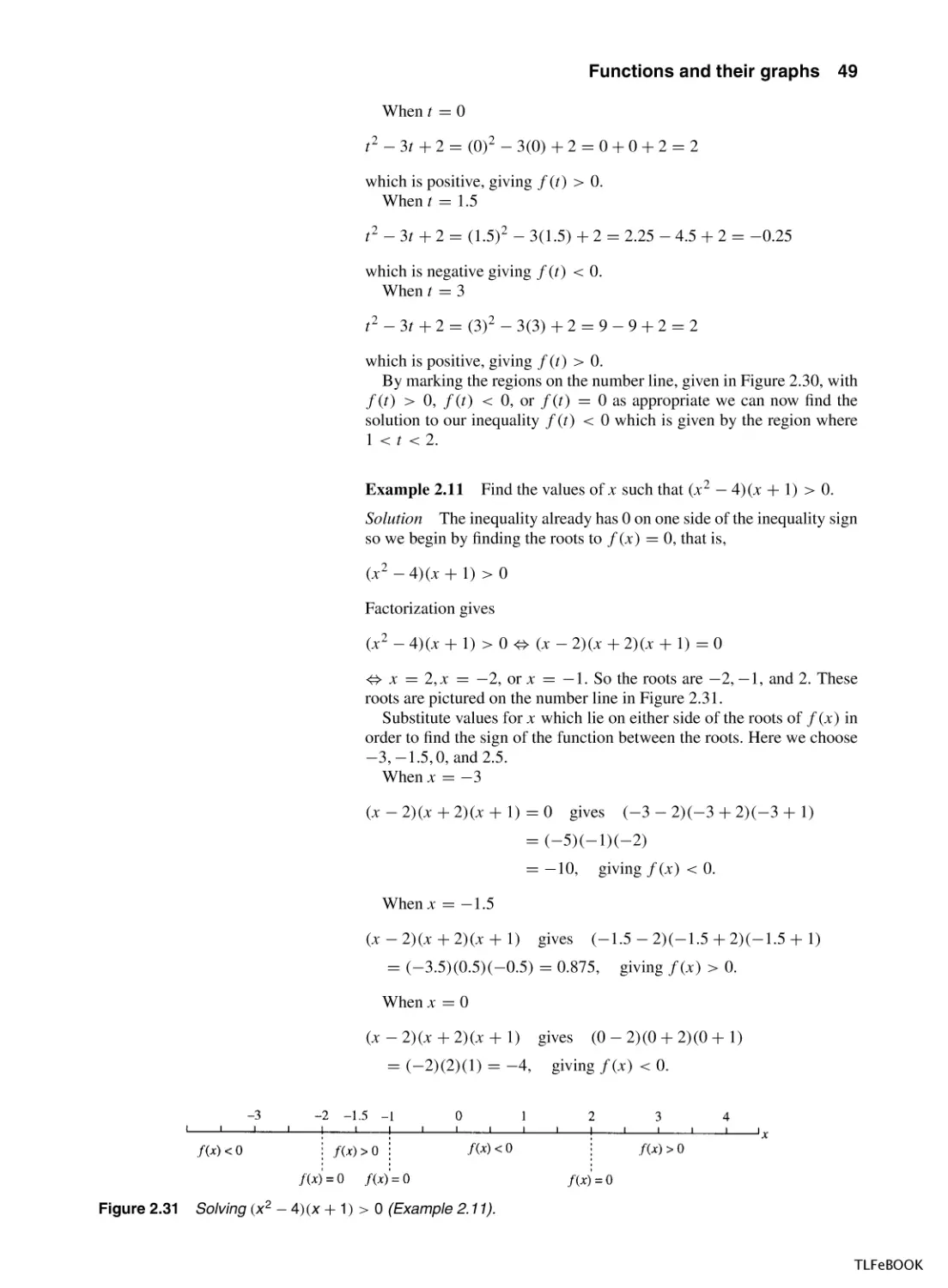
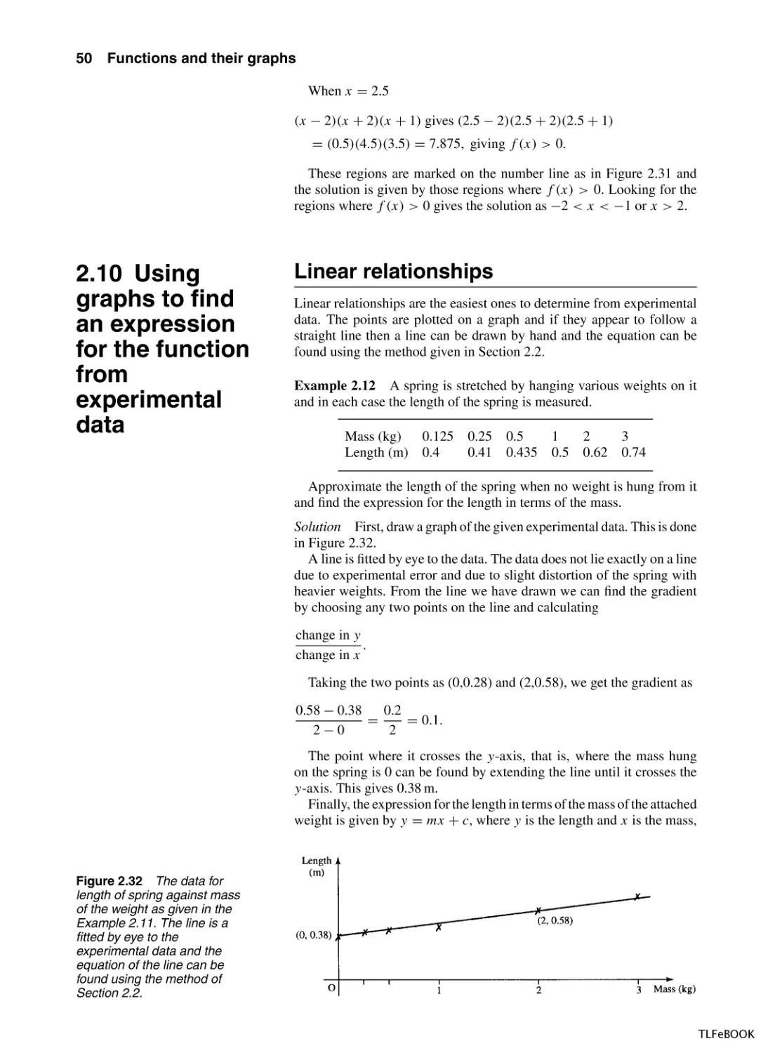
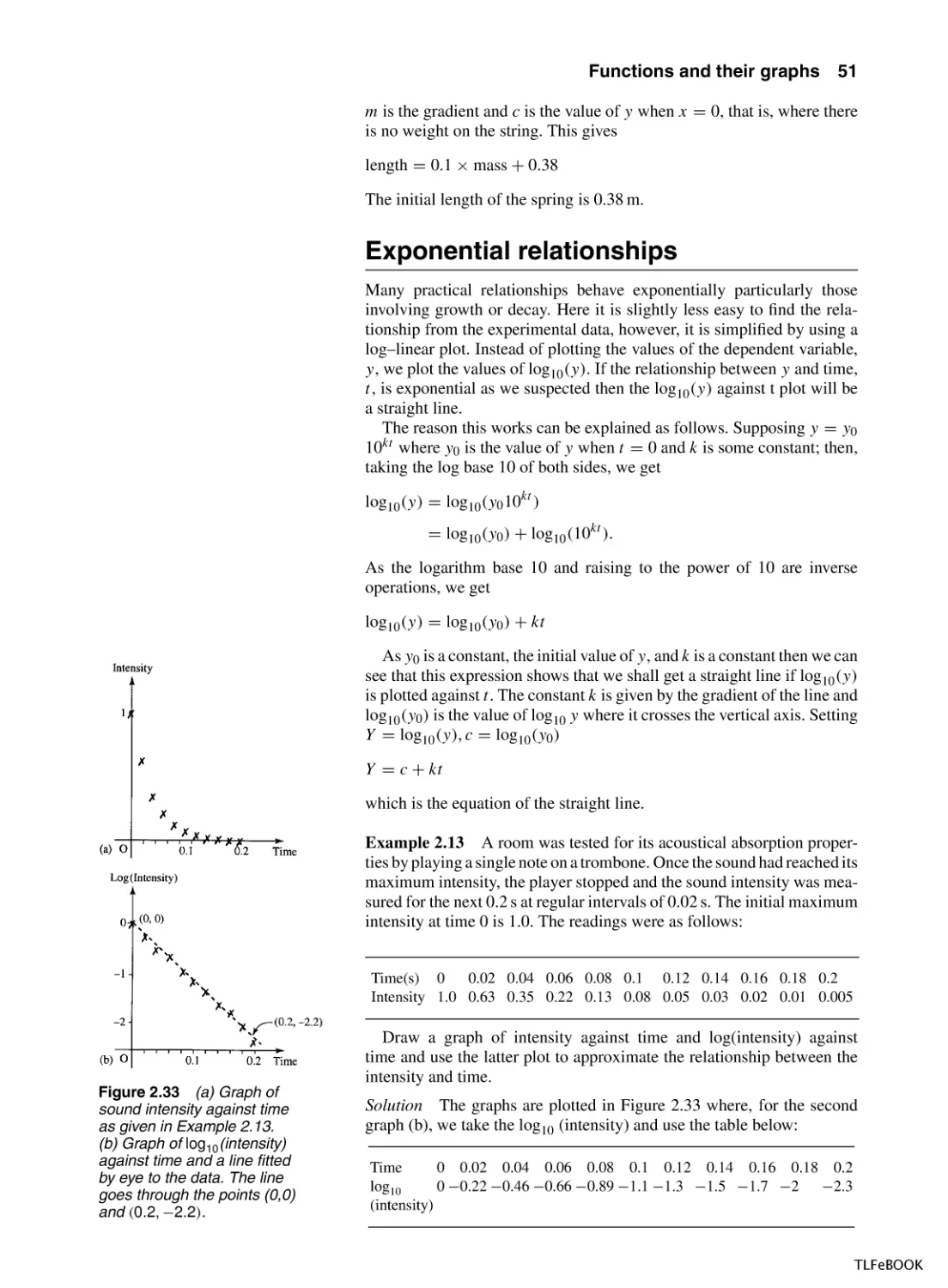
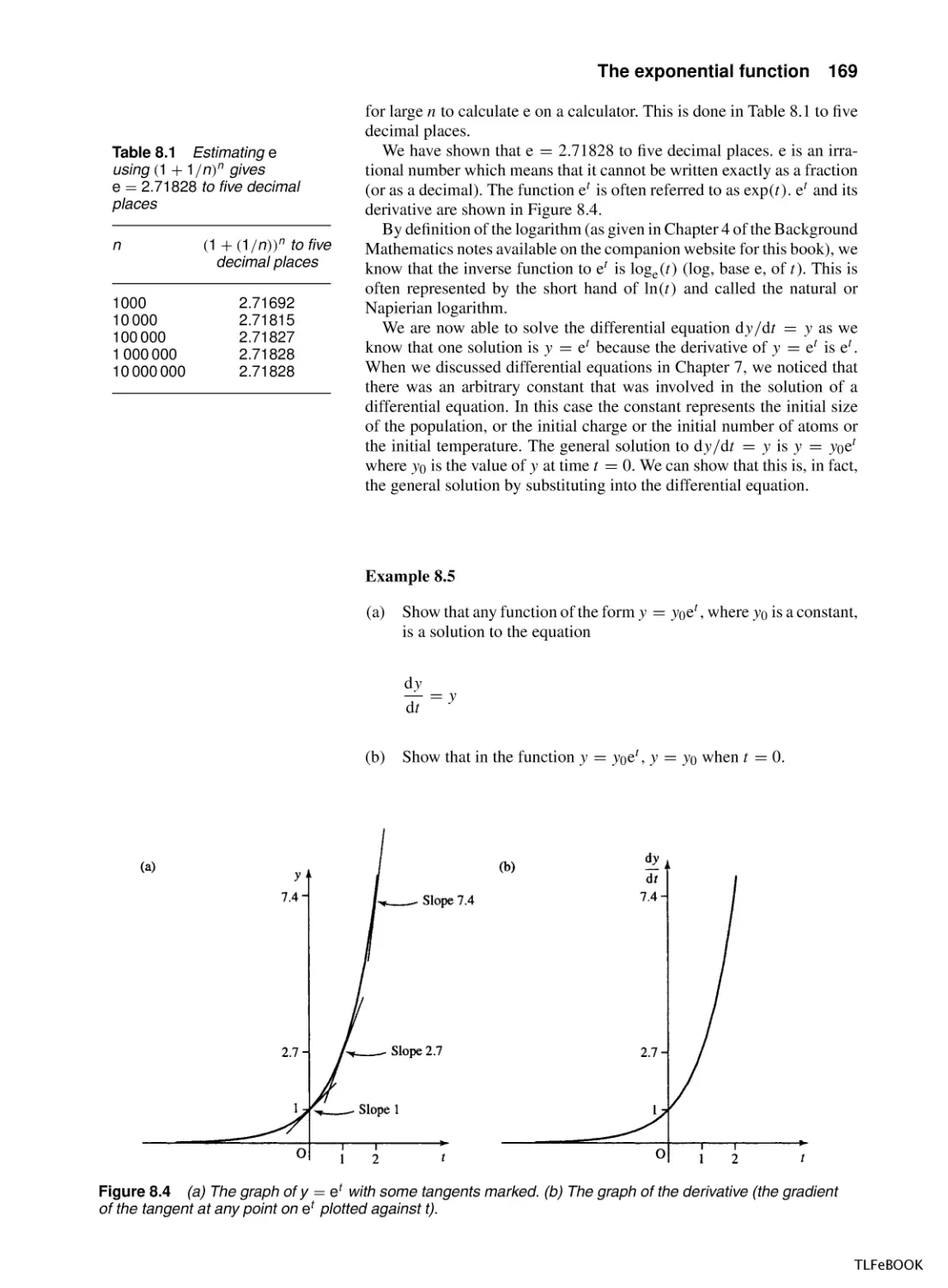
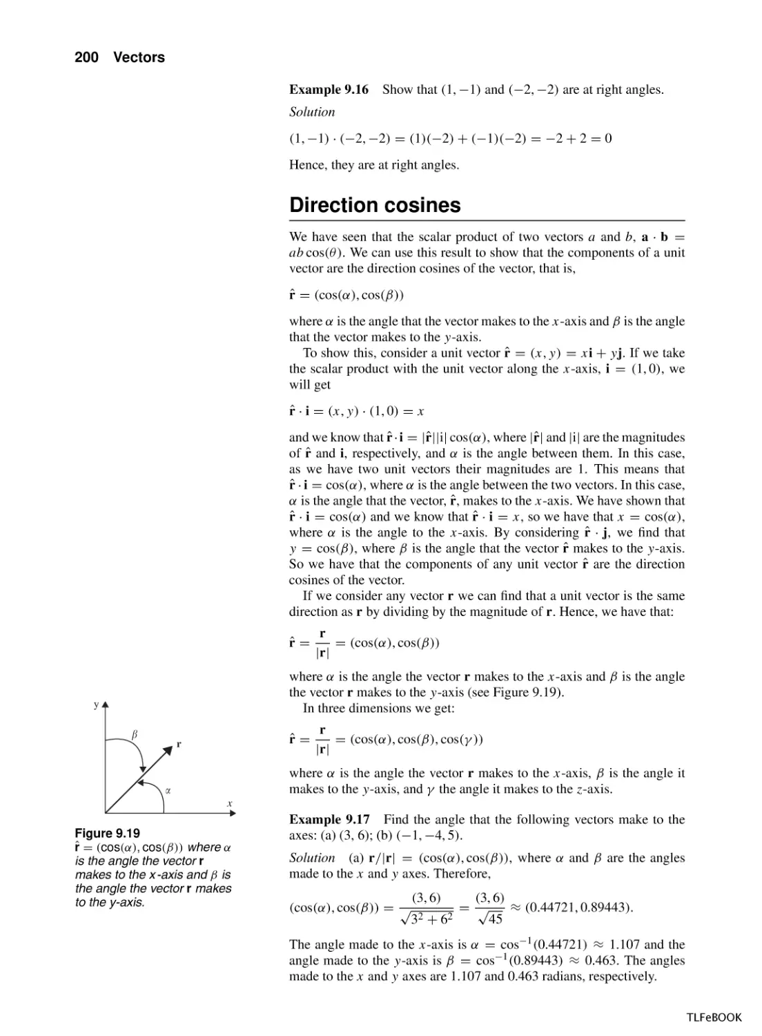
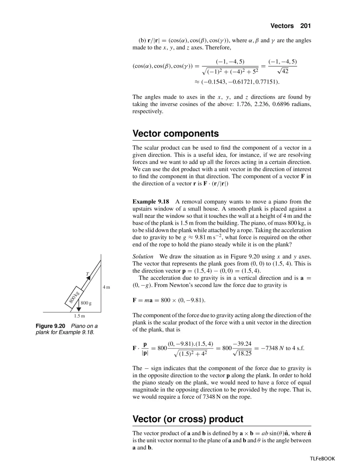
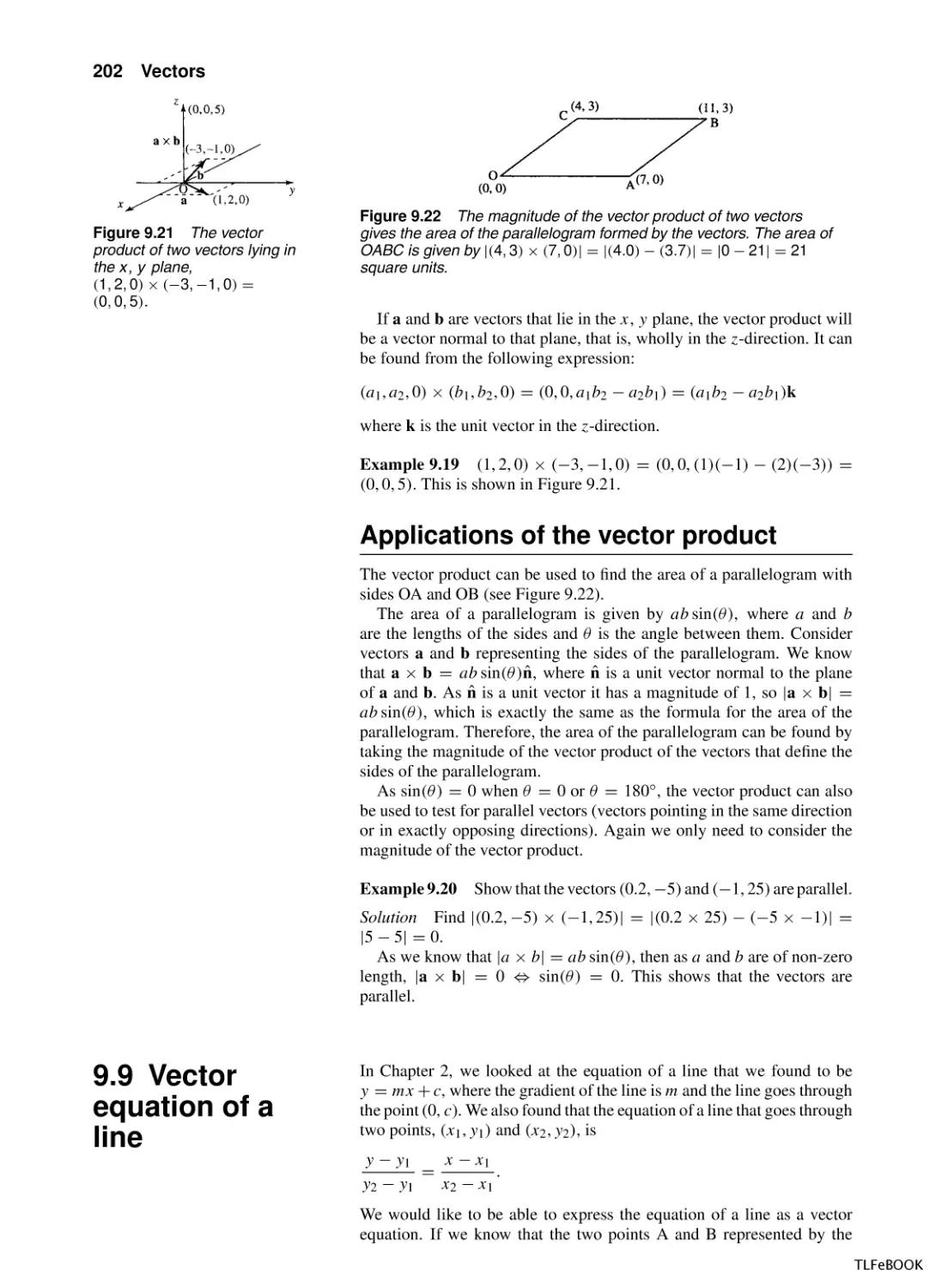
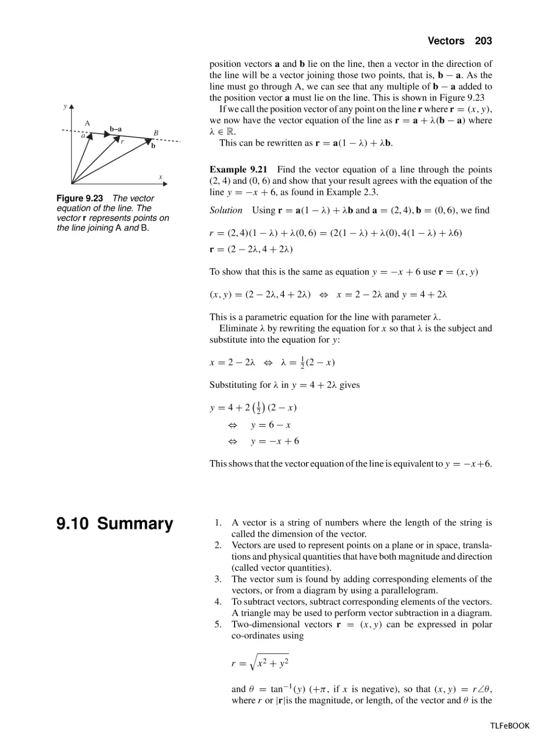
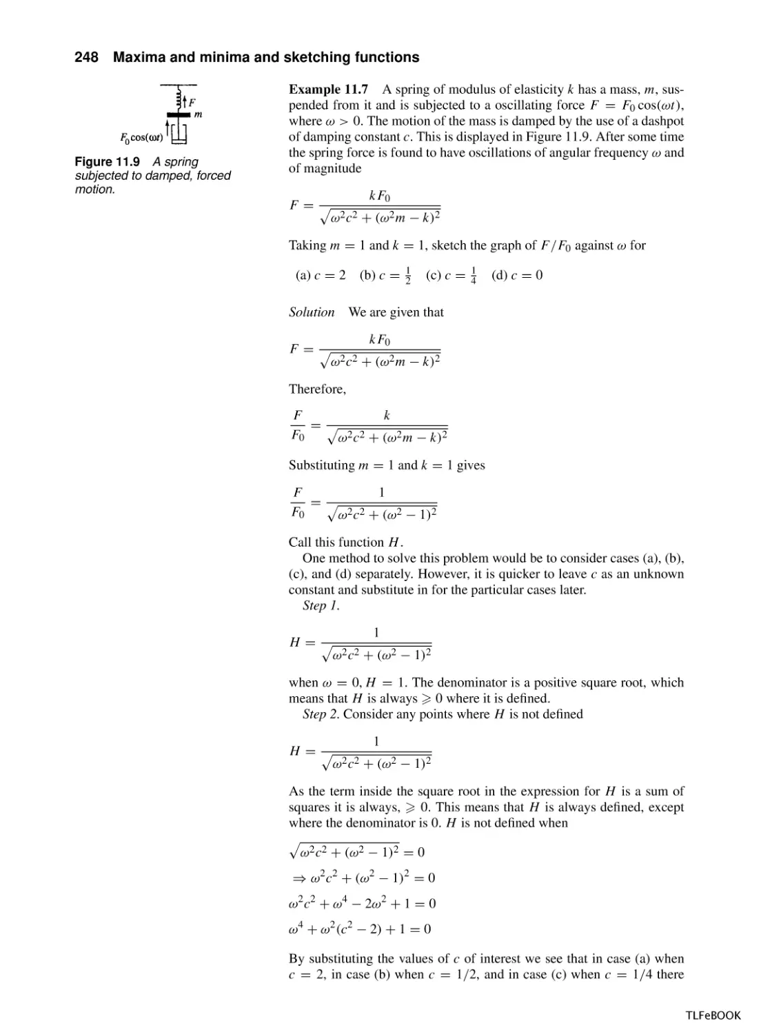
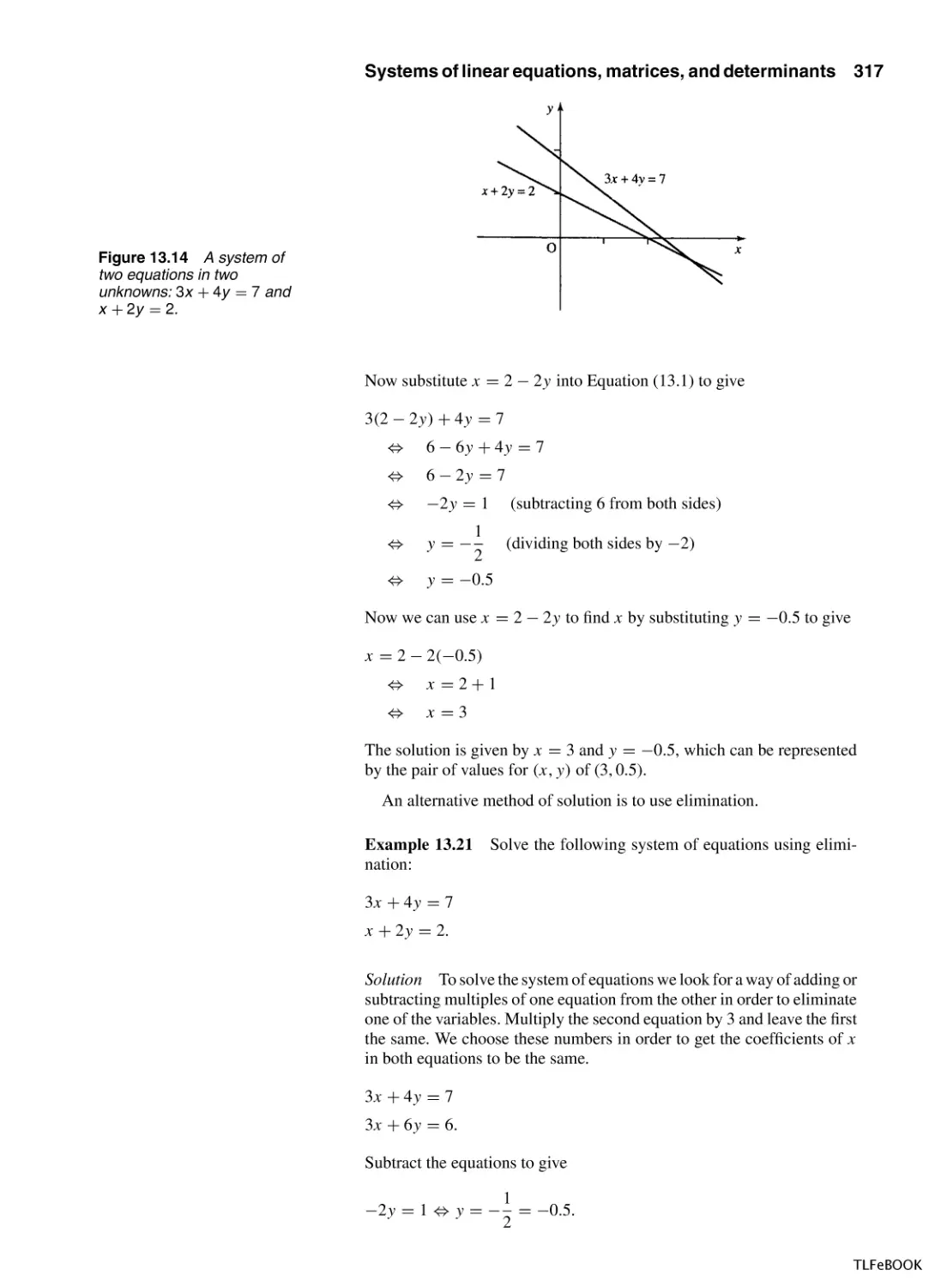
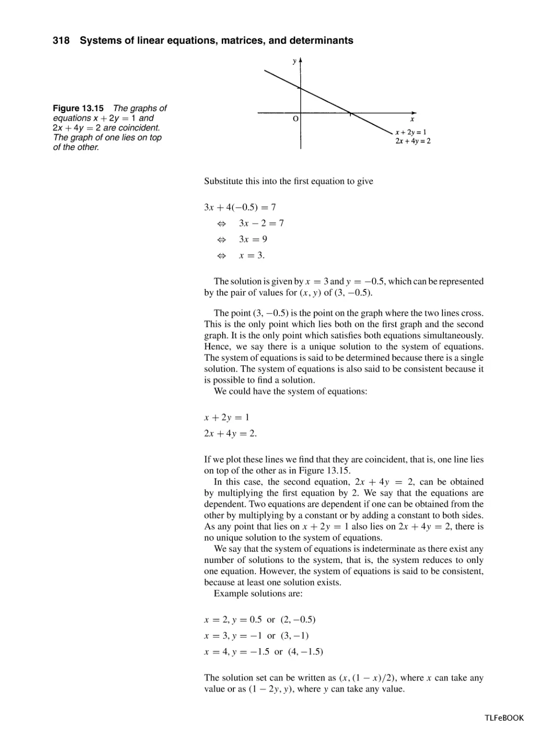
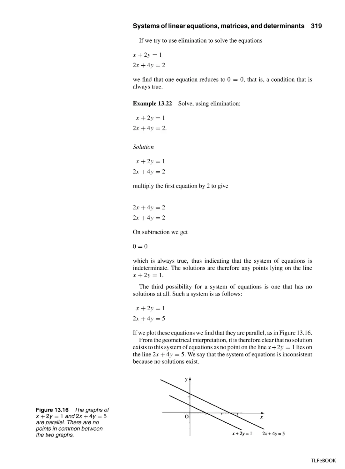
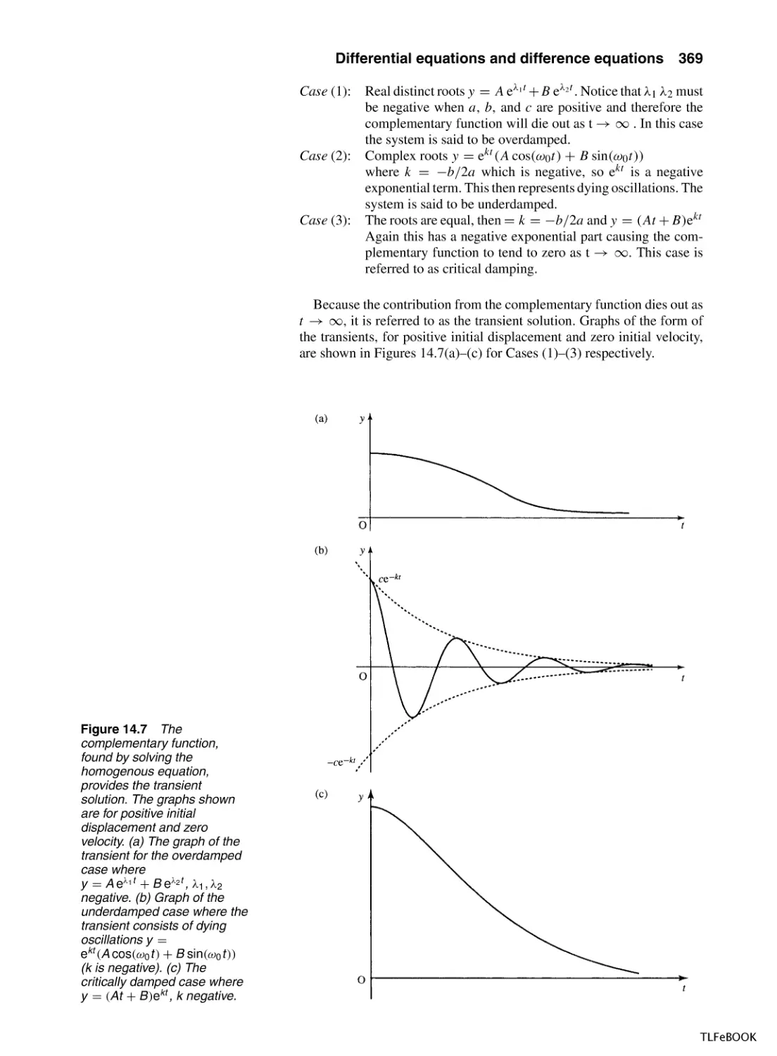
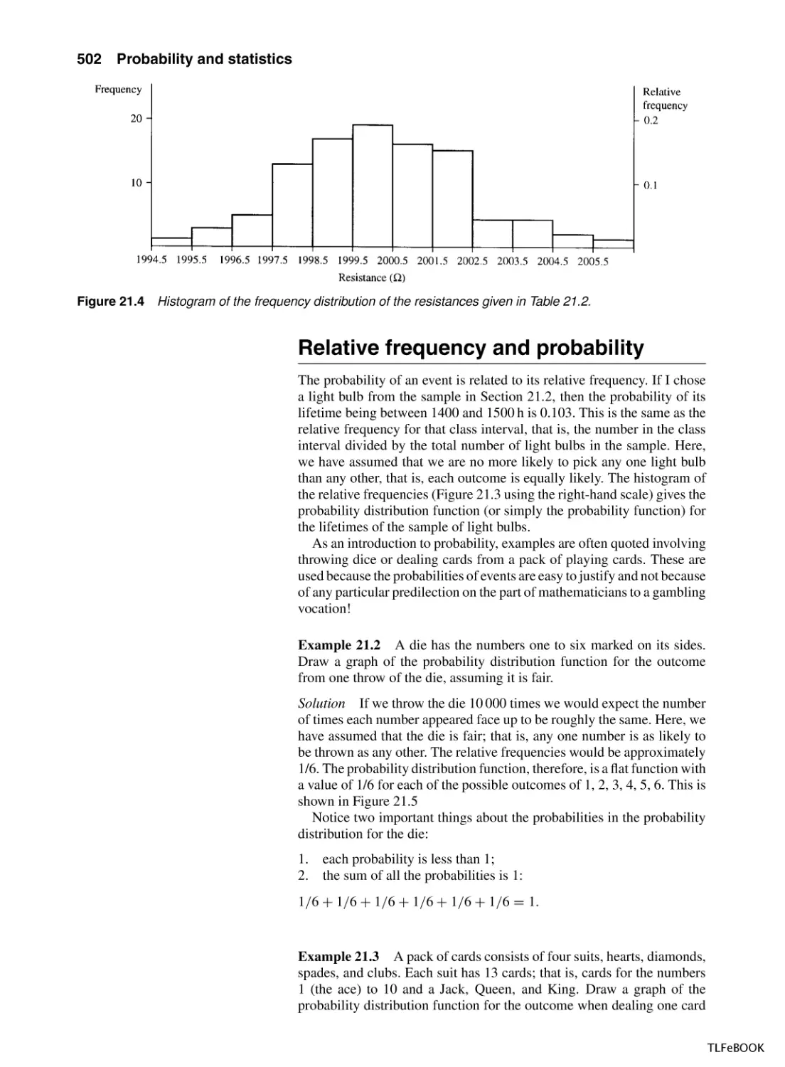
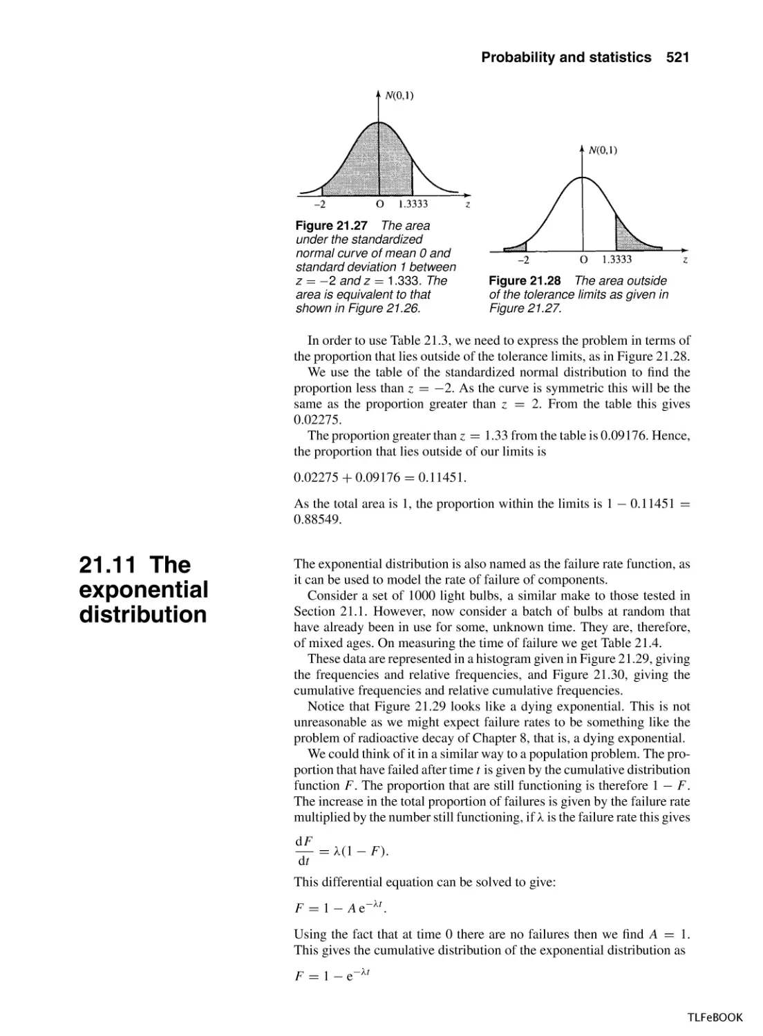
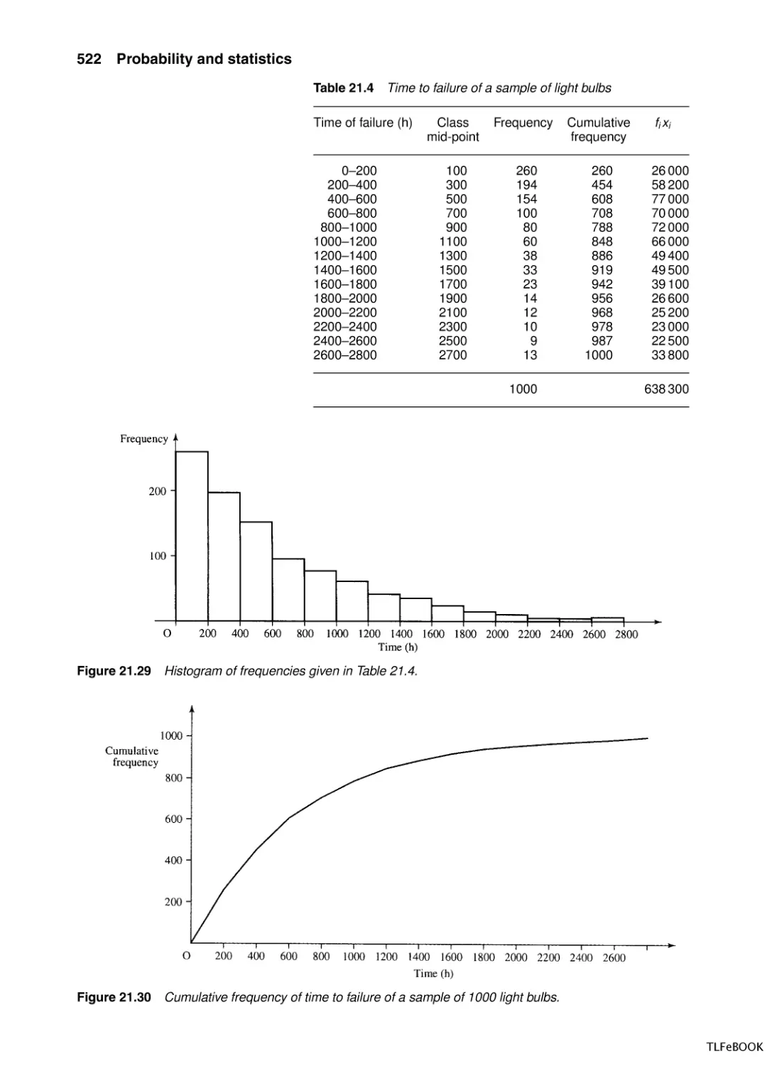
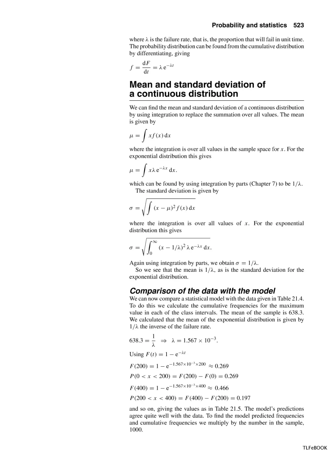
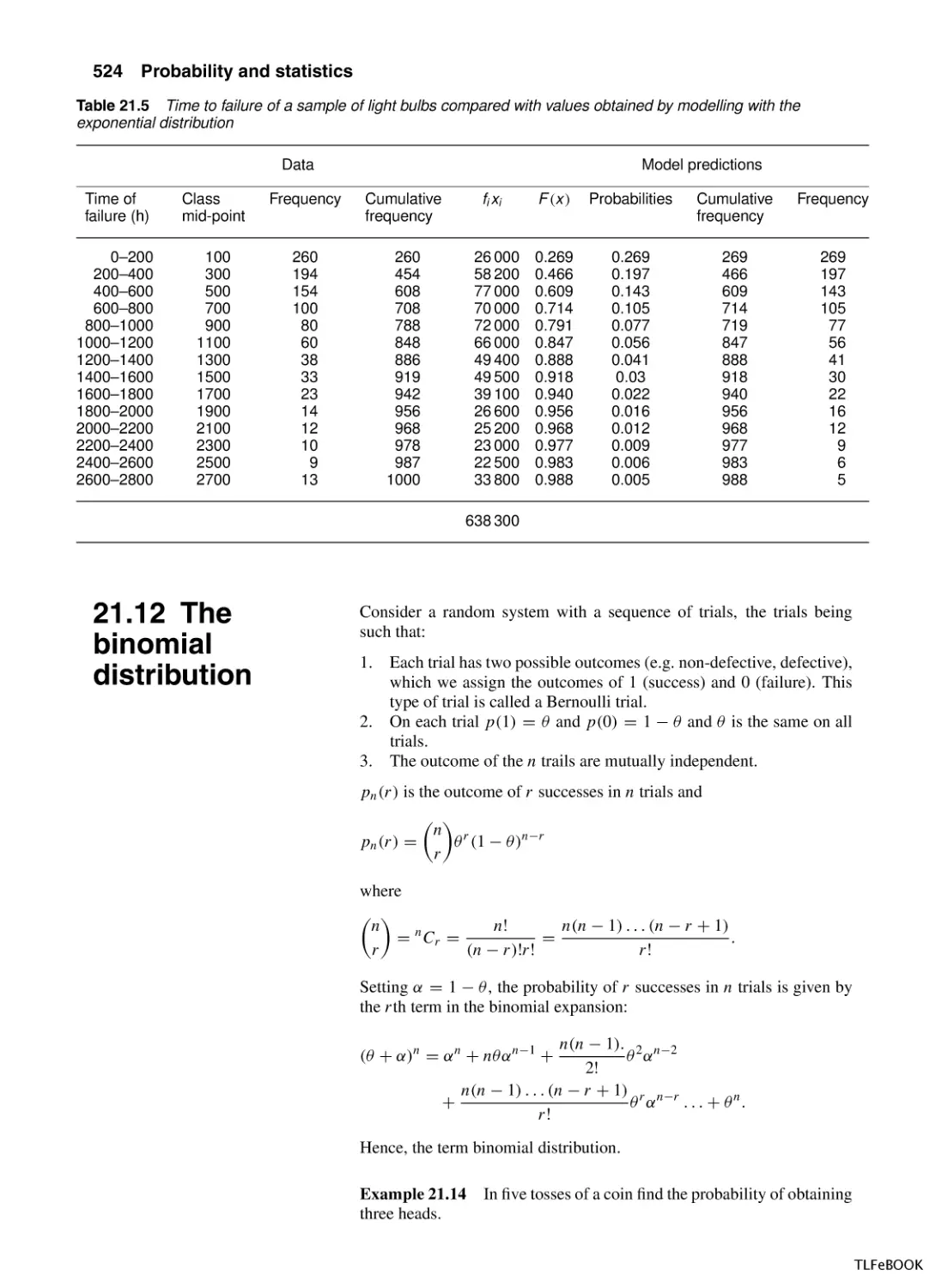
Текст
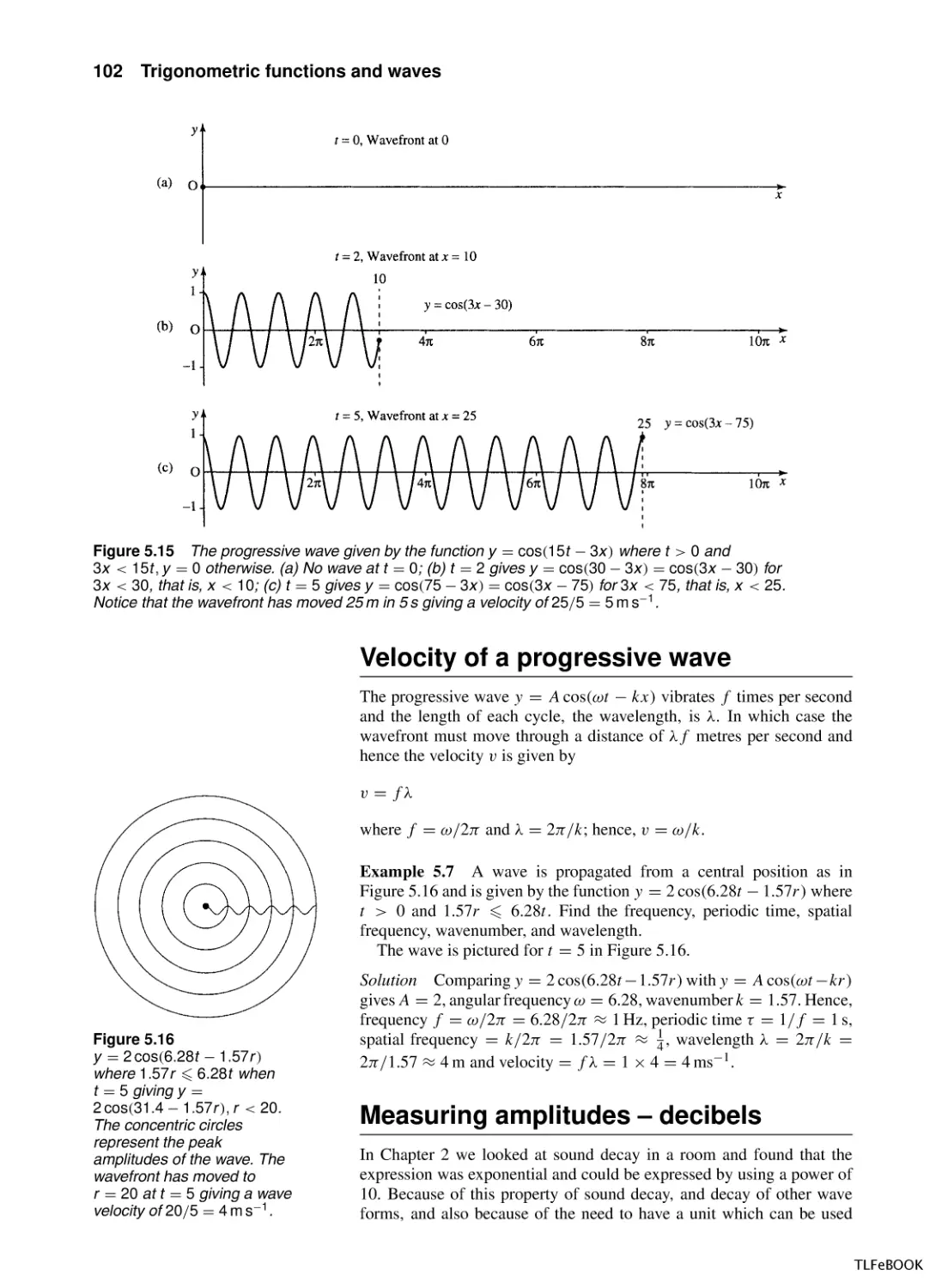
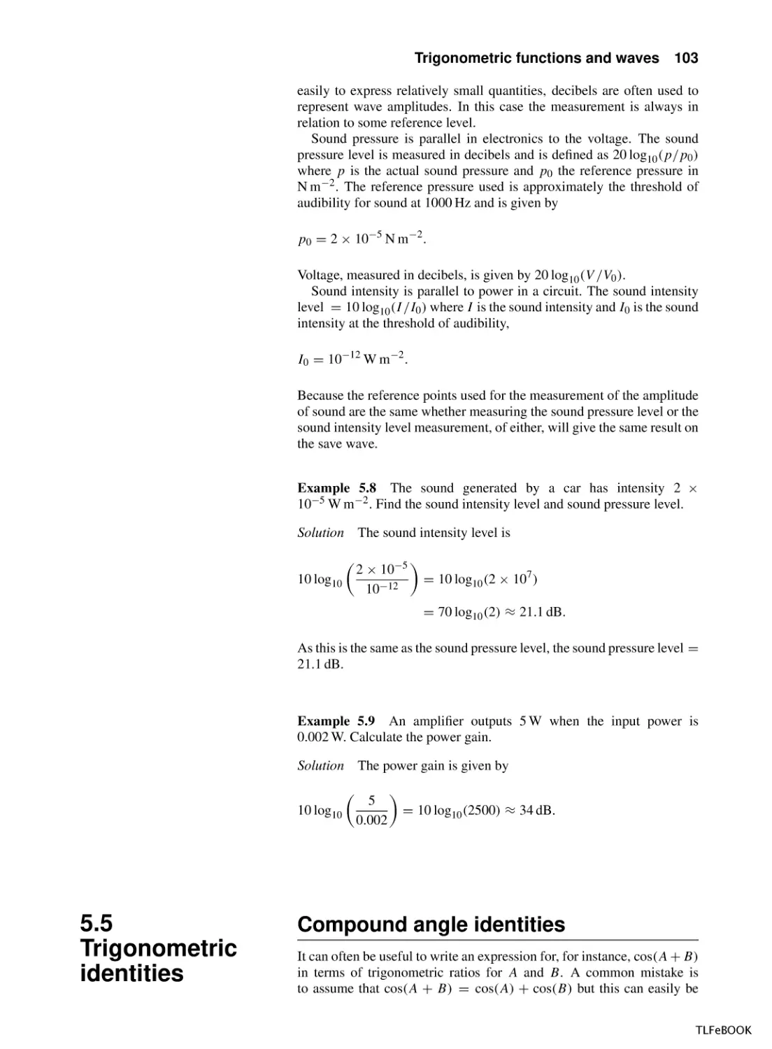
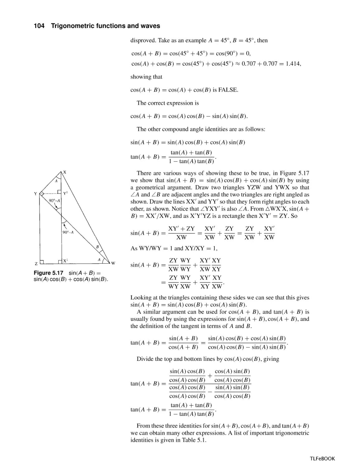
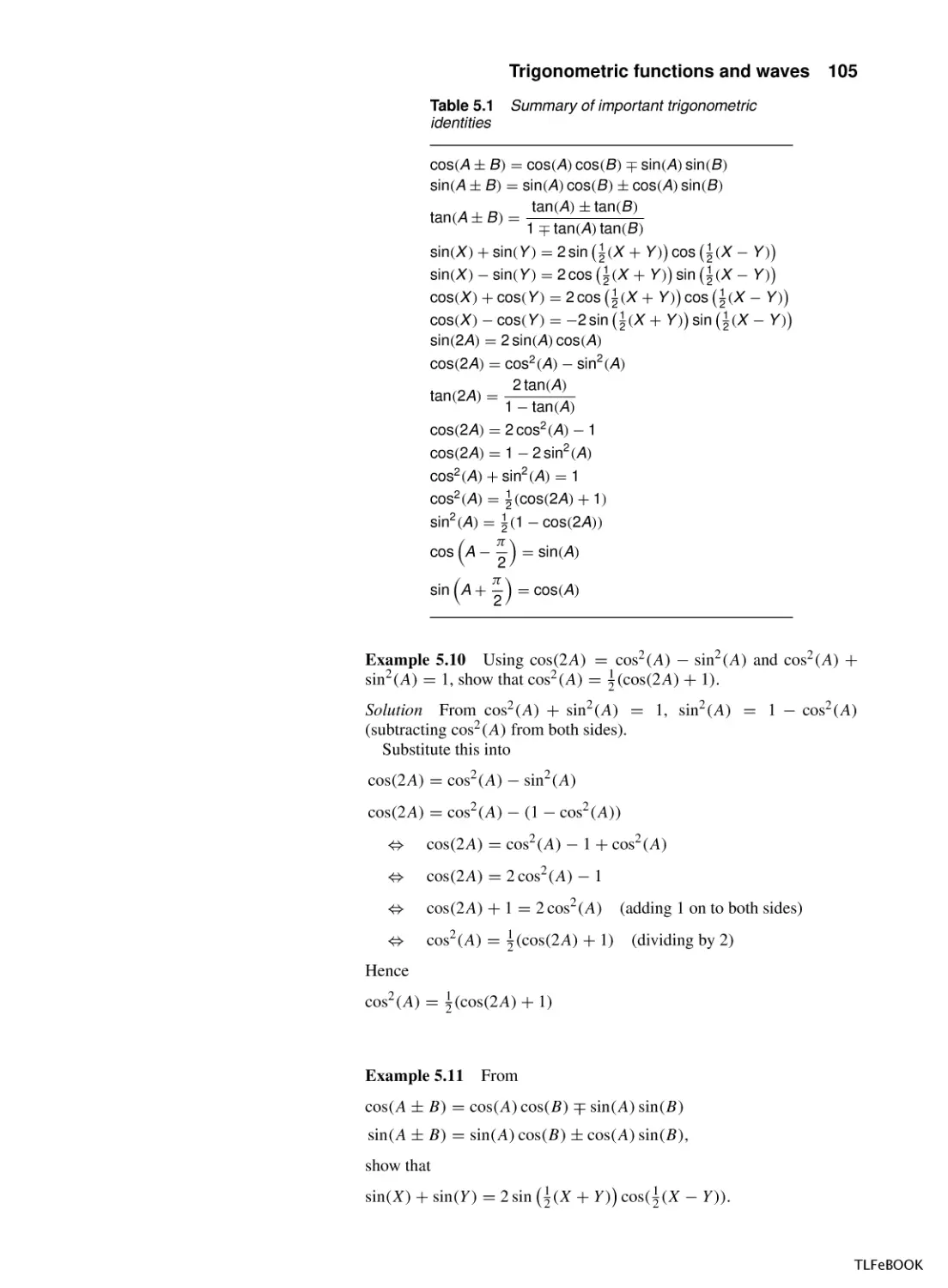
TLFeBOOK
Mathematics for Electrical
Engineering and Computing
TLFeBOOK
TLFeBOOK
Mathematics for
Electrical Engineering
and Computing
Mary Attenborough
AMSTERDAM BOSTON LONDON HEIDELBERG NEW YORK
OXFORD PARIS SAN DIEGO SAN FRANCISCO
SINGAPORE SYDNEY TOKYO
TLFeBOOK
Newnes
An imprint of Elsevier
Linacre House, Jordan Hill, Oxford OX2 8DP
200 Wheeler Road, Burlington MA 01803
First published 2003
Copyright © 2003, Mary Attenborough. All rights reserved
The right of Mary Attenborough to be identified as the author of this work
has been asserted in accordance with the Copyright, Designs and
Patents Act 1988
No part of this publication may be reproduced in any material form (including
photocopying or storing in any medium by electronic means and whether
or not transiently or incidentally to some other use of this publication) without
the written permission of the copyright holder except in accordance with the
provisions of the Copyright, Designs and Patents Act 1988 or under the terms of
a licence issued by the Copyright Licensing Agency Ltd, 90 Tottenham Court
Road, London, England W1T 4LP. Applications for the copyright holder’s written
permission to reproduce any part of this publication should be addressed
to the publisher
Permissions may be sought directly from Elsevier’s Science and
Technology Rights Department in Oxford, UK: phone: (+44) (0) 1865 843830;
fax: (+44) (0) 1865 853333; e-mail: permissions@elsevier.co.uk.
You may also complete your request on-line via the Elsevier homepage
(http://www.elsevier.com), by selecting ‘Customer Support’ and then
‘Obtaining Permissions’
British Library Cataloguing in Publication Data
A catalogue record for this book is available from the British Library
Library of Congress Cataloguing in Publication Data
A catalogue record for this book is available from the Library of Congress
ISBN 0 7506 5855 X
For information on all Newnes publications
visit our website at www.newnespress.com
Typeset by Newgen Imaging Systems (P) Ltd, Chennai, India
Printed and bound in Great Britain
TLFeBOOK
Contents
Preface
xi
Acknowledgements
xii
Part 1 Sets, functions, and calculus
1
Sets and functions
1.1
Introduction
1.2
Sets
1.3
Operations on sets
1.4
Relations and functions
1.5
Combining functions
1.6
Summary
1.7
Exercises
3
3
4
5
7
17
23
24
2
Functions and their graphs
2.1
Introduction
2.2
The straight line: y = mx + c
2.3
The quadratic function: y = ax 2 + bx + c
2.4
The function y = 1/x
2.5
The functions y = a x
2.6
Graph sketching using simple
transformations
2.7
The modulus function, y = |x| or
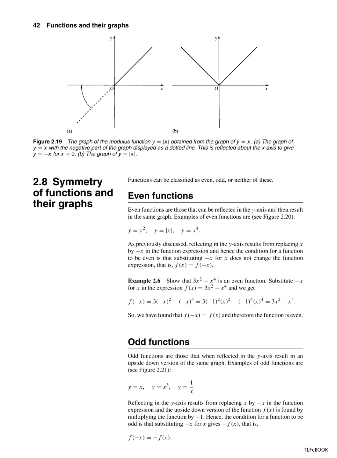
y = abs(x)
2.8
Symmetry of functions and their graphs
2.9
Solving inequalities
2.10 Using graphs to find an expression for the function
from experimental data
2.11 Summary
2.12 Exercises
26
26
26
32
33
33
3
Problem solving and the art of the convincing
argument
3.1
Introduction
3.2
Describing a problem in mathematical
language
3.3
Propositions and predicates
3.4
Operations on propositions and predicates
3.5
Equivalence
3.6
Implication
3.7
Making sweeping statements
35
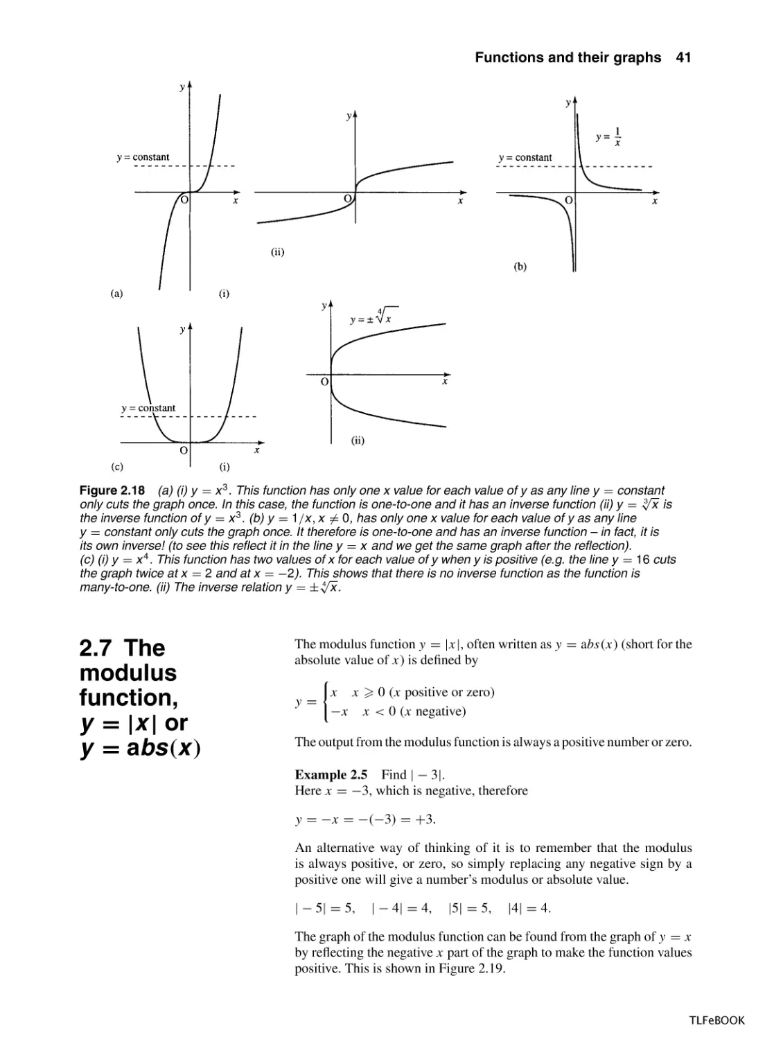
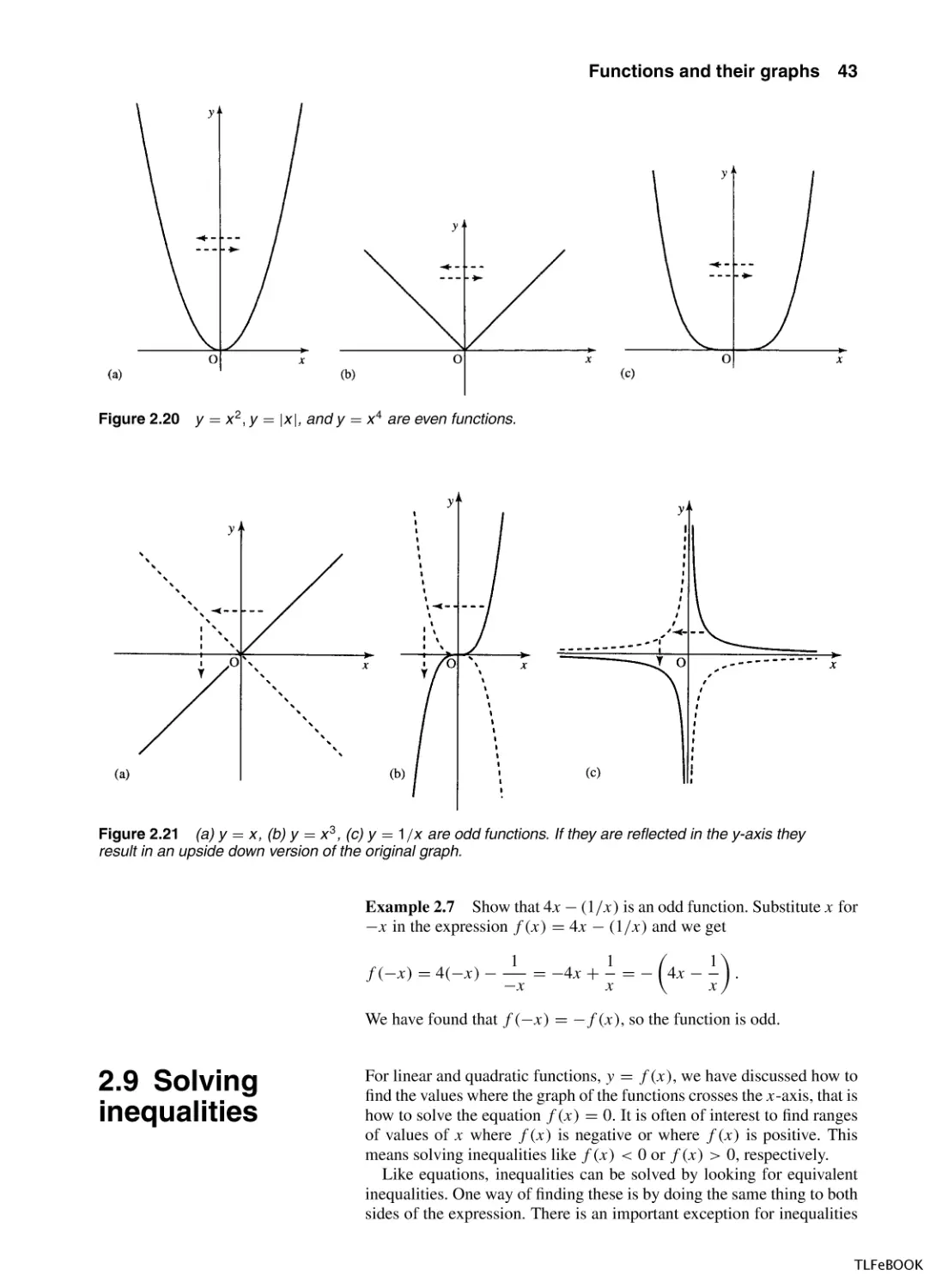
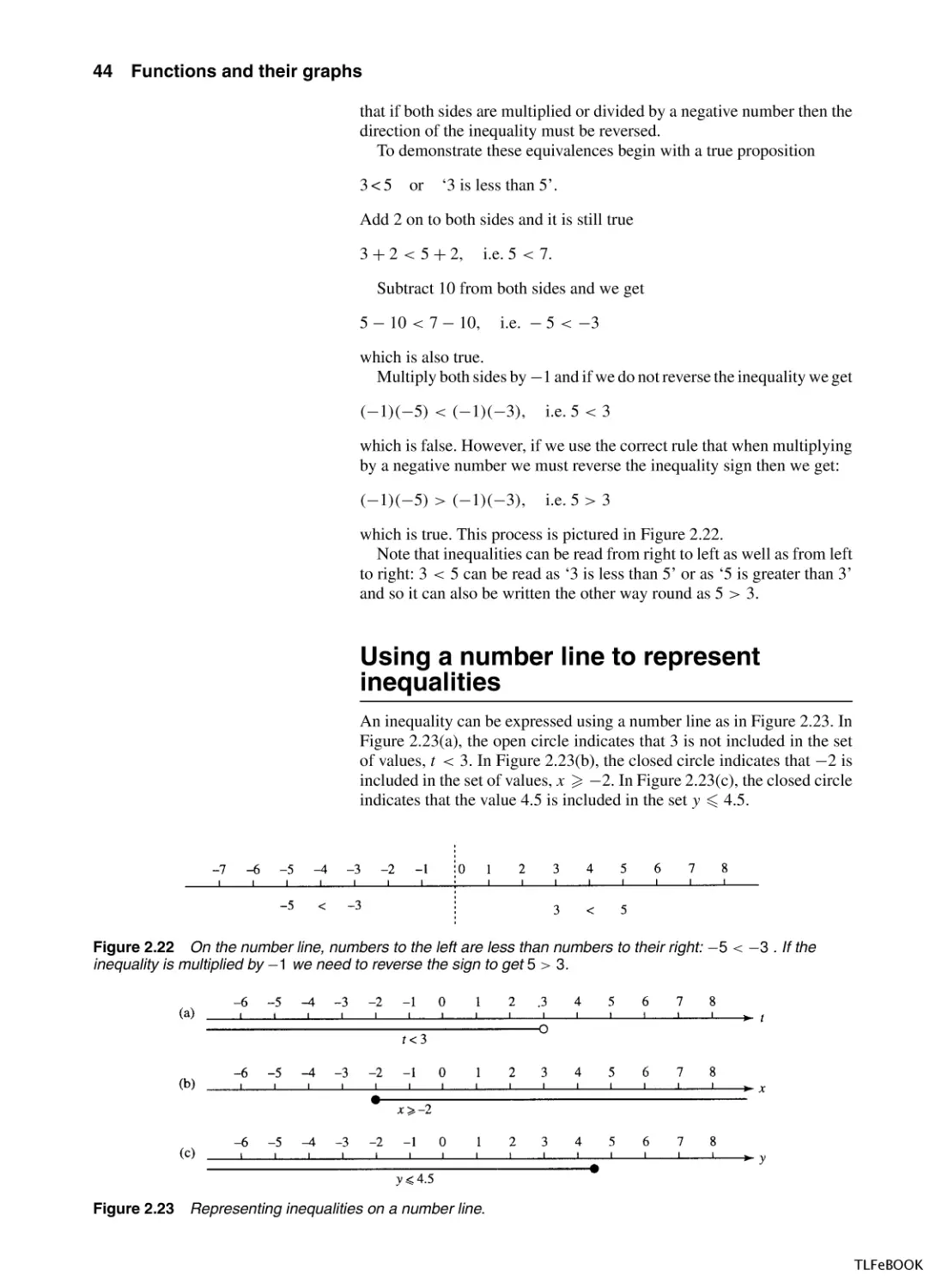
41
42
43
50
54
55
57
57
59
61
62
64
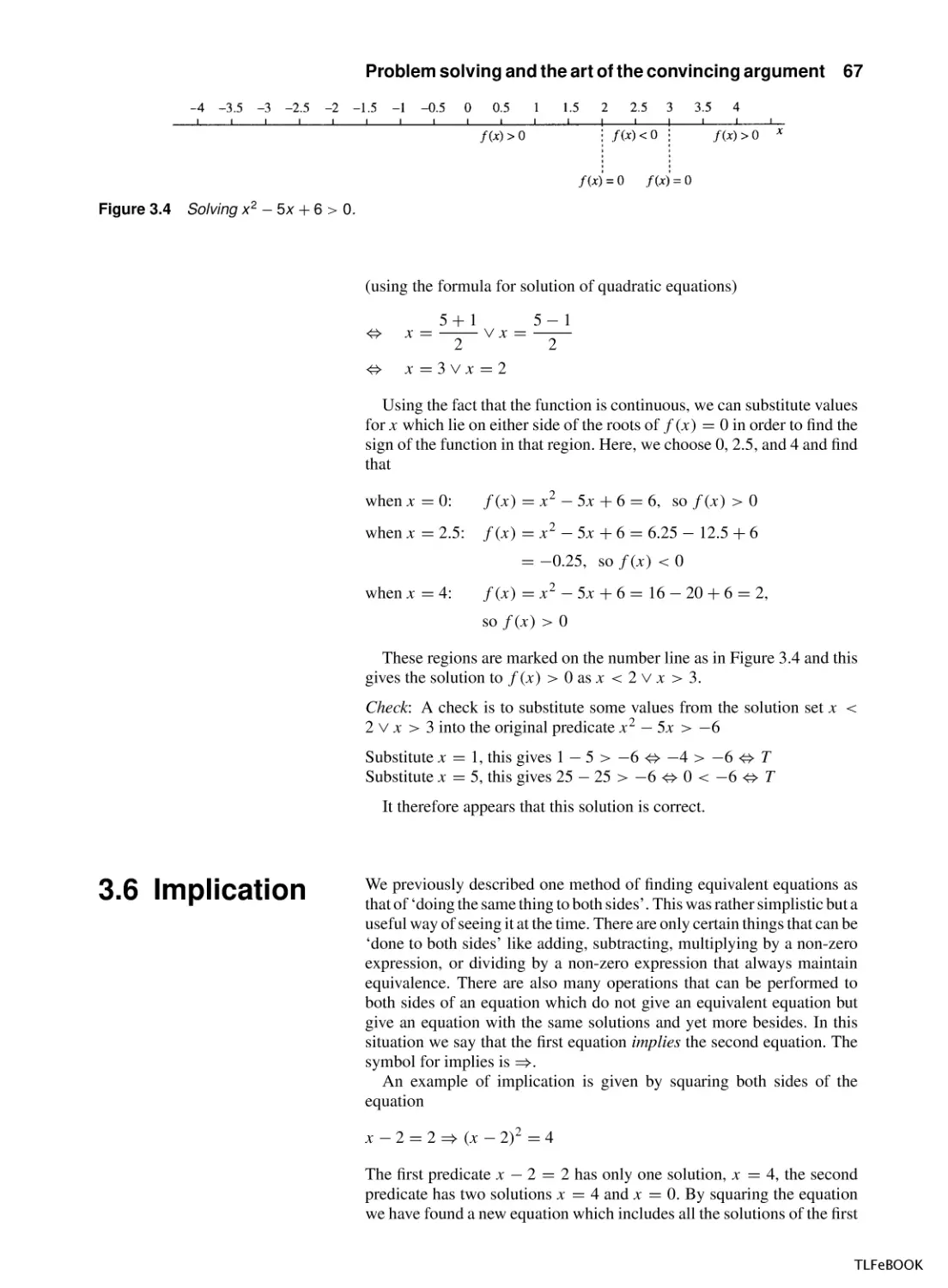
67
70
TLFeBOOK
vi
Contents
3.8
3.9
3.10
Other applications of predicates
Summary
Exercises
72
73
74
76
76
76
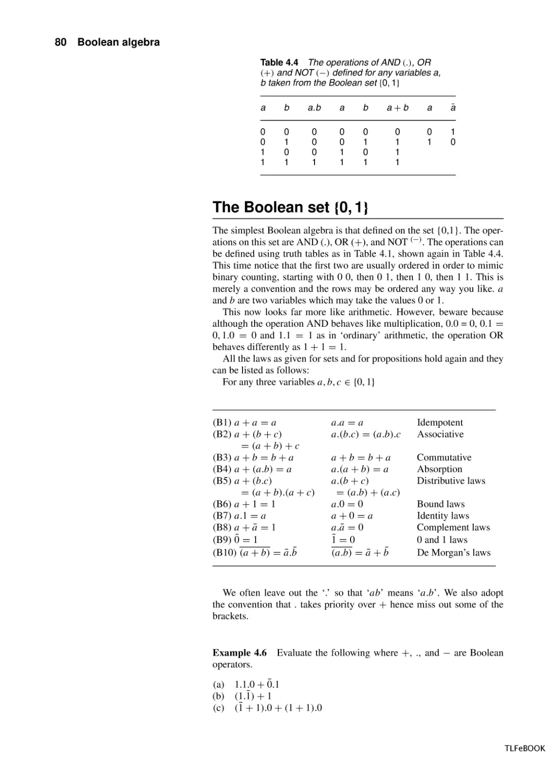
77
81
86
86
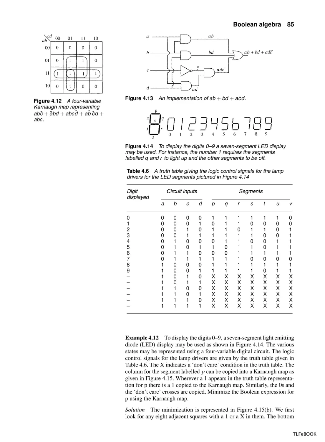
4
Boolean algebra
4.1
Introduction
4.2
Algebra
4.3
Boolean algebras
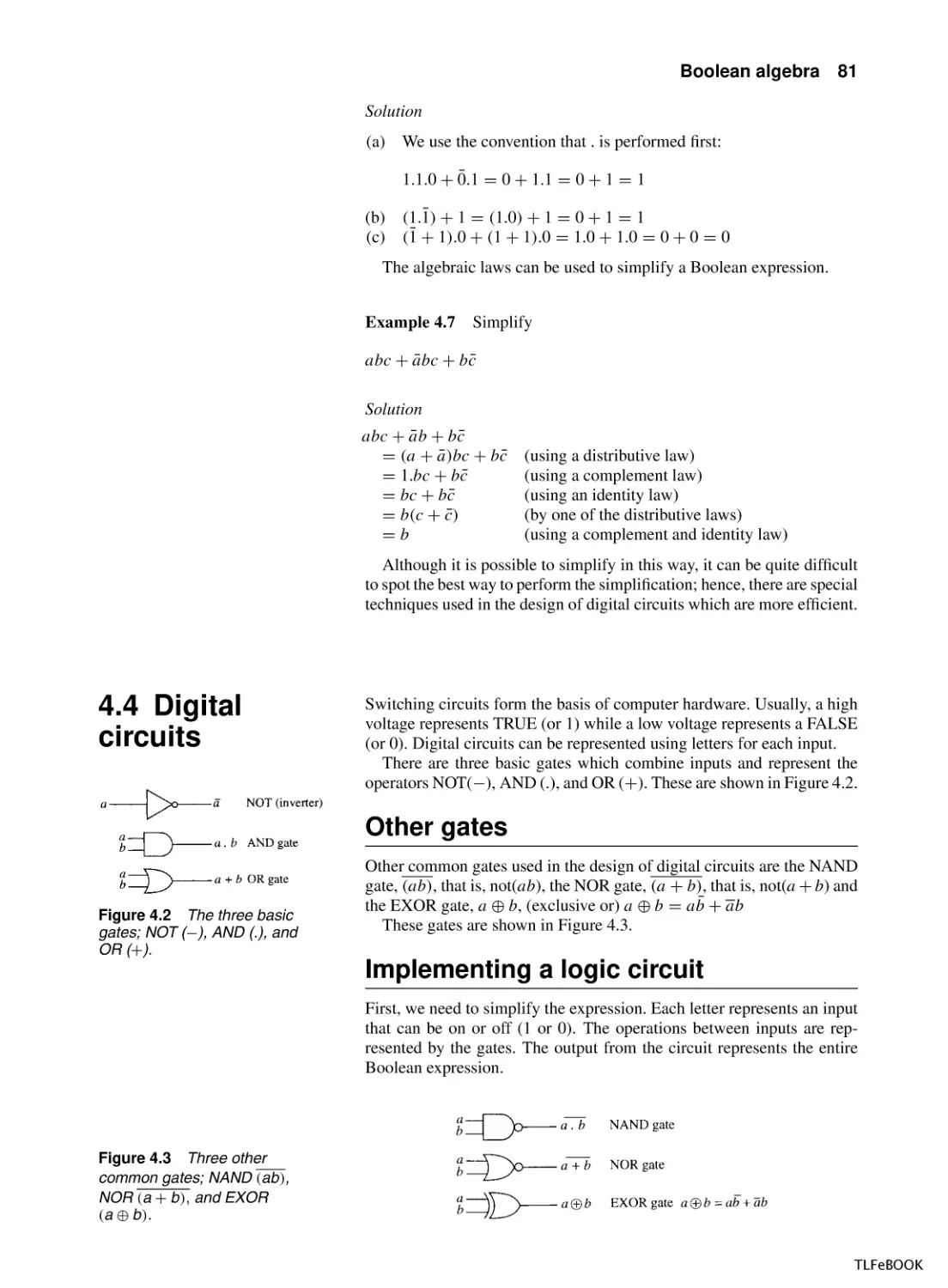
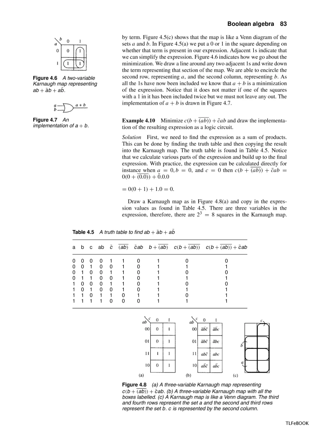
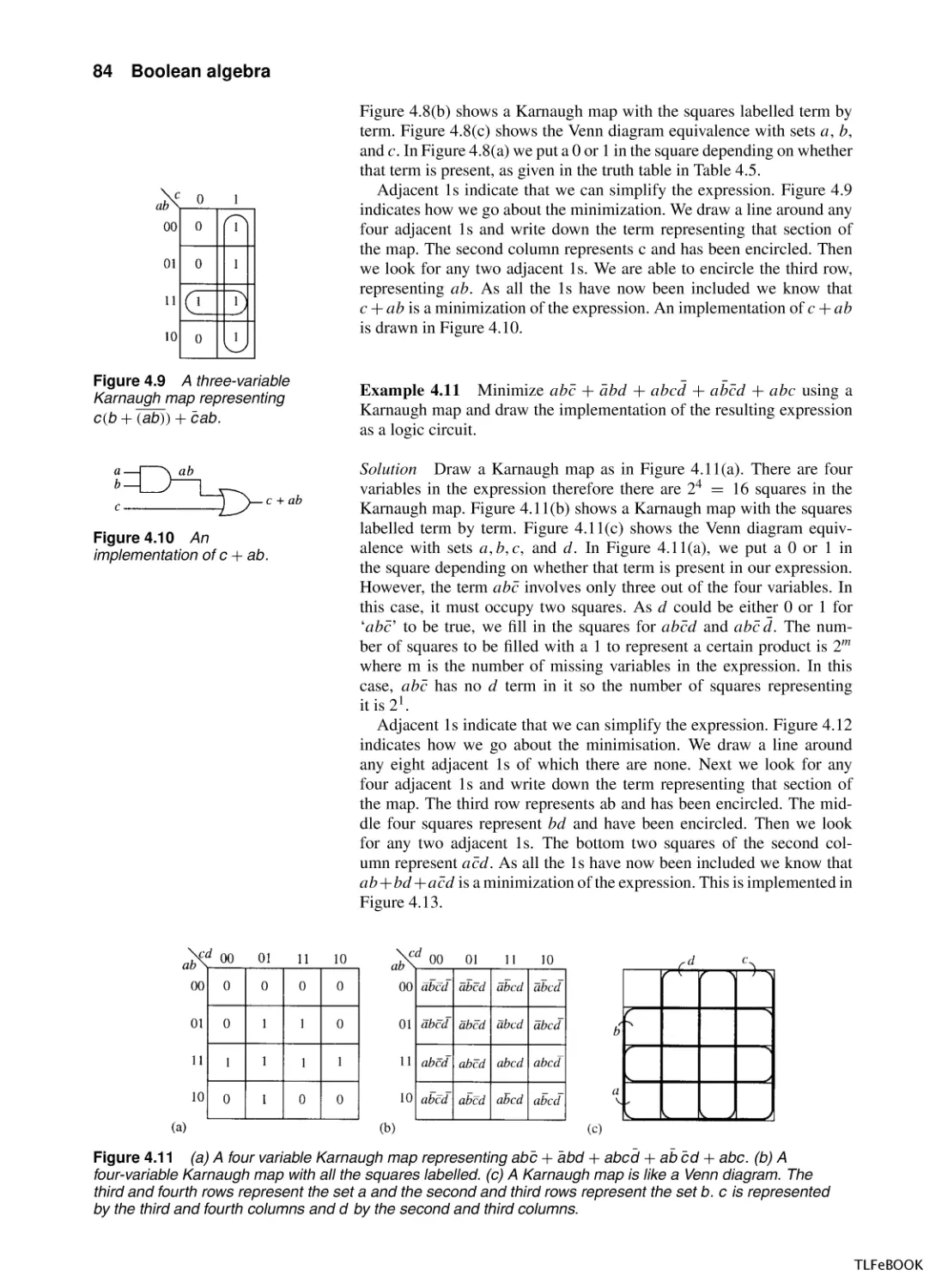
4.4
Digital circuits
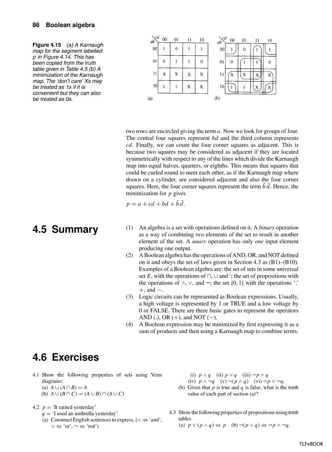
4.5
Summary
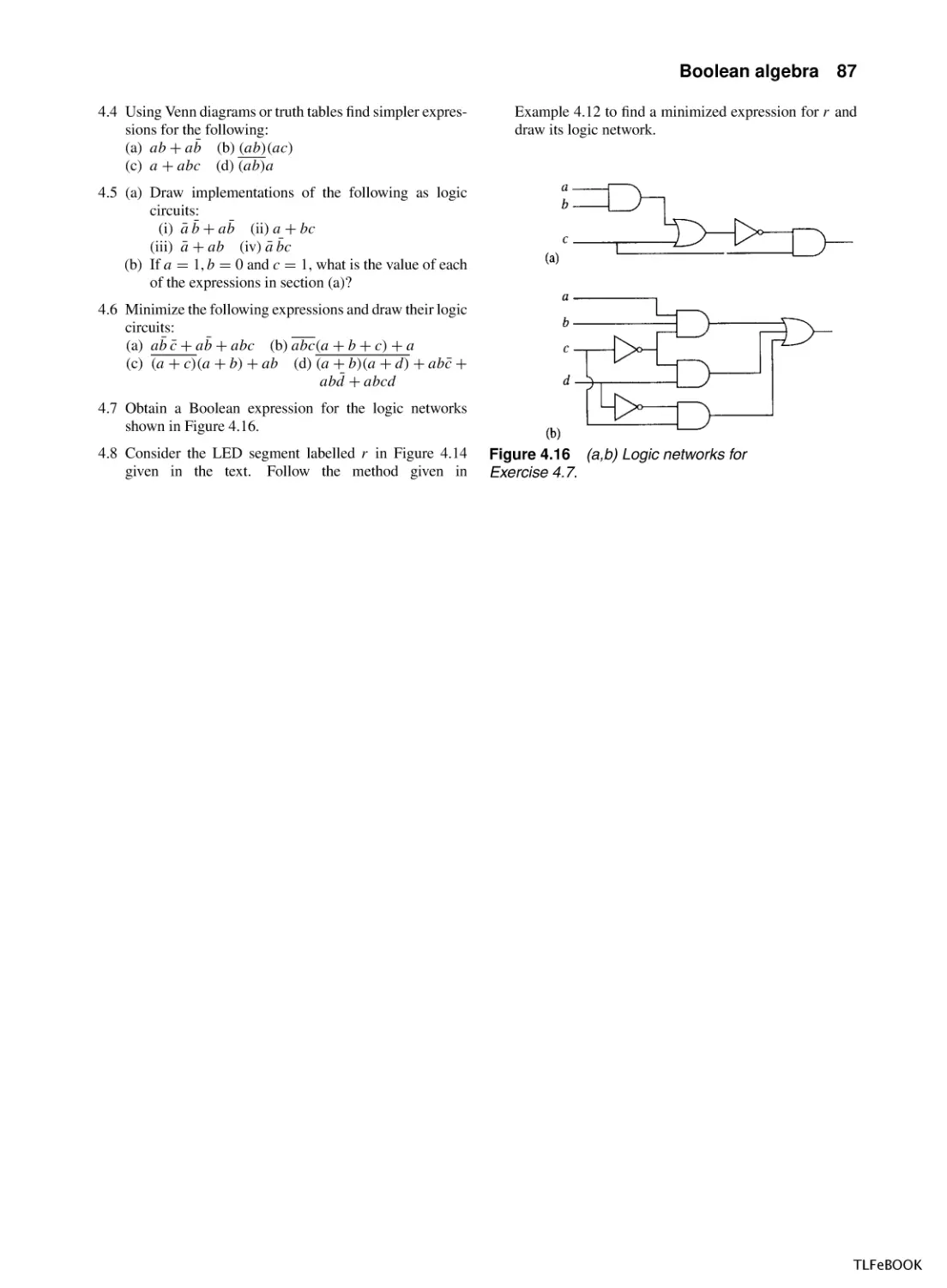
4.6
Exercises
5
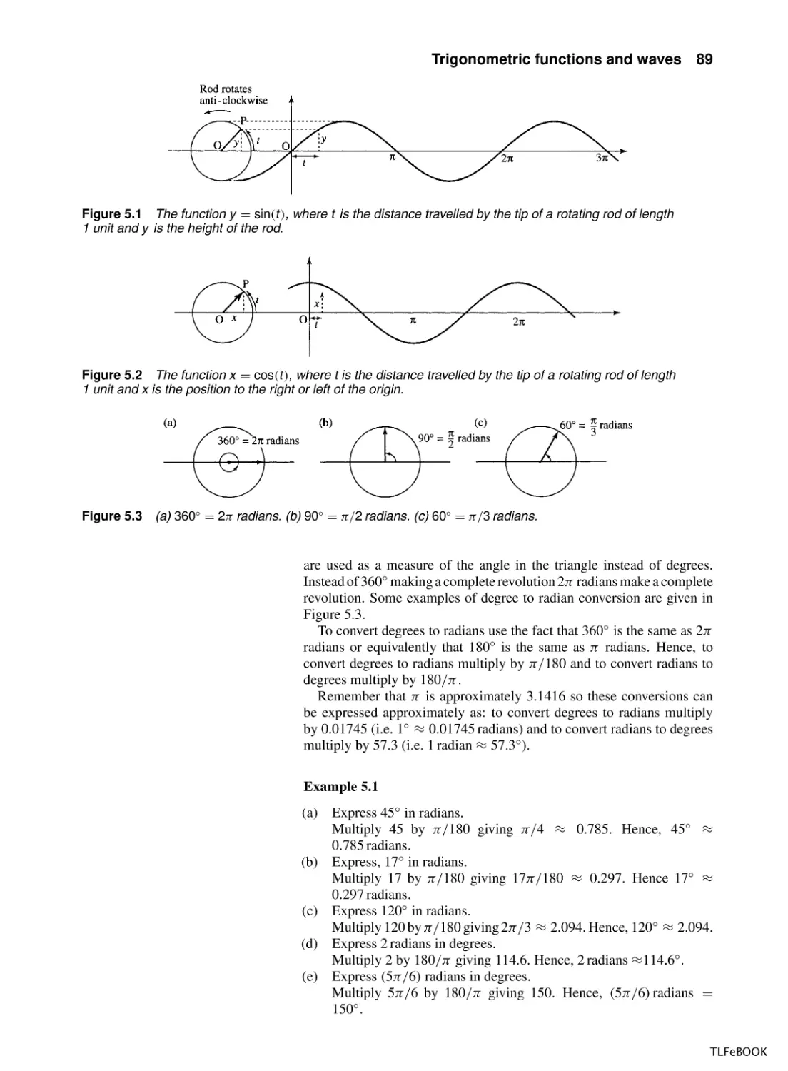
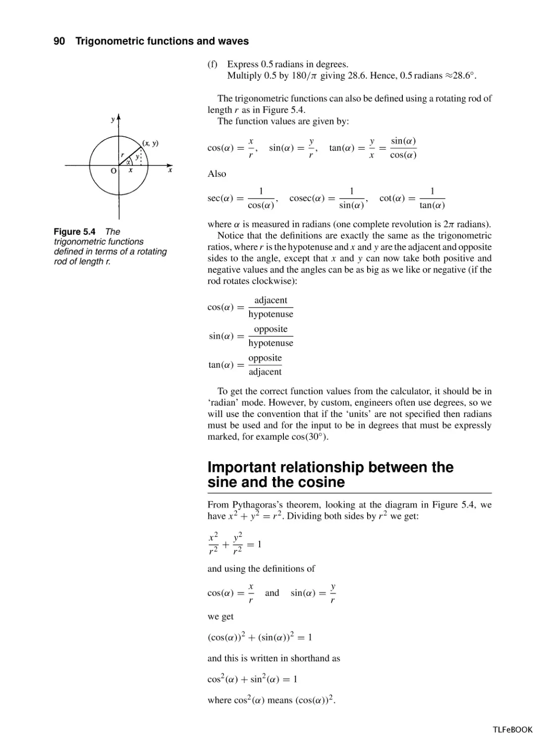
Trigonometric functions and waves
5.1
Introduction
5.2
Trigonometric functions and radians
5.3
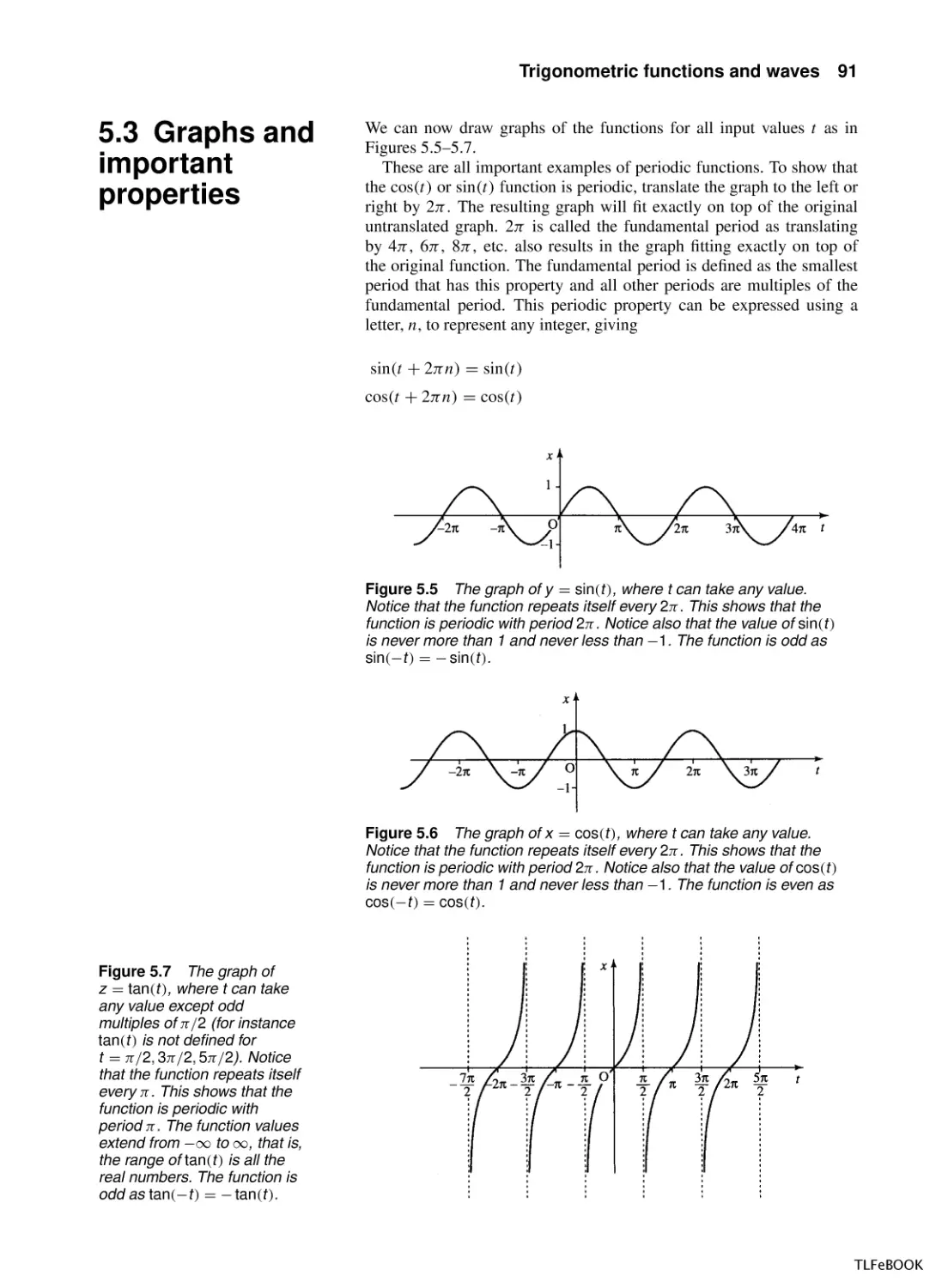
Graphs and important properties
5.4
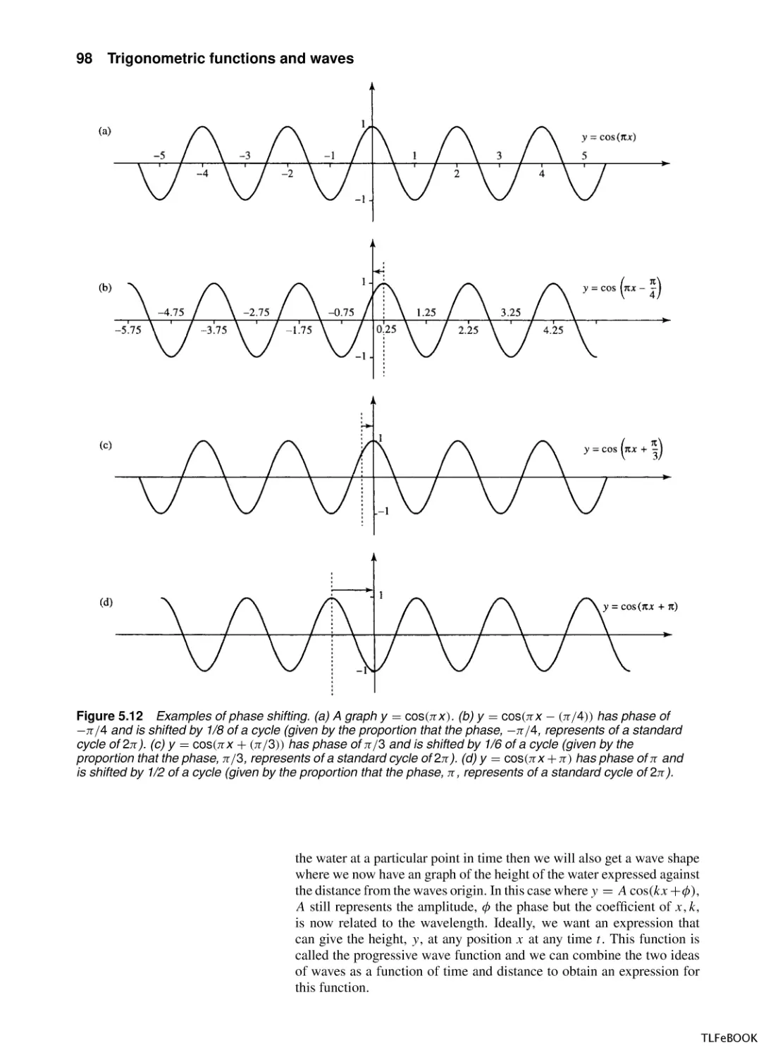
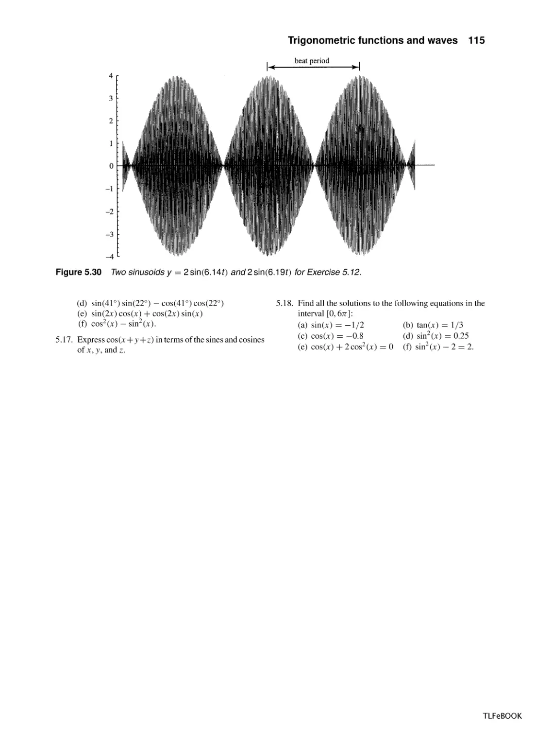
Wave functions of time and distance
5.5
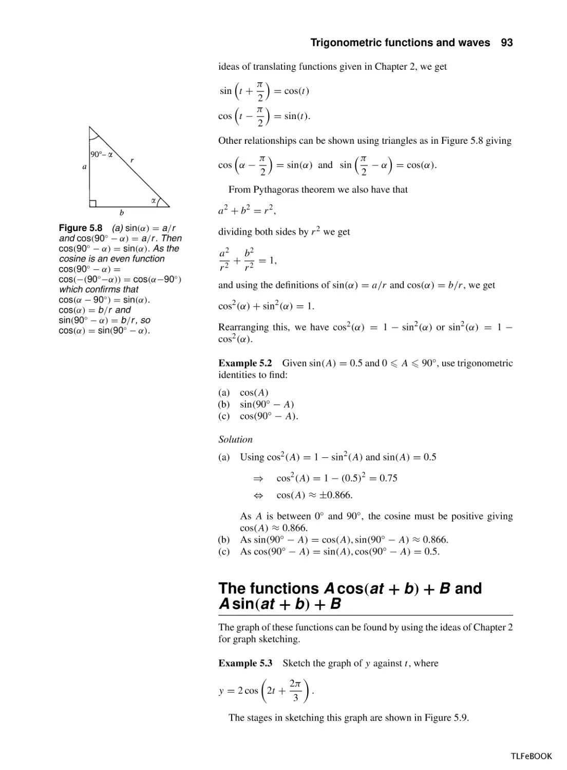
Trigonometric identities
5.6
Superposition
5.7
Inverse trigonometric functions
5.8
Solving the trigonometric equations sin x = a,
cos x = a, tan x = a
5.9
Summary
5.10 Exercises
88
88
88
91
97
103
107
109
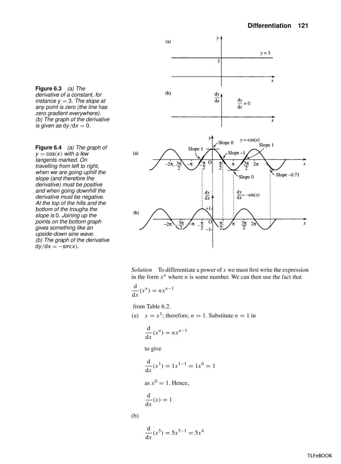
Differentiation
6.1
Introduction
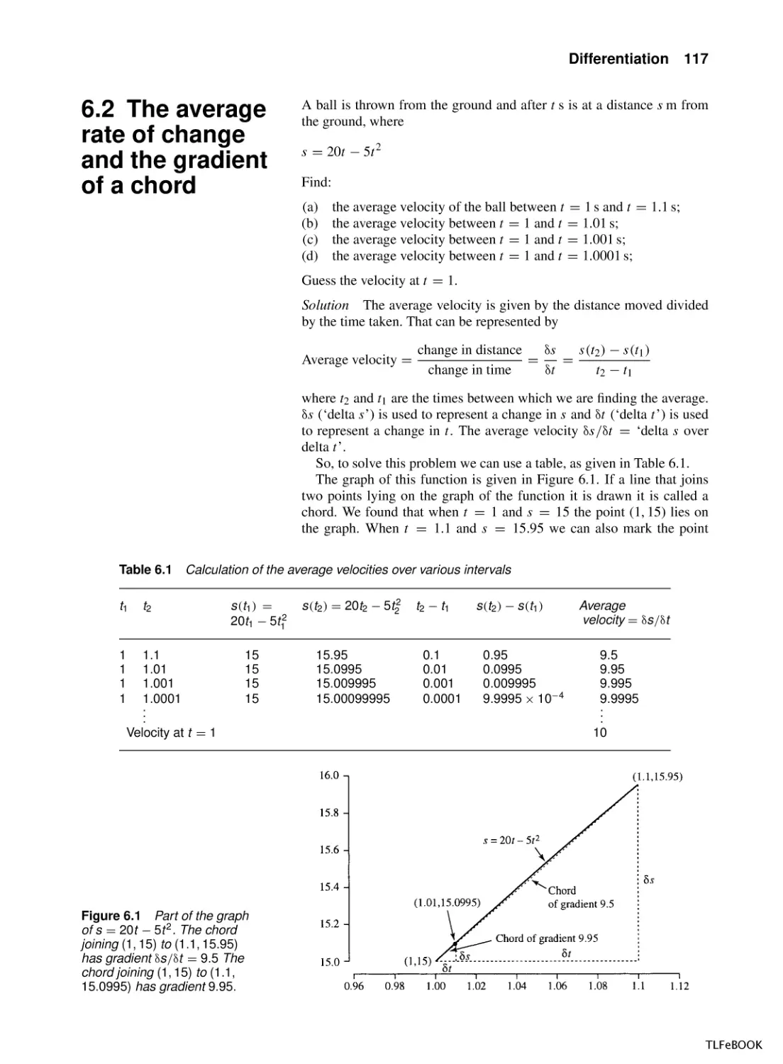
6.2
The average rate of change and the gradient of a
chord
6.3
The derivative function
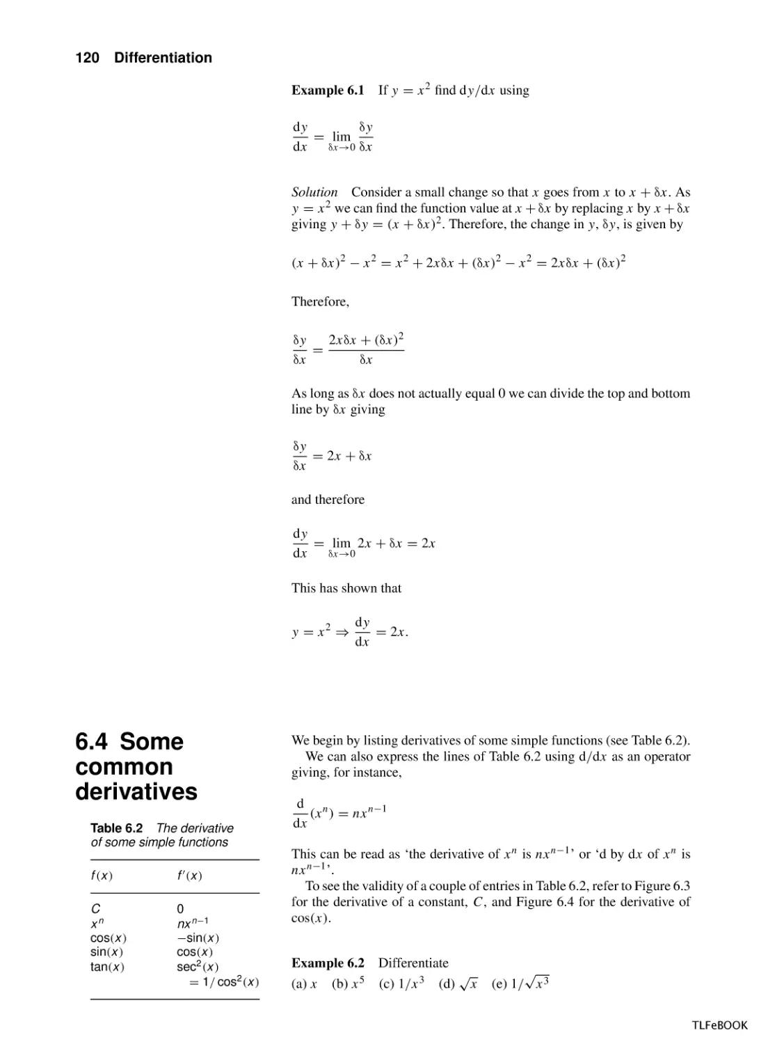
6.4
Some common derivatives
6.5
Finding the derivative of combinations of
functions
6.6
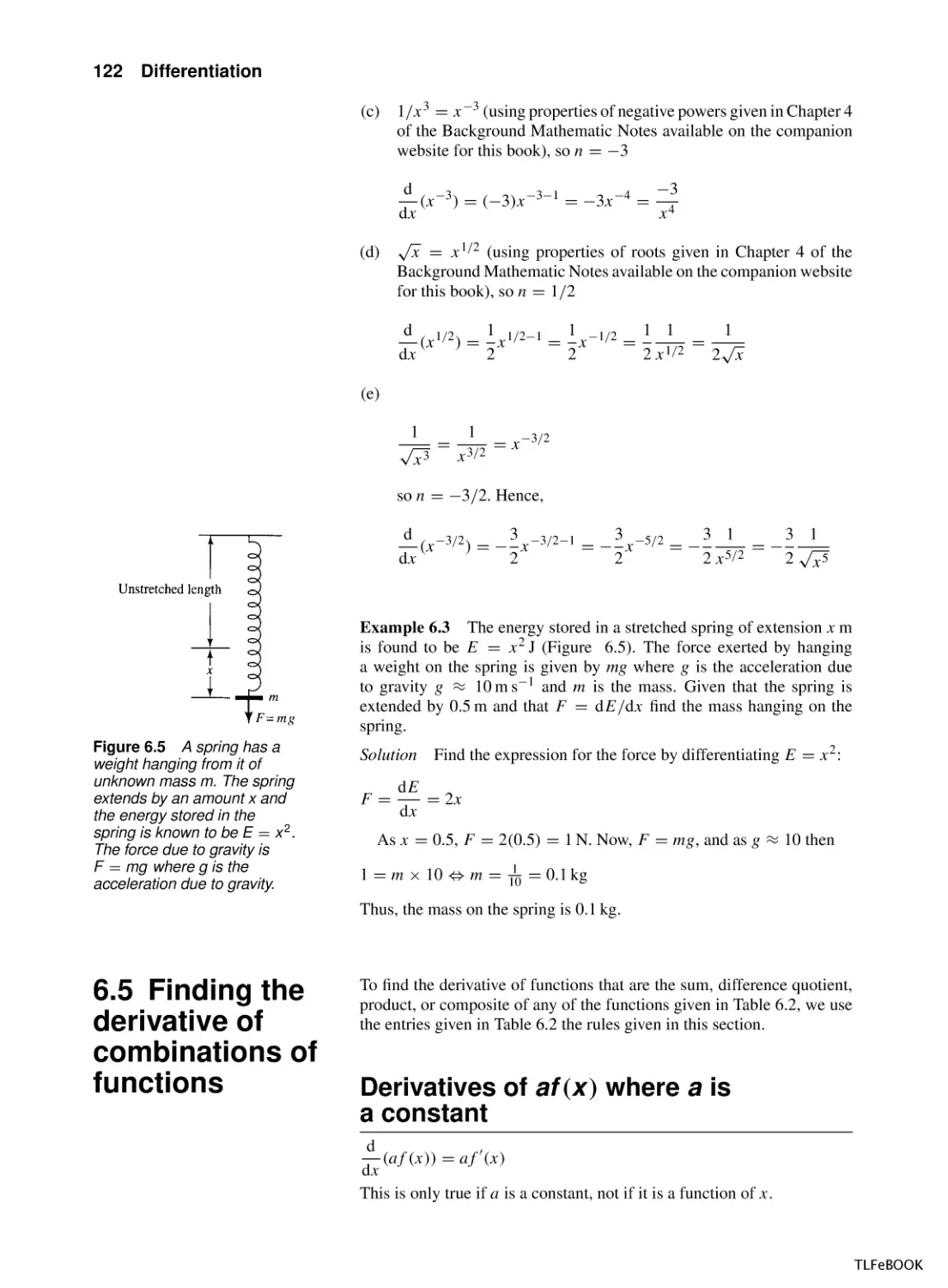
Applications of differentiation
6.7
Summary
6.9
Exercises
116
116
122
128
130
131
7
Integration
7.1
Introduction
7.2
Integration
7.3
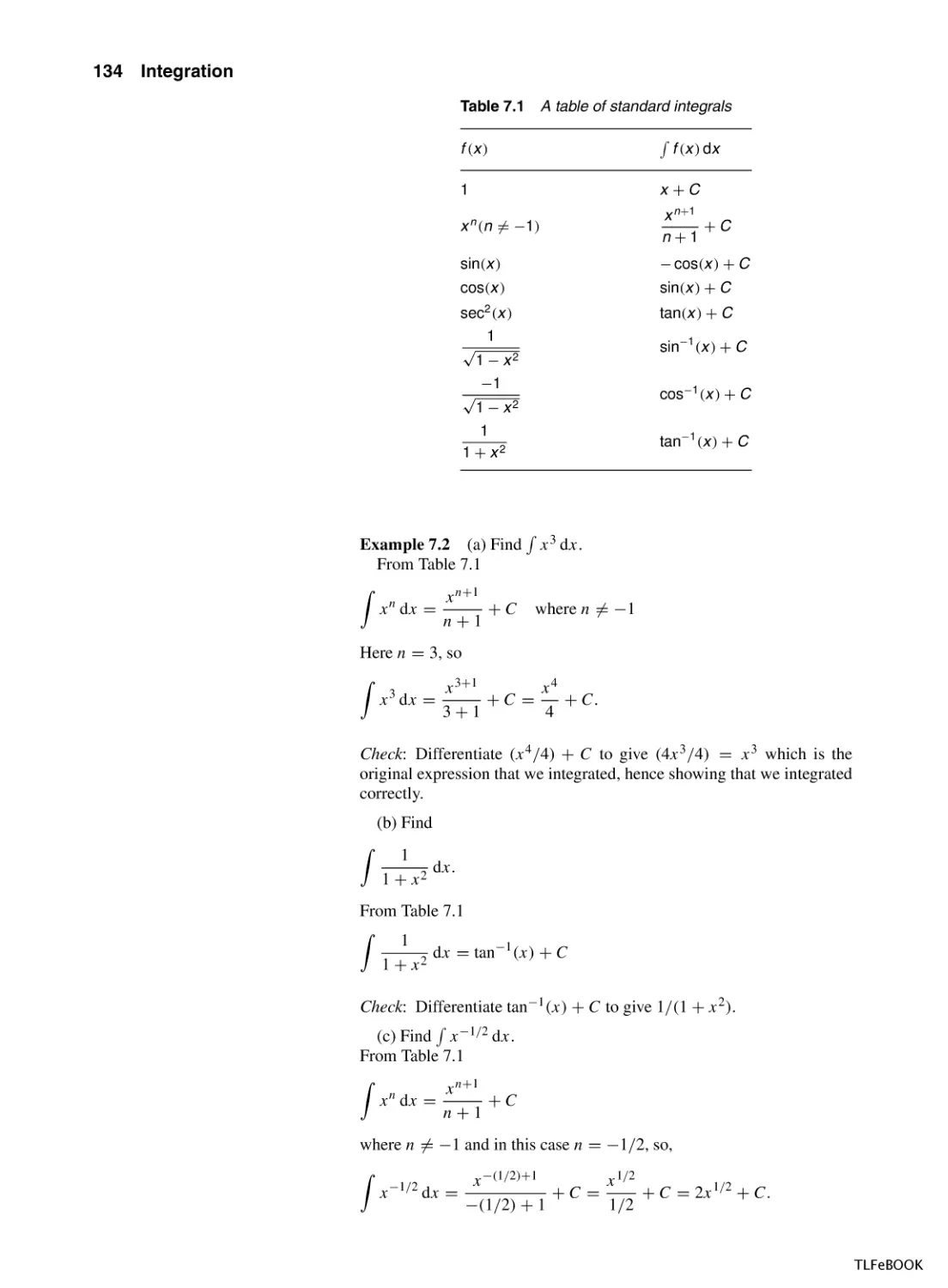
Finding integrals
7.4
Applications of integration
7.5
The definite integral
7.6
The mean value and r.m.s. value
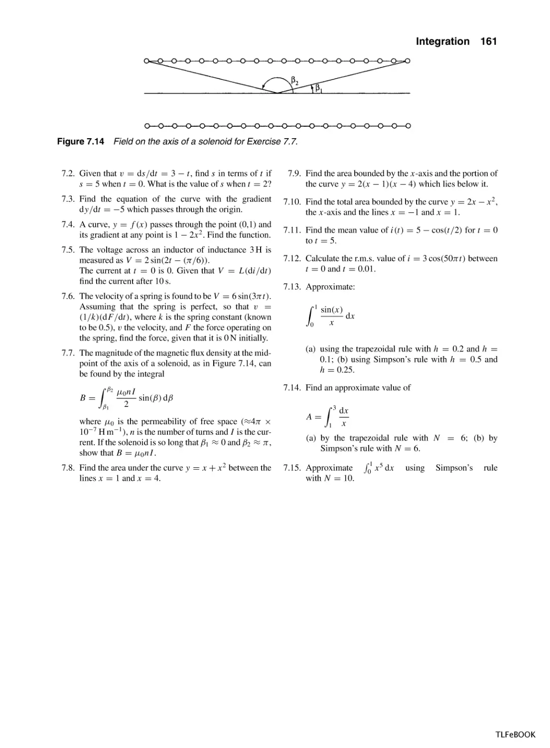
7.7
Numerical Methods of Integration
7.8
Summary
7.9
Exercises
132
132
132
133
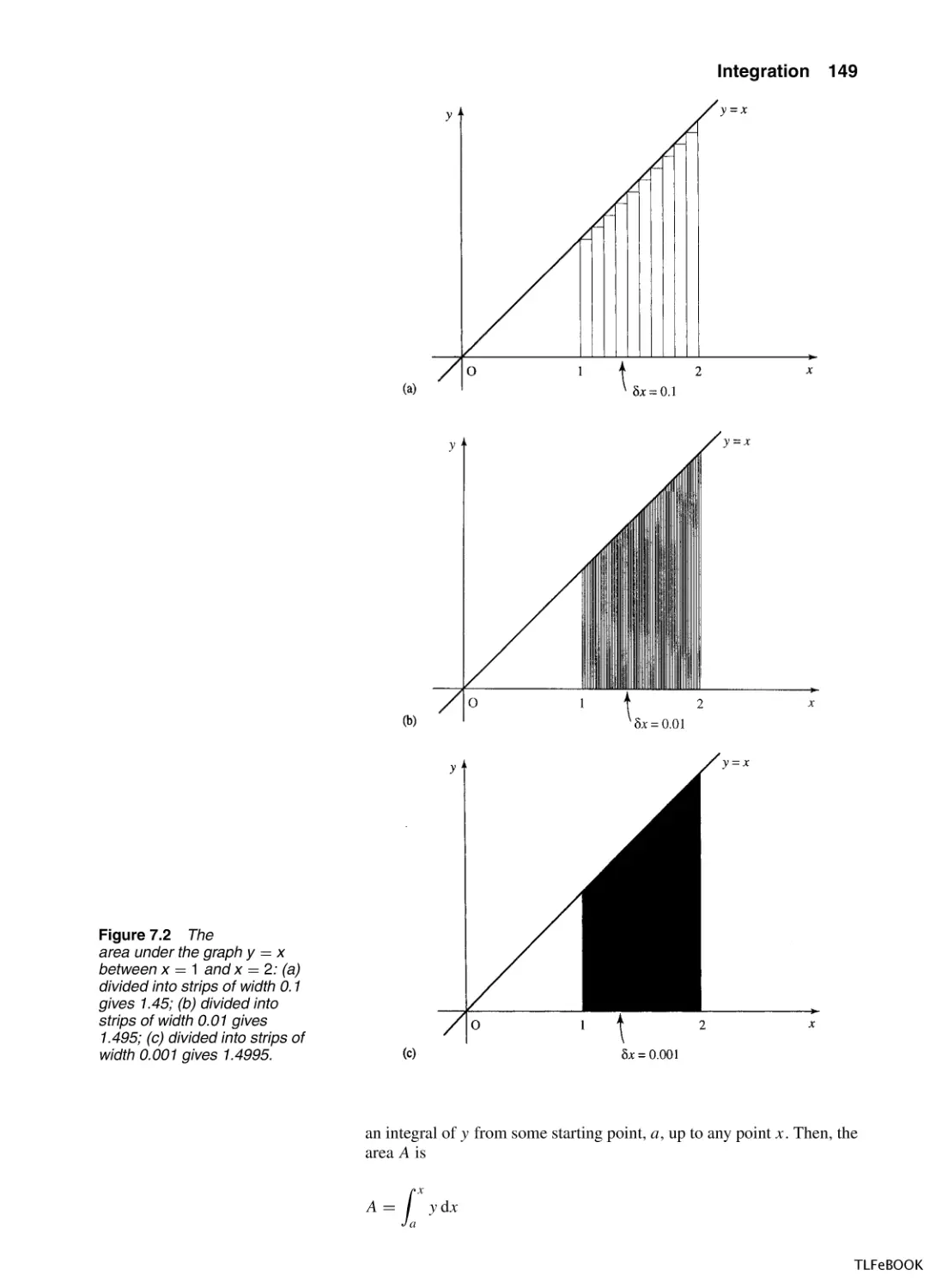
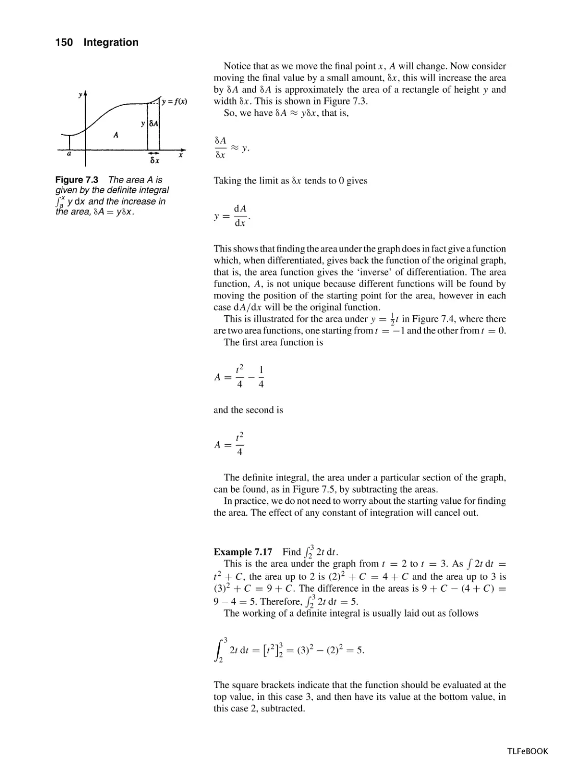
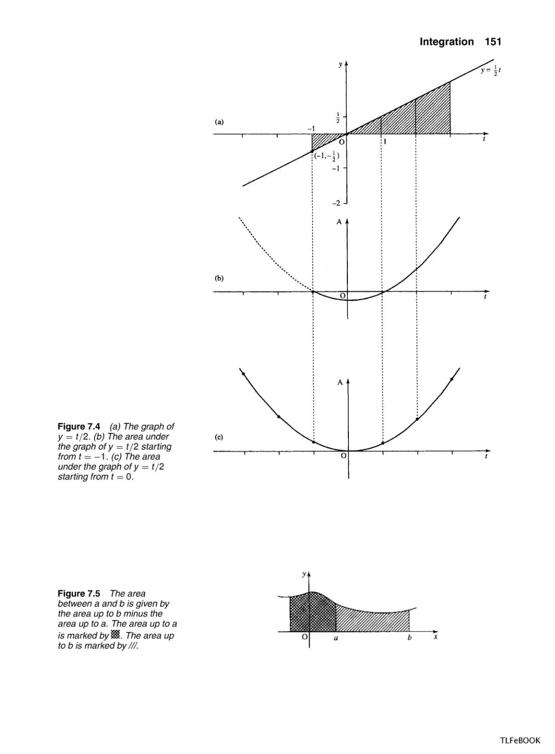
145
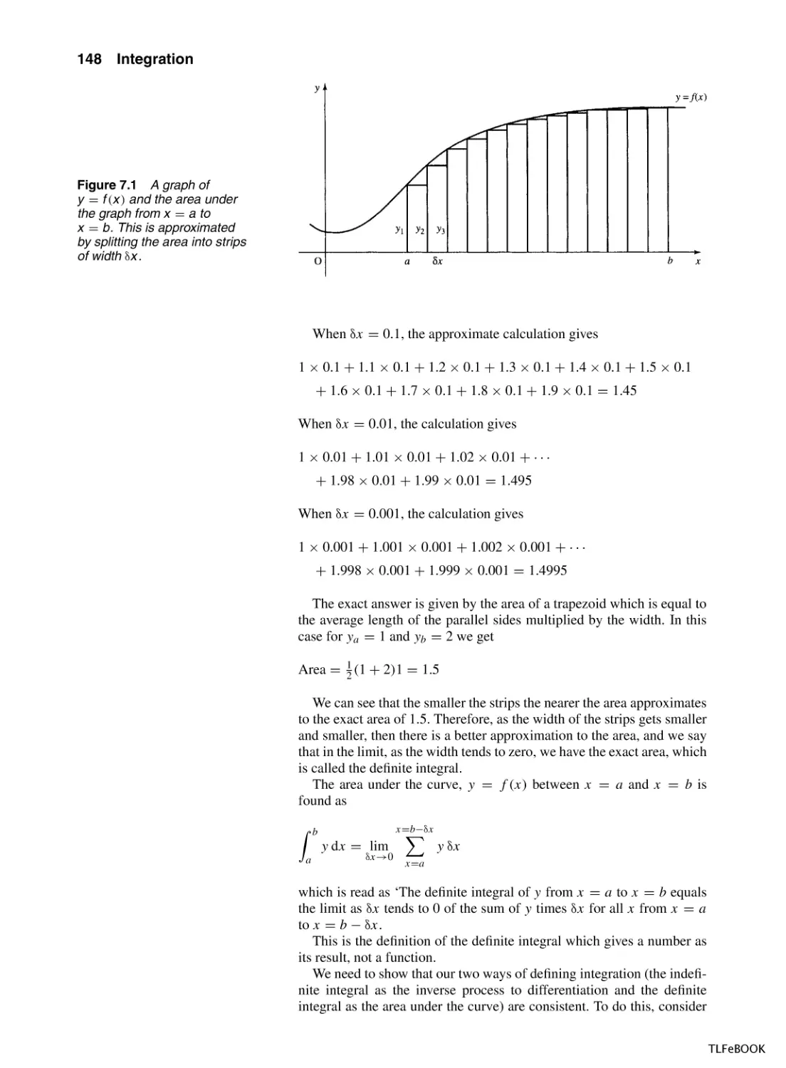
147
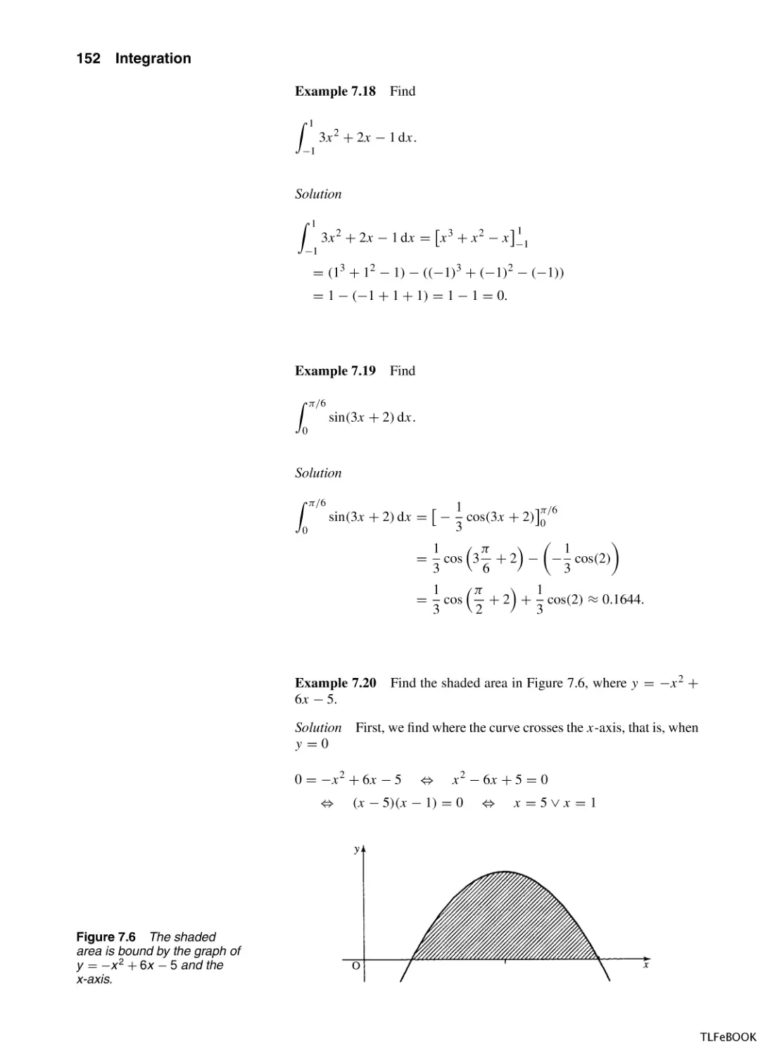
155
156
159
160
8
The exponential function
8.1
Introduction
8.2
Exponential growth and decay
8.3
The exponential function y = et
8.4
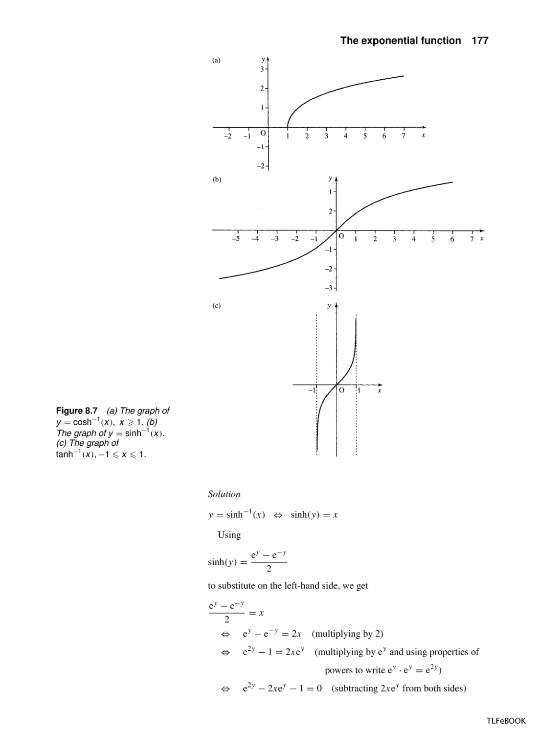
The hyperbolic functions
8.5
More differentiation and integration
8.6
Summary
8.7
Exercises
162
162
162
166
173
180
186
187
6
110
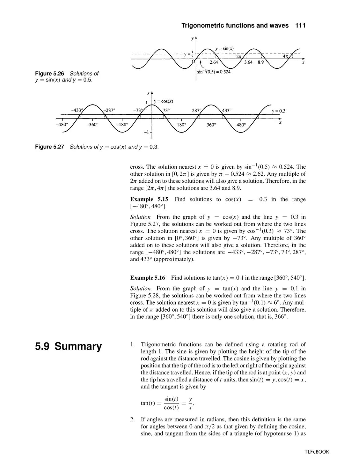
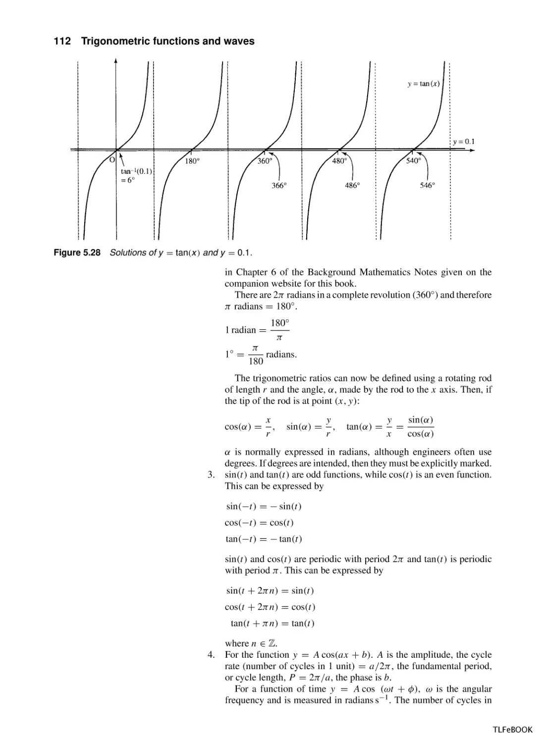
111
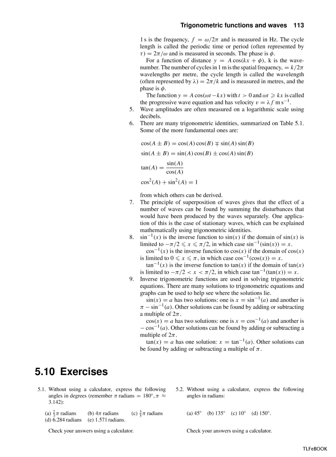
113
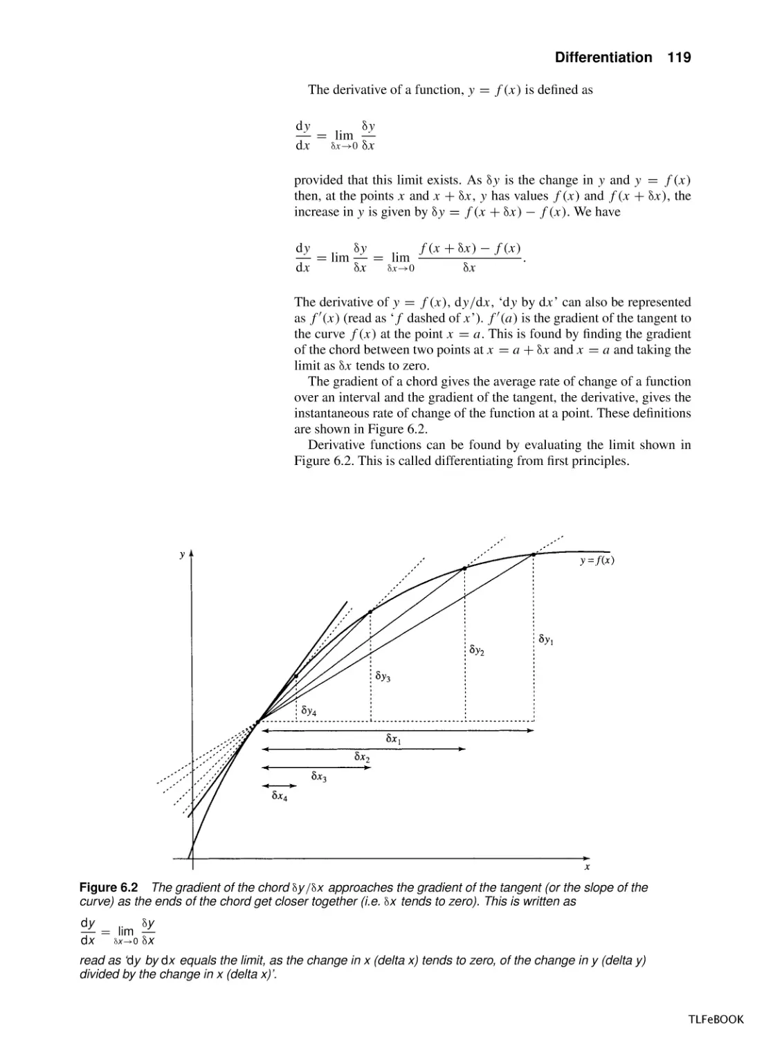
117
118
120
TLFeBOOK
Contents
vii
Vectors
9.1
Introduction
9.2
Vectors and vector quantities
9.3
Addition and subtraction of vectors
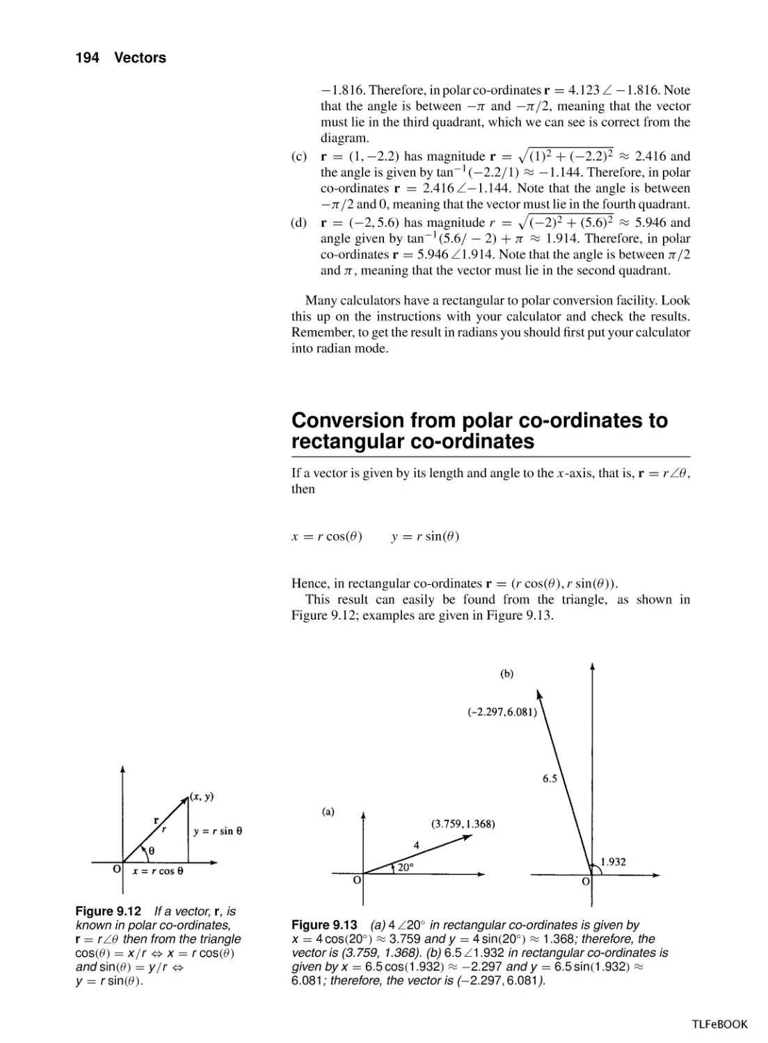
9.4
Magnitude and direction of a 2D vector – polar
co-ordinates
9.5
Application of vectors to represent waves
(phasors)
9.6
Multiplication of a vector by a scalar and unit
vectors
9.7
Basis vectors
9.8
Products of vectors
9.9
Vector equation of a line
9.10 Summary
9.12 Exercises
188
188
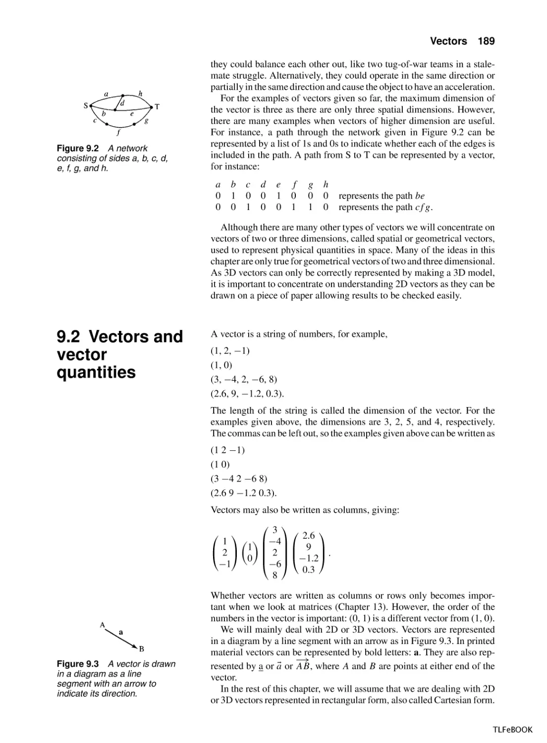
189
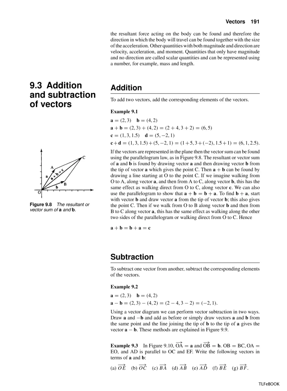
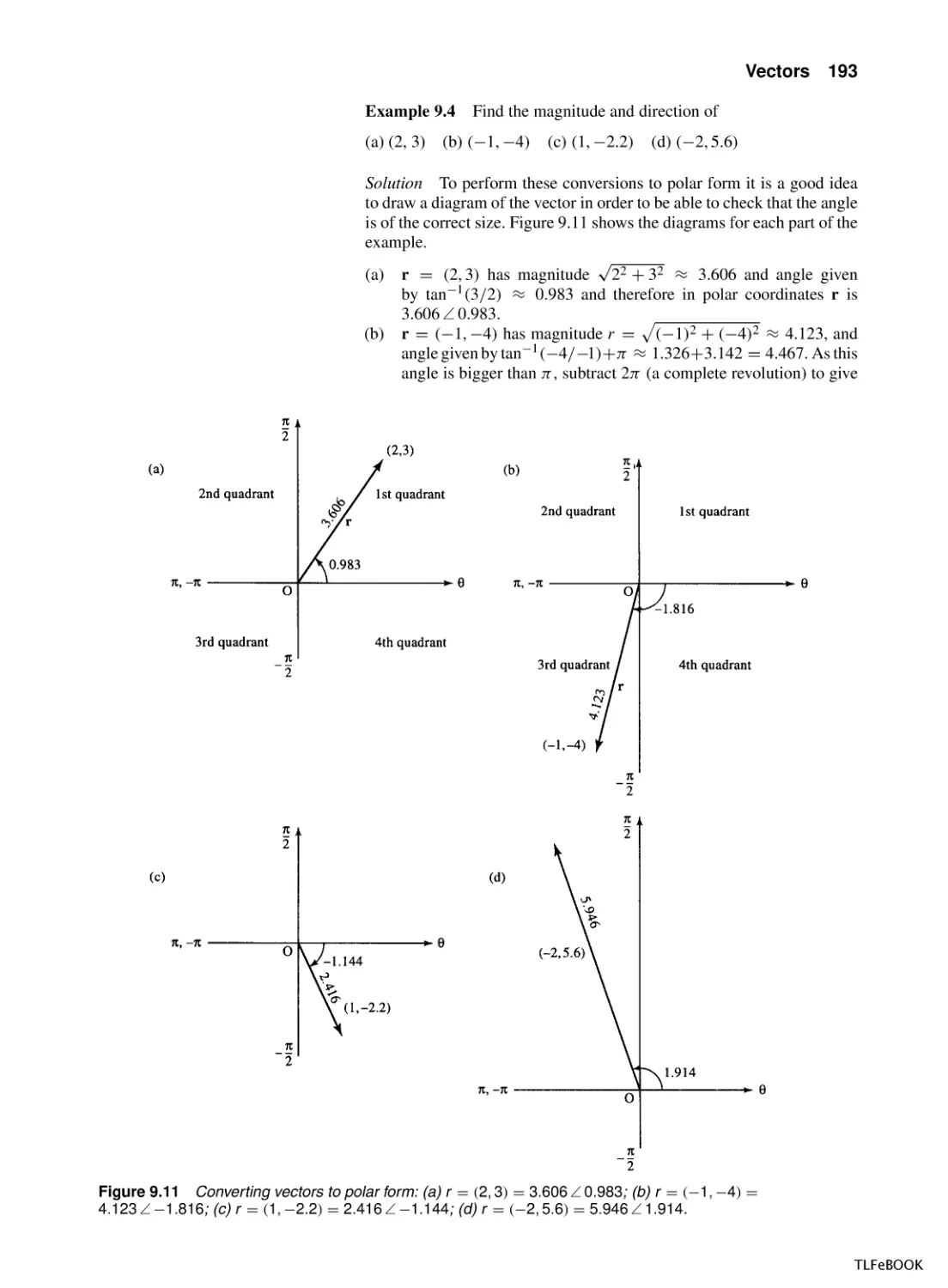
191
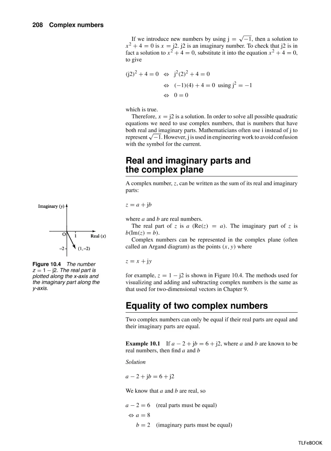
10 Complex numbers
10.1 Introduction
10.2 Phasor rotation by π/2
10.3 Complex numbers and operations
10.4 Solution of quadratic equations
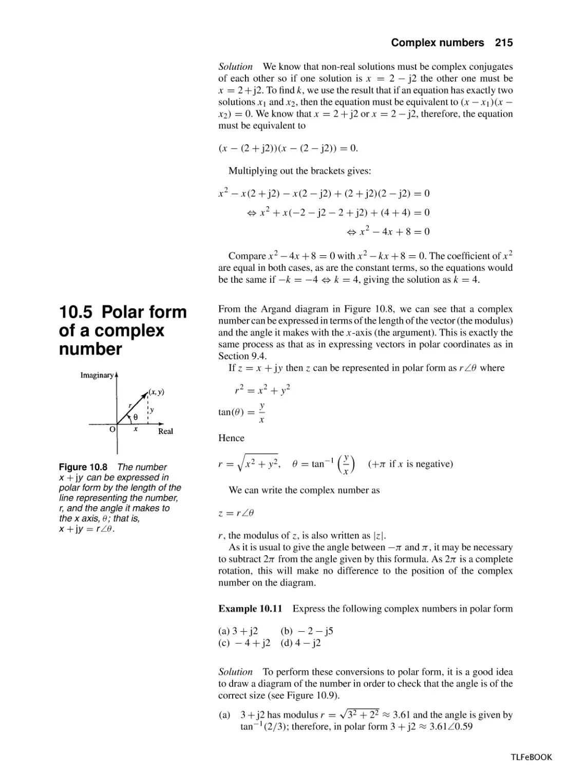
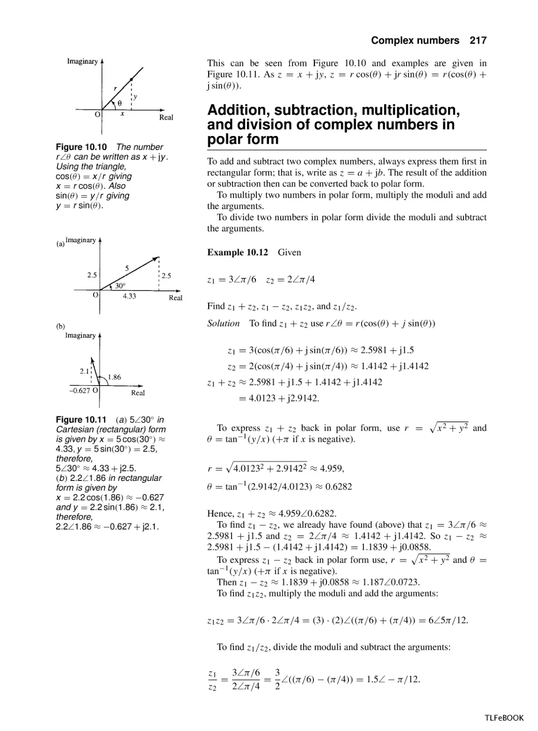
10.5 Polar form of a complex number
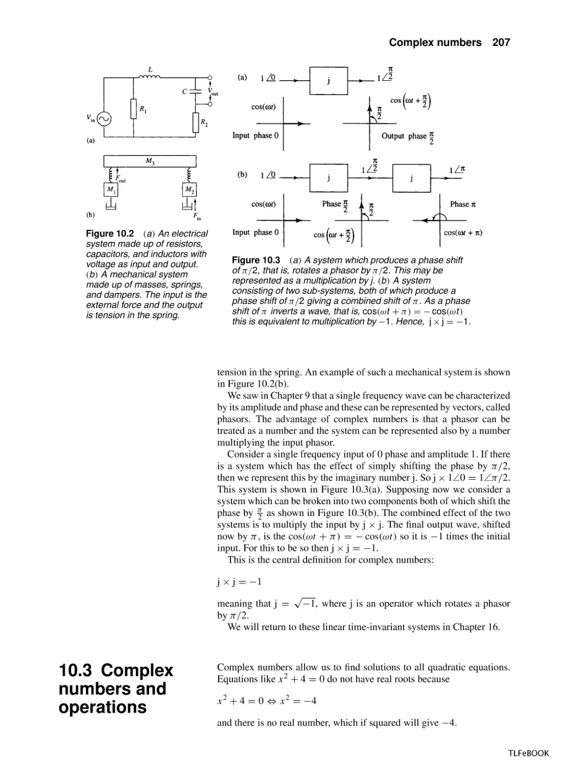
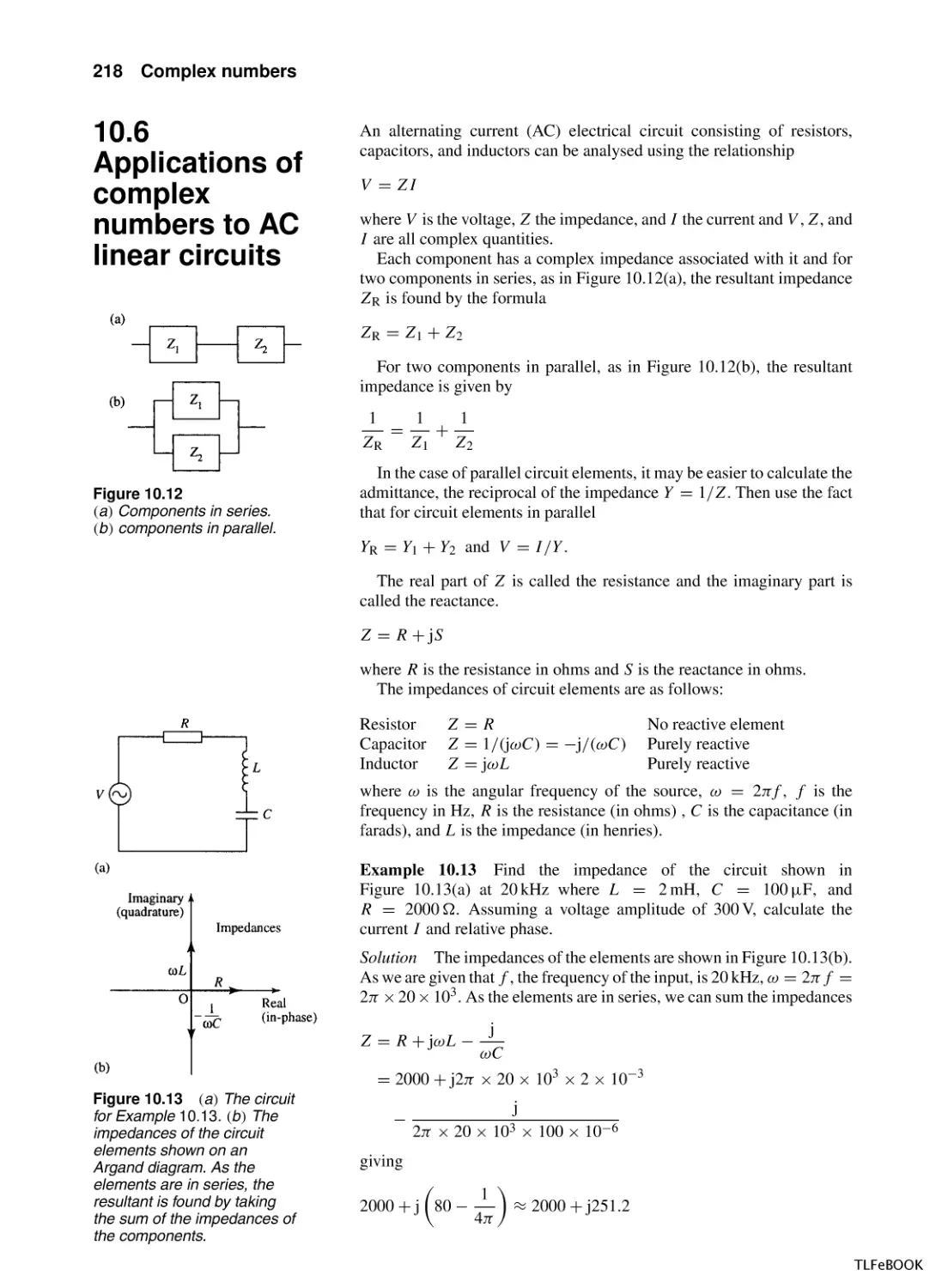
10.6 Applications of complex numbers to AC linear
circuits
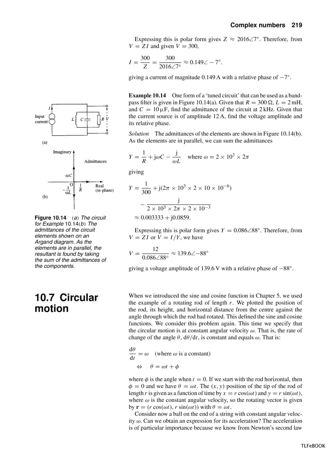
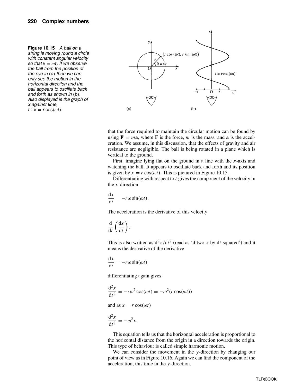
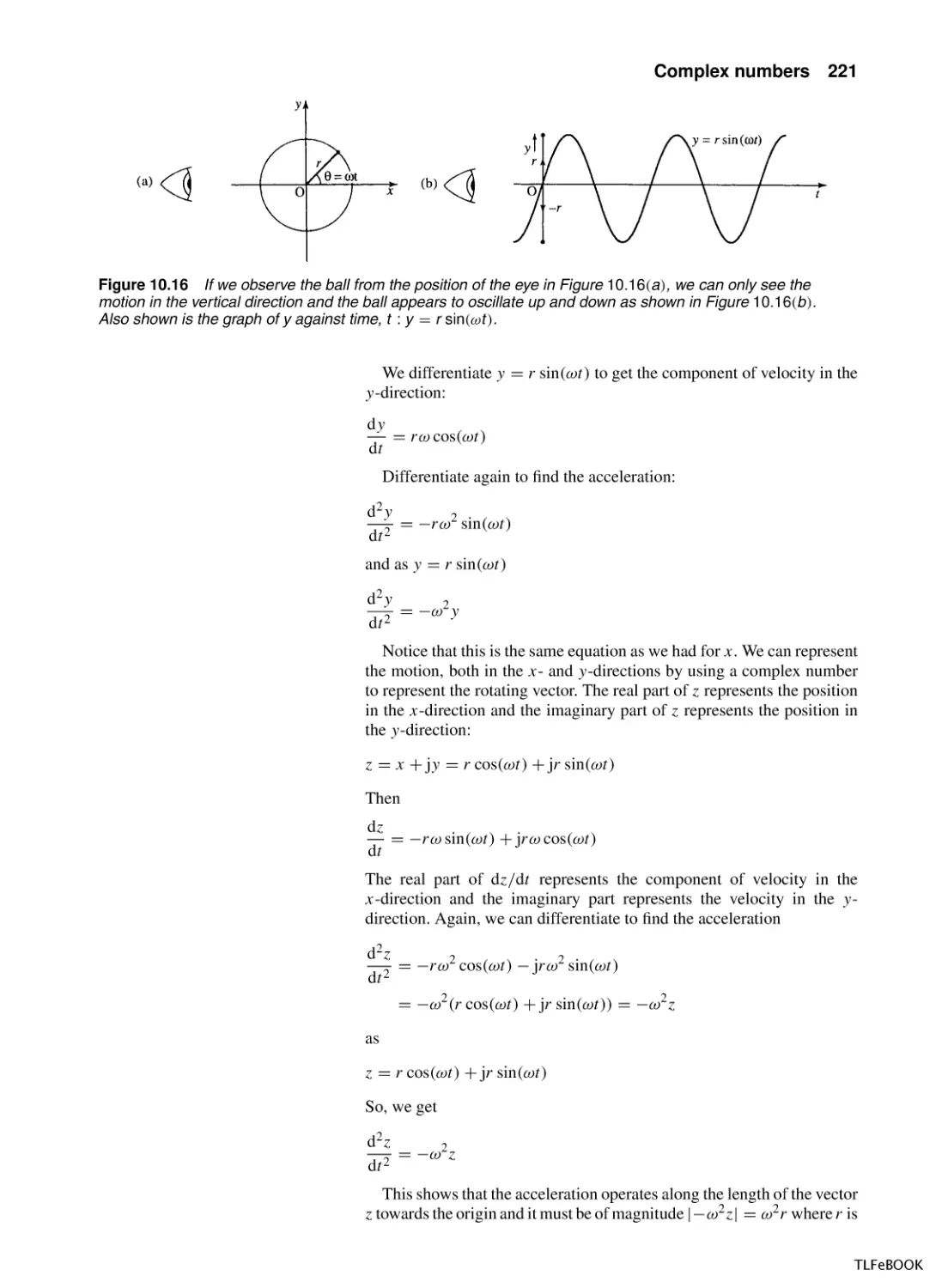
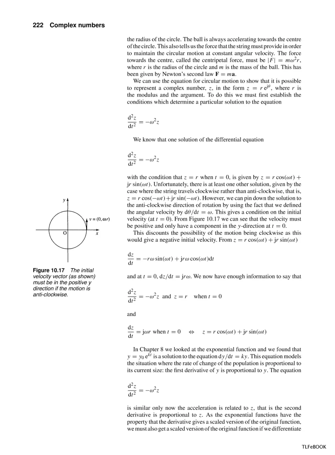
10.7 Circular motion
10.8 The importance of being exponential
10.9 Summary
10.10 Exercises
206
206
206
207
212
215
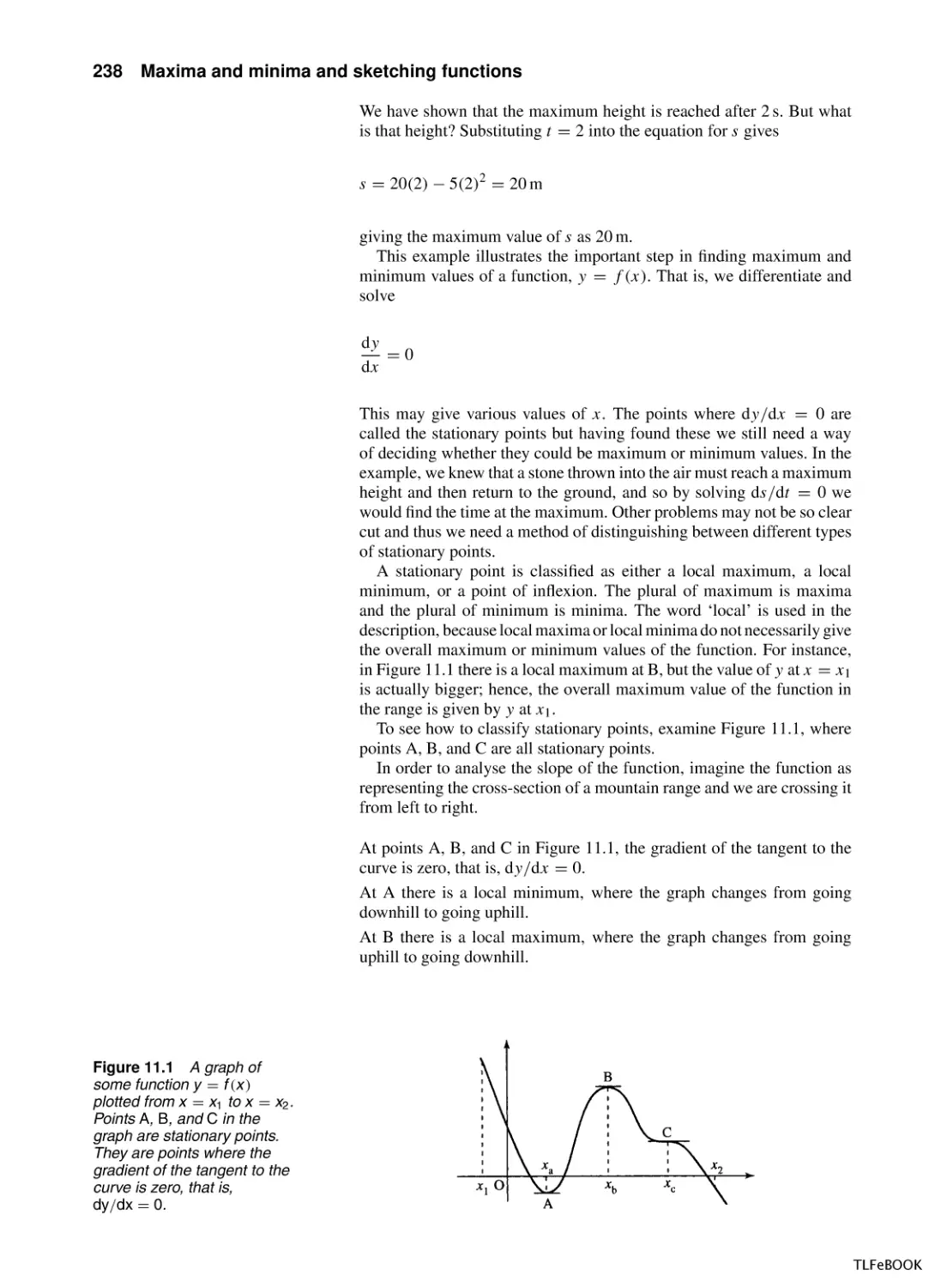
11 Maxima and minima and sketching functions
11.1 Introduction
11.2 Stationary points, local maxima and
minima
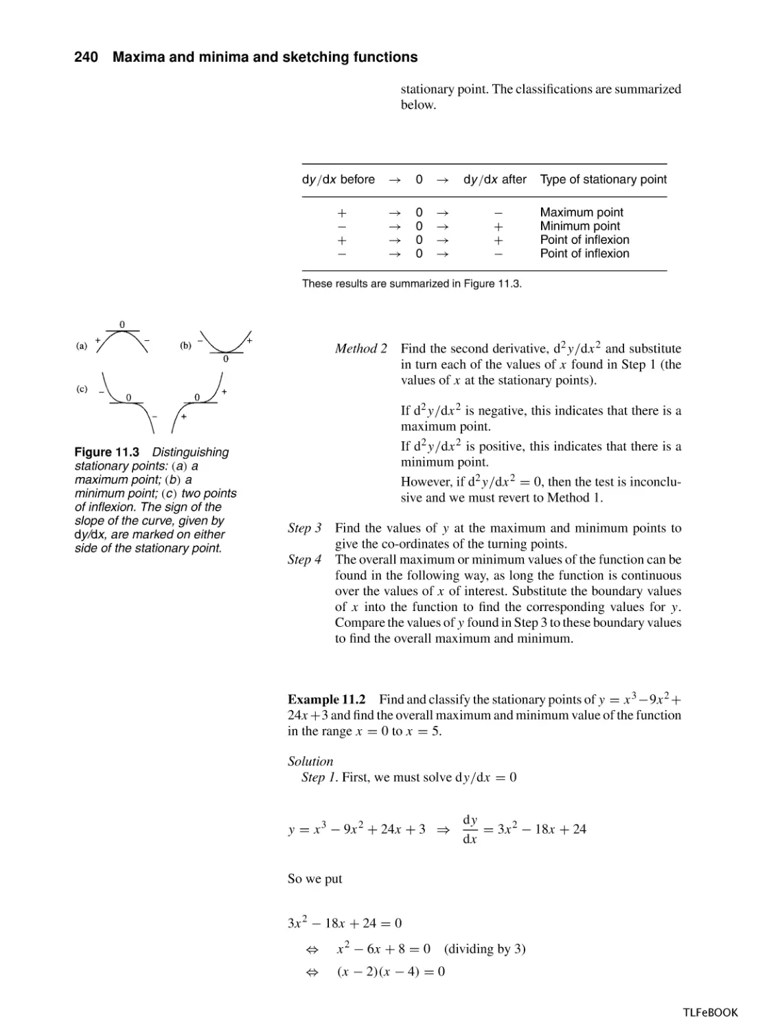
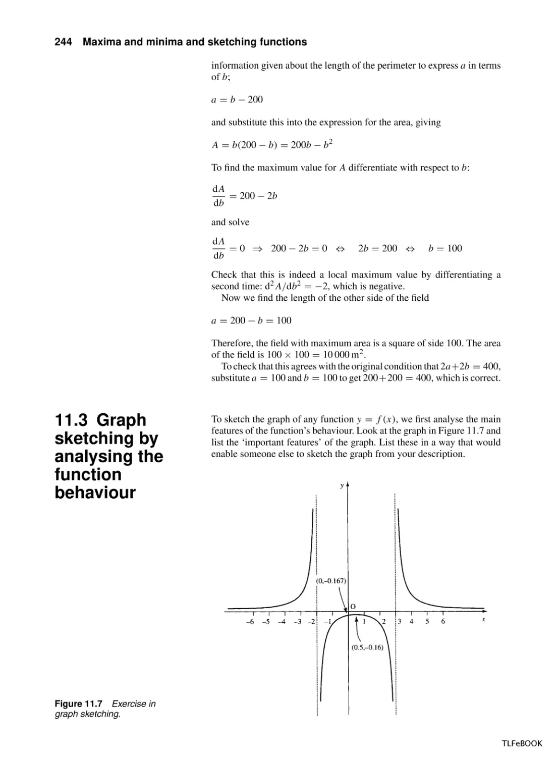
11.3 Graph sketching by analysing the function
behaviour
11.4 Summary
11.5 Exercises
237
237
12 Sequences and series
12.1 Introduction
12.2 Sequences and series definitions
12.3 Arithmetic progression
12.4 Geometric progression
12.5 Pascal’s triangle and the binomial series
12.6 Power series
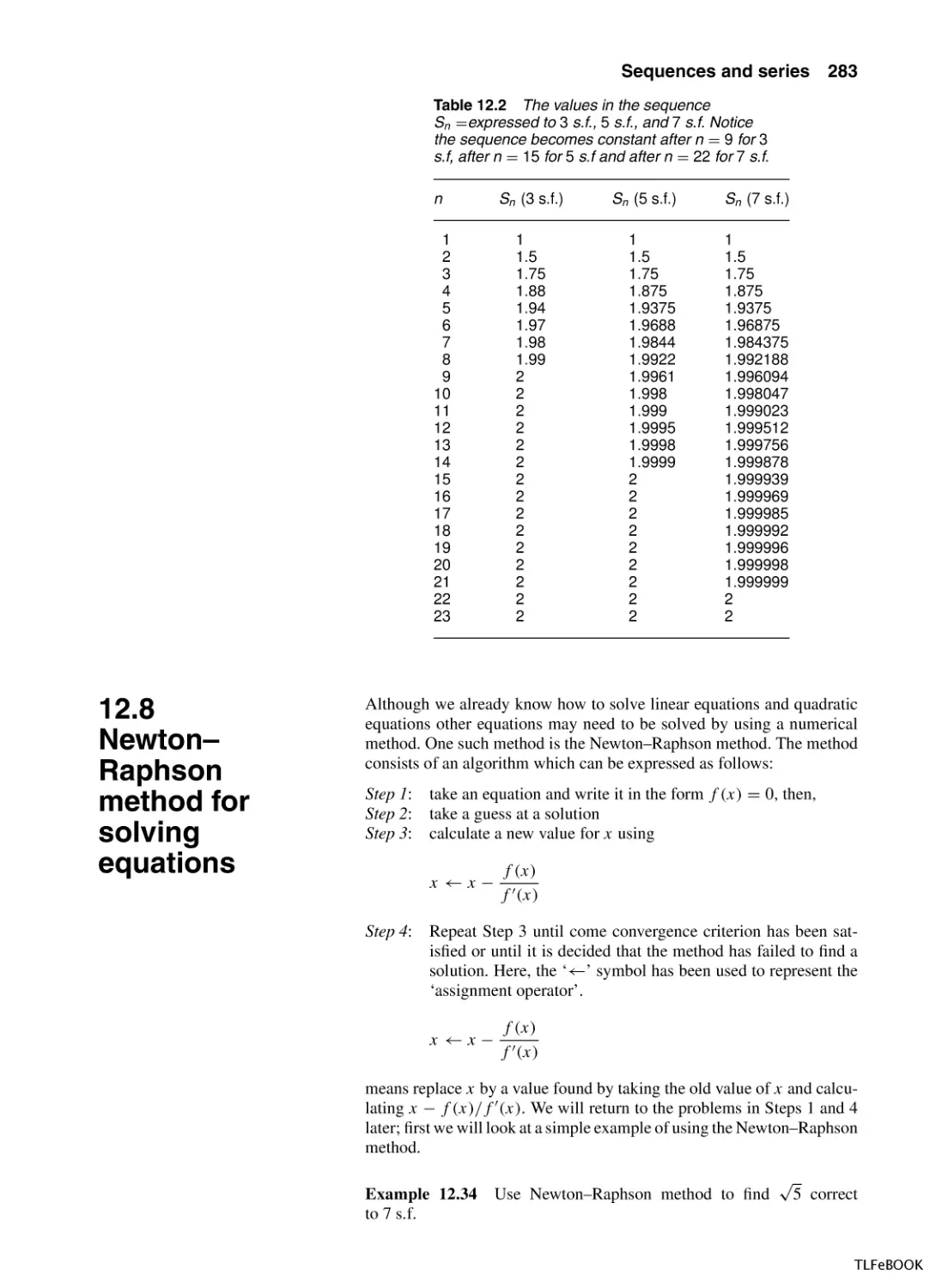
12.7 Limits and convergence
12.8 Newton–Raphson method for solving
equations
12.9 Summary
12.10 Exercises
254
254
254
259
262
267
272
282
9
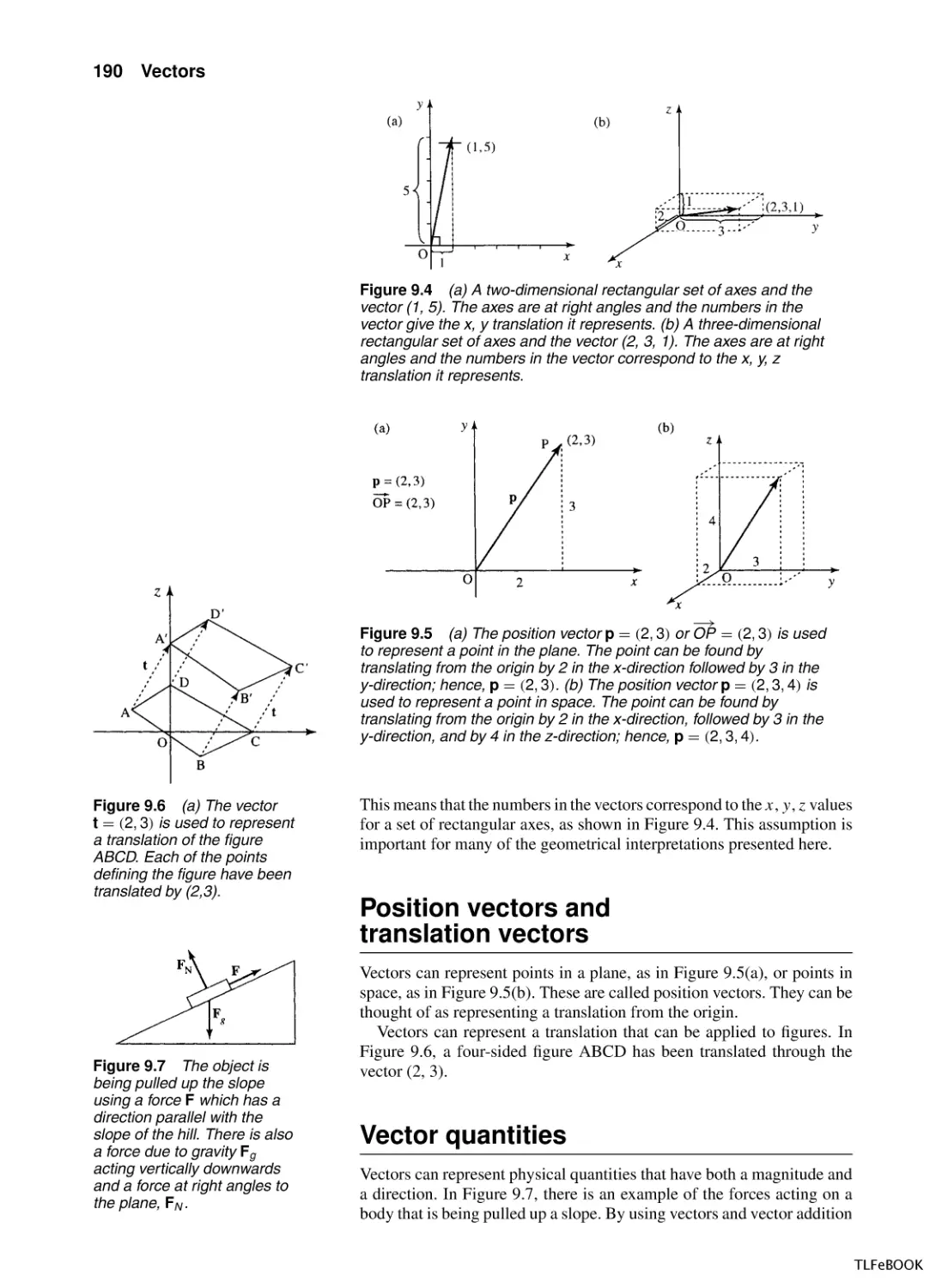
192
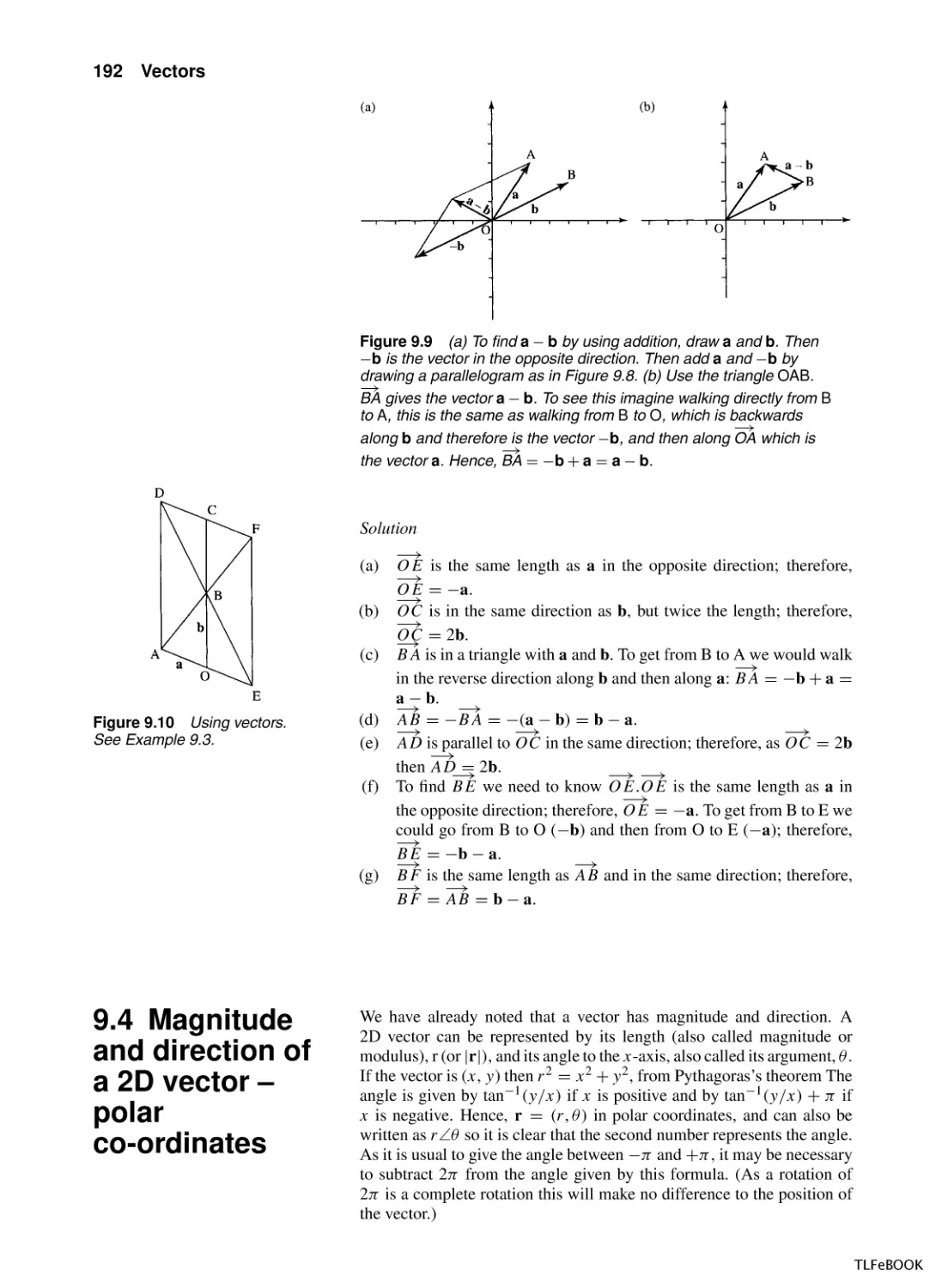
195
197
198
198
202
203
205
218
219
226
232
235
237
244
251
252
283
287
289
TLFeBOOK
viii
Contents
Part 2
Systems
13 Systems of linear equations, matrices, and
determinants
13.1 Introduction
13.2 Matrices
13.3 Transformations
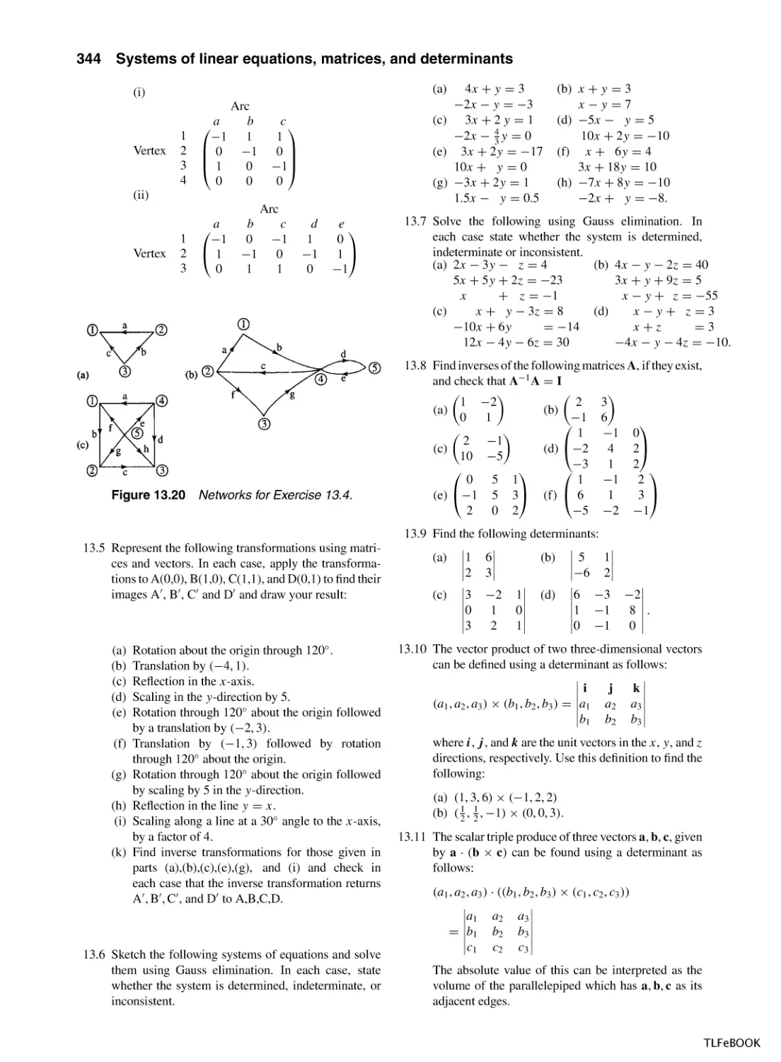
13.4 Systems of equations
13.5 Gauss elimination
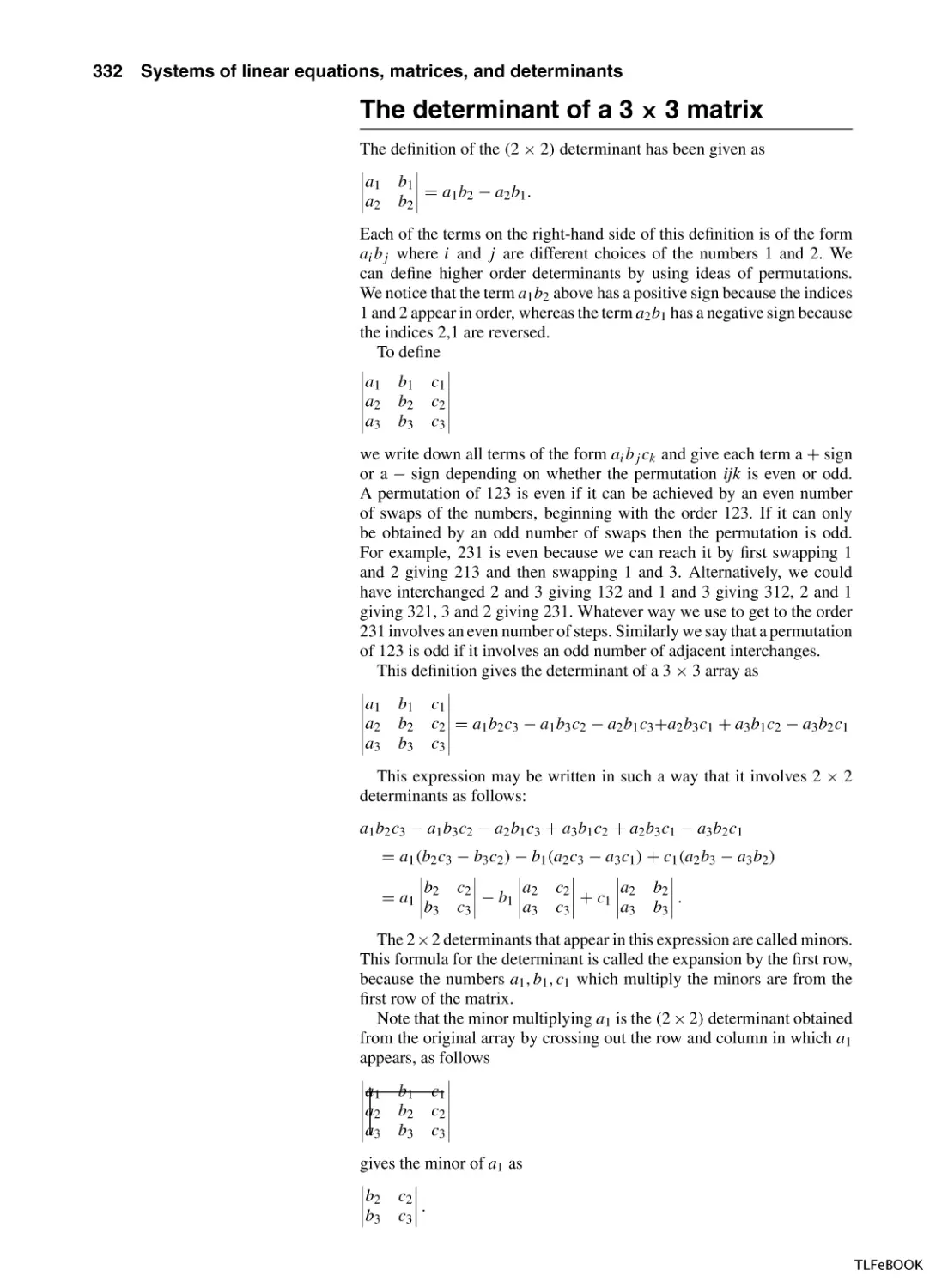
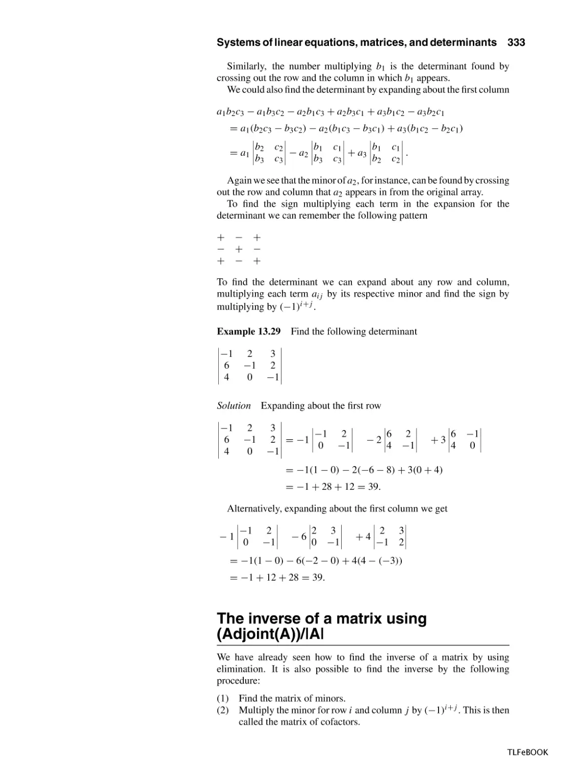
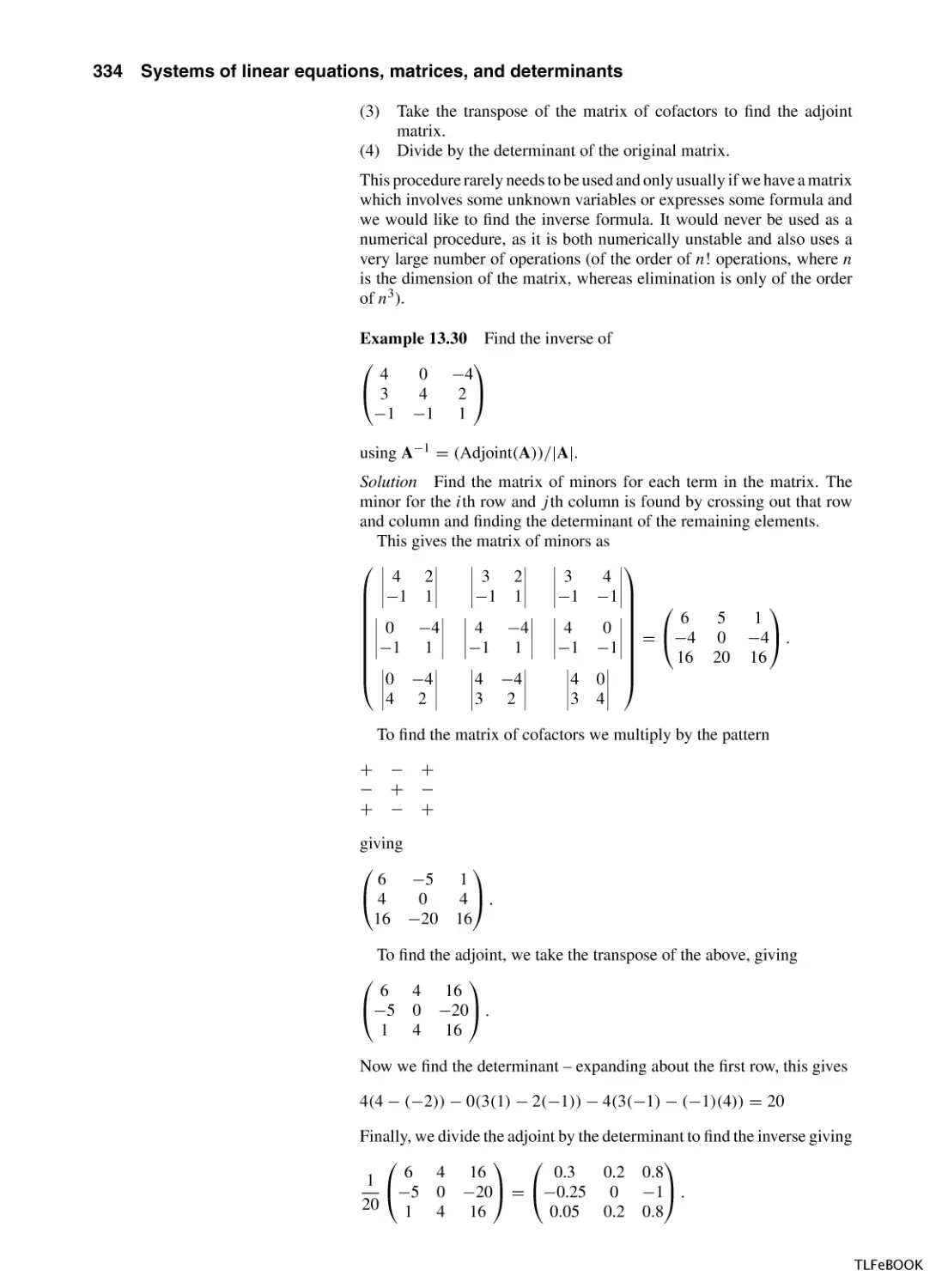
13.6 The inverse and determinant of a 3 × 3
matrix
13.7 Eigenvectors and eigenvalues
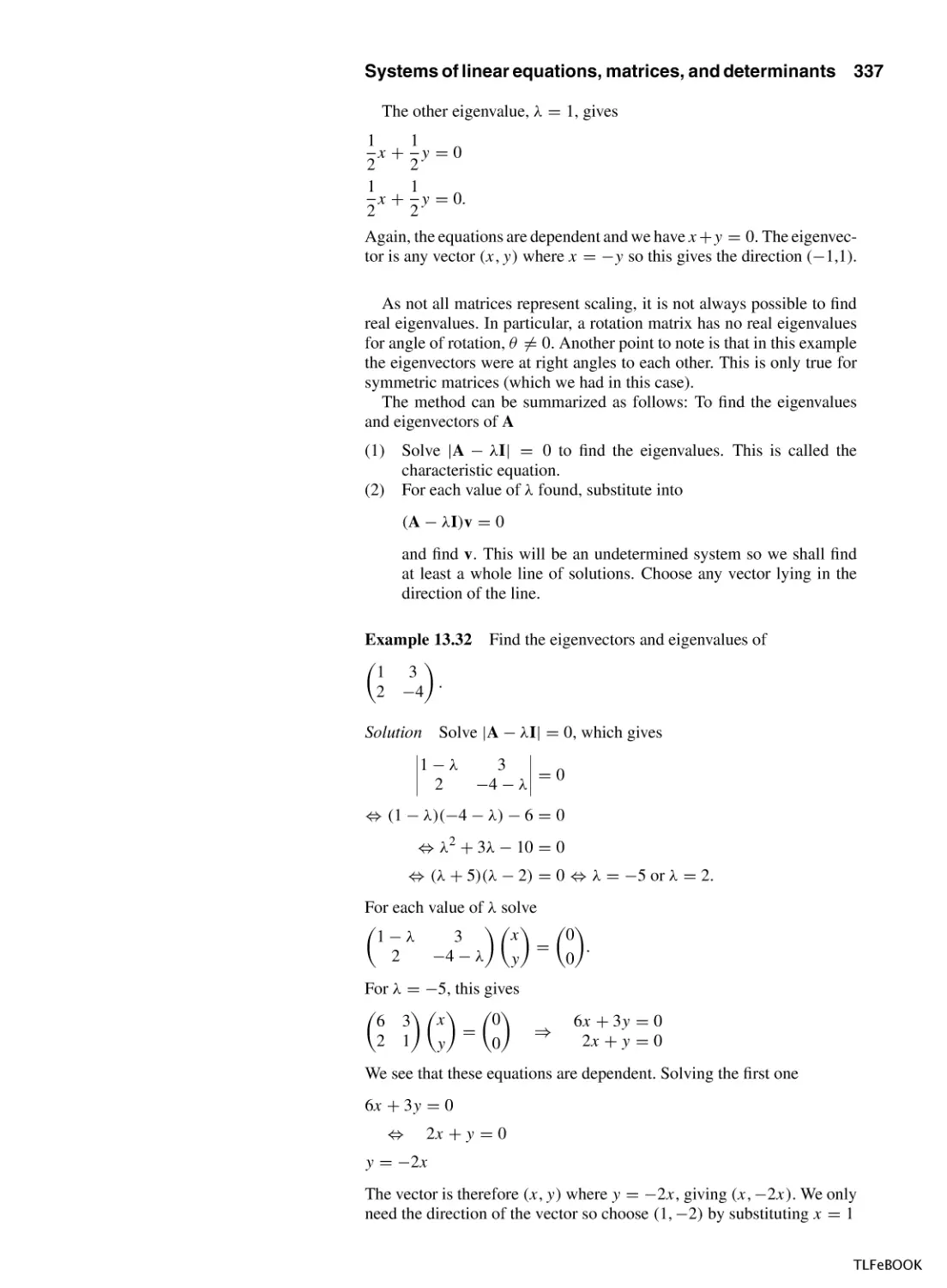
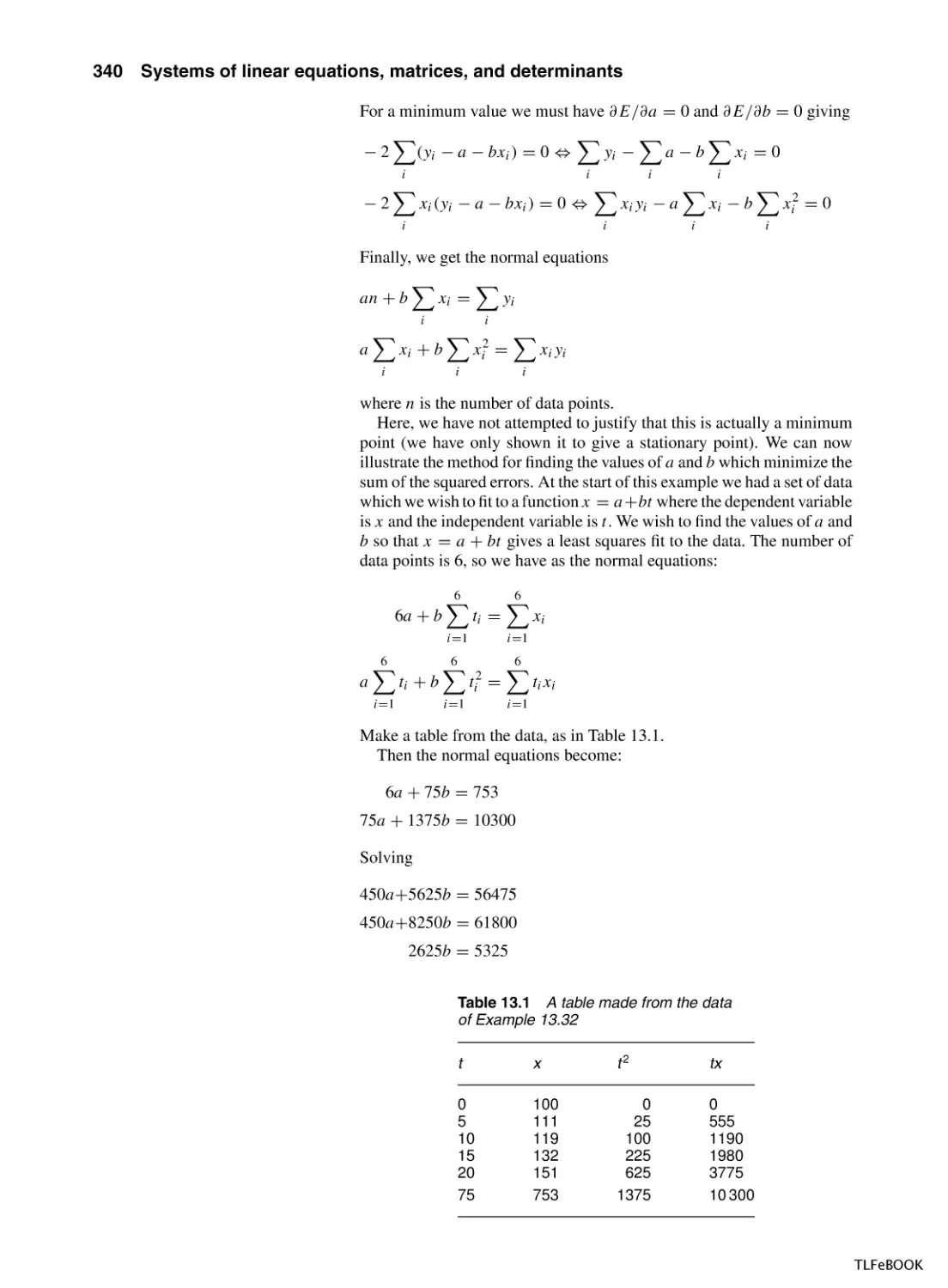
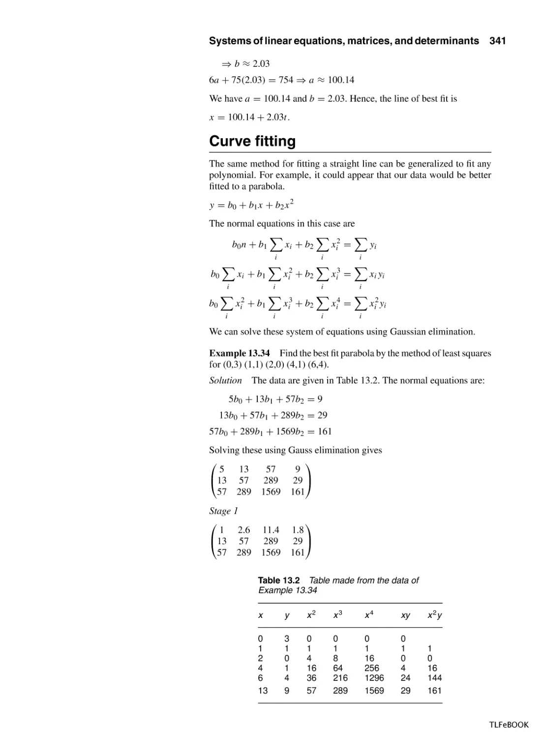
13.8 Least squares data fitting
13.9 Summary
13.10 Exercises
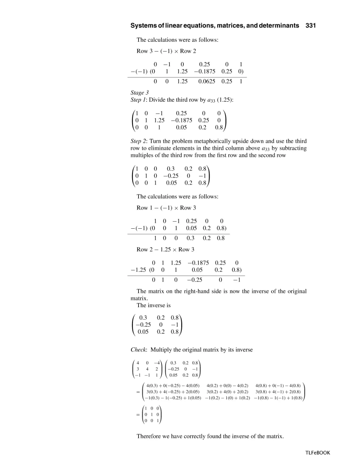
330
335
338
342
343
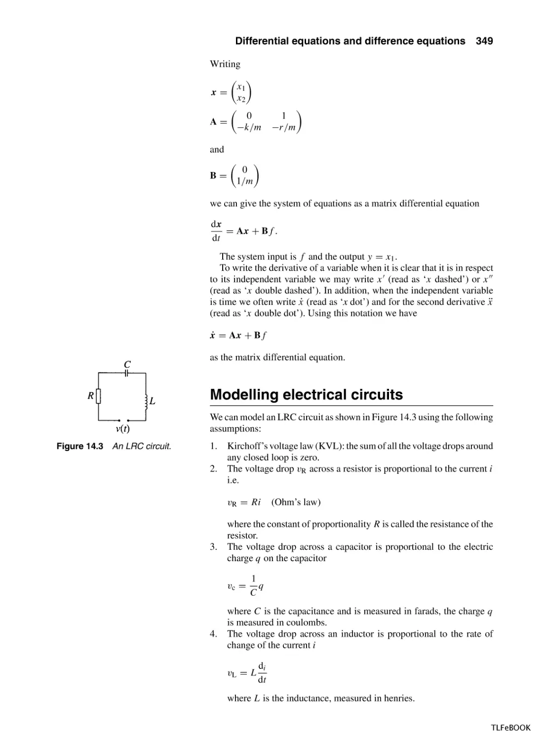
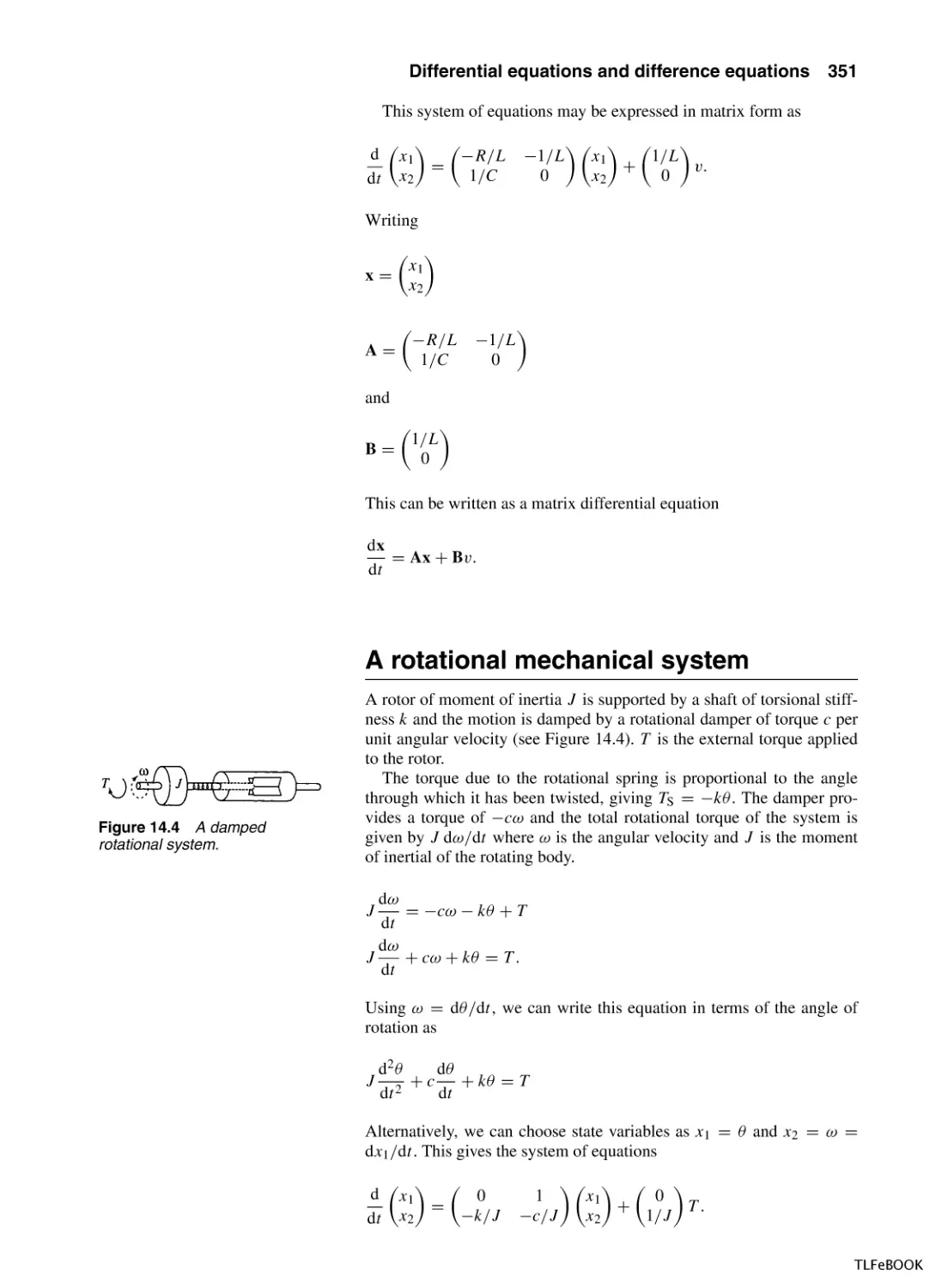
14 Differential equations and difference equations
14.1 Introduction
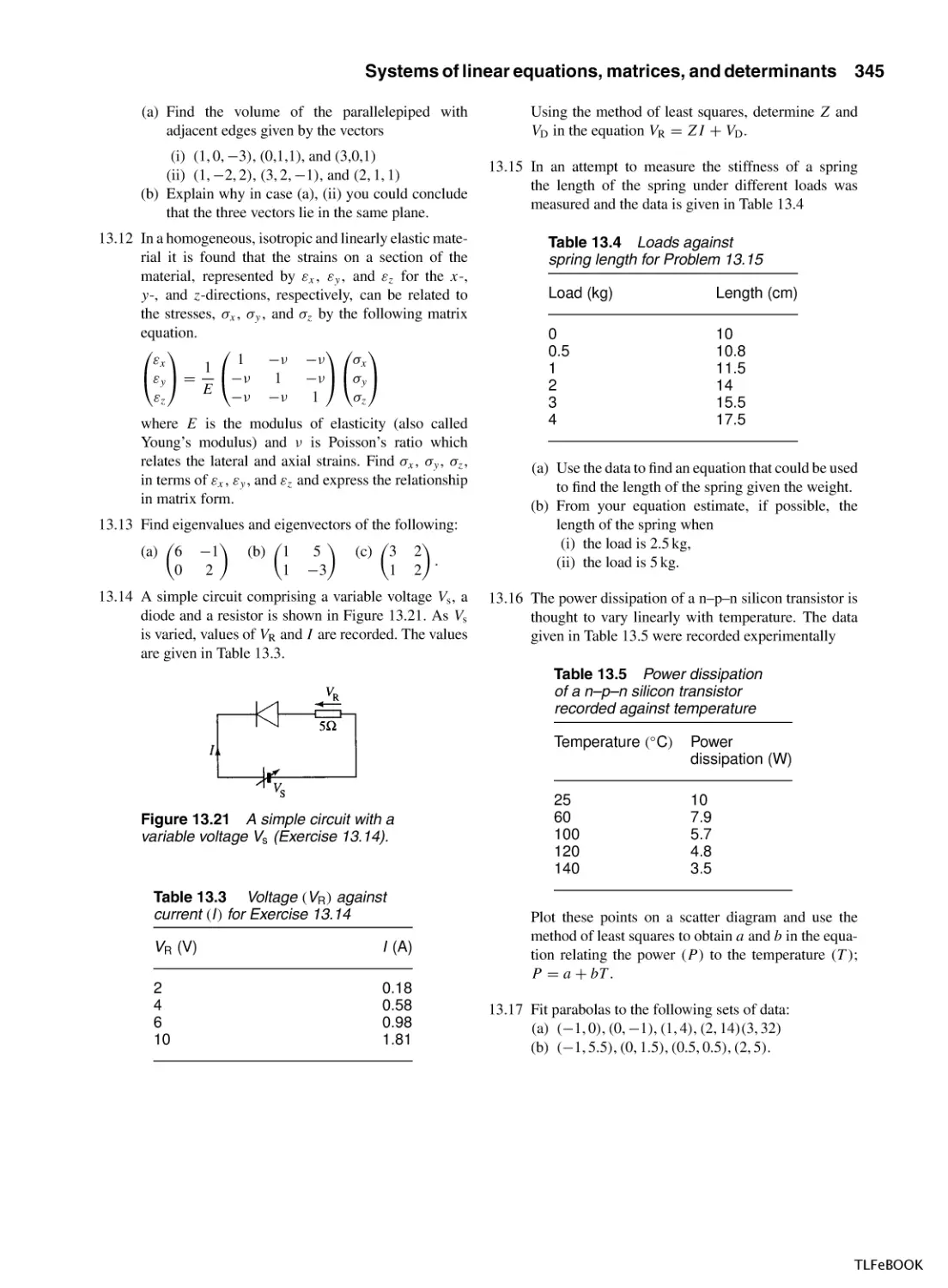
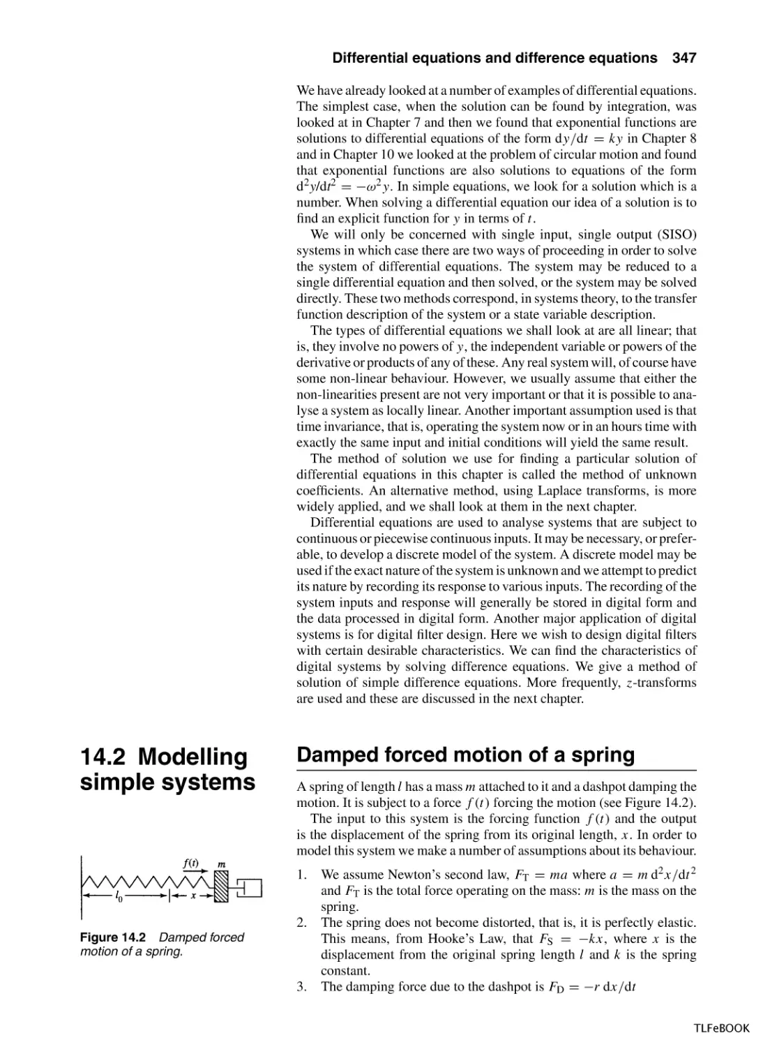
14.2 Modelling simple systems
14.3 Ordinary differential equations
14.4 Solving first-order LTI systems
14.5 Solution of a second-order LTI systems
14.6 Solving systems of differential equations
14.7 Difference equations
14.8 Summary
14.9 Exercises
346
346
347
352
358
363
372
376
378
380
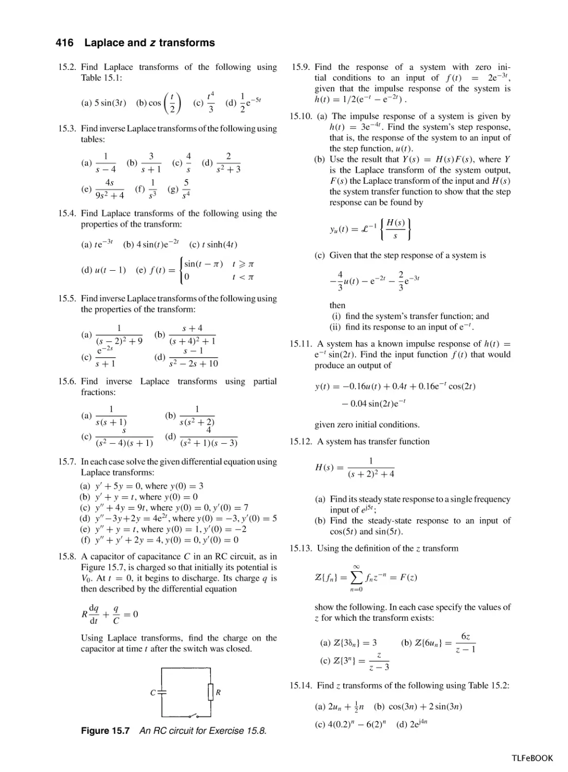
15 Laplace and z transforms
15.1 Introduction
15.2 The Laplace transform – definition
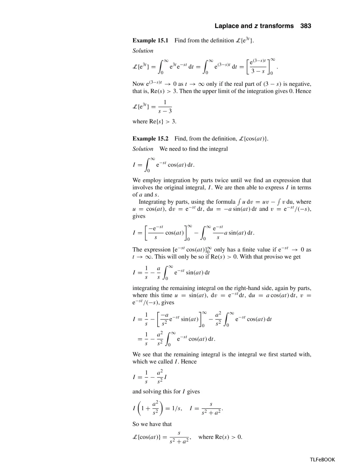
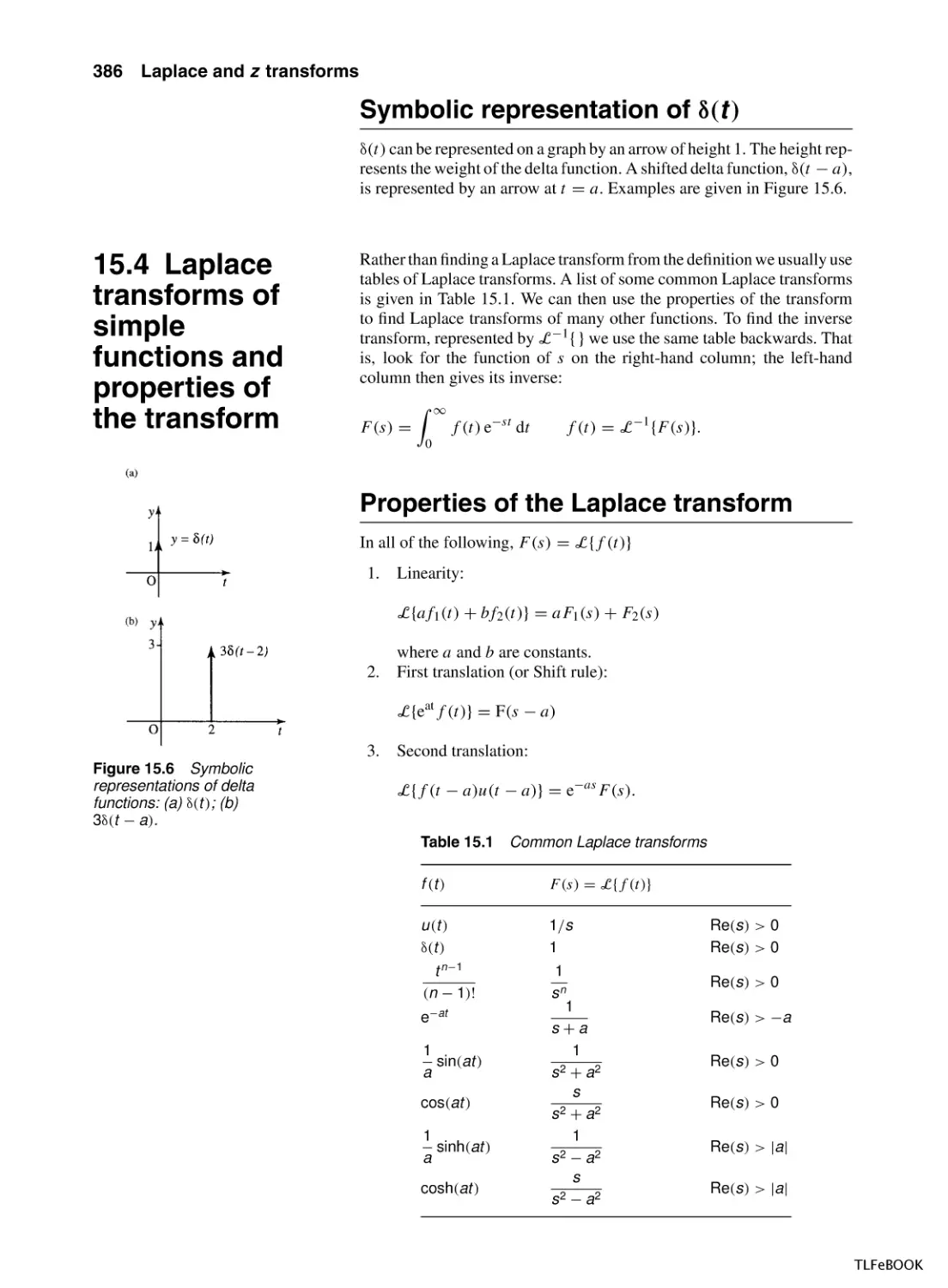
15.3 The unit step function and the (impulse) delta
function
15.4 Laplace transforms of simple functions and
properties of the transform
15.5 Solving linear differential equations with constant
coefficients
15.6 Laplace transforms and systems theory
15.7 z transforms
15.8 Solving linear difference equations with constant
coefficients using z transforms
15.9 z transforms and systems theory
15.10 Summary
15.11 Exercises
382
382
382
16 Fourier series
16.1 Introduction
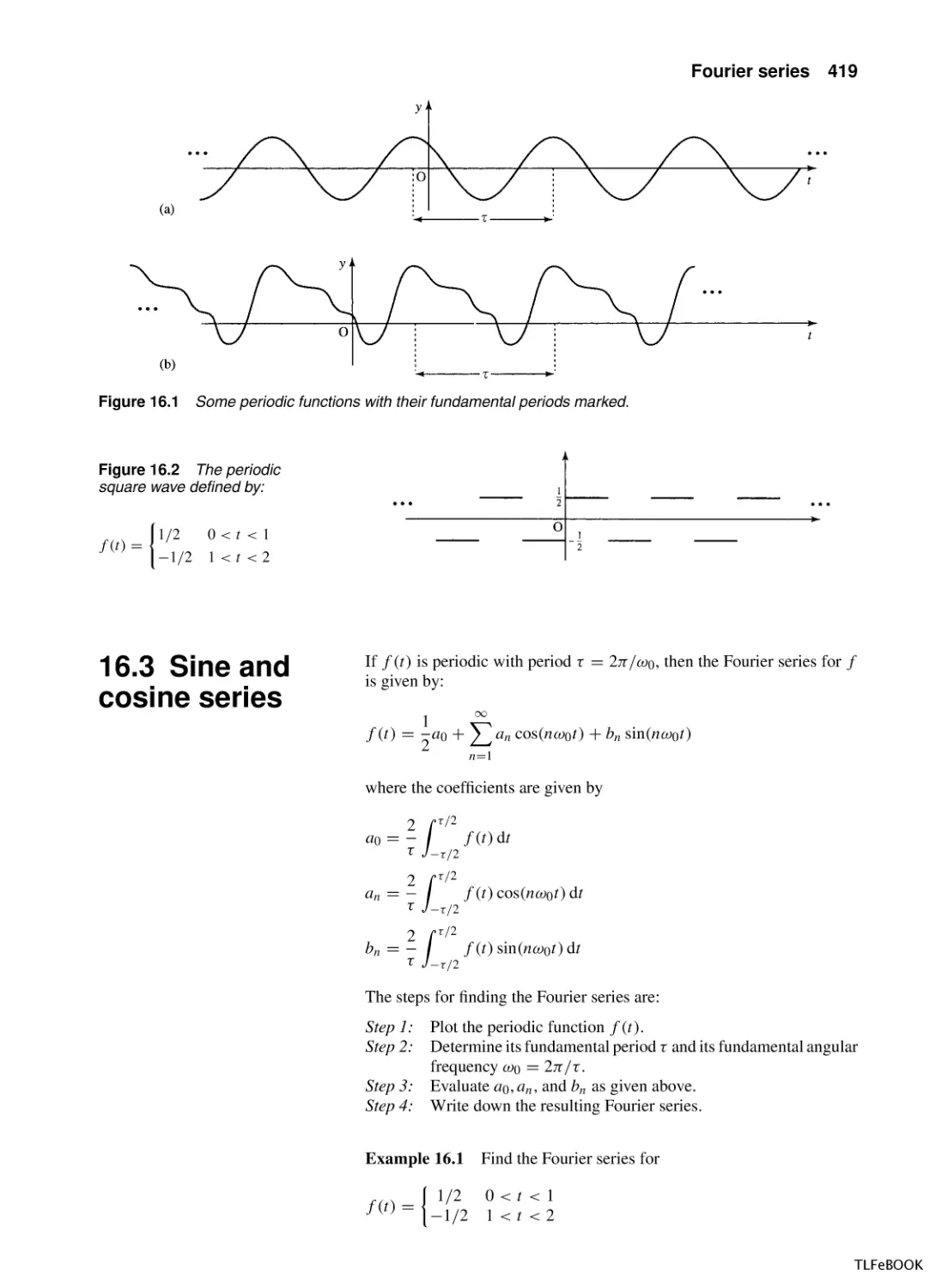
16.2 Periodic Functions
16.3 Sine and cosine series
16.4 Fourier series of symmetric periodic
functions
16.5 Amplitude and phase representation of a Fourier
series
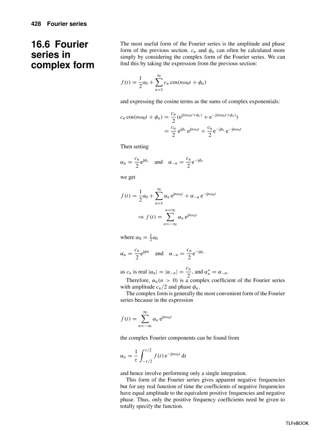
16.6 Fourier series in complex form
16.7 Summary
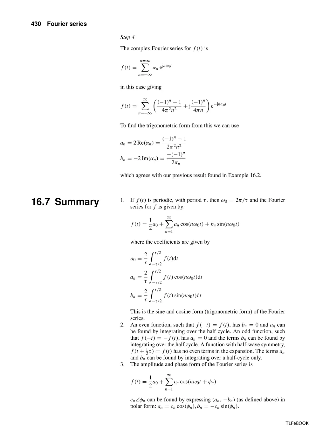
16.8 Exercises
418
418
418
419
295
295
295
306
314
324
384
386
394
397
403
408
411
414
415
424
426
428
430
431
TLFeBOOK
Contents
ix
Part 3 Functions of more than one variable
17 Functions of more than one variable
17.1 Introduction
17.2 Functions of two variables – surfaces
17.3 Partial differentiation
17.4 Changing variables – the chain rule
17.5 The total derivative along a path
17.6 Higher-order partial derivatives
17.7 Summary
17.8 Exercises
435
435
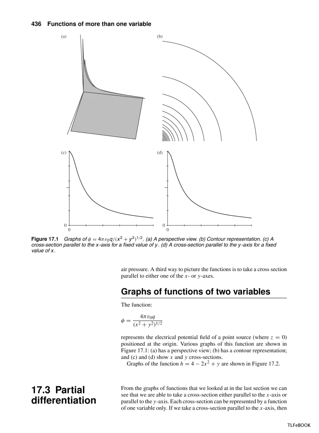
435
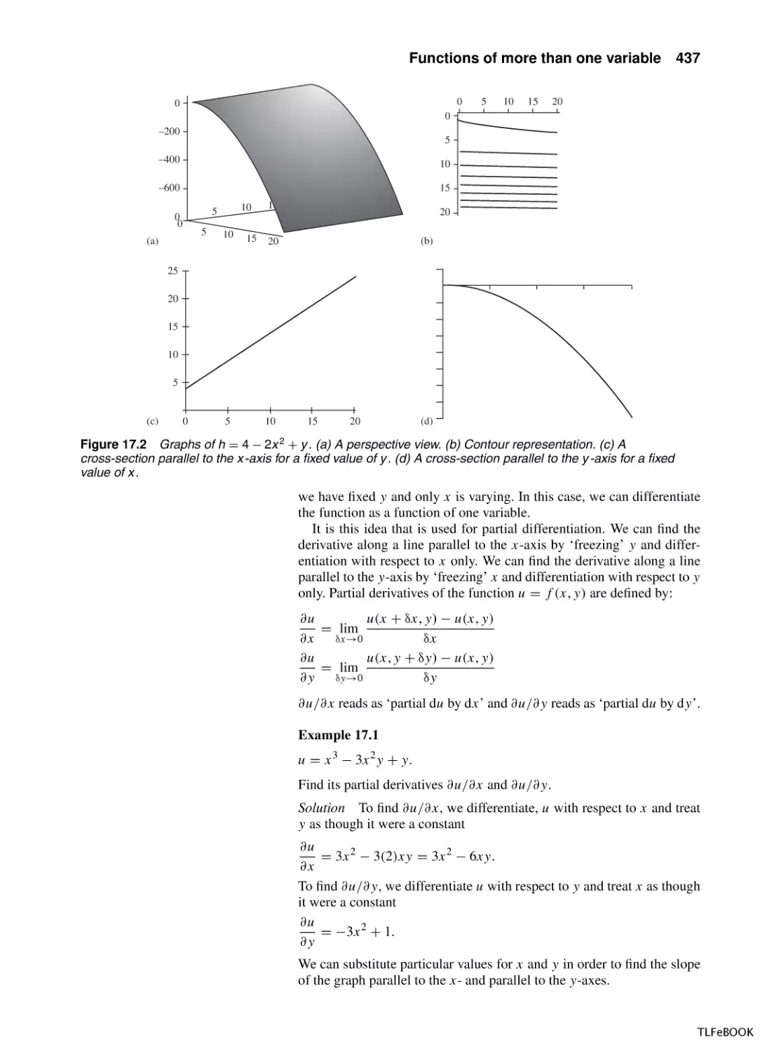
436
438
440
443
444
445
18 Vector calculus
18.1 Introduction
18.2 The gradient of a scalar field
18.3 Differentiating vector fields
18.4 The scalar line integral
18.5 Surface integrals
18.6 Summary
18.7 Exercises
446
446
446
449
451
454
456
457
Part 4 Graph and language theory
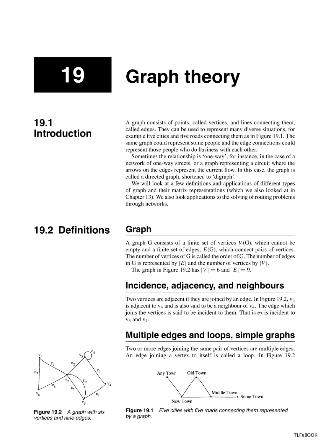
19 Graph theory
19.1 Introduction
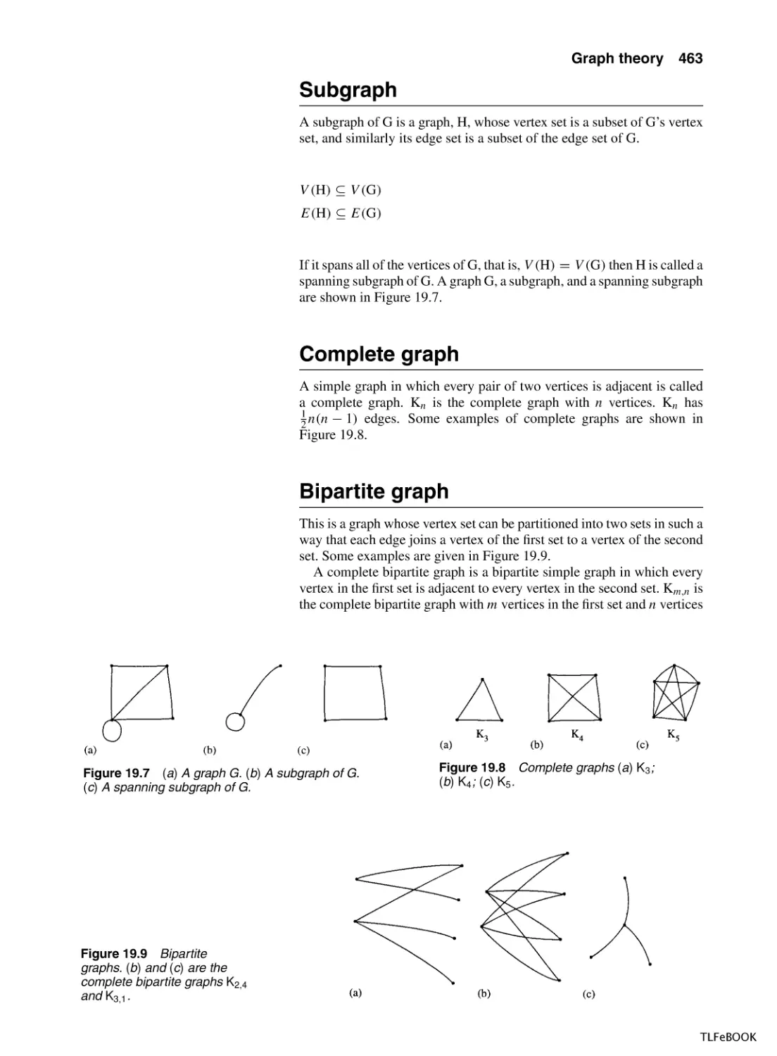
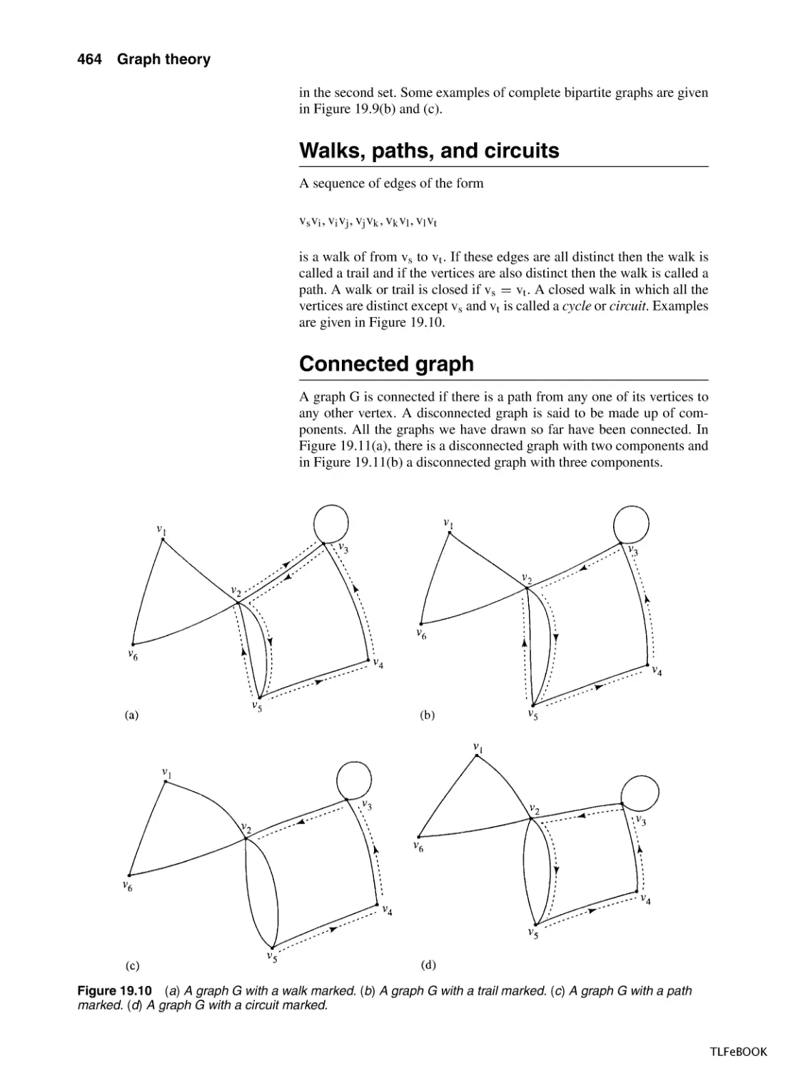
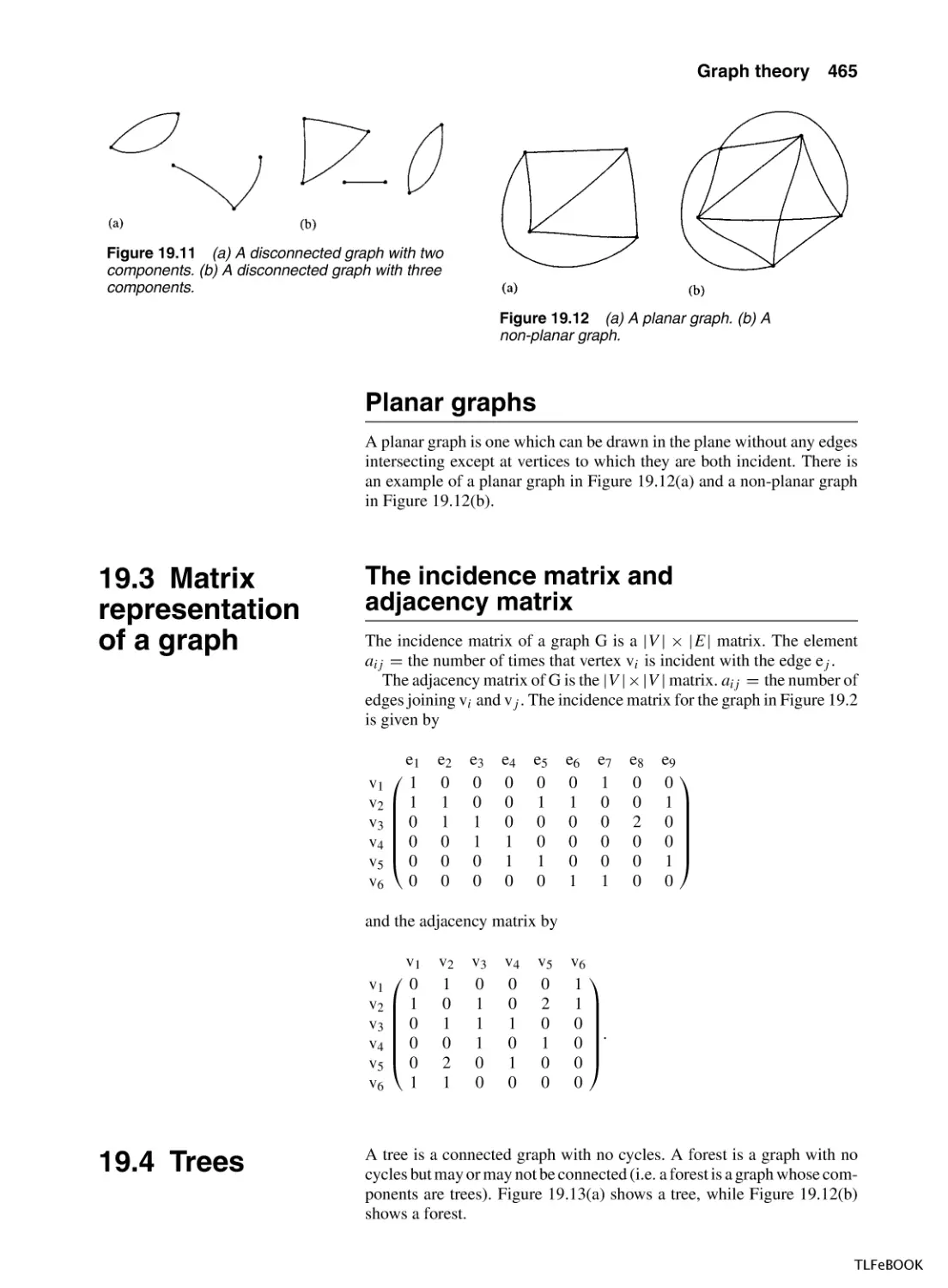
19.2 Definitions
19.3 Matrix representation of a graph
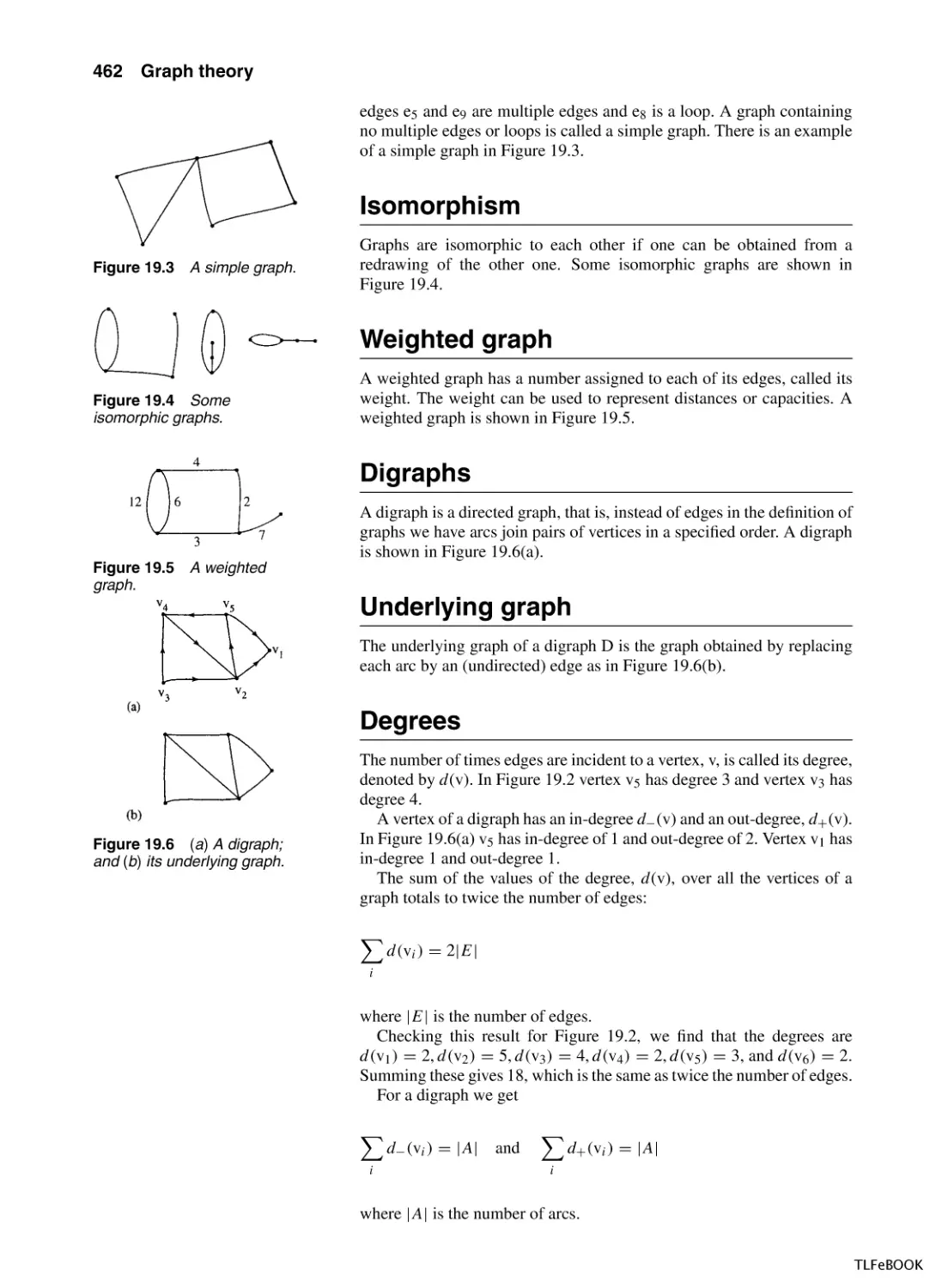
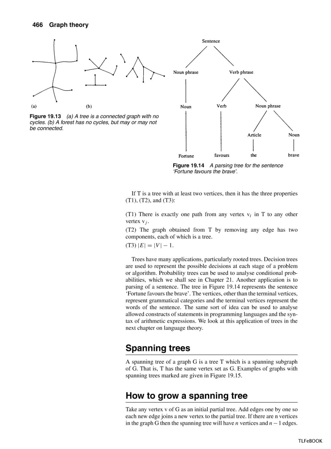
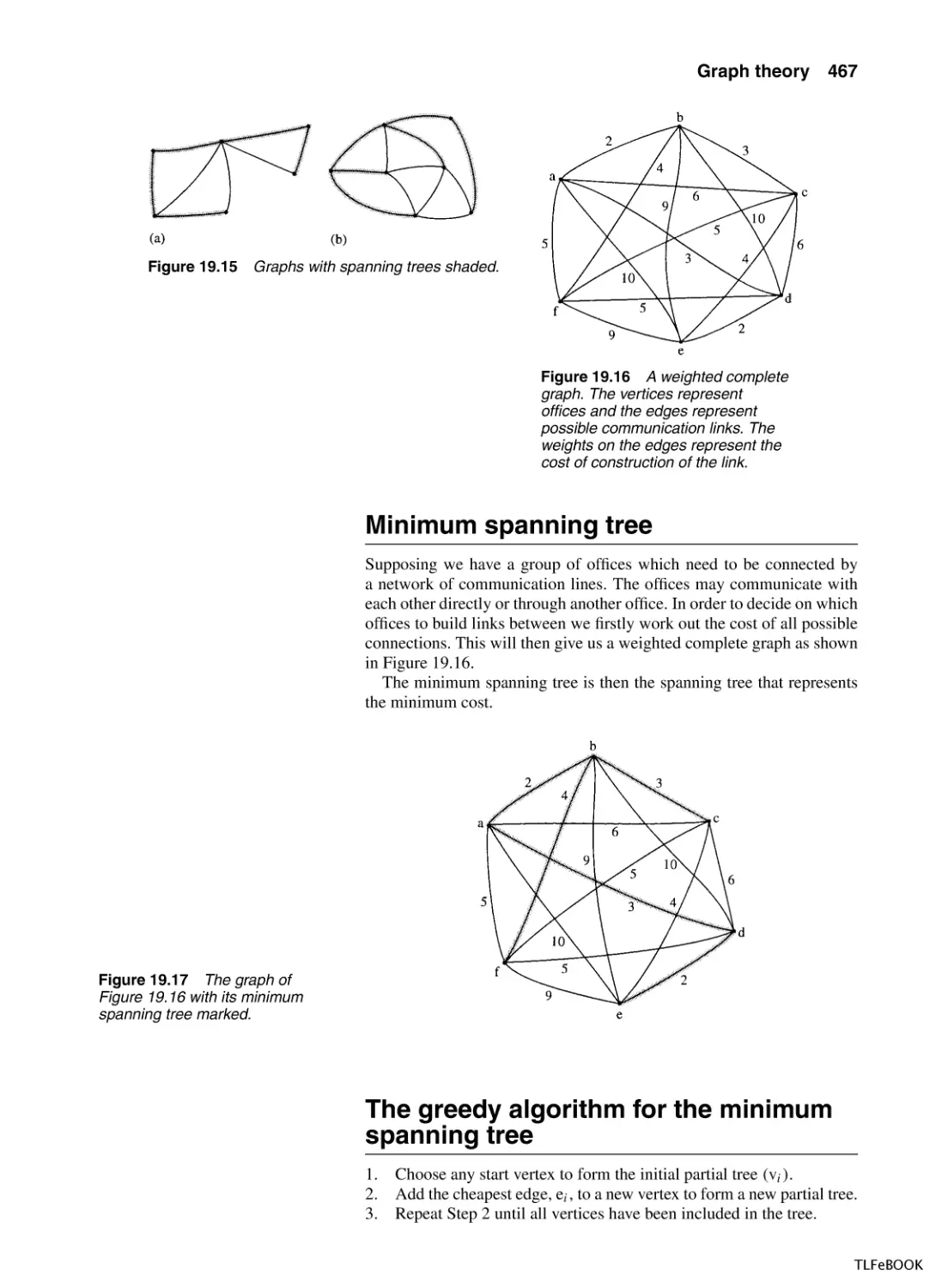
19.4 Trees
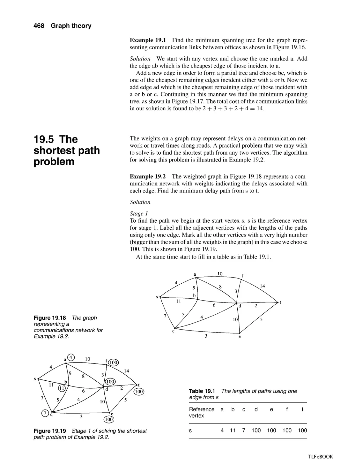
19.5 The shortest path problem
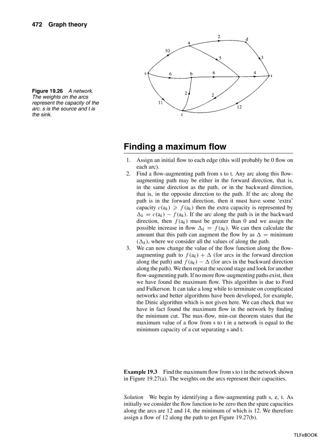
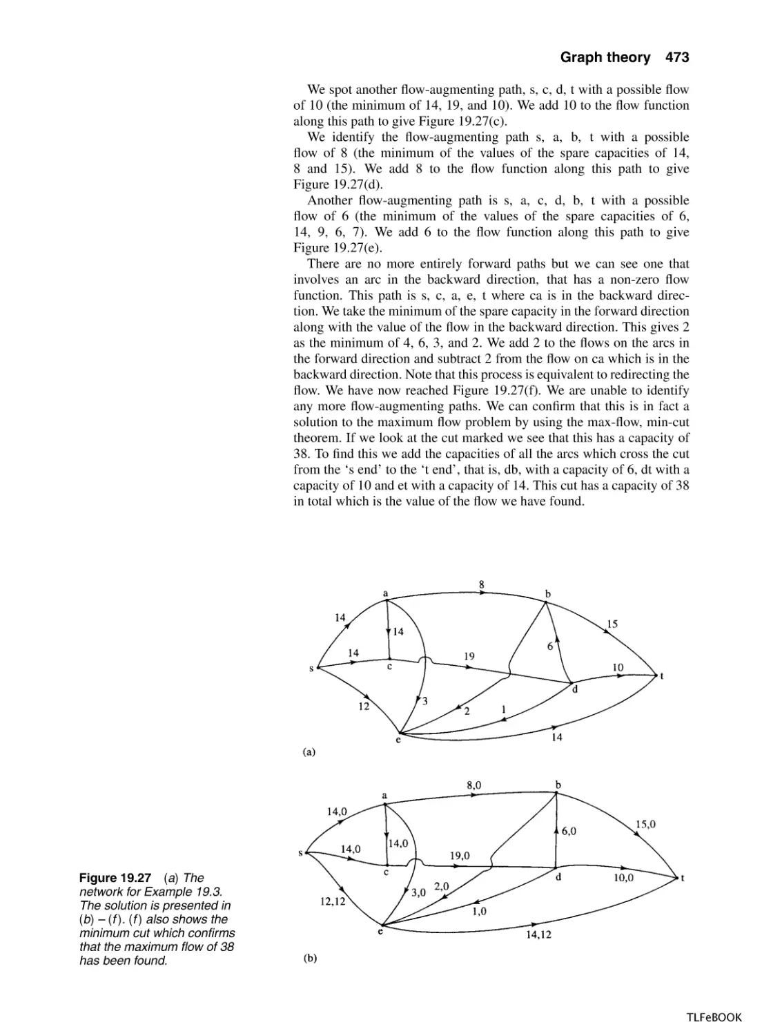
19.6 Networks and maximum flow
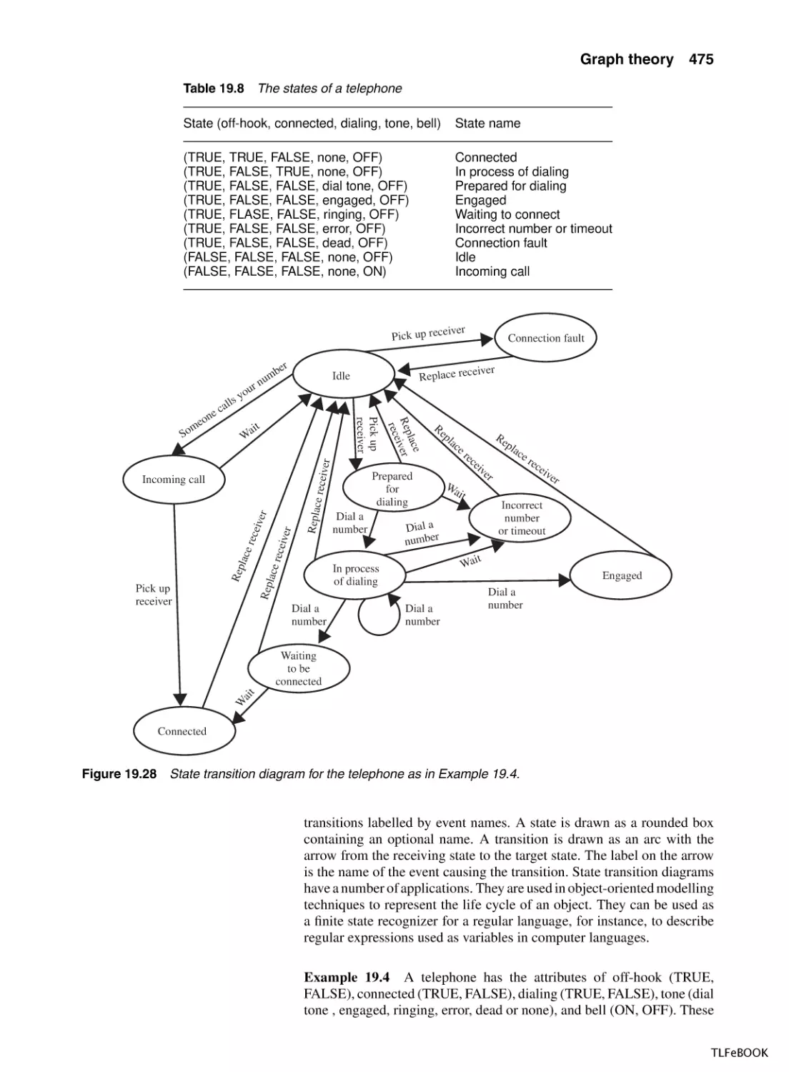
19.7 State transition diagrams
19.8 Summary
19.9 Exercises
461
461
461
465
465
468
471
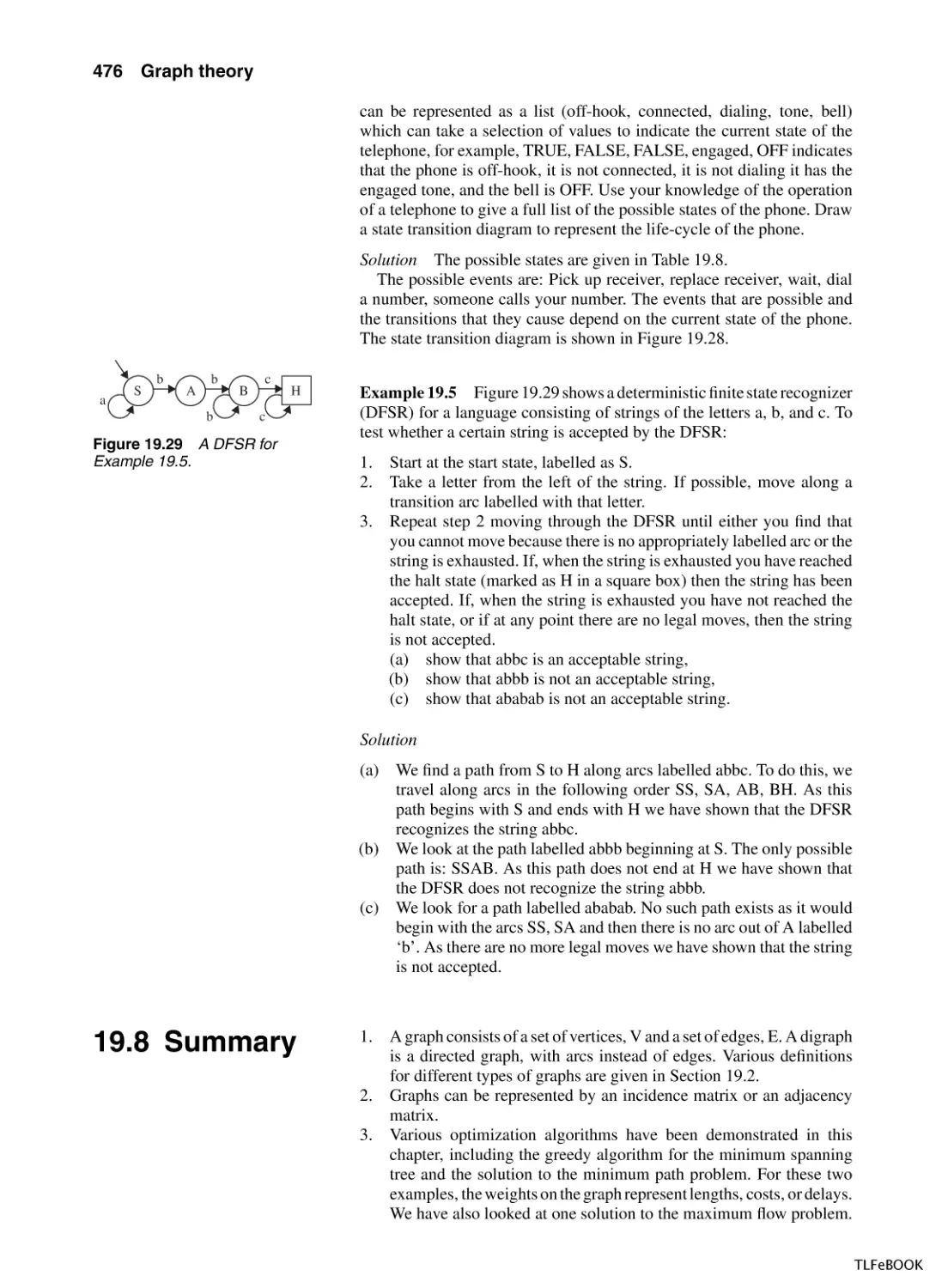
474
476
477
20 Language theory
20.1 Introduction
20.2 Languages and grammars
20.3 Derivations and derivation trees
20.4 Extended Backus-Naur Form (EBNF)
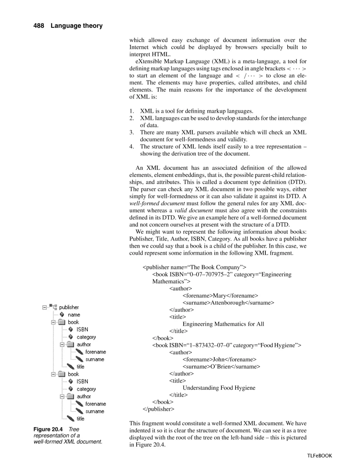
20.5 Extensible markup language (XML)
20.6 Summary
20.7 Exercises
479
479
480
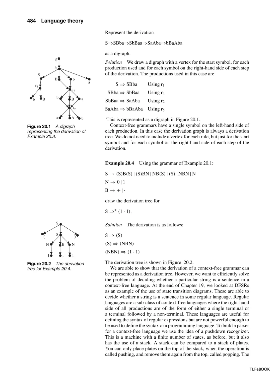
483
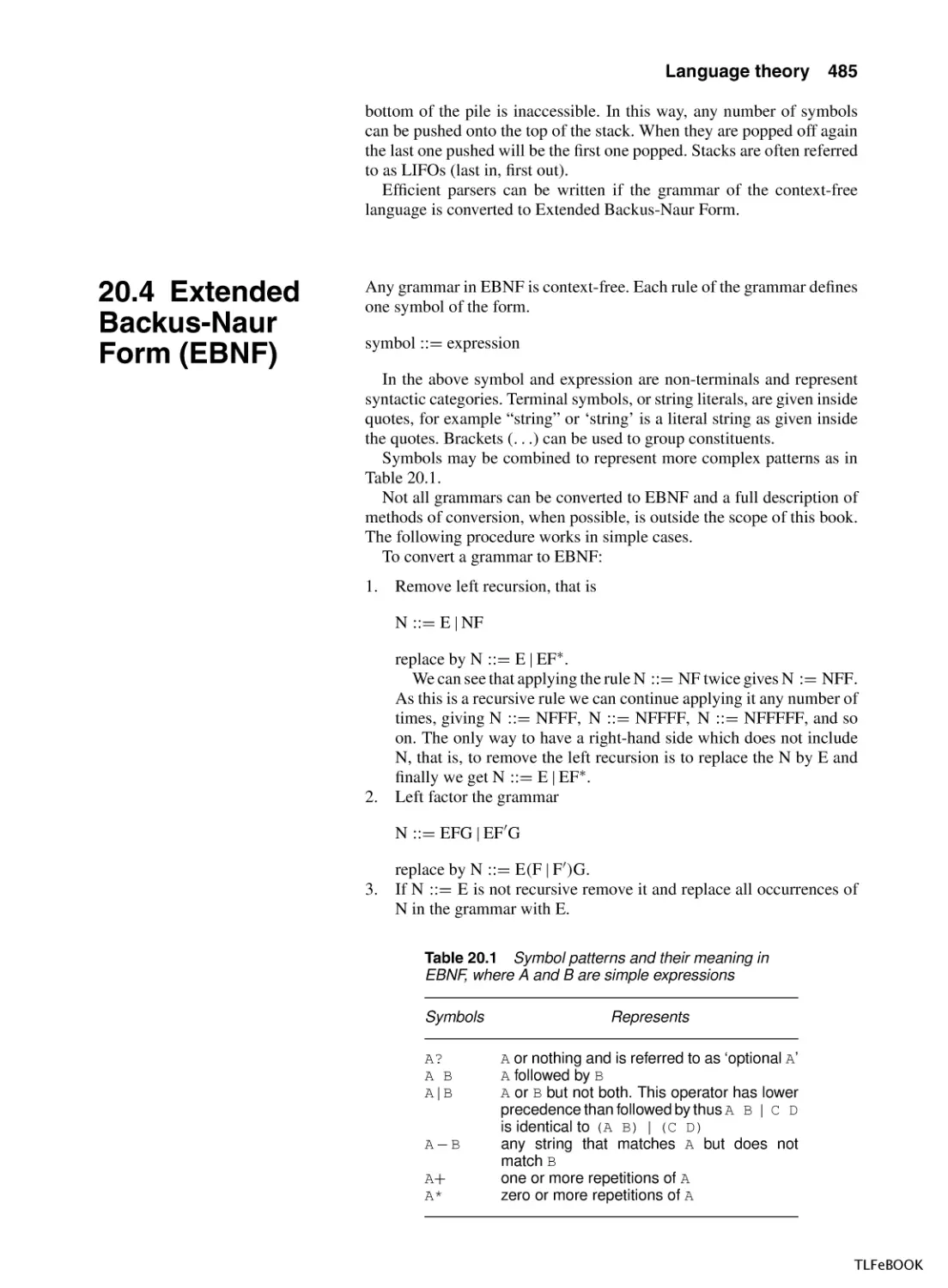
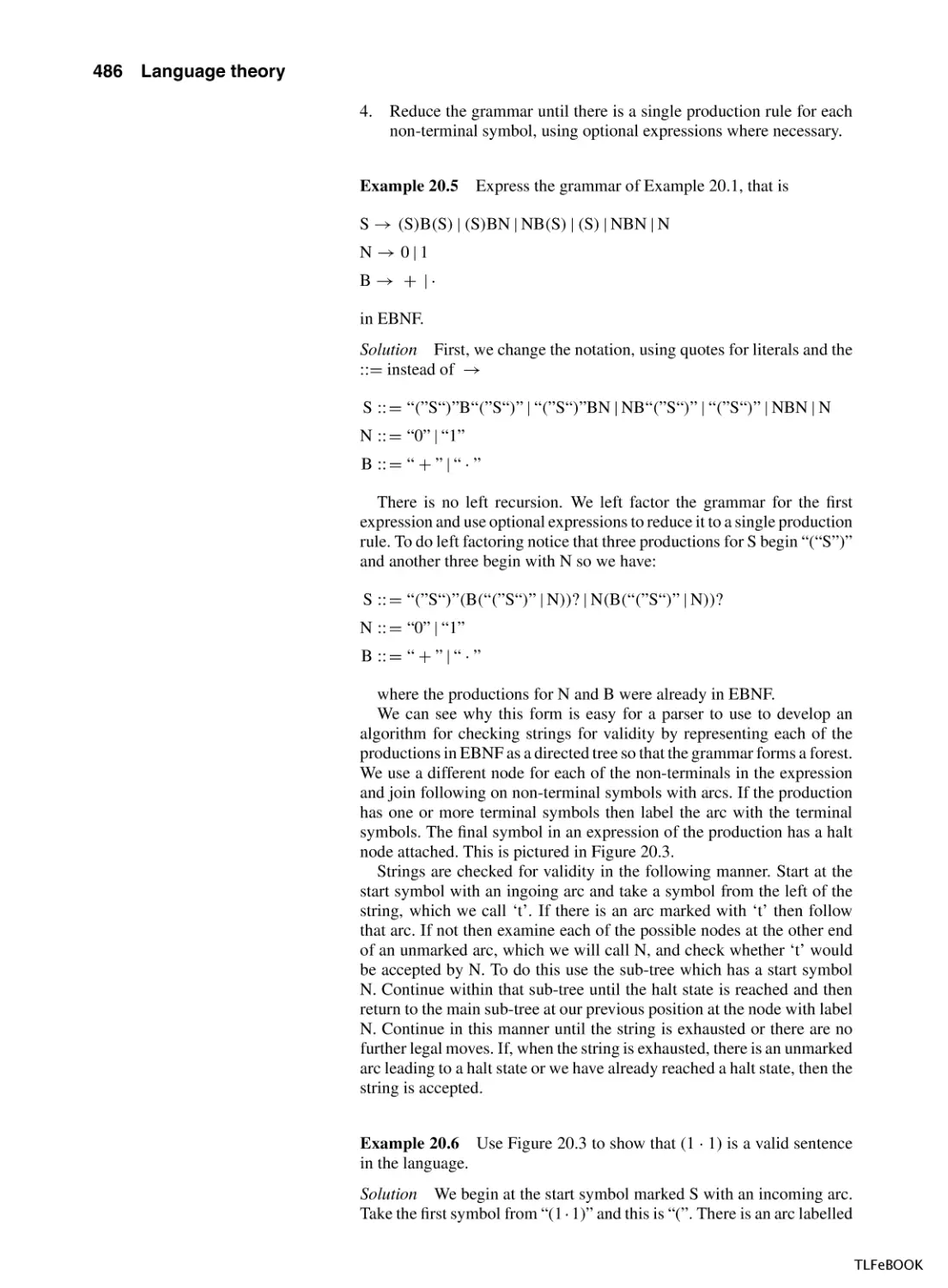
485
487
489
489
Part 5 Probability and statistics
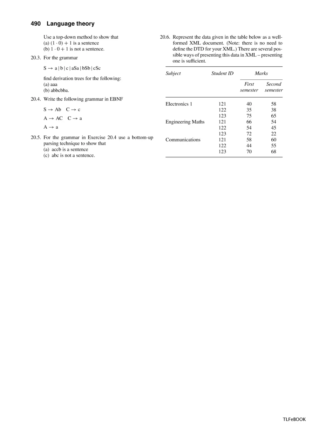
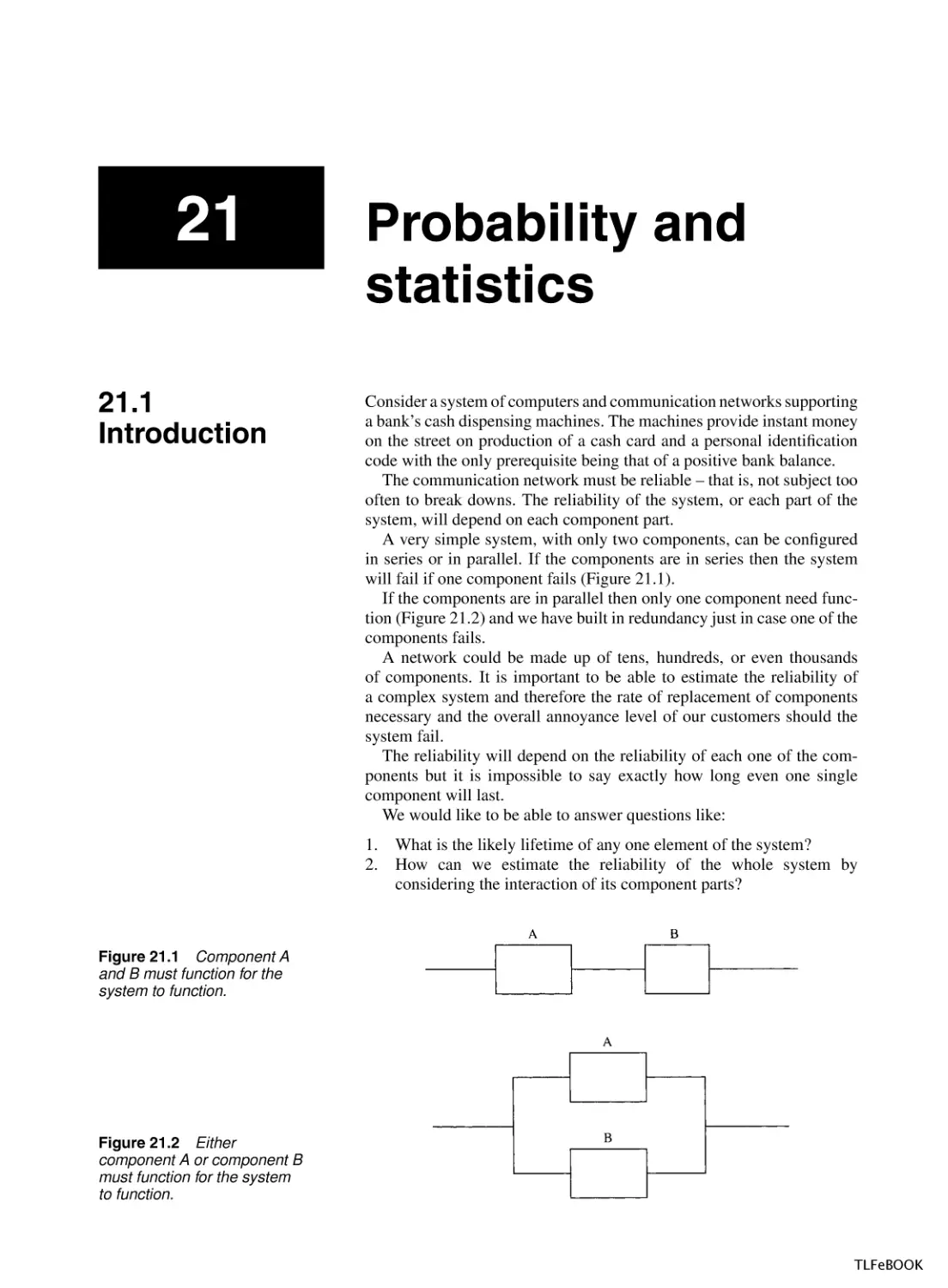
21 Probability and statistics
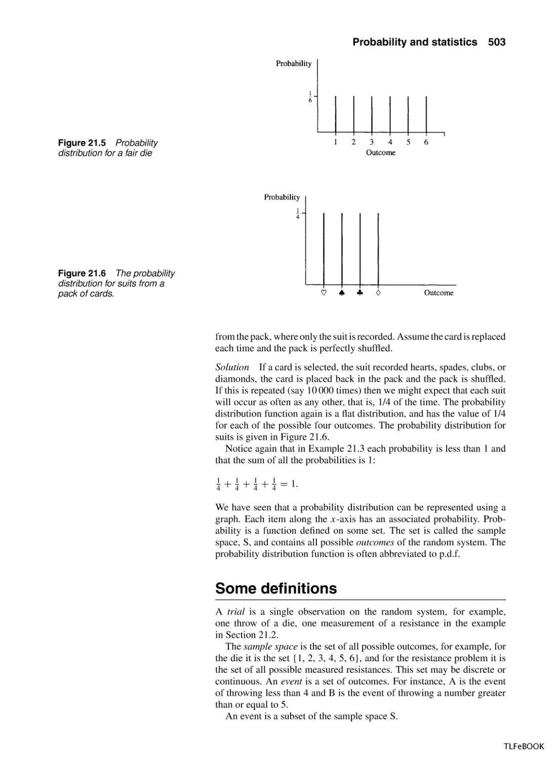
21.1 Introduction
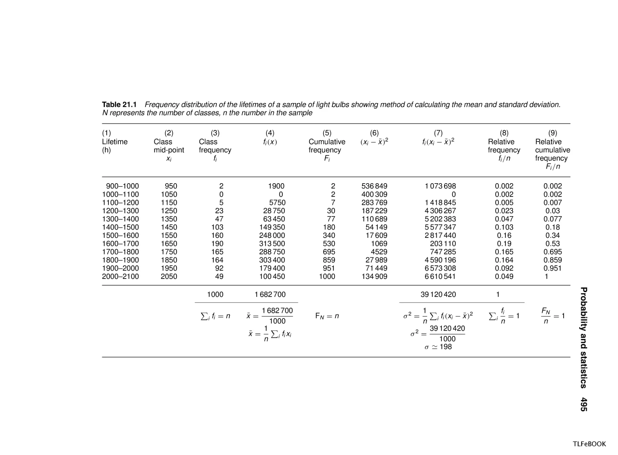
21.2 Population and sample, representation of data, mean,
variance and standard deviation
21.3 Random systems and probability
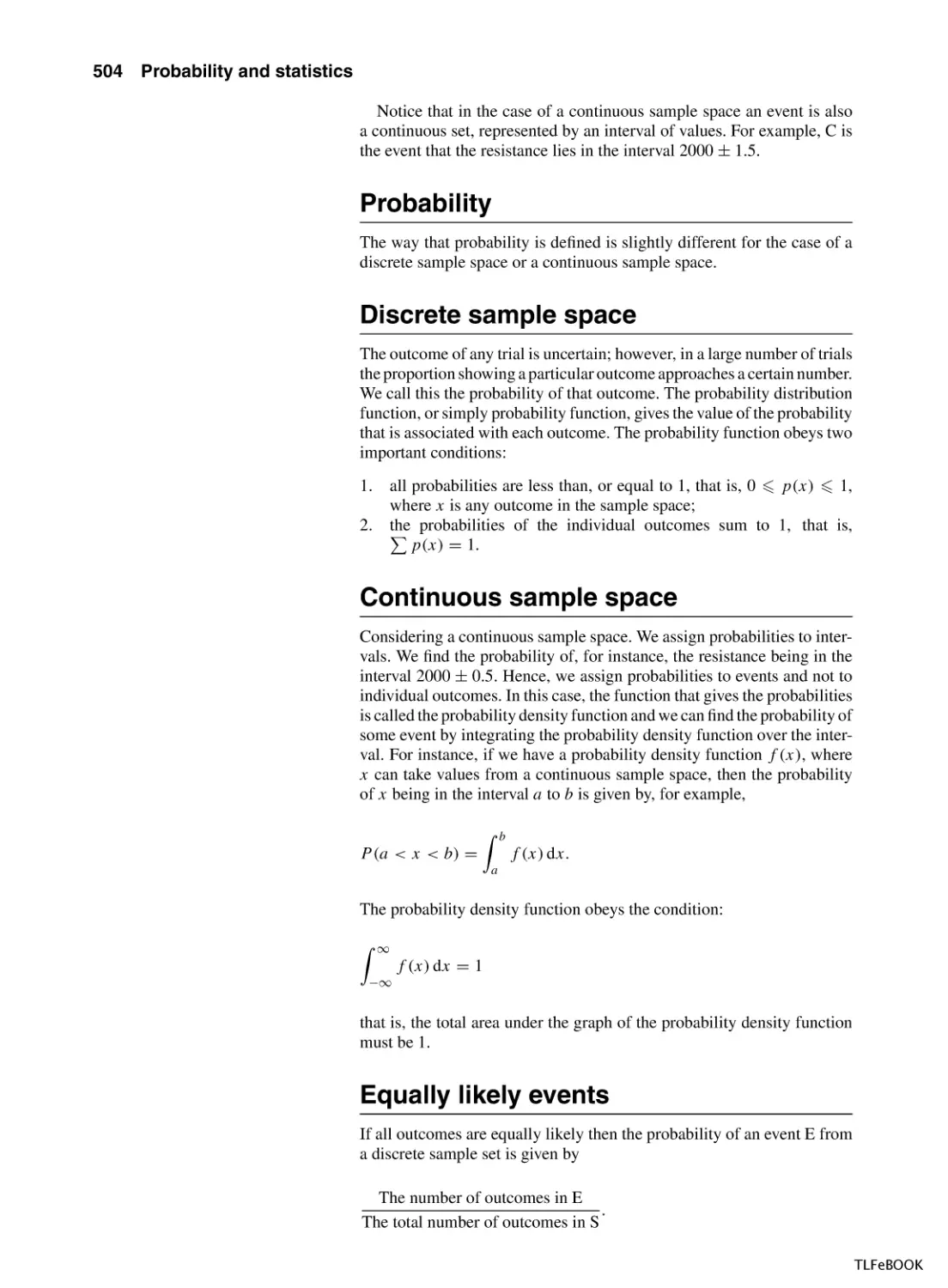
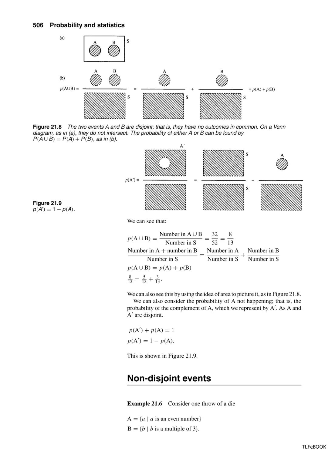
21.4 Addition law of probability
21.5 Repeated trials, outcomes, and
probabilities
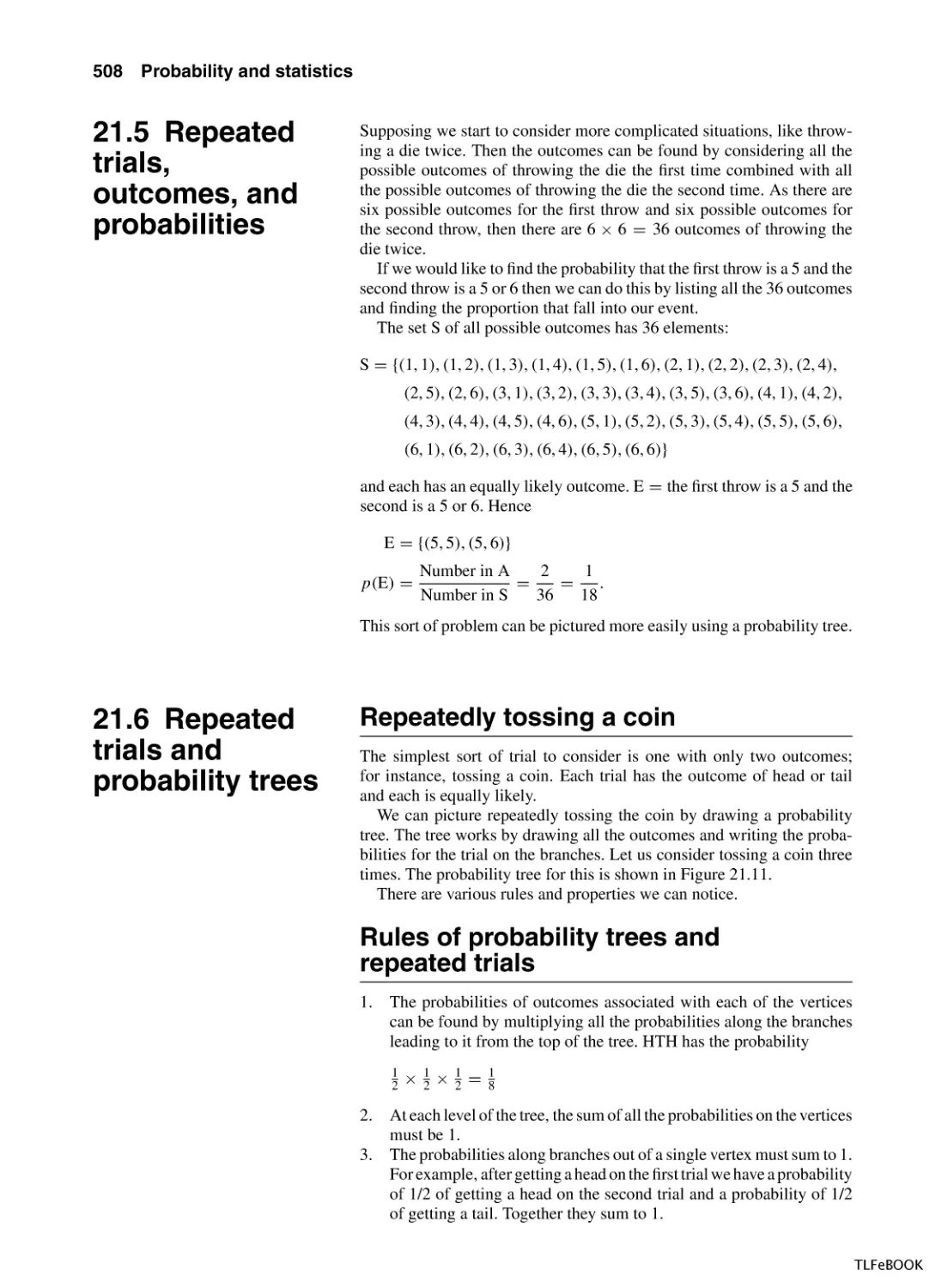
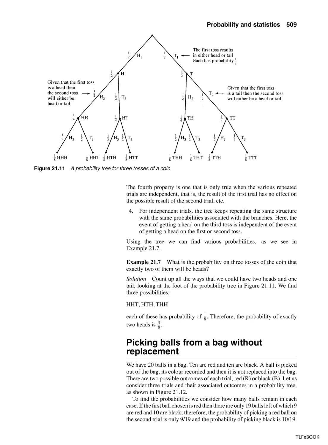
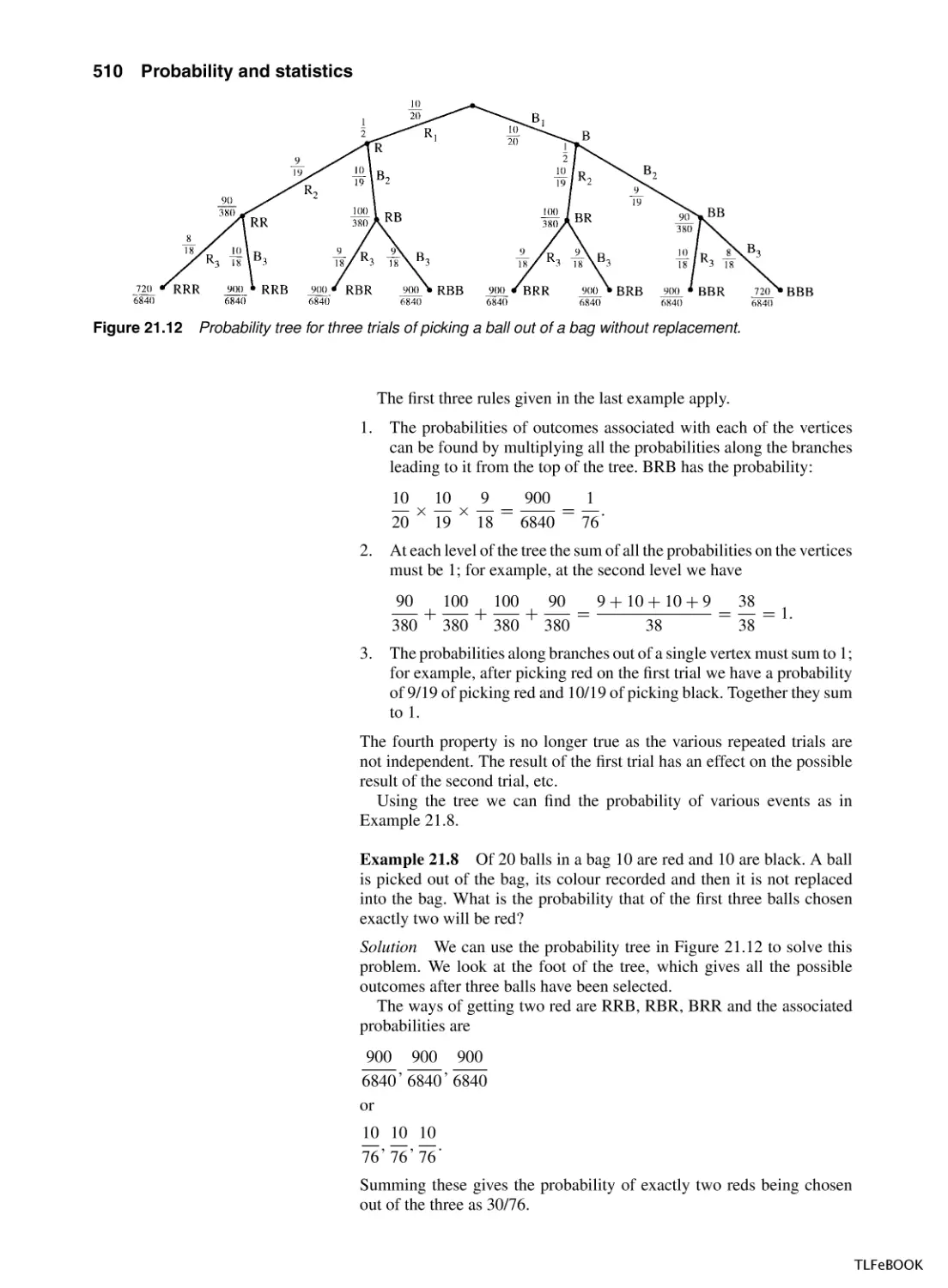
21.6 Repeated trials and probability trees
493
493
494
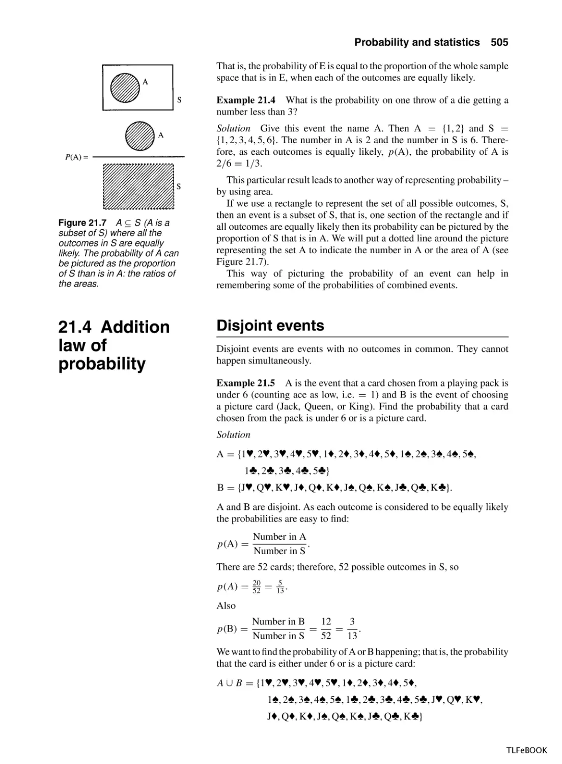
501
505
508
508
TLFeBOOK
x Contents
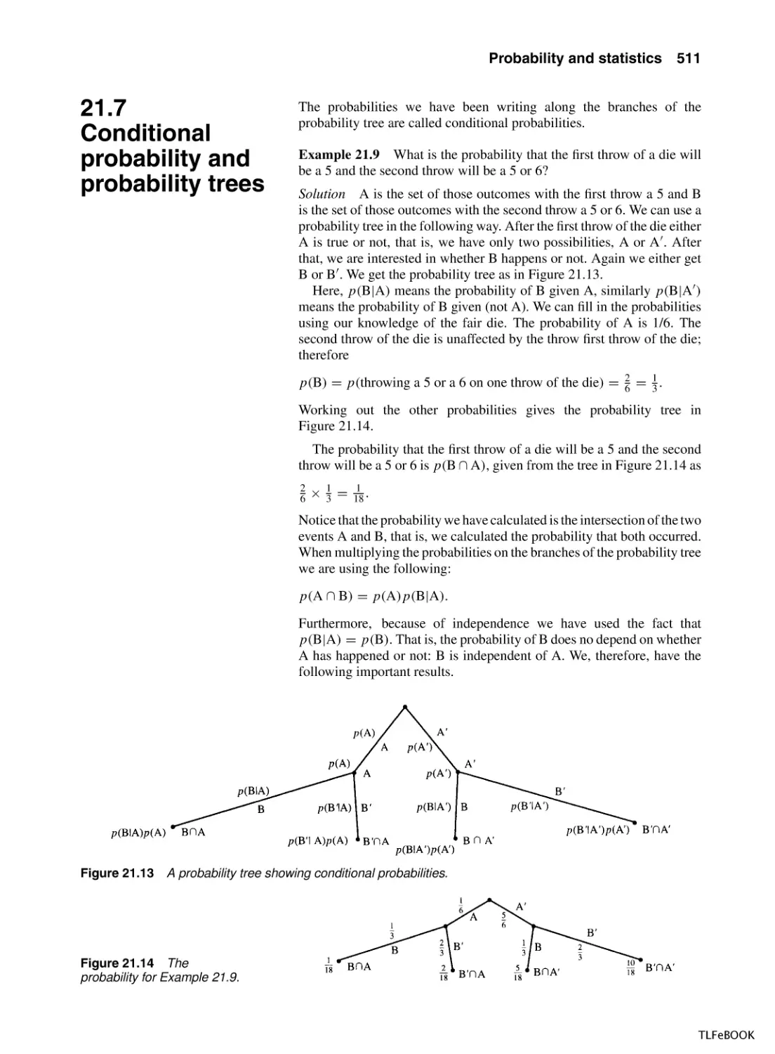
21.7
21.8
21.9
21.10
21.11
21.12
21.13
21.14
21.15
Conditional probability and probability
trees
Application of the probability laws to the probability
of failure of an electrical circuit
Statistical modelling
The normal distribution
The exponential distribution
The binomial distribution
The Poisson distribution
Summary
Exercises
Answers to exercises
Index
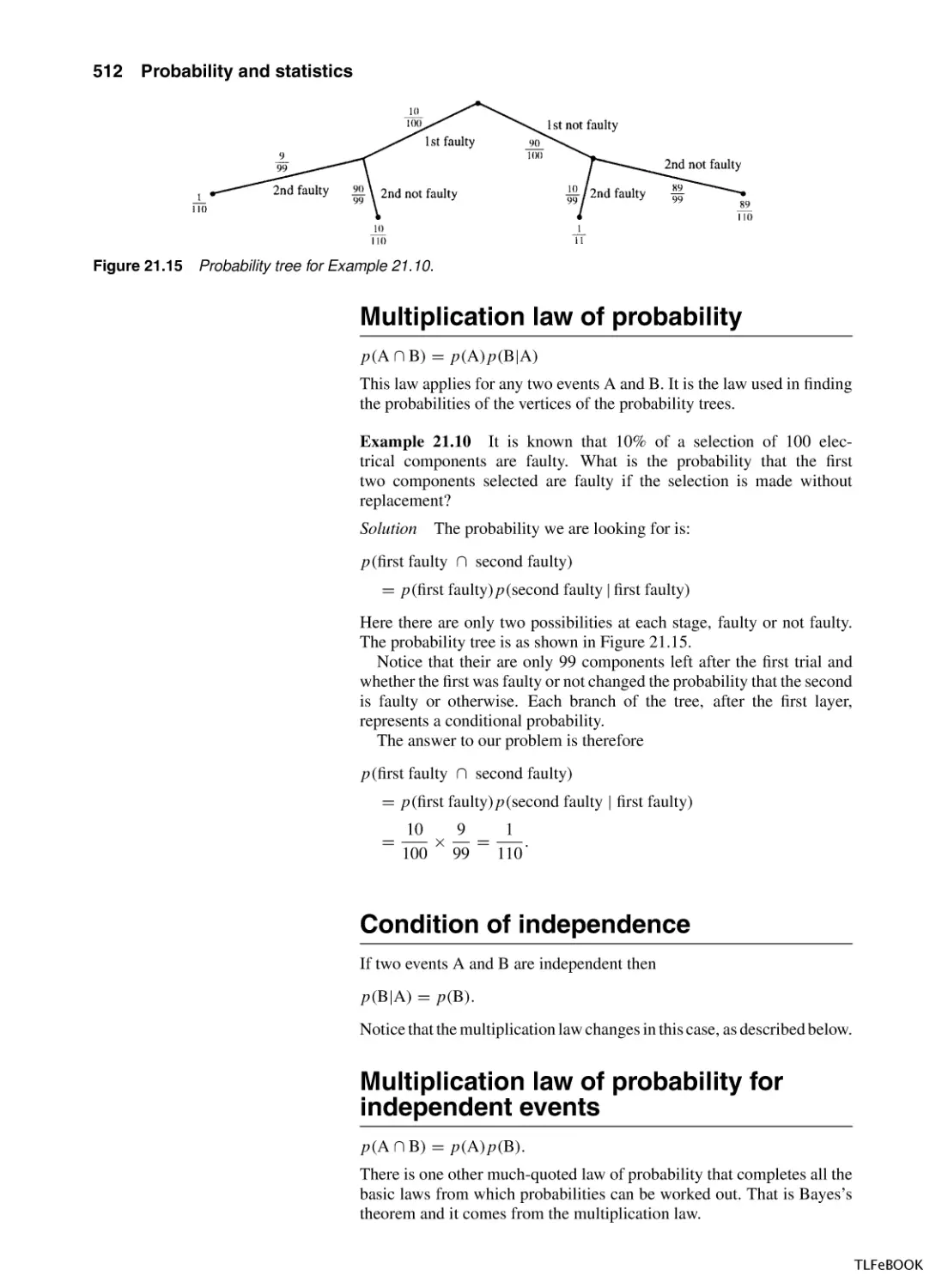
511
514
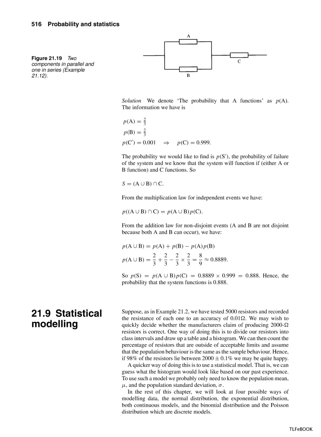
516
517
521
524
526
528
531
533
542
TLFeBOOK
Preface
This book is based on my notes from lectures to students of electrical, electronic, and computer engineering at South Bank University. It presents
a first year degree/diploma course in engineering mathematics with an
emphasis on important concepts, such as algebraic structure, symmetries, linearity, and inverse problems, clearly presented in an accessible
style. It encompasses the requirements, not only of students with a good
maths grounding, but also of those who, with enthusiasm and motivation, can make up the necessary knowledge. Engineering applications
are integrated at each opportunity. Situations where a computer should
be used to perform calculations are indicated and ‘hand’ calculations
are encouraged only in order to illustrate methods and important special
cases. Algorithmic procedures are discussed with reference to their efficiency and convergence, with a presentation appropriate to someone new
to computational methods.
Developments in the fields of engineering, particularly the extensive
use of computers and microprocessors, have changed the necessary subject emphasis within mathematics. This has meant incorporating areas
such as Boolean algebra, graph and language theory, and logic into
the content. A particular area of interest is digital signal processing,
with applications as diverse as medical, control and structural engineering, non-destructive testing, and geophysics. An important consideration
when writing this book was to give more prominence to the treatment
of discrete functions (sequences), solutions of difference equations and z
transforms, and also to contextualize the mathematics within a systems
approach to engineering problems.
TLFeBOOK
Acknowledgements
I should like to thank my former colleagues in the School of
Electrical, Electronic and Computer Engineering at South Bank
University who supported and encouraged me with my attempts to
re-think approaches to the teaching of engineering mathematics.
I should like to thank all the reviewers for their comments and the
editorial and production staff at Elsevier Science.
Many friends have helped out along the way, by discussing ideas or
reading chapters. Above all Gabrielle Sinnadurai who checked the original manuscript of Engineering Mathematics Exposed, wrote the major
part of the solutions manual and came to the rescue again by reading
some of the new material in this publication. My partner Michael has
given unstinting support throughout and without him I would never have
found the energy.
TLFeBOOK
Part 1
Sets, functions,
and calculus
TLFeBOOK
TLFeBOOK
1
1.1 Introduction
Sets and functions
Finding relationships between quantities is of central importance in
engineering. For instance, we know that given a simple circuit with a
1000 resistance then the relationship between current and voltage is
given by Ohm’s law, I = V /1000. For any value of the voltage V we can
give an associated value of I . This relationship means that I is a function
of V . From this simple idea there are many other questions that need
clarifying, some of which are:
Are all values of V permitted? For instance, a very high value of the
voltage could change the nature of the material in the resistor and the
expression would no longer hold.
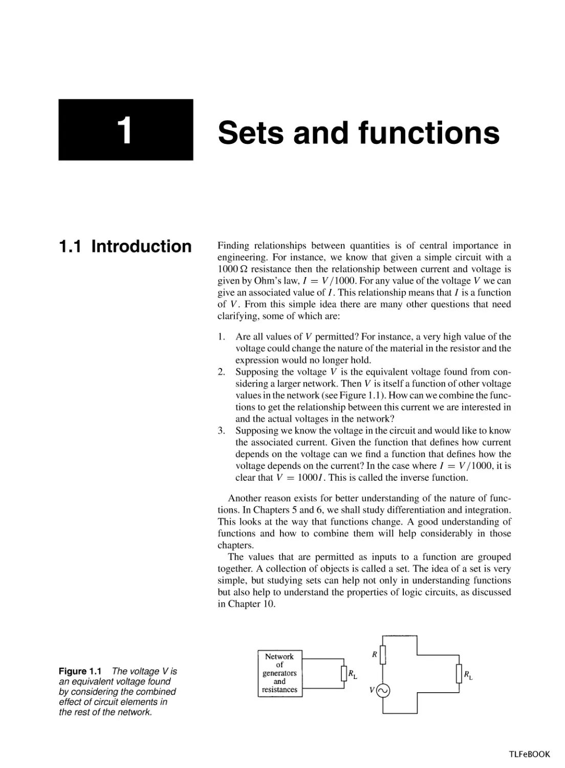
2. Supposing the voltage V is the equivalent voltage found from considering a larger network. Then V is itself a function of other voltage
values in the network (see Figure 1.1). How can we combine the functions to get the relationship between this current we are interested in
and the actual voltages in the network?
3. Supposing we know the voltage in the circuit and would like to know
the associated current. Given the function that defines how current
depends on the voltage can we find a function that defines how the
voltage depends on the current? In the case where I = V /1000, it is
clear that V = 1000I . This is called the inverse function.
1.
Another reason exists for better understanding of the nature of functions. In Chapters 5 and 6, we shall study differentiation and integration.
This looks at the way that functions change. A good understanding of
functions and how to combine them will help considerably in those
chapters.
The values that are permitted as inputs to a function are grouped
together. A collection of objects is called a set. The idea of a set is very
simple, but studying sets can help not only in understanding functions
but also help to understand the properties of logic circuits, as discussed
in Chapter 10.
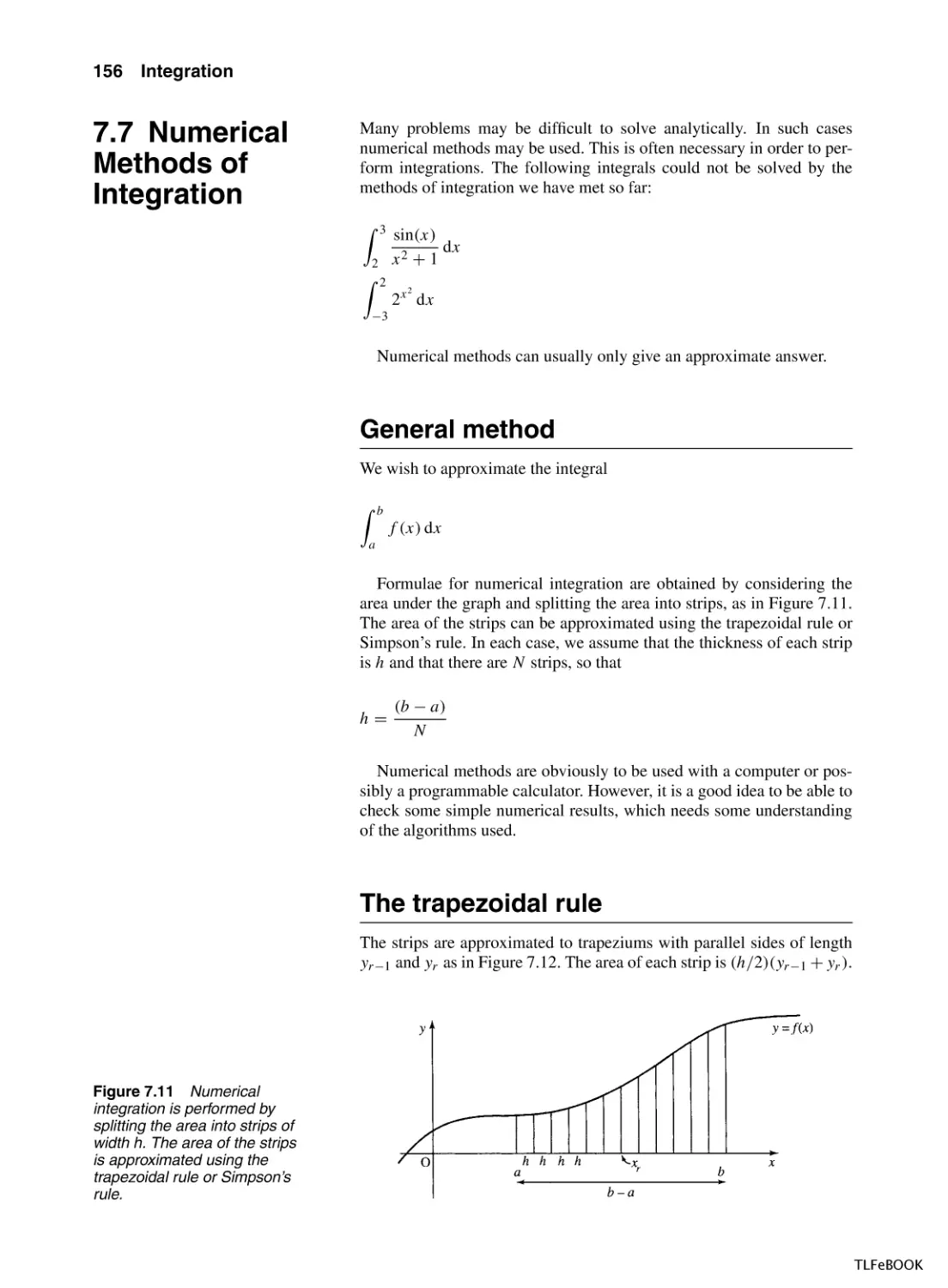
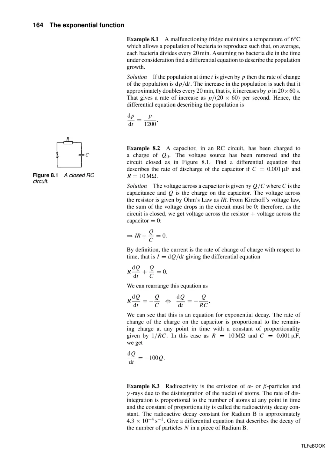
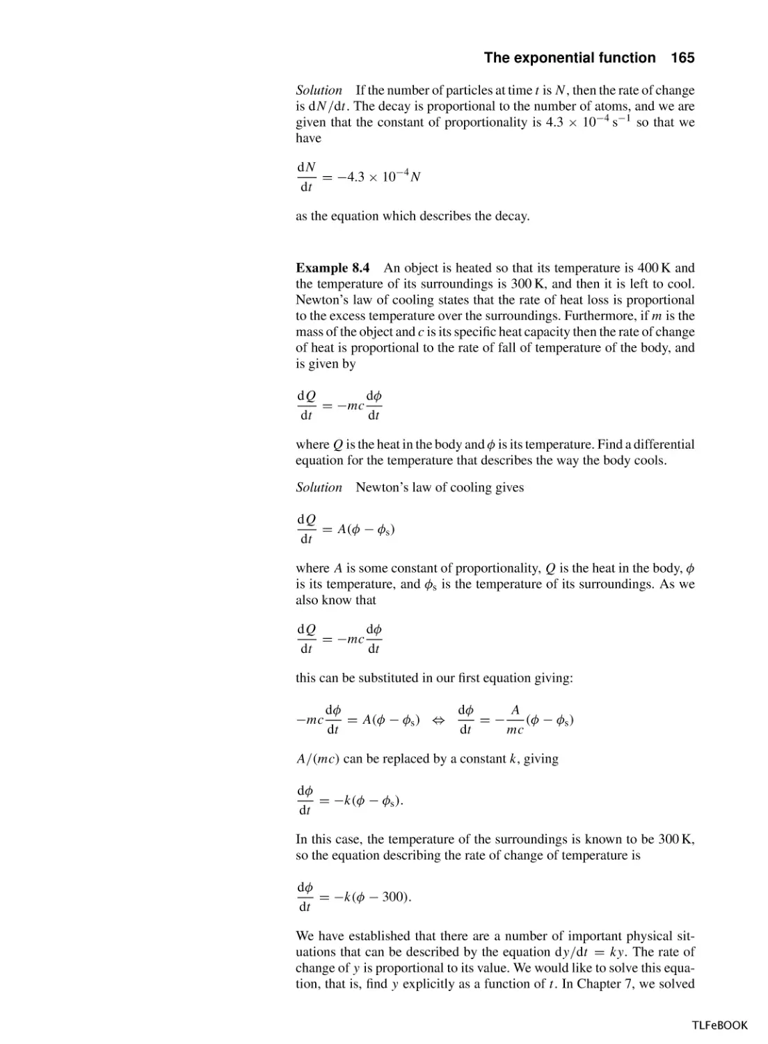
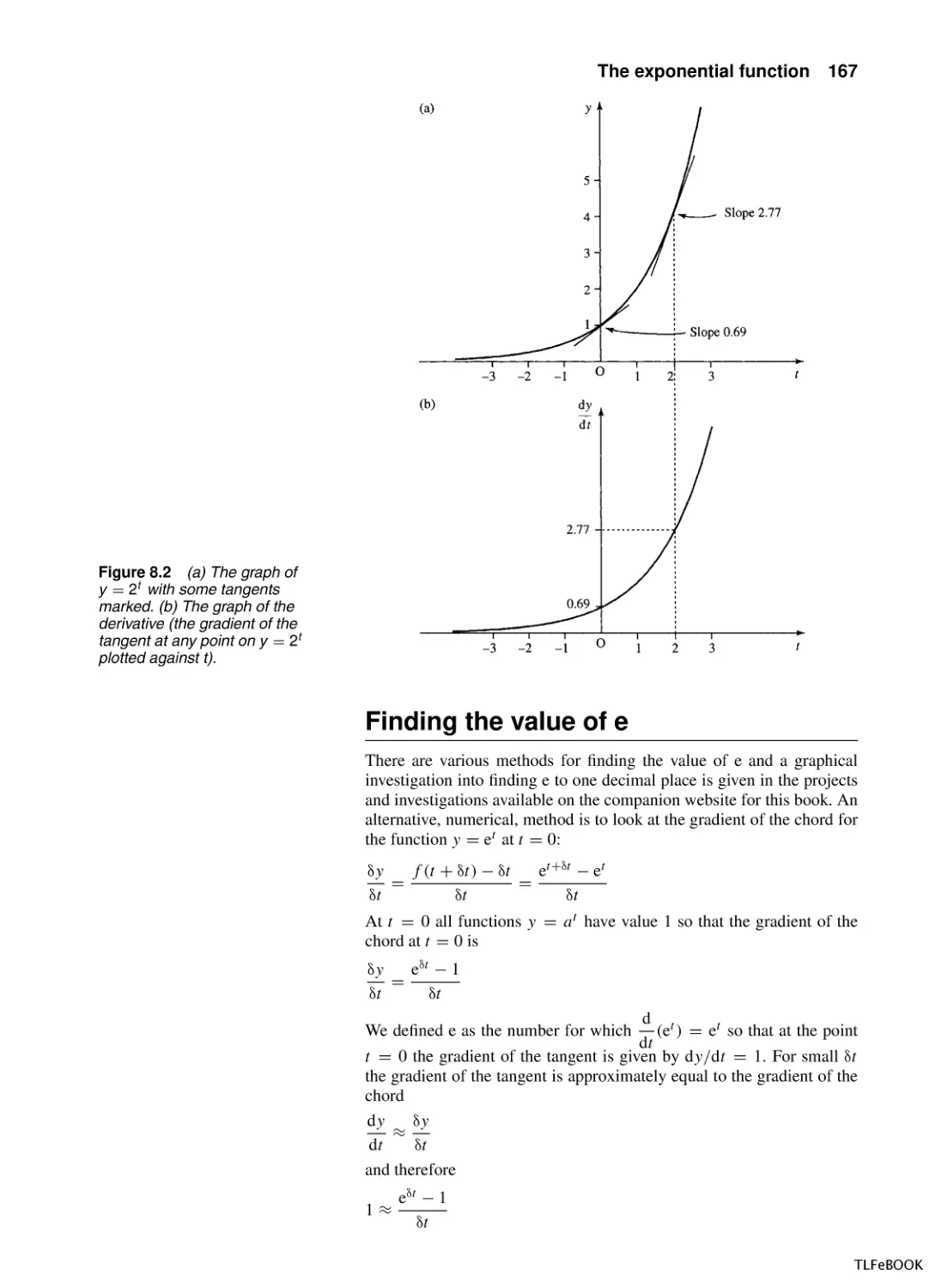
Figure 1.1 The voltage V is
an equivalent voltage found
by considering the combined
effect of circuit elements in
the rest of the network.
TLFeBOOK
4 Sets and functions
1.2 Sets
A set is a collection of objects, called elements, in which the order is not
important and an object cannot appear twice in the same set.
Example 1.1
listed, are:
Explicit definitions of sets, that is, where each element is
A = {a, b, c}
B = {3, 4, 6, 7, 8, 9}
C = {Linda, Raka, Sue, Joe, Nigel, Mary}
a ∈ A means ‘a is an element of A’ or ‘a belongs to A’; therefore in the
above examples:
3∈B
Linda ∈ C
The universal set is the set of all objects we are interested in and will
depend on the problem under consideration. It is represented by E .
The empty set (or null set) is the set with no elements. It is represented
by ∅ or { }.
Sets can be represented diagrammatically – generally as circular
shapes. The universal set is represented as a rectangle. These are called
Venn diagrams.
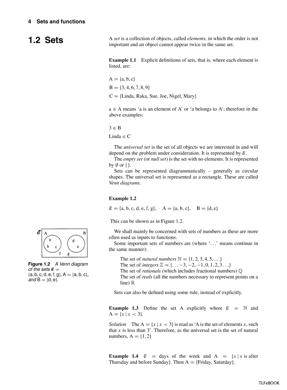
Example 1.2
E = {a, b, c, d, e, f, g},
A = {a, b, c},
B = {d, e}
This can be shown as in Figure 1.2.
We shall mainly be concerned with sets of numbers as these are more
often used as inputs to functions.
Some important sets of numbers are (where ‘. . .’ means continue in
the same manner):
Figure 1.2 A Venn diagram
of the sets E =
{a, b, c, d, e, f, g}, A = {a, b, c},
and B = {d, e}.
The set of natural numbers N = {1, 2, 3, 4, 5, . . .}
The set of integers Z = {. . . −3, −2, −1, 0, 1, 2, 3 . . .}
The set of rationals (which includes fractional numbers) Q
The set of reals (all the numbers necessary to represent points on a
line) R
Sets can also be defined using some rule, instead of explicitly.
Example 1.3 Define the set A explicitly where E
A = {x | x < 3}.
= N and
Solution The A = {x | x < 3} is read as ‘A is the set of elements x, such
that x is less than 3’. Therefore, as the universal set is the set of natural
numbers, A = {1, 2}
Example 1.4 E = days of the week and A = {x | x is after
Thursday and before Sunday}. Then A = {Friday, Saturday}.
TLFeBOOK
Sets and functions 5
Subsets
We may wish to refer to only a part of some set. This is said to be a subset
of the original set.
A ⊆ B is read as ‘A is a subset of B’ and it means that every element
of A is an element of B.
Example 1.5
E =N
A = {1, 2, 3},
B = {1, 2, 3, 4, 5}
Then A ⊆ B
Note the following points:
All sets must be subsets of the universal set, that is, A ⊆ E and
B⊆E
A set is a subset of itself, that is, A ⊆ A
If A ⊆ B and B ⊆ A, then A = B
Proper subsets
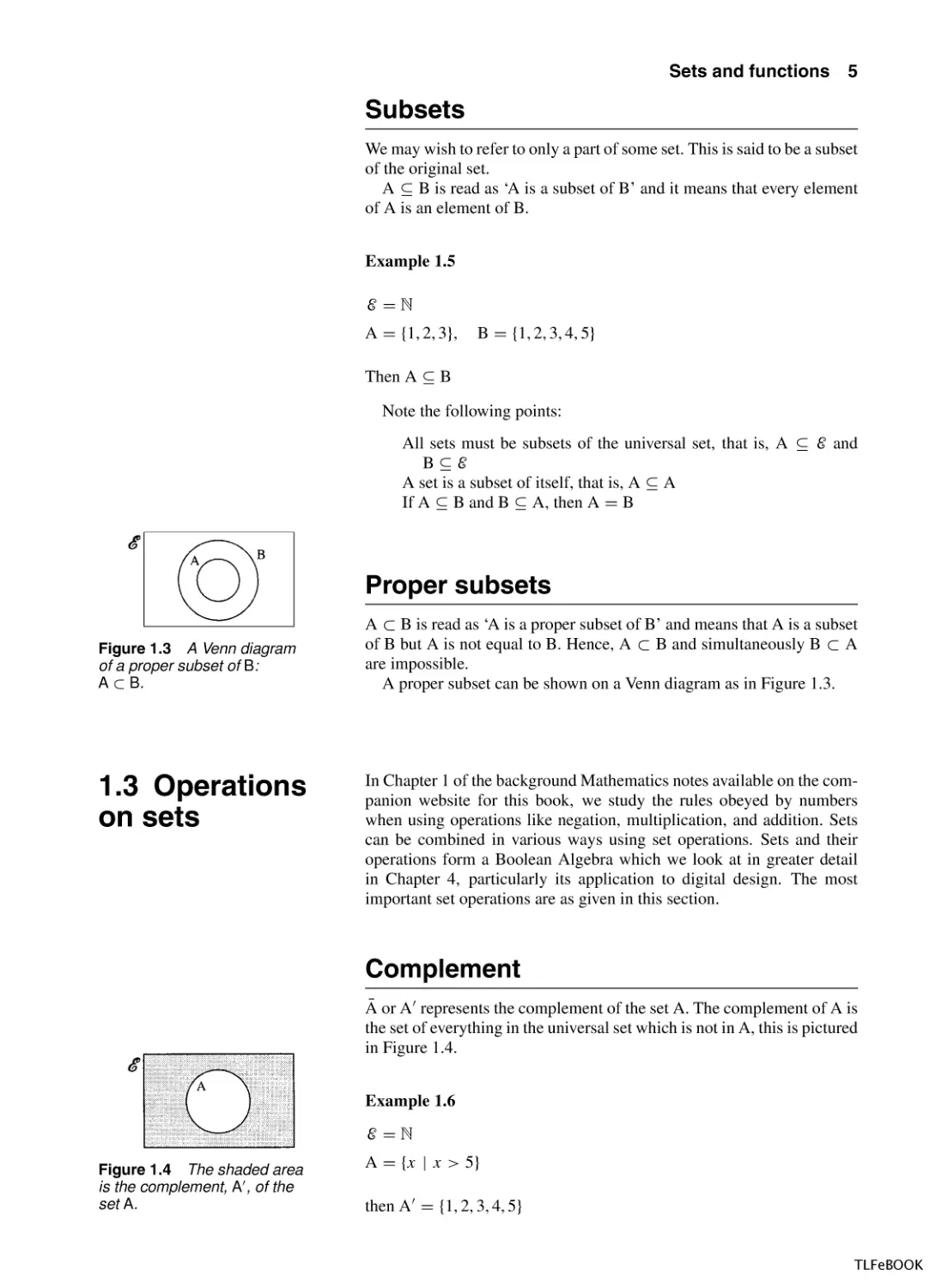
Figure 1.3 A Venn diagram
of a proper subset of B:
A ⊂ B.
1.3 Operations
on sets
A ⊂ B is read as ‘A is a proper subset of B’ and means that A is a subset
of B but A is not equal to B. Hence, A ⊂ B and simultaneously B ⊂ A
are impossible.
A proper subset can be shown on a Venn diagram as in Figure 1.3.
In Chapter 1 of the background Mathematics notes available on the companion website for this book, we study the rules obeyed by numbers
when using operations like negation, multiplication, and addition. Sets
can be combined in various ways using set operations. Sets and their
operations form a Boolean Algebra which we look at in greater detail
in Chapter 4, particularly its application to digital design. The most
important set operations are as given in this section.
Complement
Ā or A represents the complement of the set A. The complement of A is
the set of everything in the universal set which is not in A, this is pictured
in Figure 1.4.
Example 1.6
E =N
Figure 1.4 The shaded area
is the complement, A , of the
set A.
A = {x | x > 5}
then A = {1, 2, 3, 4, 5}
TLFeBOOK
6 Sets and functions
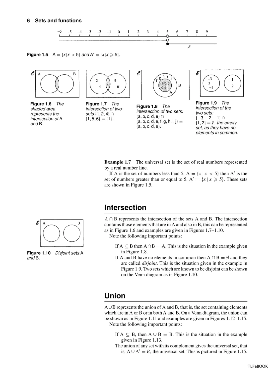
Figure 1.5 A = {x |x < 5} and A = {x |x 5}.
Figure 1.6 The
shaded area
represents the
intersection of A
and B.
Figure 1.7 The
intersection of two
sets {1, 2, 4} ∩
{1, 5, 6} = {1}.
Figure 1.8 The
intersection of two sets:
{a, b, c, d, e} ∩
{a, b, c, d, e, f, g, h, i, j} =
{a, b, c, d, e}.
Figure 1.9 The
intersection of the
two sets:
{−3, −2, −1} ∩
{1, 2} = ∅, the empty
set, as they have no
elements in common.
Example 1.7 The universal set is the set of real numbers represented
by a real number line.
If A is the set of numbers less than 5, A = {x | x < 5} then A is the
set of numbers greater than or equal to 5. A = {x | x 5}. These sets
are shown in Figure 1.5.
Intersection
A ∩ B represents the intersection of the sets A and B. The intersection
contains those elements that are in A and also in B, this can be represented
as in Figure 1.6 and examples are given in Figures 1.7–1.10.
Note the following important points:
Figure 1.10
and B.
Disjoint sets A
If A ⊆ B then A ∩ B = A. This is the situation in the example given
in Figure 1.8.
If A and B have no elements in common then A ∩ B = ∅ and they
are called disjoint. This is the situation given in the example in
Figure 1.9. Two sets which are known to be disjoint can be shown
on the Venn diagram as in Figure 1.10.
Union
A ∪ B represents the union of A and B, that is, the set containing elements
which are in A or B or in both A and B. On a Venn diagram, the union can
be shown as in Figure 1.11 and examples are given in Figures 1.12–1.15.
Note the following important points:
If A ⊆ B, then A ∪ B = B. This is the situation in the example
given in Figure 1.13.
The union of any set with its complement gives the universal set, that
is, A ∪ A = E , the universal set. This is pictured in Figure 1.15.
TLFeBOOK
Sets and functions 7
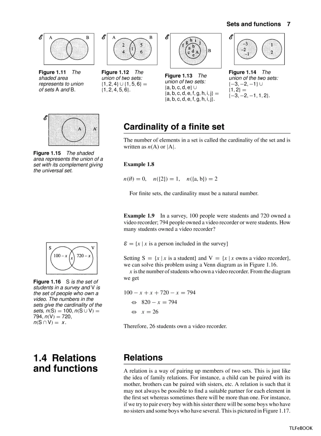
Figure 1.11 The
shaded area
represents to union
of sets A and B.
Figure 1.12 The
union of two sets:
{1, 2, 4} ∪ {1, 5, 6} =
{1, 2, 4, 5, 6}.
Figure 1.13 The
union of two sets:
{a, b, c, d, e} ∪
{a, b, c, d, e, f, g, h, i, j} =
{a, b, c, d, e, f, g, h, i, j}.
Figure 1.14 The
union of the two sets:
{−3, −2, −1} ∪
{1, 2} =
{−3, −2, −1, 1, 2}.
Cardinality of a finite set
The number of elements in a set is called the cardinality of the set and is
written as n(A) or |A|.
Figure 1.15 The shaded
area represents the union of a
set with its complement giving
the universal set.
Example 1.8
n(∅) = 0,
n({2}) = 1,
n({a, b}) = 2
For finite sets, the cardinality must be a natural number.
Example 1.9 In a survey, 100 people were students and 720 owned a
video recorder; 794 people owned a video recorder or were students. How
many students owned a video recorder?
E = {x | x is a person included in the survey}
Figure 1.16 S is the set of
students in a survey and V is
the set of people who own a
video. The numbers in the
sets give the cardinality of the
sets, n(S) = 100, n(S ∪ V) =
794, n(V) = 720,
n(S ∩ V) = x .
1.4 Relations
and functions
Setting S = {x | x is a student} and V = {x | x owns a video recorder},
we can solve this problem using a Venn diagram as in Figure 1.16.
x is the number of students who own a video recorder. From the diagram
we get
100 − x + x + 720 − x = 794
⇔ 820 − x = 794
⇔ x = 26
Therefore, 26 students own a video recorder.
Relations
A relation is a way of pairing up members of two sets. This is just like
the idea of family relations. For instance, a child can be paired with its
mother, brothers can be paired with sisters, etc. A relation is such that it
may not always be possible to find a suitable partner for each element in
the first set whereas sometimes there will be more than one. For instance,
if we try to pair every boy with his sister there will be some boys who have
no sisters and some boys who have several. This is pictured in Figure 1.17.
TLFeBOOK
8 Sets and functions
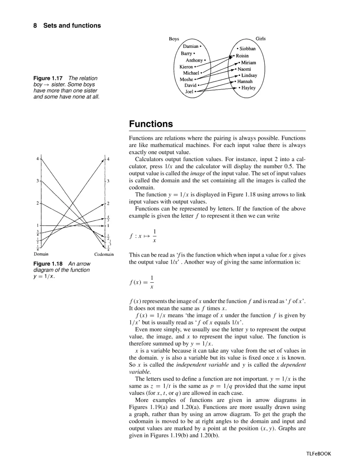
Figure 1.17 The relation
boy → sister. Some boys
have more than one sister
and some have none at all.
Functions
Functions are relations where the pairing is always possible. Functions
are like mathematical machines. For each input value there is always
exactly one output value.
Calculators output function values. For instance, input 2 into a calculator, press 1/x and the calculator will display the number 0.5. The
output value is called the image of the input value. The set of input values
is called the domain and the set containing all the images is called the
codomain.
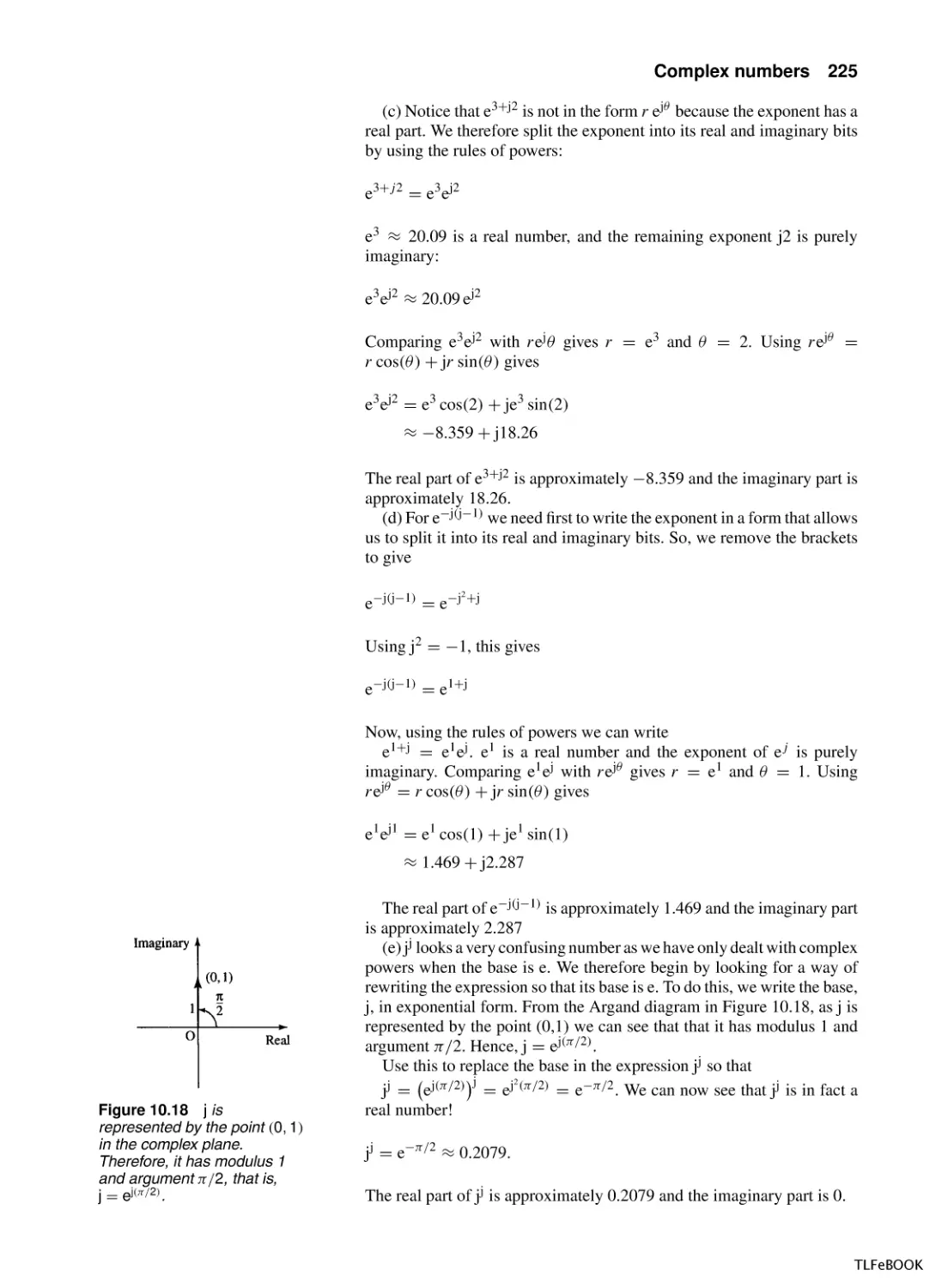
The function y = 1/x is displayed in Figure 1.18 using arrows to link
input values with output values.
Functions can be represented by letters. If the function of the above
example is given the letter f to represent it then we can write
f : x →
Figure 1.18 An arrow
diagram of the function
y = 1/x .
1
x
This can be read as ‘f is the function which when input a value for x gives
the output value 1/x’ . Another way of giving the same information is:
f (x) =
1
x
f (x) represents the image of x under the function f and is read as ‘f of x’.
It does not mean the same as f times x.
f (x) = 1/x means ‘the image of x under the function f is given by
1/x’ but is usually read as ‘f of x equals 1/x’.
Even more simply, we usually use the letter y to represent the output
value, the image, and x to represent the input value. The function is
therefore summed up by y = 1/x.
x is a variable because it can take any value from the set of values in
the domain. y is also a variable but its value is fixed once x is known.
So x is called the independent variable and y is called the dependent
variable.
The letters used to define a function are not important. y = 1/x is the
same as z = 1/t is the same as p = 1/q provided that the same input
values (for x, t, or q) are allowed in each case.
More examples of functions are given in arrow diagrams in
Figures 1.19(a) and 1.20(a). Functions are more usually drawn using
a graph, rather than by using an arrow diagram. To get the graph the
codomain is moved to be at right angles to the domain and input and
output values are marked by a point at the position (x, y). Graphs are
given in Figures 1.19(b) and 1.20(b).
TLFeBOOK
Sets and functions 9
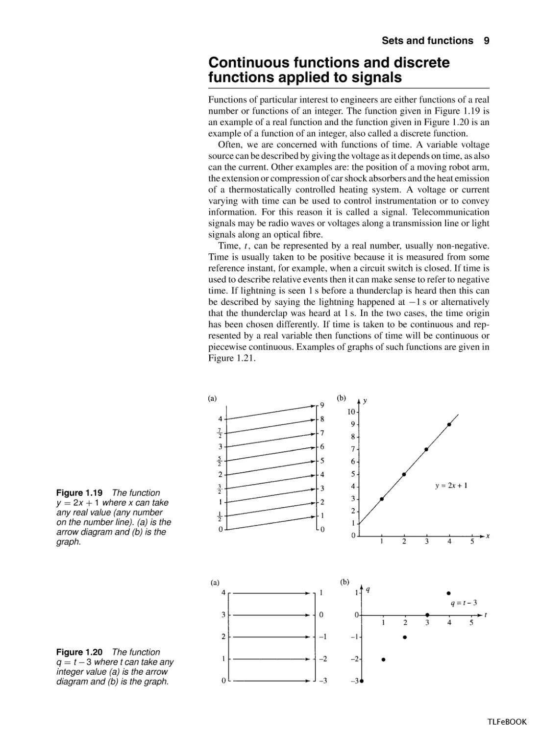
Continuous functions and discrete
functions applied to signals
Functions of particular interest to engineers are either functions of a real
number or functions of an integer. The function given in Figure 1.19 is
an example of a real function and the function given in Figure 1.20 is an
example of a function of an integer, also called a discrete function.
Often, we are concerned with functions of time. A variable voltage
source can be described by giving the voltage as it depends on time, as also
can the current. Other examples are: the position of a moving robot arm,
the extension or compression of car shock absorbers and the heat emission
of a thermostatically controlled heating system. A voltage or current
varying with time can be used to control instrumentation or to convey
information. For this reason it is called a signal. Telecommunication
signals may be radio waves or voltages along a transmission line or light
signals along an optical fibre.
Time, t, can be represented by a real number, usually non-negative.
Time is usually taken to be positive because it is measured from some
reference instant, for example, when a circuit switch is closed. If time is
used to describe relative events then it can make sense to refer to negative
time. If lightning is seen 1 s before a thunderclap is heard then this can
be described by saying the lightning happened at −1 s or alternatively
that the thunderclap was heard at 1 s. In the two cases, the time origin
has been chosen differently. If time is taken to be continuous and represented by a real variable then functions of time will be continuous or
piecewise continuous. Examples of graphs of such functions are given in
Figure 1.21.
Figure 1.19 The function
y = 2x + 1 where x can take
any real value (any number
on the number line). (a) is the
arrow diagram and (b) is the
graph.
Figure 1.20 The function
q = t − 3 where t can take any
integer value (a) is the arrow
diagram and (b) is the graph.
TLFeBOOK
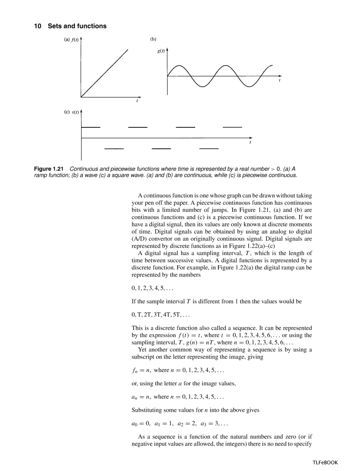
10
Sets and functions
Figure 1.21 Continuous and piecewise functions where time is represented by a real number > 0. (a) A
ramp function; (b) a wave (c) a square wave. (a) and (b) are continuous, while (c) is piecewise continuous.
A continuous function is one whose graph can be drawn without taking
your pen off the paper. A piecewise continuous function has continuous
bits with a limited number of jumps. In Figure 1.21, (a) and (b) are
continuous functions and (c) is a piecewise continuous function. If we
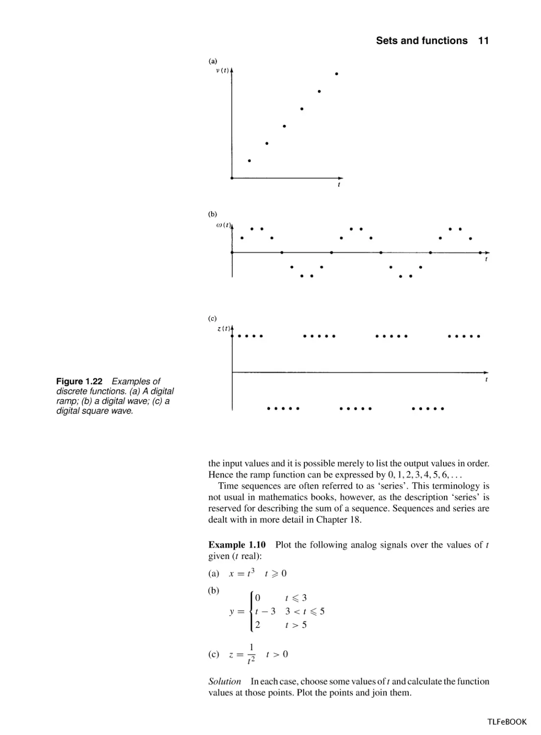
have a digital signal, then its values are only known at discrete moments
of time. Digital signals can be obtained by using an analog to digital
(A/D) convertor on an originally continuous signal. Digital signals are
represented by discrete functions as in Figure 1.22(a)–(c)
A digital signal has a sampling interval, T , which is the length of
time between successive values. A digital functions is represented by a
discrete function. For example, in Figure 1.22(a) the digital ramp can be
represented by the numbers
0, 1, 2, 3, 4, 5, . . .
If the sample interval T is different from 1 then the values would be
0, T, 2T, 3T, 4T, 5T, . . .
This is a discrete function also called a sequence. It can be represented
by the expression f (t) = t, where t = 0, 1, 2, 3, 4, 5, 6, . . . or using the
sampling interval, T , g(n) = nT , where n = 0, 1, 2, 3, 4, 5, 6, . . .
Yet another common way of representing a sequence is by using a
subscript on the letter representing the image, giving
fn = n, where n = 0, 1, 2, 3, 4, 5, . . .
or, using the letter a for the image values,
an = n, where n = 0, 1, 2, 3, 4, 5, . . .
Substituting some values for n into the above gives
a0 = 0, a1 = 1, a2 = 2, a3 = 3, . . .
As a sequence is a function of the natural numbers and zero (or if
negative input values are allowed, the integers) there is no need to specify
TLFeBOOK
Sets and functions
11
Figure 1.22 Examples of
discrete functions. (a) A digital
ramp; (b) a digital wave; (c) a
digital square wave.
the input values and it is possible merely to list the output values in order.
Hence the ramp function can be expressed by 0, 1, 2, 3, 4, 5, 6, . . .
Time sequences are often referred to as ‘series’. This terminology is
not usual in mathematics books, however, as the description ‘series’ is
reserved for describing the sum of a sequence. Sequences and series are
dealt with in more detail in Chapter 18.
Example 1.10
given (t real):
Plot the following analog signals over the values of t
t 0
(a)
x = t3
(b)
0
y = t −3
2
(c) z =
1
t2
t 3
3<t 5
t >5
t >0
Solution In each case, choose some values of t and calculate the function
values at those points. Plot the points and join them.
TLFeBOOK
12
Sets and functions
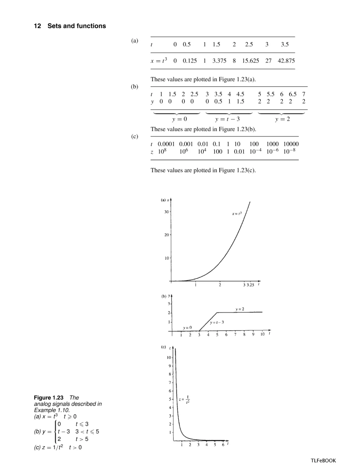
(a)
t
0
0.5
1
1.5
2
2.5
3
3.5
x = t3
0
0.125
1
3.375
8
15.625
27
42.875
These values are plotted in Figure 1.23(a).
(b)
t 1 1.5 2 2.5
y 0 0
0 0
y=0
3 3.5 4 4.5
0 0.5 1 1.5
y =t −3
5 5.5 6 6.5 7
2 2
2 2
2
y=2
These values are plotted in Figure 1.23(b).
(c)
t 0.0001 0.001 0.01 0.1 1 10 100 1000 10000
z 108
106
104 100 1 0.01 10−4 10−6 10−8
These values are plotted in Figure 1.23(c).
Figure 1.23 The
analog signals described in
Example 1.10.
(a) x = t3 t 0
t 3
0
(b) y = t − 3 3 < t 5
2
t >5
(c) z = 1/t 2 t > 0
TLFeBOOK
Sets and functions
13
Example 1.11 Plot the following discrete signals over the values of t
given (t an integer):
(a) x =
1
t −1
t >2
(b)
t 4
0
y = 1/t − 0.25 4 < t < 10
−0.15
t 10
(c)
z = 4t − 2
t >0
Solution In each case, choose successive values of t and calculate the
function values at those points. Mark the points with a dot.
(a)
t
x
2
1
3
0.5
4
0.33
5
0.25
6
0.2
7
0.17
8
0.14
9
0.13
10
0.11
These values are plotted in Figure 1.24(a).
(b)
t 3 4
y 00
5
6
7
8
9
10
11
12
−0.05 −0.08 −0.11 −0.12 −0.14 −0.15 −0.15 −0.15
1
y=0
y = − 0.25
t
These values are plotted in Figure 1.24(b).
y = −0.15
(c)
t
z
1
2
2
6
3
10
4
14
5
18
6
22
7
26
8
30
These values are plotted in Figure 1.24(c).
Undefined function values
Some functions have ‘undefined values’, that is, numbers that cannot be
input into them successfully. For instance input 0 on a calculator and
try getting the value of 1/x. The calculator complains (usually displaying ‘-E-’) indicating that an error has occurred. The reason that this is an
error is that we are trying to find the value of 1/0 that is 1 divided by 0.
Look at Chapter 1 of the Background Mathematics Notes, given on the
accompanying website for this book, for a discussion about why division
by 0 is not defined. The number 0 cannot be included in the domain of
the function f (x) = 1/x. This can be expressed by saying
f (x) = 1/x,
where x ∈ R and x = 0
which is read as ‘f of x equals 1/x, where x is a real number not equal
to 0’.
TLFeBOOK
14
Sets and functions
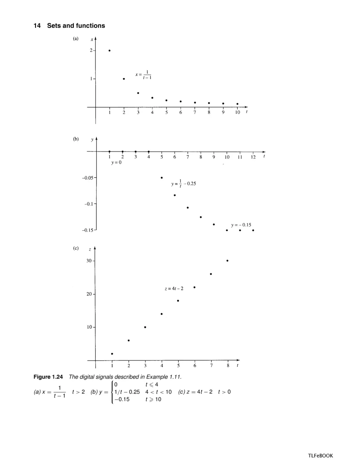
Figure 1.24
The digital signals
described in Example 1.11.
t 4
0
1
(a) x =
t > 2 (b) y = 1/t − 0.25 4 < t < 10 (c) z = 4t − 2 t > 0
t −1
−0.15
t 10
TLFeBOOK
Sets and functions
15
Often, we assume that we are considering functions of a real variable
and only need to indicate the values that are not allowed as inputs for the
function. So we may write
f (x) = 1/x
where x = 0
Things to look out for as values that are not allowed as function
inputs are :
1. Numbers that would lead to an attempt to divide by zero
2. Numbers that would lead to negative square roots
3. Numbers that would lead to negative inputs to a logarithm.
Examples 1.12(a) and (b) require solutions to inequalities which we
shall discuss in greater detail in Chapter 2. Here, we shall only look at
simple examples and use the same rules as used for solving equations. We
can find equivalent inequalities by doing the same thing to both sides, with
the extra rule that, for the moment, we avoid multiplication or division
by a negative number.
Example 1.12 Find the values that cannot be input to the following
functions, where the independent variable (x or r) is real:
√
(a) y = 3 x − 2 + 5
(b) y = 3 log10 (2 − 4x)
r + 1000
(c) R =
1000(r − 2)
Solution
√
(a) y = 3 x − 2 + 5
Here x − 2 cannot be negative as we need to take the square root of it.
x−20⇔x 2
therefore, the function is
√
y =3 x−2+5
where x 2
(b) y = 3 log10 (2 − 4x).
Here 2 − 4x cannot be 0 or negative else we could not take the logarithm.
2 − 4x > 0
⇔
2 > 4x
⇔
2/4 > x
or equivalently, x < 21 . So the function is
y = 3 log10 (2 − 4x)
(c) R =
where x < 0.5
r + 1000
1000(r − 2)
TLFeBOOK
16
Sets and functions
Here 1000(r − 2) cannot be 0, else we would be trying to divide by 0.
Solve the equation for the values that r cannot take
1000(r − 2) = 0
r −2=0
r=2
The function is
R=
r + 1000
1000(r − 2)
where r = 2
Example 1.13 Find the values that can be input to the following discrete
functions where the independent variable is an integer
1
k−4
(a)
y=
(b)
f (k) =
1
(k − 3)(k − 2.2)
(c)
an = n2
where n ∈ Z
where k ∈ Z
where k ∈ Z
Solution
(a)
y=
1
k−4
Here k − 4 cannot be 0 else there would be an attempt to divide by 0. We
get k − 4 = 0 when k = 4 so the function is:
y=
(b)
1
k−4
f (k) =
where k = 4 and k ∈ Z
1
(k − 3)(k − 2.2)
where k ∈ Z
Solve for (k − 3)(k − 2.2) = 0 giving k = 3 or k = 2.2. As 2.2 is not an
integer then there is not need to specifically exclude it from the function
input values, so the function is
f (k) =
(c)
1
(k − 3)(k − 2.2)
an = n2 ,
where k = 3 and k ∈ Z
n∈Z
Here there are no problems with the function as any integer can be squared.
There are no excluded values from the input of the function.
Using a recurrence relation to
define a discrete function
Values in a discrete function can also be described in terms of its values
for preceeding integers.
TLFeBOOK
Sets and functions
17
Example 1.14 Find a table of values for the function defined by the
recurrence relation:
f (n) = f (n − 1) + 2
(1.1)
where f (0) = 0.
Solution Assuming that the function is defined for n = 0, 1, 2, . . . then
we can take successive values of n and find the values taken by the
function. n = 0 gives f (0) = 0 as given.
Substituting n = 1 into Equation (1.1) gives
f (1) = f (1 − 1) + 2
⇔
f (1) = f (0) + 2 = 0 + 2 = 2 (using f (0) = 0)
hence, f (1) = 2.
Substituting n = 2 into Equation (1.1) gives
f (2) = f (2 − 1) + 2
⇔ f (2) = f (1) + 2
⇔ f (2) = f (1) + 2 = 2 + 2 = 4 (using f (1) = 2)
hence, f (2) = 4.
Substituting n = 3 into Equation (1.1) gives
f (3) = f (3 − 1) + 2
⇔ f (3) = f (2) + 2 = 4 + 2 (using f (2) = 4)
hence, f (3) = 6.
Continuing in the same manner gives the following table:
n 0 1 2 3 4 5 6 7 8 9 10 · · · n · · ·
f 0 2 4 6 8 10 12 14 16 18 20 . . . 2n · · ·
Notice we have filled in the general term f (n) = 2n. This was found
in this case by simple guess work.
1.5 Combining
functions
The sum, difference, product, and
quotient of two functions, f and g
Two functions with R as their domain and codomain can be combined
using arithmetic operations. We can define the sum of f and g by
(f + g) : x → f (x) + g(x)
The other operations are defined as follows:
(f − g) : x → f (x) − g(x)
difference,
(f × g) : x → f (x) × g(x)
product,
(f /g) : x →
f (x)
g(x)
quotient.
TLFeBOOK
18
Sets and functions
Example 1.15
functions:
Find the sum, difference, product, and quotient of the
f : x → x 2 and g : x → x 6
Solution
(f + g) : x → x 2 + x 6
(f − g) : x → x 2 − x 6
(f × g) : x → x 2 × x 6 = x 8
(f /g) : x →
x2
= x −4
x6
The specification of the domain of the quotient is not straightforward.
This is because of the difficulty which occurs when g(x) = 0. When
g(x) = 0 the quotient function is undefined and we must remove such
elements from its domain. The domain of f /g is R with the values where
g(x) = 0 omitted.
Composition of functions
This method of combining functions is fundamentally different from the
arithmetical combinations of the previous section. The composition of
two functions is the action of performing one function followed by the
other, that is, a function of a function.
Example 1.16 A post office worker has a scale expressed in kilograms
which gives the cost of a parcel depending on its weight. He also has an
approximate formula for conversion from pounds (lbs) to kilograms. He
wishes to find out the cost of a parcel which weighs 3 lb.
The two functions involved are:
a : kilograms → money and c : lbs → kilograms
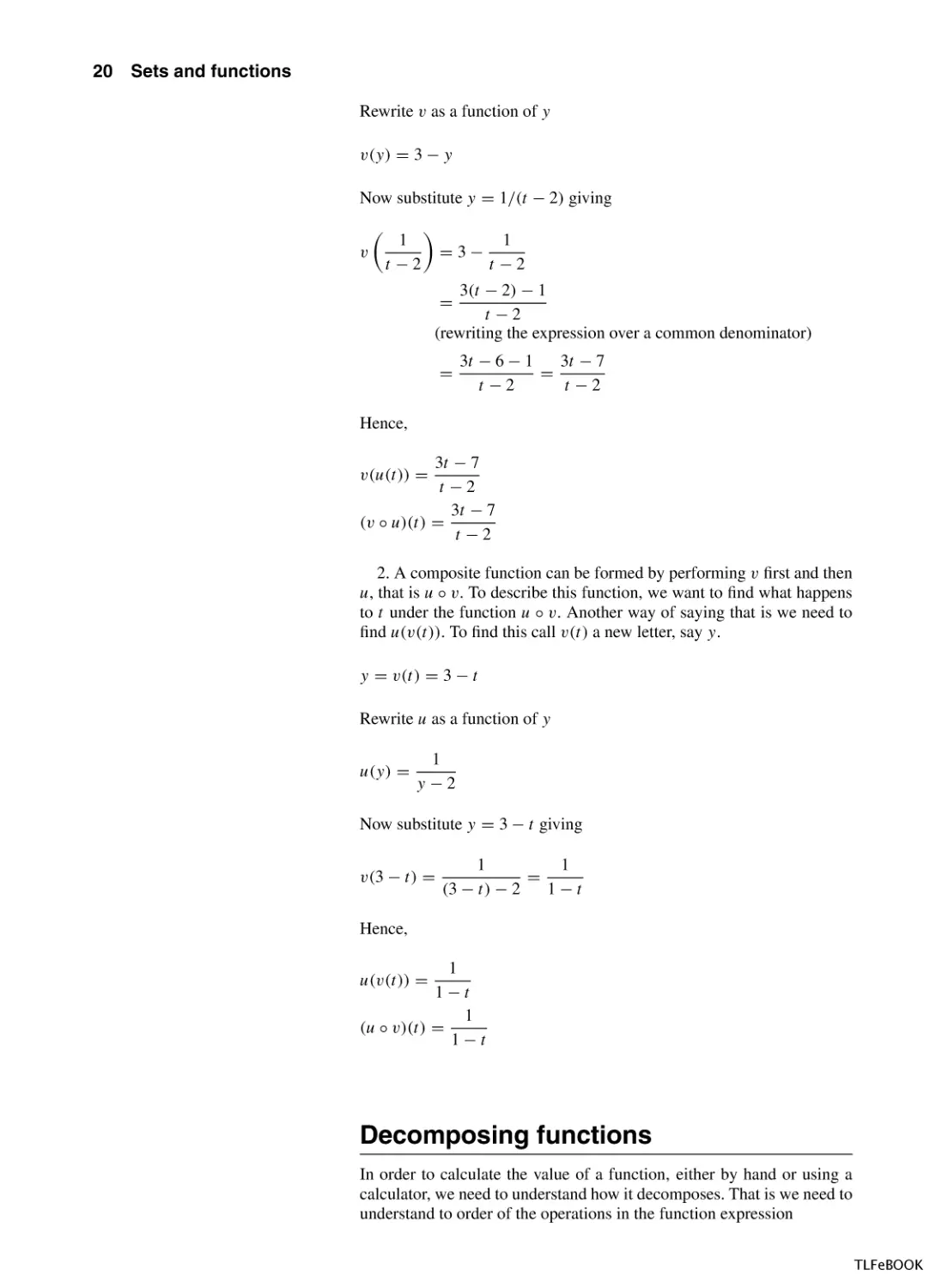
Figure 1.25 The function
a : kilograms → money used
in Example 1.16.
a is defined by Figure 1.25 and the function c is given by
c : x → x/2.2
Solution The composition ‘a ◦ c’ will be a function from lbs to money.
Hence, 3 lb after the function c gives 1.364 and 1.364 after the function
a gives e1.90 and therefore
(a ◦ c)(3) = e1.90.
Example 1.17 Supposing f (x) = 2x + 1 and g(x) = x 2 , then we can
combine the functions in two ways.
1. A composite function can be formed by performing f first and then
g, that is, g ◦ f . To describe this function, we want to find what happens
TLFeBOOK
Sets and functions
19
to x under the function g ◦ f . Another way of saying that is we need to
find g(f (x)). To do this call f (x) a new letter, say y.
y = f (x) = 2x + 1
Rewrite g as a function of y
g(y) = y 2
Now substitute y = 2x + 1 giving
g(2x + 1) = (2x + 1)2
Hence,
g(f (x)) = (2x + 1)2
(g ◦ f )(x) = (2x + 1)2 .
2. A composite function can be formed by performing g first and then
f , that is, f ◦ g. To describe this function, we want to find what happens
to x under the function f ◦ g. Another way of saying that is we need to
find f (g(x)). To do this call g(x) a new letter, say y.
y = g(x) = x 2
Rewrite f as a function of y
f (y) = 2y + 1
Now substitute y = x 2 giving
f (x 2 ) = 2x 2 + 1
Hence,
f (g(x)) = 2x 2 + 1
(f ◦ g)(x) = 2x 2 + 1.
Example 1.18 Supposing u(t) = 1/(t − 2) and v(t) = 3 − t then,
again, we can combine the functions in two ways.
1. A composite function can be formed by performing u first and then
v, that is, v ◦ u. To describe this function, we want to find what happens
to t under the function v ◦ u. Another way of saying that is we need to
find v(u(t)). To do this call u(t) a new letter, say y.
y = u(t) =
1
t −2
TLFeBOOK
20
Sets and functions
Rewrite v as a function of y
v(y) = 3 − y
Now substitute y = 1/(t − 2) giving
v
1
t −2
=3−
1
t −2
3(t − 2) − 1
t −2
(rewriting the expression over a common denominator)
=
=
3t − 6 − 1
3t − 7
=
t −2
t −2
Hence,
3t − 7
t −2
3t − 7
(v ◦ u)(t) =
t −2
v(u(t)) =
2. A composite function can be formed by performing v first and then
u, that is u ◦ v. To describe this function, we want to find what happens
to t under the function u ◦ v. Another way of saying that is we need to
find u(v(t)). To find this call v(t) a new letter, say y.
y = v(t) = 3 − t
Rewrite u as a function of y
u(y) =
1
y−2
Now substitute y = 3 − t giving
v(3 − t) =
1
1
=
(3 − t) − 2
1−t
Hence,
1
1−t
1
(u ◦ v)(t) =
1−t
u(v(t)) =
Decomposing functions
In order to calculate the value of a function, either by hand or using a
calculator, we need to understand how it decomposes. That is we need to
understand to order of the operations in the function expression
TLFeBOOK
Sets and functions
Example 1.19
21
Calculate y = (2x + 1)3 when x = 2
Solution Remember the order of operations discussed in Chapter 1 of the
Background Mathematics booklet available on the companion website.
The operations are performed in the following order:
Start with x = 2 then
2x = 4
2x + 1 = 5
(2x + 1)3 = 125
So, there are three operations involved
1.
2.
3.
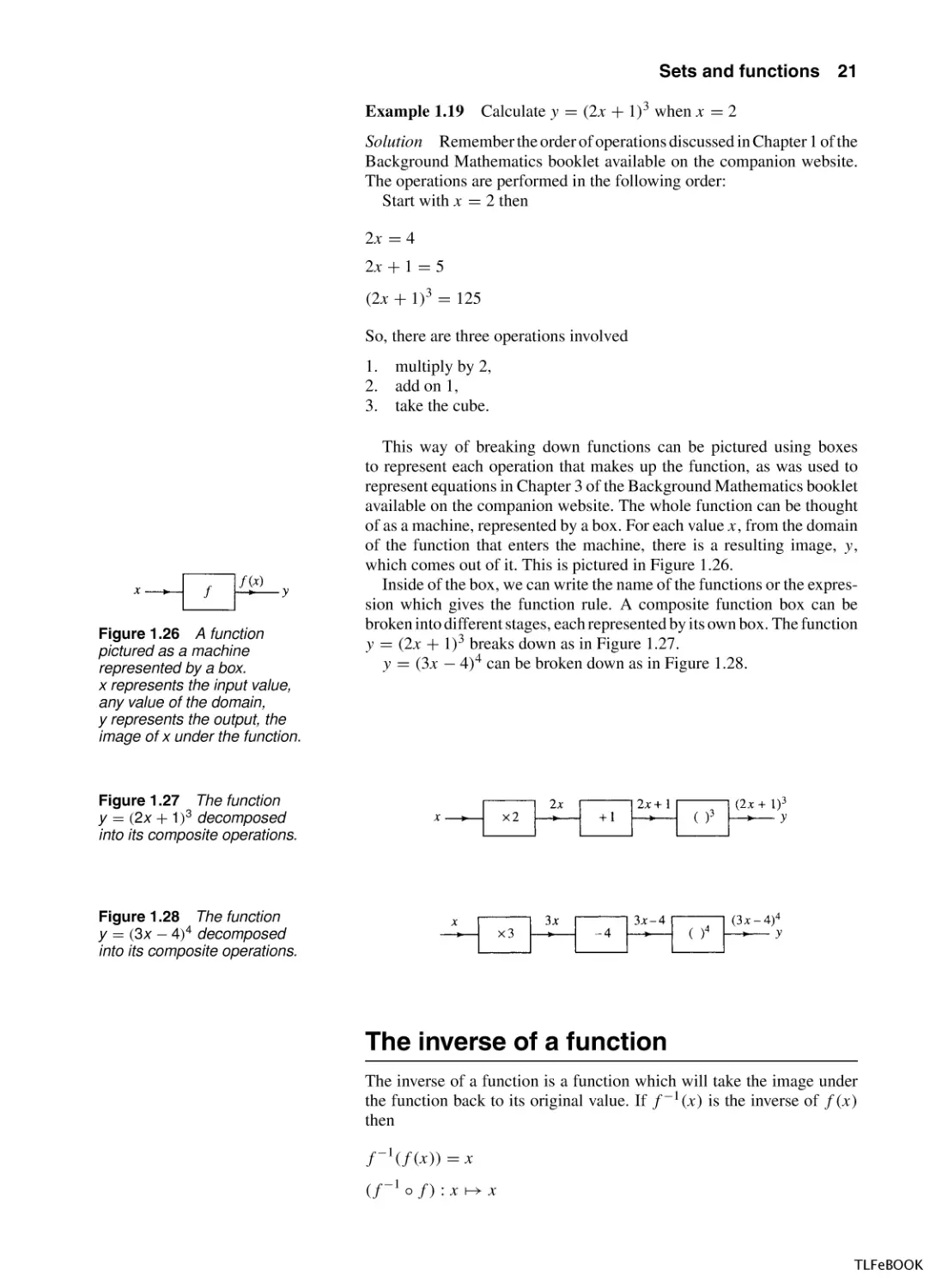
Figure 1.26 A function
pictured as a machine
represented by a box.
x represents the input value,
any value of the domain,
y represents the output, the
image of x under the function.
multiply by 2,
add on 1,
take the cube.
This way of breaking down functions can be pictured using boxes
to represent each operation that makes up the function, as was used to
represent equations in Chapter 3 of the Background Mathematics booklet
available on the companion website. The whole function can be thought
of as a machine, represented by a box. For each value x, from the domain
of the function that enters the machine, there is a resulting image, y,
which comes out of it. This is pictured in Figure 1.26.
Inside of the box, we can write the name of the functions or the expression which gives the function rule. A composite function box can be
broken into different stages, each represented by its own box. The function
y = (2x + 1)3 breaks down as in Figure 1.27.
y = (3x − 4)4 can be broken down as in Figure 1.28.
Figure 1.27 The function
y = (2x + 1)3 decomposed
into its composite operations.
Figure 1.28 The function
y = (3x − 4)4 decomposed
into its composite operations.
The inverse of a function
The inverse of a function is a function which will take the image under
the function back to its original value. If f −1 (x) is the inverse of f (x)
then
f −1 (f (x)) = x
(f −1 ◦ f ) : x → x
TLFeBOOK
22
Sets and functions
Example 1.20
f (x) = 2x + 1
f −1 (x) =
x−1
2
To show this is true, look at the combined function f −1 (f (x)) =
(2x + 1 − 1)/2 = x.
Finding the inverse of a linear function
One simple way of finding the inverse of a linear function is to:
1.
2.
Decompose the operations of the function.
Combine the inverse operations (performed in the reverse order) to
give the inverse function.
This is a method similar to that used to solve linear equations in
Chapter 3 of the Background Mathematics Notes available on the
companion website for this book.
Figure 1.29 The top line
represents the function
f (x ) = 5x − 2 (read from left
to right) and the bottom line
the inverse function.
Example 1.21 Find the inverse of the function f (x) = 5x − 2.
The method of solution is given in Figure 1.29.
The inverse operations give that x = (y + 2)/5. Here y is the input
value into the inverse function and x is the output value. To use x and y
in the more usual way, where x is the input and y the output, swap the
letters giving the inverse function as
y=
x+2
5
This result can be achieved more quickly by rearranging the expression
so that x is the subject of the formula and then swap x and y.
Example 1.22
y = 5x − 2
Find the inverse of f (x) = 5x − 2.
⇔
⇔
⇔
y + 2 = 5x
y+2
=x
5
y+2
x=
5
Now swap x and y to give y = (x + 2)/5. Therefore,
f −1 (x) = (x + 2)/5.
TLFeBOOK
Sets and functions
Find the inverse of
Example 1.23
g(x) =
23
1
2−x
where x = 2
Set
y=
1
⇔ y(2 − x) = 1
2−x
⇔ 2y − xy = 1
⇔ 2y = 1 + xy
⇔ 2y − 1 = xy
⇔ xy = 2y − 1
2y − 1
y
1
⇔x =2−
y
⇔x=
where y = 0
Swap x and y to give y = 2 − (1/x)
So
g −1 (x) = 2 −
1
x
x = 0
To check, try a couple of values of x.
Try x = 4,
g(x) =
1
1
1
=
=−
2−x
2−4
2
Perform g −1 on the output value −(1/2).
Substitute g(4) = −(1/2) into g −1 (x):
g −1 −
1
2
=2−
1
= 2 + 2 = 4.
−(1/2)
The function followed by its inverse has given us the original value of x.
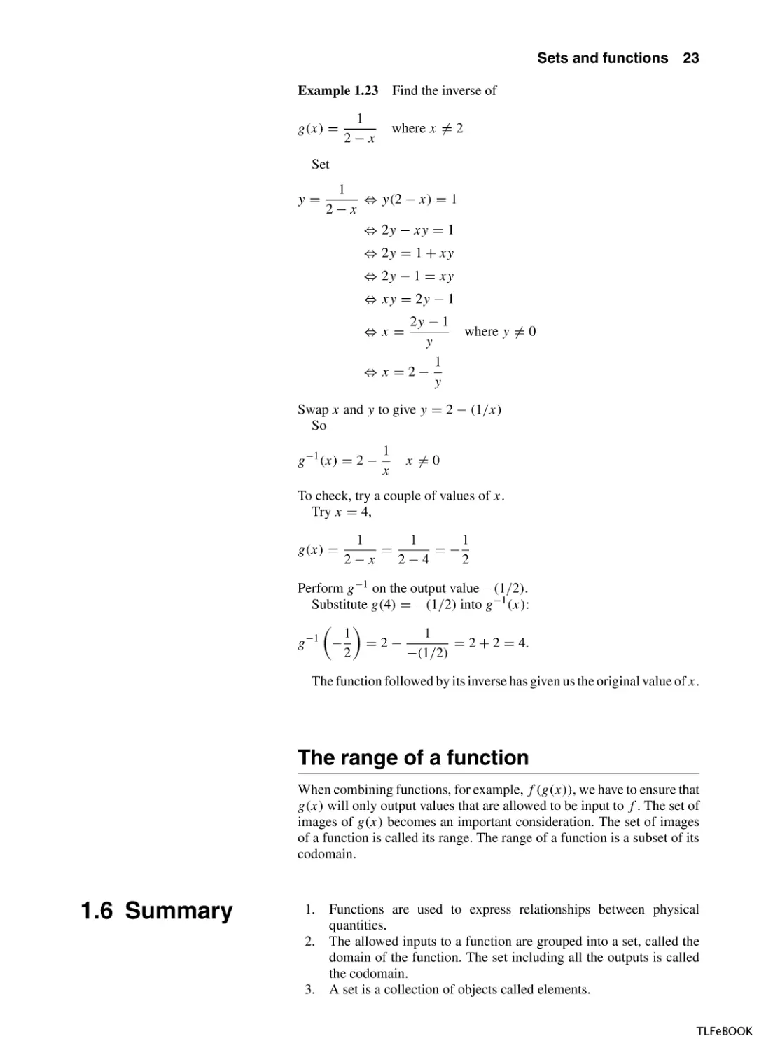
The range of a function
When combining functions, for example, f (g(x)), we have to ensure that
g(x) will only output values that are allowed to be input to f . The set of
images of g(x) becomes an important consideration. The set of images
of a function is called its range. The range of a function is a subset of its
codomain.
1.6 Summary
1. Functions are used to express relationships between physical
quantities.
2. The allowed inputs to a function are grouped into a set, called the
domain of the function. The set including all the outputs is called
the codomain.
3. A set is a collection of objects called elements.
TLFeBOOK
24
Sets and functions
E is the universal set, the set of all objects we are interested in.
∅ is the empty set, the set with no elements.
The three most important operations on sets are:
(a) intersection: A ∩ B is the set containing every element in both
A and B;
(b) union: A ∪ B is the set of elements in A or in B or both;
(c) complement: A is the set of everything, in the universal set,
not in A.
A relation is a way of pairing members of two sets.
Functions are a special type of relation which can be thought of as
mathematical machines. For each input value there is exactly one
output value.
Many functions of interest are functions of time, used to represent
signals. Analogue signals can be represented by functions of a real
variable and digital signals by functions of an integer (discrete functions). Functions of an integer are also called sequences and can be
defined using a recurrence relation.
To find the domain of a real or discrete function exclude values that
could lead to a division by zero, negative square roots, or negative
logarithms or other undefined values.
Functions can be combined in various ways including sum, difference, product, and quotient. A special operation of functions is
composition. A composite function is found by performing a second
function on the result of the first.
The inverse of a function is a function which will take the image
under the function back to its original value.
4.
5.
6.
7.
8.
9.
10.
11.
12.
1.7 Exercises
1.1. Given E = {a, b, c, d, e, f, g}, A
B = {b, c, d, f}, C = {c, d, e}.
=
{a, b, e},
Write down the following sets:
(a) A ∩ B
(b) A ∪ B
(c) A ∩ C
(d) (A ∪ B) ∩ C
(e) (A ∩ C) ∪ (B ∩ C)
(f) (A ∩ B) ∪ C
(g) (A ∪ C) ∩ (B ∪ C)
(h) (A ∩ C)
(i) A ∪ C .
1.2. Use Venn diagrams to show that:
(a) (A ∩ B) ∩ C = A ∩ (B ∩ C)
(b) (A ∪ B) ∪ C = A ∪ (B ∪ C)
(c) (A ∩ B) ∪ C = (A ∪ C) ∩ (B ∪ C)
(d) (A ∪ B) ∩ C = (A ∩ C) ∪ (B ∩ C)
(e) (A ∩ B) = A ∪ B
(f) (A ∪ B) = A ∩ B .
1.3. Let E = {0, 1, 2, 3, 4, 5, 6, 7, 8, 9} and given P =
{x|x < 5}, Q = {x|x 3} find explicitly:
(a) P
(b) Q
(c) P ∪ Q
(d) P
(e) P ∩ Q.
1.4. Below are various assertions for any sets A and B.
Write true or false for each statement and give a
counter-example if you think the statement is false.
(a) (A ∩ B) = A ∩ B
(b) (A ∩ B) ⊆ A
(c) A ∩ B = B ∩ A
(d) A ∩ B = B ∩ A .
1.5. Using a Venn diagram simplify the following:
(a) A ∩ (A ∪ B)
(b) A ∪ (B ∩ A )
(c) A ∩ (B ∪ A ).
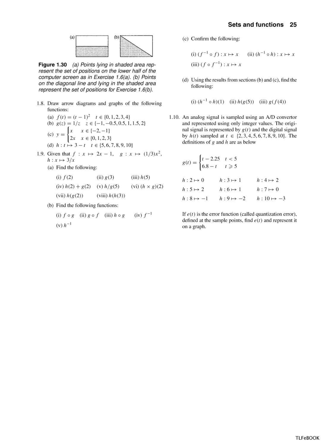
1.6. A computer screen has 80 columns and 25 rows:
(a) Define the set of positions on the screen.
(b) Taking the origin as the top left hand corner
define:
(i) the set of positions in the lower half of the
screen as shown in Figure 1.30(a);
(ii) the set of positions lying on or below the
diagonal as shown in Figure 1.30(b).
1.7. A certain computer system breaks down in two main
ways: faults on the network and power supply faults. Of
the last 50 breakdowns, 42 involved network faults and
20 power failures. In 13 cases, both the power supply
and the network were faulty. How many breakdowns
were attributable to other kinds of failure?
TLFeBOOK
Sets and functions
25
(c) Confirm the following:
(i) (f −1 ◦ f ) : x → x
Figure 1.30 (a) Points lying in shaded area represent the set of positions on the lower half of the
computer screen as in Exercise 1.6(a). (b) Points
on the diagonal line and lying in the shaded area
represent the set of positions for Exercise 1.6(b).
1.8. Draw arrow diagrams and graphs of the following
functions:
(a) f (t) = (t − 1)2 t ∈ {0, 1, 2, 3, 4}
(b) g(z) = 1/z z ∈ {−1, −0.5, 0.5, 1, 1.5, 2}
x
x ∈ {−2, −1}
(c) y =
2x x ∈ {0, 1, 2, 3}
(d) h : t → 3 − t t ∈ {5, 6, 7, 8, 9, 10}
1.9. Given that f : x → 2x − 1,
h : x → 3/x
(a) Find the following:
(iii) (f ◦ f −1 ) : x → x
(d) Using the results from sections (b) and (c), find the
following:
(i) (h−1 ◦ h)(1)
g(t) =
(ii) g(3)
(iii) h(5)
(iv) h(2) + g(2)
(v) h/g(5)
(vi) (h × g)(2)
(vii) h(g(2))
(viii) h(h(3))
(ii) h(g(5))
(iii) g(f (4))
1.10. An analog signal is sampled using an A/D convertor
and represented using only integer values. The original signal is represented by g(t) and the digital signal
by h(t) sampled at t ∈ {2, 3, 4, 5, 6, 7, 8, 9, 10}. The
definitions of g and h are as below
g : x → (1/3)x 2 ,
(i) f (2)
(ii) (h−1 ◦ h) : x → x
t − 2.25 t < 5
6.8 − t
t 5
h : 2 → 0
h : 3 → 1
h : 4 → 2
h : 5 → 2
h : 6 → 1
h : 7 → 0
h : 8 → −1
h : 9 → −2
h : 10 → −3
(b) Find the following functions:
(i) f ◦ g
(v) h−1
(ii) g ◦ f
(iii) h ◦ g
(iv) f −1
If e(t) is the error function (called quantization error),
defined at the sample points, find e(t) and represent it
on a graph.
TLFeBOOK
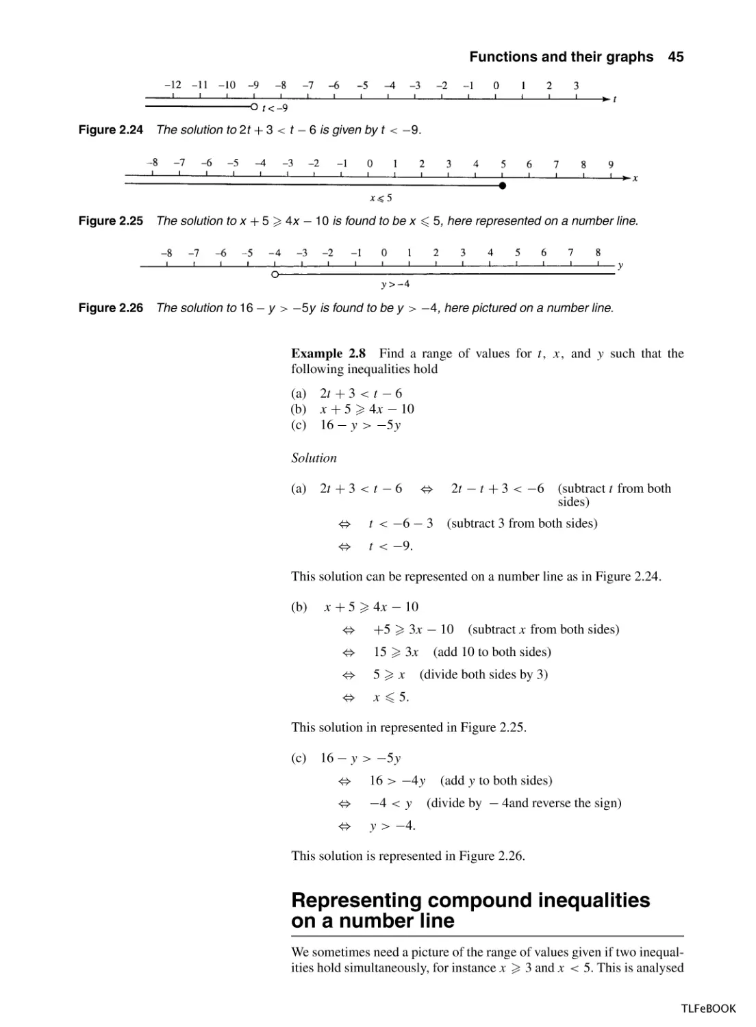
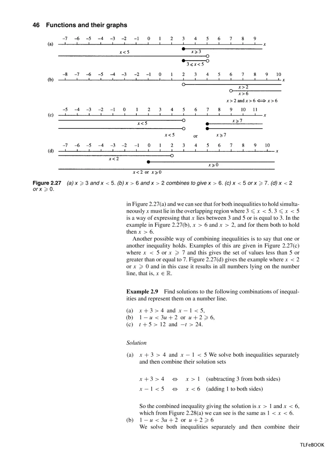
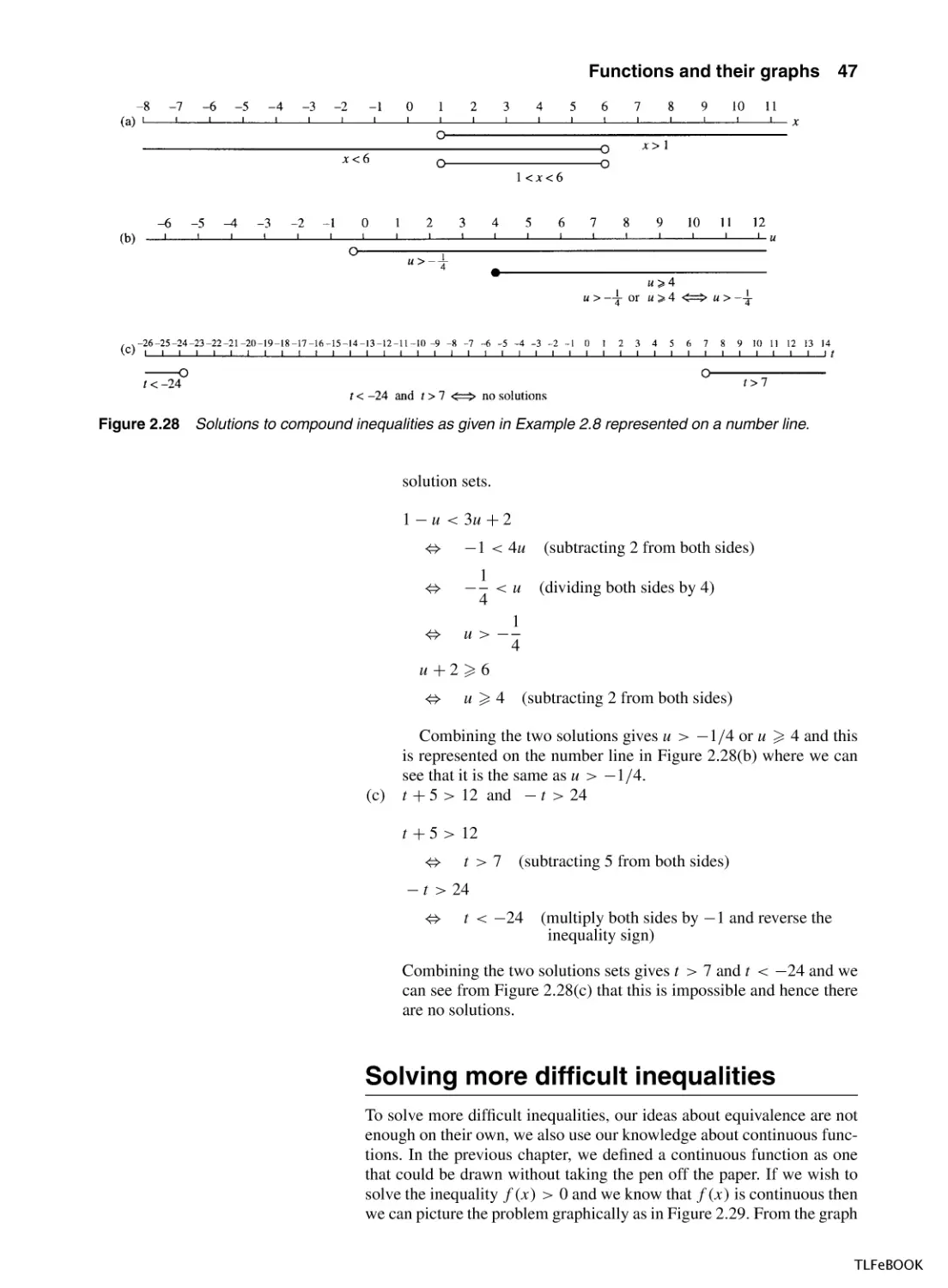
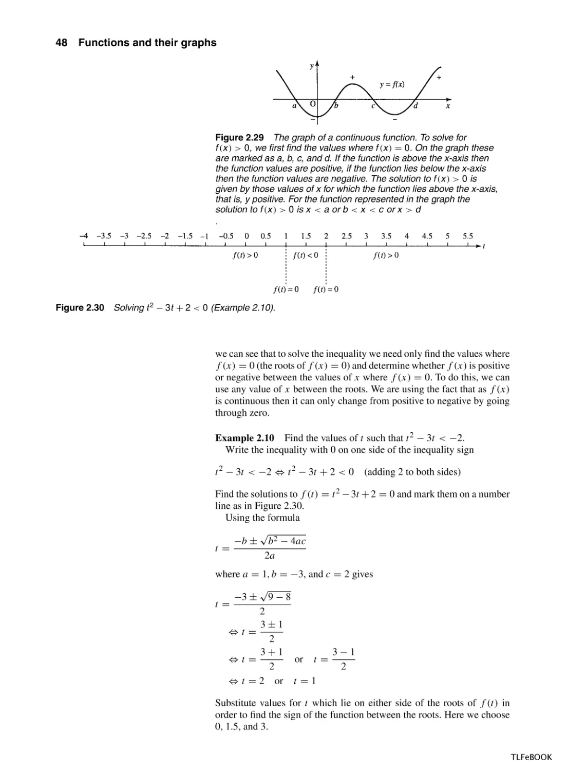
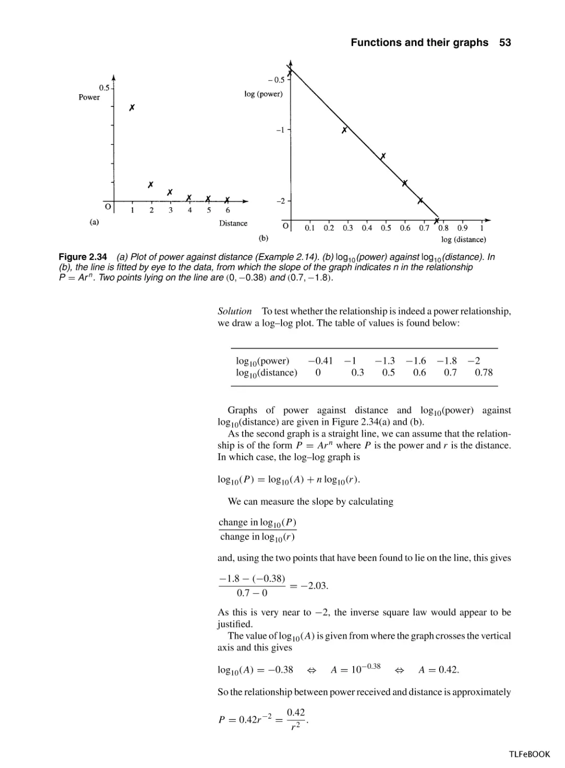
2
Functions and
their graphs
2.1 Introduction
The ability to produce a picture of a problem is an important step towards
solving it. From the graph of a function, y = f (x), we are able to predict
such things as the number of solutions to the equation f (x) = 0, regions
over which it is increasing or decreasing, and the points where it is not
defined.
Recognizing the shape of functions is an important and useful skill.
Oscilloscopes give a graphical representation of voltage against time,
from which we may be able to predict an expression for the voltage. The
increasing use of signal processing means that many problems involve
analysing how functions of time are effected by passing through some
mechanical or electrical system.
In order to draw graphs of a large number of functions, we need only
remember a few key graphs and appreciate simple ideas about transformations. A sketch of a graph is one which is not necessarily drawn strictly
to scale but shows its important features. We shall start by looking at
special properties of the straight line (linear function) and the quadratic.
Then we look at the graphs of y = x, y = x 2 , y = 1/x, y = a x and how
to transform these graphs to get graphs of functions like y = 4x − 2,
y = (x − 2)2 , y = 3/x, and y = a −x .
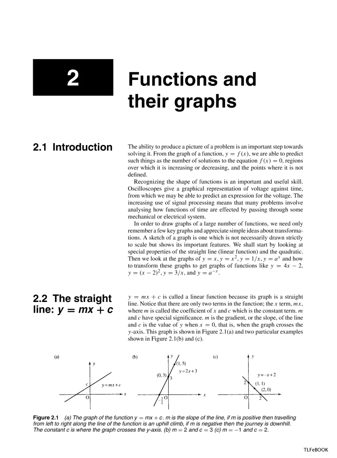
2.2 The straight
line: y = mx + c
y = mx + c is called a linear function because its graph is a straight
line. Notice that there are only two terms in the function; the x term, mx,
where m is called the coefficient of x and c which is the constant term. m
and c have special significance. m is the gradient, or the slope, of the line
and c is the value of y when x = 0, that is, when the graph crosses the
y-axis. This graph is shown in Figure 2.1(a) and two particular examples
shown in Figure 2.1(b) and (c).
Figure 2.1 (a) The graph of the function y = mx + c. m is the slope of the line, if m is positive then travelling
from left to right along the line of the function is an uphill climb, if m is negative then the journey is downhill.
The constant c is where the graph crosses the y-axis. (b) m = 2 and c = 3 (c) m = −1 and c = 2.
TLFeBOOK
Functions and their graphs
27
The gradient of a straight line
The gradient gives an idea of how steep the climb is as we travel along the
line of the graph. If the gradient is positive then we are travelling uphill
as we move from left to right and if the gradient is negative then we are
travelling downhill. If the gradient is zero then we are on flat ground. The
gradient gives the amount that y increases when x increases by 1 unit. A
straight line always has the same slope at whatever point it is measured.
To show that in the expression y = mx + c, m is the gradient, we begin
with a couple of examples as in Figure 2.1(b) and (c)
In Figure 2.1(b), we have the graph of y = 2x + 3. Take any two
values of x which differ by 1 unit, for example, x = 0 and x = 1. When
x = 0, y = 2 × 0 + 3 = 3 and when x = 1, y = 2 × 1 + 3 = 5. The
increase in y is 5 − 3 = 2, and this is the same as the coefficient of x in
the function expression.
In Figure 2.1(c), we see the graph of y = −x + 2. Take any two
values of x which differ by 1 unit, for example, x = 1 and x = 2. When
x = 1, y = −(1) + 2 = 1 and when x = 2, y = −(2) + 2 = 0. The
increase in y is 0 − 1 = −1 and this is the same as the coefficient of x in
the function expression.
In the general case, y = mx + c, take any two values of x which differ
by 1 unit, for example, x = x0 and x = x0 +1. When x = x0 , y = mx0 +c
and when x = x0 + 1, y = m(x + 1) + c = mx + m + c. The increase
in y is mx + m + c − (mx + c) = m.
We know that every time x increases by 1 unit y increases by m.
However, we do not need to always consider an increase of exactly 1 unit
in x. The gradient gives the ratio of the increase in y to the increase in x.
Therefore, if we only have a graph and we need to find the gradient then
we can use any two points that lie on the line.
To find the gradient of the line take any two points on the line (x1 , y1 )
and (x2 , y2 ).
The gradient =
change in y
y2 − y1
=
change in x
x2 − x 1
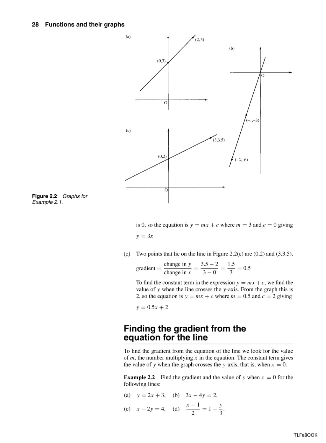
Example 2.1 Find the gradient of the lines given in Figure 2.2(a)–(c)
and the equation for the line in each case.
Solution
(a)
We are given the coordinates of two points that lie on the straight
line in Figure 2.2(a) as (0,3) and (2,5),
gradient =
change in y
5−3
2
=
= = 1.
change in x
2−0
2
To find the constant term in the expression y = mx + c, we find
the value of y when the line crosses the y-axis. From the graph this
is 3, so the equation is y = mx + c where m = 1 and c = 3, giving
y =x+3
(b)
Two points that lie on the line in Figure 2.2(b) are (−1, −3) and
(−2, −6). These are found by measuring the x and y values for
some points on the line.
gradient =
change in y
−6 − (−3)
−3
=
=
= 3.
change in x
−2 − (−1)
−1
To find the constant term in the expression y = mx + c, we find
the value of y when the line crosses the y-axis. From the graph this
TLFeBOOK
28
Functions and their graphs
Figure 2.2 Graphs for
Example 2.1.
is 0, so the equation is y = mx + c where m = 3 and c = 0 giving
y = 3x
(c)
Two points that lie on the line in Figure 2.2(c) are (0,2) and (3,3.5).
gradient =
change in y
3.5 − 2
1.5
=
=
= 0.5
change in x
3−0
3
To find the constant term in the expression y = mx + c, we find the
value of y when the line crosses the y-axis. From the graph this is
2, so the equation is y = mx + c where m = 0.5 and c = 2 giving
y = 0.5x + 2
Finding the gradient from the
equation for the line
To find the gradient from the equation of the line we look for the value
of m, the number multiplying x in the equation. The constant term gives
the value of y when the graph crosses the y-axis, that is, when x = 0.
Example 2.2 Find the gradient and the value of y when x = 0 for the
following lines:
(a) y = 2x + 3,
(b) 3x − 4y = 2,
(c) x − 2y = 4,
(d)
x−1
y
=1− .
2
3
TLFeBOOK
Functions and their graphs
29
Solution
In the equation y = 2x + 3, the value of m, the gradient, is 2 as this
is the coefficient of x. c = 3 which is the value of y when the graph
crosses the y-axis, that is, when x = 0.
(b) In the equation 3x − 4y = 2, we rewrite the equation with y as the
subject of the formula in order to find the value of m and c.
(a)
3x − 4y = 2
⇔
3x = 2 + 4y
⇔
3x − 2 = 4y
⇔
2
3x
− =y
4
4
3x
1
y=
−
4
2
⇔
We can see, by comparing the expression with y = mx + c, that m,
the gradient, is 3/4 and c = −1/2.
(c) Write y as the subject of the formula:
x − 2y = 4
⇔
x = 4 + 2y
⇔
x − 4 = 2y
⇔
2y = x − 4
x
y = −2
2
⇔
We can see, by comparing the expression with y = mx + c, that m,
the gradient, is 1/2 and c = −2.
(d) Write y as the subject of the formula
x−1
y
=1−
3
2
x
1
y
⇔
− =1−
2 2
3
3x
3
⇔
− =3−y
2
2
3x
3
⇔ y =3−
−
2
2
⇔
y=−
3x
9
+
2
2
We can see, by comparing the expression with y = mx + c, that m,
the gradient, is −3/2 and c = 9/2.
Finding the equation of a line which
goes through two points
Supposing we have been given two points, (x1 , y1 ) and (x2 , y2 ), which
lie on a line and we want to find the equation of that line. We already
found that the gradient of the line is given by:
The gradient =
change in y
y2 − y1
=
change in x
x2 − x 1
We know that the equation of a line is of the form y = mx + c, but we
would like to express the equation just in terms of the two variables, x
TLFeBOOK
Functions and their graphs
31
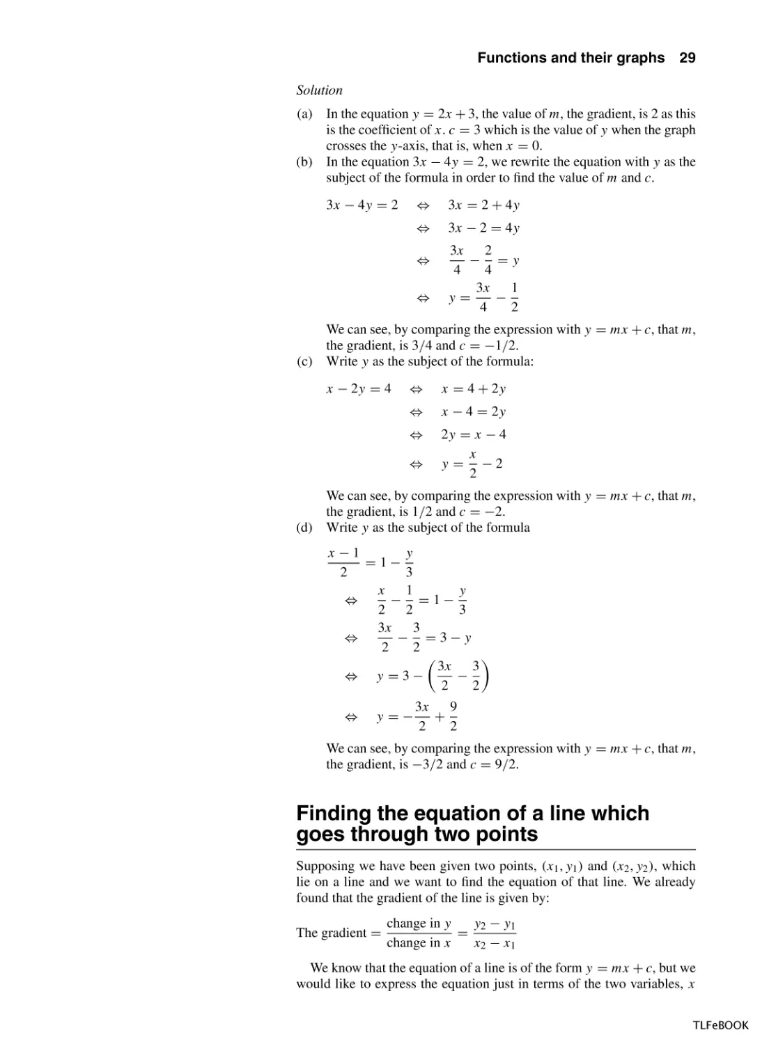
Example 2.4
(a)
Sketch the graph of y = 4x − 2.
To find where the graph crosses the y-axis, substitute x = 0 into
the equation of the line:
y = 4(0) − 2 = −2.
This means that the graph passes through the point (0,−2).
To find where the graph crosses the x-axis, substitute y = 0,
that is,
4x − 2 = 0
⇔
4x = 2
⇔
x=
2
= 0.5.
4
Therefore, the graph passes through (0.5, 0).
Mark the points (0,2) and (0.5,0), on the x- and y-axes and join
the two points. This is done in Figure 2.3(a).
(b) Sketch the graph of y = −4x When x = 0 we get y = 0, that is
the graph goes through the point (0,0). In this case, as the graph
passes through the origin, we need to choose a different value for x
for the second point. Taking x = 2 gives y = −8, so another point
is (2, −8). These points on marked on the graph and joined to give
the graph as in Figure 2.3(b).
Figure 2.3 (a) The graph of
y = 4x − 2. (b) The graph of
y = −4x .
TLFeBOOK
32
Functions and their graphs
2.3 The
quadratic
function:
y = ax 2 + bx + c
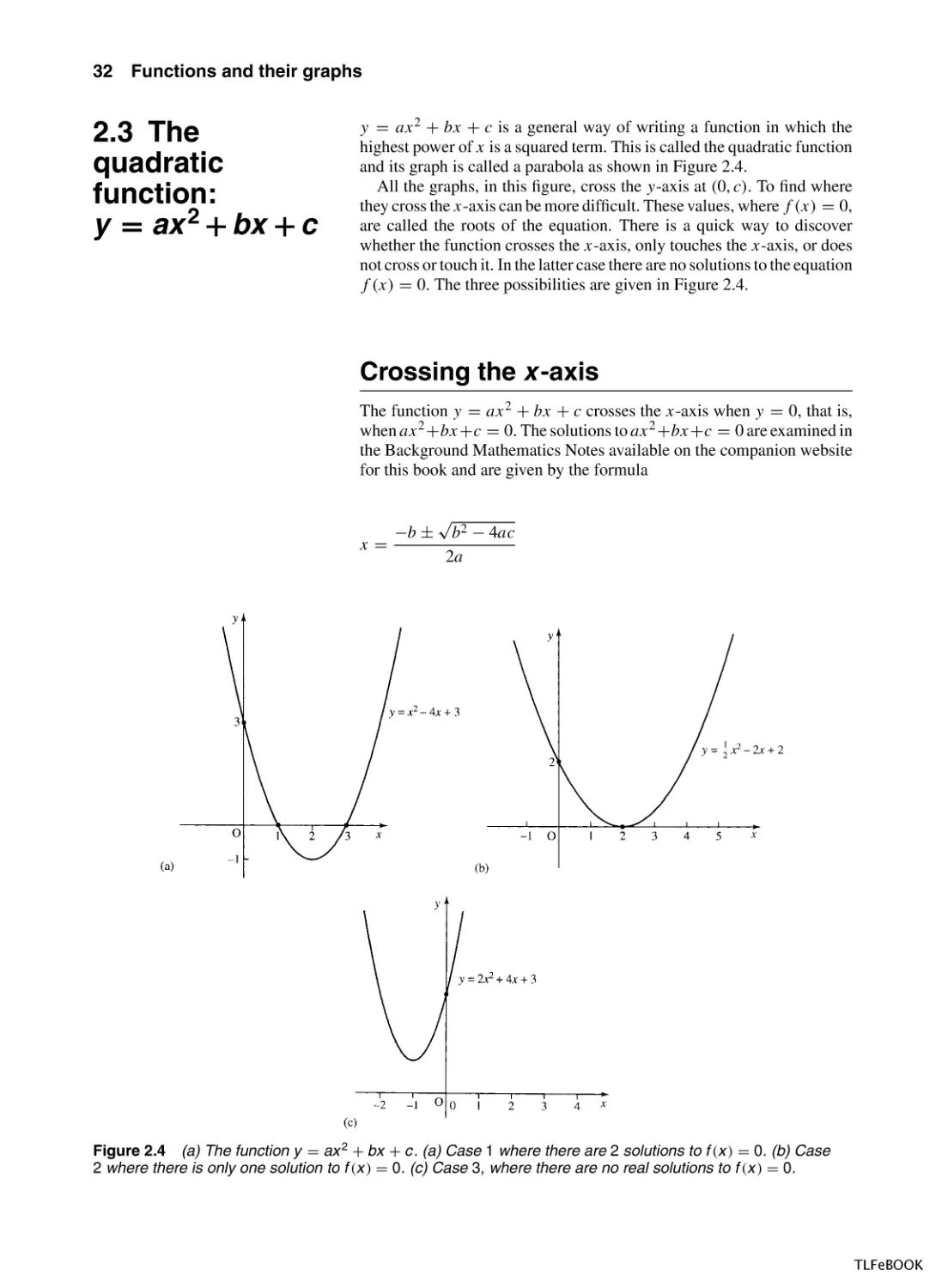
y = ax 2 + bx + c is a general way of writing a function in which the
highest power of x is a squared term. This is called the quadratic function
and its graph is called a parabola as shown in Figure 2.4.
All the graphs, in this figure, cross the y-axis at (0, c). To find where
they cross the x-axis can be more difficult. These values, where f (x) = 0,
are called the roots of the equation. There is a quick way to discover
whether the function crosses the x-axis, only touches the x-axis, or does
not cross or touch it. In the latter case there are no solutions to the equation
f (x) = 0. The three possibilities are given in Figure 2.4.
Crossing the x -axis
The function y = ax 2 + bx + c crosses the x-axis when y = 0, that is,
when ax 2 +bx +c = 0. The solutions to ax 2 +bx +c = 0 are examined in
the Background Mathematics Notes available on the companion website
for this book and are given by the formula
x=
−b ±
√
b2 − 4ac
2a
Figure 2.4 (a) The function y = ax 2 + bx + c. (a) Case 1 where there are 2 solutions to f (x ) = 0. (b) Case
2 where there is only one solution to f (x ) = 0. (c) Case 3, where there are no real solutions to f (x ) = 0.
TLFeBOOK
Functions and their graphs
33
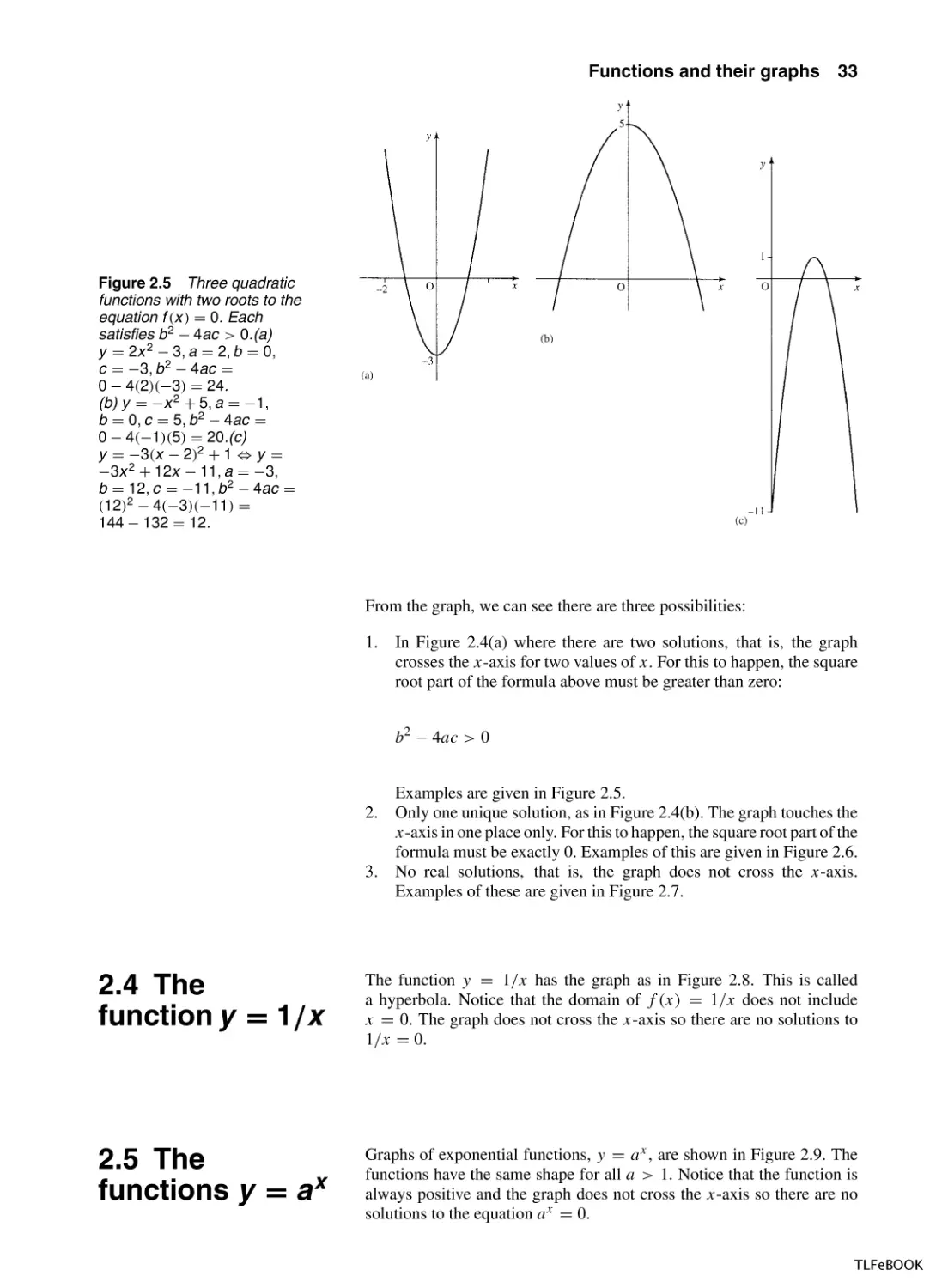
Figure 2.5 Three quadratic
functions with two roots to the
equation f (x ) = 0. Each
satisfies b 2 − 4ac > 0.(a)
y = 2x 2 − 3, a = 2, b = 0,
c = −3, b 2 − 4ac =
0 − 4(2)(−3) = 24.
(b) y = −x 2 + 5, a = −1,
b = 0, c = 5, b 2 − 4ac =
0 − 4(−1)(5) = 20.(c)
y = −3(x − 2)2 + 1 ⇔ y =
−3x 2 + 12x − 11, a = −3,
b = 12, c = −11, b 2 − 4ac =
(12)2 − 4(−3)(−11) =
144 − 132 = 12.
From the graph, we can see there are three possibilities:
1.
In Figure 2.4(a) where there are two solutions, that is, the graph
crosses the x-axis for two values of x. For this to happen, the square
root part of the formula above must be greater than zero:
b2 − 4ac > 0
Examples are given in Figure 2.5.
Only one unique solution, as in Figure 2.4(b). The graph touches the
x-axis in one place only. For this to happen, the square root part of the
formula must be exactly 0. Examples of this are given in Figure 2.6.
3. No real solutions, that is, the graph does not cross the x-axis.
Examples of these are given in Figure 2.7.
2.
2.4 The
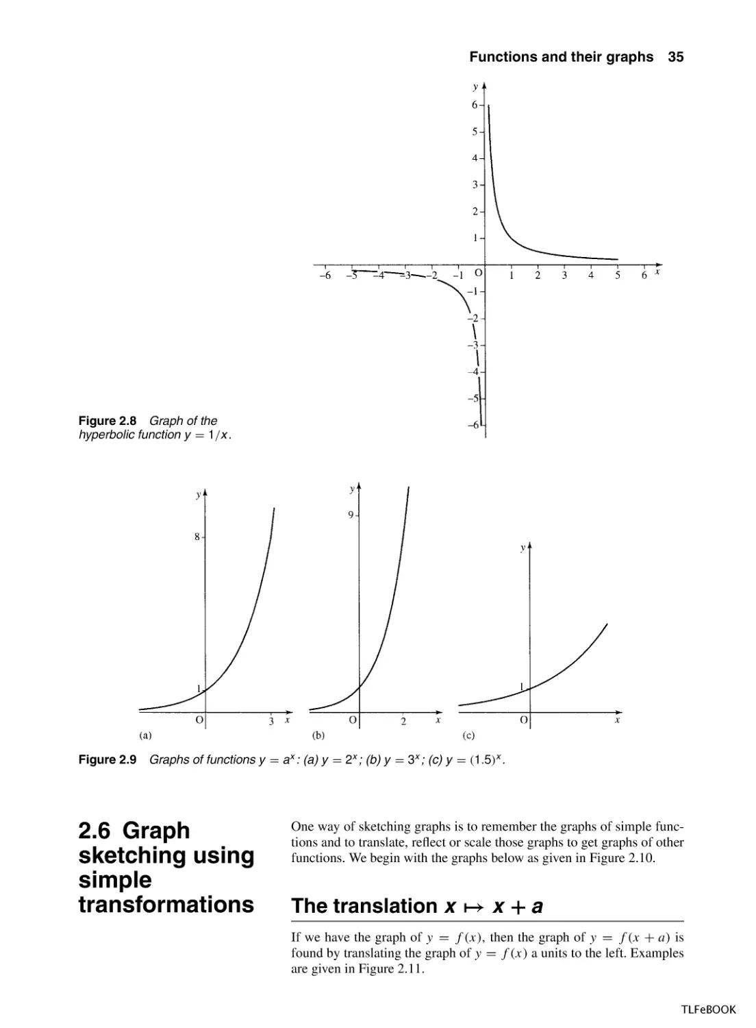
function y = 1/x
The function y = 1/x has the graph as in Figure 2.8. This is called
a hyperbola. Notice that the domain of f (x) = 1/x does not include
x = 0. The graph does not cross the x-axis so there are no solutions to
1/x = 0.
2.5 The
functions y = a x
Graphs of exponential functions, y = a x , are shown in Figure 2.9. The
functions have the same shape for all a > 1. Notice that the function is
always positive and the graph does not cross the x-axis so there are no
solutions to the equation a x = 0.
TLFeBOOK
34
Functions and their graphs
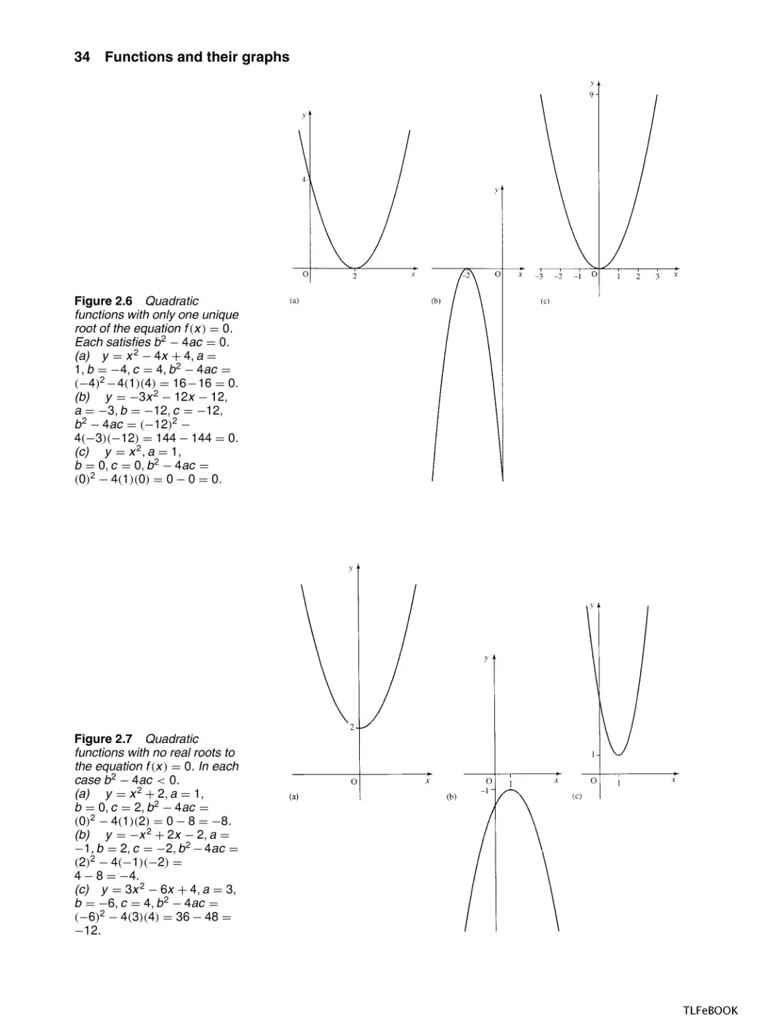
Figure 2.6 Quadratic
functions with only one unique
root of the equation f (x ) = 0.
Each satisfies b 2 − 4ac = 0.
(a) y = x 2 − 4x + 4, a =
1, b = −4, c = 4, b 2 − 4ac =
(−4)2 −4(1)(4) = 16−16 = 0.
(b) y = −3x 2 − 12x − 12,
a = −3, b = −12, c = −12,
b 2 − 4ac = (−12)2 −
4(−3)(−12) = 144 − 144 = 0.
(c) y = x 2 , a = 1,
b = 0, c = 0, b 2 − 4ac =
(0)2 − 4(1)(0) = 0 − 0 = 0.
Figure 2.7 Quadratic
functions with no real roots to
the equation f (x ) = 0. In each
case b 2 − 4ac < 0.
(a) y = x 2 + 2, a = 1,
b = 0, c = 2, b 2 − 4ac =
(0)2 − 4(1)(2) = 0 − 8 = −8.
(b) y = −x 2 + 2x − 2, a =
−1, b = 2, c = −2, b 2 − 4ac =
(2)2 − 4(−1)(−2) =
4 − 8 = −4.
(c) y = 3x 2 − 6x + 4, a = 3,
b = −6, c = 4, b 2 − 4ac =
(−6)2 − 4(3)(4) = 36 − 48 =
−12.
TLFeBOOK
Functions and their graphs
35
Figure 2.8 Graph of the
hyperbolic function y = 1/x .
Figure 2.9 Graphs of functions y = a x : (a) y = 2x ; (b) y = 3x ; (c) y = (1.5)x .
2.6 Graph
sketching using
simple
transformations
One way of sketching graphs is to remember the graphs of simple functions and to translate, reflect or scale those graphs to get graphs of other
functions. We begin with the graphs below as given in Figure 2.10.
The translation x → x + a
If we have the graph of y = f (x), then the graph of y = f (x + a) is
found by translating the graph of y = f (x) a units to the left. Examples
are given in Figure 2.11.
TLFeBOOK
36
Functions and their graphs
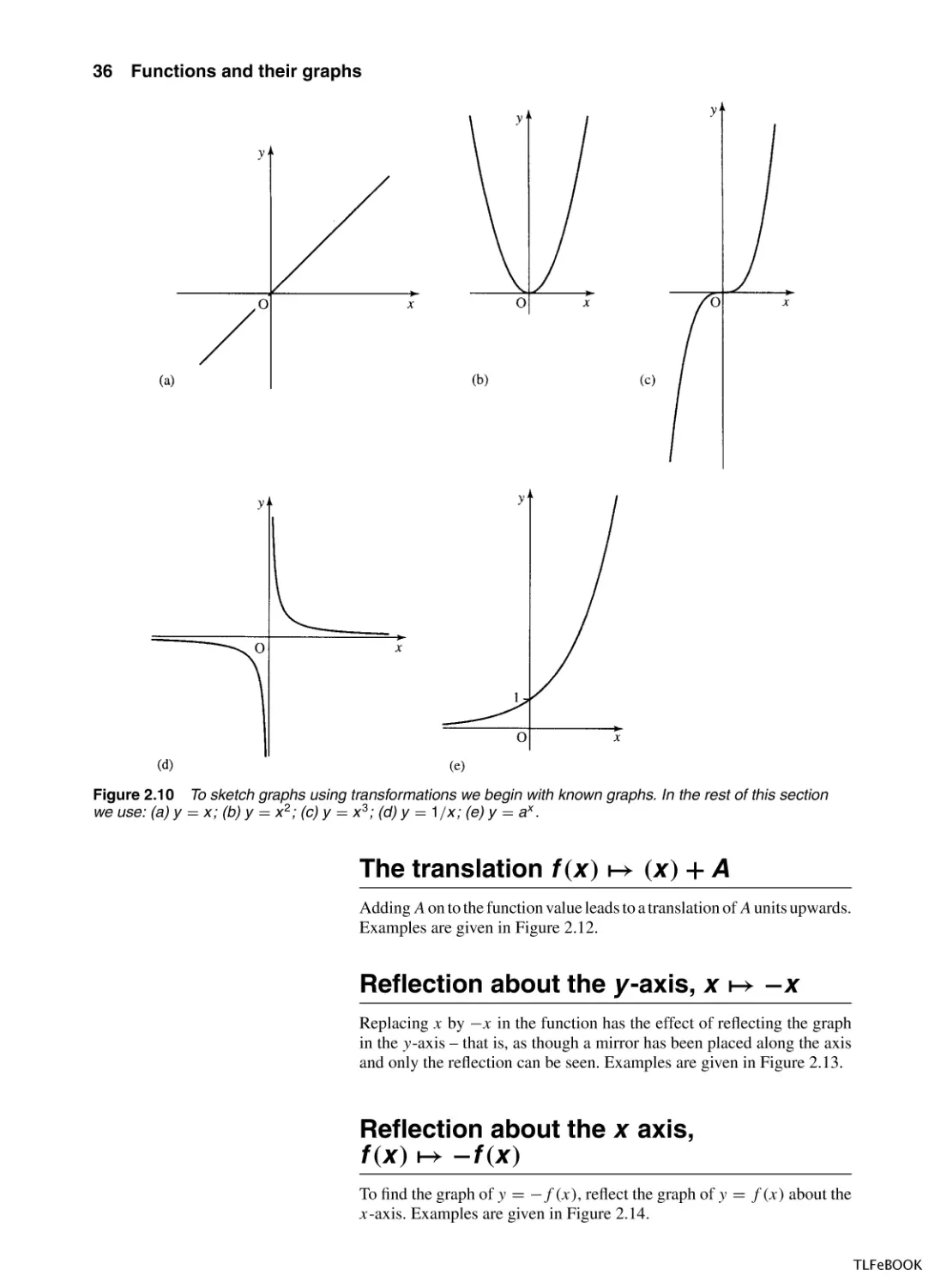
Figure 2.10 To sketch graphs using transformations we begin with known graphs. In the rest of this section
we use: (a) y = x ; (b) y = x 2 ; (c) y = x 3 ; (d) y = 1/x ; (e) y = a x .
The translation f (x ) → (x ) + A
Adding A on to the function value leads to a translation of A units upwards.
Examples are given in Figure 2.12.
Reflection about the y -axis, x → −x
Replacing x by −x in the function has the effect of reflecting the graph
in the y-axis – that is, as though a mirror has been placed along the axis
and only the reflection can be seen. Examples are given in Figure 2.13.
Reflection about the x axis,
f (x ) → −f (x )
To find the graph of y = −f (x), reflect the graph of y = f (x) about the
x-axis. Examples are given in Figure 2.14.
TLFeBOOK
Functions and their graphs
37
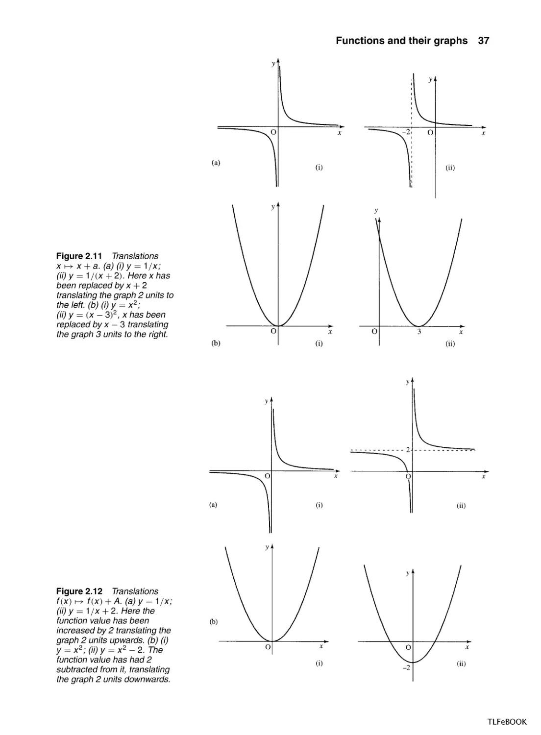
Figure 2.11 Translations
x → x + a. (a) (i) y = 1/x ;
(ii) y = 1/(x + 2). Here x has
been replaced by x + 2
translating the graph 2 units to
the left. (b) (i) y = x 2 ;
(ii) y = (x − 3)2 , x has been
replaced by x − 3 translating
the graph 3 units to the right.
Figure 2.12 Translations
f (x ) → f (x ) + A. (a) y = 1/x ;
(ii) y = 1/x + 2. Here the
function value has been
increased by 2 translating the
graph 2 units upwards. (b) (i)
y = x 2 ; (ii) y = x 2 − 2. The
function value has had 2
subtracted from it, translating
the graph 2 units downwards.
TLFeBOOK
38
Functions and their graphs
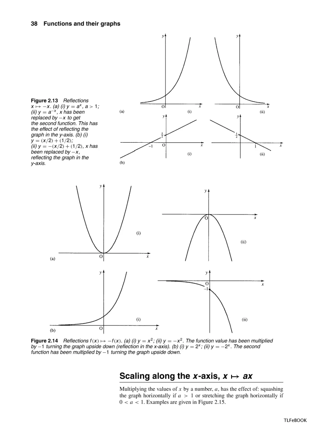
Figure 2.13 Reflections
x → −x . (a) (i) y = a x , a > 1;
(ii) y = a −x , x has been
replaced by −x to get
the second function. This has
the effect of reflecting the
graph in the y-axis. (b) (i)
y = (x /2) + (1/2);
(ii) y = −(x /2) + (1/2), x has
been replaced by −x ,
reflecting the graph in the
y-axis.
Figure 2.14 Reflections f (x ) → −f (x ). (a) (i) y = x 2 ; (ii) y = −x 2 . The function value has been multiplied
by −1 turning the graph upside down (reflection in the x-axis). (b) (i) y = 2x ; (ii) y = −2x . The second
function has been multiplied by −1 turning the graph upside down.
Scaling along the x -axis, x → ax
Multiplying the values of x by a number, a, has the effect of: squashing
the graph horizontally if a > 1 or stretching the graph horizontally if
0 < a < 1. Examples are given in Figure 2.15.
TLFeBOOK
Functions and their graphs
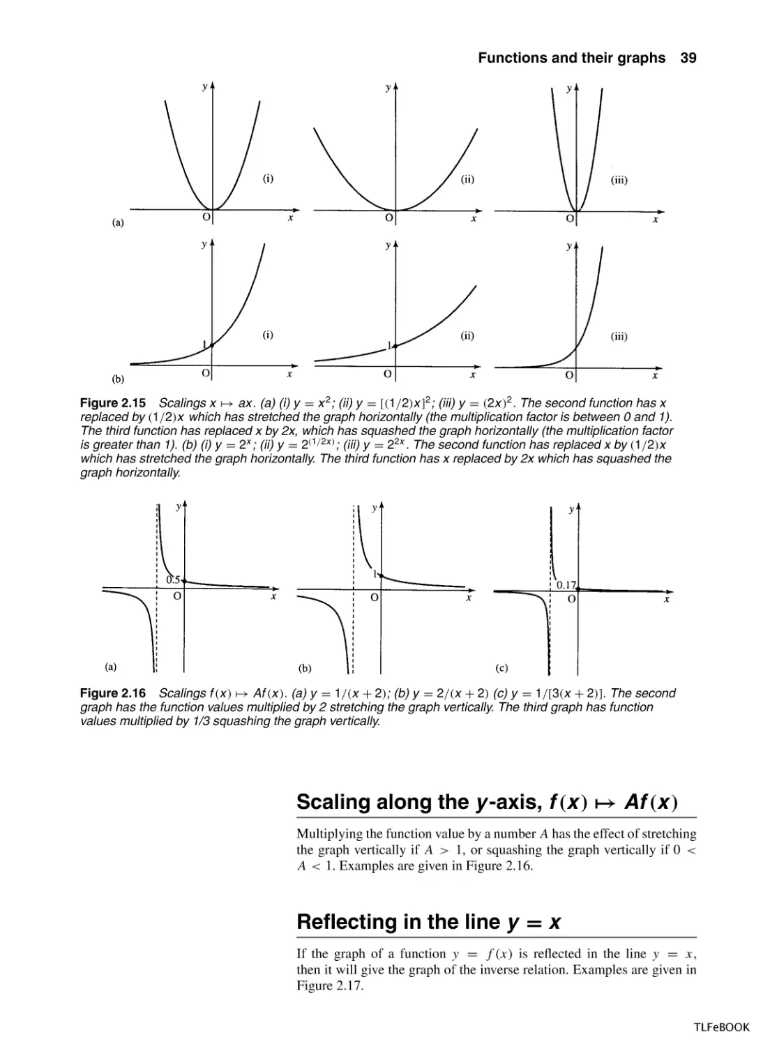
39
Figure 2.15 Scalings x → ax . (a) (i) y = x 2 ; (ii) y = [(1/2)x ]2 ; (iii) y = (2x )2 . The second function has x
replaced by (1/2)x which has stretched the graph horizontally (the multiplication factor is between 0 and 1).
The third function has replaced x by 2x, which has squashed the graph horizontally (the multiplication factor
is greater than 1). (b) (i) y = 2x ; (ii) y = 2(1/2x ) ; (iii) y = 22x . The second function has replaced x by (1/2)x
which has stretched the graph horizontally. The third function has x replaced by 2x which has squashed the
graph horizontally.
Figure 2.16 Scalings f (x ) → Af (x ). (a) y = 1/(x + 2); (b) y = 2/(x + 2) (c) y = 1/[3(x + 2)]. The second
graph has the function values multiplied by 2 stretching the graph vertically. The third graph has function
values multiplied by 1/3 squashing the graph vertically.
Scaling along the y -axis, f (x ) → Af (x )
Multiplying the function value by a number A has the effect of stretching
the graph vertically if A > 1, or squashing the graph vertically if 0 <
A < 1. Examples are given in Figure 2.16.
Reflecting in the line y = x
If the graph of a function y = f (x) is reflected in the line y = x,
then it will give the graph of the inverse relation. Examples are given in
Figure 2.17.
TLFeBOOK
40
Functions and their graphs
Figure 2.17 Reflections in the line y = x produce the inverse relation. (a) (i) y = 2x ; (ii) y = log2 (x ). The
second graph is obtained from the first by reflecting in the dotted line
√ y = x . The inverse is a function as there
2
is only one value of y for each value of x. (b) (i) y =
√ x ; (ii) y = ± x . The second graph is found by reflecting
the first graph in the line y = x . Notice that y = ± x is not a function as there is more that one possible
value of y for each value of x > 0.
In Chapter 1, we defined the inverse function as taking any image
back to its original value. Check this with the graph of y = 2x in
Figure 2.17(a): x = 1 gives y = 2. In the inverse function, y = log2 (x),
substitute 2, which gives the result of 1, which is back to the original
value.
√
However, the inverse of y = x 2 , y ± x, shown in Figure 2.17(b), is
not a function as there is more than one y value for a single value of x.
To understand this problem more fully, perform the following experiment. On a calculator enter −2 and square it (x 2 ) giving 4. Now take
the square root. This gives the answer 2, which is not the number we first
started with, and hence we can see that the square root is not a true inverse
of squaring. However, we get away with calling it the inverse because it
works if only positive values of x are considered. To test if the inverse
of any function exists, draw a line along any value of y = constant.
If, wherever the line is drawn, there is ever more than one x value
which gives the same value of y then the function has no inverse function. In this situation, the function is called a ‘many-to-one’ function.
Only ‘one-to-one’ functions have inverses. Figure 2.18 has examples
of functions with an explanation of whether they are ‘one-to-one’ or
‘many-to-one’.
TLFeBOOK
Functions and their graphs
41
Figure 2.18 (a) (i) y = x 3 . This function has only one x value for each value of y as any line y = constant
√
only cuts the graph once. In this case, the function is one-to-one and it has an inverse function (ii) y = 3 x is
the inverse function of y = x 3 . (b) y = 1/x , x = 0, has only one x value for each value of y as any line
y = constant only cuts the graph once. It therefore is one-to-one and has an inverse function – in fact, it is
its own inverse! (to see this reflect it in the line y = x and we get the same graph after the reflection).
(c) (i) y = x 4 . This function has two values of x for each value of y when y is positive (e.g. the line y = 16 cuts
the graph twice at x = 2 and at x = −2). This
√ shows that there is no inverse function as the function is
many-to-one. (ii) The inverse relation y = ± 4 x .
2.7 The
modulus
function,
y = |x | or
y = abs(x )
The modulus function y = |x|, often written as y = abs(x) (short for the
absolute value of x) is defined by
x x 0 (x positive or zero)
y=
−x x < 0 (x negative)
The output from the modulus function is always a positive number or zero.
Example 2.5 Find | − 3|.
Here x = −3, which is negative, therefore
y = −x = −(−3) = +3.
An alternative way of thinking of it is to remember that the modulus
is always positive, or zero, so simply replacing any negative sign by a
positive one will give a number’s modulus or absolute value.
| − 5| = 5,
| − 4| = 4,
|5| = 5,
|4| = 4.
The graph of the modulus function can be found from the graph of y = x
by reflecting the negative x part of the graph to make the function values
positive. This is shown in Figure 2.19.
TLFeBOOK
42
Functions and their graphs
Figure 2.19 The graph of the modulus function y = |x | obtained from the graph of y = x . (a) The graph of
y = x with the negative part of the graph displayed as a dotted line. This is reflected about the x-axis to give
y = −x for x < 0. (b) The graph of y = |x |.
2.8 Symmetry
of functions and
their graphs
Functions can be classified as even, odd, or neither of these.
Even functions
Even functions are those that can be reflected in the y-axis and then result
in the same graph. Examples of even functions are (see Figure 2.20):
y = x2,
y = |x|,
y = x4.
As previously discussed, reflecting in the y-axis results from replacing x
by −x in the function expression and hence the condition for a function
to be even is that substituting −x for x does not change the function
expression, that is, f (x) = f (−x).
Example 2.6 Show that 3x 2 − x 4 is an even function. Substitute −x
for x in the expression f (x) = 3x 2 − x 4 and we get
f (−x) = 3(−x)2 − (−x)4 = 3(−1)2 (x)2 − (−1)4 (x)4 = 3x 2 − x 4 .
So, we have found that f (−x) = f (x) and therefore the function is even.
Odd functions
Odd functions are those that when reflected in the y-axis result in an
upside down version of the same graph. Examples of odd functions are
(see Figure 2.21):
y = x,
y = x3,
y=
1
x
Reflecting in the y-axis results from replacing x by −x in the function
expression and the upside down version of the function f (x) is found by
multiplying the function by −1. Hence, the condition for a function to be
odd is that substituting −x for x gives −f (x), that is,
f (−x) = −f (x).
TLFeBOOK
Functions and their graphs
Figure 2.20
43
y = x 2 , y = |x |, and y = x 4 are even functions.
Figure 2.21 (a) y = x , (b) y = x 3 , (c) y = 1/x are odd functions. If they are reflected in the y-axis they
result in an upside down version of the original graph.
Example 2.7 Show that 4x − (1/x) is an odd function. Substitute x for
−x in the expression f (x) = 4x − (1/x) and we get
1
1
1
f (−x) = 4(−x) −
= −4x + = − 4x −
.
−x
x
x
We have found that f (−x) = −f (x), so the function is odd.
2.9 Solving
inequalities
For linear and quadratic functions, y = f (x), we have discussed how to
find the values where the graph of the functions crosses the x-axis, that is
how to solve the equation f (x) = 0. It is often of interest to find ranges
of values of x where f (x) is negative or where f (x) is positive. This
means solving inequalities like f (x) < 0 or f (x) > 0, respectively.
Like equations, inequalities can be solved by looking for equivalent
inequalities. One way of finding these is by doing the same thing to both
sides of the expression. There is an important exception for inequalities
TLFeBOOK
44
Functions and their graphs
that if both sides are multiplied or divided by a negative number then the
direction of the inequality must be reversed.
To demonstrate these equivalences begin with a true proposition
3 < 5 or
‘3 is less than 5’.
Add 2 on to both sides and it is still true
3 + 2 < 5 + 2,
i.e. 5 < 7.
Subtract 10 from both sides and we get
5 − 10 < 7 − 10,
i.e. − 5 < −3
which is also true.
Multiply both sides by −1 and if we do not reverse the inequality we get
(−1)(−5) < (−1)(−3),
i.e. 5 < 3
which is false. However, if we use the correct rule that when multiplying
by a negative number we must reverse the inequality sign then we get:
(−1)(−5) > (−1)(−3),
i.e. 5 > 3
which is true. This process is pictured in Figure 2.22.
Note that inequalities can be read from right to left as well as from left
to right: 3 < 5 can be read as ‘3 is less than 5’ or as ‘5 is greater than 3’
and so it can also be written the other way round as 5 > 3.
Using a number line to represent
inequalities
An inequality can be expressed using a number line as in Figure 2.23. In
Figure 2.23(a), the open circle indicates that 3 is not included in the set
of values, t < 3. In Figure 2.23(b), the closed circle indicates that −2 is
included in the set of values, x −2. In Figure 2.23(c), the closed circle
indicates that the value 4.5 is included in the set y 4.5.
Figure 2.22 On the number line, numbers to the left are less than numbers to their right: −5 < −3 . If the
inequality is multiplied by −1 we need to reverse the sign to get 5 > 3.
Figure 2.23
Representing inequalities on a number line.
TLFeBOOK
Functions and their graphs
Figure 2.24
The solution to 2t + 3 < t − 6 is given by t < −9.
Figure 2.25
The solution to x + 5 4x − 10 is found to be x 5, here represented on a number line.
Figure 2.26
The solution to 16 − y > −5y is found to be y > −4, here pictured on a number line.
45
Example 2.8 Find a range of values for t, x, and y such that the
following inequalities hold
(a) 2t + 3 < t − 6
(b) x + 5 4x − 10
(c) 16 − y > −5y
Solution
(a)
2t + 3 < t − 6
⇔
⇔
t < −6 − 3
⇔
t < −9.
2t − t + 3 < −6
(subtract t from both
sides)
(subtract 3 from both sides)
This solution can be represented on a number line as in Figure 2.24.
(b)
x + 5 4x − 10
⇔
+5 3x − 10
⇔
15 3x
⇔
5x
⇔
x 5.
(subtract x from both sides)
(add 10 to both sides)
(divide both sides by 3)
This solution in represented in Figure 2.25.
(c)
16 − y > −5y
⇔
16 > −4y
⇔
−4 < y
⇔
y > −4.
(add y to both sides)
(divide by − 4and reverse the sign)
This solution is represented in Figure 2.26.
Representing compound inequalities
on a number line
We sometimes need a picture of the range of values given if two inequalities hold simultaneously, for instance x 3 and x < 5. This is analysed
TLFeBOOK
46
Functions and their graphs
Figure 2.27
or x 0.
(a) x 3 and x < 5. (b) x > 6 and x > 2 combines to give x > 6. (c) x < 5 or x 7. (d) x < 2
in Figure 2.27(a) and we can see that for both inequalities to hold simultaneously x must lie in the overlapping region where 3 x < 5. 3 x < 5
is a way of expressing that x lies between 3 and 5 or is equal to 3. In the
example in Figure 2.27(b), x > 6 and x > 2, and for them both to hold
then x > 6.
Another possible way of combining inequalities is to say that one or
another inequality holds. Examples of this are given in Figure 2.27(c)
where x < 5 or x 7 and this gives the set of values less than 5 or
greater than or equal to 7. Figure 2.27(d) gives the example where x < 2
or x 0 and in this case it results in all numbers lying on the number
line, that is, x ∈ R.
Example 2.9 Find solutions to the following combinations of inequalities and represent them on a number line.
(a) x + 3 > 4 and x − 1 < 5,
(b) 1 − u < 3u + 2 or u + 2 6,
(c) t + 5 > 12 and −t > 24.
Solution
(a) x + 3 > 4 and x − 1 < 5 We solve both inequalities separately
and then combine their solution sets
x+3>4
⇔
x>1
(subtracting 3 from both sides)
x−1<5
⇔
x<6
(adding 1 to both sides)
So the combined inequality giving the solution is x > 1 and x < 6,
which from Figure 2.28(a) we can see is the same as 1 < x < 6.
(b) 1 − u < 3u + 2 or u + 2 6
We solve both inequalities separately and then combine their
TLFeBOOK
Functions and their graphs
Figure 2.28
47
Solutions to compound inequalities as given in Example 2.8 represented on a number line.
solution sets.
1 − u < 3u + 2
⇔
−1 < 4u
1
<u
4
1
⇔ u>−
4
u+26
⇔
−
⇔
u4
(subtracting 2 from both sides)
(dividing both sides by 4)
(subtracting 2 from both sides)
Combining the two solutions gives u > −1/4 or u 4 and this
is represented on the number line in Figure 2.28(b) where we can
see that it is the same as u > −1/4.
(c) t + 5 > 12 and − t > 24
t + 5 > 12
⇔
t >7
(subtracting 5 from both sides)
− t > 24
⇔
t < −24
(multiply both sides by −1 and reverse the
inequality sign)
Combining the two solutions sets gives t > 7 and t < −24 and we
can see from Figure 2.28(c) that this is impossible and hence there
are no solutions.
Solving more difficult inequalities
To solve more difficult inequalities, our ideas about equivalence are not
enough on their own, we also use our knowledge about continuous functions. In the previous chapter, we defined a continuous function as one
that could be drawn without taking the pen off the paper. If we wish to
solve the inequality f (x) > 0 and we know that f (x) is continuous then
we can picture the problem graphically as in Figure 2.29. From the graph
TLFeBOOK
48
Functions and their graphs
Figure 2.29 The graph of a continuous function. To solve for
f (x ) > 0, we first find the values where f (x ) = 0. On the graph these
are marked as a, b, c, and d. If the function is above the x-axis then
the function values are positive, if the function lies below the x-axis
then the function values are negative. The solution to f (x ) > 0 is
given by those values of x for which the function lies above the x-axis,
that is, y positive. For the function represented in the graph the
solution to f (x ) > 0 is x < a or b < x < c or x > d
.
Figure 2.30
Solving t 2 − 3t + 2 < 0 (Example 2.10).
we can see that to solve the inequality we need only find the values where
f (x) = 0 (the roots of f (x) = 0) and determine whether f (x) is positive
or negative between the values of x where f (x) = 0. To do this, we can
use any value of x between the roots. We are using the fact that as f (x)
is continuous then it can only change from positive to negative by going
through zero.
Example 2.10 Find the values of t such that t 2 − 3t < −2.
Write the inequality with 0 on one side of the inequality sign
t 2 − 3t < −2 ⇔ t 2 − 3t + 2 < 0
(adding 2 to both sides)
Find the solutions to f (t) = t 2 − 3t + 2 = 0 and mark them on a number
line as in Figure 2.30.
Using the formula
√
−b ± b2 − 4ac
t=
2a
where a = 1, b = −3, and c = 2 gives
√
−3 ± 9 − 8
t=
2
3±1
⇔t =
2
3+1
3−1
⇔t =
or t =
2
2
⇔ t = 2 or t = 1
Substitute values for t which lie on either side of the roots of f (t) in
order to find the sign of the function between the roots. Here we choose
0, 1.5, and 3.
TLFeBOOK
Functions and their graphs
49
When t = 0
t 2 − 3t + 2 = (0)2 − 3(0) + 2 = 0 + 0 + 2 = 2
which is positive, giving f (t) > 0.
When t = 1.5
t 2 − 3t + 2 = (1.5)2 − 3(1.5) + 2 = 2.25 − 4.5 + 2 = −0.25
which is negative giving f (t) < 0.
When t = 3
t 2 − 3t + 2 = (3)2 − 3(3) + 2 = 9 − 9 + 2 = 2
which is positive, giving f (t) > 0.
By marking the regions on the number line, given in Figure 2.30, with
f (t) > 0, f (t) < 0, or f (t) = 0 as appropriate we can now find the
solution to our inequality f (t) < 0 which is given by the region where
1 < t < 2.
Example 2.11
Find the values of x such that (x 2 − 4)(x + 1) > 0.
Solution The inequality already has 0 on one side of the inequality sign
so we begin by finding the roots to f (x) = 0, that is,
(x 2 − 4)(x + 1) > 0
Factorization gives
(x 2 − 4)(x + 1) > 0 ⇔ (x − 2)(x + 2)(x + 1) = 0
⇔ x = 2, x = −2, or x = −1. So the roots are −2, −1, and 2. These
roots are pictured on the number line in Figure 2.31.
Substitute values for x which lie on either side of the roots of f (x) in
order to find the sign of the function between the roots. Here we choose
−3, −1.5, 0, and 2.5.
When x = −3
(x − 2)(x + 2)(x + 1) = 0
gives
(−3 − 2)(−3 + 2)(−3 + 1)
= (−5)(−1)(−2)
= −10,
giving f (x) < 0.
When x = −1.5
(x − 2)(x + 2)(x + 1) gives
(−1.5 − 2)(−1.5 + 2)(−1.5 + 1)
= (−3.5)(0.5)(−0.5) = 0.875,
giving f (x) > 0.
When x = 0
(x − 2)(x + 2)(x + 1)
= (−2)(2)(1) = −4,
Figure 2.31
gives
(0 − 2)(0 + 2)(0 + 1)
giving f (x) < 0.
Solving (x 2 − 4)(x + 1) > 0 (Example 2.11).
TLFeBOOK
50
Functions and their graphs
When x = 2.5
(x − 2)(x + 2)(x + 1) gives (2.5 − 2)(2.5 + 2)(2.5 + 1)
= (0.5)(4.5)(3.5) = 7.875, giving f (x) > 0.
These regions are marked on the number line as in Figure 2.31 and
the solution is given by those regions where f (x) > 0. Looking for the
regions where f (x) > 0 gives the solution as −2 < x < −1 or x > 2.
2.10 Using
graphs to find
an expression
for the function
from
experimental
data
Linear relationships
Linear relationships are the easiest ones to determine from experimental
data. The points are plotted on a graph and if they appear to follow a
straight line then a line can be drawn by hand and the equation can be
found using the method given in Section 2.2.
Example 2.12 A spring is stretched by hanging various weights on it
and in each case the length of the spring is measured.
Mass (kg)
Length (m)
0.125
0.4
0.25 0.5
0.41 0.435
1
0.5
2
0.62
3
0.74
Approximate the length of the spring when no weight is hung from it
and find the expression for the length in terms of the mass.
Solution First, draw a graph of the given experimental data. This is done
in Figure 2.32.
A line is fitted by eye to the data. The data does not lie exactly on a line
due to experimental error and due to slight distortion of the spring with
heavier weights. From the line we have drawn we can find the gradient
by choosing any two points on the line and calculating
change in y
.
change in x
Taking the two points as (0,0.28) and (2,0.58), we get the gradient as
0.58 − 0.38
0.2
=
= 0.1.
2−0
2
The point where it crosses the y-axis, that is, where the mass hung
on the spring is 0 can be found by extending the line until it crosses the
y-axis. This gives 0.38 m.
Finally, the expression for the length in terms of the mass of the attached
weight is given by y = mx + c, where y is the length and x is the mass,
Figure 2.32 The data for
length of spring against mass
of the weight as given in the
Example 2.11. The line is a
fitted by eye to the
experimental data and the
equation of the line can be
found using the method of
Section 2.2.
TLFeBOOK
Functions and their graphs
51
m is the gradient and c is the value of y when x = 0, that is, where there
is no weight on the string. This gives
length = 0.1 × mass + 0.38
The initial length of the spring is 0.38 m.
Exponential relationships
Many practical relationships behave exponentially particularly those
involving growth or decay. Here it is slightly less easy to find the relationship from the experimental data, however, it is simplified by using a
log–linear plot. Instead of plotting the values of the dependent variable,
y, we plot the values of log10 (y). If the relationship between y and time,
t, is exponential as we suspected then the log10 (y) against t plot will be
a straight line.
The reason this works can be explained as follows. Supposing y = y0
10kt where y0 is the value of y when t = 0 and k is some constant; then,
taking the log base 10 of both sides, we get
log10 (y) = log10 (y0 10kt )
= log10 (y0 ) + log10 (10kt ).
As the logarithm base 10 and raising to the power of 10 are inverse
operations, we get
log10 (y) = log10 (y0 ) + kt
As y0 is a constant, the initial value of y, and k is a constant then we can
see that this expression shows that we shall get a straight line if log10 (y)
is plotted against t. The constant k is given by the gradient of the line and
log10 (y0 ) is the value of log10 y where it crosses the vertical axis. Setting
Y = log10 (y), c = log10 (y0 )
Y = c + kt
which is the equation of the straight line.
Example 2.13 A room was tested for its acoustical absorption properties by playing a single note on a trombone. Once the sound had reached its
maximum intensity, the player stopped and the sound intensity was measured for the next 0.2 s at regular intervals of 0.02 s. The initial maximum
intensity at time 0 is 1.0. The readings were as follows:
Time(s) 0
0.02 0.04 0.06 0.08 0.1 0.12 0.14 0.16 0.18 0.2
Intensity 1.0 0.63 0.35 0.22 0.13 0.08 0.05 0.03 0.02 0.01 0.005
Draw a graph of intensity against time and log(intensity) against
time and use the latter plot to approximate the relationship between the
intensity and time.
Figure 2.33 (a) Graph of
sound intensity against time
as given in Example 2.13.
(b) Graph of log10 (intensity)
against time and a line fitted
by eye to the data. The line
goes through the points (0,0)
and (0.2, −2.2).
Solution The graphs are plotted in Figure 2.33 where, for the second
graph (b), we take the log10 (intensity) and use the table below:
Time
0 0.02 0.04 0.06 0.08 0.1 0.12 0.14 0.16 0.18 0.2
log10
0 −0.22 −0.46 −0.66 −0.89 −1.1 −1.3 −1.5 −1.7 −2 −2.3
(intensity)
TLFeBOOK
52
Functions and their graphs
We can see that the second graph is approximately a straight line and
therefore we can assume that the relationship between the intensity and
time is exponential and could be expressed as I = I0 10kt . The log10 of
this gives
log10 (I ) = log10 (I0 ) + kt.
From the graph in Figure 2.33(b), we can measure the gradient, k. To do
this we calculate
change in log10 (intensity)
change in time
giving
−2.2 − 0
= −11 = k.
0.2 − 0
The point at which it crosses the vertical axis gives
log10 (I0 ) = 0 ⇔ I0 = 100 = 1.
Therefore, the expression I = I0 10kt becomes
I = 10−11t .
Power relationships
Another common type of relationship between quantities is when there
is a power of the independent variable involved. In this case, if y = ax n
where n could be positive or negative then the value of a and n can be
found by drawing a log–log plot.
This is because taking log10 of both sides of y = ax n gives
log10 (y) = log10 (ax n ) = log10 (a) + n log10 (x)
Replacing Y = log10 (y) and X = log10 (x) we get:
Y = log10 (a) + nX,
showing that the log–log plot will give a straight line, where the slope of
the line will give the power of x and the position where the line crosses
the vertical axis will give the log10 (a). Having found a and n, they can
be substituted back into the expression
y = ax n .
Example 2.14 The power received from a beacon antenna is though to
depend on the inverse square of the distance from the antenna and the
receiver. Various measurements, given below, were taken of the power
received against distance r from the antenna. Could these be used to justify
the inverse square law? If so, what is the constant, A, in the expression:
p=
A
r2
Power received (W)
Distance from antenna (km)
0.39
1
0.1
2
0.05
3
0.025
4
0.015
5
0.01
6
TLFeBOOK
Functions and their graphs
53
Figure 2.34 (a) Plot of power against distance (Example 2.14). (b) log10 (power) against log10 (distance). In
(b), the line is fitted by eye to the data, from which the slope of the graph indicates n in the relationship
P = Ar n . Two points lying on the line are (0, −0.38) and (0.7, −1.8).
Solution To test whether the relationship is indeed a power relationship,
we draw a log–log plot. The table of values is found below:
log10 (power)
log10 (distance)
−0.41
0
−1
0.3
−1.3
0.5
−1.6
0.6
−1.8
0.7
−2
0.78
Graphs of power against distance and log10 (power) against
log10 (distance) are given in Figure 2.34(a) and (b).
As the second graph is a straight line, we can assume that the relationship is of the form P = Ar n where P is the power and r is the distance.
In which case, the log–log graph is
log10 (P ) = log10 (A) + n log10 (r).
We can measure the slope by calculating
change in log10 (P )
change in log10 (r)
and, using the two points that have been found to lie on the line, this gives
−1.8 − (−0.38)
= −2.03.
0.7 − 0
As this is very near to −2, the inverse square law would appear to be
justified.
The value of log10 (A) is given from where the graph crosses the vertical
axis and this gives
log10 (A) = −0.38
⇔
A = 10−0.38
⇔
A = 0.42.
So the relationship between power received and distance is approximately
P = 0.42r −2 =
0.42
.
r2
TLFeBOOK
54
Functions and their graphs
2.11 Summary
The linear function y = mx + c has gradient (slope) m and crosses
the y-axis at y = c.
2. The gradient, m, of a straight line y = mx + c is given by:
1.
m=
3.
change in y
change in x
and this is the same along the length of the line.
The equation of a line which goes through two points, (x1 , y1 ) and
(x2 , y2 ) is:
x − x1
y − y1
=
y2 − y 1
x2 − x 1
where y2 = y1 .
The graph of the quadratic function y = ax 2 + bx + c is called a
parabola. The graph crosses the y-axis (when x = 0) at y = c.
5. There are three possibilities for the roots of the quadratic equation
a x 2 + bx + c = 0
Case I: two real roots when b2 − 4ac > 0,
Case II: only one unique root when b2 − 4ac = 0,
Case III: no real roots when b2 − 4ac < 0.
6. By considering the graphs of known functions y = f (x), for
instance, those given in Figure 2.10, and the following transformations, many other graphs can be drawn.
(a) Replacing x by x + a in the function y = f (x) results in
shifting the graph a units to the left.
(b) Replacing f (x) by f (x) + A results in shifting the graph A
units upwards.
(c) Replacing x by −x reflects the graph in the y-axis.
(d) Replacing f (x) by −f (x) reflects the graph in the x-axis
(turning it upside down).
(e) Replacing x by ax squashes the graph horizontally if a > 1
or stretches it horizontally if 0 < a < 1.
(f) Replacing f (x) by Af (x) stretches the graph vertically if A >
1 or squashes it vertically if 0 < A < 1.
(g) Reflecting the graph of y = f (x) in the line y = x results in
the graph of the inverse relation.
7. A function may be even, or odd, or neither of these.
(a) An even function is one whose graph remains the same if
reflected in the y-axis, that is, when x → −x. This can also
be expressed by the condition
4.
f (−x) = f (x)
(b)
Examples of even functions are y = x 2 , y = |x|, and y = x 4 .
An odd function is one which when reflected in the y-axis,
that is, when x → −x, gives an upside down version of the
original graph (i.e. −f (x)). This can also be expressed as the
condition:
f (−x) = −f (x)
8.
Examples of odd functions are y = x and y = x 3 .
Not all functions have true inverses. Only one-to-one functions have
inverse functions. A function is one-to-one if any line y = constant
drawn on the graph y = f (x) crosses the function only once. This
means there is exactly one value of x that gives each value of y.
TLFeBOOK
Functions and their graphs
55
9.
Simple inequalities can be solved by finding equivalent inequalities.
Inequalities remain equivalent if both sides of the inequality have the
same expression added or subtracted. They may also be multiplied
or divided by a positive number but if they are multiplied or divided
by a negative number then the direction of the inequality sign must
be reversed.
10. To solve the inequalities f (x) > 0, f (x) < 0, f (x) 0, or f (x)
0, where f (x) is a continuous function, solve f (x) = 0 and choose
any value for x around the roots to find the sign of f (x) for each
region of values for x.
11. Graphs can be used to find relationships in experimental data. First,
plot the data then:
(a) If the data lies on an approximate straight line then draw a
straight line through the data and find the equation of the line.
(b) If it looks exponential, then take the log of the values of
the dependent variable and draw a log–linear graph. If this
looks approximately like a straight line then assume there is
an exponential relationship y = y0 10kt , where k is given by
the gradient of the line and log10 (y0 ) is the value where the
graph crosses the vertical axis.
(c) If the relationship looks something like a power relationship,
y = Ax n , then take the log of both sets of data and draw
a log–log graph. If this is approximately like a straight line,
then assume there is a power relationship and n is given by the
gradient of the line and log10 A is the value where the graph
crosses the vertical axis.
2.12 Exercises
2.1. Sketch the graphs of the following:
(a) y = 3x − 1,
(c) y = −5x,
(b) y = 2x + 1,
(d) y = 21 x − 3.
In each case state the gradient of the line.
2.2. A straight line passes through the pair of points given.
Find the gradient of the line in each case.
(a) (0, 1), (1, 4)
(c) (−1, −1), (6, 3)
(b) (1, 1), (2, −4)
(d) (1, 4), (3, 4)
2.3. A straight line graph has gradient −5 and passes
through (1,6). Find the equation of the line.
2.4. In Figure 2.35 are various graphs drawn to the scale
1 unit = 1 cm. By finding the gradients of the lines
and where they cross the y-axis, find the equation of
the line.
Figure 2.35 Straight line graphs for
Exercise 2.4.
2.5. A straight line passes through the pair of points given.
Find the equation of the line in each case.
(a) (0, 1), (−1, 4)
(c) (1, 1), (6, 3)
(b) (1, 1), (−2, −4)
(d) (−1, −4), (−3, −4)
TLFeBOOK
56
Functions and their graphs
2.6. Find the values of x such that f (x) = 0 for the
following functions
(a) f (x) = x 2 − 4,
(b) f (x) = (2x − 1)(x + 1),
(c) f (x) = (x − 3)2 ,
(d) f (x) = (x − 4)(x + 4),
(e) f (x) = x 2 + x − 6,
(f) f (x) = x 2 + 7x + 12,
(g) f (x) = 12x 2 − 12x − 144.
Using the fact that the peak or trough in the parabola,
y = f (x), occurs at a value of x half-way between
the values where f (x) = 0 then sketch graphs of the
above quadratic functions.
2.7. By considering transformations of simple functions
sketch graphs of the following:
(a) y =
(c) y =
(b) y = 3.2−x ,
1
x−(1/2) ,
1 3
2x ,
(d) y = −3(1/2)x ,
(e) y = (2x − 1)
(g) y = log2 (x + 2),
2
(f) y = (2x − 1)2 − 2,
(h) y = 6 − 2x ,
(i) y = 4x − x 2 .
2.8. Consider reflections of the graphs given in Figure 2.36
to determine whether they are even, odd, or neither of
these.
2.9. By substituting x → −x in the following functions
determine whether they are odd, even, or neither of
these:
(a) y = −x 2 + x12 where x = 0,
(b) y = |x 3 | − x 2 ,
(c) y =
(d) y =
−1
x
−1
x
+ log2 (x) where x > 0,
+ x + x5,
(e) y = 6 + x 2 ,
(f) y = 1 − |x|.
2.10. Draw graphs of the following functions and draw the
graph of the inverse relation in each case. Is the inverse
a function?
(a) f (t) = −t + 2, (b) g(x) = (x − 2)2 ,
4
.
(c) h(w) =
w+2
2.11. Find the range of values for which the following
inequalities hold and represent them on a number line.
(a) 10t − 2 31,
(c) 3 − 4y 11 + y,
(b) 10x − 3x > −2,
(d) t + 15 < 6 − 2t.
2.12. Find the range of values for which the following hold
and represent them on a number line:
(a) x − 2 > 4 or 1 − x < 12,
(b) 4t + 2 10 and 3 − 2t < 1,
(c) 3u + 10 > 16 or 3 − 2u > 13.
2.13. Solve the following inequalities and represent the
solutions on a number line:
(b) (2x − 3)(x + 1)(x − 5) > 0,
(a) x 2 − 4 < 5,
(c) t 2 + 4t 21, (d) 4w 2 + 4w − 35 0.
2.14. For the following sets of data, y is thought to depend
exponentially on t. Draw log–linear graphs in each case
and find constants A and k such that y = A10kt .
(a)
y
t
75
1
48
2
y
t
2
0.1
4.2
0.2
30
3
19
4
12
5
7
6
(b)
8.5
0.3
18
0.4
35
0.5
73
0.6
2.15 An experiment measuring the change in volume of a
gas as the pressure is decreased gave the following
measurements:
P (105 N m−2 ) 1.5 1.4 1.3 1.2 1.1 1
0.95 1
1.05 1.1 1.16 1.24
V (m3 )
If the gas is assumed to be ideal and the expansion is
adiabatic then the relationship between pressure and
volume should be:
pV γ = C
Figure 2.36 Graphs of functions for
Exercise 2.7.
where γ and C are constants and p is the pressure and V is the volume. Find reasonable values
of γ and C to fit the data and from this expression
find the predicted volume at atmospheric pressure,
p = 1.013 × 10⁵ N m−2 .
TLFeBOOK
3
3.1 Introduction
Figure 3.1 A simple circuit.
Problem solving
and the art of the
convincing
argument
Mathematics is used by engineers to solve problems. This usually involves
developing a mathematical model. Just as when building a working model
aeroplane we would hope to include all the important features, the same
thing applies when building a mathematical model. We would also like to
indicate the things we have had to leave out because they were too fiddly
to deal with, and also those details that we think are irrelevant to the
model. In the case of a mathematical model the things that have been left
out are listed under assumptions of the model. To build a mathematical
model, we usually need to use scientific rules about the way things in the
world behave (e.g. Newton’s laws of motion, conservation of momentum
and energy, Ohm’s law, Kirchoff’s laws for circuits, etc.) and use numbers, variables, equations, and inequalities to express the problem in a
mathematical language.
Some problems are very easy to describe mathematically. For instance:
‘Three people sitting in a room were joined by two others, how many
people are there in the room in total?’ This can be described by the sum
3 + 2 =? and can be solved easily as 3 + 2 = 5.
The final stage of solving the problem is to translate it back into the
original setting – the answer is: ‘there are 5 people in the room in total’.
Assumptions were used to solve this problem. We assumed that no
one else came in or left the room in the meantime and we made general
assumptions about the stability of the room, for example, the building
containing it did not fall down. However, these assumptions are so obvious
that they do not need to be listed. In more complex problems it is necessary
to list important assumptions as they may have relevance as to the validity
of the solution.
Another example is as follows: ‘There are three resistors in series in a
circuit, two of the resistors are known to have resistance of 3 and 4 ohm,
respectively. The voltage source is a battery of 12 V and the current is
measured as 1 A. What is the resistance of the third resistor?’
To help express the problem in a mathematical form we may draw a
circuit diagram as in Figure 3.1.
The problem can be expressed mathematically by using Ohm’s law
and the fact that an equivalent resistance to resistances in series is given
by the sum of the individual resistances. If x is the unknown value of the
TLFeBOOK
58
Problem solving and the art of the convincing argument
third resistance and V = RI where R = R1 + R2 + R3 , we obtain:
12 = (3 + 4 + x)1
The expression of the mathematical problem has taken the form of an
equation where we now need to find x, the value of the third resistance.
The main assumptions that have been used to build this mathematical
model are:
(1)
There are such things as pure resistors that have no capacitance or
inductance.
(2) Resistances remain constant and are not affected by any possible
temperature changes or other environmental effects.
(3) The battery gives a constant voltage that does not deteriorate with
time.
(4) The battery introduces no resistance to the circuit.
These assumptions are simplifications that are acceptable because
although the real world cannot behave with the simplicity of the
mathematical model, the amount of error introduced by making these
assumptions is small.
Once we have the solution of a mathematical model then it should
be tested against a real-life situation to see whether the model behaves
reasonably closely to reality. Once the model has been accepted then it
can be used to predict the behaviour of the system for input values other
than those that it has been tested for.
The stages in solving a problem are as follows:
(1)
Take to real problem and express it as a mathematical one using any
necessary scientific rules and assumptions about the behaviour of
the system and using letters to represent any unknown quantities.
Include an account of any important assumptions and simplifications
made.
(2) Solve the mathematical problem using your knowledge of
mathematics.
(3) Translate the mathematical solution back into the setting of your
original problem.
(4) Test the model solutions for some values to check that it behaves
like the real-life problem.
Most mathematical problems are expressed by using equations, or
inequalities, differential or difference equations, or by expressing a problem geometrically or a combination of all of these. We might need to
incorporate a random element which results in the need to use a probabilistic model. In many of the following chapters we will look at the
modelling process in more detail as we come across new mathematical
tools and the situations in which they are used. To perform the entire
modelling cycle properly, we need to be able to test our results in a reallife situation in order to reconsider assumptions used in the model. This
would require access to engineering situations and tools. For this reason,
engineering mathematics books tend to concentrate on those models that
are commonly used by engineers. Many of the applied problems presented in the following chapters however do present an opportunity to
move from an English language description of a problem to a mathematical language description of a problem, which is an important step in the
modelling process.
In this chapter, we will look at translating a problem into mathematical
language and, for the main part of the chapter, we concentrate on solving
a mathematical problem and the reasoning that is involved in so doing.
TLFeBOOK
Problem solving and the art of the convincing argument
59
To solve the problem using your knowledge of mathematics, we need to
use the ideas of mathematical statements and how to decide whether, and
express the fact that, one statement leads logically on to the next. We
shall mainly use examples of solving equations and inequalities although
the same ideas apply to the solving of all problems.
3.2 Describing
a problem in
mathematical
language
The stages in expressing a problem in mathematical language can be
summarized as:
(1)
(2)
Assign letters to represent the unknown quantities.
Write down the known facts using equations and inequalities, and
using drawings and diagrams where necessary.
(3) Express the problem to be solved mathematically.
This is not a simple process because it involves a great deal of interpretation of the original problem. It is useful to try to limit the number
of unknowns used as much as possible, or the problem may appear more
difficult than necessary.
Example 3.1 Express the following problem mathematically: A web
development company employs a freelance web designer and a freelance
graphic designer to put up listings for new businesses on to their virtual
business park website. Business customers are charged e200 per year
for a listing. The fixed costs of the web development company amount
to e2000 per week over 52 weeks in the year. The web designer charges
e80 per listing and the graphic designer e100 per listing and both can
prepare these at the rate of 2.4 listings in a day. The freelancers work for
up to 200 days per year. How many listings does the company need in
the first year to break even?
Solution The mathematical problem can be expressed by firstly assigning letters to some of the unknown quantities and then write down all the
known facts as equations or inequalities.
First assign letters: Total number of listings of businesses on the park
in the first year is L. LW is the number of listings prepared by the web
designer and LG is the number of listings prepared by the graphic designer.
The costs are K per year and the profit is P . The known facts can be
expressed as follows:
L = LW + L G
This expresses the fact that the total number of listings L is made up of
those prepared by the web designer and those prepared by the graphic
designer. As there are up to 200 working days in a year and they both do
a maximum of 2.4 listings per day.
0 LW 480,
0 LG 480
The costs, K, are; fixed costs of 2000 × 52, plus the cost of the freelance
web designer at 80LW , plus the cost of the freelance graphic designer at
TLFeBOOK
60
Problem solving and the art of the convincing argument
100LG . This can be expressed as:
K = 104 000 + 80LW + 100LG .
We need to relate the profit to the other variables. As the profit is 200
multiplied by the number of jobs minus the total costs, we get:
P = 200L − K
Finally, we must express the mathematical problem that we would like to
solve. For the web development business to make a profit in the first year
then the profit must be positive, hence we get the problem expressed as:
Find the minimum L such that P > 0.
Example 3.2 Express the following in mathematical language: A car
brake pedal, as represented in Figure 3.2(a) is pivoted at point A. What
is the force on the brake cable if a constant force of 900 N is applied by
the driver’s foot and the pedal is stationary.
Solution First, we assign letters to the unknowns. Let F = the force on
the brake cable.
In order to write down the known facts we need to consider what
scientific laws can be used. As the force applied on the pedal initially
provides a turning motion then we know to use the ideas of moments.
The moment of a force about an axis is the product of the force F and its
perpendicular distance, x, to the line of action of the force. Furthermore,
as the pedal is now stationary, then the moments must be balanced so the
clockwise moment must equal the anti-clockwise moment.
To use this fact, we need to use two further measurements, currently
unknown, the perpendicular distance from the line of action of the force
provided by the driver to the axis, A. This is marked as x1 m on the diagram
in Figure 3.2(b). The other distance is the perpendicular distance from
the line of action of the force on the cable to the axis A. This is marked
as x2 m in Figure 3.2(b).
We can now write down the known facts, involving the unknowns
x1 , x2 , and F . From the right angle triangle containing x1 , we have
Figure 3.2 (a) A representation of a car brake pedal. (b) The same diagram as (a) with some unknown
quantities marked and triangles used to formulate the problem.
TLFeBOOK
Problem solving and the art of the convincing argument
61
(converting 210 mm = 0.21 m),
x1
cos(40◦ ) =
0.21
From the right angle triangle containing x2 , we have (converting 75 mm =
0.075 m),
x2
cos(15◦ ) =
0.075
The moments of the forces can now be calculated and equated. The clockwise moment is 800x1 and the anti-clockwise moment is given by F x2
and hence we have:
800x1 = F x2
Finally, we need to express the problem we are trying to solve. In this
case it is simply ‘what is F ?’.
Note that in both Examples 3.1 and 3.2, certain modelling assumptions
had been used in order to formulating the ‘natural language’ description
of the problem that we were given. For instance, it is probable that the
business park listings for the business park in Example 3.1 are not all
identical and therefore average figures for times and costings have been
used. Similarly, in Example 3.2 no mention has been made of friction
would provide an extra force to consider. Here we have only considered the transition from natural language and accompanying diagrams
to the mathematical problem. We have implicitly assumed that the modelling process can be performed in two stages. From real-life problem
to a natural language description which incorporates some simplifying
assumptions, and then from there to a mathematical description. In reality
modelling a system is much more involved. We would probably repeat
stages in this process if we decided that the mathematical description was
too complex and return to the real-life situation in order to make new
assumptions.
We are now in a position to discuss mathematical statements and how
to move from the statement of the problem to finding the desired solution.
3.3
Propositions
and predicates
When we first set up a problem to be solved, we write down mathematical
expressions like:
2 + 3 =?
(3.1)
and
12 = (3 + 4 + x) · 1
(3.2)
These are mathematical statements with an unknown value. Statements
containing unknowns (or variables) are called predicates. A predicate can
be either true or false depending on the value(s) substituted into it. When
values are substituted into a predicate it becomes a simple proposition. If
in Equation (3.1) we substitute 5 for the question mark we get:
2+3=5
⇔
5=5
which is true.
If, however, we substitute 6 we get:
2+3=6
⇔
5=6
which is false.
2 + 3 = 5 and 2 + 3 = 6 are examples of propositions. These are simple
statements that can be assigned as either true or false. They contain no
TLFeBOOK
62
Problem solving and the art of the convincing argument
unknown quantities. Notice that if we simply rewrite a proposition or
predicate we use ‘≡’ or ‘⇔’ to mean ‘is equivalent to’ or ‘is the same as’.
In Equation (3.2) if we substitute 4 for x we get:
12 = 11 which is false
but, if we substitute 5 for x we get
12 = 12
which is true.
Example 3.3
Assign true or false to the following:
(a) (3x − 2)(x + 5) = 10 where x = 1
(b) 5x 2 − 2x + 1 = 25 where x = −2
(c) y > 5t + 3 where y = 2 and t = −3
Solution
(a)
Substitute x = 1 in the expression and we get:
(3 · 1 − 2)(1 + 5) = 10
(b)
⇔
1(6) = 10
⇔
6 = 10
which is false.
Substituting x = −2 into 5x 2 − 2x + 1 = 25 gives
5(−2)2 − 2(−2) + 1 = 25
(c)
⇔
20 + 4 + 1 = 25
⇔
25 = 25
which is true.
Substituting y = 2 and t = −3 into y > 5t + 3 gives
2 > 5(−3) + 3
⇔
2 > −15 + 3
⇔
2 > −12
which is true.
Like functions, predicates have a domain which is the set of all allowed
inputs to the predicate. For instance, the predicate 1/(x − 1) = 1, where
x ∈ R, has the restriction that x = 1, as letting x equal 1 would lead to
an √
attempt to divide by 0, which is not defined.
x − 2 = 25 where x ∈ R has the restriction that x 2, as values of
x less than 2 would lead to an attempt to take the square root of a negative
number, which is not defined.
3.4 Operations
on propositions
and predicates
Consider the problem given in Example 3.1. Notice that the conditions
that we discovered when writing down the known facts must all be true
in any solution that we come up with. If any one of these conditions is
not true then we cannot accept the solution. The first condition must be
true and the second and the third, etc.
Here we have an example of an operation on predicates. In Chapter 1,
we defined an operation on numbers is a way of combining two numbers
to give a single number. ‘And’, written as ∧ is an operation on two
predicates or propositions which results a single predicate or proposition.
TLFeBOOK
Problem solving and the art of the convincing argument
Table 3.1 Truth table
for the operation ‘and’.
This table can also be
expressed by
T ∧ T ⇔ T,
T ∧ F ⇔ F,
F ∧ T ⇔ F,
F ∧ F ⇔ F . T stands
for ‘true’ and F stands
for ‘false’
p
q
p∧q
T
T
F
F
T
F
T
F
T
F
F
F
Table 3.2 Truth table
for ‘or’, This table can
also be expressed by
T ∨ T ⇔ T,
T ∨ F ⇔ T,
F ∨ T ⇔ T,
F ∨F ⇔F
p
q
p∨q
T
T
F
F
T
F
T
F
T
T
T
F
Table 3.3 The truth
table for ‘not’, ¬. This
table can also be
expressed by
¬T ⇔ F , ¬F ⇔ T
Therefore, to express the fact that both L 0 and L = LW + LG we can
write
L 0 ∧ L = LW + LG
and the compound statement is true if each part is also true.
As propositions can only be either true (T) or false (F), all possible
outcomes of the operation can easily be listed in a small table called a
truth table. The truth table for the operation of ‘and’ is given in Table 3.1.
p and q represent any two propositions, for instance, for some given
values of L, LW , and LG , p and q could be defined by:
p: ‘L 0’
q: ‘L = LW + LG ’
Another important operation is that of ‘or’. One example of the use of
this operation comes about by solving a quadratic equation. One way of
solving quadratic equations is to factorize an expression which is equal
to 0.
To solve x 2 − x − 6 = 0, the left-hand side of the equation can be
factorized to give (x − 3)(x + 2) = 0.
Now we use the fact that for two numbers multiplied together to equal
0 then one of them, at least, must be 0, to give:
(x − 3)(x + 2) = 0
¬p
T
F
F
T
⇔
(x − 3) = 0
or (x + 2) = 0
‘or’ can be written using the symbol ∨. The compound statement is true
if either x − 3 = 0 is true or if x + 2 = 0 is true. Therefore, to express
the statement that either x − 3 = 0 or x + 2 = 0 we can write:
(x − 3) = 0 ∨ (x + 2) = 0
∨ is also called ‘non-exclusive or’ because it is also true if both parts of
the compound statement are true. This usage is unlike the frequent use of
‘or’ in the English language, where it is often used to mean a choice, for
example, ‘you may have either an apple or a banana’ implies either one
or the other but not both. This everyday usage of the word ‘or’ is called
‘exclusive or’.
The truth table for ‘or’ is given in Table 3.2.
A further operation is that of ‘not’ which is represented by the
symbol ¬. For instance, we could express the sentence ‘x is not bigger
than 4’ as ¬(x > 4).
The truth table for ‘not’ is given in Table 3.3.
Example 3.4
p
63
(a)
(b)
(c)
(d)
Assign truth values to the following:
x − 2 = 3 ∧ x 2 = 4 when x = 2
x − 2 = 3 ∨ x 2 = 4 when x = 2
¬(x − 4 = 0) when x = 4
¬((a − b) = 4) ∨ (a + b) = 2 when a = 5, b = 3
Solution
(a) x − 2 = 3 ∧ x 2 = 4 when x = 2
Substitute x = 2 into the predicate, x − 2 = 3 ∧ x 2 = 4 and we get
2 − 3 = 3 ∧ 22 = 4.
TLFeBOOK
64
Problem solving and the art of the convincing argument
The first part of the compound statement is false and the second part
is true. Overall, as F ∧ T ⇔ F , the proposition is false.
(b)
x − 2 = 3 ∨ x 2 = 4 when x = 2
Substitute x = 2 into the predicate and we get
2 − 2 = 3 ∨ 22 = 4
The first part of the compound statement is false and second part is
true. As F ∨ T ⇔ T , the proposition is true.
(c) ¬(x − 4 = 0) when x = 4
When x = 4 the expression becomes:
¬(4 − 4 = 0)
⇔
¬T
⇔
F
(d) ¬((a − b) = 4) ∨ (a + b) = 2 when a = 5, b = 3
¬((a − b) = 4)
¬(5 − 3 = 4)
(a + b) = 2
when a = 5, b = 3 gives
⇔
¬F
⇔
T
when a = 5, b = 3 gives
(5 + 3) = 2
⇔
8=2
⇔
F
Overall, T ∨ F ⇔ T so ¬((a − b) = 4) ∨ (a + b) = 2 when a = 5,
b = 3 is true.
Example 3.5
Represent the following inequalities on a number line:
(a) x > 2 ∧ x 4
(b) x < 2 ∨ x 4
(c) ¬(x < 2)
Solution
(a) x > 2 ∧ x 4. To represent the operation of ‘and’, find where
the two regions overlap (Figure 3.3a). x > 2 ∧ x 4 can also be
represented by 2 < x 4.
(b) x < 2 ∨ x 4. To represent the operation of ∨, ‘or’, take all points
on the first highlighted region as well as all points in the second
highlighted region and any end points (Figure 3.3b).
(c) ¬(x < 2). To represent the operation of ‘not’ take all the points on
the number line not in the original region (Figure 3.3c). This can
also be expressed by x 2.
3.5 Equivalence
We can now express an initial problem in terms of a predicate, probably an
equation, a number of equations, or a number of inequalities. However, to
solve the problem we need to be able to move from the original expression
of the problem toward the solution. In Chapter 3 of the Background
Mathematics Notes, available on the companion website for this book,
we discussed how to solve various types of equations and introduced the
idea of equivalent equations. In Chapter 2 we also looked at equivalent
inequalities. In both cases we used the idea that in moving from one
expression to an equivalent expression the set of solutions remained the
TLFeBOOK
Problem solving and the art of the convincing argument
65
Figure 3.3 The operations (a)∧ (and); (b) ∨ (or); and (c) ¬ (not).
same. In general, two predicates are equivalent if they are true for exactly
the same set of values. We use our knowledge of mathematics to determine
what operations can be performed that will maintain that equivalence.
The rule that can be used to move from one equation to another was
given as: ‘Equations remain equivalent if the same operation is performed
to both sides of the equation’. In the case of quadratic equations we
can also use a formula for the solution or use a factorization and the
fact that:
ab = 0
⇔
a=0
or b = 0.
In passing from one equation to an equivalent equation we should use the
equivalence symbol. This then makes a mathematical sentence:
x+5=3
⇔
x =3−5
can be read as ‘The equation x + 5 = 3 is equivalent to x = 3 − 5’.
In all but the most obvious cases, it is a good practice to list a short
justification for the equivalence by the side of the expression.
x+5=3
⇔
x =3−5
⇔
x = −2.
(subtracting 5 from both sides)
Because of the possibility of making a mistake, the solution(s) should
be checked by substituting the values into the original expression of the
problem. To check, substitute x = −2 into the original equation giving
−2 + 5 = 3 which is true, indicating that the solution is correct.
Example 3.6
Solve the following equation:
x − 3 = 5 − 2x.
TLFeBOOK
66
Problem solving and the art of the convincing argument
Solution
x − 3 = 5 − 2x
⇔
x + 2x − 3 = 5
(adding 2x to both sides)
⇔
3x = 8
(adding 3 to both sides)
⇔
x=
(dividing both sides by 3).
8
3
Check by substituting x = 8/3 into the original equation:
8
3
−3=5−2×
⇔
− 13 =
8
3
1
−3,
which is true.
We looked at methods of solving inequalities in Chapter 2. The rules
for finding equivalent inequalities were: ‘Perform the same operation to
both sides’; but in the case of a negative number when multiplying or
dividing the direction of the inequality sign must be reversed. To solve
more complex inequalities, such as f (x) > 0, f (x) < 0, where f (x) is
a continuous but non-linear function, then we solve f (x) = 0 and then
use a number line to mark regions where f (x) is positive, negative or
zero. The important thing in the process is to present a short justification
of the equivalence. Finally, when the set of solutions has been found,
some of the solutions can be substituted into the original expression of
the problem in order to check that no mistakes have been made.
Solve the following inequalities:
Example 3.7
(a) 3x − 1 < 6x + 2
(b) x 2 − 5x > −6
Solution
(a)
3x − 1 < 6x + 2
⇔
−1 < 6x + 2 − 3x
(subtracting 3x from both sides)
⇔
−1 − 2 < 3x
(subtracting 2 from both sides)
⇔
−
⇔
3x
3
<
3
3
−1 < x
⇔
x > −1
(dividing both sides by 3)
Check: Test a few values from the set x > −1 and substitute into
3x − 1 < 6x + 2
Try x = 0: this gives −1 < 2 ⇔ T
Try x = 2: this gives 3(2) − 1 < 6(2) + 2 ⇔ 5 < 14 ⇔ T
(b)
x 2 − 5x > −6
Write the inequality with 0 on one side of the inequality sign
x 2 − 5x > −6
⇔
x 2 − 5x + 6 > 0
(adding 6 to both sides)
Find the solutions to f (x) = 0 where f (x) = x 2 − 5x + 6 and mark
them on a number line as in Figure 3.4.
√
5 ± 25 − 24
x 2 − 5x + 6 = 0 ⇔ x =
2
TLFeBOOK
Problem solving and the art of the convincing argument
67
Figure 3.4 Solving x 2 − 5x + 6 > 0.
(using the formula for solution of quadratic equations)
⇔
⇔
5−1
5+1
∨x =
2
2
x =3∨x =2
x=
Using the fact that the function is continuous, we can substitute values
for x which lie on either side of the roots of f (x) = 0 in order to find the
sign of the function in that region. Here, we choose 0, 2.5, and 4 and find
that
when x = 0:
f (x) = x 2 − 5x + 6 = 6, so f (x) > 0
when x = 2.5:
f (x) = x 2 − 5x + 6 = 6.25 − 12.5 + 6
= −0.25, so f (x) < 0
when x = 4:
f (x) = x 2 − 5x + 6 = 16 − 20 + 6 = 2,
so f (x) > 0
These regions are marked on the number line as in Figure 3.4 and this
gives the solution to f (x) > 0 as x < 2 ∨ x > 3.
Check: A check is to substitute some values from the solution set x <
2 ∨ x > 3 into the original predicate x 2 − 5x > −6
Substitute x = 1, this gives 1 − 5 > −6 ⇔ −4 > −6 ⇔ T
Substitute x = 5, this gives 25 − 25 > −6 ⇔ 0 < −6 ⇔ T
It therefore appears that this solution is correct.
3.6 Implication
We previously described one method of finding equivalent equations as
that of ‘doing the same thing to both sides’. This was rather simplistic but a
useful way of seeing it at the time. There are only certain things that can be
‘done to both sides’ like adding, subtracting, multiplying by a non-zero
expression, or dividing by a non-zero expression that always maintain
equivalence. There are also many operations that can be performed to
both sides of an equation which do not give an equivalent equation but
give an equation with the same solutions and yet more besides. In this
situation we say that the first equation implies the second equation. The
symbol for implies is ⇒.
An example of implication is given by squaring both sides of the
equation
x − 2 = 2 ⇒ (x − 2)2 = 4
The first predicate x − 2 = 2 has only one solution, x = 4, the second
predicate has two solutions x = 4 and x = 0. By squaring the equation
we have found a new equation which includes all the solutions of the first
TLFeBOOK
68
Problem solving and the art of the convincing argument
equation, and has one more beside. Implication is expressed in English
by using phrases like ‘If . . . then . . .’.
An expression involving an implication cannot always be turned the
other way around in the same way as those involving equivalence can.
An example of this is given by the following statement. It is true that: ‘If
I am going to work then I take the car’ which can be written using the
implication symbol as:
‘I am going to work’ ⇒ ‘I take the car’
However, it is not true that:
‘If I take the car then I am going to work’
This is because there are more occasions when I take the car than simply
going to work.
More examples are:
‘I only clean the windows if it is sunny’
‘I am cleaning the windows’ ⇒ ‘it is sunny’
This does not mean that ‘If it is sunny then I clean the windows’, as there
are some sunny days when I have to go to work or just laze in the garden,
or I am on holiday.
An implication sign can be written, and read, from left to right
‘It is sunny’ ⇐ ‘I am cleaning the windows’
which I can still read as ‘I am cleaning the windows therefore it is sunny’
or I could try rearranging the sentence as ‘Only if it is sunny will I clean
the windows’.
The various ways of expressing these sentiments can get quite involved.
The important point to remember is that p ⇒ q means that q must be true
for all the occasions that p is true, but q could be true on more occasions
besides. Going back to equations or inequalities:
Figure 3.5 P is the solution
set of p, Q is the solution set
of q. p ⇒ q means that
P ⊆ Q. D is the domain of p
and q.
p⇒q
means that the solution set, P, of p is a subset of the solution set, Q, of q.
This is pictured in Figure 3.5.
We can now see that for two equations or inequalities to be equivalent
then p ⇒ q and q ⇒ p. This means that their solution sets are exactly
the same (Figure 3.6).
Example 3.8
Figure 3.6 P is the solution
set of p and Q is the solution
set of q. Then p ⇔ q means
that P = Q.
Fill in the correct symbol in each case either ⇒, ⇐ or ⇔
(a) x 2 − 9 = 0 . . . x = −3
(b) x = − 21 . . . (1/(2x − 5)(x + 1)) = − 13 where x ∈ R, x = 5,
x = −1
(c) (x − 3)(x − 1) > 0 · · · x > 3 ∨ x < 1
TLFeBOOK
Problem solving and the art of the convincing argument
69
Solution
(a) x 2 − 9 = 0 · · · x = −3
Solving x 2 − 9 = 0 gives
x2 − 9 = 0
⇔
(x − 3)(x + 3) = 0
⇔
x = 3 ∨ x = −3.
Hence, −3 is only one of the solutions of the first equation so the correct
expression is
x 2 − 9 = 0 ⇐ x = −3.
(b) x = − 21 . . . (1/(2x − 5)(x + 1)) = − 13 where x ∈ R, x = 5,
x = −1
Solving
1
1
=−
(2x − 5)(x + 1)
3
gives
1
1
=−
(2x − 5)(x + 1)
3
⇔
−3 = (2x − 5)(x + 1)
(multiplying both sides by (2x−5)(x + 1) and as x = 5, x = 1)
⇔
−3 = 2x 2 − 3x − 5
⇔
2x − 3x − 2 = 0
⇔
(adding 3 on to both sides of the equation)
√
3 ± 9 + 16
x=
4
(using the quadratic formula to solve the equation)
⇔
x=
⇔
x = 2 ∨ x = − 21
(multiplying out the brackets)
2
3±5
4
The second predicate
1
1
=−
(2x − 5)(x + 1)
3
has more solutions than the first predicate x = − 21 . Thus, the correct
expression is:
x=−
1
1
1
⇒
=−
2
(2x − 5)(x + 1)
3
where x ∈ R, x = 5, x = −1.
(c) (x − 3)(x − 1) > 0 · · · x > 3 ∨ x < 1
Solve the inequality on the left by firstly solving f (x) = 0:
(x − 3)(x − 1) = 0
⇔
x =3∨x =1
TLFeBOOK
70
Problem solving and the art of the convincing argument
Choosing values on either side of the roots, for example 0,2,4 gives
f (0) = (−3)(−1) = 3,
i.e. f (x) > 0
f (2) = (−1)(1) = −1,
i.e. f (x) < 0
f (4) = (1)(3),
i.e. f (x) > 0
Figure 3.7 Solving
(x − 3)(x − 1) > 0.
This is then marked on a number line as in Figure 3.7.
As the solution to (x − 3)(x − 1) > 0 is x < 1 ∨ x > 3; we have
therefore shown that (x − 3)(x − 1) > 0 ⇔ x > 3 ∨ x < 1.
3.7 Making
sweeping
statements
In Chapter 1 of the Background Mathematics Notes, available on the
companion website for this book, we made some statements about numbers which we stated were true for all real numbers. Some of these were
the commutative laws:
a+b =b+a
and
ab = ba
and the distributive law:
a(b + c) = ab + bc.
There is a symbol which stands for ‘for all’ or ‘for every’ which allows
these laws to be expressed in a mathematical shorthand
∀a, b ∈ R
a+b =b+a
∀a, b ∈ R
ab = ba
∀a, b, c ∈ R
a(b + c) = ab + bc.
Rules, such as the commutative law, are axioms for numbers and need
not be proved true. However, more involved expressions, such as
∀a, b ∈ R
(a − b)(a + b) = a 2 − b2
need to be justified.
If the symbol ‘for all’ is used with a predicate about its free variable
then it becomes a simple proposition which is either true or false. To show
that an expression is true we use our knowledge of mathematics to write
equivalent expressions until we come across an expression which is obviously true (like a = a). To prove it is false is much easier. As we have
made a sweeping statement about the expression and said it is true for all
a, b then we only need to come across one example of numbers which
make the expression false.
Example 3.9
Are the following true or false? Justify your answer.
(a) ∀a, b ∈ R, a 3 − b3 = (a − b)(a 2 + ab + b2 )
(b) ∀t ∈ R, where t = 1, t = −1 1/(t + 1) = (t − 1)/(t 2 − 1)
(c) ∀x ∈ R, where x = 0 (x 2 − 1)/x = x − 1
TLFeBOOK
Problem solving and the art of the convincing argument
71
Solution
a 3 − b3 = (a − b)(a 2 + ab + b2 )
(a) ∀a, b ∈ R
Looking at the right-hand side of the equality we have
(a − b)(a 2 + ab + b2 )
= a(a 2 + ab + b2 ) − b(a 2 + ab + b2 )
(taking out the brackets)
= a 3 + a 2 b + ab2 − ba 2 − ab2 − b3
(taking out the remaining brackets)
= a 3 − b3
(simplifying)
We have shown that the right-hand side is equal to the left-hand side
∀a, b ∈ R
a 3 − b3 = (a − b)(a 2 + ab + b2 ) ⇔ a 3 − b3 = a 3 − b3
which is true. Therefore
∀a, b ∈ R
a 3 − b3 = (a − b)(a 2 + ab + b2 )
is true.
(b) ∀t ∈ R where t = 1, t = −1
1/(t + 1) = (t − 1)/(t 2 − 1)
Take the right-hand side of the equality
t −1
t −1
=
2
t −1
(t − 1)(t + 1)
1
=
(t + 1)
(factorizing the bottom line)
(dividing the top and bottom line by t − 1
which is allowed as t = 1)
Hence
t −1
1
= 2
t +1
t −1
⇔
1
1
=
t +1
t +1
which is true. Thus,
∀t ∈ R where t = 1, t = −1
t −1
1
= 2
t +1
t −1
is true.
x2 − 1
=x−1
x
To show this is false, substitute a value for x, for example, x = 2. When
x=2
(c)
∀x ∈ R where x = 0
x2 − 1
=x−1
x
becomes
3
4−1
= 2 − 1 ⇔ = 1 ⇔ F.
2
2
As the predicate fails for one value of x then
∀x ∈ R where x = 0
(x 2 − 1)/x = x − 1
is false.
TLFeBOOK
72
Problem solving and the art of the convincing argument
Another useful symbol is ∃, which means, ‘there exists’. This can
be used to express the fact that every real number has an inverse under
addition. Hence, we get
∀a ∈ R, ∃b,
a + b = 0.
If the symbol ∃ is used with a predicate about its free variable, it
becomes a simple proposition which is either true or false. In the case
of the example given concerning the inverse, this is an axiom of the
real numbers and we can just state it is true. Other statements involving
existence will need some justification. Proving existence is simpler than
disproving it. If I were to state ‘There exists a blue moon in the universe’,
to prove this to be true I only need to find one blue moon but to disprove
it I must find all the moons in the universe and show that not one of them
is blue.
In other words, to show that some value exists which makes a certain
predicate into a true proposition then we only need to find that value and
demonstrate that the resulting proposition is true. To show that no value
exists, however, is more difficult and if the domain of interest is a set of
numbers we need to present an argument about any member of the set.
Example 3.10
Are the following true or false? Justify your answer.
(a) ∃x ∈ R, (x + 2)(x − 1) = 0
(b) ∃x ∈ R, x 2 + 4 < 0
Solution
(a)
∃x ∈ R, (x + 2)(x − 1) = 0
To show this is true, we only need find one value of x which makes the
equality correct. For instance, take x = −2: when x = −2, (x + 2)(x −
1) = 0 becomes (−2 + 2)(−2 − 1) = 0 ⇔ 0 = 0, which is true.
Therefore, ∃x ∈ R, (x + 2)(x − 1) = 0 is true.
(b)
∃x ∈ R, x 2 + 4 < 0
Trying a few values for x (e.g. −1, 0, 20, −2) we might suspect that
this statement is false. We need to present a general argument in order to
convince ourselves of this.
x 2 is always positive or zero, that is, x 2 0 for all x. If we then add
on 4, then for all x, x 2 + 4 4 and as 4 is bigger than 0.
x 2 + 4 > 0 for all x; hence,
∃x ∈ R, x 2 + 4 < 0 is false.
3.8 Other
applications of
predicates
Predicates are often used in software engineering. Some simpler applications are:
(a)
To express the condition under which a program block will be carried
out (or a loop will continue execution).
(b) To express a program specification in terms of its pre- and postconditions.
Example 3.11 Express the following in pseudo-code: print x and y if
y is a multiple of x and x is an integer between 1 and 100 inclusive.
TLFeBOOK
Problem solving and the art of the convincing argument
73
Solution Pseudo-code is a system of writing algorithms which is similar
to some computer languages but not in any particular computer language.
We can use any symbols we like as long as the meaning is clear.
y is a multiple of x means that if y is divided by x then the result is an
integer. This can be expressed as
y
∈Z
x
The condition that x must lie between 1 and 100 can be expressed as
x 1 and x 100. Combining these conditions gives the following
interpretation for the algorithm:
y
if
∈ Z ∧ x 1 ∧ x 100
then
x
print x, y
endif
Example 3.12 A program is designed to take a given whole positive
number, x, greater than 1, and find two factors of x, a and b, which
multiplied together give x. a and b should be whole positive numbers
different from 1, unless x is prime. Express the pre- and post-conditions
for the program.
Solution Pre-condition is x ∈ N ∧ x > 1.
The post-condition is slightly more difficult to express. Clearly ab = x
is a statement of the fact that a and b must multiply together to give x.
Also a and b must be elements of N. a and b cannot be 1 unless x is
prime, this can be expressed by
(a = 1 ∧ b = 1) ∨ (x is prime).
Finally, we have the post-condition as
a · b = x ∧ (a ∈ N) ∧ (b ∈ N) ∧ ((a = 1 ∧ b = 1) ∨ (x is prime)).
3.9 Summary
(1)
The stages in solving a real-life problem using mathematics are:
(a) Express the problem as a mathematical one, using any necessary scientific rules and assumptions about the behaviour of the
system and using letters to represent any unknown quantities.
This is called a mathematical model.
(b) Solve the mathematical problem by moving from one statement to an equivalent statement justifying each stage by using
relevant mathematical knowledge.
(c) Check the mathematical solution(s) by substituting them into
the original formulation of the mathematical problem.
(d) Translate the mathematical solution back into the setting of the
original problem.
(e) Test the model solutions for some realistic values to see how
well the model correctly predicts the behaviour of the system.
If it is acceptable, then the model can be used to predict more
results.
(2) A predicate is a mathematical statement containing a variable.
Examples of predicates are equations and inequalities.
(3) If values are substituted into a predicate it becomes a simple
proposition which is either true or false.
TLFeBOOK
74
Problem solving and the art of the convincing argument
(4)
(5)
(6)
(7)
(8)
The three main operations on predicates and propositions are
∧, ∨, ¬, and these can be defined using truth tables as in
Tables 3.1–3.3.
Two predicates, p, q, are equivalent (p ⇔ q) if they are true for
exactly the same set of values.
p ⇒ q means ‘p implies q’, that is, q is true whenever p is true. If
p, q are equations or inequalities and p ⇒ q then all solutions of p
are also solutions of q and q may have more solutions besides.
The symbol ∀ stands for ‘for all’ or ‘for every’ and can be used
with a predicate to make it into a simple proposition, for example,
∀a, b ∈ R, a 2 − b2 = (a + b)(a − b), which is true.
The symbol ∃ stands for ‘there exists’ and can also be used with a
predicate to make it into a simple proposition, for example, ∃x ∈ R,
3x = 45, which is true.
3.10 Exercises
3.1. Assign T or F to the following
(a) 2x + 2 = 10 when x = 1
(b) 2x + 2 = 10 when x = 2
(c) 3x 2 + 3x − 6 = 0 when x = 1
(d) 1 − t 2 = −3 when t = −2
(e) t − 5 = 6.5 ∧ t + 4 = 2.5 when t = 1.5
(f) u + 3 = 6 ∧ 2u − 1 = 4 when u = 3
(g) 3y + 2 = −2.5 ∨ 1 − y = 1 when y = −1.5
(h) ¬(x 2 − x + 2 = 0) when x = −1
(i) ¬(t − 2 = 4 ∧ t = 3)
(j) ¬(t − 2 = 4) ∧ (t = 3)
(k) ¬ 3t − 4 = 6 ∨ 1 − t = −2 13 when t = 3 13 .
3.2. Solve the following, justifying each stage of the solution
and checking the result.
(a) 3 − 2x = −1, (b) 1 − 2t 2 = 1 − 10t
(c) 50t − 11 = −25t 2 , (d) 30y − 13 = 8y 2
(e) 10t − 4 −3, (f) 10 − 4x > 12.
3.3. Find the range of values for which the following hold
and represent them on a number line.
(a) x +3 5∨1−2x > 3, (b) 2−4t 3∧2−t < 1
(c) ¬(2x + 3 9).
3.4. Fill the correct sign ⇒, ⇐ or ⇔ or indicate none
of these. Assume the domain is R unless indicated
otherwise.
(a) 3x 2 − 1 = 0 · · · x = √13
√
(b) x − 1 = 5 · · · x = 26 (where x 1)
(c) t 2 − 5t = 36 · · · (t − 4)(t − 9) = 0
(d) (2x − 2)/(x − 3) = 1 · · · 3x + 4 = −x (where
x = 3)
(e) 3x = 4 · · · (3x)2 = (4)2
(f) t + 1 = 5 · · · (t + 1)3 = 53
(g) (x +1)(x −3) = (x −3)(x +2) · · · (x +1) = (x +2)
√
(h) x − 1 = 25 · · · x − 1 = 5 where x 1
(i) w/(w2 − 1) = 1 · · · 1/(w − 1) = 1 where w = 1
and w = −1
(j) (x − 1)(x − 3) < 0 · · · (x − 3) < 0 ∨ (x − 1) < 0
(k) x > 2 ∨ x < −2 · · · x 2 > 4.
3.5. Determine whether the following statements are true or
false and justify your answer.
(a) ∀a, b ∈ R, a 4 − b4 = (a − b)(a 3 − a 2 b + ab2 − b3 )
(b) ∀a, b ∈ R, a 3 + b3 = (a + b)3
(c) ∀x ∈ R, x = 0 1/(1/x) = x
(d) ∃t, t ∈ R, t 2 − 3 = 4
(e) ∃t, t ∈ R, t 2 + 3 = 0.
3.6. Write the following conditions using mathematical
symbols:
(a) x is not divisible by 3,
(b) y is a number between 3 and 60 inclusive,
(c) w is an even number greater than 20,
(d) t differs from tn−1 by less than 0.001.
3.7. Express the following problems mathematically and
solve them:
(a) A set of screwdrivers cost e10 and hammers
e6.50. Find the possible combinations of maximum
numbers of screwdriver and hammer sets that can
be bought for e40.
(b) An object is thrown vertically upwards from the
ground with an initial velocity of 10 m s−1 . The
mass of the object is 1 kg. Find the maximum height
that the object can reach using
(i) Kinetic energy (KE) is given by 21 mv 2 , where
m is its mass and v its velocity.
(ii) The potential energy (PE) is mgh, where m is
the mass, g is the acceleration due to gravity
(which can be taken as 10 m s−2 ), and h is the
height.
(iii) Assuming that no energy is lost as heat due to
friction, then the conservation of energy law
gives KE + PE = constant.
TLFeBOOK
Problem solving and the art of the convincing argument
3.8. A road has a bend with radius of curvature 100 m. The
road is banked at an angle of 10◦ . At what speed should
a car take the bend in order not to experience any side
thrust on the tyres? Use the following assumptions:
(a) The sideways force needed on the vehicle in order to
maintain it in circular motion (called the centripetal
force) = mv 2 /r where r is the radius of curvature
of the bend, v the velocity, and m the mass of the
vehicle.
(b) The only force with a component acting sideways
on the vehicle, is the reactive force of the ground.
This acts in a direction normal to the ground (i.e. we
assume no frictional force in a sideways direction).
(c) The force due to gravity of the vehicle is mg, where
m is the mass of the vehicle and g is the acceleration
due to gravity (≈ 9.8 m s−2 ). This acts vertically
downwards. The forces operating on the vehicle and
ground, in a lateral or vertical direction, are pictured
in Figure 3.8.
75
Figure 3.8 A vehicle rounding a banked bend
in the road. R is the reactive force of the ground
on the vehicle. The vehicle provides a force of
mg, the weight of the vehicle, operating vertically
downwards. The vehicle needs a sideways force
of mv 2 /r in order to maintain the locally circular
motion.
TLFeBOOK
4
Boolean algebra
4.1 Introduction
Boolean algebra can be thought of as the study of the set {0, 1} with the
operations + (or), . (and), and − (not). It is particularly important because
of its use in design of logic circuits. Usually, a high voltage represents
TRUE (or 1), and a low voltage represents FALSE (or 0). The operation
of OR (+) is then performed on two voltage inputs, using an OR gate,
AND(.) using an AND gate and NOT is performed using a NOT gate. This
very simple algebra is very powerful as it forms the basis of computer
hardware.
You will probably have noticed that the operations of ∧ (AND), ∨
(OR), and ¬ (NOT) used in Chapter 3 for propositions are very similar
to the operations ∩ (AND), ∪ OR, and (NOT) (complement) used for
sets. This connection is not surprising as membership of a set, A, could
be defined using a statements like ‘3 is a member of A’ which is either
TRUE or FALSE. In simplifying logic circuits, use is made of the different
interpretations that can be put upon the operations and variables. We can
use truth tables, borrowed from the theory of propositions, as given in
Chapter 3, or we can use Venn diagrams, borrowed from set theory, as
given in Chapter 1.
The first thing we shall examine in this chapter is what do we mean by an
algebra and why are we able to skip between these various interpretations.
Then we look at implementing and minimizing logic circuits.
4.2 Algebra
Before we look at Boolean algebra, we will have a look at some ideas
about algebra:
(a)
(b)
(c)
What is an algebra?
What is an operation?
What do we mean by properties (or laws or axioms) of an algebra?
An algebra is a set with operations defined on it. In Chapter 1 of the
Background Mathematics Notes, available on the companion website
for this book, we looked at the algebra of real numbers and defined an
operation is a way of combining two numbers to give a single number. We
could therefore define an operation as a way of combining two elements
of the set to result in another element of the set.
Example 4.1
example,
3+5=8
The set of real numbers, R, has the operations + and ., for
and
3 · 4 = 12
TLFeBOOK
Boolean algebra
77
and we could combine any two numbers in this way and we would always
get another real number.
Example 4.2
example,
Consider the set of sets in some universal set E , for
E = {a, b, c, d, e}
A = {a, d},
B = {a, b, c}
then
A ∩ B = {a}
and
A ∪ B = {a, b, c, d}.
The operations of ∩ and ∪ also result in another set contained in E .
In both of these examples, the operations are binary operations because
they use two inputs to give one output.
There is another sort of operation which is important, called a unary
operation, because it only has one input to give one output. Consider
Example 4.2: A = {b, c, e} gives the complement of A. This is a unary
operation as only one input, A, was needed to define the output A .
If we can find a rule which is always true for an algebra then that is called
a property, (law or axiom) of that algebra. For example, (3 + 5) + 4 =
3 + (5 + 4) is an application of the associative law of addition which can
be expressed in general in the following way for the set of real numbers:
∀a, b, c ∈ R,
(a + b) + c = a + (b + c)
If we can list all the properties of a particular algebra then we can give
that algebra a name. For instance, the real numbers with the operations
of + and . form a field.
4.3 Boolean
algebras
Sets as a Boolean algebra
The sets contained in some universal set display a number of properties
which can be shown using Venn diagrams.
Example 4.3 Show, using Venn diagrams, that, for any 3 sets A, B, C
in some universal set E ,
A ∩ (B ∪ C) = (A ∩ B) ∪ (A ∩ C).
Solution This can be shown to be true by drawing a Venn diagram
of the left-hand side of the expression and another of the right-hand
side of the expression. Operations are performed in the order indicated
by the brackets and the result of each operation is given a different
shading. This is done in Figure 4.1(a) and (b). The region shaded in
Figure 4.1(a) representing A ∩ (B ∪ C) is the same as that representing
(A ∩ B) ∪ (A ∩ C) in Figure 4.1(b), hence, showing that A ∩ (B ∪ C) =
(A ∩ B) ∪ (A ∩ C).
TLFeBOOK
78
Boolean algebra
Table 4.1 The truth tables defining the
logical operators
p
q
p∧q
p
q
p∨q
p
¬p
T
T
F
F
T
F
T
F
T
F
F
F
T
T
F
F
T
F
T
F
T
T
T
F
T
F
F
T
In the same way, other properties can be shown to be true. A full list
of the properties gives:
For every A, B, C ⊆ E
Figure 4.1 (a) A Venn
diagram of A ∩ (B ∪ C).
(b) A Venn diagram of
(A ∩ B) ∪ (A ∩ C).
(B1) A ∪ A = A
(B2) A ∪ (B ∪ C)
= (A ∪ B) ∪ C
(B3) A ∪ B = B ∪ A
(B4) A ∪ (A ∩ B) = A
(B5) A ∪ (B ∩ C)
= (A ∪ B) ∩ (A ∪ C)
(B6) A ∪ E = E
(B7) A ∪ ∅ = A
(B8) A ∪ A = E
A∩A =A
A ∩ (B ∩ C)
= (A ∩ B) ∩ C
A∩B=B∩A
A ∩ (A ∪ B) = A
A ∩ (B ∪ C)
= (A ∩ B) ∪ (A ∩ C)
A∩∅=∅
A∩E =A
A∩A =∅
(B9) ∅ = E
(B10) (A ∪ B) = A ∩ B
E =∅
(A ∩ B) = A ∪ B
Idempotent
Associative
Commutative
Absorption
Distributive
laws
Bound laws
Identity law
Complement
laws
0 and 1 laws
De Morgan’s
laws
Notice that all the laws come in pairs (called duals). A dual of a rule
is given by replacing ∪ by ∩ and ∅ by E and vice versa.
Propositions
We looked at propositions in Chapter 3. Propositions can either be given
a value of TRUE (T) or FALSE (F). Examples of propositions are 3 = 5
which is false and 2 < 3 which is true. The logical operators of AND, OR,
and NOT are defined using truth tables, which we repeats in Table 4.1.
Properties of propositions and their operations can be shown using
truth tables.
Example 4.4
Show, using truth tables, that for any propositions p, q, r
(p ∧ q) ∧ r = p ∧ (q ∧ r)
Solution The truth tables are given in Table 4.2. Note that there are eight
lines in the truth table in order to represent all the possible states (T, F) for
the three variables p, q, and r. As each can be either TRUE or FALSE, in
total there are 23 = 8 possibilities. To find (p ∧ q) ∧ r, p ∧ q is performed
first and the result of that is ANDed with r. To find p ∧(q ∧r) then q ∧r is
performed first and p is ANDed with the result. As the resulting columns
are equal we can conclude that
(p ∧ q) ∧ r
⇔
p ∧ (q ∧ r)
TLFeBOOK
Boolean algebra
79
Table 4.2 A truth table to show
(p ∧ q) ∧ r ⇔ p ∧ (q ∧ r ). The fifth column gives
the truth values of (p ∧ q) ∧ r and the seventh
column gives the truth value of p ∧ (q ∧ r ). As
the two columns are the same we can conclude
that (p ∧ q) ∧ r ⇔ p ∧ (q ∧ r )
p
q
r
p∧q
(p ∧ q) ∧ r
q ∧r
p ∧ (q ∧ r )
T
T
T
T
F
F
F
F
T
T
F
F
T
T
F
F
T
F
T
F
T
F
T
F
T
T
F
F
F
F
F
F
T
F
F
F
F
F
F
F
T
F
F
F
T
F
F
F
T
F
F
F
F
F
F
F
Table 4.3 A truth table to show ¬(p ∧ q) ⇔ (¬p) ∨ (¬q).
The fourth column gives the truth values of ¬(p ∧ q) and
the seventh column gives the truth value of (¬p) ∨ (¬q). As
the two columns are the same we can conclude that
¬(p ∧ q) ⇔ (¬p) ∨ (¬q)
p
q
p∧q
¬(p ∧ q)
¬p
¬q
¬p ∨ ¬q
T
T
F
F
T
F
T
F
T
F
F
F
F
T
T
T
F
F
T
T
F
T
F
T
F
T
T
T
Example 4.5
¬(p ∧ q)
⇔
Show that for any two propositions p, q:
(¬p) ∨ (¬q)
Solution The truth table is given in Table 4.3.
It turns out that all the properties we listed for sets are also true for
propositions. We list them again, for any three propositions p, q, r
(B1) p ∨ p ⇔ p
(B2) p ∨ (q ∨ r)
⇔ (p ∨ q) ∨ r
(B3) p ∧ q ⇔ q ∨ p
(B4) p ∨ (p ∧ q) ⇔ p
(B5) p ∨ (q ∧ r)
⇔ (p ∨ q) ∧ (p ∨ r)
(B6) p ∨ T ⇔ T
(B7) p ∨ F ⇔ p
(B8) p ∨ ¬p ⇔ T
(B9) ¬F ⇔ T
(B10) ¬(p ∨ q) ⇔ ¬p ∧ ¬q
p∧p⇔p
p ∧ (q ∧ r)
⇔ (p ∧ q) ∧ r
p∧q ⇔q∧p
p ∧ (p ∨ q) ⇔ p
p ∧ (q ∨ r)
⇔ (p ∧ q) ∨ (p ∧ r)
p∧F ⇔F
p∧T ⇔p
p ∧ ¬p ⇔ F
¬T ⇔ F
¬(p ∧ q) ⇔ ¬p ∨ ¬q
Idempotent
Associative
Commutative
Absorption
Distributive laws
Bound laws
Identity laws
Complement laws
0 and 1 laws
De Morgan’s laws
Notice again that all the laws are duals of each other. A dual of a rule
is given by replacing ∨ by ∧ and F by T, and vice versa.
TLFeBOOK
80
Boolean algebra
Table 4.4 The operations of AND (.), OR
(+) and NOT (−) defined for any variables a,
b taken from the Boolean set {0, 1}
a
b
a.b
a
b
a+b
a
ā
0
0
1
1
0
1
0
1
0
0
0
1
0
0
1
1
0
1
0
1
0
1
1
1
0
1
1
0
The Boolean set {0, 1}
The simplest Boolean algebra is that defined on the set {0,1}. The operations on this set are AND (.), OR (+), and NOT (−) . The operations can
be defined using truth tables as in Table 4.1, shown again in Table 4.4.
This time notice that the first two are usually ordered in order to mimic
binary counting, starting with 0 0, then 0 1, then 1 0, then 1 1. This is
merely a convention and the rows may be ordered any way you like. a
and b are two variables which may take the values 0 or 1.
This now looks far more like arithmetic. However, beware because
although the operation AND behaves like multiplication, 0.0 = 0, 0.1 =
0, 1.0 = 0 and 1.1 = 1 as in ‘ordinary’ arithmetic, the operation OR
behaves differently as 1 + 1 = 1.
All the laws as given for sets and for propositions hold again and they
can be listed as follows:
For any three variables a, b, c ∈ {0, 1}
(B1) a + a = a
(B2) a + (b + c)
= (a + b) + c
(B3) a + b = b + a
(B4) a + (a.b) = a
(B5) a + (b.c)
= (a + b).(a + c)
(B6) a + 1 = 1
(B7) a.1 = a
(B8) a + ā = 1
(B9) 0̄ = 1
(B10) (a + b) = ā.b̄
a.a = a
a.(b.c) = (a.b).c
Idempotent
Associative
a+b =b+a
a.(a + b) = a
a.(b + c)
= (a.b) + (a.c)
a.0 = 0
a+0=a
a.ā = 0
1̄ = 0
(a.b) = ā + b̄
Commutative
Absorption
Distributive laws
Bound laws
Identity laws
Complement laws
0 and 1 laws
De Morgan’s laws
We often leave out the ‘.’ so that ‘ab’ means ‘a.b’. We also adopt
the convention that . takes priority over + hence miss out some of the
brackets.
Example 4.6
operators.
Evaluate the following where +, ., and − are Boolean
(a) 1.1.0 + 0̄.1
(b) (1.1̄) + 1
(c) (1̄ + 1).0 + (1 + 1).0
TLFeBOOK
Boolean algebra
81
Solution
(a)
We use the convention that . is performed first:
1.1.0 + 0̄.1 = 0 + 1.1 = 0 + 1 = 1
(b) (1.1̄) + 1 = (1.0) + 1 = 0 + 1 = 1
(c) (1̄ + 1).0 + (1 + 1).0 = 1.0 + 1.0 = 0 + 0 = 0
The algebraic laws can be used to simplify a Boolean expression.
Example 4.7
Simplify
abc + ābc + bc̄
Solution
abc + āb + bc̄
= (a + ā)bc + bc̄
= 1.bc + bc̄
= bc + bc̄
= b(c + c̄)
=b
(using a distributive law)
(using a complement law)
(using an identity law)
(by one of the distributive laws)
(using a complement and identity law)
Although it is possible to simplify in this way, it can be quite difficult
to spot the best way to perform the simplification; hence, there are special
techniques used in the design of digital circuits which are more efficient.
4.4 Digital
circuits
Switching circuits form the basis of computer hardware. Usually, a high
voltage represents TRUE (or 1) while a low voltage represents a FALSE
(or 0). Digital circuits can be represented using letters for each input.
There are three basic gates which combine inputs and represent the
operators NOT(−), AND (.), and OR (+). These are shown in Figure 4.2.
Other gates
Figure 4.2 The three basic
gates; NOT (−), AND (.), and
OR (+).
Other common gates used in the design of digital circuits are the NAND
gate, (ab), that is, not(ab), the NOR gate, (a + b), that is, not(a + b) and
the EXOR gate, a ⊕ b, (exclusive or) a ⊕ b = a b̄ + ab
These gates are shown in Figure 4.3.
Implementing a logic circuit
First, we need to simplify the expression. Each letter represents an input
that can be on or off (1 or 0). The operations between inputs are represented by the gates. The output from the circuit represents the entire
Boolean expression.
Figure 4.3 Three other
common gates; NAND (ab),
NOR (a + b), and EXOR
(a ⊕ b).
TLFeBOOK
82
Boolean algebra
Example 4.8
Implement abc̄ + a b̄ + a c̄.
Solution We can use absorption to write this as a b̄ + a c̄ and this can
be implemented as in Figure 4.4 using AND, OR, and NOT gates. Alternatively, we can use the distributive and De Morgan’s laws to write the
expression as:
a b̄ + a c̄ = a(b̄ + c̄) = abc
which can be implemented using an AND and a NAND gate.
Minimization and Karnaugh maps
It is clear that there are numbers of possible implementations of the same
logic circuit. However, in order to use less components in building the
circuit it is important to be able to minimize the Boolean expression. There
are several methods for doing this. A popular method is using a Karnaugh
map. Before using a Karnaugh map, the Boolean expression must be
written in the form of a ‘sum of products’. To do this, we may either
use some of the algebraic rules or it may be simpler to produce a truth
table and then copy the 0s and 1s into the Karnaugh map. Example 4.9 is
initially in the sum of product form and Example 4.10 uses a truth table
to find the Karnaugh map.
Example 4.9
Minimize the following using a Karnaugh map:
ab + āb + a b̄
and draw the implementation of the resulting expression as a logic circuit.
Solution Draw a Karnaugh map as in Figure 4.5(a). If there are two
variables in the expression then there are 22 = 4 squares in the Karnaugh
map. Figure 4.5(b) shows a Karnaugh map with the squares labelled term
Figure 4.4 (a) An
implementation of
ab c̄ + a b̄ + a c̄ = a b̄ + a c̄.
(b) An alternative
implementation using
a b̄ + a c̄ = abc.
Figure 4.5 (a) A two-variable Karnaugh map representing
ab + āb + a b̄ (b) A two-variable Karnaugh map with all the boxes
labelled. (c) A Karnaugh map is like a Venn diagram. The second row
represents the set a and the second column represents the set b.
TLFeBOOK
Boolean algebra
83
by term. Figure 4.5(c) shows that the map is like a Venn diagram of the
sets a and b. In Figure 4.5(a) we put a 0 or 1 in the square depending on
whether that term is present in our expression. Adjacent 1s indicate that
we can simplify the expression. Figure 4.6 indicates how we go about the
minimization. We draw a line around any two adjacent 1s and write down
the term representing that section of the map. We are able to encircle the
second row, representing a, and the second column, representing b. As
all the 1s have now been included we know that a + b is a minimization
of the expression. Notice that it does not matter if one of the squares
with a 1 in it has been included twice but we must not leave any out. The
implementation of a + b is drawn in Figure 4.7.
Figure 4.6 A two-variable
Karnaugh map representing
ab + āb + a b̄.
Example 4.10 Minimize c(b + (ab)) + c̄ab and draw the implementation of the resulting expression as a logic circuit.
Figure 4.7 An
implementation of a + b.
Solution First, we need to find the expression as a sum of products.
This can be done by finding the truth table and then copying the result
into the Karnaugh map. The truth table is found in Table 4.5. Notice
that we calculate various parts of the expression and build up to the final
expression. With practice, the expression can be calculated directly for
instance when a = 0, b = 0, and c = 0 then c(b + (ab)) + c̄ab =
0(0 + (0.0)) + 0̄.0.0
= 0(0 + 1) + 1.0 = 0.
Draw a Karnaugh map as in Figure 4.8(a) and copy in the expression values as found in Table 4.5. There are three variables in the
expression, therefore, there are 23 = 8 squares in the Karnaugh map.
Table 4.5
A truth table to find ab + āb + a b̄
a
b
c
ab
c̄
(ab)
c̄ab
b + (ab)
c(b + (ab))
c(b + (ab)) + c̄ab
0
0
0
0
1
1
1
1
0
0
1
1
0
0
1
1
0
1
0
1
0
1
0
1
0
0
0
0
0
0
1
1
1
0
1
0
1
0
1
0
1
1
1
1
1
1
0
0
0
0
0
0
0
0
1
0
1
1
1
1
1
1
1
1
0
1
0
1
0
1
0
1
0
1
0
1
0
1
1
1
Figure 4.8 (a) A three-variable Karnaugh map representing
c(b + (ab)) + c̄ab. (b) A three-variable Karnaugh map with all the
boxes labelled. (c) A Karnaugh map is like a Venn diagram. The third
and fourth rows represent the set a and the second and third rows
represent the set b. c is represented by the second column.
TLFeBOOK
84
Boolean algebra
Figure 4.8(b) shows a Karnaugh map with the squares labelled term by
term. Figure 4.8(c) shows the Venn diagram equivalence with sets a, b,
and c. In Figure 4.8(a) we put a 0 or 1 in the square depending on whether
that term is present, as given in the truth table in Table 4.5.
Adjacent 1s indicate that we can simplify the expression. Figure 4.9
indicates how we go about the minimization. We draw a line around any
four adjacent 1s and write down the term representing that section of
the map. The second column represents c and has been encircled. Then
we look for any two adjacent 1s. We are able to encircle the third row,
representing ab. As all the 1s have now been included we know that
c + ab is a minimization of the expression. An implementation of c + ab
is drawn in Figure 4.10.
Figure 4.9 A three-variable
Karnaugh map representing
c(b + (ab)) + c̄ab.
Figure 4.10 An
implementation of c + ab.
Example 4.11 Minimize abc̄ + ābd + abcd̄ + a b̄c̄d + abc using a
Karnaugh map and draw the implementation of the resulting expression
as a logic circuit.
Solution Draw a Karnaugh map as in Figure 4.11(a). There are four
variables in the expression therefore there are 24 = 16 squares in the
Karnaugh map. Figure 4.11(b) shows a Karnaugh map with the squares
labelled term by term. Figure 4.11(c) shows the Venn diagram equivalence with sets a, b, c, and d. In Figure 4.11(a), we put a 0 or 1 in
the square depending on whether that term is present in our expression.
However, the term abc̄ involves only three out of the four variables. In
this case, it must occupy two squares. As d could be either 0 or 1 for
‘abc̄’ to be true, we fill in the squares for abc̄d and abc̄ d̄. The number of squares to be filled with a 1 to represent a certain product is 2m
where m is the number of missing variables in the expression. In this
case, abc̄ has no d term in it so the number of squares representing
it is 21 .
Adjacent 1s indicate that we can simplify the expression. Figure 4.12
indicates how we go about the minimisation. We draw a line around
any eight adjacent 1s of which there are none. Next we look for any
four adjacent 1s and write down the term representing that section of
the map. The third row represents ab and has been encircled. The middle four squares represent bd and have been encircled. Then we look
for any two adjacent 1s. The bottom two squares of the second column represent a c̄d. As all the 1s have now been included we know that
ab+bd +a c̄d is a minimization of the expression. This is implemented in
Figure 4.13.
Figure 4.11 (a) A four variable Karnaugh map representing ab c̄ + ābd + abc d̄ + a b̄ c̄d + abc. (b) A
four-variable Karnaugh map with all the squares labelled. (c) A Karnaugh map is like a Venn diagram. The
third and fourth rows represent the set a and the second and third rows represent the set b. c is represented
by the third and fourth columns and d by the second and third columns.
TLFeBOOK
Boolean algebra
Figure 4.12 A four-variable
Karnaugh map representing
ab c̄ + ābd + abc d̄ + a b̄ c̄d +
abc.
Figure 4.13
85
An implementation of ab + bd + a c̄d .
Figure 4.14 To display the digits 0–9 a seven-segment LED display
may be used. For instance, the number 1 requires the segments
labelled q and r to light up and the other segments to be off.
Table 4.6 A truth table giving the logic control signals for the lamp
drivers for the LED segments pictured in Figure 4.14
Digit
displayed
0
1
2
3
4
5
6
7
8
9
–
–
–
–
–
–
Circuit inputs
Segments
a
b
c
d
p
q
r
s
t
u
v
0
0
0
0
0
0
0
0
1
1
1
1
1
1
1
1
0
0
0
0
1
1
1
1
0
0
0
0
1
1
1
1
0
0
1
1
0
0
1
1
0
0
1
1
0
0
1
1
0
1
0
1
0
1
0
1
0
1
0
1
0
1
0
1
1
0
1
1
0
1
0
1
1
1
X
X
X
X
X
X
1
1
1
1
1
0
0
1
1
1
X
X
X
X
X
X
1
1
0
1
1
1
1
1
1
1
X
X
X
X
X
X
1
0
1
1
0
1
1
0
1
1
X
X
X
X
X
X
1
0
1
0
0
0
1
0
1
0
X
X
X
X
X
X
1
0
0
0
1
1
1
0
1
1
X
X
X
X
X
X
0
0
1
1
1
1
1
0
1
1
X
X
X
X
X
X
Example 4.12 To display the digits 0–9, a seven-segment light emitting
diode (LED) display may be used as shown in Figure 4.14. The various
states may be represented using a four-variable digital circuit. The logic
control signals for the lamp drivers are given by the truth table given in
Table 4.6. The X indicates a ‘don’t care’ condition in the truth table. The
column for the segment labelled p can be copied into a Karnaugh map as
given in Figure 4.15. Wherever a 1 appears in the truth table representation for p there is a 1 copied to the Karnaugh map. Similarly, the 0s and
the ‘don’t care’ crosses are copied. Minimize the Boolean expression for
p using the Karnaugh map.
Solution The minimization is represented in Figure 4.15(b). We first
look for any eight adjacent squares with a 1 or a X in them. The bottom
TLFeBOOK
86
Boolean algebra
Figure 4.15 (a) A Karnaugh
map for the segment labelled
p in Figure 4.14. This has
been copied from the truth
table given in Table 4.5 (b) A
minimization of the Karnaugh
map. The ‘don’t care’ Xs may
be treated as 1s if it is
convenient but they can also
be treated as 0s.
two rows are encircled giving the term a. Now we look for groups of four.
The central four squares represent bd and the third column represents
cd. Finally, we can count the four corner squares as adjacent. This is
because two squares may be considered as adjacent if they are located
symmetrically with respect to any of the lines which divide the Karnaugh
map into equal halves, quarters, or eighths. This means that squares that
could be curled round to meet each other, as if the Karnaugh map where
drawn on a cylinder, are considered adjacent and also the four corner
squares. Here, the four corner squares represent the term b̄ d̄. Hence, the
minimization for p gives
p = a + cd + bd + b̄ d̄.
4.5 Summary
(1)
An algebra is a set with operations defined on it. A binary operation
as a way of combining two elements of the set to result in another
element of the set. A unary operation has only one input element
producing one output.
(2) A Boolean algebra has the operations of AND, OR, and NOT defined
on it and obeys the set of laws given in Section 4.3 as (B1)–(B10).
Examples of a Boolean algebra are: the set of sets in some universal
set E , with the operations of ∩, ∪ and ; the set of propositions with
the operations of ∧, ∨, and ¬; the set {0, 1} with the operations ‘.’
+, and −.
(3) Logic circuits can be represented as Boolean expressions. Usually,
a high voltage is represented by 1 or TRUE and a low voltage by
0 or FALSE. There are three basic gates to represent the operators
AND (.), OR (+), and NOT (−).
(4) A Boolean expression may be minimized by first expressing it as a
sum of products and then using a Karnaugh map to combine terms.
4.6 Exercises
4.1 Show the following properties of sets using Venn
diagrams:
(a) A ∪ (A ∩ B) = A
(b) A ∪ (B ∩ C) = (A ∪ B) ∩ (A ∪ C)
(i) p ∧ q (ii) p ∨ q (iii) ¬p ∨ q
(iv) p ∧ ¬q (v) ¬(p ∧ q) (vi) ¬p ∨ ¬q.
(b) Given that p is true and q is false, what is the truth
value of each part of section (a)?
4.2 p = ‘It rained yesterday’
q = ‘I used an umbrella yesterday’
(a) Construct English sentences to express, (∧ ⇔ ‘and’,
∨ ⇔ ‘or’, ¬ ⇔ ‘not’)
4.3 Show the following properties of propositions using truth
tables
(a) p ∨ (p ∧ q) ⇔ p (b) ¬(p ∨ q) ⇔ ¬p ∧ ¬q.
TLFeBOOK
Boolean algebra
4.4 Using Venn diagrams or truth tables find simpler expressions for the following:
(a) ab + a b̄ (b) (ab)(ac)
(c) a + abc (d) (ab)a
87
Example 4.12 to find a minimized expression for r and
draw its logic network.
4.5 (a) Draw implementations of the following as logic
circuits:
(i) ā b̄ + a b̄ (ii) a + bc
(iii) ā + ab (iv) ā b̄c
(b) If a = 1, b = 0 and c = 1, what is the value of each
of the expressions in section (a)?
4.6 Minimize the following expressions and draw their logic
circuits:
(a) a b̄ c̄ + a b̄ + abc (b) abc(a + b + c) + a
(c) (a + c)(a + b) + ab (d) (a + b)(a + d) + abc̄ +
abd̄ + abcd
4.7 Obtain a Boolean expression for the logic networks
shown in Figure 4.16.
4.8 Consider the LED segment labelled r in Figure 4.14
given in the text. Follow the method given in
Figure 4.16 (a,b) Logic networks for
Exercise 4.7.
TLFeBOOK
5
Trigonometric
functions and
waves
5.1 Introduction
Waves occur naturally in a number of situations: the movement of disturbed water, the passage of sound through the air, vibrations of a plucked
string. If the movement of a particular particle is plotted against time, then
we get the distinctive wave shape, called a sinusoid. The mathematical
expression of a wave is found by using the trigonometric functions, sine
and cosine. In Chapter 6 of the Background Mathematics Notes on the
companion website for this book we looked at right angled triangles and
defined the trigonometric ratios. The maximum angle in a right angled
triangle is 90◦ so to find the trigonometric functions, sin(t), cos(t), and
tan(t) where t can be extended over the real numbers, we need a new
way of defining them. This we do by using a rotating rod. Usually the
function will be used to relate, for instance, the height of the rod to time.
Therefore, it does not always make sense to think of the input to the cosine
and sine functions as being an angle. This problem is overcome by using
a new measure for the angle called the radian, which easily relates the
angle to the distance travelled by the tip of the rotating rod.
Waves may interfere with each other, as for instance on a plucked
string, where the disturbance bounces off the ends producing a standing
wave. Amplitude modulation of, for instance, radio waves, works by the
superposition of a message on a higher signal frequency. These situations
require an understanding of what happens when two, or more cosine or
sine functions are added, subtracted, or multiplied and hence we also
study trigonometric identities.
5.2
Trigonometric
functions and
radians
Consider a rotating rod of length 1. Imagine, for instance, that it is a
position marked on a bicycle tyre at the tip of one of the spokes, as the
bicycle travels along. The distance travelled by the tip of the rod in 1
complete revolution is 2π (the circumference of the circle of radius 1).
The height of the rod (measured from the centre of the wheel), y, can be
plotted against the distance travelled by the tip as in Figure 5.1.
Similarly, the position to the right or left of the origin, x, can be
plotted against the distance travelled by the tip of the rod as in Figure 5.2.
Figure 5.1 defines the function y = sin(t) and Figure 5.2 defines the
function x = cos(t).
This definition of the trigonometric function is very similar to that
used for the ratios in the triangle, if the hypotenuse is of length 1 unit.
The definitions become the same for angles up to a right angle if radians
TLFeBOOK
Trigonometric functions and waves
89
Figure 5.1 The function y = sin(t ), where t is the distance travelled by the tip of a rotating rod of length
1 unit and y is the height of the rod.
Figure 5.2 The function x = cos(t ), where t is the distance travelled by the tip of a rotating rod of length
1 unit and x is the position to the right or left of the origin.
Figure 5.3 (a) 360◦ = 2π radians. (b) 90◦ = π/2 radians. (c) 60◦ = π/3 radians.
are used as a measure of the angle in the triangle instead of degrees.
Instead of 360◦ making a complete revolution 2π radians make a complete
revolution. Some examples of degree to radian conversion are given in
Figure 5.3.
To convert degrees to radians use the fact that 360◦ is the same as 2π
radians or equivalently that 180◦ is the same as π radians. Hence, to
convert degrees to radians multiply by π/180 and to convert radians to
degrees multiply by 180/π .
Remember that π is approximately 3.1416 so these conversions can
be expressed approximately as: to convert degrees to radians multiply
by 0.01745 (i.e. 1◦ ≈ 0.01745 radians) and to convert radians to degrees
multiply by 57.3 (i.e. 1 radian ≈ 57.3◦ ).
Example 5.1
(a)
(b)
(c)
(d)
(e)
Express 45◦ in radians.
Multiply 45 by π/180 giving π/4 ≈ 0.785. Hence, 45◦ ≈
0.785 radians.
Express, 17◦ in radians.
Multiply 17 by π/180 giving 17π/180 ≈ 0.297. Hence 17◦ ≈
0.297 radians.
Express 120◦ in radians.
Multiply 120 by π/180 giving 2π/3 ≈ 2.094. Hence, 120◦ ≈ 2.094.
Express 2 radians in degrees.
Multiply 2 by 180/π giving 114.6. Hence, 2 radians ≈114.6◦ .
Express (5π/6) radians in degrees.
Multiply 5π/6 by 180/π giving 150. Hence, (5π/6) radians =
150◦ .
TLFeBOOK
90
Trigonometric functions and waves
(f)
Express 0.5 radians in degrees.
Multiply 0.5 by 180/π giving 28.6. Hence, 0.5 radians ≈28.6◦ .
The trigonometric functions can also be defined using a rotating rod of
length r as in Figure 5.4.
The function values are given by:
cos(α) =
x
,
r
sin(α) =
y
,
r
tan(α) =
y
sin(α)
=
x
cos(α)
1
,
sin(α)
cot(α) =
Also
sec(α) =
Figure 5.4 The
trigonometric functions
defined in terms of a rotating
rod of length r.
1
,
cos(α)
cosec(α) =
1
tan(α)
where α is measured in radians (one complete revolution is 2π radians).
Notice that the definitions are exactly the same as the trigonometric
ratios, where r is the hypotenuse and x and y are the adjacent and opposite
sides to the angle, except that x and y can now take both positive and
negative values and the angles can be as big as we like or negative (if the
rod rotates clockwise):
cos(α) =
adjacent
hypotenuse
sin(α) =
opposite
hypotenuse
tan(α) =
opposite
adjacent
To get the correct function values from the calculator, it should be in
‘radian’ mode. However, by custom, engineers often use degrees, so we
will use the convention that if the ‘units’ are not specified then radians
must be used and for the input to be in degrees that must be expressly
marked, for example cos(30◦ ).
Important relationship between the
sine and the cosine
From Pythagoras’s theorem, looking at the diagram in Figure 5.4, we
have x 2 + y 2 = r 2 . Dividing both sides by r 2 we get:
y2
x2
+
=1
r2
r2
and using the definitions of
cos(α) =
x
r
and
sin(α) =
y
r
we get
(cos(α))2 + (sin(α))2 = 1
and this is written in shorthand as
cos2 (α) + sin2 (α) = 1
where cos2 (α) means (cos(α))2 .
TLFeBOOK
Trigonometric functions and waves
5.3 Graphs and
important
properties
91
We can now draw graphs of the functions for all input values t as in
Figures 5.5–5.7.
These are all important examples of periodic functions. To show that
the cos(t) or sin(t) function is periodic, translate the graph to the left or
right by 2π . The resulting graph will fit exactly on top of the original
untranslated graph. 2π is called the fundamental period as translating
by 4π, 6π, 8π , etc. also results in the graph fitting exactly on top of
the original function. The fundamental period is defined as the smallest
period that has this property and all other periods are multiples of the
fundamental period. This periodic property can be expressed using a
letter, n, to represent any integer, giving
sin(t + 2π n) = sin(t)
cos(t + 2π n) = cos(t)
Figure 5.5 The graph of y = sin(t ), where t can take any value.
Notice that the function repeats itself every 2π . This shows that the
function is periodic with period 2π. Notice also that the value of sin(t )
is never more than 1 and never less than −1. The function is odd as
sin(−t ) = − sin(t ).
Figure 5.6 The graph of x = cos(t ), where t can take any value.
Notice that the function repeats itself every 2π. This shows that the
function is periodic with period 2π. Notice also that the value of cos(t )
is never more than 1 and never less than −1. The function is even as
cos(−t ) = cos(t ).
Figure 5.7 The graph of
z = tan(t ), where t can take
any value except odd
multiples of π/2 (for instance
tan(t ) is not defined for
t = π/2, 3π/2, 5π/2). Notice
that the function repeats itself
every π. This shows that the
function is periodic with
period π. The function values
extend from −∞ to ∞, that is,
the range of tan(t ) is all the
real numbers. The function is
odd as tan(−t ) = − tan(t ).
TLFeBOOK
92
Trigonometric functions and waves
That is, adding or subtracting any multiple of 2π from the value of t gives
the same value of the functions x = cos(t) and y = sin(t).
The other important thing to remember about cos(t) and sin(t) is that
although the domain of the functions is all the real numbers, the function
values themselves lie between −1 and +1
−1 cos(t) 1
−1 sin(t) 1.
We say that the functions are bounded by −1 and +1 or, in other words,
the range of the cosine and sine functions is [−1, 1].
z = tan(t) has fundamental period π. If the graph is translated by
π to the left or right, then the resulting graph will fit exactly on top of
the original graph. This periodic property can be expressed using n to
represent any integer, giving
tan(t + πn) = tan(t).
The values of tan(t) are not bounded. We can also say that −∞ <
tan(t) < ∞.
Symmetry
Other important properties of these functions are the symmetry of the
functions. cos(t) is even, while sin(t) and tan(t) are odd. Unlike the
terms odd and even when used to describe numbers, not all functions
are either odd or even, most are neither. To show that cos(t) is even,
reflect the graph along the vertical axis. The resulting graph is exactly the
same as the original graph. This shows that swapping positive t values
for negative ones has no difference on the function values, that is,
cos(−t) = cos(t).
Other examples of even functions were given in Chapter 2 and the
general property of even functions was given there as f (t) = f (−t). The
functions sine and tangent are odd. If they are reflected along the vertical
axis then the resulting graph is an upside down version of the original.
This shows that swapping positive t values for negative ones gives the
negative of the original function. This property can be expressed by
sin(−t) = − sin(t)
tan(−t) = − tan(t).
For a general function, y = f (t), the property of being odd can be
expressed by f (−t) = −f (t).
The relationships between
the sine and cosine
Take the graph of sin(t) and translate it to the left by 90◦ or π/2 and
we get the graph of cos(t). Equivalently, take the graph of cos(t) and
translate it to the right by π/2 and we get the graph of sin(t). Using the
TLFeBOOK
Trigonometric functions and waves
93
ideas of translating functions given in Chapter 2, we get
π
sin t +
= cos(t)
2
π
cos t −
= sin(t).
2
Other relationships can be shown using triangles as in Figure 5.8 giving
π
π
cos α −
− α = cos(α).
= sin(α) and sin
2
2
From Pythagoras theorem we also have that
a 2 + b2 = r 2 ,
Figure 5.8 (a) sin(α) = a/r
and cos(90◦ − α) = a/r . Then
cos(90◦ − α) = sin(α). As the
cosine is an even function
cos(90◦ − α) =
cos(−(90◦ −α)) = cos(α−90◦ )
which confirms that
cos(α − 90◦ ) = sin(α).
cos(α) = b/r and
sin(90◦ − α) = b/r , so
cos(α) = sin(90◦ − α).
dividing both sides by r 2 we get
b2
a2
+
= 1,
r2
r2
and using the definitions of sin(α) = a/r and cos(α) = b/r, we get
cos2 (α) + sin2 (α) = 1.
Rearranging this, we have cos2 (α) = 1 − sin2 (α) or sin2 (α) = 1 −
cos2 (α).
Example 5.2 Given sin(A) = 0.5 and 0 A 90◦ , use trigonometric
identities to find:
(a) cos(A)
(b) sin(90◦ − A)
(c) cos(90◦ − A).
Solution
(a)
Using cos2 (A) = 1 − sin2 (A) and sin(A) = 0.5
⇒
cos2 (A) = 1 − (0.5)2 = 0.75
⇔
cos(A) ≈ ±0.866.
As A is between 0◦ and 90◦ , the cosine must be positive giving
cos(A) ≈ 0.866.
(b) As sin(90◦ − A) = cos(A), sin(90◦ − A) ≈ 0.866.
(c) As cos(90◦ − A) = sin(A), cos(90◦ − A) = 0.5.
The functions A cos(at + b) + B and
A sin(at + b) + B
The graph of these functions can be found by using the ideas of Chapter 2
for graph sketching.
Example 5.3 Sketch the graph of y against t, where
2π
y = 2 cos 2t +
.
3
The stages in sketching this graph are shown in Figure 5.9.
TLFeBOOK
94
Trigonometric functions and waves
Figure 5.9 Sketching the
graph of 2 cos(2t + 2π/3): (a)
start with y = cos(t ); (b) shift
to the left by 2π/3 to give
y = cos(t + (2π/3)); (c)
squash the graph in the t-axis
to give y = cos(2t + (2π/3));
(d) stretch the graph in the
y-axis giving
y = 2 cos(2t + (2π/3)).
Example 5.4 Sketch the graph of z against q where
1
π 1
z = sin π q −
− .
4
2
2
The stages in sketches this graph are given in Figure 5.10.
Amplitude, fundamental period,
phase, and cycle rate
In Figure 5.11 are some examples of functions y = A cos(ax + b) and in
each case the amplitude, phase, fundamental period, and cycle rate has
been found. In Figure 5.11(a)
1
π
y = cos 5π x +
2
2
is drawn, and has a peak value of 0.5 and a trough value of −0.5. Therefore, the amplitude is half the difference: (0.5 − (−0.5))/2 = 0.5. The
period, or cycle length, is the minimum amount the graph needs to be
shifted to the left or right (excluding no shift) in order to fit over the original graph. In this case the period is 0.4. The phase is found by finding the
proportion of the cycle that the graph has been shifted to the left. In this
case the proportion of shift is 1/4. Now multiply that by a standard cycle
length of 2π to give the phase angle of π /2. The cycle rate is the number of
cycles in unit length given by the reciprocal of the period = 1/0.4 = 2.5.
TLFeBOOK
Trigonometric functions and waves
95
Figure 5.9 Continued.
In Figure 5.11(b) y = 3 cos(2x − 1), has a peak value of 3 and a
trough value of −3. Therefore, the amplitude is half the difference =
(3 − (−3))/2 = 3. The period is the minimum amount the graph needs
to be shifted to the left or right (excluding no shift) in order to fit over
the original graph. In this case the period is π . The phase is found by
finding the proportion of the cycle that the graph has been shifted to the
left. In this case the proportion of shift is −0.5/π . Now multiply that by
a standard cycle length of 2π to give the phase angle of −1. The cycle
rate is the number of cycles in unit length given by the reciprocal of the
period 1/π ≈ 0.32.
We can generalize from these examples to say that for the function
y = A cos(ax + b), A positive, we have the following.
The amplitude is half the difference between the function values at the
peak and the trough of the wave and in case where y = A cos(ax + b) is
given by A.
TLFeBOOK
96
Trigonometric functions and waves
Figure 5.10 Sketching the graph of z = 12 sin(π q − (π/4)) − 12 : (a) start with z = sin(q); (b) shift to the
right by π/4 to give z = sin(q − (π/4)); (c) squash the graph in the q-axis to give z = sin(πq − (π/4));
(d) squash the graph in the z-axis giving z = 12 sin(πq − (π/4)); (e) translate in the z direction by 12 to get
z = 12 sin(π q − (π/4)) − 21 .
The fundamental period, P , or cycle length is the smallest, non-zero,
distance that the graph can be shifted to the right or left so that it lies on top
of the original graph. This can be found by looking for two consecutive
values where the function takes its maximum value, that is when the
cosine takes the value 1. Using the fact that cos(0) = 1 and cos(2π ) = 1,
cos(ax + b) becomes cos(0) when ax + b = 0 ⇔ x = −b/a
cos(ax + b) becomes cos(2π ) when ax + b = 2π ⇔ x = 2π/a − b/a
and the difference between them is 2π/a; giving the fundamental period
of the function cos(ax + b) as 2π/a.
TLFeBOOK
Trigonometric functions and waves
Figure 5.11
97
(a) y = cos(5πx + (π/2)); (b) y = 3 cos(2x − 1).
The phase is given by the number, b, in the expression A cos(ax + b).
The phase is related to the amount the function A cos(ax + b) is shifted
to the left or right with respect to the function A cos(ax). It expresses the
proportion of a standard cycle (maximum 2π ) that the graph has been
shifted by and therefore a phase can always be expressed between 0 and
2π or more often between −π and π. Various phase shifts are given in
Figure 5.12.
The cycle rate or frequency is the number of cycles in one unit can be
found by relating this to the length of the cycle. The longer the cycle the
less cycles there will be in one unit. If the length of one cycle is P (the
fundamental period) then there is 1 cycle in P units and 1/P cycles in
1 unit.
The cycle rate is the reciprocal of the fundamental period. As for the
function y = A cos(ax + b) the fundamental period is P = 2π/a, the
number of cycles is 1/P , that is, a/2π . Examples are given in Figure 5.13.
5.4 Wave
functions of
time and
distance
A wave allows energy to be transferred from one point to another without
any particles of the medium moving between the two points. Water waves
move along the surface of a pond in response to a child rhythmically
splashing a hand in the water. The child’s boat floating in the path of the
wave merely bobs up and down without moving in the direction of the
wave. See Figure 5.14.
If we look at the position of the boat as the wave passes, it moves
up and down with the height expressed against time giving a sinusoidal
function. This is then a wave function of time and in the expression
y = A cos(ωt + φ), the letter A represents the amplitude, φ represents
the phase, and ω is related to the wave frequency. This is explained in
detail in the next section. If we take a snapshot picture of the surface of
TLFeBOOK
98
Trigonometric functions and waves
Figure 5.12 Examples of phase shifting. (a) A graph y = cos(πx ). (b) y = cos(πx − (π/4)) has phase of
−π/4 and is shifted by 1/8 of a cycle (given by the proportion that the phase, −π/4, represents of a standard
cycle of 2π). (c) y = cos(πx + (π/3)) has phase of π/3 and is shifted by 1/6 of a cycle (given by the
proportion that the phase, π/3, represents of a standard cycle of 2π). (d) y = cos(π x + π) has phase of π and
is shifted by 1/2 of a cycle (given by the proportion that the phase, π, represents of a standard cycle of 2π).
the water at a particular point in time then we will also get a wave shape
where we now have an graph of the height of the water expressed against
the distance from the waves origin. In this case where y = A cos(kx +φ),
A still represents the amplitude, φ the phase but the coefficient of x, k,
is now related to the wavelength. Ideally, we want an expression that
can give the height, y, at any position x at any time t. This function is
called the progressive wave function and we can combine the two ideas
of waves as a function of time and distance to obtain an expression for
this function.
TLFeBOOK
Trigonometric functions and waves
99
Figure 5.13 The relationship between cycle length (fundamental period) and the number of cycles in 1 unit.
(a) y = cos(2πt ) has cycle length 2π/2π = 1 and therefore 1 cycle in 1 unit. (b) y = cos(4πt ) has cycle
length 2π/4π = 1/2 and therefore 2 cycles in 1 unit. (c) y = cos(5πt ) has cycle length 2π/5π = 0.4 and
therefore 2.5 cycles in 1 unit.
Figure 5.14 A wave created
by rhythmically splashing a
hand at the edge of a pond.
The child’s boat bobs up and
down without moving in the
direction of the wave.
TLFeBOOK
100
Trigonometric functions and waves
Sinusoidal functions of time:
amplitude, frequency, angular
frequency, period, and phase
Waves that represent a displacement from a central fixed position varying
with time can be represented by an expression such as y= A cos(ωt +φ) or
y = A sin(ωt +φ), where t is in seconds. Examples include an alternating
voltage measured across a particular circuit element or the position of the
centre of an ear drum as it vibrates in response to a pure sound wave.
As we saw in the previous section, A represents the wave amplitude, ω
(the Greek letter, omega) is called the angular frequency as it gives the
number of cycles in 2π , it is measured in radians per second. The number
of cycles in 1 s is called the frequency, f = ω/2π and is measured in hertz
(Hz). φ (the Greek letter, phi) is the phase, the cycle length is 2π/ω s. In
the case of a function of time the cycle length is called the periodic time
or just the period and we often use the greek letter, τ (tau), to represent
this, where τ = 2π/ω. Then we have that y = A cos(ωt + φ) can be
rewritten as
y = A cos(2π f t + φ)
using the frequency. As f = 1/τ , this can be written as
2π
y = A cos
t +φ
τ
Example 5.5
(a) y = 3 cos(t + 1); find the amplitude, frequency, period, angular
frequency, and phase where t is expressed in seconds.
Compare y = 3 cos(t + 1) with y = A cos(ωt + φ). Then we can see
that the angular frequency ω = 1, the phase φ = 1, and the amplitude
A = 3. As the frequency, f = ω/2π , f = 1/2π , and the period τ =
1/f = 1/(1/2π ) = 2π s.
(b) V = 12 cos(314t + 1.6); find the amplitude, frequency, period,
angular frequency, and phase where t is expressed in seconds.
Compare V = 12 cos(314t + 1.6) with V = A cos(ωt + φ). Then
the angular frequency, ω = 314, the phase φ = 1.6, and the amplitude
A = 12. As f = ω/2π , f = 314/2π ≈ 50 Hz, and the period τ =
1/f = 1/50 = 0.02 s.
Sinusoidal functions of distance:
amplitude, cycle rate, wavelength,
and phase
Waves that give the displacement from a central fixed position of various different points at a fixed moment in time can be represented by an
expression such as y = A cos(kx +φ) or y = A sin(kx +φ), where x is in
metres. Examples include the position of a vibrating string at a particular
moment or the surface of pond in response to a disturbance. As we saw
in the previous section, A represents the wave amplitude; k is called the
wavenumber and represents the number cycles in 2π. The spatial frequency gives the number of cycles in 1 m (= k/2π ). The cycle length
TLFeBOOK
Trigonometric functions and waves
101
is called the wavelength and we often use the greek letter λ (lambda), to
represent this. The phase is φ.
The expression for y can be written, using the wavelength, as
y = A cos
2π
x+φ .
λ
Example 5.6
(a) y = 4 cos(x + 0.5); find the amplitude, wavelength, wavenumber,
spatial frequency, and phase where x is expressed in metres.
Compare y = 4 cos(x + 0.5) with y = A cos(kx + φ). Then the
wavenumber k = 1, the phase = 0.5, and the amplitude A = 4. As
spatial frequency = k/2π , this gives 1/2π wavelengths per metre and the
wavelength λ = 2π/k = 2π/1 = 2π m.
(b) y = 2 sin(2π x); find the amplitude, wavelength, wavenumber,
spatial frequency, and phase where x is expressed in metres.
Using sin(θ ) = cos(θ − (π/2)), we get 2 sin(2π x) = cos(2π x −
(π/2)). Compare y = cos(2π x − (π/2)) with y = A cos(kx + φ). We
can see that the wavenumber k = 2π , φ the phase = −π/2, and the
amplitude A = 2. As spatial frequency = k/2π, this gives 1 wavelength
per metre, and the wavelength λ = 2π/k = 2π/2π = 1 m.
Waves in time and space
The two expressions for a wave function of time and space can be
combined as
y = A cos(ωt − kx)
and this is called a progressive wave equation. The − sign is used to give
a wavefront travelling from left to right and t should be taken as positive
with ωt kx.
Notice that if we look at the movement of a particular point by fixing
x, then we replace x by x0 and this just gives a function of time, y =
A cos(ωt + φ) where φ = −kx0 .
If we look at the wave at a single moment in time, then we fix time
and replace t by t0 and this just gives a function of distance x, y =
A cos(kx + φ) where φ = −ωt0 .
Waves are of two basic types. Mechanical waves need a medium
through which to travel, for example, sound waves, water waves, and
seismic waves. Electromagnetic waves can travel through a vacuum, for
example, light rays, X-rays. In all cases where they can be expressed as
a progressive or travelling wave, the frequency, wavelength, etc. can be
found from the expression of the wave in the same way.
Figure 5.15 shows three snapshot pictures of the progressive wave
y = cos(15t − 3x) at t = 0, t = 2, and t = 5. This wave has angular
frequency ω = 15, and wavenumber, k = 3 and therefore the frequency
f is 2π/15 and the wavelength λ = 2π/3. By considering the amount
the wavefront moves in a period of time, we are able to find the wave
velocity.
TLFeBOOK
102
Trigonometric functions and waves
Figure 5.15 The progressive wave given by the function y = cos(15t − 3x ) where t > 0 and
3x < 15t , y = 0 otherwise. (a) No wave at t = 0; (b) t = 2 gives y = cos(30 − 3x ) = cos(3x − 30) for
3x < 30, that is, x < 10; (c) t = 5 gives y = cos(75 − 3x ) = cos(3x − 75) for 3x < 75, that is, x < 25.
Notice that the wavefront has moved 25 m in 5 s giving a velocity of 25/5 = 5 m s−1 .
Velocity of a progressive wave
The progressive wave y = A cos(ωt − kx) vibrates f times per second
and the length of each cycle, the wavelength, is λ. In which case the
wavefront must move through a distance of λf metres per second and
hence the velocity v is given by
v = fλ
where f = ω/2π and λ = 2π/k; hence, v = ω/k.
Example 5.7 A wave is propagated from a central position as in
Figure 5.16 and is given by the function y = 2 cos(6.28t − 1.57r) where
t > 0 and 1.57r 6.28t. Find the frequency, periodic time, spatial
frequency, wavenumber, and wavelength.
The wave is pictured for t = 5 in Figure 5.16.
Figure 5.16
y = 2 cos(6.28t − 1.57r )
where 1.57r 6.28t when
t = 5 giving y =
2 cos(31.4 − 1.57r ), r < 20.
The concentric circles
represent the peak
amplitudes of the wave. The
wavefront has moved to
r = 20 at t = 5 giving a wave
velocity of 20/5 = 4 m s−1 .
Solution Comparing y = 2 cos(6.28t −1.57r) with y = A cos(ωt −kr)
gives A = 2, angular frequency ω = 6.28, wavenumber k = 1.57. Hence,
frequency f = ω/2π = 6.28/2π ≈ 1 Hz, periodic time τ = 1/f = 1 s,
spatial frequency = k/2π = 1.57/2π ≈ 41 , wavelength λ = 2π/k =
2π/1.57 ≈ 4 m and velocity = f λ = 1 × 4 = 4 ms−1 .
Measuring amplitudes – decibels
In Chapter 2 we looked at sound decay in a room and found that the
expression was exponential and could be expressed by using a power of
10. Because of this property of sound decay, and decay of other wave
forms, and also because of the need to have a unit which can be used
TLFeBOOK
Trigonometric functions and waves
103
easily to express relatively small quantities, decibels are often used to
represent wave amplitudes. In this case the measurement is always in
relation to some reference level.
Sound pressure is parallel in electronics to the voltage. The sound
pressure level is measured in decibels and is defined as 20 log10 (p/p0 )
where p is the actual sound pressure and p0 the reference pressure in
N m−2 . The reference pressure used is approximately the threshold of
audibility for sound at 1000 Hz and is given by
p0 = 2 × 10⁻⁵ N m−2 .
Voltage, measured in decibels, is given by 20 log10 (V /V0 ).
Sound intensity is parallel to power in a circuit. The sound intensity
level = 10 log10 (I /I0 ) where I is the sound intensity and I0 is the sound
intensity at the threshold of audibility,
I0 = 10−12 W m−2 .
Because the reference points used for the measurement of the amplitude
of sound are the same whether measuring the sound pressure level or the
sound intensity level measurement, of either, will give the same result on
the save wave.
Example 5.8 The sound generated by a car has intensity 2 ×
10−5 W m−2 . Find the sound intensity level and sound pressure level.
Solution The sound intensity level is
10 log10
2 × 10⁻⁵
10−12
= 10 log10 (2 × 10⁷ )
= 70 log10 (2) ≈ 21.1 dB.
As this is the same as the sound pressure level, the sound pressure level =
21.1 dB.
Example 5.9 An amplifier outputs 5 W when the input power is
0.002 W. Calculate the power gain.
Solution The power gain is given by
10 log10
5.5
Trigonometric
identities
5
0.002
= 10 log10 (2500) ≈ 34 dB.
Compound angle identities
It can often be useful to write an expression for, for instance, cos(A + B)
in terms of trigonometric ratios for A and B. A common mistake is
to assume that cos(A + B) = cos(A) + cos(B) but this can easily be
TLFeBOOK
104
Trigonometric functions and waves
disproved. Take as an example A = 45◦ , B = 45◦ , then
cos(A + B) = cos(45◦ + 45◦ ) = cos(90◦ ) = 0,
cos(A) + cos(B) = cos(45◦ ) + cos(45◦ ) ≈ 0.707 + 0.707 = 1.414,
showing that
cos(A + B) = cos(A) + cos(B) is FALSE.
The correct expression is
cos(A + B) = cos(A) cos(B) − sin(A) sin(B).
The other compound angle identities are as follows:
sin(A + B) = sin(A) cos(B) + cos(A) sin(B)
tan(A + B) =
tan(A) + tan(B)
.
1 − tan(A) tan(B)
There are various ways of showing these to be true, in Figure 5.17
we show that sin(A + B) = sin(A) cos(B) + cos(A) sin(B) by using
a geometrical argument. Draw two triangles YZW and YWX so that
∠A and ∠B are adjacent angles and the two triangles are right angled as
shown. Draw the lines XX and YY so that they form right angles to each
other, as shown. Notice that ∠YXY is also ∠A. From WX X, sin(A +
B) = XX /XW, and as X Y YZ is a rectangle then X Y = ZY. So
sin(A + B) =
XY
ZY
ZY
XY
XY + ZY
=
+
=
+
XW
XW XW
XW XW
As WY/WY = 1 and XY/XY = 1,
ZY WY XY XY
+
XW WY XW XY
ZY WY XY XY
+
.
=
WY XW
XY XW
sin(A + B) =
Figure 5.17 sin(A + B) =
sin(A) cos(B) + cos(A) sin(B).
Looking at the triangles containing these sides we can see that this gives
sin(A + B) = sin(A) cos(B) + cos(A) sin(B).
A similar argument can be used for cos(A + B), and tan(A + B) is
usually found by using the expressions for sin(A + B), cos(A + B), and
the definition of the tangent in terms of A and B.
tan(A + B) =
sin(A) cos(B) + cos(A) sin(B)
sin(A + B)
=
.
cos(A + B)
cos(A) cos(B) − sin(A) sin(B)
Divide the top and bottom lines by cos(A) cos(B), giving
cos(A) sin(B)
sin(A) cos(B)
+
cos(A) cos(B) cos(A) cos(B)
tan(A + B) =
cos(A) cos(B)
sin(A) sin(B)
−
cos(A) cos(B) cos(A) cos(B)
tan(A) + tan(B)
tan(A + B) =
.
1 − tan(A) tan(B)
From these three identities for sin(A+B), cos(A+B), and tan(A+B)
we can obtain many other expressions. A list of important trigonometric
identities is given in Table 5.1.
TLFeBOOK
Trigonometric functions and waves
Table 5.1
identities
105
Summary of important trigonometric
cos(A ± B) = cos(A) cos(B) ∓ sin(A) sin(B)
sin(A ± B) = sin(A) cos(B) ± cos(A) sin(B)
tan(A) ± tan(B)
tan(A ± B) =
1 ∓ tan(A) tan(B)
sin(X ) + sin(Y ) = 2 sin 12 (X + Y ) cos 12 (X − Y )
1
1
sin(X ) − sin(Y ) = 2 cos 2 (X + Y ) sin 2 (X − Y )
cos(X ) + cos(Y ) = 2 cos 12 (X + Y ) cos 12 (X − Y )
1
1
cos(X ) − cos(Y ) = −2 sin 2 (X + Y ) sin 2 (X − Y )
sin(2A) = 2 sin(A) cos(A)
cos(2A) = cos2 (A) − sin2 (A)
2 tan(A)
tan(2A) =
1 − tan(A)
cos(2A) = 2 cos2 (A) − 1
cos(2A) = 1 − 2 sin2 (A)
cos2 (A) + sin2 (A) = 1
cos2 (A) = 12 (cos(2A) + 1)
sin2 (A) = 12 (1 − cos(2A))
π
= sin(A)
cos A −
2
π
sin A +
= cos(A)
2
Example 5.10 Using cos(2A) = cos2 (A) − sin2 (A) and cos2 (A) +
sin2 (A) = 1, show that cos2 (A) = 21 (cos(2A) + 1).
Solution From cos2 (A) + sin2 (A) = 1, sin2 (A) = 1 − cos2 (A)
(subtracting cos2 (A) from both sides).
Substitute this into
cos(2A) = cos2 (A) − sin2 (A)
cos(2A) = cos2 (A) − (1 − cos2 (A))
⇔
cos(2A) = cos2 (A) − 1 + cos2 (A)
⇔
cos(2A) = 2 cos2 (A) − 1
⇔
cos(2A) + 1 = 2 cos2 (A)
⇔
cos2 (A) = 21 (cos(2A) + 1)
(adding 1 on to both sides)
(dividing by 2)
Hence
cos2 (A) = 21 (cos(2A) + 1)
Example 5.11
From
cos(A ± B) = cos(A) cos(B) ∓ sin(A) sin(B)
sin(A ± B) = sin(A) cos(B) ± cos(A) sin(B),
show that
sin(X) + sin(Y ) = 2 sin
1
2 (X
+ Y ) cos( 21 (X − Y )).
TLFeBOOK
106
Trigonometric functions and waves
Solution Use
sin(A + B) = sin(A) cos(B) + cos(A) sin(B)
(5.1)
and
sin(A − B) = sin(A) cos(B) − cos(A) sin(B),
(5.2)
and set
X =A+B
(5.3)
and
Y = A − B.
(5.4)
Using Equations (5.3) and (5.4), we can solve for A and B. Add
Equations (5.3) and (5.4) giving
X + Y = 2A
⇔
A=
X+Y
.
2
Subtract Equation (5.4) from Equation (5.3) giving
X − Y = A + B − (A − B)
⇔
X − Y = 2B ⇔ B =
X−Y
.
2
Add Equations (5.1) and (5.2) to give
sin(A + B) + sin(A − B) = sin(A) cos(B) + cos(A) sin(B)
+ sin(A) cos(B) − cos(A) sin(B)
⇔
sin(A + B) + sin(A − B) = 2 sin(A) cos(B).
Substitute for A and B giving
sin(X) + sin(Y ) = 2 sin
Example 5.12
1
2 (X
+ Y ) cos 21 (X − Y ) .
Given that cos(60◦ ) = 21 , find cos(30◦ ).
Solution Using
cos2 (A) = 21 (cos(2A) + 1)
and putting A = 30◦ , we get
1
1
cos (30 ) = (cos(60◦ ) + 1) =
2
2
2
⇔
◦
cos(30◦ ) = ±
√
3
2 .
1
1 3
3
+1 =
=
2
2 2
4
From the knowledge
of the graph of the cosine we know cos(30◦ ) > 0,
√
so cos(30◦ ) = 23 .
TLFeBOOK
Trigonometric functions and waves
Example 5.13
Solution
107
Using sin(90◦ ) = 1 and cos(90◦ ) = 0, find sin(45◦ )
Using
sin2 (A) = 21 (1 − cos(2A))
and putting A = 45◦ , 2A = 90◦ , we get
sin2 (45◦ ) = 21 (1 − cos(90◦ )) =
⇔ sin(45◦ ) = ± 21 .
1
2
(as cos(90◦ ) = 0)
From the knowledge of the graph of the sine function we know that
sin(45◦ ) > 0, hence,
sin(45◦ ) = 21 .
5.6
Superposition
The principle of superposition of waves states that the effect of a number
of waves can be found by summing the disturbances that would have
been produced by the individual waves separately. This behaviour is quite
different from that of travelling particles, which will bump into each other,
thereby altering the velocity of both.
The idea of superposition is used to explain the behaviour of:
1.
2.
3.
4.
stationary waves formed by two wave trains of the same amplitude
and frequency travelling at the same speed in opposite directions.
Interference of coherent waves from identical sources.
Two wave trains of close frequency travelling at the same speed,
causing beats.
Diffraction effects.
We look at some examples of these applications.
Standing waves
Suppose that a wave is created by plucking a string of a musical instrument; when the wave reaches the end of the string it is reflected back.
The reflected wave will have the same frequency as the initial wave but a
different phase and will be travelling in the opposite direction.
The sum of the incident and reflected wave forms a standing wave. An
example is shown in Figure 5.18. Figure 5.18(a) shows the incident wave
in a string at some instant in time. Its phase is 18◦ . Beyond the barrier
is shown the hypothetical continuation of the wave as if there were no
barrier. The reflected wave is found by turning this section upside down
and reflecting it, as shown in Figure 5.18(b). The reflected wave has
phase (180◦ − phase of the incident wave) = 180◦ − 18◦ = 162◦ . In
Figure 5.18(c), the sum of the incident and reflected wave produces a
standing wave. The maximum and minimum values on this are called
antinodes and the zero values are called nodes. As the string is fixed at
both ends there must be nodes at the ends.
At different moments in time, the phase of the incident wave will be
different. This changes the amplitude of the standing wave but does not
change the position of the nodes or antinodes (for a given frequency of
wave). Only waves whose wavelengths exactly divide into 2l (twice the
length of the string) can exist on the string because their amplitude must
be 0 at the two end points. Each possible wavelength defines a mode of
TLFeBOOK
108
Trigonometric functions and waves
Figure 5.18 (a) Incident wave in a string at some instant in time. (b) The reflected wave. (c) The sum of the
incident and reflected waves.
vibration of the string. λ = 2l is called the fundamental mode and is
shown in Figure 5.19.
The standing wave can be explained using
Figure 5.19 The
fundamental mode for a
standing wave in a string of
length % has wavelength 2% so
that half a cycle fits into the
length of the string. This is the
longest wavelength possible.
cos(X) + cos(Y ) = 2 cos 21 (X + Y ) cos 21 (X − Y ).
The example given in Figure 5.18 has a wavelength of 4 giving
wavenumber 360◦ /4 = 90◦ . The incident wave (phase 18◦ ) is y =
cos(90◦ x + 18◦ ) and the reflected wave is y = cos(90◦ x + 162◦ ).
Summing these gives
cos(90◦ x + 18◦ ) + cos(90◦ x + 162◦ )
= 2 cos 21 (90◦ x + 18◦ + 90◦ x + 162◦ ) cos 21 (90◦ x + 18◦
− (90◦ x + 162◦ ))
= 2 cos(90◦ x + 90◦ ) cos(72◦ ).
As a 90◦ phase-shifted version of a cosine gives a negative sine, this gives
−2 cos(72◦ ) sin(90◦ x). We see that the result is a sine wave of the same
spatial frequency as the incident and reflected wave but with an amplitude
of 2 cos 72◦ ≈ 0.62.
This result can also be found for a general situation – now expressing
the phases, etc. in radians. The initial wave is cos(kx +δ) and the reflected
wave is cos(kx + π − δ). The standing wave is given by summing these,
TLFeBOOK
Trigonometric functions and waves
109
which gives
cos(kx + δ) + cos(kx + π − δ)
kx + δ + kx + π − δ
kx + δ − (kx + π − δ)
= 2 cos
cos
2
2
π
π
= 2 cos kx +
cos δ −
.
2
2
The standing wave has the same spatial frequency as the original waves.
As cos(kx + π/2) = − sin(kx) and cos(δ − π/2) = sin(δ), this becomes
−2 sin(kx) sin(δ). So, the instantaneous amplitude of the standing wave
is 2 sin(δ) where δ is the phase of the incident wave.
5.7 Inverse
trigonometric
functions
Figure 5.20 Graph of
y = sin−1 (x ).
Figure 5.21 Graph of
y = cos−1 (x ).
From the graphs of the trigonometric functions, y = sin(x), y = cos(x),
and y = tan(x), we notice that for any one value of y there are several
possible values of x. This means that there are no inverse functions if all
input values for x are allowed. However, we can see on a calculator that
there is a function listed above the sine button and marked as sin−1 , so is
it in fact the inverse function?
Try the following with the calculator in degree mode. Enter 60 and
press sin, then press sin−1 . This is shown in Table 5.2(a). The same
process is repeated for 120◦ and for −120◦ . However, for the latter two
cases the inverse function does not work.
If we can restrict the range of values allowed into sin(x) to the range
−90◦ to +90◦ , then sin−1 (x) is a true inverse.
The inverse function of y = sin(x) is defined as f (x) = sin−1 (x)
(often written as arcsin(x) to avoid confusion with 1/ sin(x)). It is the
inverse function only if the domain of the sine function is limited to
−π/2 x π/2. Thus, sin−1 (sin(x)) = x if x lies within the limits
given above and sin(sin−1 (x)) = x if −1 x 1. The graph of
y = sin−1 (x) is given in Figure 5.20.
f (x) = cos−1 (x) is the inverse of y = cos(x) if the domain of cos(x)
is limited to 0 x π . cos−1 (cos(x)) = x if x is limited to the interval
above and cos(cos−1 (x)) = x if −1 x 1. The graph of y = cos−1 (x)
is given in Figure 5.21.
f (x) = tan−1 (x) is the inverse of y = tan(x) if the domain of tan(x)
is limited to −π/2 < x < π/2. Thus, tan−1 (tan(x)) = x if x is limited
as above and tan(tan−1 (x)) = x for all x. The graph of y = tan−1 (x) is
given in Figure 5.22.
Table 5.2
sin and sin −1 on a calculator
(a)
sin−1
60◦
60◦
→
←
(b)
sin
sin−1
0.8660
0.8660
120◦
60◦
→
←
(c)
sin
sin−1
0.8660
0.8660
−120◦
−60◦
sin
→
←
−0.8660
−0.8660
TLFeBOOK
110
Trigonometric functions and waves
5.8 Solving the
trigonometric
equations
sin x = a,
cos x = a,
tan x = a
The solutions to the equations sin(x) = a, cos(x) = a, and tan(x) = a
are shown in Figures 5.23–5.25, respectively. Where the lines y = a cross
the sine, cosine, or tangent graph gives the solutions to the equations. In
Figure 5.23, solutions to sin(x) = a are given by values of x where
the line y = a crosses the graph y = sin(x). Notice that there are two
solutions in every cycle. The first solution is sin−1 (a) and the second is
given by π − sin−1 (a). Solutions in the other cycles can be found by
adding a multiple of 2π to these two solutions.
In Figure 5.24, solutions to cos(x) = a are given by values of x where
the line y = a crosses the graph y = cos(x). Notice that there are two
solutions in every cycle. The two solutions in [−π , π ] are cos−1 (a) and
− cos−1 (a). Other solutions can be found by adding a multiple of 2π to
these two solutions.
In Figure 5.25, solutions to tan(x) = a are given by values of x where
the line y = a crosses the graph y = tan(x). Notice there is one solution
in every cycle. The solution in [0, π ] is tan−1 (a). Solutions in the other
cycles can be found by adding a multiple of π to this solution.
Example 5.14
Find solutions to sin(x) = 0.5 in the range [2π , 4π ]
Solution From the graph of y = sin(x) and the line y = 0.5 in
Figure 5.26, the solutions can be worked out from where the two lines
Figure 5.22 Graph of
y = tan−1 (x ).
Figure 5.23
sin(x ) = a.
Solutions of
Figure 5.24
cos(x ) = a.
Solutions of
Figure 5.25
tan(x ) = a.
Solutions of
TLFeBOOK
Trigonometric functions and waves
111
Figure 5.26 Solutions of
y = sin(x ) and y = 0.5.
Figure 5.27
Solutions of y = cos(x ) and y = 0.3.
cross. The solution nearest x = 0 is given by sin−1 (0.5) ≈ 0.524. The
other solution in [0, 2π ] is given by π − 0.524 ≈ 2.62. Any multiple of
2π added on to these solutions will also give a solution. Therefore, in the
range [2π, 4π ] the solutions are 3.64 and 8.9.
Example 5.15
[−480◦ , 480◦ ].
Find solutions to cos(x)
=
0.3 in the range
Solution From the graph of y = cos(x) and the line y = 0.3 in
Figure 5.27, the solutions can be worked out from where the two lines
cross. The solution nearest x = 0 is given by cos−1 (0.3) ≈ 73◦ . The
other solution in [0◦ , 360◦ ] is given by −73◦ . Any multiple of 360◦
added on to these solutions will also give a solution. Therefore, in the
range [−480◦ , 480◦ ] the solutions are −433◦ , −287◦ , −73◦ , 73◦ , 287◦ ,
and 433◦ (approximately).
Example 5.16
Find solutions to tan(x) = 0.1 in the range [360◦ , 540◦ ].
Solution From the graph of y = tan(x) and the line y = 0.1 in
Figure 5.28, the solutions can be worked out from where the two lines
cross. The solution nearest x = 0 is given by tan−1 (0.1) ≈ 6◦ . Any multiple of π added on to this solution will also give a solution. Therefore,
in the range [360◦ , 540◦ ] there is only one solution, that is, 366◦ .
5.9 Summary
1.
Trigonometric functions can be defined using a rotating rod of
length 1. The sine is given by plotting the height of the tip of the
rod against the distance travelled. The cosine is given by plotting the
position that the tip of the rod is to the left or right of the origin against
the distance travelled. Hence, if the tip of the rod is at point (x, y) and
the tip has travelled a distance of t units, then sin(t) = y, cos(t) = x,
and the tangent is given by
tan(t) =
2.
sin(t)
y
= .
cos(t)
x
If angles are measured in radians, then this definition is the same
for angles between 0 and π/2 as that given by defining the cosine,
sine, and tangent from the sides of a triangle (of hypotenuse 1) as
TLFeBOOK
112
Trigonometric functions and waves
Figure 5.28
Solutions of y = tan(x ) and y = 0.1.
in Chapter 6 of the Background Mathematics Notes given on the
companion website for this book.
There are 2π radians in a complete revolution (360◦ ) and therefore
π radians = 180◦ .
1 radian =
1◦ =
180◦
π
π
radians.
180
The trigonometric ratios can now be defined using a rotating rod
of length r and the angle, α, made by the rod to the x axis. Then, if
the tip of the rod is at point (x, y):
cos(α) =
3.
x
,
r
sin(α) =
y
,
r
tan(α) =
y
sin(α)
=
x
cos(α)
α is normally expressed in radians, although engineers often use
degrees. If degrees are intended, then they must be explicitly marked.
sin(t) and tan(t) are odd functions, while cos(t) is an even function.
This can be expressed by
sin(−t) = − sin(t)
cos(−t) = cos(t)
tan(−t) = − tan(t)
sin(t) and cos(t) are periodic with period 2π and tan(t) is periodic
with period π . This can be expressed by
sin(t + 2π n) = sin(t)
cos(t + 2π n) = cos(t)
tan(t + π n) = tan(t)
4.
where n ∈ Z.
For the function y = A cos(ax + b). A is the amplitude, the cycle
rate (number of cycles in 1 unit) = a/2π , the fundamental period,
or cycle length, P = 2π/a, the phase is b.
For a function of time y = A cos (ωt + φ), ω is the angular
frequency and is measured in radians s−1 . The number of cycles in
TLFeBOOK
Trigonometric functions and waves
113
1 s is the frequency, f = ω/2π and is measured in Hz. The cycle
length is called the periodic time or period (often represented by
τ ) = 2π/ω and is measured in seconds. The phase is φ.
For a function of distance y = A cos(kx + φ), k is the wavenumber. The number of cycles in 1 m is the spatial frequency, = k/2π
wavelengths per metre, the cycle length is called the wavelength
(often represented by λ) = 2π/k and is measured in metres, and the
phase is φ.
The function y = A cos(ωt −kx) with t > 0 and ωt kx is called
the progressive wave equation and has velocity v = λf m s−1 .
5. Wave amplitudes are often measured on a logarithmic scale using
decibels.
6. There are many trigonometric identities, summarized on Table 5.1.
Some of the more fundamental ones are:
cos(A ± B) = cos(A) cos(B) ∓ sin(A) sin(B)
sin(A ± B) = sin(A) cos(B) ± cos(A) sin(B)
tan(A) =
sin(A)
cos(A)
cos2 (A) + sin2 (A) = 1
from which others can be derived.
The principle of superposition of waves gives that the effect of a
number of waves can be found by summing the disturbances that
would have been produced by the waves separately. One application of this is the case of stationary waves, which can be explained
mathematically using trigonometric identities.
8. sin−1 (x) is the inverse function to sin(x) if the domain of sin(x) is
limited to −π/2 x π/2, in which case sin−1 (sin(x)) = x.
cos−1 (x) is the inverse function to cos(x) if the domain of cos(x)
is limited to 0 x π , in which case cos−1 (cos(x)) = x.
tan−1 (x) is the inverse function to tan(x) if the domain of tan(x)
is limited to −π/2 < x < π/2, in which case tan−1 (tan(x)) = x.
9. Inverse trigonometric functions are used in solving trigonometric
equations. There are many solutions to trigonometric equations and
graphs can be used to help see where the solutions lie.
sin(x) = a has two solutions: one is x = sin−1 (a) and another is
π − sin−1 (a). Other solutions can be found by adding or subtracting
a multiple of 2π .
cos(x) = a has two solutions: one is x = cos−1 (a) and another is
− cos−1 (a). Other solutions can be found by adding or subtracting a
multiple of 2π .
tan(x) = a has one solution: x = tan−1 (a). Other solutions can
be found by adding or subtracting a multiple of π .
7.
5.10 Exercises
5.1. Without using a calculator, express the following
angles in degrees (remember π radians = 180◦ , π ≈
3.142):
(a) 23 π radians
(d) 6.284 radians
(b) 4π radians
(e) 1.571 radians.
(c) 35 π radians
Check your answers using a calculator.
5.2. Without using a calculator, express the following
angles in radians:
(a) 45◦
(b) 135◦
(c) 10◦
(d) 150◦ .
Check your answers using a calculator.
TLFeBOOK
114
Trigonometric functions and waves
Figure 5.29 Graphs for
Exercise 5.5.
5.3. Given that cos(π/3) = 1/2, without using a calculator,
find:
(a) sin(π/3)
(b) tan(π/3)
(d) sin(7π/3)
(e) tan(4π/3)
(c) cos(2π/3)
Check your answers using a calculator.
5.4. By considering transformations of the graphs of
sin(x), cos(x), and tan(x), sketch the graphs of the
following:
(a) y = sin(x + (π/4))
(c) y = 3 sin(x)
(e) y = sin(πx)
(g) y = sin(x) + 3
(b) y = tan(x − (π/2))
(d) y = 21 cos(x)
(f) y = 2 sin( 21 x + (π/6))
(h) y = − cos(x).
5.5. From the graphs in Figure 5.29, find the phase, amplitude, period (cycle length), and number of cycles in
one unit.
5.6. For the following functions of time, find the amplitude,
period, angular frequency, and phase:
(a) y = 3 cos(4t + (π/2)) (b) V = sin(377t + 0.4)
(c) p = 40 cos(3000t − 0.8).
5.7. For the following functions of distance, x, find
the amplitude, wavelength, spatial frequency, and
wavenumber:
(c) Find the wave velocity and use your graphs to
justify it.
5.9. A pneumatic drill produces a sound pressure of
6 N m−2 . Given that the reference pressure is 2 ×
10−5 N m−2 , find the sound pressure level in decibels.
5.10. The reference level on a voltmeter is set as 0.775 V.
Calculate the reading in decibels when the voltage
reading is 0.4 V.
5.11. Show, using trigonometric identities, that
(a) cos(X + δ) − cos(X − δ) = −2 sin(δ) sin(X)
(b) sin(X + δ) + sin(X − δ) = 2 sin(X) cos(δ)
5.12. Two wave trains have very close frequencies and can
be expressed by the sinusoids y = 2 sin(6.14t) and
y = 2 sin(6.19t). Their sum is sketched in Figure 5.30.
Use the expression for the summation of two sines to
find the beat frequency (the number of times the magnitude of the amplitude envelope reaches a maximum
each second).
5.13. A single frequency of 200 Hz (message signal)
is amplitude modulated with a carrier frequency
of 2 MHz. Express the message signal as m =
a cos (ω1 t) and the carrier as c = b cos(ω2 t) and
assume that the modulation gives the product mc =
ab cos(ω1 t) cos(ω2 t). Use trigonometric identities to
show that the modulated signal can be represented by
the sum of two frequencies at 2 × 10⁶ ± 200 Hz.
5.8. Given a progressive wave t > 0
5.14. (a) Give the wavelengths of three modes of vibration
on a string of length 0.75 m.
(b) The
√ velocity v is approximately given by v =
T /m where T is the tension and m is the mass per
unit length of the string. Given that T = 2200 N
and m = 0.005 kg m−1 , find the frequency of the
fundamental mode.
3 cos(2t − 5x)
0
5.15. Use a cos(ωt +δ) = a cos(ωt) sin(δ)−a sin(ωt) sin(δ)
to find c and d in the expression 2 cos(3t + (π/3)) =
c cos(3t) + d sin(3t).
(a) y = 0.5 cos(2x − (π/2))
(b) y = 2 cos(72x + 0.33)
(c) y = 52 sin(80x)
y=
for 5x 2t
otherwise
(a) Sketch the waves for t = 1, t = 5, and t = 10.
(b) Sketch the wave as a function of time for: (i) x =
2 (t > 5); and (ii) x = 4 (t > 10).
5.16. Express as single sines or cosines:
(a) sin(43◦ ) cos(61◦ ) + cos(43◦ ) sin(61◦ )
(b) sin(22◦ ) cos(18◦ ) − cos(22◦ ) cos(18◦ )
(c) cos(63◦ ) cos(11◦ ) + sin(63◦ ) sin(11◦ )
TLFeBOOK
Trigonometric functions and waves
Figure 5.30
115
Two sinusoids y = 2 sin(6.14t ) and 2 sin(6.19t ) for Exercise 5.12.
(d) sin(41◦ ) sin(22◦ ) − cos(41◦ ) cos(22◦ )
(e) sin(2x) cos(x) + cos(2x) sin(x)
(f) cos2 (x) − sin2 (x).
5.17. Express cos(x +y +z) in terms of the sines and cosines
of x, y, and z.
5.18. Find all the solutions to the following equations in the
interval [0, 6π]:
(a) sin(x) = −1/2
(b) tan(x) = 1/3
(c) cos(x) = −0.8
(d) sin2 (x) = 0.25
(e) cos(x) + 2 cos2 (x) = 0 (f) sin2 (x) − 2 = 2.
TLFeBOOK
6
6.1 Introduction
Differentiation
We have used functions to express relationships between variables. For
instance, in an electrical circuit the current and the voltage through a
resistor can be related by V = IR. Here, one physical relationship can
be found by simply substituting in the formula the known value of the
other. Another common relationship between physical quantities is that
one quantity is the rate of change of another: for instance, speed is defined
as rate of change of distance with respect to time. It is simple to find the
average speed of a moving object if we know how far it has travelled in a
certain length of time, which is given by
Distance travelled
Time taken
This does not give an idea of the speed at any particular instant. If
I am travelling by coach from London to Birmingham the journey takes
about 2.75 h to go about 110 miles. This means that the average speed
is about 40 mph. However, I know that the coach by no means travels at
a constant speed. Through central London it travels at around 12 mph
and on the motorway at around 70 mph. Is there a way that we can
estimate the speed at any particular moment as accurately as possible,
armed only with a mileometer, to give the distance travelled, and a stop
watch? I can measure the distance travelled in a 10 s interval and find
that it is 0.2 miles. This means that the average speed is 0.2/10 miles per
second = 0.02 miles per second = 0.02 × 60 × 60 mph = 72 mph.
This gives a pretty good idea of the speed at any moment within that
10 s interval, as the length of time is small enough that the speed probably has not changed too much. The smaller the period of time over
which we take the measurement, the more accurately we should be
able to estimate the speed at any one instant. The speed is found by
looking at the ratio of the distance travelled over the time taken where
the time interval is taken as small as possible. This is an approximation to the instantaneous rate of change of distance with respect
to time.
The rate of change of one quantity with respect to another is called
its derivative. If we know the expression defining the function then we
are able to find its derivative. The techniques used for differentiating are
described in this chapter.
Many physical quantities are related through differentiation. Some
of these are current and charge, acceleration and velocity, force and
work done, momentum and force, and power and energy. Applications of differentiation are, therefore, very widespread in all areas of
engineering.
TLFeBOOK
Differentiation
6.2 The average
rate of change
and the gradient
of a chord
117
A ball is thrown from the ground and after t s is at a distance s m from
the ground, where
s = 20t − 5t 2
Find:
(a) the average velocity of the ball between t = 1 s and t = 1.1 s;
(b) the average velocity between t = 1 and t = 1.01 s;
(c) the average velocity between t = 1 and t = 1.001 s;
(d) the average velocity between t = 1 and t = 1.0001 s;
Guess the velocity at t = 1.
Solution The average velocity is given by the distance moved divided
by the time taken. That can be represented by
Average velocity =
change in distance
δs
s(t2 ) − s(t1 )
=
=
change in time
δt
t2 − t 1
where t2 and t1 are the times between which we are finding the average.
δs (‘delta s’) is used to represent a change in s and δt (‘delta t’) is used
to represent a change in t. The average velocity δs/δt = ‘delta s over
delta t’.
So, to solve this problem we can use a table, as given in Table 6.1.
The graph of this function is given in Figure 6.1. If a line that joins
two points lying on the graph of the function it is drawn it is called a
chord. We found that when t = 1 and s = 15 the point (1, 15) lies on
the graph. When t = 1.1 and s = 15.95 we can also mark the point
Table 6.1
t1
t2
1
1
1
1
1.1
1.01
1.001
1.0001
..
.
Calculation of the average velocities over various intervals
s(t1 ) =
20t1 − 5t12
15
15
15
15
Velocity at t = 1
s(t2 ) = 20t2 − 5t22
15.95
15.0995
15.009995
15.00099995
t2 − t1
0.1
0.01
0.001
0.0001
s(t2 ) − s(t1 )
0.95
0.0995
0.009995
9.9995 × 10⁻⁴
Average
velocity = δs/δt
9.5
9.95
9.995
9.9995
..
.
10
Figure 6.1 Part of the graph
of s = 20t − 5t 2 . The chord
joining (1, 15) to (1.1, 15.95)
has gradient δs/δt = 9.5 The
chord joining (1, 15) to (1.1,
15.0995) has gradient 9.95.
TLFeBOOK
118
Differentiation
(1.1, 15.95). The triangle containing the chord joining these two points
has height δs = change in s = 15.95 − 15 = 0.95 and base length δt =
change in t = 1.1 − 1.0 = 0.1. This means that the gradient = δs/δt =
0.95/0.1 = 9.5. Another chord can be drawn from t = 1 to t = 1.01.
When t = 1.01 and s = 15.0995 we mark the point (1.01, 15.0995).
The triangle containing the chord joining (1, 15) to (1.01, 15.0995) has
height δs = change in s = 15.0995 − 15 = 0.0995 and base length
δt = change in t = 1.01 − 1.0 = 0.1. This means that the gradient =
δs/δt = 0.0995/0.01 = 9.95.
As the ends of the chord are put nearer together the gradient of the chord
gives a very good approximation to the instantaneous rate of change.
Unfortunately, the chord becomes so small that we can hardly see it! To
get round this problem we can extend the line at either end. So a chord
between two points that are very close together appears to only just touch
the function curve. A line that just touches at one point is called a tangent.
As the two points on the chord approach each other the line of the chord
approaches the tangent. Therefore, the gradient of the chord must also
give a good approximation to the gradient of the tangent.
We can guess from Table 6.1 that the instantaneous velocity at t = 1
is 10 m s−1 . Although the length of time over which we take the average
gets smaller and smaller, that is, tends towards zero, the average velocity does not get nearer to zero but instead approaches the value of the
instantaneous velocity.
The instantaneous velocity is represented by ds/dt, the derivative of s
with respect to t, and can defined using
Instantaneous velocity =
ds
δs
= lim
δt→0
dt
δt
read as ‘ds by dt equals the limit, as delta t tends to zero, of delta s over
delta t’.
Note that ds/dt is read as ‘ds by dt’ (not ‘ds over dt’) because the line
between the ds and the dt does not mean ‘divided by’. However, because
it does represent a rate of change it usually ‘works’ to treat ds/dt like
a fractional expression. This is because we can always approximate the
instantaneous rate of change by the average rate of change (which is a
fraction)
δs
ds
≈
δt
dt
for small δt
‘ds by dt is approximately delta s over delta t for small delta t’.
δs/δt represents the gradient of a chord and ds/dt represents the gradient of the tangent. If δs/δt is used as an approximation to ds/dt then
we are using the chord to approximate the tangent.
6.3 The
derivative
function
We saw in Section 6.2 that if the ends of the chord are put closer together
the gradient of the chord approaches the gradient of a tangent. The tangent
to a curve is a line that only touches the curve at one point. The gradient
of the tangent is also more simply referred to as the slope of the curve at
that point. If the slope of the curve is found for every point on the curve
then we get the derivative function.
TLFeBOOK
Differentiation
119
The derivative of a function, y = f (x) is defined as
dy
δy
= lim
δx→0 δx
dx
provided that this limit exists. As δy is the change in y and y = f (x)
then, at the points x and x + δx, y has values f (x) and f (x + δx), the
increase in y is given by δy = f (x + δx) − f (x). We have
f (x + δx) − f (x)
δy
dy
= lim
.
= lim
δx→0
δx
δx
dx
The derivative of y = f (x), dy/dx, ‘dy by dx’ can also be represented
as f (x) (read as ‘f dashed of x’). f (a) is the gradient of the tangent to
the curve f (x) at the point x = a. This is found by finding the gradient
of the chord between two points at x = a + δx and x = a and taking the
limit as δx tends to zero.
The gradient of a chord gives the average rate of change of a function
over an interval and the gradient of the tangent, the derivative, gives the
instantaneous rate of change of the function at a point. These definitions
are shown in Figure 6.2.
Derivative functions can be found by evaluating the limit shown in
Figure 6.2. This is called differentiating from first principles.
Figure 6.2 The gradient of the chord δy /δx approaches the gradient of the tangent (or the slope of the
curve) as the ends of the chord get closer together (i.e. δx tends to zero). This is written as
δy
dy
= lim
δx →0 δx
dx
read as ‘dy by dx equals the limit, as the change in x (delta x) tends to zero, of the change in y (delta y)
divided by the change in x (delta x)’.
TLFeBOOK
120
Differentiation
Example 6.1
If y = x 2 find dy/dx using
δy
dy
= lim
δx→0 δx
dx
Solution Consider a small change so that x goes from x to x + δx. As
y = x 2 we can find the function value at x + δx by replacing x by x + δx
giving y + δy = (x + δx)2 . Therefore, the change in y, δy, is given by
(x + δx)2 − x 2 = x 2 + 2xδx + (δx)2 − x 2 = 2xδx + (δx)2
Therefore,
δy
2xδx + (δx)2
=
δx
δx
As long as δx does not actually equal 0 we can divide the top and bottom
line by δx giving
δy
= 2x + δx
δx
and therefore
dy
= lim 2x + δx = 2x
δx→0
dx
This has shown that
y = x2 ⇒
6.4 Some
common
derivatives
Table 6.2 The derivative
of some simple functions
f (x )
f (x )
C
xn
cos(x )
sin(x )
tan(x )
0
nx n−1
−sin(x )
cos(x )
sec2 (x )
= 1/ cos2 (x )
dy
= 2x.
dx
We begin by listing derivatives of some simple functions (see Table 6.2).
We can also express the lines of Table 6.2 using d/dx as an operator
giving, for instance,
d n
(x ) = nx n−1
dx
This can be read as ‘the derivative of x n is nx n−1 ’ or ‘d by dx of x n is
nx n−1 ’.
To see the validity of a couple of entries in Table 6.2, refer to Figure 6.3
for the derivative of a constant, C, and Figure 6.4 for the derivative of
cos(x).
Example 6.2
(a) x (b) x 5
Differentiate
√
(c) 1/x 3 (d) x
√
(e) 1/ x 3
TLFeBOOK
Differentiation
121
Figure 6.3 (a) The
derivative of a constant, for
instance y = 3. The slope at
any point is zero (the line has
zero gradient everywhere).
(b) The graph of the derivative
is given as dy /dx = 0.
Figure 6.4 (a) The graph of
y = cos(x ) with a few
tangents marked. On
travelling from left to right,
when we are going uphill the
slope (and therefore the
derivative) must be positive
and when going downhill the
derivative must be negative.
At the top of the hills and the
bottom of the troughs the
slope is 0. Joining up the
points on the bottom graph
gives something like an
upside-down sine wave.
(b) The graph of the derivative
dy /dx = −sin(x ).
Solution To differentiate a power of x we must first write the expression
in the form x n where n is some number. We can then use the fact that
d n
(x ) = nx n−1
dx
from Table 6.2.
(a) x = x 1 ; therefore, n = 1. Substitute n = 1 in
d n
(x ) = nx n−1
dx
to give
d 1
(x ) = 1x 1−1 = 1x 0 = 1
dx
as x 0 = 1. Hence,
d
(x) = 1
dx
(b)
d 5
(x ) = 5x 5−1 = 5x 4
dx
TLFeBOOK
122
Differentiation
(c)
1/x 3 = x −3 (using properties of negative powers given in Chapter 4
of the Background Mathematic Notes available on the companion
website for this book), so n = −3
−3
d −3
(x ) = (−3)x −3−1 = −3x −4 = 4
dx
x
(d)
√
x = x 1/2 (using properties of roots given in Chapter 4 of the
Background Mathematic Notes available on the companion website
for this book), so n = 1/2
1
1
1 1
1
d 1/2
= √
(x ) = x 1/2−1 = x −1/2 =
1/2
2x
dx
2
2
2 x
(e)
1
1
√ = 3/2 = x −3/2
3
x
x
so n = −3/2. Hence,
3
3
3 1
3 1
d −3/2
(x
) = − x −3/2−1 = − x −5/2 = − 5/2 = − √
dx
2
2
2x
2 x5
Example 6.3 The energy stored in a stretched spring of extension x m
is found to be E = x 2 J (Figure 6.5). The force exerted by hanging
a weight on the spring is given by mg where g is the acceleration due
to gravity g ≈ 10 m s−1 and m is the mass. Given that the spring is
extended by 0.5 m and that F = dE/dx find the mass hanging on the
spring.
Figure 6.5 A spring has a
weight hanging from it of
unknown mass m. The spring
extends by an amount x and
the energy stored in the
spring is known to be E = x 2 .
The force due to gravity is
F = mg where g is the
acceleration due to gravity.
Solution Find the expression for the force by differentiating E = x 2 :
F =
dE
= 2x
dx
As x = 0.5, F = 2(0.5) = 1 N. Now, F = mg, and as g ≈ 10 then
1 = m × 10 ⇔ m =
1
10
= 0.1 kg
Thus, the mass on the spring is 0.1 kg.
6.5 Finding the
derivative of
combinations of
functions
To find the derivative of functions that are the sum, difference quotient,
product, or composite of any of the functions given in Table 6.2, we use
the entries given in Table 6.2 the rules given in this section.
Derivatives of af (x ) where a is
a constant
d
(af (x)) = af (x)
dx
This is only true if a is a constant, not if it is a function of x.
TLFeBOOK
Differentiation
123
Example 6.4 Differentiate y = 2x 3 . Notice that this a constant, 2,
multiplied by x 3 . The derivative of x 3 is found by looking Table 6.2. The
derivative of x n is given by nx n−1 . In this case n = 3 so
d 3
(x ) = 3x 2
dx
and hence
dy
= 2(3x 2 ) = 6x 2
dx
Derivatives of a sum (or a difference) of
functions
If y can be written as the sum of two functions, that is, y = u + v where
u and v are functions of x then
du dv
dy
=
+
dx
dx
dx
Differentiate y = sin(t) +
Example 6.5
Solution
y = sin(t) +
√
t.
√
t ⇔ y = sin(t) + t 1/2
To differentiate a sum differentiate each part
dy
= cos(t) +
dt
dy
= cos(t) +
dt
1 −1/2
t
2
1
√
2 t
Derivatives of composite functions
(function of a function)
If y = f (x) is a composite function, so that we can write y = h(u) where
u = g(x), then
dy du
dy
=
du dx
dx
This is called the chain rule.
Example 6.6
Differentiate y = sin(2x).
Solution
We can substitute u = 2x giving y = sin(u):
du
=2
dx
and
dy
= cos(u).
du
Therefore,
dy du
dy
=
= 2 cos(u).
dx
du dx
Finally, resubstitute for u giving
dy
= 2 cos(2x).
dx
TLFeBOOK
124
Differentiation
Note that we always need to make substitutions so that our function is
the composite of the simple functions that we know how to differentiate,
that is, x n , sin(x), cos(x), tan(x) (or a constant times these functions,
or the sum of these functions). One simple way to guess the required
substitution is to look for a bracket.
Example 6.7
Differentiate y = (5x − 2)3 .
Solution Substitute u = 5x − 2 (the function in the bracket) so that
y = u3 . Then
du
= 5 and
dx
dy
= 3u2 .
du
Therefore,
dy du
dy
=
dx
du dx
gives
dy
= 5(3u2 ) = 15(5x − 2)2
dx
Example 6.8
(resubstituting u = 5x − 2).
Differentiate y = cos(2x 2 + 3).
Solution Substitute u = 2x 2 + 3, giving y = cos(u). Then
du
= 4x and
dx
Therefore,
dy
= − sin(u).
du
dy du
dy
=
= −4x sin(u) = −4x sin(2x 2 + 3).
dx
du dx
Because of the widespread use of the chain rule it is useful to be able
to differentiate a composite function ‘in your head’. This is a technique
that comes with practice (like mental arithmetic).
Example 6.9
Differentiate V = 1/(t + 1).
Solution Rewrite V = 1/(t + 1) as V = (t + 1)−1 and think of this as
V = ( )−1 where ( ) = t + 1.
Now differentiate V with respect to ( ) and multiply by the derivative
of ( ) with respect to t. That is,
dV d( )
dV
=
dt
d( ) dt
where ( ) can be any expression. So
d
dV
= (−1(t + 1)−2 ) (t + 1)
dt
dt
dV
= (−1(t + 1)−2 )1
dt
dV
−1
=
.
dt
(t + 1)2
TLFeBOOK
Differentiation
Differentiate
Example 6.10
y=
1
(3t 2 + 2t)2
Solution
y=
125
Rewrite
1
(3t 2 + 2t)2
as y = (3t 2 + 2t)−2 , and think of this as y = ( )−2 where ( ) = 3t 2 + 2t.
Now differentiate y with respect to ( ) and multiply by the derivative
of ( ) with respect to t. That is,
dy
dy d( )
=
dt
d( ) dt
where ( ) can be any expression. So
dy
d
= (−2(3t 2 + 2t)−3 ) (3t 2 + 2t)
dt
dt
dy
⇔
= (−2(3t 2 + 2t)−3 )(6t + 2)
dt
dy
12t + 4
⇔
.
=− 2
dt
(3t + 2t)3
Derivative of inverse trigonometric
functions
By the definition of the inverse function we know that y = sin−1 (x) ⇔
sin(y) = x, where −1 ≤ x ≤ 1, and therefore the derivatives are related.
We can find the derivative of sin−1 (x) as in Example 6.11.
Example 6.11 Given
y = sin−1 (x)
and
d
(sin(x)) = cos(x)
dx
find dy/dx.
Solution As y = sin−1 (x) then by the definition of the inverse
(assuming x is limited to [−1, 1])
sin(y) = x
The left-hand side of this is a function of y, which we can call w; hence,
w = sin(y) and w = x. By the chain rule:
dw
dw dy
=
dx
dy dx
Differentiating w = x with respect to x gives dw/dx = 1.
TLFeBOOK
126
Differentiation
Differentiating w = sin(y) with respect to y gives
dw
= cos(y)
dy
Hence,
dw dy
dw
=
dx
dy dx
becomes
1 = cos(y)
dy
dx
Dividing both sides by cos(y) (if cos(y) = 0) gives
1
dy
=
dx
cos(y)
This is an expression for the derivative we want to find but it is a
function of y instead of x. Use sin(y) = x and thetrigonometric identity cos2 (y) = 1 − sin2 (y), giving cos(y) = 1 − sin2 (y)
√
for (−π/2 ≤ y ≤ π/2). As sin(y) = x and cos(y) = 1 − x 2 ,
we get
1
dy
=√
.
dx
1 − x2
Table 6.3 The derivatives
of some simple functions
f (x )
f (x )
C
xn
cos(x )
sin(x )
tan(x )
sin−1 (x )
cos−1 (x )
tan−1 (x )
0
nx n−1
− sin(x )
cos(x )
2
sec
√(x )
1 √
1 − x2
−1
1 − x2
1 (1 + x 2 )
The same method can be used to find the derivatives of cos−1 (x) and
tan−1 (x) and we can now add these functions to the list, giving a new
table of standard derivatives, as in Table 6.3.
Derivatives of a product of two functions
If y can be written as the product of two functions so that
y = uv
where u and v are functions of x, then
dv
du
dy
=u
+v
dx
dx
dx
Example 6.12
Solution
Find the derivative of y = 5x sin(x).
y = uv, where u = 5x and v = sin(x).
du
= 5 and
dx
dv
= cos(x)
dx
Using the derivative of a product formula:
dy
= 5x cos(x) + 5 sin(x)
dx
TLFeBOOK
Differentiation
Find the derivative of y = sin(t) cos(3t)
Example 6.13
Solution
127
y = uv, where u = sin(t) and v = cos(3t):
du
= cos(t)
dt
and
dv
= −3 sin(3t)
dt
Using the derivative of a product formula:
dy
= cos(t) cos(3t) − 3 sin(t) sin(3t).
dt
Derivatives of a quotient of two
functions
If y can be written as the quotient of two functions so that y = (u/v),
where u and v are functions of x, then
v(du/dx) − u(dv/dx)
dy
.
=
dx
v2
Example 6.14
y=
Find the derivative of
sin(3x)
.
x+1
Solution
We have u = sin(3x) and v = x + 1, so
du
= 3 cos(3x) and
dx
dv
=1
dx
Hence
(x + 1)(3 cos(3x)) − (sin(3x))1
dy
=
dx
(x + 1)2
3(x + 1) cos(3x) − sin(3x)
=
(x + 1)2
Example 6.15
z=
Find the derivative of
12t
1 + t3
Solution
du
= 12
dt
Setting u = 12t and v = 1 + t 3 , we have
and
dv
= 3t 2
dt
Hence
dz
12 + 12t 3 − 36t 3
12 − 24t 3
(1 + t 3 )12 − 3t 2 (12t)
=
=
.
=
dt
(1 + t 3 )2
(1 + t 3 )2
(1 + t 3 )2
TLFeBOOK
128
Differentiation
6.6
Applications of
differentiation
As mentioned in the introduction to this chapter, many physical quantities
important in engineering are related by the derivative. Here is a list of
just some of these.
Mechanics
dx
, where v = velocity, x = distance, t = time.
dt
dv
a=
, where a = acceleration, v = velocity, t = time.
dt
dW
F =
, where F = force, W = work done (or energy used), x =
dx
distance moved in the direction of the force.
dp
F =
, where F = force, p = momentum, t = time.
dt
dW
P =
, where P = power, W = work done (or energy used), t =
dt
time.
dE
= p, where E = kinetic energy, v = velocity, p = momentum.
dv
v=
Gases
dW
= p, where p = pressure, W = work done under isothermal
dV
expansion, V = volume.
Circuits
dQ
, where I = current, Q = charge, t = time.
dt
dI
V = L
, where V is the voltage drop across an inductor, L =
dt
inductance, I = current, t = time.
I=
Electrostatics
E=−
dV
, where V = potential, E = electric field, x = distance.
dx
Example 6.16 A ball is thrown in the air so that the height of the ball
is found to be s = 3t − 5t 2 . Find
(a) the ball’s initial velocity when first thrown into the air;
(b) the time when it returns to the ground;
(c) its final velocity as it hits the ground.
Solution
(a)
v=
ds
,
dt
s = 3t − 5t 2 ⇒
ds
= 3 − 10t
dt
The ball is initially thrown into the air when t = 0, so
ds
= 3 − 10(0) = 3 m s−1
dt
TLFeBOOK
Differentiation
(b)
129
The ball returns to the ground on the second occasion so that the
distance travelled, s, is equal to 0. This time is given by solving the
equation for t when s = 0.
0 = 3t − 5t 2 ⇔ t(3 − 5t) = 0
⇔ t = 0 or 3 − 5t = 0
⇔ t = 0 or t = 3/5
(c)
Therefore, it must return to the ground when t = 3/5 = 0.6 s.
When t = 0.6, using v = ds/dt = 3 − 10t
v = 3 − 10(0.6) = 3 − 6 = −3 m s−1
Therefore, the velocity as it hits the ground is, −3 m s−1 .
Example 6.17 A rocket is moving with a velocity of v = 4t 2 +
10 000 m s−1 over a brief period of time while leaving the Earth’s
atmosphere. Find its acceleration after 2 s.
Solution Use a = dv/dt as v = 4t 2 + 10 000. Then, a = 8t, and at
t = 2 this gives a = 16, so the acceleration after 2 s is 16 m s−2 .
Example 6.18 The potential due to a point charge Q at a position r
from the charge is given by
V =
Q
4πε0 r
where ε0 , the permittivity of free space, ≈ 8.85 × 10⁻¹² F m−1 and
π ≈ 3.14.
Given that Q = 1 C, find the electric field strength at a distance of 5 m
using E = −dV /dr.
Solution
V =
Q
4πε0 r
substituting for ε0 and π and using Q = 1, we get
V =
9 × 10⁹
1
≈
= 9 × 10⁹ r −1
4 × 3.14 × 8.85 × 10−12 r
r
Now
E=−
dV
= −9 × 10⁹ (−r −2 ) = 9 × 10⁹ r −2
dr
When r = 5 m,
E=
9 × 109
= 3.6 × 10⁸ V m−1 .
25
TLFeBOOK
130
Differentiation
6.7 Summary
(1)
The average rate of change of a function over a certain interval is
the same as the gradient of the chord drawn on the graph of the
function. This chord gradient, for a function, y = f (x), is given by
change in y
δy
=
δx
change in x
(2)
If the chord is very short then the gradient of the chord is approximately the gradient of the tangent to the graph at a particular spot,
that is, the slope of the graph at that point. The slope of the graph
gives the instantaneous rate of change of the function with respect to
its independent variable, known as its derivative. This is represented
by dy/dx. Then we have the definition
δy
f (x + δx) − f (x)
dy
= lim
= lim
δx→0 δx
δx→0
dx
δx
This is read as ‘dy by dx is the limit, as delta x tends to 0, of delta
y over delta x’. The derivative of y = f (x), dy/dx, (‘dy by dx’),
can also be represented by f (x) (read as ‘f dashed of x’).
(3) Derivatives of simple functions are given in Table 6.3. Rules are
used to differentiate combinations of these functions. These are:
Product with a constant
d
(af (x)) = af (x)
dx
Sum
If y = u + v then
du dv
dy
=
+
dx
dx
dx
Composite function (function of a function) called the chain rule
If y = f (x) where y = h(u) and u = g(x) then
dy du
dy
=
dx
du dx
Product
If y = uv then
dv
du
dy
=u
+v
dx
dx
dx
Quotient
If y = u/v then
v(du/dx) − u(dv/dx)
dy
=
dx
v2
(4)
There are many applications of differentiation in all areas of
engineering, some of which are listed in Section 6.6.
TLFeBOOK
Differentiation
131
6.9 Exercises
6.1 A car is travelling such that its distance, s (m), from its
starting position after time t (s) is
1 3
0 < t < 10
t + 2t,
s=
15
s = 22(t − 10) + 86.67, t ≥ 10
(a) What is its average velocity in the first 10 s?
(b) Give the velocity as a function of time.
(c) What is the instantaneous velocity when (i) t = 5,
(ii) t = 10, and (iii) t = 15?
(d) What is the average acceleration for the first 10 s?
(e) What is the average acceleration between t = 10
and t = 15?
(f) Give the acceleration as a function of time.
(g) What is the instantaneous acceleration when
(i) t = 5, (ii) t = 10, and (iii) t = 15?
(17) cos2 (5x)
√
(18) x 3 x + 1
(19) 5x cos(x)
(20) 6x 2 sin(x)
(21) (3x + 1) tan(5x)
(22) x 3 cos−1 (x)
(23) x 3 / cos(x)
(24) 1/ sin2 (x)
(25) sin(x)/(2x + 10)
√
(27) 3x 2 / x − 1
(26) x 2 / tan(x)
(29) (x−1) cos(x)/(x 2 −1)
√
(31) x 2 x − 1 sin(x)
√
(33) tan2 ( 5x − 1)
(28) (5x 2 −1)/(5x 2 +1)
(30) sin−1 (x 2 )
(32) cos2 (x 2 )
(1) 3x 2 + 6x − 12
(3) 2x 3 − (5/6x 2 )
(2) x 1/2 − x −1/2
12.3 A current i is travelling through a single turn loop
of radius 1 m. A four-turn search coil of effective area
0.03 m2 is placed inside the loop. The magnetic flux
linking the search coil is given by
(4) sin(3x 3 + x)
φ = µ0
(5) 2 cos(6x − 2)
(6) tan(x 2 )
(7) 1/(2x − 3)
(9) 1/ x 2 − 1
(8) (4x − 5)6
6.2 Differentiate the following:
(11) tan(1/x)
(10) sin−1 (5 − 2x)
(12) x 2 + 2
(13) (x + 4)−3/2
(14) sin2 (x)
(15) 5 cos3 (x)
(16) 1/ sin3 (x)
iA
Wb
2r
where r (m) is the radius of the current carrying loop,
A (m2 ) is the area of the search coil and µ0 is the permeability of free space = 4 × 10⁻⁷ H m−1 . Find the e.m.f.
induced in the search coil, given by ε = −N (dφ/dt),
where N is the number of turns in the search coil and the
current is given by i = 20 sin(20πt) + 50 sin(30πt).
TLFeBOOK
7
Integration
7.1 Introduction
In Chapter 6, we saw that many physical quantities are related by one
being the rate of change, the derivative, of the other. It follows that there
must be a way of expressing the ‘inverse’ relationship. This is called
integration. Velocity is the rate of change of distance with time, distance
is the integral of velocity with respect to time.
Unfortunately, there are two issues that complicate the simple idea
that ‘integration is the inverse of differentiation’. First, we find that there
are many different functions which are the integral of the same function.
Luckily, these functions only differ from each other by a constant. To
find all the possible integrals of a function we can find any one of them
and add on some constant, called the constant of integration. This type of
integral is called the indefinite integral. As it is not satisfactory to have an
unknown constant left in the solution to a problem we employ some other
information to find its value. Once the unknown constant is replaced by
some value to fit a certain problem, we have the particular integral.
The second problem with integration is that most functions cannot be
integrated exactly, even apparently simple functions like sin(x)/x.
For this reason, numerical methods of integration are particularly
important. These methods all depend on understanding the idea of integration as area under the graph. The definite integral of a function, y = f (x),
is the integral between two values of x and therefore gives a number (not
a function of x) as a result. There is no uncertainty, hence it is called the
definite integral.
This chapter is concerned with methods of finding the integral, the formulas that can be used for finding exact integrals and also with numerical
integration. We also look more closely at the definitions of definite and
indefinite integrals and at applications of integration.
7.2 Integration
Integration is the inverse process to differentiation. Consider the following examples (where C is a constant):
Function → derivative
Integral ← function
x2 + C
sin(x) + C
2x
cos(x)
The derivative of x 2 + C with respect to x is 2x, therefore, the integral
of 2x with respect to x is x 2 + C. This can be written as
d 2
2x dx = x 2 + C
(x + C) = 2x ⇔
dx
TLFeBOOK
Integration 133
2x dx is read ‘the integral of 2x with respect to x’. The notation is
like an ‘s’ representing a sum, and its origin will be explained more when
we look at the definite integral.
The second example gives
d
(sin(x) + C) = cos(x) ⇔
cos(x) dx = sin(x) + C
dx
The derivative of sin(x) + C with respect to x is cos(x), which is the
same as saying that the integral of cos(x) with respect to x is sin(x) + C.
Constant of integration
Because the derivative of a constant is zero, it is not possible to
determine the exact integral simply through using inverse differentiation. For instance, the derivatives of x 2 + 1, x 2 − 2, and x 2 + 1000, all
give 2x. Therefore, we express the integral of 2x as x 2 + C, where C is
some constant called the constant of integration.
To find the value that the constant of integration should take in the
solution of a particular problem we use some other known information.
Supposing we know that a ball has velocity v = 20 − 10t. We want to
find the distance travelled in time t and we also know that the ball was
thrown from the ground which is at distance 0. We can work out the
distance travelled by doing ‘inverse differentiation’ giving the distance
s = 20t − 5t 2 + C, where C is the constant of integration. As we also
know that s = 0 when t = 0 we can substitute these values to give 0 = C,
hence, the solution is that s = 20t − 5t 2 .
In solving this problem we used the fact that v = ds/dt and therefore
we know that ds/dt = 20 − 10t. This is called a differential equation
because it is an equation and contains an expression including a derivative.
This is one sort of differential equation which can be solved directly
by integrating. Some other sorts of differential equations are solved in
Chapters 8, 10, and 14.
In this case, the solution s = 20t − 5t 2 + C represents all possible
solutions of the differential equation and is therefore called the general
solution. If a value of C is found to solve a given problem, then this is
the particular solution.
Example 7.1
x = 0.
Find y such that dy/dx = 3x 2 given that y is 5 when
Solution We know that x 3 , on differentiation, gives 3x 2 , so
dy
= 3x 2 ⇔ y = 3x 2 dx ⇔ y = x 3 + C
dx
where C is some constant. This is the general solution to the differential
equation. To find the particular solution for this example use the fact that
y is 5 when x is 0. Substitute in y = x 3 + C to give 5 = 0 + C, so C = 5
giving the particular solution as y = x 3 + 5.
7.3 Finding
integrals
To find the table of standard integrals we take Table 6.3 for differentiation,
swap the columns, rewrite a couple of the entries in a more convenient
form and add on the constant of integration. This gives Table 7.1.
As integration is ‘anti-differentiation’ we can spot the integral in the
standard cases, that is, those listed in Table 7.1.
TLFeBOOK
134
Integration
Table 7.1
A table of standard integrals
f (x )
f (x ) dx
1
x +C
x n (n = −1)
x n+1
+C
n+1
sin(x )
− cos(x ) + C
cos(x )
sin(x ) + C
sec (x )
1
√
1 − x2
tan(x ) + C
2
sin−1 (x ) + C
−1
√
1 − x2
cos−1 (x ) + C
1
1 + x2
tan−1 (x ) + C
Example 7.2 (a) Find x 3 dx.
From Table 7.1
x n+1
+ C where n = −1
x n dx =
n+1
Here n = 3, so
x 3+1
x4
+ C.
+C =
x 3 dx =
4
3+1
Check: Differentiate (x 4 /4) + C to give (4x 3 /4) = x 3 which is the
original expression that we integrated, hence showing that we integrated
correctly.
(b) Find
1
dx.
1 + x2
From Table 7.1
1
dx = tan−1 (x) + C
1 + x2
Check: Differentiate tan−1 (x) + C to give 1/(1 + x 2 ).
(c) Find x −1/2 dx.
From Table 7.1
x n+1
+C
x n dx =
n+1
where n = −1 and in this case n = −1/2, so,
x 1/2
x −(1/2)+1
+C =
+ C = 2x 1/2 + C.
x −1/2 dx =
−(1/2) + 1
1/2
TLFeBOOK
Integration
135
Check: Differentiate 2x 1/2 + C to give 2(1/2)x (1/2)−1 = x −1/2 .
(d) Find 1 dx.
From Table 7.1, 1 dx = x + C.
Check: Differentiate x + C to give 1.
We can also find integrals of some combinations of the functions listed
in Table 7.1. To do this, we need to use rules similar to those for differentiation. However, because when integrating we are working ‘backwards’,
the rules are not so simple as those used to perform differentiation and
furthermore, they will not always give a method that will work in finding
the desired integral.
Integration of sums and af (x )
We can use the fact that
(f (x) + g(x)) dx = f (x) dx + g(x) dx
and also that
af (x) dx = a f (x) dx.
Example 7.3
(3x 2 + 2x − 1) dx = x 3 + x 2 − x + C.
(a)
Check:
d 3
(x + x 2 − x + C) = 3x 2 + 2x − 1.
dx
(b)
3 sin(x) + cos(x)dx = −3 cos(x) + sin(x) + C.
Check:
d
(−3 cos(x) + sin(x) + C) = 3 sin(x) + cos(x).
dx
(c)
√
1
1 − x2
−
2
dx = sin−1 (x) − 2 tan−1 (x) + C.
1 + x2
Check:
1
2
d
(sin−1 (x) − 2 tan−1 (x) + C) = √
−
.
dx
1 + x2
1 − x2
Changing the variable of integration
In Chapter 6 we looked at differentiating composite functions. If y =
f (x) where we can make a substitution in order to express y in terms of
u, that is, y = g(u), where u = h(x), then
dy du
dy
=
.
dx
du dx
TLFeBOOK
136
Integration
We can use this to integrate in very special cases by making a substitution for a new variable. The idea is to rewrite the integral so that we
end up with one of the functions in Table 7.1. To see when this might
work as a method of integration, we begin by looking at differentiating
a composite function. Consider the derivative of
y = (3x + 2)3 .
We differentiate this using the chain rule, giving
d
dy
= 3(3x + 2)2 (3x + 2) = 3(3x + 2)2 3.
dx
dx
As integration is backwards differentiation, therefore
3(3x + 2)2 3 dx = (3x + 3)3 + C.
Supposing then we had started with the problem to find the following
integral
3(3x + 2)2 3 dx.
If we could spot that the expression to be integrated comes about from
differentiating using the chain rule then we would be able to perform the
integration. We can substitute u = 3x + 2 to give du/dx = 3, and the
integral becomes:
3u2
du
du
dx
we then use the ‘trick’ of replacing (du/dx) dx by du giving
3u2 du.
As the expression to be integrated only involves the variable u, we can
perform the integration and we get
3u2 du = u3 + C.
Substituting again for u = 3x + 2, we get the integral as
3(3x + 2)2 3 dx = (3x + 2)3 + C.
TLFeBOOK
Integration
137
We used the trick of replacing (du/dx) dx by du, this can be justified
in the following argument. By the definition of the integral as inverse
differentiation, if y is differentiated with respect to x and then integrated
with respect to x we will get back to y, give or take a constant. This is
expressed by
dy
dx = y + C.
(7.1)
dx
If y is a composite function that can be written in terms of the variable u,
then
dy du
dy
=
.
dx
du dx
Substituting the chain rule for dy/dx into Equation (7.1) gives
dy du
dx = y + C.
du dx
(7.2)
If y is a function of u, then we could just differentiate with respect to
u and then integrate again and we will get back to the same expression,
give or take a constant, that is
dy
du = y + C.
(7.3)
du
Considering Equations (7.2) and (7.3) together, we have
dy
dy du
dx =
du
du dx
du
so that we can represent this result symbolically by (du/dx) dx = du.
In practice, we make a substitution for u and change the variable of
integration by finding du/dx and substituting dx = du/(du/dx).
Example 7.4 Find the integral −(4 − 2x)3 dx.
Make the substitution u = 4 − 2x. Then du/dx = −2, so du = −2 dx
and dx = −du/2. The integral becomes
−u3
−du
2
=
u3
u4
du =
+C
2
8
Re-substitute for u = 4 − 2x, giving
1
−(4 − 2x)3 dx = (4 − 2x)4 + C.
8
Check: Differentiate the result.
1
d
d (4 − 2x)4
+ C = 4(4 − 2x)4 (4 − 2x)
8
8
dx
dx
=
1
4(4 − 2x)3 (−2) = −(4 − 2x)3
8
As this is the original expression that we integrated, this has shown that
our result was correct.
TLFeBOOK
138
Integration
When using this method, to find a good thing to substitute, look for
something in a bracket, or an ‘implied’ bracket. Such substitutions will
not always lead to an expression
which it is possible to integrate. However,
if the integral is of the form f (u) dx, where u is a linear function of x,
or if the integral is of the form
f (u)
du
dx
dx
then a substitution will work providing f (u) is a function with a known
integral (i.e. a function listed in Table 7.1).
Integrations of the form
For the integral
Example 7.5
f (ax + b) dx
f (ax + b) dx, make the substitution u = ax + b.
Find
sin(3x + 2) dx.
Solution Substitute u = 3x + 2. Then du/dx = 3 ⇒ du = 3 dx ⇒
dx = du/3. Then the integral becomes
sin(u)
du
cos(u)
=−
+C
3
3
Re-substitute u = 3x + 2 to give
sin(3x + 2) dx = −
cos(3x + 2)
+ C.
3
Check:
d
dx
cos(3x + 2)
+C
−
3
Example 7.6
=
sin(3x + 2) d
(3x + 2)
3
dx
=
3 sin(3x + 2)
= sin(3x + 2).
3
Integrate
1
1 − (3 − x)2
with respect to x.
Solution Notice that this is very similar to the expression which integrates to sin−1 (x) or cos−1 (x). We substitute for the expression in the
bracket u = 3 − x giving du/dx = −1 ⇒ dx = −du. The integral
TLFeBOOK
Integration
139
becomes
1
(−du)
(−du) =
1 − (u)2
1 − (u)2
From Table 7.1, this integrates to give
cos−1 (u) + C
Re-substituting u = 3 − x gives
1
dx = cos−1 (3 − x) + C.
1 − (3 − x)2
Check:
d
1
d
(cos−1 (3 − x) + C) = −
(3 − x)
2
dx
dx
1 − (3 − x)
=
1
1 − (3 − x)2
Integrals of the form
.
f (u)(du/dx ) dx
Make the substitution for u(x). This type of integration will often work
when the expression to be integrated is of the form of a product. One of
the terms will be a composite function. This term could well involve an
expression in brackets, in which case substitute the expression in the
bracket for a new variable u. The integral should simplify, provided
the other part of the product is of the form du/dx.
Example 7.7
Find
x sin(x 2 ) dx.
Solution Substitute u = x 2 ⇒ du/dx = 2x ⇒ du = 2x dx ⇒ dx =
du/2x to give
du
1
x sin(x 2 ) dx = x sin(u)
=
sin(u) du
2x
2
1
= − cos(u) + C.
2
As u = x 2 , we have
1
x sin(x 2 ) dx = − cos(x 2 ) + C.
2
Check:
1
1
d
d
− cos(x 2 ) + C = sin(x 2 ) (x 2 )
dx
2
2
dx
=
1
sin(x 2 )(2x) = x sin(x 2 ).
2
TLFeBOOK
140
Integration
Example 7.8
(x 2
Find
3x
dx.
+ 3)4
Solution Substitute u = x 2 + 3. Then du/dx = 2x ⇒ du = 2x dx ⇒
dx = du/2x. The integral becomes
3x du
=
(u)4 2x
3 −4
u du
2
which can be integrated, giving
1
3 u−4+1
+ C = u−3 + C.
2
2 (−4 + 1)
Re-substituting for u = x 2 + 3 gives
(x 2
3x
1
1
dx = − (x 2 + 3)−3 + C = −
+ C.
4
2
2(x + 3)3
+ 3)
2
Check:
d
1
d
1 2
−3
− (x + 3) + C = − (−3)(x 2 + 3)−4 (x 2 + 3).
dx
2
2
dx
Using the function of a function rule, we get
1
3x
− (−3)(x 2 + 3)−4 (2x) = 3x(x 2 + 3)−4 = 2
.
2
(x + 3)4
cos2 (x) sin(x) dx.
Solution This can be rewritten as (cos(x))2 sin(x) dx. Substitute
u = cos(x), then du/dx = − sin(x), so du = − sin(x) dx, or
dx = −du/ sin(x). The integral becomes
Example 7.9
u2 sin(x)
Find
du
=
− sin(x)
−u2 du.
Integrating gives
−
u3
+ C.
3
Re-substitute for u, giving
(cos(x))2 sin(x) dx = −
cos3 (x)
+ C.
3
TLFeBOOK
Integration
141
Check:
1
1
− cos3 (x) + C = − (cos(x))3 + C.
3
3
Differentiate
d
1
1
− (cos(x))3 + C = −3
(cos(x))2 (− sin(x))
dx
3
3
= cos2 (x) sin(x).
This method of integration will only work when the integral is of the
form
du
f (u) dx
dx
that is, there is a function of a function multiplied by the derivative of the
substituted variable, or where the substituted variable is a linear function.
Sometimes you may want to try to perform this method of integration
and discover that it fails to work, in this case, another method must be
used.
Example 7.10
Find
x2
dx.
(x 2 + 1)2
Substitute u = x 2 + 1, then du/dx = 2x ⇒ dx = du/2x. The integral
becomes
2
x
x du
=
du.
2
u 2x
2u2
This substitution has not worked. We are no nearer being able to perform
the integration. There is still a term in x involved in the integral, so we
are not able to perform an integration with respect to u only.
In some of these cases, integration by parts may be used.
Integration by parts
This can be useful for integrating some products, for example,
x sin(x) dx. The formula is derived from the formula for differentiation
of a product.
du
dv
d
(uv) =
v+u
dx
dx
dx
d
du
dv
⇔
(uv) −
v=u
dx
dx
dx
(subtracting (du/dx) v from both sides)
dv
d
du
⇔u
=
(uv) −
v
dx
dx
dx
du
dv
dx
⇒ u dx = uv − v
dx
dx
(integrating both sides)
TLFeBOOK
142
Integration
As we found before (du/dx) dx can be replaced by du so (dv/dx) dx
can be replaced by dv, and this gives a compact way of remembering the
formula:
u dv = uv − v du.
To use the formula, we need to make a wise choice as to which term is
u (which we then need to differentiate to find du) and which term is dv
(which
we then need to integrate to find v). Note that the second term
v du must be easy to integrate.
Find
Example 7.11
x sin x dx
Solution Use u = x; dv = sin(x) dx. Then
du
= 1 and v =
dx
Substitute in
sin x dx = − cos(x).
u dv = uv −
v du to give
x sin x dx = −x cos(x) −
− cos(x)1 dx
= −x cos(x) + sin(x) + C.
Check:
d
(−x cos(x) + sin(x) + C) = − cos(x) + x sin(x) + cos(x)
dx
= x sin(x).
We can now solve the problem that we tried to solve using a substitution,
but had failed.
Example 7.12
Find
x2
dx.
(x 2 + 1)2
Solution
We can spot that if we write this as
x
(x 2
x
dx
+ 1)2
then the second term in the product can be integrated. We set u = x and
dv =
(x 2
x
dx = x(x 2 + 1)−2 dx.
+ 1)2
Then du = dx and v = − 21 (x 2 + 1)−1 . (To find v we have performed
the integration x(x 2 + 1)−2 dx = − 21 (x 2 + 1)−1 . Check this result by
TLFeBOOK
substituting for x 2 + 1). Substitute in
x
Integration 143
u dv = uv − v du to give
x 2
−(x 2 + 1)−1
x
−1
(x
dx
dx
=
−
+
1)
−
2
2
(x + 1)
2
2
−x
1
dx
=
.
+
(x 2 + 1)
2(x 2 + 1) 2
Note that the remaining integral is a standard integral given in Table 7.1
as tan−1 (x), so the integral becomes
x2
1
−x
+ tan−1 (x) + C.
dx =
2
2
2
(x + 1)
2(x + 1) 2
Check:
d
dx
1
−x
−1
+ tan (x) + C
2(x 2 + 1) 2
d x 2
=
− (x + 1)−1 + tan−1 (x) + C
dx
2
1 2
x
1
1
= − (x + 1)−1 + (2x)(x 2 + 1)−2 +
2
2
2
2 (x + 1)
=
x2
.
(x 2 + 1)2
Integrating using trigonometric
identities
There are many possible ways of using trigonometric identities in order
to perform integration. We shall just look at examples of how to deal with
powers of trigonometric functions. For even powers of a trigonometric
function, the double angle formula may be used. For odd powers of a
trigonometric function a method involving the substitution
cos2 (x) = 1 − sin2 (x) or sin2 (x) = 1 − cos2 (x)
is used.
Example 7.13
Find
sin2 (x) dx.
Solution
As cos(2x) = 1 − 2 sin2 (x),
sin2 (x) =
1 − cos(2x)
.
2
The integral becomes
sin2 (x) dx =
1 − cos(2x)
1
1
dx = x − sin(2x) + C.
2
2
4
TLFeBOOK
144
Integration
Check:
1
1
1 1
d
=
x − sin(2x) + C = − · 2 cos(2x)
dx
2
4
2 4
=
1
(1 − cos(2x))
2
= sin2 (x)
(from the double angle formula).
Example 7.14
Find
cos3 (x) dx.
Solution As cos2 (x) + sin2 (x) = 1, we have cos2 (x)=1− sin2 (x).
cos3 (x) dx = cos(x) cos2 (x) dx
= cos(x)(1 − sin2 (x)) dx
= cos(x) − cos(x) sin2 (x) dx
= cos(x) dx − cos(x) sin2 (x) dx.
The second part of this integral is of the form
du
f (u) dx.
dx
Substitute u = sin(x); then
du = cos(x) dx ⇒ dx =
du
.
cos(x)
Hence,
u3
2
2 du
= u2 du =
+ C.
cos(x) sin (x) dx = cos(x) u
cos(x)
3
Re-substituting u = sin(x) gives
1
cos(x) sin2 (x) dx = sin3 (x) + C.
3
Therefore,
3
cos (x) dx = cos(x) − cos(x) sin2 (x) dx
= sin(x) −
1 3
sin (x) + C.
3
Check:
1
d
(sin(x) − sin3 (x) + C)
dx
3
3
= cos(x) − sin2 (x) cos(x) = cos(x)(1 − sin2 (x))
3
= cos(x) cos2 (x) = cos3 (x).
TLFeBOOK
Integration
7.4
Applications of
integration
145
In Section 6.7, we listed the applications of differentiation that are important in engineering. Here, we list the equivalent relationships using
integration.
Mechanics
x = v dt, where v = velocity, x = distance, t = time
v = a dt, where a = acceleration, v = velocity, t = time
W = F dx, where F = force, W = work done (or energy used),
x = distance moved in the direction of the force
p = F dt, where F = force, p = momentum, t = time
W = P dt, where P = power, W = work done (or energy used),
t = time
p = E dv, where E = kinetic energy, v = velocity, p = momentum.
Gases
p = W dV , where p = pressure, W = work done under isothermal
expansion, V = volume.
Electrical circuits
Q = I dt,where I = current, Q = charge, t = time
I = (1/L) V dt, where V = voltage drop across an inductor, L =
inductance, I = current, t = time.
Electrostatics
V = − E dx, where V = potential, E = electric field, x = distance.
Example 7.15 A car moving with a velocity of 12 m s−1 accelerated uniformly for 10 s at 1 m s−2 and then kept a constant velocity.
Calculate:
(a)
(b)
(c)
the distance travelled during the acceleration,
the velocity reached after 20 m,
the time taken to travel 100 m from the time that the acceleration
first started.
Solution Take as time 0 the time when the car begins to accelerate.
Fromt = 0 to t = 10, the acceleration is 1 m s−2 dv/dt = 1. Therefore,
v = 1 dt = t + C. For 0 ≤ t ≤ 10, this gives v = t + C. To find
the constant C, we need to use other information given in the problem.
We know that at t = 0 the velocity is 12 m s−1 . Substituting this into
v = t + C gives
12 = 0 + C
⇔
C = 12
so, v = t + 12. For t > 10, the velocity is constant, therefore v =
10 + 12 = 22 m s−1 for t > 10. The velocity function is therefore
v=
t + 12
22
0 ≤ t ≤ 10
t > 10.
TLFeBOOK
146
Integration
To find the distance travelled we need to integrate one more time
v=
dx
= t + 12
dt
x = t 2 + 12t + C
for 0 ≤ t ≤ 10
for 0 ≤ t ≤ 10.
To find the value of C, consider that the distance travelled is 0 at t = 0.
Hence, 0 = C and therefore
x = t 2 + 12t
for 0 ≤ t ≤ 10.
For t > 10, we have a different expression for the velocity
dx
= 22 for t > 10
dt
x = 22t + C for t > 10.
v=
To find the value of C is this expression, we need some information
about the distance travelled, for instance, at t = 10. Using x = t 2 + 12t,
we get that at t = 10, x = 100 + 120 = 220 m. Substituting this into
x = 22t + C gives 220 = 22 × 10 + C, which gives C = 0, so x = 22t
for t ≥ 10. The function for x is therefore
t 2 + 12t 0 ≤ t ≤ 10
x=
22t
t > 10.
As we now have expressions for v and x, we are in a position to answer
the questions.
(a)
The distance travelled during the acceleration is the distance
after 10 s.
x = (10)2 + 12(10) = 220 m.
(b)
To find the velocity reached after 20 m, we need first to find the time
taken to travel 20 m
x = 20 ⇒ 20 = t 2 + 12t
t 2 + 12t − 20 = 0.
Using the formula for solving a quadratic equation:
−b ±
√
b2 − 4ac
2a
at + bt + c = 0 ⇔ t =
√
√
−12 ± 144 + 80
−12 ± 224
t=
=
2
2
2
t ≈ −13.5 or t ≈ 1.5 s.
As t cannot be negative, t ≈ 1.5 s. Substituting the value for t
into the expression for v gives
v = t + 12 = 1.5 + 12 = 13.5 m s−1 .
So the velocity after 20 m is 13.5 ms−1 .
TLFeBOOK
Integration
(c)
147
The time taken to travel 100 m from when the acceleration first
started can be found from x = 100
100 = t 2 + 12t
⇔
t 2 + 12t − 100 = 0.
Using the quadratic formula gives
t=
−12 ±
√
144 + 400
−12 ± 23.2
≈
2
2
t ≈ −17.66 or t ≈ 5.66.
The time taken to travel 100 m is 5.66 s.
Example 7.16 The current across a 1 µF capacitor from time t = 3 ms
to t = 4 ms is given by I (t) = −2t. Find the voltage across the capacitor
during that period of time given that V = −0.1 V when t = 3 ms.
Solution For a capacitor V = Q/C, where Q = I dt and C is the
capacitance, V the voltage drop across the capacitor, Q the charge, and
I the current. So
V =
1
1 × 10⁻⁶
−2t dt
= 106 (−t 2 ) + C
when t = 3 ms, V = 0.1, so V = 0.1 when t = 3 × 10⁻³
0.1 = 106 (−10−6 × 9) + C
⇔
C = 0.1 + 9
⇔
C = 9.1.
So V = −106 t 2 + 9.1.
7.5 The definite
integral
The definite integral from x = a to x = b is defined as the area under
the curve between those two points. In the graph in Figure 7.1, the area
under the graph has been approximated by dividing it into rectangles. The
height of each is the value of y and if each rectangle is the same width
then the area of the rectangle is yδx.
If the rectangle is very thin, then y will not vary very much over its
width and the area can reasonably be approximated as the sum of all of
these rectangles.
The symbol for a sum is
(read as capital Greek letter sigma). The
area under the graph is approximately
x=b−δx
A = y1 δx + y2 δx + y3 δx + y4 δx + · · · =
yδx.
x=a
We would assume that if δx is made smaller, the approximation to the
exact area would improve. An example is given for the function y = x in
Figure 7.2. Between the values of 1 and 2, we divide the area into strips,
first of width 0.1, then 0.01, then 0.001.
TLFeBOOK
148
Integration
Figure 7.1 A graph of
y = f (x ) and the area under
the graph from x = a to
x = b. This is approximated
by splitting the area into strips
of width δx .
When δx = 0.1, the approximate calculation gives
1 × 0.1 + 1.1 × 0.1 + 1.2 × 0.1 + 1.3 × 0.1 + 1.4 × 0.1 + 1.5 × 0.1
+ 1.6 × 0.1 + 1.7 × 0.1 + 1.8 × 0.1 + 1.9 × 0.1 = 1.45
When δx = 0.01, the calculation gives
1 × 0.01 + 1.01 × 0.01 + 1.02 × 0.01 + · · ·
+ 1.98 × 0.01 + 1.99 × 0.01 = 1.495
When δx = 0.001, the calculation gives
1 × 0.001 + 1.001 × 0.001 + 1.002 × 0.001 + · · ·
+ 1.998 × 0.001 + 1.999 × 0.001 = 1.4995
The exact answer is given by the area of a trapezoid which is equal to
the average length of the parallel sides multiplied by the width. In this
case for ya = 1 and yb = 2 we get
Area = 21 (1 + 2)1 = 1.5
We can see that the smaller the strips the nearer the area approximates
to the exact area of 1.5. Therefore, as the width of the strips gets smaller
and smaller, then there is a better approximation to the area, and we say
that in the limit, as the width tends to zero, we have the exact area, which
is called the definite integral.
The area under the curve, y = f (x) between x = a and x = b is
found as
a
b
x=b−δx
y dx = lim
δx→0
y δx
x=a
which is read as ‘The definite integral of y from x = a to x = b equals
the limit as δx tends to 0 of the sum of y times δx for all x from x = a
to x = b − δx.
This is the definition of the definite integral which gives a number as
its result, not a function.
We need to show that our two ways of defining integration (the indefinite integral as the inverse process to differentiation and the definite
integral as the area under the curve) are consistent. To do this, consider
TLFeBOOK
Integration
149
Figure 7.2 The
area under the graph y = x
between x = 1 and x = 2: (a)
divided into strips of width 0.1
gives 1.45; (b) divided into
strips of width 0.01 gives
1.495; (c) divided into strips of
width 0.001 gives 1.4995.
an integral of y from some starting point, a, up to any point x. Then, the
area A is
A=
a
x
y dx
TLFeBOOK
150
Integration
Notice that as we move the final point x, A will change. Now consider
moving the final value by a small amount, δx, this will increase the area
by δA and δA is approximately the area of a rectangle of height y and
width δx. This is shown in Figure 7.3.
So, we have δA ≈ yδx, that is,
δA
≈ y.
δx
Figure 7.3 The area A is
given
by the definite integral
x
a y dx and the increase in
the area, δA = y δx .
Taking the limit as δx tends to 0 gives
y=
dA
.
dx
This shows that finding the area under the graph does in fact give a function
which, when differentiated, gives back the function of the original graph,
that is, the area function gives the ‘inverse’ of differentiation. The area
function, A, is not unique because different functions will be found by
moving the position of the starting point for the area, however in each
case dA/dx will be the original function.
This is illustrated for the area under y = 21 t in Figure 7.4, where there
are two area functions, one starting from t = −1 and the other from t = 0.
The first area function is
A=
1
t2
−
4
4
and the second is
A=
t2
4
The definite integral, the area under a particular section of the graph,
can be found, as in Figure 7.5, by subtracting the areas.
In practice, we do not need to worry about the starting value for finding
the area. The effect of any constant of integration will cancel out.
3
Example 7.17 Find 2 2t dt.
This is the area under the graph from t = 2 to t = 3. As 2t dt =
t 2 + C, the area up to 2 is (2)2 + C = 4 + C and the area up to 3 is
(3)2 + C = 9 + C. The
3 difference in the areas is 9 + C − (4 + C) =
9 − 4 = 5. Therefore, 2 2t dt = 5.
The working of a definite integral is usually laid out as follows
2
3
2t dt = t 2
3
2
= (3)2 − (2)2 = 5.
The square brackets indicate that the function should be evaluated at the
top value, in this case 3, and then have its value at the bottom value, in
this case 2, subtracted.
TLFeBOOK
Integration
151
Figure 7.4 (a) The graph of
y = t /2. (b) The area under
the graph of y = t /2 starting
from t = −1. (c) The area
under the graph of y = t /2
starting from t = 0.
Figure 7.5 The area
between a and b is given by
the area up to b minus the
area up to a. The area up to a
is marked by . The area up
to b is marked by ///.
TLFeBOOK
152
Integration
Example 7.18
1
−1
Find
3x 2 + 2x − 1 dx.
Solution
1
−1
3x 2 + 2x − 1 dx = x 3 + x 2 − x
1
−1
= (13 + 12 − 1) − ((−1)3 + (−1)2 − (−1))
= 1 − (−1 + 1 + 1) = 1 − 1 = 0.
Example 7.19
π/6
Find
sin(3x + 2) dx.
0
Solution
π/6
1
π/6
cos(3x + 2) 0
3
1
π
1
= cos 3 + 2 − − cos(2)
6
3
3
1
π
1
= cos
+ 2 + cos(2) ≈ 0.1644.
3
2
3
sin(3x + 2) dx = −
0
Example 7.20
6x − 5.
Find the shaded area in Figure 7.6, where y = −x 2 +
Solution First, we find where the curve crosses the x-axis, that is, when
y=0
0 = −x 2 + 6x − 5
⇔
⇔
x 2 − 6x + 5 = 0
(x − 5)(x − 1) = 0
⇔
x =5∨x =1
Figure 7.6 The shaded
area is bound by the graph of
y = −x 2 + 6x − 5 and the
x-axis.
TLFeBOOK
Integration
153
This has given the limits of the integration. Now we integrate:
5
−x 2 + 6x − 5 dx = −
1
x3
6x 2
− 5x
+
2
3
(5)3
5
1
6(5)2
− 5(5)
+
2
3
(1)3
6(1)2
− −
+
− 5(1)
3
2
=−
=−
125
1
32
+ 75 − 25 + − 3 + 5 =
= 10 23
3
3
3
Therefore, the shaded area is 10 23 units2 .
Finding the area when the
integral is negative
The integral can be negative if the curve is below the x-axis as in
Figure 7.7, where the area under the curve y = sin(x) from x = π
to x = 3π/2 is illustrated.
π
3π/2
sin(x) dx = − cos(x)
3π/2
π
= − cos
3π
2
+ cos(π ) = −1
The integral is negative because the values of y are negative in that
region. In the case where all of that portion of the curve is below the
x-axis to find the area we just take the modulus. Therefore, the shaded
area A = 1.
This is important because negative and positive areas can cancel out
giving an integral of 0. In Figure 7.8, the area under the curve y = sin(x)
from x = 0 to x = 2π is pictured. The area under the curve has a positive
part from 0 to π and an equal negative part from π to 2π .
Figure 7.7 The area under the curve given by
3π/2
π
sin(x ) dx .
Figure 7.8 The area under the graph y = sin(x ) from x = 0 to 2π.
TLFeBOOK
154
Integration
The following gives an integral of 0
2π
sin(x) dx = − cos(x)
0
2π
0
= − cos(2π ) − (− cos(0))
= −1 − (−1) = 0
To prevent cancellation of the positive and negative parts of the integration, we find the total shaded area in two stages
π
sin(x) dx = − cos(x)
0
π
0
= − cos(π ) − (− cos(0)) = 2
and
2π
π
sin(x) dx = − cos(x)
2π
π
= − cos(2π ) − (− cos(π )) = −2
So, the total area is 2 + | − 2| = 4.
We have seen that if we wish to find the area bounded by a curve which
crosses the x-axis, then we must find where it crosses the x-axis first and
perform the integration in stages.
Example 7.21 Find the area bounded by the curve y = x 2 − x and the
x-axis and the lines x = −1 and x = 1.
Solution First, we find if the curve crosses the x-axis. x 2 − x = 0 ⇔
x(x − 1) = 0 ⇔ x = 0 or x = 1. The sketch of the graph with the
required area shaded is given in Figure 7.9.
Therefore, the area is the sum of A1 and A2 . We find A1 by integrating
from −1 to 0
x2
x3
−
(x − x) dx =
3
2
−1
0
0
2
−1
=0−
=
(−1)2
(−1)3
−
3
2
5
1 1
+ =
3 2
6
therefore, A1 = 56 .
Figure 7.9 Sketch of
y = x (x − 1), with the area
bounded by the x-axis and
x = −1 and x = 1 marked.
The area above the x-axis is
marked as A1 and the area
below the x-axis is marked
as A2 .
TLFeBOOK
Integration
155
Find A2 by integrating from 0 to 1 and taking the modulus
1
(x 2 − x) dx =
0
x2
x3
−
3
2
1
=
0
1
1 1
− =−
3 2
6
Therefore, A2 =
Then, the total area is A1 + A2 =
1
6.
7.6 The mean
value and r.m.s.
value
5
6
+
1
6
= 1.
The mean value of a function is the value it would have if it were constant
over the range but with the same area under the graph, that is, with the
same integral (see Figure 7.10).
The formula for the mean value is
b
1
M=
y dx.
b−a a
Example 7.22
to 0.5.
Find the mean value of i(t) = 20 + 2 sin(π t) for t = 0
Using the formula a = 0, b = 0.5 gives
0.5
1
20 + 2 sin(π t) dt
M=
0.5 − 0 0
0.5
2
2
= 2(10 − 0 − 0 − (1) ≈ 21.27
2 20t − cos(π t)
π
π
0
Solution
Figure 7.10 The mean
value of a function is the value
it would take if it were
constant over the range but
with the same integral.
The root mean squared (r.m.s) value
The ‘root mean squared value’ (r.m.s. value) means the square root of
the mean value of the square of y. The formula for the r.m.s. value of y
between x = a and x = b is
b
1
r.m.s.(y) =
y 2 dx
b−a a
The advantage of the r.m.s.value is that as all the values for y are
squared, they are positive, so the r.m.s.value will not give 0 unless we are
considering the zero function. If the function represents the voltage then
the r.m.s. value can be used to calculate the average power in the signal.
In contrast the mean value gives zero if calculated for the sine or cosine
over a complete cycle, giving no additional useful information.
Example 7.23
x = 3.
(r.m.s.(y))2 =
Find the r.m.s. value of y = x 2 − 3 between x = 1 and
1
3−1
3
(x 2 − 3)2 dx =
1
1
2
3
(x 4 − 6x 2 + 9) dx
1
3
6x 3
1 x5
−
+ 9x
2 5
3
1
1
243
1
=
− 54 + 27 −
−2+9
= 7.2
2
5
5
√
Therefore, the r.m.s value is 7.2 ≈ 2.683.
=
TLFeBOOK
156
Integration
7.7 Numerical
Methods of
Integration
Many problems may be difficult to solve analytically. In such cases
numerical methods may be used. This is often necessary in order to perform integrations. The following integrals could not be solved by the
methods of integration we have met so far:
3
sin(x)
dx
x2 + 1
2
2
2x dx
2
−3
Numerical methods can usually only give an approximate answer.
General method
We wish to approximate the integral
a
b
f (x) dx
Formulae for numerical integration are obtained by considering the
area under the graph and splitting the area into strips, as in Figure 7.11.
The area of the strips can be approximated using the trapezoidal rule or
Simpson’s rule. In each case, we assume that the thickness of each strip
is h and that there are N strips, so that
h=
(b − a)
N
Numerical methods are obviously to be used with a computer or possibly a programmable calculator. However, it is a good idea to be able to
check some simple numerical results, which needs some understanding
of the algorithms used.
The trapezoidal rule
The strips are approximated to trapeziums with parallel sides of length
yr−1 and yr as in Figure 7.12. The area of each strip is (h/2)(yr−1 + yr ).
Figure 7.11 Numerical
integration is performed by
splitting the area into strips of
width h. The area of the strips
is approximated using the
trapezoidal rule or Simpson’s
rule.
TLFeBOOK
Integration
157
Figure 7.12 The trapezoidal
rule is found by approximating
each of the strips as a
trapezium.
The formula becomes:
A=h
1
2 y0
+ y1 + y2 + · · · + yN −1 + 21 yN
where xr = a + rh.
yr = f (xr )
N=
(b − a)
.
h
A computer program would more likely use the equivalent recurrence
relation, where Ar is the area up to rth strip (at x = xr )
Ar = Ar−1 +
h
(yr−1 + yr )
2
for r = 1 to N and A0 = 0.
This is simply stating that the area is found by adding on the area of
one strip at a time to the previously found area.
Example 7.24
3
We wish to approximate
x 2 dx.
1
The limits of the integration are 1 and 3, so a = 1 and b = 3. We choose
a step size of 0.5, therefore,
N=
(3 − 1)
(b − a)
=
= 4.
h
0.5
TLFeBOOK
158
Integration
Using xr = a + rh and yr = f (xr ), which in this case gives yr = xr2
we get
x0
x1
x2
x3
x4
=1
y0 = (1)2 = 1
= 1.5 y1 = (1.5)2 = 2.25
=2
y2 = (2)2 = 4
= 2.5 y3 = (2.5)2 = 6.25
=3
y4 = (3)2 = 9.
Using the formula for the trapezoidal rule:
A = h( 21 y0 + y1 + y2 + · · · + yN −1 + 21 yN )
we get
A = 0.5(0.5 + 2.25 + 4 + 6.25 + 4.5) = 8.75.
Hence, by the trapezoidal rule:
3
x 2 dx ≈ 8.75.
1
Simpson’s rule
For Simpson’s rule, the area of each strip is approximated by drawing a
parabola through three adjacent points (see Figure 7.13). Notice that the
number of strips must be even.
The area of the strips in this case is not obvious as in the case of the
trapezoidal rule. Three strips together have an area of:
h
(y2n−2 + 4y2n−1 + y2n )
3
where r = 2n. The formula then becomes
A=
h
(y0 + 4y1 + 2y2 + 4y3 + 2y4 + · · · + 2yN −2 + 4yN −1 + yN )
3
Figure 7.13 Simpson’s rule
is found by approximating the
areas of the strips by drawing
a parabola through three
adjacent points. To do this the
total number of strips must be
even.
TLFeBOOK
Integration
159
where
xr = a + rh,
yr = f (xr ),
N=
(b − a)
h
as before.
Again, a computer program would more likely use the recurrence
relation to define the area
A2n = A2(n−1) +
h
(y2n−2 + 4y2n−1 + y2n )
3
where r = 1, . . . , N /2 and A0 = 0.
Example 7.25
Solution
So,
N=
Find
3
1
x 2 dx using Simpson’s rule with h = 0.5.
From the limits of the integral we find that a = 1 and b = 3.
(3 − 1)
(b − a)
=
= 4.
h
0.5
Using xr = a + rh and yr = f (xr ), which in this case gives
yr = xr2
we get
y0 = (1)2 = 1
x0 = 1
x1 = 1.5 y1 = (1.5)2 = 2.25
y2 = (2)2 = 4
x2 = 2
x3 = 2.5 y3 = (2.5)2 = 6.25
y4 = (3)2 = 9.
x4 = 3
Hence,
A=
0.5
(1 + 4(2.25) + 2(4) + 4(6.25) + 9) ≈ 8.66667.
3
In this case, as we are integrating a parabola the result is exact (except
for rounding errors).
7.8 Summary
1.
Integration can be defined as the inverse process of differentiation.
If y = f (x) then
dy
dy
= f (x) ⇔ y =
dx = f (x) + C
dx
dx
or equivalently
dy
dx = y + C.
dx
2.
3.
This is called indefinite integration and C is the constant of
integration.
A table of standard integrals can be found as in Table 7.1 by swapping
the columns of Table 6.3, rearranging them in a more convenient form
and adding the constant of integration.
Integrals of combinations of the functions given in Table 7.1 cannot
always be found but some methods can be tried as follows.
(a) Substitute u = ax + b to find f (ax + b) dx.
TLFeBOOK
160
Integration
Substitute when the integral is of the form f (u)(du/dx)
dx.
Use integration by parts when the integral
is
of
the
form
u dv,
using the formula u dv = uv − v du.
(d) Use trigonometric identities to integrate powers of cos(x) and
sin(x).
4. Integration has many applications, some of which are listed in
section 7.4.
5. The definite integral, from x = a to x = b, is defined as the area under
b
the curve between those two values. This is written as a f (x) dx.
6. The mean value of a function is the value the functions would have
if it were constant over the range but with the same area under the
graph. The mean value from x = a to x = b of y is
(b)
(c)
1
M=
b−a
a
b
y dx.
7.
The root mean squared value (r.m.s. value) is the square root of the
mean value of the square of y. The r.m.s. value from x = a to x = b
is given by
b
1
y 2 dx.
r.m.s.(y) =
b−a a
8.
Two methods of numerical integration are: trapezoidal rule and
Simpson’s rule, where
A ≈ f (x) dx.
Trapezoidal rule
A = h 21 y0 + y1 + y2 + · · · + yN −1 + 21 yN
Simpson’s rule
h
(y0 + 4y1 + 2y2 + 4y3 + 2y4 + · · · + 2yN −2 + 4yN −1 + yN ).
3
In both cases, xr = a + rh and N = (b − a)/h. For Simpson’s
rule, N must be even. h is called the step size and N is the number
of steps.
A=
7.9 Exercises
7.1. Find the following integrals
(b) 2 sin(x)+ sec2 (x) dx
(a) (x 3 + x 2 ) dx
(c)
(e)
(g)
(d)
(1 − 5x) dx
(f)
√
2x − 1 dx
(i)
(1 + x + 3x ) dx
2
√
(h)
(j)
1
dx
x+2
x (1 + x 2 ) dx
cos(x)
dx
(1 + sin(x))2
(l)
4x 2
dx
2
(x − 7)2
(n)
x 2 cos(x) dx
(o)
cos(2 − 4x) dx
x(x 2 − 4)3 dx
3
(m)
1
dx
x2
(k)
cos4 (x) dx
x cos(x) dx
(t)
√
x x − 1 dx
2
(r)
(s)
4
(p)
x(2x − 3)4 dx
2
1
(q)
(x 2 +x−6)(2x+1) dx
π/2
sin5 (x) dx
0
sin(3x) cos(5x)dx.
TLFeBOOK
Integration
Figure 7.14
161
Field on the axis of a solenoid for Exercise 7.7.
7.2. Given that v = ds/dt = 3 − t, find s in terms of t if
s = 5 when t = 0. What is the value of s when t = 2?
7.9. Find the area bounded by the x-axis and the portion of
the curve y = 2(x − 1)(x − 4) which lies below it.
7.3. Find the equation of the curve with the gradient
dy/dt = −5 which passes through the origin.
7.10. Find the total area bounded by the curve y = 2x − x 2 ,
the x-axis and the lines x = −1 and x = 1.
7.4. A curve, y = f (x) passes through the point (0,1) and
its gradient at any point is 1 − 2x 2 . Find the function.
7.5. The voltage across an inductor of inductance 3 H is
measured as V = 2 sin(2t − (π/6)).
The current at t = 0 is 0. Given that V = L(di/dt)
find the current after 10 s.
7.6. The velocity of a spring is found to be V = 6 sin(3πt).
Assuming that the spring is perfect, so that v =
(1/k)(dF /dt), where k is the spring constant (known
to be 0.5), v the velocity, and F the force operating on
the spring, find the force, given that it is 0 N initially.
7.7. The magnitude of the magnetic flux density at the midpoint of the axis of a solenoid, as in Figure 7.14, can
be found by the integral
β2
µ0 nI
sin(β) dβ
B=
2
β1
where µ0 is the permeability of free space (≈4π ×
10−7 H m−1 ), n is the number of turns and I is the current. If the solenoid is so long that β1 ≈ 0 and β2 ≈ π ,
show that B = µ0 nI .
7.8. Find the area under the curve y = x + x 2 between the
lines x = 1 and x = 4.
7.11. Find the mean value of i(t) = 5 − cos(t/2) for t = 0
to t = 5.
7.12. Calculate the r.m.s. value of i = 3 cos(50πt) between
t = 0 and t = 0.01.
7.13. Approximate:
0
1
sin(x)
dx
x
(a) using the trapezoidal rule with h = 0.2 and h =
0.1; (b) using Simpson’s rule with h = 0.5 and
h = 0.25.
7.14. Find an approximate value of
A=
1
3
dx
x
(a) by the trapezoidal rule with N = 6; (b) by
Simpson’s rule with N = 6.
1 5
using Simpson’s rule
7.15. Approximate
0 x dx
with N = 10.
TLFeBOOK
8
The exponential
function
8.1 Introduction
In Example 2.11, we looked at an acoustical absorption problem. We
found that after a single note on a trombone had been played, the sound
intensity decayed according to the expression I = 10−11t . This is a dying
exponential function. Many other physical situations involve decay or
growth in an exponential fashion; for instance, population growth or the
decay of charge on a discharging capacitor. The functions y = a t , where
a can be any positive number, are called exponential functions. In this
chapter, we shall look at how they describe this particular type of growth
or decay, when the growth or decay is proportional to the current size
of the ‘population’, y. This situation can be described by a differential
equation of the form dy/dt = ky. The special case where k = 1, giving
the equation dy/dt = y, leads us to define the number e ≈ 2.7182818
and the function y = et , which is called the exponential function. The
inverse function is y = loge (t), which is also refered to as y = ln(t) and
called the natural or Napierian logarithm.
The function y = et is neither even nor odd; however, it is possible
to split any real function into an even part and an odd part and in this
case we find that this gives the hyperbolic functions. These hyperbolic
functions have properties that are surprisingly similar to the properties of
the trigonometric functions and hence have similar names, cosh(t), sinh(t)
(the hyperbolic sine and hyperbolic cosine) from which we can define
also tanh(t), the hyperbolic tangent. We also look at differentiation and
integration problems involving the exponential and hyperbolic functions.
8.2 Exponential
growth and
decay
Supposing, following some deed of heroism, the police offered you the
choice of the following rewards:
(a)
Tomorrow you receive 1 c and the following day 2 c and after that
4 c, then 8 c and each day the amount doubles for the next month.
(b) Tomorrow you receive e2, the following day e4 and the day after
e6, then e8 so that each day you receive e2 more than the day
before. Again you receive payments on every day for the next month.
If, although not motivated by personal greed, you wish to receive the
highest possible reward (in order, presumably, to donate the amount
to charity), which reward should you accept? Option (b) superficially
appears to be the best because at least it starts off with enough money
to buy a small sandwich. However, a closer look reveals the that if you
choose option (a), on the last day (assuming there are 31 days in the month)
you receive in excess of e10 000 000 with the total reward exceeding e20
million. However, option (b) only reaps e62 on the final day with a total
award of only e992.
TLFeBOOK
The exponential function
163
Both options are examples of growth. Option (b) gives a constant
growth rate of e2. If yn is the amount received on day n, the way that this
grows could be expressed by yn+1 = yn + 2. This is expressing the fact
that the amount received on day n+1 is e2 more than the amount received
on day n. This also means that the change each day in the amount received
is 2, which can be expressed as yn = 2, where yn = yn+1 − yn and
represents the change in y from day n to day n + 1.
Option (a) is an example of exponential growth (or geometric growth).
The amount received each day is proportional to the amount received the
day before, in this case twice as much. yn can be expressed by yn+1 = 2yn .
The change in y is equal to the value of y itself, yn = yn .
Because of the nature of exponential growth it is unlikely that you
would be given such an attractive award as option (a) represents. However,
exponential growth is not beyond the reach of the everyday person as
savings accounts offer this opportunity. Unfortunately, the amount you
receive does not increase as quickly as doubling each day but it is based
on how much you have already in the bank; hence, it is exponential.
Supposing you opened an account that paid an annual interest of 6%
and the annual rate of inflation was 3%, then the real rate of growth is
approximately 3% per annum. If yn is the value of the amount you have
in the bank after n years then yn+1 = 1.03yn . We can also express this by
saying that the interest received each year, that is, the change in yn , yn ,
is 3% of yn , that is, yn = 0.03yn , where yn = yn+1 − yn . If the rate
of interest remains constant then if you deposit e1 tomorrow then your
descendents, in only 500 years time, will receive an amount worth over
e2.5 million in real terms.
The models of growth that we have discussed so far give examples of
recurrence relations, also called difference equations. Their solutions are
not difficult to find. For instance, if yn+1 = 2yn and we know that on day 1
we received 1 c, that is, y1 = 0.01 then we can substitute n = 1, 2, 3, . . .
(as we did in Section 1.4) to find values of the function giving
0.01, 0.02, 0.04, 0.08, 0.16, 0.32, . . .
Clearly, there is a power of 2 involved in the expression for yn , so we
can guess that y = 0.01 (2n−1 ). By checking a few values of n we
can confirm that this is indeed the amount received each day. When we
deposit e1 in the bank at a real rate of growth of 3% we get the recurrence relation yn+1 = 1.03yn , where yn is the current day value of the
amount in the savings account after n years. Substituting a few values
beginning with y0 = 1 (the amount we initially deposit) we then get
1, 1.03, 1.06, 1.09, 1.13, 1.16, 1.19, . . . (to the nearest cent). Each time we
multiply the amount by 1.03, there must be a power of 1.03 in the solution
for y. We can guess the solution as yn = (1.03)n . By checking a few values of n we can confirm that this is, in fact, the amount in the bank after
n years.
The models we have looked at so far are discrete models. In the case
of the money in the bank the increase occurs at the end of each year.
However, if we consider population growth, for instance, then it is not
possible to say that the population grows at the end of a certain period, the
growth could happen at any moment of time. In this case, providing the
population is large enough, it is easier to model the situation continuously,
using a differential equation. Such models take the form of dy/dt = ky.
dy/dt is the rate of growth, if k is positive, or the rate of decay, if k
is negative. The equation states that the rate of growth or decay of a
population of size y is proportional to the size of the population.
TLFeBOOK
164
The exponential function
Example 8.1 A malfunctioning fridge maintains a temperature of 6◦ C
which allows a population of bacteria to reproduce such that, on average,
each bacteria divides every 20 min. Assuming no bacteria die in the time
under consideration find a differential equation to describe the population
growth.
Solution If the population at time t is given by p then the rate of change
of the population is dp/dt. The increase in the population is such that it
approximately doubles every 20 min, that is, it increases by p in 20×60 s.
That gives a rate of increase as p/(20 × 60) per second. Hence, the
differential equation describing the population is
p
dp
=
.
dt
1200
Figure 8.1 A closed RC
circuit.
Example 8.2 A capacitor, in an RC circuit, has been charged to
a charge of Q0 . The voltage source has been removed and the
circuit closed as in Figure 8.1. Find a differential equation that
describes the rate of discharge of the capacitor if C = 0.001 µF and
R = 10 M.
Solution The voltage across a capacitor is given by Q/C where C is the
capacitance and Q is the charge on the capacitor. The voltage across
the resistor is given by Ohm’s Law as IR. From Kirchoff’s voltage law,
the sum of the voltage drops in the circuit must be 0; therefore, as the
circuit is closed, we get voltage across the resistor + voltage across the
capacitor = 0:
⇒ IR +
Q
= 0.
C
By definition, the current is the rate of change of charge with respect to
time, that is I = dQ/dt giving the differential equation
R
dQ Q
+
= 0.
dt
C
We can rearrange this equation as
R
dQ
Q
dQ
Q
=−
⇔
=−
.
dt
C
dt
RC
We can see that this is an equation for exponential decay. The rate of
change of the charge on the capacitor is proportional to the remaining charge at any point in time with a constant of proportionality
given by 1/RC. In this case as R = 10 M and C = 0.001 µF,
we get
dQ
= −100Q.
dt
Example 8.3 Radioactivity is the emission of α- or β-particles and
γ -rays due to the disintegration of the nuclei of atoms. The rate of disintegration is proportional to the number of atoms at any point in time
and the constant of proportionality is called the radioactivity decay constant. The radioactive decay constant for Radium B is approximately
4.3 × 10⁻⁴ s−1 . Give a differential equation that describes the decay of
the number of particles N in a piece of Radium B.
TLFeBOOK
The exponential function
165
Solution If the number of particles at time t is N , then the rate of change
is dN /dt. The decay is proportional to the number of atoms, and we are
given that the constant of proportionality is 4.3 × 10⁻⁴ s−1 so that we
have
dN
= −4.3 × 10⁻⁴ N
dt
as the equation which describes the decay.
Example 8.4 An object is heated so that its temperature is 400 K and
the temperature of its surroundings is 300 K, and then it is left to cool.
Newton’s law of cooling states that the rate of heat loss is proportional
to the excess temperature over the surroundings. Furthermore, if m is the
mass of the object and c is its specific heat capacity then the rate of change
of heat is proportional to the rate of fall of temperature of the body, and
is given by
dQ
dφ
= −mc
dt
dt
where Q is the heat in the body and φ is its temperature. Find a differential
equation for the temperature that describes the way the body cools.
Solution
Newton’s law of cooling gives
dQ
= A(φ − φs )
dt
where A is some constant of proportionality, Q is the heat in the body, φ
is its temperature, and φs is the temperature of its surroundings. As we
also know that
dQ
dφ
= −mc
dt
dt
this can be substituted in our first equation giving:
−mc
dφ
dφ
A
= A(φ − φs ) ⇔
= − (φ − φs )
dt
dt
mc
A/(mc) can be replaced by a constant k, giving
dφ
= −k(φ − φs ).
dt
In this case, the temperature of the surroundings is known to be 300 K,
so the equation describing the rate of change of temperature is
dφ
= −k(φ − 300).
dt
We have established that there are a number of important physical situations that can be described by the equation dy/dt = ky. The rate of
change of y is proportional to its value. We would like to solve this equation, that is, find y explicitly as a function of t. In Chapter 7, we solved
TLFeBOOK
166
The exponential function
simple differential equations such as dy/dt = 3t by integrating both sides
with respect to t, for example,
dy
= 3t ⇔ y =
dt
3t dt ⇔ y =
3t 2
+ C.
2
However, we cannot solve the equation dy/dt = ky in this way because
the right-hand side is a function of y not of t. If we integrate both sides
with respect to t we get
dy
= ky ⇔ y =
dt
ky dt.
Although this is true we are no nearer
solving for y as we need to know
y as a function of t in order to find ky dt.
When we solved equations in Chapter 3 of the Background Mathematics notes available on the companion website for this book, we said
that one method was to guess a solution and substitute that value for the
unknown into the equation to see if it gave a true statement. This would
be a very long method to use unless we are able to make an informed
guess. We can use this method with this differential equation as we know
from our experience with problems involving discrete growth that a solution should involve an exponential function of the form y = a t . The
main problem is to find the value of a, which will go with any particular
equation. To do this we begin by looking for an exponential function that
would solve the equation dy/dt = y, that is, we want to find the function
whose derivative is equal to itself.
8.3 The
exponential
function y = et
Figures 8.2(a) and 8.3(a) give graphs of y = 2t and y = 3t , which are
two exponential functions. We can sketch their derivative functions by
drawing tangents to the graph and measuring the gradient of the tangent at various different points. The derivative functions are pictured in
Figure 8.2(b), dy/dt where y = 2t , and in Figure 8.3(b), dy/dt where
y = 3t .
We can see that for these exponential functions the derivative has
the same shape as the original function but has been scaled in the
y-direction, that is, multiplied by a constant, k, so that dy/dt = ky as we
expected:
d t
(2 ) = (C)(2t )
dt
and
d t
(3 ) = (D)(3t )
dt
where C and D are constants. We can see from the graphs that C < 1 and
D > 1. Thus, the derivative of 2t gives a squashed version of the original
graph and the derivative of 3t gives a stretched version of the original
graph.
It would seem reasonable that there would be a number somewhere
between 2 and 3 that we can call e, which has the property that the
derivative of et is exactly the same as the original graph. That is,
d t
(e ) = et .
dt
TLFeBOOK
The exponential function
167
Figure 8.2 (a) The graph of
y = 2t with some tangents
marked. (b) The graph of the
derivative (the gradient of the
tangent at any point on y = 2t
plotted against t).
Finding the value of e
There are various methods for finding the value of e and a graphical
investigation into finding e to one decimal place is given in the projects
and investigations available on the companion website for this book. An
alternative, numerical, method is to look at the gradient of the chord for
the function y = et at t = 0:
δy
f (t + δt) − δt
et+δt − et
=
=
δt
δt
δt
At t = 0 all functions y = a t have value 1 so that the gradient of the
chord at t = 0 is
δy
eδt − 1
=
δt
δt
d t
(e ) = et so that at the point
dt
t = 0 the gradient of the tangent is given by dy/dt = 1. For small δt
the gradient of the tangent is approximately equal to the gradient of the
chord
δy
dy
≈
dt
δt
and therefore
We defined e as the number for which
1≈
eδt − 1
δt
TLFeBOOK
168
The exponential function
Figure 8.3 (a) The graph of
y = 3t with some tangents
marked. (b) The graph of the
derivative (the gradient of the
tangent at any point on y = 3t
plotted against t).
Rearranging this equation gives e ≈ (1+δt)1/δt for small δt. Replacing
δt by 1/n, with n large, gives
1 n
e≈ 1+
n
for large n.
Let n tend to infinity and this gives the well-known limit
1 n
e = lim 1 +
.
n→∞
n
We can use the expression
1 n
e≈ 1+
n
TLFeBOOK
The exponential function
Table 8.1 Estimating e
using (1 + 1/n)n gives
e = 2.71828 to five decimal
places
n
1000
10 000
100 000
1 000 000
10 000 000
(1 + (1/n))n to five
decimal places
2.71692
2.71815
2.71827
2.71828
2.71828
169
for large n to calculate e on a calculator. This is done in Table 8.1 to five
decimal places.
We have shown that e = 2.71828 to five decimal places. e is an irrational number which means that it cannot be written exactly as a fraction
(or as a decimal). The function et is often referred to as exp(t). et and its
derivative are shown in Figure 8.4.
By definition of the logarithm (as given in Chapter 4 of the Background
Mathematics notes available on the companion website for this book), we
know that the inverse function to et is loge (t) (log, base e, of t). This is
often represented by the short hand of ln(t) and called the natural or
Napierian logarithm.
We are now able to solve the differential equation dy/dt = y as we
know that one solution is y = et because the derivative of y = et is et .
When we discussed differential equations in Chapter 7, we noticed that
there was an arbitrary constant that was involved in the solution of a
differential equation. In this case the constant represents the initial size
of the population, or the initial charge or the initial number of atoms or
the initial temperature. The general solution to dy/dt = y is y = y0 et
where y0 is the value of y at time t = 0. We can show that this is, in fact,
the general solution by substituting into the differential equation.
Example 8.5
(a)
Show that any function of the form y = y0 et , where y0 is a constant,
is a solution to the equation
dy
=y
dt
(b)
Show that in the function y = y0 et , y = y0 when t = 0.
Figure 8.4 (a) The graph of y = et with some tangents marked. (b) The graph of the derivative (the gradient
of the tangent at any point on et plotted against t).
TLFeBOOK
170
The exponential function
Solution
(a)
To show that y = y0 et are solutions, we first differentiate
d
(y0 et ) = y0 et
dt
(as y0 is a constant and d(et )/dt = et ).
Substitute for dy/dt and for y into the differential equation and
we get y0 et = y0 et , which is a true statement for all t. Hence the
solutions to dy/dt = y are y = y0 et .
(b) Substitute t = 0 in the function y = y0 et and we get y = y0 e0 . As
any number raised to the power of 0 is 1, we have y = y0 . Hence
y0 is the value of y at t = 0.
Using the function of a function rule we can find the derivative
of ekt , where k is some constant, and show that this function can be
used to solve differential equations of the form dy/dt = ky.
The derivative of ekt
To find the derivative of y = ekt where k is a constant substitute u = kt
so that y = eu
du
=k
dt
and
dy
= eu
du
therefore, using the chain rule,
dy
du dy
=
= k eu = k ekt
dt
dt du
(resubstituting u = kt). Therefore,
d kt
(e ) = k ekt
dt
Notice that if we substitute y for ekt into d(ekt )/dt = k ekt we get dy/dt =
ky, which was the differential equation we set out to solve for our growth
or decay problems.
This tells us that one solution to the equation dy/dt = ky is y = ekt .
The general solution must involve a constant, so we try y = y0 ekt where
y0 is the initial size of the population, or initial temperature, etc.
Example 8.6
(a)
Show that any function of the form y = y0 ekt , where y0 is a constant,
is a solution to the equation
dy
= ky
dt
(b)
Show that in the function y = y0 ekt , y = y0 when t = 0.
TLFeBOOK
The exponential function
171
Solution
(a)
To show that y = y0 ekt are solutions we first differentiate:
d
(y0 ekt ) = y0 kekt
dt
as y0 is a constant and d(ekt )/dt = kekt . Substitute for dy/dt and
for y into the differential equation and we get
y0 kekt = ky0 ekt
which is a true statement for all values of t. Hence the solutions to
dy/dt = ky are y = y0 ekt .
(b) Substitute t = 0 in the function y = y0 et and we get y = y0 e0 . As
any number raised to the power of 0 is 1, we have y = y0 . Hence,
y0 is the value of y at t = 0.
Example 8.7 Solve the differential equation given in Example 8.2,
describing the discharge of a capacitor in a closed RC circuit with
R = 10 M and C = 0.001 µF:
dQ
= −100Q
dt
and find a particular solution given that at t = 0 the voltage drop against
the capacitor was 1000 V.
Solution We have discovered that the solution to a differential equation
of the form dy/dt = kt is given by y = y0 ekt where y0 is the initial value
of y.
Comparing dy/dt = ky with dQ/dt = −100Q, and replacing y by Q
and k by −100, we get the solution
Q = Q0 e−100t
To find the value of Q0 we need to find the value of Q when t = 0. We are
told that the initial value of the voltage across the capacitor was 1000 V
and we know that the voltage drop across a capacitor is Q/C. Therefore,
we have
Q0
= 1000 ⇔ Q0 = 1000 × 0.001 × 10−6
0.001 × 10⁻⁶
⇔ Q0 = 10−6 C.
Therefore, the equation that describes the charge as the capacitor
discharges is Q = 10−6 e−100t C at time t s.
The derivative of a t
The derivative of y = 2t can now be found by observing that 2 = e(ln(2)) .
Therefore, y = 2t = (eln(2) )t = eln(2)t . This is of the form ekt with
TLFeBOOK
172
The exponential function
k = ln(2). As
d kt
(e ) = kekt
dt
then
d ln(2)t
) = ln(2)et ln(2)
(e
dt
Using again the fact that eln(2)t = (eln(2) )t = 2t we get
d
d t
(2 ) = (eln(2)t ) = ln(2)eln(2)t = ln(2)2t
dt
dt
that is
d t
(2 ) = ln(2)2t
dt
Compare this result to that which we found by sketching the derivative of
y = 2t in Figure 8.2(b). We said that the derivative graph was a squashed
version of the original graph. This result tells us that the scaling factor
is ln(2) ≈ 0.693, which confirms our observation that the scaling factor,
C < 1.
Using the same argument for any exponential function y = a t we find
that dy/dt = ln(a)a t .
In finding these results we have used the fact that an exponential
function, to whatever base, a, can be written as ekt where k = ln(a).
The derivative of y = ln(x )
y = ln(x) is the inverse function of f (x) = ex , and therefore we can find
the derivative in a manner similar to that used to find the derivatives of
the inverse trigonometric functions in Chapter 5.
y = ln(x) where x > 0
⇔
ey = eln(x) (take the exponential of both sides)
⇔
ey = x (as exp is the inverse function to ln, eln(x) = x)
We wish to differentiate both sides with respect to x but the left-hand side
is a function of y, so we use the chain rule, setting w = ey , thus, equation
ey = x becomes w = x and dw/dy = ey .
Differentiating both sides of w = x with respect to x gives dw/dx = 1,
where
dw dy
dw
=
dx
dy dx
TLFeBOOK
The exponential function
173
from the chain rule. So
ey
dy
=1
dx
and resubstituting x = ey we get
x
dy
1
dy
=1 ⇔
=
dx
dx
x
(we can divide by x as x > 0). Hence,
1
d
(ln x) = .
dx
x
The derivative of the log, of whatever the base, can be found using the
change of base rule for logarithms as given in Chapter 4 of the Background
Mathematics notes available on the companion website for this book. We
can write
loga (x) =
ln(x)
.
ln(a)
Therefore
d
d
(loga (x)) =
dx
dx
8.4 The
hyperbolic
functions
ln(x)
ln(a)
=
1
.
ln(a)x
Any function defined for both positive and negative values of x can be
written as the sum of an even and odd function. That is, for any function
y = f (x) we can write
f (x) = fe (x) + fo (x)
where
fe (x) =
f (x) + f (−x)
2
and
fo (x) =
f (x) − f (−x)
.
2
The even and odd parts of the function ex are given the names of hyperbolic cosine and hyperbolic sine. The names of the functions are usually
shortened to cosh(x) (read as ‘cosh of x’) and sinh(x) (read as ‘shine
of x’).
ex = cosh(x) + sinh(x)
and
cosh(x) =
ex + e−x
,
2
sinh(x) =
ex − e−x
.
2
They are called the hyperbolic sine and cosine because they bear the same
sort of relationship to the hyperbola as the sine and cosine do to the circle.
When we introduced the trigonometric functions in Chapter 5 we used
a rotating rod of length r. The horizontal and vertical positions of the
tip of the rod as it travels around the circle defines the cosine and sine
TLFeBOOK
174
The exponential function
function, respectively. A point (x, y) on the circle can be defined using
x = r cos(α), y = r sin(α). These are called parametric equations for
the circle and α is the parameter. If the parameter is eliminated then we
get the equation of the circle
y2
x2
=1
+
r2
r2
(shown in Figure 8.4(a)). Any point on a hyperbola can similarly be
defined in terms of a parameter, α, and thus we get x = a cosh(α) and
y = b sinh(α).
If the parameter is eliminated from the equations we get the equation
for the hyperbola as
x2
y2
− 2 =1
2
a
b
Figure 8.5(b) shows the graph of the hyperbola.
The function y = tanh(x) is defined, similarly to the tan(x), as
tanh(x) =
sinh(x)
cosh(x)
and the reciprocal of these three main functions may be defined as
1
(the hyperbolic cosecant)
sinh(x)
1
sech(x) =
(the hyperbolic secant)
cosh(x)
1
coth(x) =
(the hyperbolic cotangent)
tanh(x)
cosech(x) =
The graphs of cosh(x), sinh(x), and tanh(x) are shown in Figure 8.6.
Figure 8.5 (a) x = r cos(α), y = r sin(α) defines a point on the circle x 2 /r 2 + y 2 /r 2 = 1. (b) x = a cosh(α)
and y = b sinh(α) defines a point on the hyperbola x 2 /a 2 − y 2 /b 2 = 1.
TLFeBOOK
The exponential function
175
Figure 8.6 (a) The graph of y = cosh(x ). (b) The graph of y = sinh(x ). (c) The graph of y = tanh(x ).
Table 8.2
Summary of important hyperbolic identities
cosh(x ) = (ex + e−x )/2
sinh(x ) = (ex − e−x )/2
tanh(x ) = sinh(x )/ cosh(x ) = (ex − e−x )/(ex + e−x )
cosh(x ) + sinh(x ) = ex
cosh(x ) − sinh(x ) = e−x
cosh(A ± B) = cosh(A) cosh(B) ± sinh(A) sinh(B)
sinh(A ± B) = sinh(A) cosh(B) ± cosh(A) sinh(B)
tanh(A ± B) = (tanh(A) ± tanh(B))/(1 ± tanh(A) tanh(B))
Hyperbolic identities
The hyperbolic identities are similar to those for trigonometric functions.
A list of the more important ones is given in Table 8.2.
Example 8.8 Show that cosh(A + B)
sinh(A) sinh(B).
Solution
=
cosh(A) cosh(B) +
Substitute
eA + e−A
2
A
e − e−A
sinh(A) =
2
eB + e−B
cosh(B) =
2
eB − e−B
sinh(B) =
2
cosh(A) =
TLFeBOOK
176
The exponential function
into the right-hand side of the expression
cosh(A) cosh(B) + sinh(A) sinh(B)
=
(eA + e−A ) (eB + e−B ) (eA − e−A ) (eB − e−B )
.
2
2
2
2
Multiplying out the brackets gives
1
4
eA+B + eA−B + e−A+B + e−(A+B)
+(eA+B − eA−B − e−A+B + e−(A+B) ) .
Simplifying then gives
A+B
1
4 (2e
+ 2e−(A+B) ) = 21 (eA+B + e−(A+B) )
which is the definition of cosh(A + B).
We have shown that the right-hand side of the expression is equal to
the left-hand side, and therefore
cosh(A + B) = cosh(A) cosh(B) + sinh(A) sinh(B).
Inverse hyperbolic functions
The graphs of the inverse hyperbolic functions sinh−1 (x), cosh−1 (x), and
tanh−1 (x) are given in Figure 8.7.
As cosh(x) is not a one-to-one function, it has no true inverse. However,
if we limit x to zero or positive values only then cosh−1 (x) is indeed the
inverse function and cosh−1 (cosh(x)) = x. The sinh−1 (x) function is
defined for all values of x, but cosh−1 (x) is defined for x 1 only and
tanh−1 (x) is defined for −1 < x < 1.
As the hyperbolic functions are defined in terms of the exponential
function we might suspect that the inverse would be defined in terms of
the logarithm. The logarithmic equivalences are
sinh−1 (x) = ln x + x 2 + 1 for all x
cosh−1 (x) = ln x + x 2 − 1 x 1
1
1+x
−1
tanh (x) = ln
−1<x <1
2
1−x
Example 8.9
definitions
Show that sinh−1 (x) = ln(x +
√
x 2 + 1) using the
y = sinh−1 (x) ⇔ sinh(y) = x
and
sinh(y) =
ey − e−y
2
TLFeBOOK
The exponential function
177
Figure 8.7 (a) The graph of
y = cosh−1 (x ), x 1. (b)
The graph of y = sinh−1 (x ).
(c) The graph of
tanh−1 (x ), −1 x 1.
Solution
y = sinh−1 (x) ⇔ sinh(y) = x
Using
sinh(y) =
ey − e−y
2
to substitute on the left-hand side, we get
ey − e−y
=x
2
⇔ ey − e−y = 2x
⇔
e2y − 1 = 2xey
(multiplying by 2)
(multiplying by ey and using properties of
powers to write ey · ey = e2y )
⇔
e2y − 2xey − 1 = 0
(subtracting 2xey from both sides)
TLFeBOOK
178
The exponential function
This is now a quadratic equation in ey
(ey )2 − 2xey − 1 = 0.
Using the formula for solving a quadratic equation, where a = 1, b =
−2x, c = −1 gives
y
e =
2x ±
√
4x 2 + 4
.
2
Dividing the top and bottom lines by 2 gives
ey = x ±
x 2 + 1.
Taking ln of both sides and using ln(ey ) = y (ln is the inverse function
of exp) we get
y = ln(x ±
x 2 + 1).
We discount the negative sign inside the logarithm, as this would lead to
a negative values, for which the logarithm is not defined. So finally
sinh−1 (x) = ln(x +
x 2 + 1).
Calculations
The hyperbolic and inverse hyperbolic functions are often not given in a
calculator. To calculate a hyperbolic function then use the definitions
ex + e−x
2
ex − e−x
sinh(x) =
2
sinh(x)
ex − e−x
tanh(x) =
= x
cosh(x)
e + e−x
cosh(x) =
To calculate the inverse hyperbolic functions use their logarithmic
equivalences.
Example 8.10 Calculate the following, and where possible use the
appropriate inverse function to check your result:
(a) sinh(1.444) (b) tanh−1 (−0.5) (c) cosh(−1)
(d) cosh−1 (3)
(e) cosh−1 (0)
Solution
From the definition
e1.444 − e−1.444
2
≈ 2.0008152
sinh(1.444) =
= 2.001 to 4 s.f.
TLFeBOOK
The exponential function
Check: Use the inverse function of the sinh,
sinh−1 (2.0008152). From the logarithmic equivalence
(a) sinh−1 (2.0008152) = ln(2.0008152 +
that is,
179
find
(2.0008152)2 + 1)
= 1.444
As this is the original number input into the sinh function we have
found sinh−1 (sinh(1.444)) = 1.444, which confirms the accuracy of
our calculation.
(b) To calculate tanh−1 (−0.5) use the logarithmic equivalence giving
tanh
−1
1
1 + (−0.5)
1
(0.5) = ln
= ln 13 ≈ −0.5493061
2
1 − (−0.5)
2
= −0.5493 to 4 s.f.
Check: Use the inverse function of tanh−1 , that is, find
tanh(−0.5493061) =
e−0.5493061 − e0.5493061
≈ −0.5
e−0.5493061 + e0.5493061
This is the original number input to the tanh−1 function and this confirms
the accuracy of our calculation.
e−1 + e1
≈ 1.5430806
2
= 1.543 to 4 s.f.
(c) cosh(−1) =
Check: Use the inverse function of cosh, that is, cosh−1 :
cosh−1 (1.5430806) = ln(1.5430806 +
1.54308062 − 1) ≈ 1
This is not the number that we first started with, which was −1. However,
we know that cosh−1 (x) is only a true inverse of cosh(x) if the domain
of cosh(x) is limited to positive values and zero. We did not expect the
inverse to ‘work’ in this case where we started with a negative value.
(d) To calculate cosh−1 (3), use
cosh−1 (3) = ln(3 +
32 − 1) = ln(3 +
√
8)
≈ 1.7627472
= 1.763 to 4 s.f.
Check: The inverse function to cosh−1 is cosh, so we find
cosh(1.7627472) =
e1.7627472 + e−1.7627472
≈3
2
This confirms the accuracy of our calculation as we have shown
cosh(cosh−1 (3)) = 3.
(e) Using the logarithmic definition of cosh−1 leads to an attempt to
take the square root of a negative number. This confirms that cosh−1 (0)
is not defined in R.
TLFeBOOK
180
The exponential function
Derivatives
Derivatives of the hyperbolic functions can be found by reverting to their
definitions in terms of the exponential function.
Example 8.11
Show that
d
(sinh(x)) = cosh(x)
dx
Solution As
sinh(x) =
ex − e−x
2
then
d
d
(sinh(x)) =
dx
dx
=
ex − e−x
2
ex − (−1)e−x
ex + e−x
=
= cosh(x).
2
2
Therefore
d
(sinh(x)) = cosh(x).
dx
In a way similar to Example 8.6, we can find
d
(cosh(x)) = sinh(x)
dx
and
d
(tanh(x)) = sech2 (x).
dx
The derivatives of the inverse hyperbolic functions can be found using
the same method as given for the derivatives of the inverse trigonometric
functions (in Chapter 5) and give
1
d
(sinh−1 (x)) = √
dx
1 + x2
d
1
(cosh−1 (x)) = √
2
dx
x −1
d
1
.
(tanh−1 (x)) =
dx
1 − x2
8.5 More
differentiation
and integration
We are now able to add the functions y = ex and y = ln(x), y = a x , y =
loga (x), and the hyperbolic and inverse hyperbolic functions to the list
of functions (Table 8.3). By swapping the columns and rearranging some
of the terms in a more convenient fashion, and adding the constant of
integration, we get a list of integrals (Table 8.4).
The methods of differentiation and integration of combined functions,
discussed in Chapters 12 and 13, can equally be applied to exponential
and logarithmic functions.
TLFeBOOK
The exponential function
Table 8.3 The derivatives
of some simple functions
Find derivatives of the following:
Example 8.12
(a) y = e−2t
181
2
+3
(b) x = e−t cos(3t)
(c) y =
sinh(x)
x = 0.
x
f (x )
f (x )
C
xn
cos(x )
sin(x )
tan(x )
0
nx n−1
− sin(x )
cos(x )
sec2 (x )
√
1/ 1 − x 2
√
−1/ 1 − x 2
1/(1 + x 2 )
ex
(ln(a)a x )
1/x
1/(ln(a)x )
sinh(x )
cosh(x )
Solution (a) To differentiate y = e−2t +3 using the function of a
function rule think of this as y = e( ) (‘y = e to the bracket’).
Now differentiate y with respect to ( ) and multiply by the derivative
of ( ) with respect to t. That is, use
cosh−1 (x )
sech2 (x )
√
1/ 1 + x 2
√
1/ x 2 − 1
du
= −e−t
dt
tanh−1 (x )
1/(1 − x 2 )
sin−1 (x )
cos−1 (x )
tan−1 (x )
ex
ax
ln(x )
loga (x )
cosh(x )
sinh(x )
tanh(x )
−1
sinh
(x )
Table 8.4 Some standard
integrals
f (x )
1
x n (n = −1)
sin(x )
cos(x )
sec2 (x )
√
1/ 1 − x 2
√
−1/ 1 − x 2
1/(1 + x 2 )
ex
ax
1/x
cosh(x )
sinh(x )
f (x )dx f (x )
x +C
(x n+1 )/(n + 1) + C
− cos(x ) + C
sin(x ) + C
tan(x ) + C
sin−1 (x ) + C
cos−1 (x ) + C
tan−1 (x ) + C
ex + C
(a x / ln(a)) + C
ln(x ) + C
sinh(x ) + C
cosh(x ) + C
sech2 (x )
√
1/ 1 + x 2
√
1/ x 2 − 1
cosh−1 (x ) + C
1/(1 − x 2 )
tanh−1 (x ) + C
tanh(x ) + C
−1
sinh
(x ) + C
2
dy
dy d( )
=
dt
d( ) dt
where ( ) represents the expression in the bracket
d
dy
2
2
2
= e−2t +3 (−2t 2 + 3) = e−2t +3 (−4t) = −4te−2t +3 .
dt
dt
(b) To find the derivative of x = e−t cos(3t), write x = uv so that
u = e−t and v = cos(3t); then,
dv
= −3 sin(3t)
dt
where we have used the chain rule to find both these derivatives.
Now use the product rule
dx
dv
du
=u
+v
dt
dt
dt
dx
= −e−t cos(3t) − e−t 3 sin(3t) = −e−t cos(3t) − 3e−t sin(3t).
dt
(c) To find the derivative of
y=
sinh(x)
x
we use the formula for the quotient of two functions where y = u/v, u =
sinh(x), v = x, and
v(du/dx) − u(dv/dx)
dy
=
dx
v2
Hence, we get
x cosh(x) − sinh(x) · 1
d sinh(x)
=
dx
x
x2
=
x cosh(x) − sinh(x)
.
x2
Example 8.13 Find the following integrals:
2
(a) xex +2 dx (b) sinh(t) cosh2 (t) dt
(c) xex dx
2
3x 2 + 2x
(d) 1 ln(x) dx (e)
dx
x3 + x2 + 2
TLFeBOOK
182
The exponential function
2
2
Solution (a) xex +2 dx. Here, we have a function of a function e(x +2)
multiplied by a term that is something like the derivative of the term in
the bracket.
Try a substitution, u = x 2 + 2
⇒
du
du
= 2x ⇒ dx =
dx
2x
then
x 2 +2
u du
xe
=
dx = xe
2x
1 u
2 e du
= 21 eu + C
resubstituting u = x 2 + 2 gives
2
2
xex +2 dx = 21 ex +2 + C
(b) To find sinh(t) cosh2 (t) dt we remember that cosh2 (t) =
(cosh(t))2 , so
sinh(t) cosh2 (t) dt = sinh(t)(cosh(t))2 dt
sinh(t) is the derivative of the function in the bracket, cosh(t), so a
substitution, u = cosh(t), should work:
du
= sinh(t)
dt
du
⇒ dt =
sinh(t)
u = cosh(t) ⇒
sinh(t) cosh2 (t) dt =
sinh(t)u2
du
=
sinh(t)
u2 du
= u3 + C
resubstituting u = cosh(t) gives
sinh(t) cosh2 (t) dt =
cosh3 (t)
+C
3
xex dx. Use integration by parts
u dv = uv − v du
(c)
and choose u = x and dv = ex dx giving
du
= 1 and v = ex dx = ex
dx
Then
xex dx = xex − ex dx
= xex − ex + C
TLFeBOOK
The exponential function
(d)
2
1
ln(x)dx. Write ln(x) = 1 ln(x) and use integration by parts with
u = ln(x)
⇒ du =
2
1
183
and
dx
x
dv = 1 dx
v = 1 dx = x
2
1
dx
x
1
2
1dx
= 2 ln(2) − 1 ln(1) −
ln(x)dx = [x
ln(x)]21
−
x
1
= 2 ln(2) − [x]21
= 2 ln(2) − (2 − 1) ≈ 0.3863 to 4 s.f.
(e) We rewrite
3x 2 + 2x
dx =
x3 + x2 + 2
(3x 2 + 2x)(x 3 + x 2 + 2)−1 dx.
Notice that there are two brackets. To decide what to substitute we notice
that
d 3
(x + x 2 + 2) = 3x 2 + 2x.
dx
so it should work to substitute u = x 3 + x 2 + 2
⇒
du
dx
= 3x 2 + 2x ⇒ dx = 2
.
dx
3x + 2x
The integral becomes
du
(3x 2 + 2x)u−1 2
3x + 2x
du
= ln(u) + C.
u
Resubstituting for u gives
3x 2 + 2x
dx = ln(x 3 + x 2 + 2) + C.
x3 + x2 + 2
Integration using partial fractions
The fact that expressions like 1/(3x + 2) can be integrated using a
substitution which results in an integral of the form:
1
du = ln(u) + C
u
is exploited when we perform the integration of fractional expressions
like
2x − 1
.
(x − 3)(x + 1)
We first rewrite the function to be integrated using partial fractions.
TLFeBOOK
184
The exponential function
Example 8.14 Find
2x − 1
dx
(a)
(x − 3)(x + 1)
x2
(b)
dx.
(x + 2)(2x − 1)2
Solution
2x − 1
dx.
(a)
(x − 3)(x + 1)
Rewrite the expression using partial fractions. We need to find A and B
so that:
A
B
2x − 1
=
+
(x − 3)(x + 1)
(x − 3) (x + 1)
where this should be true for all values of x.
Multiplying by (x − 3)(x + 1) gives 2x − 1 = A(x + 1) + B(x − 3).
This is an identity, so we can substitute values for x:
substitute x = −1
substitute x = 3
giving − 3 = B(−4)
giving 5 = A(4)
⇔
⇔
B = 3/4
A = 5/4
Hence,
5
3
2x − 1
=
+
.
(x − 3)(x + 1)
4(x − 3) 4(x + 1)
So
2x − 1
dx =
(x − 3)(x + 1)
5
3
+
dx.
4(x − 3) 4(x + 1)
As (x − 3) and (x + 1) are linear functions of x, we can find each part of
this integral using substitutions of u = x − 3 and u = x + 1:
3
5
3
5
+
dx = ln(x − 3) + ln(x + 1) + C
4(x − 3) 4(x + 1)
4
4
2x − 1
5
3
dx = ln(x − 3) + ln(x + 1) + C.
(x − 3)(x + 1)
4
4
Check:
3
5
3
d 5
ln(x − 3) + ln(x + 1) + C =
+
dx 4
4
4(x − 3) 4(x + 1)
writing this over a common denominator gives
3
5(x + 1) + 3(x − 3)
d 5
ln(x − 3) + ln(x + 1) + C =
dx 4
4
4(x − 3)(x + 1)
5x + 5 + 3x − 9
4(x − 3)(x + 1)
8x − 4
=
4(x − 3)(x + 1)
2x − 1
=
(x − 3)(x + 1)
=
(b)
x2
dx
(x + 2)(2x − 1)2
TLFeBOOK
The exponential function
185
Again, we can use partial fractions. Because of the repeated factor in the
denominator we use both a linear and a squared term in that factor. We
need to find A, B, and C so that
x2
B
C
A
+
+
=
(x + 2)(2x − 1)2
(x + 2) (2x − 1) (2x − 1)2
where this should be true for all values of x.
Multiply by (x + 2)(2x − 1)2 to get
x 2 = A(2x − 1)2 + B(2x − 1)(x + 2) + C(x + 2)
This is an identity, so we can substitute values for x
substitute x =
1
2
substitute x = −2
substitute x = 0
giving 0.25 = C(2.5)
⇔
C = 0.1
giving 4 = A(−5)
⇔
A = 4/25 = 0.16
2
giving 0 = A + B(−1)(2) + C(2).
Using the fact that A = 0.16 and C = 0.1, we get
0 = 0.16−2B+0.2 ⇔ 0 = 0.36−2B ⇔ 2B = 0.36 ⇔ B = 0.18.
Then we have
x2
0.16
0.18
0.1
dx =
dx
+
+
(x + 2)(2x − 1)2
(x + 2) (2x − 1) (2x − 1)2
0.18
0.1
= 0.16 ln(x + 2) +
ln(2x − 1) −
(2x − 1)−1 + C
2
2
0.05
+ C.
= 0.16 ln(x + 2) + 0.09 ln(2x − 1) −
(2x − 1)
Check:
d
0.05
0.16 ln(x + 2) + 0.09 ln(2x − 1) −
+C
dx
2x − 1
d
(0.16 ln(x + 2) + 0.09 ln(2x − 1) − 0.05(2x − 1)−1 + C)
dx
0.16
0.09
=
+
(2) + 0.05(2)(2x − 1)−2
(x + 2) (2x − 1)
0.18
0.1
0.16
.
+
+
=
(x + 2) (2x − 1) (2x − 1)2
=
Writing this over a common denominator gives
0.16(2x − 1)2 + 0.18(2x − 1)(x + 2) + 0.1(x + 2)
(x + 2)(2x − 1)2
=
0.16(4x 2 − 4x + 1) + 0.18(2x 2 + 3x − 2) + 0.1x + 0.2
(x + 2)(2x − 1)2
=
0.64x 2 − 0.64x + 0.16 + 0.36x 2 + 0.54x − 0.36 + 0.1x + 0.2
(x + 2)(2x − 1)2
=
x2
.
(x + 2)(2x − 1)2
TLFeBOOK
186
The exponential function
8.6 Summary
1. Many physical situations involve exponential growth or decay where
the rate of change of y is proportional to its current value.
2. All exponential functions, y = a t , are such that dy/dt = ky, that
is, the derivative of an exponential function is also an exponential
function scaled by a factor k.
3. The exponential function y = et has the property that dy/dt = y,
that is, its derivative is equal to the original function:
d t
(e ) = et ,
dt
where e ≈ 2.71828. The inverse function to et is loge (t), which
is abbreviated to ln(t). This is called the natural or Napierian
logarithm.
4. The general solution to dy/dt = ky is y = y0 ekt , where y0 is the
value of y at t = 0.
d t
5.
(a ) = ln(a)a t and
dt
1
d
(loga (t)) =
.
dt
ln(a)t
6. The hyperbolic cosine (cosh) and hyperbolic sine (sinh) are the even
and odd parts of the exponential function:
ex = cosh(x) + sinh(x)
ex + e−x
2
x
e − e−x
sinh(x) =
2
cosh(x) =
These functions get the name hyperbolic because of their relationship to a hyperbola. The hyperbolic tangent is defined by
tanh(x) =
sinh(x)
ex − e−x
= x
cosh(x)
e + e−x
There are various hyperbolic identities, which are similar to the
trigonometric identities (Table 8.2).
7. The inverse hyperbolic functions cosh−1 (x)(x 1), sinh−1 (x),
tanh−1 (x)(−1 < x < 1) have the following logarithmic identities:
sinh−1 (x) = ln(x + x 2 + 1) for all x ∈ R
cosh−1 (x) = ln(x + x 2 − 1) x 1
1+x
1
tanh−1 (x) = ln
−1<x <1
2
1−x
cosh−1 (x) is the inverse of cosh(x) if the domain of cosh(x) is
limited to the positive values of x and zero.
8. Adding the derivatives and integrals of the exponential, ln, hyperbolic and inverse hyperbolic functions to the tables of standard
derivatives and integrals gives Tables 8.3 and 8.4.
9. Partial fractions can be used to integrate fractional functions such as
x+1
.
(x − 1)(x + 2)
TLFeBOOK
The exponential function
187
8.7 Exercises
d t
(e ) = et show that the function 2e3t is a
dt
solution to the differential equation
8.1. Using
dy
= 3y
dt
8.2. Assuming p = p0 ekt find p0 and k such that
(a) cosh(2.1)
(d) tanh−1 (1.5)
(a) z = et
and p = 1 when t = 0.
8.3. Assuming N = N0 ekt find N0 and k such that
and
N = 5 × 10 at t = 0.
6
8.4. Assuming φ = Aekt + 300 find A and k such that
dφ
= −0.1(φ − 300) and
dt
φ = 400 when t = 0.
ex + e−x
2
(f) a 4t
(g) 2t t 2
(h) 1/(et−1 )2
(d) ln(x 3 − 3x)
8.9. Find the following integrals:
e4t−3 dt
(a)
(b)
2
x sinh(2x 2 )dx
(c)
1
ex x 2 dx
(f)
(g)
2(x − 1)
dx
x 2 − 2x − 4
(h)
show that
(a) cosh2 (x) − sinh2 (x) = 1
(b) sinh(x − y) = sinh(x) cosh(y) − cosh(x) sinh(y)
(i)
8.6. Using y = tanh−1 (x) ⇔ tanh(y) = x, where
−1 < x < 1, and
ey − e−y
ey + e−y
show that
1+x
1
−1
tanh (x) = ln
2
1−x
where −1 < x < 1.
4
2
3
dt
4t − 1
x ln(x)dx
(d)
0
ex − e−x
sinh(x) =
2
tanh(y) =
(c) sinh−1 (0.6)
(b) x = e−t cosh(2t)
x2 − 1
sinh(x)
(e) log2 (2x)
(e)
and
2 −2
(c)
8.5. Using the definitions of
cosh(x) =
(b) tanh(3)
(e) cosh−1 (−1.5)
8.8. Differentiate the following:
p
dp
=
1200
dt
dN
= −4.3 × 10⁻⁴ N
dt
8.7. Calculate the following and where possible use the
appropriate inverse functions to check your result:
sinh(t)
dt
cosh(t)
t +1
dt
(t − 3)(t − 1)
−t
dt
− 1)
t 2 (t
8.10. The charge on a discharging capacitor in an RC circuit
decays according to the expression Q = 0.001e−10t .
Find an expression for the current using I = dQ/dt
and find after how long the current is half of its initial
value.
8.11. A charging capacitor in an RC circuit with a d.c. voltage of 5 V charges according to the expression q =
0.005(1 − e−0.5t ). Given that the current i = dq/dt,
calculate the current: (a) when t = 0; (b) after 10 s;
and (c) after 20 s.
TLFeBOOK
9
9.1 Introduction
Vectors
Many things can be represented by a simple number, for instance, time,
distance, mass, which are then called scalar quantities. Others, however,
are better represented by both their size, or magnitude, and a direction.
Some of these are velocity, acceleration, and force. These quantities are
called vector quantities because they are represented by vectors.
A simple example of a vector is one that describes displacement. Supposing someone is standing in a room with floor tiles (as in Figure 9.1)
and moving from one position to another can be described by the number
of tiles to the right and the number of tiles towards the top of the page.
In the example, to move from the door to the cupboard can be represented by (4, 2). This vector consists of two numbers, where the order
of the numbers is important. Moving (4, 2) results in a different final
position to that if we move (2, 4). The magnitude of the displacement can
be found by drawing a straight line from the starting position to the final
position and
√ measuring√the length. From Pythagoras theorem this can be
found as 42 + 22 = 20 ≈ 4.47. The direction can be described by an
angle, for instance, the angle made to the wall with the window on it.
This example shows that a two-dimensional vector (2D) can be used
to represent movement on a flat surface. A 2D vector is two numbers,
where the order of the numbers is important.
If the room in Figure 9.1 also had wall tiles then we could represent a
position above the floor by the number of tiles towards the ceiling. This
three-dimensional (3D) vector can be represented by three numbers. It
can also be represented by the distance travelled and the direction, angles
made to the floor and the angle made to the wall.
Velocity is an example of a vector quantity. This can be described by
two things, the speed, which is the rate of change of distance travelled with
respect to time, and also the direction in which it is travelling. Similarly,
force can be described by the size of magnitude of the force and also the
direction in which it operates.
Vectors have their own rules for addition and subtraction. If two forces
of equal magnitude operate on one object then the net effect will depend
on the direction of the forces. If the forces operate in opposite directions
Figure 9.1 A tiled room.
To reach the cupboard from
the door we need to move four
tiles to the right and two tiles
towards the top of the page.
This can be represented by
the vector (4, 2).
TLFeBOOK
Vectors
Figure 9.2 A network
consisting of sides a, b, c, d,
e, f, g, and h.
189
they could balance each other out, like two tug-of-war teams in a stalemate struggle. Alternatively, they could operate in the same direction or
partially in the same direction and cause the object to have an acceleration.
For the examples of vectors given so far, the maximum dimension of
the vector is three as there are only three spatial dimensions. However,
there are many examples when vectors of higher dimension are useful.
For instance, a path through the network given in Figure 9.2 can be
represented by a list of 1s and 0s to indicate whether each of the edges is
included in the path. A path from S to T can be represented by a vector,
for instance:
a
0
0
b
1
0
c
0
1
d
0
0
e
1
0
f
0
1
g
0
1
h
0 represents the path be
0 represents the path cf g.
Although there are many other types of vectors we will concentrate on
vectors of two or three dimensions, called spatial or geometrical vectors,
used to represent physical quantities in space. Many of the ideas in this
chapter are only true for geometrical vectors of two and three dimensional.
As 3D vectors can only be correctly represented by making a 3D model,
it is important to concentrate on understanding 2D vectors as they can be
drawn on a piece of paper allowing results to be checked easily.
9.2 Vectors and
vector
quantities
A vector is a string of numbers, for example,
(1, 2, −1)
(1, 0)
(3, −4, 2, −6, 8)
(2.6, 9, −1.2, 0.3).
The length of the string is called the dimension of the vector. For the
examples given above, the dimensions are 3, 2, 5, and 4, respectively.
The commas can be left out, so the examples given above can be written as
(1 2 −1)
(1 0)
(3 −4 2 −6 8)
(2.6 9 −1.2 0.3).
Vectors may also be written as columns, giving:
3
2.6
1 −4
9
2 1
.
2
0 −1.2
−1
−6
0.3
8
Figure 9.3 A vector is drawn
in a diagram as a line
segment with an arrow to
indicate its direction.
Whether vectors are written as columns or rows only becomes important when we look at matrices (Chapter 13). However, the order of the
numbers in the vector is important: (0, 1) is a different vector from (1, 0).
We will mainly deal with 2D or 3D vectors. Vectors are represented
in a diagram by a line segment with an arrow as in Figure 9.3. In printed
material vectors can be represented by bold letters: a. They are also rep−→
resented by a or a or AB, where A and B are points at either end of the
vector.
In the rest of this chapter, we will assume that we are dealing with 2D
or 3D vectors represented in rectangular form, also called Cartesian form.
TLFeBOOK
190
Vectors
Figure 9.4 (a) A two-dimensional rectangular set of axes and the
vector (1, 5). The axes are at right angles and the numbers in the
vector give the x, y translation it represents. (b) A three-dimensional
rectangular set of axes and the vector (2, 3, 1). The axes are at right
angles and the numbers in the vector correspond to the x, y, z
translation it represents.
−→
Figure 9.5 (a) The position vector p = (2, 3) or OP = (2, 3) is used
to represent a point in the plane. The point can be found by
translating from the origin by 2 in the x-direction followed by 3 in the
y-direction; hence, p = (2, 3). (b) The position vector p = (2, 3, 4) is
used to represent a point in space. The point can be found by
translating from the origin by 2 in the x-direction, followed by 3 in the
y-direction, and by 4 in the z-direction; hence, p = (2, 3, 4).
Figure 9.6 (a) The vector
t = (2, 3) is used to represent
a translation of the figure
ABCD. Each of the points
defining the figure have been
translated by (2,3).
Figure 9.7 The object is
being pulled up the slope
using a force F which has a
direction parallel with the
slope of the hill. There is also
a force due to gravity Fg
acting vertically downwards
and a force at right angles to
the plane, FN .
This means that the numbers in the vectors correspond to the x, y, z values
for a set of rectangular axes, as shown in Figure 9.4. This assumption is
important for many of the geometrical interpretations presented here.
Position vectors and
translation vectors
Vectors can represent points in a plane, as in Figure 9.5(a), or points in
space, as in Figure 9.5(b). These are called position vectors. They can be
thought of as representing a translation from the origin.
Vectors can represent a translation that can be applied to figures. In
Figure 9.6, a four-sided figure ABCD has been translated through the
vector (2, 3).
Vector quantities
Vectors can represent physical quantities that have both a magnitude and
a direction. In Figure 9.7, there is an example of the forces acting on a
body that is being pulled up a slope. By using vectors and vector addition
TLFeBOOK
Vectors
191
the resultant force acting on the body can be found and therefore the
direction in which the body will travel can be found together with the size
of the acceleration. Other quantities with both magnitude and direction are
velocity, acceleration, and moment. Quantities that only have magnitude
and no direction are called scalar quantities and can be represented using
a number, for example, mass and length.
9.3 Addition
and subtraction
of vectors
Addition
To add two vectors, add the corresponding elements of the vectors.
Example 9.1
a = (2, 3) b = (4, 2)
a + b = (2, 3) + (4, 2) = (2 + 4, 3 + 2) = (6, 5)
c = (1, 3, 1.5) d = (5, −2, 1)
c + d = (1, 3, 1.5) + (5, −2, 1) = (1 + 5, 3 + (−2), 1.5 + 1) = (6, 1, 2.5).
Figure 9.8 The resultant or
vector sum of a and b.
If the vectors are represented in the plane then the vector sum can be found
using the parallelogram law, as in Figure 9.8. The resultant or vector sum
of a and b is found by drawing vector a and then drawing vector b from
the tip of vector a which gives the point C. Then a + b can be found by
drawing a line starting at O to the point C. If we imagine walking from
O to A, along vector a, and then from A to C, along vector b, this has the
same effect as walking direct from O to C, along vector c. We can also
use the parallelogram to show that a + b = b + a. To find b + a, start
with vector b and draw vector a from the tip of vector b; this also gives
the point C. Then if we walk from O to B along vector b and then from
B to C along vector a, this has the same effect as walking along the other
two sides of the parallelogram or walking direct from O to C. Hence
a+b=b+a =c
Subtraction
To subtract one vector from another, subtract the corresponding elements
of the vectors.
Example 9.2
a = (2, 3) b = (4, 2)
a − b = (2, 3) − (4, 2) = (2 − 4, 3 − 2) = (−2, 1).
Using a vector diagram we can perform vector subtraction in two ways.
Draw a and −b and add as before or simply draw vectors a and b from
the same point and the line joining the tip of b to the tip of a gives the
vector a − b. These methods are explained in Figure 9.9.
−→
−→
Example 9.3 In Figure 9.10, OA = a and OB = b. OB = BC, OA =
EO, and AD is parallel to OC and EF. Write the following vectors in
terms of a and b:
−→
−→
−→
−→
−→
−→
−→
(a) OE (b) OC (c) BA (d) AB (e) AD (f) BE (g) BF .
TLFeBOOK
192
Vectors
Figure 9.9 (a) To find a − b by using addition, draw a and b. Then
−b is the vector in the opposite direction. Then add a and −b by
drawing a parallelogram as in Figure 9.8. (b) Use the triangle OAB.
−
→
BA gives the vector a − b. To see this imagine walking directly from B
to A, this is the same as walking from B to O, which is backwards
−→
along b and therefore is the vector −b, and then along OA which is
−
→
the vector a. Hence, BA = −b + a = a − b.
Figure 9.10 Using vectors.
See Example 9.3.
9.4 Magnitude
and direction of
a 2D vector –
polar
co-ordinates
Solution
−→
(a) OE is the same length as a in the opposite direction; therefore,
−→
OE = −a.
−→
(b) OC is in the same direction as b, but twice the length; therefore,
−→
OC
−→ = 2b.
(c) BA is in a triangle with a and b. To get from B to A we would walk
−→
in the reverse direction along b and then along a: BA = −b + a =
a − b.
−→
−→
(d) AB = −BA = −(a − b) = b − a.
−→
−→
−→
(e) AD is parallel to OC in the same direction; therefore, as OC = 2b
−→
then AD−→
= 2b.
−→ −→
(f) To find BE we need to know OE.OE is the same length as a in
−→
the opposite direction; therefore, OE = −a. To get from B to E we
could go from B to O (−b) and then from O to E (−a); therefore,
−→
BE = −b − a.
−→
−→
(g) BF is the same length as AB and in the same direction; therefore,
−→ −→
BF = AB = b − a.
We have already noted that a vector has magnitude and direction. A
2D vector can be represented by its length (also called magnitude or
modulus), r (or |r|), and its angle to the x-axis, also called its argument, θ.
If the vector is (x, y) then r 2 = x 2 + y 2 , from Pythagoras’s theorem The
angle is given by tan−1 (y/x) if x is positive and by tan−1 (y/x) + π if
x is negative. Hence, r = (r, θ) in polar coordinates, and can also be
written as r∠θ so it is clear that the second number represents the angle.
As it is usual to give the angle between −π and +π , it may be necessary
to subtract 2π from the angle given by this formula. (As a rotation of
2π is a complete rotation this will make no difference to the position of
the vector.)
TLFeBOOK
Vectors
Example 9.4
(a) (2, 3)
193
Find the magnitude and direction of
(b) (−1, −4)
(c) (1, −2.2)
(d) (−2, 5.6)
Solution To perform these conversions to polar form it is a good idea
to draw a diagram of the vector in order to be able to check that the angle
is of the correct size. Figure 9.11 shows the diagrams for each part of the
example.
√
(a) r = (2, 3) has magnitude 22 + 32 ≈ 3.606 and angle given
by tan−1 (3/2) ≈ 0.983 and therefore in polar coordinates r is
3.606 ∠ 0.983.
(b) r = (−1, −4) has magnitude r = (−1)2 + (−4)2 ≈ 4.123, and
angle given by tan−1 (−4/−1)+π ≈ 1.326+3.142 = 4.467. As this
angle is bigger than π , subtract 2π (a complete revolution) to give
Figure 9.11 Converting vectors to polar form: (a) r = (2, 3) = 3.606 ∠ 0.983; (b) r = (−1, −4) =
4.123 ∠ −1.816; (c) r = (1, −2.2) = 2.416 ∠ −1.144; (d) r = (−2, 5.6) = 5.946 ∠ 1.914.
TLFeBOOK
194
Vectors
−1.816. Therefore, in polar co-ordinates r = 4.123 ∠ −1.816. Note
that the angle is between −π and −π/2, meaning that the vector
must lie in the third quadrant, which we can see is correct from the
diagram.
(c) r = (1, −2.2) has magnitude r = (1)2 + (−2.2)2 ≈ 2.416 and
the angle is given by tan−1 (−2.2/1) ≈ −1.144. Therefore, in polar
co-ordinates r = 2.416 ∠−1.144. Note that the angle is between
−π/2 and 0, meaning that the vector must lie in the fourth quadrant.
(d) r = (−2, 5.6) has magnitude r = (−2)2 + (5.6)2 ≈ 5.946 and
angle given by tan−1 (5.6/ − 2) + π ≈ 1.914. Therefore, in polar
co-ordinates r = 5.946 ∠1.914. Note that the angle is between π/2
and π , meaning that the vector must lie in the second quadrant.
Many calculators have a rectangular to polar conversion facility. Look
this up on the instructions with your calculator and check the results.
Remember, to get the result in radians you should first put your calculator
into radian mode.
Conversion from polar co-ordinates to
rectangular co-ordinates
If a vector is given by its length and angle to the x-axis, that is, r = r∠θ,
then
x = r cos(θ)
y = r sin(θ)
Hence, in rectangular co-ordinates r = (r cos(θ), r sin(θ)).
This result can easily be found from the triangle, as shown in
Figure 9.12; examples are given in Figure 9.13.
Figure 9.12 If a vector, r, is
known in polar co-ordinates,
r = r ∠θ then from the triangle
cos(θ ) = x /r ⇔ x = r cos(θ)
and sin(θ ) = y /r ⇔
y = r sin(θ ).
Figure 9.13 (a) 4 ∠20◦ in rectangular co-ordinates is given by
x = 4 cos(20◦ ) ≈ 3.759 and y = 4 sin(20◦ ) ≈ 1.368; therefore, the
vector is (3.759, 1.368). (b) 6.5 ∠1.932 in rectangular co-ordinates is
given by x = 6.5 cos(1.932) ≈ −2.297 and y = 6.5 sin(1.932) ≈
6.081; therefore, the vector is (−2.297, 6.081).
TLFeBOOK
Vectors
195
Adding two vectors expressed in
polar co-ordinates
To add two vectors expressed in polar co-ordinates, first express them in
rectangular co-ordinates, then find the sum and then convert back into
polar co-ordinates.
Example 9.5
Find 2 ∠20◦ + 4 ∠50◦ .
Solution Using x = r cos(θ) and y = r sin(θ), we can express the two
vectors in rectangular co-ordinates, giving
2 ∠20◦ ≈ (1.879, 0.684)
4 ∠50◦ ≈ (2.5711, 3.064).
Therefore, 2 ∠20◦ + 4 ∠50◦ ≈ (1.879, 0.684) + (2.571, 3.064) =
(4.45, 3.748).
Finally, this can be represented in polar co-ordinates by using
r = x 2 + y 2 and θ = tan−1 (y/x) (+π , if x is negative) giving
(4.45, 3.748) ≈ 5.818 ∠40.106◦ .
Example 9.6
Find 4 ∠1 + 2 ∠−1.6.
Solution Using x = r cos(θ) and y = r sin(θ), we can express the two
vectors in rectangular co-ordinates, giving 4 ∠1 ≈ (2.161, 3.366):
2 ∠−1.6 ≈ (−0.058, −1.999).
Therefore, 4 ∠1 + 2 ∠ − 1.6 ≈ (2.161, 3.366) + (−0.058, −1.999) =
(2.103, 1.367).
Finally, this can be represented in polar co-ordinates by using
r = x 2 + y 2 and θ = tan−1 (y/x) (+π , if x is negative), giving
(2.103, 1.367) ≈ 2.508 ∠0.576.
9.5 Application
of vectors to
represent
waves
(phasors)
In Section 5.3, we found the amplitude, phase, and cycle rate (frequency)
of a wave. f (t) = A cos(ωt + φ) has amplitude A, angular frequency ω,
and phase φ. Suppose we consider waves of a fixed frequency (say 50 Hz
giving ω = 50 × 2π ≈ 314); then, different waves can be represented
by the amplitude and phase, giving y = A∠φ. The ideas of vectors can
then be used to add and subtract waves and find their combined effect.
If a wave can be represented in polar form by A∠φ, then what does
the rectangular form of the vector represent? We find that if the wave
is split into cosine and sine terms by using the trigonometric identity
cos(A + B) = cos(A) cos(B) − sin(A) sin(B), we get:
f (t) = A cos(ωt + φ) = A cos(φ) cos(ωt) − A sin(φ) sin(ωt).
As A cos(φ) is a constant, not involving an expression in t, this can be
replaced by c and similarly A sin(φ) can be replaced by d giving
f (t) = c cos(ωt) − d sin(ωt)
where c = A cos(φ) and d = A sin(φ).
So the vector (c, d) used to represent a wave represents the function f (t) = c cos(ωt) − d sin(ωt) and if expressed in polar form A∠φ
it represents the equivalent expression
f (t) = A cos(ωt + φ)
TLFeBOOK
196
Vectors
Example 9.7 Express the following as a single cosine term and give the
amplitude and phase of the resultant function:
x = 3 cos(2t) + 2 sin(2t).
Solution Comparing x = 3 cos(2t) + 2 sin(2t) with the expression
f (t) = c cos(ωt) − d sin(ωt) gives c = 3, d = −2 and ω = 2. Expressing the vector (3, −2) in polar form gives 3.605∠−0.588 and hence
x = 3.605 cos(2t − 0.588) giving the amplitude as 3.605 and phase
as −0.588.
Check: Expand x = 3.605 cos(2t − 0.588) using
cos(A − B) = cos(A) cos(B) + sin(A) sin(B)
3.605 cos(2t − 0.588) = 3.605 cos(2t) cos(0.588)
+ 3.605 sin(2t) sin(0.588)
= 3 cos(2t) + 2 sin(2t)
which is the original expression.
Example 9.8 Express the following as a single cosine term and hence
give the magnitude and phase of the resultant function:
y = −2 cos(t) − 4 sin(t)
Solution Comparing y = −2 cos(t) − 4 sin(t) with the expression
f (t) = c cos(ωt) − d sin(ωt) gives c = −2, d = 4, and ω = 1.
Expressing the vector (−2, 4) in polar form gives 4.472 ∠ 2.034 and
hence y = 4.472 cos(t + 2.034).
Check: Expand y = 4.472 cos(t + 2.034) using cos(A + B) =
cos(A) cos(B) − sin(A) sin(B) : 4.472 cos(t + 2.034) = 4.472 cos(t)
cos(2.034) − 4.472 sin(t) sin(2.034) = −2 cos(t) − 4 sin(t).
Example 9.9
terms.
Express x = 3 cos(20t + 5) as the sum of cosine and sine
Solution On representing x as the phasor 3 ∠5 with angular frequency
20, 3 ∠5 converts to rectangular form as the vector (0.851, −2.877) and
this now gives the values of (c, d) in the expression f (t) = c cos(ωt) −
d sin(ωt), giving x = 0.851 cos(20t) + 2.877 sin(20t).
Example 9.10 Find the resultant wave found from combining the
following into one term:
f (t) = 3 cos(314t + 0.5) + 2 cos(314t + 0.9).
Solution As both terms are of the same angular frequency,
314 radians s−1 , we can express the two component parts by their
amplitude and phase and then add the two vectors, giving 3 ∠0.5+2 ∠0.9.
Expressing these in rectangular form gives (2.633, 1.438) +
(1.243, 1.567) = (3.876, 3.005).
Finally, expressing this again in polar form gives 4.904 ∠ 0.659, so the
resultant expression is f (t) = 4.904 cos(314t + 0.659).
This method is a shorthand version of writing out all the trigonometric identities. It is even quicker if you use the polar – rectangular and
rectangular – polar conversion facility on a calculator.
TLFeBOOK
Vectors
Figure 9.14
by 0.5.
9.6
Multiplication of
a vector by a
scalar and unit
vectors
197
The vector (1, −2): (a) multiplied by 3; (b) multiplied
Multiplying a vector by a scalar has the effect of changing the length
without affecting the direction. Each number in the vector is multiplied
by the scalar
Example 9.11
If a = (1, −2) then
3a = 3(1, −2) = (3 × 1, 3 × (−2)) = (3, −6)
0.5a = 0.5(1, −2) = (0.5 × 1, 0.5 × (−2)) = (0.5, −1).
This is shown in Figure 9.14.
Unit vectors
Unit vectors have length 1. They are often represented by vectors with a
cap on them r̂. Hence, r̂ means the unit vector in the same direction as r.
To find the unit vector in the same direction as r, divide r by its length:
r̂ = r/|r|, where |r| represents the magnitude of vector r.
In Section 9.5, we found the length of a 2D vector (x, y) is x 2 + y 2 ,
similarly it can be shown that in three dimensions (x, y, z) the length is
x 2 + y 2 + z2 .
Example 9.12
vectors:
Find unit vectors in the direction of the following
(a) (1, −1) (b) (3, 4)
(c) (0.5, 1, 0.2).
Solution
(a)√Find the length of (1, −1) given by
√
12 + 12 = 2. Therefore, the unit vector is
Figure 9.15 The vector
r = (3, 4) has
√ modulus, or
length r = 32 + 42 = 5. The
unit vector in the same
direction is found by dividing
the vector r by its length
giving r̂ = 51 (3, 4) = (0.6, 0.8).
√1 (1, −1)
2
≈ (0.707, −0.707)
(b) Find the length of (3, 4) given by x 2 + y 2 =
Therefore, the unit vector (see Figure 9.15) is
1
5 (3, 4)
x2 + y2 =
√
32 + 42 = 5.
= (0.6, 0.8).
TLFeBOOK
198
Vectors
(c) Find the length of (0.5, 1, 0.2) given by x 2 + y 2 + z2 =
(0.5)2 + 12 + (0.2)2 ≈ 1.13578. Therefore, the unit vector is
1
(0.5, 1, 0.2) ≈ (0.44, 0.88, 1.176).
1.13578
9.7 Basis
vectors
Vectors in a plane are made up of a part in the x-direction and a part in
the y-direction, for example, (2, 3) = (2, 0) + (0, 3). i and j are used to
represent unit vectors in the x-direction and y-direction, that is, i = (1, 0)
and j = (0, 1).
Any vector in the plane can be expressed in terms of i and j. i and
j are called the Cartesian unit basis vectors, which is the name given
to a co-ordinate system where the axes are at right angles to each other
(orthogonal) (see Figure 9.16):
(2, 3) = 2(1, 0) + 3(0, 1) = 2i + 3j.
The unit vector in the z direction is often given the symbol k; and in
three dimensions, using rectangular axes we have:
Figure 9.16 Any vector in a
plane can be expressed in
terms of the vectors i and j;
for instance, (2, 3) =
2(1, 0) + 3(0, 1) = 2i + 3j.
i = (1, 0, 0)
j = (0, 1, 0)
k = (0, 0, 1)
that is
(5, −1, 2) = (5, 0, 0) + (0, −1, 0) + (0, 0, 2)
= 5(1, 0, 0) + (−1)(0, 1, 0) + 2(0, 0, 1)
= 5i − j + 2k.
Figure 9.17 A room shaped
as a parallelogram. Any
position in the room can be
found by moving parallel to
the sides. The basis vectors
used are not at right angles.
9.8 Products of
vectors
The vectors i and j form a basis set because all 2D geometrical vectors can
be expressed in such terms. Similarly, all 3D vectors can be expressed in
terms of i, j, and k. There are many other sets of vectors that can be used as
a basis set: for instance, if we were in a room shaped like a parallelogram
we could express any position in the room by moving parallel to one of
the sides and then parallel to the other side. This is shown in Figure 9.17.
Other basis sets are not as useful for interpreting spatial vectors as they
do not give the same geometrical results. For instance, the interpretation
of the scalar product, given in Section 9.8, relies on the fact that we use
Cartesian basis vectors.
There are two products of vectors that are commonly used: the scalar
product, which results in a scalar, and the vector or cross product, which
gives a vector as the result. However, both of these products are irreversible: they have no inverse operation. In other words, it is not possible
to divide by a vector.
Scalar product
The scalar product of two vectors is defined by
a · b = (a1 , a2 ) · (b1 , b2 ) = a1 b1 + a2 b2 .
Notice that the scalar product gives a simple number as the result.
TLFeBOOK
Vectors
Example 9.13
Solution
199
Find the scalar product of (2, 3) and (1, 2).
Using the definition
(2, 3) · (1, 2) = (2)(1) + (3)(2) = 2 + 6 = 8.
Interpretation of the scalar product
The scalar product of a and b is related to the length of the vectors in
the following way: a · b = ab cos(θ ), where θ is the angle between the
two vectors and a is the magnitude of a and b is the magnitude of b (see
Figure 9.18).
The magnitude of a vector is the square root of the dot product with
itself; hence, a · a = a 2 .
The scalar product can be used to find the angle between two vectors.
It can also be used to find the length of a vector and can be used to test if
two vectors are at right angles (orthogonal).
Example 9.14
Figure 9.18 The scalar
product a·b = ab cos(θ)
where θ is the angle between
the two vectors.
Find the angle between (1, −1) and (3, 2).
Solution If a = (1, −1) and b = (3, 2), then a · b = (1, −1) · (3, 2) =
(1)(3) + (−1)(2) = 3 − 2 = 1.
We now use the relationship
a · b = ab cos(θ) ⇔ cos(θ) =
a·b
ab
to find the angle between the vectors. We find the magnitude of a and the
magnitude of b
a=
12 + (−1)2 ≈ 1.414
and
b=
32 + 22 ≈ 3.606.
Hence,
cos(θ ) =
a·b
ab
becomes
cos(θ ) =
1
≈ 0.196
1.414 × 3.606
giving θ = cos−1 (0.196) ≈ 1.373 radians.
Example 9.15
Show that (2, −1) and (−0.5, −1) are at right angles.
Solution If two vectors are at an angle θ , with cos(θ) = 0, then θ =
±90◦ , so the vectors are at right angles. Hence, if we find that a · b = 0
this shows that a and b are at right angles (as long as one of the vectors
is not the null vector (0, 0)). In this case the scalar product gives:
(2, −1) · (−0.5, −1) = 2(−0.5) + (−1)(−1) = −1 + 1 = 0
As the scalar product of the two vectors is 0 the angle between them is
90◦ , so they are at right angles.
TLFeBOOK
200
Vectors
Example 9.16
Show that (1, −1) and (−2, −2) are at right angles.
Solution
(1, −1) · (−2, −2) = (1)(−2) + (−1)(−2) = −2 + 2 = 0
Hence, they are at right angles.
Direction cosines
We have seen that the scalar product of two vectors a and b, a · b =
ab cos(θ). We can use this result to show that the components of a unit
vector are the direction cosines of the vector, that is,
r̂ = (cos(α), cos(β))
where α is the angle that the vector makes to the x-axis and β is the angle
that the vector makes to the y-axis.
To show this, consider a unit vector r̂ = (x, y) = xi + yj. If we take
the scalar product with the unit vector along the x-axis, i = (1, 0), we
will get
r̂ · i = (x, y) · (1, 0) = x
and we know that r̂ ·i = |r̂||i| cos(α), where |r̂| and |i| are the magnitudes
of r̂ and i, respectively, and α is the angle between them. In this case,
as we have two unit vectors their magnitudes are 1. This means that
r̂ · i = cos(α), where α is the angle between the two vectors. In this case,
α is the angle that the vector, r̂, makes to the x-axis. We have shown that
r̂ · i = cos(α) and we know that r̂ · i = x, so we have that x = cos(α),
where α is the angle to the x-axis. By considering r̂ · j, we find that
y = cos(β), where β is the angle that the vector r̂ makes to the y-axis.
So we have that the components of any unit vector r̂ are the direction
cosines of the vector.
If we consider any vector r we can find that a unit vector is the same
direction as r by dividing by the magnitude of r. Hence, we have that:
r̂ =
r
= (cos(α), cos(β))
|r|
where α is the angle the vector r makes to the x-axis and β is the angle
the vector r makes to the y-axis (see Figure 9.19).
In three dimensions we get:
y
r̂ =
r
r
= (cos(α), cos(β), cos(γ ))
|r|
where α is the angle the vector r makes to the x-axis, β is the angle it
makes to the y-axis, and γ the angle it makes to the z-axis.
x
Figure 9.19
r̂ = (cos(α), cos(β)) where α
is the angle the vector r
makes to the x -axis and β is
the angle the vector r makes
to the y-axis.
Example 9.17 Find the angle that the following vectors make to the
axes: (a) (3, 6); (b) (−1, −4, 5).
Solution (a) r/|r| = (cos(α), cos(β)), where α and β are the angles
made to the x and y axes. Therefore,
(cos(α), cos(β)) = √
(3, 6)
32
+ 62
(3, 6)
= √
≈ (0.44721, 0.89443).
45
The angle made to the x-axis is α = cos−1 (0.44721) ≈ 1.107 and the
angle made to the y-axis is β = cos−1 (0.89443) ≈ 0.463. The angles
made to the x and y axes are 1.107 and 0.463 radians, respectively.
TLFeBOOK
Vectors
201
(b) r/|r| = (cos(α), cos(β), cos(γ )), where α, β and γ are the angles
made to the x, y, and z axes. Therefore,
(cos(α), cos(β), cos(γ )) =
(−1, −4, 5)
(−1)2
+ (−4)2
+ 52
=
(−1, −4, 5)
√
42
≈ (−0.1543, −0.61721, 0.77151).
The angles made to axes in the x, y, and z directions are found by
taking the inverse cosines of the above: 1.726, 2.236, 0.6896 radians,
respectively.
Vector components
The scalar product can be used to find the component of a vector in a
given direction. This is a useful idea, for instance, if we are resolving
forces and we want to add up all the forces acting in a certain direction.
We can use the dot product with a unit vector in the direction of interest
to find the component in that direction. The component of a vector F in
the direction of a vector r is F · (r/|r|)
Example 9.18 A removal company wants to move a piano from the
upstairs window of a small house. A smooth plank is placed against a
wall near the window so that it touches the wall at a height of 4 m and the
base of the plank is 1.5 m from the building. The piano, of mass 800 kg, is
to be slid down the plank while attached by a rope. Taking the acceleration
due to gravity to be g ≈ 9.81 m s−2 , what force is required on the other
end of the rope to hold the piano steady while it is on the plank?
T
80
0k
g
4m
Solution We draw the situation as in Figure 9.20 using x and y axes.
The vector that represents the plank goes from (0, 0) to (1.5, 4). This is
the direction vector p = (1.5, 4) − (0, 0) = (1.5, 4).
The acceleration due to gravity is in a vertical direction and is a =
(0, −g). From Newton’s second law the force due to gravity is
800 g
1.5 m
Figure 9.20 Piano on a
plank for Example 9.18.
F = ma = 800 × (0, −9.81).
The component of the force due to gravity acting along the direction of the
plank is the scalar product of the force with a unit vector in the direction
of the plank, that is
F·
(0, −9.81).(1.5, 4)
−39.24
p
= 800
= 800 √
= −7348 N to 4 s.f.
|p|
18.25
(1.5)2 + 42
The − sign indicates that the component of the force due to gravity is
in the opposite direction to the vector p along the plank. In order to hold
the piano steady on the plank, we would need to have a force of equal
magnitude in the opposing direction to be provided by the rope. That is,
we would require a force of 7348 N on the rope.
Vector (or cross) product
The vector product of a and b is defined by a × b = ab sin(θ)n̂, where n̂
is the unit vector normal to the plane of a and b and θ is the angle between
a and b.
TLFeBOOK
202
Vectors
Figure 9.21 The vector
product of two vectors lying in
the x , y plane,
(1, 2, 0) × (−3, −1, 0) =
(0, 0, 5).
Figure 9.22 The magnitude of the vector product of two vectors
gives the area of the parallelogram formed by the vectors. The area of
OABC is given by |(4, 3) × (7, 0)| = |(4.0) − (3.7)| = |0 − 21| = 21
square units.
If a and b are vectors that lie in the x, y plane, the vector product will
be a vector normal to that plane, that is, wholly in the z-direction. It can
be found from the following expression:
(a1 , a2 , 0) × (b1 , b2 , 0) = (0, 0, a1 b2 − a2 b1 ) = (a1 b2 − a2 b1 )k
where k is the unit vector in the z-direction.
Example 9.19 (1, 2, 0) × (−3, −1, 0) = (0, 0, (1)(−1) − (2)(−3)) =
(0, 0, 5). This is shown in Figure 9.21.
Applications of the vector product
The vector product can be used to find the area of a parallelogram with
sides OA and OB (see Figure 9.22).
The area of a parallelogram is given by ab sin(θ), where a and b
are the lengths of the sides and θ is the angle between them. Consider
vectors a and b representing the sides of the parallelogram. We know
that a × b = ab sin(θ)n̂, where n̂ is a unit vector normal to the plane
of a and b. As n̂ is a unit vector it has a magnitude of 1, so |a × b| =
ab sin(θ), which is exactly the same as the formula for the area of the
parallelogram. Therefore, the area of the parallelogram can be found by
taking the magnitude of the vector product of the vectors that define the
sides of the parallelogram.
As sin(θ) = 0 when θ = 0 or θ = 180◦ , the vector product can also
be used to test for parallel vectors (vectors pointing in the same direction
or in exactly opposing directions). Again we only need to consider the
magnitude of the vector product.
Example 9.20
Show that the vectors (0.2, −5) and (−1, 25) are parallel.
Solution Find |(0.2, −5) × (−1, 25)| = |(0.2 × 25) − (−5 × −1)| =
|5 − 5| = 0.
As we know that |a × b| = ab sin(θ), then as a and b are of non-zero
length, |a × b| = 0 ⇔ sin(θ ) = 0. This shows that the vectors are
parallel.
9.9 Vector
equation of a
line
In Chapter 2, we looked at the equation of a line that we found to be
y = mx + c, where the gradient of the line is m and the line goes through
the point (0, c). We also found that the equation of a line that goes through
two points, (x1 , y1 ) and (x2 , y2 ), is
y − y1
x − x1
=
.
y2 − y 1
x2 − x 1
We would like to be able to express the equation of a line as a vector
equation. If we know that the two points A and B represented by the
TLFeBOOK
Vectors
position vectors a and b lie on the line, then a vector in the direction of
the line will be a vector joining those two points, that is, b − a. As the
line must go through A, we can see that any multiple of b − a added to
the position vector a must lie on the line. This is shown in Figure 9.23
If we call the position vector of any point on the line r where r = (x, y),
we now have the vector equation of the line as r = a + λ(b − a) where
λ ∈ R.
This can be rewritten as r = a(1 − λ) + λb.
y
A
a
b–a
r
203
B
b
x
Figure 9.23 The vector
equation of the line. The
vector r represents points on
the line joining A and B.
Example 9.21 Find the vector equation of a line through the points
(2, 4) and (0, 6) and show that your result agrees with the equation of the
line y = −x + 6, as found in Example 2.3.
Solution
Using r = a(1 − λ) + λb and a = (2, 4), b = (0, 6), we find
r = (2, 4)(1 − λ) + λ(0, 6) = (2(1 − λ) + λ(0), 4(1 − λ) + λ6)
r = (2 − 2λ, 4 + 2λ)
To show that this is the same as equation y = −x + 6 use r = (x, y)
(x, y) = (2 − 2λ, 4 + 2λ) ⇔ x = 2 − 2λ and y = 4 + 2λ
This is a parametric equation for the line with parameter λ.
Eliminate λ by rewriting the equation for x so that λ is the subject and
substitute into the equation for y:
x = 2 − 2λ ⇔ λ = 21 (2 − x)
Substituting for λ in y = 4 + 2λ gives
y =4+2
1
2
(2 − x)
⇔
y =6−x
⇔
y = −x + 6
This shows that the vector equation of the line is equivalent to y = −x +6.
9.10 Summary
1.
2.
3.
4.
5.
A vector is a string of numbers where the length of the string is
called the dimension of the vector.
Vectors are used to represent points on a plane or in space, translations and physical quantities that have both magnitude and direction
(called vector quantities).
The vector sum is found by adding corresponding elements of the
vectors, or from a diagram by using a parallelogram.
To subtract vectors, subtract corresponding elements of the vectors.
A triangle may be used to perform vector subtraction in a diagram.
Two-dimensional vectors r = (x, y) can be expressed in polar
co-ordinates using
r=
x2 + y2
and θ = tan−1 (y) (+π , if x is negative), so that (x, y) = r∠θ ,
where r or |r|is the magnitude, or length, of the vector and θ is the
TLFeBOOK
204
Vectors
angle that the vector makes to the x-axis, also called its argument.
To convert from polar to rectangular co-ordinates use:
x = r cos(θ)
and
y = r sin(θ ).
To add vectors given in polar form they must first be converted to
rectangular form.
6. Waves of a fixed frequency can be represented by phasors giving the
amplitude and phase. f (t) = A cos(ωt + φ) can be represented by
its amplitude and phase A∠φ. Converting this vector to rectangular
form gives (c,d) where
f (t) = c cos(ωt) − d sin(ωt).
Using ideas of conversion from polar to rectangular form and vector
addition, waves of the same frequency can be easily combined.
7. Unit vectors have length 1. To find the unit vector in the same
direction as a vector r divide the vector by its length:
r
.
r̂ =
|r|
Any vectors in the plane can be represented in terms of i = (1, 0)
and j = (0, 1) and in three dimensions by i = (1, 0, 0), j = (0, 1, 0),
and k = (0, 0, 1). These are the Cartesian unit basis vectors and
they are at right angles to each other.
9. Where a = (a1 , a2 ) and b = (b1 , b2 ) are two vectors, the scalar
product is given by a · b = (a1 , a2 ) · (b1 , b2 ) = a1 b1 + a2 b2 and
a · b = ab cos(θ ), where a, b are the magnitudes of the vectors a
and b, and θ is the angle between them. The scalar product can be
used to find the angle between two vectors.
10. The components of any unit vector give the cosines of the angles
that the vector makes to each of the Cartesian axes. Then we have
for any vector r:
r
= (cos(α), cos(β))
r̂ =
|r|
8.
where α is the angle the vector r makes to the x-axis and β is the
angle it makes to the y-axis. In three dimensions:
r
= (cos(α), cos(β), cos(γ ))
r̂ =
|r|
where α is the angle the vector r makes to the x-axis, β is the angle
it makes to the y-axis, and γ is the angle it makes to the z-axis.
cos(α), cos(β), and cos(γ ) are called the direction cosines of the
vector.
11. The scalar product can be used to find the component of a vector in
any given direction. Component of a vector F in the direction of a
vector r = F · (r/|r|).
12. The vector product is given by a × b = ab sin(θ)n̂, where a and b
are the magnitudes of the vectors a and b, θ is the angle between
them, and n̂ is a unit vector normal to the plane of a and b. If a
and b are vectors in the x, y plane, that is, a = (a1 , a2 , 0) and
b = (b1 , b2 , 0), we have
(a1 , a2 , 0) × (b1 , b2 , 0) = (0, 0, a1 b2 − a2 b1 ) = (a1 b2 − a2 b1 )k
where k is the unit vector in the z-direction. The magnitude of the
vector product can be used to find the area of a parallelogram.
13. The vector equation of a line passing through two points a and b is
r = a(1 − λ) + λb
λ∈R
TLFeBOOK
Vectors
205
9.12 Exercises
−→
−→
9.1. In Figure 9.24, OA = a and OB = b, OA = BC =
OD, OB = AC = EO, EOB and DOA are straight
lines. Write the following in terms of a and b:
−→
(a) AB
−→
(f) ED
−→
(b) BA
−→
(g) DE
−→
(c) OC
−→
(h) DA
−→
(d) OE
−→
(i)BE
−−→
(e) OD
−→
(j)EA
9.9. Express the following vectors in terms of i = (1, 0) and
j = (0, 1) or in terms of i = (0, 0, 1), j = (0, 1, 0), and
k = (0, 0, 1) for 3D vectors:
(a) (5, 2)
(b) (−1, −2) (c) (−6, 2)
(d) (−1, 2, −3)
(e) (0.2, −1.6, 3.3)
9.10. Find the following scalar products:
(a) (1, −2) · (3, 3)
(b) (9, 2) · (−1, 6)
(c) (6, −1) · (−1, −3)
9.11. Find the angle between the following pairs of vectors:
(a) (1, −2) and (5, 1)
(b) (6, −1) and (1, 6)
(c) (2, −1) and (4, 9)
Figure 9.24 Vectors for Exercise 9.1.
9.2. Given a = (1, 3), b = (−1, 2), c = (3, 6, 2), and
d = (6, 4, −1), find the following:
(a) a + b
(e) 2b
(i) 10c
(b) a − b
(f) a + 2b
(j) c + 6d
(c) b − a
(g) 3a − b
(k) 6c − d
(d) − b + a
(h) c − d
9.3. Express the following in its polar form, r∠θ, where r
is the length of the vector and θ its angle to the x-axis:
(a) (1, 3)
(b) (3, −1)
(c) (−1, −3)
(d) (5, −6)
9.4. Express the following vectors r∠θ , where r is the modulus of the vector and θ the angle to the x-axis, in
rectangular form. The angle is expressed in radians.
(a) 5∠π
(b) 1∠ − π
(c) 21 ∠π/4
(d) 3∠π/3
9.5. Express the following as a sum of a cosine and sine
term in ωt:
(a) f (t) = 3 cos(3t − 2)
(b) f (t) = 10 cos(20t + 5)
9.12. Show that the following pairs of vectors are at right
angles to each other:
(a) (2, 1) and (−1, 2)
(b) (−6, 3) and (1, 2)
(c) (0.5, −2) and (4, 1)
9.13. Find the angles that the following vectors make to the
axes:
(a) (3, 6)
(b) (−1, −4, 5)
9.14. (a) Find the component of the vector (−1, 5) in the
direction of the following vectors:
(i) (0.5, 0.5)
(ii) (0.5, −0.5)
(iv) (1, −5)
(v) (8, 2)
(iii) (−5, 1)
(b) Find the component of the vector (−1, 2, 7) in the
direction of the following vectors:
(i) (1, 1, 1)
(ii) (6, 0, 2)
9.6. Express the following as single cosine terms:
(a) f (t) = 4 cos(10t) − 3 sin(10t)
(b) g(t) = −2 cos(157t) + 10 sin(157t)
9.15. Show that the following pairs of vectors are parallel:
9.7. Express the following as a single wave:
(a) 6 cos(2t − 3) + 10 cos(2t + 2)
(b) cos(t − π/2) + cos(t + π/2)
(c) 2 cos(628t − 1.57) − 6 cos(628t)
9.16. Find the area of the parallelogram OABC where two
adjacent sides are:
−→
−→
(a) OA = (1, −1) and OC = (5, 2)
−→
−→
(b) OA = (4, −1) and OC = (2, 2)
−→
−→
(c) OA = (−3, 1) and OC = (2, 3)
9.8. Find the unit vectors in the same direction as the
following:
(a) (6, 8)
(b) (5, 12)
(e) (3, 2) (f) (2, 0)
(i) (1, −1, 2)
(c) (5, −12)
(g) (0, −3)
(j) (0.5, 0, −0.5)
(d) (1, 1)
(h) (2, 4, 4)
(a) (−3, 1) and (1.5, −0.5)
(b) (6,3) and (18, 9)
9.17 A straight line passes through the pair of points given.
Find the vector equation of the line in each case:
(a) (0, 1), (−1, 4)
(c) (1, 1), (6, 3)
(b) (1, 1), (−2, −4)
(d) (−1, −4), (−3, −4)
TLFeBOOK
10
Complex numbers
10.1
Introduction
In the previous chapter, we have shown that a single frequency wave
can be represented by a phasor. We begin this chapter with a brief look
at linear system theory. Such systems, when the input is a single frequency wave, produce an output at the same frequency which may be
phase shifted with a scaled amplitude. Using complex numbers the system can be represented by a number which multiplies the input phasor
having the effect of rotating the phasor and scaling the amplitude. We can
define j as the number which rotates the phasor by π/2 without changing
the amplitude. If this multiplication is repeated, hence rotating the phasor
by (π/2) + (π/2) = π , then the system output will be inverted. In this
way we can get the fundamental definition j2 = −1. j is clearly not a real
number as any real number squared is positive. j is called an imaginary
number.
The introduction of imaginary numbers allows any quadratic equation to be solved. In previous chapters we said that the equation
ax 2 + bx + c = 0 had no solutions when the formula leads to an attempt
to take the square root of a negative number. The introduction of the number j makes square roots of negative numbers possible and in these cases
the equation has complex roots. A complex number, z, has a real and
imaginary part, z = x + jy where x is the real part and y is the imaginary
part. Real numbers are represented by points on a number line. Complex
numbers need a whole plane to represent them.
We shall look at operations involving complex numbers, the conversion
between polar and Cartesian (rectangular) form and the application of
complex numbers to alternating current theory.
By looking at the problem of motion in a circle, we show the equivalence between polar and exponential form of complex numbers and
represent a wave in complex exponential form. We can also obtain formulae for the sine and cosine in terms of complex exponentials, and we
solve complex equations zn = c, where c is a complex number.
10.2 Phasor
rotation by π/2
In system theory, a system is represented (Figure 10.1) as a box with
an input and an output. We think about the system after it has been in
operation for a length of time, so any initial switching effects have
disappeared.
Of particular importance are systems which, when the input is a single
frequency wave, produce an output, at the same frequency that can be
characterized by a phase shift and a change of amplitude of the wave.
Examples of such systems are electrical circuits which are made up of
lumped elements, that is, resistors, capacitors, and inductors. Here the
input and output are voltages. Such a system is shown in Figure 10.2(a).
Equivalent mechanical systems are made up of masses, springs and
dampers, and the input and output is the external force applied and the
Figure 10.1 A system is
characterized by a box with
an input and output.
TLFeBOOK
Complex numbers
Figure 10.2 (a) An electrical
system made up of resistors,
capacitors, and inductors with
voltage as input and output.
(b) A mechanical system
made up of masses, springs,
and dampers. The input is the
external force and the output
is tension in the spring.
207
Figure 10.3 (a) A system which produces a phase shift
of π/2, that is, rotates a phasor by π/2. This may be
represented as a multiplication by j. (b) A system
consisting of two sub-systems, both of which produce a
phase shift of π/2 giving a combined shift of π. As a phase
shift of π inverts a wave, that is, cos(ωt + π) = − cos(ωt )
this is equivalent to multiplication by −1. Hence, j × j = −1.
tension in the spring. An example of such a mechanical system is shown
in Figure 10.2(b).
We saw in Chapter 9 that a single frequency wave can be characterized
by its amplitude and phase and these can be represented by vectors, called
phasors. The advantage of complex numbers is that a phasor can be
treated as a number and the system can be represented also by a number
multiplying the input phasor.
Consider a single frequency input of 0 phase and amplitude 1. If there
is a system which has the effect of simply shifting the phase by π/2,
then we represent this by the imaginary number j. So j × 1∠0 = 1∠π/2.
This system is shown in Figure 10.3(a). Supposing now we consider a
system which can be broken into two components both of which shift the
phase by π2 as shown in Figure 10.3(b). The combined effect of the two
systems is to multiply the input by j × j. The final output wave, shifted
now by π, is the cos(ωt + π ) = − cos(ωt) so it is −1 times the initial
input. For this to be so then j × j = −1.
This is the central definition for complex numbers:
j × j = −1
√
meaning that j = −1, where j is an operator which rotates a phasor
by π/2.
We will return to these linear time-invariant systems in Chapter 16.
10.3 Complex
numbers and
operations
Complex numbers allow us to find solutions to all quadratic equations.
Equations like x 2 + 4 = 0 do not have real roots because
x 2 + 4 = 0 ⇔ x 2 = −4
and there is no real number, which if squared will give −4.
TLFeBOOK
208
Complex numbers
√
If we introduce new numbers by using j = −1, then a solution to
x 2 + 4 = 0 is x = j2. j2 is an imaginary number. To check that j2 is in
fact a solution to x 2 + 4 = 0, substitute it into the equation x 2 + 4 = 0,
to give
(j2)2 + 4 = 0 ⇔ j2 (2)2 + 4 = 0
⇔ (−1)(4) + 4 = 0 using j2 = −1
⇔ 0=0
which is true.
Therefore, x = j2 is a solution. In order to solve all possible quadratic
equations we need to use complex numbers, that is numbers that have
both real and
√ imaginary parts. Mathematicians often use i instead of j to
represent −1. However, j is used in engineering work to avoid confusion
with the symbol for the current.
Real and imaginary parts and
the complex plane
A complex number, z, can be written as the sum of its real and imaginary
parts:
z = a + jb
where a and b are real numbers.
The real part of z is a (Re(z) = a). The imaginary part of z is
b(Im(z) = b).
Complex numbers can be represented in the complex plane (often
called an Argand diagram) as the points (x, y) where
Figure 10.4 The number
z = 1 − j2. The real part is
plotted along the x-axis and
the imaginary part along the
y-axis.
z = x + jy
for example, z = 1 − j2 is shown in Figure 10.4. The methods used for
visualizing and adding and subtracting complex numbers is the same as
that used for two-dimensional vectors in Chapter 9.
Equality of two complex numbers
Two complex numbers can only be equal if their real parts are equal and
their imaginary parts are equal.
Example 10.1 If a − 2 + jb = 6 + j2, where a and b are known to be
real numbers, then find a and b
Solution
a − 2 + jb = 6 + j2
We know that a and b are real, so
a−2=6
(real parts must be equal)
⇔a=8
b=2
(imaginary parts must be equal)
TLFeBOOK
Complex numbers
209
Check by substituting a = 8 and b = 2 into
a − 2 + jb = 6 + j2
which gives
8 − 2 + j2 = 6 + j2
⇔ 6 + j2 = 6 + j2
which is correct
Addition of complex numbers
To add complex numbers, add the real parts and the imaginary parts.
Example 10.2
Given z1 = 3 + j4 and z2 = 1 − j2, find z1 + z2 .
Solution
z1 + z2 = 3 + j4 + 1 − j2 = (3 + 1) + j(4 − 2) = 4 + j2
On the Argand diagram, the numbers add like vectors by the parallelogram
law as in Figure 10.5.
Subtraction of complex numbers
To subtract complex numbers, we subtract the real and imaginary parts.
Example 10.3
Given z1 = 3 + j4 and z2 = 1 − j2, find z1 − z2 .
Solution
Figure 10.5 Adding two
complex numbers using the
parallelogram law.
z1 − z2 = 3 + j4 − (1 − j2) = 3 − 1 + j(4 − (−2)) = 2 + j6.
On the Argand diagram, reverse the vector z1 to give −z2 and then add
z1 and −z2 as in Figure 10.6.
Multiplication of complex numbers
To multiply complex numbers multiply out the brackets, as for any other
expression, and remember that j2 = −1.
Example 10.4
Given z1 = 3 + j4 and z2 = 1 − j2, find z1 · z2 .
Solution
Figure 10.6 To find z1 − z2
on an Argand diagram,
reverse vector z2 to give −z2
and then add giving z1 + −z2 .
z1 z2 = (3 + j4)(1 − j2) = 3 + j4 + 3(−j2) + (j4)(−j2)
= 3 + j4 − j6 − j2 8
= 3 − j2 + 8
(using j2 = −1)
= 11 − j2.
TLFeBOOK
210
Complex numbers
Example 10.5
Solution
Find (4 − j2)(8 − j).
Multiplying as before gives
(4 − j2)(8 − j) = 32 − j16 − j4 + (−j2)(−j)
= 32 − j20 + j2 2
Using j2 = −1 gives 32 − j20 − 2 = 30 − j20
The complex conjugate
The complex conjugate of a number, z = x +jy, is the number with equal
real part and the imaginary part negated. This is represented by z∗ :
z∗ = x − jy
A number multiplied by its conjugate is always real and positive (or zero).
For example, z = 3 + j4 ⇔ z∗ = 3 − j4.
zz∗ = (3 + j4)(3 − j4) = (3)(3) + ( j4)3 + 3(−j4) + ( j4)(−j4)
= 9 + j12 − j12 − j2 16
= 9 − j2 16 = 9 + 16 = 25
(using j2 = −1).
Note that the conjugate of the conjugate takes you back to the original
number.
Figure 10.7 The complex
conjugate of a number can be
found by reflecting the
number in the real axis in the
diagram are shown. The
diagram shows 1 − j2 and its
conjugate 1 + j2.
z = 3 + j4
z∗ = 3 − j4
z∗∗ = 3 + j4 = z
The conjugate of a number can be found on an Argand diagram by
reflecting the position of the number in the real axis (see Figure 10.7).
Example 10.6 Find complex conjugates of the following and show that
zz∗ is real and positive, or zero, in each case
(a) 2 − j5 (b) − 4 + j2 (c) − 5
(e) a + jb, where a and b are real.
Solution
(d) j6
(a) The conjugate of 2 − j5 is
(2 − j5)∗ = 2 + j5
Hence
zz∗ = (2 − j5)(2 + j5) = (2)(2) + (−j5)2 + 2( j5) + (−j5)( j5)
= 4 − j10 + j10 − j2 25
= 4 − j2 25
(using j2 = −1)
= 4 + 25 = 29
which is real and positive. We have shown that 2 − j5 multiplied by its
conjugate 2 + j5 gives a real, positive number.
TLFeBOOK
Complex numbers
211
(−4 + j2)∗ = −4 − j2
(b)
(−4 + j2)(−4 − j2) = (−4)(−4) + ( j2)(−4)
+ (−4)(−j2) + ( j2)(−j2)
= 16 − j8 + j8 − j2 4
= 16 − j2 4
(using j2 = −1)
= 16 + 4 = 20
which is real and positive.
(c) −5 is a real number and therefore its complex conjugate is the same:
−5. (−5)∗ = −5 and (−5)(−5) = 25, which is real and positive.
(d) (j6)∗ = −j6
(j6)(−j6) = −j2 36 = 36
which is real and positive.
(e)
(a + jb)∗ = a − jb
(a + jb)(a − jb) = (a)(a) + (jb)(a) + (a)(−jb) + (jb)(−jb)
= a 2 + jab − jab − j2 b2 = a 2 − j2 b2
using j2 = −1, this gives a 2 + b2
As a and b are real, this must be a real number. Also, we know that the
square of a real number is greater than or equal to 0. So a 2 + b2 is real,
and it is positive if a = 0, b = 0 or zero if both a and b are zero.
It is a good idea to remember this last result that a + jb multiplied by
its conjugate, a − jb, gives a 2 + b2 . That is, any number multiplied by
its complex conjugate gives the sum of the square of the real part and the
square of the imaginary part. This is the same as the value of the modulus
of z squared,that is,
zz∗ = |z|2 .
Division of complex numbers
To divide complex numbers, we use the fact that a number times its
conjugate is real to transform the bottom line of the fraction to a real
number. If we multiply the bottom line by its complex conjugate, we must
also multiply the top line in order not to change the value of the number.
Example 10.7
Given z1 = 3 + j4 and z2 = 1 − j2, find z1 /z2 .
Solution
z1
3 + j4
=
1 − j2
z2
=
(3 + j4)(1 + j2)
(1 − j2)(1 + j2)
Here, we have multiplied the top and bottom line by z2∗ to make the bottom
line entirely real. Hence, we get
(−5 + j10)
−5 j10
(3 + j4 + j6 + j2 8)
=
=
+
= −1 + j2.
2
(1 + 2 )
5
5
5
TLFeBOOK
212
Complex numbers
Example 10.8
Find
−3 + j2
10 + j5
in the form x + jy.
Solution Multiply the top and bottom line by the complex conjugate of
10 + j5 to make the bottom line real
(−3 + j2)(10 − j5)
−3 + j2
=
10 + j5
(10 + j5)(10 − j5)
=
(−3)(10) + j2(10) + (−3)(−j5) + (j2)(−j5)
(102 + 52 )
−30 + j20 + j15 − j2 10
125
−30 + j20 + j15 + 10
=
125
j35
−20 + j35
−20
+
= −0.16 + j0.28.
=
=
125
125
125
=
10.4 Solution of
quadratic
equations
In Chapter 2 of the Background Mathematics Notes available on the companion website for this book, we looked at solutions of ax 2 + bx + c = 0
where a, b and c are real numbers and said that the solutions are given by
the formula
√
−b ± b2 − 4ac
x=
2a
We discovered that there are no real solutions if b2 − 4ac < 0 because
we would need to take the square root of a negative
√ number. We can now
find complex solutions in this case by using j = −1.
Example 10.9
numbers:
Solve the following where x ∈ C, the set of complex
(a) x 2 + 3x + 5 = 0
(c) 4x 2 − 2x + 1 = 0
(b) x 2 − x + 1 = 0
(d) 4x 2 + 1 = 0
Solution (a) To solve x 2 +3x +5 = 0, compare with ax 2 + bx + c = 0.
This gives a = 1, b = 3, and c = 5. Substitute in
√
−b ± b2 − 4ac
x=
2a
to give
x=
−3 ±
√
−3 ± −11
32 − 4(1)(5)
=
2(1)
2
We write −11 = (−1) · (11), so
√ √
√
√
−11 = −1 11 ≈ j3.317 (using j = −1)
TLFeBOOK
Complex numbers
213
Therefore,
x≈
−3 ± j3.317
⇒ x ≈ −1.5 + j1.658 ∨ x ≈ 1.5 − j1.658.
2
(b) To solve x 2 − x + 1 = 0, compare it with ax 2 + bx + c = 0. We all
that a = 1, b = −1, and c = 1. Substitute in
√
−b ± b2 − 4ac
x=
2a
to give
x=
−(−1) ±
√
(−1)2 − 4(1)(1)
+1 ± −3
=
2
2(1)
We write −3 = (−1) · 3, so
√ √
√
√
−3 = −1 3 ≈ j1.732 (using j = −1)
Therefore,
x≈
1 ± j1.732
⇒ x ≈ 0.5 + j0.866 ∨ x ≈ 0.5 − j0.866.
2
(c) To solve 4x 2 − 2x + 1 = 0, compare it with ax 2 + bx + c = 0. We
get a = 4, b = −2, and c = 1. Substitute in
x=
−b ±
√
b2 − 4ac
2a
to give
x=
−(−2) ±
√
(−2)2 − 4(4)(1)
2 ± −12
=
2(4)
8
We write −12 = (−1) · 12, so
√ √
√
−12 = −1 12 ≈ j3.4641
(using j =
√
−1)
Therefore,
x≈
2 ± j3.4641
⇔ x ≈ 0.25 + j0.433 ∨ x ≈ 0.25 − j0.433.
8
(d) To solve 4x 2 + 1 = 0, we could use the formula as in the other cases
but it is quicker to do the following:
4x 2 + 1 ⇔ 4x 2 = −1
⇔x =
(subtracting 1 from both sides)
(dividing both sides by 4)
√
⇔ x = ± −0.25 (taking the square root of both sides)
2
− 41
√
√ √
as −0.25 = −1 0.25 = j0.5, we get x = ±j0.5 ⇔ x = j0.5 ∨ x =
−j0.5.
If ax 2 + bx + c = 0 and the coefficients a, b, c are all real numbers,
then we find that the two roots of the equation, if they are not entirely
TLFeBOOK
214
Complex numbers
real, must be the complex conjugates of each other. This is true for all the
cases we looked at in Example 10.9.
x 2 + 3x + 5 = 0
has solutions x = −1.5 + j1.658 and x = −1.5 − j1.658.
x2 − x + 1 = 0
has solutions x = 0.5 + j0.866 and x = 0.5 − j0.866.
4x 2 + 1 = 0
has solutions x = j0.5 and x = −j0.5.
We can show that if the coefficients a, b, and c are real in the equation
ax 2 + bx + c = 0, then the roots of the equation must either be real or
complex conjugates of each other. We know from the formula that
ax + bx + c = 0
2
⇔
x=
−b ±
√
b2 − 4ac
2a
√
If x has an imaginary part, then b2 − 4ac < 0, so that b2 − 4ac is an
imaginary number. We can write this is terms of j as follows:
√
b2 − 4ac = −(4ac − b2 ) = −1 (4ac − b2 )
= j (4ac − b2 )
So the solutions, in the case, b2 − 4ac < 0 are
√
−b ± j 4ac − b2
x=
2a
which can be written, using
p=
−b
2a
and
√
q=
4ac − b2
,
2a
as
x = p ± jq ⇔ x = p − jq ∨ x = p + jq
where p and q are real.
This shows that the two solutions are complex conjugates of each other.
This fact can be used to find the other root when one root is known.
Example 10.10 Given that the equation x 2 − kx + 8 = 0, where k ∈ R
has one solution x = 2 − j2 then find the other solution and also the
value of k.
TLFeBOOK
Complex numbers
215
Solution We know that non-real solutions must be complex conjugates
of each other so if one solution is x = 2 − j2 the other one must be
x = 2 + j2. To find k, we use the result that if an equation has exactly two
solutions x1 and x2 , then the equation must be equivalent to (x − x1 )(x −
x2 ) = 0. We know that x = 2 + j2 or x = 2 − j2, therefore, the equation
must be equivalent to
(x − (2 + j2))(x − (2 − j2)) = 0.
Multiplying out the brackets gives:
x 2 − x(2 + j2) − x(2 − j2) + (2 + j2)(2 − j2) = 0
⇔ x 2 + x(−2 − j2 − 2 + j2) + (4 + 4) = 0
⇔ x 2 − 4x + 8 = 0
Compare x 2 − 4x + 8 = 0 with x 2 − kx + 8 = 0. The coefficient of x 2
are equal in both cases, as are the constant terms, so the equations would
be the same if −k = −4 ⇔ k = 4, giving the solution as k = 4.
10.5 Polar form
of a complex
number
From the Argand diagram in Figure 10.8, we can see that a complex
number can be expressed in terms of the length of the vector (the modulus)
and the angle it makes with the x-axis (the argument). This is exactly the
same process as that as in expressing vectors in polar coordinates as in
Section 9.4.
If z = x + jy then z can be represented in polar form as r∠θ where
r 2 = x2 + y2
y
tan(θ ) =
x
Figure 10.8 The number
x + jy can be expressed in
polar form by the length of the
line representing the number,
r, and the angle it makes to
the x axis, θ ; that is,
x + jy = r ∠θ .
Hence
r = x2 + y2,
θ = tan−1
y
x
(+π if x is negative)
We can write the complex number as
z = r∠θ
r, the modulus of z, is also written as |z|.
As it is usual to give the angle between −π and π , it may be necessary
to subtract 2π from the angle given by this formula. As 2π is a complete
rotation, this will make no difference to the position of the complex
number on the diagram.
Example 10.11
(a) 3 + j2
(c) − 4 + j2
Express the following complex numbers in polar form
(b) − 2 − j5
(d) 4 − j2
Solution To perform these conversions to polar form, it is a good idea
to draw a diagram of the number in order to check that the angle is of the
correct size (see Figure 10.9).
√
(a) 3 + j2 has modulus r = 32 + 22 ≈ 3.61 and the angle is given by
tan−1 (2/3); therefore, in polar form 3 + j2 ≈ 3.61∠0.59
TLFeBOOK
216
Complex numbers
Figure 10.9 Conversion to polar form: (a) 3 + j2 ≈ 3.61∠0.59; (b) − 2 − j5 ≈ 5.39∠−1.95;
(c) −4 + j2 ≈ 4.47∠2.68; (d ) 4 − j2 ≈ 4.47∠−0.46.
(b) −2 − j5 has modulus r = (−2)2 + (−5)2 ≈ 5.39 and the angle is
given by tan−1 (−5/(−2))+π ≈ 4.332. As this angle is bigger than
2π, subtract 2π (a complete revolution) to give −1.95. Therefore,
in polar form −2 − j5 ≈ 5.39∠ − 1.95. Note that the angle is
between −π and −π/2, meaning that the number must lie in the
third quadrant, which we can
see is correct from the diagram.
(c) −4 + j2 has modulus r = (−4)2 + 22 ≈ 4.47 and the angle is
given by tan−1 (2/(−4)) + π ≈ −0.46 + π ≈ 2.68. Therefore, in
polar form −4+j2 ≈ 4.47∠2.68. Note that the angle is between π/2
and π, meaning that the number must lie in the second quadrant,
which we can see is correct
from the diagram.
(d) 4 − j2 has modulus r = (4)2 + (−2)2 ≈ 4.47 and the angle is
given by tan−1 (−2/4) ≈ −0.46. Therefore, in polar form 4 − j2 ≈
4.47∠ − 0.46. Note that the angle is between −π/2 and 0 meaning
that the number must lie in the fourth quadrant, which we can see
is correct from the diagram.
Check the calculations by using the rectangular to polar conversion
facility on your calculator.
Conversion from polar form to
Cartesian (rectangular) form
If a number is given by its modulus and argument, in polar form, r∠θ ,
we can convert back to Cartesian (rectangular) form using:
x = r cos(θ) and y = r sin(θ)
TLFeBOOK
Complex numbers
217
This can be seen from Figure 10.10 and examples are given in
Figure 10.11. As z = x + jy, z = r cos(θ) + jr sin(θ) = r(cos(θ) +
j sin(θ)).
Figure 10.10 The number
r ∠θ can be written as x + jy .
Using the triangle,
cos(θ ) = x /r giving
x = r cos(θ ). Also
sin(θ ) = y /r giving
y = r sin(θ ).
Addition, subtraction, multiplication,
and division of complex numbers in
polar form
To add and subtract two complex numbers, always express them first in
rectangular form; that is, write as z = a + jb. The result of the addition
or subtraction then can be converted back to polar form.
To multiply two numbers in polar form, multiply the moduli and add
the arguments.
To divide two numbers in polar form divide the moduli and subtract
the arguments.
Example 10.12
z1 = 3∠π/6
Given
z2 = 2∠π/4
Find z1 + z2 , z1 − z2 , z1 z2 , and z1 /z2 .
Solution
To find z1 + z2 use r∠θ = r(cos(θ ) + j sin(θ))
z1 = 3(cos(π/6) + j sin(π/6)) ≈ 2.5981 + j1.5
z2 = 2(cos(π/4) + j sin(π/4)) ≈ 1.4142 + j1.4142
z1 + z2 ≈ 2.5981 + j1.5 + 1.4142 + j1.4142
= 4.0123 + j2.9142.
Figure 10.11 (a) 5∠30◦ in
Cartesian (rectangular) form
is given by x = 5 cos(30◦ ) ≈
4.33, y = 5 sin(30◦ ) = 2.5,
therefore,
5∠30◦ ≈ 4.33 + j2.5.
(b) 2.2∠1.86 in rectangular
form is given by
x = 2.2 cos(1.86) ≈ −0.627
and y = 2.2 sin(1.86) ≈ 2.1,
therefore,
2.2∠1.86 ≈ −0.627 + j2.1.
To express z1 + z2 back in polar form, use r =
θ = tan−1 (y/x) (+π if x is negative).
r=
x 2 + y 2 and
4.01232 + 2.91422 ≈ 4.959,
θ = tan−1 (2.9142/4.0123) ≈ 0.6282
Hence, z1 + z2 ≈ 4.959∠0.6282.
To find z1 − z2 , we already have found (above) that z1 = 3∠π/6 ≈
2.5981 + j1.5 and z2 = 2∠π/4 ≈ 1.4142 + j1.4142. So z1 − z2 ≈
2.5981 + j1.5 − (1.4142 + j1.4142) = 1.1839 + j0.0858.
To express z1 − z2 back in polar form use, r = x 2 + y 2 and θ =
tan−1 (y/x) (+π if x is negative).
Then z1 − z2 ≈ 1.1839 + j0.0858 ≈ 1.187∠0.0723.
To find z1 z2 , multiply the moduli and add the arguments:
z1 z2 = 3∠π/6 · 2∠π/4 = (3) · (2)∠((π/6) + (π/4)) = 6∠5π/12.
To find z1 /z2 , divide the moduli and subtract the arguments:
z1
3∠π/6
3
=
= ∠((π/6) − (π/4)) = 1.5∠ − π/12.
2
z2
2∠π/4
TLFeBOOK
218
Complex numbers
10.6
Applications of
complex
numbers to AC
linear circuits
An alternating current (AC) electrical circuit consisting of resistors,
capacitors, and inductors can be analysed using the relationship
V = ZI
where V is the voltage, Z the impedance, and I the current and V , Z, and
I are all complex quantities.
Each component has a complex impedance associated with it and for
two components in series, as in Figure 10.12(a), the resultant impedance
ZR is found by the formula
ZR = Z1 + Z2
For two components in parallel, as in Figure 10.12(b), the resultant
impedance is given by
1
1
1
=
+
ZR
Z1
Z2
Figure 10.12
(a) Components in series.
(b) components in parallel.
In the case of parallel circuit elements, it may be easier to calculate the
admittance, the reciprocal of the impedance Y = 1/Z. Then use the fact
that for circuit elements in parallel
YR = Y1 + Y2 and V = I /Y .
The real part of Z is called the resistance and the imaginary part is
called the reactance.
Z = R + jS
where R is the resistance in ohms and S is the reactance in ohms.
The impedances of circuit elements are as follows:
Resistor
Capacitor
Inductor
Z=R
Z = 1/(jωC) = −j/(ωC)
Z = jωL
No reactive element
Purely reactive
Purely reactive
where ω is the angular frequency of the source, ω = 2πf , f is the
frequency in Hz, R is the resistance (in ohms) , C is the capacitance (in
farads), and L is the impedance (in henries).
Example 10.13 Find the impedance of the circuit shown in
Figure 10.13(a) at 20 kHz where L = 2 mH, C = 100 µF, and
R = 2000
. Assuming a voltage amplitude of 300 V, calculate the
current I and relative phase.
Solution The impedances of the elements are shown in Figure 10.13(b).
As we are given that f , the frequency of the input, is 20 kHz, ω = 2π f =
2π × 20 × 103 . As the elements are in series, we can sum the impedances
Z = R + jωL −
Figure 10.13 (a) The circuit
for Example 10.13. (b) The
impedances of the circuit
elements shown on an
Argand diagram. As the
elements are in series, the
resultant is found by taking
the sum of the impedances of
the components.
j
ωC
= 2000 + j2π × 20 × 103 × 2 × 10−3
−
j
2π × 20
× 103
× 100 × 10−6
giving
1
2000 + j 80 −
4π
≈ 2000 + j251.2
TLFeBOOK
Complex numbers
219
Expressing this is polar form gives Z ≈ 2016∠7◦ . Therefore, from
V = ZI and given V = 300,
I=
300
300
≈ 0.149∠ − 7◦ .
=
Z
2016∠7◦
giving a current of magnitude 0.149 A with a relative phase of −7◦ .
Example 10.14 One form of a ‘tuned circuit’ that can be used as a bandpass filter is given in Figure 10.14(a). Given that R = 300
, L = 2 mH,
and C = 10 µF, find the admittance of the circuit at 2 kHz. Given that
the current source is of amplitude 12 A, find the voltage amplitude and
its relative phase.
Solution The admittances of the elements are shown in Figure 10.14(b).
As the elements are in parallel, we can sum the admittances
Y =
1
j
+ jωC −
R
ωL
where ω = 2 × 103 × 2π
giving
1
+ j(2π × 103 × 2 × 10 × 10−6 )
300
j
−
2 × 103 × 2π × 2 × 10−3
≈ 0.003333 + j0.0859.
Y =
Figure 10.14 (a) The circuit
for Example 10.14(b) The
admittances of the circuit
elements shown on an
Argand diagram. As the
elements are in parallel, the
resultant is found by taking
the sum of the admittances of
the components.
10.7 Circular
motion
Expressing this is polar form gives Y = 0.086∠88◦ . Therefore, from
V = ZI or V = I /Y , we have
V =
12
≈ 139.6∠−88◦
0.086∠88◦
giving a voltage amplitude of 139.6 V with a relative phase of −88◦ .
When we introduced the sine and cosine function in Chapter 5, we used
the example of a rotating rod of length r. We plotted the position of
the rod, its height, and horizontal distance from the centre against the
angle through which the rod had rotated. This defined the sine and cosine
functions. We consider this problem again. This time we specify that
the circular motion is at constant angular velocity ω. That is, the rate of
change of the angle θ , dθ/dt, is constant and equals ω. That is:
dθ
= ω (where ω is a constant)
dt
⇔ θ = ωt + φ
where φ is the angle when t = 0. If we start with the rod horizontal, then
φ = 0 and we have θ = ωt. The (x, y) position of the tip of the rod of
length r is given as a function of time by x = r cos(ωt) and y = r sin(ωt),
where ω is the constant angular velocity, so the rotating vector is given
by r = (r cos(ωt), r sin(ωt)) with θ = ωt.
Consider now a ball on the end of a string with constant angular velocity ω. Can we obtain an expression for its acceleration? The acceleration
is of particular importance because we know from Newton’s second law
TLFeBOOK
220
Complex numbers
Figure 10.15 A ball on a
string is moving round a circle
with constant angular velocity
so that θ = ωt . If we observe
the ball from the position of
the eye in (a) then we can
only see the motion in the
horizontal direction and the
ball appears to oscillate back
and forth as shown in (b).
Also displayed is the graph of
x against time,
t : x = r cos(ωt ).
that the force required to maintain the circular motion can be found by
using F = ma, where F is the force, m is the mass, and a is the acceleration. We assume, in this discussion, that the effects of gravity and air
resistance are negligible. The ball is being rotated in a plane which is
vertical to the ground.
First, imagine lying flat on the ground in a line with the x-axis and
watching the ball. It appears to oscillate back and forth and its position
is given by x = r cos(ωt). This is pictured in Figure 10.15.
Differentiating with respect to t gives the component of the velocity in
the x-direction
dx
= −rω sin(ωt).
dt
The acceleration is the derivative of this velocity
d
dt
dx
dt
.
This is also written as d2 x/dt 2 (read as ‘d two x by dt squared’) and it
means the derivative of the derivative
dx
= −rω sin(ωt)
dt
differentiating again gives
d2 x
= −rω2 cos(ωt) = −ω2 (r cos(ωt))
dt 2
and as x = r cos(ωt)
d2 x
= −ω2 x.
dt 2
This equation tells us that the horizontal acceleration is proportional to
the horizontal distance from the origin in a direction towards the origin.
This type of behaviour is called simple harmonic motion.
We can consider the movement in the y-direction by changing our
point of view as in Figure 10.16. Again we can find the component of the
acceleration, this time in the y-direction.
TLFeBOOK
Complex numbers
221
Figure 10.16 If we observe the ball from the position of the eye in Figure 10.16(a), we can only see the
motion in the vertical direction and the ball appears to oscillate up and down as shown in Figure 10.16(b).
Also shown is the graph of y against time, t : y = r sin(ωt ).
We differentiate y = r sin(ωt) to get the component of velocity in the
y-direction:
dy
= rω cos(ωt)
dt
Differentiate again to find the acceleration:
d2 y
= −rω2 sin(ωt)
dt 2
and as y = r sin(ωt)
d2 y
= −ω2 y
dt 2
Notice that this is the same equation as we had for x. We can represent
the motion, both in the x- and y-directions by using a complex number
to represent the rotating vector. The real part of z represents the position
in the x-direction and the imaginary part of z represents the position in
the y-direction:
z = x + jy = r cos(ωt) + jr sin(ωt)
Then
dz
= −rω sin(ωt) + jrω cos(ωt)
dt
The real part of dz/dt represents the component of velocity in the
x-direction and the imaginary part represents the velocity in the ydirection. Again, we can differentiate to find the acceleration
d2 z
= −rω2 cos(ωt) − jrω2 sin(ωt)
dt 2
= −ω2 (r cos(ωt) + jr sin(ωt)) = −ω2 z
as
z = r cos(ωt) + jr sin(ωt)
So, we get
d2 z
= −ω2 z
dt 2
This shows that the acceleration operates along the length of the vector
z towards the origin and it must be of magnitude |−ω2 z| = ω2 r where r is
TLFeBOOK
222
Complex numbers
the radius of the circle. The ball is always accelerating towards the centre
of the circle. This also tells us the force that the string must provide in order
to maintain the circular motion at constant angular velocity. The force
towards the centre, called the centripetal force, must be |F | = mω2 r,
where r is the radius of the circle and m is the mass of the ball. This has
been given by Newton’s second law F = ma.
We can use the equation for circular motion to show that it is possible
to represent a complex number, z, in the form z = r ejθ , where r is
the modulus and the argument. To do this we must first establish the
conditions which determine a particular solution to the equation
d2 z
= −ω2 z
dt 2
We know that one solution of the differential equation
d2 z
= −ω2 z
dt 2
with the condition that z = r when t = 0, is given by z = r cos(ωt) +
jr sin(ωt). Unfortunately, there is at least one other solution, given by the
case where the string travels clockwise rather than anti-clockwise, that is,
z = r cos(−ωt)+jr sin(−ωt). However, we can pin down the solution to
the anti-clockwise direction of rotation by using the fact that we defined
the angular velocity by dθ/dt = ω. This gives a condition on the initial
velocity (at t = 0). From Figure 10.17 we can see that the velocity must
be positive and only have a component in the y-direction at t = 0.
This discounts the possibility of the motion being clockwise as this
would give a negative initial velocity. From z = r cos(ωt) + jr sin(ωt)
dz
= −rω sin(ωt) + jrω cos(ωt)dt
dt
Figure 10.17 The initial
velocity vector (as shown)
must be in the positive y
direction if the motion is
anti-clockwise.
and at t = 0, dz/dt = jrω. We now have enough information to say that
d2 z
= −ω2 z and z = r
dt 2
when t = 0
and
dz
= jωr when t = 0
dt
⇔
z = r cos(ωt) + jr sin(ωt)
In Chapter 8 we looked at the exponential function and we found that
y = y0 ekt is a solution to the equation dy/dt = ky. This equation models
the situation where the rate of change of the population is proportional to
its current size: the first derivative of y is proportional to y. The equation
d2 z
= −ω2 z
dt 2
is similar only now the acceleration is related to z, that is the second
derivative is proportional to z. As the exponential functions have the
property that the derivative gives a scaled version of the original function,
we must also get a scaled version of the original function if we differentiate
TLFeBOOK
Complex numbers
223
twice. So we can try a solution of the form z = r ekt for the equation
d2 z
= −ω2 z
dt 2
z = r ekt
dz
= rk ekt
dt
d2 z
⇒ 2 = rk 2 ekt
dt
⇒
Substituting into
d2 z
= −ω2 z
dt 2
we get
rk 2 ekt = −ω2 r ekt
Dividing both sides by r ekt gives k 2 = −ω2 ⇔ k = ±jω.
This gives two possible solutions: z = r ejωt when k = jω and z =
r e−jωt when k = −jω. Again, we can use the initial velocity to determine
the solution. Using z = r ejωt we get
dz
= jrω ejωt
dt
at t = 0 then we get the velocity as j ωr, which was one of the conditions
we wanted to fulfil.
This shows that the two expression z = r ejωt and z = r cos(ωt) +
jr sin(ωt) both satisfy
d2 z
= −ω2 z and z = r
dt 2
when t = 0
and
dz
= jωr
dt
when t = 0.
We have stated that these initial conditions are enough to determine
the solution of the differential equation. So, the only possibility is that
r ejωt = r cos(ωt) + jr sin(ωt)
This shows the equivalence of the polar form of a complex number and the
exponential form. Replacing ωt by θ, we get r ejθ = r cos(θ ) + jr sin(θ ),
which we recognize as the polar form for a complex number z = r∠θ
where r is the modulus and θ is the argument. We can represent any
complex number z = x + jy in the form r ejθ . r and θ are found, as given
before for the polar form, by
r = x2 + y2
y
(+π if x is negative)
θ = tan−1
x
Conversely, to express a number given in exponential form in rectangular
(Cartesian) form, we can use r ejθ = r cos(θ) + jr sin(θ).
TLFeBOOK
224
Complex numbers
Example 10.15 Show that z = 2 ej3t is a solution to d2 z/dt 2 = −9z
where z = 2 when t = 0 and dz/dt = j6 when t = 0.
Solution If z = 2 ej3t , then when t = 0, z = 2 e0 = 2
dz
= 2( j3)ej3t = j6ej3t
dt
when t = 0
dz
= j6e0 = j6.
dt
Hence
d2 z
= j6(j3)ej3t
dt 2
d2 z
⇒
= −18ej3t
dt 2
Substituting into d2 z/dt 2 = −9z gives −18 ej3t = −9(2 ej3t ) ⇔
−18 ej3t = −18 ej3t , which is true.
Example 10.16
Express z = 3 + j4 in exponential form.
Solution The modulus r if given by
r=
√
32 + 42 = 25 = 5
The argument is tan−1 (4/3) ≈ 0.9273. Hence, z ≈ 5 ej0.9273 .
Example 10.17
(a) 3 ej(π/2)
(d) e−j( j−1)
Find the real and imaginary parts of the following
(b) e−j
(e) jj
(c) e3+j2
Solution (a) Use r ejθ = r cos(θ ) + jr sin(θ) · 3 ej(π/2) has r = 3 and
θ = π/2
3 ej(π/2) = 3 cos(π/2) + j3 sin(π/2)
= 3.0 + j(3)(1) = j3
The real part is 0 and the imaginary part is 3.
(b) Comparing e−j with rejθ gives r = 1 and θ = −1. Using r ejθ =
r cos(θ ) + jr sin(θ)
e−j = 1 cos(−1) + j sin(−1)
≈ 0.5403 − j0.8415
So the real part of e−j is approximately 0.5403 and the imaginary part is
approximately −0.8415.
TLFeBOOK
Complex numbers
225
(c) Notice that e3+j2 is not in the form r ejθ because the exponent has a
real part. We therefore split the exponent into its real and imaginary bits
by using the rules of powers:
e3+j 2 = e3 ej2
e3 ≈ 20.09 is a real number, and the remaining exponent j2 is purely
imaginary:
e3 ej2 ≈ 20.09 ej2
Comparing e3 ej2 with rej θ gives r = e3 and θ = 2. Using rejθ =
r cos(θ) + jr sin(θ) gives
e3 ej2 = e3 cos(2) + je3 sin(2)
≈ −8.359 + j18.26
The real part of e3+j2 is approximately −8.359 and the imaginary part is
approximately 18.26.
(d) For e−j(j−1) we need first to write the exponent in a form that allows
us to split it into its real and imaginary bits. So, we remove the brackets
to give
e−j(j−1) = e−j
2
+j
Using j2 = −1, this gives
e−j(j−1) = e1+j
Now, using the rules of powers we can write
e1+j = e1 ej . e1 is a real number and the exponent of ej is purely
imaginary. Comparing e1 ej with rejθ gives r = e1 and θ = 1. Using
rejθ = r cos(θ) + jr sin(θ ) gives
e1 ej1 = e1 cos(1) + je1 sin(1)
≈ 1.469 + j2.287
Figure 10.18 j is
represented by the point (0, 1)
in the complex plane.
Therefore, it has modulus 1
and argument π/2, that is,
j = ej(π/2) .
The real part of e−j(j−1) is approximately 1.469 and the imaginary part
is approximately 2.287
(e) jj looks a very confusing number as we have only dealt with complex
powers when the base is e. We therefore begin by looking for a way of
rewriting the expression so that its base is e. To do this, we write the base,
j, in exponential form. From the Argand diagram in Figure 10.18, as j is
represented by the point (0,1) we can see that that it has modulus 1 and
argument π/2. Hence, j = ej(π/2) .
Use this to replace the base in the expression jj so that
j
2
jj = ej(π/2) = ej (π/2) = e−π/2 . We can now see that jj is in fact a
real number!
jj = e−π/2 ≈ 0.2079.
The real part of jj is approximately 0.2079 and the imaginary part is 0.
TLFeBOOK
226
Complex numbers
10.8 The
importance of
being
exponential
We have shown that
r ejθ = r cos(θ) + jr sin(θ) = r∠θ
Here r is the modulus of the complex number and θ is the argument.
Therefore, the exponential form is simply another way of writing the polar
form. The advantage of the exponential form is its simplicity. For circular
motion, at constant angular velocity, it can represent the motion both in
the real and imaginary (x and y) directions in one simple expression
r ejωt . The rules for multiplication and powers of complex numbers in
exponential form are given by the rules of powers, as for any other number,
given in Chapter 4 of the Background Notes in Mathematics available on
the companion website for this book, thus confirming the rules that we
gave for the polar form.
Multiplication:
r1 ejθ1 r2 ejθ2 = r1 r2 ej(θ1 +θ2 )
That is, we multiply the moduli and add the arguments.
Division:
r1 ejθ1
r1
= e(θ1 −θ2 )
r2
r2 ejθ2
That is, we divide the moduli and subtract the arguments.
The complex conjugate is of a number r ejθ is the number of same
modulus and negative argument. That is, the complex conjugate of r ejθ
is r e−jθ
Powers:
(r ejθ )n = r ejnθ .
That is, to raise a complex number to the power n, take the nth power of
its modulus and multiply its argument by n.
Example 10.18 Given z1 = 3 ej(π/6) z2 = 2 ej(π/4) , Find z1 +z2 , z1 −z2 ,
z1 z2 , z1 /z2 , z1∗ z2∗ and z13 .
Solution To find z1 + z2 , use r ejθ = r(cos(θ ) + j sin(θ))
π
π
+ j sin
≈ 2.5981 + j1.5
z1 = 3 ej(π/6) = 3 cos
6
6
π
π
z2 = 2 ej(π/4) = 2 cos
+ j sin
≈ 1.4142 + j1.4142
4
4
Therefore,
z1 + z2 ≈ 2.5981 + j1.5 + 1.4142 + j1.4142 = 4.0123 + j2.9142
To express z1 + z2 back in exponential form, use r = x 2 + y 2 and
θ = tan−1 (y/x) (+π if x is negative)
r = (4.0123)2 + (2.9142)2 ≈ 4.959 and
θ = tan−1 (2.9142/4.0123) ≈ 0.6282
Hence, z1 + z2 ≈ 4.959 ej0.6282
TLFeBOOK
Complex numbers
227
To find z1 − z2 , we already have found (above) that
z1 = 3 ej(π/6) ≈ 2.5981 + j1.5 and
z2 = 2 ej(π/4) ≈ 1.4142 + j1.4142
Therefore
z1 − z2 ≈ 2.5981 + j1.5 − (1.4142 + j1.4142) = 1.1839 + j0.0858
To express z1 − z2 back in polar form, use r = x 2 + y 2 and θ =
tan−1 (y/x) (+π if x is negative):
z1 − z2 ≈ 1.1839 + j0.0858 ≈ 1.187 ej0.0723 .
To find z1 z2 , multiply the moduli and add the arguments
z1 z1 = 3 ej(π/6) 2ej(π/4) = 3.2 ej ((π/6)+(π/4)) = 6 e−j(5π/12) .
To find z1 /z2 , divide the moduli and subtract the arguments
3 ej(π/6)
3
z1
=
= ej((π/6)−(π/4)) = 1.5 e−j(π/12) .
2
z2
2 ej(π/4)
To find z1∗ z2∗ , we find the complex conjugate of z1 and z2
z1∗ = (3 ej(π/6) )∗ = 3 e−j(π/6)
z2∗ = (2 ej(π/4) )∗ = 2 e−j(π/4)
z1∗ z2∗ = 3 e−j(π/6) 2 e−j(π/4) = 3.2 e−j((π/6)+(π/4)) = 6 e−j(5π/12) .
To find z13
z13 = (3 ej(π/6) )3 = 33 (ej(π/6) )3 = 27 ej(π/6)×3 = 27 ej(π/2) .
Expressions for the trigonometric
functions
From the exponential form, we can find expressions for the cosine or sine
in terms of complex numbers. We begin with a complex number z of
modulus 1 and its complex conjugate
ejθ = cos(θ) + j sin(θ )
(10.1)
e−jθ = cos(θ) − j sin(θ )
(10.2)
From these, we can find the expression for the cosine and sine in terms
of the complex exponential. Adding Equation (10.1) and (10.2), we have
ejθ + e−jθ = cos(θ) + j sin(θ) + cos(θ) − j sin(θ )
⇔
ejθ + e−jθ = 2 cos(θ )
Dividing both sides by 2 gives
1 jθ
2 (e
⇔
+ e−jθ) = cos(θ )
cos(θ) = 21 (ejθ + e−jθ )
TLFeBOOK
228
Complex numbers
Now, subtracting Equation (10.2) from Equation (10.1), we get
ejθ − e−jθ = cos(θ) + j sin(θ) − (cos(θ) − j sin(θ))
⇔
ejθ − e−jθ = 2j sin(θ)
Dividing both sides by 2j gives
1 jθ
(e − e−jθ ) = sin(θ)
2j
1
⇔ sin(θ ) = (ejθ − e−jθ )
2j
So, we have
cos(θ ) = 21 (ejθ + e−jθ )
sin(θ ) =
1 jθ
(e − e−j θ )
2j
Using tan(θ ) = sin(θ )/ cos(θ ), we get
tan(θ ) =
(1/2j)(ejθ − e−jθ )
1
=
jθ
−jθ
j
(1/2)(e + e )
ejθ − e−jθ
ejθ + e−jθ
Compare these with the definition of the sinh, cosh, and tanh functions
given in Chapter 8:
cosh(θ ) = 21 (eθ + e−θ )
sinh(θ) = 21 (eθ − e−θ )
tanh(x) =
eθ − e−θ
eθ + e−θ
We see that:
cos( jθ ) = cosh(θ)
sin( jθ ) = j sinh(θ)
tan( jθ ) = j tanh(θ )
De Moivre’s theorem
Using the expression for the cmoplex number in terms of a sine and cosine,
rejθ = r(cos(θ) + j sin(θ )), and using this in r ejθn = r ejnθ , we get
(r(cos(θ ) + j sin(θ))n = r n (cos(nθ ) + j sin(nθ))
This is called De Moivre’s theorem and can be used to obtain multiple
angle formulae.
Example 10.19
Find sin(3θ) in terms of powers of sin(θ) and cos(θ).
TLFeBOOK
Complex numbers
229
Solution We use the fact that sin(3θ) = Im(cos(3θ) + j sin(3θ)), where
Im( ) represents ‘the imaginary part of’. Hence
sin(3θ ) = Im(ej3θ )
= Im((cos(θ) + j sin(θ ))3 ).
Expanding
(cos(θ) + j sin(θ ))3 = (cos(θ) + j sin(θ ))(cos(θ) + j sin(θ))2
= (cos(θ) + j sin(θ ))(cos2 (θ ) + 2j cos(θ ) sin(θ) + j2 sin2 (θ))
= cos3 (θ ) + j sin(θ) cos2 (θ ) + 2j cos2 (θ ) sin(θ)
+ j2 cos(θ ) sin2 (θ) + 2j2 cos(θ) sin2 (θ ) + j3 sin3 (θ)
= cos3 (θ ) + 3j sin(θ) cos2 (θ) − 3 cos(θ) sin2 (θ) − j sin3 (θ)
= cos3 (θ ) − 3 cos(θ ) sin2 (θ) + j(3 sin(θ ) cos2 (θ) − sin3 (θ)).
As sin(3θ) = Im((cos(θ) + j sin(θ ))3 ), we take the imaginary part of the
expression we have found to get
sin(3θ) = 3 sin(θ) cos2 (θ) − sin3 (θ).
Example 10.20
Express cos3 (θ) in terms of cosines of multiples of θ .
Solution Using cos(θ) = (1/2)(ejθ +e−jθ ) and the expansion (a+b)3 =
a 3 + 3a 2 b + 3ab2 + b3 :
3
1 jθ
cos3 (θ ) =
(e + e−jθ )
2
=
1 j3θ
(e + 3ejθ + 3e−jθ + e−j3θ )
23
1 1 j3θ
3 θ
−j3θ
−jθ
) + (ej + e ) .
(e + e
22 2
2
As
cos(θ ) = 21 (ejθ + e−jθ ) and cos(3θ) = 21 (ej3θ + e−j3θ )
we get
cos3 (θ ) =
1
4
cos(3θ) +
3
4
cos(θ ).
The exponential form can be used to solve complex equations of the
form zn = c, where c is a complex number. A particularly important
example is the problem of finding all the solutions of zn = 1, called the
n roots of unity.
The n roots of unity
To solve the equation zn = 1, we use the fact that 1 is a complex number
with modulus 1 and argument 0, as can be seen in Figure 10.19(a). However, we can also use an argument of 2π , 4π , 6π , or any other multiple of
2π. As 2π is a complete revolution, adding 2π on to the argument of any
complex number does not change the position of the vector representing
it and therefore does not change the value of the number.
TLFeBOOK
230
Complex numbers
Figure 10.19 (a) 1 is the complex number ej0 , that is, with a modulus of 1 and an argument of 0. (b) 1 can
also be represented using an argument of 2π, that is, 1 = ej2π . (c) 1 represented with an argument of 4π,
that is, 1 = ej4π .
The equation zn = 1 can be expressed as
zn = ej2πN
where N ∈ Z
We can solve this equation by taking the nth root of both sides, which is
the same as taking both sides to the power 1/n.
(zn )1/n = ej2πN /n
where N ∈ Z
We can substitute some values for N to find the various solutions also
using the fact that there should be n roots to the equation zn = 1 so that
we can stop after finding all n roots.
Example 10.21
Find all the solutions to z3 = 1.
Solution Write 1 as a complex number with argument 2π N giving the
equation as
z3 = ej2πN
where N ∈ Z.
Taking the cube root of both sides:
(z3 )1/3 = ej(2πN /3)
where N ∈ Z.
Substituting
Figure 10.20 The solutions
to z 3 = 1 are z = 1,
z = ej2π/3 , and z = ej4π/3 .
Notice that one solution can
be obtained from another by
rotation through 2π/3.
N =0:
z = ej2π 0 = 1
N =1:
z = ej2π/3
N =2:
z = ej4π/3 .
There is no need to use any more values of N . We use the fact that
there should be three roots of a cubic equation. If we continued to substitute values for N , then the values will begin to repeat. For example,
substituting N = 3 gives z = ej2π 3/3 = ej2π , which we know is the same
as ej0 (subtracting 2π from the argument) which equals 1, which is a root
that we have already found.
The solutions to z3 = 1 are shown on an Argand diagram in
Figure 10.20. The principal root of a complex equation is the one found
nearest to the position of the positive x-axis. Notice that in the case of
z3 = 1, the principal root is 1 and the other solutions can be obtained
from another by rotation through 2π/3. Hence, another way of finding
the n roots of zn = 1 is to start with the principal root of z = 1 = ej0
and add on multiples of 2π/n to the argument, in order to find the other
roots.
TLFeBOOK
Complex numbers
Example 10.22
231
Find all the roots of z5 = 1
Solution One root, the principal root, is z = 1 = ej0 . The other roots
can be found by rotating this around the complex plane by multiples of
2π/5. Therefore, we have the solutions:
z = 1, ej2π/5 , ej4π/5 , ej6π/5 , ej8π/5 .
Figure 10.21 The solutions
to z 5 = 1 are z=1, ej2π/5 ,
ej4π/5 , ej6π/5 , and ej8π/5 .
Notice that one solution can
be obtained from another by
rotation through 2π/5.
These are shown in Figure 10.21.
Solving some other complex equations
If we have the equation zn = c, where c is any complex number, then we
write the right-hand side of the equation in exponential form and use the
fact that we can add a multiply of 2π to the argument without changing
the value of the number. Write
c = r ejθ = r ej(θ+2πN )
n
z =re
where N ∈ Z
j(θ+2πN )
⇔ z = r (1/n) e(j(θ+2π N )/n)
taking the nth root of both sides.
√
Solve z3 = −4 + j4 3.
√
Write −4 + j 4 3 in exponential form, r ejθ
Example 10.23
Solution
√
√
√
(−4)2 + (4 3)2 = 16 + 48 = 64 = 8
√
√
4 3
−1
= tan
+ π = 2π/3 (using tan−1 ( 3) = π/3).
−
4
r=
So, the equation becomes
z3 = 8ej(2π/3+2πN )
where N ∈ Z
⇔
z = 81/3 ej(2π/3+2πN )/3
⇔
z = 2 ej(2π/3+2πN )/3 ,
where N ∈ Z
Substituting some values for N gives
Figure 10.22 The solutions
to z 3 = −4 + j4/3 are
z = 2ej2π/9 , 2ej8π/9 , and
2ej14π/9 . Notice that one
solution can be obtained from
another by rotation through
2π/3.
N =0:
z = 2 ej2π/9
N =1:
z = 2 ej(2π/9+2π/3) = 2 ej8π/9
N =2:
z = 2 ej(2π/9+4π/3) = 2 ej14π/9 .
The solutions are
z = 2 ej2π/9 , 2 ej8π/9 , 2 ej14π/9 .
These are shown in Figure 10.22.
TLFeBOOK
232
Complex numbers
10.9 Summary
1.
Simple systems can be represented by a complex number multiplying
a single frequency input. The output then has the same frequency as
the input, with a modified amplitude and a shifted phase.
2. j is the number which when multiplying a phasor has the effect of
rotating the phase by π/2 (or 90◦ ). j × j rotates the phase by π (180◦ ),
2
which
√ is equivalent to multiplication by −1. Hence j √= −1 and
j = −1. Sometimes i is used instead of j to represent −1.
3. A complex number is any number that can be represented on the
complex plane. It can be written as z = x + jy (x and y real) where
x is the real part of z (Re(z) = x) and y is the imaginary part of
z (Im(z) = y). A complex number expressed in the form z = x + jy
is said to be in Cartesian or rectangular form.
4. The complex conjugate of a + jb is a − jb; (a + jb)∗ = a − jb.
The product of a number and its complex conjugate is always a real
number greater than or equal to 0: (a + jb)(a + jb)∗ = (a + jb)(a −
jb) = a 2 + b2 , which is real and 0. zz∗ = |z|2 , where z is
any complex number: a number multiplied by its conjugate gives its
modulus squared.
5. The operations of addition and subtraction of complex numbers are
like those for vectors: simply add or subtract the real parts and then
the imaginary parts. Multiply as follows, remembering j2 = −1.
(1 + j2)(−3 − j3) = (1)(−3) + j2(−3) + 1(−j3) + (j2)(−j3)
= −3 − j6 − j3 − j2 6
= −3 − j9 + 6 = 3 − j9
To divide multiply the top and bottom lines by the complex
conjugate of the bottom line as follows:
1 + j2
(1 + j2)(−3 + j3)
=
−3 − j3
(−3 − j3)(−3 + j3)
=
6.
−3 − j6 + j3 − 6
1
j
−9 − j3
=− −
=
(−3)2 + (3)2
18
2 6
All quadratic equations can now be solved if x ∈ C, that is, x is a
complex number. If ax 2 + bx + c = 0 where a, b, c are real numbers,
then
√
−b ± b2 − 4ac
x=
2a
The solutions are real if b2 4ac. If b2 < 4ac, then the solutions
can be written as x = p ± jq, where
p=
−b
2a
and
√
q=
7.
4ac − b2
,
2a
p and q are real
and therefore, non-real roots are complex conjugates of each other.
Complex numbers can be written in polar form r∠θ , where r is the
modulus of the number and θ is the argument. The modulus is the
TLFeBOOK
Complex numbers
233
length of the vector representing the complex number and θ is the
angle made with the positive real axis.
z = x + jy = r∠θ,
y
r = x 2 + y 2 and θ = tan−1
(+π if x < 0)
x
x = r cos(θ ) and y = r sin(θ )
To add or subtract complex numbers expressed in polar form, first
convert to rectangular form. To multiply, multiply the moduli and
add the arguments and to divide, divide the moduli and subtract the
arguments:
r1 ∠θ1 r2 ∠θ2 = r1 r2 ∠(θ1 + θ2 )
r1 ∠θ1
r1
= ∠(θ1 − θ2 )
r2 ∠θ2
r2
8.
Complex numbers are used in the analysis of alternating current (AC)
circuits. ω is the angular frequency of the source. Resistors, capacitors, and inductors have associated impedances, Z, where for a
resistor Z = R, for a capacitor Z = 1/jωC, and for an inductor
Z = jωL, where R is the resistance, C is the capacitance, and L is
the inductance. The voltage and the current are related by
V = ZI
and the impedances of circuit elements obey
ZR = Z1 + Z2
for elements in series, and
1
1
1
=
+
Z2
ZR
Z1
for elements in parallel, where ZR is the resultant impedance. The
admittance Y is the reciprocal of the impedance: Y = 1/Z.
9. d2 y/dt 2 = −ω2 y is the differential equation that defines waves
as a function of time. This is an equation of motion where the
acceleration is proportional to the distance from the origin. This
is called simple harmonic motion. By examining the case of circular motion, at constant angular velocity, where the rotating vector
z = x + jy = r cos(ωt) + jr sin(ωt) obeys this equation, we can
show the equivalence of the polar representation of a complex wave
and the exponential form:
r ejωt = r cos(ωt) + jr sin(ωt) = r∠ωt
as θ = ωt, we have
r ejθ = r cos(θ) + jr sin(θ) = r∠θ
Here, r is the modulus of the complex number and θ is the argument.
TLFeBOOK
234
Complex numbers
Replacing θ by −θ , we get
r e−jθ = r cos(θ) − j sin(θ ) = r∠ − θ
From these, using the case where r = 1, we can find the expression
for the cosine and sine in terms of the complex exponential:
cos(θ) = 21 (ejθ + e−jθ )
1 jθ
(e − e−jθ )
2j
1 ejθ − e−jθ
tan(θ) =
j ejθ + e−jθ
sin(θ) =
and by comparing these with the definition of the sinh, cosh, and
tanh function we see that:
cos( jθ) = cosh(θ )
sin( jθ) = j sinh(θ)
tan( jθ) = j tanh(θ)
10.
The advantage of the exponential form is its simplicity. For circular
motion, at constant angular velocity, it can represent the motion both
in the real and imaginary (x and y) directions in one simple expression
r ejωt . The rules for multiplication and powers of complex numbers
in exponential form are given by the rules of powers, as for any other
number, given in Chapter 4 of the Background Mathematics Notes
on the companion website for this book.
Multiplication:
r1 ejθ1 r2 ejθ2 = r1 r2 ej(θ1 +θ2 )
that is, we multiply the moduli and add the arguments.
Division:
r1
r1 ejθ1
= e(θ1 −θ2 )
jθ
2
r2
r2 e
that is, we divide the moduli and subtract the arguments.
Powers:
(r ejθ )n = r ejnθ
This last relationship can be used to show De Moivre’s theorem.
Using the expression for the complex number in terms of a sine and
cosine, r ejθ = r(cos(θ ) + j sin(θ)), and using this in the expression
above, we get
(r(cos(θ ) + j sin(θ))n = r n (cos(nθ ) + j sin(nθ))
The complex conjugate of r ejθ is r e−jθ .
The derivative of a complex exponential is easy to find. As
d t
(e ) = et
dt
therefore
d jωt
(e ) = jωejωt .
dt
TLFeBOOK
Complex numbers
235
10.10 Exercises
10.1. Given z1 = 1 − 2j, z2 = 3 + 3j, and z3 = −1 + 4j.
(a) Represent z1 , z2 , and z3 , on an Argand diagram.
(b) Find the following and show the results on the
Argand diagram
(i) z1 + z2
(ii) z3 − z1
(b) − 6 + j3
(d) − 5 − j3.
10.9. Express in rectangular (Cartesian) form
(i) z1 + z2 + z3
(iv) z1 /z2
(ii) z1 − z3 + z2
(v) z1 z3 .
(iii) z1 z1∗
(c) j28
(b) (−1 + 2j)2
6
5 + j3
−
(d)
j(4 − j9)
j
(c)
4 − j3
5−j
10.4. Find the real and imaginary parts of z + 1/z , where
z = (3 + j)/(2 − j)
2
2
10.5. Given that x and y are real and that 2x −3+j(y −x) =
x + j2, find x and y.
10.6. Find the roots x1 and x2 of the following quadratic
equations. In each case, find the product (x − x1 )(x −
x2 ) and show that the original equation is equivalent
to (x − x1 )(x − x2 ) = 0.
(a) x 2 − 3x + 2 = 0
(c) 3x 2 − x + 1 = 0
(e) 2x 2 + 3 = 0.
(b) 4∠330◦
(d) 5∠ − 0.646.
10.11. If z1 = 12∠3π/4 and z2 = 3∠2π/5, find:
10.3. Find each of the following complex numbers in the
form a + jb, where a and b are real:
(a) (3 − 7j)(2 + j4)
(a) 5∠225◦
(c) 2∠2.723
10.10. If x and y are real and 2x + y + j(2x − y) = 15 + j6,
find x and y
10.2. Simplify
(b) j11
10.8. Convert the following to polar form:
(a) 3 + j5
(c) − 4 − j5
(iii) z1∗
(c) Calculate
(a) j8
(a) What is the other root?
(b) Find b and c.
(b) − 6 + 2x − x 2 = 0
(d) 4x 2 − 7x − 2 = 0
10.7. The equation x 2 + bx + c = 0 where b and c are real
numbers, has one complex root, x = −1 + j3.
(a) z1 z2
(d) z2 − z1
(b) z1 /z2
(e) z1∗
(c) z1 + z2
(f) z22 .
giving the results in polar form.
10.12. If z = 2∠0.8, find z4 .
10.13. Find the impedance of the circuit shown in
Figure 10.23(a) at 90 kHz, where L = 4 mH, C =
2 pF, and R = 400 k
. Assuming a current source of
amplitude 5 A, calculate the voltage V and its relative
phase.
10.14. Find the admittance of the circuit given in
Figure 10.23(b) at 20 kHz given that R = 250 k
,
L = 20 mH, and C = 50 pF. Given that the voltage
source has amplitude 10 V find the current, I , and its
relative phase.
10.15. Feedback is applied to an amplifier such that
A =
A
1 − βA
where A , A, and β are complex quantities. A is the
amplifier gain, A the gain with feedback, and β the
Figure 10.23 (a) Circuit for
Exercise 10.13. (b) Circuit for
Exercise 10.14.
Figure 10.24
An amplifier with feedback, as in Exercise 10.15.
TLFeBOOK
236
Complex numbers
proportion of the output which has been fed back (see
Figure 10.24)
(a) If at 30 Hz A = 500∠180◦ and β = 0.005∠160◦ ,
calculate A .
(b) At a particular frequency it is desired to have A =
300∠100◦ where it is known that A = 400∠110◦ .
Find the value of β necessary to achieve this gain
modification.
10.16. Write the following in exponential form:
(a) 3 + j5
(c) − 4 − j5
(e) 3∠ − 4.15
(b) − 6 + j3
(d) 8∠22◦
(f ) 6(cos(1.9) + j sin(1.9))
10.19. Given z1 = 12 ej(3π/4) and z2 = 3 ej(2π/5) , find:
(a) z1 z2
(e) z1∗
(b) z1 /z2
(f) z1∗ /z2
(c) z1 + z2
(g) z1 z1∗
(d) z2 − z1
giving the results in exponential form.
10.20. If z = 3 ej0.46 , find z3 in polar and exponential forms.
10.21. Find all the solutions of the following and show them
on an Argand diagram
(a) z4 = 1
(c) z5 + 32 = 0
(b) z6 = −1
(d) 3z3 + 2 = 0.
10.22. Find cos(3θ) in powers of sin(θ) and cos(θ).
10.17. Express the following in polar form and in the form
a + jb:
(a) 4 ej2
(c) 2 e−jπ
1
(e) e−j5
2j(π/6)
(g) e
+ 3 ej(3π/4)
(b) e−j(π/2)
(d) − 6 ej4
(f ) ej(π/6) 3 ej3(π/4)
10.18. Find the real and imaginary parts of the following:
(a) 2 e−jπ
(d) 5 ej(3+j)
(b) − 3 ej0.5
(e) (3 − j4)2+j
(c) 2.5 e−2+j
10.23. Express sin3 (θ) in terms of sines of multiples of θ.
10.24. Find the fifth roots of −2+j3 and represent the results
on an Argand diagram.
10.25. Solve the following equations:
(a) z2 + 2jz − 2 = 0
(b) z2 − 3jz = j.
10.26. Show that the following are solutions to the differential equation d2 z/dt 2 = −ω2 z and find the value of
ω in each case:
(a) z = 2 e−j4t
(b) z = 4 ej0.5t .
TLFeBOOK
11
Maxima and
minima and
sketching
functions
11.1
Introduction
Differentiation can be used to examine the behaviour of a function and find
regions where it is increasing or decreasing, and where it has maximum
and minimum values. For instance, we may be interested in finding the
maximum height, maximum power, or generating the maximum profit, or
in finding ways to use the minimum amount of energy or minimum use of
materials. Maximum and minimum points can also help in the process of
sketching a function.
11.2 Stationary
points, local
maxima and
minima
Example 11.1 Throw a stone in the air and initially it will have a positive
velocity as the height, s, increases; that is, ds/dt > 0. At some point it
will start to fall back to the ground, the distance from the ground is then
decreasing, and the velocity is negative, ds/dt < 0. In order to go from
a positive velocity to a negative velocity there must be a turning point,
where the stone is at its maximum height and the velocity is zero. If the
stone has initial velocity 20 ms−1 , how can we find the maximum height
that it reaches?
In order to express the velocity of the stone we can make the assumption
that air resistance is negligible and use the relationship between distance
and time for motion under constant acceleration, giving
s = ut + 21 at 2
where s is the distance travelled, u the initial velocity, t is time, and a the
acceleration. In this case, u = 20 ms−1 and a = −g (acceleration due to
gravity ≈ 10 ms−2 ), so s = 20t − 5t 2 .
At the maximum height, the rate of change of distance with time
must be 0, that is, the velocity is 0. Therefore, we differentiate to find
the velocity:
v=
ds
= 20 − 10t
dt
Putting v = 0 gives
0 = 20 − 10t ⇔ 10t = 20 ⇔ t = 2
TLFeBOOK
238
Maxima and minima and sketching functions
We have shown that the maximum height is reached after 2 s. But what
is that height? Substituting t = 2 into the equation for s gives
s = 20(2) − 5(2)2 = 20 m
giving the maximum value of s as 20 m.
This example illustrates the important step in finding maximum and
minimum values of a function, y = f (x). That is, we differentiate and
solve
dy
=0
dx
This may give various values of x. The points where dy/dx = 0 are
called the stationary points but having found these we still need a way
of deciding whether they could be maximum or minimum values. In the
example, we knew that a stone thrown into the air must reach a maximum
height and then return to the ground, and so by solving ds/dt = 0 we
would find the time at the maximum. Other problems may not be so clear
cut and thus we need a method of distinguishing between different types
of stationary points.
A stationary point is classified as either a local maximum, a local
minimum, or a point of inflexion. The plural of maximum is maxima
and the plural of minimum is minima. The word ‘local’ is used in the
description, because local maxima or local minima do not necessarily give
the overall maximum or minimum values of the function. For instance,
in Figure 11.1 there is a local maximum at B, but the value of y at x = x1
is actually bigger; hence, the overall maximum value of the function in
the range is given by y at x1 .
To see how to classify stationary points, examine Figure 11.1, where
points A, B, and C are all stationary points.
In order to analyse the slope of the function, imagine the function as
representing the cross-section of a mountain range and we are crossing it
from left to right.
At points A, B, and C in Figure 11.1, the gradient of the tangent to the
curve is zero, that is, dy/dx = 0.
At A there is a local minimum, where the graph changes from going
downhill to going uphill.
At B there is a local maximum, where the graph changes from going
uphill to going downhill.
Figure 11.1 A graph of
some function y = f (x )
plotted from x = x1 to x = x2 .
Points A, B, and C in the
graph are stationary points.
They are points where the
gradient of the tangent to the
curve is zero, that is,
dy/dx = 0.
TLFeBOOK
Maxima and minima and sketching functions
239
Figure 11.2 (a) The graph
of Figure 11.1. (b) A sketch of
its derivative dy/dx = f (x ).
Where y = f (x ) has a
stationary point, that is, where
the tangent to the curve is flat,
then dy/dx = 0. Where f (x ) is
increasing the derivative is
positive and where f (x ) is
decreasing the derivative is
negative.
At C there is a point of inflexion, where the graph goes flat briefly before
resuming its descent.
Local maxima and minima are also called turning points because the
function is changing from increasing to decreasing or vice versa.
By looking at where the graph is going uphill, that is, dy/dx > 0, at
where it is going downhill, that is, dy/dx < 0, and especially remembering to mark the points where dy/dx = 0, the stationary points, we
can draw a very rough sketch of the derivative of any function just by
looking at its graph. This we do for our example graph in Figure 11.2. By
examining the graph of dy/dx we can see that at a local minimum point
dy/dx = 0 and dy/dx is negative just before the minimum and positive
afterwards. For a local maximum point dy/dx = 0 and dy/dx is positive
just before the maximum and negative afterwards.
If at the point where dy/dx = 0 and the derivative has the same sign
on either side of the stationary point then it must be a point of inflexion.
(At point C, dy/dx is negative just before and just after x = c.)
Analysing the sign of dy/dx on either side of a stationary point is
one way of classifying whether it is a maximum, minimum, or point of
inflexion. Another, sometimes quicker way, is to use the derivative of the
derivative, the second derivative, d2 y/dx 2 , also referred to as f (x).
To understand how to use the second derivative, examine
Figure 11.2(b). We can see that at xa , f (x) is heading uphill; hence,
its slope, f (x), is positive. At xb , f (x) is heading downhill; hence, its
slope, f (x), is negative. At xc , f (x) has zero slope and therefore f (x)
is 0.
We can now summarize the steps involved in finding and classifying
the stationary points of a function y = f (x) and in finding the overall
maximum or minimum value of a function.
Step 1 Find the values of x at the stationary points. First, find dy/dx
and then solve for x such that dy/dx = 0.
Step 2 To classify the stationary points there is a choice of method,
although Method 2 does not always give a conclusive
result.
Method 1 For each of the values of x found in Step 1, find
out whether the derivative is positive or negative
just before the stationary point and just after the
TLFeBOOK
240
Maxima and minima and sketching functions
stationary point. The classifications are summarized
below.
dy /dx before
→
0
→
dy /dx after
+
−
+
−
→
→
→
→
0
0
0
0
→
→
→
→
−
+
+
−
Type of stationary point
Maximum point
Minimum point
Point of inflexion
Point of inflexion
These results are summarized in Figure 11.3.
Method 2
Figure 11.3 Distinguishing
stationary points: (a) a
maximum point; (b) a
minimum point; (c) two points
of inflexion. The sign of the
slope of the curve, given by
dy/dx, are marked on either
side of the stationary point.
Find the second derivative, d2 y/dx 2 and substitute
in turn each of the values of x found in Step 1 (the
values of x at the stationary points).
If d2 y/dx 2 is negative, this indicates that there is a
maximum point.
If d2 y/dx 2 is positive, this indicates that there is a
minimum point.
However, if d2 y/dx 2 = 0, then the test is inconclusive and we must revert to Method 1.
Step 3
Step 4
Find the values of y at the maximum and minimum points to
give the co-ordinates of the turning points.
The overall maximum or minimum values of the function can be
found in the following way, as long the function is continuous
over the values of x of interest. Substitute the boundary values
of x into the function to find the corresponding values for y.
Compare the values of y found in Step 3 to these boundary values
to find the overall maximum and minimum.
Example 11.2 Find and classify the stationary points of y = x 3 −9x 2 +
24x +3 and find the overall maximum and minimum value of the function
in the range x = 0 to x = 5.
Solution
Step 1. First, we must solve dy/dx = 0
y = x 3 − 9x 2 + 24x + 3 ⇒
dy
= 3x 2 − 18x + 24
dx
So we put
3x 2 − 18x + 24 = 0
⇔
x 2 − 6x + 8 = 0
⇔
(x − 2)(x − 4) = 0
(dividing by 3)
TLFeBOOK
Maxima and minima and sketching functions
241
(factorizing to find the roots, although we could also use the formula for
solving a quadratic equation if no factorization can easily be found)
⇔
x−2=0
or
⇔
x=2
x=4
or
x−4=0
Therefore, the stationary points occur when x = 2 or x = 4.
Step 2. To classify these we use Method 2 as outlined above and look
at the second derivative, that is, we differentiate dy/dx
d2 y
dy
= 6x − 18
= 3x 2 − 18x + 24 ⇒
dx
dx 2
At x = 2, d2 y/dx 2 = 12 − 18 = −6, which is negative, showing that at
x = 2, f (x) is negative and we therefore have a local maximum.
At x = 4, d2 y/dx 2 = 24 − 18 = 6, which is positive, showing that at
x = 4, f (x) is positive and we therefore have a local minimum.
Step 3. We still need to know the function value, the value of y at these
stationary points. To find the value of y we substitute into the original
expression. At x = 2, we get
y = (2)3 − 9(2)2 + 24(2) + 3 = 8 − 36 + 48 + 3 = 23
Therefore, the local maximum occurs at the point (2,23). At x = 4, we get
y = (4)3 − 9(4)2 + 24(4) + 3 = 64 − 144 + 96 + 3 = 19
Hence, the local minimum occurs at the point (4,19).
Step 4. To find the overall maximum value and minimum value,
substitute the boundary values for x. These are given as x = 0 and
x = 5.
At x = 0, y = (0)3 − 9(0)2 + 24(0) + 3 = 0 − 0 + 0 + 3 = 3
At x = 5, y = (5)3 − 9(5)2 + 24(5) + 3 = 125 − 225 + 120 + 3 = 23
So the boundary points are (0, 3) and (5, 23).
Comparing the numbers 3 and 23 with the values of the function
at the maximum and minimum in Step 3, that is, 23 and 19, we
can see that the overall maximum value occurs at x = 5 and x =
2, where y = 23. The overall minimum value occurs at x = 0,
where y = 3. These findings are confirmed by the sketch of the
function, which we now have sufficient information to make, as in
Figure 11.4.
Figure 11.4 Sketch of
y = x 3 − 9x 2 + 24x + 3.
TLFeBOOK
242
Maxima and minima and sketching functions
Example 11.3
Find and classify the stationary points of y = −(2−x)4 .
Solution
Step 1
y = −(2 − x)4
⇒
dy
= 4(2 − x)3
dx
Stationary points occur where dy/dx = 0:
4(2 − x)3 = 0 ⇔ x = 2
Step 2. To classify this stationary point, we differentiate again:
d2 y
= −12(2 − x)2
dx 2
At x = 2, we get d2 y/dx 2 = −12(2 − 2)2 = 0. So the second derivative
is zero.
We cannot use the second derivative test to classify the stationary point
because a zero value is inconclusive, so we go back to the first derivative
and examine its sign at a value of x just less than x = 2 and just greater
than x = 2. This can be done with the help of a table. Choose any values
of x less than x = 2 and greater than x = 2, and here we choose x = 1
and x = 3. Be careful if the function is discontinuous at any point not to
cross the discontinuity
x
1
2
3
dy/dx = 4(2 − x)3
4
0
−4
At x = 1, dy/dx = 4(2 − 1)3 = 4 (positive); at x = 3, dy/dx =
4(2 − 3)3 = −4 (negative). Therefore, near the point x = 2 the derivative
goes from positive to zero to negative. Therefore, the graph of the function
goes from travelling uphill to travelling downhill, showing that we have
a maximum value.
Step 3. Finally, we find the value of the function at the maximum point.
At x = 2, y = 0, that is, there is a maximum at (2, 0).
Applications of maximum and
minimum values of a function
Example 11.4 The power delivered to the load resistance RL for the
circuit shown in Figure 11.5 is defined by
P =
Figure 11.5 Circuit for
Example 11.4.
25RL
(2000 + RL )2
Show that the maximum power delivered to the load occurs for RL =
2000.
TLFeBOOK
Maxima and minima and sketching functions
Solution
P =
243
For a maximum value dP /dRL = 0
25RL
(2000 + RL )2
Using the quotient rule to find the derivative we get
dP
25(2000 + RL )2 − 25RL (2)(2000 + RL )
=
dRL
(2000 + RL )4
dP
(2000 + RL )(50 000 + 25RL − 50RL )
⇔
=
dRL
(2000 + RL )4
As RL is positive 2000 + RL is non-zero so we can cancel the common
factor of 2000 + RL . Also simplifying the top line gives
50 000 − 25RL
dP
=
dRL
(2000 + RL )3
Setting dP /dRL = 0 gives
50 000 − 25RL
=0
(2000 + RL )3
multiplying by (2000 + RL )3 , we get
50 000 − 25RL = 0
⇔
RL = 2000
We have shown that there is a stationary value of the function P when
RL = 2000 but now we need to check that it is in fact a maximum
value. To do this we substitute values above and below RL = 2000 (say
RL = 1000 and RL = 3000) into dP /dRL :
50 000 − 25RL
dP
=
dRL
(2000 + RL )3
when RL = 1000 the top line is positive and the bottom line is positive,
so the sign of dP /dRL is +/+, which is positive. When RL = 3000 the
top line is negative and the bottom line is positive, so the sign of dP /dRL
is −/+, which is negative.
So the derivative of the power with respect to the load resistance goes
from positive to 0 to negative when RL = 2000, indicating a maximum
point.
We have shown that the maximum power to the load occurs when
RL = 2000.
Example 11.5 A rectangular field is to be surrounded by a fence of
length 400 m. What is the dimensions of the field such that it has maximum
area?
Solution The field is shown in Figure 11.6. Call the length of the sides
a m and b m. Then the area is given by A = ab.
The perimeter is given by P = 2a + 2b and as the length of the fence
is 400 m we get:
Figure 11.6
field.
A rectangular
400 = 2a + 2b ⇔ 200 = a + b
We wish to find the maximum area, and to do this we need to be able
to differentiate A in terms of one of the variables, a or b. We use the
TLFeBOOK
244
Maxima and minima and sketching functions
information given about the length of the perimeter to express a in terms
of b;
a = b − 200
and substitute this into the expression for the area, giving
A = b(200 − b) = 200b − b2
To find the maximum value for A differentiate with respect to b:
dA
= 200 − 2b
db
and solve
dA
= 0 ⇒ 200 − 2b = 0 ⇔
db
2b = 200 ⇔
b = 100
Check that this is indeed a local maximum value by differentiating a
second time: d2 A/db2 = −2, which is negative.
Now we find the length of the other side of the field
a = 200 − b = 100
Therefore, the field with maximum area is a square of side 100. The area
of the field is 100 × 100 = 10 000 m2 .
To check that this agrees with the original condition that 2a+2b = 400,
substitute a = 100 and b = 100 to get 200+200 = 400, which is correct.
11.3 Graph
sketching by
analysing the
function
behaviour
To sketch the graph of any function y = f (x), we first analyse the main
features of the function’s behaviour. Look at the graph in Figure 11.7 and
list the ‘important features’ of the graph. List these in a way that would
enable someone else to sketch the graph from your description.
Figure 11.7 Exercise in
graph sketching.
TLFeBOOK
Maxima and minima and sketching functions
245
Here are some of the important features. The list is not exhaustive but
should be enough to enable someone to reproduce the graph:
The graph is positive for x < −2 and x > 3 and negative for x
between −2 and +3. There are no values of x for which y is zero
and when x = 0, y = −0.167.
2. The graph is discontinuous at x = −2 and x = 3. y keeps getting
larger as x approaches −2 from the left. A more precise way of
expressing this is to say that as x tends to −2, with x less than −2,
y tends to infinity. The symbol for infinity is ∞ and the symbol for
‘tends to’ is →. x tends to −2, with x less than −2 can be expressed
more briefly as x → 2− . This gives
1.
as x → −2− , y → ∞.
Similarly
as x → −2+ , y → −∞.
For the discontinuity at x = 3 we have:
as x → 3− ,
+
as x → 3 ,
y → −∞
y→∞
3. There is a local maximum at x = 0.5, where y = −0.16.
4. For large values of x, y gets nearer to 0. This can be expressed as
as x → ∞, y → 0+
Similarly:
as x → −∞, y → 0+
This list of important features indicates the steps that should be taken
in order to sketch a graph:
Step 1.
Step 2.
Step 3.
Step 4.
Step 5.
Find the value of y when the graph crosses the y-axis; that is,
when x = 0. If possible find where the graph crosses the x-axis;
that is, the values of x where y = 0.
Find any discontinuities in the function, that is, are there values
of x where there is no value of y? Infinite discontinuities (a
‘divide by zero’) will lead to vertical asymptotes. These are
vertical lines which the function approaches but does not meet.
We must decide whether the function is positive or negative on
either side of the asymptote.
Find the co-ordinates of the maxima and minima.
Find the behaviour of the function as x tends to plus and minus
infinity.
Mark these features, found from steps 1 to 4 on the graph and
join them, where appropriate, to give the sketch of the graph.
Example 11.6
y=
Sketch the curve whose equation is
2x + 1
(x + 1)(x − 5)
TLFeBOOK
246
Maxima and minima and sketching functions
Table 11.1 Finding the sign on either side of the asymptotes
x
−2
−1
−0.75
−0.5
4
5
6
y = 2x + 1/[(x + 1)(x − 5)]
Sign of y
−0.4286
−
Not defined
Not defined
0.348
+
0
0
−1.8
−
Not defined
Not defined
0.93
+
Solution
Step 1. When x = 0:
y=
1
2.0 + 1
=
= −0.2
(0 + 1)(0 − 5)
−5
When y = 0,
2x + 1
=0
(x + 1)(x − 5)
then 2x + 1 = 0 ⇔ x = −0.5
Step 2. If the bottom line of the function were 0 this would lead to a
‘divide by zero’ which is undefined. This happens when x + 1 = 0, that
is, x = −1 and when x − 5 = 0, that is, x = 5.
These are infinite discontinuities, that is, y will tend to plus or minus
infinity as x approaches these values. The lines at x = −1 and x = 5 are
the asymptotes.
To find the sign of y on either side of the asymptotes substitute values
of x on either side of them (avoiding including any values where y = 0).
This can be done using a table, as in Table 11.1.
Using Table 11.1, we can conclude that as y is negative to the left of
the asymptote at x = −1 and positive to the right, then
as x → −1− , y → −∞
as x → −1+ , y → +∞
Similarly, as y is negative to the left of the asymptote at x = 5 and positive
to the right of it, then
as x → 5− , y → −∞
as x → 5+ , y → +∞
Step 3. To find the turning points look for points where dy/dx = 0
y=
2x + 1
(x + 1)(x − 5)
To differentiate, first multiply out the brackets on the bottom line of
the expression and then use the formula for finding the derivative of a
quotient.
y=
2x + 1
2x + 1
⇔ y= 2
(x + 1)(x − 5)
x − 4x − 5
TLFeBOOK
Maxima and minima and sketching functions
247
This gives
dy
2(x 2 − 4x − 5) − (2x + 1)(2x − 4)
=
dx
(x 2 − 4x − 5)2
dy
2x 2 − 8x − 10 − 4x 2 + 6x + 4
=
dx
(x 2 − 4x − 5)2
dy
−2x 2 − 2x − 6
= 2
dx
(x − 4x − 5)2
We now solve dy/dx = 0
−2x 2 − 2x − 6
=0
(x 2 − 4x − 5)2
⇒ −2x 2 − 2x − 6 = 0 ⇒ x 2 + x + 3 = 0
Using the formula to solve the quadratic equation gives
√
√
−1 ± 12 − 12
−1 ± −11
x=
=
2
2
Because of the square root of a negative number in this expression we
can see that there are no real solutions; here, there are no turning points.
Step 4. When x is large in magnitude then the highest powers of x on
the top and bottom lines of the function expression will dominate. In this
case ignore all the other terms. Considering
y=
2x + 1
2x + 1
= 2
(x + 1)(x − 5)
x − 4x − 5
For x large in magnitude
y∼
2
2x
=
x2
x
which tends to 0 and is positive as x → ∞ and tends to 0 and is negative
as x → −∞. We can say that as x → ∞, y → 0+ and as x → −∞,
y → 0− .
Step 5. Sketch the graph. This is done in two stages, as shown in
Figure 11.8.
Figure 11.8 Sketching the graph of y = (2x + 1)/((x + 1)(x − 5)): (a) first mark the important points as
found in Example 11.6; (b) join up these points, where relevant, to give the sketch of the function.
TLFeBOOK
248
Maxima and minima and sketching functions
Figure 11.9 A spring
subjected to damped, forced
motion.
Example 11.7 A spring of modulus of elasticity k has a mass, m, suspended from it and is subjected to a oscillating force F = F0 cos(ωt),
where ω > 0. The motion of the mass is damped by the use of a dashpot
of damping constant c. This is displayed in Figure 11.9. After some time
the spring force is found to have oscillations of angular frequency ω and
of magnitude
F =
kF0
ω2 c2
+ (ω2 m − k)2
Taking m = 1 and k = 1, sketch the graph of F /F0 against ω for
(a) c = 2
(b) c =
1
2
(c) c =
1
4
(d) c = 0
Solution We are given that
F =
kF0
ω2 c2
+ (ω2 m − k)2
Therefore,
k
F
=
2
2
F0
ω c + (ω2 m − k)2
Substituting m = 1 and k = 1 gives
1
F
=
2
2
F0
ω c + (ω2 − 1)2
Call this function H .
One method to solve this problem would be to consider cases (a), (b),
(c), and (d) separately. However, it is quicker to leave c as an unknown
constant and substitute in for the particular cases later.
Step 1.
H =
1
ω2 c2
+ (ω2 − 1)2
when ω = 0, H = 1. The denominator is a positive square root, which
means that H is always 0 where it is defined.
Step 2. Consider any points where H is not defined
H =
1
ω2 c2
+ (ω2 − 1)2
As the term inside the square root in the expression for H is a sum of
squares it is always, 0. This means that H is always defined, except
where the denominator is 0. H is not defined when
ω2 c2 + (ω2 − 1)2 = 0
⇒ ω2 c2 + (ω2 − 1)2 = 0
ω2 c2 + ω4 − 2ω2 + 1 = 0
ω4 + ω2 (c2 − 2) + 1 = 0
By substituting the values of c of interest we see that in case (a) when
c = 2, in case (b) when c = 1/2, and in case (c) when c = 1/4 there
TLFeBOOK
Maxima and minima and sketching functions
249
are no real solutions of this equation for ω. This means that there are no
points where H is undefined. However, for case (d), where c = 0 we get
the equation
ω4 − 2ω2 + 1 = 0 ⇔ (ω2 − 1)2 = 0
ω2 − 1 = 0 ⇔ ω2 = 1 ⇔ ω = 1 or ω = −1
As the frequency of the forcing function is positive then we just have
the one value where H is discontinuous, at ω = 1. For case (d), where
c = 0, H is undefined when ω = 1. This is an infinite ‘divide by zero’
discontinuity. We have already noted that H is always positive where it
is defined and so we know that as ω → 1− , H → +∞ and as ω →
1+ , H → +∞.
Step 3. To find the stationary points solve dH /dω = 0
H =
1
ω2 c2
+ (ω2 − 1)2
is easier to differentiate if we use the rules of powers to give
H = (ω2 c2 + (ω2 − 1)2 )−1/2
Using the function of a function rule we get
1
dH
= − (ω2 c2 + (ω2 − 1)2 )−3/2 (2ωc2 + 2(ω2 − 1)(2ω))
2
dω
2ωc2 + 4ω3 − 4ω
2ωc2 + 2(ω2 − 1)(2ω)
dH
=−
=−
2
3/2
2
2
2
dω
2(ω c + (ω − 1) )
2(ω2 c2 + (ω2 − 1)2 )3/2
Dividing the top and bottom lines by 2 and rearranging the terms on
the top line gives
2ω3 + ω(c2 − 2)
dH
=− 2 2
dω
(ω c + (ω2 − 1)2 )3/2
Setting dH /dω = 0 gives
−
2ω3 + ω(c2 − 2)
=0
+ (ω2 − 1)2 )3/2
(ω2 c2
multiplying both sides by −1 times the denominator of the left-hand side
gives
2ω3 + ω(c2 − 2) = 0
⇔
ω(2ω2 + c2 − 2) = 0
⇔
ω = 0 ∨ 2ω2 + c2 − 2 = 0
⇔
ω = 0 ∨ 2ω2 = 2 − c2
⇔
ω = 0 ∨ ω2 = (2 − c2 )/2
ω = 0 ∨ ω = ± (2 − c2 )/2
⇔
As we assume that the frequency
is positive (or zero) there are two possibilities and ω = 0 and ω = (2 − c2 )/2. The second case does not give
a real solution if c = 2.
TLFeBOOK
250
Maxima and minima and sketching functions
We wait until specific values of c are substituted in order to analyse the
type of stationary points and the value of H at these points. Also note that
this analysis is not valid for the case c = 0 as this completely changes
the nature of the function H .
Step 4. When ω is large in magnitude
1
H ∼√
ω4
and this tends to 0 for large ω. Therefore, as ω → ∞, H → 0+ .
Step 5. Now we can sketch the graph using the information found and
after substituting the various values of c.
Case (a): c = 2. On substituting c = 2, we have
H =
1
4ω2 + (ω2 − 1)2
.
The graph passes through (0, 1) (Step 1), and the function is defined for
all ω 0 (Step 2). The stationary point is at ω = 0. In this case
dH
2ω(ω2 + 1)
2ω3 + 2ω
=
−
=−
(4ω2 + (ω2 − 1)2 )3/2
(4ω2 + (ω2 − 1)2 )3/2
dω
This is positive for ω < 0 and negative for ω > 0 and therefore there is
a maximum value at ω = 0.
Case (b): c = 21 . Here
H =
1
ω2 /4 + (ω2
− 1)2
The graph passes through (0, 1) (Step 1), and there are nodiscontinuities
(Step
2). The stationary points are at ω = 0 and ω = (2 − c2 )/2 =
√
7/8 ≈ 0.935 (Step 3):
−ω(2ω2 − 7/4)
dH
= 2
dω
(ω /4 + (ω2 − 1)2 )3/2
dH /dω < 0 for ω < 0 and dH /dω > 0 for ω > 0; therefore, there is a
minimum value at ω = 0,
√
dH /dω > 0 for ω just less than 7/8,
√
dH /dω < 0 for ω just greater than 7/8.
√
Therefore there is a maximum value of H at ω = 7/8 ≈ 0.935.
At the maximum
H =√
1
1
=√
≈ 2.06
7/32 + 1/64
15/64
Case (c): c = 41 .
H =
1
ω2 /16 + (ω2 − 1)2
.
TLFeBOOK
Maxima and minima and sketching functions
251
The graph passes through (0, 1) (Step 1) and there are nodiscontinuities
(Step
2). The stationary points are at ω = 0 and ω = (2 − c2 )/2 =
√
31/32
√ ≈ 0.98. There is a minimum value at ω = 0 and a maximum at
ω = 31/32, where
H =√
1
≈ 4.03
31/512 + 1/1024
Case (d): c = 0
1
2
= 1 −1 ω
H =
2
2
(ω − 1)
ω2 − 1
1
for ω < 1
for ω > 1
The graph passes through (0, 1) (Step 1). There is an infinite discontinuity
at ω = 1, and for
ω → 1− , H → +∞
ω → 1+ , H → +∞
The stationary points have to be analysed separately as the general case
always assumed c > 0. Differentiating H we get
2ω
dH
= 2
dω
(ω − 1)2
ω<1
dH
−2ω
= 2
dω
(ω − 1)2
ω>1
which has a zero value at ω = 0.
dH /dω is negative for ω just less than 0 and positive for ω just greater
than 0. Therefore, there is a minimum point at ω = 0. We can now sketch
the graphs as in Figure 11.10.
11.4 Summary
1.
To find and classify stationary values of a function y = f (x), then
Step 1. find dy/dx and solve for x such that dy/dx = 0
Step 2. classify the stationary points.
Method 1. By examining the sign of dy/dx near the point, in
which case + → 0 → − indicates a local maximum point,
− → 0 → + indicates a local minimum point, and + → 0 →
+ or − → 0 → − indicates a point of inflexion.
Method 2. By finding d2 y/dx 2 at the point.
If d2 y/dx 2 < 0 then there is a local maximum point
If d2 y/dx 2 > 0 then there is a local minimum point
However, if d2 y/dx 2 = 0 then this test is inconclusive and
Method 1 must be used instead.
Substitute the values of x at the stationary points to find the relevant
values of y. Local maxima and minima are also called turning points.
2. If the function, defined for a range of values of x, is continuous, then
the overall maximum and minimum values can be found by finding
the values of y at the local maxima and minima and the values of y
at the boundary points. The maximum of all of these is the global
maximum and the minimum of all of these is the global minimum
value.
TLFeBOOK
252
Maxima and minima and sketching functions
Figure 11.10
(a) The graph
of H = 1/ ω2 c 2 + (ω2 − 1)2 ,
as in Example 11.7 for
c = 2, c = 12 , and c = 14 . (b)
The graph of H for c = 0.
H = 1/(1 − ω2 ) for ω < 1 and
H = 1/(ω2 − 1) for ω > 1.
3.
4.
There are many practical problems that involve the need to find the
maximum or minimum value of a function.
The stationary values are used when sketching a graph. We also
look for: (a) values where the graph crosses the axes; (b) points of
discontinuity and the behaviour near discontinuities; (c) behaviour
as x tends to ±∞.
11.5 Exercises
11.1. Find and classify the stationary points of the following
functions:
(a) y = x 2 − 5x + 2
(c) y = 3x 3 − x
(e) w = z4 + 4z3 − 8z2 + 2
(b) y = −3x 2 + 4x
200
(d) x = 2t +
t
11.2. Find the overall maximum and minimum value of
x/(2x 2 + 1) in the range x ∈ [−1, 1]
11.3. Sketch the graphs of the following functions:
(a) y =
(x − 3)(x + 5)
x+2
(c) y = x 3 − 3x − 1
1
x
(x − 1)(x + 4)
(d) y =
(x − 2)(x − 3)
(b) y = x +
11.4. Sketch the graph of y = 2 sin(x) − sin(2x) for x
between −2π and 2π.
TLFeBOOK
Maxima and minima and sketching functions
253
11.5. Find the overall maximum and minimum value of
y = x 3 (x − 1) in the range x ∈ [0, 2].
11.6. An open box of variable height and width is to have
a length of 3 m. It should not use more than a total of
20 m2 of surface area. Find the height and width that
gives maximum volume.
11.7. An LRC series circuit has an impedance of magnitude
Z=
R2
1
+ ωL −
ωC
2
where R is the resistance, L the inductance, C the
capacitance and ω is the angular frequency of the voltage source. Sketch Z against ω for the case where
R = 200 , C = 0.03 µF, L = 2 mH.
11.8. A crank is used to drive a piston as in Figure 11.11.
The angular velocity of the crank shaft is the rate of
change of the angle θ , ω = dθ/dt. The piston moves
horizontally with velocity vp and acceleration ap . The
crankpin performs circular motion with a velocity of vc
and centripetal acceleration of ω2 r. The acceleration
ap of the piston varies with θ and is related by
r cos(2θ )
ap = ω2 r cos(θ) +
l
where r is the length of the crank and l is the length
of the connecting rod. Substituting r = 150 mm and
l = 375 mm find the maximum and minimum values
of the acceleration ap .
Figure 11.11 Crank used to drive a piston
(Exercise 11.8).
11.9. A water wheel is constructed with symmetrical curved
vanes of angle of curvature θ. Assuming that friction
can be taken as negligible, the efficiency, η, that is, the
ratio of output power to input power, is calculated as
η=
2(V − v)(1 + cos(θ))v
V2
where V is the velocity of the jet of water as it strikes
the vane, v is the velocity of the vane in the direction of the jet, and θ is constant. Find the ratio v/V
that gives maximum efficiency and find the maximum
efficiency.
11.10. Power is transmitted by a fluid of density ρ moving
with positive velocity V along a pipeline of constant cross-section area A. Assuming that the loss
of power is mainly attributable to friction and that
the friction coefficient f can be taken to be a constant, then the power transmitted is given by P ,
P = ρgA(hV − cV 3 ), where, g is acceleration due to
gravity and h is the head (the energy per unit weight).
c = 4f l/2gd where l is the length of the pipe and d
is the diameter of the pipe. Assuming h is a constant
find the value of V which gives a maximum value for
P , and given the input power is Pi = ρgAV h, find
the maximum efficiency.
TLFeBOOK
12
Sequences and
series
12.1
Introduction
Sequences have two main applications: serving as a digital representation
of a signal after analog to digital (A/D) conversion or as a method of
solving a numerical problem by getting a sequence of answers, each one
being closer to the exact, correct solution.
The advance of digital communications has resulted from the increased
accuracy in reproduction of the stored or transmitted signal in digital form.
For instance, the reproduction of the stored signal by a compact disc player
is far superior to the analog reproduction of the old vinyl records. It is also
very convenient to be able to apply filters and other processing techniques
in digital form using computers or dedicated microprocessors.
Sequences are often defined in the form of a recurrence relation, special
sorts of which are also called difference equations. Recurrence relations
can be found which will solve certain problems numerically or they may
be derived by modelling the physical processes in a digital system.
The sum of a sequence of terms is called a series. An important example
of a series is the Taylor series which can be used to approximate a function.
Later in the book, we will look at other examples of series such as z
transforms and Fourier series.
Many problems involving sequences and series are solved using a computer. However, it is useful to be able to solve a few simple cases without
the aid of a computer, as this can often help check a result for some special
cases. Some examples of special sequences are the arithmetic progression
and the geometric progression.
12.2 Sequences
and series
definitions
A sequence is a collection of objects (not necessarily all different)
arranged in a definite order. Some examples of sequences are:
1.
2.
3.
The numbers 1 to 10, that is, 1, 2, 3, 4, 5, 6, 7, 8, 9, 10
Red, Red and Amber, Green, Amber, Red
3, 6, 9, 12, 15, 18.
When a sequence follows some ‘obvious’ rule then three dots (. . .) are
used to indicate ‘and so on’, for example, list 1 above may be rewritten as
1, 2, 3, . . . , 10.
The examples so far have all been finite sequences. Infinite sequences
may use dots at the end, meaning carry on indefinitely in the same fashion,
for example,
2, 4, 6, 8, 10, . . .
1, 2, 4, 8, 16, . . .
4, 9, 16, 25, 36, . . .
1, 1, 2, 3, 5, 8, . . .
TLFeBOOK
Sequences and series
255
and the (. . .) indicates that there is no end to the sequence of values and
that they carry on in the same fashion.
The elements of a sequence can be represented using letters, for
example,
a1 , a2 , a3 , a4 , . . . , an , . . .
The first term is called a1 , the second a2 etc. (Sometimes it is more
convenient to say that a sequence begins with a zeroth term, a0 ).
If a rule exists by which any term in the sequence can be found then this
may be expressed by the ‘general term’ of the sequence, usually called
an or ar . This rule may be expressed in the form of a recurrence relation,
giving an+1 in terms of an , an−1 , . . . . In this case, it may be quite difficult
to find the explicit function definition, that is to solve the recurrence
relation. We look at solving recurrence relations in Chapter 14.
A sequence is a function of natural numbers, or integers. The function
expression is given by the general term.
Example 12.1
1 to 10
Find the general term of the sequence of numbers from
Solution 1, 2, 3, 4, 5, 6, 7, 8, 9, 10 has the general term an = n, where
n = 1 to 10.
We can also write this in ‘standard’ function notation as
a(n) = n, where n = 1 to 10.
Check: To check that the correct general term or function expression
has been found, reproduce a few of the members of the sequence by
substituting values for n in the general term and check that the sequence
found is the same as the given values. Wherever n occurs in the function
expression or general term replace it by a value.
an = n
for n = 1 gives a1 = 1
for n = 2 gives a2 = 2, etc.
Example 12.2 Find the general term of the sequence 1, 4, 9, 16, 25, 36, . . .
and also define the sequence in terms of a recurrence relation.
Solution Notice that each term in the sequence is a complete square.
The first term is 12 , the second term 22 , etc. We therefore speculate that
the general term is
an = n2 ,
where n = 1 to ∞.
In function notation this is
a(n) = n2
Figure 12.1
numbers’.
The ‘square
To define the sequence in terms of a recurrence relation means that we
must find a way of getting to the n + 1th term if we know the nth term.
There is no prescribed way of doing this: we merely have to try out a few
ideas as to how to see a pattern in the sequence. In this case, we can best
see the pattern with the aid of a diagram where we represent the ‘square
numbers’ using a square as in Figure 12.1. Here we can see that to get
from 22 to 32 we need to add a row of two dots and a column of three
dots. To get from 32 to 42 we need to add a row of three dots and a column
of four dots. In general, to get from n2 to (n + 1)2 , we need to add a row
of n dots and a column of n + 1 dots.
TLFeBOOK
256
Sequences and series
As n2 is an and (n + 1)2 is an+1 , the rule can be expressed as
an+1 = an + n + n + 1
⇔
an+1 = an + 2n + 1.
However, we also need to give the starting value in order to define the
sequence using a recurrence relation, so we can say that
an+1 = an + 2n + 1,
where a1 = 1.
Check: To check, we substitute a few values into both the explicit definition and the recurrence relation to see if we correctly reproduce the terms
in the sequence.
Substitute n = 1, n = 2, n = 3, n = 4, and n = 5 into an = n2 .
We get 1, 4, 9, 16, 25, correctly reproducing the first five terms of the
sequence.
Substituting n = 1, n = 2, n = 3 and n = 4, into an+1 = an + 2n + 1,
where a1 = 1 gives the following.
n = 1: a2 = a1 + 2 + 1; as a1 = 1, this gives a2 = 1 + 2 + 1 = 4, which
is correct,
n = 2: a3 = a2 + 4 + 1, as a2 = 4, this gives a3 = 4 + 4 + 1 = 9, which
is correct,
n = 3: a4 = a3 + 6 + 1, as a3 = 9, this gives a4 = 9 + 6 + 1 = 16,
which is correct,
n = 4: a5 = a4 + 8 + 1, as a4 = 16, this gives a5 = 16 + 8 + 1 = 25,
which is correct.
Example 12.3 Find a recurrence relation to define the Fibonacci
sequence: 1, 1, 2, 3, 5, 8, 13, 21, . . .
Solution After some trial and error attempts to spot the rule, we should
be able to see that the way to get the next number is to add up the last
two numbers, so the next term after 13, 21 is 13 + 21 = 34 and the next
is 21 + 34 = 55, etc.
The recurrence relation is therefore
an+1 = an + an−1
and because we have two previous values of the sequence used in the
recurrence relation then we also need to give two initial values. So we
define that a1 = 1 and a2 = 1.
The recurrence relation definition of the Fibonacci sequence is
an+1 = an + an−1 ,
where a1 = 1 and a2 = 1.
Check: Substitute a few values for n into the recurrence relation to see if
it correctly reproduces the given values of the sequence
n = 2: a3 = a2 + a1 , where a1 = 1 and a2 = 1, so a3 = 1 + 1 = 2,
which is correct,
n = 3: a4 = a3 + a2 , where a2 = 1 and a3 = 2, so a4 = 2 + 1 = 3,
which is correct,
n = 4: a5 = a4 + a3 , where a4 = 3 and a2 = 1, so a5 = 3 + 2 = 5,
which is correct.
Digital representation of signals
Supposing we would like to give a digital representation of the sine wave
of angular frequency 3: f (t) = sin(3t), then we might choose a(n) =
sin(3n) to give the sequence of values.
TLFeBOOK
Sequences and series
257
Figure 12.2 The sequence
given by a(n) = sin(3n).
Figure 12.3 The function
f (t ) = sin(3t ) sampled at an
interval of T = 0.1, giving the
sequence a(n) = sin(0.3n).
Substituting some values for n gives the sequence (to 2 significant
figures or s.f.)
n = 0: a(0) = sin(0) = 0
n = 1: a(1) = sin(3) = 0.14
n = 2: a(2) = sin(6) = −0.27
n = 3: a(3) = sin(9) = 0.41
This sequence is shown on a graph in Figure 12.2.
This graph does not look like the sine wave it is supposed to represent.
This is due to ‘undersampling’. a(n) = sin(3n) is the function f (t) =
sin(3t) sampled at a sampling rate of 1, which is very inadequate to see a
good representation. Digital signals are usually expressed in terms of the
sampling interval T so that a suitable sampling interval can be chosen.
For the function f (t) = sin(3t), this gives the sequence
a(n) = sin(3T n)
where n = 0, 1, 2, 3, . . .
The original variable, usually time, t, can be given by t = T n. Choosing
T = 0.1, for instance, gives
a(n) = sin(3 × 0.1n) = sin(0.3n)
where t = nT = 0.1n.
Substituting a few values for n gives
n = 0:
n = 1:
n = 2:
n = 3:
n = 4:
n = 5:
n = 6:
a(0) = 0, t = 0
a(1) = 0.3, t = 0.1
a(2) = 0.56, t = 0.2
a(3) = 0.78, t = 0.3
a(4) = 0.93, t = 0.4
a(5) = 1, t = 0.5
a(6) = 0.97, t = 0.6.
The values are plotted against t in Figure 12.3.
We can see that the picture in Figure 12.3 is a reasonable representation
of the function. The digital representation of f (t) = sin(3t) is therefore
f (nT ) = sin(3nT ), where n is an integer.
The problem of undersampling, which we saw in Figure 12.2 leads
to a phenomenon called aliasing. Instead of looking like line sin(3t),
Figure 12.2 looks like a sine wave of much lower frequency. This same
phenomenon is the one that makes car wheels, pictured on the television,
apparently rotate backwards and at the wrong frequency. The television
TLFeBOOK
258
Sequences and series
picture is scanned 30 times per second whereas the wheel on the car is
probably revolving in excess of 30 times per second. The sample rate is
insufficient to give a good representation of the movement of the wheel.
The sampling theorem states that the sampling interval must be less than
T = 1/(2f ) seconds in order to be able to represent a frequency of
f hertz.
Example 12.4 Represent the function y = 4 cos(10π t) as a sequence
using a sampling interval of T = 0.01. What is the maximum sampling
interval that could be used to represent this signal?
Solution The digital representation of y = 4 cos(10π t) is given by
y(0.01n) = 4 cos(0.1π n).
Substituting some values for n gives (to 3 s.f.)
n 01
2
3
4
5 6
7
8
9
10
y 1 0.951 0.809 0.588 0.309 0 −0.309 −0.588 −0.809 −0.951 −1
The maximum sampling interval that could be used is 1/(2f ) where f ,
the frequency in this case, is 5, giving T = 1/(2 × 5) = 0.1.
Example 12.5 A triangular wave of period 2 is given by the function
f (t) = t
0t <1
f (t) = 2 − t 1 t < 2.
Draw a graph of the function and give a sequence of values for t 0
at a sampling interval of 0.1.
Solution To draw the continuous function, use the definition y = t
between t = 0 and 1 and draw the function y = 2 − t in the region where
t lies between 1 and 2. The function is of period 2 so that section of the
graph is repeated between t = 2 and 4, t = 4 and 6, etc.
The sequence of values found by using a sampling interval of 0.1 is
given by substituting t = T n = 0.1n into the function definition, giving
a(n) = 0.1n
0 0.1n < 1 (for n between 0 and 10)
a(n) = 2 − 0.1n 1 0.1n < 2 (for n between 10 and 20).
The sequence then repeats periodically.
This gives the sequence:
0, 0.1, 0.2, 0.3, 0.4, 0.5, 0.6, 0.7, 0.8, 0.9, 1, 0.9, 0.8, 0.7, 0.6, 0.5, 0.4,
0.3, 0.2, 0.1, 0, 0.1, 0.2, . . .
The continuous function is plotted in Figure 12.4(a) and the digital
function in Figure 12.4(b).
Figure 12.4 (a) A triangular
wave of period 2 given by
f (t ) = t , 0 < t 1, f (t ) =
2 − t , 1 < t < 2. (b) The
function sampled at a
sampling interval of 0.1.
TLFeBOOK
Sequences and series
259
Series
A series is the sum of a sequence of numbers or of functions. If the series
contains a finite number of terms then it is a finite series otherwise it is
infinite. For example,
1 + 2 + 3 + 4 + 5 + 6 + 7 + 8 + 10
is a finite series, while
1 + 1/2 + 1/4 + 1/8 + 1/16 + · · · + 1/2n + · · ·
is an infinite series.
To represent series, we may use the sigma notation .
n=10
n=0
1
2n
means ‘sum all the terms 1/2n for n from 0 to 10’.
Example 12.6
Express the following series in sigma notation
−1 + 4 − 9 + 16 + · · · + 256.
Solution To write in sigma notation, we need to first express the general
term in the sequence. We notice here that the pattern is that each term is
a complete square with every other term multiplied by −1. The general
term is, therefore
(−1)n n2 .
The (−1)n part of this will just cause the sign of the term to be negative
or positive depending on whether n is odd or even.
We can now write
−1 + 4 − 9 + 16 + · · · + 256 =
n=16
(−1)n n2 .
n=1
The limits of the summation are found by considering the value of n
to use for the first and last terms. Check that the expression is correct by
substituting a few values for n which should recover terms in the original
series.
We now look at two commonly encountered types of sequences and
series, the arithmetic and geometric progression.
12.3 Arithmetic
progression
An arithmetic progression (AP) is a sequence where each term is found by
adding a fixed amount on to the previous term. This fixed amount is called
the common difference. Some examples of arithmetic progressions are:
1.
−1, 3, 7, 11, 15, 19, 23, 27, . . .
Notice that successive terms can be found by adding 4 to the previous
term
−1 + 4 = 3
3+4=7
7 + 4 = 11
..
.
TLFeBOOK
260
Sequences and series
showing that the common difference is 4.
25, 15, 5, −5, −15, . . .
2.
Notice that successive terms can be found by adding −10 to the previous
term
25 − 10 = 15
15 − 10 = 5
5 − 10 = −5
−5 − 10 = −15
showing that the common difference is −10.
It is not difficult to obtain the recurrence relation for the arithmetic
progression. If we call the common difference d, then the (n + 1)th term
can be found by the previous term, the nth, by adding on d, that is
an+1 = an + d.
This can also be expressed using the difference operator, (the Greek
capital letter delta) so that an = d, where an = an+1 − an .
If the first term is a and the common difference is d then the sequence is
a, a + d, a + 2d, a + 3d, a + 4d, a + 5d, a + 6d, . . .
The second term is a + d, the fourth is a + 3d, the seventh term is a + 6d
and the general term
an = a + (n − 1)d.
Example 12.7 The seventh term of an AP is 11 and the sixteenth term
is 29. Find the common difference, the first term of the sequence, and the
nth term.
Solution If the first term of the sequence is a and the common difference
is d, then the seventh term is given by
an = a + (n − 1)d
with n = 7
so
a + 6d = 11.
(12.1)
Similarly, the sixteenth term is a + 15d and as we are given that this is
29, we have
a + 15d = 29.
(12.2)
Subtracting Equation (12.1) from Equation (12.2) gives 9d = 18 ⇔
d = 2, and substituting this into Equation (12.1) gives
a + 6 × 2 = 11
⇔
a = 11 − 12 ⇔ a = −1.
That is, the first term is −1 and the common difference is 2. Hence, the
nth term is a + (n − 1)d = −1 + (n − 1)2 = −1 + 2n − 2 giving,
an = 2n − 3.
TLFeBOOK
Sequences and series
261
Check: To check that the general term is correct for this sequence substitute n = 7 giving a7 = 2(7) − 3 = 14 − 3 = 11; substitute n = 16
giving a16 = 2(16) − 3 = 29, which are the values given in the problem.
The sum of n terms of an
arithmetic progression
There are some simple formulae which can be used to find the sum of the
first n terms of an AP. These can be found by writing out all the terms of
a general AP from the first term to the last term, , and then adding on
the same series again but this time reversing it. We will begin by finding
the sum of 20 terms of an AP with first term 1 and common difference 3,
giving the general term as 1 + (n − 1) × 3 and the last term as 1 + 19 × 3
S20 = 1 + (1 + 3) + (1 + 2 × 3) + · · · + (1 + 18 × 3) + (1 + 19 × 3)
on reversing, we have
S20 = (1 + 19 × 3) + (1 + 18 × 3) + (1 + 17 × 3) + · · · + (1 + 1 × 3) + 1
on adding we have 2S20 = (2 + 19 × 3) + (2 + 19 × 3) + (2 + 19 × 3) +
· · · + (2 + 19 × 3) + (2 + 19 × 3).
Notice that each term in the last line is the same, and is equal to the
sum of the first term (1) and the last term (1 + 19 × 3) giving 2 + 19 × 3.
As there are 20 terms, we have
2S20 = 20 × (2 + 19 × 3)
S20 = 10 × (2 + 19 × 3) = 590.
It would obviously be simpler to be able to use a formula to calculate
this rather than having to repeat this process for every AP. Therefore,
we go through the same process for an AP of first term a and common
difference d with last term l.
The sum of the first n terms of an AP is given by:Sn = a + (a + d) + (a + 2d) + · · · + (a + (n − 2)d)
+ (a + (n − 1)d)
Sn = (a + (n − 1)d) + (a + (n − 2)d) + (a + (n − 3)d)
+ · · · + (a + d) + a
2Sn = (2a + (n − 1)d) + (2a + (n − 1)d) + (2a + (n − 1)d)
+ · · · + (2a + (n − 1)d) + (2a + (n − 1)d).
Using the fact that there are n terms, we have
2Sn = n(2a + (n − 1)d)
n
Sn = (2a + (n − 1)d)
2
which gives the first of two formulae that can be used to find the sum of
n terms of an AP.
An alternative formula is found by noticing that the sum is the given by
the number of terms multiplied by the average term. The average term is
half the sum of the first term and the last term: average term = (a + l)/2.
This gives the sum of n terms as
Sn =
n
(a + l).
2
TLFeBOOK
262
Sequences and series
This is the second of the two formulae that may be used to find the sum
of the first n terms of an AP.
Example 12.8 Find the sum of an AP whose first term is 3 and has 12
terms ending with −15.
n
Using the formula Sn = (a +l), and then substituting n = 12, a = 3,
2
and l = −15:
12
(3 − 15) = 6(−12) = −72.
2
Sn =
Example 12.9
r=9
1−
r=1
Find
r
.
4
Write out the series by substituting values for r
r=9
r
1
2
3
4
1−
= 1−
+ 1−
+ 1−
+ 1−
4
4
4
4
4
r=1
5
6
9
+ 1−
+ 1−
+ ··· + 1 −
4
4
4
=
3 1 1
1 1
5
+ + + 0 − − ··· −
4
4 2
4 2 4
This is the sum of an arithmetic progression with nine terms where a =
and d = − 41 . Using
n
(2a + (n − 1)d)
2
=
gives Sn = 29 2 × 43 + (9 − 1) − 41
3
4
Sn =
12.4 Geometric
progression
9
2
6
4
−
8
4
= − 49 .
A geometric progression (GP) is a sequence where each term is found
by multiplying the previous term by a fixed number. This fixed number
is called the common ratio, r. We have already come across examples
of geometric progressions in Chapter 8, where we looked at exponential
growth. There we had the example of e1 deposited in a bank with a real
rate of growth of 3% so we get the sequence 1, 1.03, 1.09, 1.13, 1.16,
1.19, . . . (expressed to the nearest cent) where each year the amount in
the bank is multiplied by 1.03.
Some more examples of GPs are
16, 8, 4, 2, 1, 0.5, 0.25, 0.125, . . .
1.
Notice that successive terms can be found by multiplying the previous
term by 0.5:
16 × 0.5 = 8
8 × 0.5 = 4
4 × 0.5 = 2
..
.
TLFeBOOK
Sequences and series
263
showing that the common ratio is 0.5.
1, 3, 9, 27, 81, . . .
2.
Notice that successive terms can be found by multiplying the previous
term by 3:
1×3=3
3×3=9
9 × 3 = 27
..
.
showing that the common ratio is 3.
3.
−1, 2, −4, 8, −16, . . .
Notice that successive terms can be found by multiplying the previous
term by −2:
(−1) × (−2) = 2
2 × (−2) = −4
(−4) × (−2) = 8
..
.
showing that the common ratio is −2.
It is not difficult to obtain the recurrence relation for the geometric
progression. If we call the common ratio r then the (n + 1)th term can
be found by the previous term, the nth, by multiplying by r, that is
an+1 = ran .
This can also be expressed using the difference operator, , so that
an = (r − 1)an , where an = an+1 − an . If a GP has first term, a, and
common ratio, r, then the sequence is
a, ar, ar 2 , ar 2 , ar 4 , . . . , ar n−1 , . . .
The second term is ar, the fourth term is ar 3 and the seventh term is ar 6 ;
the general term is given by
an = ar n−1
Example 12.10 Find the general term of the GP
16, 8, 4, 2, 1, 0.5, 0.25, 0.125, . . .
Solution This GP has first term 16. The common ratio is found by taking
the ratio of any two successive terms. Take the ratio of the first two terms
(second term divided by the first term) to give
r = 8/16 = 0.5
The general term is given by ar n−1 = 16(0.5)n−1 .
Example 12.11 A GP has third term 12 and fifth term 48. Find the first
term and the common ratio.
TLFeBOOK
264
Sequences and series
Solution Call the first term a and the common ratio r. We know that the
nth term is given by an = ar n−1 . The fact that the third term is 12 gives
the equation
ar 2 = 12
(12.3)
and the fact that the fifth term is 48 gives the equation
ar 4 = 48.
(12.4)
Dividing Equation (12.4) by Equation (12.3) gives
r 2 = 4.
This means that there are two possible values for the common ratio: either
2 or −2. To find the first term, substitute for r into Equation (18.3), to get
ar 2 = 12 and r = ±2 ⇒ 4a = 12 ⇔ a = 3
So the first term is 3.
The sum of a geometric progression
Consider the sum of the first six terms of the GP with first term 2 and
common ratio 4. To try to find the sum we first write out the original
series and then multiply the whole series by the common ratio, as this
will reproduce the same terms in the series, only shifted up one place. We
can then subtract the two expressions:
S6 = 2 + 8 + 32 + 128 + 512 + 2048
4S6 =
8 + 32 + 128 + 512 + 2048 + 9192
S6 − 4S6 = 2
− 9192
So
S6 =
2 − 9192
1−4
as 9192 = 2 × 46 , this gives the sum of the first six terms as
S6 =
2(1 − 46 )
.
1−4
Applying this process to a general GP gives a formula for the sum
of the first n terms. Consider the sum, Sn , of the first n terms of a GP
whose first term is a and whose common ratio is r. Multiply this by r and
subtract.
Sn = a + ar + ar 2 + · · · + ar n−2 + ar n−1
rSn =
ar + ar 2 + · · · + ar n−2 + ar n−1 + ar n
− ar n .
Sn − rSn = a
This gives
Sn (1 − r) = a − ar n = a(1 − r n )
⇔
Sn =
a(1 − r n )
.
1−r
If r > 1, it may be more convenient to write
Sn =
a(r n − 1)
.
r −1
TLFeBOOK
Sequences and series
265
Example 12.12 The second term of a GP is 2, and the fifth term is
0.03125. Find the first term, the common ratio, and the sum of the first
10 terms.
Solution Let the first term be a and the common ratio r, then the nth
term is ar n+1 . The second term is 2 giving the equation
ar = 2.
(12.5)
The fifth term is 0.03125 giving the equation
ar 4 = 0.03125.
(12.6)
Dividing Equation (12.6) by Equation (12.5) gives
ar 4
0.03125
=
⇔ r 3 = 0.015625 ⇔ r = (0.015625)1/3 ⇔ r = 0.25.
ar
2
Substituting this value for r into Equaton (21.5) gives
a(0.25) = 2 ⇔ a = 2/0.25 ⇔ a = 8.
Therefore, the first term is 8 and the common ratio is 0.25.
The sum of the first n terms is given by
Sn =
a(1 − r n )
.
1−r
Substituting a = 8, r = 0.25, and n = 10 gives
S10 =
a(1 − (0.25)10 )
= 13.33 to 4 s.f.
1 − 0.25
Example 12.13 The general term of a series is given by
2n+1
an = n .
3
Show that the terms of the series form a GP and find the sum of the first
n terms.
Solution To show that this is a GP, we must show that consecutive terms
have a common ratio. Take two terms, the mth term and the (m + 1)th
term. The mth term is
2m+1
= am
3m
and the (m + 1)th term is found by substituting n = m + 1 into the
expression for the general term, which gives
2(m+1)+1
2m+2
am+1 = (m+1) = m+1 .
3
3
We can now spot that am+1 = 23 am , meaning that the (m + 1)th term is
found by multiplying the mth term by 23 .
Alternatively, we could divide the (m + 1)th term by the mth term
2m+2 /3m+1
2m+2
3m
2
am+1
= m+1 m = m+1 × m+1 =
am
2
/3
3
2
3
giving the common ratio as 23 .
To find the sum of n terms, we need to know the first term. To find
this, substitute n = 1 into 2n+1 /3n , giving 22 /3 = 43 . Thus, the sum of n
terms is given by:
2 n
2 n
4
4
2 n
3 1− 3
3 1− 3
=
=
4
1
−
.
3
1
1 − 23
3
TLFeBOOK
266
Sequences and series
The sum to infinity of a geometric
progression
Consider Example 12.13 concerning the series whose general term is
2n+1 /3n . This can be written as
4 4
+
3 3
n+1
2
4 2 2 4 2 3 4 2 4
2
+
+ ···
+
+
+ ··· +
3
3 3
3 3
3 3
3n
and the sum of n terms is 4(1 − (2/3)n ).
We can write out this sum for various values of n to 7 s.f. as in
Table 12.1.
After 40 terms, the sum has become 4 to 7 s.f. and however many more
terms are considered the sum is found to be 4 to 7 s.f. This shows that the
limit of the sum is 4 to 7 s.f. The limit of the sum of n terms as n tends
to infinity is called the sum to infinity.
We can see that the limit is exactly 4 in this case by looking what
happens to 4(1 − (2/3)n ) as n tends to infinity.
4(1 − (2/3)n ) = 4 − 4(2/3)n .
The second term becomes smaller and smaller as n gets bigger and
bigger, and we can see that (2/3)n → 0 as n → ∞, therefore
S∞ = lim Sn = lim (4 − 4(2/3)n ) = 4.
n→∞
n→∞
This approach can also be applied to the general GP, where
Sn =
a(1 − r n )
a
ar n
=
−
.
1−r
1−r
1−r
If |r| < 1, we have
lim (r n ) = 0
n→∞
which gives
a
a
ar n
− lim
=
.
n→∞ 1 − r
n→∞ 1 − r
1−r
lim Sn = lim
n→∞
We can write
S∞ =
a
1−r
|r| < 1.
Example 12.14 Find the sum to infinity of a GP with first term −10
and common ratio 0.1.
Table 12.1
n
The sum of the first n terms of the GP expressed to 7 s.f., for various values of n
5
4(1 − (2/3)n ) 3.47325
10
3.930634
15
3.990865
20
3.998797
25
3.999842
30
3.999979
35
3.999997
40 45 50
4
4
4
TLFeBOOK
Sequences and series
Solution
S∞ =
267
The formula for the sum to infinity gives
a
.
1−r
Substituting a = −10 and r = 0.1 gives
S∞ =
−10
1
−10
=
= −11 .
1 − 0.1
0.9
9
Example 12.15
as a fraction.
Express the recurring decimal 0.02̇ = (0.0222222 . . .)
Solution
0.02̇ = 0.02 + 0.002 + 0.0002 + · · ·
This is the sum to infinity of a GP with first term 0.02 and common ratio
0.1. The sum to infinity is therefore
S∞ =
0.02
0.02
2
=
=
1 − 0.1
0.9
90
giving 0.02̇ = 2/90.
Example 12.16
Find the sum to infinity of
1 + z − z2 + z3 − z4 · · ·
where 0 < z < 1.
Solution The first term of this series is 1 and the common ratio is −z
giving the sum to infinity as
S∞ =
1
1
=
.
1 − (−z)
1+z
Note that in the case of a GP with common ratio |r| 1, the series sum
will not tend to a finite limit. For instance, the sum of the GP
2 + 4 + 8 + 16 + 32 + · · · + 2n
gets much larger each time a new term is added. We say that the sum of
this series tends to infinity.
12.5 Pascal’s
triangle and the
binomial series
Expressions like (3 + 2y)5 are called binomial expressions. Expanding
these expressions can be very tedious as we need to multiply out (3 + 2y)
(3 + 2y)(3 + 2y)(3 + 2y)(3 + 2y) term by term. To speed up this process,
we analyse the coefficients of the terms in the expansion and find that
they make a triangular pattern, called Pascal’s triangle.
TLFeBOOK
268
Sequences and series
Pascal’s triangle
Consider a simpler case of (1 + x)5 . To work this out, we would first start
with (1 + x) and multiply by (1 + x) to get (1 + x)2 . We then multiply
(1 + x)2 by (1 + x) to get (1 + x)3 , etc. continuing this process gives the
following
1+x
1 + 2x + x 2
1 + 3x + 3x 2 + x 3
1 + 4x + 6x 2 + 4x 3 + x 4
1 + 5x + 10x 2 + 10x 3 + 5x 4 + x 5
(1)
(2)
(3)
(4)
(5)
If we write out the coefficients of each line of this in a triangular form,
we get
1
1
1
1
1
1
2
3
4
5
1
3
6
10
(1)
(2)
1
4
10
(3)
1
5
(4)
1
(5)
Notice that each line can be found from the line above by adding pairs
of numbers, where the outer numbers are always 1. That is, looking at line
5, the first number is 1, the others are found by adding the two numbers
above, 5 = 1 + 4, 10 = 4 + 6, 10 = 6 + 4, 5 = 4 + 1, and the last
number is 1.
Example 12.17
Expand (1 + x)7 in powers of x.
Solution Write out the first seven lines of the Pascal’s triangle in order
to find the coefficients in the expansion, giving
11
(1)
121
(2)
1331
(3)
14641
(4)
1 5 10 10 5 1
(5)
1 6 15 20 15 6 1
(6)
1 7 21 35 35 21 7 1 (7)
Now write out the expansion with the powers of x, giving
1 + 7x + 21x 2 + 35x 3 + 35x 4 + 21x 5 + 7x 6 + x 7 .
As we can now easily find expansions of the form (1 + x)n , we now move
on to the more difficult problem of expressions such as (1 + 2y)5 . We
can find this by substituting x = 2y into the expression for (1 + x)5
(1 + 2y)5 = 1 + 5(2y) + 10(2y)2 + 10(2y)3 + 5(2y)4 + (2y)5 .
Remembering to take the powers of 2 as well as y this gives
(1 + 2y)5 = 1 + 10y + 40y 2 + 80y 3 + 80y 4 + 32y 5 .
TLFeBOOK
Sequences and series
269
Finally, we look at (3 + 2y)5 , and to do this we need to be able to
expand expressions like (a + b)5 . To find (a + b)5 , start by dividing
inside the bracket by a to give
b 5
(a + b)5 = a 5 1 +
a
and substitute x = b/a and use the expansion for (1 + x)5 :
2
b
b
b 5
5
5
+ 10
=a 1+5
a 1+
a
a
a
4 5
3
b
b
b
.
+5
+
+10
a
a
a
Multiplying out gives
(a + b)5 = a 5 + 5a 4 b + 10a 3 b2 + 10a 2 b3 + 5ab4 + b5 .
Notice the pattern on the powers of a and b. The powers of a are decreasing
term by term as the powers of b are increasing. Always, the sum of the
power of a and power of b is 5.
We can now expand (3 + 2x)5 by using
(a + b)5 = a 5 + 5a 4 b + 10a 3 b2 + 10a 2 b3 + 5ab4 + b5
and substitute a = 3 and b = 2x, giving
(3 + 2x)5 = (3)5 + 5(3)4 (2x) + 10(3)3 (2x)2
+ 10(3)2 (2x)3 + 5(3)(2x)4 + (2x)5
= 243 + 810x + 1080x 2 + 720x 3 + 240x 4 + 32x 5 .
Example 12.18
Solution
Expand (2x − y)6 .
Find the sixth row of Pascal’s triangle
11
121
1331
14641
1 5 10 10 5 1
1 6 15 20 15 6 1
(1)
(2)
(3)
(4)
(5)
(6)
This gives the expansion of (a + b)6 as
a 6 + 6a 5 b + 15a 4 b2 + 20a 3 b3 + 15a 2 b4 + 6ab5 + b6 .
Now, substitute a = 2x and b = −y
(2x − y)6 = (2x)6 + 6(2x)5 (−y) + 15(2x)4 (−y)2 + 20(2x)3 (−y)3
+ 15(2x)2 (−y)4 + 6(2x)(−y)5 + (−y)6
(2x − y)6 = 64x 6 − 192x 5 y + 240x 4 y 2 − 160x 3 y 3
+ 60x 2 y 4 − 12xy 5 + y 6 .
TLFeBOOK
270
Sequences and series
Example 12.19
x+
1
x
Expand
3
.
Solution Find the third row of Pascal’s triangle
11
(1)
1 2 1 (2)
1 3 3 1 (3)
This gives the expansion of (a + b)3 as
(a + b)3 = a 3 + 3a 2 b + 3ab2 + b3 .
Now, substitute a = x and b = 1/x to give
x+
1
x
x+
1
x
3
= x 3 + 3x 2
3
= x 3 + 3x +
Example 12.20
Solution
11
121
1331
14641
2 3
1
1
1
+
+ 3x
x
x
x
1
3
+ 3.
x
x
Expand (ex − e−x )4 .
Find the fourth row of Pascal’s triangle
(1)
(2)
(3)
(4)
This gives the expansion of (a + b)4 as
(a + b)4 = a 4 + 4a 3 b + 6a 2 b2 + 4ab3 + b4 .
Now, substitute a = ex and b = −e−x to give
(ex − e−x )4 = (ex )4 + 4(ex )3 (−e−x ) + 6(ex )2 (−e−x )2
+ 4(ex )(−e−x )3 + (−e−x )4
= e4x − 4e2x + 6 − 4e−2x + e−4x .
The binomial theorem
The binomial theorem gives a way of writing the terms which we have
found for the binomial expansion without having to write out all the lines
of Pascal’s triangle to find the coefficients. The rth coefficient in the
TLFeBOOK
Sequences and series
271
binomial expansion of (1 + x)n is expressed by n Cr or
n
n!
=
(n − r)!r!
r
where ‘!’ is the factorial sign. The factorial function is defined by
n! = n(n − 1)(n − 2) · · · 1
For example,
3! = 3 × 2 × 1 = 6,
6! = 6 × 5 × 4 × 3 × 2 × 1 = 720.
The binomial expansion then gives
n
n 2
n 3
n 4
x+
x +
x +
x
(1 + x)n = 1 +
1
2
3
4
n r
+ ··· +
x + · · · + xn
r
and
n n−1
n n−2 2
n n−3 3
a b+
a b +
a b
1
2
3
n 4
n n−r r
+
b + ··· +
a b + · · · + bn .
4
r
(a + b)n = a n +
This can also be written as
(1 + x)n = 1 + nx +
n(n − 1) 2 n(n − 1)(n − 2) 3
x +
x + · · · + xn
2!
3!
and the expansion for (a + b)n becomes
n(n − 1) n−2 2
a b
2!
n(n − 1)(n − 2) n−3 3
+
a b + · · · + bn .
3!
(a + b)n = a n + na n−1 b +
Example 12.21
Expand (1 + x)4 .
Solution Using the binomial expansion
(1 + x)n = 1 + nx +
n(n − 1) 2 n(n − 1)(n − 2) 3
x +
x + · · · + xn.
2!
3!
Substituting n = 4 gives
(1 + x)4 = 1 + 4x +
4(3) 2 4(3)(2) 3
x +
x + x4
2!
3!
= 1 + 4x + 6x 2 + 6x 3 + x 4 .
Example 12.22
1 5
2−
.
x
Expand
TLFeBOOK
272
Sequences and series
Solution Find the binomial expansion of (a + b)n
n(n − 1) n−2 2
a b
2!
n(n − 1)(n − 2) n−3 3
+
a b + · · · + bn .
3!
(a + b)n = a n + na n−1 b +
This gives the expansion of (a + b)5 as
(a + b)5 = a 5 + 5a 4 b +
+
5(4) 3 2 5(4)(3) 2 3
a b
a b +
3!
2!
5(4)(3)(2) 4
ab + b5
4!
= a 5 + 5a 4 b + 10a 3 b2 + 10a 2 b3 + 5ab4 + b5 .
Now, substitute a = 2 and b = −1/x to give
= (2)5 + 5(2)4 (−1/x) + 10(2)3 (−1/x)2 + 10(2)2 (−1/x)3
+ 5(2)(−1/x)4 + (−1/x)5
= 32 −
1
80 80 40 10
+ 2 − 3 + 4 − 5.
x
x
x
x
x
Example 12.23
Find to 4 s.f without using a calculator: (2.95)4
Solution Write 2.95 = 3 − 0.05 so we need to find (3 − 0.05)4 . Using
the expansion
(a + b)4 = a 4 + 4a 3 b +
4(3) 2 2 4(3)(2) 3
a b +
ab + b4 .
2!
3!
Substitute a = 3 and b = −0.05:
(3 − 0.5)4 = (3)4 + 4(3)3 (−0.5) +
4(3) 2
(3) (−0.5)2
2!
4(3)(2)
(3)(−0.5)3 + (−0.5)4
3!
= 81 − 5.4 + 0.135 − 0.0015 + 0.00000625
+
= 75.73 to 4 s.f.
12.6 Power
series
A power series is of the form
a0 + a 1 x + a 2 x 2 + a 3 x 3 + a 4 x 4 + · · · + a n x n + · · ·
Many functions can be approximated by a power series. To find a series,
we use repeated differentiation. Supposing we wanted to find a power
TLFeBOOK
Sequences and series
273
series for sin(x) we could write:
sin(x) = a0 + a1 x + a2 x 2 + a3 x 3 + a4 x 4 + a5 x 5 + · · ·
+ an x n + · · ·
(12.7)
For x = 0, we know that sin(0) = 0, hence substituting x = 0 in
Equation (12.7) we find
0 = a0 .
To find a1 , we differentiate both sides of Equation (12.7) to give
cos(x) = a1 + 2a2 x + 3a3 x 2 + 4a4 x 3 + 5a5 x 4 + · · ·
+ nan x n−1 + · · ·
(12.8)
Substititute x = 0 and as cos(0) = 1, this gives:
1 = a1 .
Differentiating Equation (12.8) we get:
− sin(x) = 2a2 + 3.2a3 x 1 + 4.3a4 x 2 + 5.4a5 x 3 + · · ·
+ n(n − 1)an x n−2 + · · ·
(12.9)
Therefore, at x = 0
0 = 2a2
⇔
a2 = 0.
Differentiating Equation (12.9) we get:
− cos(x) = 3.2.1a3 + 4.3.2a4 x + · · ·
+ n(n − 1)(n − 2)an x n−3 + · · ·
(12.10)
Substituting x = 0 gives:
−1 = 3!a3 ⇔ a3 = −1/3!
A pattern is emerging, so that we can write:
sin(x) = x −
x5
x7
x3
+
−
···
3!
5!
7!
This is a power series for sin(x) which we have found by expanding
around x = 0.
When we expand around x = 0, we find a special case of the Taylor
series expansion called a Maclaurin series.
Maclaurin series: definition
If a function f (x) is defined for values of x around x = 0, within some
radius R, that is, for −R < x < R (or |x| < R) and if all its derivatives
TLFeBOOK
274
Sequences and series
are defined then:
f (x) = f (0) + f (0)x +
+
f (0) 2 f (0) 3
x +
x + ···
2!
3!
f (n) (0) n
x + ···
n!
(12.11)
Notice that this is a power series with coefficient sequence:
an =
f (n) (0)
n!
where f (n) (0) is found by finding the nth derivative of f (x) with respect
to x and then substituting x = 0.
Example 12.24 Find the Maclaurin series for f (x) = ex and give the
range of values of x for which the series is valid.
Solution
Find all order derivatives of f (x) and substitute x = 0
f (x) = ex , f (x) = ex , f (x) = ex , f (x) = ex , f (iv) (x) = ex
f (0) = e0 = 1, f (0) = 1, f (0) = 1, f (0) = 1, f (iv) (0) = 1.
Substituting into Equation (12.11), the Maclaurin series is
ex = 1 + x +
x4
xn
x2
x3
+
+ ··· +
+ ···
+
3!
4!
n!
2!
As ex exists for all values of x, we can use this series for all values of x.
Example 12.25 Find a power series for sinh(x) and give the values of
x for which it is valid.
Solution Find all order derivatives of sinh(x) and substitute x = 0 in
each one.
f (x) = sinh(x), f (x) = cosh(x), f (x) = sinh(x), f (x) = cosh(x),
etc.
f (0) = sinh(0) = 0, f (0) = 1, f (0) = 0, f (0) = 1, f (iv) (0) = 0
Then
sinh(x) = x +
x5
x3
+
+ ···
3!
5!
As sinh(x) is defined for all values of x then the series is valid for all
values of x.
TLFeBOOK
Sequences and series
Example 12.26
Solution
f (x) =
Expand f (x) = 1/(1 + x) in powers of x.
Find all order derivatives of f (x) and substitute x = 0
1
= (1 + x)−1 ,
1+x
f (x) = (−1)(−2)(1 + x)−3 ,
f (0) = 1
275
f (0) = −1
f (x) = (−1)(1 + x)−2
f (x) = (−1)(−2)(−3)(1 + x)−4
f (0) = 2!
f (0) = −3!.
Then
1
3!
2!
= 1 − x + x2 − x3 · · ·
1+x
2!
3!
= 1 − x + x 2 − x 3 · · · (−1)x n · · ·
As 1/(1 + x) is not defined at x = −1 we can only use this series for
|x| < 1.
The binomial theorem revisited
The binomial theorem, as stated in the previous section, was only given
for n as a whole positive number. We can now find the binomial expansion
for (1 + x)n for all values of n using the Maclaurin series.
f (x) = (1 + x)n .
Then
f (x) = n(1 + x)n−1
f (x) = n(n − 1)(1 + x)n−2
f (x) = n(n − 1)(n − 2)(1 + x)n−3 .
Substituting x = 0, we get
f (0) = 1,
f (0) = n,
f (0) = n(n−1),
f (0) = n(n−1)(n−2).
Therefore, using Equation (12.11) for the Maclaurin series, we find:
(1 + x)n = 1 + nx +
n(n − 1) 2 n(n − 1)(n − 2) 3
x +
x ···
2!
3!
Notice that n can take fractional or negative values, but if n is negative,
|x| < 1 (as found in Example 12.26). For many fractional values of n we
also need to keep to the restriction |x| < 1.
TLFeBOOK
276
Sequences and series
Example 12.27
Expand (1 + x)1/2 in powers of x.
Solution Using the binomial expansion
(1 + x)n = 1 + nx +
n(n − 1) 2 n(n − 1)(n − 2) 3
x +
x ···
2!
3!
(12.12)
and substituting n = 1/2 gives
1 1
1
2 2 −1 2
x
(1 + x) = 1 + x +
2
2!
1 1
− 1 21 − 2 3
x
+ 2 2
3!
1 1
− 1 21 − 2 21 − 3 4
+ 2 2
x + ···
4!
1
1
5 4
1
= 1 + x − x2 + x3 −
x + ···
2
8
16
128
√
Notice that (1 + x)1/2 = 1 + x is not defined for x < −1, so the series
is only valid for |x| < 1.
1/2
Series to represent products and
quotients
Example 12.28
function
f (x) =
Find the Maclaurin series up to the term in x 3 for the
(1 + x)1/2
.
1−x
Solution As this function would be difficult to differentiate three times
(to use the Maclaurin series directly), we use
f (x) = (1 + x)1/2 (1 − x)−1
and find series for the two terms in the product then multiply them
together.
1
1
5 4
1
x + ···
(1 + x)1/2 = 1 + x − x 2 + x 3 −
2
8
16
128
(−1)(−2)
(1 − x)−1 = 1 + x +
(−x)2
2!
(−1)(−2)(−3)
−
(−x)3 · · ·
3!
(1 − x)−1 = 1 + x + x 2 + x 3 + · · · + x n + · · ·
Then
(1 + x)
1/2
(1 − x)
−1
1 2
1
1 3
5 4
x + ···
= 1+ x− x + x −
2
8
16
128
× (1 + x + x 2 + x 3 + · · · )
TLFeBOOK
Sequences and series
277
Up to the term in x 3 :
1
1
1
(1 + x)1/2 (1 − x)−1 = 1 + x + x 2 + x 3 + x + x 2 + x 3
2
2
2
1
1
1
− x2 − x3 + x3
8
8
16
1 1
1
x+ 1+ −
x2
=1+ 1+
2
2 8
1
1 1
x3
+ 1+ − +
2 8 16
3
23
11
=1+ x+
x2 +
x3.
2
8
16
Approximation
Power series can be used for approximations.
√
Use a series expansion to find 1.06 correct to 5 s.f.
√
Solution We need to √
write 1.06
√ in a way that we could use the binomial
expansion, so we use 1.06 = 1 + 0.06 = (1 + 0.06)1/2
When doing this it is important that the second term, in this case 0.06,
should be a small number so that its higher powers will tend towards zero.
We can now use the binomial expansion, taking terms up to x 3 ,
as we estimate that terms beyond that will be very small. Using
Equation (12.12), we find
Example 12.29
1
1
1
(1 + x)1/2 = 1 + x − x 2 + x 3 − · · ·
2
8
16
Now substitute x = 0.06 giving
√
⇒
0.06 (0.06)2
(0.06)3
−
+
2
8
16
= 1 + 0.03 − 0.00045 + 0.0000135 = 1.0295635
1.06 ≈ 1 +
√
1.06 = 1.0296 to 5 s.f.
Example 12.30 Find sin(0.1) correct to five decimal places by using a
power series expansion.
Solution At the beginning of this section, we found that the power series
expansion for sin(x) was as follows:
sin(x) = x −
x3
x5
+
− ···
3!
5!
We substitute x = 0.1 to find sin(0.1) and continue until the next term
is small compared to 0.000005 which means that it would not effect the
TLFeBOOK
278
Sequences and series
result when calculated to five decimal places:
sin(0.1) = 0.1 −
(0.1)5
(0.1)3
+
− ···
3!
5!
= 0.1 − 0.00016̇ + 0.00000083̇ − . . .
= 0.09983 (to five decimal places).
Taylor series
Maclaurin’s series is just a special case of Taylor series. A Taylor series
is a series expansion of a function not necessarily taken around x = 0.
This is given by:
If a function f (x) is defined for values of x around x = a, within some
radius R, that is, for a − R < x < a + R (or |x − a| < R) and if all its
derivatives are defined, then:
f (x) = f (a) + f (a)(x − a) +
+ ··· +
f (a)
f (a)
(x − a)2 +
(x − a)3
2!
3!
f (n) (a)
(x − a)n + · · ·
n!
(12.13)
or substituting x = a + h, where h is usually considered to be a small
value, this gives
f (a + h) = f (a) + f (a)h +
+ ··· +
f (a) 2 f (a) 3
h +
h
2!
3!
f (n) (a) n
h + ···
n!
(12.14)
√
√
Example 12.31 Given sin(45◦ ) = 1/ 2 and cos(45◦ ) = 1/ 2,
approximate sin(44◦ ) by using a power series expansion.
Solution
sin(44◦ ) = sin(45◦ − 1◦ ).
Remember that the sine function is defined as a function of radians so
we must convert the angles to radians in order to use the Taylor series:
45◦ = π/4 and 1◦ = π/180.
Expand using the Taylor series for sin(a +h) where a = π/4 and using
Equation (12.14)
f (a + h) = f (a) + f (a)h +
f (a) 2 f (a) 3
h +
h
2!
3!
f (n) (a) n
h + ···
n!
f (x) = sin(x), f (x) = cos(x),
+ ··· +
f (x) = − sin(x),
1
f (π/4) = √ ,
2
1
f (π/4) = √ ,
2
f (x) = cos(x)
1
f (π/4) = √ ,
2
1
f (π/4) = √ ,
2
TLFeBOOK
Sequences and series
279
So
1 h3
1
1 h2
1
+√
+ ···
sin((π/4) + h) = √ + √ h + √
2
2
2 2!
2 3!
Substituting h = −π/180 radians, we get
1 π 2 1 π 3
1
π
sin(44◦ ) = √ 1 −
+
+
+ ···
180 2 180
6 180
2
1
= √ (1 − 0.01745 − 0.0001523 + 0.0000009 + · · · )
2
= 0.69466 to five decimal places.
L’Hopital’s rule
When sketching graphs of functions in Chapter 11, we looked at graphs
where the function is undefined for some values of x. The function f (x) =
1/x, for instance, is not defined when x = 0 and tends to −∞ as x → 0−
and tends to +∞ as x → 0+ . Not all functions that have undefined
points tend to ±∞ near the point where they are undefined. For example,
consider the function f (x) = sin(x)/x. The graph of this function is
shown in Figure 12.5. The function is not defined for x = 0, which we
can see by substituting x = 0 into the function expression. This gives
a zero in the denominator and hence an attempt to divide by 0 which is
undefined. However, we can see from the graph that the function, rather
than tending to plus or minus infinity as x → 0, just tends to 1. This
is very useful because we are able to ‘patch’ the function by giving it a
value at x = 0 and the new function is defined for all values of x.
We can define a new function. This particular function is quite famous,
and is called the sinc function
sin(x)
where x = 0
sinc(x) =
x
1
where x = 0
The points where functions may tend to a finite limit can be identified
by looking out for points which lead to 0/0. These are called indeterminate
points, indicating that they are a special type of undefined point.
Figure 12.5
The graph of the function f (x ) = sin(x )/x .
TLFeBOOK
280
Sequences and series
We can examine what happens to the function near the indeterminate point by using the power series expansions of the denominator and
numerator. Substituting the series for sin(x)/x into the expression sin(x)
gives
sin(x)
x7
1
x3
x5
−
···
=
x−
+
5!
7!
x
x
3!
and therefore
sin(x)
1
x3
x5
lim
= lim
x−
+
− ···
x→0
x→0 x
x
3!
5!
x2
x4
= lim 1 −
+
− ···
x→0
3!
5!
The last expression is defined at x = 0, so we can substitute x = 0
in order to find the limit. This gives the value 1. L’Hopital’s rule is a
quick way of finding this limit without needing to write out the series
specifically.
L’Hopital’s rule states that if a function f (x) = g(x)/h(x) is indeterminate at x = a then:
lim
x→a
g(x)
g (x)
= lim .
h(x) x→a h (x)
If g (x)/h (x) is defined at x = a, we can then use
lim
x→a
g (x)
g (a)
=
h (x)
h (a)
and if g (x)/h (x) is indeterminate at x = a, we can use the rule again.
We can show this to be true by using Equation (12.13) for the Taylor
series expansion about a:
g(x)
g(a) + g (a)(x − a) + (g (a)/2!)(x − a)2 + · · ·
=
h(x)
h(a) + h (a)(x − a) + (h (a)/2!)(x − a)2 + · · ·
and given that g(a) = 0 and h(a) = 0
lim
x→a
g(x)
g (a)(x − a) + (g (a)/2!)(x − a)2 + · · ·
= lim
h(x) x→a h (a)(x − a) + (h (a)/2!)(x − a)2 + · · ·
= lim
x→a
=
g (a) + (g (a)/2!)(x − a) + · · ·
h (a) + (h (a)/2!)(x − a) + · · ·
g (a)
h (a)
(if h (a) = 0).
TLFeBOOK
Sequences and series
Example 12.32
281
Find
x 3 −2x 2 + 4x − 3
.
x→1
4x 2 − 5x + 1
lim
Solution
Substituting x = 1 into
x 3 −2x 2 + 4x − 3
4x 2 − 5x + 1
gives 0/0, which is indeterminate. Using L’Hopital’s rule, we differentiate
the top and bottom lines:
x 3 − 2x 2 + 4x − 3
3x 2 − 4x + 4
= lim
.
2
x→1
x→1
4x − 5x + 1
8x − 5
lim
We find that the new expression is defined at x = 1, so
3x 2 − 4x + 4
3−4+4
3
=
= =1
x→1
8x − 5
8−5
3
lim
Example 12.33
lim
x→0
Find
cos(x) − 1
.
x2
Solution Substituting x = 0 into
cos(x) − 1
x2
gives 0/0, which is indeterminate. Therefore, using L’Hopital’s rule, we
differentiate the top and bottom lines:
cos(x) − 1
− sin(x)
.
= lim
2
x→0
x→0
x
2x
lim
We find that the new expression is also indeterminate at x = 0, so we use
L’Hopital’s rule again:
− sin(x)
− cos(x)
= lim
.
x→0
x→0
2x
2
lim
The last expression is defined at x = 0 so we can substitute x = 0 to
give
lim
x→0
1
− cos(x)
=− .
2
2
Hence,
cos(x) − 1
1
=− .
2
x→0
x
2
lim
TLFeBOOK
282
Sequences and series
12.7 Limits and
convergence
We have already briefly mentioned ideas of limits in various contexts.
We will now look at the idea in more detail. When we looked at the
sum to infinity of a geometric progression in Table 12.1 we looked
at Sn = 4(1 − (2/3)n ) as n was made larger and discovered that
S40 = 4 to 7 s.f. and all values of n > 40 also gave Sn = 4 to 7
s.f. This can give us an idea of how to find out if a sequence tends to
a limit:
1. Choose a number of significant figures
2. Write all terms in the sequence to that number of significant figures.
3. The sequence tends to a limit if the terms in the sequence, when
expressed to the agreed number of significant figures, become
constant, that is, do not change after some value of n.
Theoretically, this procedure must work for all possible numbers of
significant figures. As my calculator only displays 8 s.f. I cannot go
through this process for more than 7 s.f. A computer using double precision arithmetic could perform the calculations to far more (usually up to
18 s.f.).
Consider the series
1 + z + z2 + z3 + · · ·
which is a GP with first term 1 and common ratio z, the sum to n terms
gives
1 − zn
.
1−z
For z = 1/2 this gives the series
1+
1
2
+
1 2
2
+
1 3
2
+ ···
and the sum of n terms gives
Sn =
1−
1 n
2
1 − 21
n
1
.
=2 1−
2
We can write, Sn , as a sequence of values to 3 s.f., 5 s.f., and 7 s.f. as is
done in Table 12.2.
From these results we can see that the limit appears to be 2. The
limit is reached to 3 s.f for n = 9, to 5 s.f for n = 15, and to 7 s.f
for n = 22.
The more terms taken in a sequence which converges, then the nearer
we will get to the limit. However we can only get as near as the number
of significant figures, usually limited by the calculator, permits. When
using a numerical method to solve a problem we use these ideas about
convergence.
TLFeBOOK
Sequences and series
283
Table 12.2 The values in the sequence
Sn =expressed to 3 s.f., 5 s.f., and 7 s.f. Notice
the sequence becomes constant after n = 9 for 3
s.f, after n = 15 for 5 s.f and after n = 22 for 7 s.f.
12.8
Newton–
Raphson
method for
solving
equations
n
Sn (3 s.f.)
1
2
3
4
5
6
7
8
9
10
11
12
13
14
15
16
17
18
19
20
21
22
23
1
1.5
1.75
1.88
1.94
1.97
1.98
1.99
2
2
2
2
2
2
2
2
2
2
2
2
2
2
2
Sn (5 s.f.)
Sn (7 s.f.)
1
1.5
1.75
1.875
1.9375
1.9688
1.9844
1.9922
1.9961
1.998
1.999
1.9995
1.9998
1.9999
2
2
2
2
2
2
2
2
2
1
1.5
1.75
1.875
1.9375
1.96875
1.984375
1.992188
1.996094
1.998047
1.999023
1.999512
1.999756
1.999878
1.999939
1.999969
1.999985
1.999992
1.999996
1.999998
1.999999
2
2
Although we already know how to solve linear equations and quadratic
equations other equations may need to be solved by using a numerical
method. One such method is the Newton–Raphson method. The method
consists of an algorithm which can be expressed as follows:
Step 1: take an equation and write it in the form f (x) = 0, then,
Step 2: take a guess at a solution
Step 3: calculate a new value for x using
x←x−
f (x)
f (x)
Step 4: Repeat Step 3 until come convergence criterion has been satisfied or until it is decided that the method has failed to find a
solution. Here, the ‘←’ symbol has been used to represent the
‘assignment operator’.
x←x−
f (x)
f (x)
means replace x by a value found by taking the old value of x and calculating x − f (x)/f (x). We will return to the problems in Steps 1 and 4
later; first we will look at a simple example of using the Newton–Raphson
method.
Example 12.34
to 7 s.f.
Use Newton–Raphson method to find
√
5 correct
TLFeBOOK
284
Sequences and series
Solution
√
5 is one solution to the equation x 2 = 5
Step 1: Write the equation in the form f (x) = 0
x2 = 5
⇔
x2 − 5 = 0
Step √
2: Take a guess at the solution. We know that
than 4 so take a first guess as x = 2.
√
5 is slightly bigger
Steps 3 and 4: Calculate
x←x−
f (x)
f (x)
until some convergence criterion is satisfied.
As f (x) = x 2 − 5, f (x) = 2x
x←x−
f (x)
f (x)
gives
x←x−
x2 − 5
.
2x
This can be written over a common denominator, giving
x←
x2 + 5
2x
which is the Newton–Raphson formula for solving x 2 − 5 = 0.
Start with x = 2
x←
4+5
4
x = 2.25
Substitute x = 2.25
x←
(2.25)2 + 5
2(2.25)
x = 2.2361111
Substitute x = 2.2361111
x←
(2.2361111)2 + 5
2(2.2361111)
x = 2.236068
Substitute x = 2.236068
x←
(2.236068)2 + 5
2(2.236068)
x = 2.236068
We notice that in the last iteration there has been no change in the value
of x, so we assume that the algorithm has converged, giving
√
5 = 2.236068 to 7 s.f.
The sequence of values we have found is:
2, 2.25, 2.2361111, 2.236068, 2.236068, and we need to stop at this
point because the value of x has not changed in the last iteration.
TLFeBOOK
Sequences and series
285
Table 12.3 The function f (x ) = x 3 − 3x 2 + 2x + 1 evaluated for
a few values of x
x
−1
−0.5
0
0.5
1
1.5
2
f (x ) = x 3 − 3x 2 + 2x + 1
−7
−0.875
1
1.375
1
0.625
1
Example 12.35
Find a solution to the equation x 3 − 3x 2 + 2x + 1 = 0
Solution
Step 1: The equation is already expressed in the correct form.
Step 2: We need to find a first guess for the solution and to do this
we could sketch the graph to see roughly where it crosses the x-axis or
we could try substituting a few values into the function f (x) = x 3 −
3x 2 + 2x + 1 and look for a change of sign, which we have done in
Table 12.3. As the function is continuous, the function must pass through
zero in order to change from positive to negative, or vice versa. There is
a change of sign between x = −0.5 and x = 0, so we take as a first guess
a point half way between these two values, giving x = −0.25.
Step 3: Using the Newton–Raphson formula
x←x−
f (x)
f (x)
and substituting f (x) = x 3 − 3x 2 + 2x + 1 gives
x←x−
x 3 − 3x 2 + 2x + 1
3x 2 − 6x + 2
and simplifying gives
x←
2x 3 − 3x 2 − 1
.
3x 2 − 6x + 2
Starting by substituting x = −0.25 gives
x←
−1.21875
2(−0.25)3 − 3(−0.25)2 − 1
= −0.3305084
=
2
3.6875
3(−0.25) − 6(−0.25) + 2
Now substitute x = −0.3305084 giving
x←
2(−0.3305084)3 − 3(−0.3305084)2 − 1
= −0.3247489.
3(−0.3305084)2 − 6(−0.3305084) + 2
Substitute x = −0.3247489 giving
x←
2(−0.3247489)3 − 3(−0.3247489)2 − 1
= −0.3247179.
3(−0.3247489)2 − 6(−0.3247489) + 2
Substitute x = −0.3247179 giving
x←
2(−0.3247179)3 − 3(−0.3247179)2 − 1
= −0.3247179.
3(−0.3247179)2 − 6(−0.3247179) + 2
As the last two numbers are the same to the degree of accuracy we have
used, there is no point in continuing. We have thus obtained the sequence
TLFeBOOK
286
Sequences and series
of values:
−0.25, −0.3305084, −0.3247489, −0.3247179, −0.3247179.
Finally, we can check that we have found a good approximation to a
solution of the equation by substituting x = −0.3247179 into the function
f (x) = x 3 −3x 2 +2x +1, which gives 2.441×10⁻⁷ . As this value is very
close to 0 this confirms that we have found a reasonable approximation
to a solution of the equation f (x) = 0.
The convergence criterion
In Examples 12.34 and 12.35 we decided to stop the calculation when the
last two values found were equal. We had found the limit of the recurrence
relation to 7 s.f. In a computer algorithm, we could test if the last two
calculated values of x differ by a very small amount.
Example 12.36 A convergent sequence is defined by a recurrence relation. The calculation should stop when the limit has been found to an
accuracy of at least three decimal places. Give a condition that could be
used in this case.
Solution Assuming two consecutive terms are xn−1 and xn , then the
absolute difference between them is given by |xn − xn−1 |. To test whether
this is small enough to accept xn as the limit to three decimal places we
use the fact that a number expressed to three decimal places could have
an absolute error of just less than 0.0005. So the condition we can use
to stop the algorithm could be |xn − xn−1 | < 0.0005. If this condition is
satisfied we could then assume that xn is the limit to three decimal places.
To be on the safe side, however, it is better to perform the calculation one
final time and check that it is also true that |xn+1 − xn | < 0.0005 and
then use xn+1 as the value of the limit which should be accurate to at least
three decimal places.
Example 12.37 A convergent sequence is defined by a recurrence relation. The calculation should stop when the limit has been found to an
accuracy of at least 4 s.f. Give a condition that could be used in this case.
Solution Assuming two consecutive terms are xn−1 and xn then the
absolute difference between them is given by |xn − xn−1 |. To test whether
this is small enough to accept xn as the limit to 4 s.f. use the fact that a
number expressed to 4 s.f. can have an absolute relative error of just
less than 0.00005. As we do not know that value of the limit we must
approximate it by the last value calculated in the sequence, so the absolute
relative error is approximately
|xn − xn−1 |
|xn |
so an appropriate condition would be
|xn − xn−1 |
< 0.00005
|xn |
or
|xn − xn−1 | < 0.00005|xn |.
As in the previous example it would be preferable to test that this condition
holds on at least two successive iterations. Hence, we could also check
TLFeBOOK
Sequences and series
287
that
|xn+1 − xn | < 0.00005|xn+1 |
and take xn+1 as the limit of the sequence correct to four significant
figures.
Divergence
A divergent sequence is one that does not tend to a finite limit. Some
examples of divergent sequences are:
(i) 1, 0, 1, 0, 1, 0, 1, 0 . . . which is an oscillating sequence,
(ii) 1, 2, 4, 8, 16 . . . which tends to plus infinity,
(iii) −1, −3, −5, . . . which tends to minus infinity.
Recurrence relations that are used for some numerical method may not
always converge, particularly if the initial value is chosen inappropriately.
To check for this eventuality, it is usual to stop the algorithm after some
finite number of steps, maybe 100 or 1000 iterations, depending on the
problem. If no convergence has been found after that number of iterations
then it is considered that sequence is failing to converge.
12.9 Summary
1.
A sequence is a collection of objects arranged in a definite order. The
elements of a sequence can be represented by a1 , a2 , a3 , . . . , an , . . .
2. If a rule exists by which any term in the sequence can be found
then this may be used to express the general term of the sequence,
usually represented by an or a(n). This rule can also be expressed in
the form of a recurrence relation where an+1 is expressed in terms
of an , an−1 , an−2 , . . .
3. During analog to digital (A/D) conversion, a signal is sampled and
can then be represented by a sequence of numbers. f (t) can be
represented by a(n) = f (nT ), where T is the sampling interval
and t = nT . The sampling theorem states that the sampling interval must be less than T = 1/(2f ) seconds in order to be able to
represent a frequency of f Hz.
4. A series is the sum of a sequence. To represent series we may use
sigma notation, using the capital Greek letter sigma, , to indicate
the summation process, for example,
n=10
n=0
1
2n
means ‘sum all the terms 1/2n for n from 0 to 10’.
5. An arithmetic progression (AP) is a sequence where each term is
found by adding a fixed amount, called the common difference, to
the previous term. If the first term is a and the common difference
is d, then the general term is an = a + (n − 1)d and the sum of the
first n terms is given by
Sn =
6.
n
(2a + (n − 1)d)
2
or
Sn =
n
(a + l)
2
where l is the last term in the sequence and n is the number of terms.
An geometric progression (GP) is a sequence where each term is
found by multiplying the previous term by a fixed amount, called
TLFeBOOK
288
Sequences and series
the common ratio. If the first term is a and the common ratio is r,
then the general term is an = ar n−1 , and the sum of the first n terms
is given by
Sn =
a(1 − r n )
.
1−r
The sum to infinity of a GP can be found if |r| < 1 and is given by
S∞ =
7.
a
.
1−r
The binomial expansion gives
n(n − 1) n−2 2
a b
2!
n(n − 1)(n − 2) n−3 3
+
a b + ···
3!
(a + b)n = a n + na n−1 b +
8.
where n can be a whole number or a fraction.
The Maclaurin series is a series expansion of a function about x = 0.
If a function f (x) is defined for values of x around x = 0, within
some radius R, that is, for −R < x < R (or |x| < R) and if all its
derivatives are defined then:
f (x) = f (0) + f (0)x +
+ ··· +
f (0) 2 f (0) 3
x +
x
2!
3!
f (n) (0) n
x + ···
n!
This gives a power series with coefficient sequence:
an =
f (n) (0)
n!
where f (n) (0) is found by calculating the nth derivative of f (x)
with respect to x and then substituting x = 0.
9. Maclaurin’s series is just a special case of Taylor series. A Taylor
series is a series expansion of a function not necessarily taken around
x = 0. If a function f (x) is defined for values of x around x = a,
within some radius R, that is, for a−R < x < a+R (or |x−a| < R)
and if all its derivatives are defined, then:
f (a)
(x − a)2
2!
f (a)
f (n) (a)
(x − a)3 + · · · +
(x − a)n + · · ·
+
3!
n!
f (x) = f (a) + f (a)(x − a) +
or, substituting x = a + h, where h is usually considered to be a
small value, we get
f (a + h) = f (a) + f (a)h +
+ ··· +
10.
f (a) 2 f (a) 3
h +
h
2!
3!
f (n) (a) n
h + ··· .
n!
L’Hopital’s rule is a way of finding the limit of a function at a
point where it is undetermined (i.e. it gives 0/0 at the point). The
TLFeBOOK
Sequences and series
289
rule states that if a function f (x) = g(x)/h(x) is indeterminate at
x = a then:
lim
x→a
g(x)
g (x)
= lim .
h(x) x→a h (x)
If g (a)/h (a) is defined, we can then use
g (x)
g (a)
=
lim
x→a h (x)
h (a)
and if g (a)/h (a) is indeterminate, we can use the rule again.
11. To test if a sequence tends to a limit follow the following
procedure:
(a) Choose a number of significant figures.
(b) Write all the terms in the sequence to that number of significant
figures.
(c) The sequence tends to a limit if the terms in the sequence, when
expressed to the agreed number of significant figures becomes
constant, that is, do not change after some value of n.
This procedure must theoretically work for any chosen number of
significant figures.
12. The algorithm for solving an equation using Newton–Raphson
method can be described as
Step 1:
Step 2:
Step 3:
Take an equation and write it in the form f (x) = 0.
Take a guess at a solution
Calculate a new value for x using
x←x−
Step 4:
13.
f (x)
f (x)
Repeat Step 3 until some convergence criterion has been
satisfied or until it is decided that the method has failed to
find a solution.
Convergence criteria can either be based on the testing the size of
the absolute error or the relative absolute error. To find the limit of
a convergent sequence defined by a recurrence relation, correct to
three decimal places, we can test for |xn −xn−1 | < 0.0005 and to be
correct to three significant figures we could test for |xn − xn−1 | <
0.0005|xn |. It is also necessary to put a limit on the number of
iterations of some algorithm to check for the eventuality that the
sequence fails to converge (is divergent).
12.10 Exercises
12.1. Find the next three terms in the following sequences.
In each case, express the rule for the sequence as a
recurrence relation.
(a)
(b)
(c)
(d)
(e)
(f)
(g)
−3, 1, 5, 9, 13, 17, . . .
8, 4, 2, 1, 0.5, . . .
18, 15, 12, 9, 6, 3, . . .
6, −6, 6, −6, . . .
10, 8, 6, 4, . . .
1, 2, 4, 7, 11, 16, 22, . . .
1, 3, 6, 10, 15, . . .
12.2. Given the following definitions of sequences write
out the first five terms
(a)
(b)
(c)
(d)
(e)
(f)
(g)
(h)
(i)
an = 3n − 1
xn = 720/n
bn = 1 − n 2
an+1 = an + 2; a1 = 6
an+1 = 3an ; a1 = 2
an+1 = −2an ; a1 = −1
bn+1 = 2bn − bn−1 ; b1 = 1/2, b2 = 1
yn = 3; y0 = 2
yn = 2yn ; y0 = 1.
TLFeBOOK
290
Sequences and series
12.3. Express the following using sigma notation
(a) 1 + x + x 2 + x 3 + · · · + x 10
(b) −2 + 4 − 8 + 16 − · · · + 256
(c) 1 + 8 + 27 + 64 + 125 + 216
1
1
+ · · · − 6561
(d) − 13 + 19 − 27
(e)
1
4
+
1
9
+
(f) −4 − 1
1
1
1
1
16 + 25 + 36 + · · · + 100
1
1
.
− 41 − 16
− · · · − 4096
12.4. Sketch the following functions and give the first 10
terms of their sequence representation (t 0) at the
sampling interval T given:
(a) f (t) = sin(2t), T = 0.1
(b) f (t) = cos(30t), T = 0.01
(c) f (t) is the periodic function of period 16, defined
for 0 t < 16 by
2t
f (t) = 16 − 2t
2t − 32
0≤t ≤4
4 < t ≤ 12
12 < t < 16
with sample interval T = 1.
(d) The square wave of period 2 given for 0 < t < 2
by
f (t) =
1
0≤t <1
−1 1 ≤ t < 2
with a sampling interval of T = 0.25.
12.5. The following are arithmetic progressions. Find the
fifth, tenth, and general term of the sequence in each
case.
(a) 6, 10, 14, . . .
(b) 3, 2.5, 2, . . .
(c) −7, −1, 5, . . .
12.6. an is an arithmetic progression. Given the terms indicated, find the general term and find the sum of the
first 20 terms in each case:
(a) a5 = 6, a10 = 26
(b) a7 = −2, a16 = 2.5
(c) a6 = 10, a12 = −8.
12.7. The sum of the first 10 terms of an arithmetic progression is 50 and the first term is 2. Find the common
difference and the general term and list the first six
terms of the sequence.
12.8. How many terms are required in the arithmetic
series 2 + 4 + 6 + 8 + · · · to make a sum of
1056?
12.9. The following are geometric progressions. Find the
fourth, eighth, and general term in each case:
(a)
(b)
(c)
(d)
1, 2, 4, . . .
1/3, 1/12, 1/48, . . .
−9, 3, −1, . . .
15, 18.75, 23.4375, . . .
12.10. an is a geometric progression. Given the terms indicated, find the general term and find the sum of the
first 8 terms in each case.
(a) a3 = 8, a6 = 1000
(b) a6 = 54, a9 = −486
(c) a2 = −32, a7 = 1.
12.11. How many terms are required in the geometric series
8 + 4 + 2 + · · · to make a sum of 15.9375?
12.12. A loan of e40 000 is repaid by annual instalments of
e5000, except in the final year when the outstanding
debt (if less than e5000) is repaid. Interest is charged
at 10% per year, calculated at the end of each year on
the outstanding amount of the debt. The first repayment is 1 year after the loan was taken out. Calculate
the number of years required to repay the loan.
12.13. Evaluate the following
(a)
n=4
2n
n=1
r=8
1
(b)
2r
r=0
j =10
(c)
(−1)j
j =1
j −2
1
.
3
12.14. Find the sum of the first n terms of the following:
(a) 1 + z + z2 + z3 + · · ·
(b) 1 − y 2 + y 4 − · · ·
4
8
(c) 2x + + 2 + · · ·
x
x
12.15. State whether the following series are convergent and
if they are find the sum to infinity.
(a)
(b)
(c)
(d)
2 + 1 + 21 + 41 + · · ·
3 + 0 − 3 − 6···
27 − 9 + 3 − 1 · · ·
0.3 + 0.03 + 0.003 · · ·
12.16. Find the following recurring decimals as fractions:
(a) 0.4̇
(b) 0.16̇
(c) 0.02̇.
12.17. Expand the following expressions
3
(b) (1 − x)4
(a) 1 + 21 x
3
(c) (x − 1)
(d) (1 − 2y)4
8
(e) (1 + x)
(f) (2x + 1)3
3
(g) (2a + b)
(h) (x + (1/x))7
(i) (a − 2b)4
12.18. Find the following using the expansion indicated:
(a) (1.1)3 using (1 + 0.1)3
(b) (0.9)4 using (1 − 0.1)4
(c) (2.01)3 using (2 + 0.01)3 .
12.19. Give the first 4 terms in the binomial expansion of the
following:
(a) (1 + 2x)5
(c) (2 + z)6
(e) (1 − x)6
(b) (1 − 3x)8
16
(d) 1 + 21 x
5
(f) (1 − 2x)
TLFeBOOK
Sequences and series
12.20. Use sin(5θ ) = Im(ej5θ ) = Im((cos(θ)+j sin(θ ))5 ) to
find sin(5θ ) in terms of powers of cos(θ) and sin(θ).
12.21. Find the real and imaginary parts of the following:
(a) (1 − j)6 (b) (1 + j2)4 (c) (3 + j)5
12.22. Use a binomial expansion to find the following correct
to four decimal places:
291
12.26. Using a series expansion and the given value of the
function at x = a, evaluate the following correct to
four significant figures:
(a) cos(7π/16)
using
√ cos(π/2) = 0,
√
(b) 4.02 using 4 = 2.
12.27. Find the following limits:
(a) lim ((x 2 − x − 2)/(4x 3 − 4x − 7x − 2))
x→2
(a) (0.99)8
(b) (1.01)7
(c) (2.05)6 .
12.23. Find the first 4 non-zero terms in a power series expansion of the following functions and state for what
values of x they are valid in each case.
(a) cos(x) (b) cosh(x) (c) ln(1 + x)
(d) (1+x)1.5 (e) (1 + x)−2 .
12.24. Find the first 4 non-zero terms in a power series expansion for the following functions:
(a) cos2 (x) (b) tan−1 (x)
(d) (1 − x)1.5 /(1 + x).
(c) ex sin(x)
12.25. Using a series expansion find the following correct to
4 significant figures:
√
(a) √
1.05 (b) tan−1 (0.1)
(d) 1/ 1.06
(c) sin(0.03)
(b) lim (x 3 /(x − sin(x)))
x→0
(c) lim ((x 2 + 6x + 9)/(4x 2 + 11x − 3))
x→−3
(d)
lim ((π/2 − x)/ cos(x))
x→π/2
(e) lim (tan(x))/x)
x→0
(f) lim (sin(x − 2)/(x 2 − 4x + 4)).
x→0
12.28. Use the Newton–Raphson method to find a solution
to the following equations correct to six significant
figures:
(a) x 3 − 2x = 1
(b) x 4 = 5
(c) cos(x) = 2x.
12.29. Suggest a test for convergence that could be used
in a computer program so that the limit of a
sequence, defined by some recurrence relation, could
be assumed to be correct to
(a) six decimal places,
(b) six significant figures.
TLFeBOOK
TLFeBOOK
Part 2
Systems
TLFeBOOK
TLFeBOOK
13
Systems of linear
equations,
matrices, and
determinants
13.1
Introduction
The widespread use of computers to solve engineering problems means
that it is important to be able to represent problems in a form suitable for
solution by a computer. Matrices are used to represent: systems of linear equations; transformations used in computer graphics or for robotic
control; road, electrical and communication networks, and stresses and
strains in materials. A matrix is a rectangular array of numbers of dimension m×n where m is the number of rows and n is the number of columns
in the matrix. Matrices are also useful because they enable us to consider
an array of numbers as a single object, represent it by a single symbol,
and manipulate these symbols conveniently. In this chapter, we look at
applications of matrices and arithmetic operations on matrices and some
common numerical methods. We shall also look at the problem of solving systems of linear equations. The methods of solving linear systems
of equations are well understood and we only need to be able to solve
simple cases of such problems ‘by hand’. However, it is important to
be able to express a problem in matrix form and also appreciate situations where no solution exists or where more than one solution exists.
This allows to analyse the problems of ill-conditioning of systems of
equations, which can lead to instability in the solution and the problem of
over- or under-determinacy, where either we have too much information,
leading to possibly contradictory conditions, or we have not got enough
to produce a single set of solutions for the unknowns.
We shall also look at the eigenvalue problem. The technique of finding
eigenvalues will become particularly important when applied to systems
of differential equations which we meet in Chapter 14.
13.2 Matrices
A matrix is a rectangular array of numbers. They may also be used as a
simple store of information as in the following example.
Every weekday a household orders pints of milk, loaves of bread, and
yoghurt from a milk lorry. The orders for the week can be displayed
TLFeBOOK
Systems of linear equations, matrices, and determinants
as follows:
Monday
Tuesday
Wednesday
Thursday
Friday
Milk
Bread
Yoghurt
3
4
2
5
1
2
1
2
1
1
4
0
4
0
4
This information forms a matrix.
Transformations in a plane can be represented by using matrices, for
example, a reflection about the x-axis can be represented by the matrix
1
0
0
−1
and rotation through the angle by
− sin(θ )
.
cos(θ)
cos(θ)
sin(θ )
We shall return to these examples later. Also in the chapter we will see
that linear equations can be written in matrix form.
Notation
A matrix is represented by a capital letter A (bold) or by [aij ] where aij
represents a typical element in the ith row and j th column of the matrix.
We represent a general matrix in the following form:
row number
296
1
2
3
..
.
m
column number
1
2
3
a11 a12 a13
a21 a22 a23
a
31 a32 a33
.
..
..
..
.
.
am1
am2
am3
... n
. . . a1n
. . . a2n
. . . a2n
..
..
.
.
. . . amn
In order to refer to the element which is in the third row and the second
column we can say a32 . The matrix
3
6
8
2
1
2
is a 3 × 2 matrix (read as 3 by 2) as it has 3 rows and 2 columns.
The sum and difference of matrices
The sum and difference of matrices is found by adding or subtracting
corresponding elements of the matrix. Only matrices of exactly the same
dimension can be added or subtracted.
TLFeBOOK
Systems of linear equations, matrices, and determinants
297
Example 13.1
A = (2 1)
B = (6
3 7
C=
8 3
1 2
D=
2 1
8 2 1
E=
6 1 3
2
6
3
F=
12 −2 −6
2)
Find where possible: (a) A + B, (b) C + D, (c) E − F, (d) A + D.
Solution
(a) A + B = (2 1) + (6 2) = (8 3)
3 7
1 2
4 9
(b) C + D =
+
=
8 3
2 1
10 4
8 2 1
2
6
3
(c) E − F =
−
6 1 3
12 −2 −6
6 −4 −2
=
−6 3
9
(d) A + D cannot be found because the two matrices are of
different dimensions.
Multiplication of a matrix by a scalar
To multiply a matrix by a scalar, every element is multiplied by the scalar.
Example 13.2
2 5
If A =
6 1
find 2A and 13 A
Solution
2 5
4
=
6 1
12
2
1 2 5
1
3
=
A
=
3
3 6 1
2
2A = 2
10
2
5
3
1
3
Multiplication of two matrices
To multiply two matrices, every row is multiplied by every column. For
instance, if C = AB, to find the element in the second row and the third
column of the product, C, we take the second row of A and the third
TLFeBOOK
298
Systems of linear equations, matrices, and determinants
column of B and multiply them together, like taking the scalar product of
two vectors. Multiplication is only possible if the number of columns in
A is the same as the number of rows in B. For instance, if A is 2 × 3 it can
only multiply matrices that are 3 × n where n could be any dimension.
The result of a 2 × 3 multiplying a 3 × 4 is a 2 × 4 matrix. Notice the
pattern:
❄
(2 × 3) multiplying (3 ×4) gives 2 × 4
✻
Must be equal
Example 13.3
1 −1
A=
3 1
6 0 −1
B=
2 2 3
Find, if possible, AB and BA
1 −1
6 0 −1
AB =
3 1
2 2 3
1 · 6 + (−1) · 2 1 · 0 + (−1) · 2
3·6+1·2
3·0+1·2
4 −2 −4
=
20 2
0
1 · (−1) + (−1) · (3)
3 · (−1) + 1 · 3
BA cannot be found because the number of columns in B is not equal
to the number of rows in A.
We can justify the practical reasons for this method of matrix multiplication as in the following two examples. In the first, we return to our
household shopping example.
Example 13.4 Every weekday a household orders pints of milk, loaves
of bread and yoghurt from a milk lorry. The orders for the week are as
follows:
Monday
Tuesday
Wednesday
Thursday
Friday
Milk
Bread
Yoghurt
3
4
2
5
1
2
1
2
1
1
4
0
4
0
4
Next week, the dairy introduces a special offer and reduces its prices.
The prices for this week and the next are as follows:
Milk
Bread
Yoghurt
This week
Next week
0.34
0.60
0.33
0.32
0.50
0.30
Calculate the cost each day for this week and the next.
TLFeBOOK
Systems of linear equations, matrices, and determinants
299
Solution The cost each day is made up of the number of pints of milk
times the cost of a pint plus the number of loaves of bread times the
cost of a loaf plus the number of cartons of yoghurt times the cost of the
yoghurt. In other words, we can find the cost each day by performing
matrix multiplication
2 4
1 0
0.34 0.32
2 4 0.60 0.50
1 0 0.33 0.30
1 4
3 × (0.34) + 2 × (0.60) + 4 × (0.33)
4 × (0.34) + 1 × (0.60) + 0 × (0.33)
=
2 × (0.34) + 2 × (0.60) + 4 × (0.33)
5 × (0.34) + 1 × (0.60) + 0 × (0.33)
1 × (0.34) + 1 × (0.60) + 4 × (0.33)
3.54 3.16
1.96 1.78
=
3.20 2.84
2.30 2.10
3
4
2
5
1
2.26
3 × (0.32) + 2 × (0.50) + 4 × (0.30)
4 × (0.32) + 1 × (0.50) + 0 × (0.30)
2 × (0.32) + 2 × (0.50) + 4 × (0.30)
5 × (0.32) + 1 × (0.50) + 0 × (0.30)
1 × (0.32) + 1 × (0.50) + 4 × (0.30)
2.02
The rows now represent the days of the week and the columns represent
this week and the next week. Hence, for instance, the cost for Thursday
of next week is given by the element a42 = 2.10.
Example 13.5 Figure 13.1 represents a communication network where
the vertices a,b,f,g represent offices and vertices c,d,e represent switching
centres. The numbers marked along the edges represent the number of
connections between any two vertices. Calculate the number of routes
from a,b to f,g.
Figure 13.1 A
representation of a
communication network.
Solution The number of routes from a to f can be calculated by taking
the number via c plus the number via d plus the number via e. In each
case, this is given by multiplying the number of connections along the
edges connecting a to c, c to f, etc giving the number of routes from a to
f as: 3 × 2 + 4 × 6 + 1 × 1.
We can see that we can get the number of routes by matrix multiplication. The network from ab to cde is represented by:
a
b
c
3
2
d e
4 1
1 3
c
d
e
f g
2 1
6 3
1 2
and from cde to fg by
So, the total number of routes is given by
2 1
3 4 1
6 3
2 1 3
1 2
3×2+4×6+1×1 3×1+4×3+1×2
=
2×2+1×6+3×1 2×1+3×1+3×2
a
b
f g
31 17
13 11
TLFeBOOK
300
Systems of linear equations, matrices, and determinants
Hence, by interpreting the rows and columns of the resulting matrix we
can see that there are 31 routes from a to f, 17 from a to g, 13 from b to f
and 11 from b to g.
The unit matrix
The unit matrix is a square matrix which leaves any matrix, A, unchanged
under multiplication. If A is a square matrix, then
AI = IA = A
The unit matrix has 1s on its leading diagonal and 0s elsewhere. In two
dimensions
1 0
I=
0 1
In three dimensions
1 0 0
I = 0 1 0 .
0 0 1
Example 13.6
2 −1
A=
,
0 1
B=
3
2
Show that AI = IA = A and IB = B.
Solution
2 −1
1 0
AI =
0 1
0 1
2 × 1 + (−1) × 0 2 × 0 + (−1) × 1
=
0×1+1×0
0×0+1×1
2 −1
=
=A
0 1
2 −1
1 0
IA =
0 1
0 1
1 × 2 + 0 × 0 1 × (−1) + 0 × 1
=
0 × 2 + 1 × 0 0 × (−1) + 1 × 1
2 −1
=
=A
0 1
3
1 0
IB =
0 1
2
1×3+0×2
=
0×3+1×2
3
=
=B
2
The transpose of a matrix
The transpose of a matrix is obtained by interchanging the rows and the
columns. The transpose of a matrix A is represented by AT .
TLFeBOOK
Systems of linear equations, matrices, and determinants
Example 13.7
Given
−1
,
3
2
A=
6
301
2
B=
−1
1
0
8
1
find AT and BT
Solution The first row of A is (2 − 1) therefore this is the first column
of AT . The second row of A is (6 3) therefore this is the second column
of AT . This gives AT as follows.
2
A =
−1
T
6
3
Similarly
2
B = 1
8
T
−1
0
1
Some special types of matrices
A square matrix has the same number of rows as columns.
2
6
−1
3
is a square matrix of dimension 2.
8 6
−3 1
3 2
2
0
1
is a square matrix of dimension 3.
A square matrix has a leading diagonal, which comprises the elements
lying along the diagonal from the top left-hand corner to the bottom righthand corner as marked below. These elements have the same row number
as they have column number.
8. . . 6 2
.
−3 .1. . . 0
.
3 2 1
The leading diagonal is shown by the dotted line in the above matrix.
A diagonal matrix is a square matrix which has zero elements
everywhere except, possibly, on its leading diagonal, for example
4
0
0
0
−2
0
0
0
3
TLFeBOOK
302
Systems of linear equations, matrices, and determinants
An upper triangular matrix is a square matrix which has zeros below
the leading diagonal, for example
1
0
0
2
6
8
1
6
0
A lower triangular matrix has zeros above the leading diagonal, for
example
1 0 0
3 −1 0
6 8 2
A symmetric matrix is such that AT = A, that is, the elements are
symmetric about the leading diagonal, for example
1
A= 6
−3
−3
−2 ,
8
6
0
−2
1
6
B=
6
1
are symmetric matrices. If you take the transpose of one of these matrices
they result in the original matrix.
A skew-symmetric matrix is such that AT = −A.
Show that
Example 13.8
0
A=
−6
6
0
is skew symmetric.
Solution
0
AT =
6
−6
0
Multiplying A by −1, we get
0
−A =
6
−6
0
We can see that AT = −A and hence we have shown that A is skew
symmetric.
Hermitian matrix
A Hermitian matrix is such that A
Example 13.9
3
A=
7 − j2
∗
T
= A.
Show that
7 + j2
−2
and
2
B=
3 ej2
3 e−j2
1
are Hermitian.
TLFeBOOK
Systems of linear equations, matrices, and determinants
303
Solution Taking the complex conjugates of each of the elements in A
and B gives
3
A =
7 + j2
∗
7 − j2
−2
and
2
B =
3 e−j2
∗
3 ej2
1
Now taking the transposes of A and B, we get
∗
A
T
3
7 − j2
=
7 + j2
−2
and
B
∗
T
=
2
3 ej2
3 e−j2
1
So we can see that
A
∗
T
=A
and
∗
B
T
=B
showing that they are Hermitian.
In the rest of this chapter we shall assume that our matrices are real.
A column vector is a matrix with only one column, for example
1
v = 2
3
A row vector is a matrix with only one row, for example
v = (1
2
3).
The inverse of a matrix
The inverse of a matrix A is a matrix A−1 such that AA−1 = A−1 A = I
(the unit matrix).
Example 13.10
Show that
1
3
1
3
1
3
− 23
is the inverse of
2 1
.
1 −1
Multiply:
Solution
1
3
1
3
1
3
2
1
− 23
1
−1
(2) + 13 (1)
2
1
3 (2) + − 3 (1)
1 0
=
.
0 1
=
1
3
(1) + 13 (−1)
2
1
3 (1) + − 3 (−1)
1
3
TLFeBOOK
304
Systems of linear equations, matrices, and determinants
Also
2 1
1 −1
=
1
3
1
3
1
3
− 23
(2) 13 + (1) 13
(1) 13 + (−1) 13
1 0
=
.
0 1
(2) 13 + (1) − 23
(1) 13 + (−1) − 23
Not all matrices have inverses and only square matrices can possibly
have inverses. A matrix does not have an inverse if its determinant is 0.
The determinant of
a b
c d
is given by
a b
c d = ad − cb
If the determinant of a matrix is 0 then it has no inverse and the matrix
is said to be singular. If the determinant is non- zero then the inverse
exists. The inverse of the 2 × 2 matrix
a b
c d
is
1
d
(ad − cb) −c
−b
a
That is, to find the inverse of a 2×2 matrix, we swap the diagonal elements,
negate the off-diagonal elements, and divide the resulting matrix by the
determinant.
Example 13.11 Find the determinants of the following matrices and
state if the matrix has an inverse or is singular. Find the inverse in the
cases where is exists and check that AA−1 = A−1 A = I
√1
− √1
−1 3
6 −2
2
2
(a)
, (b)
, (c)
.
2 1
−3 1
√1
√1
2
2
Solution
−1 3
= (−1) × 1 − 2 × 3 = −7.
(a)
2 1
As the determinant is not zero the matrix
−1 3
2 1
has an inverse found by swapping the diagonal elements and negating the
off-diagonal elements, then dividing by the determinant. This gives
1 −1 3
1
1 −3
=
.
−7 −2 −1
7 2 1
TLFeBOOK
Systems of linear equations, matrices, and determinants
Check that AA−1 = I
−1 3 1 −1 3
2 1 7 2 1
1 (−1)(−1) + (3)(2) (−1)3 + (3)(1)
1
=
=
0
7 (2)(−1) + (1)(2) (2)(3) + (1)(1)
and that A−1 A = I
1 −1 3
−1 3
2 1
7 2 1
1 (−1)(−1) + (3)(2) (−1)3 + (3)(1)
1
=
=
0
7 (2)(−1) + (1)(2) (2)(3) + (1)(1)
6 −2
= 6 · 1 − (−3)(−2) = 0
(b)
−3 1
0
1
305
0
.
1
As the determinant is zero the matrix
6 −2
−3 1
has no inverse. It is singular.
1
√ − √1
2
2
(c) 1
√1
√
2
2
1 1
1
1
= √ √ − −√
√ = 1.
2 2
2
2
Therefore, the matrix is invertible. Its inverse is given by swapping the
diagonal elements, and negating the off-diagonal elements, and then
dividing by the determinant. This gives
√1
2
√1
2
√1
2
− √1
2
Check that AA−1 = I:
AA
−1
=
√1
2
√1
2
− √1
2
√1
2
√1
2
− √1
2
√1
2
√1
2
1
=
0
0
1
Similarly, A−1 A = I.
Solving matrix equations
To solve matrix equations, we use the same ideas about equivalent equations that we have used before. As in ordinary equations, we can ‘do
the same things to both sides’ in order to find equivalent equations.
It is important to remember that division by a matrix has not been
defined. In order to ‘undo’ matrix multiplication we have to multiply
by an inverse matrix, where it exists, and we need to specify whether
we are pre- or post-multiplying. This is necessary because matrices do
not obey the commutative law (AB = BA). If we pre- or post-multiply
both sides of an equation by a matrix we must also be able to justify
that the dimensions of the expressions are such that the multiplication
is possible. Also if we add or subtract a matrix from both sides of the
equation it must have exactly the same dimension as the current matrix
expression.
TLFeBOOK
306
Systems of linear equations, matrices, and determinants
Example 13.12 Given that A, B, and C are matrices and AB = C where
A and B are non-singular, find expressions for B and A.
Solution In this case, we are told that A and B are invertible, so they
must be square and therefore C must also be square and of the same
dimension. To find B we wish to ‘get rid’ of the A term on the left-hand
side. We pre-multiply both sides of the equation by A−1
AB = C and given A is invertible
⇔
A−1 AB = A−1 C.
Now using A−1 A = I, the unit matrix, we have
IB = A−1 C.
As the unit matrix multiplied by any matrix leaves it unchanged, we have
⇔
B = A−1 C.
To find an expression for A, use
AB = C
given that B is invertible, we post-multiply by B−1
⇔
ABB−1 = CB−1 .
Now using BB−1 = I, the unit matrix, we have
AI = CB−1 .
As the unit matrix multiplied by any matrix leaves it unchanged, we have
⇔
A = CB−1 .
Remember that it is always important to specify whether you are
pre- or post-multiplying when solving matrix equations. A term like
B−1 AB cannot be simplified because we cannot swap the order, as we
would do with numbers.
13.3
Transformations
On a computer graphics screen an object is represented by a set of coordinates, either with reference to the screen origin or with reference to
the origin of some window created by the graphical user interface (GUI).
We may wish to move the object around inside its window. We shall
consider in this section only two-dimensional objects as dealing with
three-dimensional objects would add the complication of needing to represent a perspective view. Ideas about transformations are also important
when considering movement of a robotic arm.
There are three ways of moving an object without affecting its overall
size or shape: rotation, reflection and translation. We could also stretch it
or compress it in some direction – the operation of scaling.
We shall look at how to perform these operations using matrices and
vectors. We can check that the operations performed are those that we
expected by looking at the effect on some simple shapes. In most of these
examples, we look at the effect of a unit square at the origin, defined by the
points A (0,0), B(1,0), C (1,1), D (0,1). The outcome of the transformation
is called the image which we will represent by the points A , B , C , D .
The transformation, T, is a function whose domain and codomain is the
plane (which is referred to as R2 ). The term ‘mapping’ is also used in this
context. It has exactly the same meaning as function, but is more often
used when referring to geometrical problems.
TLFeBOOK
Systems of linear equations, matrices, and determinants
307
Rotation
To perform a rotation through an angle θ , we multiply the position vector
of the point
x
y
by a matrix of the form
cos(θ) − sin(θ )
.
sin(θ ) cos(θ)
Example 13.13 Find and draw the image of the unit square with vertices
A(0,0), B(1,0), C(1,1), D(0,1) after rotation through 30◦ about the origin.
Solution Rotation through 30◦ about the origin is found by multiplying
the position vectors of the points by
0.866 −0.5
cos(30◦ ) − sin(30◦ )
≈
sin(30◦ ) cos(30◦ )
0.5 0.866
Figure 13.2 (a) The unit
square with vertices A(0,0),
B(1,0), C (1,1) D(0,1). (b)
The same unit square after
rotation by 30◦ .
Figure 13.3 In order not to
spill the tea, the axes –
defined with reference to the
lower arm – rotate but the
orientation of the tea cup
must stay the same.
To find the image of the unit square, we multiply the position vectors
of the vertices by this matrix
0.866 −0.5
0
0
=
0.5 0.866
0
0
0.866 −0.5
1
0.866
=
0.5 0.866
0
0.5
0.866 −0.5
1
0.366
=
0.5 0.866
1
1.366
0.866 −0.5
0
−0.5
=
0.5 0.866
1
0.866
This transformation is shown in Figure 13.2.
Sometimes, it is useful to be able to rotate the axes rather than the
object. For instance, the object may be held by a robotic arm and we want
the arm to rotate but keep the orientation of the object the same. This is
picture for the tea drinking robot in Figure 13.3.
In this case, if we rotate the axes Ox, Oy, by the position of the object
remains the same but even so has new coordinates relative to the the
transformed axes OX, OY . If the axes rotate through 30◦ , then the object
moves relative to the axes by −30◦ . So to rotate the axes by we multiply
the position vectors of the points
x
y
by the matrix
cos(−θ) − sin(−θ)
cos(θ )
=
sin(−θ) cos(−θ)
− sin(θ)
sin(θ)
.
cos(θ)
Example 13.14 A unit square has vertices A(0,0), B(1,0), C (1,1),
D(0,1) relative to axes Ox, Oy. The axes are rotated through 30◦ to
OX, OY , without moving the square. Find the coordinates of the vertices
relative to the new axes OX, OY .
TLFeBOOK
308
Systems of linear equations, matrices, and determinants
Solution The effect of rotating the axes through 30◦ is found by
multiplying the position vectors of the points by
cos(30◦ )
sin(−30◦ )
0.866
sin(30◦ )
=
cos(30◦ )
−0.5
0.5
.
0.866
To find the coordinates of the unit square relative to the new axes, we
multiply the position vectors of the vertices by this matrix
Figure 13.4 (a) The unit
square with vertices A(0,0),
B(1,0), C (1,1) D(0,1) relative
to axes Ox, Oy. (b) The same
unit square shown relative to
axes OX, OY found by rotating
Ox, Oy through 30◦ .
0.866
−0.5
0.866
−0.5
0.866
−0.5
0.866
−0.5
0
0
=
0
0
0.5
1
0.866
=
0.866
0
−0.5
0.5
1
1.366
=
0.866
1
0.366
0.5
0
0.5
=
.
0.866
1
0.866
0.5
0.866
This is shown in Figure 13.4.
Reflection
To perform a reflection in the x-axis, we multiply the position vectors of
the points
x
y
by the matrix
1
0
0
−1
This has the effect of keeping the x-coordinate the same whilst changing
the sign of the y-coordinate, hence turning the object upside down.
To perform a reflection in the y-axis, we multiply the position vectors
of the points
x
y
by the matrix
−1 0
0 1
which keeps the y-value constant while changing the sign of the
x-coordinate. The effect on the unit square is shown in Figure 13.5.
Figure 13.5 (a) The unit
square with vertices A(0,0),
B(1,0), C (1,1) D(0,1). (b) The
same unit square after
reflection in the x axis. (c)
After reflection in the y axis.
Translation
Translation in the plane cannot be represented by multiplying by a 2 × 2
matrix. To perform a translation, we add the vector representing the
translation to the original position vectors of the points.
TLFeBOOK
Systems of linear equations, matrices, and determinants
309
Example 13.15 Find and draw the image of the unit square with vertices
A(0,0), B(1,0), C(1,1), D(0,1) after translation through
3
.
4
Solution
3
4
Add
to the position vectors of the vertices, that is
3
v+
4
which gives A as (3,4), B as (4,4), C as (4,5), and D as (3,5).
This transformation is shown in Figure 13.6.
It is again often useful to consider what happens if the object stays
where it is and the axes are translated. If the axes are translated through
3
4
then the object appears to move relative to the axes by
−3
.
−4
Therefore, we subtract
3
4
from the coordinates defining it. This is shown in Figure 13.7.
Figure 13.6 (a) The unit square with vertices
A(0,0), B(1,0), C (1,1) D(0,1). (b) The same
unit square after translation through (3,4)
becomes A (3,4), B (4,4), C (4,5), D (3,5).
Figure 13.7 (a) The unit square with
vertices, relative to Ox, Oy A(0,0), B(1,0),
C (1,1) D(0,1). (b) The unit square has
co-ordinates (−3, −4), (−2, −4), (−2, −3),
(−3, −3) relative to the axes OX, OY which
have been translated through (3,4).
TLFeBOOK
310
Systems of linear equations, matrices, and determinants
Scaling
To scale in the x-direction, we multiply the position vectors of the points
x
y
by a matrix
Sx 0
0 1
where Sx is the scale factor. Under this transformation, vectors that
have no x-component will be unaffected. To scale in the y-direction,
we multiply the position vectors of the points
x
y
by a matrix
1 0
0 Sy
where Sy is the scale factor. Under this transformation, vectors that have
no y-component will be unaffected.
The effect on the unit square of scaling by 2 in the x-direction is
shown in Figure 13.8(b) and of scaling by 3 in the y-direction is shown
in Figure 13.8(c).
Combined transformations
Example 13.16 Find the coordinates of the vertices of the unit square
after: (a) rotation about the origin through 50◦ followed by a translation
of (−1, 2); (b) translation of (−1, 2) followed by rotation about the origin
through 50◦ .
Solution
(a) We can write this combined transformation as
p = Rp + t
Figure 13.8 (a) The unit
square with vertices A(0,0),
B(1,0), C (1,1), D(0,1). (b)
The same unit square after
scaling in the x-direction by a
factor of 2. (c) The unit square
after scaling in the y-direction
by a factor of 3.
where p is the position vector of the image point, p is the position vector
of the original point, R is the matrix representing the rotation, and t is
the vector representing the translation.
In this case
cos(50◦ ) − sin(50◦ )
0.643 −0.766
R=
≈
sin(50◦ ) cos(50◦ )
0.766 0.643
and
−1
t=
,
2
x
,
p =
y
So we have
x
0.643
=
0.766
y
−0.766
0.643
x
p=
y
x
−1
+
y
2
TLFeBOOK
Systems of linear equations, matrices, and determinants
311
For the coordinates of A substitute x = 0 and y = 0 giving
x
0.643
=
0.766
y
−0.766
0.643
0
−1
0
−1
−1
+
=
+
=
0
2
0
2
2
for B
x
1
−1
0.643
−1
0.643 −0.766
=
+
=
+
0.766
0.643
0
2
0.766
2
y
−0.357
=
2.766
for C
x
1
−1
−0.123
−1
0.643 −0.766
=
+
=
+
0.766 0.643
1
2
1.409
2
y
−1.123
=
3.409
for D
x
0
−1
−0.766
−1
0.643 −0.766
=
+
=
+
0.766 0.643
1
2
0.643
2
y
−1.766
=
2.643
The image of the unit square is pictured in Figure 13.9(b).
(b) We can write this combined transformation as
p = R(p + t)
where p is the position vector of the image point, p is the position vector
of the original point, R is the matrix representing the rotation, and t is
the vector representing the translation. We have put the brackets in to
Figure 13.9 (a) The unit
square with vertices A(0,0),
B(1,0), C (1,1) D(0,1). (b)
The same unit square after
rotation through 50◦ about the
origin and translation through
(−1, 2) and the unit square
after translation through
(−1, 2) and then rotation of
50◦ about the origin.
TLFeBOOK
312
Systems of linear equations, matrices, and determinants
indicate that the translation is performed first. As before
cos(50◦ ) − sin(50◦ )
0.643 −0.766
R=
≈
sin(50◦ ) cos(50◦ )
0.766 0.643
and
t=
−1
,
2
p =
So we have
x
0.643
=
0.766
y
x
,
y
−0.766
0.643
p=
x
y
x
−1
+
y
2
which is the same as
x
x−1
0.643 −0.766
=
0.766 0.643
y+2
y
For the coordinates of A , substitute x = 0 and y = 0 giving
x
0−1
−1
0.643 −0.766
0.643 −0.766
=
=
0.766 0.643
0.766 0.643
0+2
2
y
−2.175
=
0.52
for B
x
1−1
0.643 −0.766
0.643
=
=
0.766
0.643
0.766
0+2
y
−1.532
=
1.286
for C
1−1
x
0.643 −0.766
0.643
=
=
0.766 0.643
0.766
1+2
y
−2.298
=
1.929
for D
x
0−1
0.643 −0.766
0.643
=
=
0.766 0.643
0.766
1+2
y
−2.941
=
1.163
−0.766
0.643
−0.766
0.643
0
2
0
3
−0.766
0.643
−1
3
The image of the unit square is pictured in Figure 13.9(b).
Note that the order of the transformations is important.
Sometimes, we might need to use a trick of temporarily moving the
axes in order to perform certain transformations. Supposing we want to
scale by 2 along the line x = y we can rotate the axes temporarily so
that the new X-axis lies along the line that was previously x = y, then
perform X scaling, and then rotate back again, so the axes are back in
their original position. This is done in the next example.
TLFeBOOK
Systems of linear equations, matrices, and determinants
313
Example 13.17 Find a matrix that performs scaling by a factor of 2
along the direction x = y and draw the image of the unit square defined
by the vertices
A − 21 , − 21 , B 21 , − 21 , C 21 , 21 , D − 21 , 21 .
Solution First, we rotate the axes by 45◦ , so that the OX-axis will lie
along the line that was previously x = y. This is pictured in Figure 13.10.
The matrix that transforms the coordinates so they are relative to the
new axes at an angle of 45◦ is given by:
cos(45◦ )
− sin(45◦ )
sin(45◦ )
cos(45◦ )
A scaling of 2 in the X-direction is then performed by multiplying by
2
0
0
1
We then need to rotate the axes back to their original position, that is,
rotate the axes by −45◦ , this is done by multiplying by
sin(−45◦ )
cos(45◦ )
=
◦
sin(45◦ )
cos(−45 )
cos(−45◦ )
− sin(−45◦ )
− sin(45◦ )
cos(45◦ )
Putting the three transformation matrices together we get
Figure 13.10 (a) The line
x = y is at 45◦ to the Ox axis.
If we rotate the axes by 45◦ ,
the new OX axis will lie in this
direction. This is shown in (b).
cos(45◦ )
− sin(45◦ )
sin(45◦ )
cos(45◦ )
2
0
0
1
cos(45◦ )
sin(45◦ )
− sin(45◦ )
cos(45◦ )
which gives the matrix that represents a scaling along the line x = y.
Using cos(45◦ ) =
√1
2
√1
2
− √1
2
√1
2
2
0
0
1
√1
2
= sin(45◦ ), we get
Taking out the two factors of
1 1
2 1
−1
1
2
0
0
1
√1
2
√1
2
√1
2
− √1
2
1
−1
√1
2
gives
1
1
Multiplying the second two matrices gives
1 1
2 1
−1
1
2
−1
2
1
and multiplying out the remaining two matrices gives
1 3
2 1
1
=
3
3
2
1
2
1
2
3
2
TLFeBOOK
314
Systems of linear equations, matrices, and determinants
We can now multiply the position vectors representing the vertices of
the square
1 − 1
3
−1
2
2
2
=
1
3
1
−1
−
2
2
2
1
1 1
3
2
2
2
2
=
1
3
1
1
−
−
2
2
2
2
1 1
3
1
2
2
2
=
1
3
1
1
2
2
2
1
1 − 1
3
−2
2
2
2
=
1
3
1
1
2
2
2
2
The transformed figure is shown in Figure 13.11. We can see that has
been stretched along the x = y direction but has not been scaled along
the other diagonal. The image is no longer a square but a rhombus.
Example 13.18 Find a transformation that will rotate any point p about
(1,1) through an angle of 90◦ .
Figure 13.11 (a) The unit
square with vertices
−1
1 −1
1 1
A( −1
2 , 2 ), B( 2 , 2 ), C( 2 , 2 ),
−1 1
D( 2 , 2 ). (b) The image after
scaling by 2 along the line
y = x.
13.4 Systems of
equations
Solution To rotate about a point not at the origin, we translate the origin
temporarily, rotate, and then translate the origin back again.
Rotation through 90◦ is performed by multiplying by
cos(90◦ ) − sin(90◦ )
0 −1
=
sin(90◦ ) cos(90◦ )
1 0
The combined transformation on a point p can be represented by
1
1
0 −1
p =
p−
+
.
1 0
1
1
Example 13.19 Using Ohm’s law and Kirchoff’s laws for the electrical
network in Figure 13.12, show that
I1
7I1
−
I2
3I2
−
−
+
I3
2I3
2I3
=
=
=
0
0
8
Solution Kirchoff’s laws for an electrical network are as follows:
Kirchoff’s voltage law (KVL): The sum of all the voltage drops around any
closed loop is zero. This can also be expressed as: the voltage impressed
on a closed loop is equal to the sum of the voltage drops in the rest of
the loop.
Figure 13.12 The electrical
network for Example 13.19.
TLFeBOOK
Systems of linear equations, matrices, and determinants
315
Kirchoff’s current law (KCL): At any point of a circuit, the sum of the
in-flowing currents is equal to the sum of the out-flowing currents.
By Ohm’s law we know the voltage drop across a resistor is given by
V = IR, where R is the resistance of the resistor. Two loops have been
identified in Figure 13.12 and by using KVL and Ohm’s law in loop 1
we get
3I2 − 2I3 = 0.
Now looking at loop 2, we get
3I1 − 8 + 4I1 + 2I3 = 0
⇔
7I1 + 2I3 = 8.
Finally, we use the current law at one of the nodes to give
I1 = I2 + I3
⇐⇒
I1 − I 2 − I 3 = 0
Finally, we can list all the equations we have found
I1
−
I2
3I2
7I1
−
−
+
I3
2I3
2I3
=
=
=
0
0
8
and the problem is now to find a solution which satisfies all of these
equations simultaneously.
This is called a system of equations. In many electrical networks, there
will be far more than three unknown currents. In such situations, it is
impractical to solve the equations without the use of a computer. However,
we can discover a number of important principles and problems involved
in solving systems of linear equations by looking at some simple cases.
The first problem we have is that it is possible to get more that these
three equations from the network given in Figure 13.12. Using KVL in
the outer loop would give
7I1 + 3I2 = 8
and KCL at the other node gives
I2 + I3 = I1
⇔
−I1 + I2 + I3 = 0
We therefore have five equations and only three unknowns.
Luckily, it is possible to show that these equations are a consistent set,
that is, it is possible to find a solution. We shall return to solve for I1 , I2 ,
and I3 later. First, we shall examine all the possibilities when we have
only two unknown quantities.
Systems of equations in two unknowns
The equation
ax + by = c
where a, b, c are constants is a linear equation in two unknowns (or variables) x and y. Because there are two unknowns we need two axes to
represent it, and therefore the graph can be drawn in a plane.
Because the graph only involves terms in x, y and the constant term and
no other powers of either x or y, we know that the graph of the equation
TLFeBOOK
316
Systems of linear equations, matrices, and determinants
is a straight line, as we saw in Chapter 2. Examples of graphs of linear
equations in two unknowns are given in Figure 13.13.
We call a solution to the equation a pair of values for x and y which
satisfy the equation; that is, when they are substituted they give a true
expression. A solution to the equation x + y = 1 is x = 0.5, y = 0.5
because if we substitute these values we obtain a true expression:
0.5 + 0.5 = 1.
However, there are many other solutions to x + y = 1, for instance
x = 2, y = −1 or x = 2.5, y = −1.5, etc. We say that the equation is
indeterminate because there are any number of solutions to the equation
x + y = 1. In fact, any point on the line x + y = 1 is a solution
to the equation. We can express the solutions in terms of x or y (e.g.
x = 1 − y) therefore the solutions are (1 − y, y) where y can be any
number. Alternatively y = 1 − x gives solutions (x, 1 − x) where x can
be any number.
A system of two linear equations with
two unknowns
We want to find values for x and y which solve both a1 x + b1 y = c1 and
a2 x + b2 y = c2 simultaneously. The problem could be expressed as
(a1 x + b1 y = c1 ) ∧ (a2 x + b2 y = c2 )
When we talk of systems of equations it is understood that we want all
of the equations to hold simultaneously so they are usually just listed as
a1 x + b1 y = c1
a2 x + b2 y = c2
Each equation can be represented geometrically by a straight line.
For example, the system
3x + 4y = 7
x + 2y = 2
can be represented by the pair of straight lines as in Figure 13.14.
We can find the point where the two straight lines cross by using
substitution as follows.
Example 13.20
tution:
Solve the following system of equations using substi-
3x + 4y = 7
x + 2y = 2.
Figure 13.13 An equation
with two unknowns can be
represented as a line in a
plane: (a) x + y = 1;
(b) 2x − y = 5; (c) 2y = 3;
(d) 3x = −1.
Solution
We begin by numbering the equations in order to identify them
3x + 4y = 7
(13.1)
x + 2y = 2
(13.2)
From Equation (13.2) we can express x in terms of y as
x + 2y = 2
⇔
x = 2 − 2y
(subtracting 2y from both sides)
TLFeBOOK
Systems of linear equations, matrices, and determinants
317
Figure 13.14 A system of
two equations in two
unknowns: 3x + 4y = 7 and
x + 2y = 2.
Now substitute x = 2 − 2y into Equation (13.1) to give
3(2 − 2y) + 4y = 7
⇔
6 − 6y + 4y = 7
⇔
6 − 2y = 7
⇔
−2y = 1
⇔
1
(dividing both sides by −2)
2
y = −0.5
⇔
(subtracting 6 from both sides)
y=−
Now we can use x = 2 − 2y to find x by substituting y = −0.5 to give
x = 2 − 2(−0.5)
⇔
x =2+1
⇔
x=3
The solution is given by x = 3 and y = −0.5, which can be represented
by the pair of values for (x, y) of (3, 0.5).
An alternative method of solution is to use elimination.
Example 13.21
nation:
Solve the following system of equations using elimi-
3x + 4y = 7
x + 2y = 2.
Solution To solve the system of equations we look for a way of adding or
subtracting multiples of one equation from the other in order to eliminate
one of the variables. Multiply the second equation by 3 and leave the first
the same. We choose these numbers in order to get the coefficients of x
in both equations to be the same.
3x + 4y = 7
3x + 6y = 6.
Subtract the equations to give
−2y = 1 ⇔ y = −
1
= −0.5.
2
TLFeBOOK
318
Systems of linear equations, matrices, and determinants
Figure 13.15 The graphs of
equations x + 2y = 1 and
2x + 4y = 2 are coincident.
The graph of one lies on top
of the other.
Substitute this into the first equation to give
3x + 4(−0.5) = 7
⇔
3x − 2 = 7
⇔
3x = 9
⇔
x = 3.
The solution is given by x = 3 and y = −0.5, which can be represented
by the pair of values for (x, y) of (3, −0.5).
The point (3, −0.5) is the point on the graph where the two lines cross.
This is the only point which lies both on the first graph and the second
graph. It is the only point which satisfies both equations simultaneously.
Hence, we say there is a unique solution to the system of equations.
The system of equations is said to be determined because there is a single
solution. The system of equations is also said to be consistent because it
is possible to find a solution.
We could have the system of equations:
x + 2y = 1
2x + 4y = 2.
If we plot these lines we find that they are coincident, that is, one line lies
on top of the other as in Figure 13.15.
In this case, the second equation, 2x + 4y = 2, can be obtained
by multiplying the first equation by 2. We say that the equations are
dependent. Two equations are dependent if one can be obtained from the
other by multiplying by a constant or by adding a constant to both sides.
As any point that lies on x + 2y = 1 also lies on 2x + 4y = 2, there is
no unique solution to the system of equations.
We say that the system of equations is indeterminate as there exist any
number of solutions to the system, that is, the system reduces to only
one equation. However, the system of equations is said to be consistent,
because at least one solution exists.
Example solutions are:
x = 2, y = 0.5 or (2, −0.5)
x = 3, y = −1 or (3, −1)
x = 4, y = −1.5 or (4, −1.5)
The solution set can be written as (x, (1 − x)/2), where x can take any
value or as (1 − 2y, y), where y can take any value.
TLFeBOOK
Systems of linear equations, matrices, and determinants
319
If we try to use elimination to solve the equations
x + 2y = 1
2x + 4y = 2
we find that one equation reduces to 0 = 0, that is, a condition that is
always true.
Example 13.22
Solve, using elimination:
x + 2y = 1
2x + 4y = 2.
Solution
x + 2y = 1
2x + 4y = 2
multiply the first equation by 2 to give
2x + 4y = 2
2x + 4y = 2
On subtraction we get
0=0
which is always true, thus indicating that the system of equations is
indeterminate. The solutions are therefore any points lying on the line
x + 2y = 1.
The third possibility for a system of equations is one that has no
solutions at all. Such a system is as follows:
x + 2y = 1
2x + 4y = 5
If we plot these equations we find that they are parallel, as in Figure 13.16.
From the geometrical interpretation, it is therefore clear that no solution
exists to this system of equations as no point on the line x +2y = 1 lies on
the line 2x + 4y = 5. We say that the system of equations is inconsistent
because no solutions exist.
Figure 13.16 The graphs of
x + 2y = 1 and 2x + 4y = 5
are parallel. There are no
points in common between
the two graphs.
TLFeBOOK
320
Systems of linear equations, matrices, and determinants
If we used elimination to attempt to solve an inconsistent system of
equations like these, then we will find that we will get an impossible
condition, such as
0=3
which is false. This situation indicates that there are no solutions and the
equations are inconsistent.
Example 13.23
Solve, using elimination
x + 2y = 1
2x + 4y = 5.
Solution Multiply the first equation by 2 to give
2x + 4y = 2
2x + 4y = 5.
Subtracting the equations, we get
0 = −3.
This condition is false. This indicates that the system of equations are
inconsistent and there are no solutions.
We can express systems of equations in matrix form as
Av = b
where A is the matrix of coefficients,
x
v=
y
and b is the vector of constants on the right-hand side of the equations.
For the three cases we have looked at in Examples 13.21–13.23, we get
the following:
Case 1:
3x + 4y = 7
x + 2y = 2
which can be represented in matrix form as
x
7
3 4
=
.
1 2
y
2
Case 2:
x + 2y = 1
2x + 4y = 2
which can be represented in matrix form as
x
1
1 2
=
.
2 4
y
2
TLFeBOOK
Systems of linear equations, matrices, and determinants
321
Case 3:
x + 2y = 1
2x + 4y = 5
which can be represented in matrix form as
x
1
1 2
=
.
2 4
y
5
We can look at the determinants of the coefficient matrices in order to
help us analyse the system.
For Case 1 ( the system with a unique solution) we find
3 4
1 2 = (3 · 2) − (1 · 4) = 6 − 4 = 2.
The fact that the determinant of the matrix of coefficients is non-zero
shows that the system of equations has a unique solution.
For Case 2 (the system with many solutions) we find
1 2
2 4 = (1 · 4) − (2 · 2) = 0.
If we replace any column in this determinant by the constant terms
1
2
we get the determinants
1 1
2 2 = (1 · 2) − (2 · 1) = 0
and
1
2
2
= 0.
4
This can be shown to hold in general. If all the determinants formed in
this way are 0 then we have indeterminacy in the solutions. That is, there
will be many solutions to the system.
For Case 3 (the system with no solutions) we find
1 2
2 4 = (1 · 4) − (2 · 2) = 0
If we replace any column in this determinant by the constant terms
1
5
we get the determinants
1 1
2 5 = (1 · 5) − (2 · 1) = 3
and
1
5
2
= (1 · 4) − (2 · 5) = −6
4
This can be shown to hold in general. If the determinant of the matrix
of coefficients is zero but any one of the determinants formed using the
TLFeBOOK
322
Systems of linear equations, matrices, and determinants
vector of constant terms are non-zero, then this shows that the system is
inconsistent and there are no solutions.
We can summarize the results of this section as follows. For a system
of equations (assuming we have as many equations as unknowns) there
are three possibilities
Case 1: A determined system has a unique solution which can be found
by using elimination. Geometrically, the solution is a single point which
(in the case a a system in two unknowns) represents the intersection of
the two lines. The determinant of the coefficients is non-zero. The system
is both consistent and determined.
Case 2: An undetermined system has many solutions. If elimination
is used to solve the system it will result in a condition like 0 = 0,
which is always true. Geometrically the solutions lie (for a system in
two unknowns) anywhere along a line. The determinant of the coefficients is zero, as are any determinants found by replacing a column in
the matrix of coefficients by the vector of constant terms. The system is
undetermined but consistent (as there are solutions).
Case 3: An inconsistent system has no solutions. If elimination is used
to solve the system it will result in a condition like 0 = 3, which is
always false. Geometrically, for a system in two unknowns, the system is
represented by parallel lines which have no points in common, hence no
solutions. The determinant of the coefficients is zero but at least one of
the determinants found by replacing a column in the matrix of coefficients
by the vector of constant terms is non-zero. The system is inconsistent.
For Case 1, the solution of the system can be found by using the inverse
of the matrix of coefficients. We can represent the system by
Av = b.
As the determinant of A is non-zero, we know that A has an inverse
A−1 . We pre-multiply both sides of the matrix equation by A−1 giving
A−1 Av = A−1 b
as A−1 A = I, the unit matrix and Iv = v
we get
v = A−1 b
Av = b ∧ |A| = 0 ⇔ v = A−1 b.
Example 13.24
Solve
3x + 4y = 7
x + 2y = 2
by finding the inverse of the matrix of coefficients.
Solution The system can be expressed as
3
1
4
2
x
7
=
.
y
2
TLFeBOOK
Systems of linear equations, matrices, and determinants
323
As we know that if Av = b and A is invertible then
v = A−1 b
and in this case we have
7
3 4
A=
and b =
.
1 2
2
Then to find the solution we find the inverse of
3 4
.
1 2
We know that the inverse of
a b
c d
is
1
d
(ad − cb) −c
−b
a
this gives the inverse of
3 4
1 2
as
1
2
(3 · 2) − (4 · 1) −1
1 2
−4
=
3
2 −1
−4
3
Using x = A−1 b gives
x
1 2 −4
7
1 6
3
=
=
=
y
2 −1 3
2
2 −1
−0.5
So the solution of this system of equations is x = 3 and y = −0.5.
For a 2×2 system, this method of solving a system of equations is quite
straightforward. However, for larger systems a solution by finding the
inverse involves nearly twice as many operations as that by elimination
of variables and therefore should not be used as a method of solving
equations.
Equations with three unknowns
Figure 13.17 The plane
given by the equation
x + y + z = 1.
For three unknowns we need three axes to represent the equations.
Each equation is represented by a plane, for example, Figure 13.17 shows
the plane which represents the equation x + y + z = 1.
Two planes, if they intersect, will intersect along a line and if a third
independent equation is given then the three planes will intersect at a
point. More than three unknowns cannot be represented geometrically.
However many unknowns there are in a system of equations, the three
types of systems which we identified as Cases 1–3 remain as do the
methods to be used to distinguish between a determined, indeterminate,
and inconsistent system.
We shall later look at finding the determinant and inverse of larger
matrices, but first we look at a systematic way of doing elimination which
is suitable for a computer solution of a system of equations.
TLFeBOOK
324
Systems of linear equations, matrices, and determinants
13.5 Gauss
elimination
Gauss elimination is a structured process for the elimination of variables
in one of the equations. It is easy to generalize to larger systems of
equations and it is relatively numerically stable, making it suitable for
use with a computer.
Gauss elimination is performed in stages. At Stage 1, we concentrate on
the first column, the coefficients of x. The idea is to make the coefficient
of the first equation 1 and eliminate the variable from the other equation(s)
by using multiples of the first equation. Equation 1 is therefore the pivotal
equation for Stage 1.
Example 13.25
Solve
3x + 4y = 7
5x − 8y = 8
using Gauss elimination.
Solution We can either write out the equation each time we perform
a step or we can abbreviate the solution by expressing the equations in
short hand as an augmented matrix
3 4 7
.
5 −8 8
We shall present both notations at the same time. We shall refer to the
elements in the augmented matrix by
a11
a21
b1
.
b2
a12
a22
For the first step, the first equation is the pivotal equation:
3x + 4y = 7
5x − 8y = 8
3
5
7
.
8
4
−8
Stage 1
Step 1: Divide the first equation by a11 :
x + 43 y = 73
5x − 8y = 8
1
5
7
3
4
3
−8
8
.
Step 2: Take 5 times the first equation away from the second equation in
order to eliminate the term in x in the second equation:
x + 43 y =
7
3
− 8y − ( 43 y × 5) = 8 −
7
3
×5
which is the same as
x + 43 y =
− 44
3 y
=
7
3
1
− 11
3
0
4
3
− 44
3
7
3
− 11
3
.
TLFeBOOK
Systems of linear equations, matrices, and determinants
325
Stage 2:
Divide the second equation through by the coefficient of y(a22 ).
x + 43 y =
y =
7
3
1
4
1
4
3
0
1
7
3
1
4
.
We now already have the solution for y and we can obtain the solution for
x by substitution into the first equation. This is called ’back-substitution’.
4
1
7
x+
=
3
4
3
⇔
⇔
7 1
−
3 3
x = 2.
x=
Therefore, the solution is (2, 0.25).
We see that the point of the exercise is to write the system of equations
so that the final equation contains only one variable and the last but one
equation has up to two variables, etc. The matrix of coefficients should
be in upper triangular form like:
1 43
.
0 1
The augmented matrix is then like
7
1 43
3
1
0 1
4
...........
which is said to be in echelon form. Once this form has been achieved,
then back-substitution can be performed to find the value of the variables.
Example 13.26
Solve the system of equations
2x + y − 2z = −1
2x − 3y + 2z = 9
−x + y − z = −3.5.
Solution
2x + y − 2z = −1
2x − 3y + 2z = 9
−x + y − z = −3.5
2
2
−1
1
−3
1
−2
2
−1
−1
9 .
−3.5
Stage 1
Stage 1 concerns the first column. We use the first row (the pivotal row)
to eliminate the elements below a11 .
Step 1: Divide the first equation by a11 .
x + 0.5y − z = −0.5
1 0.5 −1 −0.5
2 −3 2
2x − 3y + 2z = 9
9 .
−x + y − z = −3.5
−1 1 −1 −3.5
Step 2: Eliminate x from the second and third equations by taking away
multiples of equation 1. To do this we take Row 2 − 2 × (Row 1) and
TLFeBOOK
326
Systems of linear equations, matrices, and determinants
Row 3 − (−1) × (Row 1).
x
+
0.5y
−4y
1.5y
−
+
−
z
4z
2z
= −0.5
= 10
= −4
1
0
0
0.5
−4
1.5
−1
0
−2
−0.5
10
−4
The calculations can be done ‘in the margin’ and were:
Row 2 − 2 × (Row 1)
2x − 3y + 2z = 9
−2 × (x + 0.5y − z = −0.5)
−4y + 4z = 10
Row3 − (−1) × (Row1)
−x + y − z = −3.5
−(−1) × (x + 0.5y − z = −0.5)
1.5y − 2z = −4
Stage 2
Stage 2 concerns the second column. We use the second row to eliminate
the elements below a22 . Here Row 2 is the pivotal row.
Step 1: Divide the second equation by the coefficient a22 :
x + 0.5y − z = −0.5
1 0.5 −1 −0.5
0 1 −1 −2.5 .
y − z = −2.5
1.5y − 2z = −4
0 1.5 −2 −4
Step 2: Eliminate y from the third equation by taking away multiples of
the second equation.
x + 0.5y − z = −0.5
1 0.5 −1
−0.5
0 1
y − z = −2.5
−1
−2.5 .
−0.5z = −0.25
0 0 −0.5 −0.25
Here, the calculation was Row 3 − 1.5 × (Row 2) and the calculation
was as follows
1.5y − 2z = −4
−1.5 × (y − z = −2.5)
−0.5z = −0.25
Stage 3
Divide the third equation by the coefficient of z.
x + 0.5y − z = −0.5
1 0.5 −1 −0.5
0 1 −1 −2.5
y − z = −2.5
z = 0.5
0 0
1
0.5
Back-substitution: We have now finished the elimination stage and we
can easily solve the equations using back-substitution.
From the third equation, z = −0.5
TLFeBOOK
Systems of linear equations, matrices, and determinants
327
Find y from the second equation
y = −2.5 + z ⇔ y = −2.5 + 0.5
⇔
y = −2
Substitute into the first equation to find x
x + 0.5(−2) − 0.5 = −0.5
⇔
x − 1.5 = −0.5
⇔
x=1
So the solution of the system of equations is (1, −2, 0.5).
Check: To check, substitute x = 1, y = −2, and z = 0.5 into the original
equations
2x + y − 2z = −1
2x − 3y + 2z = 9
−x + y − z = −3.5
giving
2(1) + (−2) − 2(0.5) = −1, which is true
2(1) − 3(−2) + 2(0.5) = 9, which is true
−(1) + (−2) − 0.5 = −3.5, which is true.
Now we can solve the system of equations for the electrical network,
which was the introductory example of Section 13.4.
Example 13.27
tions
Solve, using Gauss elimination, the system of equa-
I1 − I 2 − I 3 = 0
3I2 − 2I3 = 0
7I1
+ 2I3 = 8
Solution We shall only show the augmented matrix in this example, so
we begin with
1
0
7
−1
3
0
−1
−2
2
0
0
8
Stage 1
Stage 1 concerns the first column. We use the first row to eliminate the
elements below a11 .
Step 1: Divide the first equation by a11 . As this is already 1 we do not
need to divide by it.
Step 2: Eliminate elements in the first column below a11 by taking away
multiples of Row 1 from Rows 2 and 3. Row 2 already has no entry in
TLFeBOOK
328
Systems of linear equations, matrices, and determinants
the first column so we leave it alone. We take Row 3 − (7) × (Row 1).
1 −1 −1 0
0 3 −2 0
0 7
9 8
The calculations performed here was: Row 2 − 7 × (Row 1)
7
0
2
8
−7 × (1 −1 −1 0)
0
7
9
8
Stage 2
Stage 2 concerns the second column. We use the second row to eliminate
the elements below a22 .
Step 1: Divide the second equation by the coefficient of a22 .
1 −1 −1 0
0 1 − 23 0
0 7
9 8
Step 2: Eliminate the element in the second column below a22 by taking
away multiples of Row 2 from Row 3.
1 −1 −1 0
0 1 − 23 0
41
0 0
8
3
Here the calculation was Row 3 − (7) × (Row 2), and the calculation
was as follows:
0
−7 × (0
0
7
9
8
1 − 23 0)
0
41
3
8
Stage 3
Divide the third equation by the coefficient of z:
1 −1 −1 0
0 1 − 2 0
3
24
0 0
1
41
Back-substitution: We have now finished the elimination stage and we
can easily solve the equations using back substitution.
From the third equation, I3 = 24
41 . Find I2 from the second equation:
2
I2 − I3 = 0
3
2 24
I2 − ×
=0
3 41
⇔
I2 =
16
.
41
Substitute into the first equation to find I1 :
I1 −
16 24
−
=0
41 41
⇔
I1 =
40
41
So the solution of the system of equations is
40 16 24
, ,
.
41 41 41
TLFeBOOK
Systems of linear equations, matrices, and determinants
329
40
16
24
, I2 =
, and I3 =
into the
Check: To check, substitute I1 =
41
41
41
original equations
I1 − I2 − I3 = 0
3I2 − 2I3 = 0
7I1 + 2I3 = 8
giving
40 16 24
−
−
= 0, which is true
41 41 41
16
24
3
−2
= 0, which is true
41
41
40
24
7
+2
= 8, which is true.
41
41
Indeterminacy and inconsistency
When we analysed systems of equations in Section 13.5, we saw that one
of the equations reducing to 0 = 0, indicates that we have an indeterminate system; that is that there will be many solutions. If, in the process of
performing Gauss elimination, we find a row of zeros then we know that
we have an indeterminate system. We can use the remaining equations to
eliminate as many of the unknowns as possible, giving a solution which
will still involve one or more of the variables. This will give a whole line
or possibly (in three dimensions) a plane of solutions.
If we come across a row that is zero everywhere in the matrix of coefficients but has a non-zero constant term we have found an equation 0 = c,
which is false. This is an inconsistent system and has no solutions.
Order of the equations
At the beginning of each stage in Gauss elimination, the order of the
rows may be swapped (other than those already used in previous stages
as the pivotal equation). We will have to swap the equations if the next
‘pivotal’ equation has a zero coefficient for the next variable to be eliminated. It is usual, although we have not illustrated this point, to always
consider swapping the order of the equations, in order to choose the
equation with the largest absolute value of the coefficient in the term to
be used for eliminating, as the pivotal equation. This is called partial pivoting. This procedure as an attempt to avoid problems with equations that
may become ill conditioned in the course if performing the elimination.
The equations are ill conditioned when a small change in the coefficients
of the equations causes a large change in the values of the solutions, and
in such equations rounding errors can become large and cause significant
inaccuracies in the solutions. We have not performed partial pivoting in
these examples as they are only presented to give an idea of the method.
It is assumed that for any real life problem a computer algorithm will
be used to solve the system of equations, and such an algorithm will
incorporate partial pivoting.
TLFeBOOK
330
Systems of linear equations, matrices, and determinants
13.6 The
inverse and
determinant of a
3 × 3 matrix
Finding the inverse by elimination
To find the inverse using elimination, we write the matrix we need to
invert on the left and the unit matrix on the right. We perform operations
on both matrices at the same time. The method, called Gauss–Jordan
elimination, begins in the same way as Gauss elimination. When we have
upper triangular form for the matrix we metaphorically turn the problem
upside down and eliminate the upper triangle also.
Example 13.28 Find the inverse of
4
0 −4
3
4
2 .
−1 −1 1
Solution We start by writing the matrix along with the unit matrix
4
0 −4 1 0 0
3
4
2 0 1 0 .
−1 −1 1 0 0 1
Stage 1
Step 1: Divide the first row by a11
1
0 −1 0.25 0 0
3
4
2
0
1 0 .
−1 −1 1
0
0 1
Step 2: Eliminate the first column below a11 by subtracting multiples of
the first row from the second and third rows
1 0 −1 0.25 0 0
0 4
5 −0.75 1 0 .
0 −1 0
0.25 0 1
The calculations were as follows:
Row 2 − 3 × Row 1
3
−3.(1
4
0
2
−1
0
0.25
1
0
0
0)
0
4
5
−0.75
1
0
Row 3 − (−1) × Row 1
−(−1)
−1
(1
−1
0
1
−1
0
0.25
0
0
1
0)
0
−1
0
0.25
0
1
Stage 2
Step 1: Divide the second row by a22 (4)
1 0
−1
0.25
0
0
0 1 1.25 −0.1875 0.25 0 .
0 −1
0
0.25
0
1
Step 2: Eliminate the elements in the second column below a22 by
subtracting multiples of the second row from the third row
1 0 −1
0.25
0
0
0 1 1.25 −0.1875 0.25 0 .
0 0 1.25 0.0625 0.25 1
TLFeBOOK
Systems of linear equations, matrices, and determinants
331
The calculations were as follows:
Row 3 − (−1) × Row 2
0
−(−1) (0
−1
0
1 1.25
0
0
0.25
−0.1875
0
0.25
1
0)
0.0625
0.25
1
1.25
Stage 3
Step 1: Divide the third row by a33 (1.25):
1 0 −1
0.25
0
0
0 1 1.25 −0.1875 0.25 0
0 0
1
0.05
0.2 0.8
Step 2: Turn the problem metaphorically upside down and use the third
row to eliminate elements in the third column above a33 by subtracting
multiples of the third row from the first row and the second row
1 0 0
0.3
0.2 0.8
0 1 0 −0.25 0 −1
0 0 1
0.05 0.2 0.8
The calculations were as follows:
Row 1 − (−1) × Row 3
1 0
−(−1) (0 0
1
0
−1 0.25 0
1 0.05 0.2
0
0.3
0.2
0
0.8)
0.8
Row 2 − 1.25 × Row 3
0
−1.25 (0
1
0
1.25
1
0
1
0
−0.1875 0.25
0
0.05
0.2
0.8)
−0.25
0
−1
The matrix on the right-hand side is now the inverse of the original
matrix.
The inverse is
0.3
0.2 0.8
−0.25 0 −1
0.05 0.2 0.8
Check: Multiply the original matrix by its inverse
0.3 0.2 0.8
4
0 −4
4
2 −0.25 0 −1
3
0.05 0.2 0.8
−1 −1 1
4(0.3) + 0(−0.25) − 4(0.05)
4(0.2) + 0(0) − 4(0.2)
4(0.8) + 0(−1) − 4(0.8)
= 3(0.3) + 4(−0.25) + 2(0.05)
3(0.2) + 4(0) + 2(0.2)
3(0.8) + 4(−1) + 2(0.8)
−1(0.3) − 1(−0.25) + 1(0.05) −1(0.2) − 1(0) + 1(0.2) −1(0.8) − 1(−1) + 1(0.8)
1 0 0
= 0 1 0
0 0 1
Therefore we have correctly found the inverse of the matrix.
TLFeBOOK
332
Systems of linear equations, matrices, and determinants
The determinant of a 3 × 3 matrix
The definition of the (2 × 2) determinant has been given as
a 1 b1
a2 b2 = a1 b2 − a2 b1 .
Each of the terms on the right-hand side of this definition is of the form
ai bj where i and j are different choices of the numbers 1 and 2. We
can define higher order determinants by using ideas of permutations.
We notice that the term a1 b2 above has a positive sign because the indices
1 and 2 appear in order, whereas the term a2 b1 has a negative sign because
the indices 2,1 are reversed.
To define
a1 b1 c1
a2 b2 c2
a3 b3 c3
we write down all terms of the form ai bj ck and give each term a + sign
or a − sign depending on whether the permutation ijk is even or odd.
A permutation of 123 is even if it can be achieved by an even number
of swaps of the numbers, beginning with the order 123. If it can only
be obtained by an odd number of swaps then the permutation is odd.
For example, 231 is even because we can reach it by first swapping 1
and 2 giving 213 and then swapping 1 and 3. Alternatively, we could
have interchanged 2 and 3 giving 132 and 1 and 3 giving 312, 2 and 1
giving 321, 3 and 2 giving 231. Whatever way we use to get to the order
231 involves an even number of steps. Similarly we say that a permutation
of 123 is odd if it involves an odd number of adjacent interchanges.
This definition gives the determinant of a 3 × 3 array as
a 1 b1 c1
a2 b2 c2 = a1 b2 c3 − a1 b3 c2 − a2 b1 c3 +a2 b3 c1 + a3 b1 c2 − a3 b2 c1
a3 b3 c3
This expression may be written in such a way that it involves 2 × 2
determinants as follows:
a 1 b 2 c 3 − a 1 b 3 c 2 − a 2 b 1 c3 + a 3 b 1 c 2 + a 2 b 3 c 1 − a 3 b 2 c1
= a1 (b2 c3 − b3 c2 ) − b1 (a2 c3 − a3 c1 ) + c1 (a2 b3 − a3 b2 )
b2 c2
a2 c2
a2 b2
.
= a1
− b1
+ c1
b3 c3
a3 c3
a3 b 3
The 2×2 determinants that appear in this expression are called minors.
This formula for the determinant is called the expansion by the first row,
because the numbers a1 , b1 , c1 which multiply the minors are from the
first row of the matrix.
Note that the minor multiplying a1 is the (2 × 2) determinant obtained
from the original array by crossing out the row and column in which a1
appears, as follows
a1 b1 c1
a2 b2 c2
a3 b3 c3
gives the minor of a1 as
b2 c2
b3 c3 .
TLFeBOOK
Systems of linear equations, matrices, and determinants
333
Similarly, the number multiplying b1 is the determinant found by
crossing out the row and the column in which b1 appears.
We could also find the determinant by expanding about the first column
a1 b2 c3 − a1 b3 c2 − a2 b1 c3 + a2 b3 c1 + a3 b1 c2 − a3 b2 c1
= a1 (b2 c3 − b3 c2 ) − a2 (b1 c3 − b3 c1 ) + a3 (b1 c2 − b2 c1 )
b2 c2
b1 c1
b1 c1
.
= a1
− a2
+ a3
b3 c3
b 3 c3
b 2 c2
Again we see that the minor of a2 , for instance, can be found by crossing
out the row and column that a2 appears in from the original array.
To find the sign multiplying each term in the expansion for the
determinant we can remember the following pattern
+
−
+
−
+
−
+
−
+
To find the determinant we can expand about any row and column,
multiplying each term aij by its respective minor and find the sign by
multiplying by (−1)i+j .
Example 13.29 Find the following determinant
−1 2
3
6 −1 2
4
0 −1
Solution Expanding about the first row
−1 2
3
6 −1 2 = −1 −1 2 − 2 6
0 −1
4
4
0 −1
2
−1
6
+ 3
4
−1
0
= −1(1 − 0) − 2(−6 − 8) + 3(0 + 4)
= −1 + 28 + 12 = 39.
Alternatively, expanding about the first column we get
−1 2
2 3
2 3
− 1
− 6
+ 4
0 −1
0 −1
−1 2
= −1(1 − 0) − 6(−2 − 0) + 4(4 − (−3))
= −1 + 12 + 28 = 39.
The inverse of a matrix using
(Adjoint(A))/|A|
We have already seen how to find the inverse of a matrix by using
elimination. It is also possible to find the inverse by the following
procedure:
(1)
(2)
Find the matrix of minors.
Multiply the minor for row i and column j by (−1)i+j . This is then
called the matrix of cofactors.
TLFeBOOK
334
Systems of linear equations, matrices, and determinants
(3)
Take the transpose of the matrix of cofactors to find the adjoint
matrix.
(4) Divide by the determinant of the original matrix.
This procedure rarely needs to be used and only usually if we have a matrix
which involves some unknown variables or expresses some formula and
we would like to find the inverse formula. It would never be used as a
numerical procedure, as it is both numerically unstable and also uses a
very large number of operations (of the order of n! operations, where n
is the dimension of the matrix, whereas elimination is only of the order
of n3 ).
Example 13.30 Find the inverse of
4
0 −4
3
4
2
−1 −1 1
using A−1 = (Adjoint(A))/|A|.
Solution Find the matrix of minors for each term in the matrix. The
minor for the ith row and j th column is found by crossing out that row
and column and finding the determinant of the remaining elements.
This gives the matrix of minors as
4 2
3 2 3
4
−1 1
−1 1 −1 −1
6
5
1
0 −4 4 −4 4
0
−1 1 −1 1 −1 −1 = −4 0 −4 .
16
20
16
4 0
4 −4
0 −4
4 2
3 2
3 4
To find the matrix of cofactors we multiply by the pattern
+
−
+
−
+
−
+
−
+
giving
6
−5
4
0
16 −20
1
4 .
16
To find the adjoint, we take the transpose of the above, giving
6 4 16
−5 0 −20 .
1 4 16
Now we find the determinant – expanding about the first row, this gives
4(4 − (−2)) − 0(3(1) − 2(−1)) − 4(3(−1) − (−1)(4)) = 20
Finally, we divide the adjoint by the determinant to find the inverse giving
0.2 0.8
1 6 4 16 0.3
−5 0 −20 = −0.25 0 −1 .
20 1 4 16
0.05 0.2 0.8
TLFeBOOK
Systems of linear equations, matrices, and determinants
335
Check: To check that the calculation is correct, we multiply the original
matrix by the inverse. If we get the unit matrix as the result we can
conclude that we have indeed found the inverse.
4
0 −4
0.3
0.2 0.8
1 0 0
3
4
2 −0.25 0 −1 = 0 1 0
−1 −1 1
0.05 0.2 0.8
0 0 1
which is correct.
13.7
Eigenvectors
and eigenvalues
In Example 13.17, we looked at the problem of scaling along the line
x = y and we saw that the matrix
3
2
1
2
1
2
3
2
represents a scaling along the line y = x and it leaves points along the
line y = −x unchanged. This means that any vector in the direction (1,1)
will simply be multiplied by 2 and any vector in the direction (−1,1) will
remain unchanged after multiplication by this matrix. Other vectors will
undergo a mixed effect.
Supposing we know that a matrix A represents a scaling but without
knowing the direction of the scaling or by how much it scales. Is there
any way we can find that direction and the scaling constant?
The problem then is to find a vector v which is simply scaled by some
currently unknown amount λ when multiplied by A, and v must be such
that
Av = λv
If we manage to find values of λ and v we call these the eigenvalues and
eigenvectors of the matrix A.
We shall solve this for
3
2
1
2
1
2
3
2
as we know the result that we expect to get.
Example 13.31 Find λ and v such that Av = λv where
1
2
3
2
3
2
1
2
A=
.
Solution Subtract λv from both sides of the equation
Av = λv
⇔
Av − λv = 0
3
2
1
2
1
2
3
2
v − λv = 0
We put in the unit matrix as v = Iv and combine the terms.
3
2
1
2
1
2
3
2
0
0
v=
1
0
1
0
2
v=
.
−λ
0
1
v−λ
0
3
2
−λ
1
2
3
2
TLFeBOOK
336
Systems of linear equations, matrices, and determinants
Now substitute
x
v=
y
giving
3
1
−λ x+ y =0
2
2
1
3
− λ y = 0.
x+
2
2
Unfortunately, the solution to this gives x = 0 and y = 0, which is not
very enlightening (it is called the trivial solution).
However, we started by saying that we wanted to find the direction in
which this matrix scaled any vector. That is, we want to find a whole
line of solutions. We can use a result that we found from solving systems
of equations. The equations may have a whole line of solutions if the
determinant of the coefficients is 0.
Hence, we need to find λ such that
1
3 − λ
2
2
1
= 0.
3
− λ
2
2
Expanding the determinant gives
3
1
3
−λ
−λ − =0
2
2
4
9
1
− 3λ + λ2 − = 0 ⇔ λ2 − 3λ + 2 = 0.
4
4
This factorizes to
(λ − 2)(λ − 1) = 0 ⇔ λ = 1 ∨ λ = 1.
Hence, the eigenvalues of the matrix A are 1 and 2. To find the vectors
which go with each of these eigenvalues we substitute into the equations
3
1
−λ x+ y =0
2
2
1
3
x+
− λ y = 0.
2
2
For λ = 2
1
1
− x+ y=0
2
2
1
1
x − y = 0.
2
2
We notice that these equations are dependent, which we would have
expected as by setting the determinant = 0 we were looking for an
undetermined system.
We have
1
1
− x+ y=0
2
2
⇔
x = y.
This means that any vector (x, y) where y = x will be scaled by 2 if
multiplied by the matrix A. The eigenvector can be given as (1,1) as it is
only necessary to indicate the direction.
TLFeBOOK
Systems of linear equations, matrices, and determinants
337
The other eigenvalue, λ = 1, gives
1
x+
2
1
x+
2
1
y=0
2
1
y = 0.
2
Again, the equations are dependent and we have x +y = 0. The eigenvector is any vector (x, y) where x = −y so this gives the direction (−1,1).
As not all matrices represent scaling, it is not always possible to find
real eigenvalues. In particular, a rotation matrix has no real eigenvalues
for angle of rotation, θ = 0. Another point to note is that in this example
the eigenvectors were at right angles to each other. This is only true for
symmetric matrices (which we had in this case).
The method can be summarized as follows: To find the eigenvalues
and eigenvectors of A
Solve |A − λI| = 0 to find the eigenvalues. This is called the
characteristic equation.
(2) For each value of λ found, substitute into
(1)
(A − λI)v = 0
and find v. This will be an undetermined system so we shall find
at least a whole line of solutions. Choose any vector lying in the
direction of the line.
Example 13.32
1 3
.
2 −4
Find the eigenvectors and eigenvalues of
Solution Solve |A − λI| = 0, which gives
1 − λ
3
=0
2
−4 − λ
⇔ (1 − λ)(−4 − λ) − 6 = 0
⇔ λ2 + 3λ − 10 = 0
⇔ (λ + 5)(λ − 2) = 0 ⇔ λ = −5 or λ = 2.
For each value of λ solve
x
0
1−λ
3
=
.
2
−4 − λ
y
0
For λ = −5, this gives
x
0
6 3
=
⇒
2 1
y
0
6x + 3y = 0
2x + y = 0
We see that these equations are dependent. Solving the first one
6x + 3y = 0
⇔
2x + y = 0
y = −2x
The vector is therefore (x, y) where y = −2x, giving (x, −2x). We only
need the direction of the vector so choose (1, −2) by substituting x = 1
TLFeBOOK
338
Systems of linear equations, matrices, and determinants
For λ = 2 we get
x
0
−1 3
−x + 3y = 0
=
⇒
2 −6
2x − 6y = 0
y
0
Solving
−x + 3y = 0 ⇔ x = 3y
Hence, we have (x, y) where x = 3y giving (3y, y). Substitute y = 1
giving the vector as (3,1).
We have shown that the matrix
1 3
2 −4
has eigenvalue −5 with eigenvector (1, −2) and eigenvalue 2 with
eigenvector (3,1).
13.8 Least
squares data
fitting
Matrix methods can be employed to the problem of finding the ‘best fit’
line through a set of data. In Chapter 2 we performed a fit by eye to a
set of data points. We drew a scatter diagram of the data and if the data
appeared, more or less, to fit on a line then we would draw the line by
hand and then use any two points lying on the line, to find the equation
of the line. We do not expect experimental data to be exact and that is
the reason that the data points do not lie exactly on a line. We shall now
look at the method of least squares, which can be used to compute the
‘best fit’ line. The method is called ‘least squares’ because it minimizes
the squared error between the data points and the equation of the line
found. The method is justified in the following example.
We start with two sets of data which we suspect are related linearly.
Example 13.33 A student was late for a particularly interesting engineering maths lecture and was therefore walking briskly toward the lecture
hall in a straight line at approximately constant speed b. The student’s
position x (metres) at time t (seconds) is given by
t
x
0
100
5
111
10
119
15
132
20
140
25
151
We can plot these points on a scatter diagram, as in Figure 13.18.
We can see that they lie on an approximate straight line. We need to
decide which is the ‘best’ straight line to draw. One way is to fit the
straight line, y = a + bx, to a set of data points (xi , yi ) so that the sum
of the squares of the vertical distances of the points from the straight line
drawn is minimum. This is illustrated in Figure 13.19.
In order to fit the line y = a+bx, we can vary the values of a and b until
it satisfies our condition for minimum squared error. If the data points are
(xi , yi ), then the sum of the squares of the errors is given by
(yi − a − bxi )2
E=
i
We can vary a and b to make this a minimum. However, E is a function of
two variables a and b. We know how to find the minima or maxima with
TLFeBOOK
Systems of linear equations, matrices, and determinants
339
Figure 13.18 A scatter diagram of the data for Example 13.33.
Figure 13.19 Vertical distances between the data points and the line represent the error for each point.
The method of least squares minimises the sum of the squares of these errors.
respect to one variable, which we looked at in Chapter 11. We shall look in
more detail at functions of two variables in Chapter 17. To minimize with
respect to two variables we begin by differentiating with respect to each
variable in turn keeping the other variable constant. This is called partial
differentiation. The ideas used in finding stationary values are the same
as that for one variable although the method of distinguishing between
types of stationary values is slightly more involved because the function
represents a two-dimensional surface drawn in three dimensions rather
than a simple curve. A partial derivative is indicated by using a curly d,
∂, for the derivative and ∂E/∂a is read as ‘partial dE by da’
∂E
(yi − a − bxi )
= −2
∂a
i
∂E
= −2
∂b
xi (ti − a − bxi )
i
TLFeBOOK
340
Systems of linear equations, matrices, and determinants
For a minimum value we must have ∂E/∂a = 0 and ∂E/∂b = 0 giving
(yi − a − bxi ) = 0 ⇔
yi −
a−b
xi = 0
−2
i
−2
i
xi (yi − a − bxi ) = 0 ⇔
i
i
xi yi − a
i
i
xi − b
i
i
xi2 = 0
Finally, we get the normal equations
xi =
yi
an + b
a
i
xi + b
i
i
i
xi2
=
xi yi
i
where n is the number of data points.
Here, we have not attempted to justify that this is actually a minimum
point (we have only shown it to give a stationary point). We can now
illustrate the method for finding the values of a and b which minimize the
sum of the squared errors. At the start of this example we had a set of data
which we wish to fit to a function x = a+bt where the dependent variable
is x and the independent variable is t. We wish to find the values of a and
b so that x = a + bt gives a least squares fit to the data. The number of
data points is 6, so we have as the normal equations:
6a + b
6
ti =
6
ti + b
6
i=1
i=1
xi
i=1
i=1
a
6
ti2 =
6
ti xi
i=1
Make a table from the data, as in Table 13.1.
Then the normal equations become:
6a + 75b = 753
75a + 1375b = 10300
Solving
450a+5625b = 56475
450a+8250b = 61800
2625b = 5325
Table 13.1 A table made from the data
of Example 13.32
t
x
t2
tx
0
5
10
15
20
75
100
111
119
132
151
753
0
25
100
225
625
1375
0
555
1190
1980
3775
10 300
TLFeBOOK
Systems of linear equations, matrices, and determinants
341
⇒ b ≈ 2.03
6a + 75(2.03) = 754 ⇒ a ≈ 100.14
We have a = 100.14 and b = 2.03. Hence, the line of best fit is
x = 100.14 + 2.03t.
Curve fitting
The same method for fitting a straight line can be generalized to fit any
polynomial. For example, it could appear that our data would be better
fitted to a parabola.
y = b0 + b1 x + b2 x 2
The normal equations in this case are
xi + b 2
xi2 =
yi
b0 n + b1
b0
i
xi + b 1
i
b0
i
i
xi2 + b1
i
i
xi2 + b2
xi3 + b2
i
i
i
xi3 =
xi4 =
xi y i
i
i
xi2 yi
We can solve these system of equations using Gaussian elimination.
Example 13.34 Find the best fit parabola by the method of least squares
for (0,3) (1,1) (2,0) (4,1) (6,4).
Solution
The data are given in Table 13.2. The normal equations are:
5b0 + 13b1 + 57b2 = 9
13b0 + 57b1 + 289b2 = 29
57b0 + 289b1 + 1569b2 = 161
Solving these using Gauss elimination gives
5
13
57
9
13 57 289 29
57 289 1569 161
Stage 1
1 2.6
13 57
57 289
1.8
29
161
11.4
289
1569
Table 13.2 Table made from the data of
Example 13.34
x
y
x2
x3
x4
xy
x 2y
0
1
2
4
6
13
3
1
0
1
4
9
0
1
4
16
36
57
0
1
8
64
216
289
0
1
16
256
1296
1569
0
1
0
4
24
29
1
0
16
144
161
TLFeBOOK
342
Systems of linear equations, matrices, and determinants
1
2.6
11.4
1.8
0 23.2 140.8 5.6
0 140.8 919.2 58.4
Stage 2
1
2.6
0
1
0 140.8
1
0
0
11.4
6.069
919.2
2.6 11.4
1
6.069
0 64.685
Stage 3
1 2.6 11.4
0 1 6.069
0 0
1
1.8
0.241
58.4
1.8
0.241
24.467
1.8
0.241
0.378
Back-substitution
b0 + 2.6b1 + 11.4b2 = 1.8
b1 + 6.069b2 = 0.241
b2 = 0.378
gives b2 = 0.378, b1 = −2.054, and b0 = 2.831.
Hence, the best fit parabola is y = 2.831 − 2.054x + 0.378x 2 .
13.9 Summary
1.
Matrices are used to represent information in a way suitable for use
by a computer. They can represent, among other things, systems
of linear equations, transformations, and networks. A matrix is a
rectangular array of numbers of dimension m × n where m is the
number of rows and n is the number of columns.
2. To add or subtract matrices add or subtract each corresponding
element. The matrices must be of exactly the same dimension. To
multiply two matrices, C = AB, the number of columns in matrix A
must equal the number of rows in matrix B. The i, j th element of C
is found by multiplying the ith row of A by the j th column of B.
3. The unit matrix, I, leaves any matrix unchanged under multiplication.
1 0
I=
(2 dimensions)
1 0
1 0 0
I = 0 1 0 (3 dimensions)
0 0 1
4.
5.
IA = AI = A where A is any matrix.
The inverse of a matrix is represented by A−1 and can be found for
square, non-singular matrices. A matrix is singular if its determinant
is 0.
The 2 × 2 determinant is defined by
a b
c d = ad − cb.
TLFeBOOK
Systems of linear equations, matrices, and determinants
a b
6. The inverse of a 2 × 2 non-singular matrix
is
c d
1
d −b
.
(ad − cb) −c a
7.
8.
9.
10.
11.
12.
343
Transformations of the plane (R2 ) can be defined using vectors and
matrices as in Section 13.13.
Systems of linear equations may be determined (a single solution),
indeterminate (many solutions) or inconsistent (no solutions).
Systems of linear equations can be solved using Gaussian
elimination.
The inverse of a matrix, if it exists, can be found using Gauss–Jordan
elimination.
The determinant of a 3 × 3 matrix may be found by expanding about
any row or column, where
a1 b1 c1
a2 b2 c2 = a1 b2 c2 − b1 a2 c2 + c1 a2 b2
b 3 c3
a 3 c3
a3 b3
a3 b3 c3
gives the expansion about the first row.
The inverse of a non-singular matrix can be found using
A−1 = (1/|A|)(Adjoint(A)).
13.
14.
The eigenvalues and eigenvectors of a matrix A are the values of and
v such that Av = λv.
The method of least squares is used to fit a line or a curve through
experimental data in such a way as the sum of the square of the errors
is a minimum.
13.10 Exercises
13.1
3
−4
2
2
A = 0
0
C = (4
0
3
−1
E=
2 −1 0
6
1
B = 1
0
3
4
0
3
− 1) D =
−1 4
2
13.4 A network as in Figure 13.20(a), (b), or (c) can be used
to represent an electrical network, as system of oneway streets, or a communication system. An incidence
matrix can be defined for a network in the following
way (the lines are called arcs and the dots are called
vertices).
−2
3
aij = 1 if the arc j is leaving the vertex i
Find the following, where possible
(a) A (b) AT B (c) AB (d) BA
(e) CT (f) AC (g) CA (h) CB
(i)3CA (j) D + E (k) 3D − 21 E (l) 21 B + A
(m) B2 (n) E3 (o) AC2 (p) AT BCT .
13.2 Use
A=
a11 a12
a21 a22
B=
b11 b12
b21 b22
C=
c11 c12
c21 c22
aij = −1 if the arc j is entering the vertex i
aij = 0 if the arc j does not touch the vertex i
For instance, Figure 13.20(a) has incidence matrix
to justify the associative law for 2 × 2 matrices
A(BC) = (AB)C
13.3 Find a real square matrix which is both symmetric and
skew symmetric.
Vertex
1
2
3
a
−1
1
0
Arc
b
0
−1
1
c
−1
0
1
(i) Find incidence matrices for the networks in
Figure 13.20(b) and (c).
(b) Draw networks that have the following incidence matrices
TLFeBOOK
344
Systems of linear equations, matrices, and determinants
4x + y = 3
−2x − y = −3
(c) 3x + 2 y = 1
−2x − 43 y = 0
(e) 3x + 2y = −17
10x + y = 0
(g) −3x + 2y = 1
1.5x − y = 0.5
(a)
(i)
Vertex
1
2
3
4
Arc
b
a
−1
1
0
−1
1
0
0
0
1
2
3
a
−1
1
0
c
1
0
−1
0
(ii)
Arc
Vertex
b
0
−1
1
c
−1
0
1
d
1
−1
0
e
0
1
−1
Figure 13.20 Networks for Exercise 13.4.
13.5 Represent the following transformations using matrices and vectors. In each case, apply the transformations to A(0,0), B(1,0), C(1,1), and D(0,1) to find their
images A , B , C and D and draw your result:
(a)
(b)
(c)
(d)
(e)
(f)
(g)
(h)
(i)
(k)
Rotation about the origin through 120◦ .
Translation by (−4, 1).
Reflection in the x-axis.
Scaling in the y-direction by 5.
Rotation through 120◦ about the origin followed
by a translation by (−2, 3).
Translation by (−1, 3) followed by rotation
through 120◦ about the origin.
Rotation through 120◦ about the origin followed
by scaling by 5 in the y-direction.
Reflection in the line y = x.
Scaling along a line at a 30◦ angle to the x-axis,
by a factor of 4.
Find inverse transformations for those given in
parts (a),(b),(c),(e),(g), and (i) and check in
each case that the inverse transformation returns
A , B , C , and D to A,B,C,D.
13.6 Sketch the following systems of equations and solve
them using Gauss elimination. In each case, state
whether the system is determined, indeterminate, or
inconsistent.
(b) x + y = 3
x−y =7
(d) −5x − y = 5
10x + 2y = −10
(f) x + 6y = 4
3x + 18y = 10
(h) −7x + 8y = −10
−2x + y = −8.
13.7 Solve the following using Gauss elimination. In
each case state whether the system is determined,
indeterminate or inconsistent.
(a) 2x − 3y − z = 4
(b) 4x − y − 2z = 40
5x + 5y + 2z = −23
3x + y + 9z = 5
x
+ z = −1
x − y + z = −55
(c)
x + y − 3z = 8
(d)
x−y+ z=3
−10x + 6y
= −14
x+z
=3
12x − 4y − 6z = 30
−4x − y − 4z = −10.
13.8 Find inverses of the following matrices A, if they exist,
and check that A−1 A = I
2
3
1 −2
(b)
(a)
0
1
−1 6
1
−1 0
2 −1
4
2
(d) −2
(c)
10 −5
−3
1
2
1
−1
2
0
5 1
1
3
(e) −1 5 3 (f) 6
−5 −2 −1
2
0 2
13.9 Find the following determinants:
1
(b) 5
(a) 1 6
−6 2
2 3
(c) 3 −2 1 (d) 6 −3 −2
1 −1
0
8 .
1
0
3
0 −1
0
2
1
13.10 The vector product of two three-dimensional vectors
can be defined using a determinant as follows:
i
j
k
(a1 , a2 , a3 ) × (b1 , b2 , b3 ) = a1 a2 a3
b1 b2 b3
where i, j , and k are the unit vectors in the x, y, and z
directions, respectively. Use this definition to find the
following:
(a) (1, 3, 6) × (−1, 2, 2)
(b) ( 21 , 21 , −1) × (0, 0, 3).
13.11 The scalar triple produce of three vectors a, b, c, given
by a · (b × c) can be found using a determinant as
follows:
(a1 , a2 , a3 ) · ((b1 , b2 , b3 ) × (c1 , c2 , c3 ))
a1 a2 a3
= b1 b2 b3
c1 c2 c3
The absolute value of this can be interpreted as the
volume of the parallelepiped which has a, b, c as its
adjacent edges.
TLFeBOOK
Systems of linear equations, matrices, and determinants
345
(a) Find the volume of the parallelepiped with
adjacent edges given by the vectors
Using the method of least squares, determine Z and
VD in the equation VR = ZI + VD .
(i) (1, 0, −3), (0,1,1), and (3,0,1)
(ii) (1, −2, 2), (3, 2, −1), and (2, 1, 1)
(b) Explain why in case (a), (ii) you could conclude
that the three vectors lie in the same plane.
13.15 In an attempt to measure the stiffness of a spring
the length of the spring under different loads was
measured and the data is given in Table 13.4
13.12 In a homogeneous, isotropic and linearly elastic material it is found that the strains on a section of the
material, represented by εx , εy , and εz for the x-,
y-, and z-directions, respectively, can be related to
the stresses, σx , σy , and σz by the following matrix
equation.
σx
εx
1
−ν −ν
1
εy = −ν
1
−ν σy
E
−ν −ν
1
εz
σz
where E is the modulus of elasticity (also called
Young’s modulus) and ν is Poisson’s ratio which
relates the lateral and axial strains. Find σx , σy , σz ,
in terms of εx , εy , and εz and express the relationship
in matrix form.
13.13 Find eigenvalues and eigenvectors of the following:
5
(c) 3 2
(b) 1
(a) 6 −1
.
1 2
1 −3
0
2
13.14 A simple circuit comprising a variable voltage Vs , a
diode and a resistor is shown in Figure 13.21. As Vs
is varied, values of VR and I are recorded. The values
are given in Table 13.3.
Table 13.4 Loads against
spring length for Problem 13.15
Load (kg)
Length (cm)
0
0.5
1
2
3
4
10
10.8
11.5
14
15.5
17.5
(a) Use the data to find an equation that could be used
to find the length of the spring given the weight.
(b) From your equation estimate, if possible, the
length of the spring when
(i) the load is 2.5 kg,
(ii) the load is 5 kg.
13.16 The power dissipation of a n–p–n silicon transistor is
thought to vary linearly with temperature. The data
given in Table 13.5 were recorded experimentally
Table 13.5 Power dissipation
of a n–p–n silicon transistor
recorded against temperature
Figure 13.21 A simple circuit with a
variable voltage Vs (Exercise 13.14).
Table 13.3 Voltage (VR ) against
current (I) for Exercise 13.14
VR (V)
I (A)
2
4
6
10
0.18
0.58
0.98
1.81
Temperature (◦ C)
Power
dissipation (W)
25
60
100
120
140
10
7.9
5.7
4.8
3.5
Plot these points on a scatter diagram and use the
method of least squares to obtain a and b in the equation relating the power (P ) to the temperature (T );
P = a + bT .
13.17 Fit parabolas to the following sets of data:
(a) (−1, 0), (0, −1), (1, 4), (2, 14)(3, 32)
(b) (−1, 5.5), (0, 1.5), (0.5, 0.5), (2, 5).
TLFeBOOK
14
14.1
Introduction
Figure 14.1 A system has
an input f (t ) which produces
an output response y (t ).
Differential
equations and
difference
equations
In order to model most physical situations we need to simplify their
description. The idea of a system is central to this simplification. We
identify the important elements that interact within the system. The only
external interactions characterized as system inputs and the outputs are
the quantities related to the system behaviour which we are interested
in measuring. For instance, in examining the suspension system of a car
we consider the system input to be forces exerted on the wheels of the
car. The important elements in the system are the mass of the car and the
springs and dampers used to connect the body of the car to the suspension
links. We are interested in measuring the amount of vertical movement
of the car and the velocity of that movement in response, mainly, to a
bumpy road. We can examine the behaviour of the system for various
external forces – building up a picture of how the system behaves in
normal driving conditions. We do not need to concern ourselves with an
exact model of the surface of the major motorways. In this way we have
managed to separate the problem of modelling the system from modelling
the environment in which it is operating. A system with a single input
and output is pictured in Figure 14.1.
Dynamic physical processes involve variables which are interdependent and constantly changing. When modelling the system we will obtain
relationships between variables, many of which will be related through
derivatives. Even in a simple system with a mass, spring, and damper,
there are many variables which can be identified, for example the extension of the spring, and its velocity and acceleration, the potential energy
stored in the spring and the force exerted by it, and the force exerted by
the damper. A choice of variables that completely describe the system is
an important task in systems analysis. These variables are then called the
state variables. These can be related to each other and the system inputs
through a system of first-order differential equations which are found by
using scientific laws and engineering principles to model the system. The
system output, which is some quantity that we wish to compare with
the response of a real system, can then be calculated from the values of
the state variables.
A differential equation is one that involves some derivatives of the
dependent variable, for example, dy/dt = ky is a differential equation.
TLFeBOOK
Differential equations and difference equations
347
We have already looked at a number of examples of differential equations.
The simplest case, when the solution can be found by integration, was
looked at in Chapter 7 and then we found that exponential functions are
solutions to differential equations of the form dy/dt = ky in Chapter 8
and in Chapter 10 we looked at the problem of circular motion and found
that exponential functions are also solutions to equations of the form
d2 y/dt2 = −ω2 y. In simple equations, we look for a solution which is a
number. When solving a differential equation our idea of a solution is to
find an explicit function for y in terms of t.
We will only be concerned with single input, single output (SISO)
systems in which case there are two ways of proceeding in order to solve
the system of differential equations. The system may be reduced to a
single differential equation and then solved, or the system may be solved
directly. These two methods correspond, in systems theory, to the transfer
function description of the system or a state variable description.
The types of differential equations we shall look at are all linear; that
is, they involve no powers of y, the independent variable or powers of the
derivative or products of any of these. Any real system will, of course have
some non-linear behaviour. However, we usually assume that either the
non-linearities present are not very important or that it is possible to analyse a system as locally linear. Another important assumption used is that
time invariance, that is, operating the system now or in an hours time with
exactly the same input and initial conditions will yield the same result.
The method of solution we use for finding a particular solution of
differential equations in this chapter is called the method of unknown
coefficients. An alternative method, using Laplace transforms, is more
widely applied, and we shall look at them in the next chapter.
Differential equations are used to analyse systems that are subject to
continuous or piecewise continuous inputs. It may be necessary, or preferable, to develop a discrete model of the system. A discrete model may be
used if the exact nature of the system is unknown and we attempt to predict
its nature by recording its response to various inputs. The recording of the
system inputs and response will generally be stored in digital form and
the data processed in digital form. Another major application of digital
systems is for digital filter design. Here we wish to design digital filters
with certain desirable characteristics. We can find the characteristics of
digital systems by solving difference equations. We give a method of
solution of simple difference equations. More frequently, z-transforms
are used and these are discussed in the next chapter.
14.2 Modelling
simple systems
Damped forced motion of a spring
A spring of length l has a mass m attached to it and a dashpot damping the
motion. It is subject to a force f (t) forcing the motion (see Figure 14.2).
The input to this system is the forcing function f (t) and the output
is the displacement of the spring from its original length, x. In order to
model this system we make a number of assumptions about its behaviour.
We assume Newton’s second law, FT = ma where a = m d2 x/dt 2
and FT is the total force operating on the mass: m is the mass on the
spring.
2. The spring does not become distorted, that is, it is perfectly elastic.
This means, from Hooke’s Law, that FS = −kx, where x is the
displacement from the original spring length l and k is the spring
constant.
3. The damping force due to the dashpot is FD = −r dx/dt
1.
Figure 14.2 Damped forced
motion of a spring.
TLFeBOOK
348
Differential equations and difference equations
To relate these quantities together we use the fact that the total force
on the mass is made up of the spring force, the damping force, and the
external force FT = FD + FS + f (t).
If we wish to combine these equations to express them using a single
differential equation we simply substitute for FT in terms of x and the
derivatives of x, giving
m
dx
d2 x
= −r
− kx + f (t)
dt 2
dt
dx
d2 x
+ kx = f (t)
⇔ m 2 +r
dt
dt
Should we wish to solve the system as a system of first order differential
equations then we choose some state variables, usually the displacement
and the velocity. Called these x1 and x2 , and as x1 is the displacement x1 =
x and as x2 is the velocity this is the derivative of the displacement giving
x2 = dx1 /dt.
As the acceleration is the derivative of the velocity, we can write the
acceleration as the derivative of x2
a=
d 2 x1
d dx1
dx2
=
=
.
2
dt
dt dt
dt
Now FT = ma can be written in terms of x2 as FT = m dx2 /dt and the
force due to the dashpot becomes FD = −rx2 . So FT = FD + FS + f (t)
gives
m
dx2
= −rx2 − kx1 + f (t)
dt
dx2
r
1
k
⇔
= − x1 − x2 + f (t).
dt
m
m
m
So the system of equations that represent the system is
dx1
= x2
dt
r
1
k
dx2
= − x1 − x2 + f (t).
dt
m
m
m
The first equation expresses the fact that x2 is the velocity and the
second equation was obtained by considering the total force on the mass
and using Newton’s second law.
This system of equations may be expressed in matrix form as
d
dt
0
x1
=
−k/m
x2
1
−r/m
x1
0
+
f (t).
1/m
x2
TLFeBOOK
Differential equations and difference equations
Writing
x
x= 1
x2
0
A=
−k/m
1
−r/m
349
and
0
B=
1/m
we can give the system of equations as a matrix differential equation
dx
= Ax + Bf .
dt
The system input is f and the output y = x1 .
To write the derivative of a variable when it is clear that it is in respect
to its independent variable we may write x (read as ‘x dashed’) or x
(read as ‘x double dashed’). In addition, when the independent variable
is time we often write ẋ (read as ‘x dot’) and for the second derivative ẍ
(read as ‘x double dot’). Using this notation we have
ẋ = Ax + Bf
as the matrix differential equation.
Modelling electrical circuits
We can model an LRC circuit as shown in Figure 14.3 using the following
assumptions:
Figure 14.3
An LRC circuit.
1.
2.
Kirchoff’s voltage law (KVL): the sum of all the voltage drops around
any closed loop is zero.
The voltage drop vR across a resistor is proportional to the current i
i.e.
vR = Ri
3.
(Ohm’s law)
where the constant of proportionality R is called the resistance of the
resistor.
The voltage drop across a capacitor is proportional to the electric
charge q on the capacitor
vc =
1
q
C
where C is the capacitance and is measured in farads, the charge q
is measured in coulombs.
4. The voltage drop across an inductor is proportional to the rate of
change of the current i
vL = L
di
dt
where L is the inductance, measured in henries.
TLFeBOOK
350
Differential equations and difference equations
Then, from KVL:
L
di
q
+ Ri + = v(t)
dt
C
Since
i(t) =
dq
dt
we have
di
d
=
dt
dt
dq
dt
=
d2 q
dt 2
So we can write this differential equation in terms of q:
L
dq
q
d2 q
+R
+ = v(t).
2
dt
dt
C
Here, the system input is v and the output is the charge on the capacitor q.
To obtain a differential equation in terms of i we can differentiate the
whole of this equation and use i = dq/dt, giving
L
d2 i
dv
di
i
.
+R + =
2
C
dt
dt
dt
Here the input is dv/dt and the output is i. Notice that L, R, and 1/C are
constants.
Should we wish to solve the system as a system of first order differential
equations then we choose some state variables. The general procedure is
to choose capacitor voltages and inductor currents. Hence, we choose
x1 = i
and
x2 = vc = q/C.
We can obtain one equation relating x1 and x2 by using
dq
=i
dt
i
1 dq
=
C dt
C
x1
dx2
= .
dt
C
Now we use KVL to give the other equation
L
di
q
+ Ri + = v(t)
dt
C
substituting i = x1 and x2 = q/C gives
dx1
R
1
1
= − x1 − x2 + v(t).
dt
L
L
L
So the system of equations that give the state variables are
dx1
1
1
R
= − x1 − x2 + v(t)
dt
L
L
L
dx2
1
= x1 .
dt
C
The first equation expresses Kirchoff’s voltage law the second equation
expresses the relationship between the current and the voltage across the
capacitor.
TLFeBOOK
Differential equations and difference equations
351
This system of equations may be expressed in matrix form as
d
dt
x1
−R/L
=
x2
1/C
−1/L
0
1/L
x1
+
v.
x2
0
Writing
x=
x1
x2
−R/L
1/C
A=
−1/L
0
and
1/L
B=
0
This can be written as a matrix differential equation
dx
= Ax + Bv.
dt
A rotational mechanical system
Figure 14.4 A damped
rotational system.
A rotor of moment of inertia J is supported by a shaft of torsional stiffness k and the motion is damped by a rotational damper of torque c per
unit angular velocity (see Figure 14.4). T is the external torque applied
to the rotor.
The torque due to the rotational spring is proportional to the angle
through which it has been twisted, giving TS = −kθ . The damper provides a torque of −cω and the total rotational torque of the system is
given by J dω/dt where ω is the angular velocity and J is the moment
of inertial of the rotating body.
dω
= −cω − kθ + T
dt
dω
J
+ cω + kθ = T .
dt
J
Using ω = dθ/dt, we can write this equation in terms of the angle of
rotation as
J
dθ
d2 θ
+ kθ = T
+c
dt 2
dt
Alternatively, we can choose state variables as x1 = θ and x2 = ω =
dx1 /dt. This gives the system of equations
d
dt
x1
0
=
x2
−k/J
1
−c/J
x1
0
+
T.
x2
1/J
TLFeBOOK
352
Differential equations and difference equations
Initial conditions and boundary values
To solve these equations we also need knowledge of the state of the
system at some moment or moments in time. This is usually given
in terms of the initial displacement and the initial velocity, that is, x
and dx/dt at t = 0. This is then called an initial value problem. If
two values of the displacement are given at different times or if the
velocity and the displacement are given at different times, then the
problem is called a boundary value problem. Boundary value problems
are more difficult to specify correctly to ensure that they determine a
solution.
14.3 Ordinary
differential
equations
An ordinary differential equation is an equation which involves derivatives of y (the dependent variable) as well as functions of y and t.
dy
= cos(t)
dt
d2 y
+ 9t = 0
dt 2
d3 y dy
+ et = t
t2 3
dt dt
are all ordinary differential equations.
The other sort of differential equations, which are introduced in
Chapter 17, are partial differential equations which are used to describe a
dependency on two independent variables and involve partial derivatives
like ∂y/∂t (read as ‘partial dy by dt’).
The order of differential equations
The order of the differential equation is the order of the highest derivative
of y (the dependent variable) in the equation.
dq
q
+ =3
dt
C
dθ
= sin(θ)
dt
R
is first order in q.
is first order in θ .
x + 4t 2 = 0
is second order in x.
d3 u du
+ u = 4t 4
−
dt 3
dt
is third order in u.
The solution of a differential equation
If a function, y = g(t), is a solution to a differential equation in y then if,
in the differential equation, we replace y and by g(t) and all the derivatives
of y by the corresponding derivatives of g(t) then the resulting predicate
should be an identity for t. That is, it should be true for all values of t
where it is defined.
TLFeBOOK
Differential equations and difference equations
Example 14.1
dx/dt = 3t 2 .
353
Show that x = t 3 is a solution to the differential equation
Replace x by t 3 in the differential equation gives
Solution
d 3
(t ) = 3t 2
dt
⇔
3t 2 = 3t 2
As this is true for all values of t, we have shown that x = t 3 is a solution
to dx/dt = 3t 2 .
Example 14.2
Show that y = t 2 − 3t + 3.5 is a solution to
y + 3y + 2y = 2t 2 .
Set y = t 2 − 3t + 3.5, then differentiating gives
Solution
y = 2t − 3
and differentiating again
y = 2
We substitute these expressions for y and the derivatives of y into
y + 3y + 2y = 2t 2
so we get
2 + 3(2t − 3) + 2(t 2 − 3t + 3.5) = 2t 2
⇔
2 + 6t − 9 + 2t 2 − 6t + 7 = 2t 2
⇔
2t 2 = 2t 2
which is true for all values of t showing that y = t 2 − 3t + 3.5 is a
solution to y + 3y + 2y = 2t 2 .
A differential equation has many solutions. For instance, the equation
dx/dt = 3t 2 has solutions x = t 3 , x = t 3 + 4, x = t 3 − 5, etc.
These are called particular solutions. A general solution is one which
contains some arbitrary constants and encompasses all possible solutions
to the differential equation. This means that by choosing values of these
arbitrary constants we are able to find any of the particular solutions of the
equation. For instance, x = t 3 + C is a general solution to dx/dt = 3t 2 .
Linear differential equations
A linear differential equation can be recognized by its form. It is linear
if the coefficients of y (the dependent variable) and all order derivatives
TLFeBOOK
354
Differential equations and difference equations
of y, are functions of t, or constant terms, only.
dy/dt = 4t
d2 y/dt 2 = 6t
t dy/dt = 6
ay + by + cy = f (t)
3 d2 y/dt 2 + t 2 dy/dt + 6y = t 5
are all linear.
(dy/dt)2 + 3 = 12t + y dy/dt − t 2
θ + k sin(θ) = 0
u − (1 − u2 )u + u = 0
are all non-linear.
Linearity and superposition of solutions
The property of linearity is very important. We have applied the term
linear to equations whose graphs are straight lines. However, in an algebraic sense the term does not mean that everything represents a straight
line! The property of linearity is defined for an operator, which we shall
call O. A linear operator is one that, when operating on the sum of two
terms gives the same result as operating on the terms and then taking the
sum. This can be expressed as
O(f1 + f2 ) = O(f1 ) + O(f2 ).
The other condition is that
O(af ) = aO(f )
The two conditions can be combined to say that a linear operation
on a linear combination of inputs produces a linear combination of the
outputs. A linear combination of f1 and f2 is af1 + bf2 , where a and b
are constants and therefore if an operator, O, is linear then
O(af1 + bf2 ) = aO(f1 ) + bO(f2 )
Examples of linear operators are:
Matrices
A(x1 + x2 ) = Ax1 + Ax2 and A(ax) = a(Ax) where a is a number and
A is a matrix and x1 , x2 , and x are vectors
The differential operator
d
d
d
(3t + t 2 ) = 3 (t) + (t 2 ).
dt
dt
dt
The integral operator
(3t + t 2 )dt = 3t dt + t 2 dt
TLFeBOOK
Differential equations and difference equations
355
An example of a non-linear operator is the sine function as
sin(A + B) = sin(A) + sin(B)
For a differential equation the fact that it is linear leads to the fact that
if a solution to the differential equation with input function f1 (t) is y1
and a solution to the differential equation with input f2 (t) is y2 , then
one solution to the equation with an input function af1 + bf2 , is ay1 +
by2 , where a and b are constants. This result is central to the method of
solving differential equations used in this chapter and also to the Laplace
transform method of the next chapter.
Example 14.3
A differential equation
d2 x/dt 2 + 9x = f (t)
is found to have a particular solution x = t/9 when f (t) = t and a
particular solution
1
5
sin(2t)
whenf (t) = sin(2t).
Suggest a particular solution when f (t) = t + 5 sin(2t) and check that
your hypothesis is correct.
Solution As the differential equation is linear, if we sum the input
functions then we should be able to sum the solutions. Hence, a solution to
d2 x/dt 2 + 9x = t + 5 sin(2t)
should be given by
x=
t
1
t
+ 5 × sin(2t) = + sin(2t)
9
5
9
Check:
x = t/9 + sin(2t)
dx/dt = (1/9) + 2 cos(2t)
d2 x/dt 2 = −4 sin(2t)
Then substituting these into
d2 x/dt 2 + 9x = t + 5 sin(2t)
gives
−4 sin(2t) + 9((t/9) + sin(2t)) = t + 5 sin(2t)
−4 sin(2t) + t + 9 sin(2t) = t + 5 sin(2t)
which is true for all values of t, showing that
x = (t/9) + sin(2t)
is a solution to
d2 x/dt 2 + 9x = t + 5 sin(2t).
TLFeBOOK
356
Differential equations and difference equations
Linear equations with constant
coefficients
A linear equation is said to have constant coefficients if the coefficients
multiplying y and the derivatives of y (the dependent variable) are all
constants, that is, do not involve functions of t.
3 d2 y/dt 2 + 2 dy/dt + 4y = f (t)
has constant coefficients
t 2 d2 y/dt 2 + 3t dy/dt + 4y = f (t)
does not have constant coefficients as t 2 and 3t are functions of time.
Time invariance
A linear differential equation with constant coefficients displays time
invariance. If we use the same input and starting conditions for a system
now or at some later time then the result relative to the initial starting time
will be identical. Another way of expressing this is that if the input is time
shifted then so is the output. This idea is represented in Figure 14.5.
Figure 14.5 If a system
is time invariant, then a
time-shifted input yields a
time-shifted output.
For the differential equation
Example 14.4
d y/dt + 4y = sin(3t)
2
2
show that
y = sin(2t) −
1
5
sin(3t)
is a solution and find a solution for the equation with the same input
function delayed by 1 s, that is, find a solution to
d2 y/dt 2 + 4y = sin(3(t − 1))
Solution
First, we check that
y = sin(2t) −
1
5
sin(3t)
is a solution to the differential equation.
To do this, we must find the first and second derivatives
dy/dt = 2 cos(2t) − (3/5) cos(3t)
d y/dt 2 = −4 sin(2t) + (9/5) sin(3t)
2
Substitute into
d2 y/dt 2 + 4y = sin(3t)
giving
−4 sin(2t) + (9/5) sin(3t) + 4(sin(2t) −
⇔
1
5
sin(3t)) = sin(3t)
sin(3t) = sin(3t)
which is true for all t. Hence,
y = sin(2t) −
1
5
sin(3t)
is a solution to
d2 y/dt 2 + 4y = sin(3t).
TLFeBOOK
Differential equations and difference equations
357
To find a solution to d2 y/dt 2 +4y = sin(3(t −1)), we use the property
of time invariance, which means that a solution should be given by a
time-shifted version of the solution to the first equation, that is
y = sin(2(t − 1)) −
1
5
sin(3(t − 1))
then
dy/dt = 2 cos(2(t − 1)) − (3/5) cos(3(t − 1))
d y/dt 2 = −4 sin(2(t − 1)) + (9/5) sin(3(t − 1)).
2
Substitute into
d2 y/dt 2 + 4y = sin(3(t − 1))
giving
− 4 sin(2(t − 1)) + (9/5) sin(3(t − 1))
+ 4(sin(2(t − 1)) − (1/5) sin(3(t − 1)))
= sin(3(t − 1))
⇔
sin(3(t − 1)) = sin(3(t − 1))
which is true for all t.
Example 14.5
For the differential equation
t dy/dt + y = 6t 2
(a) show that y = 2t 2 is a solution
(b) show that the equation t dy/dt + y = 6t 2 cannot represent a time
invariant system.
Solution
(a) To show that y = 2t 2 is a solution to
t dy/dt + y = 6t 2
we need to find dy/dt
y = 2t 2
⇒ dy/dt = 4t
substituting into
t dy/dt + y = 6t 2
gives
t(4t) + 2t 2 = 6t 2
⇔
6t 2 = 6t 2 , which is true for all t.
(b) To show that this cannot represent a time-invariant system, we take
an equation with a time-shifted input, for instance, shifted by 2 s to give
t dy/dt + y = 6(t − 2)2 .
If it were to be time-invariant, then a solution to this equation would
be a time-shifted solution of the solution to the equation in part (a), that
TLFeBOOK
358
Differential equations and difference equations
is, y = 2(t − 2)2 . To show that the equation does not represent a timeinvariant system we just need to show that y = 2(t − 2)2 is not a solution
y = 2(t − 2)2
⇒ dy/dt = 4(t − 2)
Substitution into
t dy/dt + y = 6(t − 2)2
gives
t(4(t − 2)) + 2(t − 2)2 = 6(t − 2)2
⇔ 4t(t − 2) + 2(t − 2)2 − 6(t − 2)2 = 0
⇔
(t − 2)(4t + 2t(t − 2) − 6(t − 2)) = 0
⇔
(t − 2)(4t + 2t − 4 − 6t + 12) = 0
⇔ 8(t − 2) = 0
which is not true for all values of t, showing that y = 2(t − 2)2 is not a
solution to t dy/dt + y = 6(t − 2)2 and therefore we have shown that
t dy/dt + y = f (t) does not represent a time-invariant system.
We have seen that linear differential equations with constant coefficients represent linear time invariant (LTI) systems.
14.4 Solving
first-order LTI
systems
To solve ay + by = f (t), we begin by ignoring the forcing function
setting it equal to 0. This is then called the homogeneous equation
ay + by = 0.
The general solution to this equation is called the complementary
function.
We then find any particular solution and the sum of the complementary function and the particular solution gives us the general solution to
the differential equation. Summing the two solutions in this way we are
making use of the linearity property of the differential equation.
It may seem strange that a system with no input, as represented
by the homogeneous equation ay + by = 0 may have a non-zero
output! This is due to the fact that the initial conditions may be nonzero. For instance, a pendulum released from rest and performing small
oscillations, approximately obeys the differential equation
d2 y/dt 2 + ω2 y = 0
where y is the distance the tip of pendulum has moved from its rest
position and ω is its angular velocity. The pendulum will only begin to
move if either it is given a non-zero initial velocity of if it is lifted slightly
and then released. This means that either the initial position or the initial
velocity or both must be non-zero for y to be non-zero.
The method we shall use for solving the complementary function relies
on the fact that we know that y = ky has the solution y = C ekt . That
is, the derivative of an exponential function is a scaled version of the
original function. This was discussed in Chapter 8. We can also show
TLFeBOOK
Differential equations and difference equations
359
that any order derivative of an exponential function is a scaled version of
the original function. Consider
dy/dt = ky.
Differentiating this equation gives
d2 y/dt 2 = k dy/dt.
Substituting dy/dt = ky we get
d2 y/dt 2 = k 2 y
and hence the second derivative is a scaled version of the original
exponential function with scaling factor k 2 . Differentiating again, we get
d3 y/dt 3 = k 2 dy/dt
and on substituting dy/dt = ky, we get
d3 y/dt 3 = k 3 y
and hence the third derivative is a scaled version of the original function
with scaling factor k 3 . We use this property of exponential functions to
solve the homogeneous equation by trying a solution of the form y =
C eλt . We then find value(s) for λ which are appropriate for the equation
under consideration.
The equations we found in Section 14.2 were all second-order equations or systems of equations involving more than one state variable.
However, in some circumstances, we get simple first order equations. For
instance if their is no inductor present in an LRC circuit we can put L = 0
to give
R dq/dt + q/C = v(t),
which is first order in q.
The method of solution can be characterized by four steps. To find the
solution to ay + by = f (t):
Step 1: Find the complementary function
The solution of the homogeneous equation
ay + by = 0
is found by assuming a solution of the form y = A eλt . Hence, y =
Aλ eλt and substituting into ay + by = 0 we get
aAλ eλt + bA eλt = 0
We are not interested in the trivial solution A = 0 and eλt is never zero,
so we can divide through by A eλt giving
λa + b = 0
which is called the auxiliary, or characteristic equation.
The auxiliary equation has the solution λ = −b/a. Hence, the complementary function is
y = A e−(b/a)t .
TLFeBOOK
360
Differential equations and difference equations
Table 14.1 A table of trial solutions to be used to find a particular
solution. The form of the trial solution is suggested by the form of
the forcing function f (t ). The coefficients c0 , c1 , . . . and c,d are to be
determined
Input function
Trial solution
Polynomial of order n
f (t ) = a0 + a1 t + a2 t 2 + · · · + an t n
y = c0 + c1 t + c2 t 2 + · · · + cn t n
(Use all terms up to n for the
trial solution)
Exponential function
f (t ) = a eαt
Sine or cosine function
f (t ) = a cos(ωt ) or b sin(ωt ) or
f (t ) = a cos(ωt ) + b sin(ωt )
y = c eαt
y = c cos(ωt ) + d sin(ωt )
Step 2: Find a particular solution
The system output, after the effect of any initial conditions have died
out, we would expect to mimic the system input. To find a particular
solution we try a trial solution with some undetermined coefficients. Some
good guesses to use for the trial solution, depending on the type of input
function f (t), are given in Table 14.1.
The coefficients in the trial solution are determined by substituting into
ay + by = f (t).
These trial solutions will not always work. Laplace transforms may be
used to find a particular solution in that case (see Chapter 15).
Step 3: Find the general solution
The general solution to the equation is given by the sum of the
complementary function plus the particular solution.
Step 4: Find the particular solution
The final step is to use the initial condition to find the appropriate value
of A, the arbitrary constant. This solution is then the particular solution
which solves the differential equation with the given initial condition.
Example 14.6 The RC circuit in Figure 14.6 is initially relaxed and is
closed at time t = 0. Hence, applying a DC voltage of v0 the charge of
the capacitor obeys the differential equation
R dq/dt + q/C = v0 .
Figure 14.6 An RC circuit
with an applied DC voltage.
Solve for q and find an expression for the voltage across the capacitor at
a time t after the circuit was closed.
Step 1
To find the complementary function we solve the homogeneous equation
R dq/dt + q/C = 0.
Substitute q = A eλt and dq/dt = Aλ eλt to give
RλA eλt + A eλt /C = 0.
Divide by A eλt
Rλ + 1/C = 0
⇔
λ = −1/(RC).
TLFeBOOK
Differential equations and difference equations
361
The complementary function is
q = A e−t/RC
Step 2
Try a particular solution of the form q = a, where a is a constant. Then
q = 0, substituting into
R dq/dt + q/C = v0
we get
a/C = v0
⇔
a = v0 C
Step 3
The general solution is therefore the sum of the complementary function
(found in Step 1) and a particular solution (found from Step 2), so the
general solution for q is given by
q = A e−t/RC + Cv0
Step 4
Finally, we use the initial conditions to find the arbitrary constant A. We
are told that initially the circuit was relaxed meaning that all voltages
and currents are zero. In this case, this means that when t = 0, q = 0.
Substituting this condition into
q = A e−t/RC + Cv0
we get
0 = A + Cv0
⇔
A = −Cv0
Therefore, the solution is
q = −Cv0 e−t/RC + Cv0
⇔
q = Cv0 (1 − e−t/RC ).
This gives the voltage across the capacitor vc = q/C as vc = v0 ×
(1 − e−t/RC ) where v0 is the applied DC voltage.
Check:
To check that q = Cv0 (1 − e−t/RC ) is in fact a solution to
R dq/dt + q/C = v0
we carry out the following steps:
q = Cv0 (1 − e−t/RC )
⇒ dq/dt = (Cv0 /RC)e−t/RC
⇔
dq/dt = (v0 /R)e−t/RC
Substituting into
R dq/dt + q/C = v0
gives
(Rv0 /R)e−t/RC + (v0 C/C)(1 − e−t/RC ) = v0
⇔
v0 = v0
which is an identity for t, showing that q = Cv0 (1 − e−t/RC ) is a solution
to the differential equation.
TLFeBOOK
362
Differential equations and difference equations
We also check that the solution satisfies the given initial condition by
substituting q = 0 and t = 0 into q = Cv0 (1 − e−t/RC ). We find
0 = Cv0 (1 − 1)
⇔
0 = 0,
which is true.
Solve the differential equation
Example 14.7
y − 3y = 6 cos(2t),
given y(0) = 2.
Step 1
To find the complementary function we solve the homogeneous equation
y − 3y = 0
substitute y = A eλt so that dy = Aλ eλt , giving
Aλ eλt − 3A eλt = 0.
Therefore, we get the auxiliary equation
λ−3=0
⇔
λ = 3.
The complementary function is y = A e3t
Step 2
Try a particular solution (chosen from Table 14.1) of the form y =
c cos(2t) + d sin(2t) then y = −2c sin(2t) + 2d cos(2t). Substituting
into y − 3y = 6 cos(2t) we get
− 2c sin(2t) + 2d cos(2t) − 3(c cos(2t) + d sin(2t)) = 6 cos(2t)
⇔
(−2c − 3d) sin(2t) + (2d − 3c) cos(2t) = 6 cos(2t).
We want this to be true for all values of t, so we can equate the coefficients
of the sin(2t) terms on both sides of the equation and also the cos(2t)
terms.
Equating the coefficients of sin(2t) gives:
−2c − 3d = 0.
Equating the coefficients cos(2t) gives:
−2d − 3c = 6.
Therefore,
−2c − 3d = 0
−3c + 2d = 6.
Solving these equations simultaneously gives
c = −18/13
d = 12/13.
Hence, a particular solution is
y = −(18/13) cos(2t) + (12/13) sin(2t).
TLFeBOOK
Differential equations and difference equations
363
Step 3
The general solution is given by the sum of the complementary function
and a particular solution giving
y = A e3t − (18/13) cos(2t) + (12/13) sin(2t).
Step 4
Use the initial condition to find A.
When t = 0, y = 2. Substituting this into
y = A e3t − (18/13) cos(2t) + (12/13) sin(2t)
gives
2 = A − (18/13) cos(0) + (12/13) sin(0)
⇔
2 = A − 18/13
⇔
A = 44/13.
Therefore, the solution is
y = (44/13)e3t − (18/13) cos(2t) + (12/13) sin(2t).
Check: Substitute
y = (44/13)e3t − (18/13) cos(2t) + (12/13) sin(2t)
and
y = (132/13)e3t + (36/13) sin(2t) + (24/13) cos(2t)
into
y − 3y = 6 cos(2t) giving
(132/13)e3t + (36/13) sin(2t) + (24/13) cos(2t)
− 3(44/13)e3t − (18/13) cos(2t) + (12/13) sin(2t) = 6 cos(2t)
⇔
(78/13) cos(2t) = 6 cos(2t)
which is correct.
We also check the initial condition by substituting t = 0, y = 2 into
y = (44/13)e3t − (18/13) cos(2t) + (12/13) sin(2t).
We find
2 = (44/13)e0 − (18/13) cos(0) + (12/13) sin(0)
14.5 Solution of
a second-order
LTI systems
⇔
2 = (44/13) − (18/13)
⇔
2 = 26/13, which is true.
We can solve a second-order system in a manner similar to first-order
systems. To solve ay + by + cy = f (t) we solve the homogeneous
equation
ay + by + cy = 0.
The solution to this equation is called the complementary function.
TLFeBOOK
364
Differential equations and difference equations
We then find any particular solution and the sum of the complementary
function and a particular solution gives us the general solution to the
differential equation. We can again list the steps involved.
To solve ay + by + cy = f (t)
Step 1 – Find the complementary function
The solution of the homogeneous equation
ay + by + cy = 0
is found by assuming solutions of the form y = A eλt .
Hence, y = Aλ eλt and y = Aλ2 eλt and we find
aAλ2 et + bAλ eλt + cA eλt = 0
giving the auxiliary equation
aλ2 + λb + c = 0.
The auxiliary equation is a quadratic equation. It has solutions
√
−b ± b2 − 4ac
.
λ1 , λ2 =
2a
There are three possible types of solutions:
Case (1): λ1 and λ2 are real and distinct then the solution is:
y = A e λ1 t + B e λ2 t .
Case (2): λ1 and λ2 are complex. We set λ1 = k + j ω0 and λ2 = k − j ω0
so that k = −b/2a and
√
4ac − b2
ω0 =
.
2a
Then the complex exponentials can be written in terms of cosines and
sines and the solution becomes
y = ekt (A cos(ω0 t) + B sin(ω0 t)).
Case (3): The roots are equal, that is, λ1 = λ2 = k = −b/2a, then the
solution is y = (At + B)ekt .
Step 2: Find a particular solution
The particular solution is any solution of the equation
ay + by + cy = f (t).
As for the first-order system we expect the system output, after the effect
of any initial conditions have died out, to mimic the system input. Again
to find a particular solution we try a trial solution as given in Table 14.1.
The ‘guess’ at the particular solution is substituted into the differential
equation and the unknowns coefficients can be determined. If this guess
does not produce a solution then Laplace transform methods can be used
as in Chapter 15.
Step 3
The general solution to the equation is given by the sum of the
complementary function plus a particular solution.
Step 4
The final stage is to use the initial conditions or boundary conditions to
find the appropriate values of the arbitrary constants A and B.
TLFeBOOK
Differential equations and difference equations
365
Example 14.8 Solve the differential equation 5y +6y +5y = 6 cos(t),
where y(0) = 0 and y (0) = 0.
Step 1
To find the complementary function we solve the homogeneous equation
5y + 6y + 5y = 0. Trying solutions of the form y = A eλt leads to the
auxiliary equation 5λ2 + 6λ + 5 = 0. Notice that a quick way to get
the auxiliary equation is to ‘replace’ y by λ2 , y by λ, and y by 1. The
auxiliary equation has solutions
√
36 − 100
λ=
10
√
−6 ± −64
=
10
= −0.6 ± j0.8.
−6 ±
Comparing this with λ = k ± jω0 gives k = −0.6, ω0 = 0.8. This means
that the complementary function has the form
y = ekt (A cos(ω0 t) + B sin(ω0 t))
(given as Case (2) in the general method), with k = −0.6 and ω0 = 0.8.
This gives
y = e−0.6t (A cos(0.8t) + B sin(0.8t)).
Step 2
As f (t) = 6 cos(t), from Table 14.1 we decide to try a particular solution
of the form y = c cos(t) + d sin(t). Then
y = −c sin(t) + d cos(t)
and
y = −c cos(t) − d sin(t).
Substituting in
5y + 6y + 5y = 6 cos(t)
we find
5(−c cos(t) − d sin(t)) + 6(−c sin(t) + d cos(t))
+ 5(c cos(t) + d sin(t)) = 6 cos(t)
⇔
(−5c + 6d + 5c) cos(t) + (−5d − 6c + 5d) sin(t) = 6 cos(t)
⇔
6d cos(t) − 6c sin(t) = 6 cos(t).
As we want this to be an identity we equate the coefficients of cos(t) and
the coefficients of sin(t) and get the two equations
6d = 6
⇔
d=1
6c = 0
⇔
c = 0.
Hence, a particular solution is y = sin(t).
TLFeBOOK
366
Differential equations and difference equations
Step 3
The general solution is given by the sum of the complementary function
and a particular solution, so
y = e−0.6t (A sin(0.8t) + B cos(0.8t)) + sin(t).
Step 4
Use the given initial conditions to find values for the constants A and B.
Substituting y = 0 when t = 0 into
y = e−0.6t (A cos(0.8t) + B sin(0.8t)) + sin(t)
then
0 = e0 (A cos(0) + B sin(0)) + sin(0)
⇔
0 = A.
To use the other condition, that y = 0 when t = 0, we need to differentiate the general solution to find an expression for y . Differentiating
(using the product rule):
y = e−0.6t (A cos(0.8t) + B sin(0.8t)) + sin(t)
⇒ y = −0.6 e−0.6t (A cos(0.8t) + B sin(0.8t))
+ e−0.6t (−0.8A sin(0.8t) + 0.8B cos(0.8t)) + cos(t)
and using y = 0 when t = 0 gives
0 = −0.6A + 0.8B + 1.
We have already found A = 0 from the first condition, so
B = −1/(0.8) = −1.25.
Therefore, the solution is
y = −1.25 e−0.6t sin(0.8t) + sin(t).
Check
y = −1.25 e−0.6t sin(0.8t) + sin(t)
y = 0.75 e−0.6t sin(0.8t) − e−0.6t cos(0.8t) + cos(t)
y = −0.45 e−0.6t sin(0.8t) + 0.6 e−0.6t cos(0.8t)
+ 0.6 e−0.6t cos(0.8t) + 0.8 e−0.6t sin(0.8t) − sin(t).
Substitute into
5y + 6y + 5y = 6 cos(t)
giving
5(−0.45 e−0.6t sin(0.8t) + 0.6 e−0.6t cos(0.8t)
+ 0.6 e−0.6t cos(0.8t) + 0.8 e−0.6t sin(0.8t) − sin(t))
+ 6(0.75 e−0.6t sin(0.8t) − e−0.6t cos(0.8t) + cos(t))
+ 5(−1.25 e−0.6t sin(0.8t) + sin(t)) = 6 cos(t)
⇔
e−0.6t sin(0.8t)(1.75 + 4.5 − 6.25) + e−0.6t cos(0.8t)(6 − 6)
+ sin(t)(−5 + 5) + 6 cos(t) = 6 cos(t)
which is true for all values of t.
We can also check that the solution satisfies the given initial conditions.
TLFeBOOK
Differential equations and difference equations
367
Example 14.9 Find the current in an initially relaxed LRC circuit with
R = 5 %, L = 4 µH, C = 1 µF where the AC voltage source is given by
v(t) = 20 sin(10t).
Solution The differential equation is given in Section 14.2 as
L
d2 i
i
dv
di
+R + =
2
dt
dt
C
dt
As v = 20 sin(10t)
dv
= 200 cos(10t)
dt
and substituting in the given values of L, R, and C we get
(4 × 10⁻⁶ )d2 i/dt 2 + 5 di/dt +
i
= 200 cos(10t)
10−6
4 × 10⁻⁶ d2 i/dt 2 + 5 di/dt + 106 i = 200 cos(10t).
Step 1
Solve the homogeneous equation
(4 × 10⁻⁶ )d2 i/dt 2 + 5 di/dt + 106 i = 0
This has auxiliary equation
4 × 10⁻⁶ λ2 + 5λ + 106 = 0
with solutions
−5 ±
25 − 4(4 × 10−6 × 106 )
2 × 10⁻⁶
⇔
λ=
⇔
λ = −4 × 10⁶ ∨ λ = −106 .
⇔
√
−5 ± 9
λ=
2 × 10⁻⁶
The complementary function is
i = A e−10 t + B e−4×10 t .
6
6
Step 2
Find a particular solution. As the forcing function is a cosine function we
try
i = c cos(10t) + d sin(10t)
di/dt = −10c sin(10t) + 10d cos(10t)
= −100c cos(10t) − 100d sin(10t).
Substituting into
(4 × 10⁻⁶ )d2 i/dt 2 + 5 di/dt + 106 i = 200 cos(10t)
we get
4 × 10⁻⁶ (−100c cos(10t) − 100d sin(10t))
+ 5(−10c sin(10t) + 10d cos(10t))
+ 106 (c cos(10t) + d sin(10t)) = 200 cos(10t)
⇔
−0.0004c cos(10t) − 0.0004d sin(10t) − 50c sin(10t) + 50d cos(10t)
+ 106 c cos(10t) + 106 d sin(10t).
TLFeBOOK
368
Differential equations and difference equations
Equating coefficients of sine and cosine terms to make this an identity
gives
− 0.0004c + 50d + 106 c = 200
− 0.0004d − 50c + 106 d = 0
and solving these equations we find d ≈ 10−8 and c ≈ 0.0002, so
i = 0.0002 cos(10t) + 10−8 sin(10t).
Step 3
Hence, the general solution is
i = A e−10 t + B e−4×10 t + 0.0002 cos(10t) + 10−8 sin(10t).
6
6
Step 4
Given than i = 0 and di/dt = 0 when t = 0 initially, then we can
substitute into
i = A e−10 t + B e−4×10 t + 0.0002 cos(10t) + 10−8 sin(10t)
6
6
and
di
6
6
= −106 Ae−10 t − 4B106 e−4×10 − 0.002 sin(10t) + 10−7 cos(10t)
dt
to find equations for A and B
A + 4B = −10−13
A + B = −0.0002
which we solve to find A ≈ −0.000267 and B = 0.0000667.
So, the solution to the initial value problem is approximately
i = −0.000267 e−10 t + 0.0000667 e−4×10
6
6
t
+ 0.0002 cos(10t) + 10−8 sin(10t).
The transient and steady state
solution – system stability
From the systems modelled in Section 14.2 we can see that the term by
in the equation:
ay + by + cy = f (t)
comes from the damping factor in the system. For electrical systems this
is provided by the resistance. b must be a positive quantity in any of those
systems as are the other coefficients.
The auxiliary equation is aλ2 + bλ + c = 0 with solutions
√
−b ± b2 − 4ac
λ1 , λ2 =
2a
and this gives three possibilities for the complementary function.
TLFeBOOK
Differential equations and difference equations
369
Real distinct roots y = A eλ1 t +B eλ2 t . Notice that λ1 λ2 must
be negative when a, b, and c are positive and therefore the
complementary function will die out as t → ∞ . In this case
the system is said to be overdamped.
Case (2): Complex roots y = ekt (A cos(ω0 t) + B sin(ω0 t))
where k = −b/2a which is negative, so ekt is a negative
exponential term. This then represents dying oscillations. The
system is said to be underdamped.
Case (3): The roots are equal, then = k = −b/2a and y = (At + B)ekt
Again this has a negative exponential part causing the complementary function to tend to zero as t → ∞. This case is
referred to as critical damping.
Case (1):
Because the contribution from the complementary function dies out as
t → ∞, it is referred to as the transient solution. Graphs of the form of
the transients, for positive initial displacement and zero initial velocity,
are shown in Figures 14.7(a)–(c) for Cases (1)–(3) respectively.
Figure 14.7 The
complementary function,
found by solving the
homogenous equation,
provides the transient
solution. The graphs shown
are for positive initial
displacement and zero
velocity. (a) The graph of the
transient for the overdamped
case where
y = A eλ1 t + B eλ2 t , λ1 , λ2
negative. (b) Graph of the
underdamped case where the
transient consists of dying
oscillations y =
ekt (A cos(ω0 t ) + B sin(ω0 t ))
(k is negative). (c) The
critically damped case where
y = (At + B)ekt , k negative.
TLFeBOOK
370
Differential equations and difference equations
The other part of the solution, where we consider the effect of the
forcing function, is called the steady state solution. For the solution found
in Example 14.8 where
y = −1.25 e−0.6t sin(0.8t) + sin(t)
we find that −1.25 e−0.6t sin(0.8t) is the transient and sin(t) is the steady
state solution. If we consider the system after some time has passes then
the transient will effectively be zero and we are left with y = sin(t), the
steady state solution.
We have said that in any truly linear system, as represented, for
instance, by our models in Section 14.2, the constants must be positive with positive damping. However, we may wish to analyse non-linear
systems by using a locally linear approximation. In this situation they
may exhibit unstable behaviour, where the ‘transients’, instead of dying
out, display positive exponential behaviour and grow very large. This is
then referred to as an unstable system.
We can analyse systems in the following way:
Stable system:A system is stable if all the solutions to the auxiliary equation have negative real parts. A system with some purely imaginary
solutions to the auxiliary equation can also considered to be stable
although the complementary function does not die out as t → ∞ but
represents sustained oscillations.
Unstable system:A system is unstable if any solutions to the auxiliary
equation have positive real parts or, for systems of higher order, if
there is a repeated, purely imaginary, solution.
Damped oscillations of a mechanical
system – resonance
For damped oscillations of a spring we have the differential equation
⇔
m d2 x/dt 2 + r dx/dt + kx = f (t)
as shown in Section 14.2, where m is the mass, r the damping constant,
and k the spring constant. We shall look at the steady state solution in
the case where there is a single frequency input. We are interested in the
magnitude of the response in this case in order to analyse the problem of
resonance.
For simplicity we can regard the single frequency input as a complex
exponential f (t) = F0 ejωt where F0 is a constant. Having found the
response to the complex exponential, then as
F0 ejωt = F0 cos(ωt) + jF0 sin(ωt)
we can find the response to a cosine function by taking the real part of
the output or to a sine function by taking the imaginary part of the output
(this is an application of the linearity property).
We have the equation mẍ + r ẋ + kx = F0 ejωt and we want to find the
steady state solution. Try a solution of the form x = c ejωt then
ẋ = cjω ejωt
ẍ = −cω2 ejωt
and substituting into the differential equation we find
−mcω2 ejωt + crjω ejωt + kc ejωt = F0 ejωt .
TLFeBOOK
Differential equations and difference equations
371
On dividing both sides by ejωt (which is non-zero), we get
c(−mω2 + jrω + k) = F0 .
Hence
c = F0 /(−mω2 + jrω + k)
giving the steady state solution as
x=
F0 ejωt
−mω2 + jrω + k
We are interested in the magnitude of the oscillations, which is given by
F0
−mω2 + jrω + k .
We can find this by taking the magnitude of the top and bottom lines.
From Chapter 14 we know that
the magnitude of a complex number,
z = x + jy, is given by r = x 2 + y 2 . Hence, we find the amplitude
of the oscillations in response to a single frequency of input of angular
frequency is given by
F0
(mω2 − k)2 + r 2 ω2
.
This was plotted in Figure 11.10 for the case m = k = 1 and various
values of r (there called c). If the damping, r, is quite small then we can
set it to be effectively 0. In this case
F
0
for ω2 < k/m
2m
k
−
ω
|x| =
F0
for ω2 > k/m
ω2 m − k
In which case there is an infinite discontinuity at
ω=
k
.
m
√
We see that k/m represents the natural angular frequencies of m the
system in the case where r is 0. We can show this by examining the
solution to the homogeneous in the case where r = 0.
mx + kx = 0 has auxiliary equation
mλ2 + k = 0
⇔
λ2 = −k/m
and setting λ = jω0 we find that ω02 = k/m and the complementary
function x = A cos(ω0 t) + B sin(ω0 t).
We can see from this limiting case that if the damping constant is
small and the oscillations of the forcing function are near to the natural oscillations of the underdamped system then we have a situation of
resonance where the magnitude of the response can become very large.
This effect has led to the destruction of some physical systems before the
phenomenon of resonance was well understood.
TLFeBOOK
372
Differential equations and difference equations
14.6 Solving
systems of
differential
equations
To solve a system of differential equations we can combine the equations
into a single differential equation using substitution. In this case we can
use the method as outlined in Section 14.5. Alternatively, we can solve
the system directly using matrices.
We follow the same pattern as in Section 14.4 for first-order systems.
We solve the homogeneous equation, to find the complementary function
and then find a particular solution. The sum of these two terms gives a
general solution to the system.
Example 14.10 Find the displacement of the spring after time t
described by the system of differential equations
d x1
0
1
x1
0
=
f (t)
x2
−k/m −r/m
1/m
dt x2
in the case where the mass on the spring is 1, the damping constant r = 5,
the spring constant k = 4, the forcing function f (t) = t, and the initial
extension of the spring is 0 with 0 initial velocity.
Solution Substituting the given values for m, r, k, and f , we have the
system
d x1
0
1
x1
0
=
+
f (t).
x2
−4 −5
1
dt x2
Step 1
Solve the homogeneous system with f (t) = 0, giving
dx
0
1
= Ax where A =
.
−4 −5
dt
Try solutions of the form x = v eλt , where v is a constant vector. Then
dx/dt = λv eλt . Substitute for x and dx/dt into dx/dt = Ax, giving
λv eλt = Av eλt
as eλt = 0, we have
λv = Av
Av = λv
which we recognize as the eigenvalue problem of Chapter 13. In this case,
however, we shall allow the possibility of complex eigenvalues.
The solutions for λ are found by solving |A − λI| = 0 as
0
1
A=
−4 −5
this gives
−λ
1
−4 −5 − λ = 0
⇔
λ(5 + λ) + 4 = 0
⇔
λ2 + 5λ + 4 = 0
√
−5 ± 25 − 16
λ=
2
−5 ± 3
λ=
⇔ λ = −4 ∨ λ = −1.
2
⇔
⇔
TLFeBOOK
Differential equations and difference equations
373
Now, we find the eigenvector v to go with each eigenvalue by solving
(A − λI)v = 0.
−λ
−4
v1
0
=
.
0
v2
1
−5 − λ
For λ = −4
4
−4
1
v1
0
=
.
−1
v2
0
Multiplying out, this gives
4 v1 + v2 = 0
−4 v1 − v2 = 0.
These equations are dependent, solving either one of them we find
4 v1 = −v2
v2 = −4v1 .
The vector is given by (v1 , −4v1 ). As we are interested only in the
direction of the vector we can set v1 = 1 giving the eigenvector as (1, −4).
For λ = −1 we get
4
−4
1
−1
v1
0
=
.
v2
0
Multiplying out we get
v1 + v2 = 0
−4v1 − 4v2 = 0.
These equations are dependent, solving either one we get
v2 = −v1 .
The vector is given by (v1 , −v1 ). As we are interested only in the direction
of the vector we can set v1 = 1 giving the eigenvector as (1, −1).
Therefore, we have the complementary function for x as
x=a
1
1
e−4t + b
e−t
−4
−1
where a and b are arbitary constant scalars.
Step 2
Find a particular solution to the equation dx/dt = Ax + bt. For this
equation, the forcing function is bt so we try a particular solution of
the form x = c1 t + c0 where c0 and c1 are constant vectors. We see that
this is similar to the choice of trial solution suggested in Table 14.1 but
TLFeBOOK
374
Differential equations and difference equations
the constant terms are now constant vectors.
x = c1 t + c0
⇒
dx/dt = c1 .
Substitute this trial solution into
dx/dt = Ax + bt
giving
c1 = A(c1 t + c0 ) + bt.
We can equate vector coefficients of t and the constant terms on both sides
giving
0 = Ac1 + b
c1 = Ac0 .
We solve these two matrix equations
0 = Ac1 + b
⇔
Ac1 = −b.
Pre-multiply by A−1 (if it exists) giving
c1 = −A−1 b
As
0
−4
A=
1
−5
we have
A
−1
and
b=
1 −5
=
4 4
−1
−1.25
=
0
1
−0.25
0
0
1
so
c1 = −
−1.25
1
−0.25
0
0
0.25
=
.
1
0
To find c0 we can use
c1 = Ac0
we get
c0 = A−1 c1
−1.25
=
1
0.25
0
0.25
−0.3125
=
.
0
0.25
Therefore, a particular solution x = c1 t + c0 is given by
0.25
−0.3125
x=
t+
0
0.25
TLFeBOOK
Differential equations and difference equations
375
Step 3
The general solution is the sum of the complementary function and a
particular solution. This gives
1
0.25
−0.3125
1
−4t
−t
+b
e +
t+
.
x=a
e
−1
0
0.25
−4
Step 4
We can apply the initial conditions. We are told that at t = 0 both the
displacement and velocity is zero. These are the state variables x1 and x2 .
Therefore, we have
0
x=
when t = 0
0
and substituting into the solution we find
0
1
1
−0.3125
=a
+b
+
0
−4
−1
0.25
0 = a + b − 0.3125
0 = −4a − b + 0.25.
Solving these two equations gives
a ≈ −0.02083
b ≈ 0.3333
and therefore, the particular solution to this initial value problem is
1
0.25
−0.3125
1
e−t +
t+
.
x∼
e−4t + 0.3333
= 0.02083
−1
0
0.25
−4
Check:
dx
1
1
0.25
= −0.08332
e−4t − 0.3333
e−t +
.
−4
−1
0
dt
Substitute into
dx
0
1
0
=
x+
t
−4 −5
1
dt
giving
1
0.25
1
−4t
−t
− 0.3333
e +
− 0.08332
e
−1
0
−4
0 1
=
−4 −5
0.02083 e−4t + 0.3333 e−t + 0.25t − 0.3125
0
+
t.
1
−0.08332 e−4t − 0.3333 e−t + 0.25
Multiplying out and simplifying, we get
−0.08332 e−4t − 0.3333 e−t + 0.25
0.3333 e−4t + 0.3333 e−t
−0.08332 e−4t + 0.3333 e−t + 0.25
=
0.3333 e−4t + 0.3333 e−t
which is true for all t.
TLFeBOOK
376
Differential equations and difference equations
14.7 Difference
equations
Discrete systems are designed using digital adders, multipliers, and shift
registers and are represented mathematically by difference equations.
Difference equations are used in the design of digital filters and also
to approximately model continuous systems.
The system has an input which is a sequence of values f0 , f1 , f2 , . . .
and the output is a sequence y0 , y1 , y2 , . . . If yn depends solely on the
values of the input, then
yn = b0 fn + b1 fn−1 + b2 fn−2 + · · · .
This is a non-recursive system as we do not need previous knowledge
of y to determine yn . It is called a finite impulse response (FIR) system
(the meaning of ‘impulse response’ will be explained in Chapter 15).
If, however, the output y depends on the previous state of the system
as well as the input then we have a recursive system, modelled by a
difference equation (also called a recurrence relation). This is called a
infinite impulse response (IIR) system.
We shall look at linear time-invariant discrete systems. We shall
consider the solution of a second order difference equation
ayn + byn−1 + cyn−2 = fn .
The method of solution, as for differential equations, is to solve the
homogeneous system and find a particular solution. The sum of these
gives the general solution to the difference equation. We employ the
initial conditions to find the value of the arbitrary constants.
Example 14.11
Solve the difference equation (n 2):
6yn − 5yn−1 + yn−2 = 1,
y0 = 4.5 and y1 = 2.
Solution
Step 1
Solve the homogeneous difference equation
6yn − 5yn−1 + yn−2 = 0.
We know from Chapters 8 and 12 that the yn+1 = ryn defines a geometric
series yn = ar n−1 , where a is the first term of the sequence and r is the
common ratio. If we start at the zeroth term, then we have yn = a0 r n .
We therefore try a solution of this form to the homogeneous equation and
substitute yn = aλn into 6yn − 5yn−1 + yn−2 = 0. This gives
6 aλn − 5 aλn−1 + aλn−2 = 0.
Assuming that a and λn−2 are non-zero, we can divide by aλn−2 to give
6λ2 − 5λ + 1 = 0.
This is called the auxiliary equation and solving this we find
√
5 ± 25 − 24
1
1
λ=
⇔ λ= ∨λ= .
2
12
3
Hence, the general solution of the homogeneous equation is
n
n
1
1
+b
.
yn = a
3
2
As in the case of differential equations, there are three possible types
of solution, depending on whether the roots for λ are real and distinct,
TLFeBOOK
Differential equations and difference equations
377
complex, or equal, where
λ1 , λ2 =
−b ±
√
b2 − 4ac
2a
Case (1): λ1 and λ2 are real and distinct
yn = a(λ1 )n + b(λ2 )n .
Case (2): λ1 and λ2 are complex. Then we write in exponential form
λ1 = r ejθ so λ2 = r e−jθ and the solution can be expressed as
y = r n (a cos(nθ ) + b sin(nθ)).
Case (3): λ1 and λ2 are equal real roots and the solution is yn =
(a + bn)λn .
Step 2
Find a particular solution. We use a trial solution which depends on the
form of the input sequence fn as suggested by Table 14.2.
In this case the input is a constant so we try a constant output. The trial
solution is yn = c. Substituting this into
6yn − 5yn−1 + yn−2 = 1
gives the equation for c as
6c − 5c + c = 1
⇔
2c = 1
c = 1/2
A particular solution for y is yn = 1/2.
Step 3
The general solution is the sum of the solution of the homogeneous
equation and a particular solution giving
yn = a
1 n
3
+b
1 n
2
+ 21 .
Table 14.2 A table of trial solutions to be used to find a particular
solution of a difference equation. The form of the trial solution is
suggested by the form of the input sequence fn . The coefficients c0 ,
c1, . . . and c and d are to be determined
Input function
Trial solution
Power series fn = n k (k an integer)
An exponential function fn = a n
Sine or cosine function
fn = cos(ωn) or sin(ωn)
y = c0 + c1 n + c2 n 2 + · · · + ck n k
y = ca n
y = c cos(ωn) + d sin(ωn)
TLFeBOOK
378
Differential equations and difference equations
Step 4
Solve for the initial conditions y0 = 4.5 and y1 = 2. Substituting n = 0
and y0 = 4.5 in the solution
yn = a
1 n
3
1 n
2
+b
+
1
2
gives
4.5 = a + b +
⇔
1
2
a + b = 4.
Substituting n = 1 and y1 = 4.5 gives
2 = 13 a + 21 b +
⇔
1
2
2a + 3b = 9.
Solving for the constants a and b gives
a + b =4
⇔
2a+3b=9
2a+2b=8
⇒
−b=−1.
2a+3b= 9
Substituting b = 1 into a + b = 4:
a+1=4
⇔
a=3
a = 3 and b = 1, so the solution is
yn = 3
1 n
3
+
1 n
2
+ 21 .
System stability
We can see that the solution, as in the continuous case, is made up of
a transient, in this case, 3(1/3)n + (1/2)n , and a steady state response,
which in this case is 1/2. The transient tends to zero as n → ∞. This
will be so for any system as long as the roots to the auxiliary equation
are such that the modulus of λ is less than 1. If the roots have modulus
of exactly 1, then the solution of the homogeneous equation does not die
away as n → 0 but neither does it tend to infinity. Therefore, we can
identify a stable system as one with roots of the auxiliary equation such
that |λ| 1.
14.8 Summary
1. Dynamic physical processes involve variables which are interdependent and constantly changing. When modelling the system we will
obtain relationships between variables, many of which will be
related through derivatives. We can combine these to make a single
differential equation relating the system input to the system output
or we can choose state variables and express the relationship through
a system of differential equations.
2. Linear time invariant (LTI) systems are represented by linear differential equations with constant coefficients. A second-order equation
is of the form
a d2 y/dt 2 + b dy/dt + cy = f (t)
where f (t) represents the system input and y the system output.
TLFeBOOK
Differential equations and difference equations
379
If a function, y = g(t), is a solution to a differential equation in y
then if, in the differential equation, we replace y and by g(t) and
all the derivatives of y by the corresponding derivatives of g(t) then
the result should be an identity for t. That is, it should be true for
all values of t.
4. To solve linear differential equations with constant coefficients, we
solve the homogeneous equation (with f (t) = 0), thus finding the
complementary function. This leads to the auxiliary equation which,
for a second-order system is
3.
aλ2 + bλ + c = 0.
This gives three possibilities for the complementary function,
depending on the roots for λ.
√
−b ± b2 − 4ac
λ1 , λ2 =
2a
5.
6.
7.
8.
Case (1): Real distinct roots: y = A eλ1 t + B eλ2 t
Case (2): Complex roots: y = ekt (A cos(ω0 t) + B sin(ω0 t))
Case (3): The roots are equal, then λ = k = −b/2a, y = (At +
B)ekt .
We then find a particular solution to the equation by using a trial
solution as suggested in Table 14.1. The sum of the complementary function and a particular solution gives the general solution of
the differential equation. The initial conditions are used to find the
arbitrary constants A and B.
For a truly linear system, the complementary function dies out as
t → ∞ and is called the transient solution, The other part of the
solution, in response to the input f (t), is called the steady state
solution. When analysing a system as locally linear, we say that
the system is unstable if the roots of the complementary function
have a positive real part. In these circumstances, the complementary
function → ∞ as t → ∞. Higher order systems are also unstable
if there is a repeated purely imaginary root.
Resonance occurs when, in an underdamped system, the forcing
frequency approaches the natural frequency of the system.
Systems of differential equations may be solved using a matrix
method.
Discrete systems may be represented by difference equations (also
called recurrence relations). A second-order linear system is represented by ayn + byn−1 + cyn−2 = fn . To solve this equation
we find the solution to the homogeneous system (setting fn = 0),
which leads to the auxiliary equation
aλ2 + bλ + c = 0.
This leads to three possibilities for the complementary function
depending on the roots for λ:
√
−b ± b2 − 4ac
λ1 , λ2 =
2a
Case (1):
λ1 and λ2 are real and distinct.
yn = a(λ1 )n + b(λ2 )n .
TLFeBOOK
380
Differential equations and difference equations
Case (2):
λ1 and λ2 are complex. Then we write in exponential
form λ1 = r ejθ so λ2 = r e−jθ and the solution can be
expressed as
y = r n (a cos(nθ ) + b sin(nθ)).
λ1 and λ2 are equal real roots and the solution is yn =
(a + bn)λn . The system is stable if |λ| 1.
We then find a particular solution by attempting a trial solution,
as suggested in Table 14.2. The general solution of the difference
equation is given by the sum of the complementary function and a
particular solution.
Case (3):
14.9 Exercises
14.1. For the following differential equations:
(a) State whether the equation is linear
(b) Give the order of the equation
(c) Show that the given function represents a solution
to the differential equation
t dy
= y, y = ct 4
(i)
4 dy
d2 y
1 dy
−
= 0, y = t 2 − t
(ii)
t−
2
2
dt
dt
d2 y
dy
(iii) t 2 + t
+ y = 4, y = 3t e−t + 4
dt
dt
dy
= t, y 2 = t 2 + c, y 0
(iv) y
dt
2
2
dy
2d y
+ 6y
= 2, y 3 = t 2
(v) 3y
dt 2
dt
14.2. A linear differential equation
dy
+ 4y = f (t)
dt
is found to have a particular solution
y = 2t 2 − t + 1 when f (t) = 8t 2 + 3 and a particular
solution
y = 0.8 cos(3t) + 0.6 sin(3t), when f (t) = 5 cos(3t).
(a) Suggest a particular solution when f (t) =
10 cos(3t) + 4t 2 + (3/2) and show by substitution
that your solution is correct.
(b) Suggest a particular solution when f (t) =
5 cos(3(t −10)) and show by substitution that your
solution is correct.
14.3. Show that the differential equation
cos(t)dy/dt − sin(t)y = f (t)
has a solution y = t 2 / cos(t), when f (t) = 2t
and a solution y = tan(t) when f (t) = cos(t)
(a) Use the linearity property to find a solution when
f (t) = 2(t − cos(t)).
(b) By considering a time-shifted input of one of the
functions for f (t) given, show that
cos(t)dy/dt − sin(t)y = f (t)
cannot represent a time-invariant system.
14.4. Solve the following differential equations with the
given initial conditions
(a)
(b)
(c)
(d)
(e)
(f)
dy
− 3y = 0, y(0) = 1
dt
dy
− y = 4, y(0) = −2
4
dt
dy
+ 5y = sin(12t), y(0) = 0
dt
dy
+ 2y = e−t , y(0) = 3
3
dt
dy
− 6t = 0, y(1) = 6
dt
1 dy
+ 6y − 3 sin(5t) = 2 cos(5t), y(0) = 0.
2 dt
14.5. A spring of length l has a mass m attached to it
and a dashpot damping the motion. It is subject to a
force f (t) forcing the motion, as in Figure 14.2. The
extension x of the spring obeys the differential equation
m d2 x/dt 2 + r dx/dt + kx = f (t).
Solve for x given the following information
(a) m = 2, r = 7, k = 5, f (t) = t 2 , x(0) = 0,
dx(0)
= 0.16
dt
(b) m = 1, r = 4, k = 4f (t) = 4 cos(6t), x(0) = 0,
dx(0)
=0
dt
(c) m = 1, r = 4, k = 5, f (t) = e−t , x(0) = 0,
dx(0)
= 0.
dt
14.6. An LRC circuit, as in Figure 14.3 obeys the equation
Ld2 q/dt 2 + R dq/dt + q/C = v(t)
where q is the charge on the capacitor, v(t) the applied
voltage, L the inductance, R the resistance, and C
TLFeBOOK
Differential equations and difference equations
the capacitance. Find a steady state solution for q
and hence calculate the voltages across the capacitor,
resistor, and inductor, given by vc = q/C, vR =
R dq/dt and vL = L d2 q/dt 2 in each of the following
cases:
(a) R = 120 %, L = 0.06 H, C = 0.0001 F,
v(t) = 130 cos(1000t)
(b) R = 1 k%, L = 0.001 H, C = 1 µF, v(t) = t.
14.7. An RC circuit is subjected to a single frequency input
of angular frequency ω and magnitude vi .
(a) Find the steady state solution of the equation
R dq/dt + (q/C) = vi ejωt
and hence find the magnitude of
(i) The voltage across the capacitor vc = q/C
(ii) The voltage across the resistor vR = R dq/dt
(b) Using the impedance method of Chapter 10
confirm your results to part (a) by calculating
(i) The voltage across the capacitor vc
(ii) The voltage across the resistor vR
in response to a single frequency of angular
frequency ω and magnitude vi
(c) For the case where R = 1 k%, C = 1 µF find the
ratio |vc |/|vi | and fill in the table below:
ω
|vc |/|vi |
10
102
103
104
105
106
381
Explain why the table results show that an RC circuit acts as a high-cut filter and find the value of the
high-cut frequency,
√ defined as fhc = ωhc /2π , such
that |vc |/|vi | = 1/ 2.
14.8. A spring of length, l has a mass m attached to it
and a dashpot damping the motion. It is subject to
a force f (t) forcing the motion as in Figure 14.2.
The extension x1 of the spring obeys the system of
differential equations
d x1
0
1
x1
0
=
+
f (t)
x2
−k/m −r/m
1/m
dt x2
By solving this system of equations, find the extension
of the spring after time t in the following cases
(a) m = 1, r = 12, k = 11, f (t) = e−2t , with initial
extension 0 and 0 initial velocity.
(b) m = 2, r = 13, k = 20, f (t) = 10t, x1 (0) = 0 =
x2 (0).
14.9. Solve the following difference equations
(a) 2yn − yn−1 = −3,
(b) 4yn + yn−1 = n,
y0 = 1
y0 = 2
(c) yn − 1.2yn−1 + 0.36yn−2 = 4,
y0 = 3, y1 = 2
(d) yn + 0.6yn−1 = 0.16yn−2 + (0.5)n , y0 = 1, y1 = 2
πn
, y0 = 1.
(e) 2yn + yn−1 = cos
2
TLFeBOOK
15
Laplace and
z transforms
15.1
Introduction
In this chapter, we will present a quick review of Laplace transform
methods for continuous and piecewise continuous systems and z transform methods for discrete systems. The widespread application of these
methods means that engineers need increasingly to be able to apply these
techniques in multitudes of situations.
Laplace transforms are used to reduce a differential equation to a simple
equation in s-space and a system of differential equations to a system of
linear equations. We discover that in the case of zero initial conditions,
we can solve the system by multiplying the Laplace transform of the input
function by the transfer function of the system. Furthermore, if we are
only interested in the steady state response, and we have a periodic input,
we can find the response by simply adding the response to each of the
frequency components of the input signal. In Chapter 16, we therefore
look at finding the frequency components of a periodic function by finding
its Fourier series.
Similar ideas apply to z transform methods applied to difference
equations representing discrete systems.
The system transfer function is the Laplace transform of the impulse
response function of the system. The impulse response is its response to an
impulse function also called a delta function. Inputting an impulse function can be though of as something like giving the system a short kick
to see what happens next. The impulse function is an idealized kick, as
it lasts for no time at all and has energy of exactly 1. Because of these
requirements, we find that the delta function is not a function at all, in the
sense that we defined functions in Chapter 1. We find that it is the most
famous example of a generalized function.
15.2 The
Laplace
transform –
definition
The Laplace transform F (s) of the function f (t) defined for t > 0 is
∞
e−st f (t) dt.
F (s) =
0
The Laplace transform is a function of s where s is a complex variable.
Because the integral definition of the Laplace transform involves an integral to ∞ it is usually necessary to limit possible values of s so that the
integral converges (i.e. does not tend to ∞). Also, for many functions the
Laplace transform does not exist at all.
L{ } is the symbolic representation of the process of taking a Laplace
transform (LT). Therefore,
L{f (t)} = F (s).
TLFeBOOK
Laplace and z transforms
Find from the definition L{e3t }.
Example 15.1
Solution
L{e } =
3t
383
∞
3t −st
e e
dt =
0
∞
e
(3−s)t
0
e(3−s)t
dt =
3−s
∞
.
0
Now e(3−s)t → 0 as t → ∞ only if the real part of (3 − s) is negative,
that is, Re(s) > 3. Then the upper limit of the integration gives 0. Hence
L{e3t } =
1
s−3
where Re{s} > 3.
Find, from the definition, L{cos(at)}.
Example 15.2
Solution We need to find the integral
∞
I=
e−st cos(at) dt.
0
We employ integration by parts twice until we find an expression that
involves the original integral, I . We are then able to express I in terms
of a and s.
Integrating by parts, using the formula u dv = uv − v du, where
u = cos(at), dv = e−st dt, du = −a sin(at) dt and v = e−st /(−s),
gives
−st
∞ ∞ −st
−e
e
I=
cos(at)
a sin(at) dt.
−
s
s
0
0
−st → 0 as
The expression [e−st cos(at)]∞
0 only has a finite value if e
t → ∞. This will only be so if Re(s) > 0. With that proviso we get
1 a ∞ −st
e sin(at) dt
I= −
s
s 0
integrating the remaining integral on the right-hand side, again by parts,
where this time u = sin(at), dv = e−st dt, du = a cos(at) dt, v =
e−st /(−s), gives
∞
a 2 ∞ −st
−a −st
1
e
sin(at)
−
e cos(at) dt
I= −
s
s2
s2 0
0
1 a 2 ∞ −st
e cos(at) dt.
= − 2
s
s 0
We see that the remaining integral is the integral we first started with,
which we called I . Hence
I=
1 a2
− 2I
s
s
and solving this for I gives
s
a2
.
I 1 + 2 = 1/s, I = 2
s
s + a2
So we have that
L{cos(at)} =
s2
s
,
+ a2
where Re(s) > 0.
TLFeBOOK
384
Laplace and z transforms
15.3 The unit
step function
and the
(impulse) delta
function
The unit step function and delta function are very useful in systems theory.
The unit step function
The unit step function is defined as follows:
u(t) =
1
0
t 0
t <0
and its graph is as shown in Figure 15.1.
The function is used to represent an idealized switch. It switches on at
time t = 0. If it is multiplied by any other function then it acts to switch
that function on at t = 0. That is, the function
f (t)u(t) =
Figure 15.1 The graph of
the unit step function u(t ).
0
f (t)
t <0
t 0.
An example for f (t) = t 2 is given in Figure 15.2.
As the Laplace transform only involves the integral from t = 0, all
functions can be thought of as multiplied by the unit step function because
f (t) = f (t)u(t) as long as t > 0.
Shifting the unit step function
As we saw in Chapter 2, the graph of f (t − a) can be found by taking
the graph of f (t) and moving it a units to the right. There is an example
of a shifted unit step function in Figure 15.3.
Notice that the unit step function ‘switches on’ where the argument
of u is zero. Multiplying any function by the shifted unit step function
changes where it is switched on. That is
Figure 15.2 Any function
when multiplied by the unit
step function is ‘switched on’
at t = 0. (a) the function
y = t 2 ; (b) the function
y = t 2 u(t ).
f (t)u(t − a) =
0
f (t)
t <a
t a.
The example of sin(t)u(t − 1) is shown in Figure 15.4.
The delta function
The impulse function, or delta function, is a mathematical representation
of a kick. It is an idealized kick that lasts for no time at all and has energy
of exactly 1.
Figure 15.3 (a) The graph
of y = u(t ). (b) The graph of
y = u(t − 2) is found by
shifting the graph of u(t) two
units to the right.
TLFeBOOK
Laplace and z transforms
385
Figure 15.4 (a) The graph of sin(ωt ). (b) The graph of u(t − 1) sin(ωt ). Notice that this function is zero for
t < 1 and equal to sin(ωt ) for t > 1.
Figure 15.5 The sequence
of rectangular pulse functions
of area 1. Starting from a
pulse of height 1 and width 1
we double the height and half
the width.
The delta function, δ(t), is an example of a generalized function. A
generalized function can be defined in terms of a sequence of functions.
One way of defining it is as the limit of a rectangular pulse function,
with area 1, as it halves in width and doubles in height. This sequence
of functions is shown in Figure 15.5. Although the height of the pulse is
tending to infinity, the area of the pulse remains 1.
Two important properties of the delta function are
1.
2.
δ(t
∞− a) = 0 for t = a,
−∞ δ(t) = 1.
The second property expresses the fact that the area enclosed by the delta
function is 1.
The unit step function, u(t), has no derivative at t = 0. Because of the
sharp edges present in its graph and its jump discontinuity it is impossible
to define a single tangent at that point. However, if we also consider the
unit step function as a generalized function (by taking the limit of nice
smooth, continuous curves as they approach the shape of the unit step
function), we are able to define its derivative, which turns out to be the
delta function. This gives the third definition
3.
du/dt = δ(t).
TLFeBOOK
386
Laplace and z transforms
Symbolic representation of δ(t )
δ(t) can be represented on a graph by an arrow of height 1. The height represents the weight of the delta function. A shifted delta function, δ(t − a),
is represented by an arrow at t = a. Examples are given in Figure 15.6.
15.4 Laplace
transforms of
simple
functions and
properties of
the transform
Rather than finding a Laplace transform from the definition we usually use
tables of Laplace transforms. A list of some common Laplace transforms
is given in Table 15.1. We can then use the properties of the transform
to find Laplace transforms of many other functions. To find the inverse
transform, represented by L−1 { } we use the same table backwards. That
is, look for the function of s on the right-hand column; the left-hand
column then gives its inverse:
F (s) =
∞
f (t) e−st dt
f (t) = L−1 {F (s)}.
0
Properties of the Laplace transform
In all of the following, F (s) = L{f (t)}
1.
Linearity:
L{af1 (t) + bf2 (t)} = aF1 (s) + F2 (s)
2.
where a and b are constants.
First translation (or Shift rule):
L{eat f (t)} = F(s − a)
3.
Figure 15.6 Symbolic
representations of delta
functions: (a) δ(t ); (b)
3δ(t − a).
Second translation:
L{f (t − a)u(t − a)} = e−as F (s).
Table 15.1
Common Laplace transforms
f (t )
F (s) = L{f (t)}
u(t )
δ(t )
1/s
1
Re(s) > 0
Re(s) > 0
t n−1
(n − 1)!
1
sn
1
s+a
1
s 2 + a2
s
s 2 + a2
1
2
s − a2
s
s 2 − a2
Re(s) > 0
e−at
1
sin(at )
a
cos(at )
1
sinh(at )
a
cosh(at )
Re(s) > −a
Re(s) > 0
Re(s) > 0
Re(s) > |a|
Re(s) > |a|
TLFeBOOK
Laplace and z transforms
4.
Change of scale:
L{f (at)} =
5.
387
1 s
F .
a a
Laplace transforms of derivatives:
L{f (t)} = sF (s) − f (0)
L{f (t)} = s 2 F (s) − sf (0) − f (0)
and
L{f (n) (t)} = s n F (s) − s n−1 f (0) − · · · − sf (n−2) (0) − f (n−1) (0)
6.
Integrals:
t
L
f (τ ) dτ
F (s)
.
s
=
0
7.
Convolution:
t
L{f ∗ g} = L
f (τ )g(t − τ ) dτ
= F (s)G(s).
0
8.
Derivatives of the transform:
L{t n f (t)} = (−1)n F (n) (s)
where
F n (s) =
dn F (n)
(s).
ds n
Find L{3t 2 + sin(2t)}.
Example 15.3 (Linearity)
Solution From Table 15.1
2
t
1
L
= 3
2
s
and
sin(2t)
L
2
=
(s 2
1
.
+ 4)
Therefore
L{3t 2 + sin(2t)} = 6L
t2
2
+ 2L
sin(2t)
2
=
2
6
+ 2
s3
s +4
using
L{af1 (t) + bf2 (t)} = aF1 (s) + bF2 (s).
Example 15.4 (Linearity and the inverse transform)
2
4s
+ 2
L−1
s+4 s +9
Find
TLFeBOOK
388
Laplace and z transforms
Solution From Table 15.1
1
−1
= e−4t
L
s+4
and
L
−1
s2
s
+9
= cos(3t)
Therefore
2
4s
+ 2
L−1
s+4 s +9
= 2e−4t + 4 cos(3t)
Example 15.5 (First translation)
Find L{t 2 e−3t }.
Solution As
L{t 2 } =
2
s3
using
L{e−at f (t)} = F (s − a).
Then multiplying by e−3t in the t domain will shift the function F (s) by 3:
L{t 2 e−3t } =
2
(s + 3)2
Example 15.6 (First translation – inverse transform)
s+2
−1
.
L
(s + 2)2 + 9
Find
Solution As
s
L−1 2
= cos(3t)
s +9
and as
s+2
(s + 2)2 + 9
is s/(s 2 + 9) translated by 2, using the first translation rule this will
multiply in the t domain by e−2t , so
s+2
= cos(3t)e−2t
L−1
(s + 2)2 + 9
Example 15.7 (Second translation)
0
t < 23
f (t) =
sin(3t − 2) t 23
Find the Laplace transform of
TLFeBOOK
Laplace and z transforms
389
f (t) can be expressed using the unit step function
2
2
2
= sin 3 t −
u t−
.
f (t) = sin(3t − 2)u t −
3
3
3
Solution
Using L{f (t − a)u(t − a)} = e−as F (s) and as
L{sin(3t)} =
s2
3
+9
we have
2
2
3e−2s/3
sin 3 t −
u t−
= 2
3
3
s +9
Example 15.8 (Second translation – inverse transform)
e−s
L−1
.
(s + 2)2
Solution As
1
L−1
(s + 2)2
Find
= t e−2t
(using first translation), the factor of e−s will translate in the t domain,
t → t − 1. Then
e−s
L−1
= (t − 1)e−2(t−1) u(t − 1)
(s + 2)2
by second translation.
Example 15.9 (Change of scale)
L{cos(t)} =
s2
Given
s
+1
find L{cos(3t)} using the change of scale property of the Laplace
transform
L{f (at)} =
1 s
F .
a a
Solution As
L{cos(t)} =
s2
s
= F (s)
+1
to find cos(3t) we put a = 3 into the change of scale property
L{f (at)} =
1 s
F
a a
giving
L{cos(3t)} =
s/3
s
1
= 2
2
3 (s/3) + 1
s +9
TLFeBOOK
390
Laplace and z transforms
Example 15.10 (Derivatives)
L{cos(2t)} =
Given
s
+4
s2
find L{sin(2t)} using the derivative rule.
Solution
If f (t) = cos(2t) then f (t) = −2 sin(2t):
L{cos(2t)} =
s
+4
s2
and f (0) = cos(0) = 1. From the derivative rule L{f (t)} =
sF (s) − f (0),
L{−2 sin(2t)} = s
=
s
s2 + 4
−1=
s2
s2 − s2 − 4
−
1
=
s2 + 4
s2 + 4
−4
.
+4
s2
By linearity,
L{sin(2t)} =
1
−2
−4
s2 + 4
Example 15.11 (Integrals)
L
t
f (τ ) dτ
=
0
=
2
.
s2 + 4
Using
F (s)
s
and
L{t 2 } =
2
s3
find
L
t3
.
3
Solution
t
0
As
τ3
τ dτ =
3
t
=
2
0
t3
3
and
L{t 2 } =
2
s3
then
L
0
t
τ 2 dτ
=
2/s 3
2
= 4
s
s
⇒
L
t3
3
=
1
s
2
s3
=
2
.
s4
TLFeBOOK
Laplace and z transforms
Example 15.12 (Convolution)
1
L−1
(s − 2)(s − 3)
391
Find
using the convolution property:
1
f (t)g(t − τ )dτ = F (s)G(s).
L
0
Solution
1
1
1
.
=
(s − 2)(s − 3)
(s − 2) (s − 3)
Therefore, call
1
1
,
G(s) =
s−2
s−3
1
f (t) = L−1
= e2t
s−2
1
= e3t .
g(t) = L−1
s−3
F (s) =
Then by the convolution rule
t
1
e2τ e3(t−τ ) dτ .
=
L−1
(s − 2)(s − 3)
0
This integral is an integral over the variable τ . t is a constant as far as the
integration process is concerned. We can use the properties of powers to
separate out the terms in τ and the terms in t, giving
−τ t
t
e
1
e−τ dτ = e3t
= e3t
L−1
−1 0
(s − 2)(s − 3)
0
= e3t (−e−t + 1)
= −e2t + e3t .
Example 15.13 (Derivatives of the transform)
Solution
Find L{t sin(3t)}.
Using the derivatives of the transform property
L{t n f (t)} = (−1)n F (n) (s)
we have f (t) = sin(3t) and
L{sin(3t)} =
s2
3
= F (s)
+9
(from Table 15.1).
As sin(3t) is multiplied by t in the expression to be transformed, we
use the derivative of the transform property with n = 1:
L{t 1 f (t)} = (−1)1 F (1) (s) = −F (s)
to give
L{t sin(3t)} = −
d
ds
3
s2 + 9
=
6s
.
(s 2 + 9)2
TLFeBOOK
392
Laplace and z transforms
Example 15.14 (Derivatives of the transform and the inverse transform)
Find
s
L−1
2
(s + 4)2
We notice that
1
1 d
s
.
=
−
(s 2 + 4)2
2 ds s 2 + 4
Solution
Using the derivatives of the transform property
L{t n f (t)} = (−1)n F (n) (s)
and setting n = 1 we have
L−1 {(−1)dF /ds} = tf (t)
and as
L−1
1
(s 2 + 4)
we have
s
L−1
(s 2 + 4)2
=
1
sin(2t)
2
=
1
t
2
t
1
sin(2t) = sin(2t)
2
4
Using partial fractions to find the
inverse transform
Partial fractions can be used to find the inverse transform of expressions
like
11s + 7
s2 − 1
by expressing F (s) as a sum of fractions with a simple factor in the
denominator.
Example 15.15
Find the inverse Laplace transform of
11s + 7
s2 − 1
Solution Factorize the denominator. This is equivalent to finding the
values of s for which the denominator is 0, because if the denominator
has factors s1 and s2 we know that we can write it as c(s − s1 )(s − s2 )
where c, is some number. In this case we could solve for s 2 − 1 = 0.
However, it is not difficult to spot that s 2 − 1 = (s − 1)(s + 1). The values
for which the denominator is zero are called the poles of the function.
11s + 7
11s + 7
=
.
s2 − 1
(s − 1)(s + 1)
We assume that there is an identity such that
A
B
11s + 7
=
+
.
(s 2 − 1)
s−1 s+1
Multiply both sides of the equation by (s − 1)(s + 1) to get
11s + 7 = A(s + 1) + B(s − 1).
TLFeBOOK
Laplace and z transforms
393
Substitute s = 1; then 11 + 7 = 2A ⇒ A = 9.
Substitute s = −1; then −11 + 7 = −2B ⇒ B = 2.
So
L−1
11s + 7
s2 − 1
= L−1
9
2
+
s−1 s+1
= 9et + 2e−t .
A quick formula for partial fractions
There is a quick way of getting the partial fractions expansion, called
the ‘cover up’ rule, which works in the case where all the roots of the
denominator of F (s) are distinct. If F (s) = P (s)/Q(s) then write Q(s)
in terms of its factors Q(s)
Q(s) = c(s − s1 )(s − s2 )(s − s3 ) · · · (s − sr ) · · · (s − sn )
where s1 . . . sn are its distinct roots. Then we can find the constant Ar ,
etc., for the partial fraction expansion from covering up each of the factors
of Q in term and substituting s = sr in the rest of the expression:
F (s) =
P (s)
c(s − s1 )(s − s2 )(s − s3 ) · · · (s − sr ) · · · (s − sn )
then
F (s) =
A2
Ar
An
A1
+
+ ··· +
+ ··· +
(s − s1 ) (s − s2 )
(s − sr )
(s − sn )
where
Ar =
P (sr )
✘
✘
c(sr − s1 )(sr − s2 )(sr − s3 ) · · · (s✘
r − sr ) · · · (sr − sn )
In this case
F (s) =
11s + 7
A
B
11s + 7
=
=
+
s2 − 1
(s − 1)(s + 1)
s−1 s+1
Then A is found by substituting s = 1 into
11 + 7
11s + 7
=
=9
(s✘−✘1)(s + 1)
2
and B is found by substituting s = −1 into
−11 + 7
11s + 7
=
= 2.
✘
✘+ 1)
(s − 1)(s
−2
This gives the partial fraction expansion, as before, as
F (s) =
2
9
+
.
s+1 s−1
This method can also be used for complex poles; for instance,
(s 2
1
1
.
=
(s + 3)(s − j2)(s + j2)
+ 4)(s + 3)
TLFeBOOK
394
Laplace and z transforms
The roots of the denominator are −3, j2 and −j2, so we get for the partial
fraction expansion
1
1
1
=
+
(s 2 + 4)(s + 3)
13(s + 3) (−8 + j12)(s − j2)
1
.
+
(−8 − j12)(s + j2)
The inverse transform can be found directly or the last two terms can be
combined to give the expansion as
1
−16s + 48
1
3−s
1
=
+
=
+
.
(s 2 + 4)(s + 3)
13(s + 3) 208(s 2 + 4)
13(s + 3) 13(s 2 + 4)
Repeated poles
If there are repeated factors in the denominator, for example,
4
(s + 1)2 (s − 2)
then try a partial fraction expansion of the form
B
A
C
4
+
=
+
.
2
2
(s + 1) (s − 2)
(s + 1)
s+1 s−2
The ‘cover up’ rule cannot be used to find the coefficients A and B.
15.5 Solving
linear
differential
equations with
constant
coefficients
The scheme for solving differential equations is as outlined below. The
Laplace transform transforms the linear differential equation with constant coefficients to an algebraic equation in s. This can be solved and
then the inverse transform of this solution gives the solution to the original
differential equation.
Differential equation
↓
Laplace transform
↓
Algebraic equation
Solution
↑
Inverse Laplace transform
↑
→
Solution
t-domain
s-space
Example 15.16 A d.c. voltage of 3 V is applied to an RC circuit with
R = 2000
and C = 0.001 F, where q(0) = 0. Find the voltage across
the capacitor as a function of t.
Solution From Kirchoff’s voltage law, we get the differential equation
2000
q
dq
+
=3
dt
0.001
dq
+ 0.5q = 0.0015
dt
Taking Laplace transforms of both sides of the equation where Q(s) =
L{q(t)},
sQ(s) − q(0) + 0.5Q(s) =
0.0015
.
s
TLFeBOOK
Laplace and z transforms
395
Here, we have used the derivative property of the Laplace transform,
q (t) = sQ(s) − q(0). Solve the algebraic equation
(s + 0.5)Q =
0.0015
0.0015
.
⇔ Q=
s(s + 0.5)
s
We need to find the inverse Laplace transform of this function of s so that
we expand using partial fractions, giving
0.003
0.003
−
s
s + 0.5
0.003
0.003
−
q = L−1
s
s + 0.5
Q=
= 0.003 − 0.003e−0.5t .
The voltage across the capacitor is
0.003 − 0.003e−0.5t
q(t)
=
= 3(1 − e−0.5t ).
c
0.001
Example 15.17
transforms:
Solve the following differential equation using Laplace
d2 x
dx
+4
+ 3x = e−3t
dt 2
dt
given x(0) = 0.5 and dx(0)/dt = −2.
Solution Transform the differential equation
d2 x
dx
+4
+ 3x = e−3t
2
dt
dt
to get
1
dx
2
(0) + 4(sX(s) − x(0)) + 3X(s) =
.
s X(s) − sx(0) −
dt
s+3
Here we have used
2
d x
dx
L
(0)
= s 2 X(s) − sx(0) −
2
dt
dt
and
dx
L
dt
= sX(s) − x(0).
Substitute x(0) = 0.5 and dx(0)/dt = −2
1
1
s 2 X(s) − s + 2 + 4sX(s) − 2 + 3X(s) =
2
s+3
1
1
⇔ X(s)(s 2 + 4s + 3) =
+ s
s+3 2
1
s
⇔ X(s) =
+
(s + 3)(s 2 + 4s + 3) 2(s 2 + 4s + 3)
TLFeBOOK
396
Laplace and z transforms
Use partial fractions:
1
1
=
(s
+ 4s + 3)
(s + 3)(s + 3)(s + 1)
1
A
B
C
=
+
+
2
(s + 3)(s + 3)(s + 1)
(s + 3) (s + 3)
s+1
+ 3)(s 2
⇒
1 = A(s + 3)(s + 1) + B(s + 1) + C(s + 3)2 .
Substituting s = −3
1 = −2B ⇔ B = − 21 .
Substituting s = −1
1 = 4 C ⇔ C = 41 .
Substituting s = 0
1 = 3A + B + 9C.
Substituting B = − 21 and C =
1 = 3A −
1
2
+
9
4
1
4
gives
⇔ A = − 41 .
Therefore
1
1
1
1
=−
−
.
+
2
2
(s + 3) (s + 1)
4(s + 3) 2(s + 3)
4(s + 1)
We can use the ‘cover up’ rule to find
1
3
s
−
=
4(s + 3) 4(s + 1)
2(s + 3)(s + 1)
so that
3
1
1
1
+
+
−
2
4(s + 1) 4(s + 3)
4(s + 3) 2(s + 3)
1
−
4(s + 1)
−1
1
=
.
+
2(s + 3)2
2(s + 3)
X(s) = −
Taking the inverse transform, we find
1
1
e−3t
x(t) = − te−3t + e−3t =
(1 − t)
2
2
2
TLFeBOOK
Laplace and z transforms
15.6 Laplace
transforms and
systems theory
397
The transfer function and impulse
response function
An important role is played in systems theory by the impulse response
function, the Laplace transform of which is called the Transfer Function (or system function). We remember from Chapter 14 that a linear,
time-invariant system is represented by a linear differential equation with
constant coefficients. We will stick to second-order equations although
the results can be generalized to any order.
An LTI system can be represented by
a
d2 y
dy
+ cy = f (t).
+b
dt 2
dt
If we take f (t) as the delta function δ(t), then we get
a
dy
d2 y
+ cy = δ(t).
+b
2
dt
dt
By definition of the impulse response function we consider all initial
conditions to be 0.
Taking the Laplace transform we get
as 2 Y (s) + bsY (s) + cY (s) = 1
Y (s)(as 2 + bs + c) = 1
Y (s) =
1
.
as 2 + bs + c
Notice that the poles of this function are found by solving as 2 +bs+c = 0,
which we recognize as the auxiliary equation or characteristic equation
from Chapter 14.
This function, the Laplace transform of the impulse response function,
is called the transfer function and is usually denoted by H (s), so we have
H (s) =
as 2
1
+ bs + c
and L{H (s)} = h(t), where h(t) is the impulse response function.
Note that the impulse response function describes the behaviour of the
system after it has been given an idealized kick.
Example 15.18 Find the transfer function and impulse response of the
system described by the following differential equation:
3
dy
+ 4y = f (t).
dt
Solution To find the transfer function replace f (t) by δ(t) and take
the Laplace transform of the resulting equation assuming zero initial
TLFeBOOK
398
Laplace and z transforms
conditions:
3
dy
+ 4y = δ(t).
dt
Taking the Laplace transform of both sides of the equation we get
3(sY − y(0)) + 4Y = 1
As y(0) = 0,
Y =
1
= H (s).
3s + 4
To find the impulse response function we take the inverse transform of
the transfer function to find
−4t
1
=e 3 .
h(t) = L−1
3s + 4
We now discover that we can find the system response to any input function f (t), with zero initial conditions, by using the transfer function.
Response of a system with zero initial
conditions to any input f (t )
Assuming all initial conditions are zero, that is, y (0) = 0 and y(0) = 0,
then the equation
a
d2 y
dy
+b
+ cy = f (t)
2
dt
dt
transforms to become
(as 2 + bs + c)Y (s) = F (s) ⇔ Y (s) =
F (s)
.
as 2 + bs + c
We have just discovered that the transfer function, H (s), is given by
H (s) =
1
.
as 2 + bs + c
Then we find that
Y (s) = F (s)H (s).
In order to find the response of the system to the function f (t) we take the
inverse transform of this expression. We are able to use the convolution
property of Laplace transforms which states:
t
f (τ )g(t − τ ) dτ = F (s)G(s)
L
0
or equivalently
L−1 {F (s)G(s)} =
t
f (τ )g(t − τ ) dτ .
0
t
The integral 0 f (t) g(t − τ ) dτ is called the convolution of f and g
and can be expressed as f (t) ∗ g(t). So we find that the response of the
TLFeBOOK
Laplace and z transforms
399
system with zero initial conditions to any input function f (t) is given by
the convolution of f (t) with the system’s impulse response:
y(t) = L−1 {F (s)H (s)} = f (t) ∗ h(t).
We can use this result to solve two types of problems, given zero initial
conditions. If we know the impulse response function of the system then
we can find the system response to any input f (t) either by convolving in
the time domain y(t) = f (t) ∗ h(t) or by finding the Laplace transform
of f (t), F (s), and finding the transfer function of the system L{h(t)} =
H (s) and then finding Y (s) = H (s)F (s) and taking the inverse transform
of this to find y(t). This type of problem is called a convolution problem.
The other type of problem is that given any output, y(t), and given the
input, f (t), we can deduce the impulse response of the system. This
we do by finding F (s) = L{f (t)}, Y (s) = L{y(t)} and then H (s) =
Y (s)/F (s), thus giving the transfer function. To find the impulse response
we find h(t) = L−1 {H (s)}
Example 15.19 The impulse response of a system is known to be h(t) =
e3t . Find the response of the system to an input of f (t) = 6 cos(2t) given
zero initial conditions.
Solution Method 1. We can take Laplace transforms and use Y (s) =
H (s)F (s). In this case
h(t) = e3t ⇔ H (s) = L{e3t } =
1
s−3
f (t) = 6 cos(2t) ⇔ F (s) = L{6 cos(2t)} =
6s
.
4 + s2
Hence
Y (s) = H (s)F (s) =
6s
.
(s − 3)(4 + s 2 )
As we want to find y(t), we use partial fractions:
6s
6s
=
(s − 3)(4 + s 2 )
(s − 3)(s + j2)(s − j2)
18
3
=
+
13(s − 3) ( j2 − 3)(s − j2)
3
−
(using the ‘cover up’ rule)
( j2 + 3)(s + j2)
18
3(6s − 8)
−
13(s − 3) 13(s 2 + 4)
18
18s
12
2
=
−
+
.
2
2
13(s − 3) 13(s + 4) 13 (s + 4)
=
We can now take the inverse transform to find the system response:
y(t) = L−1 {Y (s)}
18
18s
12
2
= L−1
−
+
2
2
13(s − 3) 13(s + 4) 13 (s + 4)
18 3t 18
12
e −
cos(2t) +
sin(2t).
13
13
13
Alternative method. Find y(t) by taking the convolution of f (t) with
the impulse response function
=
y(t) = f (t) ∗ h(t) = (6 cos(2t)) ∗ (e3t )
TLFeBOOK
400
Laplace and z transforms
By definition of convolution
t
6 cos(2τ ) e3(t−τ ) dτ .
(6 cos(2t)) ∗ (e3t ) =
0
As this is a real integral we can use the trick of writing cos(2τ ) = Re(ej2τ )
to make the integration easier. So we find
t
I=
6e j2τ e3(t−τ ) dτ
0
= 6e
t
3t
eτ ( j2−3) dτ
0
t
eτ ( j2−3)
= 6e
j2 − 3 0
t( j2−3)
1
3t e
= 6e
−
j2 − 3
j2 − 3
3t
=
6 e3t (−j2 − 3)(e−3t (cos(2t) + j sin(2t)) − 1)
.
4+9
Taking the real part of this result we get the system response as
t
6
18
6 cos(2τ )e3(t−τ ) dτ =
(−3 cos(2t) + 2 sin(2t)) + e3t
13
13
0
12
18 3t
18
sin(2t) + e
= − cos(2t) +
13
13
13
which confirms the result of the first method.
Example 15.20 A system at rest has a constant input of f (t) = 3
applied at t = 0. The output is found to be u(t)( 23 − 23 e−2t ). Find the
impulse response of the system.
Solution Since
3 3 −2t
− e
y(t) = u(t)
2 2
we have
y(s) =
3
3s + 6 − 3s
3
3
−
=
=
2s
2(s + 2)
2s(s + 2)
s(s + 2)
and as f (t) = 3, we have
F (s) =
3
.
s
Hence
H (s) =
3/(s(s + 2))
1
Y (s)
=
=
F (s)
3/s
s+2
giving
h(t) = L−1
1
s+2
= e−2t .
Hence the impulse response is h(t) = e−2t .
TLFeBOOK
Laplace and z transforms
401
The frequency response
In this section, we shall seek to establish a relationship between the transfer function and the steady state response to a single frequency input.
Consider the response of the system
ÿ + 3ẏ + 2y = f (t)
to a single sinusoidal input ej ωt = cos(ωt) + j sin(ωt) with y(0) = 2 and
ẏ(0) = 1. Taking Laplace transforms we find
s 2 Y − 2s − 1 + 3(sY − 2) + 2Y =
1
s − jω
1
s − jω
2s + 7
1
Y = 2
+
.
s + 3s + 2 (s − jω)(s 2 + 3s + 2)
Y (s 2 + 3s + 2) = 2s + 7 +
Remember
1
1
=
s 2 + 3s + 2
(s + 2)(s + 1)
2s + 7
1
Y =
+
.
(s + 2)(s + 1) (s − jω)(s + 2)(s + 1)
H (s) =
The first term in this expression is due to non-zero initial conditions. We
are particularly interested in the second term in the expression for Y (s),
which we notice may be written as H (s)/(s − jω).
Using the ‘cover up’ rule to write Y (s) in its partial fractions,
Y (s) =
3
1
1
H ( jω)
5
−
+
+
+
.
s + 1 s + 2 (−1 − jω)(s + 1) (2 + jω)(s + 2) s − jω
Taking inverse transforms we find
y(t) = 5e−t − 3e−2t +
1
1
e−t +
e−2t + H ( jω)ejωt .
−1 − jω
2 + jω
The first two terms in this expression are caused by the non-zero initial
values and decay exponentially. The next two terms also decay with
increasing t and are as a result of the abrupt turn on of the input at t = 0.
Thus for a stable system, all four terms are part of the transient solution
that dies out as t increases. The fifth and final term is the sinusoidal input
f (t) = ejωt multiplied by H ( jω). H ( jω) is a complex constant. This is
the steady state response of the system to a single sinusoidal input, which
we have shown in this case is given by
Y (t) = H ( jω)ejωt .
We can then see that for a single sinusoid input the steady state response
is found by substituting s = jω into the transfer function for the system
and multiplying the resulting complex constant by the sinusoidal input.
In other words, the steady state response is a scaled and phase shifted
TLFeBOOK
402
Laplace and z transforms
version of the input. We can find the response to a sine or cosine input by
y(t) = Re(H ( jω)ejωt )
for f (t) = cos(ωt)
and
y(t) = Im(H ( jω)ejωt )
for f (t) = sin(ωt)
Alternatively, we can find the response to ejωt and to e−jωt and use the
fact that
cos(ωt) = 21 (ejωt + e−jωt )
sin(ωt) =
jωt
1
2j (e
− e−jωt )
to write
for f (t) = cos(ωt),
y(t) = 21 (H ( jω)ejωt + H (−jω)e−jωt )
for f (t) = sin(ωt),
y(t) =
1
(H ( jω)ejωt − H (−jω)e−jωt ).
2j
All of these results make use of the principle of superposition for linear
systems.
We have seen in this section that the response to a simple sinusoid can
be characterized by multiplying the input by a complex constant H ( jω)
where ω is the angular frequency of the input. The function H ( jω) is
called the frequency response function. It is this result that motivates us
towards the desirability of expressing all signals in terms of cosines and
sines of single frequencies – a technique known as Fourier analysis. We
shall look at Fourier Analysis for periodic functions in Chapter 16.
Example 15.21
H (s) =
A system transfer function is known to be
1
3s + 1
then find the steady state response to the following:
(a) f (t) = ej2t ;
(b) f (t) = 3 cos(2t).
Solution (a) The steady state response to a single frequency ejωt is given
H ( jω)ejωt . Here f (t) = ej2t , so in this case ω = 2 and H (s) is given as
1/(3s + 1). Hence we get the steady state response as
H ( j2)ej2t =
(1 − j6)ej2t
1
ej2t
ej2t =
=
3( j2) + 1
1 + j6
37
(b) Using (1/2)(H ( jω)ejωt +H (−jω)e−jωt ) as the response to cos(ωt)
and substituting for H and ω = 2 gives
(1 + j6) −j2t
1 (1 − 6j)ej2t
+
e
2
37
37
=
1
((1 − j6)(cos(2t) + j sin(2t))
74
+ (1 + j6)(cos(2t) − j sin(2t))
=
1
(cos(2t) + 6 sin(2t)).
37
TLFeBOOK
Laplace and z transforms
403
Hence, the steady state response to an input of 3 cos(2t) is
3
37 (cos(2t) + 6 sin(2t)).
15.7
z transforms
z transforms are used to solve problems in discrete systems in a manner similar to the use of Laplace transforms for piecewise continuous
systems. We take z transforms of sequences. We shall assume that our
sequences begin with the zeroth term and have terms for positive n .
f0 , f1 , f2 , . . . , fn , . . . is an input sequence to the system. However, when
considering the initial conditions for a difference equation it is convenient to assign them to y−j , . . . , y−2 , y−1 , etc., where j is the order of
the difference equation. So, in that case, we shall allow some elements
in the sequence with negative subscript. Our output sequence will be
of the form y−j , . . . , y−2 , y−1 , y0 , y1 , y2 , . . . , yn , . . . where the difference
equation describing the system only holds for n 0.
z transform definition
The z transform of a sequence f0 , f1 , f2 , . . . , fn , . . . is given by
∞
F (z) =
fn z−n .
n=0
As this is an infinite summation it will not always converge. The set of
values of z for which it exists is called the region of convergence. The
sequence, f0 , f1 , f2 , . . . , fn , . . . is a function of an integer, however, its z
transform is a function of a complex variable z. The operation of taking
the z transform of the sequence fn is represented by Z{fn } = F (z).
Example 15.22
Find the z transform of the finite sequence 1, 0, 0.5, 3.
Solution We multiply the terms in the sequence by z−n , where n =
0, 1, 2, . . . and then sum the terms, giving
F (z) = 1 + 0z−1 + 0.5z−2 + 3z−3 = 1 +
0.5
3
+ 3.
z2
z
Example 15.23 Find the z transform of the geometric sequence a0 r n
where n = 0, 1, . . .
Solution
∞
F (z) =
a0 r n z−n =
n=0
∞
a0
n=0
n
r
.
z
Writing this out we get
2
3
r
r
r
F (z) = a0 + a0
+ a0
+ a0
+ ···
z
z
z
From this we can see that we have another geometric progression with
zeroth term a0 and common ratio r/z; hence, we can sum to infinity
TLFeBOOK
404
Laplace and z transforms
provided |r/z| < 1, giving
F (z) =
a0
a0 z
=
1 − (r/z)
z−r
where
r
< 1 or
z
|z| > |r|
We can see that in the case of infinite sequences there will be a region of
convergence for the z transform.
The impulse function and
the step function
The impulse function or delta function for a discrete system is the
sequence
1 n=0
δn =
0 n = 0.
The step function is the function
1 n0
un =
0 n<0
and the shifted unit step function is
1 nj
un−j =
0 n < j.
As we are mainly considering sequences defined for n 0, we could
consider that all of the sequences are multiplied by the step function un .
That is, they are all ’switched on’ at n = 0.
Rather than always using the definition to find the z transform, we will
usually make use of a table of well-known transforms and properties of
the z transform to discover the transform of various sequences. A list of
z transforms is given in Table 15.2.
Table 15.2
fn
un
δn
n
rn
cos(θn)
sin(θn)
e j θn
z transforms
F (z )
z
z −1
1
z
(z − 1)2
z
z −r
z (z − cos(θ))
z 2 − 2z cos(θ) + 1
z sin(θ)
z 2 − 2z cos(θ) + 1
z
z − e jθ
|z | > 1
|z | > 1
|z | > |r |
|z | > 1
|z | > 1
|z | > 1
TLFeBOOK
Laplace and z transforms
405
Properties of the z transform
For the following
∞
Z {fn } =
fn z
−n
∞
Z {gn } =
= F (z),
n=0
n=0
1.
gn z−n = G(z).
Linearity:
Z{afn + bgn } = aF (z) + bG(z).
2.
Left shifting property:
Z{fn+k } = zk F (z) −
k
zk−i fi .
i=0
3.
Right shifting property (although usually we assume fn = 0 for n <
0 we use f−1 , f−2 for the initial conditions when solving difference
equations using z transforms):
Z{fn−1 } = z−1 Z{fn } + f−1
Z{fn−2 } = z−2 Z{fn } + f−2 + z−1 f−1
Z{fn−k } = z−k L{fn } +
k−1
fi−k z−i .
i=0
4.
Change of scale:
z
a
where a is a constant.
Convolution:
n
Z{a n fn } = F
5.
Z
gk fn−k
= G(z)F (z).
k=0
The convolution of f and g can be written as
n
g∗f =
gk fn−k .
k=0
6.
where gn and fn are sequences defined for n 0.
Derivatives of the transform:
dF
Z {nfn } = −z
(z).
dz
Example 15.24 (Linearity)
Find the z transform of 3n + 2 × 3n .
Solution From the linearity property
Z{3n + 2 × 3n } = 3Z{n} + 2Z{3n }
and from the Table 15.2
z
z
Z{n} =
and Z{3n } =
(z − 1)2
z−3
(r n with r = 3). Therefore
Z{3n + 2 × 3n } =
3z
2z
+
2
(z − 1)
z−3
TLFeBOOK
406
Laplace and z transforms
Example 15.25 (Linearity and the inverse transform)
z transform of
Find the inverse
2z
3z
+
.
z−1 z−2
Solution From Table 15.2
z
= un
Z−1
z−1
z
−1
= 2n (r = 2)
Z
z−2
So
−1
Z
3z
2z
+
z−1 z−2
= 2un + 3 × 2n
Find the inverse z transform of
Example 15.26 (Change of scale)
z
(z − 2)2
Solution
1
z
2 (z/2)
=
.
(z − 2)2
((z/2) − 1)2
From Table 15.2
z
−1
Z
=n
(z − 1)2
Using the change of scale property and linearity:
1
1
−1
2 (z/2)
Z
= n(2)n = n2n−1 .
2
((z/2) − 1)
2
Find the inverse z transform of
Example 15.27 (Convolution)
z
z
z−1z−4
Solution Note that
z
−1
Z
= un and
z−1
L
−1
z
z−4
= 4n .
Hence, using convolution
Z
−1
z
z
z−1z−4
= un ∗ 4 n =
n
uk 4n−k .
k=0
Writing out this sequence for n = 0, 1, 2, 3, . . .
1,
(n = 0)
(1 + 4),
(n = 1)
1 + 4 + 16,
(n = 2)
1 + 4 + 16 + 64, . . .
(n = 3)
TLFeBOOK
Laplace and z transforms
407
We see that the nth term is a geometric series with n + 1 terms and first
term 1 and common ratio 4. From the formula for the sum for n terms
of a geometric progression, Sn = a(r n − 1)/(r − 1) where a is the first
term, r is the common ratio and n is the number of terms. Therefore, for
the n th term of the above sequence, we get:
4n+1 − 1
4n+1 − 1
=
.
4−1
3
So we have found
−1
Z
z
z
z−1z−4
=
4n+1 − 1
.
3
Example 15.28 (Derivatives of the transform)
Z{n} =
Using
z
(z − 1)2
find Z{n2 }.
Solution Using the derivative of the transform property
d
Z{n2 } = Z{nn} = −z Z{n}
dz
d
z
.
= −z
dz (z − 1)2
As
d
dz
z
(z − 1)2
=
(z − 1)2 − 2z(z − 1)
z − 1 − 2z
=
4
(z − 1)
(z − 1)3
=
−z − 1
(z − 1)3
we obtain
Z{n2 } = −z
−z − 1
(z − 1)3
=
z(z + 1)
.
(z − 1)3
Using partial fractions to find
the inverse transform
Example 15.29
Z−1
Find
z2
.
(z − 1)(z − 0.5)
TLFeBOOK
408
Laplace and z transforms
Solution Notice that most of the values of the transform in Table 15.2
have a factor of z in the numerator. We write
z2
z
=z
(z − 1)(z − 0.5)
(z − 1)(z − 0.5)
We use the ’cover up’ rule to write
1
1
z
=
−
(z − 1)(z − 0.5)
0.5(z − 1) z − 0.5
2
1
=
−
z − 1 z − 0.5
So
z2
z
2z
−
=
z − 1 z − 0.5
(z − 1)(z − 0.5)
and using Table 15.2 we find
2z
z
−
= 2un − (0.5)n
Z−1
z − 1 z − 0.5
15.8 Solving
linear difference
equations
with constant
coefficients
using z
transforms
The scheme for solving difference equations is very similar to that for
solving differential equations using Laplace transforms and is outlined
below. The z transform transforms the linear difference equation with
constant coefficients to an algebraic equation in z. This can be solved
and then the inverse transform of this solution gives the solution to the
original difference equation.
Difference equation
↓
z transform
↓
Algebraic equation
Example 15.30
Solution
n-Domain
↑
Inverse z transform
↑
→
Solution
z-space
Solve the difference equation
yn + 2yn−1 = 2un
for n 0 given y−1 = 1.
Solution We take the z transform of both sides of the difference equation
yn + 2yn−1 = 2un
and using the right shift property to find
Z{yn−1 } = z−1 Y (z) + y−1
we get
Y (z) + 2 z−1 Y (z) + y−1 =
2z
.
z−1
TLFeBOOK
Laplace and z transforms
409
As y−1 = 1,
Y (z) 1 + 2z−1 =
Y (z) =
2z
−2
z−1
2z
2z2
−
.
(z − 1)(z + 2) (z + 2)
To take the inverse transform we need to express the first terms using
partial fractions. Using the ’cover up’ rule we get
2
4
2z
=
+
(z − 1)(z + 2)
3(z − 1) 3(z + 2)
So
Y (z) =
2z
4z
2z
2z
2z
−
.
+
−
=
3(z − 1) 3(z + 2)
3(z − 1) 3(z + 2) (z + 2)
Taking inverse transforms we find
yn = 23 un − 23 (−2)n
Check: To check that we have the correct solution we can substitute in
a couple of values for n and see that we get the same value from the
difference equation as from the explicit formula found.
From the explicit formula and using u0 = 1 (by definition of the unit
step function), n = 0 gives
y0 = 23 u0 − 23 (−2)0 =
2
3
−
2
3
=0
From the difference equation,
y−1 = 1, n = 0 gives
yn + 2yn−1
=
2un ,
where
y0 + 2y−1 = 2u0 .
Substituting y−1 = 1 gives y0 = 0 as before.
From the explicit formula, n = 1 gives
y1 =
2
2
2 4
u1 − (−2)1 = + = 2.
3
3
3 3
From the difference equation, n = 1 gives
y1 + 2y0 = 2u1
substituting y0 = 0 gives y1 = 2, confirming the result of the explicit
formula.
Example 15.31
Solve the difference equation
6yn − 5yn−1 + yn−2 = (0.25)n
n0
given y−1 = 1, y−2 = 0.
TLFeBOOK
410
Laplace and z transforms
Solution We take the z transform of both sides of the difference equation
6yn − 5yn−1 + yn−2 = (0.25)n and use the right shift property to find
Z{yn−1 } = z−1 Y (z) + y−1
Z{yn−2 } = z−2 Y (z) + z−1 y−1 + y−2
which gives
6Y (z) − 5(z−1 Y (z) + y−1 ) + z−2 Y (z) + y−2 + z−1 y−1 =
2
.
z − 0.25
Substituting the initial conditions y−1 = 1 and y−2 = 0 and collecting
the terms involving Y (z) we get
z
Y (z)(6 − 5z−1 Y (z) + z−2 ) − 5 + z−1 =
z − 0.25
z
5
⇔ Y (z) =
+
(z − 0.25)(6 − 5z−1 + z−2 ) 6 − 5z−1 + z−2
z−1
6 − 5z−1 + z−2
z2
5z
=z
+
z
(z − 0.25)(6z2 − 5z + 1)
(3z − 1)(2z − 1)
1
−z
.
(3z − 1)(2z − 1)
−
Using the ‘cover up’ rule we write each of these terms as partial fractions:
z2
(z − 0.25)(3z − 1)(2z − 1)
=
=
6 z−
1
4
1
2 z−
1
4
z2
z−
−
1
3
z−
1
2
4
1
1
+
3 z − 13
z − 21
5
−5
5z
+
=
2 z − 21
6 z − 13 z − 21
3 z − 13
1
1
=
3(z − 1)(2z − 1)
6 z − 13 z − 21
=
−1
z−
1
3
+
1
z−
1
2
giving
Y (z) =
z
2 z−
+
−
4z
3 z−
1
3
5z
z
+
z−
2 z − 21
1
3
⇔ Y (z) =
1
4
+
−
z
z−
1
2
−
5z
3 z−
1
3
z
z−
1
2
2z
z
5
+
−
.
2 z − 41
z − 13
2 z − 21
Taking the inverse transform:
n
1 1 n
1
5 1 n
yn =
−2
+
2 4
3
2 2
TLFeBOOK
Laplace and z transforms
15.9 z
transforms and
systems theory
411
The transfer function and impulse
response function
As before, when considering Laplace transforms, we find that an important role is played by the impulse response function in systems theory of
discrete systems. If this case is a sequence, hn , its z transform of is called
the transfer function (or system function). We remember from Chapter 14
that a linear, time-invariant system is represented by a linear difference
equation with constant coefficients, that is, a second-order LTI system
can be represented by
ayn + byn−1 + cyn−2 = fn .
If we take fn as the delta function δn , we get
ayn + byn−1 + cyn−2 = δn .
By definition of the impulse response function we consider all initial
conditions to be 0, that is, y−1 = 0, y−2 = 0; taking the z transform we
get
aY (z) + bz−1 Y (z) + cz−2 Y (z) = 1
Y (z)(a + bz−1 + cz−2 ) = 1
Y (z) =
1
a + bz−1 + cz−2
Y (z) =
z2
.
az2 + bz + c
Notice that the poles of this function are found by solving az2 +bz+c = 0,
which we recognize as the auxiliary equation or characteristic equation
from Chapter 14.
This function, the z transform of the impulse response function, is
called the transfer function and is usually denoted by H (z), so we have
H (z) = z2 /(az2 + bz + c)
and Z−1 {H (z)} = hn , where hn is the impulse response function.
Example 15.32 Find the transfer function and impulse response of the
system described by the following difference equation:
3yn + 4yn−1 = fn
Solution To find the transfer function replace fn by δn and take the z
transform of the resulting equation assuming zero initial conditions:
4yn + 3yn−1 = δn .
Taking the z transform of both sides of the equation we get
4Y + 3(z−1 Y + y−1 ) = 1.
As y−1 = 0,
Y =
z
z/4
= H (z) =
.
4z + 3
z + (3/4)
TLFeBOOK
412
Laplace and z transforms
To find the impulse response sequence we take the inverse transform
of the transfer function to find
z/4
1
3 n
−1
hn = Z
=
−
4
4
z + 43
We can now see why, in the design of digital filters, this is referred to
as an infinite impulse response (IIR) filter. This impulse response has a
non-zero value for all n . Hence it represents an IIR system.
We now discover that we can find the system response to any input
sequence fn , with zero initial conditions, by using the transfer function.
Response of a system with zero initial
conditions to any input fn
Assuming all initial conditions are zero, that is, y−1 = 0 and y−2 = 0,
then the equation
ayn + byn−1 + cyn−2 = fn
transforms to become
F (z)z2
.
+ bz + c
We have just discovered that the transfer function, H (z), is given by
aY (z) + bz−1 Y (z) + cz−2 Y (z) = F (z) ⇔ y(z) =
az2
z2
.
az2 + bz + c
Then we find that
H (z) =
Y (z) = F (z)H (z).
In order to find the response of the system to the function fn we take the
inverse transform of this expression. We are able to use the convolution
property of z transforms, which states:
n
Z
fk gn−k
= F (z)G(z)
k=0
or equivalently
Z−1 {F (z)G(z)} =
n
fk gn−k .
k=0
So we find that the response of the system with zero initial conditions to
any input sequence fn is given by the convolution of fn with the system’s
impulse response:
yn = Z−1 {F (z)H (z)} = fn ∗ hn .
We can use this result to solve two types of problems, given zero initial
conditions. If we know the impulse response function of the system then
we can find the system response to any input fn either by convolving the
two sequences
n
yn =
fk hn−k = fn ∗ hn
k=0
or by finding the z transform of fn , F (z), finding the transfer function of
the system Z{hn } = H (z), then finding Y (z) = H (z)F (z) and taking
TLFeBOOK
Laplace and z transforms
413
the inverse transform of this to find yn . This type of problem is called a
convolution problem. The other type of problem is that given any output,
yn , and given the input, fn , we can deduce the impulse response of the
system. This we do by finding F (z) = Z{fn }, Y (z) = Z{yn } and then
H (z) = Y (z)/F (z), thus giving the transfer function. To find the impulse
response we find hn = Z−1 {H (z)}.
Example 15.33 The impulse response of a system is known to be hn =
3(0.5)n . Find the response of the system to an input of f (t) = 2un given
zero initial conditions.
Solution Method 1. We can take z transforms and use
Y (z) = H (z)F (z)
In this case
hn = 3(0.5)n ⇔ H (z) = Z{3(0.5)n } =
f (t) = 2un ⇔ F (z) = Z{2un } =
3z
z − 0.5
2z
z−1
Hence,
Y (z) = H (z)F (z) =
6z2
.
(z − 0.5)(z − 1)
As we want to find yn , we use partial fractions
−6
12
6z
=
+
(z − 0.5)(z − 1)
z − 0.5 z − 1
(using the ’cover up’ rule). We can know take the inverse transform to
find the system response
12z
−6z
−1
−1
+
yn = Z {Y (z)} = Z
z − 0.5 z − 1
= −6(0.5)n + 12un .
Alternative method. Find yn by taking the convolution of fn with the
impulse response function
yn = fn ∗ hn = (2un ) ∗ (3(0.5)n ).
By definition of convolution
n
yn =
2uk 3(0.5)n−k =
k=0
n
6(0.5)n−k .
k=0
Writing out some of these terms we get
6,
6(0.5 + 1),
(n = 0)
(n = 1)
6((0.5)3 + 0.52 + 0.5 + 1).
(n = 3)
6((0.5)2 + 0.5 + 1),
(n = 2)
We see that each term in the sequence is a geometric progression with
first term 6 and common ratio 0.5 and n + 1 terms. Hence
yn =
6(1 − 0.5)n+1
= 12(1 − (0.5)n+1 ) = 12 − 12(0.5)(0.5)n
1 − 0.5
= 12 − 6(0.5)n
which confirms the result of the first method.
TLFeBOOK
414
Laplace and z transforms
The frequency response
As in the case of Laplace transforms and continuous systems, we find we
are able to establish a relationship between the transfer function and the
steady state response to a single frequency input.
The steady state response of the system to a sequence representing a
single frequency input, ejωn , is found to be
Y (z) = H (ejω )ejωn .
We can then see that for a single sinusoidal input the steady state response
is found by substituting z = ejω into the transfer function for the system
and multiplying the resulting complex constant by the sinusoidal input.
In other words, the steady state response is a scaled and phase shifted
version of the input. The function H (ejω ) is called the frequency response
function for a discrete system.
Example 15.34
H (z) =
A system transfer function is known to be
z
.
z + 0.2
Find the steady state response to the following:
(a) fn = ej2n ;
(b) f (t) = cos(2n).
Solution (a) The steady state response to a single frequency ejωn is given
by H (ejω )ejωn . fn = ej2n , so in this case ω = 2 and H (z) is given as
z/(z + 0.2). Hence, we get the steady state response as
ej2
ej2n .
e + 0.2
j2
(b) Using 21 H (ejω )ejωt + H (e−jω )e−iωt as the response to cos(ωn) and
substituting for H and ω = 2 gives
1
yn =
2
e−j2
ej2 ej2n
+
e−j2n
2
2
ej + 0.2 e−j + 0.2
Expressing this over a real denominator and simplifying gives
cos(2n)(1 + 0.2 cos(2)) + 0.2 sin(2) sin(2n)
1.4 + 0.4 cos(2)
Hence, the steady state response to an input of 3 cos(2n) is
3 cos(2n)(1 + 0.2 cos(2)) + 0.6 sin(2) sin(2n)
.
1.4 + 0.4 cos(2)
15.10 Summary
1.
The Laplace transform F (s) of the function f (t) defined for t 0 is:
∞
F (s) =
e−st f (t) dt.
0
The Laplace transform is a function of s, where s is a complex
variable. Because the integral definition of the Laplace transform
involves an integral to ∞, it is usually necessary to limit possible
TLFeBOOK
Laplace and z transforms
2.
3.
4.
5.
6.
7.
415
values of s so that the integral above converges (i.e. does not tend
to ∞ ).
The impulse function, δ(t), also called a delta function, is the most
famous example of a generalized function. The impulse function
represents an idealized kick as it lasts for no time at all and has
energy of exactly 1.
Laplace transforms are usually found by using a table of transforms
(as in Table 15.1) and also by using properties of the transform, some
of which are listed in Section 15.4.
Laplace transforms are used to reduce a differential equation to a
simple equation in s-space. This can then be solved and the inverse
transform used to find the solution to the differential equation.
The transfer function of the system, H (s), is the Laplace transform of
its impulse response function with zero initial conditions, h(t). The
Laplace transform of the response to any input function, with zero
initial conditions, can be found by multiply the Laplace transform
of the input function by the transfer function of the system Y (s) =
H (s)F (s).
The steady state response to a single frequency input ejωt is
H ( jω)ejωt . H ( jω) is called the frequency response function.
The z transform of a sequence f0 , f1 , f2 , . . . , fn , . . . is given by
∞
F (z) =
fn z−n .
n=0
8.
As this is an infinite summation it will not always converge. The set
of values of z for which it exists is called the region of convergence.
The discrete impulse function or delta function is defined by
1 n=0
δn =
0 n = 0.
z transforms are usually found by using a table of transforms (as in
Table 15.2) and also by using properties of the transform, some of
which are listed in Section 15.7
10. z transforms are used to reduce a difference equation to a simple
equation in z-space. This can then be solved and the inverse transform
used to find the solution to the difference equation.
11. The transfer function of a discrete system, H (z), is the z transform
of its impulse response function with zero initial conditions, hn . The
z transform of the response to any input function, with zero initial
conditions, can be found by multiply the z transform of the input
function by the transfer function of the system, Y (z) = H (z)F (z).
12. The steady state response of a discrete system to a single frequency
input ejωn is H (ejω )ejωn · H (ejωn ) is called the frequency response
function.
9.
15.11 Exercises
15.1. Using the definition of the Laplace transform
∞
e−st f (t) dt
L{f (t)} =
0
show the following. In each case specify the values of
s for which the transform exists.
2
s−4
3
(b) L{3e−2t } =
s+2
5
3
(c) L{5t − 3} = 2 −
s
s
3s
(d) L{3 cos(5t)} = 2
s + 25
(a) L{2e4t } =
TLFeBOOK
416
Laplace and z transforms
15.2. Find Laplace transforms of the following using
Table 15.1:
t4
1
t
(c)
(d) e−5t
(a) 5 sin(3t) (b) cos
2
3
2
15.3. Find inverse Laplace transforms of the following using
tables:
1
3
4
(b)
(c)
s−4
s+1
s
1
5
4s
(f) 3 (g) 4
(e) 2
9s + 4
s
s
(a)
(d)
2
s2 + 3
15.4. Find Laplace transforms of the following using the
properties of the transform:
(a) te−3t
(b) 4 sin(t)e−2t (c) t sinh(4t)
sin(t − π) t π
(d) u(t − 1) (e) f (t) =
0
t <π
15.5. Find inverse Laplace transforms of the following using
the properties of the transform:
1
(s − 2)2 + 9
e−2s
(c)
s+1
(a)
s+4
(s + 4)2 + 1
s−1
(d) 2
s − 2s + 10
(b)
15.6. Find inverse Laplace transforms using partial
fractions:
1
(a)
s(s + 1)
s
(c) 2
(s − 4)(s + 1)
1
(b)
2
s(s + 2)
4
(d) 2
(s + 1)(s − 3)
15.7. In each case solve the given differential equation using
Laplace transforms:
(a) y + 5y = 0, where y(0) = 3
(b) y + y = t, where y(0) = 0
(c) y + 4y = 9t, where y(0) = 0, y (0) = 7
(d) y −3y +2y = 4e2t , where y(0) = −3, y (0) = 5
(e) y + y = t, where y(0) = 1, y (0) = −2
(f) y + y + 2y = 4, y(0) = 0, y (0) = 0
15.8. A capacitor of capacitance C in an RC circuit, as in
Figure 15.7, is charged so that initially its potential is
V0 . At t = 0, it begins to discharge. Its charge q is
then described by the differential equation
R
q
dq
+
=0
dt
C
Using Laplace transforms, find the charge on the
capacitor at time t after the switch was closed.
15.9. Find the response of a system with zero initial conditions to an input of f (t) = 2e−3t ,
given that the impulse response of the system is
h(t) = 1/2(e−t − e−2t ) .
15.10. (a) The impulse response of a system is given by
h(t) = 3e−4t . Find the system’s step response,
that is, the response of the system to an input of
the step function, u(t).
(b) Use the result that Y (s) = H (s)F (s), where Y
is the Laplace transform of the system output,
F (s) the Laplace transform of the input and H (s)
the system transfer function to show that the step
response can be found by
H (s)
yu (t) = L−1
s
(c) Given that the step response of a system is
2
4
− u(t) − e−2t − e−3t
3
3
then
(i) find the system’s transfer function; and
(ii) find its response to an input of e−t .
15.11. A system has a known impulse response of h(t) =
e−t sin(2t). Find the input function f (t) that would
produce an output of
y(t) = −0.16u(t) + 0.4t + 0.16e−t cos(2t)
− 0.04 sin(2t)e−t
given zero initial conditions.
15.12. A system has transfer function
H (s) =
1
(s + 2)2 + 4
(a) Find its steady state response to a single frequency
input of ej5t ;
(b) Find the steady-state response to an input of
cos(5t) and sin(5t).
15.13. Using the definition of the z transform
∞
Z{fn } =
fn z−n = F (z)
n=0
show the following. In each case specify the values of
z for which the transform exists:
(a) Z{3δn } = 3
(c) Z{3n } =
z
z−3
(b) Z{6un } =
6z
z−1
15.14. Find z transforms of the following using Table 15.2:
(a) 2un + 21 n
n
Figure 15.7 An RC circuit for Exercise 15.8.
(b) cos(3n) + 2 sin(3n)
(c) 4(0.2) − 6(2)n
(d) 2ej4n
TLFeBOOK
Laplace and z transforms
15.15. Find inverse z transforms of the following using
Table 15.2:
2z
+2
(a)
z−1
(c)
z
1
(b)
+
2(z − 1)2
1 + 3/z
2z
4z
+
2z − 3 2z + 3
(d)
z2 + z(sin(1) − cos(1))
z2 − 2z cos(1) + 1
15.16. Find z transforms of the following using the properties
of the transform:
n
(a) un+2 3n+2 (b) 21 n (c) nejn (d) n3
15.17. Find inverse z transforms of the following using the
properties of the transform:
z
(z − 4)2
2z
z
(d)
z−1z−2
(a)
(b)
z
z − 2ej4
(c)
z
(z − 0.4)2
15.18. Find inverse z transforms using partial fractions
z2
(z − 1)(z + 1)
z2
(c)
(z − 0.1)(5z − 2)
z2
(e) 2
z +1
(a)
z3
(z − 1)(z2 − 2)
z2
(d)
(z − 1)2 (z + 2)
(b)
15.19. In each case solve the given difference equation using
z transforms, n 0
yn + 5yn−1 = 0, where y−1 = 3;
yn + yn−1 = n, where y−1 = 0;
yn + 4yn−1 = 9, where y−1 = 1;
yn − 3yn−1 + 2yn−2 = 4 × 2n , where y−1 =
−3, y−2 = 5;
(e) yn + yn−1 = n, where y−1 = 0, y−2 = 0
(a)
(b)
(c)
(d)
417
(f) 10yn − 3yn−1 − yn−2 = 4, y−1 = −1, y−2 = 2.
15.20. Find the response of a system with zero initial conditions, to an input of fn = 2(0.3)n , given that the
impulse response of the system is hn = (0.1)n +
(−0.5)n .
15.21 (a) The impulse response of a discrete system is given
by hn = (0.8)n . Find the system’s step response,
that is, the response of the system to an input of
the step function, un .
(b) Use the result that Y (z) = H (z)F (z), where Y is
the z transform of the system output, F (z) is the
z transform of the input and H (z) is the system
transfer function to show that the step response
can be found by
yn = Z−1
H (z)z
z−1
(c) Given that the step response of a discrete system
is
10
1
(0.2)n + un
24
48
then
(i) find the system’s transfer functions; and
(ii) find its response to an input of 6(0.5)n .
15.22. A system has a known impulse response of hn =
(0.5)n . Find the input function fn that would produce
an output of 2(0.5)n + 2n − 2un given zero initial
conditions.
15.23. A system has transfer function H (z) = z/(10z−3)
(i) find its steady state response to a single frequency
input of ej5n ;
(ii) find the steady state response to an input of
cos(5n) and sin(5n).
TLFeBOOK
16
Fourier series
16.1
Introduction
Fourier analysis is the theory behind frequency analysis of signals. This
chapter is concerned with the Fourier analysis of periodic, piecewise continuous functions. A periodic function can be represented by a Fourier
series. A non-periodic function can be represented by its Fourier transform which we shall not be concerned with here. Discrete functions may
be represented by a discrete Fourier transform, which also we shall not
look at in this book.
Any periodic signal is made up of the sum of single frequency
components. These components consist of a fundamental frequency component, multiples of the fundamental frequency, called the harmonics and
a bias term, which represents the average off-set from zero. There are three
ways of representing this information which are equivalent. We can represent the frequency components as the sum of a sine and cosine terms,
or by considering the amplitude and phase of each component, or we can
represent them using a complex Fourier series. The use of the complex
Fourier series simplifies the calculation.
Having found the Fourier components we can use the system’s frequency response function, as found in the previous chapter, to find the
steady state response to any periodic signal.
16.2 Periodic
Functions
In Chapter 5 we discussed the property of periodicity of the trigonometric
functions. A periodic function is one whose graph can be translated to the
right or left by an amount, called the period, such that the new graph fits
exactly on top of the original graph. The fundamental period, also called
the cycle, is the minimum non-zero amount the graph needs to be shifted
in order to fit over the original graph.
A periodic function, with period τ , satisfies f (t + τ ) = f (t) for all
values of t. Examples of periodic functions are given in Figure 16.1.
The fundamental frequency of a periodic function is the number of
cycles in an interval of unit length, f = 1/τ . The fundamental angular
frequency is then given by ω0 = 2πf = 2π/τ . A periodic function need
only be defined in one cycle, as the periodicity property will then define
it everywhere. For example, the graph of the periodic square wave
1/2 0 < t < 1
f (t) =
−1/2 1 < t < 2
is drawn in Figure 16.2. First, we draw the section of the graph as given
in the definition and then shift the section along by the period, in this
case 2, and copy the section. By repeatedly shifting and copying in this
way, both to the left and right, we get the graph as shown.
As we mentioned in the introduction there are three ways of expressing
the Fourier series. As a sine and cosine series or in amplitude and phase
form or in complex form.
TLFeBOOK
Fourier series
Figure 16.1
419
Some periodic functions with their fundamental periods marked.
Figure 16.2 The periodic
square wave defined by:
1/2
f (t) =
−1/2
0<t <1
1<t <2
16.3 Sine and
cosine series
If f (t) is periodic with period τ = 2π/ω0 , then the Fourier series for f
is given by:
∞
f (t) =
1
an cos(nω0 t) + bn sin(nω0 t)
a0 +
2
n=1
where the coefficients are given by
a0 =
2
τ
an =
2
τ
bn =
2
τ
τ/2
−τ/2
τ/2
−τ/2
τ/2
−τ/2
f (t) dt
f (t) cos(nω0 t) dt
f (t) sin(nω0 t) dt
The steps for finding the Fourier series are:
Step 1: Plot the periodic function f (t).
Step 2: Determine its fundamental period τ and its fundamental angular
frequency ω0 = 2π/τ .
Step 3: Evaluate a0 , an , and bn as given above.
Step 4: Write down the resulting Fourier series.
Example 16.1 Find the Fourier series for
1/2 0 < t < 1
f (t) =
−1/2 1 < t < 2
TLFeBOOK
420
Fourier series
Solution
Step 1
We have already plotted the graph as shown in Figure 16.2.
Step 2
The fundamental period of this is τ = 2, so that ω0 = 2π/2 = π .
Step 3
Calculate a0 , an , and bn . We find
a0 =
2
τ
τ/2
−τ/2
f (t) dt =
2
2
1
−1
f (t) dt
1
1
1
=
dt +
dt
2
2
−1
0
−1
1
1 1
1 0
t
+
=− + =0
= − t
2 −1
2 0
2 2
2 τ/2
2 1
f (t) cos(nω0 t) dt =
f (t) cos(nπ t) dt
an =
τ −τ/2
2 −1
0
1
1
1
=
cos(nπ t) dt
− cos(nπ t) dt +
2
2
−1
0
1 sin(nπ t) 1
1 sin(nπ t) 0
+
= −
2 nπ
2 nπ
−1
0
0
1 sin(0) sin(−nπ ) 1 sin(nπ ) 1 sin(0)
+
+
−
2 nπ
nπ
2 nπ
2 nπ
= −0 + 0 + 0 − 0 = 0
2 τ/2
bn =
f (t) sin(nω0 t) dt
τ −τ/2
2 1
=
f (t) sin(nπ t) dt
2 −1
1
0
1
1
sin(nπ t) dt
− sin(nπ t) dt +
=
−1 2
0 2
1 cos(nπ t) 1
1 cos(nπ t) 0
+ −
=
2 nπ
2 nπ
−1
0
=−
1
1
(− cos(nπ ) + cos(0))
(cos(0) − cos(−nπ )) +
2π n
2nπ
1
1
=
(1 − (−1)n ) +
(−(−1)n + 1)
2nπ
2nπ
1
(1 − (−1)n )
=
nπ
=
since cos(nπ ) = (−1)n .
TLFeBOOK
Fourier series
421
Step 4
The Fourier series for f (t) is
∞
f (t) =
1
a0 +
an cos(nω0 t) + bn sin(nω0 t)
2
n=1
in this case giving
f (t) =
∞
1 1 − (−1)n
sin(nπ t)
n
π
n=1
Note that the even values of n all give zero coefficients as 1 − (−1)n = 0
for n even. Odd values give 2/(nπ ). In this case, we can change the
variable for the summation, using n = 2m − 1, which is always odd. This
gives
f (t) =
∞
2
1
sin((2m − 1)π t)
π
2m − 1
m=1
It is interesting to plot graphs of the first few partial sums that we obtain
from this series. In Figure 16.3 we have plotted the graph given by the
terms up to n = 3, n = 5, and n = 7:
2
2
sin(π t) +
sin(3π t)
π
3π
2
2
2
S5 = sin(π t) +
sin(3π t) +
sin(5π t)
π
3π
5π
2
2
2
2
sin(7π t).
S7 = sin(π t) +
sin(3π t) +
sin(5π t) +
7π
3π
5π
π
S3 =
Figure 16.3
Partial sums of the Fourier series for the square wave.
TLFeBOOK
422
Fourier series
You will notice that there is an overshoot of the value near the jump
discontinuities. This is an example of Gibb’s phenomenon. However
many terms we take in the partial sum this overshoot remains significant, at about 10% of the function value. It is also interesting to
see the value that the Fourier series takes at the discontinuous points,
for example, t = 1. Substituting t = 1 into S3 , S5 , and S7 gives
0. This is half way between the values of f at either side of the
point t = 1.
Example 16.2 Find the Fourier series for the periodic function, defined
in the interval 0 < t < 1 by
t
0
f (t) =
0 < t < 1/2
1/2 < t < 1
Solution
Step 1
We plot the graph as shown in Figure 16.4.
Step 2
The fundamental period of this is τ = 1 so that ω0 = 2π/1 = 2π .
Step 3
Calculate a0 , an , and bn . We find
2
a0 =
1
2
an =
τ
=2
1/2
−1/2
τ/2
−τ/2
τ/2
−τ/2
f (t) dt = 2
1/2
0
1/2
t dt = [t 2 ]0
= (1/4) − 0 = 1/4
f (t) cos(ω0 nt) dt
f (t) cos(2π nt) dt = 2
1/2
t cos(2π nt) dt.
0
To find this integral we perform integration by parts. The formula, as
given in Chapter 7, is ∫ u dv = uv − ∫ v du. In this case, we choose
Figure 16.4 The graph for
Example 16.2.
TLFeBOOK
Fourier series
423
u = t, dv = cos(2π nt) dt, du = dt and v = sin(2π nt)/(2π n)
sin(2π nt)
t
2π n
an = 2
1/2
−
1/2
0
0
sin(2π nt)
dt
2π n
as sin(πn) = 0 for all n, we get
cos(2π nt)
an = 2 0 − −
4π 2 n2
1/2
=2
0
cos(π n)
1
−
4π 2 n2
4π 2 n2
cos(πn) is −1 when n is odd and 1 when n is even. This means that
cos(πn) = (−1)n . Then
an = 2
((−1)n − 1)
(−1)n − 1
=
4π 2 n2
2π 2 n2
Next:
bn =
2
τ
τ/2
−τ/2
f (t) sin(2π nt) dt = 2
1/2
t sin(2π nt)dt
0
Integrating by parts, using the formula ∫ u dv = uv−∫ v du and choosing
u = t, dv = sin(2π nt) dt
du = dt, v = − cos(2π nt)/(2π n), we obtain
1/2
cos(2π nt)
cos(2π nt) 1/2
bn = 2 t −
dt
+
2π n
2π n
0
0
cos(π n)
sin(2π nt) 1/2
=2 −
+
4π n
4π 2 n2 0
=2 −
(−1)n
4π n
=−
(−1)n
2π n
Step 4
The Fourier series for f (t) is
∞
f (t) =
1
a0 +
an cos(nω0 t) + bn sin(nω0 t)
2
n=1
in this case, giving
f (t) =
∞
∞
n=1
n=1
(−1)n+1
1 (−1)n − 1
cos(2π
nt)
+
+
sin(2π nt)
8
2π 2 n2
2π n
The signal bias: the direct current (DC)
component
The term 21 a0 is called the bias term, or the DC component (a name
adopted from electronic signals), as it corresponds to the average value
of the function over a single period.
TLFeBOOK
424
Fourier series
16.4 Fourier
series of
symmetric
periodic
functions
We looked at even functions and odd functions in Chapter 2.
Even functions
We find that even functions, which have the property that f (−t) = f (t),
have all bn = 0 in their Fourier series. They are represented by cosine
terms only. This is not surprising as the cosine is an even function and
the sine function is odd. We would expect that an even function would
be expressed in terms of other even functions. Another simplification in
this case is
2 τ/2
f (t) cos(nω0 t) dt
an =
τ −τ/2
2 0
2 τ/2
=
f (t) cos(nω0 t) dt +
f (t) cos(nω0 t) dt
τ 0
τ −τ/2
4 τ/2
=
f (t) cos(nω0 t) dt
τ 0
and it is therefore only necessary to integrate over a half cycle.
To summarize, for an even function
4 τ/2
f (t) dt
a0 =
τ 0
4 τ/2
an =
f (t) cos(nω0 t) dt
τ 0
bn = 0
all n
Odd functions
Odd functions, where f (−t) = −f (t) have all an = 0 and only have
sine terms in their Fourier series. We only need to consider the half cycle,
because
2 τ/2
f (t) sin(nω0 t)
bn =
τ −τ/2
2 0
2 τ/2
=
f (t) sin(nω0 t) dt +
f (t) sin(nω0 t) dt
τ −τ/2
τ 0
4 1/2
=
f (t) sin(nω0 t) dt
τ 0
To summarize, for an odd function
an = 0
bn =
4
τ
all n
τ/2
f (t) sin(nω0 t) dt.
0
Half-wave symmetry
There is another sort of symmetry that has an important effect on the
Fourier series representation. This is called half-wave symmetry. A function with half-wave symmetry obeys f (t + 21 τ ) = −f (t), that is, the
TLFeBOOK
Fourier series
425
graph of the function in the second half of the period is the same as
the graph of the function in the first half turned upside down. A function
with half-wave symmetry has no even harmonics. This can be shown by
considering one of the even terms where n = 2m. Then
2
=
τ
b2m
τ/2
−τ/2
2
=
τ
f (t) sin(2mω0 t) dt
0
2
f (t) sin(2mω0 t) dt +
τ
−τ/2
τ/2
f (t) sin(2mω0 t) dt
0
Substitute t = t − (1/2)τ in the second term, so that dt = dt, giving
2
τ
0
−τ/2
f t +
τ
τ
sin 2mω0 t +
2
2
dt
As τ = 2π/ω0
sin 2mω0 t +
τ
2
ω0 2π
ω0 2
= sin 2mω0 t + 2mπ = sin 2mω0 t
= sin 2mω0 t + 2m
As f (t + 21 τ ) = −f (t ), the second term in b2m becomes
2
τ
0
−τ/2
−f (t ) sin(2mω0 t ) dt
which cancels the first term, giving b2m = 0.
A similar argument shows that the coefficients of the cosine terms for
even n are also zero. In this case also it is only necessary to consider the
half-cycle, as
2
τ
τ/2
−τ/2
f (t) sin(nω0 t) dt =
4
τ
τ/2
f (t) sin(nω0 t) dt
n odd
0
To summarize, for a function with half wave symmetry
4
an =
τ
bn =
4
τ
τ/2
f (t) cos(nω0 t) dt
n odd
f (t) sin(nω0 t) dt
n odd
0
τ/2
0
an = bn = 0
n even
An even function, an odd function, and a function with half-wave
symmetry are shown in Figure 16.5.
TLFeBOOK
426
Fourier series
Figure 16.5 (a) An even function satisfies f (−t ) = f (t ), that is reflecting the graph in the y-axis results in the
same graph. This function has only cosine terms in its Fourier series. (b) An odd function satisfies
f (−t ) = −f (t ), that is reflecting the graph in the y-axis results in an upside down version of the same graph.
This function has only sine terms in its Fourier series. (c) A function with half-wave symmetry satisfies
f (t + τ/2) = −f (t ) that is the graph of the function in the second half of the period is the same as the graph of
the function in the first half reflected in the x-axis. This function has no even harmonics.
16.5 Amplitude
and phase
representation
of a Fourier
series
In Chapter 9, when considering using vectors to represent single frequency waves, we saw that terms like c cos(ωt) − d sin(ωt) can be
represented by a single cosine term A cos(ωt + φ) where A is the amplitude and φ is the phase. The terms A and φ can be found by expressing
the vector (c, d) in polar form. We can employ this idea to represent
the Fourier series in amplitude and phase form. This can be very useful
because, for instance, a filter may be designed to attenuate frequencies
outside of the desired pass band. this requirement specifies its amplitude characteristics. The phase characteristics may then be considered
separately.
The Fourier series becomes
∞
f (t) =
1
cn cos(nω0 t + φn )
a0 +
2
n=1
where
cn cos(nω0 t + φn ) = an cos(nω0 t) + bn sin(nω0 t)
From the trigonometric identity for cos(A + B), we can expand the lefthand side of the above expression to get
cn cos(nω0 ) cos(φn )−cn sin(nω0 ) sin(φn ) = an cos(nω0 t)+bn sin(nω0 t)
Equating terms in cos(nω0 t) and sin(nω0 t), we get
cn cos(φn ) = an
−cn sin(φn ) = bn
TLFeBOOK
Fourier series
427
giving
cn =
an2 + bn2
and
φn = − tan−1
bn
an
(±π if an is negative)
We see that cn ∠φn can be found by expressing (an , −bn ) in polar form.
The amplitudes can be plotted against the frequency f (or angular frequency ω) giving the amplitude spectrum and the phases
can be plotted, giving the phase spectrum. The amplitude gives
information about the distribution of energy among the different
frequencies.
For the unbiased square wave which we considered in Example 16.1
we found
f (t) =
∞
∞
1 1 − (−1)n
2
1
sin((2m − 1)π t)
sin(nπ t) =
2m − 1
π
n
π
n=1
m=1
am = 0
bm =
2
(2m − 1)π
So
cm =
2 + b2 =
am
m
2
π(2m − 1)
as there is only a sine term then the phase is given by −π/2. So we get
f (t) =
∞
m=1
2
π
cos (2m − 1)π t −
π(2m − 1)
2
where n = 2m − 1.
On plotting these amplitudes and phases we get Figure 16.6. The phases
are not defined for frequencies with zero amplitude but we can consider
them as 0.
Figure 16.6
(a) The amplitude and (b) phase spectra of the square wave given in Figure 16.1.
TLFeBOOK
428
Fourier series
16.6 Fourier
series in
complex form
The most useful form of the Fourier series is the amplitude and phase
form of the previous section. cn and φn can often be calculated more
simply by considering the complex form of the Fourier series. We can
find this by taking the expression from the previous section:
∞
f (t) =
1
cn cos(nω0 t + φn )
a0 +
2
n=1
and expressing the cosine terms as the sums of complex exponentials:
cn j(nω0 t+φn )
+ e−j(nω0 t+φn ) )
(e
2
cn jφn jnω0 t cn −jφn −jnω0 t
=
+ e
e
e e
2
2
cn cos(nω0 t + φn ) =
Then setting
αn =
cn jφn
e
2
and
α−n =
cn −jφn
e
2
we get
∞
f (t) =
1
αn ejnω0 t + α−n e−jnω0 t
a0 +
2
n=1
⇒ f (t) =
n=∞
αn ejnω0 t
n=−∞
where α0 = 21 a0
αn =
cn jφn
e
2
and
α−n =
cn −jφn
e
2
cn
as cn is real |αn | = |α−n | = , and αn∗ = α−n .
2
Therefore, αn (n > 0) is a complex coefficient of the Fourier series
with amplitude cn /2 and phase φn .
The complex form is generally the most convenient form of the Fourier
series because in the expression
f (t) =
∞
αn ejnω0 t
n=−∞
the complex Fourier components can be found from
αn =
1
τ
τ/2
−τ/2
f (t) e−jnω0 t dt
and hence involve performing only a single integration.
This form of the Fourier series gives apparent negative frequencies
but for any real function of time the coefficients of negative frequencies
have equal amplitude to the equivalent positive frequencies and negative
phase. Thus, only the positive frequency coefficients need be given to
totally specify the function.
TLFeBOOK
Fourier series
429
From the complex form, we can easily find the amplitude and phase
spectra. If we write the coefficients in exponential form, |αn |ejθ , we find
cn = 2|αn | and φn = θn = arg(αn ), n 0.
We can also easily find the sine and cosine form of the Fourier series
by using
an = 2|αn | cos(φn ) = 2 Re(αn )
bn = −2|αn | sin(φn ) = −2 Im(αn ).
Example 16.3 Find the complex Fourier series for a function defined
in the interval 0 < t < 1 by
t
0
f (t) =
0 < t < 1/2
1/2 < t < 1
Solution
Step 1
We have already plotted the graph as shown in Figure 16.4.
Step 2
The fundamental period of this is τ = 1 so that ω0 = 2π .
Step 3
Calculate αn . We find
αn =
1
τ
τ/2
−τ/2
f (t) e−jnω0 t dt =
1/2
t e−j2πnt dt
0
To find
parts using u dv =
this integral, we perform integration by −j2πnt
dt, du = dt and
uv − v du. In this case we choose u = t, dv = e
ν=
e−j2πnt
e−j2πnt
=j
−j2πn
2π n
giving
1/2 1/2 −j2πnt
je
t e−j2πnt
αn =
dt
te
= j
−
2π n
(2π n)
0
0
0
1/2
e−jπn
e−j2πnt
e−jπn − 1
j e−jπn
=j
− j
+
=
4πn
(2π n)(−j2π n) 0
4π n
4π 2 n2
1/2
−j2πnt
Since e−jπn = (−1)n , this means
αn =
(−1)n − 1
(−1)n
+j
2
2
4π n
4π n
TLFeBOOK
430
Fourier series
Step 4
The complex Fourier series for f (t) is
f (t) =
n=∞
αn ejnω0 t
n=−∞
in this case giving
f (t) =
∞
(−1)n − 1
(−1)n
+j
2
2
4π n
4π n
n=−∞
e−jnω0 t
To find the trigonometric form from this we can use
(−1)n − 1
2π 2 n2
−(−1)n
bn = −2 Im(αn ) =
2πn
an = 2 Re(αn ) =
which agrees with our previous result found in Example 16.2.
16.7 Summary
1.
If f (t) is periodic, with period τ , then ω0 = 2π/τ and the Fourier
series for f is given by:
∞
1
f (t) = a0 +
an cos(nω0 t) + bn sin(nω0 t)
2
n=1
where the coefficients are given by
2
a0 =
τ
2
an =
τ
2
bn =
τ
τ/2
−τ/2
τ/2
−τ/2
τ/2
−τ/2
f (t)dt
f (t) cos(nω0 t)dt
f (t) sin(nω0 t)dt
This is the sine and cosine form (trigonometric form) of the Fourier
series.
2. An even function, such that f (−t) = f (t), has bn = 0 and an can
be found by integrating over the half cycle. An odd function, such
that f (−t) = −f (t), has an = 0 and the terms bn can be found by
integrating over the half cycle. A function with half-wave symmetry,
f (t + 21 τ ) = f (t) has no even terms in the expansion. The terms an
and bn can be found by integrating over a half-cycle only.
3. The amplitude and phase form of the Fourier series is
∞
f (t) =
1
a0 +
cn cos(nω0 t + φn )
2
n=1
cn ∠φn can be found by expressing (an , −bn ) (as defined above) in
polar form: an = cn cos(φn ), bn = −cn sin(φn ).
TLFeBOOK
Fourier series
4.
431
The complex form of the Fourier series is given by
f (t) =
n=∞
αn ejnω0 t
n=−∞
where
αn =
1
τ
τ/2
−τ/2
f (t) e−jnω0 t dt
The coefficients are related to an and bn by
an = 2 Re(αn ),
bn = −2 Im(αn ),
αn =
1
(an − bn )
2
and to the amplitude and phase form by
cn = 2|αn |
and
φn = arg(αn ),
n 0.
16.8 Exercises
For the following periodic functions in Exercises 16.1–16.7,
find the Fourier series in trigonometric and complex form
∞
f (t) =
1
a0 +
an cos(nω0 t) + bn sin(nω0 t)
2
n=1
f (t) =
∞
αn ejnω0 t
n=−∞
and check that
the results are equivalent in each case.
1 0<t <1
16.1 f (t) =
0 1<t <4
t2 0 < t < 1
16.2 f (t) =
0 1<t <2
16.3 f (t) = cos2 (t)
t 0<t <1
16.4 f (t) =
0 1<t <2
t2
0<t <1
16.5 f (t) =
1 − (t − 1)2 1 < t < 2
Figure 16.7
cos(2πt) 0 < t < 1
0
1<t <2
16.6 f (t) =
16.7 f (t) =
t − 0.5 0 < t < 1
1.5 − t 1 < t < 2
16.8 Which of the periodic functions whose graphs are
shown in Figure 16.7 are even, odd, or have half-wave
symmetry. What consequences will such properties
have for the Fourier series in trigonometric form?
16.9 Find the fundamental period and give the amplitude
and phase spectra of the Fourier series representation
of the following periodic functions
(a) f (t) = sin(3t) − sin(t)
1
1
(b) g(t) = cos(2t) + 2 − sin(2t)
2
2
∞
1 jnt
e
n=0
(c) f (t) =
n2
n=−∞
16.10 Find and plot the amplitude and phase spectra of your
results from Exercises 16.1, 16.3, and 16.7.
Graphs for Exercise 16.8.
TLFeBOOK
432
Fourier series
16.11 Considering the functions in Exercises 16.1, 16.2, and
16.4 show that at the position of the jump discontinuities, t = td , the Fourier series converges to the
value
f (td+ ) + f (td− )
2
where f (td+ ) = limt→t + f (t) and
d
f (td− ) = limt→t − f (t)
∞
π2
1
=
n2
6
n=1
and
∞
(−1)n−1
n=1
n2
=
π2
12
16.12 The steady state response to a signal ejωt is given
by H (jω)ejωt . Find the steady state response to the
function f (t) = cos2 (t) from a system with transfer
function 1/(s + 2).
d
You may assume that:
∞
(−1)n−1
π
=
2n − 1
4
n=1
TLFeBOOK
Part 3
Functions of more
than one variable
TLFeBOOK
TLFeBOOK
17
Functions of more
than one variable
17.1
Introduction
We concentrated so far in this book on functions of time. In Chapter 5 we
looked at waves that were functions of distance, x, and time, t. For many
applications, we need to analyse functions of the three possible spatial
coordinates, x, y, and z and also of time, t. For instance, consider making
a mug of tea using a tea bag. When first brewed, the temperature will be
nearly at boiling point 100◦ C. The temperature of the water will start off
being much the same everywhere but it will be cooler near the tea bag
and at the sides of the mug. As time progresses the surface of the tea and
those parts in touch with the mug, will cool quicker than the centre of the
tea. We can see that the temperature of a mug of tea is a function both of
where in the mug we measure it and also the length of time since the tea
was first made. This is a function of more than one variable.
Some of the ideas that we have learnt for analysing a function of a
single variable we revisit here for functions of more than one variable.
In this chapter we consider graphs of functions and taking their partial
derivatives, changing variables, using the chain rule and the derivative in
any given direction. To begin we need to think about visualizing these
functions and that means considering how to visualize graphs of functions
that would require three or more dimensions when armed only with a
two-dimensional sheet of paper.
17.2 Functions
of two
variables –
surfaces
When drawing a graph we need one dimension to represent the actual
function value, the dependent variable, for which we have used the vertical axis. When drawing a graph of distance, x or of time t, we are able
to use the horizontal axis of the graph to represent the independent variable. Supposing now we have a function of two spatial dimensions – for
instance, the height above sea level on a landscape or the temperature in
a cup of tea at the surface of the tea. We would like to be able to picture
these functions. However, we need more than one horizontal axis in order
to be able to represent the spatial dimensions x and y when a picture on
a page of this book has only one horizontal direction. We could build
three-dimensional models only this would be time consuming and make
book production even more costly. One of the ways of representing these
graphs on a page of paper is to use a perspective representation of a surface. The other way of doing it is to draw a plan of the function from above
and use contours to represent the function value at each point. You are
familiar with this from maps that mark contours representing the height
of the ground at each point. Another example is meteorological forecasts
that use contours superimposed on maps of the country, to represent the
TLFeBOOK
436
Functions of more than one variable
(a)
(b)
(c)
(d)
0
0
0
0
Figure 17.1 Graphs of φ = 4πε0 q/(x + y ) . (a) A perspective view. (b) Contour representation. (c) A
cross-section parallel to the x -axis for a fixed value of y . (d) A cross-section parallel to the y -axis for a fixed
value of x .
2
2 1/2
air pressure. A third way to picture the functions is to take a cross section
parallel to either one of the x- or y-axes.
Graphs of functions of two variables
The function:
φ=
4πε0 q
+ y 2 )1/2
(x 2
represents the electrical potential field of a point source (where z = 0)
positioned at the origin. Various graphs of this function are shown in
Figure 17.1: (a) has a perspective view; (b) has a contour representation;
and (c) and (d) show x and y cross-sections.
Graphs of the function h = 4 − 2x 2 + y are shown in Figure 17.2.
17.3 Partial
differentiation
From the graphs of functions that we looked at in the last section we can
see that we are able to take a cross-section either parallel to the x-axis or
parallel to the y-axis. Each cross-section can be represented by a function
of one variable only. If we take a cross-section parallel to the x-axis, then
TLFeBOOK
Functions of more than one variable
0
0
5
10
15
437
20
0
–200
5
–400
10
–600
15
10
5
0
0
5
(a)
10
15
10
20
(b)
20
25
20
15
10
5
(c)
0
5
10
15
20
(d)
Figure 17.2 Graphs of h = 4 − 2x 2 + y . (a) A perspective view. (b) Contour representation. (c) A
cross-section parallel to the x -axis for a fixed value of y . (d) A cross-section parallel to the y -axis for a fixed
value of x .
we have fixed y and only x is varying. In this case, we can differentiate
the function as a function of one variable.
It is this idea that is used for partial differentiation. We can find the
derivative along a line parallel to the x-axis by ‘freezing’ y and differentiation with respect to x only. We can find the derivative along a line
parallel to the y-axis by ‘freezing’ x and differentiation with respect to y
only. Partial derivatives of the function u = f (x, y) are defined by:
u(x + δx, y) − u(x, y)
∂u
= lim
δx→0
∂x
δx
∂u
u(x, y + δy) − u(x, y)
= lim
δy→0
δy
∂y
∂u/∂x reads as ‘partial du by dx’ and ∂u/∂y reads as ‘partial du by dy’.
Example 17.1
u = x 3 − 3x 2 y + y.
Find its partial derivatives ∂u/∂x and ∂u/∂y.
Solution To find ∂u/∂x, we differentiate, u with respect to x and treat
y as though it were a constant
∂u
= 3x 2 − 3(2)xy = 3x 2 − 6xy.
∂x
To find ∂u/∂y, we differentiate u with respect to y and treat x as though
it were a constant
∂u
= −3x 2 + 1.
∂y
We can substitute particular values for x and y in order to find the slope
of the graph parallel to the x- and parallel to the y-axes.
TLFeBOOK
438
Functions of more than one variable
Example 17.2 Find the slope of the curve h = 4 − 2x 2 + y at the point
where x = 3, y = 2
(a) in a direction parallel to the x-axis,
(b) in a direction parallel to the y-axis.
Solution
(a)
To find the slope parallel to the x-axis, we freeze y and differentiating with respect to x, that is, we need the partial derivative with
respect to x
h = 4 − 2x 2 + y
⇒
∂h
= −4x.
∂x
At the point (3, 2), ∂h/∂x = −12 and therefore the slope parallel
to the x-axis is −12.
(b) To find the slope parallel to the y-axis, we freeze x and differentiating with respect to y, that is, we need the partial derivative with
respect to y.
h = 4 − 2x 2 + y ⇒
∂u
= 1.
∂y
At the point (3, 2), ∂u/∂y = 1 and therefore the slope parallel to
the y-axis is 1.
17.4 Changing
variables – the
chain rule
Supposing we have a function, u = f (x, y), and x and y are functions
of s and t so that x = v(s, t), y = w(s, t), and u = F (s, t). We want
to find a relationship between the partial derivatives of u with respect to
s and t and those with respect to x and y. We assume in the following
discussion that we have well-behaved functions, that is, the functions and
their partial derivatives do not have discontinuities in the region of x, y.
We want to find the partial derivative of u with respect to s, that is, we
would like to find
∂u
u(s + δs, t) − u(s, t)
= lim
.
δs→0
∂s
δs
As we are considering a change of variable so that the point (x, y)
corresponds to the point (s, t) and therefore u(x, y) = u(s, t). We consider a small change, δs, in the variable s so that the point (s + δs, t)
will correspond to some point (x + δx, y + δy) in the (x, y) plane,
where δx and δy are small. Again u(s + δs, t) will have the same value
as u(x + δx, y + δy). Using u(s + δs, t) = u(x + δy, y + δy) =
u(x + δx, y + δy) − u(x, x + δy) + u(x, y + δy) and u(x, y) = u(s, t)
we find:
∂u
u(x + δx, y + δy) − u(x, y + δy) + u(x, y + δy) − u(x, y)
= lim
δs→0
∂s
δs
u(x + δx, y + δy) − u(x, y + δy)
= lim
δs→0
δs
u(x, y + δy) − u(x, y)
+ lim
.
δs→0
δs
TLFeBOOK
Functions of more than one variable
439
As long as δx, δy are not actually equal to 0 we can multiply the first term
by δx/δx and the second term by δy/δy. As δs → 0, so also δx → 0 and
δy → 0, hence we get
δx
u(x + δx, y + δy) − u(x, y + δy)
∂u
=
lim
lim
δx→0,δy→0
δs→0 δs
∂s
δx
u(x, y + δy) − u(x, y)
δy
lim
.
δs→0 δs
δx→0 δy→0
δy
+ lim lim
In the first term, we can take the limit as δy → 0 to get:
u(x + δx, y) − u(x, y)
δx
∂u
= lim
lim
δx→0
δs→0 δs
∂s
δx
δy
u(x, y + δy) − u(x, y)
lim
.
δs→0 δs
δy→0
δy
+ lim
Using our previous definitions of the partial derivative we take the limits
to find:
∂u ∂x
∂u ∂y
∂u
=
+
.
∂s
∂x ∂s
∂y ∂s
Similarly, we can show that
∂u ∂x
∂u ∂y
∂u
=
+
.
∂t
∂x ∂t
∂y ∂t
Example 17.3 Given h = 4 − 2x 2 + y and x = r cos(θ), y = r sin(θ),
find ∂h/∂r and ∂h/∂θ .
Solution We can find the following partial derivatives:
∂h
= −4x
∂x
∂x
= cos(θ)
∂r
∂h
=1
∂y
∂y
= sin(θ )
∂r
∂x
= −r sin(θ )
∂θ
∂y
= r cos(θ).
∂θ
To find ∂h/∂r we use the chain rule:
∂h ∂x
∂h ∂y
∂h
=
+
∂r
∂x ∂r
∂y ∂r
∂h
= −4x cos(θ ) + sin(θ)
∂r
and substituting for x and y gives
∂h
= −4r cos2 (θ) + sin(θ )
∂r
TLFeBOOK
440
Functions of more than one variable
Similarly, to find ∂h/∂θ we use the chain rule:
∂h
∂h ∂x
∂h ∂y
=
+
∂θ
∂x ∂θ
∂y ∂θ
∂h
= 4xr sin(θ ) + r cos(θ)
∂θ
and substituting for x and y gives
∂h
= 4r 2 cos(θ) sin(θ) + r cos(θ ).
∂θ
Check: We should get the same result by substituting for x and y in h
and then directly finding ∂h/∂r and ∂h/∂θ .
Substituting x = r cos(θ) and y = r sin(θ) into h = 4 − 2x 2 + y
gives
h = 4 − 2r 2 cos2 (θ ) + r sin(θ ).
Differentiating h with respect to r and keeping θ constant gives:
∂h
= −4r cos2 (θ ) + sin(θ).
∂r
Differentiating h with respect to θ and keeping r constant gives:
∂h
= 2r 2 2 cos(θ ) sin(θ) + r cos(θ) = 4r 2 cos(θ) sin(θ) + r cos(θ )
∂θ
and we see that these are the same results as before.
17.5 The total
derivative along
a path
We have found the derivatives in the x- and y-directions for some function
u = f (x, y). We would now like to consider the derivative along any
given path, where for instance x = g(t) and y = h(t), that is, both x and
y are a function of t. Consider a small change in u, δu, in the direction of
the path, with a change in t of δt. Then we can define the total derivative
along the path as:
du
u(x + δx, y + δy) − u(x, y)
.
= lim
δt→0
δt
dt
Substituting u(x + δy, y + δy) = u(x + δx, y + δy) − u(x, x + δy) +
u(x, y + δy) and multiplying the first term by δx/δx and the second term
by δy/δy gives:
u(x + δx, y + δy) − u(x, y + δy)
δx
du
=
lim
lim
δx→0,δy→0
δt→0 δt
dt
δx
+
lim
δx→0,δy→0
u(x, y + δy) − u(x, y)
δy
lim
.
δt→0 δt
δy
As x and y are functions of t only,
δx
dx
=
δt→0 δt
dt
lim
and
δy
dy
=
δt→0 δt
dt
lim
TLFeBOOK
Functions of more than one variable
441
so taking the limits in the expression above we get:
∂u dx
∂u dy
du
=
+
.
dt
∂x dt
∂y dt
This is the second version of the chain rule, where we are not just making a
change of variables but now we are limiting the direction of the derivative
to be along a particular path, such that x = g(t) and y = h(t). This is
the total derivative function along the path and du/dt is the gradient of
the tangent along the path defined by (x(t), y(t)).
Approximations
As we now have a way of determining the gradient along any given path as
∂u dx
∂u dy
du
=
+
.
dt
∂x dt
∂y dt
We can use this to estimate the value of the function near some known
value (x, y). In Chapter 7, we used the approximation that for small
δx, δy/δx ≈ dy/dx. Therefore, along some known path we can use
δx/δt ≈ dx/dt, δy/δt ≈ dy/dt, and δu/δt ≈ du/dt. Substitute these
into the above chain rule above to get: δu/δt ≈ (∂u/∂x)(δx/δt) +
(∂u/∂y)(δy/δt). As long as δt is not actually equal to 0, we can multiply
both sides of this equation by δt to get
δu ≈
∂u
∂u
δx +
δy.
∂x
∂y
This expression can be used to approximate the value of a function near
a known value.
Example 17.4
The focal length of a convex lens is given by
1
1
1
= +
f
p q
where p is the distance of some object and q the distance of its image,
measured in both case from the position of the lens. The maximum error
in measurement of distances is known to be 5%. If p and q are measured
as 10 and 2.5 cm, respectively, estimate the focal length of the lens and
the maximum error in your estimate.
Solution
We have p = 0.1 m and q = 0.025 m. Substituting for f gives
1
1
1
=
+
f
0.1 0.025
1
⇒
= 10 + 40 = 50
f
⇔
f = 0.02
TLFeBOOK
442
Functions of more than one variable
We can approximate the error for f using:
δf ≈
∂f
∂f
δq
δp +
∂q
∂p
to estimate the maximum error in this value for f . If the error in measurement of p and q could be up to 5%, then the maximum errors for p
and q are given by:
δp = p × 5/100, substitute p = 0.1, giving δp = 0.005
δq = q × 5/100, substitute q = 0.025, giving δq = 0.00125
We also find the first-order partial derivatives for f from the formula for
f in terms of p and q, which we rewrite as
1
q +p
pq
=
⇔f =
f
pq
p+q
∂f
qp + q 2 − pq
q
q2
pq
=
+
=
=−
2
2
(p + q)
p+q
(p + q)
(p + q)2
∂p
∂f
p
p2
pq
p 2 + pq − pq
+
=
.
=−
=
∂q
(p + q)2
p+q
(p + q)2
(p + q)2
Substituting p = 0.1 and q = 0.025 gives
∂f
(0.1, 0.025) = 0.04
∂p
and
∂f
(0.1, 0.025) = 0.64.
∂q
Finally, we can estimate the error for f from
δf ≈
∂f
∂f
δp +
δq.
∂p
∂q
At p = 0.1, q = 0.025, we have δp = 0.005, δq = 0.00125, ∂f /∂p =
0.04, and ∂f /∂q = 0.64, which gives δf ≈ 0.04 × 0.005 + 0.64 ×
0.00125 = 0.001.
This means that the focal length of the lens is 0.02 m with a maximum
error of approximately 0.001 m.
The chain rule holds whatever variable name we use in place of t, the
parameter to describe the path in the x, y plane. It also holds whatever
path we choose, that is, whatever the functions used for x = g(t) and
y = h(t) (provided all the derivatives exist and are continuous in the
region of the path). Therefore, we can use mathematical shorthand to
give an expression for the total derivative, du:
du =
∂u
∂u
dx +
dy.
∂x
∂y
Example 17.5
du/dt:
(a)
(b)
Given u = x 3 − 3y 2 x + y 2 and x = 2t, y = 1 − 2t, find
using the chain rule,
by direct substitution.
TLFeBOOK
Functions of more than one variable
Solution
443
(a) u = x 3 − 3y 2 x + y 2 and x = 2t, y = 1 − 2t, so:
∂u
∂u
= 3x 2 − 3y 2 and
= −6yx + 2y
∂x
∂y
dy
dx
= 2 and
= −2
dt
dt
The chain rule
∂u dx
∂u dy
du
=
+
dt
∂x dt
∂y dt
gives
du
= (3x 2 − 3y 2 )2 + (−6yx + 2y)(−2)
dt
= 6x 2 − 6y 2 + 12yx − 4y.
Substituting for x and y as functions of t, we find:
du
= 6(2t)2 − 6(1 − 2t)2 + 12(1 − 2t)2t − 4(1 − 2t)
dt
= 24t 2 − 6 + 24t − 24t 2 + 24t − 48t 2 − 4 + 8t
= −48t 2 + 56t − 10.
(b) Substitute x = 2t, y = 1 − 2t into u = x 3 − −3y 2 x + y 2 giving
u = 8t 3 − 3(1 − 2t)2 2t + (1 − 2t)2
⇔ u = 8t 3 − 3(1 − 4t + 4t 2 )2t + (1 − 4t + 4t 2 )
⇔ u = 8t 3 − 6t + 24t 2 − 24t 3 + 1 − 4t + 4t 2
⇔ u = −16t 3 + 28t 2 − 10t + 1
Therefore, du/dt = −48t 2 + 56t − 10.
17.6
Higher-order
partial
derivatives
We can carry on differentiating partial derivatives to find higher-order
partial derivatives such as ∂ 2 u/∂x 2 , ∂ 2 u/∂y 2 , ∂ 2 u/∂x∂y, and ∂ 2 u/∂y∂x,
where
∂ 2u
∂ ∂u
=
2
∂x ∂x
∂x
∂ ∂u
∂ 2u
=
∂y 2
∂y ∂y
∂ 2u
∂ ∂u
=
∂x∂y
∂x ∂y
∂ 2u
∂ ∂u
=
.
∂y∂x
∂y ∂x
For functions with continuous first-order derivatives
∂ 2u
∂ 2u
=
.
∂x∂y
∂y∂x
TLFeBOOK
444
Functions of more than one variable
The partial derivatives ∂ 2 u/∂x 2 , ∂ 2 u/∂y 2 , ∂ 2 u/∂x∂y, and ∂ 2 u/∂y∂x are
called the second-order partial derivatives of u because we have differentiated twice to find them. We can continue differentiating to find thirdand higher-order partial derivatives.
Example 17.6
u = x 4 − 2x 3 y + xy 2 .
Find its first- and second-order partial derivatives with respect to x and y
Solution
u = x 4 − 2x 3 y + xy 2
∂u
= 4x 3 − 6x 2 y + y 2
∂x
∂u
= −2x 3 + 2xy.
∂y
We differentiate ∂u/∂x with respect to x, keeping y constant, to find
∂ ∂u
∂ 2u
=
= 12x 2 − 12xy.
2
∂x
∂x ∂x
We differentiate ∂u/∂y with respect to y, keeping x constant, to find
∂ ∂u
∂ 2u
= 2x.
=
∂y 2
∂y ∂y
We differentiate ∂u/∂y with respect to x, keeping y constant, to find
∂ ∂u
∂ 2u
=
= −6x 2 + 2y.
∂x∂y
∂x ∂y
We differentiate ∂u/∂x with respect to y, keeping x constant, to find
∂ ∂u
∂ 2u
= −6x 2 + 2y.
=
∂y ∂x
∂y∂x
Notice that ∂ 2 u/∂x∂y = ∂ 2 u/∂y∂x as expected.
17.7 Summary
A function u(x, y) is a function of two variables x and y; u is the
dependent variable and x and y are the independent variables. The
graph of this function can be represented on the page of a book or a
computer screen by using a perspective representation of a surface
or by using contours to represent the lines where the value of the
function is constant.
2. A function of two variables f (x, y) has two first-order partial derivatives. The partial derivative with respect to x is found by considering
y to be constant and then differentiating with respect to x only. The
partial derivative with respect to y is found by considering x to be a
constant and differentiating with respect to y only.
3. The chain rule can be used to change the variables of differentiation.
Supposing we have a function, u = f (x, y), and x and y are functions
of s and t so that x = v(s, t), y = w(s, t), and u = F (s, t), then:
1.
∂u
∂u ∂x
∂u ∂y
=
+
∂s
∂x ∂s
∂y ∂s
and
∂u
∂u ∂x
∂u ∂y
=
+
∂t
∂x ∂t
∂y ∂t
TLFeBOOK
Functions of more than one variable
4.
445
If we know the path on which we are travelling across the surface
f (x, y), so that x and y are defined in terms of a parameter t, then it
is possible to find the total derivative of f with respect to t because
the gradient along the path will be unique at each point. It this case
we can use:
du
∂u dy
∂u dx
+
.
=
∂y dt
dt
∂x dt
5.
Partial derivatives can be used for approximating the value of a
function near a known value. For a function of two variables we
have:
δu ≈
∂u
∂u
δx +
δy.
∂x
∂y
This can also be used to estimate the maximum error in a calculated
value.
17.8 Exercises
17.1 Find the first-order partial derivatives of the
following:
(a) f (x, y) = x ln(y 2 )
4x
(b) g(x, y) = x + xy −
y
x
(c) h(x, y) = tan−1
y
4x −x 2
e .
(d) f (x, y) =
y
17.2 Use the chain rule to find partial derivatives
of the following in terms of x and y where r = x 2 + y 2 and
θ = tan−1 ( yx ).
(a) u(r, θ ) = sin(θ)/r
(b) u(r, θ ) = r 2 + tan(θ).
√
17.3 Given u = (x 2 + y 2 )/ y, find the value of the
following partial derivatives at the point (0,4)
∂u
∂y
∂ 2u
(d) 2
∂x
(a)
∂ 2u
∂x∂y
∂ 2u
(e) 2 .
∂y
(b)
(c)
∂ 2u
∂y∂x
17.4 Given z = x 2 + y 2 and x = r cos(θ), y = r cos(θ),
find ∂z/∂r and ∂z/∂θ by substitution and by using the
relationships between the partial derivatives. Show that
the results obtained are equal.
17.5 Given that z = 2x + 3y 2 and x = 3t + 5, y = −2t,
find ∂z/∂x, ∂z/∂y, dx/dt, dy/dt, and dz/dt.
17.6 Given u = e−8t (A cos(2x) + B sin(2x)), evaluate
∂u/∂t and ∂ 2 u/∂x 2 and hence show that u is a solution
to the partial differential equation ∂u/∂t = 2∂ 2 u/∂x 2 .
17.7 Use the approximation
δu ≈
∂u
∂u
δx +
δy
∂x
∂y
with u =√ x 2 + y 3 near the point (6,4) to estimate the
value of 5.962 + 4.033 .
17.8 The power delivered to the load resistance RL for the
circuit is given by
P = 25RL /(R + RL )2
If R = 2000 and RL = 1000 with a possible error of
5% in either, find P and estimate the maximum error
in P .
17.9 The height, width, and length of an open box are subject to errors of 1, 2, and 3%, respectively. Estimate
to the nearest percentage the maximum relative error
in calculating the surface area of the box for a desired
height of 4 m, width of 3 m, and length of 2 m.
TLFeBOOK
18
Vector calculus
18.1
Introduction
In the previous chapter, we looked at functions of more than one variable.
For a function of two variables (x, y) we define a function u = f (x, y)
which can be represented by a surface. For each pair of values (x, y) we
can find a single value for u, showing that u is a scalar quantity. For this
reason, a function of spatial coordinates is called a scalar field. We also
saw how to calculate a gradient of a function of two variables and that
the gradient depends on the direction of the path that we choose across
the surface. This means that the gradient must be described by both a
magnitude and a direction. From Chapter 9, we know that vectors are
used to represent quantities that have both magnitude and direction and
we shall show in this chapter that we represent the gradient of a scalar
field as a vector field.
A vector field is a vector function, which means that at each point in
space the function has both magnitude and direction and can be expressed
by a vector with x, y, and z components. In Chapter 6, we quoted
many relationships between physical quantities that involve derivatives.
There we considered only movement in a single spatial direction. Many
of these equations should properly be described by vector field equations
in space. In order to express these equations, we need to define the operations of divergence and curl of a vector field. Vector field equations are
particularly important in electromagnetic field theory.
In this chapter we give an introduction to vector fields and operations
on vector fields with applications to evaluating line and surface integrals.
18.2 The
gradient of a
scalar field
We define the gradient of a scalar field as follows
∂φ
∂φ
∂φ ∂φ ∂φ
∂φ
i+
j+
k=
,
,
.
∇φ =
∂x
∂y
∂z
∂x ∂y ∂z
∇φ is the gradient of φ, or simply ‘grad φ’, ∇ is called the ‘del’ operator.
The meaning of this definition is that we take the partial derivative of the
scalar field with respect to x, y, and z, and these are the components of
our vector field.
This definition is equivalent to
∂
∂
∂
+j
+k
φ
∇φ = i
∂x
∂x
∂x
and also to
∂ ∂ ∂
,
,
φ.
∇φ =
∂x ∂x ∂x
If φ is defined for two spatial dimensions (x, y) only then we would have
∂φ
∂φ ∂φ
∂φ
i+
j=
,
.
∇φ =
∂x
∂y
∂x ∂y
TLFeBOOK
Vector calculus
Example 18.1
its gradient.
Solution
∇φ =
447
Given φ = x 2 + xyz, find the vector field that describes
We use
∂φ
∂φ
∂φ
i+
j+
k.
∂x
∂y
∂z
Differentiating φ partially with respect to x, y, and z, we find:
∂φ
= 2x + yz
∂x
∂φ
= xz
∂y
∂φ
= xy.
∂z
Therefore, we find that
∇φ = (2x + yz)i + xzj + xyk = (2x + yz, xz, xy).
Direction of maximum slope
We would like to know why this vector function is called the gradient.
We saw in the last chapter that a function of more than one variable has
many derivatives associated with it, depending on the direction that we
choose to measure it. We found that for a function of φ of two variables,
along a path defined by (x(t), y(t)), the derivative of φ is given by:
∂φ dy
∂φ dx
dφ
.
+
=
∂x dt
∂y dt
dt
Using the definition of the scalar product, we can write the above as
∂φ ∂φ
dx dy
dx dy
dφ
=
,
·
,
= ∇φ ·
,
dt
∂x ∂y
dt dt
dt dt
where (dx/dt, dy/dt) has components representing the rate of change of
x and y and therefore gives the direction of the path in the (x, y) plane.
We also know from Chapter 9 that for two vectors a and b:
a · b = ab cos(θ )
where a · b is the scalar product of vectors a and b, θ is the angle
between them and a, b are their magnitudes. If the direction of b could be
chosen in order to maximize this scalar product we would choose θ = 0,
because | cos(θ)| 1 with the maximum value occurring at θ = 0, where
cos(θ ) = 1. So to maximize the scalar product we choose the direction of
b to be along a. So the direction of the path which maximizes the scalar
product
∂φ ∂φ
dx dy
dφ
=
,
,
dt
∂x ∂y
dt dt
will be when the direction of (dx/dt, dy/dt) is the same as that of ∇φ.
So ∇φ gives the magnitude and direction of maximum gradient of φ and
the slope in any general direction can be found by taking the component
of ∇φ in the direction of interest.
TLFeBOOK
448
Vector calculus
Example 18.2 Given φ = z − x 1/2 − y 3/2 , find the vector field that
describes its gradient, where x, y > 0 and find the maximum slope at the
point (4, 9, 1).
Solution We use
∇φ =
∂φ
∂φ
∂φ
i+
j+
k.
∂x
∂y
∂z
Differentiating φ partially with respect to x, y, and z, we find:
1
∂φ
= − x −1/2
∂x
2
∂φ
1
= − y −1/2
∂y
2
∂φ
= 1.
∂z
Therefore, we find that
∇φ = − 21 x −1/2 i − 21 y −1/2 j + k = − 21 x −1/2 , − 21 y −1/2 , 1
Therefore, the maximum slope at the point (4, 9, 1) is given by substituting
x = 4, y = 9, and z = 1 into the above expression for grad φ giving
(−1/4, −1/6, 1). This has a magnitude of
1 2 1 2
− 4 + − 6 + 12 ≈ 1.044
in a direction given by the unit vector
1 1
1
− , − , 1 = (−0.261, −0.174, 1).
1.044
4 6
The ∇ (del) operator
We defined
∂ ∂ ∂
,
,
φ
∇φ =
∂x ∂x ∂x
or equivalently
∂
∂
∂
+j
+k
φ.
∇φ = i
∂x
∂x
∂x
We can see that ∇(del) can be considered as an operator defined by
∂ ∂ ∂
,
,
∇=
∂x ∂x ∂x
or equivalently
∂
∂
∂
+j
+k
.
∇= i
∂x
∂x
∂x
This same operator can be used when differentiating vector fields.
TLFeBOOK
Vector calculus
18.3
Differentiating
vector fields
449
We now consider vector fields, which represent a vector at each point in
space. Therefore, we have the field F which has components in the x, y,
and z directions, all of which are also functions of x, y, and z, that is
F(x, y, z) = iFx + jFy + kFz = (Fx , Fy , Fz )
where Fx , Fy , Fz are all functions of x, y, and z.
There are two important fields that can be found by differentiating
vector fields. The divergence of a vector field produces a scalar field and
the curl of a vector field produces a vector field. These are defined as
follows
∂Fy
∂Fx
∂Fz
+
+
∂z
∂x
∂y
∂Fy
∂Fz
∂Fx
∂Fz
∇×F = curl F =
−
i+
−
j
∂y
∂z
∂z
∂x
∂Fy
∂Fx
+
k.
−
∂y
∂x
∇·F = div F =
The last expression can also be represented by using a determinant to
define the cross-product of a vector. We have that
∇×F =
∂ ∂ ∂
,
,
∂x ∂x ∂x
i
× (Fx , Fy , Fz ) = ∂/∂x
Fx
j
∂/∂y
Fy
k
∂/∂z .
Fz
There is one more operator that is used in many equations of electromagnetic fields. This is the ‘del squared’ operator ∇ 2 which operates on a
scalar field. This is defined by
∇2 = ∇ · ∇ =
∂ ∂ ∂
,
,
∂x ∂y ∂z
∂2
∂2
∂2
∂ ∂ ∂
·
,
,
=
+
+ .
∂x ∂y ∂z
∂x
∂y
∂z
All of these operators are important in describing vector field relationships. For instance
∇2 φ = k2
∂ 2φ
∂t 2
represents the three-dimensional wave equation.
Example 18.3
Solution
∇·F =
For F = (2x 2 y, 4y 2 z, 8z2 ) find ∇·F and ∇×F.
From the definition
∂Fy
∂Fx
∂Fz
+
+
∂x
∂z
∂y
TLFeBOOK
450
Vector calculus
we see that we find the scalar field by partially differentiating the first
component by x, the second by y, and the third by z, and summing the
result. Hence
∇·F = 4xy + 8yz + 16z.
To find ∇×F we use the definition in terms of the determinant and expand
about the first row, which in this case gives:
i
j
k
∇ × F = ∂/∂x ∂/∂y ∂/∂z
2x 2 y 4y 2 z 8z2
∂
∂
∂
=
(8z2 )
(8z2 ) − (4y 2 z) i −
∂z
∂x
∂y
∂
∂
2
2
+
(4y z) −
(2x y) k
∂x
∂y
+
∂
(2x 2 y) j
∂z
= 4y 2 i − 2x 2 yk = (4y 2 , 0, 2x 2 y).
Example 18.4
Show the vector identity
∇ · ∇×F = 0.
Solution Taking F = (Fx , Fy , Fz ), we get from the definition of curl:
∇×F =
∂Fy
∂Fz
−
∂y
∂z
i+
∂Fz
∂Fx
−
∂z
∂x
j+
∂Fy
∂Fx
−
∂y
∂x
k.
Now taking the divergence of the resulting vector field we take the dot
product of
∇=
∂ ∂ ∂
,
,
∂x ∂y ∂z
with the above giving
∂Fy
∂Fy
∂Fz
∂Fx
∂Fz
∂Fx
·
−
,
−
,
−
∂y
∂z
∂z
∂x
∂x
∂y
∂ 2 Fy
∂ 2 Fy
∂ 2 Fz
∂ 2 Fz
∂ 2 Fx
∂ 2 Fx
−
−
+
.
+
−
∂x∂y
∂y∂z ∂y∂x
∂z∂y
∂x∂z
∂z∂x
∂ ∂ ∂
,
,
∂x ∂y ∂z
=
We use the fact that for functions with continuous partial derivatives
∂ 2 Fz
∂ 2 Fz
=
∂y∂x
∂x∂y
that is, the order of differentiation used to calculate higher-order partial
derivatives is not important. Then all the terms in the above cancel out
giving
∇ · ∇×F = 0.
TLFeBOOK
Vector calculus
18.4 The scalar
line integral
451
The result of integrating a scalar field along a given curve is important for
calculating many physical quantities. We know that in one dimension we
relate the work done by a force in moving from one location to another
as W = F dx, where F is the force, W is the work done or energy
used and x is the distance moved in the direction of the force. In three
dimensions, an object can move along a path and the position of the object
will vary such that r = (x(t), y(t), z(t)) where t is some parameter used
to describe the path taken. The work done in any given direction will be
given by the component of the force in that direction multiplied by the
distance moved. Hence we find:
W =
C
F · dr
where C is the path along which the object moves and r describes its
position vector. To calculate this value we need to be able to integrate
fields along a path, where the path is described in terms of a position
vector, r = (x(t), y(t), z(t)).
We use
dx dy dz
dr
=
, ,
dt
dt dt dt
and the symbolic relationship
dr =
dr
dt
dt
to give
dr =
dx dy dz
, ,
dt
dt dt dt
and
C
F · dr =
=
t2
t1
t2
t1
(Fx , Fy , Fz ) ·
Fx
dx dy dz
, ,
dt
dt dt dt
dx
dy
dz
+ Fy
+ Fz dt
dt
dt
dt
where t1 and t2 are the values of the parameter at the start and end points
of the curve C.
Example 18.5 Given F = 2xyzi − x 2 yj + z2 xk, Find the integral of F
along a path defined by 2ti − tj + k from t = 1 to t = 4.
Solution We have r = 2ti − 3tj + k, and therefore, x = 2t, y = −3t,
and z = 1 giving
dr =
dx dy dz
, ,
dt = (2, −3, 0)dt
dt dt dt
and
F = (2xyz, −x 2 y, z2 x)
Therefore, we want to find
4
1
4
(2xyz, −x 2 y, z2 x) · (2, −3, 0) dt =
(4xyz + 3x 2 y) dt
1
TLFeBOOK
452
Vector calculus
Substituting for x, y, z in terms of t, as above, we get
4
4
24t 3
24t 4
−24t 2 − 24t 3 dt =
= [−8t 3 − 6t 4 ]41
−
3
4 1
1
= −(4 × 64) − (6 × 256) − (−8 − 6)
= −1792 + 14 = −1778.
Example 18.6
C
Find
F · dr
where F = (2xy, 3z, 12xyz), and C is a path clockwise around a triangle
ABC with vertices A(1,0,−1), B (1,1,1), C (0,1,1).
Solution We need to integrate along each of the three sides of the triangle. We need, in each case to find the equation of the line along the side
of the triangle. The vector equation of a line between two points a and b
was found in Chapter 9 to be r = a(1 − t)+bt where t is some parameter
and for points between A and B then 0 t 1.
From A to B: r = (1, 0, −1)(1 − t) + (1, 1, 1)t = (1, t, −1 + 2t). So
x = 1, y = t, and z = −1 + 2t, and
dx
dy
dz
=2
= 0,
= 1,
dt
dt
dt
dx dy dz
dr =
, ,
dt ⇒ dr = (0, 1, 2)dt
dt dt dt
A to B
F · dr =
t2
(Fx , Fy , Fz ) ·
t1
1
=
dx dy dz
, ,
dt
dt dt dt
(2xy, 3z, 12xyz) · (0, 1, 2) dt
0
1
=
3z + 24xyz dt
0
1
=
3(−1 + 2t) + 24t(−1 + 2t)dt
0
1
=
−3 − 18t + 48t 2 dt
0
= [−3t − 9t 2 + 16t 3 ]10 = 4.
Similarly, we find that from B to C: r =(1, 1, 1)(1 − t) + (0, 1, 1)t =
(1 − t, 1, 1). So x = 1 − t, y = 1, and z = 1, and
dx
= −1,
dt
B to C
dy
= 0,
dt
F · dr =
t2
t1
1
=
dz
=0
dt
(Fx , Fy , Fz ) ·
dx dy dz
, ,
dt
dt dt dt
(2xy, 3z, 12xyz) · (−1, 0, 0) dt
0
1
=
0
1
−2xy dt =
0
−2(1 − t) dt = [(1 − t)2 ]10 = −1
TLFeBOOK
Vector calculus
453
From C to A: r = (0, 1, 1)(1 − t) + (1, 0, −1)t = (t, 1 − t, 1 − 2t). So
x = t, y = 1 − t, and z = 1 − 2t, and
dx
= 1,
dt
C to A
dy
= −1,
dt
F · dr =
t2
t1
1
=
dz
= −2
dt
(Fx , Fy , Fz ) ·
dx dy dz
, ,
dt
dt dt dt
(2xy, 3z, 12xyz) · (1, −1, −2) dt
0
1
=
2xy − 3z − 24xyz dt
0
1
=
2t − 2t 2 − 3(1 − 2t) − 24t(1 − t)(1 − 2t) dt
0
1
=
−48t 3 + 70t 2 − 16t − 3t dt
0
= −12t 4 +
70t 3
− 8t − 3t
3
1
0
1
70
−8−3= .
= −12 +
3
3
Therefore, the total integral around the path is given by the sum of the
integral along the three sections – that is
4−1+
1
3
= 3 13 .
Integrals round a closed curve
If we are calculating the line integral round a closed curve in a plane
(where the field is a function of x and y only) we can use Green’s theorem
in a plane to convert the integral into a double integral over the enclosed
surface. This theorem is as follows
C
Fx dx + Fy dy =
s
∂Fy
∂Fx
−
dx dy.
∂x
∂y
The left-hand side of this expression represent the integral of F · dr,
as before, however now we are limited to considering a plane so that
r = (x, y) and also the path of integration must be closed. The fact that
C is a closed path is indicated by the small circle on the integral sign.
Example 18.7
Using Green’s theorem find the integral
F · dr
C
where F = (3x 2 , −4xy), and C a path clockwise along the perimeter of
the rectangle 0 x 4, 0 y 1.
TLFeBOOK
454
Vector calculus
Solution We want to find
F · dr = Fx dx + Fy dy
C
C
which, by Green’s theorem in the plane, is equal to
s
∂Fy
∂Fx
−
dx dy.
∂x
∂y
We have F = (3x 2 , −4xy) = (Fx , Fy ) and therefore
∂Fy
= −4y
∂x
∂Fx
= 0.
∂y
and
The surface is a rectangle so the limits for the integration are easy to
establish as being for x from 0 to 4 and for y from 0 to 1. Hence, we get
the surface integral.
1 4
F · dr =
−4y dx dy.
0
C
0
To perform a multiple integral we simply do one integral and then integrate the result. The order of performing the integrations will not matter
in this case because the limits of integration are independent of the other
variable and the integrals exists and are continuous in the relevant region.
We do the inner integration with respect to x. Here we are integrating
−4y, which does not contain a term in x, so we treat it as a constant for
the purposes of the first integration giving the integral as −4yx.
4
1
1
1
−4y dx dy =
[−4yx]x=4
dy
=
−16y dy.
x=0
0
0
0
0
Now, we do the integration in y to give
[−8y 2 ]10 = −8.
18.5 Surface
integrals
Many problems in field theory involve the calculation of flux of a vector
field out of some enclosed surface. This requires us to integrate a vector field over the surface. Such problems are simplified by using the
divergence theorem, which relates the integral of a vector field over a
bounding surface to the integral of the divergence of the field over the
enclosed volume.
F · dS = (∇·F) dV .
S
V
S is a surface enclosing the volume V . This expresses the relationship
between the amount of source material in a volume and the flux out of
the enclosing surface. An example is the relationship between electric
charge within a volume and the flux of the resulting electric field.
Example 18.8 Given F = (x − y + z, 2x 2 y, 1) find the integral of F
over the closed surface consisting of the edges of the cube 0 x 3,
0 y 3 and 0 z 3.
TLFeBOOK
Vector calculus
455
Solution We want to use the divergence theorem
F · dS = (∇·F) dV
V
S
so we need to find the divergence of the vector field F = (x − y + z,
2x 2 y, 1) giving Fx = x − y + z, Fy = 2x 2 y, and Fz = 1 and
∇·F =
∂Fy
∂Fz
∂Fx
+
+
= 1 + 2x 2
∂x
∂y
∂z
The integral is
S
3
(∇·F) dV =
F · dS =
0
V
3
0
3
1 + 2x 2 dx dy dz.
0
We can now perform each of the integrations one after the other. We begin
with, the integration over x, which gives
3
0
3
0
3
3
1 + 2x dx dy dz =
2
0
0
3
0
x3
x+
3
3
dy dz
0
and evaluating the limits for x, this gives:
3
0
3
3
21 dy dz =
0
0
[21y]30 dz,
now evaluating the limits for y, we get:
3
0
63 dz = [63z]30 = 189.
Example 18.9 Use the divergence therem to evaluate the surface integral of F where R = e−(x+y+z) and S is the surface of a tetrahedron
defined by the vertices (0,0,0), (1,0,0), (0,1,0), and (0,0,1).
Solution We use
F · dS = (∇·F) dV
S
z
(0,0,1)
y
(0,0,0)
(0,1,0)
(1,0,0)
x
Figure 18.1 Tetrahedron for
Example 18.9.
V
but in order to express the limits of the integration we need to consider
the geometry of the given tetrahedron. This is shown in Figure 18.1.
We can see from the figure that the sides of the tetrahedron lie along
the x, y- and z-axes and the fourth side is the plane ABC, given by the
equation x + y + z = 1. In this simple case, we can guess the equation
of this plane and check that it is correct by substituting the values for the
points A (1,0,0), B (0,1,0), and C (0,0,1). We need to choose the limits
of integration so that we integrate correctly over this tetrahedron. x must
start from 0 and go up to values lying on the plane ABC. This means that
x is from 0 to 1 − y − z. If we integrate for x first then when considering
the integration for y, we will have eliminated the x variable and will be
left with the y, z plane. So y goes between y = 0 and the line BC, given
TLFeBOOK
456
Vector calculus
by y = 1 − z. Finally, in considering z we have the values of z from 0 to
1. This gives:
1
1−y−z
1−z
0
e−(x+y+z) dx dy dz.
0
0
We perform the integration with respect to x:
1−z
1
=
0
0
1−z
1
=
1
0
1−y−z
dy dz
−e−(1−y−z+y+z) − e−(y+z) dy dz
0
0
=
[e−(x+y+z) ]0
1−z
−e−1 − e−(y+z) dy dz.
0
Now we integrate with respect to y:
1
0
1
[−e−1 y + e−(y+z) ]1−z
dz =
0
−e−1 (1 − z) + e−1 − e−z dz
0
Finally, integrating with respect to z we get:
e−1
(z − 1)2
+ e−1 z − e−z
2
1
0
1
= e−1 + e−1 − e−1 − 1
2
=
3 −1
e − 1.
2
3
So the integral gives e−1 − 1.
2
18.6 Summary
A scalar field is a function of spatial coordinates giving a single,
scalar value at every point (x, y, z).
2. The gradient of a scalar field φ, grad φ, is defined by:
1.
∇φ =
∂φ
∂φ
∂φ
i+
j+
k=
∂x
∂y
∂z
∂φ ∂φ ∂φ
,
,
∂x ∂y ∂z
.
The gradient of a scalar field gives the magnitude and direction of
the maximum slope at any point r = (x, y, z) on φ.
4. ∇ is the ‘del’ operator where
3.
∇=
∂ ∂ ∂
,
,
∂x ∂x ∂x
or equivalently
∂
∂
∂
+j
+k
∇= i
∂x
∂x
∂x
5.
A vector field is a vector function of spatial coordinates, for example,
F(x, y, z) = iFx + jFy + kFz = (Fx , Fy , Fz ) where Fx , Fy , Fz are
all functions of x, y, and z.
TLFeBOOK
Vector calculus
6.
457
The divergence and curl of a vector field are defined by
∂Fy
∂Fz
∂Fx
+
+
∂x
∂y
∂z
∂Fy
∂Fz
∂Fx
∂Fz
∇×F = curl F =
−
i+
−
j
∂y
∂z
∂z
∂x
∂Fy
∂Fx
+
−
k.
∂x
∂y
∇·F = div F =
The expression for curl F can also be represented using a determinant,
to define the cross product of two vectors. We have that:
∂ ∂ ∂
∇×F =
,
,
× (Fx , Fy , Fz )
∂x ∂x ∂x
i
j
k
= ∂/∂x ∂/∂y ∂/∂z
Fx
Fy
Fz
7.
A line integral of a vector field, F , along some path C can be
calculated by
F · dr =
C
t2
t1
Fx
dy
dz
dx
+ Fy
+ Fz dt
dt
dt
dt
where r = (x(t), y(t), z(t)) is the position vector of a position on
the curve C represented using a parameter t and values t1 and t2
correspond to the end points of the path of C.
8. The line integral around a closed path in two dimensions can be
converted to a surface integral by using Green’s theorem in two
dimensions:
∂Fy
∂Fx
Fx dx + Fy dy =
−
dx dy.
∂y
s ∂x
C
9.
This gives a double integral evaluated over the given surface in the
plane.
A surface integral around a closed surface in three dimensions can
be converted to a volume integral over the volume enclosed within
the surface using the divergence theorem
S
F · dS =
(∇·F)dV .
V
This then gives a triple integral to be evaluated over the given volume.
18.7 Exercises
18.1. Given that φ = x 2 − yz + 5z3 , ψ = x 2 y 2 z, F =
(xy, 3xyz, x − z), and G = (3z, 4x, 2), find
(a) ∇φ at (1, 1, −2)
(b) ∇ψ at (0.5, 0.1,0)
(c) ∇·F
(d)
(e)
(f )
(g)
∇×G
curl (φi + ψj)
div(ψG)
The magnitude of the maximum slope and the unit
vector in the direction of the maximum slope of ψ
at the point (1, 2, 0).
TLFeBOOK
458
Vector calculus
18.2. φ and ψ are scalar field functions of (x, y, z). Show
the following vector identities:
(a) ∇(φψ) = φ∇ψ + ψ∇φ
(b) ∇ × (∇φ) = 0.
18.3. Calculate
F · dr
(a) F = xi + y 2 j, where C is the perimeter of a
rectangle ABCD where A = (0, 0), B = (0, 2),
C = (1, 2), and D = (1, 0);
(b) F = (x − y)i + (−x − y)j where C is the perimeter
of the square given by 1 x 3 and 0 y 2;
(c) F = (cos(y), sin(x)) where C is the region
bounded by the lines x = 0, x = 1, y = −π/2,
and y = π/2.
C
where
(a) F = (y 2 , x, zy) and C is along the line joining the
points A (2,0,0) and B (1,1,0),
(b) F = x 2 yi + 2xyj + 3xyzk and C is along the path
given by r = ti + (1 − t)j + tk for t from 1 to 3.
18.4. Find the work done by the force F = (3x, −2y, z) in
the displacement along the curve y = x, z = 2x 2 as x
goes from 1 to 2.
18.5. Use Green’s theorem in the plane to evaluate the
following line integrals clockwise around the given
closed curve
18.6. For the following vector fields, F, use the divergence
theorem to evaluate the surface integrals over the
surface, S, indicated:
(a) F = xyi + yzj + xzk, where S is the surface of
the cube given by 0 x a, −a/2 y a/2,
and −a z 0;
(b) F = zi − y 2 j and S is the surface of 0 x 4,
0 y 1 and 0 z y;
(c) F = (x + y, x − z, x 2 + z2 ) where S is the surface
of a tetrahedron defined by the vertices (0,0,0),
(1,0,0), (0,1,0), and (0,0,1).
TLFeBOOK
Part 4
Graph and
language theory
TLFeBOOK
TLFeBOOK
19
Graph theory
19.1
Introduction
A graph consists of points, called vertices, and lines connecting them,
called edges. They can be used to represent many diverse situations, for
example five cities and five roads connecting them as in Figure 19.1. The
same graph could represent some people and the edge connections could
represent those people who do business with each other.
Sometimes the relationship is ‘one-way’, for instance, in the case of a
network of one-way streets, or a graph representing a circuit where the
arrows on the edges represent the current flow. In this case, the graph is
called a directed graph, shortened to ‘digraph’.
We will look at a few definitions and applications of different types
of graph and their matrix representations (which we also looked at in
Chapter 13). We also look applications to the solving of routing problems
through networks.
19.2 Definitions
Graph
A graph G consists of a finite set of vertices V (G), which cannot be
empty and a finite set of edges, E(G), which connect pairs of vertices.
The number of vertices of G is called the order of G. The number of edges
in G is represented by |E| and the number of vertices by |V |.
The graph in Figure 19.2 has |V | = 6 and |E| = 9.
Incidence, adjacency, and neighbours
Two vertices are adjacent if they are joined by an edge. In Figure 19.2, v3
is adjacent to v4 and is also said to be a neighbour of v4 . The edge which
joins the vertices is said to be incident to them. That is e3 is incident to
v3 and v4 .
Multiple edges and loops, simple graphs
Two or more edges joining the same pair of vertices are multiple edges.
An edge joining a vertex to itself is called a loop. In Figure 19.2
Figure 19.2 A graph with six
vertices and nine edges.
Figure 19.1
by a graph.
Five cities with five roads connecting them represented
TLFeBOOK
462
Graph theory
edges e5 and e9 are multiple edges and e8 is a loop. A graph containing
no multiple edges or loops is called a simple graph. There is an example
of a simple graph in Figure 19.3.
Isomorphism
Figure 19.3
A simple graph.
Graphs are isomorphic to each other if one can be obtained from a
redrawing of the other one. Some isomorphic graphs are shown in
Figure 19.4.
Weighted graph
Figure 19.4 Some
isomorphic graphs.
A weighted graph has a number assigned to each of its edges, called its
weight. The weight can be used to represent distances or capacities. A
weighted graph is shown in Figure 19.5.
Digraphs
A digraph is a directed graph, that is, instead of edges in the definition of
graphs we have arcs join pairs of vertices in a specified order. A digraph
is shown in Figure 19.6(a).
Figure 19.5
graph.
A weighted
Underlying graph
The underlying graph of a digraph D is the graph obtained by replacing
each arc by an (undirected) edge as in Figure 19.6(b).
Degrees
Figure 19.6 (a) A digraph;
and (b) its underlying graph.
The number of times edges are incident to a vertex, v, is called its degree,
denoted by d(v). In Figure 19.2 vertex v5 has degree 3 and vertex v3 has
degree 4.
A vertex of a digraph has an in-degree d− (v) and an out-degree, d+ (v).
In Figure 19.6(a) v5 has in-degree of 1 and out-degree of 2. Vertex v1 has
in-degree 1 and out-degree 1.
The sum of the values of the degree, d(v), over all the vertices of a
graph totals to twice the number of edges:
d(vi ) = 2|E|
i
where |E| is the number of edges.
Checking this result for Figure 19.2, we find that the degrees are
d(v1 ) = 2, d(v2 ) = 5, d(v3 ) = 4, d(v4 ) = 2, d(v5 ) = 3, and d(v6 ) = 2.
Summing these gives 18, which is the same as twice the number of edges.
For a digraph we get
i
d− (vi ) = |A|
and
d+ (vi ) = |A|
i
where |A| is the number of arcs.
TLFeBOOK
Graph theory
463
Subgraph
A subgraph of G is a graph, H, whose vertex set is a subset of G’s vertex
set, and similarly its edge set is a subset of the edge set of G.
V (H) ⊆ V (G)
E(H) ⊆ E(G)
If it spans all of the vertices of G, that is, V (H) = V (G) then H is called a
spanning subgraph of G. A graph G, a subgraph, and a spanning subgraph
are shown in Figure 19.7.
Complete graph
A simple graph in which every pair of two vertices is adjacent is called
a complete graph. Kn is the complete graph with n vertices. Kn has
1
2 n(n − 1) edges. Some examples of complete graphs are shown in
Figure 19.8.
Bipartite graph
This is a graph whose vertex set can be partitioned into two sets in such a
way that each edge joins a vertex of the first set to a vertex of the second
set. Some examples are given in Figure 19.9.
A complete bipartite graph is a bipartite simple graph in which every
vertex in the first set is adjacent to every vertex in the second set. Km,n is
the complete bipartite graph with m vertices in the first set and n vertices
Figure 19.7 (a) A graph G. (b) A subgraph of G.
(c) A spanning subgraph of G.
Figure 19.8 Complete graphs (a) K3 ;
(b) K4 ; (c) K5 .
Figure 19.9 Bipartite
graphs. (b) and (c) are the
complete bipartite graphs K2,4
and K3,1 .
TLFeBOOK
464
Graph theory
in the second set. Some examples of complete bipartite graphs are given
in Figure 19.9(b) and (c).
Walks, paths, and circuits
A sequence of edges of the form
vs vi , vi vj , vj vk , vk vl , vl vt
is a walk of from vs to vt . If these edges are all distinct then the walk is
called a trail and if the vertices are also distinct then the walk is called a
path. A walk or trail is closed if vs = vt . A closed walk in which all the
vertices are distinct except vs and vt is called a cycle or circuit. Examples
are given in Figure 19.10.
Connected graph
A graph G is connected if there is a path from any one of its vertices to
any other vertex. A disconnected graph is said to be made up of components. All the graphs we have drawn so far have been connected. In
Figure 19.11(a), there is a disconnected graph with two components and
in Figure 19.11(b) a disconnected graph with three components.
Figure 19.10 (a) A graph G with a walk marked. (b) A graph G with a trail marked. (c) A graph G with a path
marked. (d) A graph G with a circuit marked.
TLFeBOOK
Graph theory
465
Figure 19.11 (a) A disconnected graph with two
components. (b) A disconnected graph with three
components.
Figure 19.12 (a) A planar graph. (b) A
non-planar graph.
Planar graphs
A planar graph is one which can be drawn in the plane without any edges
intersecting except at vertices to which they are both incident. There is
an example of a planar graph in Figure 19.12(a) and a non-planar graph
in Figure 19.12(b).
19.3 Matrix
representation
of a graph
The incidence matrix and
adjacency matrix
The incidence matrix of a graph G is a |V | × |E| matrix. The element
aij = the number of times that vertex vi is incident with the edge ej .
The adjacency matrix of G is the |V |×|V | matrix. aij = the number of
edges joining vi and vj . The incidence matrix for the graph in Figure 19.2
is given by
v1
v2
v3
v4
v5
v6
e1
1
1
0
0
0
0
e2
0
1
1
0
0
0
e3
0
0
1
1
0
0
e4
0
0
0
1
1
0
e5
0
1
0
0
1
0
e6
0
1
0
0
0
1
e7
1
0
0
0
0
1
e8
0
0
2
0
0
0
e9
0
1
0
0
1
0
and the adjacency matrix by
v1
v2
v3
v4
v5
v6
19.4 Trees
v1
0
1
0
0
0
1
v2
1
0
1
0
2
1
v3
0
1
1
1
0
0
v4
0
0
1
0
1
0
v5
0
2
0
1
0
0
v6
1
1
0
.
0
0
0
A tree is a connected graph with no cycles. A forest is a graph with no
cycles but may or may not be connected (i.e. a forest is a graph whose components are trees). Figure 19.13(a) shows a tree, while Figure 19.12(b)
shows a forest.
TLFeBOOK
466
Graph theory
Figure 19.13 (a) A tree is a connected graph with no
cycles. (b) A forest has no cycles, but may or may not
be connected.
Figure 19.14 A parsing tree for the sentence
‘Fortune favours the brave’.
If T is a tree with at least two vertices, then it has the three properties
(T1), (T2), and (T3):
(T1) There is exactly one path from any vertex vi in T to any other
vertex vj .
(T2) The graph obtained from T by removing any edge has two
components, each of which is a tree.
(T3) |E| = |V | − 1.
Trees have many applications, particularly rooted trees. Decision trees
are used to represent the possible decisions at each stage of a problem
or algorithm. Probability trees can be used to analyse conditional probabilities, which we shall see in Chapter 21. Another application is to
parsing of a sentence. The tree in Figure 19.14 represents the sentence
‘Fortune favours the brave’. The vertices, other than the terminal vertices,
represent grammatical categories and the terminal vertices represent the
words of the sentence. The same sort of idea can be used to analyse
allowed constructs of statements in programming languages and the syntax of arithmetic expressions. We look at this application of trees in the
next chapter on language theory.
Spanning trees
A spanning tree of a graph G is a tree T which is a spanning subgraph
of G. That is, T has the same vertex set as G. Examples of graphs with
spanning trees marked are given in Figure 19.15.
How to grow a spanning tree
Take any vertex v of G as an initial partial tree. Add edges one by one so
each new edge joins a new vertex to the partial tree. If there are n vertices
in the graph G then the spanning tree will have n vertices and n − 1 edges.
TLFeBOOK
Graph theory
467
Figure 19.15 Graphs with spanning trees shaded.
Figure 19.16 A weighted complete
graph. The vertices represent
offices and the edges represent
possible communication links. The
weights on the edges represent the
cost of construction of the link.
Minimum spanning tree
Supposing we have a group of offices which need to be connected by
a network of communication lines. The offices may communicate with
each other directly or through another office. In order to decide on which
offices to build links between we firstly work out the cost of all possible
connections. This will then give us a weighted complete graph as shown
in Figure 19.16.
The minimum spanning tree is then the spanning tree that represents
the minimum cost.
Figure 19.17 The graph of
Figure 19.16 with its minimum
spanning tree marked.
The greedy algorithm for the minimum
spanning tree
1. Choose any start vertex to form the initial partial tree (vi ).
2. Add the cheapest edge, ei , to a new vertex to form a new partial tree.
3. Repeat Step 2 until all vertices have been included in the tree.
TLFeBOOK
468
Graph theory
Example 19.1 Find the minimum spanning tree for the graph representing communication links between offices as shown in Figure 19.16.
Solution We start with any vertex and choose the one marked a. Add
the edge ab which is the cheapest edge of those incident to a.
Add a new edge in order to form a partial tree and choose bc, which is
one of the cheapest remaining edges incident either with a or b. Now we
add edge ad which is the cheapest remaining edge of those incident with
a or b or c. Continuing in this manner we find the minimum spanning
tree, as shown in Figure 19.17. The total cost of the communication links
in our solution is found to be 2 + 3 + 3 + 2 + 4 = 14.
19.5 The
shortest path
problem
The weights on a graph may represent delays on a communication network or travel times along roads. A practical problem that we may wish
to solve is to find the shortest path from any two vertices. The algorithm
for solving this problem is illustrated in Example 19.2.
Example 19.2 The weighted graph in Figure 19.18 represents a communication network with weights indicating the delays associated with
each edge. Find the minimum delay path from s to t.
Solution
Stage 1
To find the path we begin at the start vertex s. s is the reference vertex
for stage 1. Label all the adjacent vertices with the lengths of the paths
using only one edge. Mark all the other vertices with a very high number
(bigger than the sum of all the weights in the graph) in this case we choose
100. This is shown in Figure 19.19.
At the same time start to fill in a table as in Table 19.1.
Figure 19.18 The graph
representing a
communications network for
Example 19.2.
Table 19.1 The lengths of paths using one
edge from s
Figure 19.19 Stage 1 of solving the shortest
path problem of Example 19.2.
Reference
vertex
a
b
c
d
e
f
t
s
4
11
7
100
100
100
100
TLFeBOOK
Graph theory
469
Table 19.2 The lengths of paths using up to
two edges from s
Reference
vertex
s
a
a
4
b
c
d
e
f
t
11
11
7
7
100
12
100
100
100
14
100
100
Figure 19.20 Stage 2 of solving the shortest
path problem.
Stage 2
Choose the vertex with the smallest label, that has not already been a
reference vertex, so that this becomes the new reference vertex. In this
case we choose vertex a. Once a vertex has been used as a reference
vertex it gains a permanent label and for this reason we circle the label in
bold, as in Figure 19.20 and circle the label in the table as in Table 19.2.
This label represents the length of the shortest path from s to the new
reference vertex. Consider any vertex adjacent to the new reference vertex
and calculate the length of the path via a to this vertex. If this is less than
the current temporary label on the vertex then change the label on the
vertex. For instance, b is adjacent to vertex a. The length of the path to b
via a is 4 + 9 = 13. This is not less than the current label of 11, so we
keep the current label. However, looking at vertex d, which is adjacent
to a, the length of the path via a is 4 + 8 = 12, which is shorter than the
current label of d, hence we change the current label. Considering also
the vertices b and f, we end up at the end of Stage 2, with the labels as
given in Figure 19.20 and in Table 19.2.
Stage 3
Choose the vertex with the smallest label that has not already been a
reference vertex; this becomes the new reference vertex. In this case we
choose vertex c, so this gains a permanent label which we circle in bold
as in Figure 19.21; we also circle the label as in Table 19.3. This label
represents the length of the shortest path from s to c. Consider any vertex
adjacent to c which does not have a permanent label, and calculate the
length of the path via c to this vertex. If this is less than the current
temporary label on the vertex then change the label on the vertex. For
instance, d is adjacent to vertex c. The length of the path to d via c is
7 + 4 = 11. This is less than the current label of 12 so we change the
label. However, looking at vertex b, which is adjacent to c, the length
of the path via c is 7 + 5 = 12 which is longer than the current label of
11, so we keep the current label. Considering also the vertex e we end
up, at the end of Stage 3, with the labels as given in Figure 19.21 and
Table 19.3.
Stage 4
Choose e as the new reference vertex and mark its label in bold. Compare
paths via e to the labels on any adjacent vertices and re-label the vertices
if the paths via e are found to be shorter. The result of this stage is shown
in Figure 19.22 and Table 19.4.
Stage 5
Choose b as the new reference vertex (we could choose d instead but this
would make no difference to the final result) and circle its label in bold.
Compare paths via b to the labels on any adjacent vertices and relabel the
TLFeBOOK
470
Graph theory
Table 19.3 The lengths of paths using up to
three edges from s
Reference
vertex
s
a
c
a
4
b
c
d
e
f
t
11
11
11
7
7
100
12
11
100
100
10
100
14
14
100
100
100
Figure 19.21 Stage 3 of solving the shortest
path problem.
Table 19.4 The lengths of paths using up to
four edges from s
Reference
vertex
s
a
a
4
c
e
b
c
d
e
f
t
11
11
7
7
100
12
100
100
100
14
100
100
14
14
100
15
11
11
11
11
10
Figure 19.22 Stage 4 of solving the shortest
path problem.
Table 19.5 The lengths of paths using up to
five edges from s
Reference
vertex
s
a
c
Figure 19.23 Stage 5 of solving the shortest
path problem.
e
b
a
4
b
c
d
e
f
t
11
11
7
7
100
12
100
100
100
14
100
100
14
100
14
14
15
15
11
11
11
11
11
10
vertices if the paths via b are found to be shorter. The result of this stage
is shown in Figure 19.23 and Table 19.5.
Stage 6
Choose d as the new reference vertex and mark its label in bold. The only
vertices left without permanent labels are t and f. We find that the path
via d to t gives a smaller value than the current label of 15 and hence
we change the label to 11 + 2 = 13. The result of this stage is shown in
Figure 19.24 and Table 19.6.
Stage 7
The remaining vertex with the smallest label is t. We therefore give t the
permanent label of 13. As soon as t receives a permanent label we can
stop the algorithm as this must now represent the length of the shortest
path from s to t which is the result we set out to find. To find the actual
path that has this length we move backwards from t looking for consistent
labels. To get to t we must have gone through d as adding the label on
d to the length of edge dt gives the correct value of 13. Continuing this
TLFeBOOK
Graph theory
471
Table 19.6 The lengths of paths using up to
six edges from s
Reference
vertex
s
a
a
4
c
Figure 19.24 Stage 6 of solving the
shortest path problem.
e
b
d
b
c
d
e
f
t
11
11
7
7
100
12
100
100
100
14
100
100
14
100
14
14
14
15
15
13
11
10
11
11
11
11
Table 19.7 The algorithm to find the shortest path
stops as soon as t receives a permanent label
Reference vertex
s
a
c
e
Figure 19.25 The solution to the
shortest path problem. Vertex t now has a
permanent label, showing that the length
of the shortest path from s to t is 13. By
working backwards from t to s we find that
the actual path must be scdt.
a
4
b
c
d
e
f
t
11
11
7
7
100
12
100
100
100
14
100
100
14
100
14
15
14
15
11
11
b
d
11
11
11
10
14
13
process, we find that the shortest path is scdt and is of length 13. The final
solution is shown in Figure 19.25 and Table 19.7.
19.6 Networks
and maximum
flow
A network is a digraph with a weight function. The weight function
represents the number of links between the vertices, for example the
units of traffic (channels) in a communication network, or the maximum
capacity of a network of one way streets in a busy town. This weight
function value is called the capacity of the arc. An example of a network
is shown in Figure 19.26. s is the source and t is the sink. The capacity
of an arc, ak will be referred to as c(ak ). We wish to find the maximum
possible flow from s the source to the sink t. That is we want to find a
flow function f (ak ) assigning a flow to each of the arcs which gives this
maximum flow.
Flow function
A valid flow function must be such that:
1. f (ak ) c(ak ).
2. The out-flow at any vertex equals the in-flow except at the source or
the sink.
An arc is saturated if f (ak ) = c(ak ). The total flow is then the flow out
of s (which equals the flow into t).
TLFeBOOK
472
Graph theory
Figure 19.26 A network.
The weights on the arcs
represent the capacity of the
arc. s is the source and t is
the sink.
Finding a maximum flow
1.
Assign an initial flow to each edge (this will probably be 0 flow on
each arc).
2. Find a flow-augmenting path from s to t. Any arc along this flowaugmenting path may be either in the forward direction, that is,
in the same direction as the path, or in the backward direction,
that is, in the opposite direction to the path. If the arc along the
path is in the forward direction, then it must have some ‘extra’
capacity c(ak ) f (ak ) then the extra capacity is represented by
k = c(ak ) − f (ak ). If the arc along the path is in the backward
direction, then f (ak ) must be greater than 0 and we assign the
possible increase in flow k = f (ak ). We can then calculate the
amount that this path can augment the flow by as = minimum
(k ), where we consider all the values of along the path.
3. We can now change the value of the flow function along the flowaugmenting path to f (ak ) + (for arcs in the forward direction
along the path) and f (ak ) − (for arcs in the backward direction
along the path). We then repeat the second stage and look for another
flow-augmenting path. If no more flow-augmenting paths exist, then
we have found the maximum flow. This algorithm is due to Ford
and Fulkerson. It can take a long while to terminate on complicated
networks and better algorithms have been developed, for example,
the Dinic algorithm which is not given here. We can check that we
have in fact found the maximum flow in the network by finding
the minimum cut. The max-flow, min-cut theorem states that the
maximum value of a flow from s to t in a network is equal to the
minimum capacity of a cut separating s and t.
Example 19.3 Find the maximum flow from s to t in the network shown
in Figure 19.27(a). The weights on the arcs represent their capacities.
Solution We begin by identifying a flow-augmenting path s, e, t. As
initially we consider the flow function to be zero then the spare capacities
along the arcs are 12 and 14, the minimum of which is 12. We therefore
assign a flow of 12 along the path to get Figure 19.27(b).
TLFeBOOK
Graph theory
473
We spot another flow-augmenting path, s, c, d, t with a possible flow
of 10 (the minimum of 14, 19, and 10). We add 10 to the flow function
along this path to give Figure 19.27(c).
We identify the flow-augmenting path s, a, b, t with a possible
flow of 8 (the minimum of the values of the spare capacities of 14,
8 and 15). We add 8 to the flow function along this path to give
Figure 19.27(d).
Another flow-augmenting path is s, a, c, d, b, t with a possible
flow of 6 (the minimum of the values of the spare capacities of 6,
14, 9, 6, 7). We add 6 to the flow function along this path to give
Figure 19.27(e).
There are no more entirely forward paths but we can see one that
involves an arc in the backward direction, that has a non-zero flow
function. This path is s, c, a, e, t where ca is in the backward direction. We take the minimum of the spare capacity in the forward direction
along with the value of the flow in the backward direction. This gives 2
as the minimum of 4, 6, 3, and 2. We add 2 to the flows on the arcs in
the forward direction and subtract 2 from the flow on ca which is in the
backward direction. Note that this process is equivalent to redirecting the
flow. We have now reached Figure 19.27(f). We are unable to identify
any more flow-augmenting paths. We can confirm that this is in fact a
solution to the maximum flow problem by using the max-flow, min-cut
theorem. If we look at the cut marked we see that this has a capacity of
38. To find this we add the capacities of all the arcs which cross the cut
from the ‘s end’ to the ‘t end’, that is, db, with a capacity of 6, dt with a
capacity of 10 and et with a capacity of 14. This cut has a capacity of 38
in total which is the value of the flow we have found.
Figure 19.27 (a) The
network for Example 19.3.
The solution is presented in
(b) – (f ). (f ) also shows the
minimum cut which confirms
that the maximum flow of 38
has been found.
TLFeBOOK
474
Graph theory
Figure 19.27 continued.
19.7 State
transition
diagrams
A state transition diagram is used to represent a finite state machine.
These are used to model objects which have a finite number of possible
states and whose interaction with the outside world can be described by
its state changes in response to a finite number of events. A state transition
diagram is a digraph whose nodes are states and whose directed arcs are
TLFeBOOK
Graph theory
Table 19.8
The states of a telephone
State (off-hook, connected, dialing, tone, bell)
State name
(TRUE, TRUE, FALSE, none, OFF)
(TRUE, FALSE, TRUE, none, OFF)
(TRUE, FALSE, FALSE, dial tone, OFF)
(TRUE, FALSE, FALSE, engaged, OFF)
(TRUE, FLASE, FALSE, ringing, OFF)
(TRUE, FALSE, FALSE, error, OFF)
(TRUE, FALSE, FALSE, dead, OFF)
(FALSE, FALSE, FALSE, none, OFF)
(FALSE, FALSE, FALSE, none, ON)
Connected
In process of dialing
Prepared for dialing
Engaged
Waiting to connect
Incorrect number or timeout
Connection fault
Idle
Incoming call
iver
Pick up rece
r
e
mb
iver
ou
Pick up
receiver
Prepared
for
dialing
Dial a
number
rece
iver
Re
lace
Dial a
number
pl
Re
ac
er
pla
ec
Wa
it
eiv
er
Dial a
number
ce
rec
eiv
er
Incorrect
number
or timeout
t
Wai
In process
of dialing
Rep
Rep
lace
rece
iver
Incoming call
Replac
e receiv
er
ait
W
lace
Rep iver
rece
Pick up
receiver
o
me
So
Connection fault
Replace rece
Idle
u
rn
sy
all
c
ne
475
Engaged
Dial a
number
Dial a
number
W
ait
Waiting
to be
connected
Connected
Figure 19.28 State transition diagram for the telephone as in Example 19.4.
transitions labelled by event names. A state is drawn as a rounded box
containing an optional name. A transition is drawn as an arc with the
arrow from the receiving state to the target state. The label on the arrow
is the name of the event causing the transition. State transition diagrams
have a number of applications. They are used in object-oriented modelling
techniques to represent the life cycle of an object. They can be used as
a finite state recognizer for a regular language, for instance, to describe
regular expressions used as variables in computer languages.
Example 19.4 A telephone has the attributes of off-hook (TRUE,
FALSE), connected (TRUE, FALSE), dialing (TRUE, FALSE), tone (dial
tone , engaged, ringing, error, dead or none), and bell (ON, OFF). These
TLFeBOOK
476
Graph theory
can be represented as a list (off-hook, connected, dialing, tone, bell)
which can take a selection of values to indicate the current state of the
telephone, for example, TRUE, FALSE, FALSE, engaged, OFF indicates
that the phone is off-hook, it is not connected, it is not dialing it has the
engaged tone, and the bell is OFF. Use your knowledge of the operation
of a telephone to give a full list of the possible states of the phone. Draw
a state transition diagram to represent the life-cycle of the phone.
Solution The possible states are given in Table 19.8.
The possible events are: Pick up receiver, replace receiver, wait, dial
a number, someone calls your number. The events that are possible and
the transitions that they cause depend on the current state of the phone.
The state transition diagram is shown in Figure 19.28.
a
S
b
A
b
b
B
c
H
c
Figure 19.29 A DFSR for
Example 19.5.
Example 19.5 Figure 19.29 shows a deterministic finite state recognizer
(DFSR) for a language consisting of strings of the letters a, b, and c. To
test whether a certain string is accepted by the DFSR:
1.
2.
Start at the start state, labelled as S.
Take a letter from the left of the string. If possible, move along a
transition arc labelled with that letter.
3. Repeat step 2 moving through the DFSR until either you find that
you cannot move because there is no appropriately labelled arc or the
string is exhausted. If, when the string is exhausted you have reached
the halt state (marked as H in a square box) then the string has been
accepted. If, when the string is exhausted you have not reached the
halt state, or if at any point there are no legal moves, then the string
is not accepted.
(a) show that abbc is an acceptable string,
(b) show that abbb is not an acceptable string,
(c) show that ababab is not an acceptable string.
Solution
We find a path from S to H along arcs labelled abbc. To do this, we
travel along arcs in the following order SS, SA, AB, BH. As this
path begins with S and ends with H we have shown that the DFSR
recognizes the string abbc.
(b) We look at the path labelled abbb beginning at S. The only possible
path is: SSAB. As this path does not end at H we have shown that
the DFSR does not recognize the string abbb.
(c) We look for a path labelled ababab. No such path exists as it would
begin with the arcs SS, SA and then there is no arc out of A labelled
‘b’. As there are no more legal moves we have shown that the string
is not accepted.
(a)
19.8 Summary
1.
2.
3.
A graph consists of a set of vertices, V and a set of edges, E. A digraph
is a directed graph, with arcs instead of edges. Various definitions
for different types of graphs are given in Section 19.2.
Graphs can be represented by an incidence matrix or an adjacency
matrix.
Various optimization algorithms have been demonstrated in this
chapter, including the greedy algorithm for the minimum spanning
tree and the solution to the minimum path problem. For these two
examples, the weights on the graph represent lengths, costs, or delays.
We have also looked at one solution to the maximum flow problem.
TLFeBOOK
Graph theory
4.
477
For this problem the weights on the arcs of a digraph represent the
maximum capacity of the arc and the problem is to maximise the
flow through the network.
A state transition diagram is used to represent a finite state machine.
19.9 Exercises
19.1. From the graphs in Figure 19.30 identify any that are
isomorphic.
19.2. The sequence of complete graphs K1 , K2 , K3 , K4 . . .
can be drawn by adding a vertex to the previous member of the sequence and drawing in all the edges
necessary to make the new graph complete. Using this
method, show that the number of edges in the complete
graph Kn can be found from the series
1 + 2 + 3 + ··· + n − 1
19.3. For what values of n is the complete graph Kn planar?
For what values of m, n is the complete bipartite graph
Km,n planar?
19.4. (a) Find the incidence and adjacency matrices for the
graphs in Figure 19.31.
(b) Show that in each case the column sum of the
incidence matrix is 2 and explain this property.
(c) What are the column sums of A and what property
of the graph do they represent?
19.5. Find a minimum spanning tree for the weighted graph
in Figure 19.32. Is there more than one possible
minimum spanning tree for this graph?
19.6. Find the shortest path from s to t in the weighted graph
shown in Figure 19.33.
19.7. Find the maximum flow in the network shown in
Figure 19.34. The number next to each arc is its capacity. Use the max-flow, min-cut theorem to check you
have found the maximum flow.
19.8. In the network in Figure 19.35, the arcs represent
communication channels which have the maximum
capacity indicated. The vertices represent switching
centres, which also have a maximum capacity as indicated on the vertex. By replacing each of the vertices
by two vertices with a connecting arc with a capacity
equal to that of the original vertex, find the maximum
Figure 19.30 Graphs for Exercise 19.1.
TLFeBOOK
478
Graph theory
Figure 19.31 Graphs for Exercise 19.4.
Figure 19.32 Graph for Exercise 19.5.
Figure 19.35 The network for
Exercise 19.8.
Figure 19.33 Graph for Exercise 19.6.
‘money available’ is (TRUE, FALSE) depending
on whether the cash available in the machine is
sufficient for the current request.
‘card’ is TRUE or FALSE.
‘PIN number’ is TRUE or FALSE indicating
whether any given pin number matches for the
current card
‘authorization’ is TRUE or FALSE.
‘display’ is ‘Insert card’, ‘Enter PIN’, ‘Enter
amount’, ‘Take card’, ‘Take Money’, ‘Sorry –
unable to complete request’.
‘money issued’ is TRUE or FALSE.
List all the possible states of the ATM and draw a state
transition diagram.
19.10. Figure 19.36 shows a deterministic finite state recogniser (DFSR) for a language consisting of strings of the
letters a, b, and c. Use the method of Example 19.5 to
determine whether the following strings are accepted
by the DFSR
b
Figure 19.34 The network for
Exercise 19.7.
flow from s to t. Use the max-flow, min-cut theorem
to check you have found the maximum flow.
19.9. A bank’s automatic telling machine (ATM) is characterized by the following attributes {money available,
card, PIN number, authorization, display, money
issued}.
b
B
c
H
S
a
Figure 19.36
A
c
A DFSR for Exercise 19.10.
(a) bbbc, (b) abc, (c) acb.
TLFeBOOK
20
20.1
Introduction
Language theory
We all use natural language to communicate. In a natural language, there is
no strictly formal way of deciding exactly what is or is not an acceptable
sentence. This is because natural language is constantly evolving and
subject to cultural diversities. The meaning of a sentence in a natural
language is yet another problem. A sentence may have different meanings
in different parts of the world or because of ambiguities arising from its
structure. If I say ‘I locked my car keys in my boot’ in England I have
accidentally left my car keys in the boot (trunk) of my car. In America I
have cleverly forced them into a lockable shoe. If I say ‘Green fields like
a wet blanket’ I could be making a poetic reference to the covering of
dew or rain being helpful for keeping a field green or I could be making
disparaging comments about a cricket fielder called Green. Meanings
associated with language are called semantics whereas its structure forms
the syntax of the language.
There are reasons for requiring a simpler definition of language to use
in formal situations. For instance, there are programming languages used
for writing computer instructions. We would hope that the decision as
to whether a particular sequence of symbols forms a program could be
exactly determined. Also we would like to reduce any ambiguities as to its
meaning so that any computer faced with the same program might take
the same actions. Even in natural language it can be desirable to have
rules that can be applied to the language to produce a generally accepted
version of the language. This can be used for cross-cultural exchange
and such a formalized version of a language can also simplify translation
from one natural language to another.
A formal language consists of a set of sequences of symbols called
sentences. The membership of the language set is usually defined by
using grammar rules. Using the grammar rules to determine whether a
particular string of symbols constitutes a sentence is called parsing. One
way to do this would be to repeatedly use the grammar rules to list all
the sentences in the language and stop if our sentence appears. This is
not very practical because the number of sentences in a languages can
be very large or even infinite. A refinement of this approach would be to
use the grammar rules to find all sentences at least as long as the string
of symbols we are interested in and check whether our sentence appears.
These are called top-down approaches because we start with the rules
and derive sentences. Alternatively, we could try and start with a string
of symbols and test whether it obeys the grammar rules provided. This
is a bottom-up approach which involves applying the grammar rules in
reverse. We find that only certain sorts of grammars are easy, or possible,
to use in reverse in this manner. For these grammars, which are easier
to parse, we can define a procedure to test whether any given string is
a sentence. The procedure that is used is called a parser. Identifying
TLFeBOOK
480
Language theory
grammars with simple parsing procedures is an important consideration
when designing a new computer language.
We look at eXtensible Markup Language (XML) as a method of
defining a markup language. There are many easily accessible tools for
checking whether an XML document is well formed and it is therefore
ideal as a way of communicating data.
20.2 Languages
and grammars
Definitions
A language is a set of sequences of symbols. A sequence of symbols is
called a string.
An element of the language set is called a sentence. Some texts refer
to the element of the language as a word or sometimes a well-formed
formula or well-formed document depending on the type of language
being discussed. For instance, logical expressions involving propositions
or predicates, which we looked at in Chapter 3, can be regarded as sentences in the language of logic. In this case an expression which makes
sense is called a well-formed formula or wff (pronounced ‘woof’). An
example of a logical sentence or wff is ‘p∧q⇒p’ but ‘p⇔∧q’ is not
a sentence.
A symbol which forms part of a sentence is called a terminal symbol.
For instance, the terminal symbols in the sentence ‘The cat sat on the
mat’ are ‘The’, ‘cat’, ‘sat’, ‘on’, ‘the’ and ‘mat’. The terminal symbols
in ‘p ∧ q⇒p’ are ‘p’, ‘∧’, ‘q’ and ‘⇒’.
Other symbols are used to express the grammar rules for the language.
These symbols are called non-terminal symbols. In a natural language we
could say that a simple sentence is made up of a noun phrase followed
by a verb phrase possibly followed by a noun phrase. Then symbols
representing ‘simple sentence’, ‘noun phrase’ and ‘verb phrase’ would
be amongst our non-terminal symbols. In logic, we could say that a binary
operation consists of a proposition followed by a binary operator followed
by a proposition. Then symbols representing ‘proposition’ and ‘binary
operator’ would be amongst our non-terminal symbols.
The grammar rules for the language give rules for replacing symbols
by other symbols. For instance, in a natural language we might replace
‘noun phrase’ by ‘article’, ‘adjective’, and ‘noun’. These grammar rules
are called rewriting rules or productions.
When we write the rewriting rules or productions we will write
one symbol followed by another. This indicates the operation of
concatenation. Concatenation is the process of writing two or more
symbols as one.
We carry on using rewriting rules or productions to replace symbols
until we find a sequence of symbols that only contains terminal symbols.
Then we have found a sentence.
In order to use the rewriting rules we must have a starting point. The
starting point of the grammar is called the initial or start symbol. This is
a symbol which represents an entire sentence. For a computer program it
would represent the whole program.
We can now state that a grammar consists of four things:
1.
2.
3.
4.
A set of terminal symbols.
A set of non-terminal symbols.
A set of rewriting rules or productions. Every rule has a left-hand side
and right-hand side. The meaning of a rule is that you can substitute
its right-hand side for its left-hand side.
A designated start symbol.
TLFeBOOK
Language theory
481
Terminal symbols are often represented by lowercase letters and
non-terminal symbols by uppercase letters.
A sentence is grammatical if it can be produced by a series of rewritings
such that
1.
2.
3.
It starts with the start symbol.
It uses grammar rules to get from one rewriting to the next.
It does not contain any non-terminals.
A grammar rule or production is a pair of strings of terminal and
non-terminal symbols (P, Q). P is called the left-hand side of the rule
and Q the right-hand side. This means that P may be replaced by Q. This
is often represented as
P→Q
A derivation, of one string of symbols, Y, from another string of symbols, X, is a sequence of application of productions which derives one
string from another. If Y can be derived from X then we can write X⇒∗ Y.
The notation ‘⇒∗ ’ indicates zero or more steps and ‘⇒’ indicates a
single step.
A string of terminal symbols is a sentence if it can be derived from the
start symbol.
Example 20.1 A language, L, over the symbols a and b, is defined by
the following grammar rules, where S is the start symbol.
S→aSb
S→ab
Find a definition of the set L.
Solution We start with the symbol S and use either one of the grammar
rules to make a replacement. We choose the rule
S→aSb
to get
S⇒aSb
Using the rule S→aSb again to give
S⇒aSb⇒aaSbb
continuing using the same rule and we can see that we get
S⇒∗ an−1 S bn−1
after n − 1 applications of the rule. Here, an−1 has been used as shorthand
for the repetition of ‘a’ n-1 times. There is still at least one non-terminal
symbol in the right-hand side. We would need to use the second rule
S→ab
to obtain
S⇒∗ an bn
We can see that the language consists of a number of ‘a’s followed by the
same number of ‘b’s and so
L = {an bn where n > 0}.
TLFeBOOK
482
Language theory
Example 20.2 The language of the Boolean expressions over the set
{0,1} with the binary operations of + and · with brackets, (,), can be
defined with the following grammar rules
S → (S)B(S)
S → (S)
S → NBN
S → (S)BN
S → NB(S)
S→N
N→0
N→1
B→+
B→·
(a) Show that 1 · 10 is not a sentence.
(b) Show that (1 · 1) is a sentence.
Solution (a) We will find all the sentences of four terminal symbols. To
do this, we repeatedly use the given grammar rules. For convenience, we
can summarize the grammar rules by using ‘|’ to represent ‘or’. Then we
can combine rules with the same left-hand side as follows:
S → (S)B(S) | (S)BN | NB(S) | (S) | NBN | N
N→0|1
B→+|·
As none of the production rules have more symbols on the left than on
the right and as we are looking for sentences of four terminal symbols,
we only need to consider production rules with up to four symbols on the
right-hand side. For this reason we only need to consider:
S → (S) | NBN | N
N → 0|1
B → + |·
Substituting + or · for B and 0 or 1 for N in S → NBN gives the following
derivations:
S ⇒∗ 0 + 0
S ⇒∗ 0 + 1
S ⇒∗ 1 + 0
S ⇒∗ 1 + 1
S ⇒∗ 0 · 0
S ⇒∗ 0 · 1
S ⇒∗ 1 · 0
S ⇒∗ 1 · 1
Substituting for B and N in S → N gives the following derivations:
S ⇒∗ 0
S ⇒∗ 1
If we start with the production S → (S) and then apply S → NBN to give
S ⇒∗ (NBN) we can substitute for NBN as found above which gives:
S ⇒∗ (0 + 0)
S ⇒∗ (0 + 1)
S ⇒∗ (1 + 0)
S ⇒∗ (1 + 1)
S⇒∗ (0 · 0)
S⇒∗ (0 · 1)
S⇒∗ (1 · 0)
S⇒∗ (1 · 1)
TLFeBOOK
Language theory
483
Similarly, we can start with S → (S) and then substitute S → N followed
by N → 0 or N → 1, to give:
S⇒∗ (0)
S⇒∗ (1)
So the language consists of only the following sentences of length less
than or equal to 4
0+0
0+1
1+0
1+1
0
1
(0)
(1)
0·0
0·1
1·0
1·1
We can see that the string 1 · 10 does not appear in this list of sentences
and so 1 · 10 is not a sentence.
(b) To show that (1.1) is a sentence we need to look at sentences of five
symbols. In our solution to (a) we already found (1.1) to be a sentence
as we derived S⇒∗ (1.1) by using S → (S) followed by S → NBN with
N replaced by ‘1’ on both occurrences and B replaced by ‘·’ So we have
the derivation S⇒(S)⇒(NBN)⇒(1.1). We have shown that S⇒∗ (1.1).
This string contains only terminal symbols and therefore (1.1) is a
sentence.
Context-free languages
Formal grammars were studied by a linguist, Noam Chomsky, in the
1950s. Chomsky proposed a classification of grammars of which the most
important classification, for our current interest, is that of context-free
languages. Grammars that allow only a single non-terminal and nothing
else on the left-hand side of the rule are called context free.
Chomsky proposed a transformation procedure to transform grammars of context-free languages to Chomsky Normal Form. His work
influenced John Backus, who realized that programming languages are
mostly context free. He used context-free grammars to describe the syntax of programs, and developed what is now called ‘Backus Normal
Form’ or ‘Backus Naur Form’. It has since been further revised and
extended so nowadays programming language specifications are written
in EBNF, Extended Backus-Naur Form. Before looking at EBNF we look
at derivation graphs and derivation trees.
20.3
Derivations and
derivation trees
A derivation can be represented using a digraph. We draw a vertex for the
start symbol, a vertex for each production at each step of the derivation
and a vertex for each symbol on the right-hand side of each step of the
derivation. The following example is for a context-sensitive language.
Example 20.3 A language is defined over the symbols {a,b} with the
following productions (labelled r1 –r5 ):
r1 : S → SBba
r2 : bBa → aAb
r3 : bA → AB
r4 : Bb → bBa
r5 : S → bB
r6 : B → a
TLFeBOOK
484
Language theory
Represent the derivation
S⇒SBba⇒SbBaa⇒SaAba⇒bBaAba
as a digraph.
S
Solution We draw a digraph with a vertex for the start symbol, for each
production used and for each symbol on the right-hand side of each step
of the derivation. The productions used in this case are
r1
S
B
b
r5
b
a
r4
b
B
a
B
r2
a
A
b
Figure 20.1 A digraph
representing the derivation of
Example 20.3.
S ⇒ SBba
Using r1
SBba ⇒ SbBaa
Using r4
SbBaa ⇒ SaAba
Using r2
SaAba ⇒ bBaAba
Using r5
This is represented as a digraph in Figure 20.1.
Context-free grammars have a single symbol on the left-hand side of
each production. In this case the derivation graph is always a derivation
tree. We do not need to include a vertex for each rule, but just for the start
symbol and for each symbol on the right-hand side of each step of the
derivation.
Example 20.4
Using the grammar of Example 20.1:
S → (S)B(S) | (S)BN | NB(S) | (S) | NBN | N
N → 0|1
B → +|·
draw the derivation tree for
S ⇒∗ (1 · 1).
S
Solution The derivation is as follows:
S
(
)
N
B
N
1
.
1
Figure 20.2 The derivation
tree for Example 20.4.
S ⇒ (S)
(S) ⇒ (NBN)
(NBN) ⇒ (1 · 1)
The derivation tree is shown in Figure 20.2.
We are able to show that the derivation of a context-free grammar can
be represented as a derivation tree. However, we want to efficiently solve
the problem of deciding whether a particular string is a sentence in a
context-free language. At the end of Chapter 19, we looked at DFSRs
as an example of the use of state transition diagrams. These are able to
decide whether a string is a sentence in some regular language. Regular
languages are a sub-class of context-free languages where the right-hand
side of all productions are of the form of either a single terminal or
a terminal followed by a non-terminal. These languages are useful for
defining the syntax of regular expressions but are not powerful enough to
be used to define the syntax of a programming language. To build a parser
for a context-free language we use the idea of a pushdown recognizer.
This is a machine with a finite number of states, as before, but it also
has the use of a stack. A stack can be compared to a stack of plates.
You can only place plates on the top of the stack, when the operation is
called pushing, and remove them again from the top, called popping. The
TLFeBOOK
Language theory
485
bottom of the pile is inaccessible. In this way, any number of symbols
can be pushed onto the top of the stack. When they are popped off again
the last one pushed will be the first one popped. Stacks are often referred
to as LIFOs (last in, first out).
Efficient parsers can be written if the grammar of the context-free
language is converted to Extended Backus-Naur Form.
20.4 Extended
Backus-Naur
Form (EBNF)
Any grammar in EBNF is context-free. Each rule of the grammar defines
one symbol of the form.
symbol ::= expression
In the above symbol and expression are non-terminals and represent
syntactic categories. Terminal symbols, or string literals, are given inside
quotes, for example “string” or ‘string’ is a literal string as given inside
the quotes. Brackets (. . .) can be used to group constituents.
Symbols may be combined to represent more complex patterns as in
Table 20.1.
Not all grammars can be converted to EBNF and a full description of
methods of conversion, when possible, is outside the scope of this book.
The following procedure works in simple cases.
To convert a grammar to EBNF:
1.
Remove left recursion, that is
N ::= E | NF
replace by N ::= E | EF∗ .
We can see that applying the rule N ::= NF twice gives N := NFF.
As this is a recursive rule we can continue applying it any number of
times, giving N ::= NFFF, N ::= NFFFF, N ::= NFFFFF, and so
on. The only way to have a right-hand side which does not include
N, that is, to remove the left recursion is to replace the N by E and
finally we get N ::= E | EF∗ .
2. Left factor the grammar
N ::= EFG | EF G
3.
replace by N ::= E(F | F )G.
If N ::= E is not recursive remove it and replace all occurrences of
N in the grammar with E.
Table 20.1 Symbol patterns and their meaning in
EBNF, where A and B are simple expressions
Symbols
A?
A B
A|B
A−B
A+
A*
Represents
A or nothing and is referred to as ‘optional A’
A followed by B
A or B but not both. This operator has lower
precedence than followed by thus A B | C D
is identical to (A B) | (C D)
any string that matches A but does not
match B
one or more repetitions of A
zero or more repetitions of A
TLFeBOOK
486
Language theory
4.
Reduce the grammar until there is a single production rule for each
non-terminal symbol, using optional expressions where necessary.
Example 20.5
Express the grammar of Example 20.1, that is
S → (S)B(S) | (S)BN | NB(S) | (S) | NBN | N
N → 0|1
B → + |·
in EBNF.
Solution First, we change the notation, using quotes for literals and the
::= instead of →
S :: = “(”S“)”B“(”S“)” | “(”S“)”BN | NB“(”S“)” | “(”S“)” | NBN | N
N :: = “0” | “1”
B :: = “ + ” | “ · ”
There is no left recursion. We left factor the grammar for the first
expression and use optional expressions to reduce it to a single production
rule. To do left factoring notice that three productions for S begin “(“S”)”
and another three begin with N so we have:
S :: = “(”S“)”(B(“(”S“)” | N))? | N(B(“(”S“)” | N))?
N :: = “0” | “1”
B :: = “ + ” | “ · ”
where the productions for N and B were already in EBNF.
We can see why this form is easy for a parser to use to develop an
algorithm for checking strings for validity by representing each of the
productions in EBNF as a directed tree so that the grammar forms a forest.
We use a different node for each of the non-terminals in the expression
and join following on non-terminal symbols with arcs. If the production
has one or more terminal symbols then label the arc with the terminal
symbols. The final symbol in an expression of the production has a halt
node attached. This is pictured in Figure 20.3.
Strings are checked for validity in the following manner. Start at the
start symbol with an ingoing arc and take a symbol from the left of the
string, which we call ‘t’. If there is an arc marked with ‘t’ then follow
that arc. If not then examine each of the possible nodes at the other end
of an unmarked arc, which we will call N, and check whether ‘t’ would
be accepted by N. To do this use the sub-tree which has a start symbol
N. Continue within that sub-tree until the halt state is reached and then
return to the main sub-tree at our previous position at the node with label
N. Continue in this manner until the string is exhausted or there are no
further legal moves. If, when the string is exhausted, there is an unmarked
arc leading to a halt state or we have already reached a halt state, then the
string is accepted.
Example 20.6 Use Figure 20.3 to show that (1 · 1) is a valid sentence
in the language.
Solution We begin at the start symbol marked S with an incoming arc.
Take the first symbol from “(1 · 1)” and this is “(”. There is an arc labelled
TLFeBOOK
Language theory
)
(
H
S
B
H
(
S
N
(
)
N
H
.
H
H
H
S
+
)
S
H
B
Figure 20.3 Forest used for
parsing a context-free
grammar as in Example 20.6.
N
487
H
1
H
0
H
N
B
“(” so we follow that to the node marked S. We enter the sub-graph for
S, back at the original incoming arc, and take the next symbol from the
string “1”. The only possibility is to follow the arc to N. We check that N
will accept “1” by going into its sub-graph. The sub-graph for N has an
arc labelled “1” leading to a halt state and therefore N accepts “1”. We
take the next symbol from the string “·” and move on from N to B. We
check that B accepts “·” which it does because the sub-graph for B has an
arc labelled “·” leading to a halt symbol. We take the next symbol from
the string “1” and move on from B to N. We check that N will accept
“1” by going into its sub-graph. We have now reached a halt state in S
so we have shown that the sub-string “1 · 1” has been accepted by S. We
are back into the main graph at the S node following the “(”. We take the
next symbol from the string “)” and this leads to a halt state. As we have
reached the end of the string we have shown that the string “(1 · 1)” is
accepted.
This parsing algorithm is called LR parsing where LR stands for ‘Left
to Right Rightmost’. This is a bottom-up parsing technique which derives
the parsing tree for a string in reverse, reducing the string by replacing
right-hand sides of a production by its left-hand side until the string has
been reduced to the start symbol of the grammar. This particular example
is LR(1) because it is only ever necessary to lookahead by one symbol in
order to take the decision as to which production should be used for the
reduction.
There are programs that will take a context-free grammar as input
and output the code for the corresponding parser. Such parser generators are called compiler compilers. Some examples of these are YACC
(Yet Another Compiler Compiler) developed by Bell labs. The GNU
version is called Bison. The Java Compiler Compiler, JavaCC, originally developed by Sun Microsystems, can be downloaded free from
http://www.webgain.com/products/java_cc/ and runs on most systems.
20.5 Extensible
markup
language (XML)
Embedding mark-up in a document is not a new idea. Proofreaders refer to marking up a document in order to indicate the
changes that are to be made. Using a precise set of symbols
makes the interpretation of the proofreaders instructions much easier. Early word processing languages made extensive use of mark-up
to define how the document was to be laid out. Markup became an
expression that entered into almost everyone’s (non-formal) vocabulary with the introduction of Hypertext Markup Language (HTML)
TLFeBOOK
488
Language theory
which allowed easy exchange of document information over the
Internet which could be displayed by browsers specially built to
interpret HTML.
eXtensible Markup Language (XML) is a meta-language, a tool for
defining markup languages using tags enclosed in angle brackets < · · · >
to start an element of the language and < / · · · > to close an element. The elements may have properties, called attributes, and child
elements. The main reasons for the importance of the development
of XML is:
1.
2.
3.
4.
XML is a tool for defining markup languages.
XML languages can be used to develop standards for the interchange
of data.
There are many XML parsers available which will check an XML
document for well-formedness and validity.
The structure of XML lends itself easily to a tree representation –
showing the derivation tree of the document.
An XML document has an associated definition of the allowed
elements, element embeddings, that is, the possible parent-child relationships, and attributes. This is called a document type definition (DTD).
The parser can check any XML document in two possible ways, either
simply for well-formedness or it can also validate it against its DTD. A
well-formed document must follow the general rules for any XML document whereas a valid document must also agree with the constraints
defined in its DTD. We give an example here of a well-formed document
and not concern ourselves at present with the structure of a DTD.
We might want to represent the following information about books:
Publisher, Title, Author, ISBN, Category. As all books have a publisher
then we could say that a book is a child of the publisher. In this case, we
could represent some information in the following XML fragment.
<publisher name=“The Book Company”>
<book ISBN=“0–07–707975–2” category=“Engineering
Mathematics”>
<author>
<forename>Mary</forename>
<surname>Attenborough</surname>
</author>
<title>
Engineering Mathematics for All
</title>
</book>
<book ISBN=“1–873432–07–0” category=“Food Hygiene”>
<author>
<forename>John</forename>
<surname>O’Brien</surname>
</author>
<title>
Understanding Food Hygiene
</title>
</book>
</publisher>
Figure 20.4 Tree
representation of a
well-formed XML document.
This fragment would constitute a well-formed XML document. We have
indented it so it is clear the structure of document. We can see it as a tree
displayed with the root of the tree on the left-hand side – this is pictured
in Figure 20.4.
TLFeBOOK
Language theory
20.6 Summary
1.
2.
3.
4.
5.
6.
7.
8.
9.
10.
489
A language is a set of sequences of symbols. A sequence of symbols
is called a string. An element of the language set is called a sentence.
A symbol which forms part of a sentence is called a terminal symbol.
Other symbols are used to express the grammar rules for the
language. These symbols are called non-terminal symbols.
A grammar consists of four things:
(a) A set of terminal symbols.
(b) A set of non-terminal symbols.
(c) A set of rewriting rules or productions. Every rule has a lefthand side and right-hand side. The meaning of a rule is that
you can substitute its right-hand side for its left-hand side.
(d) A designated start symbol.
A sentence is grammatical if it can be produced by a series of
rewritings such that
(a) It starts with the start symbol.
(b) It uses grammar rules to get from one rewriting to the next.
(c) It does not contain any non-terminals.
A derivation, of one string of symbols, Y, from another string of
symbols, X, is a sequence of applications of productions which
derives one string from another. If Y can be derived from X then we
can write X⇒∗ Y. The notation ‘⇒∗ ’ indicates zero or more steps
and ‘⇒’ indicates a single step.
Grammars that allow only a single non-terminal and nothing else
on the left-hand side of the rule are called context-free.
A derivation can be represented using a digraph. A derivation of a
context-free grammar can be represented as a directed tree called
the derivation tree.
Extended Backus-Naur Form (EBNF) is used to represent the syntax
of programming languages. Any grammar in EBNF is context-free.
This form of a grammar lends itself to the easy development of
a parser to check strings for validity.
To convert a grammar to EBNF then remove left recursion, left
factor the grammar, if a rule N ::= E is not recursive remove it
and replace all occurrences of N in the grammar with E. Reduce the
grammar until there is a single production rule for each non-terminal
symbol, using optional expressions where necessary.
eXtensible Markup Language (XML) is a tool for defining
markup languages. XML languages can be used to develop standards for the interchange of data and there are many XML
parsers available which will check an XML document for wellformedness and validity. The structure of XML lends itself easily
to a tree representation – showing the derivation tree of the
document.
20.7 Exercises
20.1. A language, L, over the symbols a, b, and c, is defined
by the following grammar rules, where S is the start
symbol.
S → aS
20.2. The language of the Boolean expressions over the set
{0,1} with the binary operations of + and · with brackets, (,), can be defined with the following grammar
rules
S → aB
S → (S)B(S) | (S)BN | NB(S) | (S) | NBN | N
B → bc
N → 0|1
Find a definition of the set L.
B → + |·
TLFeBOOK
490
Language theory
Use a top-down method to show that
(a) (1 · 0) + 1 is a sentence
(b) 1 · 0 + 1 is not a sentence.
20.3. For the grammar
S → a | b | c | aSa | bSb | cSc
20.6. Represent the data given in the table below as a wellformed XML document. (Note: there is no need to
define the DTD for your XML.) There are several possible ways of presenting this data in XML – presenting
one is sufficient.
Subject
Student ID
find derivation trees for the following:
(a) aaa
(b) abbcbba.
Marks
First
semester
Second
semester
40
35
75
66
54
72
58
44
70
58
38
65
54
45
22
60
55
68
20.4. Write the following grammar in EBNF
S → Ab C → c
A → AC C → a
A→a
20.5. For the grammar in Exercise 20.4 use a bottom-up
parsing technique to show that
(a) accb is a sentence
(c) abc is not a sentence.
Electronics 1
Engineering Maths
Communications
121
122
123
121
122
123
121
122
123
TLFeBOOK
Part 5
Probability and
statistics
TLFeBOOK
TLFeBOOK
21
21.1
Introduction
Probability and
statistics
Consider a system of computers and communication networks supporting
a bank’s cash dispensing machines. The machines provide instant money
on the street on production of a cash card and a personal identification
code with the only prerequisite being that of a positive bank balance.
The communication network must be reliable – that is, not subject too
often to break downs. The reliability of the system, or each part of the
system, will depend on each component part.
A very simple system, with only two components, can be configured
in series or in parallel. If the components are in series then the system
will fail if one component fails (Figure 21.1).
If the components are in parallel then only one component need function (Figure 21.2) and we have built in redundancy just in case one of the
components fails.
A network could be made up of tens, hundreds, or even thousands
of components. It is important to be able to estimate the reliability of
a complex system and therefore the rate of replacement of components
necessary and the overall annoyance level of our customers should the
system fail.
The reliability will depend on the reliability of each one of the components but it is impossible to say exactly how long even one single
component will last.
We would like to be able to answer questions like:
1.
2.
What is the likely lifetime of any one element of the system?
How can we estimate the reliability of the whole system by
considering the interaction of its component parts?
Figure 21.1 Component A
and B must function for the
system to function.
Figure 21.2 Either
component A or component B
must function for the system
to function.
TLFeBOOK
494
Probability and statistics
This is just one example of the type of problem for which we need the
ideas of probability and statistics. Others are, a factory produces 1000
electronic components each day where we wish to be able to estimate how
many defective components are produced each day or a company with
eight telephone lines where we wish to say whether that is a sufficient
number, in general, for the number of calls likely to be received at any
one time.
All of these questions are those that need the ideas of probability and
statistics. Statistics is used to analyse data and produce predictions about
it . Probability is the theory upon which statistical models are built.
For the engineering situations in previous chapters we have considered
that we know all the factors that determine how a system will behave, that
is, we have modelled the system deterministically. This is not very realistic. Any real situation will have some random element. Some problems,
as the one we have just introduced, contain a large random element so
that it is difficult to predict the behaviour of each part of the system. However, it is possible to say, for instance, what the average overall behaviour
would be.
21.2 Population
and sample,
representation
of data, mean,
variance and
standard
deviation
In statistics, we are generally interested in a ‘population’ that is too large
for us to measure completely. For instance, we could be interested in all
the light bulbs that are produced by a certain manufacturer. The manufacturer may claim that her light bulbs have a lifetime of 1500 h. Clearly this
cannot be exact but we might be satisfied to agree with the manufacturer
if most of the bulbs have a lifetime greater than 1500 h. If the factory
produces half a million light bulbs per year then we do not have the time
to test them all. In this case we test a ‘sample’. The larger the sample, the
more accurate will be the comparison with the whole population.
We have recorded the lifetimes of samples of light bulbs in Table 21.1.
We can build up a table to give information about our sample. Columns 8
and 9 are given for comparison with statistical modelling and columns 4,
6, and 7 are to help with the calculation. The following describes each
column of Table 21.1, beginning with a list of the ‘raw’ data.
Column 1: the class intervals
Find the minimum and the maximum of the data. The difference between
these gives the range of the data. Choose a number of class intervals
(usually up to about 20) so that the class range can be chosen as some
multiple of 10, 100, 1000, etc. (like the class range of 100 above). The
data range divided by the class range and then rounded up to the integer
above gives the number of classes. The class intervals are chosen so that
the lowest class minimum is less than the minimum data value. In our
example, the lowest class minimum has been chosen as 900. Add the class
range of 100 to find the class interval, for example, 900–1000. Carry on
adding the class range to find the next class interval until you pass the
maximum value.
Column 2: the class midpoint
The class midpoint is found by the maximum value in the class interval –
the minimum value in the class interval divided by 2. For the interval
1300–1400, the class midpoint is (1400 − 1300)/2 = 1350.
The class midpoint is taken as a representative value for the class. That
is, for the sake of simplicity we treat the data in the class 1300–1400 as
TLFeBOOK
Table 21.1 Frequency distribution of the lifetimes of a sample of light bulbs showing method of calculating the mean and standard deviation.
N represents the number of classes, n the number in the sample
(1)
Lifetime
(h)
900–1000
1000–1100
1100–1200
1200–1300
1300–1400
1400–1500
1500–1600
1600–1700
1700–1800
1800–1900
1900–2000
2000–2100
(3)
Class
frequency
fi
950
1050
1150
1250
1350
1450
1550
1650
1750
1850
1950
2050
2
0
5
23
47
103
160
190
165
164
92
49
1900
0
5750
28 750
63 450
149 350
248 000
313 500
288 750
303 400
179 400
100 450
1000
1 682 700
i fi
=n
(4)
fi (x )
1 682 700
1000
1
fi xi
x̄ =
n i
x̄ =
(5)
Cumulative
frequency
Fi
(6)
(xi − x̄ )2
(7)
fi (xi − x̄ )2
2
2
7
30
77
180
340
530
695
859
951
1000
536 849
400 309
283 769
187 229
110 689
54 149
17 609
1069
4529
27 989
71 449
134 909
1 073 698
0
1 418 845
4 306 267
5 202 383
5 577 347
2 817 440
203 110
747 285
4 590 196
6 573 308
6 610 541
39 120 420
FN = n
1
fi (xi − x̄ )2
n i
39 120 420
σ2 =
1000
σ 198
σ2 =
(8)
Relative
frequency
fi /n
(9)
Relative
cumulative
frequency
Fi /n
0.002
0.002
0.005
0.023
0.047
0.103
0.16
0.19
0.165
0.164
0.092
0.049
0.002
0.002
0.007
0.03
0.077
0.18
0.34
0.53
0.695
0.859
0.951
1
1
fi
=1
i
n
FN
=1
n
Probability and statistics
(2)
Class
mid-point
xi
495
TLFeBOOK
496
Probability and statistics
though there were 47 values at 1350. This is an approximation that is not
too serious if the classes are not too wide.
Column 3: class frequency and the
total number in the sample
The class frequency is found by counting the number of data values that
fall within that class range. For instance, there are 47 values between
1300 and 1400. You have to decide whether to include values that fall
exactly on the class boundary in the class above or the class below. It
does not usually matter which you choose as long as you are consistent
within the whole data set.
The total number of values in the sample is given by the sum of the
frequencies for each class interval.
Column 4: fi xi and the mean of the
sample, x̄
This is the product of the frequency and the class midpoint. If the class
midpoint is taken as a representative value for the class then fi xi gives
the sum of all the values in that class. For instance, in the eighth class,
with class midpoint 1650, there are 190 values. If we say that each of the
values is approximately 1650 then the total of all the values in that class is
1650×190 = 313 500. Summing this column gives the approximate total
value for the whole sample = 1 682 700 h. If we only used one light bulb
at a time and changed it when it failed then the 1000 light bulbs would last
approximately 1 682 700 h. The mean of the sample is this total divided
by the number in the sample, 1000. Giving 1 682 700/1000 = 1682.7 h.
The mean is a measure of the central tendency. That is, if you wanted a
simple number to sum up the lifetime of these light bulbs you would say
that the average life was 1683 h.
Column 5: the cumulative frequency
The cumulative frequency gives the number that falls into the current
class interval or any class interval that comes before it. You could think
of it as ‘the number so far’ function. To find the cumulative frequency
for a class, take the number in the current class and add on the previous
cumulative frequency for the class below, for example, for 1900–2000
we have a frequency of 92. The cumulative frequency for 1800–1900 is
859. Add 859 + 92 to get the cumulative frequency of 951. That is, 951
light bulbs in the sample have a lifetime below 2000 h. Notice that the
cumulative frequency of the final class must equal the total number in the
sample. This is because the final class must include the maximum value
in the sample and all the others have lifetimes less than this.
Column 6: (xi − x̄ )2 , the squared
deviation
This column is used in the process of calculating the standard deviation
(see column 7). (xi − x̄) represents the amount that the class midpoint
differs from the mean of the sample. If we want to measure how spread
out around the mean the data are, then this would seem like a useful
number. However, adding up (xi − x̄) for the whole sample will just give
zero, as the positive and negative values will cancel each other. Hence,
TLFeBOOK
Probability and statistics
497
we take the square, so that all the numbers are positive. For the sixth class
interval the class midpoint is 1450; subtracting the mean, 1682.7, gives
−232.7, which when squared is 54149.2. This value is the square of the
deviation from the mean, or just the squared deviation.
Column 7: fi (xi − x̄ )2 , the variance and
the standard deviation
For each class we multiply the frequency by the squared deviation, calculated in column 6. This gives an approximation to the total squared
deviation for that class. For the sixth class we multiply the squared deviation of 54 149 by the frequency 103 to get 5 577 347. The sum of this
column gives the total squared deviation from the mean for the whole
sample. Dividing by the number of sample points gives an idea of the
average squared deviation. This is called the variance. It is found by summing column 7 and dividing by 1000, the number in the sample, giving a
variance of 39 120. A better measure of the spread of the data is given by
the square root of this number,
√ called the standard deviation and usually
represented by σ . Here σ = 39 120 ≈ 198.
Column 8: the relative frequency
If instead of 1000 data values in the sample we had 2000, 10 000, or 500,
we might expect that the proportion falling into each class interval would
remain roughly the same. This proportion of the total number is called
the relative frequency and is found by dividing the frequency by the total
number in the sample. Hence, for the third class, 1100–1200, we find
5/1000 = 0.005.
Column 9: the cumulative relative
frequency
By the same argument as above we would expect the proportion with a
lifetime of less than 1900 h to be roughly the same whatever the sample
size. This cumulative relative frequency can be found by dividing the
cumulative frequency by the number in the sample. Notice that the cumulative relative frequency for the final class interval is 1. That is, the whole
of the sample has a lifetime of less than 2000 h.
The data can be represented in a histogram as in Figure 21.3, which
gives a simple pictorial representation of the data. The right-hand side
has a scale equal to the left-hand scale divided by the number in the
sample. These readings, therefore, give the relative frequencies and the
cumulative relative frequency as given in Table 21.1.
We may want to sum up our findings with a few simple statistics.
To do this we use a measure of the central tendency and the dispersion
of the data, which are calculated as already described above. These are
summarized below.
Central tendency – the mean
The most commonly used measure of the central tendency is the mean, x̄
x̄ =
fi x i
1
fi x i =
n
n
i
i
TLFeBOOK
498
Probability and statistics
Figure 21.3
Histogram of the lifetimes of a sample of light bulbs
where xi is a representative value for the class and fi is the class frequency.
The summation is over all classes.
If the data have not been grouped into classes then the mean is found
by summing all the individual data values and dividing by the number in
the sample:
1
xi
x̄ =
n
i
where the summation is now over all sample values
Dispersion – the standard deviation
The variance is the mean square deviation given by
fi
1
(xi − x̄)2
fi (xi − x̄)2 =
v = σ2 =
n
n
i
i
where x̄ is the sample mean, xi is a representative value for the class, fi
is the class frequency, and the summation is over all classes. This value
is the same as
1
fi xi2 − x̄ 2
v = σ2 =
n
i
which can some times be quicker to calculate.
For data not grouped into classes we have
1
(xi − x̄)2
v = σ2 =
n
i
or
v = σ2 =
1 2
xi − x̄ 2
n
i
where the summation is now over all sample values.
The standard deviation is given by the square root of the variance:
1
σ =
fi (xi − x̄)2 .
n
i
We have already calculated the average lifetime and the standard deviation of the lifetimes of the sample of light bulbs. We repeat the calculation
TLFeBOOK
Probability and statistics
499
below. The mean is given by
class midpoint
↓
(2 × 950 + 0 × 1050 + 5 × 1150 + 23 × 1250 + 47 × 1350 + 103 × 1450
↑
class frequency
+ 160 × 1550 + 190 × 1650 + 165 × 1750 + 164 × 1850 + 92 × 1950
+ 49 × 2050)/1000 = 1682.7.
The variance is given by
class midpoint
sample mean
↓
↓
(2 × (950 − 1682.7)2 + 0 × (1050 − 1682.7)2 + 5 × (1150 − 1682.7)2
↑
class frequency
+ 23 × (1250 − 1682.7)2 + 47 × (1350 − 1682.7)2
+ 103 × (1450 − 1682.7)2 + 160 × (1550 − 1682.7)2
+ 190 × (1650 − 1682.7)2 + 165 × (1750 − 1682.7)2
+ 164 × (1850 − 1682.7)2 + 92 × (1950 − 1682.7)2
+ 49 × (2050 − 1682.7)2 )/1000 = 39 120 420/1000 ≈ 39120.4.
Hence, the standard deviation is
√
39120.4 ≈ 198.
Can we agree with the manufacturer’s claim that the light bulbs have a
lifetime of 1500 h? The number with a lifetime of less than 1500 h is 180
(the cumulative frequency up to 1500 h). This represents only 0.18, less
than 20% of the sample. However, this is probably an unreasonable number to justify the manufacturers claim as nearly 20% of the customers will
get light bulbs that are not as good as advertised. We might accept a small
number, say 5%, failing to live up to a manufacturer’s promise. Hence,
it would be better to claim a lifetime of around 1350 h with a relative
cumulative frequency between 0.03 and 0.077. Approximately 0.053 or
just over 5% would fail to live up to the manufacturer’s amended claim.
Example 21.1 A sample of 2000- resistors were tested and their
resistances were found as below:
1997 1998 2004 2002 1999 2000 2001 2002 1999 1998 1997 1999 2001
2003 2005 1996 2000 2000 1998 1999 1998 2001 2003 2002 1996 2002
1995 2000 2000 1999 1997 2004 2001 1999 1999 1998 2002 2003 2002
2001 1999 1998 1997 2002 2001 2000 1999 2001 1999 1998 2000 1999
1998 2000 2002 1999 2001 2000 2001 2002 2004 1996 2000 2002 2000
1998 2000 2005 2000 1999 2000 2000 2001 1999 2001 1997 2002 2001
2004 2000 2000 1999 1998 2001 1998 2000 2002 1998 1998 1999 2002
1999 2001 2002 2006 2000 2001 2001 2002 2003
Group the data in class intervals and represent it using a table and a
histogram. Calculate the mean resistance and the standard deviation.
Solution We follow the method of building up the table as described
previously.
Column 1: class intervals. To decide on class intervals look at the range
of values presented. The minimum value is 1995 and the maximum is
2006. A reasonable number of class intervals would be around 10, and in
this case as the data are presented to the nearest whole number, the smallest possible class range we could choose would be 1 . A 1- class range
would give 12 classes, which seems a reasonable choice. If we choose
the class midpoints to be the integer values then we get class intervals of
1994.5–1995.5, 1995.5–1996.5, etc. We can now produce Table 21.2.
TLFeBOOK
500
Frequency distribution of resistances of a sample of resistors. N represents the number of classes, n the number in the sample
(1)
Resistance ( )
(2)
Class
mid-point
xi
(3)
Class
frequency
fi
(4)
fi (x )
(5)
Cumulative
frequency
Fi
(6)
(xi − x̄ )2
1994.5–1995.5
1995.5–1996.5
1996.5–1997.5
1997.5–1998.5
1998.5–1999.5
1999.5–2000.5
2000.5–2001.5
2001.5–2002.5
2002.5–2003.5
2003.5–2004.5
2004.5–2005.5
2005.5–2006.5
1995
1996
1997
1998
1999
2000
2001
2002
2003
2004
2005
2006
1
3
5
13
17
19
16
15
4
4
2
1
1995
5988
9985
25 974
33 983
38 000
32 016
30 030
8012
8016
4010
2006
1
4
9
22
39
58
74
89
93
97
99
100
26.52
17.22
9.92
4.62
1.32
0.02
0.72
3.42
8.12
14.82
24.52
34.22
100
200 015
i fi
=n
200 015
100
1
x̄ =
fi xi
n i
x̄ = 2000.15
x̄ =
FN = n
(7)
fi (xi − x̄ )2
(8)
Relative
frequency
fi /n
(9)
Relative
cumulative
frequency
Fi /n
26.52
51.66
49.6
60.06
22.44
0.38
11.52
51.3
32.48
59.28
47.04
34.22
0.01
0.03
0.05
0.13
0.17
0.19
0.16
0.15
0.04
0.04
0.02
0.01
0.01
0.04
0.09
0.22
0.39
0.58
0.74
0.89
0.93
0.97
0.99
1
446.5
1
1
fi (xi − x̄ )2
n i
446.5
σ2 =
100
σ = 2.11
σ2 =
fi
=1
i
n
Probability and statistics
Table 21.2
FN
=1
n
TLFeBOOK
Probability and statistics
501
The other columns are filled in as follows:
Column 2. To find the frequency, count the number of data values in
each class interval. The sum of the frequencies gives the total number in
the sample; in this case 100.
Column 3. The cumulative frequency is given by adding up the frequencies so far. The number of resistances up to 1995.5 is 1. As there
are three in the interval 1995.5–1996.5, add 1 + 3 = 4 to get the number up to a resistance of 1996.5. The number up to 1997.6 is given by
4 + 5 = 9, etc.
Column’s 4, 6, and 7 help us calculate the mean and standard deviation. To find column 4 multiply the frequencies (column 3) by the class
midpoints (column 2) to get fi xi .
The sum of this column is an estimate of the total if we added all the
values in the sample together. Therefore, dividing by the number of items
in the sample gives the mean:
Mean = (1 × 1995 + 3 × 1996 + 5 × 1997 + 13 × 1998
+ 17 × 1999 + 19 × 2000 + 16 × 2001 + 15 × 2002
+ 4 × 2003 + 4 × 2004 + 2 × 2005 + 1 × 2006)/100
= 200 015/100 = 2000.15.
To find the standard deviation we calculate the variance first. The variance
is the mean squared deviation. Find the difference between the mean and
each of the class intervals and square it. This gives column 6. Multiply by
the class frequency to get column 7. Finally, add them all up and divide
by the total number. This gives the variance:
446.5
= 4.465
100
and the standard deviation
√
σ = 446.5 ≈ 2.11.
σ2 =
The relative frequency (given in column 8) is the fraction in each
class interval; that is, the frequency divided by the total number. For
example, the relative frequency in the class interval 2000.5–2001.5 is
16/100 = 0.16
The cumulative relative frequency is the cumulative frequency divided
by the total number n. The cumulative frequency up to 2000.5 is 58.
Divided by the total number gives 0.58 for the relative cumulative
frequency.
We can sum up this sample by saying that the mean resistance is
2000.15 with a standard deviation of 2.11. These simple figures can be
used to sum up how closely the claim that they are resistors of 2000
can be justified. We can also picture the frequency distribution using a
histogram as in Figure 21.4
Returning to the lifetimes of the light bulbs we might want to ask what
average lifetime and standard deviation might lead to less than 5% of the
light bulbs having a lifetime less than 1500 h?
To answer this sort of problem we need to build up a theory of statistical
models and use probability theory.
21.3 Random
systems and
probability
We are dealing with complicated systems with a number of random factors affecting its behaviour; for instance, those that we have already
seen, production of resistors, lifetimes of bulbs. We cannot determine
the exact behaviour of the system but using its frequency distribution we
can estimate the probabilities of certain events.
TLFeBOOK
502
Probability and statistics
Figure 21.4
Histogram of the frequency distribution of the resistances given in Table 21.2.
Relative frequency and probability
The probability of an event is related to its relative frequency. If I chose
a light bulb from the sample in Section 21.2, then the probability of its
lifetime being between 1400 and 1500 h is 0.103. This is the same as the
relative frequency for that class interval, that is, the number in the class
interval divided by the total number of light bulbs in the sample. Here,
we have assumed that we are no more likely to pick any one light bulb
than any other, that is, each outcome is equally likely. The histogram of
the relative frequencies (Figure 21.3 using the right-hand scale) gives the
probability distribution function (or simply the probability function) for
the lifetimes of the sample of light bulbs.
As an introduction to probability, examples are often quoted involving
throwing dice or dealing cards from a pack of playing cards. These are
used because the probabilities of events are easy to justify and not because
of any particular predilection on the part of mathematicians to a gambling
vocation!
Example 21.2 A die has the numbers one to six marked on its sides.
Draw a graph of the probability distribution function for the outcome
from one throw of the die, assuming it is fair.
Solution If we throw the die 10 000 times we would expect the number
of times each number appeared face up to be roughly the same. Here, we
have assumed that the die is fair; that is, any one number is as likely to
be thrown as any other. The relative frequencies would be approximately
1/6. The probability distribution function, therefore, is a flat function with
a value of 1/6 for each of the possible outcomes of 1, 2, 3, 4, 5, 6. This is
shown in Figure 21.5
Notice two important things about the probabilities in the probability
distribution for the die:
1.
2.
each probability is less than 1;
the sum of all the probabilities is 1:
1/6 + 1/6 + 1/6 + 1/6 + 1/6 + 1/6 = 1.
Example 21.3 A pack of cards consists of four suits, hearts, diamonds,
spades, and clubs. Each suit has 13 cards; that is, cards for the numbers
1 (the ace) to 10 and a Jack, Queen, and King. Draw a graph of the
probability distribution function for the outcome when dealing one card
TLFeBOOK
Probability and statistics
503
Figure 21.5 Probability
distribution for a fair die
Figure 21.6 The probability
distribution for suits from a
pack of cards.
from the pack, where only the suit is recorded. Assume the card is replaced
each time and the pack is perfectly shuffled.
Solution If a card is selected, the suit recorded hearts, spades, clubs, or
diamonds, the card is placed back in the pack and the pack is shuffled.
If this is repeated (say 10 000 times) then we might expect that each suit
will occur as often as any other, that is, 1/4 of the time. The probability
distribution function again is a flat distribution, and has the value of 1/4
for each of the possible four outcomes. The probability distribution for
suits is given in Figure 21.6.
Notice again that in Example 21.3 each probability is less than 1 and
that the sum of all the probabilities is 1:
1
4
+
1
4
+
1
4
+
1
4
= 1.
We have seen that a probability distribution can be represented using a
graph. Each item along the x-axis has an associated probability. Probability is a function defined on some set. The set is called the sample
space, S, and contains all possible outcomes of the random system. The
probability distribution function is often abbreviated to p.d.f.
Some definitions
A trial is a single observation on the random system, for example,
one throw of a die, one measurement of a resistance in the example
in Section 21.2.
The sample space is the set of all possible outcomes, for example, for
the die it is the set {1, 2, 3, 4, 5, 6}, and for the resistance problem it is
the set of all possible measured resistances. This set may be discrete or
continuous. An event is a set of outcomes. For instance, A is the event
of throwing less than 4 and B is the event of throwing a number greater
than or equal to 5.
An event is a subset of the sample space S.
TLFeBOOK
504
Probability and statistics
Notice that in the case of a continuous sample space an event is also
a continuous set, represented by an interval of values. For example, C is
the event that the resistance lies in the interval 2000 ± 1.5.
Probability
The way that probability is defined is slightly different for the case of a
discrete sample space or a continuous sample space.
Discrete sample space
The outcome of any trial is uncertain; however, in a large number of trials
the proportion showing a particular outcome approaches a certain number.
We call this the probability of that outcome. The probability distribution
function, or simply probability function, gives the value of the probability
that is associated with each outcome. The probability function obeys two
important conditions:
1.
2.
all probabilities are less than, or equal to 1, that is, 0 p(x) 1,
where x is any outcome in the sample space;
the
probabilities of the individual outcomes sum to 1, that is,
p(x) = 1.
Continuous sample space
Considering a continuous sample space. We assign probabilities to intervals. We find the probability of, for instance, the resistance being in the
interval 2000 ± 0.5. Hence, we assign probabilities to events and not to
individual outcomes. In this case, the function that gives the probabilities
is called the probability density function and we can find the probability of
some event by integrating the probability density function over the interval. For instance, if we have a probability density function f (x), where
x can take values from a continuous sample space, then the probability
of x being in the interval a to b is given by, for example,
P (a < x < b) =
a
b
f (x) dx.
The probability density function obeys the condition:
∞
−∞
f (x) dx = 1
that is, the total area under the graph of the probability density function
must be 1.
Equally likely events
If all outcomes are equally likely then the probability of an event E from
a discrete sample set is given by
The number of outcomes in E
.
The total number of outcomes in S
TLFeBOOK
Probability and statistics
505
That is, the probability of E is equal to the proportion of the whole sample
space that is in E, when each of the outcomes are equally likely.
Example 21.4 What is the probability on one throw of a die getting a
number less than 3?
Solution Give this event the name A. Then A = {1, 2} and S =
{1, 2, 3, 4, 5, 6}. The number in A is 2 and the number in S is 6. Therefore, as each outcomes is equally likely, p(A), the probability of A is
2/6 = 1/3.
Figure 21.7 A ⊆ S (A is a
subset of S) where all the
outcomes in S are equally
likely. The probability of A can
be pictured as the proportion
of S than is in A: the ratios of
the areas.
21.4 Addition
law of
probability
This particular result leads to another way of representing probability –
by using area.
If we use a rectangle to represent the set of all possible outcomes, S,
then an event is a subset of S, that is, one section of the rectangle and if
all outcomes are equally likely then its probability can be pictured by the
proportion of S that is in A. We will put a dotted line around the picture
representing the set A to indicate the number in A or the area of A (see
Figure 21.7).
This way of picturing the probability of an event can help in
remembering some of the probabilities of combined events.
Disjoint events
Disjoint events are events with no outcomes in common. They cannot
happen simultaneously.
Example 21.5 A is the event that a card chosen from a playing pack is
under 6 (counting ace as low, i.e. = 1) and B is the event of choosing
a picture card (Jack, Queen, or King). Find the probability that a card
chosen from the pack is under 6 or is a picture card.
Solution
A = {1♥, 2♥, 3♥, 4♥, 5♥, 1♦, 2♦, 3♦, 4♦, 5♦, 1♠, 2♠, 3♠, 4♠, 5♠,
1♣, 2♣, 3♣, 4♣, 5♣}
B = {J♥, Q♥, K♥, J♦, Q♦, K♦, J♠, Q♠, K♠, J♣, Q♣, K♣}.
A and B are disjoint. As each outcome is considered to be equally likely
the probabilities are easy to find:
p(A) =
Number in A
.
Number in S
There are 52 cards; therefore, 52 possible outcomes in S, so
p(A) =
20
52
=
5
13 .
Also
p(B) =
Number in B
12
3
=
=
.
Number in S
52
13
We want to find the probability of A or B happening; that is, the probability
that the card is either under 6 or is a picture card:
A ∪ B = {1♥, 2♥, 3♥, 4♥, 5♥, 1♦, 2♦, 3♦, 4♦, 5♦,
1♠, 2♠, 3♠, 4♠, 5♠, 1♣, 2♣, 3♣, 4♣, 5♣, J♥, Q♥, K♥,
J♦, Q♦, K♦, J♠, Q♠, K♠, J♣, Q♣, K♣}
TLFeBOOK
506
Probability and statistics
Figure 21.8 The two events A and B are disjoint; that is, they have no outcomes in common. On a Venn
diagram, as in (a), they do not intersect. The probability of either A or B can be found by
P (A ∪ B) = P (A) + P (B), as in (b).
Figure 21.9
p(A ) = 1 − p(A).
We can see that:
Number in A ∪ B
32
8
=
=
Number in S
52
13
Number in A + number in B
Number in A Number in B
=
+
Number in S
Number in S
Number in S
p(A ∪ B) = p(A) + p(B)
p(A ∪ B) =
8
13
=
5
13
+
3
13 .
We can also see this by using the idea of area to picture it, as in Figure 21.8.
We can also consider the probability of A not happening; that is, the
probability of the complement of A, which we represent by A . As A and
A are disjoint.
p(A ) + p(A) = 1
p(A ) = 1 − p(A).
This is shown in Figure 21.9.
Non-disjoint events
Example 21.6
Consider one throw of a die
A = {a | a is an even number}
B = {b | b is a multiple of 3}.
TLFeBOOK
Probability and statistics
507
Find the probability that the result of one throw of the die is either an
even number or a multiple of 3.
Solution
A = {a | a is an even number}
B = {b | b is a multiple of 3}
then
A = {2, 4, 6}
B = {3, 6}
A ∪ B = {2, 3, 4, 6}
and
p(A) =
p(B) =
p(A ∪ B) =
3
6
2
6
4
6
=
=
=
1
2
1
3
2
3
and
p(A ∪ B) = p(A) + p(B).
Looking at the problem and using the idea of areas in the set, we can see
from Figure 21.10 that the rule becomes
p(A ∪ B) = p(A) + p(B) − p(A ∩ B)
Figure 21.10 (a) A ∪ B.
(b) p(A ∪ B) =
p(A) + p(B) − p(A ∩ B).
TLFeBOOK
508
Probability and statistics
21.5 Repeated
trials,
outcomes, and
probabilities
Supposing we start to consider more complicated situations, like throwing a die twice. Then the outcomes can be found by considering all the
possible outcomes of throwing the die the first time combined with all
the possible outcomes of throwing the die the second time. As there are
six possible outcomes for the first throw and six possible outcomes for
the second throw, then there are 6 × 6 = 36 outcomes of throwing the
die twice.
If we would like to find the probability that the first throw is a 5 and the
second throw is a 5 or 6 then we can do this by listing all the 36 outcomes
and finding the proportion that fall into our event.
The set S of all possible outcomes has 36 elements:
S = {(1, 1), (1, 2), (1, 3), (1, 4), (1, 5), (1, 6), (2, 1), (2, 2), (2, 3), (2, 4),
(2, 5), (2, 6), (3, 1), (3, 2), (3, 3), (3, 4), (3, 5), (3, 6), (4, 1), (4, 2),
(4, 3), (4, 4), (4, 5), (4, 6), (5, 1), (5, 2), (5, 3), (5, 4), (5, 5), (5, 6),
(6, 1), (6, 2), (6, 3), (6, 4), (6, 5), (6, 6)}
and each has an equally likely outcome. E = the first throw is a 5 and the
second is a 5 or 6. Hence
E = {(5, 5), (5, 6)}
p(E) =
Number in A
2
1
=
=
.
Number in S
36
18
This sort of problem can be pictured more easily using a probability tree.
21.6 Repeated
trials and
probability trees
Repeatedly tossing a coin
The simplest sort of trial to consider is one with only two outcomes;
for instance, tossing a coin. Each trial has the outcome of head or tail
and each is equally likely.
We can picture repeatedly tossing the coin by drawing a probability
tree. The tree works by drawing all the outcomes and writing the probabilities for the trial on the branches. Let us consider tossing a coin three
times. The probability tree for this is shown in Figure 21.11.
There are various rules and properties we can notice.
Rules of probability trees and
repeated trials
1.
The probabilities of outcomes associated with each of the vertices
can be found by multiplying all the probabilities along the branches
leading to it from the top of the tree. HTH has the probability
1
2
2.
3.
×
1
2
×
1
2
=
1
8
At each level of the tree, the sum of all the probabilities on the vertices
must be 1.
The probabilities along branches out of a single vertex must sum to 1.
For example, after getting a head on the first trial we have a probability
of 1/2 of getting a head on the second trial and a probability of 1/2
of getting a tail. Together they sum to 1.
TLFeBOOK
Probability and statistics
509
Figure 21.11 A probability tree for three tosses of a coin.
The fourth property is one that is only true when the various repeated
trials are independent, that is, the result of the first trial has no effect on
the possible result of the second trial, etc.
4.
For independent trials, the tree keeps repeating the same structure
with the same probabilities associated with the branches. Here, the
event of getting a head on the third toss is independent of the event
of getting a head on the first or second toss.
Using the tree we can find various probabilities, as we see in
Example 21.7.
Example 21.7 What is the probability on three tosses of the coin that
exactly two of them will be heads?
Solution Count up all the ways that we could have two heads and one
tail, looking at the foot of the probability tree in Figure 21.11. We find
three possibilities:
HHT, HTH, THH
each of these has probability of 18 . Therefore, the probability of exactly
two heads is 38 .
Picking balls from a bag without
replacement
We have 20 balls in a bag. Ten are red and ten are black. A ball is picked
out of the bag, its colour recorded and then it is not replaced into the bag.
There are two possible outcomes of each trial, red (R) or black (B). Let us
consider three trials and their associated outcomes in a probability tree,
as shown in Figure 21.12.
To find the probabilities we consider how many balls remain in each
case. If the first ball chosen is red then there are only 19 balls left of which 9
are red and 10 are black; therefore, the probability of picking a red ball on
the second trial is only 9/19 and the probability of picking black is 10/19.
TLFeBOOK
510
Probability and statistics
Figure 21.12 Probability tree for three trials of picking a ball out of a bag without replacement.
The first three rules given in the last example apply.
1.
The probabilities of outcomes associated with each of the vertices
can be found by multiplying all the probabilities along the branches
leading to it from the top of the tree. BRB has the probability:
10 10
9
900
1
×
×
=
=
.
20 19 18
6840
76
2.
At each level of the tree the sum of all the probabilities on the vertices
must be 1; for example, at the second level we have
90
100 100
90
9 + 10 + 10 + 9
38
+
+
+
=
=
= 1.
380 380 380 380
38
38
3.
The probabilities along branches out of a single vertex must sum to 1;
for example, after picking red on the first trial we have a probability
of 9/19 of picking red and 10/19 of picking black. Together they sum
to 1.
The fourth property is no longer true as the various repeated trials are
not independent. The result of the first trial has an effect on the possible
result of the second trial, etc.
Using the tree we can find the probability of various events as in
Example 21.8.
Example 21.8 Of 20 balls in a bag 10 are red and 10 are black. A ball
is picked out of the bag, its colour recorded and then it is not replaced
into the bag. What is the probability that of the first three balls chosen
exactly two will be red?
Solution We can use the probability tree in Figure 21.12 to solve this
problem. We look at the foot of the tree, which gives all the possible
outcomes after three balls have been selected.
The ways of getting two red are RRB, RBR, BRR and the associated
probabilities are
900 900 900
,
,
6840 6840 6840
or
10 10 10
, , .
76 76 76
Summing these gives the probability of exactly two reds being chosen
out of the three as 30/76.
TLFeBOOK
Probability and statistics
21.7
Conditional
probability and
probability trees
511
The probabilities we have been writing along the branches of the
probability tree are called conditional probabilities.
Example 21.9 What is the probability that the first throw of a die will
be a 5 and the second throw will be a 5 or 6?
Solution A is the set of those outcomes with the first throw a 5 and B
is the set of those outcomes with the second throw a 5 or 6. We can use a
probability tree in the following way. After the first throw of the die either
A is true or not, that is, we have only two possibilities, A or A . After
that, we are interested in whether B happens or not. Again we either get
B or B . We get the probability tree as in Figure 21.13.
Here, p(B|A) means the probability of B given A, similarly p(B|A )
means the probability of B given (not A). We can fill in the probabilities
using our knowledge of the fair die. The probability of A is 1/6. The
second throw of the die is unaffected by the throw first throw of the die;
therefore
p(B) = p(throwing a 5 or a 6 on one throw of the die) =
2
6
= 13 .
Working out the other probabilities gives the probability tree in
Figure 21.14.
The probability that the first throw of a die will be a 5 and the second
throw will be a 5 or 6 is p(B ∩ A), given from the tree in Figure 21.14 as
2
6
×
1
3
=
1
18 .
Notice that the probability we have calculated is the intersection of the two
events A and B, that is, we calculated the probability that both occurred.
When multiplying the probabilities on the branches of the probability tree
we are using the following:
p(A ∩ B) = p(A)p(B|A).
Furthermore, because of independence we have used the fact that
p(B|A) = p(B). That is, the probability of B does no depend on whether
A has happened or not: B is independent of A. We, therefore, have the
following important results.
Figure 21.13 A probability tree showing conditional probabilities.
Figure 21.14 The
probability for Example 21.9.
TLFeBOOK
512
Probability and statistics
Figure 21.15 Probability tree for Example 21.10.
Multiplication law of probability
p(A ∩ B) = p(A)p(B|A)
This law applies for any two events A and B. It is the law used in finding
the probabilities of the vertices of the probability trees.
Example 21.10 It is known that 10% of a selection of 100 electrical components are faulty. What is the probability that the first
two components selected are faulty if the selection is made without
replacement?
Solution The probability we are looking for is:
p(first faulty ∩ second faulty)
= p(first faulty)p(second faulty | first faulty)
Here there are only two possibilities at each stage, faulty or not faulty.
The probability tree is as shown in Figure 21.15.
Notice that their are only 99 components left after the first trial and
whether the first was faulty or not changed the probability that the second
is faulty or otherwise. Each branch of the tree, after the first layer,
represents a conditional probability.
The answer to our problem is therefore
p(first faulty ∩ second faulty)
= p(first faulty)p(second faulty | first faulty)
=
10
9
1
×
=
.
100 99
110
Condition of independence
If two events A and B are independent then
p(B|A) = p(B).
Notice that the multiplication law changes in this case, as described below.
Multiplication law of probability for
independent events
p(A ∩ B) = p(A)p(B).
There is one other much-quoted law of probability that completes all the
basic laws from which probabilities can be worked out. That is Bayes’s
theorem and it comes from the multiplication law.
TLFeBOOK
Probability and statistics
513
Bayes’s theorem
As p(A ∩ B) = p(A)p(B|A) then as A ∩ B = B ∩ A we can also
write p(B ∩ A) = p(B)p(A|B) and putting the two together gives
p(A)p(B|A) = p(B)p(A|B) or
p(B|A) =
p(A|B)p(B)
.
p(A)
Bayes’s theorem is important because it gives a way of swapping conditional probabilities that may be useful in diagnostic situations where not
all of the conditional probabilities can be found directly.
Example 21.11 In a certain town there are only two brands of hamburgers available, Brand A and Brand B. It is known that people who eat
Brand A hamburger have a 30% probability of suffering stomach pain and
those who eat Brand B hamburger have a 25% probability of suffering
stomach pain. Twice as many people eat Brand B compared to Brand A
hamburgers. However, no one eats both varieties. Supposing one day you
meet someone suffering from stomach pain who has just eaten a hamburger, what is the probability that they have eaten Brand A and what is
the probability that they have eaten, Brand B?
Solution
First we define the sample space S, and the other simple events.
S = people who have just eaten a hamburger
A = people who have eaten a Brand A hamburger
B = people who have eaten a Brand B hamburger
C = people who are suffering stomach pains
We are given that:
p(A) =
p(B) =
1
3
2
3
p(C|A) = 0.3
p(C|B) = 0.25.
Note also that S = A ∪ B.
As those who have stomach pain have either eaten Brand A or B,
then A ∩ B = ∅
p(C) = p(C ∩ S) = p(C ∩ A) + p(C ∩ B)
= p(C|A)p(A) + p(C|B)p(B)
= 0.3 ×
2
8
1
+ 0.25 × =
.
3
3
30
Then
p(A|C) =
0.3 × (1/3)
3
p(C|A)p(A)
=
=
p(C)
8/30
8
and
p(B|C) =
0.25 × (2/3)
5
p(C|B)p(B)
=
= .
p(C)
8/30
8
Hence, if they have stomach pain the probability that they have eaten
Brand A is 3/8 and the probability that they have eaten Brand B is 5/8.
TLFeBOOK
514
Probability and statistics
21.8
Application of
the probability
laws to the
probability of
failure of an
electrical circuit
Components in series
We denote ‘The probability that A does not fail’ as p(A). Then the
probability that S fails is p(S ) = 1 − p(S).
As they are in series (see Figure 21.16), S will function if both A and
B function: S = A ∩ B. Therefore
p(S) = p(A ∩ B)
as A and B are independent
p(S) = p(A)p(B)
p(S ) = 1 − p(A)p(B).
Example 21.12 An electrical circuit has three components in series (see
Figure 21.17). One has a probability of failure within the time of operation
of the system of 1/5; the other has been found to function on 99% of
occasions and the third component has proved to be very unreliable with
a failure once for every three successful runs. What is the probability that
the system will fail on a single operation run.
Solution Using the method of reasoning above we call the components
A, B, and C. The information we have is
p(A ) =
1
5
p(B) = 0.99
p(C ):p(C) = 1 : 3.
The probability we would like to find is p(S ), the probability of failure
of the system and we know that the system is in series so S = A ∩ B ∩ C;
that is, all the components must function for the system to function. We
can find the probability that the system will function and subtract it from
1 to find the probability of failure:
p(S ) = 1 − p(S).
As all the components are independent,
p(A ∩ B ∩ C) = p(A)p(B)p(C).
We can find p(A), p(B), and p(C) from the information we are given:
p(A) = 1 − p(A ) = 1 − 1/5 = 0.8 and p(B) is given as 0.99.
Given that p(C ) : p(C) = 1 : 3, C fails once in every 1 + 3 occasions,
so p(C ) = 1/4 = 0.25 and p(C) = 1 − p(C ) = 0.75.
We can now find p(A)p(B)p(C) = 0.8 × 0.99 × 0.75 = 0.594. This
is the probability that the system will function, so the probability it will
fail is given by 1 − 0.594 = 0.406.
Figure 21.16 Components in
series. S fails if either A or B fails.
Figure 21.17
Three components in series.
TLFeBOOK
Probability and statistics
515
Components in parallel
If a system S consists of two components A and B in parallel, as in
Figure 21.18, then S fails if both A and B fail.
Again denote ‘The probability that A does not fail’ as p(A). Then the
probability that S fails is
p(S ) = 1 − p(S).
Figure 21.18 Two
components in parallel. S fails
if both A and B fail.
As they are in parallel, S will function if either A or B functions: S =
A ∪ B. Therefore
p(S) = p(A ∪ B).
A and B are independent, but not disjoint. They are not disjoint because
both A and B can function simultaneously. From the addition law of
probabilities given in Section 21.4
p(A ∪ B) = p(A) + p(B) − p(A ∩ B).
As A and B are independent,
p(A ∩ B) = p(A)p(B).
Therefore
p(S) = p(A ∪ B) = p(A) + p(B) − p(A)p(B)
p(S ) = 1 − (p(A) + p(B) − p(A)p(B))
= 1 − p(A) − p(B) + p(A)p(B).
As this is a long-winded expression it may be more useful to look at the
problem the other way round. S fails only if both A and B fail: S =
A ∩ B . So
p(S ) = p(A ∩ B ) = p(A )p(B )
as A and B are independent. Finally, p(S ) = p(A )p(B ).
This is a simpler form that we may use in preference to the previous
expression we derived. It must be equivalent to our previous result, so we
should just check that by substituting p(A ) = 1 − p(A) and p(B ) =
1 − p(B). Hence
p(S ) = p(A )p(B )
p(S ) = (1 − p(A))(1 − p(B))
p(S ) = 1 − p(A) − p(B) + p(A)p(B)
which is the same as we had before.
Let us try a mixed example with some components in series and others
in parallel.
Example 21.13 An electrical circuit has three components, two in parallel, components A and B, and one in series, component C. They are
arranged as in Figure 21.19. Component’s A and B are identical components with a 2/3 probability of functioning and C has a probability of
failure of 0.1%. Find the probability that the system fails.
TLFeBOOK
516
Probability and statistics
Figure 21.19 Two
components in parallel and
one in series (Example
21.12).
Solution We denote ‘The probability that A functions’ as p(A).
The information we have is
p(A) =
p(B) =
2
3
2
3
p(C ) = 0.001
⇒
p(C) = 0.999.
The probability we would like to find is p(S ), the probability of failure
of the system and we know that the system will function if (either A or
B function) and C functions. So
S = (A ∪ B) ∩ C.
From the multiplication law for independent events we have:
p((A ∪ B) ∩ C) = p(A ∪ B)p(C).
From the addition law for non-disjoint events (A and B are not disjoint
because both A and B can occur), we have:
p(A ∪ B) = p(A) + p(B) − p(A)p(B)
p(A ∪ B) =
8
2 2 2 2
+ − × = ≈ 0.8889.
9
3 3 3 3
So p(S) = p(A ∪ B)p(C) = 0.8889 × 0.999 = 0.888. Hence, the
probability that the system functions is 0.888.
21.9 Statistical
modelling
Suppose, as in Example 21.2, we have tested 5000 resistors and recorded
the resistance of each one to an accuracy of 0.01 . We may wish to
quickly decide whether the manufacturers claim of producing 2000resistors is correct. One way of doing this is to divide our resistors into
class intervals and draw up a table and a histogram. We can then count the
percentage of resistors that are outside of acceptable limits and assume
that the population behaviour is the same as the sample behaviour. Hence,
if 98% of the resistors lie between 2000 ± 0.1% we may be quite happy.
A quicker way of doing this is to use a statistical model. That is, we can
guess what the histogram would look like based on our past experience.
To use such a model we probably only need to know the population mean,
µ, and the population standard deviation, σ .
In the rest of this chapter, we will look at four possible ways of
modelling data, the normal distribution, the exponential distribution,
both continuous models, and the binomial distribution and the Poisson
distribution which are discrete models.
TLFeBOOK
Probability and statistics
21.10 The
normal
distribution
517
The normal distribution is symmetric about its mean. It is bell-shaped
and the fatness of the bell depends on its standard deviation. Examples
are given in Figure 21.20 and 21.21.
The normal distribution is very important because of the following
points:
1.
2.
3.
Many practical distributions approximate to the normal distribution.
Look at the histograms of lifetimes given in Figure 21.3 and of resistances given in Figure 21.4 and you will see that they resemble the
normal distribution. Another common example is the distribution
of errors. If you were to get a large group of students to measure
the diameter of a washer to the nearest 0.1 mm, then a histogram of
the results would give an approximately normal distribution. This is
because the errors in the measurement are normally distributed.
The central limit theorem. If we take a large number of samples from
a population and calculate the sample means then the distribution of
the sample means will behave like the normal distribution for all populations (even those populations which are not distributed normally).
This is as a result of what is called the central limit theorem. There
is a project exploring the behaviour of sample means given in the
Projects and Investigations available on the companion website for
this book.
Many other common distributions become like the normal distribution in special cases. For instance, the binomial distribution, which
we shall look at in Section 21.12, can be approximated by the normal
when the number of trials is very large.
Finding probabilities from
a continuous graph
Before we look at the normal distribution in more detail we need to find
out how to relate the graph of a continuous function to our previous idea
of probability. In Section 21.3, we identified the probability of a class
with its relative frequency in a frequency distribution. That was all right
when we had already divided the various sample values into classes.
The problem with the normal distribution is that is has no such divisions
along the x-axis and no individual class heights, just a nice smooth curve.
Figure 21.20 A normal
distribution with µ = 0 and
σ = 1 (called the standard
normal distribution N(0,1)).
Figure 21.21 Normal
distribution with µ = 2 and
σ = 3.
TLFeBOOK
518
Probability and statistics
Figure 21.22 A continuous
probability density function
and the probability that the
outcome lies in the interval a
x b.
Figure 21.23 The value of
the cumulative distribution
F(a) marked as an area on
the graph of the probability
density function, f(x), of a
continuous distribution.
To overcome this problem we define the probability of the outcome lying
in some interval of values, as the area under the graph of the probability
function between those two values as shown in Figure 21.22.
As we found in Chapter 7, the area under a curve is given by the integral;
therefore, for a continuous probability distribution, f (x), we define
p(x lies between a and b) =
a
b
f (x) dx.
The cumulative distribution function gives us the probability of this value
or any previous value (it is like the cumulative relative frequency). A
continuous distribution thus becomes the ‘the area so far’ function and
therefore becomes the integral from the lowest possible value that can
occur in the distribution up to the current value.
The cumulative distribution up to a value a is represented by
a
F (a) =
f (x) dx
−∞
and it is the total area under to graph of the probability function up to a;
this is shown in Figure 21.23.
We can also use the cumulative distribution function to represent probabilities of a certain interval. The area between two values can be found
by subtracting two values of the cumulative distribution function as in
Figure 21.24.
However, there is a problem with the normal distribution function in
that is not easy to integrate! The probability density function for x, where
x is N (µ, σ 2 ) is given by
1
2
2
e−(x−µ) /2σ .
f (x) = √
2π σ
TLFeBOOK
Probability and statistics
519
Figure 21.24 The
probability p(a < x < b) can
be found by the difference
between two values of the
cumulative distribution
function F (b) − F (a).
Compare the difference in
areas with Figure 21.22.
Figure 21.25 The area in
tail of the
∞ standardized normal
curve u f (z ) dz tabulated in
Table 21.3.
It is only integrated by using numerical methods. Hence, the values of
the integrals can only be tabulated. The values that we have tabulated are
the areas in the tail of the standardized normal distribution; that is
∞
f (z) dz
u
where f (z) is the probability distribution with 0 mean (µ = 0) and
standard deviation of 1 (σ = 1). This is shown in Figure 21.25 and
tabulated in Table 21.3. In order to use these values we need to use ideas
of transformation of graphs from Chapter 2 to transform any normal
distribution into its standardized form.
The standardized normal curve
The standardized normal curve is obtained from the normal curve by the
substitution z = (x − µ)/σ and it converts the original distribution into
one with zero mean and standard deviation 1. This is useful because we
can use a table of values for z given in Table 21.3 to perform calculations.
Finding the probability that x lies
between a given range of values
Supposing we have decided that a sample of resistors have a mean of
10.02 and a standard deviation of 0.06, then what percentage lie inside
an acceptable tolerance of 10 ± 0.1?
We want to find the area under the normal curve N (10.02, 0.062 )
between x = 9.9 and x = 10.1, that is, the shaded area in Figure 21.26.
First, convert the x values to z values, by using z = (x − µ)/σ :
9.9 − 10.02
= −2
0.06
10.1 − 10.02
x = 10.1 ⇒ z =
= 1.3333
0.06
x = 9.9 ⇒ z =
So we now want to find the shaded area for z values (which will be the
same area as above), shown in Figure 23.27.
TLFeBOOK
520
Probability and statistics
Table 21.3 Areas in the tail of the standardized normal distribution. P (z > u) values are given where z is
a variable with distribution N (0, 1)
u
0.00
0.01
0.02
0.03
0.04
0.05
0.06
0.07
0.08
0.09
0.0
0.1
0.2
0.3
0.4
0.50000
0.46017
0.42074
0.38209
0.34458
0.49601
0.45620
0.41683
0.37828
0.34090
0.49202
0.45224
0.41294
0.37448
0.33724
0.48803
0.44828
0.40905
0.37070
0.33360
0.48405
0.44433
0.40517
0.36693
0.32997
0.48006
0.44038
0.40129
0.36317
0.32636
0.47608
0.43644
0.39743
0.35942
0.32276
0.47210
0.43251
0.39358
0.35569
0.31918
0.46812
0.42858
0.38974
0.35197
0.31561
0.46414
0.42465
0.38591
0.34827
0.31207
0.5
0.6
0.7
0.8
0.9
0.30854
0.27425
0.24196
0.21186
0.18406
0.30503
0.27093
0.23885
0.20897
0.18141
0.30153
0.26763
0.23576
0.20611
0.17879
0.29806
0.26435
0.23270
0.20327
0.17619
0.29460
0.26109
0.22965
0.20045
0.17361
0.29116
0.25785
0.22663
0.19766
0.17106
0.28774
0.25463
0.22363
0.19489
0.16853
0.28434
0.25143
0.22065
0.19215
0.16602
0.28096
0.24825
0.21770
0.18943
0.16354
0.27760
0.24510
0.21476
0.18673
0.16109
1.0
1.1
1.2
1.3
1.4
0.15866
0.13567
0.11507
0.09680
0.08076
0.15625
0.13350
0.11314
0.09510
0.07927
0.15386
0.13136
0.11123
0.09342
0.07780
0.15151
0.12924
0.10935
0.09176
0.07636
0.14917
0.12714
0.10749
0.09012
0.07493
0.14686
0.12507
0.10565
0.08851
0.07353
0.14457
0.12302
0.10383
0.08691
0.07215
0.14231
0.12100
0.10204
0.08534
0.07078
0.14007
0.11900
0.10027
0.08379
0.06944
0.13786
0.11702
0.09853
0.08226
0.06811
1.5
1.6
1.7
1.8
1.9
0.06681
0.05480
0.04457
0.03593
0.02872
0.06552
0.05370
0.04363
0.03515
0.02807
0.06426
0.05262
0.04272
0.03438
0.02743
0.06301
0.05155
0.04182
0.03362
0.02680
0.06178
0.05050
0.04093
0.03288
0.02619
0.06057
0.04947
0.04006
0.03216
0.02559
0.05938
0.04846
0.03920
0.03144
0.02500
0.05821
0.04746
0.03836
0.03074
0.02442
0.05705
0.04648
0.03754
0.03005
0.02385
0.05592
0.04551
0.03673
0.02938
0.02330
2.0
2.1
2.2
2.3
2.4
0.02275
0.01786
0.01390
0.01072
0.00820
0.02222
0.01743
0.01355
0.01044
0.00798
0.02169
0.01700
0.01321
0.01017
0.00776
0.02118
0.01659
0.01287
0.00990
0.00755
0.02068
0.01618
0.01255
0.00964
0.00734
0.02018
0.01578
0.01222
0.00939
0.00714
0.01970
0.01539
0.01191
0.00914
0.00695
0.01923
0.01500
0.01160
0.00889
0.00676
0.01876
0.01463
0.01130
0.00866
0.00657
0.01831
0.01426
0.01101
0.00842
0.00639
2.5
2.6
2.7
2.8
2.9
0.00621
0.00466
0.00347
0.00256
0.00187
0.00604
0.00453
0.00336
0.00248
0.00181
0.00587
0.00440
0.00326
0.00240
0.00175
0.00570
0.00427
0.00317
0.00233
0.00169
0.00554
0.00415
0.00307
0.00226
0.00164
0.00539
0.00402
0.00298
0.00219
0.00159
0.00523
0.00391
0.00289
0.00212
0.00154
0.00508
0.00379
0.00280
0.00205
0.00149
0.00494
0.00368
0.00272
0.00199
0.00144
0.00480
0.00357
0.00264
0.00193
0.00139
3.0
3.1
3.2
3.3
3.4
0.00135
0.00097
0.00069
0.00048
0.00034
0.00131
0.00094
0.00066
0.00047
0.00032
0.00126
0.00090
0.00064
0.00045
0.00031
0.00122
0.00087
0.00062
0.00043
0.00030
0.00118
0.00084
0.00060
0.00042
0.00029
0.00114
0.00082
0.00058
0.00040
0.00028
0.00111
0.00079
0.00056
0.00039
0.00027
0.00107
0.00076
0.00054
0.00038
0.00026
0.00104
0.00074
0.00052
0.00036
0.00025
0.00100
0.00071
0.00050
0.00035
0.00024
3.5
3.6
3.7
3.8
3.9
0.00023
0.00016
0.00011
0.00007
0.00005
0.00022
0.00015
0.00010
0.00007
0.00005
0.00022
0.00015
0.00010
0.00007
0.00004
0.00021
0.00014
0.00010
0.00006
0.00004
0.00020
0.00014
0.00009
0.00006
0.00004
0.00019
0.00013
0.00009
0.00006
0.00004
0.00019
0.00013
0.00008
0.00006
0.00004
0.00018
0.00012
0.00008
0.00005
0.00004
0.00017
0.00012
0.00008
0.00005
0.00003
0.00017
0.00011
0.00008
0.00005
0.00003
Figure 21.26 The area
under the normal curve of
mean 10.02 and standard
deviation 0.06 between 9.9
and 10.1.
TLFeBOOK
Probability and statistics
Figure 21.27 The area
under the standardized
normal curve of mean 0 and
standard deviation 1 between
z = −2 and z = 1.333. The
area is equivalent to that
shown in Figure 21.26.
521
Figure 21.28 The area outside
of the tolerance limits as given in
Figure 21.27.
In order to use Table 21.3, we need to express the problem in terms of
the proportion that lies outside of the tolerance limits, as in Figure 21.28.
We use the table of the standardized normal distribution to find the
proportion less than z = −2. As the curve is symmetric this will be the
same as the proportion greater than z = 2. From the table this gives
0.02275.
The proportion greater than z = 1.33 from the table is 0.09176. Hence,
the proportion that lies outside of our limits is
0.02275 + 0.09176 = 0.11451.
As the total area is 1, the proportion within the limits is 1 − 0.11451 =
0.88549.
21.11 The
exponential
distribution
The exponential distribution is also named as the failure rate function, as
it can be used to model the rate of failure of components.
Consider a set of 1000 light bulbs, a similar make to those tested in
Section 21.1. However, now consider a batch of bulbs at random that
have already been in use for some, unknown time. They are, therefore,
of mixed ages. On measuring the time of failure we get Table 21.4.
These data are represented in a histogram given in Figure 21.29, giving
the frequencies and relative frequencies, and Figure 21.30, giving the
cumulative frequencies and relative cumulative frequencies.
Notice that Figure 21.29 looks like a dying exponential. This is not
unreasonable as we might expect failure rates to be something like the
problem of radioactive decay of Chapter 8, that is, a dying exponential.
We could think of it in a similar way to a population problem. The proportion that have failed after time t is given by the cumulative distribution
function F . The proportion that are still functioning is therefore 1 − F .
The increase in the total proportion of failures is given by the failure rate
multiplied by the number still functioning, if λ is the failure rate this gives
dF
= λ(1 − F ).
dt
This differential equation can be solved to give:
F = 1 − A e−λt .
Using the fact that at time 0 there are no failures then we find A = 1.
This gives the cumulative distribution of the exponential distribution as
F = 1 − e−λt
TLFeBOOK
522
Probability and statistics
Table 21.4
Time to failure of a sample of light bulbs
Time of failure (h)
0–200
200–400
400–600
600–800
800–1000
1000–1200
1200–1400
1400–1600
1600–1800
1800–2000
2000–2200
2200–2400
2400–2600
2600–2800
Class
mid-point
Frequency
Cumulative
frequency
100
300
500
700
900
1100
1300
1500
1700
1900
2100
2300
2500
2700
260
194
154
100
80
60
38
33
23
14
12
10
9
13
260
454
608
708
788
848
886
919
942
956
968
978
987
1000
1000
fi xi
26 000
58 200
77 000
70 000
72 000
66 000
49 400
49 500
39 100
26 600
25 200
23 000
22 500
33 800
638 300
Figure 21.29 Histogram of frequencies given in Table 21.4.
Figure 21.30 Cumulative frequency of time to failure of a sample of 1000 light bulbs.
TLFeBOOK
Probability and statistics
523
where λ is the failure rate, that is, the proportion that will fail in unit time.
The probability distribution can be found from the cumulative distribution
by differentiating, giving
f =
dF
= λ e−λt
dt
Mean and standard deviation of
a continuous distribution
We can find the mean and standard deviation of a continuous distribution
by using integration to replace the summation over all values. The mean
is given by
µ = xf (x) dx
where the integration is over all values in the sample space for x. For the
exponential distribution this gives
µ = xλ e−λx dx.
which can be found by using integration by parts (Chapter 7) to be 1/λ.
The standard deviation is given by
σ =
(x − µ)2 f (x) dx
where the integration is over all values of x. For the exponential
distribution this gives
∞
σ =
(x − 1/λ)2 λ e−λx dx.
0
Again using integration by parts, we obtain σ = 1/λ.
So we see that the mean is 1/λ, as is the standard deviation for the
exponential distribution.
Comparison of the data with the model
We can now compare a statistical model with the data given in Table 21.4.
To do this we calculate the cumulative frequencies for the maximum
value in each of the class intervals. The mean of the sample is 638.3.
We calculated that the mean of the exponential distribution is given by
1/λ the inverse of the failure rate.
638.3 =
1
⇒ λ = 1.567 × 10⁻³ .
λ
Using F (t) = 1 − e−λt
F (200) = 1 − e−1.567×10
−3
×200
≈ 0.269
P (0 < x < 200) = F (200) − F (0) = 0.269
F (400) = 1 − e−1.567×10
−3
×400
≈ 0.466
P (200 < x < 400) = F (400) − F (200) = 0.197
and so on, giving the values as in Table 21.5. The model’s predictions
agree quite well with the data. To find the model predicted frequencies
and cumulative frequencies we multiply by the number in the sample,
1000.
TLFeBOOK
524
Probability and statistics
Table 21.5 Time to failure of a sample of light bulbs compared with values obtained by modelling with the
exponential distribution
Data
Model predictions
Time of
failure (h)
Class
mid-point
Frequency
Cumulative
frequency
0–200
200–400
400–600
600–800
800–1000
1000–1200
1200–1400
1400–1600
1600–1800
1800–2000
2000–2200
2200–2400
2400–2600
2600–2800
100
300
500
700
900
1100
1300
1500
1700
1900
2100
2300
2500
2700
260
194
154
100
80
60
38
33
23
14
12
10
9
13
260
454
608
708
788
848
886
919
942
956
968
978
987
1000
fi xi
F (x )
26 000 0.269
58 200 0.466
77 000 0.609
70 000 0.714
72 000 0.791
66 000 0.847
49 400 0.888
49 500 0.918
39 100 0.940
26 600 0.956
25 200 0.968
23 000 0.977
22 500 0.983
33 800 0.988
Probabilities
Cumulative
frequency
Frequency
0.269
0.197
0.143
0.105
0.077
0.056
0.041
0.03
0.022
0.016
0.012
0.009
0.006
0.005
269
466
609
714
719
847
888
918
940
956
968
977
983
988
269
197
143
105
77
56
41
30
22
16
12
9
6
5
638 300
21.12 The
binomial
distribution
Consider a random system with a sequence of trials, the trials being
such that:
1.
Each trial has two possible outcomes (e.g. non-defective, defective),
which we assign the outcomes of 1 (success) and 0 (failure). This
type of trial is called a Bernoulli trial.
2. On each trial p(1) = θ and p(0) = 1 − θ and θ is the same on all
trials.
3. The outcome of the n trails are mutually independent.
pn (r) is the outcome of r successes in n trials and
n r
θ (1 − θ)n−r
pn (r) =
r
where
n(n − 1) . . . (n − r + 1)
n!
n
=
.
= n Cr =
(n − r)!r!
r!
r
Setting α = 1 − θ , the probability of r successes in n trials is given by
the rth term in the binomial expansion:
n(n − 1). 2 n−2
θ α
2!
n(n − 1) . . . (n − r + 1) r n−r
θ α
+
. . . + θ n.
r!
(θ + α)n = α n + nθ α n−1 +
Hence, the term binomial distribution.
Example 21.14
three heads.
In five tosses of a coin find the probability of obtaining
TLFeBOOK
Probability and statistics
525
Solution Assign the outcome of obtaining a head to 1 and tail to 0.
Assume that the coin is fair and therefore θ = 21 , 1 − θ = 21 . The
probability of obtaining three heads in five tosses of a coin is given by
the binomial probability:
5! 3
5×4 1 3 1 2
2
θ (1 − θ) =
= 0.3125.
p5 (3) =
3!2!
2!
2
2
Mean and variance of a single trial
The mean of a discrete distribution can be found by using µ =
and the variance is
(x − µ)2 p(x)
σ2 =
xp(x)
where the summation is over the sample space.
We can use these to find the mean and variance of a single trial with only
two outcomes, success or failure. The outcome of success has the value 1
and occurs with probability θ and the outcome of failure has the value 0
with probability 1−θ . Then, the mean is given by 1×θ +(1−θ)×0 = θ .
The variance of a single trial is given by
(1 − θ)2 θ + (0 − θ)2 (1 − θ) = θ − 2θ 2 + θ 3 + θ 2 − θ 3 = θ(1 − θ).
↑
x
↑
µ
↑
↑
p(1) x
↑
↑
µ p(0)
The standard deviation is the square root of the variance:
σ = θ(1 − θ).
The mean and standard deviation of
the binomial distribution
The expressions involving a summation over the entire sample space
can be used to find the mean and standard deviation of the binomial
distribution but they take a bit of manipulation to find. Instead, we can
take a short cut and use the fact that each trial is independent. The mean
of the union of n trials is given by the sum of the means of the n trials.
Similarly (for independent trials only), the variance of the union of the n
trials is given by the sum of the variances.
Therefore, the mean of the binomial distribution for n trials is given
by the number of trials × mean for a single trial = nθ . The variance is
given by nθ (1 − θ) and therefore the standard deviation is
σ = nθ(1 − θ).
Example 21.15 A file of data is stored on a magnetic tape with a parity
bit stored with each byte (8 bits) making 9 bits in all. The parity bit is set
so that the 9 bits add up to an even number. The parity bit allows errors
to be detected, but not corrected. However, if there are two errors in the
9 bits then the errors will go undetected, three errors will be detected,
four errors undetected, etc. A very poor magnetic tape was tested for the
reproduction of 1024 bits and 16 errors were found. If on one record on
the tape there are 4000 groups of 9 bits, estimate how many bytes will
have undetected errors.
TLFeBOOK
526
Probability and statistics
Solution Call 1 the outcome of a bit being in error and 0 that it is correct.
We are given that in 1024 (n) trials there were 16 errors. Taking 16 as the
mean over 1024 trials and using
1024θ = 16
θ=
16
1
=
.
1024
64
Errors go undetected if there are 2, 4, 6, etc. The probability of two errors
in 9 bits is given by
2 7
63
1
9 2
9!
P9 (2) =
= 0.0078717.
θ (1 − θ)7 =
7!2! 64
64
2
Multiplying by the number of data bytes of 4000 gives approximately 31
undetected errors.
The probability of four errors will obviously be much less.
4 5
63
9!
1
9 4
P9 (4) =
= 0.0000008.
θ (1 − θ)5 =
4!5! 64
64
4
This probability is too small to show up only 4000 bytes. As the probability of six or eight errors is even smaller then they can safely be
ignored.
The probable number of undetected errors is 31.
21.13 The
Poisson
distribution
The Poisson distribution is used to model processes where the distribution
of the number of incidents occurring in any interval depends only on the
length of that interval. Examples of such systems are:
1.
2.
3.
4.
incoming telephone calls to an exchange during a busy period;
customers arriving at a checkout counter in a supermarket from 4 to
6 p.m.;
accidents on a busy stretch of the M1;
number of misprints in a book.
When modelling situations in a Poisson process we use four assumptions:
If A is the event of n incidents in an interval and B the event of
m incidents in another non-overlapping interval then A and B are
independent, that is, p(A ∩ B) = p(A)p(B).
2. If A is the event of n incidents in an interval then P (A) depends only
on the length of the interval – not on the starting point of the interval.
3. The probability of exactly one incident in a small interval is approximately proportional to the length of that interval, that is, P1 (t) ≈ λt
for small t.
4. The probability of more than one incident in a small interval is
negligible. Thus, for small t, P2 (t) ≈ 0 and we can also say that
1.
Pn (t)
=0
t→0
t
lim
for n > 1.
It follows that P0 (t) + P1 (t) ≈ 1 and as by assumption (3), P1 (t) ≈ λt,
we get P0 (t) ≈ 1 − λt. We now think about the number of incidents in
an interval of time of any given length, (0, t), where t is no longer small.
We can divide the interval into pieces of length h, where h is small, and
use the assumptions above. We can see that in each small interval of
TLFeBOOK
Probability and statistics
527
length h there is either no event or a single event. Therefore, each small
interval is approximately behaving like a Bernoulli trial. This means that
we can approximate the events in the interval (0, t) by using the Binomial
distribution for the number of successes r in n trials. The probability of
r incidents in n intervals, where the probability of an incident in any one
interval is λh, is given by
n
Pr (t) = lim
(λh)r (1 − λh)n−r .
h→0 r
Substituting h = t/n gives
n!
λr t r
n→∞ (n − r)!r! nr
Pr (t) = lim
1−
λt
n
n−r
.
We can reorganize this expression, by taking out of the limit terms not
involving n
n!
λt n
λt −r
(λt)r
Pr (t) =
1−
1−
.
lim
r! n→∞ (n − r)!nr
n
n
We can rewrite the first term inside the limit to give
λt −r
nn−1
(λt)r
n−r
λt n
Pr (t) =
1−
.
lim
···
1−
r! n→∞ n n
n
n
n
Now we notice that the first term inside the limit is made up of the product
of r fractional expressions, which each have a term in n on the top and
bottom lines. These will all tend to 1 as n tends to ∞. The last term is
similar to the limit that we saw in Chapter 7 when calculating the value
of e. There, we showed that
1 n
=e
lim 1 +
n→∞
n
and by a similar argument we could show that
lim
n→∞
1+
x
n
n
= ex .
It, therefore follows that
λt n
= e−λt .
lim 1 −
n→∞
n
The last expression involves a negative power of (1 − λt/n), which will
tend to 1 as n tends to ∞.
This gives the Poisson distribution as
Pr (t) =
(λt)r −λt
e .
r!
This is an expression in both r and t where r is the number of events and
t is the length of the time interval being considered. We usually consider
the probability of r events in an interval of unit time, which gives the
Poisson distribution as
Pr =
λr −λ
e
r!
where λ is the expected number of incidents in unit time.
TLFeBOOK
528
Probability and statistics
The mean and variance of
the Poisson distribution
The Poisson distribution was introduced by considering the probability
of a single event in a small interval of length h as (λh). We then used
the binomial distribution, with θ = λh and h = t/n and n tending to
∞, to derive the expression for the Poisson distribution. As the mean of
the binomial distribution is nθ , it would make sense that the mean of the
Poisson distribution is nλh. Using n = t/h we get the mean as λt over
an interval of length t and therefore the mean is λ over an interval of unit
length.
By a similar argument we know that the variance of the Binomial
distribution is nθ (1 − θ). Substituting θ = λh we get the variance as
nλh(1 − λh). As n tends to infinity and h to 0 we get the limit λt.
Therefore, the variance in unit time is λ.
Example 21.16 The average number of ‘page not found’ errors on a
web server is 36 in a 24-h period. Find the probability in a 60-min period
that:
(a)
(b)
(c)
(d)
there are no errors;
there is exactly one error;
There are at most two errors;
there are more than three errors.
Solution Assuming that the above process is a Poisson process, then
we have that the average number of errors in 24 h is 36 and therefore the
average is 1.5 in 1 h. As the mean is λ, we can now assume that the number
of errors in 1 h follows a Poisson distribution with λ = 1.5, giving
Pr =
(1.5)r −1.5
e
.
r!
We want to find P (no errors) = P0 = ((1.5)0 /0!)e−1.5 = e−1.5
0.2231.
(b) We want to find P (exactly one error) = P1 = (1.5)1 /1! e−1.5
1.5e−1.5 ≈ 0.3347.
(c) P (at most two errors) = P0 + P1 + P2 = 0.2231 + 0.3347
(1.5)2 /2! e−1.5 = 0.8088.
(d) P (more than three errors) = 1 − P (at most three errors)
1 − (P0 + P1 + P2 + P3 ).
(a)
≈
=
+
=
Using the result from Part (c) we get
P (more than three errors) = 1 − 0.8808 − (1.5)3 /3! e−1.5
≈ 1 − 0.8808 − 0.1255 = 0.0657.
21.14 Summary
1.
The mean of a sample of data can be found by using
x̄ =
1
xi
n
i
where the summation is over all sample values and n is the number
of values in the sample. If the sample is divided into class intervals
TLFeBOOK
Probability and statistics
529
then
x̄ =
1
f i xi
n
i
where xi is a representative value for the class, fi is the class
frequency, and the summation is over the all classes.
2. The standard deviation of a sample of data can be found by using
σ =
1
(xi − x̄)2
n
i
where the summation is over all sample values, n is the number of
values in the sample, and x̄ is the sample mean. If the sample is
divided into class intervals then
1
fi (xi − x̄)2
σ =
n
i
where xi is a representative value for the class, fi is the class frequency, x̄ is the sample mean, and the summation is over all classes.
The square of the standard deviation is called the variance.
3. The cumulative frequency is found by summing the values of the
current class and all previous classes. It is the ‘number so far’.
4. The relative frequency of a class is found by dividing the frequency
by the number of values in the data sample – this gives the proportion
that fall into that class. The cumulative relative frequency is found
by dividing the relative frequency by the number in the sample.
5. In probability theory the set of all possible outcomes of a random
experiment is called the sample space. The probability distribution
function, for a discrete sample space, is a function of the outcomes
that obeys the conditions:
0 p(xi ) 1
where xi is any outcome in the sample space and
p(xi ) = 1
i
6.
where the summation is over all outcomes in the sample space.
An event is a subset of the sample space. The probability of an event
(if all outcomes are equally likely) is
p(E) =
The number of outcomes in the event
.
The number of outcomes in the sample space
The addition law of probability is given by P (A ∪ B) = P (A) +
P (B) − (A ∩ B) for non-disjoint events.
If A ∩B = ∅ this becomes P (A ∪B) = P (A)+P (B) for disjoint
events.
8. Multiplication law of probabilities: p(A ∩ B) = p(A)p(B|A) if
events A and B are not independent.
9. The definition of independence is that B is independent of A if
the probability of B does not depend on A: p(B|A) = p(B) if B
7.
TLFeBOOK
530
Probability and statistics
10.
is independent of A. In this case the multiplication law becomes
p(A ∩ B) = p(A)p(B), where A and B independent events.
Bayes’s theorem is
p(B|A) =
11.
12.
p(A|B)p(B)
.
p(A)
The normal, or Gaussian, distribution is a bell-shaped distribution. Many things, particularly involving error distributions, have a
probability distribution that is approximately normal.
To calculate probabilities using a normal distribution we use areas
of the standard normal distribution in table form, so the variable
must be standardized by using the transformation
z=
x−µ
σ
where µ is the mean and σ the standard deviation of the distribution.
The exponential distribution is used to model times to failure.
The probability density function of the exponential distribution is
f (t) = λ e−λt and the cumulative density function is given by
F = 1 − e−λt .
15. The mean and standard deviation of a continuous distribution can
be found by
13.
14.
µ=
xf (x) dx
and
∞
σ =
(x − µ)2 f (x) dx
0
16.
where the integration is over the sample space. For the exponential
distribution these give µ = 1/λ, that is, the mean time to failure is
the reciprocal of the failure rate. Also σ = 1/λ.
The binomial distribution is a discrete distribution that models
repeated trials where the outcome of each trial is either success
or failure and each trial is independent of the others. Its probability
function is
n r
pn (r) =
θ (1 − θ)n−r
r
where
n
n!
n(n − 1) . . . (n − r + 1)
= n Cr =
=
r
(n − r)!r!
r!
17.
18.
and r is the number of successes in n trials.
The mean of a discrete
distribution is given by µ =
xp(x) and
the variance is σ 2 =
(x − µ)2 p(x). The mean of the binomial
distribution, for n trials,√is nθ, the variance is nθ (1 − θ), and the
standard deviation σ = nθ(1 − θ).
For the Poisson distribution the number of incidents occurring in any
interval depends only on the length of that interval. Its probability
function is
Pr =
λr −λ
e
r!
where λ is the expected number of incidents in unit time. The mean
and the variance are λ.
TLFeBOOK
Probability and statistics
531
21.15 Exercises
21.1. An integrated circuit design includes a capacitor of
100 pF (picofarads). After manufacture, 80 samples
are tested and the following capacitances found for
the nominal 100-pF capacitor (the data are expressed
in pF)
outcomes are equally likely, find the probability that
a red ball will be selected:
(a) at the first time;
(b) the second time;
(c) both times.
90 100 115 80 113 114 99 105 90 99 106 103
95 105 95 101 87 91 101 102 103 90 96 97
99 86 105 107 93 118 94 113 92 110 104 104
95 93 95 85 96 99 98 83 97 96 98 84
102 109 98 111 119 110 108 102 100 101 104 105
93 104 97 83 98 91 85 92 100 91 101 103
101 86 120 96 101 102 112 119
21.12. A certain brand of compact disc (CD) player has an
unreliable integrated circuit (IC), which fails to function on 1% of the models as soon as the player is
connected. On 20% of these occasions the light displays fail and the buttons fail to respond, so that it
appears exactly the same as if the power connection is
faulty. No other component failure causes that symptom. However, 2% of people who buy the CD player
fail to fit the plug correctly, in such a way that they
also experience a complete loss of power. A customer
rings the supplier of the CD player saying that the light
displays and buttons are not functioning on the CD.
What is the probability that the fault is due to the IC
failing as opposed to the poorly fitted plug?
Express the data in table form and draw a histogram.
Find the mean and standard deviation.
21.2. What is the probability of throwing a number over 4
on one throw of a die?
21.3. What is the probability of throwing a number less than
4 or a 6 on one throw of a die?
21.4. What is the probability of throwing an odd number or
a number over 4 on one throw of a die?
21.5. What is the probability of drawing any Heart or a King
from a well shuffled pack of cards?
21.6. On two throws of a die, what is the probability of a 6
on the first throw followed by an even number on the
second throw?
21.7. Throwing two dice, what is the probability that the
sum of the dice is 7?
21.8. What is the probability that the first two cards dealt
from a pack will be clubs.
21.9. A component in a communication network has a 1%
probability of failure over a 24-h period. To guard
against failure an identical component is fitted in parallel with an automatic switching device should the
original component fail. If that also has a 1% probability of failure what is the probability that despite
this precaution the communication will fail?
21.10. Find the reliability of the system, S, in Figure 21.31.
Each component has its reliability marked in the
figure. Assume that each of the components is
independent of the others.
21.11. A ball is chosen at random out of a bag containing two
black balls and three red balls and then a selection is
made from the remaining four balls. Assuming all
21.13. If a population, which is normally distributed, has
mean 6 and standard deviation 2, then find the
proportion of values greater than the following:
(a) 9 (b) 10
(c) 12
(d) 7
21.14. If a population, which is normally distributed, has
mean 3 and standard deviation 4, find the proportion
of values less than the following:
(a) 1 (b) −5 (c) −1 (d) 0
21.15. If a population, which is normally distributed, has
mean 10 and standard deviation 3, find the proportion
of values that satisfy the following:
(a) x > 3
(b) x < 12
(c) x > 9
(e) x < 11 (f) 9 < x < 11
(g) 3 < x < 12
21.16. A car battery has a mean life of 4.2 years and a
standard deviation of 1.3 years. It is guaranteed for
3 years. Estimate the percentage of batteries that will
need replacing under the guarantee.
21.17. A certain component has a failure rate of 0.3 per hour.
Assuming an exponential distribution calculate the
following:
(a) the probability of failure in a 4-h period;
(b) the probability of failure in a 30-min period;
(c) the probability that a component functions for 1 h
and then fails to function in the second hour;
Figure 21.31 A system for Exercise 21.10.
TLFeBOOK
532
Probability and statistics
Table 21.6
Data for Exercise 21.20
Number of defects in
74 min of recording time
0
1
2
3
4
5
6+
Number of CDs with r
defects
Chosen model
probabilities
Chosen model
frequencies
23
32
26
12
5
2
0
(d) of a group of five components the probability that
exactly two fail in an hour.
21.18. A certain town has 50 cash dispenser machines but
due to inaccessibility is only visited for repairs once
a week after which all the machines are working. The
failure rate of the machines is approximately 0.05 per
24 h. A town councillor makes a public complaint in
a newspaper that on average at least one in 10 of the
machines does not function. Assume an exponential
model and calculate the number that are not functioning 1 day, 2 days, . . . , 7 days after the day of the visit.
Take the mean of these results to assess whether the
councillor is correct.
21.19. A bag contains two red balls and eight green balls. A
ball is repeatedly chosen at random from the bag, its
colour recorded and then replaced. Find the following
probabilities:
(a) the first three picked were green;
(b) in a selection of five there were exactly two red
balls;
(c) there were no more than three red balls out of the
first 10.
21.20. One hundred CDs, each containing 74 min of recording time, were tested for defects. The frequency
of defects is given in Table 21.6. Calculate the
mean number of defects per 74 min of recording
time and choose an appropriate probability model.
Using your model copy, complete the two empty
columns of the table. Comment on the agreement
between the number of incidents and the chosen
model frequencies.
21.21. Telephone calls are received at a call centre at a rate of
0.2 per second on average. Calculate the probability
that more than 11 calls are received in 1 min.
21.22. Tankers arrive at a dock at a rate of four per day.
Assume that the arrivals are a Poisson process and
find the following:
(a) the probability that less than five tankers arrive
during 1 day;
(b) the probability that there are over five arrivals;
(c) the probability that there is exactly five arrivals;
(d) The probability that there are between two and
five inclusive, arrivals.
TLFeBOOK
Answers to exercises
Chapter 1
2.11.
1.1. (a) {b}, (b) {a, b, c, d, e, f}, (c) {a, b}, (d) {c, d, e},
(e) {c, d, e}, (f) {b, c, d, e}, (g) {b, c, d, e},
(h) {a, b, c, d, f, g}, (i) {a, b, c, d, f, g}.
(a) t 3.3, (b) x > −2/7, (c) y > −8/5,
(d) t < −3.
2.12.
(a) x > −11, (b) t 2, (c) u > 2 or u < −5.
1.3. (a) {0, 1, 2, 3, 4}, (b) {3, 4, 5, 6, 7, 8, 9},
(c) {0, 1, 2, 3, 4, 5, 6, 7, 8, 9}, (d) {5, 6, 7, 8, 9},
(e) {5, 6, 7, 8, 9}.
2.13.
(a) −3 x 3, (b) −1 < x < 3/2 or x > 5,
(c) −7 t 3. (d) −3 21 w 2 21 .
2.14.
(a) A = 119, k = −0.2, (b) A = l, k = 3.1.
1.4.
(a) False, (b) False, (c) True, (d) False.
2.15.
y = 1.52, c = 1.38, volume = 1.23 m3 .
1.5.
(a) A, (b) A ∪ B, (c) A ∩ B.
1.6.
(a) {(x, y)|0 x 79 and 0 y 24},
(b) (i) {(x, y)|0 x 79 and 13 y 24}
(ii) {(x, y)|0 x 79 and 0 y 24 and
y (79/24)x}
1.7.
1
1.9.
(a) (i) 3, (ii) 3, (iii) 3/5 (iv) 2 56 , (v) 9/125, (vi) 2,
(vii) 2 41 , (viii) 3.
(b) (i) f og : x → 23 x 2 − 1,
(ii) gof : x → 13 (2x − 1)2 ,
(iii) f og : x → 9/x 2 ,
(iv) f −1 : x → (x + 1)/2,
(v) h−1 : x → 3/x.
(d) (i) 1, (ii) 9/25, (iii) 16 13 .
Chapter 2
Chapter 3
3.1.
(a) F, (b) F, (c) T, (d) T, (e) F, (f) F, (g) T, (h) T.
(i) T for all t, (j) T for t = 3, F for all other values of
t, (k) F.
3.2.
(a) 2, (b) 0, 5, (c) −2 15 , 15 , (d) 3 41 , 21 , (e) t 1/10,
(f) x < −1/2.
3.3.
(a) x 2 ∨ x < −1, (b) t > l, (c) x > 3.
3.4.
(a) ⇐, (b) ⇔, (c) No implication, (d) ⇔, (e) ⇒,
(f) ⇔, (g) ⇐, (h) ⇔, (i) No implication, (j) ⇒, (k) ⇔.
3.5.
(a) F, (b) F, (c) T, (d) T, (e) F.
3.6.
(a) x/3 ∈
/ Z, (b) 3 y 60, (c) w/2 ∈ Z ∧ w > 20,
(d) |t − tn−l | < 0.001.
2.1.
(a) 3, (b) 2, (c) −5, (d) 1/2.
3.7.
(a) (0,6), (1,4), (2,3), (3,1), (4,0), (b) 5 m.
2.2.
(a) 3, (b) −5, (c) 4/7, (d) 0.
3.8.
13.15 m s−1 .
2.3.
(a) y = −5x + 11.
2.4.
(a) y = −3.1x + 2, (b) y = 2x, (c) y = −x + 0.7.
2.5.
(a) y = −3x + 1, (b) 3y = 5x − 2, (c) 5y = 2x + 3,
(d) y = −4.
2.6.
(a) 2, −2 (b) 1/2, −l (c) 3 (d) 4, −4 (e) 2, −3.
(f) −3, −4, (g) 4, −3.
2.8.
(a) Even, (b) Neither, (c) Odd.
2.9.
(a) Even, (b) Even, (c) Neither, (d) Odd, (e) Even,
(f) Even.
2.10.
(a) Yes, (b) No, (c) Yes.
Chapter 4
4.2.
(b) (i) F, (ii) T, (iii) F, (iv) T, (v) T, (vi) T.
4.4.
(a) a, (b) abc, (c) a, (d) a b̄,
4.5.
(b) (i) 1, (ii) 1, (iii) 0, (iv) 0.
4.6.
(a) a(b̄, +c), (b) a + b + c, (c) a(b + c̄), (d) ā b̄d̄ + ab.
4.7.
(a) (ab + c) · c, (b) abc̄ + c̄d + cd̄.
4.8. r = c̄ + cd + āb.
TLFeBOOK
534
Answers to exercises
Chapter 5
(6) 2x sec2 (x 2 ), (7) −2/(2x − 3)2 , (8) 24(4x − 5)5 ,
(9) −x/ (x 2 − 1)3 , (10) −2/ 1 − (5 − 2x)2 ,
5.1.
(a) 120◦ , (b) 720◦ , (c) 108◦ , (d) 360◦ , (e) 90◦ .
5.2.
5.3.
(a) π/4, (b) 3π/4, (c) π/18, (d) 5π/6.
√
√
√
√
(a) 3/2, (b) 3, (c) −1/2, (d) 3/2. (e) 3.
(11) − sec2 (1/x)/x 2 ,
√
(12) x/ x 2 + 2, (13) − 23 (x + 4)5/2 ,
5.5.
(a) −π/4, 2,2, 1/2, (b) −π/8, 1/2, 4, 1/4.
(14) 2 sin(x) cos(x),
5.6.
(a) 3, π/2, 4, π/2, (b) 1, 2π/377, 377, 0.4 − (π/2),
(c) 40, π/1500, 3000, −0.8.
(15) −15 cos2 (x) sin(x), (16) −3 cos(x)/ sin4 (x),
5.7.
(a) 0.5, π, 1/π, 2, (b) 2, π/36, 36/π, 2,
(c) 52, π/40, 40/π, 80.
5.8.
(c) 0.4 m s−1 .
5.9.
110 dB.
5.10.
−5.74 dB.
5.12.
0.025/π Hz.
5.14.
(a) 1.5 m, 0.75 m, 0.5 m, (b) 442 Hz.
5.15.
C = 2 cos(π/3), d = −2 sin(π/3).
(17) −10 cos(5x) sin(5x),
√
√
(18) 3x 2 x + 1 + 21 x 3 / x + 1,
(19) 5 cos(x) − 5 x sin(x),
(20) 12x sin(x) + 6x 2 cos(x),
(21) 3 tan(5x) + (15x + 5) sec2 (5x),
√
(22) 3x cos−1 (x) − x 3 / 1 − x 3 ,
(23) (3x 2 cos(x) + x 3 sin(x))/ cos2 (x),
(24) −2 cos(x)/ sin3 (x),
(25) (2x + 10) cos(x) − 2 sin(x) /(2x + 10)2 ,
(26) (2x tan(x) − x 2 sec2 (x))/ tan2 (x),
√
(27) (6x/ x − 1) − (3x 2 /2 (x − 1)3 ),
(28) 20x/(5x 2 + 1)2 ,
(29) (− cos(x)/(x + 1)2 ) − (sin(x)/(x + 1)),
√
(30) 2x/ 1 − x 4 ,
√
(31) [( 25 x − 2)x sin(x) + x 2 cos(x)]/ x − 1,
5.16. (a) sin(104◦ ), (b) sin(4◦ ), (c) cos(52◦ ),
(d) − cos(63◦ ), (e) sin(3x), (f) cos(2x).
5.17.
cos(x) cos(y) cos(z) − sin(x) sin(y) cos(z)
− sin(x) cos(y) sin(z) − cos(x) sin(y) sin(z).
5.18.
(a) π + 0.5236, 2π − 0.5236, 3π + 0.5236,
4π − 0.5236, 5π + 0.5236, 6π − 0.5236,
(b) 0.3218, π + 0.3218, 2π + 0.3218, 3π + 0.3218,
4π + 0.3218, 5π + 0.3218,
(c) 2.4981, 2π − 2.4981, 2π + 2.4981,
4π − 2.4981, 4π + 2.4981, 6π − 2.4981,
(d) 0.5236, π − 0.5236, π + 0.5236, 2π − 0.5236,
2π + 0.5236, 3π − 0.5236, 3π + 0.5236,
4π − 0.5236, 4π + 0.5236, 5π − 0.5236,
5π + 0.5236, 6π − 0.5236,
(e) π/2, 3π/2, 2.0944, 2π − 2.0944, 5π/2,
7π/2, 2π + 2.0944, 4π − 2.0944, 9π/2,
11π/2, 4π + 2.0944,
6π − 2.0944,
(f) No solutions.
(32) −4 x cos(x 2 ) sin(x 2 ),
√
√
√
(33) [5 tan( 5x − 1) sec2 ( 5x − 1)]/ 5x − 1
6.3. −(9.475 × 10⁵ cos(20πt) + 3.553 cos(30πt))
Chapter 7
7.1.
(a) (x 2 /4) + (x 3 /3) + c, (b) −2 cos(x) + tan(x) + c,
−1
3x 4
3
(c) 2x
2 + c, (d) x + (x /3) + 4 + c,
(e) x − (5x 2 /2) + c, (f) − 41 sin(2 − 4x) + c,
√
(g) (2x − 1)3 /3 + c, (h) 2 x + 2 + c,
(i) [(x 2 − 4)4 /8] + c, (j) (1 + x 2 )3 /3 + c,
1 2
(k) [−1/(1 + sin(x))] + c (l) 2 (x + x − 6)2 + c,
−4
(m)
+ c, (n) 0.0207,
3(x 3 − 7)
2
(o) x sin(x) + 2x cos(x) − 2 sin(x) + c, (p) 8.633,
(q) (2x − 3)5 (10x + 3)/120 + c,
(r) − cos(x) + (2 cos3 (x)/3) − (cos5 (x)/5) + c,
(s) (sin(4x)/32) + 41 sin(2x) + (3x/8) + c,
(t) −(cos(8x)/16) + 21 cos(2x) + c.
7.2.
s = 3t − 21 t 2 + 5; when t = 2 s, s = 9 m.
7.3.
y = −5t
7.4.
y = x − (2x 3 /3) + 1.
7.5.
0.0187 A.
7.6.
F = (1 − cos(3πt))/π.
7.8.
28 21
7.9.
9
Chapter 6
6.1. (a) 8.667 m s−1 .
(b)
1 2
t + 2 for 0 t 10
v= 5
22
for t 10.
(c) (i) 7 m s−1 , (ii) 22 m s−1 , (iii) 22 m s−1 ,
(d) 2 m s−2 , (e) 0 m s−2 ,
(f)
2
t for 0 t 10
a= 5
0 for t 10
6.2.
(g) (i) 2 m s−2 , (ii) 0 m s−2 , (iii) 0 m s−2 .
√
(1) 6x + 6, (2) 21 x −1/2 + 21 x −3/2 , (3) 23 2x +
5
,
3x 3
(4) (9x 2 + 1) cos(3x 3 + x), (5) −12 sin(6x − 2),
TLFeBOOK
Answers to exercises
7.10.
2
7.11.
4.76
7.12.
1.382
7.13.
(a) 0.9450788, 0.94583209, (b) 0.9461459,
0.94608693
7.14.
(a) 1.106746, (b) 1.098942
7.15.
0.1667
Chapter 8
9.9.
(a) 5i + 2j, (b) −i − 2j, (c) −6i + 2j,
(d) −i + 2j − 3k, (e) 0.2i − 1.6j + 3.3k.
9.10.
(a) −3, (b) 3, (c) −3.
9.11.
(a) 1.305, (b) π/2, (c) 1.616.
9.13.
(a) 1.107 radians to x-axis and 0.4636 radians to
y-axis;
(b) 1.726 radians to x-axis, 2.236 radians to y-axis,
and 2.452 radians to z-axis.
9.14.
(a) (i) 2.828, (ii) −4.243, (iii) 1.961, (iv) −5.099,
(v) 0.2425;
(b) (i) 4.619, (ii) 1.265,
8.2.
Po = 1, k = 1/1200.
8.3.
No = 5 × 10⁻⁶ , k = −4.3 × 10⁻⁴ .
9.16.
(a) 7, (b) 10, (c) 11.
8.4.
A = 100, k = −0.1
9.17.
8.7.
(a) 4.14431, (b) 0.99505, (c) 0.56882,
(d) Not defined, (e) Not defined.
(a) (−λ, 1 + 3λ), λ ∈ R, (b) (1 − 3λ, 1 − 5λ),
λ ∈ R, (c) (1 + 5λ, 1 + 2λ), λ ∈ R,
(d) (−1 − 2λ, −4), λ ∈ R.
8.8.
(a) 2t et −2 , (b) e−t (2 sinh(2t) − cosh(2t)),
(c) (2x sinh(x) − (x 2 − 1) cosh(x))/(sinh2 (x)),
(d) (3x 3 − 3)/(x 3 − 3x),
(e) 1/(ln(2)x), (f) 4 ln(a)a 4t , (g) 2t (ln(2)t 2 + 2t),
(h) −2/(et−1 )2 .
8.9.
2
(a) 41 e4t−3 + c, (b) 0.113, (c) 41 cosh(2x 2 ) + C,
(d) − 21 x 2 ln(x) − (x 2 /4) + c, (e) 0.7182824,
(f) ln(cosh(t)) + c, (g) ln(x 2 − 2x − 4) + c,
(h) 2 ln(t − 3) − ln(t − 1) + c, (i) −0.40547.
8.10. I = −0.01 e
8.11.
−10t
, 0.0693 s
(a) −0.0025 A, (b) −1.684 × 10
(c) −1.135 × 10⁻⁷ A.
−5
A,
Chapter 10
10.1.
(b) (i) 4 + j , (ii) −2 + j 6, (iii) 1 + j 2;
(c) (i) 3 + j 5, (ii) 5 − j 3, (iii) 5, (iv) − 16 − j2 ,
(v) 7 + j 6.
10.2.
(a) 1, (b) −j , (c) 1.
10.3.
(a) 34 − j 2, (b) −3 − j 4, (c)
95
(d) 57
97 + j5 97 .
10.4.
j3/2.
10.5.
x = 3, y = 5.
10.6.
9.2.
(a) b − a, (b) a − b, (c) a + b, (d) −b,
(e) −a, (f) b − a, (g) a − b, (h) 2a, (i) −2b,
(j) a + b.
(a) (0,5), (b) (2,1), (c) (−2, −1),
(d) (2,1), (e) (−2, 4), (f) (−1, 7),
(g) (4,7), (h) (−3, 2, 3), (i) (30,60,20),
(j) (39, 30, −4), (k) (12,32,19).
23
26
− j 11
26 ,
√
√
(a) 1,2, (b) 1 √
+ j 5, 1 − j 5, √
(c) (1/6) + j 11/6,
(1/6)− j 11/6,
(d) −(1/4), 2 (e) j
Chapter 9
9.1.
535
3
2,
−j
3
2;
10.7.
(a) −1 − j3, (b) b = 2, c = 10.
10.8.
(a) 4.899∠1.030, (b) 6.708∠2.678,
(c) 6.403∠ − 2.246, (d) 4.899∠ − 2.601.
10.9.
(a) −3.536 − j3.536, (b) 3.464 − j2,
(c) −1.827 + j0.813, (d) 3.992 − j3.010.
10.10. x = 5 41 , y = 4 41 .
9.3.
(a) 3.162∠1.249, (b) 3.162∠ − 0.322,
(c) 3.162∠ − 1.893, (d) 7.810∠ − 0.876.
10.11.
(a) 36∠23π/20, (b) 4∠7π/20, (c) 13.626∠2.159,
(d) 10.968∠ − 0.539, (e) 12∠ − 3π/4, (f) 9∠4π/5.
9.4.
(a) (−5, 0), (b) (−1, 0), (c) (0.354, −0.354),
(d) (1.5,2.598).
10.12.
16∠3.083.
9.5.
(a) −1.248 cos(3t) + 2.728 sin(3t),
(b) 2.837 cos(20t) + 9.589 sin(20t).
9.6.
(a) 5 cos(10t + 0.644), (b) 10.20 cos(157t − 1.768).
9.7.
(a) 13.040 cos(2t + 2.457), (b) 0,
(c) 6.325 cos(628t − 2.820).
9.8.
(a) (0.6,0.8), (b) (5/13,12/13), (c) (5/12, −12/13),
(d) (0.707,0.707), (e) (0.832,0.555), (f) (1,0),
(g) (0, −1), (h) (1/3, 2/3,2/3),
(i) (0.408, −0.408, 0.816),
(j) (0.707, 0, −0.707).
10.13. Z = 409174∠ − 0.212, V = 2.046 × 10⁶ V,
relative phase = −0.212.
10.14. Y = 3.916 × 10⁻⁴ ∠ − 1.561, I = 3.916 × 10⁻³ A,
relative phase = −1.561.
10.15.
(a) 313∠32.4◦ , (b) 9.7347 × 10⁻⁴ ∠106.5◦ .
10.16.
(a) 4.899 e1.030j , (b) 6.708 e2.678j , (c) 6.403 e−2.246j ,
(d) 8 e0.384j , (e) 3 e2.13j , (f) 6 e1.9j .
10.17.
(a) 4∠2, −1.665 + 3.637j, (b) 1∠ − π/2, −j
(c) 2∠π, −2, (d) 6∠0.858, 3.922 + j4.541,
(e) 21 ∠1.283, 0.142 + j0.479, (f) 3∠11π/12,
−2.898 + j0.776,
TLFeBOOK
536
Answers to exercises
(g) 2.906∠2.017, −1.255 + j2.621.
10.18.
(a) −2, 0, (b) −2.633, −1.438, (c) 0.183, 0.285,
(d) −1.821, 0.260, (e) −3.539, −12.133.
12.3.
(a)
x n , (b)
n=0
(a) 36 ej23π/20 , (b) 4 ejπ7/20 , (c) 13.627 ej2.159 ,
(d) 10.969 e−j0.539 , (e) 12 e−j3π/4 , (f) 4 e−j23π/20 ,
(g) 144 ej0 .
(d)
10.20.
27∠1.38, 27 ej1.38 .
(e)
10.21.
(a) 1, j, −1, −j,
(b) 0.866 + j0.5, j, −0.866 + j0.5,
−0.866 − j0.5, −j, 0.866 − j0.5,
(c) 1.618 + j1.176, −0.618 + j1.902, −2,
−0.618 − j1.902, 1.618 − j1.176,
(d) 0.437 + j0.757, −0.874, 0.437 − j0.757,
10.22.
cos3 (θ) − 3 cos(θ) sin2 (θ).
10.23.
3
4
10.19.
n=10
n=1
n=8
−
n=1
n=10
n=2
n=8
n=6
(−2)n , (c)
n3 ,
1
3
n=1
n
,
n−1
n=8
1
1
,
(f)
(−4)
.
4
n2
n=1
12.4.
(a) 0, 0.1987, 0.3894, 0.5646, 0.7174, 0.8415,
0.9320, 0.9854, 0.9996, 0.9738,
(b) 1,0.9553, 0.8253, 0.6216, 0.3624, 0.0707,
−0.2272, −0.5048, −0.7374, −0.9041,
(c) 0, 2, 4, 6, 8, 6, 4, 2, 0, −2,
(d) 1, 1, 1, 1, −1, −1, −1, −1, 1, 1, 1.
12.5.
10.24. 1.174 + j0.540, −0.151 + j1.284, −1.267 + j0.252,
−0.631−j1.128, 0.877 − j0.949.
(a) 22, 42, 6 + (n − 1)4,
(b) 1, −1.5, 3 + (n − 1)(−0.5),
(c) 17, 47, −7 + (n − 1)6.
12.6.
10.25. (a) 1 − j, −1 − j,
(b) 0.327 + j3.035, −0.327 − j0.035.
(a) −10 + (n − 1)4, 560, (b) −5 + (n − 1)0.5, −5,
(c) 25 + (n − 1)(−3), −70.
12.7.
2/3, 2 + (n − 1) 23 , 2, 2 23 , 3 13 , 4, 4 23 , 5 13 .
10.26. (a) 4, (b) 0.5
12.8.
32
12.9.
(a) 8, 128, 2n−1 , (b) 1/192, 1/49152, 13 ( 41 )n−1 ,
(c) 1/3, 1/243, −9(− 13 )n−1 , (d) 29.296 875,
71.525574, 15(3/4)n−1 .
12.10.
(a) (8/25)5n−1 , 31249.92,
(b) (−1.3867)(−2.0801)n−1 , 157.3377,
(c) 64(−1/2)n−1 , 42.5.
12.11.
8
12.12.
17
12.13.
(a) 30, (b) 1.99609375, (c) −2.2499619.
12.14.
(a)
12.15.
(a) Convergent, 4 (b) Not convergent,
(c) Convergent, 20.25, (d) Convergent, 1/3.
12.16.
(a) 4/9, (b)1/6, (c) 1/45.
12.17.
(a) 1 + 3x/2 + 3x 2 /4 + (x 3 /8),
(b) 1 − 4x + 6x 2 − 4x 3 + x 4 ,
(c) x 3 − 3x 2 + 3x − 1
(d) 1 − 8y + 24y 2 − 32y 3 + 16y 4 ,
(e) 1 + 8x + 28x 2 + 56x 3 + 70x 4 + 56x 5
+28x 6 + 8x 7 + x 8 ,
(f) 8x 3 + 12x 2 + 6x + 1,
(g) 8a 3 + 12a 2 b + 6ab2 + b3 ,
(h) x 7 + 7x 5 + 21x 3 + 35x + (35/x) + (21/x 3 )
+(7/x 5 ) + (1/x 7 ),
(i) a 4 − 8a 3 b + 24a 2 b2 − 32ab3 + 16b4 .
12.18.
(a) 1.331, (b) 0.6561, (c) 8.120601,
12.19.
(a) 1 + 10x + 40x 2 + 80x 3 + · · · ,
(b) 1 − 24x + 252x 2 − 1512x 3 + · · ·
(c) 64 − 192z + 240z2 + 160z3 + · · · ,
(d) 1 + 8x + 30x 2 + 70x 3 + · · ·
sin(θ) −
1
4
sin(3θ ).
Chapter 11
11.1.
11.2.
(a) (5/2, −17/4) is a local minimum,
(b) (2/3,4/3) is a local maximum,
(c) (1/3, −2/9) is a local minimum and
(−1/3, 2/9) is a local maximum,
(d) (10,40) is a local minimum and (−10, −40) is
a local maximum,
(e) (−4, −126) is a local minimum, (0,2) is a local
maximum and (1, −1) is a local minimum.
√
√
1/(2 2), −1/(2 2).
11.5.
8, −27/256.
11.6.
1.193 m, 2.384 m.
11.8.
0.21ω , −0.106875ω .
11.9.
1/2, 21 (1 + cos(θ)).
√
h/3c, 66 23 %.
11.10.
2
2
Chapter 12
12.1.
(a) 21, 25, 29, an+1 = an + 4, a1 = −3,
(b) 0.25, 0.125, 0.0625, an+1 = 21 an , a1 = 8,
(c) 0, −3, −6, an+1 = an − 3, a1 = 18,
(d) 6, −6, 6, an+1 = −an , a1 = 6,
(e) 2, 0, −2, an+1 = an − 2, a1 = 10,
(f) 29, 37, 46, an+1 = an + n, a1 = 1,
(g) 21, 28, 36, an+1 = an + n + 1, a1 = 1.
12.2.
(a) 2, 5, 8, 11, 14, (b) 720, 360, 240, 180, 144,
(c) 0, −3, −8, −15, −24, (d) 6, 8, 10, 12, 14,
(e) 2, 6, 18, 54, 162,
(f) −1, 2, −4, 8, −16, (g) 21 , 1, 1 21 , 2, 2 21 ,
(h) 2,5,8,11,14, (i) 1,3,9,27,81.
1 − zn
2(1 − (2/x)n )
1 − (−1)n y 2n
, (c)
, (b)
2
1−z
1+y
1 − 2/x
TLFeBOOK
Answers to exercises
(e) 1 − 6x + 15x 2 − 20x 3 + · · ·
(f) (1/32) − (5x/8) + 5x 2 − 20x 3 + · · · .
(m)
12.20.
5 cos4 (θ) sin(θ) − 10 cos2 (θ) sin3 (θ) + sin5 (θ ).
12.21.
(a) 0, 8, (b) −7, −24, (c) −12, 316.
3
8
3
12.22.
(a) 0.9227, (b) 1.0721, (c) 74.2204.
12.23.
(a) 1 − x 2 /2! + (x 4 /4!) − (x 6 /6!) + · · · , all x
(b) 1 + x 2 /2! + (x 4 /4!) + (x 6 /6!) + · · · , all x
(c) x − (x 2 /2) + (x 3 /3) − (x 4 /4) + · · · , |x| < 1
(d) 1 + 1.5x + (0.75x 2 /2!) − (0.375x 3 /3!) + · · · ,
|x| < 1,
(e) 1 − 2x + 3x 2 − 4x 3 + · · · , |x| < 1.
(a) 1.025, (b) 0.09967, (c) 0.03, (d) 0.9713.
12.26.
(a) 0.1951, (b) 2.005.
12.27.
(a) 3/25, (b) 6, (c) 0, (d) 1, (e) 1, (f) −0.2273.
12.28.
(a) −0.618034, (b) 1.49535, (c) 0.450 184.
12.29.
(a) |xn − xn−1 | < 0.0000005,
(b) |xn − xn−1 | < 0.0000005|xn |.
(a)
2
3
0
−4
(b)
4
2
−2
−21
0
2
(e)
4
0
−1
(f) Not possible, (g) (8 10), (h) (8 − 7 − 4),
(i) (24 30)
(j)
3
5
−2 3 13
(k)
−3/2
−5/2
8
37/3
(l) Not possible,
−5 49
−3 17
27
13.3.
0
0
13.4.
13.5.
0
0
(a)
−1
1
0
0
0
−1
0
0
1
0
(c) Not possible
(d)
4
10
2 −19
0 −4
10 89 ,
16
4
0
4
16 13 ,
(o) Not possible
(p)
Chapter 13
13.1.
−1
10
19
−8
38
30
(n)
12.24. (a) 1 − x 2 + (x 4 /3) − (17x 6 /6!) + · · · ,
(b) 1 − (x 3 /3) + (x 5 /5) − (x 7 /7) + · · · ,
(c) x + x 2 + (x 3 /3) − (4x 5 /5!) + · · · ,
(d) 1 − 2.5x + 2.875x 2 − 2.8125x 3 + · · · .
12.25.
537
1
0
0
−1
0
0
−1
0
1
0
0
0
0
1
−1
0
0
0
−1
1
0
1
−1
0
0
0
0
1
−1
0
1
−1
0
0
0
0
1
−1
0
0
0
0
−1
1
0
0
0
0
−1
1
−1
0
0
0
1
0
−1
0
0
1
0
0
−1
0
1
(a) (0,0), (−0.5, 0.866), (−1.366, 0.366),
(−0.866, −0.5),
(b) (−4, 1), (−3, 1), (−3, 2), (−4, 2),
(c) (0,0), (1,0), (1, −1), (0, −1),
(d) (0, 0), (1, 0), (1, 5), (0, 5),
(e) (−2, 3), (−2.5, 3.866), (−3.366, 3.366),
(−2.866, 2.5),
(f) (−2.098, −2.366), (−2.598, −1.5),
(−3.464, −2), (−2.964, −2.866),
(g) (0, 0), (−0.5, 4.33), (−1.366, 1.83),
(−0.866, −2.5),
(h) (0, 0), (0, 1), (1, 1), (1, 0),
(i) (0, 0), (3.25, 1.299), (4.549, 3.049),
(1.299, 1.75),
(j) (a) Rotation through −120◦ about the origin,
(b) Translation by (4, −1),
(c) Reflection in the x-axis,
(e) Translation by (2, −3) followed by rotation
through −120◦ about the origin,
(g) Scaling by 1/5 in the y-direction followed by
rotation through −120◦ about the origin,
(i) Scaling along a line at an angle of 30◦ to the
x-axis by a factor of 1/4.
TLFeBOOK
538
13.6.
13.7.
13.8.
Answers to exercises
(a) Determined, x = 0, y = 3,
(b) Determined, x = 5, y = −2,
(c) Inconsistent, (d) Indeterminate,
(e) Determined, x = 1, y = −10,
(f) Inconsistent,
(g) Inconsistent, (h) Determined, x = 6, y = 4.
(a) Determined, x = −2, y = −3, z = 1,
(b) Determined x = 400/21, y = 430/7,
z = −265/51,
(c) Indeterminate,
(d) Inconsistent.
(a)
1
0
2
1
14.1.
(a) Linear, 1, (b) Linear, 2, (c) Linear, 2,
(d) Not linear, 1, (e) Not linear, 2.
14.2.
(a) 1.6 cos(3t) + 1.2 sin(3t) + t 2 − 21 t + 21
(b) 0.8 cos(3(t − 10)) + 0.6 sin(3(t − 10))
14.3.
(a) (t 2 − 2 sin(t))/ cos(t)
14.4.
(a) y = e3t (b) y = 2 et/4 − 4,
(c) y = (12/169)e−3t − (12/169) cos(12t)
+(5/169) sin(12t),
(d) y = 4 e−2t/3 − e−t , (e) y = 3t 2 + 3,
(f) y = (18/169)e−12t + (18/169) cos(5t)
+(92/169) sin(5t).
14.5.
(a) x = −0.064 e−5t/2 − 0.56 e−t
+0.624 − 0.56t + 0.2t 2
(b) x = (−0.2t + 0.08)e−2t − 0.08 cos(6t)
+0.06 sin(6t),
(c) x = e−2t (−0.5 cos(t) − 0.5 sin(t)) + 0.5 e−t .
14.6.
5
(a) q = − 13
× 10−3 cos(1000t) +
12
−3
×
10
sin(1000t)
13
120
VC = − 50
13 cos(1000t) + 13 sin(1000t)
(b)
2/5
1/15
−1/5
2/15
(c) No inverse,
(d)
3/4
1/4 −1/4
−1/4 1/4 −1/4
5/4
1/4
1/4
(e)
Chapter 14
VR =
600
13
sin(1000t) +
1440
13
VL =
300
13
cos(1000t) −
720
13
cos(1000t)
sin(1000t)
13.9.
(a) −9, (b) 16, (c) 0, (d) 50.
13.10.
(a) −6i − 8j + 5k, (b) 23 i − 23 j.
(b) q = −10−9 + 10−6 t, Vc = t − 10−3 ,
VR = 10−3 , VL = 0.
vi
cvi
ejωt , (b) (i) vc =
ejωt ,
14.7. (a) q =
Rcjω + 1
Rcjω + 1
Rcvi jω jωt
(ii) VR =
e ,
Rcjω + 1
(c) 0.99995, 0.995, 0.707, 0.0995, 0.0099995,
0.001, fhc = 103 /(2π).
13.11.
(a) (i) 10, (ii) 0
14.8.
(a) x1 = −(e−t /10) − (e−11t /90) − (e−2t /9),
(b) x1 = (8 e−5t/2 /15) − (5 e−4t /24)
−(13/40) + (1/2)t.
14.9.
(a) yn = 4(1/2)n − 3
(b) yn = 49(−1/4)n /25 + (1/25) + (n/5)
(c) yn = (−22 − 49n/3)(0.6)n + 25
(d) yn = (767/390)(0.2)n − (209/130)(−0.8)n
+(25/39)(0.5)n .
(e) yn = (3/5)(−(1/2))n + (2/5) cos(πn/2)
−(1/5) sin(πn/2).
1/3
4/15
−1/3
−1/3
−1/15
1/3
1/3
−1/30
1/6
(f) No inverse.
13.12. (a)
1 − ν2
σx
E
σy =
ν + ν 2
1 − 3ν 2 − 2ν 3 ν + ν 2
σz
13.13.
ν + ν2
1 − ν2
ν + ν2
ν + ν2
ν + ν2
1 − ν2
1
1
, 2,
,
0
4
5
1
(b) 2,
, −4,
,
1
−1
1
2
(c) 1,
, 4,
,
−1
1
(a) 6,
Chapter 15
13.14. vR = 4.905I + 1.147.
15.1.
13.15. (a) Length = 9.882 + 1.905 × load,
(b) (i) 14.6 cm, (ii) 19.4 cm.
(a) Re(s) > 4, (b) Re(s) > −2, (c) Re(s) > 0,
(d) Re(s) > 0.
15.2.
(a) 15/(s 2 + 9), (b) s/(s 2 + (1/4)), (c) 8/s 5 ,
(d) 1/(2(s + 5)).
√
√
(a) e4t , (b) 3 e−t , (c) 4u(t), (d) 2 sin( 3t)/ 3,
(e) (4/9) cos((2/3)t),
(f) t 2 /2, (g) 5t 3 /6.
13.16.
P = 11.327 − 0.0556T .
13.17.
(a) y = (1/70)(−82 + 123x + 215x 2 ),
(b) y = 1.29 − 2.22333x + 2.03333x 2 .
15.3.
TLFeBOOK
Answers to exercises
15.4.
(a) 1/(s + 3)2 , (b)
(d)
15.5.
15.6.
15.7.
8s
4
,
, (c) 2
2
(s + 2) + 1
(s − 16)2
e−π s
e−s
.
, (e) 2
s
s +1
−4t
(a) (1/3)e sin(3t), (b) e cos(t),
(c) e−(t−2) u(t − 2), (d) et cos(3t).
2t
(ii) (5(0.5)n /6) + 2(0.2)n /3
15.22. δn + 0.5n
15.23.
√
(a) u(t) − e−t , (b) (1/2)u(t) − (1/2) cos( 2t),
(c) −(1/3) cosh(2t) + (2/3) sinh(2t) + (1/3)e−t ,
(d) −(2/5) cos(t) − (6 sin(t)/5) + 2 e3t /5.
(a) 3 e−5t , (b) −1 + t + e−t ,
(c) 19 sin(2t)/8 + (9t/4), (d) 4 e2t + 4 t e2t − 7et ,
(e) cos(t) − 3 sin(t) + t,
√
√
2 t/2
7
7
−t/2
t − √ e sin
t .
cos
(f) 2 − 2 e
2
2
7
15.8.
Vo c e−t/RC .
15.9.
1 −t
2e
15.10.
(a) (3u(t)/4) − (3 e−4t /4),
(c) (i) −(4/3) − (s/(s + 2)) − [2s/(3(s + 3))],
(ii) −2 e−2t − e−3t .
16.1.
∞
1 sin(nπ/2) cos(nπt/2)
+
4
nπ
n=1
(1 − cos(nπ/2)) sin(nπt/2)
nπ
∞
1
cos(nπ/2) − 1 jnπt/2
sin(nπ/2)
+j
e
.
+
2nπ
nπ
4 n=−∞
+
− e−2t + 21 e−3t .
15.12. (a) (−17 − 20j)ej5t /689,
(b) (−17 cos(5t) + 20 sin(5t))/689,
(−20 cos(5t) − 17 sin(5t))/689.
n=0
16.2.
15.13. (a) All z, (b) |z| > 1, (c) |z| > 3.
15.15.
ej5n(n+1)
,
10 ej5 − 3
cos(5(n+1))(10 cos(5)−3) + sin(5(n+1)) sin(5)
,
(b)
(10 cos(5)−3)2 + sin2 (5)
sin(5(n+1))(10 cos(5)−3)− cos(5(n+1)) sin(5)
.
(10 cos(5)−3)2 + sin2 (5)
(a)
Chapter 16
15.11. 0.08δ(t) + t
21.14.
539
z
2z
−
z − 1 2(z − 1)2
z2 − z cos(3) + 2z sin(3)
(b)
z2 − 2z cos(3) + 1
4z
2z
6z
(c)
, (d)
.
−
z − ej4
z − 0.2 z − 2
(a)
∞
1
2
+
(−1)n cos(nπt)
2
6
n π2
n=1
−(−1)n
2((−1)n − 1)
+
sin(nπt)
+
nπ
n3 π 3
∞
(−1)n
1
+
6 n=−∞ n2 π 2
n=0
+j
(a) 2un + 2δn , (b) 21 n + (−3)n ,
(c) (3/2)n + 2(−3/2)n ,
(d) cos(n) + sin(n).
z3
z
− (z2 + 3z + 9), (b)
,
z−3
2(z − ( 21 ))2
z3 + 4z2 + z
z ej
,
(d)
.
(c)
(z − ej )2
(z − 1)4
15.16. (a)
15.17.
(a) n4n−1 , (b) 2n ej4n , (c) n(0.4)n−1 , (d) 2n+2 − 2.
15.l8.
n
(a) un 2 + (−1)
√ /2,
√
√
√
(b) −un + (− 2)n /(2 + 2) + ( 2)n /(2 − 2),
(c) −(0.1)n /15 + (0.4)n /15,
(d) 2un /9 + [n/3] − 2(−2)n /9,
(e) (j)n /2 + (−j)n /2.
15.19. (a) 3(−5)n+1 (b) (1/4)un + (1/2)n − (1/4)(−1)n
(c) (9un /5) + 16(−4)n /5,
(d) 17un − 32(2)n + 8n(2)n ,
(e) (1/2)un + (1/2)n − (1/2) cos(πn/2),
(f) (1/3)un + (1/2)n /14 − 11(−1/5)n /105.
15.20.
3 43 (0.3)n − (0.1)n + 5(−0.5)n /4.
15.21.
(a) 5un − 4(0.8)n (c)
z−1
5
−
24(z − 0.2) 24
+
16.3.
1
2
16.4.
1
+
4
((−1)n − 1)
(−1)n
−
2nπ
n3 π 3
1
2 cos(2t)
∞
ejnπtn .
1
1 jπt
2 + 4e
n
(−1) − 1
cos(nπt)
n2 π 2
n=1
(−1)n
−
sin(nπt)
nπ
∞
(−1)n − 1 j(−1)n
1
+
ejnπt
+
4 n=−∞
2n2 π 2
2nπ
n=0
16.5.
2((−1)n − 1)
cos(nπt)
n2 π 2
n=1
4((−1)n − 1)
−
sin(nπt)
n3 π 3
∞
1
2(1 − (−1)n
(−1)n − 1
+
+
j
ejnπt
2 n=−∞
n2 π 2
n3 π 3
∞
1
+
2
n=0
TLFeBOOK
540
16.6.
Answers to exercises
0+
cos(2πt) +
1
2
∞
n(1 − (−1)n )
sin(nπt)
π(n2 − 4)
17.7.
10.048.
17.8.
2.315 × 10⁻⁴ .
0 + 41 (ej2π t + e−j2π t )
∞
nj ((−1)n − 1) jnπ t
e
+
2π(n2 − 4)
n=−∞
17.9.
3%.
∞
((−1)n − 1)
0+
2
cos(nπt)
n2 π 2
18.1.
(a) (2x, −z, −y + 15z2 ), (b) (0,0,0.26),
(c) ∇·F = y + 3xz − 1, (d) (0,3,4),
(e) k(2xy 2 z − z), (f) 6xy 2 z2 + 8x 3 yz + 2x 2 y 2 ,
(g) maximum slope is 4 in direction (0,0,1).
18.3.
(a) −2, (b) 13 13 .
18.4.
31 21 .
n=1
n =2
16.7.
17.6. ∂u/∂t = −8 e−8t (A cos(2x) + B sin(2x)),
∂ 2 u/∂x 2 = e−8t (−4A cos(2x) − 4B sin(2x)).
Chapter 18
n =0,2,−2
n=1
0+
∞
((−1)n − 1) jnπ t
e
n2 π 2
n=−∞
n =0
16.8.
(a) Odd, (b) Even, (c) Odd.
18.5.
(a) 0, (b) 0, (c) 2.644.
16.9.
(a) 2π, c1 = 1, c3 = 1, cn = 0 for all other n,
φ1 = π/2, φ3 =
√ −π/2, φn = 0 for all other n,
(b) π, c1 = 1/ 2, cn = 0 for all other n,
φ1 = π/4, φn = 0 for all other n,
(c) 2π, cn = 2/n2 , n = 0, c0 = 0, φn = 0 for all n.
18.6.
(a) (a 4 /2) − (a 3 /2), (b) −8/3, (c) 1/12.
16.10.
(16.1)
0
√2/nπ
cn =
2/πn
0
−π/4
φn =
−π/2
−3π/4
when n = 4m for some m
when n = 4m + 1 or
n = 4m + 3 for some m
when n = 4m + 2 for some m
Chapter 19
19.1.
(a), (e), and (g) are isomorphic; (d) and (i) are
isomorphic.
19.3.
Kn is planar for n 4.
Kmn is planar for m 2 or n 2.
19.4.
(a)
Incidence matrix
1 0 0 1 0 1
1 1 1 0 0 0
0 1 0 0 0 0
0 0 1 1 1 0
0 0 0 0 1 1
1 1 1 0 0 0
1 0 0 1 0 1
0 1 0 0 1 1
0 0 1 1 1 0
1 1 0 0 0 0
0 0 1 1 0 0
0 0 0 0 1 1
1 0 1 0 1 0
0 1 0 1 0 1
when n = 4m for some m
when n = 4m + 1 for some m
when n = 4m + 2 for some m
when n = 4m + 3 for some m
(16.3) c1 = 1/2, cn = 0 for all other n, φn = 0
for all n.
(16.7)
0
when n is even
cn =
4/(πn)2 when n is odd
0 when n is even
φn =
π when n is odd
16.12.
Adjacency matrix
0 1 0 1 1
1 0 1 1 0
0 1 0 0 0
1 1 0 0 1
1 0 0 1 0
0 1 1 1
1 0 1 1
1 1 0 1
1 1 1 0
0 0 0 1 1
0 0 0 1 1
0 0 0 1 1
1 1 1 0 0
1 1 1 0 0
(1/4) + (1/8)(cos(2t) + sin(2t)).
(c) (3 3 1 3 2), (3 3 3 3), (2 2 2 3 3)
These represent the degrees of the vertices.
Chapter 17
19.5.
A minimum spanning tree has total weight 21.
There are more than one.
17.2. (a) ∂u/δx = −2yx/(x 2 + y 2 )2 ,
∂u/∂y = −x 2 − y 2 /(x 2 + y 2 )2 ;
(b) ∂u/δx = 2x − y/x 2 , ∂u/∂y = 2y + (1/x)
19.6.
The shortest path is sbdt. It has length 15.
19.7.
Maximum flow is 18.
17.3. (a) 3, (b) 0, (c) 0, (d) 1, (e) 3/8.
19.8.
Maximum flow is 6.
17.4. ∂z/∂r = 2t, ∂z/∂θ = 0.
19.10.
(a) Path SB, BB, BB, BH accepted; (b) Path begins
SA, then no more legal moves. Not accepted;
(c) Path begins with arcs SA, AH. No more legal
17.1.
17.5.
∂f /∂x = ln(y 2 ), ∂f /δy = 2xy/y 2 .
6 + 24t
TLFeBOOK
Answers to exercises
moves and string is not exhausted. Not
accepted.
<student id="123">
<semester1>70</semester1>
<semester2>68</semester2>
</student>
</subject>
</marks>
Chapter 20
20.1.
L = {a n bc|n 2}
20.3. (a) S ⇒ aSa ⇒ aaa
(b) S ⇒ aSa ⇒ abSba ⇒ abbSbba ⇒ abbcbba
20.4. S ::= A“b”
A ::= aC∗
C ::= “c”|“a”
20.6. <marks>
<subject name="Electronics 1">
<student id="121">
<semester1>40</semester1>
<semester2>58</semester2>
</student>
<student id="122">
<semester1>35</semester1>
<semester2>38</semester2>
</student>
<student id="123">
<semester1>75</semester1>
<semester2>65</semester2>
</student>
</subject>
<subject name="Engineering Maths">
<student id="121">
<semester1>66</semester1>
<semester2>54</semester2>
</student>
<student id="122">
<semester1>54</semester1>
<semester2>45</semester2>
</student>
<student id="123">
<semester1>72</semester1>
<semester2>22</semester2>
</student>
</subject>
<subject name="Communications">
<student id="121">
<semester1>58</semester1>
<semester2>60</semester2>
</student>
<student id="122">
<semester1>44</semester1>
<semester2>55</semester2>
</student>
541
Chapter 21
21.1.
99.5625, 8.9496
21.2.
1/3
21.3.
2/3
21.4.
2/3
21.5.
4/13
21.6.
1/12
21.7.
1/6
21.8.
3/51
21.9.
1/(10000)
21.10.
0.9362
21.11.
(a) 3/5, (b)3/5, (c) 3/10
21.12.
0.091
21.13.
(a) 0.06681, (b) 0.02275, (c) 0.00135, (d) 0.30854
21.14.
(a) 0.30854, (b) 0.02275, (c) 0.15866, (d) 0.22663
21.15.
(a) 0.99018, (b) 0.74751, (c) 0.63056, (d) 0.63056,
(e) 0.26112, (f) 0.73769
21.16.
17.8%
21.17.
(a) 0.699, (b) 0.139, (c) 0.192, (d) 0.273
21.18.
8.858, the councillor is correct.
21.19.
(a) 0.512, (b) 0.2048, (c) 0.879
21.20.
Model probabilities: 0.2231, 0.3347, 0.2510,
0.1255, 0.0471, 0.0141, 0.0045;
Model frequencies: 22, 33, 25, 13, 5, 1, 1
There is good agreement between the model and
the actual number of incidents.
21.21.
0.5402
21.22.
(a) 0.4823, (b) 0.3614, (c) 0.1563, (d) 0.6936
TLFeBOOK
Index
0 and 1 Laws:
Boolean Algebra, 78–80
A
Acceleration, 238
circular motion, 219–23
Absorption Laws:
Boolean Algebra, 78–80, 82
Addition:
of complex numbers, 209
of matrices, 296–7
of vectors, 191
Adjacency matrix, 465
Adjoint matrix, 333–4
Admittance, 218
Algebra, 76–7
Aliasing, 257
Amplitude, 94, 97, 100–1, 102–3
Amplitude modulation, 114
AND gate, 81
And, operation on propositions and
predicates, 62–3
Angle between two vectors, 199
Angular frequency, 418
Anti-differentiation, 133
Approximations, 441–2
Area function, 150–1
Area of a parallelogram, 202
Argand diagram, 208
Argument, of a complex number, 215–17,
222–6, 229–31
Arithmetic progressions, 259–62
common difference, 260–1
general term, 261
sum of n terms, 261–2
Array, 295
Arrow diagrams, 8–9
Assignment operator, 283
Associative laws,
Boolean Algebra, 78–80
Asymptotes, vertical, 242, 245
Augmented matrix, 325, 327
Auxiliary equation, 359, 364, 376
Average:
rate of change, 117
speed, 116
velocity, 117
B
Back-substitution, 328
Backus Naur Form, 483
Basis vectors, 198–9
Bayes’s theorem, 556–7
Bernoulli trial, 524
Best fit line, 341
Bias, 418, 423
Binary operations, 482
Binomial:
distribution, 524, 533–4
mean, 525
single trial: mean, 525; variance, 525
expansion, 271–2, 275
series, 267–72, 275–6
theorem, 270–2, 275–6
Bison, 487
Boolean:
Algebra, 76–88
operators, 79
Set, 77
Bound Laws:
Boolean Algebra, 78–80
Boundary conditions, 352
C
Capacity of a network, 471–3
Cardinality of a finite set, 7
Cartesian basis vectors, 198–9
Cartesian form:
conversion of complex numbers:
from polar form, 216
to exponential form, 223, 224
of vectors, 189
Central limit theorem, 517
Central tendency, 496
Centripetal force, 222
Chain rule, 124–6, 438–40
Characteristic equation, 360
Chord, gradient of, 117–18
Circuits, in a graph, 464
Circular motion, 220–5
Class:
frequency, 496, 498
interval, 494, 499
midpoint, 494, 496, 499
Codomain, 8
Cofactors, 333–4
Column vector, 303
TLFeBOOK
Index
Commutative Laws:
Boolean Algebra, 78–80
Complement, 5
Complement Laws:
Boolean Algebra, 78–80
Complementary function, 363–5, 368–70
Complex conjugate, 210–12, 214, 226
Complex equations, 229–31
Complex numbers, 206–36
addition, 209
application to a.c linear circuits, 218–20
argument, 215–17, 222–6, 229–31
division, 211–12, 217, 226
equality, 208
exponential form, 223–31
imaginary part, 208–11, 218, 221, 224,
225, 229
modulus, 215–16, 222–30
multiplication, 209, 217, 225
polar form, 215–7, 226–7
powers, 225–6, 228
real part, 208–11, 218, 221, 224–5
Complex plane, 208
Complex variable, 403
Composite function, derivative of, 124–6
Composite functions, 18
Composition of functions, 18
Compound angle identities, 104–5
Computer graphics, 306
Conditional probability, 511–13
Conditions, 72
Conjugate, 210–12
Consistent system, 315, 318–20, 322
Constant of integration, 133
Continuous function, 47–8
Convergence, 282, 284–5
criterion, 285
Convolution, 387, 391, 398–400, 405–6,
412–13
Cosecant (cosec), 90
cosech, hyperbolic cosecant, 174
cosh, hyperbolic cosine, 173
Cosine (cos), 90
graph, 91
relationship with sine, 92, 93
symmetry of, 92
Cotangent (cotan), 90
coth, hyperbolic cotangent, 174
Cover up rule, 393–4, 396, 399, 401, 408,
409, 410, 413
Cross product, 198
Cumulative distribution function, 517, 522
Cumulative frequency, 496
Cumulative relative frequency, 496
Curl, 449–50
Curve fitting, 51–3, 341–2
Cycle, 418
length, 96, 99
rate, 97, 100
D
De Moivre’s theorem, 230–1
De Morgan’s Laws:
Boolean Algebra, 78–80
543
Decay of charge on a capacitor, 164
Decibels, 102–3
Decomposing functions, 20–1
Degrees, 89–90
Del operator, 448–50
Delta, 117, 261
Delta function, 385–6, 405
Dependent variable, 8
Derivation:
of symbols, 481
tree, 483
Derivative, 118
function, 118–20
of a composite function, 122–4
of a product, 126–7
of a quotient, 127
of a sum, 123
of af(x), 122
of inverse trigonometric functions,
125–6
of simple functions, 120–3, 126, 181
of the derivative, 220, 239
partial, 436–45
second, 239, 240
total, 440
Determinants, 304–5, 321
Determined system, 322, 336
Deviation, 499
Diagonal matrices, 301
Difference equations, 163, 376–80
general solution, 376
homogeneous, 376–8
linear with constant coefficients,
solution of, 376–8, 408–10
particular solution, 377
trial solutions, 377
Difference operator, 261, 264
Differential equations, 133, 153–66,
346–75
boundary conditions, 364
complementary function, 363–5, 368–70
d2 x/dt2 = −ω2 x, 220
dy/dt = ky, 170
homogeneous, 358–60, 362, 363–5,
367, 371–2
initial conditions, 352
linear, 354–5
linear with constant coefficients, 356
solution of, 358–68, 394–6
general, 353, 357–8, 360–1, 364, 366,
368
particular, 133, 353, 355, 358, 360–5,
367
order of, 352
steady state solution, 369–70
systems of, 347–51, 372–5
solving, 372–5
time invariance, 356–8
transient solution, 369–70
trial solutions, 360
Differential operator, 354
Differentiating
vector fields, 449–50
Differentiation, 110–33, 180–1
applications, 134–6
TLFeBOOK
544
Index
Digital:
circuits, 81
signals, 257–9
ramp, 11
signals, 10, 12, 14
square wave, 11
wave, 11
Digraphs, 462
underlying graph, 462
see also arcs, vertices
Dimension of matrices, 298
Direct current (dc) component of a signal,
423
Discontinuities, infinite, 245–6
Discrete functions, 10, 16
Discrete systems, 375
Distributive Law:
Boolean Algebra, 78–80
Divergence, 286
Divide by zero, 246
Division of complex numbers, 211–12,
217, 226
Document Type Definition (DTD), 488
Domain:
of a function, 9, 13
of a predicate, 62
E
e, 162, 166–9
Echelon form, 325
Edges, incidence with a vertex, 461
Edges, multiple, 461
Eigenvalues and eigenvectors, 335–8,
372–3
Electrical circuits, 349–61
Elements, 4
Empty set, 4
Equality:
of complex numbers, 208
Equations:
matrix, 305–6
quadratic, 32
trigonometric, 110–11
see also Differential equations, Systems
of linear equations
Equivalence, of predicates, 64–5
Even functions, 42, 92, 172, 424–5
Even permutation, 332
Events, 501–2, 504–5
disjoint, 504
non-disjoint, 505
EXOR gate, 81
exp, 167
Exponent, 226
Exponential:
conversion to rectangular, 225
derivative of, 170–1
distribution, 521–3
form of complex numbers, 223–31
function, The, 166–72
functions, 32–4, 162–89
growth and decay, 162–6
mean, 523
standard deviation, 523
relationships, 51–2
Extended Backus Naur Form (EBNF),
485–7
Extensible Markup Language (XML),
487–8
F
Failure rate, 521, 523
Fibonacci sequence, 256
Finite impulse response (FIR), 377
Finite state machine, 474
Finite state recognisers, 476
Flow augmenting path, 473
Flow function of a network, 473
For all, 70
Forcing function, 347, 348, 360, 367,
370–3
Fourier:
amplitude and phase form, 426–7
analysis, 418
complex form, 428–30
partial sums, 421
series, 418–32
sine and cosine form, 419–21
Frequency analysis, 418
Frequency distribution, 500–2, 517
Frequency response, 401–2, 414
Function of a function, 123
Functions, 1, 8–23
codomain of, 7
combining, 17–22
composite:
derivative of, 123–5
composition, 18
decomposing, 20–1
difference, 117
domain of, 8, 13
exponential, 33–4, 162–89
image under, 8
inverse, 21–3
existence of, 40–1
linear, 22–3
many-to-one, 40–1
mean value of, 155–6
modulus, 41
of more than one variable, 435–5
one-to-one, 40–1
periodic, 418–19
product of, 17
derivative of, 126
integral of, 139–43
quadratic, 31–3
quotient of, 17
derivative of, 127
range, 23
real, 9
r.m.s. value of, 155
sum, 17
derivative of, 123
integral of, 135
TLFeBOOK
Index
symmetry, 41–3
trigonometric, 88–117
unit step, 384–5, 405
Fundamental period, 91–2, 94, 96, 97, 99
G
Gauss-Jordan elimination, 332–4
Gaussian elimination, 326–31, 344–5
partial pivoting, 331
pivotal equation, 326–31
Generalized functions, 385
Geometric growth, 163
Geometric progressions, 263–9
common ratio, 264–5
general term, 264
sum of n terms, 265–7
sum to infinity, 267–9
Geometrical vectors, 198
Gibb’s phenomenon, 421–2
Gradient, 26–30
of a chord, 117–18
of the tangent, 238
Grammar, 480
classification, 483
context free, 484
Graph sketching:
by analysing the function’s behaviour,
244–52
linear functions, 30–1
using transformations, 34–40, 94–6
Graphical user interface (GUI), 306
Graphs of functions, 8–13, 26–43
area bounded by, 154–5
area under, 147–51
hyperbolic functions, 274
inverse hyperbolic functions, 177
Graphs, 461–78
bipartite, 463
complete, 463
connected, 464
definition, 461
directed, see digraphs
isomorphism of, 462
matrix representation of, 465
planar, 465
simple, 461
subgraph, 463
weighted, 462
see also Edges; Trees; Vertices
Greedy algorithm for the minimum
spanning tree, 467–8
Growth:
constant, 163
exponential, 162–6
geometric, 163
H
Half-wave symmetry, 424–5
Harmonics, 418
Hermitian matrix, 302–3
Homogeneous equation, 358–60, 362,
363–5, 367, 371–2, 376–8
HTML, 488
Hyperbola, 33, 173
545
Hyperbolic functions, 172–4
cosech, 174
cosh, 173
coth, 174
graphs of, 175
identities, 175
relationship with Trigonometric
functions, 230
sech, 174
sinh, 173
tanh, 174
I
Idempotent Law, 78–80
Identity Laws:
Boolean Algebra, 78–80
Image, under a function, 8
Imaginary part, of a complex number,
208–11, 218, 221, 224, 225, 229
Impedance, 219–21
Implication, 67–9
Impulse function, 384–5, 404
Impulse response function, 397–400,
411–14
Incidence matrix, 461
Inconsistent system, 319–20, 322–3, 329
Independent variable, 8
Indeterminate point, 279
Indeterminate system, 314, 316, 324
Inequalities, 43–8
combining, 45–6
solving, 43–4, 47–8
Infinite impulse response (IIR), 376, 412
Infinity:
sum to, 267–9
tending to, 245–6, 286
Initial conditions, 352, 358, 360, 361, 364,
366, 375–6, 378
Instantaneous velocity, 118
Integers, 4
Integral operator, 354
Integral:
round a closed curve, 453–4
scalar line, 451–3
surface, 454–6
Integrals:
definite, 147–53
indefinite, 132
of the form ∫ f(ax + b)dx, 138
of the form ∫ f(u)du/dx dx, 139
standard, 134, 181
Integrating vector fields, 451–6
Integration, 132–61, 181–5,
applications of, 145–7
as the inverse of differentiation, 133
by parts, 142, 183, 383
changing the variable of, 135–8
constant of, 133
numerical, 156–9
of a composite function, 136–42
of a product, 139–43
of a sum, 135
of af(x), 135
using partial fractions, 183–5
TLFeBOOK
546
Index
Integration (continued)
using substitution, 135–41, 182–4
using trigonometric identities, 143–4
Intersection, 6
Inverse differentiation, 132–3
Inverse function, 21–3
existence of, 40–2
derivatives of, 125–6
graphs, 109, 110
of linear functions, 22
of hyperbolic functions, 176
graphs, 176
logarithmic equivalences, 176
of trigonometric functions, 109–11
Inverse:
of a matrix, 303–5, 322–3, 330–1, 333–5
of a power, 51
J
j, 206–7
JavaCC (Java Compiler Compiler), 487
K
Karnaugh maps, 82–7
Kirchhoff’s current law (KCL), 315
Kirchhoff’s voltage law (KVL), 314
L
L’Hopital’s rule, 279–81
Languages, 479–90
context-free, 483–5
Laplace transforms, 382–402
and systems theory, 397–402
application to solving differential
equations, 394–6
convolution property, 387, 391, 398–9
definition, 382–3
existence, 383
inverse, 386–9
poles of, 394
properties of, 386–91
table of, 386
using partial fractions, 392–4
Least squares data fitting, 338–42
LIFO, 485
Limits, 259, 266–7, 282–3
finite, 287
Line fitting, 40–1, 338
Linear differential equations, 353–4
Linear relationships, 40–1
Linear time invariant systems (LTI), 356
Linearity:
of Laplace transforms, 386–7, 390
of z transforms, 405–6
Linear functions, 22–3
Logarithms:
Napierian, 169
natural, 169
Logarithmic functions, derivative of,
172–3
Logic circuits, 81
Logic gates, 81–2
Loop, 462
LRC circuits, 349–51
M
Maclaurin series, 273–5
definition, 273–5
Many-to-one functions, 38, 42
Mapping, 306
Markup, 487
Mathematical model, 57–8
Matrices, 295–314
addition, 296
adjoint, 334
diagonal, 301
dimension of, 296–7
eigenvalues and eigenvectors, 338–41
Hermitian, 302–3
inverse of, 303–5, 322–3, 330–1, 333–5
a 2x2 matrix, 303–5
existence of, 303
finding:
by elimination, 330–1
by using the adjoint, 333–5
lower triangular, 302
multiplication, 297–9
notation, 296
skew-symmetric, 302
solving equations, 305–6
square, 301
subtraction, 296
symmetric, 302
to represent graphs, 466
transpose of, 302
unit, 300
upper triangular, 302
used for transformations, 306–16
Max-flow, min-cut theorem, 472
Maxima, 237–44
Maximum power, 243
Mean value, 155
Mean, 496–9, 501, 516–17, 519, 520, 523,
525, 528
of a continuous distribution, 523
of a single trial, 525
of binomial distribution, 525
of Poisson distribution, 528
Mechanical system:
damped oscillations, 370–2
rotational, 351–2
Minima, 237–44
Minimization, 82
Minimum spanning tree, 467
Minimum squared error, 338
Minors, 332–4
Models of growth, 163
Modulus:
function, 41
of a complex number, 212, 216, 225
Multiplication:
of complex numbers, 210, 219, 228
of matrices, 297–9
TLFeBOOK
Index
N
NAND gate, 81–2
Napierian logarithm, 169
Natural logarithm, 169
Natural numbers, 4
Networks, 468–72
capacity of, 471
flow function, 471
maximum flow, 472–4
shortest path, 468–71
Newton’s law of cooling, 165
Newton’s second law, 224, 347
Newton-Raphson method of solving
equations, 283–6
Non-terminal symbol, 480
NOR gate, 81
Normal distribution, 516–21
standardized, 519
area in the tail, 518, 519
Normal equations, 343
NOT gate, 81
Null set, 2
Number line, 44–7, 49–50
Numbers:
sets of:
integers, 4
natural, 4
rationals, 4
reals, 4
see also Complex numbers
Numerical methods:
for solving equations, 282–5
of integration, 156–7
O
Odd functions, 42–3, 92–3, 173, 424
Odd permutation, 334
One-to-one functions, 40–1
Operations:
propositions and predicates, 62–4
sets, 5–7
Operators:
Boolean, 78–81
linear, 354–6
OR gate, 81
Or:
exclusive, 63, 81
non-exclusive, 63
operation on propositions and
predicates, 63
Orthogonal axes, 198
Oscillating sequence, 287
Outcome, 502
547
Permutations, 332
Phase, 98
Phasors, 195–6, 207
rotation by π/2, 206–8
Piecewise continuous functions 10
Point of inflexion, 238
Polar coordinates, conversion to
rectangular, 194–5
Polar form of complex numbers, 216–19
conversion to rectangular, 217–18
Poles of the Laplace transform, 392–3
Poisson distribution, 526–8
Population growth, 163–4
Population, 494
Position vectors, 203
Power relationships, 53–4
Power series, 274–9
Powers of complex numbers, 225–6, 228
Predicates, 61–72
applications, 72
domain of, 62
Principal root, 232
Probability, 501–15
addition law of, 504–6
of failure of an electrical circuit, 514–16
multiplication law of, 512
independent events, 512
using a probability density function, 504
using the cumulative distribution
function, 518
where outcomes are equally likely,
504–5
Probability density function, 504, 518
Probability distribution, 502–3
Probability function, 502
Probability trees, 508–11
Problem solving, 57–61
Productions, 480
Products of vectors, 198–201
Progressive waves, 100–1
velocity, 100–1
Proper subsets, 5
Propositions, 61–72
as a Boolean Algebra, 78–9
Pushdown recognizer, 484
Pythagoras’s theorem, 90
Q
Quadratic equations, 32–3
formula, 32
complex solutions, 207–8, 212–15
roots of, 32–3
Quadratic functions, 32–3
P
Parallel vectors, 202
Parsers, 484
Partial differentiation, 339, 436–45
Partial fractions, 184–6
Particular solution, 134
Pascal’s triangle, 269–72
Paths, in a graph, 465
Period, fundamental, 418
Periodic functions, 418
R
Radians, 88–9
Radioactive decay, 164
Ramp functions, 10–11
Rationals, 4
Reactance, 218
Real part, of a complex number, 208–11,
218, 221, 224, 225
Real numbers, 4
TLFeBOOK
548
Index
Rectangular coordinates, conversion to
polar, 193
Rectangular form:
conversion to exponential, 223–4
conversion to polar, 215–16
of vectors, 190
Rectangular pulse functions, 386
Recurrence relations, 16, 255–7, 261, 264
Recursion, 485
Reflection, 309
Reflection, of graphs, 36, 37
Relations, 7
Relative frequency, 496
Resonance, 370
Resultant:
admittance, 218
impedance, 218
of vectors, 191
Rewriting rules, 480
Right-angles, 198–9
Root mean squared (r.m.s.) value, 156
Roots:
of a quadratic equation, 32–3
of unity, 229–30
Rotation:
of axes, 307, 310–11, 314
of coordinates, 307
Row vector, 303
S
Sample, 494
Sample mean, 498
Sample space, 500
Sampling:
interval, 10, 258
theorem, 258
Scalar:
product, 198–9
quantities, 188, 191
Scalar line integral, 451–4
Scaling, 310, 312–14, 335–7
of graphs, 38–9
Scatter diagram, 341
Secant (sec), 90
sech, hyperbolic secant, 174
Sentence, 480–3
grammatical, 481–3
Sequences, 11, 254–9
general term, 255
see also Arithmetic progressions and
Geometric progressions
Series, 259–60
binomial, 267–72
see also Fourier series
Sets, 4–7
as a Boolean Algebra, 77–8
cardinality, 7
complement, 5
intersection, 6
union, 6
see also Algebra and Functions
Shortest path problem, 468–71
Sigma notation, 259
Signals, 9
Simple harmonic motion, 222
Simpson’s rule, 156–7
Sine:
graph, 87
relationship with cosine, 87, 89
symmetry of, 88, 89
Single input, single output system (SISO),
343
sinh, hyperbolic sine, 173
Sinusoidal functions, 100–3
of distance, 100–1
of time, 100
Sine (sin), 90
Slope:
direction of maximum, 447
of a curve, 240
of a surface, 447
Spring, damped forced motion of, 248–9,
347–9
Square matrices, 301
Square numbers, 255
Square wave, 10–11
Stack, 485
Standard deviation, 496, 499
of a continuous distribution, 523
Standing waves, 107–8
Start symbol, 480
State transition diagrams, 474–6
State variables, 347–53
Stationary points, 238–42, 249–51
Statistical modelling, 516, 517
see also Binomial, Exponential, Normal
and Poisson distribution
Straight line, 26–30, 50–3
String, 480
Subsets, 5
Subtraction:
of matrices, 296–7
of vectors, 191
Sum of products, Boolean algebra, 82
Superposition of solutions, 354–5
Superposition of waves, 107–9
Surface integrals, 454–6
Surfaces, 435–6
Symmetry:
of functions, 41–3, 423–4
of matrices, 302
System, 346–7
resonance, 370
response, 346–7
stability, 368–9
Systems of linear equations, 314–29
consistent, 318–22
in three unknowns, 323
in two unknowns, 323
inconsistent, 318–22
indeterminate, 318–22
matrix form, 320
solving using elimination, 324–6
solving using substitution, 316–17
see also Gaussian elimination
T
Tangent, gradient of, 118
Tangent function (tan), 90
symmetry of, 92
TLFeBOOK
Index
tanh, hyperbolic tangent, 174
Taylor series, 278–80
definition, 278
Terminal symbol, 480
There exists, 72
Three dimensional (3d) vectors, 197–8,
200
Time to failure, 522, 524
Total derivative, 440
Transfer function, 397–9, 401–2, 411–14
Transformations:
combined, 310–14
of axes, 307, 310–14
of coordinates, 307
of graphs, 34–40, 94–6
of the plane, 307
Translation:
of axes, 309
of coordinates, 309
of graphs, 35–6
vectors, 190
Transpose of a matrix, 300, 302–3, 334
Trapezoidal rule, 156–7
Trees, 465–7
parsing, 466, 487
properties of, 465
spanning, 466–7
Trials, 546
independent, 509
not independent, 510
repeated, 508–10
Triangular wave, 258
Trigonometric equations, 110–11
Trigonometric functions, 88–115
complex expressions, 227–8
inverses of, 109–12
relationship with Hyperbolic functions,
228
Trigonometric identities, 103–5
compound angle, 105
use in integration, 143–4
Truth table, 63, 79
Turning points, 239–40, 246–7
Two dimensional (2d) vectors, 189–90
U
Undefined function values, 13, 279
Undersampling, 257
Union, 6
Unit matrix, 300, 322, 330, 335
Unit step function, 384–5, 389, 404, 409
Unit vectors, 197
Universal Set, 6
Upper triangular matrix, 302, 325, 330
549
Vector equation of a line, 202–3
Vector field:
differentiating, 449–50
divergence of, 449
Vector product, 201–2
Vector quantities, 188–9
Vectors, 188–205
addition of, 191
angle between, 199
at right angles, 199–200
basis, 198–9
Cartesian form, 189
dimension of, 188–9
direction cosines, 200
direction of, 192–3
geometrical, 189, 198
magnitude of, 192–3
multiplication by a scalar, 197
parallel, 202
polar coordinates, 192
rectangular form, 189
scalar product, 198–9
subtraction of, 191
unit, 197
Vector product, 201–2
Velocity, 237
average, 117
circular motion, 219–23
instantaneous, 116
of a progressive wave, 101
Venn diagrams, 4, 76–8
Vertices, 461
adjacent, 461
degree of, 462
in-degree, 462
neighbours, 461
out-degree, 462
W
Walks, in a graph, 464–5
Waves, 97–103, 107–9
functions of time, 100
functions of distance, 100
progressive, 101
standing, 107
superposition, 107–8
triangular, 258
Well-formed document, 488
wff (well formed formula), 480
X
XML, 487–9
V
Valid document, 488
Variable, 61
Variance, 494, 497–9, 501, 525, 528
Vector calculus, 447–58
Y
YACC (Yet Another Compiler Compiler),
487
TLFeBOOK
550
Index
Z
z transforms, 403–17
and systems theory, 411–15
application to solving difference
equations, 408–10
convolution property, 405–6, 412–13
definition, 403–4
existence of, 405–8
properties, 405–8
table of, 404
TLFeBOOK