Tom M. Apostol
CALCULUS
VOLUME II
M ulti Variable Calculus and Linear
Algebra, with Applications to
Differential Equations and Probability
SECOND EDITION
John Wiley & Sons
New York London Sydney Toronto

CONSULTING EDITOR
George Springer, Indiana University
Copyright © 1969 by Xerox Corporation.
All rights reserved. No part of the material covered by this copyright
may be produced in any form, or by any means of reproduction.
Previous edition copyright © 1962 by Xerox Corporation.
Lfary- of Congress Catalog Card Number: 67-14605
ISBN 0 471 0 0 0 0 7 8 Printed in the United States of America.
1098765432

To
Jane and Stephen

PREFACE
This book is a continuation of the author's Calculus, Volume /, Second Edition. The
present volume has been written with the same underlying philosophy that prevailed in the
first. Sound training in technique is combined with a strong theoretical development.
Every effort has been made to convey the spirit of modern mathematics without undue
emphasis on formalization. As in Volume I, historical remarks are included to give the
student a sense of participation in the evolution of ideas.
The second volume is divided into three parts, entitled Linear Analysis, Nonlinear
Analysis, and Special Topics. The last two chapters of Volume I have been repeated as the
first two chapters of Volume П so that all the material on linear algebra will be complete
in one volume.
Part 1 contains an introduction to linear algebra, including linear transformations,
matrices, determinants, eigenvalues, and quadratic forms. Applications are given to
analysis, in particular to the study of linear differential equations. Systems of differential
equations are treated with the help of matrix calculus. Existence and uniqueness theorems
are proved by Picard's method of successive approximations, which is also cast in the
language of contraction operators.
Part 2 discusses the calculus of functions of several variables. Differential calculus is
unified and simplified with the aid of linear algebra. It includes chain rules for scalar and
vector fields, and applications to partial differential equations and extremum problems.
Integral calculus includes line integrals, multiple integrals, and surface integrals, with
applications to vector analysis. Here the treatment is along more or less classical lines and
does not include a formal development of differential forms.
The special topics treated in Part 3 are Probability and Numerical Analysis. The material
on probability is divided into two chapters, one dealing with finite or countably infinite
sample spaces; the other with uncountable sample spaces, random variables, and dis-
distribution functions. The use of the calculus is illustrated in the study of both one- and
two-dimensional random variables.
The last chapter contains an introduction to numerical analysis, the chief emphasis
being on different kinds of polynomial approximation. Here again the ideas are unified
by the notation and terminology of linear algebra. The book concludes with a treatment of
approximate integration formulas, such as Simpson's rule, and a discussion of Euler's
summation formula.

Vlll Preface
There is ample material in tins volume for a foil year's course meeting three or four times
per week. It presupposes a knowledge of one-variable calculus as covered in most first-year
calculus courses. The author has taught this material in a course with two lectures and two
recitation periods per week, allowing about ten weeks for each part and omitting the
starred sections.
This second volume has been planned so that many chapters can be omitted for a variety
of shorter courses. For example, the last chapter of each part can be skipped without
disrupting the continuity of the presentation. Part 1 by itself provides material for a com-
combined course in linear algebra and ordinary differential equations. The individual instructor
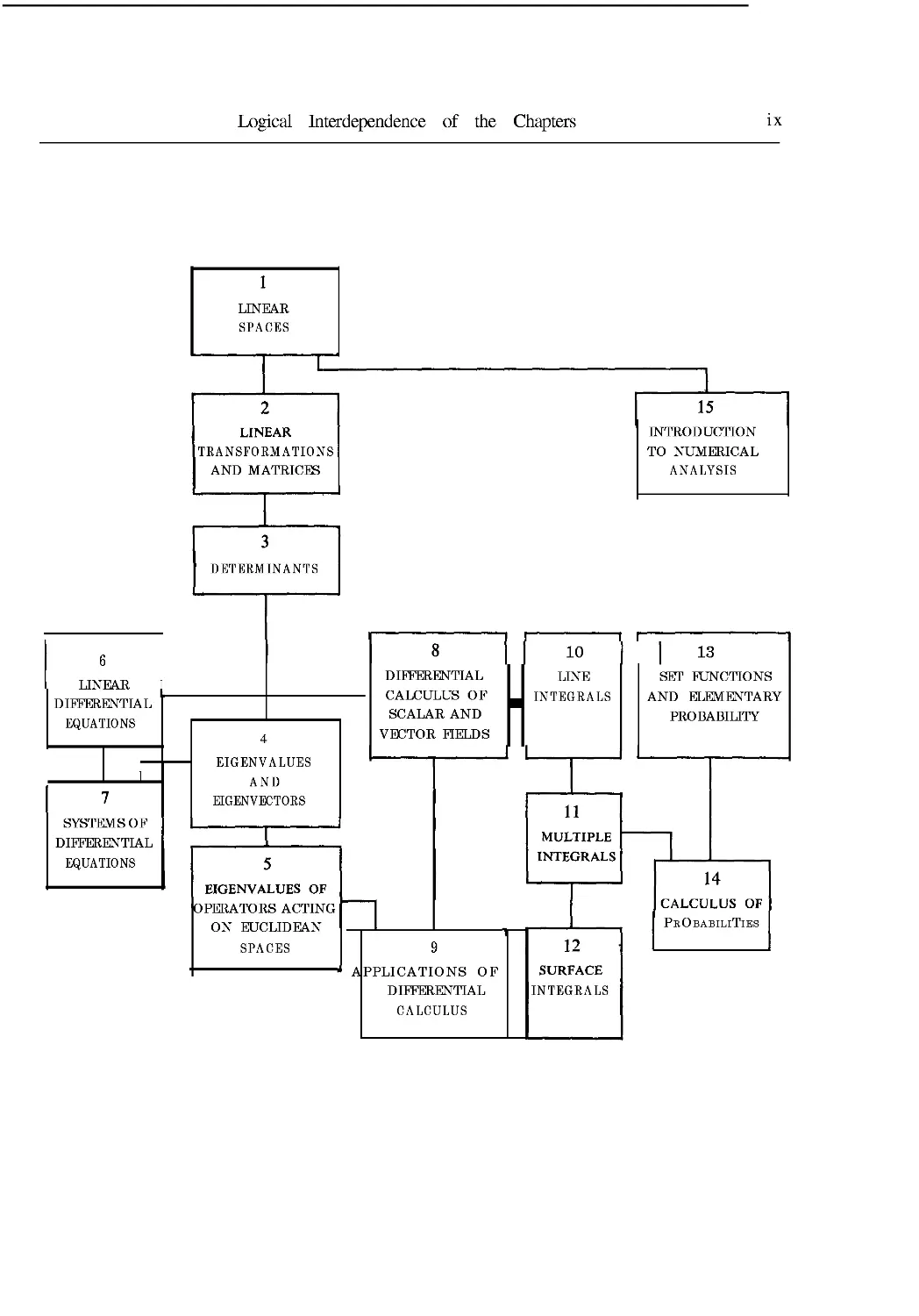
can choose topics to suit his needs and preferences by consulting the diagram on the next
page which shows the logical interdependence of the chapters.
Once again I acknowledge with pleasure the assistance of many friends and colleagues.
In preparing the second edition I received valuable help from Professors Herbert S.
Zuckerman of the University of Washington, and Basil Gordon of the University of
California, Los Angeles, each of whom suggested a number of improvements. Thanks are
also due to the staff of Blaisdell Publishing Company for their assistance and cooperation.
As before, it gives me special pleasure to express my gratitude to my wife for the many
ways in which she has contributed. In grateful acknowledgement I happily dedicate this
book to her.
Т. М. A.
Pasadena, California
September 16,1968

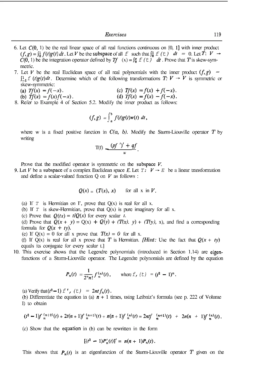
Logical Interdependence of the Chapters
6
LINEAR
DIFFERENTIAL
EQUATIONS
SYSTEMS OF
DIFFERENTIAL
EQUATIONS
LINEAR
SPACES
LINEAR
TRANSFORMATIONS
AND MATRICES
DETERMINANTS
EIGENVALUES
AND
EIGENVECTORS
EIGENVALUES OF
OPERATORS ACTING
ON EUCLIDEAN
SPACES
DIFFERENTIAL
CALCULUS OF
SCALAR AND
VECTOR FIELDS
10
LINE
INTEGRALS
11
MULTIPLE
INTEGRALS
APPLICATIONS OF
DIFFERENTIAL
CALCULUS
12
SURFACE
INTEGRALS
15
INTRODUCTION
TO NUMERICAL
ANALYSIS
I 13
SET FUNCTIONS
AND ELEMENTARY
PROBABILITY
14
CALCULUS OF
Probabilities

CONTENTS
PART 1. LINEAR ANALYSIS
1. LINEAR SPACES
1.1 Introduction 3
1.2 The definition of a linear space 3
1.3 Examples of linear spaces 4
1.4 Elementary consequences of the axioms "
1.5 Exercises '
1.6 Sub spaces of a linear space °
1.7 Dependent and independent sets in a linear space 9
1.8 Bases and dimension 12
1.9 Components 13
1.10 Exercises 13
1.11 Inner products, Euclidean spaces. Norms 14
1.12 Orthogonality in a Euclidean space 18
1.13 Exercises 20
1.14 Construction of orthogonal sets. The Gram-Schmidt process 22
1.15 Orthogonal complements. Projections 26
1.16 Best approximation of elements in a Euclidean space by elements in a finite-
dimensional subspace 28
1.17 Exercises 30
2. LINEAR TRANSFORMATIONS AND MATRICES
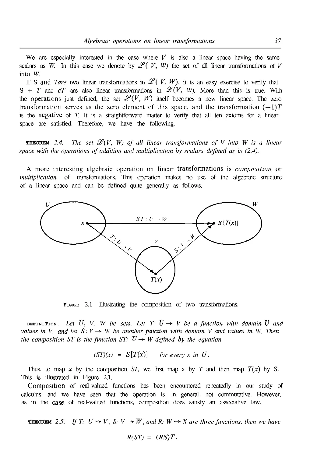
2.1 Linear transformations 31
2.2 Null space and range 32
2.3 Nullity and rank 34

xii Contents
2.4 Exercises 35
2.5 Algebraic operations on linear transformations 36
2.6 Inverses 38
2.7 One-to-one linear transformations 41
2.8 Exercises 42
2.9 Linear transformations with prescribed values 44
2.10 Matrix representations of linear transformations 45
2.11 Construction of a matrix representation in diagonal form 48
2.12 Exercises 50
2.13 Linear spaces of matrices 51
2.14 Tsomorphism between linear transformations and matrices 52
2.15 Multiplication of matrices 54
2.16 Exercises 57
2.17 Systems of linear equations 58
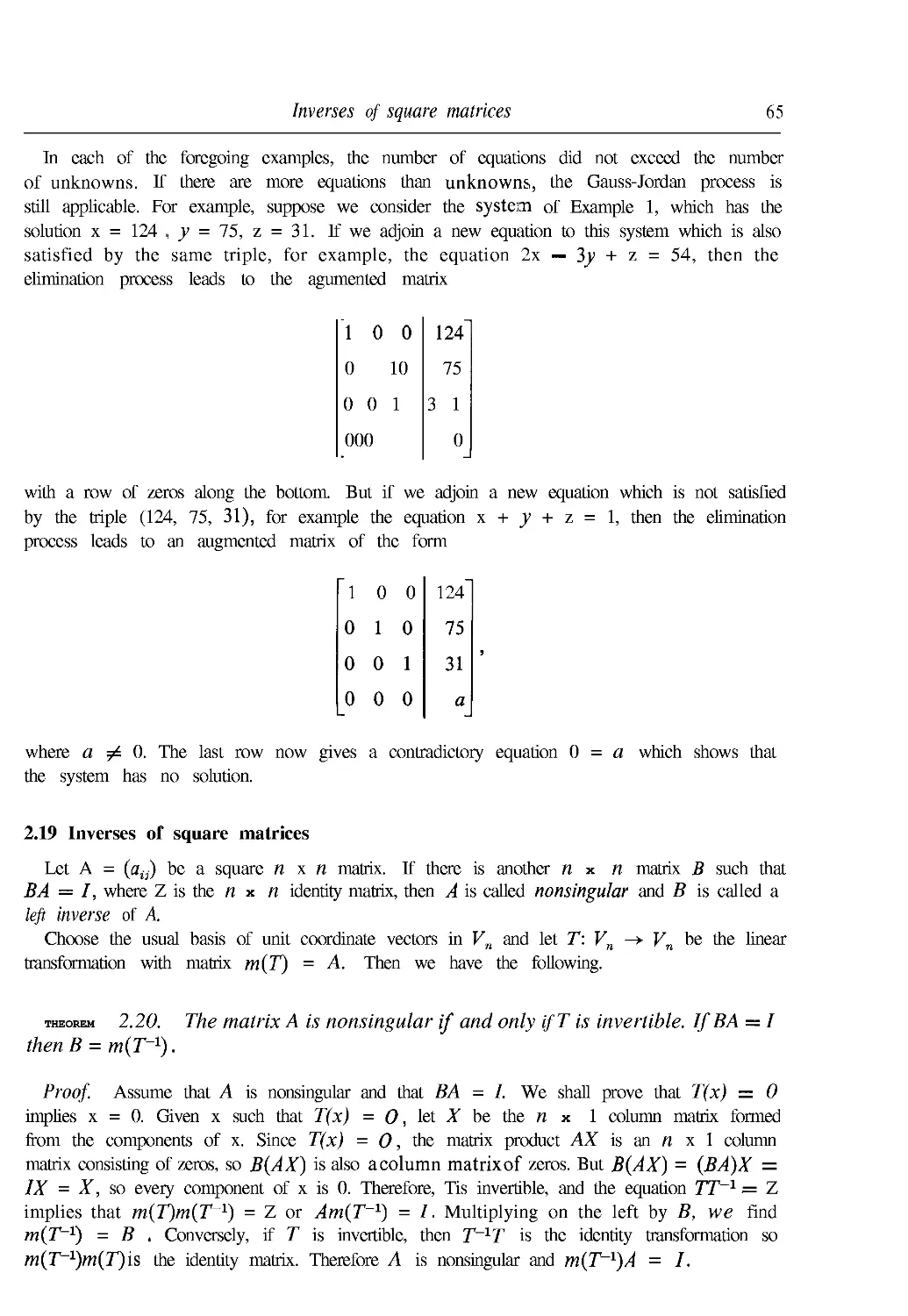
2.18 Computation techniques 61
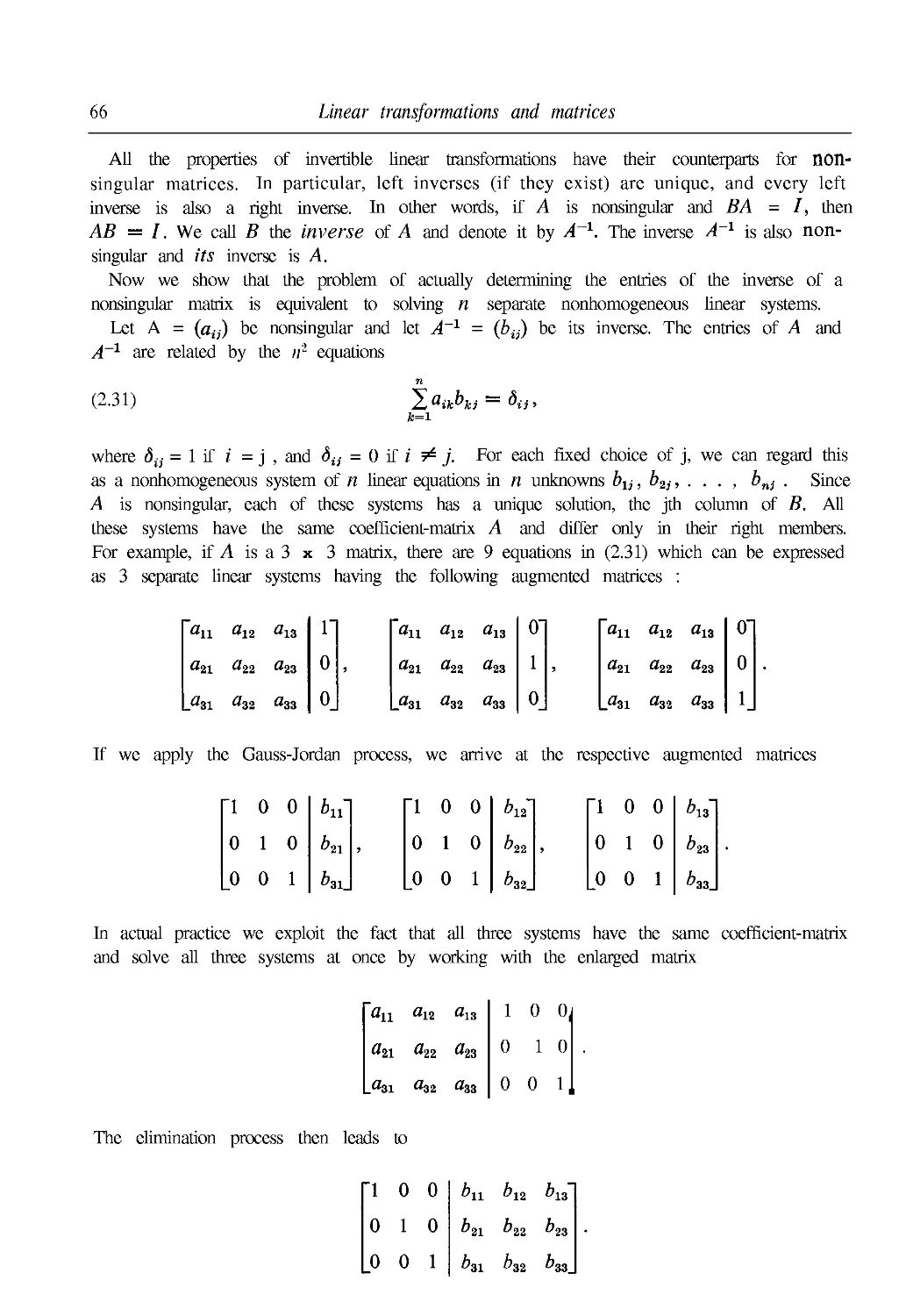
2.19 Inverses of square matrices 65
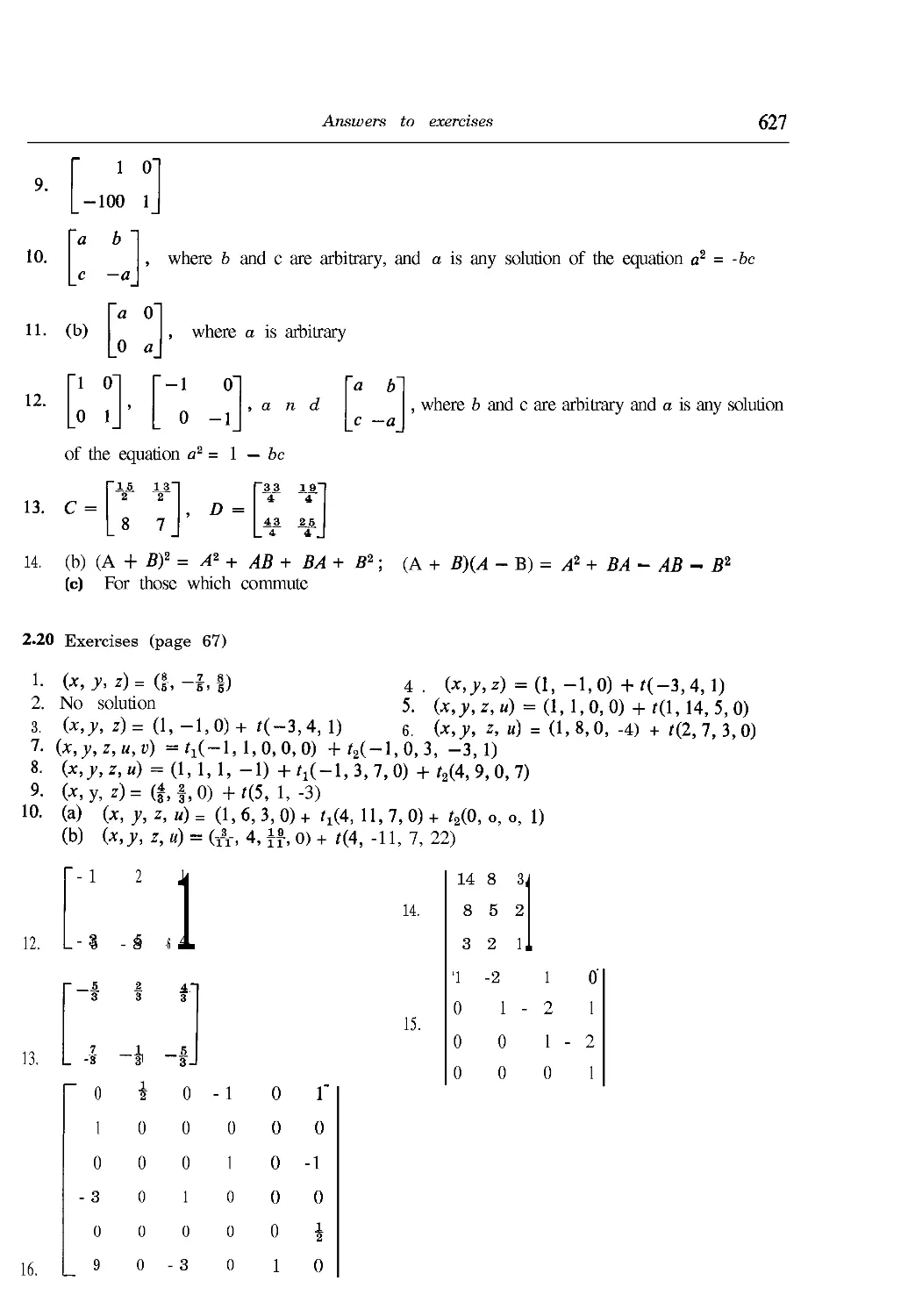
2.20 Exercises 67
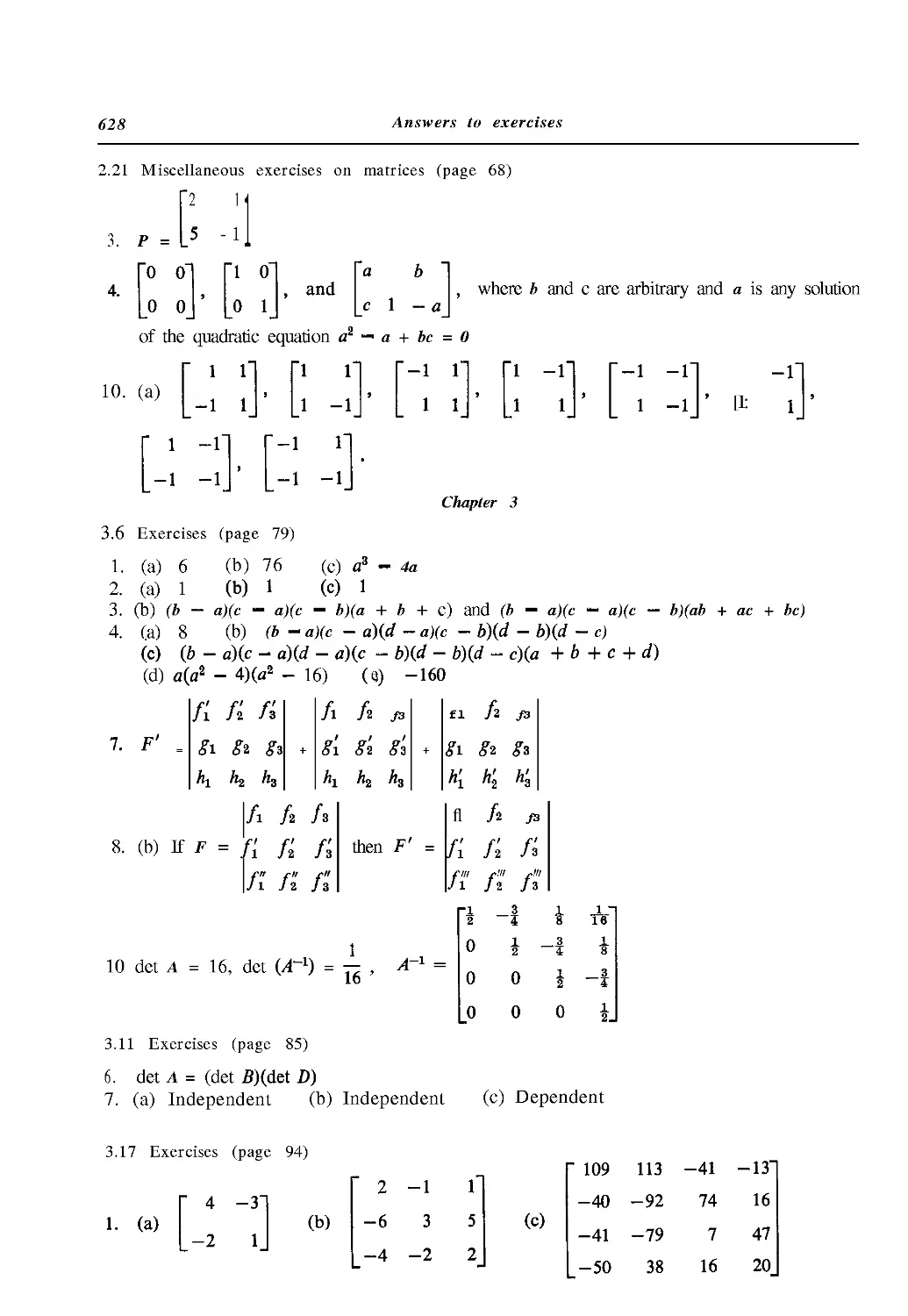
2.21 Miscellaneous exercises on matrices 68
3. DETERMINANTS
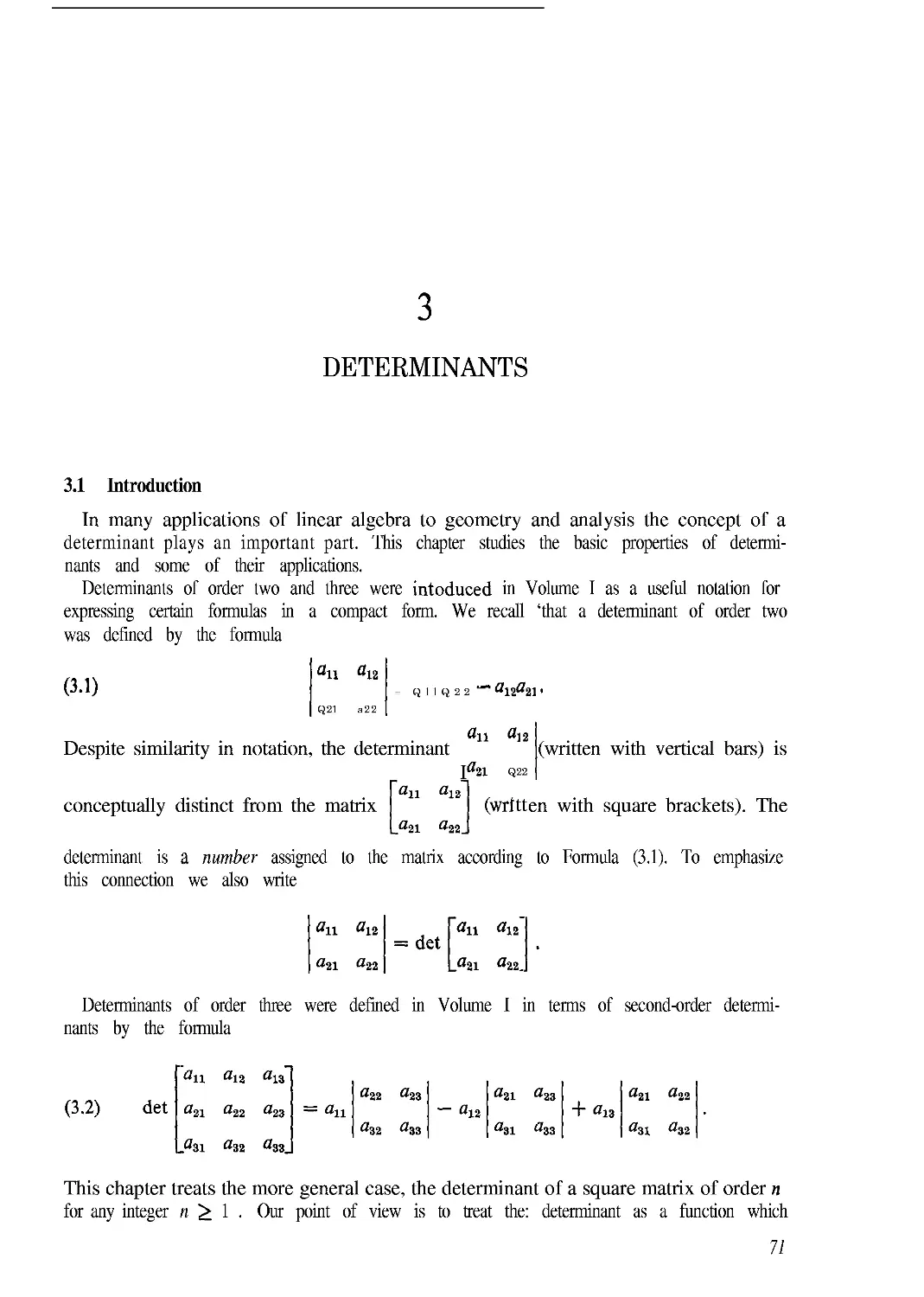
3.1 Introduction 71
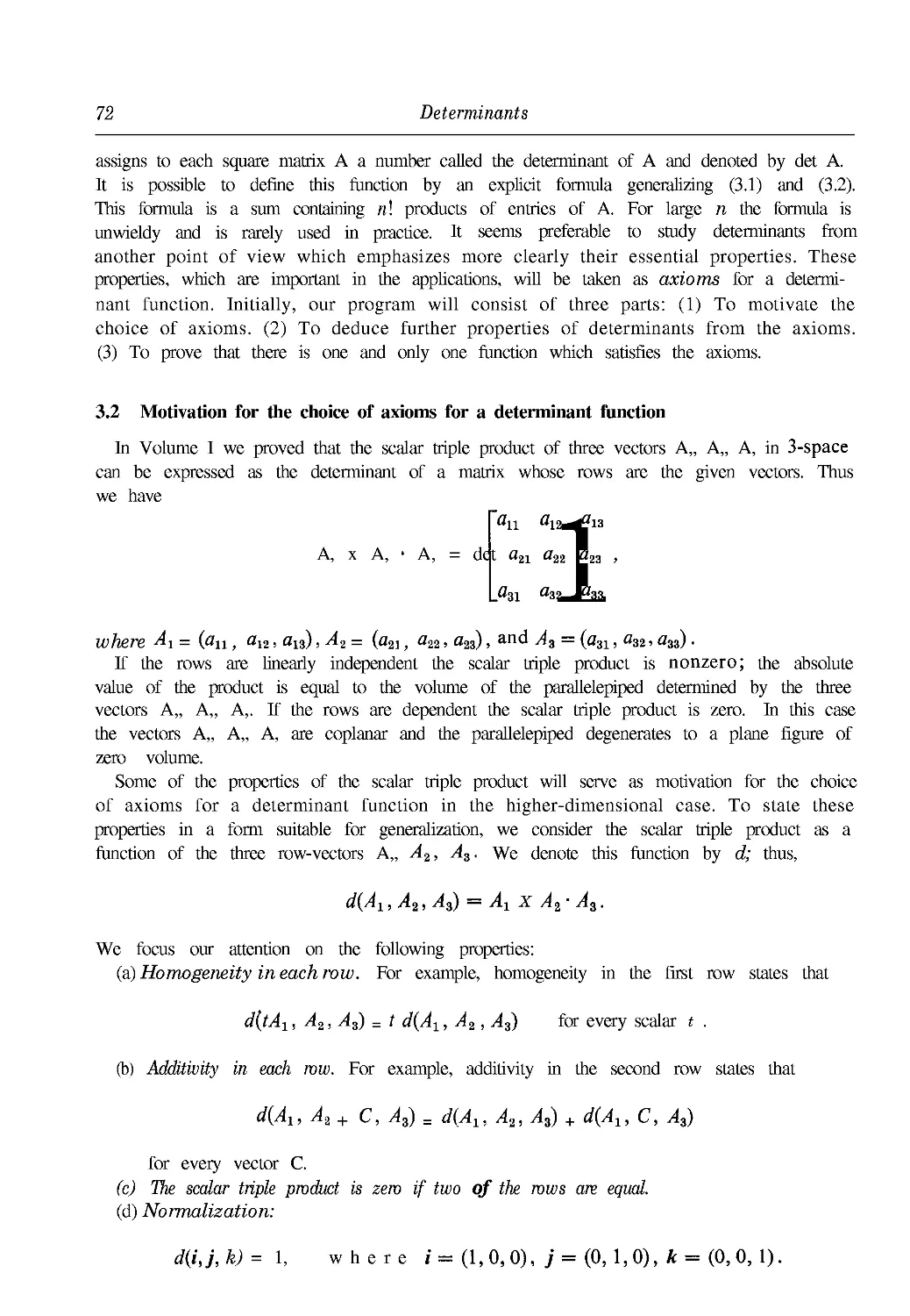
3.2 Motivation for the choice of axioms for a determinant function 72
3.3 A set of axioms for a determinant function 73
3.4 Computation of determinants 76
3.5 The uniqueness theorem 79
3.6 Exercises 79
3.7 The product formula for determinants 81
3.8 The determinant of the inverse of a nonsingular matrix 83
3.9 Determinants and independence of vectors 83
3.10 The determinant of a block-diagonal matrix 84
3.11 Exercises 85
3.12 Expansion formulas for determinants. Minors and cofactors 86
3.13 Existence of the determinant function 90
3.14 The determinant of a transpose 91
3.15 The cofactor matrix 92
3.16 Cramer's rale 93
3.17 Exercises 94

Contents xiii
4. EIGENVALUES AND EIGENVECTORS
4.1 Linear transformations with diagonal matrix representations 96
4.2 Eigenvectors and eigenvalues of a linear transformation 97
4.3 Linear independence of eigenvectors corresponding to distinct eigenvalues 100
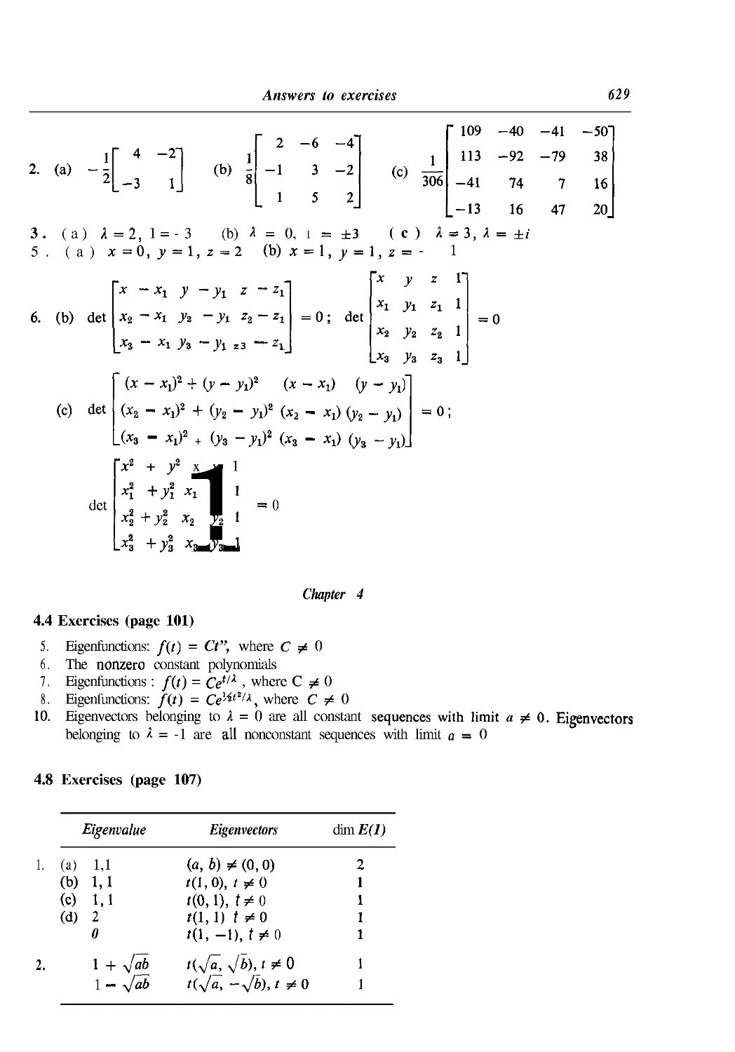
4.4 Exercises ' 101
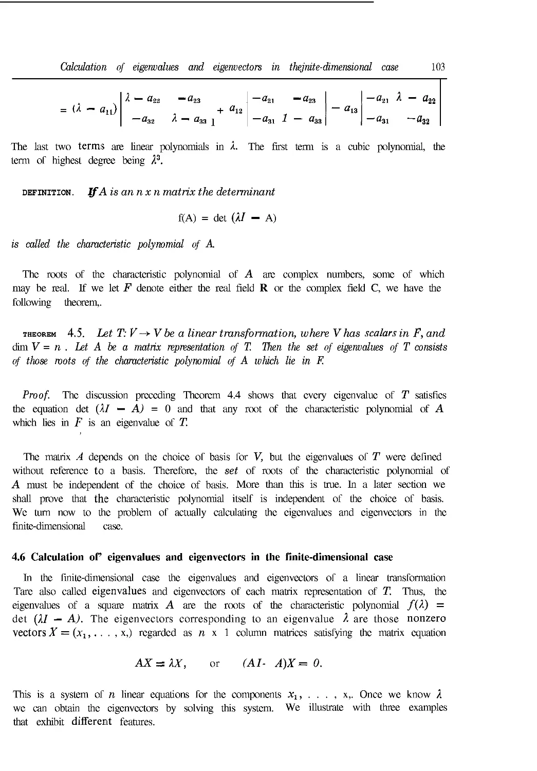
4.5 The finite-dimensional case. Characteristic polynomials 102
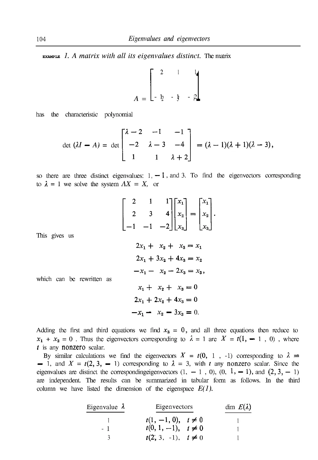
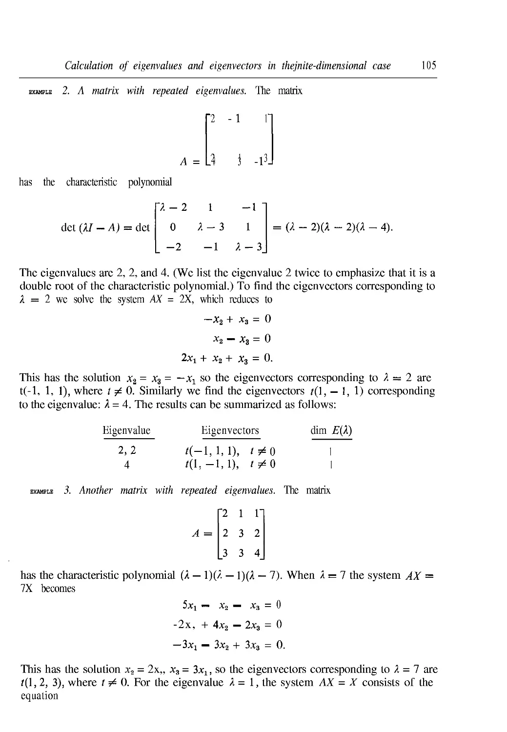
4.6 Calculation of eigenvalues and eigenvectors in the finite-dimensional case 103
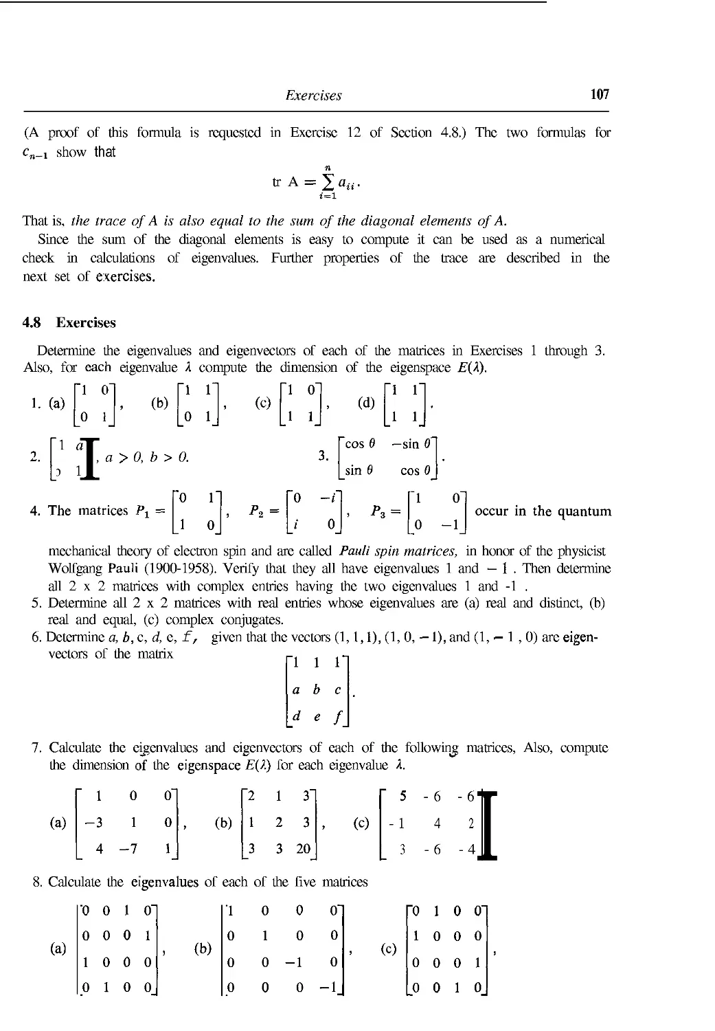
4.7 Trace of a matrix 106
4.8 Exercises 107
4.9 Matrices representing the same linear transformation. Similar matrices 108
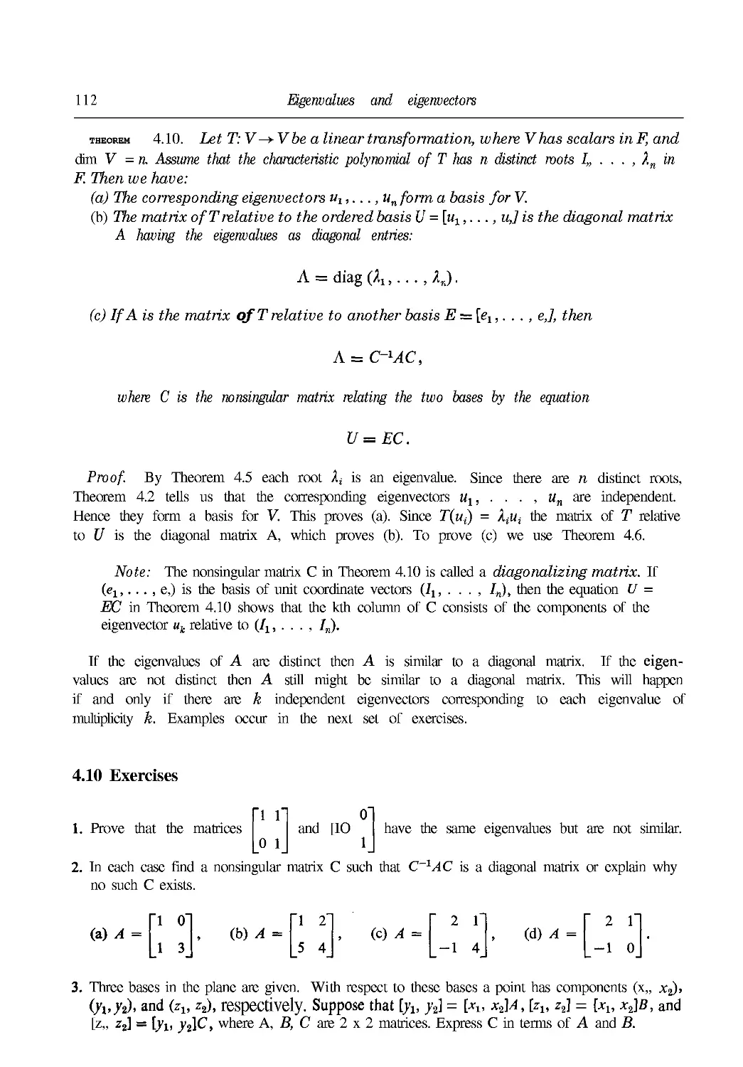
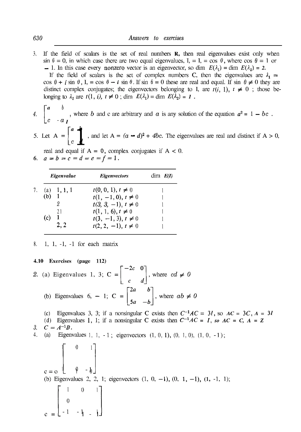
4.10 Exercises 112
5. EIGENVALUES OF OPERATORS ACTING ON
EUCLIDEAN SPACES
5.1 Eigenvalues and inner products 114
5.2 Hermitian and skew-Hermitian transformations 115
5.3 Eigenvalues and eigenvectors of Hermitian and skew-Hermitian operators 117
5.4 Orthogonality of eigenvectors corresponding to distinct eigenvalues 117
5.5 Exercises 118
5.6 Existence of an orthonormal set of eigenvectors for Hermitian and
skew-Hermitian operators acting on finite-dimensional spaces 120
5.7 Matrix representations for Hermitian and skew-Hermitian operators 121
5.8 Hermitian and skew-Hermitian matrices. The adjoint of a matrix 122
5.9 Diagonalization of a Hermitian or skew-Hermitian matrix 122
5.10 Unitary matrices. Orthogonal matrices 123
5.11 Exercises 124
5.12 Quadratic forms 126
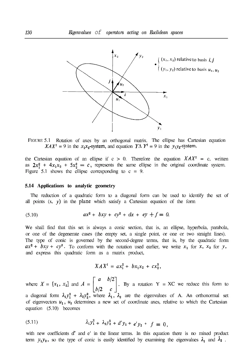
5.13 Reduction of a real quadratic form to a diagonal form 128
5.14 Applications to analytic geometry 130
5.15 Exercises 134
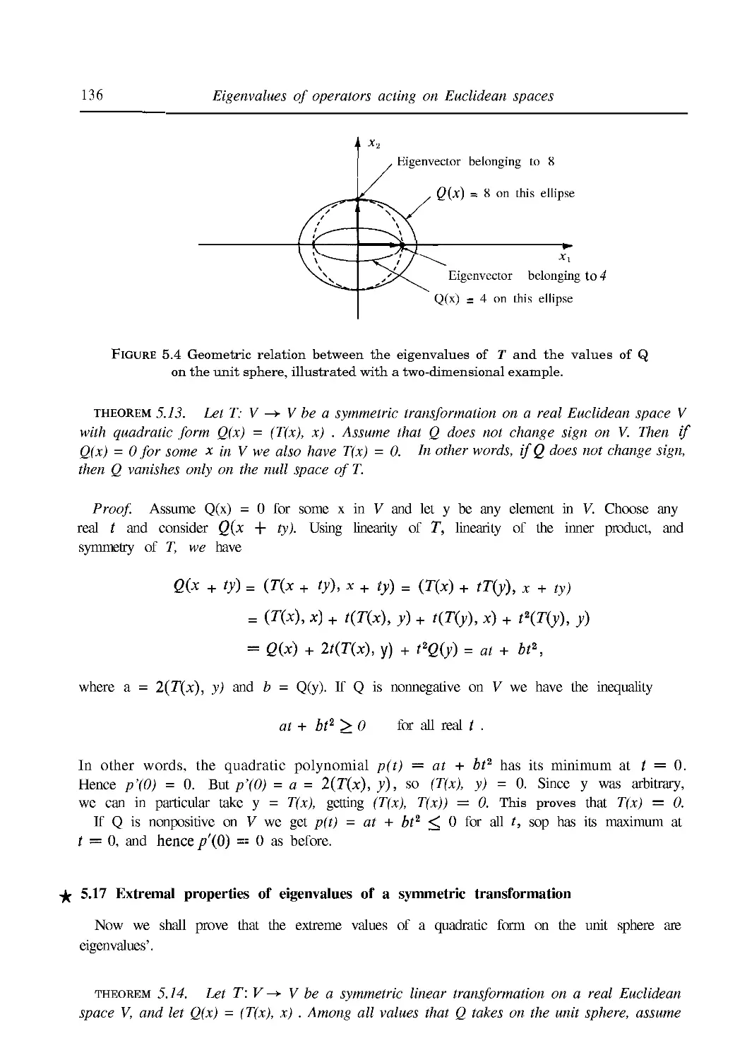
¦^¦5.16 Eigenvalues of a symmetric transformation obtained as values of its
quadratic form 135
¦?5.17 Extremal properties of eigenvalues of a symmetric transformation 136
¦^¦5.18 The finite-dimensional case 137
5.19 Unitary transformations 138
5.20 Exercises 141

Contents
6. LINEAR DIFFERENTIAL EQUATIONS
6.1 Historical introduction 142
6.2 Review of results concerning linear equations of first and second orders 143
6.3 Exercises 144
6.4 Linear differential equations of order n 145
6.5 The existence-uniqueness theorem 147
6.6 The dimension of the solution space of a homogeneous linear equation 147
6.7 The algebra of constant-coefficient operators 148
6.8 Determination of a basis of solutions for linear equations with constant
coefficients by factorization of operators 150
6.9 Exercises 154
6.10 The relation between the homogeneous and nonhomogeneous equations 156
6.11 Determination of a particular solution of the nonhomogeneous equation.
The method of variation of parameters 157
6.12 Nonsingularity of the Wronskian matrix of n independent solutions of a
homogeneous linear equation 161
6.13 Special methods for determining a particular solution of the nonhomogeneous
equation. Reduction to a system of first-order linear equations 163
6.14 The annihilator method for determining a particular solution of the
nonhomogeneous equation 163
6.15 Exercises 166
6.16 Miscellaneous exercises on linear differential equations 167
6.17 Linear equations of second order with analytic coefficients 169
6.18 The Legendre equation 171
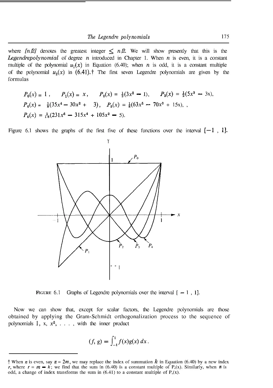
6.19 The Legendre polynomials 174
6.20 Rodrigues' formula for the Legendre polynomials 176
6.21 Exercises 177
6.22 The method of Frobenius 180
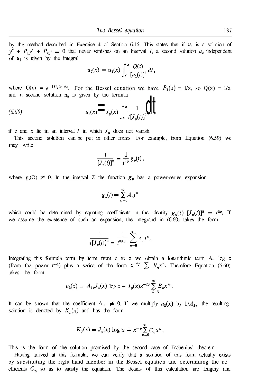
6.23 The Bessel equation 182
6.24 Exercises 188
7. SYSTEMS OF DIFFERENTIAL EQUATIONS
7.1 Introduction 191
7.2 Calculus of matrix functions 193
7.3 Infinite series of matrices. Norms of matrices 194
7.4 Exercises 195
7.5 The exponential matrix 197

Contents xv
7.6 The differential equation satisfied by etA 197
7.7 Uniqueness theorem for the matrix differential equation F'(t) = AF(t) 198
7.8 The law of exponents for exponential matrices 199
7.9 Existence and uniqueness theorems for homogeneous linear systems
with constant coefficients 200
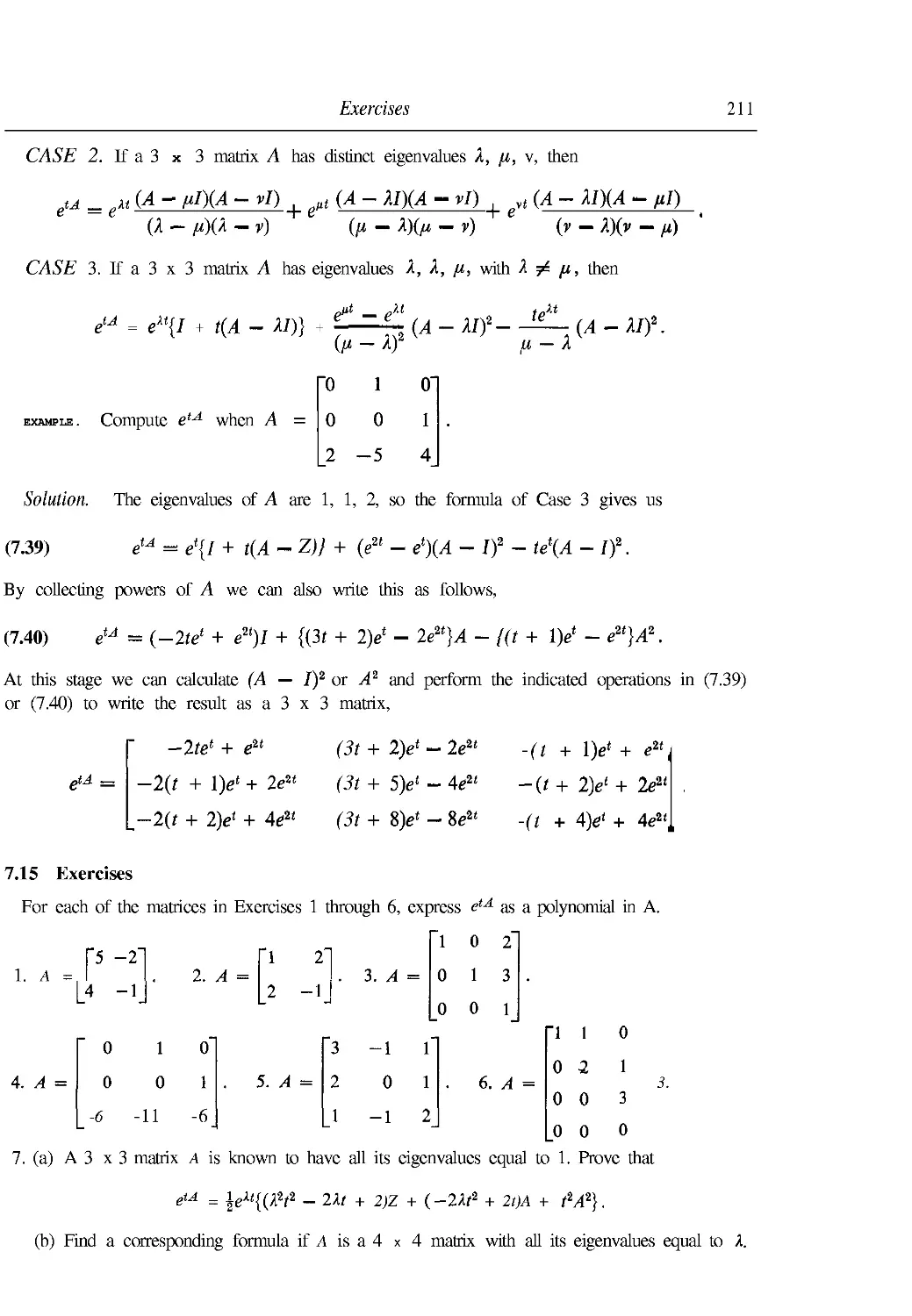
7.10 The problem of calculating etA 201
7.11 The Cayley-Hamilton theorem 203
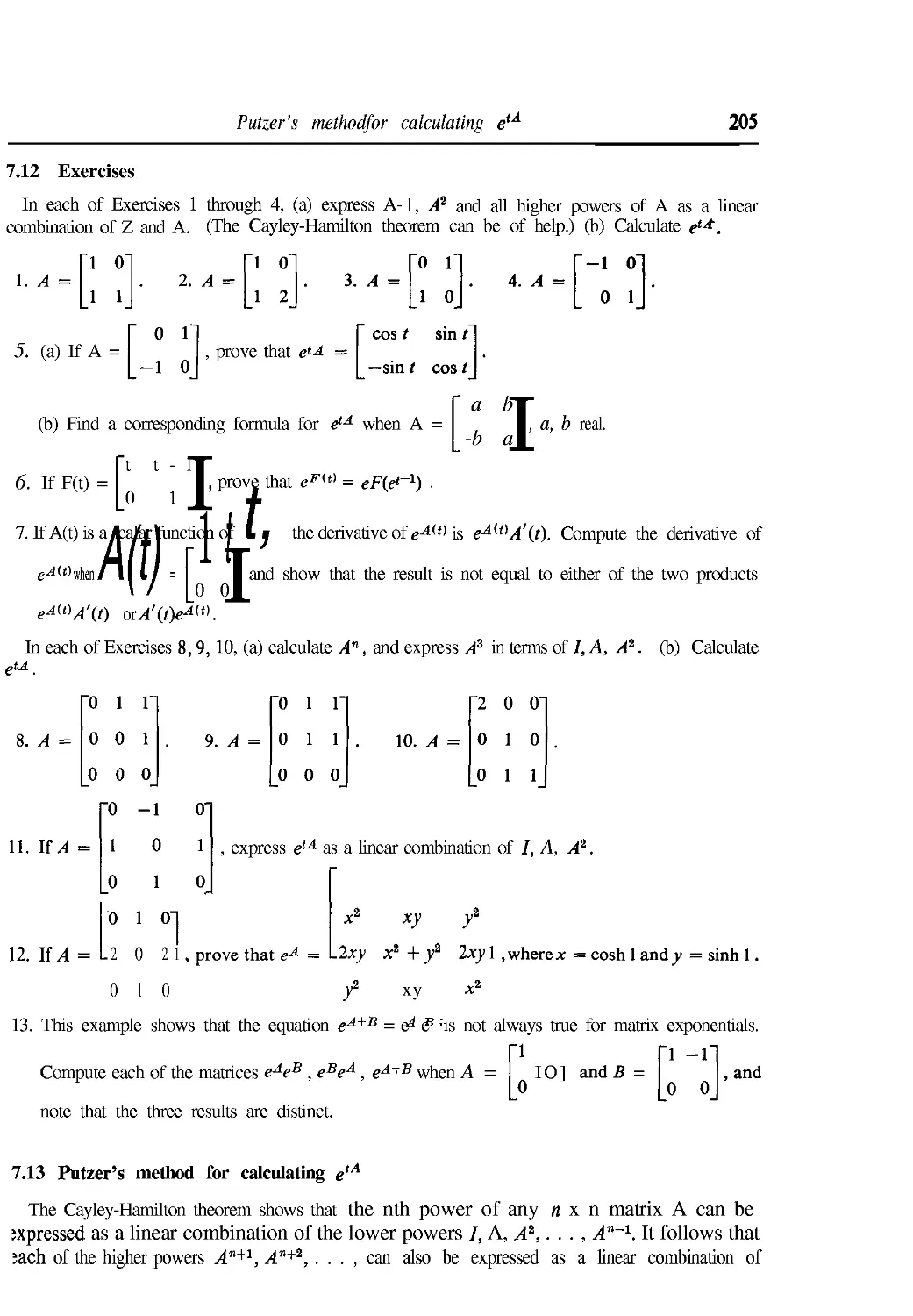
7.12 Exercises 205
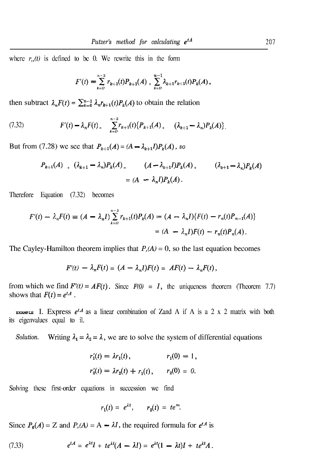
7.13 Putzer's method for calculating etA 205
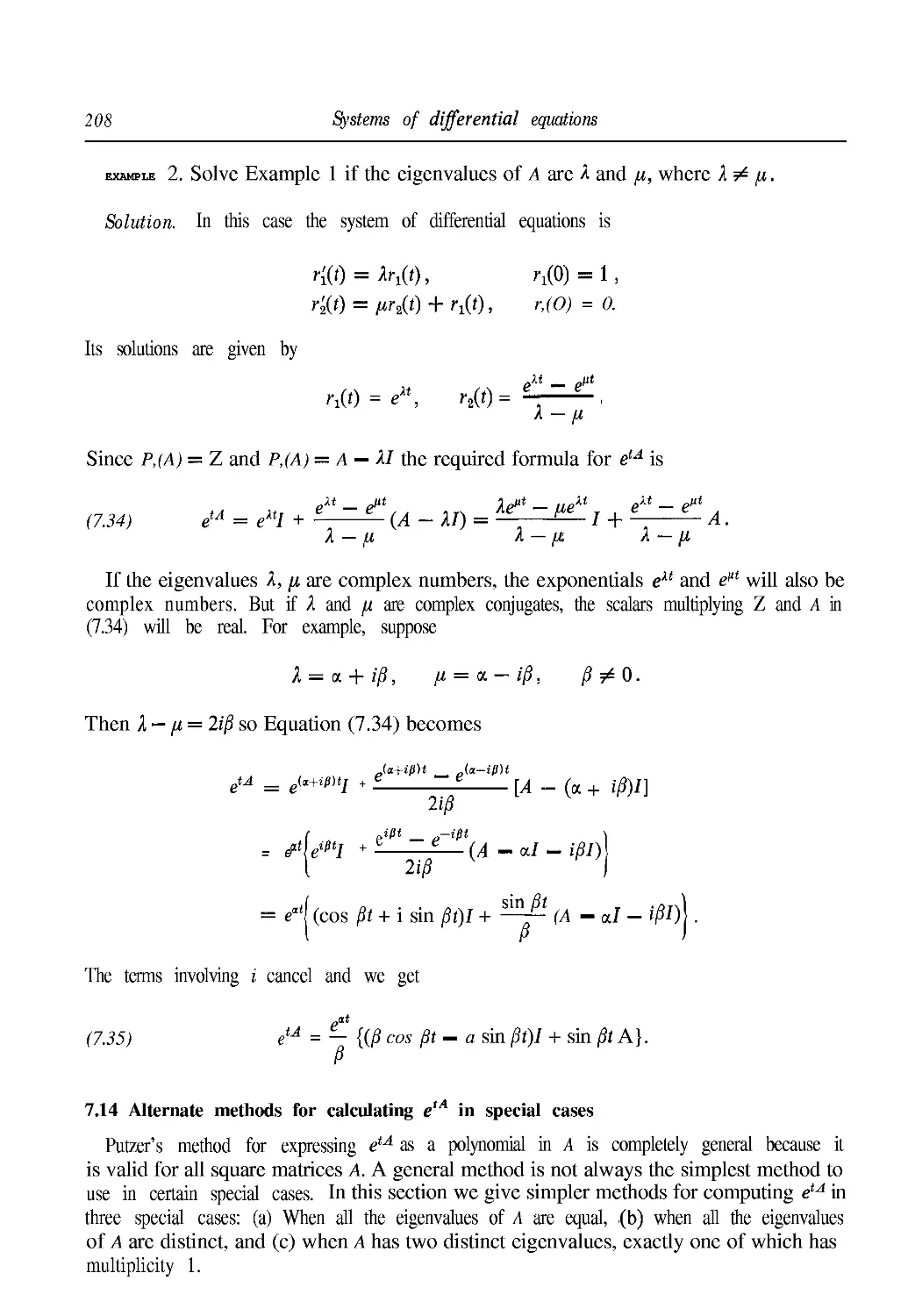
7.14 Alternate methods for calculating etA in special cases 208
7.15 Exercises 211
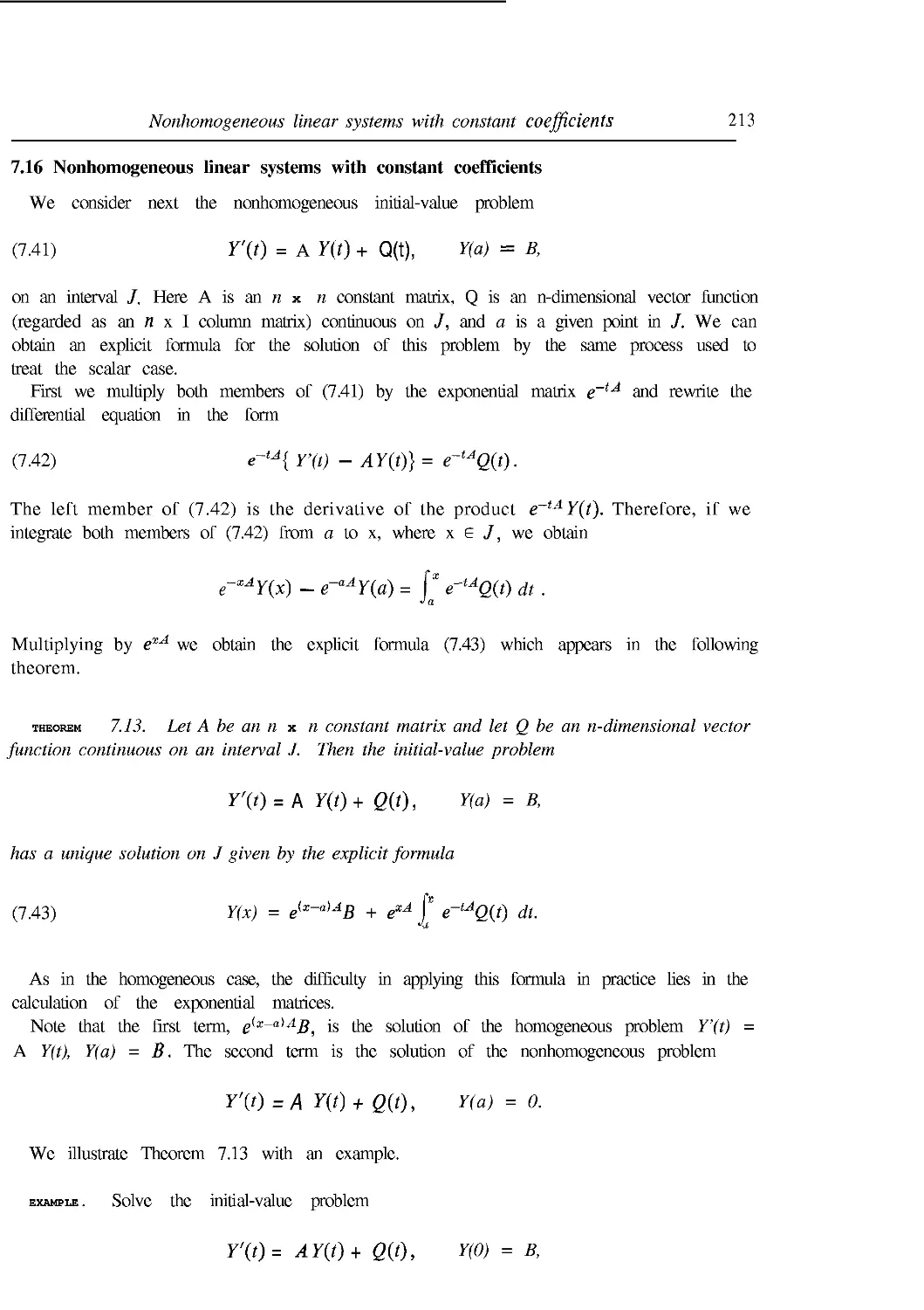
7.16 Nonhomogeneous linear systems with constant coefficients 213
7.17 Exercises 215
7.18 The general linear system Y(t) = P(t) Y(t) + Q(t) 111
7.19 A power-series method for solving homogeneous linear systems 220
7.20 Exercises 221
7.21 Proof of the existence theorem by the method of successive approximations 222
7.22 The method of successive approximations applied to first-order nonlinear systems 227
7.23 Proof of an existence-uniqueness theorem for first-order nonlinear systems 229
7.24 Exercises 230
¦^¦7.25 Successive approximations and fixed points of operators 232
^¦7.26 Normed linear spaces 233
•kl.21 Contraction operators 234
¦^¦7.28 Fixed-point theorem for contraction operators 235
¦^¦7.29 Applications of the fixed-point theorem 237
PART 2. NONLINEAR ANALYSIS
8. DIFFERENTIAL CALCULUS OF SCALAR AND
VECTOR FIELDS
8.1 Functions from R" to R". Scalar and vector fields 243
8.2 Open balls and open sets 244
8.3 Exercises 245
8.4 Limits and continuity 247
8.5 Exercises 251
8.6 The derivative of a scalar field with respect to a vector 252
8.7 Directional derivatives and partial derivatives 254
8.8 Partial derivatives of higher order 255
8.9 Exercises 255

Contents
8.10 Directional derivatives and continuity 257
8.11 The total derivative 258
8.12 The gradient of a scalar field 259
8.13 A sufficient condition for differentiability 261
8.14 Exercises 262
8.15 A chain rale for derivatives of scalar fields 263
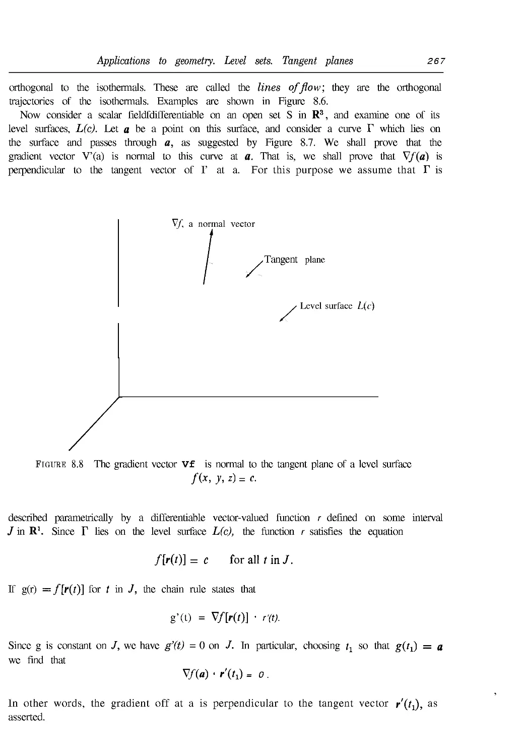
8.16 Applications to geometry. Level sets. Tangent planes 266
8.17 Exercises 268
8.18 Derivatives of vector fields 269
8. 19 Differentiability implies continuity 271
8.20 The chain rale for derivatives of vector fields 272
8.21 Matrix form of the chain rale 273
8.22 Exercises 275
^¦8.23 Sufficient conditions for the equality of mixed partial derivatives 277
8.24 Miscellaneous exercises 281
9. APPLICATIONS OF THE DIFFERENTIAL CALCULUS
9.1 Partial differential equations 283
9.2 A first-order partial differential equation with constant coefficients 284
9.3 Exercises 286
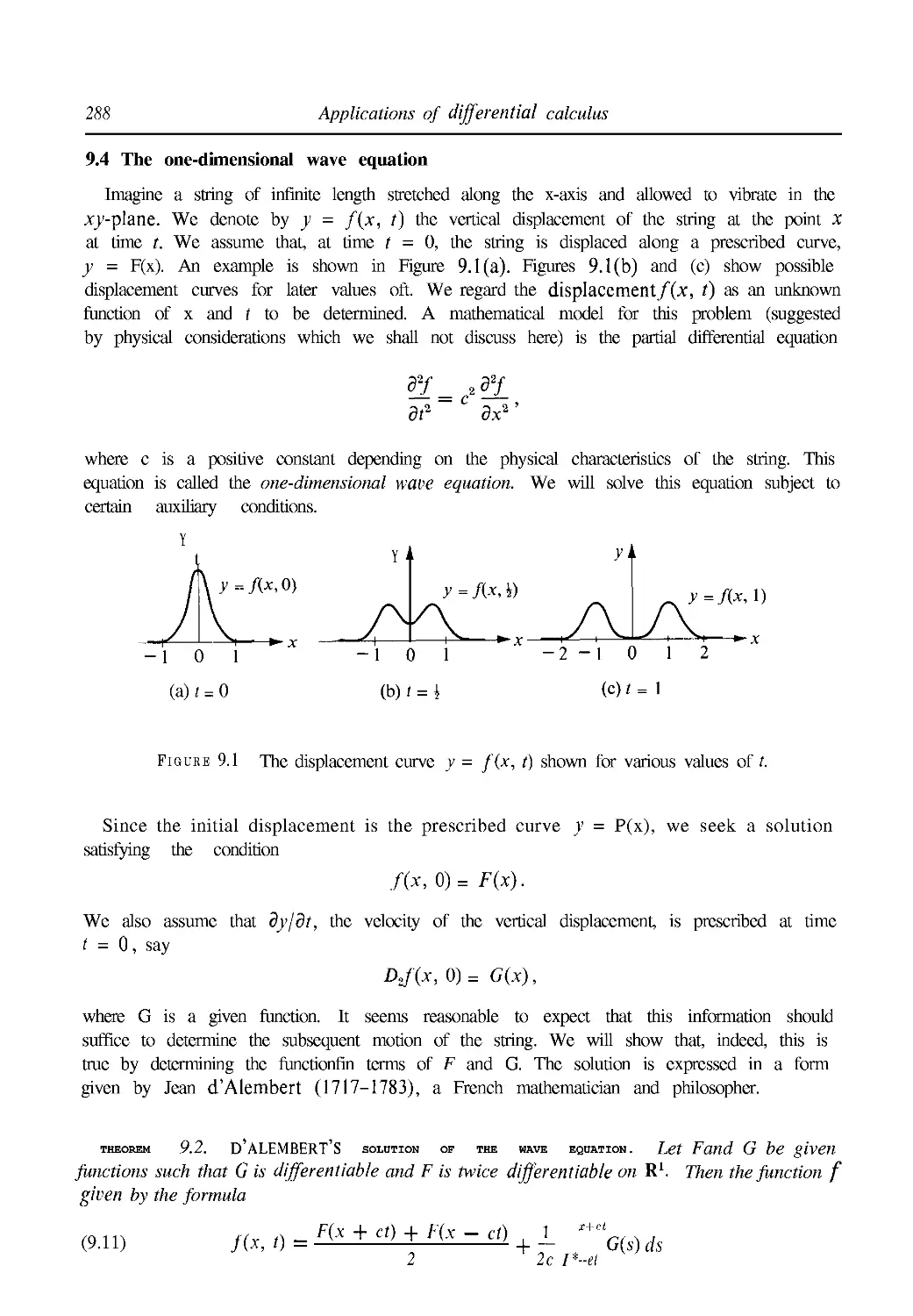
9.4 The one-dimensional wave equation 288
9.5 Exercises 292
9.6 Derivatives of functions defined implicitly 294
9.7 Worked examples 298
9.8 Exercises 302
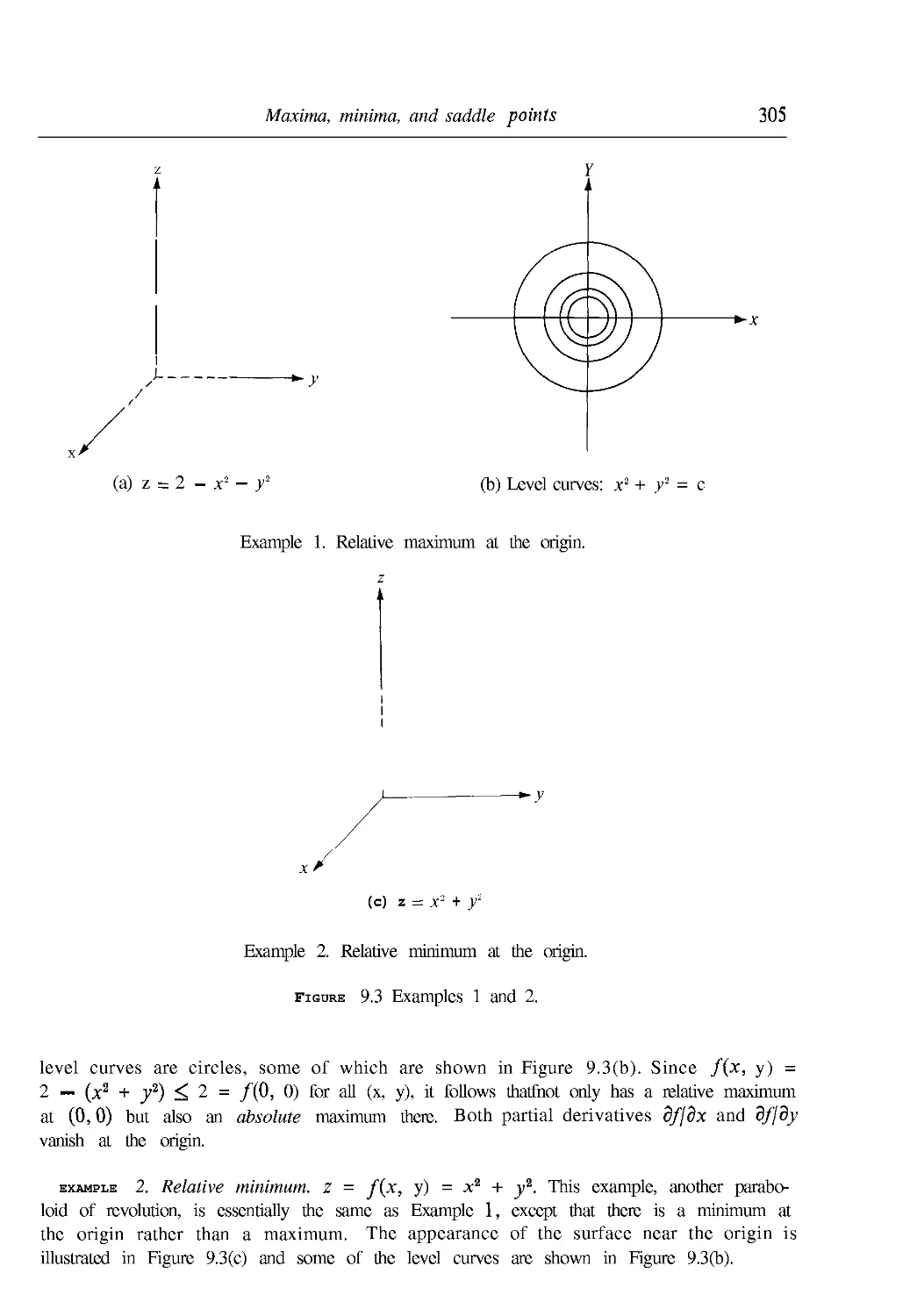
9.9 Maxima, minima, and saddle points 303
9. 10 Second-order Taylor formula for scalar fields 308
9.11 The nature of a stationary point determined by the eigenvalues of the Hessian
matrix 310
9.12 Second-derivative test for extrema of functions of two variables 312
9.13 Exercises 313
9.14 Extrema with constraints. Lagrange's multipliers 314
9. 15 Exercises 318
9.16 The extreme-value theorem for continuous scalar fields 319
9.17 The small-span theorem for continuous scalar fields (uniform continuity) 321
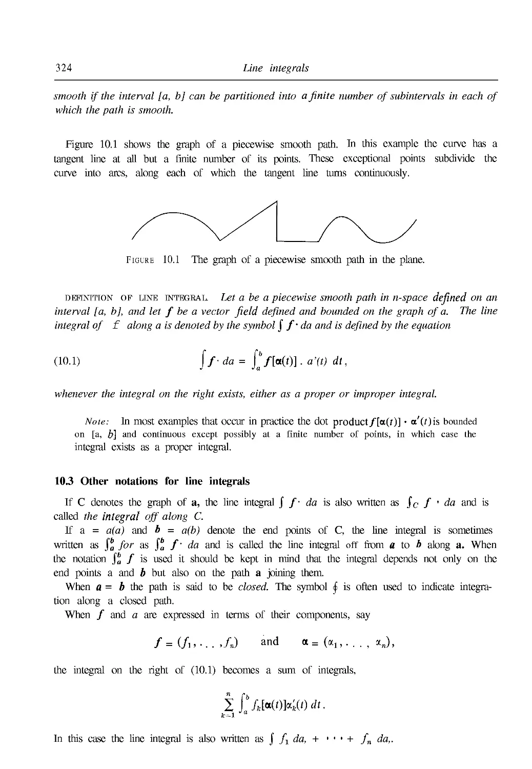
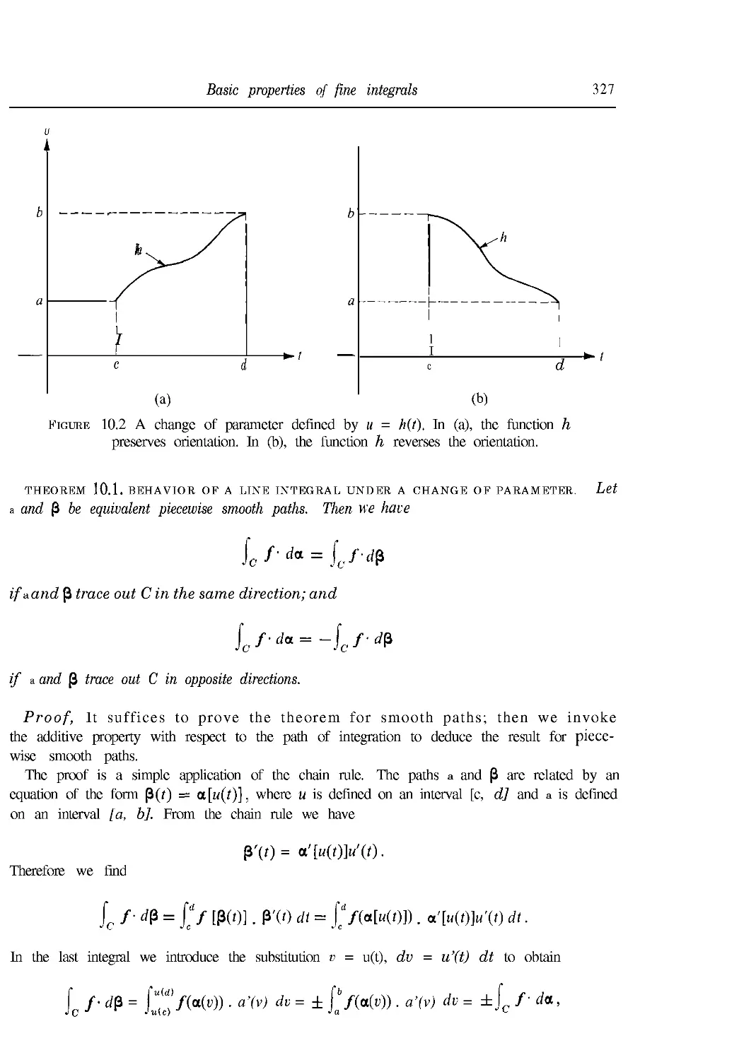
10. LINE INTEGRALS
10.1 Introduction 323
10.2 Paths and line integrals 323

Contents
10.3 Other notations for line integrals 324
10.4 Basic properties of line integrals 326
10.5 Exercises 328
10.6 The concept of work as a line integral 328
10.7 Line integrals with respect to arc length 329
10.8 Further applications of line integrals 330
10.9 Exercises 331
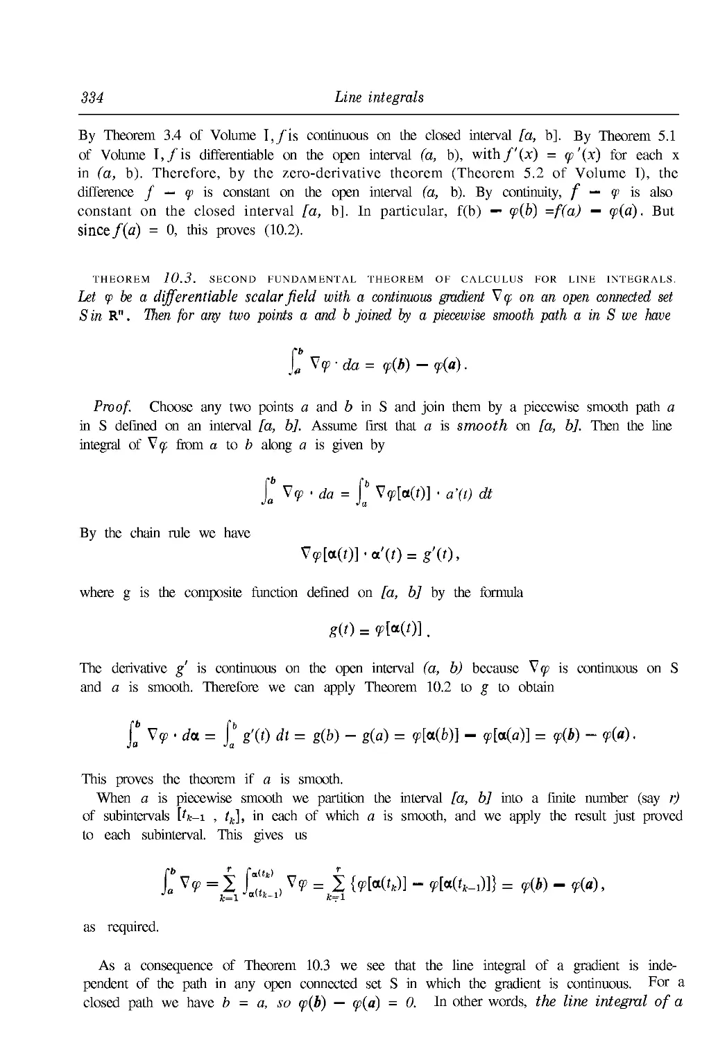
10.10 Open connected sets. Independence of the path 332
10.11 The second fundamental theorem of calculus for line integrals 333
10.12 Applications to mechanics 335
10.13 Exercises 336
10.14 The first fundamental theorem of calculus for line integrals 337
10.15 Necessary and sufficient conditions for a vector field to be a gradient 339
10.16 Necessary conditions for a vector field to be a gradient 340
10.17 Special methods for constructing potential functions 342
10.18 Exercises 345
10.19 Applications to exact differential equations of first order 346
10.20 Exercises 349
10.21 Potential functions on convex sets 350
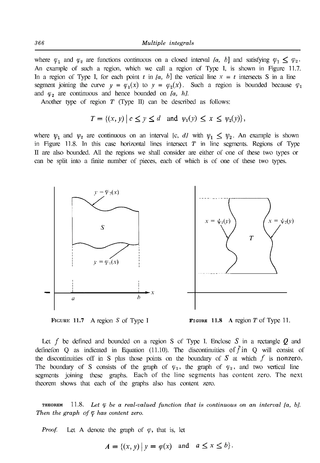
11. MULTIPLE INTEGRALS
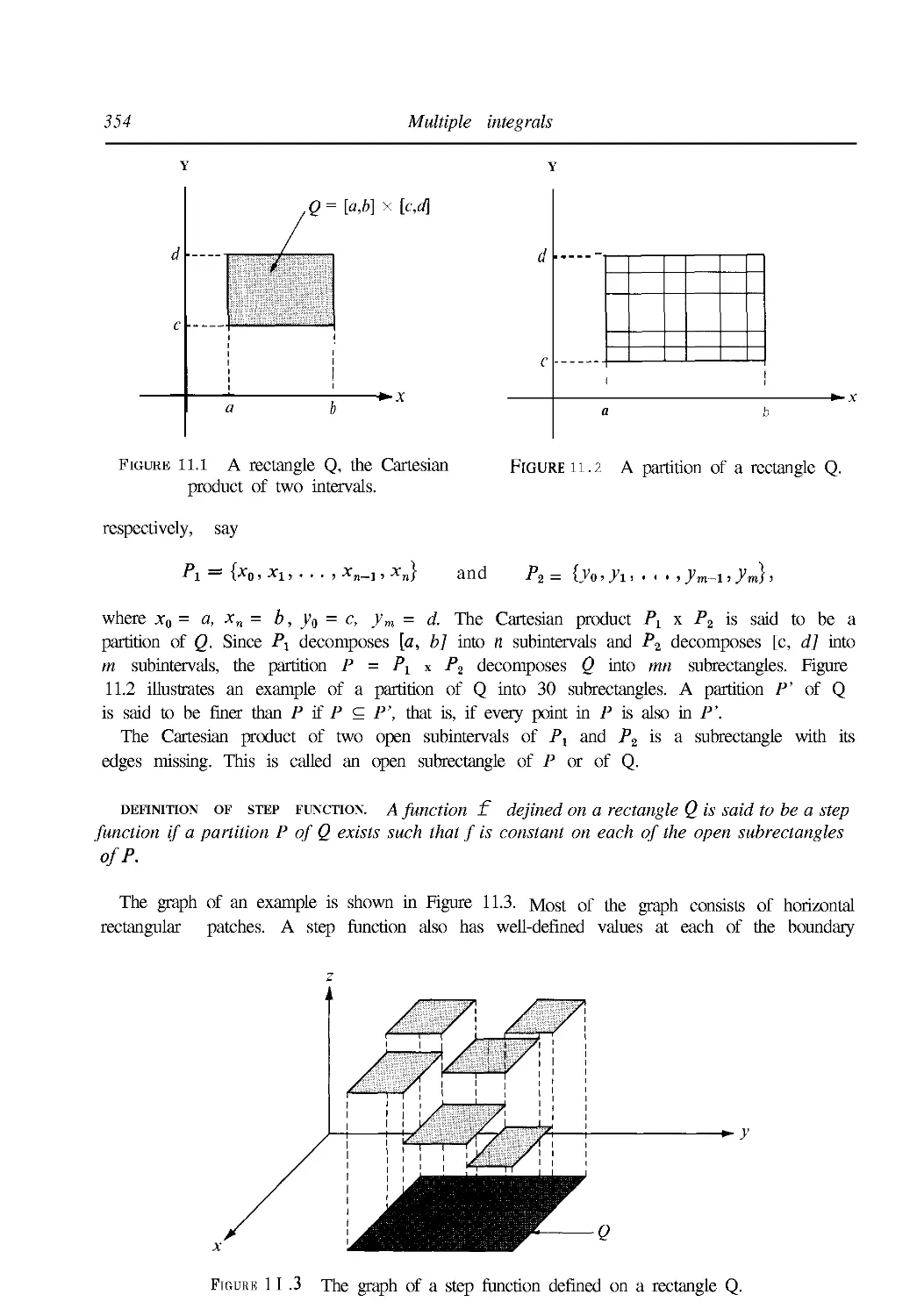
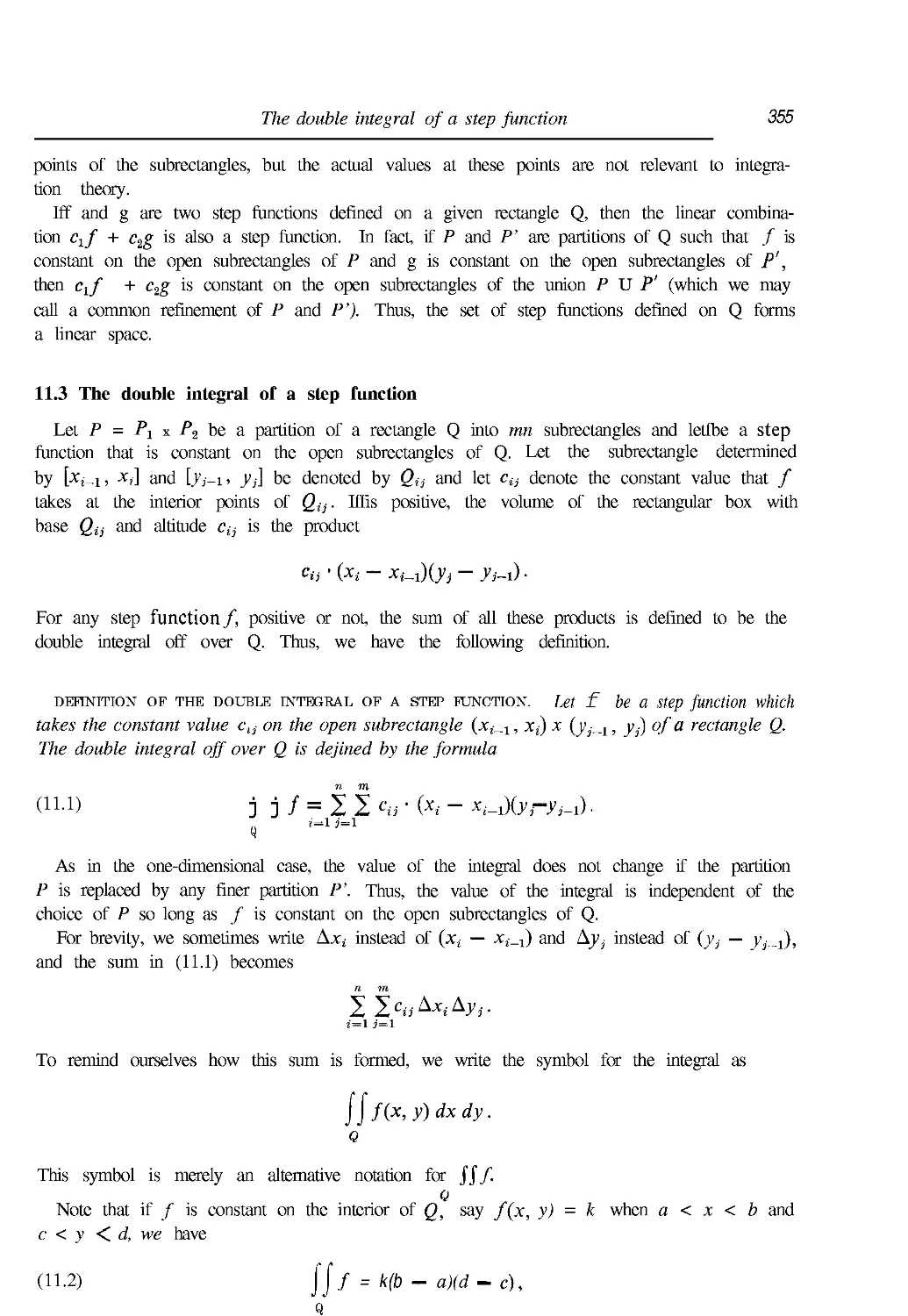
11.1 Introduction 353
11.2 Partitions of rectangles. Step functions 353
11.3 The double integral of a step function 355
11.4 The definition of the double integral of a function defined and bounded on a
rectangle 357
11.5 Upper and lower double integrals 357
11.6 Evaluation of a double integral by repeated one-dimensional integration 358
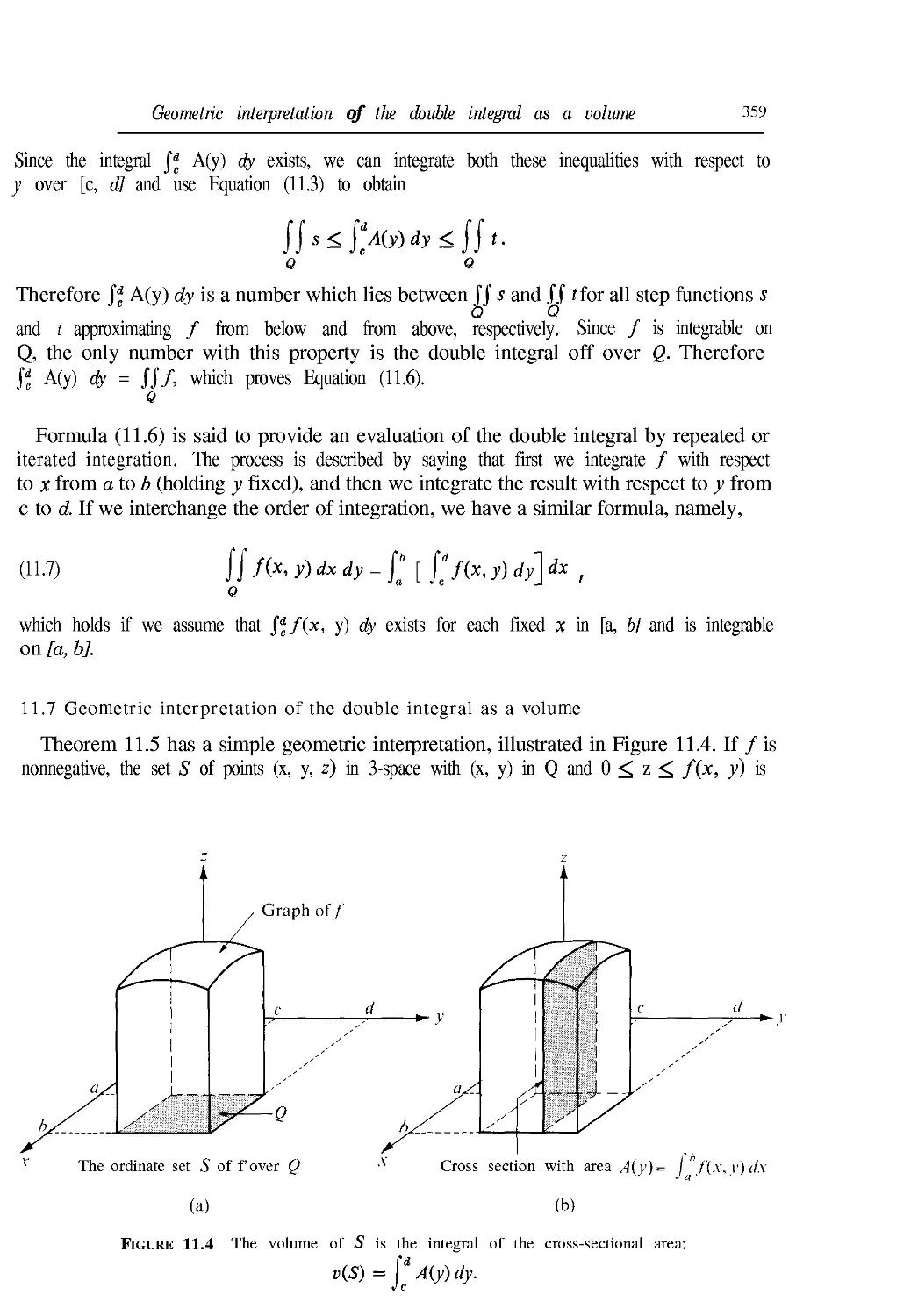
11.7 Geometric interpretation of the double integral as a volume 359
11.8 Worked examples 360
11.9 Exercises 362
11.10 Integrability of continuous functions 363
11 .1 1 Integrability of bounded functions with discontinuities 364
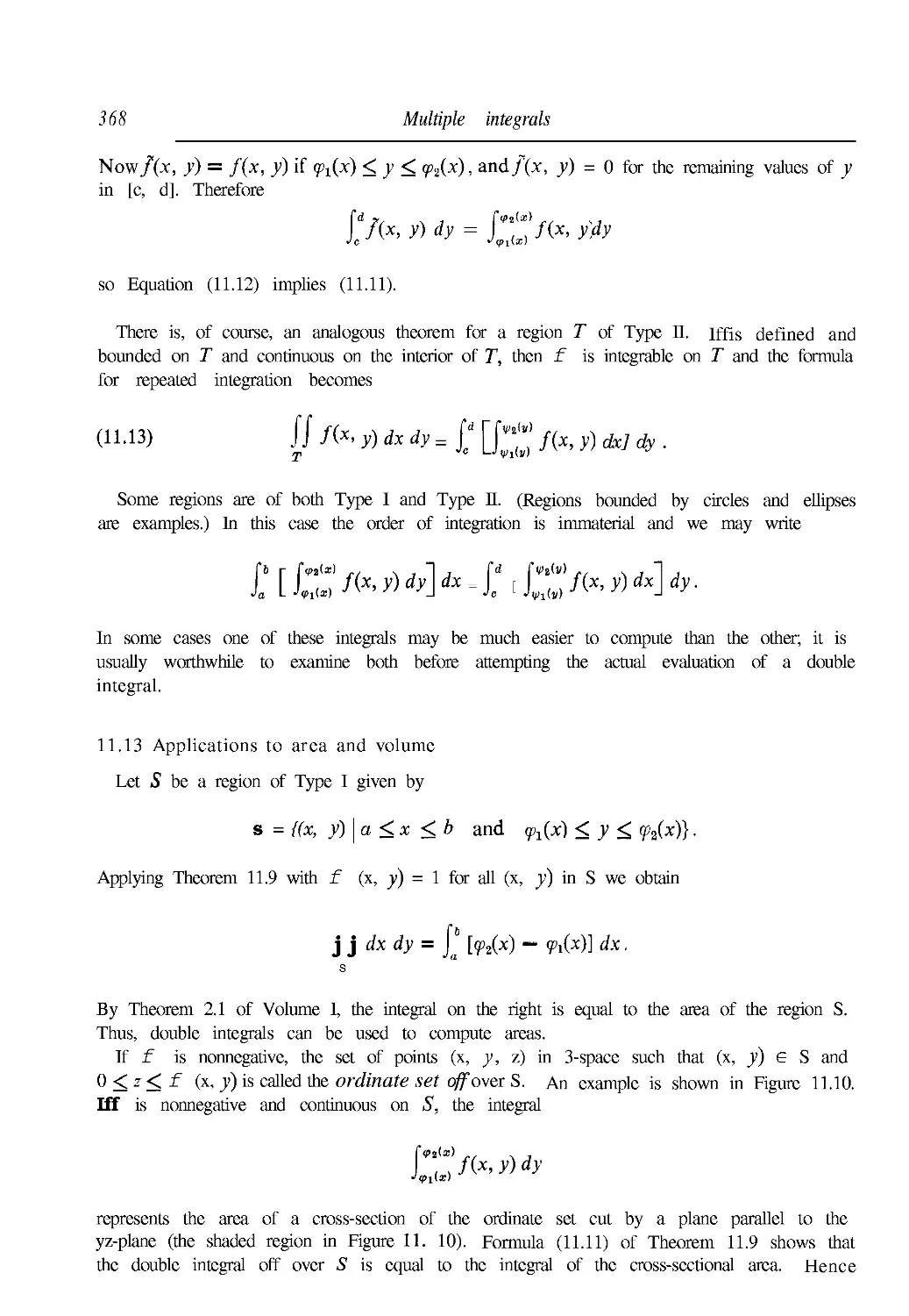
11.12 Double integrals extended over more general regions 365
11.13 Applications to area and volume 368
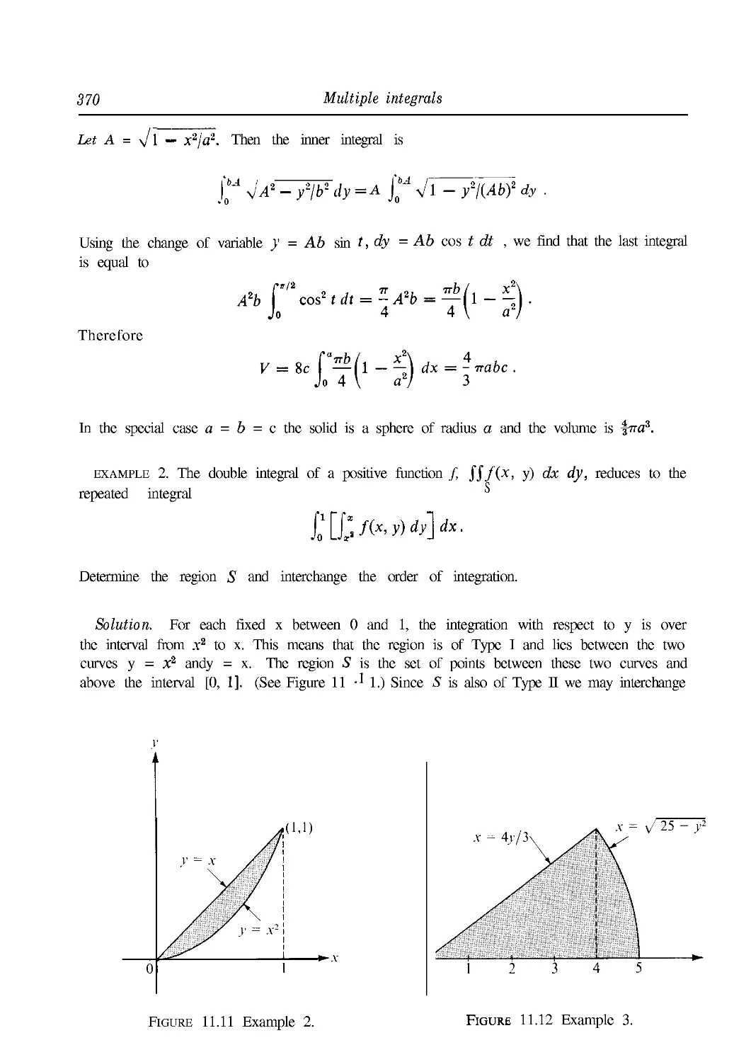
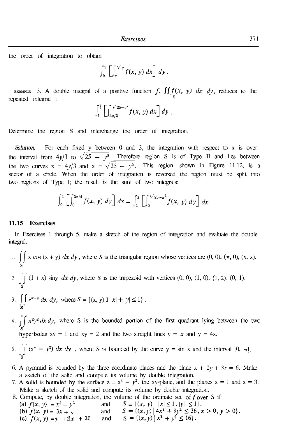
11.14 Worked examples 369
11. 15 Exercises 371
11.16 Further applications of double integrals 373
11.17 Two theorems of Pappus 376
11.18 Exercises 377

xviii Contents
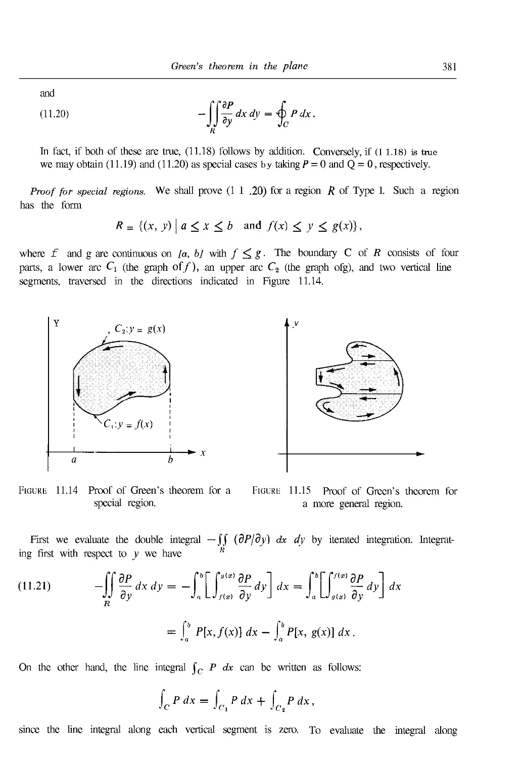
11.19 Green's theorem in the plane 378
11.20 Some applications of Green's theorem 382
11.21 A necessary and sufficient condition for a two-dimensional vector field to be a
gradient 383
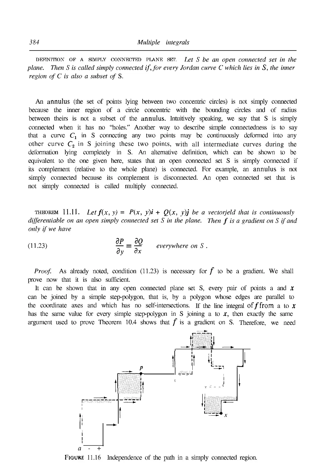
11.22 Exercises 385
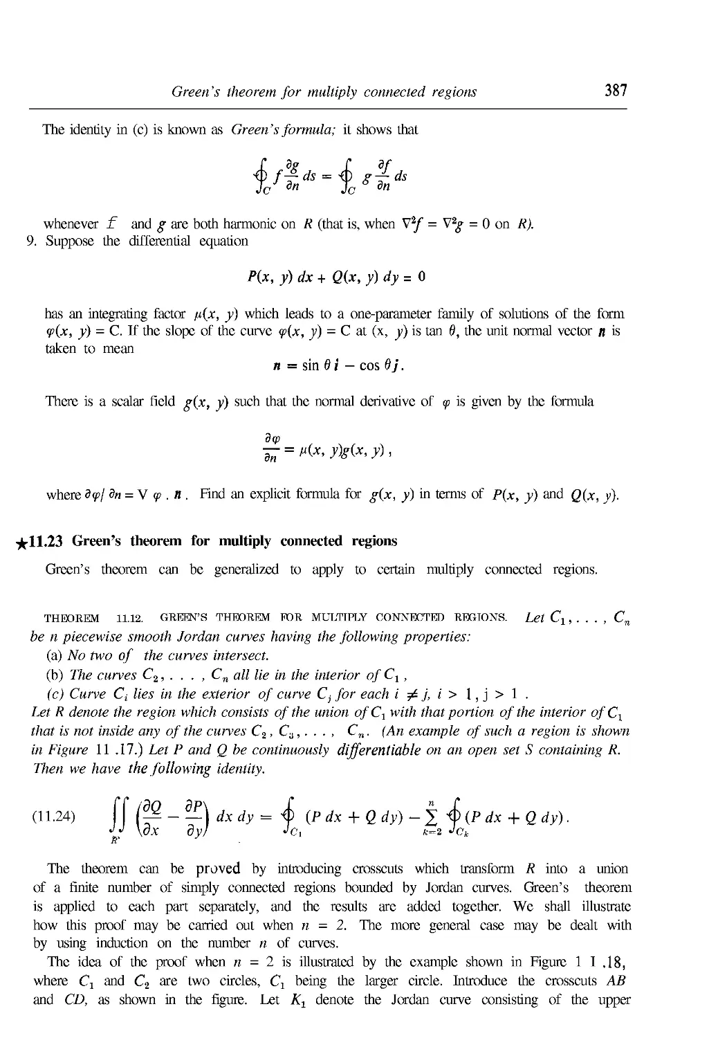
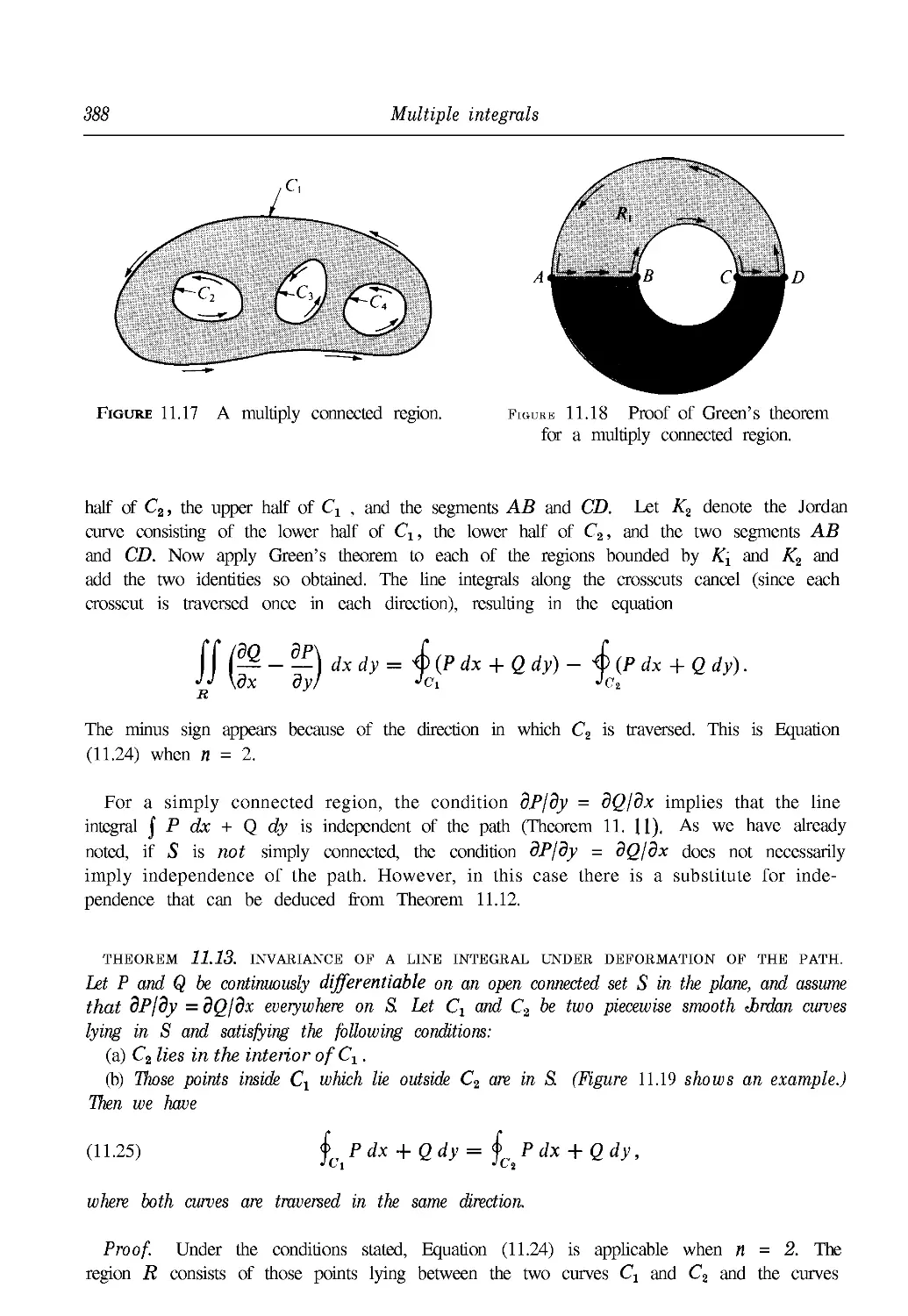
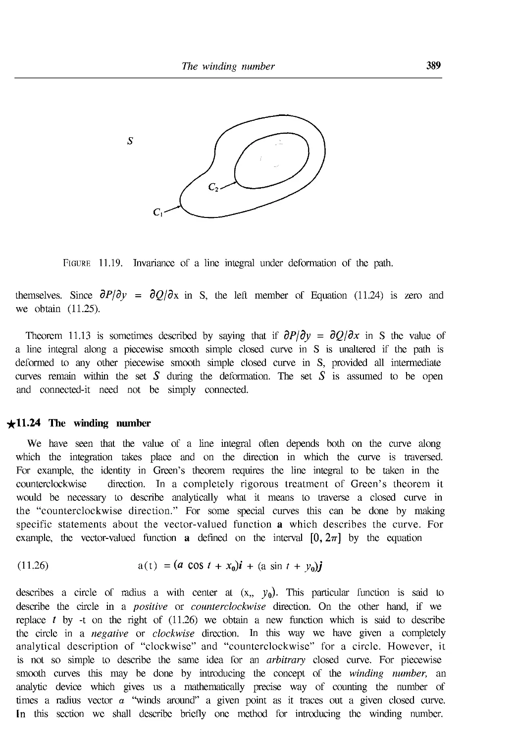
¦^¦11.23 Green's theorem for multiply connected regions 387
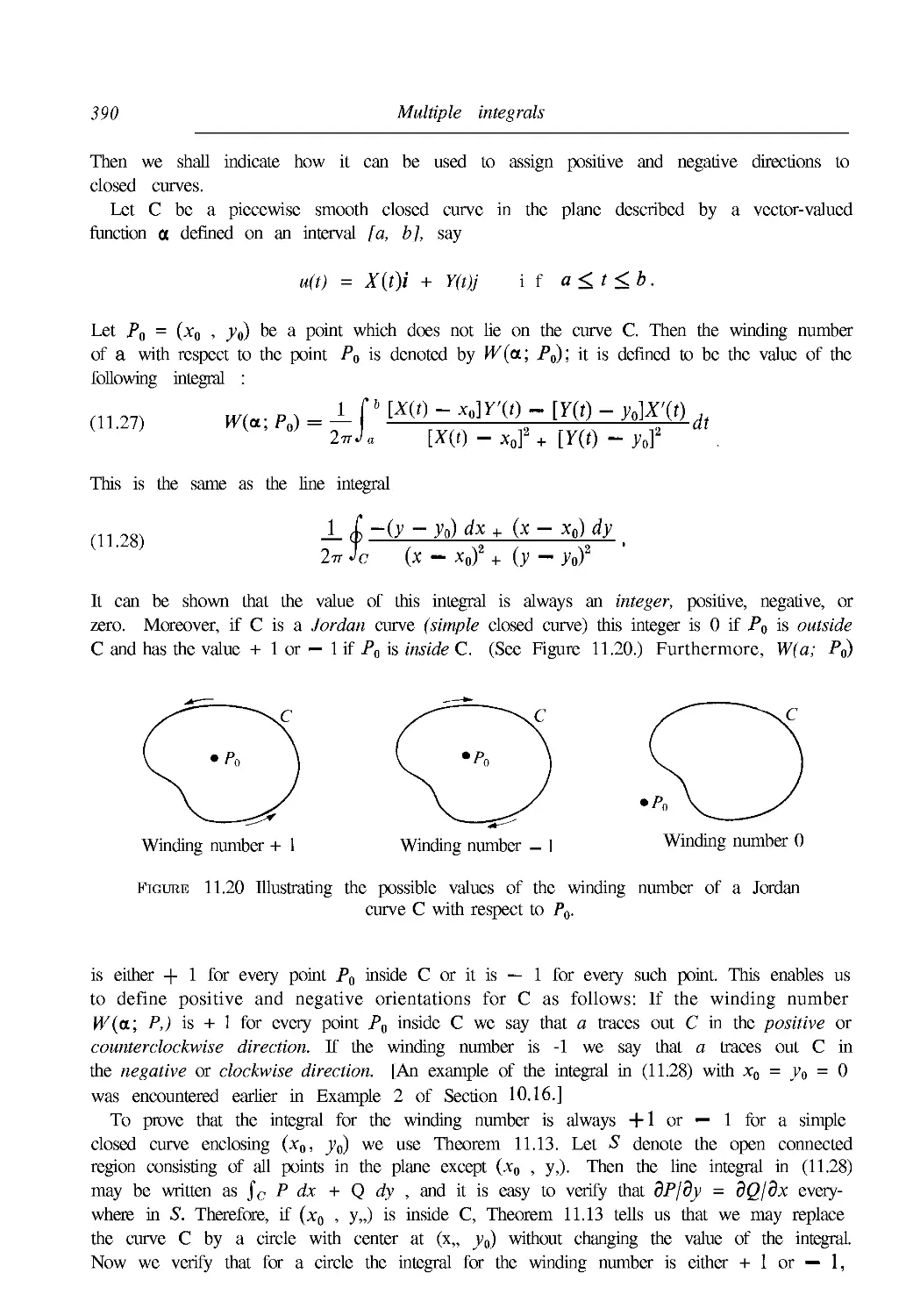
• 11.24 The winding number 389
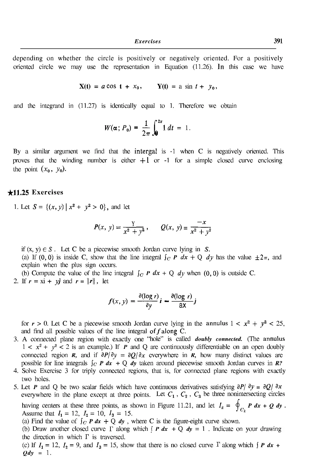
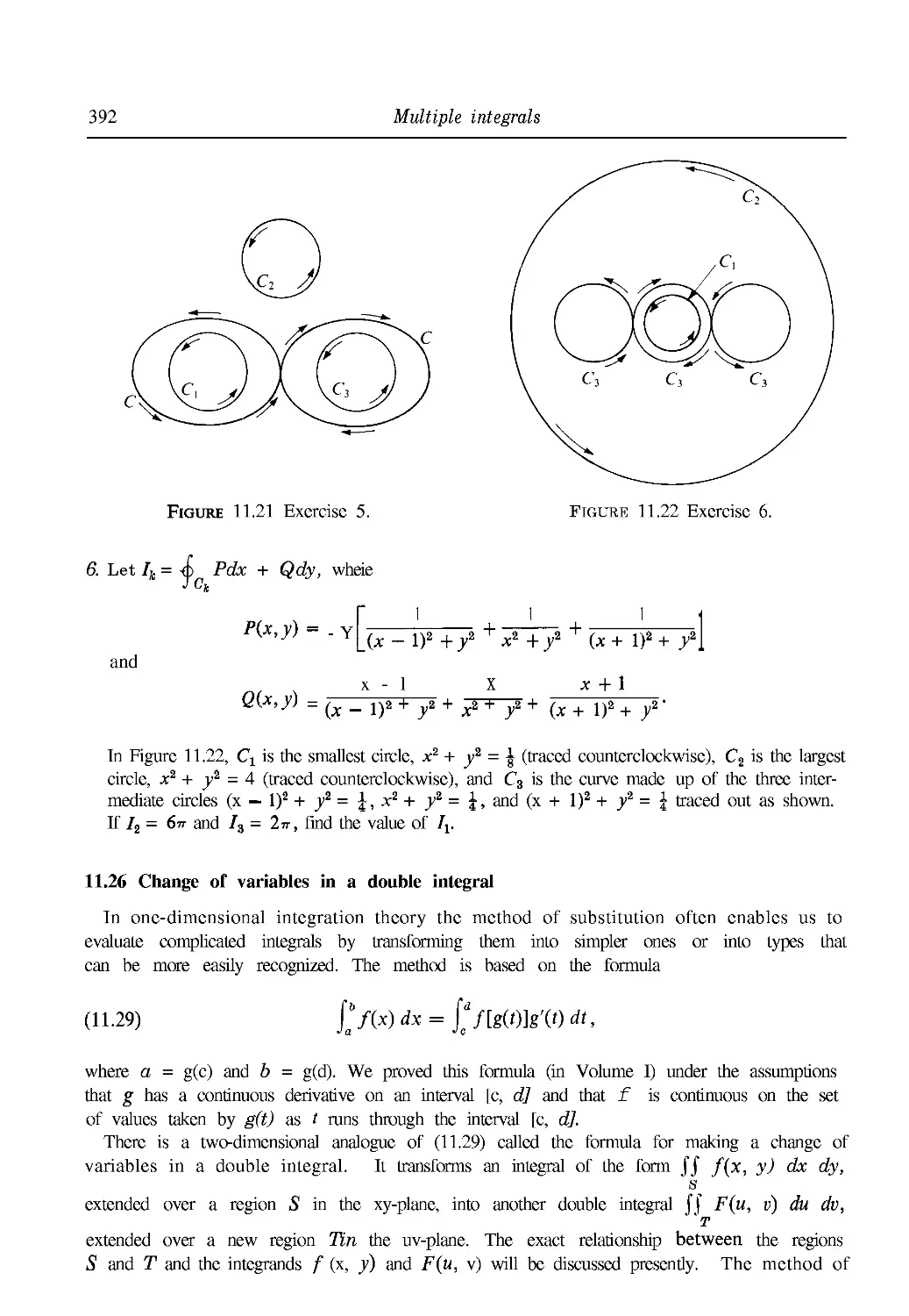
• 1 1.25 Exercises 391
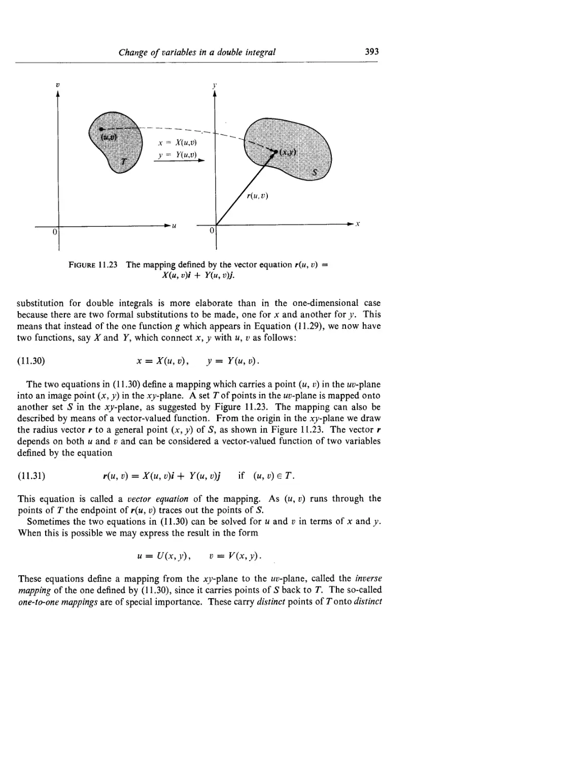
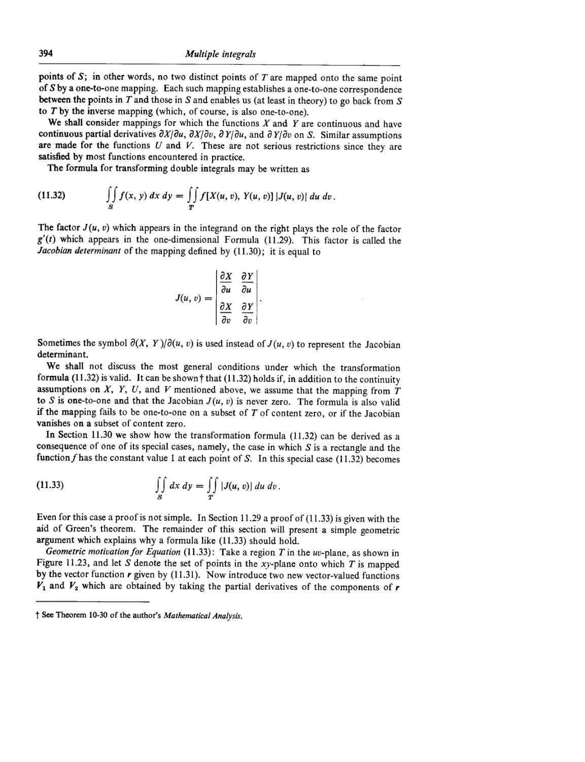
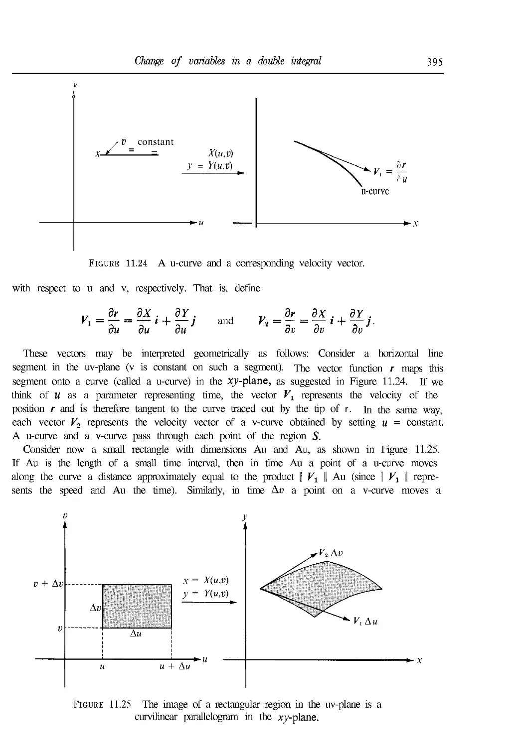
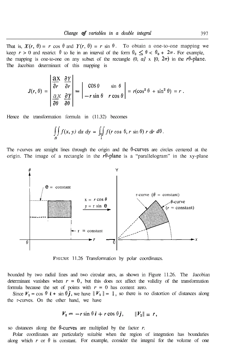
11.26 Change of variables in a double integral 392
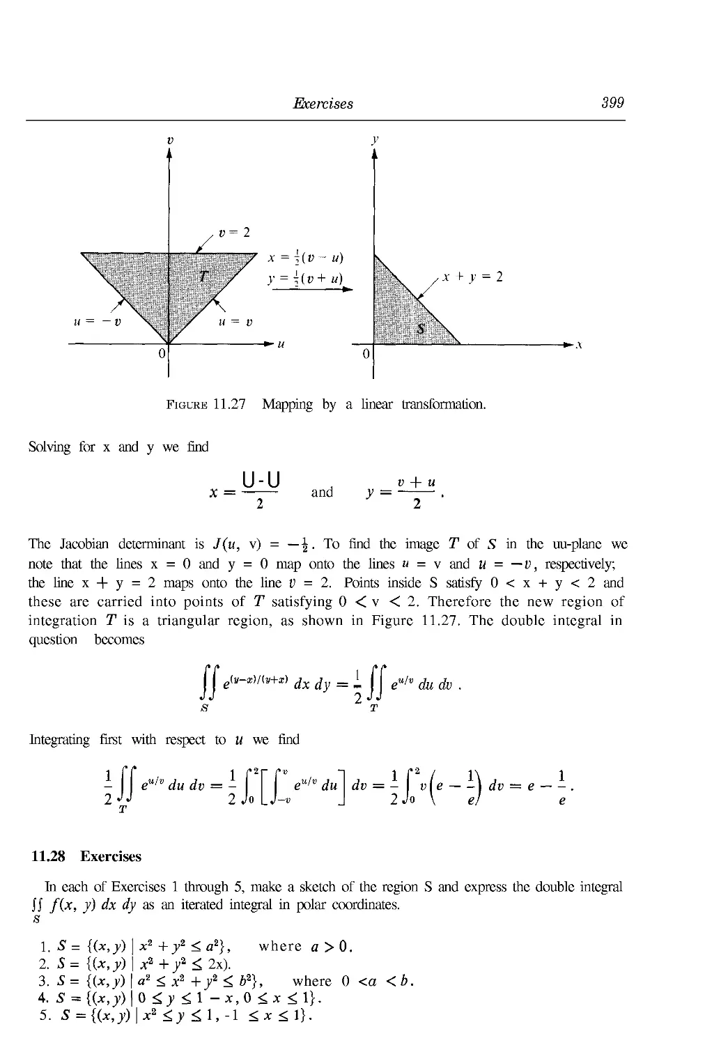
11.27 Special cases of the transformation formula 396
11.28 Exercises 399
11.29 Proof of the transformation formula in a special case 401
11.30 Proof of the transformation formula in the general case 403
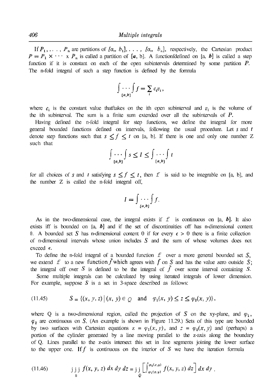
11.31 Extensions to higher dimensions 405
11.32 Change of variables in an n-fold integral 407
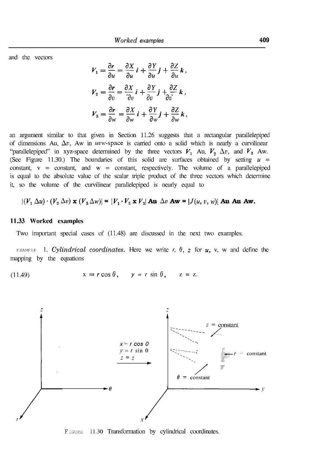
11.33 Worked examples 409
11.34 Exercises 413
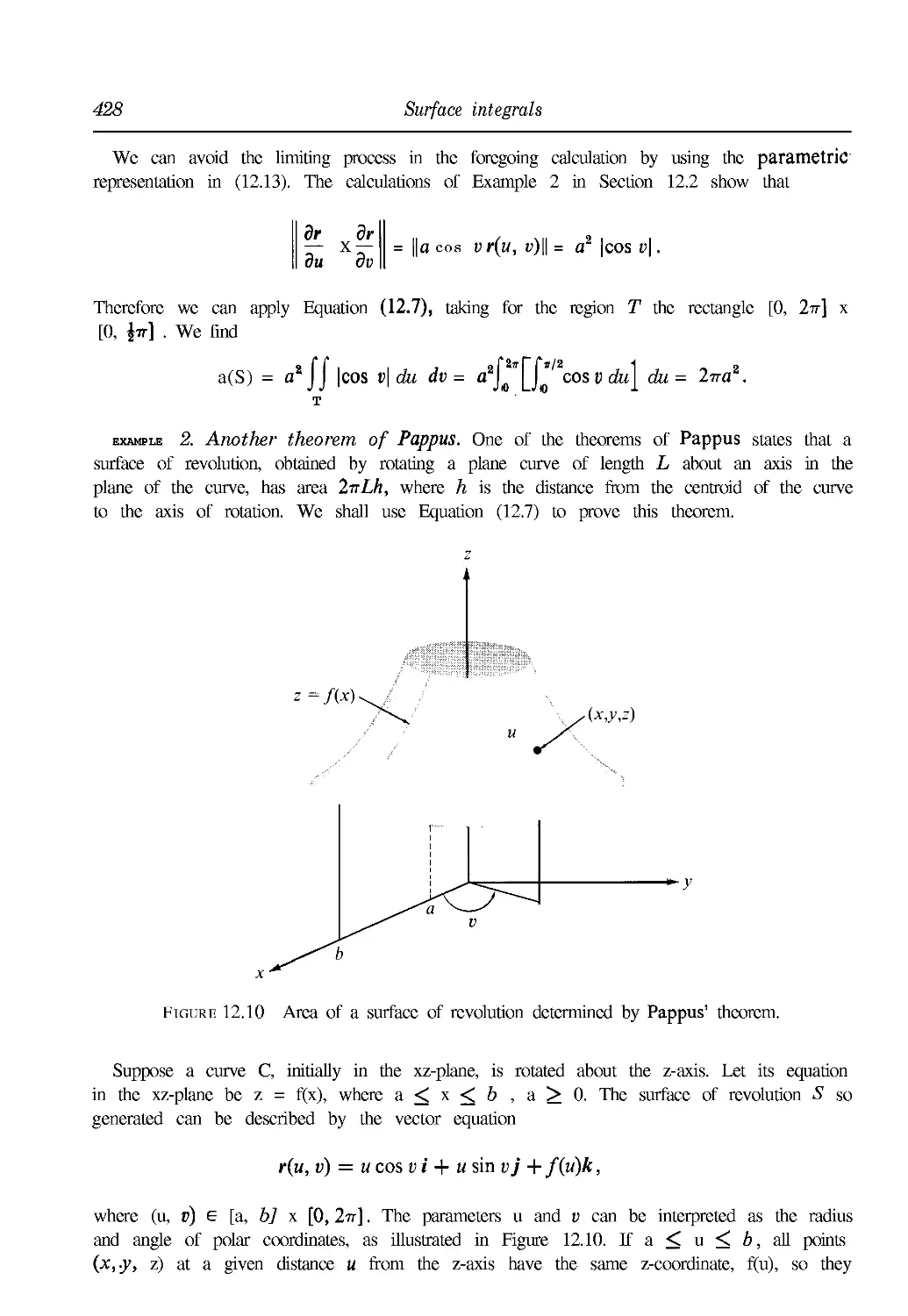
12. SURFACE INTEGRALS
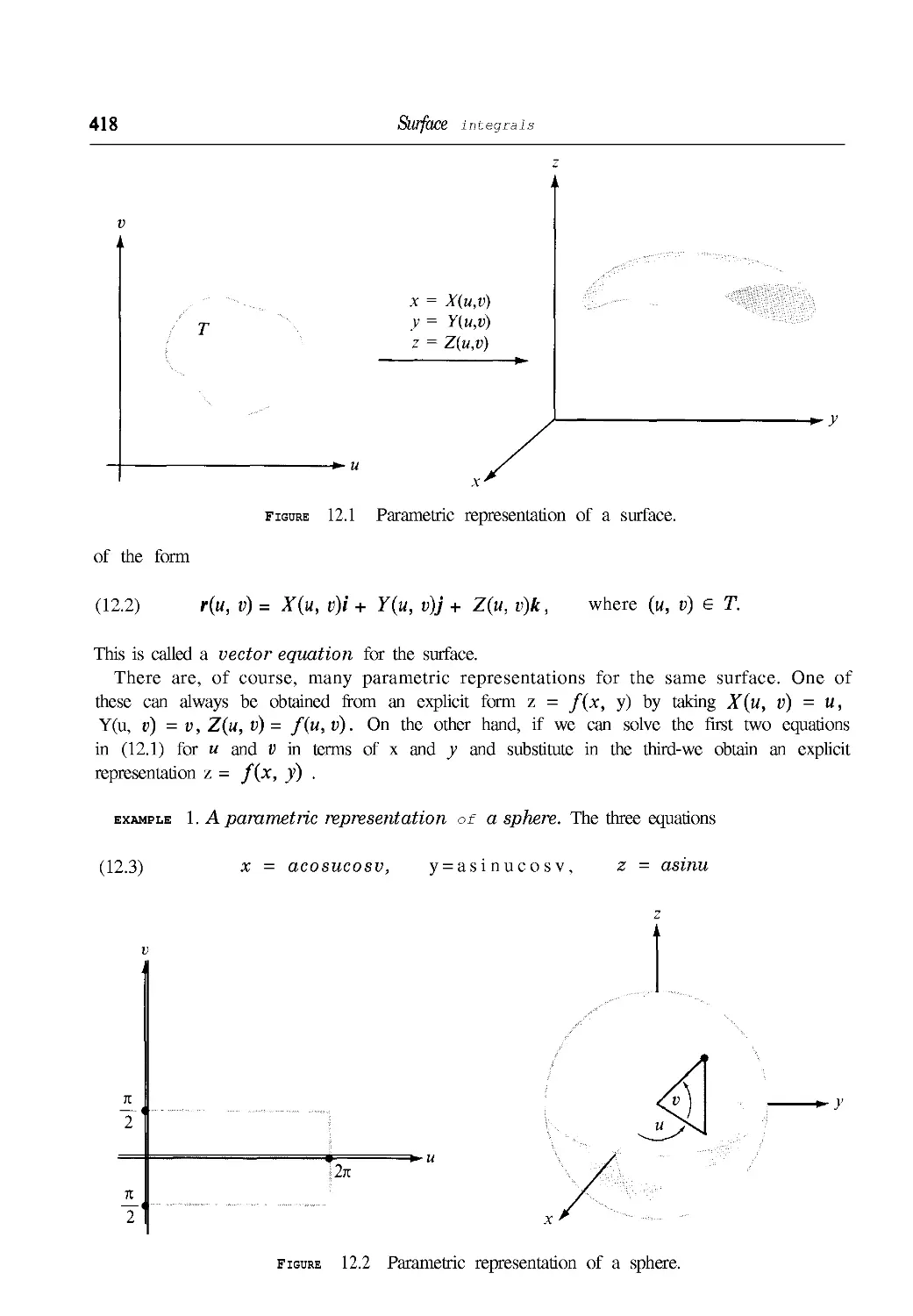
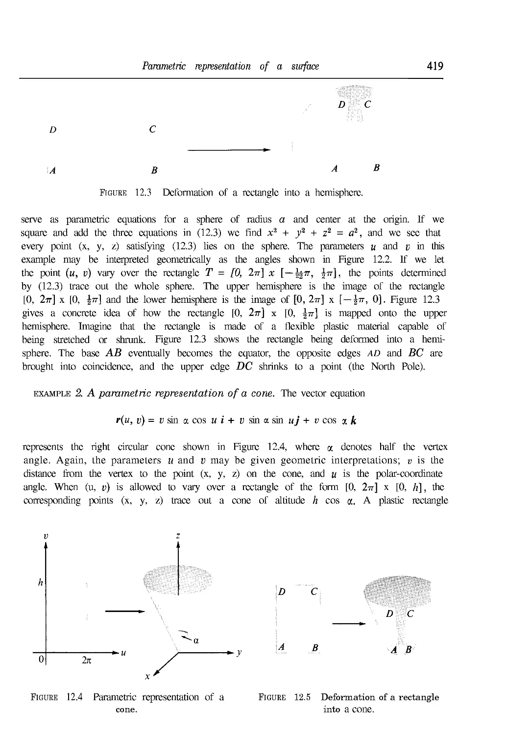
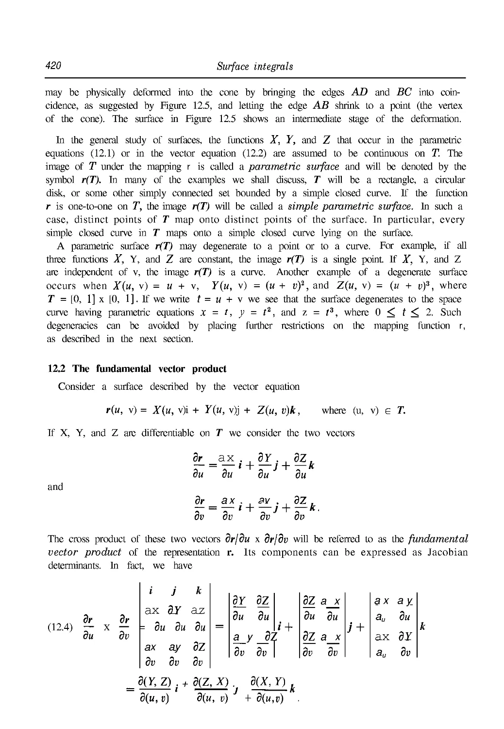
12.1 Parametric representation of a surface 417
12.2 The fundamental vector product 420
12.3 The fundamental vector product as a normal to the surface 423
12.4 Exercises 424
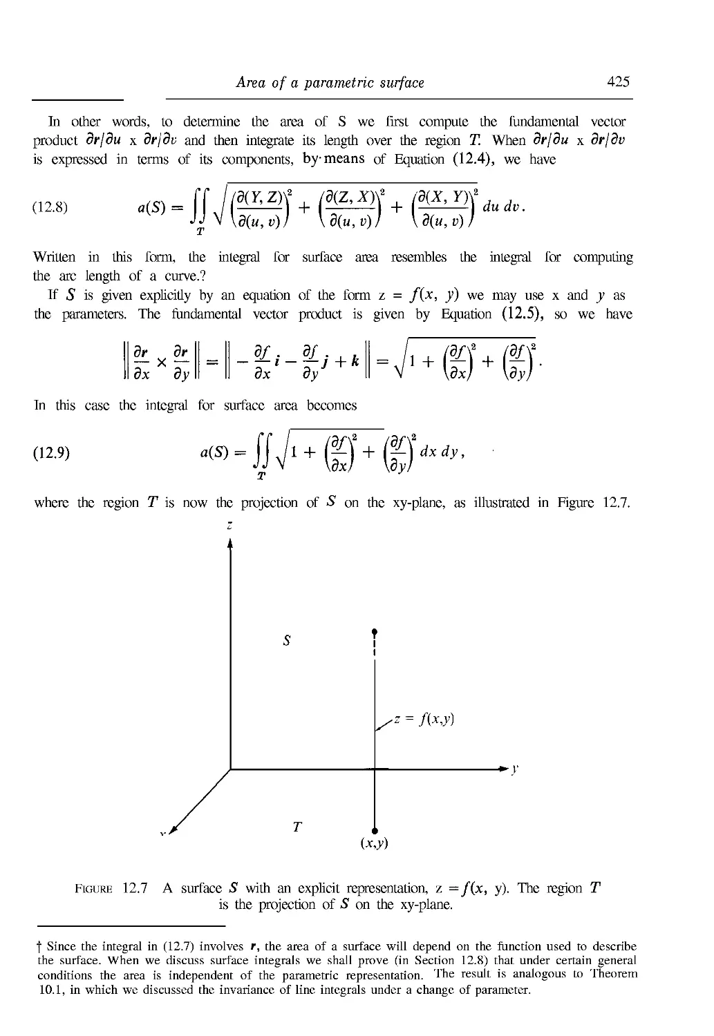
12.5 Area of a parametric surface 424
12.6 Exercises 429
12.7 Surface integrals 430
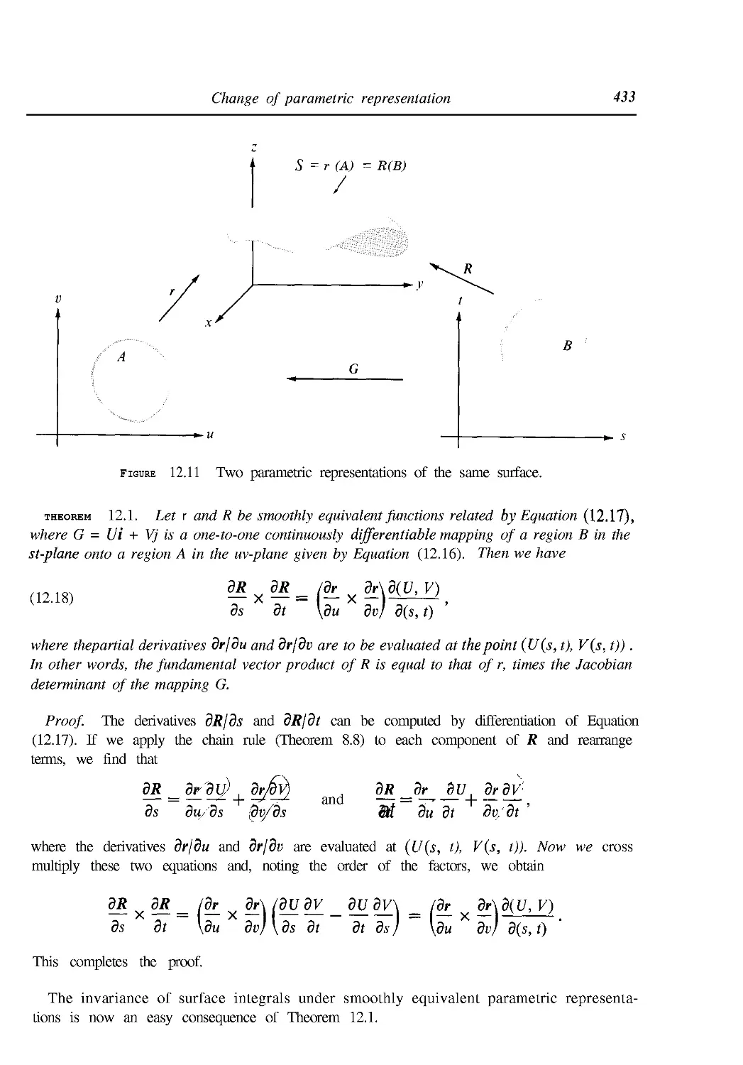
12.8 Change of parametric representation 432
12.9 Other notations for surface integrals 434
12.10 Exercises 436
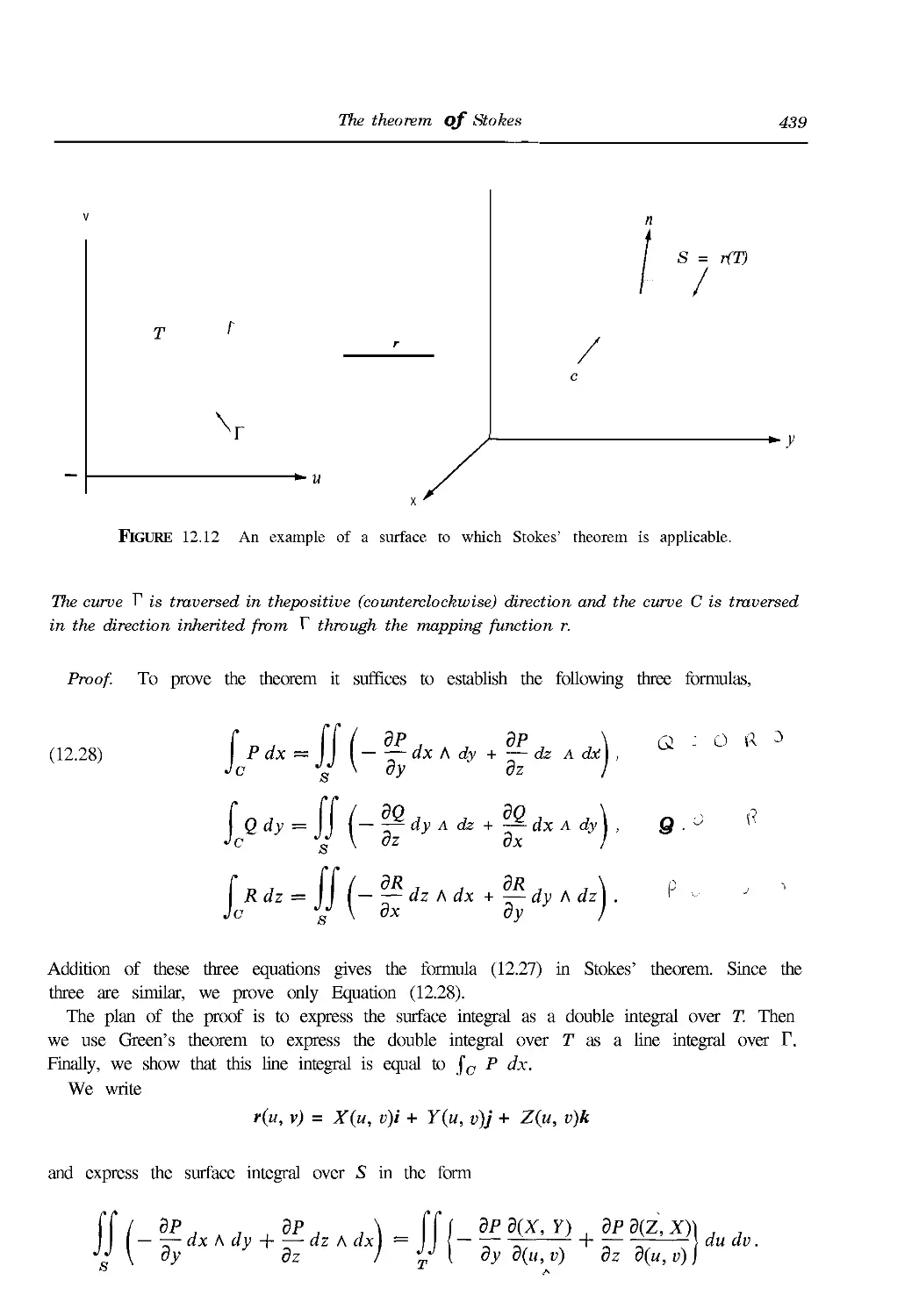
12.11 The theorem of Stokes 438
12.12 The curl and divergence of a vector field 440
12.13 Exercises 442
12.14 Further properties of the curl and divergence 443
12.15 Exercises 447
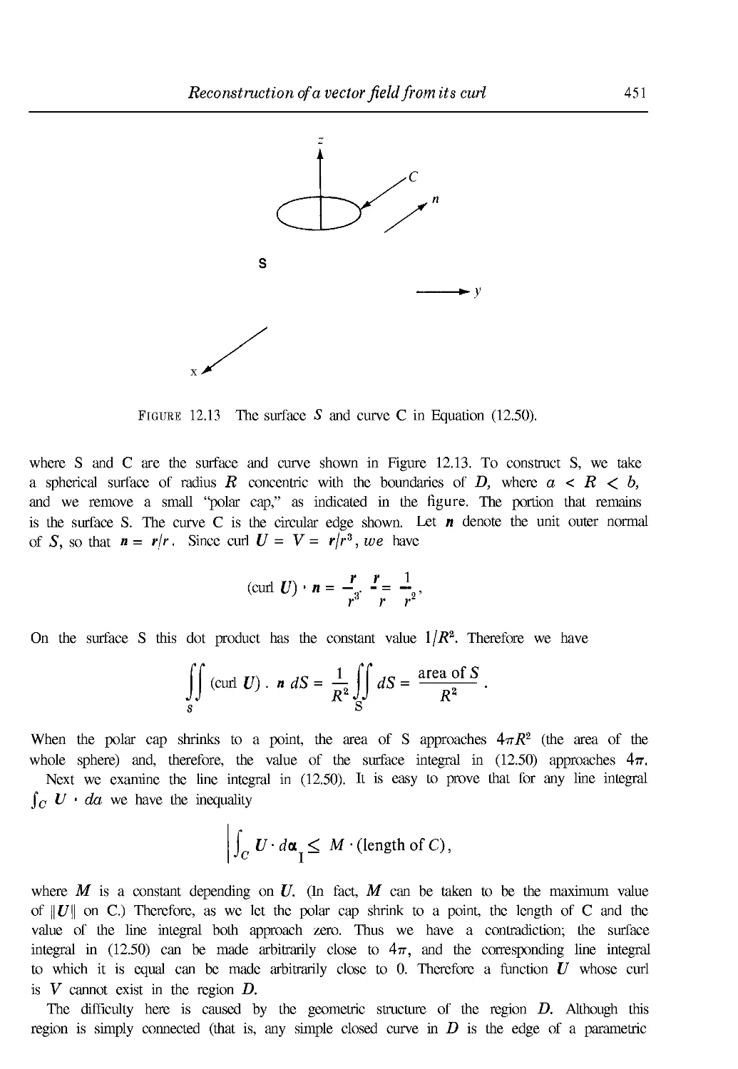
"^12.16 Reconstruction of a vector field from its curl 448
•12.17 Exercises 452
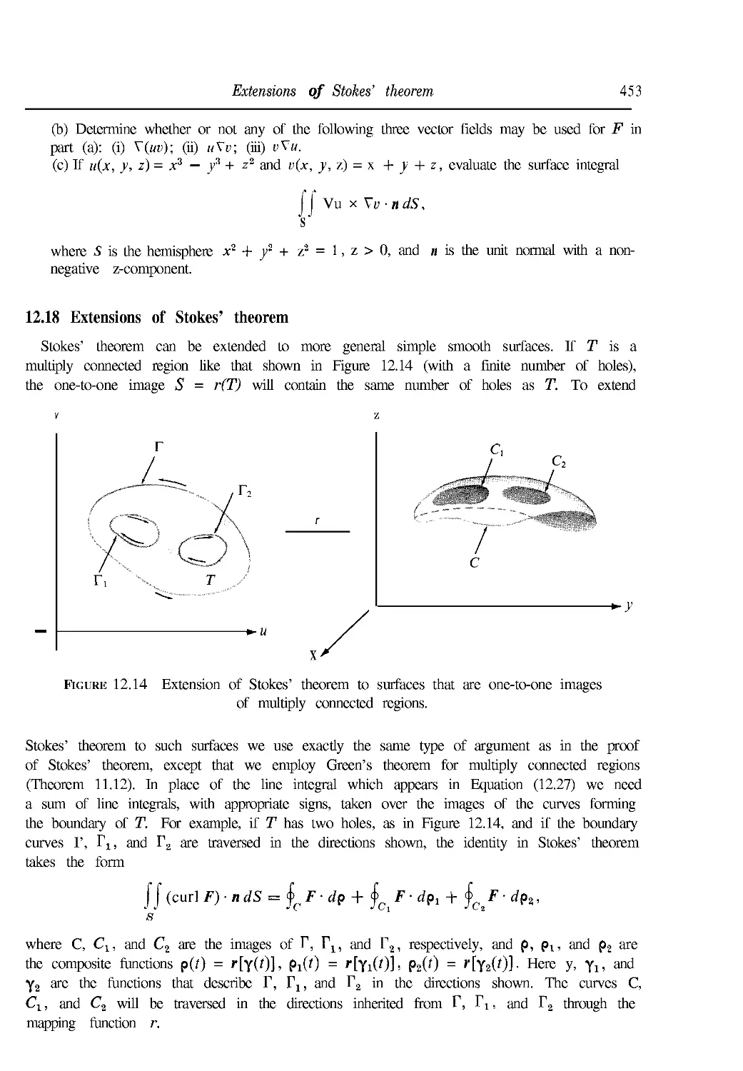
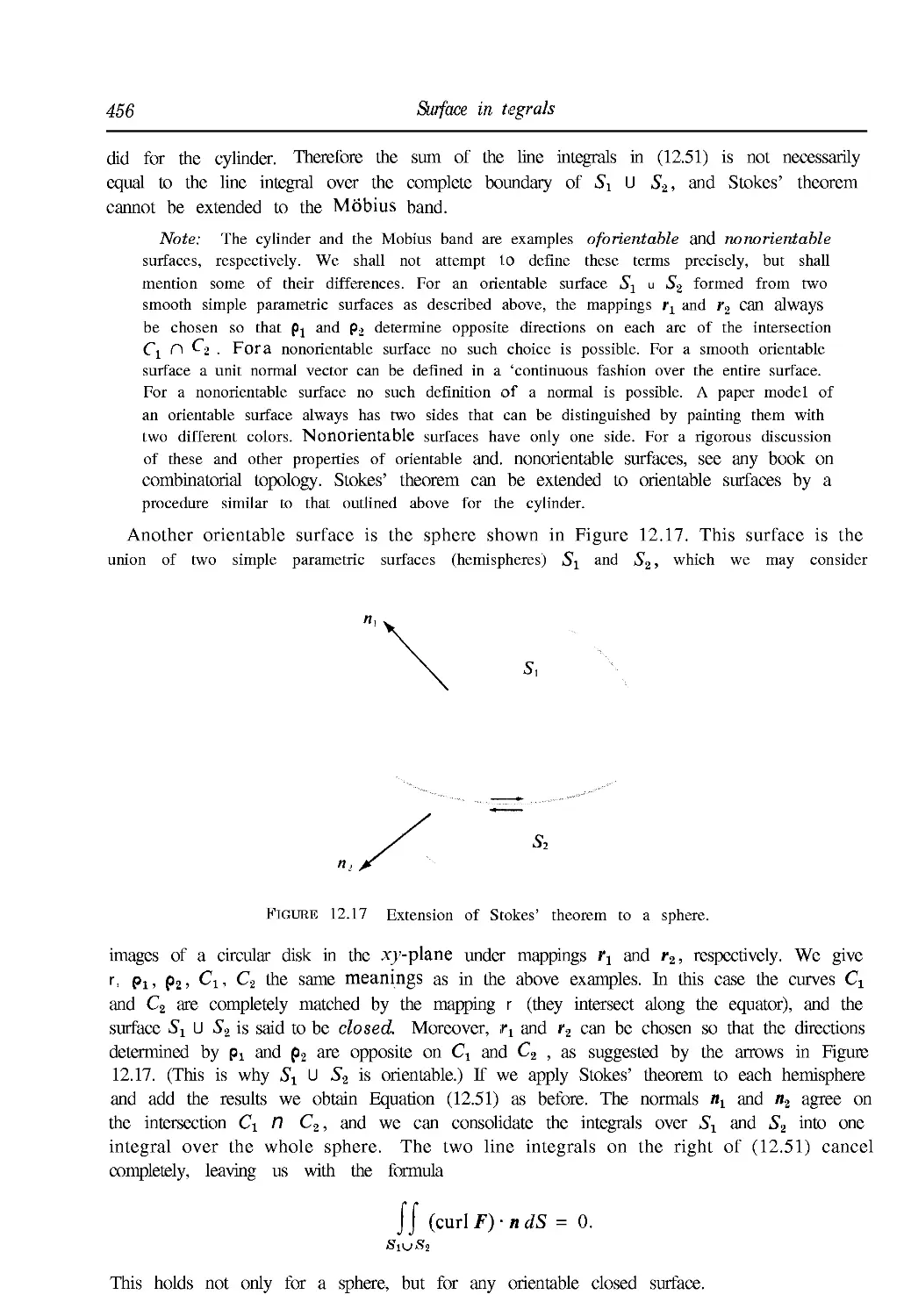
12.18 Extensions of Stokes' theorem 453
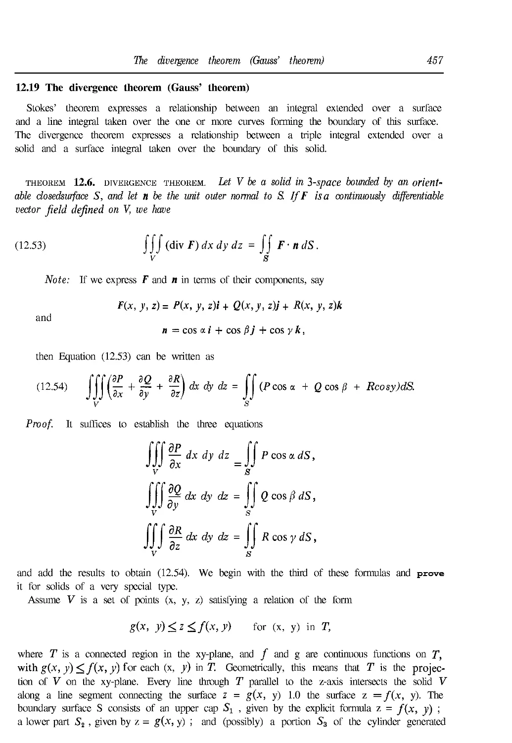
12.19 The divergence theorem (Gauss' theorem:) 457
12.20 Applications of the divergence theorem 460
12.21 Exercises 462

Contents xix
PART 3. SPECIAL TOPICS
13. SET FUNCTIONS AND ELEMENTARY PROBABILITY
13.1 Historical introduction 469
13.2 Finitely additive set functions 470
13.3 Finitely additive measures 471
13.4 Exercises 472
13.5 The definition of probability for finite sample spaces 473
13.6 Special terminology peculiar to probability theory 475
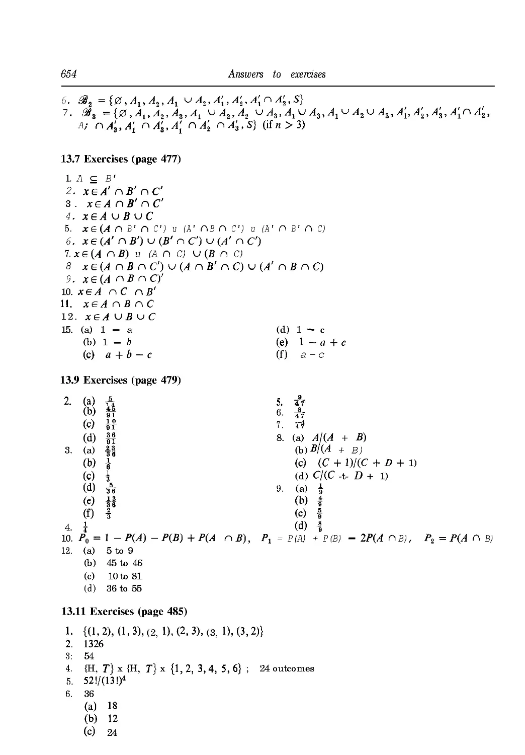
13.7 Exercises 477
13.8 Worked examples 477
13.9 Exercises 479
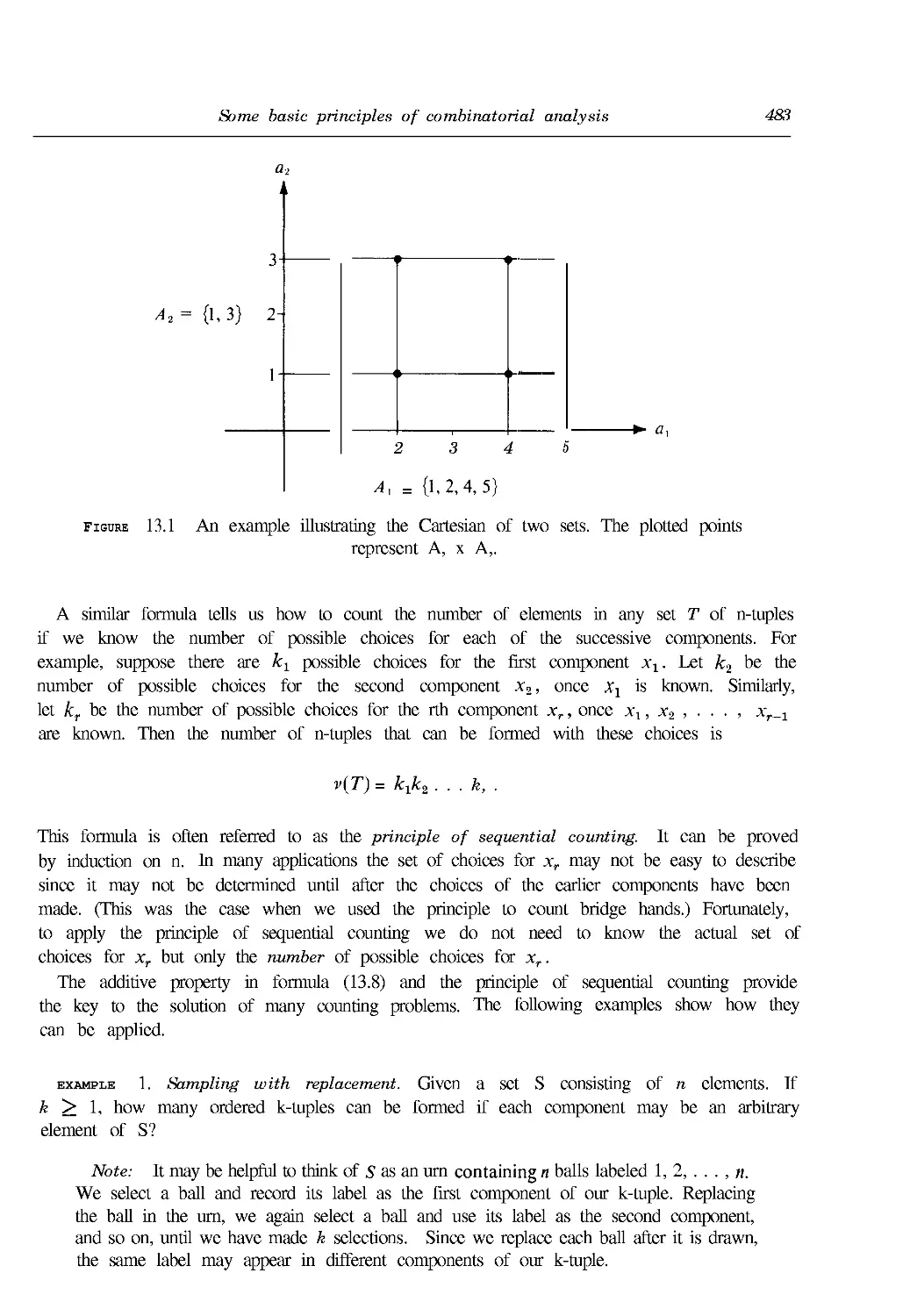
13.10 Some basic principles of combinatorial analysis 481
13.11 Exercises 485
13.12 Conditional probability 486
13.13 Independence 488
13.14 Exercises 490
13.15 Compound experiments 492
13.16 Bernoulli trials 495
13.17 The most probable number of successes in n Bernoulli trials 497
13.18 Exercises 499
13.19 Countable and uncountable sets 501
13.20 Exercises 504
13.21 The definition of probability for countably infinite sample spaces 506
13.22 Exercises 507
13.23 Miscellaneous exercises on probability 507
14. CALCULUS OF PROBABILITIES
14.1 The definition of probability for uncountable sample spaces 510
14.2 Countability of the set of points with positive probability 511
14.3 Random variables 512
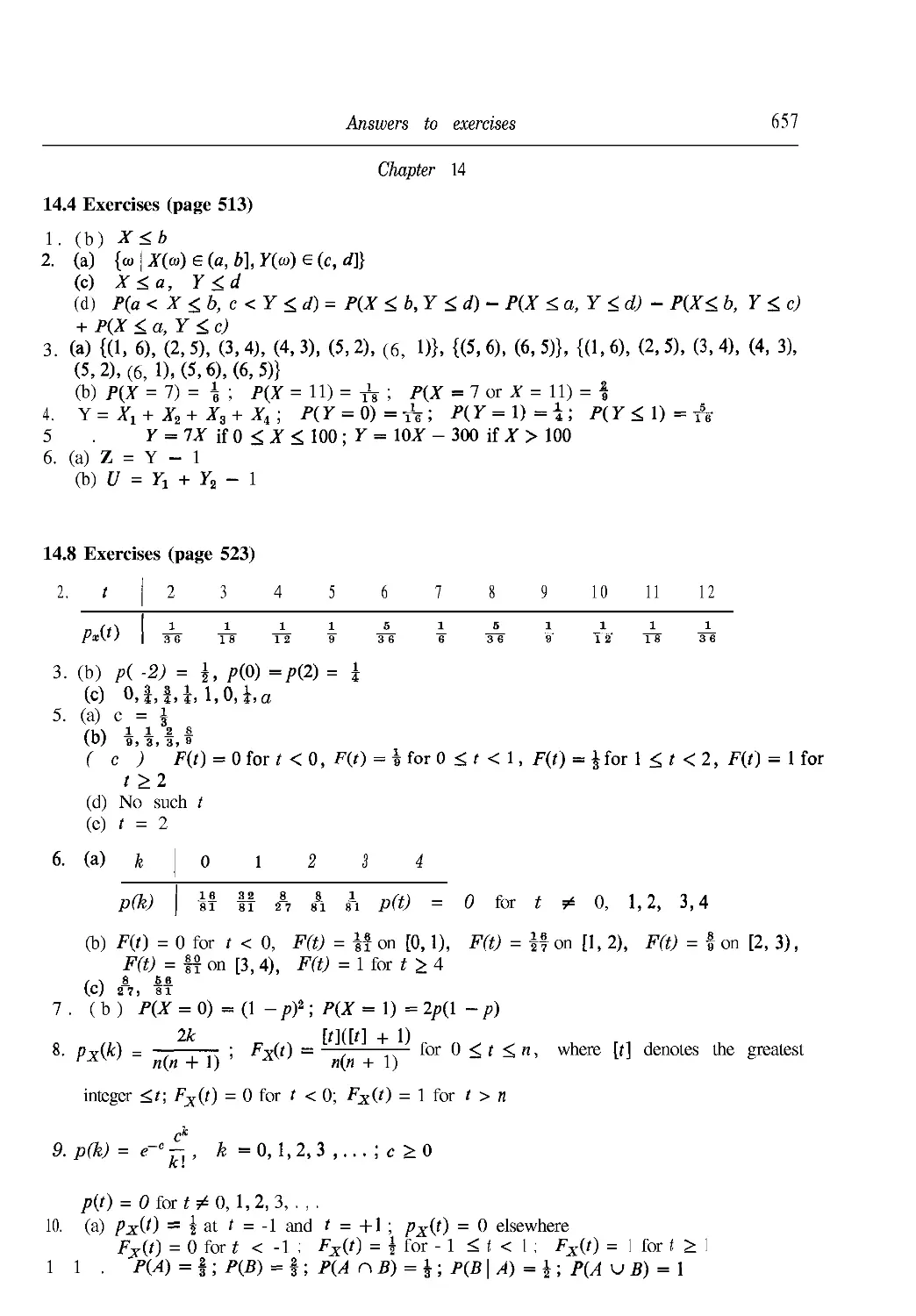
14.4 Exercises 513
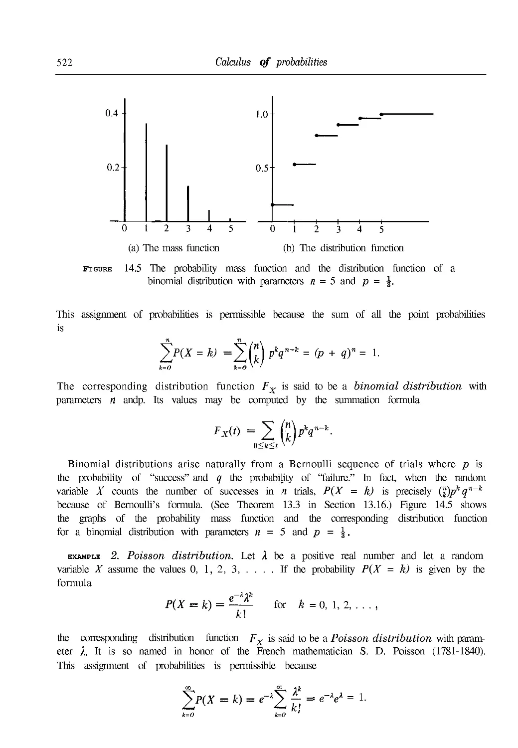
14.5 Distribution functions 514
14.6 Discontinuities of distribution functions 517
14.7 Discrete distributions. Probability mass functions 520
14.8 Exercises 523
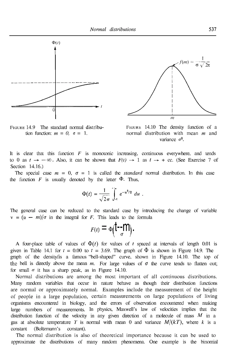
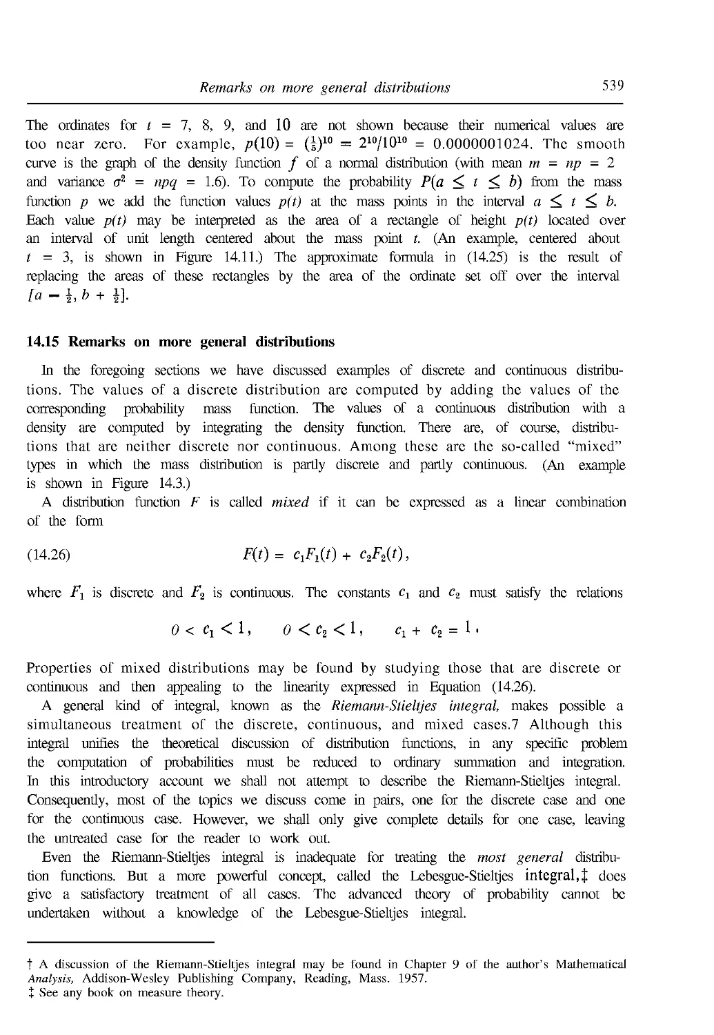
14.9 Continuous distributions. Density functions 525

xx Contents
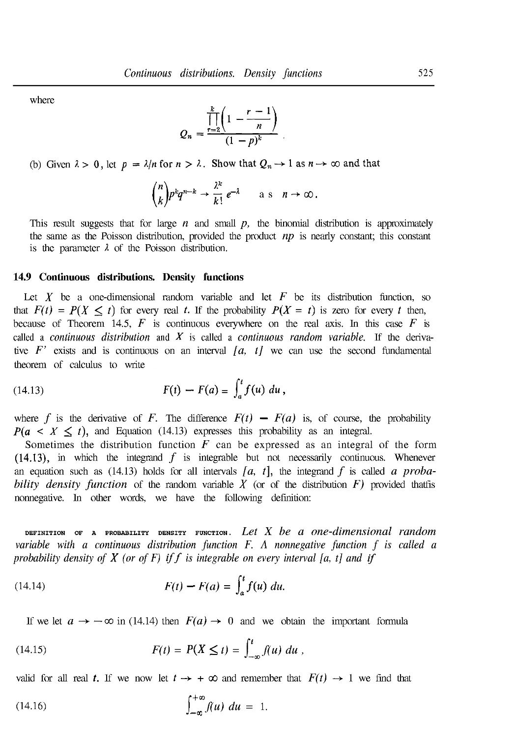
14.10 Uniform distribution over an interval 526
14.11 Cauchy's distribution 530
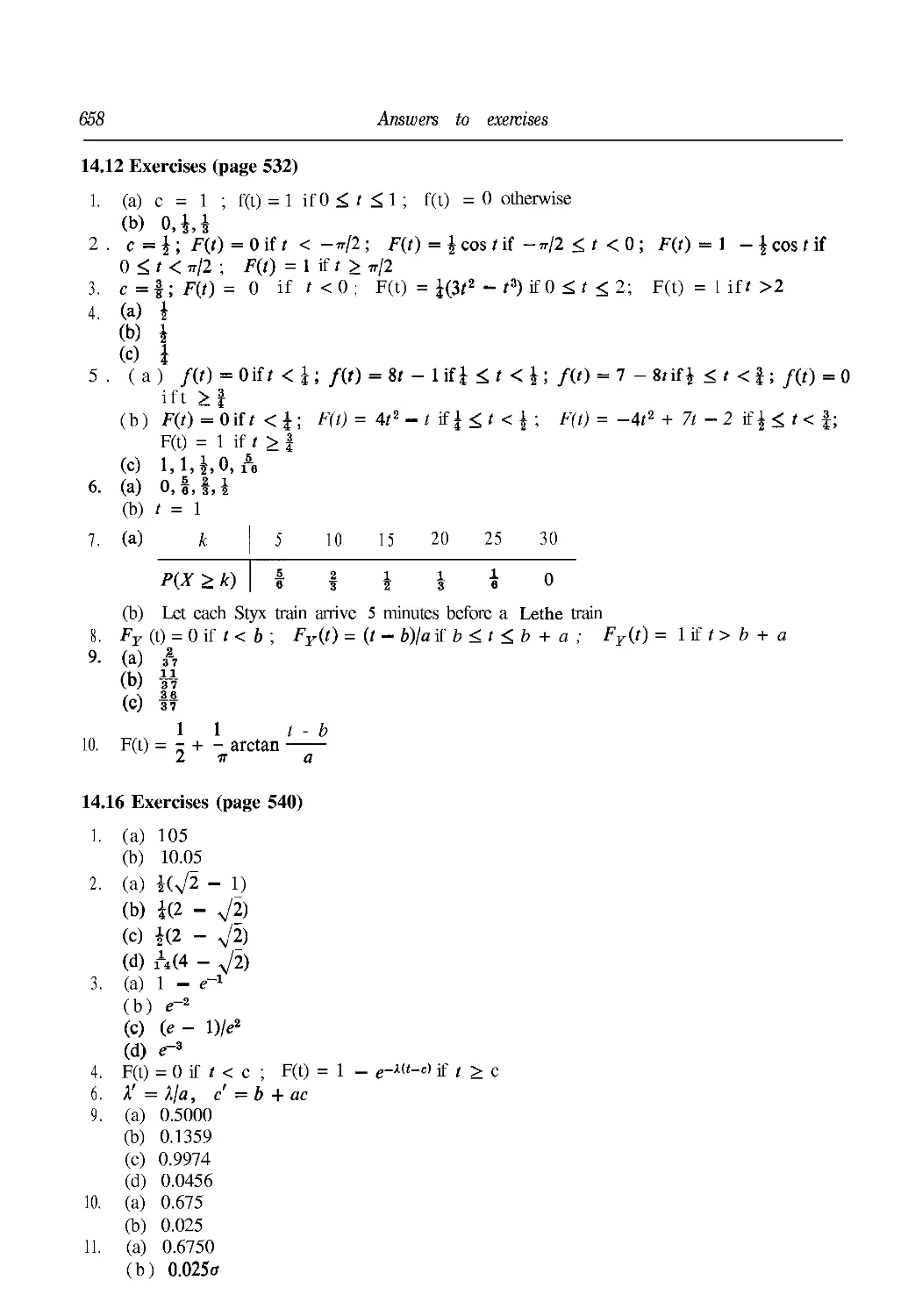
14.12 Exercises 532
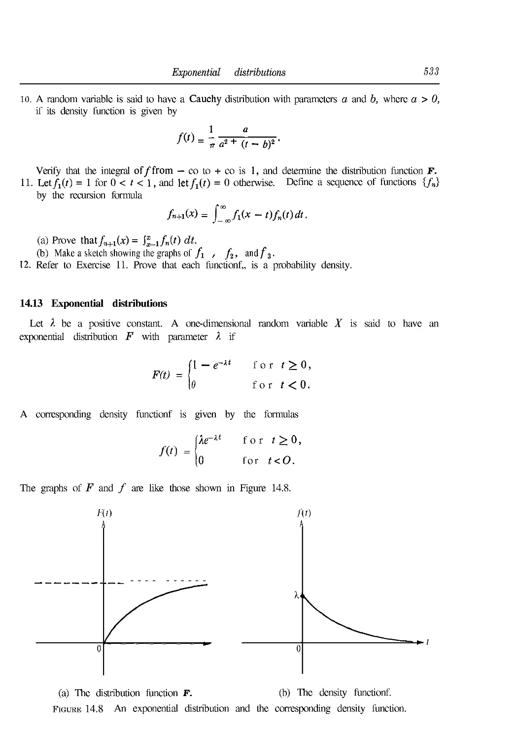
14.13 Exponential distributions 533
14.14 Normal distributions 535
14.15 Remarks on more general distributions 539
14.16 Exercises 540
14.17 Distributions of functions of random variables 541
14.18 Exercises 542
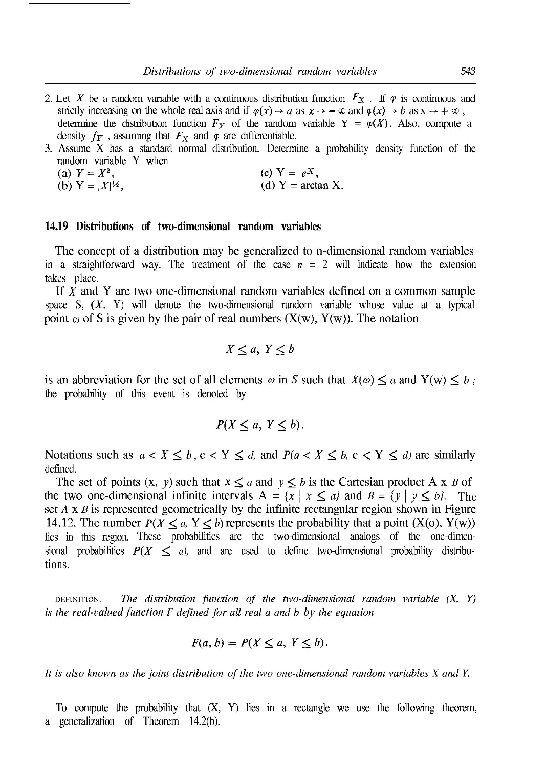
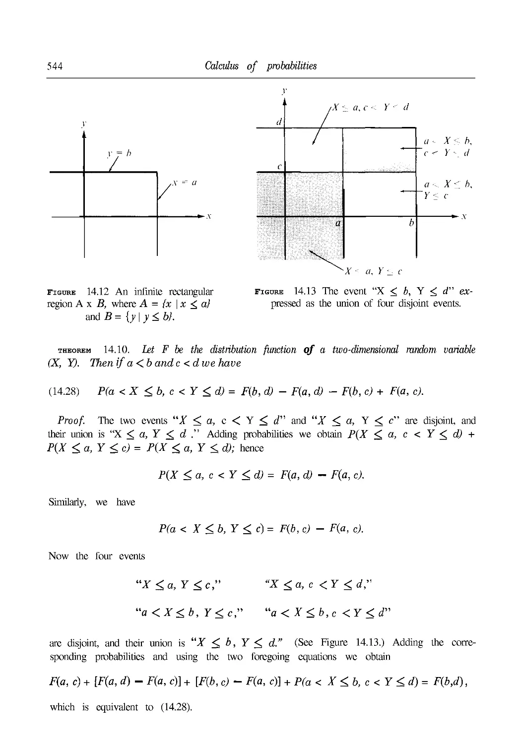
14.19 Distributions of two-dimensional random variables 543
14.20 Two-dimensional discrete distributions 545
14.21 Two-dimensional continuous distributions. Density functions 546
14.22 Exercises 548
14.23 Distributions of functions of two random variables 550
14.24 Exercises 553
14.25 Expectation and variance 556
14.26 Expectation of a function of a random variable 559
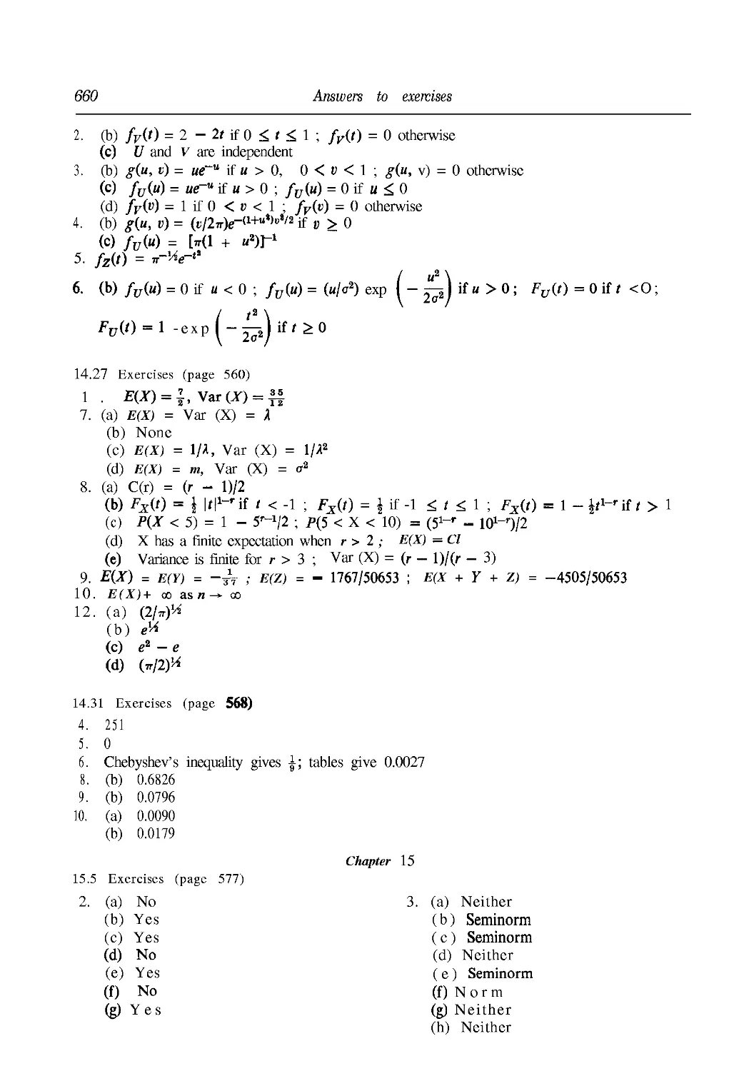
14.27 Exercises 560
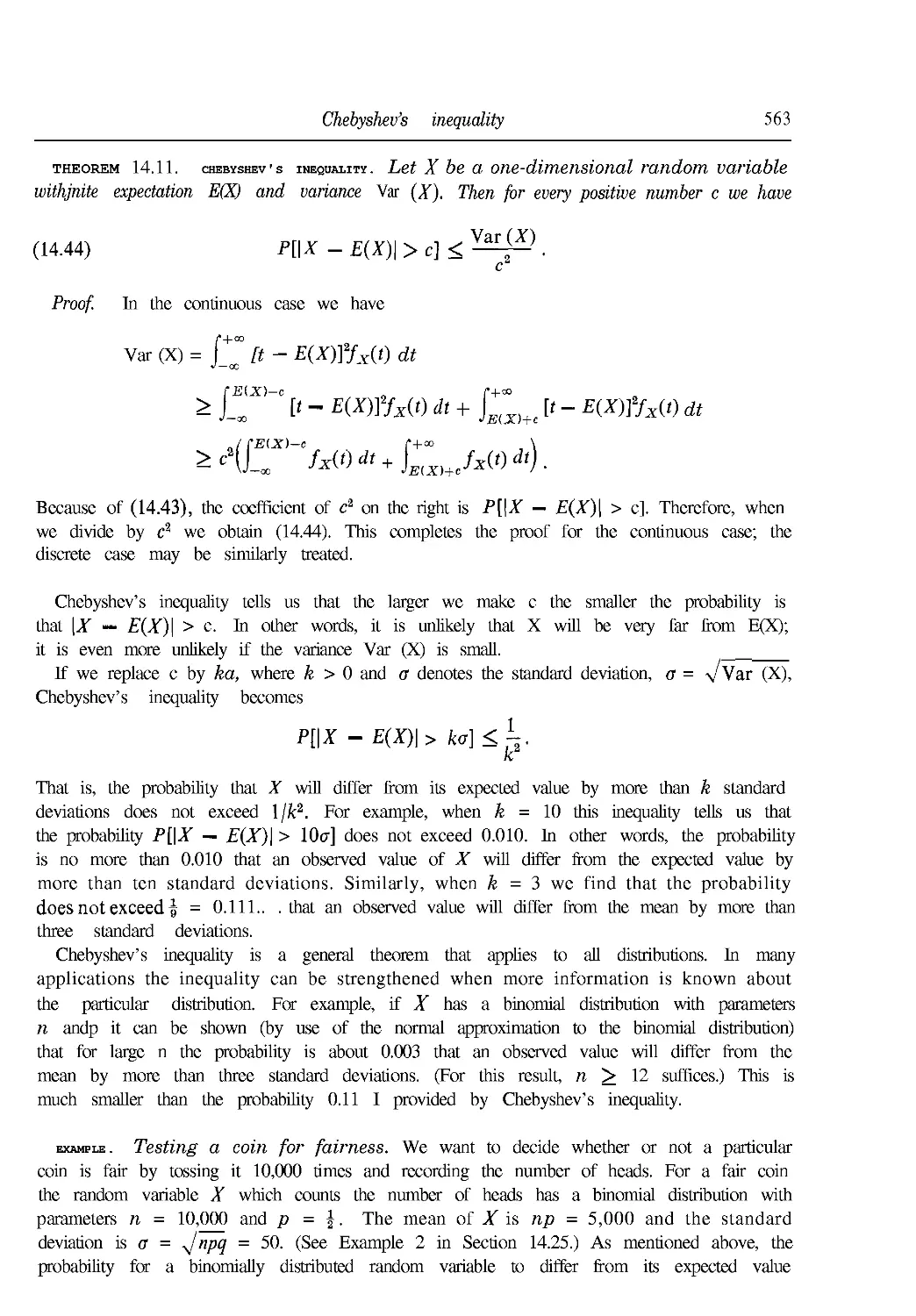
14.28 Chebyshev's inequality 562
14.29 Laws of large numbers 564
14.30 The central limit theorem of the calculus of probabilities 566
14.3 1 Exercises 568
Suggested References 569
15. INTRODUCTION TO NUMERICAL ANALYSIS
15.1 Historical introduction 571
15.2 Approximations by polynomials 572
15.3 Polynomial approximation and normed linear spaces 574
15.4 Fundamental problems in polynomial approximation 575
15.5 Exercises 577
15.6 Interpolating polynomials 579
15.7 Equally spaced interpolation points 582
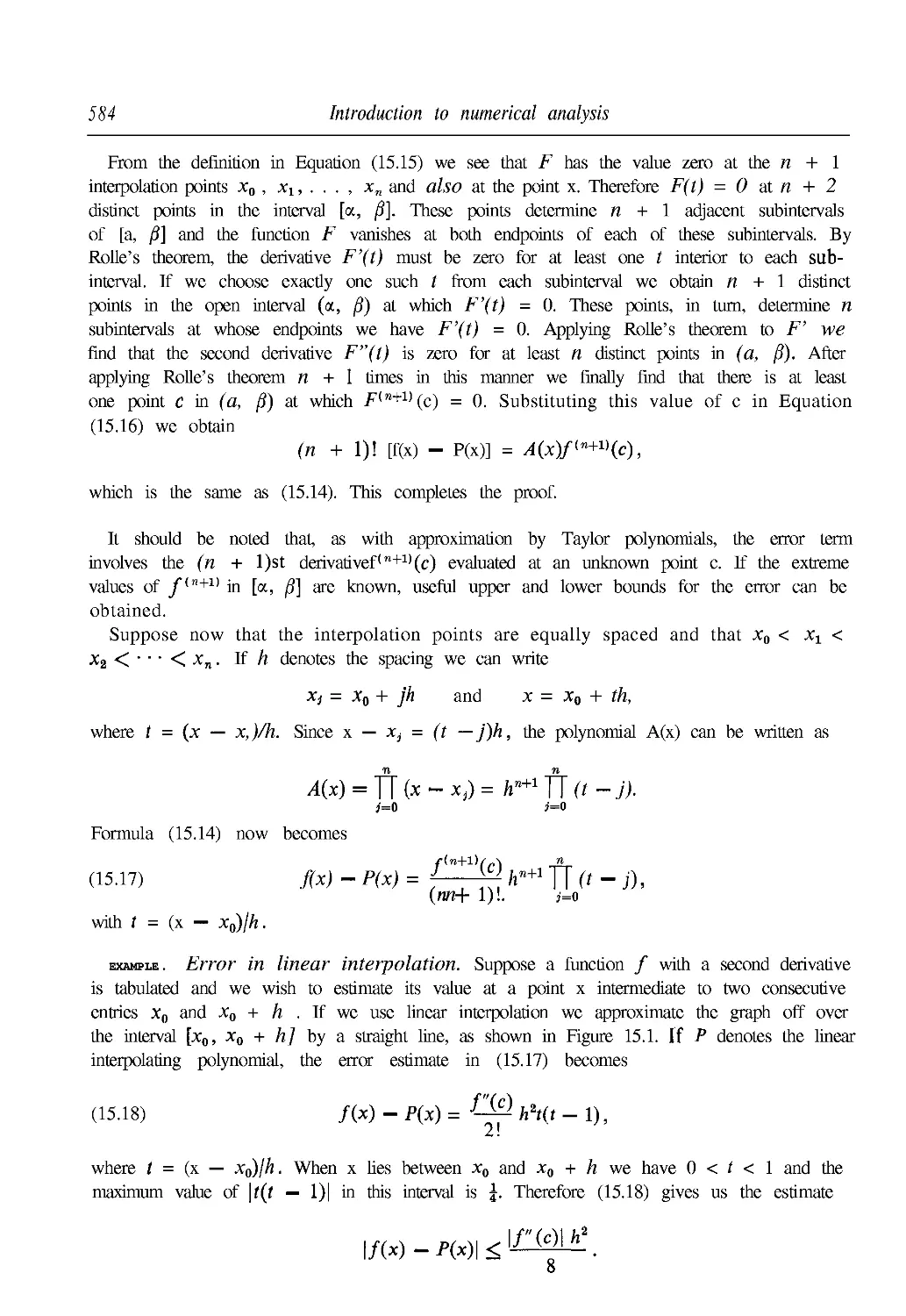
15.8 Error analysis in polynomial interpolation 583
15.9 Exercises 585
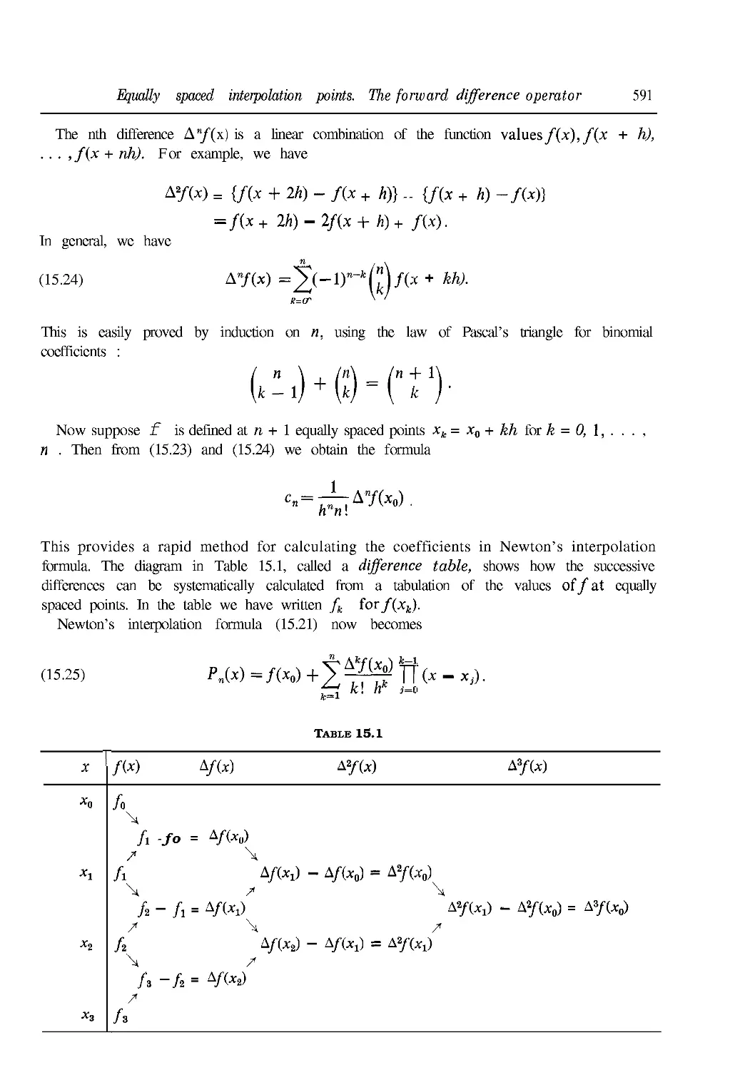
15.10 Newton's interpolation formula 588
15.11 Equally spaced interpolation points. The forward difference operator 590
15.12 Factorial polynomials 592
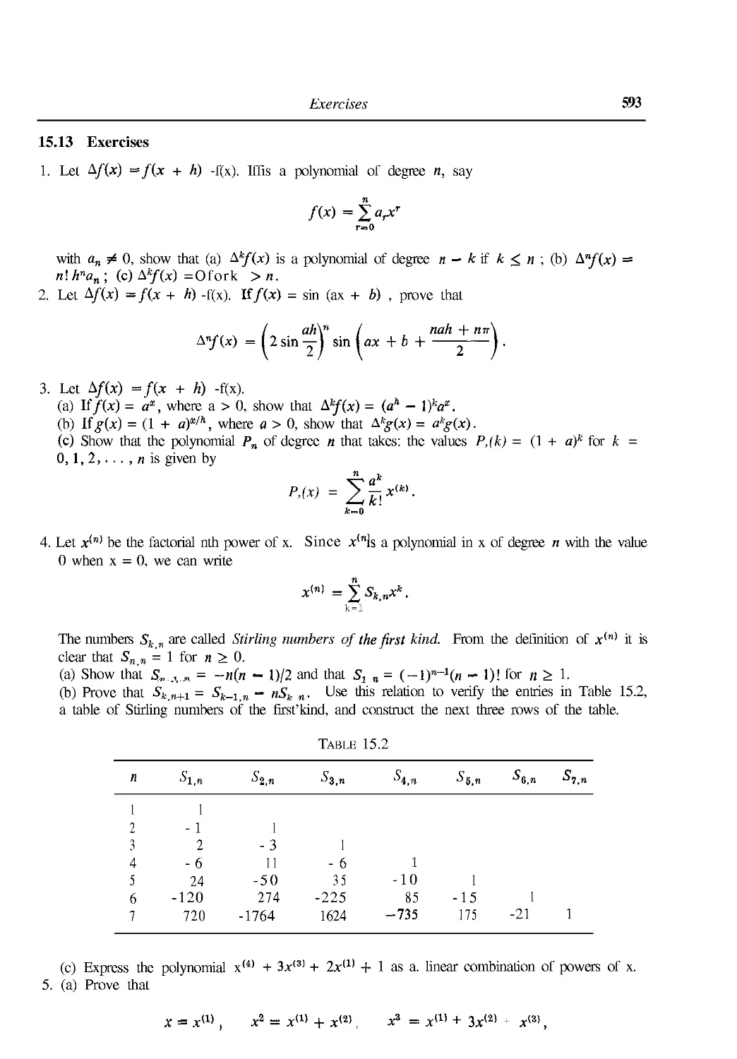
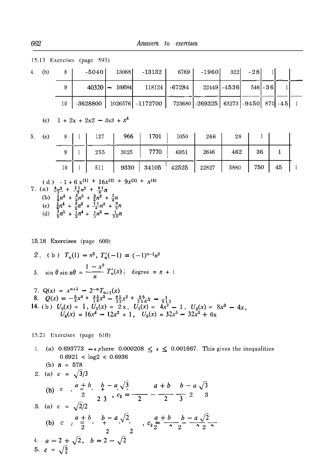
15.13 Exercises 593
15.14 A minimum problem relative to the max norm 595

Contents xxi
15.15 Chebyshev polynomials 596
15.16 A minimal property of Chebyshev polynomials 598
15.17 Application to the error formula for interpolation 599
15.18 Exercises 600
15.19 Approximate integration. The trapezoidal rale 602
15.20 Simpson's rale 605
15.21 Exercises 610
15.22 The Euler summation formula 613
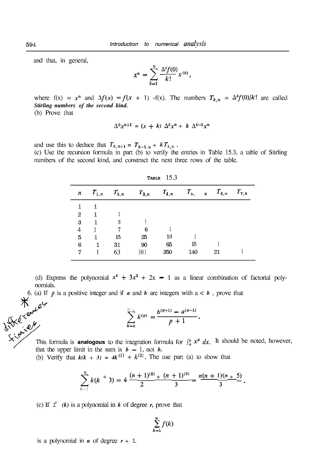
15.23 Exercises 618
Suggested References 621
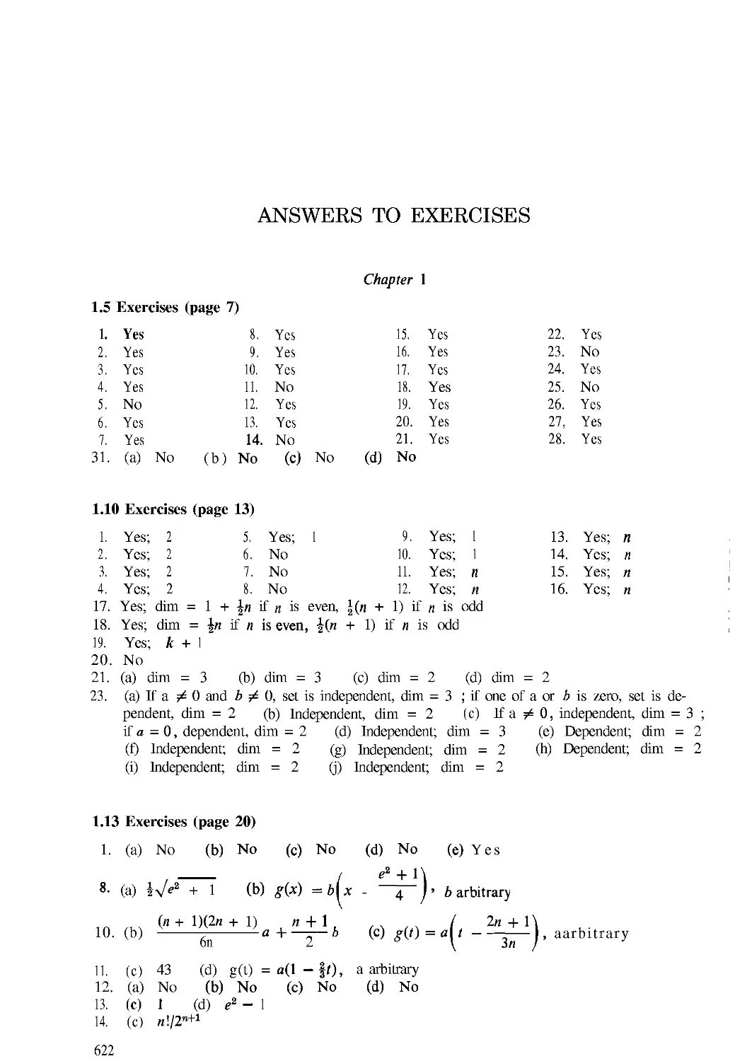
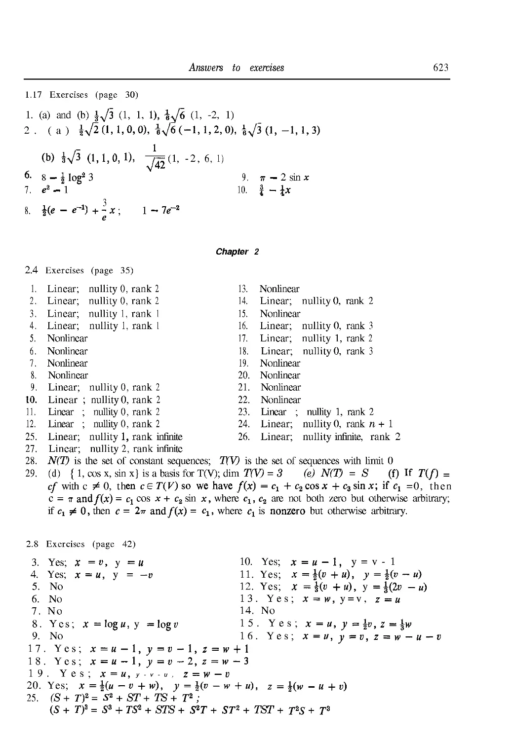
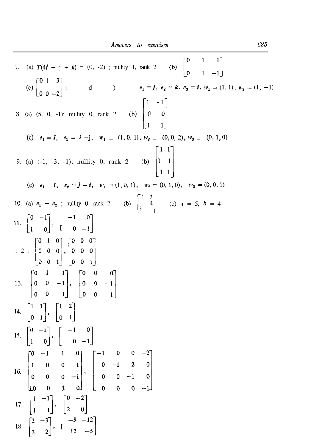
Answers to exercises 622
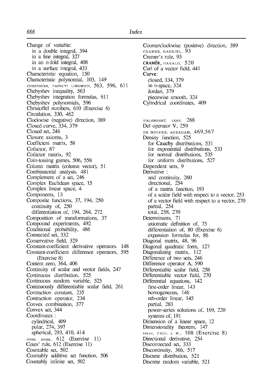
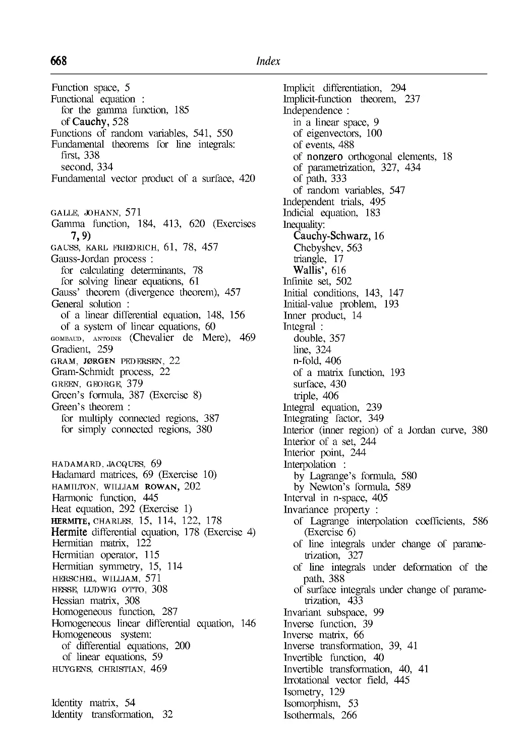
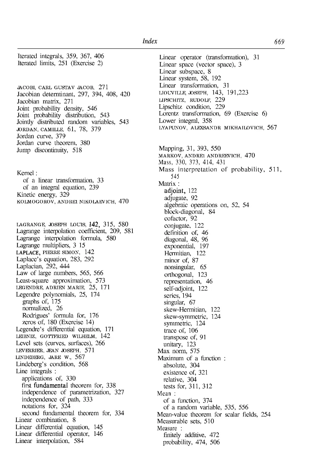
Index 665

Calculus

PART 1
LINEAR ANALYSIS

LINEAR SPACES
1.1 Introduction
Throughout mathematics we encounter many examples of mathematical objects that
can be added to each other and multiplied by real numbers. First of all, the real numbers
themselves are such objects. Other examples are real-valued functions, the complex
numbers, infinite series, vectors in n-space, and vector-valued functions. In this chapter we
discuss a general mathematical concept, called a linear space, which includes all these
examples and many others as special cases.
Briefly, a linear space is a set of elements of any kind on which certain operations (called
addition and multiplication by numbers) can be performed. In defining a linear space, we
do not specify the nature of the elements nor do we tell how the operations are to be
performed on them. Instead, we require that the operations have certain properties which
we take as axioms for a linear space. We turn now to a detailed description of these axioms.
1.2 The definition of a linear space
Let V denote a nonempty set of objects, called elements. The set V is called a linear
space if it satisfies the following ten axioms which we list in three groups.
Closure axioms
axiom 1. closure under addition. For every pair of elements x and у in V there
corresponds a unique element in V called the sum of x and y, denoted by x + у .
AXIOM 2. CLOSURE UNDER MULTIPLICATION BY REAL NUMBERS. For eVery X Ш V
every real number a there corresponds an element in V called the product of a and x, denoted
by ax.
Axioms for addition
axiom 3. commutative law. For all x and у in V, we have x + у = у + x.
axiom 4. associativelaw. Forallx,y, andzin V,wehave(x + y) + z = X + (y + z).

Linear spaces
axiom 5. existenceofzeroelement. There is an element in V, denoted by 0, such that
x + О = x for all x in V .
axiom 6. existenceofnegatives. For every x in V, the element (— l)x has the property
X + (-l)x= 0.
Axioms for multiplication by numbers
axiom 7. associative law. For every x in V and all real numbers a and b, we have
a(bx) = (ab)x.
axiom 8. distributive law for addition in V. For all x andy in V and all real a,
we hare
a(x + y) = ax + ay .
axiom 9. distributive law for addition of numbers . For all x in V and all real
a and b, we have
(a + b)x = ax + bx.
AXIOM 10. EXISTENCE OF IDENTITY. For вивГу X 1П V, Юв kuVe lx = X.
Linear spaces, as defined above, are sometimes called real linear spaces to emphasize
the fact that we are multiplying the elements of V by real numbers. If real number is
replaced by complex number in Axioms 2, 7, 8, and 9, the resulting structure is called a
complex linear space. Sometimes a linear space is referred to as a linear vector space or
simply a vector space; the numbers used as multipliers are also called scalars. A real linear
space has real numbers as scalars; a complex linear space has complex numbers as scalars.
Although we shall deal primarily with examples of real linear spaces, all the theorems are
valid for complex linear spaces as well. When we use the term linear space without further
designation, it is to be understood that the space can be real or complex.
13 Examples of linear spaces
If we specify the set V and tell how to add its elements and how to multiply them by
numbers, we get a concrete example of a linear space. The reader can easily verify that
each of the following examples satisfies all the axioms for a real linear space.
example 1. Let V = R , the set of all real numbers, and let x + у and ax be ordinary
addition and multiplication of real numbers.
example 2. Let V = C, the set of all complex numbers, define x + у to be ordinary
addition of complex numbers, and define ax to be multiplication of the complex number л:

Examples of linear spaces
by the real number a. Even though the elements of V are complex numbers, this is a real
linear space because the scalars are real.
example 3. Let V = Vn, the vector space of all n-tuples of real numbers, with addition
and multiplication by scalars defined in the usual way in terms of components.
example 4. Let V be the set of all vectors in Vn orthogonal to a given nonzero vector
N. If П = 2, this linear space is a line through 0 with N as a normal vector. If n = 3,
it is a plane through 0 with N as normal vector.
The following examples are called function spaces. The elements of V are real-valued
functions, with addition of two functions / and g defined in the usual way:
(f + g)(x) =f(x) + g(x)
for every real X in the intersection of the domains off and g. Multiplication of a function
/ by a real scalar a is defined as follows: af is that function whose value at each x in the
domain off is af (x). The zero element is the function whose values are everywhere zero.
The reader can easily verify that each of the following sets is a function space.
example 5. The set of all functions defined on a given interval.
example 6. The set of all polynomials.
example 7. The set of all polynomials of degree < n, where n is fixed. (Whenever we
consider this set it is understood that the zero polynomial is also included.) The set of
all polynomials of degree equal to n is not a linear space because the closure axioms are not
satisfied. For example, the sum of two polynomials of degree n need not have degree n.
example 8. The set of all functions continuous on a given interval. If the interval is
[a, b], we denote this space by C(a, b).
example 9. The set of all functions differentiable at a given point.
example 10. The set of all functions integrable on a given interval.
example 11. The set of all functions / defined at 1 with f(l) = 0. The number 0 is
essential in this example. If we replace 0 by a nonzero number c, we violate the closure
axioms.
example 12. The set of all solutions of a homogeneous linear differential equation
y" + ay' + by = 0, where a and b are given constants. Here again 0 is essential. The set
of solutions of a nonhomogeneous differential equation does not satisfy the closure axioms.
These examples and many others illustrate how the linear space concept permeates
algebra, geometry, and analysis. When a theorem is deduced from the axioms of a linear
space, we obtain, in one stroke, a result valid for each concrete example. By unifying

Linear spaces
diverse examples in tins way we gain a deeper insight into each. Sometimes special knowl-
knowledge of one particular example helps to anticipate or interpret results valid for other
examples and reveals relationships which might otherwise escape notice.
1.4 Elementary consequences of the axioms
The following theorems are easily deduced from the axioms for a linear space.
THEOREM 1.1. UNIQUENESS OF THE ZERO ELEMENT. In any linear space there is one
and only one zero element.
Proof. Axiom 5 tells us that there is at least one zero element. Suppose there were two,
say 0, and 0,. Taking x = Ox and 0 = 0, in Axiom 5, we obtain Ox + O2 = Ox.
Similarly, taking x = 02 and 0 = Ob we find 02 + 0, = 02. But Ox + 02 = 02 + 0,
because of the commutative law, so 0, = 02.
THEOREM 1.2. UNIQUENESS OF NEGATIVE ELEMENTS. In any linear space every element
has exactly one negative. That is, for every x there is one and only one у such that x + у = 0.
Proof. Axiom 6 tells us that each x has at least one negative, namely (- l)x. Suppose
x has two negatives, say yx and _y2. Then x + yx = 0 and x + y2 = 0. Adding y2 to both
members of the first equation and using Axioms 5, 4, and 3, we find that
/2+ (x +7i)=J2+ О =у2,
and
У1 + (x + yx) = (y2 + x) + yx = о + yi = yx + о = yi.
Therefore yx = y2, so x has exactly one negative, the element (- l)x.
Notation. The negative of x is denoted by —x. The difference у — x is defined to be
the sum у + (-x) .
The next theorem describes a number of properties which govern elementary algebraic
manipulations in a linear space.
THEOREM 1.3. In a given linear space, let x and у denote arbitrary elements and let a and b
denote arbitrary scalars. Then we'have the following properties:
(a) Ox = 0.
(b) aO = 0.
(c) (-a)x = -(ax) = a(-x).
(d) Ifax = O,theneithera = Oorx=O.
(e) Ifax = ayandaj?Q,thenx=y.
(f) If ax = bxandx^O, then a = b.
(g) -(* + y) = {-x) + (~y) = -x - y.
(h) x + x = 2x, x + x + X = 3x, andingeneral, 2"=1 X = nx.

Exercises 7
We shall prove (a), (b), and (c) and leave the proofs of the other properties as exercises.
Proof of (a). Let 2 = Ox. We wish to prove that 2 = 0. Adding z to itself and using
Axiom 9, we find that
z + z = Ox + Ox = @ + 0)x = 0* = z.
Now add — z to both members to get z = 0.
Proof oflb). Let z = aO, add z to itself, and use Axiom 8.
Proofoflc). Let z = (a)x. Adding z to ax and using Axiom 9, we find that
z + ax = {—a)x + ax = (—a + a)x = Ox = О,
so z is the negative of ax, z = -(ax). Similarly, if we add a(—x) to ax and use Axiom 8
and property (b), we find that a(—x) = -(ax).
1.5 Exercises
In Exercises 1 through 28, determine whether each of the given sets is a real linear space, if
addition and multiplication by real scalars are defined in the usual way. For those that are not,
tell which axioms fail to hold. The functions in Exercises 1 through 17 are real-valued. In Exer-
Exercises 3, 4, and 5, each function has domain containing 0 and 1. In Exercises 7 through 12, each
domain contains all real numbers.
1. All rational functions.
2. All rational functions//^, with the degree off < the degree ofg (including f = O).
3. All/with/@) =f(l). 8. All even functions.
4. All /with 2/@) =f(l). 9. All odd functions.
5. All/with/A) = 1 +f[O). 10. All bounded functions.
6. All step functions defined on [0,1]. 11. All increasing functions.
7. All/with/(л) -> 0 as x ->- + oo . 12. All functions with period 2n.
13. All / integrable on [0, 1] with ЦДх) dx = О.
14. All / integrable on [0, 1] with )\flx) dx > O.
15. All / satisfying/M = /A ~ x) for all x.
16. All Taylor polynomials of degree <, n for a fixed n (including the zero polynomial).
17. All solutions of a linear second-order homogeneous differential equation' y" + P{x)y' +
Q(x)y = 0, where P and Q are given functions, continuous everywhere.
18. All bounded real sequences. 20. All convergent real series.
19. All convergent real sequences. 21. All absolutely convergent real series.
22. All vectors (x, y, z) in V3 with z = 0.
23. All vectors (x, y, z) in Vs with x = 0 or у = 0.
24. All vectors (x, y, z) in V3 with у = 5x.
25. All vectors (x, y, z) in V3 with 3x + \y = 1, z = 0.
26. All vectors (x, y, z) in V3 which are scalar multiples of A, 2, 3).
27. All vectors (x, y, z) in V3 whose components satisfy a system of three linear equations of the
form :
aux + a12y + a13z = o, anx + а2гу + a23z = 0, anx + a3iy + a3Sz = 0.

Linear spaces
28. All vectors in Vn that are linear combinations of two given vectors A and B.
29. Let V = R+, the set of positive real numbers. Define the "sum" of two elements x and у in
V to be their product x у (in the usual sense), and define "multiplication" of an element x
in V by a scalar с to be xc. Prove that V is a real linear space with 1 as the zero element.
30. (a) Prove that Axiom 10 can be deduced from the other axioms.
(b) Prove that Axiom 10 cannot be deduced from the other axioms if Axiom 6 is replaced by
Axiom 6': For every x in V there is an element у in V such that x + у = 0.
3 1. Let S be the set of all ordered pairs (xlt x2) of real numbers. In each case determine whether
or not S is a linear space with the operations of addition and multiplication by scalars defined
as indicated. If the set is not a linear space, indicate which axioms are violated.
(a) (Xl, x2) + (yi, y2) = Ui + Ji. *2 + У2), fl(*i. *a) = (o*i . 0).
(b) (xltx2) + (ji,j2) = Ui +Л>°)> a(xi,x2) = (ax1, ax2).
(c) (x1, Xj) + (уг, y2) = (x1, x2 + y2), а(хг, x2) = (ахг, ax2).
(d) (x±,x2) + (ylty2) = (I*! + x2\,\yi +/2D. fl(*i> хг) = (Nil. l^al) .
32. Prove parts (d) through (h) of Theorem 1.3.
1.6 Subspaces of a linear space
Given a linear space V, let S be a nonempty subset of К If S is also a linear space, with
the same operations of addition and multiplication by scalars, then S is called a subspace
of V. The next theorem gives a simple criterion for determining whether or not a subset of
a linear space is a subspace.
theorem 1.4. Le? S be a nonempty subset of a linear space V. Then Sis a subspace
if and only if S satisfies the closure axioms.
Proof. If S is a subspace, it satisfies all the axioms for a linear space, and hence, in
particular, it satisfies the closure axioms.
Now we show that if S satisfies the closure axioms it satisfies the others as well. The
commutative and associative laws for addition (Axioms 3 and 4) and the axioms for
multiplication by scalars (Axioms 7 through 10) are automatically satisfied in S because
they hold for all elements of V. It remains to verify Axioms 5 and 6, the existence of a zero
element in S, and the existence of a negative for each element in S.
Let x be any element of S. (S has at least one element since S is not empty.) By Axiom
2, ax is in S for every scalar a. Taking a = 0, it follows that Ox is in S. But Ox = О, by
Theorem 1.3(a), so 0 e S, and Axiom 5 is satisfied. Taking a = — 1, we see that (-l)x
is in S. But X + (- l)x = 0 since both x and (- l)x are in V, so Axiom 6 is satisfied in
S. Therefore S is a subspace of V.
definition . Let Sbe a nonempty subset of a linear space V. An element XinV of the
form
where xy, ..., xkare all in Sand cl5..., ck are scalars, is called a finite linear combination
of elements of S The set of all finite linear combinations of elements of S satisfies the closure
axioms and hence is a subspace of V. We call this the subspace spanned by S, or the linear
span of S, and denote it by US). If Sis empty, we define I/S) to be {0}, the set consisting
of the zero element alone.

Dependent and independent sets in a linear space 9
Different sets may span the same subspace. For example, the space Vu is spanned by
each of the following sets of vectors: {i,j}, {i,j, i +j}, {0, i, —i,j, —j, i + j}. The space
of all polynomials p{t) of degree < n is spanned by the set of я + 1 polynomials
{\,t,t\ ...,tn}.
It is also spanned by the set {1, t/2, Хг\Ъ,. . . , tn\{n + 1)}, and by {I, A + /), A + tf,
A + /)"}. The space of all polynomials is spanned by the infinite set of polynomials
{l,US...}.
A number of questions arise naturally at this point. For example, which spaces can be
spanned by a finite set of elements? If a space can be spanned by a finite set of elements,
what is the smallest number of elements required? To discuss these and related questions,
we introduce the concepts of dependence, independence, bases, and dimension. These ideas
were encountered in Volume I in our study of the vector space Vn ¦ Now we extend them
to general linear spaces.
1.7 Dependent and independent sets in a linear space
definition. A set S of elements in a linear space V is called dependent if there is a finite
set of distinct elements in S,say х1г..., xk, and a corresponding set of scalars cx, . . . , ck,
not all zero, such that
к
gciXi = O.
An equation ]T ctx{ = 0 with not all c{ = 0 is said to be a nontrivial representation ofO.
The set S is called independent if it is not dependent. In this case, for all choices of distinct
elements xlt..., xkin S and scalars c1,..., ck,
к
2 CjXj = О implies cx = c2 = • • • = ck = 0.
2 = 1
Although dependence and independence are properties of sets of elements, we also apply
these terms to the elements themselves. For example, the elements in an independent set
are called independent elements.
If 5" is a finite set, the foregoing definition agrees with that given in Volume I for the
space Vn. However, the present definition is not restricted to finite sets.
example 1. If a subset Г of a set S is dependent, then S itself is dependent. This is
logically equivalent to the statement that every subset of an independent set is independent.
expmple 2. If one element in S is a scalar multiple of another, then S is dependent.
example 3. If 0 G S, then 5" is dependent.
example 4. The empty set is independent,

10 Linear spaces
Many examples of dependent and independent sets of vectors in Vn were discussed in
Volume I. The following examples illustrate these concepts in function spaces. In each
case the underlying linear space V is the set of all real-valued functions defined on the real
line.
example 5. Let 1^@ = cos2 t , u2(t) = sin2 t , u3(t) = 1 for all real t. The Pythagorean
identity shows that щ + щ — u3 = 0, so the three functions u1} u2, u3 are dependent.
example 6. Let uk(t) = tk for к = 0, 1, 2. . . . , and / real. The set 5 = {и0, м1; м2, . . .}
is independent. To prove this, it suffices to show that for each n the n + 1 polynomials
u0, щ, . . , ,un are independent. A relation of the form ]T ckuk = 0 means that
(i.i) ic/ = о
k=O
for all real t. When / = 0, this gives Co = 0 . Differentiating A.1) and setting t = 0,
we find that ct = 0. Repeating the process, we find that each coefficient ck is zero.
example 7. If a,,..., a, are distinct real numbers, the n exponential functions
ux{x) = eaiX,. . . , u,(x) = ea"x
are independent. We can prove this by induction on n. The result holds trivially when
n — 1 . Therefore, assume it is true for n — 1 exponential functions and consider scalars
c1, . . . , cn such that
A.2) fcke^ = 0.
Let aM be the largest of the n numbers a,, . . . , a,. Multiplying both members of A.2)
by е~амХ, we obtain
A.3) f cke<a*-"M)x = 0.
If А; Ф M, the number ak — aM is negative. Therefore, when x —> + со in Equation A.3),
each term with к Ф M tends to zero and we find that caI = 0. Deleting the Mth term from
A.2) and applying the induction hypothesis, we find that each of the remaining n — 1
coefficients ck is zero.
theorem 1.5. Let S = {x1, . . . , xk} be an independent set consisting of к elements in a
linear space V and let L(S) be the subspace spanned by S. Then every set of к + 1 elements
in L(S) is dependent.
Proof. The proof is by induction on k, the number of elements in S. First suppose
к = 1. Then, by hypothesis, S consists of one element xx, where x1 ^ 0 since 5 is
independent. Now take any two distinct elements yr and уг in L(S). Then each is a scalar

Dependent and independent sets in a linear space 11
multiple of x1, say y± = c1x1 and уг = с2хг, where c1 and c2 are not both 0. Multiplying
Ух by c2 and y-i by cL and subtracting, we find that
C27i - С1У2 = 0.
This is a nontrivial representation of 0 soy, and y2 are dependent. This proves the theorem
when к = 1 .
Now we assume the theorem is true for к — 1 and prove that it is also true for k. Take
any set of к + 1 elements in L(S), say T = {y\, y2, . . ., Ук+i) . We wish to prove that Tis
dependent. Since each yi is in L(S) we may write
/.•
A.4) yt = J, a, ,x,
foreachi= 1, 2,. .., к + 1 . We examine all the scalars aa that multiply Xj and split the
proof into two cases according to whether all these scalars are 0 or not.
CASE 1. aa = 0 for every i = 1, 2, . . . , к + 1 . In this case the sum in A.4) does not
involve x1; so each y{ in T is in the linear span of the set S' = {x2, . . . , xk} . But S' is
independent and consists of к — 1 elements. By the induction hypothesis, the theorem is
true for к — 1 so the set T is dependent. This proves the theorem in Case 1.
CASE 2. Not all the scalars a{1 are zero. Let us assume that а,, Ф 0. (If necessary, we
can renumber the y's to achieve this.) Taking i = 1 in Equation A.4) and multiplying both
members by ci, where c{ = аа/ап, we get
From this we subtract Equation A.4) to get
l -atl)xn
3=2
for i — 2, . . . , к + 1 . This equation expresses each of the к elements ctyx — yt as a linear
combination of the к — 1 independent elements x2, . . . , xk . By the induction hypothesis,
the к elements с{уг — yi must be dependent. Hence, for some choice of scalars t2, . . . ,
tk+i, not all zero, we have
from which we find
But this is a nontrivial linear combination of ylt . . . , yk+1 which represents the zero ele-
element, so the elements У\ , . . . , )'k+1 must be dependent. This completes the proof.

12 Linear spaces
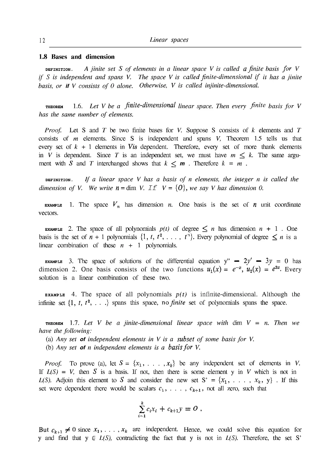
1.8 Bases and dimension
definition . A jinite set S of elements in a linear space V is called a finite basis for V
if S is independent and spans V. The space V is called finite-dimensional if it has a jinite
basis, or if V consists of 0 alone. Otherwise, V is called injinite-dimensional.
theorem 1.6. Let V be a finite-dimensional linear space. Then every finite basis for V
has the same number of elements.
Proof. Let S and T be two finite bases for V. Suppose S consists of k elements and T
consists of m elements. Since S is independent and spans V, Theorem 1.5 tells us that
every set of k + 1 elements in Vis dependent. Therefore, every set of more thank elements
in У is dependent. Since Г is an independent set, we must have m < k. The same argu-
argument with 5" and T interchanged shows that k < m . Therefore k = m .
definition. If a linear space V has a basis of n elements, the integer n is called the
dimension of V. We write n = dim V. If V = {0}, we say V has dimension 0.
example 1. The space Vn has dimension n. One basis is the set of n unit coordinate
vectors.
example 2. The space of all polynomials p(t) of degree < n has dimension n + 1 . One
basis is the set of n + 1 polynomials {1, t, /2, . . . , tn). Every polynomial of degree < n is a
linear combination of these n + 1 polynomials.
example 3. The space of solutions of the differential equation y" — 2/ — 3y = 0 has
dimension 2. One basis consists of the two functions U^x) = e~x, H2(jc) = e3x. Every
solution is a linear combination of these two.
example 4. The space of all polynomials p(t) is infinite-dimensional. Although the
infinite set {1, /, ?2, . . .} spans this space, no finite set of polynomials spans the space.
theorem 1.7. Let V be a jinite-dimensional linear space with dim V = n. Then we
have the following:
(a) Any set of independent elements in V is a subset of some basis for V.
(b) Any set of n independent elements is a basis for V.
Proof. To prove (a), let S = {xx, . . . , xk) be any independent set of elements in V.
If L(S) = V, then S is a basis. If not, then there is some element у in У which is not in
L(S). Adjoin this element to S and consider the new set S' = {xl5 . . . , xk, y} .If this
set were dependent there would be scalars clt . . . , ck+1, not all zero, such that
But ck ,.i 5^ 0 since xy, . . . , xk are independent. Hence, we could solve this equation for
у and find that у 6 L(S), contradicting the fact that у is not in L(S). Therefore, the set S'

Exercises 13
is independent but contains k + 1 elements. If L(S') = V, then S' is a basis and, since S
is a subset of S', part (a) is proved. If S' is not a basis, we can argue with S' as we did
with S, getting a new set S" which contains k -\- 2 elements and is independent. If S" is a
basis, then part (a) is proved. If not, we repeat the process. We must arrive at a basis in
a finite number of steps, otherwise we would eventually obtain an independent set with
n + 1 elements, contradicting Theorem 1.5. Therefore part (a) is proved.
To prove (b), let S be any independent set consisting of n elements. By part (a), S is a
subset of some basis, say B. But by Theorem 1.6, the basis В has exactly n elements, so
S= B.
1.9 Components
Let К be a linear space of dimension n and consider a basis whose elements e^ , . . . , en
are taken in a given order. We denote such an ordered basis as an n-tuple (el5 . . . , e,).
If x e V, we can express x as a linear combination of these basis elements:
«
A.5) x=2 Cte,.
! = 1
The coefficients in this equation determine an n-tuple of numbers (c,, . . . , cn) that is
uniquely determined by x. In fact, if we have another representation of x as a linear
combination of e1, . . . , en, say X = 2"=1 diei, then by subtraction from A.5), we find that
2?=i (ci "™ ^i)ei = 0- But since the basis elements are independent, this implies ct = dt
for each i, so we have (сг,..., cn) = {dx,.., , dn).
The components of the ordered n-tuple (c,, . . . , cn) determined by Equation A.5) are
called the components ofx relative to the ordered basis (e,,..., e,).
1.10 Exercises
In each of Exercises 1 through 10, let 5" denote the set of all vectors (x, y, z) in V3 whose com-
components satisfy the condition given. Determine whether 5 is a subspace of V3. If 5 is a subspace,
compute dim S.
1. X = 0. 6. x = у о г л: = z.
2. X +>¦ =о. 7. X2 -/ = 0.
3. х+у +z = 0. 8. х +у = 1.
4. х =у. 9. у = 2х a n d z = Зх.
5. X =у =z. 10. х + у + z = 0 and х — у — z = 0.
Let Pn denote the linear space of all real polynomials of degree <, n, where n is fixed. In each
of Exercises 11 through 20, let 5 denote the set of all polynomials / in Pn satisfying the condition
given. Determine whether or not S is a subspace of Pn . If S is a subspace, compute dim S.
11. f@) =0. 16. f@) = fB) .
12. /'@) = 0. 17. f is even.
13. /"@) = 0. 18. / is odd.
14. /@) +/'@) = 0. 19. f has degree < k, where k < n, or / = 0.
15. /@) = /A). 20. f has degree k, where k<n,orf = 0.
21. In the linear space of all real polynomials p(t), describe the subspace spanned by each of the
following subsets of polynomials and determine the dimension of this subspace.
(a) {!,<*,/*}; {b){t,t\fi}; (c) {t, t*}; (d) { 1 + t, A + /J}.

14 Linear spaces
22. In this exercise, L(S) denotes the subspace spanned by a subset S of a linear space V. Prove
each of the statements (a) through (f).
(a) S с L(S).
(b) If S ? T ? у and if T is a subspace of K, then L(S) ? Г. This property is described by
saying that L(S) is the smallest subspace of V which contains S.
(c) A subset S of У is a subspace of У if and only if L(S) = S.
(d) If S с Т с J/ then L(S) с L(T).
(e) If 5 and Tare subspaces of V, then so is 5 П Г.
(f) If 5 and Гаге subsets of K, then L(S n T) s LfS) и L(T).
(g) Give an example in which L{S n T) Ф L(S) П L(T).
23. Let V be the linear space consisting of all real-valued functions defined on the real line.
Determine whether each of the following subsets of V is dependent or independent. Compute
the dimension of the subspace spanned by each set.
(a) {1, eax, ebx}, a *b. (f) (cos x, sin x).
(b) {eax, xeax). (g) {cos2 x, sin2 x}.
(c) {1, eax, xeax}. (h) {'I, cos 2x, sin2 x).
(d) {eax,xeax,x2eax}. (i) (sin x, sin 2x).
(e) {ex, e~x, cosh x). (j) {ex cos x, e~x sin x).
24. Let У be a finite-dimensional linear space, and let 5 be a subspace of V. Prove each of the
following statements.
(a) S is finite dimensional and dim S < dim V.
(b) dim S = dim V if and only if S = V.
(c) Every basis for S is part of a basis for V.
(d) A basis for V need not contain a basis for S.
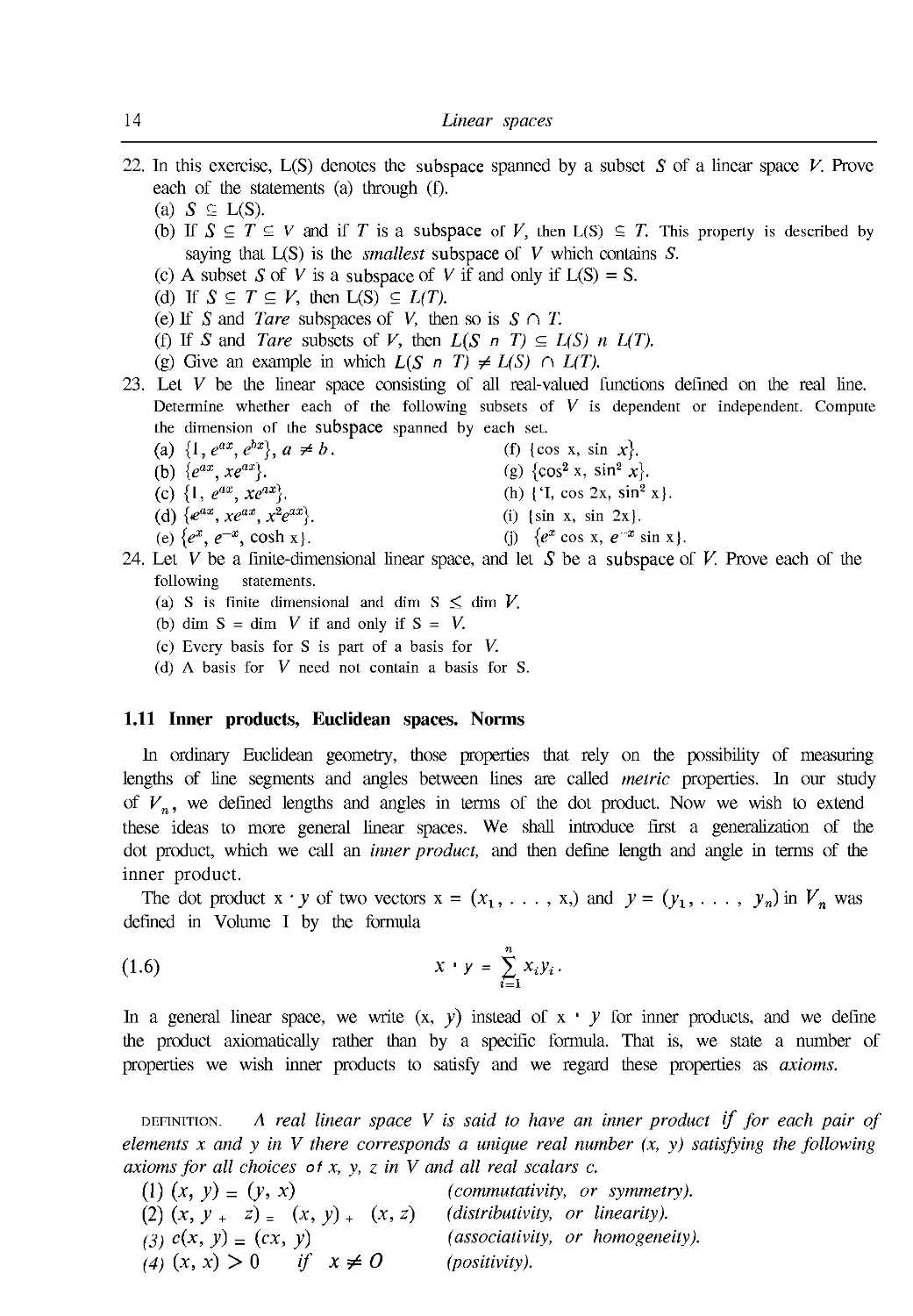
1.11 Inner products, Euclidean spaces. Norms
In ordinary Euclidean geometry, those properties that rely on the possibility of measuring
lengths of line segments and angles between lines are called metric properties. In our study
of Vn, we defined lengths and angles in terms of the dot product. Now we wish to extend
these ideas to more general linear spaces. We shall introduce first a generalization of the
dot product, which we call an inner product, and then define length and angle in terms of the
inner product.
The dot product x • у of two vectors x = (xx, . . . , x,) and у = (y1, . . . , yn) in Vn was
defined in Volume I by the formula
A.6) x • у =
^
In a general linear space, we write (x, y) instead of x • у for inner products, and we define
the product axiomatically rather than by a specific formula. That is, we state a number of
properties we wish inner products to satisfy and we regard these properties as axioms.
definition. A real linear space V is said to have an inner product if for each pair of
elements x and у in V there corresponds a unique real number (x, y) satisfying the following
axioms for all choices of x, y, z in V and all real scalars с
A) (x, y) = (y, x) (commutativity, or symmetry).
B) (x, у + z) = (x, y) + {x, z) (distributivity, or linearity).
C) c(x, y) = {ex, y) (associativity, or homogeneity).
D) (x, x) > 0 if хФ О (positivity).

Inner products, Euclidean spaces. Norms 15
A real linear space with an inner product is called a real Euclidean space.
Note: Taking с = 0 in C), we find that (O, y) = 0 for all y.
In a complex linear space, an inner product (x, y) is a complex number satisfying the
same axioms as those for a real inner product, except that the symmetry axiom is replaced
by the relation
(Г) (x,y) = (y, x), (Hermitianj symmetry)
where (y, x) denotes the complex conjugate of (y, x). In the homogeneity axiom, the scalar
multiplier с can be any complex number. From the homogeneity axiom and (Г), we get
the companion relation
C') (x, cy) = (cy, x) = c(y, x) = c(x, y).
A complex linear space with an inner product is called a complex Euclidean 'space.
(Sometimes the term unitary space is also used.) One example is complex vector space
Vn(C) discussed briefly in Section 12.16 of Volume I.
Although we are interested primarily in examples of real Euclidean spaces, the theorems
of this chapter are valid for complex Euclidean spaces as well. When we use the term
Euclidean space without further designation, it is to be understood that the space can be
real or complex.
The reader should verify that each of the following satisfies all the axioms for an inner
product.
example 1. In Vn let (x, y) = x . у , the usual dot product of x and y.
example 2. If x = (Xj, x2) and у = (y1 , y2) are any two vectors in F2, define (x, y) by
the formula
(x, y) =
This example shows that there may be more than one inner product in a given linear space.
example 3. Let C(a, b) denote the linear space of all real-valued functions continuous
on an interval [a, b]. Define an inner product of two functions / and g by the formula
This formula is analogous to Equation A.6) which defines the dot product of two vectors
in Vn. The function values f(t) and g(t) play the role of the components xt and yt , and
integration takes the place of summation.
f In honor of Charles Hermite A822-1901), a French mathematician who made many contributions to
algebra and analysis.

16 Linear spaces
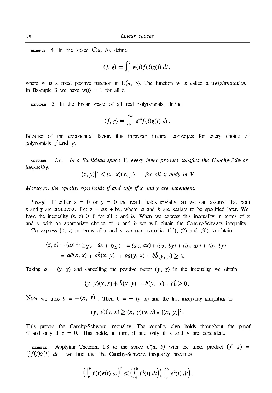
example 4. In the space C(a, b), define
(f,g) = [w(tmt)g(t)dt,
where w is a fixed positive function in C(a, b). The function w is called a weightfunction.
In Example 3 we have w(t) = 1 for all /.
example 5. In the linear space of all real polynomials, define
U, g) = \™ e-tRMt) dt.
Because of the exponential factor, this improper integral converges for every choice of
polynomials /and g.
theorem 1.8. In a Euclidean space V, every inner product satisfies the Cauchy-Schwarz
inequality:
|(*>.y)|2 < (x> Х)(У> у) f°r aH * andy in V.
Moreover, the equality sign holds if and only if x and у are dependent.
Proof. If either x = 0 or у = 0 the result holds trivially, so we can assume that both
x and у are nonzero. Let z = ax + by, where a and b are scalars to be specified later. We
have the inequality (z, z) ^ 0 for all a and b. When we express this inequality in terms of x
and у with an appropriate choice of a and b we will obtain the Cauchy-Schwarz inequality.
To express (z, z) in terms of x and у we use properties A'), B) and C') to obtain
(z, z) = (ax + by, ax + by) = (ax, ax) + (ax, by) + (by, ax) + (by, by)
= ad{x, x) + ab(x, y) + ba(y, x) + bb{y, y) > ft
Taking a = (у, у) and cancelling the positive factor (у, у) in the inequality we obtain
(y,y)(x,x) + b(x,y) +%, x) + bb>0.
Now we take b = —(x, У) . Then 6 = — (y, x) and the last inequality simplifies to
(y,y)(x,x)>(x,y)(y,x)=\(x,y)\*.
This proves the Cauchy-Schwarz inequality. The equality sign holds throughout the proof
if and only if z = 0. This holds, in turn, if and only if x and у are dependent.
example. Applying Theorem 1.8 to the space C(a, b) with the inner product (/, g) =
dt , we find that the Cauchy-Schwarz inequality becomes
(ij(t)g(t)dtJ^([f\t)dt)([g\t)dt).

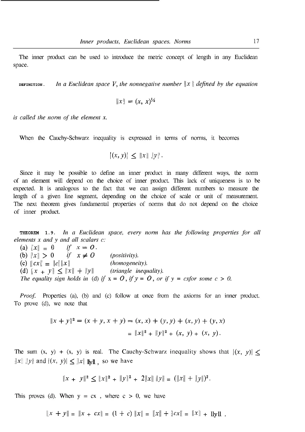
Inner products, Euclidean spaces. Norms 17
The inner product can be used to introduce the metric concept of length in any Euclidean
space.
definition. In a Euclidean space V, the nonnegative number \\x || defined by the equation
is called the norm of the element x.
When the Cauchy-Schwarz inequality is expressed in terms of norms, it becomes
\(x,y)\ < \\x\\ }y\\-
Since it may be possible to define an inner product in many different ways, the norm
of an element will depend on the choice of inner product. This lack of uniqueness is to be
expected. It is analogous to the fact that we can assign different numbers to measure the
length of a given line segment, depending on the choice of scale or unit of measurement.
The next theorem gives fundamental properties of norms that do not depend on the choice
of inner product.
theorem 1.9. In a Euclidean space, every norm has the following properties for all
elements x and у and all scalars c:
(a) ||x|| = 0 if x = O.
(b) ||*|| > 0 if ХфО (positivity).
(c) || a; || = И ||*|| (homogeneity).
(d) ||* + 71| < 11*11 + \\y\\ (triangle inequality).
The equality sign holds in (d) if x = О, if у = О, or if у = cxfor some с > 0.
Proof. Properties (a), (b) and (c) follow at once from the axioms for an inner product.
To prove (d), we note that
||* + y\\2 = (x + y, x + y) = (x, x) + (y,y) + (x,y) + (y, x)
= IWI2+ \\y\\2 + (x, y)+ (X, y).
The sum (x, y) + (x, y) is real. The Cauchy-Schwarz inequality shows that |(*, y)\ <
||x|| \\y\\ and 10, y)\ < ||*|| ]fyl; so we have
||* + y\\* < \\x\\* + WyV + 2||*|| \\y\\ = (||x|[
This proves (d). When у = ex , where с > 0, we have
||* +7|| = ||* + c*|| = A + c) ||*|| = ||*|| + ||c*|| = ||*[| + UyU .

1 8 Linear spaces
definition. In a real Euclidean space V, the angle between two nonzero elements x and
у is defined to be that number в in the interval 0 < в < 7Г which satisfies the equation
Note: The Cauchy-Schwarz inequality shows that the quotient on the right of A.7)
lies in the interval [ — 1 , 1], so there is exactly one в in [0, тт] whose cosine is equal
to this quotient.
1.12 Orthogonality in a Euclidean space
definition. In a Euclidean space V, two elements x and у are called orthogonal if their
inner product is zero. A subset S of Vis called an orthogonal set if (x, у) = О for every pair
of distinct elements x and у in S. An orthogonal set is called orthonormal if each of its
elements has norm 1.
The zero element is orthogonal to every element of V; it is the only element orthogonal to
itself. The next theorem shows a relation between orthogonality and independence.
theorem 1.10. In a Euclidean space V, every orthogonal set of flOHZ6l"O elements is
independent. In particular, in a jinite-dimensional Euclidean space with dim V = n, every
orthogonal set consisting of n HOUZefO elements is a basis for V.
Proof. Let S be an orthogonal set of nonzero elements in V, and suppose some finite
linear combination of elements of S is zero, say
2 ctxt = О ,
i=i
where each xt ? S. Taking the inner product of each member with x1 and using the fact
that (xi , Xj) = 0 if i ф 1 , we find that Cx{xx, xj = 0. But (x1, Xj) Ф 0 since x, ф 0 so
сг = 0. Repeating the argument with x1 replaced by xf, we find that each Cj = 0. This
proves that S is independent. If dim V = n and if S consists of n elements, Theorem 1.7(b)
shows that 5" is a basis for V.
example . In the real linear space C@, 2-rf) with the inner product (/, g) = ffi f{x)g{x) dx,
let 5" be the set of trigonometric functions {u0, ult u2, . . .} given by
uo(x) = 1, «2n-i(x) = cos nx, uu{x) = sin nx, for n = 1, 2, ....
If m ^ n, we have the orthogonality relations
Г2и
JB un(x)um(x) dx = о,

Orthogonality in a Euclidean space 19
so S is an orthogonal set. Since no member of S is the zero element, S is independent. The
norm of each element of S is easily calculated. We have (u0, u0) = $1" dx = 2тт and, for
n > 1, we have
[277 Г 2ГГ
:os2 nx dx = 77, (uin, u2n) =Jo sin2 nx dx = тт.
Therefore, ||uo|| = \J2tt and ||uj| = vtj- for n > 1 . Dividing each un by its norm, we
obtain an orthonormal set {q>0, cpx , <p%, . . .} where <pn = uj\\un\\ Thus, we have
1 , . cos nx , , sin nx
= -j= , 9?2n-i(x) - —j=- , ?2n(x) ^ —— i f о г и > 1
V27T
\/7T
In Section 1.14 we shall prove that every finite-dimensional Euclidean space has an
orthogonal basis. The next theorem shows how to compute the components of an element
relative to such a basis.
theorem I A 1. Let V he a finite-dimensional Euclidean space with dimension n, and
assume that S = {e1,. . . , en)s an orthogonal basis for V, [fan element x is expressed as
a linear combination of the basis elements, say
'hen its components relative to the ordered basis (e, , . . . , ej are given by the formulas
'1.9) _J*i?*L for j = ],2,...,n.
h particular, if S is an orthonormal basis, each ci is given by
: 1.10) cJ = (x,ej).
Proof. Taking the inner product of each member of A.8) with e,, we obtain
n
(x, e,) = J ct{et, e,) = c/<?,., e})
iince (e{, e}) = 0 if i 9^ j. This implies A.9), and when (e3-, e}) = 1, we obtain A.10).
If {e1, . . . , e,} is an orthonormal basis, Equation A.9) can be written in the form
n
1.11) * = 2(X, Фг .
г'=1
The next theorem shows that in a finite-dimensional Euclidean space with an orthonormal
>asis the inner product of two elements can be computed in terms of their components.

20 Linear spaces
theorem 1.12. Let V be a finite-dimensional Euclidean space of dimension n, and assume
fhat {e,, . . ., ej is an orthonormal basis for V. Then for every puir of elements x and у in V,
we have
A.12) (x, y) = ^ (x> ei){y> ei) (Parseval's formula).
i=l
In particular, when x = у , we have
A.13) l|x||2 = 2l(x,ei)|2.
Proof Taking the inner product of both members of Equation A.11) withy and using
the linearity property of the inner product, we obtain A.12). When x = y, Equation
A.12) reduces to A.13).
Note: Equation A.12) is named in honor of M. A. Parseval (circa 1776-1836), who
obtained this type of formula in a special function space. Equation A.13) is a
generalization of the theorem of Pythagoras.
1.13 Exercises
1. Let x = (x1,. . . , x,) andy = (ji, ¦ ¦ ¦ , yn) be arbitrary vectors in Vn . In each case, determine
whether (x, y) is an inner product for Vn if (x, y) is defined by the formula given. In case
(x, y) is not an inner product, tell which axioms are not satisfied.
n In \l/2
(a) (*, y) = ^ xi W W) (*, y)=\t xyA .
il \ I
(b) (x,y) =
2 *ф
i=l
(e) (Jf, y) = 2 {Xi + у if -
(c) (x,y) =^xt^
i=l 3=1
2. Suppose we retain the first three axioms for a real inner product (symmetry, linearity, and
homogeneity but replace the fourth axiom by a new axiom D'): (x, x) = 0 if and only if
x = 0. Prove that either (x, x) > 0 for all x Ф 0 or else (x, x) < 0 for all x ^ 0.
[Hint: Assume (x, x) > 0 for some x ^ 0 and {y, y) < 0 for some у ^ 0. In the
space spanned by {x, y), find an element 2^0 with (z, z) = 0.]
Prove that each of the statements in Exercises 3 through 7 is valid for all elements x and у in a
real Euclidean space.
3. (x, y) = 0 if and only if ||x + y\\ = \\x - y\\ .
4. (x, y) = 0 if and only if ||x + yf = \\x\\2 + \\y\\2.
5. (x, y) = 0 if and only if \\x + cy\\> \\x\\ for all real с
6. (x + у, x - у) = 0 if and only if \\x\ = \\y\\.
7. If x and у are nonzero elements making an angle в with each other, then
II* - y\\2 = \\x\\2 + \\yf -2 ||*|| lljH cos».

Exercises 21
8. In the real linear space C(l, e), define an inner product by the equation
(a) If/Ос) = /x, compute ||/||.
(b) Find a linear polynomial g(x) = a + bx that is orthogonal to the constant function
f(x) = 1.
9. In the real linear space C( — 1, 1), let (/, g) = Jit f{t)g{t) dt . Consider the three functions
%, u2, щ given by
Ul{t)= 1 , «2@= /, u3(t) = 1 + t.
Prove that two of them are orthogonal, two make an angle w/3 with each other, and two
make an angle тг/6 with each other.
10. In the linear space Pn of all real polynomials of degree < n, define
fc=0
(a) Prove that (/ g) is an inner product for Pn .
(b) Compute (/, g) when/(/) = / and g(t) = at + b .
(c) If/@ = t , find all linear polynomials g orthogonal to /.
11. In the linear space of all real polynomials, define (/, g) = j^° e~ff(t)g(t) dt .
(a) Prove that this improper integral converges absolutely for all polynomials / and g.
(b) If xn(t) = tn for n = 0,1, 2,... , prove that (xn,xm) = (m +n)l.
(c) Compute (f,g) when /(/) = (t + IJ and g(t) = /2 + 1 .
(d) Find all linear polynomials g(t) = a + bt orthogonal to/(/) = 1 + t.
12. In the linear space of all real polynomials, determine whether or not (/ g) is an inner product
if (f,g) is defined by the formula given. In case (f,g) is not an inner product, indicate which
axioms are violated. In (c), /' and g ' denote derivatives.
(a) if.g) =/@^A). (c) (f,g) = \lf'(t)g'{t)dt.
J 0
(b) (f,g) = I Jo7W) * | • (d) <J,g) = (/0V@ dt)(\lsit) dt) .
13. Let Kconsist of all infinite sequences {x,} of real numbers for which the series 2л| converges.
If x = {xn} and у = {)>„} are two elements of V, define
(x> У) = 2 -^ •
(a) Prove that this series converges absolutely.
[Hint: Use the Cauchy-Schwarz inequality to estimate the sum }?b=i l^riyJ-]
(b) Prove that К is a linear space with (x, y) as an inner product.
(c) Compute (x, y)'fi xn = \\n andjM = l/(« + 1) for n > 1.
(d) Compute (x, y) if х„ = 2n and^ = 1 \n\ for л ? 1.
14. Let F be the set of all real functions / continuous on [0, + со) and such that the integral
j°° e-*f*(t) dt converges. Define (f,g) = J0M e-'fiOgit) dt .

22 Linear spaces
(a) Prove that the integral for (f, g) converges absolutely for each pair of functions f and g
in V.
[Hint: Use the Cauchy-Schwarz inequality to estimate the integral j§* e~l \ f (t)g(t)\ dt.]
(b) Prove that У is a linear space with (f, g) as an inner product.
(c) Compute {f,g) if/(?) = e~* and^(?) = tn, where л = 0, 1,2, ....
15. In a complex Euclidean space, prove that the inner product has the following properties for
all elements x, у and z, and all complex a and b.
(a) (ax, by) = аЬ{х, y). (b) (x, ay + bz) = a(x, у) + Ь{х, z).
16. Prove that the following identities are valid in every Euclidean space.
(a) ||* +y\\2 = \\x\\* + \\y\\2 + {x,y) + (y, x).
(b) ||* + yf - \\x - yf = 2(x, y) + l{y, x).
(c) ||* + yf+ ||*->>||» = 2W!2+ 2\\y\\\
17. Prove that the space of all complex-valued functions continuous on an interval [a, b] becomes
a unitary space if we define an inner product by the formula
w(f)f(f)gT)dt,
where w is a fixed positive function, continuous on [a, b].
1.14 Construction of orthogonal sets. The Gram-Scltmidt process
Every finite-dimensional linear space has a finite basis. If the space is Euclidean, we can
always construct an orthogonal basis. This result will be deduced as a consequence of a
general theorem whose proof shows how to construct orthogonal sets in any Euclidean
space, finite or infinite dimensional. The construction is called the Gram-Schmidt orthog-
onalizationprocess, in honor of J. P. Gram A850-1916) and E. Schmidt A8451921).
THEOREM 1.13. ORTHOGONALIZATION THEOREM. Let %l , X4 , . . . , Ьв CLJinite ОГ infinite
sequence of elements in a Euclidean space V, and let L(xx,..., xk) denote the subspace
spanned by the first k of these elements. Then there is a corresponding sequence of elements
y!,y2, , . , , in V which has the following properties for each integer k:
(a) The element yk is orthogonal to every element in the subspace Ь(уг,..., yk-i)-
(b) The subspace spanned by yx,.. ., ykis the same as that spanned by x1;..., xk:
L(yi,.. . ,yk) = L(xx,. .. , xk).
(c) The sequence yx, уг,..., is unique, except for scalar factors. That is, ify'x, у'г,..., is
another sequence of elements in V satisfying properties (a) and (b) for all k, then for each k
there is a scalar ck such that y'k = ckyk.
Proof. We construct the elements yx, y2, ¦ ¦ ¦ , by induction. To start the process, we
take yx = xx. Now assume we have constructed yx, . . . , yr so that (a) and (b) are satisfied
when k = r . Then we define yr+x by the equation
A-14) Уг+i =

Construction of orthogonal sets. The Gram-Schmidt process 23
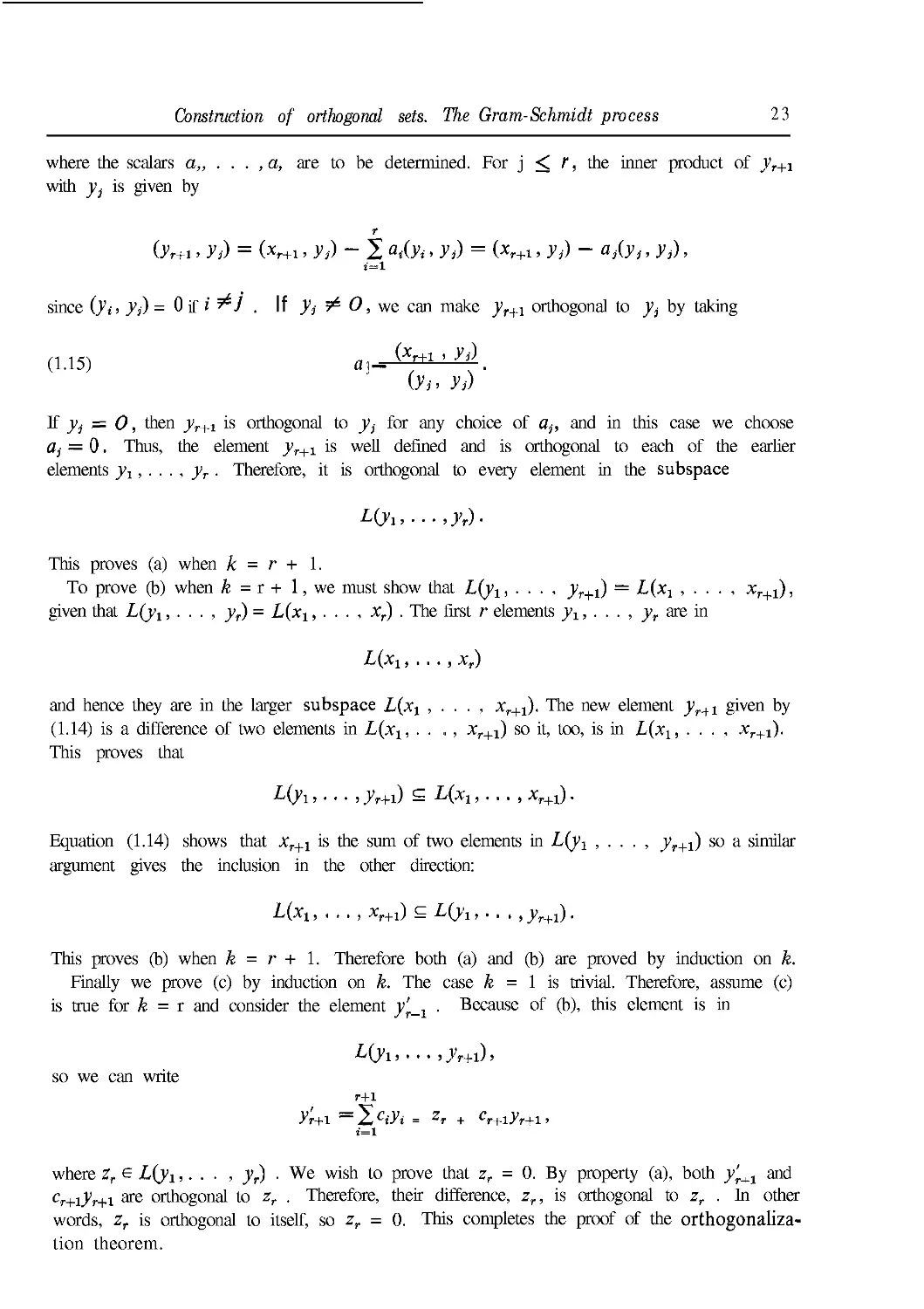
where the scalars a,, . . . , a, are to be determined. For j <* r, the inner product of yT+1
with у j- is given by
Or+i > yi) = (vn > yi) ~ 2 а*(л > J'>) = (*r+i > J'i) - аАУ). ^)>
since (ji, Jj) = 0 if г 5^У . If J3 Ф 0, we can make yr+1 orthogonal to yt by taking
(i.i5) a]-;.
(y^ У/)
If yi = 0, then yr+1 is orthogonal to _>>,,¦ for any choice of a,-, and in this case we choose
dj — 0. Thus, the element yr+1 is well defined and is orthogonal to each of the earlier
elements уг, . . . , yT. Therefore, it is orthogonal to every element in the subspace
L(ji,... ,yr).
This proves (a) when к = r + 1.
To prove (b) when k = r + 1, we must show that L(y1, . . . , yr+1) — L(x1 , . . . , xr+1),
given that L{y1, . . . , yr) = L(x1, . . . , xr) . The first r elements y±, . . . , yr are in
?(*!, . . ., л;,)
and hence they are in the larger subspace L(xt , . . . , xr+1). The new element yrJtl given by
A.14) is a difference of two elements in L(xx, . . ,, xr+1) so it, too, is in L(xlt . . . , ^r+i).
This proves that
L(yt,. .. ,yr+1) Я L(Xl,,.., xr+l).
Equation A.14) shows that Xr+j is the sum of two elements in Ь(уг , . . . , JV+i) so a similar
argument gives the inclusion in the other direction:
L{xx, ..., xr+1) ?%,. . ,,yr+1).
This proves (b) when k = r + 1. Therefore both (a) and (b) are proved by induction on k.
Finally we prove (c) by induction on k. The case k = 1 is trivial. Therefore, assume (c)
is true for k = r and consider the element y'r_x . Because of (b), this element is in
so
we
can
write
Уг+г
r+l
= zT + cr+1yr+1,
where Zr e Ыух,. . . , yr) ¦ We wish to prove that zr = 0. By property (a), both у'г^ and
cr+1yr+i are orthogonal to zr . Therefore, their difference, zr, is orthogonal to zr . In other
words, zr is orthogonal to itself, so zr = 0. This completes the proof of the orthogonaliza-
tion theorem.

24
Linear spaces
In the foregoing construction, suppose we have yr+1 = 0 for some r. Then A.14)
shows that xr+x is a linear combination of yx, . . . ,yr, and hence of xx, . . . , xr, so the
elements xx, . . . , xr+1 are dependent. In other words, if the first k elements xx,. . . , xk
are independent, then the corresponding elements yx , . . . , yk are nonzero. In this case the
coefficients at in A.14) are given by A.15), and the formulas defining yx , . . . , yk become
A.16) yx = xlt
= xr+l ~~
> Уг)
tt (Уг'Уг)
Уг
for r=l,2,...,k-l.
These formulas describe the Gram-Schmidt process for constructing an orthogonal set of
nonzero elements yx, . . . , yk which spans the same subspace as a given independent set
Xi, . . . , Xk. In particular, if хг, . . . , xh is a basis for a finite-dimensional Euclidean space,
thenj1; , yk is an orthogonal basis for the same space. We can also convert this to an
orthonormal basis by normalizing each element yit that is, by dividing it by its norm.
Therefore, as a corollary of Theorem 1.13 we have the following.
theorem i.i4. Every finite-dimensional Euclidean space has an orthonormal basis.
If x and у are elements in a Euclidean space, withy Ф 0, the element
(*. У) ..
(У, У)
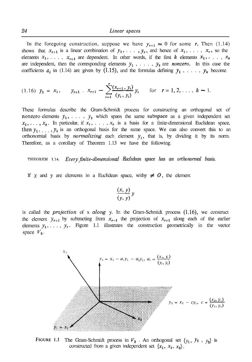
is called the projection of x along y. In the Gram-Schmidt process A.16), we construct
the element yr+i by subtracting from xr+1 the projection of xr+1 along each of the earlier
elements yx, . . . , yr. Figure 1.1 illustrates the construction geometrically in the vector
space V3.
- a.,y.,, a, =
Figure 1.1 The Gram-Schmidt process in K3 . An orthogonal set {y1, }'2 , y3} is
constructed from a given independent set {xx, x2, лг3}.

Construction of orthogonal sets. The Gram-Schmidt process 25
example 1. In F4, find an orthonormal basis for the subspace spanned by the three
vectors x1 = A, -1, 1, -1), x2 = E, 1, 1, 1), and x3 = (-3, -3, 1, -3).
Solution. Applying the Gram-Schmidt process, we find
У1 = *i = A, -1, 1, -1),
y2 х2-?^Л_ Х2-Л .D,2,0,2),
(.Уi> УО
л = Хя_(^л_^)^=х,_ Y1 + *= @,0, 0,0).
(У1. J'i) (У2, Уг)
Since j3 = О, the three vectors xx, x2, x3 must be dependent. But since y1 and уг are
nonzero, the vectors xx and x2 are independent. Therefore Ь(хх, х2, x3) is a subspace of
dimension 2. The set {ух,у2} is an orthogonal basis for this subspace. Dividing each of
jj and y2 by its norm we get an orthonormal basis consisting of the two vectors
yi =K1,-1,1,-1) and -^- = -1B,1,0,1).
example 2. The Legendre polynomials. In the linear space of all polynomials, with the
inner product (x, y) = j"^ x(t)y(t) dt , consider the infinite sequence x0 , xltx2, . . . , where
xn(t) = tn. When the orthogonalization theorem is applied to this sequence it yields
another sequence of polynomials Уо, Ух, у2, . . . , first encountered by the French mathe-
mathematician A. M. Legendre A752-1833) in his work on potential theory. The first few
polynomials are easily calculated by the Gram-Schmidt process. First of all, we have
Уо(О - *o(O = ! • Since
O-o, Уо) = /^ dt = 2 and (Xl, y0) = {^ t dt = 0,
we find that
yi(t) = *!« - т^ yo(t) = Xx@ = t.
(уъ »за)
Next, we use the relations
to obtain
.@ Ji
(Ут,Уд
Similarly, we find that
-к,
=tB-

26 Linear spaces
We shall encounter these polynomials again in Chapter 6 in our further study of differential
equations, and we shall prove that
The polynomials Pn given by
are known as the Legendrepolynomials. The polynomials in the corresponding orthonormal
sequence gr0, <pl, <рг, , , , , given by <pn = yj\\yn\\ are called the normalized Legendre poly-
polynomials. From the formulas for y0, . . . , yb given above, we find that
?0@ = Vi , <M0 = VI t, rpz{t) = iVI Cf2 - #; 953@ = W* E«3 - зо,
9>4@ = iVf C5f4 - 30?2 + 3), ?)b@ = W? F3/5 - 70/3 + 15/).
1.15. Orthogonal complements. Projections
Let V be a Euclidean space and let S be a finite-dimensional subspace. We wish to
consider the following type of approximation problem: Given an element x in V, to deter-
determine an element in S whose distance from x is as small as possible. The distance between
two elements x and у is defined to be the norm ||x — y\\ .
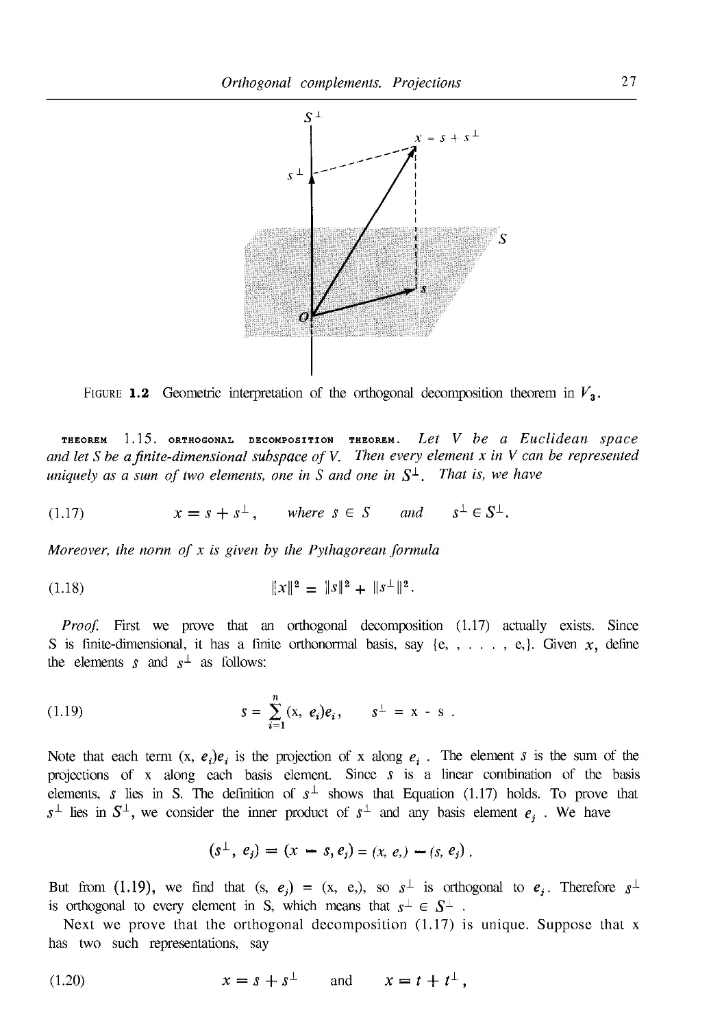
Before discussing this problem in its general form, we consider a special case, illustrated
in Figure 1.2. Here V is the vector space V3 and S is a two-dimensional subspace, a plane
through the origin. Given x in V, the problem is to find, in the plane S, that point S
nearest to x.
If x e S, then clearly s = x is the solution. If x is not in S, then the nearest point S
is obtained by dropping a perpendicular from x to the plane. This simple example suggests
an approach to the general approximation problem and motivates the discussion that
follows.
definition. Let S be a subset of a Euclidean space V. An element in V is said to be
orthogonal to S У it is orthogonal to every element of S The set of all elements orthogonal
to S is denoted by S1 and is called "S perpendicular."
It is a simple exercise to verify that S1 is a subspace of V, whether or not S itself is one.
In case S is a subspace, then S1 is called the orthogonal complement of S.
example. If S is a plane through the origin, as shown in Figure 1.2, then S1 is a line
through the origin perpendicular to this plane. This example also gives a geometric inter-
interpretation for the next theorem.

Orthogonal complements. Projections
27
О
X = S + S -
Figure 1.2 Geometric interpretation of the orthogonal decomposition theorem in V3.
THEOREM 1.15. ORTHOGONAL DECOMPOSITION THEOREM. Let V Ьв п
and let S be a finite-dimensional subspace of V. Then every element x in V can be represented
uniquely as a sum of two elements, one in S and one in S1. That is, we have
A.17) x = s + sL, where s e S and sl e S1.
Moreover, the norm of x is given by the Pythagorean formula
A.18) \\x\\ = \\s\\ + \\s || .
Proof. First we prove that an orthogonal decomposition A.17) actually exists. Since
S is finite-dimensional, it has a finite orthonormal basis, say {e, , . . . , e,}. Given x, define
the elements s and s1 as follows:
A.19)
S = 2 (X> Фг .
1
s1 = x - s .
Note that each term (x, e^)et is the projection of x along et . The element s is the sum of the
projections of x along each basis element. Since i is a linear combination of the basis
elements, S lies in S. The definition of я1 shows that Equation A.17) holds. To prove that
.j1 lies in S1, we consider the inner product of i1 and any basis element e$ ¦ We have
(sL, es) = (x - s, e,) = (x, e,) - (s, e}) .
But from A.19), we find that (s, e}) = (x, e,), so s1- is orthogonal to e,-. Therefore s^
is orthogonal to every element in S, which means that s1 e S1 ¦
Next we prove that the orthogonal decomposition A.17) is unique. Suppose that x
has two such representations, say
A.20)
X = S + SA
and

28 Linear spaces
where s and t are in S, and sL and tL are in Sl. We wish to prove that s = t and sL = t1- ¦
From A.20), we have j - ( = /-1 - j1, so we need only prove that s — t = 0. But
s — t ? Sand ?x — sA ? S1 so ^ — f is both orthogonal to t1 — s1 and equal to t1 — s1 .
Since the zero element is the only element orthogonal to itself, we must have s — t = 0.
This shows that the decomposition is unique.
Finally, we prove that the norm of x is given by the Pythagorean formula. We have
IMI2 = (x, x) = {s + sL, s + s^) = (s, s) + (Л s1),
the remaining terms being zero since s and s1 are orthogonal. This proves A.18).
definition. Let S be a finite-dimensional subspace of a Euclidean space V, and let
(ei >. . . , e,j be an orthonormal basis for S. If x ? V, the element s defined by the equation
s =
is called the projection of x on the subspace S.
We prove next that the projection of x on S is the solution to the approximation problem
stated at the beginning of this section.
1.16 Best approximation of elements in a Euclidean space by elements in a finite-
dimensional subspace
theorem Lie. approximation theorem. Let S be a finite-dimensional subspace of
a Euclidean space V, and let x be any element of V. Then the projection ofxonS is nearer to
x than any other element of S. That is, if S is the projection of x on S, we have
II* - *ll < II* - /||
for all t in S; the equality sign holds if and only if t = s.
Proof. By Theorem 1.15 we can write x = s + i1, where s ? S and ¦?-*- ? S^. Then,
for any t in S, we have
x — t = (x — s) + (s — t) .
Since s — t ? S and x — s = SL ? Sx, this is an orthogonal decomposition of x — t, so
its norm is given by the Pythagorean formula
\\x-tr = и*-,s||* + ||*-?||2.
But \\s — ?||2 > 0, so we have \\x — t\\2 > \\x — s\\2, with equality holding if and only if
S = t. This completes the proof.

Best approximation of elements in a Euclidean space 29
example 1. Approximation of continuous functions on [О, 2тг] by trigonometric polynomials.
Let V = C@, 2tt), the linear space of all real functions continuous on the interval [0, 2тг],
and define an inner product by the equation (/, g) = J^* f(x)g(x) dx . In Section 1.12
we exhibited an orthonormal set of trigonometric functions <pa, <pl} <р2, ¦ ¦ ¦ , where
a»,, / \ J. /-. COS KJC s -. bill /СЛ _ i ч> -<
.21) %(x) = — , 9W-1M = —— , cpu{x) = -—=- , for fc>l.
J2rt Jn V77
The 2n + 1 elements q>0, <Pi, • ¦ ¦ , <Ргп sPm а subspace S of dimension 2n + 1. The ele-
elements of S are called trigonometric polynomials.
If/6 C@, 2n), let/n denote the projection off on the subspace S. Then we have
A.22) fn=I(f, Ъ)<Р*> where (/. ?>*) = I /(*)?>*(*) dx-
The numbers (/, 9^) are called Fourier coefficients off. Using the formulas in A.21), we
can rewrite A.22) in the form
n
A.23) f(x) = \a0 +2(a* cos kx + bk sin kx),
k=l
where
1 C2" 1 Г2я
= — /(x) cos kx dx, bk = —I ffxj sin fcx
7T Jo 7T J0
for & = 0,1,2,...,и. The approximation theorem tells us that the trigonometric poly-
polynomial in A.23) approximates / better than any other trigonometric polynomial in S, in
the sense that the norm ||/ — /J is as small as possible.
example 2. Approximation of continuous functions on [— 1, 1] by polynomials of
degree < n. Let V = C(- 1, 1), the space of real continuous functions on [- 1, 1], and let
(/, g) = J^ f(x)g(x) dx. The n + 1 normalized Legendre polynomials <pa, <px, . . . , <pn,
introduced in Section 1.14, span a subspace S of dimension n + 1 consisting of all poly-
polynomials of degree < n. If/e C(— 1, 1), let /„ denote the projection off on S. Then we
have
/»=i(/>9'*)9'*> where (f>V*)
k-a
This is the polynomial of degree < и for which the norm ||/ — fn\\ is smallest. For example,
when f(x) = sin ттх, the coefficients (/, <pk) are given by
(/. <Pk) = j\ sin Trt cpk{t) dt.
In particular, we have (/, q>0) = 0 and
</, ,,,)-/_'J, sin

30 Linear spaces
Therefore the linear polynomial/i@ which is nearest to sin nt on [- 1, 1] is
/i@= l^-q>1(t)=-t.
Since (/, <p2) = 0, this is also the nearest quadratic approximation.
1.17 Exercises
1. In each case, find an orthonorrnal basis for the subspace of V3 spanned by the given vectors.
(a) xl= A, 1, 1), x2 = A,0,1), x3 = C,2,3).
(b) *! = A, 1, 1), x2 = (-1,1,-1), *,= A,0,1).
2. In each case, find an orthonormal basis for the subspace of Vi spanned by the given vectors.
(a) *1= A,1,0,0), x2 =@,1, 1,0), jc, = (O, 0,1,1), Xi= A,0,0, 1).
(b)*1= A,1,0, 1), x2= A,0,2, 1), x3 = A,2, -2, 1).
3. In the real linear space C@, тт), with inner product (x, y) = Jg x(t)y(t) dt, let x,(t) = cos nt
forn =0,1,2 ,.. .. Prove that the functions y0, y1, y2, . . . , given by
1 /2
yo(t)=— and yn(t) = I-cos та for n > 1,
V 77 V П
form an orthonormal set spanning the same subspace as x0, x1, x2, . . . .
4. In the linear space of all real polynomials, with inner product (x,y) = JJ x(t)y(t) dt, let
x,(t) = t" for n = 0, 1, 2, . . . . Prove that the functions
>o@ = 1- Л(') = V3 Bt - 1), y,(t) = Vs Ft2 - 6t + 1)
form an orthonormal set spanning the same subspace as {xa, хг, x2}.
5. Let V be the linear space of all real functions f continuous on [0, + <x>) and such that the
integral $* е~{/ЧО dt converges. Define (f,g) = Jo°° e-*f(t)g(t) dt, and let y0, yx ,y2,. . . , be
the set obtained by applying the Gram-Schmidt process to *0, xj, x2, ¦ ¦ ¦ , where x,(t) = /*
for n > 0. Prove that yo(t) = 1, y^i) = t - 1, y2(t) = t% - 4t + 2, y3(t) = t* - 9t2 +
18/ - 6.
6. In the real linear space C(l, 3) with inner product (f,g) = J* f (x)g(x) dx, let fix) = 1/x
and show that the constant polynomial g nearest to f is g = \ log 3. Compute \\g -f |[2 for
this g.
7. In the real linear space C@, 2) with inner product (/, g) = jo /" (x)g(x) dx, let fix) = e" and
show that the constant polynomial g nearest to f is g = \{ег - 1). Compute ||^ -f ||2 for
this g.
8. In the real linear space C( - 1, 1) with inner product (/, g) = j"lx f (x)g(x) dx , let fix) = ex
and find the linear polynomial g nearest to f. Compute \\g - f I'2 for this g.
9. In the real linear space C@, 2w) with inner product (f,g) = J2," f(x)g(x) dx, let fix) = x.
In the subspace spanned by u,,(x) = 1 , ux(x) = cos x, u2(x) = sin x, find the trigonometric
polynomial nearest to /.
10. In the linear space V of Exercise 5, let f (x) = e~x and find the linear polynomial that is nearest
to/.

LINEAR TRANSFORMATIONS AND MATRICES
2.1 Linear transformations
One of the ultimate goals of analysis is a comprehensive study of functions whose
domains and ranges are subsets of linear spaces. Such functions are called transformations,
mappings, or operators. This chapter treats the simplest examples, called linear transforma-
transformations, which occur in all branches of mathematics. Properties of more general transforma-
transformations are often obtained by approximating them by linear transformations.
First we introduce some notation and terminology concerning arbitrary functions. Let
V and W be two sets. The symbol
T: V^W
will be used to indicate that Г is a function whose domain is V and whose values are in W.
For each x in V, the element T(x) in W is called the image of x under T, and we say that T
maps x onto T(x). If A is any subset of V, the set of all images T(x) for x in A is called the
image of A under T and is denoted by T(A). The image of the domain V, T(V), is the range
of T.
Now we assume that V and Ware linear spaces having the same set of scalars, and we
define a linear transformation as follows.
definition. If Y and Ware linear spaces, a function T: V—v W is calleda linear trans-
transformation of V into W if it has the following two properties:
(a) T(x + y) = T(x) + T(y) for all x and у in V,
(b) T{cx) = cT(x) for all x in Vand all scalars с
These properties are verbalized by saying that T preserves addition and multiplication by
scalars. The two properties can be combined into one formula which states that
T(ax + by) = aT(x) + bT(y)
for all x,y in V and all scalars a and b. By induction, we also have the more general relation
for any n elements x1, . . . , xn in V and any n scalars ax,.. . , an.
31

32 Linear transformations and matrices
The reader can easily verify that the following examples are linear transformations.
EXAMPLE 1. The identity transformation. The transformation T: V -*¦ V, where T(x) = x
for each x in V, is called the identity transformation and is denoted by Z or by Iv.
example 2. The zero transformation. The transformation T: У—>¦ У which maps each
element of У onto 0 is called the zero transformation and is denoted by 0.
example 3. Multiplication by a fixed scalar с Here we have T V —>• V, where T(x) = ex
for all x in У When с = 1 , this is the identity transformation. When с = 0, it is the zero
transformation.
example 4. Linear equations. Let V = Vn and W = Vm . Given mn real numbers aik,
where / = 1,2, ... ,m and к = 1, 2, . . . , и, define Г: К„-> Fm as follows: Tmapseach
vector x = (xj, . . . , x,) in Vn onto the vector у = (Vi, . . . , ym) in Vm according to the
equations
n
Yi = ^,ai]cxk for i = 1,2 m.
k=l
example 5. Inner product with a fixed element. Let У be a real Euclidean space. For a
fixed element z in V, define T: V —*¦ R as follows: If x ? V, then T(x) = (x, z), the inner
product of x with z.
example 6. Projection on a subspace. Let У be a Euclidean space and let S be a finite-
dimensional subspace of V. Define T: V -*¦ S as follows: If x e V, then T(x) is the
projection of x on S.
example 7. The differentiation operator. Let У be the linear space of all real functions
/ differentiable on an open interval (a, b). The linear transformation which maps each
functionfin У onto its derivativef is called the differentiation operator and is denoted by
D. Thus, we have D:V —*¦ W, where D (f) = f for each / in У The space W consists of
all derivatives f.
example 8. The integration operator. Let У be the linear space of all real functions
continuous on an interval [a, b]. If/6 V, define g = T(f) to be that function in У given by
g(x) = [f(t)dt if a<x^b.
This transformation T is called the integration operator.
2.2 Null space and range
In this section, Tdenotes a linear transformation of a linear space У into a linear space W.
THEOREM 2.1. The set T(V) (the range of T) is a subspace of W. Moreover, T maps
the zero element of V onto the zero element of W.

Null space and range 33
Proof. To prove that T( V) is a subspace of W, we need only verify the closure axioms.
Take any two elements of T(V), say T(x) and T{y). Then T(x) + T{y) = T{x + y) , so
T(x) + T(y) is in T{V). Also, for any scalar с we have cT(x) = T(cx) , so cT(x) is in T(V).
Therefore, T{ V) is a subspace of W. Taking с = 0 in the relation T(cx) = cT(x), we find
that T@) = 0.
definition. The set of all elements in Vthat Tmaps onto 0 is called the null space of
Tand is denoted by N(T). Thus, we have
N(T) = {x\x e V and T(x) = 0} .
The null space is sometimes called the kernel of T.
theorem 2.2. The null space of T is a subspace ofV.
Proof. If x and у are in N(T), then so are x + у and ex for all scalars c, since
T(x + y) = T(x) + T(y) = 0 and T(cx) = cT(x) = 0.
The following examples describe the null spaces of the linear transformations given in
Section 2.1.
example 1. Identity transformation. The null space is {0}, the subspace consisting of
the zero element alone.
example 2. Zero transformation, Since every element of V is mapped onto zero, the
null space is V itself.
example 3. Multiplication by a fixed scalar с If с Ф 0, the null space contains only 0.
If с = 0, the null space is V.
example 4. Linear equations. The null space consists of all vectors (Xi, . . . , x,) in Vn
for which
п
^ ai!cxk = 0 for i = 1, 2 , . . . , m.
k=l
example 5. Inner product with a fixed element z. The null space consists of all elements
in V orthogonal to z.
example 6. Projection on a subspace S. If x e V, we have the unique orthogonal
decomposition x = s + s1 (by Theorem I .15). Since T(x) = s, we have T(x) = 0
if and only if x = sx . Therefore, the null space is Sx, the orthogonal complement of S.
example 7. Differentiation operator. The null space consists of all functions that are
constant on the given interval.
example 8. Integration operator. The null space contains only the zero function.

34 Linear transformations and matrices
23 Nullity and rank
Again in tins section T denotes a linear transformation of a linear space V into a linear
space W. We are interested in the relation between the dimensionality of V, of the null
space N(T), and of the range T(V). If V is finite-dimensional, then the null space is also
finite-dimensional since it is a subspace of V. The dimension of N(T) is called the nullity
of T. In the next theorem, we prove that the range is also finite-dimensional; its dimension
is called the rank of T.
theorem 2.3. nullity plus rank theorem. If V is finite-dimensional, then T(V) is
also finite-dimensional, and we have
B.1) dim N( T) + dim T(V) = dim V .
In other words, the nullity plus the rank of a linear tmnsformation is equal to the dimension
of its domain
Proof. Let n = dim V and let e1 , . . . , ek be a basis for N(T), where к = dim N(T) <. n.
By Theorem 1.7, these elements are part of some basis for V, say the basis
B.2) e1,.,.,ek, ek+1,... ,ek+r,
where к + r = n . We shall prove that the r elements
B.3) T(ek+1), . . . , T(ek+r)
form a basis for T(V), thus proving that dim T(V) = r . Since k + r = П , this also proves
B.1).
First we show that the r elements in B.3) span T(V). If у ? T(V), we have у = T(x)
for some x in V, and we can write x = c1e1 + ¦ • • + ск+гек+г . Hence, we have
jfc+r jfc jfc+r k+r
У = Г(х) =1с,Т(е,) = 2 с,Т(ег) + 2 с{Т(ег) = 2 сгТ{ег)
i=l t=l i=JH-l i=*+l
since Г(еО = • •'• = Т(ек) = 0. This shows that the elements in B.3) span T(V).
Now we show that these elements are independent. Suppose that there are scalars
ck+i, . . . , ck+r such that
k+r
I ctT{et) = 0 ,
i=k+l
This implies that
/ k+r ч
r( 2 cA =o
so the element x = ck+1ek+1 + • • • + ck+rek+r is in the null space N(T). This means there

Exercises 35
are scalars c1, . . . ,ck such that x = c1e1 + • . • + ckek, so we have
k+r
X = У ctet -
гШ i
0 .
But since the elements in B.2) are independent, this implies that all the scalars ct are zero.
Therefore, the elements in B.3) are independent.
Note: If К is infinite-dimensional, then at least one of N(T) or T(V) is infinite-
dimensional. A proof of of this fact is outlined in Exercise 30 of Section 2.4.
2.4 Exercises
In each of Exercises 1 through 10, a transformation T: v2 --*¦ V2 is defined by the formula given
for T(x, y), where (x, y) is an arbitrary point in V2 . In each case determine whether Tis linear. If
T is linear, describe its null space and range, and compute its nullity and rank.
1. T(x, у) = (y, x). 6. T(x, y) = {e\ e").
2. T(x, y) = (x, -y) . 7. T(x, y) = (x, 1).
3. T(x,y) = (x,0). 8. T(x,y) = (x + \,y + 1).
4. T(x,y) = (x, x) . 9. T(x,y) = (x -y,x+y).
5. T{x,y)= {x\y2). 10. T(x,y) =Bx ~y,x +y).
Do the same as above for each of Exercises 11 through 15 if the transformation T: V2 -*¦ V2
is described as indicated.
11. T rotates every point through the same angle q> about the origin. That is, T maps a point
with polar coordinates (г, в) onto the point with polar coordinates (г, в + <p), where <p is
fixed. Also, T maps 0 onto itself.
12. T maps each point onto its reflection with respect to a fixed line through the origin.
13. T maps every point onto the point A, 1).
14. T maps each point with polar coordinates (г, в) onto the point with polar coordinates Br, 6).
Also, T maps 0 onto itself.
15. T maps each point with polar coordinates (г, в) onto the point with polar coordinates (r, 26).
Also, T maps 0 onto itself.
Do the same as above in each of Exercises 16 through 23 if a transformation T: K3-> Vs is
defined by the formula given for T(x, y, z), where (x, y, z) is an arbitrary point of V3 .
16. T(x,y, z) = (z,y, x). 20. T(x,y, z) = (x + l,у + 1, z - 1).
17. T(x,y, z) = {x,y, 0). 21. T(x,y, z) = (x + \,y+ 2, z + 3).
18. T(x, y, z) = (x, 2y, 3z). 22. T(x, y, z) = (x, /, z3).
19. T(x, y, z) = (x,y, 1). 23. T(x, y, z) = (x + z, 0, x + y).
In each of Exercises 24 through 27, a transformation T: K-* V is described as indicated. In
each case, determine whether T is linear. If Г is linear, describe its null space and range, and
compute the nullity and rank when they are finite.
24. Let V be the linear space of all real polynomials p(x) of degree <, n . Ifp e V, q = T(p) means
that q(x) = p(x + 1) for all real x.
25. Let V be the linear space of all real functions differentiable on the open interval (— 1, 1).
If/6 V, g = T(f) means that g(x) = xf'(x) for all x in ( - 1, 1).

36 Linear transformations and matrices
26. Let V be the linear space of all real functions continuous on [a, b]. If/e V, g = T(f) means
that
g(x) =1 /0) sin (x — t) dt for a < x < b.
27. Let V be the space of all real functions twice differentiable on an open interval (a, b). If
у ? V, define T(y) = y" + Py' + Qy , where P and Q are fixed constants.
28. Let V be the linear space of all real convergent sequences {x,}. Define a transformation
T: V—> V as follows: If л: = {x,} is a convergent sequence with limit a, let T(x) = {}Vb
where yn = a - xn for n > 1 . Prove that Tis linear and describe the null space and range of T.
29. Let V denote the linear space of all real functions continuous on the interval [ — it, тт\. Let S
be that subset of V consisting of all / satisfying the three equations
Г f(t)dt = O, Г f(t) cos tdt =0, Г fit) sin tdt =O.
(a) Prove that S is a subspace of V.
(b) Prove that S contains the functions / (x) = cos nx and / (x) = sin nx for each n = 2,3,. . . .
(c) Prove that 5 is infinite-dimensional.
Let T: V —> V be the linear transformation defined as follows: Iff ? V,g = T(f) means that
gix) = Г {1 +cos(x-t)}f(t)dt.
J —IT
(d) Prove that T(V), the range of T, is finite-dimensional and find a basis for T(V).
(e) Determine the null space of Г.
(f) Find all real с Ф 0 and all nonzero / in V such that T(f) = cf. (Note that such an /
lies in the range of T.)
30. Let T: F—>¦ W be a linear transformation of a linear space К into a linear space VK If V is
infinite-dimensional, prove that at least one of T(V) or N(T) is infinite-dimensional.
[Hint: Assume dim N(T) = it , dim Г(Т) = r , let ег , . . , ek Ъе а basis for N(T) and
let e1, . . . , ek, ek+l, . . . , ek+n be independent elements in V, where n > r. The
elements Tiek+1),. . . , Tiek+n) are dependent since n > r. Use this fact to obtain a
contradiction.]
2.5 Algebraic operations on linear transformations
Functions whose values lie in a given linear space W can be added to each other and can
be multiplied by the scalars in W according to the following definition.
definition. Let S: V —у W and T: V—> W be two functions with a common domain V
and with values in a linear space W. If с is any scalar in W, we define the sum S + T and the
product cT by the equations
B.4) (S + T)(x) = S(x) + T(x), icT){x) = cT(x)
for all x in V.

Algebraic operations on linear transformations 37
We are especially interested in the case where V is also a linear space having the same
scalars as W. In this case we denote by =§?( V, W) the set of all linear transformations of V
into W.
If S and Tare two linear transformations in =§?( V, W), it is an easy exercise to verify that
S + T and cT are also linear transformations in &(V, W). More than this is true. With
the operations just defined, the set ^C(V, W) itself becomes a new linear space. The zero
transformation serves as the zero element of this space, and the transformation (— 1)Г
is the negative of T. It is a straightforward matter to verify that all ten axioms for a linear
space are satisfied. Therefore, we have the following.
theorem 2.4. The set <2?(V, W) of all linear transformations of V into W is a linear
space with the operations of addition and multiplication by scalars defined as in B.4).
A more interesting algebraic operation on linear transformations is composition or
multiplication of transformations. This operation makes no use of the algebraic structure
of a linear space and can be defined quite generally as follows.
W
figure 2.1 Illustrating the composition of two transformations.
definition. Let U, V, W be sets. Let T: U —>¦ V be a function with domain V and
values in V, and let S:V^> W be another function with domain V and values in W. Then
the composition ST is the function ST: E/—>- W defined by the equation
(ST)(x) = S[T(x)] for every x in U.
Thus, to map X by the composition ST, we first map x by T and then map T(x) by S.
This is illustrated in Figure 2.1.
Composition of real-valued functions has been encountered repeatedly in our study of
calculus, and we have seen that the operation is, in general, not commutative. However,
as in the case of real-valued functions, composition does satisfy an associative law.
theorem 2.5. IfT: U -> V, S: V -> W, and R: W -> X are three functions, then we have
R(ST) = (RS)T.

38 Linear transformations and matrices
Proof Both functions R(ST) and (RS)T have domain U and values in X. For each X
in U, we have
[R(ST)](x) = R[(ST)(x)] = R[S[T(x)]] and [(RS)T](x) = (RS)[T(x)] = R[S[T(x)]],
which proves that R(ST) = (RS)T.
definition. Let T: V—*¦ V be a function which maps V into itself. We define integral
powers of T inductively as follows:
T° = I, Tn = TTnl for n > 1.
Here / is the identity transformation. The reader may verify that the associative law
implies the law of exponents TmTn = Tm+n for all nonnegative integers m and n.
The next theorem shows that the composition of linear transformations is again linear.
theorem 2.6. If U, V, W are linear spaces with the same scalars, and if T: U -> V
and S: V —>¦ W are linear transformations, then the composition ST: U —>- W is linear.
Proof. For all x, у in U and all scalars a and b, we have
(ST)(ax + by) = S[T(ax + by)] = S[aT(x) + bT(y)] = aST(x) + bST(y).
Composition can be combined with the algebraic operations of addition and multiplica-
multiplication of scalars in JSf(K, W) to give us the following.
theorem 2.7. Let U, V, W be linear spaces with the same scalars, assume S and T are
in ??{V, W), and let с be any scalar.
(a) For any function R with values in V, we have
(S + T)R = SR + TR and (cS)R = c(SR).
(b) For any linear transformation R: W —> U, we have
R(S+T) = RS + RT and R(cS) = c(RS).
The proof is a straightforward application of the definition of composition and is left as
an exercise.
2.6 Inverses
In our study of real-valued functions we learned how to construct new functions by
inversion of monotonic functions. Now we wish to extend the process of inversion to a
more general class of functions.

Inverses 39
Given a function T, our goal is to find, if possible, another function S whose composition
with T is the identity transformation. Since composition is in general not commutative,
we have to distinguish between ST and TS. Therefore we introduce two kinds of inverses
which we call left and right inverses.
definition. Given two sets V and Wand a function T: V -> W. A function S: T(V) -> V
is called a left inverse ofT if S[T(xj] = xfor all X in V, that is, if
where Iv is the identity transformation on V. A function R: T(V) —>¦ V is called a right inverse
of T if T[R(y)] = у for ally in T(V), that is, if
TR = IT(V),
where IT (y) is the identity transformation on T(V).
example. A function with no left inverse but with two right inverses. Let V = A, 2)
and let W = {0}. Define T: V-> Was follows: T(l) = TB) = 0. This function has two
right inverses R: fV—>-V and R' : W-> V given by
R@) =1, R'@) = 2.
It cannot have a left inverse S since this would require
1 = S[TA)] = S@) and 2 = S[TB)] = S@).
This simple example shows that left inverses need not exist and that right inverses need not
be unique.
Every function T: V—> W has at least one right inveise. In fact, each у in T(V) has the
form у = T(x) for at least one x in V. If we select one such x and define R(y) = x , then
Г[Л(}>)] = T(x) = у for each у in T(V), so R is a right inverse. Nonuniqueness may occur
because there may be more than one x in V which maps onto a given у in T(V). We shall
prove presently (in Theorem 2.9) that if each у in T(V) is the image of exactly one x in V,
then right inverses are unique.
First we prove that if a left inverse exists it is unique and, at the same time, is a right
inverse.
theorem 2.8. A function T\ V —*¦ W can have at most one left inverse. If T has a left
inverse S, then S is also a right inverse.
Proof. Assume T has two left inverses, S: T(V)+ Vand S': T(V)+ V. Choose any
у in T(V). We shall prove that S(y) = S'(y) • Now у = T(x) for some x in V, so we have
S[T(x)] = X and S' [T(x)] = x,

40 Linear transformations and matrices
since both S and S' are left inverses. Therefore S(y) = x and S'(y) = x , so S(y) = S'(y)
for all у in T(V). Therefore S = S' which proves that left inverses are unique.
Now we prove that every left inverse S is also a right inverse. Choose any element у in
T{V). We shall prove that T[S(y)] = у . Since у € T( V), we have у = T(x) for some x in
V. But S is a left inverse, so
x= S[T(x)]= S(y).
Applying T, we get T(x) = Tlsb>)] . But у = T(x), so у = T[S(y)] , which completes the
proof.
The next theorem characterizes all functions having left inverses.
theorem 2.9. A function T: V —>¦ W has a left inverse if and only if T maps distinct
elements of V onto distinct elements of W; that is, if and only if for all x and у in V,
B.5) х^У implies T(x) Ф T(y).
Note: Condition B.5) is equivalent to the statement
B.6) T(x) = T(y) implies x =y.
A function Г satisfying B.5) or B.6) for all x and у in У is said to be one-to-one on V.
Proof. Assume Г has a left inverse S, and assume that T(x) = T(y). We wish to prove
that x = у . Applying S, we find S[T(x)] = S[T(y)] Since S[T(x)] = x and S[T(y)] = y,
this implies x = y. This proves that a function with a left inverse is one-to-one on its
domain.
Now we prove the converse. Assume Tis one-to-one on V. We shall exhibit a function
S: T(V) —>¦ V which is a left inverse of T. If у e T(V) , then у = T(x) for some x in V. By
B.6), there is exactly one x in V for which у = T(x). Define S(y) to be this x. That is,
we define S on T(V) as follows:
S(y) = x means that T(x) = у .
Then we have S|T(;>c)] = x for each x in V, so ST = I,. Therefore, the function S so
defined is a left inverse of T.
definition. Let T: V —*¦ W be one-to-one on V. The unique left inverse of T (which
we know is also a right inverse) is denoted by Г™1. We say that T is invertible, and we call
T-1 the inverse of T.
The results of this section refer to arbitrary functions. Now we apply these ideas to
linear transformations.

One-to-one linear transformations 41
2.7 One-to-one linear transformations
In this section, V and W denote linear spaces with the same scalars, and T: V—*¦ W
denotes a linear transformation in J§?( V, W). The linearity of T enables us to express the
one-to-one property in several equivalent forms.
theorem 2.10. Let T: V -> W be a linear transformation in Л?( V, W). Then the following
statements are equivalent.
(a) T is one-to-one on V.
(b) T is invertible and its inverse T^1; T(V) —>• V is linear.
(c) For all x in V, T(x) = 0 implies x = 0. That is, the null space N(T) contains only
the zero element of V.
Proof. We shall prove that (a) implies (b), (b) implies (c), and (c) implies (a). First
assume (a) holds. Then T has an inverse (by Theorem 2.9), and we must show that T~l
is linear. Take any two elements и and v in T(V). Then и = T(x) and v = T(y) for some
x and у in V. For any scalars a and b, we have
аи . kbv = aT(x) + ЪТ{у) = Т(ах + by),
since T is linear. Hence, applying Г, we have
T~\au + bv) = ax + by = aT-^u) + bT~l(v),
so T'1 is linear.. Therefore (a) implies (b).
Next assume that (b) holds. Take any x in V for which T(x) = 0. Applying Т~г, we
find that x = T~l(O) = 0, since T'1 is linear. Therefore, (b) implies (c).
Finally, assume (c) holds. Take any two elements и and v in V with T(u) = T(v). By
linearity, we have T(u — v) = T(u) — T(v) = 0, so и — v = 0. Therefore, Tis one-to-one
on V, and the proof of the theorem is complete.
When V is finite-dimensional, the one-to-one property can be formulated in terms of
independence and dimensionality, as indicated by the next theorem.
theorem 2.1 1. Let T: V -> W be a linear transformation in У( V, W) and assume that
V is finite-dimensional, say dim V = n . Then the following statements are equivalent.
(a) T is one-to-one on V.
(b) If ег , . . . , ev are independent elements in V, then T(e^), . . . , T(ev) are independent
elements in T(V).
(c) dim T(V) = n .
(d) If{ex,..., e,j is a basis for V, then {T(e^, • • • > T(en)} is a basis for T(V).
Proof. We shall prove that (a) implies (b), (b) implies (с), (с) implies (d), and (d) implies
(a). Assume (a) holds. Let elf ¦ ¦ ¦ , ev be independent elements of V and consider the

42 Linear transformations and matrices
elements T(e^, ¦ ¦ ¦ , T(ev) in T(V). Suppose that
2 ctT(.et) = 0
for certain scalars clt . . . , c,. By linearity, we obtain
2 сге( |=O, and hence 2 CA
I
since T is one-to-one. But e1; . . . , ev are independent, so Cj = • • . = cv = 0. Therefore
(a) implies (b).
Now assume (b) holds. Let {e,, . . . , e,} be a basis for V. By (b), the n elements
T(e^),. . . , T(en) in T(V) are independent. Therefore, dim T(V) > n . But, by Theorem
2.3, we have dim T(V) < n . Therefore dim T(V) = n, so (b) implies (c).
Next, assume (c) holds and let {e,, . . . , e,} be a basis for V. Take any element у in
T(V). Then у = T(x) for some x in V, so we have
n n
x = 2 ciei-> ^d hence у = T(x) = ]Г с{Г(е^).
Therefore {T{e^), . . . ,T(en)} spans T(V). But we are assuming dim T(V) = n, so
(Г^),. . . , T(en)} is a basis for T(V). Therefore (c) implies (d).
Finally, assume (d) holds. We will prove that T(x) = 0 implies x = 0. Let {ex, . . . , e,}
be a basis for V. If x e V, we may write
n n
x = J c^ , and hence T(x) = 2 сг^(ег).
J=l i=l
If Г(х) = O,thenc! = ¦ • • = cn = 0, since the elements T{e^}, . . . , T(en) are independent.
Therefore x = 0, so Tis one-to-one on V. Thus, (d) implies (a) and the proof is complete.
2.8 Exercises
1. Let V = {0, 1} . Describe all functions TV V—>-V . There are four altogether. Label them as
T\, T2, T3, T and make a multiplication table showing the composition of each pair. Indicate
which functions are one-to-one on V and give their inverses.
2. Let V = {0, 1,2}. Describe all functions TV V-* V for which T(V) = V . There are six
altogether. Label them as T1, . . . , T6 and make a multiplication table showing the com-
composition of each pair. Indicate which functions are one-to-one on V, and give their inverses.
In each of Exercises 3 through 12, a function TV V2 -*¦ V2 is defined by the formula given for
T(x, y), where (x, y) is an arbitrary point in K2. In each case determine whether T is one-to-one
on V2. If it is, describe its range T( V2); for each point (u, v) in T( V2), let (x, y) = T~l(u, v) and
give formulas for determining x and у in terms of и and v.
3. T(x,y) = (y, x). 8. T(x,y) = (еж, е»).
4. T(x, y) = (x, -y). 9. T(x,y) = (x, 1).
5. T(x, y) = (x, 0). 10. T(x, y) = (x + 1, у + 1).
6. T(x, y) = (x, x). 11. T(x,y) = (x -y,x +y).
7. T(x, y) = (x\ /). 12. T(x, y) =Bx - y, x + y).

Exercises
43
In each of Exercises 13 through 20, a function T: V3 —>¦ V3 is defined by the formula given for
T(x, y, z), where (x, y, z) is an arbitrary point in V3. In each case, determine whether Tis one-to-
one on V3. If it is, describe its range T(V3); for each point («, v, w) in T(V3), let (x,y, z) =
Т~г(и, v, w) and give formulas for determining x, /, and z in terms of u, v, and w.
13. T(x, y, z) = (z. y, x)
14. T(x,y,z) = (x,y, 0).
15. T(x,y, z) = (x, 2y,3z).
16. T(x, y, z) = (x,y,x +y + z).
17. T(x,y,z) = (x+ \,y+ \,z~ 1).
18. T(x,y,z) =(x+ I,y +2,z +3).
19. T(x, y, z) -¦ (x, x + y, x + у + z).
20. T(x,y,z) =(x +y,y +z,x+z).
21. Let T; V --> V be a function which maps V into itself. Powers are defined inductively by the
formulas T° = I, Tn = TTn~l for n > 1 . Prove that the associative law for composition
implies the law of exponents: TmTn = ттЛп. If Tis invertible, prove that T" is also invertible
and that ( T")-1 = ( Г")".
In Exercises, 22 through 25, S and Г denote functions with domain V and values in V. In
general, ST ^ TS. If ST = TS, we say that S and T commute.
22. If S and г commute, prove that (ST)" = SnTn for all integers л > 0.
23. If S and Tare invertible, prove that ST is also invertible and that (ST) = T^S'1. In other
words, the inverse of ST is the composition of inverses, taken in reverse order.
24. If S and Tare invertible and commute, prove that their inverses also commute.
25. Let V be a linear space. If S and г commute, prove that
(s + Tf = s2 + 2st + r2
and
(S + ГK = 5* + З^Г + 3ST2 + Г3.
Indicate how these formulas must be altered if ST ф TS.
26. Let S and г be the linear transformations of V3 into V3 defined by the formulas S(x, y, z) =
(z, y, x) and ГО, y, z) = (x, x + _y, x + _y + z), where (x, v, z) is an arbitrary point of V3.
(a) Determine the image of (x, y, z) under each of the following transformations : ST, TS,
ST - TS, S2, T2, (STJ, (TSJ, (ST - TSJ.
(b) Prove that S and Tare one-to-one on V3 and find the image of (u, v, w) under each of the
following transformations : S'1, T'1, (ST)'1, (TS)'1.
(c) Find the image of (x, y, z) under (T — l)n for each n > 1.
27. Let vbe the linear space of all real polynomials/^*). Let D denote the differentiation operator
and let г denote the integration operator which maps each polynomial p onto the polynomial
q given by q(x) = §lp(t) dt . Prove that DT = lv but that TD Ф lY. Describe the null space
and range of TD.
28. Let К be the linear space of all real polynomialsp(x). Let D denote the differentiation operator
and let г be the linear transformation that maps p(x) onto xp'(x).
(a) Let p(x) = 2 + 3x - x2 + 4x3 and determine the image ofp under each of the following
transformations: D, T, dt, td, dt - TD, T2D2 - D2T2.
(b) Determine those p in V for which T(p) = p .
(c) Determine thosep in V for which (DT — 2D)(p) = 0.
(d) Determine thosep in V for which (DT - TD)n(p) = Dn(p).
29. Let V and D be as in Exercise 28 but let Г be the linear transformation that maps p(x) onto
xp(x). Prove tihat DT - TD = Z and that DTn - TnD = nTn~l for л > 2.
30. Let S and г be in &(V, V) and assume that ST - TS = I. Prove that STn - TnS = nTn x
for all n > 1 .
3 1. Let V be the linear space of all real polynomials p(x). Let R, S, г be the functions which map
an arbitrary polynomial p(x) = c0 + cxx + . . . + cnxn in V onto the polynomials u(x), s(x),

Linear transformations and matrices
and t(x), respectively, where
r(x) = p{0), s(x)=fckx«-1, t(x) = 'Zckxk+1.
k=l fc=O
(a) Let p(x) = 2 + 3x - x2 + x3 and determine the image of p under each of the following
transformations: R, S, T, ST, TS, {TSJ, T2S2, S2F>, TRS, RST.
(b) Prove that R, S, and Tare linear and determine the null space and range of each.
(c) Prove that T is one-to-one on V and determine its inverse.
(d) If n > 1, express ( TS)n and SnTn in terms of / and R.
32. Refer to Exercise 28 of Section 2.4. Determine whether T is one-to-one on V. If it is, describe
its inverse.
2.9 Linear transformations with prescribed values
If К is finite-dimensional, we can always construct a linear transformation T: V-* W
with prescribed values at the basis elements of V, as described in the next theorem.
theorem 2.12. Let ex, . .., en be a basis for an n-dimensional linear space V. Let
щ,... ,un be n arbitrary elements in a linear space W. Then there is one and only one linear
transformation T: V ->¦ W such that
B.7) T(ek) = uk for k=l,2,...,n.
This T maps an arbitmry element x in V as follows:
n
B.8) If x =2>A' then T(x)=Jixkuk.
Proof. Every x in У can be expressed uniquely as a linear combination of ex, . . . , en ,
the multipliers xt, . . . , xn being the components of x relative to the ordered basis
(els . . . , e,). If we define T by B.8), it is a straightforward matter to verify that T is
linear. If x = ek for some k, then all components of X are 0 except the kth, which is 1, so
B.8) gives Т(ек) = ик, are required.
To prove that there is only one linear transformation satisfying B.7), let T be another
and compute T(x). We find that
T'(x) = T'(ixkek) =IxkT'(ek) = f хкщ = T(x).
\k=l ) *=1 k=l
Since T'(x) = T(x) for all x in V, we have T = T, which completes the proof.
example . Determine the linear transformation T: F2 —»¦ F2 which maps the basis elements
i = A, 0) and j = @, 1) as follows:
+j W = 2i -j.

Matrix representations of linear transformations
45
Solution. If x == xj + X2 j is an arbitrary element of V2, then T{x) is given by
T(x) = XiT{i) + хгТ{)) = Xi(/ + j) + x2B/ - j) = (x, + 2x2)i + (xx - x2)j.
2.10 Matrix representations of linear transformations
Theorem 2.12 shows that a linear transformation T: К->- W of a finite-dimensional
linear space V is completely determined by its action on a given set of basis elements
ex,. . . ,en. Now, suppose the space W is also finite-dimensional, say dim W = m, and let
Wx, . . . , Wm be a basis for W. (The dimensions и and m may or may not be equal.) Since T
has values in W, each element T(ek) can be expressed uniquely as a linear combination of the
basis elements
w
say
T(ek)=
llc
where t
We shall display the w-tuple (tlk ,
B.9)
are the components of T(ek) relative to the: ordered basis
. , w,).
tmk) vertically, as follows:
ix. We have such a column vector for
hem side by side and enclose them in
»ular array:
.Jtnlc_
This array is called a column vector or a column mat
each of the n elements T(e^), . . . , T(en). We place
one pair of brackets to obtain the following rectan
'
'21 '22
\Jm\
This array is called a matrix consisting of m rows and n columns. We call it an m by n matrix,
or an m x n matrix. The first row is the 1 x n matrix (tn , tn, . . . , ?l71). The m x 1
matrix displayed in B.9) is the kth column. The scalars tik are indexed so the first subscript
i indicates the row:, and the second subscript к indicates the column in which tik occurs.
We call tik the ik-entry or the ik-element of the matrix. The more compact notation
or
is also used to denote the matrix whose ik-entry is tik .

46
Linear transformations and matrices
Thus, every linear transformation Г of an n-dimensional space V into an m-dimensional
space W gives rise to an m x n matrix (tik) whose columns consist of the components of
T{e^), . T(en) relative to the basis (wl5 . . . , w,). We call this the matrix representation
of T relative to the given choice of ordered bases (e,, . . . , e,) for V and (и^, . . . , w,) for
W. Once we know the matrix (tik), the components of any element T(x) relative to the
basis (w,, . . . , w,) can be determined as described in the next theorem.
theorem 2.13. Let T be a linear transformation in У( V, W), where dim V = n and
dim W = m. Let (elt . . . , e,,) and (w1, . . . , w,) be ordered bases for Vand W, respectively,
and let (tik) be the m X n matrix whose entries are determined by the equations
B.Ю)
m
T(ek) = 2 tikwt, for к = 1, 2 , . . . , n ,
i
Then an arbitrary element
B.11) x = 2>Л
k = l
in V with components (Xj,. . . , x,) relative to (elt. , . , e,) is mapped by T onto the element
B.12)
T(x) =
in W with components (уг, . . . , у,) relative to (w,
components of x by the linear equations
, w,). The y{ are related to the
B.13)
for i =
Proof. Applying T to each member of B.11) and using B.10), we obtain
where each yi is given by B.13). This completes the proof.
Having chosen a pair of bases (e,, . . . , e,) and (м\, . . . , wm) for V and W, respectively,
every linear transformation T: V^> W has a matrix representation (tik). Conversely, if
we start with any mn scalars arranged as a rectangular matrix (tik) and choose a pair of
ordered bases for V and W, then it is easy to prove that there is exactly one linear trans-
transformation T: K—>- W having this matrix representation. We simply define Tat the basis
elements of V by the equations in B.10). Then, by Theorem 2.12, there is one and only
one linear transformation T: V—*- W with these prescribed values. The image T(x) of an
arbitrary point x in V is then given by Equations B.12) and B.13).

Matrix representations of linear transformations
47
example 1. Construction of a linear transformation from a given matrix. Suppose we
start with the 2 x 3 matrix
1 -2
0 4
Choose the usual bases of unit coordinate vectors for V3 and V2. Then the given matrix
represents a linear transformation T: V3 —>¦ V% which maps an arbitrary vector (xx, хг, x3)
in V3 onto the vector (y1, y2) in V2 according to the linear equations
yx =
x2 - 2x3,
Уг = *i + ox, + 4x3.
example 2. Construction of a matrix representation of a given linear transformation.
Let V be the linear space of all real polynomials p(x) of degree < 3. This space has dimen-
dimension 4, and we choose the basis A, x, x2, x3), Let D be the differentiation operator which
maps each polynomial p(x) in V onto its derivative p'(x). We can regard В as a linear
transformation of V into W, where W is the 3-dimensional space of all real polynomials
of degree < 2'. In W we choose the basis A, x, x2). To find the matrix representation of D
relative to this (choice of bases, we transform (differentiate) each basis element of V and
express it as a linear combination of the basis elements of W. Thus, we find that
D(l) = 0 = 0 + Ox + Ox2, ?)(x) = 1 = 1 + Ox + Ox2,
D(x2) = 2x = 0 + 2x + Ox2, D(x3) = 3x2 = 0 + Ox + 3x2.
The coefficients of these polynomials determine the columns of the matrix representation of
D. Therefore, the required representation is given by the following 3x4 matrix:
0 10 0'
0 0 2 0
0 0 0 3
To emphasize that the matrix representation depends not only on the basis elements but
also on their order, let us reverse the order of the basis elements in Wand use, instead, the
ordered basis (x3, x, 1). Then the basis elements of V are transformed into the same poly-
polynomials obtained above, but the components of these polynomials relative to the new
basis (x2, x., 1) appear in reversed order. Therefore, the matrix representation of D now
becomes
Г0 0 0 3"
0 0 2 0
0 10 0

Linear transformations and matrices
Let us compute a third matrix representation for D, usingthebasis A, 1 + x , 1 + x + x2,
1 + x + x2 + x3) for V, and the basis A, x, x2) for W. The basis elements of V are trans-
transformed as follows:
D(l) = 0, D(l + x)=l, D(l +x + x2) = l +2x,
D(l + x + x2 + xz) = 1 +2x + 3x\
so the matrix representation in this case is
0 1
0 0
0 0
I'
2|2
2.11 Construction of a matrix representation in diagonal form
Since it is possible to obtain different matrix representations of a given linear transforma-
transformation by different choices of bases, it is natural to try to choose the bases so that the resulting
matrix will have a particularly simple form. The next theorem shows that we can make
all the entries 0 except possibly along the diagonal starting from the upper left-hand corner
of the matrix. Along this diagonal there will be a string of ones followed by zeros, the
number of ones being equal to the rank of the transformation. A matrix (tik) with all
entries tik = 0 when i Ф к is said to be a diagonal matrix.
theorem 2.14. Let V and W be finite-dimensional linear spaces, with dim V = n and
dim W = m . Assume T e <?( V, W) and let r = dim T(V) denote the rank of T. Then there
exists a basis (e, , . . . , e,) for V and a basis (w^, ¦ ¦ ¦ , wm)for W such that
B.14) T(et) = wt for i= l,2,...,r,
and
B.15) T(et) = 0 f о r i = r + I,... ,n.
Therefore, the matrix (t№) of T relative to these bases has all entries zero except for the r
diagonal entries
tu= hi= ' ' ' = trr = 1 .
Proof. First we construct a basis for W. Since T(V) is a subspace of W with dim T(V) =
r, the space T(V) has a basis of r elements in W, say wt, . . . , wr. By Theorem 1.7, these
elements form a subset of some basis for W. Therefore we can adjoin elements wr+1, . . . ,
wm so that
B.16) (wl,.. . , wr, wr+1,. . . , wj
is a basis for W.

Construction of a matrix representation in diagonal form 49
Now we construct a basis for V. Each of the first r elements Ъ\ in B.16) is the image of at
least one element in V. Choose one such element in V and call it et . Then T(e^) = wt for
/ = 1, 2,... , r so B.14) is satisfied. Now let к be the dimension of the null space N(T).
By Theorem 2.3 we have n = k + r. Since dim N(T) = k, the space N(T) has a basis
consisting of k elements in V which we designate as er+1 , . . . , ет+к. For each of these
elements, Equation B.15) is satisfied. Therefore, to complete the proof, we must show
that the ordered set
B-17) (е1г. ..,er,er+1,. ,.,er+lc)
is a basis for V. Since dim V = n = r + k, we need only show that these elements are
independent. Suppose that some linear combination of them is zero, say
B.18) 5ле4 = О.
Applying T and using Equations B.14) and B.19, we find that
ICiT(et) = 2 ciWi = О .
But №[,... ,wr are independent, and hence c1 = ¦ • • = cr = 0. Therefore, the first r
terms in B.18) are zero, so B.18) reduces to
r+k
But eT+i ... e,--$Fe independent since they form a basis for N(T), and hence cr+1 =
• • • = cr+]c = 0. Therefore, all the ct in B.18) are zero, so the elements in B.17) form a
basis for V. This completes the proof.
example. We refer to Example 2 of Section 2.10, where D is the differentiation operator
which maps the space V of polynomials of degree < 3 into the space W of polynomials of
degree <2. In this example, the range T(V) = W, so T has rank 3. Applying the method
used to prove Theorem 2.14, we choose any basis for W, for example the basis A, x, x2).
A set of polynomials in V which map onto these elements is given by (x, \x2, \xz). We
extend this set to get a basis for V by adjoining the constant polynomial 1, which is a basis
for the null space of D. Therefore, if we use the basis (x, \xl, \x%, 1) for V and the basis
A, x, x2) for W, the corresponding matrix representation for D has the diagonal form
10 0 0'
0 10 0
0 0 10

50 Linear transformations and matrices
2.12 Exercises
In all exercises involving the vector space Vn , the usual basis of unit coordinate vectors is to be
chosen unless another basis is specifically mentioned. In exercises concerned with the matrix of
a linear transformation T: V-^-W where V = W, we take the same basis in both V and w unless
another choice is indicated.
1. Determine the matrix of each of the following linear transformations of Vn into Vn :
(a) the identity transformation,
(b) the zero transformation,
(c) multiplication by a fixed scalar с
2. Determine the matrix for each of the following projections.
(a) T: V3 -v V2, where T(xt, x2, xs) = (xt, x2).
(b) T: K3->- V2, where Tfa, x2, x3) = (x2, x3).
(c) T: Vb-> V3, where T(xx,x2,x3,Xi, хъ) = (x2, x3, x4).
3. A linear transformation T: V2 -> F2 maps the basis vectors / andj as follows:
(a) Compute T(ii - 4j) and T2Ci - 4j) in terms of i and j.
(b) Determine the matrix of Г and of Tz.
(c) Solve part (b) if the basis (i, j) is replaced by (e1, e2), where e1 - i - j, e2 = 3i + j.
4. A linear transformation T: V2 —>- V2 is defined as follows: Each vector (x, y) is reflected in
the y-axis and then doubled in length to yield T(x, y). Determine the matrix of Г and of T2.
5. Let T: Fg-v V3 be a linear transformation such that
T(k) =2i+ lj+ 5k, T(j + k) =/, T(i+j + k)=j-k.
(a) Compute T(i + 2j + 3k) and determine the nullity and rank of T.
(b) Determine the matrix of T.
6. For the linear transformation in Exercise 5, choose both bases to be (e,, e2, e3), where ex =
B, 3, 5), e2 = A, 0, 0), e3 = @, 1, —1), and determine the matrix of г relative to the new
bases.
7. A linear transformation T: V3 -> K2 maps the basis vectors as follows: T(i) = @, 0), T(J) =
A, 1), T(k)= A, -i).
(a) Compute TDi -j + k) and determine the nullity and rank of T.
(b) Determine the matrix of T.
(c) Use the basis (i, j, k) inF3 and the basis (и^ , w2) in V2, where и>х = A, 1), vv2 = A,2).
Determine the matrix of г relative to these bases.
(d) Find bases {e±, e2, e3) for V3 and (w1, и>2) for V2 relative to which the matrix of Twill be
in diagonal form.
8. A linear transformation T: F2 -> V3 maps the basis vectors as follows: T(i) = A, 0, 1),
T(j)= (-1,0, 1).
(a) Compute TBi - 3j) and determine the nullity and rank of T.
(b) Determine the matrix of T.
(c) Find bases (e,, e,) for K2 and (w,, w2, w3) for V3 relative to which the matrix of Twill be
in diagonal form.
9. Solve Exercise 8 if T(i) =A,0, 1) and T(j) = A,1, 1).
10. Let Kand W be linear spaces, each with dimension 2 and each with basis (^ , e2). Let 7V V—> W
be a linear transformation such that T(e1 + e2) = 3e1 + 9e2, TQex + 2ег) = 7e1 + 23e2.
(a) Compute T(e2 ~ ex) and determine the nullity and rank of T.
(b) Determine the matrix of Г relative to the given basis.

linear spaces of matrices
51
(c) Use the basis (et , e,) for V and find a new basis of the form (ex + ae2, 2ex + be,) for W,
relative to which the matrix of Twill be in diagonal form.
In the linear space of all real-valued functions, each of the following sets is independent and
spans a finite-dimensional subspace V. Use the given set as a basis for V and let D: V-+ V be
the differentiation operator. In each case, find the matrix of D and of D2 relative to this choice
of basis.
11. (sin x, cos x).
12. A, x, ex).
13. A, I + x, I + x + ex).
14. (f, xex).
15. (-cos x, sin x).
16. (sin x, cos X, x sin x, x cos x).
17. (ex sin x, ex cos x).
18. (e2x sin 3x, elx cos 3x).
19. Choose the basis A, x, x2, x3) in the linear space V of all real polynomials of degree <3.
Let D denote the differentiation operator and let T: V—>¦ V be the linear transformation
which maps/7(x) onto xp'{x). Relative to the given basis, determine the matrix of each of the
foUowingtransformations: (a) T; (b) DT; (c) TD; (d) TD - DT; (e) Г2; (f) Г2?>2 - D2T2.
20. Refer to Exercise 19. Let W be the image of Vunder TD. Find bases for Vand for W relative
to which the matrix of TD is in diagonal form.
2.13 Linear spaces of matrices
We have seen how matrices arise in a natural way as representations of linear trans-
transformations. Matrices can also be considered as objects existing in their own right, without
necessarily being connected to linear transformations. As such, they form another class of
mathematical objects on which algebraic operations can be defined. The connection
with linear transformations serves as motivation for these definitions, but this connection
will be ignored for the moment.
Let m and n be two positive integers, and let Im „ be the set of all pairs of integers (i,j)
such that 1<<'</и,1 <7<й- Any function A whose domain is Im n is called an m x n
matrix. The function value A (i, j) is called the ij-entry or ij-ehment of the matrix and will
be denoted also by atj . It is customary to display all the function values in a rectangular
array consisting of m rows and n columns, as follows:
ami
""ml
The elements ai} may be arbitrary objects of any kind. Usually they will be real or complex
numbers, but sometimes it is convenient to consider matrices whose elements are other
objects, for example, functions. We also denote matrices by the more compact notation
or
If m = n , the matrix is said to be a square matrix. A 1 x n matrix is called a row matrix;
an m x 1 matrix is called a column matrix.

52
Linear transformations and matrices
Two functions are equal if and only if they have the same domain and take the same
function value at each element in the domain. Since matrices are functions, two matrices
A = (ai;)) and В = (bi}) are equal if and only if they have the same number of rows, the
same number of columns, and equal entries ati = bti for each pair (i,j).
Now we assume the entries are numbers (real or complex) and we define addition of
matrices and multiplication by scalars by the same method used for any real- or complex-
valued functions.
definition. If A = (atl) and В = (bi}) are two m x n matrices and if с is any scalar,
we define matrices A + B and с A as follows:
A + В = (аи + bi}), с A = (cai3).
The sum is defined only when A and В have the same size.
EXAMPLE. If
1 2 - 3 Г5 0 1
A = | -1 0 41 and В =
1—2 3
then we have
6 2 -2
0-2 7
1A =
2 4-6
-2 0 8
(-1M =
-5 0 -1
-1 2 -3
We define the zero matrix 0 to be the m x n matrix all of whose elements are 0. -With
these definitions, it is a straightforward exercise to verify that the collection of all m x n
matrices is a linear space. We denote this linear space by Mm „. If the entries are real
numbers, the space Mm n is a real linear space. If the entries are complex, Mm n is a complex
linear space. It is also easy to prove that this space has dimension mn. In fact, a basis for
Mmn consists, of the mn matrices having one entry equal to 1 and all others equal to 0.
For example, the six matrices
1 0 0
0 0 0
0 1 0
0 0 0
0 0 1
0 0 0
0 0 0'
1 0 0
 0 0
0 1 0
0 0 0"
0 0 1
form a basis for the set of all 2 x 3 matrices.
2.14 Isomorphism between linear transformations and matrices
We return now to the connection between matrices and linear transformations. Let V
and W be finite-dimensional linear spaces with dim V = n and dim W = m. Choose a
basis (e,, . . . , e,) for V and a basis (wlt . . . , w,) for W. In this discussion, these bases are
kept fixed. Let =S?(K, W) denote the linear space of all linear transformations of V into
W. If T e ??(V, W), let m(T) denote the matrix of T relative to the given bases. We recall
that m(T) is defined as follows.

Isomorphism between linear transformations and matrices 53
The image of each basis element ek is expressed as a linear combination of the basis
elements in IV:
m
B.19) T(ek) = 2 tikwt for к = 1, 2, . . . , п.
The scalar multipliers tik are the ik-entries of m(T). Thus, we have
B.20) m(T) = (faM:i.
Equation B.20) defines a new function m whose domain is =5f(K, W) and whose values
are matrices in М,Л|И. Since every m x n matrix is thejnatrix m(T) for some Tin i?( K, W),
the range of m is Afm „. The next theorem shows that the transformation m: J?(V, W) —>¦
Mmn is linear and one-to-one on j?( V, W).
theorem 2.15. isomorphism theorem. For all S and 1" in ??(V, W) and all scalars
c, we have
m(S +T)= m{S) + m{T) and m(cT) = cm(T).
Moreover,
m(S) = m(T) implies S = T,
so m is one-to-one on ??(V, W).
Proof. The matrix m(T) is formed from the multipliers tik in B.19). Similarly, the
matrix m(S) is formed from the multipliers sik in the equations
B.21) S(ek) = 2 si№ for к = 1, 2 , . . . , п.
Since we have
m m
(S + T)(ek) = 2 (sik + tik)Wi and (cT)(,?fc) = ? (ctik)w{,
i=l i=\
we obtainm(S + T) = (sik + tik) = m(S) + m(T) and m(cT) = (ctik) = cm(T). This proves
that m is linear.
To prove that m is one-to-one, suppose that m(S) = m(T), where S = (sik) and T =
(tik). Equations B.19) and B.21) show that S(ek) = T(ek) for each basis element ek,
so S(x) = T(x) for all x in V, and hence S = T.
Note: The function m is called an isomorphism. For a given choice of bases, m
establishes a one-to-one correspondence between the set of linear transformations
&{V, W) and the set ofmxn matrices Mm_n . The operations of addition and multipli-
multiplication by scalars are preserved under this correspondence. The linear spaces if(K, W)
and Mmn are said to be isomorphic. Incidentally, Theorem 2.11 shows that the domain
of a one-to-one linear transformation has the same dimension as its range. Therefore,
dim se{V, IV) = dim Mm,n = mn .
If V = Wand if we choose the same basis in both V and W, then the matrix m(Z) which
corresponds to the identity transformation /: V->- V is an n x n diagonal matrix with each

54 Linear transformations and matrices
diagonal entry equal to 1 and all others equal to 0. This is called the identity or unit matrix
and is denoted by / or by /,.
2.15 Multiplication of matrices
Some linear transformations can be multiplied by means of composition. Now we shall
define multiplication of matrices in such a way that the product of two matrices corresponds
to the composition of the linear transformations they represent.
We recall that if T: U-+ V and S: V-> Ware linear transformations, their composition
ST: U—* W is a linear transformation given by
ST(x) = S[T(x)] forallxin U.
Suppose that U, V, and Ware finite-dimensional, say
dim U = П, dim V — p, dim W= m.
Choose bases for U, V, and W. Relative to these bases, the matrix m(S) is an m x p
matrix, the matrix T is a p x n matrix, and the matrix of ST is an m x n matrix. The
following definition of matrix multiplication will enable us to deduce the relation m{ST) =
m(S)m(T). This extends the isomorphism property to products.
definition. Let A be any mxp matrix, and let В be any p x n matrix, say
А = (а,Х& and B=(bu)lU-
Then the product AB is defined to be the m x n matrix С = {ci}) whose ij-entry is given by
B-22) co=2««Aj-
Note: The product AB is not defined unless the number of columns of A is equal to
the number of rows of B.
If we write Аг for the ith row of A, and Bj for thejth column of B, and think of these as
p-dimensional vectors, then the sum in B.22) is simply the dot product At • B\ In other
words, the //-entry of AB is the dot product of the ith row of A with thejth column of B:
Thus, matrix multiplication can be regarded as a generalization of the dot product.
Г4
3 1 2
example 1. Let A = \ I and В = 5—1
-1 1 0
0 2
.SinceAis2 x 3 and В is 3 x 2 ,

Multiplication of matrices
55
the product А В is the 2 x 2 matrix
AB =
17 21
1 -7
The entries of AB are computed as follows:
Al-B1 = 3-4 + 1-5 + 2-0 = 17, A, . Я2 = 3 ¦ 6 + 1 • (-1) + 2 ¦ 2 = 21,
A, • B1= (-1) -4 + 1-5+ 0-0=1,
EXAMPLE 2. Let
'2 1 -3
= -7.
A=
1 2
and B=
-2'
1
2
Here A is 2 x 3 and В is 3 x 1, so AB is the 2 x I matrix given by
AB =
A1 ¦ Br
-9
since A, • B1 = 2 ¦ (-2) + 1 • 1 + (-3) • 2 = -9 and A2 B1 = 1 • (-2) + 2 • 1 + 4 • 2 = 8.
example 3. If A and В are both square matrices of the same size, then both AB and BA
are defined. For example, if
A =
1
-1
and В =
I
we find that
AB =
13 81
2 -2
В А =
5 A2'
-1 101
3 12J
This example shows that in general AB ^ BA . If A2? = 2?A , we say A and В commute.
example 4. If /9 is the p x p identity matrix, then /рЛ = A for every p x n matrix A,
and Л/ц = 5 for every m x p matrix 2?. For example,
1
0
0
0
1
0
0'
0
1_
2
3
_4_
=
r2'
3
_4_
1
4
2
5
3"
6_
1
0
0
0
1
0
f.
1
'1 2 31
4 5 61
;i
Now we prove that the matrix of a composition ST is the product of the matrices m(S)
and m(r).

56 Linear transformations and matrices
theorem 2.16. Let T: U -+V and S: V-> W be linear transformations, where U, V, W
are finite-dimensional linear spaces. Then, for a fixed choice of bases, the matrices of S, T,
and ST are related by the equation
m(ST) = m(S)m(T).
Proof. Assume dim U = n, dim V = p, dim W = m. Let (щ, . . . , un) be a basis for
U, (vt,.. . , v,) a basis for V, and (wx, . . . , w,) a basis for W. Relative to these bases, we
have
m
m(S) = (s,,)"?i, where S(vk) = J si]cw{ for к = 1, 2,. . . , p,
i=i
and
m(T) = (ti^'Lx, where T{u}) = 2, hsvk for j = 1,2,. . . ,n.
Therefore, we have
V V m m t p \
st(u}) = smuM = 2 tkis(vk) = 2 *„ 2 s«W( = 2 2w« w«'
so we find that
m(ST) = (j,satk\ 'П = m(S)m(T).
\*=1 )i,S~l
We have already noted that matrix multiplication does not always satisfy the com-
commutative law. The next theorem shows that it does satisfy the associative and distributive
laws.
THEOREM 2.17. ASSOCIATIVE AND DISTRIBUTIVE LAWS FOR MATRIX MULTIPLICATION.
Given matrices А, В, С
(a) If the products A(BC) and (AB)C are meaningful, we have
A(BC) = (AB)C (associative law).
(b) Assume A and В are of the same size. If AC and ВС are meaningful, we have
(A + B)C = AC + ВС (right distributive law),
whereas if CA and CB are meaningjiil, we have
C(A + B) = CA + CB (left distributive law).
Proof. These properties can be deduced directly from the definition of matrix multi-
multiplication, but we prefer the following type of argument. Introduce finite-dimensional
linear spaces U, V, W, X and linear transformations T: U-*- V, S: V-+ W, R: W-> X
such that, for a fixed choice of bases, we have
A = m(R), В = m(S), С = m(T).

Exercises
57
By Theorem 2.16, we have m(RS) = AB and m{ST) = ВС From the associative law for
composition, we find that R(ST) = (RS)T. Applying Theorem 2.16 once more to this
equation, we obtain m(R)m(ST) = m(RS)m(T) or A(BC) = (AB)C, which proves (a). The
proof of (b) can be given by a similar type of argument.
definition. If A is a square matrix, we define integral powers of A inductively as follows:
A" = 1, An = AA" for n > 1.
2.16 Exercises
1. If A =
1 -4
-1
4 -2
в =
-1
BA, AC, CA, ABB-3C).
"О Г
2
3
-2
, С =
2
1
1
2'
-1
-3
, compute В + С, АВ,
2. Let A = | I Find all 2 x 2 matrices В such that (a) AB = 0 ; (b) BA = 0.
3. In each case find a, b, c, d to satisfy the given equation.
(a)
0
1
0
0
0
0
]
0
1
0
0
0
0"
0
0
1
'a'
b
с
d_
T
9
6
_5_
(b)
a b c
1 4 9
1 0 2 0"
0 0 11
0 10 0
0 0 10
10 6 6
19 8 4
4. Calculate AB — BA in each case.
(а) Л =
(b) A =
1 2 2
2 1 2
1 2 3
2 0 0
В =
1
-1
1 2
2 1
4 11
-4 2 0
1 2 1
3 1
3 -2
-3 5
in лт _ Ат+п
-2
4
11
5. If Л is a square matrix, prove that AnAm = Am n for all integers m >0, n > 0.
6. Let A =
7. Let /1 =
3. Let /1 =
1 2
. Verify that Л2 = | | and compute A".
cos в —sin в~\ fcos 20 —sin 26
. Verify that A2 =
cos 0 sin 20 cos 20
sin 0
1 1 1
0 1 1
and compute A ".
. Verify that A2 =
0 0 1
formula for A " and prove it by induction,
1
0
0
2
1
0
3"
2
1
. Compute A% and A*. Guess a general

58 Linear transformations and matrices
Г i о
9. Let A = . Prove that A2 = 2A - Z and compute A100.
L-i i/
10. Find all 2 x 2 matrices A such that A2 = 0.
11. (a) Prove that a 2 x 2 matrix A commutes with every 2x2 matrix if and only if A commutes
with each of the four matrices
10"] Г0 1
0 0 ' 0 0
0 01 Г0 01
i oj' [o ij"
(b) Find all such matrices A.
12. The equation A2 = Z is satisfied by each of the 2 x 2 matrices
: :]• [. -]¦ с -Я-
о
where Ь and с are arbitrary real numbers. Find all 2 x 2 matrices A such that A% = I.
-Г4
Г 2 -1!
13. If A = and 5=| |, find 2x2 matrices С and D such that AC = В
L-2 3j
andDA = B.
14. (a) Verify that the algebraic identities
(A + Bf = A2 + 2AB + B2 and (A + B)(A -B) = A2-.
Г1 -11 Г1 0
do not hold for the 2 x 2 matrices A = \ and В
L° 2J
(b) Amend the right-hand members of these identities to obtain formulas valid for all square
matrices A and B.
(c) For which matrices A and В are the identities valid as stated in (a)?
2.17 Systems of linear equations
Let A = (aw) be a given m x n matrix of numbers, and let Cj, . . . , cm be m further
numbers. A set of m equations of the form
n
B.23) 2а»Л = ci for i = 1, 2, . . . , m,
is called a system of m linear equations in n unknowns. Here xx, . . . , xn are regarded as
unknown. A solution of the system is any n-tuple of numbers (х1г . . . , xn) for which all the
equations are satisfied. The matrix A is called the coefficient-matrix of the system.
Linear systems can be studied with the help of linear transformations. Choose the usual
bases of unit coordinate vectors in Vn and in Vm. The coefficient-matrix A determines a

Systems of linear equations 59
linear transformation, T: Vn —*¦ Vm, which maps an arbitrary vector x = {x1, . . . , x,) in Vn
onto the vector у = (y1, . . . , ym) in Vm given by the m linear equations
«
Л = 1 я* A for i = 1, 2 ,. . ., /n.
Jc-1
Let с = (Cj , . . . , c,) be the vector in Fm whose components are the numbers appearing in
system B.23). This system can be written more simply as;
T(x) = с
The system has a solution if and only if с is in the range of T. If exactly one x in Vn maps
onto c, the system has exactly one solution. If more than one x maps onto c, the system
has more than one solution.
example: 1. A system with no solution. The system x + y=l,X+y = 2 has no
solution. 'The sum of two numbers cannot be both I and 2.
example 2. A system with exactly one solution. The system x + y=l,x— y = 0has
exactly one solution: (x, y) = (|, ^).
example: 3. A system with more than one solution. The system x + у = 1 , consisting
of one equation in two unknowns, has more than one solution. Any two numbers whose
sum is 1 gives ii solution.
With each linear system B.23), we can associate another system
n
~Zaikxk =0 for i = I, 2, . . . , m,
*=i
obtained by replacing each Ci in B.23) by 0. This is called the homogeneous system corre-
corresponding to B.23). If с ф О, system B.23) is called a nonhomogeneous system. A vector
x in Vn will satisfy the homogeneous system if and only if
T(x) = 0,
where T is the linear transformation determined by the coefficient-matrix. The homogene-
homogeneous system always has one solution, namely x = О, but it may have others. The set of
solutions of the homogeneous system is the null space of T. The next theorem describes the
relation between solutions of the homogeneous system and those of the nonhomogeneous
system.
theorem 2.18. Assume the nonhomogeneous system B.23) has a solution, say b.
(a) If a vector x is a solution of the nonhomogeneous system, then the vector v = x — b
is a solution of the corresponding homogeneous system.
(b) If a vector v is a solution of the homogeneous-v system, then the vector x = v + b is a
solution of the nonhomogeneous system.

60 Linear transformations and matrices
Proof. Let T: Vn ->- Vm be the linear transformation determined by the coefficient-
matrix, as described above. Since b is a solution of the nonhomogeneous system we have
T(b) = с . Let x and v be two vectors in Vn such that v = x — b. Then we have
T{v) = T(x - b) = T(x) - T(b) = T(x) - с
Therefore T(x) = с if and only if T(v) = 0. This proves both (a) and (b).
This theorem shows that the problem of finding all solutions of a nonhomogeneous
system splits naturally into two parts: A) Finding all solutions v of the homogeneous
system, that is, determining the null space of T; and B) finding one particular solution b of
the nonhomogeneous system. By adding b to each vector v in the null space of T, we thereby
obtain all solutions x = v + b of the nonhomogeneous system.
Let к denote the dimension of N(T) (the nullity of T). If we can find к independent
solutions vx, . . . , vk of the homogeneous system, they will form a basis for N(T), and we
can obtain every v in N(T) by forming all possible linear combinations
V = txvx + ¦ • • + tkvk ,
where tx, . . . , tk are arbitrary scalars. This linear combination is called the general solution
of the homogeneous system. If b is one particular solution of the nonhomogeneous system,
then all solutions x are given by
x = b + txvx + • ¦ . + tkvk.
This linear combination is called the general solution of the nonhomogeneous system.
Theorem 2.18 can now be restated as follows.
theorem 2.19. Let T: Vn —> Vm be the linear transformation such that T(x) = y, where
x = (xx, ... , xn), у = (ji,. . ., ym) and
n
k = l
Let к denote the nullity of T. If vx, . . . ,vk are к independent solutions of the homogeneous
system T(x) — 0 , and if b is one particular solution of the nonhomogeneous system T(x) = С ,
then the general solution of the nonhomogeneous system is
X = b + txvx + . . . + tkvk ,
where tt,..., tk are arbitrary scalars.
This theorem does not tell us how to decide if a nonhomogeneous system has a particular
solution b, nor does it tell us how to determine solutions vls . . . , vk of the homogeneous
system. It does tell us what to expect when the nonhomogeneous system has a solution.
The following example, although very simple, illustrates the theorem.

Computation techniques
example. The system x + у = 2 has for its associated homogeneous system the equation
x + у = 0. Therefore, the null space consists of all vectors in K2 of the form (t, —t),
where / is arbitrary. Since (t, —t) = t(l, —1), this is a one-dimensional subspace of V2
with basis A, — 1). A particular solution of the nonhomogeneous system is @,2). There-
Therefore the general solution of the nonhomogeneous system is given by
(x,y) =@,2)
or
X = t,
where t is arbitrary.
2.18 Computation techniques
We turn now to the problem of actually computing the solutions of a nonhomogeneous
linear system. Although many methods have been developed for attacking this problem,
all of them require considerable computation if the system is large. For example, to solve
a system of ten equations in as many unknowns can require several hours of hand com-
computation, even with the aid of a desk calculator.
We shall discuss a widely-used method, known as the Gauss-Jordan elimination method,
which is relatively simple and can be easily programmed for high-speed electronic computing
machines. The method consists of applying three basic types of operations on the equations
of a linear system:
A) Interchanging two equations;
B) Multiplying all the terms of an equation by a nonzero scalar:
C) Adding to one equation a multiple of another.
Each time we perform one of these operations on the system we obtain a new system having
exactly the same solutions. Two such systems are called equivalent. By performing these
operations over and over again in a systematic fashion we finally arrive at an equivalent
system which can be solved by inspection.
We shall illustrate the method with some specific examples. It will then be clear how the
method is to be applied in general.
EXAMPLE 1.
A system with a unique solution. Consider the system
2x - 5y + 4z = - 3
x - ly + z = 5
x - 4y + 6z = 10.
This particular system has a unique solution, X = 124, у = 75, z = 31 , which we shall
obtain by the Gauss-Jordan elimination process. To save labor we do not bother to copy
the letters x, y, z and the equals sign over and over again, but work instead with the aug-
augmented matrix
B.24)
2
1-2
1
-5
-4
1
4
6
-3'
5
1O_

62
Linear transformations and matrices
obtained by adjoining the right-hand members of the system to the coefficient matrix. The
three basic types of operation mentioned above are performed on the rows of the augmented
matrix and are called row operations. At any stage of the process we can put the letters
x, y, z back again and insert equals signs along the vertical line to obtain equations. Our
ultimate goal is to arrive at the augmented matrix
B.25)
'1
0
.0
0
0
o.
10
1 -
I
after a succession of row operations. The corresponding system of equations is x = 124,
у = 75, z = 31 , which gives the desired solution.
The first step is to obtain a 1 in the upper left-hand corner of the matrix. We can do this
by interchanging the first row of the given matrix B.24) with either the second or third
row. Or, we can multiply the first row by \. Interchanging the first and second rows, we get
1-2
2
1
-5
-4
1
4
6
-3
1
5"
0.
The next step is to make all the remaining entries in the first column equal to zero, leaving
the first row intact. To do this we multiply the first row by -2 and add the result to the
second row. Then we multiply the first row by -1 and add the result to the third row.
After these two operations, we obtetin
B.26)
0 -1
q - -i
-13
Now we repeat the process on the smaller matrix [
-1 2
-2 5
-13
5
which appears
adjacent to the two zeros. We can obtain a 1 in its upper left-hand corner by multiplying
the second row of B.26) by — 1 .
This gives us the matrix
L 0o-21-21 -251
Multiplying the second row by 2 ш
B.27)
1
1
_
0
adding
2
0 1
0
the
1
_ 2
1
resul
5
13.
31
to the third, we get

Computation techniques
63
At this stage, the corresponding system of equations is given by
x — 2y + z = 5
у - Iz = 13
Z = 31.
These equations can be solved in succession, starting with the third one and working
backwards, to give us
z = 31, у = 13 + Iz = 13 + 62 = 75, x = 5 + ly - z = 5 + 150 - 31 = 124.
Or, we can continue the Gauss-Jordan process by making all the entries zero above the
diagonal elements in the second and third columns. Multiplying the second row of B.27)
by 2 and adding the result to the first row, we obtain
Llll 001-3-21
llli
Finally, we multiply the third row by 3 and add the result to the first row, and then multiply
the third row by 2 and add the result to the second row to get the matrix in B.25).
example 2. A system with more than one solution. Consider the following system of 3
equations in 5 unknowns:
2x — 5y + 4z + и — v = — 3
B.28) x -2y + z - u + v = 5
x — Ay + 6z + 2m - v = 10.
The corresponding augmented matrix is
L 2-511-2-4 4 6 1-12 1
¦310 5.1
The coefficients of x, y, z and the right-hand members are the same as those in Example 1.
If we perform the same row operations used in Example 1, we: finally arrive at the augmented
matrix
1
0
0
0
1
0
0
0
1
-16
-9
-3
19
11
4
12'
1).
31

64
Linear transformations and matrices
The corresponding system of equations can be solved for x, y, and z in terms of и and v,
giving us
x = 124 + 16m - 19u
у = 75 + 9и-Ш
z = 3 1 + Зм- 4v.
If we let и = t1 and v = t2, where tx and t2 are arbitrary real numbers, and determine
x, y, z by these equations, the vector (x, y, z, u, v) in Vb given by
(x,y,z, u, v) = A24 + 16/x - 19r2, 75 + 9tx - Ut2, 31 + 3?x - 4t2, tlt t,)
is a solution. By separating the parts involving t1 and ?2> we can rewrite this as follows:
(x,y,z, u, v) = A24, 75, 31,0,0) + ^A6, 9,3, 1,0) + /,(-19, -11, -4,0, 1).
This equation gives the general solution of the system. The vector A24, 75, 31,0,0) is a
particular solution of the nonhomogeneous system B.28). The two vectors A6, 9, 3, 1,0)
and (-19, —11,-4 , 0, 1) are solutions of the corresponding homogeneous system. Since
they are independent, they form a basis for the space of all solutions of the homogeneous
system.
example 3. A system with no solution. Consider the system
B.29)
2x - 5y + 4z = - 3
x — 2y + z = 5
x - 4y + 5z = 10.
This system is almost identical to that of Example 1 except that the coefficient of z in the
third equation has been changed from 6 to 5. The corresponding augmented matrix is
11-2 -5 4
-3 11
Applying the same row operations used in Example 1 to transform B.24) into B.27), we
arrive at the augmented matrix
B.30)
. 001-201 -201
When the bottom row is expressed as an equation, it states that 0 = 31. Therefore the
original system has no solution since the two systems B.29) and B.30) are equivalent.

Inverses of square matrices
65
In each of the foregoing examples, the number of equations did not exceed the number
of unknowns. If there are more equations than unknowns, the Gauss-Jordan process is
still applicable. For example, suppose we consider the system of Example 1, which has the
solution x = 124 , у = 75, z = 31. If we adjoin a new equation to this system which is also
satisfied by the same triple, for example, the equation 2x — 3_y + z = 54, then the
elimination process leads to the agumented matrix
1
0
0
0
0
000
0
10
1
124"
75
3 1
0
with a row of zeros along the bottom. But if we adjoin a new equation which is not satisfied
by the triple A24, 75, 31), for example the equation x + у + z = 1, then the elimination
process leads to an augmented matrix of the form
1
0
0
0
0
1
0
0
0
0
1
0
124"
75
31
a
where a ^ 0. The last row now gives a contradictory equation 0 = a which shows that
the system has no solution.
2.19 Inverses of square matrices
Let A = (aw) be a square n x n matrix. If there is another n x n matrix В such that
В А = /, where Z is the n x n identity matrix, then A is called nonsingular and В is called a
left inverse of Л.
Choose the usual basis of unit coordinate vectors in Vn and let T: Vn —> Vn be the linear
transformation with matrix m(T) = A. Then we have the following.
theorem 2.20. The matrix A is nonsingular if and only ifT is invertible. If В A = I
then В = miT-1).
Proof. Assume that A is nonsingular and that BA = I. We shall prove that T(x) = 0
implies x = 0. Given x such that T(x) = О, let X be the n x 1 column matrix formed
from the components of x. Since T(x) = О, the matrix product AX is an n x 1 column
matrix consisting of zeros, so B(AX) is also acolumn matrixof zeros. But B(AX) = (BA)X =
IX = X, so every component of x is 0. Therefore, Tis invertible, and the equation TT~1 = Z
implies that miJ^miT^1) = Z or AmiT'1) = I. Multiplying on the left by B, we find
miT'1) = В , Conversely, if Г is invertible, then T~XT is the identity transformation so
m(T~1)m(T)is the identity matrix. Therefore A is nonsingular and wG^x)^ = /.

Linear transformations and matrices
All the properties of invertible linear transformations have their counterparts for non-
singular matrices. In particular, left inverses (if they exist) are unique, and every left
inverse is also a right inverse. In other words, if A is nonsingular and В A = I, then
AB = I. We call В the inverse of A and denote it by A*1. The inverse A'1 is also non-
singular and its inverse is A.
Now we show that the problem of actually determining the entries of the inverse of a
nonsingular matrix is equivalent to solving n separate nonhomogeneous linear systems.
Let A = (аь) be nonsingular and let A = (bi}) be its inverse. The entries of A and
A are related by the ir equations
B.31) |>ЛЬЫ = 3„,
where dtj = 1 if i = j , and 6tj = 0 if i j* j. For each fixed choice of j, we can regard this
as a nonhomogeneous system of n linear equations in n unknowns bu, b2j, . . . , bnj . Since
A is nonsingular, each of these systems has a unique solution, the jth column of B. All
these systems have the same coefficient-matrix A and differ only in their right members.
For example, if Л is a 3 x 3 matrix, there are 9 equations in B.31) which can be expressed
as 3 separate linear systems having the following augmented matrices :
«11
«21
«31
«12
«22
«32
«13
«23
«33
Г
0
0
«11
«21
«31
«12
«28
«32
«13
«23
«33
0
1
0
«11
«21
«31
«12
«22
«32
«13
«23
«33
0
0
1
If we apply the Gauss-Jordan process, we arrive at the respective augmented matrices
'1
0
0
0
1
0
0
0
1
in"
*21
*31.
)

0
0
0
1
0
0
0
1
*12~
*22
*32.
>

0
0
0
1
0
0
0
1
*13~
*23
*33.
In actual practice we exploit the fact that all three systems have the same coefficient-matrix
and solve all three systems at once by working with the enlarged matrix
«11
«21
«31
«12
«22
«32
«13
«23
«33
1
0
0
0
1
0
0,
0
1,
The elimination process then leads to

0
0
0
1
0
0
0
1

Exercises
67
The matrix on the right of the vertical line is the required inverse. The matrix on the left
of the line is the 3 x 3 identity matrix.
It is not necessary to know in advance whether A is nonsingular. If Л is singular (not
nonsingular), we can still apply the Gauss-Jordan method, but somewhere in the process
one of the diagonal elements will become zero, and it will not be possible to transform A
to the identity matrix.
A system of n linear equations in n unknowns, say
i = 1,2, ...,n,
2
k=l
can be written more simply as a matrix equation,
AX= C,
where A == (дй-) is the coefficient matrix, and X and С are column matrices,
X =
If Л is nonsingular there is a unique solution of the system given by X = А~гС.
2.20 Exercises
Apply the Gauss-Jordan elimination process to each of the following systems. If a solution
exists, determine the general solution.
1. x +y + 3z = 5
2x - у + 4z = 11
-y + z = 3.
2. 3x + 2y + z = 1
5x +Ъу h3z = 2
x + у - z = 1 .
3. 3x + 2y + z = 1
5x +3y h3z =2
7x + 4y + 5z = 3.
4. 3x + 2y + z = 1
5x +3y -Bz = 2
7x + Ay + 5z = 3
x + у - z = о .
5. 3X - ly + 5z + и = 1
X + у- 3Z + 2D = 2
6x+ у — 4z + Зи = 7.
L x+y-3z+u=5
2x-y+ z - 2u = 2
Ix + у - Iz + 3« = 3.
7 . x + у + 2z + 3U
2X + ly + Iz + ll
3x+ 3j + 6z + lOu +
8. x — 2y + Z + 2U =
2X + 3j - Z - 5и =
4 x - у + z - и =
5X — 3y + Iz + м =
9. Prove that the system л: + у + 2z =2, 2x - у + 3z = 2, 5x - j + az
solution if й ?^ 8. Find all solutions when a = 8.
10. (a) Determine all solutions of the system
5x +2y -6z +2u= -1
x- y+ z- u= — 2 .
+ 4v =
i + Uv =
15» =
- 2
9
= 5
3.
iz = 6,
0
0
= 0.
has a unique

Linear transformations and matrices
(b) Determine all solutions of the system
5x + ly - 6z + lu = - 1
x-y+ z- u = - 2
x + у + z = 6.
11. This exercise tells how to determine all nonsingular 2x2 matrices. Prove that
a 61Г d -b
с d\\ —с а
= (ad - bc)I.
1
Deduce that | | is nonsingular if and only if ad — be ^ 0, in which case its inverse is
с
1
d -b
ad - be \ -c a
Determine the inverse of each of the matrices in Exercises 12 through 16.
12.
13.
14.
2 3 4
2 1 1
-1 1 2
1 2 2
2 -1 1
1 3 2
1-2 1
-2 5 -4
1-4 6
15.
16.
'12 3 4,
0 1 2 3
0 0 12'
.0 0 0 lj
0 10 0 0 0"
2 0 2 0 0 0
0 3 0 10 0
0 0 10 2 0
0 0 0 3 0 1
0 0 0 0 2 0
2.21 Miscellaneous exercises on matrices
1. If a square matrix has a row of zeros or a column of zeros, prove that it is singular.
2. For each of the following statements about n x n matrices, give a proof or exhibit a counter
example.
(a) If AB + BA = O, then A2B3 = B3A2.
(b) If A and в are nonsingular, then A + в is nonsingular.
(c) If A and в are nonsingular, then AB is nonsingular.
(d) If A, B, and A + в are nonsingular, then A — в is nonsingular.
(e) If A3 = 0, then A — Z is nonsingular.
(f) If the product of k matrices A, ... A, is nonsingular, then each matrix At is nonsingular.

Miscellaneous exercises on matrices 69
Г1 21 Г6
3. If A — \ , find a nonsingular matrix P such that P~}AP =
|_5 4j |_0
4. The matrix A = , where j'2 = -1, a = J(l + ^5),япйЬ = |A - <J~5), has the prop-
erty that /I2 = A. Describe completely all 2 x 2 matrices A with complex entries such that
A2 =A.
5. If Л2 = A, prove that (A + If = Z + Bfc - OA
6. The special theory of relativity makes use of a set of equations of the form x' = a(x — vt),
у' = у, 2 = z, /' = a(t - vx/c2). Here v represents the velocity of a moving object, с the
speed of light, and a = cjyjc2 — y2, where |t>| < с . The linear transformation which maps the
two-dimensional vector (x, t) onto (x , t') is called a Lorentz transformation. Its matrix
relative to the usual bases is denoted by L(v) and is given by
- v
L(v)=a
Note that L(v) is nonsingular and that Ц0) = /. Prove that L(v)L(u) = L(w), where w =
(u + v)c2l(uv + c2). In other words, the product of two Lorentz transformations is another
Lorentz transformation.
7. If we interchange the rows and columns of a rectangular matrix A, the new matrix so obtained
is called the transpose of A and is denoted by A*. For example, if we have
Г 23I
A4 5 6iy
then A* =
1 4
2 5
3 6
Prove that transposes have the following properties :
(a) (AfY = A. (b) (A + BY = A1 + Bl. (c) (cA)* = cAl.
(d) (АВУ = В*Аг. (е) (А*)~г = (А~1У if A is nonsingular.
8. A square matrix A is called an orthogonal matrix if A4' := /. Verify that the 2 x 2 matrix
fcos б -sin 61
is orthogonal for each real 6. If A is any n x n orthogonal matrix, prove
|_sin 6 cos 6
that its rows, considered as vectors in Vn , form an orthonormal set.
9. For each of the following statements about n x n matrices, give a proof or else exhibit a
counter example.
(a) If A and В are orthogonal, then A + В is orthogonal.
(b) If A and В are orthogonal, then AB is orthogonal.
(c) If A and В are orthogonal, then В is orthogonal.
10. Hadumard matrices, named for Jacques Hadamard A865-1963), are those n x n matrices
with the following properties:
I. Each entry is 1 or -1 .
П. Each row, considered as a vector in Vn , has length ^Jn.
Ш. The dot product of any two distinct rows is 0.
Hadamard matrices arise in certain problems in geometry and the theory of numbers, and
they have been applied recently to the construction of optimum code words in space com-
communication. In spite of their apparent simplicity, they present many unsolved problems. The

70
Linear transformations and matrices
main unsolved problem at this time is to determine all n for which an n x n Hadamard matrix
exists. This exercise outlines a partial solution.
(a) Determine all 2 x 2 Hadamard matrices (there are exactly 8).
(b) This part of the exercise outlines a simple proof of the following theorem: If A is an n x n
Hadamard matrix, where n> 2, then n is a multiple of 4. The proof is based on two very simple
lemmas concerning vectors in n-space. Prove each of these lemmas and apply them to the
rows of Hadamard matrix to prove the theorem.
lemma 1. IfX,Y,Z are orthogonal vectors in Vn, then we have
(X+ Y)-(X + Z)= \\x\\\
lemma 2. Write X=(x, , . . ., xn), Y ={уг ,. . ., yj, Z = (zx ,. . ., zj. If each
component х{,у(, zt is either 1 or— 1, then the product {xt + уг)(х{ + zt) is either 0 or 4.

3
DETERMINANTS
3.1 Introduction
In many applications of linear algebra to geometry and analysis the concept of a
determinant plays an important part. This chapter studies the basic properties of determi-
determinants and some of their applications.
Determinants of order two and three were intoduced in Volume I as a useful notation for
expressing certain formulas in a compact form. We recall 'that a determinant of order two
was defined by the formula
C.1)
Q21
= q 11 q 2 2
Despite similarity in notation, the determinant
an
q22
(written with vertical bars) is
«11 «12 I
conceptually distinct from the matrix | (written with square brackets). The
L«21 «22.
determinant is a number assigned to the matrix according to Formula C.1). To emphasize
this connection we also write
a21
= det
«11 «
«21 «22.
Determinants of order three were defined in Volume I in terms of second-order determi-
determinants by the formula
C.2)
det
an
an a13
«22 «23
«32 a33_
= «11
«22
«32
«23
«33
— «12
«21
«31
«23
«33
+ «13
«21
«3!
«22
«32
This chapter treats the more general case, the determinant of a square matrix of order n
for any integer n J> 1 . Our point of view is to treat the: determinant as a function which
71

72 Determinants
assigns to each square matrix A a number called the determinant of A and denoted by det A.
It is possible to define this function by an explicit formula generalizing C.1) and C.2).
This formula is a sum containing n\ products of entries of A. For large n the formula is
unwieldy and is rarely used in practice. It seems preferable to study determinants from
another point of view which emphasizes more clearly their essential properties. These
properties, which are important in the applications, will be taken as axioms for a determi-
determinant function. Initially, our program will consist of three parts: A) To motivate the
choice of axioms. B) To deduce further properties of determinants from the axioms.
C) To prove that there is one and only one function which satisfies the axioms.
3.2 Motivation for the choice of axioms for a determinant function
In Volume I we proved that the scalar triple product of three vectors A,, A,, A, in 3-space
can be expressed as the determinant of a matrix whose rows are the given vectors. Thus
we have
A, x A,
where A = (au, a12, a13), A2 = (a211 a22, a23), and As = (a31, a32, a33).
If the rows are linearly independent the scalar triple product is nonzero; the absolute
value of the product is equal to the volume of the parallelepiped determined by the three
vectors A,, A,, A,. If the rows are dependent the scalar triple product is zero. In this case
the vectors A,, A,, A, are coplanar and the parallelepiped degenerates to a plane figure of
zero volume.
Some of the properties of the scalar triple product will serve as motivation for the choice
of axioms for a determinant function in the higher-dimensional case. To state these
properties in a form suitable for generalization, we consider the scalar triple product as a
function of the three row-vectors A,, A2, A3. We denote this function by d; thus,
d{A1 ,A2,A3) = A1 x A2- Аг.
We focus our attention on the following properties:
(a) Homogeneity in each row. For example, homogeneity in the first row states that
d(tA1; A2, A3) = / d(A1, A2, A3) for every scalar t .
(b) Additivity in each row. For example, additivity in the second row states that
d(Alf A, + C, As) = d(Alt A2, As) + d(A,, C, A3)
for every vector С
(c) The scalar triple product is zero if two of the rows are equal.
(d) Normalization:
d(i,j, k) = 1, where i = A, 0, 0), j = @, 1, 0), к = @, 0, 1).

A set of axioms for a determinant function
73
Each of these properties can be easily verified from properties of the dot and cross
product. Some of these properties are suggested by the geometric relation between the scalar
triple product and the volume of the parallelepiped determined by the geometric vectors
Ax, Аг, А3. The geometric meaning of the additive property (b) in a special case is of
particular interest. If we take С = A, in (b) the second term on the right is zero because of
(c), and relation (b) becomes
C.3)
d(Alt
= d{Ax, a,, A3).
This property is illustrated in Figure 3.1 which shows a parallelepiped determined by
A,, A,, A,, and another parallelepiped determined by A,, A, + Аг, A,. Equation C.3)
merely states that these two parallelepipeds have equal volumes. This is evident geometri-
geometrically because the parallelepipeds have equal altitudes and bases of equal area.
Volume = d{A ,, A 2, A ;
Volume = d(A ,, A, + A,, A3)
Figure 3.1
Geometric interpretation of the property d(At, A,, A3) = d{Ax, A, + A,, A3). The
two parallelepipeds have equal volumes.
3.3 A set of axioms for a determinant function
The properties of the scalar triple product mentioned in the foregoing section can be
suitably generalized and used as axioms for determinants of order n. If A = (atj) is an
П x n matrix with real or complex entries, we denote its rows by A,, . . . , A,, . Thus, the
ith row of A is a vector in n-space given by
At = (aa,ai2,. . . , ain).
We regard the determinant as a function of the n rows A,,
d(Ax, ... , A,) or by det A.
. , A,, and denote its values by
axiomatic definition of a determinant function. A real- or complex-valuedfunction
d, defined for each ordered n-tuple of vectors A,, . . . , A, in n-space, is called a determinant
function of order n if it satisfies the following axioms for ail choices of vectors A,, , . . , A,
and С in n-space:

7 4 Determinants
axiom 1. homogeneity in each row. If the kth row A, is multiplied by a scalar t,
then the determinant is also multiplied by t:
axiom 2. additivity in each Row. ? or each к we have
d(A1,...,Ak + C,...,An) = d(A1,... , A, , ¦ ¦ ¦ , Л) + <Mi,... , С , ¦ ¦ • > A,).
AXIOM 3. THE DETERMINANT VANISHES IF ANY TWO ROWS ARE EQUAL:
d(At,. . . , An) = 0 if At = A} for some i and j with i Ф j.
AXIOM 4. THE DETERMINANT OF THE IDENTITY MATRIX IS EQUAL TO 1 :
d(/j ,...,/„) = 1, where I, is the kth unit coordinate vector.
The first two axioms state that the determinant of a matrix is a linear function of each of
its rows. This is often described by saying that the determinant is a multilinear function of
its rows. By repeated application of linearity in the first row we can write
where tl, . . . , tt are scalars and Cx, . . . , Ct are any vectors in n-space.
Sometimes a weaker version of Axiom 3 is used:
AXIOM 3'. THE DETERMINANT VANISHES IF TWO ADJACENT ROWS ARE EQUAL:
d(A1,,. . , A,) = 0 if Ak = Ak+1 for some ? = 1,2 ,..., n -1.
It is a remarkable fact that for a given n there is one and only one function d which
satisfies Axioms 1, 2, 3' and 4. The proof of this fact, one of the principal results of this
chapter, will be given later. The next theorem gives properties of determinants deduced
from Axioms 1,2, and 3' alone. One of these properties is Axiom 3. It should be noted that
Axiom 4 is not used in the proof of this theorem. This observation will be useful later when
we prove uniqueness of the determinant function.
theorem 3.1. A determinant function satisfying Axioms 1, 2, and 3' has the following
further properties:
(a) The determinant vanishes if some row is 0:
d(A1, . , . , An) = 0 if Ak = О for some к .

A set of axioms for a determinant function 7 5
(b) The determinant changes sign if two adjacent rows are interchanged:
d{-.. , Ak, Ak+1>.. .) = -d(.. . , Ak+ltA,, . . .).
(c) The determinant changes sign if any two rows Ai and Aj with i -ф j are interchanged.
(d) The determinant vanishes if any two rows are equal:
d(A1,..., An) = 0 if At = Aj for some i and j with i ^ j.
(e) The determinant vanishes if its rows are dependent.
Proof. To prove (a) we simply take t = 0 in Axiom 1. To prove (b), let В be a matrix
having the same rows as A except for row к and row к + 11. Let both rows Bk and Bk+1
be equal to Ak + Ak+1 . Then det В = 0 by Axiom 3'. Thus we may write
d(. . . , Ak + Ak+1,Ak + Ak+1, . ..) = 0.
Applying the additive property to row к and to row к + 1 we can rewrite this equation as
follows :
d( Ak, Aki...) + d(. .. , Ak,Ak+1,,..) + d( Ak+1,Ak,...)
+ d( Ak+1,Ak+1, ...) = 0.
The first and fourth terms are zero by Axiom 3'. Hence the second and third terms are
negatives of each other, which proves (b).
To prove (c) we can assume that i < j . We can interchange rows A{ and A} by performing
an odd number of interchanges of adjacent rows. First we interchange row A, successively
with the earlier adjacent rows A}_x, Aj_2,. . . , A(. This requires j — i interchanges.
Then we interchange row A{ successively with the later adjacent rows Ai+1, Ai+2, . . . , A^_x.
This requires j — г — I further interchanges. Each interchange of adjacent rows reverses
the sign of the determinant. Since there are (j — i) + (j -- i — 1) = 2(/ — i) — 1 inter-
interchanges altogether (an odd number), the determinant changes, sign an odd number of times,
which proves (c).
To prove (d), let В be the matrix obtained from A by interchanging rows At and Ai.
Since Ai = A, we have В = A and hence det В = det A. But by (c), det В = -det A.
Therefore det A — 0.
To prove (e) suppose scalars c1; . . . ,cn exist, not all zero, such that ^*=i C*A = °-
Then any row A, with ck ^ 0 can be expressed as a linear combination of the other rows.
For simplicity, suppose that A, is a linear combination of the others, say A, = ^"=2 h^k ¦
By linearity of the first row we have
2(Л.^2. ¦ ¦ ¦ ,An\ =J,tkd(Ak,A2,.. ., An).
But each term d(Ak, A,, ... ,A,) in the last sum is zero since A, is equal to at least one of
A 2, .. . , A n. Hence the whole sum is zero. If row A, is a linear combination of the other
rows we argue the same way, using linearity in the ith row. This proves (e).

76
Determinants
3.4 Computation of determinants
At tins stage it may be instructive to compute some determinants, using only the axioms
and the properties in Theorem 3.1, assuming throughout that determinant functions exist.
In each of the following examples we do not use Axiom 4 until the very last step in the
computation.
example 1. Determinant of a 2 x 2 matrix. We shall prove that
C.4)
det
«21
•аиа22-а12а21.
Write the row vectors as linear combinations of the unit coordinate vectors / = A,0) and
j = @, 1):
A = (an, a12) = ani + auj, A2= (a21, a22) = a21i + a22 j .
Using linearity in the first row we have
d(Alt A2) = d{ani + a12j, A,) = a,, d(i, A,) + a,, d(j, A2).
Now we use linearity in the second row to obtain
d(i, A2) = d(i, a21i + a2ij) = a21 d(i, i) + ai2 d{i,j) = a22 d(i,j),
since d(i, i) = 0. Similarly we find
d(j, A)= d(j, a21i + a22j) = a21d(j, i) = -a21 d(i,j).
Hence we obtain
d(Ax, A2) = (aua22 - al2a21) d(i,j) .
But d(i,J) = 1 by Axiom 4, so d(A1, A,) = агха2% — а12а21, as asserted.
This argument shows that if a determinant function exists for 2 x 2 matrices, then it
must necessarily have the form C.4). Conversely, it is easy to verify that this formula does,
indeed, define a determinant function of order 2. Therefore we have shown that there is one
and only one determinant function of order 2.
example 2. Determinant of a diagonal matrix. A square matrix of the form
A =
an 0
0 ai2
@ 0
0
0

Computation of determinants
77
is called a diagonal matrix. Each entry au off the main diagonal (i j?j) is zero. We shall
prove that the determinant of A is equal to the product of its diagonal elements,
C.5)
det A = ana22 •- • ann ,
The kth row of .A is simply a scalar multiple of the kth unit 'coordinate vector, A, = akklk ¦
Applying the homogeneity property repeatedly to factor out the scalars one at a time we get
det A = d(Al3. ..,An)= d(anlu. . . , annln) = an - • • ann d(Iu..., /„).
This formula can be written in the form
det A = a,, •• -a,,,, det /,
where Z is the identity matrix. Axiom 4 tells us that det Z = 1 so we obtain C.5).
example 3. Determinant of an upper triangular matrix. A square matrix of the form
"«11 «!2
О w22
U =
0 0
is called an upper triangular matrix. АД the entries below the main diagonal are zero. We
shall prove that the detenninant of such a matrix is equal to the product of its diagonal
elements,
det U = «ци22 •••«„„.
First we prove that det U = 0 if some diagonal element uu = 0. If the last diagonal
element unn is zero., then the last row is 0 and det U = 0 by Theorem 3.1 (a). Suppose, then,
that some earlier diagonal element uu is zero. To be specific, say u22 = 0. Then each of
the n — 1 row-vectors U2,..., Un has its first two components zero. Hence these vectors
span a subspace of dimension at most n - 2. Therefore these я — 1 rows (and hence all
the rows) are dependent. By Theorem 3.1 (e), det U = 0. In the same way we find that
det U = 0 if any diagonal element is zero.
Now we treat the general case. First we write the first row t/j as a sum of two row-vectors,
where V1 = [uu,0, . . . , 0] and V[ = [0, u12, u13,. . . , uln]. By linearity in the first row
we have
det. U = det (Vlt Ut,. . ., Vn) + det (V[, Ult.. . , UJ.

78 Determinants
But det (V[,U2, . . . , Un) = 0 since this is the determinant of an upper triangular matrix
with a diagonal element equal to 0. Hence we have
C.6) det L/= det (F1; LA, ,...,[/„).
Now we treat row-vector U2 in a similar way, expressing it as a sum,
U 2 = V2 + V't,
where
Va=[0,H12,0, ... ,0] and KJ = [0,0,uM>.. .,«,„],
We use this on the right of C.6) and apply linearity in the second row to obtain
C.7) dettf = detCKx.^.I/j,. , . , Un),
since det (V1, V'%, U2, . . . , Un) = 0. Repeating the argument on each of the succeeding
rows in the right member of C.7) we finally obtain
where (V1, V.2, . . . , Vn) is a diagonal matrix with the same diagonal elements as U. There-
Therefore, by Example 2 we have
det U = ИцИ22- "«ЯП»
as required.
example 4. Computation by the Gauss-Jordan process. The Gauss-Jordan elimination
process for solving systems of linear equations is also one of the best methods for com-
computing determinants. We recall that the method consists in applying three types of operations
to the rows of a matrix:
A) Interchanging two rows.
B) Multiplying all the elements in a row by a nonzero scalar.
C) Adding to one row a scalar multiple of another.
By performing these operations over and over again in a systematic fashion we can transform
any square matrix A to an upper triangular matrix U whose determinant we now know
how to compute. It is easy to determine the relation between det A and det U. Each time
operation A) is performed the determinant changes sign. Each time B) is performed with
a scalar с Ф 0, the determinant is multiplied by с Each time C) is performed the deter-
determinant is unaltered. Therefore, if operation A) is performedp times and if Ci , . . . , CQ are
the nonzero scalar multipliers used in connection with operation B), then we have
C.8) det A = (- ly^Cs • • • с,)'1 det U.
Again we note that this formula is a consequence of the first three axioms alone. Its proof
does not depend on Axiom 4.

Exercises
79
3.5 The uniqueness theorem
In Example 3 of the foregoing section we showed that Axioms 1, 2, and 3 imply the
formula det U = UnU22 ' ' ¦ Unn det /. Combining this with C.8) we see that for every n x n
matrix A there is a scalar с (depending on A) such that
C.9)
d(Alt. . . ,A,) =
Moreover, this formula is a consequence of Axioms 1, 2, and 3 alone. From this we can
easily prove that there cannot be more than one determinant function.
THEOREM 3.2, UNIQUENESS THEOREM FOR DETERMINANTS. Let d Ъв п/иПСНОП Satisfying
all four axioms for a determinant function of order n, and let f be another function satisfying
Axioms 1, 2, and 3. Then for every choice of vectors A,, . . , A, in n-space we have
C.10)
In particular, iff also satisfies Axiom 4 we have f (A,, , . . , A,,) = d(Al, . . . , A,,).
Proof. hstg(Alt. ..,A,) = f(Alt. ..,A,)- d(A,,. . . , ЛИ)Ж, • ••./«)• We will
prove that g{A1, . . . , A,,) = 0 for every choice of A,, . . . , A,. Since both d and / satisfy
Axioms 1, 2, and 3 the same is true of g. Hence g also satisfies Equation C.9) since this was
deduced from the first three axioms alone. Therefore we can write
C.11)
>- .., An)=
where с is a scalar depending on A. Taking A = I in the definition of g and noting that d
satisfies Axiom 4 we find
g(Ilf..., In) =f(h,. ..,/„) - ЛЛ,. ..,/«) = 0.
Therefore Equation C.11) becomes g(Alt . . . , A,) = 0. This completes the proof.
3.6 Exercises
In this set of exercises you may assume existence of a determinant function. Determinants of
order 3 may be computed by Equation C.2).
1. Compute each of the following determinants
(a)
2
1
1
1
4
0
1
-4
2
(b)
3
5
- 1
0
0
4
8
7
2
¦ @

80
Determinants
X
3
1
У
0
1
z
2
1
2. If det
(a)
3. (a) Prove tha
= 1, compute the determinant of each of the following matrices:
2x
|
1
2j
0
1
2z
1
1
, (b)
1 1 1
а Ь с =
a2 bz c2
x у z
3a- +3 3j 3z + 2
X + 1 J + 1 Z + 1
/) - ajfc - a)(c - b).
(c),
X - 1 J - 1 Z - 1'
(b) Find corresponding formulas for the determinants
1 1 1
a b с
а3 ь3 г
and
1 1
4. Compute the deterrmnant of each of the following matrices by transforming each of them to an
uppe
(a)
(d)
triangular matrix.i
-1 11
-1 -1 -1
-1 1 -1 -1
1 1 1-1
-a 1 О О О
4 a 2 О О
0 3 a 3 0
0 0 2 a 4
0 0 0 1 a-
, (b)
1 11 Г
abed
a'
сг d*
a3 b3 c3
(c)
-1 1 1 1"
abed
a2 b2 c2 d*
a* b4 c* d*
(e)
1 -1 -1 -1
1 -1
-1 -1
-1 1
-1 1
1 -1
- 1 1
-1 -ll 1
-U
5. A lower triangular matrix A = (агз) is a square matrix with all entries above the main diagonal
equal to 0; that is, a{i = 0 whenever / <_/'. Prove that the determinant of such a matrix is
equal to the product of its diagonal entries: det A = ana22 . . . a»» .
6. Let/i, y2, gi, g2 be four functions differentiable on an interval (a, b). Define
F(x) =
AW
for each x in (a, b). Prove that
F'(x) =

The product formula for determinants
7. State and prove a generalization of Exercise 6 for the determinant
AW AW /3W
F(x)
8. (a) If F(x) =
/2W
/2'W
, prove that F'(x) =
h2(x) A3W
AW /2W
(b) State and prove a corresponding result for 3 x 3 determinants, assuming the validity of
Equation C.2).
9. Let U and V be two n x л upper triangular matrices.
(a) Prove that each of V + К and UV is an upper triangular matrix,
(h) Prove that det (UV) = (det t/)(det V) .
(c) If det U t^ 0 prove that there is an upper triangular matrix U^1 such that UU^1 = I,
and deduce that det (t/) = 1/det V.
10. Calculate det A, det (A^1), and ^4^1 for the following upper triangular matrix:
'2345
i
0 2 3 4
0 0 2 3
A =
0 0 0 2,
3.7 The product formula for determinants
In this section 'we use the uniqueness theorem to prove that the determinant of a product
of two square matrices is equal to the product of their determinants,
det (AB) = (det /l)(det B) ,
assuming that a determinant function exists.
We recall that the product AB of two matrices A
С = (си) whose i, j entry is given by the formula
= (a,,) and В = (b{j) is the matrix
C.12)
¦>**•
The product is defined only if the number of columns of the left-hand factor A is equal to
the number of rows of the right-hand factor B. This is always the case if both A and В are
square matrices of the same size.
The proof of the product formula will make use of a simple relation which holds between
the rows of AB and the rows of A. We state this as a lemma. As usual, we let At denote
the ith row of matrix A.

82
Determinants
lemma 3.3. If A is an m x n matrix and В an n x p matrix, then we have
(AB)t= AtB.
That is, the ith row eg the product AB is equal to the product of row matrix At with B.
Proof. Let B' denote thejth column of В and let С = AB. Then the sum in C.12) can
be regarded as the dot product of the ith row of A with thejth column of B,
Therefore the ith row Ct is the row matrix
Ct = [At. B', At. B\. . . , A{- BP].
But this is also the result of matrix multiplication of row matrix At with B, since
• blp~
AtB = [an,. . . , ain]
bn b12
J>nl Ьп2
= [Ar &,..., At-B>].
Therefore Q = A(B , which proves the lemma.
THEOREM 3.4. PRODUCTFORMULA FOR DETERMINANTS . FОГ пЩ П X П МШПСвЯ А пПС1 В
we have
det (AB) = (det ^)(det B) .
Proof. Since (АВ\ = A{B,we are to prove that
d(AxB,..., AnB) = d(Alt. . . , AJdiB,,. . . , B,).
Using the lemma again we also have Bt = (ZB), = ItB, where Z is the я х я identity
matrix. Therefore d(B1,. . . , B,) = d{IxB,. . . , InB), and we are to prove that
d{AxB, ...,AnB)= d(Ax ,...,An) dihB, ...,InB).
We keep В fixed and introduce a function f defined by the formula
ДА,,.. .,A,) = d(A1B,...,AnB).
The equation we wish to prove states that
(ЗЛЗ) /(Л,, . .,An) =d(A,,...,An)f(h,...,!„).

Determinants and independence of vectors 83
But now it is a simple matter to verify that / satisfies Axioms 1, 2, and 3 for a determinant
function so, by the uniqueness theorem, Equation C.13) holds for every matrix A. This
completes the proof.
Applications of the product formula are given in the next two sections.
3.8 The determinant of the inverse of a nonsingular matrix
We recall that a. square matrix A is called nonsingular if it has a left inverse В such that
В A = I. If a left inverse exists it is unique and is also a right inverse, AB = /. We denote
the inverse by A. The relation between det A and det A is as natural as one could expect.
theorem 3.5. If matrix A is nonsingular, then det А Ф (I and we have
C.14) det A'1 = —— ,
det A
Proof. From the product formula we have
(det 4)(det A'1) = det (AA'1) = det I = 1.
Hence det А Ф 0 and C.14) holds.
Theorem 3.5 shows that nonvanishing of det Л is a necessary condition for A to be non-
singular. Later we will prove that this condition is also sufficient. That is, if det A ^ 0
then A'1 exists.
3.9 Determinants and independence of vectors
A simple criterion for testing independence of vectors can be deduced from Theorem 3.5.
theorem 3.6. A set of n vectors A,, . . . , A, in n-space is independent if and only if
d(A1,...,A,)*0.
Proof. We already proved in Theorem 3.2(e) that dependence implies d{Ax , . . . , A,) =
0. To prove the converse, we assume that A,, . . . , A, are independent and prove that
d(Alt. ..,A,)ftO.
Let Vn denote the linear space of n-tuples of scalars. Since a' ,,..., A, are n independent
elements in an n-dimensional space they form a basis for Vn . By Theorem 2.12 there is a
linear transformation T: Vn -> Vn which maps these n vectors onto the unit coordinate
vectors,
T(Ak)= 4 for k = \,2,...,n.
Therefore there is an л x n matrix В such that
AkB = I, for k=l,2,...,n.

84
Determinants
But by Lemma 3.3 we have AkB = (AB), , where A is the matrix with rows A,, . . . , A,.
Hence AB = /, so A is nonsingular and det A ^ ft
3.10 The determinant of a block-diagonal matrix
A square matrix С of the form
\
= 0
1
where A and В are square matrices and each 0 denotes a matrix of zeros, is called a block-
diagonal matrix with two diagonal blocks A and B. An example is the 5 x 5 matrix
0 0 0 0"
0 10 0 0
C= 0 0 12 3
0 0 4 5 6
0 0 7 8 9
The diagonal blocks in this case

A =
0
and
B =
1 2 3"
4 5 6
7 8 9
The next theorem shows that the determinant of a block-diagonal matrix is equal to the
product of the determinants of its diagonal blocks.
theorem 3.7. For any two square matrices A and В we have
'A O'
C.15)
det | I = (det A)(det B).
О В'
Proof. Assume A is я X n and В is m X m. We note that the given block-diagonal
matrix can be expressed as a product of the form
A 01 VA ОПГ/- О
О В
О Im\\O В
where In and Im are identity matrices of orders n and m, respectively. Therefore, by the
product formula for determinants we have
C.16)
'A 01 YA 01 [In О
det I I = det | det'
о в
О L
О В

Exercises
85
Now we regard the determinant det as a function of the n rows of A. This is
1° 4
possible because of the block of zeros in the upper right-hand corner. It is easily verified
that this function satisfies all four axioms for a determinant function of order n. Therefore,
by the uniqueness theorem, we must have
ГА O'
det I = det A.
\O L
A similar argument shows that det
3.11 Exercises
О В
= det В. Hence C.16) implies C.15).
1. For each of the following statements about square matrices, give a proof or exhibit a counter
example.
(a) det(A + B) =detA +detB.
(b) det {(A + Bf} = {det (A + B)f
(c) det {(A + Bf} = det {A2 + 2AB + B2)
(d) det {(A + Bf} = det (A2 + B2).
2. (a) Extend "Theorem 3.7 to block-diagonal matrices with three diagonal blocks:
det
'А О О
О В О
о о с
= (det A)(det B)(det С).
(b) State and prove a generalization for block-diagonal matrices with any number of diagonal
blocks.
 0 0 0*
3. Let A =
0 10 0
abed
e f g h]
В =
'a b с d'
e f g h
0 0 10
0 0 0 1
fc dl
Prove that det A = det and that
IS \
det в = det
1
4. State and prove a generalization of Exercise 3 for nx n matrices.
a b 0 0
с d 0 0 [a b~\ \'g h
5. Let A = . . Prove that det A - det det
e f g h\ [c d\ [_z w
\x у i щ
6. State and prove a generalization of Exercise 5 for n x n matrices of the form
A =
в о
С D
where в, С, D denote square matrices and 0 denotes a matrix of zeros.

86
Determinants
7. Use Theorem 3.6 to determine whether the following sets of vectors are linearly dependent or
independent.
(a) A, = A, -1,0), A, = @,1, -1), A3 = B,3, -1).
(b) A1 = A, -1,2, 1),A2 = (-1,2, -1,0), Л3 = C, -1,1,0), At = A,0,0,1).
(c) Л = A,0,0,0, l),A2 = A,1, 0, 0,0), Л, = A,0, 1,0, 1),Л4 = A,1,0,1,1),
А, = @,1,0, 1,0).
3.12 Expansion formulas for determinants. Minors and cofactors
We still have not shown that a determinant function actually exists, except in the 2 x 2
case. In this section we exploit the linearity property and the uniqueness theorem to show
that if determinants exist they can be computed by a formula which expresses every deter-
determinant of order и as a linear combination of determinants of order n — 1 . Equation C.2)
in Section 3.1 is an example of this formula in the 3 x 3 case. The general formula will
suggest a method for proving existence of determinant functions by induction.
Every row of an и х п matrix A can be expressed as a linear combination of the n unit
coordinate vectors 1г, . . . , In . For example, the first row A, can be written as follows:
A, =
Since determinants are linear in the first row we have
C.17) d(At, A^, . . . , An) = d(faul^, A2 , . . . , A,\ = 2«
. . , A,).
Therefore to compute det A it suffices to compute d{I^, A,, . . . , A,) for each unit coordinate
vector /3- .
Let us use the notation A'xi to denote the matrix obtained from A by replacing the first
row A, by the unit vector /3- . For example, if n = 3 there are three such ma&ices:
1 О О
^21 ^22 ^23
а31 Й32 a33J
0 1 0
0 0 1
21 а22 Й23
La31 a32 fl33
Note that det A'xj = d{I5, A2, . . . , A,). Equation C.17) can now be written in the form
C.18)
det A = 2 d\j det A'Xi.
i
This is called an expansion formula; it expresses the determinant of Л as a linear combina-
combination of the elements in its first row.
The argument used to derive C.18) can be applied to the kth row instead of the first row.
The result is an expansion formula in terms of elements of the kth row.

Expansion formulas for determinants. Minors and cofactors
57
theorem 3.8. expansion by cofactors. Let A'kj denote the matrix obtained from A
by replacing the kth row A, by the unit coordinate vector Ir Then we have the expansion
formula
C.19)
det A = 2«« det A'M
il
which expresses the determinant of A as a linear combination of the elements of the kth row.
The number det Л'ы is called the cofactor of entry akj.
In the next theorem we shall prove that each cofactor is, except for a plus or minus sign,
equal to a determinant of a matrix of order n — 1 . These smaller matrices are called
minors.
definition. Given a square matrix A of order n > 2, the square matrix of order n — 1
obtained by deleting the kth row and the jth column of A is called the k, j minor of A and is
denoted by A,. .
example. A matrix A = (ак]) of order 3 has nine minors. Three of them are
4i.
«22
.«32 «33.
«21 <-
.«31 «33.
«21 «i
_«31 «32.
Equation C.2) expresses the determinant of a 3 x 3 matrix as a linear combination of
determinants of these three minors. The formula can be written as Mows:
det A = a,, det A,, — a12 det A,, + a13 det A,, .
The next theorem extends this formula to the n x n case for any n > 2.
theorem 3.9. expansion by Ath-row minors. For any n x n matrix A, n>2, the
cofactor of akj is related to the minor Akj by the formula
C.20) det A'kj = (— \f+1 det Akj.
Therefore the expansion of det A in terms of elements of the kth row is given by
C.21)
Proof. We illustrate the idea of the proof by considering first the special case k = j = i .
0 '
' a3n
detA= ^(-
1=1
The matrix А'г1 has the form
A;, =
10 0
«21 «22 «23
«31 «32 «33

Determinants
By applying elementary row operations of type C) we can make every entry below the 1 in
the first column equal to zero, leaving all the remaining entries intact. For example, if we
multiply the first row of A'n by — a21 and add the result to the second row, the new second
row becomes @, a22, a23, . . . , a2n). By a succession of such elementary row operations
we obtain a new matrix which we shall denote by A^ and which has the form
1 0 ••• О
О а22 ' " ' @2г,
О «32 ' ' ' ДЗг
uO an2 ¦• ¦
Since row operations of type C) leave the determinant unchanged we have
C.22) det A°u = det A'n .
But A*n is a block-diagonal matrix so, by Theorem 3.7, we have
det Айп = det An,
where A,, is the 1, 1 minor of A,
~a22 • • • a2n
Л32 • - * a3n
Therefore det A'±1 = det An, which proves C.20) for к = j = 1.
We consider next the special case к = I ,j arbitrary, and prove that
C.23)
detA'u= (-II'1 det Au.
Once we prove C.23) the more general formula C.20) follows at once because matrix А'ы
can be transformed to a matrix of the form B'u by A; — 1 successive interchanges of adjacent
rows. The determinant changes sign at each interchange so we have
C.24)
det A'kis=(- If-1 det B'u,
where 5 is an л .л matrix whose first row is /^ and whose 1 ,; minor Bu is Aki. By C.23),
we have
det B'u = (-1)' det Bu = (-1)' det Akj,
so C.24) gives us
det A'kj = (- lf~\ -1)-1 det Аы = (- 1)*+' det Аы.
Therefore if we prove C.23) we also prove C.20).

Expansion formulas for determinants. Minors and cofactors
We turn now to the proof of C.23). The matrix Axi has the form
•• l ••• 0
A'u =
0
«21
a a
By elementary row operations of type C) we introduce a column of zeros below the 1 and
transform this to
о
о
о
о
-аи1 . ' ' an,S-l " an,i+l . ' .
As before, the determinant is unchanged so det А\й = det A'ir The 1, j minor A1} has the
form
'21 ' @2,j— 1 &2.1+1 ' ' ' ^2i
Au =
Now we regard det A\. as a function of the n — 1 rows of Alt, say det A^ = f(Au) . The
functionfsatisfies the first three axioms for a determinant function of order n — 1. There-
Therefore, by the uniqueness theorem we can write
C.25)
j) = f(J)dttAlj>
where J is the identity matrix of order n — 1. Therefore, to prove C.23) we must show that
f(J) = (— IK'. Now f(J) is by definition the determinant of the matrix

0 1 0
0 0 0
0"
0 , , . 1 0 0 • •• 0
0 .. . 0 0 1 •¦• 0
о ¦ ¦ ¦ о о о
t
jth column
jth row

90 Determinants
The entries along the sloping lines are all 1. The remaining entries not shown are all 0.
By interchanging the first row of С successively with rows 2, 3, ... ,j we arrive at the n x n
identity matrix / after j — 1 interchanges. The determinant changes sign at each inter-
interchange, so det С = (- I)'. Hence/(/) = (- IK', which proves C.23) and hence C.20).
3.13 Existence of the determinant function
In this section we use induction on n, the size of a matrix, to prove that determinant
functions of every order exist. For n = 2 we have already shown that a determinant function
exists. We can also dispense with the case n = 1 by defining det [an] = a,, .
Assuming a determinant function exists of order n — 1, a logical candidate for a deter-
determinant function of order n would be one of the expansion formulas of Theorem 3.9, for
example, the expansion in terms of the first-row minors. However, it is easier to verify the
axioms if we use a different but analogous formula expressed in terms of the first-column
minors.
theorem 3.10. Assume determinants of order n — 1 exist. For any n x n matrix
A = (ajk), let f be the function defined by the formula
C.26) f(A,,. . . , AJ = 2(- iy+1a3l det An.
Then f satisfies all four axiomsfor a determinantfunction of order n. Therefore, by induction,
determinants of order n exist for every n.
Proof. We regard each term of the sum in C.26) as a function of the rows of A and we
write
fj(A1,...,A,)=(-iy+iaadetAjl.
If we verify that each/J satisfies Axioms 1 and 2 the same will be true for/.
Consider the effect of multiplying the first row of A by a scalar t. The minor A,, is not
affected since it does not involve the first row. The coefficient a,, is multiplied by t, so we
have
/1(^1 ,A?>...,A) = tan det A,, = tfx{Ax, . . . , A,).
Ifj > 1 the first row of each minor An gets multiplied by t and the coefficient ait is not
affected, so again we have
f,{tAlt A2,..,, An) = tft{Ax, A2,..., An).
Therefore each f is homogeneous in the first row.
If the kth row of A is multiplied by t, where k > 1, the minor A,, is not affected but aM is
multiplied by t, so fk is homogeneous in the kth row. If j ^ k, the coefficient an is not
affected but some row of An gets multiplied by /. Hence every f. is homogeneous in the
kth row.

The determinant of a transpose 91
A similar argument shows that each /, is additive in every row, so f satisfies Axioms 1 and
2. We prove next that f satisfies Axiom 3', the weak version of Axiom 3. From Theorem
3.1, it then Mows that f satisfies Axiom 3.
To verify that, f satisfies Axiom 3', assume two adjacent rows of A are equal, say A, =
Ak+1. Then, except for minors Akl and Ашг, each minor An has two equal rows so
det An = 0. Therefore the sum in C.26) consists only of the two terms corresponding to
j = к SLndj = к + 1,
C.27) f(Alt ...,An) = (-l)fc+4i det Aa + (-1 )*+Ч+1>1 det A,,,,, .
But Akl = Ak+Kl and akl = ак+1Л since A, = A,,, . Therefore the two terms in C.27)
differ only in sign, so f (A,, ... , A,) = 0. Thus, f satisfies Axiom 3'.
Finally, we verify that f satisfies Axiom 4. When A = I we have a,, = 1 and a,, = 0 for
j > 1. Also, A,, is the identity matrix of order n — 1, so each term in C.26) is zero except
the first, which is equal to 1. Hence f (fx ,...,/„) = 1 so/ satisfies Axiom 4.
In the foregoing proof we could just as well have used a. functionfdefined in terms of the
kth-column minors Ajk instead of the first-column minors An . In fact, if we let
C.28)
3 = 1
exactly the same type of proof shows that this f satisfies all four axioms for a determinant
function. Since determinant functions are unique, the expansion formulas in C.28) and
those in C.21) are all equal to det A.
The expansion formulas C.28) not only establish the existence of determinant functions
but also reveal a new aspect of the theory of determinants-a connection between row-
properties and column-properties. This connection is discussed further in the next section.
3.14 The determinant of a transpose
Associated with each matrix A is another matrix called the transpose of A and denoted
by AK The rows of A1 are the columns of A. For example, if
A =
1 4"
1 2 3'"
then A* =
5 6
3 6
2 5
A formal definition may be given as Mows.
DEFINITION OF TRANSPOSE. The transpose of an m X и matrix A = (aw)™y2i is tne n x m
matrix A* whose i, j entry is aH .
Although transposition can be applied to any rectangular matrix we shall be concerned
primarily with square matrices. We prove next that transposition of a square matrix does
not alter its determinant.
py q
not alter its determinant,

9 2 Determinants
theorem 3. 11. For any n x n matrix A we have
det A = det A*.
Proof. The proof is by induction on n. For n = 1 and n = 2 the result is easily verified.
Assume, then, that the theorem is true for matrices of order n — 1 . Let A = (д0) and let
В = A1 = F,). Expanding det A by its first-column minors and det В by its first-row
minors we have
det A = 2(- 1K+1ад det Aa, det В = f (- 1K+1ЬИ det Bu.
3=1 3 = 1
But from the definition of transpose we have bu = a,, and Bu = (Ап)К Since we are
assuming the theorem is true for matrices of order n — 1 we have det BXi = det An.
Hence the foregoing sums are equal term by term, so det A = det B.
3.15 The cofactor matrix
Theorem 3.5 showed that if A is nonsingular then det А ф. О. The next theorem proves
the converse. That is, if det A ?i 0, then A~x exists. Moreover, it gives an explicit formula
for expressing A~l in terms of a matrix formed from the cofactors of the entries of A.
In Theorem 3.9 we proved that the i, j cofactor of au is equal to (— l)i+> det Au , where
Au is the i, j minor of A. Let us denote this cofactor by cof au. Thus, by definition,
cof au = (- iy+j det
definition of the cofactor matrix. The matrix whose i, j entry is cof ait is called the
cofactor matrix? of A and is denoted by cof A. Thus, we have
cof A = (cof ао-)"з=1 = (( ~ 1)Ш det Ait)?ti=1 .
The next theorem shows that the product of A with the transpose of its cofactor matrix is,
apart from a scalar factor, the identity matrix /,
theorem 3.12. For any n x n matrix A with n^>_2 we have
C.29) A(cof A)' = (det A)I.
In particular, if det А -ф О the inverse of A exists and is given by
A-1 =— (cof A)'.
det A
t In much of the matrix literature the transpose of the cofactor matrix is called the adjugate of A. Some of
the older literature calls it the adjoint of A. However, current nomenclature reserves the term adjoint for
an entirely different object, discussed in Section 5.8.

Cramers' rule 93
Proof. Using Theorem 3.9 we express det A in terms of its kth-row cofactors by the
formula
n
C.30) det A = J akj cof aki.
Keep k fixed and apply this relation to a new matrix В whose ith row is equal to the kth
row of A for some i ^ k, and whose remaining rows are the same as those of A. Then
det В = 0 because the ith and kth rows of В are equal. Expressing det В in terms of its
ith-row cofactors we have
C.31) det В = J Ьи cof bu= 0.
3 = 1
But since the ith row of В is equal to the kth row of A we have
Ьц = аы and cof bi} = cof ait for every j .
Hence C.31) states that
n
C.32) 2 akj cof au = 0 if к Ф [.
Equations C.30) and C.32) together can be written as follows:
П I л
m nn\ N г Jdet A l f i = k
C.33) 2,й« cof e« = 0 i f i =? ft:
3-1
But the sum appearing on the left of C.33) is the k, i entry of the product A (cof AI. There-
Therefore C.33) implies C.29).
As a direct corollary of Theorems 3.5 and 3.12 we have the following necessary and
sufficient condition for a square matrix to be nonsingular.
theorem 3.13. A square matrix A is nonsingular if and only if det A j? 0.
3.16 Cramer's rule
Theorem 3.12 can also be used to give explicit formulas for the solutions of a system of
linear equations with a nonsingular coefficient matrix. The formulas are called Cramer's
rule, in honor of the Swiss mathematician Gabriel Cramer A704-1752).
theorem 3.14. CRaMER's rule, jjf a system of n linear equations in n unknowns
n
"\? i /-. 10 Л
?^ ii^jXj O^ \i I, Z,, . . . , Yl)

94
Determinants
has a nonsingular coefficient-matrix A = (fli3) , then there is a unique solution for the system
given by the formulas
C.34)
X * —
C0faki' for j = 1,2 ,..., n.
Proof. The system can be written as a matrix equation,
¦ AX=B,
where X and В are column matrices, X =
there is a unique solution X given by
C.35)
B =
. Since A is nonsingular
X = A~lB = —!— (cof A)*B.
det A
The formulas in C.34) follow by equating components in C.35).
It should be noted that the formula for xt in C.34) can be expressed as the quotient of two
determinants,
det C.
Xj = l ,
da A
where Ct is the matrix obtained from A by replacing the jth column of A by the column
matrix B.
3.17 Exercises
1. Determine the cofactor matrix of each of the following matrices :
3 12 4'
2-1 3
 2
(a)
3 4
(b)
2
0
-1
-1
1
-2
3"
1
0
. (c)
2 0 5 1
1-1-2 6
-2323
2. Determine the inverse of each of the nonsingular matrices in Exercise 1.
3. Find all values of the scalar Д for which the matrix U — A is singular, if A is equal to
(b)
1
0
2
0
-1
-2
2
-2
0
, (c)
11 -2 8
19 -3 14
-8 2 -5

Exercises
95
4. If A is an n x n matrix with n > 2, prove each of the following, properties of its cofactor matrix:
(a) cof {A*) = (cof A?. (b) (cof A? A = (det A)I.
(c) A(cof A)* = (cof AI A (A commutes with the transpose of its cofactor matrix).
5. Use Cramer's rale to solve each of the following systems:
(a) x + 2y + 3z = 8, 2 x - у + 4z = 7, -y + z = 1.
(b) x + у +2z = 0, Зх -у - z = 3, 2x+5y+3z=4.
6. (a) Explain why each of the following is a Cartesian equation for a straight line in the xy-plane
passing through two distinct points (xx, yx) and (x2, уг).
det
x ~ xi У ~ Ji
= 0; det
x у 1
= 0.
(b) State and prove corresponding relations for a plane in 3-space passing through three
distinct points.
(c) State and prove corresponding relations for a circle in the xy-plane passing through three
noncolinear points.
7. Given и2 functions fis, each differentiable on an interval (a, b), define F(x) = det [/^(х)] for
each x in (a, b). Prove that the derivative F'(x) is a sum of n determinants,
F(x) = ? det A,(x),
where А{(х) is the matrix obtained by differentiating the functions in the ith row of [/„(x)].
An л x л matrix of functions of the form W(x) = [м^-11 (х)]. in which each row after the first
is the derivative of the previous row, is called a Wronskian matrix in honor of the Polish mathe-
mathematician J. M. H. Wronski A778-1853). Prove that the derivative of the determinant of W{x)
is the determinant of the matrix obtained by differentiating each entry in the last row of W(x).
[Hint: Use Exercise 7.]

EIGENVALUES AND EIGENVECTORS
4.1 Linear transformations with diagonal matrix representations
Let T: V-*- V be a linear transformation on a finite-dimensional linear space V. Those
properties of T which are independent of any coordinate system (basis) for V are called
intrinsicproperties of T. They are shared by all the matrix representations of T. If a basis
can be chosen so that the resulting matrix has a particularly simple form it may be possible
to detect some of the intrinsic properties directly from the matrix representation.
Among the simplest types of matrices are the diagonal matrices. Therefore we might ask
whether every linear transformation has a diagonal matrix representation. In Chapter 2
we treated the problem of finding a diagonal matrix representation of a linear transfor-
transformation T: V —> W, where dim V = n and dim W = m . In Theorem 2.14 we proved that
there always exists a basis {ег, . . . , e,) for V and a basis (\Vj , ¦ ¦ ¦ , wm) for W such that the
matrix of T relative to this pair of bases is a diagonal matrix. In particular, if W = V
the matrix will be a square diagonal matrix. The new feature now is that we want to use the
same basis for both Vand W. With this restriction it is not always possible to find a diagonal
matrix representation for T. We turn, then, to the problem of determining which trans-
transformations do have a diagonal matrix representation.
Notation: If A = (aH) is a diagonal matrix, we write A = diag (an, a22, . . . , a,,).
It is easy to give a necessary and sufficient condition for a linear transformation to have a
diagonal matrix representation.
theorem 4.1. Given a linear transformation T: V ^*- V, where dim V = n. If T has a
diagonal matrix representation, then there exists an independent set of elements ux,. . . , un
in V and a corresponding set of scalars Xx,. . . , Xn such that
D.1) T(uk) = Kuk for k=\,2,...,n.
Conversely, if there is an independent set ux,. . . , un in V and a corresponding set of scalars
Xlt . . . , Xn satisfying D.1), then the matrix
A = diag(A1,... ,Xn)
is a representation of T relative to the basis (щ , . . . , и,).
96

Eigenvectors and eigenvalues of a linear transformation 97
Proof. Assume first that T has a diagonal matrix representation A = (aik) relative to
some basis (e1, . . . , e,). The action of T on the basis elements is given by the formula
since aik = 0 for / j? k . This proves D.1) with uk = ek and Xk = a,, .
Now suppose independent elements щ, . . . , un and scalars Xlf . . . , Xn exist satisfying
D.1). Since tfj, . . . , un are independent they form a basis for V. If we define a,, = Xk and
aik = 0 for i ^ k, then the matrix A = (aik) is a diagonal matrix which represents T
relative to the basis (щ, . . . , un).
Thus the problem of finding a diagonal matrix representation of a linear transformation
has been transformed to another problem, that of finding independent elements u1, . . . , un
and scalars Xlt . . . , 1, to satisfy D.1). Elements uk and scalars Xk satisfying D.1) are called
eigenvectors and eigenvalues of T, respectively. In the next section we study eigenvectors
and eigenvaluesf in a more general setting.
4.2 Eigenvectors and eigenvalues of a linear transformation
In this discussion V denotes a linear space and S denotes a subspace of V. The spaces 5
and V are not required to be finite dimensional.
definition . Let T:S^*Vbea linear transformation ofS into V. A scalar X is called an
eigenvalue of Tif there is a nonzero element xinS such that
D.2) T(x) = Xx.
The element x is called an eigenvector of Tbelonging to 1. The scalar X is called an eigenvalue
corresponding to x.
There is exactly one eigenvalue corresponding to a given eigenvector x. In fact, if we
have T(x) = Xx and T(x) = fix for some x ф О, then Xx о = цх so X = /л ¦
Note: Although Equation D.2) always holds for x = 0 and any scalar I, the definition
excludes 0 as an eigenvector. One reason for this prejudice against 0 is to have exactly one
eigenvalue A associated with a given eigenvector x.
The following examples illustrate the meaning of these concepts.
example 1. Multiplication by a fixed scalar. Let T: S—> V be the linear transformation
defined by the equation T(x) = ex for each x in S, where с is a fixed scalar. In this example
every nonzero element of S is an eigenvector belonging to the scalar с
t The words eigenvector and eigenvalue are partial translations of the German words Eigenvektor and
Eigenwert, respectively. Some authors use the terms characteristic vector, or proper vector as synonyms for
eigenvector. Eigenvalues are also called characteristic values, proper values, ОГ latent roots.

Eigenvalues and eigenvectors
example 2. The eigenspace E(A) consisting of all x such that T(x) = Xx. Let T: S —>¦ V
be a linear transformation having an eigenvalue X. Let E(X) be the set of all elements x in
S such that T(x) = Xx. This set contains the zero element 0 and all eigenvectors belonging
to il. It is easy to prove that E(I) is a subspace of S, because if x and у are in E(X) we have
T(ax + by) = aT(x) + bT(y) = alx + bXy = X(ax + by)
for all scalars a and b. Hence (ax + by) e E(l) so E(X) is a subspace. The space E(l) is
called the eigenspace corresponding to h It may be finite- or infinite-dimensional. If ?(A)
is finite-dimensional then dim E(I) > 1 , since E(l) contains at least one nonzero element x
corresponding to 1.
example 3. Existence of zero eigenvalues. If an eigenvector exists it cannot be zero, by
definition. However, the zero scalar can be an eigenvalue. In fact, if 0 is an eigenvalue for
x then T(x) = Ox = 0, so x is in the null space of T. Conversely, if the null space of T
contains any nonzero elements then each of these is an eigenvector with eigenvalue 0. In
general, E(k) is the null space of Г — A/.
example 4. Rejection in the xy-plane. Let S = V = V,(R) and let Г be a reflection in
the xy-plane. That is, let Tact on the basis vectors i, j, k as follows: T(i) = i, T(j) = j,
T(k) = -k. Every nonzero vector in the xy-plane is an eigenvector with eigenvalue 1.
The remaining eigenvectors are those of the form ck, where с Ф 0 ; each of them has
eigenvalue — 1 .
example 5. Rotation of the plane through a fixed angle a. This example is of special interest
because it shows that the existence of eigenvectors may depend on the underlying field of
scalars. The plane can be regarded as a linear space in two different ways: A) As a 2-
dimensional real linear space, V = V,(R), with two basis elements A, 0) and @, 1), and
with real numbers as scalars; or B) as a 1-dimensional complex linear space, V = KX(C),
with one basis element 1, and complex numbers as scalars.
Consider the second interpretation first. Each element z ^ 0 of ^i(C) can be expressed
in polar form, z = re'e. If T rotates z through an angle a then T(z) = rei{e+x) = eiaz.
Thus, each z -ф 0 is an eigenvector with eigenvalue X = eix. Note that the eigenvalue em is
not real unless C4 is an integer multiple of тт.
Now consider the plane as a real linear space, V,(R). Since the scalars of V,(R) are real
numbers the rotation T has real eigenvalues only if a is an integer multiple of 77. In other
words, if a is not an integer multiple of v then T has no real eigenvalues and hence no
eigenvectors. Thus the existence of eigenvectors and eigenvalues may depend on the choice
of scalars for V.
example 6. The differentiation gperator. Let V be the linear space of all real functions f
having derivatives of every order on a given open interval. Let D be the linear transfor-
transformation which maps each / onto its derivative, D{f) = f '. The eigenvectors of D are those
nonzero functions / satisfying an equation of the form

Eigenvectors and eigenvalues of a linear transformation 99
Г = 4
for some real X. This is a first order linear differential equation. All its solutions are given
by the formula
f(x) = ceXx,
where с is an arbitrary real constant. Therefore the eigenvectors of D are all exponential
functions f(x) == ceXx with с ^ 0 . The eigenvalue corresponding to f(x) = ceXx is X. In
examples like this one where V is a function space the eigenvectors are called eigenfunctions.
example 7. The integration operator. Let V be the linear space of all real functions
continuous on a finite interval [a, b]. If/e V define g = T(f) to be that function given by
g(x)=jj(t)dt if a<x<b.
The eigenfunctions of T (if any exist) are those nonzerofsatisfying an equation of the form
D.3)
for some real 4. If an eigenfunction exists we may differentiate this equation to obtain the
relation/(x) = lf'{x), from which we find/(x) = cexlx, provided ?. ^ 0. In other words,
the only candidates for eigenfunctions are those exponential functions of the form/(x) =
cexlx with с t^ 0 and л ^ 0. However, if we put X = a in D.3) we obtain
0 = If {a) = Ice"'".
Since еа/л is never zero we see that the equation T(f) = A/cannot be satisfied with a non-
nonzero /, so Thas no eigenfunctions and no eigenvalues.
example 8. The subspace spanned by an eigenvector. Let T: S —> V be a linear trans-
transformation having an eigenvalue 1. Let x be an eigenvector belonging to X and let L(x) be
the subspace spanned by x. That is, L(x) is the set of all scalar multiples of x. It is easy to
show that T maps L(x) into itself. In fact, if у = ex we have
T(y) = T(cx) = cT(x) = c{Xx) = X(cx) = Xy.
If с ^ 0 then у И 0 so every nonzero element у of L(x) is also an eigenvector belonging
to A.
A subspace U of S is called invariant under Tif Tmaps each element of U onto an element
of U. We have j ust shown that the subspace spanned by an eigenvector is invariant under T.

100 Eigenvalues and eigenvectors
43 Linear independence of eigenvectors corresponding to distinct eigenvalues
One of the most important properties of eigenvalues is described in the next theorem. As
before, S denotes a subspace of a linear space V.
theorem 4.2. Let «i, . . . , Щ be eigenvectors of a linear transformation T: S —*¦ V, and
assume that the corresponding eigenvalues Хг, . . . , Xk are distinct. Then the eigenvectors
Щ, i •. , Wj, are independent.
Proof. The proof is by induction on k. The result is trivial when к = 1 . Assume, then,
that it has been proved for every set of к — 1 eigenvectors. Let Щ, . . . , uk be к eigen-
eigenvectors belonging to distinct eigenvalues, and assume that scalars ct exist such that
D.4) 2 с,Щ = О .
г=1
Applying T to both members of D.4) and using the fact that Т(иг) = Х-иг we find
D.5) 2с^Щ = О.
Multiplying D.4) by Xk and subtracting from D.5) we obtain the equation
But since uv, . . . , uk_-y are independent we must have c,-(^,- — Ю = ® f°r eacn i = L 2, . . . ,
к — 1 . Since the eigenvalues are distinct we have Xi Ф Xk for i Ф к so ct = 0 for i = 1, 2,
. . . , к — 1 . From D.4) we see that ck is also 0 so the eigenvectors Щ, . . . , uk are inde-
independent.
Note that Theorem 4.2 would not be true if the zero element were allowed to be an eigen-
eigenvector. This is another reason for excluding 0 as an eigenvector.
Warning: The converse of Theorem 4.2 does not hold. That is, if T has independent
eigenvectors ult. . . ,uk, then the corresponding eigenvalues ^, . . . , lk need not be dis-
distinct. For example, if T is the identity transformation, T(x) = x for all x, then every
x ^ 0 is an eigenvector but there is only one eigenvalue, A = 1 .
Theorem 4.2. has important consequences for the finite-dimensional case.
theorem 4.3. If dim V = n , every linear transformation T: V —*¦ V has at most n distinct
eigenvalues. If T has exactly n distinct eigenvalues, then the corresponding eigenvectors form
a basis for V and the matrix of T relative to this basis is a diagonal matrix with the eigenvalues
as diagonal entries.
Proof. If there were n + 1 distinct eigenvalues then, by Theorem 4.2, V would contain
и + 1 independent elements. This is not possible since dim V = n . The second assertion
follows from Theorems 4.1 and 4.2.

Exercises 101
Note: Theorem 4.3 tells us that the existence of n distinct eigenvalues is a sufficient
condition for Tto have a diagonal matrix representation. This condition is not necessary.
There exist linear transformations with less than и distinct eigenvalues that can be
represented by diagonal matrices. The identity transformation is an example. All its eigen-
eigenvalues are equal to 1 but it can be represented by the identity matrix. Theorem 4.1
tells us that the existence of n independent eigenvectors is necessary and sufficient for
г to have a diagonal matrix representation.
4.4 Exercises
1. (a) If г has an eigenvalue A, prove that aT has the eigenvalue at
(b) If x is an eigenvector for both 7^ and Г2, prove that x is also an eigenvector for я7\ + 6Г2 •
How are the eigenvalues related?
2. Assume 'T: F-» Fhas an eigenvector x belonging to an eigenvalue 1. Prove that * is an eigen-
eigenvector of Г2 belonging to A2 and, more generally, х is an eigenvector of Tn belonging to A".
Then use the result of Exercise 1 to show that if P is a polynomial, then x is an eigenvector of
P(T) belonging to P(A).
3. Consider the plane as a real linear space, V = F2(R) , and let г be a rotation of V through an
angle of n/2 radians. Although г has no eigenvectors, prove that every nonzero vector is an
eigenvector for Г2.
4. If T: V ->¦ V has the property that Г2 has a nonnegative eigenvalue A2, prove that at least one
of к or -k is an eigenvalue for T. [Hint: Г2 - kH = (T + kl)( T - XI) .]
5. Let V be the linear space of all real functions differentiable on @, 1). If f ? V, define g =
T(f) to mean i\i2lg(t) = tf '@ for all t in @, 1). Prove that every real A is an eigenvalue for
Г, and determine the eigenfunctions corresponding to A.
6. Let V be the linear space of all real polynomials p(x) of degree < n. If p e V, define q =
T(p) to mean that q(t) = p(t + 1) for all real t. Prove that г has only the eigenvalue 1. What
are the eigenfunctions belonging to this eigenvalue?
7. Let V be the linear space of all functions continuous on ( - oo, + oo) and such that the integral
l-.cc f@ dt exists for all real x. If f e V, let g = T(f) be defined by the equation g(x) =
J--oc/(X) dt. Prove that every positive I is an eigenvalue for Tand determine the eigenfunctions
corresponding to Д.
8. Let V be the linear space of all functions continuous on ( - oo, + oo) and such that the integral
I - oo t f(t) dt exists for all real x. If / 6 V let g = T(f) be defined by the equation g(x) =
J - a,* f (t) dt . Prove that every negative A is aneigenvalue for г and determine the eigenfunc-
eigenfunctions corresponding to 1.
9. Let V = C@,77) be the real linear space of all real functions continuous on the interval [0, n].
Let S be the subspace of all functions / which have a continuous second derivative in linear
and which also satisfy the boundary conditions f@) =f(n) = 0. Let T: S ->¦ V be the linear
transformation which maps each / onto its second derivative, T(f) = f ". Prove that the
eigenvalues of Tare the numbers of the form —л2, where n = 1, 2, . . . , and that the eigen-
eigenfunctions corresponding to -л2 are f(t) = cn sin nt , where cn ^ 0.
10. Let V be the linear space of all real convergent sequences {x,}. Define T: V -* V as follows:
If x = {x,} is a convergent sequence with limit a, let T(x) = {jn}, where yn= a — xn for
n >. 1 . Prove that Thas only two eigenvalues, A = 0 and A = -1, and determine the eigen-
eigenvectors belonging to each such k.
11. Assume that a linear transformation г has two eigenvectors x and у belonging to distinct
eigenvalues A and fi. If ax + by is an eigenvector of T, prove that a = 0 or 6 = ft
12. Let T: S --»¦ Foe a linear transformation such that every nonzero element of S is an eigenvector.
Prove that there exists a scalar с such that T(x) = ex . In other words, the only transformation
with this property is a scalar times the identity. [Hint: Use Exercise 11.]

102
Eigenvalues and eigenvectors
4.5 The finite-dimensional case. Characteristic polynomials
If dim V = n, the problem of finding the eigenvalues of a linear transformation T: V -*¦ V
can be solved with the help of determinants. We wish to find those scalars X such that the
equation T(x) = Xx has a solution x with x ^ 0. The equation T(x) = Xx can be written
in the form
(Я/_ Т)(х) = 0,
where /is the identity transformation. If we let Tx = XI — T, then X is an eigenvalue if and
only if the equation
D.6)
T,(x) = 0
has a nonzero solution x, in which case Tx is not invertible (because of Theorem 2.10).
Therefore, by Theorem 2.20, a nonzero solution of D.6) exists if and only if the matrix of
Tk is singular. If A is a matrix representation for T, then XI — A is a matrix representation
for Tx. By Theorem 3.13, the matrix XI — A is singular if and only if det (XI — A) = 0.
Thus, if X is an eigenvalue for Tit satisfies the equation
D.7)
det (XI - A) = 0.
Conversely, any X in the underlying field of scalars which satisfies D.7) is an eigenvalue.
This suggests that we should study the determinant det (XI — A) as a function of X.
theorem 4.4. If A is any rix n matrix and if I isthenx n identity matrix, the function f
defined by the equation
f(X) = det (AZ - A)
is a polynomial in '/. of degree n. Moreover, the term of highest degree is Xn, and the constant
term isf@) = det (-А) = (- 1)" det A.
Proof. The statement f@) = det (-A) follows at once from the definition of /. We
prove thatf is a polynomial of degree n only for the case n < 3. The proof in the general
case can be given by induction and is left as an exercise. (See Exercise 9 in Section 4.8.)
For и = 1 the determinant is the linear polynomial f(X) = X — au. For n = 2 we have
det (XI -A) =
X - axl -a12
Й22
= (X - au)(X - a22) -
= X* - (an
a quadratic polynomial in A. For n = 3 we have
a12a2l).
det (XI -A) =
X — an —ar
-«13
^31 ^32 ^ *™ ^33

Calculation of eigenvalues and eigenvectors in thejnite-dimensional case 103
Л ^- Й22 ™ ^23
-«21
—a21 A -
a21
= (X - an) + «is
— «32 л ~™ «зз J —«31 -* — «33 —«31 #32
The last two terms are linear polynomials in X. The first term is a cubic polynomial, the
term of highest degree being A°.
definition. If A is annxn matrix the determinant
f(A) = det (XI - A)
is called the characteristic polynomial of A
The roots of the characteristic polynomial of A are complex numbers, some of which
may be real. If we let F denote either the real field R or the complex field C, we have the
following theorem,.
theorem 4.5. Let T:V-+Vbe a linear transformation, where Vhas scalars in F, and
dim V = n . Let A be a matrix representation of T. Then the set of eigenvalues of T consists
of those mots of the characteristic polynomial of A which Ik in F.
Proof. The discussion preceding Theorem 4.4 shows that every eigenvalue of T satisfies
the equation det (XI — A) = 0 and that any root of the characteristic polynomial of A
which lies in F is an eigenvalue of T.
The matrix A depends on the choice of basis for V, but the eigenvalues of T were defined
without reference to a basis. Therefore, the set of roots of the characteristic polynomial of
A must be independent of the choice of basis. More than this is true. In a later section we
shall prove that the characteristic polynomial itself is independent of the choice of basis.
We turn now to the problem of actually calculating the eigenvalues and eigenvectors in the
finite-dimensional case.
4.6 Calculation оГ eigenvalues and eigenvectors in the finite-dimensional case
In the finite-dimensional case the eigenvalues and eigenvectors of a linear transformation
Tare also called eigenvalues and eigenvectors of each matrix representation of T. Thus, the
eigenvalues of a square matrix A are the roots of the characteristic polynomial f(X) =
det (XI — A). The eigenvectors corresponding to an eigenvalue Я are those nonzero
vectors X = (xt,. . . , x,) regarded as n x 1 column matrices satisfying the matrix equation
AX=zXX, or (AI- A)X= 0.
This is a system of n linear equations for the components xlf . . . , x,. Once we know Я
we can obtain the eigenvectors by solving this system. We illustrate with three examples
that exhibit different features.

104
Eigenvalues and eigenvectors
example 1. A matrix with all its eigenvalues distinct. The matrix
2 1 U
A = I- 12 - J - Rl
has the characteristic polynomial
det (XI - A) = det
1-2 -1 -1 -
-2 A-3 -4
1 1 X + 2
so there are three distinct eigenvalues: 1, — 1, and 3. To find the eigenvectors corresponding
to X = 1 we solve the system AX = X, or
2
2
-1
1
3
-1
1
4
-2
=
X,
x*
This gives us
which can be rewritten as
v v 0 v v
"¦aj Ag ^Л3 — Л3 j
V _J_ v J~ у Q
0 v I О v I 4v ^— О
^Л1 ^^ ^^2 Т^ "^3 ^^
—X], — х2 — Злг3 = 0.
Adding the first and third equations we find x3 = 0, and all three equations then reduce to
xx + x2 = 0 . Thus the eigenvectors corresponding to Я = 1 are X = t{\, — 1 , 0) , where
t is any nonzero scalar.
By similar calculations we find the eigenvectors X = t@, 1,-1) corresponding to 2 ^
— 1, and X = tB, 3, — 1) corresponding to X = 3, with t any nonzero scalar. Since the
eigenvalues are distinct the correspondingeigenvectors A, — 1 , 0), @, 1, — 1), and B, 3, — 1)
are independent. The results can be summarized in tabular form as follows. In the third
column we have listed the dimension of the eigenspace E(l).
Eigenvalue
1
- 1
Eigenvectors
/A,-1,0), /5*0
'@,1,-1), /5*0
/B,3, -1), /5*0
dim E(X)

Calculation of eigenvalues and eigenvectors in thejnite-dimensional case
105
example 2. A matrix with repeated eigenvalues. The matrix
Г2 - 1 Г
-13J
has the characteristic polynomial
'X-2 1 -1
det {XI — A) = det
О X- 3 1
= (я - 2)(A - 2)(A - 4).
-2 -1 A-3
The eigenvalues are 2, 2, and 4. (We list the eigenvalue 2 twice to emphasize that it is a
double root of the characteristic polynomial.) To find the eigenvectors corresponding to
X = 2 we solve the system AX = 2X, which reduces to
-x% + x3 = О
x2- x3= О
2xx + x2 + x3 = 0.
This has the solution x2= X3= ~x1 so the eigenvectors corresponding to X = 2 are
t(-l, 1, 1), where / ^ 0. Similarly we find the eigenvectors t(\, — 1, 1) corresponding
to the eigenvalue: X = 4. The results can be summarized as follows:
Eigenvalue
2,2
4
Eigenvectors
/(-1,1,1), *
/A,-1,1), г
dim
1
example 3. Another matrix with repeated eigenvalues. The matrix
Г2 l r
A =
2 3 2
3 3 4
has the characteristic polynomial (X — l)(X — \)(X — 7). When X = 1 the system AX =
IX becomes
-2x, + 4x2
-V3 — U
2x3 = 0
3x3 = 0.
This has the solution x2 = 2х„ x3 = 3xj, so the eigenvectors corresponding to X = 1 are
/A, 2, 3), where t ^ 0. For the eigenvalue X = 1, the system AX = X consists of the
equation

106 Eigenvalues and eigenvectors
Xi + x% + x3 - О
repeated three times. To solve this equation we may take Xj = a, x2 = b , where a and b
are arbitrary, and then take X3= -a — b . Thus every eigenvector corresponding to X = 1
has the form
(a,b,-a - b) = a(l,0, -1) + й@, 1, -1),
where a ^ О or b ф 0. This means that the vectors A, 0, -1) and @, 1, -1) form a basis
for E(l). Hence dim E(A) = 2 when X = 1. The results can be summarized as follows:
Eigenvalue Eigenvectors dim E(X)
1 /A,2,3), t*0 !
!>1 e(l,0, -1) + b@, 1, -1), a, b not both 0. 2
Note that in this example there are three independent eigenvectors but only two distinct
eigenvalues.
4.7 Trace of a matrix
Let f{X) be the characteristic polynomial of an n x n matrix A. We denote the n roots of
f(X) by Aj,. . . , ?.n, with each root written as often as its multiplicity indicates. Then we
have the factorization
We can also write/(A) in decreasing powers of I as follows,
f(X) = A" + c^A—1 + ¦ ¦ • + cxX + c0.
Comparing this with the factored form we find that the constant term c0 and thecoefficient of
дп-i are given by the formulas
c0 = (-1L • • • Xn and cn^ =-(X1 + --- + Xn).
Since we also have сй = (-1)" det A, we see that
V 1> = det A.
That is, thepmduct of the mots of the characteristkpolymrmalof A is equal to the determinant
of A.
The sum of the roots off(A) is called the trace of A, denoted by tr A Thus, by definition,
The coefficient of Xn~l is given by cn_x = -tr A. We can also compute this coefficient
from the determinant form for/(A) and we find that

Exercises
107
(A proof of this formula is requested in Exercise 12 of Section 4.8.) The two formulas for
cn_x show that
n
tr A = 2«»-
1=1
That is, the trace of A is also equal to the sum of the diagonal elements of A.
Since the sum of the diagonal elements is easy to compute it can be used as a numerical
check in calculations of eigenvalues. Further properties of the trace are described in the
next set of exercises.
4.8 Exercises
Determine the eigenvalues and eigenvectors of each of the matrices in Exercises 1 through 3.
Also, for each eigenvalue A compute the dimension of the eigenspace E(X).
 0"
1. (a)
(b)
О 1
, а>0, b > 0.
О
1 1
0 1
(c)
1 0
1 1
4. The matrices P1 =
3.
—I
О
(d)
cos в
sin в
1 1
1 1
-sin в
cos в
1
0 -1
occur in the quantum
mechanical theory of electron spin and are called Pauli spin matrices, in honor of the physicist
Wolfgang Pauli A900-1958). Verify that they all have eigenvalues 1 and - 1 . Then determine
all 2 x 2 matrices with complex entries having the two eigenvalues 1 and -1 .
5. Determine all 2 x 2 matrices with real entries whose eigenvalues are (a) real and distinct, (b)
real and equal, (c) complex conjugates.
6. Determine a, b, c, d, e, f, given that the vectors A,1,1), A,0,— 1), and A, — 1, 0) are eigen-
eigenvectors of the matrix ,- •
a b с
d e f
7. Calculate the eigenvalues and eigenvectors of each of the following matrices, Also, compute
the dimension of the eigenspace E(X) for each eigenvalue A.
(a)
1 0
-3 1
4 -7
(b)
3"
3
20
(c)
- 1
-6 -6
4 2
-6 -4
I
8. Calculate the eigenvalues of each of the five matrices
(a)
'0
0
1
p
0
0
0
1
1
0
0
0
0
1
0
0_
, (b)
1
0
0
0
0
1
0
0
0
0
-1
0
0
0
0
-1
(c)
 10 0"
10 0 0
0 0 0 1
0 0 10

108
(d)
Eigenvalues and eigenvectors
0
i
0
0
—/
0
0
0
0
0
0
i
0 '
0
—i
0
, (e)
1
0
0
0
0
-1
0
0
0
0
1
0
0
0
0
-1
These are called Dime matrices in honor of Paul A. M. Dirac A902- ), the English
physicist. They occur in the solution of the relativistic wave equation in quantum mechanics.
9. If A and В are n x n matrices, with В a diagonal matrix, prove (by induction) that the deter-
determinant f{X) = det {IB — A) is a polynomial in A with /@) = (-1)" det A, and with the
coefficient of A" equal to the product of the diagonal entries of B.
10. Prove that a square matrix A and its transpose Ai have the same characteristic polynomial.
11. If A and В are n x n matrices, with A nonsingular, prove that AB and В A have the same set
of eigenvalues. Note: It can be shown that AB and BA have the same characteristic poly-
polynomial, even if A is singular, but you are not required to prove this.
12. Let A be an n x n matrix with characteristic polynomial/(A). Prove (by induction) that the
coefficient of A" in/(A) is -tr A.
13. Let A and В be n x n matrices with det A = det В and tr A = tr B. Prove that A and В have
the same characteristic polynomial if n = 2 but that this need not be the case if и > 2.
14. Prove each of the following statements about the trace.
(a)tr(A + B) = trA + trB.
(b) tr (cA) = с tr A.
(c) tr (AB) = tr (BA).
(d) tr A* = tr A.
4.9 Matrices representing the same linear transformation. Similar matrices
In this section we prove that two different matrix representations of a linear trans-
transformation have the same characteristic polynomial. To do this we investigate more closely
the relation between matrices which represent the same transformation.
Let us recall how matrix representations are defined. Suppose T: V—>• ff is a linear
mapping of an n-dimensional space V into an m-dimensional space W. Let (elt . . . , e,)
and (vfj,.. . , w,) be ordered bases for V and W respectively. The matrix representation
of T relative to this choice of bases is the m x n matrix whose columns consist of the com-
components of T(e-^), . . . ,T(en) relative to the basis (wl7 . . . , w,). Different matrix represen-
representations arise from different choices of the bases.
We consider now the case in which V = W, and we assume that the same ordered basis
(&!,..., e,) is used for both V and W. Let A = (aik) be the matrix of T relative to this
basis. This means that we have
D.8)
T(ek)=
for
= 1, 2, . , . , п.
Now choose another ordered basis (ux , . . . , un) for both V and Wand let В = (bkl) be the
matrix of T relative to this new basis. Then we have

Matrices representing the same linear transformation. Similar matrices 109
n
D.9) T(lh) = 2 bkiuk for j = 1, 2 , . . . , n .
k=l
Since each ui is in the space spanned by ex, . . . , en we can write
D.10) n,=icwe* for j = 1,2, . . , n,
for some set of scalars cw . The n x я matrix С = (cw) determined by these scalars is non-
singular because it represents a linear transformation which maps a basis of V onto another
basis of V. Applying T to both members of D.10) we also have the equations
D.11) T(u,) = 2 ckjT(ek) for j = 1, 2 , . . . , n .
k=l
The systems of equations in D.8) through D.11) can be written more simply in matrix
form by introducing matrices with vector entries. Let
E = [e1,... ,en] and U = [u, , . . . , u,]
be 1 x n row matrices whose entries are the basis elements in question. Then the set of
equations in D.10) can be written as a single matrix equation,
D.12) U=EC.
Similarly, if we introduce
E' „ = [ЭД,. . ., T(e J] and V = [Цщ),..., T{un)],
Equations D.8), D.9), and D.11) become, respectively,
D.13) E' = EA, U'=UB, U'=E'C.
From D.12) we also have
E = UC-'.
To find the relation between A and В we express U' in two ways in terms of U. From
D.13) we have
U' = UB
and
U' = E'C = EAC = UC-lAC
Therefore UB = UC~lAC. But each entry in this matrix equation is a linear combination

110 Eigenvalues and eigenvectors
of the basis vectors ulf . . . , un . Since the щ are independent we must have
В = С-'AC.
Thus, we have proved the following theorem.
theorem 4.6. If two n x n matrices A and В represent the same linear transformation T,
then there is a nonsingular matrix С such that
В = С-1 AC.
Moreover, if A is the matrix ofT relative to a basis E = [ег, . , . , e,] and if В is the matrix
of T relative to a basis U = [щ, . . . ,un], then for С we can take the nonsingular matrix
relating the two bases according to the matrix equation U = EC.
The converse of Theorem 4.6 is also true.
theorem 4.7. Let A and В be two n x n matrices related by an equation of the form
В = C~*AC, where С is a nonsingular nxn matrix. Then A and В represent the same
linear transformation.
Proof. Choose a basis E= [elf . . . , e,] for an n-dimensional space V. Let «i, . . . , un
be the vectors determined by the equations
2
D.14) uj = 2C*A for j = 1, 2 ,. . . , n,
where the scalars сы are the entries of С Since С is nonsingular it represents an invertible
linear transformation, so U = [щ,. . . , un] is also a basis for V, and we have U = EC.
Let Tbe the linear transformation having the matrix representation A relative to the basis
E, and let S be the transformation having the matrix representation В relative to the basis U.
Then we have
D.15) T(ek) = 2 а& for к = 1, 2,. . . , n
and
D.16) S(ut) = J Ь„ик for j = 1, 2, . . . , n.
k==l
We shall prove that S = T by showing that T(Uj) = S(Uj) for each/
Equations D.15) and D.16) can be written more simply in matrix form as Mows,

Matrices representing the same linear transformation. Similar matrices 111
[Tie,), ..., T(en)] = EA, [S(u,), ..., S(un)] = UB.
Applying T to D.14) we also obtain the relation T(u}) = ]> ckjT(ek), or
[Т(щ),..., T(un)] = EAC.
But we have
UB = ECB = ECiC^AC) = EAC,
which shows that T(u,) = S(u}) for each j. Therefore T(x) = S(x) for each x in V, so T =
S. In other words, the matrices A and В represent the same linear transformation.
definition. 'Two п X n matrices A and В are called similar if there is a nonsingular
matrix С such that В = С'1 AC.
Theorems 4.6 and 4.7 can be combined to give us
theorem 4.8. Two л x n matrices are similar if and only if they represent the same linear
transformation.
Similar matrices share many properties. For example, they have the same determinant
since
det {C~lAC) = det (C-X)(det A)(det C) = det A.
This property gives us the Mowing theorem.
theorem 4.9. Similar matrices have the same characteristic polynomial and therefore the
same eigenvalues.
Proof. If A and В are similar there is a nonsingular matrix С such that В = C~XAC.
Therefore we have
XI - В = XI - C~XAC = ХС-ЧС - С-ЫС := C~\XI - A)C.
This shows that XI — В and XI — A are similar, so det (XI — B) = det (XI — A).
Theorems 4.8 and 4.9 together show that all matrix representations of a given linear
transformation T have the same characteristic polynomial. This polynomial is also called
the characteristic polynomial of T.
The next theorem is a combination of Theorems 4.5, 4.2, and 4.6. In Theorem 4.10, F
denotes either the real field R or the complex field С

112 Eigenvalues and eigenvectors
theorem 4.10. Let T: V-* Vbe a linear transformation, where Vhas scalars in F, and
dim V = n. Assume that the characteristic polynomial of T has n distinct mots /„..., Xn in
F. Then we have:
(a) The corresponding eigenvectors u1,..., un form a basis for V.
(b) The matrix of T relative to the ordered basis U = [щ,..., и,] is the diagonal matrix
A having the eigenvalues as diagonal entries:
(с) If A is the matrix of T relative to another basis E = [e1,. . ., e,], then
A = C~lAC,
where С is the nonsingular matrix relating the two bases by the equation
rj _ pc
Proof. By Theorem 4.5 each root Xt is an eigenvalue. Since there are n distinct roots,
Theorem 4.2 tells us that the corresponding eigenvectors щ, . . . , un are independent.
Hence they form a basis for V. This proves (a). Since Г(мг) = Х{иг the matrix of T relative
to V is the diagonal matrix A, which proves (b). To prove (c) we use Theorem 4.6.
Note: The nonsingular matrix С in Theorem 4.10 is called a diagonalizing matrix. If
(в!,... , e,) is the basis of unit coordinate vectors Gl7 . . . , /„), then the equation U =
EC in Theorem 4.10 shows that the kth column of С consists of the components of the
eigenvector «j. relative to (/x, . . . , /„).
If the eigenvalues of A are distinct then A is similar to a diagonal matrix. If the eigen-
eigenvalues are not distinct then A still might be similar to a diagonal matrix. This will happen
if and only if there are k independent eigenvectors corresponding to each eigenvalue of
multiplicity k. Examples occur in the next set of exercises.
4.10 Exercises
П ll 01
1. Prove that the matrices and [10 have the same eigenvalues but are not similar.
2. In each case find a nonsingular matrix С such that С~гАС is a diagonal matrix or explain why
no such С exists.
Г1 01 Г1 2] ' Г 2 ll Г 2 1
(a) A = , (b) A = , (c) A = , (d) A =
[i sj Ls 4j L-1 4J L-i о
3. Three bases in the plane are given. With respect to these bases a point has components (x,, x2)>
(Уь/г). and (zlt z2), respectively. Suppose that [ylt уг\ - [хг, x2]A,[zlt z2] = [xu x2]B, and
[z,, z2] as [ylt y2]C, where А, В, С are 2 x 2 matrices. Express С in terms of A and B.

Exercises
113
4. In each case, show that the eigenvalues of A are not distinct but that A has three independent
eigenvectors. Find a nonsingular matrix С such that С~гАС is a diagonal matrix.
(a) A =

0
1
0'
1
0
г
0
0
(b) A =
1 -1 -1'
1 3 1
-1 -1 1
5. Show that none of the following matrices is similar to a diagonal matrix, but that each is similar
Г А 0
Ь r
\l 0
to a triangular matrix of the form where Я is an eigenvalue.
(a)
2 -1
(b)
-: :
0
0
— 1
-1
0
-3
0
1
3
and
thereby
show
6. Determine the eigenvalues and eigenvectors of the matrix
that it is not similar to a diagonal matrix.
7. (a) Prove that a. square matrix A is nonsingular if and only if 0 is not an eigenvalue of A.
(b) If A is nonsingular, prove that the eigenvalues of A~l are the reciprocals of the eigenvalues
of A.
8. Given an n x n matrix A with real entries such that A2 = —I. Prove the following statements
about A.
(a) A is nonsingular.
(b) n is even.
(c) A has no real eigenvalues.
(d)detA „= 1.

EIGENVALUES OF OPERATORS ACTING ON
EUCLIDEAN SPACES
5.1 Eigenvalues and inner products
This chapter describes some properties of eigenvalues and eigenvectors of linear trans-
transformations that operate on Euclidean spaces, that is, on linear spaces having an inner
product. We recall the fundamental properties of inner products.
In a real Euclidean space an inner product (x, y) of two elements x andy is a real number
satisfying the following properties :
A) (x,y) = (y, x) (symmetry)
B) (x + z, y) = (x, y) + (z, y) (linearity)
C) (cx,y) = c(x,y) (homogeneity)
D) (x, x) > 0 if X Ф О (positivity).
In a complex Euclidean space the inner product is a complex number satisfying the same
properties, with the exception that symmetry is replaced by Hermitian symmetry,
(О (x,y)=(y,x),
where the bar denotes the complex conjugate. In C) the scalar с is complex. From (Г)
and C) we obtain
C') (x, cy) = c(x, y),
which tells us that scalars are conjugated when taken out of the second factor. Taking
X = у in (Г) we see that (x, x) is real so property D) is meaningful if the space is complex.
When we use the term Euclidean space without further designation it is to be understood
that the space can be real or complex. Although most of our applications will be to finite-
dimensional spaces, we do not require this restriction at the outset.
The first theorem shows that eigenvalues (if they exist) can be expressed in terms of the
inner product.
theorem 5.1. Let Ebea Euclidean space, let Vbea subspace ofE, and let T:V ^>-Ebea
linear transformation having an eigenvalue X with a corresponding eigenvector x. Then we have
E.i, t
(x,x)
11Л

Hermitian and skew-Hermitian transformations 115
Proof. Since T(x) = he we have
(T(x), x) = (Xx, x) = X(x, x).
Since X 9^ 0 we can divide by (x, x) to get E.1).
Several properties of eigenvalues are easily deduced from Equation E.1). For example,
from the Hermitian symmetry of the inner product we have the companion formula
- (x, T(x))
for the complex conjugate of /.. From E.1) and E.2) we see that X is real {X = X) if and
only if (T(x), x) is real, that is, if and only if
(T(x), x) = (x, T(x)) for the eigenvector x .
(This condition is trivially satisfied in a real Euclidean space.) Also, X is pure imaginary
(X = —X) if and only if (T(x), i) is pure imaginary, that is, if and only if
(T(x), x) = — (x, T(x)) for the eigenvector x.
5.2 Hermitian and skew-Hermitian transformations
In this section we introduce two important types of linear operators which act on Euclid-
Euclidean spaces. These operators have two categories of names, depending on whether the
underlying Euclidean space has a real or complex inner product. In the real case the trans-
transformations are called symmetric and skew-symmetric. In the complex case they are called
Hermitian and skew-Hermitian. These transformations occur in many different applications.
For example, Hermitian operators on infinite-dimensional spaces play an important role in
quantum mechanics. We shall discuss primarily the complex case since it presents no added
difficulties.
definition . Let E be a Euclidean space and let V be a subspace of E. A linear trans-
transformation T: V'—>¦ E is called Hermitian on V if
(T(x), y) = (x, T(y)) for all x and у in V.
Operator T is called skew-Hermitian on V if
(T(x), y) = - (x, T(y)) for all x and у in V.
In other words, a Hermitian operator Г can be shifted from one factor of an inner product
to the other without changing the value of the product. Shifting a skew-Hermitian operator
changes the sign of the product.
Note: As already mentioned, if Eis a real Euclidean space, Hermitian transformations
are also called symmetric; skew-Hermitian transformations are called skew-symmetric.

116 Eigenvalues of operators acting on Euclidean spaces
example 1. Symmetry and skew-symmetry in the space C(a, b). Let C(a, b) denote the
space of all real functions continuous on a closed interval [a, b], with the real inner product
Let Fbe a subspace of C(a,b). If T: V -> C(a, b) is a linear transformation then (f, T(g)) =
ia /@^@ dt > wnere we have written Tg(t) for T(g)(t). Therefore the conditions for sym-
symmetry and skew-symmetry become
E.3) Si {/(')rg@ - g(t)Tf(t)} dt = 0 if T is symmetric,
and
E.4) Si {f{t)Tg{i) + g(t)Tf(t)} dt = 0 if T is skew-symmetric.
example 2. Multiplication by a fixed function. In the space C(a, b) of Example 1, choose
a fixed function/) and define Iff) = pf, the product ofp and/". For this T, Equation E.3)
is satisfied for all f and g in C(a, b) since the integrand is zero. Therefore, multiplication
by a fixed function is a symmetric operator.
example 3. The differentiation operator. In the space C(a, b) of Example 1, let К be the
subspace consisting of all functions f which have a continuous derivative in the open interval
(a, b) and which also satisfy the boundary condition f (a) = f(b). Let D: V-*¦ C(a, b) be the
differentiation operator given by D(f) = f' . It is easy to prove that D is skew-symmetric.
In this case the integrand in E.4) is the derivative of the product fg, so the integral is equal
to
SbJfg)V)dt=f(b)g(b)-f(a)g(a).
Since bothfand g satisfy the boundary condition, we have f (b)g(b) — f (a)g(a) = 0. Thus,
the boundary condition implies skew-symmetry of D. The only eigenfunctions in the sub-
subspace У are the constant functions. They belong to the eigenvalue 0.
example 4. Sturm-Liouville operators. This example is important in the theory of linear
second-order differential equations. We use the space C(a, b) of Example I once more and
let V be the subspace consisting of all f which have a continuous second derivative in [a, b]
and which also satisfy the two boundary conditions
E.5) p(a)f(a)=0, p(b)f(b) = O,
wherep is a fixed function in C(a, b) with a continuous derivative on [a, b]. Let q be another
fixed function in C(a, b) and let T: V->- C(a, b) be the operator defined by the equation

Orthogonality of eigenvectors corresponding to distinct eigenvalues 117
This is called a Sturm-Liouvilk operator. To test for symmetry we note that fT(g) —
gT(f) = f(pg')' — gipf'Y, Using this in E.3) and integrating both J? / ¦ (pg')' dt and
5a 8 ' (pf)' dt by parts, we find
Ц {/T(g) - gT(/)} dt = fpg' f- ? pg'f dt - gpf 1+ I* pf'g' dt=O,
since bothfand g satisfy the boundary conditions E.5). Hence T is symmetric on V. The
eigenfunctions of Tare those nonzero f which satisfy, for some real 1, a differential equation
of the form
on [a, b], and also satisfy the boundary conditions E.5).
53 Eigenvalues and eigenvectors of Hermitian and skew-Hermitian operators
Regarding eigenvalues we have the following theorem;
theorem 5.2. Assume T has an eigenvalue il. Then we have:
(a) If T is Hermitian, X is real: X = X.
(b) If Tis skew-Hermitian, X is pure imaginary: X = — 1.
Proof. Let x be an eigenvector corresponding to X. Then we have
(x, x) (x, x)
If Tis Hermitian we have (T(x), x) = (x, T(x)) so A = X. If Tis skew-Hermitian we have
(T(x), x) = -(x, T(x)) so X= -I.
Note: If г is symmetric, Theorem 5.2 tells us nothing new about the eigenvalues of г
since all the eigenvalues must be real if the inner product is real.. If г is skew-symmetric,
the eigenvalues of г must be both real and pure imaginary. Hence all the eigenvalues
of a skew-symmetric operator must be zero (if any exist).
5.4 Orthogonality of eigenvectors corresponding to distinct eigenvalues
Distinct eigenvalues of any linear transformation correspond to independent eigen-
eigenvectors (by Theorem 4.2). For Hermitian and skew-Hermitian transformations more is
true.
theorem 5.3. Let T be a Hermitian or skew-Hermitian transformation, and let X and ц
be distinct eigenvalues of T with corresponding eigenvectors x and y. Then x and у are
orthogonal; that is, (x, y) = 0.
Proof. We write T(x) = Lx, T(y) = цу and compare the two inner products (T(x), y)
and (x, T(y)). We have
(Цх), y) = (Xx, y) = X(x, y) and (x, T(y)) = (x, /лу) = fi(x, y).

118 Eigenvalues of operators acting on Euclidean spaces
If T is Hermitian this gives us 2.(x, y) = /й(х, у) = p(x,y) since fi = /2. Therefore
(x, y) = 0 since 1 Ф [л. If Г is skew-Hermitian we obtain Я(х, у) = —fi(x, у) = ц(х, у)
which again implies (x, y) = 0.
example. We apply Theorem 5.3 to those nonzero functions which satisfy a differential
equation of the form
E.6) (/>/')' + <?/= 4
on an interval [a, b], and which also satisfy the boundary conditions/?(a)/(a) = p(b)f (b) =
0. The conclusion is that any two solutions f and g corresponding to two distinct values of
1 are orthogonal. For example, consider the differential equation of simple harmonic
motion,
on the interval [0, 77], where к Ф 0. This has the form E.6) with p = 1, q = 0, and
X = —k2. All solutions are given by f(j) = сг cos kt + c2 sin kt . The boundary condition
f @) = 0 implies cx = 0. The second boundary condition, f G7) = 0, implies c2 sin ктг = 0.
Since c2 ?> 0 for a nonzero solution, we must have sin kit = 0, which means that к is an
integer. In other words, nonzero solutions which satisfy the boundary conditions exist if
and only if к is an integer. These solutions are f(t) = sin nt , n = ± 1, ±2, . . . . The
orthogonality condition implied by Theorem 5.3 now becomes the familiar relation
sin nt sin mt dt = 0
if m2 and n2 are distinct integers.
5.5 Exercises
1. Let ? be a Euclidean space, let V be a subspace, and let T: V -> E be a given linear trans-
transformation. Let A be a scalar and x a nonzero element of V. Prove that I is an eigenvalue of г
with x as an eigenvector if and only if
(T(x),y) = X{x,y) for every у in E.
2. Let T (x) = ex for every x in a linear space V, where с is a fixed scalar. Prove that Г is sym-
symmetric if V is a real Euclidean space.
3. Assume T: V -> V is a Hermitian transformation.
(a) Prove that Tn is Hermitian for every positive integer n, and that Г is Hermitian if Г is
invertible.
(b) What can you conclude about Tn and T~* if Г is skew-Hermitian?
4. Let 7\: К -+ E and Г2: К -* ? be two Hermitian transformations.
(a) Prove that аТг + ЬТ2 is Hermitian for all real scalars a and b.
(b) Prove that the product (composition) Т{Гг is Hermitian if 7\ and Г2 commute, that is, if
TiT2 =TtT1.
5. Let V = V3(R) with the usual dot product as inner product. Let г be a reflection in the xy-
plane; that is, let T(i) = i, T(j) = j, and Г (к) = -к. Prove that Г is symmetric.

Exercises 119
6. Let C@, 1) be the real linear space of all real functions continuous on [0, 1] with inner product
(/,^) = JJ/(%(') Л. Let К be the subspace of all f such that JJ Г (t) dt = 0. Let^: V -*
C@,1) be the integration operator defined by T/ (x) = Jj f (t) dt. Prove that T is skew-sym-
skew-symmetric.
7. Let К be the real Euclidean space of all real polynomials with the inner product (f,g) =
\\xf (t)g(t)dt. Determine which of the following transformations T: V -* V is symmetric or
skew-symmetric:
(a) Tf(x) =/(-*). (c) Tf(x) =/(*) + /(-*).
(b) Tf(x) = /(*)/(-*). (d) Tf(x) =/(*) -f(-x).
8. Refer to Example 4 of Section 5.2. Modify the inner product as follows:
.<?) =\"j{t)g{.t)w(t)dt,
where w is a fixed positive function in C(a, b). Modify the Sturm-Liouville operator T by
writing
Tffl _ (Pf У + 4f
w
Prove that the modified operator is symmetric on the subspace V.
9. Let V be a subspace of a complex Euclidean space E. Let T: V -*¦ E be a linear transformation
and define a scalar-valued function Q on К as follows :
Q(x) = (T(x), x) for all x in V.
(a) If Г is Hermitian on Г, prove that Q(x) is real for all x.
(b) If Г is skew-Hermitian, prove that Q(x) is pure imaginary for all x.
(c) Prove that Q{tx) = tt'Q(x) for every scalar /.
(d) Prove that Q(x + y) = Q(x) + Q(y) + (T(x). y) + (T(y), x), and find a corresponding
formula for Q(x + ty).
(e) If Q(x) = 0 for all x prove that T(x) = 0 for aU x.
(f) If Q(x) is real for all x prove that T is Hermitian. [Hint: Use the fact that Q(x + ty)
equals its conjugate for every scalar t]
10. This exercise shows that the Legendre polynomials (introduced in Section 1.14) are eigen-
functions of a Sturm-Liouville operator. The Legendre polynomials are defined by the equation
PnU) =2^!/(»")W, wheref' (t) = С* ~ 1>"-
(a) Verify that (P-\)f\ (t) = 2ntfn(t),
(b) Differentiate the equation in (a) n + 1 times, using Leibniz's formula (see p. 222 of Volume
I) to obtain
+ 2л(и + l)/^>@.
(с) Show that the equation in (b) can be rewritten in the form
[('2 - W)]'= n(n+ l)Pn(t).
This shows that Pn{t) is an eigenfunction of the Sturm-Liouville operator T given on the

120 Eigenvalues of operators acting on Euclidean spaces
interval [ -1 , l]by T(f) = (pf'Y, where pit) = t2 - 1 . The eigenfunction Pn{t) belongs to
the eigenvalue A = n(n + 1). In this example the boundary conditions for symmetry are
automatically satisfied since p{\) = p{ — 1) = 0.
5.6 Existence of an orthonormal set of eigenvectors for Hermitian and skew-Hermitian
operators acting on finite-dimensional spaces
Both Theorems 5.2 and 5.3 are based on the assumption that Г has an eigenvalue. As
we know, eigenvalues need not exist. However, if T acts on a/iwte-dimensional complex
space, then eigenvalues always exist since they are the roots of the characteristic polynomial.
If Г is Hermitian, all the eigenvalues are real. If Г is skew-Hermitian, all the eigenvalues
are pure imaginary.
We also know that two distinct eigenvalues belong to orthogonal eigenvectors if Г is
Hermitian or skew-Hermitian. Using this property we can prove that T has an orthonormal
set of eigenvectors which spans the whole space. (We recall that an orthogonal set is called
orthonormal if each of its (elements has norm 1.)
theorem 5.4. Assume dim V = n and let T: V'->¦ V be Hermitian or skew-Hermitian.
Then there exist n eigenvectors щ, . . . , un of T which form an orthonormal basis for V.
Hence the matrix of T relative to this basis is the diagonal matrix Л = diag (Ax, . . . , An),
where Xk is the eigenvalue belonging to uk.
Proof. We use inductian on the dimension n. If n = 1, then T has exactly one eigen-
eigenvalue. Any eigenvector щ of norm 1 is an orthonormal basis for V.
Now assume the theorem is trae for every Euclidean space of dimension n — 1 . To
prove it is also trae for V we choose an eigenvalue Хг for T and a corresponding eigenvector
щ of norm 1. Then T{u^) = ^щ and \\щ\\ = 1 . Let S be the subspace spanned by щ.
We shall apply the induction hypothesis to the subspace S1 consisting of all elements in V
which are orthogonal to щ,
SL = {x\xeV, (x,u1) = 0}.
To do this we need to know that dim S1 = n — 1 and that T maps S1 into itself.
From Theorem 1.7(a) we know that и± is part of a basis for V, say the basis
(mj, v2, . ¦ . , vn). We can assume, without loss in generality, that this is an orthonormal
basis. (If not, we apply the Gram-Schmidt process to convert it into an orthonormal
basis, keeping щ as the first basis element.) Now take any x in S1- and write
x = хгщ + x2v2 + f- xnvn,
Then xx = (x, Mj) = 0 since the basis is orthonormal, so x is in the space spanned by
v2, , . . , v,. Hence dim S1 = n — 1.
Next we show that T maps S1 into itself. Assume T is Hermitian. If x G S1 we have
, щ) = (x, T(uJ) = (x, AlMl) = Xfc, щ) = 0,

Matrix representations for Hermitian and skew-Hermitian operators 121
so T(x) e S1. Since Г is Hermitian on S1 we can apply the induction hypothesis to find
that Г has n — 1 eigenvectors u2, . . . ,un which form an orthonormal basis for S1.
Therefore the orthogonal set щ,...', un is an orthonormal basis for V. This proves the
theorem if Tis Hermitian. A similar argument works if Г is skew-Hermitian.
5.7 Matrix representations for Hermitian and skew-Hermitian operators
In this section we assume that К is a finite-dimensional Euclidean space. A Hermitian
or skew-Hermitian transformation can be characterized in terms of its action on the
elements of any basis.
theorem 5.5. Let (ex,. . . , ej be a basis for V and let TV -+¦ У be a linear transfor-
transformation. Then we have:
(a) T is Hermitian if and only if (T(e,), ег) = {es, T(et)) for all i andj.
(b) Tis skew-Hermitian if and only if (T(e,), et) = — (e,-, T{e$)for all i andj.
Proof. Take any two elements x and у in У and express each in terms of the basis
elements, say x = 2 *A and у = 2 yfii • Then we have
(T(x),y) = (i>,T(e,), jA =ix,(r(e,),iW| = 2 2 x,j><№), <*).
V=l / 3=1 \ i=l / 3=1 i=l
Similarly we find
Statements (a) and (b) following immediately from these equations.
Now we characterize these concepts in terms of a matrix representation of T.
theorem 5.6. Let (e,, . . . , ej be an orthonormal basis for V, and let A = (а^) be the
matrix representation of a linear transformation T: V-> Vrelative to this basis. Then we
have:
(a) T is Hermitian if and only tfa^ = a^for all i andj.
(b) Tis skew-Hermitian if and only if au = —a^ for all i andj.
Proof. Since A is the matrix of T we have T(e3) = 2"=i a«e* • Taking the inner product
of T(e}) with a and using the linearity of the inner product we obtain
(n
But (ek, e{) = 0 unless k = i, so the last sum simplifies to ay(e<, e() = ai} since (e,, ег) = 1.
Hence we have
ai3 = (T(ej), et) for all i, j.

122 Eigenvalues of operators acting on Euclidean spaces
Interchanging i and j, taking conjugates, and using the Hermitian symmetry of the inner
product, we find
an = (et, Т(е{)) for all i, j.
Now we apply Theorem 5.5 to complete the proof.
5.8 Hermitian and skew-Hermitian matrices. The adjoint of a matrix
The following definition is suggested by Theorem 5.6.
definition. A square matrix A = (a^) is called Hermitian if пц = djt for all i and j.
Matrix A is called skew-Hermitian if ац = —aHfor all i andj.
Theorem 5.6 states that a transformation Г on a finite-dimensional space V is Hermitian
or skew-Hermitian according as its matrix relative to an orthonormal basis is Hermitian
or skew-Hermitian.
These matrices can be described in another way. Let A denote the matrix obtained by
replacing each entry of A by its complex conjugate. Matrix A is called the conjugate of A.
Matrix A is Hermitian if and only if it is equal to the transpose of its conjugate, A = A*.
It is skew-Hermitian if A = —A*.
The transpose of the conjugate is given a special name.
definition of the adjoitstt of a matrix. For any matrix A, the transpose of the conjugate,
A\ is also called the adjoint of A and is denoted by A*.
Thus, a square matrix A is Hermitian if A = A*, and skew-Hermitian if A = -A*.
A Hermitian matrix is also called self-adjoint.
Note: Much of the older matrix literature uses the term adjoint for the transpose of the
cofactor matrix, an entirely different object. The definition given here conforms to the
current nomenclature in the theory of linear operators.
5.9 Diagonalization of a Hermitian or skew-Hermitian matrix
theorem 5.7. Every n x n Hermitian or skew-Hermitian matrix A is similar to the
diagonal matrix A = diag Qlf..., AJ of its eigenvalues. Moreover, we have
A= C-,
where С is a nonsingular matrix whose inverse is its adjoint, C~l = C*.
Proof. Let V be the space of n-tuples of complex numbers, and let (e1; . . . , e,) be the
orthonormal basis of unit coordinate vectors. If x = J xie% and у = ^у^вг let the inner
product be given by (x, y) = 2 хгУг ¦ For the given matrix A, let T be the transformation
represented by A relative to the chosen basis. Then Theorem 5.4 tells us that V has an

Unitary matrices. Orthogonal matrices 123
orthonormal basis of eigenvectors (щ, . . . , м„), relative to which T has the diagonal
matrix representation Л = diag (Лх, . . . , Я„), where Xk is the eigenvalue belonging to uk.
Since both a! and Л represent T they are similar, so we have Л = С~гАС, where С = (cis)
is the nonsingular matrix relating the two bases:
[«i un] = [ei, . . . , en]C.
This equation shows that thejth column of С consists of the components of uf relative to
(ex, . . . ; e,). Therefore cti is the ith component of w,-. The inner product of u} and ut is
given by
Since {щ , . . . , un} is an orthonormal set, this shows that CC* = /, so C" = C* .
Note: The proof of Theorem 5.7 also tells us how to determine the diagonalizing
matrix С We find an orthonormal set of eigenvectors щ, . . . , un and then use the
components of u, (relative to the basis of unit coordinate vectors) as the entries of thejth
column of С
\2
example 1, The real Hermitian matrix A = I has eigenvalues Ях = 1 and 1, = 6.
I
The eigenvectors belonging to 1 are tB, —1), t Ф 0. Those belonging to 6 are t(l, 2),
/ Ф 0. The two eigenvectors Щ = tB, -1) and u2 = t(\, 2) with t = 1/V5 form an
orthonormal set. Therefore the matrix
-1
is a diagonalizing matrix for A. In this case С* = С since С is real. It is easily verified
that О AC =
1
0 \б'
0
example 2. If A is already a diagonal matrix, then the diagonalizing matrix С of Theorem
5.7 either leaves A unchanged or merely rearranges the diagonal entries.
5.10 Unitary matrices. Orthogonal matrices
definition. A square matrix A is called unitary if AA* = I. It is called orthogonal if
AA* = I.
Note: Every real unitary matrix is orthogonal since A* = Ax.
Theorem 5.7 tells us that a Hermitian or skew-Hermitian matrix can always be diago-
nalized by a unitary matrix. A real Hermitian matrix has real eigenvalues and the corre-
corresponding eigenvectors can be taken real. Therefore a real Hermitian matrix can be

124
Eigenvalues of operators acting on Euclidean spaces
diagonalized by a real orthogonal matrix. This is not true for real skew-Hermitian matrices.
(See Exercise 11 in Section 5.11.)
We also have the following related concepts.
definition . A square matrix A with real or complex entries is called symmetric if A =
A* ; it is called skew-symmetric if A = —A1.
example 3. If A is real, its adjoint is equal to its transpose, A* = AK Thus, every real
Hermitian matrix is symmetric, but a symmetric matrix need not be Hermitian.
Г1 + i 2
example : 4. If A = \
[_3 - i 4
, - i 3 + f
and A* =
2 -Ai
example: 5. Вoth matrices
metric, the second is not.
1 2
2 3
then A —
1 - / :
3 + i -Ai
A1 =
1 + / 3 - Г
2 Ai
and
1 2 + i
2 - i 3
are Hermitian. The first is sym-
Г0 -2"
example 6. Both matrices
L2 o.
skew-symmetric, the second is not.
-2
and | | are skew-Hermitian. The first is
2 3/
example 7. All the diagonal elements of a Hermitian matrix are real. All the diagonal
elements of a skew-Hermitian matrix are pure imaginary. All the diagonal elements of a
skew-symmetric matrix are zero.
example 8. For any square matrix A, the matrix JS = \{A + A*) is Hermitian, and the
matrix С = \(A — A*) is skew-Hermitian. Their sum is A. Thus, every square matrix
A can be expressed as a sum A = В + С, where В is Hermitian and С is skew-Hermitian.
It is an easy exercise to verify that this decomposition is unique. Also every square matrix
A can be expressed uniquely as the sum of a symmetric matrix, \{A + A1), and a skew-
symmetric matrix, \(A — A().
example 9. If A is orthogonal we have 1 = det (AAl) = (det A)(det A*) = (det AJ, so
det A = f 1 .
5.11 Exercises
1. Determine which of the following matrices are symmetric, skew-symmetric, Hermitian, skew-
Hermitian.
(a)
0
1
2
1
0
3
2
3
4
(b)
0
i
-2
i
0
-3
2
3
4/
, (c)
0
—i
2
/
0
-3
2
3
0
, (d)
0
-1
-2
1
0
-3
2
3
0

Exercises
125
[cos 0 —sin |
is an orthogonal matrix.
sin в cos б J
(b) Let T be the linear transformation with the above matrix A relative to the usual basis
{i,j}. Prove that T maps each point in the plane with polar coordinates (r, a) onto the point
with polar coordinates (r, a. + в). Thus, Г is a rotation of the plane about the origin, в being
the angle of rotation.
3. Let V be real 3-space with the usual basis vectors i, j, k. Prove that each of the following
matrices is orthogonal and represents the transformation indicated.
(a)
(b)
(c)
( d )
(e)
0 sin в cos в\
"-10 0
(reflection in the xy-plane).
(reflection through the x-axis).
(reflection through the origin).
(rotation about the x-axis).
(rotation about x-axis followed by reflection in the yz-plane).
О cos в -sin 0-j
О sin б cos б j
4. A real orthogonal matrix A is called proper if det A = 1 , and improper if det A = -1 .
[cos 0 -sin
(a) If A is a proper 2x2 matrix, prove that A =
a rotation through an angle в. I sin
cos в
for some в. This represents
(b) Prove that
1 0
° -
and [
-1 0
are improper matrices. The first matrix represents a
reflection of the xy-plane through the x-axis; the second represents a reflection through the
y-axis. Find all improper 2x2 matrices.
In each of Exercises 5 through 8, find (a) an orthogonal set of eigenvectors for A, and (b)
a unitary matrix С such that C~lAC is a diagonal matrix.
5. A =
7. A =
9 12
12 16j'
•1 3 О'
3 -2 -1
0 -1 1
6. A =
8. A =
0 -2
1

126
Eigenvalues of operators acting on Euclidean spaces
9. Determine which of the following matrices are unitary, and which are orthogonal (a, b, в real).
(a)
(b)
cos б 0 sin в
0 1 0
-sin в 0 cos в
(с)
¦iV2 -1V3 iVe
0 1V3 1VI
iV2 1V3 -|V6
10. The special theory of relativity makes use of the equations
x' = a{x-vt), y'=y, z'=z, f = a{t-vxjc2).
Here v is the velocity of a moving object, с the speed of light, and a = с/ *^сг - v2. The
linear transformation which maps (x, y, z, t) onto (x', y', z', О is called a Lorentz transformation.
(a) Let (xj, x2, x3, x4) „ = (x, y, z, гсГ) and {x[, х'г, x'3, X4) = (x', у', z', /rf'j. Show that the
four equations can be written as one matrix equation,
a
О
О
0 0 -iavjc
1 О О
О 1 О
\jav\c 0 0 a \
(b) Prove that the 4 x 4 matrix in (a) is orthogonal but not unitary.
0 a
11. Let a be a nonzero real number and let A be the skew-symmetric matrix A =
[-a 0
(a) Find an orthonormal set of eigenvectors for A.
(b) Find a unitary matrix С such that C~XAC is a diagonal matrix.
(c) Prove that there is no real orthogonal matrix С such that C^AC is a diagonal matrix.
12. If the eigenvalues of a Hermitian or skew-Hermitian matrix A are all equal to c, prove that
A =cl.
13. If A is a real skew-symmetric matrix, prove that both Z — A and Z + A are nonsingular and
that (/ - A)(Z + AY1 is orthogonal.
14. For each of the following statements about n x n matrices, give a proof or exhibit a counter
example.
(a) If A and В are unitary, then A + В is unitary.
(b) If A and В are unitary, then AB is unitary.
(c) If A and AB are unitary, then В is unitary.
(d) If A and В are unitary, then A + В is not unitary.
5.12 Quadratic forms
Let V be a real Euclidean space and let T: ?—>¦ V be a symmetric operator. This means
that T can be shifted from one factor of an inner product to the other,
(T(x), y) = (x, T(y)) forallxandyin V.
Given T, we define a real-valued function Q on V by the equation

Quadratic forms 127
The function Q is called the quadratic form associated with T. The term "quadratic" is
suggested by the following theorem which shows that in the finite-dimensional case Q(x)
is a quadratic polynomial in the components of x.
theorem 5.8. Let(el, . . . , e,) be an orthonormal basis for a real Euclidean space V.
Let T: V —*¦ V be a symmetric transformation, and let A = (ai:j) be the matrix of T relative
to this basis. Then the quadratic form Q(x) = (T(x), x) is related to A as follows:
n n n
E.7) Q(x) = 2L 2,aiiXiXi if x = 2,Xiei-
i=l 1=1 1=1
Proof By linearity we have T(x) = ? xiT(ei) ¦ Therefore
(П 71 \ 71 П
?f J*i -* x^i/t ^^ зз I ~"~ ^ш ^ш i з'\ V i)' js '
i=i i=i j t=i i=i
This proves E.7) since ai} = a^ = (T(et), e}).
The sum appearing in E.7) is meaningful even if the matrix A is not symmetric.
definition. Let V be any real Euclidean space with an orthonormal basis (e, , . . . , e,), and
let A = (а{1) by any n x n matrix of scalars. The scalar-valued function Q defined at each
element x = J л,-^ of V by the double sum
n n
E.8) Q(x) = 2, Z,aiiXiXi
i=l 1=1
is called the quadratic form associated with A.
If A is a diagonal matrix, then atj = 0 if i Ф j so the sum in E.8) contains only squared
terms and can be written more simply as
ем = i ««*?.
i=l
In this case the quadratic form is called a diagonalform.
The double sum appearing in E.8) can also be expressed as a product of three matrices.
theorem 5.9. Let X = [хг, . . . , x,] be a 1 x n row matrix, and let A = (ай) be an
П x n matrix. Then XAX* is a 1 x 1 matrix with entry
n n
E.9) 11«;ЛХ,.
Proof. Th.e product XA is a 1 x « matrix, XA — \ji,...,y,], where entry y} is the dot
product of X with thejth column of A,
1=1

128 Eigenvalues of operators acting on Euclidean spaces
Therefore the product XAX* is a 1 x 1 matrix whose single entry is the dot product
n n i n
3=1 3=1 y=l / i=l 3=1
Note: It is customary to identify the 1 x 1 matrix XAX1 with the sum in E.9) and to
call the product XAX1 a. quadratic form. Equation E.8) is written more simply as follows:
Q(x) = XAX*.
example 1. Let A = I \ i, X = [*i, x2]. Then we have
- 3
ll
XA = [Xl, x2]| T_ = [xx - 3x2, -Xj + 5x2],
and hence
ГхЛ
XAX1 = [xt -- 3x2, — xx + 5x2] = Xi — 3x,x, - xtx2 + 5x;.
LxJ
Г 1
example 2. Let В = , X — [x,, x2]. Then we have
L-2 5j
г i -2ir*ii
XBX{ = [xx, x2] = Xi - 2x2Xi - 2XiX2 + 5x2,.
L-2 5jLxJ
In both Examples 1 and 2 the two mixed product terms add up to —4XiX2 so XAX1 =
XBX*. These examples show that different matrices can lead to the same quadratic form.
Note that one of these matrices is symmetric. This illustrates the next theorem.
theorem 5.10. For any n x n matrix A and any 1 x n row matrix X we have XAX* =
XBX1 where В is the symmetric matrix В = \{A + A1).
Proof. Since XAX* is a 1 x 1 matrix it is equal to its transpose, XAX* = (XAX*)*.
But the transpose of a product is the product of transposes in reversed order, so we have
(XAX*)* = XAlXl ¦ Therefore XAX* = \XAX* + \XA*X* = XBX1 .
5.13 Reduction of a real quadratic form to a diagonal form
A real symmetric matrix A is Hermitian. Therefore, by Theorem 5.7 it is similar to the
diagonal matrix Л = diag (Xx, . . . , An) of its eigenvalues. Moreover, we have Л = С*AC,
where С is an orthogonal matrix. Now we show that С can be used to convert the quadratic
form XAX* to a diagonal form.

Reduction of a real quadratic form to a diagonal form 129
theorem 5.11. let XAX1 be the quadratic form associated with a real symmetric matrix
A, and let С be an orthogonal matrix that converts A to a diagonal matrix A = ClAC.
Then we have
XAX1 = УА.Г=
where Y = [yi,. ¦ ¦, У,] is the row matrix Y=XC, and Ax,... ,Xnarethe eigenvalues of A.
Proof. Since С is orthogonal we have С = О. Therefore the equation Y = XC
implies X = YO , and we obtain
XAX1 = ( YC)A( YCJ = Y{OAC) Y{ = YA У .
Note: Theorem 5.11 is described by saying that the linear transformation Y = XC
reduces the quadratic form XAX* to a diagonal form УЛ y*.
example 1. The quadratic form belonging to the identity matrix is
the square of the length of the vector X = (xx, . , . ,x,) . A linear transformation Y = XC,
where С is an orthogonal matrix, gives a new quadratic form YAY1 with Л = С/С =
CO = I. Since XW = YIYf we have ||X||2 = || 7||2, so Y has the same length as X. A
linear transformation which preserves the length of each vector is called an isometry.
These transformations are discussed in more detail in Section 5.19.
example 2.. Determine an orthogonal matrix С which reduces the quadratic form Q(x) =
2x\ + Axxx2 + 5x\ to a diagonal form.
\2 *
Solution. We write Q(x) = XAX*, where A = \ I This symmetric matrix was
L2 jj
diagonalized in Example 1 following Theorem 5.7. It has the eigenvalues Xx = 1, Хг = 6,
and an orthonormal set of eigenvectors щ, u2, where "i = tB, —\),щ= /A,2), t =
J The corresponding
YAY' = Ky\+ Ky\= y\ +6.vt
The result of Example 2 has a simple geometric interpretation, illustrated in Figure 5.1.
The linear transformation Y = XC can be regarded as a rotation which maps the basis i,
j onto the new basis ult щ. A point with coordinates (jc1; x2) relative to the first basis has
new coordinates (yi, уг) relative to the second basis. Since XAX1 = YA Yl , the set of
points {xlf jc2) satisfying the equation XAX1 = с for some с is identical with the set of
points (yls y2) satisfying YA Yl = с . The second equation, written as yl + Ьу\ = с, is

130
Eigenvalues of operators acting on Euclidean spaces
(x,,x2) relative to basis ij
, y2) relative to basis u,,u2
Figure 5.1 Rotation of axes by an orthogonal matrix. The ellipse has Cartesian equation
XAXi = 9 in the x^-system, and equation 7Л У* = 9 in the j^
the Cartesian equation of an ellipse if с > 0. Therefore the equation XAX* = c, written
as 2x\ + 4xiX2 + 5x1 = c, reFesents the same ellipse in the original coordinate system.
Figure 5.1 shows the ellipse corresponding to с = 9.
5.14 Applications to analytic geometry
The reduction of a quadratic form to a diagonal form can be used to identify the set of
all points (x, y) in the plane which satisfy a Cartesian equation of the form
E.10)
ax2 + bxy + cy2 + dx + ey -f / = 0.
We shall find that this set is always a conic section, that is, an ellipse, hyperbola, parabola,
or one of the degenerate cases (the empty set, a single point, or one or two straight lines).
The type of conic is governed by the second-degree terms, that is, by the quadratic form
ax2 + bxy + суг. To conform with the notation used earlier, we write xx for x, x2 for y,
and express this quadratic form as a matrix product,
XAX* = ax\
cx
\,
Г a bill
where X = [x-,, x2] and A = . By a rotation Y = XC we reduce this form to
lb/2 c]
a diagonal form Xxy\ + "кгу\, where Ax, X2 are the eigenvalues of A. An orthonormal set
of eigenvectors щ, щ determines a new set of coordinate axes, relative to which the Cartesian
equation E.10) becomes
E-11) Kyi + Ky\ + d'yi + е'уг + / = 0,
with new coefficients d' and e' in the linear terms. In this equation there is no mixed product
term У1У2, so the type of conic is easily identified by examining the eigenvalues К and h .

Applications to analytic geometry 131
If the conic is not degenerate, Equation E.11) represents an ellipse if Xx, A2 have the same
sign, a hyperbola if Ax, A2 have opposite signs, and a parabola if either Xx or A2 is zero.. The
three cases correspond to ^X2 > О, XXX2 < 0, and AjA2 = 0. We illustrate with some
specific examples.
example 1. 2x" + Axy + Sy1 + 4x + I3y — | = 0. We rewrite this as
E.12) 2x1 + 4XiX2 + 5xt + 4^ + 13x2 - J = 0.
The quadratic form 2x\ + 4xjX2 + 5x^ is the one treated in Example 2 of the foregoing
section. Its matrix has eigenvalues X1 = 1 , A2 = 6, and an orthonormal set of eigenvectors
щ = tB, — 1), щ = ?A,2), where t = 1/V5. An orthogonal diagonalizing matrix is
2
Г
С = t\ . This reduces the quadratic part of E.12) to the form y\ + 6y\. To
L-l 2 i
determine the effect on the linear part we write the equation of rotation Y = XC in the
form X = YCl and obtain
[xi,x2] = —= [h, y2]\ Ax1= -j=By1+ y2), x2 . -=(->>! + 2y2).
V5 Li 2 J v5 V5
Therefore th.e linear part 4xx + 13x2 is transformed to
4 13
"у|Bл + У2) + ~Щ(-У1 - 2y2) . -у/5У1 + 675 y2.
The transformed Cartesian equation becomes
У\ + 6y\ - V5 У1 + 6^5 y% - \ = 0.
By completing the squares in y1 and уг we rewrite this as follows:
+ 6(y2 + iV5J = 9.
This is the (equation of an ellipse with its center at the point (|V5, — W^) ™ ^ Ji>V
system. The positive directions of the yt and j2 axes are determined by the eigenvectors ux
and м2, as indicated in Figure 5.2.
We can simplify the equation further by writing
-i = У\ ~ W$, Z2 = У2
Geometrically, this is the same as introducing a new system of coordinate axes parallel to
the У1У2 axes but with the new origin at the center of the ellipse. In the z^-system the
equation of the ellipse is simply
z\ + 6z\ = 9, or й + A = !.
9 3/2
The ellipse and all three coordinate systems are shown in Figure 5.2.

132
Eigenvalues of operators acting on Euclidean spaces
Figure 5.2 Rotation and translation of coordinate axes. The rotation Y = XC
is followed by the translation z^ = у у — 2\5>22 = y% +JV5.
example 2. 2x2 — Axy — j2 — 4x + IOj — 13 = 0. We rewrite this as
2x\ - 4x,x, - x\ - 4xx + 10x2 - 13 = 0.
2
The quadratic part is XAX1, where A =
-2
1
This matrix has the eigenvalues
= 3, Хг = -2. An orthonormal set of eigenvectors is Щ = tB, —1), Щ = f(l, 2),
t fr 2 r
I = 1/ JS. An orthogonal diagonalizing matrix is С = II
where I =1/ JS. An orthogonal diagonalizing matrix is С = II |. The equation
of rotation X = YC gves us [—12,
Therefore the transformed equation becomes
2y\
- 13 = 0,
or
By completing the squares in yx and _f2 we obtain the equation

Applications to analytic geometry
133
(a) Hyperbola: 3z? - 2 z\ = 12 (b) Parabola: y\ + уг - О
Figure 5.3 The curves in Examples 2 and 3.
which represents a hyperbola with its center at (fV5, b/5) in the yxy 2-system. The trans-
translation z1 = yx — f v 5, z2 = уг — *v 5 simplifies this equation further to
3z2 - 2Z2. = 12, or Z\-Z^ = \.
4 6
The hyperbola is shown in Figure 5.3(a). The eigenvectors щ and щ determine the direc-
directions of the positive yx and y2 axes.
EXAMPLE 3. 9xa + 24x;> + \6y2 ~ 20x + 15y = 0. We rewrite this as
9xi + 24x^2 + 16x; — 20x, + 15x2 = 0.
The symmetric matrix for the quadratic part is A = I . Its eigenvalues are Xx = 25,
X% = 0. An orthonormal set of eigenvectors is U\ = КЗ, 4), иг = K~4, 3). An orthog-
1
onal diagonalizing matrix is С = J

1
The equation of rotation X = YO gives us
Therefore the transformed Cartesian equation becomes
25y? — -.f Cyi — 4У2) + i5-D>'1 + З.У2) = 0.
This simplifies toy\ + у г = 0, the equation of a parabola with its vertex at the origin. The
parabola is shown in Figure 5.3(b).

134 Eigenvalues of operators acting on Euclidean spaces
example 4. Degenerate cases. A knowledge of the eigenvalues alone does not reveal
whether the Cartesian equation represents a degenerate conic section. For example, the
three equations x2 + 2уг = 1, x2 + 2y2 = 0, and x2 + 2y2 = — 1 all have the same
eigenvalues; the first represents a nondegenerate ellipse, the second is satisfied only by
(x, y) = @, 0), and the third represents the empty set. The last two can be regarded as
degenerate cases of the ellipse.
The graph of the equation y2 = 0 is the x-axis. The equation y2 — 1 = 0 represents the
two parallel lines у = 1 a.nd у = — 1 . These can be regarded as degenerate cases of the
parabola. The equation x2 — Ay2 = 0 represents two intersecting lines since it is satisfied
if either x — 2y = 0 or x + 2y = 0. This can be regarded as a degenerate case of the
hyperbola.
However, if the Cartesian equation ax2 + bxy + cy2 + dx + ey + f = 0 represents
a nondegenerate conic section, then the type of conic can be determined quite easily. The
characteristic polynomial of the matrix of the quadratic form ax2 + bxy + cy2 is
Г А - a -i/21
d e t = A2 - (a + c)X + (ac - \Ъ*) = (A - X^X - A2).
L—A/2 Я - c\
Therefore the product of the eigenvalues is
Кукг = ас -\Ь2 = Щас-Ь2).
Since the type of conic is determined by the algebraic sign of the product Я1Д2 , we see that
the conic is an ellipse, hyperbola, от parabola, according as 4ac — № '^positive, negative, or
zero. The number 4ac — b2 is called the discriminant of the quadratic form ax2 + bxy +
cy2. In Examples 1, 2 and 3 the discriminant has the values 34, -24, and 0, respectively.
5.15 Exercises
In each of Exercises 1 through 7, find (a) a symmetric matrix A for the quadratic form; (b) the
eigenvalues of A; (c) an orthonormal set of eigenvectors; (d) an orthogonal diagonalizing matrix С
1. 4X; + 4хгХ2 + x\. 5 x\ + ХхХг + ХЛ + X2X3.
2. xlx2. 6. 2x1+ 4xxx3 + x\ — x\.
3. x\ + 2x,x, - x\. 7. 3x; + 4;qx2 + 8^X3 + 4x2x3 + 3x;.
4. 34x; -24xjX2 + A\x\.
In each of Exercises 8 through 18, identify and make a sketch of the conic section represented by
the Cartesian equation.
8. y2 - 2xy + 2X2 - 5 = 0. 14. 5x2 + 6xy + 5/ -2 =0.
9. y% - 2xy + 5x = 0. 15. x2 + 2xy + y2 - 2x + 2y + 3 = 0.
10. / - 2xy + x2 - 5x = 0. 16. 2X2 + Axy + 5/ - 2x - у - 4 = 0.
11. 5x2 - 4xy + If - 6 = 0. 17. x2 + 4xy - 2/ - 12 = 0.
12. 19x2 + Axy + 16/ - 212x + \04y = 356.
13. 9x2 + 24xy + 16/ - 5:2x + Uy = 6. 18. xy + у -2х -2 =0.
19. For what value (or values) of с will the graph of the Cartesian equation 2xy — 4x + ly + с =
0 be a pair of lines ?
0. If the equation ax2 + bxy + cy2 = 1 represents an ellipse, prove that the area of the region it
bounds is 2тг/ V4ac - #!. This gives a geometric meaning to the discriminant Aac — b2.
2

Egenvalues of a symmetric transformation obtained as values of its quadratic form 135
к 5.16f Eigenvalues of a symmetric transformation obtained as values of its quadratic form
Now we drop the requirement that V be finite-dimensional and we find a relation between
the eigenvalues of a symmetric operator and its quadratic form.
Suppose x is an eigenvector with norm 1 belonging to an eigenvalue X. Then T(x) = Ix
so we have
E.13) Q(x) = (T(x), x) = (Ax, x) = A(x, x) = A,
since (x, x) -- 1. The set of all x in V satisfying (x, x) = 1 is called the unit sphere in V.
Equation E.13) proves the following theorem.
theorem 5.12. Let T: V —*¦ V be a symmetric transformation on a real Euclidean space V,
and let Q(x) о = (T(x), x). Then the eigenvalues of T (if any exist) are to be found among the
values that Q takes on the unit sphere in V.
example. Let V = V,(R) with the usual basis (i,j) and the usual dot product as inner
Г4 f
product. Let T be the symmetric transformation with matrix A = I Then the
quadratic form of T is given by [0 L?'
The eigenvalues of, Г are Aj = 4, A2 = 8. It is easy to see that these eigenvalues are,
respectively, the minimum and maximum values which Q takes on the unit circle x\ +
2
2
xl = 1 . In fact, on this circle we have
Q(x) = A(x\ + xl) + 4x1 = 4 + 4x22, where - 1 <, x2 < 1.
This has its smallest value, 4, when x2 = 0 and its largest value, 8, when jc2 = ± 1 .
Figure 5.4 shows the unit circle and two ellipses. The inner ellipse has the Cartesian
equation 4x\ -f %x\ = 4. It consists of all points x = (xx, x2) in the plane satisfying
Q(x) = 4. The outer ellipse has Cartesian equation 4x\ + 8x^ = 8 and consists of all
points satisfying Q(x) = 8. The points (± 1, 0) where the inner ellipse touches the unit
circle are eigenvectors belonging to the eigenvalue 4. The points @, ±1) on the outer
ellipse are eigenvectors belonging to the eigenvalue 8.
The foregoing example illustrates extremal properties of eigenvalues which hold more
generally. In the next section we will prove that the smallest and largest eigenvalues (if
they exist) are always the minimum and maximum values which Q takes on the unit sphere.
Our discussion of these extremal properties will make use of the following theorem on
quadratic forms. It should be noted that this theorem does not require that V be finite
dimensional.
Starred sections can be omitted or postponed without loss in continuity.

136
Eigenvalues of operators acting on Euclidean spaces
Eigenvector belonging to 8
= 8 on this ellipse
Eigenvector belonging to 4
Q(x) = 4 on this ellipse
FIGURE 5.4 Geometric relation between the eigenvalues of T and the values of Q
on the unit sphere, illustrated with a two-dimensional example.
theorem 5.73. Let T: V —*¦ V be a symmetric transformation on a real Euclidean space V
with quadratic form Q(x) = (T(x), x) . Assume that Q does not change sign on V. Then if
Q(x) = 0 for some x in V we also have T(x) = 0. In other words, if Q does not change sign,
then Q vanishes only on the null space of T.
Proof. Assume Q(x) = 0 for some x in V and let у be any element in V. Choose any
real t and consider Q{x + ty). Using linearity of T, linearity of the inner product, and
symmetry of T, we have
Q(x + ty) = (T(x + ty), x + ty) = (T(x) + tT(y), x + ty)
= (T(x), x) + t(T(x), y) + t(T(y), x) + t\T{y), y)
= Q(x) + 2t(T(x), y) + t*Q(y) = at + bt*,
where a = 2(T(x), y) and b = Q(y). If Q is nonnegative on V we have the inequality
at + bt2>0 for all real /.
In other words, the quadratic polynomial p(t) = at + bt2 has its minimum at / = 0.
Hence p'@) = 0. But p'@) = a = 2(T(x), y), so (T(x), y) = 0. Since у was arbitrary,
we can in particular take у = T(x), getting (T(x), T(x)) = 0. This proves that T(x) = 0.
If Q is nonpositive on V we get p(t) = at + bt2 <. 0 for all /, sop has its maximum at
t = 0, and hence p'{Q) == 0 as before.
5.17 Extremal properties of eigenvalues of a symmetric transformation
Now we shall prove that the extreme values of a quadratic form on the unit sphere are
eigenvalues'.
theorem 5.74. Let T: F—>¦ V be a symmetric linear transformation on a real Euclidean
space V, and let Q(x) = (T(x), x) . Among all values that Q takes on the unit sphere, assume

The finite-dimensional case 137
there is an extretnum] (maximum or minimum) at a point и with (и, и) = 1 . Then и is an eigen-
eigenvector for T; the corresponding eigenvalue is Q(u), the extreme value of Q on the unit sphere.
Proof. Assume Q has a minimum at u. Then we have
E.14) Q{x) > Q(u) for all x with (x, x) = 1.
Let X = Q(u). If (x, x) = 1 we have Q(u) = X(x, x) = {Xx, x) so inequality E.14) can be
written as
E.15) (T(x), x> > (Xx, x)
provided (x, x) = 1. Now we prove that E.15) is valid for all x in V. Suppose ||x|| = a.
Then x = ay , where \\y\\ = 1. Hence
(TV), x) = (T(ay), ay) = a\T(y), y) and (A*, x) = a\Xy, y).
But (T(y), y) > (Xy, y) since (y, y) = 1. Multiplying both members of this inequality by
Ф we get E.15) for x = ay.
Since (T(x), x) ~~ (Ax, x) = (T(x) — Xx, x) , we can rewrite inequality E.15) in the form
(TXx) - Xx,x) ^0, or
E.16) (S(x), x) > 0, where S = T-Xl.
When x = u we have equality in E.14) and hence also in E.16). The linear transformation
S is symmetric. Inequality E.16) states that the quadratic form Qx given by Q,(x) =
(S(x), x) is nonnegative on V. When x = u we have Q,(u) = 0. Therefore, by Theorem
5.13 we must have S(u) = 0. In other words, T(u) = Дм, so u is an eigenvector for T, and
X = Q(u) is the corresponding eigenvalue. This completes the proof if Q has a minimum
at u.
If there is a maximum at u аД the inequalities in the foregoing proof are reversed and we
apply Theorem 5.13 to the nonpositive quadratic form Qx .
5.18 The finitedimensional case
Suppose now that dim У = re . Then T has re real eigenvalues which can be arranged in
increasing order, say
Хг<Х, <¦¦•<!„.
According to Theorem 5.14, the smallest eigenvalue X1 is the minimum of Q on the unit
sphere, and the largest eigenvalue is the maximum of Q on the unit sphere. Now we shall
show that the intermediate eigenvalues also occur as extreme values of Q, restricted to
certain subsets of the unit sphere.
t If Kis infinite-dimensional, the quadratic form Q need not have an extremum on the unit sphere. This will
be the case when T has no eigenvalues. In the finite-dimensional case, Q always has a maximum and a
minimum somewhere on the unit sphere. This follows as a consequence of a more general theorem on
extreme values of continuous functions. For a special case of this theorem see Section 9.16.

138 Eigenvalues of operators acting on Euclidean spaces
Let щ be an eigenvector on the unit sphere which minimizes Q. Then Xl = 6(Mi) • If A
is an eigenvalue different from At any eigenvector belonging to Я must be orthogonal to Щ.
Therefore it is natural to search for such an eigenvector on the orthogonal complement of
the subspace spanned by щ.
Let S be the subspace spanned by щ. The orthogonal complement S-1- consists of all
elements in V orthogonal to %. In particular, S1- contains all eigenvectors belonging to
eigenvalues Я ^ At. It is easily verified that dim S1 = n — 1 and that T maps S1 into
itself.? Let Sn_i denote the unit sphere in the (n — l)-dimensional subspace S1. (The
unit sphere Sn_x is a subset of the unit sphere in V.) Applying Theorem 5.14 to the subspace
S1- we find that A2 = Q(u^) , where Щ is a point which minimizes Q on Sn_1.
The next eigenvector Я3 can be obtained in a similar way as the minimum value of Q on
the unit sphere 5n_2 in the (и — 2)-dimensional space consisting of those elements orthog-
orthogonal to both щ and u2. Continuing in this manner we find that each eigenvalue Xk is the
minimum value which Q takes on a unit sphere Sn_k+1 in a subspace of dimension n — k + 1.
The largest of these minima, А„, is also the maximum value which Q takes on each of the
spheres Sn^k+1. The corresponding set of eigenvectors щ, . . . , un form an orthonormal
basis for V.
5.19 Unitary transformations
We conclude this chapter with a brief discussion of another important class of trans-
transformations known as unitary transformations. In the finite-dimensional case they are
represented by unitary matrices.
definition . Let Ebea Euclidean space and Va subspace ofE A linear transformation
T: V -*¦ E is called unitary on V if we have
E.17) (Tfx), T(y)) = (x, y) for all x and у in V.
When Eis a real Euclidean space a unitary transformation is also called an orthogonal
transformation.
Equation E.17) is described by saying that T preserves inner products. Therefore it is
natural to expect that T also preserves orthogonality and norms, since these are derived
from the inner product.
theorem 5.15. IfT: V—> E is a unitary transformation on V, then for all x and у in V we
have:
(a) (x, y) = 0 implies (T(x), T(y)) = 0 (Tpreserves orthogonality).
(b) ||Г(х)|| = ||x|| (Tpreserves norms).
(c) \\T(x) - T(y)\\ = ||x — y\\ (Tpreserves distances). .
(d) Tis invertible, andT~l is unitary on T\V).
f This was done in the proof of Theorem 5.4, Section 5.6.

Unitary transformations 139
Proof. Part (a) follows at once from Equation E.17). Part (b) follows by taking x — у
in E.17). Part (c) follows from (b) because T(x) — T(y) = T(x — y).
To prove (d) we use (b) which shows that T(x) — 0 implies x = О, so Г is invertible.
If x e T(V) and у G T(V) we can write X = T(u), у = T(v), so we have
= (u, v) = <T(u), T(v)) = (x,y).
Therefore T'1 is unitary on T(V).
Regarding eigenvalues and eigenvectors we have the following theorem.
theorem 5.116. Let T: V —>¦ E be a unitary transformation on V.
(a) If T has an eigenvalue Я, then |A| = 1 .
(b) If x and у are eigenvectors belonging to distinct eigenvalues X and ц, then x and у are
orthogonal.
(c) Zf V = E and dim V = n, and if V is a complex space, then there exist eigenvectors
щ, .. ., un of T which form an orthonormal basis for V. The matrix of T relative to
this basis is the diagonal matrix A = diag (Xlt . . . , Xn), where Xk is the eigenvalue
belonging to uk.
Proof. To prove (a), let x be an eigenvector belonging to il. Then x/ 0 and T(x) = Xx.
Taking у = x in Equation E.17) we get
{Xx, Xx) = (x, x) or XX(x, x) = (x, x).
Since (x, x) > 0 and XI = |A|2, this implies |A| = 1.
To prove (b), write T(x) = Lx, T(y) = juy and compute the inner product (T(x), T(y))
in two ways. We have
(T(x), T(y)) = (x,y)
since T is unitary. We also have
( T(x), T(y)) = (Xx, цу) = Xfl(x, y)
since x and у are eigenvectors. Therefore Xfi(x, y) = (x, y) , so (x, y) = 0 unless Xfi = I .
But Xl = 1 by (a), so if we had Я/г = 1 we would also have ЯД=Я/2,/=/7)Я = /а) which
contradicts the assumption that Я and /л are distinct. Therefore Я/t Ф 1 and (x, _v) = 0.
Part (c) is proved by induction on и in much the same way that we proved Theorem 5.4,
the corresponding result for Hermitian operators. The only change required is in that part
of the proof which shows that T maps Sl into itself, where
Here щ is an eigenvector of T with eigenvalue Xx. From the equation T(u^) = Я^ we find

140 Eigenvalues of operators acting on Euclidean spaces
since ЛДх = [XJ2 = 1 . Now choose any x in S^ and note that
(T(x), щ) = (T(x), X^uJ) = ЪЩх), Цщ)) = Х,(х, «0 = 0.
Hence T(x) 6 S1 if X 6 S^, so Г maps S^ into itself. The rest of the proof is identical with
that of Theorem 5.4, so we shall not repeat the details.
The next two theorems describe properties of unitary transformations on a finite-
dimensional space. We give only a brief outline of the proofs.
theorem 5.17. Assume dim V = n and let E = (elt . . . , en) be a jixed basis for V.
Then a linear transformation T'.V^Vis unitary if and only if
E.18) (Т(ег), T(e,)) = (e{, e,) for all i andj .
In particular, ifE is orthonormal then T is unitary if and only ifT maps E onto an orthonormal
basis.
Sketch of proof. Write X = 2 х*е* , У = 2 У>ез ¦ Then we have
(n n
i=i j=i
and
(Г(х), TOO) = A2,, |
\t=l 1=1 / 1 = 1 3 =
Now compare (x, y) with (T(x), T(y)).
theorem 5.18. Assume dim V = n and let (e, , . . . , e,) be an orthonormal basis for V.
Let A = (a(l) be the matrix representation of a linear transformation T: V —»¦ V relative to
this basis. Then T is unitary if and only if A is unitary, that is, if and only if
E.19) A*A = I.
Sketch of proof. Since (et, e;) is the //-entry of the identity matrix, Equation E.19)
implies
n n
E.20) (e,-, e,) = ? dkiakj = 2 akidkj.
k=l k=l
Since A is the matrix of T we have Т(е() = 2?=i аыек' ^(ei) = 2"=i a"'er > so
(n n \ n n n
J, akiek, 2 arjeT I = 2 X <*kidrj(ek, er) = 2 audki ¦
k=l r=l / ft=l r=l Л=1
Now compare this with E.20) and use Theorem 5.17.

Exercises 141
theorem 5.19. Euery unitary matrix A has the following properties:
(a) A is nonsingular and A*1 = A*.
(b) Each ofA\ A, and A* is a unitary matrix,
(c) The eigenvalues of A are complex numbers of absolute value 1.
(d) |det A\ ~ 1; // A is real, then det A = ± 1 .
The proof of Theorem 5.19 is left as an exercise for the reader.
5.20 Exercises
1. (a) Let T: V -* V be the transformation given by T(x) = ex, where с is a fixed scalar. Prove
that T is unitary if and only if \c\ = 1 .
(b) If V is one-dimensional, prove that the only unitary transformations on V are those des-
described in (a). In particular, if Vis a real one-dimensional space, there are only two orthogonal
transformations, T(x) = x and T(x) = —x.
2. Prove each of the following statements about a real orthogonal и х л matrix A.
(a) If A is a real eigenvalue of A, then A=lorA= — 1 .
(b) If A is a complex eigenvalue of A, then the complex conjugate A is also an eigenvalue of A.
In other words, the nonreal eigenvalues of A occur in conjugate pairs.
(c) If n is odd, then A has at least one real eigenvalue.
3. Let К be a real Euclidean space of dimension n. An orthogonal transformation T-. V -* V
with determinant 1 is called a rotation. If я is odd, prove that 1 is an eigenvalue for T. This
shows that every rotation of an odd-dimensional space has a fixed axis. [Hint: Use Exercise 2.]
4. Given a real orthogonal matrix A with -1 as an eigenvalue of multiplicity k. Prove that det A =
(-!)"¦
5. If Г is linear and norm-preserving, prove that T is unitary.
6. If T: V -* У is both unitary and Hermitian, prove that T2 = I.
7. Let (e,, . . . , e,) and (%,... , un) be two orthonormal bases for a Euclidean space V. Prove
that there is a unitary transformation T which maps one of these bases onto the other.
8. Find a real a such that the following matrix is unitary:
a \i \aBi - 1)"
ia |A + 0 \a{\ - 0
a -\ \a(l - i)
9. If Л is a skew-Hermitian matrix, prove that both Z - A and Z + A are nonsingular and that
(Z - A)(Z + A)-1 is unitary.
10. If Л is a unitary matrix and if Z + A is nonsingular, prove that (/ — A)(Z + A)~x is skew-
Hermitian.
11. If Л is Hermitian, prove that A — il is nonsingular and that (A — iI)~1(A + il) is unitary.
12. Prove that any unitary matrix can be diagonalized by a unitary matrix.
13. A square matrix is called normal if AA* = A*A . Determine which of the following types of
matrices are normal.
(a) Hermitian matrices. (d) Skew-symmetric matrices.
(b) Skew-Hermitian matrices. (e) Unitary matrices.
(c) Symmetric matrices. (f) Orthogonal matrices.
14. If Л is a normal matrix (AA* = A*A) and if U is a unitary matrix, prove that U*AU is normal.

LINEAR DIFFERENTIAL EQUATIONS
6.1 Historical introduction
The history of differential equations began in the 17th century when Newton, Leibniz, and
the Bernoullis solved some simple differential equations of the first and second order arising
from problems in geometry and mechanics. These early discoveries, beginning about 1690,
seemed to suggest that the solutions of all differential equations based on geometric and
physical problems could be expressed in terms of the familiar elementary functions of
calculus. Therefore, much of the early work was aimed at developing ingenious techniques
for solving differential equations by elementary means, that is to say, by addition, sub-
subtraction, multiplication, division, composition, and integration, applied only a finite
number of times to the familiar functions of calculus.
Special methods such as separation of variables and the use of integrating factors were
devised more or less haphazardly before the end of the 17th century. During the 18th
century, more systematic procedures were developed, primarily by Euler, Lagrange, and
Laplace. It soon became apparent that relatively few differential equations could be solved
by elementary means. Little by little, mathematicians began to realize that it was hopeless
to try to discover methods for solving all differential equations. Instead, they found it more
fruitful to ask whether or not a given differential equation has any solution at all and,
when it has, to try to deduce properties of the solution from the differential equation itself.
Within this framework, mathematicians began to think of differential equations as new
sources of functions.
An important phase in the theory developed early in the 19th century, paralleling the
general trend toward a more rigorous approach to the calculus. In the 1820's, Cauchy
obtained the first "existence theorem" for differential equations. He proved that every
first-order equation of the form
Y' = fix, y)
has a solution whenever the right member, f(x,y), satisfies certain general conditions.
One important example is the Ricatti equation
/= iW+ Q(x)y+ R(x),
where P, Q, and R are given functions. Cauchy's work implies the existence of a solution
of the Ricatti equation in any open interval (—r, r) about the origin, provided P, Q, and
142

Review of results concerning linear equations of first and second orders 143
R have power-series expansions in (—r, r). In 1841 Joseph Liouville A809-1882) showed
that in some cases this solution cannot be obtained by elementary means.
Experience has shown that it is difficult to obtain results of much generality about
solutions of differential equations, except for a few types. Among these are the so-called
linear differential equations which occur in a great variety of scientific problems. Some
simple types were discussed in Volume I-linear equations of first order and linear equations
of second order with constant coefficients. The next section gives a review of the principal
results concerning these equations.
6.2 Review of results concerning linear equations of first and second orders
A linear differential equation of first order is one of the form
F.1) Y' + P(x)y = Q(x),
where P and Q are given functions. In Volume I we proved an existence-uniqueness
theorem for this equation (Theorem 8.3) which we restate here.
theorem 6.1. Assume P and Q are continuous on an open interval J. Choose any point a
in J and let b be any real number. Then there is one and only one function у = f (x) which
satisfies the differential equation F.1) and the initial condition f(a) = b . This function is
given by the explicit formula
F.2) f{x) = be~Mx) + e~AM Г Q@^(t) dt,
J a
where A(x) = J* P(t) dt .
Linear equations of second order are those of the form
ЛМ/ + Pi(x)y' + Pt(x)y = R(x).
If the coefficients Po, P1} P2 and the right-hand member R are continuous on some interval
/, and if Po is never zero on /, an existence theorem (discussed in Section 6.5) guarantees
that solutions always exist over the interval /. Nevertheless, there is no general formula
analogous to F.2) for expressing these solutions in terms of Pq, P1 , P2, and R. Thus, even
in this relatively simple generalization of F.1), the theory is far from complete, except in
special cases. If the coefficients are constants and if R is zero, all the solutions can be
determined explicitly in terms of polynomials, exponential and trigonometric functions by
the following theorem which was proved in Volume I (Theorem 8.7).
theorem 6.2. Consider the differential equation
F.3) / + a/ + by = 0>

144 linear differential equations
where a and b are given real constants. Let d = a2 — 4b. Then every solution of F.3) on the
interval (— oo, + oo) has the form
F.4) У = e-M/2[Ci«iW + сгщ(х)],
where cx and c2 are constants, and the functions ux and u2 are determined according to the
algebraic sign of d as follows:
(a) If d = 0, then u±(x) = 1 and u2(x) = x .
(b) if d> 0,then щ(х) = ekx and u2(x) = e-kx, where k = l</d.
(c) ffd < 0, then щ(х) = cos kx and иг{х) = sin kx, where k = ^\ —d.
The number d = a2 — 4b is the discriminant of the quadratic equation
F.5) r2 + ar + b = 0.
This is called the characteristic equation of the differential equation F.3). Its roots are given
- a + \]d - a — *J d
The algebraic sign of d determines the nature of these roots. If d > 0 both roots are real
and the solution in F.4) can be expressed in the form
у = с1ёГ1Х+ c&f&.
If d < 0, the roots rx and гг are conjugate complex numbers. Each of the complex
exponential functions fx{x) = e'l* and /2(.x) = eX is a complex solution of the differential
equation F.3). We obtain real solutions by examining the real and imaginary parts of/j
and /2. Writing r1 = —\a + ik , r2 = —\a — ik, where k = \\J—d, we have
f^x) = enx = e-axlieilcx = e"a:c/2cos кх + ie-ra/2sin kx
and
/2(x) = er** = е'ах/2е~Лх = e-ra/2cos kx - ie-ax/2sin kx.
The general solution appearing in Equation F.4) is a linear combination of the real and
imaginary parts of f^x) and /2(x).
6.3 Exercises
These exercises have been selected from Chapter 8 in Volume I and are intended as a review of
the introductory material on linear differential equations of first and second orders.
Linear equations of first order. In Exercises 1,2, 3, solve the initial-value problem on the specified
interval.
1. у - Ъу = eix on (-co, +oo), with у =Owhenx =0.
2. xy — 2y = x5 on @, + oo), with у = 1 when x = 1.
3. / +>>tanx = sin 2x on (-\тт, \тг), withj- = 2 when x = 0.

Linear differential equations of order n 145
4. If a strain of bacteria grows at a rate proportional to the amount present and if the population
doubles in one hour, by how much will it increase at the end of two hours?
5. A curve with Cartesian equation у =f{x) passes through the origin. Lines drawn parallel to
the coordinate axes through an arbitary point of the curve form a rectangle with two sides on
the axes. The curve divides every such rectangle into two regions A and B, one of which has an
area equal to n times the other. Find the function/.
6. (a) Let и be a nonzero solution of the second-order equation y" + P(x)y' + Q(x)y = 0.
Show that the substitution у = uv converts the equation
/ + P(x)y' + Q(x)y = R(x)
into a first-order linear equation for v' .
(b) Obtain a nonzero solution of the equation y" - Ay' + x2(v' - 4y) = 0 by inspection and
use the method of part (a) to find a solution of
/ - 4/ + x2 (y' - Ay) = 2xe-x°l3
such that у = 0 and y' = 4 when x = 0.
Linear equations of second order with constant coefficients. In each of Exercises 7 through 10, find
all solutions on ( — да, + oo).
7. / -4y =o. 9. /-2/+5j = 0.
8. y" + Ay = 0. 10. / + 2/ + у = 0.
11. Find all values of the constant к such that the differential equation y" + ky = 0 has a nontrivial
solution у =fk(x) for which&@) =fk{\) = 0. For each permissible value of k, determine the
corresponding solution у =fk(x) . Consider both positive and negative values of k.
12. If (a, b) is a given point in the plane and if m is a given real number, prove that the differential
equation y" + k2y = 0 has exactly one solution whose graph passes through (a, b) and has
slope m there. Discuss separately the case к = 0.
13. In each case, find a linear differential equation of second order satisfied by ux and «2 •
(a) u1(x)= ex , u2(x)= e~x.
(b) ux{x)= e*\ u2(x)=xe2\
(c) ux(x) = e~xli cos x, u2(x) = e~x/2 sin x.
(d) Uy(x) = sin Bx + 1), u2(x) = sin Bx + 2).
(e) Ui(x) = cosh x, u2(x) = sinh x .
14. A particle undergoes simple harmonic motion. Initially its displacement is 1, its velocity is 1
and its acceleration is - 12. Compute its displacement and acceleration when the velocity is VI.
6.4 Linear differential equations of order n
A linear differential equation of order n is one of the form
F.6) P0(x)yM + Pfc)/»-» + ¦'¦+ Pn(x)y = R(x) ,
The functions Po, Pt, . . . , Pn multiplying the various derivatives of the unknown function
у are called the coefficients of the equation. In our general discussion of the linear equation
we shall assume that all the coefficients are continuous on some interval /. The word
"interval" will refer either to a bounded or to an unbounded interval.

146 Linear differential equations
In the differential equation F.6) the leading coefficient Po plays a special role, since it
determines the order of the equation. Points at which P,(x) = 0 are called singular points
of the equation. The presence of singular points sometimes introduces complications that
require special investigation. To avoid these difficulties we assume that the function Po
is never zero on J Then we can divide both sides of Equation F.6) by Po and rewrite the
differential equation in a form with leading coefficient 1. Therefore, in our general dis-
discussion we shall assume that the differential equation has the form
F.7) J(n) + PiW/"-1' + • •• + Pn{x)y = R(x).
The discussion of linear equations can be simplified by the use of operator notation. Let
^(J) denote the linear space consisting of all real-valued functions continuous on an interval
J Let 4>n(J) denote the subspace consisting of all functions f whose first n derivatives
/',/", . . . ,/(n) exist and are continuous on J Let Р1г . . . , Pn be n given functions in
and consider the operator L: <?n{J) -*¦ Y(J) given by
Ufi -f w + P1fln~1) + " • + PJ.
The operator L itself is sometimes written as
L = Dn +P1Dn~1 + ¦¦¦ +Pn,
where Dk denotes the kth derivative operator. In operator notation the differential equation
in F.7) is written simply as
F.8) Цу) = R.
A solution of this equation is any function у in 4>n{J) which satisfies F.8) on the interval /.
It is easy to verify that L(y1 + y2) = Цу^ + L(y2), and that L(cy) = cL(y) for every
constant с Therefore L is a linear operator. This is why the equation Цу) = R is referred
to as a linear equation. The operator L is called a linear differential operator of order n.
With each linear equation Цу) = R we may associate the equation
Цу) = о,
in which the right-hand side has been replaced by zero. This is called the homogeneous
equation corresponding to Цу) = R. When R is not identically zero, the equation L{y) = R
is called a nonhomogeneous equation. We shall find that we can always solve the non-
homogeneous equation whenever we can solve the corresponding homogeneous equation.
Therefore, we begin our study with the homogeneous case.
The set of solutions of the homogeneous equation is the null space N(L) of the operator
L. This is also called the solution space of the equation. The solution space is a subspace
of <^nG). Although #"(/) IS infinite-dimensional, it turns out that the solution space N(L)
is always finite-dimensional. In fact, we shall prove that
F.9) dm N(L) = n,

The dimension of the solution space of a homogeneous linear equation U7
where л is the order of the operator L. Equation F.9) is called the dimensionality theorem
for linear differential operators. The dimensionality theorem will be deduced as a conse-
consequence of an existence-uniqueness theorem which we discuss next.
6.5 The existence-uniqueness theorem
THEOREM 6.3. EXISTENCE-UNIQUENESS THEOREM for LINEAR EQUATIONS OF order П. Let
Pi,Pz, • • • , Pn be continuous functions on an open interval 4 and let L be the linear differ-
differential operator
L = Dn + P1Dn~1 + --- +Pn.
Ifx0 ?Jandifk0, klt . .. , kn_x are n given real numbers, then there exists one and only one
function у = f(x) which satisfies the homogeneous differential equation L(y) = 0 on Jand
whkh also satisfies the initial conditions
f{xa) = К ,/'(*„) =*!,...,/ <"-»(x0) = K-\ ¦
Note: The vector in n-space given by (f(xo),f'(xo), . . . ./'"""(xo)) is called the
initial-value vector off at x0, Theorem 6.3 tells us that if we choose a point x0 in / and
choose a vector in n-space, then the homogeneous equation L{y) = 0 has exactly one
solution y=f (x) on Jwith this vector as initial-value vector at x0. For example, when
n = 2 there is exactly one solution with prescribed value f(x0) and prescribed derivative
f'(x0) at a prescribed point x0.
The proof of the existence-uniqueness theorem will be obtained as a corollary of more
general existence-uniqueness theorems discussed in Chapter 7. An alternate proof for the
case of equations with constant coefficients is given in Section 7.9.
6.6 The dimension of the solution space of a homogeneous linear equation
theorem 6. 4. dimensionality theorem. Let L\ #"(/) —>¦ ^(J) be a linear differential
operator of order n given by
F.10) I = Dn + PiD"-1 + " ' + Pn ¦
Then the solution space of the equation Цу) = О has dimension n.
Proof. Let Vn denote the n-dimensional linear space of n-tuples of scalars. Let T be the
linear transformation that maps each function / in the solution space N(L) onto the initial-
value vector off at x0,
T(f) = (f{xo),f'(xo),...,f^\x,)),
where x0 is a fixed point in J The uniqueness theorem tells us that T (f) =0 implies / = 0.
Therefore, by Theorem 2.10, T is one-to-one on N(L). Hence Г is also one-to-one and
maps Vn onto N(L)!. and Theorem 2.11 shows that dim N(L) = dim Vn= n .

148 Linear differential equations
Now that we know that the solution space has dimension n, any set of n independent
solutions will serve as a basis. Therefore, as a corollary of the dimensionality theorem we
have :
theorem 6.5. Let L: #"(/) -> V(J) be a linear differential operator of order n. If ur,. . . ,
un are П independent solutions of the homogeneous differential equation L(y) = 0 on J, then
every solution у = f (x) on J can be expressed in the form
F.11) Ж>=1слО),
where c1,. . . , cn are constants.
Note: Since all solutions of the differential equation L(y) = 0 are contained in formula
F.1 I), the linear combination on the right, with arbitrary constants ct, . . . , c,, is
sometimes called the general solution of the differential equation.
The dimensionality theorem tells us that the solution space of a homogeneous linear
differential equation of order rt always has a basis of n solutions, but it does not tell us how
to determine such a basis. In fact, no simple method is known for determining a basis of
solutions for every linear equation. However, special methods have been devised for
special equations. Among these are differential equations with constant coefficients to
which we turn now.
6.7 The algebra of constant-coefficient operators
A constant-coefficient operator A is a linear operator of the form
F.12) A = a0Dn + axDn~l + ¦ • ¦ + an_xD + a,,
where D is the derivative operator and a,, a,, . . . , a, are real constants. If a, ф 0 the
operator is said to have order n. The operator A can be applied to any function у with n
derivatives on some interval, the result being a function A(y) given by
A(y) = aoy{n) + a^1"» + ¦ • • + an_i/ + any,
In this section, we restrict our attention to functions having derivatives of every order on
(— со, + со). The set of all such functions will be denoted by ^^ and will be referred to as
the class of infinitely differentiable functions. If у е Ч?™ then A(y) is also in #°°.
The usual algebraic operations on linear transformations (addition, multiplication by
scalars, and composition or multiplication) can be applied, in particular, to constant-
coefficient operators. Let A and В be two constant-coefficient operators (not necessarily
of the same order). Since the sum A + В and all scalar multiples IA are also constant-
coefficient operators, the set of all constant-coefficient operators is a linear space. The
product of A and В (in either order) is also a constant-coefficient operator. Therefore,
sums, products, and scalar multiples of constant-coefficient operators satisfy the usual
commutative, associative, and distributive laws satisfied by all linear transformations.
Also, since we have DrDs = DsDr for all positive integers r and s, any two constant-
coefficient operators commute; AB = BA .

The algebra of constant-coefficient operators 149
With each constant-coefficient operator A we associate a polynomial pA called the
characteristic polynomial of A. If A is given by F.12),pA is that polynomial which has the
same coefficients as A. That is, for every real r we have
Pa(t) = aor" + as"'1 +"¦ + «>•
Conversely, given any real polynomial p, there is a corresponding operator A whose
coefficients are the same as those ofp. The next theorem shows that this association
between operators and polynomials is a one-to-one correspondence. Moreover, this
correspondence associates with sums, products, and scalar multiples of operators the
respective sums, products, and scalar multiples of their characteristic polynomials.
theorem 6.6. Let A and В denote constant-coefficient operators with characteristic
polynomials pA and pB, respectively, and let A be a real number. Then we have:
(a) A = В if and only ifpA = pB,
(b) Pa+b=Pa +Pb>
(c) Pab=Pa-Pb>
(d) Рх.Ры Л "Ра <
Proof. We consider part (a) first. Assume^ = pB . We wish to prove that A(y) = B(y)
for every у in ft™. Since pA = pB, both polynomials have the same degree and the same
coefficients. Therefore A and В have the same order and the same coefficients, so A(y) =
B(y) for every у in <^c0.
Next we prove that A = В implies pA = pB . The relation A = В means that A(y) = B(y)
for every у in l^c0. Take у = erx, where r is a constant. Since j(A-> = rkerx for every к ]> О,
we have
х and B(y) = pB(r)e".
The equation A(y) = B(y) implies pA(r) = pB(r). Since r is arbitrary we must have
Pa = Рв ¦ This completes the proof of part (a).
Parts (b), (c), and (d) follow at once from the definition of the characteristic polynomial.
From Theorem 6.6 it follows that every algebraic relation involving sums, products, and
scalar multiples of polynomials pA and pB also holds for the operators A and B. In
particular, if the characteristic polynomial pA can be factored as a product of two or more
polynomials, each factor must be the characteristic polynomial of some constant-coefficient
operator, so, by Theorem 6.6, there is a corresponding factorization of the operator A.
For example, $Ра(г) = Рв(г)Рс(г)> then A = ВС. ИрА(г) can be factored as a product of
n linear factors, say
F-13) Pl(r) = ao(r - Г1)(г - r2) ¦ • ¦ (r - /¦„),
the corresponding factorization of A takes the form
A = ao(D~ri)(D-ri)---(D~rn).

150 Linear differential equations
The fundamental theorem of algebra tells us that every polynomial Ра(г) of degree
n > 1 has a factorization of the form F.13), where гг, r2, . . . , rn are the roots of the equa-
equation,
Pjf) = 0,
called the characteristic equation of A Each root is written as often as its multiplicity
indicates. The roots may be real or complex. SincepA(r) has real coefficients, the complex
roots occur in conjugate pairs, a + //3, a — ifi, if /j ^ 0. The two linear factors
corresponding to each such pair can be combined to give one quadratic factor r2 — 2ar +
a2 + /?2 whose coefficients are real. Therefore, every polynomial Ра(г) can be factored as
a product of linear and quadratic polynomials with real coefficients. This gives a corre-
corresponding factorization of the operator A as a product of first-order and second-order
constant-coefficient operators with real coefficients.
example I. Let A = D2 — 5D + 6. Since the characteristic polynomial pA(r) has the
factorization r2 — 5r + 6 = (r — 2)(r — 3), the operator A has the factorization
D2 -5D + 6= (D - 2){D - 3).
example 2. Let A = D4 — 2D3 + 2D2 — 2D + 1. The characteristic polynomial pA(r)
has the factorization
r\ _ 2гз + 2r2 - 2r + 1 = (r - l)(r - l)(r2 + I),
so A has the factorization A = (D - 1)(D - 1)(I>2 + 1).
6.8 Determination of a basis of solutions for linear equations with constant coefficients
by factorization of operators
The next theorem shows how factorization of constant-coefficient operators helps us to
solve linear differential equations with constant coefficients.
theorem 6.1. Let L be a constant-coefficient operator which can be factored as a product
of constant-coefficient operators, say
L = АхАг • • • Ak,
Then the solution space of the linear differential equation L(y) = 0 contains the solution space
of each differential equation AAy) = 0. In other words,
F.14) Ы(А{) с N(L) foreachi= 1, 2 ,. .. , k.
Proof. If и is in the null space of the last factor A, we have A,(u) = 0 so
L(u) = (A,A2 ¦ ¦ ' A,)(u) = (A • " Л-ОАС") = (A ¦'¦ A-i)@) = 0.

Determination of a basis of solutions for linear equations 151
Therefore the null space of L contains the null space of the last factor A,, But since
constant-coefficient operators commute, we can rearrange the factors so that any one of
them is the last factor. This proves F.14).
If I/u) = 0, the operator L is said to annihilate u. Theorem 6.7 tells us that if a factor At
of L annihilates u, then L also annihilates u.
We illustrate how the theorem can be used to solve homogeneous differential equations
with constant coefficients. We have chosen examples to illustrate different features,
depending on the nature of the roots of the characteristic equation.
CASE I. Real distinct roots.
example 1. Find a basis of solutions for the differential equation
F.15) (D3 - ID + 6O = 0.
Solution. This lhas the form L(y) = 0 with
L = D3 - ID + 6 = (D - l)(D - 2)(D + 3).
The null space of D — \ contains u^x) = e*, that of D — 2 contains U2(x) = e2*, and that
of D + 3 contains щ(х) = e~3x. In Chapter 1 (p. 10) we proved that щ , и2, щ are inde-
independent. Since three independent solutions of a third order equation form a basis for the
solution space, the general solution of F.15) is given by
Y = c1ex+ c2e2x+ c3e~**.
The method used to solve Example 1 enables us to find a basis for the solution space of
any constant-coefficient operator that can be factored into distinct linear factors.
theorem 6.8. Let L be a constant coefficient operator whose characteristic equation
PiSf) = 0 has n distinct real roots rx, r2,..., rn. Then the general solution of the differential
equation L(y) = Oon the interval (- oo, + oo) is given by the formula
Proof. We have the factorization
^'"(O ~rn).
Since the null space of (D — rk) contains uk(x) = еГкХ, the null space of L contains the n
functions
F.17) щ(х) = eriX, щ(х) = ег*°,. . . , u,(x) = e™,

152 linear differential equations
In Chapter 1 (p. 10) we proved that these functions are independent. Therefore they form
a basis for the solution space of the equation L(y) = 0, so the general solution is given by
F.16).
CASE II. Real mots, some of which are repeated
If all the roots are real but not distinct, the functions in F.17) are not independent and
therefore do not form a basis for the solution space. If a root r occurs with multiplicity m,
then (D — r)m is a factor of L. The next theorem shows how to obtain m independent
solutions in the null space of this factor.
theorem 6.9. The m functions
щ(х) = erx, m2(x) = лее™, . . . , u,(x) = xm~leTX
are m independent elements annihilated by the operator (D — r)m .
Proof. The independence of these functions follows from the independence of the
polynomials 1, x, x2, . . . , x. To prove that щ, u2, . . . , um are annihilated by (D — r)m
we use induction on m.
If m = 1 there is only one function, щ(х) = erx, which is clearly annihilated by (D — f) .
Suppose, then, that the theorem is true for m ~ 1. This means that the functions ult . . , ,
Um_i are annihilated by (D — r)™. Since
(D - r)m = (D - r){D - r)m-]
the functions щ , . . . , um_1 are also annihilated by (D — r)" . To complete the proof we
must show that (D — r)m annihilates um . Therefore we consider
(D - r)mum = (D - r)m-\D - r)(xm-V*).
We have
(/) _ r){xm~1erx) = D{xm~1eTX) — rxm-^erx
= (m- \)xm~4n + xm-xre™ - rxm-lerx
= (m — \)хт~Чтх = (m — l)wm_1(x).
When we apply (D — r)™ to both members of this last equation we get 0 on the right
since (D — r) annihilates Mm_i . Hence (D — r)mum = 0 so um is annihilated by
(D — r)m. This completes the proof.
example 2. Find the general solution of the differential equation L(y) = 0, where
L = D3 - Z>2 - 8D + 12.
Solution. The operator L has the factorization
L = (D - 2)\D + 3).

Determination of a basis of solutions for linear equations 153
By Theorem 6.9, the two functions
щ(х) = e2x , u2(x) = xe^
are in the null space of (D — 2J. The function u3(x) = e~3x is in the null space of (D + 3).
Since щ, и2, щ are independent (see Exercise 17 of Section 6.9) they form a basis for the
null space of L, so the general solution of the differential equation is
у = схе2х + с2хе2х +
Theorem 6.9 tells us how to find a basis of solutions for any nth order linear equation
with constant coefficients whose characteristic equation has only real roots, some of which
are repeated. If the distinct roots are rx, r2, . . . , rk and if they occur with respective
multiplicities mx, тг, . . . , mk, that part of the basis corresponding to rv is given by the mB
functions
M(x\ = xi~^pr/pX whprp /7= 1 ? ryi
Asp takes the values 1, 2, . . . , к we get mx + • • • + ws functions altogether. In Exercise
17 of Section 6.9 we outline a proof showing that all these functions are independent. Since
the sum of the multiplicities mx + • • ¦ + mk is equal to n, the order of the equation, the
functions \\q form a basis for the solution space of the equation.
example 3. Solve the equation (Du + 2Z>5 - 2Z>3 - D2)y = 0.
Solution. We have Z>6 + 2Db - 2D3 - D2 = D\D - \){D + IK. The part of the
basis corresponding to the factor D2 is ux(x) = 1, щ(х) = x ; the part corresponding to
the factor (D — 1) is u3(x) = ex ; and the part corresponding to the factor (D + IK is
щ(х) = e"x, u&(x) = xe~x , M6(x) = x2e~x. The six functions ux, . . . , w6 are independent
so the general solution of the equation is
у = cx + c2x + c3ex + (c4 + сьх + с6хг)е~х.
CASE III. Complex roots.
If complex exponentials are used, there is no need to distinguish between real and complex
roots of the characteristic equation of the differential equation Цу) = 0. If real-valued
solutions are desired, we factor the operator L into linear and quadratic factors with real
coefficients. Each pair of conjugate complex roots a + //?, a — i(i corresponds to а
quadratic factor,
F.18) D2 - 2aZ> + a2 + {P.
The null space of this second-order operator contains the two independent functions
u{x) = e*x cos /5x and v(x) = e*x sin fix. If the pair of roots a ± //} occurs with multi-
multiplicity m, the quadratic factor occurs to the mth power. The null space of the operator
[D2 - 2a.D + a2 + p*]m

154 Linear differential equations
contains 2m independent functions,
uQ(x) = rtM COS /Sx, va(x) = x"-Vx sin fix, q=l,2, ... ,m.
These facts can be easily proved by induction on m. (Proofs are outlined in Exercise 20
of Section 6.9.) The following examples illustrate some of the possibilities.
example 4. /" — Ay" + 13/ = 0. The characteristic equation, r3 — Ar2 + 13r = 0,
has the roots 0, 2 ± 3i; the general solution is
у = cx + e2x(c2 cos 3x + c3 sin 3x).
example 5. y — 2y" + Ay' — 8y = 0 . The characteristic equation is
r3 - 2r2 + 4r - 8 = (r - 2)(r2 + 4) = 0 ¦
its roots are 2, 2/, —2/, so the general solution of the differential equation is
у = cxe2x + c2 cos 2x + c3 sin 2x.
example 6. /5> — 9yD) + 34/" - 66/ + 65/ - 25>> = 0. The characteristic equation
can be written as
(r - i)(r2 - 4r + 5J = о ;
its roots are 1, 2 ± i, 2 ± /, so the general solution of the differential equation is
у = Cif + e2x[(c2 + c3x) cos x + (c4 + csx) sin x] .
6.9 Exercises
Find the general solution of each of the differential equations in Exercises 1 through 12.
1. y'" _2/-3/ =0. 7. /4> + 16j = 0.
2. y"' -/ =o. 8. y'" - у = о .
3. /" + Ay" + 4/ = 0. 9. >'D) + 4/" + By" + 8/ + Ay = 0.
4. y'" - 3/ + 3/ - у = 0. 10. /4) + 2/ + у = 0.
5. /4) + 4_y'" + 6/ + 4/ + у = 0. 11. /6) + 4/4) + Ay" = 0.
6- Y<4> _ i^y = 0. 12. /6) + 8/4) + 16/ = 0.
13. If m is a positive constant, find that particular solution у =f(x) of the differential equation
/" - my" + m2y - mzy = 0
which satisfies the condition/@) =/'@) = 0,/"@) = 1 .
14. A linear differential equation with constant coefficients has characteristic equation/(r) = 0.
If all the roots of the characteristic equation are negative, prove that every solution of the differ-
differential equation approaches zero as x ->¦ + a>. What can you conclude about the behavior of all
solutions on the interval [0, + oo) if all the roots of the characteristic equation are nonpositive?

Exercises 155
1.5. In each case, find a linear differential equation with constant coefficients satisfied by all the
given functions.
(a) u1(x)= e*, u2(x)= е-, щ(х) = e2*, и.(х) = e~ix.
(b) щ(х) = e-2x, u2(x) = xe~ix, и,(х) = x2e~2x .
(c) mix) = 1 , иг{х) = x, us{x) = ex, и4(х) = xex.
(d) Ul{x) = x, u2(x) = e?, щЦх) = xe* .
(e) mix) = x2, u2ix) = e°, «3(x) = xe*.
(f) u^x) = e-** cos 3x, u2ix) = e~2x sin 3jc, и3(х) = e*, и4(х) = дге-^.
(g) «jCx) = cosh x, «2(x) = sinh л:, u3{x) = x cosh x, «4(x) = j: sinh д: .
(h) mix) = cosh x sin x, u2ix) = sinh x cos x, «3(x) = x.
16. Let /*!,..., rn be и distinct real numbers, and let 6i, . . . , Q, be n polynomials, none of which
is the zero polynomial. Prove that the n functions
Щ.(х) = Qiix)e^, ..., u,(x) = Qnix)er»x
are independent.
Outline of proof. Use induction on n. For и = 1 and n = 2 the result is easily verified.
Assume the statement is true for n =p and let q, . . . , cPH be p + 1 real scalars such that
s+l
Multiply both sides by e~ri>+ia; and differentiate the resulting equation. Then use the induction
hypothesis to show that all the scalars ck are 0. An alternate proof can be given based on order
of magnitude as x -> + cc, as was done in Example 7 of Section 1.7 (p. 10).
17. Let m1,m2, mk be k positive integers, let rlr r2, ¦ ¦ ¦ , rk be k distinct real numbers, and
letn = mx + ¦ ¦ • + mk. For each pair of integersp, q satisfying 1 < p < к, 1 < q < mv, let
u,,,(x) = х'-У»*.
For example, when p = 1 the corresponding functions are
«i,i(x) = eV, н2>1(дс) = xe'*,. . . , ит^х) = xm^er^.
Prove that the n functions ив|В so defined are independent. [Hint: Use Exercise 16.]
18. Let I be a constant-coefficient linear differential operator of order n with characteristic poly-
polynomial pir). Let L' be the constant-coefficient operator whose characteristic polynomial is the
derivative p'(r). For example, ifL = 2D2-3D + l then L' = AD — 3. More generally,
define the mth derivative L(m) to be the operator whose characteristic polynomial is the mth
derivative p{m)ir). (The operator L(m) should not be confused with the mth power Lm.)
(a) If и has n derivatives, prove that
k = o
(b) If и has n — m derivatives, prove that
«=?> p(fc+m)@)
LM(u) = > , , ulk) for m =0,1,2,.:..,«,
where L(o) = L.
k\
k=O

156 Linear differential equations
19. Refer to the notation of Exercise 18. If и and v have n derivatives, prove that
Liuv)
^-, k\
k=O
vm
[Hint: Use Exercise 18 along with Leibniz's formula for the kth derivative of a product:
(uv)m = 2 (*)m<*-'V).]
20. (a) Let^(/) = q(t)?(t), where g and r are polynomials and от is a positive integer. Prove that
p'(t) = ^r(?)m~1^(?), where 5 is a polynomial.
(b) Let L be a constant-coefficient operator which annihilates u, where и is a given function of
x . Let M = Z,m,the mth power of L, where от > 1. Prove that each of the derivatives M',
M",.. ., M1' also annihilates u.
(c) Use part (b) and Exercise 19 to prove that M annihilates each of the functions и, xu, . . . ,
xm~4.
(d) Use part (c) to show that the operator (D2 - 2aD + afi + jS2)m annihilates each of the
functions xfe"x sin fix and xqetxx cos fix for q = 1, 2, . . . , m — 1 .
21. Let Z, be a constant-coefficient operator of order n with characteristic polynomial p(r). If a
is constant and if и has n derivatives, prove that
6.10 The relation between the homogeneous and nonhomogeneous equations
We return now to the general linear differential equation of order n with coefficients that
are not necessarily constant. The next theorem describes the relation between solutions of
a homogeneous equation L(y) = 0 and those of a nonhomogeneous equation L(y) — R(x).
theorem 6.10. Let L :<6n(J) -*¦ ^(J) be a linear differential operator of order n. Letuu. ¦ ¦,
Un be n independent solutions of the homogeneous equation L(y) = 0, and let y1 be a particular
solution of the nonhomogeneous equation L(y) = R, where R ? V(J). Then every solution
у = f (x) of the nonhomogeneous equation has the form
F.19) f(x) = У1(х) +fckuk(x),
k=l
where с1г. . . , cn are constants.
Proof. By linearity we have L(f - уг) = L(f) - L(jj) = R - R = 0. Therefore
/ — у 1 is in the solution space of the homogeneous equation L(y) = 0, so / — y1 is a linear
combination of Щ, . . . , un ; sayf — }\ = ^щ + . . ¦ + cnun . This proves F.19).
Since all solutions of L(y]\ = R are found in F.19), the sum on the right of F.19) (with
arbitrary constants c1( c2, . . . , c,) is called the general solution of the nonhomogeneous

Determination of a particular solution of the nonhomogeneous equation 157
equation. Theorem 6.10 states that the general solution of the nonhomogeneous equation
is obtained by adding toy, the general solution of the homogeneous equation.
Note: Theorem 6.10 has a simple geometric analogy which helps give an insight into
its meaning. To determine all points on a plane we find a particular point on the plane
and add to it all points on the parallel plane through the origin. To find all solutions of
L(y) = R we find a particular solution and add to it all solutions of the homogeneous
equation I/y) = 0. The set of solutions of the nonhomogeneous equation is analogous
to a plane through a particular point. The solution space of the homogeneous equation
is analogous to a parallel plane through the origin.
To use Theorem 6.10 in practice we must solve two problems: A) Find the general
solution of the homogeneous equation L(y) = 0, and B) find a particular solution of the
nonhomogeneous equation L(y) = R. In the next section we show that we can always
solve problem B) if we can solve problem A).
6.11 Determination of a particular solution of the nonhomogeneous equation. The method
of variation of parameters
We turn now to the problem of determining one particular solution y1 of the nonhomo-
nonhomogeneous equation L(y) = R . We shall describe a method known as variation ofparameters
which tells us how to determine y^ if we know n independent solutions Щ, . . . , un of the
homogeneous equation L(y) = 0. The method provides a particular solution of the form
F.20) 7i = ViUj. + ... + vnun,
wherev,, . . . , vn are functions that can be calculated in terms of щ , . . . , un and the right-
hand member R, The method leads to a system of n linear algebraic equations satisfied by
the derivatives v[, . . . , v'n. This system can always be solved because it has a nonsingular
coefficient matrix. Integration of the derivatives then gives the required functions i>1; . . . ,
v, . The method was first used by Johann Bernoulli to solve linear equations of first order,
and then by Lagrange in 1774 to solve linear equations of second order.
For the nth order case the details can be simplified by using vector and matrix notation.
The right-hand member of F.20) can be written as an inner product,
F.21) Л = (v, u),
where v and и are n-dimensional vector functions given by
We try to choose v so that the inner product defining y1 will satisfy the nonhomogeneous
equation I/y) = R, given that I/u) = 0, where I/u) = (Ь(щ), . . . , ?(н„)).
We begin by calculating the first derivative of yx . We find
F.22) y[ = (v, u')+ (v1, u).

758 Linear differential equations
We have n functions vx, . . . , vn to determine, so we should be able to put n conditions on
them. If we impose the condition that the second term on the right of F.22) should vanish,
the formula for y[ simplifies to
y[ = (v, u'), provided that (v\ u) = 0.
Differentiating the relation for y't we find
yl = (v, u") + (v\ u') .
If we can choose v so that (v , и) = 0 then the formula for y\ also simplifies and we get
y'l = (v, u")) provided that also (v\ u') = 0.
If we continue in this manner for the first n — 1 derivatives of yx we find
j;^-1* = (d, m'"*), provided that also (v\ u{n~2)) = 0.
So far we have put n — 1 conditions on v. Differentiating once more we get
y[n) = (v, u{n)) + (v\ u{n~l)).
This time we impose the condition (v\ и'"1) = R(x), and the last equation becomes
y[n) = (v, M(n)) + R(x), provided that also (v', i/"') = R(x).
Suppose, for the moment, that we can satisfy the n conditions imposed on v. Let L —
Dn + Px(x)Dn-1 + ' • • + P,(x). When we apply L to y1 we find
Цуд = y[n) + P1(x)yi'-1) + ...+ Рп(х)У1
= {(v, uM) + R(x)} + PA*)(v, u{n-lY) + ...+ Pn(x)(v, U)
= (v, L(u)) + R(x) = (v, 0) + R(x) = R(x).
Thus Цуг) = R(x), so y1 is a solution of the nonhomogeous equation.
The method will succeed if we can satisfy the n conditions we have imposed on v. These
conditions state that (v\ u('cl) = 0 for k = 0, 1, ... ,n — 2, and that (v\ u{n~x)) = R(x).
We can write these n equations as a single matrix equation,
F.23) W(x)v'(x) = R(x]
0
1

Determination of a particular solution of the nonhomogeneous equation
159
where v'(x) is regarded as an n x 1 column matrix, and where W is the n x n matrix
function whose rows consist of the components of и and its successive derivatives:
W =
The matrix W is called the Wronskian matrix of Щ, . . . , un, after J. M. H. Wronski
A778-1853).
In the next section we shall prove that the Wronskian matrix is nonsingular. Therefore
we can multiply both sides of F.23)|bv W я:) to obtain
R(x)W(
Choose two points с and x in the interval / under consideration and integrate this vector
equation over the interval from с to x to obtain
where
v(x) = v(c) + R(t)W(t)
z(x) = R(t)W(tT
dt.
The formula y^ = (u, v) for the particular solution now becomes
у у . {и, v) . (u,v(c) + z) . (u,v(c)) + (u,z).
The first term (u, v(c)) satisfies the homogeneous equation since it is a linear combination of
ulf. . . ,un. Therefore we can omit this term and use the second term (u, z) as a particular
solution of the nonhomogeneous equation. In other words, a particular solution of

160
linear differential equations
I/y) = R is given by the inner product
= u(x),\ R(t)W(ty
dt) .
Note that it is not necessary that the function R be continuous on the interval J. All that is
required is that R be integrable on [c, x].
We can summarize the results of this section by the following theorem.
theorem 6.11. Let Mi,. . . , un be n independent solutions of the homogeneous nth order
linear differential equation L,(y) = Oonan interval J. Then a particular solution }\ of the
nonhomogeneous equation L{y) = R is given by the formula
where vlt..., vn are the entries in the n x 1 column matrix v determined-by the equation
0
dt.
F.24)
v(x) =j"R(t)W(t)-1
In this formula, W is the Wronskian matrix ofux,... ,un, and с is any point in J.
Note: The definite integral in F.24) can be replaced by any indefinite integral
V
R(x)W(x)~1
1
example 1. Find the general solution of the differential equation
2
У" ~ У =
on the interval (— oo, + со).
Solution. The homogeneous equation, (D2 — 1)^ = 0 has the two independent solutions
щ(х) = ех, щ(х) = e~x . The Wronskian matrix of Щ and щ is
ex e-x
-A'

Nonsingularity of the Wmnskian matrix
161
Since det W(x) = -2, the matrix is nonsingular and its inverse is given by
Therefore
and we have
—e~
\
2 -e*
R(x)W(x)-1H
\V-er*
—e
—e
Ll
Integrating each component of the vector on the right we find
Vl(x) =
and
= ~e~* " x + Iog
¦/¦
= 4og
Therefore the general solution of the differential equation is
у = Cju^x) + c2u2(x) + v^u^x) + v2(x)u2(x)
= cxe + сге~х — l — xet+{ex — e~x) log A + e?) .
6.12 Nonsingularity of the Wronskian matrix Qf /j independent solutions of a homogeneous
linear equation
In this section we prove that the Wronskian matrix W of n independent solutions
Щ. • . . i un of a homogeneous equation L(y) = 0 is nonsingular. We do this by proving
that the determinant of W is an exponential function which is never zero on the interval J
under consideration.
Let w(x) = det W(x) for each x in J, and assume that the differential equation satisfied
by щ,... ,un has the form
F.25)
Then we have:
yin) + PiOe)/"-» + • • • + Pn(x)y = 0.
¦theorem 6.12. The Wmnskian determinant satisfies the first-order differential equation
F.26) v/ + Px{x)w = 0

162 Linear differential equations
on J. Therefore, if с ? J we have
F.27) w(x) = w(c) exp [ -j* P^t) dt] (Abel'sformula).
Moreover, w(x) ?=• 0 for all x in J.
Proof. Let u be the row-vector u = (щ, . . . , un) . Since each component of и satisfies
the differential equation F.25) the same is true of u. The rows of the Wronskian matrix W
are the vectors u, u', . . . , u'"' . Hence we can write
w = det W = det (u, u', . . . , u{n~x)),
The derivative of w is the determinant of the matrix obtained by differentiating the last row
of W (see Exercise 8 of Section 3.17). That is
w' -=det(u, u',. . . , м(п-2),м(п)).
Multiplying the last row of w by Pi(x) we also have
P^x)w = det (u, u\ . . . , м(и-2), Р^хУ"-»).
Adding these last two equations we find
w' + P^xjw = det (u, u', . . . , м(п-2>, м(и) + ВД"1).
But the rows of this last determinant are dependent since и satisfies the differential equation
F.25). Therefore the determinant is zero, which means that w satisfies F.26). Solving
F.26) we obtain Abel's formula F.27).
Next we prove that w(c) ^ 0 for some с in J. We do this by a contradiction argument.
Suppose that w(t) = 0 for all / in J. Choose a fixed t in J, say t = tu, and consider the
linear system of algebraic equations
W(to)X = 0,
where X is a column vector. Since det W(t0) = 0, the matrix W(t0) is singular so this
system has a nonzero solution, say X = (cx, . . . , с,) -ф @, . . . , 0) . Using the components
of this nonzero vector, let / be the linear combination
fit) = c^it) + • • • + cnun(t) ¦
The function / so defined satisfies L(f) = 0 on J since it is a linear combination of
щ, . . . , un. The matrix equation W(to)X = 0 implies that
Therefore f has the initial-value vector 0 at t = tu so, by the uniqueness theorem, f is the
zero solution. This means c1 = • • • = cn = 0, which is a contradiction. Therefore
w(t) j? 0 for some t in J. Taking с to be this t in Abel's formula we see that w(x) ^ 0 for
all x in J. This completes the proof of Theorem 6.12.

The annihilator method for determining a partiadar solution 163
6.13 Special methods for determining a particular solution of the nonhomogeneous equation.
Reduction to a system of first-order linear equations
Although variation of parameters provides a general method for determining a particular
solution of L(y) = R, special methods are available that are often easier to apply when the
equation has certain special forms. For example, if the equation has constant coefficients
we can reduce the problem to that of solving a succession of linear equations of first order.
The general method is best illustrated with a simple example.
example 1. Find a particular solution of the equation
F.28) (D - l)(D - 2)y =
Solution. Let u = (D — 2)y. Then the equation becomes
(D - \)u = xe*+x* .
This is a first-order linear equation in и which can be solved using Theorem 6.1. A particular
solution is
u = le*+*2
Substituting this in the equation и = (D — 2)y we obtain
{D - 2)y = he*+*\
a first-order linear equation for y. Solving this by Theorem 6.1 we find that a particular
solution (withy,(O) = 0) is given by
Although the integral cannot be evaluated in terms of elementary functions we consider
the equation as having been solved, since the solution is expressed in terms of integrals of
familiar functions. The general solution of F.28) is
у = Cle* + c2e2x + \i
6.14 The annihilator method for determining a particular solution of the nonhomogeneous
equation
We describe next a method which can be used if the equation L(y) = R has constant
coefficients and if the right-hand member R is itself annihilated by a constant-coefficient
operator, say A(R) = 0. In principle, the method is very simple. We apply the operator
A to both members of the differential equation L(y) = R and obtain a new equation
AL(y) = 0 which must be satisfied by all solutions of the original equation. Since AL is
another constant-coefficient operator we can determine its null space by calculating the
roots of the characteristic equation of AL. Then the problem remains of choosing from

164 Linear differential equations
this null space a particular function yx that satisfies L(yx) = R. The following examples
illustrate the process.
example 1. Find a particular solution of the equation
(D4 - Щу = x* + x + 1 •
Solution. The right-hand member, a polynomial of degree 4, is annihilated by the
operator!M. Therefore any solution of the given equation is also a solution of the equation
F.29) D5(Di -Щу = 0.
The roots of the characteristic equation are 0, 0, 0, 0, 0,2, —2,2/, —2/, so all the solutions
of F.29) are to be found in the linear combination
We want to choose the ct so that L(yj = xi + x + 1, where L — Di — 16. Since the last
four terms are annihilated by L, we can take c6 = c, = c8 = c9 = 0 and try to find
Ci,. . . , c6 so that
L(d + c2x + c3x2 + с4л:3 + c5x4) . ^4 + x + 1.
In other words, we seek a particular solution yt which is a polynomial of degree 4 satisfying
L(yx) = jc4 + x + 1 . To simplify the algebra we write
16j! = axi + bxs + ex2 + dx + e.
This gives us 16jj4) = 24a, so y[i] = 3a/2. Substituting in the differential equation
^) ¦= *4 + x + 1, we must determine a, b, c, d, e to satisfy
\a - ax* - bx3 - cx>- dx - e = x* + x + 1.
Equating coefficients of like powers of x we obtain
a = - 1 , b = c = 0, d= -1, e= -f,
so the particular solution yt is given by
У1 = -re*4 - A-* - A.
ехдмрье 2. Solve the differential equation y" — 5/ + 6y = xe*.
Solution. The differential equation has the form
F.30) Цу)= R,

The annihilator method for determining a partiadar solution 165
where R(x) = xex and Lsfl2 - 5D+6. The corresponding homogeneous equation
can be written as
(D - 2)(D - 3)y = 0;
it has the independent solutions w1(x) = e®, м2(Х) = ^ ¦ Now we seek a particular
solution y1 of the nonhomogeneous equation. We recognize the function R(x) = xe"
as a solution of the homogeneous equation
(D - If у = 0 .
Therefore, if we operate on both sides of F.30) with the operator (D — IJ we find that any
function which satisfies F.30) must also satisfy the equation
(D - \)\D - 2)(D - Ъ)у = О.
This differential equation has the characteristic roots 1, 1, 2, 3, so all its solutions are to be
found in the linear combination
у =aex+ bxe" + ce™ + deSx,
where a, b, c, d are constants. We want to choose a, b, c, d so that the resulting solution
y\ satisfies Ь(у{) = хё* ¦ Since L(ce2x + deZx) = 0 for every choice of с and d, we need only
choose a and b so that L(ae" + bxe") = xex and take с = d = 0. If we put
>'i = ae" + bxe",
we have
J = (a + by + bxex, D*(yJ = (a + 2b)ex + bxe",
so the equation ( D2 — 5 D + 6)y1 = xex becomes
Ba - ЪЪУ -f Ibxe* = xe*.
Canceling ex and equating coefficients of like powers of x we find a = f, b = \. Therefore
}'i = \ex + \xe* and the general solution of I/y) = R is given by the formula
у = cxe2x + c2e3x + \ё* + \хё".
The method used in the foregoing examples is called the annihilator method. It will
always work if we can find a constant coefficient operator A that annihilates R. From our
knowledge of homogeneous linear differential equations with constant coefficients, we know
that the only real-valued functions annihilated by constant-coefficient operators are linear
combinations of terms of the form
where m is a positive integer and a and /3 are real constants. The function у = xm~1exx
is a solution of a differential equation with a characteristic root a having multiplicity m.

166 Linear differential equations
Therefore, this function has the annihilator (D — a)m. Each of the functions у =
xm-i^x cos px an(j у =xm-igxx ^ px is a ю\и^оп of a differential equation with complex
characteristic roots a ± /j3 , each occurring with multiplicity m, so they are annihilated by
the operator [D2 — 2aD + (a2 + /S2)]™. For ease of reference, we list these annihilators
in Table 6.1, along with some of their special cases.
Table 6.1
Y =
У =
Y =
У =
У =
У =
У =
хт-1
е"х
хт-\е*х
cos fix or
х™-'1 cos fix
exx cos fix
*-V cos /b
Function
у = sin
or у
or у =
с or
fa
— -v-m-1
— л
e*x sin
V — X7'
sin fa
fix
*-4™ sin fa
D".
D -
(?>-
D2 .
(D2
?>2
[D2
Annihilator
- a
-a)m
+ ^
+ P2T
— 2aD
-2aZ>
+ (a2 + /32)
+ (a + /» )]
Although the annihilator method is very efficient when applicable, it is limited to
equations whose right members R have a constant-coefficient annihilator. If R(x) has the
form ex2, log x, or tan x, the method will not work; we must then use variation of
parameters or some other method to find a particular solution.
6.15 Exercises
In each of Exercises 1 through 10, find the general solution on the interval (— со, + со).
1. у" -у' =*2. 6. У'"-У = е*.
2. у" - 4у = е*". 7. у'" -/ = е* + е"*.
3. у" + 2/ = Зл:^. 8. у1" + Ъу" + 3/ + у = хе-ж.
4. у" + 4у = sin х. 9. у" + у = хе* sin 2x.
5. у" - 2/ + У = е* + е2а:. Ю. уш - у = xV3' •
11. If a constant-coefficient operator A annihilates / and if a constant-coefficient operator в
annihilates g, show that the product AB annihilates f + g ¦
12. Let A be a constant-coefficient operator with characteristic polynomial pA .
(a) Use the annihilator method to prove that the differential equation ,4(y) = e«x has a
particular solution of the form
if a is not a zero of the polynomial pA .
(b) If a is a simple zero of pA (multiplicity 1), prove that the equation A(y) = eaic has the
particular solution
xe"x
(c) Generalize the results of (a) and (b) when a is a zero of pA with multiplicity m.

Miscellaneous exercises on linear differential equations 167
13. Given two constant-coefficient operators A and в whose characteristic polynomials have no
zeros in common. Let С = AB.
(a) Prove that every solution of the differential equation C(y) = 0 has the form у = у1+ y2,
where A(y\) = 0 and B(y2) = 0.
(b) Prove that the functions yx and уг in part (a) are uniquely determined. That is, for a
given у satisfying C(y) = 0 there is only one pair yx, _y2 with the properties in part (a).
14. If L(y) = y" + ay' + by, where a and b are constants, let / be that particular solution of
L(y) = 0 satisfying the conditions f@) = 0 and f @) = 1 . Show that a particular solution
of L(y) = R is given by the formula
= \Xf{x-t)R(t)dt
for any choice of с In particular, if the roots of the characteristic equation are equal, say
r2 = m , show that the formula for y,(x) becomes
Уг(х) = emx [x(x - t)e~miR(t) dt.
Jc
15. Let Q be the operator "multiplication by x." That is, Q(y)(x) = x . y(x) for each у in class #™
and each real x. Let Z denote the identity operator, defined by Z(y) = у for each у in #°°.
(a) Prove that DQ - QD = I.
(b) Show'that D2Q — QD2 is a constant-coefficient operator of first order, and determine this
operator explicitly as a linear polynomial in D.
(c) Show that D3Q — QD3 is a constant-coefficient operator of second order, and determine
this operator explicitly as a quadratic polynomial in D.
(d) Guess the generalization suggested for the operator D"Q — QDn, and prove your result
by induction.
In each of Exercises 16 through 20, find the general solution of the differential equation in the
given interval.
16. у" -у = Ух, @, -,->. >
17. у" + Ау= sec 2x, 1--^ ,-).
I Я 77 I
18. у" -у = sec3* -secx, ^~2'2
19. у" - 2/ + у = ее\ех - IJ, (-°о, +оо).
20. у - 1у" + 14у' - 8j = log x, @, + оо).
6.16 Miscellaneous exercises on linear differential equations
1. An integral curve у = u(x) of the differential equation y" — 3j/ - Ay = 0 intersects an integral
curve у = v(x) of the differential equation y" + Ay' — 5y = 0 at the origin. Determine the
functions и and v if the two curves have equal slopes at the origin and if
.. [«(*I4 5
hm—— =-.
x-,x u(x) 6
2. An integral curve у = u(x) of the differential equation y" — Ay' + 29y = 0 intersects an integral
curve у = v(x) of the differential equation y" + Ay' + Xby = 0 at the origin. The two curves
have equal slopes at the origin. Determine и and v if и'О/2) = 1 .

168 linear differential equations
3. Given that the differential equation y" + 4xy' + Q(x)y = 0 has two solutions of the form
yx = u(x) and у2 = xu(x), where и@) = 1 . Determine both u(x) and Q(x) explicitly in terms
of x.
4. Let L(y) = у" + Ргу' + Ргу . To solve the nonhomogeneous equation L(y) = R by variation
of parameters, we need to know two linearly independent solutions of the homogeneous
equation. This exercise shows that if one solution «L of L(y) = 0 is known, and if «j is never
zero on an interval J, a second solution u2 of the homogeneous equation is given by the formula
where Q(x) = е~!Р^хЫх, and с is any point in J. These two solutions are independent on J.
(a) Prove that the function «2 does, indeed, satisfy L(y) = 0.
(b) Prove that ux and u2 are independent on J.
5. Find the general solution of the equation
xy " - 2(x + 1)/ + (x + 2)y = A2*
for x > 0, given that the homogeneous equation has a solution of the form у = emx .
6. Obtain one nonzero solution by inspection and then find the general solution of the differential
equation
(/ - 4y') + хЧу' - 4y) = 0.
7. Find the general solution of the differential equation
4л:2/ +4х/ -у =0,
given that there is a particular solution of the form у = xm for x > 0.
8. Find a solution of the homogeneous equation by trial, and then find the general solution of the
equation
X(l _ x)y" - A - 2x)/ + (x2 - 3x + \)y = A - xK.
9. Find the general solution of the equation
Bx - Зх3)/ + 4/ + 6xy = 0,
given that it has a solution that is a polynomial in x.
10. Find the general solution of the equation
x\ I - x)y" + 2xB - *)/ + 2A + x)y = x2 ,
given that the homogeneous equation has a solution of the form у = xc.
11. Let g(x) = Iх eb\t dt if x > 0. (Do not attempt to evaluate this integral.) Find all values of
the constant a such that the function f defined by
fix) = - ea9{x)

Linear equations of second order with analytic coefficients 169
satisfies the linear differential equation
x2y" + Cx - x2)y + A - x - eu)y = 0.
Use this information to determine the general solution of the equation on the interval @, + да).
6.17 Linear equations of second order with analytic coefficients
A functionfis said to be analytic on an interval (x0 — r, x0 + r) iffhas a power-series
expansion in this interval,
/(x)=|an(x-x0)\
convergent for \x — xo\ < r. If the coefficients of a homogeneous linear differential
equation
Уи) + PiC*)/"1 + • • • + Pn(x)y = 0
are analytic in an interval (x,, — r, x0 + r), then it can be shown that there exist n inde-
independent solutions Щ, . . . , un, each of which is analytic o.n the same interval. We shall
prove this theorem for equations of second order and then discuss an important example
that occurs in many applications.
theorem 6.13. Let P-l and P2 be analytic on an open interval (x, — r, xo + r), say
Pi(x) = I bn(x - xX , ВД = I Ф - xo)n .
Then the differential equation
F.31) / + P1(x)y' + P2(x)y . 0
has two independent solutions ut and Щ which are analytic on the same interval.
Proof. We try to find a power-series solution of the form
F.32) y=Zan(x-xoy,
convergent in the given interval. To do this, we substitute the given series for Px and P2 in
the differential equation and then determine relations which the coefficients a,, must satisfy
so that the function у given by F.32) will satisfy the equation.
The derivatives y' and y" can be obtained by differentiating the power series for у term
by term (see Theorem 11.9 in Volume I). This gives us
У' =fnan(x - xo)"-1 = |(« + l)an+1(x - х„Г,
n=l n=0
/ = f „(„ _ l)en(jc - Xoy-* = |(n + 2)(n + l)an+2(x - xo)n.
n=2 n=0

170 Linear differential equations
The products Pi(x)y' and P2(x)y are given by the power series f
Pi(.x)y' =2 I(H l)ak+ibn-k\{x - xo)n
n—0 \k=0
and
«=0 \к=0
When these series are substituted in the differential equation F.31) we find
: + 2)(n + 1К+2 + ? [(fc + Dak+1bn_k + akcnA(x - xo)n = 0.
n=0( k=O )
Therefore the differential equation will be satisfied if we choose the coefficients a, so that
they satisfy the recursion formula
n
F.33) (n + 2)(n + l)an+2 = - 2 l(k + l)ak+1bn_k + akcn_k]
k=0
for n = 0, 1, 2 , .... This formula expresses an+2 in terms of the earlier coefficients
ай,ах,. . . , an+1 and the coefficients of the given functions Д and P2. We choose arbitrary
values of the first two coefficients a, and a, and use the recursion formula to define the
remaining coefficients a2, a3, . . . , in terms of a, and a,. This guarantees that the power
series in F.32) will satisfy the differential equation F.31). The next step in the proof is to
show that the series so defined actually converges for every x in the interval (x0 — r, x0 + r).
This is done by dominating the series in F.32) by another power series known to converge.
Finally, we show that we can choose a, and a, to obtain two independent solutions.
We prove now that the series F.32) whose coefficients are defined by F.33) converges in
the required interval.
Choose a fixed point xr ^ x0 in the interval (x0 — r, x0 + r) and let t = |xx — xo|.
Since the series for P1 and P2 converge absolutely for x = xx the terms of these series are
bounded, say
\bk\ tk < Мг and \ck\ tk < M2,
for some Мг > 0, M2 > 0. Let A4 be the larger of Mx and tM2 . Then we have
,, . . M . . . . M
\bk\ < —r and \ck\ < -— .
I I
The recursion formula implies the inequality
(n + 2)(n + 1) \a 2\ <
f Those readers not familiar with multiplication of power series may consult Exercise 7 of Section 6.21.

The Legendre equation 171
Now let A, = \ao\, A, = K|, and define А„ А„ ... successively by the recursion
formula
n+l
F.34) (и + 2)(и + \)An+2 = -^ ^(fc + \)Aktk
k = O
for n > 0. Then \an\ < A, for all П > 0, so the series 2 Я„(х — xo)n is dominated by the
series % A, \x — xo\n. Now we use the ratio test to show that 2 A Iх ~ xo\n converges if
lx - xo\ < t.
Replacing n by n — 1 in F.34) and subtracting t'1 times the resulting equation from F.34)
we find that (n + 2)(л + l)An+2 — t~\n + l)nAn+1 = M(n + 2)An+1 . Therefore
{n + 1)и + (и + 2)Mt
(п+ 2)(и + 1)<
and we find
^и+2 \* ~ ^оГ+2 = (« + 1)и + (n + 2)Mt _x \x - xo|
An+i \* ~ x«\n+1 (и + 2)(n + l)t ol t
as n ->¦ со. This limit is less than 1 if \x — xo\ < t . Hence 2 an(x ~ xo)" converges if
\x — xo\ < t. But since t = \xx — xo\ and since xx was an arbitrary point in the interval
(x0 — r , x0 + r), the series 2 an(x ~~ xo)n converges for all x in (x0 — r, x0 + r).
The first two coefficients a, and a, represent the initial values ofy and its derivative at the
point x0. If we let ux be the power-series solution with a, = 1 and ax = 0, so that
«i(*o) = ! and Ui(x0) = 0,
and let м2 be the solution with a, = 0 and a, = 1, so that
u2(x0) = 0 and Ma(x0) = 1 ,
then the solutions wx and м2 will be independent. This completes the proof.
6.18 The Legendre equation
In this section we find power-series solutions for the Legendre equation,
F.35) A - хг)у" - 2xy' + <x(oc + \)y - 0,
where a is any real constant. This equation occurs in problems of attraction and in heat-
flow problems with spherical symmetry. When a is a positive integer we shall find that the
equation has polynomial solutions called Legendre polynomials. These are the same
polynomials we encountered earlier in connection with the Gram-Schmidt process (Chapter
1, page 26).
The Legendre equation can be written as
[(x" - 1)/]' = a(a + \)y ,
which has the form
T(y) = Xy,

172 linear differential equations
where Г is a Sturm-Liouville operator, T(f) = (pf)', with p(x) = x2 — 1 and A =
<x(a + 1). Therefore the nonzero solutions of the Legendre equation are eigenfunctions of
Г belonging to the eigenvalue oc(a + 1). Since p(x) satisfies the boundary conditions
the operator T is symmetric with respect to the inner product
The general theory of symmetric operators tells us that eigenfunctions belonging to distinct
eigenvalues are orthogonal (Theorem 5.3).
In the differential equation treated in Theorem 6.13 the coefficient of y" is 1. The
Legendre equation can be put in this form if we divide through by 1-х2. From F.35) we
obtain
/ + Л(*)/ + Piix)y = 0,
where
and
if x2 jt 1 . Since 1/A — x2) = 2"=0 x2" for W < * > botn pi and ^ nave power-series
expansions in the open interval (— 1, 1) so Theorem 6.13 is applicable. To find the recursion
formula for the coefficients it is simpler to leave the equation in the form F.35) and try to
find a power-series solution of the form
У1п
n=0
valid in the open interval (— 1, 1). Differentiating this series term by term we obtain
y' = f na^"-1 and / =fn(n~ l)anxn~2 ¦
Therefore we have
2xy' = | 2nanxn = %2папхп,
and
A _ *V = In(n - IK*" - |и(и - \)anxn
«=22 и=2
00 °D
= 2> + 2)(n+ 1K+/-I«(" - i)anxn
и=0 «=0
= I K« + 2)(n + l)an+2 - n(n - l)an]xn.
n=0
If we substitute these series in the differential equation F.35), we see that the equation
wffl be satisfied if, and only if, the coefficients satisfy the relation
(n + 2)(n + l)an+2 - n(n - \)an - 2nan + <x(a + \)an = 0

The Legendre equation 173
for all n > 0. This equation is the same as
(и + 2)(и + l)an+2 - (n - а)(л + 1 + d)an = 0,
or
,, QC, (« - ")(«¦ + n + 1)
F.36) an+2 =
(n + l)(n + 2)
This relation enables us to determine аг, a,, a,, . . . , successively in terms of a,. Similarly,
we can compute Ct3, fl5, a,, . . . , in terms of a,. For the coefficients with even subscripts
we have
(« - 2)(« + 3) 2 a(g - 2)(g + l)(g + 3)
a2 = (-1) a0,
4!
й, a2 A)
3-4 4!
and, in general,
, 1ЛК q(oc - 2) ¦. . (q - 2n + ?> • (a + l)(a + 3) •. • (a + 2n - I)
This can be proved by induction. For the coefficients with odd subscripts we find
, <4. (a - 1H - 3) . . ¦ (a - 2n + !)•(«+ 2)(a + 4) ¦ • . (a + In) n
u = A} ^WT °
Therefore the series for у can be written as
F.37) Y =
where
F.38)
) = i +jw_i)« q(a - 2) ¦ ¦ ¦ (« - 2n + 2)
Ml(x) = i +jw_i)« q(a - 2) ¦ ¦ ¦ (« - 2n + 2) ija + l)(q + 3) ••¦(«+ 2n - 1) y2n
and
F.39)
(X)~ Й } Bи + 1)! * '
The ratio test shows that each of these series converges for \x\ < 1. Also, since the
relation F.36) is satisfied separately by the even and odd coefficients, each of щ and w2 is a
solution of the differential equation F.35). These solutions satisfy the initial conditions
Ki@) = 1, t*i@) = 0, м2@) = 0, MJ@) = 1.

174 Linear differential equations
Since щ and щ are independent, the general solution of the Legendre equation F.35) over
the open interval (— 1, 1) is given by the linear combination F.37) with arbitrary constants
a, and a,.
When a is 0 or a positive even integer, say a = 2m, the series for щ(х) becomes а
polynomial of degree 2m containing only even powers of x. Since we have
a(a - 2) . . . (a - 2л + 2) = 2mBm - 2) ¦ ¦ • Bm - In + 2) = 2"m!
(m - n)!
and
(a + l)(a + 3) ¦¦. (a + 2n - 1) = Bm + l)Bm + 3) . ¦ • Bm + 2n - 1)
_ Bm + 2n)\m!
~ T\2m)\(m + n)!
the formula for щ(х) in this case becomes
F.40) Ul(x) = 1 + ^? V(-1)* Bm+2k)\ a
1W Bm!) ? (m - jfcj/ (m + к)! Bк)!
For example, when a = 0, 2, 4, 6 (m = 0, 1,2, 3) the corresponding polynomials are
«i(x) = 1. 1 - 3x3, 1 - Юл;2 + ?x\ 1 - 21x2 + 63x4 - Цххв.
The series for щ(х) is not a polynomial when a is even because the coefficient of x2n+1 is
never zero.
When a is an odd positive integer, the roles of u1 and u2 are reversed; the series for
щ(х) becomes a polynomial and the series for ux(x) is not a polynomial. Specifically if,
a = 2m + 1 we have
F.41) u&) = x + -^- t(-D* <2»+2*+l)\
t(D
Bm + l)\?f (m- k)l(m + k)l Bk + 1)!
For example, when a = 1, 3, 5 (m = 0, 1,2), the corresponding polynomials are
щ(х) = x, X~ix3, x- i,V + Чхъ.
6.19 The Legendre polynomials
Some of the properties of the polynomial solutions of the Legendre equation can be
deduced directly from the differential equation or from the formulas in F.40) and F.41).
Others are more easily deduced from an alternative formula for these polynomials which
we shall now derive.
First we shall obtain a single formula which contains (aside from constant factors) both
the polynomials in F.40) and F.41). Let
F42) P (x) - l
2» ^ r! (n - r)! (n - 2r)!

The Legendre polynomials
175
where [nffl denotes the greatest integer < n/2. We will show presently that this is the
Legendrepolynomial of degree n introduced in Chapter 1. When n is even, it is a constant
multiple of the polynomial щ{х) in Equation F.40); when n is odd, it is a constant multiple
of the polynomial U2{x) in F.41). f The first seven Legendre polynomials are given by the
formulas
P0(x) = 1 , ЛМ = x, P2(x) = №*2 - I), AM = K5*3 - 3x),
ЛО) = iC5x4 - 30x2 + 3), P6(x) = K63x5 - 70x3 + 15x), ,
Pe(x) = AB31x6 _ 315x4 + 105x2 - 5).
Figure 6.1 shows the graphs of the first five of these functions over the interval f—1 , 1].
Y
Л Л
Figure 6.1 Graphs of Legendre polynomials over the interval [-1,1].
Now we can show that, except for scalar factors, the Legendre polynomials are those
obtained by applying the Gram-Schmidt orthogonalization process to the sequence of
polynomials 1, x, x2, . . . , with the inner product
= j1_1f(x)g(x)dx.
t When n is even, say n = 1m, we may replace the index of summation k in Equation F.40) by a new index
r, where r = nt — к; we find that the sum in F.40) is a constant multiple of P,(x). Similarly, when It is
odd, a change of index transforms the sum in F.41) to a constant multiple of P,(x).

176 linear differential equations
First we note that if m 9^ n the polynomials Pn and Pm are orthogonal because they are
eigenfunctions of a symmetric operator belonging to distinct eigenvalues. Also, since Pn
has degree n and Po = I, the polynomials /"„(jt),/"^*;),. . . , P,(x) span the same subspace
as l,x ,... , jc\ In Section 1.14, Example 2, we constructed another orthogonal set of
polynomials y0, yt, уг, . . . , such that y,(x), yt(x), . . . , yn(x) spans the same subspace as
1, x,... , xn for each n. The orthogonalization theorem (Theorem 1.13) tells us that,
except for scalar factors, there is only one set of orthogonal functions with this property.
Hence we must have
Pn(x) = cnyn{x)
for some scalars cn . The coefficient of xn in y,(x) is 1, so cn is the coefficient of xn in P,(x).
From F.42) we see that
n
2"(n!J.
6.20 Rodrigues' formula for the Legendre polynomials
In the sum F.42) defining P,(x) we note that
{In - 2r)! хП^.2г = ?_ х2„-2г and 1 _ J. n
(n-2r)\ dxn r! (n ~ r)! n! or
where (") is the binomial coefficient, and we write the sum in the form
рг(х) = -± ±- V (_ху/и\х2п-2г
When [nffl < r<n, the term jc2n~2r has degree less than n, so its nth derivative is zero.
Therefore we do not alter the sum if we allow r to run from 0 to a This gives us
2n-2r
X ¦
Now we recognize the sum on the right as the binomial expansion of (jc2 — 1)". Therefore
we have
p (x\ — _i—if_ fv-2 _ ]\n
This is known as Rodrigues'formula, in honor of Olinde Rodrigues A794-1851), a French
economist and reformer.
Using Rodrigues' formula and the differential equation, we can derive a number of
important properties of the Legendre polynomials. Some of these properties are listed
below. Their proofs are outlined in the next set of exercises.
For each n > 0 we have

Exercises 177
Moreover, P,(x) is the only polynomial which satisfies the Legendre equation
A _ xty _ 2xy' + n{n + \)y = 0
and has the value 1 when x = 1.
For each n > 0 we have
Pn(-x) = (-iyPn(x).
This shows that Pn is an even function when П is even, and an odd function when n is odd.
We have already mentioned the orthogonality relation,
\ Pn(x)Pm(x) dx = 0 i f
m И п.
When m = n we have the norm relation
iipj2 = Г [Вд]2 & = —~.
J-i 2n + 1
Every polynomial of degree л can be expressed as a linear combination of the Legendre
polynomials Po, Рг , . . . , Pn. In fact, iff is a polynomial of degree n we have
where
From the orthogonality relation it follows that
? g(x)PB(x) <*x = 0
for every polynomial g of degree less than n. This property can be used to prove that the
Legendre polynomial Pn has n distinct real zeros and that they all lie in the open interval
(-!,!)¦
6.21 Exercises
1. The Legendre equation F.35) with a. = 0 has the polynomial solution Ui(x) = 1 and a solution
u2, not a polynomial, given by the series in Equation F.41).
(a) Show that the sum of the series for «2 is given by
1 1 +x
u2(x)= -log - __ for \x\ < 1.
(b) Verify directly that the function м2 in part (a) is a solution of the Legendre equation when
a = о .

178 linear differential equations
2. Show that the function / defined by the equation
x 1 + x
f(X) = l--log —
for pc| < 1 satisfies the Legendre equation F.35) with a = 1 . Express this function as a linear
combination of the solutions «j and w2 given in Equations F.38) and F.39).
3. The Legendre equation F.35) can be written in the form
[(x2 - 1)/]' - <x(« + \)y = 0.
(a) If a, b, с are constants with a > b and 4c + 1 > 0, show that a differential equation of
the type
[(x - a)(x - b)y']' -cy=0
can be transformed to a Legendre equation by a change of variable of the form x = At + B,
with A > 0. Determine A and В in terms of a and b.
(b) Use the method suggested in part (a) to transform the equation
(x2 - x)y" + Bx - 1)/ - ly = 0
to a Legendre equation.
4. Find two independent power-series solutions of the Hermite equation
y" - Ixy' + 2ay = 0
on an interval of the form (-r , r). Show that one of these solutions is a polynomial when a is a
nonnegative integer.
5. Find a power-series solution of the differential equation
xy" + C + л:3)/ + 3x2y = 0
valid for all x. Find a second solution of the form у = x~2 ^ an*n valid for all x ^ 0.
6. Find a power-series solution of the differential equation
x2y" + x2/ - (ax + 2)y = 0
valid on an interval of the form (-r , r) .
7. Given two functions A and В analytic on an interval (x0 — r, x0 + r) , say
00 00
A (x) = 2 an(x - x0T, B(x) = 2 bn(x ~ xo)n ¦
It can be shown that the product C(x) = A(x)B(x) is also analytic on (x0 — r , x0 + r). This
exercise shows that С has the power-series expansion
00 П
C(x) - У cn(x - xo)n, where cn = У, akbn_k.
n=0 k=0

Exercises 179
(a) Use Leibniz's rale for the nth derivative of a product to show that the nth derivative of С is
given by
c<»>(*) = У
k=o
(b) Now use the fact that A{k)(x0) = k! ak and в in-k)(x0) ={n- k)! 6n_* to obtain
Since C(n)(x0) = л! сп , this proves the required formula for cn .
In Exercises 8 through 14, Pn(x) denotes the Legendre polynomial of degree n. These exercises
outline proofs of the properties of the Legendre polynomials described in Section 6.20.
8. (a) Use Rodrigues' formula to show that
where Qn(x) is a polynomial.
(b) Prove that Pn( 1) = 1 and that Pn( - 1) = ( - 1)" .
(c) Prove that Pn(x) is the only polynomial solution of Legendre's equation (with a = и)
having the value 1 when x = 1.
9. (a) Use the differential equations satisfied by Pn and Pm to show that
[(l-^(Vl - P'nPJ]' = [и(я + \)~m{m + \)]PnPm.
(b) If m Ф n, integrate the equation in (a) from -1 to 1 to give an alternate proof of the
orthogonality relation
j1_iPn(x)Pm(x)dx - 0.
10. (a) Let/(x) = (хг — 1)". Use integration by parts to show that
Apply this formula repeatedly to deduce that the integral on the left is equal to
2B«)! f1 A — xYdx.
Jo
(b) The substitution x = cos t transforms the integral JJ A - x2)n dx to Jj/2 sin2n+1/ dt. Use
the relation
,_,, , 2иBи-2)---2
Г
' "' = Bя + 1)Bй - 1) ¦ • • 3 • 1
and Rodrigues' formula to obtain

180 linear differential equations
11. (a) Show that
Bл)!
P()
where Q,(x) is a polynomial of degree less than n.
(b) Express the polynomial/(jc) = xi as a linear combination of Po, P1 , P2, P3, and P4.
(c) Show that every polynomial of degree n can be expressed as a linear combination of the
Legendre polynomials Po, P,, . . . , Pn.
12. (a) Iffis a polynomial of degree n, write
fc=O
[This is possible because of Exercise 11 (c).] For a fixed m, 0 < m < « , multiply both sides of
this equation by P,(x) and integrate from - 1 to 1. Use Exercises 9(b) and 10(b) to deduce the
relation
2m +
2
13. Use Exercises 9 and 11 to show that $t.ig(x)Pn(x) dx = 0 for every polynomial g of degree
less than n.
14. (a) Use Rolle's theorem to show that Pn cannot have any multiple zeros in the open interval
(-1 , 1). In other words, any zeros of Pn which lie in (-1 , 1) must be simple zeros.
(b) Assume Pn has m zeros in the interval (— 1 , 1). If m = 0, let Q0(x) = 1. If m > 1, let
Qm\x) = v* "" XV\X ~ XV ¦ ¦ ¦ \x ~ xm)>
where л^, x2, • • • , x,arethemzerosofP,in(-l, 1). Showthat,ateachpointxin(-1 , 1),
Q,(x) has the same sign as P,(x).
(c) Use part (b), along with Exercise 13, to show that the inequality m < n leads to a con-
contradiction. This shows that Pn has n distinct real zeros, all of which lie in the open interval
(-1,1).
15. (a) Show that the value of the integral JLX Pn(x)P'n+1(x) dx is independent of n.
(b) Evaluate the integral [l_x x .Pn (*).?„_! (x) dx.
6.22 The method of Frobenius
In Section 6.17 we learned how to find power-series solutions of the differential equation
F.43) / + Pi(x)j' + P2(x)y = 0
in an interval about a point x0 where the coefficients Px and P2 are analytic. If either Px or
P2 is not analytic near x0 , power-series solutions valid near x0 may or may not exist. For
example, suppose we try to find a power-series solution of the differential equation
F.44) x2y" - у - у = 0
near x0 = 0. If we assume that a solution у = 2 akxk exists and substitute this series in the
differential equation we are led to the recursion formula
n2 - n - 1

The method of Frobenius 181
Although this gives us a power series у = 2 fl*** which formally satisfies F.44), the ratio
test shows that this power series converges only for x = 0. Thus, there is no power-series
solution of F.44) valid in any open interval about x0 = 0. This example does not violate
Theorem 6.13 because when we put Equation F.44) in the form F.43) we find that the
coefficients Px and P2 are given by
Р,(х) = --. and P,(x) =--
X X
These functions do not have power-series expansions about the origin. The difficulty here
is that the coefficient of y" in F.44) has the value 0 when x = 0 ; in other words, the
differential equation has a singular point at x = 0.
A knowledge of the theory of functions of a complex variable is needed to appreciate the
difficulties encountered in the investigation of differential equations near a singular point
However, some important special cases of equations with singular points can be treated by
elementary methods. For example, suppose the differential equation in F.43) is equivalent
to an equation of the form
F.45) (x - xo)Y +(x- хй)Р(х)у' + Q(x)y = О >
where P and Q have power-series expansions in some open interval (x0 — r, xo + r). In
this case we say that x0 is a regular singular point of the equation. If we divide both sides
of F.45) by (x — x0J the equation becomes
Y" +
X - X 0 ( x ¦— Xq)
for x Ф x0. If P(x0) ^ 0 or Q(x0) Ф 0, or if Q(x0) = 0 and Q'(x0) Ф 0, either the co-
coefficient ofy' or the coefficient ofy will not have a power-series expansion about the point x0,
so Theorem 6.13 win not be applicable. In 1873 the German mathematician Georg Fro-
Frobenius A849-1917) developed a useful method for treating such equations. We shall
describe the theorem of Frobenius but we shall not present its proof.? In the next section
we give the details of the proof for an important special case, the Bessel equation.
Frobenius' theorem splits into two parts, depending on the nature of the roots of the
quadratic equation
F.46) t{t - 1) + P(xo)t + Q(x0) = 0.
This quadratic equation is called the indicial equation of the given differential equation
F.45). The coefficients P(x0) and Q(x0) are the constant terms in the power-series ex-
expansions of P and Q. Let o^ and a2 denote the roots of the indicial equation, These roots
may be real or complex, equal or distinct. The type of solution obtained by the Frobenius
method depends on whether or not these roots differ by an integer.
f For a proof see E. Hille, Analysis, Vol. П, Blaisdell Publishing Co., 1966, or E. A. Coddington, An
Introduction to Ordinary Differential Equations, Prentice-Hall, 1961.

182 Linear differential equations
THEOREM 6.14. FIRST CASE OF FROBENIUS ' THEOREM. Let 0Ц пМ 0C2 Ъе the WOtS Of the
indicial equation and assume that otj — a2 is not an integer. Then the differential equation
F.45) has two independent solutions u1 and u2 of the form
oo
F.47) щ(х) = \x -х0Г1>п(х - xo)n, with a, = 1,
и=0
and
F.48) щ(х) = \x - xopf bn(x - xo)\ with b0 = 1.
Both series converge in the interval \x — xQ\ < r , and the differential equation is satisfied for
0 < Jjc — jre| <r.
THEOREM 6.15. SECOND CASE OF FROBENIUS' THEOREM. Let (Xj , 0C2 ^в the rOOtS of the
indicial equation and assume that a, — a2 = N, a nonnegative integer. Then the differential
equation F.45) has a solution Щ of the form F.47) and another independent solution иг of the
form
00
F.49) w2(x) =\x- х0Г2 bn(x - xo)n + С щ(х) log \x - xo\,
where b0 = 1 . The constant С is nonzero if N = 0. If N > 0, the constant С may or may
not be zero. As in Case 1, both series converge in the interval \x — xo\ < r , and the solutions
are valid for 0 < \x — *0| < r .
6.23 The Bessel equation
In tins section we use the method suggested by Frobenius to solve the Bessel equation
xy + xy' + (x2 - a2)j = 0 ,
where a is a nonnegative constant. This equation is used in problems concerning vibrations
of membranes, heat flow in cylinders, and propagation of electric currents in cylindrical
conductors. Some of its solutions are known as Besselfunctions. Bessel functions also arise
in certain problems in Analytic Number Theory. The equation is named after the German
astronomer F. W. Bessel A784-1846), although it appeared earlier in the researches of
Daniel Bernoulli A732) and Euler A764).
The Bessel equation has the form F.45) with x0 = 0, P(x) = 1, and Q(x) = x2 — a2,
so the point x0 is a regular singular point. Since P and Q are analytic on the entire real line,
we try to find solutions of the form
00
F.50) y=\x\'ta«xn,
with а, Ф 0, valid for all real x with the possible exception of x = 0.
First we keep x > 0, so that |x|' = x* . Differentiation of F.50) gives us
У' = be'! aX + xl f nanxn~l = Xм f> + t)anx\
n=0 n=0 n=a

The Bessel equation 183
Similarly, we obtain
у" =
" = хг-21(п + t)(n + t - l)anxn-
If L(y) = xY + x/ + (x* - a2)j, we find
L(y) = xf f (n + t)(n + t - i)anxn + x(| (n + t)anxn
+ x'f anxn+2 - **| ч}апхп = x*f f(n + tf - a2]anxn + x'| anxn+2.
я=0 n=0 n=0 я=0
Now we put L(y) = 0, cancel x*, and try to determine the a,, so that the coefficient of each
power of x will vanish. For the constant term we need (r2 — <х2)д0 = 0. Since we seek a
solution with a, ^ 0, this requires that
F.51) ?2 - a2 = 0.
This is the indicia! equation Its roots a and — a are the only possible values of t that can
give us a solution of the desired type.
Consider first the choice t = a, For this t the remaining equations for determining the
coefficients become
F.52) [A + aJ - a2]flj = 0 and [(n + aJ - «2K + ая_2 = О
for n > 2. Since a > 0, the first of these implies that a, = 0. The second formula can
be written as
F.53) an = -
(n + aJ - a2 n(n + 2a)
so a3 = ab = a, = • • • = 0. For the coefficients with even subscripts we have
-flo -До a -«a (-1L)
= 2B + 2a) = 22A + a) ' " = 4D + 2a) = 242! A + a)B + a)
a
6 = 6F + 2a) = 263! A + a)B + a)C + a) '
and, in general,
_ = (-D4
2" 22nn! A + a)B + a) ¦ ¦. (n f a)'
Therefore the choice t = a gives us the solution
^ (-l)V
+ U
The ratio test shows that the power series appearing in this formula converges for all real x.

184 Linear differential equations
In this discussion we assumed that x > 0. If x < 0 we can repeat the discussion with
x( replaced by (—xI. We again find that t must satisfy the equation /2 — a2 = 0. Taking
t = a we then obtain the same solution, except that the outside factor x01 is replaced by
(—х)л. Therefore the function fa given by the equation
is a solution of the Bessel equation valid for all real x ?^ 0. For those values of oc for which
/^@) and/ДО) exist the solution is also valid for x = 0.
Now consider the root / = — a of the indicial equation. We obtain, in place of F.52), the
equations
[A - aJ - a2K = 0 and [(« - aJ - a2]an + an_2 = 0,
which become
A — 2a)fl! = 0 and n(n — 2a)an + an_2 = 0.
If 2a is not an integer these equations give us a, = 0 and
a, =
n(n — 2a)
for n > 2. Since this recursion formula is the same as F.53), with a replaced by —a, we
are led to the solution
valid for all real x Ф 0.
The solution /_a was obtained under the hypothesis that 2a is not a positive integer.
However, the series for/_a is meaningful even if 2a is a positive integer, so long as a is
not a positive integer. It can be verified that/_a satisfies the Bessel equation for such a.
Therefore, for each а > 0 we have the series solution fa, given by Equation F.54); and
if a is not a nonnegative integer we have found another solution/_a given by liquation F.55).
The two solutions /a and /La are independent, since one of them ->oo as x -*¦ 0, and the
other does not. Next we shall simplify the form of the solutions. To do this we need some
properties of Euler's gamma function, and we digress briefly to recall these properties.
For each real j>0we define Г (s) by the improper integral

The Bessel equation 185
This integral converges if s > 0 and diverges if s < 0. Integration by parts leads to the
functional equation
F.56) T(s + 1) = s T(s).
This implies that
T(s + 2) = (s + 1)ГE + 1) = (s + l)s T(s),
V(s + 3) = (s + 2)Г0 + 2) = (s + 2) (j + l)s T(s),
and, in general,
F.57) T(s + n)= (s + n -1)-.. (s+ i)sT(s)
for every positive integer n. Since F(l) = $? e~* dt = 1, when we put S = 1 in F.57) we
find
V(n + 1) = n\.
Thus, the gamma function is an extension of the factorial function from integers to positive
real numbers.
The functional equation F.56) can be used to extend the definition of l?(s) to negative
values of s that are not integers. We write F.56) in the form
F.58)
The right-hand member is meaningful ifs + 1 > 0 and j ^ 0, Therefore, we can use this
equation to define F(s) if — 1 < s < 0. The right-hand member of F.58) is now meaning-
Mt?s + 2>0,s^ — l,S^O, and we can use this equation to define l?(s) for -2 <
S < — 1 . Continuing in this manner, we can extend the definition of l?(s) by induction to
every open interval of the form -n < s < -n + 1 , where n is a positive integer. The
functional equation F.56) and its extension in F.57) are now valid for all real S for which
both sides are meaningful.
We return now to the discussion of the Bessel equation. The series for fa in Equation
F.54) contains the product A + a) B + a) . . ¦ (n + a). We can express this product in
terms of the gamma function by taking s = 1 + a in F.57). This gives us
A+.X2+«)¦¦¦(„ + «). ^Va) a)-
Therefore, if we choose а„ = 2~а/ГA + a) in Equation F.54) and denote the resulting
function/a(x) by /a(x) when x > 0, the solution for x > 0 can be written as
,6.59, Ux)(I ("lf ЧТ

186
Linear differential equations
The function /a defined by this equation for x > 0 and a > 0 is called the Bessel/unction
of the first kind of order a. When a is a nonnegative integer, say a = p , the Bessel function
/j, is given by the power series
2п+3)
This is also a solution of the Bessel equation for x < 0. Extensive tables of Bessel functions
have been constructed. The graphs of the two functions /0 and Jl are shown in Figure 6.2.
Figure 6.2 Graphs of the Bessel functions /0 and J\.
We can define a new function J_a by replacing a by —a in Equation F.59), if a is such
that Г (n + 1 — a) is meaningful; that is, if a is not a positive integer. Therefore, if x > 0
and а>0,ат* 1,2,3 ,..., wedeline
Taking s = 1 — a. in F.57) we obtain
Г(и + 1 - a) = A - a) B - a) . . . (n - a) Г( 1 - a)
and we see that the series for /_a(x) is the same as that for f_a(x) in Equation F.55) with
a, — 2а/ГA — a), x > 0. Therefore, if a is not a positive integer, J_a is a solution of
the Bessel equation for x > 0.
If a is not an integer, the two solutions J,(x) and /_a(x) are linearly independent on the
positive real axis (since their ratio is not constant) and the general solution of the Bessel
equation for x > 0 is
У = <а/а(х) + c2J_x(x).
If a is a nonnegative integer, say а = p , we have found only the solution /B and its con-
constant multiples valid for x > 0. Another solution, independent of this one, can be found

The Bessel equation 187
by the method described in Exercise 4 of Section 6.16. This states that if ul is a solution of
y" + Pxy + P2y = 0 that never vanishes on an interval /, a second solution щ independent
of «! is given by the integral
where Q(x) = e7'1'1'111. For the Bessel equation we have Рг(х) = 1/x, so Q(x) = 1/x
and a second solution щ is given by the formula
F.60) ()—J() \"L
t[Jv(t)\
if с and x lie in an interval I in which Jp does not vanish.
This second solution can be put in other forms. For example, from Equation F.59) we
may write
1 1
—- e (i)
"|2 — Лц opVJ J
where g,(O) Ф 0. In the interval Z the function gv has a power-series expansion
which could be determined by equating coefficients in the identity g^t) [J^t)]2 = t2p. If
we assume the existence of such an expansion, the integrand in F.60) takes the form
turn2 =
n=0
Integrating this formula term by term from с to x we obtain a logarithmic term A,, log x
(from the power t~l) plus a series of the form x~2p 2 ^"' Therefore Equation F.60)
takes the form
щ(х) = AipJ,(x) log x + JB(x)x-23)f Bnxn .
It can be shown that the coefficient А,, Ф 0. If we multiply щ(х) by l/A2:p the resulting
solution is denoted by Kp(x) and has the form
*„(*) = Ux) log x + x-*2 Crxn.
This is the form of the solution promised by the second case of Frobenius' theorem.
Having arrived at this formula, we can verify that a solution of this form actually exists
by substituting the right-hand member in the Bessel equation and determining the co-
coefficients Cn so as to satisfy the equation. The details of this calculation are lengthy and

Linear differential equations
will be omitted. The final result can be expressed as
where h0 = 0 and hn = 1 + \ + ' ' ' + 1/n for n > 1. The series on the right converges
for all real x. The function Kv defined for x > 0 by this formula is called the Besselfunction
of the second kind oforderp. Since Kv is not a constant multiple of Jp , the general solution
of the Bessel equation in this case for x > 0 is
Y = c1J,{x) + c2Kp(x).
Further properties of the Bessel functions are discussed in the next set of exercises.
6.24 Exercises
1. (a) Let f be any solution of the Bessel equation of order a and let g(x) = x'-^f (x) for x > 0.
Show that g satisfies the differential equation
= 0.
(b) When 4a2 = 1 the differential equation in (a) becomes y" + 7 = 0; its general solution
is у = A cos x + В sin x. Use this information and the equation? Г(^) = ^-л to show that,
forx >0,
2 VX . A T , , / 2 .
bin л ciiiu «/ i^cv-^) — I — I t-оь л .
(c) Deduce the formulas in part (b) directly from the series for J\A(x) and J_\A(x).
2. Use the series representation for Bessel functions to show that
d
(а) -^{хЧл{х))= Л^М,
—
(b) — (x-'JJx)) = -x-'Jx+1(x)
3. Let Fa(x) = x"Jx(x) and Gx(x) = x~*Jx(x) for x > 0. Note that each positive zero of Jx is a
zero of Fa and is also a zero of Ga. Use Rolle's theorem and Exercise 2 to prove that the posi-
positive zeros of Jx and Ja+1 interlace. That is, there is a zero of Jx between each pair of positive
zeros of Jx+i, and a zero of /a+1 between each pair of positive zeros of Ja. (See Figure 6.2.)
I The change of variable t = иг gives us
Гф = I"" t-'Ae-t dt = 2 f °V«2 du =
Jo+ Jo
(See Exercise 16 of Section 11.28 for a proof that 2 j™ e-«2 </u = V^.)

Exercises 189
4. (a) From the relations in Exercise 2 deduce the recurrence relations
-x Ja(x) + J&x) = J^ix) and -x /«(*) - ВД
(b) Use the relations in part (a) to deduce the formulas
Л-iW + Л+iW = 7 J.(x) and /а_!(дг) - /a+
5. Use Exercise 1 (b) and a suitable recurrence formula to show that
Find a similar formula for /_з^(;с). Note: /,(*; is an elementary function for every a which is
half an odd integer.
6. Prove that
and
jx {xJx(x)Jx+1(x)) = х(ЗЦх) - Px+1(
7. (a) Use the identities in Exercise 6 to show that
.ft*) + 2 f/*(*) = 1 and |B«+ l)/n
(b) From part (a), deduce that \J0(x)\ <, 1 and |/n(x)| < -} V2 for n = 1, 2, 3, . . . , and all
x >0.
8. Let gx(x) = x^f^ax") for x > 0, where a and b are nonzero constants. Show that ga satisfies
the differential equation
x2y" + (aVx2b + { - a262)j = 0
if, and only if, fx is a solution of the Bessel equation of order a.
9. Use Exercise 8 to express the general solution of each of the following differential equations in
terms of Bessel functions for x > 0.
(a) y" +xy =0. (c) /' + xmy = 0.
(b)y" + x*y =0. (d) хУ + (x* + i)y = 0.
10. Generalize Exercise 8 when fa and gt are related by the equation g,(x) = ^/„(«x6) for x > 0.
Then find the general solution of each of the following equations in terms of Bessel functions
forx >O.
(a) xy" + 6/ + у = 0. (с) ху" + by' + x4_y = 0.
(b) xy" + 6/ + xy = 0. (d) ж2/' - xy' + (x + \)y = 0.
11. A Bessel function identity exists of the form
Ш -J0(x) = aJlix),
where a and с are constants. Determine a and с

190 Linear differential equations
12. Find a power series solution of the differential equation xy" + у' + у = 0 convergent for
--to <x < -foo, Show that for x > 0 it can be expressed in terms of a Bessel function.
13. Consider a linear second-order differential equation of the form
x2A(x)y" + xP{x)y' + Q{x)y = 0,
where A(x), P(x), and Q(x) have power series expansions,
A(X) = | a**, P(X) = |/v*, Q(x) = | qkx*,
k=O k=O ft=0
with а, ф 0, each convergent in an open interval (-r, r) . If the differential equation has a
series solution of the form
00
у = x* J cnxn ,
valid for 0 < x < r, show that / satisfies a quadratic equation of the form ?z + bt + с = 0,
and determine b and с in terms of coefficients of the series for A(x), P(x), and Q(x).
14. Consider a special case of Exercise 13 in which A(x) = 1 — x, P(x) = \, and Q(x) = —\x.
Find a series solution with t not an integer.
15. The differential equation 2x2y + (x2 — X)y + у = 0 has two independent solutions of the
form
OO
у =дг'^с/,
и=0
valid for x > 0. Determine these solutions.
16. The nonlinear differential equation у" + у + ay2 = 0 is only "mildly" nonlinear if a is a small
nonzero constant. Assume there is a solution which can be expressed as a power series in a
of the form
00
У = 2 "nWa" (valid in some interval 0 < a. < r)
n=0
and that this solution satisfies the initial conditions у = 1 and y' = 0 when x = 0. To con-
conform with these initial conditions, we try to choose the coefficients t/n(jc)so tlrat «0@) = 1,
u'0(Q) = 0 and Wn@) = u'n@) = 0 for n > 1 . Substitute this series in the differential equation,
equate suitable powers of a and thereby determine uo(x) and Ui(x).

7
SYSTEMS OF DIFFERENTIAL EQUATIONS
7.1 Introduction
Although the study of differential equations began in the 17th century, it was not until
the 19th century that mathematicians realized that relatively few differential equations could
be solved by elementary means. The work of Cauchy, Liouville, and others showed the
importance of establishing general theorems to guarantee the existence of solutions to
certain specific classes of differential equations. Chapter 6 illustrated the use of an existence-
uniqueness theorem in the study of linear differential equations. This chapter is concerned
with a proof of this theorem and related topics.
Existence theory for differential equations of higher order can be reduced to the first-
order case by the introduction of systems of equations. For example, the second-order
equation
G.1) / + by' - У = е'
can be transformed to a system of two first-order equations by introducing two unknown
functions yx and y2 , where
У1 = У, У г = у[ ¦
Then we have у'г = y"x = y", so G.1) can be written as a system of two first-order equations :
У'х = Уг
G 2)
y'2= Уг- 2ty2 + e(.
We cannot solve the equations separately by the methods of Chapter 6 because each of them
involves two unknown functions.
In this chapter we consider systems consisting of n linear differential equations of first
order involving n unknown functions yx, . . . , yn . These systems have the form
• • . + Pm(t)yn
G.3)
+ " ' + pnn(t)yn + qn(t) ¦
191

192 Systems of differential equations
The functions pik and q( which appear in G.3) are considered as given functions defined on
a given interval /. The functions ylf . . . , yn are unknown functions to be determined.
Systems of this type are called first-order linear systems. In general, each equation in the
system involves more than one unknown function so the equations cannot be solved
separately.
A linear differential equation of order n can always be transformed to a linear system.
Suppose the given nth order equation is
G.4) yM + fli/"-1» + < •. + any = R(t),
where the coefficients at are given functions. To transform this to a system we write y\ = у
and introduce a new unknown function for each of the successive derivatives of y. That is,
we put
Уг = У, У2 = У[, Уз= У2, . . . , Yn= >4-i>
and rewrite G.4) as the system
>i= У г
У'г = Уз
G.5)
Yn-l = Уп
Уп = ~а»У1 - ап-\У2 - • " - a1yn + R(t).
The discussion of systems may be simplified considerably by the use of vector and matrix
notation. Consider the general system G.3) and introduce vector-valued functions Y =
(ji > • • . > Уп) i Q = (#i! •. . > qn), and a matrix-valued function P = [p^], defined by the
equations
7@ = (Л(О,..., yn{t)), 6@ = (?i@,.... ?-@), P(t) = Ы0]
for each t in /. We regard the vectors as n x 1 column matrices and write the system G.3)
in the simpler form
G.6) T = P(t) Y + Q(t).
For example, in system G.2) we have
y= п. т= Г _j, б(о
= a

Calculus of matrix functions
193
In system G.5) we have
Y =
Уг
. Pit) =
о i о ... о
О О 1 ... О
0 0 0 . . . 1
_-an -en_i -an_2 ¦ •¦ - a
SO) =
R(f)
An initial-value problem for system G.6) is to find a vector-valued function Y which
satisfies G.6) and which also satisfies an initial condition of the form Y(a) = B, where
aeJ and В = (Ь1г. . . , b,) is a given n-dimensional vector.
In the case n = 1 (the scalar case) we know from Theorem 6.1 that, if P and Q are
continuous on /, all solutions of G.6) are given by the explicit formula
G.7)
У(х) = eA(x)Y(a)
dt,
where A(x) = Jj P(t) dt , and a is any point in /. We will show that this formula can be
suitably generalized for systems, that is, when P(t) is an и х п matrix function and Q(t)
is an n-dimensional vector function. To do this we must assign a meaning to integrals of
matrices and to exponentials of matrices. Therefore, we digress briefly to discuss the
calculus of matrix functions.
7.2 Calculus of matrix functions
The generalization of the concepts of integral and derivative for matrix functions is
straightforward. If P(t) = [pa{t)], we define the integral J? P(t) dt by the equation
That is, the integral of matrix P(t) is the matrix obtained by integrating each entry of P(t),
assuming of course, that each entry is integrable on [a, b]. The reader can verify that the
linearity property for integrals generalizes to matrix functions.
Continuity and differentiability of matrix functions are also defined in terms of the
entries. We say that a matrix function P = [ptj\ is continuous at / if each entry piS is
continuous at t. The derivative P' is defined by differentiating each entry,
whenever all derivatives p'it(t) exist. It is easy to verify the basic differentiation rales for
sums and products. For example, if P and Q are differentiable matrix functions, we have
(P + Q)' = P' + Q'

194 Systems of differential equations
if P and Q are of the same size, and we also have
(PQ)' = PQ> + P'Q
if the product PQ is defined. The chain rale also holds. That is, if F(t) = P[g(t)] . where P
is a differentiable matrix function and g is a differentiable scalar function, then F'(t) =
g\t)P'[g(t)]. The zero-derivative theorem, and the first and second fundamental theorems
of calculus are also valid for matrix functions. Proofs of these properties are requested in
the next set of exercises.
The definition of the exponential of a matrix is not so simple and requires further
preparation. This is discussed in the next section.
73 Infinite series of matrices. Norms of matrices
Let A = [afj] be an n x n matrix of real or complex entries. We wish to define the
exponential eA in such a way that it possesses some of the fundamental properties of the
ordinary real or complex-valued exponential. In particular, we shall require the law of
exponents in the form
G 8) etAesA = e{i+s)A for all real s and t ,
and the relation
G.9) e° = I,
where 0 and Z are the n x n zero and identity matrices, respectively. It might seem natural
to define eA to be the matrix [&"']. However, this is unacceptable since it satisfies neither of
properties G.8) or G.9). Instead, we shall define eA by means of a power series expansion,
=0 Л
еА=У-.
/c!
We know that this formula holds if A is a real or complex number, and we will prove that
it implies properties G.8) and G.9) if A is a matrix. Before we can do this we need to
explain what is meant by a convergent series of matrices.
definition of convergent series of matrices. Given an infinite sequence ofmxn
matrices {Ck} whose entries are real or complex numbers, denote the ij-entry of Ck by cff . If
all mn series
G.10) fcjf {i = \,...,m;j=\,...,n)
are convergent, then we say the series of matrices ^=1 Ck is convergent, and its sum is defined
to bethemxn matrix whose ij-entry is the series in G.10).

Exercises 195
A simple and useful test for convergence of a series of matrices can be given in terms of the
norm of a matrix, a generalization of the absolute value of a number.
definition of norm of a matrix. If A = [ati] is an m x n matrix of real or complex
entries, the norm of A, denoted by \\A\\, is defined to be the nonnegative number given by the
formula
GЛ1) М11=2 2Ы.
i=l 1=1
In other words, the norm of A is the sum of the absolute values of all its entries. There
are other definitions of norms that are sometimes used, but we have chosen this one because
of the ease with which we can prove the following properties.
theorem 7.1. fundamental properties of norms. For rectangular matrices A and B,
and all real or complex scalars с we have
\\A + B\\ < \\A\\ + \\B\\,\\AB\\ < \\A\\ \\B\\ , \\cA\\ = \c\ \\A\\ .
Proof. We prove only the result for || AB\\, assuming that A is m x n and В is n x p .
The proofs of the others are simpler and are left as exercises.
Writing A = [aik], В = [bkj], we have AB = [T,Li Й«А*] > so from G.11) we obtain
m v
\\ab\\ =22
\ aikb.
ki
m n %> m
< 2 2>*l2>wl < I
ilftl 1 il
3=1
Note that in the special case В = A the inequality for \\AB\\ becomes \\A2\\ <, Ml2.
By induction we also have
\\A"\\ ^ \\A\\" for к = 1,2,3,....
These inequalities will be useful in the discussion of the exponential matrix.
The next theorem gives a useful sufficient condition for convergence of a series of matrices.
theorem 7.2. test roR convergence of a matrix series. If {Ck} is a sequence 0/mxn
matrices such that 2*Li I Qll converges, then the matrix series 2&li Q a^so converges.
Proof. Let the //'-entry of Ck be denoted by c\f. Since \c\f\ < ||Q||, convergence of
SfcLi ll^|fmpHes absolute convergence of each series ^=1 c^f. Hence each series 2*Li c«}
is convergent, so the matrix series 2*Li ^ ^s convergent.
7.4 Exercises
1. Verify that the linearity property of integrals also holds for integrals of matrix functions.
2. Verify each of the following differentiation rales for matrix functions, assuming P and Q are
differentiable. In (a), P and Q must be of the same size so that P + Q is meaningful. In

196 Systems of differential equations
(b) and (d) they need not be of the same size provided the products are meaningful. In (c)
and (d), Q is assumed to be nonsingular.
(a) (P + Q)' = P- + Q- . (с) «Г1)' = -Q-iQ'Q-1.
(b) (PQ)' = PQ' + P'Q. (d) (PQ-1)' = -PQ^Q'Q-1 + P'Q-1.
3. (a) Let P be a differentiable matrix function. Prove that the derivatives of P2 and P3 are given
by the formulas
CP2)' = PP' + P'P, (P3)' = P*P' + PP'P + P'P2.
(b) Guess a general formula for the derivative of Pk and prove it by induction.
4. Let P be a differentiable matrix function and let g be a differentiable scalar function whose
range is a subset of the domain of P. Define the composite function F(i) = P[g(t)] and prove
the chain rule, F'(t) = g'it)P'[g(i)] .
5. Prove the zero-derivative theorem for matrix functions: If P'(t) = 0 for every t in an open
interval (a, b), then the matrix function P is constant on (a, b).
6. State and prove generalizations of the first and second fundamental theorems of calculus for
matrix functions.
7. State and prove a formula for integration by parts in which the integrands are matrix functions.
8. Prove the following properties of matrix norms :
\\A+ 511 < И ||+ \\B\\ , \\cA\\= |c| Mil.
9. If a matrix function P is integrable on an interval [a, b] prove that
IpPW*! ^ l"\\P(t)\\dt.
II.'a || Ja
10. Let D be an n x n diagonal matrix, say D = diag (Ax, . . . , Xn). Prove that the matrix series
2?Lo Dklk]- converges and is also a diagonal matrix,
— = diag (eh,..., e>").
k = 0
(The term corresponding to к = 0 is understood to be the identity matrix /.)
11. Let D be an n X n diagonal matrix, D = diag (Xx , . . . , Xn), If the matrix series ^k=0 ckDk
converges, prove that
k = 0 \k=0 J:=0 /
12. Assume that the matrix series 2?Li Q converges, where each Q. is an и х п matrix. Prove that
the matrix series 2iS=i C^Cfc^) also converges and that its sum is the matrix
41 c?-
Here A and в are matrices such that the products ACkB are meaningful.

The differential equation satisfied by etA 197
7.5 The exponential matrix
Using Theorem 7.2 it is easy to prove that the matrix series
k=0 K-
converges for every square matrix A with real or complex entries. (The term corresponding
to к = 0 is understood to be the identity matrix Z.) The norm of each term satisfies the
inequality
IA" I < ми*
I <
Since the series 2 a*/^! converges for every real a, Theorem 7.2 implies that the series in
G.12) converges for every square matrix A.
demnition of the exponential matrk. For any n x л matrix A with real or complex
entries we define the exponential eA to be the n x n matrix given by the convergent series in
G.12). That is,
k=o K-
Note that this definition implies e° = I, where 0 is the zero matrix. Further properties
of the exponential wffl be developed with the help of differential equations.
7.6 The differential equation satisfied by etA
Let / be a real number, let A be an n x n matrix, and let E(t) be the и х и matrix given by
E(t) = etA .
We shall keep A fixed and study this matrix as a function oft. First we obtain a differential
equation satisfied by E.
theorem 7.3. For every real t the matrix function E defined by E(t) = etA satisfies the
matrix differential equation
E'(t) = E(t)A = AE(t).
Proof. From the definition of the exponential matrix we have

198 Systems of differential equations
Let c'f denote the ij-entry of Ak. Then the ij-entry of tkAklk\ is t^c^/kl . Hence, from the
definition of a matrix series, we have
Each entry on the right of G.13) is a power series in t, convergent for all t. Therefore its
derivative exists for all / and is given by the differentiated series
Jk)
C
This shows that the derivative E'(t) exists and is given by the matrix series
fc=o " •
In the last equation we used the property Ak+1 = AkA . Since A commutes with Ak we could
also have written Ak+1 = AAk to obtain the relation E'(t) = AE(t). This completes the
proof.
Note: The foregoing proof also shows that A commutes with etA .
7.7 Uniqueness theorem for the matrix differential equation F'(t) = AF(t)
In this section we prove a uniqueness theorem which characterizes all solutions of the
matrix differential equation F'(t) = AF(t) . The proof makes use of the following theorem.
theorem 7.4. nonsingularity of etA. For any и X и matrix A and any scalar t we have
G.14) etAe~tA = I.
Hence etA is nonsingular, and its inverse is e~tA.
Proof. Let F be the matrix function defined for all real t by the equation
F(t) = etAe~tJ.
We shall prove that F(t) is the identity matrix / by showing that the derivative F'(t) is the
zero matrix. Differentiating F as a product, using the result of Theorem 7.3, we find
F'(t) = eiA(e~tAy + {etA)'e-tA = etA(-Ae~tA) + AetAe~tA
= -AetAe~tA + AetAe~tA = О,
since A commutes with etA. Therefore, by the zero-derivative theorem, F is a constant
matrix. But F@) = e0Ae0A = /, so F(t) = I for all t. This proves G.14).

The law of exponents for exponential matrices 199
theorem 7.5. uniqueness theorem. Let A and В be given n x n constant matrices.
Then the only n x n matrix function F satisfying the initial-value problem
F'(t) = AF(t), F@) = В
for —oo<t< + oots
G.15) F(t) = eiAB .
Proof. First we note that etAB is a solution. Now let F be any solution and consider the
matrix function
G(t) = e~lAF{i).
Differentiating this product we obtain
G'(t) = e-tAF'(t) ~ Ae~tAF(t) = e~tAAF(t) - e'tAAF(t) = 0.
Therefore G(t) is a constant matrix,
G(t) = G@) = F@) = B.
In other words, e~tAF(t) = B. Multiplying by etA and using G.14) we obtain G.15).
Note: The same type of proof shows that F(t) = BetA is the only solution of the
initial-value problem
F'(t)= F{t)A, F@) = B.
7.8 The law of exponents for exponential matrices
The law of exponents eAeB = eA+B is not always true for matrix exponentials. A counter
example is given in Exercise 13 of Section 7.12. However, it is not difficult to prove that
the formula is true for matrices A and В which commute.
theorem 7.6. Let A and В be two n x n matrices which commute, AB = BA . Then we
have
G.16) ^+B = eV*.
Proof. From the equation AB = BA we find that
A2B = A(BA) = (AB)A = (BA)A = BA2,
so В commutes with A2. By induction, В commutes with every power of A. By writing
etA as a power series we find that В also commutes with etA for every real /.
Now let F be the matrix function defined by the equation
F{t) = et(A+B) - etAetB.

200 Systems of differential equations
Differentiating F(t) and using the fact that В commutes with etA we find
F'(t) = (A+ B)etu+B) - AetAetB - etABetB
= (A + B)et(A+B> -(A + B)etAetB = (A + B)F(t).
By the uniqueness theorem we have
F(t) = etU+B)F@).
But F(O) = 0,so F(t) = 0 for all t. Hence
eUA+B) _ etAetB
When t = 1 we obtain G.16).
example . The matrices sA and tA commute for all scalars j and t. Hence we have
7.9 Existence and uniqueness theorems for homogeneous linear systems with constant
coefficients
The vector differential equation Y'(t) = A Y(t), where A is an n x n constant matrix and
Y is an n-dimensional vector function (regarded as an n x 1 column matrix) is called a
homogeneous linear system with constant coefficients. We shall use the exponential matrix
to give an explicit formula for the solution of such a system.
theorem 7.7. Let A be a given n x n constant matrix and let В be a given n-dimensional
vector. Then the initial-value problem
G.17) Y'(t) = AY(t), Y(O) = B,
has a unique solution on the interval — oo < t < + oo. This solution is given by the formula
G.18) Y(t) = etAB.
More generally, the unique solution of the initial value problem
Y'(t) = A Y(t), Y(a) = B,
is Y(t) = eu^)AB.
Proof. Differentiation of G.18) gives us Y'(t) = AetAB = A Y(t). Since Y@) = В ,
this is a solution of the initial-value problem G.17).
To prove that it is the only solution we argue as in the proof of Theorem 7.5. Let Z(t)
be another vector function satisfying Z'(t) = АЩ with Z@) = В , and let G(t) = e~tAZ(t).
Then we easily verify that G'(t) = 0, so G(t) = G@) = Z@) = B. In other words,

The problem of calculating eb 201
e~tAZ(t) = B, so Z(t) = etAB = Y(t). The more general case with initial value Y(a) = В
is treated in exactly the same way.
7.10 The problem of calculating etA
Although Theorem 7.7 gives an explicit formula for the solution of a homogeneous
system with constant coefficients, there still remains the problem of actually computing
the exponential matrix etA. If we were to calculate etA directly from the series definition we
would have to compute all the powers Ak for к = 0, 1, 2, , . . , and then compute the sum
of each series 2ъ1о **с«7^! . where c^] is the гу-entry of Ak. In general this is a hopeless
task unless A is a matrix whose powers may be readily calculated. For example, if A is a
diagonal matrix, say
A = diag (Aj, . . . , AJ,
then every power of A is also a diagonal matrix, in fact,
4* = diag (A*,..., A*).
Therefore in this case etA is a diagonal matrix given by
еы =
w
Another easy case to handle is when A is a matrix which can be diagonalized. For
example, if there is a nonsingular matrix С such that C~XAC is a diagonal matrix, say
C~XAC = D , then we have A = CDC-1 , from which we find
A2 = (CDC
and, more generally,
Ak=
Therefore in this case we have
etA = У — = У у- CDkC~x = С[У-ТГ]^1 = CetDC~\
etA = У
to
Here the difficulty lies in determining С and its inverse. Once these are known, eiA is easily
calculated. Of course, not every matrix can be diagonalized so the usefulness of the
foregoing remarks is limited.
example 1. Calculate etA for the 2 x 2 matrix A =
' 1
1
Solution. This matrix has distinct eigenvalues Ax = 6, 1, = 1 , so there is a nonsingular
Га Ь1 Г6 (Л
matrix С = such that C~XAC = D, where D = diag (h, Л2) = \ .To
\c d\ 0 1

202 Systems of differential equations
determine С we can write AC = CD, or
5 41 Га bl Га Й1Г6 0
1 2_|[_с d\ = [c d\[o 1
Multiplying the matrices, we find that this equation is satisfied for any scalars a, b, c, d with
a = 4c, b = - d. Taking с = d = 1 we choose
4 -ll _х_1Г 1 1
.1 lJ 5L-1 4,
Therefore
~5b lJLo e^L-l 4J
_ if4 -11ГeU eU~\ _ iГ4е6( + e* 4e6t - 4e'l
~ 5U У L-e( 4e'J ~ 5L e6i - e* e6i + 4e< J
example 2. Solve the linear system
y[ = 5_Vj + 4y2
у'г= y1 + 2j2
subject to the initial conditions ji@) = 2, y2@) = 3.
Solution. In matrix form the system can be written as
Г21 Г5 4
Y'(t) = A Y(t), 7@) = , where A =
L3J Ll 2
By Theorem 7.7 the solution is Y(t) = etA Y@). Using the matrix etA calculated in Example
1 we find
fit + et 4g6« „ 4gn r2"
from which we obtain
y2= еы
There are many methods known for calculating etA when A cannot be diagonalized.
Most of these methods are rather complicated and require preliminary matrix transforma-
transformations, the nature of which depends on the multiplicities of the eigenvalues of A. In a later
section we shall discuss a practical and straightforward method for calculating etA which
can be used whether or not A can be diagonalized. It is valid for all matrices A and requires
no preliminary transformations of any kind. This method was developed by E. J. Putzer
in a paper in the American Mathematical Monthly, Vol. 73 A966), pp. 2-7. It is based on a
famous theorem attributed to Arthur Cayley A821-1895) and William Rowan Hamilton

The Cayley-Hamilton theorem 203
A8051865) which states that every square matrix satisfies its characteristic equation.
First we shall prove the Cayley-Hamilton theorem and then we shall use it to obtain
Putzer's formulas for calculating etA.
7.11 The Cayley-Hamilton theorem
theorem 7.8. cayley-hamilton theorem. Let A be an n х n matrix and let
G.19) /(A)=det(A/ - A) = Xn + cn_xXn~l + • • • + сгХ + ca
be its characteristic polynomial. Then f (A) = 0. In other words, A satisfies the equation
G.20) A" + c^A"-1 + . ¦ • + cxA+ col = 0.
Proof. The proof is based on Theorem 3.12 which states that for any square matrix A
we have
G.21) A (cof A)* = (det A)I.
We apply this formula with A replaced by II - A . Since det (Я/ — A) = f(X), Equation
G.21) becomes
G.22) (XI - A){cof(U - А)У = №1.
This equation is valid for all real 1. The idea of the proof is to show that it is also valid
when A is replaced by A.
The entries of the matrix cof (A/ — A) are the cofactors of XI — A. Except for a factor
± 1 , each such cofactor is the determinant of a minor of XI — A of order n — 1. Therefore
each entry of cof (XI — A), and hence of {cof (XI — A)}*, is a polynomial in X of degree
<и — 1. Therefore
- A)}' = l\%,
where each coefficient Bk is an n x n matrix with scalar entries. Using this in G.22) we
obtain the relation
G.23) (XI - A)^X% = f(X)I
k = O
which can be rewritten in the form
G.24) XnBn_, + nfx\Bk^ - ABk) ~ AB0 = XnI
k=l k=l

204
Systems of differential equations
At this stage we equate coefficients of like powers of A in G.24) to obtain the equations
G.25)
Bo - AB, = cj
-AB0 = C()/.
Equating coefficients is permissible because G.24) is equivalent to л2 scalar equations, in
each of which we may equate coefficients of like powers of il. Now we multiply the equa-
equations in G.25) in succession by A", An~1, . . . , A, I and add the results. The terms on the
left cancel and we obtain
0 = A" + c^A"-1 + . . - + cxA + COL
This proves the Cayley-Hamilton theorem.
Note: Hamilton proved the theorem in 1853 for a special class of matrices. A few
years later, Cayley announced that the theorem is true for all matrices, but gave no proof.
example. The matrix A =
5
1
1
4
2
2
0
0
2
has characteristic polynomial
/(A) = {X- 1)(A - 2)(A - 6) = A3 - 9Л2 + 20Л - 12.
The Cayley-Hamilton theorem states that A satisfies the equation
G.26) A3 - 9A2 + 20A -121=0.
This equation can be used to express A3 and all higher powers of A in terms of /, A, and
A2. For example, we have
Аг = 9Л2 - 20A + 121,
Ai = 9A3 - 20A2 + 12A = 9(9Л2 - 20A + 12/) - 20Л2 + 12A
= 6Ы2 - 168A + 1081.
It can also be used to express A'1 as a polynomial in A. From G.26) we write
А(Аг - 9A + 201) = 12/, and we obtain
A-1 =
- 9A + 201).

Putzer's methodfor calculating eu
205
7.12 Exercises
In each of Exercises 1 through 4, (a) express A-l, A2 and all higher powers of A as a linear
combination of Z and A. (The Cayley-Hamilton theorem can be of help.) (b) Calculate etA~.
fl 01 Г 01 ГО Л Г-1 01
1. A = . 2. A = . 3. A = . 4. A = \
Li и L1 2J L1 oj [ о ij
[Oil Г cos / sin Л
, prove that eU =
-1 Oj [-sinf cosrj
Гй IT
(b) Find a corresponding formula for &A when A = I, a, b real.
|_ -b ащ
ft t - x
6. If F(t) = I, prove tl
7. If A(t) is ауЫЬгЬшсИф ofl ¦
'V
l
the derivative of eAit) is eA{t)A'(t). Compute the derivative of
and show that the result is not equal to either of the two products
In each of Exercises 8,9,10, (a) calculate An, and express A3 in terms of /, A, A2. (b) Calculate
S. A =
11. If A =
12. If v4 =
0
0
0
1
0
0
г
1
0
9. A =

0
0
1
1
0
г
1
0
10. A =
2
0
0
0
1
1
o-
0
1
0 -1 0'
1 0 1
0 1 0
0 1 01
, express eu as a linear combination of /, А, Аг.
.2 0 2 1, prove that eA
0 1 0
2 xy y2
,2xy x* + -f Ixy 1 , where x = cosh 1 and у = sinh 1.
xy
13. This example shows that the equation eA+B = &* e4 :is not always true for matrix exponentials.
fl fl -11
Compute each of the matrices eAeB , eBeA , eA+B when A = IO] and 5= Land
note that the three results are distinct.
7.13 Putzer's method for calculating e'A
The Cayley-Hamilton theorem shows that the nth power of any n x n matrix A can be
;xpressed as a linear combination of the lower powers /, A, A2,. . . , An~x. It follows that
;ach of the higher powers An+1, An+2,. . . , can also be expressed as a linear combination of

206 Systems of differential equations
I, A, A2, . . . , An~x. Therefore, in the infinite series defining etA, each term tkAkjk\ with
к > n is a linear combination of /*/, tkA, tkA2, . . . , thAn~Y. Hence we can expect that etA
should be expressible as a polynomial in A of the form
G.27)
etA
where the scalar coefficients qk(t) depend on t. Putzer developed two useful methods for
expressing etA as a polynomial in A. The next theorem describes the simpler of the two
methods.
theorem 7.9. Let A1} . . . , Xn be the eigenvalues ofannXn matrix A, and define a
sequence of polynomials in A as follows:
G.28)
Then we
G.29)
ЧА) =
have
¦{A)
к
=д
etA
(A
%
-A
rk+l(
J),
i)Pk(
where the scalar coefficients r,(t), . . . , r,(t) are determined recursively from the system of
linear differential equations
Ф = АЛ@ , 14@) = 1 ,
G.30)
UO) WW + ^(O. ^+i(°) = ° . (fe = 1, 2 ,. .., n -1) .
Note: Equation G.29) does not express eiA directly in powers of A as indicated in
G.27), but as a linear combination of the polynomials P0(A), P^A), . . . , Pn~\iA)- These
polynomials are easily calculated once the eigenvalues of A are determined. Also the
multipliers r^t), . . . , r,(t) in G.30) are easily calculated. Although this requires solving
a system of linear differential equations, this particular system has a triangular matrix
and the solutions can be determined in succession.
Proof. Let гг{(), . . . , r,(t) be the scalar functions determined by G.30) and define a
matrix function F by the equation
G.31) F(t) ._
k=O
Note that F@) = r^P^A) = I, We will prove that F(t) = etA by showing that F
satisfies the same differential equation as etA, namely, F'(t) = AF(t) .
Differentiating G.31) and using the recursion formulas G.30) we obtain
k=O

Putzer's method for calculating etA 207
where r,,(t) is defined to be 0. We rewrite this in the form
ПО ="f rk+1(t)PkM) ¦ nlK+irk+l(t)Pk(A),
k=O k=O
then subtract XnF(t) = ^ij hrk+i(t)Pk(A) to obtain the relation
G.32) no-АЛО = "iViOX/W^ (Am-Ajp,(.4)}.
k=O
But from G.28) we see that Pk+1(A) = (A- Xk+lI)Pk(A), so
= (A -ln
Therefore Equation G.32) becomes
= (A - AJ){F(O ~ rn{t)Pn-
k=O
= (A -XnI)F(t)~rn(t)Pn(A).
The Cayley-Hamilton theorem implies that P,(A) = 0, so the last equation becomes
F'(t) - KF{t) =D- КШ) = AF(t) - АЛО.
from which we find F'(t) = AF(t). Since F@) = /, the uniqueness theorem (Theorem 7.7)
shows that F(t) = etA .
example I. Express etA as a linear combination of Zand A if A is a 2 x 2 matrix with both
its eigenvalues equal to il.
Solution. Writing Ax = A2 = A, we are to solve the system of differential equations
r2@)=0.
Solving these first-order equations in succession we find
h(t) = e", r2(t) = te'".
Since Po(^) = Z and P,(A) = A — A/, the required formula for etA is
G.33) eiA = eul + teu(A - A/) = ^'A - Xi)l + te"A.

208 Systems of differential equations
ехдмрье 2. Solve Example 1 if the eigenvalues of A are Я and /n, where X ?^ /u.
Solution. In this case the system of differential equations is
pA r,(O) = 0.
Its solutions are given by
p« _ p^
Ы0 = Л ^0= -z—-,
Х-ц
Since P,(A) = Z and P,(A) = A — aJ the required formula for etA is
eu — e^ lef1 — ueu ext — e^
G34) eiA = eul + {A - XT) = —^ ^- I + -A.
A — fi, Л — /Л Л — (I
If the eigenvalues a, /j, are complex numbers, the exponentials ext and еп will also be
complex numbers. But if Я and /л are complex conjugates, the scalars multiplying Z and A in
G.34) will be real. For example, suppose
Then X — ц = 2//S so Equation G.34) becomes
Jz+Wt Jx-ip)t
etA = еи+фЧ + ? n? [A - (a
2ifi
l +- —(A - a/ - ip
lip
= e4 (cos Pt + i sin pt)l + ^-' (A - a/ -
The terms involving j cancel and we get
at
G.35) etA = — {(P cos pt— a sin pt)I + sin pt A}.
/5
7.14 Alternate methods for calculating e'A in special cases
Putzer's method for expressing etA as a polynomial in A is completely general because it
is valid for all square matrices A. A general method is not always the simplest method to
use in certain special cases. In this section we give simpler methods for computing eiA in
three special cases: (a) When all the eigenvalues of A are equal, (b) when all the eigenvalues
of A are distinct, and (c) when A has two distinct eigenvalues, exactly one of which has
multiplicity 1.

Alternate methods for calculating etA in special cases 209
theorem 7.70. If A is an n x n matrix with all its eigenvalues equal to X, then we have
G.36) etA =
Proof. Since the matrices Xtl and t(A — XI) commute we have
etA _ extietu-xn _ (eMI)S — (A - Я/)*.
The Cayley-Hamilton theorem implies that (A ~ XI)k = 0 for every к > n , so the theorem
is proved.
theorem 7.11. If A is an n x n matrix with n distinct eigenvalues Xlt A2, . . . , An ,
we
where Lj.(yi) и a polynomial in A of degree n — 1 g*Ve« by the formula
Lk(A) - TT T^T f or * = 1> 2> • • • . "•
e: The polynomials L.fAj are called Lagrange interpolation coefficients.
Proof. We define a matrix function F by the equation
G.37) F(t) = I e^L,(,4)
and verify that F satisfies the differential equation F'(t) = AF(t) and the initial condition
F@) = I. From G.37) we see that
AF(t) - F'(t) = 2 eu*(/l - kkI)Lk(A) .
k=l
By the Cayley-Hamilton theorem we have (A — ХкГ)Ьк{А) = 0 for each k, so F satisfies
the differential equation F'(t) = AF(t) .
To complete the proof we need to show that F satisfies the initial condition F@) = I,
which becomes
G.38) 1ЫА) . I .
A proof of G.38) is outlined in Exercise 16 of Section 7.15.
The next theorem treats the case when A has two distinct eigenvalues, exactly one of
which has multiplicity 1.

210 Systems of differential equations
theorem 7.12. Let A be an n x n matrix (n > 3) with two distinct eigenvalues X and Ц,
where X has multiplicity n — 1 and ц has multiplicity 1. Then we have
Proof. As in the proof of Theorem 7.10 we begin by writing
eu = еы\ t{A _ uf = e»'%?-(A- Xlf + eu
h=oK- -k=oK" -
Й «-1+Г
2 п^
Now we evaluate the series over r in closed form by using the Cayley-Hamilton theorem.
Since
A - ц1 = A - XI - О - K)I
we find
(A - XI)n~\A - ц1) = (A - Xl)n - О - X)(A - A/)"-1.
The left member is 0 by the Cayley-Hamilton theorem so
(A - XTf = (ft- X)(A - A/)".
Using this relation repeatedly we find
(a _ 1ГГ-1+' = (p _ X)r(A - A/)".
Therefore the series over r becomes
- ")-' - o^ip J
k=n-l
= e*("-*> - У — U - Xf\(A - XI)n-\
(fi — I) \ t^o^- '
This completes the proof.
The explicit formula in Theorem 7.12 can also be deduced by applying Putzer's method,
but the details are more complicated.
The explicit formulas in Theorems 7.10, 7.11 and 7.12 cover all matrices of order n ^ 3 .
Since the 3 x 3 case often arises in practice, the formulas in this case are listed below for
easy reference.
CASE 1. If a 3 x 3 matrix A has eigenvalues X, X, X, then

Exercises
211
CASE 2. If a 3 x 3 matrix A has distinct eigenvalues А, [л, v, then
- vl) .
(Л —
etA = e
(А-
(A-M)(A-vI) | gVt (А - Х1){А - fil)
О* - ""
CASE 3. If а 3 х 3 matrix A has eigenvalues А, А, /г, with 1 Ф ц, then
¦г"' — еЯ(
ГО 1 01
- А
(A -
example. Compute еы when Л =
о о
2 -5
Solution. The eigenvalues of Л are 1, 1, 2, so the formula of Case 3 gives us
G39) etA = e\l + t(A - Z)} + (e2t - е*)(А - If - te\A - if.
By collecting powers of A we can also write this as follows,
G.40) etA = (-2te* + e2t)I + {Ct + 2)e* - 2e2(}^ - {(t + l)e' - e2i}^2.
At this stage we can calculate (A — IJ or A2 and perform the indicated operations in G.39)
or G.40) to write the result as a 3 x 3 matrix,
-2{t + l)ef + 2eu
-2(f + 2)e( + 4e2t
Ct + 2)et -
Ct + 5)e( -
Ct + 8)e( -
-f/ + i)e*
-{t + 2)e'
4e2(,
7.15 Exercises
For each of the matrices in Exercises 1 through 6, express etA as a polynomial in A.
1 0 2
1. A =
5 -2
L4 -I]'
2. /4 =
1 2
2 -1
3. Л =
0 1 3
0 0 1
4. Л =
1
0
3 -1
1
5. A =
0 1
6. A =
"I 1 0
0 2 1
0 0 3
.0 0 0
7. (a) A3 x 3 matrix A is known to have all its eigenvalues equal to 1. Prove that
-6
-11 -6
1 -1
{(я2,2 _ 2Xt + 2)Z + (-2Д?2 + 2t)A + A42}.
(b) Find a corresponding formula if A is a 4 x 4 matrix with all its eigenvalues equal to X.

212
Systems of differential equations
In eact-
condition.
A
10.
12. A =
14. A =
of
[:

.1]
0
0
-6
I
Exercises
-i
0
-1
1
0
-11
1 OA
2 l|(
0 J
8
У@)
l,
?,
>
)
0
L
1
o"
1
-6
through 15
¦H-
У@) =
У@)
У(О) =
solve
9.
Г
-1
2
=
"
0
1
1_
"Г
0
0
the system Y'
Г -5 3
A =
L-15 1
11. A =
13. A =
15- Al = i
1
= A
]¦

= 0
0
"-2
2
-1
3 0
I 0
3 0
3 0
0
1
1
2
0
0
1
Y subject
УФ) =
о"
0
1
>
2 -3"
1 -6
-21
0
2
I
4
0.
0
,'
to the given initial
:]•
У@) =
c2
, У@) =
Y@) =.
'1
0
2
.In
"8"
0
0
•
16. This exercise outlines a proof of Equation G.38) used in the proof of Theorem 7.11, Let Lk{k)
be the polynomial in Я of degree n — 1 defined by the equation
= ft
where Ях,. . . , I, are л distinct scalars.
(a) Prove that
0 if k ф A,,
if 1. = Aj..
(b) Let yx,... , yn be « arbitrary scalars, and let
Prove that />(A) is the only polynomial of degree < n — 1 which satisfies the и equations
p(*k) = yk for Л = 1, 2,... , n.
(c) Prove that 2"=i ^(^) = 1 f°r every A, and deduce that for every square matrix A we have
where Z is the identity matrix.

Nonhomogeneous linear systems with constant coefficients 213
7.16 Nonhomogeneous linear systems with constant coefficients
We consider next the nonhomogeneous initial-value problem
G.41) Y'(t) = A Y(t) + Q(t), Y(a) = B,
on an interval /. Here A is an n x n constant matrix, Q is an n-dimensional vector function
(regarded as an n x I column matrix) continuous on /, and a is a given point in /. We can
obtain an explicit formula for the solution of this problem by the same process used to
treat the scalar case.
First we multiply both members of G.41) by the exponential matrix e~tA and rewrite the
differential equation in the form
G.42) e~iA{ Y'(t) - AY(t)} = e~tAQ(t).
The left member of G.42) is the derivative of the product e~iAY(t). Therefore, if we
integrate both members of G.42) from a to x, where x ? /, we obtain
-хлуг^-л _ n~a^vin\- Iх a-tA
e~xAY(x) - e~aAY(a) = e'tAQ(t) dt .
J a
Multiplying by exA we obtain the explicit formula G.43) which appears in the following
theorem.
theorem 7.73. Let A be an n x n constant matrix and let Q be an n-dimensional vector
function continuous on an interval J. Then the initial-value problem
Y\t) = A 7(/)+ Q(t), Y(a) = B,
has a unique solution on J given by the explicit formula
G.43) Y(x) = elx~a)AB + exA f ertAQ(t) dt.
As in the homogeneous case, the difficulty in applying this formula in practice lies in the
calculation of the exponential matrices.
Note that the first term, e^x~a)AB, is the solution of the homogeneous problem Y'(t) =
A Y(t), Y(a) = B. The second term is the solution of the nonhomogeneous problem
Y'{t)=A Y(t)+Q(t), Y(a) = 0.
We illustrate Theorem 7.13 with an example.
example. Solve the initial-value problem
Y'(t)= AY(t)+ Q(t), Y@) = B,

214
Systems of differential equations
on the interval (- oo , + со), where
Г2 -1 1
Л= О 3-1
Q(t) =
0
te2
2 1 3_
Solution. According to Theorem 7.13, the solution is given by
G.44) Y(x) = exA j* e~tAQ(t) dt = jj e(x"t>AQ(t) dt.
The eigenvalues of A are 2, 2, and 4. To calculate exA we use the formula of Case 3,
Section 7.14, to obtain
ъ-л = e2x{I + x(A - 21)} + \{eix - eix){A - 2If - \хг2\А - 2lf
= e2x{I + x(A - 21) + i(e2x - 2x - \){A - 2/J}.
We can replace x by x — t in this formula to obtain e {x~t)A, Therefore the integrand in
G.44) is
e(x~t)AQ(t) = e2(*-<>{/ + (x - t)(A - 2Z) + Це21х~" - 2(x - t) - \}(A - 2If}Q(t)
¦>e~* _ 2{x - 0 -
0
le2xte~n - 2t(x - t) - d
= e
- 2I)e%
X
Ax
—
0
—
t
t)-
-(A-2lfeix
4
Integrating, we find
Y(x) = el"-t)AQ(t) dt = e2x
iv2
+ (A- 2I)e2°
Since we have
A -21 =
0 -1 1"
0 1 -1
2 1 1
-(A~ 2IJe2x
4
and (A - 2/J =
-2 0 -2
we find
Y(x) = ей
= e2x
" X '
0
—x2
+ e*x
1V3 "I
6 X
-ix3
Л I 6
1 g2x
_ 3 _ 3Y _ 3Y2 _ 1Y3"
ix -
The rows of this matrix are the required functions ylf y2, y3.

Exercises 215
7.17 Exercises
1. Let Z be a solution of the nonhomogeneous system
Z'(r) = AZ(r) + Q(r),
on an interval / with initial value Z(a). Prove that there is only one solution of the non-
homogeneous system
Y'(t)= AY(t)+ Q(t)
on / with initial value Y(a) and that it is given by the formula
Y(t) = Z{t) + e«~a)A{ Y(a) - Z(a)}.
Special methods are often available for determining a particular solution Z(t) which resembles
the given function Q(t). Exercises 2, 3, 5, and 7 indicate such methods for Q(t) = C, Q(r) =
e3tC, Q(t) = tmC, and Q(t) = (cos oe/)C + (sin v.t)D, where С and D are constant vectors.
If the particular solution Z(t) so obtained does not have the required initial value, we modify
Z(t) as indicated in Exercise 1 to obtain another solution Y{t) with the required initial
value.
2. (a) Let A be a constant n x n matrix, В and С constant n-dimensional vectors. Prove that the
solution of the system
Y'(f) = A Y{t) + c, Y(a) = B,
on (— да, + со) is given by the formula
Y(x) = e{*-a)AB + (j*~"e*A du)C.
(b) If A is nonsingular, show that the integral in part (a) has the value {e(x"a)A — I}A~X.
(c) Compute Y(x) explicitly when
:; :]¦ «¦& -й -¦
3. Let A be an и x и constant matrix, let В and С be n-dimensional constant vectors, and let a
be a given scalar.
(a) Prove that the nonhomogeneous system Z'(t) = AZ(t) + enC has a solution of the form
Z(t) = e^B if, and only if, (ot/ - A)B = С
(b) If a is not an eigenvalue of A, prove that the vector В can always be chosen so that the
system in (a) has a solution of the form Z(t) = e*fB .
(c) If a is not an eigenvalue of A, prove that every solution of the system Y'(t) = A Y(i) + extC
has the form Y(t) = e^( Y@) - B) + eutB, where В = (al - А)~К.
4. Use the method suggested by Exercise 3 to find a solution of the nonhomogeneous system
Y'(t) = AY(t) + e2tC, with
Гз 1
А = \
2 2
Г0'
Г@) =
-И 1

216 Systems of differential equations
5. Let A be an n x n constant matrix, let В and С be n-dimensional constant vectors, and let
m be a positive integer.
(a) Prove that the nonhomogeneous system Y'(t) = A Y(t) + PC, Y@) = B, has a particular
solution of the form
Y(f) = Bo + tB1 + fiB2 +••¦ + tmBm,
where BQ, Blt..., Bm are constant vectors, if and only if
С = . Am+1B
m\
Determine the coefficients Bo, B1 , . . . , Bm for such a solution.
(b) If A is nonsingular, prove that the initial vector в can always be chosen so that the system
in (a) has a solution of the specified form.
6. Consider the nonhomogeneous system
y'\ = bi + У2 + <3
(a) Find a particular solution of the form Y(f) = Bo + tB1 + fB2 + t3B3.
(b) Find a solution of the system with ^@) = ja@) = 1 .
7. Let Л be an л x n constant matrix, let в, С, D be n-dimensional constant vectors, and let
a be a given nonzero real number. Prove that the nonhomogeneous system
Y'(t) = A Y(t) + (cos at)C + (sin at)D, Y@) = B,
has a particular solution of the form
Y(f) = (cos at)E + (sin «OF,
where E and Fare constant vectors, if and only if
(A2 + x2I)B = -(AC + «?>).
Determine E and Fin terms of А, В, С for such a solution. Note that if A2 + a2/ is nonsingular,
the initial vector в can always be chosen so that the system has a solution of the specified
form.
8. (a) Find a particular solution of the nonhomogeneous system
y[ = yi + 3/2 + 4 sin 2/
У'г =Ji -У2-
(b) Find a solution of the system with ^@) = j2@) = 1 .

The general linear system Y'(t) = P(t) Y(t) + Q(t)
217
In each of Exercises 9 through 12, solve the nonhomogeneous system Y'(t) = A Y(t) + Q(t)
subject to the given initial condition.
9. A =
10. A =
-[
12. A
4
-2
-5
1
С
2
-1
0
0
1
¦J' '
-q
-з>
-q
-з}
-1 0
-1 -1
0 -1
Qit)
Q(t)
0
-2e>
e
F@)
¦0-
У@) =
7e« - 27'
C2.
7@) =
Ш
GM =
Y@) =
6
-2
1
7.18 The general linear system Y'(t) = P(t)Y(t) + Q(t)
Theorem 7.13 gives an explicit formula for the solution of the linear system
F'@ = A 7@+ 6@.
where A is a constant n X л matrix and
now to the more general case
y(«) = B>
are и X 1 column matrices. We turn
G.45)
'@ = P(t) Y(t) + 6@ , Y(a) = B,
where the n x n matrix P(t) is not necessarily constant.
If P and Q are continuous on an open interval /, a general existence-uniqueness theorem
which we shall prove in a later section tells us that for each a in / and each initial vector В
there is exactly one solution to the initial-value problem G.45). In this section we use this
result to obtain a formula for the solution, generalizing Theorem 7.13.
In the scalar case (n = 1) the differential equation G.45) can be solved as follows. We
let A(x) = §1 P(t) dt, then multiply both members of G.45) by e~AH) to rewrite the differ-
differential equation in the form
G.46)
e-^<"{ Y'(t) - P(t)Y(t)} = e-Ait)Q(t).
Now the left member is the derivative of the product e~AW Y(t). Therefore, we can integrate
both members from a to x, where a and x are points in /, to obtain
e-AU)Y(x) __ е~А(а)у(а) = j,* e~^Q(t) dt.
Multiplying by eAix} we obtain the explicit formula
G.47) Y(x) = eA(x)e-Ma)Y(a) + Иы J* e~Mt)Q{t) dt.

218 Systems of differential equations
The only part of this argument that does not apply immediately to matrix functions is
the statement that the left-hand member of G.46) is the derivative of the product e~AU> Y(t).
At this stage we used the fact that the derivative of e~Aii) is —P(t)e~Aft). In the scalar case
this is a consequence of the following formula for differentiating exponential functions :
If E(t)=eAU), then E'(t) = A'(t)eA(t).
Unfortunately, this differentiation formula is not always true when A is a matrix function.
Г1 A
For example, it is false for the 2 x 2 matrix function A(t) = О Ш . (See Exercise 7 of
Section 7.12.) Therefore a modified argument is needed to extend Equation G.47) to the
matrix case.
Suppose we multiply each member of G.45) by an unspecified n x n matrix F(t). This
gives us the relation
F(t) Y\t) = F(t)P(t) 7@ + F(t)Q(t) .
Now we add F'(t)Y(t) to both members in order to transform the left member to the
derivative of the product F(t) Y(t). If we do this, the last equation gives us
{F{t) r(t)}' = (F'(t) + F(t)Pit)} 7@ + Fit)Qit) .
If we can choose the matrix Fit) so that the sum {F\t) + F(t)P(t)} on the right is the zero
matrix, the last equation simplifies to
Integrating this from a to x we obtain
Fix)Yix) - Fia)Yia) =
If, in addition, the matrix F(x) is nonsingular, we obtain the explicit formula
G.48) Y{x) = F(x)-'F(a) Y(a) + Fix)'1 f* F(t)Q(t) dt .
This is a generalization of the scalar formula G.47). The process will work if we can find a
n x n matrix function F(t) which satisfies the matrix differential equation
and which is nonsingular.
Note that this differential equation is very much like the original differential equation
G.45) with Q(t) = 0, except that the unknown function Fit) is a square matrix instead of a
column matrix. Also, the unknown function is multiplied on the right by —Pit) instead of
on the left by Pit).
We shall prove next that the differential equation for F always has a nonsingular solution.
The proof will depend on the following existence theorem for homogeneous linear systems.

The general linear system Y'(t) = P(t) Y(t) + Q(t) 219
theorem 7.14. Assume A(t) is an n x n matrix function continuous on an open interval
J. If a E J and if В is a given n-dimensional vector, the homogeneous linear system
Y'(t) = A(t) Y(t), Y(a) = B,
has an n-dimensional vector solution Y on J.
A proof of Theorem 7.14 appears in Section 7.21. With the help of this theorem we can
prove the following.
theorem 7.15. Given an n x n matrix function P, continuous on an open interval J,
and given any point a in J, there exists an n x n matrix function F which satisfies the matrix
differential equation
G.49) F'(x) = -F(x)P(x)
on J with initial value F(a) = I. Moreover, F(x) is nonsingular for each x in J.
Proof. Let Y,(x) be a vector solution of the differential equation
ВД = -P(x)%(x)
on / with initial vector Y,(a) = Ik , where Ik is the kth column of the n x n identity matrix I.
Here Р(хУ denotes the transpose of P(x). Let G(x) be the n x n matrix whose kth column
is Y,(x). Then G satisfies the matrix differential equation
G.50) G'(x) = -P(xYG(x)
on / with initial value G(a) = I. Now take the transpose of each member of G.50). Since
the transpose of a product is the product of transposes in reverse order, we obtain
{G'(x)}" =-G(xYP(x).
Also, the transpose of the derivative G' is the derivative of the transpose G(. Therefore the
matrix F(x) = G(xI satisfies the differential equation G.49) with initial value F(a) = I.
Now we prove that F(x) is nonsingular by exhibiting its inverse. Let H be the n x n
matrix function whose kth column is the solution of the differential equation
Y'(x) = P(x) Y(x)
with initial vector Y(a) = I,, the kth column of /. Then H satisfies the initial-value problem
H'(x) = P(x)H(x), H(a) = I,
on /. The product F(x)H(x) has derivative
F(x)H'(x) + F\x)H{x) = F(x)P(x)H{x) - F{x)P(x)H(x) = О

220 Systems of differential equations
for each x in J. Therefore the product F(x)H(x) is constant, F(x)H(x) = F{a)H{a) = I,
so H(x) is the inverse of F(x). This completes the proof.
The results of this section are summarized in the Mowing theorem.
theorem 7.16. Given an n x n matrix function P and an n-dimensional vector function
Q, both continuous on an open interval J, the solution of the initial-value problem
G.51) r'(x) = P(x) Y(x) + Q(x), Y(a) = B,
on J is given by the formula
G.52) Y(x) = F(x)-'Y(a) + Fix)-1 \* F(t)Q(t) dt.
•> a
The П x n matrix F(x) is the transpose of the matrix whose kth column is the solution of the
initial-value problem
G.53) Y'(x) = -P(xyY(x), Y(a) = Ik,
where I, is the kth column of the identity matrix I.
Although Theorem 7.16 provides an explicit formula for the solution of the general
linear system G.51), the formula is not always a useful one for calculating the solution
because of the difficulty involved in determining the matrix function F. The determination
of F requires the solution of n homogeneous linear systems G.53). The next section
describes a power-series method that is sometimes used to solve homogeneous linear
systems.
We remind the reader once more that the proof of Theorem 7.16 was based on Theorem
7.14, the existence theorem for homogeneous linear systems, which we have not yet proved.
7.19 A power-series method for solving homogeneous linear systems
Consider a homogeneous linear system
G.54) Y'(x) = A(x) Y(x) , Y@) = B,
in which the given n x n matrix A(x) has a power-series expansion in x convergent in
some open interval containing the origin, say
A(x) = Ao + xA1 + x*A% + ••¦ + хкАк + , . , , for |*| < rlt
where the coefficients Ao, A,, A,, ... are given n xn matrices. Let us try to find a
power-series solution of the form
Y(x) =B0+ xBx + хгВ2+ •••+ x%+ ••• ,

Exercises 221
with vector coefficients Bo, Blf Вг, . . , , Since Y@) = Bo, the initial condition will be
satisfied by taking Bo = В, the prescribed initial vector. To determine the remaining
coefficients we substitute the power series for Y(x) in the differential equation and equate
coefficients of like powers of x to obtain the following system of equations:
к
G.55) B1 = A0B, (k + l)Bk+1 = 2 ArBk_r for fc = 1,2,
These equations can be solved in succession for the vectors Bx, Вг, . . . . If the resulting
power series for Y(x) converges in some interval \x\ < r2, then Y(x) will be a solution of the
initial-value problem G.54) in the interval \x\ < r, where r = min {rx, r2}.
For example, if A(x) is a constant matrix A, then A, = A and Ak = О for к > 1, so the
system of equations in G.55) becomes
BX = AB, (k + l)Bk+1 = ABk for i^l,
Solving these equations in succession we find
Bk = -AkB for к > 1.
k k\
Therefore the series solution in this case becomes
This agrees with the result obtained earlier for homogeneous linear systems with constant
coefficients.
7.20 Exercises
1. Let p be a real-valued function and Q an и x 1 matrix function, both continuous on an interval
/. Let A be an n x n constant matrix. Prove that the initial-value problem
Y'(x) = p(x)A Y(x) + Q(x) , Y(u) = B,
has the solution
Y(x) = e"(x)AB + е"Ы)А \х e~"U)AQ(t)dt
on J, where q(x) = l^p(t) dt.
2. Consider the special case of Exercise 1 in which A is nonsingular, a = 0, p(x) = 2x, and
Q(x) = xC, where С is a constant vector. Show that the solution becomes
Y(x)= е*гЧВ+ {A-^Q-U^C
3. Let A(t) be an n x n matrix function and let E(t) = елш. Let Q(t), Y(r), and В be л x 1
column matrices. Assume that
E'(t) = A'(t)E(t)

999
Systems of differential equations
on an open interval J. If a e / and if A' and Q are continuous on J, prove that the initial-value
problem
Y-m = A'(t)Y(t)+ 6@, Y(u) = B,
has the following solution on J:
Y(x) = ел(х)е-А<а)В + еАЫ{" e~AU)Q{t) dt.
h
4. Let E(t) = eA[t). This exercise describes examples of matrix functions A(t) for which E'(t) =
A'{t)E(t).
(a) Let A(t) = trA, where A is an n * n constant matrix and r is a positive integer. Prove that
E'(t)= A'(t)E(t) on (-00,00).
(b) Let A(t) be a polynomial in t with matrix coefficients, say
m
A(t) = ^ PA,.,
r=0
where the coefficients commute, ArAs = AsAr for all r and s. Prove that E'(t) = A'(t)E(t) on
(-co, CO).
(c) Solve the homogeneous linear system
Y'(r) = (/ + tA)Y(t), Y(O) = В
on the interval ( - со, oo), where A is an n x n constant matrix.
5. Assume that the n x n matrix function A(x) has a power-series expansion convergent for
|jc| <r. Develop a power-series procedure for solving the following homogeneous linear system
of second order:
Y"(x) = A(x)Y{x), with Y@) = B, Y'(O) = с
6. Consider the second-order system Y"(x) + A Y(x) = 0, with Y@) = B, Y'@) = C, where A
is a constant n x n matrix. Prove that the system has the power-series solution
(Ik + 1)!
convergent for — ос < x < + со ,
7.21 Proof of the existence theorem by the method of successive approximations
In this section we prove the existence and uniqueness of a solution for any homogeneous
linear system
G.56) Y'(t) = A(t) Y(t),
where A(t) is an n x n matrix function, continuous on an open interval J- We shall prove
that for any point am J and any given initial-vector В there exists exactly one solution Y(t)
on / satisfying the initial condition Y(a) = В .

Proof of the existence theorem by the method of successive approximations 223
We shafl use the method of successive approximations, an iterative method which also has
applications in many other problems. The method was first published by Liouville in 1838
in connection with the study of linear differential equations of second order. It was later
extended by J. Caque in 1864, L. Fuchs in 1870, and G. Peano in 1888 to the study of linear
equations of order n. In 1890 Emile Picard A856-1941) extended the method to encompass
nonlinear differential equations as well. In recognition of his fundamental contributions,
some writers refer to the method as Picard's method. The method is not only of theoretical
interest but can also be used to obtain numerical approximations to solutions in some cases.
The method begins with an initial guess at a solution of the equation G.56). We take as
initial guess the given initial vector B, although this is not essential. We then substitute
this guess in the right-hand member of the equation and obtain a new differential equation,
Y'(t) = A(t)B.
In this equation the right-hand member no longer contains the unknown function, so the
equation can be solved immediately by integrating both members from a to x, where x is
an arbitrary point in J. This equation has exactly one solution Уг on J satisfying the initial
condition Y,(a) = B, namely
= В +
fx A(t)B dt.
Now we replace Y(t) by Yx(t) in the right-hand member of the original differential
equation G.56) to obtain a new differential equation
Y'(t) = A(t)Y1(t).
This equation has a unique solution 72 on J with Y,(a) = B,
G.57) У,(х) =B+ j" А('Ж@ dt.
We then substitute Y2 in the right-hand member of G.56) and solve the resulting equation
to determine F3 with Y^(a) = B, and so on. This process generates a sequence of functions
Ya, Yx, Y2, . , , , where Yo = В and where Yk^ is determined from Yk by the recursion
formula
G.58) Yk+l(x) =B+ j" A(t)Yk(t) dt for к = 0, 1, 2, ....
Our goal is to prove that the sequence of functions so defined converges to a limit
function У which is a solution of the differential equation G.56) on Jand which also satisfies
the initial condition Y(a) = B. The functions Ya,Y1,Y2, . . . are called successive approxi-
approximations to Y. Before we investigate the convergence of the process we fflustrate the method
with an example.
example. Consider the initial-value problem Y'(t) = A Y(t), Y(O) = B, where A is a
constant n x n matrix. We know that the solution is given by the formula Y(x) = e°JB
for all real x. We will show how this solution can be obtained by the method of successive
approximations.

224 Systems of differential equations
The initial guess is Y,(x) = B. The recursion formula G.58) gives us
= В + jx ABdt = В + хАВ,
v 0
Y2(x) = В + Jj AY^i) dt = B+ \* (AB + tA2B) dt = B+ XAB + \хгА2В,
By induction we find
Yk(x) = B+ xAB+ \x*A2B + . • . +-xkAkB = {> —
The sum on the right is a partial sum of the series for exJ. Therefore when k -у оо we find
lim Yk(x) = exAB
k — x
for all x. Thus, in this example we can show directly that the successive approximations
converge to a solution of the initial-value problem on (— со, + oo).
Proof of convergence of the sequence of successive approximations. We return now to the
general sequence defined by the recursion formula G.58). To prove that the sequence
converges we write each term Yk(x) as a telescoping sum,
G-59) Yk(x)-_ Y0(x)l ' Z{Ym+1(x)~Ym(x)}.
To prove that Yk(x) tends to a limit as k —> со we shall prove that the infinite series
G.60) | {Ym+1(x) - YJx)}
m=0
converges for each x in /. For this purpose it suffices to prove that the series
G-61) 2 nYn+l(x)~Ym(x)\\
m=0
converges. In this series we use the matrix norm introduced in Section 7.3; the norm of a
matrix is the sum of the absolute values of all its entries.
Consider a closed and bounded subinterval Jx of / containing a. We shall prove that for
every x in Jx the series in G.61) is dominated by a convergent series of constants inde-
independent of x. This implies that the series converges uniformly on J1.
To estimate the size of the terms in G.61) we use the recursion formula repeatedly.
Initially, we have
Y.ix) - У0(х) = J" A(t)B dt.

Proof of the existence theorem by the method of successive approximations 225
For simplicity, we assume that a < x . Then we can write
G.62) || ВД - Y0(x)\\ = || j" A(t)B dt || < j' \\A(t)\\ \\B\\ dt.
Since each entry of A(t) is continuous on J, each entry is bounded on the closed bounded
interval /x. Therefore M(OII 5i M, where M is the sum of the bounds of all the entries of
A(t) on the interval Л. (The number M depends on Л .) Therefore the integrand in G.62)
is bounded by \\B\\ M, so we have
ЦВД - Y0(x)j| < J* \\B\\ M dt= \\B\\ Af(x - a)
for all x > a in Jx.
Now we use the recursion formula once more to express the difference Y2 — Yx in terms
of Y1 — Yo, and then use the estimate just obtained for Fj — Yo to obtain
1 ад - ВД|| = I А(фМ - Yo@} dt\\< \\A(t)\\ \\B\\ M(t - a) dt
л II J a II ^ &
< \\B\\ M2 J* (t -a) dt= \\B\\ M4x~ aJ
for all x > a in Л. By induction we find
ii w*) - y»wn ^ ii^ii мт^х+~1)аГ+1 for m = 0> lj 2' • • •'
and forallx>ainJ1. If x < a a similar argument gives the same inequality with |x — a\
appearing instead of (x — a). If we denote by L the length of the interval Jy, then we have
\x — a\ ^ L for all x in Л so we obtain the estimate
Mm+1Lm+1
и у s ч V ^ Ml / II Rll Z_ -P A 1 О
m+1 m ~~ (m + 1)!
and for all л: in /j. Therefore the series in G.61) is dominated by the convergent series
IIBII
This proves that the series in G.61) converges uniformly on /j.
The foregoing argument shows that the sequence of successive approximations always
converges and the convergence is uniform on J1. Let Y denote the limit function. That is,
define Y(x) for each x in Л by the equation
Y(x) = lim Yk(x).

226 Systems of differential equations
We shall prove that Y has the following properties:
(a) Y is continuous on Jt.
(b) Y(x) = В + fcA(t)Y(t)dt for all x in Л.
(c) Y(a) = В and Y'(x) = A(x)Y(x) for aU x in Jx.
Part (c) shows that Y is a solution of the initial-value problem on /x.
Proof of (a). Each function Yk is a column matrix whose entries are scalar functions,
continuous on Jx. Each entry of the limit function Y is the limit of a uniformly convergent
sequence of continuous functions so, by Theorem 11.1 of Volume I, each entry of Y is also
continuous on /j. Therefore Y itself is continuous on Jx,
Proof of(b). The recursion formula G.58) states that
Yk+1(x) =B+j' A(t)Yk(t) dt .
Therefore
Y(x) = ton Yk+1(x) = В + lim j" A(t)Yk(t) dt = В + j" A(t)hm Yk(t) dt
k-*a> k->a> " a /c-»oc
= В + j* A(t)Y(t) dt.
The interchange of the limit symbol with the integral sign is valid because of the uniform
convergence of the sequence {Yk} on Jlm
Proof of (c). The equation Y(a) = В follows at once from (b). Because of (a), the
integrand in (b) is continuous on Л so, by the first fundamental theorem of calculus, Y'(x)
exists and equals A(x) Y(x) on Jx.
The interval Л was any closed and bounded subinterval of / containing a. If Jx is
enlarged, the process for obtaining Y(x) doesn't change because it only involves integration
from a to x. Since for every x in / there is a closed bounded subinterval of / containing a
and x, a solution exists over the full interval /.
THEOREM 7.17. UNIQUENESS THEOREM FOR HOMOGENEOUS LINEAR SYSTEMS. If A(t) is
continuous on an open interval J, the differential equation
Y'(t) = A(t) Y(t)
has at most one solution on J satisfying a given initial condition Y(a) = В .
Proof. Let Y and Z be two solutions on /. Let Л be any closed and bounded subinterval
of / containing a. We will prove that Z{x) = Y(x) for every x in Jx. This implies that
Z = Y on the full interval /.
Since both Y and Z are solutions we have
Z'(t) - Y'(t) = A(t){Z(t) - Y(t)j.

The method of successive approximations applied tojrst-order nonlinear systems 227
Choose x in /j and integrate tins equation from a to x to obtain
Z(x) - Y(x) = j* A(t){Z(t) - Y(t)j dt.
This implies the inequality
G.63) \\Z(x) - Y(x)
\\2{t) - 7@11 dt
where Mis an upper bound for ||Л(ОН on/j. Let Мг be an upper bound for the continuous
function \\Z{t) — 7@|| on Д. Then the inequality G.63) gives us
G.64) \\Z(x) - Y(x)\\ < MM1 \x-a\.
Using G.64) in the right-hand member of G.63) we obtain
!'\t-a
dt
x - a\2
By induction we find
G.65)
над) - Y(X)\\ <
\x - a\
ml
When m ->¦ со the right-hand member approaches 0, so Z(x) = Y(x). This completes the
proof.
The results of this section can be summarized in the following existence-uniqueness
theorem.
theorem 7.18. Let A be an n x n matrix function continuous on an open interval J.
If a ? J and if В is any n-dimensional vector, the homogeneous linear system
Y'(t) = A(t) Y(t), Y(a) = B,
has one and only one n-dimensional vector solution on J.
7.22 The method of successive approximations applied to first-order nonlinear systems
The method of successive approximations can also be applied to some nonlinear systems.
Consider a first-order system of the form
G.66)
Y' = F(t, 7),
where Fis a given n-dimensional vector-valued function, and Yis an unknown n-dimensional
vector-valued function to be determined. We seek a solution Y which satisfies the equation
ПО = F[t, Y(t)]

228 Systems of differential equations
for each / in юте interval J and which also satisfies a given initial condition, say Y(a) = B,
where a e J and В is a given n-dimensional vector.
In a manner parallel to the linear case, we construct a sequence of successive approxi-
approximations Yo, Yx, У2, . . . , by taking YQ = В and defining Yk+1 in terms of Yk by the
recursion formula
G.67) Ykn(x) = В + j" F[t, Yk(t)] dt for k = 0, I, 2, . . . .
Under certain conditions on F, this sequence will converge to a limit function Y which will
satisfy the given differential equation and the given initial condition.
Before we investigate the convergence of the process we discuss some one-dimensional
examples chosen to illustrate some of the difficulties that can arise in practice.
example 1. Consider the nonlinear initial-value problem y' = x2 + y2 withy = 0 when
x = 0. We shall compute a few approximations to the solution. We choose Y0(x) = 0
and determine the next three approximations as follows:
3
t2dt= —,
3
вд - \'
[t2 + y№ dt=\ (t2 + Мл = \ + ^ ,
о Jo \ 9/ 3 63
J>"xr /Л /7\21 v3 v7 9V11 v15
о L \3 63) J 3 63 2079 59535
It is now apparent that a great deal of labor will be needed to compute further approxi-
approximations. For example, the next two approximations Yt and Yb will be polynomials of
degrees 3 1 and 63, respectively.
The next example exhibits a further difficulty that can arise in the computation of the
successive approximations.
example 2. Consider the nonlinear initial-value problem y' = 2x + ey , withy = 0 when
X = 0. We begin with the initial guess Y0(x) = 0 and we find
Y^x) = Jj Bt + 1) dt = x2 + X,
У2(х). = /; Bt + /+<) dt = x2 + ? /+( dt .
Here further progress is impeded by the fact that the last integral cannot be evaluated in
terms of elementary functions. However, for a given x it is possible to calculate a numerical
approximation to the integral and thereby obtain an approximation to Y2(x).
Because of the difficulties displayed in the last two examples, the method of successive
approximations is sometimes not very useful for the explicit determination of solutions
in practice. The real value of the method is its use in establishing existence theorems.

Proof of an existence-uniqueness theorem for first-order nonlinear systems 229
7.23 Proof of an existence-uniqueness theorem for first-order nonlinear systems
We turn now to an existence-uniqueness theorem for first-order nonlinear systems. By
placing suitable restrictions on the function which appears in the right-hand member of the
differential equation
Y' = F(x,Y),
we can extend the method of proof used for the linear case in Section 7.21.
Let Jdenote the open interval over which we seek a solution. Assume a ? Jand let В be a
given n-dimensional vector. Let S denote a set in (n + l)-space given by
S = {(x,Y)\ \x-a\<h,\\Y~B\\<k},
where h > 0 and k > 0. [If n = 1 this is a rectangle with center at (a, B) and with base 2h
and altitude 2k.] We assume that the domain of F includes a set S of this type and that F is
bounded on S, say
G.68) \\F(x, Y)\\<M
for all (x, Y) in S, where M is a positive constant.
Next, we assume that the composite function G(x) = F(x, Y(x)) is continuous on the
interval (a — h , a + h) for every function Y which is continuous on (a — h , a + h) and
which has the property that (x, Y(x)) E S for all x in (a — h , a + h). This assumption
guarantees the existence of the integrals that occur in the method of successive approxi-
approximations, and it also implies continuity of the functions so constructed.
Finally, we assume that F satisfies a condition of the form
\\F(x,Y)-F(x,Z)\\<ARY~Z\\
for every pair of points (x, Y) and (x, Z) in S, where A is a positive constant. This is called
a Lipschitz condition in honor of Rudolph Lipschitz who first introduced it in 1876. A
Lipschitz condition does not restrict a function very seriously and it enables us to extend the
proof of existence and uniqueness from the linear to the nonlinear case.
THEOREM 7.19. EXISTENCE AND UNIQUENESS OF SOLUTIONS TO FIRST-ORDER NONLINEAR
systems. Assume F satisfies the boundedness, continuity, and Lipschitz conditions specified
above on a set S. Let L denote the open interval (a — с , a + c), where с = min {h, k/M}.
Then there is one and only one function Ydefined on Z with Y(a) = В such that (x, Y(x)) ? S
and
Y(x) = F(x, Y(x)) for each x in I.
Proof. Since the proof is analogous to that for the linear case we sketch only the
principal steps. We let Y,,(x) = В and define vector-valued functions ^1,5^1- • . on Z by
the recursion formula
G.69)
Ym+1(x) = В + j* F[t, YJt)} dt for m = 0, 1,2, ....

230 Systems of differential equations
For the recursion formula to be meaningful we need to know that (x, Y,(x)) 6 S for each
x in I. This is easily proved by induction on m. When m = 0 we have (x, Y,,(x)) = (x, B),
which is in S. Assume then that (x, Y,(x)) e S for some m and each x in I. Using G.69)
and G.68) we obtain
|| Ym+1(x) - B\\ < | j* \\F[t, YJt)]\\ dt\<M\lXadt\ = MIx~ al.
Since |x — a|<cforxinl, this implies that
\\Ym+1(x)-B\\<Mc<k,
which shows that (x, Y,+,(x)) E S for each x in I. Therefore the recursion formula is
meaningful for every m > 0 and every x in /.
The convergence of the sequence {Y,(x)} is now established exactly as in Section 7.21.
We write
ВД= Y0(xh I{Ym+1(x)-Yn(x)}
«1=0
and prove that Y,(x) tends to a limit as k —> со by proving that the infinite series
I II Ym+1(x) - Ym(x)\\
m=0
converges on I. This is deduced from the inequality
MAm Ix — a\m+1 MAmrm+1
i| v (x^ —Y (x)l\ < ' — <
(m + 1)! (m + 1)!
which is proved by induction, using the recursion formula and the Lipschitz condition.
We then define the limit function Y by the equation
Y(x) = Um Y,(x)
m-m
for each x in I and verify that it satisfies the integral equation
Y(x)= B+ j* F[t,Y(t)]dt,
exactly as in the linear case. This proves the existence of a solution. The uniqueness may
then be proved by the same method used to prove Theorem 7.17.
7.24 Exercises
1. Consider the linear initial-value problem
у + у = 2еж, with у = 1 when x = 0.

Exercises 231
(a) Find the exact solution Y of this problem.
(b) Apply the method of successive approximations, starting with the initial guess Y0(x) = 1.
Determine Y,(x) explicitly and show that
lim Y,(x) = Y(x)
П—*-oo
for all real x.
2. Apply the method of successive approximations to the nonlinear initial-value problem
y'=x+y2, with у =Owhenx =0.
Take Y,(x) = 0 as the initial guess and compute Y3(x).
3. Apply the method of successive approximations to the nonlinear initial-value problem
У = 1 +xy2, with у =0whenx =0.
Take Y,(x) = 0 as the initial guess and compute Y,(x).
4. Apply the method of successive approximations to the nonlinear initial-value problem
у'=хг+у2, with y=0whenx =0.
Start with the "bad" initial guess Y,(x) = 1, compute Y3(x), and compare with the results of
Example 1 in Section 7.22.
5. Consider the nonlinear initial-value problem
y' = x2 + y2, with у = 1 when x = 0.
(a) Apply the method of successive approximations, starting with the initial guess Y,(x) = 1,
and compute Yz{x).
(b) Let R = [ - 1 , 1] x [ - 1 , 1]. Find the smallest Msuch that \f(x, y)\ < Mon R. Find an
interval Z = ( -c , c) such that the graph of every approximating function Yn over Z will lie in R.
(c) Assume the solution у = Y(x) has a power-series expansion in a neighborhood of the
origin. Determine the first six nonzero terms of this expansion and compare with the result of
part (a).
6. Consider the initial-value problem
у = 1 +y2, with у =0whenx =0.
(a) Apply the method of successive approximations, starting with the initial guess Y,(x) = 0,
and compute Y,(x).
(b) Prove that every approximating function Yn is defined on the entire real axis.
(c) Use Theorem 7.19 to show that the initial-value problem has at most one solution in any
interval of the form (—h , h).
(d) Solve the differential equation by separation of variables and thereby show that there is
exactly one solution Y of the initial-value problem on the interval (— тг/2 , w/2) and no solution
on any larger interval. In this example, the successive approximations are defined on the entire
real axis, but they converge to a limit function only on the interval ( — п-/2 , 7г/2).
7. We seek two functions у = Y(x) and z = Z(x) that simultaneously satisfy the system of
equations
у = z, z' = *3(y + z)

232 Systems of differential equations
with initial conditions у = 1 and z = 1/2 when x = 0. Start with the initial guesses Y,(x) = 1,
Z0(x) =1/2, and use the method of successive approximations to obtain the approximating
functions
x 3x5 x6 x9
ад 1
, s 1 3x4 x5 3x8 7jc9 x12
8. Consider the system of equations
у = 2x + z, z' = 3xy + x2z,
with initial conditions у = 2 and z = 0 when x = 0. Start with the initial guesses Y,(x) = 2,
Z,,(x) = 0, use the method of successive approximations, and determine Y,(x) and Z3(x).
9. Consider the initial-value problem
у" = хгу' + x*y, with у = 5 and у = 1 whenx = 0.
Change this problem to an equivalent problem involving a system of two equations for two
unknown functions у = Y(x) and z = Z(x), where z = y'. Then use the method of successive
approximations, starting with initial guesses Y,(x) = 5 and Z0(x) = 1, and determine Ys(x)
and Z,(x).
10. Letfbe defined on the rectangle /?=[-l,l]x[-l,l]as follows:
(a) Prove that \f(x, y)\ < 2 for all (x,y) in R.
(b) Show thatfdoes not satisfy a Lipschitz condition on R.
w For each constant С satisfying \C\ < 1 , show that у = Схг is a solution of the initial-value
problem у = f(x, y), with у = 0 when x = 0. Show also that the graph of each of these
solutions over (—1,1) lies in R.
(d) Apply the method of successive approximations to &his initial-value problem, starting
with initial guess Y,(x) = 0. Determine Y,(x) and show that the approximations converge to
a solution of the problem on the interval (- 1 , 1).
(e) Repeat part (d), starting with initial guess Y,,(x) = x. Determine Y,(x) and show that
the approximating functions converge to a solution different from any of those in part (c).
(f) Repeat part (d), starting with the initial guess Y,,(x) = x3.
(g) Repeat part (d), starting with the initial guess Y,,(x) = x1/3.
7.25 Successive approximations and fixed points of operators
The basic idea underlying the method of successive approximations can be used not only
to establish existence theorems for differential equations but also for many other important
problems in analysis. The rest of this chapter reformulates the method of successive
approximations in a setting that greatly increases the scope of its applications.

Normed linear spaces 233
In the proof of Theorem 7.18 we constructed a sequence of functions {Yk} according to
the recursion formula
Г~ AYk(t) dt.
The right-hand member of this formula can be regarded as an operator T which converts
certain functions Y into new functions TOO according to the equation
Ja
TOO = В + AY(t) dt.
•la
In the proof of Theorem 7.18 we found that the solution Y of the initial-value problem
Y'(t) = A Y(r), Y(a) = B, satisfies the integral equation
Y = В +
f* AY(t)dt.
J a
In operator notation this states that Y = TOO- In other words, the solution Y remains
unaltered by the operator T. Such a function Y is called a fixed point of the operator T.
Many important problems in analysis can be formulated so their solution depends on the
existence of a fixed point for some operator. Therefore it is worthwhile to try to discover
properties of operators that guarantee the existence of a fixed point. We turn now to a
systematic treatment of this problem.
7.26 Normed linear spaces
To formulate the method of successive approximations in a general form it is convenient
to work within the framework of linear spaces. Let S be an arbitrary linear space. When
we speak of approximating one element x in S by another element у in S, we consider the
difference x — у , which we call the error of the approximation. To measure the size of
this error we introduce a norm in the space.
definition OF A norm. Let S be any linear space. A real-valuedfunction N defined on S
is called a norm if it has the following properties:
(a) N(x) ;> 0 for each x in S.
(b) N(cx) = \c\ N(x) for each x in S and each scalar с
(c) N(x + у) < N(x) + N(y) for all x and у in S.
(d) N(x) = 0 implies x = 0.
A linear space with a norm assigned to it is called a normed linear space.
The norm of x is sometimes written \\x\\ instead of N(x). In this notation the fundamental
properties become :
(a) ||x|| > 0 for all x in S.
(b) \\cx\\ = \c\ \\x\\ for all x in S and all scalars с
(c) II* + уП < ||*|| + Ij'll for all x and у in S.
(d) ||*|| = 0 implies x = 0.
If x and у are in S, we refer to ||x — у \\ as the distance from x to y.

234 Systems of differential equations
If the space S is Euclidean, then it always has a norm which it inherits from the inner
product, namely, ||x|| = (x, х)х/г. However, we shall be interested in a particular norm
which does not arise from an inner product.
example. The max norm. Let C(J) denote the linear space of real-valued functions
continuous on a closed and bounded interval /. If <p e C(J), define
IMI =тах\ф)\,
xeJ
where the symbol on the right stands for the maximum absolute value of cp on /. The
reader may verify that this norm has the four fundamental properties.
The max norm is not derived from an inner product. To prove this we show that the
max norm violates some property possessed by all inner-product norms. For example, if a
norm is derived from an inner product, then the "parallelogram law"
\\x + y\\2 + \\x - y\\2 = 2 \\x\\2 + 2 \\y\\*
holds for all x and у in S. (See Exercise 16 in Section 1.13.) The parallelogram law is not
always satisfied by the max norm. For example, let x and у be the functions on the interval
[0, 1] given by
x(t) = t, y(t)= 1 - t.
Then we have ||;t|| = \\y\\ = \\x + y\\ = \\x — y\\= 1, so the parallelogram law is violated.
7.27 Contraction operators
In this section we consider the normed linear space C(J) of all real functions continuous
on a closed bounded interval / in which || (p\\ is the max norm. Consider an operator
T: C(J) -> C(J)
whose domain is C(J) and whose range is a subset of C(J). That is, if q> is continuous on /,
then T((p) is also continuous on /. The following formulas illustrate a few simple examples
of such operators. In each case cp is an arbitrary function in C(J) and T(<p)(x) is defined for
each x in / by the formula given:
T(<p)(x) — Xcp(x) , where A is a fixed real number,
T(q>)(x) = J <p(t) dt, where с is a given point in J,
T(cp)(x)=b+ j*f[t,<p(t)]dt,
where b is a constant and the composition f[t, <p(t)] is continuous on /.
We are interested in those operators T for which the distance || T(<p) — T(f)\\ is less than
a fixed constant multiple a < 1 of \\<p — y>\\ . These are called contraction operators; they
are defined as follows.

Fixed-point theorem for contraction operators 235
definition of a contraction operator. An operator T: C(J)- C(J) is called a
contraction operator if there is a constant a satisfying 0 < a < 1 such that for every pair of
functions <f and f in C(J) we have
G.70) IlT(<p)-T(W)\\<a\\<p-yn.
The constant a is called a contraction constant for T.
Note: Inequality G.70) holds if and only if we have
\T(<p)(x) - T(y>)(x)\ U*\\<P-V>\\ for every xin J.
example 1. Let T be the operator defined by T((p)(x) = Xq>{x), where I is constant.
Since
\T(<p)(x)-T(V)(x)\ = \X\\<p(x)-y>(x)\,
we have || T(cp) — T(y>)\\ = |A| I! (f — f\\ ¦ Therefore this operator is a contraction operator
if and only if |A| < 1 , in which case |A| may be used as a contraction constant.
example 2. Let T((p)(x) = b + §*f[t, (p(t)] dt, where f satisfies a Lipschitz condition
of the form
\f(x,y) -f(x,z)\<K\y~z\
for all x in / and all real у and z; here К is a positive constant. Let L(J) denote the length
of the interval /. If KL(J) < 1 we can easily show that Г is a contraction operator with
contraction constant KL(J). In fact, for every x in / we have
T(W)(x)\ = I f* {f[t, <p(t)] -f[t, f(t)]} dt <K \x \<p(t) - f(t)\ dt
<K\\<p-y\\\j*dt\<KL(J)\\(p-yj\\.
If KL(J) < 1, then T is a contraction operator with contraction constant y. = KL(J).
7.28 Fixed-point theorem for contraction operators
The next theorem shows that every contraction operator has a unique fixed point.
theorem 7.20. Let T: C(J) —*¦ C(J) be a contraction operator. Then there exists one and
only one function q> in C(J) such that
G.71) Щ) = q>.
Proof. Let (pa be any function in C(J) and define a sequence of functions {cpn} by the
recursion formula
qpn+1 = T{tpn) for и = 0, 1,2, ....

236 Systems of differential equations
Note that (pn+1 ? C(J) for each n. We shall prove that the sequence {<pn} converges to a
limit function f in C(J). The method is similar to that used in the proof of Theorem 7.18.
We write each <pH as a telescoping sum,
n-l
G.72) cpn{x) = n{x) + 2{<pk+i(x) - (pk(x)}
k=0
and prove convergence of {99^} by showing that the infinite series
G.73) (po(x) I
converges uniformly on /. Then we show that the sum of this series is the required fixed
point.
The uniform convergence of the series will be established by comparing it with the
convergent geometric series
Aff <x\
k=O
where M = || (po\\ + H99JI , and a is a contraction constant for T. The comparison is
provided by the inequality
G.74) \<pk+1(x) - cpk(x)\ < Мое*
which holds for every x in / and every к ;> 1 . To prove G.74) we note that
Therefore the inequality in G.74) will be proved if we show that
G-75) \\cpk - ^.J < Л/а*
for every к ^ 1. We now prove G.75) by induction. For к = 1 we have
\\<Pi - <Po\\ < \Ы\ + IIPoll = M,
which is the same as G.75). To prove that G.75) holds for к + 1 if it holds for к we note
that
A/a*.
Since this is valid for each x in / we must also have
\\<pk+i- %ll
This proves G.75) by induction. Therefore the series in G.73) converges uniformly on /.
If we let <p(x) denote its sum we have
00
G.76) ф) = lim fn(x) = (po(x) + 2 {<pk+1(x) - q>k(x)} .
n->oo k=0

Applications of thejxed-point theorem 237
The function (p is continuous on J because it is the sum of a uniformly convergent series
of continuous functions. To prove that cp is a fixed point of T we compare T((p) with
<pn+i = T{cp^). Using the contraction property of T we have
G.77) |T(cp)(x) - (pn+1(x)\ = |T(<p)(x) - T(<pJ(x)\ < a \<p(x) - <pn(x)\ .
But from G.72) and G.76) we find
iO) - <Pk(x)}
where in the last step we used G.74). Therefore G.77) implies
\T(<p)(x)-cPn+1(x)\<Mfa.k+1.
k=n
When n -*¦ со the series on the right tends to 0, so <pn+1(x) -* T(p)(x). But since <pn+i(x) -*¦
cp{x) as n -> со, this proves that <p(x) = T(<p)(x) for each x in J. Therefore (p = T(<p),
so (p is a fixed point.
Finally we prove that the fixed point (p is unique. Let f be another function in C(J) such
that T(y) = y. Then we have
This gives us A — a) || <p — у II < 0. Since a < 1 we may divide by 1 — a to obtain the
inequality Ц99 — y|| < 0. But since we also have || <p — ip\\ ^0 this means that \\<p — y>\\ =
0, and hence <p — у = 0. The proof of the fixed-point theorem is now complete.
7.29 Applications of the fixed-point theorem
To indicate the broad scope of applications of the fixed point theorem we use it to prove
two important theorems. The first gives a sufficient condition for an equation of the form
f(x, y) = 0 to define у as a function of x.
theorem 7.21. an implicit-Function theorem. Let f be defined on a rectangular strip
R of the form
R = {(x,y)\a<x<b,-co<y< +00}.
Assume that the partial derivative D2f (x, y) exists^ and satisfies an inequality of the form
G.78) 0 < m <, DJ{x, y) < M
t Dif(x, y) is the derivative off(x, y) with respect to y, holding X fixed.

238 Systems of differential equations
for all (x, y) in R, where m and M are constants with m <M. Assume also that for each
function f continuous on [a, b] the composite function g(x) — f[x, (p(x)] is continuous on
[a, b]. Then there exists one and only one function у = Y(x), continuous on [a, b], such that
G.79) / [x, Y(x)] = 0
for all x in [a, b].
Note: We describe tins result by saying that the equation /(x, j) = 0 serves to define
у implicitly as a function of x in [a, b].
Proof. Let С denote the linear space of continuous functions on [a, b], and define an
operator T: С -> С by the equation
T(9P)(x) = ф) - -J-/[x, ф)]
M
for each x in [a, b]. Here M is the positive constant in G.78). The function T(<p) E С
whenever if e С We shall prove that T is a contraction operator. Once we know this it
follows that T has a unique fixed point Y in С For this function Y we have Y = T(Y)
which means
Y(x) = Y(x) - ^-f[x, Y(x)]
M
for each x in [a, b]. This gives us G.79), as required.
To show that T is a contraction operator we consider the difference
G.80) tmm ВДОс) ф) ф}
By the mean-value theorem for derivatives we have
f[x, f(x)} -f[x, f(x)} = DJ[x, z(x)][<p(x) - f(x)},
where z(x) lies between cp(x) and y(x). Therefore G.80) gives us
G.81) T(<p)(x) - TXyXx) = [ф) -y(x)] A - DJ[X' Z(X)]) .
M I
The hypothesis G.78) implies that
0< j_ D,f[x, z(x)] < 1 _ m
~~ M ~ M'
Therefore G.81) gives us the inequality
G.82) \T(cp)(X) - Т(уШ < \ф) - ф)\ (l - fy < a ||? - f\\ ,
where a = 1 — m/M. Since 0 < m < M, we have 0 < a < 1. Inequality G.82) is valid
for every x in [a, b]. Hence Г is a contraction operator. This completes the proof.

Applications of the fixed-point theorem 239
The next application of the fixed-point theorem establishes an existence theorem for the
integral equation
ф) = ф) + X _[" K(x, 0?)@ dt .
G.83)
Here y> is a given function, continuous on [a, b], A is a given constant, and К is a given
function defined and bounded on the square
S={{x,y)\a<x<b,a<y<b}.
The function К is called the kernel of the integral equation. Let С be the linear space of
continuous functions on [a, b]. We assume that the kernel К is such that the operator T
given by
T(<p)(x) = ф) + X \l K(x, t)<p(t) dt
maps С into С In other words, we assume that T(<p) ? С whenever q> e C. A solution of
the integral equation is any function <p in С that satisfies G.83).
THEOREM 7.22. ДИ EXISTENCETHEOREMFOR INTEGRAL EQUATIONS. IJ, UYldtT tutJOI'SgOing
conditions, we have
G.84) \Цх,у)\<М
for all (x, y) in S, where A4 > 0, then for each /. such that
G-85)
|A| <
M(b — a)
there is one and only one function <p in С that satisfies the integral equation G.83).
Proof. We shall prove that Г is a contraction operator. Take any two functions 9?i and
<j92 in С and consider the difference
(.х) = X \l K(x,
Using the inequality G.84) we may write
\T(<Pi){x) - Т{щ)(х)\ < \X\ M{b - a) \\<px - 9»2|| = а Ц^ - pj ,
where a = |Aj M(b — a). Because of G.85) we have 0 < a < 1, so T is a contraction
operator with contraction constant a. Therefore Г has a unique fixed point f in С This
function (p satisfies G.83).

PART 2
NONLINEAR ANALYSIS

8
DIFFERENTIAL CALCULUS OF SCALAR AND
VECTOR FIELDS
8.1 Functions from R" to R". Scalar and vector fields
Part 1 of this volume dealt primarily with linear transformations
T: V^W
from one linear space V into another linear space W. In Part 2 we drop the requirement
that T be linear but restrict the spaces V and W to be finite-dimensional. Specifically, we
shall consider functions with domain in n-space R" and with range in m-space R'".
When both n and от are equal to 1, such a function is called a real-valued function of a
real variable. When n = 1 and от > 1 it is called a vector-valued function of a real variable.
Examples of such functions were studied extensively in Volume I.
In this chapter we assume that n > 1 and от > 1 . When от = 1 the function is called a
real-valued function of a vector variable or, more briefly, a scalar field. When от > 1 it is
called a vector-valued function of a vector variable, or simply a vector field.
This chapter extends the concepts of limit, continuity, and derivative to scalar and
vector fields. Chapters 10 and 11 extend the concept of the integral.
Notation: Scalars will be denoted by light-faced type, and vectors by bold-faced type.
If / is a scalar field defined at a point x = (xlt . . . , xn) in Rn, the notations f(x) and
/(*!,. . ., x,) are both used to denote the value of/at that particular point. If/is a vector
field we write f(x) or f(x1, . . . , x,) for the function value at x. We shall use the inner
product
and the corresponding norm ||дг|| = (x ¦ x)^, where x = (хг, .... xn) and у =
(у1г . . . , у„) ¦ Points in R2 are usually denoted by (x, y) instead of (xj, x,); points in R3
by(x,y, $ instead?^, ^,^3).
Scalar and vector fields defined on subsets of R2 and R3 occur frequently in the appli-
applications of mathematics to science and engineering. For example, if at each point x of the
atmosphere we assign a real number/(j) which represents the temperature at *, the function
243

244 Differential calculus of scalar and vector fields
f so defined is a scalar field. If we assign a vector which represents the wind velocity at
that point, we obtain an example of a vector field.
In physical problems dealing with either scalar or vector fields it is important to know
how the field changes as we move from one point to another. In the one-dimensional case
the derivative is the mathematical tool used to study such changes. Derivative theory in
the one-dimensional case deals with functions defined on open intervals. To extend the
theory to R" we consider generalizations of open intervals called open sets.
8.2 Open balls and open sets
Let a be a given point in R" and let r be a given positive number. The set of all points x
in R" such that
Ik - «IK r
is called an open n-ball of radius r and center a. We denote this set by B(a) or by B(a; r).
The ball B(a; r) consists of all points whose distance from a is less than r. in R1 this is
simply an open interval with center at a. In R2 it is a circular disk, and in R3 it is a spherical
solid with center at a and radius r.
definition of an interior point. Let S be a subset o/R", and assume that a ? S . Then
a is called an interior point ofS У there is an open n-ball with center at a, all of whose points
belong to S.
In other words, every interior point a of S can be surrounded by an n-ball B(a) such that
B(a) Я S. The set of all interior points of S is called the interior of S and is denoted by
int S. An open set containing a point a is sometimes called a neighborhood of a.
definition of an open set. A set S in R" is called open if all its points are interior points.
In other words, S is open if and only if S = int S.
examples. In R1 the simplest type of open set is an open interval. The union of two or
more open intervals is also open. A closed interval [a, b] is not an open set because neither
endpoint of the interval can be enclosed in a 1-ball lying within the given interval.
The 2-ball S = B(O; 1) shown in Figure 8.1 is an example of an open set in R2. Every
point a of S is the center of a disk lying entirely in S. For some points the radius of this
disk is very small.
Some open sets in R2 can be constructed by taking the Cartesian product of open sets in
R1. If Ax and A, are subsets of R1, their Cartesian product A, x A, is the set in R2 defined
by
A, x A2 = {(a1, a2) | a1 e Аг and а2еАг).
An example is shown in Figure 8.2. The sets A, and A2 are intervals, and A, x A2 is a
rectangle.
1 f A, and A, are open subsets of R1, then Аг х A, will be an open subset of R2. To prove
this, choose any point a = (a,, a2) in A, x A,. We must show that a is an interior point

Exercises
245
Circular disk
Figure 8.1 The disk B(O\ 1) is an open
set in R2.
, A, XAo
Figure 8.2 The Cartesian product of two
open intervals is an open rectangle.
of A, x A,. Since A1 and A2 are open in R1 there is a 1-ball B(ax; rx) in Ax and a 1-ball
B(a2 ; r2) in A,. Let r = min {rlt r2}. We can easily show that the 2-ball B(a; г) с
Al x A,. In fact, if x = (x1, x2) is any point of B(a; r) then ||jc — a\\ < r, so \xi — ax\ < rx
and \x2 — й2| < r2. Hence xx e B(al ; rj) and x2 e B(a2 ; r2). Therefore *i e A, and
x2e A2, so (*i, x2) e Ax x A,. This proves that every point of B(a; r) is in A, x Л2 ¦
Therefore every point of A, x A2 is an interior point, so A, x Л2 is open.
The reader should realize that an open subset of R1 is no longer an open set when it is
considered as a subset of R2, because a subset of R1 cannot contain a 2-ball.
definitions of exterior and boundary. A point x is said to be exterior to a set S in
Rn if there is an n-ball Щх) containing no points of S. The set of allpoints in R" exterior to S
is culled the exterior of S and is denoted by ext S A point which is neither exterior to S nor an
interior point of S is called a boundary point of S. The set of all boundary points of S is called
the boundary of S and is denoted by BS.
These concepts are illustrated in Figure 8.1. The exterior of S is the set of all x with
||jt|| > 1. The boundary of S consists of all л; with ||jc|| = 1.
8.3 Exercises
1. Letf be a scalar field defined on a set S and let с be a given real number. The set of all points
x in S such that/(x) = с is called a level set off. (Geometric and physical problems dealing
with level sets will be discussed later in this chapter.) For each of the following scalar fields.
S is the whole space R". Make a sketch to describe the level sets corresponding to the given
values of с
(a) fix, у) = x2+ y\ с =0,1,4,9.
(b) f{x, y)=ex'\ c = e~\ e~\ 1, e, e\ e\
(c) f(x, y) = cos (x + у), с = -1,0Л,|Д I-
(d)f(x,y,z) =x +}' +z, c= -1,0,1.
(e) fix, y, 2) = x* + 2/ + 3z\ с = 0, 6, 12.
(f) fix, y, z) = sin ix2 + y2 + z2), с = -1, -i, 0,iN/2, 1.

246 Differential calculus of scalar and vector fields
2. In each of the following cases, let S be the set of all points (x, y) in the plane satisfying the
given inequalities. Make a sketch showing the set S and explain, by a geometric argument,
whether or not S is open. Indicate the boundary of S on your sketch.
(a) x2 + f < 1 . (h) 1 < x < 2 and 3 < у < 4.
(b) 3x2 + 2/ < 6. (i) 1 < x < 2 and у >О.
(c) \x\ < 1 and \y\< 1. (j) x >y.
(d)x > 0 and у > 0 . (к) х >у,
(e) |x| ^ 1 and \y\ < 1. A) у > x2 and |*| < 2.
(f) x > 0 and j <O. (m) (x2 +/ - 1)D - x2 - y2) > 0.
(g) xy < 1 . (n) Bx - jc2 - /)(*2 + / - x) >O.
3. In each of the following, let S be the set of all points (x, y, z) in 3-space satisfying the given
inequalities and determine whether or not S is open.
(a) z2 - x2 - y2 - 1 >O.
(b) \x\ < 1, \y\ < 1, and \z\ < 1.
(c) x + у + z < 1.
(d) \x\ < 1, \y\ < 1, and \z\ < 1.
(e) x +y + z < 1 and л: >0,y >0,z >0.
(f) x2 + 4y2 + 4z2 - 2x + 16y + 40z + 113 <O.
4. (a) If A is an open set in n-space and if x ? a, show that the set A - {x}, obtained by
removing the point x from A, is open.
(b) If A is an open interval on the real line and в is a closed subinterval of A, show that
A — в is open.t
(c) If A and В are open intervals on the real line, show that А и в and А п В are open.
(d) If A is a closed interval on the real line, show that its complement (relative to the whole
real line) is open.
5. Prove the following properties of open sets in R":
(a) The empty set 0 is open.
(b) R" is open.
(c) The union of any collection of open sets is open.
(d) The intersection of a finite collection of open sets is open.
(e) Give an example to show that the intersection of an infinite collection of open sets is not
necessarily open.
Closed sets. A set Sin R" is called closed if its complement R™ — S is open. The next three
exercises discuss properties of closed sets.
6. In each of the following cases, let S be the set of all points (x, y) in R2 satisfying the given
conditions. Make a sketch showing the set Sand give a geometric argument to explain whether
S is open, closed, both open and closed, or neither open nor closed.
(a)*2+j2>0. (g) 1 <x ^2,3 <.y <4.
(b) л:2 + / < 0. (h) 1 <x <2,3 <y <4.
(c)x2+ y*<,\ . (i) у = x\
(d) К x2+ / < 2. (j) у >
) 2 2 2
j у
(e) 1 < x2 + y2 <, 2. (к) у > x2 and \x\ < 2.
(f) 1 < x2 +y2 ^ 2. A) у > x2 and \x\ < 2.
7. (a) If A is a closed set in n-space and л: is a point not in A, prove that A u {x} is also closed.
(b) Prove that a closed interval [a, b] on the real line is a closed set.
(c) If A and В are closed intervals on the real line, show that Аи В and А П в are closed.
t If A and В are sets, the difference A — в (called the complement of в relative to A) is the set of all
elements of A which are not in В.

Limits and continuity 247
8. Prove the following properties of closed sets in R*. You may use the results of Exercise 5.
(a) The empty set .0 is closed.
(b) Rn is closed.
(c) The intersection of any collection of closed sets is closed.
(d) The union of a finite number of closed sets is closed.
(e) Give an example to show that the union of an infinite collection of closed sets is not
necessarily closed.
9. Let S be a subset of R".
(a) Prove that both int S and ext S are open sets.
(b) Prove that R™ = (int S) и (ext S) и dS, a union of disjoint sets, and use this to deduce
that the boundary dS is always a closed set.
10. Given a set S in R" and a point x with the property that every ball B(x) contains both interior
points of S and points exterior to S. Prove that x is a boundary point of S. Is the converse
statement true? That is, does every boundary point of S necessarily have this property?
11. Let S be a subset of R". Prove that ext S = int(R" - S) .
12. Prove that a set S in Rn is closed if and only if S = (int S) и dS.
8.4 Limits and continuity
The concepts of limit and continuity are easily extended to scalar and vector fields. We
shall formulate the definitions for vector fields; they apply also to scalar fields.
We consider a function/: S ->¦ Rm , where S is a subset of R". If a e R" and b e Rm we
write
(8.1) lim /(*) = Ь (or,/O) -> b as x -> a)
X-KI
to mean that
(8.2) lim ||/(x)-*ll = 0-
||*-o||-»0
The limit symbol in equation (8.2) is the usual limit of elementary calculus. In this definition
it is not required thatf be defined at the point a itself.
If we write A = X — a, Equation (8.2) becomes
For points in R2 we write (x, y) for л: and (a, b) for a and express the limit relation (8.1) as
follows :
lim f(x, y) = b.
(x,y) — {a,b)
For points in R3 we put X = (x, y, z) and a = (a, b, c) and write
lim f(x, У, z)= b ,
(x,y,z)-+(a,b,c)
A function / is said to be continuous at a if f is defined at a and if
lim f{x) =/(«).
x—*a
We say f is continuous on a set S iff is continuous at each point of S.

248 Differential calculus of scalar and vector fields
Since these definitions are straightforward extensions of those in the one-dimensional
case, it is not surprising to learn that many familiar properties of limits and continuity can
also be extended. For example, the usual theorems concerning limits and continuity of
sums, products, and quotients also hold for scalar fields. For vector fields, quotients are
not defined but we have the following theorem concerning sums, multiplication by scalars,
inner products, and norms.
theorem 8.1. If lim/Txj = b and lim g(x) = c, then we also have:
(a) lim [/(*) + g(x)] = b + c.
x—^a
(b) lim A/(x) = Xb for every scalar X.
x->a
(c) Hmf(x) • g(x) = b1 с .
(d) Hm ||/(x)|| = ||A||.
х-ю
Proof. We prove only parts (c) and (d); proofs of (a) and (b) are left as exercises for
the reader.
To prove (c) we write
f(x) - g(x) - b • с = [f(x) - b] • [g(x) -с] + ь. [g(x) - с] + с ¦ lf(x) - b].
Now we use the triangle inequality and the Cauchy-Schwarz inequality to obtain
0 < ||Дх) ¦ g(x) -b'c\\< \\f(x) - b\\ ||*(x) - e\\ + ||й|| ||*00 - e|| + ||c|| ||Дх) - b\\ .
Since ЦДх) — b\\ -> 0 and ||*(x) — c\\ -> 0 as x -> a, this shows that ЦДх)' g(x) — b . c\\ ->
0 as x —>• a, which proves (c).
Taking/(x) = g(x) in part (c) we find
lim Ц/OOf = \\b\\2,
x—*-a
from which we obtain (d).
example 1. Continuity and components of a vector field. If a vector field f has values in
Rm, each function value f(x) has m components and we can write
/(x) = C/i(x),.. ., fm(x)) .
The m scalar fields fx , . . . ,fm are called components of the vector field/. We shall prove
that / is continuous at a point if, and only if, each component/j, is continuous at that point.
Let ek denote the kth unit coordinate vector (all the components of ek are 0 except the
kth, which is equal to I). Then/j.(x) is given by the dot product
fkix) =Ax)-ek.

Limits and continuity 249
Therefore, part (c) of Theorem 8.1 shows that each point of continuity of/is also a point of
continuity of fk. Moreover, since we have
repeated application of parts (a) and (b) of Theorem 8.1 shows that a point of continuity
of all m components /i, . . . , fm is also a point of continuity off.
example 2. Continuity of the identity function. The identity function, f(x) = x, is
continuous everywhere in R". Therefore its components are also continuous everywhere
in Rn. These are the и scalar fields given by
/iW = *i> /»(*) = *«.... ./«(*) = *„•
example 3. Continuity of linear transformations. Let/: R" -»¦ Rm be a linear transforma-
transformation. We will prove that f is continuous at each point a in R". By linearity we have
f(a + h)=f(a)+f(h).
Therefore, it suffices to prove that/(A) —>¦ 0 as h —> 0. Writing h in terms of its components
we have h = h^e^ + • • • + hnen. Using linearity again we find f(h) = hifie^ + • • • +
hj{en). This shows that f(h) -> 0 as h -*¦ 0.
example 4. Continuity of polynomials in n variables. A scalar field P defined on Rn by a
formula of the form
is called a polynomial in и variables xx, . . . , xn . A polynomial is continuous everywhere
in R" because it is a finite sum of products of scalar fields continuous everywhere in Rn-
For example, a polynomial in two variables x and y, given by
is continuous at every point (x, y) in R2.
example 5. Continuity of rational functions. A scalar field / given by / (x) = P{x)jQ{x),
where P and Q are polynomials in the components of x, is called a rational function. A
rational function is continuous at each point where Q(x) ф 0.
Further examples of continuous function can be constructed with the help of the next
theorem, which is concerned with continuity of composite functions.

250 Differential calculus of scalar and vector fields
theorem 8.2. Let f and g be functions such that the composite function f°gis defined at
a, where
СЛ g)W = /Ш] ¦
If g is continuous at a and if / is continuous at g(a), then the composition f" g is continuous
at a.
Proof. Let у = f(x) and 6 = g(a). Then we have
By hypothesis, у —*¦ b as x —*¦ a, so we have
^Jf[g(x)]-f[g(a)]\\lyl^omy) -Ш= о.
Therefore lim f[g(x)] = f[g(a)] , so / ° g is continuous at a.
example 6. The foregoing theorem implies continuity of scalar fields h, where h(x, y) is
given by formulas such as
x+v
sin (x2y\ log (x2 + /), x - - , log [cos (x" + y2)].
x + у
These examples are continuous at all points at which the functions are defined. The first is
continuous at all points in the plane, and the second at all points except the origin. The
third is continuous at all points (x, y) at which x + у Ф 0, and the fourth at all points at
which x2 + }'2 is not an odd multiple of n/2. [The set of (x, y) such that x2 + V2 = Ятт-/2,
n= 1, 3, 5, . . . , is a family of circles centered at the origin.] These examples show that
the discontinuities of a function of two variables may consist of isolated points, entire
curves, or families of curves.
example 7. A function of two variables may be continuous in each variable separately
and yet be discontinuous as a function of the two variables together. This is illustrated by
the following example:
;^ ,0), /@,0)= о .
For points (x, y) on the x-axis we have у = 0 and/(x, y) = f(x, 0) = 0, so the function
has the constant value 0 everywhere on the x-axis. Therefore, if we put у = 0 and think of
/ as a function of x alone,/is continuous at x = 0. Similarly,/has the constant value 0
at all points on the y-axis, so if we put x = 0 and think off as a function of у alone, / is
continuous at у = 0. However, as a function of two variables,/is not continuous at the
origin. In fact, at each point of the line у = х (except at the origin) the function has the
constant value | because flx, x) = x2/Bx2) = \ ; since there are points on this line
arbitrarily close to the origin and since / @, 0) Ф \, the function is not continuous at @, 0).

Exercises 251
8.5 Exercises
The exercises in this section are concerned with limits and continuity of scalar fields defined on
subsets of the plane.
1. In each of the following examples a scalar fieldfis defined by the given equation for all points
(x, y) in the plane for which the expression on the right is defined. In each example determine
the set of points (x, y) at whichfis continuous.
X
(a) fix, y) = x4 + у - 4x2y2. (f) fix, y) = arcsin —j
V" + f
(b) fix, y) = log (x2 + f). (g) fix, y) = arctan ^—-j- .
1 x
(c) fix, y) = - cos x2. (h) fix, y) = - .
у Vх + у
X2
(d) fix, y) = tan — . (i) fix, y) = x().
у .
(e) fix, У) = arctan - . (j) fix, y) = arccos ^xjy .
2. If lim fix, y) = L, and if the one-dimensional limits
lim/(x,j) and \\mfix,y)
both exist, prove that
lim [lim/(x, y)] = lim [lim/(x, y)] = L.
x-*a у-+ъ у-*ъ x-*a
The two limits in this equation are called iterated limits; the exercise shows that the existence of
the two-dimensional limit and of the two one-dimensional limits implies the existence and equality
of the two iterated limits. (Th e converse is not always true. A counter example is given in
Exercise 4.)
3. Let/(x, y) = (x - y)l(x + y) if x + у #0. Show that
lim [lim/(x, y)] = 1 but that lim [lirn/(x, y)] = -1.
e - о у--Ъ u - о ж—О
Use this result with Exercise 2 to deduce thaty(x, y) does not tend to a limit as (x, y) -+ @, 0).
4. Let
Д*> У) = Х2уг +(x _ J whenever x2y2 + (x - уJ Ф 0.
Show that
lim [lim/(x, y)] = lim [lim/(x, у)] = О
but that/(x, y) does not tend to a limit as (x, y) —> @, 0). [Hint: Examinefon the line у = x ,]
This example shows that the converse of Exercise 2 is not always true.

262
Differential calculus of scalar and vector fields
5. Let
I 1
x sin - if у Ф 0,
/(*. у)=\ У
|o if J=O,
Show that f(x, y) -> 0 as (x, y) -> @, 0) but that
lim [Mm f{x, у)] Ф lim [lim/(x, y)\ .
Explain why this does not contradict Exercise 2.
6. If (*, у) Ф @, 0), let/(x, y) = (x2 - j2)/(x2 + /). Find the limit of fix, y) as (x, _y) - @, 0)
along the line у = mx. Is it possible to define Д0, 0) so as to makefcontinuous at @, O)?
7. Let fix, y) = 0 ify < 0 or ify > x2 and let fix, y) = 1 if 0 < у < x2. Show that/(x, у) -> О
as (x,j) -»• @,0) along any straight line through the origin. Find a curve through the origin
along which (except at the origin)fix, y) has the constant-value 1. Isfcontinuous at the origin?
8. If fix, y) = [sin (x2 + у2)]Цх2 + у2) when (x, у) Ф @, 0) how must /@, 0) be defined so as
to makefcontinuous at the origin?
9. Letfbe a scalar field continuous at an interior point a of a set S in R". If/(o) Ф 0, prove that
there is an n-ball Bid) in whichfhas the same sign as fid).
8.6 The derivative of a scalar field with respect to a vector
This section introduces derivatives of scalar fields. Derivatives of vector fields are dis-
discussed in Section 8.18.
Let / be a scalar field defined on a set S in R", and let a be an interior point of S. We
wish to study how the field changes as we move from a to a nearby point. For example,
suppose/(a) is the temperature at a point a in a heated room with an open window. If we
move toward the window the temperature will decrease, but if we move toward the heater
it will increase. In general, the manner in which a field changes will depend on the direction
in which we move away from a.
Suppose we specify this direction by another vector y. That is, suppose we move from a
toward another point a + у along the line segment joining a and a + у . Each point on this
segment has the form a + hy, where h is a real number. An example is shown in Figure
8.3. The distance from a to a + hy is \\hy\\ = \h\ \\y\\ .
Since a is an interior point of S, there is an n-ball 5(a; r) lying entirely in S. If A is chosen
so that \h\ ||j>|| < r , the segment from a to a + hy will lie in S. (See Figure 8.4.) We keep
a + hy
\
B{a;r)
FIGURE 8.3 The point а + hy lies on the line
through п parallel to y.
FIGURE 8.4 The point a+hy lies in
n-ball 5(o; r) if ||й>>|| < г.
the

The derivative of scalar field with respect to a vector 253
h Ф 0 but small enough to guarantee that a + hy ? S and we form the difference quotient
(8.3, №»W-AO,
The numerator of this quotient tells us how much the function changes when we move
from a to a + hy ¦ The quotient itself is called the average rate of change off over the line
segment joining a to a + hy . We are interested in the behavior of this quotient as h ->¦ 0.
This leads us to the following definition.
DEFINITION OF THE DERIVATIVE OF A SCALAR FIELD WITH RESPECT TO A VECTOR. Given п
scalar field f: S ->¦ R, where ScR*. Let a be an interior point of S and let у be an arbitrary
point in R". The derivative off at a with respect toy is denoted by the symbol/ '(a; y) and is
defined by the equation
(8.4) Аа;у) = Пт1{а+™-т
h^o h
when the limit on the right exists.
example 1. If у = О, the difference quotient (8.3) is 0 for every h И 0, so f'(a; 0)
always exists and equals 0.
example!?. Derivative of a linear transformation. If/: ?->¦ R is linear, then f (a + hy) =
/(в) + hf(y) and the difference quotient (8.3) is equal to/(j) for every h И 0. In this case,
/'(в; у) always exists and is given by
for every a in S and every у in R". In other words, the derivative of a linear transformation
with respect to у is equal to the value of the function at y.
To study how / behaves on the line passing through a and a + у for у ^ О we introduce
the function
g(()= f(a+ ty).
The next theorem relates the derivatives g'(t) and f ' (a + ty;y).
theorem 8.3. Let g(t) =/(a + ty). If one of the derivatives g'(t) or / '(a + ty;y)
exists then the other also exists and the two are equal,
(8.5) g'@=f'(a+ ty;y).
In particular, when t = 0 we have g\0) = f'(a;y) .

254 Differential calculus of scalar and vector fields
Proof. Forming the difference quotient for g, we have
g(t + h)- g(t) _ f(a + ty + hy) - f(a + ty)
h h
Letting h -*¦ 0 we obtain (8.5).
example 3. Compute f '(a; y) if f (xj = \\x || 2 for all л: in Rn.
Solution. We let g(t) =/(« + ty) = (a + ty) ¦ (a + ty) = a • a + 2?a • у + t2y ¦ у.
Therefore g'(t) = 2а . у + 2ty . у , so g'@) =f '(a; Y)=2a ¦ У ¦
A simple corollary of Theorem 8.3 is the mean-value theorem for scalar fields.
THEOREM 8.4. MEAN-VALUE THEOREM TOR DERIVATIVES OF SCALAR FIELDS. Assume the
derivative f (a + ty; y) exists for each t in the interval 0 <t < 1. Then for some real в in
the open interval 0 < в < 1 we have
f(a + Y) -/(«) =f'(z;y), where z = a + Qy.
Proof. Let g(t) = f (a + ty) . Applying the one-dimensional mean-value theorem to g
on the interval [0, 1] we have
g(l)-?@)= g'@), where 0 < 0 < 1.
Since g(l) — g@) = f(a + y) -f(u) and g'@) = f '(a + ву; у), this completes the proof.
8.7 Directional derivatives and partial derivatives
In the special case when у is a unit vector, that is, when || y\\ = 1 , the distance between a
and a + hy is |/i|. In this case the difference quotient (8.3) represents the average rate of
change of/per unit distance along the segment joining a to a + hy ; the derivative / '(a; y)
is called a directional derivative.
definition of directional and partial derivatives. If у is a unit vector, the derivative
f '(a; y) is called the directional derivative off at a in the direction of y. In particular, if
у = ek (the kth unit coordinate vector) the directional derivative f '(a; ek) is called the partial
derivative with respect to ek and is also denoted by the symbol Dhf (a). Thus,
Dkf{a)=f'{a;eh).
The following notations are also used for the partial derivative Dkf (a):
Dkf(ai, . . . , flj, — («i, • • • , an), and f'Xk{ai ,¦¦¦, a,).

Exercises 255
Sometimes the derivative f is written without the prime as / or even more simply
as/».
In R2 the unit coordinate vectors are denoted by i and j. If a = (a, b) the partial derivatives
f '(a; i) and f '(a; j) are also written as
f(a,b) and д^(а,Ь),
дх ду
respectively. In R3, if a = (u, b, c) the partial derivatives /^/(a), D2f(a), and D3f(a) are
also denoted by
д1(а,Ь,с), d-f{a,b,c), and ^-(a,b,c).
ox ay oz
8.8 Partial, derivatives of higher order
Partial differentiation produces new scalar fields D±f, . . . , Dnf from a given scalar field
/. The partial derivatives of D\f, . . . , Dnf are called second-order partial derivatives off.
For functions of two variables there are four second-order partial derivatives, which are
written as follows:
d2f dH SV S2/
4 ? D(DJ ) Hk D2(DJ) = -^ .
д
дх2 дхду дудх ду*
Note that Dx{D2f) means the partial derivative of D2f with respect to the first variable.
We sometimes use the notation Dtijf for the second-order partial derivative Dt(D}f). For
example, D12f = D^D^f). In the &notation we indicate the order of derivatives by
writing
a2/
дх ду дх'
This may or may not be equal to the other mixed partial derivative,
a2/ _d_ldf_\
ду дх
д;1
In Section 8.23 we shall prove that the two mixed partials D^D^f) and D^iDif) are equal
at a point if one of them is continuous in a neighborhood of the point. Section 8.23 also
contains an example in which D^D^f) ^ Di{D1f) at a point.
8.9 Exercises
1. A scalar field f is defined on R" by the equation/(x) = a . x, where a is a constant vector.
Compute/'(-v; y) for arbitrary x and y.

256 Differential calculus of scalar and vector fields
2. (a) Solve Exercise 1 when/(*) = ||x||4.
(b) Take n = 2 in (a) and find all points (x, y) for which/'B/ + 3j; xi + yj) = 6.
(c) Taken = 3 in (a) and find all points (x, y, z) for whichf (i + 2j + 3k; xi + yj + zk) = 0.
3. Let T: R" ->¦ R" be a given linear transformation. Compute the derivative/'(j; y) for the
scalar field defined on Rn by the equation/(дс) = л: • T(x).
In each of Exercises 4 through 9, compute all first-order partial derivatives of the given scalar field.
The fields in Exercises 8 and 9 are defined on Rn.
x + v
4- fix, y) = x2 + y2 sin (xy) . 7. f(x, y) = —— , x Ф у.
5. fix, y) = yjx2 + y2. 8. f(x) = a . x , a fixed.
4(X' У) Ф (°« °>- 9- /W =11 а^Х1' °» = п»-
In each of Exercises 10 through 17, compute all first-order partial derivatives. In each of Exercises
10, 11, and 12 verify that the mixed partials D^Dzf) and D^D^f) are equal.
10. fix, y) = x4 + / - 4x2/. 14. /(*, y) = arctan (y/x), x # 0.
11. fix, y) = log (x2 + j2), (x, у) Ф @, 0). 15. /(дс, у) = arctan ^±Z > xy ф
12. /(x, y) = - cos x2, у Ф 0. 16. f{x, y) = x(), x >o.
13. fix,у) =tan(x2ly), у 5^0. 17. /(*, у) = arccos л/xjy, у ^0.
18. Let v(r, 0 = tne~ri^il). Find a value of the constant n such that v satisfies the following
equation :
dv IS/ dv\
2
19. Given z = м(х, y)eax+bv and Э2м/( Эх 9y) = 0. Find values of the constants a and b such that
d2z Sz dz
- -r- +z=0.
дхду дх
20. (a) Assume that/'(*; y) = 0 for every x in some n-ball B(a) and for every vector y. Use the
mean-value theorem to prove thatfis constant on B(a).
(b) Suppose that fix; y) = 0 for a fixed vector у and for every x in B(a). What can you
conclude about / in this case?
21. A set S in R" is called convex if for every pair of points a and b in S the line segment from a
to b is also in 5; in other words, ta + A — t)b 6 S for each / in the interval 0 < t < 1 .
(a) Prove that every n-ball is convex.
(b) If/'(x; y) = 0 for every л: in an open convex set S and for every у in R", prove thatfis
constant on S.
22. (a) Prove that there is no scalar fieldfsuch that/'(«; y) > 0 for a fixed vector a and every
nonzero vector y.
(b) Give an example of a scalar field f such that/'(;t; y) > 0 for a fixed vector j> and every
vector x.

Directional derivatives and continuity 257
8.10 Directional derivatives and continuity
In the one-dimensional theory, existence of the derivative of a function / at a point
implies continuity at that point. This is easily proved by choosing an h ф 0 and writing
h
As h ->¦ 0 the right side tends to the limit f(a) -0 = 0 and hence f(a + h) --f(a). This
shows that the existence off (a) implies continuity off at a.
Suppose we apply the same argument to a general scalar field. Assume the derivative
f'(a; y) exists for some y. Then if h ^ 0 we can write
f(a + hy) -f(a) =
As h —>¦ 0 the right side tends to the limit/'(a; y) ¦ 0 = 0 ; hence the existence of/'(a; y)
for a given у implies that
hy)= f(a)
ft-»0
for the same y. This means that f(x) ->-f(a) as x -> a along a straight line through a having
the direction y. Iff'(a; y) exists for every vector y, thenf(x) ->¦/(«) as л-»- a along every
line through a. This seems to suggest thatfis continuous at a. Surprisingly enough, this
conclusion need not be true. The next example describes a scalar field which has a direc-
directional derivative in every direction at 0 but which is not continuous at 0.
example. Letfbe the scalar field defined on R2 as follows:
xv2
Пх'у) = ^Дг~* if
Let a = @, 0) and let у = (a, b) be any vector. If а Ф 0 and h -ф 0 we have
f(a + hy) - /(a) _ f(hy) - f(O) _ f(ha, hb) _ ab2
h h h a2 + /i2b4 "
Letting h —*¦ 0 we find f '@; yl = b2fa. If у = @, b) we find, in a similar way, that
f'(O; y) = 0. Therefore f'(O; y) exists for all directions y. Also, f(x) —>¦ 0 as x —*¦ 0
along any straight line through the origin. However, at each point of the parabola x = уг
(except at the origin) the functionfhas the value \. Since such points exist arbitrarily close
to the origin and since / @) = 0, the function f is not continuous at 0.
The foregoing example shows that the existence of all directional derivatives at a point
fails to imply continuity at that point. For this reason, directional derivatives are a some-
somewhat unsatisfactory extension of the one-dimensional concept of derivative. A more suitable
generalization exists which implies continuity and, at the same time, permits us to extend
the principal theorems of one-dimensional derivative theory to the higher dimensional case.
This is called the total derivative.

258 Differential calculus of scalar and vector fields
8.11 The total derivative
We recall that in the one-dimensional case a function / with a derivative at a can be
approximated near a by a linear Taylor polynomial. If/ '(a) exists we let E(a, h) denote the
difference
(8.6) E(a, h) = ^tn;-jW- /'(«) if * * 0,
and we define E(a, 0) = 0. From (8.6) we obtain the formula
f(a + h)=f(a)+ f'(a)h + hE(a,h),
an equation which holds also for h = 0. This is the first-order Taylor formula for approxi-
approximating f(a +h)—f(a) by f '(a)h. The error committed is hE(a, h). From (8.6) we see
that E(a, h) ->- 0 as h -*¦ 0. Therefore the error hE(a, h) is of smaller order than h for
small h.
This property of approximating a differentiable function by a linear function suggests a
way of extending the concept of differentiability to the higher-dimensional case.
Let /• S ->- R be a scalar field defined on a set S in R". Let a be an interior point of S,
and let B(a; r) be an n-ball lying in S. Let v be a vector with \\v\\ < r, so that
a + v e B(a; r).
definition of A differentiable scalar field. We say that f is differentiable at a if there
exists a linear transformation
from R" to R, and a scalar function E(a, v) such that
(8.7) f(a+v)=f(a)+ Ta{v) + II v\\ E(a, v),
for 11[| < r, where E(a, v) —*¦ 0 as \\ v\\ —*¦ 0. The linear transformation Ta is called the total
derivative off at a.
Note: The total derivative Ta is a linear transformation, not a number. The function
value Ta(v) is a real number; it is defined for every point v in R". The total derivative was
introduced by W. H. Young in 1908 and by M. Frechet in 1911 in a more general context.
Equation (8.7), which holds for | »|| < r, is called a.first-order Taylorformula forf (a + u).
It gives a linear approximation, T,(u), to the difference f(a + v) -f(u). The error in the
approximation is || t>|| E(a, v), a term which is of smaller order than || v\\ as || v\\ -*¦ 0 ; that is,
?(a,»)=o(H)as||»||->0.
The next theorem shows that if the total derivative exists it is unique. It also tells us how
to compute TJj) for every у in R".

The gradient of a scalarjield 259
theorem 8.5. Assume f is differentiable at a with total derivative Ta. Then the derivative
f'(a;y) exists for every у inR" and we have
(8.8) Ta(y)=fXa;y).
Moreover, f '(a; y) is a linear combination of the components ofy. Infact,ify=\yi,..., Уп),
we have
(8.9) f'(a;y)=lDkf(a)yk.
Proof. Equation (8.8) holds trivially if у = 0 since both T,(O) = 0 andf (a; 0) = 0.
Therefore we can assume that у ф 0.
Since f is differentiable at a we have a Taylor formula,
(8.10) /(a + v) =/(a) + Ta(v) + \\v\\ E(a, v)
for ||p|| < r for some r > 0, where E(a, v) -> 0 as ||»|| -»¦ 0. In this formula we take
v = hy, where h Ф 0 and Щ \\y\\ < r. Then ||»|| <r. Since Ta is linear we have
To{v) = Ta(hy) = hTa(y) . Therefore (8.10) gives us
8Л1)
4t
Since ]| v|| -> 0 as h -^ 0 and since \h\jh = ± 1, the right-hand member of (8.11) tends to the
limit Tfy) as h -> 0. Therefore the left-hand member tends to the same limit. This proves
(8.8).
Now we use the linearity of Ta to deduce (8.9). If у = (y1, . . . , yn) we have у =
2
To(y) = Ta ( i ykek) = i ykTo(ek) = ? yj'(a; ek) = | yfcD,/(«).
\k=l I fc=l fc=l ft=l
8.12 The gradient of a scalar field
The formula in Theorem 8.5, which expresses/'(a; y) as a linear combination of the
components of y, can be written as a dot product,
where V/ (a) is the vector whose components are the partial derivatives off at a,
This is called the gradient off The gradient V/ is a vector field defined at each point a where
the partial derivatives D^a),..., Dnf(d) exist. We also write grad / for Vf. The symbol
V is pronounced "del."

260
Differential calculus of scalar and vector fields
The first-order Taylor I brmula (8.10) can now be written in the form
(8.12) /(> + 9) = /(«) + V/(e) • о + n »ll E(a, v) ,
where E(a, v) —>¦ 0 as »||>||| —>¦ 0. In this form it resembles the one-dimensional Taylor
formula, with the gradient vector V'(u) playing the role of the derivative/'(a).
From the Taylor forrriu.la we can easily prove that differentiability implies continuity.
theorem 8.6. ffa sca^rfield/ is differentiable at a, then f is continuous at a.
Proof. From (8.12) we have
\f(a + v) -f{a)\ = |V/(«) ¦ о + \\v\\ E(a, t)\.
Applying the triangle inequality and the Cauchy-Schwarz inequality we find
0 < l/(« + ») ~ Л«)| < IIV/(«)|| ||v|| + ||v|| \E(a, v)\.
This shows that/(a + v) —>f(o) as ||l>||—> 0, so /is continuous at a.
4f(a)
f'(a;y) is the component
of V/(a) along the unit vector у
Figure 8.5 Geometric relation of the directional derivative to the gradient vector.
When у is a unit vector the directional derivative/'(a; y) has a simple geometric relation
to the gradient vector. Assume that V/(a) ф 0 and let в denote the angle between у and
V/(fl). Then we have
f'{a;y) = Vf(a)-y = ||V/(a)|| \\y\\ COS в = ||V/(e)|| COS в.
This shows that the directional derivative is simply the component of the gradient vector
in the direction of y. Figure 8.5 shows the vectors V/(e) and у attached to the point a.
The derivative is largest when cos 6 = 1, that is, when у has the same direction as V/(a).
In other words, at a given point a, the scalar field undergoes its maximum rate of change in
the direction of the gradient vector; moreover, this maximum is equal to the length of the
gradient vector. When V/4 IS orthogonal to y, the directional derivative /'(a; y) is 0.

A sufficient condition for differentiability 261
In 2-space the gradient vector is often written as
ox ay
In 3-space the corresponding formula is
WCv v Л ^/U> У, Z) ¦¦ + ЩХ, У' Z) ; + d/fo У, Z)
ОХ С>» 0Z
8.13 A sufficient condition for differentiability
Iffis differentiable at a, then all partial derivatives D-^fia),. . . , Dnf{a) exist. However,
the existence of all these partials does not necessarily imply that / is differentiable at a.
A counter example is provided by the function
f(x,y) = ^-t if x#0, f@,y)= 0,
discussed in Section 8.10. For this function, both partial derivatives DJ(O) and D^iO)
exist but f is not continuous at 0, hence / cannot be differentiable at 0.
The next theorem shows that the existence of continuous partial derivatives at a point
implies differentiability at that point.
THEOREM 8.7. A SUFFICIENT CONDITION FOR DIFFERENTIABILITY. AsSUJYK tllut
derivatives D^f,..., Dnf exist in some n-ball B(a) and are continuous at a. Then f is dif-
differentiable at a.
Note: A scalar field satisfying the hypothesis of Theorem 8.7 is said to be continuously
differentiable at a.
Proof. The only candidate for Ta(v) is V/ (a) ¦ v . We will show that
f (a + v)- f (a) = Vf (a)'V + II v\\E(a,v),
where E(a, v) -> 0 as | »|| -> 0. This will prove the theorem.
Let 1 = \\v\\. Then v = hi, where IJulj = 1. We keep 1 small enough so that a + v lies
in the ball B(a) in which the partial derivatives Dxf,..., Dnf exist. Expressing и in terms
of its components we have
u = u1e1 + ••• + unen,
where elt . . . ,en are the unit coordinate vectors. Now we write the difference f (a + v) —
f(a) as a telescoping sum,
(8.13) f(a + v) -f(a) = f(a + Xu) -f(a) =l{f(a + Xvk) - f(a
k=l

262 Differential calculus of scalar and vectorjelds
where v0, v 1, . . . , vn are any vectors in R" such that v0 = 0 and vn = и. We choose these
vectors so they satisfy the recurrence relation vk = vk_-y + ukek . That is, we take
v0 = 0 , v1 = u1e1, v2 = ще1 + м2?2, . .. , vn = u1e1 + . • • + unen .
Then the kth term of the sum in (8.13) becomes
f(a + lvk_x + lukek) - f(a + fok_^) = f(bk + lukek) - f{bk) >
where bk = a + .Atf^i . The two points Ьк and bk + ).ukek differ only in their kth component.
Therefore we can apply the mean-value theorem of differential calculus to write
(8.14) f(bk + lukek) - f(bk) = Хщ Dkf(ck),
where Ck lies on the line segment joining Ьк to bk + htkek. Note that Ьк —*¦ a and hence
ck -*¦ a as I -> 0.
Using (8.14) in (8.13) we obtain
f( )f( ik
k=l
But V/(a) • о = I V'(u) . и = I 2Li Dkf{a)uk, so
f(a + v) -/(a) - V/(e) • г = A2 {DJ(Ct) - Dt/(a)}iifc = ||v|| E(a, v),
h = l
where
?(«. ») = 2 {^/fe) - Dkf(a)}uk.
k=l
Since ck -> a as | »|| ->- 0, and since each partial derivative Dkf is continuous at a, we see
that E(a, v) -*¦ 0 as || »|| ->¦ 0. This completes the proof.
8.14 Exercises
1. Find the gradient vector at each point at which it exists for the scalar fields defined by the
following equations :
(a) f(x, у) = хг+ / sin (xy) . (d) f(x, y, z) = x2 - y2 + 2z2.
(b) fix, y) = ex cos у . (e) fix, y, z) = log (x2 + If - 3z2).
(c) fix, y, z) = x2/z4. (f) f{x, y, z) = Xvz.
2. Evaluate the directional derivatives of the following scalar fields for the points and directions
given :
(a) f(x, y, z) = x2 + 2/ + 3z2 at A, 1, 0) in the direction of i -j + 2k.
(b) fix, y, z) = (x/y)" at A, 1, 1) in the direction of 2i +j —к.
3. Find the points (x, y) and the directions for which the directional derivative of fix, y) =
3x2 + f has its largest value, if (x, y) is restricted to be on the circle x2 + f = 1 .
4. A differentiable scalar fieldfhas, at the point A, 2), directional derivatives +2 in the direction
toward B, 2) and -2 in the direction toward A, 1). Determine the gradient vector at A, 2)
and compute the directional derivative in the direction toward D, 6).
5. Find values of the constants a, b, and с such that the directional derivative of fix, y, z) =
axy2 + byz + cz2x3 at the point A, 2, — 1) has a maximum value of 64 in a direction parallel
to the z-axis.

A chain rule for derivatives of scalar fields
263
6. Given a scalar field differentiable at a point a in R2. Suppose that/'(e; y) = 1 and/'(a; z) = 2,
where у = 2i + 3j and z = i + j. Make a sketch showing the set of all points (x, y) for which
f'(a; xi + yj) = 6. Also, calculate the gradient V'(a).
7. Let / andg denote scalar fields that are differentiable on an open set S. Derive the following
properties of the gradient:
(a) grad / = 0 iff is constant on S.
(b) grad (/ + g) = gradf + gradg .
(c) grad (cf) = с gradfif с is a constant.
(d) grad (fg) = f gradg + g grad/.
(e) grad J- =
at points at which g Ф 0.
8. In R3 let r(x, y, z) = xi + yj + zk, and let r(x, y, z) = \\r{x,y, z)\\.
(a) Show that Vr(x, y, z) is a unit vector in the direction of r(x, y, z).
(b) Show that V(r") = nr"~2r if л is a positive integer. [Hint: Use Exercise 7(d).]
(c) Is the formula of part (b) valid when n is a negative integer or zero?
(d) Find a scalar field / such that Vf = r .
9. Assume / is differentiable at each point of an n-ball B(a). If / '(x; y) = 0 for n independent
vectors Уг, . . . , yn and for every x in B(a), prove that / is constant on B(a).
10. Assume / is differentiable at each point of an n-ball B(a).
(a) If Vf (x) = 0 for every x in B(u), prove that / is constant on B(a).
(b) If /(*) < f (a) for all x in B(u), prove that V/(a) = 0.
11. Consider the following six statements about a scalar field f: S -* R, where S ? Rn and a is
an interior point of S.
(a) / is continuous at a.
(b) / is differentiable at a.
(c) f '(a; y) exists for every у in R".
(d) All the first-order partial derivatives off exist in a neighborhood of a and are continuous
at a.
(e) V/ (a) = 0.
(f) f(x) = \\x - «|| for all X in R".
In a table like the one shown here, mark T
in the appropriate square if the statement in
row (x) always implies the statement in
column (y). For example, if (a) always implies
(b), mark T in the second square of the first
row. The main diagonal has already been
filled in for you.
a
b
с
d
e
f
a
T
b
T
с
T
d
-
T
e
-
T
f
-
T
8.15 A chain rule for derivatives of scalar fields
In one-dimensional derivative theory, the chain rale enables us to compute the derivative
of a composite function g(t) =f[r(t)] by the formula
g'(t) = f '

264 Differential calculus of scalar and vector fields
This section provides an extension of the formula when / is replaced by a scalar field
defined on a set in n-space and r is replaced by a vector-valued function of a real variable
with values in the domain off.
In a later section we further extend the formula to cover the case in which both / and r
are vector fields.
It is easy to conceive of examples in which the composition of a scalar field and a vector
field might arise. For instance, suppose f(x) measures the temperature at a point x of a
solid in 3-space, and suppose we wish to know how the temperature changes as the point x
varies along a curve С lying in the solid. If the curve is described by a vector-valued
function r defined on an interval [a, b], we can introduce a new function g by means of the
formula
/M0] if a<t<b.
This composite function g expresses the temperature as a function of the parameter /, and
its derivative g'(t) measures the rate of change of the temperature along the curve. The
following extension of the chain rale enables us to compute the derivative g'(t) without
determining g(t) explicitly.
theorem 8.8. chain rule. Let f be a scalar field defined on an open set S in R", and let
r be a vector-valuedfunction which maps an interval J from R1 into S. Define the composite
function g = f ° r on J by the equation
g{t) = f[r(t)] if teJ.
Let t be a point in J at which r'(t) exists and assume that f is dijferentiable at r(t). Then g'(t)
exists and is equal to the dot product
(8.15) g'(t) = V/(a) • r'(t), where a = r(t).
Proof. Let а = r(t), where t is a point in / at which r'(t) exists. Since S is open there is
an n-ball B(a) lying in S. We take h ^ 0 but small enough so that r(t + h) lies in B(a),
and we let у =*•(/ + h) — r(t). Note that у -> 0 as h -*¦ 0. Now we have
git + h) -g(t) =f[r(t + A)]-/ [r(t)]=f(a + y)-M
Applying the first-order Taylor formula for / we have
f(a + y)-f(a) = V/(«)-j + \\y\\ E(a,y),
where E(a, y) —> 0 as \\y || —> 0. Since у = r{t + h) ~ r(t) this gives us
g(t + K)- g(Q = v/(a). г(Щ).=.г@ + jl KLlJ0-=J"(OIL E(a, y)
h h h
Letting h -> 0 we obtain (8.15).

A chain rule for derivatives of scalar fields 265
example 1. Directional derivative along a curve. When the function r describes a curve
C, the derivative r' is the velocity vector (tangent to the curve) and the derivative g' in
Equation (8.15) is the derivative off with respect to the velocity vector, assuming that
г' Ф 0 . If T(t) is a unit vector in the direction of r'(t) (Tis the unit tangent vector), the dot
product Vf [r(t)] • T(t) is called the directional derivative off along the curve С or in the
direction of C. For a plane curve we can write
T(t) = cos <x@ i + cos fi(t)j,
where <xG) and /?(?) are the angles made by the vector T(t) and the positive x- and y-axes;
the directional derivative off along С becomes
V/ [r (t) ] • T(t) = DJ[r{t)] cos a(t) + D2f[r(t)]cos/3@.
This formula is often written more briefly as
V/ • T = -J- cos a + / cos /3.
ox dy
Some authors write dfjds for the directional derivative V/ ¦ T. Since the directional
derivative along С is defined in terms of T, its value depends on the parametric representa-
representation chosen for С A change of the representation could reverse the direction of T; this,
in turn, would reverse the sign of the directional derivative.
example 2. Find the directional derivative of the scalar field f(x, y) = x2 — Ъху along
the parabola у = хг — x + 2 at the point A,2).
Solution. At an arbitrary point (x, y) the gradient vector is
, у) = %i + 11= Bx - 3y)i - 3xj.
ox dy
At the point A,2) we have V/(l, 2) = -4i — 3j. The parabola can be represented
parametrically by the vector equation r(t) = ti + (t2 — t + 2)j. Therefore, r(l) = i + 2j,
r'(t) = i + Bt — l)j, and r' (i) = i + j. For this representation of С the unit tangent
vector T(l) is (i + ])\\/~2 and the required directional derivative is V/(l , 2) ¦ T(l) = — 7/V2.
example 3. Let f be a nonconstant scalar field, differentiable everywhere in the plane,
and let с be a constant. Assume the Cartesian equation / (x, у) = с describes a curve С
having a tangent at each of its points. Prove that / has the following properties at each
point of C:
(a) The gradient vector V/ is normal to С
(b) The directional derivative off is zero along С
(c) The directional derivative off has its largest value in a direction normal to С

266
Differential calculus of scalar and vector fields
Solution. If Г is a unit tangent vector to C, the directional derivative off along С is the
dot product V/- T. This product is zero if V/ is perpendicular to T, and it has its largest
value if V/ is parallel to T. Therefore both statements (b) and (c) are consequences of (a).
To prove (a), consider any plane curve Г with a vector equation of the form r(t) =
X(t)i + Y(t)j and introduce the function g(t) = f [r(t)]. By the chain rule we have
g'(t) = V/ [r(t)] . r'(t). When Г = C, the function g has the constant value с so g'(t) = 0
if r(t) e С Since g = V/- r', this shows that V/ is perpendicular to r' on C; hence V/
is normal to C.
8.16 Applications to geometry. Level sets. Tangent planes
The chain rale can be used to deduce geometric properties of the gradient vector. Let /
be a scalar field defined on a set S in Rn and consider those points x in 5 for which / (x) has
a constant value, say / (x) = с Denote this set by L(c), so that
L(c) = {x | x e S and/Or) = c}.
The set L(c) is called a level set off. In R2, L(c) is called a level curve; in R3 it is called a
level surface.
of flow
^ Level surface L(c)
Figure 8.6 The dotted curves are iso-
thermals: / (x, у) = с The gradient vector
Vf points in the direction of the lines of flow.
Figure 8.7 The gradient vector V/is normal
to each curve Г on the level surface
f{x, y, z) = с
Families of level sets occur in many physical applications. For example, if f(x, y)
represents temperature at (x, y), the level curves off (curves of constant temperature) are
called isothermals. The flow of heat takes place in the direction of most rapid change in
temperature. As was shown in Example 3 of the foregoing section, this direction is normal
to the isothermals. Hence, in a thin flat sheet the flow of heat is along a family of curves

Applications to geometry. Level sets. Tangent planes
267
orthogonal to the isothermals. These are called the lines of flow, they are the orthogonal
trajectories of the isothermals. Examples are shown in Figure 8.6.
Now consider a scalar fieldfdifferentiable on an open set S in R3, and examine one of its
level surfaces, L(c). Let a be a point on this surface, and consider a curve Г which lies on
the surface and passes through a, as suggested by Figure 8.7. We shall prove that the
gradient vector V'(a) is normal to this curve at a. That is, we shall prove that Vf(a) is
perpendicular to the tangent vector of F at a. For this purpose we assume that Г is
V/, a normal vector
• Tangent plane
¦ Level surface L(c)
Figure 8.8 The gradient vector Vf is normal to the tangent plane of a level surface
f(x, y, z) = с
described parametrically by a differentiable vector-valued function r defined on some interval
/ in R1. Since Г lies on the level surface L(c), the function r satisfies the equation
f[r(t)]=c for all/in/.
If g(r) =f[r(t)] for / in /, the chain rale states that
g'(t) = V/[r@] • r'(t).
Since g is constant on J, we have g'(t) = 0 on /. In particular, choosing t1 so that g(tj) = д
we find that
V/(«) • r'(/i) = о .
In other words, the gradient off at a is perpendicular to the tangent vector r'(t^), as
asserted.

268 Differential calculus of scalar and vector fields
Now. we take a family of curves on the level surface L(c), all passing through the point
a. According to the foregoing discussion, the tangent vectorj of all these curves are per-
perpendicular to the gradient vector V'(a). If V/(i )s not the zero vector, these tangent vectors
determine a plane, and the gradient V'(a) is normal to this plane. (See Figure 8.8.). This
particular plane is called the tangent plane of the surface L(c) at a.
We know from Volume I that a plane through a with normal vector N consists of all
points x in R3 satisfying N ¦ (x — a) = 0. Therefore the tangent plane to the level surface
L(c) at a consists of all x in R3 satisfying
Ща)-(х-а) = 0.
To obtain a Cartesian equation for this plane we express x, a, and V'(u) in terms of then-
components. Writing x = (x, y, z), a = (Xj ,У\ , zx), and
Ща) = A/(«)i + D2f(a)j + D,f(a)k ,
we obtain the Cartesian equation
DJ{a){x - Xl) + D2f(a)(y - y,) + D3f(a)(z- Zl) = 0.
A similar discussion applies to scalar fields defined in R2. In Example 3 of the foregoing
section we proved that the gradient vector V/(e) at a point a of a level curve is perpendicular
to the tangent vector of the curve at a. Therefore the tangent line of the level curve L(c) at
a point a = (xt ,y^ has the Cartesian equation
D2f(a)(y- Л) = 0.
8.17 Exercises
In this exercise you may assume the existence and continuity of all derivatives under con-
consideration. The equations и = f(x, y) , x = X(t), у = Y(t) define и as a function of /, say
u= F(t).
(a) Use the chain rule to show that
F'{t)=blX'{t)+dlY'{t),
where Bf/дх and bfjby are to be evaluated at [X(t), Y(r)].
(b) In a similar way, express the second derivative F'(t) in terms of derivatives off, X, and
Y. Remember that the partial derivatives in the formula of part (a) are composite functions
given by
fx =D1f[X(t), Y(t)], % . D2f[X(t),
2. Refer to Exercise 1 and compute F'(t) and F'(t) in terms of t for each of the following special
cases :
(a) f{x, y) = x2 + y\ X(t) = t, Y(t) = t\
(b) fix, y) = exv cos (xf), X(t) = cos / , Y(t) = sin t .
(c) f (x, y) = log [A + e*')/(l + e)], X(t) = e, 7@' = <r*.

Derivatives of vector fields 269
3. In each case, evaluate the directional derivative off for the points and directions specified:
(a) f(x, y, z) = 3x — 5y + It at B, 2, 1) in the direction of the outward normal to the sphere
x2 + уг + z2 = 9.
(b) f(x, y, z) = x2 — y2 at a general point of the surface X2 + y2 + z2 = 4 in the direction
of the outward normal at that point.
(c) f(x, y, z) = x1 + y1 — z2 at C, 4, 5) along the curve of intersection of the two surfaces
2x2 + 2/ - z2 = 25 and x2 + / = z2.
4. (a) Find a vector F(x, y, z) normal to the surface
2 = ^X2 + / + (x2
at a general point (x, y, z) of the surface, (x, y, z) 5^ @, 0, 0).
(b) Find the cosine of the angle 0 between V(x, y, z) and the z-axis and determine the limit of
cos в as (x, y, z) -> @, 0, 0).
5. The two equations eu cos v = x and eu sin v = у define и and v as functions of x and y, say
U = U(x, y) and v = V(x, y). Find explicit formulas for U(x, y) and K(x, y), valid for x > 0,
and show that the gradient vectors V?/(x, y) and V Vix, y) are perpendicular at each point
(x,y). _
6. Letf(x, y) = y]\xy\ .
(a) Verify that dfjdx and dfj dy are both zero at the origin.
(b) Does the surface z = fix, y) have a tangent plane at the origin? [Hint Consider the
section of the surface made by the plane x = у .]
7. If (x0, y0, z,,) is a point on the surface z = xy , then the two lines z = yox , у = y0 and z = Xoy,
x = x0 intersect at (Xq, Jq, z0) and lie on the surface. Verify that the tangent plane to this
surface at the point (x0, y0, 20) contains these two lines.
8. Find a Cartesian equation for the tangent plane to the surface xyz = o' at a general point
(x0, y0 , z0). Show that the volume of the tetrahedron bounded by this plane and the three
coordinate plane is 9я3/2.
9. Find a pair of linear Cartesian equations for the line which is tangent to both the surfaces
x2 + / + 2z2 = 4 and z = e*-* at the point A,1,1).
10. Find a constant с such that at any point of intersection of the two spheres
(x - cf + / + z2 = 3 and x2 + (y - IJ + z2 = 1
the corresponding tangent planes will be perpendicular to each other.
11. If /*j and r2 denote the distances from a point (x, y) on an ellipse to its foci, show that the
equation /*j + /*2 = constant (satisfied by these distances) implies the relation
T- V(rx+ r2) = 0,
where T is the unit tangent to the curve. Interpret this result geometrically, thereby showing
that the tangent makes equal angles with the lines joining (x, y) to the foci.
12. If V^(x, y, z) is always parallel to xi + yj + zk, show thatfmust assume equal values at the
points @, 0, a) and @, 0, -a).
8.18 Derivatives of vector fields
Derivative theory for vector fields is a straightforward extension of that for scalar fields.
Let_/": S —*¦ Rm be a vector field defined on a subset S of Rn. If a is an interior point of S

270 Differential calculus of scalar and vector fields
and if у is any vector in R" we define the derivative/'(в; у) by the formula
h-Ю
whenever the limit exists. The derivativef (a; y) is a vector in Rm.
Let/j. denote the kth component off. We note that the derivative/'(a; y) exists if and
only if/^.(o; y) exists for each k = 1, 2, . . . , m, in which case we have
/'(«; y) = (/,'(«; >>),..., />; jO) = i/*(«; >'>,
к i
t=l
where e^ is the kth unit coordinate vector.
We say that f is dijferentiable at an interior point a if there is a linear transformation
such that
(8.16) f(a + v)= f(a) + Ta(v) + || v П E(a, v) ,
where E(a, a) -> 0 as v ->• 0. The first-order Taylor formula (8.16) is to hdd for all v
with II" II < г for some г > 0. The term E(a, v) is a vector in Rm . The linear trans-
transformation Ta is called the total derivative off at a.
For scalar fields we proved that Ta(y) is the dot product of the gradient vector V/(o)
withy. For vector fields we will prove that T,(y) is a vector whose kth component is the dot
product У4(о). у .
theorem 8.9. Assume f is dijferentiable at a with total derivative Ta. Then the derivative
f '(a; y) exists for every a in Rn, and we have
(8.17) Ta(y) =f'(a;y) .
Moreover, iff =(fx ,..., fm) and ify = ()>i,..., vn), we have
m
(8.18) Ta(y) =2VA(fl)'Y «*-G/i(e)-.y, ...,Vfm(a)-y) .
k-l
Proof. We argue as in the scalar case. If у = 0, then/'(a;j;) = Oand T,(O) = 0.
Therefore we can assume that у Ф 0. Taking v = hy in the Taylor formula (8.16) we have
f(a + hy)-f(u)= Ta(hy) + \\hy\\ E(a, v) = hTa(y) + \h\ \\y\\ E(a, v).
Dividing by h and letting h -> 0 we obtain (8.17).
To prove (8.18) we simply note that
m m
k-l *=1

Differentiability implies continuity
271
Equation (8.18) can also be written more simply as a matrix product,
Uy) = Df(a)y ,
where Df(a) is the m x n matrix whose kth row is Vfk(d), and where у is regarded as an
и x 1 column matrix. The matrix Df (a) is called the Jacobian matrix off at a. Its kj entry
is the partial derivative Djfk(a). Thus, we have
OJJa) D2fm(a) ¦¦¦ DJn(a
The Jacobian matrix Df(a) is defined at each point where the mn partial derivatives
Djfk(a) exist.
The total derivative Ta is also written as / '(a). The derivative f'(a) is a linear trans-
transformation; the Jacobian Df(a) is a matrix representation for this transformation.
The first-order Taylor formula takes the form
(8.19)
f(a + v) =f(a) +f '(
II»|| E(a, v),
where E(a, v) —> 0 as v —> 0. This resembles the one-dimensional Taylor formula. To
compute the components of the vector / '{a)(v) we can use the matrix product Df{a)v or
formula (8.18) of Theorem 8.9.
8.19 Differentiability implies continuity
theorem 8.10. If a vector field f is differentiable at a, then f is continuous at a.
Proof. As in the scalar case, we use the Taylor formula to prove this theorem. If we let
v —у 0 in (8.19) the error term || d|| E(a, t) —*¦ 0. The linear part / '(a)(u) also tends to 0
because linear transformations are continuous at 0. This completes the proof.
At this point it is convenient to derive an inequality which will be used in the proof of
the chain rale in the next section. The inequality concerns a vector field / differentiable at
a; it states that
(8.20)
\\f'(W)\\ <
\\v\\, where Mf(a) =
To prove this we use Equation (8.18) along with the triangle inequality and the Cauchy-
Schwarz inequality to obtain
2
k=l

272 Differential calculus of scalar and vector fields
8.20 The chain rule for derivatives of vector fields
THEOREM 8.11. CHAIN RULE. Let f and g be vector fields such that the composition
h= f о g is defined in a neighborhood of a point a. Assume that g is dffferentiable at a, with
total derivative g'(a). Let b = g(a) and assume that f is differentiable at b, with total
derivative f '(b). Then h is differentiable at a, and the total derivative h'(a) is given by
h'(a)=f'(b)°g'(a),
the composition of the linear transformations f '(b) and g'(a).
Proof We consider the difference h(a + y) — h(a) for small \\y ||, and show that we have
a first-order Taylor formula. From the definition of h we have
(8.21) h(a + y) - h(a) = f[g(a + y)]-f Ш] = f(b + v)-f(b),
where t> = g(a + y) — g(a). The Taylor formula for g(a + y) gives us
(8.22) v = g'(a)(y) + \\y\\ Eg(a, y) , where Eg(a, y)^ 0 as y- 0.
The Taylor formula for f (b + v) gives us
(8.23) f ф i v) - f(b) = f '(*)(») + II v n Ef(b, v) ,
where Ef(b, v) ->- 0 as v -> 0. Using (8.22) in (8.23) we obtain
(8.24) f(b + v) -f(b) =f'(b)g'(a)(y) +f \
= f'(b)g'(a)(y) + \\y\\E(a,y),
where E(a, О) = О and
(8.25) E(a,y)=fXb)(Eg(a,y))+^Ef(b,v) if y*O.
To complete the proof we need to show that E(a, y) -> 0 as у ->• 0.
The first term on the right of (8.25) tends to 0 as у —>¦ 0 because Eg(a, y) —»¦ 0 as у —> 0
and linear transformations are continuous at 0.
In the second term on the right of (8.25) the factor Ef(b, v) -> 0 because v ->¦ 0 as
у —>¦ 0. The quotient ЦрЦ/Ц^Ц remains bounded because, by (8.22) and (8.20) we have
\\v\\<Mg(a)\\y{\+ \\y\\ ||?,(a,j)||.
Therefore both terms on the right of (8.25) tend to 0 as У ->¦ О, so E(a,y) -> 0.
Thus, from (8.24) and (8.21) we obtain the Taylor formula
h(a + y)- h(a) = f '(b)g'(a)(y) + \\y\\E(a,y),

Matrix form of the chain rule 273
where E(a, y) —>¦ 0 as у —> 0. This proves that h is differentiable at a and that the total
derivative h'(a) is equal to the composition/'F) ° g'(u).
8.21 Matrix form of the chain rule
Let h = f о g , where g is differentiable at a andfis differentiable at Ь = g(u). The chain
rale states that
h'(a) = f(b) о g'(u).
We can express the chain rale in terms of the Jacobian matrices Dh{d), Df(b), and Dg(d)
which represent the linear transformations h'(a), f (b), and g'(u), respectively. Since
composition of linear transformations corresponds to multiplication of their matrices, we
obtain
(8.26) Dh{a) - Df(b) Dg(a), where b = g(u).
This is called the matrix form of the chain rule. It can also be written as a set of scalar
equations by expressing each matrix in terms of its entries.
Suppose that a e R" , 6 = g(u) e Rn , and f(b) e Rm. Then h(u) ? Rm and we can write
g = (g1,...,gn), /=(/i,...,/J, h=(h,, ,. . ,hj.
Then Dh(a) is an m x p matrix, Df(b) is an m x n matrix, and Dg(a) is an n x p matrix,
given by
Dh(a) = [D,ht(*)№i. L
The matrix equation (8.26) is equivalent to mp scalar equations,
DM") = I Dkft(b)Djgk(a), for i = l,2,,..,m and j = 1, 2, . . . , p.
These equations express the partial derivatives of the components of Л in terms of the
partial derivatives of the components off and g.
example 1. Extended chain rule for scalar fields. Suppose f is a scalar field (m = 1).
Then h is also a scalar field and there are p equations in the chain rale, one for each of the
partial derivatives of h :
DM") = I DJ(b)Digk(a), for j = 1, 2, . . . , p.
k = l
The special casejO = 1 was already considered in Section 8.15. In this case we get only one
equation,

274 Differential calculus of scalar and vector fields
Now take p = 2 and n = 2. Write a = (s, /) and b = (x, y) . Then the components x
and у are related to s and / by the equations
x = gi(s, t), y = gt(s, t).
The chain rale gives a pair of equations for the partial derivatives of h:
DMs, t) = DJ{x, y) Dlgl(s, t) + Dsf(x, y) DlSz(s, t),
D2h(s, 0 = DJ(x, y) D,gl(s, t) + D2f(x, y) D2g2(s, t).
In the &notation, this pair of equations is usually written as
ди д/дх dfdy dh _д/дх д?ду
[0.4/J — — —- Г~~Г~! ~T — ~ - "Г « _ •
ds dx ds dy ds a dx at dy dt
2. Polar coordinates. The temperature of a thin plate is described by a scalar
field/, the temperature at (x, y) being/(x, y). Polar coordinates x = r cos в, у = r sin б
are introduced, and the temperature becomes a function of r and в determined by the
equation
<p(r> ^) = /(/ cos B,r sin 0).
Express the partial derivatives d<p/dr and dq)/d6 in terms of the partial derivatives dfjdx
and dfjdy.
Solution. We use the chain rale as expressed in Equation (8.27), writing (г, в) instead of
(s, t), and (p instead of h. The equations
X = r COS в, у = г sin в
give us
Substituting these formulas in (8.27) we obtain
dy df df dw df df
(8.28) — = — cosO+ — sin 6, -± = -r — sin в + г — cos 6.
dr dx By do dx dy
These are the required formulas for dcpjdr and dcpjdO.
example 3. Second-order partial derivatives. Refer to Example 2 and express the second-
order partial derivative д2<р/дд2 in terms of partial derivatives off.
Solution. We begin with the formula for d(pjdQ in (8.28) and differentiate with respect
to в, treating г as a constant. There are two terms on the right, each of which must be

Exercises 275
differentiated as a product. Thus we have
—- = — r ——ь — r sin
(8.29) дв* дх дв
= —Г COS I
a /df\ , a/.a(cose)+ fl3/a/\
дв\дх) ду ге дВ\ду)
э/ . д а/эл . я а/ д а /эл
— — г sin б — I — — г sin б — + г cos 0 — I — I .
Эх эе\Эх/ Sj; эе\Эу/
То compute the derivatives of dfjdx and 9//3y with respect to 6 we must keep in mind that,
as functions of r and 6, dfjdx and df/ду are composite functions given by
^l =Df{r cos B,r sin 6) and -1= D2f(r cos 6, r sin 6).
dx ay
Therefore, their derivatives with respect to 6 must be determined by use of the chain rale.
We again use (8.27), withfreplaced by A/, to obtain
cos
-a m = 3jdj) m _+ d(Dlf) bA = n sin + ж
дв\дх) дх дв ду дв дх*К ' дудх
Similarly, using (8.27) withfreplaced by D2f, we find
+ d(Dj) ду а2/ а2/
When these formulas are used in (8.29) we obtain
= -r cos 9 ^ + r sin в —0 — r sm в cos
д д2
^ = r cos 9 ^ + r sin в 0 r sm в cos 6
дв2 дх дх2 дудх
df 2 дН - , 3f
- г sin б — - г sin б cos в ^~ + г cos в~±-.
о}» Зх ду ду
This is the required formula for д2(р/дв2. Analogous formulas for the second-order partial
derivatives d2f/dr2, дг<р\(дг дд), and d2q>j(dd dr) are requested in Exercise 5 of the next
section.
8.22 Exercises
In these exercises you may assume differentiability of all functions under consideration.
1. The substitution t = g(x, y) converts F(t) into f(x, y), where/(x, y) = F[g(x, y)] .
(a) Show that
Ч ч bS 4 dz
? = *•№№-? and -1=Р'^{х,уЦ.
(b) Consider the special case F(t) = esia *, g{x, y) = cos (x2 + y2). Compute df/Sx and
df/ду by use of the formulas in part (a). To check your result, determine f (x, y) explicitly in
terms of x and у and compute dfj dx and dfj Ъу directly from/

276 Differential calculus of scalar and vector fields
2. The substitution и = (x — y)\1, v = (x + y)J2 changes/ (u, v) into F(x, y). Use an appropriate
form of the chain rule to express the partial derivatives 8F\ 8x and bF/ 8y in terms of the partial
derivatives bfj du and 8fJ 8v.
3. The equations И =f(x, y), x = X(s, t), у = Y(s, t) define И as a function of s and t, say
It = F(s, t).
(a) Use an appropriate form of the chain rule to express the partial derivatives 8Fj8s and
8F\bt interns of bfjdx, dfjdy, 8X\ds, 8X1 dt, 8Yj8s, 8Y\8t.
(b)IfЭ2//( 8x by) = эуЦду ах), show that
SlF _ afd2X a
Is1 ~ Tx Is2 + Hx*\ ds) ' ' ds 8s Эх ду ^Tylrf ^ ~bf\js
(c) Find similar formulas for the partial derivatives 82F/( ds at) and 8 Fj dt .
4. Solve Exercise 3 in each of the following special cases:
(a) X(s, t) = S + t, Y(s, t) = St.
(b) X(s, t) = st, Y{s,t) = slt.
(c) X(s, t)= (s- 0/2, Y(s, t)=(s + 0/2.
5. The introduction of polar coordinates changes f(x, y) into <p(r, в), where x = Г cos 6 and
у = r sin 6. Express the second-order partial derivatives 82<р/дг2, 82<pj( 8r 89), and 82<pl( 89 8r)
in terms of the partial derivatives off. You may use the formulas derived in Example 2 of
Section 8.21.
6. The equations U = f(x, y, z), x = X(r, s, t), у = Y(r, s, t), and z = Z(r, s, t\ define и as a
function ofr, s, and t, say U = F(r, s, t) . Use an appropriate form of the chain rule to express
the partial derivatives 8Fj 8r, 8Fj as, and 8Fj Э/ in terms of partial derivatives off, X, Y, and Z.
7. Solve Exercise 6 in each of the following special cases:
(a) X(r, s, t) = r + S + t, Y(r, s,t) = r - 2s + 3f, Z(r, s, t) = 2r + s ~ t.
(b) X{r, s, t)= r2+ s2+ t\ Y(r, s, t) = r2 - s2 - t2, Z{r, s, t) = r2 - s2 + t2.
8. The equations U = f (x, y, z), x = X(s, t), у = Y(s, t) , z = Z{s, t) define и as a function of
S and /, say и = F(s, t) . Use an appropriate form of the chain rule to express the partial de-
derivatives 8F\ 8s and 8Fj St in terms of partial derivatives off, X, Y, and Z.
9. Solve Exercise 8 in each of the following special cases:
(a) X{s, t) = s2 + t\ Y(S, t) = s2 -t2, Z(s, t) = 2st.
(b) X(s, 0 = S + t, Y(s, t) = S - t, Z(s, t) = st.
10. The equations и = f (x, y), x = X(r, s, t), у = Y(r, s, t) define и as a function of r, s, and t,
say и = F(r, s, t). Use an appropriate form of the chain rule to express the partial derivatives
8Fj8r, 8Fj as, and 8Fj8t in terms of partial derivatives off, X, and Y.
11. Solve Exercise 10 in each of the following special cases:
(a) X{r,S,t) =r +S, Y{r, s, t) = t.
(b)X(r, s, t) = r + s + t, Y(r, s, t) = r2 + s2 + t2.
(c) X(r,s,t)= ф, Y(r,s,t)= s/t.
12. Let h(x) = f[g(x)] t where 8 = (gi , . . . , gn) is a vector field differentiable at a, and f is a
scalar field differentiable at b = g(a). Use the chain rule to show that the gradient of h can
be expressed as a linear combination of the gradient vectors of the components of g. as
follows :
VA(e) = f D
k=\
13. (a) If f(x, y, z) = xi + yj + zk, prove that the Jacobian matrix Dfix, y, z) is the identity
matrix of order 3.

Sufficient conditions for the equality of mixed partial derivatives 277
(b) Find all differentiable vector fieldsf: R3 -+ R3 for which the Jacobian matrix Df(x, y, z)
is the identity matrix of order 3.
(c) Find all differentiable vector fieldsf: R3 -> R3 for which the Jacobian matrix is a diagonal
matrix of the form diag (p(x), q{y), Ф)), wherep, q, and r are given continuous functions.
14. Let f: R2 -+ R2 and g: R3 -> R2 be two vector fields defined as follows:
f(x, y) = ex+2vi + sin (y + 2x)j,
g(u, v, w) = (u + Iv2- + 3vf3) i + Bv - u2)j.
(a) Compute each of the Jacobian matrices Df(x, y) and Dg{u, v, w),
(b) Compute the composition h(u, v, w) =f[g(u, v, w)].
(c) Compute the Jacobian matrix Dh{\, — 1, 1).
15. Let /: R3 -»• R2 and g: R3 -> R3 be two vector fields defined as follows:
f(x,y,z) = (x2 +y + z)i + Bx +y + z2)],
g(u, v, vi) = uv'2w2i + w2 sin v j + u2evk.
(a) Compute each of the Jacobian matrices Df(x, y, z) and Dg(u, v, w).
(b) Compute the composition h(u, u, w) =f[g{u, v, w)].
(c) Compute the Jacobian matrix Dh(u, 0, w).
k8.23 Sufficient conditions for the equality of mixed partial derivatives
Iffis a real-valued function of two variables, the two mixed partial derivatives D1-2/
and ?Jд/аге not necessarily equal. By D12f we mean D^D^f) = d2fj(dx dy), and by
O2,i/we mean D2(D1f) = d2fj(dy ax). For example, if/is defined by the equations
2 2
fix, У) = xy X-1^JL2 for (x, y) * @, 0), /@, 0) = 0 ,
x1 + y2
it is easy to prove that D2il/@, 0) = — 1 and D12f@, 0) = 1. This may be seen as follows:
The definition of D21f@, 0) states that
(8.30)
Now we have
and, if (x, у) ф @, 0), we find
Therefore, if k j? 0 we have Dxf @, k) = —к*/к* = -k and hence
DJ@,k) - DJ(Q, 0) _ л
к

278
Differential calculus of scalar and vectorjelds
Using this in (8.30) we find that D21f@, 0) = -1 . A similar argument shows that
?1,2/@, 0) = 1, and hence D2J@, 0)> А,2/@, О).
In the example just treated the two mixed partials D12f and Dlxf are not both con-
continuous at the origin. It can be shown that the two mixed partials are equal at a point
(a, b) if at least one of them is continuous in a neighborhood of the point. We shall prove
first that they are equal if both are continuous. More precisely, we have the following
theorem.
THEOREM 8.12. A SUFFICIENT CONDITION FOR EQUALITY OF MIXED PARTIAL DERIVATIVES.
Assumef is a scalar field such that the partial derivatives Dxf, D2f, D12f, and D21f exist on
an open set S. If (a, b) is a point in S at which both D12f and D21f are continuous, we have
(8.31)
Dli2f(a, b) = D2J(a, b) ,
Proof. Choose nonzero h and k such that the rectangle R(h, k) with vertices (a, b),
(a + h, b), (a + h, b + k), and (a, b + k) lies in S. (An example is shown in Figure 8.9.)
(a. b + к)
(a +h,b+ к)
(a, b) (a + /,: b)
Figure 8.9 A(h, k) is a combination of values off at the vertices.
Consider the expression
A(h, к) =f(a
к) -f(a + h, b) - f(a, b + к) + f(a, b).
This is a combination of the values off at the vertices of R{h, k) , taken with the algebraic
signs indicated in Figure 8.9. We shall express А(/г, k) in terms of D21/ and also in terms
of Dli9f.
We consider a new function G of one variable defined by the equation
G(x)=f(x,b +k)-f(x,b)
for all x between a and a + h . (Geometrically, we are considering the values off at those
points at which an arbitrary vertical line cuts the horizontal edges of Rih, k).) Then we
have
3.32)
A(h, k) = G(a + h) - G(a).

Sufficient conditions for the equality of mixed partial derivatives 279
Applying the one-dimensional mean-value theorem to the right-hand member of (8.32) we
obtain G(a + h) — G(a) = hG'{x^), where xx lies between a and a + h. Since G'(x) =
DJ{x, b + k) — Dtfix, b), Equation (8.32) becomes
(8.33) Д(Л, к) = h[Dj(Xl, b + k)- Djix,, b)].
Applying the mean-value theorem to the right-hand member of (8.33) we obtain
(8.34) Д(/г, к) =hkD^f(Xl,yi),
where j>i lies between b and b + k. The point (xu y^) lies somewhere in the rectangle
R(h,k).
Applying the same procedure to the function H(y) = f(q + h, y) — /(a, y) we find а
second expression for k{h, k), namely,
(8.35) A(h,k) =hkDU2f(x2,y2),
where (jc2, _y2) also lies in R(h, k) . Equating the two expressions for A(h, k) and cancelling
hk we obtain
Now we let (h, k) -> @,0) and use the continuity of D12f and D2,if to obtain (8.31).
The foregoing argument can be modified to prove a stronger version of Theorem 8.12.
theorem 8.13. Letfbe a scalar field such that the partial derivatives Dxf, D2f, and D21f
exist on an open set S containing (a, b). Assume further that -D2,i/ is continuous on S. Then
the derivative Dlfif (a, b) exists and we have
Proof. We define Д(/г, к) as in the proof of Theorem 8.12. The part of the proof leading
to Equation (8.34) is still valid, giving us
8.36)
for some (xu уг) in the rectangle R(h, k). The rest of the proof is not applicable since it
requires the existence of the derivative Dl2f(a, b), which we now wish to prove.
The definition of Z>12/(o, b) states that
,37) WW) = ln
h-ю

280 Differential calculus of scalar and vector fields
We are to prove that this limit exists and has the value D21f (a, b). From the definition of
D2f we have
and
n ,, , ь ,j ,- f(a + h, b + k) - f(a+ К b)
Da] (a + h, b) = lim
Jfe-»0 k
Therefore the difference quotient in (8.37) can be written as
DJ(a + h,b)~ DJ(a, b) = ш Ajh, к)
h k-o hk
Using (8.36) we can rewrite this as
,3.38,
.liBiWfa,a),
h *->o
To complete the proof we must show that
(8.39) ИтГнтОадЛх,,^)] = D2Af{a, b).
A-»0 \_k-*0 1
When k -> 0, the point yx-+ b, but the behavior of хг as a function of k is unknown.
If we knew that хг approached some limit, say x, as k -*¦ 0, we could use the continuity of
ZJ|1/ to deduce that
lim D2Af(Xl,yi) = D2Af(x, b) .
ifc-»0
Since the limit x would have to lie in the interval a<,x<,a + h,we could then let h -*¦ 0
and deduce (8.39). However, the fact that 3 depends on k in an unknown fashion makes a
slightly more involved argument necessary.
Because of Equation (8.38) we know that the following limit exists:
k-0
Let us denote this limit by F(h). To complete the proof we must show that
lim F\h) = D2ilf(a, b) .
h-10
For this purpose we appeal to the definition of continuity of D21f at (a, b).
Let e be a given positive number. Continuity of D2.i/ at (a, b) means that there is an
open disk N with center (a, b) and radius 6, say, such that
(8.40) |Dlfl/(x, y) - D2tJ(a, b) \ < | whenever (x, y) ? N.

Miscellaneous Exercises 281
If we choose h and k so that \h\ < <5/2 and \k\ < <5/2, the entire rectangle shown in Figure
8.9 will lie in the neighborhood N and, specifically, the point (xu jj) will be in N. Therefore
(8.40) is valid when (x, у) — (х„ y{) and we can write
(8.41) 0 < \D2J{xx, yt) - DtJ(a, b)\ < ^ .
Now keep h fixed and let k —*¦ 0. The term DiXf{xu Ji) approaches F(h) and the other
terms in (8.41) are independent of k. Therefore we have
provided that 0 < \h\ < 6j2. But this is precisely the meaning of the statement
lim F(h) = D2J(a, b)
and, as we have already remarked, this completes the proof.
Note: It should be observed that the theorem is also valid if the roles of the two
derivatives Z)li2/ and D21f are interchanged.
8.24 Miscellaneous exercises
1. Find a scalar field f satisfying both the following conditions:
(a) The partial derivatives D-^fiO, 0) and D2f@, 0) exist and are zero.
(b) The directional derivative at the origin in the direction of the vector / + j exists and has
the value 3. Explain why such an / cannot be differentiable at @, 0).
2. Let / be defined as follows :
Л*».»') =у Jt^ if ^ * (°«°)« /@'°> = °-
Compute the following partial derivatives, when they exist: Dxf @, 0), Dtf @, 0), D21f @, 0),
°Ы (о, о).
3. Let / (x, y) = 3Xy —6 if (x, y) ^ @,0), and define / @, 0) = 0.
x + у
(a) Prove that the derivative / '@; a) exists for every vector a and compute its value in terms
of the components of a.
(b) Determine whether or not / is continuous at the origin.
4. Define / (x, y) = \^xy e~'2 dt for x > 0, у > 0. Compute 3// dx in terms of x and y.
5. Assume that the equations u = f (x, y), x = x(t), у = Y(t) define и as a function of t, say
и = F(t). Compute the third derivative F'"(t) in terms of derivatives off, X, and Y.
6. The change of variables x = и + v , у = uv2 transforms / (x, y) into g(u, v). Compute the
value of d2g/(dv аи) at the point at which a = 1, v = 1 , given that
cf э2/ г2/ г2/ г2/
Ty = ^ = ~if = дхду= дудх = 1
at that point.

282 Differential calculus of scalar and vector fields
7. The change of variables x = uv, у = Ци2 - v2) transforms f(x, y) to g(u,v).
(a) Calculate d^jdu, Sgjdv, and d^gl(Bu dv) in terms of partial derivatives of f. (You may
assume equality of mixed partials.)
(b) If |J Vf(x, y)||a = 2 for all x and y, determine constants a and b such that
duj \ dv
8. Two functions F and G of one variable and a function z of two variables are related by the
equation
[F(x) + G(y)f e*'*-»' = 2F'(x)G'(y)
whenever Ffx) + G(y) Ф 0. Show that the mixed partial derivative D2 гг(х, y) is never zero.
(You may assume the existence and continuity of all derivatives encountered.)
9. A scalar field f is bounded and continuous on a rectangle R = [a, b] x [c, d] . A new scalar
field g is defined on R as follows :
(a) It can be shown that for each fixed U in [a, b] the function A defined on [c, d] by the
equation A(y) = f" f{x, y) dx is continuous on [c, d]. Use this fact to prove that dgj dv exists
and is continuous on the open rectangle S = (a, b) x (c, d) (the interior of R).
(b) Assume that
(u\\vf(x,y)dy]dx
for all (u, v) in R. Prove that g is differentiable on S and that the mixed partial derivatives
D1 2^(M5 v) an<i D% \g(u, v) exist and are equal to j(it, v) at each point of S.
10. Refer to Exercise 9. Suppose и and v are expressed parametrically as follows: и = A(t),
v = B(t) ; and let f(t) = g[A(t), B{t)].
(a) Determine q'(t) in terms off, A', and B'.
(b) Compute p)'(t) in terms of t whenf(x, y) = ex^v and A(t) = B(t) = t2. (Assume R lies
in the first quadrant.)
11. Iff(x, y, z) = (r x A) . (/• x B), where r = xi + yj + zk and A and В are constant vectors,
show that Vf(x,y,z) = В x (г х А) +А x (r x B).
12. Let r = xi + yj + zk and let r = \\r\\ . If A and В are constant vectors, show that:
1 A r
(a) A V - = r.
0 r r
„ r,I . ЪАгВг А В
(b) В ¦ V
13. Find the set of all points (a, b, c) in 3-space for which the two spheres (x — aJ + (y — bK +
(z — cJ = 1 and x2 + y1 + z^ = 1 intersect orthogonally. (Their tangent planes should be
perpendicular at each point of intersection.)
14. A cylinder whose equation is у =/(x) is tangent to the surface z2 + 2xz + у = 0 at all
points common to the two surfaces. ^

APPLICATIONS OF DIFFERENTIAL CALCULUS
9.1 Partial differential equations
The theorems of differential calculus developed in Chapter 8 have a wide variety of
applications. This chapter illustrates their use in some examples related to partial differen-
differential equations, implicit functions, and extremum problems. We begin with some elemen-
elementary remarks concerning partial differential equations.
An equation involving a scalar fieldfand its partial derivatives is called a partial differen-
differential equation. Two simple examples in which/ is a function of two variables are the first-
order equation
(9.1) ^-'.
and the second-order equation
(9 2) Э2/(*, У) + &f(x, у) _ Q
дхг ду2
Each of these is a homogeneous linear partial differential equation. That is, each has the
form L(f) = 0, where L is a linear differential operator involving one or more partial
derivatives. Equation (9.2) is called the two-dimensional Laplace equation.
Some of the theory of linear ordinary differential equations can be extended to partial
differential equations. For example, it is easy to verify that for each of Equations (9.1)
and (9.2) the set of solutions is a linear space. However, there is an important difference
between ordinary and partial linear differential equations that should be realized at the
outset. We illustrate this difference by comparing the partial differential equation (9.1)
with the ordinary differential equation
(9.3) f'W = 0.
The most general function satisfying (9.3) is/(x) = C, where С is an arbitrary constant:
In other words, the solution-space of (9.3) is one-dimensional. But the most general
function satisfying (9.1) is
f(x, y) = g(y),
283

284 Applications of differential calculus
where g is any function of y. Since g is arbitrary we can easily obtain an infinite set of
independent solutions. For example, we can take g(y) = ecy and let с vary over all real
numbers. Thus, the solution-space of (9.1) is inznite-dimensional.
In some respects this example is typical of what happens in general. Somewhere in the
process of solving a first-order partial differential equation, an integration is required to
remove each partial derivative. At this step an arbitrary function is introduced in the
solution. This results in an infinite-dimensional solution space.
In many problems involving partial differential equations it is necessary to select from the
wealth of solutions a particular solution satisfying one or more auxiliary conditions. As
might be expected, the nature of these conditions has a profound effect on the existence or
uniqueness of solutions. A systematic study of such problems will not be attempted in this
book. Instead, we will treat some special cases to illustrate the ideas introducedinChapter8.
9.2 A first-order partial differential equation with constant coefficients
Consider the first-order partial differential equation
3 +2^-o
ox oy
All the solutions of this equation can be found by geometric considerations. We express the
left member as a dot product, and write the equation in the form
C/+ 2/) • V/(x, j) = 0.
This tells us that the gradient vector V/ (x, y) is orthogonal to the vector 3i + 2/ at each
point (x, y). But we also know that V/(x, y) is orthogonal to the level curves of/. Hence
these level curves must be straight lines parallel to 3i + 2/. In other words, the level curves
off are the lines
2x - 3y = с
Therefore/(x, y) is constant when 2x — 3y is constant. This suggests that
(9.5) /(*, У) = gBx - Зу)
for юте function g.
Now we verify that, for each differentiable function g, the scalar fieldf defined by (9.5)
does, indeed, satisfy (9.4). Using the chain rule to compute the partial derivatives off we
find
% = 2g'Bx -3y), %= -3g'Bx - 3y) ,
ox oy
3j- + 2^= 6g'Bx - 3y) - 6g'Bx - 3y) = 0.
ox oy
Therefore, f satisfies (9.4).

A first-order partial differential equation with constant coefficients 285
Conversely, we can show that every differentiablefwhich satisfies (9.4) must necessarily
have the form (9.5) for some g. To do this, we introduce a linear change of variables,
(9-Ej x = Аи + Bv, у = Си + Dv.
This transforms f(x, y) into a function of u and v, say
h(u, v) =f(Au + Bv, Си + Dv) .
We shall choose the constants A, B, C, D so that h satisfies the simpler equation
dh(u, v)
(9.7)
ди
'= 0.
Then we shall solve this equation and show that / has the required form.
Using the chain rule we find
du dx ди dy ди dx dy
Since/ satisfies (9.4) we have df/dy = — C/2)(Э//Эх), so the equation for dhjdu becomes
ди дх\ 2
Therefore, h will satisfy (9.7) if we choose A = %C. Taking A = 3 and С = 2 we find
(9.8) x = 3« + Bv, у = 2u + Dv.
For this choice of A and C, the function h satisfies (9.7), so h(u, v) is a function of v alone,
say
h(u, v) = g(v)
for some function g. To express г in terms of x and v we eliminate t/ from (9.8) and obtain
2x - Ъу = BB - 3D)r. Now we choose В and D to make 2B - 3D = 1, say В = 2,
D = 1. For this choice the transformation (9.6) is nonsingular, we have r = 2x — 3y,
and hence
f(x, y) = h(u, v) = g(c) = gBx - 3y).
This shows that every differentiable solutionfof (9.4) has the form (9.5).
Exactly the same type of argument proves the following theorem for first-order equations
with constant coefficients.
theorem 9.1. Let g he differentiable on R1, and let f be the scalar field dejined on R2 by
the equation
(9.9) Kx> }') = g(bx - ay),

286 Applications of differential calculus
where a and b are constants, not both zero. Then f satisfies thejrst-order partial differential
equation
+ 1
ox ay
everywhere in R2. Conversely, every differentiable solution of (9.10) necessarily has the form
(9.9) for some g-
9.3 Exercises
In this set of exercises you may assume differentiability of all functions under consideration.
1. Determine that solution of the partial differential equation
which satisfies the condition f{x, 0) = sin x for all x.
2. Determine that solution of the partial differential equation
^
Щх, у) 2 dfjpc, у)
ах Ъу
which satisfies the conditions/@, 0) = 0 and D^ix, 0) = ex for all x.
3. (a) If u(x, y) =f(xy), prove that и satisfies the partial differential equation
ди
Find a solution such that u(x, x) = x ex for all x.
(b) If v{x, y) = f{xjy) for у Ф 0, prove that l> satisfies the partial-differential equation
bv dv
x— +y— =0.
дх ду
Find a solution such that v(\, 1) = 2 and D1v(x, 1/x) = 1/x for all x Ф 0.
4. Ifg(u, v) satisfies the partial differential equation
u, V) ()
=()
du dv
prove thatF(tt, v) = <Pi(u) + <Pz(v), where <Pi(li) is a function of и alone and 9>2(") is a function
of v alone.
5. Assume f satisfies the partial differential equation
2 3 _o,
дхг дх ду ду2
Introduce the linear change of variables, x = Аи + Bv, у = Си + Dv, where А, В, С, D
are constant, and let g(u, v) = f(All + Bv , Си + Dv) . Compute nonzero integer values of

A first-order partial differential equation with constant coefficients 287
A, B, C, D such thatg satisfies d2gj{ <>u dv) = 0. Solve this equation forg and thereby deter-
determine/. (Assume equality of the mixed partials.)
6. A function U is defined by an equation of the form
u(x,y) = xyf'
xy
Show that и satisfies a partial differential equation of the form
bit du
*2 )
and find G(x, y).
1. The substitution x = es, у = gf convertsf(x, y) into g{s, t), whereg(s, t) = f(es, el). If/is
known to satisfy the partial differential equation
show that g satisfies the partial-differential equation
+
8. Let/be a scalar field that is differentiable on an open set Sin R". We say that f is homogeneous
of degree p over S if
f(tx) =t"f(x)
for every t > 0 and every x in S for which tx & S. For a homogeneous scalar field of degreep
show that we have
X . V/(x) = p f (x) for each x in S .
This is known as Euler's theorem for homogeneous functions. If x = (x^, . . . , x,) it can be
expressed as
[Hint: For fixed x, defineg(t) = f(tx) and compute^'G)-]
9. Prove the converse of Euler's theorem. That is, if f satisfies x V/ (x) = p f (x) for all л; in an
open set S, then f must be homogeneous of degree p over S. [Hint: For fixed л:, define
g(t) =f(tx) - t»f(x) and compute/(r).]
10. Prove the following extension of Euler's theorem for homogeneous functions of degree p in
the 2-dimensional case. (Assume equality of the mixed partials.)

Applications of differential calculus
9.4 The one-dimensional wave equation
Imagine a string of infinite length stretched along the x-axis and allowed to vibrate in the
xy-plant. We denote by у = f(x, t) the vertical displacement of the string at the point X
at time t. We assume that, at time t = 0, the string is displaced along a prescribed curve,
у = F(x). An example is shown in Figure 9.1 (a). Figures 9.1(b) and (c) show possible
displacement curves for later values oft. We regard the displacementfix, t) as an unknown
function of x and t to be determined. A mathematical model for this problem (suggested
by physical considerations which we shall not discuss here) is the partial differential equation
ay эу
dt2 dx2'
where с is a positive constant depending on the physical characteristics of the string. This
equation is called the one-dimensional wave equation. We will solve this equation subject to
certain auxiliary conditions.
y=f(x,0)
Y
*-x
У
у=ЛхЛ)
/TV .
y\
/\
y=f(x, 1)
-10 1
(b) / = i
-2-10 1 2
(с) t = 1
Figure 9.1 The displacement curve v = f(x, t) shown for various values of t.
Since the initial displacement is the prescribed curve у = P(x), we seek a solution
satisfying the condition
fix, 0) = F(x).
We also assume that dyjdt, the velocity of the vertical displacement, is prescribed at time
t = 0, say
, 0)= G(x),
where G is a given function. It seems reasonable to expect that this information should
suffice to determine the subsequent motion of the string. We will show that, indeed, this is
true by determining the functionfin terms of F and G. The solution is expressed in a form
given by Jean d'Alembert A717-1783), a French mathematician and philosopher.
theorem 9.2. D ALEMBERT'S solution of the wave equation. Let Fand G be given
functions such that G is differentiable and F is twice differ'entiable on R1. Then the function f
given by the formula
(9.11)
fix t) = Я* + ct) + Fix - ct)
2 c I*-et

The one-dimensional wave equation 289
satisfies the one-dimensional wave equation
d2f 2 d2f
(9.12) -^ = c2 —
Bt2 Bx2
and the initial conditions
(9.13) f(x, 0) = F(x) , D2fix, 0) = G(x).
Conversely, any function f with equal mixed partiais which satisfies (9.12) and (9.13) neces-
sari/y has the form (9.11).
Proof. It is a straightforward exercise to verify that the function / given by (9.11)
satisfies the wave equation and the given initial conditions. This verification is left to the
reader. We shall prove the converse.
One way to proceed is to assume thatfis a solution of the wave equation, introduce a
linear change of variables,
x = An + Bv, t = Си + Dv,
which transforms/(x, t) into a function of и and v, say
gin, v) = f(Au + Bv, Си + Dv) ,
and choose the constants А, В, С, D so that g satisfies the simpler equation
= 0,
du dv
Solving this equation for g we find that g{u, v) = cp^u) + (p2{v), where cp^u) is a function
of и alone and g?2(p) is a function of v alone. The constants А, В, С, D can be chosen so
that M = x+ ct, м = x — ct , from which we obtain
(9.14) fix, t) = <рх(х + ct) + (p2ix - ct).
Then we use the initial conditions (9.13) to determine the functions (p1 and (p2 in terms of
the given functions F and G.
We will obtain (9.14) by another method which makes use of Theorem 9.1 and avoids the
change of variables. First we rewrite the wave equation in the form
(9.15) А(?2/) = 0,
where L1 and L2 are the first-order linear differential operators given by
L=!_CJL L=! + CA
1 dt dx' dt dx'
Letf be a solution of (9.15) and let
u{x, t) = LJ(x, t).

290 Applications of differential calculus
Equation (9.15) states that U satisfies the first-order equation L^u) = 0. Hence, by
Theorem 9.1 we have
u(x, t) = <p{x + ct)
for юте function <f. Let Ф be any primitive of <p, say Ф(у) = j^ (p(s) ds, and let
v(x, t) = - Ф(х + Ct) .
1С
We will show that L2(v) = L,(f). We have
^ = ±Ф'(х + «) and ^=±<D'(*
ax 2c dt 2
so
LV = — + с zr= ®'(x + ct) = w(x + ct) = u(x, t) = LJ.
dt ox
In other words, the difference / — v satisfies the first-order equation
Ш- v) = o.
By Theorem 9.1 we must have/(x, t) — v(x, t) = f{x — ct) for some function y. There-
Therefore
/(x, 0 = v(x, t) + y>(x - ct) = — Ф(х + ct) + y>(x - ct) .
2c
This proves (9.14) with <рг = — Ф and <p2 = y.
Now we use the initial conditions (9.13) to determine the functions q>x and q>2 in terms of
the given functions F and G. The relation/(jc, 0) = F(x) implies
(9.16) <р,(х) + cplx) = F(x).
The other initial condition, D^fix, 0) = G(x), implies
(9.17) c<p[{x) - C(p'2(x) = G(x).
Differentiating (9.16) we obtain
(9.18) cp[(x) + <p&x) = F'(x) .
Solving (9.17) and (9.18) for y'^x) and y'2{x) we find
<Pi(x) = \ F(x) + f G(x), <Р&) = \ F'(x) - ~ G(x).
2 2c 2 2c

The one-dimensional wave equation
291
Integrating these relations we get
=1Ях)-Я0) + 1Гс(д)<?Д|
2 2с Ji
ds.
In the first equation we replace x by x + ct; in the second equation we replace x by
X — ct. Then we add the two resulting equations and use the fact that 9^@) + <p2@) =
F@) to obtain
- Ct) =
F{x , ct) + Fjx - ct)
/(х, ?) = ср^х + ct) +
This completes the proof.
example. Assume the initial displacement is given by the formula
+ cos ттх for — 1 <, x < 1,
2c J
F(x) =
0
for
> 1.
у = /(.x, 0)) = /¦(*)
'1
-4-3-2-1 0 1 2 3
(b) 1 = 2
figure 9.2 A solution of the wave equation shown for / = 0 and / = 2.
The graph of .F is shown in Figures 9.1 (a) and 9.2(a). Suppose that the initial velocity
G(x) = 0 for all x. Then the resulting solution of the wave equation is given by the formula
, t) =
ct)
Figures 9.1 and 9.2 show the curve у = fix, t) for various values of /. The figures illustrate
that the solution of the wave equation is a combination of two standing waves, one traveling
to the right, the other to the left, each with speed с
Further examples illustrating the use of the chain rule in the study of partial differential
equations are given in the next set of exercises.

292 Applications of differential calculus
9.5 Exercises
In this set of exercises you may assume differentiability of all functions under consideration.
1. If к is a positive constant and^(x, /) = \xjsjkt, let
J 0
(a) Show that -f = e~9" —¦ and -^ = e"^ -? ,
Эл Эх Bt a t
(b) Show thatfsatisfies the partial differential equation
a2/ a/"
& —; = -?¦ (the /геа? equation).
dx? ot
2. Consider a scalar fieldfdefined in R^ such that f(x, }') depends only on the distance r of (x, y)
from the origin, say f(x, y) = g(r), where r = (x2 + y2)^ .
(a) Prove that for (x, y) ^ @, 0) we have
ВЧ ВЧ 1
CX vy Г
(b) Now assume further thatfsatisfies Laplace's equation,
дЧ 34
—L j i л
эх2 a/~u>
for all (x, у) Ф @, 0). Use part (a) to prove that f (x, y) = a log (x2 + y2) + b for (x, у) Ф
@, 0), where a and b are constants.
3. Repeat Exercise 2 for the n-dimensional case, where n > 3. That is, assume that j\X) =
/, . . . , x,) =g(r), where r = \\x\\ . Show that
for x ^ 0. If f satisfies the n-dimensional Laplace equation,
дЧ дЧ
i. i , , , j i_ _ n
дх\ Ъх\
for all x ф 0, deduce that /fx) = а ||д:||2~" + b for x 5^ 0, where a, 6 are constants.
Note: The linear operator V2 defined by the equation
дЧ дЧ
X^f — _l . . . 4-
is called the n-dimensional Laplacian.

Exercises 293
4. Two-dimensional Laplacian in polar coordinates. The introduction of polar coordinates x =
r cos в, у = r sin в, converts f(x, у) into ^(r, 6). Verify the following formulas:
(a) j| \f(y cos 0, r sin 6)||2 =J ¦
/l_\ J I J <s I <s I O
K ' 'dx2 ly2 ~ Jr1 г2^ rTr '
5. Three-dimensional Laplacian in spherical coordinates. The introduction of spherical coordinates
x = p COS в sin <p, у = p sin 6 sin q>, z = p COS 9>,
transforms /"(jc, y, z) to F(p, 6, <p). This exercise shows how to express the Laplacian 42f in
terms of partial derivatives of F.
(a) First introduce polar coordinates x = r cos 6 ,y = r sin в to transformf (x, y, z) top(/, 6, z).
Use Exercise 4 to show that
/ = ~в7* + 72~дТг + ~r~Br + ~dT2 '
(b) Now transform ^0% 6, z) to F(p, 6, <p) by taking z = p cos q>, r = p sin y. Note that,
except for a change in notation, this transformation is the same as that used in part (a). Deduce
that
92F 2 3F 1 d2F cos w dF 1 92F
Эр2 p dp p3 9y2 p2 sin у dip p2 sin q> дв2 '
6. This exercise shows how Legendre's differential equation arises when we seek solutions of
Laplace's equation having a special form. Letfbe a scalar field satisfying the three-dimensional
Laplaceequation, \2f = 0. Introduce spherical coordinates as in Exercise 5 and let F(p, 6, if) =
f(x,y,z).
(a) Suppose we seek solutions f of Laplace's equation such that F(p, в, <р) is independent of в
and has the special form F(p, Q, (p) = pnG(q>) . Show that / satisfies Laplace's equation if G
satisfies the second-order equation
dG dG
-y-s + cot q> — + n(n + \)G = 0.
d<p2 dtp
(b) The change of variable x = cos <f isp = arccos X, -1 < X <, 1) transforms G(<p) to g(x).
Show that g satisfies the Legendre equation
A - x2M? - 2x~ + "(и + % = °-
dx2 dx °
7. Two-dimensional wave equation. A thin flexible membrane is stretched over the xy-plane and
allowed to vibrate. Let z = f(x, V, t) denote the vertical displacement of the membrane at the
point (x, y) at time t. Physical considerations suggest that/" satisfies the two-dimensional wave
equation,
A + \

294 Applications of differential calculus
where c is a positive constant depending on the physical characteristics of the membrane. This
exercise reveals a connection between this equation and Bessel's differential equation,
(a) Introduce polar coordinates x = r cos в, у = r sin в, and let F(r, 6, t) = f(r cos 0, r sin в, t).
Iffsatisfies the wave equation show that F satisfies the equation
¦F 1 d*F 1 BF
(b) If F(r, в, t) is independent of в, say F(r, в, t) = q>(r, t) the equation in (a) simplifies to
d2<p I d2q> 1
= С +
IT2 = С\Э^ + rdr
Now let qi be a solution such that <p(r, t) factors into a function of r times a function of /, say
f(r, t) = R(r)T(t) . Show that each of the functions R and T satisfies an ordinary linear differ-
differential equation of second order.
(c) If the function T in part (b) is periodic with period 2n\c, show that R satisfies the Bessel
equation r2R" + rR' + r2R = 0.
9.6 Derivatives of functions defined implicitly
Some surfaces in 3-space are described by Cartesian equations of the form
F(x, y, z) = 0.
An equation like this is said to provide an implicit representation of the surface. For
example, the equation x2 + y% + z2 — 1 = 0 represents the surface of a unit sphere with
center at the origin. Sometimes it is possible to solve the equation F(x, y, z) = 0 for one
of the variables in terms of the other fwo, say for z in terms of x and y. This leads to one or
more equations of the form
2=f{x,y).
For the sphere we have two solutions,
z = Vl - x2 - / and z = -Vl - x2 - f,
one representing the upper hemisphere, the other the lower hemisphere.
In the general case it may not be an easy matter to obtain an explicit formula for z in
terms of x and y. For example, there is no easy method for solving for z in the equation
y1 + xz + z2 — ez — 4 = 0. Nevertheless, a judicious use of the chain rule makes it
possible to deduce various properties of the partial derivatives df/дх and dfjdy without an
explicit knowledge of/(x, y). The procedure is described in this section.
We assume that there is a function f(x, y) such that
(9.19) F[x,y,f(x,y)] = 0
for all (x, y) in some open set S, although we may not have explicit formulas for calculating
f(x, y). We describe this by saying that the equation F(x, y, z) = 0 defines z implicitly as a

Derivatives of functions defined implicitly 295
function of x and y, and we write
z=f(x,y).
Now we introduce an auxiliary function g defined on S as follows:
g(x,y) = F[x,y,f(x,y)].
Equation (9.19) states that g{x, y) = 0 on S; hence the partial derivatives dgjdx and
dgjdy are also 0 on S. But we can also compute these partial derivatives by thechain rule.
To do this we write
g(x, y) = Flu^x, у), щ(х, у), щ(х, у)],
where ux(x, у) = x, m2(x, y) = y, and u3(x, y) —fix, y)- The chain rule gives us the
formulas
dx dx dx dx dy dy dy dy
where each partial derivative DkF is to be evaluated at (x, y,f(x, y)). Since we have
9ui 3u.> but of ds
— =,1 — ^ Q —^ = ^-, and — = 0,
dx dx dx dx dx
the first of the foregoing equations becomes
ZV + D.F&-0,
1 3 dx
Solving this for dfjdx we obtain
Эх D3F[x, у, /(х, у)]
at those points at which DSF [x, y, f(x, у)] ф 0. By a similar argument we obtain a corre-
corresponding formula for dfjdy:
(a21)
dy DsF[x,yJix,y)]
at those points at which DsF[x, y,f(x, у)] Ф 0. These formulas are usually written more
briefly as follows:
df_ _ dFJdx _df __ _ dFfdy
дх ~ ~ dFjdz ' dy dF/dz '
example. Assume that the equation y2 + xz + z2 — ez — с = 0 defines z as a function
of x and y, say z = fix, y). Find a value of the constant с such that /@, e) = 2, and
compute the partial derivatives dfjdx and dfjdy at the point (x, }') = @, e) .

296 Applications of differential calculus
Solution. When x = 0,у = e, and z = 2, the equation becomes e2 + 4 — e2 — с = 0,
and this is satisfied by с = 4. Let F(x, y, z) = y2 + xz + z2 — gz — 4. From (9.20)
and (9.21) we have
Э/= 5/ =
= =
Эх x + 2z — ez' dy x + 2z — e2 '
When x = 0, у = e, and z = 2 we find Э//Э* = 2/(e2 - 4) and df/ду = 2e/(e2 - 4).
Note that we were able to compute the partial derivatives dfjdx and bfjdy using only the
value of/(x, y) at the single point @, e).
The foregoing discussion can be extended to functions of more than two variables.
theorem 9.3. Let F be a scalar field differentiable on an open set Tin R". Assume that
the equation
F(xu. . . ,x.) = 0
dejines xn implicitly as a differentiable function of xl,. . . , xn-i, say
xn = J \x\ j ' • ¦ j Xn-V >
for allpoints {xi, . . . , xn_i) in some open set S in R"'1, Then for each k = 1, 2, . . . , n ~ 1,
the partial derivative Dkj is given by the formula
(9.22) DJ = - ^L
DnF
at those points at which DnF -ф О. The partial derivatives DkF and DnF which appear in
(9.22) are to be evaluated at the point (л^, x2,. . . , xn_x, f(x1, . . . , xn_-J).
The proof is a direct extension of the argument used to derive Equations (9.20) and
(9.21) and is left to the reader.
The discussion can be generalized in another way. Suppose we have two surfaces with
the following implicit representations :
(9.23) F(x,y,z)=Q, G(x,y,z)=o.
If these surfaces intersect along a curve C, it may be possible to obtain a parametric
representation of С by solving the two equations in (9.23) simultaneously for two of the
variables in terms of the third, say for x and у in terms of z. Let us suppose that it is
possible to solve for x and у and that solutions are given by the equations
x = X(z), у = Y(z)
for all z in юте open interval (a, b). Then when x and у are replaced by X(z) and Y(z),
respectively, the two equations in (9.23) are identically satisfied. That is, we can write

Derivatives of functions defined implicitly
297
F[X(z), Y(z), z] = 0 and G[X(z), Y(z), z] = 0 for all z in (a, b). Again, by using the
chain rule, we can compute the derivatives X'(z) and Y'(z) without an explicit knowledge of
X(z) and Y(z). To do this we introduce new functions/ and g by means of the equations
f(z) = F[X(z), Y(z), z]
and
g(z) = G [X(z), Y(z), z].
Then f(z) = g(z) = 0 for every z in (a, b) and hence the derivatives f(z) and g'(z) are
also zero on (a, b). By the chain rule these derivatives are given by the formula
/'(z) = J? X\z) +, ^ Y(z)+^, g'(z) = f X'(z) + f Y(Z) + ^ .
ox o> oz ox dy dz
Since/'(z) and g'(z) are both zero we can determine X'(z) and Y'(z) by solving the follow-
following pair of simultaneous linear equations:
dz
dz
At those points at which the determinant of the system is not zero, these equations have a
unique solution which can be expressed as follows, using Cramer's rule:
(9.24)
X'(z) = -
dF
dz
ac
dz
dF
dx
bg
dx
dF
dy
dG
dy
dF
dy
da
dy
Y-(z) = -
dF
dx
dG
dx
dF
dx
dG
ax
dF
dz
bg
dz
dF
dy
dG
dy
The determinants which appear in (9.24) are determinants of Jacobian matrices and are
called Jacobian determinants. A special notation is often used to denote Jacobian deter-
determinants. We write
~~<A dA. . . dA
cxx dx2 dxn
^'•••¦/-Udet
Э(хх,... ,xn)
3x2
dxn

298 Applications of differential calculus
In this notation, the formulas in (9.24) can be expressed more briefly in the form
Пг) =
си) r B) , Пг) .
3(F, G)/d(x, y) d{F, С)/Э(х, у)
(The minus sign has been incorporated into the numerators by interchanging the columns.)
The method can be extended to treat more general situations in which m equations in n
variables are given, where n > m and we solve for m of the variables in terms of the
remaining n— m variables. The partial derivatives of the new functions so defined can be
expressed as quotients of Jacobian determinants, generalizing (9.25). An example with
m = 2 and n = 4 is described in Exercise 3 of Section 9.8.
9.7 Worked examples
In this section we illustrate some of the concepts of the foregoing section by solving
various types of problems dealing with functions defined implicitly.
example 1. Assume that the equation g(x, y) = 0 determines у as a differentiable
function of x, say у = Y(x) for all x in some open interval (a, b). Express the derivative
Y'(x) in terms of the partial derivatives of g.
Solution. Let G(x) = g[x, Y(x)] for x in (a, b). Then the equation g(x, у) = О implies
G(x) = 0 in (a, b). By the chain rule we have
G'(x) = дЛ.\ + ЬЛ Y'(x),
ox ay
from which we obtain
(9.26) Y\x) = -
at those points x in (a, b) at which dgjdy Ф- 0. The partial derivatives dg/дх and dgjdy
are given by the formulas dgjdx = Dig[x, Y(x)] and dgjdy = D%g[x, Y(x)].
example 2. When у is eliminated from the two equations z =f(x, y) and g(x, y) = 0,
the result can be expressed in the form z = h(x). Express the derivative h'(x) in terms of
the partial derivatives off and g.
Solution. Let us assume that the equation g(x, y) = 0 may be solved for у in terms of
x and that a solution is given by у = Y(x) for all x in some open interval (a, b). Then
the function h is given by the formula
h(x) =f[x, Y(x)] if xe(a, b).
Applying the chain rule we have
h'(x) = f + f Y'(x).

Worked examples 299
Using Equation (9.26) of Example 1 we obtain the formula
h'(x) =
dg dj _dfdg
dy dx dy dx
h
dy
The partial derivatives on the right are to be evaluated at the point (x, Y(x)). Note that
the numerator can also be expressed as a Jacobian determinant, giving us
h, = d(f, g)id(x, y)
example 3. The two equations 2x = ti2 — м2 and у = uv define и and r as functions
of x and y. Find formulas for ди/дх, ди/ду, dv/dx, dvjdy.
Solution. If we hold у fixed and differentiate the two equations in question with respect
to x, remembering that и and v are functions of x and y, we obtain
л л dv л ди , „ dv , ди
2 = 2u 2м — and О = и — + v — .
дх ox ox ox
Solving these simultaneously for ди/дх and dvjdx we find
ди и , dv v
and — =
дх и2 + v2 дх и2 + v2'
On the other hand, if we hold x fixed and differentiate the two given equations with respect
to у we obtain the equations
л . dv л ди . dv ди
0 = 2v- 2m— and 1 = « — + v — .
ду ду ду ду
Solving these simultaneously we find
du v and dv= и
dy u2 + v* dy u2 + v2
example 4. Let и be defined as a function of x and у by means of the equation
и = F(x + u, yu).
Find dujdx and dujdy in terms of the partial derivatives of F.
Solution. Suppose that и = g(x, y) for all (x, y) in some open set S. Substituting
g(,x> У) f°r u in the original equation we must have
(9.27) g{x,y) . fK(xj), щ(х, у)],

300 Applications of differential calculus
where u^x, y) = x + g(x, y) and щ(х, у) = у g(x, y). Now we hold у fixed and differ-
differentiate both sides of (9.27) with respect to x, using the chain rule on the right, to obtain
(9.28) DlF + DiF
dx ax OX
But dujdx = 1 + dgldx, and dujdx = у dgjdx. Hence (9.28) becomes
Solving this equation for dgjdx (and writing dujdx for dgjdx) we obtain
du -DjF
dx ~ DJ + у D2F -l'
In a similar way we find
|8
dy
This leads to the equation
= DlF 'f + D2F |L. = BlF |S + D2FL h + g(x, y)\
dy ay dy \ By /
du -g(x, y) D2F
dy DJ + y D2F -1
The partial derivatives DJ? and D2F are to be evaluated at the point (x + g(x, у), у g(x, y)).
example 5. When и is eliminated from the two equations x = и + v and у = uv2, we
get an equation of the form F(x, y, v) = 0 which defines v implicitly as a function of x
and y, say v = h(x, y) . Prove that
dh _ h(x, y)
dx 3h(x, y) - 2x
and find a similar formula for dhjdy.
Solution. Eliminating и from the two given equations, we obtain the relation
xv2 — v3 — у = 0.
Let F be the function defined by the equation
F(x, y, v) = xv2 — v3 - у .
The discussion in Section 9.6 is now applicable and we can write
— = - dFldx and — = -
dx~ dFjdv аП ду ~ dFjdv

Worked examp les 301
But dFjdx = i>2, dFjdv = 2xv ~ 3v2, and dF/dy — — 1. Hence the equations in (9.29)
become
v h(x, y)
dx~ 2xv - 3v2 = 2x - 3v
and
Эй - 1 1
dy ~ 2xv - 3t;2 = 2xh{x, y) - 3/i2(x, y) '
6. The equation F(x, y, z) = 0 defines z implicitly as a function of x and y,
say z = f(x, y). Assuming that d2Fj(dx dz) = d2Fj(dz dx), show that
(9.30)
?L\ (dJ\2 _ 2 /-^-^ ffi № ^ (^
WI \dx) \dx dz) \dz) \dx) + \dz) W
Эх2 (д?\3
\3z)
where the partial derivatives on the right are to be evaluated at (x, y,f(x, y)).
Solution. By Equation (9.20) of Section 9.6 we have
(9.3!) d{
a x-~ i @ % *
We must remember that this quotient really means
DJ[x, y,f(x, y)]
D3F[x, y,f(x, y)]"
Let us introduce G(x,y) = D-iF[x,y,f{x,y)\ and H(x,y) = D3F[x,y,f(x,y)]. Our
object is to evaluate the partial derivative with respect to x of the quotient
df _ G(x, y)
дх Н(х, у)'
holding у fixed. The rule for differentiating quotients gives us
(9.32)
dx2 Н2
Since G and H are composite functions, we use the chain rale to compute the partial
derivatives dG/dx and ЭЯ/Эх. For dGjdx we have
— = D^DiF) • 1 + Dg(D1F) • 0 + D3(DXF) • —
dx dx
= c*F± d2F df_ _
Эх2 dz dx dx

302 Applications of differential calculus
Similarly, we find
~ = D^DJ). 1 + D2(D3F) ¦ 0 + DS(D3F). &
ox ox
SF tfFaf
dx dz dz2 dx
Substituting these in (9.32) and replacing dfjdx by the quotient in (9.31) we obtain the
formula in (9.30).
9.8 Exercises
In the exercises in this section you may assume the existence and continuity of all derivatives
under consideration.
1. The two equations x + у = uv and xy = u — v determine x and v implicitly as functions of
и and v, say x = X{u, v) and у = У(м, v). Show that BXjBu = <xv — 1I (x — y) if x ^ у ,
and find similar formulas for BX\ dv, В Y/au, д Yjdv,
2. The two equations x + у = uv and xy = и - v determine x and v as functions of и and y,
say x = X(u, y) and v = V(u, y). Show that дХ/Bu = (u + t?)/(l + yu) if 1 + yu Ф 0, and
find similar formulas for bxj By, BVj аи, д V\ By.
3. The two equations F(x, y, u, v) = 0 and G(x, y, u, v) = 0 determine x and у implicitly as
functions of и and v, say x = X(u, v) and у = Y(u, v). Show that
ax_ _ B(F, G)l B{y, u)
~fa ~ d(F,G)ld(x,y)
at points at which the Jacobian d(F, G)jB(x, у) Ф 0, and find similar formulas for the partial
derivatives BX\ dv, a Yjdu, and 3 Yjdv.
4. The intersection of the two surfaces given by the Cartesian equations 2x2 + 3y2 - z2 = 25
and x2 + y2 = z2 contains a curve С passing through the point P = (jl, 3,4)- These
equations may be solved for x and у in terms of z to give a parametric representation of С
with z as parameter.
(a) Find a unit tangent vector Г to С at the point) P without ysing^ an explicit knowledge of
the parametric representation.
(b) Check the result in part (a) by determining a parametric representation of С with z as
parameter.
5. The three equations F(u, v) = 0, « = xy, and v = *Jx2 + z2 define a surface in xyz-space.
Find a normal vector to this surface at the point x = 1, у = 1, z = y3 if it is known that
DjFU, 2) = 1 and D2F(l,2) = 2.
6. The three equations
x2 - у cos (uv) + z2 = 0,
x2 + y2 — sin (uv) + 2z2 = 2,
xy -sinucosv +z =0,
define x, y, and z as functions of и and v. Compute the partial derivatives Bx\ du and BxjBv at
thepointx = у = \,u = -njl, v = 0, z =0.

Maxima, minima, and saddle points 303
7. The equation/(j/jc, zjx) = 0 defines z implicitly as a function of x and y, say z = g(x, y).
Show that
at those points at which D2f[yjx, g{x, y)jx] is not zero.
8. Let F be a real-valued function of two real variables and assume that the partial derivatives
DXF and D2F are never zero. Let и be another real-valued function of two real variables such
that the partial derivatives Эй/ Эх and Эм/ By are related by the equation Щ duj ax, Щ dy) = 0.
Prove that a constant n exists such that
and find л. Assume that d2u/( ax 9j) = d2uj{ By ax).
9. The equation x + z + (y + zf = 6 defines z implicitly as a function of x and y, say
z = /(x, y) . Compute the partial derivatives df/дх, df/dy, and Э2//( Эх Эу) in terms of x,
y, and z.
10.The equation sin (x + y) + sin (y + z) = 1 defines z implicitly as a function of x and y, say
z =/(x, y) . Compute the second derivative D12fm terms of x, y, and z.
11. The equation F(x + у + z, x2 + y2 + z2) = 0 defines z implicitly as a function of x and y,
say z =f{x, y). Determine the partial derivatives 3// Эх and dfj by in terms of x, y, z and the
partial derivatives Z)jF and D2F.
12. Letfandg be functions of one real variable and define F(x, y) = f[x + g(y)]. Find formulas
for all the partial derivatives of Fof first and second order, expressed in terms of the derivatives
off and g. Verify the relation
dF 32F dFd*F
ax дх ду~ ду дх2 '
9.9 Maxima, minima, and saddle points
A surface that is described explicitly by an equation of the form z =f(x, y) can be
thought of as a level surface of the scalar field F defined by the equation
F(x,y,z)=f(x,y)~z .
Iffis differentiable, the gradient of this field is given by the vector
A linear equation for the tangent plane at a point Pi = (Xj, У\, Zj) can be written in the form
2 - zx = A(x - Xj) + B(y - yi) ,
where
A = DJ(Xl, У1) and В = D2f(Xl, yi).
When both coefficients A and В are zero, the point Pj is called a stationary point of the
surface and the point (x1, yx) is called a stationarypoint or a criticalpoint of the function /.

304 Applications of differential calculus
The tangent plane is horizontal at a stationary point. The stationary points of a surface are
usually classified into three categories : maxima, minima, and saddle points. If the surface
is thought of as a mountain landscape, these categories correspond, respectively, to
mountain tops, bottoms of valleys, and mountain passes.
The concepts of maxima, minima, and saddle points can be introduced for arbitrary scalar
fields defined on subsets of R".
definition. A scalar field f is said to have an absolute maximum at a point a of a set S
in R" if
(9.33) f{x) < Да)
for all x in S. The number f (a) is called the absolute maximum value off on S The function f
is said to have a relative maximum at a if the inequality in (9.33) is satisjiedfor every x in
some n-ball Ща) lying in S
In other words, a relative maximum at a is the absolute maximum in some neighborhood
of a. The terms absolute minimum and relative minimum are defined in an analogous
fashion, using the inequality opposite to that in (9.33). The adjectives global and local are
sometimes used in place of absolute and relative, respectively.
definition. A number which is either a relative maximum or a relative minimum off is
called an extremum off.
Iff has an extremum at an interior point a and is differentiable there, then all first-order
partial derivatives ?>i/(«)>. . ., Dnf(a) must be zero. In other words, Vf(a) = 0. (This
is easily proved by holding each component fixed and reducing the problem to the one-
dimensional case.) In the case /? = 2, this means that there is a horizontal tangent plane
to the surface z = f(x, y) at the point (a, f(a)). On the other hand, it is easy to find examples
in which the vanishing of all partial derivatives at a does not necessarily imply an extremum
at a. This occurs at the so-called saddlepoints which are defined as follows.
definition. Assume f is differentiable at a. If V/ (a) = 0 the point a is called a stationary
point of f. A stationary point is called a saddle point if every n-ball B(a) contains points x
such that f (x) < j(a) and other points such that f (x) > f (a).
The situation is somewhat analogous to the one-dimensional case in which stationary
points of a function are classified as maxima, minima, and points of inflection. The
following examples fflustrate several types of stationary points. In each case the stationary
point in question is at the origin.
example 1. Relative maximum, z = f (x, y) = 2 — x2 — y2- This surface is a parabo-
paraboloid of revolution. In the vicinity of the origin it has the shape shown in Figure 9.3(a). Its

Maxima, minima, and saddle points
305
j
*-x
(a) z = 2 - x2 - yl
(b) Level curves: x2 + у2 = с
Example 1. Relative maximum at the origin.
x/
(c) z = x2 + /
Example 2. Relative minimum at the origin.
Figure 9.3 Examples 1 and 2.
level curves are circles, some of which are shown in Figure 9.3(b). Since fix, y) =
2 — (x2 + y2) < 2 = /@, 0) for all (x, y), it follows thatfnot only has a relative maximum
at @,0) but also an absolute maximum there. Both partial derivatives dfjdx and dfjdy
vanish at the origin.
example 2. Relative minimum, z = f(x, y) = x* + уг. This example, another parabo-
paraboloid of revolution, is essentially the same as Example 1, except that there is a minimum at
the origin rather than a maximum. The appearance of the surface near the origin is
illustrated in Figure 9.3(c) and some of the level curves are shown in Figure 9.3(b).

306
Applications of differential calculus
example 3. Saddle point, z = /(x, y) = xy. This surface is a hyperbolic paraboloid.
Near the origin the surface is saddle shaped, as shown in Figure 9.4(a). Both partial
derivatives df/дх and dfjdy are zero at the origin but there is neither a relative maximum
nor a relative minimum there. In fact, for points (x, y) in the first or third quadrants,
x and у have the same sign, giving us f(x, y) > 0 = /@> 0) , whereas for points in the
second and fourth quadrants x and у have opposite signs, giving us f(x, y) < 0 = f @, 0).
Therefore, in every neighborhood of the origin there are points at which the function is
less than/@, 0) and points at which the function exceeds/@, Q), so the origin is a saddle
(a) z - xy (b) Level curves: xy = С
Figure 9.4 Example 3. Saddle point at the origin.
point. The presence of the saddle point is also revealed by Figure 9.4(b), which shows
some of the level curves near @,0). These are hyperbolas having the x- and y-axes as
asymptotes.
example 4. Saddle point, z = f(x, y) = x3 — 3xy2. Near the origin, this surface has
the appearance of a mountain pass in the vicinity of three peaks. This surface, sometimes
referred to as a "monkey saddle," is shown in Figure 9.5(a). Some of the level curves
are illustrated in Figure 9.5(b). It is clear that there is a saddle point at the origin.
example 5. Relative minimum, z = f(x, y) = x2y2. This surface has the appearance of
a valley surrounded by four mountains, as suggested by Figure 9.6(a). There is an absolute
minimum at the origin, since /(x, y) >/@, 0) for all (x, y). The level curves [shown in
Figure 9.6(b)] are hyperbolas having the x- and y-axes as asymptotes. Note that these level
curves are similar to those in Example 3. In this case, however, the function assumes only
nonnegative values on all its level curves.
example 6. Relative maximum, z = /(x, y) = 1 — x2. In this case the surface is a
cylinder with generators parallel to the y-axis, as shown in Figure 9.7(a). Cross sections
cut by planes paraflel to the x-axis are parabolas. There is obviously an absolute maximum
at the origin because/(x, y) = 1 — x2 < 1 = /@, 0) for all (x, y). The level curves form a
family of parallel straight lines as shown in Figure 9.7(b).

с = О
(а) г = л:| — 3 х\'*. (b) Level curves: Л':| — 3 лт'- = с.
Figure 9.5 Example 4. Saddle point at the origin.
(a) z — xy! (b) Level curves: x"y" — с
Figure 9.6 Example 5. Relative minimum at the origin.
1
Tangent plane at @,0,1)
(a) z — 1 — x~ (b) Level curves: 1 — x~ — с
Figure 9.7 Example 6. Relative maximum at the origin.
307

308 Applications of differential calculus
9.10 Second-order Taylor formula for scalar fields
If a differentiable scalar field / has a stationary point at a, the nature of the stationary
point is determined by the algebraic sign of the difference f (x) -f(a) for x near a. If
x = a + у , we have the first-order Taylor formula
/(«+ y) - /(«) = v/(«) •у + У II E(a> у) ' where ?(«> у) -* ° as J' -* °-
At a stationary point, V/(a) = 0 and the Taylor formula becomes
f(a + y)-f(a) = \\ynE(a,y).
To determine the algebraic sign of f(a +y) - /(fljwe need more information about the
error term \\y II E(a, y). The next theorem shows that if / has continuous second-order
partial derivatives at a, the error term is equal to a quadratic form,
plus a term of smaller order than \y ||2. The coefficients of the quadratic form are the
second-order partial derivatives Di3'f = Di{DJ), evaluated at a. The n x n matrix of
second-order derivatives Dtjf(x) is called the Hessian matrix? and is denoted by H(x).
Thus, we have
whenever the derivatives exist. The quadratic form can be written more simply in matrix
notation as follows:
1
i=l 3=1
where у = (y1,. . • , yn) is considered as a 1 x n row matrix, and y* is its transpose, an
n x 1 column matrix. When the partial derivatives Dtjf are continuous we have Dtjf =
DHf and the matrix H(u) is symmetric.
Taylor's formula, giving a quadratic approximation to f(a + y) — f(u), now takes the
following form.
theorem 9.4 . SECOND-ORDER TAYLOR FORMULA FOR scalar fields. Let f be a scalar
field with continuous second-order partial derivatives DiJ in an n-oall Щи). Then for all
у in Rn such that a + у е B(u) we have
(9.34) f(a + y) -f(a) = V/(a) -y+ —yH(a+ cy)y*, where 0 < с < 1.
f Named for Ludwig Otto Hesse A811-1874), a German mathematician who made many contributions to
the theory of surfaces.

Second-onkr Thy lor formula for scalar fields 309
This can also be written in the form
(9.35) f(a + y) -f(a) . V/(a) у + -yH(a)y* + \\y\\* E2(a,y),
where E2{a, y) -> 0 as у -> 0.
Proof. Keep у fixed and define g(u) for real и by the equation
g(u) =/(a + му) for -1 <, и < 1.
Then/(a + y) —f(a) = g(\) — g@). We will prove the theorem by applying the second-
order Taylor formula to g on the interval [0,1]. We obtain
(9.36) g(l) - g@) = g'@) + 1 g"(c), where 0 < с < 1.
Here we have used Lagrange's form of the remainder (see Section 7.7 of Volume I).
Since g is a composite function given by g(u) =f[r(u)], where r(u) = a + uy, we can
compute its derivative by the chain rule. We have r'(u) = у so the chain rule gives us
g'(u) = V/[r(«)] . r'(u) = V/[r(«)] у =ZDJ
provided r(u) e B(u). In particular, g'@) = V/(a) • У . Using the chain rule once more
we find
1=1 \)=1 ) i=\ 3=1
Hence g"(c) = yH(a + cy)yl, so Equation (9.36) becomes (9.34).
To prove (9.35) we define E2(a, y) by the equation
(9.37) ||;p||2 E2{a,y) = ^y{H{a + cy) - Н(а)}/ if у Ф О
and let ?2(a, 0) = 0. Then Equation (9.34) takes the form
f(a +y) -f(u) = Vf{a)-y + j; уН{а)у* + \\y\\2 E2(a,y).
To complete the proof we need to show that E2(a, y) -> 0 as у —>¦ 0.
From (9.37) we find that
||j||2 \E2(a, y)\ = -
2 ?u=i
9 2 2 i

310 Applications of differential calculus
Dividing by ||,y II2 we obtain the inequality
\E2(a, y)\ < -2 2 J \Dtlf(a + cy) - Dtlf(a)\
for у / 0. Since each second-order partial derivative Di}f is continuous at a, we have
Djjf(a + cy) ->¦ Dijf{a) as Y -*¦ О, so E%(a, y) ~> 0 as у -»• 0. This completes the proof.
9.11 The nature of a stationary point determined by the eigenvalues of the Hessian matrix
At a stationary point we have V'(a) = 0, so the Taylor formula in Equation (9.35)
becomes
Да + у) -Да) = уН(а)у* + \\у ||2 ?,(«, у).
Since the error term ||j;||2 Ег{а, у) tends to zero faster than ||j||2, it seems reasonable to
expect that for small у the algebraic sign of f(a + y) -f(a) is the same as that of the
quadratic form yH{a)yu, hence the nature of the stationary point should be determined by
the algebraic sign of the quadratic form. This section is devoted to a proof of this fact.
First we give a connection between the algebraic sign of a quadratic form and its eigen-
eigenvalues.
theorem 9.5. Let A = [ai}] beannxn realsymmetric matrix, and let
n n
Q(y) = у A/ =22 ааУгУ j ¦
i=\ 3=1
Then we have:
(a) Q(y) > Ofor all у Ф 0 if and only if all the eigenvalues of A are positive.
(b) Q(y) < Ofor ally 7^0 if and only if all the eigenvalues of A are negative.
Note: In case (a), the quadratic form is calledpositive definite; in case (b) it is called
negative definite.
Proof. According to Theorem 5.11 there is an orthogonal matrix С that reduces the
quadratic form yAyb to a diagonal form. That is
n
(9.38) Q[y) = yAy1 = 2 kx\
2 = 1
where x = {xx,.. . , xn) is the row matrix x = yC, and Ax, . . . , Xn are the eigenvalues of
A. The eigenvalues are real since A is symmetric.
If all the eigenvalues are positive, Equation (9.38) shows that Q(y) > 0 whenever
l i^O, But since x = yCv/e have у = xC~*, so л: ^ 0 if and only if у Ф 0. Therefore
Q(y) > 0 for all у Ф 0 .
Conversely, if Q(y) > 0 for all у Ф 0 we can choose у so that X = у С is the kth co-
coordinate vector eh . For this y, Equation (9.38) gives us Q(y) = Xk, so each Xh > 0. This
proves part (a). The proof of (b) is entirely analogous.

Nature of a stationary point determined by eigenvalues of Hessian matrix 311
The next theorem describes the nature of a stationary point in terms of the algebraic
sign of the quadratic form уН(а)у*.
theorem 9.6. Let f be a scalar field with continuous second-order partial derivatives
Dijf in an n-ball B(a), and let H(a) denote the Hessian matrix at a stationary point a. Then
we have:
(a) If all the eigenvalues of H(a) are positive, f has a relative minimum at a.
(b) If all the eigenvalues of H(a) are negative, f has a relative maximum at a.
(c) If H(a) has both positive and negative eigenvalues, then f has a saddle point at a.
Proof. Let Q(y) = уН(а)у*. The Taylor formula gives us
(9.39) f(a + y)-f(a)= \Q(y) + \\y ||« Et(a, y),
where E2(a, y) —> 0 as у —*¦ 0. We will prove that there is a positive number r such that, if
0 < \\y\\ < r, the algebraic sign off (a + y) -f(u) is the same as that of Q(y).
Assume first that all the eigenvalues Ax, . . . , А„ of H(a) are positive. Let h be the
smallest eigenvalue. If и < h, the n numbers
Ax - M,.. . , А„ - и
are also positive. These numbers are the eigenvalues of the real symmetric matrix H(a) —
lil, where I is the n x n identity matrix. By Theorem 9.5, the quadratic form
y[H(a) — ul]yl is positive definite, and hence y[H(a) — ul]y* > 0 for all у jt 0. There-
Therefore
уН(а)у* >y(ul)y* =u\\yV
for all real u < h . Taking и = \h we obtain the inequality
Q(y) > \h lblla
for all у Ф 0. Since E2(a, y) —*¦ 0 as у —»¦ О, there is a positive number r such that
\E2(a, y)\ < \h whenever 0 < \y\ < r. For such у we have
0 <, \\yf \E2(a, y)\ <ih\\y\\*<\Q(y),
and Taylor's formula (9.39) shows that
/ (a + y)- f (a) > \Q(y) -\\y V\E2(a,y)\>0,
Therefore / has a relative minimum at a, which proves part (a). To prove (b) we can use a
similar argument, or simply apply part (a) to —/.
To prove (c), let I, and A2 be two eigenvalues of H(a) of opposite signs. Let h =
min {|A]J, |A2|}. Then for each real и satisfying -h < и < h the numbers
XY — и and A2 — и

312 Applications of differential calculus
are eigenvalues of opposite sign for the matrix H(a) — ul. Therefore, if и ? (—h, h) , the
quadratic form y[H(a) — ul]yf takes both positive and negative values in every neighbor-
neighborhood of у = 0. Choose r > 0 as above so that \E2(a, y)\ < \h whenever 0 < \\y\\ < r.
Then, arguing as above, we see that for such у the algebraic sign off(a + y) -f(a) is the
same as that of Q(y). Since both positive and negative values occur as У —>¦ О, f has a
saddle point at a. This completes the proof.
Note: If all the eigenvalues of H(a) are zero, Theorem 9.6 gives no information
concerning the stationary point. Tests involving higher order derivatives can be used to
treat such examples, but we shall not discuss them here.
9.12 Second-derivative test for extrema of functions of two variables
In the case и = 2 the nature of the stationary point can also be determined by the
algebraic sign of the second derivative Dlilf(a) and the determinant of the Hessian matrix.
theorem 9.7. Let a be a stationary point of a scalar field f (x,, x^} with continuous second-
order partial derivatives in a 2-ball B(u). Let
A = Dijia), В = Dli2f(a), С = D2,2/(a),
and let
[A B~\
A = det H(a) = det = А С- В2.
IB C\
Then we have:
(a) If A < 0, / has a saddle point at a.
(b) If A > 0 and A > 0, f has a relative minimum at a.
(c) If A > 0 and A < 0, / has a relative maximum at a.
(d) If A = 0, the test is inconclusive.
Proof. In this case the characteristic equation det [XI — H(u)] = 0 is a quadratic
equation,
A2 - {A + C)X + A = 0.
The eigenvalues "kx, A2 are related to the coefficients by the equations
Xt + Хг = A + С, AXA2 = A.
If A < 0 the eigenvalues have opposite signs, so / has a saddle point at a, which proves (a).
If A > 0, the eigenvalues have the same sign. In this case AC > B2 > 0, so A and С have
the same sign. This sign must be that of At and A2 since A + С = At + A2. This proves
(b) and (c).
To prove (d) we refer to Examples 4 and 5 of Section 9.9. In both these examples we have
A = 0 at the origin. In Example 4 the origin is a saddle point, and in Example 5 it is a
relative minimum.

Exercises 313
Even when Theorem 9.7 is applicable it may not be the simplest way to determine the
nature of a stationary point. For example, when f(x, y) = ellg{X:V), where g(x, y) =
x2 + 2 + COS2 у — 2 COS У , the test is applicable, but the computations are lengthy. In this
case we may express g(x, y) as a sum of squares by writing g(x, y) = 1 + x2 + A — cos yJ .
We see at once that/ has relative maxima at the points at which x2 — 0 and A — cos jJ =
0. These are the points @, 2птт), when n is any integer.
9.13 Exercises
In Exercises 1 through 15, locate and classify the stationary points (if any) of the surfaces having
the Cartesian equations given.
1. z = x2 + (y - IJ. 7. z = x3 - 3xf + f.
2. z = x2 - (y - IJ. 8. z = xYF - x - у).
3. z = 1 + x2 — у2. 9. z = x3 + ys — 3xy.
4. z = (x — у + IJ. 10. z = sin x cosh у .
5. z = 2x2 -xy - 3/ - Ъх + ly. 11. z = e2x+sv(8x2 - 6xy + If).
6. z = x2 - xy + y2 - 2x + у. 12. z = Ex + 7j - 25)e^x4xy+yi).
13. z =sinxsinysin(x +y), 0 < x < it, О <y <, тт.
i У
14. z = x - 2y + log six2 + y2 + 3 arctan - x > 0.
15. z = (x2 + j2)e-(x2+!/a).
16. Let f{x, y) = 3x4 — 4x2y + y2. Show that on every line у = mx the function has a minimum
at @, 0), but that there is no relative minimum in any two-dimensional neighborhood of the
origin. Make a sketch indicating the set of points (x, y) at which f(x, y) > 0 and the set at
whichf(x, y) < 0.
17. Let/(x, y) = C - x)C - y)(x + у - 3).
(a) Make a sketch indicating the set of points (x, y) at which f(x, y) > O.
(b) Find all points (x, y) in the plane at which Dxf (x, y) = D^f (x, y) = O. [Hint: Dj'ix, y)
has C - y) as a factor.]
(c) Which of the stationary points are relative maxima.1? Which are relative minima? Which
are neither? Give reasons for your answers.
(d) Does f have an absolute minimum or an absolute maximum on the whole plane? Give
reasons for your answers.
18. Determine all the relative and absolute extreme values and the saddle points for the function
f(x, y) = xy(l - x2 - f) on the square 0 <, x <, 1, 0 < у <, 1.
19. Determine constants a and b such 'that ?he integral
f1 {ax + b -Лх)}" ax
Jo
will be as small as possible if (a) / (x) = x2; (b)/ (x) = (x2 + I).
20. Let J(x, y) = Ax2 + 2Bxy + Cf + 2Dx + 2Ey + F, where A > О and B2 < AC.
(a) Prove that a point (jq, yt) exists at which / has a minimum. [Hint; Transform the quad-
quadratic part to a sum of squares.]
(b) Prove that f(x1,y1) = Dx^ + Ey, + Fat this minimum.
(c) Show that
А В D
1
= AC
ВСЕ
D E F

314 Applications of differential calculus
21. Method of least squares. Given n distinct numbers xlt . . . , xn and n further numbers yx, . . . ,
yn (not necessarily distinct), it is generally impossible to find a straight line/(x) = ax + b
which passes through all the points (xu y{), that is, such that/(x,) = yt for each /. However,
we can try a linear function which makes the "total square error"
a minimum. Determine values of a and b which do this.
22. Extend the method of least squares to 3-space. That is, find a linear function/Or,y) = ax +
by + с which minimizes the total square error
E(a,b,c)=Z[f(xi,yi)-zi}\
where (xt, уг) are n given distinct points and z1, . . . , zn are n given real numbers.
23. Let Z\,.. . , Zn be n distinct points in m-space. If x 6 Rm , define
5
1 -^
Prove thatfhas a minimum at the point a = - > z{ (the centroid).
24. Let a be a stationary point of a scalar fieldfwith continuous second-order partial derivatives
in an n-ball В (a). Prove thatfhas a saddle point at a if at least two of the diagonal entries
of the Hessian matrix H(a) have opposite signs.
25. Verify that the scalar field/(x, y, z) = л4 + у4 + z4 - 4xyz has a stationary point at A, 1,1),
and determine the nature of this stationary point by computing the eigenvalues of its Hessian
matrix.
9.14 Extrema with constraints. Lagrange's multipliers
We begin this section with two examples of extremum problems with constraints.
example 1. Given a surface S not passing through the origin, determine those points of
S which are nearest to the origin.
example 2. \{f{x,y, z) denotes the temperature at (x, y, z), determine the maximum
and minimum values of the temperature on a given curve С in 3-space.
Both these examples are special cases of the following general problem: Determine the
extreme values ofa scalar field f'?) when x is restricted to lie in a given subset of the domain
off
In Example 1 the scalar field to be minimized is the distance function,
fix v zi = Cx2 + j2 +z2)I/iS;

Extrema with constraints. Lagrange's multipliers 315
the constraining subset is the given surface S. In Example 2 the constraining subset is the
given curve С
Constrained extremum problems are often very difficult; no general method is known
for attacking them in their fullest generality. Special methods are available when the
constraining subset has a fairly simple structure, for instance, if it is a surface as in Example
1, or a curve as in Example 2. This section discusses the method of Lagrange's multipliers
for solving such problems. First we describe the method in its general form, and then we
give geometric arguments to show why it works in the two examples mentioned above.
The method of Lagrange's multipliers. If a scalar field f(xlt . . . , x,) has a relative
extremum when it is subject to m constraints, say
(9.40) &(*!,. . . , xn) = 0, .. . , gm(xlt ...,xn) = 0,
where m < n , then there exist m scalars X1, . . . , Am such that
(9.41) V/=A1V?1 + --- + AmV?m
at each extremum point.
To determine the extremum points in practice we consider the system of n + m equations
obtained by taking the m constraint equations in (9.40) along with the n scalar equations
determined by the vector relation (9.41). These equations are to be solved (if possible) for
the n + m unknowns x1, . . . , xn and h, . . . , 1,. The points (xx, . . . , xn) at which
relative extrema occur are found among the solutions to these equations.
The scalars Xx, . . . , Am which are introduced to help us solve this type of problem are
called Lagrange's multipliers. One multiplier is introduced for each constraint. The scalar
field f and the constraint functions gt, . . . , gm are assumed to be differentiable. The
method is valid if the number of constraints, m, is less than the number of variables, n, and
if not all the Jacobian determinants of the constraint functions with respect to m of the
variables x^, . . . , xn are zero at the extreme value in question. The proof of the validity of
the method is an important result in advanced calculus and will not be discussed here.
(See Chapter 7 of the author's Mathematical Analysis, Adldison-Wesley, Reading, Mass.,
1957.) Instead we give geometric arguments to show why the method works in the two
examples described at the beginning of this section.
Geometric solution of Example 1. We wish to determine: those points on a given surface
S which are nearest to the origin. A point (x, y, z) in 3-space lies at a distance r from the
origin if and only if it lies on the sphere
This sphere is a level surface of the function f (x, y, z) = (x2 + }'2 + z2I^ which is being
minimized. If we start with r = 0 and let r increase until the corresponding level surface
first touches the given surface S, each point of contact will be a point of S nearest to the
origin.

316
Applications of differential calculus
To determine the coordinates of the contact points we assume that S is described by a
Cartesian equation g(x, y, z) = 0. If S has a tangent plane at a point of contact, this plane
must also be tangent to the contacting level surface. Therefore the gradient vector of the
surface g(x, y, z) = 0 must be parallel to the gradient vector of the contacting level surface
f(x,y, z) = r. Hence there is a constant Л such that
at each contact point. This is the vector equation (9.41) provided by Lagrange's method
when there is one constraint.
Geometric solution to Example 2. We seek the extreme values of a temperature function
f(x, y, z) on a given curve С If we regard the curve С as the intersection of two surfaces,
say
gi(x, y,z)=Q and g2(x,y, г) = 0,
we have an extremum problem with two constraints. The two gradient vectors V^x and
Vg2 are normals to these surfaces, hence they are also normal to C, the curve of inter-
intersection. (See Figure 9.8.) We show next that the gradient vector V/ of the temperature
/
.,-0
v/
/ «'(M
с
Figure 9. 8 The vectors Vgt, V^2, and Vf Figure 9.9 The gradient vector Vf lies in a
shown lying in the same plane. plane normal to С
function is also normal to С at each relative extremum on С This implies that V/lies in the
same plane as Vgx and Vg2; hence if Vgt and Vg2 are independent we can express Vf as a
linear combination of Vgj and Vg2 , say
V/= №+ XJgi.
This is the vector equation (9.41) provided by Lagrange's method when there are two
constraints.

Extrema with constraints. Lagrange's multipliers
317
To show that V/ is normal to С at an extremum we imagine С as being described by a
vector-valued function a(t), where t varies over an interval [a, b]. On the curve С the
temperature becomes a function oft, say q>(t) = f [a(t)]. If <f has a relative extremum at an
interior point t1 of [a, b] we must have <?>'(Л) = О. On the other hand, the chain rule tells
us that <p'{t) is given by the dot product
<p'(t)= V/ [a(t)J. a'(t).
This dot product is zero at ?i , hence V/ is perpendicular to ot'(?i) . But a'^) is tangent to C,
so V/ [a^)] lies in the plane normal to C, as shown in Figure 9.9.
The two gradient vectors Vgi and Vg2 are independent if a.nd only if their cross product is
nonzero. The cross product is given by
Vg2 =
i j к
hi Hi fa _
dx dy dz
dx dy dz
Therefore, independence of Vs^ and Vg2 means that not all three of the Jacobian deter-
determinants on the right are zero. As remarked earlier, Lagrange's method is applicable
whenever this condition is satisfied.
If Vgi and Vg2 are dependent the method may fail. For example, suppose we try to apply
Lagrange's method to find the extreme values of j\x,y, z) = л:2 + уг on the curve of
intersection of the two surfaces gr(x,y, z) = 0 and g?{x, y, z) = 0, where Jifc J, z) = z
and g2(x, y, z) = z2 — (y — 1)". The two surfaces, a plane and a cylinder, intersect along
the straight line С shown in Figure 9.10. The problem obviously has a solution, because
=0
Figure 9.10 An example where Lagrange's method is not applicable.

318 Applications of differential calculus
f(x, y, z) represents the distance of the point (x, y, z) from the z-axis and this distance is a
minimum on С when the point is at @, 1, 0). However, at this point the gradient vectors
are \g1 = k , Vg2 = О, and Of = 2/, and it is clear that there are no scalars Aj and A2 that
satisfy Equation (9.41).
9.15 Exercises
1. Find the extreme values of z = xy subject to the condition x + у = 1.
?.. Find the maximum and minimum distances from the origin to the curve 5x2 + 6xy + 5y2 = 8.
3. Assume a and b are fixed positive numbers.
(a) Find the extreme values of z = x\a + y/b subject to the condition x2 + f- = 1 .
(b) Find the extreme values of z = x2 + y2 subject to the condition x/a + y/b = 1 .
In each case, interpret the problem geometrically.
4. Find the extreme values of z = cos2 x + cos2 у subject to the side condition x - у = тг/4.
5. Find the extreme values of the scalar field/(x, y, z) = x - 2y + 2z on the sphere x2 + y2 +
z2 = 1.
6. Find the points of the surface z2 - xy = 1 nearest to the origin.
7. Find the shortest distance from the point A,0) to the parabola y2 = 4x.
8. Find the points on the curve of intersection of the two surfaces
хг — xy + y2 — z2 = 1 and x2 + y2 = 1
which are nearest to the origin.
9. If a, b, and с are positive numbers, find the maximum value off (x, y, z) = xaybzc subject to
the side condition x + у + z = 1 .
10. Find the minimum volume bounded by the planes x = 0, у = 0, z = 0, and a plane which
is tangent to the ellipsoid
x2 f z2 _
72+b2+72~l
at a point in the octant jc>0,j>0,z>0.
11. Find the maximum of log x + logy + 3 log z on that portion of the sphere x2 + y2 + z2 = 5r2
where x >0,y> 0,z> 0. Use the result to prove that for real positive numbers а, Ь, с
we have
12. Given the conic section Ax2 + IBxy + Cy2 = 1, where A > 0 and B2 < AC. Let m and M
denote the distances from the origin to the nearest and furthest points of the conic. Show that
A + С + У(Л - Cf + 4Д2
~ 2ЦС-В2)
and find a companion formula for m2.
13. Use the method of Lagrange's multipliers to find the greatest and least distances of a point
on the ellipse x2 + 4y2 = 4 from the straight line x + у = 4.
14. The cross section of a trough is an isosceles trapezoid. If the trough is made by bending up
the sides of a strip of metal с inches wide, what should be the angle of inclination of the sides
and the width across the bottom if the cross-sectional area is to be a maximum?

The extreme-value theorem for continuous scalar fields
319
9.16 The extreme-value theorem for continuous scalar fields
The extreme-value theorem for real-valued functions continuous on a closed and bounded
interval can be extended to scalar fields. We consider scalar fields continuous on a closed
n-dimensional interval. Such an interval is defined as the Cartesian product of n one-
dimensional closed intervals. If a = (a,, . . . , a,) and 6 = (fc1( . . . , bn) we write
[я, b] = [aj, Ьг] X • ¦ • X К, bn] = {(*! ,...,х„)\х1е[а1,Ь1],...,хпе[а„, Ь„]}.
For example, when n = 2 the Cartesian product [a, b] is a rectangle.
The proof of the extreme-value theorem parallels the proof given in Volume I for the
1-dimensional case. First we prove that continuity offimplies boundedness, then we prove
thatfactually attains its maximum and minimum values somewhere in [a, b].
THEOREM 9.8. BOUNDEDNESS THEOREM FOR CONTINUOUS SCALAR FIELDS. Iffisu
field continuous at each point of a closed interval [a, b] in R", then f is bounded on [a, b].
That is, there is a number С > 0 such that \f(x)\ < Cforall x in [a, b].
Proof. We argue by contradiction, using the method of successive bisection. Figure
9.11 illustrates the method for the case n = 2.
Assumefis unbounded on [a, b]. Let /A) = [a, b] and let I I1' = [a,, bk], so that
7 — 1 у ¦ ¦ ¦ V f'*'
Bisect each one-dimensional interval Ikl) to form two subintervals, a left half I^\ and a
right half lj}l . Now consider all possible Cartesian products of the form
• • • x
1
I?
+
4
4,
figure 9.11 Illustrating the method of successive bisection in the plane.

320 Applications of differential calculus
where each/ = I or 2. There are exactly 2" such products. Each product is an n-dimen-
n-dimensional subinterval of [a, b], and their union is equal to [a, b]. The functionfis unbounded
in at least one of these subintervals (if it were bounded in each of them it would also be
bounded on [a, b]). One of these we denote by /B) which we express as
fl2) — rB) V • • • V /'^
where each 1^' is one of the one-dimensional subintervals of I{kv, of length \(bk — ak).
We now proceed with /B) as we did with /A), bisecting each one-dimensional component
interval /;'2) and arriving at an n-dimensional interval /C) in which / is unbounded. We
continue the process, obtaining an infinite set of n-dimensional intervals
/A», /<2>, . . . , with /(ra+1> с /<»>,
in each of which /is unbounded. The mi\\ interval Iim] can be expressed in the form
rim) i ( m ) w w / ( m)
1 — 'l л Л i „ .
Since each one-dimensional interval I'km) is obtained by m — 1 successive bisections of
[a,, bk], if we write 1{кт) = [akm), b[m)] we have
(9.42) ft* — a* = t , for /c = J, 2 , . . . , n.
For each fixed k, the supremum of all left endpoints a['"] (m = \,2, . . ) must therefore be
equal to the infimum of all right endpoints bkm) (m = I, 2, . . . ), and their common value
we denote by tk. The point I = (t1, . . . , tn) lies in [a, b]. By continuity off at t there is an
n-ball B(t; r) in which we have
|/(л:) -/@1 < I for all x in B(t; г) П /a, A] .
This inequality implies
l/tol < ] + I/(OI for all x in ?(*; rj П ^ A],
so /is bounded on the set 5(/; rj n [a, A] . But this set contains the entire interval /(m)
when m is large enough so that each of the n numbers in (9.42) is less than гД/и. Therefore
for such m the function /"is bounded on /(m), contradicting the fact that f is unbounded on
/(m). This contradiction completes the proof.
If / is bounded on [a, b], the set of all function values f(x) is a set of real numbers
bounded above and below. Therefore this set has a supremum and an infimum which we
denote by sup f and inf/, respectively. That is, we write
sup/ = sup {/(*) x e [a, A]}, inf/ = inf {/(*) x e [a, b}\.

The small-span theorem for continuous scalar fields (uniform continuity) 321
Now we prove that a continuous function takes on both values inffand supfsomewhere
in [a, b].
theorem 9.9 EXTREME-VALUE theorem FOR CONTINUOUS SCALAR fields. Iff is СОП-
tinuous on a closed interval [a, b] in R", then there exist points с and d in [a, b] such that
f(c) = sup/ and /(</) = inff.
Proof. It suffices to prove that f attains its supremum in [a, b]. The result for the
infimum then follows as a consequence because the infimum off is the supremum of —f.
Let M = sup f. We shall assume that there is no x in [a, b] for which f(x) = M and
obtain a contradiction. Let g(x) = Л/ — f(x). Then g(x) > 0 for all X in [a, b] so the
reciprocal 1/g is continuous on [a, b]. By the boundedness theorem, 1/g is bounded on
[a, b], say llg(x) < С for all x in [a, b], where С > 0. This implies M -f(x) > 1/C, so
that/(л) < A4 — 1/C for all x in [a, b]. This contradicts the fact that M is the least upper
bound off on [a, b]. Hence f(x) = M for at least one x in [a, b].
9.17 The small-span theorem for continuous scalar fields (uniform continuity)
Let f be continuous on a bounded closed interval [a, b] in R", and let M ( f) and Hi ( f)
denote, respectively, the maximum and minimum values off on [a, b]. The difference
M(f) - m(f)
is called the span off on [a, b]. As in the one-dimensional case we have a small-span
theorem for continuous functions which tells us that the interval [a, b] can be partitioned so
that the span off in each subinterval is arbitrarily small.
Write [a, b] = [a,, 6J x . . . x [a,, bn], and let Pk be a partition of the interval
[a,, bk]. That is, Pk is a set of points
Pk = {*o > xi > • • • > xr-i > xr}
such that ak = x0 < xx < • • . < Xr-1 < Xr = b,. The Cartesian product
P = P1 x • • • x Pn
is called a partition of the interval [a, b]. The small-span theorem, also called the theorem
on uniform continuity, now takes the following form.
theorem 9.10. Let f be a scalar field continuous on a closed interval [a, b] in R". Then
for every € > 0 there is a partition of [a, b] into a finite number of subintervals such that the
span off in every subintercal is less than e.
Proof. The proof is entirely analogous to the one-dimensional case so we only outline
the principal steps. We argue by contradiction, using the method of successive bisection.
We assume the theorem is false; that is, we assume that for some «0 the interval [a, b]

322 Applications of differential calculus
cannot be partitioned into a finite number of subintervals in each of which the span off is
less than e0. By successive bisection we obtain an infinite set of subintervals /A), /B), . . . ,
in each of which the span off is at least e0. By considering the least upper bound of the
leftmost endpoints of the component intervals of /A), /B), ... we obtain a point t in [a, b]
lying in all these intervals. By continuity off at t there is an n-ball B(t; r) such that the span
off is less than |e0 in Bit; г) П [a, h] . But, when m is sufficiently large, the interval /<m>
lies in the set B(t; г) П [a, b] , so the span off is no larger than |e0 in /(m), contradicting the
fact that the span off is at least e0 in /(m).

10
LINE INTEGRALS
10.1 Introduction
In Volume I we discussed the integral J? f(x) dx, first for real-valued functions defined
and bounded on finite intervals, and then for unbounded functions and infinite intervals.
The concept was later extended to vector-valued functions and, in Chapter 7 of Volume П,
to matrix functions.
This chapter extends the notion of integral in another direction. The interval [a, A] is
replaced by a curve in n-space described by a vector-valued function a, and the integrand
is a vector fieldfdefined and bounded on this curve. The resulting integral is called a line
integral, a curvilinear integral, or a contour integral, and is denoted by j f • da or by some
similar symbol. The dot is used purposely to suggest an inner product of two vectors. The
curve is called a path of integration.
Line integrals are of fundamental importance in both pure and applied mathematics.
They occur in connection with work, potential energy, heat flow, change in entropy,
circulation of a fluid, and other physical situations in which the behavior of a vector or
scalar field is studied along a curve.
10.2 Paths and line integrals
Before defining line integrals we recall the definition of curve given in Volume 1. Let a
be a vector-valued function defined on a finite closed interval J = [a, b] As / runs through
/, the function values a(t) trace out a set of points in n-space called the graph of the function.
If a is continuous on / the graph is called a curve; more specifically, the curve described
by a.
In our study of curves in Volume I we found that different functions can trace out the
same curve in different ways, for example, in different directions or with different velocities.
In the study of line integrals we are concerned not only with the set of points on a curve but
with the actual manner in which the curve is traced out, that is, with the function a itself.
Such a function will be called a continuous path.
definition. Let J = [a, b] be a finite closed interval in R1. A function a: J-*- № which
is continuous on J is called a continuous path in n-space. The path is called smooth if the
derivative a' exists and is continuous in the open interval (a, b). The path is calledpiecewise
323

324 Line integrals
smooth if the interval [a, b] can be partitioned into a finite number of subintervals in each of
which the path is smooth.
Figure 10.1 shows the graph of a piecewise smooth path. In this example the curve has a
tangent line at all but a finite number of its points. These exceptional points subdivide the
curve into arcs, along each of which the tangent line turns continuously.
Figure 10.1 The graph of a piecewise smooth path in the plane.
definition of line integrak Let a be a piecewise smooth path in n-space defined on an
interval [a, b], and let f be a vector field defined and bounded on the graph of a. The line
integral of f along a is denoted by the symbol J /• da and is defined by the equation
A0.1) \f-da= ?/[«(»)]• a'(t) dt,
whenever the integral on the right exists, either as a proper or improper integral.
Note: In most examples that occur in practice the dot product/[a(?)] • a'(/)is bounded
on [a, b] and continuous except possibly at a finite number of points, in which case the
integral exists as a proper integral.
103 Other notations for line integrals
If С denotes the graph of a, the line integral J /¦ da is also written as Jc / • da and is
called the integral off along С
If a = a(a) and b = a(b) denote the end points of C, the line integral is sometimes
written as J* for as j* /• da and is called the line integral off from a to A along a. When
the notation J* / is used it should be kept in mind that the integral depends not only on the
end points a and b but also on the path a joining them.
When a = b the path is said to be closed. The symbol tjj is often used to indicate integra-
integration along a closed path.
When / and a are expressed in terms of their components, say
/= (/i,... ,/„) and o= (al5. . . , aj,
the integral on the right of A0.1) becomes a sum of integrals,
In this case the line integral is also written as J fx da, + • • • + fn da,.

Other notations for line integrals 325
In the two-dimensional case the path a is usually described by a pair of parametric
equations,
X = ax@ , у = a2(/) ,
and the line integral Jc/' da is written as jc/i dx +/2 dy , or as Jc/iCx>.}0 dx +/2(x, j) ф1.
In the three-dimensional case we use three parametric equations,
x = ax@, J= a2(/) , г = as@
and write the line integral Scf' da as Jc /i dx + f2 dy + f3 dz , or as
IoMx, y, z) dx + f2(x, y,z)dy+ Mx, y, z) dz.
example. Let / be a two-dimensional vector field given by
f{x, y) = Jy i + (л3 + У)]
for all (x, y) withy > 0. Calculate the line integral of/from @, 0) to A, 1) along each of
the following paths :
(a) the line with parametric equations X = t , у = t ,Q <?<1;
(b) the path with parametric equations j=?2,_)'=?3,0</<1.
Solution. For the path in part (a) we take a(t) = ti + tj. Then a'(t) = i + j and
/ta@] = v'»' + ('3 + t)j. Therefore the dot product of /[a(/)] and a'(t) is equal to
V' + t3 -\- t and we find
/*(i.i) /*i
J@,0) JO
(Л + t3 + t) dt=-.
For the path in part (b) we take a(t) = t4 + t3j. Then a'(t) = 2ti + 3t2j and
/[«(/)] = ty4 + it* + ts)j. Therefore
/[«(/)] • a'(t) = 2t^+ 3f8+ 3f\
/¦ da = B/-! + 3/8 + 3r5) <7f =
.M Jo
so
ЛA.1) П
.5
42
This example shows that the integral from one point to another may depend on the path
joining the two points.
Now let us carry out the calculation for part (b) once more, using the same curve but
with a different parametric representation. The same curve can be described by the
function
|3(/) = ti + t3*j, where 0 < / < 1.

326 Line integrals
This leads to the relation
ЛЭ@] • P'@ = (t'i/4i + 03 + t*)f) ¦ d +lt*j) = t^ + \i* + \t*,
the integral of which from 0 to 1 is 59/42, as before. This calculation illustrates that the
value of the integral is independent of the parametric representation used to describe the
curve. This is a general property of line integrals which is proved in the next section.
10.4 Basic properties of line integrals
Since line integrals are defined in terms of ordinary integrals, it is not surprising to find
that they share many of the properties of ordinary integrals. For example, they have a
linearity property with respect to the integrand,
J (fl/+ bg) ¦ da = a //• da + b jg • da,
and an additiveproperty with respect to the path of integration:
where the two curves Cj and C2 make up the curve С That is, С is described by a function
a defined on an interval [a, b], and the curves C, and C2 are those traced out by a(t) as t
varies over subintervals [a, c] and. [c, b], respectively, for some с satisfying a < с < b.
The proofs of these properties follow immediately from the definition of the line integral;
they are left as exercises for the reader.
Next we examine the behavior of line integrals under a change of parameter. Let a be a
continuous path defined on an interval [a, b], let и be a real-valued function that is differen-
tiable, with u' never zero on an interval [c, d], and such that the range of и is [a, b]. Then
the function C defined on [c, d] by the equation
is a continuous path having the same graph as a. Two paths a and |3 so related are called
equivalent. They are said to provide different parametric representations of the same curve.
The function и is said to define a change of parameter.
Let С denote the common graph of two equivalent paths a and C. If the derivative of и
is always positive on [c, d] the function и is increasing and we say that the two paths a and C
trace out С in the same direction. If the derivative of и is always negative we say that a
and C trace out С in opposite directions. In the first case the function и is said to be
orientation-preserving; in the second case и is said to be orientation-reversing. An example
is shown in Figure 10.2.
The next theorem shows that a line integral remains unchanged under a change of param-
parameter that preserves orientation; it reverses its sign if the change of parameter reverses
orientation. We assume both intergals J/- da and J/- d$ exist.

Basic properties of fine integrals
327
(b)
Figure 10.2 A change of parameter defined by и = h(t). In (a), the function h
preserves orientation. In (b), the function h reverses the orientation.
THEOREM 10.1. BEHAVIOR OF A LINE INTEGRAL UNDER A CHANGE OF PARAMETER. Let
and C be equivalent piecewise smooth paths. Then we have
ifaand P trace out С in the same direction; and
if a and C trace out С in opposite directions.
Proof, It suffices to prove the theorem for smooth paths; then we invoke
the additive property with respect to the path of integration to deduce the result for piece-
wise smooth paths.
The proof is a simple application of the chain rule. The paths a and C are related by an
equation of the form C(?) = a[w(?)], where и is defined on an interval [c, d] and a is defined
on an interval [a, b]. From the chain rule we have
Therefore we find
= f*f
p'@= «X
dt =
а'[и@]м'@ dt.
In the last integral we introduce the substitution v = u(t), dv = u'(t) dt to obtain
/• dp = !**/Ш) ¦ a'M dv=± jbaf№) ¦ a'M dv = ±JC /• da,

328 Line integrals
where the + sign is used if a = u(c) and b = u(d), and the — sign is used if a = u(d) and
b = u(c). The first case occurs if a and C trace out С in the same direction, the second if
they trace out С in opposite directions.
10.5 Exercises
In each of Exercises 1 through 8 calculate the line integral of the vector field / along the path
described.
1. f(x,y) = (x2 — 2xy)i + (y2 — 2xy)j, from (— 1, 1) to A, 1) along the parabola у = x2.
2. f(x,y) = Ba — y)i + xj, along the path described by a(t) = a(t - sin /)/ + a(l - cos t)j,
0 < t < In.
3. f(x, y, z) = (y2 - z2)i + 2yzj - x2k, along the path described by a(t) = ti + t2j + t3k,
0 <t й 1.
4. f{x, y) = (x2 + y*)i + (x2 -y2 )j, from @,0) to B,0) along the curve у = 1 — |1 — jc .
5. f(x, y) = (x + y)i + (x — y)j, once around the ellipse b2x2 + a2y2 = a2b2 in a counterclock-
counterclockwise direction.
6. f(x,y, z) = 2xyi + (x2 + z)j + yk, from A, 0, 2) to C, 4, 1) along a line segment.
7. f{x, y, z) = xi + yj + (xz - y)k, from @, 0, 0) to A, 2, 4) along a line segment.
8. f(x, y, z) = xi + yj + (xz — y)k, along the path described by a(t) = t2i + 2tj + 4t3A,
0 <t <, 1.
In each of Exercises 9 through 12, compute the value of the given line integral.
9. Jc (x2 ~ 2xy) dx + (y" - 2xy) dy , where С is a path from (-2, 4) to A, 1) along the parabola
y=X2.
f (x + y) dx - (x - y) dy . .
'. 5 5 — , where С is the circle xi + yi - a1, traversed once in a counter-
Jc xL + y-
rection.
, where С is the square with vertices A, 0), @,!),(-!, 0), and @, -1), traversed
¦'¦/,
clockwise direction.
dx + dy
+ \y\
once in a counterclockwise direction.
12. ^ydx + zdy + xdz, where
(a) С is the curve of intersection of the two surfaces x + у = 2 and x2 + y2 + z2 = 2(x + y) .
The curve is to be traversed once in a direction that appears clockwise when viewed from the
origin.
(b) С is the intersection of the two surfaces z = xy and x2 + y2 = 1, traversed once in a
direction that appears counterclockwise when viewed from high above the xy-plane.
10.6 The concept of work as a line intregal
Consider a particle which moves along a curve under the action of a force field/. If the
curve is the graph of a piecewise smooth path a, the work done by f is defined to be the line
integral J f • da. The following examples illustrate some fundamental properties of work.
example 1. Work done by a constantforce. If f is a constant force, say f = c, it can be
shown that the work done by f in moving a particle from a point a to a point b along any
piecewise smooth path joining a and b is с • (b — a), the dot product of the force and the
displacement vector b — a. We shall prove this in a special case.
We let a = (ax, . . . , аи) be a path joining a and b, say a(a) = a and a(b) = b, and we

Line integrals with respect to arc length 329
write с = (с„ . . . , с,). Assume a' is continuous on [a, b]. Then the work done by f is
equal to
}f-da=Zck\ а*@ dt = 2скКФ) - a,(a)] = с . [a(b) - a(a)] = с . (b-a).
For this force field the work depends only on the end points a and b and not on the curve
joining them. Not all force fields have this property. Those which do are called conservative.
The example on p. 325 is a nonconservative force field. In a later section we shall determine
all conservative force fields.
example 2. The principle of work and energy. A particle of mass m moves along a curve
under the action of a force field f. If the speed of the particle at time / is v(t), its kinetic
energy is defined to be Imv2(t). Prove that the change in kinetic energy in any time interval
is equal to the work done by f during this time interval.
Solution. Let r(t) denote the position of the particle at time t. The work done by f
during a time interval [a, b] is $rr[ba\ f ¦ dr . We wish to prove that
fr(b)
J,(e) f-dr=\mv\b)-lmv\a).
From Newton's second law of motion we have
f [r@] = mr"(t) = mu'(t),
where v(t) denotes the velocity vector at time Л The speed is the length of the velocity
vector, v(t) = II «КО II • Therefore
f [r(t)] • r'(t) = f[r(t)] . u(t) = mu'(t) • u(t) = \m у (u(t) ¦ u(t)) = \m - (v%t)).
at dt
Integrating from a to b we obtain
ГЬ). f'dr=jbf [r@] ¦ r'(t) dt = imv\t)Ь = \mv\b) - \mv\a),
as required.
10.7 Line integrals with respect to arc length
Let a be a path with a' continuous on an interval [a, b]. The graph of a is a rectifiable
curve. In Volume I we proved that the corresponding arc-length function s is given by the
integral
5@ = J*« а'(и)|| du .
The derivative of arc length is given by
Л0 = lla'COII ¦

330 Line integrals
Let у be a scalar field defined and bounded on C, the graph of a. The line integral of у
with respect to arc length along С is denoted by the symbol $c <p ds and is defined by the
equation
c<pds=j*<p[a(t)]s'(t)dt,
whenever the integral on the right exists.
Now consider a scalar field <p given by <p [o.(t)] =/[«(?)] ' T(t), the dot product of a
vector fieldfdefined on С and the unit tangent vector T(t) = (da/ds) . In this case the line
integral Jc if ds is the same as the line integral jcf' da because
/WO] . a'(t) = /WO] • T5 у = Л*® ¦ T(t)s'(t) = <p[<t)]s'(t) .
ds at
When f denotes a velocity field, the dot product /• T is the tangential component of
velocity, and the line integral Jc f' • T ds is called the flow integral off along С When С is a
closed curve the flow integral is called the circulation off along С These terms are commonly
used in the theory of fluid flow.
10.8 Further applications of line integrals
Line integrals with respect to arc length also occur in problems ccfncerned with mass
distribution along a curve. For example, think of a curve С in 3-space as a wire made of a
thin material of varying density. Assume the density is described by a scalar field <f, where
q>(x, y, z) is the mass per unit length at the point (x, y, z) of С Then the total mass M of
the wire is defined to be the line integral of (p with respect to arc length:
M —
The center of mass of the wire is defined to be the point (x, y, z) whose coordinates are
' determined by the equations
xM = }c x<p(x, y, z) ds, yM = )c уф, у, z) ds , zM = )c гф, у, z) ds.
A wire of constant density is called uniform. In this case the center of mass is also called the
centroid.
example 1. Compute the mass M of one coil of a spring having the shape of the helix
whose vector equation is
a(f) = a cos ti + a sin tj + btk
if the density at (x, y, z) is x2 + y2 + z2.
Solution. The integral for A4 is
M = j (x1 + / + z2) ds = J1" (a" cos21 + a2 sin2 . + bY)s'(t) dt .

Exercises 331
Since s'(t) = II«'(Oil and a'(f) = -a sin t i + a cos tj + bk, we have s'(t) = \la2 +
and hence
M = Va2+ b2 [ "(a' + b2t2) dt = si a2 + b2 (lira2 + - тт3Ь2) .
Jo \ 3 /
In this example the z-coordinate z of the center of mass is given by
f 2 2 "A /~
= bVa2 + b2 Bт72а2 + 4т74Ь2).
The coordinates x and j/ are requested in Exercise 15 of Section 10.9.
Line integrals can be used to define the moment of inertia of a wire with respect to an
axis. If b(x, y, z) represents the perpendicular distance from a point (x, y, z) of С to an
axis L, the moment of inertia IL is defined to be the line integral
= L d%*> У> z)q>(x,y, z)ds,
where <p(x, y, z) is the density at (x, y, z). The moments of inertia about the coordinate
axes are denoted by I,, /„ and I,.
example 2. Compute the moment of inertia lt of the spring coil in Example 1.
Solution. Here &2(x, y, z) = x2 + y2 = a2 and q>(x, y, z) = x2 + y2 + z2, so we have
Iz = jc (x2 + y2)(x2 + / + z2)ds= a2 jc (x2 + / + z") ds = Ma2,
where M is the mass, as computed in Example 1.
10.9 Exercises
1. A force field f in 3-space is given by f(x, y, z) = xi + yj + (xz — y)k . Compute the work
done by this force in moving a particle from @, 0, 0) to A, 2, 4) along the line segment joining
these two points.
2. Find the amount of work done by the force/(x, y) = {x2 - y2)i + 2xyj in moving a particle
(in a counterclockwise direction) once around the square bounded by the coordinate axes and
thelinesx =aandy =a,a >O.
3. A two-dimensional force fieldfis given by the equation/(x, y) = cxyi + xsy2j, where с is a
positive constant. This force acts on a particle which must move from @, 0) to the line x = 1
along a curve of the form
у = ахъ, where a > 0 and b >O.
Find a value of a (in terms of c) such that the work done by this force is independent of b.
4. A force field/in 3-space is given by the formula/(x, y, z) = yzi + xzj + x(y + \)k. Calculate
the work done by fin moving a particle once around the triangle with vertices @, 0, 0), A, 1, 1),
(-1, 1, -1) in that order.

332 Line integrals
5. Calculate the work done by the force field/(x, y, z) = (y — Z)i + (z — x)j + (x — y)k along
the curve of intersection of the sphere x2 + y2 + z2 = 4 and the plane z = у tan 0, where
0 < в < тг/2. The path is transversed in a direction that appears counterclockwise when
viewed from high above the xy-plane.
6. Calculate the work done by the force field f{x, )', z) = уЦ + z2/ + x2k along the curve of
intersection of the sphere хг + V2 + Z2 = a2 and the cylinder x2 + _y2 = ax, where z !> 0 and
a > 0. The path is traversed in a direction that appears clockwise when viewed from high
above the xy-plane.
Calculate the line integral with respect to arc length in each of Exercises 7 through IO.
7. ](-, (x + y) ds, where С is the triangle with vertices @, 0), A, 0), and @, 1), traversed in a
counterclockwise direction.
8. \q y2 ds, where С has the vector equation
aftj = a(t — sin t)i + a{\ — cos t)j, 0 <, t < 2*.
9. Jc (x2 + у2) ds, where С has the vector equation
a(t) = a(cos t + t sin t)i + a(sin t — t cos t)j, 0 < / < 2тг.
10. Jc z ds, where С has the vector equation
a(t) = tcosti + tsintj + tk, 0 <, t <t0.
11. Consider a uniform semicircular wire of radius a.
(a) Show that the centroid lies on the axis of symmetry at a distance 2й/тг from the center.
(b) Show that the moment of inertia about the diameter through the end points of the wire
is \Ma2, where M is the mass of the wire.
12. A wire has the shape of the circle x2 + V2 = fl2. Determine its mass and moment of inertia
about a diameter if the density at (x, y) is \x\ + \y\ .
13. Find the mass of a wire whose shape is that of the curve of intersection of the sphere x2 + уг +
z2 = 1 and the plane x + у + z = 0 if the density of the wire at (x, у, г) is x2.
14. A uniform wire has the shape of that portion of the curve of intersection of the two surfaces
x2 +J2 = Z2andj'2 = x connecting the points @, 0,0) and A, 1, ^2). Find the z-coordinate
of its centroid.
15. Determine the coordinates x and у of the center of mass of the spring coil described in Example
1 of Section 10.8.
16. For the spring coil described in Example 1 of Section 10.8, compute the moments of inertia Ix
and Iv .
10.10 Open connected sets. Independence of the path
Let S be an open set in R". The set S is called connected if every pair of points in S can be
joined by a piecewise smooth path whose graph lies in S. That is, for every pair of points a
and b in S there is a piecewise smooth path a defined on an interval [a, b] such that a(t) e S
for each / in [a, b], with a(a) = a and a(b) = b.
Three examples of open connected sets in the plane are shown in Figure 10.3. Examples
in 3-space analogous to these would be (a) a solid ellipsoid, (b) a solid polyhedron, and (c)
a solid torus; in each case only the interior points are considered.

The second fundamental theorem of calculus for line integrals 333
An open set S is said to be disconnected if 5 is the union of two or more disjoint non-
nonempty open sets. An example is shown in Figure 10.4. It can be shown that the class of
open connected sets is identical with the class of open sets that are not disconnected.?
Now let / be a vector field that is continuous on an open connected set S. Choose two
points a and h in S and consider the line integral off from a to b along some piecewise
smooth path in S. The value of the integral depends, in general, on the path joining a to A.
For some vector fields, the integral depends only on the end points a and b and not on the
path which joins them. In this case we say the integral is independent of the path from a to b.
We say the line integral off is independent of the path in 5 if it is independent of the path from
a to b for every pair of points a and b in S.
(a) (b) (с)
Figure 10.3 Examples of open connected sets. Figure 10.4 A disconnected set S, the
union of two disjoint circular disks.
Which vector fields have line integrals independent of the path? To answer this question
we extend the first and second fundamental theorems of calculus to line integrals.
10.11 The second fundamental theorem of calculus for line integrals
The second fundamental theorem for real functions, as proved in Volume I (Theorem
5.3), states that
<p'(t) dt = <p(b) — (p(a) ,
provided that <p' is continuous on some open interval containing both a and b. To extend
this result to line integrals we need a slightly stronger version of the theorem in which
continuity of <p' is assumed only in the open interval (a, b).
theorem 10.2. Let <p be a realfunction that is continuous on a closed interval [a, b] and
assume that the integral J* y'(t) dt exists. If <p' is continuous on the open interval (a, b), we
have
b и \
<p (t) dt = (p(b) — (p(a).
Proof. For each x in [a, b] define f(x) = J* <p'@ dt . We wish to prove that
A0.2) f(b) =
f For a further discussion of connectedness, see Chapter 8 of the author's Mathematical Analysis, Addison-
Wesley, Reading, Mass., 1957.

334 Line integrals
By Theorem 3.4 of Volume I,/is continuous on the closed interval [a, b]. By Theorem 5.1
of Volume I,/is differentiable on the open interval (a, b), with/'(x) = <p'(x) for each x
in (a, b). Therefore, by the zero-derivative theorem (Theorem 5.2 of Volume I), the
difference / — q> is constant on the open interval (a, b). By continuity, f — q> is also
constant on the closed interval [a, b]. In particular, f(b) — <f(b) =f(a) — <p{a). But
since/(fl) = 0, this proves A0.2).
THEOREM 10.3. SECOND FUNDAMENTAL THEOREM OF CALCULUS FOR LINE INTEGRALS.
Let (p be a differentiable scalar field with a continuous gradient Чу on an open connected set
Sin R". Then for any two points a and b joined by a piecewise smooth path a in S we have
Proof. Choose any two points a and b in S and join them by a piecewise smooth path a
in S defined on an interval [a, b]. Assume first that a is smooth on [a, b]. Then the line
integral of V<p from a to b along a is given by
V99 . da = V<j9[a(f)] • a'(t) dt
By the chain rule we have
where g is the composite function defined on [a, b] by the formula
g(t) = <p[*(t)].
The derivative g is continuous on the open interval (a, b) because V<p is continuous on S
and a is smooth. Therefore we can apply Theorem 10.2 to g to obtain
J* V^ 'da = \l g'@ dt = g(b) - g(a) = <p[a(b)] - <рШ] = <p(b) - ф).
This proves the theorem if a is smooth.
When a is piecewise smooth we partition the interval [a, b] into a finite number (say r)
of subintervals [h-i , tk], in each of which a is smooth, and we apply the result just proved
to each subinterval. This gives us
as required.
As a consequence of Theorem 10.3 we see that the line integral of a gradient is inde-
independent of the path in any open connected set S in which the gradient is continuous. For a
closed path we have b = a, so cp(b) — <p(a) = 0. In other words, the line integral of a

Applications to mechanics 335
continuous gradient is zero around every piecewise smooth closed path in S. In Section 10.14
we shall prove (in Theorem 10.4) that gradients are the only continuous vector fields with
this property.
10.12 Applications to mechanics
If a vector field / is the gradient of a scalar field cp, then <p is called a potential function
for/. In 3-space, the level sets of <p are called equipotential surfaces; in 2-space they are
called equipotential lines. (If <p denotes temperature, the word "equipotential" is replaced
by "isothermal"; if (f denotes pressure the word "isobaric" is used.)
example 1. In 3-space, let (p(x, y, z) = r", where r = (я2 + уг + z2L For every
integer n we have
V(r") = nrn-*r,
where r = xi + yj + zk. (See Exercise 8 of Section 8.14.) Therefore 95 is a potential of
the vector field
f(x,y,z)= nrn~h.
The equipotential surfaces of q> are concentric spheres centered at the origin.
example 2. The Newtonian potential. Newton's gravitation law states that the force /
which a particle of mass M exerts on another particle of mass от is a vector of length
GmMjr2, where G is a constant and r is the distance between the two particles. Place the
origin at the particle of mass M, and let r = xi + yj + zk be the position vector from the
origin to the particle of mass от. Then r = ||r| and -Y/r is a unit vector with the same
direction as f, SO Newton's law becomes
f
= -GmMr-h
Taking n = — 1 in Example 1 we see that the gravitational force / is the gradient of the
scalar field given by
f(x, y, z) = GmMr-1.
This is called the Newtonian potential.
The work done by the gravitational force in moving the particle of mass от from
(*i. Ji. Zj) to (x2, уг, z2) is
y2, z2) = GmM (---
V r
where r-i = {x\ + y\ + zjI-^ and r2 = {x\ + y\ + zfI^. If the two points lie on the same
equipotential surface then tx = гг and no work is done.
example 3. Theprinciple of conservation of mechanical energy. Let f be a continuous force
field having a potential у in an open connected set S. Theorem 10.3 tells us that the work
done by fin moving a particle from a to x along any piecewise smooth path in S is

336 Line integrals
(p(x) — (p(a), the change in the potential function. In Example 2 of Section 10.6 we proved
that this work is also equal to the change in kinetic energy of the particle, k(x) — k(a)
where k(x) denotes the kinetic energy of the particle when it is located at x. Thus, we have
k(x)-k(a) = cp(x)-<p(a),
or
A0.3) к(х)-ф) = к(а)-<р(а).
The scalar — q>(x) is called the potential energy^ of the particle.
If a is kept fixed and x is allowed to vary over the set S, Equation A0.3) tells us that the
sum of k(x) and — (p(x) is constant. In other words, if a force field is a gradient, the sum
of the kinetic andpotential energies p/ aparticle moving in this field is constant. In mechanics
this is called the principle of conservation of (mechanical) energy. A force field with a
potential function is said to be conservative because the total energy, kinetic plus potential,
is conserved. In a conservative field, no net work is done in moving a particle around a
closed curve back to its starting point. A force field will not be conservative if friction or
viscosity exists in the system, since these tend to convert mechanical energy into heat
energy.
10.13 Exercises
1. Determine which of the following open sets S in R2 are connected. For each connected set,
choose two arbitrary distinct points in S and explain how VOU would find a piecewise smooth
curve in S connecting the two points.
(a) S = {(x,y) | xa +/ > 0}. (c) S = {(x, /)U2+/<1}.
(b) S = {(x,y) i x* +/ > O}. (d) S = {(x, y) I К x2 + / < 2).
(e) S =
+y2 >1 a n d (x -3J +/>!}.
(f) S = {{x,y) x2 +/ < 1 о r (x - 3J +y2 < 1}.
2. Given a two-dimensional vector field
f{x,y)= P(x,y)i+ Q(x,y)j,
where the partial derivatives dPjdy and dQjdx are continuous on an open set S. If / is the
gradient of some potential <p, prove that
ЬР dQ
~dy=lx
at each point of S.
3. For each of the following vector fields, use the result of Exercise 2 to prove that / is not a
gradient. Then find a closed path С such that §c f Ф 0.
(a) f(x, y) = yi-xi
(b) f{x,y) =yi +{xy -~x)j.
4. Given a three-dimensional vector field
f(x, y, z) = P(x, y, z)i + Q(x, y, z)j + R(x, y, z)k,
t Some authors refer to — <p as the potential function of/so that the potential energy at x will be equal to the
value of the potential function cp at x.

The first fundamental theorem of calculus for line integrals 337
where the partial derivatives
дР дР dQ dQ dR dR
are continuous on an open set S. Iffis the gradient of some potential function q>, prove that
ЬР dQ ЬР dR dQ dR
by dx ' dz dx dz = dy
at each point of S.
5. For each of the following vector fields, use the result of Exercise 4 to prove that / is not a
gradient. Then find a closed path С such that §c f Ф 0.
(a)f(x,y,z) = yi +xj +xk.
(b) f(x, y, z) = xyi + (x2 + \)j + z2k.
6. A force field / is defined in 3-space by the equation
f(x,y,z) =yi + zj +yzk.
(a) Determine whether or not fis conservative.
(b) Calculate the work done in moving a particle along the curve described by
a(t) = cos ti + sin tj + e*k
as t runs from 0 to v.
7. A two-dimensional force field F is described by the equation
F(x, y) = (x + y)i + (x - y)j.
(a) Show that the work done by this force in moving a particle along a curve
«@ = f(t)i + g(t)j, a<t<,b,
depends only on/(я), f(b), g(a),g (b).
(b) Find the amount of work done when/(a) = 1, f(b) = 2, g(a) = 3, g(b) = 4.
8. A force field is given in polar coordinates by the equation
F(r,0) = -4 sin в i + 4 sin 6j.
Compute the work done in moving a particle from the point A,0) to the origin along the spiral
whose polar equation is r = e~e.
9. A radial or "central" force field F in the plane can be written in the form F(x, y) =f(r)r,
where r = xi + yj and r = \\r\\ . Show that such a force field is conservative.
10. Find the work done by force F(x, y) = Cj2 + 2)i + 16xj. in moving a particle from (—1,0)
to A, 0) along the upper half of the ellipse b2x2 + y1 = №. Which ellipse (that is, which
value of b) makes the work a minimum?
10.14 The first fundamental theorem of calculus for line integrals
Section 10.11 extended the second fundamental theorem of calculus to line integrals.
This section extends the first fundamental theorem. We recall that the first fundamental
theorem states that every indefinite integral of a continuous function / has a derivative

338 Line integrals
equal to f. That is, if
Ф) = I" fit) dt,
then at the points of continuity off we have
<p'(x) =f(x).
To extend this theorem to line integrals we begin with a vector field/, continuous on an
open connected set S, and integrate it along a piecewise smooth curve С from a fixed
point a in S to an arbitrary point x. Then we let <p denote the scalar field defined by the line
integral
= jaf'da'
where a describes C. Since S is connected, each point x in S can be reached by such a
curve. For this definition of (p(x) to be unambiguous, we need to know that the integral
depends only on x and not on the particular path used to join a to x. Therefore, it is natural
to require the line integral off to be independent of the path in S. Under these conditions,
the extension of the first fundamental theorem takes the following form:
THEOREM 10.4. FIRST FUNDAMENTAL THEOREM FOR LINE INTEGRALS. Let f Ье п Vector
field that is continuous on an open connected set S in R", and assume that the line integral off
is independent of the path in S. Let a be a fixed point of S and define a scalar field cp on S by
the equation
ф)= Jaf-da,
where a is any piecewise smooth path in S joining a to x. Then the gradient of (p exists and is
equal to f; that is,
V(p(x) = fix) for every x in S,
Proof, We shall prove that the partial derivative Dkq>(x) exists and is equal to fk(x),
the kth component of fix), for each к = 1, 2, . . . , n and each x in S.
Let B(x; r) be an n-ball with center at X and radius r lying in S. If у is a unit vector, the
point x + hy also lies in S for every real h satisfying 0 < \h\ < r, and we can form the
difference quotient
cp(x + hy) - <p(x)
h
Because of the additive property of line integrals, the numerator of this quotient can be
written as
<p(x + hy) - <p(x) = jx J- da,
and the path joining X to X + hy can be any piecewise smooth path lying in S. In particular,

Necessary and sufficient conditions for a vector field to be a gradient 339
we can use the line segment described by
a(t) = x + thy, where 0 < t < 1.
Since a'(t) = hy , the difference quotient becomes
A0.4)
Now we take у = ek, the kth unit coordinate vector, and note that the integrand becomes
f{x + thy) . у = fk(x + the,). Then we make the change of variable и = ht, du = h dt ,
and we write A0.4) in the form
A0 5) ф + he) - ф) = 1 *x + uek) du = m - g@)
h h Jo h
where g is the function defined on the open interval (-r, r) by the equation
g@ = j*Mx + uek) du .
Since each component fk is continuous on S, the first fundamental theorem for ordinary
integrals tells us that g'(t) exists for each t in (-r, r) and that
g'(t) =fk(x + tek) .
In particular, g'@) =/Jfc(x). Therefore, if we let h -> 0 in A0.5) we find that
/
h->o h /j->0 h
This proves that the partial derivative Dkq>(x) exists and equals/j.(x), as asserted.
10.15 Necessary and sufficient conditions for a vector field to be a gradient
The first and second fundamental theorems for line integrals together tell us that a
necessary and sufficient condition for a continuous vector field to be a gradient on an open
connected set is for its line integral between any two points to be independent of the path.
We shall prove now that this condition is equivalent to the statement that the line integral
is zero around every piecewise smooth closed path. All these conditions are summarized in
the following theorem.
THEOREM 10.5. NECESSARY AND SUFFICIENT CONDITIONS FOR A VECTOR FIELD TO BE A
gradient. Let fbe a vector field continuous on an open connected set S in R". Then the
following three statements are equivalent.
(a) / is the gradient of somepotentialfinction in S.
(b) The line integral off is independent of the path in S.
(c) The line integral off is zero around every piecewise smooth closedpath in S.

340 Line integrals
Proof. We shall prove that (b) implies (a), (a) implies (c), and (c) implies (b). State-
Statement (b) implies (a) because of the first fundamental theorem. The second fundamental
theorem shows that (a) implies (c).
To complete the proof we show that (c) implies (b). Assume (c) holds and let C1 and C2
be any two piecewise smooth curves in S with the same end points. Let Cj be the graph of a
function a defined on an interval [a, b], and let C2 be the graph of a function C defined on
[e, d).
Define a new function у as follows:
т@ =
Then у describes a closed curve C such that
o@ if a<>t<b,
d-t) if b<,t<b + d-c.
Since <j>c / • dy = 0 because of (c), we have f c f ' da = §c f • fifC, so the integral off is
independent of the path. This proves (b). Thus, (a), (b), and (c) are equivalent.
Note: If §c f Ф 0 for a particular closed curve C, then f is not a gradient. However,
if a line integral §c f is zero for a particular closed curve С or even for infinitely many
closed curves, it does not necessarily follow that f is a gradient. For example, the reader
can easily verify that the line integral of the vector field f(x, y) = xi + xyj is zero for every
circle С with center at the origin. Nevertheless, this particular vector field is not a
gradient.
10.16 Necessary conditions for a vector field to be a gradient
The first fundamental theorem can be used to determine whether or not a given vector
field is a gradient on an open connected set S. If the line integral off is independent of the
path in S, we simply define a scalar field (p by integrating f from some fixed point to an
arbitrary point x in S along a convenient path in S. Then we compute the partial derivatives
of <p and compare Dkcp with/,., the kth component off. If Dk(p(x) = fk(x) for every x in
S and every k, then f is a gradient on S and cp is a potential. If Dkcp{x) Ф fk(x) for some к
and some x, then f is not a gradient on S.
The next theorem gives another test for determining when a vector field f is not a gradient.
This test is especially useful in practice because it does not require any integration.
THEOREM 10.6. NECESSARY CONDITIONS FOR A VECTOR FIELD TO BE A GRADIENT. Let
f— (/i > • • •. fn) be a continuously differ entiable vector field on an open set S in R". Iff is a
gradient on S, then the partial derivatives of the components off are related by the equations
(Ю.6) Dtff(x) = Dji
for i,j=l,2,...,n and every x in S.

Necessary conditions for a vector field to be a gradient 341
Proof. If/is a gradient, then / = V<js for some potential function (p. This means that
Si =
foreachj= 1,2 , . . . , Я. Differentiating both members of this equation with respect to xt
we find
Similarly, we have
D,f{ =
Since the partial derivatives Difi and D^ are continuous on S, the two mixed partial
derivatives DiD^cp and DjD^ must be equal on S. This proves A0.6).
example 1. Determine whether or not the vector field
f(x, y) = 3x2yi + x*yj
is a gradient on any open subset of R2.
Solution. Here we have
Mx, y) = 3x2y, f2(x, y) = x3y.
The partial derivatives D2fi and Dxf% are given by
Dtf1(x,y) = 3x', D1f2(x,y)=Wy.
Since D^fx{x,y) Ф Ог/2(х, у) except when x = 0 or у = 1, this vector field is not a
gradient on any open subset of R2,
The next example shows that the conditions of Theorem 10.6 are not always sufficient
for a vector field to be a gradient.
example 2. Let S be the set of all (x, y) ^ @, 0) in R2, and let / be the vector field
defined on S by the equation
— V x
f(x, У) = — „ / + ~r J ¦
X2 + / x2 + /
Show that Dxf2 = I^/i everywhere on S but that, nevertheless, f is not a gradient on S.
Solution. The reader can easily verify that D1/2(x, y) = D2fx{x, y) for all (x, y) in S.
(See Exercise 17 in Section 10.18.)
To prove thatfis not a gradient on S we compute the line integral offaround the unit
circle given by
a(/) = cos / i + sin tj, 0 < t < 2n.

342
Line integrals
We obtain
jf- da =
a'@
dt = j*' (sin2
t + cos2 t) dt =
Since the line integral around this closed path is not zero, f is not a gradient on S. Further
properties of this vector field are discussed in Exercise 18 of Section 10.18.
At the end of this chapter we shall prove that the necessary conditions of Theorem 10.6
are also sufficient if they are satisfied on an open convex set. (See Theorem 10.9.)
10.17 Special methods for constructing potential functions
The first fundamental theorem for line integrals also gives us a method for constructing
potential functions. If f is a continuous gradient on an open connected set S, the line
integral off is independent of the path in S. Therefore we can find a potential <p simply by
integrating f from some fixed point a to an arbitrary point x in S, using any piece wise
smooth path lying in S. The scalar field so obtained depends on the choice of the initial
point a. If we start from another initial point, say b, we obtain a new potential y>. But,
because of the additive property of line integrals, 155 and гр can differ only by a constant,
this constant being the integral off from a to A.
The following examples illustrate the use of different choices of the path of integration.
(x.y)
(a,b)
(x,b)
figure 10.5 Two polygonal paths from (a, b) to (x, y).
example 1. Construction of a potential on an open rectangle. If/" is a continuous gradient
on an open rectangle in R", a potential 9? can be constructed by integrating from a fixed
point to an arbitrary point along a set of line segments parallel to the coordinate axes.
A two-dimensional example is shown in Figure 10.5. We can integrate first from (a, b) to
(x, b) along a horizontal segment, then from (x, b) to (x, y) along a vertical segment.
Along the horizontal segment we use the parametric representation
a(t) = ti + bj, a <i t < x,

Special methods for constructing potential functions 343
and along the vertical segment we use the representation
a(t) = xi + tj, b <t <y.
If/(x, y) = /j(x, y)i + A(x, y)j, the resulting formula for a potential q>{x, y) is
A0.7) f(x, y) = Ja /i(t, b) dt + J^ /2(x, t) dt.
We could also integrate first from (a, b) to (a, y) along a vertical segment and then from
(a, y) to (x, y) along a horizontal segment as indicated by the dotted lines in Figure 10.5.
This gives us another formula for (p(x, y),
(Ю.8) ф, y)=/; ua, t) dt+/; /x(f, y) dt.
Both formulas A0.7) and A0.8) give the same value for q)(x, y) because the line integral
of a gradient is independent of the path.
example 2. Construction of a potentialfunction by the use of indefinite integrals. The use
of indefinite integrals often helps to simplify the calculation of potential functions. For
example, suppose a three-dimensional vector field / = (/2 ,/2 ,/3) is the gradient of a
potential function cp on an open set S in R3. Then we have
_ — /i > ,-, — /2 > -, — /3
ox dy 02
everywhere on S. Using indefinite integrals and integrating the first of these equations with
respect to x (holding у and z constant) we find
cpix, y, z) = J U{x, y, z) dx + A(y, z) ;
where A(y, z) is a "constant of integration" to be determined. Similarly, if we integrate the
equation dfpjdy = /2 with respect to у and the equation dyjdz = /3 with respect to z we
obtain the further relations
f(x, y, z) = j /2(x, y, z) dy + B(x, z)
and
cp(x, y, z) = j /3(x, у, z) dz + C(x, JO ,
where B(x, z] and C(x, y) are functions to be determined. Finding (p means finding three
functions A(y, z), B(x, z), and C(x, y) such that all three equations for (p{x, y, z) agree in
their right-hand members. In many cases this can be done by inspection, as illustrated by
the following example.

344 Line integrals
example 3. Find a potential function cp for the vector field defined on R3 by the equation
f(x, y, z) = (Ixyz + z2 - 2/ + l)j + {xh ~ 4xy)j + (x2y + Ixz - 2)k.
Solution. Without knowing in advance whether or not / has a potential function cp, we
try to construct a potential as outlined in Example 2, assuming that a potential cp exists.
Integrating the componentfx with respect to x we find
<p{x, y, z)= \ Bxyz + z2 — 2/ + 1) dx + A(y, z) = x2yz + xz2 — 2хуг + x + A(y, z).
Integrating /2 with respect to y, and then/3 with respect to z, we find
f(x, У, z) = J (x2z — 4xy) dy + B(x, z) = x2yz - 2хуг + B(x, z),
ф, y,z)=\ (x2y + Ixz -2) dz+ C(x, y) = x2yz + xz2 ~ 2z + C(x, y),
By inspection we see that the choices A(y, z) = — 2z, B(x, z) = xz2 + x — 2z, and
C(x, y) = x — 2хуг will make all three equations agree; hence the function (p given by the
equation
<p(x, y, z) = x2yz + xz2 — 2xy2 + x — 2z
is a potential for f on R3.
example 4. Construction of a potential on a convex set. A set S in R" is called convex
if every pair of points in S can be joined by a line segment, all of whose points lie in S.
An example is shown in Figure 10.6. Every open convex set is connected.
Iff is a continuous gradient on an open convex set, then a potential q> can be constructed
by integratingf from a fixed point a in S to an arbitrary point x along the line segment
joining a to X. The line segment can be parametrized by the function
a(t) = a + t(x - a), where 0 < t < 1.
This gives us a'(t) = x — a, so the corresponding potential is given by the integral
A0.9) ф) = JoV(a + t(x - a)) • (x - a) dt.
Convex Not convex
Figure 10.6 In a convex set S, the segment joining a and b is in S for all points a and
b inS.

Exercises 345
If S contains the origin we can take a = 0 and write A0.9) more simply as
A0.10) (p(x)= J0V(tt)' *dt.
10.18 Exercises
In each of Exercises 1 through 12, a vector fieldfis defined by the formulas given. In each case
determine whether or not / is the gradient of a scalar field. When / is a gradient, find a correspond-
corresponding potential function f.
1. f{x,y) = xi +yj.
2- f(x,y) = 3x2j/+ X*j.
3. f(x, y) = Bxey + y)i + (A» + x - 2y)j.
4. f(x,y) = (siny — J sin x + x)i + (cos X + xcosy + y)j ¦
5. f(x, y) = [sin (xy) + xy cos (xy)]i + X2 cos (xy)j.
6. f(x,y,z) =xi +yj + zk.
1. f{x,y, z) = (x + z)i - (y + z)j + (x - y)k.
8. f{x, y, z) = 2xy4 + x2z3j + 3x2yz4.
9. f(x,y, z) = 3/z2; + 4A2/ - 3x2y2k.
10. fix,y, z) = Bx2 + 8xy2)/ + Охъу - 3xy)j - D/z2 + 2x3z)k.
1L /(^. 7. z) = (j2 cos x + z3)' - D - 2j> sin x)v + Cxz2 + 2)k.
12. /(x, y, z) = Dxj - 3x2z2 + l)i + 2(x2 + \)j
13. A fluid flows in the xy-plane, each particle moving directly away from the origin. If a particle
is at a distance r from the origin its speed is arn, where a and n are constants.
(a) Determine those values of a and n for which the velocity vector field is the gradient of
some scalar field.
(b) Find a potential function of the velocity whenever the velocity is a gradient. The case
П = -1 should be treated separately.
14. If both q) and ip are potential functions for a continuous vector field f on an open connected
set S in R", prove that (p — y> is constant on S.
15. Let S be the set of all x /0 in R". Let r = \\x\\ , and let f be the vector field defined on S by
the equation
f(x)=r>x,
where p is a real constant. Find a potential function for f on S. The case p = -2 should be
treated separately.
16. Solve Exercise 15 for the vector field defined by the equation
where g is a real function with a continuous derivative everywhere on R*.
The following exercises deal with the vector field f defined on the set S of all points (x, у) Ф @, 0)
in R2 by the equation

346 Line integrals
In Example 2 of Section 10.16 we showed that f is not a gradient on S, even though Dxf^ =
everywhere on S.
17. Verify that for every point (x, y) in S we have
у1 - х~"
j)
18. This exercise shows that f is a gradient on the set
T =R2-{(x,y)\y=0, x^o},
consisting of all points-in the xy-plane except those on the nonpositive x-axis.
(a) If (x, у) e Т, express x and у in polar coordinates,
X = rcos 0, у = r sin в,
wherer > Oand — ¦п < в < п. Prove that в is given by the formulas
Y
arctan -
X
it
2
Y
arctan - + 7Г
X
if
i
if
X >
f X
X <
o,
= 0,
0.
[Recall the definition of the arc tangent function: For any real t, arctan t is the unique real
number <p which satisfies the two conditions tan <f = t and — w/2 < <f < n/2. ]
(b) Deduce that
ae у дв x
эх = "~ 7+7 ' ay = x2 + y2
for all (x, y) in Г. This proves that б is a potential function for f on the set Г.
This exercise illustrates that the existence of a potential function depends not only on the
vector field f but also on the set in which the vector field is defined.
10.19 Applications to exact differential equations of first order
Some differential equations of the first order can be solved with the aid of potential
functions. Suppose we have a first-order differential equation of the form
If we multiply both sides by a nonvanishing factor Q(x, y) we transform this equation
to the form Q(x, y)y' - f(x, y)Q(x, y) = 0. If we then write P(x, y) for -f(x, y)Q(x, y)
and use the Leibniz notation for derivatives, writing dyjdx for y', the differential equation
takes the form
A0.11) P(x,y)dx + Q{x, y)dy =0.

Applications to exact differential equations of first order 347
We assume that P and Q are continuous on some open connected set S in the plane.
With each such differential equation we can associate a vector field V, where
V(x,y)=P(x,y)i+Q(x,y)j.
The components P and Q are the coefficients of dx and dy in Equation A0.11). The differ-
differential equation in A0.11) is said to be exact in S if the vector field V is the gradient of a
potential; that is, if V(x, у) = У(р(х, у) for each point (x, y) in S, where (p is some scalar
field. When such a <p exists we have d<pjdx = P and dcpjdy = Q, and the differential
equation in A0.11) becomes
-* dx + -f dy = 0.
ox dy
We shall prove now that each solution of this differential equation satisfies the relation
q>(x, y) = C, where С is a constant. More precisely, assume there is a solution Y of the
differential equation A0.11) defined on an open interval (a, b) such that the point (x, Y(x))
is in S for each x in (a, b). We shall prove that
<p[x, Y(x)] = С
for some constant C. For this purpose we introduce the composite function g defined on
(a, b) by the equation
g(x) = <p[x, Y(x)] .
By the chain rule, the derivative of g is given by
A0.12) g'(x) = DlV[x, Y(x)] + D2cp[x, Y(x)] Y'(x) = P(x, y) + Q(x, y)y',
where у = Y(x) and y' = Y'(x). If у satisfies A0.11), then P(x, y) + Q{x, y)y = 0, so
g'(x) = 0 for each x in (a, b) and, therefore, g is constant on (a, b). This proves that every
solution у satisfies the equation f(x, y) = С
Now we may turn this argument around to find a solution of the differential equation.
Suppose the equation
A0.13) <p(x,y) = С
defines у as a differentiable function of x, say у = Y(x) for x in an interval (a, b), and
let g(x) = (p[x, Y(x)]. Equation A0.13) implies that g is constant on (a, b). Hence, by
A0.12), P(x, y) + Q(x, y)y' = 0, so у is a solution. Therefore, we have proved the
following theorem :
theorem 10.7. Assume that the differential equation
A0.14) P(x, y) dx + Q(x, y) dy = 0

348 Line integrals
is exact in an open connected set S, and let fbea scalar field satisfying
*L=P and 9/=Q
ox dy
everywhere in S. Then every solutiony = Y(x) of A0.14) whose graph lies in S satisfies the
equation cp[x, Y(x)] = С for some constant С Conversely, if the equation
ф,у) = С
defines у implicitly as a differentiable function ofx, then this function is a solution of the
differential equation A0.14).
The foregoing theorem provides a straightforward method for solving exact differential
equations of the first order. We simply construct a potential function cp and then write
the equation. <p(x, y) = C, where С is a constant. Whenever this equation defines у
implicitly as a function ofx, the corresponding у satisfies A0.14). Therefore we can use
Equation A0.13) as a representation of a one-parameter family of integral curves. Of
course, the only admissible values of С are those for which <р{хй, y0) = С for some (x0 , y0)
in S.
example 1. Consider the differential equation
dy_ _ 3x2 /
dx 6x*y + 4/ '
Clearing the fractions we may write the equation as
Cx2 + 6xy2) dx + Fx2y + 4/) dy = 0.
This is now a special case of A0.14) with P(x, y) = 3x2 + 6xy2 and Q(x, y) = 6x*y + 4y3.
Integrating P with respect to x and Q with respect toy and comparing results, we find that
a potential function <p is given by the formula
<p(x, y) = xs + 3x2y2 + yi.
By Theorem 10.7, each solution of the differential equation satisfies
x3 + 3x2_yz + j4 = с
for some С This provides an implicit representation of a family of integral curves. In
this particular case the equation is quadratic in j2 and can be solved to give an explicit
formula for у in terms of x and С
example 2. Consider the first-order differential equation
A0.15) ydx + 2xdy = 0.

Exercises 349
Here P(x, у) = у and Q(x, y) = 2x. Since dPjdy = 1 a.nd dQ/дх = 2, this differential
equation is not exact. However, if we multiply both sides by у we obtain an equation
that is exact:
A0.16) y*dx + 2xydy = 0.
A potential of the vector field y2i + 2xyj is <p{x, y) = xy2, and every solution of A0.16)
satisfies the relation xy2 = С This relation also represents a family of integral curves for
Equation A0.15).
The multiplier у which converted A0.15) into an exact equation is called an integrating
factor. In general, if multiplication of a first-order linear equation by a nonzero factor
/л(х, у) results in an exact equation, the multiplier /л(х, у) is called an integrating factor of
the original equation. A differential equation may have more than one integrating factor.
For example, /л(х, у) = 2xy3 is another integrating factor of A0.15). Some special differ-
differential equations for which integrating factors can easily be found are discussed in the
following set of exercises.
10.20 Exercises
Show that the differential equations in Exercises 1 through 5 are exact, and in each case find a
one-parameter family of integral curves.
1. (x + ly) dx + Bx + y) dy = 0.
2. 2xydx+ x2dy = 0.
3. (x2 -y)dx - (x + sin8 y) dy = 0.
4. 4 sin x sin 3y cos x dx — 3 cos 3jcos 2xdy =O.
5. Cx2y + 8xy2) dx + (xs + 8x2y + \2yev) dy = 0.
6. Show that a linear first-order equation, y' + P(x)y = Q(x), has the integrating factor /n(x) =
eip(x)dx_ use this to solve the equation.
7. Let /i(x, y) be an integrating factor of the differential equation P(x, y) dx + Q(x, y) dy = 0.
Show that
гр до э э
Use this equation to deduce the following rales for finding integrating factors:
(a) If (dPjdy — 8Q/8x)IQ is a function of x alone, say j"(x), then esf{x)ix is an integrating
factor.
(b) If (SQI dx — dP/ dy)jP is a function ofy alone, say.ifCj), then е№у)йу is an integrating factor.
8. Use Exercise 7 to find integrating factors for the following equations, and determine a one-
parameter family of integral curves.
(a) у dx - Bx + y) dy = 0.
(b) (x3 + /) dx - xy2 dy = 0.
9 If dPldy ~ dQjdx =f(x)Q(x, y) - g{y)P(x, y), show that exp {J/(x) dx + $g(y) dy} is an
integrating factor of the differential equation P(x, y) dx + Q(x, y) dy = 0. Find such an
integrating factor for each of the following equations and obtain a one-parameter family of
integral curves.
(a) Bx2y + y2) dx+ Bxs - xy) dy = 0.
(b) (e*secj - tany)dx +dy = 0.

350 Line integrals
10. The following differential equations have an integrating factor in common. Find such an
integrating factor and obtain a one-parameter family of integral curves for each equation.
Cy + 4xy2) dx + Dx + 5x2y) dy = 0,
{6y + x2y2) dx + (8x + x3y) dy = 0.
10.21 Potential functions on convex sets
In Theorem 10.6 we proved that the conditions
DtMx) = Dtft(x)
are necessary for a continuously differentiable vector field/ = (J[ , . . . ,/„) to be a gradient
on an open set S in R". We then showed, by an example, that these conditions are not
always sufficient. In this section we prove that the conditions are sufficient whenever the
set S is convex. The proof will make use of the following theorem concerning differentiation
under the integral sign.
theorem 10.8. Let S be a closed interval in R" with nonempty interior and let J = [a, b]
be a closed interval in R1. Let Jn+1 be the closed interval S x J in Rn+1. Write each point in
Jn+1 as (x, t), where x e S and t ? J,
(x,t) = (*!,... ,xn,t).
Assume that y> is a scalarjeld defined on Jn+1 such that the partial derivative Dky> is continuous
OTlJn+1, wherekisoneof 1, 2, . . . , n. Define a scalarjeld (p on S by the equation
cp(x) = Г ф, t) dt.
Then the partial derivative Dkcp exists at each interior point of S and is given by the formula
In other words, we have
Dk J' ф, t) dt = j* Dkxp(x, t) dt.
Note: This theorem is usually described by saying that we can differentiate under the
integral sign.
Proof Choose any x in the interior of S. Since int S is open, there is an r > 0 such that
X + he, e int S for all h satisfying 0 < \h\ < r. Here ek is the kth unit coordinate vector
in R". For such h we have
A0.17) ф + hek) - ф) = У {ф + he,, t) - ф, t)} dt .

Potential functions on convex sets 351
Applying the mean value theorem to the integrand we have
ф + hek, t) - ф, t) = h Dky>(z, t),
where z lies on the line segment joining x and x + he,. Hence A0.17) becomes
Ф + hek)
h
Therefore
Ja
t)dt.
] hek) - ф)
- Сокф, t) dt = f {Dkxp{z, t) - Бкф, t)J dt.
Je Ja
h
The last integral has absolute value not exceeding
\Dkxp{z, t) - Бкф, t)\ dt<(b- a) max \DkV(z, t) - Dkxp{x, t)\
where the maximum is taken for all z on the segment joining x to x + he,, and all / in
[a, b]. Now we invoke the uniform continuity of Dk on S X J (Theorem 9.10) to conclude
that for every « > 0 there is a <5 > 0 such that this maximum is <e/(Z) — a), whenever
0 < \h\ < д. Therefore
Ф + hek) - ф)
f
Ja
dt
h
This proves that Dk(p{x) exists and equals J* Dkf{x, t) dt, as required.
Now we shall use this theorem to give the following necessary and sufficient condition for
a vector field to be a gradient on a convex set.
theorem 10.9. Let f = (fu . . . , /n) be a continuously differentiable vector field on an
open convex set S in R". Then f is a gradient on S if and only if we have
for each x in S and all к, j = 1,2 ,..., n.
Proof. We know, from Theorem 10.6, that the conditions are necessary. To prove
sufficiency, we assume A0.18) and construct a potential cp on S.
For simplicity, we assume that S contains the origin. Let (p{x) be the integral of/along
the line segment from 0 to an arbitrary point X in S. As shown earlier in Equation A0.10)
we have
= Jo/('*) ' xdt= So V(x, t) dt,

352 Line integrals
where tp(x, о = гы • x . There is a closed n-dimensional subinterval T of S with non-
nonempty interior such that ip satisfies the hypotheses of Theorem 10.8 in T * J, where
J = [0, 1]. Therefore the partial derivative Dkcp{x) exists for each к = I, 2, . . . , n and
can be computed by differentiating under the integral sign,
To compute Dkxp{x, t), we differentiate the dot productf{tx) ¦ x and obtain
Dkyj{x, t) =f{tx) ¦ Dkx + Dk{f{tx)} - x
- f(tx)'ek+ ({DJ^tx),,. . , Dkfn{tx)yx
= fk{tx)+ ({DJ^tx),. . . , DJk{tx))-x,
where in the last step we used the relation A0.18). Therefore we have
Dkxp{x,t > =fk{tx)+ tVfk{tx). x.
Now let g{t) = fk{tx) . By the chain rale we have
g'{t) = Vfk{tx) ¦ x
so the last formula for Dky{x, t) becomes
Dkxp{x, t) = g{t) + tg'{t).
Integrating this from 0 to 1 we find
A0.19) Dkcp(x) = I1 Dkf{x, t) = ? g(» dt + Po tg'{t) dt .
We integrate by parts in the last integral to obtain
? tg'{t) dt = tg{t) l~ \l g{t) dt = g(i) - ? g(t) dt.
Therefore A0.19) becomes
Dk<p(x). g(l). fk{x).
This shows that V99 = f on S, which completes the proof.

11
MULTIPLE INTEGRALS
11.1 Introduction
Volume I discussed integrals J* f(x) dx, first for functions defined and bounded on finite
intervals, and later for unbounded functions and infinite intervals. Chapter 10 of Volume
П generalized the concept by introducing line integrals. This chapter extends the concept in
yet another direction. The one-dimensional interval [a, b] is replaced by a two-dimensional
set Q, called the region of integration. First we consider rectangular regions; later we
consider more general regions with curvilinear boundaries. The integrand is a scalar field /
defined and bounded on Q. The resulting integral is called a double integral and is denoted
by the symbol
Я
/, or by f(x, y) dx dy.
Q Q
As in the one-dimensional case, the symbols dx and dy play no role in the definition of the
double integral; however, they are useful in computations and transformations of integrals.
The program in this chapter consists of several stages. First we discuss the definition of
the double integral. The approach here is analogous to the one-dimensional case treated in
Volume I. The integral is defined first for step functions and then for more general
functions. As in the one-dimensional case, the definition does not provide a useful
procedure for actual computation of integrals. We shall find that most double integrals
occurring in practice can be computed by repeated one-dimensional integration. We shall
also find a connection between double integrals and line integrals. Applications of double
integrals to problems involving area, volume, mass, center of mass, and related concepts
are also given. Finally, we indicate how the concepts can be extended to n-space.
11.2 Partitions of rectangles. Step functions
Let Q be a rectangle, the Cartesian product of two closed intervals [a, b] and [c, d],
Q = [a, b] x [c, d] = {{x, y)\xe [a, b] and у е [с, d]}.
An example is shown in Figure 11 .1. Consider two partitions Px and P2 of [a, b] and [c, d],
353

354
Multiple integrals
d
с
/
/
/
1
1
I
[a,b] x
Figure 11.1 A rectangle Q, the Cartesian
product of two intervals.
respectively, say
Л = {*o > *i > • • • > *n-i > *n} and
Figure 11.2 A partition of a rectangle Q.
> Ут-l > 7mJ '
where x0 = a, xn = b, yq = c, ym = d. The Cartesian product Рг х P2 is said to be a
partition of Q. Since /\ decomposes [a, b] into « subintervals and P2 decomposes [c, d] into
m subintervals, the partition P = Pt x P2 decomposes Q into mn subrectangles. Figure
11.2 illustrates an example of a partition of Q into 30 subrectangles. A partition P' of Q
is said to be finer than P if P с p', that is, if every point in P is also in P'.
The Cartesian product of two open subintervals of Рг and P2 is a subrectangle with its
edges missing. This is called an open subrectangle of P or of Q.
dehnitton of step function. A function f dejined on a rectangle Q is said to be a step
function if a partition P of Q exists such that f is constant on each of the open subrectangles
ofP.
The graph of an example is shown in Figure 11.3. Most of the graph consists of horizontal
rectangular patches. A step function also has well-defined values at each of the boundary
Figure 11 .3 The graph of a step function defined on a rectangle Q.

The double integral of a step function 355
points of the subrectangles, but the actual values at these points are not relevant to integra-
integration theory.
Iff and g are two step functions defined on a given rectangle Q, then the linear combina-
combination cxf + c2g is also a step function. In fact, if P and P' are partitions of Q such that / is
constant on the open subrectangles of P and g is constant on the open subrectangles of P',
then cxf + c2g is constant on the open subrectangles of the union P U P' (which we may
call a common refinement of P and P'). Thus, the set of step functions defined on Q forms
a linear space.
11.3 The double integral of a step function
Let P = P\ x P2 be a partition of a rectangle Q into mn subrectangles and letfbe a step
function that is constant on the open subrectangles of Q. Let the subrectangle determined
by [-*i-i) xii and [y3-1, y,] be denoted by Qa and let cti denote the constant value that /
takes at the interior points of Qti. Iffis positive, the volume of the rectangular box with
base Qij and altitude Сц is the product
For any step function/, positive or not, the sum of all these products is defined to be the
double integral off over Q. Thus, we have the following definition.
DEFINITION OF THE DOUBLE INTEGRAL OF A STEP FUNCTION. Let f Ье п Step function which
takes the constant value ctj on the open subrectangle (х(_х, xt) x (y^i, y^) of a rectangle Q.
The double integral off over Q is dejined by the formula
n m
(ii.i) j j / = 2 2 ca ¦ (Xi - x^iyry^).
As in the one-dimensional case, the value of the integral does not change if the partition
P is replaced by any finer partition P'. Thus, the value of the integral is independent of the
choice of P so long as / is constant on the open subrectangles of Q.
For brevity, we sometimes write Дхг- instead of (x, — xt_^) and Лу^ instead of (_y,- — y^),
and the sum in A1.1) becomes
n m
2 2c»A*i4>v
г=1 3=1
To remind ourselves how this sum is formed, we write the symbol for the integral as
j j f(x, y) dx dy.
Q
This symbol is merely an alternative notation for fj$f.
Q
Note that if / is constant on the interior of Q, say f(x, y) = k when a < x < b and
с < у < d, we have
(И.2) /// = k(b- a)(d-c),

356 Multiple integrals
regardless of the values off on the edges of Q. Since we have
Сь [л
b — a = dx and d - с = \ dy,
formula A1.2) can also be written as
A1.3) \\ f = ? [j' f(x, y) dx] dy = f* [ j*f(x, y) dy] dx .
Q
The integrals which appear on the right are one-dimensional integrals, and the formula
is said to provide an evaluation of the double integral by repeated or iterated integration.
In particular, when f is a step function of the type described above, we can write
Summing on i and j and using A1. 1), we find that A1.3) holds for step functions.
The following further properties of the double integral of a step function are generaliza-
generalizations of the corresponding one-dimensional theorems. They may be proved as direct
consequences of the definition in A1.1) or by use of formula A1.3) and the companion
theorems for one-dimensional integrals. In the following theorems the symbols s and t
denote step functions defined on a rectangle Q. To avoid trivial special cases we assume
that Q is a nondegenerate rectangle; in other words, that Q is not merely a single point
or a line segment.
theorem 11.1. linearity property . For every real сг and c2 we have
j j [c^ix, y) + c2t(x, y)] dx dy= cx j j s(x, Y) dx dy + c2 j j t(x, Y) dx dy.
Q Q Q
theorem 11.2. additive property. If Q is subdivided into two rectangles Qxand Q2,
then
j j s(x, y) dx dy = j j s(x, y) dx dy + j j s(x, y) dx dy .
theorem 11.3 comparison theorem. Ifs{x,y) < t(x,y)for every (x,y)in Q, we have
j j s(x, y) dx dy <, j j t(x, y)dxdy.
Q Q
In particular, if t(x, y) > 0 for every (x, y) in Q, then
t(x,y)dxdy>0.
The proofs of these theorems are left as exercises.

Upper and lower double integrals 357
11.4 The definition of the double integral of a function defined and bounded on a rectangle
Let / be a function that is defined and bounded on a rectangle Q; specifically, suppose
that
\f(x,y)\<M if (x,y)eQ.
Then / may be surrounded from above and from below by two constant step functions 5
and t, where s(x, y) = —M and t(x, y) = M for all (x, y) in Q. Now consider any two
step functions s and t, defined on Q, such that
A1.4) s(x, y) < f(x, y) < t(x, y) for every point (x, y) in Q .
DEFINITION OF THE INTEGRAL OF A BOUNDED FUNCTION OVER A RECTANGLE. // there is one
and only one number Z such that
A1.5)
for every pair of step functions satisfying the inequalities in G 1.4), this number I is called
the double integral off over Q and is denoted by the symbol
jjf or . sf(x,y)dxdy.
Q 0
When such an I exists the function f is said to be integrable on Q.
11.5 Upper and lower double integrals
The definition of the double integral is entirely analogous to the one-dimensional case.
Upper and lower double integrals can also be defined as was done in the one-dimensional
case.
Assume / is bounded on a rectangle Q and let s and t be step functions satisfying A1.4).
We say that s is below f, and t is above f, and we write s < / < t. Let S denote the set of all
numbers Jj s obtained ass runs through all step functions below /, and let T be the set of
Q
all numbers §§ t obtained as t runs through all step functions above f. Both sets S and T
Q
are nonempty since / is bounded. Also, §§ s < J| t ifs K, / < ?, so every number in S is
Q Q
less than every number in T. Therefore S has a supremum, and Г has an infimum, and they
satisfy the inequalities
s < sup S <, inf T < \\ t
Q
for all s and t satisfying s < / <? t . This shows that both numbers sup S and inf T satisfy
A1.5). Therefore, / is integrable on Q if and only if sup S = inf T, in which case we have
J/ / = sup S = inf T.
Q

358 Multiple integrals
The number sup S is called the lower integral off and is denoted by /(/ ). The number
inf T is called the upper integral off and is denoted by /(/). Thus, we have
/(/) = sup ||/ s I s </], /(/) = inf f/j ' I/ < <} •
The foregoing argument proves the following theorem.
theorem 11.4. Every function f which is bounded on a rectangle Q has a lower integral
/(/) and an upper integral i (f) satisfying the inequalities
j j s < /(/) </(/)< j ] (
Q Q
for all step functions s and t with s < / < ? . The function f is integrable on Q if 'and only if
its upper and lower integrals are equal, in which case we have
\\f= /(/)=/(/)•
Q
Since the foregoing definitions are entirely analogous to the one-dimensional case, it is
not surprising to learn that the linearity property, the additive property, and the comparison
theorem as stated for step functions in Section 11.3, also hold for double integrals in general.
The proofs of these statements are analogous to those in the one-dimensional case and will
be omitted.
11.6 Evaluation of a double integral by repeated one-dimensional integration
In one-dimensional integration theory, the second fundamental theorem of calculus
provides a practical method for calculating integrals. The next theorem accomplishes the
same result in the two-dimensional theory; it enables us to evaluate certain double integrals
by means of two successive one-dimensional integrations. The result is an extension of
formula A1.3), which we have already proved for step functions.
theorem 11.5. Let f be defined and bounded on a rectangle Q = [a, b] x [c, d] , and
assume that f is integrable on Q. For each fixed у in [c, d] assume that the one-dimensional
integral j* f(x, y) dx exists, and denote its value by A(y). If the integral jj? A(y) dy exists it
is equal to the double integral J j /. In other words, we have the formula
Q
A1.6) J7 f(x, y) dx dy = j* [jj (x, y) dx] dy.
Q
Proof Choose any two step functions .У and / satisfying s </ < / on Q. Integrating
with respect to x over the interval [a, b] we have
ba s(x, y)dx<A(y)<jbat(x,y)dx.

Geometric interpretation of the double integral as a volume
359
Since the integral j* A(y) dy exists, we can integrate both these inequalities with respect to
}' over [c, d] and use Equation A1.3) to obtain
Therefore J* A(y) dy is a number which lies between ff s and Я 'for all step functions s
Q Q
and t approximating / from below and from above, respectively. Since / is integrable on
Q, the only number with this property is the double integral off over Q. Therefore
f* A(y) dy = $$f, which proves Equation A1.6).
Q
Formula A1.6) is said to provide an evaluation of the double integral by repeated or
iterated integration. The process is described by saying that first we integrate / with respect
to x from a to b (holding у fixed), and then we integrate the result with respect to у from
с to d. If we interchange the order of integration, we have a similar formula, namely,
A1.7)
// fix, y) dx dy = ? [ jdj(x, y) dy] dx f
which holds if we assume that $*f(x, y) dy exists for each fixed x in [a, b] and is integrable
on [a, b].
11.7 Geometric interpretation of the double integral as a volume
Theorem 11.5 has a simple geometric interpretation, illustrated in Figure 11.4. If / is
nonnegative, the set S of points (x, y, z) in 3-space with (x, y) in Q and 0 < z < f(x, y) is
Cross section with area A(y)= / f'(x, v) (Ix
(b)
The ordinate set S of f'over Q
(a)
FIGURE 11.4 The volume of S is the integral of the cross-sectional area:
v(S)= \d A(y)dy.

360
Multiple integrals
called the ordinate set off over Q. It consists of those points between the rectangle Q and
the surface z = / (x, y) . (See Figure 11.4(a).) For each у in the interval [c, d], the integral
A(y) = \" f(x, y) dx
is the area of the cross section of S cut by a plane parallel to the xz-plane (the shaded region
in Figure 11.4(b)). Since the cross-sectional area A(y) is integrable on [c, d], Theorem 2.7
of Volume 1 tells us that the integral J* A(y) dy is equal to v(S), the volume of S. Thus, for
nonnegative integrands, Theorem 11.5 shows that the volume of the ordinate set off over Q
is equal to the double integral $$f.
Q
Equation A1.7) gives another way of computing the volume of the ordinate set. This
time we integrate the area of the cross sections cut by planes parallel to the yz-plane.
11.8 Worked examples
In this section we illustrate Theorem 11.5 with two numerical examples.
example 1. If Q = [-1, 1] x [0,77/2], evaluate $$ (x sin у — ye") dx dy, given that
Q
the integral exists. The region of integration is shown in Figure 11.5.
Solution. Integrating first with respect to x and calling the result A(y), we have
f1 /x2 \
A(y) = (x sin у — ye") dx = — sin у- у e I
J-i \ 2 /
x=l
= - e у + у / e .
figure 11.5 The region of integration for figure 11.6 The region of integration for
Example 1. Example 2.

Worked examples 361
Applying Theorem 11.5 we find
jj (x sin у - ye") dx dy = )^A{y) dy = J*'2 (- ey + y/e) dy
Q
= (l/e -e)
As a check on the calculations we may integrate first with respect to y:
(x sin у — ye") dx dy = \_^[ JJ (x sin у — yex) dy] dx
~\угех)
!/=0
dx
= J^ (_ tjV/8 + x) dx = A/e - e)n2j8 .
example 2. If Q = [- 1, 1] x [0,2], evaluate the double integral Я ^\y - *2I dx dy,
given that it exists. Q
Solution. If we integrate first with respect toy and call the result H(x), we have H(x) =
Jo v\y — x2| dy . The region of integration is the rectangle shown in Figure 11.6. The
parabola у = x2 is also shown because of the presence of \y — x2| in the integrand. Above
this parabola we have у > x2 and below it we have у < x2. This suggests that we split the
integral for H(x) as follows:
Я(Х) = /o2 sj\y - X2\ dy = jf sjx2-y dy + /J2 Vj-X2 dy .
We remember that x is treated as a constant in each of these integrals. In the first integral
we make the change of variable / = x2 — у and in the second we put t = у — x2. This
gives us
Applying Theorem 11.5 we find
Adx dy = Г [| x3 + | B - xT2] dx = | Г B _
= - . — + 3xV2 — x2 + 6 arcsin (-^|
3LxB x2f2 VV2/J
3 2
The same result may be obtained by integrating first with respect to x, but the calculations
are more complicated.

362 Multiple integrals
11.9 Exercises
Evaluate the double integrals in Exercises 1 through 8 by repeated integration, given that each
integral exists.
1. jjxy(x+y)dxdy, where Q = [0, 1] x [0, 1].
Q
2. ^ (x3 + 3x2y + f) dx dy, where Q = [0, 1] X [0, 1].
Q
3. I I (Vj + x - 2xf) dx dy , where Q = [0, 1] X [1, 31.
Q
4. sin2 x sin2 у dx dy, where Q = [0, w] x [0, тг].
Q
5. . sin (л; +y)dxdy, where Q = [0, тг/2] х [0, 77/2].
Y
6. J [ |cos (x + y)\ dx dy , where Q = [0, тг] X [0, тт].
Q
7. у f(x + у) dx dy, where Q = [0, 2] x [0,2], and fffj denotes the greatest integer <; f.
y~3 etx/v dx dy, where Q = [0,t] x [l,t], t >O.
9. If Q is a rectangle, show that a double integral of the form §§ f{x)g{y) dx dy is equal to the
Q
product of two one-dimensional integrals. State the assumptions about existence that you are
using.
10. Letfbe defined on the rectangle Q = [0, 1] x [0, 1] as follows:
.1 - x - у if x + у < 1,
0 otherwise.
Make a sketch of the ordinate set off over Q and compute the volume of this ordinate set by
double integration. (Assume the integral exists.)
11. Solve Exercise 10 when
x + у if x2 <, у <, 2хг,
0 otherwise.
12. Solve Exercise 10 when Q = [ -1, 1] x [ -1, 1] and
fc2 + y* if л:2 + 72 ^ 1,
I) otherwise

Integrability of continuous functions 363
13. Let / be defined on the rectangle Q = [1, 2] x [1, 4] as follows:
Ux +)>Г2 if x <y <2x,
f(x, y) =
[0 otherwise.
Indicate, by means of a sketch, the portion of Q in which f is nonzero and compute the value
of the double integral j"f/, given that the integral exists.
Q
14. Let f be defined on the rectangle Q = [0, 1] x [0, 1] as follows:
A i f x=y,
@ if x Фу
Prove that the double integral JJ /exists and equals 0.
11.10 Integrability of continuous functions
The small-span theorem (Theorem 9.10) can be used to prove integrability of a function
which is continuous on a rectangle.
THEOREM 11.6. INTEGRABILITY OF CONTINUOUS FUNCTIONS. IfilfinCtiOTl f IS COntUlUOUS
on a rectangle Q = [a, b] x [c, d], then f is integrable on Q. Moreover, the value of the
integral can be obtained by iterated integration,
(И.8) JJ7 =S! LC f(*>') dA dy = ? [f л*, у) dy]dx ¦
Q
Proof Theorem 9.8 shows that / is bounded on Q, so / has an upper integral and a
lower integral. We shall prove that /(/) = /(/). Choose € > 0. By the small-span
theorem, for this choice of e there is a partition P of Q into a finite number (say n) of sub-
rectangles Qi, . . . , Qn such that the span of/in every subrectangle is less than e. Denote
by Mk(f) and mk(f), respectively, the absolute maximum and minimum values off in
Qk. Then we have
Mk(f) - mk(f) < €
for each к = 1, 2, .. . , п. Now let s and / be two step functions defined on the interior of
each Qk as follows:
s(x)=mk(f), t(x)=Mk(f) if *6inte*.
At the boundary points we define s(x) = m and t(x) = M, where m and Mare, respectively,
the absolute minimum and maximum values off on Q. Then we have .?</<? for all*
in Q. Also, we have
Я s = I mk(f)a(Qk) and // < = I Mk(f)a(Qk),
„ ft=l _ k—l

364 Multiple integrals
where a(Qk) is the area of rectangle Qk . The difference of these two integrals is
Я t - Я \Z i
where a(Q) is the area of Q. Since J"j s < /(/) < /(/) < Я I we obtain the inequality
Q о
Letting e -> 0 we see that /(/) = /(/), so f is integrable on Q.
Next we prove that the double integral is equal to the first iterated integral in A1.8).
For each fixed у in [c, d] the one-dimensional integral J? f (x, у) dx exists since the integrand
is continuous on Q. Let A(y) = $ba f (x, y) dx . We shall prove that A is continuous on
[c, d]. Ify and/! are any two points in [c, d] we have
My) - А(У1) = j; {/(x, y)-f(x,yi)}dx
from which we find.
\A{y) - А(У1)\ <(b- a) max |/(x, y) - f(x, y±)\ = (b - a) \f(Xl, y) - /(xlf л)|
а<х<Ь
where xx is a point in [a, b] where \f(x, y) — f (x, yjl attains its maximum This inequality
shows that A(y) -+ A{y^ as y-*yi, so A is continuous at jj. Therefore the integral
J* A(y) dy exists and, by Theorem 11.5, it is equal to JJ/. A similar argument works when
the iteration is taken in the reverse order. Q
11.11 Integrability of bounded functions with discontinuities
Let f be defined and bounded on a rectangle Q. In Theorem 11.6 we proved that the
double integral off over Q exists if f is continuous everywhere on Q. In this section we
prove that the integral also exists if f has discontinuities in Q, provided the set of dis-
discontinuities is not too large. To measure the size of the set of discontinuities we introduce
the Mowing concept.
definition of a bounded set of content zero. Let A be a bounded subset of the plane.
The set A is said to have content zero if for every e > 0 there is a finite set of rectangles whose
union contains A and the sum of whose areas does not exceed e,
In other words, a bounded plane set of content zero can be enclosed in a union of rec-
rectangles whose total area is arbitrarily small.
The Mowing statements about bounded sets of content zero are easy consequences of
this definition. Proofs are left as exercises for the reader.
(a) Any finite set of points in the plane has content zero.
(b) The union of a finite number of bounded sets of content zero is also of content zero.
(c) Every subset of a set of content zero has content zero.
(d) Every line segment has content zero.

Double integrals extended over more general regions 365
theorem 11.7. Let f be defined and bounded on a rectangle Q = [a, b] x [c, d]. If the
set of discontinuities off in Q is a set of content zero then the double integral JJ f exists.
Q
Proof. Let M > 0 be such that \f | < M on Q. Let D denote the set of discontinuities
off in Q. Given 6 > 0, let P be a partition of Q such that the sum of the areas of all the
subrectangles of P which contain points of D is less than д. (This is possible since D has
content zero.) On these subrectangles define step functions s and t as follows:
s(x) = -M, t(x) = M.
On the remaining subrectangles of P define s and t as was done in the proof of Theorem 11.6.
Then we have s </ < t throughout Q. By arguing as in the proof of Theorem 11.6 we
obtain the inequality
A1.9) jjt - jjs <, ea(Q) + 2Mb.
Q Q
The first term, ea(Q), comes from estimating the integral of f — s over the subrectangles
containing only points of continuity off; the second term, 2Mb, comes from estimating
the integral of f — S over the subrectangles which contain points of D. From A1.9) we
obtain the inequality
0 </(/)-/(/)< ea(Q) +2M6.
Letting e ->¦ 0 we find 0 < i(f) — /(/) < 2Mb. Since <5 is arbitrary this implies /(/) =
/(/), so f is integrable on Q.
11.12 Double integrals extended over more general regions
Up to this point the double integral has been defined only for rectangular regions of
integration. However, it is not difficult to extend the concept to more general regions.
Let S be a bounded region, and enclose S in a rectangle Q. Let f be defined and bounded
on S. Define a new function / on Q as follows :
r ч {fix, у) if (x,y) eS,
A1.10) /(*,>') =
@ if (x,y)eQ -S .
In other words, extend the definition off to the whole rectangle Q by making the function
values equal to 0 outside S. Now ask whether or not the extended function / is integrable
on Q. If so, we say that f is integrable on S and that, by dejinition,
Si f-Sir.
S Q
First we consider sets of points S in the xy-plane described as follows:
s = {(x,y) \a <,x<b and <Pi(x) < у ? <p2(x)},

366
Multiple integrals
where qpx and <p2 are functions continuous on a closed interval [a, b] and satisfying (py < <p2.
An example of such a region, which we call a region of Type I, is shown in Figure 11.7.
In a region of Type I, for each point t in [a, b] the vertical line x = t intersects S in a line
segment joining the curve у = <рх(х) to у = q>2(x). Such a region is bounded because <Pi
and ер 2 are continuous and hence bounded on [a, h].
Another type of region T (Type П) can be described as follows:
T = {(x,y) | с < у < d and v»iO0 < x < rpa(y)},
where щ and y>2 are continuous on an interval [c, d] with yx < ip2 ¦ ^n example is shown
in Figure 11.8. In this case horizontal lines intersect T in line segments. Regions of Type
П are also bounded. All the regions we shall consider are either of one of these two types or
can be split into a finite number of pieces, each of which is of one of these two types.
X = $,(У)
x = ЫУ)
Figure 11.7 A region S of Type I figure 11.8 A region T of Type
11.
Let / be defined and bounded on a region S of Type I. Enclose S in a rectangle Q and
definefon Q as indicated in Equation A1.10). The discontinuities of/in Q will consist of
the discontinuities off in S plus those points on the boundary of S at which / is nonzero.
The boundary of S consists of the graph of (pi, the graph of (p2, and two vertical line
segments joining these graphs. Each of the line segments has content zero. The next
theorem shows that each of the graphs also has content zero.
theorem 11.8. Let (f be a real-valued function that is continuous on an interval [a, b].
Then the graph of (p has content zero.
Proof. Let A denote the graph of cp, that is, let
A = {(x, y) | у = <p(x) and a < x < b).

Double integrals extended over more general regions
367
Choose any e > 0. We apply the small-span theorem (Theorem 3.13 of Volume I) to
obtain a partition P of [a, b] into a finite number of subintervals such that the span of <p in
every subinterval of P is less than e/(Z> — a). Therefore, above each subinterval of P the
graph of <p lies inside a rectangle of height e/(b — a). Hence the entire of graph 99 lies
within a finite union of rectangles, the sum of whose areas is e. (An example is shown in
Figure 11.9.) This proves that the graph of cp has content zero.
Figure 11.9 Proof that the graph of a continuous function 93 has content zero.
The next theorem shows that the double integral JJ/exists if/is continuous on int S, the
interior of S. This is the set s
int S = {(jc, y) I a < x < b and
< у < (p2(x)} .
theorem 11.9. Let S be a region of Type I, between the graphs of (px and (fi. Assume that
f is defined and bounded on S and that f is continuous on the interior of S. Then the double
integral J"| f exists and can be evaluated by repeated one-dimensional integration,
S
A1.11)
Proof. Let Q = [a, b] x [c, d] be a rectangle which contains S, and let / be defined by
A1.10). The only possible points of discontinuity of/are the boundary points of S. Since
the boundary of S has content zero,/is integrable on Q. For each fixed x in (a, b) the one-
dimensional integral |й/(х, у) dy exists since the integrand has at most two discontinuities
on [c, d]. Applying the version of Theorem 11.5 given by Equation A1.7) we have
A1.12)

368 Multiple integrals
Now/(л:, }') = f(x, у) if q>i(x) < у < <p2(.x), and/(x, y) = 0 for the remaining values of _y
in [c, d]. Therefore
so Equation A1.12) implies A1.11).
There is, of course, an analogous theorem for a region T of Type П. iffis defined and
bounded on T and continuous on the interior of T, then f is integrable on T and the formula
for repeated integration becomes
Я я*, у) dX dy = /; [/««f{x, y) ы dy.
Some regions are of both Type I and Type П. (Regions bounded by circles and ellipses
are examples.) In this case the order of integration is immaterial and we may write
In some cases one of these integrals may be much easier to compute than the other; it is
usually worthwhile to examine both before attempting the actual evaluation of a double
integral.
11.13 Applications to area and volume
Let S be a region of Type I given by
s = {(x, y) | a < x < b and «^(x) < у < (p2(x)}.
Applying Theorem 11.9 with f (x, y) = 1 for all (x, y) in S we obtain
j j dx dy = ja [(p2(x) - (pM] dx,
s
By Theorem 2.1 of Volume I, the integral on the right is equal to the area of the region S.
Thus, double integrals can be used to compute areas.
If f is nonnegative, the set of points (x, y, z) in 3-space such that (x, у) е S and
0 < z < f (x, y) is called the ordinate set <#over S. An example is shown in Figure 11.10.
Iff is nonnegative and continuous on S, the integral
represents the area of a cross-section of the ordinate set cut by a plane parallel to the
yz-plane (the shaded region in Figure 11. 10). Formula A1.11) of Theorem 11.9 shows that
the double integral off over S is equal to the integral of the cross-sectional area. Hence

Worked examples
369
Area of cross section -J /(x.y)dy
У = Ч>2 (x)
У = 4>\
Figure 11.10 The integral Г2" /(*, v) rfy is the area of a cross section of the ordinate
set. The iterated integral f(r y) dy dx IS the volume of the ordinate set.
Ja LJ<Pi(x) J J J
the double integral JJ/is equal to the volume of the ordinate set of/over S. (See Theorem
s
2.7 of Volume I, p. 113.)
More generally, if / and g are both continuous on S with f < g , then the double integral
И (S ~ /) is equal to the volume of the solid lying between the graphs of the functions /
s
and g. Similar remarks apply, of course, to regions of Type П.
11.14 Worked examples
example 1. Compute the volume of the solid enclosed by the eflipsoid
X2 V2 Z2
+ +
Solution The solid in question lies between the graphs of two functions / and g, where
g(x, y) = cVl - x2\a2 - y*l& and f(x, y) = -g(x, y).
Here (x, у) е S, where 5 is the elliptical region given by
Applying Theorem 11.9 and using the symmetry we find that the volume V of the ellipsoidal
solid is given by
V=JJ (g~f)=2 }}g=Sc
s s
dx.

370
Multiple integrals
Let A = v 1 — х2)а3. Then the inner integral is
J ^yWdy = A J
"
dy .
Using the change of variable }' = Ab sin t, dy = Ab cos t dt , we find that the last integral
is equal to
Therefore
cos21 dt = --A2b = — 1 -- .
Jo 4 4 \ ay
V = 8c — 1 : \ dx = - тгабс .
Jo 4 \ a2/ 3
In the special case a = b = с the solid is a sphere of radius a and the volume is
example 2. The double integral of a positive function /, §$f(x, y) dx dy, reduces to the
repeated integral *
Determine the region S and interchange the order of integration.
Solution. For each fixed x between 0 and 1, the integration with respect to у is over
the interval from x2 to x. This means that the region is of Type I and lies between the two
curves у = хг andy = x. The region 5 is the set of points between these two curves and
above the interval [0, 1]. (See Figure 11 -1 1.) Since S is also of Type П we may interchange
v " .v
A.1)
Figure 11.11 Example 2.
x ¦ 4v/3\
2 3 4 5
Figure 11.12 Example 3.

Exercises 371
the order of integration to obtain
example 3. A double integral of a positive function f, §§f(x, y) dx dy, reduces to the
repeated integral : s
Determine the region S and interchange the order of integration.
Solution For each fixed у between 0 and 3, the integration with respect to x is over
the interval from Ay ft to V25 — y2. Therefore region S is of Type П and lies between
the two curves x = 4}'/3 and x = V25 - yi. This region, shown in Figure 11.12, is a
sector of a circle. When the order of integration is reversed the region must be split into
two regions of Type I; the result is the sum of two integrals:
Г4ГГЗХ/1 "I f5 r[V25~x2 "I
Jo Ц f^y)dy\dx+\i LJo f{x,y)dy\dx.
11.15 Exercises
In Exercises 1 through 5, make a sketch of the region of integration and evaluate the double
integral.
1. x cos (x + y) dx dy , where S is the triangular region whose vertices are @, 0), (тг, О), (х, x).
s
2. f ) A + x) siny dx dy, where S is the trapezoid with vertices @, 0), A, 0), A, 2), @, 1).
s
e*+" dx dy, where S = {(x, y) I \x\ + \y\ <, 1}.
4. x2y2 dx dy, where S is the bounded portion of the first quadrant lying between the two
J J
s
hyperbolas xy = 1 and xy = 2 and the two straight lines у = x and у = 4x.
5. (x" — y2) dx dy , where S is bounded by the curve у = sin x and the interval [0, я-],
s
6. A pyramid is bounded by the three coordinate planes and the plane x + 2y + 3z = 6. Make
a sketch of the solid and compute its volume by double integration.
7. A solid is bounded by the surface z = x2 - j2, the xy-plane, and the planes x = 1 and x = 3.
Make a sketch of the solid and compute its volume by double integration.
8. Compute, by double integration, the volume of the ordinate set of/over S if:
(a) f(x,y) = x2 + / and S={(x,y) \x\ < 1, |y] < 1}.
(b) f(x, у) = Зх + у and S = {{x,y) \ 4x2 + 9/ < 36, x > 0,у > 0}.
(c) f(x,у) =y +2x + 20 and S = {(x,y) \ x2 +/ < 16}.

372 Multiple integrals
In Exercises 9 through 18 assume that the double integral of a positive function f extended over
a region S reduces to the given repeated integral. In each case, make a sketch of the region S and
interchange the order of integration.
10.
11.
¦¦ SI [ J>*> $ *> • 15- ? U%* f{x' y] dAdx
19. When a double integral was set up for the volume Yof the solid under the paraboloid z = x2 +
y2- and above a region S of the xy-plane, the following sum of iterated integrals was obtained:
v=Jo[ Si{x2+y2) ^dy+SI Ul
Sketch the region S and express V as an iterated integral in which the order of integration is
reversed. Also, carry out the integration and compute V.
20. When a double integral was set up for the volume V of the solid under the surface z = f(x, y)
and above a region S of the xy-plane, the following sum of iterated integrals was obtained:
fa sin с Г/1 Л2-!,2 "I f&sincrfvV-!/8 .. ч , 
Jo LJ va2—»2 J J Jasin cLJj/cot с J J J J
Given that 0 < a < i and 0 < с < тг/2, sketch the region S, giving the equations of all curves
which form its boundary.
21. When a double integral was set up for the volume V of the solid under the surface z = f(x, y)
and above a region S of the xy-plane, the following sum of iterated integrals was obtained:
V =
fix, y)dy]dx+jjJlf(x,y)dy]dX.
(a) Sketch the region S and express V as an iterated integral in which the order of integration
is reversed.
(b) Carry out the integration and compute V when/Or, y) = ex(xlyI/2.
22. Let A = ji e~i2 dt and в = J^ e~t2 dt . Evaluate the iterated integral
in terms of A and B. These are positive integers m and n such that
1 = mA-nB 4-e -e/4.
Use this fact to check your answer.

Further applications of double integrals 373
23. A solid cone is obtained by connecting every point of a plane region S with a vertex not in the
plane of S. Let A denote the area of S, and let h denote the altitude of the cone. Prove that:
(a) The cross-sectional area cut by a plane parallel to the base and at a distance / from the
vertex is {tjhfA, if 0 < / ^ h .
(b) The volume of the cone is \Ah.
24. Reverse the order of integration to derive the formula
ffi'o «"""*№ dx] йУ = /° (a - x)em{a-x)f(x) dx,
where a and m are constants, a > 0.
11.16 Further applications of double integrals
We have already seen that double integrals can be used to compute volumes of solids
and areas of plane regions. Many other concepts such as mass, center of mass, and moment
of inertia can be defined and computed with the aid of double integrals. This section
contains a brief discussion of these topics. They are of special importance in physics and
engineering.
Let P denote the vector from the origin to an arbitrary point in 3-space. If n positive
masses Щ, Щ, . . . , ftln are located at points P1, P2, . . . ,?,, respectively, the center of
mass of the system is defined to be the point С determined by the vector equation
c
The denominator, 2 Щ > *s called the total mass of the system.
If each mass mk is translated by a given vector A to a new point Qk where Qk = Pk + A,
the center of mass is also translated by A, since we have
I mkQk I mk(Pk + A) ImkPk
~r = ^ "n- \A = C A
This may also be described by saying that the location of the center of mass depends only
on the points P1,P2, ¦. . , Pn and the masses, and not on the origin. The center of mass is
a theoretically computed quantity which represents, so to speak, a fictitious "balance
point" of the system.
If the masses lie in a plane at points with coordinates (xx ,y\), . . . , (x,, yn), and if the
center of mass has coordinates (Jc, y), the vector relation which defines С can be expressed
as two scalar equations
and
In the numerator of the quotient defining x, the kth term of the sum, mkxk, is called the
moment of the mass mk about the y-axis. If a mass m equal to the total mass of the system
were placed at the center of mass, its moment about the y-axis would be equal to the
moment of the system,
mx = ^ mkx
kxk.

374 Multiple integrals
When we deal with a system whose total mass is distributed throughout some region
in the plane rather than at a finite number of discrete points, the concepts of mass, center
of mass, and moment are defined by means of integrals rather than sums. For example,
consider a thin plate having the shape of a plane region S. Assume that matter is
distributed over this plate with a known density (mass per unit area). By this we mean
that there is a nonnegative function / defined on S and that f (x, y) represents the mass
per unit area at the point (x, y). If the plate is made of a homogeneous material the density
is constant. In this case the total mass of the plate is defined to be the product of the density
and the area of the plate.
When the density varies from point to point we use the double integral of the density as
the definition of the total mass. In other words, if the density function f is integrable over
S, we define the total mass m(S) of the plate by the equation
= jjf(x,y)dxdy.
s
The quotient
Я/(*, У) dx dy
mass _s
area Ц dx dy
s
is called the avemge density of the plate. If S is thought of as a geometric configuration
rather than as a thin plate, this quotient is called the average or mean value of the function
f over the region S. In this case we do not require f to be nonnegative.
By analogy with the finite case, we define the center of mass of the plate to be the point
(x, y) determined by the equations
A1.14) jcm(S) = j/ xf{x, y) dx dy and ym(S) = /J yf(x, y) dx dy .
8 8
The integrals on the right are called the moments of the plate about the y-axis and the
x-axis, respectively. When the density is constant, say f(x, y) = c, a factor с cancels in
each of Equations A1.14) and we obtain
xa(S) = J J x dx dy and ya(S) = IJ у dx dy ,
s s
where a(S) is the area of S. In this case the point (Jc, y) is called the centroid of the plate
(or of the region S).
If L is a line in the plane of the plate, let д(х, у) denote the perpendicular distance from
a point (x, y) in S to the line L. Then the number IL defined by the equation
/L = JJ d%x,y)f(x,y)dxdy
s
is called the moment of inertia of the plate about L. When ./Где, у) = 1,1, is called the
moment of inertia or second moment of the region S about L. The moments of inertia

Further applications of double integrals 375
about the x- and y-axes are denoted by Ix and /„, respectively, and they are given by the
integrals
Ix = j j y2f(x, y) dx dy and I, = jj x2f(x, y) dx dy.
s s
The sum of these two integrals is called the polar moment of inertia I,, about the origin :
/0 = I, \lv = j j(x2 +/)/(x, y)dxdy.
s
Note: The mass and center of mass of a plate areproperties of the body and are inde-
independent of the location of the origin and of the directions chosen for the coordinates axes.
The polar moment of inertia depends on the location of the origin but not on the directions
chosen for the axes. The moments and the moments of inertia about the x- and y-axes
depend on the location of the origin and on the directions chosen for the axes. If a plate of
constant density has an axis of symmetry, its centroid will lie on this axis. If there are two
axes of symmetry, the centroid will lie on their intersection. These facts, which can be
proven from the foregoing definitions, often help to simplify calculations involving center
of mass and moment of inertia.
example 1. A thin plate of constant density с is bounded by two concentric circles with
radii a and b and center at the origin, where 0 < b < a. Compute the polar moment of
inertia.
Solution The integral for /0 is
I, = cjj(x2+y2)dxdy,
s
where S = {(x, у) | Ъг < x2 + y2 < a2} . To simplify the computations we write the integral
as a difference of two integrals,
I0 = cjj (x2 + /) dx dy - с jj (x2 + /) dx dy,
S(a) Sib)
where S(a) and S(b) are circular disks with radii a and b, respectively. We can use iterated
integration to evaluate the integral over S(a), and we find
У + /) dx dy = 4 I "I I ° (x2 + y") dy dx = — .
S(a)
(We have omitted the details of the computation because this integral can be evaluated
more easily with the use of polar coordinates, to be discussed in Section 11.27.) Therefore
•where m = 7rc(a2 — b2), the mass of the plate.

376 Multiple integrals
example 2. Determine the centroid of the plane region bounded by one arch of a sine
curve.
Solution We take the region S bounded by the curve у = sin x and the interval
0 < x < 77. By symmetry, the x-coordinate of the centroid is x = irjl. The y-coordinate,
y, is given by
tfydxdy Sl[$r*ydy]dx j-04sin2xrfx ^
У ~ JJ dx dy ~ JS s i n x dx ~ 2 ~ 8 '
s
11.17 Two theorems of Pappus
Pappus of Alexandria, who lived around 300 A.D., was one of the last geometers of the
Alexandrian school of Greek mathematics. He wrote a compendium of eight books
summarizing much of the mathematical knowledge of his time. (The last six and a part of
the second are extant.) Pappus discovered a number of interesting properties of centroids,
two of which are described in this section. The first relates the centroid of a plane region
with the volume of the solid of revolution obtained by rotating the region about a line in
its plane.
Consider a plane region Q lying between the graphs of two continuous functions / and g
over an interval [a, b], where 0 < g </. Let S be the solid of revolution generated by
rotating Q about the x-axis. Let a(Q) denote the area of Q, v(S) the volume of S, and у the
y-coordinate of the centroid of Q. As Q is rotated to generate S, the centroid travels along a
circle of radius y. Pappus' theorem states that the volume of Sis equal to the circumference
of this circle multiplied by the area qfQ; that is,
A1.15) u(S) = 2nya(Q)
To prove this formula we simply note that the volume is given by the integral
v(S) = it jba [f\x) - g\x)] dx
and that у is given by the formula
MQ) = jjydy dx= jj |/(x" ydy]dx= jba \[f\x) - g\x)] dx.
Q
Comparing these two formulas we immediately obtain A1.15).
example 1. Volume of a torus. Let S be the torus generated by rotating a circular disk Q
of radius R about an axis at a distance b > R from the center of Q. The volume of S is
easily calculated by Pappus' theorem. We have у = b and a(Q) = ttR2, so
u(S)= 2irya(Q)=
The next example shows that Pappus' theorem can also be used to calculate centroids.

Exercises УП
example 2. Centroid of a semicircular disk. Let у denote the y-coordinate of the centroid
of the semicircular disk
Q = {(x,y)\x* + y*<R*, y>0}.
The area of Q is ^nR2. When Q is rotated about the x-axis it generates a solid sphere of
volume inR3. By Pappus' formula we have
4R
The next theorem of Pappus states that the centroid of the union of two disjoint plane
regions A and В lies on the line segment joining the centroid of A and the centroid of B.
More generally, let A and В be two thin plates that are either disjoint or intersect in a set of
content zero. Let m(A) and m(B) denote their masses and let CA and CB denote vectors
from an origin to their respective centers of mass. Then the union A u В has mass
m(A) + m(B) and its center of mass is determined by the vector C, where
A1.16)
m(A) + m(B)
The quotient for С is a linear combination of the form aCA + bCB, where a and b are
nonnegative scalars with sum 1. A linear combination of this form is called a convex
combination of CA and CB . The endpoint of С lies on the line segment joining the endpoints
of CA and CB .
Pappus' formula A1.16) follows at once from the definition of center of mass given in
A1.14). The proof is left as an exercise for the reader. The theorem can be extended in an
obvious way to the union of three or more regions. It is especially useful in practice when a
plate of constant density is made up of several pieces, each of which has geometric symmetry.
We determine the centroid of each piece and then form a suitable convex combination to
find the centroid of the union. Examples are given in Exercise 21 of the next section.
11.18 Exercises
In Exercises 1 through 8 a region S is bounded by one or more curves described by the given
equations. In each case sketch the region S and determine the coordinates x and у of the centroid.
1. y= x2, x +y =2.
2. / =* +3, / =5 -x .
3. x -2y + 8 = 0, x +3y + 5 =0, x = -2, x =4.
4. y= sin2*, у =0, 0 < x й тт.
77
5. у = sinx, y=COSA:, 0 их <,-.
6. у = logx, у 0, 1 < х <, а.
7- V*+ Jy = l, = х = 0, у =0.
8. x% +уУз = 1, х = 0, у = 0, in first quadrant.

378 Multiple integrals
9. A thin plate is bounded by an arc of the parabola у = 2x — x2 and the interval 0 < x <, 2.
Determine its mass if the density at each point (x, y) is A - j)/(l + x) .
10. Find the center of mass of a thin plate in the shape of a rectangle A BCD if the density at any
point is the product of the distances of the point from two adjacent sides AB and AD.
In Exercises 11 through 16, compute the moments of inertia Ix and Iv of a thin plate S in the
xy-plane bounded by the one or more curves described by the given equations. In each case f(x, y)
denotes the density at an arbitrary point (x, y) of S.
11. ^=sin2x, y = -sin2*, -тг<,х<тт; f(x,y)=l.
12. -+{ = 1, -+У- = \, y=0, 0<c<a, b >O; f(x,y) = l.
а о с о
13. (*-г)* + (у-г)*= г», x =o, y=0, 0 <*</-, 0<y<r; f(x,y) = 1.
U.xy=l, xy=2, x =2y, у =2x, x>0, y>0; f(x,y) = l.
15. у = e*. y=0, 0<x<a; f{x,y)=xy.
16. у = fix, y=0, 0<x<2; f(x, y) = \x - y\.
17. Let S be a thin plate of mass m, and let Lo and L be two parallel lines in the plane of S, where
Lo passes through the center of mass of S. Prove the parallel-axis theorem:
4= 40+ mh\
where h is the perpendicular distance between the two lines L and Lo ¦ [Hint: A careful choice
of coordinates axes will simplify the work.]
18. The boundary of a thin plate is an ellipse with semiaxes a and b. Let L denote a line in the
plane of the plate passing through the center of the ellipse and making an angle a with the axis
of length 2a. If the density is constant and if the mass of the plate is m, show that the moment
of inertia IL is equal to \m(a2 sin2 a+ b2 cos2 a).
19. Find the average distance from one comer of a square of side h to points inside the square.
20. Let 6 denote the distance from an arbitrary point P inside a circle of radius r to a fixed point
Po whose distance from the center of the circle is h. Find the average of the function d2 over
the region enclosed by the circle.
21. Let А, В, С denote the following rectangles in the xy-plane:
A = [0,4] x [0, 1], В = [2,3] x [1,3], С = [2,4] x [3,4].
Use a theorem of Pappus to determine the centroid of each of the following figures:
(a) А у В. (с) В и С.
(b) Аи С. (d) А и В и С.
22. An isosceles triangle T has base 1 and altitude h. The base of T coincides with one edge of a
rectangle R of base 1 and altitude 2. Find a value of h so that the centroid of R и Twill lie
on the edge common to R and T.
23. An isosceles triangle T has base 2r and altitude h. The base of T coincides with one edge of a
semicircular disk D of radius r. Determine the relation that must hold between r and h so that
the centroid of T и D will lie inside the triangle.
11.19 Green's theorem in the plane
The second fundamental theorem of calculus for line integrals states that the line integral
of a gradient V/ along a path joining two points a and b may be expressed in terms of the
function values f (a) and f(b). There is a two-dimensional analog of the second fundamental

Green's theorem in the plane 379
theorem which expresses a double integral over a plane region Л as a line integral taken
along a closed curve forming the boundary of R. This theorem is usually referred to as
Green's theorem.? It can be stated in several ways; the most common is in the form of the
identity :
A1.17)
R
The curve С which appears on the right is the boundary of the region R, and the integra-
integration symbol Ф indicates that the curve is to be traversed in the counterclockwise direction,
as suggested by the example shown in Figure 11.13.
FIGURE 11.13 The curve С is the boundary of R, traversed in a counterclockwise
direction.
Two types of assumptions are required for the validity of this identity. First, conditions
are imposed on the functions P and Q to ensure the existence of the integrals. The usual
assumptions are that P and Q are continuously differentiable on an open set 5 containing
the region R. This implies continuity of P and Q on С as well as continuity of dPjdy and
dQfdx on R, although the theorem is also valid under less stringent hypotheses. Second,
there are conditions of a geometric nature that are imposed on the region R and its boundary
curve С The curve С may be any rectifiable simple closed curve. The term "rectifiable"
means, of course, that С has a finite arc length. To explain what is meant by a simple
closed curve, we refer to the vector-valued function which describes the curve.
Suppose С is described by a continuous vector-valued function a defined on an interval
[a, b]. If a(a) = a(b), the curve is closed. A closed curve such that a(?j) Ф o(A) for every
pair of values tx Ф t2 in the half-open interval (a, b] is called a simple closed curve. This
means that, except for the end points of the interval [a, b], distinct values of t lead to
distinct points on the curve. A circle is the prototype of a simple closed curve.
Simple closed curves that lie in a plane are usually called Jordan curves in honor of
Camille Jordan A838-1922), a famous French mathematician who did much of the pioneer-
pioneering work on such concepts as simple closed curves and arc length. Every Jordan curve С
f In honor of George Green A793-1841), an English mathematician who wrote on the applications of
mathematics to electricity and magnetism, fluid flow, and the reflection and refraction of light and sound.
The theorem which bears Green's name appeared earlier in the researches of Gauss and Lagrange.

380 Multiple integrals
decomposes the plane into two disjoint open connected sets having the curve С as their
common boundary. One of these regions is bounded and is called the interior (or inner
region) of С (An example is the shaded region in Figure 11.13.) The other is unbounded
and is called the exterior (or outer region) of С For some familiar Jordan curves such as
circles, ellipses, or elementary polygons, it is intuitively evident that the curve divides
the plane into an inner and an outer region, but to prove that this is true for an arbitrary
Jordan curve is not easy. Jordan was the first to point out that this statement requires
proof; the result is now known as the Jordan curve theorem. Toward the end of the 19th
century Jordan and others published incomplete proofs. In 1905 the American mathe-
mathematician Oswald Veblen A880-1960) gave the first complete proof of this theorem.
Green's theorem is valid whenever С is a rectifiable Jordan curve, and the region R is the
union of С and its interior.? Since we have not defined line integrals along arbitrary
rectifiable curves, we restrict our discussion here to piecewise smooth curves.
There is another technical difficulty associated with the formulation of Green's theorem.
We have already remarked that, for the validity of the identity in A1.17), the curve С
must be traversed in the counterclockwise direction. Intuitively, this means that a man
walking along the curve in this direction always has the region R to his left. Again, for
some familiar Jordan curves, such as those mentioned earlier, the meaning of the expression
"traversing a curve in the counterclockwise direction" is intuitively evident. However, in a
strictly rigorous treatment of Green's theorem one would have to define this expression in
completely analytic terms, that is, in terms of the vector-valued function a that describes
the curve. One possible definition is outlined in Section 11.24.
Having pointed out some of the difficulties associated with the formulation of Green's
theorem, we shall state the theorem in a rather general form and then indicate briefly why
it is true for certain special regions. In this discussion the meaning of "counterclockwise"
will be intuitive, so the treatment is not completely rigorous.
THEOREM 11.10. GREEN'S THEOREM TOR PLANE REGIONS BOUNDED BY PIECEWISE SMOOTH
Jordan curves. Let P and Q be scalar fields that are continuously differentiable on an
open set S in the xy-plane. Let С be apiecewise smooth Jordan curve, and let R denote the
union of С and its interior. Assume R is a subset of S. Then we have the identity
A1.18)
where the line integral is taken around С in the counterclockwise direction.
Note: The identity in A1.18) is equivalent to the two formulas
Язе Г
— dx dy = €> Q dy
dx Jc
¦f A proof of Green's theorem for regions of this generality can be found in Chapter 10 of the author's
Mathematical Analysis.

Green's theorem in the plane
381
and
A1.20)
-tfv
dxdy =<Y) P dx.
с
In fact, if both of these are trae, A1.18) follows by addition. Conversely, if A1.18) is true
we may obtain A1.19) and A1.20) as special cases by taking P = 0 and Q = 0, respectively.
Proof for special regions. We shall prove A I .20) for a region R of Type I. Such a region
has the form
Л = {(x, )')\a<x<b and f{x] <y< g(x)},
where f and g are continuous on [a, b] with / < g. The boundary С of Л consists of four
parts, a lower arc C1 (the graph of/), an upper arc C2 (the graph ofg), and two vertical line
segments, traversed in the directions indicated in Figure 11.14.
,C2:y= g(x)
-*- x
Figure 11.14 Proof of Green's theorem for a
special region.
Figure 11.15 Proof of Green's theorem for
a more general region.
First we evaluate the double integral —$$ (дР/ду) dx dy by iterated integration. Integrat-
Integrating first with respect to у we have R
A1.21)
jj Oy
= \" P[x,f(x)] dx - j"p[x, g(x)] dx.
On the other hand, the line integral j*c P dx can be written as follows:
since the line integral along each vertical segment is zero. To evaluate the integral along

382 Multiple integrals
i we use the vector representation a(t) = ti + ./(/)./ and obtain
To evaluate the integral along C2 we use the representation a(t) = ti + g(t)j and take into
account the reversal in direction to obtain
Therefore we have
f P dx = - fЬ P[t, g(t)] dt.
Г P dx = (" P[t,f{t)] dt - \h P[t, g(t)l dt.
Comparing this equation with the formula in A1.21) we obtain A1.20).
A similar argument can be used to prove A1.19) for regions of Type П. In this way a
proof of Green's theorem is obtained for regions that are of both Type I and Type П.
Once this is done, the theorem can be proved for those regions R that can be decomposed
into a finite number of regions that are of both types. "Crosscuts" are introduced as shown
in Figure 11.15, the theorem is applied to each subregion, and the results are added
together. The line integrals along the crosscuts cancel in pairs, as suggested in the figure,
and the sum of the line integrals along the boundaries of the subregions is equal to the line
integral along the boundary of R.
11.20 Some applications of Green's theorem
The following examples illustrate some applications of Green's theorem.
example 1. Use Green's theorem to compute the work done by the force field
f(x, y) = (y + 3x)i -f Bу — x)j in moving a particle once around the ellipse 4x2 + j2 = 4
in the counterclockwise direction.
Solution. The work is equal to Jr P dx + Qdy, where P = y + 3x,Q = 2y — x, and
С is the ellipse. Since dQ/дх — dPjdy = -2, Green's theorem gives us
Jc P dx + Q dy = jj (-2) dx dy = -2a(R),
E
where a(R) is the area of the region enclosed by the ellipse. Since this ellipse has semiaxes
a = 1 and b = 2, its area is ттаЬ = 2-й- and the value of the line integral is —477-.
example 2. Evaluate the line integral Jc E — xy — y2) dx — Bxy — x2) dy , where С is
the square with vertices @, 0), A, 0), A, 1), @, 1), traversed counterclockwise.
Solution. Here P = 5 ~ xy ~- y2, Q = x2 - 2xy, and dQjdx - dPjdy = 3x. Hence,
by Green's theorem, we have
jcPdx
+ Qdy = 3 J J xdxdy = 3x,
R

A necessary and sufficient condition for a vector field to be a gradient 383
where x is the x-coordinate of the centroid of the square. Since x is obviously \, the value
of the line integral is |.
example 3. Area expressed as a line integral. The double integral for the area a(R) of a
region R can be expressed in the form
where P and Q are such that dQjdx — дР/ду = 1. For example, we can take Q(x, y) = |x
and P(x, y) = —\y . If Л is the region enclosed by a Jordan curve С we can apply Green's
theorem to express a(R) as a line integral,
Г 1 Г
a(R) = \Pdx + Qdy = -\ - ydx + xdy.
Jc 2 Jc
If the boundary curve С is described by parametric equations, say
x = X(t), у = Y(t), a<t <b,
the line integral for area becomes
Y(t)
a(R)
1 Гь ]
= i {-Y(t)X'(t) + X(t)Y'(t)} dt =-
2 }a
X'(t) Y'(t)
dt.
11.21 A necessary and sufficient condition for a two-dimensional vector field to be a
gradient
Let f(x, y) = P(x, y)i -\- Q(x, y)j be a vector field that is continuously differentiable on
an open set S in the plane. Iff is a gradient on S we have
A1.22) ^ = ^
ду дх
everywhere on S. In other words, the condition A1.22) is necessary for f to be a gradient.
As we have already noted, this condition is not sufficient. For example, the vector field
/(*! У) = ' + ~~~ f"
x2 + У xi + yl
satisfies A1.22) everywhere on the set S = R2 — {@, O)}, but f is not a gradient on S.
In Theorem 10.9 we proved that condition A1.22) is both necessary and sufficient for /
to be a gradient on 5 if the set S is convex. With the help of Green's theorem we can extend
this result to a more general class of plane sets known as simply connected sets. They are
defined as follows.

384
Multiple integrals
definition of a simply connected plane set. Let S be an open connected set in the
plane. Then S is called simply connected if, for every Jordan curve С which lies in S, the inner
region of С is also a subset of S.
An annulus (the set of points lying between two concentric circles) is not simply connected
because the inner region of a circle concentric with the bounding circles and of radius
between theirs is not a subset of the annulus. Intuitively speaking, we say that S is simply
connected when it has no "holes." Another way to describe simple connectedness is to say
that a curve C1 in S connecting any two points may be continuously deformed into any
other curve C2 in S joining these two points, with all intermediate curves during the
deformation lying completely in S. An alternative definition, which can be shown to be
equivalent to the one given here, states that an open connected set S is simply connected if
its complement (relative to the whole plane) is connected. For example, an annulus is not
simply connected because its complement is disconnected. An open connected set that is
not simply connected is called multiply connected.
theorem 11.11. Let f(x, y) = P(x, y)i + Q(x, y)j be a vectorjeld that is continuously
differentiable on an open simply connected set S in the plane. Then f is a gradient on S if and
only if we have
A1.23)
— = — everywhere on S .
dy ox
Proof. As already noted, condition A1.23) is necessary for f to be a gradient. We shall
prove now that it is also sufficient.
It can be shown that in any open connected plane set S, every pair of points a and x
can be joined by a simple step-polygon, that is, by a polygon whose edges are parallel to
the coordinate axes and which has no self-intersections. If the line integral of/from a to x
has the same value for every simple step-polygon in S joining a to x, then exactly the same
argument used to prove Theorem 10.4 shows that f is a gradient on S. Therefore, we need
H
11.16 Independence of the path in a simply connected region.

Exercises 385
only verify that the line integral off from a to x has the same value for every simple step-
polygon in S joining a to x.
Let Ct and C2 be two simple step-polygons in S joining a to x. Portions of these polygons
may coincide along certain line segments. The remaining portions will intersect at most a
finite number of times, and will form the boundaries of a finite number of polygonal
regions, say R1, . . . , R,. Since S is assumed to be simply connected, each of the regions
Rk is a subset of S. An example is shown in Figure 11.16. The solid line represents C1 ,
the dotted line represents C2, and the shaded regions represent Rt, . . . , Rm . (These two
particular polygons coincide along the segment pq.)
We observe next that the line integral off from a to x along Q plus the integral from x
back to a along C2 is zero because the integral along the closed path is a sum of integrals
taken over the line segments common to C1 and C2 plus a sum of integrals taken around
the boundaries of the regions R,. The integrals over the common segments cancel in pairs,
since each common segment is traversed twice, in opposite directions, and their sum is
zero. The integral over the boundary Гк of each region Rk is also zero because, by Green's
theorem we may write
and the integrand of the double integral is zero because of the hypothesis dQ/дх = дР/ду.
It follows that the integral from a to x along Cx is equal to that along C2. As we have
already noted, this implies that f is a gradient in S.
11.22 Exercises
1. Use Green's theorem to evaluate the line integral -Ф y2 dx + x dy when
(a) С is the square with vertices @, 0), B,0), B, 2), @, 2).
(b) С is the square with vertices ( ± 1, ± 1).
(c) С is the square with vertices (±2,0), @, f2).
(d) С is the circle of radius 2 and center at the origin.
(e) С has the vector equation a(t) = 2 cos31 i + 2 sin3 f j, 0 < f < 2n.
2. If P(x, y) = xe~yi and Q(x, y) = -x2y e~  + \j{x2 + y2), evaluate the line integral Ф Pdx +
Q dy around the boundary of the square of side 2a determined by the inequalities \x\ < a and
\y\ < a.
3. Let С be a simple closed curve in the xy-plane and let Iz denote the moment of inertia (about
the z-axis) of the region enclosed by С Show that an integer и exists such that
n/2 = -a) x3dy — y3dx.
4. Given two scalar fields и and v that are continuously differentiable on an open set containing
the circular disk R whose boundary is the circle x2 + y2 = 1 . Define two vector fieldsfand g
as follows:
(du du\ [ dv dv
Tx~~5y '
Find the value of the double integral JJ/- g dx dy if it is known that on the boundary of R we
have u(x, y) = 1 and v(x, y) = V • H

386 Multiple integrals
5. If/ and g are continuously differentiable in an open connected set S in the plane, show that
¦Ф f^g ' da = —4>~g4f- da for every piecewise smooth Jordan curve С in S.
6. Let и and v be scalar fields having continuous first- and second-order partial derivatives in an
open connected set Sin the plane. Let R be a region in S bounded by a piecewise smooth Jordan
curve С Show that:
Г CCl /Su du\ /dv dv\)
(a) 4)uvdx +uvdy = \\v\- — + u\- — \\dxdy.
Ус JJ{ \дх дУ! \а* дУ!)
R
NormaMerivatives. In Section 10.7 we defined line integrals with respect to arc length in such a
way that the following equation holds:
\cPdx + Qdy = \gf- Tds,
where / = Pi + Qj and T is the unit tangent-vector to С (The dot product / T is called the
tangential component off along C.) If С is a Jordan curve described by a continuously differ-
differentiable function a, say a(t) = X(t)i + Y(t)j, the unit outer normal л of С is defined by the
equation
whenever ||а'(г)Ц Ф 0. If <p is a scalar field with gradient V<p on C, the normalderivative дср/дп is
defined on С by the equation
d
dm
-f =
This is, of course, the directional derivative of q> in the direction of n. These concepts occur in the
remaining exercises of this section.
7. If / = Qi - Pj, show that
(The dot product /• n is called the normal component off along C.)
8. Let / and g be scalar fields with continuous first- and second-order partial derivatives on an
open set S in the plane. Let R denote a region (in S) whose boundary is a piecewise smooth
Jordan curve С Prove the following identities, where V2« = d2ujdx2 + д2и/ду2.
(b) <j> /Ц Л = jj (fV'g + Щ. V?) dx dy

Green's theorem for multiply connected regions 387
The identity in (c) is known as Green's formula; it shows that
4) ff
Jc dn
whenever f and g are both harmonic on R (that is, when V2/ = V2^- = 0 on R).
9. Suppose the differential equation
P(x, y) dx + Q(x, y)dy=0
has an integrating factor ц{х, у) which leads to a one-parameter family of solutions of the form
q>(x, y) = С If the slope of the curve cp(x, у) = С at (x, y) is tan B, the unit normal vector n is
taken to mean
и = sin В i - cos Bj.
There is a scalar field g(x, y) such that the normal derivative of <p is given by the formula
¦^ = Kx, y)g(x, y) ,
where d<pj dn = V у .П . Find an explicit formula for g{x, y) in terms of P(x, y) and Q(x, y).
¦fcll.23 Green's theorem for multiply connected regions
Green's theorem can be generalized to apply to certain multiply connected regions.
THEOREM 11.12. GREEN'S THEOREM TOR MULTIPLY CONNECTED REGIONS. Let Clf . . . , Cn
be n piecewise smooth Jordan curves having the following properties:
(a) No two of the curves intersect.
(b) The curves C2, . . . , Cn all lie in the interior of C\ ,
(c) Curve Ci lies in the exterior of curve Cj for each i ф j, i > 1, j > 1 .
Let R denote the region which consists of the union ofC1 with that portion of the interior ofCx
that is not inside any of the curves Ca, Ca,. . . , Cn. (An example of such a region is shown
in Figure 11 .17.) Let P and Q be continuously differenttable on an open set S containing R.
Then we have the following identity.
•>J \OX By/
A1.24) (Ш - dZ\ dx dy =
•>J \OX By/
it
The theorem can be proved by introducing crosscuts which transform R into a union
of a finite number of simply connected regions bounded by Jordan curves. Green's theorem
is applied to each part separately, and the results are added together. We shall illustrate
how this proof may be carried out when n = 2. The more general case may be dealt with
by using induction on the number n of curves.
The idea of the proof when n = 2 is illustrated by the example shown in Figure 1 I .18,
where C1 and C2 are two circles, C\ being the larger circle. Introduce the crosscuts AB
and CD, as shown in the figure. Let K± denote the Jordan curve consisting of the upper

388
Multiple integrals
Figure 11.17 A multiply connected region.
figure 11.18 Proof of Green's theorem
for a multiply connected region.
half of C2, the upper half of Ct , and the segments AB and CD. Let K2 denote the Jordan
curve consisting of the lower half of Clt the lower half of C2, and the two segments AB
and CD. Now apply Green's theorem to each of the regions bounded by Kt and K2 and
add the two identities so obtained. The line integrals along the crosscuts cancel (since each
crosscut is traversed once in each direction), resulting in the equation
f f № -d-l
•>•> \dx dy
R
c1
The minus sign appears because of the direction in which C2 is traversed. This is Equation
A1.24) when n = 2.
For a simply connected region, the condition dPjdy = BQ/дх implies that the line
integral j P dx + Q dy is independent of the path (Theorem 11. Ц). As we have already
noted, if 5 is not simply connected, the condition дР/ду = dQjdx does not necessarily
imply independence of the path. However, in this case there is a substitute for inde-
independence that can be deduced from Theorem 11.12.
THEOREM 11.13. INVASIANCE OF A LINE INTEGRAL UNDER DEFORMATION OF THE PATH.
Let P and Q be continuously differentiable on an open connected set S in the plane, and assume
that дР/ду = dQjdx everywhere on S Let Cj and C2 be two piecewise smooth Jbrdan curves
lying in S and satisfying the following conditions:
(a) C2 lies in the interior of Ct.
(b) Those points inside Cx which lie outside С\ are in S. (Figure 11.19 shows an example.)
Then we have
A1.25)
Ф P dx + Q dy = <f P dx + Qdy,
where both curves are traversed in the same direction.
Proof. Under the conditions stated, Equation A1.24) is applicable when n = 2. The
region R consists of those points lying between the two curves Q and C2 and the curves

The winding number 389
Figure 11.19. Invariance of a line integral under deformation of the path.
themselves. Since дР/ду = dQ/дх in S, the left member of Equation A1.24) is zero and
we obtain A1.25).
Theorem 11.13 is sometimes described by saying that if dPjdy = dQjdx in S the value of
a line integral along a piecewise smooth simple closed curve in S is unaltered if the path is
deformed to any other piecewise smooth simple closed curve in S, provided all intermediate
curves remain within the set S during the deformation. The set S is assumed to be open
and connected-it need not be simply connected.
¦fcll.24 The winding number
We have seen that the value of a line integral often depends both on the curve along
which the integration takes place and on the direction in which the curve is traversed.
For example, the identity in Green's theorem requires the line integral to be taken in the
counterclockwise direction. In a completely rigorous treatment of Green's theorem it
would be necessary to describe analytically what it means to traverse a closed curve in
the "counterclockwise direction." For some special curves this can be done by making
specific statements about the vector-valued function a which describes the curve. For
example, the vector-valued function a defined on the interval [0,2тг] by the equation
A1.26) a(t) =(a COS t + xo)i + (a sin t + yo)j
describes a circle of radius a with center at (x,, _y0). This particular function is said to
describe the circle in a positive or counterclockwise direction. On the other hand, if we
replace t by -t on the right of A1.26) we obtain a new function which is said to describe
the circle in a negative or clockwise direction. In this way we have given a completely
analytical description of "clockwise" and "counterclockwise" for a circle. However, it
is not so simple to describe the same idea for an arbitrary closed curve. For piecewise
smooth curves this may be done by introducing the concept of the winding number, an
analytic device which gives us a mathematically precise way of counting the number of
times a radius vector a "winds around" a given point as it traces out a given closed curve.
In this section we shall describe briefly one method for introducing the winding number.

390 Multiple integrals
Then we shall indicate how it can be used to assign positive and negative directions to
closed curves.
Let С be a piecewise smooth closed curve in the plane described by a vector-valued
function a defined on an interval [a, b], say
u(t) = X{t)i + Y(t)j i f a < t < b.
Let Po = (x0 , _y0) be a point which does not lie on the curve С Then the winding number
of a with respect to the point Po is denoted by W(a; ./>„); it is defined to be the value of the
following integral :
2ttL [X(t) - xof + [Y(t) - y,f
This is the same as the line integral
1 I -0 ~ Уо) dx + (x - x0) dy
AL28) ^ T (x-xY (v-
(X — Xo) + (y —
It can be shown that the value of this integral is always an integer, positive, negative, or
zero. Moreover, if С is a Jordan curve (simple closed curve) this integer is 0 if Po is outside
С and has the value + 1 or — 1 if Po is inside С (See Figure 11.20.) Furthermore, W(a; Po)
Winding number + 1 Winding number - 1 Winding number 0
Figure 11.20 Illustrating the possible values of the winding number of a Jordan
curve С with respect to Po.
is either -f 1 for every point Po inside С or it is — 1 for every such point. This enables us
to define positive and negative orientations for С as follows: If the winding number
W(a.; P,) is + 1 for every point Po inside С we say that a traces out С in the positive or
counterclockwise direction. If the winding number is -1 we say that a traces out С in
the negative or clockwise direction. [An example of the integral in A1.28) with x0 = y0 = 0
was encountered earlier in Example 2 of Section 10.16.]
To prove that the integral for the winding number is always +1 or — 1 for a simple
closed curve enclosing (x0, j>0) we use Theorem 11.13. Let S denote the open connected
region consisting of all points in the plane except (x0 , y,). Then the line integral in A1.28)
may be written as Jc P dx + Q dy , and it is easy to verify that dPjdy = dQjdx every-
everywhere in S. Therefore, if (x0 , y,,) is inside C, Theorem 11.13 tells us that we may replace
the curve С by a circle with center at (x,, y0) without changing the value of the integral.
Now we verify that for a circle the integral for the winding number is either + 1 or — 1,

Exercises 391
depending on whether the circle is positively or negatively oriented. For a positively
oriented circle we may use the representation in Equation A1.26). In this case we have
X(t) = a cos t + x0, Y(t) = a sin t + y0,
and the integrand in A1.27) is identically equal to 1. Therefore we obtain
1 f2"
W(a;P0)= ^ I Ut = 1.
By a similar argument we find that the intergal is -1 when С is negatively oriented. This
proves that the winding number is either +1 or -1 for a simple closed curve enclosing
the point (x0, y0).
^rll.25 Exercises
1. Let S = {(x,y) | x2 + y2 > 0}, and let
if (x, y) 6 S . Let С be a piecewise smooth Jordan curve lying in S.
(a) If @,0) is inside C, show that the line integral Jc P dx + Q dy has the value ±2т7, and
explain when the plus sign occurs.
(b) Compute the value of the line integral Jc P dx + Q dy when @, 0) is outside C.
2. If r = xi + yj and r = \\r\\, let
r). a(iOg r).
for r > 0. Let С be a piecewise smooth Jordan curve lying in the annulus 1 < л:2 + уг < 25,
and find all possible values of the line integral of/along C.
3. A connected plane region with exactly one "hole" is called doubly connected. (The annulus
1 < x2 + y2 < 2 is an example.) If P and Q are continuously differentiable on an open doubly
connected region R, and if BPjdy = BQ/Bx everywhere in R, how many distinct values are
possible for line integrals \c P dx + Q dy taken around piecewise smooth Jordan curves in R?
4. Solve Exercise 3 for triply connected regions, that is, for connected plane regions with exactly
two holes.
5. Let P and Q be two scalar fields which have continuous derivatives satisfying dPj dy = dQj dx
everywhere in the plane except at three points. Let Cl, C2, C3 be three nonintersecting circles
having centers at these three points, as shown in Figure 11.21, and let Ik = ч> P dx + Q dy .
Assume that h = 12, 72 = 10, /3 = 15. *
(a) Find the value of Jo P dx + Q dy , where С is the figure-eight curve shown.
(b) Draw another closed curve Г along which f P dx + Q dy = 1 . Indicate on your drawing
the direction in which Г is traversed.
(c) If Д = 12, /2 = 9, and /3 = 15, show that there is no closed curve Г along which J P dx +
Qdy = 1.

392
Multiple integrals
Figure 11.21 Exercise 5.
Figure 11.22 Exercise 6.
6. Let A. = -ф _ Pdx + Qdy, wheie
IJ
and
x - 1
+
1
x2 + / (x + IJ +
X x + 1
In Figure 11.22, C1 is the smallest circle, x2 + j2 = | (traced counterclockwise), C2 is the largest
circle, x2 + _y2 = 4 (traced counterclockwise), and C3 is the curve made up of the three inter-
intermediate circles (x — IJ + y2 = J, x2 + y2 = J, and (x + IJ + у2 = \ traced out as shown.
If /2 = 6n and /3 = 2тг, find the value of Iv
11.26 Change of variables in a double integral
In one-dimensional integration theory the method of substitution often enables us to
evaluate complicated integrals by transforming them into simpler ones or into types that
can be more easily recognized. The method is based on the formula
A1.29)
where a = g(c) and b = g(d). We proved this formula (in Volume I) under the assumptions
that g has a continuous derivative on an interval [c, d] and that f is continuous on the set
of values taken by g(t) as / runs through the interval [c, d].
There is a two-dimensional analogue of A1.29) called the formula for making a change of
variables in a double integral. It transforms an integral of the form $$ f(x, y) dx dy,
s
extended over a region S in the xy-plane, into another double integral Jf F(u, v) du dv,
extended over a new region Tin the uv-plane. The exact relationship between the regions
S and T and the integrands f (x, y) and F(u, v) will be discussed presently. The method of

Change of variables in a double integral
393
Figure 11.23 The mapping defined by the vector equation r{u, v) =
X(u, v)i + Y(u, v)j.
substitution for double integrals is more elaborate than in the one-dimensional case
because there are two formal substitutions to be made, one for x and another for y. This
means that instead of the one function g which appears in Equation A1.29), we now have
two functions, say X and Y, which connect x, у with u, v as follows:
A1.30)
x = X{u, v), у = Y(u, t>).
The two equations in A1.30) define a mapping which carries a point (u, v) in the му-plane
into an image point (x, y) in the xy-plane. A set T of points in the wi)-plane is mapped onto
another set S in the xy-plane, as suggested by Figure 11.23. The mapping can also be
described by means of a vector-valued function. From the origin in the xy-plane we draw
the radius vector r to a general point (x,y) of S, as shown in Figure 11.23. The vector r
depends on both и and v and can be considered a vector-valued function of two variables
defined by the equation
A1.31)
r(u, v) = X(u, v)i + Y(u, v)j if (и, v) e T.
This equation is called a vector equation of the mapping. As (u, v) runs through the
points of T the endpoint of r(u, v) traces out the points of S.
Sometimes the two equations in A1.30) can be solved for и and v in terms of x and y.
When this is possible we may express the result in the form
u=U(x,y), v=V(x,y).
These equations define a mapping from the xj-plane to the ire-plane, called the inverse
mapping of the one defined by A1.30), since it carries points of S back to T. The so-called
one-to-one mappings are of special importance. These carry distinct points of Г onto distinct

394 Multiple integrals
dx
ди
дХ
dv
dY
ди
dY
dv
points of S; in other words, no two distinct points of T are mapped onto the same point
of S by a one-to-one mapping. Each such mapping establishes a one-to-one correspondence
between the points in T and those in S and enables us (at least in theory) to go back from S
to Г by the inverse mapping (which, of course, is also one-to-one).
We shall consider mappings for which the functions X and Y are continuous and have
continuous partial derivatives дХ\ди, дХ/dv, dYjdu, and dY/dv on S. Similar assumptions
are made for the functions U and V. These are not serious restrictions since they are
satisfied by most functions encountered in practice.
The formula for transforming double integrals may be written as
A1.32) jjf(x, y) dx dy = jff[X(u, v), Y(u, »)] \J(u, v)\ du dv.
S T
The factor J(u, v) which appears in the integrand on the right plays the role of the factor
g'(t) which appears in the one-dimensional Formula A1.29). This factor is called the
Jacobian determinant of the mapping defined by A1.30); it is equal to
J(u, v) =
Sometimes the symbol d(X, Y)jd{u, v) is used instead of J(u, v) to represent the Jacobian
determinant.
We shall not discuss the most general conditions under which the transformation
formula A1.32) is valid. It can be shownf that A1.32) holds if, in addition to the continuity
assumptions on X, Y, U, and V mentioned above, we assume that the mapping from T
to S is one-to-one and that the Jacobian J(u, v) is never zero. The formula is also valid
if the mapping fails to be one-to-one on a subset of T of content zero, or if the Jacobian
vanishes on a subset of content zero.
In Section 11.30 we show how the transformation formula A1.32) can be derived as a
consequence of one of its special cases, namely, the case in which S is a rectangle and the
function/has the constant value 1 at each point of S. In this special case A1.32) becomes
A1.33) jj dx dy = jj \J(u, v)\ du dv.
8 T
Even for this case a proof is not simple. In Section 11.29 a proof of A1.33) is given with the
aid of Green's theorem. The remainder of this section will present a simple geometric
argument which explains why a formula like A1.33) should hold.
Geometric motivation for Equation A1.33): Take a region Tin the иу-plane, as shown in
Figure 11.23, and let S denote the set of points in the xy-plane onto which T is mapped
by the vector function r given by A1.31). Now introduce two new vector-valued functions
Fx and Vz which are obtained by taking the partial derivatives of the components of r
t See Theorem 10-30 of the author's Mathematical Analysis.

Change of variables in a double integral
395
V constant
X(u,v)
У = Y(u.v)
u-curve
-+-.X
Figure 11.24 A u-curve and a corresponding velocity vector,
with respect to u and v, respectively. That is, define
dr dX . dY .
— = —- i + —] and
.. dr дХ . , dY .
ov ov ov
These vectors may be interpreted geometrically as follows: Consider a horizontal line
segment in the uv-plane (v is constant on such a segment). The vector function r maps this
segment onto a curve (called a u-curve) in the xy-plane, as suggested in Figure 11.24. If we
think of и as a parameter representing time, the vector V1 represents the velocity of the
position r and is therefore tangent to the curve traced out by the tip of r. in the same way,
each vector V2 represents the velocity vector of a v-curve obtained by setting и = constant.
A u-curve and a v-curve pass through each point of the region S.
Consider now a small rectangle with dimensions Au and Au, as shown in Figure 11.25.
If Au is the length of a small time interval, then in time Au a point of a u-curve moves
along the curve a distance approximately equal to the product || Vx \ Au (since || V1 \\ repre-
represents the speed and Au the time). Similarly, in time Au a point on a v-curve moves a
v + Av
Av
Au
x = X(u,v)
у = Y(u,v)
Аи
V.2Av
V{Au
Figure 11.25 The image of a rectangular region in the uv-plane is a
curvilinear parallelogram in the xj-plane.

396
Multiple integrals
distance nearly equal to || V2\\ Au. Hence the rectangular region with dimensions Au and
Av in the w-plane is traced onto a portion of the xy-plane that is nearly a parallelogram,
whose sides are the vectors V1 Au and F2 Av, as suggested by Figure 11.25. The area of
this parallelogram is the magnitude of the cross product of the two vectors Fj Au and
V2 Av; this is equal to
x (FaAp)|| = \\V1X FJ AuAv.
If we compute the cross product Vx x F2 in terms of the components of Fx and F2 we find
V1 X V2 =
i
ax
ди
ax
dv
j
BY
ди
BY
dv
к
0
0
=
a x
a^
a x
Hv
BY
ди
BY
dv
к = J(u, v)k,
Therefore the magnitude of V± x V2 is exactly \J(u, v)\ and the area of the curvilinear
parallelogram in Figure 11.25 is nearly equal to \J{u, v)\ Au Av.
If J(u, v) = 1 for all points in T, then the "parallelogram" has the same area as the
rectangle and the mapping preserves areas. Otherwise, to obtain the area of the parallelo-
parallelogram we must multiply the area of the rectangle by \J(u, v)\. This suggests that the Jacobian
may be thought of as a "magnification factor" for areas.
Now let P be a partition of a large rectangle R enclosing the entire region T and consider
a typical subrectangle of P of, say, dimensions Au and Ad. If Au and Av are small, the
Jacobian function J is nearly constant on the subrectangle and hence J acts somewhat like a
step function on R. (We define J to be zero outside T.) If we think of J as an actual step
function, then the double integral of |/| over R (and hence over T) is a sum of products
of the form \J(u, v)\ Au Av and the above remarks suggest that this sum is nearly equal to
the area of S, which we know to be the double integral $$ dx dy.
's
This geometric discussion, which merely suggests why we might expect an equation like
A1.33) to hold, can be made the basis of a rigorous proof, but the details are lengthy and
rather intricate. As mentioned above, a proof of A1.33), based on an entirely different
approach, will be given in a later section.
If J(u, v) = 0 at a particular point (u, v), the two vectors Fx and V2 are parallel (since
their cross product is the zero vector) and the parallelogram degenerates into a line segment.
Such points are called singular points of the mapping. As we have already mentioned,
transformation formula A1.32) is also valid whenever there are only a finite number of such
singular points or, more generally, when the singular points form a set of content zero.
This is the case for all the mappings we shall use. In the next section we illustrate the use of
formula A1.32) in two important examples.
11.27 Special cases of the transformation formula
example 1. Polar coordinates. In this case we write r and в instead of и and v and
describe the mapping by the two equations:
x = Г COS I
у = r sin .

Change of variables in a double integral
397
That is, X(r, в) = r cos 6 and Y(r, в) = r sin в. To obtain a one-to-one mapping we
keep r > 0 and restrict б to lie in an interval of the form 00 < В < 60 + 2тт. For example,
the mapping is one-to-one on any subset of the rectangle @, a] x [0, 2тг) in the /-plane.
The Jacobian determinant of this mapping is
J(r, 0) =
ax
dr
ax
дв
эу
dr
dY
дв
cose sin в
-rsinB rcosd
= r(cos2 в + sin2 0) = r
Hence the transformation formula in A1.32) becomes
///0, y) dxdy = U f(r cos 6,rsin6)rdrd6.
The r-curves are straight lines through the origin and the 9-curves are circles centered at the
origin. The image of a rectangle in the гб-plane is a "parallelogram" in the xy-plane
G = constant
x = r cos о
у = r sin G
r = constant
r-curve F =
constant)
,. 0-curve
¦( [r = constant)
Figure 11.26 Transformation by polar coordinates.
bounded by two radial lines and two circular arcs, as shown in Figure 11.26. The Jacobian
determinant vanishes when r = 0, but this does not affect the validity of the transformation
formula because the set of points with r = 0 has content zero.
Since Vx = cos 0 i + sin Bj, we have II Vx \ = 1, so there is no distortion of distances along
the r-curves. On the other hand, we have
V2= —rsindi + r cos Oj, \\ V2 \\ = r,
so distances along the 9-curves are multiplied by the factor r.
Polar coordinates are particularly suitable when the region of integration has boundaries
along which г or б is constant. For example, consider the integral for the volume of one

398 Multiple integrals
octant of a sphere of radius a,
where the region S is the first quadrant of the circular disk x% + y2 <i a2. In polar co-
coordinates the integral becomes
jj Jaz~-r2rdrd6,
where the region of integration T is now a rectangle [0, a] x [0, f 77]. Integrating first with
respect to 0 and then with respect to r we obtain
f f
a _va3..
7° 2-3
The same result can be obtained by integrating in rectangular coordinates but the calculation
is more complicated.
example 2. Linear transformations. Consider a linear transformation defined by a pair of
equations of the form
A1.34) x = Аи + Bv, у = Си + Dv,
where A, B, C, D are given constants. The Jacobian determinant is
J(u, v) =AD - ВС,
and in order to have an inverse we assume that AD — ВС ф 0. This assures us that the
two linear equations in A1.34) can be solved for и and v in terms of x and y.
Linear transformations carry parallel lines into parallel lines. Therefore the image of
a rectangle in the i/f-plane is a parallelogram in the xy-plane, and its area is that of the
rectangle multiplied by the factor \J(u, v)\ = \AD — BC\ . Transformation formula A1.32)
becomes
}} f(x,y) dxdy = \AD - BC\ j j f(Au + Bv, Си + Dv) du dv.
s т
To illustrate an example in which a linear change of variables is useful, let us consider
the integral
] dxdy
where S is the triangle bounded by the line x + у = 2 and the two coordinate axes. (See
Figure 11.27.) The presence of у — x and у + х in the integrand suggests the change of
variables
и = у — x, v = y + x.

Exercises
399
>¦ = 2
Figure 11.27 Mapping by a linear transformation.
Solving for x and у we find
X =
u-u
and
У =
v + и
The Jacobian determinant is J(u, v) = —\. To find the image T of S in the uu-plane we
note that the lines x = 0 and у = 0 map onto the lines и = у and и = — v, respectively;
the line x + у = 2 maps onto the line V = 2. Points inside S satisfy 0 < x + у < 2 and
these are carried into points of T satisfying 0 < v < 2. Therefore the new region of
integration T is a triangular region, as shown in Figure 11.27. The double integral in
question becomes
eu!v du dv .
Integrating first with respect to и we find
- j\ eu/v dudv = - ГТ Г eu/v du] dv = - Vvle - -\ dv = e - - .
11.28 Exercises
In each of Exercises 1 through 5, make a sketch of the region S and express the double integral
J| f{x, y) dx dy as an iterated integral in polar coordinates.
s
\.S=
2. S=
x2+y2<a2},
2x).
where д>0.
3. S = {(x,y) | a2 < x2 + y2 < b2}, where 0 <a <b.
4. S = {{х,у)\0 йу <1 -x,0 <x <l}.
5. S = {(x,y)\x2 <y ^1,-1 <x <1}.

400 Multiple integrals
In each of Exercises 6 through 9, transform the integral to polar coordinates and compute its
value. (The letter a denotes a positive constant.)
8. jl I J' <*> + ff* dyl
In Exercises 10 through 13, transform each of the given integrals to one or more iterated integrals
in polar coordinates.
10. jl [jl fix, y) dy~\ dx . 12. ? [/^""'A*. У) dyl <&¦
11. /:[J;VV(V^7)^] Л. 13. ?\J?f<!.y)dy] dx.
14. Use a suitable linear transformation to evaluate the double integral
(x - yf sin2 (x + y) dx dy
s
where S is the parallelogram with vertices (w, 0), Bn-, w), (ir, 2n-), @, я-),
15. A parallelogram S in the xy-plane has vertices @,0), B, 10), C, 17), and A, 7).
(a) Find a linear transformation и = ax + by, v = ex + dy, which maps 5 onto a rectangle
Л in the uu-plane with opposite vertices @,0) and D, 2). The vertex B, 10) should map onto
a point on the u-axis.
(b) Calculate the double integral JJ xy dx dy by transforming it into an equivalent integral
over the rectangle R of part (a). s
16. If r > 0, let Z(r) = J% e~u" du.
(a) Show that /2(r) = Я e~lxl+!/2> dx dy , where R is the square R = [-r, r] x [-r, r].
R
(b) If C1 and C2 are the circular disks inscribing and circumscribing R, show that
П е-^+уЦ dxdy < /2(r)< \\ e~{x4yi) dx dy .
Cl d
(c) Express the integrals over Ct and C2 in polar coordinates and use (b) to deduce that
Z(r) -»• Jit as r ~>oo . This proves that j,f e" du = ^/2.
(d) Use part (c) to deduce that Г(^) = ^/w, where Г is the gamma function.
17. Consider the mapping defined by the equations
x = и +v, y=v-«2.
(a) Compute the Jacobian determinant J(u, v).
(b) A triangle T in the «y-plane has vertices @, 0), B, 0), @, 2). Describe, by means of a
sketch, its image S in the xy-plane.
(c) Calculate the area of S by a double integral extended over S and also by a double integral
extended over T.
(d) Evaluate j f (x - у + 1)~2 dx dy .
s
18. Consider the mapping defined by the two equations x = u% ~ v2. у = 2uv.
(a) Compute the Jacobian determinant J(u, v) .

Pmof of the tmnsformation formula in a special case 401
(b) Let T denote the rectangle in the uu-plane with vertices A, 1), B, I), B, 3), A, 3). De-
Describe, by means of a sketch, the image S in the xy-plane.
(c) Evaluate the double integral Jf xy dx dy by making the change of variables x = u2 — v2,
с
у = luv, where С = {(x,y) \ x2 + у2 й 1}.
19. Evaluate the double integral
' Г) = JJ (p-+*¦+/)>
и
KP
over the circular disk R = {(x, y) \ x2 + y2 < r2} . Determine those values of p for which
I(p, r) tends to a limit as r -+ + <x .
In Exercises 20 through 22, establish the given equations by introducing a suitable change of
variables in each case.
20. jjf(x + y) dx dy = J^ /(«) du, where 5 = {(*, у) \\х\ + \у\?\}.
8
1. f ("/(ax + fry + cj dx dy = 2 Г ^/l - u2f(uja2 + b2 + c) du,
8 J~*
j
8
21.
8
where S = {(x, y)|^+/^l)and a2 + b2 ?¦ 0.
22. /(^j) dx dy = log 2 f{u) du, where S is the region in the first quadrant bounded by
s
thecurvesxy = 1, xy =2,у =>х,у =4x.
11.29 Proof of the transformation formula in a special case
As mentioned earlier, the transformation formula
A1.35) j jf(x, y)dxdy = jj f[X(u, v), Y(u, v)] \J(u, v)\ du dv
S т
can be deduced as a consequence of the special case in which S is a rectangle and / is
identically 1. In this case the formula simplifies to
A1.36) jj dx dy = jj \J(u, v)\ du du.
R R*
Here R denotes a rectangle in the xy-plane and R* denotes its image in the wt>-plane (see
Figure 11.28) under a one-to-one mapping
и = U(x,y), v = V(x,y).
The inverse mapping is given by
x = X(u, u), у = Y(u,v),

402
Multiple integrals
x = X(u,v)
У = Y(u,v)
.C*
Figure 11.28 The transformation law for double integrals derived from Green's theorem.
дх
ди
dY
ди
дх
dv
dY
dv
and J(u, v) denotes the Jacobian determinant,
J(u, v) =
In this section we use Green's theorem to prove A1.36), and in the next section we deduce
the more general formula A1.35) from the special case in A1.36).
For the proof we assume that the functions Xand Y have continuous second-order partial
derivatives and that the Jacobian is never 0 in R *. Then J(u, v) is either positive everywhere
or negative everywhere. The significance of the sign of J(u, v) is that when a point (x, y)
traces out the boundary of Й in the counterclockwise direction, the image point (u, v)
traces out the boundary of R* in the counterclockwise direction if J(u, v) is positive and in
the opposite direction if J(u, v) is negative. In the proof we shall assume that J(u, v) > 0.
The idea of the proof is to express each double integral in A1.36) as a line integral, using
Green's theorem. Then we verify equality of the two line integrals by expressing each in
parametric form.
We begin with the double integral in the xy-plane, writing
tf**-tf
where Q(x, y) = x and P(x, y) = 0. By Green's theorem this double integral is equal to
the line integral
= f xdy.
Here С is the boundary of R traversed in a counterclockwise direction.

Proof of the tmnsformation formula in the general case 403
Similarly, we transform the double integral in the wy-plane into a line integral around the
boundary C* of R*. The integrand, J(u, v), ean be written as follows:
-x^
= + xx
du dv dv ddu дш dv du dv dv du dv du
хЩ (x
du\ dv/ dv\ du)
Applying Green's theorem to the double integral over R* we find
\(j(u, v) du dv = f (x — du + X — dv) .
->•> Jc*\ du dv }
R*
Therefore, to complete the proof of A1.36) we need only verify that
A1.37) [xdy=[ (x— du + X^dv).
Jc Jc* \ du dv )
We introduce a parametrization of C* and use this to find a representation of C. Suppose
C* is described by a function a defined on an interval [a, b], say
a(t) = U(t)i
Let
№=XWt),V(t)]i+ Y[U(t),V(t)]j.
Then as t varies over the interval [a, b], the vector a(t) traces out the curve C* and CG)
traces out С By the chain rale, the derivative of C is given by
Hence
ь
Г Сь dYTi dY \
xdy= X[U(t), V(t)] -т-^mt) + -/ V(t) dt.
JC Ja \OU OV /
The last integral over [a, b] is also obtained by parametrizing the line integral over C* in
A1.37). Therefore the two line integrals in A1.37) are equal, which proves A1.36).
1130 Proof of the transformation formula in the general case
In this section we deduce the general transformation formula
A1.38) jjf(x, y) dx dy = jjf[X(u, v), Y(u, v)] \J(u, v)\ du dv

404 Multiple integrals
from the special case treated in the foregoing section,
A1.39) jj dx dy = jj \J(u, v)\ du dv,
R B*
where R is a rectangle and R* is its image in the wu-plane.
First we prove that we have
A1.40) jj s(x, y)dx dy= j J s[X(m, v), Y(u, v)] \J{u, v)\ du dv,
R R*
where s is any step function defined on R. For this purpose, let P be a partition of R into
/nn subrectangles R,j of dimensions Дх* and Ay.,-, and let c8;j be the constant value that 5
takes on the open subrectangle Ra . Applying A1.39) to the rectangle R(j we find
^xi Ay, = jj dxdy = \\ \J{u, v)\ du dv.
Ru Ra*
Multiplying both sides by Сц and summing on i and j we obtain
n m n m r r
A1.41) I 2cit &х<Ау, = I 2>« J J U(u, v)\ du dv.
i=l >=1 д.,.*
Since 5 is a step function, this is the same as
n m n m I* r
A1.42) 2 JcH Ax, Ay, = 2 IJ J s[X(u, v), Y(u, v)] I J(u, v)\ du dv.
i-n-i '-1'-1BW«
Using the additive property of double integrals we see that A1.42) is the same as A1.40).
Thus, A1.40) is a consequence of A1.39).
Next we show that the step function s in A1.40) can be replaced by any function / for
which both sides of A1.40) exist. Let / be integrable over a rectangle R and choose step
functions s and t satisfying the inequalities
A1.43) s(x,y)<f(x,y)<t(x,y),
for all points (x, y) in R. Then we also have
A1.44) s[X(u, v), Y(u, v)] <f[X(u, v), Y(u, v)] < t[X(u, v), Y(u, v)]
for every point (u, v) in the image R*. For brevity, write S(u, v) for s[X(u, v), Y(u, v)] and
define F(u, v) and T(u, v) similarly. Multiplying the inequalities in A1.44) by \J(u, v)\
and integrating over R* we obtain
xS(u,v)\J(u,v)\ du dv < jj F(u, v) \J(u,v)\dudv<jjT(u,v)\J(u,v)\ du dv.

Extensions to higher dimensions 405
Because of A1.40), the foregoing inequalities are the same as
jj s(x, >•) dx dy <jj F(u, v) \J(u, v)\ du dv < j J t(x, y) dx dy .
R R* R
Therefore JJ F(u, v) \J(u, v)\ du dv is a number which lies between the integrals
R*
$$ s(x, y) dx dy and Jf t(x, y) dx dy for all choices of step functions s and t satisfying A1.43).
R R
Since / is integrable, this implies that
f(x, у) dx dy — 1 1 F(u, v) \J(u, v)\ du dv
R R"
and hence A1.38) is valid for integrable functions defined over rectangles.
Once we know that A1.38) is valid for rectangles we can easily extend it to more general
regions S by the usual procedure of enclosing S in a rectangle R and extending the function
f tea new function/which agrees with f on S and has the value 0 outside S. Then we note
that
\ v^ y(M>y)] №> l')l du dv = j j f("'y) IJ("> ^ du dv
s r в* т
and this proves that A1.38) is, indeed, a consequence of A1.39).
1131 Extensions to higher dimensions
The concept of multiple integral can be extended from 2-space to n-space for any n ;> 3.
Since the development is entirely analogous to the case n = 2 we merely sketch the principal
results.
The integrand is a scalar field f defined and bounded on a set S in n-space. The integral
off over S, called an n-fold integral, is denoted by the symbols
/•"J/. or j ¦¦¦ jf(x1,...,xn)dx1---dxn,
s s
with n integral signs, or more simply with one integral sign, Js f (x) dx, where X =
(x1, ... , xn). When n = 3 we write (x, y, z) instead of (xi, x2, xa) and denote triple
integrals by
jjjf, or jjjf(x,y,z)dxdy
dz.
First we define the n-fold integral for a step function defined on an n-dimensional interval.
We recall that an n-dimensional closed interval [a, b] is the Cartesian product of n closed
one-dimensional intervals [a,, bk], where a = (a,, . . . , a,) and b = (bi, . . . , bn). An
n-dimensional open interval (a, b) is the Cartesian product of n open intervals (ak, bk).
The volume of [a, b\ or of (a, b) is defined to be the product of the lengths of the component
intervals,
{bx - a,) • ¦ ¦ (*„ - a,).

406 Multiple integrals
К Pi, ¦ ¦ . , Р„ are partitions of [а„ Ьг],. . . , [a,, bn], respectively, the Cartesian product
P = Pi x • • ¦ x Pn is called a partition of [a, b]. A functionfdefined on [a, b] is called a step
function if it is constant on each of the open subintervals determined by some partition P.
The n-fold integral of such a step function is defined by the formula
j---J7=5>,,
where ct is the constant value thatftakes on the ith open subinterval and vt is the volume of
the ith subinterval. The sum is a finite sum extended over all the subintervals of P.
Having defined the n-fold integral for step functions, we define the integral for more
general bounded functions defined on intervals, following the usual procedure. Let s and t
denote step functions such that 5 </ < t on [a, b]. If there is one and only one number Z
such that
[e,b]
for all choices of 5 and t satisfying 5 < / < t, then f is said to be integrable on [a, b], and
the number Z is called the n-fold integral off,
As in the two-dimensional case, the integral exists if f is continuous on [a, b]. It also
exists iff is bounded on [a, b] and if the set of discontinuities off has n-dimensional content
0. A bounded set S has n-dimensional content 0 if for every e > 0 there is a finite collection
of n-dimensional intervals whose union includes S and the sum of whose volumes does not
exceed e.
To define the n-fold integral of a bounded function f over a more general bounded set S,
we extend f tea new function/which agrees with f on S and has the value zero outside S;
the integral off over S is defined to be the integral of / over some interval containing S.
Some multiple integrals can be calculated by using iterated integrals of lower dimension.
For example, suppose S is a set in 3-space described as follows:
A1.45) S={(x, y, z) I (x, y) e q and ^(x, y) < z < <pt(x, y)},
where Q is a two-dimensional region, called the projection of S on the xy-plane, and <px,
(p2 are continuous on S. (An example is shown in Figure 11.29.) Sets of this type are bounded
by two surfaces with Cartesian equations z = q>i{x,y), and z = фг{х,у) and (perhaps) a
portion of the cylinder generated by a line moving parallel to the z-axis along the boundary
of Q. Lines parallel to the z-axis intersect this set in line segments joining the lower surface
to the upper one. If/ is continuous on the interior of S we have the iteration formula
A1.46) j j j f(x, y, z) dxdydz=a[)i {x'y) /(*' У' z) dz\ dx аУ ¦

Change of variables in an n-fold integral
407
I ... -~~~Q
Figure 11.29 A solid S and its projection Q in the xy-p\a.r\e.
That is, for fixed x andj, the first integration is performed with respect to z from the lower
boundary surface to the upper one. This reduces the calculation to a double integral over the
projection Q, which can be treated by the methods discussed earlier.
There are two more types of sets analogous to those described by A1.45) in which the x-
'and y-axes play the role of the z-axis, with the projections taken in the yz- or xz-planes,
respectively. Triple integrals over such sets can be computed by iteration, with formulas
analogous to A1.46). Most 3-dimensional sets that we shall encounter are either of one of
the three types just mentioned or they can be split into a finite number of pieces, each of
which is of one of these types.
Many iteration formulas exist for n-fold integrals when n > 3. For example, if Q is a
k-dimensional interval and R an m-dimensional interval, then an (m -\- fc)-fold integral over
Q x R is the iteration of an m-fold integral with a k-fold integral,
QxR
dx
m+k >
provided all the multiple integrals in question exist. Later in this chapter we illustrate the
use of iterated multiple integrals in computing the volume of an n-dimensional sphere.
1132 Change of variables in an n-fold integral
The formula for making a change of variables in a double integral has a direct extension
for n-fold integrals. We introduce new variables иг, . . . , un related to xx, . . . , xn by n
equations of the form
= *i(«i >•••>«„),
xn= Xn(Ul, . . . ,un).

408
Multiple integrals
Let * =(*!,..., .xn), и = («!,..., м„), and X = (Хг, . . . , Xn). Then these equations
define a vector-valued mapping
X: T->S
from a set Tin n-space to another set S in n-space. We assume the mapping X is one-to-one
and continuously differentiable on T. The transformation formula for n-fold integrals
assumes the form
A1.47)
jj(x) dx = jTf[X(u)] Idet DX{u)\ du,
where DX(ii) = [DjXk(u)] is the Jacobian matrix of the vector field X. In terms of com-
components we have
DX(u) =
_D1Xn(u) D2Xn{u)
DnXn{u).
As in the two-dimensional case, the transformation formula is valid if Xis one-to-one on
T and if the Jacobian determinant J(u) = det DX(u) is never zero on T. It is also valid if
the mapping fails to be one-to-one on a subset of T having n-dimensional content zero, or if
the Jacobian determinant vanishes on such a subset.
For the three-dimensional case we write (x, y, z) for (xl5 x2, x3), (u, v, w) for («i, щ, м3),
and (X, Y, Z) for (X1, X2, X3). The transformation formula for triple integrals takes the
form
A1.48)
, y,z)dxdydz
= jjjf[X(u, v, w), Y(u, v, w), Z(u, v, W)] \J(u, v, w)\ du dv dw ,
т
where J(u, v, w) is the Jacobian determinant,
J(u, v, w) =
ax и az
du du du
ax ЗУ az
dv dv dv
ax d_Y_ az_
dw dw dw
In 3-space the Jacobian determinant can be thought of as a magnification factor for volumes.
In fact, if we introduce the vector-valued function r defined by the equation
r(u, v, w) = X(u, v, w)i + Y(u, v, w)j + Z(u, v, w)k,

and the vectors
ом
Worked
дх.
ди
дХ .
ъ
examples
dY .
ди1
dY -j
+ dv j
1 dZk
ou
dZ
ldv '
409
И2 =
ov
v dr dX . dY dZ
F3 = — = — i + — j H k,
dw dw ow dw
an argument similar to that given in Section 11.26 suggests that a rectangular parallelepiped
of dimensions Au, Af, Aw in uvw-spa.ce is carried onto a solid which is nearly a curvilinear
"parallelepiped" in xyz-space determined by the three vectors V1 Au, V2 Ai>, and F3 Aw.
(See Figure 11.30.) The boundaries of this solid are surfaces obtained by setting и =
constant, v = constant, and w = constant, respectively. The volume of a parallelepiped
is equal to the absolute value of the scalar triple product of the three vectors which determine
it, so the volume of the curvilinear parallelepiped is nearly equal to
|(Pi Au) • (V2 Ao) x (F3 Aw)| = |Fj • V2 x V3\ Au До Aw = \J(u, v, w)\ Au Au Aw.
11.33 Worked examples
Two important special cases of A1.48) are discussed in the next two examples.
example 1. Cylindrical coordinates. Here we write г, в, z for u, v, w and define the
mapping by the equations
A1.49)
X = Г COS I
у = г sin
z = z.
x= r cos 0
у ~ г sin 0
г- г
= constant
-/• — constant
= constant
Figure 11.30 Transformation by cylindrical coordinates.

410
Multiple integrals
In other words, we replace x and у by their polar coordinates in the xy-plane and leave
z unchanged. Again, to get a one-to-one mapping we must keep r > 0 and restrict 9 to
be in an interval of the form 0o <^ в < 0O + 2тг. Figure 11.30 shows what happens to a
rectangular parallelepiped in the r&-space.
The Jacobian determinant of the mapping in A1.49) is
cos в sin 9 0
/(r, 0, Z) 4 -r sin в г cos 0 0
0 0 1
= r(cos2 в + sin2 0) = r,
and therefore the transformation formula in A1.48) becomes
I I I f(x, y, z) dx dy dz = IJJ f(r cos в, r sin 6, z)r dr dd dz .
The Jacobian determinant vanishes when r = 0, but this does not affect the validity of the
transformation formula because the set of points with r = 0 has 3-dimensional content 0.
example 2. Spherical coordinates. In this case the symbols p, в, <р are used instead of
u, v, w and the mapping is defined by the equations
x = p cos о sin q>,
у = p sin в sin
z = pcos
The geometric meanings of p, в, and (p are shown in Figure 11.31. To get a one-to-one
mapping we keep р>0,0Кв<С.2тт, and 0 < у < тт. The surfaces p = constant are
spheres centered at the origin, the surfaces 9 = constant are planes passing through the
z-axis, and the surfaces <p = constant are circular cones with their axes along the z-axis.
Therefore a rectangular box in pdcp-space is mapped onto a solid of the type shown in
Figure 11.31.
x = p sin?'cos б
у = р sin <P sin в
z = p cos (p
j
¦
p
в
N
/~
4\
= constan
У
•s.
t P =
\
.
\
N
(p =
-¦ f) COS
constant
/
\
\
constant
<p
Figure 11.31 Transformation by spherical coordinates.

Worked examples
411
The Jacobian determinant of the mapping is
cos в sin w sin б sin
J(P, 0, <p) =
cos (p
— p sin в sin <p p cos б sin 99 0
p cos 0 cos
p sin б cos 9? — p sin
— /э2 sin
Since sin 9? ^ 0 if 0 < q> < v, we have |/(/э, б, 9?)| = />2 sin cp and the formula for trans-
transforming triple integrals becomes
JJ)f(x,y, z) dx dy dz = щ F(p, в, qj)p2 sin <p dp dB d<p,
s т
where F(p, в, q>) = f(p cos в sin q>, p sin в sin <p, p cos <p). Although the Jacobian deter-
determinant vanishes when <p = 0 the transformation formula is still valid because the set of
points with (p = 0 has 3-dimensional content 0.
The concept of volume can be extended to certain classes of sets (called measurable sets)
in n-space in such a way that if S is measurable then its volume is equal to the integral of the
constant function 1 over S. That is, if v (S) denotes the volume of S, we have
v(S) j= •¦/• dx1---dxn.
We shall not attempt to describe the class of sets for which this formula is valid. Instead,
we illustrate how the integral can be calculated in some special cases.
example 3. Volume of an n-dimensional interval. If S is an n-dimensional interval, say
S = [a1,b1] x ••¦ x [an,bn], the multiple integral for v(S) is the product of n one-
dimensional integrals,
v(S) = l dx, •. • " dx, = (bx — aO • • • (bn — a,).
Jai Jan
This agrees with the formula given earlier for the volume of an n-dimensional interval.
example 4. The volume of an n-dimensional sphere. Let S,(a) denote the n-dimensional
solid sphere (or n-ball) of radius a given by
and let
K(a) = I ' ¦ ' I dx, ' ¦ ' dx, ,
the volume of Sn(a). We shall prove that
A1.50) Vn(a) =
Щп+
¦o".

412 Multiple integrals
where Г is the gamma function. For n = 1 the formula gives V^a) = 2я, the length of the
interval [-a, a]. For n = 2 it gives V,(a) = -na2, the area of a circular disk of radius a.
We shall prove A1.50) for n > 3.
First we prove that for every a > 0 we have
A1.51) Vn(a) = anVn{\).
In other words, the volume of a sphere of radius a is a" times the volume of a sphere of
radius 1. To prove this we use the linear change of variable * = au to map S,(l) onto
S,(a). The mapping has Jacobian determinant an. Hence
Vn(a) = / ... fdx1-..dx,=j..-j andux...du,= anVn(l).
8„(а) SBA)
This proves A1.51). Therefore, to prove A1.50) it suffices to prove that
AL52) вд = Ш77ТУ.
First we note that x\ + • . . + x\ < 1 if and only if
x\ + ¦ ¦ ' + xl_2 < 1 - x\_x - x\ and x\_x + xl < 1.
Therefore we can write the integral for Vn(l) as the iteration of an (n — 2)-fold integral and
a double integral, as follows:
A1.53) Vn{\) = j j [ j . . .j dx,... с1хп_Л dxn_x dx, .
2 _, 2 2
¦+Xn~2<l—Xn-1—Xn
The inner integral is extended over the (n — 2)-dimensional sphere S,-,(R), where
R = V1 — ^_i ~ X2n, so it is equal to
Now we write x for xn^ and у for xn . Then A1.53) becomes
VnJLl)J[ A - x2 - /Г'2 dx dy .
X +V <1
We evaluate the double integral by transforming it to polar coordinates and obtain
Va(\) - K-2(l)f0* ? A - г2)2-1 rdrde= Vn^(l) ~ .
In other words, the numbers Kn(l) satisfy the recursion formula
vn(i) = -vuv ifn ? з.
n

Exercises 413
But the sequence of numbers {f(n)} defined by
nli
'<"> = ЩГП)
satisfies the same recursion formula because V(s + 1) = sF(s). Also, Г(-?) = Vn (see
Exercise 16, Section 11.28), so Г(|) = W^and/H) = F^l) = 2. Also, fB) = K2(l) = n,
hence we have/(tt) = Vn(l) for all n > 1. This proves A1.52).
11.34 Exercises
Evaluate each of the triple integrals in Exercises 1 through 5. Make a sketch of the region of
integration in each case. You may assume the existence of all the integrals encountered.
1. JJJ xy2z3 dxdy dz, where S is the solid bounded by the surface z = xy and the planes
s
у =x,x = 1, and z =0.
2- Ш A + x + у + z)~*dxdydz, where S is the solid bounded by the three coordinate
s
planes and the plane x + у + z = 1.
3. Hlxyzdxdydz, where S = {(x, y, z) хг + у2 + z2 < 1,x > 0,y > 0, z > 0}.
8
Г Г I/* J \
4. ^ + 7^ + ~~z\ dxdydz, where 51 is the solid bounded by the ellipsoid
J J J \a? b2 c2!
f z2
+
5. JJJ лД2 + J2 ^x Ф7 dz, where S is the solid formed by the upper nappe of the cone
s
z2 = x2 + y2 and the plane z = 1.
In Exercises 6, 7, and 8, a triple integral JJJ f(x, y, z) dx dy dz of a positive function reduces
s
to the iterated integral given. In each case describe the region of integration S by means of a
sketch, showing its projection on the xy-plane. Then express the triple integral as one or more
iterated integrals in which the first integration is with respect toy.
7-
9. Show that:
Evaluate the integrals in Exercises 10, 11, and 12 by transforming to cylindrical coordinates. You
may assume the existence of all integrals encountered.
10. JJJ (x2 + y1) dx dy dz, where S is the solid bounded by the surface x2 + y2 = 2z and the
s
plane z = 2.

414 Multiple integrals
11. \\\dxdydz, where S is the solid bounded by the three coordinate planes, the surface
s
z = x2 + y2, and the plane x + у = 1.
12. Я1 (j2 + z2) dx dy dz, where S is a right circular cone of altitude h with its base, of radius
s
a, in the xy-plane and its axis along the z-axis.
Evaluate the integrals in Exercises 13, 14, and 15 by transforming to spherical coordinates.
13. Щ dx dy dz, where S is a solid sphere of radius a and center at the origin.
14. JJJ dx dy dz, where S is the solid bounded by two concentric spheres of radii a and b,
s
where 0 < a < b, and the center is at the origin.
15. Щ [(x - af + (y - bf + (z - c?YVi dx dy dz, where S is a solid sphere of radius R
8
and center at the origin, and (a, b, c) is a fixed point outside this sphere.
16. Generalized spherical coordinates may be defined by the following mapping:
x = ap COS™ в sin" q>, у = bp sin" в sin" cp, z = Cp cos" <p,
where a, b, c, m, and n arc positive constants. Show that the Jacobian determinant is equal to
-abcmnp2 cos в sin™-1 в cos"-1 q> sin2"-1 <?.
Triple integrals can be used to compute volume, mass, center of mass, moment of inertia, and
other physical concepts associated with solids. If S is a solid, its volume V is given by the triple
integral
= \\\dxdydz.
If the solid is assigned a densityf(x, y, z) at each of its points (x, y, z) (mass per unit volume), its
mass M is defined to be
f(x,y,z)dxdydz,
s '
and its center of mass the point (x, y, z) with coordinates
i = — xf{x, y, z) dx dy dz,
s
and so on. The moment of inertia Ixy about the xy-plane is detined by the equation
Ixy = z2f (x, y, z) dx dy dz
JJJ
s
and similar formulas are used to define Iyz and Izx . The moment of inertia IL about a line L is
detined to be
IL = jjjd2(x, y, z)f(x, y, z) dx dy dz,
s

Exercises 410
where 6(x, у, z) denotes the perpendicular distance from a general point (x, y, z) of S to the line L.
17. Show that the moments of inertia about the coordinate axes are
Ix=Ixy + Ixz, Iy = Iyx+Iyz, Iz=IZx+Izy
18. Find the volume of the solid bounded above by the sphere x2 + y2 + z2 = 5 and below by
the paraboloid X2 + y2 = 4z.
19. Find the volume of the solid bounded by the xy-plane, the cylinder X2 + уг = 2х, and the
cone z = ^/л2 +• у2 .
20. Compute the mass of the solid lying between two concentric spheres of radii a and " , where
0 < a < о , if the density at each point is equal to the square of the distance of this point from
the center.
21. A homogeneous solid right circular cone has altitude h. Prove that the distance of its centroid
from the base is h/4.
22. Determine the center of mass of a right circular cone of altitude h if its density at each point
is proportional to the distance of this point from the base.
23. Determine the center of mass of a right circular cone of altitude h if i.ts density at each point is
proportional to the distance of this point from the axis of the cone.
24. A solid is bounded by two concentric hemispheres of radii a and b, where 0 < a < b. If the
density is constant, find the center of mass.
25. Find the center of mass of a cube of side h if its density at each point is proportional to the
square of the distance of this point from one corner of the base. (Take the base in the xy-plane
and place the edges on the coordinate axes.)
26. A right circular cone has altitude h, radius of base a, constant density, and mass M. Find its
moment of inertia about an axis through the vertex parallel to the base.
27. Find the moment of inertia of a sphere of radius R and mass M about a diameter if the density
is constant.
28. Find the moment of inertia of a cylinder of radius a and mass M if its density at each point is
proportional to the distance of this point from the axis of the cylinder.
29. The stem of a mushroom is a right circular cylinder of diameter 1 and length 2, and its cap
is a hemisphere of radius R. If the mushroom is a homogeneous solid with axial symmetry,
and if its center of mass lies in the plane where the stem joins the cap, find R.
30. A new space satellite has a smooth unbroken skin made up of portions of two circular cylinders
of equal diameters D whose axes meet at right angles. It is proposed to ship the satellite to
Cape Kennedy in a cubical packing box of inner dimension D. Prove that one-third of the box
will be waste space.
31. Let S,(u) denote the following set in n-space, where a > 0:
Sn(a) = {(*i xn)\ |*xl + • • • + \xn\ <a}.
When n = 2 the set is a square with vertices at @, ifl) and (±a, 0). When П = 3 it is an
octahedron with vertices at @, 0, ±a), @, ±a, 0), and (fu, 0, 0). Let Vn(a) denote the volume
of S,(u), given by
(a) Prove that Vn(a) = anVn{\).
(b) For я > 2, express the integral for Vn{\) as an iteration of a one-dimensional integral and
an (n — l)-fold integral and show that
Vn{\) = Гп_гA) Г (l - \x\y~1 dx = - ?„_,(!).

416 Multiple integrals
lnan
(c) Use parts (a) and (b) to deduce that Vn(a) = ——.
32. Let Sn(a) denote the following set in n-space, where a > 0 and л > 2 :
Sn(a) = {{xx,,.. ,xn)\ \x{\ + \xn\ < a for each / = 1,. . . , n - 1}.
(a) Make a sketch of Sn(l) when я = 2 and when n = 3.
(b) Let Vn(a) = J . . . f dxx . . . dxn, and show that Vn(a) = anVn(l) ¦
(c) Express the integral for Vn{\) as an iteration of a one-dimensional integral and an (л — 1).
fold integral and deduce that Vn(a) = 2nanjn.
33. (a) Refer to Example 4, p. 411. Express the integral for Vn(l), the volume of the n-dimensional
unit sphere, as the iteration of an (n — l)-fold integral and a one-dimensional integral and
thereby prove that
= 2 ^A) Г A - ^)(n-
У п\1) — *-* * п— 1\l) | \1 X ) пХ.
(b) Use part (a) and Equation A1.52) to deduce that
12 , V»
cosntdt=—

12
SURFACE INTEGRALS
12.1 Parametric representation of a surface
This chapter discusses surface integrals and their applications. A surface integral can be
thought of as a two-dimensional analog of a line integral where the region of integration is a
surface rather than a curve. Before we can discuss surface integrals intelligently, we must
agree on what we shall mean by a surface.
Roughly speaking, a surface is the locus of a point moving in space with two degrees
of freedom. In our study of analytic geometry in Volume I we discussed two methods
for describing such a locus by mathematical formulas. One is the implicit representation
in which we describe a surface as a set of points (x, y, z) satisfying an equation of the
form F(x, y, z) = 0. Sometimes we can solve such an equation for one of the coordinates
in terms of the other two, say for z in terms of x and y. When this is possible we obtain
an explicit representation given by one or more equations of the form z = f (x, y) . For
example, a sphere of radius 1 and center at the origin has the implicit representation
x2 + y% -\- z2 — 1 = 0. When this equation is solved for z it leads to two solutions,
z = v 1 — x2 — y2 and z = — V1 — x2 — y2. The first gives an explicit representation
of the upper hemisphere and the second of the lower hemisphere.
A third method for describing surfaces is more useful in the study of surface integrals;
this is the parametric or vector representation in which we have three equations expressing
x, y, and z in terms of two parameters и and v:
A2.1) x = X(u, v), у = Y(u, v) , z = Z(u, v).
Here the point (u, v) is allowed to vary over some two-dimensional connected set T in
the wy-plane, and the corresponding points (x, y, z) trace out a surface in xyz-space. This
method for describing a surface is analogous to the representation of a space curve by three
parametric equations involving one parameter. The presence of the two parameters in
A2.1) makes it possible to transmit two degrees of freedom to the point (x, y, z), as suggested
by Figure 12.1. Another way of describing the same idea is to say that a surface is the image
of a plane region T under the mapping defined by A2.1).
If we introduce the radius vector r from the origin to a general point (x, y, z) of the
surface, we may combine the three parametric equations in A2.1) into one vector equation
417

418
Surface integrals
x = X(u,v)
У = Y(u,v)
z = Z(u,v)
figure 12.1 Parametric representation of a surface,
of the form
A2.2) r(u, v) = X(u, v)i + Y(u, v)j + Z(u, v)k, where (u, v) e T.
This is called a vector equation for the surface.
There are, of course, many parametric representations for the same surface. One of
these can always be obtained from an explicit form z = f(x, y) by taking X(u, v) = u,
Y(u, v) = v, Z(u, v) = f(u, v). On the other hand, if we can solve the first two equations
in A2.1) for и and V in terms of x and у and substitute in the third-we obtain an explicit
representation z = f(x, y) .
example 1. A parametric representation of a sphere. The three equations
A2.3) x = acosucosv, y = asinucosv, z = asinu
figure 12.2 Parametric representation of a sphere.

Parametric representation of a surface 419
D С
D С
А В А В
Figure 12.3 Deformation of a rectangle into a hemisphere.
serve as parametric equations for a sphere of radius a and center at the origin. If we
square and add the three equations in A2.3) we find x'2 + y2 + z2 = a2, and we see that
every point (x, y, z) satisfying A2.3) lies on the sphere. The parameters и and у in this
example may be interpreted geometrically as the angles shown in Figure 12.2. If we let
the point (u, v) vary over the rectangle T = [0, 2тт] х [—i$ir, j7r], the points determined
by A2.3) trace out the whole sphere. The upper hemisphere is the image of the rectangle
[0, 2тг] x [0, ^77] and the lower hemisphere is the image of [0, 277] x [—|тг, 0]. Figure 12.3
gives a concrete idea of how the rectangle [0, 2тг] х [0, %тт] is mapped onto the upper
hemisphere. Imagine that the rectangle is made of a flexible plastic material capable of
being stretched or shrank. Figure 12.3 shows the rectangle being deformed into a hemi-
hemisphere. The base AB eventually becomes the equator, the opposite edges AD and ВС are
brought into coincidence, and the upper edge DC shrinks to a point (the North Pole).
example 2. A parametric representation of a cone. The vector equation
r(u, v) = v sin a cos и i + V sin a sin uj + v cos a k
represents the right circular cone shown in Figure 12.4, where a denotes half the vertex
angle. Again, the parameters и and v may be given geometric interpretations; v is the
distance from the vertex to the point (x, y, z) on the cone, and и is the polar-coordinate
angle. When (u, v) is allowed to vary over a rectangle of the form [0, 277] x [0, h\, the
corresponding points (x, y, z) trace out a cone of altitude h cos a. A plastic rectangle
ID С
D С
\A. В а В
2n
Figure 12.4 Parametric representation of a Figure 12.5 Deformation of a rectangle
cone. into a cone.

420
Surface integrals
may be physically deformed into the cone by bringing the edges AD and ВС into coin-
coincidence, as suggested by Figure 12.5, and letting the edge AB shrink to a point (the vertex
of the cone). The surface in Figure 12.5 shows an intermediate stage of the deformation.
In the general study of surfaces, the functions X, Y, and Z that occur in the parametric
equations A2.1) or in the vector equation A2.2) are assumed to be continuous on T. The
image of T under the mapping r is called a parametric surface and will be denoted by the
symbol r(T). In many of the examples we shall discuss, T will be a rectangle, a circular
disk, or some other simply connected set bounded by a simple closed curve. If the function
r is one-to-one on T, the image r(T) will be called a simple parametric surface. In such a
case, distinct points of T map onto distinct points of the surface. In particular, every
simple closed curve in T maps onto a simple closed curve lying on the surface.
A parametric surface r(T) may degenerate to a point or to a curve. For example, if all
three functions X, Y, and Z are constant, the image r(T) is a single point. If X, Y, and Z
are independent of v, the image r(T) is a curve. Another example of a degenerate surface
occurs when X{u, v) = и + v, Y(u, v) = (и + vf, and Z(u, v) = (u + vf, where
T = [0, 1] x [0, 1]. If we write t = и + v we see that the surface degenerates to the space
curve having parametric equations x = t, у = t2, and z = t3, where 0 < t < 2. Such
degeneracies can be avoided by placing further restrictions on the mapping function r,
as described in the next section.
12.2 The fundamental vector product
Consider a surface described by the vector equation
r(u, v) = X{u, v)i + Y(u, v)j + Z(u, v)k, where (u, v) e T.
If X, Y, and Z are differentiable on T we consider the two vectors
dr ax . dY . , dZ
аи аи ди ди
and
дг ах .
. 3Z
The cross product of these two vectors drjdu x drjdv will be referred to as the fundamental
vector product of the representation r. Its components can be expressed as Jacobian
determinants. In fact, we have
A2.4)
du
x —
dv
ax
= di
ax
dv
3(y,i
d(u,
J
dy
i du
ay
dv
Z).+
v)
к
ал
du
3Z
dv
=
djZ,X)
, v)
dY
du
а У
dv
3Z
du
dv \
3Z
du
dz
dv
a x
du
a x
dv
j +
ax
au
ax
au
ay
du
dx
dv
d(x, Y)
+ d(u,v)

The fundamental vector product
All
Av
AU
dr ir dr dr
12.6 Geometric interpretation of the Vectors т- , r- , and r- X —
If (u, v) is a point in T at which drjdu and drjdv are continuous and the fundamental
vector product is nonzero, then the image point r{u, v) is called a regular point of r.
Points at which drjdu or drjdv fails to be continuous or drjdu x drjdv = '0 are called
singular points of r. A surface r(T) is called smooth if all its points are regular points.
Every surface has more than one parametric representation. Some of the examples
discussed below show that a point of a surface may be a regular point for one repre-
representation but a singular point for some other representation. The geometric significance
of regular and singular points can be explained as follows:
Consider a horizontal line segment in T. Its image under r is a curve (called a u-curve)
lying on the surface r(T). For fixed v, think of the parameter u as representing time. The
vector drjdu is the velocity vector of this curve. When и changes by an amount Au, a point
originally at r(u, v) moves along a u-curve a distance approximately equal to \drjdu\ Au
since ||Эг/Эм|| represents the speed along the u-curve. Similarly, for fixed и a point of a
v-curve moves in time Ay a distance nearly equal to ||9г/Эу|| Ди. A rectangle in T having
area Au Ди is traced onto a portion of r(T) which we shall approximate by the parallelogram
determined by the vectors (drjdu) Au and (drjdv) Ad. (See Figure 12.6.) The area of the
parallelogram spanned by (drjdu) Au and (drjdv) Ay is the magnitude of their cross
product,
dr . dr
— iu X —
du dv
dr
du
X
dr
dv
Дц Ди.
Therefore the length of the fundamental vector product may be thought of as a local
magnification factor for areas. At the points at which this vector product is zero the
parallelogram collapses to a curve or point, and degeneracies occur. At each regular
point the vectors drjdu and drjdv determine a plane having the vector drjdu x drjdv as
a normal. In the next section we shall prove that drjdu x drjdv is normal to every smooth
curve on the surface; for this reason the plane determined by drjdu and drjdv is called the
tangent plane of the surface. Continuity of drjdu and drjdv implies continuity of drjdu x
drjdv; this, in turn, means that the tangent plane varies continuously on a smooth surface.

422
Surface integrals
Thus we see that continuity of drjdu and dr/dv prevents the occurrence of sharp
corners on the surface; the nonvanishing of drjdu х drjdv prevents degeneracies.
or
example 1. Surfaces with an explicit representation, z = f (x, y) . For a surface with an
explicit representation of the form z =f(x, y) , we can use x and у as the parameters,
which gives us the vector equation
r(x,y) =xi + yj +f(x,y)k.
This representation always gives a simple parametric surface. The region T is called the
projection of the surface on the xy-plane. (An example is shown in Figure 12.7, p. 425.)
To compute the fundamental vector product we note that
dr . df
— = I + —k
ax ox
and
-r= • + -a/k
by by
iffis differentiable. This gives us
A2.5)
dr
дх
хдг -
Ьу
У
1
0
0
1
k
dx
a/
dy
dx dy
Since the z-component of drjdx x drjdy is 1, the fundamental vector product is never zero.
Therefore the only singular points that can occur for this representation are points at
which at least one of the partial derivatives dfjdx or dfjdy fails to be continuous.
A specific case is the equation z = \Jl — X2 — уг, which represents a hemisphere of
radius 1 and center at the origin, if x2 + у2 К 1. The vector equation
r(x, y) = xi + yj + v 1 - x* — угк
maps the unit disk T = {(x, y) I x2 + yz < 1} onto the hemisphere in a one-to-one
fashion. The partial derivatives orjdx and drjdy exist and are continuous everywhere in
the interior of this disk, but they do not exist on the boundary. Therefore every point
on the equator is a singular point of this representation.
example 2. We consider the same hemisphere as in Example 1, but this time as the image
of the rectangle T = [0, 277] x [0, J77] under the mapping
r(u,v)=acosucosvi+asinucosvj+asinvk.

The fundamental vector product as a normal to the surface 423
The vectors drjdu and drjdv are given by the formulas
Эг . .
— = -asmucosvi+acosucosvj,
du
- = — a cos и sin v i — a sin и sin v j + a cos vk.
dv
An easy calculation shows that their cross product is equal to
dr dr . 4
— x — = a cos v r{u, v).
du ov
The image of T is not a simple parametric surface because this mapping is not one-to-one
on T. In fact, every point on the line segment v = \n, 0 < и < 2тг, is mapped onto
the point @, 0, a) (the North Pole). Also, because of the periodicity of the sine and
cosine, r takes the same values at the points @, v) and Bn, v), so the right and left edges
of Tare mapped onto the same curve, a circular arc joining the North Pole to the point
(a, 0,0) on the equator. (See Figure 12.3.) The vectors drjdu and drjdv are continuous
everywhere in T. Since \\dr\du x drjdv\\ = a1 cos v , the only singular points of this repre-
representation occur when cos v = 0. The North Pole is the only such point.
123 The fundamental vector product as a normal to the surface
Consider a smooth parametric surface r(T), and let C* be a smooth curve in T. Then
the image С = r(C*) is a smooth curve lying on the surface. We shall prove that at each
point of С the vector дг\ди х drjdv is normal to C, as illustrated in Figure 12.6.
Suppose that C* is described by a function a defined on an interval [a, b], say
a(t) = U(t)i
Then the image curve С is described by the composite function
p(t) = r[a(t)] = X[a(t)]i + Y[a(t)]j + Z[a{t)]k.
We wish to prove that the derivative p'@ is perpendicular to the vector drjdu x drjdv
when the partial derivatives drjdu and drjdv are evaluated at (U(t), V{i)). To compute
p'@ we differentiate each component of pG) by the chain rule (Theorem 8.8) to obtain
A2.6) p'@ = VX • a.'(t)i + VY • a'(t)j + VZ • ot'@*,
where the gradient vectors OX, V Y, and VZ are evaluated at (U(t), V{t)). Equation A2.6)
can be rewritten as
P'(t)= ^ u'@ + f>@,
Oil OV
where the derivatives drjdu and drjdv are evaluated at (U(t), V(t)). Since drjdu and drjdv
are each perpendicular to the cross product drjdu x drjdv, the same is true of p'(t). This

424
Surface integrals
proves that drldu x drjdv is normal to C, as asserted. For this reason, the vector product
drldu x dr/dv is said to be normal to the surface r(T). At each regular point P of r(T) the
vector drldu x dr/dv is nonzero; the plane through P having this vector as a normal is
called the tangent plane to the surface at P.
12.4 Exercises
In Exercises 1 through 6, eliminate the parameters и and v to obtain a Cartesian equation, thus
showing that the given vector equation represents a portion of the surface named. Also, compute
the fundamental vector product Эг/ ди х 9r/ dv in terms of и and v.
b2v)j + (z0 + a3u + b3v)k.
1. Plane:
r(u, v) = (x0 + axu + V)' + (yo + a
2. Elliptic paraboloid:
r(u, v) = аи cos v i + bit sin vj + u%k.
3. Ellipsoid:
r(u,v) = a sin «cos v i + bsinusinvj +ccosuk.
4. Surface of revolution:
r(u, v) = и cos v i + и sin v j + f(u)k .
5. Cylinder:
r(u, v) = ui + a sin v j + a cos v к.
6. Torus:
r(u,v)=(a + bcosu)sinvi + (a + bcosu)cosvj + bsinuk,whereO<b <a.Whatare
the geometric meanings of a and b?
In Exercises 7 through 10 compute the magnitude of the vector product dr/дих drjdv.
7. r{u, v) = a sin и cosh v i + bcosucoshvj +csinhufc.
8. r(u, v) = (u + v)i + (u — v)j + 4v2k,
9. r(u, v) =(u + v)i + (u2 + v2)j + (и3 + v3)k.
10. r(u, v) = и cos v i + и sin v j + |и2 sin 2v k.
12.5 Area of a parametric surface
Let S = r(T) be a parametric surface described by a vector-valued function r defined
on a region Tin the uv-plane. In Section 12.2 we found that the length of the fundamental
vector product drldu x drjdv could be interpreted as a local magnification factor for areas.
(See Figure 12.6.) A rectangle in г of area Au kv is mapped by r onto a curvilinear paral-
parallelogram on S with area nearly equal to
dr dr
^ ^^
du dv
AuAv.
This observation suggests the following definition.
definition of area of A parametric surface. The area of S, denoted by a(S), is defined
by the double integral
A2.7)
a(S) =
du dv
du dv.

Area of a parametric surface
425
In other words, to determine the area of S we first compute the fundamental vector
product drjdu x drjdv and then integrate its length over the region T. When дг/ди х drfdv
is expressed in terms of its components, by-means of Equation A2.4), we have
A2.8)
„(S) _ \[l mm+mm+mm
JJV\d(u,v)) \d(u,v)J \d(u,v)J
*.
Written in this form, the integral for surface area resembles the integral for computing
the arc length of a curve.?
If S is given explicitly by an equation of the form z = f(x, y) we may use x and у as
the parameters. The fundamental vector product is given by Equation A2.5), so we have
дх ду дх
In this case the integral for surface area becomes
A2.9)
where the region T is now the projection of S on the xy-plane, as illustrated in Figure 12.7.
,z = f(x,y)
-*- v
Figure 12.7 A surface S with an explicit representation, z =f(x, y). The region T
is the projection of S on the xy-plane.
f Since the integral in A2.7) involves r, the area of a surface will depend on the function used to describe
the surface. When we discuss surface integrals we shall prove (in Section 12.8) that under certain general
conditions the area is independent of the parametric representation. The result is analogous to Theorem
10.1, in which we discussed the invariance of line integrals under a change of parameter.

426
Surface integrals
When S lies in a plane parallel to the xy-plane, the function / is constant, so
dfjdy = 0, and Equation A2.9) becomes
a(S) = J/ dx dy
This agrees with the usual formula for areas of plane regions.
Equation A2.9) can be written in another form that gives further insight into its geometric
significance. At each point of S, let у denote the angle between the normal vector
N = drjdx x drjdy and the unit coordinate vector k. (See Figure 12.8.) Since the 2-
component of N is 1, we have
N-k
cos у -
and hence \\drjdx x drjdy \\ = 1/cos у . Therefore Equation A2.9) becomes
A2.10) a(S)
dx
1
X
1
dr
dy
= (\J-dxdy.
JJ cos у
Suppose now that S lies in a plane not perpendicular to the xy-plane. Then у is constant
and Equation A2.10) states that the area of S = (area of r)/cos у , or that
A2.11)
a(T) = a(S) cos у .
Equation A2.11) is sometimes referred to as the area cosine principle. It tells us that if
a region S in one plane is projected onto a region Tin another plane, making an angle у
with the first plane, the area of T is cos у times that of S. This formula is obviously true
dr dr
Figure 12.8 The length of— x — is 1/cos y.
dx dy
Л
a cos у
Y
Figure 12.9 The area cosine principle for
a rectangle.

Area of a parametric surface 427
when 5* is the rectangle shown in Figure 12.9, because distances in one direction are
shortened by the factor cos у while those in a perpendicular direction are unaltered by
projection. Equation A2.11) extends this property to any plane region S having an area.
Suppose now that S is given by an implicit representation F(x, y, z) = 0. If S can be
projected in a one-to-one fashion on the xy-plane, the equation F(x, y, z) = 0 defines z
as a function of x and y, say z = / (x, y), and the partial derivatives dfjdx and dfjdy are
related to those of F by the equations
9/ . dF/dx and df _ _ dF/dy
ЭХ- dF/dz аП dy dljdz
for those points at which dF\dz Ф 0. Substituting these quotients in A2.9), we find
A2.12) a(S) = Г|У(№)8+ (9JW+ (dFldzf
dx dy
example 1. Area of a hemisphere. Consider a hemisphere S of radius a and center at
the origin. We have at our disposal the implicit representation x% + y2 + z2 = a2, z > 0;
the explicit representation z = Va2 — хг — у2; and the parametric representation
A2.13) r{u, v) = a cos mcos vi + a sin mcos vj + a sin vk.
To compute the area of S from the implicit representation we refer to Equation A2.12)
with
F(x,y,z) = x2 +/+ z2- a2.
The partial derivatives of F are dFjdx = 2x, dF/ду = 2y, dF\dz = 2z. The hemisphere S
projects in a one-to-one fashion onto the circular disk D = {(x, у) хг + у2 < a2} in
the xy-plane. We cannot apply Equation A2.12) directly because the partial derivative
bF\bz is zero on the boundary of D. However, the derivative dFjdz is nonzero everywhere
in the interior of D, so we can consider the smaller concentric disk D(R) of radius R,
where R < a. If S(R) denotes the corresponding portion of the upper hemisphere, Equa-
Equation A2.12) is now applicable and we find
area of S(R) =
|2z|
-Я \dxdy=a Я j^~^rjdx dy-
The last integral can be easily evaluated by the use of polar coordinates, giving us
C2T CR I /
area of S(R) = a \ — r dr dd = 2тта{а - Va2 - Rz) ¦
When R —*¦ a this approaches the limit 2тта2.

428
Surface integrals
We can avoid the limiting process in the foregoing calculation by using the parametric"
representation in A2.13). The calculations of Example 2 in Section 12.2 show that
= ||о cos vr(u, v)\\ = a2 |cos v\.
Therefore we can apply Equation A2.7), taking for the region T the rectangle [0, 277] x
[0, |тг] . We find
dr
du
dr
x —
dv
a(S) = aa J J |cos v\ du dv = ^^"[.Г cost><*4 du=
example 2. Another theorem of Pappus. One of the theorems of Pappus states that a
surface of revolution, obtained by rotating a plane curve of length L about an axis in the
plane of the curve, has area 2я?,Л, where h is the distance from the centroid of the curve
to the axis of rotation. We shall use Equation A2.7) to prove this theorem.
z =/(.*)-
Figure 12.10 Area of a surface of revolution determined by Pappus' theorem.
Suppose a curve C, initially in the xz-plane, is rotated about the z-axis. Let its equation
in the xz-plane be z = f(x), where a<x<6,a>0. The surface of revolution 5" so
generated can be described by the vector equation
r(u, v) = и cos v i + и sin vj + f(u)k,
where (u, v) e [a, b] x [0, 2tv] . The parameters u and v can be interpreted as the radius
and angle of polar coordinates, as illustrated in Figure 12.10. If a < u ¦K b, all points
(x,.y, z) at a given distance и from the z-axis have the same z-coordinate, f(u), so they

Exercises
429
all lie on the surface. The fundamental vector product of this representation is
i j к
dr_ dr _
du dv
COS V
sin v f(u)
= —uf'{u) cos vi — uf'(u) sin v j + uk,
and hence
—и sin v u cos v 0
dr dr
— x —
du dv
Therefore Equation A2.7) becomes
a(S) = f2* Г1 mVi + [f'(u)f du] dv= 2тг ] u\Jl + [/'(")]" dw •
Jo LJa Jo
The last integral can be expressed as Jc x *fe, a line integral with respect to arc length along
the curve С As such, it is equal to xL, where x is the x-coordinate of the centroid of С and
L is the length of С (See Section 10.8.) Therefore the area of S is 2-nLx. This proves the
theorem of Pappus.
12.6 Exercises
1. Let S be a parallelogram not parallel to any of the coordinate planes. Let 5X , S%, and S3
denote the areas of the projections of S on the three coordinate planes. Show that the area of S
is у S1 + S% + S3.
Jk2. Compute the area of the region cut from the plane x+j + z = abythe cylinder
3. Compute the surface area of that portion of the sphere x2 + yz + z2 = a2 lying within the
cylinder x2 + y2 = ay , where a > 0.
4. Compute the area of that portion of the surface z2 = 2xy which lies above the first quadrant
of the xy-plane and is cut off by the planes x = 2 and у = 1.
0$, A parametric surface S is described by the vector equation
r(u, v) = ucosvi + usinvj + u2k,
whereO <, и < 4 and 0 < v <,2-n.
(a) Show that S is a portion of a surface of revolution. Make a sketch and indicate the
geometric meanings of the parameters « and v on the surface.
(b) Compute the fundamental vector product drj du x drj dv in terms of « and v.
(c) The area of S is 77F5^/65 - l)/n, where л is an integer. Compute the value of n.
6. Compute the area of that portion of the conical surface хг + у2 = z2 which lies above the
xy-plane and is cut off by the sphere x2 + y% + z2 = 2ax.
7. Compute the area of that portion of the conical surface x2 + y2 = z2 which lies between the
two planes z = 0 and x + 2z = 3.
8. Compute the area of that portion of the paraboloid x2 + z2 = lay which is cut off by the
planey = a,
9. Compute the area of the torus described by the vector equation
r(u, v) = (a + b cos и) sin v i + (a + b cos u) cos vj + b sin и к,
where 0 < b < a and 0 <й^2тг,0 ^v ^2тг. [Hint: Use the theorem of Pappus.]

430
Surface integrals
10. A sphere is inscribed in a right circular cylinder. The sphere is sliced by two parallel planes
perpendicular to the axis of the cylinder. Show that the portions of the sphere and cylinder
lying between these planes have equal surface areas.
11. Let Г be the unit disk in the uv-plane, T = {(u, v) | w2 + v2 <, 1}, and let
r{u, v) =
2u
i +
2v
+
u2 + v2 - 1
«2 + v2 + 1 «2 + v2 + 1 •* «2 + v2 + 1
k.
(a) Determine the image of each of the following sets under r: the unit circle u2 + vl = 1 ;
the interval -1 <, и < 1 ; that part of the line и = v lying in T.
(b) The surface S = r(T) is a familiar surface. Name and sketch it.
(c) Determine the image of the uv-plane under r. Indicate by a sketch in the xyz-space the
geometric meanings of the parameters и and v.
12.7 Surface integrals
Surface integrals are, in many respects, analogous to line integrals; the integration takes
place along a surface rather than along a curve. We defined line integrals in terms of a
parametric representation for the curve. Similarly, we shall define surface integrals in
terms of a parametric representation for the surface. Then we shall prove that under
certain general conditions the value of the integral is independent of the representation.
definition of a surface iNTfeGRAL. Let S = r(T) be a parametric surface described
by a differentiable function r defined on a region T in the uv-plane, and let f be a scalar field
defined and bounded on S. The surface integral off over S is denoted by the symbol jj f dS
[or by Sjf(x,y, z) dS], and is defined by the equation
r(T)
A2.14)
\\f dS = \(f[r(u, v)]
r(T) T
whenever the double integral on the right exists.
— X —
du dv
du dv
The following examples illustrate some applications of surface integrals.
example 1. Surface area. When f = 1 , Equation A2.14) becomes
Я-Я1
г(Г) Т
dr dr
— x —
du dv
du dv.
The double integral on the right is that used earlier in Section 12.5 to define surface area.
Thus, the area of S is equal to the surface integral // dS. For this reason, the symbol
r(T)
dS is sometimes referred to as an "element of surface area," and the surface integral
§jfdS is said to be an integral off with respect to the element of surface area, extended
r(T)
over the surface r(T).

Surface integrals 431
example 2. Center of mass. Moment of inertia. If the scalar field f is interpreted as
the density (mass per unit area) of a thin material in the shape of the surface S, the total
mass m of the surface is defined by the equation
m = jjf(x,y,z)dS.
s
Its center of mass is the point (x, y, z) determined by the equations
xm = jj xf(x, y, z) dS, ym = J j yf(x, y, z) dS, zm = J J z/(x, y, z) dS .
s s s
The moment of inertia IL of S about an axis L is defined by the equation
h = j j *'(*> y,z)f(x,y,z)dS,
s
where d(x, y, z) denotes the perpendicular distance from a general point (x, y, z) of S
to the line L.
To illustrate, let us determine the center of mass of a uniform hemispherical surface of
radius a. We use the parametric representation
r(u, v) = a cos и cos v i + a sin и cos vj + a sin v к ,
where (u, v) ? [0,2n] x [0, \тт]. This particular representation was discussed earlier in
Example 2 of Section 12.2, where we found that the magnitude of the fundamental vector
product is a2 (cos v\. In this example the density / is constant, say / = c, and the mass
m is 2тта2с, the area of S times с Because of symmetry, the coordinates x and у of the
center of mass are 0. The coordinate z is given by
I
so S = a/2.
Pm = с z dS=c \\ a sin v . a |cos v\ du dv
S T
/г/2 а
= 2ш3с sin v cos v dv = тга с = - rn,
example 3. Fluid flow through a surface. We consider a fluid as a collection of points
called particles. At each particle (x, y, z) we attach a vector V(x, y, z) which represents the
velocity of that particular particle. This is the velocity field of the flow. The velocity field
may or may not change with time. We shall consider only steady-state flows, that is, flows
for which the velocity V(x, y, z) depends only on the position of the particle and not on
time.
We denote by p(x, y, z) the density (mass per unit volume) of the fluid at the point
(x, y, z). If the fluid is incompressible the density p will be constant throughout the fluid.
For a compressible fluid, such as a gas, the density may vary from point to point. In any
case, the density is a scalar field associated with the flow. The product of the density and

432
Surface integrals
the velocity we denote by F; that is,
F(x, y, i) = p(x, y, z)V{x, y, z).
This is a vector field called the flux density of the flow. The vector F(x, y, z) has the same
direction as the velocity, and its length has the dimensions
mass
distance
unit volume unit time (unit area)(unit time) .
In other words, the flux density vector F(x, y, z) tells us how much mass of fluid per unit
area per unit time is flowing in the direction of V(x, y, z) at the point (x, y, z).
Let S = r(T) be a simple parametric surface. At each regular point of S let и denote the
unit normal having the same direction as the fundamental vector product. That is, let
A2.15)
Л =
х
du dv
дг дг
— х —
ди dvll
The dot product F • n represents the component of the flux density vector in the direction
of n. The mass of fluid flowing through S in unit time in the direction of я is defined to be
the surface integral
F n
rlT)
X
du dv
du dv.
12.8 Change of parametric representation
We turn now to a discussion of the independence of surface integrals under a change
of parametric representation. Suppose a function r maps a region A in the Mf-plane onto
a parametric surface i(A). Suppose also that A is the image of a region В in the ,s/-plane
under a one-to-one continuously differentiable mapping G given by
A2.16) G(s, t) = U(s, t)i + V{s, t)j if (s, 0 G B.
Consider the function R defined on В by the equation
A2.17)
R(s, t) = r[G(s, 01 •
(See Figure 12.11.) Two functions r and R so related will be called smoothly equivalent.
Smoothly equivalent functions describe the same surface. That is, r(A) and R(B) are
identical as point sets. (This follows at once from the one-to-one nature of G.) The next
theorem describes the relationship between their fundamental vector products.

Change of parametric representation
433
S =r (A) = R(B)
В
figure 12.11 Two parametric representations of the same surface.
theorem 12.1. Let r and R be smoothly equivalent functions related by Equation A2.17),
where G = Ui + Vj is a one-to-one continuously differentiable mapping of a region В in the
st-plane onto a region A in the uv-plane given by Equation A2.16). Then we have
A2.18)
dR_ dR_ _ jdr_ dr\d(V, V)
ds X dt ~ [du X dv) d(s, t)
where thepartial derivatives dr/ди and dr/dv are to be evaluated at the point (U(s, t), V(s, t)).
In other words, the fundamental vector product of R is equal to that of r, times the Jacobian
determinant of the mapping G.
Proof. The derivatives dR/ds and dRjdt can be computed by differentiation of Equation
A2.17). If we apply the chain rale (Theorem 8.8) to each component of R and rearrange
terms, we find that
dR
ds
+
дц/ds 0v/'ds
шГ-dudt +Bv
where the derivatives dr/ди and drjdv are evaluated at (U(s, t), V(s, t)). Now we cross
multiply these two equations and, noting the order of the factors, we obtain
ds X dt ~ [du X dv) [ds dt dt ds) ~ [du X dv) d(s, t)
This completes the proof.
The invariance of surface integrals under smoothly equivalent parametric representa-
representations is now an easy consequence of Theorem 12.1.

434
Surface integrals
theorem 12.2. Let randR be smoothly equivalent functions, as described in Theorem
12.1. If the surface integral $$ f dS exists, the surface integral §§ f dS also exists and we
have
!SfdS=jjfdS.
r(A) RU3)
Proof. By the definition of a surface integral we have
\\fdS = JJ/[K«,«O]
r(A) A
dr dr
у
du dv
du dv.
Now we use the mapping G of Theorem 12.1 to transform this into a double integral over
the region В in the St-plane. The transformation formula for double integrals states that
jjfHu,
V)]
du dv
du dv = jjf{r[G(s, 0]}
Эг dr
du dv
d(U, V)
d(s, t)
ds dt,
where the derivatives dr/du and drjdv on the right are to be evaluated at (U(s, t), V(s, t)).
Because of Equation A2.18), the integral over В is equal to
Я
, 0]
dR dR
ds X dt
dsdt.
This, in turn, is the definition of the surface integral $$ f dS. The proof is now complete.
R(i)
12.9 Other notations for surface integrals
If S = r(T) is a parametric surface, the fundamental vector product N = drjdu x drjdv
is normal to S at each regular point of the surface. At each such point there are two unit
normals, a unit normal пг which has the same direction as N, and a unit normal n2 which
has the opposite direction. Thus,
N
and
n2 = —
Let n be one of the.two normals nx or и2. Let F be a vector field defined on S and assume
the surface integral §§ F • n dS exists. Then we can write
s '
A2.19)
— x -
du dv
JJ FndS = I I F[r(u, v)] . ф, v
S т
F[r(u,v)] < -^ x -^ du dv,
du dv
dv
where the + sign is used if It = П\ and the — sign is used if n = Щ.

Other notations for surface integrals 435
Suppose now we express F and r in terms of their components, say
F{x, y, z) =P{x, y, z)i +Q{x, y, z)j +R(x, y, z)k
and
r(u, v) = X(u, v)i + Y(u, v)j + Z(u, v)k.
Then the fundamental vector product of r is given by
N = dJL x dS = d(Y>V i + 3(^H. + d(x, Y)
du dv d(u, v) d(u, v) d(u, v)
If и = /»i, Equation A2.19) becomes
A2.20) F-ndS = P[r(u, и)] -^~du dv
д(щ v)
S
ff GW«.»)] ^гЛ} du dv + ff
JJ o(u, v) JJ
,»)]
о(м, p) JJ о(м, o)
т т
if n = щ, each double integral on the right must be replaced by its negative. The sum of
the double integrals on the right is often written more briefly as
P(x, y,z)dy Adz + Q(x, y,z)dz A dx + R(x, y, z) dx A dy ,
s s s
or even more briefly as
A2.22) jj P dy A dz + Q dz A dx + R dx A dy.
s
The integrals which appear in A2.21) and A2.22) are also referred to as surface integrals.
Thus, for example, the surface integral /J P dy a dz is defined by the equation
A2.23) f f P dy A dz = IT P[r(u, »)] |З
v)
This notation is suggested by the formula for changing variables in a double integral.
Despite similarity in notation, the integral on the left of A2.23) is not a double integral.
First of all, P is a function of three variables. Also, we must take into consideration the
order in which the symbols dy and dz appear in the surface integral, because
' 8G, Z) = _ g(Z, Y)
d(u, v) 3(w, v)
and hence
jj P dy A dz = ~ j s Pdz A dy.

436 Surface integrals
In this notation, formula A2.20) becomes
A2.24) jj F-ndS = jj P dy л dz + Q dz л dx + R dx л dy
s s
ifn = n,. If n = «2 the integral on the right must be replaced by its negative. This formula
resembles the following formula for line integrals:
jc F ¦ da = jc P dx + Qdy + Rdz.
If the unit normal « is expressed in terms of its direction cosines, say
n = cos oc i + cos flj + cos у к,
then F- n = P cos a + Q cos /3 + R cos у, and we can write
j'j F ¦ n dS = jj (P cos a + Q cos /3 + R cos y) dS.
s s
This equation holds when n is either их or и2. The direction cosines will depend on the
choice of the normal. If n = пх we can use A2.24) to write
A2.25)
Jj (P cos a + Q cos /3 + R cos y) dS = jj P dy л dz + Q dz A dx + R dx л dy.
s s
If и = и2 we have, instead,
A2.26)
J J (P cos a + Q cos /3 + R cos y) dS = - J J P dy Л dz + Q dz Л dx + R dx A dy .
s s
12.10 Exercises
1. Let S denote the hemisphere x2 + y2 + z? = 1, z > 0, and let F(x, y, z) = jci + yj. Let
n be the unit outward normal of S. Compute the value of the surface integral Jj F n dS,
using: s
(a) the vector representation r{u, v) = sin и cos v i + sin и sin v j + cos и k,
(b) the explicit representation z = y/l — x2 — y2.
2. Show that the moment of inertia of a homogeneous spherical shell about a diameter is equal to
f ma2, where m is the mass of the shell and a is its radius.
3. Find the center of mass of that portion of the homogeneous hemispherical surface x2 + y2 +
z2 = a2 lying above the first quadrant in the ;cy-plane.

Exercises 437
4. Let S denote the plane surface whose boundary is the triangle with vertices at A, 0, 0), @, 1, 0),
and @, 0, 1), and let F(x, y, z) = xi + yj + zk . Let Я denote the unit normal to S having
a nonnegative z-component. Evaluate the surface integral JJ F ¦ П dS, using:
S
(a) the vector representation r(ll, v) = (u + v)i + (u — v)j + A — 1u)k,
(b) an explicit representation of the form z = f(x, y) .
5. Let S be a parametric surface described by the explicit formula z = fix, y) , where (x, y) varies
over a plane region T, the projection of S in the xy-plane. Let F = Pi + Qj + Rk and let
П denote the unit normal to S having a nonnegative z-component. Use the parametric re-
representation r(x, y) = xi + yj +f(x, y)k and show that
where each of P, Q, and R is to be evaluated at (x, y,f{x, y)).
6. Let S be as in Exercise 5, and let <p be a scalar field. Show that:
(a) jj ф, y, z) dS = jj <p[x,y,f(x,y)]Jl + Щ + {^
(b) IT <p(x,y,z)dy *dz=
S T
(c) <p{x,y,z)dz Adx = - <p[x,y,f(x,y)]y dxdy.
S T
7. If S is the surface of the sphere x2 + y2 + Z2 = a2, compute the value of the surface integral
J J xz dy л dz + yz dz л dx + x2 dx Ady.
Choose a representation for which the fundamental vector product points in the direction of the
outward normal.
8. The cylinder x^ + y^ = 2x cuts out a portion of a surface S from the upper nappe of the cone
X2 + уг = z2. Compute the value of the surface integral
22 _ A2
9. A homogeneous spherical shell of radius a is cut by one nappe of a right circular cone whose
vertex is at the center of the sphere. If the vertex angle of the cone is a, where 0 < oc < it ,
determine (in terms of a and a) the center of mass of the portion of the spherical shell that lies
inside the cone.
10. A homogeneous paper rectangle of base lira and altitude h is rolled to form a circular cylindrical
surface S of radius a. Calculate the moment of inertia of S about an axis through a diameter
of the circular base.

438 Surface integrals
11. Refer to Exercise 10. Calculate the moment of inertia of S about an axis which is in the plane
of the base and is tangent to the circular edge of the base.
12. A fluid flow has flux density vector F(x, y, z) = xi - Bx + y)j + zk. Let S denote the hemi-
hemisphere x2 + y2 + z2 = 1, z >_ 0, and let n denote the unit normal that points out of the sphere.
Calculate the mass of fluid flowing through S in unit time in the direction of n.
13. Solve Exercise 12 if S also includes the planar base of the hemisphere. On the lower base the
unit normal is -k .
14. Let S denote the portion of the plane x + у + z = t cut off by the unit sphere x2 + y2 +
z2 = 1. Let q>(x, y, z) = 1 - x2 — y2 — z2 if (x, y, z) is inside this sphere, and let q>(x, y, z)
be 0 otherwise. Show that
<f{x,y,z)dS =
\o if
[Hint: Introduce new coordinates (xx, y1 ,Zj) with the zraxis normal to the plane
x + у + z = / . The use the polar coordinates in the х^-рЫпе as parameters for S.]
12.11 The theorem of Stokes
The rest of this chapter is devoted primarily to two generalizations of the second funda-
fundamental theorem of calculus involving surface integrals. They are known, respectively, as
Stokes' theorem? and the divergence theorem. This section treats Stokes' theorem. The
divergence theorem is discussed in Section 12.19.
Stoke's theorem is a direct extension of Green's theorem which states that
dx
-d-f\dxdy= [ Pdx + Qdy,
ayj Jc
where S is a plane region bounded by a simple closed curve С traversed in the positive
(counterclockwise) direction. Stokes' theorem relates a surface integral to a line integral
and can be stated as follows.
THEOREM 12.3 STOKES' THEOREM. Assume that S is a smooth simple parametric surface,
say S = r(T), where T is a region in the uv-plane bounded by a piecewise smooth Jordan
curve Г. (See Figure 12.12.) Assume also that r is a one-to-one mapping whose components
have continuous second-order partial derivatives on some open set containing T U /'. Let С
denote the image of Г under r, and let P, Q, and R be continuously differentiable scalar fields
on S. Then we have
(( ldR dQ
JJ [Ту -o-z
- &r)dz A * + fc - Yy)^ A dy
= Г Pdx + Qdy + Rdz,
t In honor of G. G. Stokes A819-1903), an Irish mathematician who made many fundamental contributions
to hydrodynamics and optics.

The theorem of Stokes
439
S = r(T)
FIGURE 12.12 An example of a surface to which Stokes' theorem is applicable.
The curve V is traversed in thepositive (counterclockwise) direction and the curve С is traversed
in the direction inherited from Г through the mapping function r.
Proof. To prove the theorem it suffices to establish the following three formulas,
A2.28)
Jc
fRdz=
Jc
dP , J dP J
dx Л dy + — dz A doi
dy dz
dx
dy
Q
9
О ft
Addition of these three equations gives the formula A2.27) in Stokes' theorem. Since the
three are similar, we prove only Equation A2.28).
The plan of the proof is to express the surface integral as a double integral over T Then
we use Green's theorem to express the double integral over Г as a line integral over Г.
Finally, we show that this line integral is equal to Jo P dx.
We write
r(u, v) = X(u, v)i + Y(u, v)j + Z(u, v)k
and express the surface integral over S in the form
- —dxKdy + —dz /\dx\ =
dy dz J
— ——- + — — A
dy d{u,v) dz d(u,v)j
du dv.

440 Surface integrals
Now let p denote the composite function given by
p(u, v) = P[X(u, v), Y(u, v), Z(u, v)] .
The last integrand can be written as
djz1x} = l(d_x\d_/d_x
d\ d J d\ d
A2.29) =
dy 9(m, v) dz d(u,v) du\ dv J dv\ du
The verification of A2.29) is outlined in Exercise 13 of Section 12.13. Applying Green's
theorem to the double integral over T we obtain
дХ , , ЬХ ,
d + d
where Г is traversed in the positive direction. We parametrize Г by a function у defined on
an interval [a, b] and let
A2.30) o(/) = r[y@]
be a corresponding parametrization of С Then by expressing each line integral in terms
of its parametric representation we find that
p — du + p — dv — Pdx,
Jr du dv Jo
which completes the proof of A2.28).
12.12 The curl and divergence of a vector field
The surface integral which appears in Stokes' theorem can be expressed more simply in
terms of the curl of a vector field. Let F be a differentiable vector field given by
F(x, y, z) = P(x, y, z)i + Q(x, y, z)j + R(x, y, z)k.
The curl of F is another vector field defined by the equation
The components of curl F are the functions appearing in the surface integral in Stokes'
formula A2.27). Therefore, this surface integral can be written as
]] (curl F) • ndS,
s

The curl and divergence of a vector field
441
where n is the unit normal vector having the same direction as the fundamental vector
product of the surface; that is,
n =
The line integral in Stokes' formula A2.27) can be written as Jc F • da, where a is the
representation of С given by A2.30). Thus, Stokes' theorem takes the simpler form
du
dr
du
X
dv
dr
dv
\\ (curl F) ¦ n dS = If-da.
For the special case in which S is a region in the xy-plane and n= k, this formula reduces
to Green's theorem,
'dA_dJ\dxdy = [pdx + Qdy.
.dx By/ Jc
Equation A2.31) defining the curl can be easily remembered by writing it as an expansion
of a 3 x 3 determinant,
curl F =
i j k
111
дх ду dz
P Q R
dR
№ дЛ\;,(дО ?Р\
Y~d)J+\d" дг'
This determinant is to be expanded in terms of first-row minors, but each "product" such
as djdy times R is to be interpreted as a partial derivative BR/By. We can also write this
formula as a cross product,
curl f=Vx F,
where the symbol V is treated as though it were a vector,
ox oy oz
If we form the "dot product" V . F in a purely formal way, again interpreting products
such as djdx times P as dPjdx, we find that
A2.32)
Equation A2.32) defines a scalar field called the divergence of F, also written as div F.

442, Surface integrals
We have already used the symbol V99 to denote the gradient of a scalar field (p, given by
This formula can be interpreted as formal multiplication of the symbolic vector V by the
scalar field <p. Thus, the gradient, the divergence, and the curl can be represented sym-
symbolically by the three products V<p, V . F, and V x F, respectively.
Some of the theorems proved earlier can be expressed in terms of the curl. For example,
in Theorem 10.9 we proved that a vector field/ = (fx, . . . ,/„) , continuously differentiable
on an open convex set Sin n-space, is a gradient on S if and only if the partial derivatives of
the components off satisfy the relations
A2.33) Dtf, (x) = DJk(x) (J, к = 1, 2, . . . , n)
In the 3-dimensional case Theorem 10.9 can be restated as follows.
theorem 12.4. Let F= Pi + Qj + Rkbea continuously differentiable vector field on an
open convex set S in Ъ-space. ThenFis a gradient onSifand only if we have
A2.34) curlF = O on S.
Proof. In the 3-dimensional case the relations A2.33) are equivalent to the statement
that curl F = 0.
12.13 Exercises
In each of Exercises 1 through 4, transform the surface integral Ц (curl F). n dS to a line integral
by the use of Stokes' theorem, and then evaluate the line integral!
1. F(x, y, z) = yH + xyj + xzk, where S is the hemisphere хг + у2 + z2 = 1, z > 0, and я is
the unit normal with a nonnegative z-component.
2. F(x, y, z) = yi + zj + xk, where S is the portion of the paraboloid z = 1 — x2 — y2 with
z > 0, and л is the unit normal with a nonnegative z-component.
3. F(x, y, z) = (y — z)i + yzj — xzk, where S consists of the five faces of the cube 0 < x < 2,
0 < у < 2, 0 < z <: 2 not in the xy-plane. The unit normal n is the outward normal.
4. F(x, )», z) = xzi - yi + x2yk, where S consists of the three faces not in the xz-plane of the
tetrahedron bounded by the three coordinate planes and the plane Зх + у + 3z = 6. The
normal л is the unit normal pointing out of the tetrahedron,
In Exercises 5 through 10, use Stokes' theorem to show that the line integrals have the values
given. In each case, explain how to traverse С to arrive at the given answer.
5. \cy dx +z dy +x dz = я-а^З, where С is the curve of intersection of the sphere x2 +
y% + z2 = a1 and the plane x + у + z = 0.
6. Jc (y + z) dx + (z + x) dy + (x + y) dz =0, where С is the curve of intersection of the
cylinder x2 + y2 = ly and the plane у = z.
7. Jc y2 dx + xy dy + xz dz = 0, where С is the curve of Exercise 6.

Further properties of the curl and divergence
443
8. Jc (y — z) dx + (z — x) dy + (x — у) dz = 2тгб(а + b), where С is the intersection of the
cylinder x2 + y2 = a2 and the plane x/a + z/b = 1, a > 0, b > 0.
9. |p (y2 + z2) dx + O2 + z") dy + (x2 + /) dz = 2ттаЬ2, where С is the intersection of the
hemisphere X2 + y2 + z2 = 2a*, z > 0, and the cylinder x1 + J2 = 2/>л:, where 0 < b < a.
10. Jc (/ - z2) dx + (z2 - ДГ2) dy + (x2 - J2) dz = 9ая/2, where С is the curve cut from the
boundary of the cube 0<x<o,0^j<o,0<z<obythe plane x + у + z = 3o/2.
11. If r = xi + yj + zk and Pi + Qj + Rk = a X Г, where a is a constant vector, show that
j(, P dx + Q dy + R dz =2 jf a . n dS, where С is a curve bounding a parametric surface S
8
and Я is a suitable normal to S.
12. Let F = Pi + Qj + Rk, where P = -у/(х2 + у2), Q = x[{x2 + /), R = z, and let Z) be
the torus generated by rotating the circle (x — 2J + Z2 = 1, у = 0, about the z-axis. Show
that curl F = 0 in D but that $c P dx + Q dy + R dz is not zero if the curve С is the circle
X2 + y2 = 4, Z = о .
13. This exercise outlines a proof of Equation A2.29), used in the proof of Stokes' theorem,
(a) Use the formula for differentiating a product to show that
Э / дХ\ д / дХ\ dp dX dp дХ
Т~ I Р "^— I ^~ I Р Т~ I = ~^~ "Т" ~~ Т~ "^— •
ди\ <>v ) ovy ои ) oil ov vv аи
(b) Now let p(u, v) = P[X(u, v), Y(u, v), Z(u, v)]. Compute dpidu and dpjbv by the chain
rule and use part (a) to deduce Equation A2.29),
Y) dP d(Z, X)
Э / дХ\ Э / dX\ _ ЭР Э(Х, У)
i«v э7/ ~ a^v "агГ/ ~ ~ Ну д(и, v)
d(u,v)
12.14 Further properties of the curl and divergence
The curl and divergence of a vector field are related to the Jacobian matrix. If F
Pi + Qj + Rk, the Jacobian matrix of F is
DF(x,y,z)=*
~SP dP df
dx dy dz
dQ BQ dQ
dx By dz
Ш Ш .JR
_dx dy dz |_ L
The trace of this matrix (the sum of its diagonal elements) is the divergence of F.
Every real matrix A can be written as a sum of a symmetric matrix, \{A + Ar), and a
skew-symmetric matrix, I (A — A1). When A is the Jacobian matrix DF, the skew-symmetric
part becomes
A2.35)
0
dQ.
dx
dP
dy
dp
dz
dy dx
0
dy dz
dp
dz
dQ
dl
dR
dx
dR
dy
0

444
Surface integrals
The nonzero elements of this matrix are the component of curl F and their negatives. If the
Jacobian matrix DF is symmetric, each entry in A2.35) is zero and curl F = 0.
example 1. Let F(x, y, z) = xi + yj + zk. Then we have
P(x,y,z)=x, Q(x,y,z) = y, R(x,y,z)=z,
and the corresponding Jacobian matrix is the 3 x 3 identity matrix. Therefore
div F = 3 and curl F = 0 .
More generally, if F(x, y, z) = f(x)i + g(y)j + h(z)k , the Jacobian matrix has the elements
f'{x), g'{y), h'{z) on the main diagonal and zeros elsewhere, so
div f =/'(x) + g'(y) + h'(z) and curlF = 0 .
example 2. Let F(x, y, z) = xy2z4 + z2 sinyj + x2evk. The Jacobian matrix is
~y2z2 ^Zxyz2 / 2xy2z '
0 z2 cos у 2z sin у
Therefore,
div F = y2z2 + z2 cos у
and
curl F = (xV — 2z sin y)i + Bxy2z — 2xey)j — 2xyzlk.
example 3. The divergence and curl of a gradient. Suppose F is a gradient, say
F = grad q> = d<pldx i + dtpjdy j + dcpjdz k. The Jacobian matrix is
A2.36)
Therefore,
dxz дудх dz dx
dx dy dy2 dz dy
Jx dz dy dz a?
ox dy dz
The expression on the right is called the Laplacian of cp and is often written more briefly
as V2<p. Thus, the divergence of a gradient V99 is the Laplacian of cp. In symbols, this is
written
A2.37)
div

Further properties 0/ the curl and divergence
44.5
When Y29? = 0, the function tp is called harmonic. Equation A2.37) shows that the gradient
of a harmonic function has zero divergence. When the mixed partial derivatives in matrix
A2.36) are continuous, the matrix is symmetric and curl F is zero. In other words,
curl (grad ер) = О
for every scalar field <p with continuous second-order mixed partial derivatives. This
example shows that the condition curl F = 0 is necessary for a continuously differentiable
vector field F to be a gradient. In other words, if curl F Ф 0 on an open set S, then F is
not a gradient on S. We know also, from Theorem 12.4 that if curl F = О on an open
convex set S, then Г is a gradient on S. A field with zero curl is called irmtational.
example 4. A vector field with zero divergence and zero curl. Let S be the set of all
(x, у) ф @, 0), and let
У • x
/дХ, j) - - I ~J
x + у x + у
if (x, y) ? S. From Example 2 in Section 10.16 we know that F is not a gradient on S
(although F is a gradient on every rectangle not containing the origin). The Jacobian
matrix is
2xy
DF(x, y) =
f-x2
- x2 -Ixy
0
(x" + yaJ(x2 + ff
0 0 0
and we see at once that div F = 0 and curl F = 0 on S.
example 5. The divergence and curl oj' a curl. If F = Pi + Qj + Rk, the Curl of F
is a new vector field and we can compute its divergence and curl. The Jacobian matrix of
curl F is
дхду dxdz dy2 dydz dzdy dz2
3'P d2R Ь2Р dzR дгР d2R
dx dz dx2 dy dz dy dx dz2 dz dx
d*Q d2P d2Q d2P d2Q d2P
_ 9xa dx dy dy dx By2 dz dx dz dy_
If we assume that all the mixed partial derivatives are continuous, we find that
div (curl F) = 0
and
A2.38)
curl (curl F) = grad (div F) -

446 Surface integrals
where V2F is defined by the equation
V2F = (V2P)i + (V20j
The identity in A2.38) relates all four operators, gradient, curl, divergence, and Laplacian.
The verification of A2.38) is requested in Exercise 7 of Section 12.15.
The curl and divergence have some general properties in common with ordinary
derivatives. First, they are linear operators. That is, if a and & are constants, we have
A2.39) div(aF+ bG) = adivF+ bdivG,
and
A2.40) curl (aF + bG) = a curl F + b curl G.
They also have a property analogous to the formula for differentiating a product:
A2.41) div (<pF) = <p div F+Vy ¦ F,
and
A2.42) curl (<pF) = <p curl F + V<p x F,
where <p is any differentiable scalar field. These properties are immediate consequences
of the definitions of curl and divergence; their proofs are requested in Exercise 6 of
Section 12.15.
If we use the symbolic vector
v_JL, + A, + it
Эх ay dz
once more, each of the formulas A2.41) and A2.42) takes a form which resembles more
closely the usual rale for differentiating a product:
V • (<pF) =(pV-F+V<p-F
and
V x (<pF) = q> V X F + \(p X F.
In Example 3 the Laplacian of a scalar field, V2<p, was defined to be d^q.jdx2 + д2(р\ду2 +
d2cpldzi. In Example 5 the Laplacian V2F of a vector field was defined by components. We
get correct formulas for both V2<p and V2F if we interpret V2 as the symbolic operator
V2 = ^ + ^ + ^.
dx2 dy* az2
This formula for V2 also arises by dot multiplication of the symbolic vector V with itself.

Exercises 447
Thus, we have V2 = V • V and we can write
V2?) = (V ¦ V)p and V2F = (V ¦ V)F.
Now consider the formula V • S/<p. This can be read as (V . V)rp, which is V2<p; or as
V . (V99), which is div (V99). In Example 3 we showed that div (V95) = V2«p, so we have
(V ¦ V)? = V • (V9P);
hence we can write V ¦ V<p for either of these expressions without danger of ambiguity.
This is not true, however, when q. is replaced by a vector field F. The expression (V ¦ V)F
is V2.F, which has been defined. However, V ¦ (VF) is meaningless because VF is not
defined. Therefore the expression V . VF is meaningful only when it is interpreted as
(V • V)F. These remarks illustrate that although symbolic formulas sometimes serve as a
convenient notation and memory aid, care is needed in manipulating the symbols.
12.15 Exercises
1. For each of the following vector fields determine the Jacobian matrix and compute the curl
and divergence.
(a) F(x, y, z) = (x2 + yz)i + (y2 + xz)j + (z2 + xy)k,
(b) F(x, y, z) = Bz - 3y)i + Cx - z)j + (y - 2x)k.
(c) F(x, y, z) = (z + sin y)i — (z - x cos y)j.
(d) F{x, y, z) = exyi + cos xy j + cos xz2k.
(e) F(x, y, z) = x2 sin у i -f уг sin xzj + xy sin (cos z)k .
2. If r = xi + yj + zk and r = \\r\\ , compute curl [f{r)r], where /is a differentiable function.
3. If r = xi + yj + zk and A is a constant vector, show that curl (A x r) = 2A.
4. If r = xi + yj + zk and r = ||r|| , find all integers n for which div (rnr) = 0.
5. Find a vector field whose curl is xi + yj + zk or prove that no such vector field exists.
6. Prove the elementary properties of curl and divergence in Equations A2.39) through A2.42).
7. Prove that curl (curl F) = grad (div F) — V2^ if the components of F have continuous mixed
partial derivatives of second order.
8. Prove the identity
V (F x G) = G ¦ (V x F) - F ¦ (V x G),
where F and G are differentiable vector fields.
9. A vector field F will not be the gradient of a potential unless curl F = 0. However, it may be
possible to find a nonzero scalar field t* such that nF is a gradient. Prove that if such a /<
exists, F is always perpendicular to its curl. When the field is two-dimensional, say F = Pi + Qj,
this exercise gives us a necessary condition for the differential equation Pdx + Q dy = 0 to
have an integrating factor. (The converse is also true. That is, if F ¦ curl F = 0 in a suitable
region, a nonzero /i exists such that fiFis a gradient. The proof of the converse is not required.)
10. Let F(x, y, z) = y2z2i + z2x2j + x2y2k. Show that curl F is not always zero, but that
F ¦ curl F = 0. Find a scalar field /' such that fiF is a gradient.
11. Let V(x, y) = yH + x'j, where с is a positive constant, and let r(x, y) = xi + yj- Let R be
a plane region bounded by a piecewise smooth Jordan curve C. Compute div (V x r) and
curl (V x r), and use Green's theorem to show that
V x Г da =0,
С
where a describes C.

448 Surface integrals
12. Show that Green's theorem can be expressed as follows:
jj (curl V)kdxdy =JV-Tds,
R с
where T is the unit tangent to С and j denotes arc length.
13. A plane region R is bounded by a piecewise smooth Jordan curve С The moments of inertia
of R about the x- and y-axes are known to be a and b, respectively. Compute the line integral
л V(/-4). л ds
С
in terms of a and b. Here r = \\xi + yj\\, л denotes the unit outward normal of C, and 5 denotes
arc length. The curve is traversed counterclockwise.
14. Let F be a two-dimensional vector field. State a definition for the vector-valued line integral
Jc F x da. Your definition should be such that the following formula is a consequence of
Green's theorem:
\ F x da =, ( Г (divF)dxdy,
J J J
С R
where R is a plane region bounded by a simple closed curve С
•к 12.16 Reconstruction of a vector field from its curl
In our study of the gradient we learned how to determine whether or not a given vector
field is a gradient. We now ask a similar question concerning the curl. Given a vector field
F, is there a G such that curl G = F? Suppose we write F = Pi + Qj + Rk and G =
Li + Mj + Nk. To solve the equation curl G = F we must solve the system of partial
differential equations
A2. 4S )^-^^Р^-^ = ^-^
by dv dz dz дх ч дх ду
for the three unknown functions L, M, and N when P, Q, and R are given.
It is not always possible to solve such a system. For example, we proved in Section
12.14 that the divergence of a curl is always zero. Therefore, for the system A2.43) to have
a solution in some open set S it is necessary to have
„2.44, T + f + r-°
ox oy dz
everywhere in S. As it turns out, this condition is also sufficient for system A2.43) to have
a solution if we suitably restrict the set S in which A2.44) is satisfied. We shall prove now
that condition A2.44) suffices when S is a three-dimensional interval.
¦шюЕЕм 12.5 Let F be continuously differentiable on an open interval S in 3-space.
Then there exists a vector field G such that curl G = Fif and only if divF= 0 everywhere
inS.

Reconstruction of a vector field from its curl 449
Proof. The necessity of the condition div F = 0 has already been established, since
the divergence of a curl is always zero. To establish the sufficiency we must exhibit three
functions L, M, and N that satisfy the three equations in A2.43). Let us try to make a
choice with L = 0. Then the second and third equations in A2.43) become
dN , dM „
— = -Q and - = R .
дх дх
This means that we must have
N(x, y, z) = -? Q(t, y, z) dt + f(y, z)
and
M(x, y, z) = j^ R(t, y, z) dt + g(y, z),
where each integration is along a line segment in S and the "constants of integration"
f(y, z) and g{y, z) are independent of x. Let us try to find a solution with f(y, z) = 0.
The first equation in A2.43) requires
A2.45)
ay az
For the choice of M and N just described we have
Я/v дМ д f*, ч , д
A2.46) — = - — Q(t, У, z) dt
At this stage we interchange the two operations of partial differentiation and integration,
using Theorem 10.8. That is, we write
A2.47) — (XQ(t, y, z) dt = (XD2Q(t, y, z) dt
and
A2.48) f\XR{t,y,z)dt= \tDzR{t,y,z)dt.
Then Equation A2.46) becomes
A2.49)
Ш_Ш = f'[_D2Qit, y,z)_D3R{tfyt
ay az Ja0
dz
Using condition A2.44) we may replace the integrand in A2.49) by DxP(t, y, z); Equation
A2.49) becomes
ay az

450 Surface integrals
Therefore A2.45) will be satisfied if we choose g so that dg/dz — —P(x0, y, z) . Thus, for
example, we may take
g(y, z) = - P(x0, y, u) du .
This argument leads us to consider the vector field G = Li + Mj + Nk, where
L(x, y, z) = 0 and
M(xy, z) = _? Д(*. y, z) Л - ?* P(*o, У, u) du, N(x, y, 2) = - ?" Qityfilt.
For this choice of L, M, and N it is easy to verify, with the help of A2.47) and A2.48),
that the three equations in A2.43) are satisfied, giving us curl G = F, as required.
It should be noted that the foregoing proof not only establishes the existence of a vector
field G whose curl is F, but also provides a straightforward method for determining G by
integration involving the components of F.
For a given F, the vector field G that we have constructed is not the only solution of the
equation curl G = F. If we add to this G any continuously differentiable gradient Vcp we
obtain another solution because
curl (G + V<p) = curl G + curl (V<p) = curl G = F,
since curl (V<p) = 0. Moreover, it is easy to show that all continuously differentiable
solutions must be of the form G + V<p. Indeed, if H is another solution, then curl H =
curl G, so curl (H — G) = 0. By Theorem 10.9 it follows that H ~ G = V95 for some
continuously differentiable gradient V93; hence H = G + V<p, as asserted.
A vector field F for which div F = 0 is sometimes called solenoidal. Theorem 12.5
states that a vector field is solenoidal on an open interval S in 3-space if and only if it is the
curl of another vector field on S.
The following example shows that this statement is not true for arbitrary open sets.
example. A solenoidal vector field that is not a curl. Let D be the portion of 3-Space
between two concentric spheres with center at the origin and radii a and b, where
0 < a < b . Let V = г\гг, where r = xi + yj + zk and r = \\r \\ . It is easy to verify that
div V = 0 everywhere in D. In fact, we have the general formula
div (rnr) = (n + 3)rn,
and in this example n = -3. We shall use Stokes' theorem to prove that this V is not a
curl in D (although it is a curl on every open three-dimensional interval not containing the
origin). To do this we assume there is a vector field U such that V = curl U in D and obtain
a contradiction. By Stokes' theorem we can write
A2.50) /J (curl U)-ndS = j>cU-daL,

Reconstruction of a vector field from its curl
451
Figure 12.13 The surface S and curve С in Equation A2.50).
where S and С are the surface and curve shown in Figure 12.13. To construct S, we take
a spherical surface of radius R concentric with the boundaries of D, where a < R < b,
and we remove a small "polar cap," as indicated in the figure. The portion that remains
is the surface S. The curve С is the circular edge shown. Let n denote the unit outer normal
of S, so that я = r\r. Since curl U = V = r/r3, we have
(curl V) • n = -r. -' = \,
On the surface S this dot product has the constant value l/i?a. Therefore we have
ofS
i
s
When the polar cap shrinks to a point, the area of S approaches 4ttR2 (the area of the
whole sphere) and, therefore, the value of the surface integral in A2.50) approaches 4т7.
Next we examine the line integral in A2.50). It is easy to prove that for any line integral
Jc U • da we have the inequality
jcU-da < M-(lengthof C),
where M is a constant depending on U. (In fact, M can be taken to be the maximum value
of \\U\\ on C.) Therefore, as we let the polar cap shrink to a point, the length of С and the
value of the line integral both approach zero. Thus we have a contradiction; the surface
integral in A2.50) can be made arbitrarily close to 4v, and the corresponding line integral
to which it is equal can be made arbitrarily close to 0. Therefore a function U whose curl
is V cannot exist in the region D.
The difficulty here is caused by the geometric structure of the region D. Although this
region is simply connected (that is, any simple closed curve in D is the edge of a parametric

452 Surface integrals
surface lying completely in D) there are closed surfaces in D that are not the complete
boundaries of solids lying entirely in D. For example, no sphere about the origin is the
complete boundary of a solid lying entirely in D. If the region D has the property that
every closed surface in D is the boundary of a solid lying entirely in D, it can be shown that a
vector field U exists such that V = curl U in D if and only if div V = 0 everywhere in D.
The proof of this statement is difficult and will not be given here.
•kl2.ll Exercises
1. Find a vector field G(x, y, z) whose curl is 2i + j + ЗА everywhere in 3-space. What is the
most general continuously differentiable vector field with this property?
2. Show that the vector field F(x, y, z) = (y — z)i + (z — x)j + (x - y)k is solenoidal, and
find a vector field G such that F = curl G everywhere in 3-space.
3. Let F(x, y, z) = -zi + хук. Find a continuously differentiable vector field G of the form
G(x, y, z) = L(x, y, z)i + M(x, y, z)j such that F = curl G everywhere, in 3-space. What is
the most general G of this form?
4. If two vector fields Uand Vare both irrotational, show that the vector field U x Vis solenoidal.
5. Let r = xi + yj + zk and let r = ||r|| . Show that n = -3 is the only value of n for which
rnr is solenoidal for г -ф 0. For this n, choose a 3-dimensional interval S not containing the
origin and express r 3r as a curl in S. Note: Although r~zr is a curl in every such S, it is not
a curl on the set of all points different from @, 0, 0).
6. Find the most general continuously differentiable functionfof one real variable such that the
vector field f(r)r will be solenoidal, where r = xi -f yj + zk and r = \\r\\.
7. Let V denote a vector field that is continuously differentiable on some open interval S in 3-
space. Consider the following two statements about V:
(i) curl V = 0 and V = curl U for some continuously differentiable vector field U (everywhere
on S).
(ii) A scalar field <p exists such that V<p is continuously differentiable and such that
V = grad rp and V2<p = 0 everywhere on S.
(a) Prove that (i) implies (ii). In other words, a vector field that is both irrotational and
solenoidal in S is the gradient of a harmonic function in S.
(b) Prove that (ii) implies (i), or give a counterexample.
8. Assume continuous differentiability of all vector fields involved, on an open interval S, Suppose
H = F + G, where F is solenoidal and G is irrotational. Then there exists a vector field U
such that F = curl U and a scalar field <p such that G = \J<p in S. Show that U and <p satisfy
the following partial differential equations in S:
V2?> = div H, grad (div U) - V2{/ = curl H.
Note: This exercise has widespread applications, because it can be shown that every
continuously differentiable vector field H on Scan be expressed in the form H = F +
G, where F is solenoidal and G is irrotational.
9. Let H(x, y, z) = x2yi + y2zj + z'-xk. Find vector fields F and G, where F is a curl and G
is a gradient, such that H = F + G.
10. Let и and v be scalar fields that are continuously diflerentiable on an open interval R in 3-space.
(a) Show that a vector field F exists such that \u xVc = curl F everywhere in R.

Extensions of Stokes' theorem
453
(b) Determine whether or not any of the following three vector fields may be used for F in
part (a): (i) V(«o); (ii) uXv; (iii) v^u.
(c) If u(x, y, z) = x3 — y3 + z2 and v(x, y, z) = x + у + z, evaluate the surface integral
Vu
¦ ndS,
S
where S is the hemisphere x2 + y1 + z2 = 1, z > 0, and л is the unit normal with a non-
negative z-component.
12.18 Extensions of Stokes' theorem
Stokes' theorem can be extended to more general simple smooth surfaces. If T is a
multiply connected region like that shown in Figure 12.14 (with a finite number of holes),
the one-to-one image S = r(T) will contain the same number of holes as T. To extend
f
¦ с"
г,
г
М
А
СУ)
т ., /
с,
c2
С
Figure 12.14 Extension of Stokes' theorem to surfaces that are one-to-one images
of multiply connected regions.
Stokes' theorem to such surfaces we use exactly the same type of argument as in the proof
of Stokes' theorem, except that we employ Green's theorem for multiply connected regions
(Theorem 11.12). In place of the line integral which appears in Equation A2.27) we need
a sum of line integrals, with appropriate signs, taken over the images of the curves forming
the boundary of T. For example, if T has two holes, as in Figure 12.14, and if the boundary
curves I', Г\, and Г2 are traversed in the directions shown, the identity in Stokes' theorem
takes the form
(сш\ F)- ndS = jcF¦ dp +
d?1 +
¦ dpz,
where C, C1? and C2 are the images of Г, Г15 and Г2, respectively, and p, px, and p2 are
the composite functions p(f) = r[y(t)], pj(?) = i*[Yi@]' Рг(О = |"[Уг@]- Here у, Yn and
y2 are the functions that describe Г, I\, and Г2 in the directions shown. The curves C,
Сг, and C2 will be traversed in the directions inherited from Г, I\, and Г2 through the
mapping function r.

454 Surface integrals
Stokes' theorem can also be extended to some (but not all) smooth surfaces that are not
simple. We shall illustrate a few of the possibilities with examples.
Consider first the cylinder shown in Figure 12.15. This is the union of two simple smooth
parametric surfaces Sx and S2, the images of two adjacent rectangles 7\ and T2, under
mappings rx and r2, respectively. If Yi describes the positively oriented boundary Г\ of
7\ and Y2 describes the positively oriented boundary Г2 of T2, the functions p1 and p2
defined by
describe the images Сг and C2 of I\ and Г2, respectively. In this example the representa-
representations ?! and r2 can be chosen so that they agree on the intersection Гх а Г2. If we apply
г, г, ----L-=s ^c<
Figure 12.15 Extension of Stokes' theorem to a cylinder.
Stokes' theorem to each piece 5\ and S2 and add the two identities, we obtain
A2.51) jj (curl F) ¦ nxdS + \\ (curl F) . n^dS = JCi F • dPl + ^ F • dpt,
Si $2
where п± and л2 are the normals determined by the fundamental vector products of fi
and r2, respectively.
Now let r denote the mapping of Tt U T2 which agrees with r1 on 7\ and with f2 on
T2, and let n be the corresponding unit normal determined by the fundamental vector
product of r. Since the normals «i and й2 agree in direction on S1 П S2, the unit normal
tt is the same as nx on 5\ and the same as и2 on S,. Therefore the sum of the surface
integrals on the left of A2.51) is equal to
(curl F)-ndS .
For this example, the representations r1 and r2 can be chosen so that pt and p2 determine
opposite directions on each arc of the intersection Cx П C2, as indicated by the arrows
in Figure 12.15. The two line integrals on the right of A2.51) can be replaced by a sum
of line integrals along the two circles C[ and C2 forming the upper and lower edges of
S-^ U S2, since the line integrals along each arc of the intersection Q П C2 cancel. There-
Therefore, Equation A2.51) can be written as
A2.52) (curl F). n dS = Г F¦ d^ + F ¦ dp2,

Extensions of Stokes' theorem 455
where the line integrals are traversed in the directions inherited from Г\ and Г2. The two
circles Cj and C'2 are said to form the complete boundary of St и S2. Equation A2.52)
expresses the surface integral of (curl F) • й over 5X U S.2 as a line integral over the
complete boundary of .S^ u S2. This equation is the extension of Stokes' theorem for a
cylinder.
Suppose now we apply the same concepts to the surface shown in Figure 12.16. This
surface is again the union of two smooth simple parametric surfaces Sx and S2, the images
of two adjacent rectangles 7\ and T2 . This particular surface is called a Mobius band\\ a
/
/
»;¦'./
FIGURE 12.16 A Mobius band considered as the union of two simple parametric
surfaces. Stokes' theorem does not extend to a Mobius band.
model can easily be constructed from a long rectangular strip of paper by giving one end a
half-twist and then fastening the two ends together. We define pl5 p2, C1; and C2 for the
Mobius band as we defined them for the cylinder above. The edge of Sl u S2 in this case is
one simple closed curve C, rather than two. This curve is called the complete boundary
of the Mbbius band.
If we apply Stokes' theorem to each piece S^ and Sa, as we did for the cylinder, we obtain
Equation A2.51). But if we try to consolidate the two surface integrals and the two line
integrals as we did above, we encounter two difficulties. First, the two normals щ and л2
do not agree in direction everywhere on the intersection Cx П C2. (See Figure 12.16.)
Therefore we cannot define a normal n for the whole surface by taking л = пу on S^ and
n = и, on S2, as we did for the cylinder. This is not serious, however, because we can define
и to be /ij on Si and on Cx П C2 , and then define n to be n2 everywhere else. This gives a
discontinuous normal, but the discontinuities so introduced form a set of content zero in
the му-plane and do not affect the existence or the value of the surface integral
$j (curl F)- ndS.
A more serious difficulty is encountered when we try to consolidate the line integrals.
In this example it is not possible to choose the mappings rl and r2 in such a way that pj
and p2 determine opposite directions on each arc of the intersection Сг П C,. This is
illustrated by the arrows in Figure 12.16; one of these arcs is traced twice in the same
direction. On this arc the corresponding line integrals will not necessarily cancel as they
t After A. F. Mobius A790-1868), a pupil of Gauss. At the age of 26 he was appointed professor of
astronomy at Leipzig, a position he held until his death. He made many contributions to celestial mechanics,
but his most important researches were in geometry and in the theory of numbers.

456
Surface in tegrals
did for the cylinder. Therefore the sum of the line integrals in A2.51) is not necessarily
equal to the line integral over the complete boundary of S\ U 52, and Stokes' theorem
cannot be extended to the Mobius band.
Note: The cylinder and the Mobius band are examples oforientable and nonorientable
surfaces, respectively. We shall not attempt to define these terms precisely, but shall
mention some of their differences. For an orientable surface Sj u St formed from two
smooth simple parametric surfaces as described above, the mappings r1 and r2 can always
be chosen so that Pj and p> determine opposite directions on each arc of the intersection
f j П Q . Fora nonorientable surface no such choice is possible. For a smooth orientable
surface a unit normal vector can be defined in a 'continuous fashion over the entire surface.
For a nonorientable surface no such definition of a normal is possible. A paper model of
an orientable surface always has two sides that can be distinguished by painting them with
two different colors. Nonorientable surfaces have only one side. For a rigorous discussion
of these and other properties of orientable and. nonorientable surfaces, see any book on
combinatorial topology. Stokes' theorem can be extended to orientable surfaces by a
procedure similar to that outlined above for the cylinder.
Another orientable surface is the sphere shown in Figure 12.17. This surface is the
union of two simple parametric surfaces (hemispheres) Si and S2, which we may consider
Figure 12.17 Extension of Stokes' theorem to a sphere.
images of a circular disk in the xj'-plane under mappings r1 and r2, respectively. We give
r> Pi, p2> Ci' ?-2 the same meanings as in the above examples. In this case the curves Cx
and C2 are completely matched by the mapping r (they intersect along the equator), and the
surface S1 U S2 is said to be closed. Moreover, r1 and r2 can be chosen so that the directions
determined by Pi and p2 are opposite on C1 and C2 , as suggested by the arrows in Figure
12.17. (This is why St U S2 is orientable.) If we apply Stokes' theorem to each hemisphere
and add the results we obtain Equation A2.51) as before. The normals пх and n2 agree on
the intersection С\ П C2, and we can consolidate the integrals over 5\ and S2 into one
integral over the whole sphere. The two line integrals on the right of A2.51) cancel
completely, leaving us with the formula
// (curl F)-ndS = 0.
This holds not only for a sphere, but for any orientable closed surface.

The divergence theorem (Gauss' theorem) 457
12.19 The divergence theorem (Gauss' theorem)
Stokes' theorem expresses a relationship between an integral extended over a surface
and a line integral taken over the one or more curves forming the boundary of this surface.
The divergence theorem expresses a relationship between a triple integral extended over a
solid and a surface integral taken over the boundary of this solid.
theorem 12.6. divergence theorem. Let V be a solid in Ъ-space bounded by an orient-
able dosedsurface S, and let n be the unit outer normal to S. IfF is a continuously differentiable
vector field defined on V, we have
A2.53) \jj (div F) dxdydz = jj FndS.
v s
Note: If we express F and n in terms of their components, say
F(x, y, z) = P(x, y, z)i + Q(x,y, z)j + R(x, y, z)k
and
и = cos a i + cos Pj + cos у к,
then Equation A2.53) can be written as
A2.54) Гj I (— + d~- + Ь—\ dx dy dz = (Pcos a + Q cos /? + Rcosy)dS.
v s
Proof. It suffices to establish the three equations
111 — dx dy dz _ I \ P cos a dS,
v ~ s
\\\^dx dy dz = \]Q cos /3 dS,
V S
JT f ^ dx dy dz = Jj R cos у dS,
dz
V S
and add the results to obtain A2.54). We begin with the third of these formulas and prove
it for solids of a very special type.
Assume У is a set of points (x, y, z) satisfying a relation of the form
g(x, y)<Z<f(x,y) for (x, y) in T,
where T is a connected region in the xy-plane, and / and g are continuous functions on T,
with g(x, y) < f(x, y) for each (x, y) in T. Geometrically, this means that T is the projec-
projection of V on the xy-plane. Every line through T parallel to the z-axis intersects the solid V
along a line segment connecting the surface z = g(x, y) 1.0 the surface z =f(x, y). The
boundary surface S consists of an upper cap Si , given by the explicit formula z = f(xt y) ;
a lower part S2 , given by z = g(x, y) ; and (possibly) a portion S3 of the cylinder generated

458
Surface integrals
by a line moving parallel to the z-axis along the boundary of T. The outer normal to S has a
nonnegative z-component on S1 , has a nonpositive component on S2 , and is parallel to the
xy-plane on S3 . Solids of this type will be called "xy-projectable." (An example is shown
in Figure 12.18.) They include all convex solids (for example, solid spheres, ellipsoids,
cubes) and many solids that are not convex (for example, solid tori with axes parallel to the
z-axis).
The idea of the proof is quite simple. We express the triple integral as a double integral
extended over the projection T. Then we show that this double integral has the same value
5,
X
figure 12.18 An example of a solid lhal is xy-projectable.
as the surface integral in question. We begin with the formula
The one-dimensional integral with respect to z may be evaluated by the second fundamental
theorem of calculus, giving us
A2.55) jjj |j dx dy dz = JJ {R[x, y,f(x, y)] - R[x, y, g(x, y)]} dx dy.
V T
For the surface integral we can write
A2.56) jj RcosydS = // RcosydS + jj R cos у dS + // RcosydS.
X Si Si 83
On Sa the normal и is parallel to the xy-plane, so cos у = 0 and the integral over S3 is zero.
On the surface Sx we use the representation
r{x,y) =xi \yj \ f(x, y)k,

The divergence theorem (Gauss' theorem) 459
and on S2 we use the representation
r(x, y) = xi + yj + g(x, y)k.
On St the normal л has the same direction as the vector product дг/дх х dr/ду , so we can
write [see Equation A2.25), p. 436]
jj R cos у dS =jj R dx A dy =jj R[x,y, f(x, y)J dx dy .
Si Si T
On S2 the normal И has the direction opposite to that of дг/дх х дг\ду so, by Equation
A2.26), we have
R cos у dS= -jj Rdx A dy = —jj R[x,y, g(x, y)J dx dy .
S2 Si T
Therefore Equation A2.56) becomes
jj R cos у dS=jj {R[x, y,f(x, y)] - R[x, y, g(x, y)]} dx dy.
S T
Comparing this with Equation A2.55) we see that
ПТ Ш dx dy dz _ \j R cos у dS.
In the foregoing proof the assumption that V is xy-projectable enabled us to express
the triple integral over V as a double integral over its projection T in the xy-plane. It is
clear that if V is yz-projectable we can use the same type of argument to prove the identity
— dx dy dz = \\ PcosxdS;
V s
and if V is xz-projectable we obtain
jQ-dxdy dz = jjQcospdS.
V s
Thus we see that the divergence theorem is valid for all solids projectable on all three
coordinate planes. In particular the theorem holds for every convex solid.
A solid torus with its axis parallel to the z-axis is xy-projectable but not xz-projectable
or yz-projectable. To extend the divergence theorem to such a solid we cut the torus into
four equal parts by planes through its axis parallel to the xz- and yz-planes, respectively,
and we apply the divergence theorem to each part. The triple integral over the whole torus
is the sum of the triple integrals over the four parts. When we add the surface integrals over
the four parts we find that the contributions from the faces common to adjacent parts cancel

460 Surface integrals
each other, since the outward normals have opposite directions on two such faces. There-
Therefore the sum of the surface integrals over the four parts is equal to the surface integral over
the entire torus. This example illustrates how the divergence theorem can be extended to
certain nonconvex solids.
12.20 Applications of the divergence theorem
The concepts of curl and divergence of a vector field F = Pi + Qj + Rk were introduced
in Section 12.12 by the formulas
,. _ ЭР dj) dR
A2.57) div - — + zr + —
OX Oy 02
and
A2.58) curl F = P-* - Щг+ №
\dz dx)J^[dx dy)
To compute div F and curl F from these formulas requires a knowledge of the components
of F These components, in turn, depend on the choice of coordinate axes in 3-space. A
change in the position of the coordinate axes would mean a change in the components of F
and, presumably, a corresponding change in the functions div F and curl F. With the help
of Stokes' theorem and the divergence theorem we can obtain formulas for the divergence
and curl that do not involve the components of F These formulas show that the curl and
divergence represent intrinsic properties of the vector field F and do not depend on the
particular choice of coordinate axes. We discuss first the formula for the divergence.
theorem 12.7. Let V(t) be a solid sphere of radius t > 0 with center at a point a in
3-space, and let S(t) denote the boundary of V(t). Let F be a vector field that is continuously
differentiable on V(t). Then if \ V(t)\ denotes the volume of V(t), and if n denotes the unit
outer normal to S, we have
A2.59) div F\a) = lim FndS.
l"Wlii
Proof. Let (p = div F Ife>0is given we must find a <5 > 0 such that
< € whenever 0 < t < д.
A2.60) <p(a) — \\FndS
Sit)
Since (f is continuous at a, for the given e there is a 3-ball B(a; h) such that
\(p(x) — <p{a)\ < - whenever дг е B(a; h) .
Therefore, if we write <p(a) = <p(x) + [<p(a) — (p(x)] and integrate both sides of this
equation over a solid sphere V(t) of radius t < h, we find
Ф) Ш01 = Я/ 9>W dx dy dz + Ш W«) - vW dx dy dz ¦
V(t) VH)

Applications of the divergence theorem 461
If we apply the divergence theorem to the first triple integral on the right and then trans-
transpose this term to the left, we obtain the relation
q<a)\V(t)\-
SU) VU)
jjj \<p{a) - <p{x)\ dx
When we divide this inequality by | ^@1 we see that A2.60) holds with д = h. This proves
the theorem.
In the foregoing proof we made no special use of the fact that V(t) was a sphere. The
same theorem holds true if, instead of spheres, we use any set of solids V(t) for which
the divergence theorem is valid, provided these solids contain the point a and shrink to
a as t —* 0. For example, each V(t) could be a cube inscribed in a sphere of radius t about
a; exactly the same proof would apply.
Theorem 12.7 can be used to give a physical interpretation of the divergence. Suppose F
represents the flux density vector of a steady flow. Then the surface integral JJ F • n dS
sit)
measures the total mass of fluid flowing through S in unit time in the direction of n. The
quotient $$ F • tt dS/\ V(t)\ represents the mass per unit volume that flows through S in
Sit)
unit time in the direction of n. As t —> 0, the limit of this quotient is the divergence of F at
a. Hence the divergence at a can be interpreted as the time rate of change of mass per unit
volume per unit time at a.
In some books on vector analysis, Equation A2.59) is laken as the dejnition of diver-
divergence. This makes it possible to assign a physical meaning to the divergence immediately.
Also, formula A2.59) does not involve the components of F. Therefore it holds true in
any system of coordinates. If we choose for V(t) a cube with its edges parallel to the
xyz-coordinate axes and center at a, we can use Equation A2.59) to deduce the formula
in A2.57) which expresses div F in terms of the components of F. This procedure is out-
outlined in Exercise 14 of Section 12.21.
There is a formula analogous to A2.59) that is sometimes used as an alternative definition
of the curl. It states that
A2.61) curl F(a) = lim —— \\ n x FdS,
where V(t) and S(t) have the same meanings as in Theorem 12.7. The surface integral
that appears on the right has a vector-valued integrand. Such integrals can be defined in
terms of components. The proof of A2.61) is analogous to that of Theorem 12.7.
There is another formula involving the curl that can be deduced from A2.61) or derived
independently. It states that
1 Г
A2.62) И • curl F(a) = lim Л) F da.
t-10\S(t)\ Jcu)
In this formula, S(t) is a circular disk of radius t and center at a, and \S(t)\ denotes its
area. The vector я is a unit normal to S(t), and a is the function that traces out C(t) in a

462 Surface integrals
direction that appears counterclockwise when viewed from the tip of n. The vector field
F is assumed to be continuously differentiable on S(t). A proof of A2.62) can be given by
the same method we used to prove A2.59). We let cp(x) = n • curl F(x) and argue as
before, except that we use surface integrals instead of triple integrals and Stokes' theorem
instead of the divergence theorem.
If F is a velocity field, the line integral over C(t) is called the circulation of F along C(t);
the limit in A2.62) represents the circulation per unit area at the point a. Thus, n • curl F(a)
can be regarded as a "circulation density" of F at point a, with respect to a plane perpen-
perpendicular to л at a.
When n takes the successive values i, j, and k, the dot products i • curl F, j • curl F,
and к . curl F are the components of curl F in rectangular coordinates. When Equation
A2.61) is taken as the starting point for the definition of curl, the formula in A2.58) for the
rectangular components of curl F can be deduced from A2.62) in exactly this manner.
12.21 Exercises
1. Let S be the surface of the unit cube, 0 < x < 1, 0 <; у < 1, 0 < z < 1, and let n be the
unit outer normal to S. If F(x, y, z) = хЧ + y2j + z2k, use the divergence theorem to evaluate
the surface integral Jf F ¦ n dS. Verify the result by evaluating the surface integral directly.
s
2. The sphere x2 + y2 + z2 = 25 is intersected by the plane z = 3. The smaller portion forms a
solid V bounded by a closed surface So made up of two parts, a spherical part Sx and a planar
part 52 . If the unit outer normal of V is cos a i + cos fi j + cos у к, compute the value of the
surface integral
I I (xz cos (X + yz cos p + cos y) dS
if (a) S is the spherical cap Sx, (b) S is the planar base S2, (c) S is the complete boundary So.
Solve part (c) by use of the results of parts (a) and (b), and also by use of the divergence
theorem.
3. Let л = cos a i + cos /S j + cos у к be the unit outer normal to a closed surface S whichbounds
a homogeneous solid V of the type described in the divergence theorem. Assume that the
center of mass (x, y, 2) and the volume | V\ of V are known. Evaluate the following surface
integrals in terms of j V\ and x, y, z.
(a) Я (x cos a + у cos j3 + z cos y) dS.
s
(b) J/ (xz cos а + 2yz cos /? + 3z2 cos y) dS.
s
(c) И (у2 cos a + 2xy cos ft — xz cos y) dS.
s
(d) Express H (x2 + y2)(xi + yj) n dS in terms of the volume | VI and a moment of inertia
of the solid. s
In Exercises 4 through 10, df/ an and dgj bn denote directional derivatives of scalar fields /and g
in the direction of the unit outer normal и to a closed surface S which bounds a solid V of the type

Exercises 463
described in the divergence theorem. That is, dfj dn = Vf ¦ n and dgj dn = Vg . n ¦ In each of these
exercises prove the given statement. You may assume continuity of all derivatives involved.
S V
ЯЧ
— dS = 0 whenever i is harmonic in V.
dn
s
6. П7-|;<Й = UlfVgdxdydz + III V/- Vgdxdydz.
V
8
8.
:. f-~ dS = \\ g y dS if both f and g are harmonic in V.
S S
. \\f-?dS= l\\ \Vf\4xdydz iff is harmonic in V.
S V
1 Г Г Tsf
10. V2/(a) = lim т~ dS, where Vft) is a solid sphere of radius / with center at a,
t-*olr(t)\ JJ dn
sit)
S(t) is the surface of V(t), and | V(t)\ is the volume of V(t).
11. Let V be a convex region in 3-space whose boundary is a closed surface S and let и be the
unit outer normal to S. Let F and G be two continuously differentiable vector fields such that
curl F = curl G and div F = div G everywhere in V,
and such that
G ¦ n = F ¦ n everywhere on S ,
Prove that F = G everywhere in V. [Hint: Let H = F — G, find a scalar field / such that
H = V/, and use a suitable identity to prove that Ц$ || V/ ||2 dx dy dz = 0. From this deduce
that H = 0 in V.] у
12. Given a vector field G and two scalar fields f and g, each continuously differentiable on a
convex solid V bounded by a closed surface S. Let n denote the unit outer normal to S. Prove
that there is at most one vector field F satisfying the following three conditions:
curl F = G and div F = g in V, F ¦ n =/ on S.
13. Let S be a smooth parametric surface with the property that each line emanating from a point
P intersects S once at most. Let Q(S) denote the set of lines emanating from P and passing
through S. (See Figure 12.19.) The set n(S) is called the solid angle with vertex P subtended
by S. Let S(a) denote the intersection of tl(S) with the surface of the sphere of radius a
centered at P. The quotient
area of

464
Surface integrals
Figure 12.19 The solid angle C1(S) with vertex P subtended by a surface S. It is
area of ?(a)
measured by the quotient |ii(S)| = § ¦
is denoted by | C1(S)\ and is used as a measure of the solid angle ftE).
(a) Prove that this quotient is equal to the surface integral
where r is the radius vector from P to an arbitrary point of S, and r = ||r||. The vector и is
the unit normal to S directed away from P. This shows that the quotient for |ft(S)| is inde-
independent of the radius a. Therefore the solid angle can be measured by the area of the intersection
of 0E) and the unit sphere about P. [Hint: Apply the divergence theorem to the portion of
U{S) lying between S and C(a).]
(b) Two planes intersect along the diameter of a sphere with center at P. The angle of inter-
intersection is 6, where 0 < fl < тт. Let S denote the smaller portion of the surface of the sphere
intercepted by the two planes. Show that Q(S)| = 2%.
14. Let k'(t) denote a cube of edge 2t and center at a, and let S(t) denote the boundary of the
cube. Let n be the unit outer normal of S(t) and let | V(t)\ denote the volume of the cube.
For a given
limit exists :
vector field F that is continuously differentiable at a, assume that the following
я
Sit)
FndS,
and use this limit as the definition of the divergence, div F(a). Choose xyz-coordinate axes
parallel to the edges of V(t) and let P, Q, and R be the components of F relative to this coordi-
coordinate system. Prove that div Ща) = D^ia) + D2Q(a) + D3R(a). [Hint: Express the surface

Exercises 465
integral as a sum of six double integrals taken over the faces of the cube. Then show that
1/| V{t)\ times the sum of the two double integrals over the faces perpendicular to the z-axis
approaches the limit D3R{a) as / -+ 0. Argue in a similar way for the remaining terms.]
15. A scalar field q> which is never zero has the properties
p[|2 = 4<p and div (<pV<p) = \0q>.
Evaluate the surface integral
Я Вер
where S is the surface of a unit sphere with center at the origin, and By/dn is the directional
derivative of <p in the direction of the unit outer normal to S.

PART 3
SPECIAL TOPICS

13
SET FUNCTIONS AND ELEMENTARY PROBABILITY
13.1 Historical introduction
A gambler's dispute in 1654 led to the creation of a mathematical theory of probability by
two famous French mathematicians, Blaise Pascal and Pierre de Fermat. Antoine
Gombaud, Chevalier de Mere, a French nobleman with an interest in gaming and gambling
questions, called Pascal's attention to an apparent contradiction concerning a popular dice
game. The game consisted in throwing a pair of dice 24 times; the problem was to decide
whether or not to bet even money on the occurrence of at least one "double six" during
the 24 throws. A seemingly well-established gambling rale led de Mere to believe that
betting on a double six in 24 throws would be profitable, but his own calculations indicated
just the opposite.
This problem and others posed by de Mere led to an exchange of letters between Pascal
and Fermat in which the fundamental principles of probability theory were formulated
for the first time. Although a few special problems on games of chance had been solved
by some Italian mathematicians in the 15th and 16th centuries, no general theory was
developed before this famous correspondence.
The Dutch scientist Christian Huygens, a teacher of Leibniz, learned of this corre-
correspondence and shortly thereafter (in 1657) published the first book on probability; entitled
De Ratiociniis in Ludo Aleae, it was a treatise on problems associated with gambling.
Because of the inherent appeal of games of chance, probability theory soon became popular,
and the subject developed rapidly during the 18th century. The major contributors during
this period were Jakob Bernoulli? A654-1705) and Abraham de Moivre A667-1754).
In 1812 Pierre de Laplace A749-1827) introduced a host of new ideas and mathematical
techniques in his book, Theorie Analytique des Probabilites. Before Laplace, probability
theory was solely concerned with developing a mathematical analysis of games of chance.
Laplace applied probabilistic ideas to many scientific and practical problems. The theory
of errors, actuarial mathematics, and statistical mechanics are examples of some of the
important applications of probability theory developed in the 19th century.
Like so many other branches of mathematics, the development of probability theory
has been stimulated by the variety of its applications. Conversely, each advance in the
theory has enlarged the scope of its influence. Mathematical statistics is one important
branch of applied probability; other applications occur in such widely different fields as
t Sometimes referred to as James Bernoulli.
469

470 Set functions and elementary probability
genetics, psychology, economics, and engineering. Many workers have contributed to the
theory since Laplace's time; among the most important are Chebyshev, Markov, von
Mises, and Kolmogorov.
One of the difficulties in developing a mathematical theory of probability has been to
arrive at a definition of probability that is precise enough for use in mathematics, yet
comprehensive enough to be applicable to a wide range of phenomena. The search for a
widely acceptable definition took nearly three centuries and was marked by much
controversy. The matter was finally resolved in the 20th century by treating probability
theory on an axiomatic basis. In 1933 a monograph by a Russian mathematician
A. Kolmogorov outlined an axiomatic approach that forms the basis for the modern theory.
(Kolmogorov's monograph is available in English translation as Foundations of Probability
Theory, Chelsea, New York, 1950.) Since then the ideas have been refined somewhat and
probability theory is now part of a more general discipline known as measure theory.
This chapter presents the basic notions of modern elementary probability theory along
with some of its connections to measure theory. Applications are also given, primarily to
games of chance such as coin tossing, dice, and card games. This introductory account is
intended to demonstrate the logical structure of the subject as a deductive science and to
give the reader a feeling for probabilistic thinking.
13.2 Finitely additive set functions
The area of a region, the length of a curve, or the mass of a system of particles is a
number which measures the size or content of a set. All these measures have certain
properties in common. Stated abstractly, they lead to a general concept called a finitely
additive set function. Later we shall introduce probability as another example of such a
function. To prepare the way, we discuss first some properties common to all these
functions.
A function/: s/ -> R whose domain is a collection s# of sets and whose function values
are real numbers, is called a set function. If A is a set in class j/, the value of the function
at A is denoted by f(A).
DEFINITION OF A FINITELY ADDITIVE SET FUNCTION. A set function f\ S# ->• R is Said to be
finitely additive if
A3.1) f(AuB)=f(A)+f{B)
whenever A and В are disjoint sets in sd such that A U В is also in s/.
Area, length, and mass are all examples of finitely additive set functions. This section
discusses further consequences of Equation A3.1).
In the usual applications, the sets in j/ are subsets of a given set S, called a universal set.
It is often necessary to perform the operations of union, intersection, and complementation
on sets in s/. To make certain that j/ is closed under these operations we restrict sd to be
a Boolean algebra, which is defined as follows.

Finitely additive measures 471
definition of a boolean algebra of sets. A nonempty class л/ of subsets of a given
universal set S is called a Boolean algebra if for every A and В in j/ we have
A\J Bsstf and А' ел/.
Here A' = S — A, the complement of A relative to S.
A Boolean algebra stf is also closed under intersections and differences, since we have
А ПВ = (А' и B')' and A - В = А П B'.
This implies that the empty set 0 belongs to s/ since 0 = A — A for some A in j/.
Also, the universal set S is in s/ since 5 = 0'.
Many Boolean algebras can be formed from the subsets of a given universal set S. The
smallest such algebra is the class s#u = { 0 , S} , which consists of only two special subsets:
0 and S. At the other extreme is the class л/г, which consists of all subsets of S. Every
Boolean algebra stf consisting of subsets of S satisfies the inclusion relations s/0 Я stf ?
The property of finite additivity of set functions in Equation A3.1) requires A and В to
be disjoint sets. The next theorem drops this requirement
theorem 13.1. Let f: s4 -*¦ R be a finitely additive set function defined on a Boolean
algebra s/ of sets. Then for all A and В in stf we have
A3.2) f(AvB)=AA)+f(B-A),
and
A3.3) f(A U В) = f(A) + f(B) - f(A П B) .
Proof. The sets A and В — A are disjoint and their union is A U B. Hence, by applying
A3.1) to A and В - A we obtain A3.2).
To prove A3.3) we first note that А П B' and В are disjoint sets whose union is А и В.
Hence by A3.1) we have
A3.4) f(AVB)=f(AC\B')+f(B),
Also, An B' and A n В are disjoint sets whose union is A, so A3.1) gives us
A3.5) f(A) = f(A П В') + ДА П B).
Subtracting A3.5) from A3.4) we obtain A3.3).
13.3 Finitely additive measures
The set functions which represent area, length, and mass have further properties in
common. For example, they are all nonnegative set functions. That is,
f(A) > 0
for each A in the class sd under consideration.

472 Set functions and elementary probability
definition of a finitely additive measure. А nonnegative set function f: si —*¦ R thai is
finitely additive is called a finitely additive measure, or simply a measure.
Using Theorem 13.1 we immediately obtain the following further properties of measures.
theorem 13.2. Let f: s# —* R be a finitely additive measure defined on a Boolean algebra&.
Then for all sets A and В in si we have
(*)f(AVB)<f(A) + f(B).
(b) f(B -A)= f{B) - ДА) if A^B.
(c) f(A) < f(B) if А с Я (Monotone property)
= O.
Proof. Part (a) follows from A3.3), and part (b) follows from A3.2). Part (c) follows
from (b), and part (d) follows by taking A = В = 0 in (b).
example . The number of elements in a finite set. Let S = {a,, a2, . . . , aj be a set
consisting of n (distinct) elements, and let si denote the class of all subsets of S. For each
A in si, let v(A) denote the number of distinct elements in A (v is the Greek letter "nu").
It is easy to verify that this function is finitely additive on =s/. In fact, if A has k elements
and if В has m elements, then v(A) = k and v(B) = m . If A and В are disjoint it is clear
that the union A U В is a subset of S with k + m elements, so
v(A U В) = к + m = v(A) + v(B).
This particular set function is nonnegative, so v is a measure.
13.4 Exercises
1. Let s# denote the class of all subsets of a given universal set and let A and В be arbitrary sets
in s# . Prove that:
(a) A n B' and В are disjoint.
(b) A u В = (A n B') u B. (This formula expresses A u В as the union of disjoint sets.)
(c) А п В and А П B' are disjoint.
(d) (A n В) и (A n B') = A. (This formula expresses A as a union of two disjoint sets.)
2. Exercise l(b) shows how to express the union of two sets as the union of two disjoint sets.
Express in a similar way the union of three sets Al и А, и A, and, more generally, of n sets
A1 u A2 v ¦ ¦ • v An. Illustrate with a diagram when n = 3.
3. A study of a set S consisting of 1000 college graduates ten years after graduation revealed
that the "successes" formed a subset A of 400 members, the Caltech graduates formed a subset
В of 300 members, and the intersection A C\ В consisted of 200 members.
(a) For each of the following properties, use set notation to describe, in terms of unions and
intersections of A, B, and their complements A' and B' relative to S, the subsets consisting of
those persons in S that have the property:
(i) Neither a "success" nor a Caltech graduate.
(i) A "success" but not a Caltech graduate.
(iii) A "success" or a Caltech graduate, or both.

The definition of probability for finite sample spaces 473
(iv) Either a "success" or a Caltech graduate, but not both,
(v) Belongs to not more than one of A or B.
(b) Determine the exact number of individuals in each of the five subsets of part (a).
4. Letfbe a finitely additive set function defined on a class j/ of sets. Let A,, . . ., A, be n sets
in л/ such that Л, n Aj = 0 if i ф j. (Such a collection is called a disjoint collection of sets.)
m
If the union (J Ak is in class j-/ for all m <, n, use induction to prove that
« \ «
f, U аЛ 2/ш
k=l I k=l
In Exercises 5, 6, and 7, S denotes a finite set consisting of n distinct elements, say S =
5. Let A, = {flj}, the subset consisting of a, alone. Show that the class Ш1 = { 0, A,, A[, S} is
the smallest Boolean algebra containing A,.
6. Let A, = {flj}, A, = {аг}. Describe, in a manner similar to that used in Exercise 5, the smallest
Boolean algebra ^2 containing both A, and A,.
7. Do the same as in Exercise 6 for the subsets A, = {a^, Аг = {a2}, and A, = {a3}.
8. If ?&k denotes the smallest Boolean algebra which contains the к subsets A, = {at}, A, =
{a2},... , Ak = {ak}, show that 3$k contains 2k+1 subsets of S if к < n and 2n subsets if к = п.
9. Letfbe a finitely additive set function defined on the Boolean algebra of all subsets of a given
universal set S. Suppose it is known that
f(A n B) =f(A)f(B)
for two particular subsets A and В of S. If/(S) = 2, prove that
f(A UB)= f{A') + f(B'). f(.A')f(B').
10. If A and В are sets, their symmetric difference А А В is the set defined by the equation A AB =
(A — В) и (В — A). Prove each of the following properties of the symmetric difference.
(a) А л в = В Д А.
(b) А А А = 0 .
(c) А А В с (Л АС) и (С А В).
(d) А А В is disjoint from each of A and B.
(e) (A AB) Д С = А А (В А С).
(f) Iffis a finitely additive set function defined on the Boolean algebra j/ of all subsets of a
given set S, then for all A and В in j/ we have f(A A B) =f(A) +f(B) - If (A n B).
13.5 The definition of probability for finite sample spaces
In the language of set functions, probability is a specific kind of measure (to be denoted
here by P) defined on a specific Boolean algebra !M of sets. The elements of 8$ are subsets
of a universal set S. In probability theory the universal set S is called a sample space. We
discuss the definition of probability first for finite sample spaces and later for infinite sample
spaces.
definition of probability roR finite sample spaces. Let SS denote a Boolean algebra
¦whose elements are subsets of a given finite set S. A set function P dejined on Sfl is called a

474 Set functions and elementary probability
probability measure if it satisfies the following three conditions.
(a) P is finitely additive.
(b) P is nonnegative.
(c) P(S) = 1.
In other words, for finite sample spaces probability is simply a measure which assigns the
value 1 to the whole space.
It is important to realize that a complete description of a probability measure requires
three things to be specified: the sample space S, the Boolean algebra & formed from certain
subsets of S, and the set function P. The triple (S, 3S, P) is often called aprobability space.
In most of the elementary applications the Boolean algebra $ is taken to be the collection
of all subsets of S.
example . An illustration of applied probability theory is found in the experiment of
tossing a coin once. For a sample space S we take the set of all conceivable outcomes of
the experiment. In this case, each outcome is either "heads" or "tails," which we label by the
symbols h and t. Thus, the sample space S is {h, tj, the set consisting of h and t. For the
Boolean algebra we take the collection of all subsets of S; there are four, 0, S, H, and T,
where H = {hj and T = {t}. Next, we assign probabilities to each of these subsets. For
the subsets 0 and S we have no choice in the assignment of values. Property (c) requires
that P(S) = 1, and, since P is a nonnegative measure, P@) = 0. However, there is some
freedom in assigning probabilities to the other two subsets, Hand T. Since H and Tare
disjoint sets whose union is S, the additive property requires that
P(H) + P(T) = P(S) = 1.
We are free to assign any nonnegative values whatever to P(H) and P(T) so long as then-
sum is 1. If we feel that the coin is unbiased so that there is no apriori reason to prefer
heads or tails, it seems natural to assign the values
P(H) = P(T) = \.
If, however, the coin is "loaded," we may wish to assign different values to these two
probabilities. For example, the values P(H) = \ and P(T) = f are just as acceptable as
P(H) = P(T) = i. In fact, for any real p in the interval 0 < p < 1 we may define
P(H) = p and P(T) = 1 — p, and the resulting function P will satisfy all the conditions
for a probability measure.
For a given coin, there is no mathematical way to determine what the probability p
"really" is. If we choosey = | we can deduce logical consequences on the assumption that
the coin is fair or unbiased. The theory for unbiased coins can then be used to test the
fairness of an actual coin by performing a large number of experiments with the coin and
comparing the results with the predictions based on the theory. The testing of agreement
between theory and empirical evidence belongs to that branch of applied probability known
as statistical inference, and will not be discussed in this book.
The foregoing example is a typical application of the concepts of probability theory.
Probability questions often arise in situations referred to as "experiments." We shall not

Special terminology peculiar to probability theory 475
attempt to define an experiment; instead, we shall merely mention some familiar examples:
tossing one or more coins, rolling a pair of dice, dealing a bridge hand, drawing a ball from
an urn, counting the number of female students at the California Institute of Technology,
selecting a number from a telephone directory, recording the radiation count of a Geiger
counter.
To discuss probability questions that arise in connection with such experiments, our
first task is to construct a sample space S that can be used to represent all conceivable
outcomes of the experiment, as we did for coin tossing. Each element of S should represent
an outcome of the experiment and each outcome should correspond to one and only one
element of S. Next, we choose a Boolean algebra 3S of subsets of S (usually all subsets of
S) and then define a probability measure P on J1. The choice of the set S, the choice of J1,
and the choice of P will depend on the information known about the details of the experi-
experiment and on the questions we wish to answer. The purpose of probability theory is not to
discuss whether the probability space (S, &, P) has been properly chosen. This motivation
belongs to the science or gambling game from which the experiment emanates, and only
experience can suggest whether or not the choices were well made. Probability theory is the
study of logical consequences that can be derived once the probability space is given. Making
a good choice of the probability space is, strictly speaking, not probability theory — it is
not even mathematics; instead, it is part of the art of applying probability theory to the
real world. We shall elaborate further on these remarks as we deal with specific examples
in the later sections.
If S = {a,, a,, . . . , a,}, and if 31 consists of all subsets of S, the probability function P
is completely determined if we know its values on the one-element subsets, or singletons:
In fact, every subset A of S is a disjoint union of singletons, and P(A) is determined by the
additive property. For example, when
A = {fll} и {а2} и .-. и {a,},
the additive property requires that
P(A)= 1Р({а,}).
To simplify the notation and the terminology, we write Р(а() instead of P{{at}). This
number is also called the probability of the point at . Therefore, the assignment of the point
probabilities P(x) for each element x in a finite set S amounts to a complete description of
the probability function P.
13.6 Special terminology peculiar to probability theory
In discussions involving probability, one often sees phrases from everyday language
such as "two events are equally likely," "an event is impossible," or "an event is certain
to occur." Expressions of this sort have intuitive appeal and it is both pleasant and helpful
to be able to employ such colorful language in mathematical discussions. Before we can do
so, however, it is necessary to explain the meaning of this language in terms of the funda-
fundamental concepts of our theory.
Because of the way probability is used in practice, it is convenient to imagine that each

476 Set functions and elementary probability
probability space (S, 38, P) is associated with a real or conceptual experiment. The
universal set S can then be thought of as the collection of all conceivable outcomes of the
experiment, as in the example of coin tossing discussed in the foregoing section. Each
element of S is called an outcome or a sample and the subsets of S that occur in the Boolean
algebra 38 are called events. The reasons for this terminology will become more apparent
when we treat some examples.
Assume we have a probability space (S, 38, P) associated with an experiment. Let A
be an event, and suppose the experiment is performed and that its outcome is X. (In other
words, let x be a point of S.) This outcome x may or may not belong to the set A. If
it does, we say that the event A has occurred. Otherwise, we say that the event A has not
occurred, in which case x e A', so the complementary event A' has occurred. An event A
is called impossible if A = 0 , because in this case no outcome of the experiment can be
an element of A. The event A is said to be certain if A = S, because then every outcome
is automatically an element of A.
Each event A has a probability P(A) assigned to it by the probability function P. [The
actual value of P(A) or the manner in which P(A) is assigned does not concern us at
present.] The number P(A) is also called the probability that an outcome of the experiment
is one of the elements of A. We also say that P(A) is the probability that the event A occurs
when the experiment is performed.
The impossible event 0 must be assigned probability zero because P is a finitely additive
measure. However, there may be events with probability zero that are not impossible.
In other words, some of the nonempty subsets of S may be assigned probability zero. The
certain event S must be assigned probability 1 by the very definition of probability, but
there may be other subsets as well that are assigned probability 1. In Example 1 of Section
13.8 there are nonempty subsets with probability zero and proper subsets of S that have
probability 1.
Two events A and В are said to be equally likely if P(A) = P(B). The event A is called
more likely than В if P(A) > P(B), and at least as likely as В if P(A) > P(B). Table 13.1
provides a glossary of further everyday language that is often used in probability discus-
discussions. The letters A and В represent events, and x represents an outcome of an experiment
associated with the sample space S. Each entry in the left-hand column is a statement
about the events A and B, and the corresponding entry in the right-hand column defines the
statement in terms of set theory.
table 13.1. Glossary of Probability Terms
Statement Meaning in set theory
At least one of A or В occurs x e А и В
Both events A and В occur x ? A n В
Neither A nor В occurs x e A' n B'
A occurs and В does not occur x e A n B'
Exactly one of A or В occurs x e (A n В') и (A' C\B)
Not more than one of A or В occurs x e (A n B)'
If A occurs, so does В (A implies В) А с В
A and В are mutually exclusive А П В = 0
Event A or event В А и В
Event A and event В A n В

Worked examples 477
13.7 Exercises
Let S be a given sample space and let A, B, and С denote arbitrary events (that is, subsets of S
in the corresponding Boolean algebra 8$). Each of the statements in Exercises 1 through 12 is
described verbally in terms of А, В, С Express these statements in terms of unions and intersections
of А, В, С and their complements.
1. If A occurs, then В does not occur. 7. At least two of А, В, С occur.
2. None of the events А, В, С occurs. 8. Exactly two occur.
3. Only A occurs. 9. Not more than two occur.
4. At least one of А, В, С occurs. 10. A and С occur but not B.
5. Exactly one of А, В, С occurs. 11. All three events occur.
6. Not more than one occurs. 12. Not more than three occur.
13. Let A denote the event of throwing an odd total with two dice, and let В denote the event of
throwing at least one 6. Give a verbal description of each of the following events:
(a) A U В, (d) А' Г\ B,
(Ъ)А глВ, (е)А' nB',
(с) А п В', (f) А' и В.
14. Let A and В denote events. Show that
P(A Пй)< p(A) < P{A U В) < P(A) + P(B).
15. Let A and В denote events and let a = P(A), b = P(B), с = P(A П B) . Compute, in terms of
a, b, and c, the probabilities of the following events:
(a) A', (d) А' и В',
(b) В', (е)А' и В,
(c) Аи В, (f) A n В'.
16. Given three events А, В, С. Prove that
P(AUBvC) = Р(А) + Р{В) + Р(С) - Р(А глВ)- Р(А п С) - Р{В п С) + Р(А п В п С),
13.8 Worked examples
We shall illustrate how some of the concepts of the foregoing sections may be used to
answer specific questions involving probabilities.
example 1. What is the probability that at least one "head" will occur in two throws
of a coin?
First Solution. The experiment in this case consists of tossing a coin twice; the set S
of all possible outcomes may be denoted as follows:
S = {hh, ht, th, tt}.
If we feel that these outcomes are equally likely, we assign the point probabilities P(x) = |
for each x in S. The event "at least one head occurs" may be described by the subset
A = {hh, ht, th}.

478 Set functions and elementary probability
The probability of this event is the sum of the point probabilities of its elements. Hence,
Second Solution. Suppose we use the same sample space but assign the point proba-
probabilities as follows :f
P(hh) = 1, P(ht) = P{th) = p{tt) = 0.
Then the probability of the event "at least one head occurs" is
P(hh) + P(ht) + P{th) = 1 + 0 + 0 = 1.
The fact that we arrived at a different answer from that in the first solution should not
alarm the reader. We began with a different set of premises. Psychological considerations
might lead us to believe that the assignment of probabilities in the first solution is the more
natural one. Indeed, most people would agree that this is so if the coin is unbiased. How-
However, if the coin happens to be loaded so that heads always turns up, the assignment of
probabilities in the second solution is more natural.
The foregoing example shows that we cannot expect a unique answer to the question
asked. To answer such a question properly we must specify the choice of sample space
and the assignment of point probabilities. Once the sample space and the point proba-
probabilities are known only one probability for a given event can be logically deduced. Different
choices of the sample space or point probabilities may lead to different "correct" answers
to the same question.
Sometimes the assignment of probabilities to the individual outcomes of an experiment
is dictated by the language used to describe the experiment. For example, when an object
is chosen "at random" from a finite set of n elements, this is intended to mean that each
outcome is equally likely and should be assigned point probability l/и. Similarly, when we
toss a coin or roll a die, if we have no apriori reason to feel that the coin or die is loaded,
we assume that all outcomes are equally likely. This agreement wiJl be adopted in all the
exercises of this chapter.
example 2. If one card is drawn at random from each of two decks, what is the proba-
probability that at least one is the ace of hearts?
Solution. The experiment consists in drawing two cards, a and b, one from each deck.
Suppose we denote a typical outcome as an ordered pair (a, b). The number of possible
outcomes, that is, the total number of distinct pairs (a, b) in the sample space S is 522.
We assign the probability 1/522 to each such pair. The event in which we are interested
is the set A of pairs (a, b), where either a or b is the ace of hearts. There are 52 + 51
elements in A. Hence, under these assumptions we deduce that
52+J1 L. !
522 = 26 522'
t Note that for this assignment of probabilities there are nonempty subsets of S with probability zero and
proper subsets with probability 1.

Exercises 419
example 3. If two cards are drawn at random from one deck, what is the probability
that one of them is the ace of hearts?
Solution. As in Example 2 we use ordered pairs (a, b) as elements of the sample space.
In this case the sample space has 52-51 elements and the event A under consideration
has 51 + 51 elements. If we assign the point probabilities 1/E2 • 51) to each outcome,
we obtain
52-51 26
example 4. What is the probability of throwing 6 or less with three dice?
Solution. We denote each outcome of the experiment as a triple of integers (a, b, c)
where a, b, and с may take any values from 1 to 6. Therefore the sample space consists
of 63 elements and we assign the probability 1/63 to each outcome. The event A in question
is the set of all triples satisfying the inequality 3 < a + b + с <, 6. If A, denotes the
set of (a, b, c) for which a + b + с = п, we have
A = Aa иЛ4 иЛ6 V Ar>.
Direct enumeration shows that the sets A,, with n = 3, 4, 5, and 6 contain 1, 3, 6, and 10
elements, respectively. For example, the set A, is given by
At = {A,2, 3), (l, 3, 2), A,1,4), A, 4, 1), B, 1, 3),
B, 3, 1), B, 2, 2), C, 1,2), C,2,1), D, 1,1)}.
Therefore A has 20 elements and
P(A) = ™=±.
63 54
example 5. A die is thrown once. What is the probability that the number of points
is either even or a multiple of 3 ?
Solution. We choose the sample space S = {1,2, 3,4, 5,6}, consisting of six elements,
to each of which we assign the probability \. The event "even" is the set A = {2, 4, 6},
the event "a multiple of 3" is В = C, 6). We'are interested in their union, which is the
set A U В = B, 3,4, 6). Since this set contains four elements we have P(A U B) = 4/6.
This example can be solved in another way, using the formula
P(A U В) = Р(А) + P(B) -?(ini?) = U|-i
13.9 Exercises
1. Let 5 be a finite sample space consisting of n elements. Suppose we assign equal probabilities to
each of the points in S. Let A be a subset of S consisting of к elements. Prove that P(A) = k/n.
For each of Exercises 2 through 8, describe your choice of sample space and state how you are

480 Set functions and elementary probability
assigning the point probabilities. In the questions associated with card games, assume all cards
have the same probability of being dealt.
2. Five counterfeit coins are mixed with nine authentic coins.
(a) A coin is selected at random. Compute the probability that a counterfeit coin is selected.
If two coins are selected, compute the probability that:
(b) one is good and one is counterfeit.
(c) both are counterfeit.
(d) both are good.
3. Compute the probabilities of each of the events described in Exercise 13 of Section 13.7. Assign
equal probabilities to each of the 36 elements of the sample space.
4. What is the probability of throwing at least one of 7, 11, or 12 with two dice?
5. A poker hand contains four hearts and one spade. The spade is discarded and one card is
drawn from the remainder of the deck. Compute the probability of filling the flush-that is, of
drawing a fifth heart.
6. In poker, a straight is a five-card sequence, not necessarily all of the same suit. If a poker hand
contains four cards in sequence (but not A234 or JQKA) and one extra card not in the sequence,
compute the probability of filling the straight. (The extra card is discarded and a new card is
drawn from the remainder of the deck.)
7. A poker hand has four cards out of a five-card sequence with a gap in the middle (such as
5689), and one extra card not in the sequence. The extra card is discarded and a new one is
drawn from the remainder of the deck. Compute the probability of filling the "inside straight."
8. An urn contains A white stones and в black stones. A second urn contains С white stones and
D black stones. One stone is drawn at random from the first urn and transferred to the second
urn. Then a stone is drawn at random from the second urn. Calculate the probability of each
of the following events.
(a) The first stone is white.
(b) The first stone is black.
(c) The second stone is white, given that the transferred stone was white.
(d) The second stone is white, given that the transferred stone was black.
9. Two stones are drawn with replacement from an urn containing four red stones and two white
stones. Calculate the probability of each of the following events.
(a) Both stones are white.
(b) Both stones are red.
(c) Both stones are the same color.
(d) At least one stone is red.
10. Let Pn denote the probability that exactly n of the events A and в will occur, where n takes the
values 0, 1, 2. Express each of Po, Pt, P2 in terms of P(A), P(B), and P(A n B).
Odds. Some gambling games are described in terms of "odds" rather than in terms of
probabilities. For example, if we roll a fair die, the probability of the event "rolling a three" is ^.
Since there are six possible outcomes, one of which is favorable to the event "rolling a three" and
five of which are unfavorable, this is often described by saying that the odds in favor of the event
are 1 to 5, or the odds against it are 5 to 1. In this case the odds are related to the probability by
the equation
1 _ 1
6 = 1 +5'
In general, if л is an event with probability P(A) and if a and b are two real numbers such that
A3.6) P(A) = —— ,
a + о

Some basic principles of combinatorial analysis 481
we say the odds in favor of A are a to b, or the odds against A are b to a. Since 1 — aj{a + b) =
ЬЦа + b) , the odds against A are the same as the odds in favor of the complementary event A'.
The following exercises are devoted to further properties of odds and their relation to probabilities.
11. If P(A) = 1, show that A3.6) can be satisfied only when b = 0 and а Ф 0. If P(A) & 1,
show that there are infinitely many choices of a and b satisfying A3.6) but that all have the
same ratio alb.
12. Compute the odds in favor of each of the events described in Exercise 2.
13. Given two events A and B. If the odds against A are 2 to 1 and those in favor of A u в are
3 to 1, show that
Give an example in which P(B) = fy and one in which P(B) = §.
13.10 Some basic principles of combinatorial analysis
Many problems in probability theory and in other branches of mathematics can be
reduced to problems on counting the number of elements in a finite set. Systematic methods
for studying such problems form part of a mathematical discipline known as combinatorial
analysis. In this section we digress briefly to discuss some basic ideas in combinatorial
analysis that are useful in analyzing some of the more complicated problems of probability
theory.
If all the elements of a finite set are displayed before us, there is usually no difficulty in
counting their total number. More often than not, however, a set is described in a way
that makes it impossible or undesirable to display all its elements. For example, we might
ask for the total number of distinct bridge hands that can be dealt. Each player is dealt
13 cards from a 52-card deck. The number of possible distinct hands is the same as the
number of different subsets of 13 elements that can be formed from a set of 52 elements.
Since this number exceeds 635 billion, a direct enumeration of all the possibilities is clearly
not the best way to attack this problem; however, it can readily be solved by combinatorial
analysis.
This problem is a special case of the more general problem of counting the number of
distinct subsets of к elements that may be formed from a set of n elements,! where n > к .
Let us denote this number by/(и, к). It has long been known that
A3.7) /(и, к) =
where, as usual (?) denotes the binomial coefficient,
fe!(n - k)!'
In the problem of bridge hands we have fE2, 13) = (Ц) = 635,013,559,600 different
hands that a player can be dealt.
f When we say that a set has я elements, we mean that it has n distinct elements. Such a set is sometimes
called an n-element set.

482 Set functions and elementary probability
There are many methods known for proving A3.7). A straightforward approach is to
form each subset of к elements by choosing the elements one at a time. There are n
possibilities for the first choice, n — 1 possibilities for the second choice, and n — (к — 1)
possibilities for the kth choice. If we make all possible choices in this manner we obtain
a total of
„(„ - 1) • • • (B - к + 1) = "'
(n - k)\
subsets of к elements. Of course, these subsets are not all distinct. For example, if к = 3
the six subsets
{fl, b, c), {b, c, a), {c, a, b}, {a, c, b}, {c, b, a}, {b, a, c]
arc all equal. In general, this method of enumeration counts each k-element subset exactly
к! times.7 Therefore we must divide the number n\j{n — к)! by к! to obtain/(и, к). This
gives us /(и, к) = ф , as asserted.
This line of argument is more or less typical of the combinatorial analysis required in
the later sections. Hence it seems worthwhile to digress briefly to discuss the fundamental
principles on which this analysis is based.
We often wish to count the number of elements in the Cartesian product of n finite sets
A1? .... A~n. The Cartesian product is denoted by the symbol A, x • • . x A, and is
defined by the equation
A, x ¦•¦ xAn = {(й! , .. . , an) | ax e Ax,.. . , an в Ап}.
That is, the Cartesian product consists of the set of all ordered n-tuples (a,, . . . , a,) where
the kth component of the n-tuple comes from the kth set A,.
An example with n = 2 is shown in Figure 13.1. Here A, = { 1, 2, 4, 5} and A, = {I, 3).
There are 4 elements in Ai, and 2 elements in A,, giving a total of 8 elements in the Cartesian
product A, x A,. More generally, if A, consists of k^ elements and A, consists of k2
elements, then A1 x A, consists of kxk2 elements. By induction on n, it follows that if A,
consists of kr elements, then the Cartesian product A, x . • • x A, consists of kx • • • kn
elements.
To express this result in the language of set functions, let J^ denote the class of all
finite sets and let v be the set function defined on 3F as follows : If Л е^, v(A) is the number
of distinct elements in A. (For the empty set we define v@) = 0 .) Then it is easy to verify
that V is a finitely additive set function, so we may write
A3. (
/ i=\
if {Slt S2, ¦ . . , S,} is a disjoint collection of finite sets (that is, if St- n Sj = 0 whenever
i 9^j). The number of elements in a Cartesian product may be expressed in terms of v
as follows :
v(Ai x A, x ... x A,) = viAMAz) •. • v(An).
¦f The reason for this will become clear in Example 3 on p. 484, where we give a more detailed derivation
of A3.7).

Some basic principles of combinatorial analysis
483
2= {1,3} 2-
2 3 4 5
A = {1,2,4,5}
figure 13.1 An example illustrating the Cartesian of two sets. The plotted points
represent A, x A,.
A similar formula tells us how to count the number of elements in any set T of n-tuples
if we know the number of possible choices for each of the successive components. For
example, suppose there are кг possible choices for the first component x1. Let k2 be the
number of possible choices for the second component x2, once Xj is known. Similarly,
let kr be the number of possible choices for the rth component xr, once xx, x2 , . . . , xr_j
are known. Then the number of n-tuples that can be formed with these choices is
v{T) = kxk2 . . . k, .
This formula is often referred to as the principle of sequential counting. It can be proved
by induction on n. In many applications the set of choices for xr may not be easy to describe
since it may not be determined until after the choices of the earlier components have been
made. (This was the case when we used the principle to count bridge hands.) Fortunately,
to apply the principle of sequential counting we do not need to know the actual set of
choices for xr but only the number of possible choices for xr.
The additive property in formula A3.8) and the principle of sequential counting provide
the key to the solution of many counting problems. The following examples show how they
can be applied.
example 1. Sampling with replacement. Given a set S consisting of n elements. If
k > 1, how many ordered k-tuples can be formed if each component may be an arbitrary
element of S?
Note: It may be helpful to think of S as an urn containing n balls labeled 1, 2, . . . , n.
We select a ball and record its label as the first component of our k-tuple. Replacing
the ball in the urn, we again select a ball and use its label as the second component,
and so on, until we have made k selections. Since we replace each ball after it is drawn,
the same label may appear in different components of our k-tuple.

484 Set functions and elementary probability
Solution. Each k-tuple is an element of the Cartesian product
T = Sj x ••• x sk,
where each St = S. Conversely, each element of T is one of the k-tuples in question.
Hence the number of k-tuples formed in this way is
v(T) = K-Si)'" v(Sk)= n\
example 2. Sampling without replacement. Given a set S consisting of n elements. If
к ^ n, how many ordered k-tuples can be formed if the components are chosen from S
without replacement, that is to say, if no element of S may be used twice in any given
k-tuple ?
Solution. Consider any k-tuple (x,, x2, ¦ ¦ ¦ ,Xle) formed from the elements of 5 without
replacement. For the first component x1 there are n choices (the n elements of S). When
x1 is chosen there remain n ~ 1 ways to choose x2. With x2 chosen, there remain n — 2
ways to choose x3, and so on, there being n — к + I ways to choose xk. Therefore, by
the principle of sequential counting, the total number of k-tuples so formed is
n(n - l)(n - 2) ¦ • ¦ (n - к + t) =
(n - k)\
In particular, when к = n this result tells us that n! distinct n-tuples may be formed from
a given set S of n elements, with no two components of any n-tuple being equal.
example 3. The number of k-element subsets of an n-element set. If к < п, how many
distinct subsets of к elements can be formed from a set S consisting of n elements?
Solution. Let r denote the number of subsets in question and let us denote these subsets
by
Ai, A2,. . . , Ar.
These sets are distinct but need not be disjoint. We shall compute r in terms of n and к
by an indirect method. For this purpose, let Bt denote the collection of k-tuples that can
be formed by choosing the components from the elements of At without replacement.
The sets Bx, B2, . . . , Br are disjoint. Moreover, if we apply the result of Example 2 with
n = к we have
v(Bt) = k! foreachi= 1,2 r.
Now let
T = Bx U B% U • • • U Br.
Then T consists of all k-tuples that can be formed by choosing the components from S
without replacement. From Example 2 we have
v(T) = n\j{n - k)l

Exercises 485
and by additivity we also have
V(T) = J,v(Bi) = k! r.
Equating the two expressions for v(T) we obtain
n!
This proves formula A3.7) stated earlier in this section.
If we use the result of Example 3 to count the total number of subsets of a set S consisting
of n elements, we obtain
s=o
Since this sum is also obtained when we expand A + 1)" by the binomial theorem, the
number of subsets of S is 2".
13.11 Exercises
1. Let A = {1,2,3}. Display in roster notation the set of ordered pairs (a, b) obtained by
choosing the first component from A and the second component from the remaining elements
of A. Can this set of pairs be expressed as a Cartesian product?
2. A two-card hand can be dealt from a deck of 52 cards in 52.51 = 2652 ways. Determine the
number of distinct hands, and explain your reasoning.
3. A senate committee consisting of six Democrats and four Republicans is to choose a chairman
and a vice-chairman. In how many ways can this pair of officers be chosen if the chairman
must be a Democrat ?
4. An experiment consists of tossing a coin twice and then rolling a die. Display each outcome
of this experiment as an ordered triple (a, b, c), where each of a and b is either H (heads)
or T (tails) and с is the number of points on the upturned face of the die. For example,
(H, H, 3) means that heads came up on both tosses and 3 appeared on the die. Express the
set of all possible outcomes as a Cartesian product and determine the number of possible
outcomes.
5. In how many ways can a bridge deck of 52 cards be dealt into four hands, each containing 13
cards? Explain your reasoning.
6. Two dice, one red and one white, are tossed. Represent the outcome as an ordered pair (a, b),
where a denotes the number of points on the red die, b the number on the white die. How
many ordered pairs (a, b) are possible ? How many are there for which the sum a + b is:
(a) even? (b) divisible by 3? (c) either even or divisible by 3?
7. A poker hand contains five cards dealt from a deck of 52. How many distinct poker hands
can be dealt containing:
(a) two pairs (for example, 2 kings, 2 aces, and a 3)?
(b) a flush (five cards in a given suit)?
(c) a straight flush (any five in sequence in a given suit, but not including ten, jack, queen,
king, ace)?
(d) a royal flush (ten, jack, queen, king, ace in a single suit)?

486 Set functions and elementary probability
8. Refer to Exercise 7. Compute the probability for a poker hand to be:
(a) a flush.
(b) a straight flush.
(c) a royal flush.
9. How many committees of 50 senators can be formed that contain:
(a) exactly one senator from Alaska?
(b) both senators from Alaska?
10. A committee of 50 senators is chosen at random. Compute the probability that both senators
from Alaska are included.
11. A code group consists of four symbols in a row, each symbol being either a dot or a dash.
How many distinct code groups can be formed?
12. How many k-letter words can be formed with an alphabet containing n letters?
13. Show that:
(Ь) L +
СУ - О ¦
14. Suppose a set of ordered pairs (a, b) is constructed by choosing the first component from a
set of к elements, say from the set {a,, . . . , a,}, and the second component from a set of m
elements, say from {blf. . . , bm}. There are a total of m pairs with first component at, namely,
(«!, bx),. . ., (flj, bm). Similarly, there are m pairs (a,-, b^), . . . , (a,-, bm) with first component
at. Therefore the total number of ordered pairs (a, b) is m + m + + m (k summands).
This sum equals km, which proves the principle of sequential counting for sets of ordered
pairs. Use induction to prove the principle for sets of ordered л-tuples.
13.12 Conditional probability
An unbiased die is thrown and the result is known to be an even number. What is the
probability that this number is divisible by 3? What is the probability that a child is color
blind, given that it is a boy? These questions can be put in the following form: Let A and
В be events of a sample space S. What is the probability that A occurs, given that В has
occurred? This is not necessarily the same as asking for the probability of the event
А П B. In fact, when A = В the question becomes: If A occurs, what is the probability
that A occurs? The answer in this case should be 1 and this may or may not be the proba-
probability of А П B. To see how to treat such problems in general, we turn to the question
pertaining to rolling a die.
When we ask probability questions about rolling an unbiased die, we ordinarily use
for the sample space the set S = {1, 2, 3,4, 5, 6) and assign point probability i to each
element of S. The event "divisible by 3" is the subset A = C, 6) and the event "even" is
the subset В = {2,4, 6). We want the probability that an element is in A, given that it is
in B. Since we are concerned only with outcomes in which the number is even, we disregard
the outcomes 1, 3, 5 and use, instead of S, the set В = {2, 4, 6} as our sample space. The
event in which we are now interested is simply the singleton {6}, this being the only outcome
of the new sample space that is divisible by 3. If all outcomes of В are considered equally
likely, we must assign probability I to each of them; hence, in particular, the probability of
{6} is also \.
Note that we solved the foregoing problem by employing a very elementary idea. We

Conditional probability 487
simply changed the sample space from S to В and provided a new assignment of probabilities.
This example suggests a way to proceed in general.
Let (S, 33, P) be a given probability space. Suppose A and В are events and consider
the question: "What is the probability that A occurs, given that В has occurred?"
As in the example just treated, we can change the sample space from S to В and provide a
new assignment of probabilities. We are at liberty to do this in any manner consistent with
the definition of probability measures. For В itself we have no choice except to assign the
probability 1. Since we are interested in those elements of A which lie in the new sample
space B, the problem before us is to compute the probability of the event А П В according
to the new assignment of probabilities. That is, if P' denotes the probability function
associated with the new sample space B, then we must compute P'(A П B).
We shall show now that if P(B) ^ 0 we can always define a probability function P'
and a Boolean algebra 3$' of subsets of В such that (B, 3S', P') is a probability space. For
the Boolean algebra 3$' we take the collection of all sets T п В where Г is in the original
Boolean algebra 3&. It is easy to verify that ?&'', so defined, is indeed a Boolean algebra.
One way to define a probability function P' on &' is simply to divide each of the old
probabilities by P(B). That is, if С е 3&' we let
P(B)
(This is where the assumption P(B) -ф 0 comes in.) We are only changing the scale, with
all probabilities magnified by the factor l/P(B). It is easy to check that this definition of
P' gives us a bona jide probability measure. It is obviously nonnegative and it assigns
probability 1 to B. The additive property follows at once from the corresponding additive
property for P.
Since each С in 3$' is of the form А П B, where A is an event in the original sample
space S, we can rewrite the definition of P' as follows:
P(B)
This discussion suggests that the quotient P(A П B)/P(B) provides a reasonable measure
of the probability that A occurs, given that В occurs. The following definition is made
with this motivation in mind:
definition of conditional probability. Let (S, 38, P) be a probability space and let
В be an eoent such that P(B) 5^ 0. The conditional probability that an event A will occur,
given that В has occurred, is denoted by the symbol P(A B) (read: "the probability of A,
given B") and is defined by the equation
The conditional probability P(A B) is not defined if P(B) = 0.
The following examples illustrate the use of the concept of conditional probability.

488 Set functions and elementary probability
example 1. Let us consider once more the problem raised earlier in this section: A die
is thrown and the result is known to be an even number. What is the probability that this
number is divisible by 3 ? As a problem in conditional probabilities, we may take for the
sample space the set S ={ 1, 2, 3,4, 5, 6) and assign point probabilities i to each element
of S. The event "even" is the set В = {2,4, 6) and the event "divisible by 3" is the set
A = C, 6). Therefore we have
P(B) 3/6 3
This agrees, of course, with the earlier solution in which we used В as the sample space
and assigned probability \ to each element of B.
example 2. This is an example once used by the Caltech Biology Department to warn
against the fallacy of superficial statistics. To "prove" statistically that the population of
the U.S. contains more boys than girls, each student was asked to list the number of boys
and girls in his family. Invariably, the total number of boys exceeded the total number of
girls. The statistics in this case were biased because all undergraduates at Caltech were males.
Therefore, the question considered here is not concerned with the probability that a child
is a boy; rather, it is concerned with the conditional probability that a child is a boy, given
that he comes from a family with at least one boy.
To compute the probabilities in an example of this type consider a sample of 4n families,
each with two children. Assume that n families have 2 boys, 2n families one boy and one
girl, and n families 2 girls. Let the sample space S be the set of all 8л children in these
families and assign the point probability P(x) = 1/(8и) to each x in S. Let A denote the
event "the child is a boy" and В the event "the child comes from a family with at least one
boy." The probability P(A) is obviously \. Similarly, P(B) = f since 3n of the 4n families
have at least one boy. Therefore the probability that a child is a boy, given that he comes
from a family with at least one boy, is the conditional probability
P(B) P(B) 3/4 3
13.13 Independence
An important idea related to conditional probability is the concept of independence of
events, which may be defined as follows:
definition of isdependence . Two events A and В are called independent (or stochasti-
stochastically independent) if and only if
A3.9) P(A П B) = P(A)P(B).
If Л and В are independent, then P(A | B) = P(A) if P(B) ^ 0. That is, the conditional
probability of A, given B, is the same as the "absolute" probability of A. This relation
exhibits the significance of independence. The knowledge that В has occurred does not
influence the probability that A will occur.

Independence 489
example 1. One card is drawn from a 52-card deck. Each card has the same probability
of being selected. Show that the two events "drawing an ace" and "drawing a heart" are
independent.
Solution. We choose a sample space S consisting of 52 elements and assign the point
probability ?-2 to each element. The event A, "drawing an ace," has the probability
P(A) = 542 = ^ . The event B, "drawing a heart," has the probability P(B) = if = i.
The event А П В means "drawing the ace of hearts," which has probability ^2, Since
P(A П B) = P(A)P(B), Equation A3.9) is satisfied and events A and В are independent.
example 2. Three true dice are rolled independently, so that each combination is equally
probable. Let A be the event that the sum of the digits shown is six and let В be the event
that all three digits are different. Determine whether or not these two events are independent.
Solution. For a sample space S we take the set of all triples (a, b, c) with a, b, с ranging
over the values 1, 2, 3, 4, 5, 6. There are 63 elements in S, and since they are equally
probable we assign the point probability 1/63 to each element. The event A is the set of all
triples (a, b, c) for which a + b + с = 6. Direct enumeration shows that there are 10
such triples, namely :
A,2,3), A,3, 2), A,1, 4), A,4,1),
B, 1,3), B, з,1), B,2,2),
C, 1,2), C,2, 1),
D,1,1).
The event В consists of all triples (a, b, c) for which а Ф b, b Ф с, and a ^ с. There
are 6 . 5 • 4 = 120 elements in B. Exactly six of these elements are in set A, so that А П В
has six elements. Therefore
P(A ПВ) = — , P(A) = ^ , and P(B) = ~ .
6 6 6
In this case P(A П B) ^ P(A)P(B); therefore events A and В are not independent.
Independence for more than two events is defined as follows. A finite collection л/ of
n events is said to be independent if the events satisfy the multiplicative property
(m \ m
П Al = ViP(Ak)
for every finite subcollection {A,, A,, . . . , A,}, where m may take the values m = 2,
3, ,..,«, the sets Аг being in stf.
When s$ consists of exactly three events A, B, and C, the condition of independence in
A3. 10) requires that
A3.11) P(A П B)= P(A)P(B), P{A П C) = P{A)P(C), P(B П C) = P(B)P(C),

490 Set functions and elementary probability
and
A3.12) P(A П В П C) = P{A)P{B)P{C).
It might be thought that the three equations in A3.11) suffice to imply A3.12) or, in other
words, that independence of three events is a consequence of independence in pairs. This
is not true, as one can see from the following example:
Four tickets labeled a, b, c, and abc, are placed in a box. A ticket is drawn at random,
and the sample space is denoted by
S = {a, b, c, abc}.
Define the events A, B, and С as follows:
A = (a, abc}, В = {b, abc}, С = (с, abc}.
In other words, the event X means that the ticket drawn contains the letter x. It is easy
to verify that each of the three equations in A3.11) is satisfied so that the events A, B,
and С are independent in pairs. However, A3.12) is not satisfied and hence the three
events are not independent. The calculations are simple and are left as an exercise for
the reader.
13.14 Exercises
1. Let A and В be two events with P(A) Ф О, Р(В) Ф 0. Show that
A3.13) P(A r\B)= P(B)P{A j B) = P(A)P(B | A).
Sometimes it is easier to compute the probabilities P(A) and P(B A) directly by enumeration of
cases than it is to compute P(A n B). When this is the case, Equation A3.13) gives a con-
convenient way to calculate P(A n B) . The next exercise is an example.
2. An urn contains seven white and three black balls. A second urn contains five white and
five black balls. A ball is selected at random from the first urn and placed in the second. Then
a ball is selected at random from the second. Let A denote the event "black ball on first draw"
and В the event "black ball on second draw."
(a) Compute the probabilities P(A) and P(B j A) directly by enumerating the possibilities.
Use Equation A3.13) to compute P(A n B) .
(b) Compute P(A n B) directly by enumerating all possible pairs of drawings.
3. (a) Let A,, A,, A, be three events such that Р(Аг А А,) ф 0. Show that
P(AX ПА2П A3) = P(AJP(A% | A1)P(A3 \ Ax n A2).
(b) Use induction to generalize this result as follows: If A,, A,, . . . , A, are n events (n > 2)
such that Р(Аг ПА, п . . Г\ Ап^) ^ 0, then
/>(/*! <ла, r\ n a, ) = Р(А,)Р(А21 AJP(A3 А, п'Л2). P(An A, <~\a, n . . П An_^.
4. A committee of 50 senators is chosen at random. Find the probability that both senators
from Alaska are included, given that at least one is.

Exercises 491
5. An urn contains five gold and seven blue chips. Two chips are selected at random (without
replacement). If the first chip is gold, compute the probability that the second is also gold.
6. A deck of cards is dealt into four hands containing 13 cards each. If one hand has exactly
eight spades, what is the probability that a particular one of the other hands has (a) at least
one spade? (b) at least two spades? (c) a complete suit?
7. Show that P(AvB\C) = P(A | C) + P(B \ C) - P(A n В | С).
8. Let A,, A,, . . , A, be n disjoint events whose union is the entire sample space 5. For every
event Ewe have the equation
n n
E = ? nS =E n (J A( = \J(E nA{).
This equation states that E can occur only in conjunction with some At. Show that
(a) P(E) = \p{E n At).
(b)P(E)= 2p(E\
i=l
This formula is useful when the conditional probabilities P(E\ Аг) are easier to compute
directly than P(E).
9. An unbiased coin is tossed repeatedly. It comes up heads on the first six tosses. What is the
probability that it will come up heads on the seventh toss?
10. Given independent events A and В whose probabilities are neither 0 nor 1. Prove that A'
and B' are independent. Is the same true if either of A or В has probability 0 or 1 ?
11. Given independent events A and B. Prove or disprove in each case that :
(a) A' and в are independent.
(b) A vj в and A n в are independent.
(c) P(A и B) = 1 - P(A')P(B').
12. If Ax, A2,... , A, are independent events, prove that
>(Cl a]+ fjPW = i.
13 If the three events A, B, and С are independent, prove that лив and С are independent.
[Hint: Use the result of Exercise 7 to show that P(A и в j С) = P(A и в).]
14. Let A and В be events, neither of which has probability 0. Prove or disprove the following
statements :
(a) If A and в are disjoint, A and в are independent.
(b) If A and в are independent, A and в are disjoint.
15. A die is thrown twice, the sample space S consisting of the 36 possible pairs of outcomes
(a, b) each assigned probability ^g. Let A, B, and С denote the following events:
A = ((a, fe; | a is odd}, в = ((a, b) | b is odd}, С = {(a, b) I а + Ь is odd}.
(a) Compute P(A), P(B), P(C), P(A n B), P(A n C), P(B n C), and P(A n В п С).
(b) Show that A, B, and С are independent in pairs.
(c) Show that A, B, and С are not independent.

492 Set functions and elementary probability
13.15 Compound experiments
We turn now to the problem of de Mere mentioned in the introduction -whether or not
it is profitable to bet even money on the occurrence of at least one "double six" in 24 throws
of a pair of dice. We treat the problem in a more general form: What is the probability of
throwing a double six at least once in n throws of a pair of dice? Is this probability more
than one-half or less than one-half when n = 24?
Consider first the experiment of tossing a pair of fair dice just once. The outcomes of this
game can be described by ordered pairs (a, b) in which a and b range over the values 1, 2,
3,4, 5, 6. The sample space S consists of 36 such pairs. Since the dice are fair we assign the
probability ?e to each pair in S.
Now suppose we roll the dice n times. The succession of the n experiments is one
compound experiment which we wish to describe mathematically. To do this we need a
new sample space and a corresponding probability measure. We consider the outcomes of
the new game as ordered n-tuples (X], . . . , xn), where each component xt is one of the
outcomes of the original sample space S. In other words, the sample space for the com-
compound experiment is the n-fold Cartesian product S x • ¦ • x S, which we denote by S".
The set 5" has 36" elements, and we assign equal probabilities to each element:
P(x) = — if xeS".
v 36"
We are interested in the event "at least one double six in n throws." Denote this event
by A. In this case it is easier to compute the probability of the complementary event A',
which means "no double six in и throws." Each element of A' is an n-tuple whose com-
components can be any element of S except F, 6). Therefore there are 35 possible values for
each component and hence C5)" n-tuples altogether in A'. Since each element of A' has
probability (-re)n, the sum of all the point probabilities in A' is (ft)". This gives us
P(A) = 1 - P{A')=\ -(If)".
To answer de Mere's question we must decide whether P(A) is more than one-half or less
than one-half when n = 24. The inequality P(A) > ? is equivalent to 1 — (ft)" > ?, or
(II)" < i- Taking logarithms we find
nlog35 - nlog36 < -log2, or n> ^^ = 24.6+.
log 36 — log 35
Therefore P(A) < \ when n = 24 and P(A) > \ when n > 25. It is not advantageous to
bet even money on the occurrence of at least one double six in 24 throws.
The foregoing problem suggests a general procedure for dealing with successive experi-
experiments. If an experiment is repeated two or more times, the result can be considered one
compound experiment. More generally, a compound experiment may be the result of
performing two or more distinct experiments successively. The individual experiments may
be related to each other or they may be stochastically independent, in the sense that the
probability of the outcome of any one of them is unrelated to the results of the others.
For the sake of simplicity, we shall discuss how one can combine two independent experi-
experiments into one compound experiment. The generalization to more than two experiments
will be evident.

Compound experiments 493
To associate a bonafide probability space with a compound experiment we must explain
how to define the new sample space S, the corresponding Boolean algebra @) of subsets
of S, and the probability measure P defined on 31. As in the above example, we use the
concept of Cartesian product.
Suppose we have two probability spaces, say (S,, 3SX, PJ and (S,, 3&2, ^2)- These
spaces may be thought of as associated with two experiments E1 and E2. By the compound
experiment E we mean the one for which the sample space S is the Cartesian product
Si x S2. An outcome of E is a pair (x, y) in S, with the first component x an outcome of
?1 and the second component у an outcome of E2, If ^i has n elements and if S2 has m
elements, then Sx x S2 has nm elements.
For the new Boolean algebra 3D we take the collection of all subsets of S. Next we
define the probability function P. Since S is finite we can define P(x, y) for each point
(x, y) in S and then use additivity to define P for subsets of S. The point probabilities
P(x, y) can be assigned in many ways. However, if the two experiments Ex and E2 are
stochastically independent, we define P by the equation
A3.14) P(x, y) = Pi.(x)P2(y) for each (x,y) in S.
Motivation for this definition can be given as follows. Consider two special events A
and В in the new space S,
A = {(*!, Jj), (Xj, y2), ¦¦ ¦ , (Xi,yJ)
and
В = {(*!, yt), (x2, jj),... ,(xn, yi)}.
That is, A is the set of all pairs in Sx x S2 whose first element is xlt and В is the set of all
pairs whose second element is yl. The intersection of the two sets A and В is the singleton
{(¦Xi,J'i)}. If we feel that the first outcome xy should have no influence on the second out-
outcome у\ it seems reasonable to require events A and В to be independent. This means we
would like to define the new probability function P in such a way that we have
A3.15) P(AC\B) = P(A)P(B).
If we decide how to assign the probabilities P(A) and P(B), Equation A3.15) will tell us
how to assign the probability P(A п В), that is, the probability P(xt, /1). Event A occurs
if and only if the outcome of the first experiment is xx. Since PiXxi) is its probability, it
seems natural to assign the value P^x^ to P(A) as well. Similarly, we assign the value
P'ziyi) to P(B). Equation A3.15) then gives us
P(x1,y1)=Pi(xl)P2(y1).
All this, of course, is merely motivation for the assignment of probabilities in A3.14).
The only way to decide whether or not A3.14) is a permissible assignment of point proba-
probabilities is to check the fundamental properties of probability measures. Each number
P(x, y) is nonnegative, and the sum of all the point probabilities is equal to 1, since we have

494 Set functions and elementary probability
When we say that a compound experiment E is determined by two stochastically inde-
independent experiments ?j and E2, we mean that the probability space (S, SB, P) is defined in
the manner just described, "independence" being reflected in the fact that P(x,y) is the
product P1{x)P2{y). Й can be shown that the assignment of probabilities in A3.14) implies
the formula
A3.16) P(U XV)= Px(U)Pi(V)
for every pair of subsets U in 3SX and V in J. (See Exercise 12 in Section 13.23 for an
outline of the proof.) We shall deduce some important consequences of this formula.
Let A be an event (in the compound experiment E) of the form
A = C1 x S2,
where Cx e ^. Each outcome in A is an ordered pair (x, y) where x is restricted to be
an outcome of C1 (in the first experiment ?x) but у can be any outcome of S2 (in the second
experiment E2). If we apply A3.16) we find
p(A) = P(d x s2) = A(d)
since -P2(S2) = 1 . Thus the definition of P assigns the same probability to A that Px
assigns to Q. For this reason, such an event A is said to be determined by the first experi-
experiment E,. Similarly, if В is an event of E of the form
В = St x С 2,
where C2 ? ^2> we have
P(B) = ?E, x Q) = P1(S1)P2(C2) = P2(C2)
and В is said to be determined by the second experiment E2. We shall now show, using
A3.16), that two such events A and В are independent. That is, we have
G3.77) P(A П B)= P(A)P(B),
First we note that
А П В = {(x, y) | (jc, y) e Q x S2 and (*, y) e S, x C2)
= {(x,y)\xeC] and/eCJ
= d X C2.
Hence, by A3.16), we have
A3.18) P(A OB) = P(d x CJ = /\(d)-P2(d)-
Since ^(d) = p(A) and7J2(Q = pW we obtain A3.17). Note that Equation A3.18) also
shows that we can compute the probability P(A П В) as a product of probabilities in the

Bernoulli trials 495
individual sample spaces S± and S2; hence no calculations with probabilities in the
compound experiment are needed.
The generalization to compound experiments determined by n experiments E1 , E2 , . . . ,
En is carried out in the same way. The points in the new sample space are n-tuples
(x1, xt, . . . , x,) and the point probabilities are defined as the product of the probabilities
of the separate outcomes,
A3.19) P{xx ,xt,...,xn)= P&Mxz) • • • Pn(xn).
When this definition of P is used we say that E is determined by n independent experiments
E\, E2, E,. In the special case in which all the experiments are associated with the
same probability space, the compound experiment E is said to be an example of independent
repeated trials under identical conditions. Such an example is considered in the next
section.
13.16 Bernoulli trials
An important example of a compound experiment was studied extensively by Jakob
Bernoulli and is now known as a Bernoulli sequence of trials. This is a sequence of repeated
trials executed under the same conditions, each result being stochastically independent of
all the others. The experiment being repeated has just two possible outcomes, usually
called "success" and 'Tailure ;" the probability of success is denoted byp and that of failure
by q. Of course, q = 1 — p. The main result associated with Bernoulli sequences is the
following theorem:
theorem 13.3. Bernoulli's formula. The probability of exactly к successes in n
Bernoulli trials is
A3.20)
where I , denotes the binomial coefficient, I I = —— —.
\k/ \k/ k! (n — k)l
Proof. Denote "success" by S and 'Tailure" by F and consider a particular sequence of
n results. This may be represented by an n-tuple
where each x{ is either an S or an F. The event A in which we are interested is the collection
of all n-tuples that contain exactly к S's and n — к F's. Let us compute the point probability
of a particular n-tuple in A. The probability of each S isp, and that of each F is q. Hence,
by A3.19), the probability of each particular n-tuple in A is the product of к factors equal
top with n — к factors equal to q. That is,
P(x1, x2,..., xn) =pkqn-k if (x!,a:2,. . . ,xn)eA.

496 Set functions and elementary probability
Therefore, to compute P(A) we need only count the number of elements in A and multiply
this number by pk qn~k. But the number of elements in A is simply the number of ways
of putting exactly к S's into the n possible positions of the n-tuple. This is the same as
the number of subsets of к elements that can be formed from a set consisting of n elements;
we have already seen that this number is ('[). Therefore, if we add the point probabilities
for all points in A we obtain
-(!)
P(A) = ,\pkq
*-
example 1. An unbiased coin is tossed 50 times. Compute the probability of exactly
25 heads.
Solution. We interpret this experiment as a sequence of 50 Bernoulli trials, in which
"success" means "heads" and "failure" means "tails." Since the coin is unbiased we assign
the probabilities p = q = \, and formula A3.20) gives us (^XlM0 for the probability of
exactly к heads in 50 tosses. In particular, when к = 25 we obtain
50\ /If 50!
»
.25/W 25I25!\2
To express this number as a decimal it is best to use logarithms, since tables of logarithms
of factorials are readily available. If we denote the number in question by P, a table of
common logarithms (base 10) gives us
log P = log 50! - 2 log25! - 50log2
= 64.483 - 50.381 - 15.052 = -0.950 = 0.05 - 1.00
= log 1.12 - log 10 = log 0.112,
so P = 0.112.
example 2. What is the probability of at least r successes in n Bernoulli trials?
Solution. Let A, denote the event "exactly к successes in n trials." Then the event E
in which we are interested is the union
= Ar\JAr+1\J---\JAn.
Since the A, are disjoint, we find
Since
k=Q

The most probable number of successes in n Bernoulli trials 497
the probability of the complementary event E' can be computed as follows:
This last sum gives us the probability of at most r — 1 successes in n trials.
13.17 The most probable number of successes in n Bernoulli trials
A pair of fair dice is rolled 28 times. What is the most probable number of sevens?
To solve this problem we let f(k) denote the probability of exactly к sevens in 28 tosses.
The probability of tossing a seven is \. Bernoulli's formula tells us that
f(k) =
- a8) em
We wish to determine what value (or values) of к in the range к = 0, 1, 2, . . . , 28 make
f(k) as large as possible. The next theorem answers this question for any sequence of
Bernoulli trials.
theorem 13.4. Given an integer и > 1 and a real p, 0 < p < 1, consider the set of
numbers
№ = hp\l - p)n-\ for к = 0, 1, . . . , п.
(a) If (n + Y)p is not an integer, the largest value off(k) occursfor exactly one k:
к = [{n + \)p], thegreatest integer < (n + \)p.
(b) If (n + \)p is an integer, the largest value off(k) occurs for exactly two values of k:
к = (n + l)p and к = (n + \)p — 1.
Proof To study the behavior off(k) we consider the ratio
Kk)
= f(k + 1) n - к p
for к = 0, 1, . . . , n — 1. The function r(k) is strictly increasing so we have
0 <r@) <r(l) < ' ' • < r{n - 1).
We consider six cases, illustrated in Figure 13.2. In the first three cases we show that / (k)
takes its largest value for exactly one k. In the remaining cases f(k) takes its largest value
for two consecutive values of k.

498
Set functions and elementary probability
0 1 2
1Л*)
I ;
Casel
n 0
0 1 5 n
Case 4
¦*>*
Case 2
Case 5
*- к — -
л О I
s n
Case 3
: i
: !
I
0 12 n
Case 6
Figure 13.2 Calculation of the most probable number of successes in n Bernoulli
trials.
CASE I. r@) > 1. In this case r(k) > 1 for every к so we have
/@) > /A) > . . • > f(n).
Therefore the largest value off(k) occurs only for к = 0. Also, r@) = A — p)j(np) > 1 ,
so 1 — p > np, (n + \)p < 1, hence [(n + l)p] = 0.
CASE 2. r(n - 1) < 1. In this case r(k) < 1 for every к so f@) </(l) < . • • <f(n)
and the largest value off(k) occurs only for к = n. Since r(n — 1) = иA — p)jp < 1, we
haven-np<p,hencen<(n + l)p<n + l.,so[(n + l)p] = n.
CASE 3. r@) < 1, r(n — 1) > 1, and r(k) ф 1 fior all k. In this case there is a unique
integer s, 0 < .s < n, such that r(s — 1) < 1 and r(s) > 1 . The function f(k) increases in
the range 0 < к < s and decreases in the range s < к < п. Therefore f(k) has a unique
maximum at к = s. Since r(s — 1) = .s(l — p)j{np ~ sp + p) < 1 we have s < (n + l)p.
The inequality r(s) > 1 shows that (n + \)p < s + 1 , hence [ (n + \)p] = s.
Note that in each of the first three cases the maximum value of f(k) occurs when
к = [(n + \)p]; also (n + \)p is not an integer in any of these cases.
CASE 4. r@) < 1, r(n — 1) > 1, and r(s — 1) = I for some S, 2 < s < n. In this case
f(k) increases for 0 < к < s — 1 and decreases for s < к < п. The maximum value of
f(k) occurs twice, when к = s — 1 and when к = s. The equation r(s — 1) = 1 implies
(n + \)p = s.
CASE 5. r(n — 1) = 1. In this case r(k) < 1 for к < n — 2, so J'(k) increases in the
range 0 <C к < n — 1, and /(« — 1) =/(«). Hence the maximum of f(k) occurs twice,
when к = n — 1 and when к = n. The equation r{n — 1) = 1 implies (n + \)p = n.

Exercises 499
CASE 6. r@) = 1. In this case r(k) > 1 for к > 1 , so f(k) decreases in the range
1 < к < п. The maximum/(&) occurs twice, when к = 0 and when к = 1. The equation
r@) = 1 implies (n + l)p = 1.
In each of the last three cases the maximum value off(k) occurs for к = (n + l)p and
for к = (n + l)p — 1 . This completes the proof.
example 1. A pair of fair dice is rolled 28 times. What is the most probable number of
sevens ?
Solution. We apply Theorem 13.4 with n = 28, p = |, and (n ¦+- \)p = -<r. This is
not an integer so the largest value off(k) occurs for к = [^6a] = 4.
Note: If the dice are rolled 29 times there are two solututions, к = 4 and к = 5.
example 2. Find the smallest n such that if a pair of fair dice is thrown n times the
probability of getting exactly four sevens is at least as large as the probability of getting any
other number of sevens.
Solution. We take p = i in Theorem 13.4. We want the largest value of f(k) to occur
when к = 4. This requires either [{n + \)p\ = 4, (n •+ 1)/) = 4, or (n + \)p — 1 = 4.
The smallest n satisfying any of these relations is n = 23.
13.18 Exercises
1. A coin is tossed twice, the probability of heads on the first toss beings and that on the second
toss p-i. Consider this a compound experiment determined by two stochastically independent
experiments, and let the sample space be
S = {(#, H), (H, T), (T, H), (T, T)},
(a) Compute the probability of each element of S.
(b) Can pi and p2 be assigned so that
щи, щ = i, p(h, 1) = p(t, щ=%, p(t, t) = f?
(c) Can px and p2 be assigned so that
P(H, H) = P(T, V = Ь Р(Н, v = P(T,H)=i?
(d) Consider the following four events (subsets of S):
H1 : heads on the first toss,
H2 '¦ heads on the second toss,
Tl : tails on the first toss,
T2 : tails on the second toss.
Determine which pairs of these four events are independent.

500 Set functions and elementary probability
In each of Exercises 2 through 12 describe your sample space, your assignment of probabilities,
and the event whose probability you are computing.
2. A student takes a true — false examination consisting of 10 questions. He is completely unpre-
unprepared so he plans to guess each answer. The guesses are to be made at random. For example,
he may toss a fair coin and use the outcome to determine his guess.
(a) Compute the probability that he guesses correctly at least five times.
(b) Compute the probability that he guesses correctly at least nine times.
(c) What is the smallest П such that the probability of guessing at least П correct answers is
less than ^?
3. Ten fair dice are tossed together. What is the probability that exactly three sixes occur?
4. A fair coin is tossed five times. What is the probability of getting (a) exactly three heads?
(b) at least three heads? (c) at most one head?
5. A man claims to have a divining rod which locates hidden sources of oil. The CaltCCh Geology
Department conducts the following experiment to test his claim. He is taken into a room in
which there are 10 sealed barrels. He is told that five of them contain oil and five contain
water. His task is to decide which of the five contain oil and which do not.
(a) What is the probability that he locates the five oil barrels correctly just by chance?
(b) What is the probability that he locates at least three of the oil barrels correctly by chance?
6. A little old lady from Pasadena claims that by tasting a cup of tea made with milk she can tell
whether the milk or the tea was added first to the cup. The lady's claim is tested by requiring
her to taste and classify 10 pairs of cups of tea, each pair containing one cup of tea made by
each of the two methods under consideration. Letp denote her "true" probability of classifying
a pair of cups correctly. (If she is skillful, p is substantially greater than J; if not, p К \ .)
Assume the 10 pairs of cups are classified under independent and identical conditions.
(a) Compute, in terms of p, the probability that she classifies correctly at least eight of the
10 pairs of cups.
(b) Evaluate this probability explicitly whenp = \.
7. (Another problem of Chevalier de Mere.) Determine whether or not it is advantageous to
bet even money on at least one 6 appearing in four throws of an unbiased die. [Hint: Show
that the probability of at least one 6 in n throws is 1 — (¦§)" .]
8. An urn contains w white balls and b black balls. If k < n, compute the probability of drawing
k white balls in n drawings, if each ball is replaced before the next one is drawn.
9. Two dice are thrown eight times. Compute the probability that the sum is 11 exactly three
times.
10. Throw a coin 10 times or 10 coins once and count the number of heads. Find the probability
of obtaining at least six heads.
11. After a long series of tests on a certain kind of rocket engine it has been determined that in
approximately 5 % of the trials there will be a malfunction that will cause the rocket to misfire.
Compute the probability that in 10 trials there will be at least one failure.
12. A coin is tossed repeatedly. Compute the probability that the total number of heads will be
at least 6 before the total number of tails reaches 5.
13. Exercise 12 may be generalized as follows: Show that the probability of at least m successes
before n failures in a sequence of Bernoullian trials is
П+к -1 /
2
m + n - 1
14. Determine all n with the following property: If a pair of fair dice is thrown n times, the prob-
probability of getting exactly ten sevens is at least as large as the probability of getting any other
number of sevens.

Countable and uncountable sets 501
15. A binary slot machine has three identical and independent wheels. When the machine is
played the possible outcomes are ordered triples (x, y, z), where each of x, y, z can be 0 or 1.
On each wheel the probability of 0 is p and the probability of 1 is 1 - p , where 0 < p < 1 .
The machine pays $2 if the outcome is A,1, 1) or @, 0, 0); it pays $1 for the outcome A, 1,0);
otherwise it pays nothing. Let f(p) denote the probability that the machine pays $1 or more
when it is played once.
(a) Calculate f(p).
(b) Define the "payoff to be the sum ^xiSg{x)P(x), where S is the sample space, P(x) is the
probability of outcome x, &ndg{x) is the number of dollars paid by outcome x. Calculate the
value of p for which the payoff is smallest.
13.19 Countable and uncountable sets
Up to now we have discussed probability theory only for finite sample spaces. We wish
now to extend the theory to infinite sample spaces. For this purpose it is necessary to
distinguish between two types of infinite sets, countable and uncountable. This section
describes these two concepts.
To count the members of an n-element set we match the set, element by element, with the
set of integers {1,2, . . . , nj. Comparing the sizes of two sets by matching them element by
element takes the place of counting when we deal with infinite sets. The process of "match-
"matching" can be given a neat mathematical formulation by employing the function concept:
definition. Two sets A and В are said to be in one-to-one correspondence if a function f
exists with the following properties:
(a) The domain off is A and the range off is B.
(b) If x and у are distinct elements of A, then f (x) and f (y) are distinct elements of B.
That is, for all x and у in A,
A3.21) хфу implies f(x)^f{y).
A function satisfying property A3.21) is said to be one-to-one on A. Two sets A and В
in one-to-one correspondence are also said to be equivalent, and we indicate this by
writing A ~ B. It is clear that every set A is equivalent to itself, since we may let f (x) = x
for each x in A.
A set can be equivalent to a proper subset of itself. For example, the set p = {1, 2,
3, . . .}, consisting of all the positive integers, is equivalent to the proper subset Q =
{2, 4, 6, . . .} consisting of the even integers. In this case a one-to-one function which
makes them equivalent is given by f(x) = 2x for x in P.
If A ~ В we can easily show that В ~ A. In fact, if / is one-to-one on A and if the
range of/is B, then for each b in В there is exactly one a in A such that / (a) = b . Therefore
we can define an inverse function g on В as follows: If b e B, g(b) = a, where a is the
unique element of A such that f(a) = b. This g is one-to-one on В and its range is A;
hence i?~ A. This property of equivalence is known as symmetry:
A3.22) A~B implies B~A.

502 Set functions and elementary probability
It is also easy to show that equivalence has the following property, known as transitivity:
A3.23) A - В and В - С implies A - С.
A proof of the transitive property is requested in Exercise 2 of Section 13.20.
A set S is called finite and is said to contain n elements if
The empty set is also considered to be finite. Sets which are not finite are called infinite sets.
A set S is said to be countably injinite if it is equivalent to the set of all positive integers,
that is, if
A3.24) S~ {1,2,3,...}.
In this case there is a function / which establishes a one-to-one correspondence between
the positive integers and the elements of S; hence the set S can be displayed in roster
notation as follows:
Often we use subscripts and denote f(k) by ak (or by a similar notation) and we write
S = {ax, a2,«3, .} . The important thing here is that the correspondence in A3.24)
enables us to use the positive integers as "labels" for the elements of S.
A set is said to be countable if it is finite or countably infinite. A set which is not countable
is called uncountable. ? (Examples will be given presently.) Many set operations when
performed on countable sets produce countable sets. For example, we have the following
properties :
(a) Every subset of a countable set is countable.
(b) The intersection of any collection of countable sets is countable.
(c) The union of a countable collection of countable sets is countable.
(d) The Cartesian product of a finite number of countable sets is countable.
Since we shall do very little with countably infinite sets in this book, detailed proofs of
these properties will not be given. $ Instead, we shall give a number of examples to show
how these properties may be used to construct new countable sets from given ones.
example 1. The set S of all integers (positive, negative, or zero) is countable.
Proof. If n 6 S, let/(«) = 2n if n is positive, and let/(«) = 2 \n\ + 1 if n is negative or
zero. The domain off is S and its range is the set of positive integers. Since / is one-to-one
on S, this shows that S is countable.
example 2. The set R of all rational numbers is countable.
Proof. For each fixed integer n > 1, let Sn denote the set of rational numbers of the
form x/n, where x belongs to the set S of Example 1. Each set Sn is equivalent to S [take
¦f The words denumerable and nondenumerable are sometimes used as synonyms for countable and un-
uncountable, respectively.
J Proofs are outlined in Exercises 3 through 8 of Section 13.20.

Countable and uncountable sets 503
f(t) = nt if t 6 Sn] and hence each Sn is countable. Since R is the union of all the Sn,
property (c) implies that R is countable.
Note. If & = {А„ А„ A,, . . .} is a countable collection of sets, the union of all sets
in the family J5" is denoted by the symbols
CO
U A, or А, и A% <j A3 и • • •.
k = l
example 3. Let A be a countabiy infinite set, say A = (a,, ci2, a,, . . . } . For each integer
n !> 1, let ^ denote the family of n-element subsets of A. That is, let
&n = {S | S с A and S has n elements}.
Then each 3Fn is countable.
Proof. If S is an n-element subset of A, we may write
S = {aH,ak2,. . . , akj,
where kt < k2 < ¦ . • < k,. Let f(S) = (fl4], a4, . . . , ak). That is, / is the function
which associates with S1 the ordered n-tuple (aki, ak2, . . . , akn). The domain of / is
^n and its range, which we denote by Tn, is a subset of the Cartesian product
Cn = A x A x . . • xA (n factors). Since A is countable, so is Cn [by property (d)] and
hence Tn is also [by property (a)]. But Tn ~ 3Fn because/is one-to-one. This shows that
S'n is countable.
example 4. The collection of all finite subsets of a countable set is countable.
Proof. The result is obvious if the given set is finite. Assume, then, that the given set
(call it A) is countabiy infinite, and let & denote the class of all finite subsets of A:
^ = {s | S ? A and S is finite}.
Then !f is the union of all the families ^n of Example 3; hence, by property (c), !F is
countable.
example 5. The collection of all subsets of a countabiy infinite set is uncountable.
Proof. Let A denote the given countable set and let з# denote the family of all subsets
of A. We shall assume that si is countable and arrive at a contradiction. If si is countable,
then ,s/ ~ A and hence there exists a one-to-one function/ whose domain is A and whose
range is stf. Thus for each a in A, the function value/(й) is a subset of A. This subset
may or may not contain the element a. We denote by В the set of elements a such that
а фДа). Thus,
В = {a I a e A but а ф/(а)}.

504 Set functions and elementary probability
This B, being a subset of A, must belong to the family j/. This means that В = f(b) for
some b in A. Now there are only two possibilities: (i) b e Д or (ii) b ф В. If b ? Д then
by the definition of 2? we have fc ф/(Ь), which is a contradiction since /ffcj = B. There-
Therefore (i) is impossible. In case (ii), b ф В, which means b Ф/{Ь) . This contradicts the defini-
definition of B, so case (ii) is also impossible. Therefore the assumption that л/ is countable
leads to a contradiction and we must conclude that л/ is uncountable.
We give next an example of an uncountable set that is easier to visualize than that in
Example 5.
example 6. The set of real x satisfying 0 < x < 1 is uncountable.
Proof. Again, we assume the set is countable and arrive at a contradiction. If the set
is countable we may display its elements as follows: {x,, x2, x3, . . .}. Now we shall con-
construct a real number у satisfying 0 < у < 1 which is not in this list. For this purpose we
write each element xn as a decimal:
xn = О.апЛ апЛ anS
where each anл is one of the integers in the set {O., 1,2,..., 9}. Let у be the real number
which has the decimal expansion
y= O.j^jajv. • ,
where
fl i f <*„.„ Ф 1,
Yn =
B i f an,n = 1.
Then no element of the set {xx, x2 , x3, . . .} can be equal to y, because у differs from xx
in the first decimal place, differs from x2 in the second decimal place, and in general, у
differs from xk in the kth decimal place. (A situation like xn = 0.249999 . • • and у =
0.250000 • • • cannot occur here because of the way the yn are chosen.) Since this у satisfies
0 < у < 1, we have a contradiction, and hence the set of real numbers in the open interval
@, 1) is uncountable.
13.20 Exercises
1. Let P = {1, 2, 3,. . .} denote the set of positive integers. For each of the following sets,
exhibit a one-to-one function f whose domain is P and whose range is the set in question:
(a) A = {2, 4,6,...}, the set of even positive integers.
(b) В = C, З2, 33,. . .}, the set of powers of 3.
(c) С = B, 3, 5,7, 11, 13, .. .}, the set of primes. [Note: Part of the proof consists in
showing that С is an infinite set]
(d) P x P, the Cartesian product of P with itself.
(e) The set of integers of the form 2m3n, where m and n are positive integers.
2. Prove the transitive property of set equivalence:
If A - В and B-C, then A-C.
[Hint: Iffmakes A equivalent to В and ifg makes В equivalent to C, show that the
composite function h= g °f makes A equivalent to C]

Exercises 505
Exercises 3 through 8 are devoted to providing proofs of the four properties (a), (b), (c), (d)
of countable sets listed in Section 13.19.
3. Prove that every subset of a countable set is countable. [Hint: Suppose S is a countably
infinite set, say S = {x1; X2, X3, . . .}, and let A be an infinite subset of S. Let k(l) be the
smallest positive integer m such that Xm ? A. Assuming k(l), kB), . . . , kill — 1) have been
defined, let k(n) be the smallest positive integer m > kill — 1) such that Xm ? A. Let/(fl) =
Хщп) • Show that f is a one-to-one function whose domain is the set of positive integers and
whose range is A. This proves the result when S is countably infinite. Construct a separate
proof for a finite S.]
4. Show that the intersection of any collection of countable sets is countable. [Hint: Use the
result of Exercise 3.]
5. Let P = {1,2,3,- . .} denote the set of positive integers.
(a) Prove that the Cartesian product P x P is countable. [Hint: Let Q denote the set of
positive integers of the form 2m3n, where m and П are positive integers. Then Q с Р, so Q is
countable (by Exercise 3). If (m, n) 6 P x P, let j(m, n) = 2™3" and use this function to
show that P x P ~ Q .]
(b) Deduce from part (a) that the Cartesian product of two countable sets is countable. Then
use induction to extend the result to П countable sets.
6. Let 3% — {Bx, B2, B3, . . .} be a countable collection of disjoint sets (Bt A B, = 0 when / фj)
CO
such that each Bn is countable. Show that the union [J Bk is also countable. [Hint: Let
Bn = {^l цЛиЛш. .} an(^ S = U B>- If x G ^, then x = bm n for some unique pair
/c=l
(m, It) and we can define f(x) = (m, «) . Use this f to show that S is equivalent to a subset
of P x P and deduce (by Exercise 5) that S is countable.]
7. Let s/ = {Aly A2, As, . . .} be a countable collection of sets, and let St = (B,, B,, B,, . . .}
be defined as follows: B± = A, and, for It > 1,
n-l
Bn =A, -U A,.
k = l
That is, Bn consists of those points in A, which are not in any of the earlier sets A,, . . . , An_x ¦
Prove that 3& is a collection of disjoint sets (Bj n Bj = 0 when i ф j) and that
This enables us to express the union of any countable collection of sets as the union of a count-
countable collection of disjoint sets.
8. If &" is a countable collection of countable sets, prove that the union of all sets in ?F is count-
countable. [Hint: Use Exercises 6 and 7.]
9. Show that the following sets are countable:
(a) The set of all intervals on the real axis with rational end points.
(b) The set of all circles in the plane with rational radii and centers having rational coordinates.
(c) Any set of disjoint intervals of positive length.
10. Show that the following sets are uncountable:
(a) The set of irrational numbers in the interval @, 1).
(b) The set of all intervals of positive length.
(c) The set of all sequences whose terms are the integers 0 and 1. (Recall that a sequence is
a function whose domain is the set of positive integers.)

506 Set functions and elementary probability
13.21 The definition of probability for countably infinite sample spaces
This section extends the definition of probability to countably infinite sample spaces.
Let S be a countably infinite set and let J be a Boolean algebra of subsets of S. We define
a probability measure P on 88 as we did for the finite case, except that we require countable
additivity as well as finite additivity. That is, for every countably infinite collection
{Alt A2, . . ¦} of elements of ?$, we require that
A3.25) p(\Ja\ =J,P(Ak) if At П A, = 0 whenever i ф j.
k=i
Finitely additive set functions which satisfy A3.25) are said to be countably additive (or
completely additive). Of course, this property requires assuming also that the countable
union A, U A, U A, U . • • is in 8fi whenever each A, is in 88. Not all Boolean algebras
have this property. Those which do are called Boolean c-algebras. An example is the
Boolean algebra of all subsets of S.
DEFINITION OF PROBABILITY FOR COUNTABLY INFINITE SAMPLE SPACES. Let 88
Boolean o-algebra whose elements are subsets of a given countably infinite set S. A set
function P is called a probability measure on 88 if it is nonnegative, countably additive, and
satisfies P(S) = 1 .
When 88 is the Boolean algebra of all subsets of S, a probability function is completely
determined by its values on the singletons (called point probabilities). Every subset A of
S is either finite or countably infinite, and the probability of A is computed by adding the
point probabilities for all elements in A,
The sum on the right is either a finite sum or an absolutely convergent infinite series.
The following example illustrates an experiment with a countably infinite sample space.
example. Toss a coin repeatedly until the first outcome occurs a second time; at this
point the game ends.
For a sample space we take the collection of all possible games that can be played. This
set can be expressed as the union of two countably infinite sets A and B, where
A = {TT, THT, THHT, THHHT, . . .} and В = (HH, HTH, HTTH, НТГТН, . . .}.
We denote the elements of set A (in the order listed) as a,, a,, a,, . . ., and those of set В
as b,, bl, Ъг,. . . . We can assign arbitrary nonnegative point probabilities P{an) and P{bn)
provided that
n=0 n—0

Miscellaneous exercises on probability 507
For example, suppose the coin has probability p of coming up heads (H) and proba-
probability q = 1 — p of coming up tails (T), where 0 < p < 1. Then a natural assignment of
point probabilities would be
A3.26) P(an) = q2pn and P(bn) = pY-
This is an acceptable assignment of probabilities because we have
n=0
- P 1 - 4
Now suppose we ask for the probability that the game ends after exactly n + 2 tosses.
This is the event {a,} U {b,j , and its probability is
P(an) + P(bn) = qY + pY-
The probability that the game ends in at most n + 2 tosses is
%Ы 4P(K) = '*Lr^ + ^nfr - • - ^ - «•"¦
13.22 Exercises
The exercises in this section refer to the example in Section 13.21.
1. Using the point probabilities assigned in Equation A3.26), let fn(jp) denote the probability that
the game ends after exactly /j + 2 tosses. Calculate the absolute maximum and minimum values
offn(p) on the interval 0 <, p < 1 for each of the values n = 0, 1,2, 3.
2. Show that each of the following is an acceptable assignment of point probabilities.
(a) P(an) = P(bn) = —я for n = 0, 1,2, ....
(b) P{an) = P(bn) = {n + 1){n + 3) for «= 0, 1, 2 .....
3. Calculate the probability that the game ends before the fifth toss, using:
(a) the point probabilities in A3.26).
(b) the point probabilities in Exercise 2(a).
(c) the point probabilities in Exercise 2(b).
4. Calculate the probability that an odd number of tosses is required to terminate the game, using:
(a) the point probabilities in A3.26).
(b) the point probabilities in Exercise 2(a).
(c) the point probabilities in Exercise 2(b).
13.23 Miscellaneous exercises on probability
1. What is the probability of rolling a ten with two unbiased dice?
2. Ten men and their wives are seated at random at a banquet. Compute the probability that a
particular man sits next to his wife if (a) they are seated at a round table; (b) they are seated in
a row.

508 Set functions and elementary probability
3. A box has two drawers. Drawer number 1 contains four gold coins and two silver coins.
Drawer number 2 contains three gold coins and three silver coins. A drawer is opened at
random and a coin selected at random from the open drawer. Compute the probability of each
of the following events:
(a) Drawer number 2 was opened and a silver coin was selected.
(b) A gold coin was selected from the opened drawer.
4. Two cards are picked in succession from a deck of 52 cards, each card having the same prob-
probability of being drawn.
(a) What is the probability that at least one is a spade?
The two cards are placed in a sack unexamined. One card is drawn from the sack and
examined and found not to be a spade. (Each card has the same probability of being drawn.)
(b) What is the probability now of having at least one spade?
The card previously drawn is replaced in the sack and the cards mixed. Again a card is
drawn and examined. No comparison is made to see if it is the same card previously drawn.
The card is again replaced in the sack and the cards mixed. This is done a total of three times,
including that of part (b), and each time the card examined is not a spade.
(c) What is a sample space and a probability function for this experiment? What is the prob-
probability that one of the two original cards is a spade?
5. A man has ten pennies, 9 ordinary and 1 with two heads. He selects a penny at random,
tosses it six times, and it always comes up heads. Compute the probability that he selected
the double-headed penny.
6. Prove that it is impossible to load a pair of dice so that every outcome from 2 to 12 will have
the same probability of occurrence.
7. A certain Caltech sophomore has an alarm clock which will ring at the appointed hour with
probability 0.7. If it rings, it will wake him in time to attend his mathematics class with proba-
probability 0.8. If it doesn't ring he will wake in time to attend his class with probability 0.3.
Compute the probability that he will wake in time to attend his mathematics class.
8. Three horses A, B, and Care in a horse race. The event "A beats B" will be denoted symboli-
symbolically by writing AB. The event "A beats в who beats C" will be denoted by ABC, etc. Sup-
Suppose it is known that
P(AB) = f, P(AC)= f, P(BC) = |,
and that
P(ABC) = P(ACB), P(BAC) = P(BCA) , P(CAB) = P(CBA) .
(a) Compute the probability that A wins.
(b) Compute the probability that В wins.
(c) Compute the probability that С wins.
(d) Are the events AB, AC, and CB independent?
9. The final step in a long computation requires the addition of three integers «1; аг, аъ. Assume
that (a) the computations of a,, a2, and a3 are stochastically independent; (b) in the com-
computation of each at there is a common probability p that it is correct and that the prob-
probability of making an error of + 1 is equal to the probability of making an error of -1; (c)
no error larger than + 1 or less than - 1 can occur. Remember the possibility of compensating
errors, and compute the probability that the sum at+ a2 + fl3 is correct.
10. The game of "odd man out." Suppose n persons toss identical coins simultaneously and in-
independently, where n > 3. Assume there is a probabilityp of obtaining heads with each coin.
Compute the probability that in a given toss there will be an "odd man," that is, a person whose
coin does not have the same outcome as that of any other member of the group.
11. Suppose n persons play the game "odd man out" with fair coins (as described in Exercise 10).
For a given integer m compute the probability that it will take exactly m plays to conclude the
game (the mth play is the first time there is an "odd man").

Miscellaneous exercises on probability 509
12. Suppose a compound experiment (S, &, P) is determined by two stochastically independent
experiments (Si , SS^, P\) and \S% , ?&2 > ^2) > where S = S^ x «S2 and
. у) = Р&Шу)
for each (x, y) in ?. The purpose of this exercise is to establish the formula
A3.27) P(U x V) = P^
for every pair of subsets U in Шг and V in g§2 ¦ Tne sample spaces S1 and 52 are assumed to
be finite.
(a) Verify that Equation A3.27) is true when U and V are singletons, and also when at least
one of U or V is empty.
Suppose now that
U = {u1,U2,...,Uk) and F = W,i;2,. .. ,vm}.
Then I/ x У consists of the km pairs (мг-, ik). For each ?=1,2,..., k let /^ denote the set
of m pairs in U x У whose first component is U, .
(b) Show that the At are disjoint sets whose union is V x V.
(c) Show that
(d) From (b) and (c) deduce that
p(u x

14
CALCULUS OF PROBABILITIES
14.1 The definition of probability for uncountable sample spaces
A line segment is broken into two pieces, with the point of subdivision chosen at random.
What is the probability that the two pieces have equal length? What is the probability that
the longer segment has exactly twice the length of the shorter? What is the probability
that the longer segment has at least twice the length of the shorter? These are examples of
probability problems in which the sample space is uncountable since it consists of all
points on a line segment. This section extends the definition of probability to include
uncountable sample spaces.
If we were to use the same procedure as for countable sample spaces we would start with
an arbitrary uncountable set S and a Boolean o-algebra 38 of subsets of S and define a
probability measure to be a completely additive nonnegative set function P defined on Sfi
with P(S) = 1. As it turns out, this procedure leads to certain technical difficulties that
do not occur when S is countable. To attempt to describe these difficulties would take us
too far afield. We shall avoid these difficulties by imposing restrictions at the outset on the
set S and on the Boolean algebra 38.
First, we restrict S to be a subset of the real line R, or of n-space R". For the Boolean
algebra 38 we use special subsets of S which, in the language of modern integration theory,
are called measurable subsets of S. We shall not attempt to describe the exact meaning of a
measurable set; instead, we shall mention some of the properties possessed by the class of
measurable sets.
First we consider subsets of R. The measurable subsets have the following properties:
1. If A is measurable, so is R — A, the complement of A.
2. If {A,, A,, A,, . . .} is a countable collection of measurable sets, then the union
A, U A, U A, U • ¦ . is also measurable.
3. Every interval (open, closed, half-open, finite, or infinite) is measurable.
Thus, the measurable sets of R form a Boolean o-algebra which contains the intervals.
A smallest Boolean o-algebra exists which has this property; its members are called Borel
sets, after the French mathematician Emile Borel A871-1956).
Similarly, in 2-space a smallest Boolean o-algebra exists which contains all Cartesian
products of pairs of intervals; its members are the two-dimensional Borel sets. Borel sets
in n-space are defined in an analogous fashion.
510

Countability of the set of points with positive probability 511
Henceforth, whenever we use a set S of real numbers as a sample space, or, more
generally, whenever we use a set S in n-space as a sample space, we shall assume that this
set is a Borel set. The Borel subsets of S themselves form a Boolean a-algebra. These
subsets are extensive enough to include all the events that occur in the ordinary applications
of probability theory.
DEFINITION OF PROBABILITY TOR UNCOUNTABLE SAMPLE SPACES. Let S be a Subset of R",
and let ?$ be the Boolean a-algebra of Borel subsets of S. A nonnegative completely additive
set function P defined on & with P(S) = 1 is called a probability measure. The triple
(S, ?й, Р) is called a probability space.
14.2 Countability of the set of points with positive probability
For countable sample spaces the probability of an event A is often computed by adding
the point probabilities P(x) for all x in A. This process is not fruitful for uncountable
sample spaces because, as the next theorem shows, most of the point probabilities are zero.
theorem 14.1. Let E, &, P) be a probability space and let T denote the set of all x in S
for which P(x) > 0. Then T is countable.
Proof. For each n = 1, 2, 3 , . .. , let Tn denote the following subset of S:
T. = [x
—^- < P(x) < -
n + 1 я
If P(x) > 0 then x e Tn for some П. Conversely, if x e Tn for some n then x e T. Hence
T = Tx U Г2 U • • . . Now Tn contains at most n points, because if there were n + 1 or
more points in Tn the sum of their point probabilities would exceed 1. Therefore T is
countable, since it is a countable union of finite sets.
Theorem 14.1 tells us that positive probabilities can be assigned to at most a countable
subset of S. The remaining points of S will have probability zero. In particular, if all the
outcomes of S are equally likely, then every point in S must be assigned probability zero.
Note: Theorem 14.1 can be given a physical interpretation in terms of mass distri-
distribution which helps to illustrate its meaning. Imagine that we have an amount of mass, with
the total quantity equal to 1. (This corresponds to P(S) = 1.) Suppose we are able to
distribute this mass in any way we please along the real line, either by smearing it along
the line with a uniform or perhaps a varying thickness, or by placing discrete lumps of mass
at certain points, or both. (We interpret a positive amount of mass as a discrete lump.)
We can place all the mass at one point. We can divide the mass equally or unequally in
discrete lumps among two points, among ten points, among a million points, or among
a countably infinite set of points. For example, we can put \ at 1,1 at 2, \ at 3, and so on,
with mass (J)" at each integer n > 1 . Or we can smear all themasswithoutanyconcentrated
lumps. Or we can smear part of it and distribute the rest in discrete lumps. Theorem 14.1
tells us that at most a countable set of points can be assigned discrete lumps of mass.
Since most (if not all) the point probabilities for an uncountable sample space will be
zero, a knowledge of the point probabilities alone does not suffice to compute the

512 Calculus of probabilities
probabilities of arbitrary events. Further information is required; it is best described in
terms of two new concepts, random variables and distribution functions, to which we turn
next. These concepts make possible the use of integral calculus in many problems with
uncountable sample spaces. Integration takes the place of summation in the computation
of probabilities.
14.3 Random variables
In many experiments we are interested in numbers associated with the outcomes of the
experiment. For example, n coins are tossed simultaneously and we ask for the number of
heads. A pair of dice is rolled and we ask for the sum of the points on the upturned faces.
A dart is thrown at a circular target and we ask for its distance from the center.
Whenever we associate a real number with each outcome of an experiment we are dealing
with a function whose domain is the set of possible outcomes and whose range is the set
of real numbers in question. Such a function is called a random variable. A formal
definition can be given as follows:
definition of a random variable. Let S denote a sample space. A real-valuedfunction
defined on S is called a one-dimensional random variable. If the function values are ordered
pairs of real numbers (that is, vectors in 2-space), the function is said to be a two-dimensional
random variable. More generally, an n-dimensional random variable is simply a function
¦whose domain is the given sample space S and whose range is a collection of n-tuples of real
numbers (vectors in n-space).
Thus, a random variable is nothing but a vector-valued function defined on a set. The
term "random" is used merely to remind us that the set in question is a sample space.7
Because of the generality of the above definition, it is possible to have many random
variables associated with a given experiment. In any particular example the experimenter
must decide which random variables will be of interest and importance to him. In general,
we try to work with random variables whose function values reflect, as simply as possible,
the properties of the outcomes of the experiment which are really essential.
Notations. Capital letters such as X, Y, 2 are ordinarily used to denote one-dimensional
random variables. A typical outcome of the experiment (that is, a typical element of the
sample space) is usually denoted by the Greek letter w (omega). Thus, X(w) denotes that
real number which the random variable X associates with the outcome w.
The following are some simple examples of random variables.
example 1. An experiment consists of rolling a die and reading the number of points
on the upturned face. The most "natural" random variable X to consider is the one
stamped on the die by the manufacturer, namely:
X(w) = ш for ш = 1,2,3,4,5,6.
t The terms "stochastic variable" and "chance variable" are also used as synonyms for "random variable."
The word "stochastic" is derived from a Greek stem meaning "chance" and seems to have been invented by
Jakob Bernoulli. It is commonly used in the literature of probability theory.

Exercises 513
If we are interested in whether the number of points is even or odd, then we can consider
instead the random variable Y, which is defined as follows:
Y@) = 0 if m is even,
Y(w) = 1 if wisodd.
The values 0 and 1 are not essential-any two distinct real numbers could be used instead.
However, 0 and 1 suggest "even" and "odd," respectively, because they represent the
remainder obtained when the outcome w is divided by 2.
example 2. A dart is thrown at a circular target. The set of all possible outcomes is
the set of all points w on the target. If we imagine a coordinate system placed on the
target with the origin at the center, we can assign various random variables to this experi-
experiment. A natural one is the two-dimensional random variable which assigns to the point ft)
its rectangular coordinates (x, y). Another is that which assigns to ы its polar coordinates
(r, 19). Examples of one-dimensional random variables are those which assign to each m
just one of its coordinates, such as the x-coordinate or the r-coordinate (distance from the
origin). In an experiment of this type we often wish to know the probability that the dart
will land in a particular region of the target, for example, the first quadrant. This event can
be described most simply by the random variable which assigns to each point ft) its polar
coordinate angle 0, so that X(m) = в; the event "the dart lands in the first quadrant" is the
set of ft) such that 0 < X(m) < \n.
Abbreviations. We avoid cumbersome notation by using special abbreviations to describe
certain types of events and their probabilities. For example, if t is a real number, the set
of all ft) in the sample space such that X(w) = t is denoted briefly by writing
X= t.
The probability of this event is written P{X = t) instead of the lengthier P({w | X(m) = t}).
Symbols such as P(X = a or X = b) and P(a < X < b) are defined in a similar fashion.
Thus, the event "X = a or X = V is the union of the two events "X = a" and "X = b" ;
the symbol P(X = a or X = b) denotes the probability of this union. The event
"a < X < Ь" is the set of all points a> such that X(m) lies in the half-open interval (a, b],
and the symbol P(a < X < b) denotes the probability of this event.
14.4 Exercises
1. Let X be a one-dimensional random variable.
(a) If a < b, show that the two events a < X < b and X < a are disjoint.
(b) Determine the union of the two events in part (a).
(c) Show that P(a < X <. b) = P(X <.b) - P(X < a).
2. Let (X, Y) denote a two-dimensional random variable defined on a sample space S. This means
that (X, Y) is a function which assigns to each a> in S a pair of real numbers (X(w), Y(w)).
Of course, each of X and Y is a one-dimensional random variable defined on S. The notation
X <,a, Y <,b

514 Calculus of probabilities
stands for the set of all elements ш in S such that X(w) < a and Y(w) < b.
(a) If a < b and с < d, describe, in terms of elements of S, the meaning of the following
notation: a < X <>b,c < Y <,d.
(b) Show that the two events "X <, a, Y <, c" and "X < а, с < Y < rf"are disjoint. Interpret
these events geometrically.
(c) Determine the union of the two events in (b).
(d) Generalize Exercise 1 (c) to the two-dimensional case.
3. Two fair dice are rolled, each outcome being an ordered pair (a, b), where each of a and b is
an integer from 1 to 6. Let X be the random variable which assigns the value a + b to the
outcome (a, b).
(a) Describe, in roster notation, the events "X = 7," "X = 11," "X = 7 or X = 11."
(b) Compute the probabilities of the events in part (a).
4. Consider an experiment in which four coins are tossed simultaneously (or one coin is tossed
four times). For each coin define a random variable which assigns the value 1 to heads and the
value 0 to tails, and denote these random variables by Xlt X2, Xs, Xt. Assign the probabilities
P(Xi = 1) = P(Xi = 0) = | for each X{. Consider a new random variable Y which assigns
to each outcome the total number of heads among the four coins. Express Yin terms of Xlt
X2, Хь, Хц and compute the probabilities P{ Y = 0), P( Y = 1), and P( Y < 1).
5. A small railroad company has facilities for transporting 100 passengers a day between two cities,
at a fixed cost (to the company) of $7 per passenger. If more than 100 passengers buy tickets
in any one day the railroad is obligated to provide bus transportation for the excess at a cost of
$10 per passenger. Let X be the random variable which counts the number of passengers that
buy tickets in a given day. The possible values of Xare the integers 0, 1, 2, 3, ... up to a certain
unknown maximum. Let Y denote the random variable which describes the total daily cost
(in dollars) to the railroad for handling passengers. Express Yin terms of X.
6. A factory production line consists of two work stations A and B. At station A, X units per
hour are assembled; they are immediately transported to station B, where they are inspected
at the rate of Y units per hour, where Y < X. The possible values of X and Y are the integers
8,9, and 10. Let Z denote the random variable which counts the number of units that come off
the production line during the first hour of production.
(a) Express Z in terms of X and Y, assuming each of X and Y is constant during this hour.
(b) Describe, in a similar way, the random variable U which counts the number of units de-
delivered in the first two consecutive hours of production. Each of X and Y is constant during each
hour, but the constant values during the second hour need not be the same as those during the
first.
14.5 Distribution functions
We turn now to the problem of computing the probabilities of events associated with
a given random variable. Let I be a one-dimensional random variable defined on a
sample space S, where S is a Borel set in n-space for some « > 1 . Let P be a probability
measure defined on the Borel subsets of S. For each ш in S, X(o)) is a real number, and
as со runs through the elements of S the numbers X(o)) ran through a set of real numbers
(the range of X). This set may be finite, countably infnite, or uncountable. For each real
number / we consider the following special subset of S:
A{t) = {со | X@) < t).
If / is less than all the numbers in the range of X, the set A(t) will be empty; otherwise,
A(t) will be a nonempty subset of S. We assume that for each t the set A(t) is an event,

Distribution functions 515
that is, a Borel set. According to the convention discussed at the end of Section 14.3, we
denote this event by the symbol X < t.
Suppose we know the probability P(X < /) for every real /. We shall find in a moment
that this knowledge enables us to compute the probabilities of many other events of
interest. This is done by using the probabilities P(X < t) as a basis for constructing a
new function F, called the distribution function of X. It is defined as follows:
definition of a distribution function. Let X be a one-dimensional random variable.
The function F defined for all real t by the equation
F(t) = P(X < t)
is called the distribution function of the random variable X.
Note: Sometimes the notation Fx is used to emphasize the fact that the distribution
function is associated with the particular random variable X. The value of the function
at t is then denoted by Fx(/).
It is important to realize that the distribution function F is defined over the entire real
axis, even though the range of X may be only a bounded portion of the real axis. In fact,
if all numbers X(u>) lie in юте finite interval [a, b], then for t < a the probability P(X < t)
is zero (since for t < a the set X < / is empty) and for t > b the probability P(X < t) is 1
(because in this case the set X < / is the entire sample space). This means that for bounded
random variables X whose range is within an interval [a, b] we have F(t) = 0 for all
/ < a and F(t) = 1 for all? > b.
We now proceed to derive a number of properties common to all distribution functions.
theorem 74.2. Let F denote a distribution function of a one-dimensional random variable
X. Then we have:
(a) 0 < F(t) < 1 for all t.
(b) P(a< X <b) = F(b) - F(a) if a<b.
(c) F(a) < F{b) if a<b.
Proof Part (a) follows at once from the definition of F because probabilities always lie
between 0 and 1.
To prove (b) we note that the events "a < X < b" and "X < a" are disjoint. Their
union is the event "X < b." Using additivity we obtain
P(a < X < b) + P(X < a) = P(X ? b),
which can also be expressed as
P(a < X < b) = P{X <b)- P(X <, a) = F(b) - F(a).
Part (c) follows from (b) since P(a < X < b) > 0.
Note: Using the mass analogy, we would say that F(t) represents the total amount of
mass located between - oo and / (including the point t itself). The amount of mass located
in a half-open interval (a, b] is F(b) — F(a).

516
Calculus of probabilities
W
t
Figure 14.1 A distribution function
of a bounded random variable.
Figure 14.2 A distribution function of an
unbounded random variable.
Figure 14.1 shows a distribution function of a bounded random variable X whose
values X((ti) lie in the interval [0, 1]. This particular example is known as a uniform
distribution. Here we have
F(t) = Ofor l<0, F(t) = t for 0 < / < 1, F(t) = 1 for t > 1.
Figure 14.2 shows an example of a distribution function corresponding to an unbounded
random variable. This example is known as a Cauchy distribution and its function values
are given by the formula
F(t) = - + - arctan t .
2 17
Experiments that lead to uniform and to Cauchy distributions will be discussed later.
Note: Using the mass analogy, we would say that in Figure 14.1 no mass has been
placed to the left of the origin or to the right of the point 1. The entire mass has been
distributed over the interval [0, 1]. The graph of F is linear over this interval because the
mass is smeared with a uniform thickness. In Figure 14.2 the mass has been smeared along
the entire axis. The graph is nonlinear because the mass has been smeared with a varying
thickness.
Theorem 14.2(b) tells us how to compute (in terms of F) the probability that X lies in a
half-open interval of the form (a, b]. The next theorem deals with other types of intervals.
theorem 14.3. Let F be a distribution function of a one-dimensional random variable X.
Then if а К b we have:
(a) P(a < X < b) = F(b) - F(a) + P(X = a).
(b) P(a < X < b) = F(b) - F(a) - P{X = b).
(c) P(a < X < b) = F(b) - F(a) + P(X = a) - P(X = b).
Proof. To prove (a) we note that the events "a < X < b" and "X = a" are disjoint and
their union is "a < X < b ." Using additivity and Theorem 14.2(b) we obtain (a). Parts
(b) and (c) are similarly proved.

Discontinuities of distribution functions 517
Note that all four events
a<X<b, a<X<,b, a<X<b, and a<,X<b
have equal probabilities if and only if P(X = a) = 0 and P(X = b) = 0.
The examples shown in Figures 14.1 and 14.2 illustrate two further properties shared by
all distribution functions. They are described in the following theorem.
theorem 14.4. Let F be the distribution function of a one-dimensional random variable X.
Then we have
A4.1) lim F(t) = 0 and lim F(t) = 1 .
Proof. The existence of the two limits in A4.1) and the fact that each of the two limits
lies between 0 and 1 follow at once, since F is a monotonic function whose values lie between
0 and 1.
Let us denote the limits in A4.1) by Lt and L2, respectively. To prove that Ьг = 0 and
that L2 = 1 we shall use the countably additive property of probability. For this purpose
we express the whole space S as a countable union of disjoint events:
S = U(-n < X й -n + 1) U U(« < X < n + 1).
Then, using additivity, we get
P(S) = ?,P(-n < X < -n + 1) + ?Р(и < X < n + 1)
= lim 2 [F(~n + 1) " H-n)] + Hm 2 [F(n + 1) - F(n)].
M-*oc n=\ JV-*°o n=0
The sums on the right will telescope, giving us
P(S) = lim [F(O) - F(-M)} + Mm [F(N + 1) - F(O)]
M-+ oo N-* oo
= F@) -L^Lz- F@) = L2- Lx.
Since P(S) = 1, this proves that L% — Lx = 1 or L2 = 1 + L,. On the other hand, we also
have L2 < I and Lx > 0. This implies that Lx = 0 and L2 = 1, as asserted.
14.6 Discontinuities of distribution functions
An example of a possible distribution function with discontinuities is shown in Figure
14.3. Using the mass analogy we would say that F has a jump discontinuity at each point
which carries a positive amount of mass. As the next theorem shows, the jump is equal to
the amount of mass concentrated at that particular point.

578
Calculus of probabilities
Jump = P(X = a)
Figure 14.3 A possible distribution function.
lim F(t)
Figure 14.4 Illustrating a jump dis-
discontinuity of a distribution function.
THEOREM 14.5. Let F be the distribution function of a one-dimensional random variable X.
Then for each real a we have
A4.2)
and
A4.3)
lim F(t) = F(a)
t->a+
lim Fit) = F(a) -
t->a-
= a).
Note: The limit relation in A4.2) tells us that Fis continuousfrom the right at each point
a, because F(t)+ F(a) as t —>- a from the right. On the other hand, Equation A4.3) tells
us that as t —> a from the left, F(t) will approach F(u) if and only if the probability
P(X = a) is zero. When P(X = a) is nor zero, the graph of F has a jump discontinuity at
a of the type shown in Figure 14.4.
Proof. The existence of the limits follows at once from the monotonicity and bounded-
ness of F. We prove now that the limits have the values indicated. For this purpose we
use part (b) of Theorem 14.2. If / > a we write
A4.4) F(t) = F(a) + P(a < X < t) ;
if / < a we write
A4.5) Fit) = F(a) - P(t < X < a).
Letting t -> a+ in A4.4) we find
lim F(t) = F(a) + lim P(a < X < t) ,
t~>a+ t->a+
whereas if / —*¦ a- in A4.5) we obtain
lim Fit) = F(a) - lim P(t < X < a).
t-*a— t-*a—
Therefore to prove A4.2) and A4.3) we must establish two equations:
A4.6) limP(a < X < 0 = 0

Discontinuities of distribution functions 519
and
A4.7) lim P(t < X < a) = P(X = a).
t-*a-
These can be justified intuitively as follows: When t —> a+ , the half-open interval (a, t]
shrinks to the empty set. That is, the intersection of all half-open intervals (a, t], for
t > a, is empty. On the other hand, when t -> a- the half-open interval (/, a] shrinks
to the point a. (The intersection of all intervals (t, a] for t < a is the set (a}.) Therefore,
if probability behaves in a continuous fashion, Equations A4.6) and A4.7) must be valid.
To convert this argument into a rigorous proof we proceed as follows:
For each integer n > 1, let
A4.8) pn =
To prove A4.6) it suffices to show that pn -*¦ 0 as n ->¦ со. Let Sn denote the event
a + —^— < X <a + -.
n+ 1 ~ n
The sets Sn are disjoint and their union Sx U S2 U S3 U ¦ • • is the event a < X ^ a + 1.
By countable additivity we have
A4.9) f P(Sn) = P(a<X^a + l) = Pl.
n=l
On the other hand, Equation A4.8) implies that
Д,- pn+i= P(Sn),
so from A4.9) we obtain the relation
A4.10) 2(Pn - Pn+i)= Pi-
n=l
The convergence of the series is a consequence of A4.9). But the series on the left of
A4.10) is a telescoping series with sum
Therefore A4.10) implies that lim,,^^ pn = 0, and this proves A4.6).
A slight modification of this argument enables us to prove A4.7) as well. Since
PC < X < a) = P(t < x < a) + p(X = a)
we need only prove that
\imP(t < X < a) = 0.
t-a-

520 Calculus of probabilities
For this purpose we introduce the numbers
and show that qn -*¦ 0 as n -*¦ oo. In this case we consider the events Tn given by
д _ 1 1_
n и + 1
for n = 1, 2, 3, . . . . These are disjoint and their union is the event a — 1 < X < a,
so we have
We now note that qn — qn+1 = P(Tn), and we complete the proof as above.
The most general type of distribution is any real-valued function F that has the Mowing
properties :
(a) F is monotonically increasing on the real axis,
(b) F is continuous from the right at each point,
(c) lim(_>_00 F(t) = О and lim(_+00 F(t) = 1.
In fact, it can be shown that for each such function F there is a corresponding set function
P, defined on the Borel sets of the real line, such that P is a probability measure which
assigns the probability F(b) — F(a) to each half-open interval (a, b]. For a proof of this
statement, see H. Cramer, Mathematical Methods of Statistics, Princeton University Press,
Princeton, N.J., 1946.
There are two special types of distributions, known as discrete and continuous, that are
of particular importance in practice. In the discrete case the entire mass is concentrated
at a finite or countably infinite number of points, whereas in the continuous case the
mass is smeared, in uniform or varying thickness, along an interval (finite or infinite).
These two types of distributions will be treated in detail in the next few sections.
14.7 Discrete distributions. Probability mass functions
Let X be a one-dimensional random variable and consider a new function p, called the
probability mass function of X. Its values p(t) are defined for every real number t by the
equation
p(t) = P(X = t).
That is, p(t) is the probability that X takes the value /. When we want to emphasize that
p is associated with X we writep, instead ofp and px(t) instead of p{t).
The set of real numbers t for which p(t) > 0 is either finite or countable. We denote
this set by T; that is, we let
T = {t.\p(t)>0}.

Discrete distributions. Probability mass functions 521
The random variable X is said to be discrete if
ter
In other words, X is discrete if a unit probability mass is distributed over the real line by
concentrating a positive mass pit) at each point t of some finite or countably infinite set
Г and no mass at the remaining points. The points of Tare called the mass points ofX.
For discrete random variables a knowledge of the probability mass function enables
us to compute probabilities of arbitrary events. In fact, we have the following theorem.
theorem 14.6. Let Abe a Borel subset of the real line R, and let P(XeA) denote the
probability of the set ofa> such that X(o) e A. Then we have
A4.11) P(XeA)= I p(x),
xeAnT
where T is the set of mass points of X.
Proof. Since An T^A and T — А с R — A, we have
A4.12) 2 P(*)<P(X?A) and 2 р(х)<Р(ХфА).
xeAnT хеТ-А
But А П T and T — A are disjoint sets whose union is T, so the second inequality in
A4.12) is equivalent to
!" 2 p(x) < 1 - P(X e A) or I p(x)>P(XeAX
хеАПТ xeAnT
Combining this with the first inequality in A4.12) we obtain A4.11).
Note: Sincep(x) = 0 when x $ T, the sum on the right of A4.11) can be written as
2хел Р(х) without danger of its being misunderstood.
When A is the interval (- со, t], the sum in A4.11) gives the value of the distribution
function F(t). Thus, we have
F(t) = P{X<t) = J,p(x).
ot<t
If a random variable X is discrete, the corresponding distribution function i^is also called
discrete.
The following examples of discrete distributions occur frequently in practice.
example 1. Binomial distribution. Let p be a given real number satisfying 0 <^ p <, 1
and let q = 1 — p. Suppose a random variable X assumes the values 0, 1, 2, . . . , n,
where n is a fixed positive integer, and suppose the probability P(X = k) is given by the
formula
PCX = k) = (?)pV~* for fe = 0,l,2,...,a

522
Calculus of probabilities
0.4-
0.2-
I
0 12 3 4 5
(a) The mass function
1.0-
0.5-
0 12 3 4 5
(b) The distribution function
figure 14.5 The probability mass function and the distribution function of a
binomial distribution with parameters n = 5 and p = \.
This assignment of probabilities is permissible because the sum of all the point probabilities
is
= ю =
"* = (p
The corresponding distribution function Fx is said to be a binomial distribution with
parameters n andp. Its values may be computed by the summation formula
= 2 (;V<r*.
Binomial distributions arise naturally from a Bernoulli sequence of trials where p is
the probability of "success" and q the probability of 'Tailure." In fact, when the random
variable X counts the number of successes in n trials, P(X = k) is precisely (l)phqn~k
because of Bernoulli's formula. (See Theorem 13.3 in Section 13.16.) Figure 14.5 shows
the graphs of the probability mass function and the corresponding distribution function
for a binomial distribution with parameters n = 5 and p = \.
example 2. Poisson distribution. Let A be a positive real number and let a random
variable X assume the values 0, 1,2, 3, . . . . If the probability P(X = k) is given by the
formula
P(X = k) =
fc!
for k = 0, 1, 2, . . . ,
the corresponding distribution function Fx is said to be a Poisson distribution with param-
parameter A, It is so named in honor of the French mathematician S. D. Poisson A781-1840).
This assignment of probabilities is permissible because
2p(* = k) =
ki

Exercises 523
The values of the distribution function are computed from the partial sums
f
0<k<t
The Poisson distribution is applicable to many problems involving random events
occurring in time, such as traffic accidents, connections to wrong numbers in a telephone
exchange, and chromosome interchanges in cells induced by x-ray radiation. Some specific
applications are discussed in the books by Feller and Parzen listed at the end of this
chapter.
14.8 Exercises
1. A perfectly balanced die is rolled. For a random variable X we take the function which counts
the number of points on the upturned face. Draw a graph of the corresponding distribution
function Fx .
2. Two dice are rolled. Let X denote the random variable which counts the total number of
points on the upturned faces. Construct a table giving the nonzero values of the probability
mass function px and draw a graph of the corresponding distribution function Fx .
3. The distribution function F of a random variable X is given by the following formulas:
F(t) =
(a) Sketch the graph of F.
(b) Describe the probability mass function p and draw its graph.
(c) Compute the following probabilities: P(X = 1), P(X <, 1), P(X < I), P(X = 2),
P(X <2),P@ <X <2),P@ <X<2),P(l <X <2).
4. Consider a random variable X whose possible values are all rational numbers of the form
0
1
4
1
i f
if
i f
i f
t *
-2
0 ;
t;
С-2,
<t <
ut <
>2.
n n + \
-яп d - , where n = 1, 2, 3, .... If
n + 1
verify that this assignment of probabilities is permissible and sketch the general shape of the
graph of the distribution function F'.
5. The probability mass function p of a random variable X is zero except at points t = 0, 1, 2.
At these points it has the values
p@) = 3c3, p(l) = 4c - 10c2, pB) = 5c - 1,
forsomec >O.
(a) Determine the value of с
(b) Computethefollowingprobabffities: P(X < l),P(X < 2),PA < X <, 2),P(Q < x < 3).
(c) Describe the distribution function F and sketch its graph.
(d) Find the largest t such that F(t) < \.
(e) Find the smallest t such that F(t) > J.

524 Calculus of probabilities
6. A random variable X has a binomial distribution with parameters я = 4 andp = J.
(a) Describe the probability mass function p and sketch its graph.
(b) Describe the distribution function F and sketch its graph.
(c) Compute the probabilities P(l < X < 2) and. P(l < X < 2).
7. Assume that if a thumbtack is tossed on a table, it lands either with point up or in a stable
position with point resting on the table. Assume there is a positive probability p that it lands
with point up.
(a) Suppose two identical tacks are tossed simultaneously. Assuming stochastic independence,
show that the probability that both land with point up is p2.
(b) Continuing part (a), let X denote the random variable which counts the number of tacks
which land with point up (the possible values of Xare 0, 1, and 2). Compute the probabilities
P(X = 0) and P(X = 1).
(c) Draw the graph of the distribution function Fx when p = ^,
8. Given a random variable X whose possible values are 1, 2, . . . , n. Assume that the prob-
abilityP(X = k) is proportional to k. Determine the constant of proportionality, the probability
mass function px , and the distribution function Fx.
9. Given a random variable X whose possible values are 0, 1, 2, 3, .... Assume that P(X = k)
is proportional to ck/kl, where с is a fixed real number. Determine the constant of proportion-
proportionality and the probability mass function p.
10. (a) A fair die is rolled. The sample space is S = {1, 2, 3, 4, 5, 6}. If the number of points on
the upturned face is odd a player receives one dollar; otherwise he must pay one dollar. Let
X denote the random variable which measures his financial outcome (number of dollars) on
each play of the game. (The possible values of X are + 1 and — 1.) Describe the probability
mass function px and the distribution Fx . Sketch their graphs.
(b) A fair coin is tossed. The sample space S == {H, T}. If the outcome is heads a player
receives one dollar, if it is tails he must pay one dollar. Let Y denote the random variable
which measures his financial outcome (number of dollars) on each play of the game. Show that
the mass function pY and the distribution FY are identical to those in part (a). This example
shows that different random variables may have the same probability distribution function.
Actually, there are infinitely many random variables having a given probability distribution
F. (Why?) Such random variables are said to be identically distributed. Each theorem
concerning a particular distribution function is applicable to any of an infinite collection of
random variables having this distribution.
11. The number of minutes that one has to wait for a train at a certain subway station is known
to be a random variable X with the following probability mass function:
pit) = 0 unless / = Зк/W for some к = 0, 1, 2 ,.. . , 10.
Pit) = -A- if ' = 0, 0.3, 0.6,0.9, 2.1, 2.4, 2.7, 3.0.
pit) = i if t = 1.2, 1.5, 1.8.
Sketch the graph of the corresponding distribution function F. Let A be the event that one
has to wait between 0 and 2 minutes (including 0 and 2), and let В be the event that one has
to wait between 1 and 3 minutes (including 1 and 3). Compute the following probabilities:
P(A), P(B), P(A n B), P(B | A), P(A и В).
12. (a) IfO <p < 1 andq = 1 -p,showthat

Continuous distributions. Density functions 525
where
*n ~ A -pf
(b) Given Я > 0, let p = Цп for n > I. Show that Qn ->¦ 1 as n ->¦ oo and that
„n-J: _„ е-Д a s и _> да.
This result suggests that for large n and small p, the binomial distribution is approximately
the same as the Poisson distribution, provided the product np is nearly constant; this constant
is the parameter I of the Poisson distribution.
14.9 Continuous distributions. Density functions
Let X be a one-dimensional random variable and let F be its distribution function, so
that F(t) = P(X < /) for every real t. If the probability P(X = t) is zero for every t then,
because of Theorem 14.5, F is continuous everywhere on the real axis. In this case F is
called a continuous distribution and X is called a continuous random variable. If the deriva-
derivative F' exists and is continuous on an interval [a, t] we can use the second fundamental
theorem of calculus to write
A4.13) F(t)-F(a)= jj(u)du,
where / is the derivative of F. The difference F(t) — F(a) is, of course, the probability
P(a < X < t), and Equation A4.13) expresses this probability as an integral.
Sometimes the distribution function F can be expressed as an integral of the form
A4.13), in which the integrand / is integrable but not necessarily continuous. Whenever
an equation such as A4.13) holds for all intervals [a, t], the integrand / is called a proba-
probability density function of the random variable X (or of the distribution F) provided thaffis
nonnegative. In other words, we have the following definition:
DEFINITION OF A PROBABILITY DENSITY FUNCTION. Let X Ьв п ОПе-<ИГПетЮПа1
variable with a continuous distribution function F. A nonnegative function f is called a
probability density of X (or of F) iff is integrable on every interval [a, t] and if
A4.14) F(t) - F(a) = j'j(u) du.
If we let a —v — oo in A4.14) then F(a) —*¦ 0 and we obtain the important formula
A4.15) F(t) = P(X ?t) = \[j(u) du ,
valid for all real t. If we now let t —v + oo and remember that F(t) —> 1 we find that
C+oo
A4.16) flu) du = 1.

526
Calculus of probabilities
For discrete random variables the sum of all the probabilities P(X = t) is equal to 1.
Formula A4.16) is the continuous analog of this statement There is also a strong analogy
between formulas A4.11) and A4.15). The density functionf plays the same role for con-
continuous distributions that the probability mass function p plays for discrete distributions —¦
integration takes the place of summation in the computation of probabilities. There is
one important difference, however. In the discrete case p(t) is the probability that X = t,
but in the continuous case/@ is not the probability that X = t . In fact, this probability is
zero because F is continuous for every /. Of course, this also means that for a continuous
distribution we have
P(a < X < b) = P(a < X < b) = P(a < X < b) = P(a < X < b).
If F has a density /each of these probabilities is equal to the integral j* f(u) du.
Note: A given distribution can have more than one density since the value of the
integrand in A4.14) can be changed at a finite number of points without altering the
integral. But iffis continuous at t then/@ = F'(t) ; in this case the value of the density
function at t is uniquely determined by F.
Since / is nonnegative, the right-hand member of Equation A4.14) can be interpreted
geometrically as the area of that portion of the ordinate set of/lying to the left of the line
x = t . The area of the entire ordinate set is equal to 1. The area of the portion of the
ordinate set above a given interval (whether it is open, closed, or half-open) is the proba-
probability that the random variable X takes on a value in that interval. Figure 14.6 shows an
example of a continuous distribution function F and its density function f. The ordinate
F(t) in Figure 14.6(a) is equal to the area of the shaded region in Figure 14.6(b).
The next few sections describe some important examples of continuous distributions.
14.10 Uniform distribution over an interval
A one-dimensional random variable X is said to have a uniform distribution function F
over a finite interval [a, b] if F is given by the following formulas:
F(t) =
0
t — a
b -a
if t <a,
if a <t<b,
if t > b.
/(/)= \l(b- a)
fit) = 0
4
/(/) = 0
(a) The distribution function F.
(b) The density function/.
figure 14.6 A uniform distribution over an interval [a, b] and the corresponding
density function.

Uniform distribution over an interval 527
This is a continuous distribution whose graph is shown in Figure 14.6(a).
The derivative F'(t) exists everywhere except at the points a and b, and we can write
J(u)du,
where f is the density function, defined as follows:
- a) if e<Ki,
.0 otherwise.
The graph off is shown in Figure 14.6(b).
The next theorem characterizes uniform distributions in another way.
theorem 74.7. Let X be a one-dimensional random variable with all its values in a finite
interval [a, b], and let F be the distribution function of X. Then F is uniform over [a, b] if
and only if
A4.17) P(XeI)= P(XeJ)
for every pair of subintervals Z and J of [a, b] having the same length, in which case we have
b - a
where h is the length of I.
Proof Assume first that X has a uniform distribution over [a, b]. If [с, с + h] is any
subinterval of [a, b] of length h we have
P(c <X <C с + h) = F(c + h) - F(c) = C + ?1a C^ ±
b —a b -~-a b
This shows that P(XeI) = P(XeJ) = h\{b~ a) for every pair of subintervals Z and J of
[a, b] of length h.
To prove the converse, assume that X satisfies A4.17). First we note that F(t) = 0 if
/ < a and F(t) = 1 if / > b, since X has all its values in [a, b].
Introduce a new function g defined on the half-open interval @, b — a] by the equation
A4.18) g(u) = P(a < X <L a + u) if 0 <u<b - a.
Using additivity and property A4.17) we find
g(u + v) = P(a < X <; a + и + v)
= P(a<X<,a + u) + P(a + u<X<a + u + v)
= g(u) +P(a<X<a + v)= g(u) + g(v),

528 Calculus of probabilities
provided that 0<m + v<6 — a. That is, g satisfies the functional equation
g(u + v)= g(u) + g(v)
for all и and v such that м > 0, v > 0, и + v < b — a. This is known as Cauchy's
functionalequation. In a moment we shall prove that every nonnegative solution of Cauchy's
functional equation is given by
g(«) = -**— g(b - a) for 0<ийЬ-а.
b — a
Using this in Equation A4.18) we find that for 0 < u^b — awe have
P(a<X ^ a + u) = —— P(a < X <, b) = -JL-
b — a b - a
since P(a < X < b) = 1. In other words,
F(a + и) - Ща) = -г~ if Q<u<,b-a.
b — a
We put t = a + u and rewrite this as
Fit) - Ща) = ^^- if a < t < b.
b — a
But Ща) = 0 since .Fis continuous from the right. Hence
F(t) = t--a if a<t<b,
b - a
which proves that .Fis uniform on [a, b].
THEOREM 14.8. SOLUTION OF CAUCHY' S FUNCTIONAL EQUATION. Let g Ьв. Я Гв.0,1-V'allied
function defined on a half-open interval @, c] and satisfying the following two properties:
(a) g(i/ + v) = g(u) + g(v) whenever u, v, and и + v are in @, c],
and
(b) g is nonnegative on @, c].
Then g is given by the formula
g(n) = -g(c) for 0<u^c.
с
Proof. By introducing a change of scale we can reduce the proof to the special case in
which с = 1 . In fact, iet
G(x)= g(cx) for 0<x<, 1.

Uniform distribution over an interval 529
Then G is nonnegative and satisfies the Cauchy functional equation
G(x + y) = G(x) + G(y)
whenever x, y, and x + у are in @, 1]. If we prove that
A4.19) G(x) = xG(l) for 0 < x < 1
it follows that g(cx) = xg(c) , or that g(u) = (ujc)g{c) for 0 < и < с.
If x is in @, 1] then x/2 is also in @, 1] and we have
By induction, for each x in @, 1] we have
A4.20) G(x) = nG(-\ for n = 1,2, 3, ....
Similarly, if у and my are in @, 1] we have
G(my) = mG(y) for m = 1, 2, 3 ,....
Taking у = xjn and using A4.20) we obtain
Gi-x) =-G(x)
if x and ntx/n are in @, 1]. In other words, we have
A4.21) G(rx) = rGKx)
for every positive rational number r such that x and XX are in @, 1].
Now take any x in the open interval @, 1) and let {rn} and {R,} be two sequences of
rational numbers in @, 1] such that
rn < x < Rn and such that lim rn = Mm Rn = x.
Cauchy's functional equation and the nonnegative property of G show that G(x + у) ^
G(x) so G is monotonic increasing in @, 1]. Therefore
G(rn)<G(x)<,G(Rn).
Using A4.21) we rewrite this as
rnGa)<G(x)<RnG(l).
Letting n -> 00 we find xG(l) <, G(x) < xG(l) , so G(x) = xG(l) , which proves A4.19).

530 Calculus of probabilities
Note: Uniform distributions are often used in experiments whose outcomes are points
selected at random from an interval [a, b], or in experiments involving an interval [a, b] as
a target, where aiming is impossible. The terms "at random" and "aiming is impossible"
are usually interpreted to mean that if Z is any subinterval of [a, b] then the probability
P(X G /) depends only on the length of Z and not on its location in [a, b]. Theorem 14.7
shows that uniform distributions are the only distributions with this property.
We turn now to the probability questions asked at the beginning of this chapter.
example. A line segment is broken into two pieces, with the point of subdivision chosen
at random. Let X denote the random variable which measures the ratio of the length of the
left-hand piece to that of the right-hand piece. Determine the probability distribution
function Fx .
Solution. Use the interval [0, 1] to represent the line segment and let the point of
subdivision be described by the random variable Y(w) = ы for each ш in @, 1). Since the
point of subdivision is chosen at random we assume that Y has a uniform distribution
function FY over [0, 1]. Hence
FY(t) = t for 0<(^l.
If the segment is broken at со, then w/(l — су) is the ratio of the length of the left-hand
piece to that of the right-hand piece. Therefore X(co) = w/(l — су).
If t < 0 we have F, (t) = 0 since the ratio X(<x>) cannot be negative. If t > 0, the
inequality X{m) < Ms equivalent to co/(l — со) К, t , which is equivalent to ft) <. tj{\ + /).
Therefore
- p (
- nx s. о - p (r S j-L-) - f
t
since 0 < f/(l +?)<!•
Now we can calculate various probabilities. For example, the probability that the two
pieces have equal length is P{X = 1) = 0. In fact, since Fx is a continuous distribution,
the probability that X takes any particular value is zero.
The probability that the left-hand segment is at least twice as long as the right-hand
segment is P(X > 2) = 1 — P(X < 2) = 1 — § = ?. Similarly, the probability that the
right-hand segment is at least twice as long as the left-hand segment is P(X < \) = \. The
probability that the longer segment is at least twice as long as the shorter segment is
P(X>2)+P{X <!) = §.
14.11 Cauchy's distribution
A random variable X is said to have a Cauchy distribution F if
F(t) = - + - arctan t
2 77

Cauchy's distribution
531
F{t)
0
Д0)= 1/тг
0
(a) The distribution function F. (b) The density function /
Figure 14.7 Cauchy's distribution function and the corresponding density function.
for all real /. This function has a continuous derivative everywhere; a continuous density
functionfis given by the formula
fit) =:
1
П
The graphs of F and /are shown in Figures 14.7(a) and (b), respectively.
The following experiment leads to a Cauchy distribution. A pointer pivoted at the point
(-1, 0) on the x-axis is spun and allowed to come to rest. An outcome of the experiment
is в, the angle of inclination from the x-axis made by a line drawn through the pointer;
6 is measured so that — \тт < в < \тт. Let X be the random variable defined by XF) = в,
and let Y be the random variable which measures the y-intercept of the line through the
pointer. If 0 is the angle described above, then
Y@) = tan в.
We shall prove that Y has a Cauchy distribution Fr if X has a uniform distribution over
[-\tt, \tt].
If a < t let a = arctan a and let д = arctan t. Then we have
*e a
FY(t) ~ F,(a) = P(a < Y < t) = P(a< X < в) = fxM du = .
Since a —>• — |7r as a —>¦ — oo we find
MO =
П 7Г
This shows that Y has a Cauchy distribution, as asserted.

532 Calculus of probabilities
14.12 Exercises
1. A random variable X has a continuous distribution function F, where
!0 i f t <,0,
ct i f 0 ? t < 1,
1 i f t > 1.
(a) Determine the constant с and describe the density function/.
(b) Compute the probabilities P(X = ?), P(X < |), P(\X\ < |).
2. Let fit) = с | sin /1 for | /1 < irjl and let/(f) = 0 otherwise. Determine the value of the constant
с so that f will be the density of a continuous distribution function F. Also, describe F and
sketch its graph.
3. Solve Exercise 2 if/(<) = cD/ - 2t2) for 0 ? t <, 2, and/(O = 0 otherwise.
4. The time in minutes that a person has to wait for a bus is known to be a random variable with
density function / given by the following formulas :
fit) =1 for 0< / < 1, f{t) = a for 2<r<4, fit) = 0 otherwise.
Calculate the probability that the time a person has to wait is (a) more than one minute;
(b) more than two minutes; (c) more than three minutes.
5. A random variable X has a continuous distribution function F and a probability density/.
The density has the following properties : fit) = 0 if t < \ ,/(j) = 1 ,/(/) is linear if J < / <, |,
/A- 0 =/@ for all t.
(a) Make a sketch of the graph of/
(b) Give a set of formulas for determining F and sketch its graph.
(c) Compute the following probabilities: P(X < 1), P(X <%), P(X <\), PiX <|),
РЦ<х <|).
6. A random variable X has a uniform distribution over [ -3, 3].
(a) Compute P(X = 2),P(X < 2), Pi\X\ < 2), PQX - 2| < 2).
(b) Find a / for which PiX > t) = %.
7. The Lethe Subway Company schedules a northbound train every 30 minutes at a certain
station. A man enters the station at a random time. Let the random variable X count the
number of minutes he has to wait for the next train. Assume X has a uniform distribution over
the interval [0, 30]. (This is how we interpret the statement that he enters the station at
"random time.")
(a) For each k = 5, 10, 15, 20, 25, 30, compute the probability that he has to wait at least
k minutes for the next train.
(b) A competitor, the Styx Subway Company, is allowed to schedule a northbound train
every 30 minutes at the same station, but at least 5 minutes must elapse between the arrivals
of competitive trains. Assume the passengers come into the station at random times and always
board the first train that arrives. Show that the Styx Company can arrange its schedule so that
it receives five times as many passengers as its competitor.
8. Let X be a random variable with a uniform distribution Fx over the interval [0, 1]. Let Y =
aX + b, where a > 0. Determine the distribution function FY and sketch its graph.
9. A roulette wheel carries the integers from 0 to 36, distributed among 37 arcs of equal length.
The wheel is spun and allowed to come to rest, and the point on the circumference next to a
fixed pointer is recorded. Consider this point as a random variable X with a uniform distri-
distribution. Calculate the probability that X lies in an arc containing (a) the integer 0; (b) an
integer n in the interval 11 <, n <, 20 ; (c) an odd integer.

Exponential distributions
533
10. A random variable is said to have a Cauchy distribution with parameters a and b, where a > 0,
if its density function is given by
1 a
1
f(t) =; a a - bf
Verify that the integral of/from — со to + со is 1, and determine the distribution function F.
11. Let/j@ = 1 for 0 < t < 1, and let/x(r) = 0 otherwise. Define a sequence of functions {/„}
by the recursion formula
(a) Prove that/n+1(x) = ?л/„@ dt.
(b) Make a sketch showing the graphs of /i , /2, and/.
12. Refer to Exercise 11. Prove that each functionf,, is a probability density.
14.13 Exponential distributions
Let Я be a positive constant. A one-dimensional random variable X is said to have an
exponential distribution F with parameter I if
F(t) =
1 - e~u for t :> 0,
0
for t <0.
A corresponding density functionf is given by the formulas
iXe-lt for t>0,
@ for t<0.
The graphs of F and / are like those shown in Figure 14.8.
(a) The distribution function F. (b) The density functionf.
Figuhe 14.8 An exponential distribution and the corresponding density function.

534 Calculus of probabilities
Exponential distributions have a characteristic property which suggests their use in
certain problems involving radioactive decay, traffic accidents, and failure of electronic
equipment such as vacuum tubes. This property is analogous to that which characterizes
uniform distributions and can be described as follows.
Let X denote the observed waiting time until a piece of equipment fails, and let F be the
distribution function of X. We assume that F(t) = 0 for t < 0, and for the moment we
put no further restrictions on F. If t > 0, then X К t is the event 'Tailure occurs in the
interval [0, t]." Hence X > t is the complementary event, "no failure occurs in the interval
[0, /]."
Suppose that no failure occurs in the interval [0, t]. What is the probability of continued
survival in the interval [t, t + s]? This is a question in conditional probabilities. We wish
to determine P(X > t + S X > t), the conditional probability that there is no failure in
the interval [0, t + s], given that there is no failure in the interval [0, t].
From the definition of conditional probability we have
A4.22)
P(x > о p(x > о
Suppose now that F is an exponential distribution with parameter X > 0. Then F(t) =
1 _ e-« for г > o, and P(X > t) = 1 - P(X < i) = e~u. Hence Equation A4.22)
becomes
P(X > t + s | x > t) = ^—j- = e~As = P(X > s).
In other words, if the piece of equipment survives in the interval [0, t], then the probability
of continued survival in the interval [t, t + s] is equal to the probability of survival in the
interval [0, s] having the same length. That is, the probability of survival depends only on
the length of the time interval and not on the age of the equipment. Expressed in terms of
the distribution function F, this property states that
A4.23) —-—^ + = 1 - F(s) for all t > 0 and s > 0.
1 - F(t)
The next theorem shows that exponential distributions are the only probability distribu-
distributions with this property.
theorem 14.9. Let F be a probability distribution function satisfying the functional
equation A4.23), where F(t) < 1 for t > 0. Then there is a positive constant X > 0 such that
F(t) = I - e~kt for all t > 0.
Proof. Let g(t) = -log [1 — F(t)] for t > 0. Then 1 - F(t) = e"9"*, so to prove the
theorem it suffices to prove that g(t) = Xt for some Л > 0.
Now g is nonnegative and satisfies Cauchy's functional equation,
git + s)= g(t) ¦

Normal distributions 535
for all / > 0 and s > 0. Therefore, applying Theorem 14.8 with с = 1, we deduce that
g(t) = rg-(l) for 0 < t < 1 . Let A = g(l). Then A = -log [I - F(l)] > 0, and hence
g(t) = h for 0 < t <, 1 .
To prove that g(t) = A/ for all t > 0, let G(y = gf?) — Xt. The function G also satisfies
Cauchy's functional equation, Moreover, G is periodic with period 1 because G(t + 1) =
G(t) + G(l) and G(l) = 0. Since G is identically 0 in @, I] the periodicity shows that
G(t) = 0 for all / > 0. In other words, g(t) = Xt for all / > 0, which completes the proof.
example 1. Let A' be a random variable which measures the lifetime (in hours) of a
certain type of vacuum tube. Assume X has an exponential distribution with parameter
1 = 0.001. The manufacturer wishes to guarantee these tubes for T hours. Determine T
so that P(X > T) = 0.95.
Solution. The distribution function is given by F(t) = 1 — e~xt for t > 0, where
Я = 0.001. Since P(X > T) = 1 - F(T) = e~xT, we choose T to make e~xT = 0.95.
Hence T = -(log 0.95)/A = - 1000 log 0.95 = 51.25+ .
example 2. Consider the random variable of Example 1, but with an unspecified value
of 1 The following argument suggests a reasonable procedure for determining il. Start
with an initial number of vacuum tubes at time / = 0, and let g(t) denote the number of
tubes still functioning / hours later. The ratio [g(O) — g(t)]jg(O) is the fraction of the
original number that has failed in time t. Since the probability that a particular tube fails
in time f is 1 — e~u, it seems reasonable to expect that the equation
A4.24) g@) " g@ = 1 - e~»
g@)
should be a good approximation to reality. If we assume A4.24) we obtain
8@ =
In other words, under the hypothesis A4.24), the number g(t) obeys an exponential decay
law with decay constant ).. The decay constant can be computed in terms of the half-life.
If tx is the half-life then \ = gOi)/g@) = e~xh, so Я = (log 2)It,. For example, if the
half-life of a large sample of tubes is known to be 693 hours, we obtain X = (log 2)/693 =
0.001.
14.14 Normal distributions
Let m and a be fixed real numbers, with a > 0. A random variable X is said to have a
normal distribution with mean m and variance a2 if the density function / is given by the
formula
for all real /. The corresponding distribution function F is, of course, the integral
F(t) = ~j= f e-t<«-™>M2/2 du •
0\2it J-°°

table 14.1 Values of the standard normal distribution function
1
\J2ir J-
0.00 0.01 0.02 0.03 0.04 0.05 0.06 0.01 0.08 0.09
0.0
0.1
0.2
0
0
0
.5000
.5398
.5793
0
0
0
.5040
.5438
.5832
0
0
0
.5080
.5478
.5871
0
0
0
.5120
.5517
.5910
0
0
0
.5160
.5557
.5948
0
0
0
.5199
.5596
.5987
0
0
0
.5239
.5636
.6026
0
0
0
.5279
.5675
.6064
0
0
0
.5319
.5714
.6103
0
0
0
.5359
.5753
.6141
0.3 0.6179 0.6217 0.6255 0.6293 0.6331 0.6368 0.6406 0.6443 0.6480 0.6517
0.4 0.6554 0.6591 0.6628 0.6664 0.6700 0.6736 0.6772 0.6808 0.6844 0.6879
0.5
0.6
0.7
0.8
0.9
1.0
1.1
1.2
1.3
1.4
1.5
1.6
1.7
1.8
1.9
2.0
2.1
2.2
2.3
2.4
2.5
2.6
2.7
2.8
2.9
3.0
3.1
3.2
3.3
3.4
3.5
3.6
0.6915
0.7257
0.7580
0.7881
0.8159
0.8413
0.8643
0.8849
0.9032
0.9192
0.9332
0.9452
0.9554
0.9641
0.9713
0.9772
0.9821
0.9861
0.9893
0.9918
0.9938
0.9953
0.9965
0.9974
0.9981
0.9987
0.9990
0.9993
0.9995
0.9997
0.9998
0.9998
0.6950
0.7291
0.7611
0.7910
0.8186
0.8438
0.8665
0.8869
0.9049
0.9207
0.9345
0.9463
0.9564
0.9649
0.9719
0.9778
0.9826
0.9864
0.9896
0.9920
0.9940
0.9955
0.9966
0.9975
0.9982
0.9987
0.9991
0.9993
0.9995
0.9997
0.9998
0.9998
0.6985
0.7324
0.7642
0.7939
0.8212
0.8461
0.8686
0.8888
0.9066
0.9222
0.9357
0.9474
0.9573
0.9656
0.9726
0.9783
0.9830
0.9868
0.9898
0.9922
0.9941
0.9956
0.9967
0.9976
0.9982
0.9987
0.9991
0.9994
0.9995
0.9997
0.9998
0.9999
0.7019
0.7357
0.7673
0.7967
0.8238
0.8485
0.8708
0.8907
0.9082
0.9236
0.9370
0.9484
0.9582
0.9664
0.9732
0.9788
0.9834
0.9871
0.9901
0.9925
0.9943
0.9957
0.9968
0.9977
0.9983
0.9988
0.9991
0.9994
0.9996
0.9997
0.9998
0.9999
0.7054
0.7389
0.7704
0.7995
0.8264
0.8508
0.8729
0.8925
0.9099
0.9251
0.9382
0.9495
0.9591
0.9671
0.9738
0.9793
0.9838
0.9875
0.9904
0.9927
0.9945
0.9959
0.9969
0.9977
0.9984
0.9988
0.9992
0.9994
0.9996
0.9997
0.9998
0.9999
0.7088
0.7422
0.7734
0.8023
0.8289
0.8531
0.8749
0.8944
0.9115
0.9265
0.9394
0.9505
0.9599
0.9678
0.9744
0.9798
0.9842
0.9878
0.9906
0.9929
0.9946
0.9960
0.9970
0.9978
0.9984
0.9989
0.9992
0.9994
0.9996
0.9997
0.9998
0.9999
0.7123
0.7454
0.7764
0.8051
0.8315
0.8554
0.8770
0.8962
0.9131
0.9279
0.9406
0.9515
0.9608
0.9686
0.9750
0.9803
0.9846
0.9881
0.9909
0.9931
0.9948
0.9961
0.9971
0.9979
0.9985
0.9989
0.9992
0.9994
0.9996
0.9997
0.9998
0.9999
0.7157
0.7486
0.7794
0.8078
0.8340
0.8577
0.8790
0.8980
0.9147
0.9292
0.9418
0.9525
0.9616
0.9693
0.9756
0.9808
0.9850
0.9884
0.9911
0.9932
0.9949
0.9962
0.9972
0.9979
0.9985
0.9989
0.9992
0.9995
0.9996
0.9997
0.9998
0.9999
0.7190
0.7517
0.7823
0.8106
0.8365
0.8599
0.8810
0.8997
0.9162
0.9306
0.9429
0.9535
0.9625
0.9699
0.9761
0.9812
0.9854
0.9887
0.9913
0.9934
0.9951
0.9963
0.9973
0.9980
0.9986
0.9990
0.9993
0.9995
0.9996
0.9997
0.9998
0.9999
0.7224
0.7549
0.7852
0.8133
0.8389
0.8621
0.8830
0.9015
0.9177
0.9319
0.9441
0.9545
0.9633
0.9706
0.9767
0.9817
0.9857
0.9890
0.9916
0.9936
0.9952
0.9964
0.9974
0.9981
0.9986
0.9990
0.9993
0.9995
0.9997
0.9998
0.9998
0.9999
536

Normal distributions
537
Ф(')
Figure 14.9 The standard normal distribu-
distribution function: m = 0, a = 1.
Figure 14.10 The density function of a
normal distribution with mean m and
variance a2.
It is clear that this function F is monotonic increasing, continuous everywhere, and tends
to 0 as t —*¦ — oo. Also, it can be shown that F(t) —>• 1 as t —>¦ + cc. (See Exercise 7 of
Section 14.16.)
The special case m = 0, a = 1 is called the standard normal distribution. In this case
the function F is usually denoted by the letter Ф. Thus,
Ф@ =
1
V277 -.
du .
The general case can be reduced to the standard case by introducing the change of variable
v = (u — m)/a in the integral for F. This leads to the formula
F{t)-
A four-place table of values of Ф(?) for values of / spaced at intervals of length 0.01 is
given in Table 14.1 for t = 0.00 to t = 3.69. The graph of Ф is shown in Figure 14.9. The
graph of the densityfis a famous "bell-shaped" curve, shown in Figure 14.10. The top of
the bell is directly above the mean m. For large values of a the curve tends to flatten out;
for small a it has a sharp peak, as in Figure 14.10.
Normal distributions are among the most important of all continuous distributions.
Many random variables that occur in nature behave as though their distribution functions
are normal or approximately normal. Examples include the measurement of the height
of people in a large population, certain measurements on large populations of living
organisms encountered in biology, and the errors of observation encountered when making
large numbers of measurements. In physics, Maxwell's law of velocities implies that the
distribution function of the velocity in any given direction of a molecule of mass M in a
gas at absolute temperature T is normal with mean 0 and variance Mj{kT), where к is a
constant (Boltzmann's constant).
The normal distribution is also of theoretical importance because it can be used to
approximate the distributions of many random phenomena. One example is the binomial

538
Calculus of probabilities
0.2
10
Figure 14.11 The density function of a normal distribution considered as an approxi-
approximation to the probability mass function of a binomial distribution.
distribution with parameters n and p. If X is a random variable having a binomial distri-
distribution with parameters П andp, the probability P{a < X < b) is given by the sum
k=a
where q = 1 — p. For a large n, laborious computations are needed to evaluate this sum.
In practice these computations are avoided by use of the approximate formula
G4.25)
Ъ -пр
\/npq
np
r
2
Inpq
where the symbol <~v means that the two sides of A4.25) are asymptotically equal; that is,
the ratio of the left member to the right member approaches the limit 1 as n —>• oo. The
limit relation expressed in A4.25) is a special case of the so-called central limit theorem of
the calculus of probabilities. This theorem (discussed in more detail in Section 14.30)
explains the theoretical importance of normal distributions.
Figure 14.11 illustrates approximate formula A4.25) and shows that it can be accurate
even for a relatively small value of n. The dotted lines are the ordinates of the probability
mass function p of a binomial distribution with parameters n = 10 and p = \. These
ordinates were computed from the formula
= 0, 1,2, ...,10.

Remarks on more general distributions 539
The ordinates for t = 7, 8, 9, and 10 are not shown because their numerical values are
too near zero. For example, />A0) = (iI0 = 210/1010 = 0.0000001024. The smooth
curve is the graph of the density function / of a normal distribution (with mean m = np = 2
and variance cr2 = npq = 1.6). To compute the probability P(a < t < b) from the mass
function p we add the function values p(t) at the mass points in the interval a < t < b.
Each value p(t) may be interpreted as the area of a rectangle of height p(t) located over
an interval of unit length centered about the mass point t. (An example, centered about
t = 3, is shown in Figure 14.11.) The approximate formula in A4.25) is the result of
replacing the areas of these rectangles by the area of the ordinate set off over the interval
[a - i, b + 1].
14.15 Remarks on more general distributions
In the foregoing sections we have discussed examples of discrete and continuous distribu-
distributions. The values of a discrete distribution are computed by adding the values of the
corresponding probability mass function. The values of a continuous distribution with a
density are computed by integrating the density function. There are, of course, distribu-
distributions that are neither discrete nor continuous. Among these are the so-called "mixed"
types in which the mass distribution is partly discrete and partly continuous. (An example
is shown in Figure 14.3.)
A distribution function F is called mixed if it can be expressed as a linear combination
of the form
A4.26) F(t)= с^х@+
where /\ is discrete and F2 is continuous. The constants ct and c2 must satisfy the relations
0 < Сг < 1, 0 < C2 < 1, q + C2 = 1 •
Properties of mixed distributions may be found by studying those that are discrete or
continuous and then appealing to the linearity expressed in Equation A4.26).
A general kind of integral, known as the Riemann-Stieltjes integral, makes possible a
simultaneous treatment of the discrete, continuous, and mixed cases.7 Although this
integral unifies the theoretical discussion of distribution functions, in any specific problem
the computation of probabilities must be reduced to ordinary summation and integration.
In this introductory account we shall not attempt to describe the Riemann-Stieltjes integral.
Consequently, most of the topics we discuss come in pairs, one for the discrete case and one
for the continuous case. However, we shall only give complete details for one case, leaving
the untreated case for the reader to work out.
Even the Riemann-Stieltjes integral is inadequate for treating the most general distribu-
distribution functions. But a more powerful concept, called the Lebesgue-Stieltjes integral,! does
give a satisfactory treatment of all cases. The advanced theory of probability cannot be
undertaken without a knowledge of the Lebesgue-Stieltjes integral.
t A discussion of the Riemann-Stieltjes integral may be found in Chapter 9 of the author's Mathematical
Analysis, Addison-Wesley Publishing Company, Reading, Mass. 1957.
+ See any book on measure theory.

540 Calculus of probabilities
14.16 Exercises
1. Let X be a random variable which measures the lifetime (in hours) of a certain type of vacuum
tube. Assume X has an exponential distribution with parameter A = 0.001 . Determine Г
so that P(X > T) is (a) 0.90; (b) 0.99. You may use the approximate formula -log A — x) =
x + хг\2 in your calculations.
2. A radioactive material obeys an exponential decay law with half-life 2 years. Consider the
decay time X (in years) of a single atom and assume that X is a random variable with an
exponential distribution. Calculate the probability that an atom disintegrates (a) in the interval
1 <, X <, 2 ; (b) in the interval 2 <, X <, 3 ; (c) in the interval 2 < X <, 3, given that it has
not disintegrated in the interval 0 < X < 2 ; (d) in the interval 2 < X < 3, given that it
has not disintegrated in the interval 1 < X < 2.
3. The length of time (in minutes) of long distance telephone calls from Caltech is found to be a
random phenomenon with probability density function
forX/>0,
Л
Determine the value of с and calculate the probability that a long distance call will last (a)
less than 3 minutes; (b) more than 6 minutes; (c) between 3 and 6 minutes; (d) more than
9 minutes.
4. Given real constants A > 0 and с Let
ne-A(t-c) if / >.c>
@ if / <c.
Verify that Jfxf{t) dt = 1, and determine a distribution function F havingfas its density.
This is called an exponential distribution with two parameters, a decay parameter I and a
location parameter c.
State and prove an extension of Theorem 14.9 for exponential distributions with two parameters
A and с
A random variable X has an exponential distribution with two parameters A and с Let Y =
aX + b, where a > 0. Prove that Y also has an exponential distribution with two parameters
I' and c, and determine these parameters in terms of a, b, c, andji.
In Exercise 16 of Section 11.28 it was shown that |^° e~x2 dx = ^Jtr/2. Use this result to prove
that for о > 0 we have
8. A random variable X has a standard normal distribution Ф. Prove that (а) Ф( —x) = 1 -
Ф(х); {Ъ)Р(\Х\ < к) = 2®{k) - 1 ; (с) W| > к) = 2A - Q(k)).
9. A random variable X has a standard normal distribution Ф. Use Table 14.1 to calculate each
of the Mowing probabilities: (a) P(X > 0) ; (b) P(l < X < 2) ; (c) P(\X\ < 3) ; (d)
P(\X\>2).
10. A random variable X has a standard normal distribution Ф. Use Table 14.1 to find a number с
such that (a.)PQX\ > c) = \; (b) P{\X\ > c) = 0.98.
11. Assume Xhas a normal distribution function Fwith mean m and variance a2, and let Ф denote
the standard normal distribution.

Distributions d functions d random variables 541
(a) Prove that
(b) Find a value of с such that P(\X — m\> c)= \.
(c) Find a value of с such that P(\X - m\ > c) = 0.98.
12. A random variable Xis normally distributed with mean m = 1 and variance a2 = 4. Calculate
each of the Mowing probabilities: (a) P( -3 < X < 3) ; (b) P{ -5 < X < 3).
13. An architect is designing a doorway for a public building to be used by people whose heights
are normally distributed, with mean от = 5 ft. 9 in., and variance a2 where с = 3 in. How low
can the doorway be so that no more than 1 % of the people bump their heads?
14. If X has a standard normal distribution, prove that the random variable Y = aX + b is also
normal if а Ф 0. Determine the mean and variance of Y.
15. Assume a random variable X has a standard normal distribution, and let Y = X2.
(a) Show that FY{t) = ~= [ 'V/2 du if / > 0.
V2?rjo
(b) Determine FY{t) when t < 0 and describe the density function fY ¦
14.17 Distributions of functions of random variables
If (p is a real-valued function whose domain includes the range of the random variable
X, we can construct a new random variable Y by the equation
Y=4>iX),
which means that Y(w) = ср[Х(т)] for each ы in the sample space. If we know the distribu-
distribution function Fx of X, how do we find the distribution FY of Y? We begin with an impor-
important special case. Suppose that (p is continuous and strictly increasing on the whole real
axis and takes on every real value. In this case q> has a continuous strictly increasing
inverse ip such that, for all x and y,
у = <p{x) if and only if x = y(y) ¦
By the definition of FY we have
Since f is strictly increasing and continuous, the events "<p(X) < t" and "X < ip(t)" are
identical. Therefore P[q>{X) < t] = P[X < yi(t)] = Fx[yi(t)] . Hence the distributions FY
and Fx are related by the equation
A4.27) FT(t) = Fx[W(t)].
When the distribution Fx and the function у have derivatives we can differentiate both
sides of A4.27), using the chain rule on the right, to obtain
F'Y(t)=F'x[xp(t)]-w'{i).

542 Calculus of probabilities
This gives us the following equation relating the densities:
example 1. Y = aX + b , a > 0. In this case we have
<p(x) = ax + b, y>GO = y-Jz^- , v'OO = - •
a a
Since (p is continuous and strictly increasing we may write
and M) = h
example 2. F = A'2. In this case q>(x) = x2 and the foregoing discussion is not directly
applicable because q> is not strictly increasing. However, we can use the same method of
reasoning to determine FT and/F . By the definition of FY we have
Fr(t) = P(X* < t).
If t < 0 the event "X2 < t" is empty and hence P(X2 < t) = 0. Therefore FY(t) = 0 for
t<0. Ift>Owehave
<t) = P(-yTt < ^ < V0 = Fx(V0 - Fx{-4t) + P(X = -Vf)-
For a continuous distribution Fx we have P(X = — V t) = 0 and we obtain the following
relation between FY and Fx:
@ i f t<0,
[Fx(>Jt)-Fx(-y/t) if t>0.
For all t < 0 and for those f > 0 such that Fx is differentiable at \t and at —V? we have
the following equation relating the densities:
frit) =
0 i f t <0,
^ if t > 0
Further problems of this type will be discussed in Section 14.23 with the help of two-
dimensional random variables.
14.18 Exercises
1. Assume X has a uniform distribution on the interval [0, 1]. Determine the distribution function
Fr and a probability density/F of the random variable Y if:
(a) Y = 3X+ 1, (d) Y= log \X\,
(b) Y = -3X + 1, (e) Y = log X2,
(c) Y = X2, (f) Y = ex.

Distributions of two-dimensional random variables 543
2. Let Ibea random variable with a continuous distribution function Fx . If <p is continuous and
strictly increasing on the whole real axis and if q>{x) -> a as x -+ - od and <p(x) -* b as x -+ + qo ,
determine the distribution function Fy of the random variable Y = <p(X). Also, compute a
density fy , assuming that Fx and у are differentiable.
3. Assume X has a standard normal distribution. Determine a probability density function of the
random variable Y when
(aO = J2, (c)Y=e*,
(b) Y = | X\ И, (d) Y = arctan X.
14.19 Distributions of two-dimensional random variables
The concept of a distribution may be generalized to n-dimensional random variables
in a straightforward way. The treatment of the case л = 2 will indicate how the extension
takes place.
If X and Y are two one-dimensional random variables defined on a common sample
space S, (X, Y) will denote the two-dimensional random variable whose value at a typical
point o} of S is given by the pair of real numbers (X(w), Y(w)). The notation
X й a, Y < b
is an abbreviation for the set of all elements ш in S such that X(co) <? a and Y(w) < b ;
the probability of this event is denoted by
Notations such as a<X<b,c<Y<d, and P(a < X < b, с < Y < d) are similarly
defined.
The set of points (x, y) such that x < a and у < b is the Cartesian product Ax В of
the two one-dimensional infinite intervals A = {x \ x < a} and В = {у \ у < b}. The
set A x В is represented geometrically by the infinite rectangular region shown in Figure
14.12. The number P(X <a,Y< b) represents the probability that a point (X(o), Y(w))
lies in this region. These probabilities are the two-dimensional analogs of the one-dimen-
one-dimensional probabilities P(X < a), and are used to define two-dimensional probability distribu-
distributions.
definition. The distribution function of the two-dimensional random variable (X, Y)
is the real-valued function F defined for all real a and b by the equation
F(a, b) = P(X < a, Y<b).
It is also known as the joint distribution of the two one-dimensional random variables X and Y.
To compute the probability that (X, Y) lies in a rectangle we use the following theorem,
a generalization of Theorem 14.2(b).

544
Calculus of probabilities
/X '_ а, с < Y • d
a •
с «¦
a ¦
Y -
X <:
¦ Y_
x-i
с
b,
d
b.
figure 14.12 An infinite rectangular
region Ax B, where A = {x | x <, a}
and В = {у | у < b}.
-X a, Y ¦__ с
figure 14.13 The event "X < b, Y <, d" ex-
expressed as the union of four disjoint events.
theorem 14.10. Let F be the distribution function of a two-dimensional random variable
(X, Y). Then if a <& and с < dive have
A4.28) P(a <X <b, с <Y < d) = F(b, d) - F(a, d) - F(b, c) + F(a, c).
Proof. The two events "X < а, с < Y < d" and "X < a, Y < c" are disjoint, and
their union is "X < a, Y < d ." Adding probabilities we obtain P(X < а, с < Y < d) +
P(X <a,Y <c)= P(X <a,Y< d); hence
P(X <a, с <Y <d)= F(a, d) - F(a, c).
Similarly, we have
P(a< X <b,Y <c)= F(b, c) - F(a, c).
Now the four events
"X <a,Y <c," "X <a,c <Y <d,"
"a<X<b,Y<cr "a<X<b,c <Y < d"
are disjoint, and their union is "X < b, Y < d." (See Figure 14.13.) Adding the corre-
corresponding probabilities and using the two foregoing equations we obtain
F(a, c) + [F(a, d) - F(a, c)] + [F(b, c) - F(a, c)} +P(a < X <b, с <Y <d) = F(b,d),
which is equivalent to A4.28).

Two-dimensional discrete distributions 545
Formula A4.28) gives the probability that the random variable (X, Y) has a value in
the rectangle (a, b] x (c, d]. There are, of course, corresponding formulas for the rec-
rectangles, [a, b] x [c, d], (a, b) x (c, d), [a, b) x [c, d), and so forth.
Note: The analogy with mass may be extended to the two-dimensional case. Here the
total mass 1 is distributed over a plane. The probability P(a < X < b, с < Y < d)
represents the total amount of mass located in the rectangle (a, b] x (c, d]. The number
F(a, b) represents the amount in the infinite rectangular region X < a, Y < b . As in
the one-dimensional case, the two most important types of distributions are those known as
discrete and continuous. In the discrete case the entire mass is located in lumps concen-
concentrated at a finite or countably infinite number of points. In the continuous case the mass
is smeared all over the plane with a uniform or varying thickness.
14.20 Two-dimensional discrete distributions
If a random variable {X, Y) is given we define a new function p, called the probability
mass function of (X, Y), such that
p(x,y)=P(X=x, Y = y)
for every pair of real numbers (x, y). Let T denote the set of (x, y) for which p(x, y) > 0.
It can be shown that T is either finite or countably infinite. If the sum of the p(x, y) for
all (x, y) in T is equal to 1, that is, if
A4.29) 2 p(x,Y)= 1,
(х.у)еТ
the random variable (X, Y) is said to be discrete (or jointly discrete). The points (x, y)
in Tare called the mass points of (X, Y).
Suppose that xlf x2, x3, . . . and y1, y2, y3, . . . are among the possible values of X and
Y, respectively, and let
If each pi} is positive and if the sum of all the pit is 1, then the probability of an event
"(X, Y) e E" is the sum of all the pit taken over all xt and yi for which (x(, y}) ? E. We
indicate this by writing
P[(X,Y)eE]=
Xi Vj
(xt,Vj)eE
In particular, since P(X < x, Y < y) = F(x, y), the joint distribution F (which is also
called discrete) is given by the double sum
A4.30) F(x,y)=X 2 Ри-
The numbers pi} can also be used to reconstruct the probability mass functions px
and pY of the one-dimensional random variables X and Y. In fact, if Ei} denotes the

546 Calculus Oj probabilities
event "X = .y,-, Y = j';," the events Ea, E{i, Ei3, ... are disjoint and their union is the
event "X = .y, ." Hence, by countable additivity, we obtain
A4.31)
j=l 3 = 1
Similarly, we have
00 «>
A4.32) P(Y = у,) = 2 Р(Ец) = I Pa ¦
Therefore, the corresponding one-dimensional distributions Fx and FY can be computed
from the formulas
Xi<t Xi<t 3 =
and
Vj<t
For finite sample spaces, of course, the infinite series are actually finite sums.
14.21 Two-dimensional continuous distributions. Density functions
As might be expected, continuous distributions are those that are continuous over the
whole plane. For the majority of continuous distributions F that occur in practice there
exists a nonnegative function / (called the probability density of F) such that the proba-
probabilities of most events of interest can be computed by double integration of the density.
That is, the probability of an event "(X, Y) G Q" is given by the integral formula
A4.33) P[(X, Y) 6 Q] = j jr.
Q
When such anfexists it is also called a probability density of the random variable (X, Y),
or a joint density of X and Y. We shall not attempt to describe the class of regions Q for
which A4.33) is to hold, except to mention that this class should be extensive enough to
include all regions that arise in the ordinary applications of probability. For example, if a
joint density exists we always have
A4.34) P(a < X < b, с < Y < d) = J J f(x, y) dx dy,
R
where R = [a, b] x [c, d]. The integrand / is usually sufficiently well behaved for the
double integral to be evaluated by iterated one-dimensional integration, in which case
A4.34) becomes
на < x < b, с < y < d) = /; [f;/(x, y) dx] dy = /; [j;/(x, y) dy]
In all the examples we shall consider, this formula is also valid in the limiting cases in

Two-dimensional continuous distributions. Density functions 547
which a and с are replaced by — oo and in which b and d are replaced by + oo. Thus
we have
A4.35) Fib, d) = f_x [j_x fix, y) dx] dy = /^ [?ю fix, y) dy] dx
for all b and d, and
Л+СС j-M-OC , -, .+ oc H-»
A4-36) .!_«, U-oo У W rfxJ ^ = 1Ю [ -U, Л*' ^ ^7 dx = 1.
Equations A4.35) and A4.36) are the continuous analogs of A4.30) and A4.29),
respectively.
If a density exists it is not unique, since the integrand in A4.33) can be changed at a
finite number of points without affecting the value of the integral. However, there is at
most one continuous density function. In fact, at points of continuity off we have the
formulas
fix, y) = D^Fix, y) = D^Fix, y),
obtained by differentiation of the integrals in A4.35).
As in the discrete case, the joint density / can be used to recover the one-dimensional
densities fx and fY ¦ The formulas analogous to A4.31) and A4.32) are
fix, y)dy and fYiy) = /_J/(x, y) dx.
The corresponding distributions F,(t) and FF(f) are obtained, of course, by integrating the
respective densities fx and fY from — oo to /.
The random variables X and Y are called independent if the joint distribution Fix, y) can
be factored as follows,
Fix, y) = Fxix)FYiy)
for all ix, y). Some consequences of independence are discussed in the next set of exercises.
example. Consider the functionfthat has the constant value 1 over the square R =
[0, 1] x [0, 1], and the value 0 at all other points of the plane. A random variable iX, Y)
having this density function is said to be uniformly distributed over R. The corresponding
distributions function F is given by the following formulas:
Fix,y) =
'xy
x
у
1
,0
if
i f
i f
i f
(*,
0
0
X
У)
<
<
>
otherwise
e
X
У
1
R,
<
<
1
1
and
and
and
У
X
У
>
>
>
1,
1,
1,
The graph of F over R is part of the saddle-shaped surface z = xy . At all points (x, y) not
on the boundary of R the mixed partial derivatives D12F(x, y) and D2 xFix, y) exist and

548 Calculus of probabilities
are equal to f(x, y). This distribution is the product of two one-dimensional uniform
distributions Fx and FY < Hence X and Y are independent.
14.22 Exercises
1. Let X and Y be one-dimensional random variables with distribution functions Fx and FY,
and let F be the joint distribution of X and Y.
(a) Prove that X and Y are independent if and only if we have
P(a < X <, b, с < Y <, d) = P(a < X <, b)P{c < Y ^ d)
for all a, b, c, d, with a < b and с < d.
(b) Consider the discrete case. Assume xx, x2, • • • and y1, y2, . . . are the mass points of x
and Y, respectively. Let at = P(X = xt) and b} = P( Y = y3). If pu = P(X = Xi,Y = y,),
show that X and Y are independent if ptj = djbj for all / and j.
(c) Let X and Y have continuous distributions with corresponding densities fx and fY and
let f denote the density of the joint distribution. Assume the continuity of all three densities.
Show that the condition of independence is equivalent to the statement f(x, y) =fx( x)fY(y)
for all (x, y). [Hint: Expressfas a derivative of the joint distribution P.]
2. Refer to Exercise 1. Suppose that P(X = xx, Y = yj = P(X = x2, Y = y2) = p/2 and that
P(X = xlt Y = y2) = P(X = x2, Y = yt) = qjl, where p and q are nonnegative with sum 1.
(a) Determine the one-dimensional probabilities P(X = xt) and P( Y = y.) for / = 1, 2 and
7=1,2.
(b) For what value (or values) of p will X and Y be independent?
3. If a < b and с < d, definefas follows:
if (x,y)e[a,b]x[c,d],
f(x, y) = Ub - a)(d - c)
\Q otherwise.
(a) Verify that this is the density of a continuous distribution F and determine F,
(b) Determine the one-dimensional distributions Fx and FY .
(c) Determine whether or not X and Y are independent.
4. If P( Y <, b) Ф 0, the conditional probability that X <, a, given that Y ^ 6 , is denoted by
P(X <; a | Y ^ b) , and is defined by the equation
If P( Y <, b) = 0, we define P(X <, a \ Y <, b) = P{X <, a). Similarly, if P(X <, a) * 0,
we define P(Y ? b | X <, a) = P{X <, a, Y <. b)jP{X <,a). If P(X < a) =0, we define
(a) Refer to Exercise 1 and describe the independence of X and Y in terms of conditional
probabilities.
(b) Consider the discrete case. Assume х1,хг,... and y1, y2,. . . are the mass points of x
and Y, respectively. Show that
P(X = Xi)=fp(Y= У1)Р{Х = xt\Y=
3=1
and

Exercises 549
5. A gambling house offers its clients the following game: A coin is tossed. If the result of the
first throw is tails, the player loses and the game is over. If the first throw is heads, a second
throw is allowed. If heads occur the second time the player wins $2, but if tails comes up the
player wins $1. Let X be the random variable which is equal to 1 or 0, according to whether
heads or tails occurs on the first throw. Let Y be the random variable which counts the number
of dollars won by the player. Use Exercise 4 (or some other method) to compute P( Y = 0),
P(Y = 1), andP{Y = 2).
L Refer to Exercise 4. Derive the so-called Bayes' formulas :
-xk\Y- y,) -
p(x = x.)p{ Y =
7. Given two urns A and B. Urn A contains one $5 bill and two $10 bills. Urn В contains three
$5 bills and one $10 bill. Draw a bill from urn A and put it in urn B. Let Y be the random
variable which counts the dollar value of the bill transferred. Now draw a bill from urn в
and use the random variable Xto count its dollar value. Compute the conditional probabilities
P( Y = 5 j X= 10) and P(Y = 10 | X = 10).
[Hint: Use Bayes' formulas of Exercise 6.]
8. Given three identical boxes, each containing two drawers. Box number 1 has one gold piece
in one drawer and one silver piece in the other. Box 2 has one gold piece in each drawer and
Box 3 has one silver piece in each drawer. One drawer is opened at random and a gold piece
is found. Compute the probability that the other drawer in the same box contains a silver piece.
[Hint: Use Bayes' formulas of Exercise 6.]
9. Let Q be a plane region with positive area u(Q). A continuous two-dimensional random
variable (X, Y) is said to hav? a uniform distribution over Q if its density functionfis given by
the following formulas :
fl/fl(G) if (x,y)eQ,
f{x>y)=[o if (,,,)*e.
(a) If ? is a subregion of Q with area a (E), show that a(E)/a(Q) is the probability of the event
(X, Y)eE.
(b) Raindrops fall at random on the square Q with vertices A, 0), @, 1), (-1, 0), @, -1).
An outcome is the point (x, y) in Q struck by a particular raindrop. Let X(x, у) = х and
Y(x, у) = у and assume (X, Y) has a uniform distribution over Q. Determine the joint
density function f and the one-dimensional densities/^ and/"y . Are the random variables X
and Y independent?
10. A two-dimensional random variable (X, Y) has the joint distribution function F. Let U =
X — a, V = Y — b, where a and b are constants. If G denotes the joint distribution of
(?/, V) show that
G(u, v) = F(u + a, v + b).
Derive a similar relation connecting the density functionfof (X, Y) andg of (U, V) whenfis
continuous.

550 Calculus of probabilities
14.23 Distributions of functions of two random variables
We turn now to the following problem: If X and Y are one-dimensional random
variables with known distributions, how do we find the distributionof new random variables
such as X + Y, XY, or Хг + У2? This section describes a method that helps to answer
questions like this. Two new random variables U and V are defined by equations of the
form
U = M(X, Y), v= N(X, Y),
where M(X, Y) or N(X, Y) is the particular combination in which we are interested. From
a knowledge of the joint distribution / of the two-dimensional random variable (X, Y)
we calculate the joint distribution g of (U, V). Once g is known, the individual distribu-
distributions of U and V are easily found.
To describe the method in detail, we consider a one-to-one mapping of the xy-plane
onto the Mtf-plane defined by the pair of equations
и = M(x, y), V = N(x, y).
Let the inverse mapping be given by
x = Q(u,v), у =R(u, v) ,
and assume that Q and R have continuous partial derivatives. If T denotes a region in the
xy-plane, let T denote its image in the uv-plane, as suggested by Figure 14.14. Let X and
Y be two one-dimensional continuous random variables having a continuous joint distribu-
distribution and assume (X, Y) has a probability density function/. Define new random variables
U and V by writing U = M(X, Y), V = N(X, Y). To determine a probability density g
of the random variable (U, V) we proceed as follows:
The random variables X and Y are associated with a sample space S. For each m in S
we have U(co) = M[X(a>), Y(w)] and V(w) = N[X(a>), Y(a>)]. Since the mapping is
one-to-one, the two sets
{w | (U(co), V(co)) e T'} and {со | (X(co), Y(co)) e T)
are equal. Therefore we have
A4.37) P[(U, V) G T'] = P[(X, Y)eT].
Since/is the density function of (X, Y) we can write
A4.38) P[(X, У) е Г] = ///(*, y) dx dy.
T
Using A4.37) and the formula for transforming a double integral we rewrite A4.38) as
follows :
P[(U, Y) eT] = f[Q(u, v), R(u, »)L^—'T dudv.
JJ 1д(щ v) 1

Distributions of functions of two random variables
551
1
%
\
>
т
X
I
j
/
/
и = M(x,y)
v = N(x,y)
x = Q(u,v)
У = R(u,v)
T
-*~h
14.14 A one-to-one mapping of a region Tin the xy-plane onto a region f' in
the uv-plane.
Since this is valid for every region T in the uu-plane a density g of (U, V) is given by the
integrand on the right; that is, we have
A4.39)
g(u,v)=f[Q(u,v),R(u,v))
9F, R)
d(u, v)
The densities fv and fv can now be obtained by the integration formulas
Ыи) = j_x SD, v) dv, fv(v) = J^ g(u, v) du.
example 1. The sum and difference of two random variables. Given two one-dimensional
random variables X and Y with joint density /, determine density functions for the random
variables U = X + Yand V = X- Y.
Solution, We use the mapping given Ьуи = х + у,у=х — у . This is a nonsingular
linear transformation whose inverse is given by
The Jacobian determinant is
3F,
d(u,
R)
v)
dQ
du
dR
du
Щ
dv
dR
dv
l
2
1
2
1
2
1
2
1
2

552 Calculus of probabilities
Applying Equation A4.39) we see that a joint density g of ([/, V) is given by the formula
2 2
u, v) 2 \ 2 2
To obtain a density fv = fx+y we integrate with respect to v and find
U -
The change of variable x = \{u + v), dx = \ du, transforms this to
^x'u ~ *)dx ¦
Similarly, we find
, , . lf% /u + v u-v\ , f00 ., w
An important special case occurs when X and Y are independent. In this case the joint
probability density factors into a product,
f(x,y)=fAx)fr(y),
and the integrals for fx+y and fX-y become
/*00
/xW/fC" -x)dx, fx-yiv) = j_xfx(x)fy(x -v)dx.
example 2. The sum of two exponential distributions. Suppose now that each of X and Y
has an exponential distribution, say fx{t) = fY(t) = 0 for / < 0, and
fx(t) = Xe~u, Mi) = ve-" for t > 0.
Determine the density of X + Y when X and Y are independent.
Solution. If и < 0 the integral for fx+Y(u) is 0 since the factor fx(x) = 0 for x < 0,
and the factor fr(u — x) = 0 for x > 0. If w > 0 the integral for fx+r(u) becomes
fx+A») = /„" Ae-^e""'*- dx = Xixe-*u Jj* e("-A):E dx .
To evaluate the last integral we consider two cases, ц = Я and /j ^ 1.
If /4 = Я the integral has the value и and we obtain
fx+r(u)= A2ue~A" for u>0.
If [i ф I we obtain
J*i-A)« _ -I -Аи _ _-
— /I

Exercises 553
example 3. The maximum and minimum of two independent random variables. Let X and
Y be two independent one-dimensional random variables with densities fx and fT and
corresponding distribution functions Fx and FY ¦ Let U and V be the random variables
U = max {X, Y}, V = min {X, Y}.
That is, for each ft) in the sample space, U(a>) is the maximum and V(co) is the minimum of
the two numbers X(o), Y(o). The mapping и = max {x,y}, v = min {x, y) is not one-
to-one, so the procedure used to deduce Equation A4.39) is not applicable. However, in
this case we can obtain the distribution functions of U and V directly from first principles.
First we note that U < t if, and only if, X <, t and Y < t . Therefore P(U < t) =
P(X <, t, Y <, t). By independence this is equal to P(X <, t)P( Y < t) = Fx(t)Fr(t).
Thus, we have
Fv(t) = Fx{t)FY(t).
At each point of continuity of/x and fY we can differentiate this relation to obtain
Similarly, we have У > t if and only if X > t and Y > t. Therefore
Fr(t) = P(V ut) = 1 - P(V > t) = 1 - P(X > t, Y > t) = 1 - P(X > t)P( Y > t)
= !_(!_ Fx(t))(\ - Fr(t)) = Fx{t) + FT{t) - Fx(t)FY(t).
At points of continuity of fx and fY we differentiate this relation to obtain
MO =fx(t) +fY{t) -fx(t)Fr(t) - Fx(t)fY(t).
14.24 Exercises
1. Let X and Y be two independent one-dimensional random variables, each with a uniform
distribution over the interval [0, 1]. Let U = X + Y and let V = X - Y.
(a) Prove that U has a continuous density fv given by
!u i f 0 <u <, 1,
2-й if 1<и<2,
0 otherwise.
(b) Describe, in a similar way, a continuous density fv for V.
(c) Determine whether or not U and V are independent.
2. Let X and Y be as in Exercise 1, and let U = max {X, Y} , V = min {X, Y} .
(a) Prove that U has a density function such that fv(t) = 2t for 0 < t < 1, and fv{t) = 0
otherwise.
(b) Describe a density function fv for V.
(c) Determine whether or not U and V are independent.

554 Calculus of probabilities
3. Let A'and Y be two independent one-dimensional random variables, each having an exponential
distribution with parameter A = 1, and let/(x, у) =/хМ/у(;), the product of the densities of
Xand Y.
(a) Let A denote the set of points in the xy-plane at whichf(x, y) > 0. Make a sketch of
A and of its image A' under the mapping defined by и = x + у , v = xf{x + y) .
(b) Let U = X + Y and V = X/(X + Y) be two new random variables, and compute a
probability density g of (U, V).
(c) Compute a probability density&.
(d) Compute a probability density fr .
4. Let X and Y be two independent random variables, each with a standard normal distribution
(mean = 0, variance = 1). Introduce new random variables V and V by the equations U =
X/Y, v = Y.
(a) Show that a probability density function of (U, V) is given by the formula
g(u,V) = - — e-V+u')v*/2 if v <0.
lit
(b) Find a similar formula for computingg(u, v) when v > 0.
(c) Determine a probability density function of U,
5. Assume X has the density function given by
If an independent random variable Y has density
<ye-v2/2 if у >о,
(o if у <О,
find a density function of Z = X Y.
6. Given two independent one-dimensional random variables X and Y with continuous densities
fx and fy ¦ Let U and V be two random variables such that X = U cos V, Y = U sin V, with
U >0and -it < V <, it.
(a) Prove that U has a density such that/[7(«) = 0 for и < 0, and
fu(u) = u I /x(" cos y)/F(« sint;)rfy for " ^ °-
(b) Determine/у and the corresponding distribution Fv explicitly when each of X and Y has
a normal distribution with mean m = 0 and variance <r2.
7. (a) Assume ^ > 0 and o2 > 0. Verify the algebraic identity
X — Wi \ it — X — W-2 \ IX — Wq \ / t — \П1\ "г ^2^ \
ffl / + I ff2 /lff0/+\ «Г /'
where
ffljff^ + (f - /Я2)(Т2
and о = a? + al

Exercises 555
(b) Given two independent one-dimensional random variables X and Y. Assume X has a
normal distribution with mean m1 and variance o\, and that Y has a normal distribution with
mean m2 and variance e\, Prove that X + Y has a normal distribution with mean m = mx + m2
and varianct <з% — of + a\.
Given two one-dimensional random variables Xand Ywith densities fx and/r and joint density
f. For each fixed y, define
fx(x \y= y)= Jy^ whenever fY (y) > 0.
This is called the conditional probability density of X, given that Y = у . Similarly, we define
the conditional probability density of Y, given that X = x, by the equation
fY(y\X = x)= ' У whenever fx{x) > 0.
fx (x)
(a) If/V and fx are positive, prove that /"„ fx{x | Y = y) dx = ^xfr(j \ X = x) dy = 1.
(b) If/y and fx are positive, prove that
frWxi* \Y=y)dy and fY(y) = f °° fx(x)fY{y \ X = x) dx.
. A random variable (X, Y) is said to have a normal bivariate distribution if its density function
/ is given by the formula
where Q(x, у) is the quadratic form
Q(x, y) = Au(x - x0J + 2A12(x - xo)(y - y0) + A22(y - y0J.
The numbers An, А„ , Л22 are constants with Au > 0. The number D = AnA22 —A",, is
called the discriminant of Q and is assumed to be positive. The numbers хй and y0 are arbitrary.
(a) Show that Q(x, y) can be expressed as a sum of squares as follows:
и + — v I + — v2, where м =л; — x0, и =_у — y0.
(b) Define the "improper" double integral j$ f (x, y) dx dy to be the limit
— 00
+ 00
Hf(x,y)dxdy= lim Hf(x,y)dxdy,
where Л@ is the square [-/, t] x [-t, /]. Show that
jjf(x,y)dxdy = 1.
—00

556 Calculus of probabilities
[Hint: Use part (a) to transform the double integral over R(t) into a double integral
in the uu-plane. Then perform a linear change of variables to simplify the integral and,
finally, let t -*¦ + x .]
10. If a two-dimensional random variable (X, Y) has a normal bivariate distribution as described
in Exercise 9, show that X and Y themselves are normal one-dimensional random variables
with means x0 and y0, respectively, and with variances o2(X) = Ai2lD , a\Y) = AnjD.
11. If (X, Y) has a normal bivariate distribution as described in Exercise 9, show that the random
variable Z = X + Y has a one-dimensional normal distribution with mean x0 + y0 and
variance (A,, - 2An + Ai2)ID.
14.25 Expectation and variance
The mass interpretation of probability distributions may be carried a step further by
introducing the concepts of expectation and variance. These play the same role in proba-
probability theory that "center of mass" and "moment of inertia" play in mechanics. Without
the Stieltjes integral we must give separate definitions for the discrete and continuous cases.
definitions of expectation and variance. Let Xbe а оne-dimensioпо1 random variable.
The expectation of X and the variance of X are real numbers denoted by E(X) and Var (X)
respectively, and are defined as follows:
(a) For a continuous random variable with density function fx ,
\dt,
Var (X) = j_x [t - E(X)ffx(t) dt .
(b) Fora discrete random variable with mass points х1г хг,. . . having probabilities
pk = PQC = xk), we define
00
E(X)=J,xkpk,
Var(X)=J,[xk-E(X)fPk.
k = l
Note: We say that E(X) and Var (X) exist only when the integral or series in question
is absolutely convergent. It is understood that the series is a finite sum when the sample
space is finite; in this case E(X) and Var (X) always exist. They also exist when fx is 0
outside юте finite interval.
The mathematical expectation E(X) is a theoretically computed value associated with
the random variable X. In some respects, the distribution acts as though its entire mass
were concentrated at a single point, E(X). The true significance of mathematical expecta-
expectation in probability theory will be discussed in Section 14.29 in connection with the so-called
"laws of large numbers."
In mechanics, a knowledge of the center of mass alone gives no indication of how the
mass is spread or dispersed about its center. A measure of this dispersion is provided by
the "second moment" or "moment of inertia." In probability theory, this second moment

Expectation and variance 557
is the variance. It measures the tendency of a distribution to spread out from its expected
value. In Section 14.28 we shall find that a small variance indicates that large deviations
from the expected value are unlikely.
Although the expectation E(X) may be positive or negative, the variance Var (X) is
always nonnegative. The symbol cr2 is also used to denote the variance. Its positive square
root is called the standard deviation and is denoted by ст. The standard deviation is a
weighted average; in fact, a is a weighted root mean square of the distance of each value
of X from the expected value ЩХ). The analogous concept in mechanics is the "radius of
gyration."
example 1. Uniform distribution. Let X have a uniform distribution over an interval
[a, b]. Then/(?) = l/(b — a) if a < t < b, and f(t) = 0 otherwise. Therefore the expec-
expectation of X is given by
Л+00 1 fb
ЩХ) = tf{t) dt = —— tdt =
J-cc b — a Ji
h2-»2 _g + b
2(b -a) 2
Thus the mean is the mid-point of the interval. If we write m for (a + b)j2 and note that
m — a = b — m = (b — a) 12 we find
Var (X) = —— Г (t - mf dt = —!— Г " иЧи =
b — а л b — a Jam
Note that the variance depends only on the length of the interval.
(b - af
12
example 2. Binomial distribution. If X has a binomial distribution with parameters n
and p we have
fc=0
where q = 1 — p. To evaluate this sum, let
and note that
If we multiply both sides of this last equation by x and put x = p and у = q, we obtain
E(X) = np.
By a similar argument we may deduce the formula
hfq = npq.
Two proofs of this formula are suggested in Exercise 6 of Section 14.27.

558 Calculus of probabilities
example 3. Normal distribution. The terms "mean" and "variance" have already been
introduced in connection with our description of the normal distribution in Section 14.14.
These terms are justified by the formulas
E(X) = -i= Г"" te-ut-m)M*>2 dt = m
о\у2тг J-oo
and
Var (X) = -Ц Г" (t - mfe-iU-m)M"l2dt = a2
Proofs of these formulas are requested in Exercise 7 of Section 14.27
Gamblers often use the concept of expectation to decide whether a given game of chance
is favorable or unfavorable. As an illustration we shall consider the game of betting on
"red" or "black" in roulette.
example 4. Roulette. A roulette wheel carries the numbers from 0 to 36. The number
0 appears on a gray background, half of the remaining 36 numbers on a red background,
and the other half on a black background. The usual methods of betting are:
A) Bet $1 on a color (red or black). Possible return: $2.
B) Bet SI on a single number @ excepted). Possible return: $36.
C) Bet $1 on any dozen numbers @ excepted). Possible return: $3.
If 0 is the winning number the house wins and all other players lose.
Let X be the random variable which measures the financial outcome of betting by
method A). The possible values of X are xx = — 1 and x2 = + 1 . The point probabilities
are P(X = Xx) = |f, P(X = x2) = Ц. Therefore the expectation is
E(X)= (-l)if + (+l)|f= -3V;
this is usually interpreted to mean that the game is unfavorable to those who play it. The
mathematical justification for this interpretation is provided by one of the laws of large
numbers, to be discussed in Section 14.29 The reader may verify that the expectation has the
same value for methods B) and C) as well.
example 5. A coin-tossing game. In a coin-tossing game there is a probability p that
heads (#) will come up and a probability q that tails (T) will come up, where 0 < p < 1
andq=l— p ¦ The coin is tossed repeatedly until the first outcome occurs a second time;
at this point the game ends. If the first outcome is H we are paid $1 for each T that comes
up until we get the next H. For example, HTTTH pays $3, but HH pays $0. If the first
outcome is T the same rules apply with Hand T interchanged. The problem is to determine
how much we should pay to play this game. For this purpose we shall consider the random
variable which counts the number of dollars won and compute its expected value.
For the sample space we take the collection of all possible games that can be played in
this manner. This set can be expressed as the union of two sets A and B, where
A = {TT, THT, THHT, THHHT, . . .} and В = (HH, HTH, HTTH, HTTTH, . . .}.

Expectation of a function of a random variable 559
We denote the elements of set A (in the order listed) as a,, , a,, a,, a3, , . . and those of set
В as b0, bx, b2, b3, . .. . Next, we assign the point probabilities as follows:
P(an) = pY and
(When p = 0, we put P(a0) = I and let P(x) = 0 for all other x in A U B. When'q = 0
we put P(b0) = 1 and let P(x) = 0 for all other x.) In Section 13.21 it was shown that this
is an acceptable assignment of probabilities.
The random variable X in which we are interested is defined on the sample space A U В
as follows :
X{an)= X{bn) = n for и = 0,1,2 .....
The event "X = n" consists of the two games a, and bn , so we have
p{x = n) = /»v+ чУ'
where />° and q" are to be interpreted as 1 when p = 0 or q = 0. The expectation of A" is
given by the sum
A4.40) ЩХ) = f nP(X = n) = g2f npn + p2j,nqn.
If either p = 0 or q = 0, we obtain E(X) = 0. Otherwise we may compute the sums of
the series in A4.40) by noting that for 0 < x < 1 we have
nx
n d X n d t 1
= x — > x: = x — I
dx\l — x) A — xJ
Using this in A4.40) with x = p and X = q we obtain, for 0 < p < 1,
A - V) + A - q)"
We interpret this result by saying that the game is unfavorable to those who pay more than
$1 to play it.
This particular example is of special interest because the expectation ЩХ) is independent
ofp when 0 < p < 1. In other words, loading the coin in favor of heads or tails does not
affect the expected value except in the extreme cases in which it is so loaded that it always
falls heads or always falls tails. Note that, as a function of p, the expectation E(X) is
discontinuous at the points p = 0 and p = 1. Otherwise it has the constant value 1. This
interesting example was suggested to the author by H. S. Zuckerman.
14.26 Expectation of a function of a random variable
If a new random variable Y is related to a given one I by an equation of the form
Y = <p(X), its expectation is given (in the continuous case) by the equation
A4.41) E(Y) = J_+°° tfY(t) dt.

560 Calculus of probabilities
The expectation E(Y) can be computed directly in terms of the density fx without deter-
determining the density of Y. In fact, the following formula is equivalent to A4.41):
A4.42) E(Y) = ?J <p(t)fx(t) dt .
A proof of A4.42) in the most general case is difficult and will not be attempted here.
However, for many special cases of importance the proof is simple. In one such case, f
is differentiable and strictly increasing on the whole real axis, and takes on every real value.
For a continuously distributed random variable X with density fx we have the following
formula for the density function fY (derived in Section 14.17):
where ip is the inverse of (p. If we use this in A4.41) and make the change of variable
и = f(t) [so that t = <p(u)], we obtain
E(Y) = ?J tfY(t) dt = J_+J tfx[v(t)] ' f'(t) dt = J_+J <p(u)fx(u) du,
which is the same as A4.42).
When Equation A4.42) is applied to Y = (X — mf, where m = E(X), we obtain
E(Y) = ГГ (' ~ mJ/x@ dt = Var (X)-
This shows that variance is itself an expectation. A formula analogous to A4.42) also
holds, of course, in the discrete case. More generally, it can be shown that
E[<p(X, Y)] = j_x J_e ф, y)f(x, y) dx dy
if (X, Y) is a continuous random variable with joint density f.
Note: For two-dimensional random variables, expectation and variance may be
defined in a manner similar to that used for the one-dimensional case, except that double
integrals and double sums are employed. We shall not discuss this extension here.
14.27 I^xercises
1. A die is rolled. Let X denote the number of points on the upturned face. Compute E(X)
and Var (X).
2. Assume that X is a continuous random variable with a probability density function. Let
Y = (X - m)ja, where m = E(X) and a = ^/Var (X) . Show that E(Y) = 0 and E( У2) = 1.
3. Derive the following general properties of expectation and variance for either the discrete or
the continuous case.
(a) E(cX) = cE(X), where с is a constant.
(b) Var {cX) = c2 Var (X) , where с is a constant.
(c) E(X + Y) = E(X) + E(Y).
(d) Var(X)= E(X*) - [E(X)f.
(e) Var (X + Y) = Var (X) + Var (Y) + 2E[(X - E(X))( Y - E(Y))].
(f) Eto^X) + <p2( Y)] = E[Vl(X)] + E[<p2( Y)] . [Part (c) is a special case.]

Exercises 561
4. If X and Y are independent random variables, show that
(a) Var (X + Y) = Var (X) + Var (Y).
(b) ЕЫХ)- v{Y)] = EMX)] ¦ E[V(Y)}.
(c) If Xx, X2,... , Xn are independent random variables with E(Xk) = mk, show that
Var ГI (Xk - тЛ = | Var (Xk -mt) = f Var (Xk) .
Lk = l 1 k=l k=\
5. Let Х1г X2, X3,... , Xn be n independent random variables, each having the same expectation,
E(Xk) = m, and the same variance, Var (Xk) = o2. Let X denote the arithmetic mean, X =
0/"J?=i Xi- Use Exercises 3 and 4 to prove that E(X) = от and Var {X) = G*jn.
6. (a) If q = 1 - p, prove the formula
" n
(к - npf k py-k = npq,
thereby showing that Var (X) = npq for a random variable X having a binomial distribution
with parameters я andp. [Hint: k2 = k(k - 1) + k.]
(b) If X has a binomial distribution with parameters n and p, show that X can be expressed
as a sum of n independent random variables Xx, X2,. . . , Xn , each assuming the possible values
0 and 1 with probabilities p and y, respectively, and each having a binomial distribution. Use
this result and Exercise 5 to show that E(X) = np and Var (X) = npq.
7. Determine the expectation and variance (whenever they exist) for a random variable X having
(a) a Poisson distribution with parameter A.
(b) a Cauchy distribution.
(c) an exponential distribution with parameter X.
(d) a normal distribution.
8. A random variable A' has a probability density function given by
/W = ^r if I'l > 1. /@ =0 if I'l ? 1,
where r > 1 and C(r) is independent of t.
(a) Express C(r) in terms of r and make a sketch to indicate the nature of the graph off.
(b) Determine the corresponding distribution function Fx and make a sketch to indicate the
nature of its graph.
(c) Compute P(X < 5) and PE < X < 10) in terms of r.
(d) For what values of r does Xhave a finite expectation ? Compute E(X) in terms of r when the
expectation is finite.
(e) For what values of r does X have a finite variance ? Compute Var (X) in terms of r when
the variance is finite.
9. A gambler plays roulette according to the following "system." He plays in sets of three games.
In the first and second games he always bets $1 on red. For the third game he proceeds as
follows:
(a) If he wins in the first and second games, he doesn't bet.
(b) If he wins in one of the first or second and loses in the other, he bets $1 on the color
opposite to the outcome of the second game.
(c) If he loses in both the first and second, he bets $3 on red.
Let X, Y, and Z denote, respectively, the financial outcomes of the first, second, and third
games. Compute E(X), E(Y), E(Z), and E(X + Y + Z) .

562 Calculus of probabilities
10. (Petersburg Problem). A player tosses a coin and wins $1 if his first toss is heads. If he tosses
heads again he wins another dollar. If he succeeds in tossing heads a third time he gets another
$2 (for a total of $4). As long as he tosses heads in succession n times, his accumulated winnings
are 2n dollars. The game terminates when he tosses tails. Let X denote the number of dollars
won in any particular game. Compute E(X). In view of your result, how much would you
be willing to pay Harold's Club in Reno for the privilege of playing this game?
11. (a) Assume I is a continuous random variable with probability density fx. Let Y =
(X - m)jo, where m = E(X) and a = ,/Var (X) . Prove that
E{eY) = e~mla J^ etla fx(t) dt.
(b) Let X be a discrete random variable having a Poisson distribution with parameter A.
Define Y as in part (a) and prove that
E(er) = е-яои), where G{X) = 1 + — - e1/v*.
12. A random variable X has a standard normal distribution. Compute: (a) E(\X\), (b) E(ex),
(c) Var (ex), (d) E(y/x2 + Y2). In part (d), Y also has a standard normal distribution but is
independent of X.
14.28 Chebyshev's inequality
As mentioned earlier, a small value for the variance means that it is unlikely that a
random variable X will deviate much from its expected value. To make this statement more
precise we introduce the absolute value \X — E(X)\ which measures the actual distance
between X and E(X). How likely is it that this distance is more than a given amount? To
answer this question we must determine the probability
where с is a given positive number. In the continuous case we have
P[\X - E(X)\ > c/ = 1 - P[\X - E(X)\ ? c] = 1 - P[ECK) - с <X<E(X) + c]
(•+» ГЕ(Х)+с
= fxif) dt - fx(t) dt
ГЕ{Х)-с Г+°о
A4.43) = fx(t) dt + U(t) dt;
therefore, the calculation of this probability can be accomplished once the density function
fx is known, Of course, \tfx is unknown this method gives no information. However, if the
variance is known, we can obtain an upper bound for this probability. This upper bound is
provided by the following theorem of P. L. Chebyshev A821-1894), a famous Russian
mathematician who made many important contributions to probability theory and other
branches of mathematics, especially the theory of numbers.

Chebyshev's inequality 563
theorem 14.11. chebyshev's inequality. Let X be a one-dimensional random variable
withjnite expectation E(X) and variance Var (X). Then for every positive number с we have
A4.44) P[\X - E(X)\ >c]
Proof. In the continuous case we have
Var (X) = /_+J [t - E(X)ffx(t) dt
_ [t - E(X)ffx(t) dt + jmx)+c [t - E{X)ffx{i) dt
> П fx(t) dt + fx(t) dt)
Because of A4.43), the coefficient of c2 on the right is P[\X — E(X)\ > c]. Therefore, when
we divide by c% we obtain A4.44). This completes the proof for the continuous case; the
discrete case may be similarly treated.
Chebyshev's inequality tells us that the larger we make с the smaller the probability is
that \X — E(X)\ > с In other words, it is unlikely that X will be very far from E(X);
it is even more unlikely if the variance Var (X) is small. ____^_
If we replace с by ka, where k > 0 and a denotes the standard deviation, a = vVar (X),
Chebyshev's inequality becomes
P[\X -E(X)\> kc]<1-.
That is, the probability that X will differ from its expected value by more than k standard
deviations does not exceed 1/fc2. For example, when k = 10 this inequality tells us that
the probability P[\X — E(X)\ > 10c] does not exceed 0.010. In other words, the probability
is no more than 0.010 that an observed value of X will differ from the expected value by
more than ten standard deviations. Similarly, when k = 3 we find that the probability
does not exceed | = 0.111.. . that an observed value will differ from the mean by more than
three standard deviations.
Chebyshev's inequality is a general theorem that applies to all distributions. In many
applications the inequality can be strengthened when more information is known about
the particular distribution. For example, if X has a binomial distribution with parameters
n andp it can be shown (by use of the normal approximation to the binomial distribution)
that for large n the probability is about 0.003 that an observed value will differ from the
mean by more than three standard deviations. (For this result, n > 12 suffices.) This is
much smaller than the probability 0.11 I provided by Chebyshev's inequality.
example. Testing a coin for fairness. We want to decide whether or not a particular
coin is fair by tossing it 10,000 times and recording the number of heads. For a fair coin
the random variable X which counts the number of heads has a binomial distribution with
parameters n = 10,000 and p = \. The mean of X is np = 5,000 and the standard
deviation is a = Jnpq = 50. (See Example 2 in Section 14.25.) As mentioned above, the
probability for a binomially distributed random variable to differ from its expected value

564 Calculus of probabilities
by more than 3ff is about 0.003. Therefore, let us agree to say that a coin is not fair if
the number of heads in 10,000 tosses differs from the mean by more than 30. Since
ЩХ) = 5,000 and 3a = 150, we would say the coin is unfair if the number of heads in
10,000 tosses is less than 4,850 or more than 5,150.
14.29 Laws of large numbers
In connection with coin-tossing problems, it is often said that the probability of tossing
heads with a perfectly balanced coin is f This does not mean that if a coin is tossed twice
it will necessarily come up heads exactly once. Nor does it mean that in 1000 tosses heads
will appear exactly 500 times. Let us denote by h(n) the number of heads that occur in n
tosses. Experience shows that even for very large n, the ratio h(n)jn is not necessarily ?.
However, experience also shows that this ratio does seem to approach | as n increases,
although it may oscillate considerably above and below \ in the process. This suggests that
it might be possible to prove that
A4.45) lim^b-1
n-»oo П 2'
Unfortunately, this cannot be done. One difficulty is that the number h(n) depends not
only on n but also on the particular experiment being performed. We have no way of
knowing in advance how h(n) will vary from one experiment to another. But the real
trouble is that it is possible (although not very likely) that in some particular experiment
the ratio h{n)\n may not tend to \ at all. For example, there is no reason to exclude the
possibility of getting heads on every toss of the coin, in which case h(n) = n and h(n)jn -> 1.
Therefore, instead of trying to prove the formula in A4.45), we shall find it more reasonable
(and more profitable) to ask how likely it is that h(n)\n will differ from J by a certain
amount. In other words, given some positive number c, we seek the probability
By introducing a suitable random variable and using Chebyshev's inequality we can get
a useful upper bound to this probability, a bound which does not require an explicit
knowledge of h(n). This leads to a new limit relation that serves as an appropriate substitute
for A4.45).
No extra effort is required to treat the more general case of a Bernoullian sequence of
trials, in which the probability of "success" is p and the probability of 'failure" is q.
(In coin tossing, "success" can mean "heads" and for p we may take |.) Let X denote the
random variable which counts the number of successes in n independent trials. Then X
has a binomial distribution with expectation E(X) = np and variance Var (X) = npq.
Hence Chebyshev's inequality is applicable; it states that
A4.46) P(\X -np\>c) < ^ .
с
Since we are interested in the ratio X\n, which we may call the relative frequency of success,

Laws of large numbers
565
we divide the inequality \X — np\ > с by И and rewrite A4.46) as
A4.47)
Since this is valid for every с > 0, we may let с depend on n and write с = en, where
e is a fixed positive number. Then A4.47) becomes
The appearance of n in the denominator on the right suggests that we let n
leads to the limit formula
oo. This
A4.48)
limP
=0 foreveryfixed e > 0,
called the law of large numbers for the Bernoulli distribution. It tells us that, given any
e > 0 (no matter how small), the probability that the relative frequency of success differs
from p by more than e is a function of и which tends to 0 as n —> oo. This limit relation
gives a mathematical justification to the assignment of the probability \ for tossing heads
with a perfectly balanced coin.
The limit relation in A4.48) is a special case of a more general result in which the
"relative frequency" Xjn is replaced by the arithmetic mean of n independent random
variables having the same expectation and variance. This more general theorem is usually
referred to as the weak law of large numbers; it may be stated as follows:
theorem 14.12. weak law of large numbers. Let Xx, X2,-.., Xn ben independent
random variables, each having the same expectation and the same variance, say
E{Xk) = m and Var (Xk) = a2 for к = 1, 2,... ,n.
Define a new random variable X (called the arithmetic mean of XltX2,. . ., Xn) by the
equation
Then, for every fixed e > 0, we have
A4.49) \imP(\X- m\ > e) = 0.
n~*oo
An equivalent statement is
A4.50) limP(|Z- m\ <e)= 1 .
И-+С0

566 Calculus of probabilities
Proof. We apply Chebyshev's inequality to X. For this we need to know the expectation
and variance of X. These are
E(X) = m and Var(Z)=-.
n
(See Exercise 5 in Section 14.27.) Chebyshev's inequality becomes P(\X — m\ > c) <
e2l(nc2). Letting n —*¦ oo and replacing с by e we obtain A4.49) and hence A4.50).
Note: To show that the limit relation in A4.48) is a special case of Theorem 14.12, we
assume each Xk has the possible values 0 and 1, with probabilities P(Xk = 1) = p and
PiXjc = 0) = 1 - p . Then X is the relative frequency of success in n independent trials,
E(X) = p , and A4.49) reduces to A4.48).
Theorem 14.12 is called a weak law because there is also a strong law of large numbers
which (under the same hypotheses) states that
A4.51) p(lim\X- m\=o) = 1.
\n->cc /
The principal difference between A4.51) and A4.50) is that the operations "limit" and
"probability" are interchanged. It can be shown that the strong law implies the weak law,
but not conversely.
Notice that the strong law in A4.51) seems to be closer to formula A4.45) than A4.50) is.
In fact, A4.51) says that we have lim^^ X = m "almost always," that is, with probability
1. When applied to coin tossing, in particular, it says that the failure of Equation A4.45)
is no more likely than the chance of tossing a fair coin repeatedly and always getting heads.
The strong law really shows why probability theory corresponds to experience and to our
intuitive feeling of what probability "should be."
The proof of the strong law is lengthy and will be omitted. Proofs appear in the books
listed as References 1, 3, 8, and 10 at the end of this chapter.
1430 The central limit theorem of the calculus of probabilities
In many applications of probability theory, the random variables of interest are sums of
other random variables. For example, the financial outcome after several plays of a game
is the sum of the winnings at each play. A surprising thing happens when a large number
of independent random variables are added together. Under general conditions (applicable
in almost every situation that occurs in practice) the distribution of the sum tends to be
normal, regardless of the distributions of the individual random variables that make up the
sum. The precise statement of this remarkable fact is known as the central limit theorem of
the calculus of probabilities. It accounts for the importance of the normal distribution
in both theory and practice. A thorough discussion of this theorem belongs to the
advanced study of probability theory. This section will merely describe what the theorem
asserts.
Suppose we have an infinite sequence of random variables, say Хг , X2, . . . , with finite
expectations and variances. Let
rnk = E(Xk) and a\ = Var (Xk) , к = 1, 2, . . . .

The central limit theorem of the calculus of probabilities 567
We form a new random variable Sn by adding the first n differences Xk — mk :
A4.52) Sn
We add the differences rather than the Xk alone so that the sum Sn will have expected
value 0. The problem here is to determine the limiting form, as n —*¦ oo, of the distribution
function of Sn.
If A'j, X2, ¦ ¦ ¦ , Xn are independent, then [by Exercise 4(c) of Section 14.27] we have
Var (Sn) = | Var (*fc - mk) = f Var (Xk) = f a\.
k=l k=i k=i
Ordinarily, Var (S,) will be large even though the individual variances <r? may be small.
Random variables with a large variance are not fruitful objects of study because their
values tend to be widely dispersed from the expected value. For this reason, a new random
variable Tn is introduced by the equation
A4.53) Tn =
VVar(Sn)
This new variable has expectation 0 and variance 1 and is called a standardized random
variable. The standardized variable Tn is meaningful even if the random variables A\,
X2, . , , , Xn are not independent.
We now introduce the following definition:
DEFINITION OF THE CENTRAL LIMIT PROPERTY. Let
A4.54) XUX2,X3,...
be a sequence of random variables (not necessarily independent), where each Xk has a finite
expectation mk and a finite variance a\. Define Sn and Tn by A4.52) and A4.53). The
sequence in A4.54) is said to satisfy the central limit property if, for all a and b with a < b,
we have
A4.55) lim P(a < Tn < b) = -Li f e'^l% du .
n->tx> \I2tT J"
In other words, the random variables in A4.54) satisfy the central limit property if the
distribution of the standardized variable Tn approaches a standard normal distribution
as n ->oo. [Equation A4.55) is to hold also if a = — oc or b = + oo.]
Laplace was the first to realize that this property is shared by many sequences of random
variables, although a special case (random variables describing a Bernoullian sequence of
trials) had been known earlier by DeMoivre. (Figure 14.11 shows a binomial distribution
and a corresponding normal approximation.) Laplace stated a general central limit
theorem which was first completely proved by the Russian mathematician A. Lyapunov in
1901. In 1922, J. W. Lindeberg generalized Laplace's result by showing that the property

568 Calculus of probabilities
is satisfied if the random variables are independent and have a common distribution giving
them the same expectations and variances, say E(Xk) = m and Var (Xk) = a2 for all k.
In this case the standardized variable becomes
T _ 1U*k - nm
ln i-
О\]П
Lindeberg realized that independence alone is not sufficient to guarantee the central limit
property, but he formulated another condition (now known as the Lindeberg condition)
which, along with independence, is sufficient. In 1935, W. Feller showed that the Lindeberg
condition is both necessary and sufficient for independent random variables to satisfy the
central limit property. We shall not discuss the Lindeberg condition here except to mention
that it implies
Var (S,) ->• со as n ->- oo.
Fortunately, many independent random variables that occur in practice automatically
satisfy the Lindeberg condition and therefore also have the central limit property. Up
to now, the theory for dependent random variables is incomplete. Only a few special
cases have been treated. Much of the contemporary research in probability theory centers
about the search for general theorems dealing with dependent variables.
14.31 Exercises
1. Carry out the proof of Chebyshev's inequality in the discrete case.
2. If a is any real number, prove that
P(\X -a\> cl) < -2
for every с > 0, where Я2 = J+?J (t — dffx{t)dt. Chebyshev's inequality is the special case
in which a = E(X).
3. Let X denote the random variable which counts the number of successes in n independent
trials of a Bernoullian sequence; the probability of success is p. Show that, for every . > 0,
> Л < —-.
) 4m2
4. A fair coin is tossed n times; the number of heads is denoted by X. Find the smallest n for
which Chebyshev's inequality implies
P io.4 < - < О.б) > 0.90.
\ n I
5. In a production line the number X of the defective articles manufactured in any given hour is
known to have a Poisson distribution with mean E(X) =100. Use Chebyshev's inequality
to compute a lower bound for the probability that in a given hour there will be between 90 and
110 defective articles produced.
6. Assume that a random variable X has a standard normal distribution (mean 0 and variance
1). Let p denote the probability that X differs from its expectation E(X) by more than three

Exercises 569
times its standard deviation. Use Chebyshev's inequality to find an upper bound for p. Then
use suitable tables of the normal distribution to show that there is an upper bound for p that
is approximately one-fiftieth of that obtained by Chebyshev's inequality.
7. Given a sequence of independent random variables X^ , X% , . . . , each of which has a normal
distribution. Let m^ = E(Xk) and let a| = Var {Xk) . Show that this sequence has the central
limit property. [Hint: Refer to Exercise 7 in Section 14.24.]
8. Let X±,X%t ... be independent random variables having the same binomial distribution.
Assume each Xk takes the possible values 0 and 1 with probabilities P(X), = 1) =p and
P(Xk =0) =q,wherep + q = 1. LetZn = X1 + • ¦ . + Xn . The random variable^ counts
the number of successes in n Bernoulli trials.
(a) Show that the central limit property takes the following form:
sjnpq I s/lTr J-
(b) Use the approximation suggested by part (a) to estimate the probability of obtaining
between 45 and 55 heads if a fair coin is tossed 100 times. Refer to Table 14.1, p. 536 for the
computation.
9. With the notation of Exercise 8, the central limit theorem for random variables describing a
Bernoullian sequence of trials can be written in the form
hm 1 ,
4Q - 4h)
where Ф is the standard normal distribution. For this particular case it can be shown that the
formula is also valid when I, and /2 are functions of n given by /j = (a — np)jsjnpq and /2 =
(b — np)j\jnpq ,w^here a and b are fixed positive constants, a < b ¦
(a) Show that this relation implies the asymptotic formula
k=a
(b) An unbiased die is tossed 180 times. Use the approximation suggested in part (a) to esti-
estimate the probability that the upturned face is a six exactly 30 times. Refer to Table 14.1,
p. 536 for the computation.
An unbiased die is tossed 100 times. Use the approximation suggested in Exercise 9(a) to
estimate the probability that the upturned face is a six (a) exactly 25 times, (b) at least 25
times. Refer to Table 14.1, p. 536 for the computation.
Suggested References
1. H. Cramer, Elements of Probability Theory, Wiley, New York, 1955.
2. H. Cramer, Mathematical Methods of Statistics, Princeton Univ. Press, Princeton, N.J., 1946.
3. W. Feller, An Introduction to Probability Theory and Its Applications, 2nd ed., Wiley, New
York, 1957.
4. B. V. Gnedenko and A. N. Kolmogorov, Limit Distributions for Sums of Independent Random
Variables, Addison-Wesley, Reading, Mass., 1954.

570 Calculus of probabilities
5. S. Goldberg, Probability, an Introduction, Prentice-Hall, Englewood Cliffs, N.J., 1960.
6. H. Levy and L. Roth, Elements of Probability, Oxford Univ. Press, London and New York,
1936.
7. M. Loeve, Probability Theory: Foundations, Random Sequences, Van Nostrand, New York,
1955.
8. M. E. Munroe, Theory of Probability, McGraw-Hill, New York, 1951.
9. J. Neyman, First Course in Probability and Statistics, Holt, Rinehart and Winston, New York,
1950.
10. E. Parzen, Modem Probability Theory and Its Applications, Wiley, New York, 1960.
11. I. Todhunter, A History of the Mathematical Theory of Probability from the Time of Pascal
to Laplace, Chelsea, New York, 1949.
12. J. V. Uspensky, Introduction to Mathematical Probability, McGraw-Hill, New York, 1937.

15
INTRODUCTION TO NUMERICAL ANALYSIS
15.1 Historical introduction
The planet Uranus was discovered in 1781 by a gifted amateur astronomer, William
Herschel A738-1822), with a homemade IO-ft. telescope. With the use of Kepler's laws,
the expected orbit of Uranus was quickly calculated from a few widely separated observa-
observations. It was found that the mean distance of Uranus from the sun was about twice that
of Saturn and that one complete orbit would require 84 years. By 1830 the accumulated
empirical data showed deviations from the scheduled orbit that could not be accounted
for. Some astronomers felt that Newton's law of universal gravitation might not hold for
distances as large as that of Uranus from the sun; others suspected that the perturbations
were due to a hitherto undiscovered comet or more distant planet.
An undergraduate student at Cambridge University, John Couch Adams A819-1892),
was intrigued by the possibility of an undiscovered planet. He set himself the difficult
task of calculating what the orbit of such a planet must be to account for the observed
positions of Uranus, assuming the validity of Newton's law of gravitation. He completed
his calculations in 1845 and asked the Royal Observatory at Greenwich to search for the
hypothetical planet, but his request was not taken seriously.
A similar calculation was made independently and almost simultaneously by Jean
Joseph Leverrier A811-1877) of Paris, who asked Johann Galle, head of the Berlin
Observatory, to confirm his prediction. The same evening that he received Leverrier's
letter, Galle found the new planet, Neptune, almost exactly in its calculated position.
This was another triumph for Newton's law of gravitation, and one of the first major
triumphs of numerical analysis, the art and science of computation.
The history of numerical analysis goes back to ancient times. As early as 2000 B.C.
the Babylonians were compiling mathematical tables. One clay tablet has been found
containing the squares of the integers from 1 to 60. The Babylonians worshipped the
heavenly bodies and kept elaborate astronomical records. The celebrated Alexandrian
astronomer Claudius Ptolemy (circa 1.50 A.D.) possessed a Babylonian record of eclipses
dating from 747 B.C.
In 220 B.C., Archimedes used regular polygons as approximations to a circle and
deduced the inequalities УЛ < тг < Ъ\. Numerical work from that time until the 17th
century was centered principally around the preparation of astronomical tables. The
advent of algebra in the 16th century brought about renewed activity in all branches of
571

572 Introduction to numerical analysis
mathematics, including numerical analysis. In 1614, Napier published the first table of
logarithms. In 1620, the logarithms of the sine and tangent functions were tabulated to
seven decimal places. By 1628, fourteen-place tables of the logarithms of the numbers
from 1 to 100,000 had been computed.
Computations with infinite series began to flourish near the end of the 17th century,
along with the development of the calculus. Early in the 18th century Jacob Stirling and
Brook Taylor laid the foundations of the calculus of finite differences, which now plays a
central role in numerical analysis. With the prediction of the existence and location of
the planet Neptune by Adams and Leverrier in 1845, the scientific importance of numerical
analysis became established once and for all.
Late in the 19th century the development of automatic calculating machinery further
stimulated the growth of numerical analysis. This growth has been explosive since the
end of World War П because of the progress in high-speed electronic computing devices.
The new machines have made possible a great many outstanding scientific achievements
which previously seemed unattainable.
The art of computation (as distinct from the science of computation) lays much stress
.on the detailed planning required in a particular calculation. It also deals with such
matters as precision, accuracy, errors, and checking. This aspect of numerical analysis
will not be discussed here; it is best learned by carrying out actual numerical calculations
with specific problems. For valuable advice on practical methods and techniques the
reader should consult the existing books on numerical analysis, some of which are listed
in the bibliography at the end of this chapter. The bibliography also contains some of the
standard mathematical tables; many of them also give practical information on how to
carry out a specific calculation.
This chapter provides an introduction to the science of computation. It contains some
of the basic mathematical principles that might be required of almost anyone who uses
numerical analysis, whether he works with a desk calculator or with a large-scale high-
highspeed computing machine. Aside from its practical value, the material in this chapter is
of interest in its own right, and it is hoped that this brief introduction will stimulate the
reader to learn more about this important and fascinating branch of mathematics.
15.2 Approximations by polynomials
A basic idea in numerical analysis is that of using simple functions, usually polynomials,
to approximate a given function/. One type of polynomial approximation was discussed
in Volume I in connection with Taylor's formula (Theorem 7.1). The problem there was
to find a polynomial P which agrees with a given function / and some of its derivatives
at a given point. We proved that iff is a function with a derivative of order n at a point
a, there is one and only one polynomial P of degree <n which satisfies the n + 1 relations
P(a) = /(a), P'(a) = f(a), ..., P<»>(a) = /(n)(a) •
The solution is given by the Taylor polynomial,
fc!.
4=0

Approximations by polynomials 573
We also discussed the error incurred in approximating/^) by P(x) at points x other than a.
This error is defined to be the difference E,(x) =f(x) — P(x), so we can write
/(*) =
To make further statements about the error we need more information about /. For
example, if/ has a continuous derivative of order n + 1 in some interval containing a, then
for every x in this interval the error can be expressed as an integral or as an (n + l)st
derivative :
E,(x) = - \ (x- tTf(n+1)(t) dt = i &- (x - d)n+\
"*Jaa (#+1)!
where с lies between a and x. (See Sections 7.5 and 7.7 in Volume I.)
There are many other ways to approximate a given functionfby polynomials, depending
on the use to be made of the approximation. For example, instead of asking for a poly-
polynomial that agrees with f and some of its derivatives at a given point, we can ask for a
polynomial that takes the same values as f at a number of distinct points. Specifically, if
the given distinct points are x0, x1; . . . , xn we seek a polynomial P satisfying the
conditions
A5.1) P(xo)=f(xo), P(x1)=f(x1), ..., P(xn)=f(xn).
Since there are n + 1 conditions to be satisfied we try a polynomial of degree <n, say
n
P(x) = %акхь,
k=O
with n + 1 coefficients a0, a,, . . . , a, to be determined. The и + I conditions A5.1) lead
to a system of n + 1 linear equations for the coefficients. From the theory of linear equa-
equations it can be shown that this system has one and only one solution; hence such a poly-
polynomial always exists. If the equations are solved by Cramer's rale the coefficients a,,
аг, a, are expressed as quotients of determinants. In practice, however, the poly-
polynomial P is seldom determined in this manner because the calculations are extremely
laborious when n is large. Simpler methods have been developed to calculate the poly-
polynomial approximation. Some of these will be discussed in later sections. The polynomial
which solves the foregoing problem is called an interpolating polynomial.
Another common type of polynomial approximation is the so-called least-square
approximation. Here the given function f is defined and integrable on an interval [a, b]
and we seek a polynomial P of degree <n such that the mean-square error
jba\f(x)-P(x)fdx
will be as small as possible. In Section 15.4 we shall prove that for a continuous f such a
polynomial exists and is uniquely determined. The Legendre polynomials introduced in
Section 1.14 play a fundamental role in the solution of this problem.

574 Introduction to numerical analysis
153 Polynomial approximation and normed linear spaces
All the different types of polynomial approximation described in the foregoing section
can be related by one central idea which is best described in the language of linear spaces.
Let К be a linear space of functions which contains all polynomials of degree <« and
which also contains the function f to be approximated. The polynomials form a finite-
dimensional subspace S, with dim S = n + 1. When we speak of approximating f by a
polynomial P in S, we consider the difference f — P, which we call the error of the approxi-
approximation, and then we decide on a way to measure the size of this error.
If V is a Euclidean space, then it has an inner product (x, y) and a corresponding norm
given by || jc || = (x, xjA, and we can use the norm ||/— P\\ as a measure of the size of
the error.
Sometimes norms can be introduced in non-Euclidean linear spaces, that is, in linear
spaces which do not have an inner product. These norms were introduced in Section 7.26.
For convenience we repeat the definition here.
definition of a norm. Let V be a linear space. A real-valued function N defined on V
is called a norm if it has the following properties:
(a) N(f) > Ofor allf in V.
(b) N(cf) = \c\ N(f) for allf in V and every scalar с
(c) N(f+g)? N(f) + N(g) for all f and g in V.
(d) N(f) = 0 implies f = 0.
A linear space with a norm assigned to it is called a normed linear space.
The norm off is sometimes written \\f || instead of N(f ). In this notation, the funda-
fundamental properties become :
(a) 11/11 ;> 0,
(b) lk/|| = \c\ I/I ,
(c)ll/ + ЯП ?11/11 +III? II,
(d) || / || = 0 implies / = 0.
A function N that satisfies properties (a), (b), and (c), but not (d), is called a seminorm.
Some problems in the theory of approximation deal with seminormed linear spaces;
others with normed linear spaces. The following examples will be discussed in this chapter.
example 1. Taylor seminorm. For. a fixed integer n J> 1, let V denote the linear space of
functions having a derivative of order n at a given point a. Iff e V, let
It is easy to verify that the function N so defined is a seminorm. It is not a norm because
N(f) = 0 if and only if
f(a) = f '(a) = '¦ ¦ =/<»>(e) = 0,
and these equations can be satisfied by a nonzero function. For example, N(f) = 0 when
fix) = (x - a)n+l .

Fundamental problems in polynomial approximation 575
example 2. Interpolation seminorm. Let V denote the linear space of all real-valued
functions defined on an interval [a, b]. For a fixed set of n + 1 distinct points Xo,
*i > • • • > xn in [a, b], let N be defined by the equation
if f e V. This function N is a seminorm on V. It is not a norm because N(f) = 0 if and
only if/(jt0) = / (x-j) = ¦ •. =f(x,) = 0, and it is clear that these equations can be satis-
satisfied by a function / that is not zero everywhere on [a, b].
example 3. Square norm. Let С denote the linear space of functions continuous on
an interval [a, b]. If/ e С define
A5.2) N(f) = ((" |/(x)|2 dxf'2 .
This is a norm inherited from the inner product
Note: Let S denote the set of functionsfthat are integrable on [a, b]. The set S is a
linear space, and the function N defined by A5.2) is a seminorm on S. It is not a norm
because we can have N(f) = 0 withoutfbeing identically zero on [a, b].
example 4. Max norm. Let С denote the linear space of functions continuous on an
interval [a, b]. If / G С, define
N(f) = max |/(x)|,
a<x<b
where the symbol on the right stands for the absolute maximum value of | /1 on [a, b]. The
verification of all four norm properties is requested in Exercise 4 of Section 15.5.
15.4 Fundamental problems in polynomial approximation
Let С be the space of functions continuous on a given interval [a, b], and let S be the
linear subspace consisting of all polynomials of degree <n. Assume also that a norm or
seminorm has been defined on C. Choose a function / in С If there is a polynomial P in S
such that
II/ - P\\ < II/ - 6||
for all polynomials Q in S, we say that P is a best polynomial approximation to / with the
specified degree. The term "best" is, of course, relative to the given norm (or seminorm).
The best polynomial for one choice of norm need not be best for another choice of norm.
Once a norm or seminorm has been chosen, three problems immediately suggest them-
themselves.
1. Existence. Given / in C, is there a best polynomial approximation to / with the
specified degree ?

576 Introduction to numerical analysis
2. Uniqueness. If a best polynomial approximation to f exists with the specified degree,
is it uniquely determined?
3. Construction. If a best polynomial approximation to f exists with the specified degree,
how can it be determined ?
There are, of course, many other problems that can be considered. For example, if a
unique best polynomial Pn of degree <n exists, we may wish to obtain upper bounds for
II/— Pn || that can be used to satisfy practical requirements. Or we may ask whether
||/ — Pn || -*¦ 0 as n -> со for the given norm or possibly for some other norm. If so, we
say that the polynomial approximations converge to f in this norm. In such a case
arbitrarily close approximations exist relative to this norm if n is sufficiently large. These
examples illustrate some of the types of problems considered in the general theory of
polynomial approximation. In this introductory treatment we restrict our attention
primarily to the three problems of existence, uniqueness, and construction, as described
above.
For approximation by Taylor polynomials these three problems can be completely
solved. If/ has a derivative of order n at a point a, it is easy to prove that the best poly-
polynomial approximation of degree <« relative to the Taylor seminorm for this n is the
Taylor polynomial
A5.3) Pyx) =
In fact, for this polynomial we have
\\f-P\\=i\fW(a)-P(k)(a)\ = 0,
fc=0
so the inequality \\ f — P|| < ||/ — Q || is trivially satisfied for all polynomials Q. Therefore
P is a best polynomial approximation relative to this seminorm. To establish uniqueness,
we consider any polynomial Q of degree <^n such that \\ f — g|| = 0. This equation
implies that
Q{a) =/(fl), Q'(a)=f'(a), ..., 6<»>(e)= f (и)(а).
From Theorem 7.1 of Volume I we know that the Taylor polynomial in A5.3) is the only
polynomial satisfying all these equations. Therefore Q = P. Equation A5.3) also solves
the problem of construction.
All three problems can also be solved for any norm derived from an inner product. In
this case, Theorem 1.16 tells us that there is a unique polynomial in S for which the norm
|| f — P || is as small as possible. In fact, this P is the projection off on S and is given by
an explicit formula,
where e0 , et, . . . , en are functions forming an orthonormal basis for S.

Exercises 577
For example, if С is the space of real functions continuous on the interval [- 1,1] and if
(f,g)= J1_1f(x)g(x)dx,
the normalized Legendre polynomials (рй , (px, . . . , (pn form an orthonormal basis for S,
and the projection fn off on S is given by
ЛW = I (/. 9>*) <Pk(x), where (/, cpk) = j\ f(t) <pk(t) dt.
We recall that the normalized Legendre polynomials are given by
?>*(*) = ^2A~ Ых)> where Pk(x) =^~ (*" - D"
The first six normalized polynomials are
<Po(x) = V*, ft(*) = Vf x, <?2(x) = b/f Cx2 - 1), <p3(x) = У\ Ex3 - 3x),
nix) = Wf C5x4 - 3Ox2 + 3)) (pb(x) = |V? F3%3 - 70x3 + 15x).
The corresponding problems for the interpolation seminorm will be treated next in
Section 15.6. In later sections we discuss polynomial approximation relative to the max
norm.
15.5 Exercises
1. Prove that each of the following collections of functions is a linear space.
(a) All polynomials.
(b) All polynomials of degree <,n.
(c) AH functions continuous on an interval /.
(d) All functions having a derivative at each point of /.
(e) AH functions having a derivative of order n at each point of /.
(f) AH functions having a derivative of order n at a fixed point x0.
(g) All functions having power-series expansions in a neighborhood of a given point x0 .
2. Determine whether or not each of the following collections of real-valued functions is a linear
space.
(a) All polynomials of degree п.
(b) All functions defined and bounded on an interval [a, b].
(c) All step functions defined on an interval [a, b].
(d) All functions monotonic on an interval [a, b].
(e) All functions integrable on an interval [a, b].
(f) All functions that are piecewise monotonic on an interval [a, b].
(g) All functions that can be expressed in the form f — g, where f and g are monotonic in-
increasing on an interval [a, b].
3. Let С denote the linear space of real-valued functions continuous on an interval [a, b]. A
function N is defined on С by the equation given. In each case, determine which of the four

578 Introduction to numerical analysis
properties of a norm are satisfied by N, and determine thereby whether N is a norm, a seminorm,
or neither.
(aOV(/) = /(<*)• {e)N(f) = \lbJ(x)dx .
(b) N(f) = \f{a)\. (f) N(f) = I" \f(x)\ dx .
(c) N(f) = |/F) -f(a)\ , (g) N(f) = ? |/W|2 dx.
(d) N(f) = f*/(*) «** • 00 N(f) = I f7(x) dx
4. Let С be the linear space of functions continuous on an interval [a, b]. If/e C, define
N(f) = max |/(*)| .
a<x<b
Show that N is a norm for C.
5. Let В denote the linear space of all real-valued functions that are defined and bounded on an
interval [a, b]. If/e B, define
N(f)= sup \f(x)\,
a <x<b
where the symbol on the right stands for the supremum (least upper bound) of the set of all
numbers \f(x)\ for x in [a, b]. Show that N is a norm for B. This is called the sup norm.
6. Refer to Exercise 3. Determine which of the given functions N have the property that
N(fg) й N(f)N(g) for allfandg in С
7. For a fixed integer n > 1, let S be the set of all functions having a derivative of order n at a
fixed point x0. If/e S, let
(a) Show that N is a seminorm on S.
(b) Show that N(fg) <, N(f)N(g) for all/ g in S. Prove also that the Taylor seminorm does
not have this property.
8. Let / be a real continuous function on the interval [ - 1,1].
(a) Prove that the best quadratic polynomial approximation relative to the square norm on
[-1, 1] is given by
P(x) = I l[j{t) dt + ix ? tf(t)dt + fC*2 - 1) l\ C/2 - Df(t)dt.
(b) Find a similar formula for the best polynomial approximation of degree <?4.
9. Calculate constants a, b, с so that the integral \\_x \ex — (a + bx+ ox2)|2 dx will be as small as
possible.
10. Letf{x) = \x\ for -1 < x <, 1 . Determine the polynomial of degree <;4 that best approxi-
matesfon [ — 1, 1] relative to the square norm.
11. Let С denote the linear space of real continuous functions on [a, b] with inner product
(/ g) = \baf{x)g{x) dx . Let ?„;. ..; en be an orthonormal basis for the subspace S of poly-
< normals of degree <,n. Let P be the polynomial in S that best approximates a given f inC
relative to the square norm,
(a) Prove that the square of the norm of the error is given by
k=0
(b) Calculate this error explicitly when [a, b] = [-1, 1], n = 2, and/(;c) = |;t| .

Interpolating polynomials 579
12. Letf{x) = 1/x for x Ф 0.
(a) Show that the constant polynomial P that best approximates f over the interval [1, n]
relative to the square norm is P(x) = (log ri)j(n — 1). Compute \\P -/||2 for this P.
(b) Find the linear polynomial P that best approximates / over the interval [1 , n] relative to
the square norm. Compute \\P — /||2 for this P when n = 2.
13. Let f(x) = ex .
(a) Show that the constant polynomial P that best approximates f over the interval [0, n]
relative to the square norm is P(x) = (en - \)jn. Compute || P -f ||2 for this P.
(b) Find the linear polynomial P that best approximates / over the interval [0, 1] relative to
the square norm. Compute \\P -/ ||2 for this P.
14. Let Po, P1,... , Pn be n + 1 polynomials orthonormal on [a, b] relative to the inner product
in Exercise 11. Assume also that pk has degree k.
(a) Prove that any three consecutive polynomials in this set are connected by a recurrence
relation of the form
Pk+1{x) = (akx + bk)Pk(x)
for 1 < к <, n — 1, where ak, bk, c^ are constants.
(b) Determine this recurrence relation explicitly when the polynomials are the orthonormal
Legendre polynomials.
15. Refer to Exercise 14, and let pk denote the coefficient of xk in Pk(x).
(a) Show that ak = pk+1lpk.
(b) Use the recurrence relation in Exercise 14 to derive the formula
x- Y
valid for x Ф у . Discuss also the limiting case x = у .
15.6 Interpolating polynomials
We turn now to approximation by interpolation polynomials. The values of a function
fare known at n + 1 distinct points x0, xx, . . . , xn and we seek a polynomial P of degree
<,n that satisfies the conditions
A5.4) P(xo)=f(x0), P(x1)=f(x1), . ... P(*») =/(*„)•
First we prove that if such a polynomial exists it is unique. Then we prove it exists by
explicit construction. This polynomial minimizes the distance from f to P, measured in
the interpolation seminorm for this n,
A=0
Since this distance is 0 if P satisfies A5.4), the interpolating polynomial P is the best
approximation relative to this seminorm.
theorem 15.1. uniqueness theorem. Given и + 1 distinct points ха, хг, . . . , xn, let
P and Q be two polynomials of degree <.n such that
P{xk) = Q(xk)
for each к = 0, 1, 2, . . . , n . Then P(x) = Q(x) for all x.

580 Introduction to numerical analysis
Proof. Let R(x) = P(x) — Q(x). The function R is a polynomial of degree <,n which
has n + 1 distinct zeros at the points x0 , xt, . . . , xn. The only polynomial with this
property is the zero polynomial. Therefore R(x) = 0 for all x, so P(x) = Q(x) for all x.
The interpolating polynomial P can be constructed in many ways. We describe first a
method of Lagrange. Let A(x) be the polynomial given by the equation
n
A5.5) A(x) = (x - xo)(x - xj • • • (x - xj = TT (* - x,).
This polynomial has a simple zero at each of the points xt. Let Ak(x) denote the poly-
polynomial of degree n obtained from A(x) by deleting the factor x — xk . That is, let
A5.6) Ak(x) = TT(x -x,).
The polynomial Ak(x) has a simple zero at each point x,- ф xk. At the point xk itself we
have
A5.7) Ak(xk) _ f[ (xk - x,) .
3=0
1Фк
This is nonzero since no factor in the product is zero. Therefore the polynomial
Ak(x)/Ak(xk) has the value 1 when x = xk and the value 0 when x = xi for Xj ^ xk. Now
let
h=0 KV'KS
When x = Xj, each term in this sum vanishes except the jth term, which has the value
f(Xj). Therefore P{x}) =f(x,) for each j. Since each term of this sum is a polynomial of
degree n, the sum itself is a polynomial of degree <w. Thus, we have found a polynomial
satisfying the required conditions. These results can be summarized by the following
theorem :
theorem 15.2. Given n + I distinct points x0, xx,. . . , xn and n + 1 real numbers
f(xo)>f(xi)> ¦ • • > f (XJ> mt necessarily distinct, there exists one and only one polynomial P of
degree <и such that P(x}) = f (x^ for each j = 0,1,2,..., n, This polynomial is given by
the formula
A5.8)
where Ak(x) is the polynomial defined by A5.6).

Interpolating polynomials 581
Formula A5.8) for P(x) is called Lagrange 's interpolation formula. We can write it in
the form
where Lk(x) is a polynomial of degree П given by
Thus, for each fixed x, P(x) is a linear combination of the prescribed values f{xo),f(xj),
. . . ,f(xn). The multipliers Lk{x) depend only on the points x0, xit . . . , xn and not on the
prescribed values. They are called Lagrange interpolation coefficients. If we use the
formulas in A5.6) and A5.7) we can write Equation A5.9) in the form
A5.10)
j=fl Хъ.
This product formula provides an efficient method for evaluating the number Lk(x) for
a given x.
Note: The Lagrange coefficients Lic(x) are often expressed in the form
ЫХ) - A'(xk) '
where A' is the derivative of the polynomial in A5.5). To prove this formula it suffices to
show that A'(xk) = Ak(xk) . Differentiating the relation
A(x) = (x
we obtain A'(x) = (x — x^A'^x) + Ak(x). When x = xk this gives us A'(xk) = Ak(xk) .
example. Determine the polynomial of degree ^3 that takes the values j0, y1 , y>2 , y3
at the points -2, — 1, 1, 2, respectively.
Solution. We take x0 = -2, xx = —1 , x2 = 1, хя = 2. The polynomials Lk(x) in
A5.10) are given by the formulas
(y _l IVy — T\Cy — 0Л 1
Lo(x) = ( 2lVl)(-2--%-2^U) = - - (к l)(x- \){x - 2),
Ll(x)
= (x + 2X*+D(*-2) _ 1 ( )( )( _
A + 2)A + 1)A 2) = 6V
= (x+2)(x+l)(x-l) = 1 _
3W B + 2)B + 1)B - 1) 12V Д

582 Introduction to numerical analysis
Therefore the required polynomial is
P(x) = y0LQ(x) + y^x) + }>2L2(x)
= _ 2» (X + l)(x _ l)(x _ 2) + ^ (x + 2)(x - l)(x - 2)
12 6
- — (x + 2)(x + l)(x - 2) + — (x + 2)(x + l)(x - 1).
6 12
To compute the value of P(x) for a specific x it is usually better to leave the polynomial
in this form rather than to rewrite it in increasing powers of x. For example, if y0 = -5,
Ji = 1 > У2 — 1. and Уз = 7, the value of P{x) for x = f is given by
_ _.25. _ 7 I 3.5 I ^45 _ .27.6 _ 17
— 96 481^484^ 96 — 96 — ^8 •
15.7 Equally spaced interpolation points
In the foregoing discussion the interpolation points x0 , xlt . . . , xn were assumed to be
distinct but otherwise arbitrary. Now we assume they are equally spaced and show that
the Lagrange coefficients Lk(x) can be considerably simplified. Suppose x0 < x1 <
x2 < ' • • < xn, and let h denote the distance between adjacent points. Then we can write
for; = 0, 1, 2,. . . , n. Since xk - x} = (k - j)h , Fx[uation A5.10) becomes
j=0 (К — J)h i=0 к — J
where
f _ X — Xg
h
In the last term on the right of A5.11) the product of the factors independent of / is
\LJ.LZ,) ii, . 111. .Ilii, .1 ,|i'. ,
/ — к
= к! (n - k)! n! Okf
where (?) is the binomial coefficient. Since X = x0 + th , Equation A5.11) now becomes
A5.13) Lk(x0 + th) = (zzlTl!/"] fj(t _j).
и! Vе/ з=о
jtlc

Error analysis in polynomial interpolation 583
For each fixed n, the right member of A5.13) is a function of k and t that can be tabulated.
Extensive tables of the Lagrangian coefficients for equally spaced interpolation points have
been prepared by the National Bureau of Standards. (See Reference 13 in the bibliography
at the end of this chapter.) If x and h are chosen so that the number t = (x — x,)/h is one
for which the Lagrangian coefficients Lk(x0 + th) are tabulated, the actual calculation of
P(xQ + th) is reduced to a multiplication of thef(xk) by the tabulated Lk{xa + th), followed
by addition.
15.8 Error analysis in polynomial interpolation
Let / be a function defined on an interval [a, b] containing the n + 1 distinct points
x0, x-i, . . . , х„, and let P be the interpolation polynomial of degree <и which agrees
with f at these points. If we alter the values off at points other than the interpolation
points we do not alter the polynomial P. This shows that the function / and the poly-
polynomial P may differ considerably at points other than the interpolation points. If the
given function f has certain qualities of "smoothness" throughout the interval [a, b] we
can expect that the interpolating polynomial P will be a good approximation to / at points
other than the xk. The next theorem gives a useful expression that enables us to study the
error in polynomial interpolation when the given function has a derivative of order n + 1
throughout [a, b].
theorem 15.3. Let x0, Xi, ¦ ¦ ¦ ,xn be n + 1 distinct points in the domain of a function f,
and let P be the interpolation polynomial of degree <и that agrees with fat these points.
Choose a point x in the domain off and let [a, B] be any closed interval containing the points
x0, xx, . , , , xn, and x. Iff has a derivative of order n + I in the interval [a, B] there is at
least one point с in the open interval (a, /3) such that
A5.14) f(x) - P(x) = /(c),
(n + 1)!
where
A(x) = (x - xo)(x - xj • •. (x - x,).
Note: Point с depends on both x and n.
Proof. If x is one of the interpolation points xk, then A(xk) = 0 and Equation A5.14)
is trivially satisfied for any choice of с in (a, B). Suppose, then, that x is not one of the
interpolation points. Keep x fixed and define a new function F on [a, /?] by the equation
A5.15) F(t) = A(x)[f(t) - P(t)] - A(t)[f(x) - P(x)].
The right-hand side of this equation, as a function of /, has a derivative of order n + 1 ;
hence the same is true of the left-hand side. Since P(t) is a polynomial in t of degree <n,
its (n + l)st derivative is identically zero. The polynomial A(t) has degree n + 1, the
term of highest degree being tn+1, and we have Аы+1)A) = (n + 1)! . Therefore, if we
differentiate Equation A5.15) n + 1 times with respect to t we obtain the formula
A5.16) Я"+«@ = A(x)f{n+1\t) - (n + 1)! [f(x)

584 Introduction to numerical analysis
From the definition in Equation A5.15) we see that F has the value zero at the и + 1
interpolation points x0, xl, . . . , xn and also at the point x. Therefore F(t) = 0 at n + 2
distinct points in the interval [a, /J]. These points determine n + 1 adjacent subintervals
of [a, /?] and the function F vanishes at both endpoints of each of these subintervals. By
Rolle's theorem, the derivative F'(t) must be zero for at least one t interior to each sub-
interval. If we choose exactly one such t from each subinterval we obtain n + 1 distinct
points in the open interval (а, Д) at which F'(t) = 0. These points, in turn, determine n
subintervals at whose endpoints we have F'(t) = 0. Applying Rolle's theorem to F' we
find that the second derivative F"(t) is zero for at least n distinct points in (a, /?). After
applying Rolle's theorem n + 1 times in this manner we finally find that there is at least
one point С in (a, {$) at which Fin+1) (c) = 0. Substituting this value of с in Equation
A5.16) we obtain
(n +1)! [f(x) - P(x)] = A(x)fin+»(c),
which is the same as A5.14). This completes the proof.
It should be noted that, as with approximation by Taylor polynomials, the error term
involves the (n + l)st derivativef(n+1)(c) evaluated at an unknown point с If the extreme
values of /("+1) in [a, fi\ are known, useful upper and lower bounds for the error can be
obtained.
Suppose now that the interpolation points are equally spaced and that x0 < хг <
x2 < • ¦ • < xn. If h denotes the spacing we can write
Xj = xo+ jh and x = x0 + th,
where t = (x — x, )/h. Since x — xt = (t — j)h, the polynomial A(x) can be written as
A(x) = f\(x-xj)= hn+1f\(t-j).
;=0 i=0
Formula A5.14) now becomes
f(n+l)(r\ n
A5.17) fix) - P(x) = ; )C) hn+1 JJ(t- j),
(m+ 1)!. ,=o
with t = (x — xo)jh.
example. Error in linear interpolation. Suppose a function / with a second derivative
is tabulated and we wish to estimate its value at a point x intermediate to two consecutive
entries x0 and x0 + h . If we use linear interpolation we approximate the graph off over
the interval [x0, x0 + h] by a straight line, as shown in Figure 15.1. If P denotes the linear
interpolating polynomial, the error estimate in A5.17) becomes
A5.18) /(x) - P(x) = -^ hh{t - 1),
where / = (x — хо)//г. When x lies between x0 and x0 + h we have 0 < / < 1 and the
maximum value of \t(t — 1)| in this interval is j. Therefore A5.18) gives us the estimate

Exercises 585
x0 x0 + h
Figure 15.1 Linear interpolation.
The point с is an unknown point in the interval (x0, Xo + h). If the second derivative
f" is bounded in this interval, say \f"{x)\ < M, the error estimate becomes
In particular, if/is a sine or cosine, then \f"(x)\ < 1 for all x and we have \f(x) — P(x)\ <
/г2/8. If a table of sines or cosines has entries for every degree (one degree = тт/180
radians) we have h = 77/180, so
L2_*2 ?. io <_]_=000004
8 8A80)^2 59,200 25,000
Since this error does not exceed \ in the fourth decimal place, linear interpolation would be
satisfactory in a four-place table. The error estimate can be improved in portions of the
table where \f"(c)\ is considerably less than 1.
15.9 Exercises
1. In each case find the polynomial P of lowest possible degree satisfying the given conditions.
(a) P(-l) = 0, P@) = 2, PB) = 7.
(b) P(l) = 1, PB) = 0, PC) = 0, PD) = 1.
(c) P(l) = 1, PB) = 2, PC) = 3, P@) = 1.
(d) P@) = -2, P(l) =0, P(-l) = -2, PB) = 16.
(e) P(-2) = 11, P(-l) = -11, P@) = -5, P(l) = -1.
2. Lctf(x) = cos (пх/А). Find the polynomial of smallest possible degree that takes the same
values as / at the points -2, —f, 0, f, 2.
3. Let P be a polynomial of degree <n and let A(x) = (x — xQ)(x - x,) . (x - xn), where
*o > *i > • <. , xn are n + 1 distinct points.
(a) Show that for any polynomial В the polynomial Q given by Q(x) = P(x) + A(x)B(x)
agrees with P at the points x0, x±,. . . , xn,

586 Introduction to numerical analysis
(b) Prove also the converse. That is, if Q is any polynomial that agrees with P at the points
xo,x1,. .. ,xn, then Q(x) = P(x) + A(x)B(x) for юте polynomial B.
4. (a) Find the polynomial Q of lowest possible degree that satisfies the conditions
Q(-2) = -5, Q(-l) = -1, 6A) =1, G'@)=-l.
[Hint: First find a polynomial P that takes the prescribed values at -2, — 1, 1,
and then use Exercise 3 to determine Q.]
(b) Find the polynomial Q of lowest possible degree that satisfies the conditions in part (a)
with Q'@) = -3 instead of Q'@) = -1.
5. Let/(x) = lo^x for x > 0. Compute P{32), where P is the polynomial of lowest possible
degree that agrees with f at the points:
(a) x =1,64. (c) x =4, 16,64.
(b) x = 1, 16,256. (d) x= 1,4, 16,64,256.
In each case compute the difference/C2) — PC2). These examples show that the accuracy in
polynomial interpolation is not necessarily improved by increasing the number of interpolation
points.
6. The Lagrange interpolation coefficients Lk(x) given by Equation A5.10) depend not only on
x but also on the interpolation points x0, х1г . . . , xn . We can indicate this dependence by
writing Lk(x) = Lk{x; X), where X denotes the vector in (n + l)-space given by X =
(xo,x1,... ,xn). For a given real number b, let * denote the vector in (n + l)-space all of
whose components are equal to b. If a / 0, show that
Lk(ax + b ; aX + b) =Lk(x;X).
This is called the invariance property of the Lagrange interpolation coefficients. The next
exercise shows how this property can be used to help simplify calculations in practice.
7. Let P denote the polynomial of degree ^4 that has the values
PB.4) = 72, PB.5) = 30, PB.7) = 18, PB.8) = 24, PC.0) = 180.
(a) Introduce new interpolation points ui related to the given points x by the equation
иi = КЦ - 24. The u} are integers. For each k = 0, 1,2, 3,4, determine the Lagrange
interpolation coefficients Lk(x) in terms of u, where и = Юх — 24.
(b) Use the invariance property of Exercise 6 to compute PB.6).
8. A table of the function/(x) = log x contains entries for x = 1 to x = 10 at intervals of 0.001.
Values intermediate to each pair of consecutive entries are to be computed by linear inter-
interpolation. Assume the entries in the table are exact.
(a) Show that the error in linear interpolation will not exceed a in the sixth decimal place.
(b) For what values of x will linear interpolation be satisfactory for a seven-place table?
(c) What should be the spacing of the entries in the interval 1 < x <; 2 so that linear inter-
interpolation will be satisfactory in a seven-place table?
In Exercises 9 through 15, x0, xx, . . . , xn are distinct points and
П n Ah(x')
A(x) = TT (x - x}), Ak(x) = TT (x - xs), Lk(x) = -—г-¦ .
j=0 1=0 Ak\xk)

Exercises 587
9. Derive the formula A'(x) = 2ь=о A>(x) by use of (a) logarithmic differentiation; (b)
Lagrange's interpolation formula.
10. Prove each of the following formulas:
(а) У Lk(x) =1 and V -?р = о for aU x.
fc=O
n 1
(b) у —г—; = 0. [Hint: Use part (a) with suitable values of x.]
11. Let P be any polynomial of degree <,n. Show that the coefficient of xn is equal to
Z A'(xk)'
12. (a) Determine a and b so that the polynomial
A« = {a + b(x -
will have the following properties :
Ph{xt) = 0 for all /, P'k(xk) = 1, and Рк{хъ) = 0 for / / k.
(b) Determine с and d so that the polynomial
Qk(x) -_ {с + i(x - Xlc)}Lk(xf
will have the following properties:
е*<Л) = 1> QiK-) = 0 for 1Ф k, and Q^)=0 for all;.
(c) Let #(*) = ]?Lo /fe)Gfc(^) + 2Lo f'(xk)Pk(x), where / is a given function that is
differentiable at x0, x1, . . . , x,. Prove that
Щхг) = fix,) and Я'С^г) = /'(*<) for aU i.
Prove also that there is at most one polynomial H(x) of degree <,2n + 1 with this property.
13. (a) Let P and Q be two polynomials of degree <n satisfying the n + 1 conditions
p(x0) = ew, p'w = e'Oi), J"(*a) = G"W. • • •.
Prove that P(x) = Q(x) for all x.
(b) Let B0(x) = 1, and for л > 1 define
x(x - и)"-1
д.(*)-—7l—
Show that B'n(x) = B^^x - 1) for n > 1 and deduce that
2>»@) = я;A) = ^B) = . . . = д;-1)(и - 1) = 0 and

588 Introduction to numerical analysis
(c) Show that the one and only polynomial of degree <n satisfying the conditions
P(Q) = c0, P'(l) = clt p"B) = ct, ..., P""(n) = Cn
is given by
P(x) = % ckBk(x).
k=0
(d) If xk = x0 + kh for к = 0, 1, 2,... , n, where h > 0, generalize the results in (b) and (c).
14. Assume x0, xx,... , xn are integers satisfying x0 < x1 < . . • < x,.
(a) Prove that \A'(xk)\ > k! (n - k)! and deduce that
-<^ 1 2
(b) Let P be any polynomial of degree n, with the term of highest degree equal to x". Let M
denote the largest of the numbers |Л>0I> \Р(хг)\, . . . , \P(xn)\. Prove that M > n\j2n. [Hint:
Use part (a) and Exercise 11.]
15. Prove the following formulas. In parts (a) and (b), x is any point different from x0, xlt. . . , xn .
A'(x) _ ЧЬ 1
A(x) 4-1 x ~ XJ •
n , n , ., . и
V4 1 "^v A(x} -s^
/1W =^t(x) у 1
1 } ^'(x) A'(x) 2 x x
A'(x) Zv x - Xj f^ x - xs A'(x) f^(x - x;J
16. Let Pn(x) be the polynomial of degree <n that agrees with the function/(x) = eaa) at the л + 1
integers x = 0, 1,... ,n. Since this polynomial depends on a we denote it by Pn(x; a).
Prove that the limit
.. Pn(.x; a) - 1
lim
a-*o a
exists and is a polynomial in x. Determine this polynomial explicitly.
15.10 Newton's interpolation formula
Let Pn denote the interpolation polynomial of degree <и that agrees with a given
functionfat и + 1 distinct points x0, xlt . . . , x,. Lagrange's interpolation formula tells
us that
where Lk(x) is a polynomial of degree n (the Lagrange interpolation coefficient) given by
the product formula
A5.19) L^x)s=f\^Uki for fc = 0,1,2 и.
|=o xk - xj

Newton's interpolation formida 589
Suppose we adjoin a new interpolation point xn+1 to the given points x0 , x1, . . . , xn . To
determine the corresponding polynomial Pn+1 by Lagrange's formula it is necessary to
compute a new interpolation coefficient Ln+1 and to recompute all the earlier coefficients
Lo, Lx, . . . , Ln, each of which is now a polynomial of (degree n + 1. In practice this
involves considerable labor. Therefore it is desirable to have another formula for deter-
determining Pn that provides an easier transition from Pn to Pn+1. One such formula was
discovered by Newton; we shall derive it from the following theorem.
theorem 15.4. Given n + 2 distinct points x0, хг,.. ., xn, xn+1, Let Pn be the poly-
polynomial of degree <n that agrees with a given function f at x0, . . . , xn, and let Pn+1 be the
polynomial of degree <ji + 1 that agrees with f at x0, xlt..., xn, xn+1. Then there is a
constant cn+i, uniquely determined by f and by the interpolation points x0 , . . . , xn+1, such
that
A5.20) P,+,(x) = P,(x) + cn+l(x - x0) " • (x - xj.
Proof. Let Q(x) = P,(x) + c(x — x0) . . . (x — x,) , where с is an unspecified constant.
Then Q is a polynomial of degree Kri + 1 that agrees with Pn and hence with f at each of
the n + 1 points x0, .. . , xn. Now we choose с to make Q agree with / also at xn+i. This
requires
/ (xn+l) = Pn(Xn+l) + C\Xn+l — X0> ' ' ' \xn+l ~ xn) •
Since the coefficient of с is nonzero, this equation has a unique solution which we call
cn+1. Taking с = cn+1 we see that Q = Рп+г.
The next theorem expresses P,(x) in terms of the numbers c1} . . . , c,.
THEOREM 15.5. NEWTON ' SINTERPOLATIONFORMULA . IfXf), . . . ,Xn aredlStinCt, We
A5.21) Pn(x) = f(x0) + i ck(x - x0) ¦ ¦ ¦ (x - xk_,).
Proof. We define PJx) = f (x0) and take n = 0 in A5.20) to obtain
Pi(x) = f Oo)
Now take n = 1 in A5.20) to get
P2(x) = P^x) + c2(x - xo)(x - xx) = f (x0) + сЛх - x0) + c2(x - xo)(x - xx).
By induction, we obtain A5.21).
The property of Newton's formula expressed in Equation A5.20) enables us to calculate
Pn+1 simply by adding one new term to Pn . This property is not possessed by Lagrange's
formula.
The usefulness of Newton's formula depends, of course, on the ease with which the
coefficients clt c2, • • • , cn can be computed. The next theorem shows that cn is a linear
combination of the function values f (x,), . . . , f (x,).

590 Introduction to numerical analysis
theorem 15.6. The coefficients in Newton's interpolation formula are given by
A5.22) Сп=у1Ы where A.k{xk) = ~[\{xk-x,).
J—i AJxk) i=0
Proof By Lagrange's formula we have
where Lk{x) is the polynomial of degree n given by A5.19). Since the coefficient of xn in
Lk(x) is llAk(xk), the coefficient of xn in P,(x) is the sum appearing in A5.22). On the other
hand, Newton's formula shows that the coefficient of xn in P,(x) is equal to c,. This
completes the proof.
Equation A5.22) provides a straightforward way for calculating the coefficients in
Newton's formula. The numbers Ak(xk) also occur as factors in the denominator of the
Lagrange interpolation coefficient Lk(x). The next section describes an alternate method
for computing the coefficients when the interpolation points are equally spaced.
15.11 Equally spaced interpolation points. The forward difference operator
In the case of equally spaced interpolation points with xk = xa + kh for к = 0, ],..., n
we can use Equation A5.12) to obtain
Ak(xk) Ц xk - x, hn i=o k-j n\ hn' № '
In this case the formula for cn in Theorem 15.6 becomes
A5.23) cn. -L
The sum on the right can be calculated in another way in terms of a linear operator A
called the forward difference operator.
definition. Let h be a fixed real number and let f be a given function. The function
Af defined by the equation
ДД*) = f(x +h)~ fix)
is called the first forward difference off. It is dejined at those points x for which both x and
x + h are in the domain off. Higher order differences A2/, A3/, ... are defined inductively as
follows:
Д*+1/=Д(Д*/) for k= 1,2,3 ,....
Note: The notations Д,, / (x) and Af (x; h) are also used for ДДл;) when it is desirable to
indicate the dependence on h. It is convenient to define Д0/ = f.

Equally spaced interpolation points. The forward difference operator
591
The nth difference A"/(x) is a linear combination of the function values f(x), f(x + h),
.. . ,f(x + nh). For example, we have
In general, we have
A5.24)
= {f{x + 2/0 - f{x + h)} - {fix + A) -fix)}
= /(* + 2h)-2f(x + h)+ fix).
A7(x) =2(-ir
This is easily proved by induction on n, using the law of Pascal's triangle for binomial
coefficients :
(n +
Now suppose f is defined at n + 1 equally spaced points xk = x0 + kh for k = 0, 1, . . . ,
П . Then from A5.23) and A5.24) we obtain the formula
This provides a rapid method for calculating the coefficients in Newton's interpolation
formula. The diagram in Table 15.1, called a difference table, shows how the successive
differences can be systematically calculated from a tabulation of the values of/ at equally
spaced points. In the table we have written fk forfixk).
Newton's interpolation formula A5.21) now becomes
A5.25)
= fix,) +
У
k\ hk
ft ix - Xj) .
X
xa
Xl
x2
x3
fix)
/o
\
/l
/l
л
h
/3
/0 =
-/1 =
Table 15.1
У(х) ДУМ
Д/Uo)
\
ДДж,) - ДД*о) = Д2/
Д/(%)
\
'\
¦(*l)
дум

ff
592 Introduction to numerical analysis
If we write
ff(x - *,) = ft (* ~ xo-jh) = h"f\ fc^) TJ
j=0 )=0 3-0
where / = (x — xo)lh, Equation A5.25) becomes
A5.26) Pn(x) = f(x0) +У ^^ ff (t - J) .
15.12 Factorial polynomials
The product t(t — 1) . . • (t — к + 1) which appears in the sum in A5.26) is a polynomial
in / of degree к called a factorial polynomial, or the factorial kth power oft. It is denoted
by the symbol <(i). Thus, by definition,
t™= tt(t-j).
We also define tm = 1. If we consider the forward difference operator A with h = 1,
that is, Af (x) = f (x + 1) — fix), we find that
Дг<»> = иг1"-11 for n > l.
This is analogous to the differentiation formula Dt" = ntn~1 for ordinary powers. Thus,
the factorial power t{n) is related to differences much in the same way that the ordinary
power /" is related to derivatives.
With the use of factorial polynomials, Newton's interpolation formula A5.26) becomes
Expressed in this form, Newton's formula resembles the Taylor formula for the poly-
polynomial of degree <и that agrees with f and its first n derivatives at x0. If we write
tM trt -1)" ¦ (t -k+ 1)
= U~ it/ '
Newton's formula takes the form
Further properties of factorial polynomials are developed in the following exercises.

Exercises 593
15.13 Exercises
1. Let Д/Х*) =/(* + h) -f(x). Iffis a polynomial of degree n, say
/(*)=
r=0
with an jt 0, show that (a) &kf(x) is a polynomial of degree и — A: if & < л ; (b) hnf(x) =
n\hnan ; (с) Д*/(х) =Ofork > n.
2. Let A/(x) = /(* + Л) -f(x). Iff(x) = sin (ax + b) , prove that
/ ah\n I nah + mr\
V/(x) = I 2 sin — \ sin I ax + b + 1.
3. Let Д/О) =/(x + h) -f(x).
(a) If/(x) = аж, where a > 0, show that Akf(x) = (ah - l)kax.
(b) If^(x) = A + a)x/h, where a > 0, show that Д*у(л:) = akg(x).
(c) Show that the polynomial Pn of degree n that takes: the values P,(k) = A + a)" for к =
0,1, 2,. . . , n is given by
4. Let *<n) be the factorial nth power of x. Since x(nls a polynomial in x of degree n with the value
0 when x = 0, we can write
Xм =
k = l
The numbers Sk „ are called Stirling numbers of the first kind. From the definition of xM it is
clear that Snn = 1 for n > 0.
(a) Show that ?„_.,,.„,, = -n(n - l)/2 and that St n = (-l)"-1^ - 1)! for n > 1.
(b) Prove that Skn+1 = Sk_ln - nSk n. Use this relation to verify the entries in Table 15.2,
a table of Stirling numbers of the first'kind, and construct the next three rows of the table.
Table 15.2
2
3
4
5
6
7
-1
2
-6
24
-120
720
1
-3
11
-50
274
-1764
1
- 6
35
-225
1624
1
-10
85
-735
1
-15
175
-21
(с) Express the polynomial x<4) + 3xC) + 2xA' + 1 as a. linear combination of powers of x.
5. (a) Prove that
Y v(l) y2 — v(l) _i_ vB) y3 = v(l) + lvB) + vC)

594 Introduction to numerical analysis
and that, in general,
x - L, k\ '
where f(x) = xn and Af(x) =f(x + 1) -f(x). The numbers Tk>n = Д*/@)/?! are called
Stirling numbers of the second kind.
(b) Prove that
дkxn+l = (x + у /±кхп + k д*=-1хп
and use this to deduce that TkJl+1 = Tk_ln + kTkn .
(c) Use the recursion formula in part (b) to verify the entries in Table 15.3, a table of Stirling
numbers of the second kind, and construct the next three rows of the table.
n
1
2
3
4
5
6
7
1
1
1
1
1
1
1
1
3
7
15
31
63
Table
г,.«
1
6
25
90
301
15.3
1
10
65
350
т т
2 о, n J 6,п
1
15 1
140 21
1
(d) Express the polynomial x* + 3x3 + 2x - 1 as a linear combination of factorial poly-
polynomials.
6. (a) If p is a positive integer and if a and b are integers with a < b , prove that
2
y$F\fi/'s ~« " + 1
*N/ This formula is analogous to the integration formula for J? Xs </*. It should be noted, however,
that the upper limit in the sum is b — 1, not b.
(b) Verify that k(k + 3) = 4k{1) + k{2}. The use part (a) to show that
+ (n + 1)B) + (n + 1)C) n{n + 1)(и +
k{k 3) = 4 ¦ —
2
k = l
(c) If f (A:) is a polynomial in A: of degree r, prove that
is a polynomial in и of degree /• + 1.

A minimum problem relative to the max norm 595
7. Use the method suggested in Exercise 6 to express each of the following sums as a polynomial
in a
(a) 5 Dk2 -t 7k + 6). (c) i к(к + \)(к + 2).
Jt=l k=l
(b) 2 k\k + 1). (d) 2 fc4.
8. Let A denote the linear operator defined by the equation
A(f) = a, A"/ + аг Д«-у + . . + an_:L Д/ + „„/,
where а,„ a,,. . . , a, are constants. This is called a constant-coefficient difference operator.
It is analogous to the constant-coefficient derivative operator described in Section 6.7. With each
such A we can associate the characteristic polynomial pA defined by
- a<fn + airn + • • • + an^r + a,.
Conversely, with every polynomial p we can associate an operator A having this polynomial as its
characteristic polynomial. If A and В are constant-coefficient difference operators and if A is a
real number, define A + В, АВ, and Я A by the same formulas used in Section 6.7 for derivative
operators. Then prove that Theorem 6.6 is valid for constant-coefficient difference operators.
15.14 A minimum problem relative to the max norm
We consider a problem that arises naturally from the theory of polynomial interpolation.
In Theorem 15.3 we derived the error formula
A5.27) /W-PW = ^
(n + 1)!
where
A(x) = (x - xo)(x - *i) • • • (x - xn).
Here P is the unique polynomial of degree < n that agrees with f at n + 1 distinct points
Xa, Xi, . . ., х„ in [a, b]. The function f is assumed to have a derivative of order n + 1
on [a, b], and С is an unknown point lying somewhere in [a, b]. To estimate the error in
A5.27) we need bounds for the (n + l)st derivative f (и+1) and for the product A(x). Since
A is a polynomial, its absolute value has a maximum somewhere in the interval [a, b].
This maximum will depend on the choice of the points x0, xx , . . . , Xn , and it is natural to
try to choose these points so the maximum will be as small as possible.
We can denote this maximum by || A ||, where || A || is the max norm, given by
M|| = max \A(x)\.
a<x<b
The problem is to find a polynomial of specified degree that minimizes | A ||. This problem
was first solved by Chebyshev; its solution leads to an interesting class of polynomials that
also occur in other connections. First we give a brief account of these polynomials and then
return to the minimum problem in question.

596 Introduction to numerical analysis
15.15 Chebyshev polynomials
Let x + iy be a complex number of absolute value 1. By the binomial theorem we have
(X
for every integer n > 0. In this formula we write x = cos в, у = sin в, and consider the
real part of each member. Since
(x + iy)" = (cos в + i sin 0)" = eine = cos пв + i sin пв,
the real part of the left member is cos nO. The real part of the right member is the sum over
even values of k. Hence we have
A5.28) cos пв = хи -
Since v2 = sin2 6=1 — cos2 6 = 1 — x2, the right-hand member of A5.28) is a poly-
polynomial in x of degree n. This polynomial is called the Chebyshev polynomial of the first
kind and is denoted by T,(x).
definition. The Chebyshev polynomial T,(x) is defined for all real x by the equation
From Equation A5.28) we obtain the following theorem.
theorem 15.7. If -1 < x <, 1 we have
T,(x) = cos (n arccos x) .
Proof. If в = arccos x then x = cos в and T,(x) = cos пв.
The Chebyshev polynomials can be readily computed by taking the real part of (x + iy)n
with y2 = 1 — x2, or by using the following recursion formula.
theorem 15.8. The Chebyshev polynomials satisfy the recursion formula
Tn+1(x) = 2xTn{x) - Тп_г(х) for n^l,
with Тй(х) = 1 and T,(x) = x.

Chebyshev polynomials 597
Proof. First assume — 1 < x < 1 and put x = cos в in the trigonometric identity
cos (n + 1N + cos (n — 1N = 2 cos в cos nd.
This proves that T,+,(x) + T^^x) = 2xTn(x) for x in the interval -1 < x < 1. But
since both members are polynomials, this relation must hold for all x.
The next five polynomials are
T,(x) = 2x2 - 1 , TA(x) = 4x3 - 3X) Tt(x) = 8л;4 - 8л;2 + 1,
Ть(х) =1 б*5 - 20jc3 + 5х, Гв(х) = 32л-6 - 48х4 + 18jc2 - 1.
The recursion formula shows that all the coefficients of T,(x) are integers; moreover,
the coefficient of x" is 2".
The next theorem shows that T,(x) has exactly n first order zeros and that they all lie in
the interval [ — 1, 1].
theorem 15.9. If n > 1 the polynomial T,(x) has zeros at the npoints
xk = cos — , k = 0, 1, 2, . . . , n — 1.
2n
Hence T,(x) has the factorization
rc-l
Tn(x) = 2п~Ь ~ х„)(х - x2) •• • (x - xn_0 = 2" ff (x -
cos
(x cos o
Proof. We use the formula T/xJ = cos nd. Since cos иб = О only if n6 is an odd
multiple of тт/2, we have T,(x) = 0 for x in [— 1, 1] only if n arccos x = Bk + 1O7/2 for
some integer k. Therefore the zeros of Tn in the interval [ — 1, 1] are to be found among the
numbers
A5.29) x* = cos ^±^ - /c = 0, ±1, ±2 .....
n ~2'
The values k = 0, 1, 2, . . . , й — 1 give И distinct zeros x0, xlt . . . , xn_x, all lying in the
open interval (- 1, 1). Since a polynomial of degree n cannot have more than n zeros,
these must be all the zeros of Tn . The remaining xk in A5.29) are repetitions of these n.
theorem 15.10. In the interval [- 1, 1] the extreme values of T,(x) are + 1 and — 1,
taken alternately at the n + 1 points
A5.30) tk = cos — , for k = 0,1, 2,.. . , n.
и
Proof. By Rolle's theorem, the relative maxima and minima of Tn must occur between
successive zeros; there are n — 1 such points in the open interval (- 1, 1). From the cosine
formula for Tn we see that the extreme values, ± 1, are taken at the n — 1 interior points

598
Introduction to numerical analysis
T, (x)
4 тА
(x)
figure 15.2 Graphs of Chebyshev polynomials over the interval [— 1, 1].
cos (ктт/п), k= 1, 2, . . . , n — 1, and also at the two endpoints x = 1 and x = — 1.
Therefore in the closed interval [- 1, 1] the extreme values + 1 and — 1 are taken alter-
alternately at the n + 1 points t0, tt, . . . , tn given by tk = cos (kn/n) for к = 0, 1, 2, . . . , n.
Figure 15.2 shows the graphs of T2 , . . . , Tb over the interval [ — 1, 1].
15.16 A minimal property of Chebyshev polynomials
We return now to the problem of finding a polynomial of a specified degree for which the
max norm is as small as possible. The problem is solved by the following theorem.
theorem 15.11. Let pn(x) = xn + • * • be any polynomial of degree n> 1 with leading
coefficient 1, and let
|| pj = max|pn(x)|.
Then we have the inequality
A5.31) \\Pn\\>\\fn\\,
where fn{x)= Tn{x)\2n~x .Moreover, equality holds in A5.31) ifpn= fn.
Proof. In the interval [-1, 1] the polynomial Tn takes its extreme values, \\2n~^ and
— 1/2", alternately at the И + 1 distinct points tk in Equation A5.30). Therefore || fn \\ =
1/2"-1.
We show next that the inequality
A5.32) ||pn|| < -j-
2
leads to a contradiction. Assume, then, thatp, satisfies A5.32) and consider the difference
r(x) = fn(x) - pn{x).
At the points tk given by A5.30) we have
Kb) =

Application to the error formula for interpolation 599
Because of A5.32) the factor in square brackets is positive. Therefore r(tk) has alternating
signsatthen+ 1 points t0, tt ,... , tn. Since r is continuous it must vanish at least once
between consecutive sign changes. Therefore r has at least n distinct zeros. But since r is a
polynomial of degree < n — 1, this means that r is identically zero. Therefore Pn = Tn,
so \\Pn I = Hfjl = 1/2™-1, contradicting A5.32). Thiis proves that we must have \\pn || )>
1/2"-1 = I fn || .
Although Theorem 15.11 refers to the interval [-1,1] and to a polynomial with leading
coefficient 1, it can be used to deduce a corresponding result for an arbitrary interval [a, b]
and an arbitrary polynomial.
theorem 15.12. Let qn{x) = cnxn + • • ¦ be any polynomial of degree n > 1, and let
\\qn\\ = max \qn{x)\.
a<x<b
Then we have the inequality
Moreover, equality holds in A5.33) if
Proof. Consider the transformation
2x - a - b
t =
b-a
This maps the interval a < x < b in a one-to-one fashion onto the interval — 1 < t < 1.
Since
Л = l -Г "" —
2 2
we have
c" = | \ f + terms of lower degree,
hence
(b - a\n
where pn(t) is a polynomial in / of degree n with leading coefficient 1. Applying Theorem
15.11 to pn we obtain Theorem 15.12.
15.17 Application to the error formula for interpolation
We return now to the error formula A5.27) for polynomial interpolation. If we choose
the interpolation points x0, x±, . . . , xn to be the n + 1 zeros of the Chebyshev polynomial

600 Introduction to numerical analysis
Tn_x we can write A5.27) in the form
f(x)p(x) J;^ f%)
2 (n + l)\
The points x0, x1; . . . , xn all lie in the open interval (— 1, 1) and are given by
Bk + 1 tt\ c . n . л
1 for к = 0,1,2,... ,n.
n + 1 2/
If x is in the interval [- 1, 1] we have |7"n+1(x)| < 1 and the error is estimated by the
inequality
|/()р()^|/<п+1>()|
If the interpolation takes place in an interval [a, b] with the points
b - a , b + a
* = —** + —
as interpolation points, the product
A(x) =(x- yo)(x -yj...(x- yn)
satisfies the inequality \A{x)\ < (b — a)n+1j22n+1 for all x in [a, b]. The corresponding
estimate for/(x) — P(x) is
15.18 Exercises
In this set of exercises Tn denotes the Chebyshev polynomial of degree n.
1. Prove that Tn( -x) = (- l)nTn(x). This shows that Tn is an even function when n is even
and an odd function when и is odd.
2. (a) Prove that in the open interval ( — 1, 1) the derivative T'n is given by the formula
n яппв
T'(x) = —:—— , where в = arccos x.
" sin в
(b) Compute T^l) and T'n{ -1).
3. Prove that Tn(u)du = - { — : it n > I.
Jo 2 l я + 1 n - 1 j
4. (a)Provethat2rm(xO;(x) = Tm+n{x) + Tm_n(x).
(b) Prove that Tnn{x) = Tm[Tn(x)] = Tn[Tm(x)] .
5. If X = cos в, prove that sin в sin пв is a polynomial in x, and determine its degree.
6. The Chebyshev polynomial Tn satisfies the differential equation
A - хг)у" - xy + n2y = 0

Exercises
601
over the entire real axis. Prove this by each of the following methods:
(a) Differentiate the relation T'(x) sin в = П sin пв obtained in Exercise 2(a).
(b) Introduce the change of variable x = cos в in the differential equation
d2 (cos пв)
—я2 cos пв.
7. Determine, in terms of Chebyshev polynomials, a polynomial Q(x) of degree Kn which best
approximates Xn+1 on the interval [ —1,1] relative to the max norm.
8. Find a polynomial of degree <4 that best approximates the function f(x) = x^ in the interval
[0, 1], relative to the max norm.
9. A polynomial P is called primary if the coefficient of the term of highest degree is 1. For a
given interval [a, b] let | P|| denote the maximum of P\ on [u, b]. Prove each of the following
statements :
(a) If b — a < 4, for every ( > 0 there exists a primary polynomial P with ||Р|| < e,
(b) If for every ? > 0 there exists a primary polynomial P with \\P\\ < e, then h — a < 4.
In other words, primary polynomials with arbitrarily small norm exist if, and only if, the
interval [a, b] has length less than 4.
10. The Chebyshev polynomials satisfy the following orthogonality relations:
?:
Tn{x)Tm{x)
dx
0
IT
tt
2
i
i
i
f
f
f
n
n
n
ф т
= m
= m
=
>
0,
0
Prove this by each of the following methods:
(a) From the differential equation in Exercise 6 deduce that
Write a corresponding formula with П and m interchanged, subtract the two equations, and
integrate from -1 to 1.
(b) Use the orthogonality relations
0 if n Фт, n >0, m >0,
Г
cos тв cos пв d6 =
if n = m — 0,
if n = m > 0,
and introduce the change of variable x = cos в.
11. Prove that for -1 < x < 1 we have
Tn(x)
12. Let Vi, V2> i . . , Ул be n real numbers, and let
Bk - 1O7
Zn
for к = 1, 2 ,... , п.

602 Introduction to numerical analysis
Let P be the polynomial of degree <n — 1 that takes the value yk at xk for 1 < k < n. If x is
not one of the x^ show that
P(x) = -
И
K-l
13. Let P be a polynomial of degree <n — 1 such that
JT=3? \P(X)\ ? 1
for-1 < x <, 1. Prove that \\P\\ < n , where||P|| is the maximum of |P| on the interval [ - 1 ,1].
[Hint: Use Exercise 12. Consider three cases: X!<x^l;-l<x^xn;
xn <, X <, хг ; in the first two use Exercise 15(a) of Section 15.9. In the third
case note that Jl — x2 > sin (тг/2/г) > 1/n.]
In Exercises 14 through 18, Un(x) = 7^+1(x)/(n + 1) for n = 0, 1,2,. . . .
14. (a) Prove that Un{x) = ixU^x) - ?/„_2О) for n > 2.
(b) Determine the explicit form of the polynomials Uo, Ux, . . . , Ub.
(c) Prove that \Un{x)\ й n + 1 if -1 й x <, 1.
15. Show that Un satisfies the differential equation
A - x2)y" - Зху' + Ып + 2)y = 0.
16. Derive the orthogonality relations
A) if m
J 1 V1 - хг Um{x)Un(x) dx = ,
- if m =n.
17. Prove that
2n(n + 1)! dn
Jl - X2 U (x) ~ (- Un ————¦ —- Q - v2)"+l/2
18. Let yx, j2,.. . , }>„ be n real numbers and let
ктт
хк = cos for к = 1, 2 ,... , n,
n + 1
Let P be the polynomial of degree <,n — 1 that takes the value _у4 at xk for 1 < k <; n. if x is
not one of the х4 show that
15.19 Approximate integration. The trapezoidal rule
Many problems in both pure and applied mathematics lead to new functions whose
properties have not been studied or whose values have not been tabulated. To satisfy
certain practical needs of applied science it often becomes necessary to obtain quantitative

Approximate integration. The trapezoidal rule
603
a a -f h a + 2h . • . a + nh — b
Figure 15.3 The trapezoidal rale obtained by piecewise linear interpolation.
information about such functions, either in graphical or numerical form. Many of these
functions occur as integrals of the type
= j'f(t)dt,
where the integrandfis given by an explicit analytic formula or is known in part by tabular
data. The remainder of this chapter describes some of the most elementary methods for
finding numerical approximations to such integrals. The basic idea is very simple. We
approximate the integrand f by another function P whose integral is easily computed, and
then we use the integral of P as an approximation to the integral off.
If/is nonnegative the integral J"* f(x) dx represents the area of the ordinate set off over
[a, b]. This geometric interpretation of the integral immediately suggests certain proce-
procedures for approximate integration. Figure 15.3 shows an example of a function / with
known values at n + 1 equally spaced points a, a + h , a + 2h, ¦ ¦ ¦ , a + nh= b, where
h = (b - a)jn. Let xk = a + kh. For each к = 0, 1, 2, . .. , n — 1 the graph of/ over
the interval [xk , xk+1] has been approximated by a linear function that agrees with f at the
endpoints xk and xk+1. Let P denote the corresponding piecewise linear interpolating
function defined over the full interval [a, b]. Then we have
A5.34) P(x) =
X — Хъ
7 J \ К/ ' j J \ W~T
Integrating over the interval [xk , xk+l] we find that
P(x) dx~h '^Xk'
When f
[xk,xk+l].
if
is positive this is the area of the trapezoid determined by the graph of P over
The formula holds, of course, even iff is not positive everywhere. Adding the

604 Introduction to numerical analysis
integrals over all subintervals [xk, xk+1] we obtain
A5.35) pf.j d, - -> [/(**)+/(**«)]
To use this sum as an approximation to the integral /„/(•*) dx we need an estimate for
the error, $*f(x) dx — j? P(x) dx. Iff has a continuous second derivative on [a, b] this
error is given by the following the&em.
theorem 15.13. trapezoidal RnLE. Assume f has a continuous second derivative f"
on [a, b]. Zfnis a positive integer, let h = (b — d)\n. Then we have
f*b L. / ""— /1 \3
A5.36) /(x) dx = ^P^(f{a) + iSfia + kh) + f(b)) - ( " f f"{c)
Ja 2n \ -^ Yin*
for some с in [a, b].
Note: Equation A5.36) is known as the trapezoidal rule. The term -f"(c)(b — аK/12л2
represents the error in approximating J* f(x) dx by ]ba P(x) dx. Once the maximum value
off' on [a, b] is known we can approximate the integral off to any desired degree of
accuracy by taking n sufficiently large. Note that no knowledge of the interpolating
function Pis required to use this formula. It is only necessary to know the values off at the
points a, a + h, . . . , a + nh, and to have an estimate for |/"(c)l-
Proof. Let P be the interpolating function given by A5.34), where xk= a + kh .In each
subinterval [xk, xk+l] we apply the error estimate for linear interpolation given by Theorem
15.3 and we find
A5.37) f(x) - P(x) = (x - xk)(x - ^
for some ck in (xk, Xj.+1). Let M2 and m2 denote the maximum and minimum, respectively,
off' on [a, b], and let
B(x) = (x - xk){xM - x)/2.
Then B(x) ^ 0 in the interval [xk, xk+1], and from A5.37) we obtain the inequalities
m2B(xK P(x) ~f(x) <, M2B(x)
in this interval. Integrating, we have
J'xt+h fxic+li txt+h
B(x) dx < [P(x) - f(x)] dx <M2 B(x) dx .
Xk * Xk ^%lc
The integral of В is given by
rxk+h i PXk+h л (-л 1,3
B(x) dx = - (x~ xk)(xk+1 - x) dx = - I t(h-t)dt= — .
Jxk 2 jxh 2 JO 12

Simpson's rule 605
Therefore the inequalities A5.38) give us
m2 <, —t\ [P(x) - f(x)] dx<M2.
h Jxt
Adding these inequalities for k = 0, 1, 2, . . . , и — 1 and dividing by n, we obtain
~ tlhS Ja
Since the functiony" is continuous on [a, b], it assumes every value between its minimum
те 2 and its maximum M2 somewhere in [a, b]. In particular, we have
f(c) = Ц-аС [P(x) - f(x)] dx
for some с in [a, b]. In other words,
(x)dx= P(x)dx^
fl 12
Using A5.35) and the relation h = (b — d)\n we obtain A5.36).
f(x)dx=
Ja Jfl
To derive the trapezoidal rule we used a linear polynomial to interpolate between each
adjacent pair of values off. More accurate formulas can be obtained by interpolating with
polynomials of higher degree. In the next section we consider an important special case
that is remarkable for its simplicity and accuracy.
15.20 Simpson's rule
The solid curve in Figure 15.4 is the graph of a function / over an interval [a, b]. The
mid-point of the interval, (a + b)\2, is denoted by m. The dotted curve is the graph of a
quadratic polynomial P that agrees with / at the three points a, m, and b. if we use the
integral J* P(x) & as an approximation to J'/(x) dx we are led to an approximate inte-
integration formula known as Simpson's rule.
Instead of determining P explicitly, we introduce a linear transformation that carries the
interval [a, b] onto the interval [0,2]. If we write
x - a . ч
t = , or x = a + (m — a)t,
m - и
we see that t takes the values 0, 1, 2 when x takes the values a, m, b. Now let
q>(t)= P[a+ (m - a)t].
Then cp(t) is a quadratic polynomial in t that takes the values P(u), P(m), P(b) at the points
t = 0, 1, 2, respectively. Also, we have
Г 99@ dt = f P[a + (m - a)t] dt == —^— f P(x) dx ;
Jo Jo m — a J(

606
Intmduction to numerical analysis
f
Figure 15.4 Interpolation by a quadratic polynomial P.
hence
A5.39)
f
Ja
C2 b
P(x) dx=(m -a) <p@ dt = —
Jo
<p\t)dt.
о 2 Jo
Now we use Newton's interpolation formula to construct <p. We have
99@ = ф) + t Д?)@) + t(t - 1)
2!
where k(p(t) = <p(t + 1) — <p(t). Integrating from 0 to 2 we obtain
i0
dt = 295@) + 2 ,
Since Д99(О) = 99A) - 99@) and Д2?>@) = 95B) - 2<p(l) + <p@), the integral is equal to
99B)]= i[P(a) + AP(m)
Using A5.39) and the fact that P agrees with / at a, m, b, we obtain
A5.40) Г
J &
Therefore, we may write
[f(a) + 4/(m)
[/(a) + 4/(m) + f(b)]
where R = J?/(jc) dx — pa P(x) dx.

Simpson's rule
607
If/ is a quadratic polynomial, P is identical tofand the error R is zero. It is a remark-
remarkable fact that we also have R = 0 when / is a cubic polynomial. To prove this property we
use the error estimate for Lagrange interpolation given by Theorem 15.3, and we write
A5.41)
fix) - P(x) = (x - a)(x - m)(x - b)J
3!
where с е (a, b). When f is a cubic polynomial the third derivative f" is constant, say
f"(x) = C, and the foregoing formula becomes
fix) - P(x) = 7 (x - a)(x - m)(x ~b)= -(t+ h)t(t - h),
6 6
where t = x — m and h = (b — a)/2. Therefore
R = ff(x) _ P(X)] dx
-1 f
6 U
(t3 - h2t) dt = 0,
since the last integrand is an odd function. This property is illustrated in Figure 15.5. The
dotted curve is the graph of a cubic polynomialf that agrees with P at a, m, b. In this
case R = |? [f(x) — P(x)] dx = A, — A,, where A, and A2 are the areas of the two shaded
regions. Since R = 0 the two regions have equal areas.
We have just seen that Equation A5.40) is valid if P is a polynomial of degree < 3 that
agrees with / at a, m, and b. By choosing this polynomial carefully we can considerably
improve the error estimate in A5.41). We have already imposed three conditions on P,
namely, P(a) =f(a),P(m) —f{m),P(b) =f(b) . Now we impose a fourth condition,
P'(m) =f'(m). This will give P andfthe same slope at (m,f(m)), and we can hope that
this will improve the approximation off by P throughout [a, b].
Cubic
Figure 15.5 The two shaded regions have equal areas, for every cubic interpolating
polynomial.

608 Introduction to numerical analysis
To show that such a P can always be chosen, we let Q be the quadratic polynomial that
agrees with / at a, m, b, and we let
P(x) = Q(x) + A(x - a)(x - m){x - b),
where A is a constant to be determined. For any choice of A, this cubic polynomial P
agrees with Q and hence with / at a, m, b. Now we choose A to make P'(m) = f '(m).
Differentiating the formula for P(x) and putting x = m we obtain
P'(m) = Q'(m) + A(m - a)(m — b),
Therefore if we take A = [f'(m) — Q'(w)]/[(m — a)(m — b)] we also satisfy the condition
P'(m) = f(m).
Next we show that for this choice of P we have
A5.42) fix) - P(x) = (x - a)(x - m)\x - b)J
4!
for some z in (a, b), provided that the fourth derivative /<4) exists in [a, b]. To prove
A5.42) we argue as in the proof of Theorem 15.3. First we note that A5.42) is trivially
satisfied for any choice of z if x = a, m, or b. Therefore, assume x ^ a, x ?" m , x ф b ,
keep x fixed, and introduce a new function F defined on [a, b] by the equation
F(t) = A(x)[f(t) - P(t)] - A{t)[f(x) - P(X)],
where
A(t) = (t - a)(t - mf{t - b).
Note that F(t) = 0 for / = a, in, b, and x. By Rolle's theorem, F'(t) vanishes in each of
the three open intervals determined by these four points. In addition, F'(m) = 0 because
A'(m) = 0 and f(m) = P'(m). Therefore F'(t) = 0 for at least four distinct points in
(a, b). By Rolle's theorem F"(t) = 0 for at least three points, F'"(t) = 0 for at least two
points, and F{i)(t) = 0 for at least one point, say for t = z. From the definition of F we
find
<«) W() - P(x)]
= A(x)f^(t) - 4! [fix) - P(x)].
When we substitute t = z in this equation we obtain A5.42).
Now it is a simple matter to prove Simpson's rule in the following form.
theorem 15.14. simpson's RnLE. Assume f has a continuous fourth derivative on
[a, b], and let m = (a + b)\l. Then we have
A5.43) Гf(x) dx = b-^ [f(a) + 4/(m)
Ja О
for some с in [a, b].

Simpson's rule 609
Proof. Let Mt and w4 denote, respectively, the maximum and minimum values of
/<4> on [a, b], and let B(x) = -(x - a)(x - m)\x - b)\A\. Since B(x) > 0 for each x
in [a, b], Equation A5.42) leads to the inequalities
т,В(х)<Р(х)-Дх)<М,В(х).
Integrating, we find
A5.44) m4 j* B(x) dx < ? [P(x) -fix)] dx < M4 JJ B(x) dx .
To evaluate the integral J^ B(x) dx we let h = (b — a)/2 and we have
P 1 f 1 Гл
ЯМ dx = - — (x - a)(x - m)\x - b) dx = - — - \ (t + h)t\t - h) dt
Jt 4! Ja 4! J-h
4! J© 4! 15 2880
Therefore the inequalities in A5.44) give us
m, < -^-r Г [P(x) - f(x)} dx<M,.
(b — a) Ja
But since/D) is continuous on [a, b], it assumes every value between its minimum mi and
its maximum Л/4 somewhere in [a, b]. Therefore
tt) = -Ш- С [P(x) - f{x)] dx
(ft — a) J<j
(ft — a)
for some с in [a, b]. Since J* P(x) dx = ЦЬ — a) [/(a) + 4/(m) + fib)] , this equation
gives us A5.43).
Simpson's rale is of special interest because its accuracy is greater than might be expected
from a knowledge of the functionfat only three points. If the values of/are known at an
odd number of equally spaced points, say at a, a + h, . . . , a + 2nh, it is usually simpler
to apply Simpson's rale successively to each of the intervals [a, a + 2h], [a + 2h, a + 4/i],
. . . , rather than to use an interpolating polynomial of degree <2n over the full interval
[a, a + 2nh]. Applying Simpson's rule in this manner, we obtain the following extension
of Theorem 15.14.
theorem 15.15. extended Simpson's rule. Assume f has a continuous fourth derivative
in [a, b]. Let h = (b — а)Ц2п) and let fk = fia + kh) for к = 1, 2, . . . , 2n — 1. Then
we have
J
>)<b -
for some с in [a, b].
The proof of this theorem is requested in Exercise 9 of the next section.

610 Introduction to numerical analysis
15.21 Exercises
1. (a) Apply the trapezoidal rale with л = 10 to estimate the value of the integral
1082 -J,7-
Obtain upper and lower bounds for the error. (See Exercise 10(b) to compare the accuracy
with that obtained from Simpson's rule.)
(b) What is the smallest value of n that would ensure six-place accuracy in the calculation of
log 2 by this method?
2. (a) Show that there is a positive number с in the interval [0, 1] such that the formula
is exact for all polynomials of degree <3.
(b) Generalize the result of part (a) for an arbitrary interval. That is, show that constants cx
and c2 exist in [a, b] such that the formula
is exact for all polynomials of degree <;3. Express cx and c2 in terms of a and b.
3. (a) Show that a positive constant с exists such that the formula
J_i/2/(*)rfx=H/(-c)+/@)
is exact for all polynomials of degree <3.
(b) Generalize the result of part (a) for an arbitrary interval. That is, show that constants
and c2 exist in [a, b] such that the formula
is exact for all polynomials of degree <3. Express q and c2 in terms of a and b.
4. Show that positive constants a and b exist such that the formula
X
is exact for all polynomials of degree <3.
5. Show that a positive constant с exists such that the formula
1
<r/M dx=VZ [/( -c) + 4/@) + /(c)]
_oo 6
is exact for all polynomials of degree ^5.
6. Let Pn be the interpolation polynomial of degree <n that agrees with fat n + 1 distinct points
^0 » 1 > ¦ • ¦ ' n '
(a) Show that constants A0(n), A,(n), . . . , A,(n) exist, depending only on the numbers
x0, xx,... , xn, a, and b, and not on f, such that
The numbers Ak(n) are called weights. (They are sometimes called Christoffel numbers.)

Exercises 611
(b) For a given set of distinct interpolation points and a given interval [a, b], let fV0(n),
W-Jji),. . ., Wn(ri) be л + 1 constants such that the formula
?/« dx = f Wk(n)f(x*)
is exact for all polynomials of degree <,n. Prove that
A br+1 -ar+1
У xrkfV,c(n) = ¦— for r =0,1,... , n.
fc=0
This is a system of n + 1 linear equations that can be used to determine the weights. It can
be shown that this system always has a unique solution. It can also be shown that for a suitable
choice of interpolation points it is possible to make all the weights equal. When the weights
are all equal the integration formula is called a Chebyshev integration formula. Exercises 2
and 3 give examples of Chebyshev integration formulas. The next exercise shows that for a
proper choice of interpolation points the resulting integration formula is exact for all poly-
polynomials of degree <,2n + 1 .
7. In this exercise you may use properties of the Legendre polynomials stated in Sections 6.19
and6.20. Let x0, x1 ,... , xn be the zeros of the Legendre polynomial Pn+1(x). These zeros
are distinct and they all lie in the interval [ -1, 1]. Let/(jc) be any polynomial in x of degree
<2n + 1 . Divide/(x) by Pn+1(x) and write
f(x) = Pn+i(x)Q(x)-t R(x),
where the polynomials Q and R have degree <n.
(a) Show that the polynomial R agrees with f at the zeros of Pn+i and that
f{x) dx =
(b) Show that n + 1 weights Wu(n), . . . , Wn(ri) exist (independent off) such that
\\j(x)dx =f Wk{n)fixk).
This gives an integration formula with л + 1 interpolation points that is exact for all poly-
polynomials of degree <2n + 1.
(c) Take л = 2 and show that the formula in part (b) becomes
?/(*)<** =§/(-V!) +1/@) +i/(VI>-
This is exact for all polynomials of degree <5.
(d) Introduce a suitable linear transformation and rewrite the formula in part (c) for an
arbitrary interval [a, b].
8. This exercise describes a method of Peano for deriving the error formula in Simpson's rule,
(a) Use integration by parts repeatedly to deduce the relation
J u(t)v"'(t) dt = u(t)v"(t) - u(t)v'(t) + u"(t)v(t) - jg(t) dt,
where g(t) = u'"(t)v(t).

612 Introduction to numerical analysis
(b) Assume q> has a continuous fourth derivative in the interval [ -1,1]. Take
v(t)= /A-076, u(t)=
and use part (a) to show that
4>{t) dt=
Then show that JJ^(O dt = ?>D)(c)/90 for some с in [ - 1, 1].
(c) Introduce a suitable linear transformation to deduce Theorem 15.14 from the result of
part (b).
9. (a) Let a,, a2, ¦ . . , a, be nonnegative numbers whose sum is 1. Assume <p is continuous on
an interval [a, b]. If clt c2, . . . , cn are any n points in [a, b] (not necessarily distinct), prove
that there is at least one point с in [a, b] such that
[Hint: Let M and m denote the maximum and minimum of q> on [a, b] and use
the inequality m < qi(ck) < M.]
(b) Use part (a) and Theorem 15.14 to derive the extended form of Simpson's rale given in
Theorem 15.15.
10. Compute log 2 from the formula log 2 = J2 x dx by using the extension of Simpson's rule
with (a) n = 2 ; (b) n = 5. Give upper and lower bounds for the error in each case.
11. (a) Let (fit) be a polynomial in f of degree ^3. Express P)(t) by Newton's interpolation
formula and integrate to deduce the formula
V(t)dt= f[?@)+ 3(p(l)+ 3<pB) + <PC)].
(b) Let P be the interpolation polynomial of degree <3 that agrees with f at the points a,
a +h,a +2h,a +3A,whereA >O. Usepart(a)toprovethat
I
о+ЗЛ ЗЙ
P(x) dx=—[f (a) + 3f (a+ h)+ If {a + 2A) + f(a + ЗА)].
й
(с) Assume f has a continuous fourth derivative in [a, b], and let h = (b — a)/3. Prove that
- 3/(a + h) + 3f(a + 2h.
f
for some с in [a, b]. This approximate integration formula is called Cotes' rule.
(d) Use Cotes' rale to compute log 2 = J2 x~x dx and give upper and lower bounds for the
error.
12. (a) Use the vector equation r(t) = a sin t i + b cos t j, where 0 < b < a, to show that the
circumference L of an ellipse is given by the integral
С it/2 I
L=4a J\ — k2 sin2 tdt,
Jo v '
where k =

The Euler summation formula 613
(b) Show that Simpson's rale gives the formula
L=-[a+b
[a+b + V»(« + 6)]
for some с in [0, тг/2], where/(?) = sjl-k* sin2/.
15.22 The Euler summation formula
Let и be a positive integer. When the trapezoidal formula (Theorem 15.13) is applied to
the interval [0, n] it becomes
I
J \X) CIX 7 J\'~/ ¦ av v/ "\ ~ // 1 ~
0 ^T* *-*¦
k-0
for some с in [0, n]. If f is a quadratic polynomial then/" is constant and hence / "(c) =
f'@). In this case the formula can be rewritten in the form
A5.45) > /(fe) = /(x) rfx +Jy ' ' J^-1 + ¦У—y-L- ¦
^ Jo 2 12
It is exact when f is any polynomial of degree <2.
Euler discovered a remarkable extension of this formula that is exact for any function
with a continuous first derivative. It can be used to approximate integrals by sums, 'or, as
is more often the case, to evaluate or estimate sums in terms of integrals. For this reason
it is usually referred to as a "summation" formula rather than an integration formula. It
can be stated as follows.
theorem 75.76. euler's summation formula. Assume f has a continuous derivative on
[0, n]. Then we have
V Г» f(Q) + f(n\ Cn
A5.46) > fik) = f{x) dx + :L1_LU-12 + (x _ [x] _ ?)/'(x) dx,
h Jo 2 Jo
where [x] denotes the greatest integer <^х.
Proof. Integration by parts gives us
A5.47) \l (x - i)f'(x) dx = (n- \)fin) + i/@) - JjVto dx.
Now we consider the integral Jj [x]f '(x) dx and write it as a sum of integrals in each of
which [x] has a fixed value. Thus, we have
Jo M/'(x) dx = 2 Jr [x]/'(x) dx = I r Jr fix)
I Jr fi) dx
- l\f(r + 1) - fir)) = Trfir + 1) - 5V(r)
r=0 r==0 r=0
i i\ ) fi ) i
r=0 r=0 r=0
+ nfin) = -Ifik) +/@) + nfin),
0

614
Introduction to numerical analysis
Subtracting this from Equation A5.47) we obtain
(x - [x] - ?)/'(*) dx = V f(k) - -Я2)-±-/(«)-_ Г" цхл dx ,
which is equivalent to A5.46).
The last integral on the right of A5.46) can be written as
/0" (* ~ [x] - *)/'(*) dx = /o" pMf'W dx,
where 9?! is the function defined by
— [x] — \ if x is not an integer,
0 if x is an integer.
The graph of (fx is shown in Figure 15.6(a). We note that щ{х + 1) = <fi(x), which means
that <?>! is periodic with period 1. Also, if 0 < x < 1 we have (Рх(х) = x — \, so
JJ n(t) dt = 0.
Figure 15.6(b) shows the graph of <p2, the indefinite integral of q>Y, given by
It is easily verified that (p 2 is also periodic with period 1. Moreover, we have
if 0< x < 1.
x(x - 1)
ЫХ) = ;
This shows that — | < (p2(x) < 0 for all x. The strict inequalities —-j < (р2(х) < О hold
except when x is an integer or half an integer.
The next theorem describes another version of Euler's summation formula in terms of
the function срг.
P.W
l-
-1-
-!¦•
D (b)
Figure 15.6 Graphs of the periodic functions yx and <p2.

The Euler summation formula 615
theorem 15.17. If f" is continuous on [0, n] we have
A5.48) У /(/С) = ["fix) dx + /@) + f(n) - Г<Р2Ш"(Х) dx .
Proof. Since <?^(x) = ?>iM at the points of continuity of <p1, we have
f" Vi(x)f'(x) dx = f" <p'2(x)f'(x) dx .
Integration by parts gives us
Jo" <p2(x)f'(x) dx = <M*)/'« |*- jj ^2(x)/"(x) dx = -Jo" <p2(x)f"(x) dx ,
since 992(n) = <p2@) = ^- Using this in A5.46) we obtain A5.48).
Note: Although Theorems 15.16 and 15.17 refer to the interval [0, n], both formulas
are valid when 0 is replaced throughout by 1 or by any positive integer < n.
To illustrate the use of Euler's summation formula we derive the following formula for
logn!.
theorem 15.18. For any positive integer n we have
A5.49) log n! = (n + \) log n — n + С + E(n),
where 0 < E(n) < l/(8n) and С = 1 + j? t~2(p2(t) dt .
Proof. We take f(x) = log x and apply Theorem 15.17 to the interval [1, n]. This
gives us
У log к = f" log x dx
+ i log n +
x
Using the relation | log t dt = t log t — t we rewrite this equation as follows,
A5.50) logn! =(n + i)logn - n + 1 + Г Щр-dt.
Since |дз2(О1 < i the improper integral J^ t~2(Pz(t) dt converges absolutely and we can
write
r^dt=rm
Jl Г Ji t1
Уп Г
Therefore Equation A5.50) becomes
log n! = (n + i) log n - n + С - Г %$¦ dt,
Jn t

616 Introduction to numerical analysis
where С = 1 + j"^ t^2<p2{t) dt . Since we have — \ < (p2(t) < 0 except when t is an integer
or half an integer, we obtain
Ц<
This proves A5.49), with E(n) = -J™ t~2(p2(t) dt.
From Theorem 15.18 we can derive Stirling's formula for estimating n!.
theorem 15.19. Stirling's formula. If n is a positive integer we have
J2^ nn+1/2e-n <n\< J2^
+ )
4n/
Proof. Using Fx[uation A5.49) and the inequalities for E(n) we obtain
exp ((n + \) log n - n + C)< n! < exp Un + |) log n - n + С + —),
\ otl/
where exp ylj =el. Using the relation ex < 1 + 2x, with x = 1/(8л), we can rewrite these
inequalities as
A5.51) Апп+1/2е~п< n! < Ann+me-n([ + —\ ,
\ 4nJ
where A = ec. To complete the proof we need to show that A = \J2ir.
We shall deduce this from the inequality
discovered by John Wallis A616-1703). First we show how Wallis' inequality implies
A = \2тт ; then we discuss the proof of A5.52).
If we let
the inequality in A5.51) implies
This shows that An ->• A as n ->• oo. In A5.52) we write n! = nn+ll2e-nAn to obtain
. / 22nn2n+1e-2nA2n \2 . nBn
which is equivalent to
<7T
2A22n ~ 2»

The Euler summation formula 617
We let n —> со in this last inequality. Since A = ec > 0 we obtain
n<A^_
This shows that A? = 2тг, so A = \J2ir, as asserted.
It remains to prove Wallis' inequality A5.52). For this purpose we introduce the numbers
/•я/2
I, = Jo sin" t dt ,
where n is any nonnegative integer. We note that /0 = 77/2 and Д = 1. For 0 ^ t < 77/2
we have 0 < sin / < 1 ; hence 0 < sinn+1 t < sin" t. This shows that the sequence {I,}
is monotonic decreasing. Therefore we can write
A553) ^^
*2n'2n-l l2n 12n'2n+l
Now we shall evaluate each member of this inequality; this will lead at once to Wallis'
inequality.
Integration of the identity
— (cos t sinn+1 t) = (n+ 1) sin" t-(n +2) sinn+2 /
dt
over the interval [0,77/2] gives us
0 = (л + 1L - (и + 2)/n+2,
or
A5.54) 1^1 = ?^-In.
n 4- 2
Using this recursion formula with n replaced by 2 k — 2 we find
I21c 2k-1 2kBk - 1)
Iu-*~ 2k ~ BkJ
Multiplying these equations for к = 1, 2, . . . , n, we find
fr /„ _ TT 2fcBfc - 1) = Bm)!
»-''«^ '^ B^J 22"(n!J"
The product on the left telescopes to I^Jh- Since /0 = тг/2 we obtain
Bл)! tt
A5.55) hn =
22и(п!J 2 '

618 Introduction to numerical analysis
In a similar way we apply the recursion formula A5.54) with n replaced by 2k — 1 and
multiply the resulting equations for k = 1, 2, . . . , n to obtain
_f? = 22"(n!J _ 1 77. 1
fc_i *=i2fcBJfc+ 1) Bn+l)\ 2n + 1 2 I,, .
The product on the left telescopes to Iin+ilh = hn+i > so we 8et
A5.56)
™+1 2Bn + 1)
Since /2n+i = 2n/2n_1/Bn + 1), Equation A5.56) implies
II —
12n12n-l = . ¦
4n
We use this in A5.53), together with the two relations A5.55) and A5.56). Then we multiply
by 772/4 to obtain Wallis' inequality A5.52).
15.23 Exercises
1. Iffis a polynomial of degree < 2, show that Euler's summation formula A5.48) reduces to the
trapezoidal formula, as expressed in Equation A5.45).
2. Euler's constant С is defined by the limit formula
I П Л \
/ "ЧГ 1 , \
С = lim I 2_ 1 ~ loS n I •
(See Section 10.17 in Volume I.) Use Euler's summation formula to prove that
vi_ 1
^—i к In
k=l
where 0 < Щп) < 4. Also, show that
3. (a) Ifs > 0, s -ф 1, use Euler's summation formula to prove that
" 1 i~s Г oo
/ — = С(Л i. I At
/ I^s 1 + ^vV + Л I *34-l '
^ ft I — S Jn '
where

Exercises 619
(b) If s > 1, show that C(s) = ?(s), where ? is the Riemann zeta function defined for s > 1
by the series
j
Ы
The series for ?(s) diverges for .$ < 1 . However, since the formula for C(s) in part (a) is meaning-
meaningful for 0 < .$ < 1, it can be used to extend the definition of l(s) to the open interval 0 < s < 1 .
Thus, for s > 0 and .s Ф 1 we have the formula
This is a theorem ifs > 1, and a definition if 0 < s < 1 .
In Exercises 4 through 6, <p2 is the function introduced in Section 15.22.
4. (a) Use Euler's summation formula to prove that
«, f" logx - 1
> log2 к = (n + |) log2 л -2nlogn +2л-2 + 2 <p2{x) —г—.
(b) Use part (a) to deduce that for n > e we have
JT log" k= (n + \) log2 я - 2nlogn + 2n + A - E(n),
log и
where A is a constant and 0 < E(n) <
5. (a) Use Euler's summation formula to prove that
logk 1 1 log и
(b) Use part (a) to deduce that for n > i^ we have
lo8k l. 2 .
log n
where A is a constant and 0 < E(n) < -5-9" •
on
6. (a) If л > 2 use Euler's summation formula to prove that
2 + 310gx + 2 log2 л:
2) " Ф(Х)

620 Introduction to numerical analysis
(b) Use part (a) to deduce that for n > 2 we have
n
2r-7—г = log (log n) + A + ^—¦ E(n),
klogk ь ° 2n\ogn
where A is a constant and 0 < E(n) < —-r- ¦
4и2 log n
7. (a) If a > 0 andp > 0, use Euler's summation formula to prove that
where I' is the gamma function,
(b) Use part (a) to deduce that
2\1/p в> where ° < в < l-
8. Deduce the following limit relations with the aid of Stirling's formula and/or Wallis' inequality.
k) li
(n\J22n
Um (-!)«(/)«= ~.
П-*CO \ / yl IT
9. Let In = sin" t dt, where и is a nonnegative integer. In Section 15.22 it was shown that the
Jc
sequence {/„} satisfies the recursion formula
Let/(и) =lV7rr(—T~) l\l + r where Г is the gamma function,
(a) Use the functional equation T(s + 1) = sT(s) to show that
(b) Use part (a) to deduce that
sinn tdt =Ц:
2

Suggested references 621
SUGGESTED REFERENCES
This small list contains only a few books suggested for further reading on the general principles
of numerical analysis. All these books contain further references to works of a more special nature.
The list of tables given in Todd's survey (Reference 9 below) is especially recommended.
Books
1. A. D. Booth, Numerical Methods, Academic Press, New York, 1958; 3rd ed., Plenum Press,
New York, 1966.
2. P. J. Davis, Interpolation and Approximation, Blaisdell, Waltham, Mass., 1963.
3. D. R. Hartree, Numerical Analysis, Oxford Univ. Press (Clarendon), London and New York,
1958.
4. F. B. Hildebrand, Introduction to Numerical Analysis, McGraw-Hill, New York, 1956.
5. A. S. Householder, Principles of Numerical Analysis, McGraw-Hill, New York, 1953.
6. W. E. Milne, Numerical Calculus, Princeton Univ. Press, Princeton, N.J., 1950.
7. J. B. Scarborough, Numerical Mathematical Analysis, Johns Hopkins Press, Baltimore, Md.,
1958, 6th ed., 1966.
8. J. Todd, Introduction to the Constructive Theory of Functions, Academic Press, New York, 1963.
9. J. Todd (ed.), Survey of Numerical Analysis, McGraw-Hill, New York, 1962.
Tables
10. L. J. Comrie (ed.), Chambers' Six-figure Mathematical Tables, W. & R. Chambers, London
and Edinburgh, 1949.
11. L. J. Comrie, "Interpolation and Allied Tables," 2nd rev. reprint from Nautical Almanac
for 1937, H.M. Stationery Office, London, 1948.
12. A. J. Fletcher, J. С. Р. Miller, and L. Rosenhead, Index of Mathematical Tables, McGraw-
Hill, New York, 1946.
13. Tables of Lagrangian Interpolation Coefficients, Natl. Bur. Standards Columbia Press Series,
Vol. 4,, Columbia Univ. Press, New York, 1944.

ANSWERS TO EXERCISES
Chapter 1
1.5 Exercises (page 7)
1.
2,
3.
4.
5.
6.
7.
31.
Yes
Yes
Yes
Yes
No
Yes
Yes
(a) No
8.
9.
10.
11.
12.
13.
14.
(b) No
Yes
Yes
Yes
No
Yes
Yes
No
(c) No
15.
16.
17.
18.
19.
20.
21.
(d) No
Yes
Yes
Yes
Yes
Yes
Yes
Yes
22.
23.
24.
25.
26.
27,
28.
Yes
No
Yes
No
Yes
Yes
Yes
1.10 Exercises (page 13)
1.
2.
3.
4.
17.
18.
19.
20.
Yes;
Yes;
Yes;
Yes;
Yes;
Yes;
Yes;
No
2
2
2
2
dim =
dim =
к +
5.
6.
7.
8.
1 + \n
\n if n
Yes; 1
No
No
No
if л is even, \{
is even, \{n +
9.
10.
11.
12.
n + 1)
1) if n
Yes;
Yes;
Yes;
Yes;
if n is
is odd
1
1
n
n
odd
13.
14.
15.
16.
Yes;
Yes;
Yes;
Yes;
n
n
n
n
21. (a) dim = 3 (b) dim = 3 (c) dim = 2 (d) dim = 2
23. (a) If а ф 0 and b Ф 0, set is independent, dim = 3 ; if one of a or A is zero, set is de-
dependent, dim = 2 (b) Independent, dim = 2 (c) If а ф 0, independent, dim = 3 ;
if a = 0, dependent, dim = 2 (d) Independent; dim = 3 (e) Dependent; dim = 2
(f) Independent; dim = 2 (g) Independent; dim = 2 (h) Dependent; dim = 2
(i) Independent; dim = 2 (j) Independent; dim = 2
1.13 Exercises (page 20)
1. (a) No (b) No (c) No (d) No (e) Yes
, / e2 + 1\
(a) W*2 + 1 (b) g(x) =b\x - ~4~)' b arbitrary
8-
10. (b)
6n
a +
\x - ~4
(с)
= alt — I, aarbitrary
11. (c) 43 (d) g(t)=a(l-|O, aarbitrary
12. (a) No (b) No (c) No (d) No
13. (c) 1 (d) e2 - 1
14. (c) n!/2n+1
622

Answers to exercises
623
1.17 Exercises (page 30)
1. (a) and (b) У~3 A, 1, 1), \Jl A, -2, 1)
2. (a) ^/2A,1,0,0), i^/6 (-1,1,2, 0), i>/3(l, -1,1,3)
(b) УЗ A,1,0,1), -ЩA, -2,6,1)
6- 8-
7. e2-
- е-1) +-Х;
9. it - 2 sin
10. | - \x
Chapter 2
2.4 Exercises (page 35)
1. Linear; nullity 0, rank 2
2. Linear; nullity 0, rank 2
3. Linear; nullity 1, rank 1
4. Linear; nullity 1, rank 1
5. Nonlinear
6. Nonlinear
7. Nonlinear
8. Nonlinear
9. Linear; nullity 0, rank 2
10. Linear ; nullity 0, rank 2
11. Linear ; nullity 0, rank 2
12. Linear ; nullity 0, rank 2
25. Linear; nullity 1, rank infinite
27. Linear; nullity 2, rank infinite
28. N(T) is the set of constant sequences; TfV) is the set of sequences with limit 0
29. (d) {1, cos x, sin x} is a basis for T(V); dim T(V) = 3 (e) N(T) = S (f) If T(f) =
cf with с Ф 0, then ceT(V) so we have f(x) = cx + c2 cos x + c3 sin x; if Cj =0, then
с = i7 and/(x) = Cj cos x + c2 sin x, where cx, c2 are not both zero but otherwise arbitrary;
if cx Ф 0, then с = 2n andf(x) = cly where ct is nonzero but otherwise arbitrary.
13.
14.
15.
16.
17.
18.
19.
20.
21.
22.
23.
24.
26.
Nonlinear
Linear;
Nonlinear
Linear;
Linear;
Linear;
Nonlinear
Nonlinear
Nonlinear
Nonlinear
linear ;
Linear;
Linear;
nullity 0,
nullity 0,
nullity 1,
nullity 0,
nullity 1,
nullity 0,
rank
rank
rank
rank
rank
rank
nullity infinite,
2
3
2
3
2
n+ 1
rank 2
2.8
3.
4.
5.
6.
7.
8.
9.
17
18
1 9
20.
25.
Exercises
Yes;
Yes;
No
No
No
Yes
No
. Ye
. Ye
. Y
Yes;
(S +
(S +
X
(page
= V, у
x = и, у
; x
s;
s;
e s
X
Tf
Tf
= log
X = U
X = U
; x =
= *(«¦
= S34
42)
= И
= —У
И, У =
-L У
-\,у
U, у - v
logf
= V -
= V -
- и ,
- V + W), у
-ST +
-TS2 +
TS +
STS-
-1, z =
-2, z =
z = w -
= i(v-
T2;
i- S*T +
10.
11.
12.
13
14.
1 5
16
w + 1
w -3
- с
w + u)
ST2 +
Yes;
Yes;
Yes;
. Ye
No
. Ye
. Ye
. z =
TST +
x — и
x = i
s; x =
s ; x •¦
s; x =
\{w -
T2S +
-1
(v +
, У
и),
:(» +»),
= W,
= «,
= ",
и +
Г3
У = '
7 =
У =
«)
= V - 1
у = i(v - и)
у = ^Bv — и)
V , Z = Й
= ?р , 2 = Jw
и, z — w — и ¦

624
Answers to exercises
. z) = (z, z + J», z + ^ + x) ;
y, z) = (x, >», z) ;
26. (a) (ST)(x,y, z)= (x + y + z, x + y, x) ;
(ST - TWX, y, z) = (x + y, x - z, ->> - z) ;
T2(x,y,z) =(x,2x +y,3x +2y +z);
EГJ(х, л г) = Cx + ly + z, 2x + ly + z, x + у + z);
{JSf(x,y, z) = (x + у + z, x + 2y + 2z, x + 2y + 3z);
(ST ~TSf = Bx + y- z,x + 2y +z, -x + y+ Iz)
(b) S~l(u, v, w) = (w, v, u) ; T~l(u, v, w) = (u, v — u, w — v) ;
(Sr)-1(tt, u, w) = (w, v — w, и — v); CTS)^, v, w) = (w — v, v — u, u)
(c) (r-/)(x,j,z) ={O,x,x +y); (T-m*,y,z) =@,0,x);
(T - I)n(x,y, z) = @, 0,0) if n > 3
28. (a) Dp(x) = 3 - 2x + 12x2; Tp{x) = 3x - 2x2 + 12л^ ; (DT)p(x) = 3 - 4x + 36x2 ;
(TD)p{x) = -2x + 24x2 ; (Z)J - Г?))/?(л:) = 3 - 2x + 12x2;
( T2D2 - D2T2)p(x) = 8 - 192x (b) p(x) = ax, a an arbitrary scalar
(c) p(x) = ax2 + b, a and b arbitrary scalars (d) All/> in V
31. (a) /?/)(jc) =2; Sp(x) =3 - x + л:2; Tp{x) =2x + 3jc2 - x3 + x4 ;
= 2 + 3x - x2 + x3 ; (Г5)р(х) = 3x - x2 + x3 ; (Г5"J/)(л:) = 3x - x2 + Xs ;
рх) = -x2 + x3 ; (БгТг)р(х) = 2 + Зх - x2 + Xs ; (TRS)p(x) = Зх ;
{RST)p(x) = 2 (b) N(R) = {p | /7@) = 0}; R(V) = (p \ p is constant} ; N(S) =
/p j p is constant} ; S(V) = V; N(T) = {0}; 7YVJ = /p \p(fl) = 0} (c) T-1 = s
(d) (TS)n = Z - /? ; SnTn = Z
32. T is not one-to-one on V because it maps all constant sequences onto the same sequence
2.12 Exercises (page 50)
1. (a) The identity matrix Z = (djk), where <5Jjfc = 1 ifj = к, and djk = 0 ifj ф к
(b) The zero matrix 0 = (aik) where each entry ajk = 0
(c) The matrix (cdjk), where (<5д.) is the identity matrix of part (a)
2- (a)
0 О
1 О
3. (a) -5i + \
1
1 -
-2 01 Г4 0
0 2 ' 0 4
(Ь)
/, 9i - 12/
(b)
0 1 0
0 0 1
(с)
(c)
i
4.
5. (а)
2 0-2
1 -1 1
2 1 0
0 10 0 0
0 0 10 0
0 0 0 10
3 О'
0 3
4к ; nullity 0, rank 3 (b)
-1
1
-1
-1
-3
-5
2
3
5

Answers to exercises
625
7. (a) TDi - j + k) = @, -2) ; nullity 1, rank 2 (b)
d )
Г0 1 31
(c) (
U) 0 -2
0 1 Г
.0 1 -1
ei =h e2 =k, e3 =i, wx = A,1),
-Г
= A, -1)
3. (a) E, 0, -1); nullity 0, rank 2 (b)
0 о
1 l
(c) <>!=/, <?2=i+j, w1 = A,0,1),»,= @,0,2),»,= @,1,0)
9. (a) (-1, -3, -1); nullity 0, rank 2 (b)
1
)
1
1
1
1
(с) е1=,\ et**j-i, wj = A,0,1), и>2 = @,1,0), wa = @, 0,1)
(b) |. 4 (с) а = 5, 6 = 4
10. (a) ex — e2 ; nullity 0, rank 2
Г0 -ll -1 0'
1 2
4
> I
"•
. о
о -¦
1 2 .
13.
14.
15.
16.
17.
18.
0
0
_0
1
0
0
0
0
1_
0
0
0
0
0
0
0"
0
1
0
0
0

0
'0
1

1
0
L0

1

3
1
0
0
П
i}
_ii
-l
0
0
0
J
1
-1
1.
n
г
[
1
0
0
:i
P
¦ L
'[
0
0
0
2"!
lj
-1 01
0-1J
0"
1
-1
0.
) -2-1
. oj
-5 -12
12
-5
0
0
0
'-
_
1
J
1
0
0
0
0
-1
1
-
0
1
0
0
0
2
-1
0
-2"
0
0
-1.

626
Answ
TS
to exercise,
19. (a)
(d)
0 0 0 0'
0 10 0
0 0 2 0
Lo о о 3J
ГО -1 О
0 0-2
о о
о о
(Ь)
О -3
о о
го i
о о
о о
Lo о
(е)
с)
О О
0 0 4 0
.0 0 0 9.
(f)
О
О
О -48
О О
© - 8
20. Choose (х3, х2, х, 1) as a basis for V, and (х2, x) as a basis for W. Then the matrix of TD is
 0 0 0'
0 2 0 0
2.16 Exercises (page 57)
 4"
О 2
1. В + С =
AC =
.6 -5.
О О
AB
15 -14"!
-15 14J'
В А =
-1
-4
4 -2"
16 -8
2. (a)
p о
a b
С А =
О О
2 -8
0"
4 -16
, a and 6 arbitrary
О О
|_ •
3. (а) а =9, 6=6, с =
"-9 -2 -10
8_
(Ь)
, A{2B - 3C) =
7 -28 14.
30 -28
4. (а)
6
j-7
14
5
8
-5
(b)
-la a
-26 6
= 5 (b) a =
-3 5 -4'
О 3 24
12 -27 О
7. А"
An =
"cos пв
sin ив
1 п
0 1
0 0
—sin пв
cosnd
п(п + 1)"
2
п
1
-30
28
a and 6 arbitrary
6=6, с =0, rf<
-2

Answers to exercises
627
1 О
-100 1
10. , where Ъ and с are arbitrary, and a is any solution of the equation a2 = -be
I с -а]
a 0i
11. (b) I , where a is arbitrary
L° «J
Г1 01 Г-1 01 \a b]
12. 1,1 , a n d , where b and с are arbitrary and a is any solution
10 11 I 0 -1 \c -a\
of the equation a2 = 1 — be
"? ?1
8 7J
4 4
14. (b) (A + BJ = A*+ AB+ BA+ B2; (A + B)(A - B) = A2 + BA - AB - B2
(c) For those which commute
2.20 Exercises (page 67)
1. (x, y, z) = (|, -I, f) 4. (x,j>,z)=(l, -1,0) +/(-3,4,1)
2. No solution 5. (x,y, z, u) = A,1, 0, 0) + t(l, 14, 5, 0)
3. (x,y, z)= A,-1,0)+ r(-3,4, 1) 6. (*, J, 2, «) = A,8,0, -4) + /B,7,3,0)
7. (x,y,z,u,v) =^(-1, 1,0, 0,0) +/2(-l,0,3, -3,1)
8. (x,y,z,u) = A,1,1, -1) +/!(-l, 3,7,0) +/2D,9,0,7)
9. (x, y, z) = (I, f, 0) + /E, 1, -3)
10. (a) {x,y,z,u)= A,6,3,0)+ ^D, 11,7,0)+ ф, о, о, 1)
(b) (x,y, z, и) = (-А-, 4, if, 0) + tD, -11, 7, 22)
12.
13.
16.
1
14.
Г-Д
-h -i
15.
0
1
0
- 3
0
9
i
0
0
0
0
0
0
0
0
1
0
- 3
-1
0
1
0
0
0
0
0
0
0
0
1
1
0
-1
0
\
0
14 8 3
8 5 2
3 2 1
1 -2
1
1 - 2
0
1
0
1 - 2
0 1

62 8
Answers to exercises
2.21 Miscellaneous exercises on matrices (page 68)
P "
= 5 -1
3.
4.
0 01 Г1 01
о oj' [o ij'
a b
and | I, where b and с are arbitrary and a is any solution
с 1 - a\
of the quadratic equation a2 — a + be = 0
10. (a)
[.: :]¦ [: J- r: :]• с 1- г: ::]• -1-
Chapter 3
3.6 Exercises (page 79)
1. (a) 6 (b) 76 (c) a3 - 4a
2. (a) 1 (b) 1 (c) 1
3. (b) (b - a)(c - a)(c - b)(a + b + c) and (b - a)(c -
4. (a) 8 (b) (b - a)(c - a)(d - a)(c - b)(d - b)(d - c)
(c) (b - a)(c - a)(d - a)(c - b)(d - b)(d - c)(a + b + с + d)
(d) я(я2 - 4)(a2 - 16) (Q) -160
fl /2 ./3
<?2 #1
Л I U> Ul
1  3
— b)(ab + ac + be)
7. F'
л л /з
Л gi g:
К h2 h3
Л h Л
к
h
g2
К
S3
g'l
h
+
8. (b) If F =
fl fl Л
then F' =
10 det A = 16, det (A~l) = —
Id
3.11 Exercises (page 85)
6. det A = (det 5)(det D)
1. (a) Independent (b) Independent
3.17 Exercises (page 94)
4 -3"
1. (a)
-2
1
(b)
2 -1
-6 3
-4 -2
f
1
n
4
0
0
0
1 ~
1
5
z
h
л
ft
-
(c)
/3
л
fl
I i A"
i -I i
о i -i
0 0 |.
Dependent
(c)
" 109
-40
-41
-50
113
-92
-79
38
-41
74
7
16
-13
16
47
20

Answers to exercises
629
II 4 -2
2 (а) --з i
(b) о
2 -6 -4
-1 3 -2
1 5 2
(C) 306
109 -40 -41 -50"
113 -92 -79 38
-41 74 7 16
-13 16 47 20
3. (a) A = 2, I = - 3 (b) Л = 0, i = ±3 ( с ) Я =3, Л = ±/
5. (a)x=0,j = l,z=2 (b) x = l, j/= 1, z = - 1
6. (b) det
(c) det
x ~*i У ~Уг z ~zi
•*2 ~ *1 У2 У% ^2 Zl
Хг - xx уг - yt z3 — zx
= 0; det
у
z 1"
Xi yi *i 1
x2 y2 z2 1
,x3 Уз Ч 1.
-ух)_
= o;
= 0
Chapter 4
4.4 Exercises (page 101)
5. Eigenfunctions: f{t) = Ct", where С ^ 0
6. The nonzero constant polynomials
7. Eigenfunctions: /0) = Cet/X , where С ?? 0
8. Eigenfunctions: /(/) = Ce-^u, where С ^ 0
10. Eigenvectors belonging to A = 0 are all constant sequences with limit а Ф 0. Eigenvectors
belonging to Л = -1 are all nonconstant sequences with limit a = 0
4.8 Exercises (page 107)
(a)
(b)
(c)
(d)
Eigenvalue
U
1,1
1,1
2
0
(a,
td
t{0
t(l
'A
Eigenvectors
b) * @,0)
,0), /7*0
'. 1)> f 5* 0
,l)f*0
, -1), f ^0
dim E(l)
2
1
1
1
1
2.
1 -

630
Answers to exercises
3. If the field of scalars is the set of real numbers R, then real eigenvalues exist only when
sin 6 = 0, in which case there are two equal eigenvalues, I, = I, = cos в, where cos в = 1 or
— 1. In this case every nonzero vector is an eigenvector, so dim ?(^1) = dim Е(Л2) = 2-
If the field of scalars is the set of complex numbers C, then the eigenvalues are ^ =
cos 6 + / sin в, I, = cos в — i sin в. If sin 6 = 0 these are real and equal. If sin 6^0 they are
distinct complex conjugates; the eigenvectors belonging to I, are t(i, 1), / Ф 0 ; those be-
belonging to l2 are '(!> i), t Ф0 ; dim E(XX) = dim ?(Л2) = 1 .
where b and с are arbitrary and a is any solution of the equation a2 = 1 - be .
с - a i
5. Let A =
1
, and let A = (a - dJ + 4bc. The eigenvalues are real and distinct if A > 0,
real and equal if A = 0, complex conjugates if A < 0.
6. a=b=c=d = e=f=\.
7.
Eigenvalue
(а)
(b)
(с)
1,1,1
1
2
21
1
2,2
Eigenvectors
Ко, о, i), / ф о
t{\, -1,0), / Ф
tC, 3, -\)^Ф
?A, 1, 6),/ Ф 0
КЗ, -1,3), г*
/B,2, -1), 1Ф
0
0
0
0
dim Щ1)
1
1
1
1
1
1
1, 1, -1, -1 for each matrix
4.10 Exercises (page 112)
Г-2c 01
2. (a) Eigenvalues 1, 3; С = , where cd Ф 0
L с d\
Г2а 61
(b) Eigenvalues 6, — 1; С = , where ab ф 0
15a -b\
(c) Eigenvalues 3, 3; if a nonsingular С exists then C~XAC = 31, so AC = 3C, A = 3/
(d) Eigenvalues 1, 1; if a nonsingular С exists then C~XAC = I, so AC = C, A = Z
3. C=A~1B.
4. (a) Eigenvalues 1, 1, -1; eigenvectors A,0, 1), @, 1,0), A,0, -1);
0
с = о
(b) Eigenvalues 2, 2, 1; eigenvectors A, 0, -1), @, 1, -1), A, -1, 1);
i о Г
с =
0
-\ - и

Answers to exercises
631
5. (a) Eigenvalues 2, 2; eigenvectors t{\, 0), t Ф 0. If С
П
C-'AC = L1 21
(b) Eigenvalues 3, 3; eigenvectors /A, 1), t Ф o. If С =
ГЗ 0<
a h
—6 0
, b ^0, then
, b j^O, then
6. Eigenvalues 1, 1,1; eigenvectors t(l, -1, -1), t ^ 0
Chapter 5
5.5 Exercises (page 118)
3. (b) Tn is Hermitian if и is even, skew-Hermitian if n is odd
7. (a) Symmetric (b) Neither (c) Symmetric (d) Symmetric
9. (d) Q(x + ty) = Q(*) + «GO) + i(T(x),y) + t(T(y), x)
5.11 Exercises (page 124)
1. (a) Symmetric and Hermitian
(b) None of the four types
(c) Skew-symmetric
(d) Skew-symmetric and skew-Hermitian
TcosS sin SI
4. (b)
Lsin в —cos Sj
5. Eigenvalues ^ =0, Л2 = 25; orthonormal eigenvectors % = ^D, —3), u2 = iC,4).
if 4 3
6. Eigenvalues \ = 2i, l% = -2i; orthonormal eigenvectors
1 j i} =_LA л С= —Г1 1
:A>"f'  " '' ' ' -Jl
7. Eigenvalues ^ = 1, 12 = 3, Я3 = -4; orthonormal eigenvectors
% =^A,0,3), «i = -7i=C,2,-1), «,=^==C,-5,-1).
JlO \/l4 г/35

632
Answers to exercises
8. Eigenvalues Ax = 1, A2 = 6, A3 = -4; orthonormal eigenvectors
1
«i = КО, 4, -3), и2 = -= E, 3, 4), и3 = ~j=? E, -3, -4).
j/50 yj'50
5 5
i =34J
С = —==
9. (a), (b), (c) are unitary; (b), (c) are orthogonal
11. (a) Eigenvalues Л-, = ia, A2 = —/a; orthonormal eigenvectors
1 1 If11
Hl = -= (i,o, «2 = -t= а. -»л (Ь) с = —
v2 \z V2 i -«¦
5.15 Exercises (page 134)
Г4 21 11
1. (a) A = | (b) Я1=0,12=5 (с) «1=-7гA,-2)) и2 = — B, 1)
2 lj V5 V5
2. (a) A =
(c) % =^=A,1),
'1 Г
з. «а.;
(b) Ax =1, Д2= -i
1
1 U 1
(d) С = -V2
(b) Я1= V2, A, = - y/2
(с) нх = /A + ^2, 1), и2 = '(-1, 1 + V2)' where t = УМ+ 2 у/2
С = t\ where t = 1/Л +2^2
4. (а) А =
34 -¦*
-12 J_
( b
=50, Я2 =25
1 1 if 3 4
(с) иг = - C, -4), и2 = - D, 3) (d) С = - _
5
5. (а) ^ =
'1
i
Нет
0
Нет
?
i
0
(b) Д, = О, Л2 = I, A, = -l

Answers to exercises
633
(c) % = ~ A, -1, -1), u2 = —, B, 1, 1), «3=4" @, 1, - 1)
(c)
6. (a) A =
¦ ф. 2 О'
= -у/2 ! V3
--V2
2 0 2
Л 1 I.
2 0-1
(b) Aj = 1, A2 = 3, A3 = - 2
(c) «!- @,1,0), «2 =-=B,0,1), «3=^
V5 V5
-/5
(d) С =
7. (a) A =
0 2
3 2
4 2 3
(b) Л1=Л2= -1, A3=,
(с) ^= — A,0,-1), «2 = — (-1,4, -1), us =-B, 1,2)
¦у 2 3-у2 ^
3 - 1 2, '"
14. Ellipse; center at @,0)
15. Parabola; vertex at (f, f)
16. Ellipse; center at ( - 1, \)
17. Hyperbola; center at @,0)
18. Hyperbola; center at ( -1,2)
19. -14
(d) С =—.L-3 -% 2%
8. Ellipse; center at @,0)
9. Hyperbola; center at (-¦§, -|)
10. Parabola; vertex at (ys, — Jf)
11. Ellipse; center at @,0)
12.. Ellipse; center at F, -4)
13. Parabola* vertex at (Д, -||)
5.20 Exercises (page 141)
8. a = ±1/3
13. (a), (b), and (e)
6.3 Exercises (page 144)
1. у =еЗ*_й2х
2. у = fx2 + \хъ
3. у = 4 cos x — 2 cos2 x
4. Four times the initial amount
5. f(x) = Cxn,ov f(x) = Cxlh
Chapter 6
6. (b) У = e** - e-x*13
1. у = cje2* + Cie-2x
8. у = q cos 2x + c2 sin 2x
9. у = ег°{сл cos 2x + c2 sin 2x)
10. у = e-*(Cl + c^c)

634
Answers to exercises
11. k = л2тг2 ; fk{x) = С sin пттх (n = 1,2, 3, . . .)
13. (a) y" -y = 0
(b) y" - 4/ + 4y = 0
(c) / + y- + \y = о
(d) y" + Ay = 0
(e) / - у = О
14. у = J^/6, / = -12y = -^
6.9 Exercises (page 154)
1. у = q + c2e~x + c3eSx
2. у = ^ + c,,^ + c3e"*
5. у = (Ci + c2x + c3x2 + с^)е~х
6. у = c1elx + с2ё~2х + сл cos 2x + c4 sin 2x
3. у = ^ + (c2 + c3x)e~2x
4. 3/ = (cx + сгх + сгхг)е*
7. 3/ = ел/2з:(с1 cos
8. у =
+ сг sin
e~x/2
(c2
+ C3 sin
+ e~V_2x(c
in \yjlx)
)
+ c4 sin
/ j
9. у = e~*[(C! + C2x) cos JC + (c3 + C4jc) sin x]
10. у = (ci + C2x) cos x + (c3 + c4x) sin x
11. у = q + сгх + (c3 + c4x) cos yf2x + (c5 + csx) sin y
12. у = q + c2x + (c3 + с4д:) cos 2x + (c5 + c6jc) sin 2x
13. f(x) = —- (emx — cos mx — sin mx)
2ml
15. (a) y<4> - 5/ + 4y = о
(b) y'" + 6/ + 12/ + 8y= 0
(c) yD) — 2/" + у" = 0
(d) y<4> - 2/ + / = 0
(e) y<s> -
/" = 0
y /
(f) /4) + 8/" + 33y" + 68y' + 52y = о
(g) YW-2/+y = 0
(h) j(«) + 4/ = 0
6.15 Exercises (page 166)
1. уг = -2x - x2 - Ja:3
2. У1 = \xe2x
3. y± = (x ~ %)ex
4. ji = 1 sin x
9. 50)/! = A1 - 5x)ex sin 2x + (-2
5. Л =
6. Jj
7. yt = x cosh
8. yl = -±?Х*е~
cos 2x
12. Y 1 = ~щ^
15. (b) 2Z> (c) 3D2 (d) йЛ»4
1 С e~x 1 /V
16. з/ = Ae* + Be~* + -ex\ — dx --it* — dx
2 J x 2 J x
17. у = (A + \x) sin 2x + (B + \ log |cos 2x\) cos 2x
18. у = Ae* + Be~x + \ sec x
19. у = (A + Bx)<? + ee" - xe* f e°x dx + ex J xe°x d

Answers to exercises
635
20. У = - ;
1 Г e~ix
— eix \ dx + Aex + Beix + Ceix
24 x
6.16 Miscellaneous exercises on linear differential equations (page 167)
1. u(x) = 6(eix - e~x)l5 ; v(x) = ex - e~bx
2. u(x) = %е**~' sin 5x ; v(x) = f^2*-" sin 3x
3. u(x) = e~xi; Q(x) = Ax2 + 2
6. у = (A + Вхъ)ё" + (jc2 - 2x + 2)e2x
6. у = Aeix J й-4а!-а!!1/3 ^ + 5ete
7. у = ^x1-^ + Bx-M
i. у = Ле* + Вх2е~х - x
9. у = A(x% - 2) + Bjx
10. у = x~2[A + B{x - IK + \xz + lx2 - \x + ^ - (x - IK log \x -
11. a = 1,-1; у = [Аея{х) + Be-gM\jx
6.21 Exercises (page 177)
2. f(x) = Ul(X) (a = 1)
3. (a) A = (a - ЬI2, В = (a + b)l2
)
d Г dy]
-г (f2 - 1) -r - «(a + l)y = 0, where a = 1 or -2, and x = (t + l)/2
at |_ atj
4. ttlW =1+2 (-
m=l
all *;
m=l
for all
5.
= 1 +
m=l
=х-Ч\
(Зт+ 2)C/и- 1) ... 8 5'
forallx
for aU x;
»и!
6. у=х^-6 +
11. (b) fix) =
n=l
(a - 2Xa - 3) • • • (a - n - 1)
—
n\{n + 3)!
\
xn
/
for all x
6.24 Exercises (page 188)
с г ( y\ —
sin x

63 6 Answers to exercises
9. (а) у = xHcxJH
(b) у = *^My4 уД
(c) у = jc'%1/aBocjc1+""'2) + c2J_^Bxx1+m/2)], where a = l/(w + 2), provided that
l/(»i + 2) is not an integer; otherwise replace the appropriate J by К
(d) у = хЩс^Дх2) + С2/_Л*2)]> where a = V2/8
10. у =<?J satisfies x2y" + A - 2c)jc/ + (a2b2x2b + с2 - <^Ьг)у = О
(a) у = ^Л1А Щ
(b) y=
(c) у =
(d) у =
11. а =2, с = о
0
2 w *; ^л() if х
п=0
13. А = (/70 - ао)/ао, С =
14. _у = л:1^
15. t = \: у =2 (-!)
п=0
16. «о(л:) = cos х ; Uj{x) = % — \ cos x — \ cos 2x
7.4 Exercises (page 195)
3. (Ь) (Pk)' = J pmp'pk-l-m
m=0
7.12 Exercises (page 205)
1. (a) A-1 = 21 - A, An = nA-(n - 1)Z
Г1 ol
(b) eiA= e*(l -t)Z+ telA = е*\
\J U
2. (a) A = %l - \A, An = Bn - \)A - B« - 2)Z
e* 0
f-l)-.+ 1 -(-I)"
(b) etA = Be* - ezt)I + (e2t -
3. (a) A-1 = A, An =
("cosh t sinh f 1
(b) eiA = (cosht)Z + (sinht)A =
[_sinh f cosh f J

Answers to exercises
637
4. (a) A-1 = A, An= 1 + (-l)n + 1 -(-l)n
/ a
(b) etA = (cosh t)I + (sinh t)A =
e~f 0
5. ( b ) etA =
cos 6? sin bf\
—sin 6? cos bt\
7. eA^ = Z + (e- \)A(t) ; (eAW)' = (e - l)A'(t) =
0 e - 1
0 0
.0
8. (a) An = 0 if n > 3
o» - - \
9. (a) ^n = A if и > 1
(b) e^ = / + (e* - \)A
0 1 r
0 0 1
 e* - 1 e* - 1'
0 e* e* - 1
10. (a) A3 = 4Л2 - 5Л + 2/; An =
0
.0
0
1
л
0
0
1
(b) etA =
e2t 0 0'
0 e* 0
11.
13.
= Z + tA
- евел =
7.15 Exercises @age 211)
etA =
1
2. eM = (cosh V5 0/ + —f- (sinh V5
V5
3. etA = УЦ((г -2t + 2)Z + (-2f2 + 2t)A
4. etA = C<r( - Ъе~и + e^3')/ + (fe"'
5. etA = Dеь - 3e2( + Ite^l + De2i - 3/e2( - 4e*)A + (e* - e2t + teu)A2
6. etA = De* - 6e2( + 4e3( - e4')/ + r -^e« + i V - 7e3' + -<teu)A
7. (b) g^ = |e«{F - 61/ + ЗЛ2/2 - Я3/3)/ + F/ - 6Л/2 + ЗЯ2/3)^ + Cf2 - 3k3)A2 + tzA*}

638 Answers to exercises
8. y1=c1 cosh ^5 t + - C" sinh JSt, y2 - c2 cosh y/5 I + 1 - ' sinh ^5 t
V5 v5
9. jx = e((cos 3t — sin 3/), Уг = e'(cos Л - 3 sin 3f)
10. ji = e21 + 4/e2', y2 = -2el + e2t + 4te2t, y3 = -2el + 4e2t
11. y1=cle2t, y2=c2eb, y3 = (c2t + c3)el
12. У1 = le~% - 3e~2t + e~3t, y2 = -3<r* + 6e~2t - 3e~3t, y3 = Ъе~ь - \2е~г* + 9е~
13. У1 = eu + 7e~3t, y2 = 2еы - 2e~Bt, y3 = -ebt + e~3t
14- Vi = -?* + e2t + W*, Уг = e2t + e3t, y3 = eu, yi = ei{
15. ух=1ё*-\, ^=2e«-/-2, Уз = 2е™, у, = е*
7.17 Exercises (page 215)
2. (Cj Уг = (b - De* + 2(c + l - i^e* + i, ^ = ce* + 2fc + 1
4- л = -i«f - ie4' + ie2(, J2 = le' - *e*' + ie«
5. (a) Bo = B, B1 = AB, B2 = - ^25,. . . , Bm=—lAmB
(b) В = -m\ (A-1
/ 1 1 \ 3 ГП
6. (a) Y(t) = / + tA + - tlA2 + - t3ASi \B, where В = -6А~*С =
I 2 6/ 128|_lJ-
'This gives the particular solution Vj = y2 = —xij 8 — -^t — Ygt2 — it3
(b) jt = y2 = -t|^ - 3V - tV2 - i'3 + Hie4'
7 . ? = 5, F = -(AB + C)
8. (a) yi = -cos 2t — \ sin 2/, j2 = —| sin 2t
(b) yx ~ 2 cosh It + | sinh 2/ - cos 2f — | sin 2?, уг = cosh 2r + i sinh 2r - i sin •
J2W= he*'+ 3Zee2x + (c2 - \\\)е~^ + (cx + c2 - \\)xe~ix
11. jiW = e~ixB cos x + sin x) + Цех - ft, /2(x) = e-te(sin x + 3 cos x) - h<? + i1
12. jj(jc) = e~x(x2 + 2x + 3) + x2 — 3x + 3, ^2(д:) = e~x{-2x - 2) + x,
J3(x) = ге1 + x - 1
7.20 Exercises (page 221)
4. fc) Y(x) = g^e^^-^B
5. If Afxj = 2X^I:> then Y(x) = B + xC + 2 Л:''-8*'
fc=0 A:=2
where (/: + 2)(Л + l)Bk+2 = ^ ^rS&~r for к > 0.
7.24 Exercises (page 230)
1. (a) Y(x) = ex
n , n ,.
(Ъ) У„(дг) = 2^ - У — if я is odd; YJx) = / — if n is even
^—< k\ ^—< k\
k=0 k=o

Answers to exercises 639
х x x x
г- ?'(Х)=1+ГО+Т6О+44ОО
x x x
3. Y,(x)= *+-+-+-
x3 4x' 8x9 184л11 4x13
4. r3W = ^ + 63" + ^ + ТЙТО + 12285
2x3 x*
5. (a) YM=l+X+*+T+1+-+-
( b ) M = 2; с =|
o 4л:3 7x4 6л5
(с) Y(x) = l+x+x2+ — + —+—+...
5 о 5
л3 2x5 17x7 38x9 134л:11 4x13
6. (а) ад = х+1+-+— +_j
x3 2x5 17x7 62x9 . . . "
(d) У(х) = йпх=дС+т+- + —+ —+..for|x|< -
9. ВД =5+x + j2+6+-6l+72;
10. (d) Y,(x) = 0; lim Y,(x) = 0
Я-КЮ
x2ifx>0 f x2 f x > 0
(e) Ги(х) = ; Hm Y,(x) =\
{—x2 if л: < 0 «->« (—дг if x <0
(f) Y,(x) = JL ; Bm Yn(x) = 0
(x2if;c>0 ( x2 $ x > 0
(g) Гп(х) = ; lim Y,(x) =
^ nW -x2 if x < 0 n^co -x2 i f x < 0
Chapter 8
8.3 Exercises (page 245)
2. All open except (d), (e), (h), and (j)
3. All open except (d)
5. (e) One example is the collection of all 2-balls B(O; 1/k), where k = 1, 2, 3, . . .
6. (a) Both (b) Both (c) Closed (d) Open (e) Closed (f) Neither
(g) Closed (h) Neither (i) Closed (j) Closed (k) Neither A) Closed
8. (e) One example is the collection of all sets of the form Sk = {x | |]x|| < 1 - 1/k} for
к = 1, 2, 3, . . . . Their union is the open ball B(O; 1)
10. No

640 Answers to exercises
8.5 Exercises (page 251)
1. (a) All (x,y)
(b) All (x, y) * @, 0)
(c) All (дс, у) withy ^ 0 xi v
(d) All (x,y) with у * 0 and — ^ у + for (k = 0, 1, 2,...)
(e) АД (x, y) with x ^ О -^
(f) All (x, y) * @, 0)
(g) All (x, y) with xy ^ 1
(h) All (x, у) ф @, 0)
(i) All (x, y) * @, 0)
(j) All (x, y) with j ^ 0 and 0 <, x <>y or у <, x <, 0
5. lim f(x, y) does not exist if x ?> 0
6. (T°- /na)/(l + от2) ,. wo
1. у = \хг\ f not continuous at @, 0)
8. /@,0) = i
8.9 Exercises (page 255)
i- f'(x;y) = a-j>
2. (a) f'(x;y) = 4 ||л:||2 д: . j»
(b) All points on the line 2x + 3y = -^
(c) All points on the plane x + 2y + 3z = 0
3. f'{x;y) =x-T(y) +y-T(x)
4. g- =2x +y3 cos (xy); J- = 2y sin (xy) + xy2 cos (xy)
5. jp = X/(JC2 + J2I^ ; / = y/(x2
6. ^=
Э/ Э/-
1 й 2^/(x J; i
¦Jy=2x/(x -yY
8. Dkf(x) = ak, where a = (a,, . . . , an)
n
9. Dhf(x) = 2 J efci*,
10. ^ = 4л:3 -
' 9л: Х2+/' ay л
9/" 2л: а/1 1
12. /-= sin(x2); f- = --5cos(x2)
Ол: J чу J
а/ 2л- ,х2 а/ л-2 л-2
13. / = -sec2-; ^- = --sec2-
ox у у ay У У

Answers to exercises 641
df _ у д? 1
1 + x2 +/ + x2/ ' ду 1 + x2 +/ + x
дх = 2\lx(y - х) ' ду 2y\ly ~ x
18. n = -f
19. a =b = 1
22. (b) One example is f (x) = x . у , where у is a fixed nonzero vector
8.14 Exercises (page 262)
1. (a) Bx + y3 cos xy)i + By sin xy + xy2 cos лу)/
(b) e" cos yi - ex sin yj
(d) 2xi — 2yj + 4zk
(f) /x»"-1! + zf-^x*' log x/ + J^«S log x log jA
2. (a) -2/V6
(b) 1/V6
3. A, 0), in the direction of i; (-1, 0), in the direction of -i
4. 2i + 2j ; A/
5. (a, b, c) = F,24, -8) or (-6, -24, 8)
6. The set of points (x, y) on the line 5x — Ъу = 6 ; Vf (a) = 5/ - 3j
8. (c) Yes
(d) f(x, y, z) = \{x* + f + z2)
11. (b) implies (a) and (c); (d) implies (a), (b), and (c); (f) implies (a)
8.17 Exercises (page 268)
F»/+\d4 дЧ дЧ df df
\Ч = a? [x'{t)f + 2 ~tlh x>(t) T(t) -ял-1 Y'W2 + T- X*V + 4:. ™
2. (a) F'(t) = 4t3 + 2t ; F"(t) = 12t2 + 2
(b) F'(t) = B cos2? - l)ecos(sln( cos(cos t sinV) + C sin3/ - 2 sin r)ecos'sin' sin(cos t sin2/);
F"(t) = E cos61 - 3 cos4 * - 4 cos3 * - cos2 t-4cos t)ecm'sin' cos (cos t sin21)
+ A4 sin31 - 12 sin5 ? - 4 sin ? + 7 cos ? - 9 cos3 /)ecosEin( sin (cos t sin21)
2e2*exp(e2<) 2<r2t exp (е')
(c) F (t) = r: ТТ7Г + -; Г=2(Т> where exp (u) = eu ;
v y v 7 1 + exp (e2t) 1 + exp (e 2t)
_ 4[1 + e2' + exp (e2')]e2< exp (e2t) 4[1 + e~2' + exp (e-2t)]e-2t exp
(t) ~ [1 + exp (e2*)]2 [1 + exp (*-«)]»

642 Answers to exercises
3. (a) -|
(b) x2 -/
(c) О
4. (a) A + 3x2 + 3y2)(xi + yj) — {x2 + у2)^к, or any scalar multiple thereof
(b) cos в = - [1 + A + 3(x2 + /))ТИ; cos в -> -1>/2 as (x, y, z) -> @, 0,0)
5. U(x, y) = \ log (x2 + y2) ; V(x, y) = arctan (yjx)
6. (b) No
8. xlx0 + yly0 + zlz0 = 3
9 . x +y + 2z =4,x -y -z = -1
10. с = ±V3
8.22 Exercises (page 275)
1. (b) p- = -2x sin (x2 + уг) cos [cos (x2 +
dx "гЭм +2dv ' Ну = ~2du+2dv
dF,dfdX dfdY dF dfdx dfdY
' 3j ~ Зл: ds dy ds ' dt dx dt dy dt
ч d2F dJdXdX d2f IdXdY dXdY\ dHdYdY af d2X af d2Y
dsdt 3x2 ds dt + dxdy\ds dt + dt ds)+ dy2 ds dt + dxdsdt + dydsdt
dF af af dF af af d2F d2f d2f „Эу
" {!i)Ts=tx + tty'd7=tx+Sty''d?=dt2+2td^'y+t'%2''
dt2 ~ dx2 + dxdy +s df ' dsdt ~ dx2 +l + }dxdy + Э/ +dy
w ds~ dx + tdy' dt~ dx t2dy' ds*~ dxi+ dxdy+t*dy2'
dt2~s dx2~ t2dxdy+ t*df + t3dy; dsTt ~ Ъх*'" Р ~ty*~- +dt ~T2ty
dF _ 1 df \df dF _ 1 df I df d2F _ 1 d2f 1 d2f
(C) Ts~2d~x + lTy' Tt~ ~2dx+2dy'' dsTt = ~ 4 dx2 + 4 df ''
1 d2f 1 d2f 1 &f d2F _1 d2f 1 d2f 1Э2/
4dx~2+2dx~d~y + 4df' W2 = ldx~2~ 2d~x~d~y + Id/
¦5-57
ЗгЭб
d2f dH d2f d2f
= -r cos в sin б -д-, + г cos2 9 3 a " г sin2 б =-4- + г cos б sin 9 -5^
Эх2 dxoj 9y9x Эу2
-sin б -4 + ОСБ б 4- ;

Answers to exercises
643
dF_dfdX SfdY tydZ d?_dfdx dfdY dfdZ
dr ~ dx dr dy dr dz dr ' ds dx ds dy ds dz ds '
dF_dfdx dfdY dfdZ
dt dx dt dy dt dz dt
J
Tr ~ dx + dy
1 д1-д1
dz ' ds ~dx
7 ,л dF-df Jf±-,д1 д1-д1 ЛЛ- д1-?1
(a> T ~ d + d + d ' d ~d d+d' dt~dx
dy+dz' dt~dx + dy dz
dz)>
dF_dfdX dfdY dfdZ dF_dfdX dfdY dfdZ
8i Ts ~ TxTs + d~yTs + TzTs ' ~d~t " WxTt +dy dt +dz dt
dF df df df dF 3/ , df df
д- = 2s-?-' + 2s^r + It ~ ; 3- = It Я; -2tJ-+2s'r
os dx oy dz dt Ox vy oz
9. (а)
dx
oy
dt
10.
dF df df df dF df df df
(b) ^— = ^— -4* ^r~ 4* t ~^- ', ^— = ~— — ~^~ ~\~ s -~-
os ox oy dz at ox oy dz
dF dfdX dfdY dF _df dX dfdY dF _ d[dX df_d_Y
dr~ =dx~dr~ +dy~dr' ~ds=Tx~ds+lFy~ds' It ~ dx dt + dy dt
dF_cf d_F_df_ dF_of
Ul w dr ~ dx' ds ~dx' dt ~ dy
dF _df_ , df „ dF d? j df ^ dF_ _ df df,
dr dx dy ' ds ~ dx dy ' dt dx dy
dF \df dF -rdf 1 df dF -sdf
dr s dx' ds s2 dx t dy ' dt t* dy
13. (a) f(x, y, z) = xi + yj + zk, plus any constant vector
(b) f(x, y, z) = P{x)i + Q(y)j + R(z)k, where P, Q, R are any three functions satisfying
P' =P,Q' =q,R' =r
Г ex+2v 2ea)+2" \ ^ Г 1 4v 9w2~]
14. (a) Df(x, y) =\ ; Dg(u, v,w) — \
J \l cos (y + 2x) cos (y + 2x)l \_-2u 2 0 J
(b) h(u, v, w) = e"+2+3"'3+*i)-2f + sin Bv -
-3 0 9
0 - 6 с о s 9 18 cos !
2u
6ws)j
(c)
, -1, 1) =
15. (a) Df(x, y, z)
x 1
1
; Dg(u, v, W) =
~v2w2 2uvw2 2uv2w
О w2 cos v 2v/ sin v
_2uev uV О
(b) h(u, v, w) = (m2zj4w4 + w2 sin v + uV)i + Buv2w2 + w2 sin v + A2')/
2u w2 + и2 О
(c) Dh{u, 0, w) =
4и3 w2 +

644
Answers to exercises
8.24 Miscellaneous exercises (page 281)
1. One example: f(x, y) = 3x when x = y,f(x, у) = О otherwise
2. DJffl, 0) = 0 ; D2f{0, 0) = -1; Dt ^/@, 0) = 0 ; D, ,/@, 0) does not exist
3 . (a) If a = (alt a2), then f'(O; a) = a|/af if at ^0, and/'@; a) =0ifa1=0
(b) Not continuous at the origin
= Ц [X'(t)f + 3
Y(f) + 3
3? ЬЧ д
+ f-3[Y'(t)f + 3 g^2 X\t)X"{t) + 3 ^
m Y(r)]2
Y(t) + Л"
assuming the mixed partial derivatives are independent of the order of differentiation
6. 8
7 (a) ^ a ^- « a . 4~»= # " ~ a" v> aa
ou ox ay dv dx dy du dv
дЧ df
uv+i (b) a=^ b ^
Э*/
a"l
dx2
ox by
10. (a) tp'(t) = A'(t) Ics<<) //АГ*Л J] rfj + B'(t)
(b) v'@ = 2?e*2Be'2 - ea - ec)
13. A sphere with center at the origin and radius
14. f(x) = x2
9.3 Exercises (page 286)
1. f(x, y) = sin (x - fy)
2. f(x,y)= e*+5*/2- 1
3. (a) u(x, yj =
(b) v(x, yj = 2 +
5. A = В = С = 1,
6. G(jc,j) =x-y
Chapter 9
= -3; /(x, у) =
B(t)] dx
- у/
9.8 Exercises (page 302)
1. dXldv=(l+xu)Kx-yy,dYldu =
2.dXlBy=-(l+xu)KUu)\dVldu =
dX d(F, G) /d(F, G) . dY
dv d{y^.v)ld(x, y) ' du
4. T=±—— B4i -4Jlj+3s
A - д«)/(х -у) ;
- дч>)/A + д-и);
, G) ld(F, G) _ ^Г
р = A + уиI(у - х)
)/A +
и)
J{u7xj/ d(x,y) ' dv
<k)
, G) / G)
(v, x) / d(x,y)

Answers to exercises
5. 2i + j + у/3 к , or any nonzero scalar multiple thereof
6. дх/ди = 0, dxjdv = тг/12
8. л =2
9. Э//Э* = -l/By + 2z + 1); Э//Э>/ = -2(y + z)/By + 2z + 1);
Э2//(Эх Эу) = 2/By +2z + IK
10. d2zj(dxdy) = [sin (х + j) cos2 (y + z) + sin(y + z)cos2 (x + y)]jcos3 (y + z)
9/ _ DjF
11
12. D1F=f'[x
"
; D2F=f[x
= /"[x + g(y)];
9.13 Exercises (page 313)
2.
3.
4.
5.
6.
7.
8.
9.
10.
11.
12.
13.
14.
15.
17.
18.
19.
21.
22.
Absolute minimum at @, 1)
Saddle point at @, 1)
Saddle point at @,0)
Absolute minimum at each point of the line у = x + 1
Saddle point at A, 1)
Absolute minimum at A,0)
Saddle point at @,0)
Saddle points at @, 6) and at (x, 0), all x; relative minima at @, y), 0 < у < 6 ; relative
maxima at B, 3) and at @, y) for у < 0 and у > 6
Saddle point at @,0); relative minimum at A, 1)
Saddle points at (mr + a/2, 0) , where л is any integer
Absolute minimum at @,0); saddle point at (—?, -\)
Absolute minimum at {—те, — Д); absolute maximum at A, 3)
Absolute maximum at (w/3, тг/3); absolute minimum at Bтг/3,2w/3); relative maximum at
(w, 77); relative minimum at @, 0); saddle points at @, w) and (n, 0)
Saddle point at A, 1)
Absolute maximum at each point of the circle x2 + y* = 1 ; absolute minimum at @, 0)
(c) Relative maximum at B, 2); no relative minima; saddle points at @, 3), C,0), and C, 3)
Relative maximum \ at (|, |) and (—\, —\); relative minimum — \ at (|, — \) and (—•J, \);
saddle points at @, 0), ( fl, 0), and @, ±1); absolute maximum 1 at A, -1) and (-1, 1);
absolute minimum — 1 at A, 1) and ( — 1, — 1)
(a) a = 1, b = -i
(b) a = 6 log 2 - 3W2, Ь = я - 31og2
' Ui =*i-x*.
andb — y* -ax*
i=l
, and let
1=1
Д =
2
, where the sums are for i = 1, 2, . . . , n. Then

646
Answers to exercises
a=~
С =z* . a x * ~ hv*
by*
25. Eigenvalues 4, 16, 16; relative minimum at A, 1, 1)
9.15 Exercises (page 318)
1. Maximum value is J; no minimum
2. Maximum is 2; minimum is 1
3. (a) Maximum is
( -b(a2 + Ь*)-Н,
(b)
V fl2 +
а* +
ab
at (b(a2 + b\^, a(a2 + 62)~И) ; minimum is - Уа + ^ at
ab
i ab2 cfb \
Minimum is й2й2/(й2 + b2) at I „ , „ , -s—rz I ;
\й +o a + b J
; no maximum
4. Maximum is I + ^/2/2 at the points (тт + тг/8, птт — 77/8), where n is any integer, minimum
is 1 — -n/2/2 at (л7г + 5тг/8, птг + Зтг/8), where л is any integer
5. Maximum is 3 at Q, -f, f); minimum is -3 at (-J, f, —|)
6. @, 0, 1) and @,0, -1)
7. 1
Я. A,0,0), @,1,0), (-1,0,0), @, -1,0)
aabbcc
ft Га + b + c)a+b+c at
10. дЬсД/2
11. 5 log /- + 3 log V3
12
С -
- Cf + 4Д2
- B2)
13. Г4 ±
14. Angle is 7г/3 ; width across the bottom is c/3 ; maximum area is
10.5 Exercises (page 328)
l. _ii
2.
3.
4.
5.
6.
7.
—
1
0
40
?
Chapter 10
2
10. -2тг
11. 0
12. (a) -2 ,
(b) -7Г

Answers to exercises 647
10.9 Exercises (page 331)
1. 8 3 8. 256a3/15
2. 2«3 9. 2тЛг3A + 2л2)
3. a = (Зс/2)И Ю. [B + ф* - 2V2]/3
4. 0 12. moment of inertia = 4fl4
5. 87r(sin в - cos 6) 13. 2ф
6. .аз/4 14. 600-36^/2 -49 log (9-4V2)
64[6^2 + log C +
6ab2 _
~ Зй2 + 4Л2 ' * = ~ Зй2
16. 4 = (a2 + Ь2Ул[тта* + Dтг3 - w/2)e2f>2 + 32Л4/5]
10.13 Exercises (page 336)
1. All except (f) are connected
6. (a) Not conservative
(b) Be2T - 5e" - 5тг - 3)/10
7. (b) 3
8. !
10. 462 — 8tt-6 + 4 ; minimum occurs when b = -n
10.18 Exercises (page 345)
1. q>(x, y) = i(x2 + /) + с
2. <p(x, y) = x3y + с
3 . у(л:, j) = A" + JCj - / + С
4- ^(^.j) =xsiny +ycosx + (x2 +j2)/2 + С
5. <p(x, y) = x sin (xy) + С
6. <p(x, y, z) = (x2 + / + z2)/2 + С
7. (p(x, y, z) = x2j2 - уг\2 + xz - yz + с
8. / is not a gradient
9. f is not a gradient
10. /" is not a gradient
11. <p(x, y, z) = y2 sin x + xz3 - Ay + 2z + С
12. <p(x,y, z) =x + 2x2y - x3z2 + ly - z3 + с
arn+l
13. (b) ^U,_y) =—— +Cifn И-l; 9)(jc,j) =alogr +Cifn = -
15. y(x) = ——. + Cifp * -2; ф) = logr + Cifp = -2
/> +2
16. »(x) =^W + С
10.20 Exercises (page 349)
1 . x2/2 + 2xy + //2 = С
2. jc2j = с

648 Answers to exercises
3. jr»/3 - xy -y/2 + (sin 2j)/4 = С
4. cos 2x sin Ъу = С
5. x*y + 4x2/ - 12e* + 12ye* = С
6. J <2(х>№(*»^ <fr - ye!Pix)i* = С
8. (a) x + у = С
(b) //x3 - 3 log |x| = С
9. (a) 6(xyfA -{yjxfA = С ; (хРу)-1* is an integrating factor
(b) д: + e~* sin у = С ; e~x cos у is an integrating factor
10. ]?-f + х*у* = с, Юдс3/ + д^/5 = С, respectively; x2f is a common integrating factor
Chapter 11
11.9 Exercises (page 362)
io. i
11. 5l 8 "
12. 77/2
13. (log 2)/6
11.15 Exercises (page 371)
1. -Зтг/2 5. 7Г2 - ^
2. I + cos 1 + sin 1 - cos 2 - 2 sin 2 6 6
q p _ e-i 7. ifl.
4- i log 2 8. (a) f (b) 2 (c) 32Ott
1.
2.
3.
4.
5.
6.
J
1
2/3
7T2/4
2
2тг
38
3
11.
*> + SlU^uf^yidxl
14.
,„ fo ffi "I fi Г ГF_arcsin у "I
17. / (л:, у) ал: ay + /(дг, у) dx dy
J—\.L.J—'i&TCi\uyJ J J - Jo LJarcslny ' J Л

Answers to exercises 649
19. ?[? "V + f)dyidk= !
20. у =0, у =xtanc, x2 + y2 =a2, x2 + y» = b2
(b) 4e8 + 2e/3
22 . m =2; n = l
11.18 Exercises (page 377)
I- *= -1, J>=t
2. Л = 1, .p =0
3. x=ih У=П
4. jc = тг/2, .P = W8
2a2loga-a2 + l
6 д 1
4(a log a — a + 1) ' 2(a log a - a + 1)
7. x =y =|
8. ^ = у = 256/C15тг)
9. ?-?log3
10. x = | Ц/4ЯЦ, j = | ||/4Z>|| ; assuming the x- and y-axes are chosen along sides AB and AD,
respectively
12. 4 = hb\a - c) , Iy=
13. 4 = /„ = (l - 5W16>4
j4 j = j = в.
. 4 = Хк-te - l)e4a - 1], /, = зх?[(а3 - За2 + ба - 6)е2а + 6]
16.
19.
20.
21.
22.
23.
11.
1.
4 =
h2 4
(a)
(b)
(c)
(d)
A =
A >
72
У2 +
(*?,
(| |
(V,
(?,
2J3
log A +
1)
!•)
4)
8 )
22 Exercises (page
(a)
(b)
(c)
(d)
(e)
- 4
4
8
477
377/2

650 Answers to exercises
2. О
3. n = 3
4. -it
9. ?(*,H
• 11.25 Exercises (page 391)
1. (b) 0
2. 0, lit, -2n
3. As many as three
4. As many as seven
5. (a) - 3
6. 277
11.28 Exercises (page 399)
1 • I" Г l"Ar cos в, г sin Ъ)г dr] d6
J О L.»' О
fW2 Г (cos»
J Uo ^ C0J б
3. JJ* [ [*/(r cos 6, r sin
4- Jj'8 [Jj'8'/(r cos fl, r sin fl)r Л-] </0, where g{Q) = l/(cos б + sin в)
5- J! [Jfl /(»¦ cos 9, r sin в> drj de + Jt/4 |Jo fir cos 6, r sin в)г dr\ de
Си Г ("tan б sec e
+ J,,/« Uo /(rcose.rm
6. f 77Я* _
7. M72 + log A + 72)]
8. 72 - 1
9. 77O4/8
10. Г*'* Г Г*0 V (r coj fl, r sin fl)r rfr/ de + fW2 Г fCSC $f(rcose,ran 0)r dr~]d6
Jo LJo Jvl& Uo J
12< Jo" U*<e)-^r C0J 6'r sine)rdr\ d6, where g@) = l/(cos в + sin 0)
13-Jo
Г»/4
Jo
14. 7Г4/3
15. ( a ) и =7х -у, v = -5x +y
(b) 60
17. (a) 1 +2«
(c) V
(d) 2 + -pi arctan —F - arctan —^ I
7з \ 7з 73/

Answers to exercises 651
18. (а) 4(«2 + V2)
(с) О
/(p, rj tends to a finite limit whenp > 1
11.34 Exercises (page 413)
l _1_
1- 364
2. logVi-A
3- -Л-
4. |т7айс
5. 77/6
6-
if p *1 > w log A + r2) if p = l ¦
10. 16тг/3
11. I
12. -io-77a2/!Ca2 + 2A2)
13. |т7а3
14. f тт(Ь3 - й3)
15. f ttRV + 62 +
18. |^E75 - 4)
19. 32
20. |w(i5 - й8)
22. On the axis at distance -|/г from the base
23. On the axis at distance \h from the base
3 b* - a4
24. On the axis of symmetry at distance - . Tp~Z—3 from tne "cutting plane" of the hemispheres
25. x = у = z = Y^h (assuming the specified corner is at the origin)
26. тоМ(а2+ 4/г2)
27.
28. f
2 9. 2^
Chapter 12
12.4 Exercises (page 424)
1. (аф3 - a362)(x - x0) + («3^ - афъ)(у - ya) + (агЪ2 - аф№ - г0) = 0 ;
дг дг
— X - = (аф3 - аф2I + (афг - аф^Я + (аф2 - аф^к
аи <№
дг дг
2. х*1а2 + у2/Ь2 = z ; — х — = —2bu2 cos vi — 2аи2 sin vj + ubuk
du dv

652 Answers to exercises
x2 y2 z2 dr dr
3. -2+72+-2=17' Г X T =
a' bl (r du dv
/sin и cos v sin и sin v cos и \
Sin "I ' H 1 J + k
\ a b с J
4. Z = f(Jx2 + V2) ; — x — = —uf'Ul) cos vi — uf'(u) sin vj +
v2 г2 )f3f dr
5 . -s 4- ri = 1 ; — x -= b sin vj + a cos v&
a2 b2 du dv J
6.
dr dr
— x — = b(a + b cos u)(cos и sin vi + cos и cos vj + sin uk)
du dv
r/sin2 и cos2 h\
7. |aic| cosh v I —— + —75- I cosh2
v + —г
с
12.6 Exercises (page 429)
2 wa273
3 ' Bтт - V
4: 4
5. (a) A circular paraboloid
(b) — 2и2 cos vi — 2h2 sin vj + u&
(с)_л = 6
6 . ф. -ппЩ
7 . г^т^/б
8 . 2ттй2C73 - D/3
9 . 4А6
11. (a) A unit circle in the xy-plane; a unit semicircle in the xz-plane, with z <, 0 ; a unit
semicircle in the plane x = у with z ^ 0
(b) The hemisphere x2 + y2 + z2 = 1, z < 0
(c) The sphere *2 + _y2 + z2 = 1 except for the North Pole; the line joining the North
Pole and (x, y, z) intersects the xy-plane at (u, v, 0)
12.10 Exercises (page 436)
3.
4.
7.
8.
9.
10.
11.
x = у
\
?1
0
On the
sphere
na3h +
ЪттаЧ -
= z == a/2
axis of the cone, at a distance \t
\тта}?
v |ттаЛ3
i(l —
12
13.
COS a)/|
277/З
-W3
- cos a)/[l - cos (a/2)] from the center of the

Answers to exercises
653
12.13 Exercises (page 442)
1.0 3.-4
2. -w 4. *
12.15 Exercises (page 447)
1. (a) div F(x, y, z) = 2x + 2y + 2z ; curl F(x, у, г) = О
(b) div F(x, y, z) = 0 ; curl F(x, y, z) = 2i + 4j + 6A
(c) div F(x, y, z) = —x sin у ; curl F(x, y, z) = i + j
(d) div F(x, y, z) = ye™ - x sin (xy) - 2xz sin (xz2) ;
curl f(x, y, z) = z2 sin (Xz2)j - \xe*v + у sin (xy)]k
(e) div F(jc, y, z) = 2x sin у + 2y sin (xz) — xy sin z cos (cos z) ;
curl F(x, y, z) = [x sin (cos z) — xy2 cos (xz)]i - у sin (cos z)j + [yh cos (xz) -
x2 cos y]k
2. 0
4 . n = -3
5. No such vector field
10. One such field is fi(x, y, z) = (хуг)~2
11. div(F x r) =0; curl (V x r) = (c + 1)V
13. 16(a + b)
¦к12.П Exercises (page 452)
1. Cx — 2z)j — xk is one such field
2. (x2/2 - xy - jz + z2/2); + (л2/2 - хгД is one such field
3. (*2_y/2 + z2l2)j + Vf(x, y) for somefindependent of z
5. G(x, y, z)
yz
i —
xz
^ i — rj
+ У) r(x2 + f)
6. f(r) = Cr~3
9. F(x, y, z) = -^{z3i + x*j + fk), G(x, y, z) =
10. (с) Зтт/2
¦j satisfies curl G = r~3r at all points not on the z-axis
+ -fz + zsx)
12.21 Exercises (page 462)
1. 3
2. (a) 14477
(b) -16t7
(c) 128т7
15. 877
3. (a) 3\V\
(b) 9\V\2
(c) \V\x
(d) 4/,
13.4 Exercises (page 472)
2. 4u^ujs = (A1 n a; n
Chapter 13
(a, n 0
и
(J
n-l
= и
П
(i)
(И)
(iii)
(iv)
(V)
(a)
(b)
A'
О В'
500
А (Л В'
200
A kj В
500
(A
n
В') и (А'
300
n
B)
A
' uB'
800

654 Answers to exercises
6. 38г = {0 , Alt /42, Ах <J А„, А[, А'2, А^п А'2, S}
7. 383 = {0,A1,A2,A3,A1 vA2,A2 u Л3, Axv A3, A^<J A2\j A3, A'v A'2> A'3, A[n A'2,
A; r\A'3,A[ n^,^ nA'2 nA'3,S} (ifи > 3)
13.7 Exercises (page 477)
1. А С В'
2. xeA' nB' nc'
з . xeA nB' nC'
4. xeA ufiuC
5. xe(A П В' П С) и (А' ГЛВ П С) и (А' Г\ В' П C)
6. x e (A' n В') и (В' n С') и (A' n С')
т.хе(А пв) и (A n С) и (в п С)
8 хе(А п В п С') и (А п В' п С) и (А' п В п С)
9. хе(А пв псу
10. х 6 А п С пВ'
11. хе А п В пС
12. xeA UJuC
15. (а) 1 - a (d) 1 - с
(b) 1 - b (е) 1 - а + с
(c) а + Ь - с (f) а - с
13.9 Exercises (page 479)
2. (а) А 5. А"
(b) Й 6. ?-
(c) 1й 7 if
(d) |f 8. (а) АЦА + В)
3. (а) || (Ъ)В1(А + в)
(b) J- (с) (С + 1)/(С + Д + 1)
(c) i (d) C/(C -t- Д + 1)
№ А 9. (a) i
(e) if (b) |
(f) I (с) f
4. | (d) |
10. Ро = 1 - .Р(Л) - ^E) + Р(А nB), Pi = Р(А) + Р (В) - 2Р(А пв), Р2= Р(А п В)
12. (а) 5 to 9
(b) 45 to 46
(c) 10 to 81
(d) 36 to 55
13.11 Exercises (page 485)
1. {A,2), A,3), B,1), B,3), (з,1), C,2)}
2. 1326
3: 54
4. Щ, Г) x {H, T) x {1, 2, 3, 4, 5, 6} ; 24 outcomes
5. 52!/A3!L
6. 36
(a) 18
(b) 12
(c) 24

Answers to exercises 655
7. (a) 13. 12 11 .72 = 123552 (not including triplets or quadraplets)
(b) 5148
(c) 36 (not including 10JQKA)
(d) 4
(s)
2-98! 98!
9- (a) ^9J)i W 481-50!
/98\ //100\
- U)/U)
10,
11. 16
12. nk
13.14 Exercises (page 490)
2. (a) P(A) = Д; P(B\A) = jS- ; P(A n B) = J
4.
100\ /98
5. A
26! -34!
(I
/34\ /62X
\13/ \5 J
=1
о
9. |
15. (a) P(A) = P(B) = P(C) = | ; P(A n B) = P(A n С) = Р(В П С) =
13.18 Exercises (page 499)
1. (a) P{H, H) =plP2 ; P(H, T) =Pl(l - Pi) ; .Р(Г, Я) = A - ^^ ;
(b) Yes
(c) No
(d) Hi and H2, #i and T2, Я2 and Tx, Тг and Г2
2. (a)
@ 6

656
Answers to exercises
1\) 5' 390625
3.
4.
5.
6.
7.
15.
\3
(a)
(b)
(c)
(a)
(b)
(a)
(b)
It is
.6ю
Те
\
Те
\
36/>10
2519424
10! = «h
- 8O/>9 +
advantageous to
(a) /(/>) =
(b)
(\/з1
A ~pf
- 4)/3
45/
bet even money
+ p*
9.
10
11.
12.
14.
/n\ wkbn~k
/8\_i7=
\?jl88 "
9938999
1377495072
1 - A9/20I0 = 0.4013
T2
59 <tl <, 65
13.20 Exercises (page 504)
1. (a) f(k) = 2k
(b) f(k) = 3"
(c) f (к) = Pic, where/>j. is thekthprime ]>2
(d) one such function is f(k) = (g(k), h(k)), where
Ът{к)
-к + 2, h(k)=k -
тг(к) + m(k)
and
m(k)
¦[
-7-1
where M denotes the greatest integer <*
(e) f(k) = 2я{~ЩП(к\ where^(A:) and h(k) are as defined in part (d)
13.22 Exercises (page 507)
1 . n =
n =
n =
n =
3. (a) 1
(b)
(c)
= 0
1 :
2:
3:
—
1
a
5
: max =
max =
max =
max =
qp3 - p
13.23 Miscellaneous
1. T*
1,
1,
h
1
4?
min
min
min
min
exercises
= i
= 0
= 0
= 0
on probability
4.
(page 507)
8.
(a)
(b)
(c)
ЪРЯ1(РЧ + 2)
\
2 log 2 - 1
(a) I
2. (a) A
(b) h
3. (a) J
(b) 1-
4. fcX II
5. «4
73
7. 0.65
(b)
(c)
(d)
No
10.
11.
"Hi -p)

Answers to exercises
657
Chapter 14
14.4 Exercises (page 513)
1. (b) X^b
2. (а) {со \X(w)e (a, b],Y(v)e(c,d]}
(c) X^a, Y<d
(d) P(a < X <, b, с < Y <, d) = P(X <, b,Y <, d) - P(X <, a, Y < d) - P(X<, b, Y <, c)
+ P(X<a,Y <, c)
3. (a) {A, 6), B,5), C,4), D,3), E,2), F, 1)}, {E,6), F,5)}, {A,6), B,5), C,4), D, 3),
E, 2), F,1), E,6), F, 5)}
(b) p{x = i) = i ; P{x = ii) = ^ ; P{x = 7 or x = ii) = !
4. Y=Xl+Xi+Xt+Xl; P(Y = 0)=-^; P{Y=l)=\; P(Y <, 1) = A
5 . Y = IX if 0 < X <, 100 ; Y = WX - 300 if X > 100
6. (a) Z = Y - 1
(b) U = Yx + У2 - 1
14.8 Exercises (page 523)
2. /
3
8 9
10 11
/>.(')
3 6 18 12
3. (b) p( -2) = i, /)@) =/>B)=
(c) 0,1,1,1,1,0,1,0
5. (а) с = J
/K\ 112 8
@) -9, -3,^,9
/ >2
(d) No such /
(e) t = 2
6. (a) k
P(k)
0
12
T2 18 36
If If 2a7 8-i Л
= 0 for *
= 1 for
О, 1,2, 3,4
= ton [2,3),
(b) F@ = 0 for t < 0, F(t) = |f on [0,1), F(t) = Ц on [1, 2),
F(t) = M on [3,4), 2*УУ = 1 for t > 4
(С) 27, 81
7 . ( b ) P(Z = 0) = A -pf ; P{X = 1) = 2/>(l -^
8. px(k) = ———— ; F^t) = —-: —— for 0 <, t <, n, where [t] denotes the greatest
integer <t; Fx(t) = 0 for t < 0; Fx(t) = 1 for t > n
9. p(k) = e-° - , k = 0, 1, 2, 3 ,... ; с Z 0
/>(') = Ofor^O, 1,2, 3, . , .
10. (a) Px@ - \ at / = -1 and t = +1 ; ^(/) = 0 elsewhere
Fx(t) = 0 for t < -1 ; ^@ = { for -1 <. t < 1 ; Fx(t) = 1 for t
1 1 . ДЛ) = |; P(B) = %\ P(A гл B) = %; P{B\ A) = \; P{A v В) = \

658 Answers to exercises
14.12 Exercises (page 532)
1. (а) с = 1 ; f(t) = 1 if 0 й t < 1 ; f(t) =0 otherwise
(b) o,U
2 . с = \ ; F(t) = 0 if t < -n/2 ; F(t) = \ cos /if -W2 ^ / < 0 ; F@ = 1 - |cos (if
0 <, t < 77/2 ; F(<) = 1 if / > тг/2
3. c=|;F@=0 if / < 0 ; F(t) = JC/2 - t3) if 0 ^ / <, 2; F(t) = 1 if/ >2
4. (a) 4
(b) *
(c) i
5 . ( a ) f(t) « Oif / < i ; /(f) - 8f - 1 if i ? Г < 4 ; /@ - 7 - 8/ifl ? * < i ; /(r) = 0
ift >f
(b) F(/) = Oif / < ? ; F(t) = At2 - t if ?^ / < \ ; Ffrj = -4г2 + 7/ - 2 if ^ / < |;
F(t) = 1 if / ^ I
(c) i, 1,4,0, A
6. (а) 0ЛЛЛ
(b) / = 1
7. (a) ife 5 10 15 20 25 30
? 2 1 1 1 n
e 5 1 3 e w
(b) Let each Styx train arrive 5 minutes before a Lethe train
8. FY (t) = 0 if / < b ; Fr@ = (/ - 6)/a if fc <> t <, b + a ; FY(t) = 1 if / > b
9- (а) з~7
10.
14.
1.
2.
3.
4.
6.
9.
10.
11.
(b)
(c)
F(t)
11
T7
If
11 t - b
— „ + arctan
2 it a
16 Exercises (page 540)
(a)
(b)
(a)
(b)
(O
(d)
(a)
(b)
(c)
(d)
F(t)
A' =
(a)
(b)
(c)
(d)
(a)
(b)
(a)
(b)
105
10.05
4(>/2 - 1)
4B - V2)
4B - V2)
ii4D - 72)
1 — e~x
e~2
(e - l)/e2
e~3
= 0 if / < с ; F(t) = 1
= A/a, с = b + ac
0.5000
0.1359
0.9974
0.0456
0.675
0.025
0.6750
0.025<J
_ e-Mt-c) if /

Answers to exercises 659
12. (a) 0.8185
(b) 0.8400
13. 75.98 inches
14. mean = b, variance = a2
15. FY(t) = Cl if / < 0 ; fv(t) = 0 if t<, 0 ; fY(t) = e-t/2lj2^t if t> 0
14.18 Exercises (page 542)
1. (a) FF(r)=0if /<l ; FT(t) = (f - l)/3 if 1 ^r^4; FF(/) = 1 if t > 4; fY(t) = ±if
1 ^ t <, 4 ; /F(/) = 0 otherwise
(b) Fr(t) = 0 if t < -2 ; FY(t) = (t + 2)/3 if -2 < / < 1 ; FY(t) = 1 if / > 1 ;
fY(t) = | if -2 ^ / < 1 ; fY{t) = 0 otherwise
( c ) FY(t) = 0 if t < 0 ; FY(t) = № if 0 < t < 1 ; FF@ = 1 if / > 1 ; fY{t) = Bt)~^ if
0 ^ t < 1 ; /"r(;) = 0 otherwise
(d) FF(r) = e* if / ^ 0 ; FF@ = 1 if t > 0 ; fY(t) = el if г < 0 ; /F(/) = 0 if / > 0
(e) Fr(t) = e^ if t<, 0 ; Fr@ = 1 if / > 0 ; /F(r) = |ef/2 if / < 0 ; /r(/) = 0 if t > 0
(f) Fr0) = 0 if t < 1 ; FY{t) =\ogt$\ <,tue; FY(t) = 1 if t > e; /z(f) = Vt if
1 ^ ? < e ; /"F@ = 0 otherwise
2. Let у be the inverse of <p, defined on the open interval (a, b).
Then FY(t) = 0 if t й a; FY(t) = Fx[w(t)] if a < ? < b ; FY{t) = 1 if / > b ; fY(t) =
fxMOWit) if a < / < b ; fY{t) = 0 otherwise
3. (a) fT(t) = 0 if / < 0 ; fY{t) = Birt)-Y*e-m if / > 0
(b) fY{t) = 0 if f < 0; /y@ = 4/Bт7)-^е-'4/2 if t > 0
(C) /y(f) = 0 if г < 0 ; /V(?) = B77f2)-1^-(I°e<J/2 if, > о
(d) fY(t) = {Itt)-^ sec2 t e-«an2 0/2 tf |,| < ^ . уу(,) = о if
14.22 Exercises (page 548)
2. (a) i>(Z = Xl) = i»(Jf = x2) = P( Y = д) = P( Y = y,) = k
(b) p - q = i
3. (a) F(x,y) = It II- ifalx <b and с <у <d,
x — а у — с
F{x,y) = if a Ix < b and у > d, F(x, v) = ifx>b and с <y <d,
о — a d — с
F(x, y) = 1 if x > b and у > d, F(x, у) = О otherwise
(b) Fx(x) = (x- a)/(b -o)iffl<X<6; Fx(x) = 0 if x < a ; Fx(x) = 1 if x > b ;
Friy) =(У ~ c)l(d -c)ifc<,y<d; FY(y) = 0 if у < с ; FY(y) = 1 if у > d
(c) X and Y are independent
5 . P(Y = 0) =|; P(Y = 1) =P{Y = 2) =|
7 .
8.
9.
10.
l
6>
1
3
(b)
g(u
5
f(*,y) =
/iW = i
X and Y
, ») =/(« +
iif
_
are
a,
(*,J
л: if
y\ if
not
t) +
;)GG; /(x,I)
W ^ i ; fx(x
independent
b)
= 0
) = о
) = 0
if
if
if
(x,y)
\x\ >
\y\>
1 ;
1.
14.24 Exercises (page 553)
!¦ (b) fv(v) = 1 + 1; if -1 <,v < 0 ; /F(y) =1 -vif0<D<l ; fv(v) = 0 if \V\ > 1
(c) f/ and F are not independent

660 Answers to exercises
(b) M') = 2-2/ifO?r?l; fv{t) = 0 otherwise
(c) U and V are independent
(b) g(u, v) = ue~u if и > 0, 0 < i? < 1 ; g{u, v) = 0 otherwise
(c) /„(и) = ue~u if и > 0 ; fv(u) = 0 if и <, 0
(d) /F(t>) = 1 if 0 < f < 1 ; fv(v) = 0 otherwise
(b) g(u, v) = (и/277)е-<1+и')Л2 if » > 0
(C) fjjill) = Wl + И2)]
fz(t) = ^e
6. (b) fv{u) = 0 if и < 0 ; /^(e) = (и/а2) exp ( - ^J if и > 0 ; Fv{t) = 0 if t <O;
I - ^
Fp@-l -exp
14.27 Exercises (page 560)
1 . E(X) = 1, Var (*) = ¦?
7. (a) ?да = Var (X) = A
(b) None
(c) жда = 1УА, Var (X) = I/A2
(d) яда = га, Var (X) = a2
8. (a) C(r) = (r - l)/2
(b) Fx{t) = | l^if / < -1 ; Fx{t) = | if-1 ^ / ^ 1
(c) P(X < 5) = 1 - 5г-!/2 ; PE < X < 10) = E1-1- - Ю^/г
(d) X has a finite expectation when r > 1; E(X) = Cl
(e) Variance is finite for r > 3 ; Var (X) = (r - i)/(r - 3)
9. E(X) = E(Y) = -rr ; E(Z) = - 1767/50653 ; E(X + Y + Z) = -4505/50653
10. E(X)+ oo as n -* oo
12. (a) B/t)«
(b) e1^
(c) e2 — e
(d)
14.
4.
5.
6.
8.
9.
10.
15.
2
31 Exercises (page 568)
251
0
Chebyshev's inequality gives ¦!¦;
(b) 0.6826
(b) 0.0796
(a) 0.0090
(b) 0.0179
5 Exercises (page 577)
(a) No
(b) Yes
(c) Yes
(d) No
(e) Yes
(f) No
(g) Yes
tables give 0.0027
Chapter 15
3. (a) Neither
(b) Seminorm
(с) Seminorm
(d) Neither
(e) Seminorm
(f) N о г m
(g) Neither
(h) Neither

Answers to exercises 661
6- (a), (b), (c)
8. (b) The polynomial in (a) plus ЦЗх3 - 3x) Jix E/3 - 3t)f(t) dt + ^C5^ - ЗОл:2 + 3)
x Jii C5;4 - 30/2 + 3)/(o dt
9. a = -3e/4 + 33/De), b = 31 e, с = xt(e - 7/e)
10. А-8A + 14x2 - 7*4)
п. (b) ||/ - pf = л
12. (a) \\P-ff= V-n^l
12 б(и + 1), \ 4(«3-l)log« 6(« + 7)
||P -/Ц2 = 36 log 2 - 28 log2 2 - ii = 0.0007 when и = 2
13 (a) ||P -/i|2 = ^-n [(» ~ 2Уп + 4en - n-2]
(b) P(x) = A8 - 6e)x + 4e - 10; ||p -ff = 20e - |e2 - ^ = 0.0038
JBA: + l)BAr ЗУ А: /2А: +3
14. (b) ywW = ТГ+\ ' X9k^ ~ к + 1\/2A: - 1 'Pk'1^' where
m
15. (b) J W - /=- W,(*n+1W - Pm+1(x)P'm(x)]
15.9 Exercises (page 585)
1. (a) P(x) = Ux* + 13x + 12)
(b) P(x) = \{x2 - 5x + 6)
(c) P(x) = -^{x3 - 6x2 + 5x -6)
(d) P(x) = 2X3 + x2 - x - 2
(e) P(x) = -5x3 - x2 + Юх - 5
2. P(x) = тгтоС9*4 - 196x2 + 640)
4. (a) Q(x) = 2л3 + 3x2 - x - 3
(b) Q(x) = 4x3 + lx2 -3x - 7
5. (a) PC2) = " ; fC2) - PC2) = i|
(b) PC2) = HI- ; fC2) - PC2) = -1^
(C) PC2) = *« ; /C2) - PC2) a -i|
(d) PC2) =s -T^p ; fC2) - PC2) = Д^
7. (a) XqW = A(" - !)(" ~ 3)(" ~ 4)(« - 6) ; Li(x) = --^u(u - 3)(н - 4)(м - 6) ;
AW = A"(" - !)(« - 4)(« - 6),- L3(x) = -±u(u - Щи - 3)(и - 6) ;
AW = x^o"(" ~ D(« " 3)(и - 4)
(b) PB.6) = 20
8. (b) x ^ 1.581
(c) h <; о.оооб
12. (а) й=0, 6 = 1
(b) с = 1, d = -2L'k(xk)
13. (d) Let B0(x) = 1 and let Bn(x) = (x — лго)(л- - x0 - пк)п~г1п\ for n ^ 1 ; the one and
only polynomial P of degree <n satisfying the conditions P{x0) = c0, P'ixj) = cx.
Р"{хг) = c2)... , Р(")(а:я) = cn is given by P(x) = c0B0(x) + . . + сябя(л:)
16. x

662
Answers to exercises
15.13 Exercises (page 593)
4. (b)
8
9
10
-5040
40320
-3628800
13068
- 109584
1026576
-13132
118124
-1172700
6769
-67284
723680
-1960
22449
-269325
322
-4536
63273
-28
546
-9450
1
-36
870
1
-45
(c) 1 + 2x + 2x2 - 3x3 + X*
5. (c) 8
9
10
1
1
1
127
255
511
966
3025
9330
1701
7770
34105
1050
6951
42525
266
2646
22827
28
462
5880
1
36
750
1
45
7. (a) *j« + lirf + _|
(b) \n* + |ла + fл2
(c) i«4 + f Л3 + -^n
(d) in5 + ^ + frfi
15.18 Exercises (page 600)
2. (b) Г„A) =n\T^(-\) = (-ir-V
5. sin0sinn0 =
1-х2
T'n(x)\ degree = n + 1
7. Q(x) = xn+1 - Т~пТп+1(х)
3 гТв 511
14. (b) U9(x) = 1, t/iW = 2x, иг(х) = 4x2 - l,
= 16д:4 -
, Ub(x) =
3()
32д;3 + 6x
- 4x,
15.21 Exercises (page 610)
1. (a) 0.693773 -€,vhere 0.000208 <; e ^ 0.001667. This gives the inequalities
0.6921 < Iog2 < 0.6936
(b) n = 578
2. (а) с = ,/3/3
2 2 3 )C2~~T"
2 3
3. (а) с =
(Ь) с
b -a
. ч<
2 3
-a
2 " ' "а2 л 2 "
4. a=2 +72, b=2-
5- С = Vf

Answers to exercises 663
» b-aV /b+a b - а /з\ tb
/() Л [5f[^) 8/ (
Г baV /b+a b а /з\
7. (d) J /(*) Л = — [5f[- -^) + 8/
10. (a) log 2 = 0.693254 - e, where 0.000016 < e < 0.000521 ; this leads to the inequalities
0.69273 < log 2 < 0.69324
(b) log 2 = 0.69315023 - с, where 0.00000041 ^ « ^ 0.00001334 ; this leads to the in-
inequalities 0.693136 < log 2 < 0.693149
11. (d) log 2 = 0.693750 - e, where 0.000115 <, ( < 0.003704 ; this leads to the inequalities
0.69004 < log 2 < 0.69364

INDEX
ABEL, NIELS HENRIK, 162
Abel's formula for Wronskian determinants,
162
Absolute maximum, 304
Absolute minimum, 304
ADAMS, JOHN COUCH, 571
Adjoint of a matrix, 122
Angles in a real Euclidean space, 18
Annihilators, 151
method of, 163
table of, 166
Approximate integration :
by Cotes' rule, 612 (Exercise 11)
by Euler's summation formula, 613,
615
by Simpson's rule, 608, 609
by the trapezoidal rule, 604
Approximations :
by interpolation polynomials, 579
by Legendre polynomials, 29
by Taylor polynomials, 576
by trigonometric polynomials, 29
in a Euclidean space, 28
successive, 223
ARCHIMEDES, 571
Area :
as a line integral, 383
of a plane region, 368
of a surface, 424
Area cosine principle, 426
At random, 478
Attraction, gravitational, 335
Average density, 374
Average of a function, 374
Average rate of change, 253
Axioms :
for a determinant function, 73
for a linear space, 3
for an inner product, 14
for probability, 474, 506, 511
Ball in n-space, 244
Basis, 12
Bayes' formulas, 549 (Exercise 6)
BERNOULLI, DANIEL, 182
BERNOULLI, JAKOB, 469, 495
Bernoulli trials, 495
BESSEL, FRIEDRICH WILHELM, 182
Bessel differential equation, 182
Bessel functions :
graphs of, 186
of first kind, 186
of second kind, 188
Binomial coefficients, 481
Binomial distribution, 521
approximation by normal, 538
Boolean algebra of sets, 471
BOREL, EMILE, 510
Borel set, 510
Boundary of a set, 245
Boundary point, 245
Bounded function, 357
Boundedness of continuous functions, 319
Bridge hands, 481
caque, j., 223
Cartesian product, 244,
CAUCHY, AUGUSTIN-LOUIS, 16, 142, 191, 530
Cauchy distribution, 530
Cauchy functional equation, 528
Cauchy-Schwarz inequality, 16
CAYLEY, ARTHUR, 202
Cayley-Hamilton theorem, 203
Center of mass, 373, 374,431
Central limit property, 567
Central limit theorem, 566
Centroid, 374
Chain rule for derivatives :
of matrix functions, 194
of scalar fields, 264, 273
of vector fields, 272
665

666
Index
Change of variable:
in a double integral, 394
in a line integral, 327
in an n-fold integral, 408
in a surface integral, 433
Characteristic equation, 150
Characteristic polynomial, 103, 149
CHEBYSHEV, PAPNUTI LIWOWICH, 563, 596, 611
Chebyshev inequality, 563
Chebyshev integration formulas, 611
Chebyshev polynomials, 596
Christoffel numbers, 610 (Exercise 6)
Circulation, 330, 462
Clockwise (negative) direction, 389
Closed curve, 334, 379
Closed set, 246
Closure axioms, 3
Coefficient matrix, 58
Cofactor, 87
Cofactor matrix, 92
Coin-tossing games, 506, 558
Column matrix (column vector), 51
Combinatorial analysis, 481
Complement of a set, 246
Complex Euclidean space, 15
Complex linear space, 4
Components, 13
Composite functions, 37, 194, 250
continuity of, 250
differentiation of, 194, 264, 272
Composition of transformations, 37
Compound experiments, 492
Conditional probability, 486
Connected set, 332
Conservative field, 329
Constant-coefficient derivative operators. 148
Constant-coefficient difference operators, 595
(Exercise 8)
Content zero, 364, 406
Continuity of scalar and vector fields, 247
Continuous distribution, 525
Continuous random variable, 525
Continuously differentiable scalar field, 261
Contraction constant, 235
Contraction operator, 234
Convex combination, 377
Convex set, 344
Coordinates :
cylindrical, 409
polar, 274, 397
spherical, 293, 410, 414
cotes, roger, 612 (Exercise 11)
Cotes' rule, 612 (Exercise 11)
Countable set, 502
Countably additive set function, 506
Countably infinite set, 502
Counterclockwise (positive) direction, 389
CRAMER, GABRIEL, 93
Cramer's rule, 93
CRAMER, HARALD, 520
Curl of a vector field, 441
Curve:
closed, 334, 379
in n-space, 324
Jordan, 379
piecewise smooth, 324
Cylindrical coordinates, 409
D'ALEMBERT, JEAN, 288
Del operator V, 259
DE MOIVRE, ABRAHAM, 469,567
Density function, 525
for Cauchy distributions, 531
for exponential distributions, 533
for normal distributions, 535
for uniform distributions, 527
Dependent sets, 9
Derivative :
and continuity, 260
directional, 254
of a matrix function, 193
of a scalar field with respect to a vector, 253
of a vector field with respect to a vector, 270
partial, 254
total, 258, 270
Determinants, 71
axiomatic definition of, 73
differentiation of, 80 (Exercise 6)
expansion formulas for, 86
Diagonal matrix, 48, 96
Diagonal quadratic form, 127
Diagonalizing matrix, 112
Difference of two sets, 246
Difference operator A, 590
Differentiable scalar field, 258
Differentiable vector field, 270
Differential equations, 142
first-order linear, 143
homogeneous, 146
nth-order linear, 145
partial, 283
power-series solutions of, 169, 220
systems of, 191
Dimension of a linear space, 12
Dimensionality theorem, 147
dirac, paul a. m., 108 (Exercise 8)
Directional derivative, 254
Disconnected set, 333
Discontinuity, 366, 517
Discrete distribution, 521
Discrete random variable, 521

Index
667
Discriminant of a quadratic form, 134
Disk, 244
Distance in a Euclidean space, 26
Distribution function:
binomial, 521
Cauchy, 530
continuous, 525
discrete, 521
exponential, 533
joint, 543
mixed, 539
normal, 535
normal bivariate, 555 (Exercise 9)
of a function of a random variable, 541, 550
of a one-dimensional random variable, 515
of a two-dimensional random variable, 543
Poisson, 522
standard normal, 537
uniform, 526
Divergence of a vector field, 441, 460
Divergence theorem, 457
Dot product, 14
Double integral(s) :
applications of, 374
evaluation by repeated integration, 358, 367
existence of, 358, 363
in polar coordinates, 397
of a bounded function, 357
of a step function, 355
transformation formula for, 394
Doubly connected region, 391 (Exercise 3)
Eigenfunction, 99
Eigenspace, 98
Eigenvalue, 97
Eigenvector, 97
Element of a linear space, 3
Entries of a matrix, 45, 51
Equipotential lines and surfaces, 335
Equivalence of sets, 501
Error :
in Lagrange's interpolation formula, 583
in linear interpolation, 584
in Taylor polynomial approximation, 573
in Taylor's formula, 258, 270
Euclidean space, 15
EULER, LEONARD, 142, 182, 613
Euler's constant, 618 (Exercise 2)
Euler's gamma function, 184, 413,620 (Exer-
(Exercises 7, 9)
Euler's summation formula, 613, 615
Euler's theorem for homogeneous functions,
287
Events, 476
Exact differential equation, 347
Existence theorem(s) :
for determinants, 90
for first-order linear differential equations,
143
for first-order linear systems of differential
equations, 213, 219, 220
for first-order nonlinear systems of differ-
differential equations, 229
for implicit functions, 237
for integral equations, 239
for interpolation polynomials, 580
for linear nth-order differential equations,
147
forlinearsecond-orderdifferentialequations,
143
for potential functions, 339
for Taylor polynomials, 572
for vector fields with prescribed curl, 448
Expectation (expected value) :
of a function of a random variable, 559
of a random variable, 556
Exponential distribution, 533
Exponential matrix, 197
Exterior:
of a Jordan curve, 380
of a set, 245
Exterior point, 245
Extreme-value theorem for continuous scalar
fields, 321
Extremum, 304
second-derivative test for, 312
with constraints, 314
Factorial polynomials (factorial nth powers),
592
FELLER, WILLIAM, 568
FERMAT, PIERRE DE, 469
Finite additivity, 470
Finite sample space, 473
Finite set, 502
Finitely additive measure, 472
Finitely additive set function, 470
Fixed point of an operator, 233
Fixed-point theoremforcontractionoperators,
235
applications of, 237
Flow integral, 330
Flux density, 432, 461
Forward difference operator A, 590
FOURIER, JOSEPH, 29
Fourier coefficients, 29
FRECHET, RENE MAURICE, 258
FROBENIUS, GEORG, 181
Frobenius' method, 180
FUCHS, LAZARUS, 223

668
Index
Function space, 5
Functional equation :
for the gamma function, 185
ofCauchy, 528
Functions of random variables, 541, 550
Fundamental theorems for line integrals:
first, 338
second, 334
Fundamental vector product of a surface, 420
GALLE, JDHANN, 571
Gamma function, 184, 413, 620 (Exercises
7,9)
GAUSS, KARL FRIEDRICH, 61, 78, 457
Gauss-Jordan process :
for calculating determinants, 78
for solving linear equations, 61
Gauss' theorem (divergence theorem), 457
General solution :
of a linear differential equation, 148, 156
of a system of linear equations, 60
gombaud, антоше (Chevalier de Mere), 469
Gradient, 259
GRAM, J0RGEN PEDERSEN, 22
Gram-Schmidt process, 22
GREEN, GEORGE, 379
Green's formula, 387 (Exercise 8)
Green's theorem :
for multiply connected regions, 387
for simply connected regions, 380
HADAMARD, JACQUES, 69
Hadamard matrices, 69 (Exercise 10)
HAMILTON, WILLIAM ROWAN, 202
Harmonic function, 445
Heat equation, 292 (Exercise 1)
HERMITE, CHARLES, 15, 114, 122, 178
Hermite differential equation, 178 (Exercise 4)
Hermitian matrix, 122
Hermitian operator, 115
Hermitian symmetry, 15, 114
HERSCHEL, WILLIAM, 571
HESSE, LUDWIG OTTO, 308
Hessian matrix, 308
Homogeneous function, 287
Homogeneous linear differential equation, 146
Homogeneous system:
of differential equations, 200
of linear equations, 59
HUYGENS, CHRISTIAN, 469
Identity matrix, 54
Identity transformation, 32
Implicit differentiation, 294
Implicit-function theorem, 237
Independence :
in a linear space, 9
of eigenvectors, 100
of events, 488
of nonzero orthogonal elements, 18
of parametrization, 327, 434
of path, 333
of random variables, 547
Independent trials, 495
Indicial equation, 183
Inequality:
Cauchy-Schwarz, 16
Chebyshev, 563
triangle, 17
Wallis', 616
Infinite set, 502
Initial conditions, 143, 147
Initial-value problem, 193
Inner product, 14
Integral :
double, 357
line, 324
n-fold, 406
of a matrix function, 193
surface, 430
triple, 406
Integral equation, 239
Integrating factor, 349
Interior (inner region) of a Jordan curve, 380
Interior of a set, 244
Interior point, 244
Interpolation :
by Lagrange's formula, 580
by Newton's formula, 589
Interval in n-space, 405
Invariance property :
of Lagrange interpolation coefficients, 586
(Exercise 6)
of line integrals under change of parame-
parametrization, 327
of line integrals under deformation of the
path, 388
of surface integrals under change of parame-
parametrization, 433
Invariant subspace, 99
Inverse function, 39
Inverse matrix, 66
Inverse transformation, 39, 41
Invertible function, 40
Invertible transformation, 40, 41
Irrotational vector field, 445
Isometry, 129
Isomorphism, 53
Isothermals, 266

Index
669
Iterated integrals, 359, 367, 406
Iterated limits, 251 (Exercise 2)
JACOBI, CARL GUSTAV JACOB, 271
Jacobian determinant, 297, 394, 408, 420
Jacobian matrix, 271
Joint probability density, 546
Joint probability distribution, 543
Jointly distributed random variables, 543
JORDAN, CAMILLE, 61, 78, 379
Jordan curve, 379
Jordan curve theorem, 380
Jump discontinuity, 518
Kernel:
of a linear transformation, 33
of an integral equation, 239
Kinetic energy, 329
KOLMOGOROV, ANDREI NIKOLAEVICH, 470
LAGRANGE, JOSEPH LOUIS, 142, 315, 580
Lagrange interpolation coefficient, 209, 581
Lagrange interpolation formula, 580
Lagrange multipliers, 3 15
LAPLACE, PIERRE SIMON, 142
Laplace's equation, 283, 292
Laplacian, 292, 444
Law of large numbers, 565, 566
Least-square approximation, 573
LEGENDRE, ADRIEN MARIE, 25, 171
Legendre polynomials, 25, 174
graphs of, 175
normalized, 26
Rodrigues' formula for, 176
zeros of, 180 (Exercise 14)
Legendre's differential equation, 171
LEIBNIZ, GOTTFRIED WILHELM, 142
Level sets (curves, surfaces), 266
LEVERRIER, JEAN JOSEPH, 571
LINDEBERG, JARE W., 567
Lindeberg's condition, 568
Line integrals :
applications of, 330
first fundamental theorem for, 338
independence of parametrization, 327
independence of path, 333
notations for, 324
second fundamental theorem for, 334
Linear combination, 8
Linear differential equation, 145
Linear differential operator, 146
Linear interpolation, 584
Linear operator (transformation), 31
Linear space (vector space), 3
Linear subspace, 8
Linear system, 58, 192
Linear transformation, 31
LIOUVILLE, JOSEPH, 143, 191,223
LIPSCHITZ, RUDOLF, 229
Lipschitz condition, 229
Lorentz transformation, 69 (Exercise 6)
Lower integral, 358
LYAPUNOV, ALEXSANDR MIKHAILOVICH, 567
Mapping, 31, 393, 550
MARKOV, ANDREI ANDREEVICH, 470
Mass, 330, 373, 414, 431
Mass interpretation of probability, 511,
545
Matrix :
adjoint, 122
adjugate, 92
algebraic operations on, 52, 54
block-diagonal, 84
cofactor, 92
conjugate, 122
definition of, 46
diagonal, 48, 96
exponential, 197
Hermitian, 122
minor of, 87
nonsingular, 65
orthogonal, 123
representation, 46
self-adjoint, 122
series, 194
singular, 67
skew-Hermitian, 122
skew-symmetric, 124
symmetric, 124
trace of, 106
transpose of, 91
unitary, 123
Max norm, 575
Maximum of a function :
absolute, 304
existence of, 321
relative, 304
tests for, 311, 312
Mean :
of a function, 374
of a random variable, 535, 556
Mean-value theorem for scalar fields, 254
Measurable sets, 510
Measure :
finitely additive, 472
probability, 474, 506

670
Index
Minimum of a function :
absolute, 304
existence of, 321
relative, 304
tests for, 311, 312
Minor of a matrix, 87
MISES, RICHARD VON, 470
MOBIUS, AUGUSTUS FERDINAND, 455
Mobius band, 455
Moment of inertia, 331, 374, 414, 431
Multiple integrals:
applications of, 373, 414, 431
definition of, 357, 406
evaluation of, 358, 406
existence of, 363
transformation formulas for, 394, 408
Multiply connected region, 384
NAPIER, JOHN, 572
Negative definite quadratic form, 310
Negative (clockwise) direction, 389
Neighborhood, 244
Neptune, 571
newton, isaac, 142, 335, 571, 589
Newton's interpolation formula, 589
Newtonian potential, 335
n-fold integral, 405
Nonlinear differential equation, 228
Nonorientable surface, 456
Nonsingular matrix, 65
Norm :
in a Euclidean space, 17
in a linear space, 233
max, 575
of a matrix, 195
square, 575
Normal approximation to binomial dis-
distribution, 538
Normal bivariate distribution, 555 (Exercise 9)
Normal derivative, 386
Normal distribution, 535
Normal vector to a surface, 267, 423
Norrned linear space, 233, 574
Null space, 33
Nullity, 34
Numerical integration :
by Chebshev formulas, 611
by Cotes' rule, 612 (Exercise 11)
by Euler's summation formula, 613, 615
by Simpson's rule, 608, 609
by the trapezoidal rule, 604
Odd man out, 508 (Exercises 10, 11)
Odds, 480
One-element set (singleton), 475
One-to-one correspondence, 501
One-to-one function, 40
Open ball, 244
Open set, 244
Operator:
contraction, 235
curl, 441
derivative, 32
divergence, 441
forward difference, 590
gradient, 259
identity, 32
integration, 32
Laplacian, 292
linear, 31
Ordered basis, 13
Ordinate set, 360, 368
Orientable surface, 456
Orientation of Jordan curve, 389
Orthogonal basis, 19
Orthogonal complement, 27
Orthogonal decomposition theorem, 27
Orthogonal elements, 18
Orthogonal functions, 18
Orthogonal matrix, 123
Orthogonal operator, 138
Orthogonal projection, 28
Orthogonal trajectory, 267
Orthogonalization theorem, 22
Orthonormal set, 18
Outcome, 476
PAPPUS OF ALEXANDRIA, 376, 426
Pappus' theorems, 376, 428
Parallel-axis theorem, 378 (Exercise 17)
Parametric surface, 420
PARSEVAL, MARK-ANTOINE, 20
Parseval's formula, 20
Partial derivative, 254, 255
Partial differential equation, 283
Partition of a rectangle, 354
PASCAL, BLAISE, 469
Path in n-space, 323
PAULI, wolfgang, 107 (Exercise 4)
Pauli spin matrices, 107 (Exercise 4)
PEANO, GUISEPPE, 223, 611
Petersburg problem, 562 (Exercise 10)
PICARD, charles EMILE, 223
Picard's method, 223, 227
Piecewise linear interpolation, 603
Piecewise smooth path, 324
POISSON, SIMEON DENIS, 522
Poisson distribution, 522
Polar coordinates, 274, 397

Index
671
Polar moment of inertia, 375
Polynomials :
Chebyshev, 596
interpolation, 579, 589
Legendre, 26, 176, 577
Taylor, 572
Positive detinite quadratic form, 310
Positive (counterclockwise) direction, 390
Potential energy, 336
Potential function, 335
construction of, 338, 342
existence of, 339
Newtonian, 335
on convex sets, 344
Power series solutions :
of linear differential equations, 169
of homogeneous linear systems, 220
Probability :
conditional, 487
definition of, 474, 506, 511
Probability density function, 525, 546
Probability distribution, 515, 543
Probability mass function, 520, 545
Probability measure, 474
Probability space, 474
Projections, 24, 28
PTOMELY, CLAUDIUS, 57 1
PUTZER, E. J., 202
Putzer's method, 205
Pythagorean formula, 10, 20, 27
Quadratic form, 127, 310
extreme values of, 137
negative definite, 310
positive definite, 310
reduction to diagonal form, 129
Radius of gyration, 557
Random variable(s), 512
continuous, 525
discrete, 521, 545
functions of, 541
independent, 547
jointly distributed, 543
Range of a linear transformation, 32
Rank, 34
Rate of change, 253
Rational function, 249
Real linear space, 4
Regular point of a surface,, 421
Regular 'singular point, 181
Relative maximum. 304
Relative minimum,' 304
Repeated experiments, 492
Repeated integrals, 359, 406
Repeated trials, 495
RICATTI, VINCENZO, 142
Ricatti's differential equation, 142
RIEMANN, GEORG FRIEDRICH BERNHARD, 539,
619
Riemann zeta function, 619 (Exercise 3)
RODRIGUES, OLINDE, 176
Rodrigues' formula, 176
Rotation, 129
Roulette, 558
Saddle point, 304
Sample, 476
Sample space, 473
Sampling, 483, 484
Saturn, 571
Scalar, 4
Scalar field, 243
total derivative of, 258
SCHMIDT, ERHARD, 22
SCHWARZ, HERMANN AMANDUS, 16
Second-derivative test for extrema, 311, 312
Self-adjoint matrix, 122
Seminorm, 574
interpolation, 575
Taylor, 574
Sequential counting, principle of, 483
Series of matrices, 194
Series solutions :
of homogeneous linear systems, 220
of linear differential equations, 169
Set function, 470
Similar matrices, 111
Simple closed curve, 379
Simple parametric surface, 420
Simply connected set, 384
SIMPSON, THOMAS, 608
Simpson's rule, 608, 609
Singleton (one-element set), 475
Singular point:
of a differential equation, 146, 181
of a mapping, 396
of a surface, 421
Skew-Hermitian matrix, 122
Skew-Hermitian operator, 115
Skew-symmetric matrix, 124
Skew-symmetric operator, 115
Smooth path, 323
Smooth surface, 421
Solenoidal vector field, 450
Solid angle, 463 (Exercise 13)
Sphere :
area of, 427
volume of (in n-space), 411

672
Index
Spherical coordinates, 293,410, 414
Standard deviation, 557
Standardized normal distribution, 537
table of values of, 536
Standardized random variable, 567
Stationary point, 304
Step function, 354,406
integral of, 355, 406
STIRLING, JAMES, 572, 593
Stirling formula for n factorial, 616
Stirling numbers :
of first kind, 593 (Exercise 4)
of second kind, 594 (Exercise 5)
Stochastic, 512
Stochastic independence, 488
Stochastic variable, 512
STOKES, GEORGE GABRIEL, 438
Stokes' theorem, 438, 455
Strong law of large numbers, 566
Sturm-Liouville operator, 116
Subspace, 8
Summation formula of Euler, 613, 615
Surface:
area of, 424
closed, 456
equipotential, 335
nonorientable, 456
of revolution, 428
orientable, 456
parametric, 420
smooth, 421
Surface integrals, 430
applications of, 431
independence of parametrization, 434
notations for, 434
Symmetric difference, 473 (Exercise 10)
Symmetric matrix, 124
Symmetric operator, 115
Systems :
of differential equations, 197
of linear algebraic equations, 58
Tangent plane to a surface, 268, 424
TAYLOR, BROOK, 571
Taylor's formula :
for scalar fields, 258, 308
for vector fields, 270
Taylor polynomials, 571
Torus, 376
Total derivative :
of a scalar field, 258
of a vector field, 270
Trace of a matrix, 106
Trajectory, orthogonal, 267
Transformations:
linear, 31
of double integrals, 394
of n-fold integrals, 408
Trapezoidal rule, 604
Triangle inequality, 17
Trigonometric polynomial, 29
Triple integrals :
applications of, 414
in cylindrical coordinates, 410
in spherical coordinates, 411
Uncountable set, 502
Uniform continuity, 321
Uniform distribution :
over an interval, 526
over a plane region, 549 (Exercise 9)
over a square, 547
Uniqueness theorem for determinants, 79
Uniqueness theorems for differential equa-
equations :
first-order linear systems, 226
first-order nonlinear systems, 229
linear equations of order n, 147
matrix differential equations, 198
Unit sphere in n-space, 135
volume of, 411
Unitary matrix, 123
Unitary operator, 138
Unitary space, 15
Upper integral, 358
Uranus, 571
Variance, 556
binomial distribution, 557
Cauchy distribution, 561 (Exercise 7)
exponential distribution, 561 (Exercise 7)
normal distribution, 558
Poisson distribution, 561 (Exercise 7)
uniform distribution, 557
Variation of parameters, 157
VEBLEN, OSWALD, 380
Vector equation of a surface, 418
Vector field, 243
total derivative of, 270
Vector space, 4
Volume :
of an ordinate set, 360, 369
of an n-dimensional sphere, 411
WALLIS, JOHN, 616
Wallis' inequality, 616

Index 673
Wave equation, 288 young, w. h., 258
Weak law of large numbers, 565
Winding number, 389
Work : Zeros :
and energy principle, 329 of Bessel functions, 188 (Exercise 3)
as a line integral, 328 of Chebyshev polynomials, 597
wRONsm, j. м. hoene, 95 (Exercise 8), 159 of Legendre polynomials, 177
Wronskian determinant, 161 Zeta function of Riemann, 619 (Exercise 3)
Wronskian matrix, 95 (Exercise 8), 159 zuckerman, Herbert s., 559