Klaus Weihrauch
• •
k • I
An Introduction
D3 Springer

Texts in Theoretical Computer Science
An EATCS Series
Editors: W. Brauer G. Rozenberg A. Salomaa
On behalf of the European Association
for Theoretical Computer Science (EATCS)
Advisory Board: G. Ausiello M. Broy S. Even
J. Hartmanis N. Jones T. Leighton M. Nivat
C. Papadimitriou D. Scott

i
Springer
Berlin
Heidelberg
New York
Barcelona
Hong Kong
London
Milan
Paris
Singapore
Tokyo

Klaus Weihrauch
Computable Analysis
An Introduction
With 44 Figures
Springer

i
Author
Prof. Dr. Klaus Weihrauch
FernUniversitat Hagen, Fachbereich Informatik
Theoretische Informatik I
Postfach 940,58084 Hagen
Germany
Klaus.Weihrauch@FernUni-Hagen.de
Series Editors
Prof. Dr. Wilfried Brauer
Institut fur Informatik, Technische Universitat Munchen
ArcisstraGe 21,80333 Munchen, Germany
Brauer@informatik.tu-muenchen.de
Prof. Dr. Grzegorz Rozenberg
Leiden Institute of Advanced Computer Science
University of Leiden
Niels Bohrweg 1, 2333 CA Leiden, The Netherlands
rozenber@liacs.nl
Prof. Dr. Arto Salomaa
Turku Centre for Computer Science
Lemminkaisenkatu 14 A, 20520 Turku, Finland
asalomaa@utu.fi
Library of Congress Cataloging-in-Publication Data
Weihrauch, K. (Klaus), 1943-
Computable Analysis. An Introduction / Klaus Weihrauch.
p. cm. — (Texts in theoretical computer science)
Includes bibliographical references and index.
ISBN 3540668179 (alk. paper)
1. Computable functions. 2. Recursion theory. 3. Mathematical analysis. I. Title. II. Series.
ACM Computing Classification (1998): F.l.l, F.l.m, G.l.m
ISBN 3-540-66817-9 Springer-Verlag Berlin Heidelberg New York
This work is subject to copyright. All rights are reserved, whether the whole or part of the
material is concerned, specifically the rights of translation, reprinting, reuse of illustrations,
recitation, broadcasting, reproduction on microfilm or in any other way, and storage in data
banks. Duplication of this publication or parts thereof is permitted only under the
provisions of the German Copyright Law of September 9, 1965, in its current version, and
permission for use must always be obtained from Springer-Verlag. Violations are liable for
prosecution under the German Copyright Law.
Springer-Verlag Berlin Heidelberg New York,
a member of BertelsmannSpringer Science+Business Media GmbH
© Springer-Verlag Berlin Heidelberg 2000
Printed in Germany
The use of general descriptive names, trademarks, etc. in this publication does not imply,
even in the absence of a specific statement, that such names are exempt from the relevant
protective laws and therefore free for general use.
Cover Design: design & production GmbH, Heidelberg
Typesetting: Camera ready by author
SPIN: 10694615 45/3142/PS - 5 4 3 2 1 0 - Printed on acid-free paper

For Susanne

Preface
Computable analysis is a branch of computability theory studying those
functions on the real numbers and related sets which can be computed by
machines such as digital computers. The increasing demand for reliable software
in scientific computation and engineering requires a sound and broad
foundation not only of the analytical/numerical but also of the computational
aspects of real number computation. Although many researchers have been
active in computable analysis, it has never belonged to the main stream of
research in computability. Our knowledge of this field is remarkably insufficient
and only very few mathematicians or computer scientists know a definition
of computable real functions. At present, computable analysis appears as a
juxtaposition of several partly independent approaches which are more or less
developed. For the interested newcomer this situation is bewildering, since
there are not even generally accepted basic definitions; therefore, learning the
state of the art from the fragments is a laborious undertaking.
This book is a new attempt to present a coherent basis for computable
analysis. It is intended as a textbook suitable for graduate students in
computer science or mathematics. Merely elementary knowledge in computability
and analysis is assumed as prerequisite. Although many parts of the book
offer themselves for extension or generalization, I have tried to concentrate
on the most important elementary topics and to remain at a homogeneous
moderate "level of abstraction" in order to keep the text short and make it
accessible to a broader readership.
The central subject of the book is "Type-2 Theory of Effectivity" (TTE),
one of the approaches to effective analysis being discussed today. It is based on
definitions of computable real numbers and functions by A. Turing [Tur36]
A. Grzegorczyk [Grz55] and D. Lacombe [Lac55]. Basic concepts of TTE
are explained informally in Section 1.3. Chapters 2-7 systematically develop
foundations of TTE. A framework of "concrete" computability on finite and
infinite sequences of symbols is introduced in Chapter 2. Computability on
finite and infinite sequences of symbols can be transferred to other sets by
using them as names. Computability induced by naming systems is discussed
in Chapter 3, where, in particular, the important class of "admissible
representations" is introduced. Chapter 4 is devoted to computable real numbers
and functions. Computability on spaces of subsets of R" and on spaces of
real functions are introduced and discussed in Chapters 5 and 6, respectively.

i
VIII Preface
As a refinement of computability, the computational complexity of real
functions is introduced in Chapter 7. Computable metric spaces and degrees of
discontinuity are extensions of the basic theory which are discussed in
Chapter 8. Finally, in Chapter 9 some other approaches to computable analysis
are introduced and compared with TTE.
Most sections end with a number of exercises which particulary provide
the instructor with material for homework and tests. Unmarked exercises are
of medium difficulty. Exercises marked by 0 are easy and may be solved in
a straightforward manner with a proper understanding of the text. Exercises
marked by ♦ are difficult or require a trick to solve. Such a rating of difficulty
is, of course, subjective. The reader should make every effort to solve the
exercises, at least the easier ones. Similarly, in the text itself, the reader
should attempt to prove theorems, whenever possible, without first reading
the proof in the text. Many exercises are extensions or generalizations of the
material presented in the main text. Throughout the book, the square □
denotes the end of a proof or example.
Since discussion on models of computation and the most adequate
concepts and tools for computable analysis is still ongoing, I have put an
emphasis on explaining and discussing the central definitions in detail and pointing
out their distinctive features.
The origins of this book lie in a number of research papers, and more
concretely in Part 3 of a monograph [Wei87], a correspondence course [Wei94]
and a technical report [Wei95]. While still writing it, some gaps appeared
in the subject which had to be filled, and therefore the book contains
material not yet published elsewhere. However, numerous important questions in
computable analysis, and even many elementary ones, are still unsettled and
await systematic exploration. Although many references are included, the list
is far from being complete. I apologize to all those whose work is insufficiently
or not mentioned.
I should like to thank the students and collaborators who have contributed
to the development of TTE, in particular U. Schreiber, G. Schafer, C. Kreitz,
T. Deil, N. Miiller, T. v. Stein, U. Mylatz, M. Schroder, V. Brattka, P.
Hertling, X. Zheng and N. Zhong. I have benefited from the discussions with
many friends and colleagues, and I am especially grateful to V. Brattka,
P. Hertling, M. Schroder, X. Zheng, N. Zhong, J. Zucker and several other
people, last but not least the Springer-Verlag copy editors, who have read
preliminary versions of the text and made many helpful corrections and
suggestions. The research would not have been so efficient without the support
of two projects of the DFG (Deutsche Forschungsgemeinschaft) under grants
We843/3 and We843/8.
Finally, a big thank to my wife, Susanne, for her patience and
encouragement during the numerous phases of writing of this book.
August, 2000
Klaus Weihrauch

Contents
1. Introduction 1
1.1 The Aim of Computable Analysis 1
1.2 Why a New Introduction? 2
1.3 A Sketch of TTE 3
1.3.1 A Model of Computation 3
1.3.2 A Naming System for Real Numbers 4
1.3.3 Computable Real Numbers and Functions 4
1.3.4 Subsets of Real Numbers 7
1.3.5 The Space C[0; 1] of Continuous Functions 8
1.3.6 Computational Complexity of Real Functions 9
1.4 Prerequisites and Notation 10
2. Computability on the Cantor Space 13
2.1 Type-2 Machines and Computable String Functions 14
2.2 Computable String Functions are Continuous 27
2.3 Standard Representations of Sets of Continuous String
Functions 33
2.4 Effective Subsets 43
3. Naming Systems 51
3.1 Continuity and Computability Induced by Naming Systems . . 51
3.2 Admissible Naming Systems 62
3.3 Constructions of New Naming Systems 75
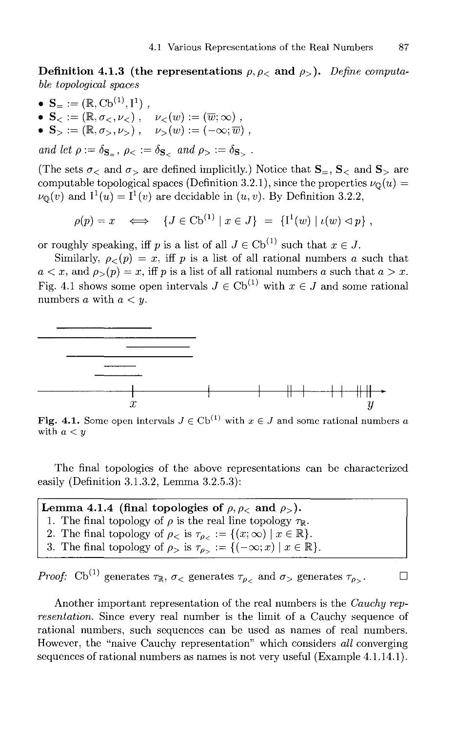
4. Computability on the Real Numbers 85
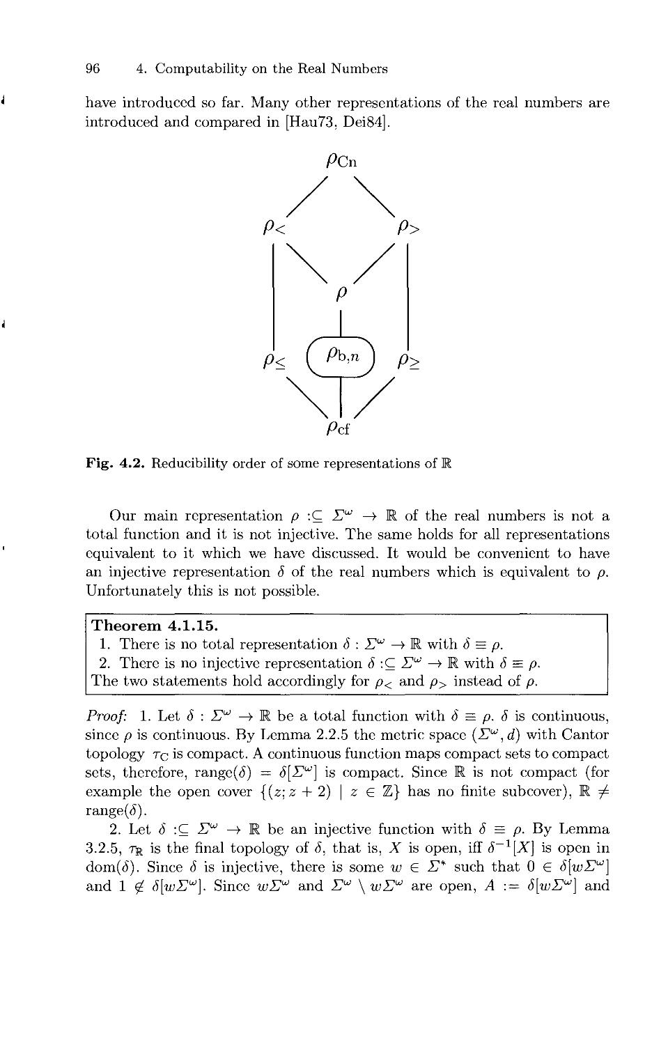
4.1 Various Representations of the Real Numbers 85
4.2 Computable Real Numbers 101
4.3 Computable Real Functions 108
5. Computability on Closed, Open and Compact Sets 123
5.1 Closed Sets and Open Sets 123
5.2 Compact Sets 143

i
X
Contents
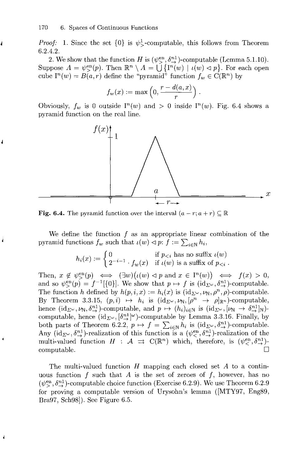
6. Spaces of Continuous Functions 153
6.1 Various representations 153
6.2 Computable Operators on Functions, Sets and Numbers 163
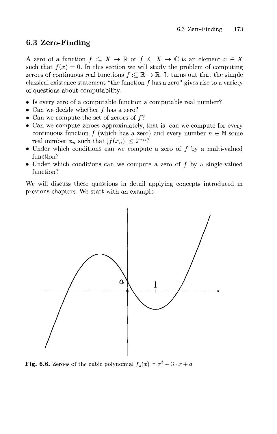
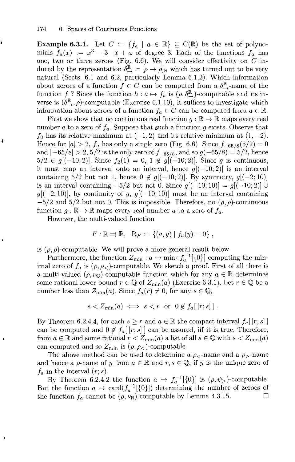
6.3 Zero-Finding 173
6.4 Differentiation and Integration 182
6.5 Analytic Functions 190
7. Computational Complexity 195
7.1 Complexity of Type-2 Machine Computations 195
7.2 Complexity Induced by the Signed Digit Representation 204
7.3 The Complexity of Some Real Functions 218
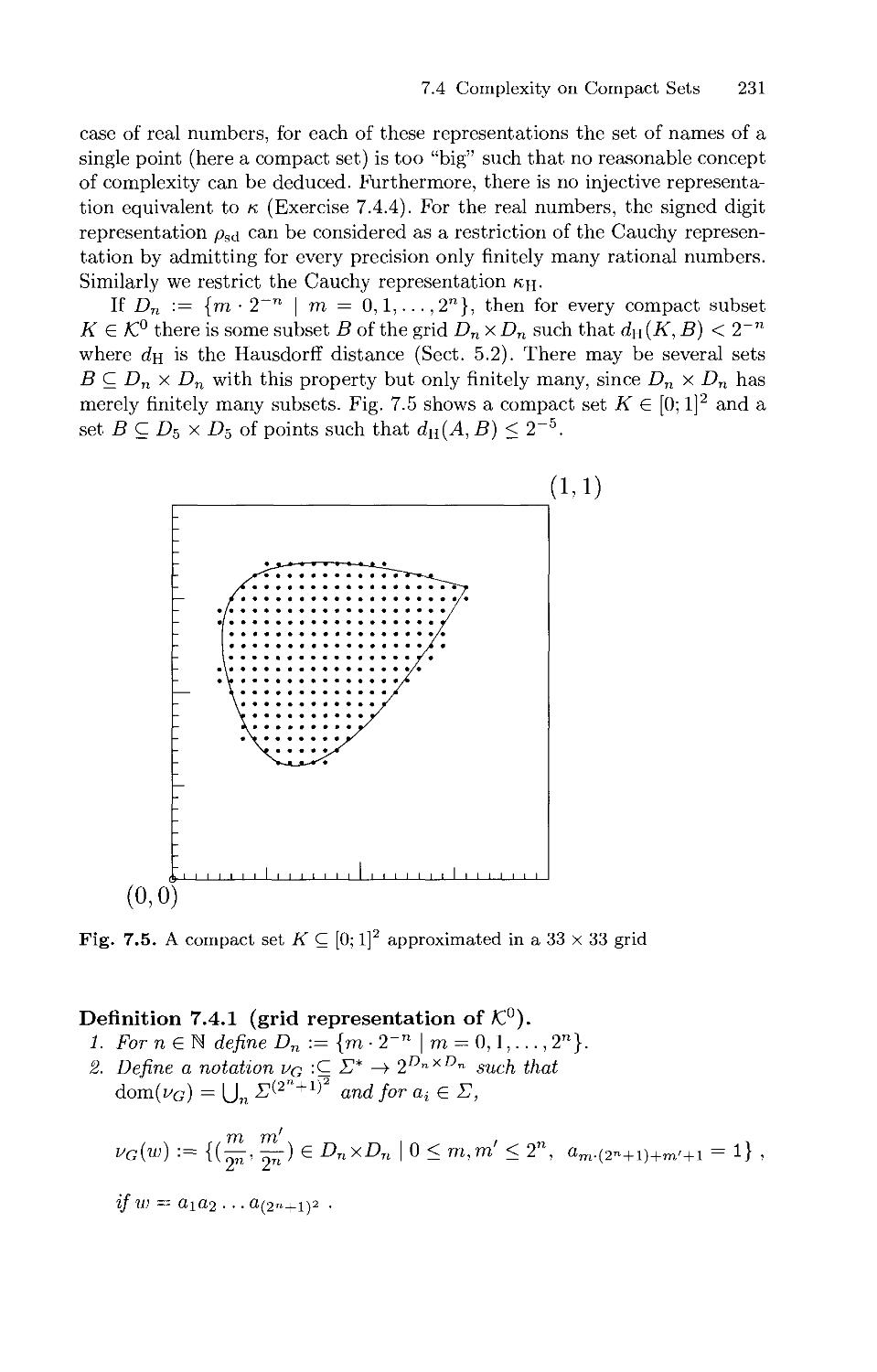
7.4 Complexity on Compact Sets 230
8. Some Extensions 237
8.1 Computable Metric Spaces 237
8.2 Degrees of Discontinuity 244
9. Other Approaches to Computable Analysis 249
9.1 Banach/Mazur Computability 249
9.2 Grzegorczyk's Characterizations 250
9.3 The Pour-El/Richards Approach 252
9.4 Ko's Approach 254
9.5 Domain Theory 256
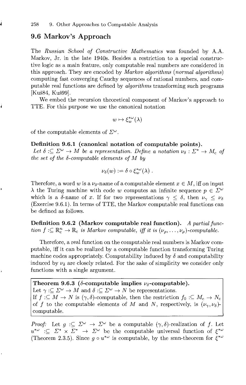
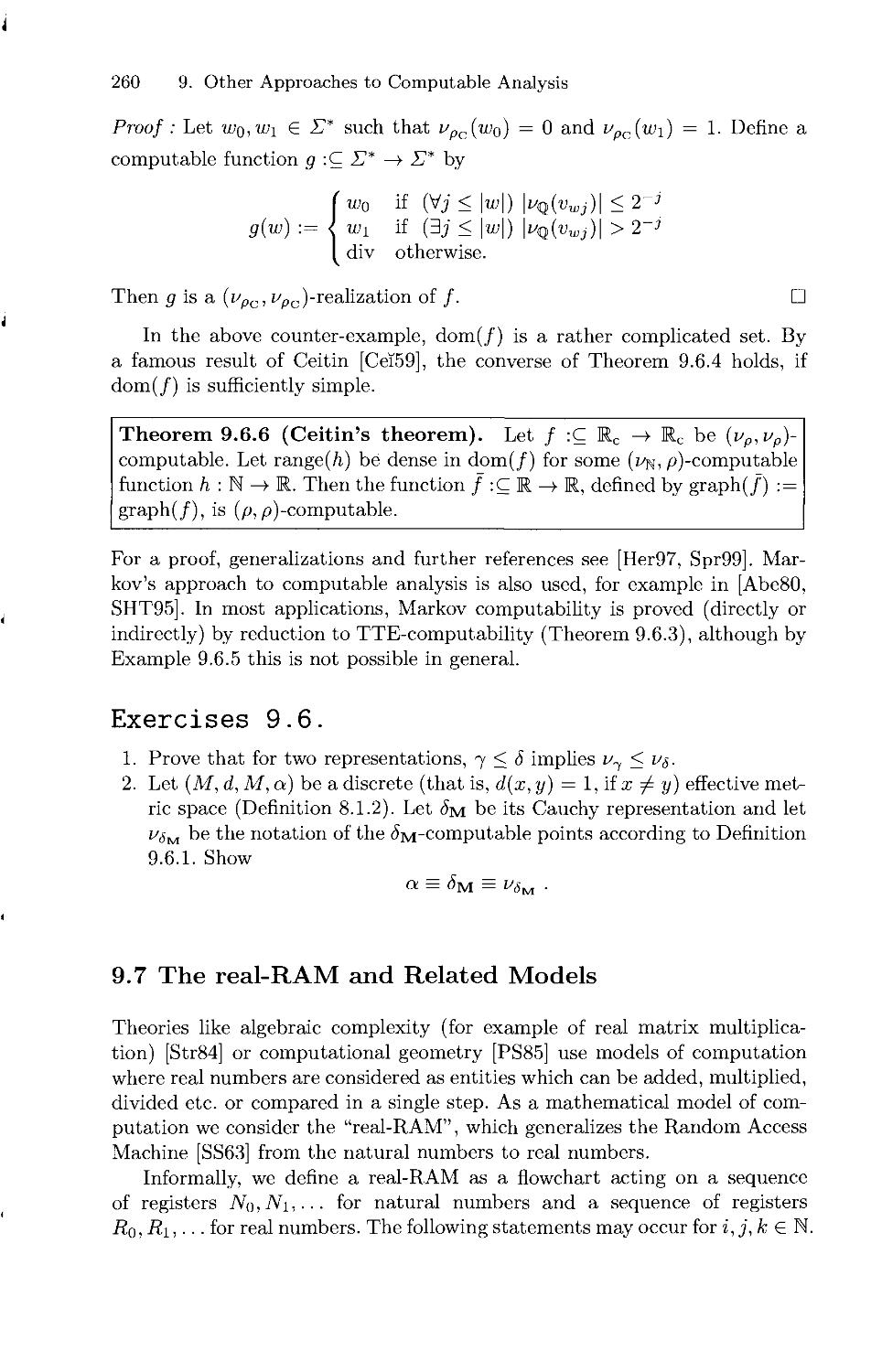
9.6 Markov's Approach 258
9.7 The real-RAM and Related Models 260
9.8 Comparison 266
References 269
Index 277

1. Introduction
1.1 The Aim of Computable Analysis
All over the world numerous computers are used for real number computation.
They evaluate real functions, find zeroes of functions, determine eigenvalues
and integrals and solve differential equations. They perform, or at least are
expected to perform, computations on sets like K (the set of real numbers),
R™, O(R) (the open subsets of real numbers), /C(R") (the compact subsets
of R") or C[0; 1] (the continuous functions from the real unit interval to the
real numbers). The increasing demand for reliable as well as fast software in
scientific computation and engineering requires a sound and broad
foundation. We agree with L. Blum et al. [BCSS96] (also in [BCSS98], however, see
Sect. 9.7):
Our perspective is to formulate the laws of computation. Thus, we
write not from the point of view of the engineer who looks for a good
algorithm which solves his problem at hand, or wishes to design a faster
computer. The perspective is more like that of a physicist, trying to
understand the laws of scientific computation. Idealizations are appropriate,
but such idealizations should carry basic truths.
Scientific computation is the domain of computation which is based
mainly on the equations of physics. For example, from the equations of
fluid mechanics, scientific computation helps to understand better design
for airplanes, or assists in weather prediction. The theory underlying this
side of computation is called numerical analysis.
There is a substantial conflict between theoretical computer science and
numerical analysis. These two subjects with common goals have grown
apart. For example, computer scientists are uneasy with calculus, while
numerical analysis thrives on it. On the other hand numerical analysts see
no use for the Turing machine.
The conflict has its roots in another age-old conflict, that between the
continuous and the discrete. Computer science is oriented by the digital
nature of machines and by its discrete foundations given by Turing machines.
For numerical analysis systems of equations, and differential equations are
central and this discipline depends heavily on the continuous nature of
the real numbers. [...] Algorithms are primarily a means to solve
practical problems. There is not even a formal definition of algorithm in the
subject. [...] Thus, we view numerical analysis as an eclectic subject with
weak foundations; this certainly in no way denies the great achievements
through the centuries.

i
2 1. Introduction
For a deep understanding and for future development of computation
in analysis, a sound theoretical foundation is indispensable. In this book
Computable Analysis is developed as the theory of those functions on the real
numbers and other sets from analysis, which can be computed by machines.
Computable analysis connects the two classical disciplines analysis/numerical
analysis and computability/complexity theory. It merges concepts from both
of them, in particular, the central concepts of limit and approximation on
the one hand and of machine models and discrete computation on the other
hand.
1.2 Why a New Introduction?
While analysis and numerical analysis have a very long tradition
(mathematicians like Gaufi or Lagrange were experts in numerical calculation),
it was not until the 1930s that S. Kleene, A. Church, A. Turing and
others proposed various definitions of effectively calculable functions on the
natural numbers, all of which turned out to be equivalent. Meanwhile for
functions on the natural numbers or on finite words there exists a well-
established and very rich theory of computability and computational
complexity [Rog67, HU79, Wei87, Odi89]. Although a number of authors also
studied computability on the real numbers, computable analysis is still
underdeveloped. In contrast to ordinary computability theory there are several
partially non-equivalent suggestions of how to model effectivity in analysis
and, in particular, computability of real functions. Even today no theory of
computable analysis has been accepted by the majority of mathematicians
or computer scientists.
The first author who introduced computable real numbers was A. Turing
in his famous article "On computable numbers, with an application to the
Entscheidungsproblem" [Tur36, Tur37]. Since that time computable analysis
developed continuously. Among the large number of publications there are
also some books on computable analysis or closely related topics, for
example, R. L. Goodstein[Goo59], D. Klaua [Kla61], S. Mazur [Maz63], O. Aberth
[Abe80], B. Kushner [Kus84], E. Bishop and D. Bridges [BB85], K. Weihrauch
[Wei87], M. Pour-El and J. Richards [PER89], J. Traub, G. Wasilkowski and
H. Wozniakowski [TWW88], K. Ko [Ko91] and L. Blum, F. Cucker, M. Shub,
S. Smale [BCSS98]. While for mathematical branches like linear algebra or
recursion theory there are canonical foundations and well established
introductions, all these books have important concepts in common, but differ in
their contents and technical framework, and each author presents the topic
from his individual point of view. This mirrors the fact that computable
analysis still has no generally accepted foundation.
This book is a new attempt to present a coherent foundation of
computable analysis. It is rooted in a definition of computable real functions via
representations introduced by A. Grzegorczyk [Grz55] and later work on the

1.3 A Sketch of TTE 3
theory of representations by J. Hauck [Hau73, Hau78, Hau80, Hau81, Hau82]
and others. To distinguish it from other approaches, it will be called "Type-2
Theory of Effectivity", TTE, for short.
1.3 A Sketch of TTE
Type-2 Theory of Effectivity extends ordinary (Type-1) computability and
complexity theory. We note already here that TTE admits two levels of
effectivity, continuity and computability as a specialization of continuity. It is
applicable to a variety of problems from analysis and provides a common
framework for combining approximation, computation and computational
complexity. TTE still allows a variety of computability concepts on the real
numbers and other sets. We will select the seemingly most important ones
and point out their distinctive features. Before we start developing TTE in
detail, in this section we explain some essential ideas and concepts informally,
in particular, without using a mathematically precise model of computation.
1.3.1 A Model of Computation
Ordinary computability theory first introduces computable partial word
functions / :C S* —» S* explicitly, for example, by means of Turing machines.
For defining computability on other sets M (rational numbers, finite graphs,
etc.) words are used as "names" or "codes" of elements of M. While a
machine still transfers words to words, the user interprets these words as names
of elements from the set M. Equivalently, one can start also with the
computable number functions /:CN->N and use numbers as names. Since the
sets S* and N are only countable, they are not sufficient as sets of names for
the uncountable set R of real numbers.
However, real numbers can be represented by infinite sequences, for
example by infinite decimal fractions (example: 3.14159 ... is a name of ir). In
TTE, infinite sequences are used as names of real numbers, and machines
which transfer infinite sequences to infinite sequences are used to compute
real functions. Obviously, this method of defining computable functions is not
restricted to the real numbers and can be applied to many other sets. Fig.
1.1 shows a machine transforming infinite sequences to infinite sequences.
• • •, 12) h, lo
MACHINE
• • • , J 21 J\ i Jo
Fig. 1.1. A machine transforming infinite sequences

4 1. Introduction
On input (Iq,I\,I2, • • • ), from time to time the machine reads a new
sequence element 7/j from its input file and from time to time it writes a new
sequence element Jm to its output file, where Ik+i is read after Ik and Jm+\
is written after Jm.
1.3.2 A Naming System for Real Numbers
Since infinite decimal fractions are commonly used for representing real
numbers, it seems to be natural to take them as inputs and outputs for machines.
However, we will prove later that the induced computability concept on the
set K of real numbers is not very interesting. Instead of infinite decimal
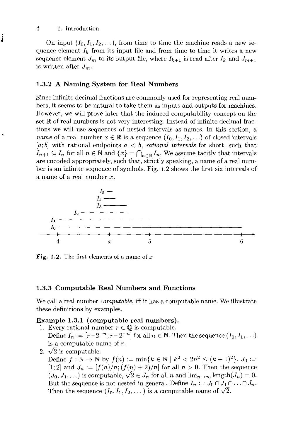
fractions we will use sequences of nested intervals as names. In this section, a
name of a real number x G K is a sequence (Io,Ii,l2, ■ ■ ■) of closed intervals
[a; b] with rational endpoints a < 6, rational intervals for short, such that
Ai+i Q In for all n G N and {x} = f]ne^In- We assume tacitly that intervals
are encoded appropriately, such that, strictly speaking, a name of a real
number is an infinite sequence of symbols. Fig. 1.2 shows the first six intervals of
a name of a real number x.
Is —
h
h
h
h
h
1 1 1 1 >-
4 a; 5 6
Fig. 1.2. The first elements of a name of x
1.3.3 Computable Real Numbers and Functions
We call a real number computable, iff it has a computable name. We illustrate
these definitions by examples.
Example 1.3.1 (computable real numbers).
1. Every rational number r G Q is computable.
Define In := [r-2_n; r+2'n] for all n G N. Then the sequence (J0, h,...)
is a computable name of r.
2. y/2 is computable.
Define / : N -> N by /(n) := min{/c G N | k2 < 2n2 < (k + l)2}, J0 :=
[1;2] and Jn := [f(n)/n; (/(n) + 2)/n] for all n > 0. Then the sequence
(Jo, J\,...) is computable, \/2 G Jn for all n and linin^oo length(J„) = 0.
But the sequence is not nested in general. Define /„ := Jo fl J\ fl... fl Jn.
Then the sequence (Iq,Ii,I2, ■ ■ ■ ) is a computable name of y/2.

1.3 A Sketch of TTE 5
3. log3 5 is computable.
Define f(n) := min{/c G N | 3k < 5" < 3fe+1} and continue as above. □
Example 1.3.2 (Specker sequences). For 4CN
xa '■= 2_j 2~J is computable -£=>■ A is recursive
Assume that A is recursive. Define In := [sn; sn + 2 • 2~n] where sn :=
Y2i<n ieA ^ '• Then (T0, Ti,...) is a computable name of xA.
On the other hand, let (Io,I\,...) be a computable name of xa- If A
is finite or co-finite, then A is recursive. Assume that A is neither finite
nor co-finite. Then m/2™ ^ xa for all m,n G N. For n = 0,1,... (in this
order) decide whether n £ A as follows. Define An := {i G A \ i < n}
and tn := ElSAn 2~' + 2~"- Notice that ° < EieA,i>n 2~l < 2~"- Then
n G A => xa > i„ and n £ A => x^ < i„. Find the smallest k G N with
in ^ -ffe- If max(Jfe) < tn then x^ < tn, hence n (£ A, if tn < min(Ik) then
tn < xa, hence n € A. Therefore, A is recursive.
Let A C N be recursively enumerable but not recursive. Then the real
number xa '■— 'YLi^A 2~% ls no* computable. From recursion theory we know
that A = range(/) for some computable injective function / : N —» N. We
obtain xA = I]jeN2~/(8>. Then (x0,xi,...) with xn = J2i<n 2_/(i) is an
increasing and bounded computable sequence of rational numbers. Its limit,
however, is the non-com put able real number Xa- Sometimes such a sequence
is called a Specker sequence [Spe49]. □
We call a real function /:Cl4l computable, iff some machine maps any
name of any x G dom(/) to a name of f(x). For real functions /:Cl"4l
we consider machines reading n names in parallel. Notice that the machine
must behave correctly only for every name of every x G dom(/), for other
input sequences it may behave arbitrarily.
Example 1.3.3 (computable real functions).
1. Real multiplication (x, y) >->• x ■ y is computable.
For closed intervals /, J with rational endpoints define the interval / • J
by / • J := {x ■ y | x G /, y G J}. There is a machine with two input files
which maps the inputs (Tqi Ii, ■ ■ ■) and (J0, J\,...) to (To ' Jo, I\ ■ Ji, ■ ■ •)•
If (To, h, ■ ■ ■) is a name of x and (Jo, Ji, ■ ■.) is a name of y then
(To • Jo, Ti • Ji,...) is a name of x • y. Therefore, multiplication is
computable.
2. The square root y/~ :C R —> R is computable.
Since for example v/[2; 3] is not a rational interval, we have to modify the
above method. We map each input interval T to a rational interval which
is slightly longer than yfl. For any rational numbers a, b with 0 < a < b
there are rational numbers r, s > 0 such that
a - (b - a) < r2 < a < b < s2 < b + (b - a) .

6 1. Introduction
Therefore, there is a computable function / which for each rational
interval 7" with no negative elements determines (for example by
exhaustive search) a rational interval K = /(J) such that I C K2 and
length^2) < 3 • length(J). For any rational interval [a;b] with 0 < b
let g[a;b] := [max(0,a); b). If (I0,Ii,...) is a name of x > 0 then the
sequence (/ o g(Io), f o g(I\),...) of rational intervals converges to \fx.
This sequence is not necessarily nested. There is a machine M which
transforms any name (Jo, I\, ■ ■.) of a non-negative real number to the
sequence (J0, Ji,...), where J„ := / o g(I0) n / o g^) n ... n / o g(In).
Then M computes the square root. □
We will prove later that elementary real functions like exp, sin, log and
arcsin are computable, that the computable real functions map computable
numbers to computable numbers and that the computable real functions are
closed under composition. Our definition is essentially the definition of
computable real function introduced by A. Grzegorczyk in [Grz55] and studied in
more detail in [Grz57], where he proves, in particular, that computable real
functions are continuous.
Theorem 1.3.4. Every computable real function is continuous.
Proof: We sketch a proof for the case / : R —» R. Let M be a machine
computing / and let x G dom(/) = R. It suffices to show that for every
open set V C R with f(x) G V, there is some open set (/Cl with x G U
and f[U] C V. Therefore, let V be an open set with f(x) G V. The real
number x has a name ([ao; bo], [a,u b\],...) such that a^ < a,+i < bi+i < fej.
Let (Jo, J\,...) be the name of f(x) which M produces on this input. Then
Jn C V for some number n. For producing the initial part (Jo, J\,..., J„)
of the output, the machine M needs k steps for some k. In k steps the
machine M can read at most the first k intervals from the input. We choose
U := (a/.; ft/.). Obviously, we have x G U. Assume y G U. Then y has a name
of the form ({a0;b0], [ai;^],..., [a*;; bk],Lk+i,Lk+2, ■ ■ ■)■ On this input, the
machine M writes also (Jo, Ji,..., Jn) within the first k steps which is the
initial part of a name of f(y). We obtain f(y) G J„. This shows f[U] C J„ C V.
Therefore, the function / is continuous at x. □
In the above proof we have used the essential observation that any finite
portion (Jo, Ji,..., Jn) of the output of a computation is determined already
by a finite portion (Jo, I\,..., Ik) of its input. However, we did not use that
the transformation from inputs to outputs is computable. As a consequence of
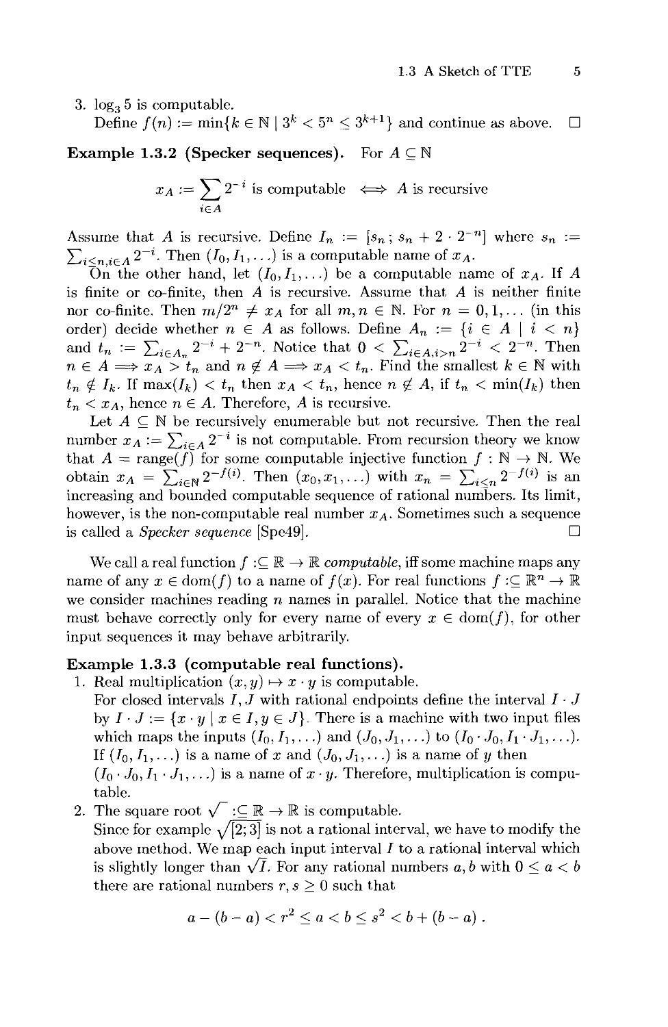
the continuity theorem, simple real functions like the step function s(x) := (0
if x < 0, 1 otherwise) and the Gaufi staircase g(x) := [xj (the integer part
of x) are not computable (Fig 1.3). Obviously, these functions are easily
definable in our mathematical language, but "easily definable" does not mean
"computable" in general. As far as we know neither the step function or the
Gaufi staircase nor any other non-continuous real function can be computed
by physical devices.

1.3 A Sketch of TTE 7
Fig. 1.3. Two non-computable real functions
Some people do not accept the model of computation presented here,
since they believe that the above simple functions are or should be called
computable. Although the Gaufi staircase is not computable according to our
present definition, we will see that the framework of TTE admits to define
other natural computability concepts such that it is a computable object
(Exercise 4.3.2).
1.3.4 Subsets of Real Numbers
A subset A C N is decidable or recursive, iff its characteristic function cf a ■
N —» N is computable. Assume for the moment that we call a subset ACR
recursive, iff its characteristic function cf^ : R —» R is computable. Then
cf a •' K —» R is not continuous and hence not computable by the continuity
theorem, unless A = 0 or A = R. Therefore, this definition is useless.
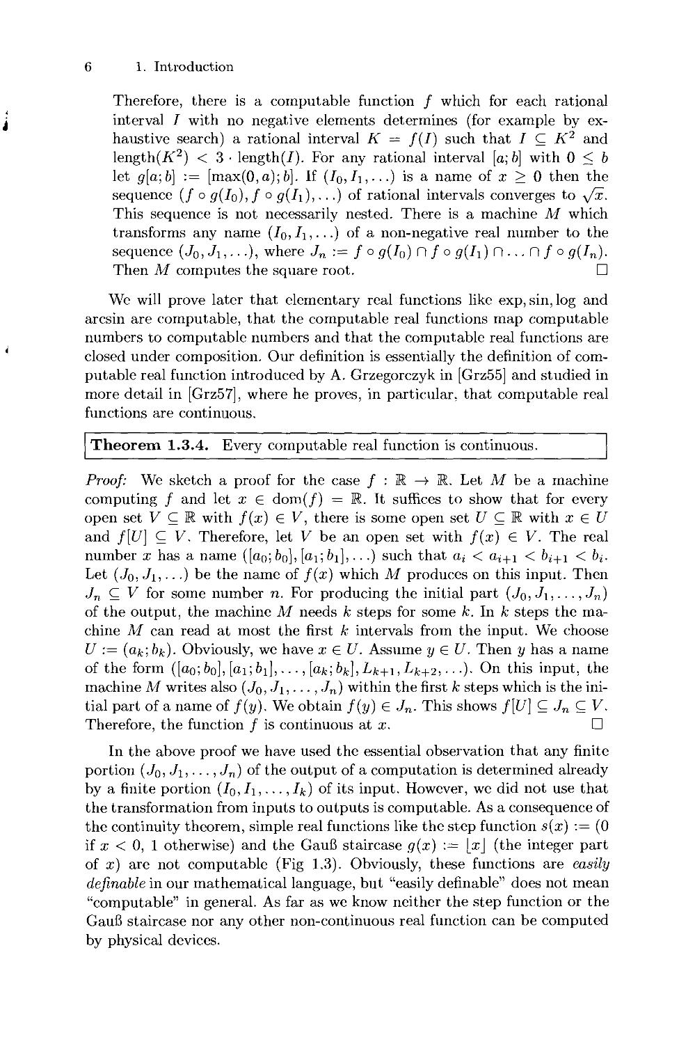
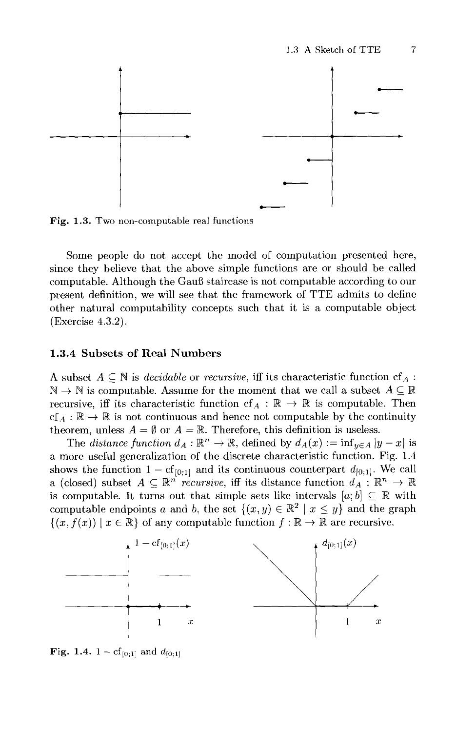
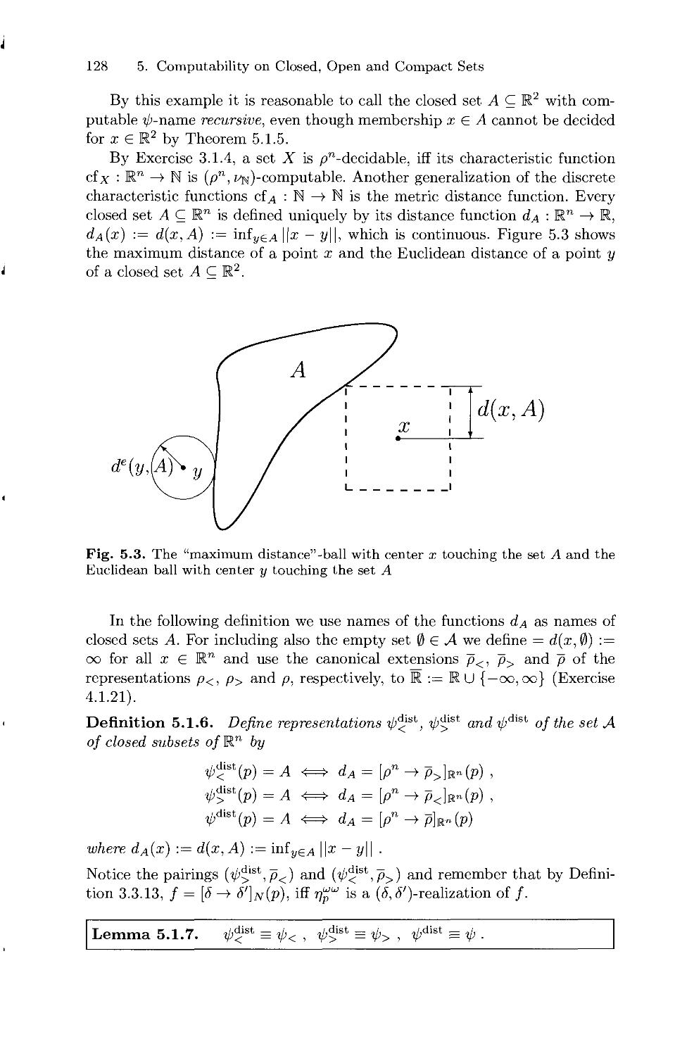
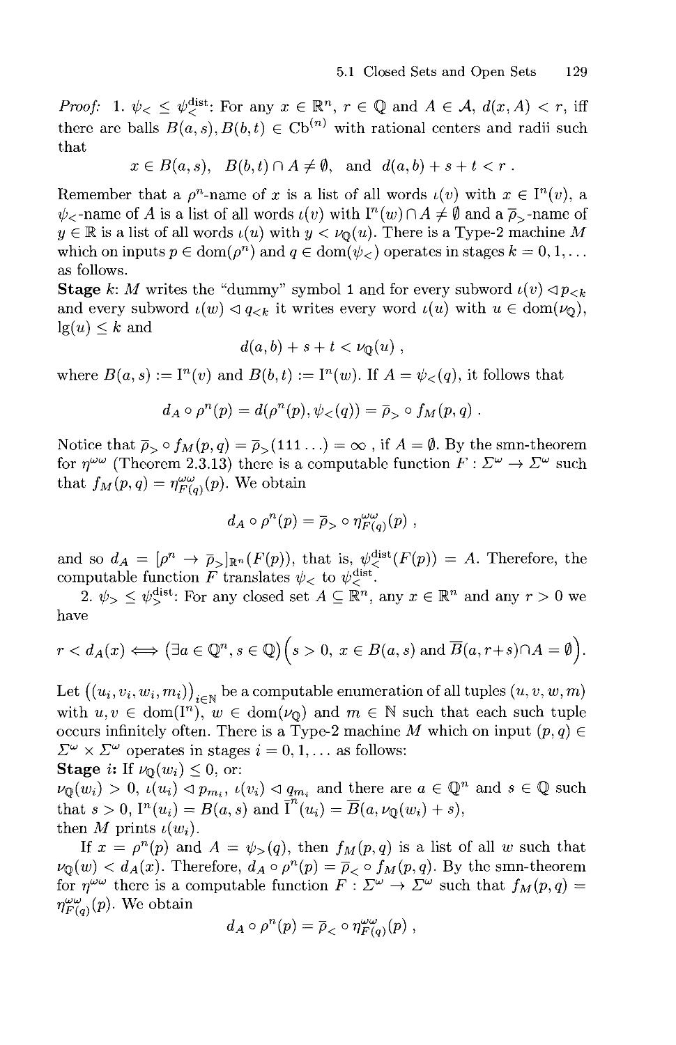
The distance function dA ■' R" —» R, defined by cIa(x) := miyeA \y — x\ is
a more useful generalization of the discrete characteristic function. Fig. 1.4
shows the function 1 — cf[o;i] and its continuous counterpart d[o,i]- We call
a (closed) subset A C R™ recursive, iff its distance function d^ : Rn —» R
is computable. It turns out that simple sets like intervals [a; b] C R with
computable endpoints a and b, the set {(x,y) € R2 | x < y} and the graph
{(x, f(x)) | x G R} of any computable function / : R —» R are recursive.
.
1 -ci[0;i](2:;
1 x
Fig. 1.4. 1 - cf[0;i] and d[0;1]

8 1. Introduction
For defining computability on subsets of R, we introduce naming systems
of sets of subsets. Since the set 2R of all subsets of R is too large, we consider
only subsets of 2R. Here we merely introduce a naming system for the set
i C(R) of the open subsets of real numbers. Later we will study various naming
systems of the open, the closed and the compact subsets of Rn. As is well
known, a subset U C R is open, iff it is the union of a set of open intervals
with rational endpoints.
We define: a name of an open subset U C R is a sequence (Iq, I\,...) of
open intervals with rational boundaries such that U = Iq U I\ U ... . In the
general case U C R", each 7/. is a product of n open intervals with rational
endpoints. We call an open set recursively enumerable, iff it has a computable
name.
Examples of recursively enumerable open sets are the open intervals (a; b)
with computable endpoints a and b, the set {(x, y) C R2 | x < y} and every
interval (0;xa) where xa is from Example 1.3.2 with r.e. (recursively enu-
< merable) but non-recursive A C N. As for real functions, we call a function
on the set of open sets computable, iff some machine maps names of
arguments to names of the results. The functions intersection and union on open
sets are computable. For example, let M be a machine with two input files
which transforms any two names (Jo, I\,...) and (Jo, J\,...) of open sets to
a sequence (Ko, K\,...) which is a list of all Im fl Jn with m, n G N. Then M
computes the intersection on C(R).
We define computability for functions of mixed type accordingly. For
example, the function / : R —» C(R) with f(x) := R \ {x} is computable. A
machine computing / maps any name of x G R to a name of R \ {x}. Since a
computable function maps computable names to computable names, X fl Y
and X U Y are recursively enumerable open sets, if X and Y are recursively
enumerable open sets, and R \ {x} is a recursively enumerable open set, if x
is a computable real number.
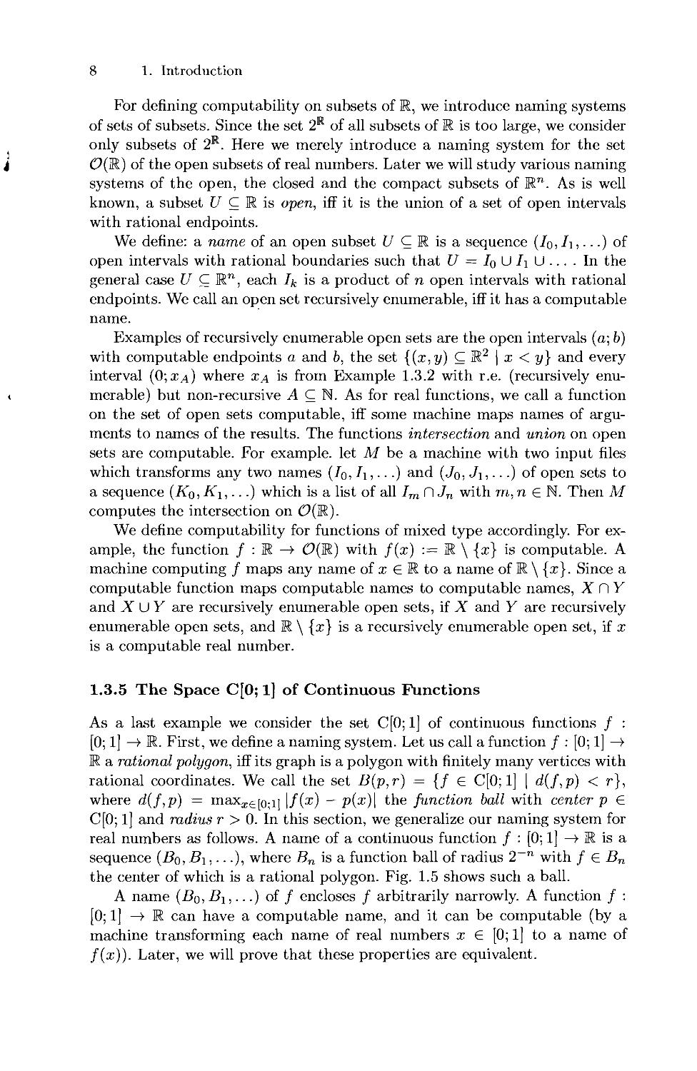
1.3.5 The Space C[0; 1] of Continuous Functions
As a last example we consider the set C[0; 1] of continuous functions / :
[0; 1] —» R. First, we define a naming system. Let us call a function / : [0; 1] —»
R a rational polygon, iff its graph is a polygon with finitely many vertices with
rational coordinates. We call the set B(p,r) = {/ G C[0; 1] | d(f,p) < r},
where d(f,p) = maxx€[0.1] |/(£) — p(%)\ the function ball with center p G
C[0; 1] and radius r > 0. In this section, we generalize our naming system for
real numbers as follows. A name of a continuous function / : [0; 1] —» R is a
sequence (Bo, B\,...), where Bn is a function ball of radius 2~n with / G Bn
the center of which is a rational polygon. Fig. 1.5 shows such a ball.
A name (Bo, B\,...) of / encloses / arbitrarily narrowly. A function / :
[0; 1] —» R can have a computable name, and it can be computable (by a
machine transforming each name of real numbers x G [0; 1] to a name of
f(x)). Later, we will prove that these properties are equivalent.

1.3 A Sketch of TTE 9
Fig. 1.5. A function / in a function ball with radius 2 n with a rational polygon
as center and radius 2~n
Our naming systems of R and C[0; 1] make the evaluation function
Apply : C[0; 1] x [0; 1] -» R, defined by Apply(/,x) := f(x), computable,
that is, there is a machine which transforms any name of any / and any name
of any x to a name of f(x). There are many other naming systems of C[0; 1],
for which the evaluation function becomes computable, however, among all
of these our naming system is the "weakest" one (we will explain this later).
Thus, our naming system for C[0; 1] is tailor-made for the evaluation function.
Integration f *-> f0 f(x)dx on C[0; 1] is an important computable
operator, while differentiation f *-> f for continuously differentiable / G C[0; 1]
is not computable. By the classical intermediate value theorem every
continuous function / : [0; 1] —» R with /(0) < 0 < /(l) has a zero, that is, a
point x with f(x) = 0. Unfortunately, there is no computable operator for
zero-finding working correctly for all continuous functions / : [0; 1] —> R with
/(0) < 0 < /(l). However, a restricted problem has a computable solution:
the operator Z : f i->- (the zero of /) for continuous increasing functions with
/(0) < 0 < /(l) is computable. Later, we will discuss in detail the problem
of zero-finding under various assumptions.
1.3.6 Computational Complexity of Real Functions
Ordinary discrete complexity theory studies resources like time or storage
used by machines for computing functions [HU79]. If M is a Turing machine
computing a word function / : E* —» S*, then complexity theory considers

10 1. Introduction
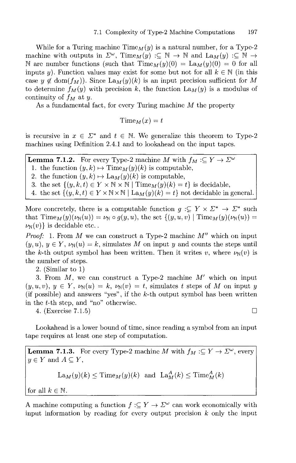
TimeM(x), the number of steps which M makes on input x before halting.
This concept cannot be transferred to machines which map infinite sequences
to infinite sequences, since these machines do not halt. However, we can
consider for each input sequence s = (Iq,Ii,...) and for each number n
the number Timers) (n) of steps which M makes before it prints the first
i interval J/, of its output (Jo, J\,...) of length < 2~™. For a machine M
computing a real function / : 1 -> I we would like to have a complexity
TimeM(x)(n), which depends on the real number x but not on a name of x.
For this pupose we define
Timem(#)(«) := ma,x{TimeM(s)(n) \ s is a name of x} .
Since in our naming system we admit arbitrarily redundant names of the real
numbers, this maximum does not exist.
However, for the signed digit representation of the real numbers, we
obtain very natural complexity results. In the signed digit representation, a
name of a real number is an infinite binary fraction where the digit 1 := — 1
, can be used in addition to the digits 0 and 1, that is, an... ao«a_ia_2 - - •
with afc 6 {0,1,1} is a name of x := Y^~k^n ak- These names encode strongly
normalized sequences of nested intervals and induce the same computabil-
ity on R as our standard names. The induced computational complexity of
real functions is sometimes called "bit complexity". Bit complexity has been
studied by several authors, in particular, by Ko [Ko91, Ko98], who applied
concepts from discrete complexity theory to prove upper and lower bounds
for the complexity of basic numerical operations. It turns out that Turing
machines operating on signed digit representations of real numbers can compute
addition in time 0(n) and multiplication, sin, exp and log in time 0(n2).
1.4 Prerequisites and Notation
We assume that the reader is familiar with the basic concepts of analysis, that
is, the theory of real numbers and functions, and of ordinary computability
theory at undergraduate level in computer science. For details the reader
should consult standard textbooks, e.g. parts of [Die60, HU79].
By N, Z, Q and R we denote the set {0,1,...} of natural numbers, of
integer numbers, of rational numbers and of real numbers, respectively. For a
set A the power set of A, that is, the set of all subsets of ^4, is denoted by 2A
and the set of all finite subsets of A is denoted by E(>1). If X = Ax x ... x An
is a Cartesian product of sets, then for n = 0, X = {()} is the set the only
element of which is the empty tuple "()" .
If < is a binary relation on A x B, x < y will abbreviate "x < y and
y£x".
We will consider multi-valued partial functions and as special cases
partial functions and total functions. A correspondence or multi-valued partial

1.4 Prerequisites and Notation 11
function from A to B is a triple / = (A B, Rf) such that Rf C Ax B, where
A is called the source, B the target and R/ the graph of /. For X C A we
define the image of X under / by
f[X) := {b £ B | (3a G X)(a, b) G R/} .
We define the inverse, the domain and the range of / by
.T1 := (B, AR/1) such that R"1 := {{b,a) \ (a,b) £ Rf} ,
range(/) := f[A\ and
domtf) := f-'lB] ,
respectively. The multi-valued partial function / is completely defined by
the family of sets /[{a}] (a £ A).
Usually we will denote a correspondence / from A to B by f :C A ^ B.
A partial function f :C A —» B from ^4 to B is a multi-valued function
/ :C A =? B such that the set /[{a}] contains only one element for each
a G dom(/). A total function f : A —» B from ^4 to B is a partial function
/ :C A -» B such that dom(/) = A The set of all (total) functions f : A ^ B
is denoted by BA. For a partial function f :C A —> B, f(a) denotes the
single element from /[{a}], if a G dom(/), and we will write f(a) = div, if
a (£ dom(/). Usually we will call / a function, if / is a partial function or a
total function.
For multi-valued functions /, :C A ^ Bi (i—1... ,k) define (/i,..., ft) :C
A^B1x...xBkby(f1,..., fk)[{a}} := A [{a}] x ... x /fc[{a}]. For
multivalued functions / :C A =? B and g :C B =t C define the composition
g o f :C A ^ C by a £ dom(gof), iff a £ dom(/) and f[{a}] C dom(B), and
9 ° /[{«}] == 5-[/[{a}]] for all a £ dom(<? o /).
For a multi-valued function / :C A —» 5, X C yl and Y C B, we define
the restrictions in the source, the target, the domain and the range as follows:
source: f\x -Q X -> B, f\x ■= (X,B, Rf C\X x B)
domain: f\x :Q A ^ B, f\x := (A,B, R/ C\X x B)
target: f\Y :C A ^ Y, f\Y := (A,Y, Rf C\A x Y)
range: f]Y :C A ^ B, f\Y := (A, B, Rf C\A x Y) .
For combinations of restrictions we use the symbols |, ], J and ], for example
f\x- Usually, idx : X —» X denotes the identity function on X.
For any set S, S" denotes the set of all words over S of length n, E-n
the set S° U ... U Sn and S* the set of all finite words over S. We denote the
length of a word w by \w\ and the empty word which has length 0 by A. By
iy we denote the set {p \ p : N —» Z1} = {a$a\a2 ... | Oj € X1} of all infinite
sequences over Z1. Occasionally finite or infinite sequences of symbols will be
called strings.
We extend concatenation from S* x S* to S* x E". Consider u, v, w £ S*
and p £ Su. If x = uvw £ S* and q = uvp £ Su, then u is a prefix of x

12 1. Introduction
and q (abbreviated byuCi and u C q, respectively), v is a subword of x
and g (abbreviated by v <1 x and w <1 g, respectively) and w is a suffix of x.
A set ^4 C S* is called prefix-free, iff x % y for all x,y £ A with i^j. We
( define u™ := uu...u (n times) as usual and uu := uuu... G Eu. By p<n
i we denote the prefix p(0).. .p(n — 1) of length n of p and by p<„ the prefix
p(0).. -p(n). We extend concatenation straightforwardly to sets of finite or
infinite sequences: AB := {up | u G A,p G £?} for A C X' and B C E*
or B C Eu. In particular, ,4" := A... A (n factors). (If A C 17*, it will
be clear from the context, whether An denotes the Cartesian product or the
concatenation product.) The prefix relation can be expressed by means of
product: u C v <==>■ v G uS* (for u,v G S*) and u Q q <==>■ q G uE" (for
u G r* and p G rw).
Later Z1 will be a non-empty finite set, an alphabet, the symbols of which
we will denote in typewriter style (abc...012...#.$ etc.). In emphasizing that
an expression denotes a word, we occasionally set it into quotes. For example:
if u and v denote words and if 0 and ; are elements of E, then "uO;w" denotes
< the word which begins with u, has 0 and ; as the next symbols and ends with
the word v.
Ordinary "Type-1" recursion theory considers the computable number
functions /:CNfc->N and the computable word functions g :C (E*)k —» E*.
Computability can be transferred to other sets M by means of numberings. A
numbering of a set M is a surjective (that is, "onto") function v :C N —» M.
For a given finite alphabet E = {a\,... ,an} define the bijective standard
numbering vs : N —> E* of E* as follows:
v^}{\) :=0; i/~1(aik...aio) := ik ■ nk + ... + i0 ■ n° .
Then / :C N -> N is computable, iff vE o f o i/^,1 :C 27* -> E* is
computable (correspondingly for / :C Nm —> N). Occasionally, we will extend the
definition of computable functions to functions of mixed type (N and 17*) by
calling vs and u^} computable and closing under composition. This way we
can, for example, define the r.e. subsets ^4 C 17* x N x 17* and the computable
functions / :C N x 17* -> N.
We will need the bijective Cantor pairing function { , ) : N2 —» N,
defined by {x, y) := y + (x + y)(x + y + l)/2, which is computable, as well as
the projections { )i and { )% of its inverse. For n > 2 arguments, we define
inductively
\X\, . . . ,Xn) '.= \\X\: . . ■ ,Xn—i) ,Xn)
as usual.

2. Computability on the Cantor Space
Classically, computability is introduced explicitly for functions / :C (S*)n —»
S* on the set S* of finite words over an arbitrary finite alphabet E, for
example by means of Turing machines. For computing functions on other sets
M such as natural numbers, rational numbers or finite graphs, words are used
as "code words" or "names" of elements of M. Under this view a machine
transforms words to words without "understanding" the meaning given to
them by the user. Equivalently, one can start with computable functions on
the natural numbers instead of words and use numbers as "names". Since
the set S* of words over a finite alphabet is only countable, this method
cannot be applied for introducing computability on uncountable sets M like
the set R of real numbers, the set of open subsets of R or the set CfO; 1] of
real continuous functions on the interval [0; 1].
We will extend the above concepts by using infinite sequences of symbols
as names and by defining computability for functions which transform such
infinite sequences. The set Su of infinite sequences of symbols from a finite
alphabet S (provided S has at least two elements) has the same cardinality
as the set of real numbers ("continuum cardinality"), therefore, it can serve
as a set of names for every set with at most continuum cardinality. An
example is the traditional representation of real numbers by infinite decimal
fractions (for example the number ix by the sequence 3.14159 ...). Also our
names of real numbers from Sect. 1.3 are infinite sequences of symbols, if
rational intervals are encoded by words. As a first step, we introduce and
study computability on finite and infinite sequences of symbols.
In Sect. 2.1 we define the computable functions on finite and infinite
sequences of symbols, introduce tupling functions and, among others, prove
closure theorems for composition and primitive recursion. In Sect. 2.2 we
introduce the Cantor topology on Su and show that computable functions
are continuous. Sect. 2.3 is devoted to naming systems of sets of computable
or continuous functions. The reader may skip details in a first reading. Later
we will apply essentially the smn- and the utm-theorems (Theorems 2.3.5
and 2.3.13). Finally, in Sect. 2.4 we introduce the recursively enumerable,
the decidable and the recursive open subsets. We mention already that two
differing concepts "decidable" and "recursive open" must be distinguished on

14 2. Computability on the Cantor Space
Convention 2.0.1. In this chapter we assume that E is a fixed finite
alphabet containing the symbols 0 and 1. In some examples we will assume
that E is sufficiently large.
2.1 Type-2 Machines and Computable String Functions
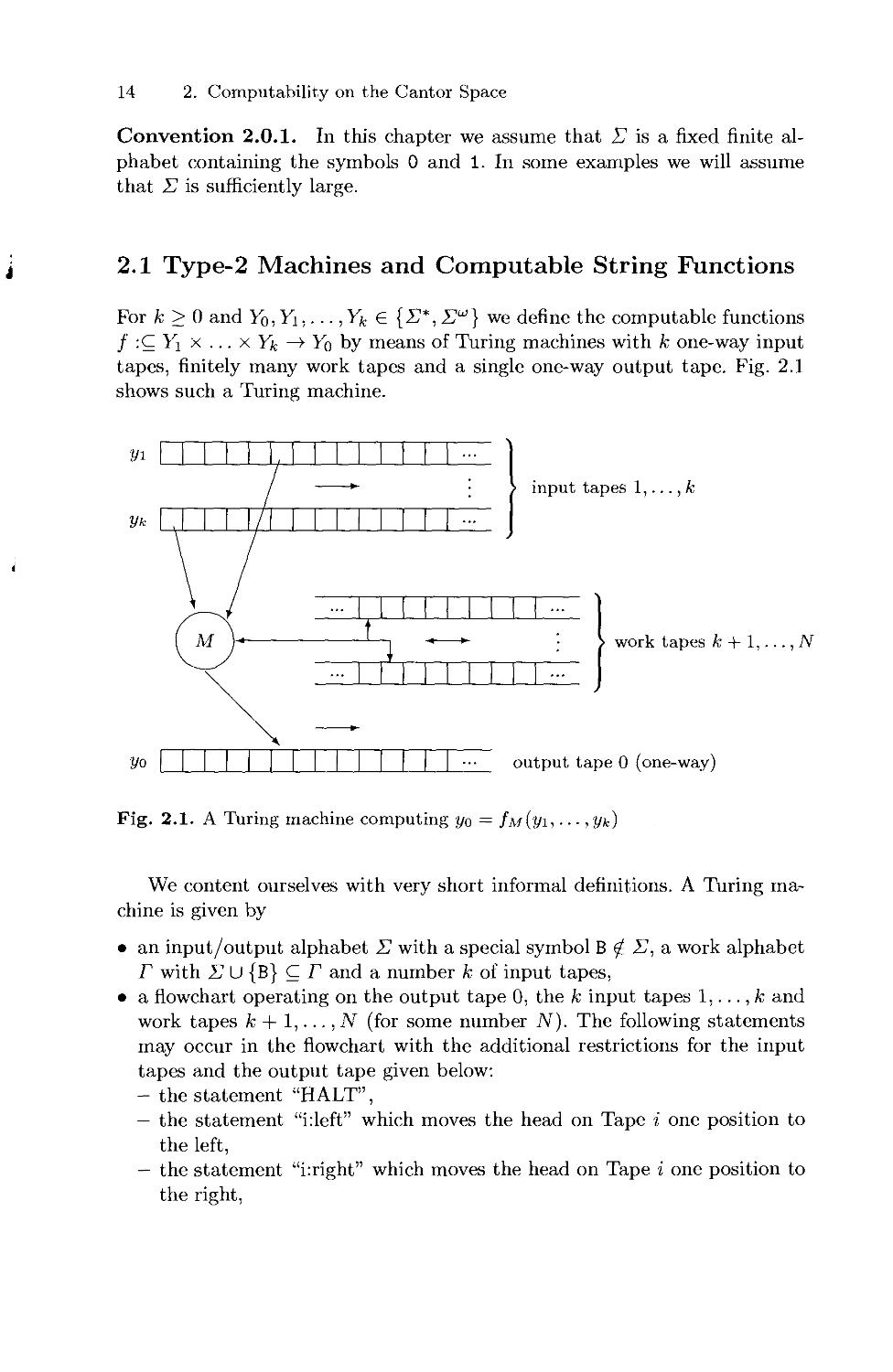
For k > 0 and Yo, Y\,..., Yk £ {E*, E^} we define the computable functions
/ :C Y: x ... x Yk —» Yo by means of Turing machines with k one-way input
tapes, finitely many work tapes and a single one-way output tape. Fig. 2.1
shows such a Turing machine.
yi \ | | | | |, | | | | | | | | -
Vk 1 ,1 1 1 1 /1 1 1 1 1 II 1 1 •••
2/o f
\
| |
\,
)
| |
- 1 II 1 1 II
t , ,
1
1 1 1 1 II 1 —
> input
1 •-
output t
work tapes k + 1,
,N
Fig. 2.1. A Turing machine computing y0 = fM(yi, ■ ■ ■,yk)
We content ourselves with very short informal definitions. A Turing
machine is given by
• an input/output alphabet E with a special symbol B ^ E, a work alphabet
r with E U {B} C r and a number k of input tapes,
• a flowchart operating on the output tape 0, the k input tapes 1,..., k and
work tapes k + 1,..., N (for some number N). The following statements
may occur in the flowchart with the additional restrictions for the input
tapes and the output tape given below:
— the statement "HALT",
— the statement "i:left" which moves the head on Tape i one position to
the left,
— the statement "irright" which moves the head on Tape i one position to
the right,

2.1 Type-2 Machines and Computable String Functions 15
— for each a G r the statement "i:write(a)" which writes the symbol a on
the tape cell scanned by the head of Tape i,
— for each a G r the branching statement "i:if(a)" which tests whether a
is the symbol scanned by the head of Tape i.
The restrictions are:
— "i:left" and "r.write(a)" are not allowed on an input tape i,
— on the output tape only sequences "0:write(a) ; Orright" with a € E are
allowed.
The restrictions guarantee that the input tapes are one-way read-only
tapes and that on the output tape only symbols from E can be written
and no written symbol can be erased (one-way output). We assume that the
reader is familiar with the concept of step by step computation for Turing
machines. Mathematically exact definitions can be found in introductory text
books, for example [HU79, Wei87].
Definition 2.1.1 (Type-2 machine). A Type-2 machine M is a Turing
machine with k input tapes together with a type specification (Y\,..., Yk, Yo)
with Yi G {E*, E^}, giving the type for each input tape and the output tape.
We define the string function /m :C Yj x ... x Yk —» Y0 computed by a
Type-2 machine M.
Definition 2.1.2 (computable string function). The initial tape
configuration for input (j/i,..., yk) G Yj x ... x Y/. is as follows: for each input tape
i the (finite or infinite) sequence yi G Yj is placed on the tape immediately to
the right of the head, all other tape cells contain the symbol B; on all the other
tapes all tape cells contain the symbol B. For all yo G Yo, y\ G Yi,..., yu G Y*.
we define:
1. Case Y0 = E*:
/m(2/i , • • •, yk) ■= Vo € E*, iff M halts on input (j/i,..., yk) with y0 on
the output tape.
2. Case Y0 = E":
/m(j/i , • • •, Vk) ■= Vo e E", iff M computes forever on input {yY,..., yk)
and writes yo on the output tape.
We call a string function f :C Yx x ... x Yk —> Yo computable, iff it is
computed by a Type-2 machine M.
Notice that /m(j/1j • • • )2/fc) is undefined, if the machine computes forever
but writes only finitely many symbols on the output tape. We do not use the
"partial" results of such computations in our definition of semantics. Since
Type-2 machines are essentially Turing machines, they are as realistic and
powerful as Turing machines. Clearly, infinite inputs or outputs do not exist
and infinite computations cannot be finished in reality. But finite
computations on finite initial parts of inputs producing finite initial parts of the
outputs can be realized on physical devices as long as enough time and
memory are available. All doubts about realizability of Type-2 machines have been
removed by the recently built machine shown in Fig. 2.2.

16 2. Computability on the Cantor Space
Trwa
'■-'*--x P & ~Wl -mm.
II 2
Fig. 2.2. A realization of a Type-2 machine (material: marzipan, year of
construction: 1996)
Of course, Type-2 machines can be simulated by digital computers.
Therefore, infinite computations of Type-2 machines can be approximated by finite
physical computations with arbitrary precision. The restriction to one-way
output guarantees that any partial output of a finite initial part of a
computation cannot be erased in the future and, therefore, is final. For this reason,
models of computation with two-way output would not be very useful.
Since it is very cumbersome to specify Turing machines concretely, we will,
as usual, only outline algorithms in such a way that constructing concrete
Turing machines remains (often rather tedious) routine. If only computability
is considered, the reader's favourite algorithmic language may be used instead
of Turing machines for formulating algorithms which read from finitely many
input files and write on a one-way output file, as long as these algorithms
can be translated (at least in principle) to Turing machines. Only in Chap.
7, where we study computational complexity, will we use the special Turing
machine model.

2.1 Type-2 Machines and Computable String Functions 17
Definition 2.1.2 includes the standard definition of computable word
functions (choose Yo =Yi = ... Yn = E*). We define computable elements of E*
and E" straightforwardly.
Definition 2.1.3 (computable elements).
1. Every word w G E* is computable.
2. A sequence p G E" is computable, iff the constant function
f '■ {()} ~~*■ E" > /() = P> is computable.
3. A tuple (j/1,1/2) • • • ,Vk) with yt € E* or yi € E" is computable, iff each
component yi is computable.
Obviously, a sequence p G Eu is computable, iff p = /(A) for some
computable function / : E* —► Eu. We illustrate the definitions by several examples.
Example 2.1.4.
1. A constant function / : Y\ x ... x Yk —► Yq is computable, iff its value
c G Yq is computable.
2. Every projection pri : Y\ x ... x Y^ —► Yi is computable.
There is a Type-2 machine which copies the input tape i to the output
tape.
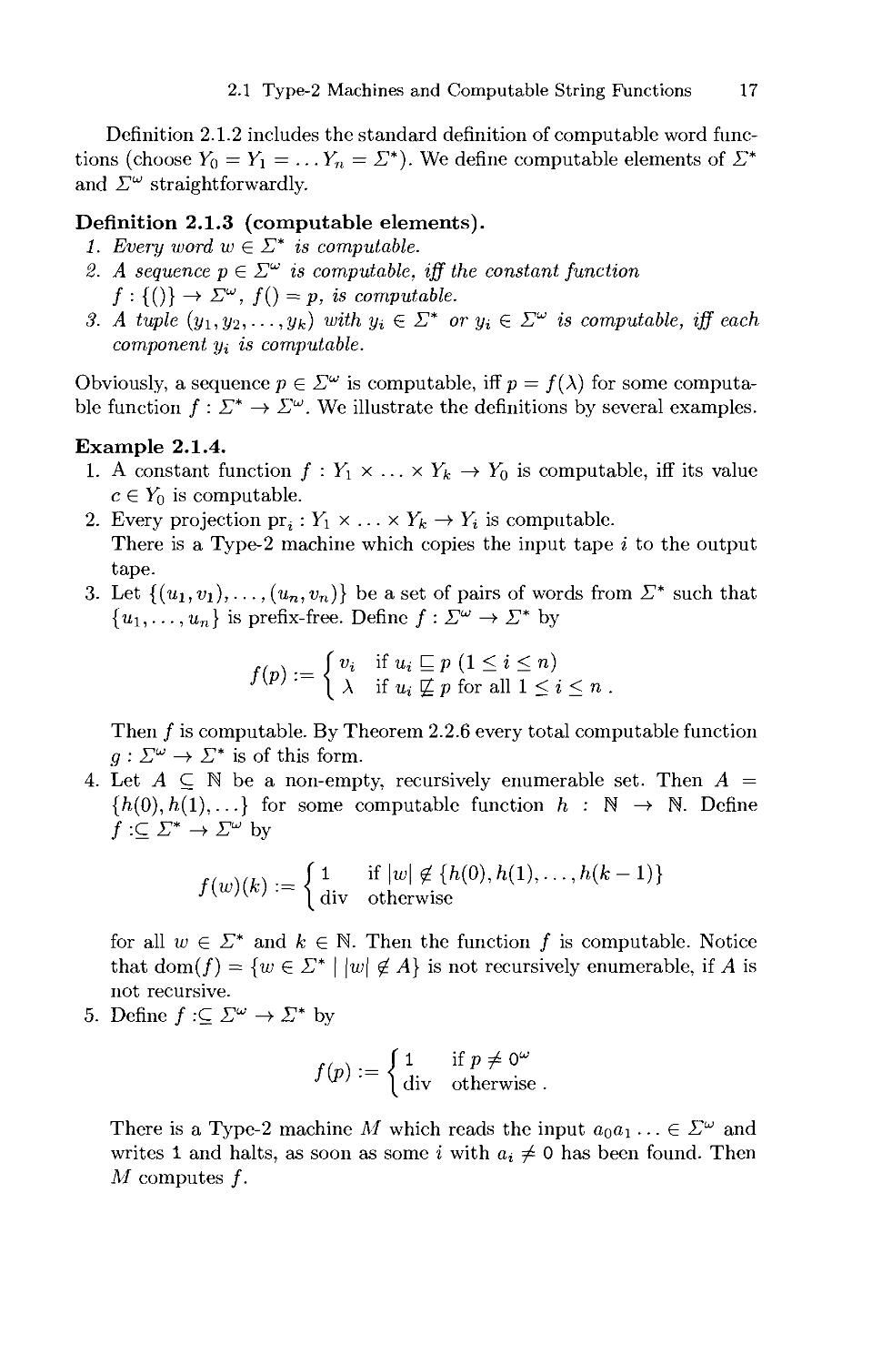
3. Let {{ui,vi),..., (un,vn)} be a set of pairs of words from E* such that
{ui,..., un} is prefix-free. Define / : E" —► E* by
tr ) — ) "■<■ '^UiQp (1 <i <n)
JVP) — \ x if Ui % p for all 1 < i < n .
Then / is computable. By Theorem 2.2.6 every total computable function
g : E" ->■ E* is of this form.
4. Let A C N be a non-empty, recursively enumerable set. Then A =
{/i(0),/i(l),...} for some computable function h : N —► N. Define
/ :C E* -> E» by
fMffc) ■= (x if H * {/l(0)'ft(1)' •' •'h{k ~1)}
./ *, J\ | ^jy otherwise
for all w E E* and fc G N. Then the function / is computable. Notice
that dom(/) = {w € E* | |if| ^ ^4} is not recursively enumerable, if A is
not recursive.
5. Define / :C E" ->• 17* by
( , = fl ifp^O"
| jjy otherwise .
There is a Type-2 machine M which reads the input aoa\ ... G Eu and
writes 1 and halts, as soon as some i with dj ^ 0 has been found. Then
M computes /.

2. Computability on the Cantor Space
The function / : E" ->• E* defined by
1 ifp^O
^ ' ' \ 0 otherwise
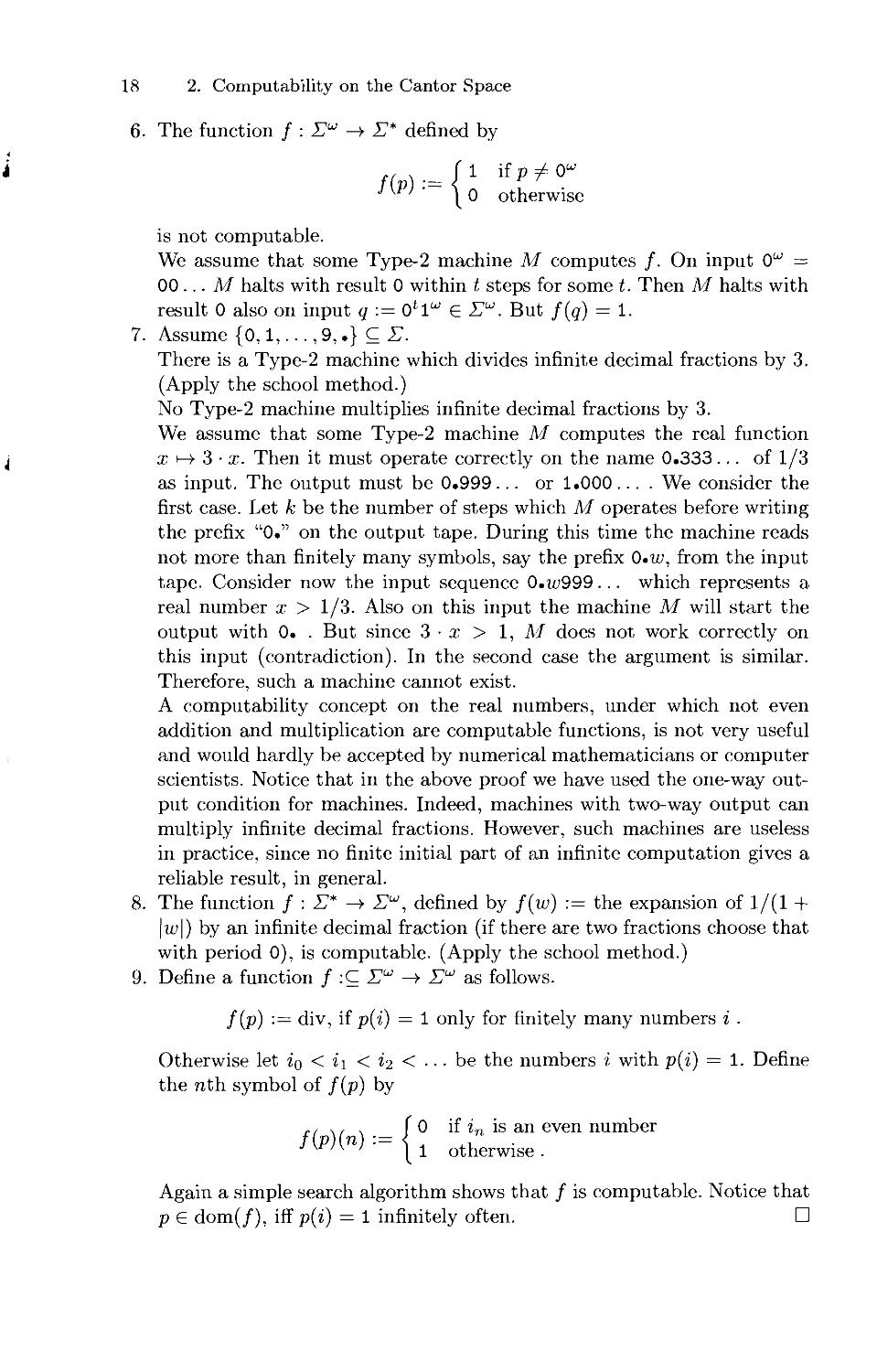
is not computable.
We assume that some Type-2 machine M computes /. On input 0" =
00... M halts with result 0 within t steps for some t. Then M halts with
result 0 also on input q := 0*1" G E". But f{q) = 1.
Assume {0,1,..., 9,.} C E.
There is a Type-2 machine which divides infinite decimal fractions by 3.
(Apply the school method.)
No Type-2 machine multiplies infinite decimal fractions by 3.
We assume that some Type-2 machine M computes the real function
14 3-1. Then it must operate correctly on the name 0.333... of 1/3
as input. The output must be 0.999... or 1.000.... We consider the
first case. Let k be the number of steps which M operates before writing
the prefix "0." on the output tape. During this time the machine reads
not more than finitely many symbols, say the prefix 0.u>, from the input
tape. Consider now the input sequence 0.u;999... which represents a
real number x > 1/3. Also on this input the machine M will start the
output with 0. . But since 3 • x > 1, M does not work correctly on
this input (contradiction). In the second case the argument is similar.
Therefore, such a machine cannot exist.
A computability concept on the real numbers, under which not even
addition and multiplication are computable functions, is not very useful
and would hardly be accepted by numerical mathematicians or computer
scientists. Notice that in the above proof we have used the one-way
output condition for machines. Indeed, machines with two-way output can
multiply infinite decimal fractions. However, such machines are useless
in practice, since no finite initial part of an infinite computation gives a
reliable result, in general.
The function / : E* —► E", defined by f(w) := the expansion of 1/(1 +
\w\) by an infinite decimal fraction (if there are two fractions choose that
with period 0), is computable. (Apply the school method.)
Define a function / :C E" ->■ E" as follows.
f(p) ■= div, ifp(i) = 1 only for finitely many numbers i .
Otherwise let Iq < i\ < %2 < ■ ■ ■ be the numbers i with p(i) = 1. Define
the nth symbol of f(p) by
0 if in is an even number
otherwise .
fiPKn) := I
Again a simple search algorithm shows that / is computable. Notice that
p G dom(/), iff p(i) — 1 infinitely often. □

2.1 Type-2 Machines and Computable String Functions 19
The next technical lemma on the initial parts of computations is related to
Kleene's T-predicate or Blum's 2nd axiom for complexity measures [Wei87].
Lemma 2.1.5 (partial computations). Let M be a Type-2 machine
with k input tapes. Let Tm be the set of all (ui,... ,Uk,Om,v) with
m,... ,Uk,v G E* and m G N such that on any input (j/i,..., J/jt) such
that Ui is a prefix of y* for i = 1,..., k in m steps the machine M reads at
most the prefix «j from the input tape i (i = 1,..., k) and writes v on the
output tape. Then the set 7m is recursive.
We omit the elementary proof. By the following lemma, computable
functions / :C Y —► E" can be represented by computable functions
F :C Y x E* ->• X1*.
Lemma 2.1.6 (type conversion). For any function / :C Y —> Eu,
Y = Yi x ... x Yfc with Yi,..., yfe e {£*, Z1"}, / is computable, iff there
is a computable function F :C Y x E* ^ E* such that the following two
properties hold:
[y G dom(/) ^^ (Vra G N){y, 0n) G dom(F)] for all y G Y ,
(Vj/ e dom(/))(Vn G N)F(y,On) = f(y)(n) .
Proof: See Exercise 2.1.3. □
Computability on E* and Eu can be reduced to computability on
{0,1}* and {0,1}W, respectively, by encoding the symbols of the alphabet
E — {ai,..., an} for example as follows: at ^-> 14_10 for % < n and an ^-> 1™,
see Exercise 2.1.8.
As in ordinary recursion theory, tupling functions are useful tools.
Definition 2.1.7 (tupling functions). Define the "wrapping function"
i : E* -> E* by
i{a\a2 ■■■ an) := \\Oa1Oa2O ■■ ■ a„011
for all n G N and a\,a2, ■ ■ ■, an G E.
For x, xq, X\,... G E*, p,po,pi,. ■. G Eu and i,j, k G N with k > 1 define
(xi,... ,xk) := i-(xi). ..t(xk) G E* ,
(x,p):=t,{x)p£S",
(p,x) :=t(x)pe E" ,
(pi,...,Pfc):=Pi(0)...Pfc(0)p1(l)...pfc(l) GS",
(x0, xi,...) := l(x0)l(xi) ... e E" ,
(p0,pi,...)(i,j) :=Pi(j) ((p0,Pi,...) G Z") .

20 2. Computability on the Cantor Space
We use the same notation ( ) for each of the above tupling functions.
Each of them is injective and even bijective, if the arguments are from Eu.
The definition of the wrapping function i guarantees that subwords i{u) and
t(v) of a word w can overlap only trivially: If t(u) is a subword of t(v), then
t(u) = t(v), and if x is a suffix of t(u) and a prefix of t(v), then t(u) = t(v) = x
or x G {11,1, A}.
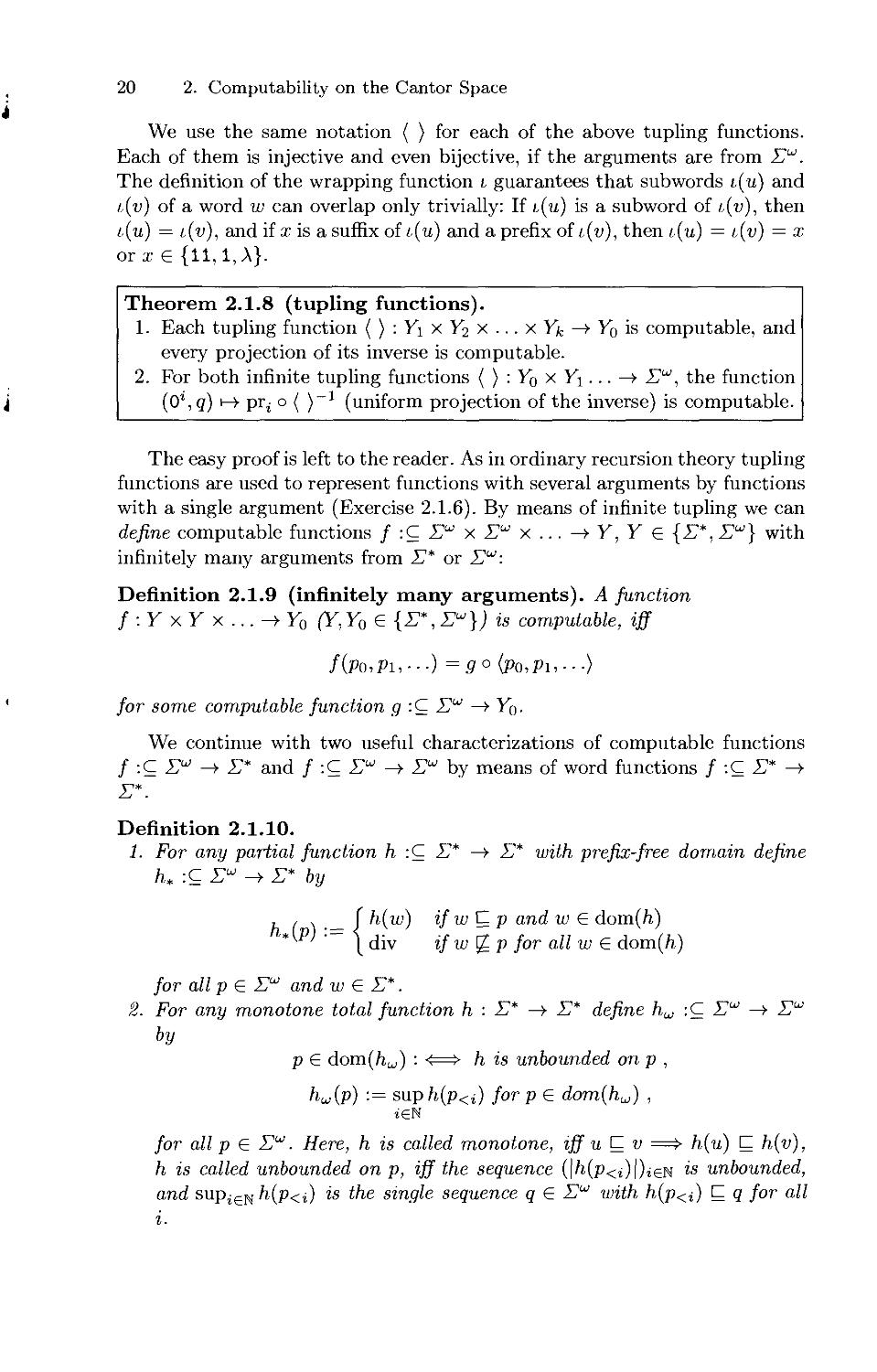
Theorem 2.1.8 (tupling functions).
1. Each tupling function ( ) : Y\ x Y2 x • • • x Yk —► Y~o is computable, and
every projection of its inverse is computable.
2. For both infinite tupling functions ( ) : Yo x Y\... —> Eu, the function
i (0l,q) h-> pr^ o ( )-1 (uniform projection of the inverse) is computable.
The easy proof is left to the reader. As in ordinary recursion theory tupling
functions are used to represent functions with several arguments by functions
with a single argument (Exercise 2.1.6). By means of infinite tupling we can
define computable functions / :C E" x E" x ...->■ Y, Y G {£*, E"} with
infinitely many arguments from E* or E":
Definition 2.1.9 (infinitely many arguments). A function
f:YxYx...^Y0 (Y,Y0 G {£*, E"}) is computable, iff
f(p0,Pi,-..) = g ° <J>q,P\, ■ ■ ■)
for some computable function g :C Eu —► Yq.
We continue with two useful characterizations of computable functions
/ :C E" ->■ E* and f :C E" ^ E" by means of word functions f :C E* ^
E*.
Definition 2.1.10.
1. For any partial function h :C E* —► E* with prefix-free domain define
K :C E" -> E* by
... J h(w) ifwQp and w G dom(/i)
* \ div ifw^p for all w G dom(/i)
for all p G E" and w G E*.
2. For any monotone total function h : E* —► E* define hu : C E" —► E"
by
p G dom(/iw) : <=> h is unbounded on p ,
hu(p) ■= sup/i(p<i) for p G dom(hu) ,
for all p G Eu. Here, h is called monotone, iff u Q v => h(u) C. h(v),
h is called unbounded on p, iff the sequence (|/i(p<i)|)ieN ^s unbounded,
and supieN h(p<i) is the single sequence q G E" with /i(p<j) C q for all
i.

2.1 Type-2 Machines and Computable String Functions 21
Lemma 2.1.11 (computable string functions).
1. A function / :C E" —► E* is computable, iff / = h* for some
computable function h :C E* —> E* with prefix-free domain.
2. A function / :C Eu —► E" is computable, iff / = hu for some
computable monotone function h : E* —► E*.
Proof: 1. Let M be a Type-2 machine computing / :C Eu —► E*. Define
h :C E* ->• E* by
{f(wO") if on input wO" machine M halts
after exactly \w\ steps
div otherwise.
Then h is computable, has prefix-free domain and satisfies / = /i*. Notice
that dom(/i) is even recursive.
On the other hand, let M be a Turing machine computing h :C E* —> E*
with prefix-free domain. There is a Type-2 machine N which on input p G E"
searches for the smallest number k := (i,t), such that machine M halts on
input p<i in exactly t steps, prints the result /i(p<j) and halts. Since dom(/i)
is prefix-free, there is at most one such number k. Obviously, N computes
the function /i*.
2. Let M be a Type-2 machine computing / :C E" ->■ E". Define
h : E* ->■ E* by: h(w) :— the word x G E* which M on input «;0"
produces in |ui| steps. Then the function h is monotone and computable, and
/ = hw.
On the other hand, let h : E* —► E* be a computable monotone function.
Then for any p G E" and z G N, /).(p<i) C /i(p<i+1). There is a Type-2
machine N which on input p G Eu works in stages n = 0,1,... as follows:
In Stage n, N extends the result /i(p<n-i) from Stage n — 1 to h{p<n). The
function / :C Eu —t E" computed by the machine N satisfies f = hu. □
The lemma can be generalized easily to functions / :C [Eu')k —t E* and
functions / :C (Eu')k —> E" (Exercise 2.1.12). By the next theorem the
computable functions are "essentially" closed under composition.
Theorem 2.1.12 (closure under composition). For k,n G N and
X1,...,Xk,Y1,...,Yn,Z e {£*,£"} let
9i '-Q Xi x ... x Xk —> Yi and /:Cy, x ... x Yn —► Z
(i = 1,..., n) be computable functions. Then the composition
f°(9l,--.,9n)-QXi X . . . X Xk ->■ Z

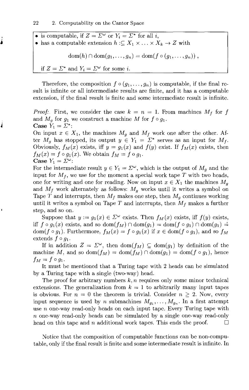
22 2. Computability on the Cantor Space
• is computable, if Z
= E" or Yt
• has a computable extension h :
dom(/i) f
HZ = E* and Yi =
dom(gi,..
=: E*
QXt
-,9n)
E" for some i.
for all i,
x ... x Xk
= dom(/ o
"►
(9i
Z with
, •••)5n)) ,
Therefore, the composition f ° (gi, ■ ■ ■ ,gn) is computable, if the final
result is infinite or all intermediate results are finite, and it has a computable
extension, if the final result is finite and some intermediate result is infinite.
Proof: First, we consider the case k = n = 1. From machines Mf for /
and Mg for g\ we construct a machine M for / o glm
i CaseYl = E*:
On input x G Xi, the machines Mg and Mf work one after the other.
After Mg has stopped, its output y G Y\ = E* serves as an input for Mf.
Obviously, /m(x) exists, iff y = g\(x) and f(y) exist. If /m(x) exists, then
Im(x) = / o gi(x). We obtain fM = f° Si-
Case Yx = Z":
For the intermediate result y G Y\ = E", which is the output of Mg and the
input for Mf, we use for the moment a special work tape T with two heads,
one for writing and one for reading. Now on input x E Xi the machines Mg
and Mf work alternately as follows: Mg works until it writes a symbol on
Tape T and interrupts, then Mf makes one step, then Mg continues working
until it writes a symbol on Tape T and interrupts, then Mf makes a further
« step, and so on.
Suppose that y := g\(x) G E" exists. Then Jm(x) exists, iff f(y) exists,
iff / o gi(x) exists, and so dom(/M) n dom(<7i) = dom(/ ° </i) fl dom(<7i) =
dom(/ ° gi). Furthermore, /m(x) = f ° gi(x) if a; G dom(/ o gi), and so fM
extends / o gx.
If in addition Z — E", then dom(/M) Q dom(t;i) by definition of the
machine M, and so dom(/M) = dom(/M) n dom(t;i) = dom(/ o gi), hence
/m = / ° 5i •
It must be mentioned that a Turing tape with 2 heads can be simulated
by a Turing tape with a single (two-way) head.
The proof for arbitrary numbers k, n requires only some minor technical
extensions. The generalization from k = 1 to arbitrarily many input tapes
is obvious. For n = 0 the theorem is trivial. Consider n > 2. Now, every
input sequence is used by n submachines Mgi,..., M9n. In a first attempt
use n one-way read-only heads on each input tape. Every Turing tape with
n one-way read-only heads can be simulated by a single one-way read-only
head on this tape and n additional work tapes. This ends the proof. □
Notice that the composition of computable functions can be
non-computable, only if the final result is finite and some intermediate result is infinite. In

2.1 Type-2 Machines and Computable String Functions 23
Exercises 2.1.9 and 2.1.10 we give examples of computable functions with non-
computable composition. The next important theorem follows from closure
under composition.
Theorem 2.1.13. Every computable function maps computable elements
to computable elements.
Proof: Let / :C Yx x . .. x Yk ->• Y0 (Y0,.. ., Yk e {E*, Z"}) be computable
and let j/j G Vj (1 < i < k) be computable constants such that (yx,..., yk) G
dom(/). By Definition 2.1.3 the functions gi : {()} —► Vj such that gi{) =
Vi (1 < i < k) are computable. By Theorem 2.1.12, /o (gi,... ,gn) has a
computable extension h, and so
f(yi,---,Vk) = f°(9i,---,9n)0 =h()
is a computable element of Yq by Definition 2.1.3. □
The computable functions are also closed under primitive recursion.
Theorem 2.1.14 (primitive recursion). Let /' :C Y\ x... xYk —> Y0 be
a computable function and for each o G E let fa :C E* x Yq x Y\ x ... x Yk —>■
Vb be a computable function (where Y0,Y\,... ,Yk G {E*,EU}). Then the
function g :C E* x Y\ x ... x Yk —t Yo, defined by the recursion equations
9{\yi,---,Vk) = f'(yi,---,yk),
g(aw,y1,...,yk) = fa{w,g{w,yl,... ,yk),yi, ■ ■ ■ ,yk)
for all w G E*, y\ G Vi,..., yk G Yk and o G E, is computable.
Proof: If Yq — E* then a Type-2 machine M which computes the function
g can be constructed by standard methods, since all intermediate values and
computations are finite.
Suppose Yq = Eu. First, we prove as a special case that there is a
computable function G ;C E* x E" ->■ E" with
G(A,p)=p,
G(aw,p) = Fa(G(w,p))
for all w G £*, p G E" and o G Z1, provided Fa :C E" ->■ Z1" is computable
for all o G 17. (Explicitly written, G(oi .. .am,p) = Fai o ... o Fam(p).) By
Theorem 2.1.11, for each o G E there is a computable monotone function
ha:Z*-> Z* with Fa = ha<u. The function h : E* x E* ^ E*, defined by
/i(A,x) = x ,
h(aw,x) = ha(h(w,x))
for all if, a; G E* and o G E, is computable. The function h can be defined
explicitly by h(ai ... am, x) = /ia, o.. .°ham (x). For each if G 17* the function

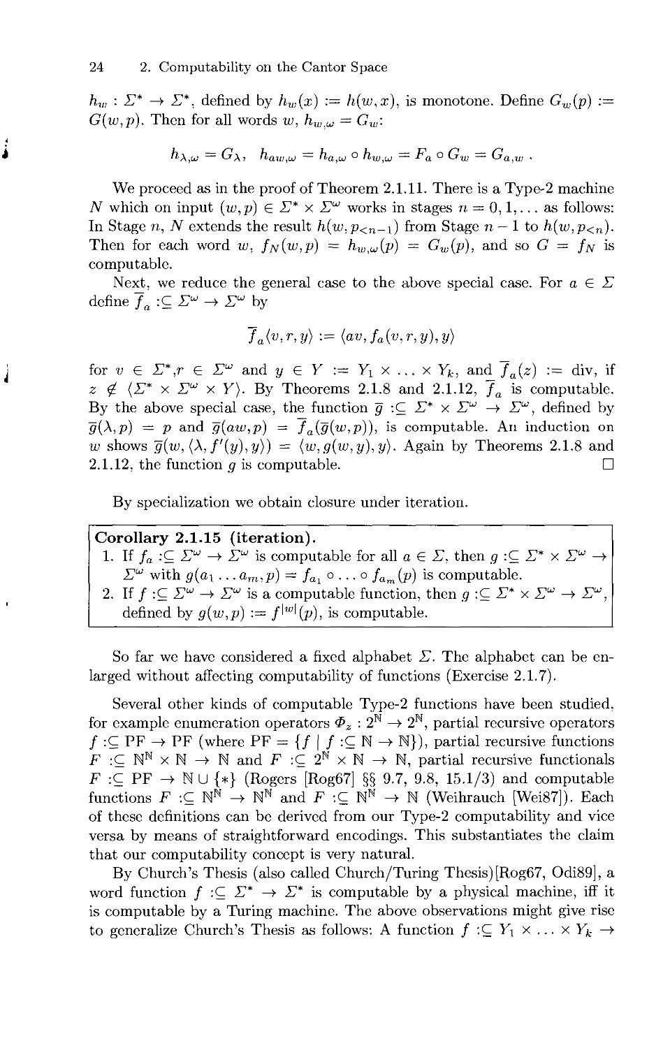
24 2. Computability on the Cantor Space
hw : E* —> E*, defined by hw(x) := h(w,x), is monotone. Define Gw(p) :=
G(w,p). Then for all words w, hWtUJ = Gw:
We proceed as in the proof of Theorem 2.1.11. There is a Type-2 machine
N which on input (w,p) G E* x Z" works in stages n = 0,1,... as follows:
In Stage n, N extends the result h(w,p<n-i) from Stage n— 1 to h(w,p<n).
Then for each word w, /n(w,p) = hWtUJ(p) = Gw(p), and so G = fw is
computable.
Next, we reduce the general case to the above special case. For o G E
define /„ :C E" ->• £" by
7a(v>r>y) ••= {av,fa(v,r,y),y)
for u G i7*,r G E" and y G Y := Yx x ... x Yk, and Ja(z) := div, if
z £ (Z* x Z" x Y). By Theorems 2.1.8 and 2.1.12, Ja is computable.
By the above special case, the function g~ :C E* x Z" —► Z", defined by
^(A,p) = p and g(aw,p) = fa(~g(w,p)), is computable. An induction on
u; shows g~{w, (A, f'(y),y)) = (w,g(w,y),y). Again by Theorems 2.1.8 and
2.1.12, the function g is computable. □
By specialization we obtain closure under iteration.
Corollary 2.1.15 (iteration).
1- If fa :C E" ->■ Z" is computable for all a G Z, then 5 :C Z* x E" ->■
Z" with 51(0! ... om,p) = fai o ... o fam (p) is computable.
2. If / :C E" ->■ Z" is a computable function, then 5 :C E* x Z" ->■ Z",
defined by g(w,p) := /'"''(p), is computable.
So far we have considered a fixed alphabet Z. The alphabet can be
enlarged without affecting computability of functions (Exercise 2.1.7).
Several other kinds of computable Type-2 functions have been studied,
for example enumeration operators <I>Z : 2N —► 2N, partial recursive operators
/ :C PF ->■ PF (where PF = {/ | / :C N ->■ N}), partial recursive functions
F :C NN x N ->■ N and F :C 2" x N 4 N, partial recursive functionals
F:CPF^NU {*} (Rogers [Rog67] §§ 9.7, 9.8, 15.1/3) and computable
functions F :C NN ->• NN and F :C NN ->• N (Weihrauch [Wei87]). Each
of these definitions can be derived from our Type-2 computability and vice
versa by means of straightforward encodings. This substantiates the claim
that our computability concept is very natural.
By Church's Thesis (also called Church/Turing Thesis) [Rog67, Odi89], a
word function / :C Z* —► Z* is computable by a physical machine, iff it
is computable by a Turing machine. The above observations might give rise
to generalize Church's Thesis as follows: A function / :C Yx x ... x Yk —>

2.1 Type-2 Machines and Computable String Functions 25
YQ (Yo,... ,Yk G {£*,£"}) is computable by a physical machine, iff it is
computable by a Type-2 machine.
We refrain from doing this, since there is no convincing reason to exclude
generalized Type-2 machines with two-way output or machines with more
sophisticated input/output conventions. The main reason for choosing com-
putability defined by Type-2 machines as a basis for computable analysis is
a practical one. We believe that for our purpose this kind of computability is
the most useful choice. From Church's Thesis we adopt the conviction that
computations on Turing tapes can be realized by physical machines and that
every (discrete) computation of a physical machine can be simulated by a
Turing tape.
Exercises 2.1.
<0> 1. Show that permitting two-way input tapes does not increase the
computational power of Type-2 machines.
0 2. Generalize the Type-2 machine model by admitting two-way output.
Show that there is a machine of this kind which multiplies infinite decimal
fractions by 3.
3. Prove Lemma 2.1.6.
4. Prove Theorem 2.1.8.
5. Show that there is a computable function / :C Eu —► Eu with dom(/) =
{E* x E"). Show that there is a computable function g :C E" ->■ E"
with dom(g) = Ew \ {E* x Ew).
0 6. Show that a function / : E* x E" ->■ Y0 (Y0 G {E*, E"}) is computable,
iff f(x,p) = g(x,p) for some computable function g :C E" —> Y0.
7. Let E and A be finite alphabets with E C A. For oo, ■ • • ,afc G {*,w}
let / :C Eai x ... x Eak ->■ Ea° and g :C Aai x ... x Aak ->■ Aa° with
graph(/) = graph(t;). Show that / is computable, iff g is computable.
Therefore, extension of the alphabet preserves computability.
8. For n > 2, computability on E* for E — {oi,... ,an} can be reduced to
computability on {0,1}*. Define a mapping c : E —► {0, l}* by c(ai) :=
lt_10 for i < n and c(an) := ln. Define
c» : E* -)• {0,1}* by c»(&i&2 .. .6fe) := c(6i)c(62).. .c(6fe) and
cu-.iy^ {0,1}- by cUbohb2 ...):= c(60)c(6i)c(62)....
a) Show that c, c„ are injective and cw is bijective.
b) Show that the target extensions of c, and cw to E* and E",
respectively, and the inverses of these functions are computable (Convention
2.0.1).
c) Show that / :C Edl x ... x Edk ->■ Edo (di G {*,uj}) is computable,
iff co f(c~l,..., (Tl) is computable, where c(w) := c*(w) and c{p) :=
Cuj(p) for w G E* and p e £".
9. (non-computable composition) Show that there are computable functions
/ :C E* ->■ Z1" and 5 : E" ->■ Z1*, such that 5 o / :C Z* ->■ Z*

26 2. Computability on the Cantor Space
is not computable. (Hint: consider / from Example 2.1.4.4 and define
9(p) := A.)
10. (non-computable composition) Let / : E" —► Eu be the function from
Example 2.1.4.9 and define g : E" ->• Z* by s(p) := A for all p G Z".
Then / and g are computable. Show that g o / cannot be computable.
11. Call a partial function h :C X1* —► 17* upwards constant, iff
(/i(m) exists and u is a prefix of v) => /i(m) = /i(i>) .
Show that in Definition 2.1.10 and Lemma 2.1.11 functions with prefix-
free domain can be replaced by upwards constant functions.
12. Generalize the characterization from Lemma 2.1.11 to functions / :C
(Z")fc ->• E* and functions / :C (Z")fc ->• £".
13. (Closure under simultaneous recursion, Theorem 2.1.14) For i = 1,..., I
let /,' :C Y\ x ... x Yj. —> Yq be computable functions and for each o G E
let fia '.C E* x V0 xYi x ... x Yfc —> V0 be computable functions (where
Vo, Y1,..., Yk G {Z*, Z"}). Show that the functions gz :C E* xY1 x ... x
Yk —► ^o (*' = 1) • • • t 0> defined by the recursion equations
9i(^,yi,---,yk) = fl(yi,---,yk),
9i(aw,yi,...,yk) = fia(w, 9i(w,yi, ■ ■ ■ ,Vk), ■ ■ ■,
9i(w,yi,...,yk),yi,-..,yk)
for all w G E*, y\ G Yi,... ,yk G Vfc and o G IT, are computable.
♦ 14. The following theorem on term evaluation generalizes composition,
primitive recursion and iteration.
Assume that the alphabet E contains the symbols x and f. Let /z : N —► N
be a computable function (/x(i) will be the arity of the function fa) and
let n G N.
a) Define the set Tm C E* of terms in n variables (in Polish notation)
inductively as follows:
• x0fe is a term for k = 1,..., n,
• if t\,..., iM(j) are terms, then f 0lti ... t^i) is a term (for all i G N),
• no other words are terms.
b) For each i G N let f{ :C (£")»<.*) ->■ £" be a function. For terms
t G Tm, define the semantics [[£]] :C (Z")™ —► Z" recursively as
follows:
[[xOfe]](p):=pfc,
110% . . . t^ ]](p) := fidh }(p), ..., p„(0 ]](p))
forallp:=(p1,...,pn)G(Z")".
c) Assume that the "universal" function
(0*,(pi,...,^(i))) n- fi(pi,---,P»(i))
is computable. Prove that the "term evaluation function"

2.2 Computable String Functions are Continuous 27
(t,pi,...,pn)^lt]](p1,...,pn) (( £ Tm, pi,...,pn G E")
is computable,
d) Derive Theorem 2.1.14 (case V; = E" for all i) and Corollary 2.1.15
as corollaries.
2.2 Computable String Functions are Continuous
Let M be a Type-2 machine such that fM :Q E" ->■ Eu. Consider u G E*
with u C /m (p). Then on input p, the machine M writes the prefix u of the
output /m(p) in t steps for some t. Within t steps, M can read not more than
the prefix w := p<t of the input p G Eu. Therefore, the output u depends
only on the finite prefix w of p but not on the rest p{t)p{t + 1)... . We obtain
fM[wEu] C UEW. Roughly speaking:
(FP) Every finite portion of the output Jm(p) is already determined
by a finite portion of the input p.
We have already used this finiteness property (FP) repeatedly for proving
non-computability of functions (Examples 2.1.4.6/7 and Exercise 2.1.10). We
will see that it is equivalent to continuity of the function /m , if we consider
the Cantor topology on the set Eu.
Since topology is a mathematical theory for studying approximation, it is
not surprising that we can use it for describing the approximation of infinite
sequences of symbols by finite ones or of real numbers by rational intervals.
For readers who are not familiar with the language of topology we summarize
briefly some basic definitions below. More details can be found in textbooks
on analysis or in any introduction to topology [Die60, Rud64, Eng89].
Definition 2.2.1 (some definitions from topology). A topology on a
set M is a system r C 2M of subsets of M, called the open sets, with the
following three properties:
(Tl) 0 and M are open.
(T2) If U and V are open, then U C\V is open.
(T3) If a is a set of open sets, then its union (J a is open.
A subset A C M is called closed, iff its complement M \ A is open. The
pair (M, t) is called a topological space. An example is the Euclidean space
(R", t) , where r is the set of open subsets of K", which contains 0 and K™ and
is closed under finite intersection and arbitrary union. For sets A, B C M,
B is called a neighborhood of A, iff A C U C B for some open set U. B
is a neighborhood of a point x, iff it is a neighborhood of {x}. Then a set
V C M is open, iff V is a neighborhood of every x G V. For a subset X C M
the closure cls(X) is the smallest closed subset of M containing X and the
interior int(X) is the greatest open subset of M contained in X.
A base of the topology r is a set /? C t of open sets, such that for all
U E t there is some 7 C /? such that J7 = (J 7. A subbase of r is a subset

28 2. Computability on the Cantor Space
a C r such that the set {p)7 | 7 is a finite subset of cj} is a base of r. Let a
be any set of subsets of M, let (3 := {[)"/ | 7 is a finite subset of a} and let
T := {U 7 I 7 ^ /?}• Then r is a topology, /J is a base of r, and a is a subbase
of t. (We use the canonical definitions |~)0 = M and (J0 = 0.)
Let (M, t) and (M',t') be topological spaces. A function / : M ->■ M'
is called continuous, iff /_1[J7] G r for all J7 G r'. A function f : M —t M'
is called continuous at x G M, iff for all V G r' with /(a;) G V there is
some U e t with x e U and /[[/] C V. (If various topologies are considered,
we shall say more precisely (t,t')-continuous.) In both cases it suffices to
consider V G (3 for some base (3 or V G a for some subbase c of the topology
t'. A function / : M —> M' is continuous, iff it is continuous at x for all
x G M. The composition of two continuous functions is continuous.
Let (M,t) be a topological space and let D C M. The topology on D
induced by r is r|£> := {D HU \ U e t}. We shall call a set X C M open
in O, iff X = D n C for some open set U G r. We shall call a partial
function / :C M ->■ M' with dom(/) = D (t, T')-continuous (at x G -D), iff
its restriction f\jj is (t|d,t')-continuous (at x G D).
A subset X C M is called a G^-set, iff X = C/o n C/i fl... for some sequence
(Uq, Ui, ...) of open sets. We may assume that the sequence of open sets is
decreasing (choose Vn := Uq fl... fl Un). For a topological space (M, r) a set
ICMis dense, iff XnC 7^ 0 for all non-empty U e t. The discrete topology
on a set M is the set 2M of all subsets of M (every subset of M is open).
For any family (Mj,Tj)i6j of topological spaces, the product space
(Xje/Mj, <3)ig/ Ti) is defined as follows: Xj6/Mj is the Cartesian product
and the topology ®i6/ tv has the base
(3 := {XieiUi I Ui G Tj for all i and t/j ^ Mi only for finitely many i}.
On Cartesian products the product topologies are used tacitly.
A pseudometric space is a pair (M,d), where M is a set and d : M x
M —► K is a function (the distance or pseudometric on M) such that for all
x,y,z G M:
(Ml) rf(x,y) >0
(M2) d{x,x) =0
(M3)d(i,y) = d(y)a:)
(M4) d(x, z) < d(x, y) + d(y, z)
d is a metric and (M, rf) is a metric space, iff in addition
(M5) d{x,y) = 0 implies x = y.
For a; G M and r > 0, B(x,r) := {y G M | d(x,y) < r} is the open 60ZZ wii/i
center x and radius r and B{x,r) := {y G M | d(x,y) < r} is the closed
ball with center x and radius r. The set of open balls is a base of a topology
Td on the set M, the topology generated by the pseudometric d. Already the
set of open balls with rational radius is a base of 7^. A subset X C M of a
metric space is compact, iff every open cover of X has a finite subcover, that
is, if X C |J T for a set T of open sets, then X C (J S1 for some finite subset
SCT.

2.2 Computable String Functions are Continuous 29
We introduce the discrete topology and the Cantor topology as our
standard topologies on E* and i7", respectively.
Definition 2.2.2 (standard topologies on E* and £").
1. t* := 2s = {A | A C E*} is called the discrete topology on E*.
2. tc :— {AE" | A C E*} is called the Cantor topology on E".
(17", re) is called the Cantor space (over E).
3. As a canonical base of t* we consider the set {{w} \ w G E*}.
4. As a canonical base of tq we consider the set {wE" \ w G E*}.
5. On Y := Yx x ... x Yk (Yx,..., Yk G {E*, E"}) we consider the product
topology with the canonical base (5y := {y o Y \ y G (E*)k}, where
(yi,..., yk) o Y := Ux x ... x Uk with
Tj ._ / {Vi) if K = Z*
Ul- \yiiy if Yt = E" .
Obviously, t* is a topology on E* and {{w} \ w G E*} is a base of t*.
For any word w G E*, wEu = {wq \ q G 17"} = {p G 17" \ w C p} G rc.
For t>, u; G 17* we have vE" n wZ"" = (wI7" if ti C w, wI7" if ro C «, and
0 otherwise). Therefore, the set /? := {u;i7" | u; G 17*} is closed under finite
intersection, and so it is a base of a topology. Since AS" = (J {wE" \ w G A}
for each A C 17*, /? is a base of the topology tq.
The set i7" of infinite sequences over E can be visualized by a tree where
every p G i7" is represented by an infinite descending path from the root.
Fig. 2.3 shows this tree for the alphabet E = {0,1} with two elements.
etc.
Fig. 2.3. The tree of infinite paths representing the set {0,1}"
A base element wE" G tq is represented by a full subtree and an open
subset of i7" is represented by a set of full subtrees. Figure 2.4 shows four
subtrees representing the open set 00117" U 011017" U 1017" U 111117".

30
2. Computability on the Cantor Space
001Z1" OllOZ1" 10Z1" 111127"
etc.
Fig. 2.4. The subtrees representing the set 001EU U OllOZ"" U 10EU U llllT"
The finiteness property (FP) for the function fM : E" —> E" computed
by a machine M can be formulated as follows: For all p G Ew and u G E*
with /M(p) S uE" there is some w e E" with p G wIT" C f^[uE"]. This
means exactly that the fimction fM is (tq, Tc)-continuous. Therefore, every
computable function / : Eu —► E" is continuous.
After these preparations we prove our main theorems.
Theorem 2.2.3 (computable => continuous). Every computable
string function /:Cy, x ... x Yk —► Y0 is continuous.
Proof: Let M be a Type-2 machine computing /. Assume
(yi, ■ ■ ■ ,2/fc) e dom(/) C Y := Yx x ... x Yk.
Case Yq = E*: It suffices to show that /_"1[{w}] is open for every base
element {w} of t*. Assume /(j/i,..., yjt) G {if}. Since the machine M halts on
this input, during its computation from every input tape i with Yi = E" it
can read only a prefix m G 17* of yt G 17". Define Uj := yt for V; = 17*. Then
y G (ui,...,ufe) oY and /[(mx, ... ,wfc) oV]C {«;}. The set (ui,...,uh) °Y
is an open neighborhood of (yi,... ,yk) contained in /_1[{w}]. Therefore,
/_1[{u;}] is open.
Case Yq = Eu: It suffices to show that f~l[wEu'\ is open for every base
element wE" of tq. Assume /(j/i,.. ■,yk) G w;i7w. Since on this input the
machine M needs only finitely many computaton steps for producing the
prefix w of the result, during this computation from every input tape i with
Yi = E" it can read only a prefix Ui G E* of yi G Eu. Define Ui := j/j
for Yi = E*. Then y G (ui,...,uk) o Y and /[(ux,... ,uk) oY]C WEW.
The set («i,..., uk) o y is an open neighborhood of (yi,..., yk) contained in
/-'[wl"]. Therefore, f~l[wEw] is open. D
Fig. 2.5 illustrates the above proof for the case / :C Eu —► E": Any finite
portion of the output depends only on a finite portion of the input.

2.2 Computable String Functions are Continuous 31
Oo
Oi
a2
a3
04
o5
06
a7
o8
O9 Clio On
O12 Ol3
0,14 O15 Ol6
Oi7 0i8
M
bo
bi
b2
b3
b4
h
be
b7
bs
Fig. 2.5. The machine M has computed bobi ... bg from the input 00O1 ... 015
In numerous applications, functions are not computable because they are
not even continuous. Continuous but not computable functions can be
defined explicitly but occur in practice very rarely. The domains of computable
functions have nice topological properties.
Theorem 2.2.4 (domains of computable functions). Assume
Y = Y1x...xYk with Y1,...,Yke {E*, S"}.
1. If / :C Y —> E* is computable, then dom(/) is open.
2- If / :C F —► E" is computable, then dom(/) is a G^-set.
Proof: 1. In the proof of Theorem 2.2.3 we have shown that every element
{y\i • • • 1 Vk) ^ dom(/) has an open neighborhood (u\,..., uk) ° Y C dom(/).
Therefore, dom(/) is open.
2. Let M be a Type-2 machine which computes /. Then, for each n G N
there is a machine Mn which on input y E Y halts, if M on input y writes at
least n symbols on the output tape, and does not halt otherwise. By Property
1, dom(/M„) is open for each n, therefore,
dom(/M) = dom(/Mo) n dom(/Ml) n ... is a G^-set. D
The Cantor topology can be generated from a metric.
Lemma 2.2.5 (metric on Cantor space). Define d : E" x E" —t K
by d(p,p) := 0 and d(p,q) := 2~n where n is the smallest number with
p(n) ^ q(n) for p f q.
Then M := {E",d) is a metric space, tq (the Cantor topology) is the
topology generated by d, and E" is a compact set .

32 2. Computability on the Cantor Space
The proof is left to the reader. The sets wEu which form a base of the
Cantor topology are the open balls as well as the closed balls in the metric
space (Eu,d). As a closed subset of a compact set, every ball is compact.
In the following a set A C E" is called clopen, iff it is closed and open, and
decidable, iff its characteristic function is computable (Sect. 2.4). As a
consequence of compactness, total computable functions / : Eu —► E*, clopen
subsets and decidable subsets X C Eu are very simple.
Theorem 2.2.6 (decidable set, total continuous function).
1. A subset X C Eu is clopen, iff it is decidable, iff X = AE" for some
finite set ACE*.
2. A (total) function / : E" —► E* is continuous, iff it is computable, iff
there are pairs (u\,vi),..., (uk,Vk) G E* x E* such that {u\,..., Uk}
is prefix-free, E" = uxE" U ... U ukE" and /[mE"] = {vt} for all i.
Proof: Let / : Eu —► 17* be a continuous function. Then for each
p € IT" there are words up,vp with p G UpE" and /[wpZ1"] = {i>p}.
Since IT" = [jpeSu, UpE" and IT" is compact, there are finitely many pairs
(ui,Vi) eE* xE*,ie I, such that E" = \JieIUiE" and f[uiEu] = {^} for
all i. If ttj C Mj then Ujiy C Mji>' and Uj = Vj. Therefore, the pair (uj,Vj) is
unnecessary and can be omitted. After finitely many omissions we obtain a
sequence (u\, v\),..., (uk,Vk) G E* x E* of pairs with the properties stated
in Part 2. The remaining statements of the theorem can be proved easily. □
In this book we will develop a theory of computability and simultaneously
a formally similar "theory of continuity".
Exercises 2.2.
<0> 1. Define continuous functions / :C Eu —► E* and g : E" —► E" which are
not computable.
2. Show that the characteristic function of the set {0"} C Eu is not
continuous (Example 2.1.4.6).
0 3. Show that E" \ {CT} is open but not closed.
4. a) Show that G := {p G E" | p(i) = 1 infinitely often} is a G^-set but
neither open nor closed. (Its complement is not a G^-set, Exercise
2.3.2.)
b) Conclude that the composition gof is not computable, where / is the
function from Example 2.1.4.9 and g : E" —► E* is any computable
function.
5. Let D := {0,1,..., 9}*{.}{0,1,..., 9}" C Ew be the set of all infinite
decimal fractions. Show that the set D is
a) not open,
b) not closed,
c) the intersection of an open and a closed subset of E".

2.3 Standard Representations of Sets of Continuous String Functions 33
6. Prove Lemma 2.2.5.
7. Complete the proof of Theorem 2.2.6.
8. Let (Mi, Tt) := ({0,1}, 2^°'1>) for alH G N. Identify xieNMi with {0, l}".
Show that tq is the product topology.
9. Define B := N" = {p \ p : N ->■ N} and a topology tb on B by the basic
open basic sets ioN" with w G N*. B (or (B,tb) ) is called Baire space.
In [Wei85, KW85, Wei87] the Baire space is used in TTE instead of the
Cantor space. Define /? : B ->■ E" by P(a0axa2 ...):= 0a°10ai 10a2l... .
Show that
a) range(/J) is a G^-subset of E",
b) P and its inverse /J-1 are continuous,
A function / :C B —► B is computable according to [Wei85, KW85,
Wei87], iff /? o / o /J-1 is computable according to Definition 2.1.2. In
particular, every computable function / :C B —► B is continuous.
10. Let / :C Eu —► E* be a computable function with compact domain.
Show that / has a computable extension g : E" —► E*.
♦ 11. For X C E*, X G II2, iff there is a recursive set T C E* x N x N such
that X = {w\ (Vi)(3j)T(w,i,j} [Rog67, Odi89]. Show that X C 772, iff
X = dom(/) for some computable function / :C E* —> E".
2.3 Standard Representations
of Sets of Continuous String Functions
In ordinary (Type-1) recursion theory the concept of an "effective Godel
numbering" or "admissible Godel numbering" ip : N —► P^1^ of the set P^1^
of partial recursive functions (that is, computable number functions) / :C
N —► N is fundamental [Rog67, Wei87, Odi89]. This numbering ip is defined
uniquely up to equivalence by the universal Turing machine theorem, utm-
theorem for short, and the smn-theorem. In this section we generalize the
numbering <p to notations of the computable functions / :C Ea —► Eb by
means of E* and to representations of certain continuous functions / :C
Ea ->■ Eb by means of E", where a, b G {*, w}.
First, we introduce general notations and representations.
Definition 2.3.1 (notation, representation).
1. A notation of a set M is a surjective function v :C E* —► M.
2. A representation of a set M is a surjective function S :C Eu —t M.
A "naming system" is a notation or a representation.
Occasionally we abbreviate v(w) by vw and 5(p) by 5p.
Sometimes we will say that p G Y is a y-name oi x e M, ii y :C Y ^ M
is a naming system and y(p) = x. Notice that we do not consider functions
7 :C E* U Eu —t M with finite and infinite sequences as names. We compare
naming systems by continuous and by computable reduction or translation.

34 2. Computability on the Cantor Space
Definition 2.3.2 (reduction and equivalence). For arbitrary functions
7 :C y ->• M and 7' :C Y' ->• M' with Y, Y' G {E*, E"} we define:
1. The function f :C Y —► Y' translates or reduces 7 to 7', iffy(y) = "/ f(y)
for all y G dom(7).
2. 7 < 7', iff some computable function translates 7 to 7'.
<?• 7 <t l'i iff ■sowe continuous function translates 7 to 7'.
^. 7 = 7' :<==> 7 < 7' and 7' < 7.
5. 7 =t 7' :^=> 7 <t 7' a«rf 7' <t 7.
(Pronunciations: < "reducible to", <t "continuously reducible to", =
"equivalent to", =t "continuously equivalent to").
Occasionally, we extend the definitions of reduction and equivalence to
numberings by calling the standard numbering v^ and its inverse v~^}
computable and closing the computable functions under composition (Sect. 1.4).
This extension allows Y = N or Y' = N.
Notice that we do not require M = M', Y = Y', range (7) = M or
range(7') = M'. As usual, 7 < 7' means (7 < 7' and not 7' < 7), etc.. Since
the identity on Y is computable and continuous, the relations < and <t
are reflexive. Since continuous functions are closed under composition and
computable functions closed under composition up to extension (Theorem
2.1.12), the relations < and <t are transitive. Therefore, on the class of
naming systems, < and <t are pre-orders and = and =t are equivalence
relations.
Consider the "information" about elements of M which can be obtained
from names of a naming system computationally. Since intuitively
information cannot be increased by translation, we may call 7' poorer than 7 or 7
richer than 7', if 7 < 7' or 7 <t 7' or .
In elementary computability theory, Turing machines computing word
functions / :C E* —¥ E* are encoded canonically by words from E*. If
ipw :^ E* —> E* is the word function computed by the Turing machine with
code w, then the partial notation w *-> ipw of the computable word functions
satisfies the utm-theorem and the smn-theorem:
utm(i/>): The function (w,x) 1—> ipw(x) is computable.
smii(ip): For every computable function / :C E* x E* —> E* there is a
total computable function r : E* —> E* with r(x) G dom(ip) for
all x G E* and f(x,y) = ipr(x)(y) f°r &H X-,V S E*■
We generalize these properties as follows.
Definition 2.3.3 (general utm- and smn-property). Let
a, b, c G {*, uj}, let Gah be a set of functions g :C Ea —> Eb and let ( :C Ec —>
Gab be a naming system of Gab. Define:
utm(C): There is a computable ("universal") function u :C Ec x Ea —> Eb
with (x(y) = u(x,y) for all x G dom(£) and y G Ea.
smn((): For every computable function f :C Ec x Ea —> Eb there is a total

2.3 Standard Representations of Sets of Continuous String Functions 35
computable function s : Ec —> Ec such that s(x) e dom(£) for
all x G Ec and f(x,y) = Cs(x){y) for oil x E Ec and y E Ea.
If £ is a total function, then the universal function is defined uniquely. First
we define the standard notations of the computable functions / :C Ea —> Eb.
Definition 2.3.4 (standard notations of computable functions).
Consider a canonical encoding of Type-2 machines with one input tape by
words w E E*, such that the set TC of code words is recursive. For all
a,b E {*, ui} define
1. Yab := {/ :C Ea ->■ Eb \ f is computable },
2. a notation £ab : E* ->■ Pa6 of the set Pab by
{the nowhere defined function, if w $ TC,
the function f E Pa6 computed by the
Type-2 machine with code w otherwise .
Since canonical encodings of Turing machines are defined in every
introduction to computability theory [HU79], we use them here without further
explanation. The following generalized utm- and the smn-properties can be
proved in exactly the same way as the "classical" theorems. Therefore, we
omit the proofs.
Theorem 2.3.5 (utm- and smn-property for £a6). For all
a,b E {*,uj} we have utm(^a6) and smn(£a6).
For obtaining a powerful and elegant theory we introduce representations
of sets of continuous functions / : C Ea —> Eb.
Consider the case o = * : Since every subset of E* is open, every function
/ :C E* ->■ Eb is continuous. The set of all functions / :C E* ->■ Eb has the
same cardinality as Ew or K ("continuum cardinality") and, therefore, has a
representation.
Consider the case a = u : Let / : Eu —> Eb be a constant function. Then /
as well as all its restrictions are continuous. The set of all these restrictions
has the same cardinality as the power set of Eu which is bigger than Eu.
Therefore, the set of all continuous functions / :C Eu —> Eb has no
representation. We solve the problem by considering only continuous functions with
"natural" domains which in some sense represent all continuous functions.
Definition 2.3.6 (classes of continuous functions).
F** :={/|/ :C E* -»• E*} ,
F*" :={/|/ :C E* ^ E»} ,
p^* :={/|/ :C Ew —> E* is continuous and dom(/) is open} ,
Fuw :={/!/ :C E" —> Ew is continuous and dom(/) is a G$-set} .

36 2. Computability on the Cantor Space
Remember that by Theorem 2.2.4 the domain of every computable
function from F"* is open and the domain of every computable function from Fww
is a G^-set. The following two theorems may serve as further justifications for
considering the above sets F"* and Fww. The first theorem is a continuous
version of Lemma 2.1.11.
Theorem 2.3.7 (characterization of F"* and F""").
1. F"* = {A, | A :C E* ->■ E* has prefix-free domain}.
2. F""" = {hw\h: E* ->■ E* is monotone}.
By the next theorem, the sets F"* and F""" represent essentially all partial
continuous functions / :C Ew ->■ E* and / :C Ew ->■ Ew, respectively. The
second part is a special case of a well-known extension theorem for continuous
functions on metric spaces [Kur66].
Theorem 2.3.8 (continuous extension).
1. Every continuous partial function / :C Eu —> E* has an extension in
Fw*.
2. Every continuous partial function / :C Eu —> Eu has an extension in
Proof of Theorems 2.3.7 and 2.3.8:
1. A* G F"* for every A :C E* ->■ E* with prefix-free domain:
Let / := A*. If f(p) = y then there is a unique x C. p with h(x) = y. We obtain
fl [{v}} = U)i(i)=» x^u (which is an open set) for every y e E*. Since the
set of all {y} is a base of the discrete topology on E*, f is continuous. Since
rl[E*} = [jyes. rl[{y}], dom(/) is open.
2. If / :C Eu —> E* is continuous, then A* extends / for some A :C E* —>
iT* with prefix-free domain:
Define A :C £*->£* by
A(i) = y :<=? [f[xEw] = {y} and f[x Ew] = {y} for no i'ci).
The function A is well-defined and has prefix-free domain. Suppose, f(p) = y.
Since the set {y} is open and / is continuous, there is some shortest word
x G E* such that p e xiT" and f[xEu] = {y}. We conclude h(x) = y and
A*(p) = y. Therefore, A* extends /.
3. If V C dom(A*) is open, then the restriction of A* to V is equal to </„
for some function 5 :C iT* -^ E*\
There is some prefix-free set B C E* with V = BE". Define C : =
{max(«, v) \ u £ dom(A), v € B}, where max(«, u) := (u, if v C u, u, if u C
u, div otherwise). C is prefix-free, since dom(A) and B are prefix-free. We
obtain CEW = \J{max(u,v)E" \ u e dom(A),u e 5} = \J{uE" HvE" |
u e dom(h),v e B} = dom(h)Ew n ££" = V. Define J :C £» -> £* by
dom(g) = C and g(w) := A(u), where u is the (uniquely determined) word
from dom(A) with u C. w. Consider p E V and A*(p) = y. Then there are

2.3 Standard Representations of Sets of Continuous String Functions 37
words u G dom(/i) and v G B with u Q p, v Q p and h{u) = y. We obtain
w := max(it, v) G C and g(u>) = /i(m) = y, that is, g*(p) = y. If, on the other
hand, g*(p) exists, then g(w) exists for some w G C with w C. p. Then there
are words u G dom(/i) and v G B with w := max(«,t)), hence v Q p and
p G BiT" = V. Therefore, g* is the restriction of A» to V.
The above three properties imply Theorems 2.3.7.1 and 2.3.8.1.
4. ^ € F""" for every monotone function h : E* ->■ £*:
Assume hu{jp) = q and g G uiT". Then u CI /i(m) for some it rz p. We obtain
p G uEu and Aw[ui:w] C h{u)Eu C uiTw. Therefore, Aw is continuous. For
n G N define Bn := {u e E* \ \h(u)\ > n}. The sets BnEw are open. Then
p G dom(/iw), iff p G BnEw for all n, that is, dom(/iw) is the G^-set f]n BnEw.
5. If / :C iTw —>■ iTw is continuous, then hu extends / for some monotone
function h: E* ^ E*:
We define h : E* ^ E* inductively as follows:
h(X) := A,
( h(x) if f[xaEw] C h(x)bEw for no 6 G £ ,
h(xa) := I h(x)b for the unique b & E with
[ /[rraZ"'-'] C /i(:r)&Z"';, otherwise
for all a; G 17* and o G E. Obviously, the function h is monotone. Suppose
f(p) — 1- An easy induction proof shows x \Z p => h(x) rz q. It remains to
show that the sequence \h(p<n)\n is unbounded. Assume h(p<n) = u for all
n > N. For some b e E, q e ubEw. By continuity of /, f\p<n+1Ew] C uftiT"
for some n > N. Then by definition, A(p<n+i) = h(p<npn) = h(p<n)b — ub
(contradiction). We conclude hLO(p) = q. Therefore, hu extends /.
6. If G C dom(/iw) is a G^-set, then the restriction of hu to G is equal to
gu for some monotone function g : E* —> E*:
There is a decreasing sequence (Vn)nen of open sets such that G = ("IneN ^n-
We may assume Vo = Eu. Define d : E* —> E* by d(x) := y where t/Cj and
\y\ is the greatest number k < \x\ with xEw C Vfc. Then dom(d^) = G and
^w(p) = P f°r an P & G. Choose g := h o d.
Properties 4, 5 and 6 imply Theorems 2.3.7.2 and 2.3.8.2. □
The functions from the sets Fa6, a, b G {*, cj}, are essentially closed under
composition. The following theorem is a continuous counterpart to Theorem
2.1.12. We leave the proof to the reader.
Theorem 2.3.9 (composition). Consider
o, b, c G
dom(d)
{*,u}.l£b
fl dom(<7) =
= u> and c =
dom(/ o g)
*, then fog
otherwise /
9 e
-pab
and / G
has an extension d
oge
Fac.
pftc
where
G Fa* with
Now we introduce standard representations of the sets Fa6. We derive
them from our standard notations £ of the computable functions.

38 2. Computability on the Cantor Space
Definition 2.3.10 (standard representations of the sets Fa6). For all
a,b G {*,w} define the standard representation rjab : 27" —> Fab ofFab by
Vab((x,p))(y):=Zf(p,y)
for all x G 27*, p G 27" and y G 27a,
v" {q) := ^e nowhere defined function,
if for no x e 27*, t(x) is a prefix ofq. We will abbreviate r]ab(q) by v^.
Therefore, roughly speaking, rffb ■, (y) is the result of the Type-2 machine
M with code x applied to input (p, y). We may regard M as an oracle machine
[Rog67, Odi89, HU79, Wei87], which for any fixed oracle p G 27" computes
the continuous function r]?b ■.. Occasionally we will call q a "program" of
the function rf^. First, we must show that the representations rfb are well-
defined.
Lemma 2.3.11. For all a,b G {*, uj}, r]ab is a representation of Fa6.
Proof: Let us say that p G 27" is a list of Q C 27*, iff Q = {x G 27* | i(x) op}
(Definition 2.1.7).
Case o = 6 = *:
Obviously, r]** G F** for every q G 27".
There is a Type-2 machine M with one input tape which on input (p, y),
p G 27" and y G 27*, works as follows: the machine M searches for a subword
t{y, z), z G 27* of p. It prints z on the output tape and halts, if it has found
such a subword, and diverges otherwise. Consider / G F**. Let p be a list of
{{y>z) I f(y) = z}- Then fAj(p,y) = f(y) for ally G 27*. Let x be a code of the
machine M (that is, fM = £*). Then V*{*p) (y) = ^*(p, y) = fM(p, y) = f(y)
for all y G 27*, and so rf,* ■, = f. Therefore, F** = range(ry**).
Case a = *, b = uj:
Obviously, 77*" G F*" for every q G 27".
There is a Type-2 machine M with one input tape which on input (p,y),
p G 27" and y G 27*, works in stages n = 0,1,... as follows: Let zn be the
word on the output tape before Stage n. Then in Stage n the machine M
searches for a subword t(y,z), z G 27*, of p with zn C z. It extends zn on
the output tape to z and finishes Stage n, if it has found such a subword
(and remains in Stage n forever without further writing otherwise). Consider
/ G F*". Let p be a list of all (y,z) with y G dom(/) and z C f(y). Then
fiw(p, y) = f{y) for all y G 27*. As above we obtain vfixv) = -^' wnere x ^s a
code of the machine M. Therefore, F*" = range(ry*").
Case a = uj, b — *:
For fixed x G 27* and p G 27", ^*p)(9) = ^*(p,g) = ^* o ff(g) where
g{q) := (p,9). By Theorems 2.2.3 and 2.2.4 and Definition 2.3.4, ££* G F"*.

2.3 Standard Representations of Sets of Continuous String Functions 39
Since g G F""" and dom(g) = Eu, rf{*p) G F"* by Theorem 2.3.9. Therefore,
ranged*) CP*.
There is a Type-2 machine M with one input tape which on input (p,q),
p,q G Ew, works as follows: M searches for a subword i{y,z), y,z G E* of p
such that y C q. It prints z on the output tape and halts, if it has found such
a subword, and diverges otherwise.
Consider / € F""". Then / = ft* for some function ft :C E* ->■ £*
with prefix-free domain by Theorem 2.3.7, and there is a list p e 17" of
{(j/, 2:} I /i(y) = z}. Then Jm(p, q) = h„(q) for all q G E". If a: is a code of the
machine M, %\p)(q) = £TM = fM(p,q) = K(q) = f(q) for all ,6^,
and so rf{* p) = /. Therefore, F"* = ranged*).
Case a = b = u:
The property range^"") C Fww can be proved as in the last case.
There is a Type-2 machine M with one input tape which on input (p,q),
p,q G Eu, works in stages n = 0,1,... as follows: Let zn be the word on the
output tape before Stage n. Then in Stage n the machine M searches for a
subword t(y, z), y,z G E*, of p with y \Z q and zn \Z z. It extends zn on the
output tape to z and finishes Stage n, if it has found such a subword.
Now, the property Fww C range(rya;a;) can be proved as in the last case.
Therefore, F""" = range(rfw). □
Computable functions have computable names:
Lemma 2.3.12. A function /:CP4 Eb is computable, iff / = rfb for
some computable p G Eu.
Proof: If / is computable, then there is some Turing machine with code x such
that f(y) = £?(&•>, y). Then f(y) = r,^ (y). Choose p := (x, 0"). If, on the
other hand, / = rf^ ■, for some computable p G iT" then f(y) = ^b(p,y),
hence / is computable. D
Theorem 2.3.13 (utm- and smn-theorem for rjab). For each
a,b G {*,ui}, we have utm(r;a6) and smn(r;a6).
Proof: Let v :C E* x Eu —> Eb be a computable universal function of £u
Define u :C Ew x Ea ^ Eb by
u{{x,p),y) :=v{x,(p,y))
for all igT'.pgr" and y G £a,
"(9,2/) :=div ,
if for no x G E*, l(x) is a prefix of q. The function u is computable. Since
vt,P)(y) =C6(P>2/> =v(x,(p,y)) =u((x,p),y) ,

40 2. Computability on the Cantor Space
the representation rfb has the utm-property (Definition 2.3.3).
Let g :C Ew x Ea ->■ Eb be computable. Then there is some x G TC
(Definition 2.3.4) with g(p,y) = &b(p,y) for all p e Ew and y £ Ea. Define
s : Eu —> Eu by s(p) := (x,p). Then s is computable and
<„)(!/) = <P)(2/) = C6<P.!/> = ff(P.!/)
for all p e i?" and y € <Ca. Therefore, the representation rya6 has the smn-
property (Definition 2.3.3). D
H. Rogers [Rog67] has proved that the numbering ip : N —> P^ of the
set PW of partial recursive functions / :C N —> N is, up to equivalence, the
only numbering of P^1' satisfying the utm-theorem and the smn-theorem.
This equivalence theorem can be generalized easily to our naming systems of
function spaces. In the following we apply Definitions 2.3.3 and 2.3.4.
Theorem 2.3.14. For notations /3, 7 and S of a set Gab of functions
/ :C Ea -> Eb with utm(<5)
1- [P < 7 and utm(7)] =>
2. |smn(/3) and (3 < 7] =>
3. [utm(/3) and smn(7)] =
4. utm(/3) <=> (3<S
5. smn(/3) «=^ <5 < /3
6. [utm(7) and smn(7)] -4=
and smn(<5)we have:
utm(/3)
smn(7)
=^/3<7
=> 7 = <5
The statements hold accordingly for representations /3, 7 and <5.
Proof: See Exercise 2.3.4. □
Properties 1 and 2 describe heredity of the smn- and the utm-property
under reduction. Property 6 is a general form of the equivalence theorem by
Rogers. It applies, in particular, to our notations £ab and to our
representations rfb substituted for 7: A notation (representation) 7 is equivalent to £ab
(r]ab), iff it has the utm-property and the smn-property. Property 4 deserves
special attention. For a representation S it can be interpreted as follows:
• S is complete in the set of all representations of Gab which have the utm-
property.
• S is, up to equivalence, the poorest representation of Gab with the utm-
property.
Therefore, the equivalence class of S can be defined axiomatically by the utm-
property and a "maximality" or "universality" property. Fig. 2.6 illustrates
Property 4 for the case S — rfw (( is below (', if £ < ('). Later we will
characterize many other important naming systems similarly.

2.3 Standard Representations of Sets of Continuous String Functions 41
Fig. 2.6. Characterization of i/""1
Example 2.3.15. Let a,b G {*,u}. Let M be the machine considered in
the proof of Lemma 2.3.11, Case (a, b). Define a function Sab : Ew ->■ Fa6 by
tfiy) ■= Im(p, V) for all p G iy and y G Ea. Then <5a6 = rjab. D
For representations, Theorems 2.3.13 and 2.3.14 have purely topological
versions.
Theorem 2.3.16 (topological utm- and smn-property for rjab).
For each a,b G {*,ui}, we have t\itm(rjah) and tsmn(77a6), where for a
representation S of F°6:
1. tutm(<5): There is a function u G F"6 such that u(p,y) = Sp(y) for all
p G dom(<5) and y G ^a-
2. tsmn(<5): For every function / G F"6 there is a continuous function
S : £w -> iTw with S(p) G dom(<5) and /(p, y) = Ss{p) (y) for all p e £w
and y G iTa.
Proof: Define a function u :C iTw —>■ iTa by u(r) := v(p, y), if r = (p, y) with
p G iTw and y G iTa, w(r) := div otherwise, where v is the universal function
of rjab. By Theorem 2.3.13, u is computable, hence u G F"6.
Assume f eFwb. Then / = <6 for some r e Ew. Define !):Cruxi'"4
Eb by v((p,q),y) := u(q,(p,y)) for all p,q E Eu and y S iTa, where m
is the universal function of rfb, which is computable by Theorem 2.3.13.
Since u is computable, v((p, q),y) = rj^, ■, (y) for some computable function
R : jy -> jy by Theorem 2.3.13. Define S(p) := fl(p, r). □
We transfer the last two statements of Theorem 2.3.14 from the
computable to the continuous case.
representations
(utm(C)

42 2. Computability on the Cantor Space
Corollary 2.3.17. For representations 7 and 5 of Fa6 with tutm(<5) and
tsmn(<5) we have:
1. [tutm(7) and tsmn(7)] «=> 7 =t S
2. Va[tutm(a) <=> a <t S]
The second statement can be expressed informally as follows:
• rjab is continuously complete in the set of all representations of Fa6 which
have a continuous universal function.
• rfb is, up to continuous equivalence, the poorest representation of Fa6 with
a continuous universal function.
Therefore, the continuous equivalence class of rfb can be defined axiomati-
cally by the continuous utm-property and a "maximality" or "universality"
property.
As in Type-1 computability theory the utm-theorem and the smn-theorem
can be used to prove computability of numerous operations on computable or
continuous Type-2 functions, for example composition (cf. Theorem 2.1.12).
Lemma 2.3.18 (computable composition). There is a computable
function / : Ew x Ew ->■ Eu such that for all a,b,c G {*,u}
ac ( = VqC°Vpb if 6 = * or c = u
vf(P'i) \ extends rjbc o vf if b = uj and c = * .
Proof : Define h : Ew x Ea -> Ec by h{{p, q),r) := r]bc o r]f{r) (p, q G Ew).
Then h((p,q),r) = ubc(q,uab(p,r)), where uab and ubc are the computable
universal functions of r\ab and rjbc, respectively (Theorem 2.3.13). By Theorem
2.1.12 there is a computable function g such that g = h, iib = * or c = ui, and
g extends h, otherwise (!!). By the smn-theorem for r\ac there is a computable
function s : £" ->■ £" such that r^(ct)(r) = h{t, r) for all t G Ew and r € Ea.
Define f{p,q) := s{p,q). □
Exercises 2.3.
1. Define /iC^-j £* by /(O^oq) := 0* for all i G N, a G £, a ^ 0, and
q G iTw and /(0W) = div. Then / is a computable function which has no
proper continuous extension. Show that the function / :C Eu —> Eu from
Example 2.1.4.9 has a G^-domain and no proper continuous extension.
Therefore, the extension Theorem 2.3.8 is sharp.
2. Show that the set F := {p G Eu | p(i) = 0 for almost all i} is not a G^-
set (cf. Exercise 2.2.4). For a proof assume that F is a G^-set. Then F =
A0 n AY n... for open sets An. Now 0" G F, therefore, 0" G A0. Since A0
is open, there is n0 such that O"0^ C A0. Now 0n°10w G F, therefore,
0no10w G Ai. Since Ai is open, there is m such that 0"° 10"1 Eu C Ai.

2.4 Effective Subsets 43
By repetition we obtain a sequence p = 0n° 10"11... s A$ n Ai n... = F,
contradiction.
3. Prove the composition theorem 2.3.9.
4. Prove Theorem 2.3.14.
5. Prove Sab = rjab for the representations 5ab from Example 2.3.15.
6. Prove £ab = (ab for all a, b € {*, uj}, where (°b := J7"^0„) •
7. Prove £ab < r?a6 for all a,b € {*,w}.
8. Show that for all Yq, ■ ■ ■ ,Yk € {27*, 27"} there is a computable function
g :C. E" xYi x ... xYk -> Y0 such that a function / :C Y\ x ... x Yk -^Y0
is continuous, iff there is a sequence p s 27" such that f(y\,.. ■ ,yk) =
g(P,yu---,yk) for all (yY,...,yk) G dom(/).
9. Prove Lemma 2.3.18 with £ replacing r\.
10. Show that there is a computable function / : 27" x 27" —> 27" such that
»?/&>,<») (*) = rl?(xK"(x) for a11 P'9 e ^ and i G 27*.
11. Show that there is a computable function / : 27" —> 27" such that
^T(p) = (^p*)"1 whenever 77** is injective.
♦ 12. Computability on 27" can be derived from domom-computability (Sect.
9.5):
Define a partially ordered space (27^", C) by 27^" := 27*U27" and xQy,
iff x = y or x is a prefix of y. For every increasing sequence Xo C. x\ C ...
the least upper bound sup^^ Xj exists. Call a function / : 27-" —>
27-" continuous, iff it is monotone and /(supi Xi) = sup, f(xi) for every
increasing sequence io E ^i E ■ ■ ■ ■ Call / computable, iff it is continuous
and {(u,v) G 27* x 27* | v Q /(«)} is r.e. Show:
a) F"" = {f\§Z | / : 27^" -> 27^" is continuous},
b) g :C 27" —>■ 27" is computable, iff g = /|JL for some computable
/ : 27^" ->■ 27^".
For N" instead of 27" (cf. Exercise 2.2.9) a proof can be found in [Wei87].
2.4 Effective Subsets
A subset A C 27* is called recursive or decidable, iff its characteristic function
is computable, and it is called recursively enumerable, r.e. for short, iff it is
the domain of a computable function / :C 27* —> 27*. The set A is recursive,
iff it is r.e. and its complement is r.e. [Rog67]. We generalize these concepts
as follows, where we use the term decidable. Recursive subsets will be defined
later (Definition 2.4.9).
Definition 2.4.1 (r.e. open in Z, decidable in Z). Consider
X C Z C Y := Fi x ... x Yk, where k>landYu...Yke {27*, 27"}.
1. X is called recursively enumerable open (r.e. open) in Z, iff X =
dom(/) fl Z for some computable function f :C Y —> 27*.
2. X is called decidable in Z, iff X and Z\X are r.e. open in Z.
IfZ = Y, we omit "in Z".

44 2. Computability on the Cantor Space
For k = 1 and Z = Yx = E* we obtain the ordinary definition of r.e. and
decidable sets. There is a striking similarity to topological concepts, where
"r.e. open" corresponds to "open": By definition,
1. X is open in Z, iff X = U n Z for some open set £/ C Y,
2. X is open and closed in Z, iff X and Z\X are open in Z.
As usual, we abbreviate "open and closed" by "clopen". The following
corollary justifies the term "r.e. open". Later we will also introduce r.e. closed
sets (Sect. 5.1).
Corollary 2.4.2. If X is r.e. open (decidable) in Z, then X is open
(clopen) in Z.
This follows immediately from Theorem 2.2.4. Decidable sets can also
be defined by computable characteristic functions. Notice that the decision
function below is not total in general but may behave arbitrarily for z $ Z.
Theorem 2.4.3 (characterization of decidable and clopen sets).
1. X is clopen in Z, iff there is a continuous function /:C7-> E* with
f(z) = l,ifzeX, and f(z) = 0, if z E Z \ X.
2. X is decidable in Z, iff there is a computable function / :C Y —> E*
with f(z) = l,ifzeX, and f(z) = 0, if zeZ\X.
Proof: 1. Let X and Z \ X be open in Z. Then there are open sets U,V CY
with X = UnZandZ\X = VnZ. Define / :C Y -> E* by dom(/) := Z,
f(z) := 1, if z E U n Z, and f(z) := 0, if z E V n Z. The function /
is continuous, since /-1[{1}] = U (~l dom(/) and /-1[{0}] = V (~l dom(/).
Furthermore, /(z) = 1, if z e X, and /(z) = 0, if z G ^ \ X.
On the other hand, let / be continuous with f(z) = 1, if z G X, and /(z) = 0.,
if z G Z \ X. Then Z"1 [{1}] = U n dom(/) for some open set [/. We obtain
I = f1[{l}]nZ = [/n dom(/) flZ = [/nZ. Therefore, X is open in Z.
For a similar reason Z \ X is open in Z.
2. Let AT and Z\X be r.e. open in Z. Then there are Type-2 machines M
and AT with X = dom(/M)nZ and Z\X = dom(fN)nZ. Let L be a machine
which on input x simulates the computation of M on input x in parallel with
the computation of A^ on input z. As soon as the simulation of M on input
z halts, L writes the output 1 and halts. As soon as the simulation of Af on
input z halts, L writes the output 0 and halts. Obviously, the machine L
decides, whether z E X or not for all z G Z.
On the other hand, let L be a machine which decides, whether z E X ot
not for all z E Z. From L we construct a machine M which on input z E Y
halts, iff the machine L halts on input z with result 1. Then X = dom(/M)n.Z,
that is, X is r.e. open in Z. The case UZ \ A" can be proved accordingly. □

2.4 Effective Subsets 45
Remember that by Theorem 2.2.6 each decidable set X C Eu has the
form X = AEW for some finite ACE*.
Example 2.4.4.
1. Z is decidable in Z. If X is r.e. open (decidable), then X is r.e. open
(decidable) in Z, whenever X C Z.
2. The set X = {p e E" \ p ^ Qw} is r.e. open. Its complement {0"} is not
open, since it does not contain a set wEw (Definition 2.2.2). Therefore,
X is not closed, hence not clopen and not decidable.
3. Let ( } be the tupling function for Yx x ... x Yk (Definition 2.1.7). Then
X C Yj x ... x Yfc is r.e. open (decidable), iff (X) is r.e. open (decidable)
m(Y1x...xYk). a
The r.e. open and decidable sets have the expected closure properties.
Theorem 2.4.5 (union, intersection, complement). Assume
X1,X2,Zcy1x...xyfc with Xi, X2 C Z, assume U, W C Y0 with U CW
and/:Cy,x...xy^ y„, where Y0,... ,Yk e {£*, ^}.
1. If Xi and X2 are r.e. open in Z, then X\ n X2 and Xi U X2 are r.e.
open in Z.
2. If A"i and X2 are decidable in Z, then A"i n X2, Xi U X2 and Z \ X1
are decidable in Z.
3. If / is computable and U is r.e. open (decidable) in W, then f~l[U] is
r.e. open (decidable) in /_1[M^].
The statements hold accordingly with "open", "clopen" and "continuous"
instead of "r.e. open", "decidable" and "computable", respectively.
Proof: 1. There are Type-2 machines M, such that Xi = dom(/M;) f~l Z
(i = 1,2). Let M be a machine which simulates Mi and M2 in parallel and
halts, if Mi and M2 halt (case intersection) or if Mi halts or M2 halts (case
union).
2. See Exercise 2.4.1.
3. Let U be r.e. open in W. Then U = dom(</) (~l W for some computable
function j :C y0 -> E*. By Theorem 2.1.12, 50/ has a computable extension
h with dom(h) (~l dom(/) = dom((? o /). Consider j/ s /_1[^]- Then y s
dom(/), /(?/) e W and y e f~l[U] «=>• /(j/) G £/ «=>• g°f(y) exists «=>•
2/ e dom(# o /) <^> y e dom(/i). Therefore, f^[U] = dom(h) n /-1[W"]>
hence /_1[f/] is r-e- open in /_1[W]. If U is decidable in W, then U as well
as W \ U are r.e. open in W. As we have shown above, f~1[U] as well as
f~l[W\U}= f'^WWf-^U] are r.e. open in f-l[W\. Therefore, f~l[U] is
decidable in f'^W].
The proof of the topological version is trivial. □

46 2. Computability on the Cantor Space
Corollary 2.4.6 (pre-image). Consider /, U and W from Theorem 2.4.5.
1. If / is computable, U is r.e. open and /_1[W] is r.e. open, then f~l[U]
is r.e. open.
2. If / is a total computable function and U is r.e. open (decidable), then
f~1[U] is r.e. open (decidable).
In the following we characterize the recursively enumerable open subsets
of Y := Yx x ... x Yk {Yx,...,Yk G {E*, Ew}) and define the co-r.e. open
and the recursive open subsets of Y. We use the notation y oY introduced
in Definition 2.2.2.
Theorem 2.4.7 (
(Yi
1.
2.
3.
1 • •
X
X
X
,Yke{E*,
is r.e. open,
= A o Y for
is open and
r.e. open sets). For X CY :
E"}) the following properties
some r.e. set AC (E*)k,
{ye {E*)k | yoY C X} is r.e
= Yi
are e
x ... x Yk
quivalent:
Proof: For the sake of simplicity we consider the case Y = E* x Ew. The
general case is proved correspondingly.
1 => 2: Let X be r.e. open. Then X = dom(fM) for some Type-2 machine
M. Define a computable function g :C E* x E* —> E* by
{1 if M halts on input (21,220") after reading at most
the first \x2\ symbols from the second input tape,
div otherwise.
The set A:=g-l[{l}} is r.e.
Assume (21,0:2) S A. Then the machine M halts on input (21,229) for
every q G Eu, and so (xl5x2) oY C X. Therefore, AoY C X.
On the other hand assume (xi,p) S X. Then for some prefix X2 of p the
machine M halts on input (xi,p) after reading at most the first \x2\ symbols
from the second input tape. Therefore, (21,22) S A, and (x,p) E AoY. We
obtain X C AoY.
2 => 1: Let M be a Turing machine with A — dom(/jvf). Let N be
a Type-2 machine which on input (x,p) E E* x Ew searches the smallest
number n = (k, m) such that M on input (x,p<k) halts in m steps and halts
as soon as it has found such a number n. Then AoY = dom(/jv).
2 ==$■ 3: Suppose, t/oY C AoY. Since 1/ o V is a compact subset of Y
(Exercise 6), there is a finite subset CCA such that y oY C C o y. Since
this property is decidable in y and C, the set {y G (E*)k \y oY C AoY} is
r.e. , if A is r.e. Clearly, X is open, if X = A o y.
3=^2:IfXisopenandB:= {y G (Z'*)fc | yoy C X}, then X = Boy. □
For the special case Y\ = ... = Yk = E*, Theorem 2.4.7 becomes trivial,
since A o Y = A for all A C (Z'*)fc. Properties 2.4.7.2 and 2.4.7.3 could be

2.4 Effective Subsets 47
strengthened for defining recursive open subsets or Y. The first alternative
is useless:
Example 2.4.8. For every r.e. open subset X C Ew there is a recursive
subset B C E* such that X = BE". For a proof assume X = dom(fM) for
some Type-2 machine M. Define a computable function g : E* —> E* by
.s in exactly |x| steps,
p<n0a; halts in n steps
p halts in n steps
□
The second alternative leads to the following important definition:
Definition 2.4.9 (r.e., co-r.e. and recursive open sets). For any open
subset X C Y := Y1 x ... x Yk (Yx,...,Yke {E*, E"}) define:
X is r.e. <=^ {ye (E*)k \ yoY C X} is r.e., (2.1)
X is co-r.e. <=^ {y e {E*)k \ y o Y <£ X} is r.e., (2.2)
X is recursive ■<==> {y e {E*)k \yoY CX} is decidable. (2.3)
By this definition, an open set X C Y is recursive, iff it is r.e. and co-r.e.
Formula (2.1) is consistent with Definition 2.4.1 by Theorem 2.4.7. Notice
that for Y = (E*)k, X is r.e. open, iff X is r.e. in the usual sense, X is co-r.e.
open, iff its complement Y\X is r.e., and X is recursive open, iff X is recursive
in the usual sense. Later we will define r.e. open subsets and recursive open
subsets of the Euclidean space R™ similarly (Sect. 5.1). Definition 2.4.9 is
particularly simple, since every base set y °Y (ye (E*)k) is not only open
but also compact.
By Theorem 2.4.5, the r.e. open subsets of Y are closed under union and
intersection. The recursive open subsets of Ew are closed under intersection
(proof straightforward) but:
Lemma 2.4.10. The recursive open subsets of Y := Y\ x ... x Yk
(Yi,..., Yfc e {E*, E^}) are not closed under union.
. , J 1 if M on input xQw hi
^ ' ' \ 0 otherwise
and B := g^1 [{1}]. Then for any p e Ew,
p e BE™ ^=^ (3 n) p<n e B
<=> (3 n) g{p<n) = 1
-£=> (3n) M on input
«=> (3 n) M on input
«=>• p e dom(/M)
Proof: See Exercise 2.4.7.
□

48 2. Computability on the Cantor Space
Similarly, the recursive open subsets of the real numbers are not closed
under union, cf. Corollary 5.1.18 and Exercise 5.1.15. As in ordinary recursion
theory, the projection theorem is a useful tool.
Theorem 2.4.11 (projection theorem). For X C Y := Yi x ... x Yfc
(Yi,..., Yfc € {E*, Eu}) the following properties are equivalent:
1. X is r.e. open.
2. There is some decidable set V C Y x E* such that
X = {yeY\(3ueZ*)(y,u)eV}.
3. There is some r.e. open set V CY x E* such that
X = {yeY\(3ueZ*)(y,u)eV}.
Proof: The proof is similar to that of the classical special case k = 1 and
Yx = E* (Exercise 2.4.2). □
Lemma 2.4.12. Every decidable set X C Yx x ... x Yk (Yt e {E*,EU})
is recursive. There are recursive sets which are not decidable.
Proof: For the first part the proof of Theorem 2.2.6 can be generalized (as
Exercise 2.4.9). The set E" \ {0"} = (J{0nirw | n G N} is recursive but not
decidable by Theorem 2.2.6. □
Exercises 2.4.
1. Prove Theorem 2.4.5.2
2. Prove the projection theorem.
3. Prove the continuous version of the projection theorem, where "r.e. open"
and "decidable" are replaced by "open" and "clopen", respectively.
4. Prove the statement from Example 2.4.4.3.
+ 5. For A,B C £w define A < B (A <w B, "Wadge reducible"), iff A =
f~~l[B] for some computable (continuous) function / : iy —> iy'. Show
that
a) A is r.e. open, iff A < (E" \ {0"}),
b) A is open, iff A <w (E" \ {0"}),
c) A is a G,s-set, iff A <w {p £ Eu \ p(i) = 0 infinitely often}.
6. Show that yo Y is a compact subset of Y for every y € (E*)k (Definition
2.2.2).
7. Consider E = {0,1}. Let / : N —> N be a computable function such that
K := range(/) is not recursive. Define
A':=U{0i10mli^' |i,meN} and Y :=\J{Qi\0mEu> \i = f{m)} .
Show that X and Y are recursive open sets and that XUY is not recursive
open.
(Remark: ie K <=^ O'l^ClUF)

2.4 Effective Subsets 49
8. Consider Theorem 2.4.7. Call B C (Z*)fc prefix-free, iff (yoY C y'oY =>
y = y') for all y, y' e 5. Show that XCFis r.e. open, iffl = 5o7for
some prefix-free recursive set B C (Z*)fc.
9. Show that every decidable subset X CYlx ...xYk (Yl £ {E*, E"}) is
recursive open.
010. Show that the open sets E" \ {0"} and E" \ (E* x E") are recursive but
not decidable.
Oil. Find an r.e. open set X C E" which is not recursive open.
♦ 12. For every subset X C E" define Wx := {w G Z* | wZ" fll/fl}. Call
X H-recursive or H-r.e., iff Wx is recursive or r.e., respectively ([Hau73],
Definition 1). Show that
a) X is H-r.e. iff E" \ cls(X) is r.e. open,
b) X is H-recursive iff E" \ cls(X) is recursive open.

3. Naming Systems
So far we have defined computability on the sets E* of finite words and E^
of infinite sequences explicitly by Type-2 machines (Sect. 2.1). In TTE we
introduce computability on other sets M by using finite or infinite words as
"names". Machines, therefore, still transform "concrete" sequences of
symbols. Only the user of the machine interprets theses sequences as finite or
infinite names of "abstract objects". Although there are several other
suggestions to define computability on sets or structures, in this book we will
confine ourselves exclusively to computability concepts induced by naming
systems. As we have seen, some concepts from computability theory have
formally similar topological counterparts. In the following we will continue to
develop computability theory, considering also the weaker topological aspects
whenever advisable.
Sect. 3.1 is devoted to computability and the topological concepts induced
on sets by naming systems. We introduce some standard naming systems and
transfer the theorems on composition and primitive recursion to functions on
named sets. In Sect. 3.2 we introduce and discuss the important class of
admissible representations. Most representations which we will use later are
admissible. In Sect. 3.3 we construct new naming systems from given ones
and investigate their topological and computational properties. The most
important ones are representations of products and of spaces of continuous
functions. The reader may skip conjunction and disjunction in a first reading.
3.1 Continuity and Computability Induced by Naming
Systems
In this section we transfer topological concepts and computability from E*
and Eu to sets M by means of naming systems and illustrate the definitions
by examples.
We have already introduced notations v :C E* —>■ M and representations
S :C E^ —> M, which we called naming systems (Definition 2.3.1). We will not
consider naming systems where both, finite and infinite sequences of symbols,
are used as names simultaneously. (They can be modelled by representations
if necessary.) Let 7 :C Y —> M be a naming system. Then every element of

52 3. Naming Systems
M has a name since a naming system is surjective. Not every element of E*
or E" must be a name of an element of M, since a naming system may be a
partial function. Furthermore, an element of M may have several names, since
a naming system is not one-one in general. We have also defined computable
and continuous reducibility and equivalence for comparing naming systems
(Definition 2.3.2).
For later use we first introduce some concrete naming systems.
Convention 3.1.1. We still assume that E is a fixed finite alphabet
containing the symbols 0 and 1 and consider sufficiently large alphabets in
examples.
Definition 3.1.2 (some standard notations and representations).
1. The identity id^* : E* —> E* is a notation of E* and the identity
id^v : E^ —> Eu is a representation of E^.
2. Define the binary notation i^ :C E* —> N of the natural numbers by:
dom(t^) := {0} U l{0,1}* and i^(ak ... a0) = ]T*L0 a, • 2*
(a0,...,ak £ {0,1};.
3. Define a notation v^ :C E* —» Z of the integers by
dom(i/z) := {0} U 1{0,1}* U -1{0,1}*,
vtl{w) = vn(w) and vz(-w) = -v®(w) for w £ dom(i^) \ {0}.
4- Define a notation vq :C E* —> Q by
dom(^Q) := {u/v \ u £ dom(^z),w G dom(^), i^(ti) ^ 0} and
vq(u/v) := v%(u)J'vn(y). Later we will abbreviate vq(w) byw.
5. Define the enumeration representation En : E^ —> 2N by
En(p) := {n G N | 110n+1ll <ip}.
6. Define the characteristic function representation Cf : E^ —> 2N by
Cf(p):={i|p(i) = l}.
7. For ACE define the enumeration representation En^\ : Eu —> 2A by
EnA(p) := {w G A* | l(w) <p} (Definition 2.1.7).
8. Define a representation 8-® of the Baire space B = N" by
dom^s) := {p £ {0,1}" | p(n) — 1 infinitely often} and
(5B(Ono10ni10n2l...) := (n0nin2...).
In the following definition we introduce effectivity of sets and functions.
This is also the place where multi-valued functions (Sect. 1.4) naturally come
into play.
Definition 3.1.3 (effectivity induced by naming systems). Let
7 :C Y —> M and 70 :C Yq —> Mq be naming systems. Assume x £ M,
X C M, f :C M -> M0 and F :C M =t M0.
1. The element x is called 7-computable, iff x = 7(2/) for some computable
y£Y.
2. The set X is called 7-open (■y-clopen, ■y-r.e. , ■y-decidable), iff 7_1[X] is
open (clopen, r.e. open, decidable) in dom(7). The set t7 of the ■y-open
subsets of M is called the final topology of 7 on M .

3.1 Continuity and Computability Induced by Naming Systems 53
3. A function g :C Y —> Yq is called a (7^^-realization of the function f,
iff f ° l(y) = 7o ° d(y) for all y G Y such that f o 7(2/) exists. The
function f is called (7,70)-continuous (-computable), iff it has a continuous
(computable) (7,70)-realization.
4- A function g :C Y —» Yq is called a (7, ^-realization of the
multivalued function F, iff ^0 o g(y) g F[{7(2/)}] for all y G Y such that
7(y) G dom(F). The multi-valued function F is called (7, jo)-continuous
(-computable), iff it has a continuous (computable) (7, ^-realization.
5. A choice function for the multi-valued function F is a function h :C M —>
M0 such that h{y) G F[{y}\ for all y G dom(F).
By substituting (71(2/1), ••• ,lk(yk)) for 7(2/), dom(7i) x ... x dom(7fc) /or
dom(7) etc. we generalize the definitions straightforwardly to the case M =
Mi x...xMfc with naming systems7j :C Y{ —> M, (i = I,... ,k) and thus,
define (7!,... ,7fc)-computable points, (71;... ,~fk)-open subsets, (7!,... ,7fc,7o)-
computable functions etc..
As long as we consider various naming systems for sets we will use the
somewhat unwieldy prefixes "(71,... ,7fc,7o)~" etc.. They can be omitted, if
each set has a naming system fixed in advance. The set X C M is 7-open, if
the set of its 7-names is open in dom(7). The set t7 is indeed a topology on
M since 7^1[ ] commutes with union and intersection. For any representation
7 of M the final topology t7 is the finest (that is, greatest as a subset of 2M)
topology t on M for which 7 :C Eu —> M is (Tc,T)-continuous. For any
notation 7 of M, t7 is the discrete topology 2M. In Fig. 3.1, the "concrete"
function g :C Y —> Y0 is a (7,7o)-realization of the "abstract" function
/ :C M -> M0.
f°i(y)
70 o g(y)
Fig. 3.1. p :C y —>• Yo is a (7,7o)-realization of / :C M
Mo
The condition
/ ° 7(2/) = 7o ° 9{y) f°r all V € ^ such that / o 7(2/) exists

i
54 3. Naming Systems
means that g maps any 7-name y of some x G dom(/) to some 70-name
of f(x). Notice that g may behave arbitrarily on all other arguments y G
y\dom(/o'y). Consequently, g is a (7,7o)-realization also of every restriction
of the function /. In contrast to partial recursive functions and functions
from Fab, a (7,70)-computable function / has no "natural" domain (Exercise
3.1.5). Definition 3.1.3.3 can be considered as the special case of Definition
3.1.3.4, where F{y) has exactly one element for all y G dom(F).
A (7,7o)-realization g of a function / must be "(7,7o)-extensional" on
dom(/o7), i.e,
7(2/) = l(y') € dom(/) =>■ 70 o g(y) = 7o o g(y') . (3.1)
Many-valued partial functions can be used as models, if it suffices to
determine only a single element from a set of possible ones. For a (7,70)-
realization g of a multi-valued function F, instead of (3.1) only the weaker
property
i(y) = i{y') = xe dom(/) =>■ 70 o g(y),-y0 ° g{y) e F[{x}\
is necessary (the function g may map equivalent names to non-equivalent
ones).
By the axiom of choice, every multi-valued function has a choice function.
In our context, we are interested in (7,70)-continuous or (7,7o)-computable
choice functions. If a multi-valued function has a (7,70)-computable choice
function, then it is (7,7o)-computable, but we will see that it may be (7,70)-
computable without having a (7,7o)-c,ontinuous choice function.
Example 3.1.4. Let E be a fixed sufficiently large alphabet.
1. The real number 7r G R is Pb,io-computable, where pt>,io :^ E" —> R
is the representation of the real numbers by infinite decimal fractions.
The sequence 3.14159... G £" is the computable unique pb,icrname of
ttgR.
2. A tuple (x\,... ,Xk) is (71,... ,7fc)-computable, iff Xj is 7j-computable
for 1 < i < k.
3. A sequence on M is a function / : N —» M usually written as (/n)ngN-
A sequence (/n)„gN will be called 7-computable, iff it is a (1^,7)-
computable function.
4. Let v and vx be notations of M and let 7 be a naming system of M'.
Then
a) every element of M is ^-computable (Definition 2.1.3);
b) every subset iCMis ^-clopen, in particular, the final topology of
v is the discrete topology on M;
c) v =t u';
d) every function / :C M —> M is (i>, 7)-continuous.

3.1 Continuity and Computability Induced by Naming Systems 55
5. The sets {0}, N, Z and {a € Q | a > 0} are ^Q-decidable, the set {(a, b) e
Q2 | a < b} is (i/q, ^Q)-decidable.
6. A set A C N is En-computable, iff it is r.e. , and Cf-computable, iff it is
recursive.
7. im < vz < vq: The identity function id : E* —> E* is computable and
translates (Definition 2.3.2) i/^ to v%. The function g : E* —> E* defined
by g(w) := "iu/1" is computable and translates i/g to vq.
8. Addition and multiplication are (v®, v®, z^-computable, (vz, v%, v£)-
computable and (i/q, i/q, i/q) -computable. Subtraction is (i/z,vz,vz)-
computable and (i/q, i/q, t^-computable. Inversion Inv :C Q —> Q is
(i/q, t'Q)-computable:
There is a Turing machine M which adds natural numbers in binary
notation. This means, +(i^(u), v®(v)) = i^o }m(u,v) for all "binary
numbers" u, v € dom(t'N), that is, the function /m is a (i^, i^, i^)-realization
of addition on N.
There is a computable function g : E* —» E* with g(uu/v") = "v/u"
and g("-u/v") = "-v/u" for all u,v € dom(i^). Assume that Iiivoz/q(u>)
exists. Then Inv o vq(w) = i/q o g(w) for all w £ vq with i/q(w) ^ 0.
Therefore, g is a (i/q, ^(^-realization of the function Inv.
The remaining proofs are left as Exercise 3.1.12.
9. Cf < En but En £t Cf. (Of course, this implies Cf <t En and En £ Cf):
There is a Type-2 machine M which on input p € Eu for each n = 0,1,...
reads the input symbol p(n) and writes 110n+1ll on the output tape,
if p(n) = 1, and writes 1 otherwise. Obviously, /m translates Cf to En.
Assume that some continuous function / : Eu —> Eu translates En
to Cf. Then /(111...) = 000... .By continuity, there is some n with
f[lnE"] C or". But /(ln1101u') = 1000 ... (contradiction).
10. Union and intersection on 2N are both (En, En, En)-computable and
(Cf, Cf, Cf )-computable. Complementation on 2N is (Cf, Cf )-computable
but not (En, En)-continuous:
There is a Type-2 machine M with 2 input tapes which reads the
input tapes and for each n G N writes 110" 11 on the output tape as
soon as it has found 110nll as a subword on one of the input tapes.
If En(p) = A and En(q) = B then En o fM(p,q) = A U B, that is,
U(En(p),En(g)) = En o /m(p, q) for all p,q e E". Therefore, /m is an
(En, En, En)-realization of union.
Suppose that complementation has a continuous (En, En)-realization
h : £" -> E". Then N \ En(p) = En o h(p) for all p e £". Since
0 e N \ En(lll...), 11011 < h(lll...). Therefore, there are n G N and
u £ E* with /i[l"Z"J] C wllOllZ^. But /i(ln110111u') £ wllOllZ^
(contradiction).
The remaining proofs are left as Exercise 3.1.14.
11. The Scott topology ts on 2N is the topology generated by the base (3 :=
{Oe £CN finite}, where Oe ■= {A C N | E C A}. The set /3 is

56 3. Naming Systems
closed under intersection, since Oe f~l Op = Oeuf- Therefore, it is a base
i of a topology. The set a := {0{n} | n G N} is a subbase of ts- We
show that Ts is the final topology TEn = {U C 2N | En_1[£7] is open}
of the representation En. For each subbase element 0{n} of ts we have
En~l[0{n}] = {p G Z" | 110n+1ll<lp}, an open subset of Z". Therefore,
Ts Q i~En- On the other hand for w G Z*, EnfiyZ1"] = Oe G ts, where
E := {n G N | 110n+1ll < w}. Assume U G TEn- Then En-1[[/] = AZ"
for some A C 17*, hence [/ = En[AZ"] = LL6/t En[wZ"] G rs.
12. The set {(A, n) G 2N x N | n G A} is (En, i^)-r.e., (Cf, ^N)-decidable but
not (En, ^N)-clopen.
13. Is there a "method" to find some n G A for each non-empty subset A of
N? Our terminology admits precise answers. Consider the multi-valued
function F :C 2N =t N such that RF = {(A, n) | n G A}.
' a) F is (En, t^-computable and (Cf, i^-computable,
b) F has no (En, t^-continuous choice function,
c) F has a (Cf, i^)-computable choice function.
13a: There is a Type-2 machine which on input p G Z" prints a binary
name u of n and halts, as soon as it has found a subword 1100" 11 < p.
Then v^ o /m(p) € En(p) whenever En(p) G dom(F). Therefore, /m is a
computable (En, t^)-realization of F. (The argument is similar for Cf.)
13b: Assume that / :C 2N —> N is an (En, t^-continuous choice
function of F with a continuous realization h :C Z" —> Z*. Then
/i(110111") = u with i^(«) = 0 and ^(1100111") = v with i^(v) = 1.
By continuity of h there are numbers i,j such that ^[110111'Z"] = {«}
and /i[1100111J'Z"] = {v}. The sequences p := 110111*1100111" and
q := HOOlll-HlOlll" are En-names of {0,1}. Then h(p) = u and
h(q) = v, therefore, /({0,1}) = / o En(p) = 1^0 h(p) = 0 and
/({0,1}) = / o En(g) = v® o /i(g) = 1 (contradiction).
13c: The function / :C 2N -> N, defined by /(0) := div and f(A) :=
min(A), if A 7^ 0, is a (Cf, ^-computable choice function of F. □
The next lemma expresses reducibility by induced computability and vice
versa.
Lemma 3.1.5 (reducibility versus computability). Consider naming
systems 7 :C Y -> M and 70 :C Y0 -> M0.
1. 7 < 70 (7 <t 7o), iff M C Mo and the identical embedding idMM0 is
(7,7o)-computable (-continuous).
2. A function / :C M —> M0 is (7,7o)-computable (-continuous), iff
/07 < 70 (/07 <t 70).
The easy proof is left as Exercise 3.1.1. Computable functions map
computable elements to computable elements and are closed under composition.

3.1 Continuity and Computability Induced by Naming Systems 57
Theorem 3.1.6 (composition). Let / :C Mi x ... x Mn —> M0,
9i -Q Ni x ... x Nk -> Mi (i = 1,..., n) be functions, and let 7; :C Yt -> Mt
and 7' :C K-' -) JVj be naming systems.
1. If / is (7i,...,7n,7o)-computable and x e dom(/) is (71,...,7n)-
computable, then f(x) is 70-computable.
2. If / is (71,... ,7n,7o)-computable and <?; is (7J,... ,7^,7j)-computable
(i = l,...,n), then /o (gi,...,gk) is (7^ ..., 7^,70 )-computable.
Part 2 holds accordingly for multi-valued functions.
The proof is left as Exercise 3.1.2. The computable functions are also
closed under primitive recursion.
Theorem 3.1.7 (primitive recursion, iteration). Let 7 :C Y —> M
and 7' :C Y —> M' be naming systems.
1. Let / :C M -> M' be (7,7')-computable and let fa :C E* x M' x M ->
M' be (ids*,7',7,7')-computable for each a e £.
Define 5 :C E* x M -> M' by
<7(A,x) = /(x), (3.2)
g(aw,x) = fa(w,g(w,x),x) (3.3)
for all x G M, a G Z1 and toGl".
Then the function g is (id£«,7,7')-computable.
2. Let /:CM->tf'be (7,7')-computable and let /' :C N x M' x M ->
M' be (i^,7',7,7')-computable. Define 5' :C N x M -> M' by
<7'(0,x) = /(x),
fir'(n + l,x) = f'(n,g'(n,x),x)
for all x e M and n G N.
Then the function g is (1^,7,7')-computable.
3. Let h :C M -> M be (7,7)-computable. Then i/ :C N x M -> M,
defined by
#(0,x) = x, H(n + l,x) = hoH(n,x)
(that is, H(n,x) := hn(x)) is (i^,7,7)-computable.
Proof: 1. Let / be a computable realization of / and let /a be a computable
realization of /„ for all a € E. By Theorem 2.1.14 there is a computable
function <? with
g(X,x) = f_(x) ,
g(aw,x) = fa(w,g(w,x),x) .
A simple induction shows that g realizes g.

i
58 3. Naming Systems
2. Define v(w) := \w\. Since v = i/N, it suffices to prove the statement
for v instead of v^. For each a € E define fa(w,y,x) := f'(\w\,y,x) and
define g from / and the fa by primitive recursion according to 1 above.
Since /' is (v,7',7,7')-computable, each /„ is (id^*,7',7,7')-computable.
Therefore, g is (id£«,7,7')-computable by Property 1. An inductive proof
shows g'(\w\,x) = g(w,x) for all w,x. Since g is (id£»,7,7')-computable, g'
is (1/, 7,7')-computable.
3. Consider the following special case of Part 2: f(x) := x, f'(w,z,x) :=
h(z). Then g'(n,x) = hn(x) = H(n,x), and so H is (1^,7,7)-computable. D
The next theorem describes heredity of the induced effectivity concepts
under reduction.
Theorem 3.1.8 (heredity under reduction). Let 7 :C Y —> M,
7' :C Y' -> M, 70 :C Y0 -> M0 and 7q :C F0' -> M0 be naming systems.
Assume x G M, X C M, / :C M -> M0 and F :C M =| M0.
1. If x is 7'-computable and 7' < 7, then x is 7-computable.
2. If X is 7-open (-clopen) and 7' <t 7, then X is 7'-open (clopen),
therefore, 7' <t 7 ==^ t7 C r7/.
3. If X is 7-r.e. (-decidable) and 7' < 7, then X is 7'-r.e. (-decidable).
4. If the function / is (7,7o)-continuous, 7' <t 7 and 70 <t 7o, then / is
(7',7o)-continuous. (Accordingly for the function F)
5. If the function / is (7,7o)-computable, 7' < 7 and 70 < 7q, then / is
(7',7o)-computable. (Accordingly for the function F)
The properties hold correspondingly for the general case M = Mi x... x Mk
with naming systems 7, :C Y^ —> Mj and 7^ :C y/ —> M, (z = 1,..., A;).
Proof: 1. Let / :C T -> 7 be a computable translation from 7' to 7. Let y
be a computable 7'-name of x. Then f(y) is a computable 7-name of x.
2. Let X be 7-open and let / :C Y' —> Y be a continuous translation
from 7' to 7. Then 7_1[X] is open in dom(7). By Theorem 2.4.5 /_1[7_1[^]]
is open in /_1[dom(7)]. Then /_1[7_1[^]] n dom(7') = 7/_1[X] is open in
/^1[dom(7)] fl dom(7') = dom(7'). Therefore, X is 7'-open. Let X be 7-
clopen. Then X and M \ X are 7-open and hence 7'-open. Therefore, X is
7'-clopen.
3. Replace in the proof of Property 2 "open", "clopen" and "continuous"
by "r.e.", "decidable" and "computable", respectively.
4. Let h translate 7' to 7, let g be a (7,70)-realization of / and let ho
translate 70 to 70. Then h0 ° g ° h is a (7', 7o)-realization of /. If h, g, ho are
continuous, then h^ogoh is continuous. For the multi-valued function F the
argument applies as well.
5. The proof resembles that of Property 4. In this case notice that ho°g°h
has a computable extension, if h, g, ho are computable. □

3.1 Continuity and Computability Induced by Naming Systems 59
From Property 2 it follows immediately that naming systems 7 and 7'
have the same final topology, t7 = Ty, if they are continuously equivalent,
that is, 7 =t 7'. We conclude with an important corollary characterizing the
variety of computability concepts which can be defined on a set by means of
naming systems.
Corollary 3.1.9.
1.
2.
Naming systems 7
:C
computability concepts
Naming systems 7
:C
topological concepts on
Y -> M and 7' :C
Y'
on the set M, iff they
Y -> M and 7' :C
the set M, iff they
Y'
are
->
are
->
M induce the
equivalent.
M induce the
same
same
continuously equivalent.
Proof: If 7 = 7', then by Theorem 3.1.8 7 and 7' induce the same
computability concept on M. Suppose 7 j£ 7'. Then the identity on M is (7,7)-
computable but not (7,7')-computable, that is, 7 and 7' induce different
computability concepts on M. The topological case can be proved
correspondingly. □
We have reduced computability on countable sets M to computability on
the set S* of words by means of notations. Equivalently it can be reduced to
computability on the set N of natural numbers by means of numberings. The
connection is given by the bijection v v-> vovs from notations to numberings
(Exercise 3.1.18). The theory of numberings has been investigated in detail
[Mal71, Ers73, Ers75, Ers77].
Exercises 3.1.
0 1. Prove Lemma 3.1.5.
0 2. Prove Theorem 3.1.6.
0 3. Prove Example 3.1.4.4.
4. Show that for any naming system 7 :C Y —> M a set X C M is
7-decidable, iff its characteristic function cf x ■ M —> N is (7,
incomputable.
5. There is a more restricted, stronger kind of realization of functions or
multi-valued functions /. A (7,7o)-realization g of a function / is called
strong, iff g(y) = div for all y € dom(7) with 7(2/) ^ dom(/). This
"strong" (7,7o)-computability and -continuity has been considered, for
example in [KW85, Wei87, Wei93]. Prove Theorem 3.1.8.4 and 5 for
strong computability in the case that 7 and 70 are representations.
6. Consider Definition 3.1.3. Call a function g :C Y —> Yq (7, 7o)-extensional
in x £ M, iff
7(P) = 7(9) =x =^> 70 o g(p) = 70 o g(q) g M0 .
Define / :C M -> M0 such that dom(/) is the set of all x £ M in
which the function g is (7, 7o)-extensional and f(x) := 70 o g(p) for some

60 3. Naming Systems
Pe-/-1[{x}}.
Show that the function g is a (7,7o)-realization of the function /, and g
is a (7,7o)-realization of a function /', iff /' is a restriction of /.
Not much is known about such "maximal" functions / for naming systems
7 and 70 realized by functions g G Fab in general.
7. Sometimes it is reasonable to use a finite or infinite sequence of symbols
as a name of many elements of a set M. We formalize this situation by
a set-valued naming system 7 : Za —> 2M (notice that dom(7) = Za).
Informally, p G Za serves as a name of every x G 7(p). If card(7(p)) < 1
for every p G Za, then 7 can be identified with an ordinary naming
system 7 :C Za —> M defined by 7(p) = x -£=> x € 7(p). Continuous and
computable reduction and equivalence are defined by means of
translation according to Definition 2.3.2. A translation from 7 : Za —> 2M to
V : Z6 -> 2M' is a function / :C Z° -> Z6 such that x G 7(p) =>
x G 7' o /(p) for all p, x, that is, 7(p) C 7' o /(p) for all p, which is true
by convention, if 7(p) = 0 and /(p) = div. Relative computability and
continuity of functions is defined via realizations according to Definition
3.1.3.3. A function g :C Za -> Z6 is called a (7, 7')-realization of a
function / :C M -> M', iff x G 7(p)ndom(/) => /(x) G l' og(p) for all p, x,
that is, /[7(p)] C 7' o g(p) for all p. (Set-valued representations are used
in [Wei93]).
As an example consider composition g o f for / G F*" and g G F"*. If
g and / are computable, then g ° f has a computable extension
(Theorem 2.1.12) which is not computable in general (Exercise 2.1.9), and so
computability of composition cannot be expressed by means of Definition
3.1.3. For a, b G {*,w} define a set-valued representation by
a
W:={/:CI^r|< extends /} .
Show that composition /, g i-» g o f for continuous f :C Za —> Z6 and
continuous g :C Z6 —> Zc is (aa6,a6c, aac)-computable. (This means
that there is a computable function h :C Z" —> Z" such that 77^? >
extends g o /, if 77^ extends / and rf'd extends <?.)
0 8. Show that division by 3 is (pb,icbPb,io)~comPutable but multiplication
by 3 is not even (pb,i(bPb,io)-continuous, where Pb.io :f= ^u —> IR is the
representation of the real numbers by infinite decimal fractions.
9. Show that
0 a) every notation has an equivalent representation,
♦ b) there is a total representation of {0,1} which has no equivalent
notation. (Hint: cardinality)
10. Define v : Z* —> N by v(w) := \w\. Show: v = v® .
11. ^q|N < ^z|N < vn (Sect. 1.4).
12. Prove the remaining statements from Example 3.1.4.8 .
13. Prove the remaining statements from Example 3.1.4.10 .

3.1 Continuity and Computability Induced by Naming Systems 61
14. Define a representation 6 : {0,1}" —> Eu such that for any
representations 7 :C Eu -> M and 70 :C Eu -» M0 a function / :C M -> M0 is
(7,7o)-computable, iff it is (7 o 6,70 o (5)-computable.
15. Define a representation Enc ; £" -> 2N by Enc(p) := N \ En(p). Show
that for every representation J of 2N:
(6 < En and 6 < Enc) «=> <5 < Cf .
(6 <t En and J <t Enc) «=> <5 <t Cf .
Therefore, Cf is the greatest lower bound of En and Enc w.r.t. computable
and to continuous reducibility.
16. Show that a := {Cn \ n £ N} U {Dn \ n € N} is a subbase of the final
topology of the representation Cf : E" —> 2N, where Cn := {A C N | n G
A} and Z)„ := {A C N I n ^ A} .
17. Let Pb.io ^ ■^l" -> R be the decimal representation of the set of real
numbers. Show: X C R is open, iff it is pb,io-open.
18. A numbering v :C N —> M induces a computability theory on the set
M (modify Definition 3.1.3 accordingly), Let vs : N —> E* be the bijec-
tive standard numbering of E* (Sect. 1.4 ). Show that for any notation
v :C E* —> M, 1/ and the associated numbering 1/ o us induce the same
computability concept on the set M.
19. Show that every partial (En, En)-computable function / :C 2N —> 2N has
a total (En, En)-computable extension /' : 2N —> 2N.
20. (See [Wei87] Theorem 3.3,17)
a) There is a representation 6 with 6 = En such that J_1[0] has one
element, 6~l [A] is countable, if A is finite, and 5~l [A] is uncountable,
if A is infinite.
♦ b) For every representation 6 with 6 = En, <5~X[A] is at least countably
infinite, if A is non-empty and finite, and 6~l [A] is uncountable, if A
is infinite.
021. Let / be a (S\, $2,83)-computable function and let c be a ^-computable
point. Then the function g, defined by g(x) := f(x,c), is (61,63)-
computable.
22. Let 6 :C E" —> M be a representation. Show that the set M must be
countable, if the diagonal {(x,x) \ x s M} is (6,6)-open (cf. Theorem
4.1.16).
23. Consider Definition 3.1.3. Show that a total function / : M —> Mo is
(t7,t7o)-continuous, if it is (7,7o)-continuous [Wie80] (also [Eng89]
Exercise 2.4.F).
24. Define a multi-valued function F :C P** =4 E* by
RF :={(/,«;) I wedom(f)}.
a) Show that F is (^**,idx,*)"comPutable.
♦ b) Show that F has no (£**,id£,*)"comPirtat>le choice function.

62 3. Naming Systems
3.2 Admissible Naming Systems
Let M be a countable set, for example the set of integer numbers, the set
of polynomials with rational coefficients, the set of finite graphs with non-
negative integer vertices or the set P"" of computable functions / :C Eu —>
Eu. Usually, computability on such a set is defined via a notation v :C E* —>
M. As we have shown (Corollary 3.1.9), two notations v, v' :C E* —> M
induce the same kind of computability on the set M, iff v = v'. Since the set
M has more than countably many total notations (provided it has at least
two elements) and since there are only countably many computable word
functions for reduction, there are still more than countably many different
kinds of computability on the set M that can be defined via notations.
For commonly used sets M only a single computability concept is of
practical interest, which is defined by a so-called "effective" notation. Our
notations i>fi,vz and vq (Definition 3.1.2) of the natural, the integer and the
rational numbers, respectively, and the notations £,ab of the sets Pab
(Definition 2.3.4) are examples of such "effective" notations. In most applications,
"ad hoc" definitions of notations of a set M turn out to be equivalent, and
the meaning of the word "effective" remains unexplained. Therefore, an
independent characterization of the computability theory (that is, the equivalence
class of the "effective" notation) by "natural" axioms derived from a
structure on the set M is useful. We will give some examples in Exercises 3.2.2,
3.2.3 and 3.2.4.
An interesting example is the notation £** of the set P** of the computable
functions /:CS'->r. The equivalence theorem by Rogers [Rog67] states
that a notation v is equivalent to £**, iff it satisfies the utm- and the smn-
theorem (Theorem 2.3.14). Therefore, the "effectivity" of £** and the induced
computability can be characterized by the utm- and the smn-property. Since
£** is <-complete in the set of all notations v of P** which satisfy the utm-
theorem (Theorem 2.3.14), the utm-property and the completeness property
characterize the intended computability theory on the set P**. The set {AC
E* | A is recursive} is an example of a set which has at least two non-
equivalent important ("effective") notations: U(w) = A : 4=S> ££* is the
characteristic function of A and V(w) := dom(£^*).
For representations 6 :C Eu —> M similar arguments show that the set of
=t-classes as well as the set of =-classes (and therefore, the sets of continuity
theories and of computability theories) on M are larger than the continuum
(provided the set M has at least two elements). Also in this case only very
few of them are of practical interest. Indeed, many "ad hoc" definitions of
representations have proved to be not very useful. An example is the decimal
representation pt>,io of the real numbers (which traditionally is considered
to be very natural) since by Example 2.1.4.7 not even multiplication by 3
is (Pb,io,Pb,io)-comPutable. For this reason we will discuss each
representation we will use in detail and put emphasis on characterizing the induced
computability theory.

3.2 Admissible Naming Systems 63
We will now introduce a class of very natural representations and com-
putability theories. In Sect. 1,3,1 we have considered a machine model, where
infinite sequences (Iq, I\,,.,) of pieces of finite information are used as names
of "abstract objects" and machines transform such infinite sequences to
infinite sequences (Fig, 3.2).
• • •, h, h j lo
MACHINE
• • • , J 2 j J l -, Jo
Fig. 3.2. A machine transforming infinite sequences
For the case of real numbers we have used intervals / = [a; b] with rational
endpoints as pieces of finite information, We have assumed tacitly that these
intervals are encoded appropriately, such that the concrete machine can read
them. We generalize this concept as follows.
Definition 3.2.1 (effective/computable topological space).
1. An effective topological space is a triple S = (M,a,v) where M is a
non-empty set, a C 2M is a countable system of subsets of M such that
x = y if {A € a \ x £ A} = {A £ a | y £ A} , (3.4)
and v :C E* —> a is a notation of a.
2. Let Ts be the topology on M generated by a as a subbase .
3. A computable topological space is an effective topological space for which
the equivalence problem
{(u,v) | u, v £ dom(^) and v(u) = v(v)} is r.e. . (3.5)
We will call the elements A £ a atomic properties. Notice that for a
computable topological space the numbering v must have an r.e. domain. By
(3.4) any two different elements of M can be distinguished by their atomic
properties. In other words, every element of the set M can be identified by
its atomic properties. The set j3 of finite intersections I\ (~l... (~l Ik of atomic
properties is a countable base of the topology ts, that is, ts = {(J a \ a C /?}
where j3 = {Hi I 7 ^ ail finite}. A topological space (M,t), for which each
element x £ M can be identified by the set of its neighborhoods, is called a
To-space. A To-space with countable base is called a second countable Tq-
space [Eng89]. In the example of Fig. 3.3, {x} = f| {-4 £ a | x £ A}, but
this is not true in general (Exercise 3.2.5).

64 3. Naming Systems
Fig. 3.3. Some properties A G a of x G R2, where a C 2R is the set of all open
rectangular boxes with rational vertices
With each effective topological space we associate a representation:
Definition 3.2.2 (standard representation).
Let S = (M, a, v) be an effective topological space. Define the standard
representation 6S :C E" -» M o/ S by
(p G dom((5s) and l(w) < p) => u> G dom(^) (3.6)
<5s(p) = x : 4=> {A G a \ x G A} = {^(w) | i(u>) < p} (3.7)
/or allw e £*, x £ M and p e Eu (Definition 2.1.7 and Sect. 1.4).
A Js-name p of an element x G M is a list of i^-names of all atomic
properties A G a of x. More precisely, p has subwords i{w) (Definition 2.1.7) such
that x G v(w). Informally, we will say that p is a list of all properties A G a
such that x G A Since x can be identified by its atomic properties, the
representation 6s is well-defined. In general, any x G M has many Js-names, since
the (/-names can be listed in any order. The set {A G a \ x G A} can be finite
or even empty. In such a case a Js-name p G Su contains many repetitions or
dummy regions. A (5s-name p of an element x G M cannot contain subwords
l(w) such that w $ dom(^). However, there can be words w G dom(^) such
that x G v(w) and l(w) is not a subword of p ("incomplete names"). The
representation 6$ can be restricted to the set of complete names.
Lemma 3.2.3 (complete names). For an effective topological space
S = (M,a,v) define a representation S's :C E" —> M by
fi'siP) = x '■ ^^ iw I x e K^)} — {^ I L(w) <! P} = Ens(p)
for all x G M and p G Z1". Then Jg =t 5s, and Js = S&, if S is computable.
Proof: See Exercise 3.2.16.
□

3.2 Admissible Naming Systems 65
Therefore, for a computable topological space S the restriction of the
standard representation 6s to the complete names is equivalent to 6s- Most
effective topological spaces of practical interest are computable.
If S = (M,a,v) and S' = (M, a, u1) are computable topological spaces
such that v = v', then 6's = 6s- Notice that for every notation v
satisfying (3.5) there is an equivalent one with recursive domain satisfying (3.5)
(Exercises 3.2.14 and 15).
Example 3.2.4 (some computable topological spaces).
1. Let /x be a notation of a set M. Define an effective topological space S =
(M,a,i/) by v(w) := {fi(w)}. Then 6s =t £t, and ts = tm is the discrete
topology on M (Theorem 3.1.9). If the equivalence problem {(u,v) |
u,v £ dom(/x), /x(m) = fi(v)} is r.e. , then S is a computable topological
space and 6s = /x.
2. Define a computable topological space S = (R, a, v) by
a := {(a; b) C R | a, b £ Q and a < b}:
dom(^) :— {(u,v) £ Z* | u,v £ dom(^Q) and ^q(m) < ^q(^)} and
z/((u, u)) := (fQ(u);fQ(w)) Q R- Then the topology ts on R has the
set of open intervals with rational endpoints as a subbase. Since a is
closed under intersection, it is a base, and obviously ts is the set of all
open subsets of the real numbers with "open" in the usual meaning. A
(5s-name p of a real number x is a list of all open intervals I with rational
endpoints (more precisely, a list of (/-names of all open intervals / with
rational endpoints) such that x € /. Remember that in Sect. 1.3 a name
of a real number was a sequence (To, h,l2, ■ ■ ■) of closed intervals with
rational endpoints such that In+i C In and {x} = C\ne^ In- We can
deduce from Lemma 4.1.6 that these names can be translated to Js-names
and vice versa by machines, hence both naming systems induce the same
computability theory on R.
3. Define a computable topological space S = (Zy,a,v) by i/(w) := wEu.
The representation 6s is equivalent to the identity id^v : Eu —> Eu and
Ts is the Cantor topology on Eu.
4. Define a computable topological space S = (£", a, v) by dom(^) := {lla \
i € N, a € S} and v(\%a) := {p € Eu | p(i) = a}. The representation
6s is equivalent to the identity id^v : Eu —> Z1" and ts is the Cantor
topology on Z1".
5. Define a computable topological space S+ = (2N,cr, ^) by dom(^) :=
{0n | n £ N} and v(Qn) := {A C N | n e A}. Then <JS = En and ts is the
Scott topology on 2N (Definition 3.1.2, Example 3.1.4.11).
6. Define a computable topological space S0 = (2N,u, v) by
dom(^) := {010n,0010n | n £ N}, ^(010n) := {A C N | n £ A} and
1/(0010") := {A C N | n £ A}. Then 6S = Cf (Definition 3.1.2) and ts is
the Cantor topology on 2N, if we identify A with cf^.

66 3. Naming Systems
7. Define a computable topological space S = (Nu,a,u) by dom(^) :=
{TO™ | i,n £ N} and i/(l*On) := {p £ N" \ p(i) = n}. Then 6S = 6B
(Definition 3.1.2).
The proofs are left as Exercise 3.2.9. □
In Sect. 4.1 we will discuss various representations of the real numbers.
Observe that an En-name of a set A lists all valid properties "n £ A" and
that a Cf-name lists all valid properties "n £ A" as well as all valid properties
"m£ A".
For an effective topological space S = (M, a, v), the set a of atomic
properties specifies a concept of approximation on the set M: an element x £ M
can be approximated by a sequence of its atomic properties. Formally, this
concept of approximation is given by the topology rs- (Remember that
mathematical topology is the general theory for studying approximation.) The
notation v of a specifies computability on the set a (it expresses in which way
atomic properties can be handled by machines) and the representation 6s
induces a computability concept on the set M. The two ingredients
approximation and ("discrete") computability seem also to be necessary for defining
computability on uncountable sets.
For a given setM (which is not too big) there are many computable
topological spaces S = (M, a, v\ that is, many kinds of approximation and many
kinds of computability. In applications the set M is the domain of an already
given (algebraic or topological) structure M, and the computability concept
should be compatible with this structure. Therefore, for most of the
fundamental sets used in analysis (real numbers, compact subsets of real numbers,
Lebesgue integrable functions, ...) there are only very few interesting
computability concepts most of which can be defined by computable topological
spaces.
Consider a user who wants to compute a function / : M —» M' where
M and M' are not countable. Since the set M has no notation, the machine
cannot read elements or names of elements entirely in a finite amount of time
but only "finite portions of information" (properties) of the ideal input x.
However, the user cannot choose the supply a of properties arbitrarily, but
instead has to consider those properties which are available in the specific
situation (for example results of measurements, of a preceeding computation
or of throwing the dice). Similarly, the user will not choose the notation of
the set a arbitrarily but will consider a "canonical" one or the one which is
already given. Although in principle the computable topological space for the
output of the machine can be chosen arbitrarily, only for very few cases the
function / will turn out to be computable.
For an effective topological space S = (M, a, v) the topology rs and the
representation 6s are very closely related.

3.2 Admissible Naming Systems 67
Lemma 3.2.5 (properties of 5s)- Let S = (M, a, v) be an effective
topological space.
1. The representation 5s is (re, rs)-continuous
(that is, X £ rs => (Sg^X] °Pen m dom(Js)).
2. 6S is (rc,rs)-open (that is, V £ tc => SS[V] £ rs).
3. rs is the final topology of 6s-
4- C <t <^S for all (rc,rs)-continuous functions ( :C i7" —> M.
5. Let (M', r') be a topological space and let H :C M —> M' be a function
such that #o(5s :C Z1" -» M' is (rc,r')-continuous. Then if is (rs,r')-
continuous.
Proof: 1. Consider X € rs- f^g1 [X] is the set
{p £ dom((5s) | t(w) < p for some word w with i/(u>) C X},
which is open in dom((5s)-
2. It suffices to consider V = uE". For u £ 17*11,
(5SKw] = f) {i/(a:) | t(a;) < u) £ rs .
If u <£ 17*11 then there is some v £ 17*11 such that for all x £ E*, t(x) < u,
iff t(x) < uu. (Notice that w must have odd length, if l(z) = llwll.) Then
uv £ 17*11 and 6s[u£"\ = 6s[uviy} £ rs.
3. This follows from Properties 1 and 2.
4. Let £ be (rc,rs)-continuous. Then for any p £ dom(C) and any X £ a
there is some number n with Q\p<nEUJ] C X, iff £(p) € X. Let (wo,wi,...)
be a list of dom(z/). Define / ; ^ -> ^ by /(p) := /i(0)/i(l)... , where
/j/j n\ .= / lK) if ClP<n£"1 C !/(«;,)
| 11 otherwise
for all i, n £ N. Then / is continuous and for p € dom(£), f(p) is a list of all
Wi with £(p) e v(u)i). Therefore, / translates Q to 6s-
5. Consider T £ t'. Then (// o (5s)_1[T] is open in dom(/f o Js), hence
^[ff-ipT]] = Fn dom(# o 8S) for some open V C 17". We obtain
ff-ipl =(5s[^ndom(/f oJs)] =<5s[^ri(5s"1[dom(/f)]] = 6S[V] n dom(#).
Since <Js[V] is open by Property 2, H~l\T] is open in dom(/f). Therefore, H
is continuous. D
By the following lemma every second countable To-space can be extended
to an effective topological space, and the continuous equivalence class of the
standard representation 6s of an effective topological space S depends only
on the topology rs-
Lemma 3.2.6.
1. For every second countable To-space (M,t) there is an effective
topological space S = (M, a, v) with r = rs-
2. If S = (M,a,i>) and S' = (M, ct',j/) are effective topological spaces
such that rs = rs', then 5s =t 5s> •

68 3. Naming Systems
Proof: 1. Let a be a countable subbase of r and let v be a notation of a.
Then r = rs-
2. By Lemma 3.2.5.1, 6s is (re, rs)-continuous and so (re, rs')-continuous.
By Lemma 3.2.5.4 (for S'), 6s <t $s'- Correspondingly, 6s> <t <5s and so
Properties 1 and 3 to 5 from Lemma 3.2.5 hold correspondingly for
every naming system 7 replacing 6s which is continuously equivalent to 6s-
Therefore, we are interested in all naming systems which are continuously
equivalent to a standard representation 6s-
Definition 3.2.7 (admissible naming systems).
1. Let (M,t) be a second countable To-space. A naming system 7 :C Y —»
M is called admissible w.r.t. r, iff 7 =t $s for some effective topological
space S = (M, a, v) with r = rs-
2. A naming system 7 :C Y —> M is called admissible, iff it is admissible
w.r.t. t for some second countable To-space (M,t).
The following theorem summarizes some important properties.
Theorem 3.2.8 (admissible naming systems). Let (M,t) be a
second countable To-space. Then:
1. The naming systems of M admissible w.r.t. r form a non-empty
continuous equivalence class.
2. If a naming system 7 is admissible w.r.t. r, then r is the final topology
of 7,
3. If 7 is admissible w.r.t. r and to r', then r = r'.
4. A notation v of M is admissible w.r.t. r, iff r is the discrete topology;
in particular, every notation is admissible.
Proof: 1. Suppose, 7 and 7' are admissible w.r.t. r. Then there are effective
topological spaces S and S' such that 7 ~t 6s, 7' =t <5s' and r = rs = rs' .
By Lemma 3.2.6.2, 6s =t $S', and so 7 =t 7'. By Lemma 3.2.6.1, M has a
representation admissible w.r.t. r.
2. 7 =t 6s for some effective topological space S = (M, a, v) with r = rs-
By Lemma 3.2.5.3, rs is the final topology of 6s- By Theorem 3.1.8, r is the
final topology of 7.
3. This follows immediately from Property 2.
4. If v is admissible w.r.t. r, then by Property 2, r is the final topology
of v, that is, the discrete topology on M by Example 3.1.4.4. On the other
hand, let r be the discrete topology. Define an effective topological space
S = (M,a,fi) by fi(w) := {v(w)}. By Example 3.2.4.1, v =t 6s, and so v and
6s have the same final topology, that is, the discrete topology. Therefore, v
is admissible w.r.t. the final topology of 6s, the discrete topology. □

3.2 Admissible Naming Systems 69
By Properties 3 and 2, an admissible naming system 7 is admissible w.r.t.
a single topology r which is the final topology of 7. Therefore, there is a
one-to-one correspondence between the second countable To-spaces and the
continuous equivalence classes of admissible naming systems. The converse
of Property 2 is false in general (Theorem 4.1.13).
Sometimes we will say "7 is admissible with final topology r" instead of
"7 is admissible w.r.t. r".
By definition every continuous equivalence class of admissible naming
systems contains a standard representation 6s- By Property 4 it contains all
notations of M, if rs is the discrete topology on M, and no notation,
otherwise. Further properties follow immediately from Definition 3.2.7 and Lemma
3.2.5. In particular, from Property 3.2.5.4 we can derive a very interesting
characterizations of the admissible representations.
Theorem 3.2.9 (characterization of admissible representations).
Let 6 :C jy —» M be a representation of a second countable To-space
(M,t). Then the following properties are equivalent:
1. 6 is admissible w.r.t. r.
2. a) 6 is (rc,r)-continuous and
b) C <t 6 for every (re, r)-continuous representation £ of M.
3. For all representations Q of M,
C is (tc,t) -continuous 4=> C <t 6 •
Proof: l.=> 2. There is some effective topological space S such that 6 =t 6s-
Then 6 is (rc,r)-continuous, since S <t $s and 5s is continuous by Lemma
3.2.5.1. Let £ be a (re, r)-continuous representation of M. By Lemma 3.2.5.4,
C <t 6s, and so C <t 6.
2.==4- 1. By Lemma 3.2.6.1, there is some effective topological space S such
that r = rs- By Lemma 3.2.5.1, 5s is (rc,r)-continuous, and so 5s <t 5 by
b). Since by a), 5 is (rc,r)-continuous, 5 <t 6s by Lemma 3.2.5.4. Therefore,
5 =t 6s, and so 6 is admissible w.r.t. r.
2. <=> 3. See Exercise 3.2.7. □
A representation 6 is admissible w.r.t. r, iff it is <t-complete in the class
of all (tc, r)-continuous representations. It is the "poorest" continuous
representation of M. Its continuous equivalence class is defined by continuity
and a maximality property. Fig. 3.4 illustrates the theorem.
If v is a notation of a subbase of the topology r, then £ :C E^ —» M is
continuous, iff G := {(w,p) e r*x£u I £(p) e !/(«;)} is open in dom(i/)xdom(C)
(Exercise 3.2.8). Replacing "open" by "r.e. open" we obtain a computational
version of Theorem 3.2.9 on admissible representations. It characterizes the
equivalence class of 6s and hence the computability theory induced by it by
a computability property and a maximality property.

i
70 3. Naming Systems
5
(jc, r)-continuous
representations £
Fig. 3.4. Characterization of admissible representations 8
Theorem 3.2.10 (computable characterization). Let S = (M,a,v)
be a computable topological space and let 5s be the associated standard
representation of M. Then
{(x, A) e M x a | x e A} is (C, z/)-r.e. <=$> C < <^s
for all representations £ :C Z1" —» M.
Proof: See Exercise 3.2.12. D
Roughly speaking, the representation 5s is <-complete in the set of all
representations C of M for which the property £(p) € i/(u>) is r.e. open. Fig.
3.4 illustrates Theorem 3.2.10 accordingly.
Let Si = (Mi,o~i,Vi) be effective topological spaces with standard
representations 5i (i = 1,2) and let g :C Z1" —» Z1" be a continuous (ii,*^)-
realization of a function / :C M\ —» M2. Then <? maps every Ji-name p of
any x € dom(/) to a c^-name of /(x). Roughly speaking, the function g maps
every list {Aq, Ai, ...) of all properties (s <Ji) of a; to a list (JBo, J5i, - - ■) of all
properties (s 1J2) of/(x). This induces continuity of/ (cf. Fig. 1.1 and
Theorem 1.3.4). By our "main theorem" for admissible naming systems continuity
induced by admissible representations is the same as topological continuity.
Theorem 3.2.11 (MAIN THEOREM). For i = 0,..., k let
5i :C E^ —» Mi be an admissible naming system w.r.t. a topology Tj. Then
for any function /:CMiX...xMt-) M0,
/ is (ti, ..., Tfc, To) -continuous •<=>■ /is (<Si,..., 6^, ^-continuous.
Proof: First consider the case k — 1. By Definition 3.2.7 for i = 0,1 there is
a standard representation 5st equivalent to <Sj. By Corollary 3.1.9 it suffices
to prove the theorem for 5st (i = 0,1) instead of 5i (i = 0,1).

3.2 Admissible Naming Systems 71
Let / be (n, To)-continuous. Then fo$s1 is (re, To)-continuous. By Lemma
3.2.5.4, fo6s1 <t <5s0 > that is, there is a continuous function <? with fo6s1 (p) =
<^s0 ° 9(p) f°r aH P e dom(/ o <SSl). Therefore, / is (Ss1, Ss0)-continuous.
Let / be (Jsj, (5s0)-continuous. Then there is a continuous function g with
f o6st (p) = Ss0 °g(p) for all p € dom(/o<J1). Therefore, fo6st is continuous.
By Theorem 3.2.5.5, / is (ri,ro)-continuous.
Consider now k > 2. Define a representation J of M := Mi X ... X Mfc
by <S(pi ,pfc) := (8i(pi),- ■ ■ ,Sk(p))- For any representation ( of M by
Theorem 3.2.9 we have:
£ is continuous 4=> pit o £ :C Z1" —> Mj is continuous for all i
<=> Pri ° C <t Si for all i «=> ( <t 6 .
Again by Theorem 3.2.9, 6 is admissible and, therefore, / is continuous, iff
it is (6,(5o)-continuous (Case k = 1). Finally, f is (6,(5o)-continuous, iff it is
(<Si,..., 5k, (5o)-continuous. D
The theorem may fail for non-admissible representations. As an
example consider the decimal representation Pb.io of the real numbers . Its final
topology is tr (the real line topology, see Theorem 4.1.13), but the (tr,tr)-
continuous real function x \—> 3 • x is not (pb,io,Pb,io)-continuous (Example
2.1.4.7).
Corollary 3.2.12 (computable implies continuous). For i = 0,..., k
let 6i admissible w.r.t. tj. Then every (6\,..., (5/-,(5o)-computable function
is (6i,..., 6k, (5o)-continuous and hence (ti, ..., Tk, ro)-continuous.
This follows immediately from the above theorem, since every
computable function on E" is continuous. Theorem 1.3.4 is a special case of the
corollary. Although continuous but non-computable functions can be
constructed, in almost all applications from analysis non-computable functions
are not even continuous. In such a case the finiteness property (every
finite portion of output information is determined already by a finite portion
of input information), which is much more elementary than computability,
is violated. Usually, proofs of discontinuity are not very difficult (Examples
2.1.4.6, 2.1.4.7, 3.1.4.9, 3.1.4.10, 3.1.4.13, Exercise 2.1.10).
A topological space (M, r) is called connected, iff (U € r and M \ U € r)
implies (U = 0 or U = M). The following simple corollary has many
important applications.
Corollary 3.2.13. Let 8 :C jy —» M be an admissible representation
with connected final topology and let v :C E* —» N be a notation. Then
every (6, i/)-continuous or (5, i/)-computable total function / : M —» N is
constant.

72 3. Naming Systems
Proof: The notation v is admissible. Its final topology r„ is the discrete
topology on N, that is, the set {x} is open for every x € N. By Theorem 3.2.11,
the function / is (ts, T„)-continuous. Assume x € range(/). Since {x} e r„
andiV\{a;} erv, /'^{x}} and M\f~1[{x}] = f-1[N\{x}] are open, that
is, € Ts- Since ts is connected and /"Mi3-}] 7^ $> /"Mi3-}] = -^> and so / is
a constant function. □
A subset of the set M can be considered as a property on M. As a
consequence of the corollary, for an admissible representation of a set M with
connected final topology, no non-trivial property ACM can be decided (the
characteristic function cf^ : M —» N cannot be (6, i^j)-computable). This
statement resembles Rice's theorem from recursion theory for the standard
numbering <j> of the partial recursive functions [Rog67, Odi89]. Later we will
use admissible representations of the real line (R,tr), which is connected.
There is a very interesting topological characterization of computable
functions on computable topologival spaces (P. Hertling, private
communication) .
Theorem 3.2.14 (topological computability). Let Si = (Mi,ai,vi)
and So = (Mo,<7o> vo) be computable topological spaces. Define a notation
(3 of a base of ts1 by
(3(w) ■= |) {v\(u) | l(u) < w and u € dom(i/i)} .
Then a function / :C M\ —> Mo is (j$sx, <5s0)-comPutable, iff there is an r.e.
set AC E* x E* with
f~>o(v)]= |J 0(w) ndom(/).
This theorem effectivizes the topological definition of a continuous
function /: the pre-image of every open set is open in dom(/). We leave the proof
as Exercise 3.2.13.
By Definition 3.2.2 a Js-name of an element i is a list of all atomic
properties A e a with x € A. In almost all important examples there are
equivalent representations 8, where J-names list merely "sufficiently many"
atomic properties. Later we will use such simpler representations.
If in Definition 3.2.1, Condition (3.4) does not hold, points cannot be
identified by their atomic properties, formally the topology rs is not To.
In this case the representation 5$ can be considered as a representation of
equivalence classes on M, where
x = y <=$> {A e a | x e A} = {A e a \ y e A} .

3.2 Admissible Naming Systems 73
Earlier definitions of standard representations started with a (partial or
total) numbering U of a base of the T0-topology of M [KW85, Wei87] and
the standard representation 6u of M was defined by one of the following
alternatives: 6u(p) = x, iff
• i G N is enumerated by p, iff x G U(i) ,
• {U(i) | i is enumerated by p} = {£/(i) | x G I/(i)} ,
• {{/(i) | « is enumerated by p} is a subbase of the set of neighborhoods
of x.
In each case the representation 6u is continuously equivalent to 6s from
Definition 3.2.2, hence admissible. In most applications for natural choices of
v and U, 6u and 6s are even (computationally) equivalent.
Our definition of admissibility does not apply to spaces with uncountable
base. M. Schroder [SchOO] has extended this concept to more general spaces.
He uses Theorem 3.2.9.2 as a definition and then, in particular, can prove
the main theorem 3.2.11 with sequentially continuous replacing continuous.
Exercises 3.2.
1. Let U and V be the notations of the recursive subsets of E* defined at
the beginning of this section. Show U < V.
2. Let S be the set of all notations v of the set N of natural numbers, for
which the successor function x \-> x+l is (v, i/)-computable. Then i^65
and v^<v for all v G S. This means that v^ is the smallest (or richest)
notation of N, for which the successor function is computable.
3. Let S be the set of all notations v of the set Z of integers such that
subtraction (x,y) >-> x — y is (v, u, ^-computable. Then v% G S and
v% < v for all v G S. This means that j/z is the smallest (or richest)
notation of Z, for which subtraction is computable.
4. Let S be the set of all notations v of the set Q of rational numbers such
that subtraction and division (x, y) —» x/y are (v, v, ^-computable. Then
i/q6S and i/q < v for all v G S. This means that uq is the smallest (or
richest) notation of Q, for which subtraction and division are computable.
5. Consider the computable topological space from Example 3.2.4.5. Show
that{{0}}^n{^ea|{0}GV}.
6. Define computable topological spaces S* = (N,<Ji,Vi) (i = 1,2) by
ai(w) := {n G N | n < i^(w)} and a2(w) := {n G N | n > i^(w)}.
Show: l>n < 6Sl, vn < 6s2, 6Sl & <^s2, 6s2 %t 6Sl.
0 7. Show that the second and third property in Theorem 3.2.9 are equivalent.
8. Let v be a notation of a subbase of a topology r on M. Show that a
function C :C E" -» M is continuous, iff G := {(w,p) G E* x E" \ Q(p) G
v(w)} is open in dom(f) x dom(^).
9. Prove the statements from Example 3.2.4.

74 3. Naming Systems
010. Show that Properties 1 and 3 to 5 from Lemma 3.2.5 hold correspondingly
for every naming system 7 replacing 6s which is continuously equivalent
to
fell. Let 6s be the standard representation for some computable topological
space S and let 6 = 6s- Show that 6 has a restriction 6' which is equivalent
to 6 and maps open sets to open sets (cf. Lemma 3.2.5.2).
12. Prove Theorem 3.2.10.
13. Prove Theorem 3.2.14.
14. Let S = (M, a, v) and S' = (M, <r, v') be computable topological spaces
with v = v'. Show that 6s = 6s> ■
15. Let v be a notation such that {(u,v) | v(u — v(v) ^ div} is r.e. Show
that there is some notation 1/ with recursive domain which is equivalent
to v.
16. Prove Lemma 3.2.3. The representations 6s and 6's may be non-equivalent,
if the equivalence problem of v is not r.e.
♦ 17. In this book we are using infinite sequences p G E^ of symbols from
a finite alphabet E as names of infinite objects. Such sequences can
be considered as inscriptions of Turing tapes which have immediate
physical realizations. Only slightly more abstract names are infinite
sequences p G B := {q I q : N —» N} which are used, for example in
[Wei85, KW85, Wei87]. Computability on Baire space B can be defined
via the standard embedding a : B -» E", a(i0,ii,---) := 0io10';il...
(Exercise 2.2.9).
Another possibility are subsets ACffas names.
Define a topological space (2N, r) by the basic sets Oe := {^4 C N | E C
A} with finite ECN.A function / : 2N -» 2N is called computable, iff
it is continuous and {(i,j) | Dj C f(Di)} is r.e. (where D is a standard
numbering of the finite subsets of N). These computable functions are
called enumeration operators [Rog67, Odi89]. Let En be the
representation from Definition 3.1.2. Show:
a) / is continuous, iff / is (En, En)-continuous,
b) / is computable, iff / is (En, En)-computable.
A set-representation is a surjective function ip :^ 2N —» M.
Definition 3.1.3.3 can be transferred to set-representations. Let tpjtp' be set-
representations. Show that for injective set-representations ip -^ 2N —» M
and ip' :C 2N ->■ M', a function / :C M ->■ M' is
a) (tp, V'')-CC)ntinuous, iff it is (ip o En, V'' ° En)-continuous,
b) (tp, V'')-comPutable) iff it is (V' ° En, tp' o En)-computable.
However, computability of multi-valued functions cannot be defined
directly as in Definition 3.1.3.4 via enumeration operators. For a
computable topological space S = (M,a,v), the (injective) standard set-
representation ips ■ 2N -» M is defined by tp^ix) := {i G N | x G
v o i>E(i)}. It is a homeomorphism from dom(V's) to M (cf. Lemma
3.2.5.1/2). Show: Vs ° En = 6s- For generalizations, see [Bla97, Bla99].

3.3 Constructions of New Naming Systems 75
3.3 Constructions of New Naming Systems
In this section we present canonical methods for constructing naming systems
from given ones. The most important constructs are the representations of
products and of spaces of continuous functions. The other parts may be
skipped in a first reading.
For a naming system S :C Ew -> M and a subset N C M consider the
restriction S\N (Sect. 1.4). Since the identities i : N -» M and j :C M -» N
are ((5|iv,(5)-computable and (5, J| ^-computable, respectively, we can use 6
instead of 6\N for mappings from or to N. However, the 5\N-r.e. subsets of
N are not J-r.e. in general.
Lemma 3.3.1 (restriction). Let S :C Ea —> M be a naming system and
let N CM.
1. If X C AT is J-r.e, then it is 5\N-r.e.
2. Every J^-r.e. set 1 G JV is 6-r.e. , iff N is J-r.e.
The properties hold accordingly with "open" instead of "r.e." .
Proof: 1. If X is 6-r.e, then c5_1[X] = U D dom(J) for some r.e. open set
£/C Ea. Then((5|iV)-1[X] = (5-1[X]ndom((5|;v) =U(ldom(6\N).
2. If every 6\N-v.e. set X C N is J-r.e. , then N is J-r.e. since it is
S\N-i.e. On the other hand, if N is J-r.e. and X C N is 5\N-r.e. , then
S~l[X] = (J^)-1^] =yn<5-1[Ar] = ynf/ndom((5) for some r.e. open sets
u,v.
For "open" instead of "r.e." the proof is similar. □
The restriction of an admissible representation is admissible.
Lemma 3.3.2 (admissible restriction). If S is an admissible
representation of M and N C M, then S\N is an admissible representation of N.
The proof is left as Exercise 3.3.1. We introduce naming systems of Cartesian
products by means of tupling functions (Definition 2.1.7).
Definition 3.3.3 (products of naming systems). For alii GN let
6i :C Ea —» Mi be a naming system.
1. For k>\ define the naming system [6\,... ,5k] of Mi x ... x Mk by
[S1,...,Sk](pl,...,pk) ■= (Si{pi),...,Sk(pk)) ■
2. If for all i, 6i is a notation or for all i, Si is a representation, define a
representation [S0, S\,...] of MQ x M\ x ... by
[<5o,<5i,---](Po,Pi,-"> = (S0(po),6i(pi),...) .
We will use the abbreviations [S]k := [S,..., S] (k times) and [S]" := [S, S,...].

76 3. Naming Systems
Therefore, p = (pi,p2) is a [Ji,(52]-name of (x1,X2)> iff Pi is a Jj-name
of xi and p2 is a (52-name of x2- For a family (Mi,Ti)i£j of topological
spaces, the product topology (^)ie/ Tj on X^g/Mj is defined by the subbase
{Vfct/ | A; e /, U £ Tk} where Vku = XieIUi with Uk = U and f/j = Mj for
all i ^z k. It is the coarsest (that is, smallest as a set) topology r such that
for every k £ I the projection prfc : XieIMi —» M/. is (r, r^)-continuous. We
characterize the equivalence class of a product naming system
correspondingly.
Lemma 3.3.4 (characterization of product). For all i S N let
Si :C Ea —> Mi be a naming system.
1. For all naming systems J of Mi x M2 we have:
The projection pr^ : M\ x M2 —» Mi is (J, (^-computable for every
t G {1,2}, iff <5< [«5i,«52].
2. For all naming systems 6 of Mo x Mi x ... we have:
There is a computable function / :C E* x Z1" —> Z1" such that for
each i£N the function /(()%•) is a (J, (^-realization of the projection
pr^ : M0 x Mi x ...-)■ Mj, iff (5 < [60, <$i,...] .
Proof: 1. Assume that /j is a computable (J, (^-realization of pr^ for
i £ {1,2}. Then / with f(p) := (fi(p), f2(p)) is a computable translation
from J to [£i,(52]. On the other hand, for each i £ {1,2}, pr^ is ([Si, 62],6i)-
computable. If S < [61,62], then each pr^ is also (6, Ji)-computable.
2. The proof for infinite products is similar. □
Roughly speaking, the product naming system is, up to equivalence,
the greatest (or "poorest") naming system 6 of the Cartesian product for
which the i-th projection becomes (6, (^-computable for all i. Compare
this characterization with Theorem 2.3.14.4, Corollary 2.3.17 and
Theorems 3.2.9 and 3.2.10. The product is associative on equivalence classes:
[[<Si,<y,<y = [61, [62,63]]■ The product of admissible representations is
admissible where the final topology is the product topology.
Lemma 3.3.5
(admissible product).
computable topological spaces.
For i
1. Define a computable topological space S12
i>(01w) :=
Then <Sg12
i>i(w) x M2 and v(001w)
= [6s!, 6s2] and rSl2 — rSl
2. Assume that {(i,w) Vi(w) = Mi} is
:=Mi
®TS2
r.e.
Define a computable topological space Soo
v(Ollw) :=
Then <5Soo
= U0 x Ui x ... with Ui :=
= [(Jso.^S!,---] andrSoo =
Vi(w)
£ N let S
= (Mi x
x v2(w).
= (M0x
and Uj :-
rso ®tSi® ...
i
M2
Mi
= M
(Mi,<Ti,i>i) be
a,v) by
x ..., a, v) by
j otherwise.

3.3 Constructions of New Naming Systems 77
Proof: 1. Since {w | i>i(w) — M{\ is r.e. for i ~ 1, 2, S12 is a computable
topological space and range(i/) = <r is a subbase of the product topology tsx ®
rs2. For every a; e Mi x M2 every (5s12-name as well as every [Ss1, (5s2]-name
lists all atomic properties of every component of x. Programs translating the
two representations to each other can be specified easily.
2. The second part can be proved similarly. □
For naming systems the product of the final topologies is not equal to
the final topology of the product in general but at least one inclusion holds
(Exercise 3.3.7). The product on naming systems generalizes pairing on E*
and E".
Lemma 3.3.6.
1.
2.
3.
4.
A tuple (#i,.
iff it is [6\,...
A set is (Si,..
iff it is [61,...
A function or
(-continuous),
A function /
iff pri 0 / is (<5
.,xk) is (Si,...,Sk
, (^-computable.
)-computable,
. ,(5fc)-decidable (-r.e. , -clopen, -open),
, (5fc]-decidable (-r.e
, -clopen, -open).
multi-valued function is (61,..., Sk, (5o)-computable
iff it is ([Si,...,8k]
, (50)-computable (-continuous).
s (So, [Si,..., (5fc])-computable (-continuous),
0, Si)-computable (-continuous) for i = 1,... .k.
The proof is left as Exercise 3.3.3. The infinite product can be used to
define computability of w-ary functions: / is (So, Si,..., (5)-computable, iff it
is ([So,Si,.. .],(5)-computable.
Definition 3.3.7 (conjunction of naming systems). For all i € N let
Si :C Ea —» Mi be a naming system.
1. For k > 1 define a naming system Si A ... A Sk of the set Mi Pi ... Pi Mk
by
Si A...ASk(pi,...,Pk) = x : <=$> Si(pi) = ... =Sk(pk) =x .
2. If for all i, Si is a notation or for all i, Si is a representation, define a
representation (So A Si A ...) of Mo D Mi D ... by:
(S0ASiA.. .)(po,Pi, ■ ■ ■) = x, iff SQ(po) = Si(pi) = ... = x .
Therefore, p = (pi,P2) is a (Si Ac^-name of x, iff pi is a Ji-name andp2 is
a (52-name of x. For a family (Mi, Tj)j6/ of topological spaces, the conjunction
topology f\ieI Ti on f]ieI Mt is defined by the subbase {U fl f]ieI Mt \ (3k G
I)U G Tk}. It is the coarsest (that is, smallest as a set) topology r such
that for every k € / the canonical injection id/. : C\ieI Mi —» Mk is (r, Tk)-
continuous. We characterize the equivalence class of a conjunction naming
system correspondingly.

78 3. Naming Systems
Lemma 3.3.8 (characterization of conjunction). For all ieN let
Si :C Za —» Mi be a naming system.
1. For all naming systems S we have:
5<6i and <5 < <52 , iff <5 < <5i A <52.
2. For all naming systems 6 we have:
There is a computable function / :C Z* x Z" —» Z" such that for each
i e N the function f(0l, ■) translates S to Si, iff S < (S0 A Si A ...).
Proof: 1. For i = 1, 2 let /$ be a computable translation from S to Si. Then
<S(p) = (Si A S2){fi(p), f2(p))- Therefore, the computable function /, defined
by f(p) '•= (fi(p),f2(p)), translates S to Si A S2. On the other hand, if / is a
computable translation from S to Si A S2, then irf o / with 7if (pi,p2) = Pi is
a computable translation from J to Si.
2. The proof is similar to that of Statement 1. □
Obviously, Si AS2 is the, up to equivalence unique, greatest lower bound of
Si and S2. Conjunction is commutative and associative on equivalence classes:
Si A S2 = S2 A Si and (Si A S2) A S3 = Si A (S2 A S3).
Lemma 3.3.9 (admissible conjunction). For i e N let Sj = (M, ctj, Vi)
be computable topological spaces for a single set M.
1. Define a := Ui Ua2, v(01w) := Vi(w) and i/(001u>) := v2(w). If {(w,f) |
i/(m) = ^(f)} is r.e. , then S := (M, a, v) is a computable topological
space with Ss = Ssx A S$2 and rs = rsj A rs2-
2. Define u := ct0 U ui U ... and i/(0*l«;) := Vi(w) for all i,w. If {(u,v) \
v(u) = v(v)} is r.e. , then S := (M,a,v) is a computable topological
space with Ss = (<5s0 A 5Sl A ...) and rs = (rs0 A rsj A ...).
Proof: 1. Since iJi identifies points in M, cr identifies points in M. Since the
equivalence problem of v is r.e. , S is a computable topological space.
We show S's < Ss!, S's from Lemma 3.2.3:
There is a Type-2 machine L such that for any p € Z", jx (p) is a list of all
words l(w) such that l(01w) <\p. Then fa translates S's to c^Sj.
For a similar reason S's < Ss2- By Lemmas 3.2.3 and 3.3.8 we obtain Ss <
Ss! A SS2 ■
On the other hand, let L be a Type-2 machine, which on input (pi,p2)
writes all words (.(01m) for which l(u) <\ pi and all words t(001v) for which
l(v) < p2- This way, the machine L translates every Ssx A (5s2-name of some
iGMtoa Js-name of x. Therefore, Sst A Ss2 < Ss-
Since a := o~iUa2 is a subbase of rs, rs = rsj A rs2.
2. The proof is similar to that of Statement 1. □
If the equivalence problem for v is not r.e. , then still rs = ts1 A rs2
(Exercise 3.3.7). For the conjunction of arbitrary naming systems at least
one inclusion holds (Exercise 3.3.7).

3.3 Constructions of New Naming Systems 79
Example 3.3.10. (See Exercise 3.1.15) Consider the enumeration
representation En and the characteristic function representation Cf of the set 2N
(Definition 3.1.2). Define a representation Enc of 2N by Enc(p) := N\En(p).
A straightforward proof shows Cf = En A Enc: There are Type-2 machines
which compute an enumeration of A and an enumeration of N \ A from the
characteristic function of any set A. On the other hand, there is a Type-2
machine which computes the characteristic function of A from an
enumeration of A and an enumeration of N \ A. We obtain as an immediate corollary
that a subset of A C N is recursive, iff A and N \ A are r.e. □
Definition 3.3.11 (disjunction of naming systems).
Let Si :C E* —» Mi be a notation for all i or let Si :C Ew —» Mi be a
representation for all i.
1. For k > 1 define a naming system Si V ... V S^ of the set Mi U ... U Mk
by
6iV...V8k(Onlp):=6n(p) (l<n<k).
2. Define a naming system (So V Si V ...) of Mo U Mi U ... by:
(S0VSiV...)(Onlp):=Sn(p).
For a family (Mi, Tj),;e/ of topological spaces define the disjunction
topology Midi Ti on Ue/ Mi by X e \JieI n :4=> (Vi G I)X fl M, G n. It is the
finest (that is, biggest as a set) topology r such that for every k E I the
canonical injection idfc : Mk —» Uie/^ ^s (t/c, ^-continuous. \\re
characterize the equivalence class of a disjunction naming system correspondingly.
Lemma. 3.3.12 (characterization of disjunction). Let Si :C E* —» Mi
be a notation for all i or let Si :C Eu —> Mi be a representation for all i.
1. For all naming systems J we have:
Ji < S and (52 < S , iff ^ V S2 < S.
2. For all naming systems S we have:
There is a computable function / : C E* x Ea —» Z16 such that for each
i G N the function /(0*, ■) translates St to J, iff (S0 V <J2 V ...) < (5.
The proof is easy (Exercise 3.3.6). Obviously, Si V S2 is the, up to
equivalence unique, least upper bound of Si and S2- Disjunction is
commutative and associative on equivalence classes: Si V S2 = S2 V Si and
(S\ V S2) V (53 = Si V (J2 V J3). In general, r^ V r^2 is not second
countable. However, if Si and S2 are admissible and Mi (1 M2 = 0, then Si V S2 is
admissible (Exercise 3.3.9).
In the following we use any i)™-name of a (Si, (^-realization g of a
function / as a name of / (Theorem 2.3.8, Definition 3.1.3). Since g realizes also
every restriction of /, we fix iV = dom(/) in advance.

80 3. Naming Systems
Definition 3.3.13 (space of continuous functions). For any two
naming systems 71 :C Ea —» Mi and 72 :C Eh —> M2 (a,b G {*,a;}^ and any set
JVCMi tei
i. [71 —» 72]at ^e ^e representation of the set C(7i,72,Ar) of the (71,72)-
continuous functions f :C Mi —> M2 wii/i iV = dom(/), defined by
[71 -» 72]at(p) = / : «=> (/°7i(?) = l2or]pb(q) whenever 71(g) G iVj ,
2- [7i ~~^ 72]^ 6e i/ie notation of the set Cc(7i,72,-W) 0/ £/ie (71,72)-
computable functions g :C Mi —> M2 wii/i AT = dom(g), defined by
[71 -» 72] wM = 5 : ^=^ (5 ° 7i(9) = 72 o C6(«) whenever 71(g) G iVJ
for all p G Z", g G ZQ and w G Z*.
By the following characterization the representations [71 —» 72] iv and
[71 -► 72]^ are tailor-made for making the evaluation function computable.
Lemma 3.3.14 (characterization). Define the function
apply :C C(7i,72, iV) x Mi -» M2 by apply(/,x) := f(x). Then, for any
representation 8 of any subset of C(7i, 72, N) and notation v of any subset
ofCc(7i,72,iV),
apply is (J,7i,72)-computable, iff 8 < [71 -» 72]iv ,
apply is (8,7i,72)-continuous, iff 8 <t [71 -» 72]iv ,
apply is (1/,7i,72)-computable, iff 1/ < [71 -» 72]^ .
Therefore, [71 —> 72] iv is the "poorest" representation which makes
evaluation computable etc..
Proof: Assume that apply is (8, 7i,72)-computable. Then there is a
computable function h :C Z" x Ea ->■ Z6 with <5(p) 071(g) = apply (<5(p),71(g)) =
72°h(p, g). By the smn-theorem, there is a computable function r : Z" —» Z"
with /i(p,g) = <(6p)(g), hence <5(p) 071(g) = 72 o r)tfp)(q). We obtain
S(p) = [71 —> 72]iv(^(p)) by Definition 3.3.13, hence 8 < [71 —> 72]^-
On the other hand, apply([71 -» 72]iv(p),7i(a)) = [71 -> 72]at(p) °7i(<?) =
72 °Vpb(<l) by Definition 3.3.13. By the utm-theorem, (p,q) >-> rjpb(q) is
computable. Therefore, the function apply is ([71 -» 72]iv,7i,72)-computable. If
8 < [71 —> 72]at, then apply is also (J,7i,72)-computable.
The other two statements can be proved similarly. □
Lemma 3.3.14 can be considered as the naming system version of the smn-
theorem and the utm-theorem.

3.3 Constructions of New Naming Systems 81
Theorem 3.3.15 (type conversion)
tation of Mi.
T(f):
Then
1. T
2. /
where
Mi ->
°\\6i,&
is ([<*!,
we use
For any total function /
M^ by
T(f)(x)(y) :=
2] ->■ <53] = [Ji ->■ [<52 -> S3]
<52],<53)-computable •<=>•
For
Mi
--f(x
1.
r(/)
the abbreviations [71 —> 72] :=
» = i
x M2
2/)-
is (<$!
[li ->
2, 3 let Jj be
—> M3 define
a represen-
a function
, [S2 —> (53])-computable
72jrange(7i) •
Proof: 1. We have
(To[[ii,i2] -► *3])(p)(<Si(g))<S2(r) = [pi.fc] -► <J3](p)(<Ji(g),<J2(r))
= [[Si,S2]^S3](P)[Si,S2](q,r)
and
[<*i -► [S2 -► <53]](s)(<5i(g))<52(r) = ([fc -► WW)^)
= *3^(„(r).
By the utm-theorem and the smn-theorem for rfu (Definition 2.3.3, Theorem
2.3.13), there are computable functions a, b, c, d, e with
VpU(Q,r) = a((p,q),r) = vt(P,q){r) = <^(g)(r) >
V^(q)(r) = d(p, (q, r)) = r)^p)(q, r) .
Then c translates To [[Ji,^] —> S3] to [Si —> [<S2 —> (53]] and e translates
Pi-Mfc-xy] to To [ft,<J2]-xJ3].
2. This follows from Property 1. □
The set of infinite sequences on M can be considered as an infinite
product (Definition 3.3.3) or as the set of functions / : N —» M (Definition 3.3.13).
The canonical representations are equivalent.
Lemma 3.3.16 (sequences). For any representation 6 :C Xw —» M,
[i*-x*]n = Ww.
The proof is left as Exercise 3.3.14. In general, not very much can be
said about the final topology of [71 —» 72] iv in terms of the final topologies
of 71 and 72, even for admissible representations. However, we will get an
interesting characterization for real functions and standard representations
of real numbers (Lemma 6.1.7).

82 3. Naming Systems
The restriction to a class of functions with a single domain N C M is
inconvenient in many applications. In general a continuous function g G Fafe
is a (7,7o)-realization of many functions / :C M —» Mq . We can associate
with each function g G Fafe
• the function / :C M —> M0 strongly (7,70)-realized by g (if it exists)
(Exercise 3.1.5),
• the function / :C M —» Mo with maximal domain (7,7o)-realized by g
(Exercise 3.1.6),
• the set of all functions / :C M —> M0 (7,70)-realized by 5 (Exercise 3.1.10.
Via the representation rj we obtain three representations of (7,70)-
continuous functions.
Remark 3.3.17 (representations of continuous functions).
1. Consider Definition 3.1.3, where Y = Ea and Y0 = Eh (a,b G {*,w}).
Let [7 —> 7o]s denote the standard representation of the set of all strongly
(7 —» 7o)-continuous functions / :C M —> Mo (Exercise 3.1.5) defined by
[7 -> 7o]s(p) = /, iff Vpb is a (7,7o)-realization of / and ^{q) = div,
if g G dom(7) and 7(g) G" dom(/). Strong representations have been
considered, for example in [Wei87, Wei93].
2. Consider Definition 3.1.3, where Y = Ea and Y0 = Eb (a,b G {*,w}).
Define a representation [7 —» 70] m of functions / :C M —» Mo by
[7 ~^ 7o]m(p) = /> iff f is the function with maximal domain (7,70)-
realized by ripb (Exercise 3.1.6).
3. Consider Definition 3.1.3, where Y = Ea and Y0 = Eb (a,b G {*,uj}).
Define a representation [7 —» 7o]Set of sets of functions / :C M —» Mo by
[7 ~^ 7o]set(p) is the set of all functions / :C M —> Mo (7,7o)-realized
by ??p6. Thus, [7 —> 7o]Set(p) is the set of all restrictions of [7 —» 7o]m(p)
(see 2 above). Define reducibility for set-valued naming systems by
6 < 6' ^=> (Vp)<S(p) Cj'o /(p) for some computable function /
(Exercise 3.1.7). In particular,
[7 -> 7o]set < [7' -> 7o]set if l' < 7 and 70 < 7o ■
Representations can be adjusted to make given functions computable
([Wei87], Chap. 2.7).
Remark 3.3.18 (adjustment of representations). For i = 1,2 let S, :C
Ew -> Mj be representations and let / : Mi -» M2. If / is not (<5i, <52)-
computable, there are two possibilities to make it computable: either to
strengthen 8\ or to weaken 62-
1. Define a representation Sf of M\ by
Sf(p) = x, iff p = (pi,p2> with Ji(pi) = a; and (52(p2) = /(x) .

3.3 Constructions of New Naming Systems 83
Then for any representation 7 of Mi with 7 < 8\:
f is (7,(52)-computable ^=> 7 < 8f .
Therefore, 8f is the weakest representation 7 < 81 for which / is (7, 82)-
computable. There are straightforward extensions to finitely many
functions and to an infinite sequence of functions. As we will see, a
generalization to the case / : M\ x M\ —» M2 is not possible in general (Theorem
4.1.16).
2. Define a representation 8? of M2 by
6* := f o Si V 82 .
Then for any representation 7 of M2 with 82 < 7:
/ is (c5i,7)-computable •<=>• <^ < 7 .
Therefore, <S^ is the strongest representation 7 with 82 < 7 for which / is
((5i,7)-computable. The definition of 8? can be generalized to functions
with two or more arguments. For two or more functions use disjunctions
(Lemma 3.3.12).
The properties of Sj and 8? hold accordingly for "<t" and "-continuous"
instead of "<" and "-computable", respectively.
Exercises 3.3.
1. Prove Lemma 3.3.2. The equivalence problem of v^ is not r.e. in general.
Find a counter example.
(Hint: v(0w) := {vN(w)}, i>(lw) := {i^(w), t>n(w) + 1},N\N not r.e.)
2. Consider Lemma 3.3.5. Define S' by substituting v' for v in the definition
of S12, where v'(u,v) := u\{u) x u2(v). Show Ss> = <5s12-
3. Prove Lemma 3.3.6. Can Property 4 be generalized to multi-valued
functions?
4. Prove Lemma 3.3.8.2.
5. Define computable topological spaces Sj = (N, <jj,^j) (i = 1,2) by
a\(w) := {b E N | n < ^n(w)} and a2(w) := {n e N | n > vn(w)}.
Show: v^ = 8st A 8s2-
6. Prove Lemma 3.3.12.
7. Show that for any two representations 8\ and 82 with final topologies tsx
and t<52,
a) TSl ®T«52 C T[SuS2] ,
b) T$i A T$2 C Ts1 /\S2 ,
c) Ts1 V T$2 = T$1 V(52 ,
d) t$x A Ts2 = Ts1^s2 1 if <^i and (52 are admissible.

84 3. Naming Systems
(The product of the final topologies is a subset of the final topology of
the product etc., see Lemma 3.4.5 and Corollary 3.4.16 in [Wei87].)
8. Show that in Lemma 3.3.9.1 the equivalence problem of v is r.e. , if
cti n a2 = 0.
9. Show that S\ V 62 is admissible, if S\ and 62 are admissible and
Mi n M2 = 0.
10. Complete the proof of Lemma 3.3.14.
11. For i = 1,2, 3 let Si be a representation of Mj. Then the composition
# :(S./)^S°/
for total functions / : Mi -» M2 and 5 : M2 -» M3 is
([S2 -» £3], [<5i -> £2], [<^i -> £3]) -computable
(where [7l -> 72] := [71 -> 72]range(7i))-
12. Prove SK = [vN -> i^j]N .
13. Show that the operations "product", "conjunction" and "disjunction"
are monotone w.r.t. "<" and "<t" and, furthermore, that
(So < Si and S2 < 63) => [SY -» S2]n < [So -> S3]N ,
(S0 <t <*i and <52 <t £3) => [<*i -> S2]n <t [<^o -> £3] at •
14. Let J :C £" -» M be a representation. Show [^ -» <S]N = [S\u .

4. Computability on the Real Numbers
Real numbers are the basic objects in analysis. For most non-mathematicians
a real number is an infinite decimal fraction, for example 7r = 3.14159... .
Mathematicians prefer to define the real numbers axiomatically as follows:
(K, +, •, 0,1, <) is, up to isomorphism, the only Archimedean ordered field
satisfying the axiom of continuity [Die60]. The set of real numbers can also
be constructed in various ways, for example by means of Dedekind cuts or
by completion of the (metric space of) rational numbers. We will neglect all
foundational problems and assume that the real numbers form a well-defined
set K with all the properties which are proved in analysis. We will denote the
real line topology, that is, the set of all open subsets of K, by tr.
In Sect. 4.1 we introduce several representations of the real numbers, three
of which (and the equivalent ones) will survive as useful. We introduce a
representation pn of Kn by generalizing the definition of the main representation
p of the set K of real numbers. In Sect. 4.2 we discuss the computable real
numbers. Sect. 4.3 is devoted to computable real functions. We show that
many well known functions are computable, and we show that partial
summation of sequences is computable and that limit operator on sequences of
real numbers is computable, if a modulus of convergence is given. We also
prove a computability theorem for power series.
Convention 4.0.1. We still assume that E is a fixed finite alphabet
containing all the symbols we will need.
4.1 Various Representations of the Real Numbers
According to the principles of TTE we introduce computability on K by
naming systems. Since the set K is not countable, it has no notation v :C £* —> R
(onto) but only representations. Most of its numerous representations have no
applications. In this section we introduce three representations p, p< and p>
of the set of real numbers (and some equivalent ones) which induce the most
important computability concepts. We will also discuss some other
representations which, for various reasons, are only of little interest in computable
analysis.

86 4. Computability on the Real Numbers
Since the set Q of rational numbers is dense in R, every real number has
arbitrarily tight lower and arbitrarily tight upper rational bounds. Every real
number x can be identified by the set
{(a; 6) | a,b £ Q, a < x < b}
of all open intervals with rational endpoints containing x, by the set
{a e Q | a < x}
of all rational numbers smaller than x or by the set
{a e Q | a > x}
of all rational numbers greater than x. According to the concept of standard
admissible representations
(Definitions 3.2.1, 3.2.2) a name of x will be a list of all open intervals
with rational endpoints containing x, a list of all rational lower bounds of x
or a list of all rational upper bounds of x, respectively.
Convention 4.1.1. In the following we will abbreviate v<q(w) by w where
fQ is our standard notation of the rational numbers (Definition 3.1.2).
First, we introduce a standard notation In of all rational n-dimensional cubes
with edges parallel to the coordinate axes and rational vertices.
Definition 4.1.2 (notation of rational cubes). Assume n > 1.
1. For (ai,..., an) 6 Kn define the (maximum) norm
||(ai,...,an)|| := max |ai|,..., \an\
and for x, y 6 Kn define the (maximum) distance by
d(x,y) := \\x-y\\ .
2. Let Cb(n) := {B(a,r) \ a e Qn,r e Q, r > 0} be the set of open rational
balls (or cubes), where B(a,r) := {i 6 1" d(x,a) < r}.
3. Define a notation ln of the set Cb^n' by
ln{i{vi)... i{vn)i{w)) := B((W[,.. .,v^),w) .
4- By I (w) we denote the closure of the cube ln(w) .
In particular, Cb*-1-* is the set of all open intervals with rational endpoints
and I1(t(w)t(w)) is the open interval (v — wJ; v + w), Cb1- ' is the set of all
open squares with rational vertices (edges parallel to the coordinate axes)
and I2(i(wi)i(w2)i(w)) is the open square (uf — wJ; v\ + w) x (v^ — w; «2 + w),
Cb(3) is the set of all open cubes with rational vertices (edges parallel to the
coordinate axes), etc..
We introduce representations p, p< and p> as our standard
representations of computable topological spaces as follows.

4.1 Various Representations of the Real Numbers 87
Definition 4.1.3 (the representations p, p< and p>). Define
computable topological spaces
• S=
• S<
• S>
^Cb^I1),
I, &<,"<) , v<{w) := (w;oo) ,
I, &>,">) , v>{w) := (-oo;w)
and let p :— 6s=, p< := <5s< and p> := 6s> ■
(The sets a< and a> are defined implicitly.) Notice that S=, S< and S> are
computable topological spaces (Definition 3.2.1), since the properties uq(u) =
i>q(v) and Ix(u) = lx(v) are decidable in (u,v). By Definition 3.2.2,
p{p)=x ^> {JeCb(1) \xe J} = {^(w) \i(w)<P} ,
or roughly speaking, iff p is a list of all J 6 Cb'1' such that x 6 J.
Similarly, p< (p) = x, iff p is a list of all rational numbers a such that
a < x, and p>(p) = x, iff p is a list of all rational numbers a such that a > x.
Fig. 4.1 shows some open intervals J 6 Qr ' with x 6 J and some rational
numbers a with a < y.
X y
Fig. 4.1. Some open intervals J 6 Cb*1' with x 6 J and some rational numbers a
with a < y
The final topologies of the above representations can be characterized
easily (Definition 3.1.3.2, Lemma 3.2.5.3):
Lemma 4.1.4 (final topologies
1.
2.
3.
The final
The final
The final
topology of p is
topology of p<
topology of p>
of p, p<
the real line
iSTp^
isrp>
:={(x
:={(-
and p>).
topology tr.
oo) | x e K}.
oo;x) | a; e K}.
Proof: C\r ' generates tr, ct< generates rp< and cr> generates tp>. □
Another important representation of the real numbers is the Cauchy
representation. Since every real number is the limit of a Cauchy sequence of
rational numbers, such sequences can be used as names of real numbers.
However, the "naive Cauchy representation" which considers all converging
sequences of rational numbers as names is not very useful (Example 4.1.14.1).

4. Computability on the Real Numbers
For the Cauchy representation we consider merely the "rapidly converging"
sequences of rational numbers.
Definition 4.1.5 (Cauchy representation). Define the Cauchy
representation pc :C Xw —» K by
{there are words wq, w\ ... 6 dom(i^Q)
such that p = l(wq)l(wi)l(w2) ■ ■ ■,
\wi — Wk\ < 2_z /or i < k and x = lim^ooHJj .
The representation p, the Cauchy representation pc and many variants
of them are equivalent:
Lemma 4.1.6 (representations equivalent to p). The following
representations of the real numbers are equivalent to the standard representation
p :C £*" -> K:
1. the Cauchy representation pc,
2. the representations p'c, p'q and Pq' obtained by substituting
\wi - wk\ < T\ \wl~x\<2~i or \Wi - x\ < 2~i ,
respectively, for |uJj — Wk\ < 2-8 in the definition of pc,
pQ(p)=x:
there are words uq, U\ ... 6 dom(I1)
such that p = l(uq)l(ui) ...,
(Vfc) (i^ufc+i) C I1^) and length(I1(wfc)) < 2"fc
and {x} = I1(u0)nl1(ui)n... ,
4.
pb(p) = x
{a;}=n{ll(")l4(")<p}
The representations p'c, p'q and p'q are inessential modifications of the
Cauchy representation, and pa is a representation by strongly nested, rapidly
converging sequences of open intervals. A p -name of a; is a list of closed
rational intervals for which x is the only common point. While a p-name of
a; is a list of all open rational intervals containing x, these characterizations
show that it suffices to list merely "sufficiently many" of them.
Proof:
pb < pa: Define representations 6\ and 62 of K by 6\(p) = x, iff
p = i(u0)i(ui)..., I (wfc+i) C I (ufe) and {x} = I (u0) n I (ui) n ... ,
and ^(p) = x, iff

4.1 Various Representations of the Real Numbers 89
p = i(uo)i(ui)..., I (ufe+i) C I1^) and {x} = I^uo) nl^ui) n... .
There is a computable function h :C Su —> U" such that
h(p) = i(v0)i(vi)... where f(vt) = P [i («) I t(«) <P<«+iPj ,
where ip is the smallest number k such that t(w) <£><& for some w G dom(I1).
Then obviously, the function h translates pb to S\.
There is a computable function g : N x £* —» U* such that
I1(u;) = JB(a,r) => I1 o 5(i, w) = B(a, (1 + 2"1) • r) .
There is a computable function / :C Xw —» U" such that
f(i(w0)t(wi)i(w2) ■■■) = lo g(0, w0)l o £/(l, u^i o 5(2, w2)... .
Then / translates 6i to 62- It remains to select from any <S2-name a rapidly
converging subsequence of intervals. There is a Type-2 machine M which on
input p = l(uq)l(ui) ... 6 dom(82) computes a sequence q = t(Mmo)t(v) • • •
where mk is the smallest number i > rrik-i such that length^1 (wj)) < 2_fc.
Then /m, the function computed by the machine M, translates 62 to pa.
Therefore, pb < pa.
pa < p'c and pa < p'c: There is a computable function / :C £"" -> Ew
mapping any p = l(uq)l(ui)l(ui) ... G dom(p°) to q = l(vq)l(vi)l(vi) ... such
that vq(vi) = inf (I1 (v,i)) for all i. If pa(p) — x, then vq < v\ < v2 < ... < x
and \Vi — x\ < 2~l for all i. Therefore, / translates pa to p'c and p'c.
p'c ^ Pc and p'c < p'q-. The identity in jy translates p'c into pq and p'q
into p'q.
Pc < p'q'- Suppose \wi — Wk\ < 2~l for i < k and x = lim^oo uJj. Since
|uJj - x\< \Wi - wk\ + \wk - x\ < 2~! + \wk - x\
for all i < k, \Wi — x\ < 2~8, and so the identity translates pq to p'q.
p'q < p: If p'q (l(wq)l(wi)l(w2) ■ ■ ■) = x, then for any v G dom(I1):
iGl1 (v) «=► (3 i) [«J, - 2_i; wJi + 2_i] C I1 (v) .
Let ^x; be the standard numbering of £* (Sect. 1.4). There is a Type-2
machine M mapping every p — i(wq)l(w\)i(w2) • •. G dom(pQ') to a sequence
1 = i>(vo)i(vi)l(v2) ■ ■ ■ such that
C vE{k) if vE(k) G dom^I1)
«<i,fc> = < and [w, - 2-l;«J, + 2~l] C I1 ("£(*))
[ m otherwise
where w is a word with I1 (w) = (Wq — 2; wJo + 2). If Pq(p) = x, then g is a list
of all words v such that x G I1^). Therefore, the function /m translates p^'
to p.

i 90 4. Computability on the Real Numbers
p < pb: The identity on E" translates p to ph.
Therefore, the given representations are equivalent. □
The representation 6 informally introduced in Sect. 1.3.2 has the property
pa < 5 < pb (Lemma 4.1.6) and so is equivalent to p.
By definition, a p-name of a; is a list of all intervals (a; b) with rational
endpoints such that x 6 (a; b). Every arbitrarily tight lower and every
arbitrarily tight upper rational bound of x can be obtained from a finite prefix
of p. This is the characteristic common property of all representations
equivalent to p:
i
Lemma 4.1.7 (characterization of p). For every representation
S :C Ew -> K,
A j {(x,a) e R x Q | a < x] is (S, fQ)-r.e. and
~ P <=^ |{(i,o)eRxQ|3;<o} is (8, vq)-T.e. .
This is essentially a special case of Theorem 3.2.10. For a proof see
Exercise 4.1.3. Therefore, p is up to equivalence the "poorest" representation 6 of
the real numbers such that the properties "a < x" and ux < a" are r.e.
Also the representations p< and p> can be simplified.
Lemma 4.1.8
(representations equivalent to p<).
The following rep-
resentations of the real numbers are equivalent to the representation
P<
1.
2.
:C E" -> K:
P<(P)
-x:^
Pb<(p) =
( there are uq, u\ ... E dom(fQ)
< such that p = l(uq)l(ui) .
[ Mo < W < ■ ■ ■ < x and x
x : ^=> x = sup{w i(v) <
■ i
P} ■
The proof is left as Exercise 4.1.5. However, if we force rapid
convergence, we obtain a representation equivalent to p (Exercise 4.1.6). Lemma
4.1.7 holds correspondingly for p< replacing p. Therefore, p< is the
"poorest" representation 6 of the real numbers such that the property "a < x" is
r.e. The above considerations hold correspondingly for p> replacing p<.
The following lemma is obvious already from our informal
characterizations of p, p< and p>.
Lemma 4.1.9.
1.
2.
p = p< A p> (that is,
in particular, p < p<
P< £t P , P> £t P ,
p is
and
P<
the
P<
&
greatest lower bound of
P> ■
p> and
P> £t P< ■
P<
and
P>)>

4.1 Various Representations of the Real Numbers 91
Proof: 1. By Definition 3.3.7, (p< Ap>)(p,q) = x •<=>• p<(p) = p>(q) = x.
There is a Type-2 machine M which on input p g dom(p) produces a list of
all l(w) for which there is some word v such that t(v) < p and wJ is the left
endpoint of the interval I^w). Then the function Jm translates p to p< . For
a similar reason, p < p>. By Lemma 3.3.8, p < p< A p>.
For the other direction it suffices to prove p< A p> < ph. There is a Type-2
machine M which on input (p,q) € dom(p" A p"), where p = l(uq)l(u\) ...
and q = l(vq)l(vi) ... , produces a sequence t(wo)i(wi)... , such that
^(wi) = (TLijVi). The function /m translates p< A p> to pb.
2. This follows from the simple observation that a lower bound cannot be
obtained from a finite set of upper bounds and vice versa. More formally we
can use the fact 7' <t 7 =^~ r7 C ry from Theorem 3.1.8: p< ^t P since
tp 2 tp< etc • □
To sum up, one can roughly say that for a real number x, a p<-name
consists of all rational lower bounds of x, a p>~name consists of all rational
upper bounds of x, and a p-name consists of all rational lower bounds and
all rational upper bounds of x. Since by Corollary 3.2.12 for admissible
representations only continuous functions can be computable, Lemma
4.1.4 tells us which of the three computability concepts is adequate in a
given topological setting.
Computability of elements and functions induced by the representations
p, p< and p> will be discussed in the following sections. As an instructive
example we discuss the problem of finding a rational upper bound for a real
number.
Example 4.1.10. Consider the multi-valued function
F:R^Q, RF :={(x,a) eRxQ\x<a} .
We prove the following effectiveness properties (Definition 3.1.3):
1. F is not (p<, fQ)-continuous.
2. F is (p>, fQ)-computable (and therefore, (p, fQ)-computable).
3. F has no (p, fQ)-continuous choice function (and therefore, no (p>; ^q)-
continuous choice function).
Remember, that i>q is admissible with discrete final topology r„Q (Example
3.2.4.1) .
1. Suppose F is (p<, fQ)-continuous. Then F has a continuous (p<,mq)-
realization g :C E" —» £* (Lemma 4.1.8). Consider p<(p) = x. By
assumption, g(p) = w with x < vq(w) = w for some w g £*. Since g is continuous,
there is some number n with g\p<nEbJ] = {w}. For some k > n, 11 is the
suffix of p<fc. Choose u S dom(fQ) with w <u and define q := p<ki{u)i{u)....
Then p< (q) = u and i>q o g[q) = w, since q 6 p<nElJJ (~1 dom(^). However, by
assumption on g we must have u = p<((?) <^qo g(q) = w. Contradiction!
2. Let M be a Type-2 machine which for any input p = l(wq)l(wi) ...
prints the word wq and halts. Then p>(p) < wq = ^q ° Im(p) for all

92 4. Computability on the Real Numbers
p = l(wq)l(wi) ... 6 dom(p>). Therefore, /m is a (p>, t'Q)-realization of
the relation R.
3. Since the final topology tr of the admissible representation p is
connected, every (p, fQ)-continuous function is constant by Corollary 3.2.13. But
a choice function of F cannot be constant. □
The definitions of p, pc, p< and p> (and their variants) can be modified
in various other ways without affecting the induced continuity or
computability, respectively. So far we have used the set Q of the rational numbers as a
"standard" dense countable subset of the real numbers and vq as its standard
notation. Can we replace vq by some other notation vq of a dense subset Q
of K such that the resulting representations induce the same continuity or
computability concepts on K? The following "robustness" theorem gives an
answer.
Theorem 4.1.11 (robustness). For any representation 6 of the real
numbers introduced in Definitions 4.1.3, 4.1.5, 4.1.6 and 4.1.8 consider 6 as a
function of vq, that is, 6 = D(vq). Then for every notation vq of a dense
subset QCR,
1. 6 =t D(vQ) ,
2. S = D(vq) , if vq and vq are r.e.-related
(that is, if {(v,w, i) \ |^q(w) — vq(w)\ < 2~1} is r.e.).
The proof is left as Exercise 4.1.8. Examples for notations r.e.-related to
vq, are any notation of Q equivalent to ^q and any standard notation of the
binary rational numbers Q2 := {z/2n \ z 6 Z,n 6 N}.
Computability concepts introduced via robust definitions are not sensitive
to "inessential" modifications. It can be expected that they occur in many
applications. On the other hand, computability concepts introduced via non-
robust definitions are not very relevant.
The Turing machine is another famous example of a robust definition.
Numerous variants of the original definition are used in the literature, all
of which define the same notion of computable functions. Usually the
representation by infinite decimal fractions is considered to be the most natural
representation of the real numbers.
Definition 4.1.12 (finite and infinite base-n fractions). For n > 2
define the notation v^n of the finite base-n fractions and the representation
Pb,n :Q £u —> R 0/ the real numbers by infinite -n fractions as follows:
domK,n):={A,-}(r*\or*).r*,
dom(pb,n)-.= {A,-}(r*\or*).rw,
Vb,n(sak .. .a0.a-ia-2 ■.. a_m) := s ■ 2J ai ' n*>
k>i>— m
Pb,n(sak ... a0.a_ia_2 ■ ■ ■) := s ■ ]P a* ■ n\
i<k

4.1 Various Representations of the Real Numbers 93
where at £ Tn := {0,1,... ,n — 1} for all i < k, s := 1, if s = \, and! : = —1,
if s = -. (We assume tacitly Fn C E.)
(Remember that A is the empty word.) The following theorem summarizes
some interesting properties of the representations by infinite base-n fractions.
Theorem 4.1.13 (infinite base-n fractions). For any m,n > 2
(assuming rm,rn^ s)
1- Pb,n|Ir = p|Ir (where Ir := K \ Q is the set of irrational real numbers),
2. x is pb,n-computable, iff x is p-computable.
3- Pb,n < P and p ^t Pb,n,
4. Pb,m < Pb,n, if pd(n) C pd(m), pb,m ^t Pb,n otherwise
(where pd(n) denotes the set of prime divisors of n),
5. pb,n has the final topology tr.
6. pb,n is not admissible,
7. / :C K —> K is (pb,n,p)-computable (-continuous),
iff it is (p, p)-computable (-continuous).
Proof: 1. and 2. See Exercise 4.1.10
3. There is a Type-2 machine M which maps any sequence
p = sak ■ ■ ■ ao»a-ia-2 ... S dom(pb,n) to a sequence t(wo)<<(wi) • • • with
(sak ■ ■ ■ a0.a_ia_2 • • • a-j). Then M translates pb,n to pC-
The relation p ^t Pb,n will be concluded from Property 4.
4. Suppose, pd(n) C pd(m). Then for each k G N numbers Zfc, 6^ G N can
be determined such that mlk = bk ■ nk. For computing a pb,n-name of x =
Pb,m(p), it suffices to compute integers Co, ci,... such that Ck < nk-x < Ck+l
for all k. There is a Type-2 machine M, which on input (p,u) (x := Pb,m(p),
A; := um(u)) determines (names of) numbers lk,bk G N such that mlk = bk-nk
and then (a name of) a number Ck such that
Cfc • bk < mlk ■ x < (cfe + 1) • bk ■
(For this purpose, M must read only the first Ik digits of p after the dot.)
Since mlk = bk ■ nk, we obtain immediately Ck < nk ■ x < Ck + 1, as required.
Therefore, pb,m can be translated to pb,n by a Type-2 machine.
Now consider that the prime number r G N divides n but not m. There
is some c G N, 1 < c < n, with n = c • r. The number 1/r has a pb,m-name
p := .a_ia_2-.. which has neither the period 0 nor the period (m — 1).
Suppose some continuous function / :C Xw —» Xw translates pb,m to pb,n-
Then f(p) = .c00... or f(p) = .0(c - l)(n - l)(n - 1)... .
Consider the first case f(p) = .c00 .... By continuity of / there is some I such
that /[.a_ia_2 ... a-iE"] C ,cSu. Choose p' := .a_ia_2 • • • d-jOO .... Then
f(p') G .cU". We have Pb,m(p') < 1/r (since p does not have the period
0) and PbAf(p')) e
Pb.nl'Ci^"], hence Pb,n(f(p')) ^ Vr (contradiction).
Therefore, ph,m ^t Pb,n-
The second case can be treated similarly.

i
94 4. Computability on the Real Numbers
3. (continued) Suppose p <t pbjTi,. Choose some prime number m which
does not divide n. Then pbjTO <t p <t pb>n by Property 1, but pbjm ^t pb:71,
as proved above (contradiction). This shows p ^t Pb,n-
5. If X C K is open, then it is p-open by Lemma 4.1.4. Since pbjTl < p by
Property 3, X is pbjTl-open by Theorem 3.1.8. Let ICRbe pbjTl-open. Then
Pb.nM = ASbJ n dom(Pb,n) for some A C £"*. Consider a; G X, x > 0.
Case 1: x = a/n3 for some integer a and some natural number j.
Then a; has two pbn-names p := "a^ ... ao»0-i • • • " and q := "6^ ... 6o»6_i • • • '\
such that there is some some m < k with am > 0, e^ = 0 for i < m,
km = o-m — 1 and 6^ = n — 1 for i < m. Since p^ln[X\ is open in dom(pbn),
there is a number Z > m such that pbjTi,["afc ... ao«fl-i • • • a-i"£"] C X
and pbin["6fc...6o.6_! . ..6_z"i7w] C X. We obtain [x;x + n-1) C X and
(x — n_!; x] C X, i,e, a; has the open neighborhood (x — n~l\ x + n~l) C X.
Case 2: Not Case 1.
Then a; has a pbjTi,-name p := "afc ... a^M-i..." which has neither the period
0 nor the period (n— 1). Since P^^[X] is open in dom(pb:„), there is a number
1 such that pb,n["afc ... ao«fl-i ■ • ■ «-;"£u\ Q X. Then x G (j/; 2:) C X, where
2/ := Pb,n("afc---ao«a-i •• .a_z00. ..") and
z := pb>n("flfc • ■ • «o«fl-i • • • a-i(n— l)(n— 1)... "), hence x has an open
neighborhood in X.
For the case x < 0 the proof is similar. If x = 0 consider the two names
".00..." and "-.00...".
6. By Lemma 4.1.4, the representation p is admissible with final topology
tr. By Theorem 3.2.8.1 any two admissible representations with final topology
tr are continuously equivalent. Since the representation pbjTl has the final
topology tr but is not continuously equivalent to p, it cannot be admissible.
7. See Exercise 4.1.12. □
Restricted to the irrational numbers, pb,n and p are equivalent. Therefore,
a real number x is pbjTi,-computable, iff it is p-computable (notice that the
rational numbers are pbjTi,-computable and p-computable).
Since pbj„ is not admissible, a pbj„-name cannot be interpreted as a
(sufficiently rich) list of atomic properties from a subbase of its final topology
tr. Although pbjTi,-names are richer than p-names by Property 3, this
additional information is useless for computing real functions by Property 7.
From Property 7 we conclude also that every (pbn,pbjm)-computable
function is (p, p)-computable. However, already the simple (p, p)-computable real
function x 1—► 3 • x is not (pbjio,pb,io)-continuous (Example 2.1.4.7).
We discuss some further representations of the real numbers which,
however, have only very few applications.
Example 4.1.14 (further representations of K).
1. Naive Cauchy representation: Define the naive Cauchy representation
pen of the real numbers by
pcn(p) = x : ^=> p = i(wo)i(wi)... and lim wi = x .

4.1 Various Representations of the Real Numbers 95
Since pc, p< and p> are restrictions of pen, we have PctP<tP> < Pen-
pen has the final topology {0,R} (no property of x = pcn(p) can be
concluded from a finite prefix w of p). From this fact and Theorem 3.1.8
we conclude pCn ^t Pc, Pen ^t P< and pCn ^t P>-
2. Cw£ representations: Define computable topological spaces
• S< = (R, a<,v<) by ^<(u>) := [vq(w);oo) and
• S> = (R,a>,v>) by v>{w) := (-oo;vq(w)}
(cf. Definition 4.1.3). Define the left cut representation and the right cut
representation by p< := 6s< and p> := 6s>, respectively.
If P<(p) = x (p>(p) = x), then p is a list of all a G Q with a < x (a > x).
The final topology of p< is rp< U <r<, that is, also intervals ("atomic
properties") [a; oo) with a G Q are called "open". We have p< < p<, but
neither p<, p>, pc nor P> are t-reducible to p<.
As an example assume pc <t P<- Then rp< C rp by Theorem 3.1.8. But
[0; oo) G tp< \ tp. Restricted to the irrational numbers p< and p< are
equivalent: p<|Ir = p<|Ir. (The properties hold accordingly for p>.) The
definitions of p< and p> are not topologically robust, that is, replacement
of Q in the definitions by another dense subset Q yields representations
which are not continuously equivalent to p< and p>, respectively.
3. Continued fraction representation: For any real number x > 0 define its
continued fraction fr(x) := [ao,ai,...] (o^ G N) inductively by:
x0 :— x,
J —
Then, informally
otherwise.
a0
ax
where the fraction is finite (an = 0 for all n > no), iff the number x
is rational. Define the continued fraction representation pc{ of the real
numbers by pcf(p) = x, iff (x > 0 and p = la°01ai0... where fr(x) :=
[a0,ai,...]) or (x < 0andp = -la°01ai0... where fr(-x) := [a0, aY,...}).
One can show
Pcf = P< A p> ,
in particular, pcf < p< and pCf < P>- Furthermore, pcf < Pb,n for all
n > 2. Neither p<, p> nor pt,,n for n > 2 are t-reducible to pc{. Restricted
to the irrational numbers, p and pcf are equivalent: p\Ir = Pcf |Ir- O
The definitions of the cut representations p< and p> are not even
topologically robust. Neither the representations by infinite base-n fractions and the
naive Cauchy representation nor the cut representations p< and p> and their
greatest lower bound pCf are of much interest in computable analysis. Fig.
4.2 shows the reducibility order of the representations of the real numbers we

96 4. Computability on the Real Numbers
have introduced so far. Many other representations of the real numbers are
introduced and compared in [Hau73, Dei84].
PCn
p< r^vM p>
Fig. 4.2. Reducibility order of some representations of ]
Our main representation p :C E^ -> R of the real numbers is not a
total function and it is not injective. The same holds for all representations
equivalent to it which we have discussed. It would be convenient to have
an injective representation 6 of the real numbers which is equivalent to p.
Unfortunately this is not possible.
Theorem 4.1.15.
1. There is no total representation 6 : E" —> M. with 8 = p.
2. There is no injective representation 6 :C E^ —> M. with 5 = p.
The two statements hold accordingly for p< and p> instead of p.
Proof: 1. Let 6 : E^ —> M. be a total function with 6 = p. S is continuous,
since p is continuous. By Lemma 2.2.5 the metric space (E", d) with Cantor
topology re is compact. A continuous function maps compact sets to compact
sets, therefore, range(<5) = J[Z'U'] is compact. Since M. is not compact (for
example the open cover {(z; z + 2) | z G Z} has no finite subcover), R ^
range(<5).
2. Let S :C E^ -> R be an injective function with 6 = p. By Lemma
3.2.5, tr is the final topology of 6, that is, X is open, iff <5-1[X] is open in
dom(<5). Since 6 is injective, there is some w G E* such that 0 G SlwE1^}
and 1 0 8[wE"\. Since wE" and E" \ wE" are open, A := 8[wE"} and

4.1 Various Representations of the Real Numbers 97
B := £[£"" \ wE"] are open subsets of R such that OeA, 1 e B, AuB = K
and AnB = 0. This is impossible.
The proofs for p< and p> are left for Exercise 4.1.17. □
In the "real-RAM" model of computation which is used, for example, in
computational geometry [PS85] and studied in detail by Blum et al. [BCSS98]
one uses the test x < y for real numbers x, y as a basic operation. We show
that no representation makes this test decidable. The test x < y is
"absolutely non-decidable", at least in the framework of TTE.
Theorem 4.1.16 (x < y is absolutely undecidable). For every
representation 6 :C jy —> M. the relations "x = y" and "x < y" are not
(S, <5)-open and the relation "x < y" is not (S, <5)-clopen.
Proof: Assume that the relation "x = y" is (S, <5)-open. By Definitions 2.4.1
and 3.1.3.2 there is a continuous function / :C E" x E" —> E* such that
fiPt q) = Oj if 3(p) = ^(9)1 and f(Pi q) = div otherwise for all p,q G dom(<5).
Consider z and p with <5(p) = z. We obtain f(p,p) = 0. Since / is continuous,
flwE^ x tu£u] = {0} for some prefix w G E* of p. We obtain x = y for any
x,y £ SlwE^}, hence {z} = <5[«;Z'u;]. Therefore, for every zeR there is some
w £ E* with {z} = SlwE^}. But this is impossible, since E* is countable and
M. is uncountable. If "x < y" is (S, <5)-open, then also "x > y" is (S, <5)-open,
hence "x = y" is (S, <5)-open by Theorem 2.4.5. If "x < y" is (J, <5)-clopen,
then "x > y" is (J, <5)-open. D
Among the representations of the real numbers discussed in this section,
p, p< and p> (and equivalent ones) are the most natural ones. For
representations of M.n (n > 2) we generalize Definition 4.1.3 straightforwardly.
Definition 4.1.17 (standard representation pn of Rn). Forn > 1 letpn
be the standard representation of M.n derived from the computable topological
space Sn := (Rn, Cb(n),In) (Definition 4.1.2).
A sequence p G E^ is a p"-name of x G M.n, iff it is a list of all n-
dimensional open rational cubes J G Cb^ such that x G J. Fig. 4.3 shows
some rational squares J G Cb^ ' and a point iel2 such that x G J.
The definitions of the other representations equivalent to p given above
can be generalized straightforwardly to n dimensions by substituting the n-
dimensional norm || . || for the absolute value | . | and the notation In for I1.
Lemma 4.1.18 (representations equivalent to pn). For n > 2
generalize the definitions of p, pc, Pc>Pc>Pc>Pa and Pb from Definitions 4.1.3,
4.1.5 and Lemma 4.1.6, respectively, from M. to M.n by substituting the B-
dimensional norm | . | for the absolute value | . | and the notation In for
I1. Then all the resulting representations are equivalent to pn.

i
98 4. Computability on the Real Numbers
Fig. 4.3. Some open rational squares J G Cb^2' such that x £ J
Proof: The proof of Lemma 4.1.6 can be generalized straightforwardly. □
Instead of maximum norm, distance and balls, sometimes we will use
Euclidean norm (absolute value), distance and balls:
• !(«!,..., ara)| = ^aj+ +al,
• de(x, y) := \x-y\ = ^J(xx - yx)2 + ... + (xn - yn)2,
• Be(a, r) := {x eRn \\x-a\< r}.
The two metrics are related by
d(x, y) < de{x, y) < \fn d(x, y)
and generate the same topology on the set M.n.
If we replace the maximum metric by the Euclidean metric in the above
definitions, we obtain representations of Kn which are equivalent to pn. We
leave the proofs to the reader. According to Definition 3.3.3, the product
[p]n — [p,..., p] is defined by
[p]n(Pi, ...,Pn> = (p(Pi),---,p(Pn)) ■
The following lemma summarizes some useful properties.
Lemma 4.1.19.
1. [p]n = pn, pn is admissible with final topology tr™.
2. A tuple (xi,..., xn) is (p,..., p)-computable, iff it is ^"-computable.
3. A set X C M.n is (p,..., p)-decidable (-r.e. , -clopen, -open), iff it is
pn-decidable (-r.e. , -clopen, -open).
4. A function or multi-valued function / : C Rn =£ M is (p,..., p, 5)-
computable (-continuous), iff it is (pn,<5)-computable (-continuous).
5. A function / :C M —> M.k is (S,pfc)-computable (-continuous), iff priof
is (S, p)-computable (-continuous) for i = 1,..., k.

4.1 Various Representations of the Real Numbers 99
Proof: 1. Every pn-name of (x\,..., xn) essentially consists of arbitrarily tight
upper and arbitrarily tight lower bounds for every component Xj. The same
is true for every [p]"-name of (xi,..., xn). Translations from pn to [p]n and
from [p]n to pn can be constructed straightforwardly.
2.-5. These properties follow from Property 1 and Lemma 3.3.6. □
Convention 4.1.20. From now on we will consider as standard the
notations i^, v%, i/Q and idi7« of the natural numbers, the integers, rational
numbers and the set E*, respectively, and the representations id^> : jy —> iy,
p and pn of iy, R and Rn, respectively. Occasionally, we will omit prefixes
vn-, v%-<. vq-, id^«-, id^- p- and pn- and say computable instead of p-compu-
table, recursively enumerable (r.e.) instead of (i/pj, p)-r.e., computable instead
of (p, i/Q, p)-computable etc.. Often we will use representations which we have
proved to be equivalent to p or pn.
The representations p, p< and p> can be extended to representations of
R, the closure of R under supremum and infimum. We now modify Definition
4.1.3.
Definition 4.1.21 (representations of R). For R := RU {—oo, oo} define
computable topological spaces
an
S< := (R, <t< , v<) , v< (w) := (w; oo] ,
S> := (R,ct>,i/>) , v>(w) :=[-oo;w) ,
d let ~p< := Ss< , ~p> := <5S> and 'p:=~p<A~p> .
Exercises 4.1.
0 1. Show that the set of real numbers is not countable.
2. Show p|N = vh, p\z = v-l, ^Q < P and p|Q & mq (Sect. 1.4).
3. Prove Lemma 4.1.7.
4. Show that a representation <5 of the real numbers is reducible to p<, iff
the set {(x, a) e R x Q | a < x} is (8,i/q)-r.e. (cf. Lemma 4.1.7).
5. Prove Lemma 4.1.8. (See the proof of Lemma 4.1.6.)
6. Define a representation pc< : E^ —> R by: pc<(p) = x, iff pc(p) — % and
«Jo < W\ < ... < x (wi from Definition 4.1.5). Show pc< = p.
7. Show that p = pq where
Pg(p) = x :
there are words wo,u>i ... G dom(fz)
such that p = i{wo)i{w\)i{w2) ■ ■ ■
and
x i+1
< ~rr for all
8. Prove that the definitions of p, p< and p> are topologically and
computationally robust (Theorem 4.1.11).

100 4. Computability on the Real Numbers
9.<) a) Show that multiplication by 3 is not continuous with respect to pb,2-
0 b) Show that neither addition nor multiplication are continuous with
respect to pb.n for n > 2.
10. Prove Theorem 4.1.13.1 and 4.1.13.2.
♦ 11. The representations by infinite base-n fractions can be studied as
members of a larger class of representations [Wei92a]:
Let v : N —> Q be a numbering of a dense subset Q C. M.. Define a
representation du of the real numbers by
q i \ ^^ (vi-\ I K0 < x =>■ P(0 = °
vyy' v y \ v{i) > x ==> p(i) = 1 .
Show:
a) If p is a standard numbering of the finite base-n fractions, for example
p(i,j,k) := {i-j)/nk, then pb,n = i9M.
b) For any two numberings p : N —> P and v : N —> Q of dense subsets
of R we have:
• $v <t P , P £t $v ,
• ^ < P , if f and ^q are r.e.-related,
• v < p =>• dil<dv .
c) Define ^ : N -> Q by i/0(i, j,fc) := (t - j)/(l + k). Then tf„0 =
Pb,2 A Pb,3 A ... , that is, dVo is the greatest lower bound of all pb,n
(Definition 3.3.7).
d) Let v and i/q be r.e.-related. Then / :C R —> R is (#„, p)-computable,
iff it is (p, /^-computable.
e) / :C R —> R is (pb,n,p)-computable, iff it is (p, /^-computable.
♦ 12. Prove Theorem 4.1.13.7 without using Exercise 4.1.11 [Her99b].
13. Let pen be the naive Cauchy representation. Prove:
a) pen ^t P< ,
b) pen has the final topology {0,R},
c) there is a (pen, /9cn)-computable function, which is not (p,
/^-computable (hint: consider a constant function with value xa (Example
1.3.2) where A is an r.e. non-recursive set),
♦ d) A real function is continuous, iff it is (pcn,Pcn)-continuous [BH00].
14. Prove the properties of the cut representations p< and p> stated in
Example 4.1.14.2.
15. For an arbitrary notation p :C E* —> Q of a dense subset Q C R define
the effective topological space SM = (R,<rM,z/M) by v^iw) := [p(w);oo)
and <5M := 5s (cf. Example 4.1.14.2). For notations /i :C I* -> Q and
p' :C £* -> Q' show: <5M <t <V, iff Q' C Q.
16. Prove the properties of the continued fraction representation stated in
Example 4.1.14.3.
17. Show that there is neither a total nor an injective representation of the
real numbers which is equivalent to p<.

4.2 Computable Real Numbers 101
18. Complete the proof of Lemma 4.1.18.
<)19. Let 8 and 6' be representations of an uncountable set M. Show that the
set {(x, y) | x, y G M, x = y} is not (6, <5')-open.
20. Show that the definition of pn is computationally robust, that is,
replacement of vq in Definition 4.1.17 by a notation vq of a dense subset of R
which is r.e.-related to it (Theorem 4.1.11) yields an equivalent
representation.
021. Show that p< and p> are the restrictions of p< and p>, respectively, to
R and that p is equivalent to the restriction of p to R. (See Definition
4.1.21.) _ _
022. Show that the function / : R —> R, /(#) := l/^2, is (p,p<)-computable.
4.2 Computable Real Numbers
We will denote the set of computable (that is, p-computable) real numbers
by Rc. Informally, a real number x is computable, iff arbitrarily tight lower
and arbitrarily tight upper rational bounds of x can be computed. This is
formalized by each of the following characterizations.
Lemma 4.2.1. For any i£R the following properties are equivalent:
1. £ is p-computable.
2. [Tur36] x is pb,n-computable, that is, the number x has a computable
infinite base-n fraction (n G N, n > 2).
3. There is a computable function g : N —> E* such that
\x - UQg{n)\ < 2~n for all n G N .
4. [Grz55] There is a computable function / : N —> N such that
< for all n e N .
n+1
5. [PER89] There are computable functions s, a, b, e : N —> N with
< 2~N, if k > e(N), for all k, N G N .
Proof: 1 «=> 2: This follows from Theorem 4.1.13.
1 =$■ 3: Let l(uo)l(u\) ... be a computable pc-name of x. Then
\x — VQ(un)\ < 2~n for all n. Define g(n) := un.
f(n)
n+1
(_1)»C=)
a(k)
b(k)

i
102 4. Computability on the Real Numbers
3 =$■ 5: There are computable functions s, a, b with
v®9(k) = (-l)s(fc)ff§. Define e(N) := N.
5 => 4: From Property 5 we obtain | |x| - aN/bN\ < 2~^N+^
< 1/(2(AT + 1)), where aN := a o e(A^ + 2) and bN :=bo e(N + 2). There is
a computable function / : N ->■ N with |ajv(AT + l)/6jv - /(AOI < 1/2. We
obtain
f(N)
N + l
<
x
ON_
bN
+
a at
6jv
/(A7)
A^+l
<2
1
<
1
2(AT+1) ~ AT + 1
4 => 1: Assume x > 0. There is a computable function g : N —> E* such
that i/Q5(n) = /(2n+1)/(2n+1 + 1). We obtain
/(2n+l) !
x-
(n)| =
x
2n+l + 1
<
2n+l + 1
<2^
Define p e I?" by p := t(<?(0))t(g(l)).... Then p is computable,
Wqg{n) - i>Qg(m)\ < \uqg(n) - x\ + \x - UQg(m)\ < 2~™ for m > n and
limn_>00 vqg{ri) = x, hence pc(p) = x. If x < 0, define g such that
v®g(n) = -f(2n)/(2n + 1) . D
Every rational number a is computable (if vq(u) = a, define g(n) := u
for all n in Lemma 4.2.1.3). In Example 1.3.1 we have shown that y/2 and
log3 5 are computable real numbers. Many other examples will follow from
theorems below (Example 4.3.13.8). By Lemma 4.1.19, a vector (xi,..., xn)
of real numbers is ^"-computable, iff all its components x» are computable.
Definition 4.2.2 (modulus of convergence). A function e : N —> N is
called a modulus of convergence of a sequence (xi),epj, iff |x» — xjt| < 2~n
for i,k > e(n).
If e is a modulus of convergence then e' with e'(n) := maxfc<n e(k) is
a modulus of convergence, which is computable, if e is computable.
Therefore we may assume in most cases that the modulus of convergence is non-
decreasing. If e is a modulus of convergence then |x — Xj| < 2_n for i > e(n),
where x = lim^oo x,. If e' is a function with |x — x,| < 2_n for i > e'(n), then
e with e(n) := e'in + 1) is a modulus of convergence, which is computable, if
e' is computable.
Therefore, it follows from Lemma 4.2.1.5 that the limit of any
computable (more precisely (i/pj, f(Q>)-computable) sequence of rational numbers with
computable modulus of convergence is a computable real number. This
observation can be generalized as follows:
Theorem 4.2.3. Let (xj)jem be a (t^,p)-computable sequence of real
numbers with computable modulus of convergence e : N —> N. Then its
limit x = lim^oo x, is computable.

4.2 Computable Real Numbers 103
Proof: Since the sequence is (i/pj, pc)-computable, for any i, j E N, a word u,j
can be computed such that Xi = pc(i(uio)i'(uii) ■ • •)• Define Vi := ue(!+2),i+2
and q := (t(wo)t(^i)...). For all k < m we obtain
\vk ~X\< \ue(k+2),k+2 - Xe(k+2)\ + \Xe{k+2) ~ x\
< 2"fc"2 + 2~k-2
< 2~k~1
and \vk - vm\ < \vk - x\ + \vm - x\ < 2~k~1 + 2-m~l < 2~k. Therefore,
x = pc{q) and x is pc-computable, since q G E" is computable. D
Example 4.2.4.
1. Define x, := J2k=o Vs-'- Then e = limi-j.co Xj. Obviously the sequence
(xj^gpj is (i/pj, fQ)-computable, hence (i/pj, /^-computable. Define e(n) :=
n + 1. Then |xj —Xj| < 2~n for i, j > e(n). By Theorem 4.2.3, the number
e is computable.
2. A famous result by Leibnitz states 7r/4 = 1 — 1/3 + 1/5 — 1/7 .... Define
Xi := X]fc=o(~l)fcafc wnere %■ = l/(2fc + 1). Then the sequence (x,)jGm
is computable. For i < j and even j — i,
0 < (a* - ai+1) + (ai+2 - ai+3) + • • • + (%-2 - %-i) + a.;
= (-im=,(-i)fe«fc
= a* - (ai+1 - ai+2) - ... - (a.,-1 - a.,-)
< a,
and similarly for odd j—i, 0 < (—l)1 X/fc=?(~l)fcafc — ai~aj < a^. In both
cases, I X/jLi(-l)fcafc| < fli- Define e(n) := 2n. Then for e(n) < i < j,
\*j ~ XA = IEi=l+i(-l)fcafc| < Oi+i = V(2i + 3) < 1/i < 2-". By
Theorem 4.2.3, the number 7r/4 is computable, hence 7r is computable.
3. By Example 1.3.2 for any set A C N of numbers, the sum
is a computable real number, iff A is a recursive set.
Let A be recursively enumerable but not recursive. Then there is a
computable injective function / : N —> N with A = range(/). We obtain
xA :=y^2-fU) = lim V2
•*- ' TJ.—i-OO •*- '
j=0
/(j)
n—Voo ■
Therefore, (an)nGN with an := Xl?=o 2 ^ ^s a computable increasing
sequence of rational numbers. Its limit xa is p<-computable. Since xa is

104 4. Computability on the Real Numbers
not computable, by Theorem 4.2.3 the sequence (an)ngN cannot have a
computable modulus of convergence. Since the set A is not recursive, the
enumerating function / cannot have a computable lower bound which is
monotone and unbounded. Therefore, unforseeable values f(n) are very
small and terms 2~-^n) are large. □
The p<-computable numbers are also called left-computable or left-r.e.
and the p>-computable numbers are also called right-computable or right-
r.e.. By Specker's example there is a left-computable real number which is
not computable (Examples 1.3.2, 4.2.4.3).
Lemma 4.2.5. A real number x
1. is left-computable, iff — x is right-computable,
2. is computable, iff it is left-computable and right-computable.
Proof: A direct proof is easy. Property 2 follows also from p = p< A p>
(Lemma 4.1.9). □
The computable real numbers are a countable set which, however, cannot
be enumerated "effectively". We prove a "positive" version of this statement
by diagonalization.
Theorem 4.2.6.
1. Let (x,)igpj be a (^n,/^-computable sequence of real numbers. Then
there is a computable real number x such that x ^ Xi for all i G N.
2. There is no numbering or notation v of the set M.c of the computable
real numbers with r.e. domain such that v < p.
Proof: 1. We construct x by diagonalization. We may assume that the
sequence is (fN,/9c)-computable. For any i G N we can determine a sequence
qi := i(uio)i(un)... with xi = pcili)- Therefore, there is a computable
function 5 : E* ->■ E* with #(()*) = uit2i+2- Weobtain Wqog^-x,] < 2~2i-2. We
compute a nested sequence ([u^; Uj]),epj of closed intervals with Vi—Hi = 3_I
such that Xi $ [ui',Vi] as follows:
{u0,v0) := (i>Qog(X) + l,u0 + 1)
/_ _ . _f(ui,ui+i + ±-3-i) iiiyQog(0i+l) >ui + I.3-*
[ui+1,vi+1) :- j(u. + | .3-.)I7i) otherwise.
If i/q o g(0i+1) > u% + \ ■ 3~\ then xi+1 > Hi + \ ■ 3~l - 2-2(i+1)"2 >
u.
\ ■ 3_i, and if i/Q o 5(0i+1) t Ui + \ ■ 3"% then xi+1 < ut + | • 3"1. We
obtain x,+i 0 [u,+i;Uj+i]. There is a computable sequence i t-> Wj of words
such that I1 (it;,) = [«,;«,]. Therefore, q := a(u;o)a(iui) • • • is computable and
x := p6(g) (p6 from Lemma 4.1.6) differs from all numbers xi. Since pb = p,
x is computable.

4.2 Computable Real Numbers 105
2. Assume that there is such a numbering v :C N —> Rc. There is a
computable function / : N —> N with range(/) = dom(i/). Then vf is a
total numbering of Rc with vf <v < p. Therefore, (vf(i))l(zN is a (^,p)-
computable sequence of all computable real numbers. This is impossible by
Property 1.
If v is a notation, there is a computable function / : N —> E* with
range(/) = dom(^). Continue as above. □
We derive a notation of the computable real numbers canonically from the
representation p using the standard notation ^*w of the computable functions
f :QE* ^ E" (Definition 2.3.4).
Definition 4.2.7. Define the notation vp :C E* —> Rc of the computable
real numbers by
For w G dom(i/p), vp(w) = p(p) where p G jy is the sequence computed
by the Turing machine with code w on input A. By the utm-theorem for
C"\ vP < P- By Theorem 4.2.6 the domain &om(yp) = {w G E* \ C"(A) G
dom(p)} is not r.e.
Every countable subset ICR can be covered by arbitrarily small open
sets. The (countable) set Rc of computable real numbers can be covered by
arbitrarily small "r.e. open" sets [Spe59] (cf. Sect. 5.1).
Theorem 4.2.8.
of words wt
Kc
For each N G
N there is
G dom(I1), such that
QUN
and
a computable
length^1 (Wi))
sequence
<2-N .
' t-> Wi
Proof: For each i — (k, t) define the word Wi as follows:
If the Turing machine with code vs(k) on input A in t steps (but not in (t — 1)
steps) writes an output l(uq)l(u\) ... t(uk+N+4) G E* with \Hj — um\ < 2~:>
for 0 < j < m < k + N + 4, then
I1^) = (uk+N+i - 2-k~N~3 ; uk+N+i + 2-fc"iv"3) ,
otherwise
Suppose x is computable. Then x = pc(p) for some computable p G E".
There is some number k such that 6*"^) (A) = p. Then there is some t such
that the machine with code v^ik) on input A in t steps computes a prefix
l(uq)l{u\) ... i{uk+N+i) £ E* oi p with u, G dom(vq). For i = (k,t) we

106 4. Computability on the Real Numbers
obtain x G ll{wi). Therefore, M.c C \JieN I1^).
For each k there is at most one t such that the first condition holds, therefore,
J2 length^1 (Wi)) < J2 2-*~N-2 + J2 2'k~N~2 = T
ieN fceN
Since the function (w,t) t-> u, where u is the word which the machine with
code w on input A produces in t steps, is computable, the sequence i t-> w^
is computable (cf. Lemma 2.1.5). □
Exercises 4.2.
0 1- Show that a real number x is computable, iff there are computable
functions f,g, h : N -» N with |x - (/(n) - 5(n))/(l + h(n))\ < 2~n for all
n GN.
2. a) Define a (fN,/9<)-computable sequence (£;)igN which lists all p<-
computable real numbers,
b) Construct by diagonalization a /^-computable real number which is
not p<-computable.
3. Let a : N —> M. be a computable sequence of real numbers with infinite
range. Then there is an injective computable sequence of real numbers
b : N —> M. with range(a) = range(6).
4. Let (afc)fcgN be a computable sequence of real numbers converging to 0.
a) Show that the sequence (ak)k^n nas a computable modulus of
convergence, if eifc < eifc+i for all k.
b) Show that there is an increasing computable function / : N —> N with
la/(n)l < 2~n for all n (hence n t-> n is a modulus of convergence of
the computable subsequence n t-> a/(n))-
c) Show that there is a computable sequence (6fc)fceN of real numbers
converging to 0 which has no computable modulus of convergence.
(Hint: define bk := 2~f^ where / is an injective enumeration of a
non-recursive r.e. set.)
5. Show that the sequence (an)ngN in Example 4.2.4.3 is (i/pj, fQ>)-compu-
table, (j/n, p)-computable and (fpj, p<)-computable (Example 4.1.14.2).
6. Consider n G N, n > 2. Is X)ie/t n~l computable, if A C N is recursive
(r.e.)?
7. Show that there is a sequence (a*) jgm of rational numbers which is (i/pj, p)-
computable but not (i/pj, fQ)-computable. Hint: Let a : N —> N be a
computable injective function such that range(a) is not recursive. Define
xn := 0, if n $ range(a), xn := 2~k, if a(k) = n.
8. Define a (fQ,p)-computable function / : Q -> R such that range(/) C Q
and the restriction /|Q : Q —> Q is not (i/q, fQ)-computable. [Hau87]

4.2 Computable Real Numbers 107
9. Show that there is a computable sequence y : N —> M. of real
numbers, such that the sequence sgn o y is not computable (where sgn(x) :=
0, if x < 0,1 otherwise).
♦ 10. By Taylor's theorem, /TTT = J2T=o (I) ' ^ for all* G R with \t\ < 1.
The series converges also for \t\ = 1. For t = — 1 we obtain
1 _ 1 1-3 1-3-5
~ 2 ~ 2-4 ~ 2-4-6 ~ 2-4-6-8 ~ '" '
Determine a modulus of convergence (find an expression in elementary
functions and do not use summation J^) for the sequence i t-> x, with
xi '■= £Lo (I) ■ (-1)fc- (Consult, for example, [BB85].)
Oil- Show that for every bounded (j^,/9<)-computable sequence (xj)jepj of
real numbers, supieN x, is p<-computable.
12. There is a left-computable real number x G (0; 2) such that x ^ YI^a ^~*
for every r.e. set A C N. Hint: Let BCNbe recursively enumerable but
not recursive and define
yB :=J22-{2i+1) + J22^2l+2) ■
ieB i<£B
13. Let [xi)i^ be a computable sequence of real numbers such that
X)ieN \xi+\ — xi\ is finite. Show that x is the sum of a left-computable
and a right-computable real number. There are real numbers of this type,
which are neither left- nor right-computable. Left-computable and more
general types of real numbers are investigated in [WZ98a].
14. Show that the multi-valued function F:CRxR^Q, defined by RF :=
{(Or, j/), a) | x < a < y}, is (p>,p<, ^-computable.
15. The open set C/jv := UieN^1(u'i) from Theorem 4.2.8 containing all
computable real numbers can be written as a disjoint union of open intervals.
Let K C C/jv be the interval of this partition of Un containing the
(computable) number OeR and let c := sup(K) be its right-hand endpoint.
a) Show c is not computable, that is, c ^ Rc.
b) Let cn be the right-hand endpoint of the longest interval J C
UlLo I1^) with 0 G J. Show that (cn)„eN is a non-decreasing
computable sequence with c = supneNcn. (Hence c is left-computable.)
c) Show that c„ < a or cn > b, if n > i and (a, b) := V-(wi).
d) Show that /:CR^N, defined by
R/ := {(x, n) € Mc x N | (Vfc > n)\ck -x\> 2~n} ,
is (p, fpj)-computable.

108 4. Computability on the Real Numbers
16. EfFectivize Theorem 4.2.6.1. Define a multi-valued function
fl:RN^R by RD:={((x0,xi,...,),x)\(Vi)x^Xi}.
a) Show that D is ([p]"', /^-computable.
b) Show that D has no ([p]"', p)-continuous choice function.
17. By Theorem 4.1.13.2, x G R is pb^-computable, iff it is pb.io-computable.
By Theorem 4.1.13.4, pt>,2 ^t Pb.io- Show that there is a [pb^]1"-
computable sequence (xq, x\, ...) which is not [p^io^-computable [Mos57].
Hint: There are injective computable functions a, b : N —> N such that
A := range(a) and B := range(6) are recursively inseparable, that is,
A n B = 0 and for no recursive set C, A C C and B C N \ C
[Rog67, Odi89]. Let pht2(0.did2 ...) = 1/5 and define
{Pb,2 (0.did2 ...) for n^iUB,
Pb,2(0.d\d2 ■ ■ .dfcOO ...) for a(fc) = n ,
Pb,2(0^1^2 .. -rffcll • • •) for b(k) = n .
4.3 Computable Real Functions
A real function / :C M. —> M. is computable (more precisely (p, p)-computable),
iff some Type-2 machine transforms any p-name p of any x G dom(/) to a
p-name of f(x), where a p-name of y is a list of all rational open intervals
J G Cb^ such that y G J. Since equivalent representations induce the same
computability, p can be replaced by any representation equivalent to it, for
example by the Cauchy representation pc (Lemma 4.1.6). Computable
functions with n real arguments are realized accordingly by machines with n input
tapes. Since the representation p is admissible with final topology tr (Lemma
4.1.4), we obtain as a special case of our Main Theorem 3.2.11:
Theorem 4.3.1 (continuity). Every computable real function is
continuous.
More precisely, every (pn, p)-computable real function is continuous w.r.t.
the real line topology tr. Many easily definable functions like the step
function or the Gaufi staircase (Fig. 1.3) are not (p, p)-computable, since they are
not continuous. Some people reject TTE and similar approaches to
computable analysis since they think that a reasonable computability theory for
analysis should make such functions computable. This objection can be removed,
since TTE admits various natural computable topological spaces which make
the step function, the Gaufi staircase and similar functions computable (for
example the Gaufi staircase is (p, p>)-computable).
The following theorem lists some computable real functions.

4.3 Computable Real Functions 109
Theorem 4.3.2 (some computable
functions are computable:
1.
2.
3.
4.
5.
6.
7.
8.
9.
10.
(x\,.. •, xn) t-> c (where c G M. is a
(xi,. ..,x„) t-> x, (1 < i < n),
X 1 r X,
Or, y) t-> x + y,
(x, y) t-> x • y,
x t-> 1/x,
(x, y) t-> min(x, y), (x, y) t-> max(x
x t-> |x|,
real funct
ons). The following real
computable constant),
,y),
every polynomial function in n variables with
(i, x) t-> x* for i G N and x e R (0°
:=!)■
computable coefficients,
Proof: We will use the representations pc and p'H which are equivalent to p
by Lemma 4.1.6.
1. Let M be a Type-2 machine with n input tapes which on every
input computes some computable p-name of c. Then Jm realizes the constant
function with value c.
2. Let M be a Type-2 machine with n input tapes which copies the i-th
input tape to the output tape. Then Jm realizes the i-th projection.
3. There is a computable word function / : E* —> E* such that
— vq(w) = vqf{w) for all w G dom(fQ). There is a Type-2 machine M, which
transforms any input p := i(uo)t,(ui) ... G dom(pc) (where Uj G dom(i/Q)) to
the sequence q := i(f(u0))i(f(ui)) • ■ ■ ■ Obviously, pc{q) = ~x, if Pcip) = x-
Therefore, Jm realizes negation on R.
4. Since addition on Q is (i/q, mq>, fQ)-computable, there is a computable
function / :C E* x Z1* —> E* such that u + v = i/qf(u,v) for all u, v G
dom(fQ). There is a Type-2 machine M, which transforms any input (p,q),
p := i(uo)i(ui)... G dom(pQ') and q := i(^o)t(^i) • ■ • G dom(pc') (where
Ui, Vi G dom(fQ)) to the sequence r := t(yo)t(yi). •. with y; := f(ui+1, vi+i).
Since yi = u^+i + ^s+i, we have
Wi ~ (p'c(p) + Pc(9))l < l«i+i ~ Pc(p)I + l«i+i - Pc(9)1 < 2 ■ 2—1 = 2"' .
We obtain r = /m(p,q) € dom(pc') and Pc'(r) = x + y. Therefore, /M is a
(Pc'j Pc'' Pc')"realizati°n of addition.
5. Since multiplication on Q is (uq, vq, fQ)-computable, there is a
computable function / :C E* x E* —> E* such that u ■ v = uq/(u, v) for all
u, v G dom(fQ). There is a Type-2 machine M which transforms any input
(p,q), p := l(u0)l(ui) ... G dom(p'p) and q := l(v0)i(vi) ... G dom^'^), to
the sequence r := t(yo)t(yi) ■ • ■ with y, := f(um+i, vm+i), where m G N is
the smallest number with |u0| + 2 < 2m_1 and \v0\ + 2 < 2m_1. For all n we
have
\Un\ < K ~ P'c'(p)| + |PC'(P) " «01 + |«01 < 2 + |u„ | < 2™"1

i
110 4. Computability on the Real Numbers
and accordingly \vn\ < 2m~1. With x := p'q{p) and y := p'c(q) we obtain
\Vi-x-y\ = \um+i ■ vm+i - x ■ y\
< \um+i ■ vm+i - um+i ■ y\ + \um+i -y- x -y\
< \um+i ■ {vm+i -y)\ + \{um+i -x)-y\
< 2-2™"1 ■ 2~m~*
= 2"' .
We obtain r = Jm(p, l) G d°m(Pc') and Pc(r) = x ' V- Therefore, Jm is a
(Pc'j Pci Pc')"realizati°n of multiplication.
6. There is a Type-2 machine M which works as follows on input p :=
l{uq)l{u\) ... G dom(pQ'): First M searches for the smallest N G N with
\un\ > 3 ■ 2~N. As soon as such a number N has been found, M starts to
write the sequence r := o(yo)o(yi) ■ ■ ■ with yi = l/TZ2jv+i-
Suppose that x := p'c(p) ^ 0. Then N exists and \uk\ > 2~N for all k > N
and hence \x\ > 2~N. We obtain
1 1
U2N+i X
F u2N+i\ < 2N-i .0N-2N=2~
\U2N+i\ ■ \X\
Therefore, Jm is a (p'q, pQ^-realization of inversion. Notice that Jm(p) does
not exist, if p'c(p) = 0.
7. There is a Type-2 machine M which transforms any input (p, q), p :=
i(uo)i(ui)... G dom(pQ') and q := l(vo)l(v\) ... G dom(p^,'), to the sequence
r := i(y0)i(yi)... with y4 = min(uj,Uj).
If a; = min(a;, y, Uj, tJj), then
|^j — min(a;, y)\ = min(uj, Vi) — x <Ui — x < 2~l .
liHi = min(x, y,Ui,T>i), then
\yt - min(x, y)\ = min(x, y) - ut < x - Hi < 2~l .
For the cases y = min(a;, y, Hi, Vi) and Vi = min(x, y,Hi,Vi), \yi — min(a;, y)\ <
2~l can be concluded similarly. Therefore, Jm is a (p'q, p'q, p'")-realization of
min. Since max(i, y) = (x + y) — min(a;, y), max is computable by Properties
3 and 4 and the composition theorem 3.1.6.
8. \x\ = max(:r, —x), apply Properties 3 and 7.
9. We apply the composition theorem 3.1.6. Every monomial / of degree
0 (that is, f(x\,... ,xn) := c) with computable constant c is computable by
Property 1. Suppose that all monomials of degree k with computable
coefficients are computable. If fk+\ is a monomial of degree k +1 with computable
coefficient, then fk+i(xi, ...,£„) = fk{x\, ...,£„)• pr^z*,... ,xn) for some
monomial of degree k with computable coefficient and some i. By induction
and Properties 2 and 5, fk+\ is computable.
Another easy induction shows that every polynomial function with
computable coefficients is computable.

4.3 Computable Real Functions 111
10. For h{i, x) := xl we have
h(0, x) = 1 ,
h(n +l,x) ~ x ■ h(n, x) .
If we define f(x) := 1 and f'(n, y, x) := x ■ y, then / and /' are computable
by Properties 1 and 5 above, and h is computable by Theorem 3.1.7.2 on
primitive recursion. □
Example 4.3.3. The exponential function exp : M. —> M. is computable. We
use the estimation
JLxi \x\N+1 N
exp(x) = 2^ — + rN(x) , where rN(x) < 2 • ( y , if \x\ < 1 + — .
i=0
i! JVW ' »w - (jv+1)!
Let M be a Type-2 machine which for any p = l{uq)l(u\) ... G dom(pc)
computes a sequence q = l(vq)l(v\) ..., where for each n, vn is determined as
follows.
1. M determines the smallest Ni G N with |u0| + 1 < 1 + Nx/2.
2. M determines the smallest N G N, N > NY, with
ii+jy1/2r+i _2
(N+l)\ "
3. M determines the smallest m G N with
i=i
4. M determines vn G S* such that
71-2
i=0
Assume a; = Pc(p) = Pc(4(uo)t(ui) • ■ •)• Then |.t| < 1 + -ATi/2 and |um| <
1 + Ni/2. We obtain
AT j AT _.,
I exp(a:) -«"l^lZ!l[-Z!-fl + M*
i=0 ' i=0
<\x-%n\-y^i~1+lti~2'ur^-^^'i+2
'X* ^X* 2Um + ... + uj„1| . „_„-2
j=l
AT
■n-2
n—2 1 <-)—n—2
< 2-"-^+ 2

112 4. Computability on the Real Numbers
We obtain furthermore exp(x) = /OcM^oM^i) • • •)> smce f°r i < j\
\vi -Vj\< \vi - exp(x)| + | exp(x) -Vj\< 2"'"1 + 2_j_1 < 2_i .
Therfore, /m realizes the exponential function. □
The computable real functions are closed under composition (Theorem
3.1.6) and under primitive recursion (Theorem 3.1.7). There are some other
useful operations which map computable real functions to computable real
functions.
Corollary 4.3.4. If /, g :C W1 —> R are computable functions and a£M
is a computable number, then x t-> a-f(x), x t-> f{x) +g(x), x t-> /(x) -g(x),
x t-> max(/(i), <?(x)), x t-> min(/(x), <?(x)) and a; t-> 1/f(x) are computable
functions.
Proof: By Theorem 3.1.6 the computable real functions are closed under
composition. Apply Theorem 4.3.2. □
The join of two computable functions at a computable point is a
computable function (Fig. 4.4).
Fig. 4.4. The join / of /i and f% at a
Lemma 4.3.5 (join of functions). Let /i,/2 :Cf->f be computable
real functions and let c 6 I be a computable real number. Then the
function / :C R 4 R, defined by
/i(x) if x < c,
f2(x) ifx>c,
fi(a) if x = c and fi(a) = f2(a)
div otherwise,
is computable.
/(*) := {

4.3 Computable Real Functions 113
Proof: First consider the case c = 0. We may assume that /i and f2
are (/9a,/9a)-computable, pa from Lemma 4.1.6. There are Type-2 machines
M\ and M2 such that /^ and /m2 realize j\ and /2, respectively. For
i = 1,2 let Mi(p,k) be the output written by the machine M* in A; steps.
For any w £ S* let N(w) := (A, if u> has no subword l(w'), its rightmost
subword t(w') otherwise). There is a Type-2 machine M which on input
p = i(u0)i(u1)... G dom(pa) operates in stages k = 0,1,2 ... as follows:
Stage &:
• If 0 G I^Ufc) and if N o Mi(p, k) = A or NoM2(p,k) = A, then M goes to
the next stage;
• If 0 G I^Ufc) and if TV o Mi(p,k) = t(wi) and N o M2(p,k) = t(w2), then
M writes some word i(w), such that tl(w) is the smallest interval with
l1(w1)Ul1(w2)CIl(w);
• If I^Ufc) < 0, then M writes AT o Mi(p, k);
• if I^Ufc) > 0, then M writes AT o M2(p,k).
Suppose that x = pa(p) and /(x) exists. If x < 0, then M finally produces
the output intervals of Mi on input p. If x > 0, then M finally produces the
output intervals of M2 on input p. If x = 0, then M produces a combination
of both outputs which converges to /i(0) = f2(0). The result is always a
p'-name of/(x), pb from Lemma 4.1.6. Therefore, / is (/9a,/9b)-computable.
If c / 0, apply the above join operation to the functions /{ and f^,
f[(x) := /i(x + c) and f2 := f2(x + c), which are computable by
Theorem 4.3.2, and shift the result /': /(x) := /'(x - c). □
We turn now to functions on infinite sequences of real numbers. We use
the representation [p]u (Definition 3.3.3) which is equivalent to \u^ —> p}^ by
Lemma 3.3.16. Projection and partial summation are computable:
Lemma 4.3.6 (sequences). For sequences (xo,Xi,...) of real numbers
1. The projection pr : ((xo,Xi,...),«) t-> Xi is ([p]w, i^,p)-computable;
2. The function So : ((xo, x\,...), i) t-> xq + X\ + ... + x,
is (\p]w, i^,/^-computable;
3. the function S : (xo,Xi,...) t-> (yo, j/i,...) where
yi := x0 + xi + ... + xu is ([/?]", [/^-computable.
Proof: 1. The function ((P07P17 • ■ ■)>w) ^ P^-nO) realizes the projection.
2. We apply Theorem 3.1.7 on primitive recursion. Define
/i(0, (x0,xi, ...))= xo
h{n + l,(x0,xi, ...))= h(n, (x0,xi,...)) +xn+i .
Since /(xo,Xi,...) := xo and f'(n,y, (xo,Xi,...)) := y+xn+i are computable
by Property 1, h is computable by Theorem 3.1.7. Since So((xo,Xi,.. .),i) =
xq + Xi + . .. + x, = h(i, (xq,Xi, ...)), So is ([p]w, ^n,/^-computable.

i
114 4. Computability on the Real Numbers
3. By Property 2 and Theorem 3.3.15, S is ([p]", [vn —> pjp^-computable,
and so ([p]w, [p]")-computable. D
The limits of converging sequences and series are computable. We add as
a further variable a modulus e : N —> N of convergence and use the
representation [i/pj —> i^]pj (Definition 3.3.13).
Theorem 4.3.7 (limit of sequences and series of numbers). For
i sequences (xo,Xi,...) of real numbers and modulus functions e : N —> N,
the functions
L : ((xo,Xi,. . ,),e) t-> lim x, and (4.1)
SL: ((x0,x1,...),e)^^x, (4.2)
where ((xo,Xi,.. ,),e) G dom(L), iff (Vj > i > e(n))\xj — Xj| < 2~n, and
((x0,xi,.. ,),e) G dom(SL), iff (Vj > i > e(n))|xj + ...+ Xj\ < 2"n, are
([p]", [i/f$ —>■ t'N]N,p)-computable.
Proof: 4.1. We generalize the proof of Theorem 4.2.3. It suffices to show that
* the function is ([pc]w, [^n ~~>■ ^N]N;Pc)-comPutable. There is a Type-2
machine M which on input ((po,Pi, ■ ■ -),q), Pi = i(ui0)i(uti) .. . G dom(pc),
e := [^N ->■ ^n]n(<7), writes the sequence q := i(ue(2)2)i(we(3)3)t(ue(4)4) ■ ■ • ■
Then /m is a ([pc]w, [^n —> ^]N,Pc)-realization of L (cf. the proof of
Theorem 4.2.3).
4.2. By Lemma 4.3.6, S : (x0,Xi,...) t-> (j/o,2/i, ■ ■ ■)> 2/« ■'= Em<;x*>
is ([p]w, [p]w)-computable. If for all j > i > e(n), |x, + . .. + Xj\ < 2"n,
then for all j > i > e(n), \yj — j/,| = |x,+i + ... + Xj\ < 2~n. Therefore,
SL((xo,xi,.. .),e) = L(S'(xo,xi,.. .),e), L from 4.1 above, if |xj+ ... +Xj\ <
2~n for all j > i > e(n), and so SL is ([p]w, [j-'n —> fN]N,p)-comPutable. D
We apply Theorem 4.3.7 to show that the uniform limit of a fast
converging computable sequence of real-valued functions is computable (Fig 4.5).
Theorem 4.3.8 (limit of sequences and series of functions). Let
S :C Eu ^ M be a, representation, let X CM. Let (fi)i(zn with fa :C M ->
K and dom(/j) = X be a sequence of functions such that (i,x) —> fi(x) is
(^N, 8, p)-computable.
1. If there is a computable function e : N ->■ N with |/,(x) - fi{x)\ < 2~~n
for all j > i > e(n) and x G X, then the function / :C M ->■ K, defined
by dom(/) = X and /(x) = lim,.^ fi(x), is (£, p)-computable.
2. If there is a computable function e : N ->■ N with |/,(x) + ... + /,(x)| <
2"n for all j >i > e(n) and x G X, then the function / :C M -> K,
defined by dom(/) = X and /(x) = 52ieN/i(^), is (£,p)-computable.

4.3 Computable Real Functions 115
Fig. 4.5. Functions /o, /i, ji ■ ■ ■ uniformly converging to /
Proof: 1. Since the function (x,i) t-> fi(x) is (5, i^,p)-computable, by
Theorem 3.3.15.2 the function F:it-> (/«(a;))ieN is (<^> [^ —>■ pjr^-computable and
hence (J, [/9]")-computable by Lemma 3.3.16. We obtain f(x) = L(F(x),e)
for all x G X where L is the limit operator from Theorem 4.3.7,4.1. The
function / is (6, p)-computable, since L is ([/>]", [v® —>■ i^n]n,/^-computable
and e is [v® —>■ i^]pj-computable.
1. This follows correspondingly from Theorem 4.3.7.4.2. □
Lemma 4.3.6 and Theorems 4.3.7 and 4.3.8 can be generalized
straightforwardly from K to Kn.
Every complex number z = x + iy G C has an absolute value \z\ =
\Jx2 + y2 and a norm ||z|| = max(|x|, \y\) satisfying ||;z|| < \z\ < y/2 ■ \\z\\.
The set C of complex numbers can be identified with the set K2 of pairs of
real numbers, x + iy -H- (x,y), with standard representation [p]2. Then Cn
is represented by [[p]2
[pf
(where we assume that the Cartesian
product is associative, see Definitions 3.3.3, 4.1.17). We call a point a G C
computable, iff it is p2-computable (iff it is (p, p)-computable), a function
/ :C Cn —> C computable, iff it is (p2n,p2)-computable etc.. A complex-
valued function is computable, iff its real part and its imaginary part are
computable (Lemma 3.3.6).
Theorem 4.3.9 (computable complex functions). The complex
functions zt-)a (for computable a G C), (2:1,2:2) t-> Z\ + 22, (-£1,22) *~^ zi ' z2,
z 1—> I/2, 2 t-> \z\, 2 t-> ||2||, 2 1—> Re(2) and 2 1—> Im(2) are computable.
Furthermore, every complex polynomial function with computable coefficients
and the function (j, 2) t-> 2J are computable.
Proof: Consider the function / : z t-> I/2. By Lemma 3.3.6 it suffices to show
that the projections Re(/) and Im(/) are (p, p, /^-computable. We have
f(x + iy) = —— =
x + iy
x — iy x
x2 + y2 x2 + y-
+ i
-y
x2 + y2

i
116 4. Computability on the Real Numbers
therefore, / is computable by Theorem 4.3.2. Computability of \z\ follows
from computability of x t-> y/x for x G R, x > 0, which will be proved below
(Example 4.3.13.6). The remaining proofs are left to the reader. □
Theorem 4.3.10 (sequences of complex numbers). Lemma 4.3.6 and
Theorem 4.3.7 hold for sequences of complex numbers accordingly.
Every sequence (aj)j-em of complex numbers defines a power series with
coefficients ao, <2i,... and a function /:CC->C, defined by
oo
f(z) ■=J2arz3-
j=o
The sum f{z) of the series is defined for all z with \z\ < R and is not
defined for all z with \z\ > R where R := l/limsupj^^ ^/[ajf is the radius
of convergence. By Cauchy's estimate for every number r < R there is a
constant M such that
\a,j\ <M-r~j for all j'eN.
Neither the radius R of convergence nor a function h mapping each r < R
to an appropriate constant M for Cauchy's estimate can be computed from
(aj)j(zn in general. For computing f(z) from z and the sequence (aj)jepj of
coefficients further information about this sequence must be available. We
will use a radius r < R and a number M such that \a,j\ < M ■ r~i for all
jeN.
We represent the set of sequences j t-> a,j of complex numbers by [vjq —>
p2]pj (Definition 3.3.13) or by [p2]u (Definition 3.3.3) which are equivalent by
Lemma 3.3.16.
Theorem 4.3.11
defined for
(power
P : ((a,
arguments with
(ip2r,
series). The function
oo
)j£N,r,M,z) i—>^2arz
3=0
\z\ < r and \a,j\ < M -r~j
vq, vn, p2, p2)-computable.
;'
for all j is
Proof: The multi-valued function ft:CQxC=(Q with graph
Rh := {(r, z, s) \ \z\ < s < r} is (i/q, [p]2, t-Q)-computable.
Now we show that the following variant Q of P which has a further input
parameter s,
oo
Q : (K)jeN, r, s, M,z) '—>^2 ao ' z°
3=0

4.3 Computable Real Functions 117
denned for arguments with \z\ < s < r and \a,j\ < M ■ r~i for all j, is
([p2]", uq, uq, u®, p2, p2)-computable.
The function (j,z) t-> zJ is (i^,p2,/92)-computable (Theorem 4.3.9). By the
complex generalization of Lemma 4.3.6.1, the function ((aj)jeN; z, k) ^ o,k-zk
is ([p2]w,/92, t,N,/92)-computable. Therefore, by Theorem 3.3.15.2 and Lemma
3.3.16,
G : ((aj)j,zf<s,z) t-> (a,j ■ z^)j£N is ([p2]W;P2; [p2]")-computable.
Next we determine a modulus of convergence. The function
H : (r, s,M,n)>~* minim GN|M- f-)™ ■ —^— < 2~n\
(r, s G Q, s < r, M, n G N) is computable, and so by Theorem 3.3.15.2,
H' : (r, s, M) t-> e, e(n) := H(r, s,M,n) ,
is (i/q, i/q, i^j, [i^ —>■ i^])-computable. For |z| < s < r and k > j > e(n) we
have
\arzi+...+ak-zk\< Ek>j M ■ \z\k < Ek>j M ■ (f)k
= M ■ (2-Y ■ -^- < 2~n .
\r / r — s —
Let SL be the complex version of the summation operator from Theorem
4.3.7.4.2. Then
OO
J2 <H ■ z* = SL(G((aj)jeN, z), H'(r, s, M)) ,
i—0
if \z\ < s < r, and \a,j\ < M ■ r~i for all j. Therefore, the function Q is
computable.
Combining machines for h and Q we can construct a machine computing P. □
For a computable sequence (aj)jgpj of complex numbers we obtain the
following useful consequences:
Theorem 4.3.12. Let {aj)j^ be a computable sequence of complex
numbers and let R := l/limsup,.^ jj\a,j\.
1. The function / : z t-> Xi^o a» ' z% ^s computable on every closed ball
{z G C | \z\ < r) with r < R.
2. Let k t-> rfc, and A; t-> Mfc (r/t G Q, Mfc G N) be computable sequences
such that \a,j\ < Mk ■ r^3 for all j, k.
Then the function /:zH X^o a* ' z* *s computable on the open ball
{z GC I |z| <supfceNrfc}.

i
118 4. Computability on the Real Numbers
Proof: 1. There is some rational number r' such that r < r' < R. There is a
Cauchy bound M G N for r'. Then for all \z\ < r', f(z) = P((aj)jeN, r', M, z),
P from Theorem 4.3.11.
2. For input z first find some number k with \z\ < rk and then compute
f(z) = P((ai)i(zn,rk,Mk,z), P from Theorem 4.3.11. D
The above theorems have many applications.
Example 4.3.13.
1. If (aj)j^ is a computable sequence of complex numbers, z0 G C is
computable and r < R := l/limsup-^,^ ^/|aj|, then g :C C —> C, defined
by
oo
g(z) ■= J2aj ~(z~ z°y'
is computable on the disc {2 | |z — z0| < r}. For a proof consider the
function / from Theorem 4.3.12. Then g(z) = f(z — zq), hence g is
computable by Theorem 4.3.9.
2. The exponential function exp : C —> C can be defined by the power series
OO j
exp(z) = J2 ^
3=0 J'
for all z G C Since limsup^^ yTJj\ = 0, the radius of convergence is
R = oo. By Theorem 4.3.12, for every JVeN the exponential function is
computable on the disc {z | \z\ < N}. This means, for every number N
there is a machine Mn which computes exp on this disc.
There is also a single machine computing exp(z) for all z G C To show
this we apply Theorem 4.3.12.2. Consider N > 1. For j < N we have
■^ < 1 < NN~i = NN ■ N~j ,
and for j > N we have
I < I < -J— = NN ■ N-J
j! " (N + 1) • (N + 2) •... • j ~ N3~N
Define rk := k + 1 and Mf. := rj_k. By Theorem 4.3.12.2, the exponential
function is computable on C.
3. The trigonometric functions sin : C —> C and cos : C —> C are
computable. For a proof use the identities sin(.z) = (exp(iz) — exp(—iz))/(2i) and
cos(z) = (exp(iz) + exp(—iz))/2 and Example 2. In particular, the real
trigonometric functions are computable.
i

4.3 Computable Real Functions 119
4. For \z\ < 1 we have
iog(i + z) = £(-iy+i
3
3
The radius of convergence is 1. The function z t-> log(l + z) is computable
on the disc {z \ \z\ < 1} (Exercise 4.3.12).
5. The real function x t-> logx is computable on the interval (0; oo):
By Example 4.3.13.4 the number log 2 = log(l + 1/3) - log(l - 1/3) is
computable. There is a machine M which on input x (more precisely,
on input p with p(p) = x > 0) first determines some integer d G Z
with 1/2 < x ■ 2d < 3/2 and then computes -d ■ log 2 + log (a; • 2d). The
function /m realizes the function x t-> logx. (The multi-valued function
g :C R =* Z with Rs = {(x, d) | 1/2 < x • 2d < 3/2} is (p, vz)-computable
but has no (p, v-£)-continuous choice function.)
6. The function (x, y) t-> xy for x, y G R and x > 0 is computable:
xv = exp(j/ • logx) . In particular, x t-> -y/x is computable.
7. For real x with |x| < 1 we have
1 x3 1 • 3 x5 1 • 3 • 5 x7
arcsin x = x H— • 1 • 1 • h ... .
2 3 2-4 5 2-4-6 7
The function arcsin is computable on ( —1; 1) (Exercise 4.3.13).
8. Since computable functions map computable elements to computable
ones, and since the rational numbers are computable, numbers like
y/2 = 21/2, ^/n(m,n> 1), e = exp 1, log 2, loga b = log 6/log a (a, be Q,
a, b > 0), it = 6 • arcsin(l/2) and e71" are computable real numbers. □
Complex functions / :C C —> C which can be defined by power series are
called analytic [Ahl66]. We will discuss computability of analytic functions in
Sect. 6.5.
Let / : R —> R be a (total) computable real function and let X C R
be a "very complicated" set. Then by definition the restriction f\x is also
computable. But /J x has a computable extension with the simple domain R.
There is, however, a computable real function with very complicated domain,
which has no computable extension.
Example 4.3.14 (a computable function with inherent G^-domain).
Define the function / :C R -> R by
f(x) := { E{2-' I Mi) < x} ifx^Q
[ div otherwise,
where n(i,j, k) := (i — j)/(1 + k). Let M be a Type-2 machine which on input
p = i(uo)i(ui)... G dom(pc) operates in stages i = 0,1, 2,... as follows. Let
^q(u-i) = 0.

i
120 4. Computability on the Real Numbers
Stage i:
M searches for some m with \um — p{i)\ > 2~m. If no such m exists, then
the computation remains in Stage i forever. Otherwise, M prints t(vi) where
Vi = Vi-i + 2~l, if /J.(i) < um — 2_m, and vt = Vi-\ otherwise.
Then, M produces an infinite output q := l{vq)l(v{) ... G dom(pc), iff
Pcip) $ Q> and in this case pc(q) — f ° Pc(p)- Therefore, /m realizes the
function /.
The function / has the domain dom(/) = K \ Q which is a G^-set, that
is, it can be written as an intersection of a sequence of open sets: K \ Q =
nieN(R\{M«')})- R\Q is even a "computable" G^-set (Exercise 4.3.17). Since
i for each rational number a = v(k), limx_>a+ /(x) — \m\x^a- f(x) = 2_fc, the
function / has no proper continuous extension and hence no proper
computable extension. □
Every continuous partial real function has an extension with G^-domain
[Kur66]. Every (pn, p)-computable real function has a strongly (pn,
/^-computable extension. The domain of each strongly (pn, p)-computable real function
is a computable G^-set (Exercise 3.1.5 and Exercises 4.3.17 and 18).
In Chap. 9 we will discuss several other definitions for computable real
functions and compare them with the definitions given here. As a special case
of Corollary 3.2.13, every computable or continuous function from Kn to a
discrete space is constant.
Lemma 4.3.15. Let p be a notation of a set M, M ^= 0. If a function
/ : Kn —> M is (pn,/^-continuous, then / is a constant function.
Proof: The final topology rgn of the admissible representation pn of Kn is
connected. Apply Corollary 3.2.13. □
Corollary 4.3.16.
1. Every (pn, i^)-continuous or -computable function / : Kn —> N is
constant.
2. Every (pn, i/q)-continuous or -computable function / : Kn —> Q is
constant.
3. Every (/9n,^B)-continuous or -computable function / : Kn —> B is con-
* stant (^b from Definition3.1.2).
Proof: The first two statements are immediate. Consider i G N. The function
Hi : h t-> h(i) is (SK, ^-computable, hence Hi o f is (pn, i^)-continuous, and
so constant. Therefore, / is constant. □
Exercises 4.3.
0 1. Let /:lxl4lbea computable function and let c 6 1 be a
computable constant. Define g(x) := f(x,c) for all x. Show that g is
computable.
i

4.3 Computable Real Functions 121
0 2. The Gaufi staircase is (p, /9>)-computable. Its restriction to K \ Z is
(p, p)-computable.
0 3. Use Exercise 3.1.4 to show that 0 and K are the only p-decidable subsets
or K.
0 4. Show that in Theorem 4.3.2 Property 3 follows from Properties 1,2 and
5.
5. Show that the real functions x t-> \x\, x t-> ||x||, (x,y) t-> d(x,y) and
(x, y) t-> de(x, j/) for x,y £ M.n are computable.
6. Let ao, bo,... ,an,bn G Q with ao < ... < an. Show that the rational
polygon f : K —> K, denned by
{6o if x < ao
h + (x - aj)(6i+i - 6i)/(ai+i - at) if a, < x < ai+i
6n if an < x ,
is computable.
7. Show that the function
n
((xi)i(zN,n) t-> JJx,
i=0
is ([p]w, i/pj, p)-computable.
8. Show that Lemma 4.3.6, Theorem 4.3.7 and Theorem 4.3.8 hold for Kn
replacing K (and, in particular, for complex numbers).
9. Let (/i)ieN with /, : K —> K be a sequence of real functions with
a) (i,x) t-> fi(x) is {i%,p,p)-computable,
b) there is a computable function e : N2 —>■ N with \fi(x) — fj(x)\ < 2~n
for all i,j > e(n, k) and |x| < k.
Show that the sequence converges to a computable function / : K —> K.
10. Complete the proof of Theorem 4.3.9.
11. Let a, b G R, a < b, a right-computable and b left-computable, a and
b not computable. Show that there is a real function / :C K —> K such
that / is strictly increasing, dom(/) = (0; 1), range(/) = (a; b), f and
/_1 are computable. The computable function / has a (unique)
continuous extension to [0; 1] which is not computable. (Hint: consider Example
4.2.4.3; let / be an infinite polygon.)
12. Prove that z t-> log(l + z) is computable on the open disc {z \ \z\ < 1}.
13. Prove that x t-> arcsinx is computable on the open interval {x | |x| < 1}.
14. Show that the real exponential function x t-> ex is (/9<,/9<)-computable.
15. (Sorting real numbers)
a) Show that the function / : Wl -> Kn, denned by
/(xi,...,xn) := (yi,...,yn) such that {xi,...,xn} = {yu...,yn}
and j/i < J/2 < • • • < 2/nj is computable.
b) Show that the multi-valued function / : K2 =t N, denned by R/ :=
{((xi,X2),i) | Xi = min(xi,X2)}, is not (p2, i^)-continuous.

i
122 4. Computability on the Real Numbers
c) Show that the function
(xi,... ,xn) t-> tv, Xi G R, Xi 7^ Xj for 1 < i, j < n ,
where 7r is the permutation of {l,...,n} such that a;ff(i) < ... <
x7r(n); is (p"; ^-computable (where ^ is a canonical notation of the
permutations of {1,..., n} ).
16. Let 0 < a < b be left-computable real numbers. Show that there is
a (i^n, z^-computable sequence of rational numbers a, with b — a =
limj^ooa,.
17. Show that there is some r.e. set A C E* x E* with K \ Q = (\ \JV {i* |
(u, u) G vl} (that is, K \ Q is a "computable" G^-set).
♦ 18. [Wei93] CallX C K a computable Ga-set, iff X = (\ IX W I (u,v) G ^}
for some r.e. set ACE* x E*.
a) Show that every computable real function /:Cl4l has a strongly
(p,p)-computable extension (Exercise 3.1.5).
b) Show that dom(/) is a computable G^-set for every strongly (p, p)-
computable real function / : K —> R.
c) Show that for every computable G^-set X there is a strongly (p, p)-
computable real function / : K —> R with X = dom(/).
d) Let X C N be a 772-subset, that is, X = {x G N | (Vi)(3/c)(x,i, jfc) G
£?} for some decidable set £? C N . Show that X is a computable G
6-
subset of K. (If X is r.e. , then X,N\X and K \ X are computable
G^-subsets of K.)
♦ 19. For a function / : Km —> Kn, the following properties are equivalent:
a) / is (pm,pn)-computable,
b) the set {(u,v) | /[!"(«)] C I"(u)} is r.e. ,
c) /"^"(i;)] = 1J {Im(u) | (u,v) G B) for some r.e. set B C E* x E*
(Theorem 3.2.14).
20. Show that every continuous, (pn, id^^ )-continuous or (pn, id^ )-computable
function / : Kn —> Eu is constant.
021. Let / : Rn -> Rn be computable. Show that the function (n,x) M- /™(x)
is (fN,pn,pn)-computable. Hint: Apply Theorem 3.1.7.
22. For c G C define fc : C —>■ C by /c(^) := z2 + c. Show that the function
(n,c) t-> /"(0) is (z-^p^p2)-computable. Hint: Apply Theorem 3.1.7.
23. Show that every continuous (and hence (pn, p)-continuous) function / :
Rn -> K with range(/) C Q is constant.

5. Computability on Closed, Open and
Compact Sets
Since the set 2R of all subsets of K has a cardinality greater than that of E^,
it has no representation. Therefore, the framework of TTE cannot be applied
to define computable functions on all subsets of K like sup :C 2R -> R, which
determines the least upper bound for each set IC1 with upper bound. In
this section we select three subclasses of subsets of Kn which have continuum
cardinality, the open, the closed and the compact sets. As usual for a subset
X of R, we denote the closure of X by X and the open kernel or interior of
X by X°. We will use the notation I" of the set Cb'7^ of open rational cubes
(balls) in Kn from Definition 4.1.2. By I (w) we denote the closure of the
open cube In(w).
Convention 5.0.1. In the following let n > 1 be a fixed natural number,
let A be the set of closed, O the set of open and /C the set of compact subsets
of W1.
In Sect. 5.1 we introduce and discuss three standard representations of the
set A and various characterizations of them. The corresponding computable
closed sets are called recursively enumerable, co-recursively enumerable and
recursive, respectively. We transfer the concepts to the open subsets by
complementation. Various representations of the compact sets are introduced and
discussed in Sect. 5.2, in particular, representations via finite open covers and
the Hausdorff representation.
5.1 Closed Sets and Open Sets
A closed subset A C Rn can be identified by the set of all open cubes
J G CXyn> intersecting A. The set A can also be identified by the set of
all closed cubes J, J £ Cb^ not intersecting A C Kn. (See Exercise 5.1.1)
Fig. 5.1 shows a closed subset of K2 with some rational open cubes
intersecting it and some rational closed cubes not intersecting it. From these
observations we arrive at two computable topological spaces for the set A of
closed subsets of K".

i
124 5. Computability on Closed, Open and Compact Sets
Fig. 5.1. Open cubes intersecting and closed cubes not intersecting a closed set A
Definition 5.1.1 (the representations %p<, ?/>> and ip of .4).
1. Define computable topological spaces S< = (A, cr< , i><) and
S£ = (A,<rA,V*)by
A £ v<(w)
A £ v>(w)
r(w)nA^V>
r(w)nA = V)
for all closed sets A £ A and w £ E*.
2. Let if>< and \j)> be the associated standard representations and t< and
t> the associated topologies on the set A, respectively (Definitions 3.2.1,
3.2.2).
3. Let ip := ip< A -0> and ta := t<
4- A closed set A £ A is called
t? At£ (Definition 3.3.7).
r.e.
co-r.e.
recursive
A is ij}< -computable,
A is -0> -computable,
A is -ip-computable.
A ■0<-name of a closed set A C Kn is a list of all open rational cubes
intersecting A, it "enumerates A". For each open rational cube J £ Ctr ^
the set
{A £ A | J D A ^ 0}
is a subbase element of the topology t< on the set A of closed subsets of Kn.
Similarly, a -0>-name of a closed set A C Kn is a list of all closed rational
cubes not intersecting A, it "enumerates the exterior of A". For each closed
rational cube J, J £ Ctr , the set
{A£A\J<1A = 0}
is a subbase element of the topology t> on the set A of closed subsets of Kn.
Furthermore, by Lemma 3.3.9, ip ls admissible and a -0-name of a closed set

5.1 Closed Sets and Open Sets 125
A C W1 is a combination of a list of all open rational cubes intersecting A
and a list of all closed rational cubes not intersecting A, and the set <r< U <r>
is a subbase of the final topology ta of if). By definition, if) < -0< and -0 < -0>,
but:
Lemma 5.1.2. ^< ^t ^, ^> £t ^, ^< £t ^>> ^> £t ^< •
Proof: By Theorem 3.1.8 it suffices to show t< <2 r> and t> <2 r< •
We have 0 £ £/, if £/ G o^. On the other hand, 0 G V for all V G a£. Since
0 G .A, 0 G W for all non-empty W G r^. Therefore, t£ <2 t£.
The proof of t> <2 t< is similar (use Kn instead of 0). □
By definition, a closed set A C Kn is recursive, iff it is r.e. and co-r.e.
However, in contrast to subsets of N the complement of the closed set A is
open, hence of different type.
Example 5.1.3. The proofs of the first four examples are very easy and
left to Exercise 5.1.2.
1. The empty set and Kn are recursive closed subsets of Kn.
2. A closed real interval [a; b] is
a) r.e. , iff a is right-computable and b is left-computable,
b) co-r.e. , iff a is left-computable and b is right-computable,
c) recursive, iff a and b are computable.
3. The closed balls If (a, r) := {x G Kn | |x - a\ < r) and B(a, r) := {x G
W1 | ||x - a\\ < r} with computable a G Kn and computable r G K are
recursive.
4. The closed sets {(x,y) G K2 | x < y} and {(x,y) G K2 | x = j/} are
recursive.
5. Assume n = 1. Define a function F :C R x 1 -> A by dom(F) := {(x, y) \
x < y} and F(x,y) := [x;j/]. Then F is
• (p>,p<,'0<)-comPutable,
• (/9<,p>,'0>)-computable,
• (p, p, -0)-computable.
Let x = p> (p) and y = p< (g). Then for any open rational interval J C K,
J n [x; j/] /0, iff Jfl (a; 6) ^= 0 for some rational number a listed by p
and some rational number b listed by q. There is some Type-2 machine
M which on input p, q lists all open intervals J with rational endpoints
such that J D (a; b) ^ 0 for some rational number a listed by p and some
rational number b listed by q. Then /m realizes the function F w.r.t.
(p>,P<,-0<)-
Let x = p<(p) and y = p>(q)- Then for any closed rational interval
J C K, J n [x; j/] = 0, iff J n (a; 6) = 0 for some rational number a listed
by p and some rational number b listed by q. As above one shows that F
is (/9<,/9>,-0>)-computable.

i
126 5. Computability on Closed, Open and Compact Sets
From the first two statements we conclude that F is (p, p, %p< )-computable
and (p,p,-0>)-computable. Since ip< A </>> < if), F is also (p, p,
^-computable.
6. The function F : x t-> {x} is (pn,-0)-computable:
The identity function idj;^ on Su is a (pn, %p< )-realization of the function
F. There is a Type-2 machine N which on input p G dom(pn) lists all
words w such that {pn(p)}Dl (w) = 0. Then //v is a (pn,-0>)-realization
i of the function F. Define g :C Z" -> Z" by #(p) := (p, /jv(p)) (Definition
3.3.7). Then for p e dom(pn), F o p"(p) = V<(p) = V> ° Mp), and so
F o p" (p) = xj;< A -0> (p, /jv(p)) = "0 ° fl(p)- Therefore, the function <? is a
(pn, ^-computable realization of F.
7. The function x t-> B{x, 1) is (pn,-0)-computable (Exercise 5.1.3). □
Definition 5.1.1.4 generalizes the definitions of recursively enumerable and
recursive subsets of N.
Lemma 5.1.4. A subset A C N is
1. r.e. , iff it is an r.e. closed subset of K (that is, ^-computable),
2. co-r.e. , iff it is a co-r.e. closed subset of K (that is, ?/>>-computable),
3. recursive, iff it is recursive as a closed subset of R (that is,
-incomputable) .
Proof: The statements are trivial for the empty set. Suppose A ^ 0. There
is a computable function k t-> u>k such that ^(wk) '■— (k - 1/2 ; k + 1/2).
1. If A is r.e., then {w \ I1(w)tlA ^ 0} is r.e. and so A is ^-computable.
On the other hand, let A be a -0<-computable subset of K. Then Xa '■— {w \
ll(w) C\A 7^ 0} is r.e. Since A = {k \ Wk G Xa}, A is an r.e. set.
2. Assume that N \ A is r.e. Since
f (w) n A = 0 <^=>- I1 (w) D N is a (finite) subset of N \ A ,
the set {w | I (w) D A = 0} is r.e. and so A is -0>-computable.
On the other hand, let A be ^-computable. Then Ya := {w | I (w)n>l = 0}
is r.e. and N \ yl = {& | u>fc £ Ya}, which is also an r.e. set.
3. The statement for recursive sets follows from Properties 1 and 2. □
While many closed subsets of K™ are recursive only trivial subsets of
Wl are p"-decidable (Definition 3.1.3), that is, [p]n-decidable or (p, ...,p)-
decidable (Lemmas 3.3.5, 3.3.6).
Theorem 5.1.5. 0 and Kn are the only p"-decidable subsets of K™.
Proof: Let X C Wl be p"-decidable. Then by Exercise 3.1.4 its characteristic
function cfx : Rn ->■ N is (pn, ^-computable. By Corollary 4.3.16, cfx is a
constant function, hence X = 0 or X — Kn. D

5.1 Closed Sets and Open Sets 127
The atomic properties available from a -0-name of a closed set A C R2
are sufficient for plotting it on a screen with arbitrary "metric" precision.
Consider the closed set A from Fig. 5.1 and assume A C [0; l]2. Suppose we
have a screen with k rows and k columns. For 0 < i, j < k define
Kir.=
i i + 1
P~k~
j . 3 + 1
jfe' k
Li j, :—
jfe
J. i + 2
J-l J+2
jfe
jfe
Then for every i,j, ~Kij D ,4 = 0 or Ltj D A ^ 0 (or both). Let j) 6 ^ be a
■0-name of the set A. Then p is (more precisely, encodes) a list of all I G Cb^ '
with 7 D yl = 0 and a list of all J G Cb(2) with J D A ^ 0. For every i, j, AT^
is in the first list or Lij is in the second list (or both properties hold).
For every i,j determine the color of the "pixel" at Position (i,j) as follows:
Search the lists simultaneously until Ktj has been detected in the first list or
J^ij rias been detected in the second list.
Print the pixel
J white, if JQj has been detected
[ black,
if L^ has been detected.
Every pixel which is outside A and far enough from A will be colored
white and every pixel intersecting A will be colored black. Only pixels close
to the boundary of A may be colored black or white, depending on the orders
of the two lists and the procedure for searching. Fig. 5.2 shows a plot of our
set A on a 24 x 24 pixel screen.
• • • • • • • •*• •
•*•••¥••
'.VA.'.'
. . • . .
black pixels
black or white
pixels
Fig. 5.2. A a 24 x 24 pixel plot of a closed set A

i
128 5. Computability on Closed, Open and Compact Sets
By this example it is reasonable to call the closed set ACR2 with
computable </>-name recursive, even though membership x € A cannot be decided
for x e R2 by Theorem 5.1.5.
By Exercise 3.1.4, a set X is pn-decidable, iff its characteristic function
cfx : Rn —> N is (pn, i^j)-computable. Another generalization of the discrete
characteristic functions cf^ : N —» N is the metric distance function. Every
closed set A C Rn is denned uniquely by its distance function dA ■ Rn -» R,
dA(x) := d(x,A) := inf^g^ \\x — y\\, which is continuous. Figure 5.3 shows
the maximum distance of a point x and the Euclidean distance of a point y
of a closed set ACM.2.
de(y,(A^ y
d(x,A)
Fig. 5.3. The "maximum distance"-ball with center x touching the set A and the
Euclidean ball with center y touching the set A
In the following definition we use names of the functions dA as names of
closed sets A. For including also the empty set 0 e A we define = d(x, 0) : =
oo for all x s Rn and use the canonical extensions p<) p~> and p~ of the
representations p<, p> and p, respectively, to R := R U {—00,00} (Exercise
4.1.21).
Definition 5.1.6. Define representations </><lst, -0^ist and xpdlst of the set A
of closed subsets of
o/Rn by
^i8t(p) =
^i8t(p) =
^dist(p) =
4
A
A
«=►
<^
«=►
dA
dA
dA
= [pn
= [pn
= lPn
->
->
->
P>]
P<]
p]r
R"(p) ,
R"(p) ,
»(p)
where dA(x) := d(x, >1) := inf^g^ | |x — y 11 .
Notice the pairings (V'>lst>P<) and (V'<lst)P>) and remember that by
Definition 3.3.13, /=[<*-> <*']jv(p)> iff <" is a (<5, <5')-realization of /•
Lemma 5.1.7.
^dist
</><
</>>ist = V;
^dist _ ^

5.1 Closed Sets and Open Sets 129
Proof: 1. V< < ^<ist: For any x G Rn, r G Q and A G A d(x,>l) < r, iff
there are balls B(a,s),B(b,t) G Cb^ with rational centers and radii such
that
xeB(a,s), B(b,t)DA^0, and d(a, b) + s + t < r .
Remember that a pn-name of a; is a list of all words u(y) with x G ln(v), a
</><-name of A is a list of all words l(v) with P(u;) n A ^ 0 and a p>-name of
y G K is a list of all words t(u) with y < vq(u). There is a Type-2 machine M
which on inputs p G dom(pn) and q G dom(-0<) operates in stages k = 0,1,. ..
as follows.
Stage k: M writes the "dummy" symbol 1 and for every subword u(v) <3p<fc
and every subword t(w) < q<fc it writes every word t(u) with u G dom(i'Q),
lg(w) < A; and
d(a,6) + s + t < uq(u) ,
where B(a, s) := ln(v) and B(b,t) := ln(w). If A = ip<(q), it follows that
dA°pn(p) = d(pn(p),^<(q)) =p> ofM(p,q) .
Notice that p> o Jm(p, q) = P>(m ■ ■ ■) = oo , if yl = 0. By the smn-theorem
for rf" (Theorem 2.3.13) there is a computable function F : Eu -> 17" such
that /M(p,«) = ^(p). We obtain
dA°pn(p) =P~>°rfFb(q)(p) ,
and so dA = [pn -> p>]Rn(F(p)), that is, V<ist(f(p)) = ^- Therefore, the
computable function F translates tf>< to -0^lst.
2. -0> < -0>st: For any closed set ACR", any iel" and any r > 0 we
have
r < ^(x) <=> (3a 6Q",s£Q)fs>0,i6 JB(a, s) and B(a,r+s)DA = ®).
Let [(ui,Vi,Wi,rrii)) be a computable enumeration of all tuples (u, v, w, m)
with u,v G dom(P), iu G dom(vq) and m G N such that each such tuple
occurs infinitely often. There is a Type-2 machine M which on input (p, q) G
jjuj x jjoj 0perates m stages i = 0,1,... as follows:
Stage i: If vqfai) < 0, or:
VQ(wi) > 0, L(ui) < pTO., t(tij) < qmi and there are a G Qn and s G Q such
that s > 0, In(wi) = £?(a, s) and I (i*j) = £?(a, vq{wi) + s),
then M prints i(wi).
\{ x = pn(p) and >1 = '0>(<7)i then /m(p, </) is a list of all iy such that
Mq(w) < dyt(x). Therefore, d^ o pn(p) = p< ° /m(p><z)- By the smn-theorem
for ?)™ there is a computable function F : 17" —> IT" such that /m(p, <z) =
^(p)- We obtain
dA°pn(p) =P< °vT(q){P) >

130 5. Computability on Closed, Open and Compact Sets
and so dA = [pn -> p<]ru(F(p)), that is, ip>st{F(p)) = A- Therefore, the
computable function F translates \j>> to -0^lst.
3. %p < -0dist: We reduce this case to the cases 1 and 2 above. By definition,
p = ~p< A J)>. By Case 1 there is a computable function F : Eu —» £u
translating if>< to -0dist, and by Case 2 there is a computable function G :
E" —» 17" translating -0> to -0dlst. By the utm-theorem and the smn-theorem
there is a computable function H : Eu —» £u such that
(r)Gfq)(r)'r)Ffp)(r)) = VH^q) (r) ■
Since for all p,q e 17",
^(P,«) = -4 <=> V<(P) = -4 and V>(<?) = -4
«=► V<ist^(p) = A and V>istG(<?) = 4
«=► (Vr) (d* o p» = ~P> o r^p) (r) and
dA°pn(r)=p<OV^q)(r))
^ (Vr)(dAopn(r) = p<Ap>(^)(r),^p)(r)))
^ (Vr)(dA o p» = p(^)(r),^p)(r)))
^ (W)(d,op"(r)=po^M)(r))
the computable function H translates xj) to -0dlst.
4. -0<st < "0<: Each element of Cbn is a ball JB(a,r) with a € Qn and
r G Q. For ,4 e A we have
JB(a, r)nA^Q <=> d^(a) < r .
There are computable functions /, g such that pn o /(«;) is the center and
vq o ^(w) is the radius of \n(w). It follows that
I"(B))n^ist(?) 7^0
«=*> P>C/(«>) < "QffM
<=> j/q(u) < vqg(w) for some subword a(ii) of rf^" f(w) .
By the utm-theorem there is a Type-2 machine M which on input q s
dom(i/)d:lst) lists all words w such that vq(v) < VQg(w) for some subword
i(v) of r)guf(w). The function /M translates V<ist to xp<.
5. -0>st < "0>: For each ball B(a,r) with a e Qn and r G Q and each
A € A we have
JB(a, r) D A = 0 <=> r < dA(a) .
With the functions /, g from 4 we have

5.1 Closed Sets and Open Sets 131
f (io)n#J.ist(g)=0
«=► vQg(w) < p^Hw)
<=> vqg(w) < vq(v) for some subword i(v) of rj^ f(w) .
Continue as in 4 above.
6. -0dist < "0:
We have p~ <~p>, therefore, -0dist < %p^}st < ■0< by 4, and correspondingly,
^dist < ^dist < ^> by 5. Since if) is the greatest lower bound of tf)< and V>
(Definition 5.1.1, Lemma 3.3.8), -0dist <i>- □
Corollary 5.1.8. A closed set A C Rn is
r.e. , iff the distance function d,A is (pn,p>)-computable ,
co-r.e. , iff the distance function d^ is (pn, J)< )-computable ,
recursive , iff the distance function d,A is (pn, p)-computable .
We introduce two further enumeration representations.
Definition 5.1.9. Define representations ■0^.n,-0S>n :C Eu -^ A as follows:
</><n(0w) :=0,
^n(Ofclp) := els o range([^N -> pn]N(p))
/or all k eN and p e 17", and
p G dom(^>n) : <=> (VwG r)(t(w) < p => u> G dom(In)) ,
^"(p) := R"\|J{lnHUM<p}
for all pe £".
For a non-empty closed set >1 a i/><n-name of A is a sequence 0fclp such
that p is a "program" (Definition 3.3.13) of a function / : N —> Rn such that
range(/) = {/(0), /(l), /(2),...} is dense in A The sequence 0" is the only
■0<n-name of the empty set. A ^"-narne of A is a list of open rational cubes
exhausting R™ \ A. Notice that not all open cubes in Rn \ A must appear in
the list.
Lemma 5.1.10. -0<n = i>< , "0>n = i>> ■
Proof: 1. V< < "0<n: Define a multi-valued function F :C .4 x Cb(n) =$ Rn by
RF := {((A,J),x) | x G >ln J}. We show that F is (i/><,In,pna)-computable,
where pna is the n-dimensional version of pa from Lemma 4.1.6. There is
a Type-2 machine M which on input (p,w) such that ip<(p) H In(w) 7^ 0
determines a sequence 4(1*0)4(1*1)-.. such that uq = w and for all k > 1,
i(i*fc) <lp, the diameter of In(iifc) is less than 2~k and cls(In(itfc)) C In(iifc_!).
If ip<(p)r\In(w) ^ 0, then }m{p,w) is a p""-name of a point in xj)<(p)C\\n{w).

i
132 5. Computability on Closed, Open and Compact Sets
There is a Type-2 machine N which on input (j\v) G dom(^><) x dom(t^)
tries to determine the k-th (k = is®(v) + 1) subword i(w) of p and tries to
produce the output Jm{p,w). Let h be a computable translation from pna
to pn. By the smn-theorem there is a computable function g : E" —» 17"
with ??*fp)(w) = ho fN(p,v). If V<(p) 7^ 0, then g(p) exists and rj*fp) is a
(i^,p)-realization of an enumeration of a dense subset of ip<(p)- There is a
Type-2 machine L which on input p G dom(-0) prints 0", if i(w) < p for no
word u>, and Qk\g(p) for some A;, otherwise. Then /j, translates -0< to -0™.
2. -0<n < "0<: (See Exercise 5.1.10)
3. V> < -0>n-' The identity on Z"" translates ^> to ^>n-
4. -0™ < -0>: Since J is compact for J G Or , finitely many open balls
enumerated by a ^™-name p suffice to cover J, iff J D ip™(p) = 0, and so
T(w) D iA>n(P) =0 <s=^ (3ui,...,ufc)(4(iti)<pfor 1 <i< A;
and l"(u>) C In(Ul) U . .. U In(wfc)) .
Therefore, there is a Type-2 machine M which on input p G dom(-0S>n)
enumerates all l(w) such that I (u>) D ^"(p) == 0- Then /m translates -01" to
</>>■ □
Corollary 5.1.11. A closed set A G A is
1. r.e. , iff it is empty or has a dense computable sequence {xi)i&
2. co-r.e. , iff Rn \ A = \JweX ln(w) for some r.e. set X C E*.
Example 5.1.12.
1. For any point x G Rn,
x is computable <=> {x} is r.e. <=> {x} is co-r.e. <=> {x} is recursive.
By Lemma 4.1.19, x is computable, iff {w | x G In(u>)} is r.e. , iff {w \
{x} D In(iu) 7^ 0} is r.e. , iff {x} is -0<-computable, iff {x} is r.e.
If x is computable then the set of all J G CVn' with {x} D J = 0 can be
enumerated, and so {x} is co-r.e.
On the other hand, assume that {x} is co-r.e. , that is, -0>n-computable.
Then Rn \ {x} = \Jwexln(w) for some r-e- set x ^ s*- For some k e
N, \\x\\ < k. Then for every K G Cb'n' with x G K the compact set
5(0, k) \ K is covered by already finitely many elements In(w), w G X.
Therefore, from an enumeration of X we can find smaller and smaller
neighborhoods K G of x. Therefore, x is computable.
By definition, {x} is r.e. and co-r.e. , iff it is recursive.
2. A closed set A C Rn is co-r.e. , iff there is a computable function / :
Rn -> R such that 4 = /_1[{°}]-
Let >1 be co-r.e. If A = Rn, then choose the constant zero function for
/. Assume A^W1. Then by Corollary 5.1.11, Rn \ A = (Jfc I" ° 5(*0 for
some computable function g : N -> Z*. For A; G N define /ifc : Rn -> R by

5.1 Closed Sets and Open Sets 133
hi~(x) := 2 k ■ max(0,r — d(x,a)) ,
where I™ o g(k) = B(a,r). Define fk(x) := ho(x) + ... + hh(x). Then
(k,x) i->- fk(x) is computable and \fi(x) — fj(x)\ < 2~k for i, j > k.
By Theorem 4.3.8, the function /, denned by f(x) := lim^oo fk(x), is
computable. Obviously, A = /_1[{0}]-
On the other hand, let / : Rn —» R be computable. There is a Type-2
machine M such that Jm is a (/3n, /3c)-realization of /. Suppose f(x) ^ 0.
Then there are sequences p = l(uq)l(u\) ... and q = l(vq)l(v\) ... and
some j e N such that pn(p) = x, p(q) = f(x), /m(p) = q and \f(x)\ >
2 ■ 2_J;. There are a number k and words uq,ui, ... ,Uk,vo,V\,... ,Vj such
that u := 4(1*0)4(1*1) ■ ■ ■ t(ufc) is a prefix of p, v :— 4(i;o)i(i>i) ■ ■ ■ t(^j) is
a prefix of q and (it, 0k,v) € TV, ?m the set from Lemma 2.1.5. Then
x e In(w) C In(uo) n ... n In(iifc) for some word w, \vq(vj)\ > 2_J and
so 0 £ /[In(uo) n ... D ln(uk)}. Now let X be the set of all words w
such that there are numbers j, k and words uq, iti, ..., uk, vq, vit..., Uj
such that it := 4(110)4(1x1)... i(uf.) is a prefix of some p s dom(pn), i; :=
t(wo)t(wi) ■ ■ -i-(vj) is a prefix of some q G dom(p), (u, 0k,v) G Tm and
In(w) C P(ii0) D ... D P(iifc). Then X is r.e. by Lemma 2.1.5 and {x \
f(x) ± 0} = U^6xInH- % Corollary 5.1.11, /^[{O}] is co-r.e.
3. For every computable function / : Rn —> Rn the function
F : A i->- els (/[>!]) for ,4 G .4 is (i/><, V><)-computable:
It suffices to show that / is (V><\ '0<n)-comPutable. If D C >l C R is dense
in A and / : R —» R is continuous, then /[£>] is dense in /[A] and also
in cls(/[A]). Let h :C £w ->• Iw be a (pn,pn)-realization of /. By the
utm-theorem and the smn-theorem for r]*" there is a computable function
r : £" -> 17" such that /io??*" = r?*^(iy). There is a computable function
g :C Ew ->• E" such that g(0") = 0" and #(0fclp) = 0fclr(p). The
function g is a (■0<, -0<)-realization of the function F : A 1—> c\s(f[A\).
D
Theorem 5.1.13 (union and intersection of closed sets).
1. Union (A, B) 1—> AUB on A is (-0<, -0<, -0<)-computable, (-0>, -0>, "0>)-
computable and (-0, -0, ^-computable.
2. Intersection (A, £?) 1—> A D £? on .4 is (-0>, "0>i tl>>)-couiputable.
3. The function A >->• An{0} is not (-0, -0<)-continuous, and so intersection
(A, B) >-^ An B on A is not (-0, -0, -0<)-continuous.
Proof: 1. For any J <E Cb(n), (>luJB)n J ^ 0 <=> (An J ^0or5nJ^ 0).
There is a Type-2 machine M which on input (p, q) produces a list of all words
"i(w)" such that "i(w)" is a subword of p or a subword of q. If A = ip< (p) and
B = ip<(q)i then >1 U B = -0< o /m(p,^)- Therefore, union is (i/><,ip<,-0<)-
computable.
For any J e Cb(n), (A U J5) D J = 0 <=> (>1 U J = 0 and B U J = 0).
There is a Type-2 machine M which on input (p, q) produces a list of all

134 5. Computability on Closed, Open and Compact Sets
words ul(w)" such that "i(ui)" is a subword of p and a subword of q. If
A = ip>(p) and B = ip>(q), then A U B = -0> o /M(p, g). Therefore, union is
(</>>,tp>,tf>> )-computable.
Since </> = -0< A-0>, union is also (V','0> V')-comPutable.
2. If R- \ A = \Jwex In(w) and Rn\B = \JweY ln(w), then
i r\(inB)=r\i u K"\5 = (J r(w).
wexuY
There is a Type-2 machine M which on input (p, q) produces a list of all words
"i(ui)" such that "l(w)" is a subword of p or a subword of q. If A = -0>n(p)
and B = ^™(q), then An B = -0>n ° /m(p,q)- Therefore, intersection is
(i/)S>n,-0S>n,-0S>n)-computable. Apply Lemma 5.1.10.
3. Assume that / : A -> A, denned by f(A) := {0} D ,4, is (</>,-0<)-
continuous, and so (ta, T^)-continuous by Theorem 3.2.11. Define U G er<
by £/ := {>! G .4 | 4 D 5(0,1) ^ 0}. Since / is continuous in {0} G A
and /({0}) = {0} G U, there is an open set V G ta such that {0} G V
and /[V] C U. Since er;^ U aA is a subbase of ta, we may choose V =
Ai D ... D ylfc D Bi n . .. n Bm where >lj G <T^ and Bi G <r^. Since {0} G Ait
there is some r^ > 0 such that {x} G >!$, whenever \x\ < rt (i = 1,..., k).
Since {0} G Bi, there is some Si > 0 such that {x} G Bi, whenever \x\ < Sj
(i = l,...,m). Choose £ G Rn with 0 < \x\ < min(minj<fc ri,minj<OT Sj).
Then {>} G V and /({>}) = 0 £ £/ (contradiction). □
As in many other examples, also for intersection of closed sets
discontinuity is connected with computational irregularity: There are two recursive
closed sets the intersection of which is not r.e. (Exercise 5.1.15).
In Definition 5.1.1 for a closed set A C Rn, we have considered atomic
properties
JnA^Q and J D A = 0
< with J G Cb' , but not the other two variants
JtlA^H) and J n A = <D .
Only the first two cases induce robust definitions (cf. Theorem 4.1.11).
Theorem 5.1.14 [ip< and tj)> are robust). Consider the
representations xp< and rp> (Definition 5.1.1) as functions of the notation vq, that is,
ip< = E<(vq) and -0> = .E>(i/q). Let E'K be the modification of E< where
" J n A ^ 0" isjeplaced by " J D A ^ 0", and let £> be the modification
of E> where " J D A = 0" is replaced by " J D A = 0". For every notation
VQ '-Q £* -> Q °f a dense subset of Rn,
1. V< = ^<(^q) =t E<(vQ) and ^> = £>(^q) =t E>(vQ),
2. </>< = E<{vq) = E^vq) and </>> = £>(^q) = E>(vQ),
if j/q and j/q are r.e.-related.
3. E'^vq) ^t E'^vq) and £>(^q) ^t E'^vq) in general.

5.1 Closed Sets and Open Sets 135
Proof: 1. and 2. Let vq be a notation of a dense subset Q of R. Define
Iq{l{vy) ... i(vn)i(w)) := B((vQ(vY),..., vQ(vn)),vQ(w))
(cf. Definition 4.1.2). Define a notation v of a subbase of a topology tq on .4
by
A e v{w) : <=> Iq(w) DA^®
(cf. Definition 5.1.1) and let Sq := E<(i>q) be the induced representation of
A- From the definitions
A e v£(w) <=> InH_D A^%
«=► (3u)(7q(u) C P(«;) and IQ(v) D A ^ ®)
<=> (3u)(7q(u) C ln(w) and 4 G u{v)) .
Let p G E" be a list of all (v,w) with 7Q(u) C In(w). There is a Type-2
machine M which on input (p, q) s 17" x £u operates in stages 0,1,... as
follows. In Stage (k,n), M searches for the fc-th subword ui(v)" in q with
v € dom(/Q) and the n-th pair (vn,wn) from the list p and prints ui(wn)",
if vn = v. If q is a t^Q-name of >1, that is, a list of all v with >1 s ^(f),
then fM(p,Q) is a list of all w with >1 S v£(w). Therefore, the continuous
function q \—> /m (p, q) translates Sq to xp<. If vq and i/q are recursively
related, then there is a computable sequence p e 17" and the translation
becomes computable.
The properties ip< <t Sq and ip< < Sq, respectively, can be proved in the
same way. This proves the first parts of Properties 1 and 2.
For the case of -0> the proof is only slightly more complicated. If A €
Vy(w), that is, I (w) D A = 0, then for some e > 0, d(I (w),A) > e, since
I («;) is compact (where d(X, Y) := mi{d(x,y) \ x s X, y € F}).
Again since I («;) is compact, it can be covered by the union of finitely
many open cubes Iq(v\), Iq(v2), ... of diameter < e/2 intersecting it. Then
lQ(vi)tlA = 0 for each i. We obtain A € v^(w), iff there are words Vi,..., Vk
such that
i"Hc/Q(i;1)u...U7Q(i;fc) and (Vi)A G vQ{Vi) .
The rest of the proof is similar to that of the first case. Notice that
{i(w)l(vi) ... i{vk) | T(w) C Iq(vi) U ... U lQ(vk)} is r.e. , if vq and vq
are r.e.-related.
3. We construct counter examples for the space R1 which can be
generalized easily to the case Rn for n > 1. We show that we obtain non-equivalent
representations, if Q is replaced by the dense set Qio := {z/10m | z s Z, m €
N} of finite decimal fractions. Let Ik) be a standard notation of the set of all
open intervals with endpoints in Qio.
Define computable topological spaces on A by the notations v and V\§ of
subsets of A by

136 5. Computability on Closed, Open and Compact Sets
A G v(w) : <=> IX(w) D A ^ 0 ,
A G ui0(w) : <=> lw(w) nA^%.
Let <5 and <!>io be the induced standard representations of A and let t and t\q
i be the induced topologies on A, respectively (Definitions 3.2.1, 3.2.2).
We prove tw C t.
Since range(^io) Q range(J/)) Tio Q t.
There is some w e E* with ^(w) = (0; 1/3) and so [1/3; 1] G j/(u>) G t.
Assume ^(w) G t\q. Since range(^io) is a subbase of Tio, there are words
vi,..., Vk such that
[1/3; 1] G i/ioM n .. . D i^o(wfe) C i/(io) .
It follows that [1/3; 1] D T\o(vi) ¥= 0 for all i. Since the Iio(^i) are intervals
with endpoints in Qio and 1/3 ^ Qio, there is some m such that a $ (1/3 —
2_m; 1/3 + 2_m) for all endpoints a of the intervals Iio(^)- It follows that
[1/3 + 2-m-1;l] G u10(vi) for all i but [1/3 + 2"m-1;l] £ u{w), and so
i ^io(^i) n ... n v\o{vk) <2 v(w) (contradiction). Therefore, t % T\o and by
Theorem 3.1.8 Sw ^t 5 and 5w ^ 5.
For the second case "A G ^(u;) : <=> P(«;) n>l = 0" the proof is similar.
Choose the closed set [1/3 — 2~m~1; 1] as a counter-example. □
Also in this situation topological irregularities are correlated with
computational ones (Exercise 5.1.18). We will not consider the non-robust variants,
since they do not seem to be relevant.
If tp^(p) = A, then p is a list of open balls J G Cb'n' which exhaust
R™\yl (Definition 5.1.11). If E'>(vq)(p) = A, then p is a list of all open balls
J G Cb(n) with JCR"\A Since E'^vq) is a restriction of #>n, £>("q) ^
^>>n, however, -0™ ^t -^(mjj) (Exercise 5.1.16). Since a set £/ C Rn is open,
iff its complement Rn \ t/ is closed, each representation S of the set A of closed
sets induces a representation <5' of the set O of open sets: 5'(p) := Rn \ <5(p).
Definition 5.1.15 (the representations #<, #>, 0 and #<n of O).
1. Define representations of the set of open subsets O ofW1 by
e<(p):=Rn\xP>(p), e>(p):=Rn\xP<(p), 8(p) := R" \ </>(?) .
{R™ \ B | B G U} G r^,
{Rn \ B \ B G t/} e^,
{Rn\S | BgC/}6/.
5. An open set U G O is called
r.e. : <=> U is 0<-computable,
co-r.e. : <=> £/ is 9>-computable,
recursive : <=> U is 8'-computable.
2. Define topologies on O by
Uer° 4
Uer° 4
Uer° <

5.1 Closed Sets and Open Sets 137
4- Define the representation 0<n by
ff^ip) ■.= r \ r>(p) = U (inM I 4M < p} ■
A 0<-name of an open set U C Rn is a list of all closed rational cubes
contained in U, it "enumerates the inside" of U. For each rational cube J G
Cb(n) the set
{UeO\~Jcu}
is a subbase element of the topology t® on the set O of open subsets of Rn.
Similarly, a 0>-name of an open set U C Rn is a list of all open rational cubes
not contained in U, it "enumerates the outside" of U. For each open rational
cube J e Cb(n), the set
{UeO\J<£U}
is a subbase element of the topology t® on the set O of open subsets of R™.
A 0<n-name p of f/ is a list of open (not necessarily all) rational balls which
exhausts the set U.
We summarize some obvious properties of our representations of the open
subsets of R™ (cf. Lemmas 5.1.2 and 5.1.10).
Corollary 5.1.16.
1.
2.
3.
4.
9<, #> and 9 are admissible with final topologies
spectively,
6 = <?> A 0< , in
o< & 0, #> &
0< = <^.n .
particular, 0 < 9< and 0 < 0> ,
0 , 0< & 0> and 0> ^t 0< ,
T01
^
and
r°,
re-
Example 5.1.17 (r.e. , co-r.e. and recursive open sets).
1. The empty set and Rn are recursive open subsets of Rn.
2. A real interval (a; b) is
a) r.e. , iff a is right-computable and b is left-computable,
b) co-r.e. , iff a is left-computable and b is right-computable,
c) recursive, iff a and b are computable.
3. The open balls Be(a,r) := {i G R" | \x - a\ < r} and B(a,r) := {x G
Rn | ||x — a\\ < r} with computable a G Rn and computable r G R are
recursive.
4. The open sets {(x,y) G R2 | x < y} and {(x,y) 6 K2 | i / t/} are
recursive.
5. The set C/jv from Theorem 4.2.8 containing all computable real numbers
is r.e. open.
The easy proofs are left to Exercise 5.1.19.
□

138 5. Computability on Closed, Open and Compact Sets
From Theorem 5.1.13 we obtain immediately:
Corollary 5.1.18 (union and intersection of open sets).
1. Intersection (U,V) >-)• U D V on O is (6<,6<, #<)-computable,
(#>,#>,#>)-computable and (9, 9, #)-computable.
2. Union (U,V) >->• U U V on O is (9<,9<,9<)-computable but not
(9,9, #>)-continuous.
Therefore, union is not (9, 9, #> )-computable and not (9<, 9, #> )-continuous
etc., since 9 < 9< and 9 < 9> . There are two recursive open sets the union
of which is not co-r.e. (Exercise 5.1.15).
Example 5.1.19.
1. Let [#<]" be the infinite product of the representation 9< according
i to Definition 3.3.3. Then infinite union F : £>N ->• O denned by
F(U0, U1, ...):= U0 U Ui U ... is ([0<]w, <9<)-computable. It suffices to
show that the function F is ([6^"]", (^-computable. There is a Type-2
machine M which on input {po,Pi, ■ ■ •) prints a list of all l(w) such that
l{w) < pi for some t £ M. Obviously, the function fM is a ([#<"]", #<n)-
realization of F.
2. This example is a special case of Theorem 6.2.4.1 we will prove later. By
definition, a function / : Rn —» Rn is continuous, iff /~1[A] is closed for
any closed subset A C Rn, iff f~l[U] is open for any open subset U C Rn.
As a computational version of this fact we show:
For every computable function / : Rn —> Rn the function
t U^f~l[U] for UeU
is (#<, #<)-computable. In general this function is not (9, #>)-computable.
(See Exercise 5.1.6.) We show that the function is (#<n, #<n)-computable.
By Theorem 3.2.14 there is an r.e. set C C E* x E* such that f'1 [ln(v)\ =
U(v,w)ec n {ln(«) K«) < w}. Since
{(u',w) | r(u')cf]{r(u)\c(u)<w}}
is r.e. ,
r1[in(«)]= U inM
for some r.e. set £> C 17* x E*. There is a Type-2 machine M which maps
any p G 17" to a list of all i(ui) such that t(ti) < p and (v,w) G £> for
some ti G 17*. The function fM is an (#<n, (9^n)-realization of the function
U i->- /~ *[£/], which, therefore, has a computable (#<,#< )-realization /i.
Since /"M^MP)] =r1[R"\^<(p)] =Rn\r1[^<(P)] = R"\0<°Mp) =
■0> o /i(p), the function
A^f f-l[A] for i G i
is (-0>, -0> )-computable. □
J

5.1 Closed Sets and Open Sets 139
By Theorem 3.2.10, for all representations S :C Eu —> O of the open
subsets of Rn,
{(J,U) G Cb(n) x O | J C t/} is (r)(J)-r.e. «=► J < 6>< ,
that is, #< is complete in the set of all representations S of O, for which the
property J C U is (In, <5)-r.e. The equivalence class of #< can be characterized
also as follows: for all representations 6 :C Sw —y O of the open subsets of
Rn,
{(a:, U) G Rn x O \ x G U} is (pn, <5)-r.e. «=► J < 6>< ,
that is, 9 is, up to equivalence, the poorest representation of the open sets
such that membership x G U can be proved (Exercise 5.1.25).
In this section we have considered representations of subset spaces of Rn
for fixed dimension n. We will use the same names ip,9< and so on, if the
dimension is given in advance. If necessary, we add it as a superscript, for
example, -0?, is a representation of the non-empty closed subsets of R2.
The definitions and some characterizations of the recursive and recursively
enumerable subsets of Rn are from [Zho96]. Further representations of the
closed subsets of Rn equivalent to %p<, -0> or -0 are discussed in [BW99].
Further examples of non-effective set operations can be found in [Bra99a].
Exercises 5.1.
1. Show that for closed sets A,B, each of the following conditions implies
A = B:
• {JeCb(n) | JnA^0} = {JeCb(n) | Jns^0},
• {J e Cb(n) | J n A = 0} = {J e Cb(n) | J n B = 0},
• {J e Cb(n) | J n A = 0} = {J e Cb(n) | J n B = 0},
• {JeCb(n) | Jn^^0} = {^eCb(n) | Jn5^0}.
Show that there are closed sets A, B C Rn such that {a G Qn | a G A} =
{a G Qn | a G B} but >1 7^ B. Hint: Choose one-element sets.
2. Prove the first four statements in Example 5.1.3.
3. Show that
a) the function x >->• B(x, 1) is (pn,-0)-computable,
b) the function J 1—> J is (In,#)-computable,
c) the function J i->- cls(J) is (P,-0)-computable.
4. Construct an r.e. closed set A C Rn which is not co-r.e. and a co-r.e.
closed set B C Rn which is not r.e.
0 5. Show that the closed set {0} U {2~n \ n G A} C R is r.e., iff >1 C N is r.e.
6. Show that there are a computable function / : Rn —» Rn and a recursive
closed set A C Rn such that /_1[vl] is not recursively enumerable. Hint:
Example 5.1.12.2.

140 5. Computability on Closed, Open and Compact Sets
7. In Definition 5.1.1, replace the notation I" of Cb^ by the notation I" of
rational Euclidean balls, denned by \™(l(v\)l(v2) ■ ■ ■ t(vn)t(w)) := {x G
Rn | \x — (vq(v\), ..., vq(vn))\ < i/q(w)}. Show that the resulting
representations are equivalent to the original ones.
8. Prove V>lst < "0> m detail.
9. Replace the maximum distance in Definition 5.1.6 by the Euclidean
distance and show that Lemma 5.1.7 holds accordingly for the Euclidean
distance.
10. Prove V<n < "0<-
11. Show that a closed set A C Rn is recursive, iff there is a recursive subset
ZCNxQ"xQ such that
(k, a,b) eZ => d(a, A) < b + 2~k ,
(k,a,b)& Z => d(a, A) > b - 2~k
for all k G N, a G Qn and b G Q.
12. Define topologies t< and t> on the set A of closed subsets of Rn by
(uncountable) subbases:
a) t^: all {A G A \ A D U ^ 0} with open U C R",
'<
b) rl,: all {A G A \ A D K = 0} with compact AT C W1.
Then r< = t£ and t> = t>. The topologies are discussed in [Bee93].
13. Define the multi-valued function /:C^lr|Rn by
Rf := {(A,x) | x G A}. Show:
a) / has no (-0, pn)-continuous choice function;
b) / is (■0<,pn)-computable;
c) / is not (-0>,pn)-continuous.
Therefore, a point x G A can be determined from a -0<-name of A but not
from a -i/^-name of A In particular, every r.e. (that is, -0<-computable)
closed non-empty set has a computable point.
Define the multi-valued function g :C O =1 R™ by
R9:={(0,a:) | a: G O}. Show:
a) g has no (9, pn)-continuous choice function;
b) g is (#<,pn)-computable;
c) g is not (#>, pn)-continuous.
Therefore, a point x G £/ can be determined from a 0<-name of U but not
from a #>-name of U. In particular, every r.e. (that is, 9<-computable)
open non-empty set has a computable point.
Hint for a): consider sets {x}, {y} and {x,y} (x j^ y). See Example
3.1.4.13.
♦ 14. Let S and 6' be representations of the set of closed subsets of Rn. Show
that intersection (A,B) >->• A D B is not (5,5', -0<)-continuous. (Hint:
Exercise 4.1.19)
15. Show that there are recursive closed sets X, Y C R such that X D Y is
not r.e. Hint: Let / : N —» N be a computable enumeration of an r.e. set
C C N which is not recursive. Let X := {2'n | n G N} U {0} and let Y be
the closure of the set Z := {(1 + 2"fc"2) • 2~n \ f(i) ^ n for all i < k} .

5.1 Closed Sets and Open Sets 141
♦ 16. Define a representation -ip' of A by ip'{p) = A, iffp is a list of all J G Cb^n'
such that JnA = V) (that is, J C Rn \ yl). Show:
a) -ip' < ip™ and V>n & *P',
b) There is a -^-computable (that is, recursive) closed set A C R which
is not ■(/''-computable. Hint: Let / : N —> N be a computable
enumeration of an r.e. set C which is not recursive, define
A := R \ |J {( (1 + 2"fc-2) • 2~n ; | • 2~n) \ f(i) + n for all i < k} .
17. There is a recursive closed set Y C R such that {w G E* | I (w) n Y ^ 0}
is not r.e. Hint: Exercise 5.1.15.
♦ 18. Consider Theorem 5.1.14 and let vq be the restriction of i/q to the set
Q:=Q\{2'n |nGN}.
a) Show that the set Y from Exercise 5.1.15 is E'^vq)-computable but
not ^(z^-computable.
b) Show that the set A from Exercise 5.1.16 is E'y (vq)-computable but
not _E^(^Q)-computable.
19. Prove the statements from Example 5.1.17.
20. Show that the function N >->• Un from Theorem 4.2.8 is (fN,0<)-
computable. Generalize the theorem to n dimensions.
21. Let els : O —> A be the closure operator. Show:
a) els is (0<,'i/'<)-computable,
b) els is not (9, ip> )-continuous.
c) cls(£/) is not ip>-computable for some (^-computable open set U C R.
(Hint: U := R \ A, A from 16 above)
22. Define a function \ ■ {0, 2}" ->• R by x(«oai .. ■) ■= £ieN ai ' 3~'-
a) Show that \ is injective.
b) Show that \ is a homeomorphism from {0,2}" to range(x) (that is,
X is (Tc,T]$)-continuous and x_1 is (tr, rc)-continuous, where tq is
the Cantor topology on {0,2}").
c) Show that the "Cantor discontinuum" CD := range(x) is a recursive
closed set of real numbers.
♦ 23. Show that for every continuous function / : Rn —► Rn the function
A^ f-l[A\ for ,4 G .A
is (ipy, ip> )-continuous.
♦ 24. A set X C Rn is convex, iff x,y G X implies x + (y - x) ■ t G X for
0 < t < 1. Let U be the set of all convex open subsets of Rn. Define
computable topological spaces S< = (U,a<,i><) and S> = (U,a>,^>)
byUe v<{w) : <^=>- [v®\n(w) £ f/ and f/ G v-^w) : <^=>- h}]n(w) & U-
Show that S< and S> are computable topological spaces.
Roughly speaking, 5$< (p) = U (5s> (p) = U), iff p is a list of all rational
points a G U (a $ U). Show:

142 5. Computability on Closed, Open and Compact Sets
a) Ss< & 6S> , 6S> £t 6S< ,
b) 0<\u = ss<,
c) Ss> <0>|",
d) 0>|"^t<5s>,
e) there is a 0-computable (that is, recursive) convex open subset of R2
which is not 6g> -computable.
♦ 25. a) Show that for all representations 6 :C E" —> O of the open subsets
of Rn,
{(x, U) G Rn x O | x G U} is (pn, S)-i.e. <=> 6 < 0< ,
{(a,U) G Qn x O | a G £/} is (Pn,S)-T.e. <=> (5 < 0< .
The set {(«,£/) G Qn x O | a G U} is not ([i/Q]",0<)-r.e. Hint: use
the set U :— Rn \ A from Exercise 5.1.16 as a counter example.
Let U be the set of all convex open subsets of R". Show that for all
representations 6 :C Eu —► U of the convex open subsets of Rn,
{(a,U) eQn xU\aeU} is ([i/Q]n, 5)-r.e. <=^> 6 < 0< \u .
Hint: Exercise 24 above.
26. For X CRn let dX := cls(X) n cls(Rn \ X) be the boundary of X. Find
a recursive open set U Q R such that c*£7 is not co-r.e. closed.
27. Define pr : R2 —► R by pr(x,y) := x. For every open set U C R2 the
projection pr[£/] C R is open. Show: the function U >-> pr[U] for open
U C R2 is
a) (0< > ^< )-computable,
b) not (02, 0J,)-continuous.
28. Show that the Cartesian product (U, V) \->• U x V for open sets U,V Q
R is (0^,0^,02 )_computable, (0^, 0^, 02 )-computable and (01,01,02)-
computable.
29. For yl,BCRn define the set distance by
d(A, B) := inf {d(a, 6) | a G ,4, 6 G B} .
For which triples of representations (6\,62,63), 61,62 G {i/j<, i/>> ,il>,0<,9>,
63 G {p<,p>,p}, is the set distance (6\, 62, (^-computable?
30. Let / :C Rn ->• R, £/, V C dom(/), £/, V r.e. open. Show that / is
computable on U U V, if / is computable on U and on V.
♦ 31. Show that a real function / : R —► R is computable, iff its graph
{(x,y) I y = f(x)} is an recursive closed set.
32. (Julia sets, Mandelbrot set)
a) Let / : N x R" ->• R be computable. Show that
{ieR" (3k)f(k,x) >0}
is an r.e. open set.

5.2 Compact Sets 143
b) The filled Julia set of a polynomial function / : C —> C [Bar93] is
defined by
if := {z G C | the sequence (/ (z))k<=N is bounded} .
Show that if is a co-r.e. closed set for all computable polynomial
functions / of degree greater than 1. Hint: Exercise 4.3.21.1
c) The Mandelbrot set [Bar93] is defined by
M:={ceC|(Vfc)|/rfe(0)|<2},
where fc : C —> C is defined by fc(z) '•= z2 + c. Show that M is a
co-r.e. closed subset of C Hint: Exercise 4.3.22. 2
5.2 Compact Sets
A set K C Rn is compact, iff it is closed and bounded. By the Heine/Borel
theorem, K is compact, iff for every set a C tr« of open sets with K C [J a
there is a finite subset cto C a such that K C |J cto ("every open cover
has a finite subcover"). There is another well-known characterization: K C
R™ is compact, iff every sequence (xj)jgN in K has a subsequence (xj.)jgN
converging to some x 6 K. We will deduce representations from the first two
characterizations. Remember that /C is the set of all compact subsets of R™.
Definition 5.2.1 (the representations k<, k> and k of fC). Define
representations > and k of K. by
1. K<{p,w) = K : 4=> ip<(p) = K and K C B(0,i>N(w)) ,
2. Ky {p, w) - K : 4=> V> (p) = ^ and K ^ 5(°> ^(w)) ,
3. k{p, w) =K : 4=> ip(p) = K and K C B(0, ^N(w)) .
Therefore, a K-name of a compact set if consists of a i/j-name of if and a
name of a bound of K. Obviously, «;< < ip<, «> < V'> and k < tp-
Lemma 5.2.2.
1.
2.
3.
4.
«<
V><
K =
«<
< ^< , «>
|K & «< ,
z K< A K> =
^t « , «>
<V>> ,
^>|K^t
E V< AK
& K ,
K
«>
> —
«<
<Vs
, V|K & K
K< A ^> ,
^t K> , K>
7
&
K< .
Proof: 1. Immediate.
2. It is impossible to find continuously a bound of ijj(p) (^<(p), ip>(p))
from p. See Exercise 5.2.4.
3. This follows from ijj = tpK A ip> ■
4. Similar to the proof of Lemma 5.1.2. □
1 Many Julia sets are even recursive [Zho98].
It is an open problem whether the Mandelbrot set is recursive ([Pen89], p. 124;
[BCSS98]; Sect. 9.7 in this book).

144 5. Computability on Closed, Open and Compact Sets
Remark 5.2.3. If we replace ip< (?/>>, tp) in Definition 5.2.1 by ^<ist (ip>s\
i/'dlst), we obtain a representation K<lst («;>lst, Kdist) equivalent to «;< («;>, «).
We introduce two further representations by means of finite open covers
T G E(Cb(Tl)), where E(Cb(Tl)) is the set of finite subsets of Cb(n).
Definition 5.2.4 (representations via covers). Define a representation
kc by covers and a representation Kmc by minimal covers of the compact
subsets of M.n by computable topological spaces as follows.
1. Sc := (fC,ac, vc), where
(k G vc{w), iffln{v) exists for l(v) ow and K C \J {ln(i>) | l(v) Ow} J,
and kc : = Ssc,
2. Smc := (IC,(7mc,i/mi;), where
(if G vmc{w), iffln{v) exists and ln{v) n K ^ 0 for all t(v) < w and
KC\J{l"(v)\i{v)<w} ),
and Kmc := dSmc-
If, in particular, Kc(p) = 0, then also words w are listed by p such that
t(v) < w for no word v (the empty cover). And if Kmc(p) = 0, then only
words w are listed such that t,(y) <1 w for no word v. Since every compact set
K can be identified by the set of J G Cb^n' such that J' (~l K ^ 0, the sets
<rc and <rmc identify points (that is, compact sets), and so Sc and Smc are
in fact computable topological spaces. As a refinement of the Heine/Borel
characterization, a set K C W1 is compact, if for all a C Cb^n' {not a C O =
tr».) if C IJa implies if C [J (3 for some finite subset (3 C a (Exercise 5.2.2).
Lemma 5.2.5. kc = Ky, Kmc = k .
Proof: kc < k>: Let p G £w be a list of all finite covers T G E(Cb(n)) of K.
The first element gives a bound i such that K C B(0,i). Furthermore, for
any J G Cb(n), 1 n if = 0, iff 7 f~l (J T = 0 for some set T enumerated by p.
Therefore, some Type-2 machine translates kc to n>.
k> < kc: Assume if = Ky(p,w). Then if C L := B(0,^(w)) and if =
tp>(p). Let S be the set of cubes J G Cb(n) listed by p. Then T G E(Cb(n))
covers if, iff T U S covers L. Since L is compact, T G E(Cb^n') covers if,
iff T U So covers L for some finite subset Sq C. S. Therefore, a list of all
T G E(Cb(n)) with if C \JT can be computed from p.
Kmc < k: For any J G Cb^™\ J (~1 if 7^ 0 iff J G T for some minimal finite
cover T G E(Cb(n)) of if. Therefore, a list of all J G Cb(n) with J n if 7^ 0
can be computed from a list of all minimal finite covers of if. This shows
«mc < Vk- The statement follows from nmc S kc < «;> (see above) and
^<AK> < K.

5.2 Compact Sets 145
k < Kmc: A cover T G E(Cb(n)) of K is minimal, iff J n K ^ 0 for all
J E T. Let n(p) = K. Since k < k> < kc, from p we can get a list of all
covers T of if. Since k < k<, we can get a list of all J G Cb^n' intersecting
if. Therefore, we can produce a list of all minimal covers T of if, and so
K S "mc. U
Every compact subset if C R has a maximum. By the following lemma
it can be computed.
Lemma 5.2.6 (maximum of compact sets). Consider the special case
n = 1. The maximum function max :C K. —> R, dom(max) = K. \ {0}, on
the non-empty compact subsets of R is
1. (ijj< 1^, /5<)-computable,
2. («;>,/?>)-computable,
3. (k, p)-computable.
Proof: 1. If ip< (p) — if, then p is a list of all open rational intervals J such that
if (~l J 7^ 0. For every such interval J, inf (J) is a lower bound of max(if), and
since arbitrarily short intervals are listed by p, these lower bounds approach
max(if) arbitrarily closely. There is a Type-2 machine which on input p G
dom(i/'<) produces a list of all inf (J) (more precisely, of all words i(w) with
uq(w) = inf (J)) such that J is listed by p. Then /m is a (i/j<, /?<)-realization
(/?< from Lemma 4.1.8) of the function max.
2. We show that max is (Kc,py)-computable (/?< from Lemma 4.1.8). If
Kc(p) = if, then p is a list of all finite covers of if with rational open intervals.
The supremum of the union of each such cover is a rational upper bound of
if, and these upper bounds approach max(if) arbitrarily closely. There is
a Type-2 machine which on input p G dom(«;c) produces a list of rational
numbers containing the supremum of the union of each finite cover listed by
p. Then /m is a (kc,p>)-realization of max.
3. Since k < ip<, it follows from Property 1. that max is («,/?<)-
computable. Since k < «>, it follows from Property 2. that max is («,/?>)-
computable. The final statement follows from /?< A p> < p. □
By symmetry, the minimum function is (■!/;<, p>)-computable, («>,/?<)-
computable and («, p)-computable. However, the function max on K. \ {0}
is not (ip>, p>)-continuous, since no upper bound of if = ip>(p) can be
determined from a prefix of p (see Exercise 5.2.5 on negative results). An
arbitrary upper bound given additionally by a /t>-name allows to approximate
the maximum from above.
The Heine/Borel definition of compactness gives rise to another
representation of the compact sets. A name of a compact set if will be a program
which for every countable open cover of if determines a finite subcover.

146 5. Computability on Closed, Open and Compact Sets
Theorem 5.2.7 (computable Heine/Borel theorem). Call /
-E*" ->• E* an HB-function for K G JC, iff for all p = (p0,pi,...) G Ew ,
Pi G dom(6»™),
k c u {0e<nfe) I» g Nl => if c u {o?(pi) \i<^o f(p)},
K % U {^"(Pi) | » G N} => /(p) = div
Define the Heine/Borel representation khb :^ ^ —> JC by
khb(p) = K : <$=> rjp* is an HB-function for K.
Then khb = K> ■
Proof: By Lemma 5.2.5 it suffices to prove khb = kc.
Krb < kc: There is a computable function g :C JC* —► JC" with [J {l"(v) |
i(v) <ltti}= 6>^n o gi(u;). Let K = khbO)- Then
K C |J {l» | t(t;) < W} <s=> ^•(jW.sW, • • •) exists.
Use standard techniques to construct a Type-2 machine M which on input
p G dom(«;HB) computes a list of all i{w) such that rjp*(g(w),g(w),...) exists.
Then /m translates khb to «c.
«c — khb: Assume kc(<?) = -K"- Assume w.l.o.g. that by compactness of
K, K Q UigN^<n(P«)' ^ there are numbers i\,... ,ifc and words w^,
, Wi
such that
^(wjJ <pil,...,4(u;ifc) <pik and if C P^J U...Uln(w,J .
Notice that if C I" {wix) U ... U I" (wik), iff there is some w G E* such that
l(w) <q andI"(wil)U...Uln(wtJ = \J {ln(v) \ t(v) < w}.
Use standard techniques to construct a Type-2 machine which on input
(9iP)i 9 G dom(«;c) and p = (p0,pi,---) G -£*", tries to find numbers and
words with the above properties and in case of success prints some word u
with v®(u) = 1 + max{ii,... ,ifc}. By the smn-theorem (Theorem 2.3.13)
there is a computable function / : E" —► E" such that /m(<?,p) = ^/(^(p)-
The function / translates kc to «hb- D
The Hausdorff metric is a useful concept for studying computability on
the compact sets. In the following we will consider the set JC* := JC \ {0} of
non-empty compact subsets of Rn. By definition, d{x,A) := infygj4 d(x,y) is
the distance from x G Rn to A C R". For s > 0 define the s-neighborhood
of A G /C* by A, := {z G R" | d{x,A) < s}. The Hausdorff distance dH :
JC* x JC* ->• R is denned by
rfH(A-B) := inf{s > 0 | ^ C Bs and B C AJ .
The Hausdorff distance of A and B, A,B E JC*, is less than s, iff A C Bs and
_B C j4s. An equivalent definition is

5.2 Compact Sets 147
dn(A, B) := max(sup d(y, A), sup d(x, B))
yeB xeA
(see Exercise 5.2.8). The HausdorfF distance is a metric on the set fC* of
non-empty compact sets, that is,
• dH(A,B)>0,
• du(A,B) = 0 <=> A = B ,
• dH(A,B)=dH(B,A),
• dH(A,C)<dH(A,B)+dH(B,C)
for all A, B, C G fC*. The countable set E*(Qn) of the non-empty finite subsets
of Qn is dense in K*, that is, for each compact set K and each r > 0 there is
some finite set L C Qn such that du(K, L) < r. The proof is easy: Since Qn
is dense in Rn, K C \J {B(a,r) | a G Q™}- Since K is compact, finitely many
such balls each of which intersects K are sufficient. Let L be the set of their
centers. Fig. 5.4 shows a finite cover of a compact set /TCI2 with balls of
radius r.
K:
Fig. 5.4. Finitely many open balls of radius r cover K; du(K, L) < r for the set L
of their centers
For the set L of centers, dn(K,L) < r. Therefore, for each compact
set K there is some sequence (Li)igN of finite subsets of Qn such that
du(K,Li) < 2~l~1, and so this sequence converges to K and satisfies
dn(Li,Lj) < dH(Li,K) + dn(K,Lj) < 2~* for i < j. On the other hand,
let (L,),sn be a sequence of finite subsets of Qn such that du(Li,Lf;) < 2~l
for i < k, Let
K := {limj-j.oo a^ | (fli)ieN is a sequence with
a^ G L^ and dn(di, flj+i) < 2~* for all i G N} .
An easy consideration shows that every Cauchy sequence in K converges to
an element of K, and so K is closed. Furthermore, dn(K, Li) < 2~l for all i.

i
148 5. Computability on Closed, Open and Compact Sets
As usual, we call K the limit of the sequence (Lj)jgN, K = lim^oo Lj. From
the above results it follows easily, that (JC*,dn) is a complete metric space
with countable dense subset E*(Q").
As for the real metric space (R, d) we can define a representation of
(fC*,du) by fast converging Cauchy sequences (Definition 4.1.5).
Definition 5.2.8 (Cauchy representation of compact sets). Let EQn
be a standard notation of the set E*(Qn) of non-empty finite subsets ofQn.
Define the Cauchy representation ku :C E" —> K* by
KH(p)=K, iff p = l(w0)l{Wi) ... , such that dH(EQn(wi),EQn(wk)) < 2~<
for i < k and K = lim^oo EQn(w,).
Fig. 5.5 shows the first four finite sets of a Cauchy sequence converging
fast to a compact set K.
points of set L\: 9
points of set L2: □
points of set L^. o
points of set L^. ■
Fig. 5.5. The first four finite sets of a Cauchy sequence converging to a compact
set K
By our previous considerations the Cauchy representation kh is well-
defined and surjective. As for the definition of the Cauchy
representation p of the real numbers (Definition 4.1.5), replacement of the condition
"dH(EQn(wi),EQn(wk)) < 2_i " in Definition 5.2.8 by one of the
conditions "rfH(EQnK),EQn(ti;fe)) < 2-' " , udH(WF(wi),K) < 2~* " or
lldn(EQn(wi), K) < 2~l " gives a representation equivalent to «h-
Theorem 5.2.9.
Kr
\K*
j-dist |/C*
Proof: kh < k: Suppose the sequence Lq,L\,... converges to K and
d\\{Li,Lk) < 2~l for i < k. A bound of K can be obtained from L0. For
J G Cb(n) we have
JHK j^
(3i)(3a e Li)B(a,2-l+l) C J,

5.2 Compact Sets 149
JnK = ® <=^ (3»Vn(Li)2-i+i =0
(where (Lj)2-*+i is the 2~l+1 -neighborhood of Lj), and so a Type-2 machine
can determine a ^-name of K from (a code of) Lq, Lx,... . Therefore, kh < «•
^mcl*" < «h: Let So, S\,... be a list of all minimal finite covers of K
with balls from Cb(n). A machine M can compute a Cauchy name Lq, L\,...
of K as follows. For i e N, M searches for the smallest number j such that
the radius of the ball J is less than 2~*_1 for each J 6 Sj and writes (a code
of) Li, where L» is the set of centers of the elements J of Sj. Then machine
M translates Kmc|'c to «h-
By Lemma 5.2.5, Kh = ^1*" • □
The equivalence classes of «> and « can be defined via computable
topological spaces.
Lemma 5.2.10. Define a computable topological space S> = (/C,<r>,i'>)
by
K G i/>(0u;) : <=^- T(w) r\ K = 0,
if G f>(1w) : <=^> KCB(0,i>q(w)).
Then: Ss> = «> ; V'< A ^S> = K ■
Proof: Ss> < Ky is immediate.
k> < Ss>: By Lemma 5.2.5 it suffices to show kc < 8s>- Suppose, K =
nc{p). Then for a G Q,
KCB(0,a) <=^> (3w)L{w)<ipaiid[j{r{v)\i{v)<iw} CB{0,a)\ .
Therefore, there is a Type-2 machine M, mapping every Kc-name of a compact
set K to a list of all words u with K C B(0, z^q(u)). Since kc < •!/;>, kc < 8s> ■
V'< A (5s> = k: V< A (5s> =4></\k> = k by Lemma 5.2.2. D
While a /t>-name of a compact set X contains a single integer bound of it,
a Js > -name of K contains all positive rational bounds of K. The equivalences
mean that a single bound suffices to find all other rational bounds. Since ip<
and Sg> are admissible, also k is admissible by Lemma 3.3.9.
As we will prove later, the final topology of a Cauchy representation of a
metric space is the topology generated by the open balls of the space. Since
kh =^K t\5s>\K', the sets {K G £* | J n K ^ 0}, {K e K." \ Jn K = 0}
and {K G JC* \ K C 5(0, r)} for J G Cb(n) and r G Q are a subbase of the
metric topology on JC*.
Example 5.2.11. For every computable function / : Rn —► Rn the function
F : JC —> JC, defined by
F(K) := f[K]

150 5. Computability on Closed, Open and Compact Sets
is («>, K>)-computable and («, «;)-computable.
First we show that F is («c, Kc)-computable. By Theorem 3.2.14 and Exercise
4.3.19, there is an r.e. set B C E* x E* such that /_1[InO)] = \J {ln{u) \
(u,v) G -B}. Suppose, K = Kc{p). Then for any w G E*,
f[K}C{J{l"(v)\L(v)<lw}
<=^ (Vx G K)(3v) (f(x) G ln(v),i(v) <t w)
<=^ (Vx G /0(3u, *, «) (x G ln(u), (u, t) G B, ln{t) C P(w), t(w) < u;) .
Since .K" is compact, finitely many ln(u) suffice to cover K, and so the last
property is equivalent to
(3w', l(w') < p)(Vu, l{u) < u/')(3*, v) ((u, t) G B, I"(f) C F», t{v) < w) .
Since B is r.e. , there is a Type-2 machine M which on input p G dom(«;c)
prints all words t(w) such that F{K) C |J {ln(i>) | i(i>) O w}. We obtain Fo
Kc(p) = Kc°/m(p)i and so F is («c, Kc)-computable and («>, K>)-computable.
We show that F is («, «;)-computable. Since F is («>, «>)-computable,
it is («, «;>)-computable. By Example 5.1.12.3, 7l i—>• c1s(/[j4]) is (ip<,ip<)-
computable. Since k < i/;< and f[K] is , hence closed, for compact K, K \->
f[K] is (n,^p< )-computable. Combining the two results we obtain that F is
(«, «;)-computable, since «;< A ip> < « by Lemma 5.2.2. □
Further representations of the compact subsets of Rn are discussed in
[BW99].
Exercises 5.2.
0 1. Show that a compact set X C Rn is recursive, iff it is K-computable.
+ 2. Show that K C Rn is compact, iff for all a C Cb(Tl) with if C \J a there
are Ji,..., Jfc G a such that if C Jx U... U Jk ■ (The "if" is the important
case!)
3. Let «<, «> and k' be the restrictions of «;<, n> and «, respectively to
the set {{x} | x G Rn}. Show «/< ee «/> = «/ = pn.
4. Show k < tp. Show that the multi-valued function F : fC =3 N, defined
by its graph R^ := {(K, i) \ K C _B(0,«)} is («, ^)-compiitable but not
(-01^, ^-continuous and conclude i/'|X: ^t «•
5. Consider the special case n = 1. Show that the maximum function max :C
/C —>■ R, dom(max) = /C \ {0}, on the non-empty compact subsets of R is
not
a) (i/'|'c,/3>)-contmuous,
b) («;>,/?<)-continuous,
c) (k< , /?> )-continuous.

5.2 Compact Sets 151
6. Call / :C Ew ->• E* a bHB-function for K G JC, iff
if c 0™(p) =^/(CU (P(W) | t(u/) <p<lW(p)} and
A^^(p)^/(p) = div.
Define k' :C i?" -+ £ by
K'(p) = K : <=^ Tip* is a bHB-function for if.
Prove kc = k' . (A s'-name of if is a program of a function which
determines for every cover with base elements J G Cb^n' a finite subcover.)
7. Call /:Ci"4 Z1* an mbHB-function for if G /C, iff
if C 6^n(p) => if C [J {F(w) | t(w) o /(p)} and
(OH < p and In(w) n if ^ 0), if t(w) < /(p)) ,
if g0en(p)=>/(p)=div_
Define k" :C i?" -+ £ by
k"(p) = K '■ "£=> *7p* is an mbHB-function for if.
Prove k = k" . (A «,"-name of if is a program of a function which
determines for every cover with base elements J G Cb^n' a minimal finite
subcover.)
8. Show
infjs > 0 I A C Bs and B C A A = max( inf s, inf s)
~ ACBa BCAa
and inf{s | B C yls} = sup{rf(y, ^4) | j/ G B} and conclude that the two
given definitions of the Hausdorff distance are equivalent.
9. Show that the function g?h is in fact a metric on £*.
10. Let (if,),gN be a (i^, KH)-computable sequence of non-empty compact
sets such that dH(Ki,Kj) <2~k, iii,j > e(k) for some computable
function e : N —► N. Show that the sequence converges to a Kn-computable
compact set if.
11. a) Show that intersection (if, L) \-> K n L on £ is not («,«,«<)-
continuous,
b) Find two K-computable sets i,BCR such that ^4 (~l -B is not K<-r.e.
12. Define a computable topological space S'y = (JC, o>,v>) by
if G i/>(0w) : 4=> In(ui) n if = 0, if G v>(lw) : 4=> K C
B(0,i^(w)). Then: ^ = k>. (cf. Lemma 5.2.10)
13. Generalize Example 5.2.11 to computable functions / : Rm —► Rn.
14. For i,BCRn define the set distance by
d(A, B) := inf{rf(a, 6) | a G A 6 G B} .
For which triples of representations (81,62,83), 81 G {k<,k>,k}, 82 G
{K<,K>,K,i/j<,ip>,ip,0<,0^,,0}, 83 G {/3<,/9>,p} is the set distance
(81,82,83 )-computable?

152 5. Computability on Closed, Open and Compact Sets
15. For dimension n — 1 let S be the restriction of the representation k to
the set E(N) of the finite subsets of N C R. Define a standard notation v
of E(N) by
v(i(wi)... t(wn)) := {^nOi), ..., i^(wn)} .
Show v = 8.
16. Show that every computable function / : Rm —► Rm has a computable
rate of growth, that is, a computable function g : N —► N such that
N|<n=>||/(i)||<5(n)
for all x eM.m and all n G N. (Hint: use Example 5.2.11)

6. Spaces of Continuous Functions
This chapter is devoted to representations of continuous functions and to
applications of the concepts introduced so far. In Sect. 6.1 we define and discuss
several representations of spaces of continuous real functions, in particular,
representations via names of realizing programs, the "compact-open"
representations and the representations by uniform approximation with rational
polygons. In Sect. 6.2 we prove computability of many standard operations
on functions, closed, open and compact sets. In particular, we prove a
computable version of Urysohn's lemma for closed subsets of R". Computability of
zero-finding for real functions under various restrictions is discussed in Sect.
6.3. Sect. 6.4 is devoted to computability problems of differentiation and
integration, and Sect. 6.5 contains some further results on analytic functions.
6.1 Various representations
In this section let m, n > 1 be fixed natural numbers. We will introduce and
compare representations of spaces of real functions / :C M"' —> Rn. For any
subset A C Rm let
C(AKn) := {/ :CRm^Rn|/ continuous and dom(/) = A}
be the set of continuous partial functions from Rm to Rn with domain A.
Usually, C(^4,Rn) denotes the set of all total continuous functions / : A —>
Rn, but the above definition is more convenient in our context. As usual we
will abbreviate
C(A) := C(A,R) and C[a;b] := C([a;6],R) .
For finding a "natural" representation of the set C(A,M.n) we remember the
main theorem for admissible representations (Theorem 3.2.11), by which a
real function / :C Rm —► Rn is continuous, iff it is (pm,//^-continuous
(Definitions 4.1.17 and 3.3.13, Fig. 6.1).
Definition 6.1.1 (standard representation of C(^4,Rn)). Define a
representation 5^ :C E" ->• C(ARn) ofC(A,Wn) by
5* := [pm ^pn]A.

154 6. Spaces of Continuous Functions
f°Pm(q)
Pn°??r(9)
vr(«)
Fig. 6.1. /
[pn
pn]A{p) = 6*(p)
The following lemma summarizes some immediate consequences.
Lemma 6.1.2.
1.
2.
3.
A real function /:CRm-tI"
with dom(/) =
(/?m,/?n)-computable, iff it is (54,-computable.
The function (f,x) i—> f(x)
(5^., pm, pn)-computable.
For every representation S of a i
f(x)iovf e C(A,Rn)andx G
for / g C(A
A is
Rn) and x
G Rm is
subset of C(A, Rn), the function (/, x) H-
Rm is (5,pm,pn)-
■computable,
iS6<6*.
Proof: 1. Immediate from the definitions.
2., 3. This follows from Lemma 3.3.14.
□
Therefore, (54, is up to equivalence the weakest or "poorest"
representation S of C(A, Rn) for which the evaluation functionis (8, pm, pn)-computable.
Furthermore, a real function / G C(A,Wn) is computable, iff it has a
computable (//™,/?n)-realization, iff it is (54,-computable. The representation (54, is
tailor-made for evaluation (w.r.t. p-names).
For open or compact sets A C Rm the sets C(A, W1) of continuous
functions / : A —> Rn are of particular importance in analysis. We will introduce
other representations of C(A, Rn) for r.e. open and for r.e. closed sets A C Rm
(Definitions 5.1.1 and 5.1.15). Important examples are C(R) and C[0; 1]. The
next representation of C(A,Wn) is defined by means of a computable
topological space generated by "compact-open boxes".
Definition 6.1.3 (admissible representation by "box-properties").
Let A C Rm be an r.e. open or r.e. closed set. Define a computable topological
space Sco = (C(A,Rn),o-co, vca), such that
_ j{R(J,L) | JGCb(m),LGCb(n\jC,4}, if A is open,
aco '~ \ {R{J,L) J J G Cb(m),L G Cb(n\ JnA ^ 0}, if A is closed,

6.1 Various representations 155
where
R(J,L) := {f £ C(A,Rn) \ f[J] C L} and
vco(i(u)l(v)) := R(Im(u),In(v)) ■
We will call S^Q := Ssco the compact-open representation of C(A,Wl).
Convention 6.1.4. In the following let A C Mm be a fixed r.e. open set
(that is, A is open and {w G E* | I (w) C A} is r.e.) or a fixed r.e. closed set
(that is, A is closed and {w G E* \ lm(w) (~l A ^ 0} is r.e.). See Definitions
5.1.1 and 5.1.15.
For J C A, if A is open, and for J(~l j4 ^ 0, if A is closed, a function / has
the "box-property" R(J,L), iff it maps the compact cube J C Rm into the
open cube L. A (5^,-name of a continuous real function / G C(A, Rn) is a list
of all of its box-properties. Fig. 6.2 is an illustration for the case m = n = 1.
X
Fig. 6.2. Some box-properties of a continuous function / G C(R)
By definition [Eng89], on the space C(A, B) of continuous functions from
A to B, the compact-open topology is generated by the set of all T(C, U) as
a subbase where C is compact and U is open, and T(C, U) is the set of all
continuous functions / such that f[C] C U. In our example, the final
topology r^ of S£0 is not generated by the set of all T(C,U) but by the properly
smaller set o~co. However, the generated topology is the same:
Lemma 6.1.5. The final topology rc^ := rsco of the admissible
representation 5^0 is the compact-open topology on C(A, Rn).
Proof: This follows from Proposition 2 below. Let (M, d) be a locally
compact metric space and let (JV, r) be a topological space. The compact-open
topology rco on the set C(M,N) of continuous functions / : M —» N is
defined by the subbase of all T(K, U) := {/ G C(M, N) | f[K] C [/} such that

156 6. Spaces of Continuous Functions
K C M is compact and U Q N is open. Let /3 be a base of (M, d) such that
7 := cls(7) is compact for every 7 £ /3 and let 7 be a base of (iV, r).
Proposition 1:
Let / : M -> iV be continuous and let £/ C JV be open. Then x £ f~l [£/], iff
there are 7 £ /3 and J £ 7 such that x £ 7 and /[7] C J C [/.
Proof 1: There is some J £ 7 such that /(x) £ J C U and by continuity of
/ there is some e > 0 such that /[£?(x, e)] C J. Since /3 is a base, there is
i some 7 £ /3 such that x £ 7 C £?(x, e/2). Then x £ T and /[7] C J C [/.
Proposition 2:
The set of all T(7, J) such that 7 £ /3 and J £ 7 is a subbase of the compact
open-topology rco on C(M,N).
Proof 2:
Let if C M be compact, U C N open and / : M —> N continuous. By
Proposition 1 and compactness of K we obtain:
feT(K,U),
iff f[K] CU,
iff (Vx £ K) (34 £ /3, Jx £ 7)(x £ 4 and f[Ix] CJXCU),
iff there are families (Ix)xeK and (Jx)x£k (4 £ /3 and Jx £ 7) such that
x £ 4 and f[Ix] ^ Jx ^ U for all x E K,
\ iff there are Ii,... ,Im £ /3 and Ji,..., Jm £ 7 such that
K C 4 U ... U Im and /[7fc] C Jfc C [/ for 1 < k < m,
iff there are 4, ■ ■ •, Im £ (3 and 4,..., Jm £ 7 such that
AT C 4 U ... U Im, and / £ T{Ik, Jk) and Jk C [/ for 1 < A; < m,
iff / e U{rii<fc<m r(7fc, 4) I m > 1, 4, • • ■, im e /3, 4,..., Jm e 7,
(VA04 c u, Arc4u...u4J. □
In Definition 6.1.3 we have considered atomic properties f[J] C L where
J and L are balls with a rational center and radius.
The definition is robust, that is, one can replace the balls J and L by
other appropriate compact and open sets, respectively, without changing the
induced computability concept (c.f. Theorems 4.1.11, 5.1.14). For an example
\ see Exercise 6.1.1. More general robustness properties can be obtained from
the formula derived for T(K, U) in the proof of Lemma 6.1.5. If in Definition
6.1.3 the condition "/[J] C L" is replaced by one of the conditions "/[J] C
£"> "/[J] ^ L" or "/[J] ^ L"i the resulting definitions are very sensitive
(Exercise 6.1.2). However, if not all properties "/[J] C V must be listed but
only sufficiently many of them, we obtain another useful representation of
C(A,M.n) (cf. Definition 5.1.15 of the representations 6»< and 6»^n).
Definition 6.1.6. Define a representation S^0 of C(A,Rn) as follows.
8M = f, iffl. and 2. hold:
1. If l{z) <\p, then there are words u £ dom(Im),w £ dom(P) such that
z = l{u)l{v), f[lm(u)} C ln(v) and
\ I (u) C A for open A and lm(u) n A ^ 0 for closed A.
2. For all x £ A and k £ N there are words u, v such that
x£lm(u), i{i{u)i{v))<\p and radius(F») < 2~k .

6.1 Various representations 157
Lemma 6.1.7. The three representations 8^, S^0 and S^0 are equivalent.
Proof: We prove the special case m = n = 1. The general case can be proved
analogously. We assume that AClis open. For closed A the proof is similar.
5^> < <^o: Since p = pa (pa from Lemma 4.1.6), 6^, = [p ->■ p]a = [pa ->■
pa]A- We prove [pa -> pa\A < S^0. By Definition 3.3.13, [pa -> p^b) °
Pa(?) = Pa ° Vp^il)- Let M be a Type-2 machine computing the universal
function of the representation 77""" (Theorem 2.3.13). The set
L := {i(uo) • ■ • i(ufc) I i(uo) • ■ ■ L{uk) C (7 for some g G dom(pa)}
of "complete" prefixes of pa-names is a recursive subset of E*. Let Tm be
the recursive set from Lemma 2.1.5. Since A is r.e. open, there is a Type-2
machine N which on input p prints a list of all t(t(u)t(v)) for which there
are words w, Vi G E*, U\ G L and a number t G N such that I (u) C A,
(w, Ui,Ol,Vi) G Tm, w C. p, i(u) is a suffix of Mi and i(v) < ^i.
Consider / = [pa -> p0]^)- We show f = 6*0o fN(p).
Let i(i(u)i(i>)) < /n(p)- Then there are words w,v\ G i7*, Mi G L and a
number t G N such that I (u) C A, (10, Ui, 0*,Ui) G TM, w C. p, t(u) is a
suffix of Mi and t(v) < ^i. Therefore, Jm(p, u\q) G Ui-E*" for all g G J7" such
that (p,uiq) G dom(/M), and so /[I1^)] = /°p>ii7l C p°o7^fc,[uiI7w] C
pa[viEu'] C I1^). This proves the first condition from Definition 6.1.6.
Let x G A and A; G N. There is some q such that pa(q) = x. Since
/ ° Pa{q) = pa ° /m(p,q), there are words w,Vi,u,v G E*, Ui £ L and a
number teN such that (tu, Hi, 0', v\) G Tm, ») C j), «i Cg, i(u) is a suffix
of uj, i(u) < ui, I (u) C A and radius(In(w)) < 2~fc. Then x G ll(u) and
i(i(u)i(u)) < Jn(p)- This proves the second condition from Definition 6.1.6.
<^0 < <^>: We apply Corollary 5.1.16 for the case of open subsets of K
(n = 1). Suppose / := S^0(p). Then p is a list of words i(i(u)t(v)) such that
I (u) C A, /[^(u)] C I1^) and for any x e A and A; G N the list p contains
a word i(i(u)t(v)) such that x G ^(u) and radius(I1(w)) < 2~k. Therefore,
f-l[\l(w)) = {J{l\u) I L{t{u)t{v))<pimA\l{v) CI'(ib) for some «} .
There is a Type-2 machine M which on input (p,w) G Ew x E* lists all
t(u) such that i(i(u)i(v)) <\p and I1^) C I1 (to) for some v. If / = <5^0(p),
then/-1 [I1 (w)] = 6e<?ofM(p,w).Let M1 be a Type-2 machine translating 0^
to #< (Corollary 5.1.16). Combining M and Mi we get a machine M2
mapping (p, ti>) to a #<-name of /_1 [I1 (w)]. From M2 one can construct a machine
TV mapping p G dom((5(^)) to a list of all i(i(u)i(u)), such that I (u) C A and
/[I (u)] C I1^). The function /jv translates 6^0 to <5^. S^0 < [p -> p]a: By
Lemma 4.1.6 it suffices to prove ^ < [pa —» p6]/!. If <^(p) = /, then p is a list
of all l{l{u)l{v)), such that /(i^u)] C I1^) and f(u) C A. If pa(q) = x, then
<7 encodes a nested sequence of closed rational balls converging to x. There

158 6. Spaces of Continuous Functions
is a Type-2 machine M which on input (p,q), p £ dom(5^0), q £ dom(pa),
produces a list of all t(v) for which there is some word t(u) listed by q such
that i(i(u)i(v)) < p. If 5*0(p) = f and pa{q) = x, then pb o /M(p, g) = /(x),
that is, <5^,(p) o pa(g) = pb o fM(p, q) for all p £ dom^^) and g £ dom(pa).
By the smn-theorem for if" there is some computable function h : E" —> U"
such that fM(p,q) = vt(P)(l)- We obtain 6*0(p) = [pa -> pb}A o h(p) for all
p £ dom(<5£), hence <5^, < [pa -> p6]^. D
Example 6.1.8.
1. Consider m = n = 1. For a £ K. define i/(a) : K. -> K. by H(a)(x) := a-x.
Then the function H : R. -> C(K) is (p, (^-computable. This follows
immediately from Theorem 3.3.15.
2. Consider m = n. Composition on C(Rn, Kn) is (6^, SE,', 5^ )-computable.
For a proof, assume / = 6^ (p) and g = S^(q). Then
9 o / o p"(r) = 5 o p" o t£» = p" o r,™ ° t£» .
Applying the utm-theorem and the smn-theorem we get a computable
function h : £" -> £" such that ry^ °rf£"(r) = Vh(qp)(r)- Therefore,
S^(q) o S^(p) = ^ ° h{q,p), and so composition is (#?;", 6^, 6^)-
computable.
3. Consider m = n = 1. We call a function moc : N —» N a modulus of
continuity of the function / : R. -> R. in x £ R, iff \f(y) - /(x)| < 2~k
whenever \y — x| < 2~moc(fc). If / £ C(R) is continuous, it has a modulus
of continuity at every point x £ R. We consider the representation 6®
of the set B of all functions / : N —» N from Definition 3.1.2. Can a
modulus of continuity of / in 0 be computed from /? We formalize the
problem by means of the multi-valued function F : C(R) =3 NN, defined
by (/, moc) £ Rf, iff the function moc : N —» N is a modulus of
continuity of / in 0.
We show that F is ((5jf0,(5B)-computable:
If SfQ(p) = f then p is a list of "sufficiently many" i(i(u)l(v)) such that
/[^(u)] C V-(v) etc. (Definition 6.1.6). There is a Type-2 machine M
which on input p £ dom((5jf0) prints a sequence 0n° 10™ 1... , where n, is
determined as follows. M searches in p a subword l(l(u)l(v)) such that
0 £ ll(u) and I*(v) has a diameter less than 2~\ Then let n; be the
smallest number k £ N such that [-2"fc; 2"fe] C \l{u). Now, if |y - 0| < 2"71*,
then y £ I», hence /(0),/(y) £ I» and so \f(y) - /(0)| < 2"'.
Therefore, the function /m realizes the multi-valued function F.
Assume that F has a (<5^,(^-continuous choice function G. Then the
function a n- (G o i/(a))(0), i/ from Example 1 above, is (p,isw)-
continuous. By Corollary 4.3.16, this function has a constant value k £ N.
Therefore, for all a £ R, |a • y| < 2~° = 1, whenever \y\ < 2~k, which
cannot be true. □

6.1 Various representations 159
For any closed finite interval 4C1 the maximum metric on C(A) is defined
by
d(f,g) :=max|/(x) - g(x)\ .
xEA
Notice that the maximum d(f,g) £ K exists since the functions / and g are
continuous and the interval A is compact. By the Weierstrafi approximation
theorem the set of polynomials with rational coefficients restricted to A form
a dense subset of C[A]. The polygon functions with rational vertices are
another dense subset. Fig. 6.3 shows a function / £ C[0; 1] and a polygon
function with rational vertices close to it.
Fig. 6.3. A function / £ C[0; 1], a rational polygon close to / and a set of open-open
squares narrowly enclosing graph(/)
In the following let A = [ai;ar] be a recursive closed interval. Remember
that the endpoints of A are computable real numbers. We introduce the
Cauchy representation Sq of C(A), where a name of a function / is a sequence
of rational polygons converging fast to it.
Definition 6.1.9 (Cauchy representation of C(A)). Let A = [c;d] be a
recursive interval. A rational polygon (on A) is a function f £ C(A) for which
there are rational numbers ao,bo,...,a,k,bk such that ao < a\ < ... < a^,
do < c, d < ak and for all x £ A,
/(x) = &i_i + (x-aj_i)(&i-&i_i)/(ai-ai_i) if a*_i < x < a*
for i = 1,... ,k. Let i/pg be a standard notation of the set Pg of rational
polygons on A. The Cauchy representation Sq of C(A) is defined as follows:
Sq(p) = / : <^=> p = i(wq)l(wi) ... such that
d(upg(wi),iypg(wk)) < 2"1 fori<k
and f = lim^oo uPg(wi) .

160 6. Spaces of Continuous Functions
If 5q(l(wo)l(wi) ...) = /, then for each n, f is in the ball with center
i/pg(w„) and radius 2~n which is presented graphically by a band around
vpg(wn) of width 2 • 2-n (Fig. 1.5).
Lemma 6.1.10. For any recursive closed finite interval A, Sq = 62y ■
Proof: By Lemma 6.1.7 it suffices to prove Sq < S^0 and S^0 < Sq .
Sq - <^>: Assume 5£(p) = f and p = i(w0)i(wi).... Then / £ R(J,L)
(Definition 6.1.3), iff vVg{wn) - 2~n £ R(J,L) and J/Pg(wn) + 2~n £ R(J,L)
for some n £ N. Therefore, there is some Type-2 machine M which on input
p = i(wo)i(wi)... £ dom((5c) prints a list of all pairs of intervals (J, L) such
that / £ R(J,L). The function /m translates Sq to S^0.
Sq0 < $c: Assume S^Q(p) = f and n € N. Then by Definition 6.1.6 for
each x £ A there is a pair (Jx, Lx) of intervals listed by p, such that x £ Jx,
f[Jx] Q Lx and the diameter of Lx is less than 2~n~1. Since A is compact
and A C \J {Jx \ x £ A},
A C.\ \ {Jx \ x £ Xn\ for some finite set Xn C A
(finitely many open-open boxes suffice to cover the interval A, see Fig. 6.3).
Let g £ Pg be any rational polygon running through all of these open-open
boxes. Then d(f,g) < 2~n~1. Let M be a Type-2 machine which on input
p £ dom(S^0) prints a sequence q = t(w0)t(wi) ■■■ £ £*", where for each n
the word wn is determined as follows: M searches in p finitely many pairs of
intervals (Jj, Li), i = 1,..., k, such that the diameter of Li is less than 2~n_1
for all i and AC J,U...UJfc. Then M determines some word wn such that
the rational polygon ispg(wn) runs through the k open-open boxes. Since
d(vpg{wn),vpg{wm)) < d(ispg(wn),f) + d(f, i>pg(wm))
< 2~n
for m > n, the sequence q — l(w0)l(wi) ... £ Z"" is a (5^-name of S^0(p).
Therefore, /m translates S^0 to <5^. D
The set of open balls {B(p,r) \ p £ Pg,r £ Q,r > 0}, B(p,r) := {/ £
C(A) | d(p, f) < r}, is a base of the final topology of Sq (Exercise 6.1.12),
which is the compact-open topology on C(A), since 5q = J^,. Therefore, the
compact-open topology is the topology induced by the metric d.
The rational polygons in Definition 6.1.9 can be replaced by the set Pn of
rational polynomials, that is, polynomial functions with rational coefficients,
restricted to A, which are known to be dense in C(A). Let i/pn be a standard
notation of Pn and let Sq be the derived Cauchy representation according to
Definition 6.1.9. Since d|pgxpn is (t'pg, j/pn,p)-computable, the two Cauchy
representations Sq and Sq are equivalent (Exercise 6.1.7). Lemma 6.1.10

6.1 Various representations 161
with a polynomial Cauchy representation can be generalized to C(A, Kn) for
K-computable A C Km. The property
?A cA
°Cp = <U
can be called the "effective Weierstrafi theorem".
Exercises 6.1.
1. Replace Q in Definitions 4.1.2 by the finite decimal fractions Qio, and let
r and (via Definition 4.1.17) 8 be the resulting topology and
representation, respectively in Definition 6.1.3. Show that t^ = t and 5^0 = 5.
♦ 2. Let t' be the topology generated by the set of all R'(J,L) := {/ G
C(K) | f[J] C L} (J, L e Cb(1)) as a subbase, and let r" be the topology
generated by the set of all R"(J,L) := {/ e C(K) | f[J] C L} such that
the center and radius of J and L are finite decimal fractions as a subbase.
Show that t^, t' and r" are three different topologies.
♦ 3. A function / : K —» K is called lower semi-continuous, iff it is (tp,tp<)-
continuous (Lemma 4.1.3). Define two representations on the set LSC(K)
of lower semi-continuous functions / : K —» K as follows.
a) 5^. '■= [p —» P<]r (cf. Definition 6.1.1).
b) Let 5<0 be the canonical representation for the computable
topological space S<0 = (LSC(K),ct^,,^), such that af0 := {Rabc \ a,b,c E
Q, a < b} where Rabc : = {/ £ LSC(K) | c < f[[a;b]]} and v<0 is a
canonical notation of 0~<o (cf. Definition 6.1.3).
Show 8% = 5<0.
4. Prove Lemma 6.1.7 for r.e. closed sets A.
5. Show that the function (a, b) n- fab, a, b, E K, where fab(x) ■= a ■ x + b,
is (p, p, 8^ )-computable.
6. Let A = [af, ar] be a recursive closed interval. Prove:
a) The restriction R : C(K) -> C(A),
i?(/):=/jA,
is (<5^, (5^ )-computable.
b) The extension E : C(A) -> C(K),
(g(ai), if x < ai ,
g(x), if at <x <ar ,
g(ar), if x > ar ,
is ((5^,(5^)-computable. Hint: consider the representations 8f0 and
8^0 and enrich names.
♦ 7. Let d : C[0; 1] x C[0; 1] ->■ K be the maximum metric on C[0; 1]. Let i/Pn
be a standard notation of the set of rational polynomials restricted to
[0; 1] and let and let 8q be the Cauchy representation of C[0; 1] derived
from it. Show that

162 6. Spaces of Continuous Functions
a) d|pgxPg is (t'pg, ^pg,p)-computable,
b) d is (6q ,Sq ', p)-computable,
c) ^|pgxPn is (i^pg, t'pn,p)-computable,
d) 40;11 - C •
^ ♦ 8. A real function / : K —» K is continuous, iff its graph is closed. Define a
representation Sg of C(K) as follows:
Sg(p) = f ■■ <^=> rp(p) = graph(/)
where tp is the representation of the closed subsets of K2 from Definition
5.1.1. Show Sg = S^.
9. Let A, B C K be intervals, let ft :C I 4 I be increasing such that
dom(h) = A and range(ft) = B. Define a transformation 7\ : C(B) —>
C(A) by Th(f) := f o h.
a) Let A := [af,ar], a; < ar, be a recursive closed interval. Define the
real function ft :C R -> R by dom(ft) := A and h(x) := {x — a{)/{ar —
i ai). Show:
b) Find a computable increasing real function ft such that
c) Let A be an r.e. open interval. Find a computable increasing real
function ft such that X^ o 5^ = 5^. (Exercise 4.3.11).
10. Show that the function ft : a i—► /a where /a(x) := x3 — 3 • x + a is
(p, <5^)-computable and that its inverse is ((5^,p)-computable
♦ 11. In this chapter we have studied the representation 6~y (and equivalent
ones) of the set C(A,Rn) of all continuous functions /:Clm-> Rn with
' explicitly given domain A C Km. There are various useful representations
of sets C of continuous real functions which have no common domain.
Let R(f,p) abbreviate "7?£"" is a (^/^-realization of /" .
a) The function [pm —> pn]s (Remark 3.3.17.1) represents the set of
strongly (pm,pn)-continuous functions. A function / :C Km —» Kn is
strongly (pm, /9n)-continuous, iff it is continuous and its domain is a
G^-subset of Km (cf. Definition 2.3.6, [Wei93]). Notice that R(f,p),
if / = \pm _> p«]B(p).
b) [pm —» pn]m(p) is the continuous function / with maximal domain
such that R(f,p) (Remark 3.3.17.2).
c) [pm —» pn]Set(p) is the set of all continuous functions / such that
R(f,p) (Remark 3.3.17.3).
For the following representations the name of a function contains
explicitly a name of its domain (Definition 6.1.3).
f = diip,q) : <=> R(f,p) and dom(/) = 0<(g) ,

6.2 Computable Operators on Functions, Sets and Numbers 163
f = S2{p,Q) ■ <=> R(f,p) and dom(/) = tp<(q) ,
f = S3{p,q) : <=> i?(/,p) and dom(/) = n(q) .
Generalize Lemma 6.1.7 to the representations 6\, 82 and 63 from above,
where the set A is no longer fixed but another parameter.
12. Show that the set of open balls {B(p,r) | p £ Pg,r £ Q,r > 0}, B(p,r) : =
{/ G C(A) I d(p, /) < r}, is a base of the final topology of 8q (Definition
6.1.9).
13. Let Jj,..., Jm C K be intervals with computable endpoints and let J be
the rectangle J\ x ... x Jm. Show that there is a (6^,5^ )-computable
function E extending every continuous function / £ C(J, Rn) to a
continuous total function E(f) : Km -> Kn (Sect. 0.4 in [PER89]).
6.2 Computable Operators on Functions, Sets and
Numbers
We are now able to formulate and prove computability of many interesting
operators on real numbers, open, closed or compact subsets of real
numbers and continuous real functions. In this section, for m, n > 1 define
fimn ._ j-^m _^ pn]Rm. Our first theorem generalizes Corollary 4.3.4.
Theorem 6.2.1. Consider k,m,n > 1.
1. The function H with H{a){x) := a for a € Kn and x £ Km
is (pn, (5™n)-computable;
2. the function H with H(f,g)(x) := f(x) op 5(x) for f,g £ C(Km),
where op £ {+ , • , max ,min}, is ((5™1, (5™1, (5™1 )-computable;
3. the function H with H(f)(x) := l//(x)
for all / e C(Km) with (Vx)/(x) ^ 0 is (^J^-computable;
4. the function (/,#) n- g o / for / £ C(Kfc,Km) and 5 € C(Km,K") is
((5^m, (5™n, ^-computable;
5. the function (i,f) n- f for i e N and / € C(Kn,Kn) is (1^,5^,5™)-
computable.
Proof: 1. By the smn-theorem there are computable functions g : i7" x E" —>
E" and / : Z*" -> E" such that
H(pn(P)) ° pm(9) = pn(P) = pn o g(p, q)=pno V^p)(q) .
We obtain H(pn(p)) = <5™n o f(p), and so if is (/9n,(5™n)-computable.
2. As an example we consider addition. By Theorem 4.3.2, addition has a
computable (p, p, p)-realization h. By the utm-theorem and the smn-theorem
there is a computable function s : E" x E" —> E" such that

164 6. Spaces of Continuous Functions
HtfZHp), W«)) ° Pm(r) = S^(P) ° Pm(r) + SZHq) ° pm(r)
and so /f(<5™1(p))*™1(9)) = t™1 ° s(p,q). Therefore, H is (J™1, <5™1,<5™1)-
computable.
3. and 4 can be proved similarly (cf. Exercise 3.3.11).
5. is a special case of Theorem 3.1.7. □
Appropriate generalizations to C(A) or C(A, M.n) for A C Km are
straightforward. Also some fundamental operations on infinite sequences of functions
are computable.
Theorem 6.2.2.
ft e C(Km) for i €
1. the operation
2.
is ([<5™1]'",[<5™
the operation
and (fi)ieN £
i<j, \s ([SHI1
Let (5™1 := [pm -> p]R„
N,
(fi)ieN ^ (/ii)i6N,
M^) := /o(z) +
1]")-computable,
£' : (Zi)ieN i-> / where
,. For
...+
/(*)
dom(L'), iff \fi(x) - /,(x)|
".(^-computable.
sequences (fi)ien,
fi(x) .
:= lim
i—>oc
< 2_i
/<(*)
for all x G Km
and
Proof: 1. The function ((fi)i,j) n- /j is ([(5™1]", vn, (5™1)-computable, hence
(K1]",^, [pm -> p^^-computable. By Theorem 3.3.15 the function
((fi)i,3,x) ^ /jW is ([J™1]", ^,pm, ^-computable,
and so ((fi)i,x,j) n- /j(x) is ([(5™1]",pm, i^,p)-computable. Again by
Theorem 3.3.15 the function
(Ui)i,x) -► {fj(x))j is (Kf,/)™, K -► p]N)-computable,
and so ([5™1]1", pm, [p]")-computable by Lemma 3.3.16. By composition with
the function S from Theorem 4.3.6.3 we obtain that
(ifihx) -► (hi{x))i is (K1]<",pm, [^-computable,
and so ([(5™1]",/9m, [i/N —>■ p] ^-computable by Lemma 3.3.16. By Theorem
3.3.15,
((fi)i,3,x) >->• Mx) is (K1]",^N,pm,p)-computable,

6.2 Computable Operators on Functions, Sets and Numbers 165
((fi)i,j) ^ hj is (K1]",^, [pm -> /o]Rm)-computable,
hence ([(5™1]", i^,(5™1)-computable and
(fi)i -»• (fti)i is (Kf. N -> ^1]N)-computable,
and so ([SHI1]", [<5™1]")-computable by Lemma 3.3.16.
2. From Part 1 above we know that
((/<)<>*) -»• (/;(*)),- is (Kt,Pm, Mw)-computable.
Applying the limit operator on L from Theorem 4.3.7 to
((/o(x),/i(x),...), idpj), we obtain by composition that
((fi)i,x) M- lim /,(x) = /(x) is ([5Z1]",pm,^-computable.
By Theorem 3.3.15, V : {fi)l n- / is ([6™1]", [pm -> p]Rm)-computable, hence
([6™1]", (^-computable. D
The theorem can be generalized easily to functions from C(A) with
A € Km. So far we have considered effectivity on spaces of functions with a
common domain. The following example of a more general type of effectivity
generalizes Theorem 6.2.1.3.
Example 6.2.3. For any function /:C1->1 define H(f) :C R. -> R. by
H(f)(x) := l//(x). We show that there is a computable function
h : E" ^ E" such that ry^} is a (p, ^-realization of #(/), if 7£"" is a
(p, p)-realization of / :C R —» K. Notice that nothing is said about dom(/).
Since x *-¥ 1/x is (p, /^-computable, there is a computable function g :C
i7" —» i7" such that l/p{q) = P°g(q)- By the utm-theorem and the smn-
theorem for ryww, there is a computable function h : E" —> E" such that
9 ° VpW(Q) = <(p)(<7)- Suppose, 7?£"" is a (p, ^-realization of / :C R. -> R.
Then
H(f)op(q) = — = —— = p o g o 7)%"(q) = p o rj^Aq) ,
f°P{q) P°Vp (q)
and so rf^\ is a (p,p)-realization of H(f). Notice that a single
computable function h : E" —» i7" determines the inverse of all partial continuous
functions / :C I 4 1. The operator H is computable w.r.t. the set-valued
representation [pn —> p]set (Exercise 3.1.7 and Remark 3.3.17.3). Also the
other statements from Theorem 6.2.1 have more general domain-independent
versions (Exercise 6.2.5). □
It is well known that for a continuous function / : K —» R, /_1 [U] is open,
if U is open, f~l [A] is closed, if A is closed, f[K] is compact, if K is compact,
and obviously, cls(/[A|) is closed, if A is closed. Effective versions for a fixed

166 6. Spaces of Continuous Functions
computable function / are given in Examples 5.1.12.2 and 3, 5.1.19.2 and
5.2.11. We prove versions which are effective also in the function /.
Theorem 6.2.4. Consider the representations V", "0O V'™ > #n> #o K"' K>
from Sects. 5.1 and 5.2, where n indicates the dimension.
1. The operation (/, U) M- /_1[£/] for / £ C(Rm,Rn) and open E/CI"
is ((5™n,6>",6>™)-computable.
2. The operation (/, A) m- f~l[A} for / £ C(Km, Kn) and closed iCl"
is ((5™n,-0",-0™)-computable.
3. The operation (/, A) m- ds(f[A\) for / £ C(Km,Kn) and closed
A C Km is (<5™n,i/'<,i/'<)-computable.
4. The operation (/, K) n- f[K] for / £ C(Rm, W1) and compact AT C Km
is ((5™n, k™, k™ )-computable and (<$™n, Km, Kn)-computable.
Proof: For simplifying the notations we formulate the proof for the case
m = n = 1. The generalization is straightforward.
1. By Corollary 5.1.16 and Lemma 6.1.7 it suffices to show that the
operation is ((5*0,#<n,#<n)-computable. If / — Sf0(p), then p is a list of pairs
(J, L) G (Cb'1))2 such that f[J] C L and for every x and n there is some pair
(J,L) listed by p such that x £ J and the diameter of L is less than 2~n. If
U = @e<(q), then g is a list of cubes L^ £ Cb(1), i G N, such that U = [jieN U.
Therefore, f(x) £ U, iff there are a pair (J, L) listed by p and a cube L' listed
by g such that x £ J and L C L'. We conclude that f~l[U] is the union of
all open cubes J for which there are cubes L, L' such that (J, L) is listed by
p, L' is listed by q and L C L'. There is a Type-2 machine M which on input
(p,q) (p £ dom((5*0), q £ dom(#^n)) lists all open cubes J £ Cb(1) for which
there are cubes L, L' £ CW1' such that (J, L) is listed by p, L' is listed by
q and L C L'. If / - Sf0(p) and tf = 0™{q), then /"^t/] = 0» o fM(p,q).
Therefore, (/,£/) n- /^[Cl] is ((^,6^, ^-computable.
2. Let g be a realizing computable function from 1 above. For / = 6^(p)
we obtain
f-1[^>{q)]=R\f-1\R\r^>{q)]=R\f-1[e<(q)]
= R\0<og(p,q) =ip>g(p,q),
and so (/, A) n- f~l[A] is (#?;,#<, #<)-computable.
3. It suffices to show that the operation is (5^,i/><",■)/'<")-computable
(Lemma 5.1.10). If D C A C R. is dense in i and / : R -> R is
continuous, then f[D] is dense in f[A] and also in els (/[.A]). By the utm-
theorem and the smn-theorem for ry*" and rf" there is a computable
function r : £" x £" ^ £" such that rfq" o r)*"(w) = Vr(q,P)(w)- There is a
computable function g :C Z*" x Z*" -> Z" such that g{q,0") = 0" and
g(q,0klp) = 0klr(q,p). Then the function g is a (<5^, ■0<n, V'<n)-realization of
(f,A)^c\S(f[A}).

6.2 Computable Operators on Functions, Sets and Numbers 167
4. We modify the proof from Example 5.2.11. First we show that the
operation is (Sf0, kc, Kc)-computable and so (S^, k>, K>)-computable by Lemmas
5.2.5 and 6.1.7.
Suppose / = <5jf0(<7) and K = nc(p). In order to leave the notation from
Example 5.2.11 unchanged we may assume that q is a list of coded pairs i(u, v)
such that /[^(u)] C \l{v) plus the other properties from Definition 6.1.6. For
any w £ S*,
f[K]C\J{V(v)\i(v)<w}
^> (Vie/f)(3i;)(/(i)el1(«))t(t))<Hj)
<=> (Vx £ K)(3u,t,v)(xe \l{u),t{u,t) <g,I1(*) ^ I1^)^) < w) ■
Since K is compact, finitely many open intervals I1 (u) suffice to cover K, and
so the last property is equivalent to
(3u/, l(w') < p)(Vu, i{u) < w')(3t, v) L(u, t) < q, I1 (t) C I1 (v),t(v) < w\ .
There is a Type-2 machine M which on input (q,p) £ dom(<$Jf0) x dom(Kc)
prints a list of all words t(w) such that f[K] C IJil1^) | i(v)<w\. Therefore,
/m is a (6®0, kc, Kc)-computable realization of the operation (f,K) i-j- /[if]
for / e C(R).
We show that the operation is (5^, k, k)-computable. Since the
operation is (S^, k>, K>)-computable, it is (6^., k, K>)-computable. By Theorem
6.2.4.3, the operation is also (S^,ip<,ip<)-computable. Since k < ip< and
f[K] are compact, hence closed, the operation is (S®>, K,^<)-computable.
Combining the two results, we obtain that the operation is (<$?>,«;, k)-
computable, since k< A ip> < k by Lemma 5.2.2. □
Every continuous real-valued function / has a maximum value on every
compact subset K of its domain. It can be computed from / and K:
Corollary 6.2.5 (maximum). The maximum operation
(f,K) n- max(/[AT]) for / e C(Kn) and compact K C W1, K ^ 0, is
(S^, k, /^-computable.
Proof: Combine Theorem 6.2.4.4 and Lemma 5.2.6. □
By Example 6.1.8.3 the multi-valued operator mapping a real function
to its modulus of continuity at 0 is computable. We study the modulus of
continuity in more generality.

168 6. Spaces of Continuous Functions
Definition 6.2.6 (modulus of continuity). Let f :C K —» R be a real
function.
1. A modulus of continuity of the function f at x G dom(/) is any function
m : N —>■ N suc/i t/iat
|x - y| < 2"m(") => |/(x) - f(y)\ < 2~n, if y G dom(/) and n G N .
2. A modulus of continuity of the function f on A C dom(/) is any function
m : N —>■ N suc/i f/iat
|x - y| < 2-m^ => |/(x) - /(y)| < 2"", ifx,y€A.
By the (e, (5)-definition of continuity, a real function is continuous, iff it
has a modulus of continuity at each point x of its domain. Similarly, a real
function is uniformly continuous on a subset A of its domain, iff it has a
modulus of continuity on A. A continuous function is uniformly continuous
on each compact subset of its domain. We show that a modulus of continuity
can be determined from / G C(K) and K G K. Remember the standard
representation <5B of the set B — {m \ m : N -» N} (Definition 3.1.2).
Theorem 6.2.7 (modulus of continuity).
F : C(R) x K =3 B denned by its graph
R,fT
is ((&*,«>,
:={(f,K,m)\m
8® )-computable.
The multi
is a modulus of continuity of
-valued function
/on A"}
Proof: We show that F is (Sf0, kc, (^-computable (Lemmas 5.2.5 and 6.1.7).
For any open ball B(x,r) define 3-B(x,r) := B(x,3-r) and diam(B(x,r)) :=
2-r.
Assume / = Sf0(p), K = nc{q) and k G N. We may assume that p is a list of
coded pairs i(u,v) such that /[^(u)] C ll(v) plus the other properties from
Definition 6.1.6. Then
(VxG K)(3u,v)(x el^u),^^) <p,d\a,m(l\v)) < 2"fc).
Since lx(u) is open,
(Vx G K){3t, u, v) (x G I1^), 3 • I1^) C I^u), i(u, v) < p, diam(I1 («)) < 2~fc).
Since K is compact, finitely many cubes ll(t) suffice to cover K. Since q is a
list of all finite covers of K with rational cubes, there is some word w with
t(w) <\q such that
{Vt,b{t) <w){3u,v)(z-l1{t) Cl1(u),i(u,v)<ip,diam(l1(v)) < 2"fc). (6.1)
Let rik be a natural number such that 2_7lfe < min (diam(I1(i)) | t(t) < w}
(where min(0) := oo). If x, y G K and \x-y\ < 2~nk, then x,y G 3 -I1^) for

6.2 Computable Operators on Functions, Sets and Numbers 169
some t with t(t) < w and so \f(x) — f(y)\ < 2~k.
There is a Type-2 machine M which on input (p,q), p £ dom((5*0) and
q £ dom(Kc), operates in stages k — 0,1,... as follows.
Stage k: M searches for some word t(w) <\p such that (6.1). Then it
determines some number n^ such that 2~nk < min{diam(I1(i)) | t(t) < w} and
prints the word 0n*l. The output 0n°10n!l... e £"" is the <5B-nanie of a
modulus of continuity of the function / on the compact set K. Therefore, /m
is a ((5*OJ kc, (^-realization of the function F. D
The above multi-valued computable function has no (6^, k>, (^-continuous
choice function (Exercise 6.2.8, cf. Example 6.1.8.3).
Corollary 6.2.8 (modulus of continuity). The multi-valued function
G:C(I)xI^l denned by its graph
Rq '■= {(f,x,m) | m is a modulus of continuity of / at x}
is (6^,p, (^-computable.
Proof: The function H : R —» K., x n- [x — 2; x + 2], is (p, K>)-computable.
Let h be a (p, ^-realization of H and let / be a (6^., k>, (^-realization of
the function F from Theorem 6.2.7. Define ~g(p,q) := f(p,h(q)). Then g is a
(S^,p, (^-realization of G. D
In particular, a computable function has a computable modulus of
continuity on each K>-computable subset K and at each computable point of
its domain. Also the above multi-valued computable function G has no
continuous choice function (Exercise 6.2.8). However, there is a (8^,p,p,p)-
computable function H such that
\f(x)-f(y)\<e if \x-y\<H(f,x,e)
(see [WZ97]). Theorem 6.2.7 and its corollary can be generalized from C(K)
toC(Km,Kn).
By Example 5.1.12.2, a closed set A C Rn is co-r.e. , iff A = /-1[{0}] for
some computable function / : Rn —» K. We show that A can be computed
from / and vice versa.
Theorem 6.2.9 (set of zeroes).
1. The function / n- f~l [{0}] for / £ C(Kn)
2. The multi-valued function H : A =3 C(Kn)
RH:={(A,f)\A = f-
is (V>>, S^ )-computable.
with graph
'[{0}]}
computable.

170 6. Spaces of Continuous Functions
Proof: 1. Since the set {0} is ^-computable, this follows from Theorem
6.2.4.2.
2. We show that the function H is (^>n, 5^)-computable (Lemma 5.1.10).
Suppose A = V>n(p)- Then Kn \ A = \J {ln(w) \ t(w) < p}. For each open
cube ln(w) = B(a,r) define the "pyramid" function fw e C(Kn) by
fw(x) := max ^0, -J .
Obviously, /„, is 0 outside In(u;) and > 0 inside ln(w). Fig. 6.4 shows a
pyramid function on the real line.
/(s)t
rc
Fig. 6.4. The pyramid function over the interval (a — r\a + r) C
wer>
if p<i has no suffix t(w)
if i(w) is a suffix of p<i .
We define the function / as an appropriate linear combination of the
pyramid functions fw such that t(w) <\p: f := X^™ hi
Hi{x):=\2-i-^Ux)
Then, x 0 V>n(p) <=> (3w)(t(w) < p and x £ In(u;)) <=> /(x) > 0,
and so ^>n(p) = /_1[{0}]. We show that p n- / is (id^^I^-computable.
The function /i denned by h(p,i,x) := /ij(x) is (id^u, i^, p™, p)-computable.
By Theorem 3.3.15, (p,i) n- hi is (id^u, i^, [pn —» /9]Rn)-computable,
hence (id^u, i^,<$I!^)-computable, and p i-*- (/ij)j6n is (id^Ji^ —> <5I^]n)-
computable, hence (id^u, [(5!^]w)-computable by Lemma 3.3.16. Finally, by
both parts of Theorem 6.2.2, p h / = 52ieN hi is (id^u, ^ )-computable.
Any (id^, (^^-realization of this function is a (?/'<", (51^ )-realization of the
multi-valued function H : A =t C(Kn) which, therefore, is (ipe< , S'Of)-
computable. D
The multi-valued function H mapping each closed set A to a
continuous function / such that A is the set of zeroes of /, however, has no
(ip™, 5^)-computable choice function (Exercise 6.2.9). We use Theorem 6.2.9
for proving a computable version of Urysohn's lemma ([MTY97, Eng89,
Bra97, Sch98]). See Figure 6.5.
i

6.2 Computable Operators on Functions, Sets and Numbers 171
Theorem 6.2.10 (computable Urysohn lemma).
1. There is a t^",^",^-computable function G :C A x A -> C(Kn)
mapping every disjoint pair A,BCR™ of non-empty closed sets to a
continuous function / : K" —» K such that
/(x) = 1 for x e A, /(x) = 0 for x G B and 0 < /(x) < 1, otherwise.
2. The multi-valued function F :C _4x_4 =£ C(Kn) mapping every disjoint
pair A, B C E" of closed sets to continuous functions / : Kn —» K such
that f(x) = 1 for x e A, /(x) = 0 for x £ B and 0 < f(x) < 1,
otherwise, is (?/>" , V'™) ^ )-computable.
0 < f(x) < 1
Fig. 6.5. An Urysohn function / :
for the closed sets A, B C
Proof: 2. If Ja,/b '■ Kn —► K are continuous functions such that A —
fA 1 [{0}] and B = fg1 [{0}], then / with
f(x) ==
I/b(x)
|/A(x)| + |/B(x)|
has the desired property. By Theorem 6.2.9, J^-names of suitable functions
/a and fg from ^"-names of A and B, respectively, can be computed. From
these names a i^-name of the function / can be computed by Theorem
6.2.1.2 and 6.2.1.3.
1. As Exercise 6.2.10; use the distance functions d,A and dg for /a and
/b, respectively, in the above proof (see Definition 5.1.6 and Lemma 5.1.7). □
Many results of this section have more general versions with the
representations [pm —» pn]set, Si, 82 or 63 from Exercise 6.1.11 substituted for S~y.

172 6. Spaces of Continuous Functions
Exercises 6.2.
0 1. Complete the proof of Theorem 6.2.1.
2. Show that the operator
{{fi)i€N,n) H-> ^fi
i=0
for fi e C(R) is ([c^^i/N, (^-computable.
3. Show that the operator
(/iW £_!_.,-., where ^W:-^
for ^ e C(R) is ([J?;^, (^-computable.
4. Let {fi)ieN be a (t^,^ ^-computable sequence of functions in C[0; 1]
such that d(fi, fk) < 2_l for i < k. Show that lim^oo /j is computable.
5. For the set PRmn of all partial continuous real functions / :C Km ->• Kn
consider the set-valued representation \pm —> pn)set (Remark 3.3.17.3).
Extend the operations from Theorem 6.2.1, Parts 2 - 5, to all partial
continuous real functions with the given dimensions. Show that these
extensions are computable w.r.t. the set-valued representations [pm —>
PnU-
6. Show that the function (f,x) i-> max{/(x,y) | 0 < y < 1} for / e C(R2)
and x G R is (S^l, p, /))-computable.
7. Show that the function (/» h-> max{/(y) | 0 < y < x} for / e C(R)
and x G R (with value 0 for x < 0) is (JiJ,p,^iJ)-computable.
8. Show that the multi-valued functions F and G from Theorem 6.2.7 and
Corollary 6.2.8 have no continuous choice functions. (Apply Corollary
4.3.16, see Example 6.1.8.3)
94 a) Show that there is no (V>>, ^1J )-continuous single-valued function G
such that A is the set of zeroes of G(A) for each closed set A C R.
b) Show that there is a {ipn, (^ )-computable single-valued function G
such that A is the set of zeroes of G(A) for each non-empty closed
set ACE".
♦ c) Show that the function / h-> /-1[{0}] is not (Ji^, V><)-continuous.
10. Prove Theorem 6.2.10.1.
11. Prove generalizations of the statements from Theorem 6.2.4 for
[pm -> pn]set (Remark 3.3.17.3) substituted for 5™n.
♦ 12. Show that there is a function g : [0; 1] —> R which has a computable
modulus of continuity at every x G [0; 1] but has no computable modulus of
continuity on [0; 1]. (Hint: consider the function /' from Example 6.4.9.)
Of course, g cannot be computable.
♦ 13. Show that the Urysohn function F from Theorem 6.2.10.2 has no
(i/>™ , i/)>, 5^ )-continuous choice function.

6.3 Zero-Finding 173
6.3 Zero-Finding
A zero of a function / :C X —> R or / :C X —> C is an element x € X
such that f(x) = 0. In this section we will study the problem of computing
zeroes of continuous real functions / :C R —» R. It turns out that the simple
classical existence statement "the function / has a zero" gives rise to a variety
of questions about computability.
• Is every zero of a computable function a computable real number?
• Can we decide whether / has a zero?
• Can we compute the set of zeroes of /?
• Can we compute zeroes approximately, that is, can we compute for every
continuous function / (which has a zero) and every number n s N some
real number xn such that |/(x„)| < 2~nl
• Under which conditions can we compute a zero of / by a multi-valued
function?
• Under which conditions can we compute a zero of / by a single-valued
function?
We will discuss these questions in detail applying concepts introduced in
previous chapters. We start with an example.
Fig. 6.6. Zeroes of the cubic polynomial fa{x) = x —3-x + a

174 6. Spaces of Continuous Functions
Example 6.3.1. Let C := {fa | a G R} C C(R) be the set of
polynomials fa(x) := x3 — 3 • x + a of degree 3. Each of the functions fa has
one, two or three zeroes (Fig. 6.6). We will consider effectivity on C
induced by the representation 8\ = [p —> p]n which has turned out to be very
natural (Sects. 6.1 and 6.2, particularly Lemma 6.1.2). Which information
about zeroes of a function / € C can be computed from a i^-name of the
function / ? Since the function h : a i—> fa is (p, J^J-computable and its
inverse is (^,p)-computable (Exercise 6.1.10), it suffices to investigate which
information about zeroes of a function /0gC can be computed from a£l.
First we show that no continuous real function g : R —> R maps every real
number a to a zero of fa. Suppose that such a function g exists. Observe that
/o has its relative maximum at (—1,2) and its relative minimum at (1,-2).
Hence for \a\ > 2, fa has only a single zero (Fig. 6.6). Since /_65/8(5/2) = 0
and | —65/8| > 2, 5/2 is the only zero of /-65/8> and so g(—65/8) = 5/2, hence
5/2 G ff[(-10;2)]. Since /2(1) = 0, 1 0 g[(-10;2)]. Since g is continuous,
it must map an interval onto an interval, hence g[(—10; 2)] is an interval
containing 5/2 but not 1, hence 0 0 g[(—10; 2)]. By symmetry, g[(—2; 10)]
is an interval containing —5/2 but not 0. Since g[(—10; 10)] = g[(—10; 2)] U
g[(—2; 10)], by continuity of g, g[(—10;10)] must be an interval containing
—5/2 and 5/2 but not 0. This is impossible. Therefore, no (p, /^-continuous
function g : R —» R maps every real number a to a zero of fa.
However, the multi-valued function
F:R^R, RF:={{a,y)\fa{y)=0},
is (p, p)-computable. We will prove a more general result below.
Furthermore, the function Zm-m : a i—)• mino/J"1[{0}] computing the
minimal zero of fa is (p, p<)-computable. We sketch a proof. First of all there is
a multi-valued (p, MQ)-computable function which for any a G R determines
some rational lower bound r G Q of Zmm(a) (Exercise 6.3.1). Let r G Q be a
number less than Zm{n(a). Since /a(r) ^ 0, for any s 6 Q,
s < Zmin(a) <^^> s <r or 0 0 fa[ [r; s] ] .
By Theorem 6.2.4.4, for each s > r and a G R the compact interval fa[ [r; s] ]
can be computed and 0 0 fa[ [r; s] ] can be assured, iff it is true. Therefore,
from a G R and some rational r < Zmm(a) a list of all s G Q with s < Zmm(a)
can computed and so Zm[n is (p,p< )-computable.
The above method can be used to determine a p<-name and a p>-name
and hence a p-name of y from a G R and r, s G Q, if y is the unique zero of
fa in the interval (r; s).
By Theorem 6.2.4.2 the function a h-> /^"1[{0}] is (p, ^>)-computable.
But the function a i—> card(/Q"1[{0}]) determining the number of zeroes of
the function fa cannot be (p, t^)-computable by Lemma 4.3.15. □

6.3 Zero-Finding 175
In the following we will state and prove our theorems for the space C[0; 1].
More general cases can be treated similarly. By our first theorem there is no
method for determining zeroes for arbitrary functions from C[0; 1].
Theorem 6.3.2. The multi-valued function
Z :C C[0; 1] =4 R , Rz ■= {(/, x) \ f(x) = 0} ,
is not ((^;11,/^-continuous.
Proof: For a G R let ga G C[0; 1] be the polygon function (see Fig. 6.7) defined
by the vertices
(0,-1), (1/3,a), (2/3,a), and (1,1).
Fig. 6.7. The polygon functions ga from the proof of Theorem 6.3.2 and ha from
Exercise 6.3.3
First, we show that the multi-valued function
H:R=tR, Rh-= {{a,x) \ ga{x) = 0} ,
is not (p, p)-continuous. Suppose, there is a continuous function
/ :C E^ —> Eu mapping any /9-name p of a real number a to a /j-name f(p) of
a zero of ga, that is, po f(p) is a zero of gp(p) for all p G dom(p). By Lemma
4.1.6 we may assume for the moment that p is the Cauchy representation

176 6. Spaces of Continuous Functions
from Definition 4.1.5. Let w G dom(^Q) such that vq(w) = 0. Then p(q) = 0
for q := l(w)l(w) ... and y := p o f(q) is a zero of go, and so 1/3 < y < 2/3.
Assume y > 1/3. Since p is admissible with final topology tr (Lemma
4.1.4), it is (rc,TR)-continuous by Lemma 3.2.5, and so p o f is (tc,tr)-
continuous. Since y > 1/3, y G (1/3; 1). By continuity of p o f, p o
/[((-(w;))7"^"] C (1/3; 1) for some m G N. Let wm G dom(^Q) such that
VQ(wm) = 2"m and pm := (i{w))mi{wm)i{wm) .... Then p(pm) = 2"m > 0
and so po f{pm) < 1/3 by assumption on /. But on the other hand,
pof{pm) epof[[i{w))mEUJ} C (1/3; 1) (contradiction).
The case y < 2/3 can be handled accordingly. Therefore, the function H
is not (p, /^-continuous.
The function h : a \—> ga is (p, ^;1l)-computable (Exercise 6.3.2). Therefore,
if Z is (($I^;11, ^-continuous, then H is (p, ^-continuous, which has been
disproved above. □
Notice that we have proved the stronger result: The multi-valued function
Y :C C[0;1] =l R , Ry := {(ga,x) | a G R, <?a(x) = 0} is not (^.p)-
continuous.
Although there is no method for finding from / G C[0; 1] a (/3-name of
some) number y such that f(y) = 0, there is a method for finding numbers y
such that /(y) is as tight as we please to 0.
Theorem 6.3.3 (approximate zero). The multi-valued function
Zapp :C C[0; ljxQ^Q, RZapp := {(f,a,y) \ \f(y)\ < a} ,
is (Ji°;1l, i/q, ^Q)-computable.
Proof: By Lemma 6.1.7 it suffices to show that Z&pp is (^U
computable. Suppose \f(y)\ < a for some y G [0;1]. Then by continuity
of / there is some open interval K G Cb'1) such that K n [0; 1] ^ 0 and
\f(y)\ < a for all y G K n [0; l]. Therefore, |/(y)| < a for some y G [0; 1],
iff there is some K G Cb(1) such that K n [0; 1] ^ 0 and /[#] C (-a; a).
If ^co' (p) = /, then p is a (coded) list of all pairs (J, L) of open intervals
J,Le Cb(1) such that Jn[0; 1] ^ 0 and f[J] C L (Definition 6.1.3). Let M be
a Type-2 machine which on inputs p G dom(Jco) and w G dom(^Q) searches
inp for a pair (K,L) G Cb^ x Cb^1^ such that L = (—a; a) (a := vq(w)) and
prints (a ^Q-name of) the left endpoint of K. Obviously, the function Jm is
a (Jco , ^q, i^-realization of Zapp. D
The above function Zapp and its real-valued modification do not have
continuous choice functions (Exercise 6.3.4). While a /9-name of a zero of
/ cannot be computed in general, a /o<-name of the minimal zero can be
computed.

6.3 Zero-Finding 177
Theorem 6.3.4. The function Zmin : f h-> mino/-1[{0}] is (J!°;11,p<)-
computable.
Proof: We outline an algorithm for computing a p<-name of Zm\n(f) from a
^;1]-name of / e C[0; 1]. Compute a i*-name of the extension /' e C(R) of
/ defined by f'(x) := /(0), if x < 0, and f'(x) := /(l), if x > 1. Determine
a ^>-name of A := /'_1[{0}] (Theorem 6.2.4.2). Determine a ^>-name of
An [0;1] = /_1[{0}] (Theorem 5.1.13). Determine a K>-name of /_1[{0}]
(Definition 5.2.1). Determine a /3<-name of mino/_1[{0}] (Lemma 5.2.6).
For a more direct proof see Exercise 6.3.5. □
By symmetry, / t-> maxo/_1[{0}] is (<^;11, /3>)-computable. If a function
/ has a single zero, then it is the maximum and the minimum of /_1[{0}].
Therefore:
Corollary 6.3.5. The function Zu :C C[0; 1] -> R, defined by
Zu{f) — 2/ : ^=^ 2/ is the unique zero of / ,
is ((^;11, ^-computable.
In classical analysis the intermediate value theorem guarantees the
existence of a zero.
Example 6.3.6 (intermediate value theorem). In its simplest form the
intermediate value theorem can be stated as follows: "Every continuous
function / G C[0; 1] with /(0) < 0 < /(l) has a zero." We give an elementary
proof by bisection. Define sequences (aj)jgpj and (6j)igN of rational numbers
inductively as follows:
a0:=0, b0 := 1,
al+i := ml and 6i+1 := 6i; if /(m,) < 0 ,
ai+i := at and bi+i := m;, if /(m*) > 0 ,
where m^ := (a, + 6j)/2. Then for all ieN:
aj < ai+i < 6i+i < bit b, - a, = 2~\ /(a*) < 0 < /(6j) ,
hence the sequences converge to a common limit y. Since the continuous
function / commutes with lim, we obtain
0 < lim f{bi) = /( lim bi) = f{y) = /( lim at) = lim f{<n) < 0
and so f(y) = 0. Although this proof looks constructive it cannot be realized
directly w.r.t. (S^\ p) on a Type-2 machine, since tests "/(™i) < 0 ?" have
to be performed repeatedly which are not decidable. For the subset of strictly
increasing functions, however, there is a modification, the trisection method,
which can be computed on a Type-2 machine (Exercise 6.3.6). □

178 6. Spaces of Continuous Functions
The multi-valued function Z from Theorem 6.3.2 for determining a zero
of a continuous function / G C[0; 1] is "discontinuous" at the function go (see
the proof of Theorem 6.3.2) which is constantly 0 on an open interval. The
function Z is discontinuous also at non-negative functions with exactly two
zeroes (Exercise 6.3.3). The restriction of Z to the functions which are not 0
on some open interval and which change sign is computable. Our proof is a
general version of the trisection method [Abe80].
Theorem 6.3.7. Let Co be the set of all functions / e C[0; 1], such that
(Cl) For every open interval J intersecting [0; 1] there is some y e Jn[0; 1]
such that f(y) ^ 0,
i (C2) f{x) ■ f{z) < 0 for some x, z e [0; 1] .
Then the multi-valued function
Z0 :C C[0; 1] =1 R, (/, y) e Rz0 <=> (/ e C0 and f(y) = 0) ,
1. is (Jl°;1l,p)-computable,
2. has no (J[°;11,/^-continuous choice function.
Proof: 1. The following properties can be proved easily:
(PI) If f(x) > 0 or f(x) < 0, then for some neighborhood J of x,
(Vy e J)f(y) > 0 or (Vy e J)f(y) < 0, respectively.
(P2) The sets
{(/,r)€C[0;l]xQ|/(r)>0},
{(/,r)eC[0;l]xQ|/(r)<0}
are ((5l^;1',^Q)-r.e. (Definition 3.1.3, apply Lemma 6.1.2.2).
(P3) If a < b and f(a) < 0 < f{b), then there are rational numbers a',b'
such that
a < a' < b' < 6, f(a') < 0 < f{b') and b' - a! < {b - a)/2 .
We outline a Type-2 machine M which on input p e dom(^;1l) (/ :=
j[°;1l(p)) computes a (coded) sequence [do; bo], [a,\; b\],... of nested intervals
with rational endpoints.
, First M determines rational numbers ao < &o such that /(ao) ■ f{bo) < 0.
(Such rational numbers exist by Conditions (Cl) and (C2), they can be
computed by Property (P2).) Then for i — 1,2,... the machine determines ai: 6j
as follows:
Assume /(ao) < 0 < f{bo). The machine determines rational numbers
Oj+i, 6j+i such that
ai < ai+i < bi+i < bi, f{ai+1) < 0 < /(6,+i) and 6,+i-ai+i < (6i-a,:)/2 .
(Such numbers exist by Property (P3), and by induction they can be
computed by Property (P2).)

6.3 Zero-Finding 179
If f(ao) > 0 > f(bo), the machine operates similarly.
As in Example 6.3.6, y := lim,-^ a* = lim^oo 6, is a zero of /, and so the
machine M maps any -name of any / S C0 to some pb-name (Lemma
4.1.6) of a zero of /. Therefore, the function Zq is (j!^;1],p)-computable.
2. The function on/a where /a(x) := x3-3-x+a is (p, ^;1l)-computable.
Since the function F from Example 6.3.1 has no (p, ^-continuous choice
function, Zq has no ((5l^;1l,/^-continuous choice function. D
After we have studied computability of operators which determine zeroes
the next theorem considers zeroes of computable functions (see [Spe59] for
Theorem 6.3.8.2).
Theorem 6.3.8 (computable zeroes).
1. Every computable function / e C[0; 1] such that f(x) ■ f(z) < 0 for
some x,z s [0; 1] has a computable zero.
2. There is a computable non-negative function / e C[0; 1] such that the
set /_1[{0}] of zeroes has a Lebesgue measure > 1/2 but / has no
computable zero.
Proof: 1. If / is constantly 0 on some open interval J intersecting [0;1],
then f(y) = 0 for some rational number y, which is computable. Otherwise,
/ G dom(Zo), where Z0 is the multi-valued operator from Theorem 6.3.7
which has a computable (<$I^;11,/^-realization h :C E^ —> Eu. The function
h maps any computable (^;1l-name of / to a computable /j-name of a zero of
/, and so / has a computable zero.
2. Let Ui be the set from Theorem 4.2.8 with Lebesgue measure < 1/4
containing all computable real numbers, which is #™-computable. Its
complement W\Ui has a computable ^>-name p s J>\ By Theorem 6.2.9 some
computable function maps p to a computable S^-name of a function /' ; R —» R
such that R \ U2 = (/')-1 [{()}]■ The restriction / := /'J[0;i] of /' to the
interval [0; 1] is non-negative, computable, has no computable zero and has a
Lebesgue measure > 1/2. □
We call a zero y of / isolated, iff it is the only zero of / in some open
interval. From Corollary 6.3.5 we obtain:
Corollary 6.3.9 (isolated zeroes). Every isolated zero of a computable
function / s C[0; 1] or / e C(R) is computable.
Proof: Consider / e C[0;1]. There are rational numbers 0 < a < b < 1
such that y is the only zero of / in [a; b}. The function g e C[0; 1] defined by
g(x) := f{a), if x < a, g(x) := f{x), if a < x < b and g(x) := f(b), if b < x, is
computable and has y as its only zero. By Corollary 6.3.5, y is computable.
For / e C(R), apply the transformation x h-> a + (b — a) ■ x. Details are left
as Exercise 6.3.9. □

180 6. Spaces of Continuous Functions
Since every zero of a polynomial function / : R —» R is isolated, every
j zero of a polynomial function with computable coefficients is computable,
therefore:
Corollary 6.3.10 (real closed field). The computable real numbers
form a real closed field.
As a further consequence of Corollary 6.3.5 we show that the inverse of any
increasing computable function is computable.
Theorem 6.3.11 (inverse function). If / € C[0; 1] is increasing and
computable, then its inverse /_1 is computable.
Proof: Define A := [/(0);/(l)]. We have
i
f~1{y) = x ^^ f{x) = y ^^ f{x)-y = 0 ^^ fy{x) = 0,
where fy{x) := f(x) — y. Since (y,x) t-> f{x) — y is (p, p, p)-computable,
H : y i-> fy for y s A is (p, ^;1')-computable by Theorem 3.3.15. Let Zu be
the function from Corollary 6.3.5. If x is the (only) zero of fy for y E A, the
(p, p)-computable function Zu o H maps y to x. Therefore, /_1 = Zu o H is
computable. □
The theorem holds for decreasing functions and for other computable
intervals accordingly (Exercise 6.3.7).
Finding the position of a maximum value is closely related to zero-finding.
, By Corollary 6.2.5 finding the maximum value of a function / G C[0; 1]
is (($[°;1l,/o)-computable. The following two observations show that finding
the position of a maximum, however, is as difficult as zero-finding. For any
function / s C[0; 1] and number x s [0; 1],
1. x is a zero of /, iff x is a maximum point of g where g(x) := — \f(x)\ ,
2. x is a maximum point of /, iff x is a zero of h where
h(x) := f(x) - max{/(x) | 0 < x < 1} .
Notice that the above functions / i-> g and / i-> h are (Jl°;1l,(J^;1l)-
computable.
Exercises 6.3.
1. For a e R define fa : R -» R by /a(x) := x3 - 3 • x + a .
a) Show that the multi-valued function
G : R =1 Q, RG := {(a, r) | r < min o/"1 [{0}] ,
is (p, ^Q)-computable.
b) Is there a single-valued (p, ^-computable function G : R -» Q such
that G(a) <mino/-1[{0}] ?

6.3 Zero-Finding 181
c) Is there a single-valued (p, /))-computable function G : R —> R such
that G(a) <mino/-1[{0}] ?
2. Show that the function fc:ai-> <7a, <7a from the proof of Theorem 6.3.2,
is (p, <$I^;^-computable.
3. For any a G R define a polygon function /ia G C[0; 1] by the vertices
(0,1), (1/4, a), (1/2,1), (3/4,0), (1,1), if a > 0 and by the vertices
(0,1), (1/4,0), (1/2,1), (3/4,-a), (1,1), if a < 0 (Fig. 6.7). Show that
the multi-valued function
Z :C C[0; 1] =t R, Rz := {(/, x) \ f(x) = 0} ,
is not (^;1],/))-continuous at ho (see the proof of Theorem 6.3.2). More
generally, the function Z is discontinuous at any non-negative function
h G C[0; 1] which has exactly two zeroes.
♦ 4. Consider the function Zapp from Theorem 6.3.3 and define
Z':CC[0;l]xQ^R by RZ, := {(f,a,y) \ \f(y)\ < a} .
a) Show that Zapp has no (S^1',i'q,i'q)-contmuous choice function.
b) Show that Z' is (<^;11, MQ,/o)-computable.
c) Show that Z' has no (<$[B.;1', mq, p)-continuous choice function /'.
Hint: consider the family (/ia)aeR °f functions from Exercise 6.3.3
and investigate the function a i—)• f'(ha, 1/2).
5. Prove Theorem 6.3.4 directly by using the Cauchy representation Sc'
(Definition 6.1.9, Lemma 6.1.10).
6. By Corollary 6.3.5 the function Zs mapping each strictly increasing
function / G C[0; 1] with /(0) < 0 < /(l) to its zero is (<^;1],^-computable.
Prove this fact using trisection instead of bisection (Example 6.3.6).
Notice that f(li) = f{ri) = 0 is impossible, if a, < £* < r* < &,.
7. Generalize Theorem 6.3.11 to functions from C[a;6], C(a;b), and C(R)
where a < b are computable numbers.
8. Show that the function / h-> f'1 for increasing / : R -» R is {6^,6^)-
computable.
9. Complete the proof of Corollary 6.3.9.
♦ 10. Show that there is no ([p2, p2],[p2,p2])-contmuous function (Definition
3.3.3) / : C2 —> C2 such that /(a,i,ao) is a vector of the zeroes of the
complex polynomial z2 +a\z + ao. Generalize the result to complex
polynomials of degree n > 2.
♦ 11. (Computable version of the fundamental theorem of algebra) Consider
n > 1. Show that the multi-valued function Z : Cn z3 Cn such that
{{o-n-i, ■ ■ ■, ao)> (^lj • • ■ ,Zn)) € R-Z) iff {zi, ■ ■ ■ zn} is the set of zeroes of
the polynomial P{z) := zn +an-izn~1 + ... + axz + a0, is {[p2]n, [p2]n, )-
computable (Definition 3.3.3). Proceed as follows:
a) Find a #™-name of {z \ \P(z) > 0} (Theorem 6.2.4.1).

i
182 6. Spaces of Continuous Functions
012.
b) Assume that (/, J) i—> the number of zeroes of / in J s Cb^ '
(/ polynomial, / has no zero on the boundary of J) is computable
(Exercise 6.5.4).
c) For k = 1, 2,... compute a tuple w^ = (w\,ni,... ,Wj,rij) such that
the boundary of I2(u>i) has no zero, the radius of I2(u>j) is less than
2~k, f has exactly rij > 0 zeroes in I2(iUj) and rii + ... + rij = n.
(Hint: Search exhaustively, cover boundaries of the I2(wi) by finitely
many balls enumerated in 11a).
Show that there is a (p, p)-computable function /:CM->R such that
dom(/) = [0; 1], maxo<j<i f(x) = 1, f(x) < 1 for every computable real
number and {x G [0; 1] | f(x) = 1} has measure > 1/2.
6.4 Differentiation and Integration
For the sake of simplicity we will consider merely continuous functions from
or C[0; 1]. We start with integration which is computable.
Theorem 6.4.1 (integration).
1. For A = [0; 1] or A = R the functior
2.
3.
FA:f^ f f(x)t
Jo
is (6^,/))-computable.
The function
G:
(/, a, b) ^ / f(x) dx for /
J a
is (6®>, p, p, p)-computable.
For any computable net function
is (J*
H ■ f i-> g, where g(y) :=
(^)-computable. (H(f) is a
i
ix for / e C{A)
e C(R) and a, b e R, a < b ,
/ f{x)dx, fe
J a
primitive of /.)
C(R),
Proof: 1. Consider the case A = [0; 1]. We use the Cauchy representations
(Lemma 4.1.6, Lemma 6.1.10) and show that the function F[o;i] is {Sc' ,p'q)-
computable. There is a Type-2 machine M which on input p := i(wq)l(w\) ...
(w-i G dom(^pg), see Definition 6.1.9) prints a sequence q := l{u$)l(ui) ...
such that
vq(ui)
f
Jo
vPg{wi)(x)dx

6.4 Differentiation and Integration 183
for alii G N (Fig. 6.3). Let / := S[°;1]{p) and fc := vPg{wt). Since
\F[o-,i](f) ~ m(ui)\ = /o f(x) dx ~ Jo fi(x) dx
= Jo (f(x) - fi(x)) dx\
<;Z\f(x)-fi(x)\dx
< 2~l ,
/m(p) is a Pc'-name of -F]o;i](/)- Therefore, Fjoji] is (^c ,/^-computable.
Consider the case A = R. The function Fj : / >->• /J[0;1] is (^,^;11)-
computable (Exercise 6.1.6). Then Fr = -F]o;i] ° fi is computable.
2. We reduce this case to the first one. The function Hi : (/, a, b, x) >->
f(a + (b — a) ■ x) is (S^>,p,p,p,p)-computable by Lemma 3.3.14. Define Hi :
(/, 0,6)496 C(R) such that g(x) := f(a + (b - a) ■ x). Then by Theorem
3.3.15.2, Hi is {S^,p, p, (^-computable and f* f(x) dx = {b- a) ■ J^ g{x) dx.
Since G(f,a, b) = (b — a) ■ F^o Hi(f,a, 6), G is (5^, p, p, p)-computable.
3. By Statement 2. above, the function
H>:{f,y)^ f f(x)dx, (a < y)
J a
is (£^, p, p)-computable, since a is computable. Similarly, the function
H< : (/, y) -> fV f(x) dx = - f f(x) dx, (y < a)
J a J y
is {S^,p,p)-computable. Lemma 4.3.5 can be generalized easily to functions
with a second variable / G C(R) as a parameter. Therefore,
(f,y)^ I f(x)dx, (aeR)
J a
is (6?>,/3,/^-computable. By Theorem 3.3.15.2, H is (#?>, (^-computable. D
In particular, every computable function / € C(R) has a computable
primitive g G C(R), g(y) '.= J^ f(x) dx. While integration over intervals [a; b]
is computable in a, b, integration over compact sets is not even continuous
(Exercise 6.4.4). As a corollary we show that two dimensional integration is
computable. The corollary can be generalized to n > 2 dimensions.
Corollary
is (6^
6.4.2 (two dimensional
T:/->
/>)-computable.
Jo Jo
f{x,y)
integral).
dxdy,
/e
The function
C(R2) ,

184 6. Spaces of Continuous Functions
Proof: Let 6 := 6* = [p2 -> p]R2. By Lemma 3.3.14, (/, {x,y)) .-> f{x,y)
i for / G C(R2) and x,y G R is (J, p2,/))-computable. By Lemmas 3.3.6 and
4.1.18, ((/, y),x) i-> f(x,y) is ([[J, p],p],p)-computable, and by Theorem
3.3.15.2, (/,y) h-> /„, /y(x) := f{x,y), is ([J, p], (^-computable. By
Statement 1 above, g >-> J0 g{x)dx for g G C(R) is (#^,p)-computable. Therfore,
(/)2/) ^ Jo /y(x)<^a; ^s ([<5, p]5p)-computable. By Theorem 3.3.15.1, / i—> h,
h(y) := JQ fy(x)dx, is (S, (^)-computable. Finally, by Statement 1 above,
f *~* fo h(y) dy = T(f) is (6, /))-computable. D
In contrast to integration, differentiation is complicated. As usual, /' will
denote the derivative of the function /. In the following we will consider the
set
i CMOjll-f/eC^lll/'eCtO;!]}
of continuously differentiable functions / :C R —» R with dom(/) = [0;1].
While every (p, p)-computable function is continuous, there are computable
functions which are not differentiable, for example the function x >-> \x\
(for a more sophisticated example see Exercise 6.4.10). By our first theorem
differentiation is not computable w.r.t. names for continuous functions.
Theorem 6.4.3.
1.
2.
For every a G
continuous.
The function
[0;i]
/->
the function / (->• /'(a), / G
/',
/GCMO;!]
is not (JEO:1!
CMO;!]
,^H)-
, is not {6™
continuous.
,P)-
Proof; 1. Suppose that the function H ; / i—)• f'(a) is (^;11, ^-continuous.
Then it is (tIo ,TR)-continuous by Theorem 3.2.11, since S^j1' = Scd which
is admissible with final topology rio' (Lemmas 6.1.5 and 6.1.7) and p is
admissible with final topology tr (Lemma 4.1.4). Let /o(x) := 0 for all x G
[0;1], Then i/(/o) = 0, and by continuity of H there are open intervals
Ji,Li,..., Jn,Ln G Cb(1) such that /o G R{J\, Li) n ... n R{Jn, Ln) and
#[i?(Ji,Li)n...ni?(Jn,Ln)] C (-1;1) (Definition 6.1.3). There is some k G
N such that 1/fc G L1n.. .nLn. Define g G C^O; 1] by g(x) := sm(k{x-a))/k.
Then g G R{Ji,Li)n. . .ni?(Jn, Ln) but H(g) = 10 (-1; 1) (contradiction).
2. This follows from Statement 1, since g t-> g{l/2) is (6{^;11, ^-continuous
by Lemma 3.3.14. □
Roughly speaking, the information available from 6{^;1l-names of
continuously differentiable functions is not sufficient to compute (${^;1l-names of the
derivatives. By brute force we define a representation of C^O; 1], such that
(/, x) i-> f(x) as well as (/, x) h-> f'(x) become computable (Remark 3.3.18).

6.4 Differentiation and Integration 185
Definition 6.4.4 (standard representation of C1[0;1]). Define a
representation 5^ of the set C^O;!] by
S{1)(P,l) = f <=> S^(p) = f and 6™{q)=f .
In fact, 5^ is the poorest representation of C^O; 1] such that (/, x) i—>
/(x) and (/, x) i-> /'(x) are computable (cf. Lemmas 3.3.14 and 6.1.2):
Lemma 6.4.5.
1.
2.
(/,
(/,
x) .-> f(x)
x) .-> f(x)
?or every i
and
and
(f,x)
(/.a:)
•epresentation S of C
i—)- /'(x) are
i—)- /'(x) are
(<^.P
{$,P
P>
P>
l[0;i],
computable
continuous,
iff S<
ms<t
6W,
S(LK
The proof is left as Exercise 6.4.6. Remember that by Lemma 3.3.14,
(/, x) i—)- /(x) is (5, p, ^-computable, iff />—)•/ is (5, <$!^; ^-computable, and
(/, x) i-> /'(x) is (6, p, ^-computable, iff / h-> /' is (6, <^;1l)-computable
(correspondingly for continuous replacing computable).
By extending Definition 6.1.3 of the compact-open representation S
co ^ we
obtain a computable topological space the canonical representation of which
is equivalent to 5^ (Definitions 3.2.1 and 3.2.2).
Lemma 6.4.6. Define a computable topological space
S = (C1[0;l],<r(1), ^ by
^\0t{u)t{v)) := {/ | ff{u)] C I»} (F>) n [0; 1] ^ 0) ,
^(lt^Mt;)) := {/ | f'[t(u)} C P»} (F>) n [0; 1] ^ 0) .
Then
1. 6S=S^\
2. the topology Ts, the final topology of 5$ and S^\ is generated by the
metric SV on C^l] defined by
d*1) (/, ff) := max (d(/,ff) ,<*(/',</))■
Proof; 1. Define a representation J of C1^; 1] by S(p,q) = /, iff SlCo \p) = f
and 8cd (q) = /'. Then S = J^1' follows from Lemma 6.1.7 and 5 = S& can
be proved easily.
2. Let C := C^l^C^1) := C(1)[0;1]. For l,Je Cb(1), J n [0; 1] ^ 0 let
R{I,J) :={f eC\ f[I] C J} (Definition 6.1.3).
Since the representations SCo and J^' of C are equivalent, the compact-
open topology rco on C (Definition 6.1.3) is generated by the maximum metric
d on C (Definition 6.1.9) and has the set of all R{I,J), I,J e Cb(1) and
i" n [0; 1] 7^ 0 as a subbase.
On the product space C x C the product topology rco ® tco is generated
by the metric di defined by

i 186 6. Spaces of Continuous Functions
d2((/i,/2), (ffi,ff2)) :=max(d(/1,g1), d(f2,g2))
and has the set of all
R{I, J) x R(K, L), I, J,K,Le Cb(1), I n [0; 1] ^ 0, in [0; 1] ^ 0
as a subbase. The restriction of this space to E := {(/,/') | / G C^} C CxC
is generated by (the restriction of) d2 and has the set of all R(I, J) x R{K, L)C\
E as a subbase. The bijection H : E ^ C^\ (/, /') 1—)• / induces a topology
onCW which has the set of all T(I, J, K, L) := H[R(I,J) xR(K,L)nE] as a
subbase and which is generated by the metric S1^, since d2((f, /'), (g, g')) =
dW(f,g) =_d^{H{fJ'),H{g,g')). Since T{I,J,K,L) = {/ G C™ \ /[i] C
J and /'[if] C L}, the sets T(I, J, K, L) are a subbase of rs, □
The final topology rs of 5^ is the well-known standard topology on
C^O;!]. Two functions f,g G C^Ojl] are close w.r.t. the distance d^\ iff
they are close w.r.t the distance d and their derivatives are close w.r.t. the
distance d. A Jg-name of a function / G C^O; 1] is a list of all compact-open
boxes R(I,J) (Definition 6.1.3) such that / G R(I,J) and all compact-open
boxes R(I, J) such that /' G R{I, J).
A j'^-name of a function / G C^O; 1] consists of a ^'Uame p of / and
a -name g of its derivative /'. By the following theorem either q can be
replaced by a name of a modulus of continuity of /' or p can be replaced by
a /9-name of /(0). Recall that <$b = [^n —> ^m]n by Exercise 3.3.12.
Theorem 6.4.7 (further representations of C1[0;1]). Define
representations Sm and S\ of C^O; 1] as follows:
1. S£>(p,q) = /, iff S^1](p) = / and [i/pj -» *^n]n(<7) is a modulus of
continuity of /' on [0; 1],
2- 8V(p,q) = /, iff p{p) = /(0) and ^(g) = /'.
Proof: <^} < c^1); The function
Fo:CC1[0;l]xNNxRxN->R,
F0(/, g, x, n) := 2^™)+2 . (f(x + 2-^~2) - f(x)) ,
is ((J!^;11, [i^n -» i^j]n,P, ^,p)-computable.
Let j be a modulus of continuity of /' and consider 0 < x < 2/3 and n G N.
By the mean value theorem there is some y, x < y < x + 2~9^~2, such that
29(n)+2 . (/(x + 2-9(n)-2) _ /(x)) = ;/(y)
Since |x - y| < 2-s<n\ |/'(x) - f'(y)\ < 2~n, and so

6.4 Differentiation and Integration 187
\f'(x) - F0(f,g,x,n)\ <2~n and f'(x) = lim F0(f,g,x,n) .
n—>oo
By Theorem 3.3.15.2, the function Go : (f,g,x) (->• (Fo(f,g,x,n + 2))N is
(6!^;1l,[fN —> ^n]n)P, [p]a;)-computable. By Theorem 4.3.7.4.1, the function
H0 ■■ (f,9,x) ^ f'(x) is {$[°j1], [»n -> ^n]n, P, ^-computable for / e C^O; 1],
g a modulus of /' and 0 < x < 2/3.
For similar reasons there is a function Hi computing f'{x) for 1/3 < x < 1.
Combining a machine computing Ho and a machine computing Hi we obtain
a machine computing H : (f,g,x) >-> f'(x) for 0 < x < 1. By Theorem
3.3.15.2, (f,g) ^ /' is (^;1],[^N -> ^N]N,^;11)-comPutable, and so 6$ <
S^l < 8$: this follows from Theorem 6.2.7.
5^ < 6} : this is obvious.
S^ < 5^: this follows from Theorem 6.4.1.1. D
Since a computable function maps computable points to computable
points, we have:
Corollary 6.4.8 (computable derivatives). Let / G C[0; 1] be 5^
-computable.
1. The derivative /' is computable, if it has a computable modulus of
continuity.
2. The derivative /' is computable, if /" is continuous.
3. The n-th derivative /(n) is computable for all n, if /^ exists for all n.
Proof: 1. This follows from S^' < 5^ (Theorem 6.4.7).
2. If /" is continuous, then it has a maximum M on [0; 1]. By the mean
value theorem, \f'(x) - f'(y)\ < M ■ \x - y\ for all x,y e [0; 1]. For 2m > M
and g(n) := m + n, g is a computable modulus of continuity of /' on [0; 1],
and so /' is computable by Property 1.
3. This follows from Property 2. □
While computable functions map computable points to computable ones,
it is hardly surprising that the differentiation operator, which is not even
continuous w.r.t. the standard topology on C[0;1], maps some computable
function to a non-computable one. The following example is due to Myhill
[Myh71]. We present a modification by Pour-El and Richards [PER89].
Example 6.4.9 (non-computable derivative). There is a function
/ e C[0; 1] such that
1. / is computable,
2. /' is continuous but not computable,
3. /" exists but is not continuous.

188 6. Spaces of Continuous Functions
We define /' explicitly and obtain / by integration: f(x) = J0 f'(y)dy.
Let g : R —> R be the canonical "pulse" function:
g(x) := J e_T^ for N < X .
[0 for \x\ > 1 .
Then g and all its derivatives are computable. Let a : N —> N be an injective
computable function such that A := range(a) is not recursive and 0,1 $. A.
Define the k-th pulse gk G C[0; 1] by
gk{x) := g(2k+<k)+2 ■ (x - 2~a(fc))) .
Then g^ is a pulse of height 1 such that gk(x) = 0 for x ^ Ja(k)i where
Jn := (| ■ 2~n ; | ■ 2"n). Notice that the left end-point of Jn is the right
end-point of Jn+\. Define
oo
f(x):=J2^a{k)-9k(x).
fc=0
For all n G N and x G Jn, if n ^ A, then /'(x) = 0, and if n 6 A, then
f'{x) — 4~a(h^ • gk(x) for the single k G N such that a(/c) = n. Furthermore,
/'(0) = 0.
We show that /" exists. Since g'( — l) = ff'(l) = 0, f"(x) exists for all
0 < x < 1. For determining /_^(0) we estimate (/'(x) - /'(0))/(x - 0) =
f'(x)/x for 0 < x < 1. If x G Jn and n £ A, then f (x)/x = 0. If x G Jn
and n = a(jfc), then /'(x)/x < 4-°W/(§ • 2"°^) < 2 • 2-n. Therefore,
/"(0) = limx-yo f'(x)/x = 0. Since /" exists, /' is continuous.
We show that /' is not (p, p)-computable. We have
f'(2-n) = I4 H f°r neA
' y0 otherwise .
If /' is computable, we can decide n G A for n G N as follows: determine an
interval J of length < 4~n such that f{2'n) G J. Then n G A, iff 4~n G J.
Since A is not recursive, /' cannot be computable.
It remains to show that / is computable. The inverse function w of a,
w(n) := max{ra | a(m) < n}, is non-decreasing and unbounded. If
i
/i(x):=^4-°W-<7fc(x),
fc=0
then for i < j, |/,(x) — fj(x)\ < max{4_a^fc) | i < k < j}, and so
\fi(x) ~ fj(x)\ < 4_n for % > w(n). Therefore, the sequence (fi)ten
converges uniformly to /', and for every x the sequence i >-> J0 fi(y) dy
converges to L f'(y) dy = f(x). Since the functions a and g are
computable, the sequence k i—> g^ is (i/pj, ^;1')-computable and the sequence

6.4 Differentiation and Integration 189
i I—> fi is (^,($!^;1 ^-computable by Theorem 6.2.2.1 (C[0; l]-variant). Since
(h,x) >-> JoHv) dy is ((Jl°;1],/9,^-computable by Theorem 6.4.1.2 (C[0; 1]-
variant), (x,i) i—> J0 fi(y) dy is (p, i^j,/^-computable, that is,
T : x i-> (j/j)i6N, j/j := / /j(y) dy, is (p, [p^-computable.
Jo
Since #fc is a very narrow pulse, j^ gk(y) dy is very small: /0 gk(y) dy =
2~k-a(k)-2 , J_ig(y~) dy < 2fc_1, and so the sequence (j/i)igN has e(n) := n
as a modulus of convergence: for n < i < j,
\Vj ~Vi\<
<
fX 4-ali+Vgi+1(y) dy + ... + f 4-^\(y) dy
Jo Jo
/ 9i+i(y) dy + ...+ / gj(y)dy
Jo Jo
< 2-i-2 + ... + 2-J'-1
< 2"n .
We obtain / = L'oT, V from Theorem 6.2.2.2, and so / is (p, /^-computable.
As a consequence of Theorem 6.2.2.2 the computable sequence i >-* ft
cannot have a computable modulus of convergence, since its limit /' is non-
computable; it converges extremely slowly. Our modulus function w is very
fast increasing (in fact faster than any computable function). However, the
computable sequence i i—> J* fi(y) dy converges to f(x) very fast. □
By Corollary 6.4.8.3, the n-th derivative f(n> of / is computable for every
n, if / G C°°([0; 1],K) is computable. However, the sequence n t-> /(") is not
(t^^'^-computable in general (Exercise 6.4.8). Furthermore, Corollaries
6.4.8.2 and 6.4.8.3 break down, if the domain [0; 1] is replaced by R (Exercise
6.4.9).
Exercises 6.4.
1. Show that / -> g, g(y) := fif{x)dx, f G C[0;1], is {6™, 6™)-
computable.
2. Show that the function
To:f^f I f(x,y)dxdy, /GC([0;1]2),
Jo Jo
is (<^;1' , /^-computable
a) by reduction to Corollary 6.4.2,
b) by using the polynomial Cauchy representation Sp of C([0; l]2) (see
the remarks after Lemma 6.1.10).

190 6. Spaces of Continuous Functions
3. Let 7 :C Y -> M (Y E {E*,EW}) be a naming system and let /
M x R —> R be (7, p, /^-computable. Show that
Jo
/(2;,x)dx is (7, p)-computable.
♦ 4. Consider integration of the function 1 4 1, 1 6 E, over subsets ylCR,
that is, determining the Lebesgue measure (J,(A) of a set A.
Show that A i-)- /i(A)
a) for open ACRis (^<,p<)-computable (Exercise 4.1.21),
b) for compact A is (K>,/9>)-computable,
c) for compact A is not (k, p< )-continuous.
♦ 5. (Integration over compact sets)
a) Show that the function
(f,A)^> I f(x)dx, /eC(R2), ACM2 compact,
J A
is not (d^y, k, /9<)-computable.
b) Show that its restrictions to the convex subsets is (6^ ,K,p)-coia-
putable.
6. Prove Lemma 6.4.5.
7. Show that the function (f,n,k) ^ f{n) for / e C°°([0;1],R) and
max{|/(n+1)(x)| I 0 < x < 1} < k is (6^'1], v®, v®, <^; ^-computable.
♦ 8. Show that there is a computable function / E C°°([0; 1], R) such that the
sequence n i-> /(") is not (vN, ^;11 )-computable. (See [PER89], Chap. 1,
Theorem 3.)
♦ 9. Show that there is a computable function / E C°°(R,R) such that /' is
not computable. (See [PER89], p. 58.)
♦ 10. The function / E C[0; 1] denned by
00 / o \ "
/(*):=E (4) -9(4n-x),
n=0 ^ '
where g is a sequence of peaks denned by g(m+x) := g(m—x) := 1 — x for
all even m E N and 0 < x < 1, is continuous but nowhere differentiable
[Rud64]. Show that / is computable.
6.5 Analytic Functions
In this section we deal with computability of analytic functions. A complex
function / :C C —> C is said to be analytic in the region Q C C, iff fl C
dom(/) and the derivative

6.5 Analytic Functions 191
J y ' h^o h
exists for all z G £2, where a region is an open connected subset of C [Ahl66].
For every z$ G Q there is a (unique) sequence ao, a\,... of complex
numbers such that
oo
f(z) = ^2an- (z- z0)n for all z G B(20, r) ,
n=0
if the open ball B{zQ)r) is contained in fl. By Theorem 4.3.12 the function
/ is computable on the closed ball B(zq, r), if zq and n *-> an are computable
and r < R where R := l/limsup,,^^ \/|a„| is the radius of convergence of
the power series. Below we will show that the sequence n *-> an of coefficients
can be computed from /, z0 and a radius r > 0 such that B(z0, r) C Q.
In general it is impossible to compute the radius of convergence R of a
power series Y^oai ' z% from the sequence (a,)jgN of coefficients. The
function (a,),eN ^ -R f°r real numbers a, is not even ([p]"", /^-continuous (Exercise
6.5.1). For a computable sequence (a^)igN of coefficients, the radius of
convergence can not be even left- or right computable (use, for example, Exercise
4.3.16 and see [ZW99]. Although the power series J2iLoai ' z% converges for
all {z G C | z < R}, for computable (a,),gN with even computable radius
R = l/limsupjj^,^ y/\ an\ of convergence, the function z h-> Y^iLoai ' z% is
not computable on the full open disc {z G C | z < R} in general:
Example 6.5.1 (analytic continuation [CPE75]). Let A C N be an
r.e. set which is not recursive. There is an injective computable function
a : N —> N with A = range(a). Define w : N —> N by w(n) := max{ra |
a(m) < n}. Then n G A <=>- n G {a(0),..., a(w(n))}. Assume that w(n) <
d{n) for some computable function d : N -> N. Then n e A <=> n G
{a(0),..., a(d(n))}, which gives a decision procedure for the set A, which is
non-recursive by assumption. Therefore, w has no computable upper bound.
Define
OO j
Since limsupi_>0O(l/a(i)) = 0, the radius of convergence is oo. We assume
that / is computable on C (or on R). Then the restriction g : N —> R of /
to N is (vN, /^-computable. From Example 4.1.10 we conclude that there is a
computable function h : N —> N with g(n) < h(n) for all n. For any n G N
and m := w(n) we obtain a(m) < n and
fc(2n) > f-^T^f > (—Y = 2m = 2WW > w(n) .
\a(m)J \nj
Therefore, w has the computable upper bound n i—>• h(2n) (contradiction).
Although by Theorem 4.3.12.1 the function / is computable on every disc
{z \ \z\ < n} it is not computable on the whole plane C. D

192 6. Spaces of Continuous Functions
We will say that / :C C -> C is analytic on A C C, iff A C fi and / is
analytic in fl for some region Q.
Theorem 6.5.2
computable and
(power series).
let
(p2,p2 )-computable,
/(^) = E~=oa«
•(*
/ :C C -> C be
Let z$ G
analytic
then the sequence (aj)jgN
- z0)n for z G A
is (i^, p2
C and r £ 1, r
on A := -6(2:0, ?")■
such that
)-computable.
>
If
0,
fU
be
is
Proof: By Cauchy's integral formula [Ahl66]
„ -J- f /(O A,
a"^27Tiic(C^20)" + 1 C
where C is the circle with center z$ and radius r, and so
r2v r f{z0 + r-elt)-eu
in = /
./o
2tt (r • e1')
n+l
d*.
Since the constants and functions occurring in the integrand are computable,
the integrand as well as its real part RE and its imaginary part IM are
computable function of n and t:
= / RE(n,£) d£ + i- / lM(n,t) dt .
Jo Jo
By Theorem 3.3.15, the function n 1—)• gn, where gn(t) := KE(n,t) is
(^,^;27r])-computable. By Theorem 6.4.1.1 (generalized to A = [0;27r]),
the function n 1—> J0 RE(n, i) dt is (i/pj, p)-computable. For the same reason
the imaginary part of an is a computable function of n, and soni-)a„ is
computable. □
If zq and the sequence ni-)fl„ are computable, then by Theorem 4.3.12.1,
z i—)- Y^~o an-(z — zo)n is computable on every closed ball {z G C | \z — zo\ <
r} such that r is less than the radius of convergence. Using analytic
continuation we can prove the following generalization:
Theorem 6.5.3 (analytic continuation). Let / :C C —> C be analytic
in the region Q C C. If / is computable on some non-empty open subset
U C ft, then / is computable on every compact subset K C Q.
Proof: First we show how the domain of computability can be extended by
a single ball.
Proposition 1: If/ is computable on B(ci,ri), c-i G B(ci,ri) and B{ci,r-i) C
fi (ci,C2 rational), then / is computable on B{ci,r-i).
Proof 1: There is some radius r G Q such that B(c<z,r) C S(ci,ri). By
Theorem 6.5.2, the sequence (an)neN such that f(z) = X^o a™ ' (z ~~ c2)" f°r

6.5 Analytic Functions 193
z G B(c2,r) is computable. Since B(ci,r-i) C £2, r-i < R where R is the
radius of convergence of the power series. By Theorem 4.3.12, the function /
is computable on B(ci,r-i).
Proposition 2: For every point z' G fl there is a sequence
-B(ci,ri),..., B(cn,rn) of balls with rational centers and radii such that
ci G U, B(ck,rk) C J2, cfc+i G B(ck,rk) and 2' G B(cn,rn) (Fig. 6.8).
Fig. 6.8. A sequence B(c\,ri),..., B(ci4,ri4) of balls from ci to z'
Proof 2: Let V C 12 be the set of all points z' with the above property. If z' G
V, then there is a sequence B(ci,r\),... ,B(cn,rn) of balls with the above
properties and z' G B{cn, rn). Then B(z', s) C B(c„, r„) and hence -6(2:', s) C
V for some e > 0. Therefore, every point in V has an open neighborhood in
V, and so V is open.
On the other hand, suppose, z" G fi \ V. Then B(z"',s) C 12 for some
e > 0. Suppose, z' e V for some 2' G B(z",e/5). Then there is a sequence
B(c\,ri),..., B(cn,rn) of balls with the above properties such that z' G
B(cn,rn). There is some rational point cn+i G B(cn,rn) such that |cn+1 —
z'\ < e/5. Choose some rational number rn+i such that 2s/5 < rn+\ < e/2.
Then z" G S(cn+i,rn+i) and B(cn+i,rn+i) C B{z",s) C 12 and so 2" G V
(contradiction). Therefore, the point 2" has an open neighborhood in Q \ V.
Consequently, also fl \ V is an open subset of fl. Since fl is connected, V = 0
or 12 \ y = 0. Since ci G V, V = fl. This proves Proposition 2.
Proposition 3: For every point w G fi there is an open ball B(cw,rw) C 12
with rational center and radius such that w G B(cw,rw) and the function /
is computable on B(cw,rw).
Proof 3: By Proposition 2 there is a sequence B(c\, r\),..., B(cn, rn) of balls
with rational centers and radii such that C\ G U, B(ck,rk) C 12, c^+i G
B(ck,rk) and w G -B(cn, rn). Let c0 = Ci and r0 G Q such that -B(co, ro) C [/.
Applying Proposition 1 n-times we obtain that / is computable on B(cn, rn).
Define cw := cn and rw := rn.

194 6. Spaces of Continuous Functions
Finally we prove the statement of the theorem. By Proposition 3, for every
w £ K there is a rational ball B(cw,rw) C Q such that w G B(cw,rw) and /
is computable on B(cw,rw). Therefore,
Kc\J{B(cw,rw) \weK} .
Since K is compact, there are finitely many balls B{c\, r\),..., B(cn, rn) with
rational centers and radii such that
KCB(c1,r1)U...UB(cn,rn) C fl
and / is computable on B(ck,rk) for /c = l,...,n. Therefore, for every
k = l,...,n there is a Type-2 machine Mf. computing the function / on
B(ck,rk)- There is a Type-2 machine M0 which for any z G K computes
some index k such that z G B(ck,rk) (actually the machine Mq computes
a multi-valued function F :C C =} N). Combining Mo with M\,..., Mn we
obtain a machine computing / on K. □
Interesting studies on computable analytic functions are [Miil95, Zho96,
Her99a],
Exercises 6.5.
1. We use \p\" as our standard representation of sequences of real numbers
(Definition 3.3.3). Show that the function (6j)jgN l—*• limsupj^^ bi is not
([/)]",/o)-continuous. (It is not even ([^n]w, /^-continuous for sequences of
natural numbers.)
2. Show that the function f(z) := Y.Zo ci ' z% with <k := (1 + 2~aW)J (a(z)
from Example 6.5.1) is computable on {z \ \z\ < r} for every r < 1 but
not on {z | \z\ < 1}.
♦ 3. Construct a sequence k —> fk of analytic functions denned on C such that
the sequence k \-> /^J^i is computable and the sequence k i—)• /fcjyi2 is not
computable, where Ai := Se(0,1) and Ax := Se(0,2). (Hint: [PER89],
Sect. 1.2)
4. Show that the operator H mapping every complex polynomial function
/ : C -> C and every rectangle Q e Cb^1-1 x Cb^1-1 such that / has
no zero on the boundary of Q to the number of zeroes of / in Q is
(\p2 —> p2], I1,11, i^j)-computable.
(Hint: H(f,Q) = J f'(z)/f(z) dz/2m where the integral is along the
boundary of Q [Ahl66].)
i

7. Computational Complexity
Conventional complexity theory refines computability theory. Total recursive
word functions / : E* —> E* or recursive subsets X C E* are classified with
respect to the resource which machines need to compute or decide them,
respectively. By means of notations complexity can be transferred to other sets.
Complexity theory has grown to an extensive field with numerous important
results.
In this chapter, we generalize traditional "discrete" computational
complexity theory to TTE. In Sect. 7.1 we define time complexity of a Type-2
machine as the number of steps for producing an output of given length.
We will consider merely time complexity. The basic concepts for space
complexity are similar. However, seemingly no concrete results concerning space
complexity in analysis are known. In addition to complexity we introduce
lookahead of machines measuring the number of input symbols for producing
an output of given length. In Sect. 7.2 we transfer complexity and
lookahead from Cantor space to the real numbers, and in Sect. 7.3 we determine
complexity bounds for some elementary functions. Finally, we suggest some
definitions of the computational complexity of closed or compact subsets of
7.1 Complexity of Type-2 Machine Computations
In this section we introduce time and lookahead for Type-2 machines and
show, in particular, that complexity and lookahead can be bounded uniformly
on compact subsets of the domain of a function.
Let M be a Type-2 machine such that fM :C (E*)m -> E* (that is, an
ordinary Turing machine with m input tapes). Then the computation time
of M on input (xi,..., xm) G (E*)m is defined by
{the number of steps which the machine M
on input (xi,..., xm) needs
until it reaches a HALT statement,
and Time^f (a;i,... ,xm) :— oo, if Jm(xi, ■ ■ ■ ,xm) does not exist. This
definition of TimeM can be extended straightforwardly to Type-2 machines M
with finite or infinite inputs and finite output. We do not deal with this
generalization.

196 7. Computational Complexity
However, for a machine M with infinite output the above definition is
useless, since it does not halt on input (x\,..., xm), if /m(^i> • • • > xm) 6 Ew
exists. In this case we introduce the "output precision" k 6 N as a further
parameter, and measure the time until the machine M has produced the k-th
output symbol of its output q 6 E". In addition to computation time the
number of input symbols which the machine M uses for computing the first
k output symbols is significant.
Definition 7.1.1 (time complexity and lookahead).
Let M be a Type-2 machine computing a function /m :C Yx x ... x Ym —> Ew,
(¥,,...,¥„, e{E*,E^}).
1. For all y eYi x ... xYm and for all k G N define:
the number of steps which the machine M
TimeM(y)(k) := ( on input y needs
until it has printed the k-th output symbol,
La.M(y)(k) := <
the maximal number of symbols
which the machine M on input y reads
from some infinite input tape
until it has printed the k-th output symbol.
2. For all A C dom(/M) and all k 6 N define:
Time^(/c) := maxyej4 Tim.eM{y){k) ,
La^(fc) := maxyej4 LaM(y)(k) .
Fig. 7.1 illustrates the definitions of time and lookahead.
Fig. 7.1. In this situation, TimeM(2/)(9) > 33 (16 for moving the input head, 9 for
writing the output symbols and 8 for moving the output head) and LaM(y)(9) = 16

7.1 Complexity of Type-2 Machine Computations 197
While for a Turing machine Timejvf (y) is a natural number, for a Type-2
machine with outputs in E", Timejvf(y) :C N —> N and Lajvf(y) :C N —»
N are number functions (such that TimeM(y)(0) = Lajvf(y)(0) = 0 for all
inputs y). Function values may exist for some but not for all k G N (in this
case y ^ dom(/M))- Since L&M(y)(k) is an input precision sufficient for M
to determine /m(?/) with precision k, the function Lajvf(y) is a modulus of
continuity of /m at y.
As a fundamental fact, for every Turing machine M the property
TimeM(x) = t
is recursive in x G E* and t G N. We generalize this theorem to Type-2
machines using Definition 2.4.1 and to lookahead on the input tapes.
Lemma 7.1.2. For every Type-2 machine M with fM :C Y -> E"
1. the function (y,k) >-> TimeM(y)(k) is computable,
2. the function (y,k) >-> ~L&M(y)(k) is computable,
3. the set {(y, k,t) e Y x N x N | TimeM(y)(k) = t} is decidable,
4. the set {(y, k, t) G Y x N x N | LaM(y)(&) = t} not decidable in general.
More concretely, there is a computable function g :C. Y x E* ^ E* such
that TimeM(y)(t^(u)) = v® o g(y, u), the set {(y, u, u) | TimeM(?/)(^(w)) =
i^(v)} is decidable etc..
Proof: 1. From M we can construct a Type-2 machine M" which on input
(y,u), y G y, i>n(u) = ^, simulates M on input y and counts the steps until
the k-th output symbol has been written. Then it writes v, where v^{v) is
the number of steps.
2. (Similar to 1)
3. From M, we can construct a Type-2 machine M' which on input
(y,u,v), y G Y, i^q(u) = k, i^q(v) = t, simulates t steps of M on input y
(if possible) and answers "yes" > if the k-th output symbol has been written
in the t-th step, and "no" otherwise.
4. (Exercise 7.1.5) □
Lookahead is a lower bound of time, since reading a symbol from an input
tape requires at least one step of computation.
Lemma 7.1.3. For
y G Y and A C Y,
LaM (y)(k)
for all keN.
every Type-2 machine M with /m
< TimeM(y)(^)
and
:CF
La^(fc) < Time^
-^ E"
(k)
every
A machine computing a function /:C7-> E^ can work economically with
input information by reading for every output precision k only the input

i
198 7. Computational Complexity
symbols which are necessary for fixing the first k output symbols. On the
other hand, it can waste input information by reading many more symbols
than necessary. Every computable function / : E" —> E" can be computed
by a machine not wasting input information [GS83], Some functions have a
trade-off between computation time and lookahead. Saving lookahead may
increase the time complexity considerably [WK91](Exercise 7.1.7).
The composition / o g of computable functions /, g :C E" —> E^ is
computable. To prove this, consider Type-2 machines Mf and Mg computing
/ and g, respectively. The machine M for fog in the proof of Theorem 2.1.12
repeats the following statements using a common work tape for the output
of Mg and the input of Mf.
- simulate Mg until it writes a symbol and interrupt,
- simulate one step of Mf.
This way, whenever Mf requires the next input symbol, it has already been
computed by Mg. However, this method is not very efficient, since in general
Mf produces symbols unnecessarily early. The following composition lemma
can be obtained by a refined method, which determines an extension of the
composition in general.
Lemma 7.1.4 (complexity of composition). Let M, Mi,..., Mn be
Type-2 machines computing functions / :C (E")n —> Eu,
9i,---,9n :f= (E")m —> E", respectively. Then there are a machine N
computing an extension of / o (gi,..., gn) and a constant c such that
LaN(p)(k) < La!(p) oLaM(gi{p), ■ ■ ■ ,9n(p))(k) and
TimeN(p)(k) < c ■ TimeM(g1(p),..., gn(p))(k)
+ c-Time'(p) o LaM(ffi(p), • • • ,9n(p))(k) + c
for all p e (Z"")m and keN, where
ha!(p)(l) := max{L&Ml(p)(l),... ,L&Mn(p)(l)} and
Time (p)(l) := max{TimeMl(p)(l),..., TimeMn(p)(l)} .
Proof: First consider the special case m = n = 1. Let N be a Type-2 machine
with a common work tape for the output of Mi and the input of M which
on input p iterates the following statements:
- simulate M until it requires the next input symbol and interrupt,
- simulate Mi on input p until it writes the next output symbol and
interrupt.
Consider p e dom(/ o jj). Upon input p, N writes g\{p) on the common
input/output tape and / o g\{p) on the output tape. For producing the first
k output symbols, ./V reads the first h&M{9i{p))(k) symbols of g\{p). These
and only these symbols are written on the input/output tape by simulation
of Mi up to this moment. Therefore,

7.1 Complexity of Type-2 Machine Computations 199
LaN (p)(k) < La'(p) o LaM{9i(p)){k) and
TimeN(k) < c • TimeM(91 (p))(k) + c-Time'(p) oLaM(gi(p))(k) + c .
Now consider m = 1 and n > 1. In this case, iV has n additional
intermediate input/output tapes and simulates one of the machines Mi,..., Mn,
whenever the machine M needs a new input symbol. However, notice that
now n machines need access to the single input tape containing p 6 jy. The
time estimation remains true, if N has n independent read-only, one-way
heads on its input tape. A straightforward simulation of such a multi-head
tape by an ordinary one-way input tape and n work tapes as input tapes for
Mi,..., Mn, respectively, requires time 0(k2) in the worst case for reading
at most the first k symbols with each head. However, there is a simulation
working in time 0(k) (Exercise 7.1.8).
The generalization to m > 1 is straightforward. □
In ordinary complexity theory computation time is usually measured
as a function of the size (for example, size(xi,..., xm) := max^Lj \xj\ or
size(xi,... ,xm) := \xY\ + ... + \xm\ ) of the input {x\,... ,xm) G (E*)m by
taking the maximum over all inputs of size n:
timeAf(n) := max{TimeM(^i, • • • ,xm) \ size(xi,... ,xm) = n} . (7.1)
The maximum exists, since there are only finitely many inputs of each size n.
As an example consider multiplication of natural numbers in binary notation
ffi. Applying the school method for multiplication a Turing machine M can
be constructed such that for some constant c,
m{u)-vn{v) = 1^0 fM(u,v) ,
TimeM(w,i') < c ■ n2 where n = max(|u|, \v\)
for all u,v 6 dom(i^j). Therefore, there is a Turing machine which multiplies
natural numbers in binary notation in time timeM £ 0(n2).
Since \x\ is not defined for x 6 E^, Definition (7.1) for uniform time
complexity timeM (n) cannot be generalized to machines with infinite input
tapes. In this more general case, we will consider maxima over compact
subsets A C Y\ x ... x Ym (Definition 2.2.1) instead of finite subsets. This is
a generalization, since a subset of the space {E*)m with discrete topology
is compact, iff it is finite. For every computable time bound t : N —> N,
the set of inputs for which a Type-2 machine works in time t is a closed and
hence compact subset of dom(fM) with r.e. complement (Exercise 7.1.6). The
complexity of a Type-2 machine can be bounded by a computable function
uniformly on every compact subset of its domain which has an r.e.
complement (Definitions 2.4.1, 2.4.9), and this is true for lookahead replacing time
accordingly.

200 7. Computational Complexity
i
Theorem 7.1.5 (uniform complexity bounds on compact sets).
Let M be a Type-2 machine with /m -Q Y —> £"■ For every compact
set A C dom(/M) with r.e. complement there are computable functions
h, ti : N -> N such that
Time^) < h(k) and La^(fc) < /i'(fc)
for all keN.
Proof: We prove only the first statement. The proof of the second one is
almost identical. First we show that the set A has a very simple compact
superset B D A. Since A C [J{v oY \v E {E*)m} (Definition 2.2.2), every
set v o Y is open and A is compact, there are words v\,..., vr such that
ACu,oyu...UDroy. Every set Vi o Y is the product of sets {u} C 2?*
or wl?" C E" which are not only open but also compact, and so Vi o Y is
compact. Therefore, also the set B := v\ o Y U ... U vr o y is compact.
x Y„
Fig. 7.2. The compact set ^4 and its simple compact superset B. The set Y \ A is
recursively enumerable
For a Type-2 machine L with /L :C Y -> ^, let TL be the set of all
(k, u, t) e N x (E*)m x N such that for any input y = (j/i, • ■ ■, j/m) £ u ° Y,
the machine L writes the k-th output symbol in t steps reading at most the
prefix Ui of j/j for all i with Yi = X1" (where u = (u1;..., um)). The set T^ is
recursive.
By Definition 2.4.1 there is a Type-2 machine ./V such that dom(/jv) is the
set y \ A (Fig. 7.2). Therefore, for every keN and y G B we have some
uy G (Z'*)m and ts£N such that (k, uy, ty) G Tm or (&, uy, ty) G Tjy. Clearly,
BC|J {uy o y | y G B}. By compactness of B, there is a finite cover, and so
there are finitely many pairs (u1, t1),..., (us, ts) such that B <Z u1 oYU.. .U
us o y and (k, u\ tl) G TM or (fc, ui, f) G TN for i = 1,..., s.

7.1 Complexity of Type-2 Machine Computations 201
Since B C u1 oY U ... U«s oY is recursive in ^(w1)... l(us) £ ■£"* and Tj^
and T/v are recursive, there is a Turing machine L which on input k 6 N
• determines by exhaustive search pairs (u1, t1),..., (us, £s) such that B C
u1 o Y U ... U us o y and (k, u\ f) e TM or (k, u\ t{) e TN for i = 1,..., s.
• determines t :— maxft1,..., ts} as its output.
Consider y e A and k £ N. Then t/ ^ dom(/jv) and t/ e a' o y for some i.
Therefore, (k,u\ tl) E TM and so TimeM(y)(fe) < ^ < /L(fe). □
If the complement of the compact set A is not r.e., bounds h and h!
still exist, which, however, might be non-computable (Exercise 7.1.2). If a
compact set A Q Y has a recursive complement (Definition 2.4.9), then the
functions TimeM and LaM are not only recursively bounded but are recursive
functions themselves (Exercise 7.1.3). For both cases versions computable in
A can be proved (Exercise 7.1.4).
The exact computation time functions TimeM (y) :f= N —> N for y 6 Y or
TimeM :CN^NforAC dom(/M) are very sensitive to modifications of the
Turing machine model. Such a modification may change complexities by
additive or multiplicative constants. Therefore, also in Type-2 theory commonly
"robust" properties like TimeM(y) £ 0(h), where
0(h) := {g : N -> N | (3c)(\/k)g(k) < c ■ h(k) + c} ,
are considered instead of the sensitive properties (\/k)Timem(y)(k) < h(k).
On the other hand, lookahead is robust. Translating Turing machines from
one model to the other usually can be arranged in such a way that the
lookahead is preserved exactly. Therefore, it is reasonable to consider the
functions LaM(y) and LaM exactly and not only their order of magnitude.
By Theorem 7.1.5, every machine is recursively time bounded on every
compact subset of its domain with r.e. complement. On the other hand, by
the next theorem for every computable time bound t : N —> N there is a
computable function not computable in time t. The next theorem is a way of
expressing this.
Theorem 7.1.6 (complexity hierarchy). For every computable
element y E Y and every computable t : N —> N there is a sequence q G S^
such that the following holds.
If M is a Type-2 machine such that /m(?/) — 1, then
TimeM(y)(k) > t(k) for infinitely many k e N .
Proof: For the sake of simplicity consider Y = S". The general case can be
proved similarly. Since y is computable, y = /l() for some Type-2 machine
L by Definition 2.1.3. From Type-1 complexity theory [HU79] we know that
there is some q G Eu such that there are no Type-2 machine K and no
constant c such that fx() = 9 and

202 7. Computational Complexity
TimeK()(k) < c ■ t(k) + c ■ TimeL() o t{k) + c for all k G N . (7.2)
Assume that there is some machine M such that
Time M (y) (k) <t(k) for almost all iteN. (7.3)
By the composition lemma 7.1.4 there are a machine N and a constant c such
that /jv — /m ° fi (hence /jv() = q) and for all fceN,
Timejv()(/c) < c • TimeM(y)(fc) + c • TimeL() o LaM(y)(k) + c .
Since Lajvf(y)(^) < TimeM(y)(&) (Lemma 7.1.3) and TimerQ is increasing,
Timejv()(/c) < c • TimeM(y)(&) + c • Timer() ° TimeM(y)(&) + c
for all A: and so
TimeJV()(/c) < c • t(k) + c ■ TimeL() o t(k) + c
for almost all k. Therefore, there is a constant c' > c such that
Timejv()(/c) < c' • t(k) + c' ■ TimeL() o t(k) + c'
for all k, contradicting (7.2). □
Notice that the sequence q is so complicated that no machine can compute
it fromy in time t. By Theorems 7.1.5 and 7.1.6 our definition of Time induces
a non-trivial complexity hierarchy on the computable Z^-valued functions.
Definition 7.1.7 (complexity class). Let s,t : N —» N be number
functions andletY = YiX ... xYm (Yu...,Ym€ {£*, E"}).
1. A point p e Eu is computable in time t, iff there is some Type-2 machine
M such that /m() = V and TimejvfO G O(0-
2. A function f :C Y —> E" is computable on A C dom(/) in time t
(and simultaneously with lookahead s), iff there is some Type-2 machine
M such that /m(2/) = f(y) for all y G A and TimeM G O(t) (and
ha^(k) < s(k) for all k G N).
Property 1 refines computability from Definition 2.1.3. Notice that in
Property 2 the least upper bound of all functions TimeM(y) with y G A must
be in 0(£). Notice that we do not use the weaker condition "TimeM(y) £ 0(£)
for all y G Av where for every y G A there is some constant cy depending on
y such that TimeM(y)(&) < cy ■ t(k) + cy.
Definition 7.1.8 (M is finite on X). Consider a Type-2 machine M,
which for any input y G X (X C dom(/M)) uses at most dx tape cells on its
work tapes (where dx is a constant not depending on y). In this case we will
say that M is finite on X.

7.1 Complexity of Type-2 Machine Computations 203
If M is finite on X, then there is a constant c such that TimeM(y)(k) <
c • La(y)(fc) + c for all y G X and /c G N.
Exercises 7.1.
0 1. Show that for every Type-2 machine Af, the property Time^f (y)(k) < t
is decidable in y, k and £.
2. Let Af be a Type-2 machine with /m :C7-> Zw. Show that for every
compact set A C dom(/M) TimeM(/c) and LaM(/c) exist for all fceN.
♦ 3. Let Af be a Type-2 machine and let A C dom(/M) be a compact set with
recursive open complement. Show that Time^f : N —» N and LaM : N —»
N are computable functions.
♦ 4. For y := y x. ..xYm (Yi,.. .,Ym G {Z*,ZW}) we define representations
k;> and ky (which correspond to the representations «> and k of the
compact subsets on 8", (see Sect. 5.2)) of the compact subsets of Y:
k>{v,p) = X
Jv = (vu...,vs), xcul0yu...uusoy
>^'W~ ' \and r\X = U{«;oy|i(ti;)<p})
k (v,p,q)
y ( Ky{v,p) = X and
:^ |(Va))(«)oyni/'
=> t{w) < q)
(Definitions 2.2.2, 2.4.9). Let Af be a Type-2 machine such that
/M :C y ->■ Z".
a) Show that the multi-valued function mapping every compact set
X C dom(/jvf) to some upper bound ft : N -> N of Time^ is
(k>, [i^ —» f^J^-computable.
b) Show that the function X >->■ TimeM for compact X C dom(/M) is
(«y, [i^ —» f^] ^-computable.
Show that the above properties hold for lookahead substituted for time
accordingly.
5. Show that the relation La^f (y)(A;) = t is not decidable in general.
6. Let k;> be the representation defined in Exercise 7.1.4. Show that for
every Type-2 machine Af the function
t^-{yeY \ (Vfc) TimeM{y){k) < t(k)} , t : N -> N ,
is ([i^ —» fN]N,K;^)-computable. (Is this function ([j^n —► vn]n,kY)-
computable?) Show that the statement holds accordingly with lookahead
replacing time.
7. For a continuous function / : Zw —» Zw, define the minimal modulus of
continuity or dependence in p G Zw by
DeP/(p)(A) := min{n G N | /b<„r] C (/(p))<fc^}
for all k e N. Let Af be a Type-2 machine computing / : Z" -> Z".
Construct a Type-2 machine jV computing / such that Dep* = LaM-
Find an upper bound of Timejv in terms of TimeAf. (There is a trade-off
between lookahead and time complexity, see [GS83, WK91].)

204 7. Computational Complexity
8. Show that a Turing tape with k one-way read-only heads can be simulated
in linear time by a tape with a single one-way read-only head and k
ordinary Turing tapes. Hint: For the sake of simplicity consider k = 2
and assume that Head 1 is never to the left of Head 2. Let Tape a simulate
Head 1 and Tape b simulate Head 2. The simulating machine copies a
new symbol from the input tape to Tape a and reads it as soon as Head
1 in the original machine reads a new symbol. The symbols for Tape b
are copied from Tape a: whenever the symbols on Tape b are exhausted
all available further symbols are copied from Tape a.
7.2 Complexity Induced by the Signed Digit
Representation
In Definition 3.1.3 we have transferred computability of points and functions
from the "concrete" sets E* and Eu to "abstract" represented sets. In this
section we discuss how computational complexity can be transferred from Eu
to the real numbers and real functions via representations. In Sect. 4.1 we
selected the three representations p<, p> and p of the real numbers which
induce important computability concepts. A complexity concept for the p<-
computable or the p> -computable real numbers induces a complexity concept
on the set of all r.e. subsets on N (Exercise 7.2.1). However, recursion theory
offers no reasonable definition of computational complexity separating the
r.e. sets. Therefore, we start from the computability concept on K induced
by our standard representation p (and the equivalent ones).
First we show that computational complexity of real numbers and real
functions denned straightforwardly via the Cauchy representation is useless.
Then we introduce a new representation pscj, the signed digit representation, of
the real numbers, discuss its properties and show that it induces a reasonable
concept of computational complexity on the real numbers. Finally, we list
some modified definitions of complexity.
By Definition 3.1.3, a real number is pc-comPutable, iff it has a
computable pc_name P ^ £>"■> and a real function is (pc>Pc)-computable, iff it has
a computable (pc, pc Realization g :C Eu —> Eu. In the following example
we show that straightforward extension of this definition to computational
complexity is useless.
Example 7.2.1 (a useless definition of complexity). Consider the
following definition:
A real number x is computable in time t : N —» N, iff it has a pc-n&me
p e Eu computable in time t.
We show that according to this definition every computable real number is
computable in time idn '• k >->■ k (that is, linear time).

7.2 Complexity Induced by the Signed Digit Representation 205
Let x be pc-comPutable. Then it has a computable pc_name P =
l(wq)l(wi) ... such that x = lim^oo z/q(u;j). There are words Uj, vt such
that Wi = Ui/vi and t(wi) = HuiO/viOll, where v = 0ai0a2 ■ ■ ■ Oak, if
v = a\a,2 ■ ■ • ctfe-
There is a Type-2 machine M such that /m(-M = P = t(wo)l(wi) • • • • We
will outline a Type-2 machine N which works in linear time on input A such
that fN(X) = q = i(w'0)i(w[)... , where w[ = Ui0ni/vi0ni for some n; G N.
Then by Definition 3.1.2.4, pc(p) = Pc(l)-
Let N be a Type-2 machine which using M as a submachine on input
A first writes the words uq, vq on work tapes without writing on the output
tape and then operates in stages i = 0,1,... as follows:
Stage i: Suppose, N has already stored the words Ui and Vi on work tapes.
1. iV writes 11 and then transfers Ui to the output tape.
2. Simulating the machine M, the machine iV computes Uj+i and Vi+\, and
for every step of simulation it writes 00 on the output tape and also on
some work tape C.
3. ./V writes 0/ on the output tape and transfers {^ to the output tape.
4. ./V transfers the content of Tape C to the output tape and writes 011 on
the output tape.
In fact, on input A the machine ./V writes a sequence /jv(A) = q =
l(w'0)l(w[) ... where t(«4) = llu.O^O/UiO^'Oll, if t,(Wi) = 11^0/^011,
where n, is a computation time in Stage i), and so pc(q) = x.
To produce the words Uq and Vq without writing on the output tape the
machine ./V needs some number c\ of steps. In the following stages ./V writes
continuously symbols on the output tape needing at most c<2 elementary
Turing steps of computation for each output symbol (for some constant C2).
Therefore, TimeM(A) G O(k), that is, ./V computes q in linear time.
In the proof fQ-names of rational numbers are padded in such a way that
the sequence of symbols can be computed in linear time. Since every
computable real number is computable in linear time, the above definition is useless.
For the same reason the following definition of computational complexity of
a computable real function is useless.
A real function / : K —» M is computable in time t : N —» N, iff it has
a (pc,Pc)-realization computable in time t.
The "padding" method works similarly for the other representations
equivalent to the Cauchy representation pc as introduced in Sect. 4.1. □
Padding does not decrease complexity, if we measure the time not as a
function of the number of printed symbols but as a function of precision on
the real line.
Example 7.2.2 (complexity of ^/2). By simple trial and error one can
determine successively digits a\, ct2,... G {0,1} such that
(l.aia2 ... a/c)2 < \2 < (l.aia2 • • • a/t)2 + 2

206 7. Computational Complexity
where (11)2 denotes the value of the finite binary fraction u. Since integers
in binary representation of length k can be multiplied in time 0(k2), the
digits ai, a,2,. ■., a,k can be determined in time 0(12 + ... + k2) = 0(/c3).
i If we define w{ :="lai ... ai/101" (Definition 3.1.2), then t(w0)t(wi)... is a
Pc-name °f "v/2 and the prefix l(w0)l(wi) ... i{wk) can be computed in time
0(/c3). Therefore, y/2 can be computed with precision 2 fc in time 0(/c3). □
Whereas for constants measuring the time as a function of precision seems
to be reasonable, this concept is useless for functions.
Example 7.2.3 (a further useless definition). Consider the following
definition:
A real function / :C M. —> M. is computable at x G dom(/) in time
t : N —» N, iff there are a Type-2 machine M and a constant cx such
that /m is a (pcpc)-realization of / and for every pc-name p of x
i as an input the machine M computes the first k rational numbers of
the resultant Cauchy sequence in at most cx ■ t(k) + cx steps.
Notice that a realizing machine must work correctly on all pc-names of x, in
particular, on extremely padded ones. As a consequence, f(x) — f(y) for all
y G dom(/) with \x — y\ < 1, if / :C R —» R is computable at x G dom(/)
in time t : N —> N (Exercise 7.2.2). Since most functions of interest are not
piecewise constant, the above definition is useless. The argument holds
similarly for the other representations equivalent to the Cauchy representation
PC as introduced in Sect. 4.1. □
In Example 7.2.1, complexity classes are too big, and in Example 7.2.3
complexity classes are too small. In both cases the problems are caused by
l the "padded" or "highly redundant" pcnames of real numbers. By Theorem
4.1.15, there is no representation 8 of the real numbers which is equivalent to
PC (and hence induces the same computability theory on the real numbers
as pc) such that every i£l has only a single <5-name.
We solve the problems by introducing the signed digit representation pscj
as a new standard representation of the real numbers which is equivalent to pc
but does not allow padding of names. It extends the ordinary representation
Pb,2 (by infinite base-2 fractions, Definition 4.1.12) by admitting not only
the digits 0 and 1 but also the digit -1 which we abbreviate by 1. Avizienis
[Avi61] applies the signed digit notation for digital computer arithmetic and
Wiedmer [Wie80] introduces the decimal signed digit representation of real
numbers for computing real functions concretely.
i
Definition 7.2.4 (signed digit notation and representation). Let
1 G E abbreviate -1. Define the signed digit notation k^ of the binary
rational numbers and the signed digit representation pscj :C Eu —> M. of the real
numbers as follows.

7.2 Complexity Induced by the Signed Digit Representation 207
all an ... ao«a_ia_2 ... G Eu such that n > —1,
dom(psd) := { at G {1,0,1} for i < n,
an ^ 0, ifn>0 and anan-\ $ {11,11}, if n > 1 ,
dom(j/sd) := {u.v \ u,v E E*, u.vO" G dom(psd)} ,
psd(an ... a0.a_ia_2 ...):= ^^ cti • 2\
i/sd(u.u) := ^(u.uO") .
For p := a„ ... ao.a_ia_2 . •. G dom(pscj) and A; G N define
p[k] := an... a0.a_i ... a_fe G E* .
For reducing the number of names we have excluded the prefix 0, which could
be omitted, the prefix 11, which could be replaced by 1, and the prefix 11,
which could be replaced by 1.
Notice that 14,,2 can be translated easily to vs(\ and pb,2 can be translated
easily to pscj (see Definition 4.1.12). Notice also that by separating negative
and non-negative digits every pscj-name p can be decomposed easily into two
Pb,2-names (Definition 4.1.12) q and r such that psd(p) = Pb,2{l) — Pb,2(r).
Similarly, every fscj-name w can be decomposed into two i^^-names
(Definition 4.1.12) u and v such that fsd(p) = 1^,2(u) — 1^,2(w). Therefore, the
notations j/scj and 14,,2 can be translated to each other very easily.
Every pscj-name p of a real number x can be considered as a strongly
normalized nested sequence of closed intervals converging to x (cf. Lemma
4.1.6). Let p := an ... ao.a_ia_2 ... G dom(psd). Then pad(p[k]0u) is the
center of the closed interval /Osdip^jZ1"] and psd(p[k]0u') = z ■ 2~k for some
integer z G Z. For this number z,
psd[p[k]E"} =[z-l;z + l]-2-k (= [22-2;22 + 2]-2-(fc+1)) ,
pad\p[k]TZu] = [2z-2;2z]-2-W ,
PsdbW0^] = i2z - l;2z + 1] • 2"(fc+1) ,
psd[p[/c]irw] = [2z;2z + 2] • 2-(fe+1) .
Therefore, the name p determines a sequence (Jfe)feeN, Jk '■= Psd^k]^],
such that
Jk has the center pai(p\k]0u) and length 2 • 2~ ,
f left \
Jk+i is the < middle > half of Jk if ctfc+i =
1 right J
wp)}=n j* •
Notice that an ordinary pb,2_name determines a sequence (Jk)keN of closed
intervals such that Jfc+i is either the left or the right half of Jk- As an
example consider p = 111.10110... . The first intervals Jq, ..., J5 are shown in

208 7. Computational Complexity
-1 0
k = 0
k = 1
etc.
Fig. 7.3. The diagram of paths k >-»• psd(p[fc]0w); the path for p = .11011... and
the closed intervals psd[p[fc]i7w] in thick lines (k = 0,..., 5)
Fig. 1.2. The sequences k h-> psd(p[/c]0w) can be visualized in a diagram. Fig.
7.3 shows the sequences for all p G p~/[(-l; 1)] U {T.0W, 1.0"}.
The condition (an ^ 0, if n > 0 and anan-\ g {11,11}, if n > 1) in
Definition 7.2.4 implies
|A,d(«.p)| < 2|u| and 2^~2 < \psd(u.p)\ if |u| > 2 (7.4)
and so for |psd(u.p)| > 4,
2|u|"2 < \Psd(u.p)\ < 2l»l . (7.5)
Therefore, the length of the integer part of a name of x is roughly log2 |x|.
If q = UM-ia-2 ■ ■ ■ and x = psd(q)i then
\x - psd(u.a_ia_2 ... a_-fe0w)| < 2~k .
If |u| > 2, then by (7.4),
x - Psd(w«a-ia-2 • •. a-fcO")
o —fc
/ _f _ 9-|u|-fe+2
S 2M-2

7.2 Complexity Induced by the Signed Digit Representation 209
Therefore, the prefix q[k] = uM-\ .. .a-k determines x up to an absolute
error of 2~k. And if |u| > 2 or \x\ > 4, then q[k] determines x up to a relative
error which is 2~'ul~fe+2. This is false for |u| < 1, since in this case x may be
arbitrarily tight or even equal to zero.
While the set of pc_names of a real number is "big", the set of pscj-names
is "small" where small means compact. More generally, K := p~^[X] is
compact for every compact subset X of K. We prove a computable version using
the representation «> of the compact subsets of M™ (Definition 5.2.1) and
the characterization of the r.e. open subsets of (Eu)m of Theorem 2.4.7.
Theorem 7.2.5 (signed digit representation).
1. psd = p
2. For every K>-computable compact subset X C Rm, the pre-image
{(Pi, • • • ,Pm) I (Psd(pi), • • • ,Psd(Pm)) € X} C (I?")™
is compact with r.e. complement.
Proof: 1. We prove pSd < pc'- There is a Type-2 machine M which on input
p = am ... ao.a_ia_2 ... G dom(psd) prints a sequence q — t(wo)'(wi) • • •
such that vq(wi) = psd(p[i]0"). Then psd(p) = Pc(q), and so fu translates
Psd to pc-
We prove pa < psd (pa from Lemma 4.1.6): there is a Type-2 machine M
which on input p = l(wq)l(wi) ... G dom(pc) determines digits am,..., a® G
{0,1,1} such that
^(wo) Q psd[am •• .a0.J?"]
and prints "am ... ao." and then successively for k = 1,2,... prints a symbol
a-k £ {0,1,1} such that
^(wfe) Q Psd[am ■■. a0.a_i .. .a_fc+ia-^u) •
Then the function /m translates pa to pS(j.
2. For the sake of simplicity we assume m = 1. The general case can be
proved similarly. Let X C R be a «>-computable compact set. By Definition
5.2.1 there are a number n e N and an r.e. set B € E* such that
XC(-2";2") and R\X=lJl1(«;).
Then the set
C := {u e E* | (3w G 5) psd[w^w] C I1^) or uE" n dom(psd) = 0}
is an r.e. subset of E* by the projection theorem 2.4.11, and the sets
E/i := [J u£w and U2 := \J {vE" \ v G (E \ {.})*, \v\ > n + 2}
uec

210 7. Computational Complexity
and U := UY U C/2 are r.e. We show p^ [X] = ru \ C/.
Assume p G /^[X], that is, psd(p) £ ^-
Then p G u.Z'" for some v G {0,1,T}* such that |u| < n + 1, since X C
(—2"; 2n), and so p £ C/2- Suppose p £ U\. Then there are some u G C and
somew G S such that p G m£u and/^[u^?"] C ^(w) or uE"ndom(psd) = 0.
In both cases p $ p~^ [X] (contradiction).
From p $ U\ and p $ C/2 we obtain p $ U.
On the other hand, assume p $ p^1 [X].
First, consider p $ dom(psd). If p G (E \ {•})", then p G C/2- Assume p G
wl.}!?" for some »e(r\ {•})*• Since p ^ dom(psd), there is some prefix u
of p such that uE" n dom(psd) = 0, and so u G C and p G C/i.
Finally, consider p G dom(psd). Since psd(p) ^ -X\ there are some prefix u of
p and some w E B such that psd[u^w] C ^(w), and so p G U\.
From p G f/i or p G C/2 we obtain p G U.
Therefore, U is the r.e. open complement of the set p^ [X] which is a
closed and hence compact subset of Ew. □
More generally, the operator mapping every compact subset of Rm to its
pre-image under pscj is computable with respect to natural representations
(Exercise 7.2.9).
Definition 7.2.6 (real complexity and lookahead).
1. A Type-2 machine M computes a real function f :C Rm -4 1 on X C
dom(/) in time t : N -> N with lookahead s : N -> N, iff
/(Psd(Pl),---,Psd(Pm)) =Psd°/M(Pl,---,Pm) ,
TimeM G 0(t) and
LaM(fc) < s(k)
for all (pi,...,pm) G A := (psd,... ,psd)_1[^] and al1 k 6 N.
2. A real number a is computable in time t: N —» N, iff the constant function
() I—y a is computable in time t.
In the first part the condition on computation time is stronger than the
nonuniform condition
TimeM (Pi,..., pm) e 0(t), if (psd(Pi), ■ ■ ■ ,ftd(pm)) e X ,
where the constant c with TimeM (pi, • • • ,Pm)(k) < c-£(/c) + c may depend on
the input (pi,... ,pm). But it is sufficiently weak to make complexity robust
to the usual modifications of the Turing machine model. As an immediate
consequence of Theorems 7.1.5 and 7.2.5 we obtain:
Theorem 7.2.7. If for some Type-2 machine M the function /m is a
(Psdi ■ ■ ■ ,psd)-realization of the real function / :C Rm —» M. and
X C dom(/) is a compact «>-computable set, then there are computable
functions s, t : N —» N such that M computes / on X in time t with
lookahead s.

7.2 Complexity Induced by the Signed Digit Representation 211
Therefore, computable uniform bounds of complexity and lookahead can
be guaranteed on every compact subset of the domain with r.e. open
complement.
Example 7.2.8.
1. For every square Kn := [-n;n] x [-n;n] C I2 (n € N) there are
computable functions s, t : N —>■ N such that addition (multiplication) is
computable on Kn in time t with lookahead s. This follows from
Theorem 7.2.7, since Kn is /-c>-computable and addition (multiplication) is
computable by Theorem 4.3.2 and p = psd by Theorem 7.2.5.
2. For every interval [a; b] G R (a, b G Q, 0 < a < b) there are computable
functions s,t : N —> N such that inversion x i—» l/x is computable on
[a; b] in time t with lookahead s. This follows from Theorem 7.2.7, since
[a; b] is /-c>-computable and inversion is computable by Theorem 4.3.2
and p = psd by Theorem 7.2.5.
3. Consider inversion on the set A := [—1; 1] \ {0}. Assume that some
machine M computes inversion on A in time t : N —> N. Then for every
input p G Pg^A], the machine M prints the leftmost output symbol in
at most t(0) steps. We obtain
/M(0.0t(0)10") G IE" and
/M(o.o*(°)Tow)GTi:" .
But this is impossible, since in t(0) steps M can read at most the common
prefix 0.0*(°)of both inputs. Therefore, on the set A the complexity of
inversion has no uniform bound. □
In the next section we will determine concrete complexity bounds for
addition, multiplication and inversion. It remains to show that our definition of
complexity classes admits non-trivial hierarchies.
Lemma 7.2.9. For every computable function t : N —> N there is a
computable real number t/6R which is not computable in time t.
Proof: For any set A C N define pa •'= •aiOc^OasO... with ai := 1, if
i - 1 £ A, and a* := 1 otherwise, and xa '•— psd{pA)- For a G {l, 1} define
a := 1, if a = 1, and a := 1, if a = 1. Since
|psd(.ai0a20 ... aiOO") -xA\< 2"2i and (7.6)
\psd(.a10a20...ai00") - psd(.ai0a20 ... a;00")| = 4 • 2~2i , (7.7)
|/0sd(.aiOa2O .. .a;00") - xA\ > T21
for i > 1, and so (xA = xb <S=> A = B).
Let xA = psd(u*did2 ...). Since

212 7. Computational Complexity
\psd{u.dld2 ■ ■. d2l0") -xA\< 2~2i , (7.8)
|psd(.ai0a20 ... aiOO") - psd{u.dxd2 ... d2i0")| < 2 • 2~2i (7.9)
by (7.6) and
|psd(.ai0a20 ... SiOO") - p^u.d^ ... d2l0ul)\ > 2 • 2~2i (7.10)
by (7.7).
Using Equations (7.9) and (7.10) we can construct a Type-2 machine L
which for any set A C N on input u.d\d2 ... G S" with xa = psd(u'did2 ...)
computes the sequence pa = 'a\0a20a30.... By (7.9)
psd(.ai0a20 ... aiOO") - psd(u.dYd2 ... d2i0") = b,, ■ 2~21 (7.11)
for some b{ G {1,0,1}. The machine L first determines b0 from the word
u. Suppose, b{-\ has already been determined. Then L reads the symbols
d2i-\d2i and with 6j_! determines the symbol a, G {1,1} such that (7.9)
holds (a; is unique by (7.10)). Then L determines the symbol bi for the
difference (7.11) and prints a;0 on the output tape. Since the intermediate
computations are determined by finite decision tables, the machine L can be
designed without any work tape (that is, the function fi, can be computed
by a finite automaton).
From ordinary Type-1 complexity [HU79] we know that there is a
recursive set A C N such that the set {0l | i G A} C E* is not decidable in time
t(2- k + l), that is, there is no Turing machine M working in time t(2- k + l)
(more precisely, 0(i(2 • k + 1))) such that /m(01) = A «=> i G A. Since
A is recursive, the sequence pa := •ai0a20a30... is computable and so the
constant real function / : () i—» xa is computed with respect to psd by some
Type-2 machine M. Combining M with L we get a machine N which on
input () prints the sequence pa = «ai0a20a30.... Suppose the machine M
computes / in time t. Then Timejv() G 0(t) and /jv() = Pa = •ai0a20... .
From N we can construct a Turing machine K which on input 0'£ X*
determines the symbol a; and operates in time 0(i(2 • k + 1)). Therefore, A is
decidable in time 0(t(2 -k+l)) (contradiction). □
The result can be transferred to proper real functions as follows:
Corollary 7.2.10. Let /:CP^Rbea real function and let x G R be
a real number not computable in time t : N —>■ N.
If f(y) = x f°r some y G Qm, then / is not computable in time t.
Proof: Suppose some Type-2 machine M computes / in time t. From M we
can construct a machine N which on input () simulates the machine M on
input y G Qm. Then N computes the constant x in time t (contradiction). □

7.2 Complexity Induced by the Signed Digit Representation 213
Theorem 7.2.7 can be effectivized: there are computable functions which
for every /t>-name of a compact subset X C dom(/) determine uniform
bounds of time and lookahead, respectively, of M on X (Exercise 7.2.15). In
particular, there are uniform bounds t and s even if X is compact but not
k>-computable. However, these bounds may be non-computable (Exercise
7.2.16).
Since important functions like inversion 14 l/i cannot be computed
with uniformly bounded time on their (non-compact) domain (Example
7.2.8.3), the following definition of complexity classes is useful.
Definition 7.2.11 (time and lookahead real complexity class).
For t,s : N -» N let TL(t,s) be the set of all real functions f :C Rm -» R
(m G N), such that on every compact subset X C dom(/), the function f
can be computed in time t with lookahead s. For sets T, S of functions define
TL(T, S) := U{TL(i, s) \ t G T, s G S}.
From the composition lemma 7.1.4 for E" we can derive the following
composition theorem for complexity classes of real functions.
Theorem 7.2.12 (composition in complexity classes). Let T,S be
classes of non-decreasing number functions such that for all functions
s,s' G S and t,t' G T,
1. there are functions s+, sm £ S such that
s' o s(k) < s+(k) and max(s(fc), s'(k)) < sm(k), and
2. tos e O(T) and max(t,t') G O(T).
Then the class TL(T, S) is closed under composition.
Proof: For the sake of simplicity we take f,g :C M. —> M. leaving the
general case / :C W1 -» R and gly... ,gn :C Rm ->■ R to the reader. Let
/, g G TL(T, S) and let X C dom(/ o g) be compact. Then X C dom(g()
and g[X] is a compact subset of dom(/). By Definitions 7.2.6 and 7.2.11
there are Type-2 machines M and M' and functions s, s' G S and t,t' G T
such that M' computes j on X in time t' with lookahead s', and M computes
/ on g[X) in time t with lookahead s. The function /m ° fw realizes fog.
By Lemma 7.1.4, there is a Type-2 machine N computing /m ° fw such that
LaAr(p)(fc) = LaM'(p) ° LaM(/M'(p))(^) and
TimeAr(p)(fc) < c • TimeM(/M'(p))(fc)
+ c • TimeM'(p) ° LaM(/M'(p))(^) + c .
If p G p^1 [X], then psd o /M/ (p) G g[X], and so
Lajv(p)(fc) < s' o s(fc) and
Timeiv(p)(fc) < c • i(fc) + c • i' o s(fc) + c
for some constant c not depending on p. Therefore, machine N computes fog
on X in time ^ with input lookahead S\ for some t\ G 0(T) and S\ G 5.
The max-condition in the theorem is needed for the case n > 2. □

214 7. Computational Complexity
Since lookahead is bounded by time (Lemma 7.1.3), TL(T, 5) C TL(T, O(T))
for all classes T and 5. The composition theorem 7.2.12 applies to many
interesting complexity classes.
Corollary 7.2.13
For So :
= {idN}, Si
(complexity classes closed under composition).
:= {fc + c|ceN}andS2
TL(T, 5) is closed under composition, if
1. T =
2. T =
3. T =
4. T =
Sq and 5«
- {k • log k}
{ka} (a >
{kl\l=l
= {50,51,52} ,
and 5 e {5o,5i,52} ,
1) and5e{50,5i,52},
2,...} and S e {50,5i,52
= {c
,T}.
k + c
c e N} the class
By Property 4, the class of real function computable in polynomial time is
closed under composition. Also for real functions there is a trade-off between
computation time and lookahead [Wei91b]
In Type-1 computability theory, computational complexity is defined
explicitly for word functions / : E* —> E* (for example time or space complexity
of Turing machines) and then transferred to other sets X by means of
notations v :C E* —> X. Examples are the natural numbers denoted binary by vjq,
decimal or "unary" (v(i) := 0l), finite graphs denoted by adjacency lists or
adjacency matrices, or regular languages denoted by right-linear grammars,
deterministic finite automata or regular expressions [HU79]. The examples
show that in practice, various notations are used for modelling
computational complexity on a set X . Usually, these notations are computationally
equivalent and induce the same complexity classes for big complexity bounds
like exponential space. For small complexity bounds like time n2, however,
complexity classes induced by the various notations may differ considerably.
Similarly the definition of computational complexity of real numbers and
functions can be modified in various ways. We give some examples.
Example 7.2.14 (other definitions of computational complexity).
1. In Definition 7.2.4 the digits 1,0 and 1 can be replaced by the signed
decimal digits {9, 8,..., 1,0,1,..., 8,9}. In this case the prefixes 0, 19
and 19 must be excluded. The subsequent definitions can be generalized
straightforwardly.
2. In Definition 7.2.6.2, a psd-name of a real number must be computed in
time t digit by digit from left to right. A somewhat weaker definition is
as follows:
A real number x is computable in time t : N —>■ N, iff there is a function
h : E* -> E* computable in time t such that \x - psd(/i(0fc)0")| < 2~k
for all keN. Here h(0k) and h(0k+1) may be completely different words.
3. If we allow arbitrary rational approximate numbers, we have the following
definition: A real number x is computable in time t : N —> N, iff there is
a function h : E* —>■ E* computable in time t such that \x — VQoh(0k)\ <
2~k for all keN.

7.2 Complexity Induced by the Signed Digit Representation 215
The following definition is similar to (3) above:
A real number x can be computed in time t : N —>■ N, iff x = pc(p) for
some p = i(wq)l{w\) ... and some Type-2 machine M computes p on
input () such that the prefix l{wq)l{w\) ... i{u)k) of p is determined in at
most c • t(k) + c steps (for some constant c).
If p G dom(psd), then p has the form "u.q" . The position of the dot can
be encoded in binary notation at the beginning of the sequence uq £
{0,1,1}. We obtain the following representation p'sd of K:
dom(p'sd) := {u#q \ u G dom(v^),q£ {1,0,1}",
q £{0,11,11}!;" for vn{u) > 0} ,
p'sd(u#aia2...):=2^-J2
CLi
1
For every compact set X C R the restrictions of pS(j and p'sd to X can
be translated into each other very fast. Theorem 7.2.5 holds accordingly
with p'sd replacing psd.
By Definition 7.1.1, TimeM(p)(&) is the number of steps which the
machine M on input p G E" needs until it has printed the fc-th output
symbol. Since every input or output in dom(pscj) has a dot, we can
modify Definition 7.1.1 by counting symbols after the dot instead of from the
beginning:
the number of steps which the machine M
DotTimeAf (y)(k) := I on input y needs until it has printed the fc-th
symbol after the dot,
DotLaM(y)(^) := "
the maximal number of symbols after the dot
which the machine M on input y reads from some
infinite input tape until it has printed the fc-th
symbol after the dot.
In this case the parameter k corresponds exactly with the precision 2~k
of the written output data or the read input data, respectively. For every
compact subset A C dom(/jvf) such that /m[-<4] C dom(psd) there is some
constant c G N such that
TimeM(fc) < DotTimeM(fc) and DotTime^(fc) < Time^ + c)
for all k G N (Exercise 7.2.13).
7. Definition 7.2.14.2 can be generalized to real functions as follows:
A real function / :C M -> R is computable on X C dom(/) in time
t : N -» N, iff there is a Type-2 machine of type fM :C E" x E* ->■ E*
such that for all p G p~d [X] and all k G N there are words u G {1, 0,1}*
and v G {l,0,T}fc with

216 7. Computational Complexity
fM(p,Ok) =u.v ,
\fopsd(p) -psd(u,vO")\ < 2~k and
M halts on input (p, 0fc) in at most t(k) steps.
This definition is similar to Definition 2.18 in Ko's book [Ko91, Ko98].
8. Define the set BI of binary intervals by
BI := {2Z ■ psd[.vE"} \zeZ,v€ {0,1,1}*} .
For each K := 2Z ■ p^.vZ!"] G BI, define a representation px by
pK(q) := 2Z • psd(.vq) for all q G {0,1,1}" .
Suppose the input data are from a set K = 2Z ■ pg<j{,vE"\ G BI. If the
data z and v identifying the common scale K are omitted we get the
representation px. If / : R —> R is continuous and K C dom(/), then
f[K] is compact and so f[K] C L for some common scale L G BI. If / is
computable, then it is (px,/^-computable. Complexity and lookahead
lookahead can be measured with respect to these simplified names. □
For studying computational complexity we will usually consider the signed
digit representation psd as our standard representation of the real numbers
and use lengths of prefixes for defining complexity and lookahead.
Exercises 7.2.
1. Show that a definition of computational complexity for all p<-computable
real numbers induces a definition of computational complexity for all r.e.
subsets of N. Hint: Consider the real numbers ^{4~l | i G A} for r.e.
subsets A C N.
2. Prove f(x) = f(y) for all y G dom(/) with \x - y\ < 1, if / :C R -> R
is computable in x G dom(/) in time t : N —> N according to Example
7.2.3.
3. Consider Definition 7.2.14.3. Show:
a) For every computable real number x there is a computable function
t such that x can be computed in time t.
b) For every computable time bound t : N —>■ N there is some
computable real number not computable in time t.
4. Show that p~d [{a}] is countable, iff a = z/2k for some zeZ and k G N.
5. Show that there is some restriction p' of psd such that p' = psd and the
real number 0 has the only p'-name .000 ....
6. Let 5 be a representation obtained from psd by omitting one of the
restrictions an j^ 0, anan-i ^ 11 or anan_i ^ 11 in Definition 7.2.4. Show:
a) 5 = psd,
b) 5_1[iC] is not compact for some compact K C R (cf. Theorem 7.2.5).

7.2 Complexity Induced by the Signed Digit Representation 217
7. In his famous famous paper [Tur36] on "Turing machines", A.Turing
used the binary representation pb,2 (Definition 4.1.13) of the real
numbers. Shortly after publication he recognized some difficulty arising from
this representation. In his "Correction" [Tur37] he proposes the following
representation 5 :C E" —> R by overlapping intervals:
S(p) = x iff p = colnOciC2 ... with Co, C\, C2, • • • G {0,1} such that
°° /2 V
a; = (2co - 1) • n + ^(2ci - 1) • f-J .
Prove 5 = p.
8. Show that dom(psd) is
a) not open,
b) not closed,
c) a countable union of compact sets,
d) a countable intersection of open sets,
e) the intersection of an open and a closed set.
9. Let k> be the representation of the compact subsets of Rm (Definition
5.2.1) and let k\ be the representation of the compact subsets of (Z1")"1
introduced in Exercise 7.1.4. Show that for every computable function
/ :C Rm -» R the function
K <-> (psd, Psd, • • •, Psd)-1 [K]
mapping every compact subset of dom(/) to the set of its names with
respect to psd is (k>, K>)-computable.
10. Show that there is no function t : N —>■ N such that on the interval (0; 1]
inversion x i—» \jx is computable in time t.
11. Let t : N —>■ N be a computable function. Construct a computable real
function / : R —» R such that /[Q] C Q and on [0; 1], /is not computable
in time t (cf. Corollary 7.2.10).
12. Show that every representation 5 of the real numbers which is equivalent
to p has a restriction 5' such that 5' = p and 5/_1 [K] is compact for every
compact subset K C R (cf. Theorem 7.2.5).
13. Consider the definition of DotTime from Example 7.2.14.6. Let M be a
Type-2 machine. Show that for every compact subset A C dom(/jvf) such
that /m[-<4] C dom(psd) there is some constant c G N such that
Time^(fc) < DotTime^(fc) and DotTime^(fc) < TimeM(k + c)
for all k € N.
14. Let / :C R -> 1 be a real function with dom(/) = [0; 1]. Show that /
is computable in polynomial time (according to Definition 7.2.6), iff it is
computable in polynomial time according to Definition 7.2.14.7.

218 7. Computational Complexity
15. Prove the following effective version of Theorem 7.2.7. Let M be a Type-2
machine realizing a real function / : Rm —» R. Then there are computable
functions /T, // : E" -» Z1" such that for all p G £" such that k> (p) C
dom(/) (Definition 5.2.1), M computes / on «>(p) in time [is® —>■ i^Jpj o
/t(p) with lookahead [i^j —>■ j^Jpj o fi(p).
♦ 16. Show that there is a computable function / :C 1 4 1 such that every
Type-2 machine M realizing / has the following property. For every
function s : N —» N there is some x G dom(/) such that Lajvf(p)(fc) > s(k), if
Psd(p) = £ and fc G N (notice that this implies TimeM(p)(&) > s(&))-
Hint: Let </ :C Z1" —>■ Z1" be a computable translation from Psdl*^ to
pb,2, where £> := {2/2* 2 e Z,i 6 N} (cf. Theorem 4.1.13.1). Define
h :C £" -> £" by /i(0lo01a00il01a1...) := a0ai ... (a0,ai,... € 17).
The function h o g is & (psd,pSd)-realization of a real function / with
dom(/) = [0; 1] \ D. For s : N —» N consider the real number x :=
Psdt.O^OllOsWoil...).
17. Show that the class TL(T, 5), T := {idN} and 5 := {c • Vk + c | c G N},
is closed under composition.
7.3 The Complexity of Some Real Functions
As we know (Exercise 4.1.9) neither addition nor multiplication of real
numbers can be computed on pb,2-names. Since the signed digit representation
psd is equivalent to p, these functions can be computed on psd-names (reading
and writing from left to right).
Real numbers can be added very fast. First we consider a machine
operating correctly on the set .{1, 0,1}" of psd-names.
Theorem 7.3.1 (complexity of local addition). There is a Type-2
machine M such that for all p, q G .{1, 0,1}",
1- Psd(p) + psd(q) = Psd ° Im(p, q),
2. M is finite on (.{1, 0,T}")2
3. LaM(p, q)(k) < k + 2 for all k G N.
See Definition 7.1.8. Notice that machine M operates on (.{1,0,1}") in
linear time.
Proof: Let M be a Type-2 machine which on input (p, q),
p = .a\CL2 . .. G .{1, 0,1}" and q = .6162 • • • •{!, 0,1}", works as follows.
M determines a word w G {1, A, 1} and a number r0 G {—2, —1, 0,1, 2} such
that
psd(w.0") + r0 • 2"2 = psd(.aia20") + ftd^iM") (7.12)
and writes the word "u>.". (This is possible, since the distance of the sum on
the right hand side to the next integer is at most 1/2.) Then for i = 1, 2,...

7.3 The Complexity of Some Real Functions 219
the machine M determines numbers C{ G {1,0,1} and r; G {—2,-1,0,1,2}
such that
2ri_1 + ai+2 + bi+2 = 4c j + r{ (7.13)
and writes c, on the output tape. (Since, by induction, r;_i G {—2, —1, 0,1, 2},
|2r,_i + ai+2 + bi+2\ < 6 and so Cj and r4 can be determined easily.)
Let cm := 1 if w = 1, cm := 0 if w = A and cw := — 1 if w = 1. Then
53 ai-2-l+ J] 6i-2-i = cu; + 53ci-2-i + r„-2-n-2 (7.14)
i<n+2 i<n+2 i<n
for all n > 0. This can be proved by induction from Equations (7.12) and
(7.13). Taking linin^oo over Equation (7.14) we obtain psd(p) + Psd(q) =
Psd(f) where r = w%c\C2 ... , and so /m is a (psd,psd,psd)-realization of
addition. This proves the first statement.
By Equation (7.13) for determining the output symbol a and the remainder
rj, the machine must merely read the symbols dj+2 and bi+2 and
remember the remainder r^_i from the previous stage. Therefore, M is finite on
(.{1,0,T}")2 andLaM(p,g)(fc) < k + 2 for all k G N. D
We extend the result to a machine operating on all pscj-names.
Corollary 7.3.2 (complexity of global addition). There are a Type-2
machine M and a constant c G N such that for all n G N and
p,qe E^.E" n dom(psd),
1. /m is a (psd,psd,Psd)-realization of addition,
2. M is finite on every bounded set,
3. Timejvf(p, q)(k) < c • (n + k) + c for all k G N,
4. LaM(p,g)(fc) < n+fc + 2 for all k G N.
Proof: Let M be a machine which on input (p,q), p = u»a\(i2 ■ ■ ■ , q =
t;.&i&2 • • • , first reads the prefixes "m." and "?;.".
Suppose |m| = \v\+ j for some j > 0. Then M adds .waia2 ... and •0Jii6162 • • ■
using the machine from Theorem 7.3.1. The result r := w.C\C2 ■ ■ ■ satisfies
Psd{p) + Psd{q) — 2'"' • Psd(r). Therefore, a subsequent procedure in M must
shift the dot \u\ positions to the right. Simultaneously every 0 at the beginning
of the output must be cancelled, every prefix 11 must be replaced by 1 and
every prefix 11 must be replaced by 1, before the first symbol is written in
order to achieve the conditions for the prefix of a psd-name. If |u| = |u| + j
for some j > 0, M proceeds accordingly.
Obviously /m realizes addition. Suppose, max(|u|, |u|) = n. In its first
phase, M reads at most the first n + 1 symbols from each input tape. In the
worst case for time and lookahead, the result begins with ".". For writing the
final dot, the machine works at most C\ ■ n + C\ steps and reads the first n + 3
symbols from one of the tapes. After writing the dot, M performs addition

220 7. Computational Complexity
like the special machine from Theorem 7.3.1. Therfore, La(p, q)(k) < n + k + 2
for all k and there is some c such that Time(p, q)(k) < c ■ (n + k) + c for all
keN.
Since X is bounded, X C [-2N; 2N}2 for some N G N.
If UM\CL2 ... G dom(pscj) and |u| > AT + 2, then by Formula (7.4),
2N < 2W-2 < \psd{u.axa2 ...)\. Therefore, \u\ < N + 2, if
\psd{u.a\a2 ■ ■ -)| < 2N. For inputs (p,q), p = w.aia2... , q = v.b\b2--- ,
\u\, \v\ < N + 2, M needs only a finite number of tape cells which is of order
n. Therefore, M is finite on X. □
Also the maximum and the minimum of two real numbers can be
computed very fast.
Theorem 7.3.3 (complexity of local maximum/minimum).
There is a Type-2 machine M such that for all p,q G .{1, 0,1}",
1. max(psd(p),psd(q)) = psd o fM(p,q),
2. M is finite on (.{1, 0,T}")2
3. LaM(p,q)(k) < k for all k € N.
This is also true for a minimum replacing the maximum.
Proof: There is a Type-2 machine M which on input (p,q), p = .a\<i2 ■ ■ ■ ,
q = .6162 • • • ) prints a sequence .C1C2 ... according to the following rules. Let
do := 0. Consider i > 1. Let
di := 2 ■ dj_i + a,i - bi .
If di > 2 (then psd{p) > psd(<7)), then Cj := a,j for all j > i.
If c?i < —2 (then psd(p) < psd(q)), then c, := 6j for all j > i.
If di G {1,0}, then Cj := at,
If di = — 1, then q := bi.
We leave the verification of the algorithm as Exercise 7.3.3 □
As for addition we can extend the result to a machine operating on all
psd-names.
Corollary 7.3.4 (complexity of global maximum/minimum).
There are a Type-2 machine M and a constant c G N such that for all
n G N and p, q G E^n.Ew n dom(psd),
1. /m is a (/9sd,Psd)Psd)-i'ealization of the maximum function,
2. M is finite on every bounded set,
3. Time(p, q){k) < c ■ (n + k) + c for all k G N,
4. La(p,g)(fc) < n + k for all fc G N.
Proof: Similar to the proof of Corollary 7.3.2 (see Exercise 7.3.4). □

7.3 The Complexity of Some Real Functions 221
By the following technical lemma any initial part of a psd-name of a real
number can be extended, if some other better approximation for x is known.
This can be done very fast.
Lemma 7.3.5 (improvement lemma).
Let J := psd[u.aia2 ... CLmE") n psA[v*bib2 ■ ■ ■ bm+kE"] ^ 0.
Then there are symbols am+i,..., am+k € {1,0,1} such that
J = psd[u.a1a2 ... am+kEu)] n psd[v'bxb2 ■ • ■ bm+kZ"] ■
There is a Turing machine which determines the word am+\ ... am+k from
UM\a2 ■ ■ ■ am and v»b\b2 ... bm+k m time n := \u\ + m + k.
Proof: Since J ^ 0, for i = 0,..., m, there is a number d; G {—2, — 1,0,1, 2}
such that
psd(u.ai ... a,iOu) - psd(v.bi ... biQ") = dt ■ 2~l
(Fig. 7.3). The number do can be determined from u and v in time \u\ + \v\,
since u and v can be written as the difference of two binary numbers, and
addition and subtraction of binary numbers are computable in linear time.
Since di = 2 • d^_i + a^ — 6j, di can be determined easily from di-\ and so dm
can be determined in time \u\ + \v\ + m. In the following we abbreviate
Ki := psd[M.aia2 ... am+iE"] , Li := psd[v.bibi ... bm+iE"] ,
dm+i := 2m+1\psd(u.aYa2 ... am+i0") - psd(v.bYb2 ... bm+i0")) .
By assumption, Kq n Lk = J ^ 0, and so Kq n L; 7^ 0, since Lj+i C Lj
(i = 0,...,fc)-
Proposition: Suppose
if0 n Lj = Ki n Lj and dm+i G {-2,..., 2} .
Then we can find am+j+i € {1, 0,1} such that
K0 n Lj+1 = ifj+i n Li+1 and dm+m G {-2,..., 2} .
Consider various cases in the proof:
Case dm+i = 2: Then _ftTj n Li consists of a single point and Ki must be a left
end of _Ko- Since Kq n Lj+i 7^ 0, 6m+i+i = 1. If we define am+j+i := 1, then
K0 n Lj+i = Kl+i n Lj+i and dm+i+i = 2.
Case dm+; = 1: Then Kid Li is a proper interval K' and iQ must be a left end
of K0. Define am+i+\ := 1 (and so Ki+i = K'). Then ifoHLi+i = ifj+inLj+1
and dm+i+i = 2, if fom+i+i = 15 c?m+i+i = 1> if &m+i+i = 0 and dm+i+\ = 0,

222 7. Computational Complexity
Case dm+i = 0: In this case K± = Li. If we define am+j+i := 6m+j+i, then
K0 n Ll+i = Ki+i n Lj+i and dm+i+i = 0.
The cases dm+i = — 1 and dm+,: = — 2 are symmetrical to the first two
cases. Thus, the proposition is proved. The first statement of the lemma
follows from the proposition by induction on i. Since the symbols am+i and
dm+i can be computed easily, the sequence am+\ ... am+k can be computed
in time \u\ + \v\ + m + k.
By J 7^ 0 and Formula (7.4) after Definition 7.2.4, v and u have almost
the same length. Therefore, we obtain the time bound \u\ + m+ k. □
We will apply this lemma to find a fast algorithm for real
multiplication. By the school method, natural numbers in binary notation fpj can
be multiplied in time 0(n2). There are faster methods, for example a
divide-and-conquer algorithm working in time O(nlog23) [AHU83] and the
Schonhage/Strassen algorithm with upper bound 0(n-log n-log log n) [SGV94].
These methods apply also to rational numbers notated by finite prefixes of
psd-names. The above time bounds are regular [FS74, Mul86b].
Dejflnition 7.3.6 (regular time bounds). A function t : N —> N is
regular, iff f is non-decreasing and there are numbers N,c G N such that t(N) > 0
and
2 • t(n) < t(2n) < c ■ t(n) for all n> N .
We will use the following properties of regular functions.
Lemma 7.3.7
1.
2.
3.
4.
neO(t),
t e 0(nfc)
t(cn + c) G
£{*(*) 1
. For every regular function t
or some k G N,
0(i) for every c G N,
2i < 2n} G 0(t).
N
—>
N,
Proof: See Exercise 7.3.7 [Mul86b]. □
Convention 7.3.8. In the following let tm : N —> N be a regular time bound
for multiplication of natural numbers in binary notation vjq.
First we consider multiplication on ps(j-names of real numbers beginning with
".". The algorithm applies the "doubling method". For j = 0,1,... we
multiply the finite prefixes of (approximately) length 2J (using a fast algorithm)
for obtaining better and better approximations of the exact product. The
improvement lemma is used for extending the output of Stage j to that of
Stage j + 1.

7.3 The Complexity of Some Real Functions 223
Theorem 7.3.9 (complexity of local multiplication). There are a
Type-2 machine M and a constant c such that for all p,q G .{1, 0,1}",
!■ Psd(p) ■ Psd(q) = Psd ° /m(p,<?)>
2. LaM(p, q)(k) < max(4, 2k - 1),
3. Time M (p, q) (k) < c-tm(k) + c.
Proof: There is a Type-2 machine M which on input (p, q), p = .a,\a2 ... and
q = .&1&2 • • ■ , produces a sequence .C1C2 ... as follows:
First it prints "." and then operates in stages j = 0,1, 2,... .
Stage j: Let .Ci ... c^ be the output computed so far and let n := 2°. Then
k < n. M determines digits e^ G {1, 0,1}, 1 < i < n, such that
|psd(.ei ...ek ...e„0") - psd(.ai... a„+20") • psd(.&i... bn+20w)\ < 2~n~1 .
From .Ci ... c^ and ..ei ... e^ ... en, M determines an extension
.ci... CfcCfc+i... cn according to the improvement lemma 7.3.5.
We show that /m realizes multiplication. Define x := psd('0-iO-2 • • •)> V :=
Psd{-hb2 ■ ■.), xt := psd(-aia2 ■ ■ ■ a;0") and y{ := psd(.&i&2 ■ • ■ M")- For every
j € N and n = 2J', we have |y| < 1, |x„+2| < 1, \x - xn+2\ < 2~n-2,
\y - Vn+2\ < 2~n~2 and \xn+2yn+2 - psd(.ei... e„)| < 2~n~1 by rounding.
We obtain
\xy - psd(.ei... enO^l < \xy - xn+2yn+2\ + \xn+2yn+2 -psd(.ei ...e„0")|
< \xy - xn+2y\ + \xn+2y - xn+2yn+2\ + 2~n~1
<\x- xn+2\ ■ \y\ + \xn+2\ ■ \y - yn+2\ + 2~n~l
< 2~n~2 +2~n~2 +2-™-1
< 2"n
and so
xy G psd[.ei .. .e2i^\ .
We show xy G psd[.Ci ... c23E^\ for all j by induction. In Stage 0, the
output "." is extended by c\ := e\. Since xy G psd[.e2oi7w], xy G psd[.c2oZ'w].
Suppose xy G psd[«Ci ... c2j-iEu']. Since xy G psd[.e\... e2jEu], in Stage j
we obtain xy G psd[»ci ... c2J S^] by the improvement lemma 7.3.5.
We obtain xy = psd(.CiC2 ...) and so /m realizes multiplication.
We estimate the lookahead. In Stage 0, M determines c\ from a\a2a^ and
bib2bs, and so L&M(p, q)(l) = 0 and L&m(p, q)(2) = 4. In Stage j (j > 1), M
determines the symbols Q for 2J~1 + 1 < i < 2J from the symbols ai,bi for
i < 2J' + 2. Hence, LaM(p, q)(i) = 2J' + 3 < 2i - 1 for 2-?"1 + 2 < i < 2^' + 1.
Therefore, Lajvf(p, <7)(*) < 2i — 1 for all i > 3.
We estimate Timejvf(p, <7)(«) for i > 2. The time for Stage k is bounded
by
di-«m(2fc + 2) + d2-2fc + d3
for multiplication of (2fc + 2)-bit numbers and the remaining manipulations by
Lemma 7.3.5 where d\,d2,d% are constants not depending on k. By Lemma
7.3.7 there are constants e?5, de such that

224 7. Computational Complexity
di • tm(2k + 2)+d2-2k+d3<d5- tm(2k) + d6 .
The symbol q (i > 2) is determined in Stage j where j is uniquely determined
by 2j~1 + l<i<2j. Therefore, TimeM(p, q)(l) < d4 and for i > 2,
3
TimeM(p,q)(i) < ^(d5 • tm(2k) + d6) + dA
k=0
j
< d5 -^tm(2k) + (j + 1) ■ d6 + d4 .
k=0
Since 2^~1 + 1 < i and so 2j < 2i, ELo-M2*0) < d7 ■ tm(i) + d8 and
j + 1 < dg ■ tm(i) + dg by Lemma 7.3.7. Therefore, Timejvf(p,q) & 0(tm). O
The above algorithm is fast but it has a bad lookahead. The first 2k
digits are used from each input tape for determining the first k digits of the
output, although k + 2 digits are sufficient. We obtain a machine with
lookahead LaM(p)(7)(fc) = A; + 2, if in Stage j we determine Cj from C\ ... Cj_i,
a\ ... Oj+2 and b\ ... 6^+2- But this machine works only in time k ■ tm(k). It
can be modified to a machine working with the same lookahead in time k2
(Exercise 7.3.1). Schroder [Sch97] has shown that there is a machine
multiplying real numbers in time tm(k) -log(fc) with dot lookahead fc + 3 (if applied to
inputs from .{1,0,1}"). In [Sch99] the results are extended to differentiable
functions.
A machine multiplying arbitrary real numbers fast can be constructed
from the machine from Theorem 7.3.9.
Corollary 7.3.10 (complexity of global multiplication). There is a
Type-2 machine M such that
1. /m is a (psd,psd,Psd)-realization of multiplication on R,
2. For every bounded set X C R2 there is a constant ex such that M
operates on X in time tm with lookahead 2k + ex ■
Proof: Let M be a machine which on input (p, q) G (psd)Psd) 1[^]) P =
UMid2 ■ ■ ■ and q = i>.6162 • ■ • 1
• multiplies the inputs using the method from Theorem 7.3.9 ignoring the
dots on the inputs,
• simultaneously counts the number of symbols of u and v and prints the
dot on the output at the correct position,
• simultaneously avoids printing the prefixes 0, 11 and 11 by cancelling 0
and replacing 11 by 1 and 11 by 1.
Since X is bounded, there is a constant c such that |u| + \v\ < c, if
(psd(u,ai<i2 ■ ■ ■),Psd(f«')i')2 ■ • •)) e ^> and so in the third procedure at most
c symbols can be deleted. Therefore, our machine works in time tm(k + c) G
0(tm(k)) with lookahead 2k + ex for some constant cx- O

7.3 The Complexity of Some Real Functions 225
In addition, inversion of real numbers can be reduced to multiplication of
integers.
We apply Newton's method for zero-finding.
Newton's method for zero finding: Let J C R be an open interval
and let / : J —>■ R be a function such that the first derivative /' is continuous
on J and the second derivative /" exists on J. Then by Taylor's Theorem for
all x,y G J there is some £ G J such that
f(y) = m + f'(x)(y -x) + \f"{0(v - x? ■
(7.15)
Assume /(a) = 0 for some a G J. Under suitable conditions for the function
/ and for a suitable initial value Xq G J the sequence xo,X\,X2, ■ ■ ■ defined
by
Zn + 1 := Zn - — -. (7.16)
f (Xn)
converges very fast to the zero a of / (Fig. 7.4).
X
Fig. 7.4. The first four terms of a Newton sequence. Notice the fast convergence!
Assume, for example, that there are positive constants c, d such that
- [a — d; a + d] C J ,
- f'(x) ? 0 and \f"(y)/f'(x)\ < c for all x,y£j,
- \xq — a\ < min(d, 1/c).
Then for all n,
xn & J and |x„ — al < - • 2
c
(7.17)
This follows by induction from (7.15) and (7.16) (Exercise 7.3.6).

226 7. Computational Complexity
In the proof of Theorem 7.3.11 below we reduce fast inversion to fast
multiplication via Newton iteration. For a G R, a > 0, define fa :Cl4l
by
fa(x) := l/x-a .
Then l/a is the zero of fa, the Newton iteration formula is
~h~ a _ 2 _
._ _ f(xn)
Xn+l •— Xn £i/ \
f (X„)
and in this special case
xn+i
ZXn dXn
1
—
a
= a •
i
- —
a
(7.18)
First, we consider a realization of inversion working on pscj-names p G
\,aia2<i3Z!" with a\,02,a$ G {0,1}.
Theorem 7.3.11 (complexity of local inversion). There are a Type-2
machine M and a constant c such that for all p G 1»{1, 0}3{0,1,1}",
!• VPsd(p) = PsdO fM(p),
2. LaM(p)(fc) < max(fc + 2,2k - 4),
3. TimeM(p)(fc) < c • £m(fc) + c.
Proof: Let M be a Type-2 machine which on input p G l.{l,0}3{0, 1, T}",
p = l.aia2 ... , produces a sequence l«CiC2 ... G dom(psd) in stages
n = 0,1,... as follows.
Stage 0: From ai ... a§ the machine M determines symbols c\,..., c\ such
that 1/x G psd[l»Ci .. . C4E"], if x G psd[l«ai • • • a^E"] and prints l.Ci . .. C4.
Define zo := Psd(l»ci ... c^Q").
Stage n (n> \): The machine M determines
yn := zn_i•(2 - rnzn_i),
where rn := psd(l«ai ... afcn+30" ) and kn := 2n + 3, and determines a word
wn G {l,0,T}fc» such that
i{l.wnQT) - yn\ <2
kn 1
(7.19)
Let zn := psd(l«wn0")- Then from l.C\ ... Ckn_t and l.u>„, M determines an
improvement l.Ci ... Cfcn according to Lemma 7.3.5.
We have to prove correctness and to estimate time and lookahead. Let
p G l.{l,0}3{0,1,1}" and a = psd(p). Then 7/8 < psd(p) < 2. In Stage 0,
psd[l«ai • • • oqE") is a subinterval of [7/8; 2] of length 2~5. By the mean value
theorem,
length(/[psd[l.ai... a6E"}}) = length(psd[l.ai... a6^]) • |/'(£)l (7-20)

7.3 The Complexity of Some Real Functions 227
for some £ G psA[l.a\ ... a^E^] C [7/8; 2], where f(x) := 1/x. Since
/'(£) = -l/£2 and max{l/£2 | £ G [7/8; 2]} = (8/7)2 < 2, the interval
/[psd[l»ai • • • 06^"]] is shorter than 2 • 2-5 = 2-4. Therefore, there are
symbols ci,...,C4 in Stage 0. In particular, \zq — l/a| < 2-4 = 2~k° where
k0 := 2° + 3.
Now consider n > 1 and assume that z„_i = psd(l«w„-iO") has been
determined such that \zn-\ - l/a| < 2~kn~1. If xn := zn_i(2 - az„_i), then
|x„ - l/a| < a ■ (2"'0"-1)2 by Equation (7.18), and so
\xn - l/a\ < 2-fc--2 .
Since \rn - a\ < 2-fc""3 and zn_1 < 5/4 (since \zn_x - l/a\ < 2~k"-1 < 2"4
and 1/a < 8/7),
kn -Vn\ = \zn-i ■ (2 - azn-i) - zn_i • (2 - rnzn_i)|
= z2_1|a-rn|
< 2"fc"-2.
Since \yn-zn\ <2~k~-1 by (7.19),
\z„ - l/a\ < \zn - yn\ + \yn-xn\ + \xn - \/a\
< 2-fc„-l + 2-fc„-2 + 2-fc„-2
< 2~fc".
By induction, 1/a G psdll-WnZ1"] for all n. By Lemma 7.3.5,
1/a G psd[l»Ci... CknHu] for all n, and so 1/a = psd(l.CiC2 ...). Therefore,
machine M realizes inversion.
We estimate the lookahead. Simple numerical calculations show that C\
can already be determined from a^, C\C2 from a\...a^ and C1C2C3 from
a\ ... 05. The machine M determines C\ ... C4 from a\ ... a§ and for n > 1,
the symbol c; {kn-\ + 1 < i < &„) from ai ... afc„+3. It follows that Lajvf(p)(*)
is bounded by i + 2 for i < 6 and by 2i — 4 for i > 7, and so Laju(£>)(*) <
max(i + 2, 2i - 4).
Since in Stage n, 2n + 3-digit integers must be multiplied, the time for
Stage n can be bounded by di ■tm(2n+3) + d,2 -2™ + d3. Since im is regular, we
obtain Timejvr(p)m(^) < c • tm(k) + c for some c as in the proof of Theorem
7.3.9. □
Inversion of arbitrary real numbers x G R \ {0} can be reduced to the
special case of Theorem 7.3.11.
Theorem 7.3.12 (complexity of global inversion). There is a Type-2
machine M such that
1- VPsd(p) = Psd ° /m(p) for p G dom(psd),
2. for every compact set X C R \ {0} there is a constant c^ such that M
operates in time tm with lookahead 2k + Cx ■

228 7. Computational Complexity
Proof: We will explain how the machine M inverts positive real numbers.
For negative inputs it works similarly. We want to reduce inversion of x to
the special case of Theorem 7.3.11.
Since X is compact, there is a constant m G N such that 2~m < \x\ < 2m
for all x G X. Let x E X and p = u.q G dom(psd) such that psd(p) — x > 0.
Then x = 2^ -ps<i('Uq). The first non-zero digit of ,uq must be 1, since x > 0.
Suppose x = 2'ul -ps<i('P') and the first four significant digits of p' are la^a2a^
(a,- G {0,1,1}). If the digit 1 occurs in this word, its first occurrence can be
deleted by one of the subword substitutions
lTi->01, 101 i-> Oil, 1001 >-> 0111 (7.21)
which produce an equivalent psd-name. (The substitutions can be visualized
very well in Fig. 7.3.) By repeated application of these subword substitutions
to the first four significant digits the name .uq can be transformed step by
step to an equivalent name ,0llbib2b3(uq)>i+4 of x such that i G N and
b\,b2,b^ G {0,1} (where (a\a2 . ■ .)>j '.= aj+1a,j+2 ■ ■ ■)■ The substitutions
need to be applied only finitely often: If x = 2lulpsd(.0Jls), then
2~m <x< 2lu|psd(.0Jls) < 2l"l ■ 2"J ,
and so j < m + \u\. We obtain
x = 2lul-^Vsd(l.foifo2fo3(«g)>i+4) • (7.22)
A machine M for inverting positive real numbers can work as follows on input
p = u.q G dom(psd). M determines \u\, i G N and bi,b2, &3 € {0,1} such that
Psd(u.q) = 2^~l~lpsd(l.bib2b^{uq)>i+4). Then it inverts l'b±b2bz(uq)>i+i
using the machine from Theorem 7.3.11 and simultaneously inserts the dot
at the correct position.
We estimate time and lookahead on the compact set X. Since 2~m < \x\ <
2m, \u\ < m + 2 by Formula (7.4) and i < \u\ + m (see above). Therefore,
TimeM(w.g) (k) < c ■ t(k + c) + c where t € 0(tm) is the time from Theorem
7.3.11 and c is a constant. Therefore, TimeM(u-q) € 0(im) by Lemma 7.3.7.
Since inversion from Theorem 7.3.11 has lookahead < 2k + c, this machine
M has lookahead Lajvr(u.q)(k) < 2k + ex where ex is a constant depending
onX. D
A function / :C Rm ->■ R is rational, iff f(x) = J2hei aix%I' YLi^j Ax*
where 7, J are finite subsets of Nm, at, fa G R and a^i'—.im) ._ xji . _ _ _ -x^.
Since real addition, multiplication and inversion are computable on every
compact subset of their domains in time tm with lookahead s G {c • k + c \
c G N}, we obtain immediately from Theorem 7.2.12:
Corollary 7.3.13 (complexity of rational functions). Every rational
function / :C Rm —> R with coefficients computable in time tm is
computable in time tm with input lookahead c • k + c for some c.

7.3 The Complexity of Some Real Functions 229
In the proof of Theorem 7.3.11 we have reduced fast inversion to fast
multiplication via Newton iteration. In further steps many other problems
can be reduced to fast multiplication and inversion by means of Newton
iteration or other methods.
We now merely list some interesting results. By Corollary 6.4.8, a
computable real function on [0; 1] has a computable derivative, if its second
derivative is continuous. This property can be refined as follows.
Theorem 7.3.14 (complexity of derivative). [Mul86b] Let t : N ->■ N
be a regular function with tm G O(i) and let / :C R —> R, dom(/) = [0; 1],
be a real function computable in time t with a continuous second derivative.
Then the derivative /' is computable in time t.
Lemma 7.3.15 (complexity of a zero). [Miil86b] Let t : N ->■ N be a
regular function such that tm G 0(t). Let / :C R —> R, dom(/) = J for
some open interval J, be a two times differentiable function computable in
time t. If a G J is a simple zero of /, then a is a real number computable
in time t.
A real closed field F is a subset of the real numbers such that for every
polynomial with coefficients from F, every real root is in F.
Corollary 7.3.16 (real closed field). [Mul86b] For every regular time
bound t such that tm G O(i), the class of real numbers computable in time
t is a real closed field.
Consequently, the set of numbers computable in polynomial time is a real
closed field [Ko91], and the set of all computable real numbers is a real closed
field (Corollary 6.3.10).
A function / :C R —> R is called real analytic on J C dom(/) for some
open interval J, iff it can be computed by a real power series (cf. Sect. 6.5).
Theorem 7.3.17 (complexity of integral). [Mul87] Let / :C R ->■ R
be real analytic on J C dom(/). Let / be computable in time t, where t is
regular and k2 ■ tm(k\ogk) G 0(t). Then for every rational number a G J,
the integral function x i-> J /(£) dQ is computable in time k2t(k).
The proofs and further results can be found in [Alt85, Mul86a, Mul87, Sch90,
Ko91, Ko98].
Theorem 7.3.18 (complexity of transcendental functions). [Bre76]
On compact subsets of their domains the real functions exp, sin, cos, tan
and their inverses can be computed in time tm(k) ■ log A;.

230 7. Computational Complexity
Exercises 7.3.
1. Let S be the restriction of psd to .{l, 0,1}". Show that real numbers can
be multiplied with respect to S in time k2 with lookahead k + 2.
2. Let a be a rational number. Show that the real function i4(i'i can be
computed by a machine which is finite on dom(psd) (Definition 7.1.8).
3. Verify the algorithm given in the proof of Theorem 7.3.3 for computing
the maximum.
4. Prove Corollary 7.3.4.
5. Show that for a regular function t : N —> N real numbers on [—1; 1] can
be multiplied in time t with respect to the representation psd, only if
natural numbers in binary notation can be multiplied in time t.
0 6. Let f,J,a,d,c satisfy the conditions for the Newton iteration (7.16)
formulated above. Show by induction that \xn — a\ < d and \xn — a\ < - -2~2
for all n, if \x0 — a\ < min(d, ^).
7. Prove Lemma 7.3.7.
8. Define f(x) := x2 - 2. Then y/2 is a zero of / which can be determined
by Newton iteration. Show that V2 can be computed in time tm (where
tm is a regular time bound for integer multiplication).
7.4 Complexity on Compact Sets
In this section we introduce various complexity definitions applicable to
recursive compact subsets of Euclidean space.
In Sect. 5.2 we studied three computability concepts on the set of compact
subsets or W1 via the representations k<, k> and k. For A C N the set
Ka '■= {0} U {2~k | k G A} is K<-computable, iff A is r.e. For r.e. subsets
of numbers there is no reasonable definition of computational complexity,
merely recursive sets have a computational complexity. Therefore, it is very
unlikely that computational complexity can be defined reasonably for the
k<-computable compact sets. For a similar reason the representation k> is
not suitable for introducing computational complexity. Thus, we try to define
the computational complexity of the K-computable compact sets.
For the sake of simplicity we will consider merely the set
K° := {K C [0; 1] x [0; 1] | K ^ 0, K compact}
of the non-empty compact subsets of the unit square [0; 1] x [0; 1]. The
concepts can be generalized straightforwardly to other squares and dimensions.
We want to refine the computability theory induced by the representation k
on /C°. Remember that restricted to KP, k is equivalent to the representation
Kmc by minimal covers (Lemma 5.2.5), to the distance representation Kdlst
(Remark 5.2.3) and the Cauchy representation (Theorem 5.2.9). As in the

7.4 Complexity on Compact Sets 231
case of real numbers, for each of these representations the set of names of a
single point (here a compact set) is too "big" such that no reasonable concept
of complexity can be deduced. Furthermore, there is no injective
representation equivalent to k (Exercise 7.4.4). For the real numbers, the signed digit
representation psd can be considered as a restriction of the Cauchy
representation by admitting for every precision only finitely many rational numbers.
Similarly we restrict the Cauchy representation kjj-
If Dn := {to • 2~n | to = 0,1,..., 2ra}, then for every compact subset
K G K? there is some subset B of the grid Dn x Dn such that du (K, B) < 2~n
where dn is the Hausdorff distance (Sect. 5.2). There may be several sets
B C Dn x Dn with this property but only finitely many, since Dn x Dn has
merely finitely many subsets. Fig. 7.5 shows a compact set K € [0; l]2 and a
set B C D5 x £>5 of points such that dH(A, B) < 2~5.
(1,1)
(0,0)
Fig. 7.5. A compact set K C [0; l]2 approximated in a 33 x 33 grid
Definition 7.4.1 (grid representation of K°).
1. For n G N define Dn := {to ■ 2"n | to = 0,1,..., 2n}.
2. Define a notation vq m-Q S* ->■ 2DnXD™ such that
dom(^G) = |Jn S^n+1)2 and for a{ e S,
. TO TO
vG{w) := {( —, —) e DnxDn | 0 < to, to' < 2n, am.(2"+i)+m'+i = 1} >
i/w = aia2 ... a(2^+i)2 .

i
232 7. Computational Complexity
3. Define the grid representation kg of KP by
kg(p) = K -<=> p = t(w0)t(wi)... such that \wi\ = (2* + l)2
and dH(K, vG{wi)) < 2_i for allien .
Roughly speaking, every subset of Dn x Dn can be encoded by a boolean
matrix of dimension 2n +1 and vG is the "line by line" notation of the boolean
matrices of dimension 2n + 1, n € N. A Kg-name of a compact set K is a
strongly normed Cauchy sequence of grids converging to K with respect to
the Hausdorff metric.
I First we state that this new representation induces the same computabil-
ity concept on KP an k:
Lemma 7.4.2. On the non-empty compact subsets of [0; l]2 the
representations k and kg are equivalent.
Proof: See Exercise 7.4.2. □
Although the representation Kg is not injective, the set of names of a
compact set K is "small", since at every level i of precision there are only
finitely many choices for to,. Theorem 7.2.5 holds accordingly (Exercise 7.4.3).
In the following we suggest several definitions of computational complexity
j of compact subsets of the unit square which can be derived from the grid
representation kg-
Definition 7.4.3 (complexity of compact sets). Define the complexity
of a compact set K € KP alternatively as follows: K has complexity t : N —> N,
iff there is a sequence Wq, w\, ... of words with K = kg(l(wq)i(w{) ...) such
that
1. the sequence p := i{wq)i{w{) ... € Eu is computable in time t (Definition
7.1.7),
2. there is a word function g : E* —> E* computable in time t such that
g(0l) — u>i for all i.
3. the set {wq, w\, ...} C E* is decidable in time t,
4- the set of words
L:= {Ohiu^iv) \ieN,u,ve E*,(i^(u) -2-\vn(v) • 2_i) G vG{wi)}
is decidable in time t.
5. There is a function f : (E*)3 —> E* computable in time t such that
^ ' \0 otherwise.
The above definitions measure the complexity of a "picture" by different
"scales". Definition 2 considers the time to construct the whole picture with
i

7.4 Complexity on Compact Sets 233
(metric) precision 2~%. Complexity from Definition 1 can be obtained by
summing up complexities from Definition 2. Definition 5 is the pointwise version
of Definition 2. Definition 3 and Definition 4 (cf. Exercise 5.1.11) reduce the
complexity of a compact set to the complexity of a set of words. They allow
definition of, for example, NP-computable compact sets. Definition 5, which
is equivalent to Definition 4, can be considered as a way to generalize the
concept of "characteristic functions" to subsets of R2. The above scales are
recursively related (Exercise 7.4.5).
Notice that the definitions begin with "there is a sequence wq, wi, ... of
words", and so the sets and functions the complexity of which determine the
complexity of the set K are not uniquely defined by K.
All the definitions can be applied, in particular, to singleton sets {x} and
so induce various ways to define the computational complexity of a point.
The definitions can be generalized straightforwardly to the compact subsets
of [0; l]n for n € N. A compact set not in [0; l]n can be mapped into [0; l]n
by an affine function x i-> a-x + b with simple binary rational numbers a e Q
and b e Qn.
Example 7.4.4 (complexity of some sets).
1. The set K\ :— {(x,y) € [0; l]2 | x < y} has complexity id^ with respect
to Definition 7.4.3.5. Define
ffni „ „<, ._ / 1 if ° < «*(«) < «*(«) < 2'
j(U,u,v).-^0 otherwise
Obviously, the function / is computable in linear time. If
vclwi) = (M«) ■ 2-',i*(u) ■ 2~l) | f(0\u,v) = 1} ,
then K\ = kg(l(wq)l(wi) ...) .
2. The Euclidean closed Ball K2 := Be((l/2,1/2), 1/2) has complexity tm
with respect to Definition 7.4.3.5. For precision 2~l choose the grid
^,~\ |a,foeN,0<a,fo<2i, (£ -
The function / can be computed in time tm (Convention 7.3.8). This is
a worst case bound, for the majority of inputs linear time is sufficient.
A non-empty compact subset K C [0; l]2 is K-computable, iff it is Kdlst-
computable (Remark 5.2.3). Therefore, K is K-computable, iff its distance
function <1k •' x i-> d(x, K) is computable (see Fig. 7.6. If <1k is computable,
then by Theorem 7.2.7 it can be computed by some Type-2 machine on [0; l]2
in time t for some computable function t : N —> N. Such a function t can be
considered as a complexity of the set K.

234 7. Computational Complexity
it
\Td(x, A)
1
4 \-*-
Fig. 7.6. The ball with center x and radius d(x, A) touches the set A
Definition 7.4.5 (distance complexity of a compact set). A
nonempty compact subset K C [0; l]2 has distance complexity t : N —> N, iff its
distance function dn : R2 —>■ R, dx(x) = d(x,K), is computable on [0; l]2 in
time t.
Distance complexity is recursively related to the complexities from
Definition 7.4.3.5. As we have already mentioned in Sect. 1.3.4, the distance
function dn : K2 —>■ K can be considered as a generalization of the discrete
characteristic function cfs '• N —> N for B C N. In comparison with the
(non-computable) characteristic function da : K2 —> N the distance function
provides more information for points x 0 K, namely the distance to K and
not only the answer "no" . According to this aspect the function / from
Definition 7.4.3.5 is more similar to the characteristic function than the distance
function. Notice that this function / is not determined uniquely by K.
Since the representation kq is formally similar to the representation psc[
of the real numbers, it can be used to define the computational complexity of
computable functions T : KP —> K? transforming black and white pictures.
Exercises 7.4.
1. Define a representation «/ of KP by n'(p) := n(p) fl [0; l]2 (k from
Definition 5.2.1). Show k' ^ k. Hint: Exercises 5.1.15 or 5.2.11.
2. Show that on the non-empty compact subsets of [0; l]2 the representations
k and kg are equivalent.
3. Let £ be a subset of KP which is compact with respect to the Hausdorff
metric. Show that /tg1^] is compact.
4. Show that there are no injective representations equivalent to k or to kg-
Hint: Exercise 5.2.3 and Theorem 4.1.15.

7.4 Complexity on Compact Sets 235
5. For every pair (i,j) of complexity definitions from 7.4.3, find a simple
operator H such that K has complexity H(t) according to Definition j,
if it has complexity t according to Definition i.
6. Compare the complexity of a real number x € [0; 1] according to
Definition 7.2.6 with the complexity of the set {x} according to Definition
7.4.3.5.
7. Call a closed subset X C E" recursive, iff
Ax := {yeE*\yE"nX^ 0}
is recursive (Definition 2.4.9) and define: X has complexity t : N —> N,
iff Ax is decidable in time t.
a) Introduce the Hausdorff metric on the closed subsets of E" and
compare this definition with Definition 7.4.3.4.
b) Find a complexity bound for the set ({0,1}0)W C Eu.

8. Some Extensions
8.1 Computable Metric Spaces
In this book, we study computability concepts which are induced by
notations and representations. Although every representation S :C Eu —> M of
a set induces a computability concept, only very few of them are useful. As
an important class we have studied representations constructed from
computable topological spaces (Sect. 3.2). Remember that every To-space with
countable base can be extended to a computable topological space by an in-
jective notation of a subbase. Many important To-spaces with countable base
can be generated from separable metric spaces (Definition 2.2.1). Therefore,
it is useful to study computability on metric spaces separately. The reader
who is not familiar with the mathematical concepts used in this section is
referred to any standard textbook on real analysis, for example, Rudin [Rud64].
Continuity of functions on metric spaces can be defined via the induced
topologies (Definition 2.2.1). There are two other well-known useful
definitions of continuity. Let (M,d) and (M',a") be metric spaces with induced
topologies r and r', respectively, and let / :C M —> M' be a function and
x G dom(/). Then the following properties are equivalent:
topological continuity:
for all V £t' with f(x) G V there is U G r with x G U and f[U] C V.
- (e, <5)-continuity:
(V e > 0)(3 S > 0)(V y G dom(f))(d(x,y) < S =* d'(f(x), f{y)) < s).
- sequential continuity:
if (V i)xi G dom(/) and lim x; = x, then lim /(x;) = f(x).
i—>oo i—>oo
We will consider only representations S :C Eu —> M of metric spaces
(M, d) such that the distance d : M x M —> M is (6, S, p)-continuous. Already
a properly weaker condition has far-reaching consequences.
Lemma 8.1.1. Let S :C £u ->Mbea representation of a metric space
(M, d) such that the distance d : M x M —> K is (6, S, p>)-continuous.
Then the representation S is continuous and the space is separable.

238 8. Some Extensions
Proof: By assumption there is a continuous function / :C Eu x E" —> E"
such that d(S(p),S(q)) = p> o f(p, q) for all p,q E dom(<5).
First, we show that S is (re, TR)-continuous. Since by Lemma 2.2.5 the
Cantor topology on Eu is generated by a metric dc, it suffices to show that S is
sequentially continuous. Let po,Pi,... be a sequence in dom(<5) converging to
p G dom(<5). Since / is sequentially continuous on Eu, the sequence qo,qi . .. ,
1i '■— f{P>Pi)> converges to q :— f(p,p). We obtain
P>{q) = P> o f(p,p) = <*(<*(?), %)) = 0 .
Consider a G R, a > 0. Since p>(g) = 0, there is some prefix w of q such
that p>(p') < a for all p' G wE" n dom(p>). Since lim (^ = g, there is some
«o € N such that qi G ib£" for all i > i0 and so p>(qi) < a for all i > Iq. We
obtain d(S(p),S(pi)) = p> o f(p,Pi) = p>{qt) < a for all i > «o- Hence, the
sequence <5(po), <^(pi), • • • converges to S(p). Therefore, the representation 6 is
continuous.
Next, we construct a countable dense subset of M. Let
V := {v e E* | (3p e r) vp e dom(<5)} .
There is a function /i :C E* ->■ Z1" such that t;/i(t;) e dom(<5) for all v £ V.
Let X := {t;/i(t;) | v G V} and Y := {S(q) \q eX}. We show that X is dense
in dom(<5). Let wE" n dom(<5) 7^ 0. Then w G V and w/i(w) G X n dom(<5).
Therefore, every non-empty open subset of dom(<5) has an element from X,
and so X is dense in dom(<5). Since X is dense in dom(<5) and / is continuous,
Y = f\X] is dense in M = range(<5) (Exercise 8.1.1). □
We define effective metric spaces and the associated Cauchy
representations.
Definition 8.1.2 (effective metric space, Cauchy representation).
1. An effective metric space is a tuple M = (M,d,A,a) such that (M,d) is
a metric space and a :C E* —» A is a notation of a dense subset A C M.
2. The Cauchy representation <5m '-Q Eu —> M associated with the effective
metric space M = (M,d,A,a) is defined by
$m(p) = x :
' there are words wq, w\,... G dom(o;)
such that p = l(wq)i(wi) ... ,
d(a(wi),a(wk)) < 2~l for i<k
and x = lim^oo a(wi) .
3. A computable metric space is an effective metric space M = (M, d, A, a)
such that
{(t,u,v,w) G (E*)4 I vQ(t) < d(a(u),a(v)) < ^q(w)} is r.e. (8.2)
The dense set A "spreads" the full metric space M and the notation a
induces computability on A. Roughly speaking, a Cauchy name of a point

8.1 Computable Metric Spaces 239
x € M is a sequence (of names) of elements from the dense set A which
converges to x rapidly. By Property (8.2), for any two points a,b € A, the
distance can be approximated from below and from above arbitrarily closely.
Condition (8.2) is equivalent to:
dom(o;) is r.e. and (1\axA is (a, a, p)-computable. (8-3)
In [Wei93] an effective metric space is called computable, if
{(u,v,w) E (£*)3 \d(a(u),a(v)) < vQ(w)} is r.e. , (8.4)
or equivalently,
dom(o;) is r.e. and d\AxA is (a,o;,p>)-computable. (8-5)
We suggest to call such metric spaces semi-computable. Definition 8.1.2
generalizes several earlier ones:
Example 8.1.3 (some computable metric spaces).
1. M := (R, d, Q, vq) where d(x, y) := \x — y\ is a computable metric space.
In this case, the Cauchy representation (5m is exactly pc from Definition
4.1.5. The generalization to R" is obvious (Lemma 4.1.18).
2. Consider Definition 5.2.8. Then M := (/C*,dH, E*(Q"),EQn) is a
computable metric space and kh is the associated Cauchy representation of
the non-empty compact subsets of Rn.
3. Consider Definition 6.1.9. Then M := (C(A),d,Pg,upg) where d is the
maximum distance of continuous functions on the recursive interval A is a
computable metric space and Sq is the associated Cauchy representation.
4. Consider Definition 7.4.1. Then M := (/C°, dn, range(^c), vq) is a
computable metric space. However, because of the condition "|iuj| = (2* + l)2",
kg is not the Cauchy representation associated with M, but it is
equivalent to it. □
For every effective metric space there is a canonical effective topological
space. Often the derived representation (Definition 3.2.2) is equivalent to the
Cauchy representation. This generalizes the property p = pc from Theorem
4.1.6.
Theorem 8.1.4. Let M = (M,d,A,a) be an effective metric space.
Define an effective topological space S = (M, a, v) by
a := {B(a, r) \ a G A, r £ <Q>, r > 0} and
v{u,v) := B(a(u),vq(v)) .
Then for <5M) the Cauchy representation associated with M, and 5s, the
representation derived from the computable topological space S,
1. <5M =t <5s, and
2. <5m = <5s, if M is computable and S is a computable topological space.
Proof: See Exercise 8.1.4
□

240 8. Some Extensions
Let (M, d) be a pseudometric space. Then there may be elements x,y G M
such that i/j; and d(x,y) = 0. A metric space (M',d') can be constructed
canonically from (M, d) by identifying elements x, y with d(x, y) = 0.
Formally, an equivalence relation is intrduced on M by x ~ y -<=>- d(x, y) = 0
and define M' := {x/~ \ x G M} and d'(x/~,y/~) := d{x,y), where
z/~ :={y GM | d(x,y) = 0}.
A metric space (M, d) is complete, iff every Cauchy sequence has a limit
in M. Every metric space has a minimal complete extension (its
completion) which is unique up to renaming. The completion can be constructed as
follows. Let S be the set of all Cauchy sequences on M. Define a distance
ds : S x S ->■ R by
ds((xo,xu ...), (yo,2/i, ■■■)) := lim d(xi,2/i) . (8.6)
Then (S,ds) is a pseudometric space. The completion (M',d') of (M,d) is
defined as the canonical factorization of (S,ds). The function h : M —> M',
/i(x) := (x,x,...)/~, embeds M in M' such that d(x,y) = d'(h(x), h(y)). Up
to renaming, every metric space is a subspace of its completion and every
complete metric space is isometric to the completion of its restriction to any
dense subset.
In the above completion, the set S of all Cauchy sequences can be replaced
by the subset Sq of all rapidly converging Cauchy sequences. Furthermore,
(M,d) can be a pseudometric space. In this case, (M',d') is the completion
of the canonical factorization of (M,d). From a notation of (M,d) a
representation of its completion can be derived canonically:
Definition 8.1.5 (constructive completion). A noted pseudometric
space is a triple Ao := (^0,^0,^0) such that (Ao,do) is a pseudometric space
and ao :CS'-) Aq is a notation of Ao. Call Ao computable, iff
{(t,u,v,w) e {S*)A I vQ{t) < d0(a0(u),a0(v)) < ^q(w)} (8.7)
is r.e.
The constructive completion M := (M,d, A,a) of Aq is defined as follows.
1. Define S and ds : S x S ->■ R by
S := {(ao,a\,...) | a, G A0 and do(ai,ak) < 2~l for all i < k} ,
ds((a0,ai,.. .),(b0,bi,...)) := lim d0(ai,bi) .
2. Let (M,d) be the factorization of the pseudometric space (S,ds) with
respect to ~ where
(a0,ai,...) ~(b0,bi,...) «=> lim cfoK, &i) = 0 .
i—>oo

8.1 Computable Metric Spaces 241
3. Define A and a :C E* ->■ A by
dom(a)
a(w)
A
dom(ao),
(a0(w), a0(w),...)/^ for all w G dom(a),
range (a).
Lemma 8.1.6. The constructive completion M = (M, d, A, a) of a noted
pseudometric space Ao = (Ao,do,cto) is a complete effective metric space,
such that
<W<<(u>o)t(wi) ■ ■ ■) = (a0(w0), ao(wi),.. .)/~ .
(where <5m is the Cauchy representation associated with M).
If Aq is computable, then M is computable.
Proof: See Exercise 8.1.5. □
Constructive completion extends the computability concept from a
(countable) noted pseudometric space to its complete extension. If, in particular,
Ao is a metric space, then the function h : a i-> (a, a,...)/^ embeds Ao in
M isometrically (do(a, a') = d(h(a), h(a'))), and so (Aq, do) can be identified
with (A,d\AxA)- Every effective metric space M = (M,d,A,a) is (isometric
to) a restriction of the constructive completion of the noted metric space
(A, d\AxA,ct). See Exercise 8.1.6 and Example 8.1.3. Constructive
completion can be applied to define a natural representation of (up to isometric
mappings) all separable complete metric spaces (Exercise 8.1.13, [Wei93]).
Example 8.1.7 (Lp-space). Call a function s : [0; l]-*la step function
(Fig. 8.1), iff there are numbers 0 = a0 < a\ < ... < au = 1 and 6i, 62, • • ■ ,bk
(k>\) such that
s{x) .= / bi if x =
\ bi if cii-i
0
< x < ai (i = 1,..., k)
For a step function s let L s(x) dx := ~}2i=1 bi ■ (a, — e^-i) be the integral
as usual. Let RSF be the set of rational step functions, that is, the set of all
step functions definable by rational numbers a,, foj, and let as :C E* —> RSF
be some canonical notation of the set RSF. For 1 < p < 00 define a metric
dp on RSF by
dp(s,s'):= (f \s(x)-s'(x)\Pdx) .
It is well-known that dp is a metric on RSF and that the completion of
(RSF,dp) is (isometric to) the space LP[0;1].
Let pbea computable real number. Then
{(t,u,v,w) e (E*)4 I i/®{t) < dp(as(u),as(v)) < vq(w)}

242
Some Extensions
y k
1
X
Fig. 8.1. A step function
is r.e. (see 8.7), and so Ap := (RSF,dp,a:s) is a computable, noted metric
space. Therefore, its constructive completion (Lp[0; l],d, A, a) is a
computable metric space. The associated Cauchy representation <5m induces a
"natural" computability concept on Lp[0; 1]. Notice that we have constructed a new
space together with a computability concept on it explicitly from a simple
countable metric space. □
Very often, continuous functions on metric spaces are defined by
continuous extension. Let M,M' be metric spaces, let A C M be dense and let
M' be complete. If / : A —> M' is a uniformly continuous function, then it
has a unique continuous extension / : M —> M'. Examples are addition and
multiplication which can be extended from the rational numbers to the real
numbers.
Example 8.1.8 (integration on Li[0;l]). Consider p = 1 in Example
8.1.7. Extend the integral J* s(x) dx from RSF to Li[0; 1] by
lim Si dx := lim / Si(x) dx
for all di-Cauchy sequences sequences So, s\,... (s, € RSF). The integration
operator
F4 / F dx, FeLi[0;l] is (<5M,p)-computable,
Jo
where <5m is the canonical Cauchy representation from Example 8.1.7. For a
proof assume F = lim^oo s, and j0 \si — Sk\ dx < 2~l for all i < k. Then
/0 Si(x)dx-JQ sk(x)dx = JQ(si(x) - sk(x))dx
< Jo\s*(x) -sk(x)\dx
< 2~l .

8.1 Computable Metric Spaces 243
There is a Type-2 machine M which on input l(uq)l(ui) ... € dom(<5]y[)
produces a sequence l(vo)l(vi) ... such that J0 as(ui)(x) dx = VQ(vi). Then
/m is a ((5M,Pc)-realization of integration on Li[0; 1]. D
The various definitions of representations of open, closed or compact
subsets of Rn from Chap. 5 can be generalized to arbitrary computable metric
spaces. As an example consider the definition of r.e. and of recursive open
subsets of S" (Definition 2.4.9) . Some of the equivalences proved in Chap. 5,
however, may fail for other spaces [Pre99]. Also the representations for
function spaces from Chap. 6 can be generalized to computable metric spaces in
various ways. The details have not yet been investigated.
Exercises 8.1.
0 1. Let / : M —> M' be a surjective continuous function from a metric space
M to a metric space M'. Show that f[X] is dense in M', if X is dense
in M.
0 2. Show that (8.2) and (8.3) are equivalent.
0 3. Let (£!", d) be the metric space from Lemma 2.2.5. Define a(w) := wOw.
Show that (Eu,d, E*{Ou},a) is a computable metric space.
4. Prove Theorem 8.1.4.
5. Prove Lemma 8.1.6.
6. Let M = (M,d,A,a) be a computable metric space. Show that M is
(isometric to) a restriction of the constructive completion of the noted
metric space (A,d\AxA,&)-
7. Verify the statements from Example 8.1.7.
8. Let (5m be the Cauchy representation associated with an effective metric
space M.
a) Show that the function
(xo,Xi,...) h-> lim Xi
for sequences (x0,xi,...) with d(xt,Xk) < 2_l for i < k is
([^n —> <5M]N)^ivi)-computable (cf. Theorem 4.3.7).
b) (computable Banach fixed point theorem) Let M be complete and
computable. Let X C M be a closed set containing a <5M-computable
element and let / :C M —> M be a (<5m> <5iv[)-computable function
such that X C dom(/), f[X] C X and / is contracting on X, that
is, there is some 0 < c < 1 such that d(f(x), f(y)) < c ■ d{x, y) for all
x, y € X. Show that / has a computable fixed point Xf € X.
♦ 9. (Computable Baire's theorem) Let M be a complete, computable metric
space; consider v and <5m for Theorem 8.1.4. Define a representation 0 of
the open subsets of M by 0(p) := U Ww) I w <• P}- Show that there is a
([0]", [<5ivi]w)-computable multi-valued function mapping every sequence
Uo, U\,... of dense open sets to a sequence xo,X\,... of points which is
dense and contained in every set {/;. This generalizes a result in [YMT99].

244 8. Some Extensions
♦ 10. Let M = (M,d,A,a) be a complete computable metric space. Let K.*
be the set of all non-empty compact subsets of M, let du be the Hausdorff
metricon K.*, and let a^ : t,{u\)t(u2) ■ ■. i{uk) >-> {a(u\), 0.(112), • • •, ct(uk)}
be the standard notation of the set E°(A) of the non-empty finite subsets
of A. Let (/1,... ,/fc) be a hyperbolic iterated function system(th&t is, a
list of contracting functions on M [Bar93] (see Exercise 8 above)) such
that /1,..., fk are (<5m, <5]v[)-computable.
a) Show that K := (K.*, c?h, E°(A), a^) is a complete computable metric
space. Let 8k be the associated Cauchy representation.
b) Show that / : K* -> K*,
f(K):=f1[K]Uf2[K}U...Ufk[K]
is a contracting ((^^/O-computable function.
c) Show that the fixed point of / (the attractoroi the iterated
function system) is a ^-computable compact set (apply Exercise 8), see
[KK99].
11. Consider Examples 8.1.7 and 8.1.8. Show that
(F,a,b) >-> J Fdx, 0 < a < b < 1, FeLi[0;l],
J a
is (<5m , p, p, p)-computable.
♦ 12. Consider Examples 8.1.7 and 8.1.8. Show that
(f,F)^f-F, /€C[0;1], FeLx[0;l],
is (<5[^;1l,(5M,(5M)-computable.
♦ 13. Effectivity on the space of all complete separable metric spaces [Wei93]:
a) Show that every complete effective metric space is isometric to the
constructive completion of a noted pseudometric space A = (A, d, a)
such that ACE* and a(w) = w.
b) Let NPS be the set of all noted pseudometric spaces from 13a) above.
Define a notation v of subsets of NPS by
(A,d,a) G i/{t,u,v,w) : •<=> u,v e A and i/Q(t) < d(u,v) < vq(w) ,
cf. (8.7). Show that S := (NPS,c, v), where a := range(^), is a
computable topological space.
Let Sm(p) be the constructive completion of Sg(p) (S from 13b) above).
Then 6m is a canonical representation of (essentially all) complete
effective metric spaces.
8.2 Degrees of Discontinuity
In recursion theory, the difficulty of non-recursive sets and functions can
be compared by means of reducibilities [Rog67, Wei87, Odi89]; for example,
many-one reducibility or Turing reducibility. In TTE we have two kinds of

8.2 Degrees of Discontinuity 245
effectivity: continuity and computability. In this section we will compare the
difficulty of problems by continuous reductions.
In recursion theory, A C N is called "many-one reducible" to B C N,
A <mB for short, iff A = f~1[B] for some (total) recursive function / : N —>
N. We transfer this definition to subsets of Eu as follows.
Definition 8.2.1 (Wadge reducibility). For subsets A,B C £*", define
Wadge reducibility and equivalence by
A <WB : ■<=>■ A = f~ [B] for some continuous function f : Eu —> Eu ,
A =WB : «=> A <WB and B <WA .
The equivalence classes A/=^ (A C Eu) are called "Wadge degrees".
Obviously, <w is a pre-order and =w is an equivalence relation on the power
set of Eu, and the equivalence classes are partially ordered by <w /=w which
we abbreviate by <w .
Example 8.2.2.
1. 0 <„B, iff B ^ 2",
2. A is clopen, iff A <w0£"",
3. A is open, iff A <w£"" \ {0W} (Exercise 2.4.5),
4. {0"} ^w^"\{0"},
5. A is a G,5-set (Definition 2.2.1), iff A <WG0 where G0 := {p G E" \ p(i) =
0 infinitely often} (Exercise 2.4.5),
6. Eu \ G0 ^w G0 (Exercise 2.3.2). □
While the partial order on the many-one degrees of subsets of N is very
complicated and still subject of investigations, the order of the Wadge
degrees is surprisingly simple, at least on the Borel sets (where the set of Borel
subsets of Eu is the smallest class of subsets of Eu which contains the open
sets and is closed under complement and countable union).
Theorem 8.2.3 (Wadge hierarchy). There are an ordinal number aw
and three families (Sp)p<avi/, (Pp)p<aw and {Ep)p<a^ of subsets of Eu such
that
1. Sp <wEp, Pp <wEp, Sp ^wPp and Pp ^wSp for all (3 < aw,
2. Ep <wSy and Ep <WP7 for /3 < 7 < aw,
3. For every Borel set A C Eu there is some f3 < aw such that A =wSp,
A =wPp, or A =wEp,
Fig. 8.2 shows the Wadge hierarchy on the Borel sets. If every set is
replaced by its equivalence class, we obtain the hierarchy of the Wadge degrees.
For proofs and more details see [Wad72, Wad83, Eng86].
Let u> be the first infinite ordinal and u>i the first uncountable ordinal
[Sch77]. The Wadge degrees with index j3 < u>\ can be constructed easily.

i
246 8. Some Extensions
*\ A / \ A /
Eq E\ • ♦ • • Eu Ewj-i»
/\/\ /\/\
P0 Pi Pu Pu+i
SU1 A1+1 /
\/ \/
A A-
pui pwi+i
1 1-
0 1
U! Ul + 1
LU\ <jj\ + 1
Fig. 8.2. The Wadge hierarchy
We use the following fact: for every ordinal 7 < w\, there is an increasing
sequence a7(0), a7(l),... of ordinals such that supi a7(i) = 7.
Theorem 8.2.4 (u>i-segment of the Wadge hierarchy). Consider
Theorem 8.2.3. For (3 < w\ suitable sets Sp, Pp and Ep can be defined
inductively as follows.
5O:=0, 5i:=27"\{0"},
SU1 := G0 : = {p G Eu \ p{i) = 0 infinitely often},
Pf,:=£»\Si3, Ep:=Sp®Pp,
{p, q) G S0+1 : 4=> p + 0" and q 0 5/3,
5
'7 •"
,0*151,
for all 1 < /3 < u>i and all limit numbers 7 < u>i (where ^©B := 0.AU IB).
For more details see Exercise 8.2.2 and [Wei91a]. We extend the Wadge
reducibility to functions and sets of functions as follows.
Definition 8.2.5 (Wadge reducibility for functions). Let W, X, Y, Z be
finite Cartesian products of E* and E". Let f :C W —» X and j:CF->Z
be partial functions, let S be a set of partial functions h : C W —> X and let
T be a set of partial functions h :C Y —> Z. Define Wadge reducibility and
equivalence by
there are continuous functions F, G such that
f(w) = F(w,goG(w)) for all w G dom(/),
there are continuous functions F, G such that
(\/g G T)(w H> F(w,g o G(w)) extends some f G 5),
/ =w 9 <=> f <w 9 and g <w /,
S=WT 4=> S <WT and T <w 5.
If / <w 9, then / can be determined from g and two additional
continuous functions by composition such that for determining f(w), g(y) must be
evaluated only for a single y EY. For subsets A,BC Eu,
/ <w 9
S<WT
cf/i <w cf ?
A®(E"\A) <VIB®(EU\B)

8.2 Degrees of Discontinuity 247
(Exercise 8.2.4), and so Wadge reducibility on functions generalizes Wadge
reducibility on sets. There are problems which do not have a single but
instead a set of (possibly non-continuous) solutions, for example the problem of
translating pb,2 to pb,io (Theorem 4.1.13). If S <w T, then there is a uniform
method defined by two continuous functions F an G for transforming every
"solution" g G T to a "solution" f eS, where f(w) = F{w,go G{w)).
By the next lemma the characteristic function of {0"} is the "easiest"
discontinuous function.
Lemma 8.2.6. For any function g :C £" -» E* or jiC^M 27",
cfrQ^i <w 9 •*=>• 9 is discontinuous.
Proof: See Exercise 8.2.8. □
Several degrees are characterized in [Ste89, Myl92, Wei92b, Wei92c]. There
is a close relation between the degrees of discontinuity of functions and the
number of branchings in flowchart programs operating on the real numbers
(real-RAMS, Sect. 9.7) which compute them [HW94, Her96].
Exercises 8.2.
Let cf rg^i '. E" —> E* be the characteristic function of {0"} and let EC :
27" —> Eu be the translation from the enumeration representation En to the
characteristic function representation Cf of 2N (Definition 3.1.2), which are
not continuous (Exercise 2.2.2, Example 3.1.4.9).
1. Verify the statements from Example 8.2.2.
+ 2. Consider Theorems 8.2.3 and 8.2.4.
a) Prove 1 and 2 of Theorem 8.2.3 for finite /3,7.
b) Prove A <wSn or Pn <WA for all n < u> and all A C 27w.
c) Show that A C E" is a Boolean combination of open sets, iff A =wSn
or A =wPn or A =wEn for some n < w.
0 3. Show that for functions /, g, h,
f <w 9 and g <w h =» / <w h .
4. Show that for subsets A,B C 27",
ciA <w cfB 4=> A © (27" \ A) <w B © (27" \ B) .
5. Let / :C 27" -> E* such that /(0") := 0 and f(p) := div for p ^ 0".
Prove / =w cf^o1"}-
6. Define / : 27" x 27" -> 27* by dom(/) := dom(p) x dom(p) and
/(P.«) : |i otherwise
0 if p(p) = p(<?)
1 0
for p, q e dom(p). Prove / =w cf^g^}-

248 8. Some Extensions
♦ 7. Prove cf{Cr.} <w EC.
8. Prove Lemma 8.2.6.
9. Consider the problem of finding an index i G {0,1} such that p; = 0"
for any pair (p0,Pi) G Z" x Z" such that p0 = 0" or pi = 0" (or both).
The following functions /o and A solve this problem:
fi(po,Pi) ■= <
i if p0 = 0" and pi = 0"
0 if Po = 0" and p1 + 0U
1 if po ^ 0" and pi = 0^
_ div if po + 0" and p1 + 0"
Prove /o =w cf{0-}, A =w cf{Q-} and {/0, A} <w {cf{ou'}}- (Therefore,
cf rQ^i can be reduced to /o and to A but not to the set {/o, A}-)
10. If Xq ■ x\ =0 for two real numbers xq, x\, then Xi = 0 for some i G {0,1}.
Let 5 be the set of all functions g :G Z" x Z" —^ Z* such that for all
p0,pi G dom(p),
[g{0,1} if p(p0) = 0 and p(pi) = 0
[ = 1 if p(po)^0 and p(pi) = 0.
Prove 5 =w {/o, A}> where /o, A are from Exercise 9. above.
11. Let T be the set of all functions h :C Z" x Z" -» Z* such that for all
p0,Pi G dom(p),
xh(Po,Pi) = min(x0,xi) if x0 = p(p0) and xx = p(pi).
The set T contains no continuous function (Exercise 4.3.15). Prove 5 =w
{/o, fi}i where /o, A are from Exercise 9 above.
♦ 12. For representations 5,5' let (5 —> 5') be the set of all translations / :C
Z" -» Z" from <5 to 5' (Definition 2.3.2). Prove
{EC} =w (pCn -» P) =w (P< -» P>)
(Definitions 4.1.4 and 4.1.14.1).
♦ 13. Let 5 be the set of all (<5l^;1\ p)-realizations of the function
/ -> /'(1/2)
and let S' be the set of all (J^1!, (^^-realizations of
(cf. Theorem 6.4.3). Prove {EC} =w S =w 5'.

9. Other Approaches to Computable Analysis
In the preceeding chapters we have developed Type-2 Theory of effectivity,
TTE, which provides tools for studying various aspects of computability in
analysis and, in particular, offers a "natural" definition of computable real
functions. In contrast to the computable number functions where numerous
definitions coincide (Church's Thesis) and alternatives are no longer
considered seriously [Rog67, Odi89] several partly non-equivalent approaches to
computable analysis have been proposed and are still being investigated. In
this chapter we outline the concepts of some of these approaches and compare
them with TTE. For avoiding additional technical framework we will express
the original definitions in the terms used in this book whenever advisable.
9.1 Banach/Mazur Computability
On the basis of joint work with S. Banach in about 1950, S. Mazur [Maz63]
introduced a weak kind of computability for functions operating on the set Rc
of computable real numbers. As we know, every (p, p)-computable real
function / maps computable real numbers to computable real numbers (Theorem
3.1.6) and, more uniformly, maps every (i^,p)-computable sequence i H> xi
in dom(/) to a (i^,p)-computable sequence i H> f(xi) (Exercise 9.1.3). This
second property is interesting, since by Theorem 4.2.6, no (^n, p)-computable
sequence i H> Xi of real numbers lists all computable real numbers. Banach
and Mazur take it as the axiom of computability.
Definition 9.1.1 (Banach/Mazur computable). A real function
f :C R —» R with dom(/) C Rc is Banach/Mazur computable (BM-
computable) or sequentially computable, iff i H> f(xi) is (i^, p)-computable
for every (i^, p)-computable sequence i h> X{ in dom(/).
The remarkable result this uniformity condition induces is sequential
continuity restricted to computable sequences. Remember that a function on a
metric space is continuous, iff it is sequentially continuous: if i i—► Xi is any
sequence in dom(/) converging to x € dom(/), then the sequence i i—► f{xi)
converges to f(x).

250 9. Other Approaches to Computable Analysis
Theorem 9.1.2. Let /:Ct^Rbea BM-computable function. If i H> xt
is a computable sequence in dom(/) converging to x s dom(/), then the
sequence i H> /(xj) converges to f(x).
Proof: See [Maz63]. □
A BM-computable real function / is continuous, if its domain has a "dense
r.e. subset" ( Exercise 9.1.2). On the other hand, there is an infinite
subset Y C Rc such that every function / :C R —> R with dom(/) = Y and
range(/) C Rc is BM-computable, in particular, a discontinuous one, which
cannot be (p, p)-computable (Exercise 9.1.4). Therefore, the uniformity
condition in Definition 9.1.1 is not strong enough to exclude such strange examples.
Exercises 9.1.
1. Show that there is a real function / :C R —» R with dom(/) = Rc
mapping every computable number to a computable number which is
not BM-computable.
♦ 2. Let /:CR-»1 with dom(/) C Rc be a BM-computable function such
that range(s) is dense in dom(/) for some (i^,p)-computable sequence
s : N —> R. Show that / is continuous.
3. Show that every (p, p)-computable function / with dom(/) C Rc is BM-
computable.
4. Let ACNbe immune (that is, A is infinite and has no infinite r.e. subset
[Rog67, Odi89]). Define Y := {2~l \ i € A} U {0}.
a) Show that every function / :C R —^ R with dom(/) = Y and
range(/) C Rc is BM-computable.
b) Show that there is a BM-computable real function which is not
continuous and so not (p, p)-computable.
9.2 Grzegorczyk's Characterizations
In his paper [Grz55] A. Grzegorczyk proposes a definition of the computable
real functions which can be written in our terms as follows:
Definition 9.2.1 (Grzegorczyk computable). A real function
f :C R —» R is G-computable, iff it is (pc, Pg)-computable, where
Pg(p) = x :
' there are words %, w\ ... s dom(^z)
such that p = t(wo)i(wi)i(w2) ■ ■ ■
and x - ^pf1 < i±i for all i .

9.2 Grzegorczyk's Characterizations 251
Since the representations p and pq are equivalent (Exercises 4.1.7, 9.2.1),
a real function is computable, iff it is G-computable. In [Grz57j the G-
computable functions are characterized in various ways, two of which are
given below. For the sake of simplicity, we will consider real functions defined
on the interval [0; 1].
Theorem 9.2.2. A real function /:CI->I with domain [0; 1] is G-
computable, iff 1 and 2 hold.
1. The restriction of / to [0; 1] n Q is BM-computable.
2. / has a computable modulus of continuity on [0; 1].
Proof: See Exercise 9.2.2 for "if" and Theorem 6.2.7 for "only if". □
The condition "/ is continuous" replacing Condition 2 is not sufficient for
computability of /: Pour-El and Richards [PER89] have constructed a
continuous function satisfying 1 which is not computable.
The other characterization from [Grz57] we mention here considers
functions on rational intervals (Definition 4.1.2). It is similar to the
characterization of the computable functions / :C Eu —> E" by monotone word functions
from Lemma 2.1.11.
Theorem 9.2.3. A real function / : R —» R is G-computable, iff there is
an (I1,I1)-computable function F : Cb1 —¥ Cb1 such that
1. f[K] C F(K),
2. F(K) C F(L), UK C L (F is monotone) and
3- {/(*)} = DxeAr^W ** all a; eR.
Exercises 9.2.
1. Prove that pc from Definition 9.2.1 is equivalent to p.
2. Prove the "if" part of Theorem 9.2.2.
3. Consider Theorem 9.2.3.
a) Prove the "if" part.
♦ b) Prove the "only if" part for a bounded function /.
Hint: Let Jo be a closed interval with rational endpoints such that
range(/) C J0. Define the "open extension" of a closed interval [a;b]
by ext[a; b] := (a — (b — a); b + (b — a)). By Lemma 2.1.11 there is
a monotone function h : E* —» E* such that hu :C E" —» E" is a
(pSd, psd)-realization of /. For J G Cb let F(J) be the open extension
of the intersection of Jo and
|) {Psdix'U^} I (3 u,v G E*){J C ps<i[u»vZ!"] and h{u»v) = x,y)} .
c) Prove the general "only if" part by modifying the above proof.

i
252 9. Other Approaches to Computable Analysis
9.3 The Pour-El/Richards Approach
In their book "Computability in Analysis and Physics" [PER89] (also [PE99])
M. Pour-El and J. Richards introduce computable real functions
according to Grzegorczyk's [Grz57] characterization given in Theorem 9.2.2 (Ba-
nach/Mazur computable + computable uniform modulus of continuity). Part
I deals in a systematic way with the computability theory of real numbers,
real sequences, continuous functions, uniform convergence, integration,
maxima and minima, the intermediate value theorem and several other topics.
Part II of the book generalizes the concept of a computable sequence
of real numbers to Banach spaces. The set of computable sequences CS of
a Banach space X is introduced axiomatically and the behaviour of linear,
possibly non-continuous operators on computable elements and computable
sequences is investigated.
Definition 9.3.1 (computability structure [PER89]). A
computability structure on a Banach space X is a pair (X,CS) where CS is a set of
sequences on X satisfying the following axioms:
1. (Linear Forms) Let n i—► xn and n H> yn be sequences in CS, let nH>a„
and ni->/3n be computable sequences of real (or complex) numbers and
let d : N —> N be a computable function. Then the sequence
d(n)
n H> Sn := Y^ {a(n,k)Xk + P(n,k)yk)
fc=0
is in CS.
2. (Limits) Let «i->in be a sequence in CS, let n H> yn be a sequence on
X and let e : N2 —¥ N be a computable function such that
\\x(n,k) -yn\\<2-N for all k>e(n,N).
Then n H> yn is a sequence in CS.
3. (Norms) Ifn<-^xn is a sequence in CS, then n <—> \\xn\\ is a computable
sequence of real numbers.
An element x G X is called PER-computable, iff the constant sequence n i—► x
is in CS.
A sequence n i—► en generates ([PER89]: is an effective generating set for)
the computability structure (X, CS), iff it is in CS and the linear span (that
is, the set of finite linear combinations) of {en \ n € N}) is dense in X.
Examples of computability structures are the computable sequences of
real numbers generated by n H> 1 (Exercise 9.3.1) and the (^n,<5^+ )~
computable sequences on C[0; 1] generated by n >—> xn (Exercise 9.3.2). The
following "First Main Theorem" has many interesting applications.

9.3 The Pour-El/Richards Approach 253
Theorem 9.3.2 (First Main Theorem [PER89]). Let (X,C<S) and
(Y, CS') be computability structures and let n^t en generate (X,CS).
Let T :C X —» Y be a linear operator such that graph(T) is closed,
{en | n G N} C dom(T) and n H> T(e„) is in CS'. Then T is continuous,
iff T(x) is computable for every computable element x e dom(T).
The differentiation operator onl) :C C[0;1] -> C[0; 1] is an example of
a linear discontinuous operator with closed graph. By the First Main
Theorem it maps some computable continuously differentiable function to a non-
computable one (Example 6.4.9). As another example, the solution operator
of the wave equation maps some computable initial condition at time 0 to a
non-computable solution at time 1. This surprising result has caused
numerous discussions. For a detailed discussion in terms of TTE see [WZ98b]. For
a more general discussion of computable invariance see [Bra99a].
A computable metric space (Definition 8.1.2) can be related to every
computability structure with a generating sequence such that the
computable sequences in both contexts coincide:
Theorem 9.3.3. Let n i—► en generate the computability structure
{X, CS). Let A be the set of all finite rational linear combinations of
elements of {en \ n € N}, let a be a standard notation of A by means of
terms and let d be the metric on X induced by the norm. Then
1. M :— (X, d, A, a) is a computable metric space,
2. CS is the set of all (i/^, <5]yi)-computable sequences n <—> xn on X where
<5m is the Cauchy representation associated with M.
Proof: See Exercise 9.3.4. □
For computability structures with generating sequences, this theorem
embeds the Pour-El/Richards approach in TTE (see also [SHT99]).
Part III of [PER89] deals with effectively determined operators on
effectively generated Hilbert spaces and studies computability of the spectrum and
the eigenvalues.
Exercises 9.3.
1. Show that the computable sequences of real numbers are a computability
structure generated by n <—> 1.
2. Show that the (i/fo, <5^;11)-computable sequences on C[0;1] are a
computability structure generated by n h> xn.
3. For representations 5 :C Eu -» M and 5' :C Eu -» M' let / :C M -»
M' be (8, <5')-computable. Show that / maps every (fpj,<5)-computable
sequence to a (i^q, <5')-computable sequence.
4 4. -Prove Theorem 9.3.3.

i 254 9. Other Approaches to Computable Analysis
9.4 Ko's Approach
In his book "Complexity Theory of Real Functions" [Ko91] (see also the
survey [Ko98]), K. Ko applies the famous NP-completeness theory from
discrete complexity to prove lower bounds for basic numerical operations, such
as maximization and integration. His definitions of computability and
complexity of real functions are essentially equivalent to the definitions in TTE.
Ko represents real numbers by Cauchy functions.
Definition 9.4.1 (Cauchy functions of a real number).
1. For n G N let
i Dn := {z ■ 2~n \ z G Z} and
WD„ := {su.v | s G {-, A}, u G l{0,1}* U {A}, v G {0,1}™} .
Let Vht2 -Q £* —^ D := |J{Dn | n G N} be the base-2 notation from
Definition 4.1.12 with domain WD := U{WDn | n G N}.
2. A Cauchy function for x G R is a function <p '■ N —¥ WD such that
4>{n) G WDn and |fb,2 o <f>(n) - x\ < 2~n (9.1)
for all n € N. Let CFX be the set of all Cauchy functions of x and let
6K(<p) = x,iff<peCFx.
In terms of TTE, the function 6k is a "representation" of the real numbers,
' where sequences of words are used as names. This representation <5k and our
signed digit representation pscj (Definition 7.2.4) are very similar. If Sk(<P) =
x, then by (9.1), ft,,2 o <p(n) € Dn is the center of a closed interval J of length
2 • 2~n such that x G J. Correspondingly, if pSd(p) = x> then also fsd(pN)
(Definition 7.2.4) is the center of a closed interval J of length 2-2_n such that
x € J (cf. the discussion after Definition 7.2.4). Therefore, the prefix p[n] of
p gives the same kind and amount of information as the sequence element
Instead of Type-2 machines transforming infinite sequences p G Eu of
symbols, Ko uses function-oracle Turing machines [HU79] (oracle machines,
for short) mapping Cauchy functions to Cauchy functions. An oracle machine
M (of the type we are considering here) is an ordinary Turing machine with
one input and one output tape equipped with an additional distinguished
work tape (the query tape) in which a new statement "call oracle" can
occur arbitrarily often. Supplied with an oracle <j> : N —¥ E*, the machine M
replaces the current inscription w of the query tape by </>(|u>|) in one step,
whenever the statement "call oracle" has been reached. The result of the
computation of M on input 0n supplied with the oracle <j> is denoted by
M<t>(n).
Definition 9.4.2 (computable real function, complexity [Ko91]).
Consider an oracle machine M, a real function / :C R -> R with
dom(/) = [a; b] and a function t : N —» N.

9.4 Ko's Approach 255
1. The machine M computes f, iff
(f> e CFX =» M* e CF/(a;) (/or aM x G [a; &] and <j>: N -> 27*) .
<?. TTie machine M computes f in time t, iff it computes f and additionally,
on input 0n with oracle <j>, it halts after at most t(n) steps.
Notice that the formula in 1 can be written as "/ o 5k(4>) = <5k(M*), if
<j> G dom(/o<5K)" (cf. Definition 3.1.3.3). Informally, a Cauchy function <j> for
x can be easily translated to a pS(j-name of x and vice versa. Therefore, oracle
machines can be simulated by Type-2 machines and vice versa without much
loss of time. More precisely we obtain:
Theorem 9.4.3 (Ko's definitions versus TTE). A real function
/:CK4R with dom(/) = [a; b]
1. is computable according to Ko's definition, iff it is (pSd>Psd)-
computable,
2. is computable in polynomial time according to Ko's definition, iff it is
computable in polynomial time according to Definition 7.2.6.
Proof : See Exercise 9.4.1. □
From the large number of very interesting theorems in [Ko91, Ko98] we
select two examples. In the following let P be the class of languages accepted by
deterministic Turing machines in polynomial time, NP the class of languages
accepted by non-deterministic Turing machines in polynomial time, FP the
class of functions computed by deterministic Turing machines in polynomial
time, and #P the class of functions that enumerate the number of accepting
computations of polynomial-time nondeterministic Turing machines.
By Theorem 6.2.5, the maximum value of a computable function on a
recursive compact set is a computable number, and various max operators
map computable functions to computable ones (Exercises 6.2.6 and 6.2.7). By
the next theorem it is unknown whether two important max operators map
polynomially computable functions to polynomially computable functions.
Theorem 9.4.4 (maximum of pol-computable functions [Ko91]).
The following properties are equivalent:
1. P = NP,
2. g{x) := max{/(x, y) \ 0 < y < 1} is computable in polynomial time for
every function / e C([0; l]2) computable in polynomial time,
3. h(x) := max{/(y) | 0 < y < x} is computable in polynomial time for
every function / e C[0; 1] computable in polynomial time.
In addition, integration of functions computable in polynomial time may
be difficult:

i
256 9. Other Approaches to Computable Analysis
Theorem 9.4.5
equivalent:
1. FP = #P,
2. the function
(integration
h{x)
every function / G
[Ko91]).
The following properties are
= f* f(y) dy is computable in polynomial time for
C[0; 1] computable
in polynomial time.
i Exercises 9.4.
1. Prove Theorem 9.4.3.
9.5 Domain Theory
Domain theory [Wei87, AJ94, SHLG94] has been developed as a tool for
the mathematical semantics of higher order programming languages and to
understand computability of higher type functionals [Sco70, Ers72, Wei87,
AJ94, SHLG94]. In his early paper Scott [Sco70] has already suggested to
embed the real numbers in a domain consisting of real numbers and intervals
of real numbers. Later this idea has been realized in various ways (for example
[WD80, WS81, SHT95, DG96, Eda95a, Eda96, Eda97, Esc97, ES99b, SHT99,
Bla99]).
In the following, we define a domain containing the real numbers such that
the computable real functions are the restrictions of the computable functions
on this domain [DG99]. We will tacitly use some elementary concepts from
domain theory (for example [Wei87, AJ94, SHLG94]). In particular, for a
partial order (M, <) a subset X C M, is an ideal, iff it is directed (that is,
(Va, b G X)(3c G X)(a < c and b < c)) and closed downwards (that is, a G X,
if a < b and b G X).
Definition 9.5.1 (a domain extending the real numbers). Define a
noted partial order Bo := (Bo, <, /3q) by
1. B0 := {{z • 2"n; (z + 2) • 2'n) CR\z£l,neN}U {R},
2. the partial order on Bo, a < b : 4=> b C a
3. and a standard notation (30 :C E* —» Bo of Bo-
Let D := (D, C, ±, B, j3) be the ideal completion of Bo, that is, (D,Q) is
the set of all non-empty ideals of the partial order (Bq,<), ordered by set
inclusion, ± is the ideal {R} and {3 is a notation of B C D such that f3(w) :=
{beB0\b</30(w)}.
Embed Bq in D by c H> c := {b G Bo \ b < c}.
Embed the real numbers in D by e(x) := {b G Bq \ x G b} G D.
A function / : D —» D is continuous, iff it is monotone and commutes
with sup on directed sets, that is, f(supX) = sup f[X] for every directed
set X C D. Every monotone function / : B -> D has a unique continuous

9.5 Domain Theory 257
extension / : D —¥ D. A continuous function / : D —¥ D is computable, iff
the set {(u, v) \ (3(v) C / o (3{u)} is r.e.
Call a (7,7o)-realization g of a function / :C M —^ M0 (Definition 3.1.3)
strong, iff (jr(y) = div for all y € dom(7) such that 7(2/) & dom(/) (Exercise
3.1.5).
By the following theorem, TTE continuity and computability on the real
numbers can be characterized by means of domain continuity and
computability, respectively.
Theorem 9.5.2 (TTE effective versus domain effective). Let D be
the effective domain from Definition 9.5.1. Then for every partial function
/:CI->R,
1. / is strongly (p,p)-continuous, iff / = e_1 o/oc for some continuous
function / : D —> D,
2. / is strongly (p,p)-computable, iff / = e_1 o/oe for some computable
function / : D —> D,
Proof: We merely outline a proof of Part 2. The proof of Part 1 is similar. If /
is computable, then from the r.e. set {(u, v) | f3(v) C / o f3(u)} a program for
a strong (p, p)-realization of e_1 o/oe can be programmed straightforwardly.
On the other hand, let / be strongly (pS(j,pS(j)-computable. By Lemma
2.1.11 there is a computable monotone function h : E* —¥ E* such that
hu :C 27" —» E" is a strong (pS(j, pS(j)-realization of /. For b e £?0 let f(b) := a
where o is the shortest interval in Bo such that
Psdiu.vE"} and h(u.v) = x.y)} C a
where Q0 = R (cf. Exercise 9.2.3). From domain theory it is known that
f{d) = sup{/(&) \be B0,~bQd} for all d G D. To verify / = e"1 o /o e use
the fact that p^1[{x}] is compact for every i€R (Exercise 7.2.9). □
Notice that in the above construction f(a) 6 B, if a € 5, cf. Theorem
9.2.3. Here we have considered merely algebraic domains. Sometimes more
general domains are useful [Eda95a, Eda95b, Eda96, ES99a], Since all of these
domains have To-topologies with countable base, computability on them can
be defined also via representations (see [WS83] for the algebraic case) and,
therefore, can be expressed in TTE ([SHT99]).
Exercises 9.5.
1. Complete the proof of Theorem 9.5.2.

i 258 9. Other Approaches to Computable Analysis
9.6 Markov's Approach
The Russian School of Constructive Mathematics was founded by A.A.
Markov, Jr. in the late 1940s. Besides a restriction to a special
constructive logic as a main feature, only computable real numbers are considered in
this approach. They are encoded by Markov algorithms (normal algorithms)
computing fast converging Cauchy sequences of rational numbers, and
computable real functions are defined by algorithms transforming such programs
[Kus84, Kus99].
We embed the recursion theoretical component of Markov's approach to
i TTE. For this purpose we use the canonical notation
of the computable elements of 27".
Definition 9.6.1 (canonical notation of computable points).
Let S :C 27" —» M be a representation. Define a notation v$ : 27* —» Mc of
the set of the S-computable elements of M by
Therefore, a word w is a z^-name of a computable element x € M, iff on input
' A the Turing machine with code w computes an infinite sequence p € 27"
which is a <5-name of x. If for two representations 7 < 6, then v1 < vs
(Exercise 9.6.1). In terms of TTE, the Markov computable real functions can
be defined as follows.
Definition 9.6.2 (Markov computable real function). A partial
function f :C R™ —» Rc is Markov computable, iff it is (vp,..., vp)-computable.
Therefore, a real function on the computable real numbers is Markov
computable, iff it can be realized by a computable function transforming Turing
machine codes appropriately. Computability induced by 6 and computability
induced by v§ are closely related. For the sake of simplicity we consider only
functions with a single argument.
Theorem 9.6.3 ((^-computable implies ^-computable).
Let 7 :C 27" -» M and 6 :C 27" -» N be representations.
If / :C M —» N is (7, <5)-computable, then the restriction f0 :C Mc —^ Nc
of / to the computable elements of M and N, respectively, is (i/7,
incomputable.
Proof: Let g :C 27" —^ 27" be a computable (7, <5)-realization of /. Let
u*u .g j;* x 27* -» 27" be the computable universal function of £*"
(Theorem 2.3.5). Since g o m*" is computable, by the smn-theorem for £*"

9.6 Markov's Approach 259
(Theorem 2.3.5) there is a computable function r : S* —> S* such that
g o u*u(w,v) = ^*fw\(v) for w G dom(/0 o v7). We obtain
/o o Vl{w) = /o7oC(A) = *ojo er (A) = <5 o ^(A) = us o r(«,) ,
and so /o is (i/7, z^-computable. D
Corollary 9.6.4 (TTE-computable implies Markov computable).
The restriction of every TTE-computable real function to the computable
real numbers is Markov computable.
But not every Markov computable real function is the restriction of a TTE-
computable real function. The following counter-example by P. Hertling
[Her94] is a variant of an example by My hill ([KLS59]).
Example 9.6.5. We construct a {vp, fp)-computable function / which is not
continuous. Since every (p, p)-computable function is continuous, / cannot be
the restriction of such a function. We may use the Cauchy representation pq
instead of p, since vPc = vp.
For w G dom(^pc) let £^(A) = l(vwo)l(vw\)l(vW2) ■ ■ ■ ■ Define a function
/ :C Rc -> Rc as follows.
C 0 if x = 0
f(x) := I 1 if x G M
y div otherwise,
where M is the set of all x G Rc such that
(V^G^-1 [WD (3J<H) M«»i)l > 2"J',
that is, for every name w of x among the first \w\ elements of the related
Cauchy sequence there is a witness for x ^ 0. Obviously, x ^ 0 for all x G M.
Proposition 1: (Vn0 G N) (3x0 G M) \x0\ < 2~n°
Proof: Let no G N. Since Rc is dense in R, also its finite variant
T := Rc \ {x G R | (3w) (vpc(w) = x and \w\ < n0 + 1)}
is dense in R.
Therefore, there is some number xq G T such that 2~n°~1 < xo < 2_n°.
Assume vpc{u) = xo- Then |u| > no + 2 by the definition of T. Since
M«u(n0+2)) " xo\ < 2-n°-2, |mq(u„(„0+2))I > 2~n°~2. Therefore, x0 G M
and xq < 2~n° and so the proposition is proved. Since /(0) = 0 and f(x) = 1
for numbers x G M.c arbitrarily close to 0, the function / cannot be
continuous.
Proposition 2: / is (vpc, fpc)-computable.

260 9. Other Approaches to Computable Analysis
Proof : Let wq, w\ G U* such that vPc(wq) = 0 and vpc(w{) = 1. Define a
computable function g :C 17* —> S* by
r^o if (vj< H) i^Ki)i<2-j;
3(iy) := I w1 if (3j < \w\) \vq(vwj)\ > 2~j
I div otherwise.
Then g is a (^Pc, fpc)-realization of /. □
In the above counter-example, dom(/) is a rather complicated set. By
a famous result of Ceitin [Cei59], the converse of Theorem 9.6.4 holds, if
dom(/) is sufficiently simple.
Theorem 9.6.6 (Ceitin's theorem).
computable
function h :
graph(/), is
Let
Let range(h) be dense in dom(/)
N -> R. Then the function /
{p, p)-computable.
:CR
/
foi
—>
:C Rc
some
-^ Rc be (yp,vp)-
{v^, p)-computable
R, defined by graph(/) :=
For a proof, generalizations and further references see [Her97, Spr99].
Markov's approach to computable analysis is also used, for example in [Abe80,
SHT95]. In most applications, Markov computability is proved (directly or
indirectly) by reduction to TTE-computability (Theorem 9.6.3), although by
Example 9.6.5 this is not possible in general.
Exercises 9.6.
1. Prove that for two representations, 7 < 6 implies v1 < i/g.
2. Let (M, d, M, a) be a discrete (that is, d(x, y) = 1, if x ^ y) effective
metric space (Definition 8.1.2). Let 5m be its Cauchy representation and let
vsM be the notation of the <5M-comPutable points according to Definition
9.6.1. Show
a = 5M = vSm ■
9.7 The real-RAM and Related Models
Theories like algebraic complexity (for example of real matrix
multiplication) [Str84] or computational geometry [PS85] use models of computation
where real numbers are considered as entities which can be added, multiplied,
divided etc. or compared in a single step. As a mathematical model of
computation we consider the "real-RAM", which generalizes the Random Access
Machine [SS63] from the natural numbers to real numbers.
Informally, we define a real-RAM as a flowchart acting on a sequence
of registers N0,Ni,... for natural numbers and a sequence of registers
i?o, Ri, ■ ■ ■ for real numbers. The following statements may occur for i,j,k G N.

9.7 The real-RAM and Related Models 261
Assignments: Aj := Aj + 1, Aj := Aj — 1, Ri := Nj and i?j := Rj op R^
where op G {+,-,-,/},
Branchings: Aj = 0 and i?j < Rj.
Instead of direct addresses i,j,..., indirect addresses Aj, Nj,... are also
allowed. For example, the statement Ajv5 := Ajv5 + 1 increments the register
Afc by 1, where k is the actual content of the register A5.
With canonical input and output encodings (all registers except the
specified input registers contain 0 at the beginning) and flowchart semantics, a
real-RAM can be used to compute functions / :C Rm -> Rn, f :C R -> N or
/ :C R* —► R*, where R* := \Jnl-nRn. The complexity of a computation is
its length.
Example 9.7.1 (real-RAM computability).
1. The GauB staircase x i—>• [x\ (Fig. 1.3) is real-RAM computable but not
(p, p)-computable. The following real-RAM can be used:
input i?o
L3
U
L5
if i?o < Ri then goto L3, else goto L2;
Ri := Ri + 1, goto L\\
if i?o < R\ then goto L4, else goto L5;
Ri := Ri - 1, goto L3;
HALT;
output Ri.
2. The characteristic function cfx : M2 —^ N of the open square
X := {z G R2 I ||z|| < 1} is real-RAM computable, and so X is decidable
w.r.t. this model of computation. Remember that 0 and R are the only
p2-decidable subsets of R2 (Corollary 4.3.16, Theorem 4.1.16).
3. Neither the square root \J~ nor the exponential function exp : R —> R are
real-RAM computable (Exercise 9.7.5). Remember that both functions
are (p, p)-computable.
4. There is some real-RAM computable function / :C R2 —> R such that
\f(x, e) — exp(x) I < e for all x, e > 0 .
(Exercise 9.7.3).
5. The epigr aph {(x,y) I y < ^/x} C R2 of the square root function is a
recursive closed set (Exercise 5.1.31) and its characteristic function is
real-RAM computable.
6. The epigraph {{x, y) | y < exp(x)} C R2 of the exponential function is
a recursive closed set (Exercise 5.1.31), but its characteristic function is
not real-RAM computable [Bra99b].
These examples already show that real-RAM computability and TTE-
computability are incomparable concepts. Since every (non-trivial) branching
Ri < Rj in a real-RAM causes a point of discontinuity, most real-RAM

262 9. Other Approaches to Computable Analysis
computable real functions are discontinuous, and so not TTE-computable. On
the other hand, important computable functions like the exponential function
are not real-RAM computable.
Many TTE-computable real functions can be approximated by real-RAMs
(Example 9.7.1.4). But approximate computation is an insufficient substitute
for exact computation: in programming languages as well as models of
computation, usually programs for functions /, g can be combined easily to a
program of the composition g o / by using the output of the first program as
the input for the second one. This composition method fails for approximate
algorithms in the real-RAM model.
Turing machines which can store a real number in every tape cell can
be used as a model of computation [BSS89, Nov95]. They are equivalent to
real-RAMs. Occasionally, further functions are considered as primitive, for
example computable real constants, \f~ or the exponential function exp. But
adding finitely many computable functions to the basic assignments of a real-
RAM is not sufficient, since there still remain (p, p)-computable functions
which are not real-RAM computable (Exercise 9.7.4).
Computability and complexity in the real-RAM model of computation,
often called the "BSS-model", have been investigated in detail by L. Blum
et al. [BCSS98]. Information Based Complexity [TWW88], "IBC" for short,
uses the real-RAM model [Nov95].
Real-RAMs cannot be realized by physical machines, that is, they are
unrealistic, for the following reason: in a finite amount of time every physical
information channel can transfer only finitely many bits of information and
every physical memory is finite. Since there are uncountably many real
numbers, it is impossible to identify an arbitrary real number by a finite amount
of information. Therefore, it is impossible to transfer an arbitrary real
number to or from a computer in a finite amount of time or to store a real number
in a computer.
iGl
MACHINE
2/l,2/2,...,2/n G R
zeR
Fig. 9.1. An unrealistic machine model
In scientific computation, often (or even mostly?) PASCAL, FORTRAN,
real-RAM, ... programs for real functions are designed such that they are
(mathematically) correct with respect to the real number semantics, and then
they are realized on computers where the data type REAL means
floatingpoint semantics. Although the real-RAM model is unrealistic, in many
applications real-RAM computations can be "approximated" reasonably by cor-

9.7 The real-RAM and Related Models 263
responding computations on floating-point numbers. Fig. 9.2 shows all pairs
(x, y) of floating-point numbers with basis 2 for which mantissa and exponent
have 2 digits.
*ll2-2112
i 1 I if!!!!
102-2
2H2
H2
: oil.
;;:;;;; I ; ; 2li2 I lO?:- 2112 11, i 2
■lllll Mil i 2I ^^4*-
)H2
_2io2 _2 _i 0 1 2
J L
J I MM I I | L
2io2
J L
2H2
Fig. 9.2. Top: all pairs (a;, y) of floating-point numbers (basis 2, mantissa and
exponent 2 digits); a smooth function and the best approximation of its graph by
pairs of floating-point numbers. Bottom: zoom in on the a>axis, amplification factor
3
A typical set of computer floating-point numbers is
FN:= {m-2e
m.e
e Z, -264 < m < 264, -(214 - 1) < e < 214}

i
264 9. Other Approaches to Computable Analysis
Well-behaved real functions can be approximated reasonably by functions
on a given (finite) set FP of floating-point numbers. Fig. 9.2 shows the graph
of a "smooth" real function and its approximation by pairs of floating-point
numbers. However, a function which varies several times between 2112 and
—2112 in the interval (2ll2;ll2 • 2102) (in decimal notation: between 8 and
—8 in the interval (8; 12) ) cannot be approximated reasonably by a function
on these floating-point numbers. Often the quality of approximation can be
improved by using multiple precision floating-point numbers. In the case of
discontinuous functions even multiple precision does not help.
Example 9.7.2. The following real function is real-RAM computable but
cannot be approximated by floating-point computations with longer and
longer mantissas:
if x GQ
f{x) := { 0 if x £ Q and x2 G Q
otherwise.
□
Therefore, only sometimes the floating-point realization of a real-RAM is
a good approximation, and so only sometimes a theorem proved in the real-
RAM theory has a meaning for computations on physical machines. As a
negative example consider the following theorem [BCSS98]: "The
characteristic function of the Mandelbrot set M C R2 is not real-RAM computable."
The black part in Figure 9.3 is the Mandelbrot set.
:V
1;
•J*
Fig. 9.3. The Mandelbrot set

9.7 The real-RAM and Related Models 265
Since real-RAMs cannot be realized anyway, seemingly this result is
irrelevant for computations on machines.1 There are attempts to explain why
in many cases the realization of real-RAMs by floating point computations
is so successful [Cuc99, Vig96, Woz99].
In [TW91] for "Information Based Complexity" (IBC) the "real-number
model" is justified as follows:
The rationale for the real-number model is that fixed-precision
floatingpoint numbers are almost universally used for numerical calculations
whether they occur in science, engineering, or economics. The cost of
floating-point operations is independent of the size of operands. [...] The
real-number model is used in IBC to decouple complexity from
roundoff issues. The numerical stability of optimal algorithms requires further
study; [...]
For detailed discussions see also [Wei98, Woz99].
Exercises 9.7.
0 1. Prove the statement from Example 9.7.1.2.
2. Prove Example 9.7.2.
3. Show that there is some real-RAM computable function / :C M.2 —> M.
such that
|/(x, e) — \fx | < e for all x, e > 0 .
♦ 4. Consider real-RAMs with assignments from a finite set F = {/i,..., fm}
of computable real functions and the two types of branchings given above.
Show that there is a (/>, /^-computable real function / : M. —> M. which is
not computable by such a real-RAM.
Hint: The result of such a real-RAM on input 0 (if it exists) can be
obtained by composition of the primitive functions. Show that there is a
(fN,/^-computable sequence i h> Xj listing all such real numbers
(Exercise 2.1.14) and apply Theorem 4.2.6. The argument can be extended
to a computable sequence /o,/i, • • • of computable functions (Exercise
2.1.14).
♦ 5. Show that the exponential function and the square root yf~ are not real-
RAM computable.
Hint: Let M be a real-RAM computing a function / : M. —> IL Unwind
the flowchart to a (generally infinite) tree. For every finite path p from
the root to a "HALT" statement there are a set Xp C M. and a rational
function fp :C R —>■ R, such that f(x) = fp(x) for x e Xp and {Xp \
p is a finite halting path, Xp ^ 0} is a partition of IL Choose some p
such that Xp D [0; 1] is infinite. Remember that two analytic functions
are equal, if they coincide on an infinite bounded set.
1 The characteristic function of M is not (p, p, p)-computable (Corollary 4.3.16),
the Mandelbrot set is co-r.e. (Definition 5.1.1, Exercise 5.1.32), it is an open
problem whether it is a recursive closed set.

266 9. Other Approaches to Computable Analysis
9.8 Comparison
Let us consider computable analysis as the mathematical theory of those
real functions (and other functions from analysis) which can be computed by
physical machines like digital computers. Since we do not know the precise
meaning of "computable by physical machines", every mathematical
investigation in computable analysis must be based on a model of computation.
Such a model of computation is not "true" or "false" but can merely be
more or less realistic, powerful, expressive, illudicating or useful in practice
according to the specific situation. In this section, we compare the models
of computation presented in this chapter and TTE (which extends Grzegor-
czyk's definition and includes Ko's complexity theory) under various points
of view.
While TTE as well as the domain and the real-RAM approaches include
functions on all real numbers, the approaches by Banach/Mazur and Markov
consider only functions on the computable real numbers. Non-computable
real numbers do not exist in their settings. From a formal point of view Pour-
El and Richards also handle only computable real numbers and computable
points in their axiomatic approach (Definition 9.3.1).2
In most of the models, a computable function can be realized canonically
by a machine or program. The two exceptions are BM-computability and the
axiomatic approach by Pour-El and Richards (Definition 9.3.1). They differ
in their input (and output) conventions. In Markov's approach, the input
for a machine is a program computing a real number. In TTE, the input is
an infinite sequence of symbols considered as a name of a real number. In
the real-RAM model, the input is a real number. In the domain approach,
computable functions can be represented by recursively enumerable sets or
by enumeration operators [Rog67, Odi89] getting sets of natural numbers as
inputs.
Almost all the approaches mentioned in this chapter reduce computability
of real functions to discrete computations on Turing machines. Only the real-
RAM approach introduces computable real functions explicitly using merely
the register machine (or Turing machine) control structure as an ingredient
from ordinary computability theory. For further and more detailed
comparisons of models of computation for analysis see [Zho98, SHT99, ES99b].
So far we have not mentioned "Constructive Analysis" by E. Bishop,
[BB85] who has developed large parts of classical and modern analysis within
a strictly constructive framework. It can be considered as a foundation for
computable analysis [Bri99]. His development is based on an informal,
unspecified notion of algorithm. This vagueness enables him to leave open the
2 Since in their setting a computable function (on the computable numbers) must
have a uniform modulus of continuity, it has a unique continuous extension from
the dense set of computable numbers to the real numbers, and so it can be
assumed that they actually study computable functions on the real numbers.

9.8 Comparison 267
possibility of interpreting his work within a variety of formal systems. In
particular, constructive analysis by Bishop and his followers is a rich source of
material for algorithms in TTE.
As a theory of those real functions (and other functions from analysis)
which can be computed by physical machines, TTE (Type-2 Theory of Ef-
fectivity) seems to be the best choice.
• The Banach/Mazur definition considers only computable real numbers.
It allows more than countably many computable real functions (Exercise
9.1.4).
• Although the Pour-El/Richards approach is consistent with TTE to a large
extent, seemingly it is not as expressive and flexible. For example, it is not
obvious, how (p<, p> )-computability, (<5_>., <5_>. )-computability, computabil-
ity of multi-valued functions or computational complexity can be
formalized in that framework.
• The domain approach developed so far is consistent with TTE. Roughly
speaking, a domain (for the real numbers) contains approximate objects
as well as precise objects which are treated in separate sets in TTE. A
computable domain function must map also all approximate objects
reasonably. In many cases, constructing a domain which correspond to given
representation still is a difficult task. Concepts for handling multi-valued
functions and for computational complexity have not yet been developed
for the domain approach. The elegant handling of higher type functions
in domain theory can be simulated in TTE by means of function space
representations [S —> 6'} (Definition 3.3.13). To date, there seems to be no
convincing reason to learn domain theory as a prerequisite for computable
analysis.
• Markov's approach considers only computable real numbers, and seemingly
it does not allow a definition of computational complexity.
• Most real-RAM computable real functions are not TTE-computable and
most TTE-computable real functions are not real-RAM computable.
Although some real-RAMs can be realized approximately by floating-point
computations, real-RAMs cannot be realized (exactly) by physical
machines, they are unrealistic. The theory does not separate realistic and
unrealistic results.
On the other hand, Type-2 Theory of Effectivity, TTE, has a number of
advantages:
• The model of computation (Type-2 machine) is realistic (see Fig. 2.2).
• The basic computability concept via naming systems and realizations
(Definition 3.1.2) is very concrete.
• It allows definition of computable functions on the set of all real numbers.
• It combines the concepts of computation and approximation (topology) in
a single theory.

i
268 9. Other Approaches to Computable Analysis
• Various computability concepts on the real numbers (p<-, /)>-, ...) and
other spaces can be studied.
• It allows study of computability on many other sets, for example spaces of
subsets and spaces of continuous functions.
• It allows a natural complexity theory.
• Computable multi-valued functions can be studied.
For a theoretical foundation of computability and computational complex-
i ity of real functions we have used Type-2 machines, that is, Turing machines
with infinite input and output tapes as our basic model of computation. For
more convenient programming they can be replaced by programs from some
higher level programming language such as PASCAL (still with infinite input
and output tapes).
The use of discrete computations for a foundation of scientific
computation has been criticized repeatedly. In their "manifesto" [BCSS96, BCSS98]
L. Blum et al. substantiate the real-RAM model as follows:
A major obstacle in reconciling scientific computation and computer
science is the present view of the machine, that is, the digital computer. As
long as the computer is seen simply as a finite or discrete object, it will
be difficult to systematize numerical analysis. We believe that the Tur-
, ing machine as a foundation for real number algorithms can only obscure
concepts.
The theory presented in this book refutes their statement. The authors
continue:
Toward resolving the problem we have posed, we are led to expanding
the theoretical model of the machine to allow real number inputs. There
has been a great hesitation to do this because of the digital nature of the
computer. [...]
The arguments point to the real-RAM model of computation. However,
there is an excellent alternative to their solution. V. Brattka and P. Hertling
[BH95, BH98] propose the feasible real-RAM, a model of computation which
uses "real numbers as entities of their own right" [Sma92] as in the real-RAM
model and which allows computation of all and only all TTE-computable
real functions. Furthermore, translation to Type-2 machines preserves
polynomial time. V. Brattka [Bra99c] has generalized this concept of a higher level
programming language for real functions to multi-valued functions on more
general topological structures like spaces of sets or functions. J. Tucker and
J. Zucker [TZ99] call such models as well as the real-RAM abstract models
of computation in contrast to the concrete models of computation based on
Turing machines.

References
[Abe80] Oliver Aberth. Computable Analysis. McGraw-Hill, New York, 1980.
[Ahl66] Lars Valerian Ahlfors. Complex Analysis. McGraw-Hill, New York, 1966.
[AHU83] Alfred V. Aho, John E. Hopcroft, and Jeffrey D. Ullman. Data Structures
and Algorithms. Addison-Wesley, Reading, 1983.
[AJ94] S. Abramsky and A. Jung. Domain theory. In S. Abramsky, D.M. Gabbay,
and T.S.E. Maibaum, editors, Handbook of Logic in Computer Science, Volume
3, pages 1-168, Oxford, 1994. Clarendon Press.
[Alt85] Helmut Alt. Multiplication is the easiest nontrivial arithmetic function.
Theoretical Computer Science, 36:333-339, 1985.
[Avi61] Algirdas Avizienis. Signed-digit number representations for fast
parallel arithmetic. IRE Transactions on Electronic Computers, EC-10:389-400,
September 1961.
[Bar93] M.F. Barnsley. Fractals Everywhere. Academic Press, Boston, 1993.
[BB85] Errett Bishop and Douglas S. Bridges. Constructive Analysis, volume 279
of Grundlehren der mathematischen Wissenschaften. Springer, Berlin, 1985.
[BCSS96] Lenore Blum, Felipe Cucker, Mike Shub, and Steve Smale. Complexity
and real computation: A manifesto. International Journal of Bifurcation and
Chaos, 6:3-26, 1996.
[BCSS98] Lenore Blum, Felipe Cucker, Michael Schub, and Steve Smale.
Complexity and Real Computation. Springer, New York, 1998.
[Bee93] Gerald Beer. Topologies on Closed and Closed Convex Sets, volume 268 of
Mathematics and Its Applications. Kluwer Academic, Dordrecht, 1993.
[BH95] Vasco Brattka and Peter Hertling. Feasible real random access machines.
Informatik Berichte 193, FernUniversitat Hagen, Hagen, December 1995.
[BH98] Vasco Brattka and Peter Hertling. Feasible real random access machines.
Journal of Complexity, 14(4):490-526, 1998.
[BH00] Vasco Brattka and Peter Hertling. Topological properties of real number
representations. Theoretical Computer Science, 2000. accepted for publication.
[Bla97] Jens Blanck. Domain representability of metric spaces. Annals of Pure and
Applied Logic, 83:225-247, 1997.
[Bla99] Jens Blanck. Effective domain representations of H(X), the space of
compact subsets. Theoretical Computer Science, 219:19-48, 1999.
[Bra97] Vasco Brattka. Order-free recursion on the real numbers. Mathematical
Logic Quarterly, 43:216-234, 1997.
[Bra99a] Vasco Brattka. Computable invariance. Theoretical Computer Science,
210:3-20, 1999.
[Bra99b] Vasco Brattka. The emperor's new recursiveness, preprint, 1999.
[Bra99c] Vasco Brattka. Recursive and computable operations over topological
structures. Informatik Berichte 255, FernUniversitat Hagen, Fachbereich
Informatik, Hagen, July 1999. Dissertation.

i
270 References
[Bre76] R.P. Brent. Fast multiple-precision evaluation of elementary functions.
Journal of the ACM, 23(2):242-251, 1976.
[Bri99] Douglas S. Bridges. Constructive mathematics: a foundation for
computable analysis. Theoretical Computer Science, 219:95-109, 1999.
[BSS89] Lenore Blum, Mike Shub, and Steve Smale. On a theory of
computation and complexity over the real numbers: ArP-completeness, recursive
functions and universal machines. Bulletin of the American Mathematical Society,
21(l):l-46, July 1989.
[BW99] Vasco Brattka and Klaus Weihrauch. Computability on subsets of
Euclidean space I: Closed and compact subsets. Theoretical Computer Science,
219:65-93, 1999.
[Cei59] G.S. Ceitin. Algorithmic operators in constructive complete separable
metric spaces. Doklady Akad. Nauk, 128:49-52, 1959. (in Russian).
[CPE75] J. Caldwell and Marian Boykan Pour-El. On a simple definition of
computable functions of a real variable - with applications to functions of a complex
variable. Zeitschrift fur Mathematische Logik und Grundlagen der Mathematik,
21:1-19, 1975.
[Cuc99] Felipe Cucker. Real computations with fake numbers. In Jiff Wiedermann,
Peter van Emde Boas, and Mogens Nielsen, editors, Automata, Languages and
Programming, volume 1644 of Lecture Notes in Computer Science, pages 55-
73, Berlin, 1999. Springer. 26th International Colloquium, ICALP'99, Prague,
Czech Republic, July, 1999.
[Dei84] Thomas Deil. Darstellungen und Berechenbarkeit reeller Zahlen. Infor-
matik Berichte 51, FernUniversitat Hagen, Hagen, December 1984.
Dissertation.
[DG96] Pietro Di Gianantonio. Real number computation and domain theory.
Information and Computation, 127:11-25, 1996.
[DG99] Pietro Di Gianantonio. An abstract data type for real numbers. Theoretical
Computer Science, 221:295-326, 1999.
[Die60] J. Dieudonne. Foundations of Modern Analysis. Academic Press, New
York, 1960.
[Eda95a] Abbas Edalat. Domain theory and integration. Theoretical Computer
Science, 151:163-193, 1995.
[Eda95b] Abbas Edalat. Dynamical systems, measures, and fractals via domain
theory. Information and Computation, 120(1):32-48, 1995.
[Eda96] Abbas Edalat. Power domains and iterated function systems. Information
and Computation, 124(2):182-197, 1996.
[Eda97] Abbas Edalat. Domains for computation in mathematics, physics and
exact real arithmetic. Bulletin of Symbolic Logic, 3(4):401~452, 1997.
[Eng86] A.J.M. Engelen. Homogeneous zero-dimensional absolute Borel sets,
volume 27 of CWI Tracts. Centrum voor Wiskunde en Informatica, Amsterdam,
1986.
[Eng89] Ryszard Engelking. General Topology, volume 6 of Sigma series in pure
mathematics. Heldermann, Berlin, 1989.
[Ers72] Ju. L. Ersov. Computable functionals of finite type. Algebra and Logic,
ll(4):203-242, 1972.
[Ers73] Ju. L. Ersov. Theorie der Numerierungen I. Zeitschrift fur Mathematische
Logik und Grundlagen der Mathematik, 19(4):289-388, 1973.
[Ers75] Ju. L. Ersov. Theorie der Numerierungen II. Zeitschrift fur Mathematische
Logik und Grundlagen der Mathematik, 21(6):473-584, 1975.
[Ers77] Ju. L. Ersov. Theorie der Numerierungen III. Zeitschrift fur Mathematische
Logik und Grundlagen der Mathematik, 23(4):289-371, 1977.

References 271
[ES99a] Abbas Edalat and Philipp Siinderhauf. Computable Banach spaces via
domain theory. Theoretical Computer Science, 219:169-184, 1999.
[ES99b] Abbas Edalat and Philipp Siinderhauf. A domain-theoretic approach to
computability on the real line. Theoretical Computer Science, 210:73-98, 1999.
[Esc97] Martin Hotzel Escardo. PCF extended with real numbers: a domain-
theoretic approach to higher-order exact real number computation. PhD thesis,
Imperial College, University of London, London, Great Britain, 1997.
[FS74] M.J. Fischer and L. Stockmeyer. Fast on-line integer multiplication. Journal
of Computer and Systems Sciences, 9:317-331, 1974.
[Goo59] R.L. Goodstein. Recursive analysis. In A. Heyting, editor, Constructivity
in Mathematics, Studies in Logic and The Foundations of Mathematics, pages
37-42, Amsterdam, 1959. North-Holland. Proc. Colloq., Amsterdam, Aug. 26-
31, 1957.
[Grz55] Andrzej Grzegorczyk. Computable functionals. Fundamenta Mathemati-
cae, 42:168-202, 1955.
[Grz57] Andrzej Grzegorczyk. On the definitions of computable real continuous
functions. Fundamenta Mathematicae, 44:61-71, 1957.
[GS83] Dan Gordon and Eliahu Shamir. Computation of recursive functionals using
minimal initial segments. Theoretical Computer Science, 23:305-315, 1983.
[Hau73] Jiirgen Hauck. Berechenbare reelle Funktionen. Zeitschrift fur Mathema-
tische Logik und Grundlagen der Mathematik, 19:121-140, 1973.
[Hau78] Jiirgen Hauck. Konstruktive Darstellungen reeller Zahlen und Folgen.
Zeitschrift fur Mathematische Logik und Grundlagen der Mathematik, 24:365-
374, 1978.
[Hau80] Jiirgen Hauck. Konstruktive Darstellungen in topologischen Raumen mit
rekursiver Basis. Zeitschrift fur Mathematische Logik und Grundlagen der
Mathematik, 26:565-576, 1980.
[Hau81] Jiirgen Hauck. Berechenbarkeit in topologischen Raumen mit rekursiver
Basis. Zeitschrift fur Mathematische Logik und Grundlagen der Mathematik,
27:473-480, 1981.
[Hau82] Jiirgen Hauck. Stetigkeitseigenschaften berechenbarer Funktionale.
Zeitschrift fur Mathematische Logik und Grundlagen der Mathematik, 28:377-383,
1982.
[Hau87] Jiirgen Hauck. Eine berechenbare Funktion mit rationalen Werten, die
nicht rekursiv ist. Zeitschrift fur Mathematische Logik und Grundlagen der
Mathematik, 33:255-256, 1987.
[Her94] Peter Hertling. Der Satz von Ceitin. preprint, 1994.
[Her96j Peter Hertling. Unstetigkeitsgrade von Funktionen in der effektiven
Analysis. Informatik Berichte 208, FernUniversitat Hagen, Hagen, November 1996.
Dissertation.
[Her97] Peter Hertling. Effectivity and effective continuity of functions between
computable metric spaces. In Douglas S. Bridges, Cristian S. Calude, Jeremy
Gibbons, Steve Reeves, and Ian H. Witten, editors, Combinatorics, Complexity,
and Logic, Discrete Mathematics and Theoretical Computer Science, pages 264-
275, Singapore, 1997. Springer. Proceedings of DMTCS'96.
[Her99a] Peter Hertling. An effective Riemann Mapping Theorem. Theoretical
Computer Science, 219:225-265, 1999.
[Her99b] Peter Hertling. A real number structure that is effectively categorical.
Mathematical Logic Quarterly, 45(2): 147-182, 1999.
[HU79] John E. Hopcroft and Jeffrey D. Ullman. Introduction to Automata Theory,
Languages and Computation. Addison-Wesley, Reading, 1979.

i
272 References
[HW94] Peter Hertling and Klaus Weihrauch. Levels of degeneracy and exact
lower complexity bounds for geometric algorithms. In Proceedings of the Sixth
Canadian Conference on Computational Geometry, pages 237-242. University
of Saskatchewan, 1994. Saskatoon, Saskatchewan, August 2-6, 1994.
[KK99] Hiroyasu Kamo and Kiko Kawamura. Computability of self-similar sets.
Mathematical Logic Quarterly, 45:23-30, 1999.
[Kla6l] D. Klaua. Konstruktive Analysis. Deutscher Verlag der Wissenschaften,
Berlin, 1961.
[KLS59] G. Kreisel, D. Lacombe, and J.R. Shoenfield. Partial recursive functionals
and effective operations. In A. Heyting, editor, Constructivity in Mathematics,
Studies in Logic and The Foundations of Mathematics, pages 290-297,
Amsterdam, 1959. North-Holland. Proc. Colloq., Amsterdam, Aug. 26-31, 1957.
[Ko91] Ker-I Ko. Complexity Theory of Real Functions. Progress in Theoretical
Computer Science. Birkhauser, Boston, 1991.
[Ko98] Ker-I Ko. Polynomial-time computability in analysis. In Yu. L. Ershov,
S.S. Goncharov, A. Nerode, and J.B. Remmel, editors, Handbook of Recursive
Mathematics, volume 139 of Studies in Logic and The Foundations of
Mathematics, pages 1271-1317, Amsterdam, 1998. Elsevier. Volume 2, Recursive
Algebra, Analysis and Combinatorics.
[Kur66] K. Kuratowski. Topology, Volume 1. Academic Press, New York, 1966.
[Kus84] Boris Abramovich Kusner. Lectures on Constructive Mathematical
Analysis, volume 60. American Mathematical Society, Providence, 1984.
[Kus99] Boris Abramovich Kusner. Markov's constructive analysis; a participant's
view. Theoretical Computer Science, 219:267-285, 1999.
[KW85] Christoph Kreitz and Klaus Weihrauch. Theory of representations.
Theoretical Computer Science, 38:35-53, 1985.
[Lac55] Daniel Lacombe. Extension de la notion de fonction recursive aux fonctions
d'une ou plusieurs variables reelles III. Comptes Rendus Academie des Sciences
Paris, 241:151-153, July 1955. Theorie des fonctions.
[Mal7l] Anatolif Ivanovic Mal'cev. Constructive algebras. I. In The Metamathe-
matics of Algebraic Systems, pages 148-214, Amsterdam, 1971. North-Holland.
Collected papers: 1936-1967.
[Maz63] S. Mazur. Computable Analysis, volume 33. Razprawy Matematyczne,
Warsaw, 1963.
[Mos57] A. Mostowski. On computable sequences. Fundamenta Mathematicae,
44:37-51, 1957.
[MTY97] Takakazu Mori, Yoshiki Tsujii, and Mariko Yasugi. Computability
structures on metric spaces. In Douglas S. Bridges, Cristian S. Calude, Jeremy
Gibbons, Steve Reeves, and Ian H. Witten, editors, Combinatorics,
Complexity, and Logic, Discrete Mathematics and Theoretical Computer Science, pages
351-362, Singapore, 1997. Springer. Proceedings of DMTCS'96.
[Miil86a] Norbert Th. Miiller. Computational complexity of real functions and real
numbers. Informatik Berichte 59, FernUniversitat Hagen, Hagen, June 1986.
[Miil86b] Norbert Th. Miiller. Subpolynomial complexity classes of real functions
and real numbers. In Laurent Kott, editor, Proceedings of the 13th International
Colloquium on Automata, Languages, and Programming, volume 226 of Lecture
Notes in Computer Science, pages 284-293, Berlin, 1986. Springer.
[Miil87] Norbert Th. Miiller. Uniform computational complexity of Taylor series.
In Thomas Ottmann, editor, Proceedings of the 14th International Colloquium
on Automata, Languages, and Programming, volume 267 of Lecture Notes in
Computer Science, pages 435-444, Berlin, 1987. Springer.

References 273
[Miil95] Norbert Th. Miiller. Constructive aspects of analytic functions. In Ker-
I Ko and Klaus Weihrauch, editors, Computability and Complexity in
Analysis, volume 190 of Informatik Berichte, pages 105-114. FernUniversitat Hagen,
September 1995. CCA Workshop, Hagen, August 19-20, 1995.
[Myh71] J. Myhill. A recursive function defined on a compact interval and having a
continuous derivative that is not recursive. Michigan Math. J., 18:97-98, 1971.
[Myl92] Uwe Mylatz. Vergleich unstetiger Funktionen in der Analysis. Diplomar-
beit, Fachbereich Informatik, FernUniversitat Hagen, 1992.
[Nov95] Erich Novak. The real number model in numerical analysis. Journal of
Complexity, ll(l):57-73, 1995.
[Odi89] Piergiorgio Odifreddi. Classical Recursion Theory, volume 129 of Studies in
Logic and the Foundations of Mathematics. North-Holland, Amsterdam, 1989.
[PE99] Marian Boykan Pour-El. The structure of computability in analysis and
physical theory: An extension of Church's thesis. In Edward R. Griffor, editor,
Handbook of Computability Theory, volume 140 of Studies in Logic and The
Foundations of Mathematics, pages 449-471, Amsterdam, 1999. Elsevier.
[Pen89] Roger Penrose. The Emperor's New Mind. Concerning Computers, Minds
and The Laws of Physics. Oxford University Press, New York, 1989.
[PER89] Marian B. Pour-El and J. Ian Richards. Computability in Analysis and
Physics. Perspectives in Mathematical Logic. Springer, Berlin, 1989.
[Pre99] Gero Presser. Effektive Teilmengen metrischer Raume. Diplomarbeit,
Fachbereich Informatik, Universitat Dortmund, 1999.
[PS85] Franco P. Preparata and Michael Ian Shamos. Computational Geometry.
Texts and Monographs in Computer Science. Springer, New York, 1985.
[Rog67] Hartley Rogers. Theory of Recursive Functions and Effective
Computability. McGraw-Hill, New York, 1967.
[Rud64] Walter Rudin. Principles of Mathematical Analysis. McGraw-Hill, New
York, 1964.
* [Sch77] Kurt Schiitte. Proof Theory, volume 225 of Grundlehren der mathemati-
schen Wissenschaften. Springer, Berlin, 1977. Translated by J.N. Crossley.
[Sch90] Arnold Schonhage. Numerik analytischer Funktionen und Komplexitat.
Jahresbericht der Deutschen Mathematiker-Vereinigung, 92:1-20, 1990.
[Sch97] Matthias Schroder. Fast online multiplication of real numbers. In Riidiger
Reischuk and Michel Morvan, editors, STACS 97, volume 1200 of Lecture Notes
in Computer Science, pages 81-92, Berlin, 1997. Springer. 14th Annual
Symposium on Theoretical Aspects of Computer Science, Liibeck, Germany, February
27-March 1, 1997.
[Sch98] Matthias Schroder. Effective metrization of regular spaces. In Ker-I Ko,
Anil Nerode, Marian B. Pour-El, Klaus Weihrauch, and Jiff Wiedermann,
editors, Computability and Complexity in Analysis, volume 235 of Informatik
Berichte, pages 63-80. FernUniversitat Hagen, August 1998. CCA Workshop,
Brno, Czech Republik, August, 1998.
[Sch99] Matthias Schroder. Online computations of differentiable functions.
Theoretical Computer Science, 219:331-345, 1999.
[SchOO] Matthias Schroder. Extended admissibility. Submitted, 2000.
[Sco70] Dana Scott. Outline of a mathematical theory of computation. Technical
Monograph PRG-2, Oxford University, Oxford, November 1970.
[SGV94] A. Schonhage, A.F.W. Grotefeld, and E. Vetter. Fast Algorithms. B.I.
Wissenschaftsverlag, Mannheim, 1994.
[SHLG94] V. Stoltenberg-Hansen, I. Lindstrom, and E.R. Griffor. Mathematical
Theory of Domains, volume 22 of Cambrige Tracts in Theoretical Computer
Science. Cambridge University Press, Cambridge, 1994.

274 References
i [SHT95] Viggo Stoltenberg-Hansen and John V. Tucker. Effective algebras. In
S. Abramsky, D.M. Gabbay, and T.S.E. Maibaum, editors, Handbook of Logic
in Computer Science, Volume 4, pages 357-527, Oxford, 1995. Clarendon Press.
[SHT99] Viggo Stoltenberg-Hansen and John V. Tucker. Concrete models of
computation for topological algebras. Theoretical Computer Science, 219:347-378,
1999.
[Sma92] Steve Smale. Theory of computation. In A. et al. Casacuberta,
editor, Mathematical Research Today and Tomorrow, pages 60-69, Berlin, 1992.
Springer.
[Spe49] Ernst Specker. Nicht konstruktiv beweisbare Satze der Analysis. The
Journal of Symbolic Logic, 14(3):145-158, 1949.
[Spe59] Ernst Specker. Der Satz vom Maximum in der rekursiven Analysis. In
A. Heyting, editor, Constructivity in mathematics, Studies in Logic and The
Foundations of Mathematics, pages 254-265, Amsterdam, 1959. North-Holland.
. Proc. Colloq., Amsterdam, Aug. 26-31, 1957.
[Spr99] Dieter Spreen. Representations versus numberings: On the relationship
of two computability notions. Informatik Berichte 99-02, Universitat Siegen,
Siegen, 1999.
[SS63] J.C. Shepherdson and H.E. Sturgis. Computability of recursive funtions.
Journal of the ACM, 10:217-255, 1963.
[Ste89] Thorsten von Stein. Vergleich nicht konstruktiv losbarer Probleme in der
Analysis. Diplomarbeit, Fachbereich Informatik, FernUniversitat Hagen, 1989.
[Str84] V. Strassen. Algebraische Berechnungskomplexitat. In W. Jager, J. Moser,
and R. Remmert, editors, Perspectives in Mathematics, pages 509-550, Basel,
1984. Birkhauser.
[Tur36] Alan M. Turing. On computable numbers, with an application to the
"Entscheidungsproblem". Proceedings of the London Mathematical Society,
42(2):230-265, 1936.
[Tur37] Alan M. Turing. On computable numbers, with an application to the '
"Entscheidungsproblem". A correction. Proceedings of the London Mathematical
Society, 43(2):544-546, 1937.
[TW91] Joseph F. Traub and H. Wozniakowski. Information-based complexity:
New questions for mathematicians. The Mathematical Intelligencer, 13(2):34-
43, 1991.
[TWW88] Joseph F. Traub, G.W. Wasilkowski, and H. Wozniakowski.
Information-Based Complexity. Computer Science and Scientific Computing.
Academic Press, New York, 1988.
[TZ99] J.V. Tucker and J.I. Zucker. Computation by 'While' programs on
topological partial algebras. Theoretical Computer Science, 219:379-420, 1999.
[Vig96] Jean Vignes. A stochastic approach to the analysis of round-off error
propagation - a survey of the CESTAC method. In Jean-Paul Allouche, Jean-Claude
Bajard, Laurent-Stephane Didier, and Pierre Liardet, editors, Second Real
Numbers and Computer Conference, pages 233-251. Centre International de
Rencontres Mathematiques, 1996. Marseille, April 9-11, 1996.
[Wad72] W. W. Wadge. Degrees of complexity of subsets of the Baire space. Notices
of the Amer. Math. Soc, A:714-715, 1972.
[Wad83] W.W. Wadge. Reducibility and determinateness on the Baire space.
Thesis, University of California, Berkeley, 1983.
[WD80] Klaus Weihrauch and Thomas Deil. Berechenbarkeit auf cpo-s. Schriften
zur Informatik und angewandten Mathematik 63, Technische Hochschule
Aachen, Aachen, 1980. Eine Vorlesung von Klaus Weihrauch ausgearbeitet
von Thomas Deil.

References 275
[Wei85] Klaus Weihrauch. Type 2 recursion theory. Theoretical Computer Science,
38:17-33, 1985.
[Wei87] Klaus Weihrauch. Computability, volume 9 of EATC'S Monographs on
Theoretical Computer Science. Springer, Berlin, 1987.
[Wei91a] Klaus Weihrauch. The lowest Wadge-degrees of subsets of the Cantor
space. Informatik Berichte 107, FernUniversitat Hagen, Hagen, April 1991.
[Wei91b] Klaus Weihrauch. On the complexity of online computations of real
functions. Journal of Complexity, 7:380-394, 1991.
[Wei92a] Klaus Weihrauch. The degrees of discontinuity of some translators
between representations of the real numbers. Informatik Berichte 129,
FernUniversitat Hagen, Hagen, July 1992.
[Wei92b] Klaus Weihrauch. The degrees of discontinuity of some translators
between representations of the real numbers. Technical Report TR-92-050,
International Computer Science Institute, Berkeley, July 1992.
[Wei92c] Klaus Weihrauch. The TTE-interpretation of three hierarchies of
omniscience principles. Informatik Berichte 130, FernUniversitat Hagen, Hagen,
September 1992.
[Wei93] Klaus Weihrauch. Computability on computable metric spaces. Theoretical
Computer Science, 113:191-210, 1993. Fundamental Study.
[Wei94] Klaus Weihrauch. Effektive Analysis. Correspondence course 1681,
FernUniversitat Hagen, 1994.
[Wei95] Klaus Weihrauch. A simple introduction to computable analysis.
Informatik Berichte 171, FernUniversitat Hagen, Hagen, July 1995. 2nd edition.
[Wei98] Klaus Weihrauch. A refined model of computation for continuous problems.
Journal of Complexity, 14:102-121, 1998.
[Wie80] E. Wiedmer. Computing with infinite objects. Theoretical Computer
Science, 10:133-155, 1980.
[WK91] Klaus Weihrauch and Christoph Kreitz. Type 2 computational complexity
of functions on Cantor's space. Theoretical Computer Science, 82:1-18, 1991.
Fundamental Study.
[Woz99] Henryk Wozniakowski. Why does information-based complexity use the
real number model? Theoretical Computer Science, 219:451-465, 1999.
[WS81] Klaus Weihrauch and Ulrich Schreiber. Embedding metric spaces into
cpo's. Theoretical Computer Science, 16:5-24, 1981.
[WS83] Klaus Weihrauch and G. Schafer. Admissible representations of effective
cpo's. Theoretical Computer Science, 26:131-147, 1983.
[WZ97] Klaus Weihrauch and Xizhong Zheng. Effectiveness of the global
modulus of continuity on metric spaces. In Eugenio Moggi and Giuseppe Rosolini,
editors, Category Theory and Computer Science, volume 1290 of Lecture Notes
in Computer Science, pages 210-219, Berlin, 1997. Springer. 7th International
Conference, CTCS'97, Santa Margherita Ligure, Italy, September 4-6, 1997.
[WZ98a] Klaus Weihrauch and Xizhong Zheng. A finite hierarchy of the recursively
enumerable real numbers. In Lubos Brim, Jozef Gruska, and Jiff Zlatuska,
editors, Mathematical Foundations of Computer Science 1998, volume 1450 of
Lecture Notes in Computer Science, pages 798-806, Berlin, 1998. Springer. 23rd
International Symposium, MFCS'98, Brno, Czech Republic, August, 1998.
[WZ98b] Klaus Weihrauch and Ning Zhong. The wave propagator is Turing
computable. In Ker-I Ko, Anil Nerode, Marian B. Pour-El, Klaus Weihrauch, and Jiff
Wiedermann, editors, Computability and Complexity in Analysis, volume 235
of Informatik Berichte, pages 127-155. FernUniversitat Hagen, August 1998.
CCA Workshop, Brno, Czech Republik, August, 1998.

276 References
[YMT99] Mariko Yasugi, Takakazu Mori, and Yoshiki Tsujii. Effective properties
of sets and functions in metric spaces with computability structure. Theoretical
i Computer Science, 219:467-486, 1999.
[Zho96] Qing Zhou. Computable real-valued functions on recursive open and closed
subsets of Euclidean space. Mathematical Logic Quarterly, 42:379-409, 1996.
[Zho98] Ning Zhong. Recursively enumerable subsets of Rq in two computing
models: Blum-Shub-Smale machine and Turing machine. Theoretical Computer
Science, 197:79-94, 1998.
[ZW99] Xizhong Zheng and Klaus Weihrauch. The arithmetical hierarchy of real
numbers. In Miroslaw Kutylowski, Leszek Pacholski, and Tomasz Wierzbicki,
editors, Mathematical Foundations of Computer Science 1999, volume 1672
of Lecture Notes in Computer Science, pages 23-33, Berlin, 1999. Springer.
24th International Symposium, MFCS'99, Szklarska Por§ba, Poland,
September, 1999.

Index
0,io
2A, 10
BA, 11
[71 -> 72] jv, 80
[5]", 75, 84
[5]fc, 75
[Si,...,6k],75
Cb(n), 86
Cf, 52, 55, 61
En, 52, 55, 61
B, 52
r, 86
F, 86
N, 10
Q, 10
M, 10
z, 10
5^, 153
5A, 159
4o, 155
500, 157
fe, 64
5B, 52, 65, 84
5c, 238
dom( ), 11
=, equivalent, 34
=t, continuously equivalent, 34
=w, 245
riab, 38
i{ ), 19
k, 143
Kdi8t, 144, 148
4"8\ 144
4i8t, 144
/c<, 143
/c>, 143
KH, 148
Kc, 144
Kmc, 144
A, 11
( >, 12, 19
< >i, 12
<, reducible, 34
<t, continuously reducible, 34
<w, 48, 245
<, 12
^sd, 206
ifj, 52
fQ, 52
vz, 52
vs, 12
i/p, 105
^b,n, 92
E", 11
V>, 124
ipdist, 128
V><8\ 128
V'>ist, 128
r<, 131
^e>", 131
V<, 124
V>>, 124
range( ), 11
P, 87
p, 99, 101
P°, 88
P<,90
Ph, 88
P<, 90
p", 97
P<,87
P<,99
P>,87
P>,99
PC 88
Pc, 88
Pc, 88
Pc', 88
Pb,io, 18, 32, 54, 60-62, 71, 94, 108,
pb,„, 92, 93, 108
p8d, 206-210
£•*, 11
247

278 Index
E, 12
t£, 124
r£, 124
ts, 63
7m, 71, 72, 85, 87, 92, 93, 96, 108
7U», 98, 120
9, 137
6^", 137
6><,137
6>>, 137
y?, 33
V, 79
A, 77
f \ 35
rf(x,j/), 28, 86
de(x,y), 98
cU, 128
rfH, 146
/[*], 11
/r, ii
f\x,n
}m, 15
/|y,H
/|x, 11
h„ 20, 36
/i„, 20, 36
P<n, 12
p<n, 12
V o y, 29
FP, 255
NP, 255
P, 255
#P, 255
A 123
/C, 123
K°, 230
C, 123
C[0;l],8
C(A), 153
C(A,M"), 153
E(A), 10
F""\ 36
F°\ 35, 37
Ga-set, 28, 31, 32, 35, 42, 48, 119, 122
h&M, 196
Li[0;l], 242
LP[0;1], 241
P(1), 33
P°\ 35
R/, 11
TimeM, 10, 196
To, 63
smn(), 35
utm(), 34
M, ii
||x||, norm, 86
Aberth, O., 2, 178, 260
Abramsky, S., 256
addition, 18, 55, 100, 109, 163, 211,
218, 219
admissible, 68
- conjunction, 78
- Godel numbering, 33
- naming system, 68, 62-74, 76, 78, 79
- notation, 68
- product, 76
- representation, 51, 69, 71, 75, 83, 84,
86, 91, 98, 124, 137, 149, 155
- restriction, 75
Ahlfors, L.V., 119, 191, 192, 194
Alt, H., 229
analytic
- continuation, 191, 192
- function, 119, 153, 190-194, 229, 265
- real, 229
arcsin, 6, 119, 121
atomic property, 63, 64, 66, 72, 77, 94,
95, 127, 134, 156
attractor, 244
Avizienis, A., 206
Baire
- space, 33, 52, 65, 74
Baire's theorem, 243
ball, 8, 28, 32, 98, 117, 123, 125, 128,
136, 137, 160, 191
- closed, 28
- open, 28
- rational, 86
Banach, S., 243, 249, 252, 266
Banach/Mazur computable, 249
Barnsley, M.F., 143, 244
base, 27-29, 32, 55, 63, 65, 73, 151, 160,
163, 237, 257
base-n fraction, 92, 100
Beer, G., 140
bisection method, 177
Bishop, E., 2, 266
bit complexity, 10
Blanck, J., 74, 256
Blum, L., 1, 2, 262, 264, 268
BM-computable, 249
Borel sets, 245
Brattka, V., 100, 139, 150, 170, 253,
261, 268

Index 279
Bridges, D., 2, 266
BSS-model, 262
Caldwell, J., 191
Cantor
- pairing function, 12
- space, 13-49
- topology, 27, 29, 31, 33, 65, 96, 141
Cauchy representation of
- M: pc, 88
- M: naive, 94, 100
- C(A,Rn): 5g, 159
- /C: kh, 148
- effective metric space, 238
Cauchy sequence, 87, 147, 148, 232,
240, 258
Cauchy's estimate, 116
Ceitin's theorem, 260
Ceitin, G.S., 260
center, 28
characteristic function, 7
characteristic function representation
Cf of 2N, 52, 79, 247
choice function, 53, 54, 56, 61, 91, 108,
119, 140, 158, 169, 170, 172, 176,
178, 181
Church's Thesis, 24, 249
Church, A., 2
Church/Turing Thesis, see Church's
Thesis
clopen, 32
- 7", 52
- subset of Cantor space, 32, 44, 245
closed
- set, 27
- subsets of R", 123
closure, 27
co-r.e. closed
- subset of M, 126
- subset of R", 124, 131, 132, 169
- subset of Cantor space, 243
co-r.e. open
- subset of R", 136
- subset of Cantor space, 47
compact, 28, 31-33, 48, 96, 123, 156,
159, 165-167, 183, 190, 199, 200, 203,
209, 216, 227, 244, 257
- subset ofM", 143-152
compact-open topology, 155
complement, 43, 45, 55
complete in, 40, 42, 69
completion, constructive, 240
complexity, 9, 195-235
- class, 202
- class, real, 213, 214
- hierarchy, 201
- integral, 229
- of addition, 218, 219
- of compact sets, 232
- of composition, 198
- of derivative, 229
- of inversion, 226, 227
- of maximum, 220
- of multiplication, 223, 224
- of rational functions, 228
- of square root, 205
- of transcendental functions, 229
- of zero, 229
- on compact sets, 230-235
- real, 210
- space, 195
- time, 195
- uniform, 200
composition, 11, 26, 37, 57, 163
- computable, 21, 42, 84
- non-computable, 22, 25, 26, 32
computability structure, 252
computable
- Banach/Mazur , 249
- BM-, 249
- complex function, 115, see analytic
function
- composition, 42, 84
- derivative, 187
- element, 7-, 52
- function, (7,70)-, 53
- Grzegorczyk , 250
- Markov, 258
- metric space, 237, 238
- number function, 12
- operators, 163
- real function, 2, 5, 6, 99, 108-122,
251, 252, 255, 257, 259, 262, 266, 267
- real number, 2, 4, 8, 93, 99, 101-108,
119, 180, 216, 229, 249, 258, 266, 267
- real RAM, 261, 267
- sequence, 54
- string, 17, 23
- string function, 15, 14-33, 39
- topological space, 63, 65
- TTE, 267
- word function, 12
- zero position, 179
computational complexity, see
complexity
conjunction

280 Index
- admissible, 78
- of naming systems, 77, 78, 84
connected, 71, 92, 120, 191
constructive completion, 240
continued fraction representation, 95
continuous
- choice function, 54, 56, 91, 108, 119,
169, 176, 178, 181
- extension, 36, 42
- function, 28, 70
- function space, 8, 35, 38, 80-82,
153-163
- function, (7,70)-, 53, 70
- real function, 6
continuously equivalent, =t, 34, 245
continuously reducible, <t, 34, 245
correspondence, 10
cos, 118, 229
Cucker, F., 1, 2, 262, 264, 265, 268
cut representation, 95
decidable, 7, 126
- 7-, 52, 58, 77, 97, 98
- by real-RAM, 261
- in, 43
- subset of E", 126
- subset of Cantor space, 32, 43, 43-49
decimal fractions, infinite, see pb.io
degree of discontinuity, 244
Deil, T, 96
Deil, T., 256
dense, 28, 86, 92, 95, 100, 101, 132-135,
147, 148, 159, 160, 166, 238, 240,
242, 243, 250, 252, 260, 266
dependence, 203
derivative, 229
- computable, 187
- non-computable, 187
Di Gianantonio, P., 256
Dieudonne, J., 85
differentiation, 9, 184-189
- operator, 253
discrete topology, 28
disjunction
- of naming systems, 79
distance, 28
- complexity, 234
- function, 7, 128
domain, 11
- -computability, 43
- effective algebraic, 256
- of computable function, 31
- theory, 256
Edalat, A., 256, 257, 266
effective
- metric space, 238
- topological space, 63
empty word, 11
Engelen, A.J.M., 245
Engelking, R., 61, 63, 155, 170
enumeration operator, 266
enumeration representation En of 2 ,
52, 79, 131, 247
epigraph, 261
equivalent
- =, 34, 59
- continuously, =t, 34, 59, 245
- Wadge, =w, 245
Ershov, J.L., 59, 256
Escardo, M., 256
Euclidean
- ball, 98
- distance, 98, 140
- metric, 98
- norm, 98
- space, 27
evaluation function, 9, 80, 154
exp, 6, 10, 111, 118, 229, 261
exponential function, see exp
extensional
- (7,70), 54, 59
final topology, 52, 68
- ts of 5s, 67
- m of p, 87
- rp< of p<, 87
- rP> of p>, 87
finite on, 202
finiteness property, 27, 30, 71
Fischer. M.J., 222
floating-point numbers, 263
function
- (7,7o)-computable, 53
- (7,7o)-continuous, 53, 70
- continuous, 70
- inverse, 180
- multi-valued, 11, 52
- partial, 11
- total, 11
fundamental theorem of algebra, 181
GauB staircase, 6, 108, 121, 261
Godel numbering
- admissible, 33
- effective, 33
Goodstein, L., 2

Index 281
Gordon, D., 198, 203
graph, 11
Griffor, E.R., 256
Grotefeld, A.F.W., 222
Grzegorczyk computable, 250
Grzegorczyk, A., 2, 6, 250, 252
Hauck, J., 3, 49, 96, 106
Hausdorff
- metric, 146, 232, 234, 235, 244
- representation, 123
Heine/Borel theorem, 143-146
Hertling, P., 100, 194, 247, 259, 260,
268
Hilbert space, 253
Hopcroft, J.E., 2, 9, 15, 201
IBC, 262
image, 11
improvement lemma, 221
induced topology, 28
Information Based Complexity, 262
integer number, 10
integral, 229
integration, 9, 182-184, 242, 256
interior, 27
intermediate value theorem, 9, 177, 178
intersection, 8, 45, 55, 133, 138, 140,
151
inverse
- function, 180
- of a correspondence, 11
- of real functions, 112
inversion, 109, 163
isometric, 240, 241, 243, 244
iterated function system, 244
iteration, 24, 26, 57, 163
join of functions, 112
Julia set, 142, 143
Jung, A., 256
Klaua, D., 2
Kleene, S., 2, 19
Ko, K., 2, 10, 216, 229, 254, 255, 266
Kreisel, G., 259
Kreitz, C, 33, 59, 73, 74, 198, 203
Kuratowski, K., 36, 120
Kushner, B., 2, 258
Lp-space, 241
Lacombe, D., 259
Lebesgue, 66, 179, 190
left-computable, 104, 107, 121, 122,
125, 137
left-r.e., 104
Leibnitz, 103
limit of a sequence, 114, 164
Lindstrom, I., 256
log, 5, 6, 10, 119, 121
logarithm, see log
lookahead, 196, 195-235
- real, 210
main theorem, 70, 73, 153
Malcev, A.I., 59
Mandelbrot set, 142, 143, 264, 265
Markov computable, 258, 258-260
Markov, A.A., Jr., 258
max, 109, 112, 145, 150, 163, 167, 172,
177, 180, 182, 220, 255
maximum, see max
- distance, 86, 140
- metric, 98, 159, 185
- norm, 86
- of real functions, 112
Mazur, S., 2, 249, 266
metric, 28, 98, 128
metric space, 28, 31, 36, 85, 96
- computable, 237, 238
- effective, 238
- semi-computable, 239
minimum, 109, see also max
model of computation, 2, 3, 7, 25, 63,
97, 266, 249-268
- abstract, 268
- concrete, 268
modulus
- of continuity, 158, 168, 169, 172, 186,
187, 197, 203, 252, 266
- of convergence, 102, 104, 106, 107,
114, 189
Mori, T., 170
Mostowski, A., 108
Muller, N., 194, 222, 229
multi-valued function, 11, 52, 91, 243
- (7,7o)-computable, 53
- (7,7o)-continuous, 53
multiplication, 5, 18, 55, 100, 109, 163,
211, 223, 224, 226, 230
Myhill, J., 187, 259
Mylatz, U., 247
name, 33
naming system, 9, 33, 34, 51, 52, 59,
60, 75, 75, 77, 79, 80, 82, 267
- admissible, 68, 62-74, 76, 78

282 Index
- of M, 4
- of C(M), 8
- of C[0;1], 8
neighborhood, 27
Newton's method, 225, 226, 229, 230
non-computable
- composition, 22, 25, 26, 32
- derivative, 187
- function, 71
- operator, 253
- real function, 6, 7, 121, 187, 190, 234,
251, 253
- real number, 5, 103, 107
- sequence function, 18
- string function, 18, 27, 32
norm, 86, 97
notation, 33
- admissible, 68
notation (standard) of
- Cb(n): I", 86
- N: i/jj, 52, 73
- Q: v®, 52, 73
- Z: vz, 52, 73
- E*: ids-, 52
- Pab: C\ 35
- computable points, 258
- rational cubes: I", 86
- rational intervals: I, 86
Novak, E., 262
numbering, 12
numbering (standard) of
- £*: uE, 12
- P1: if, 33
Odifreddi, P., 2, 24, 33, 38, 249, 266
one-way
- input, 14, 15, 22
- output, 14-16, 18
open
- 7-, 52
- in, 28, 53
- set, 27, 31
- subsets of R", 123, 136-139
oracle machine, 38, 254
ordinal number, 245, 246
pairing function
- Cantor, 12
partial
- computation, 19
- function, 11
Penrose, R., 143
physical realization, 6, 15, 25, 74, 262,
264, 266
polynomial, 109, 159, 160
- complex, 115, 143, 181, 194
- time, 214, 217, 229, 255, 256, 268
Pour-El, M., 2, 101, 187, 190, 191, 194,
251, 252, 266, 267
power series, 116, 117, 192
pre-image, 28, 45, 46, 48, 132, 138, 166,
169, 172, 209, 210, 217, 245
prefix, 11
prefix-free, 12
Preparata, F., 97, 260
Presser, G., 243
primitive, 182, 183
primitive recursion, 23, 26, 57
product, see also multiplication
- admissible, 76
- Cartesian, 12, 142
- concatenation, 12
- empty, 10
- infinite, 81
- of naming systems, 75, 77
- of real functions, 112
- space, 28
- topology, 28, 29, 33
projection theorem, 48
pseudometric, 28
pseudometric space, 28, 240
r.e. closed
- subset of M, 126
- subset of R", 124, 131, 132, 154
- subset of Cantor space, 243
r.e. open
- in, 43, 45
- subset of M, 8, 105
- subset of R", 136, 154
- subset of Cantor space, 43, 43-49
r.e. , 7-, 52, 58, 75, 77, 90, 98
radius, 28
range, 11
rational
- ball, 86
- cube, 86
- function, 228
- number, 10
- polygon, 8
real
- closed field, 180, 229
- complexity, 210
- complexity class, 213, 214
- lookahead, 210
real function

- computable, see computable real
function
- non-computable, see non-computable
real function
real number, 10
- computable, see computable real
number
- left r.e., 104
— left-computable, see left-computable
- non-computable, 5
- right computable, see right-
computable
- right r.e., 104
real RAM, 266, 268
real-RAM, 97, 247, 260, 260-265
- feasible, 268
realization
- (7,7o)-, 53
- strong (7,70)-, 59
recursive closed
- subset of M, 126
- subset of M", 7, 124, 131
recursive open
- subset of R", 136
- subset of Cantor space, 47
recursively enumerable, see r.e.
reducible
- <, 34
- continuously, <t, 34, 245
- Wadge, <w, 245
regular time bounds, 222
representation, 33
- admissible, see admissible
representation
- continued fraction, 95
- cut, 95
- injective of M, 96
- signed digit, 10, 206-210
representations (standard) of
- 2N
-- Cf, 52
-- En, 52
- B
— 5b, 52
- M
— p, 87
-- P<,87
-- P>,87
- M
-- p, 99
— P<,99
-- P>,99
- E"
—
- SL
--
- A
--
--
--
- K.
--
--
--
- O
--
--
--
p",97
O
ids-, 52
ip, 124
V<<, 124
V>,124
k, 143
«<, 143
k>, 143
9, 137
6><, 137
6>>, 137
- C(A,M")
—
- C1
—
_ Ya
—
6*, 153
[0;1]
5™, 185
6
«°\ 38
- continuous functions
--
[71 -> 72] jv, 80
- effective metric space, 238
- effective topological space
__
5s, 64
representations (various) of
- M,
--
--
--
—
—
__
—
--
—
--
--
--
--
- A,
--
--
--
--
--
- K,
—
--
--
--
--
85-101
P°, 88
p\88
P<,90
P<, 90
P<,95
PCn, 94
PC 88
Pc,88
Pc, 88
Pc', 88
Pcf, 95
Pb,n, 92
Psd, 206
123-136
V<di8\ 128
V><8t, 128
V>>ist, 128
<", 131
^>n, 131
143-152
Kdist, 144, 148
K^st, 144
k^34, 144
KC, 144
Kmc, 144

284 Index
- K*
-- kh, 148
- K°
- kg, 231
- O, 136-139
- 0^\ 137
- C(A)
- 5£, 159
- C(A,Rn), 153-163
5co, 155
- <&, 157
< representations of
- strongly continuous functions, 82
restriction, 11
- admissible, 75
- of a naming system, 75
Rice's theorem, 72
Richards, J., 2, 101, 187, 190, 194, 251,
252, 266, 267
right-computable, 104, 107, 121, 125,
137
right-r.e., 104
robust, 92, 99, 101, 134
Rogers, H., 2, 24, 33, 38, 40, 62, 72, 74,
108, 244, 249, 250, 266
Rudin, W., 190, 237
Russian school, 258
Schafer, G., 257
Schonhage, A., 222, 229
Schonhage/Strassen algorithm, 222
Schreiber, U., 256
Schroder, M., 170, 224
Scott topology, 55
Scott, D., 55, 65, 256
second countable, 63
semi-computable metric space, 239
Shamir, E., 198, 203
Shamos, M.I., 97, 260
Shepherdson, J.C., 260
Shoenfield, J.R., 259
Shub, M., 1, 2, 262, 264, 268
signed digit
- notation, 206
- representation, 10, 206-210
sin, 6, 10, 118, 229
Smale, S., 1, 2, 262, 264, 268
smn
- -property, 34
- -theorem, 33-35, 39, 41
sorting, 121
source, 11
space of continuous functions, 8, 35, 38,
80-82, 153-163
Specker, E., 5, 104, 105, 179
Spreen, D., 260
square root, 4, 5, 107, 119, 205, 230,
261, 265
standard
- notation, see notation (standard)
- numbering, see numbering (standard)
- representations, see representations
(standard)
- topology, see topology (standard)
Stein von, T., 247
step function, 6, 108, 241, 242
Stockmeyer, L., 222
Stoltenberg-Hansen, V, 256
Stoltenberg-Hansen, V., 256
Stoltenberg-Hansen. V., 256
Strassen, V., 260
string, 11
string function
- comutable, 14-33
strong (7,7o)-realization, 59
strongly
- (7,7o)-computable, 59, 120, 122, 257
- (7,7o)-continuous, 82, 162, 257
Sturgis, H.E., 260
subbase, 27, 28, 56, 61, 63, 65, 69, 73,
76-78, 94, 124, 125, 134, 137, 140,
149, 155, 161, 185, 237
subword, 12
Sunderhauf, P., 256, 257, 266
suffix, 12
sum of real functions, 112
tan, 229
target, 11
term evaluation, 26
time complexity, 196
topological space, 27
- To, 63
- computable, 63, 65
- effective, 63
- second countable, 63
topology, 27
- To, 72
- Cantor, 27, 29, 29, 31
- discrete, 28, 29
- final, 52
- induced, 28
- product, 28
- Scott, 55, 65
topology (standard) on

Index 285
- M: 7*, 85
- R": TUr,, 98
- E": tc, 29
- E*: r„ 29
total function, 11
translate, 34
Traub, J., 2, 262, 265
trisection method, 177, 181
Tsujii, Y., 170
TTE, 3, 3, 7, 33, 51, 85, 97, 108, 123,
195, 244, 249, 253-255, 257, 258, 260,
261, 266, 267, 267, 268
Tucker, J.V., 268
Tucker. J.V., 256
tupling functions, 19, 20
Turing machine, 1-3, 9, 10, 13, 14, 15,
16, 24, 34, 35, 92, 195, 210, 255, 262,
266, 268
- oracle, 254
Turing, A., 2, 217
two-way
- input, 25
- output, 16, 18, 25
type conversion, 19, 81
Type-1, 3, 12, 33, 201, 212, 214
Type-2, 3, 249
Type-2 machine, 14, 15, 16, 254, 267,
268
- complexity, 195, 196
Ullman, J.D., 2, 9, 15, 201
union, 8, 45, 47, 55, 133, 138
Urysohn lemma, 171, 172
utm
—property, 34
- -theorem, 33-35, 39, 41
Vetter, E., 222
Vignes, J., 265
Wadge
- degree, 245
- equivalent, 245
- hierarchy, 245
- reducible, 48, 245
Wadge, W.W., 48, 245, 246
Wasilkowski, G.W., 2, 262
Weierstrafi, 159, 161
Weihrauch, K., 2, 33, 59, 60, 73, 74,
82, 100, 107, 122, 139, 150, 162, 169,
198, 203, 214, 246, 247, 253, 256, 257
Wiedmer, E., 61, 206
word, 11
Wozniakowski, H., 2, 262, 265
wrapping function, 19
Yasugi, M., 170
zero
- -finding, 9, 173
- approximate, 176
- computable, 179
- isolated, 179
zeroes, set of, 169
Zheng, X., 107, 169
Zhong, N., 143, 253, 266
Zhou, Q, 139, 194
Zucker, J.I., 268

Monographs in Theoretical Computer Science • An EATCS Series
C. Calude
Information and Randomness
An Algorithmic Perspective
K. Jensen
Coloured Petri Nets
Basic Concepts, Analysis Methods
and Practical Use, Vol. 1
2nd ed.
K. Jensen
Coloured Petri Nets
Basic Concepts, Analysis Methods
and Practical Use, Vol. 2
A. Nait Abdallah
The Logic of Partial Information
Z. Fiilop, H. Vogler
Syntax-Directed Semantics
Formal Models
Based on Tree Transducers
A. de Luca, S. Varricchio
Finiteness and Regularity
in Semigroups
and Formal Languages
K. Jensen
Coloured Petri Nets
Basic Concepts, Analysis Methods
and Practical Use, Vol. 3
Texts in Theoretical Computer Science • An EATCS Series
J. L. Balcazar, J. Diaz, J. Gabarro
Structural Complexity I
2nd ed. (see also overleaf, Vol. 22)
M. Garzon
Models of Massive Parallelism
Analysis of Cellular Automata
and Neural Networks
J. Hromkovic
Communication Complexity
and Parallel Computing
A. Leitsch
The Resolution Calculus
G. Paun, G. Rozenberg, A. Salomaa
DNA Computing
New Computing Paradigms
A. Salomaa
Public-Key Cryptography
2nd ed.
K. Sikkel
Parsing Schemata
A Framework for Specification
and Analysis of Parsing Algorithms
H. Vollmer
Introduction to Circuit Complexity
A Uniform Approach
W. Fokkink
Introduction to Process Algebra
K. Weihrauch
Computable Analysis
An Introduction
S. Jukna
Extremal Combinatorics
With Applications in Computer Science

Former volumes appeared as
EATCS Monographs on Theoretical Computer Science
Vol. 5: W. Kuich, A. Salomaa
Semirings, Automata, Languages
Vol. 6: H. Ehrig, B. Mahr
Fundamentals of Algebraic Specification 1
Equations and Initial Semantics
Vol. 7: F. Gecseg
Products of Automata
Vol. 8: F. Kroger
Temporal Logic of Programs
Vol. 9: K. Weihrauch
Computability
Vol. 10: H. Edelsbrunner
Algorithms in Combinatorial Geometry
Vol. 12: J. Berstel, C. Reutenauer
Rational Series and Their Languages
Vol. 13: E. Best, C. Fernandez C.
Nonsequential Processes
A Petri Net View
Vol. 14: M. Jantzen
Confluent String Rewriting
Vol. 15: S. Sippu, E. Soisalon-Soininen
Parsing Theory
Volume I: Languages and Parsing
Vol. 16: P. Padawitz
Computing in Horn Clause Theories
Vol. 17: J. Paredaens, P. DeBra, M. Gyssens,
D. Van Gucht
The Structure of the
Relational Database Model
Vol. 18: J. Dassow, G. Paun
Regulated Rewriting
in Formal Language Theory
Vol. 19: M. Tofte
Compiler Generators
What they can do, what they might do,
and what they will probably never do
Vol. 20: S. Sippu, E. Soisalon-Soininen
Parsing Theory
Volume II: LR(k) and LL(k) Parsing
Vol. 21: H. Ehrig, B. Mahr
Fundamentals of Algebraic Specification 2
Module Specifications and Constraints
Vol. 22: J. L. Balcdzar, J. Diaz, J. Gabarro
Structural Complexity II
Vol. 24: T. Gergely, L. Ury
First-Order Programming Theories
R. Janicki, P. E- Lauer
Specification and Analysis
of Concurrent Systems
The COSY Approach
O. Watanabe (Ed.)
Kolmogorov Complexity
and Computational Complexity
G. Schmidt, Th. Strohlein
Relations and Graphs
Discrete Mathematics for Computer Scientists
S. L. Bloom, Z. fisik
Iteration Theories
The Equational Logic of Iterative Processes

4
Printing (Computer to Film): Saladruck, Berlin
Binding: Liideritz & Bauer, Berlin

Texts in Theoretical Computer Science
An EATCS Series
K. Weihrauch
Computable Analysis - An Introduction
Is the exponential function computable? Are union and
intersection of closed subsets of the real plane
computable? Are differentiation and integration computable
operators? Is zero finding for complex polynomials
computable? Is the Mandelbrot set decidable? And in
case of computability, what is the computational
complexity? Computable analysis supplies exact definitions
for these and many other similar questions and tries to
solve them.
Merging fundamental concepts of analysis and
recursion theory to a new exciting theory, this book provides
a solid fundament for studying various aspects of
computability and complexity in analysis. It is the result of
an introductory course given for several years and is
written in a style suitable for graduate-level and senior
students in computer science and mathematics. Many
examples illustrate the new concepts while numerous
exercises of varying difficulty extend the material and
stimulate readers to work actively on the text.
ISBN 3-540-66817-9
9 783540"668176
http://www.springer.de