/


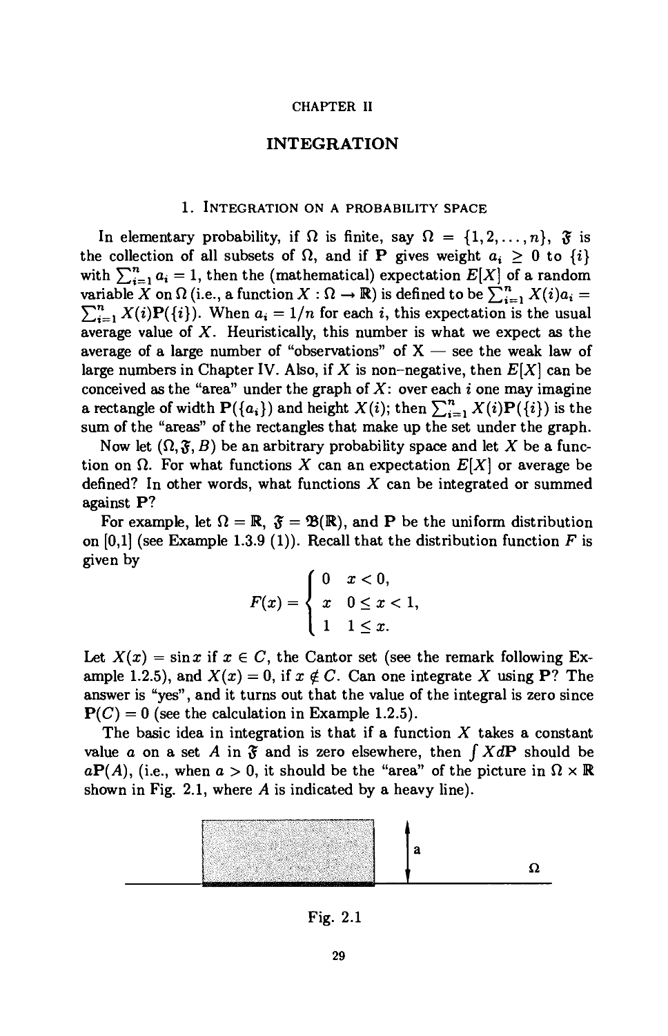


Текст
J.C. Taylor
An Introduction to Measure
and Probability
With 12 Illustrations
Springer
J.C. Taylor
Department of Mathematics and Statistics
McGill University
805 Sherbrooke Street West
Montreal, Quebec H3A 2K6
Canada
Library of Congress Cataloging-in-Publication Data
Taylor, J.C. (John Christopher), 1936-
An introduction to measure and probability/J.C. Taylor.
p. cm.
Includes bibliographical references and index.
ISBN 0-387-94830-9 (pbk.:alk. paper)
1. Measure theory. 2. Probabilities. I. Title.
QA325.T39 1996
519.2-dc20 96-25447
Printed on acid-free paper.
© 1997 Springer-Verlag New York, Inc.
All rights reserved. This work may not be translated or copied in whole or in part without the
written permission of the publisher (Springer-Verlag New York, Inc., 175 Fifth Avenue, New
York, NY 10010, USA), except for brief excerpts in connection with reviews or scholarly
analysis. Use in connection with any form of information storage and retrieval, electronic
adaptation, computer software, or by similar or dissimilar methodology now known or
hereafter developed is forbidden.
The use of general descriptive names, trade names, trademarks, etc., in this publication, even
if the former are not especially identified, is not to be taken as a sign that such names, as
understood by the Trade Marks and Merchandise Marks Act, may accordingly be used freely
by anyone.
Production managed by Hal Henglein; manufacturing supervised by Jeffrey Taub.
Camera-ready copy prepared from the author's Aj^S-1&. files.
Printed and bound by Maple-Vail Book Manufacturing Group, York, PA.
Printed in the United States of America.
98765432 1
ISBN 0-387-94830-9 Springer-Verlag New York Berlin Heidelberg SPIN 10524399
PREFACE
The original version of this book was an attempt to present the basics of
measure theory, as it relates to probability theory, in a form that might be
accessible to students without the usual background in analysis. This set of
notes was intended to be a "primer" for measure theory and probability —
a cross between a workbook and a text — rather than a standard "manual".
They were intended to give the reader a "hands-on" understanding of the
basic techniques of measure theory together with an illustration of their
use in probability as illustrated by an introduction to the laws of large
numbers and martingale theory. The sections of the first five chapters not
marked by an asterisk are the current version of the original set of notes
and constitute the essential core of the book.
Since the main goal of the core of this book is to be a "fast-track",
self-contained approach to martingale theory for the reader without a solid
technical background, many details are put into exercises, which the reader
is advised to do if a basic mastery of the subject is the goal.
The present book retains the basic purpose and philosophy of the original
set of notes but has been expanded to make it of more use to statisticians
by adding a sixth chapter on weak convergence, which is an introduction
to this very large circle of ideas as well as to the central limit theorem.
In addition, having in mind its possible use by students of analysis,
several sections in this book branch off from the central core to examine the
Radon-Nikodym theorem, functions of bounded variation, Fourier series
(very briefly), and differentiation theory and maximal functions. Measure
theory for er-finite measures reduces in many respects to the study of finite
measures and hence (after normalization) to the study of probabilities.
From this point of view, this book can serve as an introduction to measure
theory.
Each chapter, except for Chapter V, concludes with a section of
additional exercises in which various ancillary topics are explored. They may
be omitted on first reading and are not used in the core of this text. Much
of the material in the exercises may be found in the standard texts on
measure theory or probability that are cited. The author is of the opinion that
it is more useful to fill in details for many of these items than to read
completed arguments but is well aware that it is more time-consuming! Note
that the additional exercises and other sections marked by asterisks may
be omitted without prejudice to understanding the core of these notes.
There are six chapters: the first two chapters constitute the basic
introduction; and the remaining four explain some uses of measure theory and
Vll
Vlll
PREFACE
integration in probability. They have been written to be "self-contained",
and as a result, some background information from analysis is scattered
throughout. While this may no doubt appear to be excessive to the "well-
prepared" reader, it is my hope that with this approach the technical details
of the subject will be made accessible to the "well-motivated'' reader who
may not have all the appropriate background. In other words, I hope to
empower readers who wish to learn the subject but who have not come to
this point by a standard route. As in many things, a user-friendly
attitude seems to me to be very desirable. Whether these notes exhibit that
is obviously up to you, the reader, to judge.
As stated before, the main purpose of these notes is to explain and then
make use of the main tools and techniques of the theory of Lebesgue
integration as they apply to probability. To begin, Chapter I shows how to
construct a probability measure on the er-algebra 93 (R) of Borel subsets
of the real line from a distribution function F. Then Chapter II defines
integration with respect to a probability measure and proves the main
theorems of integration theory (e.g., the theorem of dominated convergence).
Also, it defines Lebesgue measure on the real line and explains the
relation between the Lebesgue integral and the Riemann integral. These two
chapters (excepting for §2.7 and §2.8 on the Radon-Nikodym theorem and
functions of bounded variation, respectively) constitute the essential part
of the central core of the book, and the reader is advised to be familiar
with them before proceeding further.
Chapter III is concerned with independence and product measures. It
deals mainly with finite products, although the existence of countable
products of probability measures is proved following ideas of Kakutani (and
independently Jessen) as an illustration of the use of measure-theoretic
techniques. This is the first technically difficult result in these notes, and
the reader can skip the details (as indicated) without any loss of
continuity. The extension of these ideas to prove the existence of Markov chains
associated with transition kernels on the real line is made in §3.5*.
Chapter IV discusses the main convergence concepts for random
variables (i.e., measurable functions) and proves Khintchine's weak law and
Kolmogorov's strong law of large numbers for sums of independent,
identically distributed (i.i.d.) integrable random variables. The chapter closes
with a discussion of uniform iiitegrability and truncation.
The last chapter of the original version, Chapter V, covers conditional
expectation and martingales. While sufficient statistics are discussed in
§5.3* as an application of conditional expectation, the bulk of the chapter
is an introduction to martingales. Doob's optional stopping theorem (finite
case) and the martingale convergence theorem (for discrete martingales) are
proved. The chapter concludes with Doob's proof of the Radon-Nikodym
theorem on countably generated er-algebras and the backward martingale
proof of Kolmogorov's strong law.
The final chapter, Chapter VI, examines weak convergence and the cen-
PREFACE
IX
tral limit theorem. It is independent of Chapter V and can be read
after having worked through §4.1 and §4.3 of Chapter IV together with the
beginning of §4.2. Tightness is emphasized, and an attempt is made to
enhance the mathematical focus of the standard discussions on weak
convergence. The discussion of uniqueness and the continuity theorem for the
characteristic function follows Feller's and Lamperti's approach of using the
Gaussian or normal densities. The central limit theorem is first discussed
in the i.i.d. case and concludes with the case of a sequence or triangular
array satisfying the Lindebergh condition.
The reader may find the references to standard texts and sources on
probability distracting. In that case, please ignore them. They are there
to encourage one to look at and explore other treatments as well as to
acknowledge what I have learned from them. In addition, if you are currently
using one of them as a text, it may be helpful to have some connections
pointed out. References are mainly to books listed in the Bibliography, and
the occasional reference to an article is done with a footnote. The book
by Loeve [L2] has many references in it and will be helpful if the reader
wants to explore the classical literature. For information and references on
martingales, Doob's book [Dl] has lots of historical notes in an appendix
and an extensive bibliography. Since these notes emphasize the connection
between analysis and probability, the reader wishing to go further into the
subject should consult the recent book [S2] by Stroock, which has a
decidedly analytic flavour. Finally, for a more abstract version of many of the
topics covered in these notes and for detailed historical notes, the book by
Dudley [D2] is recommended.
For several years since 1986, versions of these notes have been used
at McGill University (successfully, from my perspective) to teach a one-
semester course in probability to a mixed audience of statisticians and
electrical engineers. Depending on the preparation of the class, most of the
original version of this book was covered in a one-semester course. These
notes have also been used to teach an introductory course on measure
theory to honours students (in this case, the course was restricted to the first
four chapters with the sections on infinite product measures and Markov
chains omitted as well as §4.5* and §4.6*).
I would like to thank all the students who have (unwittingly)
participated in the process that has led to the creation of this set of notes; my
wife, Brenda MacGibbon of UQAM, for her enthusiastic encouragement,
my colleagues Minggao Gu and Jim Ramsay of McGill University and Ah-
mid Bose of Carleton University for their support and encouragement, as
well as Regina Liu of Rutgers and D. Phong of Columbia University. I
thank Jal Choksi of McGill University and Miklos Csorgo of Carleton
University for useful conversations on various points. In addition, I wish to
thank all my colleagues and friends who have helped me in many, many
ways over the years. I also wish to thank Mr. Masoud Asgharian and Mr.
Jun Cai for their diligent search for misprints and errors, and Mr. Erick
X
PREFACE
Lamontagne for help in final editing. Finally, I also wish to thank my copy
editor, Kristen Cassereau, and my editor at Springer, John Kimmel, for
their patience and professional help.
J.C. Taylor
CONTENTS
Preface vii
List of Symbols xiii
Chapter I. Probability Spaces 1
1. Introduction to R 1
2. What is a probability space? Motivation 5
3. Definition of a probability space 9
4. Construction of a probability from a distribution
function 16
5. Additional exercises* 26
Chapter II. Integration 29
1. Integration on a probability space 29
2. Lebesgue measure on R and Lebesgue integration 44
3. The Riemann integral and the Lebesgue integral 49
4. Probability density functions 55
5. Infinite series again 58
6. Differentiation under the integral sign 59
7. Signed measures and the Radon-Nikodym theorem* 60
8. Signed measures on R and functions of bounded
variation* 71
9. Additional exercises* 78
Chapter III. Independence and Product
Measures 86
1. Random vectors and Borel sets in Kn 86
2. Independence 89
3. Product measures 95
4. Infinite products 110
5. Some remarks on Markov chains* 119
6. Additional exercises* 131
Chapter IV. Convergence of Random Variables
and Measurable Functions 137
1. Norms for random variables and measurable functions 137
2. Continuous functions and Lp* 149
3. Pointwise convergence and convergence in measure or
probability 167
4. Kolmogorov's inequality and the strong law of large
numbers 176
5. Uniform integrability and truncation* 180
xi
CONTENTS
6. Differentiation: the Hardy-Littlewood maximal
function* 186
7. Additional exercises* 199
Chapter V. Conditional Expectation and
an Introduction to Martingales 210
1. Conditional expectation and Hilbert space 210
2. Conditional expectation 217
3. Sufficient statistics* 226
4. Martingales 229
5. An introduction to martingale convergence 238
6. The three-series theorem and the Doob decomposition 241
7. The martingale convergence theorem 245
Chapter VI. An Introduction to
Weak Convergence 250
1. Motivation: empirical distributions 250
2. Weak convergence of probabilities:
equivalent formulations 251
3. Weak convergence of random variables 255
4. Empirical distributions again: the Glivenko-Cantelli
theorem 260
5. The characteristic function 262
6. Uniqueness and inversion of the characteristic function 266
7. The central limit theorem 273
8. Additional exercises* 281
9. Appendix* 284
Bibliography 291
Index 293
LIST OF SYMBOLS
ZA, 6
a, 6
A, 15
Ac, 6
a A 6, 5
aVb, 5
»(R), 14
93(R2), 87
93(Rn), 87
93(E), 131
93(1)^,82
6(n,p), 141
Cb(E), 153
CC(R), 150
Cc(0), 150
C(E), 151
Ct(R), 153
Cc(Rn), 152
6o,26
d(F,,F2),257
Dh, 258
£>F+(x), 194
DF-(x), 194
DF+(x), 194
DF.(i), 194
dist(x,C), 150
EAB, 78
eo,26
e«, 26
{En i.o.}, 148
E+, 64
xiv LIST OF SYMBOLS
£+,66
£-,64
£-,66
E[a], 30
E[X], 38
E[X\Y = y], 220
E[X\0], 212
{$t)tei, 229
/, 158
S,9
Si O &, 97
Si x fo, 97
®~=1&,, 113
</>c 181
xn=l"n, 11"
/ *2w 5, 160
/ • A", 232
/* 5,157
/i * /2, 109
/i * P2, 108
Fn -¾ F, 251
Fn => F, 251
Fn{x,u), 250
ffr, 234
H„(x,0,80
51, 193
/a(w)P(dw), 30
/ sdP, 30
/ XdP, 38
/0+oo/(x)dx,54
/>(s)dz,50
#„, 160
^(n.&PMl
eu 58
/2, 59
/, 217
LIST OF SYMBOLS
xv
/P, 143
C> 143
lim inf n an, lim inf an, 33
n
lim supn an, lim sup an, 33
n
L, 137
L(n,tp), 49
LJ,41
L^N.^NJ.dn), 58
L2, 139
L°°, 144
Lp, 141
L?(n, 3, m), 146
LP(n,5,P), 146
M2(x0,dx), 123
M2(xo,dxi,dx2), 123
Mn(xo,dxi,dx2, ■ ■. ,dxn), 128
371,25
Ml x M2 X • •• X Hn, 104
Af, 239
(, ),(, ),59
N, 1
N, 120
N(x0,dxi), 123
i/+,65
v~, 65
v « ft, 66
II II, 58
n(x), 79
nt{x), 79
(n,5,P),9
(fti xn2,5i xfo.Pi xPj), 99
(fii x n2,$i x ^2,Mi x M2), 105
(fii x n2 x • • • x fin, Jj x fo x • • • x £„, Pj x P2 x • • • x Pn), 102
(x2i,nfc, x^=15fc, x~ jPfc), 118
x~ ,nn, 113
Pi x P2, 99
XVI
LIST OF SYMBOLS
P,9
P(du\B), 223
P*, 21
P[X < x\Y = y], 221
Pi ® P2, 99
Pj x P2 x • • • x Pn, 102
Pi*P2, 108
j)*, 187
X»=1Pn, , US
Pn, 175
Q, 1
Q2(dxo,dxi,dx2), 124
Qn(dxo,dxi,...,dx„), 125
R, 1
9¾. 45
<r(€), 14
a{X), 140
<r2(X), 140
a, 140
<T({Xt | i € F}), 110
tr({Xt | l € /}), 110
<r({X,- | 1 < z < n}), 93
<r({X,- | i € F}), 93
<r2, 140
5„, 170
T, 159
U([a,b}), 246
U(v,<p),49
Ux([a,b}),246
V(E), 62
V(E), 65
V(*), 72
V(*,[a,b]),71
V(*,7r),71
V+($,7r), 74
V" (*,«■), 74
LIST OF SYMBOLS xvii
Xn -^ X, 255
|| X II,, 137
II X U, 144
II X ||2, 139
II X ||p, 141
XAY, 233
X\ 237
X+,35
X-,35
x+, 5
x~, 5
X e 5, 32
Xc, 180
Xn t±5- X, 167
Xn ^ X, 167
Xn -^ 0, 145
Xn -^ X, 168
Xn -^ X, 168
Xn -^ X, 255
Xn => X, 255
Xn P-^ X, 167
Xn ^^ X, 167
Xr, 235
|X|,41
1*1,5
Z, 1
CHAPTER I
PROBABILITY SPACES
l. Introduction to R
An introduction to analysis usually begins with a study of properties of
R, the set of real numbers. It will be assumed that you know something
about them. More specifically, it is assumed that you realize that
(i) they form a field (which means that you can add, multiply, subtract
and divide in the usual way), and
(ii) they are (totally) ordered (i.e., for any two numbers a, b € R, either
a < b, a = b, or a > b) and a > b if and only ifb— a > 0. Note that
a < b and 0 < c imply ac < be; a < b imply a + c < b + c for any
ceK;0< 1 and-l< 0.
Inside R lies the set Z of integers {..., —2, —1,0,1,2,3,... } and the
set N of natural numbers {1,2,...}. Also, there is a smallest field inside
R that contains Z, namely Q, the set of rational numbers {p/q : p,q €
Z and q ^ 0}. A real number that is not rational is said to be irrational.
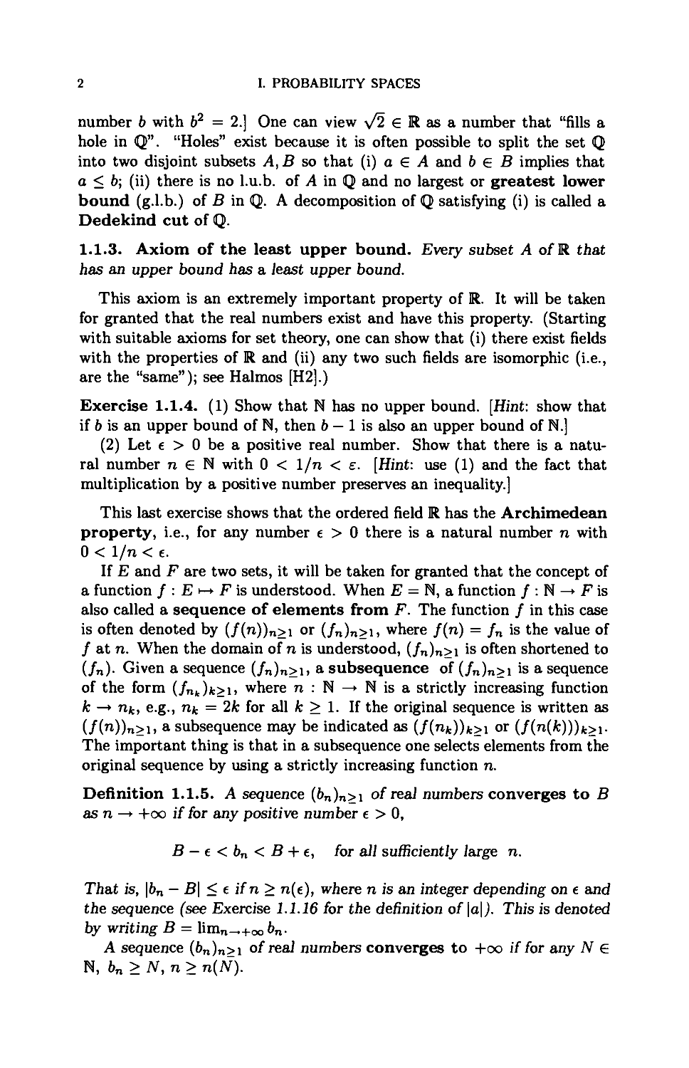
It is often useful to view R as the points on a straight line (see Fig. 1.1).
1 1 »-
0 1
Fig. 1.1
Then a < b is indicated by placing a strictly to the left of b, if the line
is oriented by putting 0 to the left of 1. The field Q is also totally ordered,
but it differs from R in that there are "holes" in Q. To explain this, it is
useful to make a definition.
Definition 1.1.1. Let A C R. A number b with the property that b> a
for all a e A is said to be an upper bound of A. Ifb<a for all a € A, b
is said to be a lower bound of A.
Example. Let A = {a €R\ a < 1}. Then any number b > 1 is an upper
bound of A. Here there is a smallest or least upper bound (l.u.b.),
namely 1.
Exercise 1.1.2. Let A = {a e Q | a2 < 2}. Show that if there is a
least upper bound of A, it cannot belong to Q. [Hints: show that, for small
p > 0,a2 < 2 implies that (a+p)2 < 2 and a2 > 2 implies that {a-p)2 > 2;
conclude that if b is a l.u.b. of A, then b2 = 2; show that there is no rational
l
2
I. PROBABILITY SPACES
number b with b2 = 2.] One can view \/2 € R as a number that "fills a
hole in Q". "Holes" exist because it is often possible to split the set Q
into two disjoint subsets A, B so that (i) a 6 A and b e B implies that
a < b\ (ii) there is no l.u.b. of A in Q and no largest or greatest lower
bound (g.l.b.) of B in Q. A decomposition of Q satisfying (i) is called a
Dedekind cut of Q.
1.1.3. Axiom of the least upper bound. Every subset AofR that
has an upper bound has a least upper bound.
This axiom is an extremely important property of R. It will be taken
for granted that the real numbers exist and have this property. (Starting
with suitable axioms for set theory, one can show that (i) there exist fields
with the properties of R and (ii) any two such fields are isomorphic (i.e.,
are the "same"); see Halmos [H2].)
Exercise 1.1.4. (1) Show that N has no upper bound. [Hint: show that
if b is an upper bound of N, then b — 1 is also an upper bound of N.]
(2) Let e > 0 be a positive real number. Show that there is a
natural number n € N with 0 < 1/n < e. [Hint: use (1) and the fact that
multiplication by a positive number preserves an inequality.]
This last exercise shows that the ordered field R has the Archimedean
property, i.e., for any number e > 0 there is a natural number n with
0 < 1/n < e.
If E and F are two sets, it will be taken for granted that the concept of
a function / : E >-► F is understood. When E = N, a function / : N —► F is
also called a sequence of elements from F. The function / in this case
is often denoted by (/(n))n>i or (/n)n>i, where f(n) = fn is the value of
/ at n. When the domain of n is understood, (/n)n>i is often shortened to
(/„). Given a sequence (/n)n>i) a subsequence of (/n)n>i is a sequence
of the form (/nt)fc>i) where n : N —► N is a strictly increasing function
k —* Tik, e.g., nfc = 2k for all k > 1. If the original sequence is written as
(/(n))n>i, a subsequence may be indicated as {f{n.k))k>\ or (/W0))fc>i-
The important thing is that in a subsequence one selects elements from the
original sequence by using a strictly increasing function n.
Definition 1.1.5. A sequence (6n)n>i of real numbers converges to B
as n —> +oo if for any positive number e > 0,
B — t < bn < B + e, for all sufficiently large n.
That is, \bn — B\ < e ifn > n(e), where n is an integer depending on e and
the sequence (see Exercise 1.1.16 for the definition of \a\). This is denoted
by writing B = limn_+00 6n.
A sequence (6n)n>i of reai numbers converges to +oo if for any N e
N, bn>N,n> n{N).
1. INTRODUCTION TO R
3
Exercise 1.1.6. Let (6n)n>i be a non-decreasing sequence of real
numbers, i.e., bn < 6n+i for all n > 1. Show that
(1) the sequence converges,
(2) the limit is finite if and only if the sequence has an upper bound,
(3) when the limit is finite, it equals the l.u.b. of {bn \ n> 1}.
Let (b'n)n>\ be another non-decreasing sequence with 6n < b'n for all
n > 1. Show that
(4) limnb„ < lim 6^,.
Definition 1.1.7. Let (an)n>o be a. sequence of real numbers. Let sn —
ao + ai + Q2 H 1- an- The sequence (sn)n>o is called the infinite series
H^Lo °n' an(^ ^e senes 1S ^^ to converge if (sn)n>o converges.
Exercise 1.1.8. Let (an)n>0 be a sequence of positive real numbers. Show
that
(1) the series YlnLoan converges if and only if {sn | n > 0} has an
upper bound,
(2) if 5I^L0 an converges, then it converges to l.u.b. {sn | n > 0}.
Finally, show that
(3) if H^Lo °n converges to a finite limit, then lim^_00 5Z^LN an = 0.
Exercise 1.1.9. Suppose one has a random variable X whose values are
non-negative integers. Let (an)n>o be a sequence of positive real numbers.
When can the probability that X is n equal can where c is a fixed constant?
What happens if an = £? (if an = £ or an = ;n^or („3"^)?) This
exercise begs the question: what is a random variable? For the time being,
think of it as a procedure that assigns probabilities to certain outcomes.
The definition is given in Chapter II, see Definition 2.1.6.
Exercise 1.1.10. A random variable X has a Poisson distribution with
mean 1, if the probability that X is n is e_1/n!. (see Feller [Fl] for the
Poisson distribution).
Proposition 1.1.11. (Exchange of order of limits). Let (6m,n)m,n>i
be a double sequence of reai numbers, i.e., a function b : N x N —► R.
Assume that
(1) m! < m2 => 6mi,„ < 6m2,n for all n > 1,
(2) m < n2 => 6m,ni < 6m,„2 for allm> 1.
Then
lim ( lim 6mn)= lim ( lim bmn) = lim bnn,
n—>+oo m—»+00 m—»+oo n—»+oo ' n—>+oo
where an increasing sequence has limit +00 if it is unbounded.
Proof. By symmetry it suffices to verify the second equality. Now 6m,m <
def
6nri if m < n and so B = 1101,,-.006nn exists, as does Bm = limn_oobm^n.
4
I. PROBABILITY SPACES
Also, by Exercise 1.1.6, Bm < B as 6mn < 6nn when n > m. It follows
from (1) and Exercise 1.1.6 that Bmi < Bm2. Hence, limm_oo£m = B!
exists and is less than or equal to B (see Exercise 1.1.6 again).
If B is finite, let e > 0 and n = n(e) be such that B — e < &„,„ < B if
n > n(e). Let m = n(e). Then Bm = limn_oobm,n > &n(e),n(e) > B - t.
Hence, B' = B as B' > Bm for all m.
If B = +00 and N < &„,„ for n > n(N), then Bm = limn_oo 6m,n > N
if m = n(N) and so B' = +00. D
Corollary 1.1.12. £~i(£°Li atj) = E^i(ESi °o) ^¾ > 0,1 < i, J-
Proof. Let 6m,n = £^! H"=i 0*3 and verify that the conditions of
Proposition 1.1.11 are satisfied. D
Exercise 1.1.13. Decide whether Proposition 1.1.11 is valid when only
one of (1) and (2) is assumed. In Corollary 1.1.12, what happens if an =
IjOt.t+i = —1 for alii > 1 and all other ay = 0?
Exercise 1.1.14. (See Feller [Fl], p. 267.) Let p„ > 0 for all n > 0 and
assume E^oPn = 1. Let mT = E^=onrPn- Show that E~ 0 Tf<r =
E~=oPnentfort>0.
This brief discussion of properties of K concludes with a discussion of
intervals.
Definition 1.1.15. A set I c K is said to be an interval if x < y < z
and x,z e I implies y € I.
If an interval I has an upper bound, then I c (—00,6], where 6 = l.u.b.
I and (-00,6] = {x € R \ x < b}. If it also has a lower bound, then
I C [a, 6] = {x I a < x < b} if a = g.l.b. I. A bounded interval I — one
having both upper and lower bounds — is said to be
(1) a closed interval when I = [a,b],
an open i
by ]a,b[),
(3) a half-open interval when I = (a,b] or [a,6), where (a,b] = {a
a < x <b} and similarly [a,b) = {a \ a < x < b}.
One also denotes (a,b\ by }a,b] and [a, 6) by [a,b[.
An unbounded interval I is one of the following:
(-00,6) = {x I x < b);
(-00,6] = {x I x < 6};
(a, +00) = {x I a < x};
[a, +00) = {x I a < x}; or
(-00,+00) = R.
def
(2) an open interval when I = (a, b) = {x | a < x < b) (often denoted
2. WHAT IS A PROBABILITY SPACE? MOTIVATION 5
Exercise 1.1.16. If x e R, define |x| = x if x > 0 and = (—l)x if x < 0.
Let a, b be any two real numbers. Show that
(1) \a + b\ < \a\ + |6| (the triangle inequality),
(2) conclude that ||a| - |6|| < \a — b\ by two applications of the triangle
inequality.
If a, b are two numbers, let a V b denote their maximum, also denoted by
max{a, b}, and a A b denote their minimum, also denoted by min{a, b}.
Define x+ to be max{x, 0} = x V 0 and x~ to be max{—x, 0} = (—x) V 0.
Show that
(3) x~ = -(xAO),
(4) x = x+ — x",
(5) |x| = x++x~,
(6) aV6= i{a + 6+ |a-6|}, and
(7) aAb= ±{a + b-\a-b\}.
Exercise 1.1.17. Verify the following statements for —oo < a < b < +oo:
(1) (a,6) = U~=N(a,6-i], where 6 - a > £;
(2) [a,6) = n~N(a-l,6);
(3) [a,6] = n~ ,^,6+1).
Show that if Xo € (a, b), then (xo — 6, Xo + S) C (a, b) for some 6 > 0 (this
implies that (a, b) is an open set; see Exercise 1.3.10).
Exercise 1.1.18. Let 0 < a < 1. If p > 0, show that qp = eploga is an
increasing function of p and that limp-.oo a' = 1.
Exercise 1.1.19. Let R be the union of two disjoint intervals I\ and h-
Show that
(1) one of the two intervals is to the left of the other (either Xi e I\
and X2 6 h always implies Xi < X2 or vice-versa), and
(2) if neither of these two intervals is the void set, then sup/i = inf /2
if /1 is to the left of /2-
Let (/„) be an increasing sequence of intervals. Show that
(3) if I = Un/n, then I is an interval.
Assume that each In above is unbounded and bounded below, i.e., there
is an € R with (an,+oo) c In C [an,+00). Assume that I has the same
property. Show that
(4) if (a, +00) C I C [a, +00), then lim an = a.
For further information on the real line and general background
information in analysis, consult Marsden [Ml] or Rudin [R4].
2. What is a probability space? Motivation
A probability space can be viewed as something that models an
"experiment" whose outcomes are "random" (whatever that means). There
6
I. PROBABILITY SPACES
are often "simple" or "elementary outcomes" in the model (as points in an
underlying set fi and weights assigned to these outcomes that indicate the
likelihood or probability of the outcome occurring (see Feller [Fl]). The
general outcome or "event" is often a collection of "elementary outcomes".
For example, consider the following.
Example 1.2.1. The "experiment" consists of rolling a fair six-sided die
two times. The "elementary outcomes" could be taken to be ordered pairs
w = (m, n), where m and n are integers from 1 to 6. The set fi of elementary
outcomes may be taken to be the set of all such ordered pairs (it is usual to
denote this set as the Cartesian product {1,2,..., 6} x {1,2,..., 6}). The
set of all events may be taken as the collection of all subsets of fi, denoted
by 7>(fi). If each elementary outcome w is assigned weight ^,, then one
may define the probability P(A) of an event A by P{A) = J2ueA ^({^}) =
= Jjj^, where \A\ denotes the number of elements in A. If the die is
not fair — the probability of getting either a 1,2,3, or a 4 is § and for
example that of getting either a 5 or a 6 is | — then the basic probabilities
or weights of the elementary outcomes will need to be altered to correspond
to the new situation.
For elementary situations as in Example 1.2.1, it suffices to consider a
so-called finitely additive probability space. This is a triple (fi,2l, P),
where fi is a set (corresponding intuitively to the set of "elementary
outcomes" , 21 is a collection of subsets of fi (the "events") with certain
"algebraic" properties that make it into a Boolean algebra of subsets of fi,
and for each event A € 21 there is a number P(A) assigned that lies between
0 and 1 (the probability of the occurrence of A). More explicitly, to say
that 21 is a Boolean algebra means that the collection 21 of subsets satisfies
the following conditions:
(210 «€*;
(2l2) Ai, A2 € 21 implies that Ax U A2 € 21; and
(¾) A € 21 implies that Ac € 21, where Ac =f {w e fi | u ¢ A) =f CA.
The statement that P is a probability means that it is a function defined
on 21 with the following properties:
(A) P(fi) = 1;
(Fi) 0 < P(A) < 1; and
{FAP3) Ax n A2 = 0 =► P(A, U A2) = P(Ai) + P(A2).
It is not hard to see that Example 1.2.1 is a finitely additive probability
space.
Some simple consequences of the properties of a Boolean algebra 21 and
a finitely additive probability defined on it are given in the next exercise.
Exercise 1.2.2. Show that
(1) A\, A2 € 21 implies that Ax n A2 € 21 and A\ n A2 e 21 (one often
denotes A\ n A2 by A^\A2 or A^ n CA2),
2. WHAT IS A PROBABILITY SPACE? MOTIVATION
7
(2) P(0) = 0,
(3) Ax c A2 implies that P(Ai) < P(A2),
(4) P(A1uA2)<P(Al)+P(A2),
(5) P(Aj U A2) + P(Aj n A2) = P(Aj) + P(A2),
(6) P(U£=1Afc) = ELi P(M Uk,1 A,-) < ELi P(A*).
Remark 1.2.3. In Exercise 1.2.2 (6), a union of sets u£=1Afc is converted
to a disjoint union u£=1 A'fc, where A'k = Afc\ uJl/ A,. This is a standard
device or trick that is often used, especially for countable unions A =
Here is another example of an "experiment" with "random" outcomes.
Example 1.2.4. What probability space is it natural to use to discuss
the probability of choosing a number at random from [0,1]? What is the
probability of choosing a number from (^, |]? Clearly, one should take fi to
be [0,1] and 21 to be the collection of finite unions of intervals contained in
[0,1] (so that 21 is a Boolean algebra containing intervals and their unions).
Show that 21 is a Boolean algebra. How do you define P on 21?
Example 1.2.5. Continuing with the same probability space as in
Example 1.2.4, suppose that one wants to discuss the probability of selecting at
random a number x with the following property: it does not lie in (^, §)
— i.e., the middle third of [0,1] — nor does it lie in the middle third of
either [0, g] or [|, 1] — and so on, infinitely often. This describes a subset
C of [0,1], an event.
Look at the complementary event Cc: it is the disjoint union of middle
third intervals; C< = (I, §)u[(i, |)u(|, §)]u[(£, &)U(£, Jr)U(i|, §g)U
(i,§i)]u....
Let q be the probability of Cc. Then one sees that
(1) Q>h
(2) <7>3 + ! + i = 3 + l.
(3) 9>i + | + f7,
(n) q>\ + l + 4t + --- + *£-.
To verify this, one makes use of the principle of mathematical induction,
stated below.
The principle of mathematical induction. Let P{n) be a proposition
or statement for each n € N. If
(1) P(l) is true and
(2) P(n+ 1) is true provided P(n) is true,
then P(n) is true for all n. (This principle amounts to saying that if A c N
is such that (1) 1 e A and (2) n € A implies n + 1 e A, then A = N).
8
I. PROBABILITY SPACES
Now g + | + ^H H ^yr- is the nth partial sum of the series YlT=o 3^rr-
This is a geometric series with ao = g and r = |, and so the sum is
g(l — |)-1 = 1. Consequently, one expects the probability of choosing
such an x from C to be zero!
Remark. The subset C of [0,1] described in Example 1.2.5 is called the
Cantor set or Cantor discontinuum. It contains no interval with
distinct end points. Why? What would happen if instead of extracting middle
thirds one removed the middle quarter at each stage?
Note that neither the Cantor set C nor its complement is in the Boolean
algebra 21 defined in Example 1.2.4, as the set Cc is the union of an infinite
number of open intervals each of which is in the Boolean algebra 21: it
can be shown that Cc cannot be expressed as a finite union of sets from
21 — this has to do with the fact that each of the intervals involved is a
connected component of Cc, i.e., for any point x in one of these intervals
I, the largest open interval that contains it coincides with I (see Exercise
1.3.11).
Example 1.2.6. (Coin tossing) Suppose one tosses a fair coin until a
head occurs. What is the probability of this event? To begin with, what
could one take as fi, the set of "elementary outcomes"? Take fi to be N,
where each n > 1 corresponds to a finite string of length n that commences
with n — 1 heads and concludes with a tail. Here probabilities may be
assigned to each integer n > 1, namely ^ for the string of length n. Since
J2^L i 2^r = \ (t^"1") = * ^is gives a probability space with 21 taken to
be all the subsets of fi and P{A) defined to be J2neA 2^- Therefore, the
probability of first obtaining a head on an even number toss is YlV=i 2*^ =
3 (yzt) = g- In this example, you can verify that if A = Uj^-A,, and
An n Am = 0 when n ^ m, then P{A) = £~=1 P(i4n). This is clearly
a desirable property of a probability, but how can it be obtained in the
context of the previous exercise, where fi = [0,1]?
Example 1.2.7. Suppose X is a random variable with unit normal
distribution, i.e., the probability that a < X < b is —i= fa e'^^^dx = P((a, b]).
What is the probability p that X takes values in the Cantor set? Imitating
Example 1.2.5, one may compute the probability q of the complementary
set. Then
(1) 9>P((3,1)),
(2) 9>P((i,§)) + P((I,|))+P((I,|)),and
(n) 9>P((i,§)) + P((I,|)) + P((I,|)) + ... + P((3^2,3^i)).
Therefore, one expects the probability p to be
l-limn^fPUl, §)) + P((i, |)) + P((|, §)) + P((£, &)) + P((£, Jr))
+ P((»,»)) + P((» »)) + ... + P((31=2, 31=1))}.
3. DEFINITION OF A PROBABILITY SPACE 9
At this point, it is not so clear what the answer should be here. In fact it
is zero! (See Proposition 2.4.1.)
Exercise 1.2.8. Write a more explicit formula for the probability that the
above random variable X takes values in the set Cn, which results after the
procedure for constructing the Cantor set has been applied n times. This
amounts to getting a handle on this set by writing an explicit description
of the intervals involved in the removal process.
[Hints: after completion of the nth stage of the procedure for
constructing the Cantor set, one is left with 2n intervals each of length -L. They
are all translates of the interval [0, g^]. To describe Cn, it suffices to
determine the left hand endpoints of these intervals. One may do this by
observing that, for each integer n, if k < 3n, then k has a unique
expression as k = Yl^Zo °>3' witn the a* e {0,1,2}. One may use this to write
a triadic "decimal" expansion for the left hand endpoints of the intervals
remaining at the nth stage. Show that they will be of the form O.&162 • • • bn
with bi € {0,2}, where O.&162 • • • &n = ^r E"=i W1-'- Show that one may
obtain them from the 2n_1 left hand endpoints occurring at the (n — l)st
stage by first putting a zero in the "first position", i.e., by shifting the
"decimal" over to the right by one place and inserting a zero and then
doing the same thing but this time inserting a two.]
What Examples 1.2.5, 1.2.6, and 1.2.7 hint at is the following: while
one often starts to construct a probability using some "obvious" definition
for certain simple sets (those in 21), it is soon useful and necessary to try
to extend the probability to more complicated sets that are made up from
those of 21 by infinite operations. In addition the probability should not
only be finitely additive (i.e., satisfy (FAP3)), but also countably additive,
as its computation will often involve infinite series.
3. Definition of a probability space
Definition 1.3.1. (fi, 5, P) is said to be a probability space if Q is a
set, 5 is a er-algebra of subsets of fi, and P is a (countably additive)
probability on 5- To say that 5 is a <7-aJgebra means that the collection
5 of subsets of fi satisfies
(ffi) ftefr
($2) A e 5 implies Ac e 5; and
(¾) (A„)n>i C 5 implies U~ ,A„ € 5-
furthermore, P is a function defined on 5 that satisfies
(P,) P(fl) = 1;
(P2) 0 < P{A) < 1 if A e 5; and
(P3) {An)n>\ C 5, and An D Am = 0 ifn ^ m implies
P(U£°=1>ln) = E~=i P(An) (countable additivity).
10
I. PROBABILITY SPACES
Remarks. (1) A probability differs from a finitely additive probability
by the important property of being countably additive (/¾) (also called
er-additive).
(2) A probability space is also a finitely additive probability space since
countable additivity (/¾) implies finite additivity (FAP3).
(3) A er-algebra is also called a er-field.
In Example 1.2.4, the basic way of computing probability was to assign
length to intervals contained in [0,1]. Corresponding to this is a natural
function F, which determines these probabilities: define F(x) to be the
length of [0,x] if 0 < x < 1. This function can be extended to all of R
by setting F(x) = 0 when x < 0 and F(x) = 1, if 1 < x. This extended
function can be used to assign a probability to any interval (a, b]: namely,
P((a,6]) = F(b) - F(a). This probability is the length of (a,b] C\ [0,1]. As
a result, the "experiment" of Example 1.2.4 can also be modeled by using
all the intervals of R as basic events, with the proviso that any interval
disjoint from [0,1] has probability zero. The function F is an example of a
distribution function (see Definition 1.3.5).
Whenever one has a probability space (fi, J, P) with fi = R and the a-
algebra 5 contains every interval (—oo,x], then the probability determines
a natural function in the same way: let F(x) = P((-oo,x]).
This function has the properties (DF\), (DF^), and {DF3) stated in the
following proposition.
Proposition 1.3.2. The function F(x) = P((—00,x]) associated with a
probability P has the following properties:
(DFi) x < y implies F(x) < F(y) (i.e., F is a non-decreasing function);
{DF2) (i) limx_+00 F(x) = 1 (i.e., for any positive number e, F(x) > 1 - e
if x is large enough and positive); and
(ii) limx__oo F(x) = 0 (i.e., for any positive number e, F(x) < e if
x is negative and \x\ is sufficiently large);
(.0/¾) for any x, if(xn) is a sequence that decreases to x, then the vaJues
F(xn) decrease to F(x) (i.e., F(x) = lim,,-,,*, F(xn)).
Proof. As an exercise prove {DF\) and (DF^) using properties (^1),(^2),
and (/¾). [For the first part of (DF2) use Exercise 1.1.8 (3) and the fact
that R = u£r-oo(". n + 1] to show that 1 = F(n) + ££Ln P((k, k + 1]).]
The property (.0/¾) says that for any x, the values of F(xn) as xn
approaches x from above (i.e., from the right) approach F(x). The technical
formulation of this statement is that limn_00 F(xn) = F(x) if x < xn+i <
xn and limn xn = x. Since F is non-decreasing, it suffices to show that for
any x, F(x) = lim,,^ F{x + ±).
Let An = (x,x + £]. Then i4n+1 c An and n£°=1,4n = 0. Now Ai =
(x,x+l] =Uf=1(x + v^ryx + \}a.ndAn = U£Ln(x+ ^,x+ ±]. Hence,
P(Ai) = £r=iP((*+*TT.z+j]) < 1. andso£~„P((z+*TT>*+s]) =
3. DEFINITION OF A PROBABILITY SPACE
11
P(i4n) —► 0 as n —► +oo since it is the tail end of a convergent series. Now
F(x + £) = F{x) + P{An). Hence, lim,,^ F(x + ^) = F(x). D
Exercise 1.3.3. Let (i4n)n>i be a sequence in 5, where (fi,5,P) is a
probability space. Show that P(An) —► 0 if (1) An D An+\ for all n > 1
and (2) n~ xAn = 0.
The property {DF3) of a distribution function is a reflection of the
countable additivity of P. It can be reformulated by saying that F(x) is right
continuous at every point x.
Definition 1.3.4. A function F : R —► R has a right limit A at a point
a e R if, for any e > 0, there exists a 6 > 0, where 6 = 6(a, e), such that
\F(x) — A| < e whenever a < x < a + 6.
The right limit A is denoted by F(a+). The function F is right
continuous at a if F(a) = F(a+). Similarly, one defines the left limit F(a-) to
be A if, for any e > 0, there exists a 6 > 0, where 6 = 6(xo, e), such that
|F(x) - A| < e whenever a - 6 < x < a
and F is left continuous at a ifF(a) = F(a-).
Remark. When F is the distribution function of a probability, then F(a—)
= P((-oo,a)) (see Exercise 1.4.14 (3)).
Definition 1.3.5. A function F : R —► [0,1] is said to be a distribution
function if
(1) it is non-decreasing and right continuous; and
(2) limI__00 F(x) = 0 and limI_+00 F(x) = 1.
A distribution function F determines the probability of certain sets,
namely the probability of (a, b], where P((a, 6]) = F(b) — F(a). This notion
of probability can then be extended to the Boolean algebra 21 generated by
the intervals (a, b], where A G 21 if and only if A is a finite union of intervals
of the form (a, b], with —oo < a < b < +oo, and by convention one takes
(—oo, +oo] = R. Note that 21 is the smallest Boolean algebra containing
all the intervals (-oo,x]),x G R. A priori, there is no reason why the
probability P on 21 determined in this way by a distribution function F
should come from a probability on a er-algebra J containing the Boolean
algebra 21. This raises the following issue.
Basic Problem 1.3.6. Given a distribution function F on R, are there a
(T-algebra 5 D 21 and a probability P on J such that F is the distribution
function ofP? Note that for such a probability P, it follows that P( (a, b]) =
F(b) - F(a) whenever a<b?
12
I. PROBABILITY SPACES
Remark. As will be seen later in Theorem 2.2.2, this basic problem has
an important generalization: the distribution function F is replaced by
any right continuous, non-decreasing function G on R. Then the question
becomes: is there a er-algebra J D 21, and is there a function /joiiJ that
behaves like a probability except that its value on fi = R is not forced to
be 1? For example, if G(x) = x for all x, then such a set function fi would
compute the length of sets.
Returning to distribution functions, the rest of this chapter is devoted
to the solution of Basic Problem 1.3.6: to show that every distribution
function comes from a probability. As a first step, one has the following.
Exercise 1.3.7. Let 21 be the collection of finite unions of intervals of
the form (a, b], where —oo < a < b < +oo, and by convention one takes
(-oo, +oo] = R. Verify that
(1) 21 is a Boolean algebra, (i.e. it satisfies (2li), (212),(¾) of §1.2 ),
and
(2) there is one and only one finitely additive probability P on 21 such
that P{{a,b}) = F{b) - F{a) for all a < b.
Hints: (1) Show that any A G 21 can be written as a finite pairwise
disjoint union of intervals of the form (a, b); note that the union of two
intervals of this type is an interval of this type if they are not disjoint and
observe that (a, b] D (c, d] is 0 or (a V c, b A d\. (2) Convince oneself of (2) by
showing that if A = U"=i(aj,6j] with the intervals pairwise disjoint, then
52"=1{F(6j) - F(a,i)} is not dependent on the particular way A is written
as a disjoint union. For example if A = (0,3] = (0,l]u(l,3] = (0,2]u(2,3],
thenP((0,3]) = F(3)-F(0) = {F(1)-F(0)} + {F(3)-F(1)} = P((0,1]) +
P((l,3]). [Suggestion: given two disjoint unions, make up a "finer" disjoint
union by using the second one to "cut up" all the intervals of the first.]
Convention 1.3.8. Until further notice, unless otherwise stated or the
context makes it evident (see Definition 1.4.2), 21 wiJJ denote the above
Boolean algebra of finite unions of half-open intervals (a, b] C R.
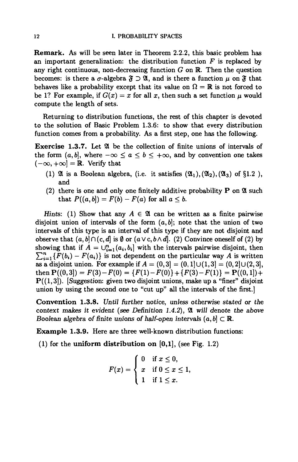
Example 1.3.9. Here are three well-known distribution functions:
(1) for the uniform distribution on [0,1], (see Fig. 1.2)
{0 if x < 0,
x if 0 < ar < 1,
1 if 1 < x.
3. DEFINITION OF A PROBABILITY SPACE
13
(0.1)
(1.0)
Fig. 1.2
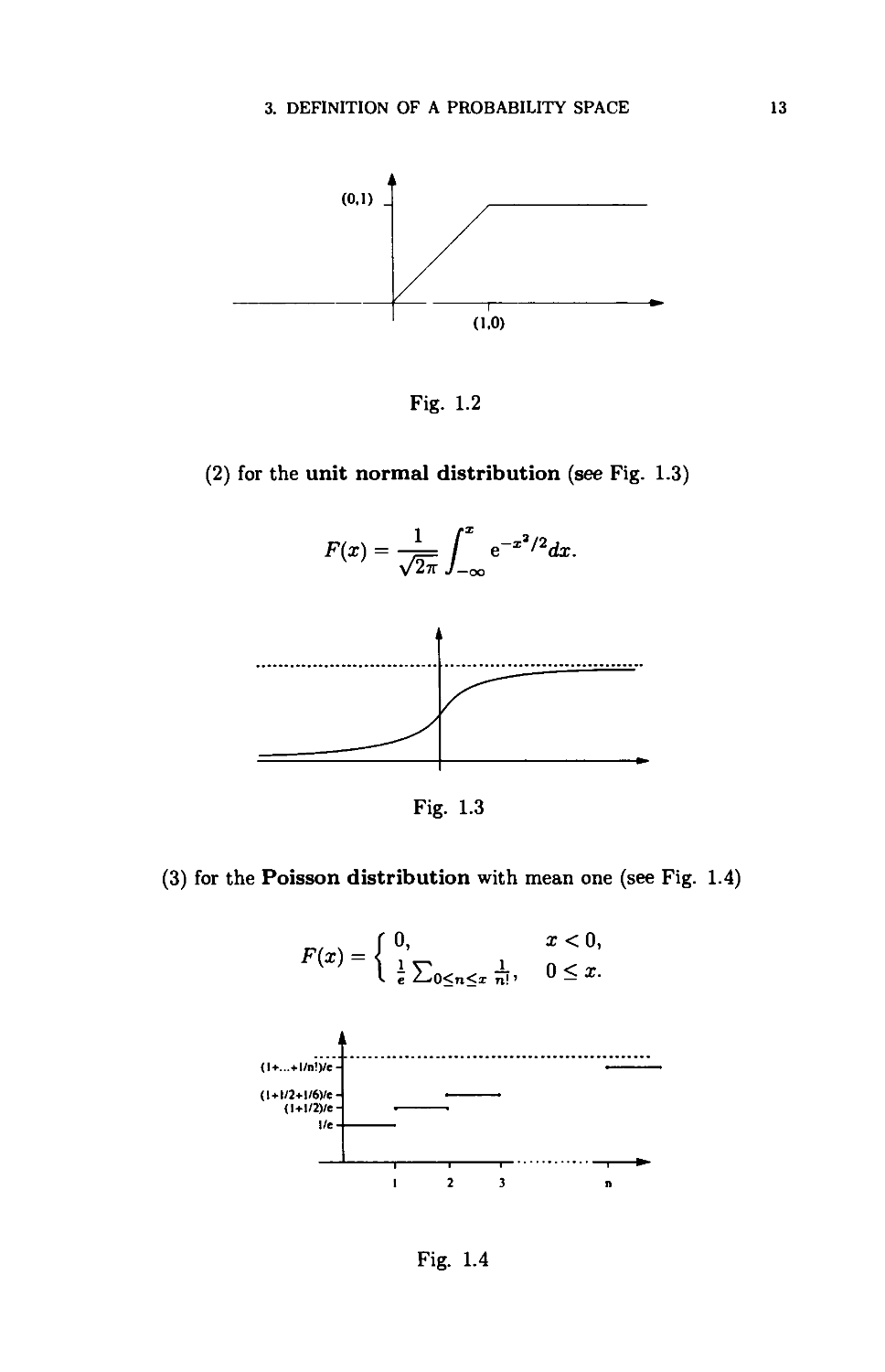
(2) for the unit normal distribution (see Fig. 1.3)
F(x)
= — f
\fhtJ-c
e~*3'2dx.
Fig. 1.3
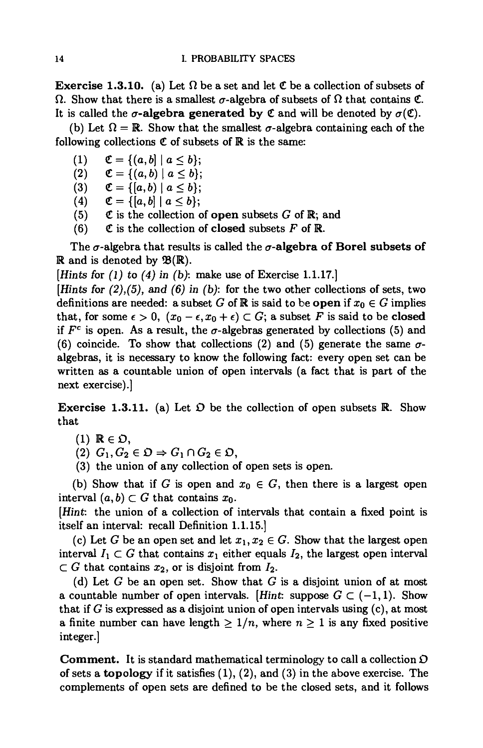
(3) for the Poisson distribution with mean one (see Fig. 1.4)
F(x)
l e Z^0<n<i n!'
X <0,
0<X.
(l+...+l/n!)/e-
(l+l/2+l/6Ve
(l+l/2)/e
l/e
I 2 3
Fig. 1.4
14
I. PROBABILITY SPACES
Exercise 1.3.10. (a) Let Q be a set and let € be a collection of subsets of
fi. Show that there is a smallest er-algebra of subsets of fi that contains €.
It is called the er-algebra generated by € and will be denoted by <r(€).
(b) Let fi = R. Show that the smallest er-algebra containing each of the
following collections € of subsets of R is the same:
(1) €={(a,b}\a<b);
(2) €={(a,b)\a<b};
(3) €={[a,b)\a<b};
(4) €={[a,b]\a<b};
(5) € is the collection of open subsets G of R; and
(6) € is the collection of closed subsets F of R.
The er-algebra that results is called the er-algebra of Borel subsets of
R and is denoted by <8(R).
[Hints for (1) to (4) in (b): make use of Exercise 1.1.17.]
[Hints for (2),(5), and (6) in (b): for the two other collections of sets, two
definitions are needed: a subset G of R is said to be open if Xo G G implies
that, for some e > 0, (xo - e,Xo + e) C G; a subset F is said to be closed
if Fc is open. As a result, the er-algebras generated by collections (5) and
(6) coincide. To show that collections (2) and (5) generate the same a-
algebras, it is necessary to know the following fact: every open set can be
written as a countable union of open intervals (a fact that is part of the
next exercise).]
Exercise 1.3.11. (a) Let D be the collection of open subsets R. Show
that
(1) RgD,
(2) Gi,G2 eD=>GinG2eD,
(3) the union of any collection of open sets is open.
(b) Show that if G is open and Xo G G, then there is a largest open
interval (a, b) C G that contains Xo-
[Hint: the union of a collection of intervals that contain a fixed point is
itself an interval: recall Definition 1.1.15.]
(c) Let G be an open set and let Xi,x2 G G. Show that the largest open
interval I\ C G that contains Xi either equals h, the largest open interval
C G that contains x2, or is disjoint from /2.
(d) Let G be an open set. Show that G is a disjoint union of at most
a countable number of open intervals. [Hint: suppose G C ( — 1,1). Show
that if G is expressed as a disjoint union of open intervals using (c), at most
a finite number can have length > 1/n, where n > 1 is any fixed positive
integer.]
Comment. It is standard mathematical terminology to call a collection D
of sets a topology if it satisfies (1), (2), and (3) in the above exercise. The
complements of open sets are defined to be the closed sets, and it follows
3. DEFINITION OF A PROBABILITY SPACE
15
from (3) that for any set A, the intersection of all the closed sets containing
it is a closed set. It is called the closure of A and is usually denoted by A.
Digression on countable sets. It is about time to say what the word
"countable" means. A set E is countable if all its elements can be labeled
by natural numbers in a 1:1 way, i.e., if there is a function c : N —► E such
that (i) E = {c(n) | n E N}, (ii) c(ni) = c(ri2) implies ni = n-i- A set
is at most countable if it is either finite (i.e., it can be "counted" using
{1,...,n} for some n) or countable (i.e., it can be "counted" using N).
Given two sets A and B, the Cartesian product A x B = {(a, b) \
aeA,beB}.
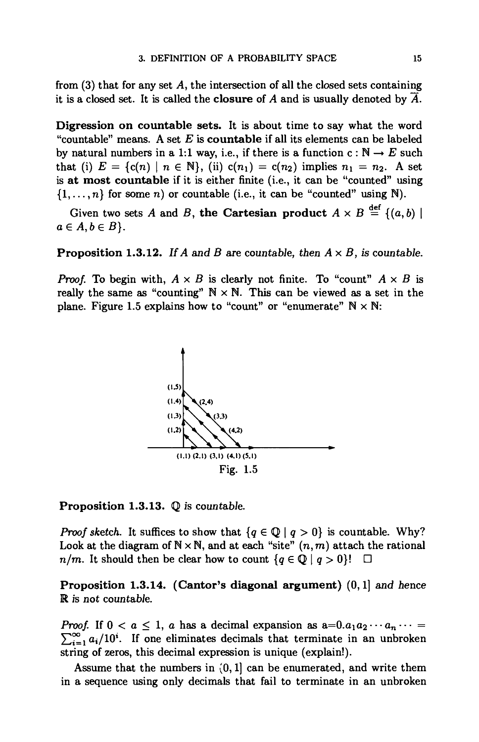
Proposition 1.3.12. If A and B are countable, then Ax B, is countable.
Proof. To begin with, A x B is clearly not finite. To "count" A x B is
really the same as "counting" N x N. This can be viewed as a set in the
plane. Figure 1.5 explains how to "count" or "enumerate" N x N:
1
(1.5)
(1.4)
(13)
(1.2)
X(2.4)
nNN^'
V v V<42>
yvvv
*-
(1.1)(2.1) (3.1) (4.1)(5.1)
Fig. 1.5
Proposition 1.3.13. Q is countable.
Proof sketch. It suffices to show that {q G Q | q > 0} is countable. Why?
Look at the diagram of N x N, and at each "site" (n, m) attach the rational
n/m. It should then be clear how to count {q G Q | q > 0}! □
Proposition 1.3.14. (Cantor's diagonal argument) (0,1] and hence
R is not countable.
Proof. If 0 < a < 1, a has a decimal expansion as a=0.aiO2 • • • an • • • =
Hi^i Ot/10'. If one eliminates decimals that terminate in an unbroken
string of zeros, this decimal expression is unique (explain!).
Assume that the numbers in (0,1] can be enumerated, and write them
in a sequence using only decimals that fail to terminate in an unbroken
16
I. PROBABILITY SPACES
string of zeros:
a\ = 0.aiiai2Oi3
02 = 0.021022023
an = 0.anian2an3 • • • ann
Let a = O.ai ^22033 • • -aj,n • • •, where 0 ^ .a'nn ^ ann for each n ^ 0.
In other words, use the diagonal entries of the above infinite table to make
a number in (0,1]. Then a is not in the list since its decimal expansion
fails to agree with that of any of the expansions for a,\, a^,... . This is a
contradiction.
Since (0,1] is not countable, R is not countable. □
This argument applies to any non-void interval since, for example, the
function f(x) = |5y maps [a, b] in a 1:1 way onto [0,1]. As a result, any
non-void open set is not countable, as it contains some interval [a, b] with
a ^ b. In particular, one has the following observation.
Exercise 1.3.15. Let C be any countable subset of R. Then the closure
R\C of R\C equals R. Show this by observing that C D CR\C, which is
an open set. This property of the complement R\C of C is referred to by
saying it is dense. Show that a set D is dense in R if and only if every
non-void open set contains a point of D.
Finally, one can verify the following fact.
Exercise 1.3.16. Let £1,..., En be a finite collection of disjoint countable
sets. Then E = U"=i£j is countable. Let E\,..., En,... be a countable
collection of countable sets. Then E = U^i?* is countable.
4. Construction of a probability
from a distribution function
Now consider the basic problem of constructing a probability from a
distribution function F. Exercise 1.3.10 (b) shows that if one is to get a
probability space (R, 5, P) from F with 5 D 21, then J will have to contain
the <7-algebra <8(R) of all Borel subsets of R.
Furthermore, if A G 21 and A = U^L^n, where the An are in 21 and
pairwise disjoint for example, (0,1] = U^i(^y, £] — then, it will be
necessary (as shown later) that
00
P(A) = £P(An)
n=l
if there is to be a probability P on a er-algebra 5 D 21. Recall that P is to
be er-additive.
•ain---
• a2n • ••
4. CONSTRUCTION OF A PROBABILITY
17
Exercise 1.4.1. Show that F(l) -F(0) = £~i{F(^)-^(^y)}- [Hint
use Exercise 1.1.8 and the right continuity of F.}
Definition 1.4.2. A finitely additive probability P on a Boolean aJgebra
21 is said to be er-additive if A = U^=1An implies
oo
P(A) = £P(A«),
n=l
when A in 21, the sets An are all in 21, and are pairwise disjoint.
A finitely additive probability P on 21 need not be er-additive, as the
following example shows.
Example. Define P on 21 by setting P( A) = 0 if A has an upper bound
and P(j4) = 1 if A has no upper bound (remember that 21 is a special
Boolean Algebra — see Convention (1.3.8)). Show that (R,2l, P) satisfies
conditions (2li), (212),(83)(^1),(^2), and lFAp3) in §12- Show that it is
not er-additive. To see this, try to calculate P(K) as 5Z^=_00 P((n,n + 1]).
Notice that this "probability" does not come from a distribution function.
What is missing?
Returning to the problem of extending P from 21 to 2$(R), it will now
be shown that if P on 21 is determined by a distribution function, then it
is er-additive.
Exercise 1.4.3. Show that P on 21 is er-additive if and only if (a, b] =
UfcL](cfc,dfc], with the (cjt.dfc] pairwise disjoint, implies
00
P((a,b}) = F(b) - F(a) = £{F(dfc) - F(cfc)}.
fc=i
Theorem 1.4.4. Let F be a distribution function on R. Let P be the
unique finitely additive probability on 21 such that P((a, b}) = F(b) — F(a)
whenever a < b. Then P is a-additive on 21.
Remark. This theorem may appear obvious to you in view of Exercise
1.4.3. In a way it should. However, its actual justification depends on the
Axiom 1.1.3.
Proof. By Exercise 1.4.3, it suffices to prove that if (a, b] = U^^Cfcjdfc]
with the intervals (cfc,dfc] pairwise disjoint, then
00
(*) F(b) - F(a) = £{F(dfc) - F(ck)}.
fc=i
Now it is obvious that F(b) - F(a) > ££=i{F(dfc) - F(ck)} since (a, b] D
Ufc=i(cfc,dfc]. Hence, by Exercise 1.1.8, F(b) - F(a) > E£Li{F(dfc) -
18
I. PROBABILITY SPACES
F(cfc)}. Therefore, it is enough to verify the opposite inequality, and it
is here that the Axiom 1.1.3 and the right continuity of the distribution
function F come into play.
First, one shows that it suffices to verify (*) when -oo < a < b < +00.
Suppose, for example, that —00 = a < b < +00. Then, for large n, one
has — n < b. If (—00,6] = U^-^Cfc.dfc] with the intervals (cfc,dfc] pairwise
disjoint, then (—n,b] = UfcL^CfcV^—n),dk]. If (*) holds when the endpoints
are both finite, then
F(b) - F(-n) = J2 F(dk) ~ F(ck V (-n)) < £ F(dk) - F(ck).
k=\ fc=i
Since P((-oo, b}) = F(b) and F(—n) converges to zero as n tends to +00, it
follows that F{b) < YXLi F(dk) ~ F(c*)> and hence F(6) = £*Li F(dk) -
F(cit) (the opposite inequality is valid, as observed above). Similar
arguments apply when —00 < a < b = +00 and when —00 = a < b = +00.
This shows that the theorem holds provided it holds for intervals with finite
endpoints.
Assume -00 < a < b < +00, and choose any positive number e > 0.
For each k, there is a positive number ek > 0 such that
F(dk) < F(dk + efc) < F(dk) + ^
because the distribution function F is increasing and right continuous. In
other words,
P((cfc,dk}) < P((cfc, dk + ek}) < P((cfc, dk}) + ^.
Therefore,
£{F(dfc + efc) - F(ck)} = J2 P((cfc, dk + ek)) < ^{F(dfc) - F(ck)} + e.
fc=i fc=i fc=i
Note that (a, b] = U^L^Ck,^] c U^^Cfc^fc^eit), which is an open set.
Using the right continuity once again (at Xo = a), there is a positive number
e < b- a such that F(a + e) < F(a) + e.
In other words,
P((a,b])-€<P((a + e,b}).
Since [a + e,6] C (a,6] C U^^Cfcjdfc + efc), the closed interval [a + e,b] is
contained in a countable union of open intervals. A very famous theorem
(the Heine-Borel theorem) asserts that, as a result, the union of some
finite number of the open intervals (ck,dk+ek) contains [a + e,6]: the proof
will be given below and it uses the Axiom 1.1.3. Assuming the validity of
4. CONSTRUCTION OF A PROBABILITY
19
the Heine-Borel theorem, suppose that one has [a+e, b] C U£=1 (cit, dk+ek).
Then
(a + e, b] C Uj=1 (cfc, dfc + e*] = A' G 21,
and so
P((a + e, 6]) = F(6) - F(a + e) < P(A')
n n
< J2 P((<*.dfc + efc]) = £{F(dfc + efc) - (cfc)}
fc=i fc=i
(recall that P(A') < £fc=iP((cfc>dfc + efc]) by Exercise 1.2.2 (6). The
conclusion is then that
F{b) - F{a) - t = P((a, b]) - e < P((a + e, b\)
<J2{F(dk + ek)-F(ck)}
fc=i
oo oo
< £{F(dfc + efc) - F(cfc)} < £{F(dfc) - F(ck)} + e.
fc=i fc=i
Since e is any positive number, the desired inequality is proved. □
For completeness, the key theorem that was used in the proof of this
result will now be proved.
Theorem 1.4.5 (Heine-Borel). Let [a,b] be a closed, bounded interval
in K. Assume that there is a collection of open intervaJs (at,6t) whose
union contains [a, 6]. Then the union of some finite number of the given
collection of open intervals also contains [a, 6].
Proof. The idea of the proof is to see how large an interval [a,x] with
a < x < 6 can actually be covered by a finite number of the open intervals
(i.e., [a,x] c some finite union of these intervals). One knows that for some
i, say ii, a G (^,,6^,). So, ifx = min{6, |(a + 6i,)}, then [a,x] C (^,,6^,).
Let H equal the set of x in the interval [a, 6] such that [a, x] is contained in
a finite number of the intervals. This is a set with an upper bound b. Note
that if x G H and a < y < x, then y G H. Also, if d is an upper bound of
H, then d < e < b implies e ¢ H. By Axiom 1.1.3, H has an l.u.b. Call it
c.
Exercise 1.4.6. (1) Show that [a,c] is contained in a finite union of the
open intervals. [Hint: c is in some interval.] (2) Show that if [a,x] is
contained in a finite union of the open intervals and x < b, then x is not
an upper bound of H.
This exercise implies c = b, and so the theorem is proved. □
20
I. PROBABILITY SPACES
Remark. An equivalent form of the Heine-Borel theorem is the following
result.
Theorem 1.4.7. Let (Ot)te./ be a family of open sets that covers the
closed, bounded interval [a,b] C R (i.e., UiejOi D [a,b]). Then a finite
number of the sets Oj covers [a, b] (i.e., for some finite set F c J, UjefOj D
[a,b)).
Exercise 1.4.8. Show that Theorem 1.4.7 and Theorem 1.4.5 are
equivalent.
The Heine-Borel theorem is so basic that the class of sets for which it
is true is given a name.
Definition 1.4.9. A set K c R is said to be compact if, whenever K c
UjejOj, each Oj open, there is a finite set F c J with K c UjefOj.
The Heine-Borel theorem states that every closed and bounded interval
is compact. Given this theorem, it is not hard to show that a set K c R is
compact if and only if K is closed and bounded (see Exercise 1.5.6). For
example, the Cantor set is compact!
Returning again to the extension problem for P, it is clear that if A =
U£Lij4„, An G 21 for all n and A not necessarily in 21, then A e $. Also,
by Remark 1.2.3, A can be written as a disjoint union of sets in 21: one
replaces each An by j4n\ U"^1 j4j. Consequently, if there is an extension,
P(A) = £~=i P(An\ U?",1 At) < £~ , P(An). Without assuming the
extension to be possible, one may define P*(-<4) to be the greatest lower
bound of {Z™=1P(An)\A = U~ xAn,An G 21 for all n}. Then P*{A)
is an estimate for the value P(A) of a possible extension when A G 2lCT,
the collection of sets that are countable unions of sets from 21. Since R =
Un=-oo(n'n "*" I)' eveT E C R is a subset of some set A G 2lCT. Hence
if E c A, then one expects to have P{E) < P*(A). This motivates the
definition of the following set function P*.
If E c R, define P*(E) to be the greatest lower bound of {P*{A)\E c
A G 2lff}, i.e.,
P*(E) Hf ^nf P*(A) = inf|£ P(An)\E c U~ ,An,An G 21 for all n|.
Remark. The terms infimum (abbreviated to "inf") and supremum
(abbreviated to "sup") are merely other words for "g.l.b." and "l.u.b.",
respectively.
In general, the set function P* does not behave like a probability because
(/¾) need not hold! However, it has certain important properties which
make it into what is called an outer measure. They are stated in the
next definition.
4. CONSTRUCTION OF A PROBABILITY
21
Definition 1.4.10. An outer measure on the subsets of R is a set
function P* such that
(1) 0<P*(E) forallEcR,
(2) Ei C E2 implies P*(#i) < P*(E2), and
(3) E = u~ i^n implies P*{E) < £~l p*(^n) (i.e., it is countably
subadditive).
Proposition 1.4.11. The set function P* defined above is an outer
measure with P*(E) <l for all E e R. Furthermore, since P is a-additive on
a, P(A) = P*(A), for aJJ A e a.
Pnoo/. Properties (1) and (2) of Definition 1.4.10 are obvious. Let e > 0
and, for each n, let En C UgL^,* be such that YlT=\ p(^n.fc) < P*(E„) +
^- where the sets An,fc G 3. Then E = U^E,, C U^ U^ A„ifc, which
is a countable union of sets from 21. Hence,
oo oo °° ( \ °°
p*(£) < EEp(^^) ^ E p*(^») + £ = Ep*(£»)+e-
n=l fc=l n=l "- ^ n=l
If A G a is contained in U^A,,, A„ G a, n > 1, then A = U~=1A^,
where A^ = A n [An\ UjlJ Afc]. Then, by the <r-additivity of P on a
(Theorem 1.4.4), P(A) = £~i P(^n) < £~=i P(^n) as A'n c An, for
all n > 1. This shows that P(A) < P*(A) and hence P(A) = P*(A) if
ag a. □
Remark. The fact that P and P* agree on a is crucial in what follows.
This is why it is so important that P be er-additive on a.
While P* is defined for all subsets of R, it is not necessarily a probability.
This raises the problem as to whether there is a natural class of sets on
which it is a probability. The following way of solving this problem is due
to a well-known Greek mathematician, C. Caratheodory. He observed that
(i) the sets in any er-algebra <9 containing a have a special property (see
(C) below) provided the outer measure P* restricted to 0 is a probability,
and (ii) the collection of all sets with this property is in fact a er-algebra,
and the restriction of P* to this er-algebra is a probability.
First, notice that because of property (3) of Definition 1.4.10, for any
two sets E and Q, one has P*(E) < P*{EnQ) + P*(E\Q). However, if
Q G a, then in fact
(C) P*(E) = P*(Er\Q) + P*(EnQc),
for any set E because P and P* agree on a.
To prove (C) for sets Q G a, let e > 0 and let An G a for all n > 1 be
such that E c U~=1A„ and YlT=i p(An) < P*{E) + e. These sets An may
be assumed to be pairwise disjoint by Remark 1.2.3. Further, An n Qc G a
for all n > 1, since Q e a.
22
I. PROBABILITY SPACES
Now
p*(En Q)+P*(En Qc) < P* (u~ ,(A„ n Q)) + P* (u~ ,(A„ n Qc))
oo oo
< £{P(An n Q)} + £{P(An n Qc)}
n=l n=l
oo oo
= £{P(An n Q) + P(An n Qc)} = £ P(An) < P*(E) + e.
n=l n=l
Therefore, P*(E nQ) + P(£n Qc) < P*(E), proving (C).
Now suppose that 0 D 21 is a er-algebra and that P* restricted to 0 is a
probability, say R. Then, since a er-algebra is a Boolean algebra and R is
er-additive on 0, one could construct a new outer measure R* from R. As
stated later in Exercise 1.5.4, in fact R* = P*. Therefore, it follows from
what has just been proved for 21 that condition (C) holds for all the sets
in 0.
This suggests that one should look at the collection 5 of all sets for
which condition (C) holds, i.e.,
ff = {Q | P*(E) = P*(Er\Q) + P*{Er\Qc) for any E c K}.
It will now be shown that
(i) 5 is a er-algebra (containing 21), and
(ii) P* restricted to 5 is a probability.
Hence, (K, 5, P*) is a probability space and 5 D 21 (also, in view of
Exercise 1.3.10 (b), J D <8(R) — the algebra of Borel sets).
It remains to verify (i) and (ii).
To verify (i), first note that Q = R G 5 and that A G J implies Ac G £.
If Ax, A2 G 5, then Ax U A2 G £. To see this, let EcK. Then, by (C), one
has
P*(E) = P*{E(lAx) + P*{E n A\).
Since, by (C),
P*(E n Ax) = P*{E nA,n A2) + P*(£ n Ax n A%),
and, again by (C),
p*(E n A\) = P*{Er\A\c\ A2) + P*(£ n A\ n a%),
this implies that
P*{E) = P*(E n Ax n A2) + P*{E n Ax n Al)
(1) +P*{Ec\A\C\A2) + P*{Er\A\C\Al).
4. CONSTRUCTION OF A PROBABILITY 23
Since
E n (Ai u A2) = {Er\A1n A2) u(£ni4,n AD u (£: n A\ n A2)
it follows from (1) and Definition 1.4.10 (3) that
p*(E) >p*(#n(AiuA2)) + p*(£nAjnA|).
Hence, A\, A2 e 5 implies that A\ U A2 e 5-
By now it should be clear that J is a Boolean algebra. Therefore, J
is a er-algebra providing \J^LxAn G 5 whenever the A„ £ J are pairwise
disjoint.
To verify this, one has to show that for any set Ecfl,
P*(E) = P*(£n(u~ ,A„)) + F(£n(uS°=1An)c),
when the j4„ ej are pairwise disjoint. To do this, it will suffice to show
that for all n > 1,
n
(2) P*(E)>J2p*(EnAi) + p*(En(Vn=iAn)c).
The reason is that this inequality and Definition 1.4.10 (3) imply that
oo
P*(E) > J2 P*(EnAn) + P*(En(U^=1An)c)
>P*(En(U^=lAn)) + P*(En(U^=lAn)c).
In view of the validity of the opposite inequality, again by Definition 1.4.10
(3), one then has
p*(£;) = p*(£;n(u~1An)) + p*(£;n(u~1An)c), i.e., u~=1AneS.
Now (2) holds if
n
(3) P*(E) >Y^P*(En Ai) + P*{En (U?=1 Ai)c).
Hence, to verify (2), it suffices to prove this last inequality (i.e., inequality
(3)) as (up=1Ai)c D {U^Ai)0. Note that (3) is equivalent by Definition
1.4.10 (3) to the identity
n
(4) P*(E) = Y, P*(£n A,) + P*(E n (\j?=lAi)e).
24
I. PROBABILITY SPACES
To prove (4), let A\,...,An be pairwise disjoint and in $• Then, by
applying the defining property of 5 first to A\ using E, and then to A^ and
using E D A\ in place of E, it follows that
p*(E) = P*(E n Ai) + P'fEn^)
= p*(E n A,) + p*(E n Af n A2) + p*(£ n A^ n A|)
= p*(EnA1) + p*(EnA2) + P*(EnASnA£),
since A\ D A2 = 0.
Hence, (4) holds for n = 2. Note that this follows immediately from
formula (1) if A\ D A2 = 0. Assume that (4) is true for n — 1 pairwise
disjoint sets Aif i.e., for any EcR,
n-l
p*(E) = J2 P*(E n Ai) + P*(E n (U^1 AO0).
t=i
Apply the defining property of 5 to An and use the set E D (U^T/Ai)c. It
then follows that
p*(En (ujL"!1 Ai)c) = p*(£;n (u^j-!1 Ai)c n An) + p*(En (u^A*)' n Acn)
= p*(£;nAn) + p*(£;n(ur=1Ai)c).
Therefore,
n
P*(E) = J2 P*(E n Ai) + p*(E n (uj"=1 Ai)c).
This completes the proof of (i). The proof of (ii) is given below.
Definition 1.4.12. The a-algebra 5 of sets Q that satisfy
(C) P*{E) = P*{EnQ) + P*{EnQc)
for all E c R is called the cr-algebra of P*-measurable sets.
The following theorem is the goal to which all these arguments have
been leading.
Theorem 1.4.13. Let F be a distribution function on R.
(1) Then there is a unique probability P on 2$(R), the <7-aJgebra of
Bore! subsets of R, such that P((a, 6]) = F(b) - F(a) whenever
a< b.
(2) The a-algebra 5 of P*-measurable subsets contains 2$(R), and P*
restricted to 5 is a probability such that P*((a, 6]) = F(b) - F(a)
whenever a < b.
4. CONSTRUCTION OF A PROBABILITY
25
furthermore, the a-algebra $ of P* -measurable sets is the largest a-algebra
8 containing 21 with the property that the restriction of P* to (5 is a
probability.
Proof. First consider (2). It has been shown that 5 is a <r-algebra. To prove
that P* restricted to 5 is a probability, it will suffice to verify (P3) of
Definition 1.3.1 since P* obviously satisfies (Pi) and (P2). Let (i4n)n>i C 5 be
pairwise disjoint. Since P* is an outer measure, it is countably subadditive,
i.e., (3) of Definition 1.4.10 holds. Hence
oo
p*(u~,An)<£pvn).
n=l
To prove the reverse inequality, note that P*(u£Lii4n) > P*(U^=1i4n) =
En=i p*(An)in view of (4) (take E = U^=1i4n). This completes the proof
of (2) and of (ii) above.
To prove the first statement, let Pi and P2 be two probabilities on
S8(R) such that Pi((a,6]) = P2((a,6]) = F(b) - F(a) whenever a < b. Let
SOI = {A G S8(R) I Pi (A) = P2(A)}. Then, by Exercise 1.3.7, Pi and P2
agree on 21 .
Exercise 1.4.14. Let (fi,5, P) be a probability space and let (;4.n)n>i c
J. Show that
(1) if An C An+l for all n, then lim,,^ P(An) = P(U~=iAn),
(2) if An D An+1 for all n, then lim,,^ P(An) = P(n~ ^).
[Hint: recall Exercise 1.3.3.]
If F is the distribution function of a probability P on 2$(R), show that
(3) F(x-) = P((-oo,x)) for all x G R.
Exercise 1.4.15. Show that the set SOI defined above has the following
two properties (where (i4n)n<i c 9H):
(1) An C An+X for all n implies U^ii4n G SDt; and
(2) An D An+i for all n implies n£Li,4n G 9Jt,
i.e., SOI is a so-called monotone class.
Exercise 1.4.16. (Monotone class theorem for sets) Let SOI be a
monotone class that contains a Boolean algebra 21. Show that 9Jt contains
the smallest <r-algebra 5 containing 21. [Hints: let S0l0 be the smallest
monotone class containing 21 (why does it exist?). Let A G 21. Show that
{B G SOlo I B UA G S0l0} is a monotone class. Conclude that B G S0l0, A G
21 imply BuAe S0l0. Now fix Bx G S0l0 and look at {B G S0l0 | Bi U B G
SOlo}. Conclude as before that BX,B G S0l0 implies Bx U B G S0l0. Make
a similar argument to show that {Bc \ B G S0l0} is S0l0. Conclude that
SOlo D 5.]
26
I. PROBABILITY SPACES
The monotone class theorem has a function version, which is stated as
Theorem 3.6.14. It gives conditions that ensure that a given collection H of
bounded functions on fi contains all the bounded random variables in the
er-algebra determined by a subset C of H that is closed under multiplication.
From these three exercises and Exercise 1.3.10 (b), one concludes that
SOt = S8(R), as it contains 21, and so (1) is established.
The last statement of the theorem is a consequence of Exercise 1.5.4 and
the observation made following Proposition 1.4.11 that condition (C) holds
for all the sets in (5 if (5 is a er-algebra containing 21 such that P* restricted
to 0 is a probability. □
Remark 1.4.17. It is easily verified that the collection SOt defined above
has the following properties: (i) Q G SOI and (ii) if A, B G SOI with A C B,
then B\A G SOI. Dynkin proved (see Proposition 3.2.6) that the smallest
such system £ containing a collection €, of sets closed under finite
intersections is the smallest er-field containing €. This is another version of the
monotone class theorem. It is proved in Exercise 3.2.5, part C, that any
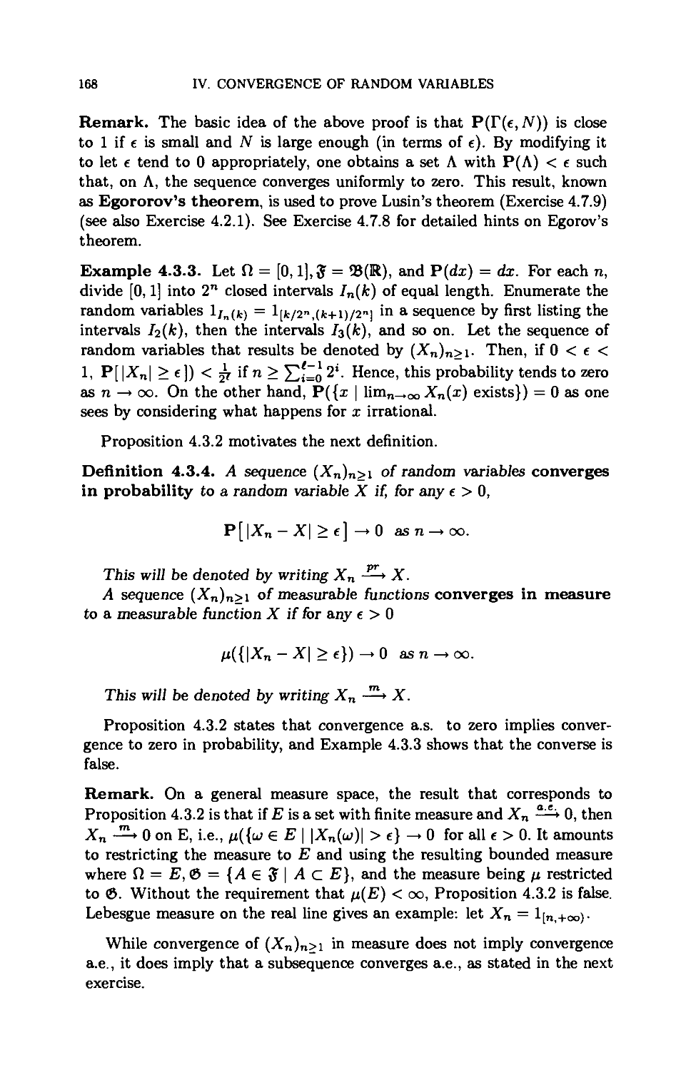
collection of sets £ D € satisfying (i) and (ii) also contains the smallest
Boolean algebra 21 containing € if the collection € is closed under finite
intersections. Taking € as {(a, b] \ -oo < a < b < +00} Proposition
3.2.6 also proves the uniqueness of the probability P on S8(R) for which
P((a,b))=F(b)-F(a).
5. Additional exercises*
Exercise 1.5.1. Let (fi, 5, P) be a probability space. Show that
(1) P(U~=1An) < Y.n=\ P(An) (see Exercise 1.2.2 (6)); and
(2) P(U~=1An) = 0 if P(An) = 0 for all n > 1.
Exercise 1.5.2. The so-called Heaviside function is the function H,
where
H(X) = \l, x>0.
Calculate for this distribution function the corresponding outer measure
P*, and determine the er-algebra 5 of P*-measurable subsets of K. [Hint:
guess the er-algebra 5 and P*. Then see if they "work".]
The resulting measure, denoted by eo or ^o is called the Dirac measure at
the origin or unit point mass at the origin. Replace H(x) by H(x -
def
a) = Ha(x), and let ea denote the resulting measure. Give the formula for
ea(A),A G 5, where 5 is the corresponding er-algebra of measurable sets.
The measure ea is the Dirac measure or unit point mass at a.
Exercise 1.5.3. For the distribution function of the Poisson distribution
(see Example 1.3.9 (3)), calculate the corresponding outer measure P* and
determine the er-algebra J of P*-measurable subsets of K.
5. ADDITIONAL EXERCISES*
27
Exercise 1.5.4. Let (5 D 21 be a er-algebra, and assume that P* restricted
to (5 is a probability R. Define the outer measure R* by setting R*(£) =
inf{£~=i R-(fin) | E C Un=iBn, Bn e 0 for all n}. Show that
(1) R*(E) = inf{R(B) | E c B, B e 0},
(2) R*(E) < P*(E) for all E c R,
(3) R*(E) = P*(E) for all EcR, and [Hint: R(B) = P*(B).]
Exercise 1.5.5. Show that Q is P*-measurable if and only if P*(Q) +
P*(QC) = 1- This exercise may be done by going through the following
steps.
(1) Let Q, E be subsets of R, and let (Am), (Bm), and (Cp) be pair-
wise disjoint collections of sets from 21 such that (i) E c UPCP = C
and (ii) Q c UmAm = A, Qc c U„Bn = B. Show that
p*(£n Q) + p*(£;n Qc) < J2P(^m n c„) + ^P(B„ n cp)
< ^ P(CP) + 2 P(Am n sn n cp)
p m,n,p
<£p(Cp) + £p(AmnBn).
p tn,n
[Hint: for the second inequality use Exercise 1.2.2 (5).]
(2) If {Am) and (Bn) are two collections of pairwise disjoint sets from 21
such that (i) R = AuB, where A = U~=1i4m and B = U~=1B„, and
(») Em P(Am)+Zn P(B„) < 1+e , show that Em,„ P(Amr\Bn) <
e.
[Hint: make use of Exercise 1.2.2 (5) to compute P(i4m) + P(Bn)
and use the fact that R = Uminj4m U Bn.\
(3) If P*(Q) + P*(QC) = 1 and E c R, show that for any e > 0 one
has P*(E n Q) + P*{E\QC) < P*{E) + e.
Remarks. Result (2) says that P(A D B) < e, i.e., the overlap of A and
B is small (relative to P) if (i) and (ii) hold. It will help to realize that all
the sets in 2lCT are Borel and that, for example, ^2m P(i4m) = P{A), where
P is the probability on 93(R). It is also of some interest to realize that all
the above computations can be done without knowing that P on 21 has an
extension as a probability to 93(R). As a result, the P*-measurable sets Q
may be defined by the equation P*(Q) + P*(QC) = 1 and Theorem 1.4.13
proved using this definition (see Neveu [Nl]).
Exercise 1.5.6. (The Bolzano-Weierstrass property)
This exercise characterizes the compact subsets of R.
Part A. Let A be a subset of R. Show that A is compact if and only if it
is closed and bounded. [Bints: if A is closed and bounded, then for some
28
I. PROBABILITY SPACES
N > 0 one has A C [-N,N\; if A C UA, then [-TV, TV] C UA U Ac;
now use the Heine-Borel Theorem 1.4.5. For the converse, observe A C
Un(-n,n); and if Xo G j4c and no open interval (xo - ^,Xo + ^) C Ac, look
at the open sets [xo - ^,Xo + ^]0.]
Part B. Let A be a compact subset of K, and let (xn)n>i be a sequence
of points of A. Let S = {xn | n > 1}. If the sequence has no convergent
subsequence, show that
(1) 5 is infinite [Hint what happens if it is finite?],
(2) S is closed [Hint: if a £ S, show that some open interval centered
at a is disjoint from 5; otherwise what happens?],
(3) for each point s of 5, there is an open interval centered at s
containing no other point of S. [Hint: start off with the first point.]
Show that (3) contradicts the assumption that A is compact [use (2)].
Conclude that (xn)n>i has a convergent subsequence.
Part C. Let A be subset of K, and assume that every sequence (xn)n>i of
points in A has a subsequence that converges to a point of A. Show that
(1) A is closed [Hint: consider the hint for Part B (2)] ,
(2) A is bounded. [Hint: if a sequence converges it is bounded.]
This exercise emphasizes the importance of the Bolzano—Weierstrass
property (see Royden [R3]) for a set: every sequence (in the set) has a
convergent subsequence (convergent to a point in the set). It is equivalent
to the property of compactness.
CHAPTER II
INTEGRATION
1. Integration on a probability space
In elementary probability, if fi is finite, say fi = {1,2,..., n}, 5 is
the collection of all subsets of fi, and if P gives weight Oj > 0 to {i}
with 5Z"=1 a,i = 1, then the (mathematical) expectation E[X] of a random
variable X on fi (i.e., a function X : fi —► K) is defined to be 5Z"=1 X(z)ai =
5Z"_i X(z)P({z}). When a* = 1/n for each z, this expectation is the usual
average value of X. Heuristically, this number is what we expect as the
average of a large number of "observations" of X — see the weak law of
large numbers in Chapter IV. Also, if X is non-negative, then E[X] can be
conceived as the "area" under the graph of X: over each z one may imagine
a rectangle of width P({oj}) and height X(i); then £"=1 X(i)P({i}) is the
sum of the "areas" of the rectangles that make up the set under the graph.
Now let (0,5, B) be an arbitrary probability space and let X be a
function on fi. For what functions X can an expectation E[X] or average be
defined? In other words, what functions X can be integrated or summed
against P?
For example, let fi = K, 5 = 2$(R), and P be the uniform distribution
on [0,1] (see Example 1.3.9 (1)). Recall that the distribution function F is
given by
{0 x<0,
x 0< x< 1,
1 l<x.
Let X(x) = sin x if x G C, the Cantor set (see the remark following
Example 1.2.5), and X(x) = 0, if x £ C. Can one integrate X using P? The
answer is "yes", and it turns out that the value of the integral is zero since
P(C) = 0 (see the calculation in Example 1.2.5).
The basic idea in integration is that if a function X takes a constant
value a on a set A in 5 and is zero elsewhere, then J XdP should be
aP(A), (i.e., when a > 0, it should be the "area" of the picture in fi x R
shown in Fig. 2.1, where A is indicated by a heavy line).
a
Fig. 2.1
29
30
II. INTEGRATION
Just as a distribution function F immediately determines a probability
P on simple sets, namely the intervals (a, b], so does a probability (more
generally, a measure) determine an obvious notion of integral for certain
simple functions. In both instances, the problem arises as to how to extend
to more general situations.
Define the characteristic or indicator function of a set A to be the
function that equals 1 on A and 0 on Ac. In these notes, it will be denoted
by l,i. ( It is also often denoted by \A-)
Definition 2.1.1. A function s : fi —► R is said to be a simple function
or to be ^-simple if it can be written as s = 5Zn=1 anl/i„ with an > 0,
and the sets An € 5 pairwise disjoint.
Let Sj" denote the class of simple functions.
Proposition 2.1.2. Let s be a simple function, and assume
N M
s= ^2anlA„ = ^2 tmls".'
n=l m=l
where the collections of sets An, 1 < n < N, and Bm, 1 < m < M, are
both pairwise disjoint. Then
N M
J2*nP(An)= £&mP(Bm).
n=l m=l
Proof. Note that s has a "natural" representation as 5Zn=1 anlA„,An pair-
wise disjoint and the an all distinct. To obtain it, consider the sets {w |
s(w) = a} as a varies over R. If s is expressed as $3m=1 bmlBm, then
M N
£&mp(Bm) = 5>n{ J2 p(fi-)}
m=l n=l m,bm=a„
N
= ^2 anP(An) as Um {Bm \ bm = an} = An. D
n=l
Remark. This result corresponds to Exercise 1.3.7 (2), for the probability
P defined by a distribution function.
Definition 2.1.3. Let s € $f. Define the integral or expectation of
s with respect to P to be 5Zn=1 anP(.An) if s = J2n=ian^A„, the sets
An e 5 and pairwise disjoint. This number will be variously denoted by
E[s\, JsdP, or /s(w)P(du>).
1. INTEGRATION ON A PROBABILITY SPACE
31
Remark. Proposition 2.1.2 shows that this definition makes sense, i.e.,
the value of E[s\ does not depend on the particular representation of s.
Proposition 2.1.4. (Properties of simple functions and their
integrals) Let s, si,S2, etc., denote simple functions, i.e., elements ofSt- The
collection St has the following properties:
(Si) for all A > 0, As e St *""* J{^s)dP = \(f sdP);
(52) si + s2 € St and /(si + s2)dP = / sidP + / s2dP;
(53) si < S2 implies J s\dP < J s2dP, where s\ < S2 means that for aJJ
w,si(w) < s2(w),-
(54) si, S2 € St implies s\ A S? and s\ V S? € St> where
(s\ As2)(lj) = min{si(w),S2(w)} and
(si Vs2)(w) = max{si(w),S2(w)} ; and
(55) if(sn) is a sequence of S-simple functions with sn < sn+\ < s for all
n, where s is S-simple and such that s = limn sn (i.e., limn sn(u>) =
s(lj) for all w), then limn / sndP = J sdP.
Proof. (Si) is obvious. It suffices to verify (52) for s\ = o,1a and S2 =
£^=1a„l,t„. Then si + s2 = alB + Hn=i{anl/i„\/i + (a„ + a)lAnnA),
where B = A\U%=1 An.
Exercise. Use this expression for s\ + S2 when s\ = o,\a to verify that in
this case
[(si+s2)dP= jsidP+ J s2dP.
Explain why it is enough to prove (52) in this case.
To prove (53), let s = s2 - s\. Then s e 5+, as can be seen by writing
a formula for s if s2 = Hn=1 "nU„ > s\ = £fc=1 bklBl!-
Exercise. Determine the desired formula. First, show that U^=1.An D
u£_jBfc and then use the Bk to "cut up" each An and use this observation
to define s.
Hence,
/ s2dP = / sidP + / sdP > / sidP.
To show (54), first note that if s = 5Zn=i anlA„ with the sets An pair-
wise disjoint, then s = V^=1anl,tt, (i.e., s(w) = max{anl/i„(w) | n =
1,..., #})•
Exercise. Use this observation to verify that if si, S2 € 3^, then s\ V S2 €
St (first let si = qIa and s2 = £n=1 a„lyi„).
32
II. INTEGRATION
Exercise. Let a and b be any two real numbers. Show that a + b = a V
b + a A b, where a V b = max{a, b) and a A 6 = min{a, b).
(S4) follows from the above two exercises and from the first part of (52).
The most difficult part of the proposition — and also the most important
— is the last part. To prove (5s), first assume s = 1^. Choose m > 1,
and let An,m = {u}\sn(u>) > 1 — l/rn). Since sn | l/i (i-e., the functions
sn increase to 1a), the sets An<m increase with n : i4nm c -<4n+i,m and
Un=l An,m = A.
Exercise. Verify this statement.
Returning to the proof, note that (1 — 1/tti)1a„ m < sn < 1a- Hence,
(1 - l/m)P(i4„im) < J sndP < P(A). From the next exercise and Exercise
1.4.14, it follows that f sndP -► P{A) = J sdP.
This proves (S5) in case s = oIa-
Exercise 2.1.5. (Properties of limits: see Definition 1.1.5)
Let (an) have limit A and (6n) have limit B. Show that
(1) (an + 6n) has limit A + B (i.e., limn(an + bn) = A + B), and
(2) (anbn) has limit AB (i.e., limnan6n = AB).
Suppose that A = B and that (xn) is such that an < xn < bn. Show
that
(3) (xn) has limit A.
Now consider s = Ylk=\ai'^Ak, where the Ak are pairwise disjoint.
Since 0 < sn < s, it follows that sn = 5Zfc=1 snlyit, where (snl,tt)(w) =
sn(u})lAk{u). Now f sndP = J2k=i JsnlAkdP and, by what has been
proved, limn_oo JsnlAkdP = akP(Ak)- Therefore, limn_00/sndP exists
and equals 5Zfc=1 afcP(.Afc), which by definition is J sdP. O
The next definition determines the class of functions on (fi, 5, P) that
can be nicely approximated by simple functions (see Proposition 2.1.11
(RV7)). One defines the integral of such a function as the limit of the
integrals of the approximating functions.
Definition 2.1.6. A function X : fi -» R U {±00} such that, for all
A e K, {bJ I X((jj) < A} € 5 is caJJed a random variable on the probability
space (fi, 5, P) or a measurable function on (fi, 5, P) (5-measurable
if the a-algebra 5 needs to be indicated). Recall that one assumes —00 <
x < +00 for all x eR.
Remarks. (1) The above concept can be extended to functions on a
measurable space, i.e., a pair (fi, 5), where fi is a set and 5 is a o-
algebra. Define X : fi —► R U ±00 to be a measurable function on
the measurable space (fi, 5) or an ^-measurable function, if, for all
A e R, {bJ I X{bj) < A} e 5- Note that no probability is needed for the
1. INTEGRATION ON A PROBABILITY SPACE
33
definition. However, the use of the term "random variable" signifies that
the underlying measurable space is equipped with a probability.
(2) The fact that X is a random variable w.r.t. 5 or an ^-measurable
function will be denoted by writing "X e 5" or "X in 5".
Exercise 2.1.7. Show that X is a random variable if and only if X has
any one of the following properties:
(1) for all A e R, {u \ X(u>) <A}eJ;
(2) for all A e R, {w | X(lj) > A} € J;
(3) for all A e R, {u | X(u) >A}eJ.
Show that every ^-simple function is a random variable.
Definition 2.1.8. Let (an) CRU {±oo}. The limit supremum or lim-
sup of (an) is defined to be infn{supm>nan}. The limit infimum or
liminf of (an) is defined to be supn{infm>nan}. These numbers
"measure" the "oscillation at +oo" of the sequence (an) and are denoted by
limsupnan for limsupanj and liminfnan for liminf an), respectively.
n n
Exercise 2.1.9. Show that for any sequence (an) CRU {±oo},
(1) limsupnan and liminfnan exist, and
(2) liminfnan < limsupnan. [Hint: find some monotone sequences.]
Calculate limsupnan and liminfnan for the following sequences.
(3) an = 1 — 1/n if n is even and = 1/n if n is odd,
(4) an = sin(n7r/2),
(5) an = sin nw if n is not divisible by and an — n otherwise.
Exercise 2.1.10. Show that liminfnan = limsupnan and is finite if and
only if the sequence (an) converges in R to this common value.
Proposition 2.1.11. (Properties of random variables)
Let X,Y,X\,X2, ■ ■ ■, etc, be random variables on (0,5, P). Then
(RVi) q € R, X € 5 implies aX € £;
(RV2) Xx + X2 € 3 if X, e 5, i = 1 or 2, where (X, + X2)(uj) =f Xx(w) +
X2(lj), providing the sum makes sense (i.e., where one observes the
conventions, A + (±oo) = ±oo if A € R and (±oo) + (±oo) = ±oo
while (+oo) + (-oo) is not defined);
(RV3) Xi V X2 and XXAX2€ & where
(A"i V X2)(uj) =f max{Xi(uj),X2(uj)} for allujeil, and
(A"j AX2)(uj) d=mm{Xi(w),X2(uj)} for all uj € SI;
(RV4) (Xn) C 5 implies infn Xn and supn Xn € 5, where
(infn Xn)(u) d= inf{Xn(w) \n> 1} for allu e fi, and
def
(supnXn)(w) = sup{Xn(w) \n> 1} for alluj e fi,-
(RV5) liminfnXn and limsupnXn e 5 if (Xn)n>i C 5, where
def
(liminfn Xn)(u) = liminfn Xn(tj) for all uj € SI, and
34
II. INTEGRATION
(limsupnXn)(u;) = limsupnXn(u;) for all lj € fi;
{RV6) ifX = lim„X„ and {Xn)n>\ C 3, then X € 5, where
def
(limn Xn)(u>) = limn Xn(ui) for all ui e fi;
(RVj) if X ej, and X non-negative, then there is a sequence (sn)n>i of
simple functions with sn < sn+\ for all n and X = limn sn;
(RV&) if X,Y e 5 and are both non-negative or both reai-vaiued, then
XY e$.
Proof. (RV\) is obvious in view of Exercise 2.1.7. (RV2): Let A e K. Let
A = UreQ^ I -^i (w) < r} n {w | X2(w) < A - r}. Since Q, the set
of rational numbers, is countable, the set A € J. Also, if w € A, then
Xi(u;) + X2(ui) < A and so A C {Xi + X2 < A} (note that {X\ + X2 < A}
denotes {w | Xi(u;) + .^2(0)) < A}). To simplify matters, assume that X\
and X2 are real-valued and that (X\ + ^2)(^) = X\(w) + X2(u) < A. Let
Qi = Xi(isj) and Q2 = ^2(0»). The point lj € A if there is a rational number
r with Qi < r and Q2 < A — r. Since Qi + Q2 < A implies Qi < A — a2, one
wants to find a rational number r with Qi < r < A — a2. This is possible
in view of the following fundamental property of K.
Exercise 2.1.12. Let a < 6 be two real numbers. Then there is a rational
number r with a < r < b. Show that, as a result, in every non-void open
subset of K, there is a rational number. (Recall that a subset A of R
is said to be dense if it has this property (see Exercise 1.3.15): in other
words, Q is dense in K.) [Hints: choose an n > 1. The distance between
consecutive rational numbers of the form k/n, k € Z, is 1/n. Choose n so
that 1/n < b — a (this is possible in view of Exercise 1.1.4). Now look at the
numbers k/n < a and those of this form > b. If there is no rational number
between a and b, what happens?] For a related exercise, see Exercise 2.9.15.
The upshot of this is that A = {X\ + X2 < A} and so X\ + X2 e 5 if
both are real-valued.
Exercise. Prove (RV2) when the Xi are not necessarily finite. [Hint: let
A = {Xi > -00,X2 > -00}. Show that An {Xx + X2 < A} € ff.]
Exercise. Prove {RV3). [Hint: express {w | max{X\(u)),X2(u))} < A} in
terms of {Xi < A} and {X2 < A}.]
Exercise. Prove (RV4). [Hint: express {infnXn < A} in terms of the sets
{X„<A},n>L]
Exercise. Prove (RV5). [Hint: use (RV4).\
Exercise. Prove (RV6). [Hint: use Exercise 2.1.10.]
The verification of (RV7) is a bit more exciting. To understand the
argument, Fig. 2.2 is useful:
1. INTEGRATION ON A PROBABILITY SPACE
35
: ; : ; : : a
' i i i__i
Fig. 2.2
The set where '*2~^ < X < £ is indicated by heavy lines.
For each n > 1, divide R into intervals using the dyadic rationals ^-, k €
Z. Define
iyi if iyi < X(u>) < i and 1 < k < 22n,
2n if 2n < X(uj), i.e.,
_^(fc-l)
fc=i
Then each sn is simple and sn < X for all n. Since the dyadic rational
*|^ divides the interval [^¾^. £] in half, ^¾^ < X{u>) < £ implies
sn+i(u;) > '*2~^ = sn(u;), and so sn < sn+\ < X for all n.
Let s = limn_oo sn. Then s < X. If X(w) < +oo, then s(u;) = X(u»)
since |sn(w) - X(w)| < ^ for large enough n since X(u) < 2n for large n.
If X(lj) = +oo, then sn(w) = 2n for all n and so s(u;) = +oo. Therefore,
s = X.
Exercise. Prove (RV&). [Hint: first verify it for products of ^-simple
functions; then observe that each real-valued X can be written as X =
X+ - X~, where X+ =f X V 0 and X~ = -{X A 0) = {-X) V 0 (see
Exercise 1.1.16).] □
When the probability space (fi, 5, P) has a specific description, it is often
useful and important to know that certain functions are random variables.
For example, if fi = K, and 5 = 2$(R), then every continuous function is
measurable.
sn(w)
36
II. INTEGRATION
Definition 2.1.13. A function f : R -» R is continuous at x0 e R if for
any e > 0 there is a 6 = 6(xo, e) > 0 such that
|/(x) - /(xo)| < e when \x - Xo| < 6.
A function f : R —* R is continuous if it is continuous at every point
ofR.
A function f : E C R —* R, (i.e., defined on a subset E of R), is
continuous at xo € E if for any e > 0 there is a 6 = 6(x0,t) such that
|/(x) - /(xo)| < e when \x - x0| < 6 and x € E.
It is continuous on E if it is continuous at every point of E.
Exercise 2.1.14. Let / : R —► R. (1) Show that / is continuous at Xo
if and only if for any open set O containing y0 = /(x0), the set /_10 =
{x | /(x) € 0} contains an open interval about Xo (such a set is called a
neighbourhood of x0).
(2) Show that / : R —► R is continuous if and only if for any open set
0 C R, /_10 is also open.
Remember that a set 0 is open if and only if a € 0 implies 0 contains
an open interval about a (i.e., if and only if 0 is a neighbourhood of each
of its points).
Given the above results, one has the following result.
Proposition 2.1.15. Let (R, 5, P) be a probability space, and assume
5 D 93(R). Then every continuous function X : R —► R is a random
variable, i.e., is measurabJe.
Proof, {u | X(ui) < A} is open since (—oo, A) is open. Every open set is a
Borel set (see Exercise 1.3.10 (b)). □
Definition 2.1.16. A function <p : R —► R is called a Borel function if
it is Borel-measurable, i.e., if it is a measurable function on (R, 93(R)).
Proposition 2.1.17. (Composition of measurable functions) Let X
be a finite random variable or measurabJe function on (fi, 5, P), and Jet <p be
a BoreJ function. Then the function <p°X defined by (<poX)(u)) = ip{X{u))
for all u) e fi is again a random variabJe.
In particular, if B € (S(R),X-1(B) =f {w | X(uj) € B) € $, as it
is {lj I (1b o X)(lj) > 0}. Hence, X is a random variabJe if and only if
X-l(B)€$forallB€*B{R).
Proof, {uj | (tpoX)(uj) < A} = {w | X(uj) € {x | tp(x) < A}}. Now
{x | ip{x) < A} = y?_1((-oo,A)) e 93(R)}, so the result will be proved if
{lj I X(lj) efl} 6 J whenever B is a Borel set (i.e., if the proposition is
proved for (p=lB,B € <8(R)).
1. INTEGRATION ON A PROBABILITY SPACE
37
Exercise 2.1.18. If A C R, define X'^A) = {w | X(u) e A). Show that
(1) X-'(Ac) = (X~l(A))c,
(2) x-1(A,nA2) = x-1(A1)nx-1(Aa),
(3) X-1(U~1An) = U~1X-1(A„).
Let 0 = {A c R | X~l(A) € 5}. Show that
(4) 0 is a <r-algebra.
Given this exercise, the fact that X is a random variable implies that
0 D {(-co, A] | A e R}. Hence, in view of Exercise 1.3.10 (b), 0 D <8(R).
Clearly, if 0 D 93(R), it follows that X is a random variable since the
intervals (-co, A] are Borel sets. □
As an almost immediate consequence, one has the following important
result.
Proposition 2.1.19. Let X be a finite random variable on a probability
space (0,5, P). Then there is a unique probability Q on 93(R) such that
its distribution function F satisfies F(x) = P{X < x} for all x € R.
Proof. Let B € <8(R). Define Q(B) to be P(A'-1(B)). Since X~x
preserves the er-algebra operations by Exercise 2.1.18, it follows automatically
that Q is a probability.
Clearly, Q((-oo,x]) = F(x) is P{X < x}, and the uniqueness of Q
follows from Theorem 1.4.13. □
Remark. One way to prove this is to start from the distribution function
of X, which is F(x) = P[X < x], and then appeal to Theorem 1.4.13 for
the existence of Q. The point of the above argument is that since one
has a probability available, namely P, one obtains Q by a straightforward
set-theoretic formal procedure. In analysis, one refers to Q as the image
of P under the measurable map X. This procedure, which produces an
image measure, is very general and is not at all restricted to the situation
of the above proposition. It will appear again in Proposition 3.1.10 when
random vectors are considered.
Definition 2.1.20. The probability Q that occurs in Proposition 2.1.19
is called the distribution (or probability law) of X.
Remarks 2.1.21. (1) Every probability Q on 93(R) is the distribution of
some random variable; namely X(x) = x on (R, <8(R),Q).
(2) Statisticians are usually interested only in the distribution of a
random variable X; its domain of definition is often of little interest to
them. The construction of random variables with specified properties is a
mathematical problem that for statistical purposes may often be taken for
granted.
Returning to the main theme, what can be said about the integral of
a random variable X, its so-called expectation E[X\? To define this, one
38
II. INTEGRATION
uses property (RV&) of Proposition 2.1.11 of a positive random variable.
The next result allows E[X] to be defined by approximation.
Proposition 2.1.22. Let X be a non-neg&tive random variable, and Jet
(sn)n>i and (s^m^i be two increasing sequences of simple functions with
limn sn = X = limm s'm. Then
lim / sndP = lim / s^dP.
Proof. Let tn,m = sn A s'm. By (54) and (S5) of Proposition 2.1.4, tnjtn €
3^ and limm_00 / tn,mdP = / sndP. Hence
lim I sndP = lim lim / tn mdP
n—»00 J n—»00 tn—.00 y '
= lim lim / tn mdP
tn—.00 In—»00 J '
m—ooy
,dP. □
(by Proposition 1.1.11)
Definition 2.1.23. Let X be a non-neg&tive random variable on a
probability space (fi, 5, P), and Jet (sn)n>i be an increasing sequence of simple
random variables with X = limnsn. Define f XdP to be Hmn/sndP. It
is called the integral of X with respect to P or the expectation of X
and is also denoted by E[X\.
Remarks. (1) This definition makes sense because of Proposition 2.1.22.
(2) The integral J XdP can also be defined as the supremum of
{fsdP I s simple ,0 < s < X} (see Exercise 2.9.8).
The expectation of X may be +00 for X > 0. If E[X\ < +00, then X
is said to be integrable, and one writes X € 2^(0,5, P) to indicate this.
Example 2.1.24.
(1) Let n = NU{0}, and let 5 be the collection <P(fi) of all subsets of Q.
A probability P is defined on 5 by the numbers pn = P({n}) provided that
Hn^=o Pn = 1- A real-valued random variable X on (fi, 5, P) may be viewed
as a sequence (an)n>o, i.e., an = X(n). When X is non-negative, the simple
functions sn defined by sn(i) = X(i) = a*, 0 < i < n, and sn(i) = 0 for
i > n have the property that sn | X. Further, J sndP = 52n=0a»Pt' and
so E[X\ = 52iloa>P>- Consequently, on this probability space integration
amounts to "summing" infinite series.
(2) Let P be the Poisson distribution with mean A > 0, i.e., pn =
e_A(^) if n > 0. Show that (i) if X(n) = n, for all n >, then E[X] = A,
and (ii) if X{n) = n!, for all n > 0, then E[X\ < +00 if and only if
0< A< 1.
1. INTEGRATION ON A PROBABILITY SPACE
39
(3) In Feller's classic book [Fl], the definition of mathematical
expectation for a non-negative X is the extension of part (1) of this example
obtained by replacing fi with the countable set {xn | n > 1} of values of X.
This means that the mathematical expectation is defined by means of the
distribution of X; in other words, E[X] = Hi^0-^)P> = £^n=i xn^({i I
X(i) = xn}) (see Lemma 3.5.3).
Proposition 2.1.25. (Properties of the integral for non-negative
X)
(Ei) A > 0 implies E[XX] = XE[X\.
(E2) E[X\ +X2] = E[Xi] + E[X2] ifXi and X2 are non-negative random
variables.
(E3) 0 < X\ < X2 implies E[Xi] < E[X2\.
(En) (Principle of monotone convergence) If (Xn) is a sequence of
non-negative random variables Xn such that 0 < Xn < Xn+\ < X
for all n and \\mXn = X, then E[X] = WmE[Xn].
n n
(E$) (Fatou's lemma) E[liminf Xn] < liminf E[Xn\ for any sequence
n n
(Xn) of non-negative random variables Xn.
Proof. (E\) is obvious since sn | X implies Asn | XX, where as before
sn | X means that sn < sn+i < X for all n and limn sn(w) = X(u) for all
wefi. (¾) is also obvious since sn | X\, tn | X2 implies sn + tn | X\ +X2
and hence E[X\ + X2] = limn_00 E[sn + tn] = limn_00(E[s„] + ^[tn]) =
limn_oo E[sn] + limn_oo E[tn] = E[X\] + £^[^2] (even if one of the limits
is +00).
To prove (E3), let
X2(u)-Xx(u) if A-i(w)<+oo,
0 if A"i(w) =+00.
Then X is a random variable and X2 = X + X\ (remember that X\, X2
are non-negative and can take infinite values). Then, by (i%), £[.¾] =
E[Xi] + E[X2\ > E[X2\.
The proof of (E4) is less trivial. First, observe that X is a random
variable as X = limn Xn. Note that E[Xn] < E[A"n+i] < E[X] for all n
and so lim,,^ E[Xn] < E[X}.
Let (sn,fc)fc>i be an increasing sequence of simple functions with limit sn,fc
= Xn for each n > 1.
X(u>) =
40 II. INTEGRATION
Consider the following infinite array:
Sl,l Sii2 Si,3 ... Si,„... -» Xi
S2,l S2,2 S2,3 ••• S2,„... -» X2
Sm,l Sm,2 Sm,3 . . . SmiTl . . . ► Am
s(m+l),l S(m+1),2 S(m+i)]3 ... S(m+l),n —► Xm+\
If one replaces the entry at the (m, n) position with the maximum of all
the simple functions Sk,e for 1 < k < m,l < £ < n and calls this simple
function tmin, then it is clear that
(1) smn < tmn < Xm, for all m, for all n;
(2) > for all m, for all n.
*m,n S *(m+l),n J
Hence, limn_00 tm,n = Xm for all m, and the sequence (tm,m) is
increasing. Let Y = limtmm. Then Y = X since by Proposition 1.1.11,
limm tm,m(w) = limm limn tm,„(w)) = limm Xm{u) = X(u).
Consequently, E[X] > \immE[Xm] = limmlimn E[tmtTl], which by
another application of Proposition 1.1.11 equals limm E[tmim]. Since by
Proposition 2.1.22, limm £[<m,m] = E[X], this proves (£4).
Fatou's lemma (£5) is obtained by applying the principle of monotone
def
convergence (£4). Let Un = infm>n-Xm- Then liminfnXn = limnC/n =
U and C/„ < Un+i for all n. Hence E[U] = limn E[Un] by (E4). Now
C^n < Xm if m > n and so E[t/n |< E[Xm] if m > n. Therefore, E[t/„] <
infm>„ E[Xm] < liminfn E[X„], and so E[U] < liminfn E[Xn\. D
Remarks.
(1) Fatou's lemma is an extremely useful estimating tool.
(2) Exercise 2.1.24 (1) is an illustration of (£4), the principle of
monotone convergence.
Exercise 2.1.26. Show that if X is a non-negative integrable random
variable, then P[X = +00] = 0. [Hint: let A = {lj \ X(u) = +00}. Then
sn > 2nlyi, where sn is defined in Proposition 2.1.11 (ilVs).]
Exercise 2.1.27. Let Y and Z be two random variables on (fi, 5, P), and
let A e J. Show that Y1a+Z1ac is a random variable, where by convention
0 • (±00) = 0. Note that the sum is always defined since for any u at most
one of y(w)lyi(w) and 2(^)1^= (w) is infinite.
1. INTEGRATION ON A PROBABILITY SPACE
41
Exercise 2.1.28. A random variable N such that P[ N ^ 0] = 0 will be
called a null variable or null function. Show that
(1) P(j4) = 0 if and only if I a is a null function,
(2) if AT is a non-negative null variable, then E[N\ = 0,
(3) every non-negative null variable N is integrable with E[N\ = 0, and
| AT | is a null variable if AT is a null variable,
(4) if £[|X|] = 0, then X is a null variable or function, where |X|(w) =
|X(w)| for all u) € fi, (note that |x| = x+ +x~ by Exercise 1.1.16).
Exercise 2.1.29. Let Y be a non-negative integrable random variable,
and let A € 5 be such that P(A) = 1. Show that
(1) E[Y] = E[Y1A] = E[U], where U = Y1A + Z\Ac and Z is any
non-negative random variable, and
(2) JB YdP = JB YlAdP = JB UdP for any Be?.
Exercise 2.1.29 shows that modifying (in a measurable way) a non-
negative random variable Y on a set of probability zero does not change
its expectation or its integral over any set B in the <r-algebra $. In view
of Exercise 2.1.28, any non-negative integrable random variable X may be
modified to be (say) zero on {X = +00} without changing its expectation
or integral over any set in J. So when dealing with questions involving
integration of non-negative integrable random variables, one may as well
assume that they are real-valued, i.e., are everywhere finite. It is therefore
convenient to make the following convention.
Convention 2.1.30. If X is a non-negative integrable random variable,
it will be assumed that X is real-valued.
To integrate arbitrary finite random variables X, it suffices to express
them in terms of non-negative finite random variables.
Definition 2.1.31. A finite random variable X is said to be integrable
if X = X\ — X2, where Xi, i = 1,2, are finite, non-negative integrable
random variables. If X is an integrable random variable with X = X\ —
X2 and Xi non-negative and integrable, then E[X] = E[X\] - E[X2] (i.e.,
/ XdPd= J XidP - J X2dP). Let Ll = Ll(Q,$,P) denote the set of finite
integrable random variables.
Remarks 2.1.32.
(1) The definition of E[X] makes sense if it is independent of the
expression of X as a difference of non-negative integrable random variables.
Let X = X\ — X2 = Y\ — Yz, where the Xi and the Vj are non-negative
integrable random variables. Then X\ + Y2 = Y\ + X2 and by (E2),
E[X,\ + E[Y2] = E[YX\ + E[X2\. Hence, E[XX) - E[X2] = E[YX\ - E[Y2]
since these are real (and hence) finite numbers.
(2) For any random variable X, if X V 0 = X+ and X A 0 = -X~, then
X will also be said to be integrable if X+ and X~ are integrable whether
42
II. INTEGRATION
they are finite or not, and one sets E[X] = E[X+] - E[X~\. Let Y(u) =
X{u) if |X(w)| < oo and = 0 otherwise. Then, Y is integrable in the
sense of Definition 2.1.31, and E[Y] = E[Y+] - E[Y~] = E[X+] - E[X~\.
This extended notion of integrability is equivalent to the following: there
is a set A e J with P(A) = 1 and two non-negative random variables
X\ and X2, both finite on A and with E[Xi\ < 00, i = 1,2, such that
X(lj) = X\(lj) — X2(lj) for all lj e A. As a result, a random variable X is
integrable in the above extended sense if and only if after being modified
to equal zero on a set of probability zero, the resulting random variable
is integrable in the sense of Definition 2.1.31. In order to comply with
standard usage, one writes X € Lx if X is integrable in the above sense.
The above remark explains the connection between this usage and the
requirement of Definition 2.1.31 that the random variables in LX(Q,$, P)
be finite.
(3) In the context of Example 2.1.24 (1), where Q = N U {0}, 5 is
the collection of all subsets of fi, and P({n}) = pn for all n, a random
variable X is integrable if and only if the series 5Z^_0 X(n)pn is absolutely
convergent. For such an X, E[X] = Yl^Lo X(n)pn. In Feller [Fl], X is said
to have finite expectation if it is integrable.
Proposition 2.1.33. Let (0,5, P) be a probability space. Then
(1) LX(Q, 5, P) is a real vector space and the function X —► E[X\ is
linear (i.e., it is a linear functional);
(2) X eLx if and only if \X\ d=X+ + X~ e Lx and \E[X}\ < E[\X\};
(3) |X| < V, Y eLx implies X e L1.
Proof. (1) Let X = X, - X2 and Y = Yx - Y2. Then X + Y = (X, + y,) -
(X2 + Y2) e Lx if X,Y e Ll. Let X = Xx - X2 e Ll and A e R. Then
AX = \Xi - \X2 e L1 if A > 0 and AX = (-A)X2 - (-A)Xi € Lx if A < 0.
It is clear that E[XX + pY] = XE[X] + pE\Y] if X, Y € Ll and A, n € R.
(2) If X = Xx - X2 e L\Xi > 0, then X+ < Xx and X~ < X2. Hence
X± e Lx and so |X| =X+ + X~ eLx. Conversely, if |X| eLl,X± e Ll
and so X = X+—X~ € Ll. It follows from the triangle inequality (Exercise
1.1.16) that \E[X]\ = \E[X+] - E[X~]\ < E[X+\ + E[X~] = E[\X\\.
Therefore, \E[X]\ < E[\X\] if X e L1.
(3) \X\ = X+ +X~ <Y e Lx implies E[X+], E[X~] < 00. □
Everything is now in place (barring the three exercises that follow) for
a proof of Lebesgue's famous theorem of dominated convergence.
Theorem 2.1.34. (Theorem of dominated convergence, first
version) Let (Xn) be a sequence of random variables dominated in modulus
by an integrable random variable Y (i.e., for all n, \Xn\ <Ye Lx).
If X = limn Xn, then
(1) X € Lx and
(2) E[X] = limn^ E[Xn\.
1. INTEGRATION ON A PROBABILITY SPACE 43
Proof. (1) |AT„| -► |AT| by Exercise 2.1.35 and so |AT| < Y e L1. Hence by
Proposition 2.1.33 (3), let1.
(2) The proof uses Fatou's lemma. Note that Xn+Y > 0 for all n. Hence
by Fatou's lemma (i.e., (E5) of Proposition 2.1.25), E[liminfn(y + Xn)\ <
liminfn E[Y + Xn\ = liminfn(E[y] + E[Xn\) = E[Y\ + liminfn E[Xn\ in
view of Exercise 2.1.36.
Applying this exercise again, one has that liminfn(y + ATn) = Y +
liminfn Xn = Y + X. Hence, E[Y\ + E[X\ < E[Y\ + liminf„ E[Xn\ and so
E[X\ < liminfn E[Xn\.
Since lim„(-ATn) = —X and | - ATn| = |ATn| < Y, it follows from
what has been proved that -E[X] = E[-X] < liminf„ E[-Xn]. By
Exercise 2.1.37, liminfn E[-Xn] equals -limsupn E[Xn] as E[-Xn] =
-E[Xn\. Hence, -E[X] < - limsupn E[Xn] and so limsupn E[Xn\ <
E[X\ < liminfn E[Xn\. By Exercise 2.1.10, this implies that E[X\ =
limn £[*„]. D
Exercise 2.1.35. If (an) is a sequence of real numbers that converges to
A, then (|an|) converges to |A|. [Hint: use Exercise 1.1.16.]
Exercise 2.1.36. Let (an) be any sequence of real numbers. Then if a is
a real number, limn inf(an + a) = (limn inf an) + a. [Hint: remember that
limn inf an is the lower bound for the oscillation at oo of the sequence (an).]
Exercise 2.1.37. Let (an) be any sequence of real numbers. Then
limninf(-an) = -(limnsupan).
If AT is a null variable, E[\N|] = 0. So if X € L1 in the sense of Remark
2.1.32 (2), then X ± N e Ll and E[X ± N] = E[X}. Consequently, to
decide whether a random variable X is integrable in the sense of Remark
2.1.32 (2), it suffices to know X modulo a null variable N, i.e., X ± N.
This leads to the final version of Lebesgue's theorem.
Theorem 2.1.38. (Theorem of dominated convergence) Let (Xn)
be a sequence of random variables dominated in modulus almost surely
(usually written as "a.s.") by an integrable random variable Y (i.e., for aJJ
n, P({W | |X„(W)| < Y(u)}) = 1).
IfX = \\mnXn bl.s. (i.e., P({w | X(u) = limn Xn(u)}) = 1), then
(1) XeL\and
(2) E[X] = limn^ E[Xn}.
Proof. Let F = {u \ X(lj) = limn^oo Xn(w)}, and let Fn = {w | |AT„(w)| <
Y{u)}. Then fij = Fnfn™^,] € 5 and P(fii) = 1 (see Exercise 1.5.1
(2)). If U is a random variable on (fi, 5, P), let U be defined by setting
U(uj) = U(uj) if w e fii and 0 otherwise. Then U = U + N, AT a null
variable, and U is in Ll if U is in Ll in the sense of Remark 2.1.32 (2).
The initial version of the theorem, Theorem 2.1.34, applies to (Xn)n>\ and
44
II. INTEGRATION
X. Since X = X + Nlt Nx a null variable, X € L1 and E[X] = E[X] =
limnE[X„] = limn £[*„]. D
Remark. In analysis, the phrase "almost surely" is replaced by "almost
everywhere" and consequently "a.s." by "a.e."
Remark 2.1.39. The hypotheses of the theorem of dominated
convergence not only imply that £[.Xn] —► E[X] as n —► oo: they also imply that
E[ \Xn - X\} —► 0 as n —► oo. It suffices to observe that \Xn - X\ -* 0
a.e. and that \Xn - X\ <2Y e L\ Conversely, since | E[Xn] - E[X] \ =
\E[Xn - X\\ < E[ \Xn ~ X\}, it follows that E[Xn] — E[X] as n — oo if
E[ \Xn - X\ ] —► 0 as n —► oo. In other words, there is an equivalent form
of the theorem of dominated convergence, which is stated below.
Theorem 2.1.40. (Theorem of dominated convergence:
equivalent form) Let (Xn) be a sequence of random variables dominated in
modulus almost everywhere (usually written as a.e.) by an integrable
random variable Y (i.e., for all n, P({w | |X„(w)| < Y(u)}) = 1).
IfX = limnXn a.e. (i.e., P({w | X(u>) = limnX„(w)}) = 1), then
(1) X eL\and
(2) Wmn^ E[\Xn - X\\ = 0.
Remarks. (1) The convergence of £^[|Xn - X\\ —* 0 is what is later
referred to as convergence in L1, i.e., Xn converges to X in Ll if E[ \Xn —
X\ ] -► 0 (see Definition 4.1.23).
(2) This theorem gives a very important sufficient condition in order that
one may pass to the limit when integrating to get E[limn Xn] = limn £[A„].
It is by no means necessary, since for non-decreasing sequences of non-
negative random variables, the result is always valid by monotone
convergence. Later on, in Chapter IV, a necessary and sufficient condition is given
for this result to be true (see Remark 4.5.10).
2. Lebesgue measure on R and Lebesgue integration
(A) <7-finite measures.
The preceding discussion of probability and integration makes very little
use of the fact that P is a probability. What is extremely important is that
P is a function defined on a <r-algebra 5 of subsets of a set fi that has the
following two properties:
(Mi) 0 < P(A) < +oo for all A e 5 and P(0) = 0;
(M2) if A = U^L^n with the sets An € 5 and pairwise disjoint, then
P(A) = E~=iP(^»)-
Definition 2.2.1. A non-negative measure fx on a a-algebra 5 is a
function satisfying (Mi) and (M2). A measure fx on a a-algebra 5 of
subsets ofQ is said to be finite if fi(Q) < 00 and is said to be er-finite if
fi = U£Lij4n with n(An) < +00 for aJJ n. A measure space (fi,3,/i)
2. LEBESGUE MEASURE ON R AND LEBESGUE INTEGRATION 45
is defined to be a triple consisting of a set Q, a <7-aJgebra 5 of subsets of
fi, and a non-negative measure fx on 5- It is said to be a finite measure
space (respectively, a er-finite measure space) if fx is finite (respectively,
(j-finite).
It was shown in Chapter I (Theorem 1.4.13) that there is a one-to-one
correspondence between probabilities on 93 (R) and distribution functions
F on R. In the case of er-finite measures fj, on 93 (R), there is an analogous
result provided one assumes that fi((a, b]) is finite whenever —oo < a < b <
+oo. One replaces a distribution function F on R by a finite-valued, non-
constant, non-decreasing, right continuous function G. Each such function
determines a unique er-finite measure on 93(R) as stated in the following
result, and the measure determines G uniquely if one sets G(0) = 0. This
corresponds to the solution for non-decreasing functions of the analogue of
Basic Problem 1.3.6 for distribution functions (see the remark following its
statement).
Theorem 2.2.2. To each non-constant, non-decreasing, right continuous
G : R —► R, there is a unique a-fnite measure fi on 93(R) with fj.((a, b\) =
G(b) — G(a) ifa<b are any two reaJ numbers. Further, if G(0) = 0, then
fi determines G :
r MM), x>o,
\ -m((x,0]), x<0.
One way to prove this theorem consists of looking a little carefully at
the arguments used to prove Theorem 1.4.13 and "handwaving" a bit.
To begin, it is usual to replace 21 by 9t, the collection of finite unions
of finite intervals (a,b\. It is a Boolean ring: A, B e 9t implies that
A n Bc, A U B, and A n B all belong to 9t; so that Ac need not be in 9¾ if
A e 9t, but its relative complement B D Ac is in 9¾ for all B € 9¾.
Exercise 1.3.7 has to be modified. There is a unique finite set function
(i on 9¾ that is finitely additive (i.e., (FAP3) holds) such that fj,((a,b\) =
G(b) - G{a) for all a < b, and with n(A) > 0 for all A € 9¾.
Remark. One may also carry the whole discussion through using the
Boolean algebra 21. The price one pays is that the set function on 21 may
take +00 as a value; e.g., in the case of G(x) = x, which is used to define
Lebesgue measure.
As every subset E of R is a subset of a countable union of sets from 91,
one may define the outer measure (i* as
00
H'{E) = iaS(%2n(An) I E C U~ tAn, Ane9K for all n > 1}.
n=l
Since, as before, fj, is <r-additive on 91, fJ.{R) = p*{R) for R € 9¾.
Furthermore, Caratheodory's definition of /T-measurable sets is the same as
46
II. INTEGRATION
that for P*-measurable sets and once again the class 5 of /i*-measurable
sets is a er-algebra, and the restriction of (i* to 5 is a measure on J.
Exercise 1.4.14 (1) remains true, but (2) is false unless fJ,{An) < +oo
for some n. To verify the uniqueness statement in Theorem 1.4.13, one
uses the fact that fj,((—n,n\) = G(n) — G(-n) < +oo. Then, if n\ and
fX2 are two measures on 93(R) that agree on intervals (a, 6], the set 9Jtn =
{An(-n,n\, A € 93(R) | ^(An(-n,n\) = H2{A2n(-n,n})} isamonotone
class of subsets of (— n, n] that contains the Boolean algebra 2ln of subsets
R D (-n,n\ of (—n,n], where R € 9t. Hence by Exercise 1.4.16, 9Hn
contains the smallest er-algebra $n of subsets of (—n,n] containing 21,,.
Exercise 2.2.3. Show that $n equals {An(-n,n] | A € <8(R)}. [Hint:
show that {A e 93 (R) | An(-n,n] e $n} is a monotone class containing
a.]
Consequently, fii(A) = (12(A) since it follows from Exercise 1.4.14 (1),
that for i = 1,2, fii{A) = \imn-.0o fii(An(—n,n]), for all Borel sets A. □
(B) Lebesgue measure.
In particular, if G(x) = x for all x, the resulting measure is called
Lebesgue measure. It is commonly denoted by dx if x is the variable
of integration and will also be sometimes denoted by A. This measure
computes the length of a set. If E is a Lebesgue measurable set, its Lebesgue
measure is often denoted by |E| (i.e., |E| = A*(£), where A* is the outer
measure corresponding to the measure A on 9¾ such that A((a, b]) = b — a,
if a < b).
Another way to prove Theorem 2.2.2 is outlined in the following exercise
for the case of Lebesgue measure, i.e., when G(x) = x for all x e R.
Exercise 2.2.4. For each n > 1, define the distribution function Fn by
the formula
{0, x < -n,
^j(x + n), -n<x<n,
1, n < x.
This distribution function corresponds to the probability of choosing a
number at random from [—n,n], the uniform distribution on [—n,n]. It is
also constructed by adding n and scaling by ^ the function Gn defined by
{— n, x < — n,
x, -n < x <n,
n, n < x.
Let Pn be the probability on 93(R) determined by the distribution
function Fn.
2. LEBESGUE MEASURE ON R AND LEBESGUE INTEGRATION 47
def
Show that An = 2nPn is the unique positive measure fi on 93(R) such
that
(1) fi((a, b]) = b — a, if — n < a < b <n, and
(2) M(-oo,-n]) = M((n,oo)) = 0.
Show that
(3) if A is a Borel set and A C (-n,n], then An+i(j4) = A„(j4).
Define [i on <8(R) by setting fi{A) = £~=1 -M^n), where Ai = A D
(-1,1], An+1 =(An(-n-l,-n|)U(An(n,n + l]).
Show that
(4) /i is the unique positive measure v on 93(R) such that i/((a,6]) =
6 — a if— oo < a < 6 < oo; in other words, that fi agrees with A on
»(R).
With the approach of Exercise 2.2.4, there remains the problem of
determining the er-field 5 of Lebesgue measurable sets. Following Exercise 1.5.4,
one may use the measure fj, to determine an outer measure fi' and then
show that the er-algebra of fx*-measurable sets is the same as the er-algebra
5 of Lebesgue measurable sets produced via the Caratheodory procedure
applied to the function G(x) = x. Hence, Lebesgue measure A is the same
as the restriction of the outer measure fx* to J. Alternatively, one may
use completion to extend the measure fi (which is Lebesgue measure on
93(R)) to the Lebesgue measurable sets (see Exercises 2.9.11 and 3.3.13).
Remark. The basic idea of Exercise 2.2.4 is that given a positive measure
H on a er-algebra 5, to each set A e J with 0 < fi(A) < oo one can
associate a probability Pa on 5 by defining Pa{E) = -K^fj,(EnA). In other
words, by "normalizing" the measure fi on the subsets of A, one obtains
a probability. When fi itself is a probability, the probability Pa is called
the conditional probability of E given A. Pa(E) is usually denoted
by P[E | A], and one has the familiar formula P[E \ A] = P[E n A]/P[A].
Exercise 2.2.5. Carry through the procedure outlined in the previous
exercise for any non-constant, non-decreasing, right continuous, finite
function G on R. Begin by choosing n large enough that G(n) — G(—n) > 0.
Exercise 2.2.6. If E is a Borel set, let \E\ denote its Lebesgue measure.
Define fi(E) = \E D [0,1]|. Show that fx is a probability and that its
distribution function F is the first one of Example 1.3.9. Hence, fx is the
probability on 93(R) corresponding to F.
(C) Integration with respect to a a-finite measure fi.
Let (fi, 5,n) be a er-finite measure space (Definition 2.2.1). Instead of
being called random variables, the functions X that satisfy the condition
in Definition 2.1.6 are called measurable functions and, as before, every X
non-negative is the limit of an increasing sequence (sn)n>i of non-negative
simple functions sn (defined as before). For a simple function s, J sdfj,
48
II. INTEGRATION
is defined as before. As in the case of a probability measure, limn J snd(i
depends only on X, and hence one defines J Xdfx as this limit. The
discussion of integration on a probability space applies without change to a
er-finite measure space. One writes J Xdfi, J X(x)(i(dx) or J X(x)dfj,(x)
for the integral with respect to fi of X € L1 = L*(Q,$,(i). The
principle of monotone convergence, Fatou's lemma, and Lebesgue's theorem of
dominated convergence all hold in the context of a er-finite measure space.
In particular, if fi = R and dp = dx, the integral J Xdx is called the
Lebesgue integral of X. One often denotes 1^(11,93(11), dar) by Ll{dx)
or Ll(R).
If E c R is a Lebesgue measurable set, let 93(E) = {AtlE \ A € 93(R)}.
The set E determines a er-finite measure space: fi = E,$ = 93(E), and the
measure (i(A(~\E) = \AC\E\ — this measure is called Lebesgue measure
on E. Note that since the usual metric on R induces a metric on E, the
er-algebra 93(E) is also the same as the smallest er-algebra of subsets of
E that contains all the open subsets of the metric space E (Definition
4.1.25). This is because a subset O' of E is open in E if and only if
O' = O D E, O an open subset of R (see Exercise 3.6.3).
Exercise 2.2.7. Let 5 denote the <r-algebra of Lebesgue measurable sets
(i.e., the A*-measurable sets where A* is the outer measure corresponding
to G(x) = x). Then one knows that J D 93 (R). Show the following:
(1) if E € 5, then there is a Borel set A D E with |A| = \E\ (where
these values may be +oo);
(2) if E € $ and \E\ < oo, then there is a Borel set A D E with
\A\E\ = 0;
(3) if £ € 5 and \E\ < oo, show that there are Borel sets B and
A with B c E c A with \A\E\ = \E\B\ = 0; [Hint: let Fn =
F n (-n, n], Fed, and verify (3) for En and ££. Note that (3)
says 1b < 1e < 1a and /lfl(x)dx = /l,t(x)dx, cf. the situation
in Proposition 2.3.4.]
(4) show that E e 5 if and only if there are Borel sets B and A with
B c E C A and |A\B| = 0. [Hints: (only if) use (3); (if) use (2.3.6)
or use the definition of a A*-measurable set.]
(5) let X be ^-measurable and non-negative. Show that there are Borel
measurable functions U and V such that (a) 0 < U < X < V and
(b)\{U<V}\=0.
Exercise 2.2.8. Let /ibea <r-finite measure on 93(R). If b € R, define
Hb{A) = n{A-b) for A € 93(R), where A-b = {u-b \ u e A}. Show that
(1) fi), is a er-finite measure on 93 (R),
(2) if A denotes Lebesgue measure, then A(,((c,d\) = A((c, d\) for any
c < d, and
conclude that
(3) A = A(, for any b e R (this property of Lebesgue measure is called
3. THE RIEMANN INTEGRAL AND THE LEBESGUE INTEGRAL 49
translation invariance and Lebesgue measure is said to be
translation invariant).
Show that
(4) Lebesgue measure is the only translation invariant measure fi on
<8(R) such that /i((0,1]) = 1. [Hint: show that n{{0,r]) = r for any
rational number r > 0.]
Remark 2.2.9. (A set that is not Lebesgue measurable) Not every
subset of K is Lebesgue measurable. The standard example of a non-
(Lebesgue)-measurable set E makes use of a countable dense subgroup G
of K; for example Q, or the structurally simpler one that is discussed in
Exercise 2.9.15. The sets x + G,x e K are called the cosets of G and
either are disjoint or else coincide: (xi + G) fl (X2 + G) ^ 0 if and only if
Xi — X2 6 G, in which case Xi + G = X2 + G. The set E is given by choosing
exactly one point out of each of the cosets of G, an apparently obvious
possibility but which technically speaking involves the use of the so-called
axiom of choice (see [H2]). It follows that if yi,y2,€ E, then j/i - y2 ¢ G.
One proves that E is not Lebesgue measurable by contradiction: (i) if E
is Lebesgue measurable, then \E\ ^ 0 since R = U96g(<? + E) implies that
|K| = J2geG lff+^1 (recall G is countable), which equals zero if 0 = \E\ since
for any Lebesgue measurable set E, \E\ = \g + E\; (ii) for any Lebesgue
measurable set E with \E\ ^ 0, the set D = {j/i - y2 \ yi € E} contains
a non-void open set (see Exercise 4.7.18) and so, by the denseness of the
countable group DOG ^ 0, this contradicts the basic property of E, namely
that, if 7/1,2/2 6 E, then yx - y2 ¢ G.
Example 2.2.10. X e L1 = #(11,3(11), dz) if X(x) = e'^.x € R.
To see this, one can define a new function Y(x) = e (T~Mf k < \x\ <
k + 1. Then, since 0 < X < Y, it suffices to show Y € Ll by Proposition
2.1.33 (3) (as applied to a er-finite measure space). Let sn = yi(_nn).
Then sn < sn+i and limn sn = Y. Also, the sn are simple functions
and Jsn(x)dx = 2^3fc=i e~^~*~^- Since the series YlV=i e-^-5"^ converges,
limn_oo / sn(x)dx = J Y(x)dx < oo, and so Y € L1.
Note that this discussion does not compute /e~(~%~^dx. It merely says
that it is finite. To actually compute the integral, it is necessary to relate
the Lebesgue integral to the Riemann integral.
3. The Riemann integral and the Lebesgue integral
Let tp(x) be a bounded function on [a, b]. A partition n of [a, b] is a
finite sequence of points a = to < t\ < ... < tn = b. A partition n' refines
7r if 7r' is given by adding more points to those that determine n.
Let m,i = inf{y?(x) \U <x < ti+\} and Mj = sup{y?(x) \U< x < ti+\}.
The upper sum U(w,ip) is defined to be Yl^Zo M(fc+i ~U) and the lower
50 II. INTEGRATION
sum L(w,(p) is defined to be 5ZfcT0 mt(*t+i — U)-
Definition 2.3.1. A bounded function <p on [a, b] is Riemann integrable
if for any e > 0 there is a partition n with U(n, <p) — L(w, <p) < t.
Proposition 2.3.2. Assume <p is Riemann integrable on [a, 6]. Then
inf„ t/(7r, ip) = sup„ L(n, tp).
Proof. If w' refines n, then L(n,(p) < L(Tr',(p) < U(n',<p) < U(n,(p) (one
sees this by adding one point to n, then another, and so on). Given any two
partitions ni,W2, there is a least partition w that refines w\ and 7^. Hence,
L(n\,<p) ^ i(fi^) < U(TT2,tp). Consequently, inf„C/(7r,y?) > supwL(7r,y?).
The fact that <p is Riemann integrable implies that the difference between
these numbers is less than e, for any e > 0. Therefore, these numbers
agree. □
Definition 2.3.3. Let ip be a bounded function on [a, b] that is Riemann
integrable. The Riemann integral of ip over [a, b] is defined to be
inf„ U(n, (p) = sup,,. L(n, ip). It is denoted by /a ip{x)dx.
Assume that |y?(x)| < M for all x e [a,b\. Let 7r be a partition of [a, 6]
defined by n + 1 points tf, and define
0 if x < a,
-M if x = U,0 <i<n + l,
mi if tj < x < ti+1,0 < i < n,
0 if 6 < x,
M*) =
and
u„(x) =
if x < a,
if x = tj,0 < i < n + 1,
if U < x < U+i,0 <i<n,
if b <n.
These functions are Borel functions, ln < uw and |^w(x)|, |u„(x)| < Ml[a<b]
e L1. These functions are therefore in L*{dx), and one has L(w,<p) =
j£n(x)dx, U(n,tp) = Jun(x)dx. They are like simple functions, except
that they are not necessarily positive.
Proposition 2.3.4. Assume ip is bounded and Riemann integr&ble on
[a,b\. Then there exists a sequence (nn) of partitions with nn+i a
refinement of 7rn, for all n > 1 such that
tp(x)dx = lim U(TTn,tp) = lim L(nn,<p).
I
J a
n—»oo
Hence, there are Bore] functions f < </?l[a,6] ^ 9 that are in L1 with
/ f(x)dx = / g(x)dx.
3. THE RIEMANN INTEGRAL AND THE LEBESGUE INTEGRAL 51
Consequently, <pl[a,b] ,s a lebesgue measurable function that is
integrate and (the Lebesgue integral) /</5(x)l[ai()](x)dx = J tp(x)dx (the Rie-
mann integral).
Proof. For each n, there is a partition n'n with U(i^n, tp) — L(n'n, tp) < l/n.
Let 7rn be the smallest partition that refines tt[,tt'2, ... , and 7rJ,. Then,
£«,¥>) < L(nn,<p) < U(*n,<p) < UtfnV)
and so
U(nn,<p) - L(wn,(p) < l/n.
Hence,
6
(p(x)dx = lim U{nn,<p) = lim L(nn,(p).
n—>oo n—>oo
Since 7rn+i refines 7r„, l„n < 4„+1 < uWfi+1 < u„n. Let / = lim„^oo^r„
and g = Wmn-.oo unn. These are Borel functions, with / < ¥?l[a,6] < 5-
Since |^ir„|,|«ir„| < Ml[a,6] € L1, by dominated convergence (Theorem
2.1.38 applied to dx) f,g € L1 and / f(x)dx = limn_oo/^n(x)dx =
limn^ooI^TTn,^) = /o ip(x)dx = lim„^oo ^(7rn, </?) = limn^oo / "ir„ (x)dx
= /ff(x)dx.
At this point, the full strength of Theorem 1.4.13 comes into play. So
far no explicit use has been made of the a- algebra 5 of A*-measurable sets
(the Lebesgue measurable sets if A* is the outer measure determined by
G(x) = x) as opposed to the cr-algebra 93 (R) of Borel subsets. Also, in the
case of a probability, no explicit use has been made of the P*-measurable
sets that are not Borel measurable, where P* is the outer measure defined
by a distribution function.
Look at E = {x \ g(x) > /(x)}. This is a Borel set since g and /
are Borel functions. Its Lebesgue measure is zero: let En = {x \ g(x) >
f(x)+l/n}\ asg > f and f g(x)dx = f f(x)dx,f{g(x)-f(x)}dx = 0; since
J{g(x)-f(x)}dx > (l/n)/lE„(x)dx = (l/n)|E„|, it follows that |E„| = 0
and hence, \E\ = 0. Since g > <pl[a,b] ^ /> the function <pl[a,b] = ft is a
function that agrees with a Borel function (say / or g) except possibly on
the set E of Lebesgue measure zero.
Once one shows that <pl[a,b] 1S measurable with respect to the cr-algebra
5 of Lebesgue measurable sets, then by integrating on (R, 5, dx), rather
than on (R,93(R),dx), the integral f <p(x)l[ab](x)dx is defined (in the sense
of Lebesgue). Since / < tpl[a,b] < 9, where f,g € L1 and J f(x)dx =
fg(x)dx, the fact that Jf(x)dx < f ip(x)l[ab](x)dx < Jg(x)dx implies
that /</5(x)l[a)l,](x)dx = /a ip(x)dx.
To complete the proof of Proposition 2.3.4, it suffices to verify the
Lebesgue measurability of yl[a,6]-
L
52
II. INTEGRATION
Lemma 2.3.5. Let tp be a function on R such that there exists (1) a BoreJ
set E with \E\ = 0 and (2) a BoreJ function / with tp = f on R\E. Then
</j is Lebesgue measurable, i.e., is measurable with respect to the cr-aJgebra
5 of Lebesgue measurable sets.
Proof. {<p < \} = {<p< A}n(R\E)U{</5 < \}DE = {/ < A}n(R\E)n{</5 <
A}nE. Since / is Borel, {/ < A} € ®(R) and so {/ < A}n(R\E) € ®(R).
Also, if {</5 < A} D E = E\, it is a subset of a Borel set E of Lebesgue
measure zero.
Sublemma 2.3.6. Every subset Ei of a set E of Lebesgue measure zero
is Lebesgue measurable and of measure aero.
Proof. Let F C R be any set. Since A*(F n £^) < |E| = 0, A*(F) >
\*{F n Ef) = A'(Fn£i)+A*(Fn E\). As the opposite inequality is
always true by Definition 1.4.10 (3), the result is proved. □
The sublemma shows that {tp < A} D E e J, the cr-algebra of Lebesgue
measurable sets. Hence, {tp < A} € 5 for all A € R, i.e., tp is Lebesgue
measurable. □
Remark. Sublemma 2.3.6 is stated for Lebesgue measure, but it applies
to any probability associated with a distribution function and equally well
to any positive cr-finite measure.
Exercise 2.3.7. (See Lusin's theorem (Exercise 4.7.9).) Let E be a
Lebesgue measurable set and / : E —► R a function such that, for any e > 0,
there is a closed set A with A c E such that (i) the restriction of / to A is
continuous (on A) (see Definition 2.1.13) and (ii) |E\j4| < e.
For each n > 1, let An be a closed set with An c E such that (i) the
restriction of / to An is continuous and (ii) |E\j4n| < £. Show that
(1) An n {x € E | /(x) > A} is closed for each A,
(2) if A =f U~=1i4n, then An{x € E \ f(x) > A} is a Borel set for each
A, and
(3) \E\A\ = 0.
Conclude that / is Lebesgue measurable, i.e., {x € E \ f(x) > A} is a
Lebesgue measurable set for any A. Note that Lusin's theorem (Exercise
4.7.9) states that the converse is true.
Remark. From now on, unless explicitly stated or the context makes it
clear, if tp is a Lebesgue measurable function defined on an interval [a, b]
(or any of the other three bounded intervals with these endpoints), then
J tp(x)dx denotes the Lebesgue integral Jtp(x)l[ab](x)dx of the Lebesgue
measurable function tpl[ab\ on R, which agrees with tp on [a, b] and is zero
on its complement.
In a calculus course, the Riemann integral is usually discussed only for a
3. THE RIEMANN INTEGRAL AND THE LEBESGUE INTEGRAL 53
function ip(x) that is continuous on [a, b]. For such functions, the Riemann
integral exists. A proof is outlined below.
2.3.8. Some properties of real-valued functions continuous on
[a,b).
(1) Let ip\,<f2 both be continuous on [a,b]. Then ip\ ± ip2 and ipnp2 are
continuous on [a, b]. If ip(x) > 0 for all x, a < x < b, and is continuous,
then l/</5 is continuous on [a, b].
(These facts are to be found in [Ml] or [R4], for example. One can also
try to prove them.)
(2) ip is bounded on [a,b].
For each x, a < x < b, if one takes e = 1, by definition of continuity
at x there is a 6 = 6(x) > 0 such that \ip(x) - ip(y)\ < 1 if |x - y\ <
6(x) and y € [a,b\; the open intervals (x - 6(x),x + 6(x)) cover [a,6];
by the Heine Borel theorem (Theorem 1.4.5), there is a finite number of
points Xi,...,xm such that [a,b] c Uj^Xj - 6(xj),Xj + 6(Xi)). Hence,
if y € [a,b], \ip(y) — </?(xt)| < 1 for some 1 < i < m. Consequently,
1^(2/)1 < 1 + maxi<j<m |</?(Xi)| = M, i.e., ip is bounded. Alternatively, the
continuous image of a compact set is compact and so bounded.
(3) ip is uniformly continuous on [a, b]: i.e., given e > 0, there exists 6 > 0
such that \<p(x) — </?(y)| < e whenever \x - y\ < 6 and {x, y} C [a,b]. Note
that the 6 does not depend on x or y.
Proof. Choose e > 0 and for each x, let 6(x) > 0 be such that \(f(x) —
<p(y)\ < e/2 if |x - y| < 6(x). The open intervals (x - 6(x)/2,x + 6(x)/2)
cover [a,b}. Let [a,b] c L)J^1(Xi-6(xi)/2,xi + 6(xi)/2) i = 1,... ,m, where
such a set of points x* exists by virtue of the Heine-Borel theorem. Let
6 = min1<i<m6(xi)/2.
Let \s-t\ < 6 and s,t € [a, b]. Then s is in some [xj-6(Xj)/2, Xj+6(Xj)/2]
and by the choice of 6, t € (x* - 6(xj), x* + 6(Xi)).
Hence,
\<p(s) - f{t)\ < \<p(s) - <p{Xi)\ + \<p{Xi) - <p{t)\ < e/2 + e/2 = e.
(4) If ip is continuous on [a, b], there are points xm,XM G [a, b] such that
m = <p(xm) < ip(x) < <p(xm) = M, a < x <b. In other words, ip attains
its maximum and its minimum on [a, b\.
(1) Let <fi,<f2 both be continuous on [a,b]. Then <pi ± <p2 and <pi<f2 are
continuous on [a, b]. If <p(x) > 0 for all x, a < x < b and is continuous,
then l/</5 is continuous on [a, 6].
Proo/. By (2) above, </? is bounded above and below. Let M = sup{</?(x) |
a < x < b}. The function /(x) = M — <p(x) is continuous on [a, 6] by (1),
and if it never vanishes, l//(x) is again continuous on [a, b]. It is bounded
— see (2)- by a constant N. So 1/{M - i/?(x)} < .V if a < x < b. Hence,
1/AT < M - <p(x), (i.e., <p{x) < M - l/N if a < x < b). This contradicts
54
II. INTEGRATION
the fact that M = sup{y?(x) \ a < x < b}. Therefore, M — <p(x) vanishes
somewhere. Applying this to — ip, —m + ip(x) also vanishes somewhere.
Proposition 2.3.9. Let <p be a continuous reaJ-vaiued function on [a, 6].
Then ip is Riemann integrable.
Proof. By (2) above, ip is bounded. Let e > 0, and choose n so that
\s — t\ < (b — a)/n implies \tp(s) — (p{t)\ < e (possible by (3)). Let 7r be
given by dividing [a, b] into intervals of length (b — a)/n. Then in view
of (4), applied to each closed subinterval [tj,tj+i], and the choice of n,
Mi — m-i < e for all i. Hence, U(n,(p) — L(n,ip) < (b — a)t. Since e is
arbitrary, <p is Riemann integrable.
Improper integrals and Lebesgue integrable functions.
The function X{x) = e (~^~' is continuous, even representable by a
power series that converges uniformly. As a result, the Riemann integral
/0 e~(T~)dx exists.
Definition 2.3.10. JQ+°° f(x)dx = limfl_+00 /0 f(x)dx is called the
improper Riemann integral of f over [0, +oo), if this limit exists (to
simplify questions of existence of the integral over [0, R], f is assumed
continuous). If the improper integrai /0 °° |X(x)|dx < +oo, the improper
integrai /0°° X(x)dx exists and is said to be absolutely convergent. If the
improper integral /0°° X(x)dx exists but /0°° \X(x)\dx = +oo, the improper
integrai is said to be conditionally convergent.
From calculus (see Marsden [Ml], p. 322) one learns that /0 °° e~^^~^dx
= ^- and so /^ C^dx = sfa.
Proposition 2.3.11. Let X(x) be a non-negative continuous function on
[0,+oo). Iffo°° X(x)dx exists, then Xl[0t+oo) e Ll and J Xl[0t+oo)(x)dx
= f0°° X(x)dx. When X is continuous but not necessarily non-negative,
the improper integral /0+°° X(x)dx can be conditionally convergent.
Proof. Assume X is non-negative. Since Xl[o,+oo) = lim^_oo Xl[otN\ with
Xl[0,N] < Xl[0i(N+i)), and /0+o° X(x)dx = limN^+00 /„ X(x)dx, it
follows from the principle of monotone convergence (Proposition 2.1.25 (£4))
that
IXl
[0,+00) (x)dx ^J^
J Xl[0,N](x)dx
r-N /-+00
= lim / X(x)dx= / X(x)dx.
w—°° Jo Jo
Let
r ?mi if x > 0,
v ' \ 1 if x = 0.
4. PROBABILITY DENSITY FUNCTIONS
55
Then one can show that |X(a:)|l[oi+00)(a:) ¢ L1, i.e., Xl[0<+oo) ¢ L1 but
that J+°° ^^r dx exists by using an argument similar to the argument used
to show that an alternating series converges. □
Remark 2.3.12. When X is non-negative, then /0+°° X(x)dx
= /Xl[o)+CX))(x)dx even if this limit (the improper integral) is infinite.
Proposition 2.3.11 shows how to calculate the integral f e~(~*~'dx. of
the L'-function X(x) = e (~^~'. The value of this Lebesgue integral is
y/2n.
4. Probability density functions
2
Consider the distribution function F(x) = -J^ /f ^ e~(~?~)du of
Example 1.3.9 (2). According to Theorem 1.4.13, there is a unique probability
P on 93 (R) with F as its distribution function.
Proposition 2.4.1. For any Bore] set E,
1 r+°° 2 j , 1 r 2
In particular, ifC is the Cantor set, then P(C) = 0. (See Example 1.2.7.)
Proof. Define (i(E) = -j= fEe~^^du for any Borel set E. Then F(x) =
fj,((—oo, x]), and the first statement follows from Theorem 1.4.13 once it is
shown that n is a probability.
Clearly, 0 < (J.(E) < 1 and n.(R) = 1 since the Lebesgue integral over R
equals the improper Riemann integral -j^ J_OQ e~^^~^du, which equals 1.
Let A = U'^'=lAn with the sets An pairwise disjoint and Borel. Let
Bn = U?=1^ and Yn(u) = -j=e-^lBn(u) = £?=1 U» • j=e~^.
Then Wmn^ooYniu) = ^-e^^l^u). Call this function Y.
Now Yn < Yn+\. Thus, by the principle of monotone convergence, (E4)
2
of Proposition 2.1.25 applied to the Lebesgue integral, ^^
2
J Y(u)du = limn_00 Yn(u)du = limn_oo 5Z"=1 -^ JA. e_( t~ >du. In other
words,
n oo
t=l t=l
To compute (C) in Example 1.2.7, notice that \C\ = 0. Let s be a simple
function. Then fcs(x)dx = 0 as s is a null function by Exercise 2.1.28.
Hence, Jc X(x)dx = 0 for any non-negative, measurable function X. □
This proposition illustrates a general fact. Namely, the integral of a non-
negative integrable random variable X over a set A € 5, determines a set
function v(A) that is a measure (see Definition 2.2.1). The next exercise
explains the details of the argument.
56
II. INTEGRATION
Exercise 2.4.2. Use the preceding arguments to show the following, where
(£),5,/1) is a cr-finite measure space.
(1) Let X be non-negative and p-integrable, i.e., X € L'^fop). Let
i/(A) = JA Xdfi =f / lA(w)X(w)fi(dw).
(2) Show that v is a cr-finite measure on 5 with v(£l) = J Xdfj,.
(3) Let X be a non-negative, measurable function, and let E € 5 be a
set with n{E) = 0: show that fE Xdp = 0.
(4) Show that J fdv = J fXdfx for any non-negative measurable
function /.
(5) Show that f e l}{Q.,$,v) if and only if fX € L1 (12,fop) and
Jfdu = ffXdfi.
Examples 2.4.3.
(1) Let A > 0 and set P(E) = { /En[0+Oo) e~Xxdx. Then P is a
probability. This follows once it is observed that the function X € Ll,
with J X(x)dx = 1, where
{.*
, U~Xx ifx>0,
X x) = ^ A
w ^ " ifx<0.
A random variable with this distribution or law is said to be
exponentially distributed (with parameter A ).
(2) The function X € L\ where
x(x)= f a"*"-^— ifx>0,
V ' \ 0 if x < 0,
and q, v > 0.
The function 7(t) = /0 °°ut_1e_udu is called the Gamma function.
7(n + 1) = n!, n = 0,1,... . The probability P = PQ)1/ given by P{E) =
:4^ JE X(x)dx is called a Gamma distribution.
(3) Other familiar distributions from statistics are given by integrating
other L'-functions (e.g. Beta distributions, Student's t, etc., see Feller [F2]
for additional examples).
These examples (should) raise the following question. When can a
probability P on <8(R) be written as P(E) = JE X{x)dx, X € L1?
In view of Exercise 2.4.2 (3), for this to happen it is necessary that
P{E) = 0 if \E\ = 0. It is an important result that this condition is not
only necessary but sufficient. In other words, a probability P on 93(R)
is determined by a non-negative L'-function of integral one — a so-called
probability density function — if and only if P(£) = 0 when \E\ = 0.
This theorem is a special case of the Radon-Nikodym theorem (Theorem
4. PROBABILITY DENSITY FUNCTIONS
57
2.7.19) which will be proved later in §7 using the Hahn decomposition
for signed measures and again at the end of these notes using martingale
theory (see Corollary 5.7.4 and Exercise 5.7.6). Such a probability is said
to be absolutely continuous with respect to Lebesgue measure A. The
(probability) density is called the Radon-Nikodym derivative of P
with respect to A.
The derivative of the distribution function F of a probability P exists
almost everywhere (see Wheeden and Zygmund [Wl], p. Ill, Theorem
7.21). In particular, the derivative of the distribution function of an
absolutely continuous probability P exists almost everywhere, as is shown
in Chapter IV. In this case, the derivative X (or /) of the distribution
function is the probability density function for P.
In general, the derivative / of a distribution function F is a non-negative
integrable function. The probability P can then be written as the sum of
the absolutely continuous measure £ given by / and another so-called
singular measure t/, where a measure fi is said to be singular if there is a Borel
set E with \E\ = 0 and n{Ec) = 0. This decomposition of P (Theorem
2.7.22) is known as Lebesgue's decomposition theorem, and the measures £
and T) are unique. By normalizing these measures (i.e., multiplying them by
scalars), it follows that every probability that is neither absolutely
continuous nor singular is a unique convex combination of an absolutely continuous
probability and a singular one (Exercise 2.7.25).
Another decomposition of a probability results from the fact that a
distribution function has at most a countable number of jumps (Exercise
2.9.13), where a jump occurs at x if F is not continuous at x (i.e., if
F(x) ^ F(x-), where F(x-) is defined in Definition 1.3.4). It is explained
in Exercise 2.9.14 that every distribution function that is neither
continuous nor discrete is a unique convex combination of a continuous distribution
function and a so-called discrete one: a distribution function F is said to
be discrete if the corresponding probability P is concentrated on a
countable set D (i.e., P(D) = 1); note that one may assume that P({x}) > 0
for all x € D. Since a countable set has Lebesgue measure zero, every
discrete probability is singular. Further, Exercise 2.4.4 explains how the
corresponding distribution function increases only by jumps.
Continuous distribution functions do not necessarily determine
absolutely continuous probabilities. In fact, a continuous distribution function
F can have a derivative equal to 0 almost everywhere: a classic example,
the Cantor-Lebesgue function (see Wheeden and Zygmund [Wl], p. 35),
is defined by using the complement of the Cantor set (see Exercise 2.9.16).
The resulting probability is therefore singular with respect to Lebesgue
measure. In the case of the Cantor-Lebesgue function, it lives on the
Cantor set C (i.e., the Cantor set has probability equal to one).
If a continuous probability is not absolutely continuous, Lebesgue's
decomposition theorem (Theorem 2.7.22) applied to it produces a singular
continuous probability. As a result, every probability that is neither con-
58
II. INTEGRATION
tinuous nor discrete, neither absolutely continuous nor singular, is a unique
convex combination of an absolutely continuous probability, a singular
continuous probability, and a discrete probability (Exercise 2.9.14).
Alternatively, one may obtain this result by decomposing the singular part of a
probability using (Exercise 2.9.14) into a continuous part and a discrete
part.
Hence, every probability is a convex combination of an absolutely
continuous one, a continuous singular one, and a discrete one. This decomposition
is in fact unique in the sense that the resulting measures are unique (see
Exercise 2.9.14 (5)).
Exercise 2.4.4. Let F be the distribution function of a finite random
variable X defined on a probability space (0,5, P). Let £ be a Borel
subset, and assume that X{Q) C E (i.e., all the values of X lie in E).
Let Q be the distribution of X, i.e., the unique probability on (K,93(R))
determined by F. Show that
(1) Q(E) = 1, and
(2) F(x) = P[X e£n(oo,i]] = Q(E n (oo,x]) for all x e R.
Assume that E is a countable set and that P[X = x] = Q({x}) > 0 for
each x € E. Show that
(3) F(x) = F(x-) if and only if x ¢ E;
(4) conclude that F increases only by jumps and that at a point x of
E the jump size is Q({x}).
5. Infinite series again
The analogue for N (or any countable set) of Lebesgue measure is often
called counting measure. If E c N, let \E\ denote the number of points in
E. Then, | • | is a measure on ?P(N) — the collection of all subsets of N.
The corresponding integral could be written as J Xdn.
The real-valued functions a on N are just the real-valued sequences
(On)n>l-
Exercise 2.5.1. Let a = (an)n>i be > 0. Show that 5Z^=1On is the
integral of a with respect to counting measure dn on N.
Exercise 2.5.2. Let £i denote the space L1(N,<P(N),dn). Show that a €
£\ if and only if ^Z^l t an is absolutely convergent.
Definition 2.5.3. Let V be a reaJ vector space. A norm on Vis a function
|| ||: V -» R+ such that
(1) for all u,v e V, \\ u + v \\<\\ u\\ + \\ v ||;
(2) for allueV and A € K, || Au ||= |A| || u \\; and
(3) || u ||= 0 implies u = 0.
6. DIFFERENTIATION UNDER THE INTEGRAL SIGN
59
Exercise 2.5.4. Show that £\ is a real vector space and that the function
n=l l°"l= II a 111 1S a norm on °\-
Exercise 2.5.5. Let £2 denote the set of sequences a = (an)n>i such that
H^Li °n < +°° (*he set of square summable sequences). Show that
(1) £2 is a real vector space, and
(2) a,b € £2 implies ab e £\, where (ab)n = anbn, n > 1.
Definition 2.5.6. Let V be a real vector space. An inner product on V
is a function (, ) : V x V —► K such that
(1) for aJJ u,v € V, (u,v) = (v,u),
(2) for aJJ ui,v.2,v € V, (ui + u2,v) = {u\,v) + (u2,v),
(3) foraJJu,ve^2,AeK, (Xu,v) = \{u,v),
(4) for aJJ u ? 0 € £2, (u, u) > 0.
One often denotes (u,v) by {u,v). In addition, if the vector space is a
complex vector space, then an inner product is complex-valued, and the
above conditions are satisfied, with the important difference that (1) now
states that (v, u) = (u,v). The simplest example of a complex inner product
def _ _
is defined on C itself by (u, v) = uv, where if v = a + ib, then v = a — ib.
In this case, the corresponding norm of v = a + ib is the modulus \v\ =
\/a2 + b2 of the complex number v.
Exercise 2.5.7. For a,b e £2, define (a, b) = 5Z^=1an&n (why does this
series converge?). Show that (, ) is an inner product on £2-
Exercise 2.5.8. Verify the Cauchy-Schwarz inequality: \(a,b)\ <\\
a II2II & L) where || a ||2= [22^^0^] • Show that a —>|| a H2 is a norm.
[Hint: consider the discriminant B2 — A AC of the quadratic polynomial of
A, Q{\) =|| a + Xb \\l= AX2 + BX + C > 0. The quadratic formula A =
B±VTa ° for the roots of Q(A) shows that, since Q > 0, (i) B2-AAC < 0
and (ii) B2 - AAC = 0 if and only if Q has a (unique) root and this root
equals ^ as it is a root of Q'{X) = 2AX + 2B = 0. (See also Proposition
5.1.4.)]
Example 2.5.9. The Poisson distribution on Nu {0} with mean 1 can be
viewed as a probability distribution given by an ^-density a, wherean =
e_1(ni)- Is this density in £2?
6. Differentiation under the integral sign
In many circumstances functions f(x) are transformed by integrating
with a kernel K(x, y), a function of x, y € R. For example,
(i) K(x,y) = 7^e-t£^or
(ii) K{x,y) = e-*y.
60
II. INTEGRATION
The transformed function Kf(x) = f K(x, y)f{y)dy, assuming the integral
(with respect to Lebesgue measure dx on K) exists. The kernel may be
differentiable in x, and it is then natural to expect that Kf is differentiable
and that
±Kf{x) = JlxK{x,y)f{y)dy.
When this is so, differentiation under the integral sign allows the
computation of (Kf)'.
Theorem 2.6.1. Let y -» K{x,y)f(y) € Ll(R) for a < x < b. If a <
Xo < b, assume that there is an L'-function Y(y) with
K{x0 + h,y)- K{x0,y)
\f(y)\ < Y(y),
for a.lmost all y e K and aJJ h sufficiently smaJJ.
If j^K(x,y) exists for all y &t x = x0, then Kf(x) = J K(x,y)f(y)dy
is differentiable at x0 and (Kf)'(xo) = f -^.K{x, y)(x0, y)f(y)dy.
Proof. Let a < xo < b, and let(fen)n>i be a sequence with a < xn < b
for all n. Set Fn{y) = {M£o±^h^£°^}/(y). if hn - 0 as n - oo,
then by hypothesis Fn(y) -» J^K(x,y)f{y). Since and \Fn{y)\ < Y(y), by
dominated convergence (Theorem 2.1.38),
/
d Vl w, w ,. Kf(x0 + fen) - Kf(Xp)
VxK(x0, y)f(y)dy = l™ - >.
Hence, (Kf)'(x0) exists and is this limit since the sequence (fen)n>i was
arbitrary. □
7. Signed measures and the Radon-Nikodym theorem*
Let (fi, 5, fi) be a cr-finite measure space. Exercise 2.4.2, indicates how
to define a new measure v by means of a non-negative function X €
Ll(Sl,3,n): set u(A) = JA Xdfx d= J 1a{u)X{lj)(Lj.
The measure v is non-negative because X is non-negative. However,
the set function v(A) = fA Xdfj, is still defined without this requirement
of positivity, and it continues to satisfy the condition (M2) of Definition
2.2.1.
Exercise 2.7.1. Let X e Ll(£l,$,(i), and define u(A) = JAXd^t for all
A € 5. Show that
(1) v{A) e R for all A e $ (i.e., v is finite),
(2) if A = u£L ji4n, where the An are pairwise disjoint sets in $, then
V{A) = H^Li "(-^n) [Hint: make use of dominated convergence
(Theorem 2.1.38) and the fact that \X\ e L1 (£1,3».],
(3) show that v is the difference of two (non-negative) measures. [Hint:
X = X+ - x-.]
7. SIGNED MEASURES AND THE RADON NlKODYM THEOREM 61
The set function thus defined by an L'-function is an example of a
signed measure.
Definition 2.7.2. A real-valued function v defined on a a-algebra 5 will be
called a signed measure if whenever A = \Jn°=1An, with the An pairwfse
disjoint sets in 5, then u(A) = 5Z^°=1 v{An).
Remarks.
(1) If v is a signed measure, then v(0) = Oas0 = 0U0.
(2) The word" measure" will be reserved to mean a non-negative measure
in the sense of Definition 2.2.1. At times, this usage will be reinforced by
also writing "non-negative measure".
(3) Usually the term "signed measure" denotes a set function that in
addition to taking real values may also take one of the values ±oo. For
such signed measures, the analogue of a cr-finite measure is a signed measure
(in the above extended sense) with the property that il is a countable union
of sets of finite measure. Such a signed measure is called a cr-finite signed
measure.
(4) Complex-valued measures are also considered, but not in this book:
they are cr-additive complex-valued functions; their real and imaginary
parts are signed measures in the sense of Definition 2.7.2.
The signed measure v determined by an L'-function can be written as
the difference of two finite measures v\ and vz as indicated in Exercise
2.7.1 (3): let v\ be the measure determined by X+ and 1/2 be the measure
determined by X~. Given any two finite measures v\ and 1/2, it is easy
to see that their difference v\ — u2 is a signed measure whose value at
A e 5 is vi(A) — V2{A) (and it is a cr-finite signed measure if one of the two
measures is cr-finite while the other is finite). It is a natural question to
ask whether every signed measure can be written as the difference of two
finite measures. This is in fact the case, as will be shown below.
As a first step in proving this result, one has the following
characterization, for X €. L1, of the set where X > 0, in terms of the measure v defined
by A".
Proposition 2.7.3. Let X € L1((n,Sr,/x) and A € $. The following
properties of A are equivalent, where v is the measure defined by X:
(1) i/(A) = v+(A), where i/+(A) = fAX+dv;
(2) ^) = /^%
(3) v- (A) = 0, where v~ {A) = JA X'dv;
(4) if Be A, Be 5, then i/(B) > 0;
(5) fi(A\{X+ > 0}) = 0.
Proof. (1) implies (2) by definition of v+. Since v{A) = v+{A) - v~(A), it
is obvious that (2) implies (3). If B c A, then 0 < v~{B) = fB X'dfj, <
fAX~dn. Hence, if v~{A) = 0, it follows that v~{B) = 0 and so v(B) =
u+{B) > 0, i.e., (3) implies (4).
62
II. INTEGRATION
Assume (4) and let B = A\{X+ > 0}. Then B = U~=1Bn, where
Bn = A n {X~ > ±} = An{X < -±}. If fj.{B) > 0, then for some n,
fj,(Bn) > 0. Now u(Bn) = JB Xdfi < -±(j,(Bn) < 0, which contradicts
(4).
Finally, (5) implies (1). Since A\{X+ > 0} = A n {X~ > 0} has fi-
measure zero, it follows that JAXdft = fAl{x+>o}Xdfi
= fAX+dn = v+(A).
D
Note that condition (4) in this proposition is formulated in terms of the
signed measure v alone. It motivates the following definition.
Definition 2.7.4. Let v be a signed measure on a measurabJe space (fi, $)•
A set A € $ is said to be ^-positive or positive if v{B) > 0 for aJJ Jf-
measurabJe subsets B of A. It is said to be ^-negative or negative if
v{B) < 0 for aJJ J-measurabJe subsets B of A.
Remark. Obviously, a set is ^-negative if and only it is (—1)^-positive.
Using this terminology, Proposition 2.7.3 implies that if dv = Xdfi (i.e.,
if v{A) = JA Xdfi for all AeJ), then a set is ^-positive if and only if it is
a subset of {X > 0} except for a set of fi-measure zero.
Given a subset £e5 that is ^-positive, the restriction of v to E is a
finite (non-negative) measure as the next exercise shows.
Exercise 2.7.5. Let v be a signed measure on a measurable space (0,5)
def
and Eejbea ^-positive set. Show that the set function t](A) = i/(A(~)E)
is a finite measure on (tl,$).
This suggests that one way to decompose a signed measure v into the
difference of two finite measures is to look for a largest ^-positive set E and
see if the difference between v and its restriction to E is a finite measure.
The first thing to check is whether in fact, given a signed measure v, there
are any ^-positive sets. Let £ e J, and assume that A c E. Then
v{E) = v{A) + v(E\A). If the set E is ^-positive, then it is clear that
v{E) > v{A). This property characterizes ^-positive sets as stated in the
next exercise.
Exercise 2.7.6. Show that a set E e 5 is ^-positive if and only if, for any
subset A e $ of E, one has v{E) > v{A).
It is therefore of interest to investigate the set function V(E), where
V(E) = s\ipAcEv(A) for EeJ. It is called the upper variation of v
(see Halmos [HI], p. 122 and Wheeden and Zygmund [Wl], p. 164).
Exercise 2.7.7. Show that
(1) the upper variation of a signed measure v is a measure [Hint: first
show it is countably subadditive (Definition 1.4.10).],
(2) the upper variation of a (non-negative) measure ft coincides with fx,
7. SIGNED MEASURES AND THE RADON-NIKODYM THEOREM 63
(3) the upper variation of a signed measure equals zero if the signed
measure is — fi, with fi a finite (non-negative) measure.
In fact, not only is the upper variation of v a measure, it is a finite
measure, as the next proposition shows.
Proposition 2.7.8. Ifv is a signed measure, then V(£l) < oo.
The key to proving this result is the following lemma.
Lemma. Let v be a signed measure, and assume that A € 5 has V(A) =
+oo. If q > 0, there is a subset B of A with (i) V(B) = +oo and (ii)
v{B) > Q.
Proof of the lemma. Since V(A) = +oo, there is a subset Bi of A with
v(B\) > a. As V is a measure, either (i) V(Bi) = +oo or (ii)V(Bi) < +oo.
Assume that the second alternative holds (otherwise B\ is a set with the
desired property). Then V(A\B\) = +oo, and hence there is a subset B<i
of A\B\ with v(Bi) > a. Again assume that the second alternative holds
and continue in this way, always assuming the second alternative holds.
Then there is a sequence of pairwise disjoint subsets (Bfc)fc>i of A with
f(Sfc) > Q- Since v is finite-valued, this is impossible, as v{\Jk>\&k) =
Efc>i^(Bfc) = +0°-
It follows, therefore, that there is a subset B of A with the desired
property. □
Proof of Proposition 2.7.8. If V(fl) = +oo, then by the lemma there is
a subset A\ with (i) V{A\) = +oo and (ii) v{A\) > 1. Using the lemma
once again, one gets a subset Ai of A\ with (i) V(A2) = +oo and 1^(^2) >
v(Ai)+l. Continuing in this way, one obtains a sequence (Ak)k>i of subsets
of E with Ak D Ak+i and v(Ak+i) > v{Ak) + 1 for all k > 1. Let A^ =
D~=1i4n, and let A = A^A^ = U^L^kXAk+i. Once again, since u(A)
is finite , this leads to a contradiction, as v{Ak) = v(Ak\Ak+i) + v{Ak+\)
implies that ^(i4fc\i4fc+i) < -1 and so u(A) = £ "(-AfcX-Afc+i) = -00. □
Proposition 2.7.9. Let v be a signed measure that takes on both negative
and positive vaiues. If E\ e 5 and v(E\) > 0, then there is a subset E of
Ei with v(E) > 0 that is v-positive.
Proof. The idea of the proof is to remove successively from £1 sets of
negative measure that are as large as possible. What is left over will then
turn out to be the desired ^-positive set. Of course, if by luck every subset
of £1 has non-negative v-measure, then one takes E to be E\.
The concept of "as large as possible" amounts to the following: choose
a measurable subset A\ of E\ (i.e., one belonging to 5), with v{A\) < —■£-
where n\ > 1 is as small as possible. If £^-^ is a ^-positive set, it
has positive ^-measure as 0 < v{E±) = v{A{) + v{E\\A{), and one sets
E = .EiX-Ap If E\\A\ is not a positive set, then again choose a subset A2
64
II. INTEGRATION
of negative measure that is less than or equal to - ^- where ri2 > 1 is as
small as possible: note that ni > ni. If Ei\(A\ U A2) is not ^-positive,
continue, by choosing as large as possible a subset A$ of £1 disjoint from
A\ U A2 that has negative ^-measure, and so on. If this procedure stops at
the ith. stage, then Ei\{uek=lAk) is a ^-positive set of positive ^-measure.
On the other hand, if it never stops, then one has a sequence (;4fc)fc>i
of pairwise disjoint subsets Ak of E\ with v{Ak) < —£-, where n* is as
small as possible. Let A = U^^fc. Then -00 < v{A) = YlT=i u(Ak) ^
— 5Z^.j ^-. This implies that the series ^1¾^ ^- converges, and hence
limit nfc = +00.
Now suppose that B C £1 is disjoint from A. If v{B) < 0, then there
is an integer k > 1 with v(B) < — j. This means that at every stage of
the above procedure, v{Ak) < -¾ (i.e., £- > \). This contradicts the
fact that the series YlT=i ^~ converges. Hence, i/(B) > 0, i.e., E = E\\A
is a ^-positive set and, since 0 < v{E\) = v(A) + u(E), it follows that
v{E) > 0. D
Without loss of generality, for a signed measure one can assume v(tl) > 0
(if not, consider —v).
The basic idea of the above proof is now used to determine a measurable
subset of il that is ^-positive and has a ^-negative complement, a so-called
Hahn decomposition of Q relative to v. The argument uses the following
observation.
Exercise 2.7.10. Let (j4n) be a sequence of pairwise disjoint ^-positive
sets. Then A = U^L^,, is also ^-positive.
Theorem 2.7.11. (Decompositions associated with a signed
measure) Let v be a signed measure on (0,5).
(1) There is a set E+ e J that is positive and whose complement
def
il\E+ = E~ is negative (this is a Hahn decomposition of £1
relative to v).
(2) Ifu+ denotes the restriction of v to E+ and v~ denotes the
restriction 05(-1)^ to E~, then v± are finite measures and v = v+ — v~
(see the Jordan decomposition ofv below).
Proof. Statement (2) is obvious given the existence of the sets E+ and E~:
each set A = A D E+ U A n E~; by Exercise 2.7.5, u± are finite measures
and v{A) = v{AC\E+)+v{AC\E~) = v+{A) - v~ {A).
It suffices to verify (1) when u(il) > 0. To determine the set E+, let A\
be a measurable subset of il that is (i) ^-positive with positive ^-measure
and (ii) as large as possible (i.e., v(A\) > £-, where n\ > 1 is as small as
possible). If il\A\ is not ^-negative, let A2 be a subset that is (i) ^-positive
and (ii) as large as possible. If this procedure stops at the ^th stage set
E+ = u[=1;4fc and E~ = fi\E+. By Exercise 2.7.10, these sets have the
desired properties.
7. SIGNED MEASURES AND THE RADON NIKODYM THEOREM 65
If the procedure does not stop, then one has, as in the proof of
Proposition 2.7.9, a sequence {Ak)k>i of pairwise disjoint ^-positive sets Ak with
"(•<4fc) > £- and n* as defined above. Since J^kLi v{A-k) = v{A) < +oo,
the series Ylk^i n~ converges: as a result, limit njt = +oo. If B is disjoint
from A, then by an argument similar to the one used in the proof of
Proposition 2.7.9, one has u(B) < 0. Set E+ = A. By Exercise 2.7.10, it has the
desired property. □
The measures v± are given by the upper and lower variations of v, as
shown in the next exercise. For this reason, the decomposition of v is its
so-called Jordan decomposition v = V — V.
Exercise 2.7.12. Show that
(1) the measure i/+ equals V.
Define the lower variation V of v by setting V(E) = -'mfAcEv(A) =
supAcE-i>(A). Show that
(2) v~ = V; and hence, conclude that
(3) v = V - V (the Jordan decomposition of v).
Note that the total variation V of v is defined to be V + V (see [HI], p.
122 and [Wl], p. 164). In case du = Xdfj, with X € L1 (^,5,^), show that
(4) dV = X+dn (i.e., V{A) = JA X+dn),
(5) dV = X'dfi (i.e., V(A) = fA X'dp), and
(6) dV = \X\dp (i.e., V(A) = fA \X\dfi).
Remark. These decompositions exist for cr-finite signed measures t/ . One
decomposes the whole space fl into a sequence of disjoint measurable sets
An on each of which the restriction of t/ is a signed measure vn , i.e., a finite
signed measure. On each of these sets, Hahn and Jordan decompositions for
un may be defined, and one merely puts them together in the obvious way
to get a decomposition for the whole space. For example, if An = A+ U A~
is a Hahn decomposition for i/n, then A+ = U„j4+ and A~ = U„j4~ give a
Hahn decomposition of fl for t/.
Definition 2.7.13. Let fix and m be two measures defined on a measure
space (0,5). They are said to be mutually singular if there is no set
A e 5 with both m{A) > 0 and H2{A) > 0.
It follows from Theorem 2.7.11 that the two measures u+ = V and
v~ = V are mutually singular. This property characterizes the Jordan
decomposition of a signed measure v.
Exercise 2.7.14. Let v = v\ - v?. = pi - fi2 be a signed measure where
1/1,1^,/ii, and fi2 are finite measures. Then v\ = fi\ and V2 = Pi if v\ and
V2, as well as \i\ and \i2- are pairs of mutually singular measures.
Hence, not only is every signed measure the difference of two finite
measures, but in addition the measures in this decomposition are unique and
"live" on disjoint sets if they are mutually singular.
66
II. INTEGRATION
Hahn decompositions of the underlying set fi into positive and negative
parts are by no means unique, because a set of measure zero need not be
empty (see the following exercise).
Exercise 2.7.15. Let v denote the signed measure t\ - e_ i on (K, 93(R)).
Determine all the Hahn decompositions of R associated with v.
The Radon-Nikodym theorem.
An essential feature of a signed measure v given by X 6 L1 (tl,$,(i) is
that v(A) = 0 if fi(A) = 0.
Definition 2.7.16. Let fx be a measure on a measurable space (0,5). A
signed measure v on (tl,$) is said to be absolutely continuous with
respect to n if n(A) = 0 implies that v{A) = 0. This is denoted by
writing v « fx.
In other words, the signed measures determined by L'-functions are all
absolutely continuous with respect to the basic measure fx. The Radon-
Nikodym theorem states that the converse is true.
Remark 2.7.17. Note that a signed measure is absolutely continuous with
respect to fi if and only if v± are both absolutely continuous with respect
to ft.
To prove the Radon-Nikodym theorem, it suffices to prove it for a (non-
negative) measure. If X € Ll(ft) is non-negative, the measure dv = Xdft
clearly has the property that if Fn:k = {^ft < X < ^r}, where k > 0,
then ±n{A n F„,0 < v{A n Fn,fc) < *$±n{A n FnJc).
Given the connection between a Hahn decomposition for v — £n and
the sets {^ < X},{X < ^}, the above suggests a way to approximate
the measure v by measures defined by simple functions sn.
Let v be any finite measure, and let D denote the set of positive dyadic
rationals (i.e., r € D if and only if r = ^ for some k, n € N). Assume
that for each a e D it is possible to determine a Hahn decomposition
SI = E+ U E~ for 4 = v - a/j, such that if cm < q2, then E+ D E+2 (while
it is not totally obvious that this monotone condition can be satisfied, it is
not hard to find such a countable family of Hahn decompositions, as shown
later in Proposition 2.7.28).
Since v is a measure (i.e., it is non-negative), the Hahn decomposition
corresponding to 0 can be assumed to be ft = Eq and 0 = Eq .
The function sn is constructed from the Hahn decompositions associated
with D+, the set of non-negative dyadic rationals of the form ^-, 1 < k <
22n,n> 1.
Let
^n,0 = E , ,
Fn,fc = E+ \E+ =E+ HE', for l<k< 22n,
7. SIGNED MEASURES AND THE RADON-NIKODYM THEOREM 67
These sets are pairwise disjoint, and for any A e $, it follows that, for
0 < it < 22n,
^{A n Fn,fc) < u{A n Fn,fc) < ±p(A n Fn,fc) + ^{A n Fn,fc).
Define
f 0 if u; e Fn,0,
sn(u;) = i
2
2n if we Fn22-..
It follows that, for any A e J, one has
£ ifu>eFn,fc, forl<fc<22",
(t)
/ snd/i < v(An£2„)< / snd/i + ^M(tt),
where F2„ = (F2„)c = U0<fc<22"^n,fc-
Since E * D £ 2>+i D £4+1, it follows that sn < sn+\ for all n > 1. Let
X = limn sn. It follows from (f) that / ^nE^^M = "(^ n ^2~") f°r any
A e 5. Let F/ denote the union of all the sets E^„, n > 1. This is the set
on which X is finite.
Lemma 2.7.18. Let Ej denote F+qq = UnE^. Then fi(Ef) = (i(£l), i.e.,
KEj) = 0.
Proof. If B c F^, then j^(B) > 2nn(B). Since j^(B) < +00, this implies
that fi(B) = 0 if B c ^££. Hence, f*(£^) = 0. □
This completes most of the proof of the following theorem.
Theorem 2.7.19. (Radon-Nikodym theorem: measures) Let fi be
a finite measure on a measure space (fi, 5) and v be another finite measure
that is absolutely continuous with respect to fi (i.e., v « fi). Then there
is a non-negative function X € L1 (£l,$,(i) such that
(*) f Xdfx = u(A) for allAe$.
Furthermore, X is unique in the sense that ifYefi satisfies (*), then
X = K/i- a.e. (i.e., /i({u; | A» = Y{w)}) = 0).
Proof. Using the previous notations, v{Ecj) = 0 since v « fi and so, for
any set A e 5, one has
u(A) = \\m.u(A nF2~ ) = lim / Xd/i = / AVfy*.
n n JAnE-„ J A
Since v is finite, this also implies that X e L1^).
Assume that V satisfies (*), and let A = {Y > X- £}. Then fA Xdp =
JA Ydfi > JA Xdfj, - ±n(A). Hence, (i(A) = 0 and so Y > X /i-a.e. By
symmetry, it follows that X = Y /i-a.e. □
68
II. INTEGRATION
Corollary 2.7.20. (Radon-Nikodym Theorem: signed measures)
Let ft be a finite measure on a measure space (fi, 5) and v be a signed
measure that is absolutely continuous with respect to ft (i.e., v « ft).
Then there is a function X € L1 (tl,$,ft) such that
(*) f Xdfj, = v{A) for aJJ A e £.
furthermore, X is unique in the sense that if Y e J satisfies (*), then
X = Y fi- a.e. (i.e., n({u \ X{lj) = Y(u)}) = 0).
Proof. Let v = u+ — v~ denote the Jordan decomposition of v. Then,
as pointed out in Remark 2.7.17, both u± are absolutely continuous. Let
du+ = X\dfi and dv~ = Acetyl. Then X = Xi - Xi € L1^) and satisfies
(*). Uniqueness is proved as in the case of measures. □
Remark. The Radon-Nikodym theorem is usually stated when the basic
measure fx is assumed to be cr-finite and v is a signed measure. The
extension from the case when fi is finite to the more general cr-finite case may be
carried out by cutting fl up into a countable collection of pairwise disjoint
sets of finite /i-measure and applying Corollary 2.7.20 to each piece.
Exercise 2.7.21. Prove the Radon-Nikodym theorem when fi is cr-finite.
The Lebesgue decomposition of a finite signed measure with
respect to a finite measure.
The basic argument just used to prove the Radon-Nikodym theorem
only made use of the hypothesis of absolute continuity to guarantee that
v(A) = v(A) D Ej). In fact, if v is any finite measure, one always has
(t) v(A r\Ef) = \\mu(A n E^r.) = lim / Xdfi = [ Xdfi
n n JAnE-„ J A
since ft{Ej) = 0 by Lemma 2.7.18.
Let r)(A) = v(A n Ej). Then n is a finite measure that is singular with
respect to fi, and so one has
v(A) = n{A) + v(A n Ef) = t](A) + / Xdfi for any € £
This proves the following result.
Theorem 2.7.22. (Lebesgue decomposition theorem: measures)
Let fx be a finite measure on a measure space (fi, 5) and v be another finite
measure. Then there is a unique decomposition of v as a sum
(*) v = t,+rf
of an absolutely continuous measure 4 and a singular measure n.
7. SIGNED MEASURES AND THE RADON NIKODYM THEOREM 69
In terms of the notations used earlier, r)(A) = v{A D Ej) and £(A) =
JAXdfi with X anon-negative function e L1 (tl,$,(i), i.e.,
v(A) = u{A n Ef) + r)(A) = / Xdfj, + r](A) for any A e £.
The Ll(fi)-function X is unique modulo a nuJJ function.
Proof. If £(A) = u{A D Ej), then by (t) it follows that n and 4 are two
mutually singular measures whose sum is v with £ « (i and n singular
with respect to fx.
Assume that v is the sum n\ + £i of two mutually singular measures
with £i << fi and n\ singular with respect to p.
Lemma 2.7.23. Let v = n\ + £i with n\ singular with respect to fi. Let
E be a set in 5 on which v — ct\i is negative for some 0 < a + oo. Then
T]i{B) = OforallBcE.
Proof. Since t/i(B) < v(B) < afi(B), the fact that t/i and fi are singular
implies that t/i(B) = 0. □
It follows from this lemma that for any B c E^, one has rji(B) = 0.
Hence, for all B c Ef, it follows that t/i(B) = 0.
As a result, for any A e 5, it follows that v{A D Ej) = t]\(Ar\ Ej) +
£i(A n £/) = 4i(A n £/). Since ^ << /i and /i(^/) = 0, it follows that
hiA) = ti(A n Ef) + Zi(A n Ef = Zi(A n £/)• Hence, 4i = 4 and so
r)i = r). The uniqueness of X follows in the usual way, or by appeal to the
Radon-Nikodym theorem (Theorem 2.7.19). □
Exercise 2.7.24. Formulate and prove the Lebesgue decomposition
theorem (i) when v is a signed measure with fi finite and (ii) when fj, is er-finite
and v is a signed measure.
Exercise 2.7.25. Let P be a probability on (R,93(R)) that is neither
absolutely continuous nor singular. Show that there is a unique probability
P3 that is singular with respect to Lebesgue measure dx, a unique non-
negative L'-function / with J f(x)dx = 1, and a unique A € [0,1] such
that, for any Borel set A, one has
P(A) = \f f(x)dx + (l - A)P.(A).
In the terminology of the next section, the probability determined by the
L1 -function / is absolutely continuous with respect to Lebesgue measure.
In other words, every probability that is neither absolutely continuous nor
singular is a unique convex combination of a singular probability and an
absolutely continuous one, i.e., if Pac(i4) = JA f(x)dx, then P has a unique
representation
P = APac + (l-A)P3
70
II. INTEGRATION
as a convex combination of an absolutely continuous probability and a
singular probability.
Countable families of Hahn decompositions.
It remains to show that the basic assumption made above can be verified:
namely, that for each a € D, the set of dyadic rationals, it is possible to
determine a Hahn decomposition fl = E+ U E~ for £ = v - an such that
ifQl <a2, then£+ 3¾.
The first step is to see how Hahn decompositions of £ = v — a.\i may be
chosen to be "compatible" in the above sense for two values of a.
Exercise 2.7.26. Let E+ denote the positive subset of a Hahn
decomposition for v — a.\i. Show that
(1) if Q! < q2, then niE+^E^) = 0 [Hint: if A C E+, then v{A) >
an(A), and if A C E~, then v(A) < afi(A)},
(2) if A is (i/ — Qi/x)-negative, it is (i/ — Q2/i)-negative,
(3) E+x D E+2 is the positive set for a Hahn decomposition associated
with v — Q2/i, and
(4) E~x U E~2 is the negative set for a Hahn decomposition associated
with v — 012/1.
Therefore, the original Hahn decomposition E+2 and E~2 for v - a^fi,
where on < Q2, may be replaced by E+y n E+2 and E~x U E~2. The
modification amounts to observing that the union of the two (u — 02/1)-
negative sets E~2 and £^ is also a {v — a2/i)-negative set. This observation
about the union of negative sets may be extended to countable unions, as
indicated in the following exercise.
Exercise 2.7.27. Let 4 be a signed measure and (Bfc)fc>i be a sequence
of ^-negative sets. Show that Ufc>iBfc is a ^-negative set. [Hint: express
the union as a countable disjoint union of sets (see Remark 1.2.3).]
Proposition 2.7.28. Let D be a countabie subset ofR. For each a e D,
there is a Hahn decomposition ofv — ctfx such that if E+ is the positive set
of this decomposition, then Qi < Q2 implies E+t D E+2 for 01,02 € D.
Proof. For each o e D, let E'a be the positive set of some Hahn
decomposition associated with v — ap. Define £+ to be n^6Dt^<Q^ . Then £+ is
(u — a/i)-positive, as it is a subset of the {v — a/i)-positive set E'a and its
complement (-¾-)° = U0eD,0<a(E'p)c. Since (-¾)° is (v - a/i)-negative
by Exercise 2.7.26 (2), if /3 < a, it follows from Exercise 2.7.27 that (E'0)°
is (1/ — a/i)-negative. Let E~ equal (E'p) .
Then E£ UE~ is a Hahn decomposition of v - ap. The "compatibility"
property holds by construction. □
8. SIGNED MEASURES ON R AND FUNCTIONS OF BOUNDED VARIATION 71
8. Signed measures on K and functions of bounded variation*
Functions of bounded variation.
Let v = v+ — v~ be a signed measure on 93(R), and define
' i/((0,x]) if0<x,
T(x) = ^0 if x = 0,
_ -K(x,0]) ifx<0.
Then, if -oo < a < b < +oo, it follows that T(6) -T(a) = v{{a,b}).
Furthermore, while T is right continuous, it is not necessarily non-decreasing,
as the signed measure v is not necessarily a measure.
On the other hand, the measures v*- define non-decreasing, right
continuous functions G± by Theorem 2.2.2:
{^((O.x]) if0<x,
0 if x = 0,
-^((x.O]) ifx<0.
It follows from these definitions that T = G+ - G~. This formula has the
folbwing proposition as an immediate consequence since ti-\ < U implies
that
\T(U) - T(U-i)\ < {G+(U) - G+(U-i)} + {G-(U) - G-(«i_i)}
= V+{{ti-l,ti])+V-[[ti-l,ti]).
Proposition 2.8.1. Let n : to = a < t\ < t2 < • • • < tn = b be a. finite
partition of the bounded intervai [a, 6]. Then
J2 \T{U) - r(«i-i)| < {G+(b) - G+(a)} + {G~(b) - G-(a)}
t=i
i/+((a,6]) + i/-((a,6]).
Since the upper bound u+((a,b]) + v~((a,b}), while dependent upon the
interval, does not depend upon the partition, the function T is of bounded
variation on every finite interval [a, 6]: in point of fact, in this instance,
the upper bound v+{{a,b}) + i/~((a,b}) < u+(R) + i^_(K) < oo since it is
assumed here unless otherwise stated that a signed measure is the difference
of two finite measures.
Definition 2.8.2. Let $ be a function defined on [a,b]. It is said to have
bounded variation or to be of bounded variation if there is a constant
72
II. INTEGRATION
M > 0 such that, for any partition n : to = a < h < t2 < • •• < tn = b of
[a,b], one has
n
J2 Mh) - *(«i-i)| =f V(*,tt) < M.
i=l
The least upper bound of {V($,7r) | 7r a partition of [a, 6]} is defined to be
the total variation of$ on [a, 6] and wiJJ be denoted by V($, [a, 6]).
Remark. If 7r' refines 7r (i.e., if it contains all the partition points of n),
then V($,tt)< V($,7r').
It will be shown in what follows that every function of bounded variation
is the difference of two non-decreasing functions and that in the case of the
function T associated with a signed measure, its total variation over a finite
interval [a, b] is exactly f+((a, b}) +v~((a, b}) (see Proposition 2.8.11 later).
The argument used to establish Proposition 2.8.1 shows that if $ is a
function denned on [a, b] and if $ is the difference of two non-decreasing
functions (denned on [a, b}), then $ is of bounded variation. The converse
is stated as the following result.
Proposition 2.8.3. Let 4» be a function of bounded variation on [a, 6], and
Jet V(*)(x) = V(*, [a,x]). Then V(*) is a finite non-decreasing function
on [a,b] and V($) ± $ is also a non-decreasing function on [a,b\. Hence,
$ = v(*) - {V(*) - $} = {V(*) + $} - v(*) is the difference of two
non-decreasing functions.
This result is an easy consequence of the following lemma.
Lemma 2.8.4. Let $ be a function of bounded variation on the finite
interval [a, 6]. Ifa<x<x + h<b, then
V(*. [a, x + ft]) = V(*. [a, x]) + V(*. [x, x + ft]).
Proof. To begin, if n\ and 7¾ are two partitions contained in [a, b] and if
the partition n\ ends at the first point of 7¾, then their union n\ U 7¾ is
a partition such that V(4»,7r1) + V($,7T2) = V($,7Ti U 7¾). From this, it
follows that V($, [a,x + ft]) > V($, [a,x]) + V($, [x,x + ft]). Since one
may always add the point x to any partition of [a, x + /i], it follows that
V(*. [a, x + h]) < V(*. [a,x]) + V(*. [x, x + ft]). D
Proof of Proposition 2.8.3. First observe that, when ft > 0, every partition
7r of [a, x] can be extended to give a partition 7T/, of [a, x + ft] simply by
adding the point x + h. Hence, V($,7r) < V($,7r/,), which implies that
V($)(x) < V($)(x + ft), i.e., V($) is a non-decreasing function of x.
It follows from Lemma 2.8.4 that V($)(x + ft) - V($)(x) = V($, [x,x +
ft]) > |$(x + ft) - $(x)| > ±{$(x + ft) - $(x)}, and so V($)(x) ± $(x)
are two non-decreasing functions of x on [a, 6], the sign choice being fixed
independent of x. □
8. SIGNED MEASURES ON R AND FUNCTIONS OF BOUNDED VARIATION 73
While every function $ of bounded variation is a difference of finite,
non-decreasing functions, say Hi and H2, this representation is not unique
since not only can a constant be added to a non-decreasing function without
changing this property, but also any non-decreasing function may be added.
Note that if $ = Hi-H2, then V(*) < Hi + H2, and if Hi = ±{V($) + $}
and #2 = 5{V($) — $}■ tnen *ne representation of $ given by $ = H\ - H2
is such that H\ + H2 = V($). The converse is true since, given 7 and 6,
if two numbers a and /3 are such that a + /3 = 7 and a - 0 = 6, then
q = ^{7 + 6} and /3 = 5(7-6}. This proves the following proposition.
Proposition 2.8.5. Let $ be a function of bounded variation on [a, b] and
V($)(x) = V($, [a, x]) be its totaJ variation on [a,x]. Then, the
representation of $ given by
*(x) = ^{V(*)(x) + *(x)} - ^{V(*)(x) - *(x)}
is the unique representation of $ as the difference of two non-decreasing
functions whose sum is the total variation V($).
Functions of bounded variation determine signed measures when they
are right continuous. Any non-decreasing function H on [a, b] may always
be "regularized" by looking at the corresponding right continuous, non-
decreasing function H, where H(x) = inf{H(u) | x < u}.
Exercise 2.8.6. Show that H is right continuous on [a, 6].
Consequently, every function $ of bounded variation on [a, b] may also
be "regularized" by taking right limits, and so determines a signed measure.
_ Given a function / on a closed finite interval [a, 6], let its "natural"
extension to all of K (also denoted by /) be denned by setting /(x) =
/(a) if x < a and /(x) = /(6) if b < x. With this convention, to each
right continuous function $ of bounded variation on a finite interval, there
corresponds a right continuous function on R that is of bounded variation
on every finite interval.
Exercise 2.8.7. Let $ be a real-valued function on R whose restriction
to every finite interval is of bounded variation. Show that
(1) if *(y) =f -*(-y), then V(*. [a, b}) = V(9, [-b, -a]),
(2) there are non-decreasing functions Hi and H2 on R such that 4» -
Hi - H2 [Hint: first define these functions for 0 < x < +00, then
use (1) and imitate the formula in Theorem 2.2.2.],
(3) if $ is right continuous, the functions Hi in (2) can be assumed to
be right continuous and "standardized" to have value zero at 0.
Further, if the total variation V($, [a, b}) < M for all finite intervals [a, b\
for some constant M > 0, show that
(4) $ is a bounded function and Hi and H2 may be taken to be
bounded.
74
II. INTEGRATION
It follows from this exercise and Theorem 2.2.2, that to each right
continuous function $ on R for which the total variation V($, [a, 6]) is uniformly
bounded by a constant M > 0 (i.e., independent of the interval), there
corresponds a signed measure n on *8(R) such that (i((a, b}) = ¢(6) - $(a)
for each finite interval (a, 6].
Remark. If one wants to include er-finite signed measures in the
discussion, then at least one of the non-decreasing functions in a representation
of $ has to be bounded. When $ is a right continuous function on K of
bounded variation on every finite interval, it suffices that there is a
constant M > 0 such that for every finite interval [a, b] one has either (i)
V($, [a,b]) - {¢(6) - 4>(a)} < M or (ii) V(*. [a,6]) + {¢(6) - ¢(0)} < M.
The signed measure fx has a total variation \fi\ = fi+ + fi~. This total
variation measure (Exercise 2.7.12) is related to the total variation of the
function ¢: in fact, |/i|((a,6]) = V(^ [a,6]) for any finite interval [a,b\.
This is not entirely obvious and will require some additional discussion of
the variation V(^7r) given by any partition.
Lemma 2.8.8. If n : to = a < t\ < <2 < ••• < tn = b is a
partition of the finite interval [a, 6], Jet V+{$,n) =f £?=1{*(*i) - ¢(^-1)} V 0
and V-(*,tt) ^ (-l)[E?=i{*(*0 - *(«i-i)} AO] = E?=i[(-l){*(*i) -
¢(¢.-1)}] VO. Then
(1) V(*,b-) = V+(*,b-) + V-(*,b-),
(2) V+(*,7r)<V(M)((a,6]),and
(3) V-(*,tt)< ^)(((0,6]).
where V((i)((a,b\) is the value of the upper variation of the signed
measure fx for the set (a, 6] and V{fi){{a,b]) is the value of the lower variation
(Exercise 2.7.12) of the signed measure fx for the same set.
Hence,
(4) V{9,[a,b))<V(n)((a,b]),
where V(fi)((a,b}) = \fx\((a,b\) is the value of the total variation of the
signed measure fx for the set (a, 6].
Proof. Identity (1) is obvious, since for any real number a one has by
Exercise 1.1.16 that \a\ = a V 0 - {a A 0} = a V 0 + {-a} V 0.
Let A denote the union of the intervals (ti-i,tj] for which $(U) -
*(«i_i) > 0. Then n(A) = V+(*,7r) and so (2) V+(*,7r) < V((a,b\) =
fi+((a,b}). Similarly, (3) V~{9,ir) < V((a,b]) = fj.-((a,b}), and so by (1)
V(*,tt) < V((a,b]) = \n\{{a,b]), i.e., (4) holds. □
An almost immediate consequence of this lemma and Lemma 2.8.4 is
the following corollary.
8. SIGNED MEASURES ON R AND FUNCTIONS OF BOUNDED VARIATION 75
Corollary 2.8.9. Let $ be a right continuous function on R that is of
bounded variation on each finite interval. Then, for any reai number a,
(1) the function V($)(x) = V($, [a,x]) is right continuous for x > a,
and
(2) the function V($, [x,a]) is right continuous for x < a.
Proo/. Let ft > 0. Lemma 2.8.4 implies that |V($)(x) - V($)(x + h)\ =
V($, [x,x + ft]) < \fi\((x,x + ft]). To complete the argument for (1), note
that \fi\((x,x + ft] tends to zero as ft tends to zero.
The argument for (2) is the same since |V($, [x,a]) - V($, [x + ft,a])| =
V($, [x,x + ft]) as long as0<ft<a-x. D
Exercise 2.8.10. Use Hahn and Jordan decompositions of fi to show that
if the signed measure fi = fii — fi2, then for any measurable set A one
has fj,\(A) > n+{A) and fi2{A) > n~{A). [Hint: if E+ is the positive set
of a Hahn decomposition, show that for any measurable set A, one has
ti+(A)<ti1(Ar\E+).}
Proposition 2.8.11. Let $ be right continuous on R with uniformly
bounded variation on each finite interval [a,b], i.e., there is a constant
M > 0 such that V($, [a, 6]) < M for all finite intervals [a, b}. Let n
be the corresponding signed measure. Then, for any finite interval [a,b],
V($,[a,b)) = \»\((a,b)).
Proof. One may assume a > 0: if not, consider the right continuous
function $a{x) = $(x + a). Let fi' denote the corresponding signed measure.
ThenM'((c-a,d-a]) = M((c,d]), V($a,[c-a,d-a]) = V($, [c,d]), |/x'|((c—
a,d-a} = \n\(c,d}), and V($a,[c -a,d-a)) = V($, [c,d].
Since V($)(x) = V([0,x]) is right continuous in x for x > 0, the
representation of 4» ( for x > 0) as $ = ^{V($) + $}- ±{V($)-$} determines
two measures pi and H2 on R for which /ii((-oo,0]) = /12((-00,0]) = 0.
They are the measures such that m{(a, b}) = ^{V{$) + $}(&) - ^{V(<&) +
$}(a) if a > 0 and fi\((a,b}) = 0 if b < 0, and m is similarly denned by
i{V($) - $}. It follows from Exercise 2.8.10 that |/i|((0,x]) < /n((0,x]) +
/i2((0,x]) = V($)(x) = V($, [0,x]). This combined with Lemma 2.8.8 (4)
proves that V($, [0,x]) = |/i|((0,x]) for all x > 0. Since by Lemmas 2.8.4
and 2.8.8, V($,[0,6]) = V($,[0,a]) + V($, [a, 6]) < |M|((0,a]) + |M|((a,6]) =
|M|((0,6]) = V($,[0,6]), it follows that V($,[a,6]) = |/i|((a,&]) for all
0 < a < b < +00. □
Absolutely continuous functions. Absolutely continuous
measures on R.
Let $ be a function on the finite interval [a, b}. If it is of bounded
variation and right continuous, then, for any e > 0, it follows from the
right continuity of V($, [a, x]) and its additivity (Lemma 2.8.4) that there
exists a 6 = 6(x) > 0 such that V($, [x,x + ft]) < e if 0 < ft < 6(x).
76
II. INTEGRATION
Definition 2.8.12. A function * on [a, b] is said to be absolutely
continuous on [a, b] if for any e > 0 there exists a.6 = 6t > 0 such that for any
finite collection of points a < a\ < b\ < a? < 62 < • ■ ■ < bn-i < °n < &n < b
(equivalently for any finite collection of subintervals [a;, 6j],l < i < n, of
[a, b] with non-overlapping interiors), it follows that
n n
J21*(* - *(<>i)l < * if £(fc - °«) < 6-
i=l i=l
Remark. The key point in this definition is that the intervals are not
required to be contiguous. When 6j_i = a*, 2 < i < n, then 5Z"=11^(¾ -
«(a0| = V([ai,fc„],«).
The first thing to observe is that if one takes e = 1, then V([x, x+/i], ¢) <
1 if 0 < h < 6\. From the additivity property (Lemma 2.8.4), it follows
that * is of finite variation on [a, 6] if * is absolutely continuous on [a, 6]. It
also follows from the definition that V([0,x], *V(*)(x), and *(x) are right
continuous functions of x (even continuous functions). The significance of
the non-contiguity of the intervals is shown by the following result
Proposition 2.8.13. Let v denote the measure on 93(R) defined by the
"natural" right continuous extension ofty to R: it equaJs ¢(0) for x < a
and ¢(6) for b < x. If E C [a, b] is a Borel set of measure zero, then
v(E) = \v\{E) = 0. Hence, v and \v\ are absolutely continuous with
respect to Lebesgue measure dx.
Proof. Since the endpoint a has Lebesgue measure zero, one may assume
E C (a, b}. Recall that \E\ = 0 implies that for any 6 > 0 there is a
sequence (an,6n])n of intervals that can be assumed to be pairwise disjoint
with (i) E c U£°=1(an,6n] and (ii) | U~=1 (an,6n]| = £~=i(&» - an) < 6.
Furthermore, one has \v\{E) = 0 if for any e > 0 this sequence can also
be chosen so that (iii) |^|(U^=1(an,6n]) = £~=1 |^|((an,6n]) < e.
Since E c (a, b], all these intervals can be assumed to be
subintervals of (a,b}. If (an,6n] c (a,b], then |*(6n) - *(an)| < V(*,[an,6n]) =
|i>|((an,6n]). Assume that 6 = 6t, where 6t implies that
n n
2 |«(Oi- ¢(04)^6 if £(¾-*)<««.
t=l t=l
Clearly, one wants to replace 5Z"=1 ^(M — *(°t)| m this inequality by
HiLi y([at>&t]>*) = H"=i M((atA])- I' ^s now shown that this gives a
similar inequality that holds for 6 = 6t but with e replaced by 2e. This
suffices to prove the proposition.
Observe that for each interval (a„, 6n] one may find a partition nn such
that V(*,7rn) + ^r > V(*,[an,6nj) = M((an,6n]). Each partition wn
8. SIGNED MEASURES ON R AND FUNCTIONS OF BOUNDED VARIATION 77
subdivides [an,6n] into subintervals with non-overlapping interiors. It
follows that 5Z"=1 V(^,7rn) < e since the sum of the lengths of the
intervals involved equals 5Z"=1(&t — a,) < 6 = 6t. Hence, 5Z"=1 |^|((ai,6i]) =
E?=i ^(*. Kb]) < E?=i V(*,*») + ET=i F < 2e. Since this inequality
holds independent of n, it follows that Yl™=i M((anifcn]) < 2e. As a result,
M(E) = 0 and so also !/(£) = 0. □
From this, it follows that if $ is an absolutely continuous function on
[a, 6], then there is a signed measure v on 93 (R) such that all the mass of
\v\ and hence of v is concentrated on [a, b], which is absolutely continuous
in the sense of Definition 2.7.5. Hence, by the Radon-Nikodym theorem
(Theorem 2.7.20), there is an L'-function ip such that v(A) = fAip(x)dx
and M(j4) = JA \i/}(x)\dx. As a result, it follows that one may assume that
{x | \il>{x)\ ^ 0} C [a, 6] (since this is true up to a set of measure zero, one
may assume it by modifying V if necessary on a set of Lebesgue measure
zero); in other words, V € ^([a,b],dx). This essentially proves the first
part of the following result.
Theorem 2.8.14. A function * on [a,b] is absolutely continuous if and
only if there is a function V € Ll([a,b],dx) with *(x) = f* ip(u)du,a <
x<b.
Proof. If $ is absolutely continuous in the sense of Definition 2.8.12, the
resulting signed measure v is determined by the fact that \v\(A) = 0 if A C
(—oo,a) U (6,+00) is a Borel subset and <£(x) = u(a, x] = Jx ip(u)du,a <
x < b, where the last inequality follows from the Radon-Nikodym theorem.
On the other hand, if v is given by a function ip e Ll([a,b],dx) in
the sense that v(A) = $Aip(u)du for any A e 93(R), then given e > 0,
|v|(A) < e if |A| < 6 = 6(e) as stated in the following exercise.
Exercise 2.8.15. (see Lemma 4.5.5) Let ip e L^R), and define \v\(A) =
JA \i/}\(u)du. Show that, for any n > 0, one has
(1) M(A) < n \A n {x I |V(x)| < n}\ + J{xM{x)>n} 1>{u)du, and
(2) /(1111(-(1)^711^(11)^11 —► 0 as n —► 00 [Hint: use dominated
convergence (Theorem 2.1.35).], and conclude that
(3) if e > 0, then there is a 6 = 6(ijj, e,n) such that |f |(A) < e if |j4| < 6.
It follows from this that if *(x) = f* ip(u)du, then * is absolutely
continuous in the sense of Definition 2.8.12: observe that if Oj < 6j, then
|*(6i) - ¢(04)1 < V(*, [04,¾]) = |i/|((oi,Oi])- Hence, if in Definition 2.8.12
I U?=1 (oi,bi]\ = E?=i(fc* - °0 < «(^,e,n). then £?=! |*(6*) - 9{oi)\ <
EIU V(*,(<*iA]) = |i/|(U?=i(ai,M) < ¢- □
In other words, the absolutely continuous functions on [a, 6] are the
"indefinite" integrals in the sense of Lebesgue of the L'-functions on [a, b]
(relative to Lebesgue measure on [a, b}). From calculus, one is familiar with
the fact that for continuous functions V. the derivative of its indefinite
78
II. INTEGRATION
integral coincides with tp. This is true a.e. for the indefinite Lebesgue
integral, but its proof is more difficult and is postponed until Chapter IV,
where it is proved as a consequence of Lebesgue's differentiation theorem,
which states that, if f € Ll (R), then a.e. ^ f*+£ }{u)du -► /(x) as h -» 0.
9. Additional exercises*
Exercise 2.9.1. Define G(x) = [x], where [x] = n if n < x < n + 1.
(1) Show that every subset of K is /i*-measurable, where fx is the
measure for which n((a,b]) = G(b) — G(a).
(2) What are the /i-measurable functions?
(3) Determine £,1 (R,*P(R),^t) (recall from (1) that <P(K) is the <r-field
of /i*-measurable sets).
Exercise 2.9.2. Show that
(1) the union of a countable family of sets of measure zero is also of
measure zero (here "measure" refers to any er-finite measure, for
example, one constructed from a right continuous, non-decreasing
function G : R -> R),
(2) E is a Lebesgue measurable set if and only if there is a Borel set B
with EAB a set of Lebesgue measure zero where EAB = (E\B)\J
(B\E) (this set is called the symmetric difference of E and B.
[Hint: see Exercise 2.9.12.]
Exercise 2.9.3. Let E C R. Show that
(1) the outer Lebesgue measure X*(E) is the infimum of {|0| | E C
0,0 open} [Hint: if E c U^L^an.&n], replace each interval (an,bn]
by (an,bn+ ■£).],
(2) if E is bounded and Lebesgue measurable, then for any e > 0 there
is a bounded open set O D E with |0\E| < |.
Assume E C [-N, TV]. Show that
(3) if P D Ectl[-N,N] = ECN is open and |P\E^| < f, then |E\C| <
\ where C = Pc n [-N, N] C E.
The set C is closed and bounded, i.e., it is compact (Exercise 1.5.6).
Conclude that
(4) if E is a bounded Lebesgue measurable set and e > 0, then there
exist a compact set C and an open set O with C C E C O and
\0\C\ < e, and
(5) if E is a Lebesgue measurable set with \E\ < +oo, then there exist a
compact set C and an open set O with C C E C O and |0\C| < e.
Finally, show that
(6) for any Lebesgue measurable set E, \E\ = sup{|C| | C compact C
E) = inf{|0| | O open D E).
9. ADDITIONAL EXERCISES
79
Exercise 2.9.4. (Differentiating the Fourier transform) Let f €
L^R). Show that
(1) fcos{tx)f(x)dx is denned for all (eR, and
(2) /sin(tx)/(x)dx is denned for all t € R.
Assume that x —► x/(x) € L^K). Show that
(3) ft /cos(tx)/(x)dx = -/xsin(tx)/(x)dx, and
(4) £ fsin(tx)f(x)dx = J xcos(tx)f(x)dx.
Using complex notation with elxt = cos(xt) + i sin(xt) (see the appendix
to Chapter VI), this shows that the derivative of the Fourier transform
f(t) =f f e~ixt f{x)dx (see Korner [K3]) is given by
(5) ft J eixtf(x)dx =-/ ixeixtf(x)dx.
In probability and statistics, when / > 0 and J f(x)dx = 1 (i.e., / is a
probability density function), a variant of this form of the Fourier transform
is called the characteristic function of the corresponding probability.
The value of the characteristic function at t is the value f(—t) at —t of the
Fourier transform.
Exercise 2.9.5. (Differentiating the Laplace transform) Let / be
a Borel measurable function on R with /(x) = 0, x < 0. Assume that
for some constants C and q > 0, |/(x)| < CeQX, x > 0. Let £/(s) =
J e~axf(x)dx,s > q. Show that
(1) Cf is differentiable on (q,+oo), and
(2) (Cf)'(8) = -Jxe-«f(x)dx.
Exercise 2.9.6. Let n(x) = ni(x) = 775=6-^-^ &nd nt{x) = -):^(-¾)
= -75=? e ~("it"). The main purpose of this exercise is to show that if
nt(x) = ~j2n{-j;)i then for any t and bounded measurable function /,
the function nt * f is smooth — it has derivatives of all orders and hence
is a so-called infinitely differentiable function — where nt * /(x) =
Jnt{x — y)f{y)dy. This exercise is long and is divided into parts A,B, and
C. The main reason for all the difficulty is that at this point convolution
(Exercise 3.3.21) has not been denned and the relation (Theorem 4.2.5)
between continuous functions and Lebesgue integrable functions has not been
made clear (see also Exercise 4.2.10). This exercise follows from
Proposition 4.2.29 once it is shown that all the derivatives of nt(x) are integrable
(part C (3)].
Part A. Show that for all r > 0 one has
(1) e~^ < Co(a)e~r [Hint: complete the square r2 - 2ar.],
(2) rm < C{m)e* if m > 1 [Hint: recall the power series for eu.], and
(3) rme~T < C(m)e-5 if m > 1.
80
II. INTEGRATION
Part B. Let / be a non-negative even function that takes its maximum
value at x = 0 ("even" means that /(x) = /(-x) for all x € R). Assume
that / e L^K) = L^R.fodx), where J is the <r-algebra of Lebesgue
measurable subsets of R.
(1) Find a function tpN e L^K) such that, if |6| < N, then <Pn(x) >
f(x-b) for all x € R. [Hint: "split" the graph of the function at x =
0 and "insert" a constant value C on [-N, N] so that J ipN(x)dx =
2CN + ff(x)dx.}
Assume that (1 + |x|m)/(x) e L^R), where m > 1.
(2) Find a function 0N € Ll(R) such that (l+|x-6|m)/(x-&) < <£N(x)
for all x e K provided |6| < N. [Hint: first show that |x - b\ <
|x - 7V| + 2N and (a + b)m < 2m(am + bm) for a, b > 0 implies that
1 + |x - b\m < C(l + |x - N\m if |6| < N; then make use of the
function ipn in (1).]
(3) Find a function 7N e L^K) such that (l+\x-b\m)e^x-bl < 7N(x)
for all x e K provided |6| < N. [Hint: make use of (2) and part A
(3).]
Part C. Recall that nt(x) = ~w=te~(~ii~\ Use mathematical induction to
show that
(1) -gp;Tit{x) = Hn{x,t)nt{x), for each n > 1, where for each fixed
t > 0, Hn(x,t) is a polynomial of degree n in x, the so-called
Hermite polynomial of degree n when t = 1.
Show that
(2) nt(x) < C(t)e"|:E| [Hint: see part A.],
(3) |tfn(x,t)nt(x)| < C{t,n)e-^ [Hint: see part A].
Conclude that -§^nt € L^K). Find a function 0N,t,m,fc e L^K) such that
(4) (1 + rfc|x - b\m)nt{x -b) < 9N:t,m,k{x) for all x e K provided
|6| < N. [Hint: make use of (2) and part B (3).]
Finally, show that if / is a bounded Borel (or even Lebesgue measurable)
function, then
(5) i^[Jnt(x-y)f(y)dy] = jHn{x-y,t)nt{x-y)f{y)dy, for each
n> 1.
Conclude that J nt{x — y)f(y)dy is a C°°-function of x (i.e., it is smooth).
Exercise 2.9.7. Find a sequence (</?n)n>i of Riemann integrable functions
tpn on [0,1] that are uniformly bounded, converge everywhere to a function
<p, and are such that
(1) the Riemann integral /0 ipn(x)dx = 1, for all n > 1, and
(2) the Riemann integral /0 <p(x)dx does not exist.
9. ADDITIONAL EXERCISES
81
Note that /</5(x)l[0,i](x)dx = limn/</5n(x)l[0,i](x)dx = 1, in view of the
theorem of dominated convergence (2.1.38). [Hint: enumerate the ratio-
nals.]
Exercise 2.9.8. Let X be non-negative. Show that E[X] = / XdP =
sup{/sdP | 0 < s < X, s simple}.
Remark. The integral J XdP is often denned as sup{/sdP | 0 < s <
X, s simple}, see Rudin [R4]. One then has to prove the additivity of the
integral, which amounts to verifying the above exercise using the definition
of the integral given in Definition 2.1.23.
Exercise 2.9.9. Let ea denote the Dirac measure at a or unit point mass
at a (also denoted by 6a). If X € i'(ll,i8(R),e0), compute /Xdea. For
any measurable space (0,5), define an analogous measure eUo, for any
point uo€fl, and compute J Xdewo.
Exercise 2.9.10. Let Y be a random variable on (0,5, P), and let a(Y)
denote the smallest er-algebra (5 contained in 5 such that Y is (5-measurable
(i.e., is a random variable on (fl,(5,P)). Show that A e (5 if and only if
there is a Borel set B with A = Y~l(B); equivalently, 1a = 1b ° Y.
Exercise 2.9.11. Let G be any non-decreasing, real-valued function on
R, and let fx be the corresponding er-finite measure that Caratheodory's
procedure (Theorem 1.4.13) produces. It is defined on the er-algebra 5 of
/i*-measurable subsets of R. Show that
(1) if E e 5, then there are two Borel sets A and B with (i)BcEcA
and (ii) n(A\B) = 0 (see Exercise 2.2.7), and
(2) J is the smallest er-algebra, containing 93(R) and all the sets that
are subsets of a Borel set B with fi{B) = 0; and
(3) consider fx restricted to the Borel er-algebra, and show that if one
starts the Caratheodory procedure with 93 (R) and fj,, in place of 21
and (i, the resulting measure is the same, i.e., the same <r-algebra
5 results and the measure on it is fx (see Exercise 1.5.4).
Exercise 2.9.12. If fx is a er-finite measure on 93(R), let Ot denote the
collection of sets that are subsets of a Borel set B with fi(B) = 0. Define 5
to be the set of symmetric differences AAN, where A € 93(R) and N € 9T.
Show that
(1) 5 is a <7-algebra, and
(2) the function v defined by v(AAN) = fi{A) is a er-finite measure on
5-
Remark. The er-algebra determined in Exercise 2.9.12 is called the
completion of 93(R) with respect to fx and is often denoted by 93(R) . Exercise
2.9.12 says that a <r-finite measure on 93(R) can be extended as a measure
to the completion 93 (R) . The intersection over all possible er-finite (even
82
II. INTEGRATION
finite) measures fx of the completions 93 (R) is an important er-algebra. It
is called the er-algebra of universally measurable sets. Every er-finite
measure can be extended as a measure to the er-algebra of universally
measurable sets.
Exercise 2.9.13. This exercise shows that a non-decreasing function is
not too discontinuous. In particular, the set of points at which it is
discontinuous has Lebesgue measure zero, since it is a countable set.
Let H be a non-decreasing, finite-valued function defined on R. Observe
that
(1) for any a € R, H(a) is an upper bound of the set {H(x) \ x < a}
and is a lower bound of {H(x) \ x > a}.
Define H(a-) to be the least upper bound of {H(x) \ x < a} and H(a+)
to be the greatest lower bound of {H(x) \ x > a}. Show that
(2) limxTa H(x) = H(a-), where A = limxTa H(x) if for any e > 0
there is a 6 > 0 such that \H(x) -A|<eifa-6<x<a,
def
(3) limxia H(x) = H(a+), where A = limxia H(x) if for any e > 0
there is a 6 > 0 such that \H(x) — A| < e if a < x < a + 6,
(4) there are at most a countable number of points a with H(a+) ^
H(a-) (note that the difference H(a+) — H(a~) measures the size
of the jump of H at a) [Hint: estimate the number of points a in
[-N, N] with the jump of H at a greater than £.],
(5) H is continuous at a if and only if H{a—) = H(a+),
(6) if Hi and H% are two non-decreasing functions on R that are right
continuous, they coincide if Ht(x) = H2(x) for any point x at which
both functions are continuous. [Hint: make use of Exercise 1.3.15.]
Exercise 2.9.14. Let F be a distribution function that is not continuous.
Then there is a non-void, at most countable set of points x at which F is
not continuous. Since F is right continuous, Exercise 2.9.13 implies that
this happens if and only if F(x) ^ F(x—)
Let G(x) = J2a<x{F(a) ~ F(a~)} (see tne following remark). Show
that
(1) G is non-decreasing, right continuous, with limxj-oo G(x) = 0,
(2) F(x) - G(x) is continuous and non-decreasing.
Let G(+oo) = £aeiJF(a) - F{a-)} and let Fd(x) =f ^¾. Show that
if G ^ F, then
(3) there is a continuous distribution function Fc and a number A e
(0,1) with F = \Fc + (l — \)Fd, i.e., F is a convex combination of Fc
and Fd- Equivalently, every probability that is neither continuous
nor discrete is a unique convex combination of a continuous and a
discrete probability.
9. ADDITIONAL EXERCISES
83
Show that
(4) every continuous probability that is neither absolutely continuous
nor singular is a unique convex combination of an absolutely
continuous probability and a continuous singular probability.
A measure fj, is said to be continuous if fj.{{x}) = 0 for all x e K;
singular if there is a Borel set E with \E\ = 0 and (i(Ec) = 0; and
discrete if there is a countable set D with fi(Dc) = 0. Finally, show that
(5) given any probability P, there are three unique non-negative
measures Hac,f*sc,f*d are absolutely continuous, singular and
continuous, and discrete, respectively, such that
P = fiac + Mac + (id',
and
(6) if a probability is neither continuous nor discrete, neither
absolutely continuous nor singular, then there are three unique positive
scalars Ai, A2, A3 with A! + A2 + A3 = 1 and three unique
probabilities Pac, Pes and P<j that are absolutely continuous, singular and
continuous, and discrete, respectively, for which
P = A1Pac + A2P3C + A3Pd.
Remark. Since all the terms are non-negative, the sum Y2a<x{F(a) —
F(a-)} may be defined as supj5Za<ia6J{F(a)-F(a-)}, where the supre-
mum is taken over the finite subsets J of (—oo,x]. Note that these finite
sums are always bounded above by F(x).
Exercise 2.9.15. Let £ be an irrational number and let G = {m + n£ \
m, n € Z}. Show that
(1) G is an additive subgroup of K, i.e., (G is closed under addition
and subtraction),
(2) if x = m + n£ = m' + n'£, then n = n' and m = m',
(3) if n ^ 0, there is a unique integer mn such that 0 < mn + n£ < 1
(in fact, 0 < mn +n£ < 1),
(4) if 0 < it, at least one of the it intervals ({, ^),0 < £ < k - 1,
contains two distinct points of G (in fact, an infinite number),
(5) if 0 < it, there is a point a € G with 0 < q < ^,
(6) if -oo < a < b < +oo, show that (a, b) contains a point of G [Hint:
consider the subgroup Zq and recall the use in Exercise 2.1.12 of
Z^.], and finally,
(7) if O is a non-void open subset of K, then O DG ^ 0, i.e., G is dense
inK.
84
II. INTEGRATION
Exercise 2.9.16. (a singular distribution function on [0,1])
(See Wheeden and Zygmund [Wl], pp. 34-35, where it is referred to as the
Cantor-Lebesgue function.) Let
F0(x) = x if 0 < x< 1
and
Fi(z)
\x ifO<x<i,
\x-\ if § < x < 1.
The graph of the function F\ may be obtained from the graph of Fo by
viewing it as a diagonal of the rectangle denned by (0,0) and (1,1); divide
the base of this rectangle into three equal pieces by two lines parallel to
the y-axis and the vertical sides into two halves by a line parallel to the
x-axis. This subdivides the original rectangle into 6 new rectangles. The
graph of F\ coincides with the line bisecting the vertical sides between the
two lines that divide the base and the top into thirds. Outside these two
lines, it is given by two diagonal lines in two of the 6 new rectangles: the
line joining (0,0) to {\,\) and the line joining (\,\) to (1,1).
The graph of F2 is obtained from the graph of F\ by carrying out this
construction for each of the new rectangles in which the graph of F\ is given
by a diagonal line. Continuing by induction on n, this defines a sequence of
non-decreasing, continuous (even piecewise linear) functions Fn that map
[0,1] to [0,1].
Show that
(1) for each n > 1, the maximum of |Fn_i(x) - Fn(x)|,0 < x < 1 is
Conclude that
(2) the sequence of continuous functions converges uniformly on [0,1]
to a non-decreasing function F with F(0) = 0 and F(l) = 1.
Extend F to all of R by setting F(x) = 0 if x < 0 and F(x) = 1 if X > 0.
Then F is a continuous distribution function. If P is the corresponding
probability, show that
(3) P(C) = 1, where C is the Cantor set (see Example 1.2.5), and
(4) P is singular with respect to Lebesgue measure (and any
probability that has a probability density function relative to Lebesgue
measure).
Exercise 2.9.17. (see Titchmarsh [T], pp. 229-230 and pp. 366-367)
It follows from Exercise 1.2.8 that the intervals removed at the nth stage
of the procedure that produce the Cantor set are of the form (5Z"-T\ §^ +
^r.Er^i1 h + £)• where bi e {°>2}- Let c« = 6'/2-1 < » < " - 1- Show
that
(1) if Er=7 ^ + £ < * < E?="il h + £, then F(x) = £^1 §> + £ =
Fn(x), where F„(x) and F(x) are defined in Exercise 2.9.16.
9. ADDITIONAL EXERCISES
85
Each x e [0,1] has a triadic expansion of the form x = 0.aiO2 ... an ... ,
where a* e {0,1,2}; in other words, x = J2iL\ y- Show that
(2) x € C if and only if x has a triadic expansion in which only 0 or 2
occurs; e.g., 3 = 0.1... = 0.0222..., and so 3 e C, and
(3) if x € C, then F(0.ai<i2 ... an ...) = O.&1&2 ...bn... , where aj e
{0,2} and 6j = ^Oj (note that the expansion of y = F(x) =
O.6162 ... 6n ... is understood to be dyadic; i.e., y = J2iLi ?»•
Exercise 2.9.18. (characterization of a bounded Riemann
integrate function on [a, 6]) In the proof of Proposition 2.3.4, show that
(1) each partition nn can be assumed to contain (for example) all the
dyadic rationals on [0,1] of the form ^-,0 < k < 2n, which implies
that the "mesh" of nn (which is defined as the maximum distance
between adjacent partition points) is < ^-.
Let J denote the union of all the points in all the partitions 7rn. Then
\J\ = 0. Show that
(2) if f(x) = g{x) and x ¢ J (see Proposition 2.3.4 for the definition of
/ and g), then <p is continuous at x; and conversely,
(3) if tp is continuous at x ¢ J, then /(x) = g{x);
(4) conclude that <p is Riemann integrable if and only if it is continuous
at almost every point of [a, 6] (i.e., ip is a.e. continuous on [a, 6]).
Exercise 2.9.19. Let W be a random variable and assume that W =
X\ — Y\ = X2 — ¥2, where ^1,^2,^1,^2 aie a^ non-negative random
variables and in addition Y\ and Y2 are integrable. Show that
(1) E[Xl}-E[Yl} = E[X2\-E[Y2\.
Define E[W] to be E[X] - E[Y] if X and Y are non-negative and Y is
integrable.
Now assume that W = Z + X with Z non-negative and X integrable.
Show that
(2) E[W) = E[Z) + E[X).
CHAPTER III
INDEPENDENCE AND PRODUCT MEASURES
1. Random vectors and Borel sets in Rn
Let (fi, 5, P) be a probability space and let X : Q —► R2 be a vector
valued function, i.e., the values are vectors in R2. For each w € fi, let
X(lj) = (Xi(lj),X2(lj)), where X\(lj) and X2(u) are the components of
X(lj) with respect to the canonical basis of R2 consisting of ei = (1,0) and
62 = (0,1).
It is a natural question to ask what condition X should satisfy in order
to be a measurable vector-valued function, in other words, a random
vector.
Suppose that X\ and X2 are random variables, i.e., they are measurable
when R is equipped with the Borel er-algebra 95(R). What happens if
instead of the basis {ei, 62} one uses another basis? The new components
remain measurable, as they are linear combinations of X\ and X2. So this
is a basis-free condition and is the one that will be imposed: X will be
said to be measurable or a random vector if of its components Xx,X2
with respect to the canonical basis are measurable, i.e., if they are random
variables.
A (real-valued) random variable X has a distribution (on R). Does a
vector-valued random variable X (with values in R2, say) have a
distribution on R2? To answer this question, it is necessary to introduce a er-algebra
on R2 — the Borel <r-algebra 95(R2) of R2.
Proposition 3.1.1. Let X : fl —► R2 and Jet 95 be the smallest a-algebra
on R2 containing all the sets Ex x E2 where Ex and E2 G 95(R). The
following statements are equivalent:
(1) BeiB implies X~l(B) G &
(2) if X = X\e\ + X2e2, then X\ and X2 are random variables on
(0,5, P).
Proof. Assume (1). Let Ex G 95(R). Then Xil{Ei)^{u | Xi(u) G #1} =
{w I X(lj) G Ex x R}. Since EixRg95, (1) implies Xf'(Ei) G & i.e., Xi
is a random variable. Similarly, (1) implies that X2 is a random variable.
Assume (2) and let EUE2 € 95(R). Then {w | X{u) G Ex x E2) = {w |
Xi(w) G Ex} n {lj I X2(u) eE2}e$ (i.e., X-^Ex x Ei) G J).
Let (5 be the collection of subsets E of R2 such that X~1(E) G 5. Then,
by Exercise 2.1.18 (with R replaced by R2), 0 is a er-algebra.
Hence, since Ex x E2 G (5 for all Ex,E2 e 95(R), the <r-algebra (5 D
95. D
86
1. RANDOM VECTORS AND BOREL SETS IN Rv
87
Definition 3.1.2. The er-algebra of Borel subsets of K2 (respectively
Rn), is the smallest a- algebra, containing all the open subsets ( Definition
3.1.3) of R2 (respectively, Rn). It will be denoted by <8(R2) (respectively,
93(Rn)).
Definition 3.1.3. A subset O C K2 is said to be an open subset of K2
if a € O implies, that for some r > 0, O contains the open disc about
a of radius r (i.e., {x | (xi - a.\)2 + (X2 - 02)2 < r2} C O). Similarly,
Ocl" is said to be an open subset of Kn if a € O implies that there
is some r > 0 such that O contains the open ball about a of radius r (i.e.,
B(a;r) = {x | 5Z"=1(xj - Oj)2 < r2}, is a subset of 0).
Exercise 3.1.4. On Kn define || x ||2= 5Z"=1 x2 and |x| = maxi<j<n |Xj|.
(1) Show that || • || and | • | are norms on Kn (see Definition 2.5.3 for
the definition of a norm).
(2) Given a norm on Kn, define the open ball about Xo of radius r to
be the set of x such that the norm of x — Xo is less than r. Sketch
the open ball about 0 € R2 of radius 1 for each of the norms in (1).
(3) Show that a set O C Kn is open if and only if for any Xo € O there
exists r such that {x | |x —Xo| <r} c O, where |y| is defined above.
(4) Show that an open ball is an open set.
Remark. This exercise shows that the open sets of Kn do not depend
upon which of the two norms is used to define open balls. In fact, any
norm on Kn determines the open sets in the same way. The collection of
open sets is a topology ( Exercise 1.3.11), and, as in R, the closure of a set
A is defined to be the smallest closed set that contains it.
Proposition 3.1.5. The a-algebra 93(R2) is the smallest (T-algebra S
containing all the sets Etx E2,Eie 2$(R), i = 1,2.
To carry out the proof, it will be convenient to use the following lemma.
Lemma. Every open set O C R2 is the union of those open balls with
rational radii that are centered at points with rational coordinates and
that lie inside O.
Exercise 3.1.6. Prove this lemma, using either of the two norms given in
Exercise 3.1.4 to define the open balls. This lemma relies on the fact that
between any two real numbers there lies a rational number (see Exercise
2.1.12).
Remark 3.1.7. The lemma says that there is a fixed, countable collection
of open balls such that any open set is a union of a certain number of these
balls (this implies that K2 satisfies what is known as the second axiom
of countability).
Proof of Proposition 3.1.5. For convenience, use the norm | • |, since an open
ball is a "box". In view of the lemma, *8(R2) is the smallest er-algebra of
88 III. INDEPENDENCE AND PRODUCT MEASURES
subsets of K2 that contains every open ball. Now {x \ \x - a\ < r} =
(a\ - r,a\ + r) x (02 -r,a2 + r) if a = (01,02), and so <8(R2) c S since
S contains all of these "boxes".
To show that S c <8(R2), it suffices to show that if Ex and E2 €
<8(R), ^xRandMx^e <8(R2), since then ElxE2 = (#i xR)fl(Kx
E2) € 93(R2).
Let (5 be the collection of subsets E of R such that £ x R 6 B(R2),
i.e., 0 = {E c R I prf 1{E) e S(K2)}, where pri(ii,i2) = Xi- Then, by
Exercise 2.1.18 (with a minor change), 0 is a er-algebra. Since it contains
all open intervals (a, b), it contains *8(R). Therefore, E\ e 93(R) implies
^xMe <8(R2). Similarly, Rx E2e <8(R2) if #2 e <8(R). D
Exercise 3.1.8. (1) Show that <8(Rn) is the smallest <r-algebra S
containing all the sets Et x E2 x • • • x En, Ei € <8(R).
(2) Let X : n -» Kn. Show that if X = (Xu-.-.X,,), then each
component Xj, i = 1,2,..., n, is a random variable if and only if for all
E € <8(Rn),X_1(E) € 5 (here £1 denotes a probability space (ft.foP)).
Finally, one defines a random vector as follows.
Dennition 3.1.9. Let X : SI -► Rn where (Sl,$, P) is a probabiJity space.
Then X is a random vector if it is measurable with respect to or relative
to 93(Rn), i.e., E e <8(Rn) implies X'^E) € £.
Proposition 3.1.10. Let (ft, 5, P) be a probabiJity space and X : ft -► Kn
be a random vector. Then there is a unique probability Q on 93(Rn) such
that E e 93(Rn) impJies Q(E) = P(X~1(£:)).
Proof. Use the argument that established Proposition 2.1.19. □
Dennition 3.1.11. The probability Q in Proposition 3.1.10 is caJJed the
distribution or law of the random vector X.
Remark. A probability Q on Rn is determined by a distribution function
F as in the case of R: F(xi,x2,... ,xn) = Q((-oo,xi] x (-00,12] x ••• x
(-00,xn]) = P(Xi < Xi,X2 < ¢2,...,Xn < £„)■ The distribution
function determines the values of Q on sets of the form (ai, b\] x (02, b2] x • • • x
(an, bn], which determines the probability Q on 93(Rn) in view of the next
exercise.
Exercise 3.1.12. Show that *8(Rn) is the smallest <r-algebra of subsets of
Rn that contains any one of the following collections ¢, of sets:
(1) ¢1: the finite "boxes" or intervals of the form (a 1,61] x (a2,b2] x
•••x (a„,b„];
(2) €2: the finite "boxes" or intervals of the form (ai,&i) x (a2,b2) x
•••x (a„,6„);
(3) ¢3: the finite "boxes" or intervals of the form [ai.&i) x [02,62) x
•••x [a„.bn);
2. INDEPENDENCE
89
(4) <£4: the finite "boxes" or intervals of the form [ai,6i] x [02,62] x
•••x [an,bn];
(5) C5: the closed subsets of Rn.
If X = (Xi,...,Xn), the "randomness" of a vector-valued function X :
il —► Rn is determined by that of its components Xi,. This leads one to ask
what can be said about the distribution of X in terms of the distributions of
its components? For example, can it be calculated knowing the distribution
of each of the Xj's?
For example, given a two dimensional random vector X for which the
so-called marginal distributions (i.e., the distributions of X\,X2) are
known, does this enable one to compute or to say anything about the
distribution XI More concretely, suppose that X measures two variables or
parameters of an individual, say height and weight. Knowing that height
and weight have normal distributions with given means and variances, can
one say anything about the joint distribution of XI (More dramatic
examples involving, say, smoking and lung cancer, etc., can be imagined.)
In general, one cannot determine the distribution of X = (X\,..., Xn)
from the distributions of its components Xi unless they are
independent. Then, the distribution of X is the product of the distributions of
the components, as will be shown in the next section.
2. Independence
One of the ways in which probability is distinguished from merely being
a branch of analysis is the emphasis given to (and the importance of) the
notion of independence.
Definition 3.2.1. Let (Q, 5, P) be a probability space and Ci, ¢2 be two
subsets of J. They are said to be independent collections of events
(relative to P) if
At e €UA2 e ¢2 implies P(At n A2) = P(A!)P(A2).
Example 3.2.2. Let A, B e £ be such that P(A nfl) = P(A)P(B),
in which case A and B are said to be independent events. Set 5i =
{¢, A, Ac£l} and fo = &,B,Bc,£l}. Then 5i and $2 are independent
<7-algebras.
Proposition 3.2.3. Let ffi. 3½ be independent sub <7-aJgebras of 3 and Jet
X\ e ffii X2 € $2 (i.e., Xi is an (fi.ffi.P) random variable and X2 is an
(n.foiP) random variable).
Assume that X\,X2 are either both integrabJe or both non-negative.
Then,
E[XiX2] = E[Xi]E[X2].
90
III. INDEPENDENCE AND PRODUCT MEASURES
In particular, XiX2 is integrable (in both cases) if each Xi is integrable.
Proof. Consider first the case where Xi and X2 are both non-negative.
Let X2 = 1A„ A2 € fo, and 9l = {Xr > 0,Xx € 3i | E[XilA,] =
E[Xi]E[lM) = E[Xl}P(A2)}.
Since the er-algebras are independent, 1,1, € ¢1 for all A\ € 3i- Hence,
every simple function s = J2n=ian^An,An € 3i, 1 < n < N, is in ty^
The principle of monotone convergence and (RVs) in Proposition 2.1.11
imply that ¢1 contains all the non-negative random variables X\ € 3i-
Now fix a non-negative Xi € 3i and look at ¢2 = {X2 € 32,¾ > 0 |
E[XiX2] = E[Xi]E[X2]}. Since by what has been shown, ¢2 contains
lyi2 for all A2 € 32, it follows (as above) that ¢2 contains all the non-
negative X2 € 32- This proves the result for X\ and X2 when they are
both non-negative.
Now assume X\ = Y\ — Z\, X2 = Y2 - Z2, where Vj and Zi are
non-negative, belong to 3t, and both are integrable (i.e., i?[yi],iJ[2?j] <
+00). Then Y\Y2, Y1Z2, Z1Y2, and Z1Z2 are all integrable by what has
been proved. Also, for example, £[^1-2] = E[Yi]E[y2] < +°o- Hence,
X1X2 = {YiY2 + Z1Z2) - (YiZ2 + ZiY2) is integrable and E[XiX2] =
E[YxY2 + ZxZ2] - E\YXZ2 + ZXY2\ = E[Xi]E[X2], since for each of the
products Y\ir2,Y\Z2,Z\ir2, and Z\Z2, the expectation of the product is
the product of the expectations of the factors. □
Remark. In general, the product of two integrable random variables is
not integrable. However, if each of their squares is integrable, then the
product is integrable (see Proposition 4.1.6).
The next result shows that the marginal distributions of X = (X\,X2)
determine the law of X if X\ and X2 are independent random variables.
Proposition 3.2.4. Let 3i &nd 32 be independent sub er-afgebras of 3,
where (fl,3, P) is a probability space.
Let X\ € 3i and X2 € 32 have distributions Qi and Q2, respectively.
Let X = (Xi,X2). The distribution Q of X is determined by Qi and Q2
and is the unique probability Q on 93 (R2) such that
(*) Q(E1 x E2) = Qi(£i)Q2(£2) ifEt e 93(R).
Proof. X~l(Ei x E2) = X-\EX) n X^ifr). Let A{ = Xrl(Ei). Then
P(A1nA2) = P(Ai)P(A2), i.e., Q(#i x E2) = Qi(^i)Q2(^2). It remains
to verify that there is at most one probability on 93(R2) satisfying (*). Let
21 denote the collection of finite unions U"=1£i,i x E2,i, where E\ti and
E2,i € 93(R). Then, in view of Exercise 3.2.5, 21 is a Boolean algebra.
Any two probabilities on 93(R2) that satisfy (*) agree on 21. Since by
Proposition 3.1.5 93(R2) is the smallest <r-algebra containing 21, it follows
from the monotone class argument used in the proof of Theorem 1.4.13
that two probabilities on 93(R2) that agree on 21 also agree on 93(R2). □
2. INDEPENDENCE
91
Exercise 3.2.5. This is an algebraic exercise that has to do with the
relation between collections € of sets that are closed under finite intersections
and the smallest Boolean algebra 21 containing ¢. It has three parts.
Part A. Let € be a collection of subsets of fl such that
(1) Ci,C2 € € implies C\ n C2 € ¢, and
(2) C € € implies Cc is the union of a finite number of sets from ¢.
Let 21 = {A | A = U?=1Ci,Ci€£,n> 1}. Show that
(3) 21 is a Boolean algebra of subsets of fi.
Part B. Let <£ be a collection of subsets of il that is closed under
complements, i.e., if E € ¢, then Ec e ¢. Let <£ be the collection of finite
intersections of sets from <£: C € € implies C = Ci"=1Ei, Ei € <£.
Show that
(1) if C € ¢, then Cc is a finite disjoint union of sets from ¢. [Hint:
use Remark 1.2.3.]
Now assume that <£ has property (1). Show that
(2) each A € 21 may be written as a finite disjoint union of sets from €.
Part C. Let C be a collection of subsets of il such that
(1) Ci, C2 € € implies C\ n C2 € ¢,
and let £ D C be a collection of subsets of fl such that
(2) !)6£, and
(3) if A c B are sets in £, then B\A € £.
Let <£ = € U Cc, where B e Cc if and only if Bc € ¢. Show that
(4) <H C £,
(5) if A, Bi, B2,. ■ ■, Bp e € then A n (npi=1B-) e £. [Hints: AnB{ e
£ since it coincides with A\(A n Bi); since A n Bf 6 £ for any
A, B! e ¢, then A n Bf n B2 e £, and so (A n Bf)\(A n Bf n B2) =
A n Bf n B| € £.]
Let Co be the collection of finite intersections of sets from ¢. Then (5)
implies that C0 C £. It follows that <£0 satisfies part B (1), and so the
collection of finite disjoint unions of sets from <£0 is a Boolean algebra by
part B (2). Show that
(6) if 21 is the smallest Boolean algebra containing ¢, then 21 D Co,
(7) 21 is the collection of finite disjoint unions of sets from <£0, and
(8) if Ei, E2, ■ ■ ■, Eq are pairwise disjoint sets from ¢0, then u'=1#i €
£. [Hint: if EUE2 € £ and Ex n E2 = 0, then E\ D E2 and so
E\ n Ec2 e £.]
Conclude that 21 C £.
The uniqueness question that was settled before this long exercise can
be handled very easily using the next result, which is due to Dynkin [D3]
92
III. INDEPENDENCE AND PRODUCT MEASURES
(referred to as Dynkin's w-\ theorem by Billingsley [Bl]). It follows from
part C of the previous exercise that it is in effect another version of the
monotone class theorem (1.4.16) and is therefore more appropriately
referred to nowadays by that name. The advantage of Dynkin's version of
this theorem is that its hypotheses are easier to apply than those of the
earlier form in Exercise 1.4.16.
Proposition 3.2.6. (Dynkin's version of the monotone class
theorem). Let € be a class of subsets of fl that is closed under finite
intersections. Let £ D <£ be a monotone class (Exercise 1.4.15) of subsets such
that (i) (l6£ and (ii) A C B sets € £ implies B\A € £. Then £ contains
the smaiJest <7-aJgebra So containing ¢.
Proof. Let £o D € be the smallest monotone class satisfying (i) and (ii).
Then So 3 £o- Since £o is closed under complementation (in view of (i)
and (ii)), it is closed under finite intersections if and only if it is closed
under finite unions. When either of these two conditions is verified, £o is
a <7-algebra since U^=1An is the monotone union U^^U^^A,,). Hence,
£o = So if £o is closed under finite intersections.
To show that £o is closed under finite intersections, first note that £i =
{E € £0 | E n A € £o for all A e €} is a monotone class containing €
that satisfies (i) and (ii). Hence £i = £0 (i.e., E € £o, A € € implies
EnAe£o).
Now let £2 = {E e £o I E n F e £o for all F € £0}. Then £2 is a
monotone class containing € (by the previous observation) and satisfies (i)
and (ii). Hence, £2 = £o- d
Remarks. (1) One cannot replace condition (ii) by the weaker condition
(ii): £ is closed under complements. Consider the class consisting of the
unbounded intervals of K and the empty set: it is a monotone class, closed
under complements, contains K, and yet does not contain the smallest a-
algebra containing all the intervals (-oo,x],x e K, which is 93(R).
(2) A monotone class £ satisfying the conditions of Proposition 3.2.6
is called a A-system by Dynkin [D3] if, in addition, it contains A\ U A2
whenever A\, A2 € £ and A\ n A2 = 0.
Corollary 3.2.7. Let il be a set and J be a <7-aJgebra of subsets of il.
Let Pi and P2 be two probabilities on J. If C c 5 is closed under finite
intersections and P\(A) = P2(^4) for all A e €, then Pi and P2 agree on
So, the smallest <7-aJgebra containing ¢.
Proof. Let £ = {E € 5 | Pi(E) = P2(#)}. Then £ D C is a monotone
class satisfying (i) and (ii) of Proposition 3.2.6 and so £ D Jo- d
Remark. This corollary gives the uniqueness of the probability Q in
Proposition 3.2.4: let t = {Et x E2 \ E, € <8(R)}.
Let {Xi)\<i<n be a finite collection of real-valued functions on a set fi.
Consider all the <r-algebras (5 on fl for which all the Xi are measurable.
2. INDEPENDENCE
93
Such er-algebras exist, e.g., (5 = ^P(fi), the er-algebra of all subsets of fi.
Let <r({Xi | 1 < i < n}) denote the smallest of these er-algebras (the
intersection of all the above er-algebras). If, for each i, Ei e 2$(R), then
X~\Ei) = {Xi e E^ e a({Xi | 1 < i < n}) and so too is n?=lXrl(Ei).
Let € be the collection of all sets of this form (it includes, for example,
n^X,"1^), by setting En = R, and each Xrl(Ei) by setting all the
other Ej = R). Then € is closed under finite intersections, and a({Xi | 1 <
i < n}) is the smallest er-algebra of subsets of il containing ¢.
In particular, if (0,5, P) is a probability space and the Xi are random
variables, then CcJ and hence <r{{Xi | 1 < i < n}) c J. The result in
Proposition 3.2.4 about the distribution of X = (Xi.-fo) when Xi and Xi
are independent, — when they are measurable with respect to independent
<7-algebras — has a corresponding version for n random variables, which is
stated as the next proposition. Notice that here the form of the distribution
of X = (X\, X2, ■ ■ ■, Xn) is equivalent to a statement about independence.
Proposition 3.2.8. Let {Xi)i<i<„ be a finite collection of real-valued
random variables on (fi, 0, P). The following conditions are equivalent:
(1) if Q is the distribution of X = (X\,X2,-- ■ ,Xn) and Qj is the
distribution of Xi, 1 < i < n, then
Q(Ei x E2 x • • • x En) = JJQi(Ei);
(2) if Ei € S(R), for 1 < i < n, then
n
P[nU{XieEi}]=Y[p[xieEi]
(where Y\"=l Pi denotes the product of the numbers pi); and
(3) foreveryFc {1,2,... ,n} andF' = {1,2,... ,n}\F, the a-algebras
5 = <r{{Xi \ieF}) and 5' = o{{Xi \ i € F'})
are independent.
Proof. The equivalence of (1) and (2) is evident. Assume (2). Let C be
the collection of sets of the form r\i£p{Xi e Ei} and <£.' be the collection
of sets of the form CiieF'{Xi € Ei}. Hypothesis (2) implies P(A n A') =
P(i4)P(i4') if A e £ and A' e €' (to see this, note, for example, that (2)
implies that P[r\i^F{Xi € Ei}] = Tli^fP[Xi € Ei]: set the remaining
Ei = R).
Let £ = {E € 5 I for all A' e €',P(E n A') = P{E)P{A')}. Then
£ D £ is a monotone class satisfying (i) and (ii) of Proposition 3.2.6 and
so £ D a({Xi I i € F}). Similarly, if £1 = {E € 5 | for all A € <r{{Xi \ i €
F}),P{AnE) = P(A)P(E)}, then £1 is a monotone class containing €'
and hence o-{{X, | i € F'}). This proves (3).
94
III. INDEPENDENCE AND PRODUCT MEASURES
Assume (3). If n = 2, then (2) is obvious. Assume that the conclusion
holds forn = it. Ifn = k + 1, let F = {1,2,...,it} and F' = {it + 1}. Then
P[(n?=1{Xi € Ei})n{Xk+l e Ek+l}} = P[n?=1{Xi e Ei}\P[Xk+i e
Ek+i ]. By the inductive assumption, this is J}*+/ PfnJlt^Xi € Ei}}. □
Definition 3.2.9. A finite collection of random variables (Ai)i<i<„ is said
to be independent if
n
for any collection (£i)i<j<„ of Bore] sets Ei.
Remark. Proposition 3.2.8 shows that a finite collection of independent
random variables is a particular case of a family of independent
random variables (see Definition 3.4.3.). Definition 3.2.9 is the standard
definition of a finite collection of independent random variables (see Loeve
[L2], Chung [C], pp. 49-50, Billingsley [Bl], p. 16).
Corollary 3.2.10. Let (Xj)i<j<„ be a finite collection of real-valued
random variables on (0,5, P) that is independent, i.e., is such that, if Ei e
<8(R), 1 < i < n, then
n
P[nU{XieEi}]=Y[p[xieEi].
i = l
Let tp(xi,... ,xjt) and V(xfc-(-i,... ,xn) be BoreJ functions on Kfc,Kn_fc,
i < k < n. Define® = <p{Xi,... ,Xk) and * = %lj(Xk+i,..-,Xn). Then
for A, Be »(R),
P[$e A,*e B] = P[$e A]P[9 e B].
In other words, X and Y are independent random variables.
Proof. Let X = (Xi,...,Xk) and Y = (Xk+l,.. .,Xn). Then 9~l(A) =
X~1((p~l(A)). Since <p~l(A) € <8(Rfc) and X is a random vector relative
to Jo = v{{X, | 1 < i < it}), it follows that 4>-1(i4) € &)• Similarly,
*-1(B) € 5i = <r({Xi | fc + 1 < i <}).
Since these two a-algebras are independent, the result follows. □
Exercise 3.2.11. Let C be a class of measurable subsets of a probability
space (n,5,P).
If <L is independent of itself, show that P(A) = 0 or 1 if A € €. In
particular, show that if X c 5 is a er-algebra that is independent of itself,
then the probability of any event is either 0 or 1. (The probability space
(fl,X, P) is therefore an example of an ergodic probability space.)
3. PRODUCT MEASURES
95
Exercise 3.2.12. Let £1 = {0,1,2,... ,n} and J = 93(ft). Determine all
the probabilities on (fi, 5) that take only the values 0 and 1.
Exercise 3.2.13. Let € be a class of measurable subsets of a probability
space (0,5, P). Show that the class £ of sets A such that P(A n B) =
P(A)P(B) for all B € <£ is a A-system (see the remarks following
Proposition 3.2.6 for the definition of a A-system). Show, with an example, that £
need not be a <r-algebra (see Feller [Fl], p. 127).
3. Product measures
At this point, it is not evident that independent random variables exist,
even pairs of independent random variables. Intuitively, in cases like coin
tossing, they can be seen to exist, but in these notes no mathematical
construct has yet been given that explains their existence. In the case of
the real line, it follows from the first two chapters that for any distribution
function F\ (equivalently, the corresponding probability Pi) on the real
line there is at least one probability space and a random variable on it
whose distribution function is the given one: one may take the probability
space to be (R,93(R), Pi) and X{x) = x for all x e R.
In view of the earlier discussion in §1 concerning random vectors, one
could also take the following space (R2,5?,Pi) and X\(x,y) = x for all
(x, y) € R2, where Ji consists of the sets AxR, A € 93(R), and P?(AxR) =
Pi (A).
Suppose that P2 is another probability on the real line. Then it is
the distribution of the random variable X2 defined on (R2,^, P°), where
X2(x,y) = y for all y € R, P^(R x B) = P2(B) for all B € 93(R), and $%
consists of the sets RxBBe 93(R).
The two a-algebras 5? and $2 generate the a-algebra 93 (R2) in view
of Proposition 3.1.5, i.e., 93(R2) is the smallest er-algebra containing them
both. So the question arises: is there a probability Q on 93 (R2) that agrees
with P° on each 5^? If so, then given two probabilities on the real line, one
would have one probability space and a pair of random variables on it whose
distributions are the respective probabilities. Notice that Proposition 3.2.4
shows that there is at most one solution Q to the problem, if in addition
one requires X\ and X2 to be independent random variables.
To motivate further the construction of the probability Q from Pi and
P2, consider the problem of choosing a point (x, y) at random from the unit
square [0,1] x [0,1]. From Fig. 3.1, it is intuitively clear that if g < x < 5
and \ < y < |, then this probability should be |(|, ^]| x |(^, |]| = -¾.
96
III. INDEPENDENCE AND PRODUCT MEASURES
75
25
—b~
t •
\
■
!
\
; ;
.123
.5
(1.1)
Fig. 3.1
What about the probability that the point lies in a more general set?
For example, suppose that x € E\ and y e E2, where E\ and E2 are Borel
subsets of [0,1]. The probability that x lies in E\ is \E\\ and that y lies
in Ei is |i?2|. This suggests that the probability that the point (x, y) lies
in E\ x E2 should be |Ei| x |£^|. What if x < y? Then the point (x,y)
lies above the diagonal of the square and the probability should be \, the
area of this portion of the square. For a general subset E of the square one
expects the probability to be the area of the set E. This begs the question:
which subsets of the unit square have an "area"? Quite general "boxes"
E\ x Ei with Borel sides E\, E2 should have an area equal to the product
of the length of the sides, where length is determined by Lebesgue measure.
In general, the "area" of a Borel "box" E\ x E2 is determined by two
probabilities or positive measures, one for the first side and the other for
the second. The problem is then how to extend this notion of "area" to the
Borel subsets of the plane. Rather than proceeding with this specific
example, consider the problem of defining the product of two probability spaces
(or, more generally, two measure spaces) (^1,^1, Pi) and (^2,^2^2)-
The first question to settle is how it is possible to define a "natural"
a-algebra 5 on Qi x fl2 that contains all the "boxes" E\ x E2, with Ei €
&, 1 = 1,2.
The determination of this a-algebra 5 is not hard. Define two projections
pr\: Sl\ x £l2 —* Sl\ and pr2: fii x JI2 -• ^2 by pr\{bj\,bJ2) = wi and
pr2(u 1,^2) = W2. Let 5 be the smallest a-algebra of subsets of fli x f^2
that contains all the sets pr^l(Ei),Ei € &. Equivalently, let 5 be the
smallest a-algebra of subsets of S7i x fl2 that contains all the sets E\ x fl2
and ill x E2. Note that j>r^l{E{) = Ex x £l2 and pr^'(^2) = fli x E2.
Fig. 3.2 is a diagram of E\ x fl2-
3. PRODUCT MEASURES
97
E, XQ,
Fig. 3.2
The <T-algebra 5 will be denoted by 5i x fo (it is often denoted by
5i <8> fo)- Note that in case fij = R and fc = ®(R), then $x$2 = S(R2)
by Proposition 3.1.5.
The next step is to make use of the two probabilities (or measures) to
define a probability P (or measure) on 5i x 3½ such that
(*)
p(e1xE2) = Pi(e1)p2(e2)
whenever £; 6 J, i = 1,2.
The er-algebra Si x $2 is generated by a Boolean algebra 21. To describe
it, let € be the collection of sets of the form E\ x E2 C fii x fl2, where
£t G ^, i = 1,2. If <£ consists of the sets of the form E\ x fl2 or fl i x £2 with
£^i e ^, this collection is closed under complements and € is the collection
of finite intersections of sets from ¢. Hence € satisfies the hypotheses of
part B of Exercise 3.2.5. As a result, if 21 is the collection of finite unions
of sets from ¢, it follows that 21 is a Boolean algebra and every set A e 21
can be written as a finite disjoint union of sets from ¢.
Exercise 3.3.1. Show that there is a unique finitely additive probability
Pon2lsuchthatP(£:1x£;2) = P1(£;1)P2(£;2) for all sets Ei €$i,i = 1,2.
[Hints: First show that it suffices to show that if a "box" E\ x E2 is a finite
disjoint union of "boxes" £jx£J,l<!<n, then
(**)
P(ElxE2) = J2P(E\xE2).
i=l
The identity (**) may be proved in at least two ways.
(1) Use the "sides" of the boxes E\ x E2 to define an equivalence
relation on E\ and on £J2: set x ~ y if x € E\ if and only if y € E\. The
equivalence relation on E\ splits it into a finite number of measurable sets
j4i,.A2,...,j4fc,.. .,A/<, and similarly i?2 is split into a finite number of
98
III. INDEPENDENCE AND PRODUCT MEASURES
measurable sets Bi,B2,..., Bt,..., BL. Show that the sets Ak x Bt
partition E\ x E2, i.e., they are pairwise disjoint and their union is £1 x E2.
Make use of this partition to prove (**).
(2) The ideas involved in Lemma 3.3.3 may also be used to prove (**).]
If P is er-additive on 21, the Caratheodory procedure applies without
change to the corresponding outer measure P*, which one defines by setting
P*(£)=finf{£r= iP(^) I E C U?=1An,An e H, for all n > 1}. As a
result, to obtain a probability P on 5 satisfying (*), it suffices to show that
P is er-additive (see Definition 1.4.2) on 21. Note that since 5 = 5i x fo is
the smallest er-algebra containing 21, the outer measure P* is a probability
when restricted to J.
Exercise 3.3.2. Let P be a finitely additive probability on a Boolean
algebra 21. Show that the following conditions are equivalent:
(1) P is er-additive on 21;
(2) (A„)„>i C!J,A„D An+l, and n~ xAn = A imply P(An) | P(A)
if A e 21;
(3) (An)„>i ca,A„D An+U and n~ xAn = 0 imply P(An) | 0;
(4) if {An)n>! c 21, An D An+1, and for all n > 1, P(An) > 6 for
some 6 > 0, then n^=lAn ^ 0; and
(5) (>!„)„>! ca,AnC An+U and u~ xAn = A imply P(An) T P(A)
when A € 21.
The principle of monotone convergence implies that the probability P
is er-additive on 21. To see this, the following lemma is useful.
Lemma 3.3.3. If A e 21 and u\ e fii, then
(1) the function lj2 —* 1/1(^1,^2) is in $2, i.e., it is measurable relative
to ^2,
(2) the function lj\ —> f 1,4(^1,^2)^2(^2) is in Ji, and
(3) P(A) = /[/lyl(wi,W2)ft(dta2)]Pl(dWl).
Proo/. Clearly, (1), (2), and (3) hold if A = #i XE2, Ei e fc. It is therefore
true for finite disjoint unions of sets of the form E\ x E2, £j e J(, and
hence for all sets in 21. □
To prove Exercise 3.3.2 (4), and thus the er-additivity of P on 21, note
that \a„ T l/i if An C An+i and Unj4n = A. The principle of monotone
convergence and Lemma 3.3.3 (2) imply that
Yn(LJl)= J lA„("U"2)P2(duJ2) T Yitj^1 J Ia(lj1,lj2)P2(cLj2)
and hence (again by monotone convergence and Lemma 3.3.3)
P(An) = yVB(wi)Pi(dwi) T JYfaWdui) = P(A). D
This completes most of the proof of the following theorem.
3. PRODUCT MEASURES
99
Theorem 3.3.4. Let (fii.Si.Pi) and (^2,^2^2) be two probability
spaces. Then there is a smallest <r-algebra 5 of subsets ofQi x fl2 and
a unique probability PonJ such that
(1) £1 x £2 6 J if Ei e $i,i = 1,2, and
(2) P(E! x E2) = P1(El)P2(E2) ifEi € &,i = 1,2.
Proof. It remains to show the uniqueness of P. This follows from Corollary
3.2.7. □
Remarks. (1) The probability P is called the product of Pi and P2 and
is denoted by Pi x P2. When Ji x fo is denoted by Ji <8>32, it is usual to
denote Pi xP2 by PixP2. The probability space {^ixQ2>5i x3r2,Pi><P2) is
called the product of the probability spaces (fii.ffi.Pi) &nd (^2>i?2>P2).
(2) If P = Pi x P2, an integral JXdP = /A"d(Pi x P2) will
sometimes be denoted by J X(lj)Pi x P2(du}), f X(lji,lj2)Pi x P2(tL;i,tL;2),
or J JX(iJi,LJ2)Pi(duJi)P2(duj2)- This last notation is especially
compatible with Fubini's theorem (Theorems 3.3.5 and 3.3.6), where the integral
is computed as an iterated integral.
(3) Proposition 3.2.4 states in effect that the distribution Q of (Xi, X2)
is Qi x Q2 if Qj is the distribution of X, and the random variables Xi, X2
are independent.
(4) If 0i = {Ei x n2 I #i € Si} and 02 = {^i x E2 | E2 € &}> then
0i and 02 are independent relative to P = Pi x P2.
The next theorem has to do with computing an integral on a product of
probability spaces as an iterated integral.
Theorem 3.3.5. (Fubini's theorem for positive random variables
functions)
Let (fli x n2, $1 x 3½. Pi x P2) be the product of the probability spaces
(ni.ffi.Pi) and (n2,&,P2). Let P = pi * p2-
If X is a non-negative random variable on (fli x fi2, ffi x &2>P)> then
(1) for aJJ u\ e fii, the function w2 —► X(wi,w2) € fo, and
(2) the function u\ —► /X(wi, ^2^2(^2) G 5i , and
(3) /[/X(wi,W2)ft(dW2)]Pl(dwi) = /XdP.
Pnoo/. First, assume that X is the characteristic function of a set A 6 J.
If A € 21, then, by Lemma 3.3.3, X = 1A satisfies (1), (2), and (3). Let
OT = {A e 5 I (1), (2), and (3) hold for 1^}. Then OJl is a monotone
class: it is closed under increasing unions by the principle of monotone
convergence and under decreasing intersections by the theorem of
dominated convergence. Since it contains 21, it follows from Exercise 1.4.16 that
Conditions (1), (2), and (3) hold for Xi + X2 and XX, A > 0, if they are
satisfied by X 1,.^2, and X. Consequently, the result holds for any simple
function.
100
III. INDEPENDENCE AND PRODUCT MEASURES
If (1), (2), (3) are true for Xn, n > 1, with 0 < Xn < X and lim„ Xn =
X, then X satisfies these three conditions. This follows by monotone
convergence. □
Corollary 3.3.6. (Fubini's theorem for integrable random
variables)
Let (il\ x fl2. t?i x t?2> Pi x P2) be the product of the probability spaces
(ni.ffi.Pi) and (n2,&,P2). Let P = Pi x P2.
If X is an integrable random variable on (fli x fi2, ffi x t?2> P), then
(1) for Pi-aJmost allu)\, the function w2 —* X(lj\,lj2) € $2,
(2) there is an integrable random variable Y on (fii.ffi.Pi) such that
Pi-aJmost everywhere /.^(^1,^2)-^2(^2) = ^(^l), and
(3) fY(uJl)Pl(dwl) = fXdP.
Proof. X is integrable if and only if X+ and X~ are integrable. Applying
Fubini's theorem for positive functions (Theorem 3.3.5) to X+
(respectively, X~), it follows from Exercise 2.1.26 that for Pi-almost all u\ (i.e.,
the exceptional set has Pi-measure zero), u)2 -* X+(lji, W2) is an integrable
random variable on (^2)^2^2) (respectively, W2 —* X~ (^1,^2) is an
integrable random variable on (^2.^2^2))- Hence, there is a set N\ e Ji
with Pi(Ni) = 0 such that if wi ¢ Nu /1+(^1,1,)2)^2(^2) < +00
and f X~ (^1,^2)-^2(^2) < +00. As a result, JX(lj 1,^2)^2((^2) =
JX+(LJi,LJ2)P2(duj2) — f X~ (u;i,LJ2)P2(duJ2) is defined for wi ¢ N\.
Defi Y( )=1° lfWl €NU
ne (UJl) \ JX[Ljl,Lj2)P2(duj2) ifwi ¢^1-
Now, by Exercise 2.1.31,
f \ f X+[LJi,LJ2)P2{dui)] Pi[dui) = f X+dP < +00,
Jni\Ni U 1 J
and
X~dP < +00.
f \ fx-(LJi,U2)P2(dui)] Pi(cLj2) = f
Hence, /XdP = fY{ui)Pi(dui). D
Remarks 3.3.7. Condition (2) in Corollary 3.3.6 is a bit clumsy because
one does not know that for integrable X, /^(^1,^2)-^2(^2) is defined for
all u)\. All that can be said is that it is defined and finite outside a set of
Pi-probability zero. The formulation of Corollary 3.3.6 (2) can be tidied
up if one uses the phrase "integrable random variable" to mean a function
Y defined on a subset il\ of il where Y : Q\ —> K U {—00, +00} and such
that
(a) there is a finite integrable random variable Z on (0,5, P) (i.e.,
E[Z+],E[Z-}< +00), with
(b) P({Z = Y}) = 1; note that {Z = Y) c fii.
3. PRODUCT MEASURES
101
Then, it follows from Exercise 2.1.31 that E[Z] depends only on Y. One
sets E[Y] equal to E[Z\.
With this terminological modification, Corollary 3.3.6 (2) and (3) can
be replaced by
(2') the functional —► /X(wi,^2)^2(^2) is an integrable random
variable on (fli,3i,Pi), and
(3') /[/X(wi,W2)ft(dW2)]A(dwi) = JXdP.
This meaning of the phrase "integrable random variable" is clearly at
variance with Convention 2.1.32 which requires an integrable random
variable to be finite valued. That convention was introduced to make it easy
to see why Ll(il, 3, P) is a real vector space.
With this extended notion of integrable random variables, it can be seen
that they form a real vector space provided (i) one views null functions as
"equal to zero" and (ii) one defines (X + Y)(u) to be X(lj) + Y(lj) whenever
both X(lj) and V(w) are finite and zero otherwise.
These somewhat clumsy devices can be avoided by passing to the vector
space of equivalence classes of integrable functions, where X is equivalent
to Y if X equals Y+ a null function. This formalizes the identification of
the null functions with zero. In this volume however, this formal step will
not be taken.
Once the product of two probability spaces has been defined, arbitrary
finite products S7i x fl2 x ••• x ^n = (^i x fi2 x ••• x ^n>3i x 3½ x
• • • x 3n, Pi x P2 x • • • x Pn) can be defined starting with S7i x fl2, then
(fli x n2) x Q3, etc., One notes that there is no "associativity" problem,
that is S7i x (¾ x Q3) and (S7i x fl2) x Q3 are the same and so the product
fli x fl2 x • • • x iln may be defined via the obvious formula: fli x fl2 x • • • x
n„ = (fli xn2 x ••• x nn_i) x nn.
The following result makes this statement more explicit.
Proposition 3.3.8. Let (fli,3i,Pi), 1 < i < n, be n probability spaces.
Let 5i x 3½ x • • • x 5„ denote the smallest er-aJgebra on S7i x fl2 x • • • x fln
that contains aJJ the sets of the form E\xE2x- ■ xEn, Ej e 3t, 1 < i < n.
Then there is a unique probability P on 3t x J2 x • • • x 3„ such that
(*) P(EixE2x-.-x£;n) = Pi(£;i)p2(£;2)...pn(£;n)
for aJJ £j e J,.
furthermore, if 1 < k < n, 3i x 32 x • • • x $n is the smaJJest <7-aJgebra on
fli x fl2 x • • • x iln containing the sets Ax B, where A € 3i x J2 x • • • x 3k
and B e $k+i x 3fc+2 x---x J„. Also, P is the unique probability on
3i x 32 x • • • x 3n such that
(**) P(A x B) = (Pi x P2 x ■ ■ ■ x Pfc)(A)(Pfc+1 x Pfc+2 x • • • x P„)(B)
for aJJ
A € 3i x J2 x • • • x 3fc and Be £fc+i x 3fc+2 x • • • x 3„.
102 III. INDEPENDENCE AND PRODUCT MEASURES
Proof. Let C denote the collection of sets of the form E\xE2x-xEn, Ei€
3i> 1 < i < n. It is closed under finite intersections, and so by Corollary
3.2.7 there is at most one probability P on Ji x 32 x • • • x 3n satisfying
For a similar reason, there is at most one probability P on Ji x 52 x
• • • x 5n satisfying (**) provided Ji x ?2 x • • • x Jn is also the smallest
a- algebra (5 containing all the sets A x B, A € 3i x 32 x • • • x 3fc, and
B € $k+i x 3fc+2 x • • • x &,• This will now be proved.
Since E\ x E2 x • • • x Ek = A € 5i x 3½ x • • • x $k and Efc+i x Ek+2 x • • • x
En = B e 3fc+i x 3fc+2 x • • • x 5n when Ej e 3t, 1 < » < n, it follows that
0 3 3i x 32 x • • • x 3„. Fix B = Efc+1 x Ek+2 x • • • x En,Ei e 3i, fc + 1 <
i < n.
Then {A e 3i x 32 x • • • x $k | A x B e 3i x fo x • • • x $„} is a er-algebra
that contains all sets of the form E\ x E2 x • • • x Ek,Ej e 3>, 1 < j < k.
It therefore equals 3i x 32 x • • • x 3k, and so for all A € 3i x 3½ x • • • x $k
and Ei e Si, k + 1 < i < n, one has A x (Ek+i x Ek+2 x • • • x £„) e
3i x ^2 x • • • x 3v,- Now fix A e Ji x 32 x • • • x 3¾. By an entirely similar
argument, A x B € 3i x 32 x • • • x 3„ for all B € 3k+i x 3fc+2 x--xjn.
Hence, 3i x 32 x • • • x 3„ D 0.
To complete the proof of this proposition, it remains to establish the
existence of P satisfying (*). Proceeding by induction, when n = 2 it restates
the result proved earlier as Theorem 3.3.4. Assume that the proposition
holds for n = TV, i.e., that the product probability Pi x P2 x • • • x Pyy
exists on 3i x 32 x • • • x 3W in this case.
Now assume n = N + 1. The product probability Pi x P2 x • • • x PN =
Q exists on 3i x 32 x • • • x 3W, and there is a unique probability P on
(3i x32x-x3^)x3^+i such that P(i4xB) = Q(i4)P^+i(B) whenever
A € 3i x 32 x • • • x 3N and B e 3n+i- Taking A = Ei x E2 x • • • x En, Ei e
3t> 1 < i < W, ^ is clear that P satisfies (*). □
Definition 3.3.9. The probabiJity determined in Proposition 3.3.8 will be
referred to as the product probability and will be denoted by Pi x P2 x
•xPn.
The probability space (£l\ x fi2 x ••• x fl„,3i x 32 x • •• x 3n,Pi x
P2 x ••• x Pn) wiJJ be caJJed the product of the probability spaces
(tU,3i,P&l<i<n.
Remark. The second part of the previous proposition states that (fli x
n2 x • xnn,3i x 32 x ••• x 3„,Pi x P2 x ... x Pn) = (ni.Si.Pi) x
(fi2,32,P2), where J)i = fi,|X fi2 x xfifc,3i = 3i x J2 x x3fc,Pi =
Pi x P2 x • • x Pfc, and (l2,$2, and P2 are similarly defined using the
spaces (ni,3i,P,),fc + 1 < i < n.
The possibility of defining such a product allows one to solve the
following problem. Let Qi,Q2,...,Qn be n probabilities on R. Are there a
probability space (fl,3,P) and a collection of random variables (X,)i<,<„
3. PRODUCT MEASURES
103
on il such that (1) they are independent and (2) Qi is the distribution of
Xi, 1 < i < n? Yes. It suffices to take Q = Rn, Xi(x\,... ,xn) = xt, and
P = Qi x Q2 x • • • x Qn (in view of Proposition 3.2.8).
These results on the products of probability spaces extend with very
little additional work to products of er-finite measure spaces. To begin with,
given two er-finite measure spaces (fii5i,/ii) and {£l2,$2,p2), define the
set function fx on "boxes" E\ x E2 by setting fx(E\ x E2) = (Xi{Ei)(x2(E2),
where this product is taken to be zero if one of the terms fXi(Ei) equals
zero even if the other is +00. Note that in general the values of fx lie
in [0,+oo]. Then fx extends as a finitely additive function (recall that
(+00) + q = q + (+00) = +00 for any real number a) to the smallest
Boolean algebra 21 containing the sets £1 x E2 x • • • x En since by Exercise
3.2.5 each A G 21 is a finite disjoint union of "boxes" and Exercise 3.3.1
holds in this context. In addition, Lemma 3.3.3 is still valid and so fx is
countably additive on 21.
The Caratheodory procedure applies, and since 5 = 5i x $2 is the
smallest er-algebra containing 21, it follows that the restriction to 5 of the outer
measure fx* is a er-finite measure such that (x{E\ x E2) = fX\(E\)fx2(E2) for
any pair of sets Ei G 5i-
This property defines a unique measure as the next exercise shown.
Exercise 3.3.10. Let (fli,5i,/ii), 1 < i < n, be n er-finite measure spaces.
Assume that none of the measures fx{ is identically equal to zero. Let fx
and fx' be two er-finite measures defined on 5i x $2 x • • • x 5n = 5 that agree
on sets of the form E\ x E2 x • • • x En where E{ G 5i and fXi(Ei) < +00
with common value fliLi Mt(^t)- Show that /1 and \x' agree on 5- [Hints:
(i) if E G 5 and fx(E) and tx'{E) are finite and positive for some E G 5, use
the basic idea of Exercise 2.2.4 — see the remark that follows the exercise
— to show that if A G 5,^4 c E, then (x(A) = n'{A) (it will be slightly
simpler to first show that E may be written as E° x E2 x • • • x E® with
0 < /it(£?) < +00,1 < i < n); and (ii) show that ftt x ft2 x • • • x ftn is
a countable increasing union of sets E for which both fx(E) and fx'(E) are
finite.]
One consequence of this is that the same measure results if, instead
of defining /x on the Boolean algebra 21 determined by arbitrary "boxes",
one first defines it only on the Boolean ring 5H generated by the "boxes"
whose sides Ei have finite measure Hi{Ei) and then applies the procedure
of Caratheodory.
Using the uniqueness result of Exercise 3.3.10, the proof of Proposition
3.3.8 also proves the following result.
Proposition 3.3.11. Let (fii,5i,/ii)> 1 < i < n, be a-finite measure
spaces. Then there is a unique a-finite measure fx on 5i x $2 x • • • x Jn
such that if Et G 5i, 1 < i < n, then
(*) n(El xE2x---xEn) = fi1{E1)fi2{E2)...fin{En).
104 III. INDEPENDENCE AND PRODUCT MEASURES
This measure/i, denoted by pi x/i2 x- ••x/i,,, fsaiso the unique measure
H on 5i x §2 x • • • x 5„ such that
(**) n(A x B) = {m x H2 x • • • x Hk){A){(ik+i x /ifc+i x • • • x fin)(B)
for all A e 5i x Ji x • • • x 5fc and B e 5fc+i x 3fc+2 x • • • x 5„.
These observations applied to Lebesgue measure on 93 (R) determine its
n-fold product on 93(R) x 93(R) x • • • x 93(R) = 93(Rn).
Definition 3.3.12. The a-finite measure defined by the product of n
copies of (R,93(R),dx) is called Lebesgue measure on 93(Rn).
Remark. If, in the above definition, the cr-algebra 5 of Lebesgue
measurable sets is used, instead of the er-algebra 93(R), the resulting measure
extends Lebesgue measure on 93(Rn). However, it is not be the "largest"
extension. This extension may be obtained by applying the Caratheodory
procedure to the function A defined on the Boolean ring 9¾ of sets that are
finite unions of "boxes" of the type (ai,6i] x (02,62] x ••• x (an,6n], where
the endpoints of all the intervals are all finite, and for which A((ai,&i] x
(02,62] x • • • x (an, bn]) = II?=1(&i - at) — the volume of the "box". Since
the restriction of Lebesgue measure on the Borel sets of Rn to 9¾ coincides
with A, it follows that A is er-additive on 9¾. Hence, one may then apply
the procedure of Caratheodory. The resulting measure, which will also be
denoted by A, is defined on what is called the er-algebra of Lebesgue
measurable subsets of Rn. Since it agrees with Lebesgue measure on
the "boxes" (ai,61] x (02,62] x • • • x (an,6n], it agrees with Lebesgue
measure on the Borel sets in view of Exercise 3.1.12. The measure A defined
on the g- algebra of Lebesgue measurable subsets of Rn is called Lebesgue
measure on Kn.
Note that A is not a product measure, because the er-algebra of Lebesgue
measurable subsets of Rn is not a product of a- algebras, one for each copy
of R (see Exercise 3.6.20).
There is another way to obtain Lebesgue measure on Rn from the
Lebesgue measure on the Borel sets. It involves what is called completing
the measure and is explained in the following exercise.
Exercise 3.3.13. Show that
(1) a subset N of Rn is Lebesgue measurable and has |7V| = 0 if and
only if for any e > 0 there is a sequence (j4n)n>i of Borel sets with
ji4n and 5Zn=1 l-^nl < e. A set with this property will be
called a set of Lebesgue measure zero or a null set; and
(2) a set has Lebesgue measure zero if and only if it is a subset of a
Borel set of Lebesgue measure zero.
Let 5 be the collection of symmetric differences AAN = (A\N)U(N\A)
(see Exercise 2.9.2), where A G 93(Rn) and TV is a set of measure zero.
3. PRODUCT MEASURES
105
Show that
(3) if, for all n > 1, An G 2$(Rn) and Nn has Lebesgue measure zero,
then \J^=l(An^.Nn) G 5 [Hint: show E G 5 if and only if E =
(j4\7Vo) U N\, where No and Ni are sets of Lebesgue measure zero
and A G <8(Kn)],
(4) 5 is a er-algebra,
(5) 5 is the er-algebra of Lebesgue measurable subsets of Kn, and
(6) 5 is the smallest er-algebra containing 93(Rn) and all the sets that
are subsets of a Borel set of measure zero (see Exercise 2.9.12 ).
Definition 3.3.14. Let (fi, 5> fi) be a measure space. A subset of fl is said
to have measure zero (relative to fi) if, for any e > 0, there is a sequence
{An)n>i C 5 with (i) E c U~=1A„ and (ii ) £~=1Ai(A„) < «• A o-Knite
measure space (fi, 5>m) 1S ^d to be a complete measure space if every
subset of il of measure zero is in 5-
Exercise 3.3.15. Show that the er-finite measure space (Kn, 5, dx) is
complete, where 5 is the er-algebra of Lebesgue measurable sets. Show that if X
is an 5-measurable function, then there is a Borel function Y with {X ^Y}
of Lebesgue measure zero.
Exercise 3.3.13 illustrates a procedure that can be applied to any <r-finite
measure space to obtain a complete measure space. This complete measure
space is called the completion of the original one (see Exercise 2.9.12 and
the remark that follows).
Having now established the existence of products of measure spaces, the
following Fubini theorems may be proved almost exactly as in the case of
probability spaces (Theorem 3.3.5 and Corollary 3.3.6). The only slight
difference that occurs is in the proof of Theorem 3.3.5. The argument
involving the class SOI needs to be handled a little carefully. One way is to
proceed as in the proof of Theorem 2.2.2. The whole space il\ x il2 =
U^A^An = E? x E2,Hi{E?) < +oo,i= 1,2. Let OTn = {An n E \ E G
5 such that (1), (2), and (3) of Theorem 3.3.16 hold for lAnA„}-
Then, for each n, 9Jtn is a monotone class that satisfies the
hypotheses of Dynkin's result (Proposition 3.2.6). Since it contains the
collection Cn = {An n (E\ x E2) | Ei G 5i,i = 1,2}, which is closed
under finite intersections, it follows from Proposition 3.2.6, that it contains
5„ = {An n E | E G 5}. This shows that Fubini's theorem is true for any
function X = lA„nE,E G 5. It then follows from monotone convergence
that Fubini's theorem holds for X = 1e,E G J. Once this is established,
the rest of the proof goes through without change.
Theorem 3.3.16. (Fubini's theorem for positive functions)
Let (il\ x ^2) 5i x 52> Mi x H2) be the product of the measure spaces
(fli,5i,/ii) and (^2)52)^2)- Let fi denote Hi x (i2. Let X be a non-
106
III. INDEPENDENCE AND PRODUCT MEASURES
negative, measurable function. Then
(1) for aJJ w\ G fii, the function W2 —► -^(1^1,0¾) G §2»
(2) the function u}\ —> f X(u}\,0^)/12(^2) G 5i, and
(3) /(/^(^1,^2)^2(^2))^1(^1) = /^^(^1 XM2)-
This theorem extends to L'-functions exactly as in the case of probability
measures.
Corollary 3.3.17. (Fubini's theorem for L'-functions)
Let (il\ x ^2) 5i x 52,Mi x H2) be the product of the measure spaces
(^i)5i>Mi) znd (^2)52)^2)- Let fx denote fi\ x fx2-
If X is an integrabJe function on (il\ x fi2» 5i x 52>m)> then
(1) for (i\-a.lmost all u}\, the function u^ —* X (1^1,0¾) is an integrabJe
function on (n2,52>M2)>
(2) there is an integrabJe function Y on (fii,5i>Mi) sucn that m-almost
everywhere /X^(0^1,^2)^2(^2) = ^(k>i)> and
(3) /y(wi)Mi(dwi) = /XdAi.
Remark. Fubini's theorem is also valid for Lebesgue measurable functions
on Kn (see Exercise 3.6.5). The statement is complicated by the fact that
the a-algebra of Lebesgue measurable subsets of Kn is not a product of
a- algebras.
An alternate way to construct the product of a finite number of er-finite
measures is illustrated in the next exercise for Lebesgue measures. This
exercise therefore gives another way to construct the Lebesgue measure in
Kn and is the n-dimensional version of Exercise 2.2.4.
Exercise 3.3.18. Let Bm be the closed box in Kn all of whose sides equal
[—m,m], i.e., Bm = [—Tn,m] x [—m,m] x ••• x [—Tn,m\. Show that
(1) there is a unique probability Pm on 93(Rn) such that, for any box
B = (ai,6i]x(a2,&2]x"-x(an,6n],Pm(B) = j2my?\BnB">\> where
\Bn Bm\ denotes the volume of the box \Bn Bm\, i.e., \Bn Bm\ =
nr=i \[-m,m] n (ai,bi]\ = EKU^ A m - fli V (-m)).
Define fj,m = (2m)nPm,m > 1.
Show that
(2) if A G <8(Rn) is a subset of Bm, then fj.m(A) = (im+i{A),
(3) there is a unique a-additive measure \i on 93(Rn) such that fi(A) =
fim(A) if Ac Bm, and
(4) /i((ai,&i]x(a2,&2]x---x(an,&n]) = |(ai,&i]x(a2,&2]x---x(an,&n]|
for any finite box (ai,&i] x (02,62] x ••• x (an,bn].
Conclude that /x equals Lebesgue measure A on 93(Rn).
Riemann and Lebesgue integration on Kn.
Consider a bounded function <p on a finite closed "box" B = [ai,&i] x
[02,62] x ••• x [an,6n]. To define the Riemann integral of if on B, one
3. PRODUCT MEASURES
107
subdivides each of the sides of the box B to get subboxes, and forms upper
and lower sums. By definition, the function is Riemann integrable over the
box B if and only if the supremum of the lower sums equals the infimum of
the upper sums. In exactly the same way as in the case of K (see Chapter II
§3), one shows that if the Riemann integral of ip exists, then there are two
bounded Borel functions / and g with f < <p < g and J f(x)dx = J g(x)dx.
This implies as before that (i) ip is Lebesgue measurable — we extend it to
have value zero outside the box B —, (ii) its Lebesgue integral exists (i.e.,
it is in L1), and (iii) the two integrals agree.
Example 3.3.19. Let D = {(x,y) | 0 < x,0 < y < x}, and let f{x,y) =
2
e~(~3-). Then /Id is a Borel function, and Fubini's theorem shows that
/■+00 r /-+00 -| /-+00 r ,i
/ / /(*> V)dx dy= \ f(x, y)dy
JO \Jy J ^0 L/0
dx = 1,
since both integrals coincide with the Lebesgue integral over R2 of Id/ and
the second one is computable. To see this, note that F(y) = J °° /(x, y)dx
= /1d(x,y)/(x,y)dx (Lebesgue integral) by what was said earlier about
improper Riemann integrals. Fubini's theorem states that F is Borel
measurable and J F(y)dy is the Lebesgue integral J lofdxdy of / on K2. Since
F is non-negative, it follows from Remark 2.3.12 that the improper integral
/0°° F(y)dy = f F(y)dy, providing that the Riemann integral /0 F(y)dy
exists for any b > 0. For this it suffices to show that F is continuous: if
2
2/i < 2/2^(2/2) — F(lJ\) = /1° e~(~S-)dx, which tends to zero as 7/1 —»2/2
or vice versa. Hence, /0 °°[/ °° /(x, y)dx]dy = J lofdxdy. Note that,
although this is not needed for the above, in fact /0 F(y)dy < 00 as
2 2
f °° e~(^~^dx ~ -e~(~f> (see Exercise 3.6.5), as y tends to 00.
To see that the other iterated integral equals / lofdxdy, one proceeds
in a similar fashion.
Example 3.3.20. A random vector X (on (fi,5, .P)) has a (non-singular)
multivariate normal distribution with mean 6 and (positive definite)
covariance matrix E if the distribution Q of X has a density /(x) with
respect to Lebesgue measure dxi,..., dxn on Kn and
Q(E) = I f{x)dxxdx2 ...dxn for E G <8(Rn),
Je
where
f(x) = -^(x-0)'£-'(x-0)
IK ' (27r|detE|)"/2
Notice that to show that Q is indeed a probability, one must resort
ultimately to computing an improper Riemann integral in Kn. First, one
108 III. INDEPENDENCE AND PRODUCT MEASURES
observes that E = ODO*, where O is an orthogonal matrix and D is a
diagonal matrix with all its entries strictly positive. Assuming that the usual
change-of- variable formula is valid, the integral reduces to computing the
integral for the case where E = D. In other words, it reduces to showing
that
(2*| detD\rl> JGM--2Y.Mxl-eif}dxldx2...dxn =1,
where the dt are the diagonal entries of D.
One shows, as in one dimension, that the integral coincides with the
improper Riemann integral
/+oo /-+00 /-+00 1 «
/ ••• / exp{--^2di(xi-6i)2}dxldx2-dxn.
■OO J—CXI J —CXI ^ ^_j
By making use of Fubini's theorem, this integral is easily seen to equal
(2w\detD\)n'2.
Convolution of measures.
Exercise 3.3.21. Let P! x P2 be a probability on (R2,93(R2)). The
random variable s : R2 —► R defined by s(x, y) = x + y has a distribution
Q. This distribution is called the convolution P! * P2 of Pi and P2.
If A G 93(R), then P! * P2{A) d= Pi x P2({(x,y) | x + y G A}) =
f\A{x + y)(P! x P2)(dx,dy) = f f lA{x + y)Pi(dx)P2(dy) (see remark
(2) following Theorem 3.3.4). It follows from Fubini's theorem, (Theorem
3.3.5), that
Pi*P2{A) = f lA{x + y)(Pi xP2){dx,dy)
= J\JlA(x + y)P2(dy) P1(dx) = Jp2(A-x)P1(dx)
= J\JlA(x + y)P1(dx) P2(dy) = Jpl(A-y)P2(dy)
= P2*Pl(A),
where A — u = {a — u | a G A}.
Assume that P\(dx) = f\{x)dx. Show that
(1) Pi(j4 — y) = Ja f\(x — y)dx [Hint: Lebesgue measure is invariant
under translation (Exercise 2.2.8).],
(2) P!*P2(du) =g(u)du, where g(u) = /i*P2(u) =f $ h{u-y)P2{dy).
3. PRODUCT MEASURES
109
If, in addition, P2{dy) = /2(2/)^2/, note that g(u) = /1 * /2(11), where
def
/i*/2(u) = / f\(u-y)f2(y)dy.
-JTt(*-">i)2 anA f„(^\ - 1 „-2^(*-m2)2
(3) if/i(*> = ^~"r(,~m,) and/^) = ^"^
that /»*W = ^5^^^^^^^^^-
show
Extend the definition of convolution to er-finite measures, and show that
(4) (n\ +H2)*v = Mi *v + H2*v for any three er-finite measures /11,/12,
and ja
Compute
(5) ea *£b (see Exercise 1.5.2).
Let 0 < p, g < 1, and p + q = 1. Compute
(6) (geo+P£i)*(geo +P£i) = (geo+pei)*2 [Hint: use (4).],
(7) (geo + P£i)*n, the n-fold convolution of qe0 +p£i with itself.
Finally, show that if X\ and X2 are two independent random variables,
then
(8) the distribution of X\ + X2 is the convolution of the distributions
of X\ and X2, and
(9) the distribution function Fx+y is the convolution F\ * Py of the
distribution function of X and the distribution Py of Y (see (2) for
the definition of the convolution of a function and a probability).
Remark. While it is usual to denote the distribution function Fx*Py by
Fx*Fy, this notation will not be used in these notes. It is an unfortunate
notation since it is standard mathematical usage to define the convolution
of two functions by the formula /1 * /2(2:) = //i(x — 2/)/2(2/)^2/- The
(mathematical) convolution F\ * Fy(x) = J Fx(x — y)FY(y)dy, whereas
Fx*Py(x) = /Fx(x-2/)dPy(y) = / Fx(x-y)dFY{y), using the notation
dF(y) for dP{y) when F is the distribution function associated with P. For
example, Ha * Hb ^ Ha+b> where Ha(x) = H(x — a) is the distribution of
the point mass ea. In case Py has a density /y, then in fact Fx *Py(x) =
Fx*/y(x). Further, if/x is the density of Px, the distribution of X, then
it is true that fx * /y is the density fx+Y of the distribution of X + Y as
shown in Exercise 3.3.21 (2).
Exercise 3.3.22. Let X\ and X2 be two independent Poisson random
variables with means Ai and A2 (a Poisson random variable has a Poisson
distribution; see Exercise 2.1.24 (2)). Show that X\ + X2 is a Poisson
random variable with mean Ai + A2.
Exercise 3.3.23. Compute Ha * Hb for a < b (where Hc(x) = H(x — c)
is the distribution of the point mass er), and show why this convolution is
not a distribution function.
110 III. INDEPENDENCE AND PRODUCT MEASURES
Exercise 3.3.24. Let fj, be any probability on R (i.e., on 93(R)). A
bounded Borel function ip is said to vanish at infinity if, for any e > 0,
there is an integer N >\ such that |x| > N implies that \ip(x)\ < e. Show
that if ip vanishes at infinity, then ip*fi also vanishes at infinity. [Hints: ip*
A*(*) = J>(* - y)n{dy) = /{|y|<M} 1>(x ~ w)A*(dw)+/{|»i>m> ^x -vMdvY>
choose M with n([—M, M\) > 1 — e, and observe that one can force |x — y\
to be very large for all y G [— M, M] if |x| is very large.]
4. Infinite products
Let (fi, 5, P) be a probability space.
Definition 3.4.1. A stochastic process on (fl,5, P) is a family (Xt)iei
of random variables on (0,5. P)-
Heuristically speaking, one may think of I as a set of "times" and XL
as the observation (of some phenomenon) at time V. If one takes a
finite set F C I, say F = {tt,..., tn} then the n-random variables Xlk give
"information" about the states of the phenomenon or process "during F".
One may calculate probabilities then for the events E G <^{{Xt \ i G F}).
The random vector (Xtl, • • • , XLn) associates with this er-algebra and P a
distribution Q on Kn. This is called the finite-dimensional joint
distribution of the stochastic process (Xt)t6/, corresponding to the finite set
Fcl.
Just as for a finite collection of random variables, there is a smallest o-
algebra relative to which they are all measurable, so too for any collection
(Xt)t6/ of random variables (or stochastic process) there is a smallest o-
algebra for which the functions XL are all measurable. It will be denoted
by <r({Xt | i G /}).
The events that the stochastic process (Xt)t6/ determines belong to
0 = <r({Xt | i G /}), and the probability P on 0 is completely determined
by knowing all the finite-dimensional joint distributions of the process. This
fact is an immediate consequence of the following proposition.
Proposition 3.4.2. Let (Xt)iei be a stochastic process on (0,5>P)- Let
0 denote (r({XL \ i G /}) and 0f = <r{{XL \ i G F}), where Fcl denotes
an arbitrary Bnite subset. Then
(1) 21 = Uf c/0f is a Boolean algebra, and
(2) 0 is the smaJJest <7-aJgebra containing 21.
Proof. (1) If Ai,A2 G 21, then there are finite sets F{ c I with Ax G 0f,.
Since F = Fi\jF2 is finite, AUA2 G 0f and so At\jA2 G 21 and AiC\A2 G 21.
It is clear that A G 21 implies Ac G 21.
(2) If J C I, then 0j c 0/ = 0 and so 21 C 0. If fj is a <r-algebra
D 21, then each random variable Xt is measurable with respect to fj and
so fj D o-({Xt | l G /}) = 0. □
4. INFINITE PRODUCTS
111
Remark. If I0 denotes an arbitrary at most countable subset of I, then
<& = U/oC/<9/o-
There is a special class of stochastic processes for which the finite-
dimensional joint distributions are always finite products of the
distributions of the individual random variables. This is the class of processes that
are independent.
Definition 3.4.3. A family (Xt)iei of random variables on (fl,5,P) (i.e.,
a stochastic process) is said to be an independent family of random
variables if, for any J C I, the <r-aJgebras 5i = <*{{XL I >■ £ J}) and
52 = <f{{X<. I *■ £ I\J}) are independent. A family (Et)iei of events or
sets is said to be an independent family of events or sets if the famiJy
(Ifijie/ of random variables 1^ is independent (see Exercise 3.6.8).
Remark. In view of Proposition 3.2.8, this definition agrees with
Definition 3.2.9 in case I is finite.
Proposition 3.4.4. (Kolmogorov's 0-1 law) Let (Xn)n>i be a
sequence of independent random variables on a probability space (fi, 5, P)-
Let X„ = <r({Xi \ i > n}) and X = n^X,,. Then, for A G X, it foJJows
that either P(A) = 0 or P(A) = 1. In addition, if Z G X, then Z is a.s.
constant.
Proof. Let 5n = <r{{Xi | 1 < i < n}) and a = U~=15„. It follows from
Definition 3.4.3 that 5n and Xn are independent for all n > 1 and hence X
is independent of each 5n> n>l. Hence,
P(AnA) = P(A)P(A) if A e 21 and A 6 1.
Let 5oo = °{{Xi | i > 1}), and let SOT = {B G 5oo | P(B n A) =
P(B)P(A) for all A G X}. Note that 5oo is the smallest er-algebra
containing a.
Exercise. Show that SOI is a monotone class (Exercise 1.4.15).
Now a is a Boolean algebra: since each 5n is a <r-algebra, it contains Q
and Ac if A G a; also, if A\, Ai G a, then there is an integer n such that
both A\ and Ai belong to 5n; hence, A\ U Ai G a. Since a C 9H, it follows
from Exercise 1.4.16 that SOI D 5oo-
It follows, for any B G 5oo and A G X, that P(B n A) = P(B)P(A). In
particular, if A G X, then P(A) = P(A)2, i.e., P(A)(1 - P(A)) = 0. Hence,
either P(A) = 0 or P(A) = 1.
If Z G X and A G K, then P[Z < A] equals 0 or 1. If it is always 0, then
Z = +00 a.s. If it is always 1, then Z = —oo a.s. If neither is the case,
there is a unique A0 G R with P[Z < A0] = 0 and P[Z < \0 + 6] = 1 for
any 6 > 0. This implies Z = A0 a.s. as P[A0 < Z < A0 -I- £] = 1 for all
n > 1. □
112 III. INDEPENDENCE AND PRODUCT MEASURES
Remark. One may also prove this result by making use of Dynkin's
version of the monotone class theorem (Proposition 3.2.6) if one prefers to
argue from the independence of the er-algebra X and the class C of sets of
the form n^Xf1^), E{ G »(R).
Exercise 3.4.5. Let (Xt)t6/ be a family of independent variables defined
on a probability space (fi, 5, P). For each i, let Vt : K —> K be a Borel
function. Let YL = rpt o XL. Show that (Vi)i6/ is again an independent
family. In particular, show that if (£t)i6/ is a family of independent sets
(i.e., the family of random variables (IeJ^/ is independent), then the
family (£f )t6/ of sets Ect is also independent (see Exercise 3.6.7).
The question of independence involves only the finite-dimensional joint
distributions, as the next result shows.
Proposition 3.4.6. A family (Xt)tei of random variables is independent
if and only if, for every finite F C I, the family (Xt)t6f is independent.
Proof. If (Xt)tei is independent and I' C I, then (Xt)ie/' is independent.
Hence, for any finite F C I, the family (Xt)iep is independent.
Conversely, if J c I, let £\ be the class of sets of the form C\i^f1X~1(E1),
where F\ runs over the collection of finite subsets of J, and the sets Et are
Borel subsets of K. Let €2 be the class of sets of the form nt6f2Xt-1(£^t),
where F2 runs over the collection of finite subsets of I\J, and the sets EL
are as before.
Since the union of two finite sets is finite, each of these classes ¢, is closed
under finite intersections. Furthermore, if A\ G ¢1 and A2 G ¢2, P(-<4i n
A2) = P(j4i)P(j42), since by hypothesis every finite subfamily (Xt)t6f
is independent. The er-algebra <r{{Xt \ t G J}) is the smallest <r-algebra
containing ¢1. The er-algebra o-({X,, \ 1 G I\J}) is the smallest <r-algebra
containing €2- It therefore follows, as in the proof of Proposition 3.2.8,
that these two <r-algebras are independent. □
As in the case of finite families of distributions (or probabilities) Qn on
K, the problem arises of constructing a sequence of independent random
variables {Xn)n>i on a probability space with a prescribed distribution Qn
for each Xn- For example, Qn(dx) could be ^{eo(dx) + t\(dx)} for each n,
and then one wants to find an independent sequence of random variables
Xn with equally likely values of 0 or 1 (intuitively, such a space exists in
view of the possibilities for tossing a fair coin).
To show that there are probability spaces (fl,5,P) with such sequences
of random variables on them, one now proceeds to construct the (countably)
infinite product of a sequence of probability spaces.
To begin with, if fii, 1¾. • • •, fin> • • • 1S & sequence of sets, what is the set
x£°=1fln? If one notices that fti x ... x ftn (as a set) can be viewed as the
set of functions lj : {1,... ,n} with w(i) G flt, 1 < i < n, then it is clear
how to define the set x^Ljfl,,.
4. INFINITE PRODUCTS
113
Definition 3.4.7. The (infinite) product set x^fl,, is the set of
functions lj : N —► U^L^n such that u;(n) G iln for each n G N.
On the infinite product x^jfl,, there is a "natural" sequence {Xn)n>\
of functions (the coordinate projections) where Xn(u}) = u}(n) for each n
(i.e., Xn(uj) is the evaluation of the function lj in x^Ljfl,, at n). If, for
example, iln = K for each n, then x^jfl,, is the set of all real-valued
sequences a = (fln)n>i> and Xn(a) = an is the nth term of the sequence
a. If one plots the sequences in the plane, one obtains a "picture" of this
product space, as shown in Fig.3.3.
"i
n,
Q,
"„
Fig. 3.3
In general, one may think schematically as follows: arrange the sets
ili, ^2) • • •, ^n> • • • m a sequence, viewing iln as over the integer n; choosing
a point in each set iln over n determines a point il G x^Ljfl,,. In Fig. 3.3,
two points in xJJL^,, are indicated: the values of one point are indicated
by the locations of an "x" and the other by an "o" .
Suppose now that, for each n > 1, a probability space (fln,5n>Pn) is
given. Form the set x^Ljfl,, = il, and consider the functions Xn : il —► iln
given by Xn(u>) = u>(n). On the set iln there is a er-algebra 5n.
Definition 3.4.8. The smallest a-algebra $ on il such that each Xn '■
il —* iln,n > 1, is measurable with respect to 5 and 5n will be called the
product of the cr-algebras 5n,n > 1. It will be denoted by x^L^n
{often denoted by g^Sn). Note that x~=1Jn = a({Xn \ n > 1}).
For each n, the finite product (Hi xil2x-- xfln,5i x$2 x- •• x5n>Pi x
P2x- • xPn) is defined. The aim is to construct a probability Ponx*=13n
such that for each n > 1, Pt x P2 x • • • x Pn is the (finite-dimensional)
joint distribution of (Xi,X2,--- ,Xn), in other words, P(Ei x ••• x E„ x
n„+ix...) = nr=iPi(^)-
Heuristically, the finite product corresponds to forgetting about the
remaining factors. Formally, for each n, one may define prn : il —>
ill x f^2 x ••• x iln by setting prn(ij) = (u(l),u(2),... ,lj(ti)). Then, if
114
III. INDEPENDENCE AND PRODUCT MEASURES
Xk{wi x u;2 x • • • x u;n) = Wfc, 1 < fc < n, it follows that Xk = Xk°prn, 1 <
k < n. In other words, Fig. 3.4 is commutative.
a — » Q^af—*^
A
Fig. 3.4
The function prn, which "forgets" the tail end of a point in fi, allows
one to set up a correspondence between the sets in xjJLjJ,,, which are
determined by the coordinate functions X\,X2--- ,Xn, and the sets in
5i x 52 x • • • x 5n- More precisely, if <5n = o~({Xi | 1 < i < n}), one has
the following result.
Proposition 3.4.9. The following statements about A c fi are
equivalent:
(1) Ae<&„;
(2) A = pr"1(A), Ag3i x52x---x5„.
furthermore, the map A —» pr~ l(A) maps 5i x 52 x • • • x 5n in a one-to-one
way onto <5n. In addition,
(3) A = Ax(x£in+1fifc), Ae31x32x--x5„.
Proof. To verify that (1) is equivalent to (2), first note that n^X"1^) =
pr~l(Ei x E2 x ••• x En) since w G n^X"1^,) if and only if, for all
i, 1 < i < ", -^i(w) = u>(i) G £^i- Hence, the proposition holds for
A = n?=1Xfl(E<)-
Let 5 = {A G 5i x 52 x •• • x 5n I pr-^A) G <&„}• Then 5 is a <r-
algebra (see Exercise 2.1.18). Since it contains all the sets E\ x £2 x • • • x
•^n, £i G 5i, 1 < i < n, it follows that 3 = 3i x J2 x ••• x 3n> and
so A G 5i x 52 x ••• x 5n implies that pr^^A) G <5n. Conversely, let
0n = {A G <5„ | A = pr~l(A) for some A G 5i x J2 x • • • x 5n}. It is also
a er-algebra, and as it contains all the sets n"=1Xf 1(Ei), it coincides with
<5n. This shows that (1) is equivalent to (2).
To see that A and A determine each other, observe that
(a) if (xi,x2)... ,xn) = x G x"=1fli, then there is a function w G fl
with w(i) = x{, 1 < i < n (i.e., x = prn(u}) for some lj G Q), and
(b) ifu; G A G <5n and prn(u;') = prn(ij) (i.e., if u;(i) = u)'{i), 1 < i < n),
then u;' G A.
The first statement is clear enough: pick any function 0¾ G x ^-^n
and define tj(i) = X{, 1 < i < n and w(i) = u}0,i > n. The second one
is true because (i) it is true for any set A of the form n"=1X_1(E,); if
4. INFINITE PRODUCTS
115
it is true for Ai and for A0 C Ai it is true for Ai\Ao; and finally, the
class of sets in (5 for which it is true is a monotone class (Exercise 1.4.15);
hence, by Proposition 3.2.6 it is true for every set in (5 as the class <£
of sets of the form n"-^"'^) is closed under finite intersections. Let
pr~l(A) = A. Then A = prn(A): if x G A c xj^fij, then by (a) above,
there is a function lj G Q such that x{ = w(i), 1 < i < n; then lj G A and
prn{u)) = x; since prn(A) C A in any case, A = prn(A). Hence, A\ = Ai if
pr-l(A1)=pr-l(A2).
On the other hand, if prn(A1) = prn(A2) = A, then A! = A2: if lj\ G Ai
and x = prn(u;i) = prn(u}2) with u;2 G A2, then by (b) above, u}\ G A2 (i.e.,
Ai C A2); by symmetry, Ai = A2.
This shows that A and A determine each other. Formula (3) follows
from the above discussion. □
The main goal here is to construct a probability P on x^LjJn- Using
Proposition 3.4.9, one determines P on the Boolean algebra 21 = U^li<5n
as follows.
Corollary 3.4.10. If A G 21 = U~=1<&„, define P(A) = (Pi x P2 x
• • • x Pn)(i4), where A = Ax (xgin+1fijt). Then P is a finitely additive
probability on 21.
Proof. Since A G 21, for some n, A G <5n- By Proposition 3.4.9, A =
-A x (x£ln+inn) for a unique A G 3i x J2 x • • • x 5n. Since A G <5n+i> one
has A = A x nn+l x (x£ln+2nn).
In order to see that the formula for P defines a function on 21, it suffices
to show that, for any A G 5i x J2 x • • • x Jn, (Pi x P2 x • • • x Pn)(;4.) =
(Pi x P2 x • • • x Pn x Pn+1)(i4 x fln+i). However, by Proposition 3.3.8,
this last probability is ((Pi x P2 x • • • x Pn) x Pn+i)(j4 x fln+i) = (Pi x
P2 x • • • x Pn)(A)Pn+l(nn+l) = (Pi x P2 x • • • x P„)(A).
The fact that P is a finitely additive probability on 21 follows from the
fact that P restricted to each <5n is a probability. □
Exercise 3.4.11. Verify this last statement.
At this stage, one has (x^fl,,, x£°=i3n) defined and P defined on 21 =
U£°=i<9n> which is a Boolean algebra with the property that xjjl
i5n — 3 is
the smallest a-algebra containing 21. As a result, there is at most one way
to define P on 3, and this is possible if and only if P is er-additive on 21.
Comment. The reader may avoid the following technicalities and skip to
the statement of Theorem 3.4.14.
The er-additivity of P on 21 is proved using a technique due to Jessen
(see Anderson and Jessen1) and to Kakutani.2 The argument given here
iSome limit theorems on integrals in an abstract set. Det Kgl. Danske Videnskabemes
Selskab Mat-Fys. Medd. Bind XXII Nr. 14 (1946). 3 29.
2Note on Infinite Product Measure Spaces /, Proc. Imp. Acad. Tokyo, vol XIX (1943),
148 151.
116
III. INDEPENDENCE AND PRODUCT MEASURES
can be found in Halmos [HI], pp. 157-158. To see more closely how this
technique works, it is worthwhile first to consider two probability spaces
(fii,5i,Pi), (^2>52> P2) and Fubini's theorem. Let E G 5i x $2 and,
for each u}\ G fii, let E(u)\) be the "slice" or section of E over u>i, i.e.,
E(u{) = {u)2 I (u>i,u>2) G E) (see Fig. 3.5).
ECb,)
E
V...
y
\
J
Fig. 3.5
Fubini's theorem (Theorem 3.3.5 (1)) states that
(i) E(lji) € 3½ for each u>\ € fii,
(ii) u)\ —» P2(£(u>i)) is a random variable on (fti.ffnPi), and
(iii) (Pi x P2)(E) = J P2(E(u;1))P1((Lj1).
Lemma 3.4.12. If (Pi x P2)(E) > 6 > 0, then Pi({u;i | P2(E(u;i)) >
f})> I-
Proof. Let B = {wi \ P2(E(u}1)) > |} e Si- Then
0<6< fP2{E{u}1))P1{(Lj1)
= [ P2(E(u,1))P1(<Lj1)+ [ P2(£(u;i))Pi(<k;i)
Jb Jbc
<Pi(B) + ^Pi(Bc)<Pi(B) + ^. D
To prove the er-additivity of P on A, one uses a variant of this lemma
over and over again to construct a function u;0 € n^=1Cn if (Cn)n>i C 21
is decreasing and P(C„) > f> > 0 for all n > 1. It follows from this that P
is er-additive on 21 by Exercise 3.3.2 (4): if not, then there is a decreasing
sequence (Cn)n>i of sets Cn G 21 and a positive number 6 such that (i)
nJ^Cn = 0 and (ii) limn P(C„) = 6 > 0. If, as will now be shown in the
context of the infinite product, (ii) implies that (i) is false, then by Exercise
3.3.2 (4), P is <7-additive on 21.
4. INFINITE PRODUCTS
117
The argument goes as follows. After relabeling (if necessary), one may
assume that
C„ = An x (x£in+1fifc) with An e ft x ft x • • • x ft.
Exercise. Explain this statement. [For example, if Ci e <5ni, one may
redefine Cn to be fi for 1 < n < n\ and Cni to be C\. Explain how to
continue: show that there is a strictly increasing sequence (fcn)n such that
C„e0fc„.]
Having arranged the labeling of the sets Cn, the problem of showing
that nJ^Cn 7^ 0 can be reformulated. It amounts to proving the following
lemma.
Lemma 3.4.13. Assume that, for each n > 1, one has a set An e ft x
ft x • • • x 3n such that, for aJJ n > 1,
(1) An x nn+1 D An+1 , and
(2) (Pi xP2x...xPn)(A„)>«>0.
Then there is a function lj° e xf=ink such that (u}°{l),u}°{2),... ,uj0{ti)) €
An for all n>l.
To determine a value for u>°(l), let .4,,(^) be the slice of An over w\ in
Sli x (fi2 x •• • x fin) when n > 2, (i.e., in Lemma 3.4.12, take fii = fii
and Q2 = 1¾ x ■ • ■ x ^n)- Since (P! x P2 x • • • x Pn)(An) > 6 for all
n > 2, it follows from Lemma 3.4.12 that Pi(B„) > § for all n > 2, where
Bn = {wi | (P2 x ... x P„)(4(Wl)) > §}.
Since A\ x fi2 3 A2, if A2(u;i) ^ 0, then wi € Ai : (u;i,u;2) e A2 implies
u;i e Ai. Hence, A! D B2-
Further, An x fin+1 D An+i implies that An(u;i) x fin+i D An+i(u;i):
if (u;2,...,u;n+i) e An+i(u;i), then (u>i,u;2,... ,u>n+i) e An+i and so
(u;i,...,u;n) e An since (u;i,u;2,... ,u>n+i) e An x fin+i. This implies
that (u;2,...,u;n+i) € An(ui) xnn+1. Hence, (P2 x • • • x Pn+1)(An+1(u;1))
< (P2 x • • • x Pn)(An(u;i)) and so Bn D Bn+l for all n > 2.
Since Pi is a probability and A\ D Bn D Bn+i for all n > 2, the fact
that Pi(B„) > | for all n > 2 implies that Pi(nn>2Bn) > |. Hence, there
is a point u;? e nn>2Bn. Note that u;? e A! and An(u;?) ^ 0 for all n > 2.
This establishes the following variant of Lemma 3.4.12.
Lemma 3.4.12*. Assume that
(P! x P2 x • • • x Pn)(An) > 6 for aJJ n > 2.
Then there is a point cu® e A\ such that
(P2 x • • • x Pn)(An(u;°)) > 6- for aJJ n > 2.
118
III. INDEPENDENCE AND PRODUCT MEASURES
One now "forgets" about fii and replaces the sets An by their slices
A„(w?) € fo x fo x • • • x &,. Since (P2 x P3 x • • • x Pn)(An(o>°)) > §
for all n > 2, it follows from the above lemma that there is a point o>2 6
i42(w?) such that (P3 x • • • x Pn){An{u}^,u}^)) > Jr for all n > 3, where
j4„(^1,^2) = ^,,(0^)(072). Using this lemma, it follows, by induction on
m, that for each m > 2, if n > m there are 0^,0^,... ,Wm-i such that
(a) (wf,w§,...,<_1)eAm-i,and
(b) (Pm x Pm+1 x • • • x Pn)(>ln(o;°,o;°,... .u&.i) > ^.
To go from the case m = k to the case m = k + 1, one replaces the sets
An(tjJ°,LJ2, ■ • • ,w°-i) ^ t*1^ slices ^11(^11^2,...,^2), where ^(o^o;",
... ,o>°) = i4n(u;i,u;2,... ,0^^)(0^), and then makes use of the lemma.
This proves Lemma 3.4.13 and hence the er-additivity of P on 21.
This completes the proof of the following result.
Theorem 3.4.14. Let ((fi„,3n,Pn))n>i denote a sequence of probabiJity
spaces. Then there is a unique probabiJity P on the <7-aJgebra xJJLjSn
on x£°=1fi„ such that, for aJJ A € <5„ = <?({Xi | 1 < i < n}), P(A) =
(P! x • • • x P„)(i4) if A = A x (x£°=n+1fifc). It will be denoted by x£°=1Pn.
Definition 3.4.15. The (infinite) product of the probability spaces
((!li,5n,Pn))n>i is defined to be the probabiJity space constructed by
Theorem 3.4.14. It will be denoted by (xj^fifc, xgi^k, x£°=1Pfc).
As a result, given a sequence of probabilities (Qn)„>i on K, one can find
a probability space (fi, 5, P) and a sequence of random variables {Xn)n>\
such that (1) the sequence is independent and (2) the distribution of each
Xn is Qn.
Exercise 3.4.16. Let (0,.,3,., P„) = (R,33(R),Q„),n > 1. Show that
the infinite product of the spaces with the random variables Xn(u}) = o>(n)
gives a probability space with the desired properties.
Remarks. (1) The first proof of this theorem is due to Von Neumann.3
(2) A corollary of the theorem is its extension to arbitrary products as
stated below. The reason is that if (Xt)l6i is any family of functions, the o-
additivity of a set function P on the Boolean algebra 21 =
U . <*{{XL I l e F}) may be determined by using only a countable
number of the variables (see the remark following Proposition 3.4.2).
Corollary 3.4.17. Let (fiti&.PiJ.i € I, be any famiJy of probabiJity
spaces. Let fi be the product set xl6/fit (i.e., the set of functions o> :
I —» Ul6/fit with lj(l) € fit, for aJJ t € I) and let xl6/3i be the er-aigebra
(t({Xl I 1 € I}), where X^lj) = u(i) for all o> e fi, 1 € I. Then there is a
3 Functional operators, Vol. I: Measure and Integration, Annals of Mathematics Studies
no.21, Princeton University Press, Princeton, N.J., 1950.
5. SOME REMARKS ON MARKOV CHAINS
119
unique probability P on xl6/3i such that
(*) P(nte/{Xt€Et}) = nPi(£0
if EL e So for all i, and EL = fit for all but a finite number of indices.
5. Some remarks on Markov chains*
This starred section of the book may be omitted without any loss of
continuity in the succeeding chapters. It is even more technical than the
proof of er-additivity for the product measure. In fact, it deals with an
important generalization of the concept of a product measure, namely a
so-called Markov Chain, one simple example of which may be constructed
from a series of real-valued i.i.d. random variables (Xn)n>i by considering
the partial sums of the random series J2^=o -^n, where Xq is an arbitrary
random variable.
In Neveu [Nl], the above results on infinite products are obtained as
consequences of a more general result due to I. Tulcea (see [Nl], p. 162;
also in Doob [Dl], pp. 613-615). This more general result also applies to
Markov chains. What follows is a presentation of the result for Markov
chains (see Revuz [Rl], Theorem 2.8).
Let (Xn)n>o be a real-valued stochastic process defined on a probability
space (0,5, P), where the parameter n is to be thought of as the time at
which the nth observation of some phenomenon is made. In general, one
might suppose that the (n+ l)st observation depends upon all the previous
ones (the complete past). Since these observations are known only
probabilistically (i.e., via their distributions Pn,n > 0,), this suggests that to
compute Pn+i(B) = P[Xn+i e B], one should average over the past using
the joint distribution Qn of (Xo, X\,..., Xn). Intuitively, there is a
transition that occurs from the observation Xn to the observation Xn+\ that
in principle involves Xo,Xi,-.- ,Xn- The process is said to be a Markov
chain if in fact this transition depends only upon Xn- Furthermore, if the
way the transition occurs does not depend upon the particular time, the
chain is said to be homogeneous.
In this case, there is a function N(x, B) of position x and Borel set B
that describes the transition from being in "state" x at one time to being in
B at the next time with probability N(x, B). Using the so-called transition
function, one has (for a homogeneous chain) P[Xn+i € B] = E[N(Xn,B)],
the average over the possible positions of Xn of the probability of then
being in B after time increases by one unit. For this formula to make
sense, the transition function N has to satisfy certain conditions, which
are spelled out in the following definition. Note that in the above heuristic
discussion, N is a transition function from (R,<B(R)) to (R,<B(R)) in the
terminology to follow.
120
III. INDEPENDENCE AND PRODUCT MEASURES
Definition 3.5.1. Let (fio,So) and (fii,Si) be measurable spaces (i.e.,
each one consists of a set fi and a er-algebra S e.g., fi = Kn, S = *B(Rn)).
A transition function (or Markovian kernel) N from fio to fii is a
function N : fi0 x Si -» K+ such that
(1) for each ljo € fio, ^ —» N(u;o, A) is a probability measure on Si
(a probability because N is to be Marfcouian),
(2) for each A € Si, the function ljo —> N(u;o,j4) e So (see Revuz
[ill]).
Exercise 3.5.2. If X € Si is non-negative, show that NX e So, where
NA-(wo) =f jN^cLj^XiiJr).
Examples.
(1) n4 = R, Si = <B(R), and N(x, A) = j^ fA e'^dy,
(2) Qi = Z, ^ =, all subsets of Z, and N(n,A) = ±|;4n{n- l,n + l}|.
These two examples of kernels have extensions to higher dimensions.
(3) fii = R», ^ = <B(R"), and N(x,A) = j^fa* Sa e-LL^dy,
(4) fii = Zd, S» = all subsets of Zd, and N(n, A) = ^\A n {n ± eu 1 <
i < d}|, where ei is the canonical basis vector of Rn that has a 1 in the
ith position and zero elsewhere, and n = (m, ri2,..., n<i), i.e., 2dN(n, A) is
the number of so-called nearest neighbours of n that are in A.
(5) fii is a countable set, say N, and Si is the er-algebra of all subsets of
fii. Let (?r(i, j))i,j>i be an infinite stochastic matrix (i.e., w(i, j) > 0 for
all i, j and 51^11 ""(*> j) = 1 f°r a^ *)■ Define N(i,j4) = 5Zj£v4 ""(*> j)-
The first four examples are all convolution kernels, i.e., they have
the form N(x,j4) = fj,(A — x), where (i is a probability on the abelian
group Rn or Zd. For example, in (1), the probability is the unit normal
2 2
n(x)dx since ^2J)1/2 J l/i_I(u)e_("5")du = j^m J l/i(u+ x)e"(_5")du =
(2^175 flA{y)e-i!t^-dy.
Knowing N and Xn, or rather its distribution Pn, one may immediately
compute Pn+i as Pn+i(B) = E[N(Xn, B)\. The following lemma, applied
to tp(x) = N(x, B), implies that
(1) Pn+i(B) = Jpn(dx)N(x,B).
Lemma 3.5.3. Let X be a. random variable on (fi, S, P) with distribution
Q. Let ip : R —» R+ be a non-negative BoreJ function. Then
E[<poX\ = f <p(x)Q{dx).
Proof. Let ip > 0 be Borel and sn 1 ip be a. sequence of Borel simple
functions. Then J ip(x)Q(dx) = limn-.oo J sn(x)Q(dx). Also, s„oX T P°X
5. SOME REMARKS ON MARKOV CHAINS
121
and so E[tpoX] = limn-.oo J(snoX)(uj)P(ij). It therefore suffices to verify
the formula for simple functions.
Let s = 5Zn=1 anl/i„ be a Borel simple function. Then 5Zn=1 anl{xe/in}
= s o X, and since by definition Q(j4„) = P[X € An], E[s o X] =
EDLi °"P[* € A„] = / s(x)Q(dx). a
Remark. The integral f Pn(dx)N(x, B) equals J <p(x)Pn(dx), where tp(x)
= N(x, B). This different order in the expression for the integral is used
because in effect two integrations occur in a specified order: first one
computes N(x,B) = /fiN(x,dy); then, to compute Pn+i, one integrates with
respect to Pn. There is a definite order here, suggested by writing the
integral in this new way which looks "backwards". This usage will be common
in what follows, (see Proposition 3.5.4).
Now suppose that one wants to determine the joint distribution of Xn
and Xn+l. To compute P[Xn € A,Xn+i € B] = P[{Xn,Xn+i) € A x B],
note that if P[Xn € A] = Pn(--4) ^ 0, then formula (1) using the conditional
probability Pn[ • | A] in place of Pn gives
P[Xn+l €B\Xn€A}= fpn(dx | A)N(x,B).
Since
P[Xn € A,Xn+i €B} = P[Xn € A\P[Xn+i € B \ Xn € A],
and
Jpn{dx\A)^{x) = p-L^Pn(dx)V>(x)
it follows that
(2) P[Xn e A, Xn+l e B] = J P„(dx)N(x, B).
To summarize, given a real-valued homogeneous Markov chain {Xn)n>o
on a probability space (fi, 5, P) with transition kernel N, the distributions
Pn, are related by the transition kernel: Pn+i(B) = J Pn(dx)N(x, B) and
the joint distributions Pn n+i of (Xn, ^n+i) &re given by P„in+i(i4 x B) =
fAPn(dx)N(x,B).
The goal now is to obtain the formulas for the joint distributions Qn of
(Xo, Xi,..., Xn) and to relate them to the distributions of the Xk and N.
First, however, it is necessary to show that the right-hand side of formula
(2) determines a probability on *B(R2): the reason is that ultimately one
wants to show the existence of the Markov chain, i.e., of the basic
probability space (fi, 5, P) and of the sequence of random variables Xn with
the above properties. Of course, when the Markov chain exists, it is clear
that (2) defines a probability, namely the distribution of (Xn,Xn+i). In
fact, the right-hand side of (2) always determines a probability as the next
result shows.
122
III. INDEPENDENCE AND PRODUCT MEASURES
Proposition 3.5.4. Let Po be a probability on (¾)¾) and Jet N be a
Marlcovian IcerneJ from fio to fii. Then there is a unique probability P on
(fio x fiiitfo x Si) such that
P(E0xE1) = J [/"N(wo,dwi)lE>i)
Po(dwo)
(*) =f / Po(dwo) /"n^c^OIe.K)
where/N^o.d^iJlE,(^1)=^(^0,^1),(^65).
Proof. Let 21 be the Boolean algebra of finite disjoint unions of sets of the
form £b x E\, E^ € fo. The formula (*) determines P on 21. To verify
that P is er-additive on 21, one first proves a lemma for Markov kernels that
corresponds to Lemma 3.3.3. Then the argument used for the er-additivity
in the case of the product of two measures applies. □
Interpretation of Proposition 3.5.4 in the case of Example (4) for
d = 2. Consider an initial probability distribution Po on Z2 = fi together
with the given transition kernel N. Now N(w, A) can be interpreted as
giving the probability for the transition or motion of a random particle starting
at u; = (ni, n2) = n to a point in A c Z2 after one jump. On fi x fi = Z2 x
Z2 define Xo(woiWi) = u>o and ^1(^01^1) = ^1- One may view Xo as
giving the initial position of the random particle and X\ as giving its position
after one jump, with the result distributed according to the transition
kernel N and the initial distribution Po of position. The probability P, which
is the joint distribution of (Xo, Xi), also determines the distribution P0 of
Xo since P[X0 e A] = P{A x Z2) = JAN{uo,Z2)P0{duo) = P0(A), and
the distribution of Xi since P[^ € A] = P(Z2 x A) = /z2 N(n, A)P0{dri).
For example, if P0 = ^eo + ^Ce, + g£e2, where £„ is a unit or point
mass at the point n (see Exercise 2.9.9) and A = {0,e1,e2,e1 + 62}, then
P[Xi € A] = $N(0,A)+iN(ei,A)+iN(ea,A) = (± + ± + ±)± = £, as each
point in A has two nearest neighbours in A. If B = {0^,62,-e! + e2},
then P[Xi € B] = ±N(0, B) + ±N(ei, B) + ^N(e»,B) = H + H + S 5 =
^. Also, if C = {0,-e1,e2,-e1 + e2}, then P(C x B) = ±N(0,B) +
iN(e2,B) = y + ii = i
Turning to the computation of the joint distributions Qn, observe that
Qo = Po and Qi is determined by P0 and N as
Qi(EoxEi)= f P0(dx0)N(x0,£i).
Notice that
Q2(K xE,x E2) = Pi,2(£i x E2) = [ Pi(dn)N(n,^).
Jex
5. SOME REMARKS ON MARKOV CHAINS
123
Now
Pi(Ei)= |Po(dx0)N(x0,£i)= fPo(dxo) I N(x0,dx
i.e., P^dxi) = Po(dxo)N(xo,dxi), and so
(3) Q2(R xEtx E2) = fPo(dxo) I N(x0,dx1)N(x1,£;2)
Assume that P[Xo € Eq] = Po{Eq) ¥" 0- Then one may replace P0 in
(3) by the conditional probability Po[- \E0] and obtain
P[Xx eEuX2eE2\X0eE0)
= Jp0(dx0\E0)\J N(x0,dxi)N(xi,E2)
= ^7^ I po(dx0) [ N(x0,dii)N(xi,£i,) .
Po(-c-o) Je0 iJex
As a result,
Q2(E0 x£lX Ea) = P[X0 € E0, Xi€EuX2€ E2)
= I Po(dxo) I Nfxo.dxONfxi.Eb) .
JEo UE1
In this formula, the term fE N(xo, dxi)N(xi, E2) in the brackets
determines a kernel M2(x0,E) from (R,<B(R)) to (R2,<B(R)), where
M2(x0,E) =f / N(x0,dxi)
N(Xl,dx2)lE(x1)X2)
Exercise 3.5.5. Verify this statement. [Hint: consider the collection of
Borel sets E c R2 such that N(xi,dx2)l£(xi,x2) is a Borel function of
The kernel M2 will also be denoted by the following formal expression:
M2(x0,dx) = M2(x0,dxi,dx2) = N(x0,dxi)N(xi,dx2),
where dx stands for dx\dx2 and the integer 2 indicates the dimension of
R2.
In a similar way, the probability Q2 will also be denoted by the formal
expression
Q2(dx0,dx1,dx2) = P0(dx0)N(x0,dxi)N(xi,dx2) = P0(dx0)M2(x0,dx).
124
III. INDEPENDENCE AND PRODUCT MEASURES
These formal formulas for kernels and probabilities have to be
interpreted for integration purposes as requiring integration first on X2, then on
Xi, and finally on Xo-
Since Q2(dxo,dxi,dx2) = Po(dxo)M2(xo,dx), it follows that Q2 is the
probability determined by Proposition 3.5.4 from Po and the kernel M2. It
is also determined in the same way by Qt and N since Q2(dxo, dx\, dx2) =
Qi(dx0,dxi)N(xi,dx2) as Qi(dxo,dxi) = P0(dx0)N(x0,dxi). The
kernel N(xi,dx2) is here viewed as a kernel from (R2,<B(R2)) to (R,93(R)):
as a function of (xo,Xi), the probability N(xi,j4) of A € 93(R) is Borel
measurable.
The statement about how to use formulas like
Q2(dx0,dxi,dx2) = Qi(dx0,dxi)N(xi,dx2)
for integration follows from the next formal result, which can be viewed as
a generalization of Fubini's theorem.
Proposition 3.5.6. (An extension of Fubini's theorem). Let Po be a
probability on (fi0, So) and N be a Markov kernel from (fi0, So) to (fii, Si)-
Let P be the probability on (fio x fii,So x Si) such that
P(E0xEl)= [ Po(dwo) [N(uo,dui)lEl{ui)
Je0 U
=f / P0(dWo) / N^o.dw^lEoxEj^o,^) ,
where Ei € St, i = 0 or 1. Let X be a. non-negative random variable on
(fioxfi^So xft.P). Then
(1) for aJJ uj0 € fio, the function u}\ —» X(u;o,u>i) € Si,
(2) the function wo —* fN(u}0,dui)X(u}o,Wi) € So, and
(3) E[X) =/P0(«iwo)[/N(wo,«iwi)X(wo,u;0].
Proof. The proof of this proposition is essentially the same as the proof
of the Fubini theorem (Theorem 3.3.5). One reduces to the case of X =
1e,E € Jo x Si, and then uses the same argument. Note that (2) extends
Exercise 3.5.2. □
Remark. If E € So x Si, and E(ljo) is the slice of E over w0 € fio, this
result applied to X = \e shows that
»(E) = J[N(uo,E(uo))]Po(du0).
Then, one has the following result.
5. SOME REMARKS ON MARKOV CHAINS 125
Lemma 3.5.7. IfP(E) > 6, then P0({u>o I N(u;0, E(u>o)) > |}) > f •
Proof. Repeat the proof of Lemma 3.4.12. □
It should be clear by now what to expect for the formula for Qn, namely
Qn(dx0, dx\,..., dxn) = Q„_i{dx0, dx\,..., dxn_i)N(x„_i, dxn).
Since
Qn-i(dxo,dxi,..., dxn-\) = Qn-2(dxo, dx\, ■ ■ ■, dxn-2)N(x„_2,dxn-i),
it follows that
Qn(dx0,dxi,...,dxn)
= Qn-2{dx0,dxi,... ,dxn_2)N(xn_2dxn_1)N(xn_i,dxn)
= P(dxo)N(dx0,dxi)N(x1,dx2) • ■ ■N(xn-i,dxn).
This is formalized as the following result.
Proposition 3.5.8. For any n > 1, there is a unique probabiJity Q = Qn
on (K x Rn,<B(Rn+1)) such that
Q„(dx0,dxi,... ,dx„) = Qn_i(dx0,dxi,... ,dxn_i)N(x„_i,dx„),
i.e., such that
QntEoxSi x---xEn)
-L
Eq X"« x En — \
Q„_i(dxo,dx1,...,dxn_1)N(x„_i,£;n)
(t)
= / P0(dx0) / N(xo,dx!) / N(xi,dx2)---
./Eo L-'Ei U E2
/ N(xn_i,dx„) ••
where E^ € 93 (R), 0 < i < n. Furthermore, if X is a non-negative
126 III. INDEPENDENCE AND PRODUCT MEASURES
random variable on (Kn+1,03(Kn+1),Q„), then
E[X] = / Q„(dx0,dxi,... ,dxn)X(x0,Xi,... ,xn)
= Qn-i{dx0,dxu...,dxn-l) / N(xn_1,dxn)X(xo,x1,...,xn)
(tt)
= / P0(dx0) /N(xo,dxi) / N(x0,dx2)
/ N(xn_i,dx„)X(xo,xi,...,x„)
Proof. There is at most one such probability since *B(Rn+1) is the smallest
er-algebra containing all the sets Eq x E\ x • • • x En.
For n = 1 this result follows from Propositions 3.5.4 and 3.5.6. Assume
the result to be true for n = k. Let Qk = Po be the probability on
(KxKfc,03(Kfc+1)) such that (f) holds. DefineN((x0,Xi,... ,xfc),dxfc+1) =
N(xfc,dxfc+1). Then N is a Markov kernel from fi0 = (R * R\B(Rfc+1))
to Qi = (R,B(R)). Let Qfc+i be the unique probability on (K x Rk x
R,B(Rfc+1) x B(R)) = (R x Rfc+1,B(Rfc+2)) such that for E0 € B(Rfc+1)
and Ek+l € B(R),
Qk+l(Eo x Ek+\)
= I Qk(dx0,dxi,...,dxk) / N((xo,Xi,...,xfc),dxfc+1)
= Qk(dx0,dxi,...,dxk) / N(xfc,dxfc+1)
J Eo U Ek+i
(4)
JEo
Qk+i{dx0,dxi,... ,dxk)N(xk,Ek+i).
By using (ft) for the case n = k and the function X(xo,Xi,... ,xk) =
lgJxcX!,... ,xk)N(xk,Ek+i), when E0 = E0 x Et x • • • x Ek, it follows
that
JEo
Qk(dx0,dxi,.. .,dxk)N(xk,Ek+i)
= f P0(dxo)\ [ N(x0,dii)f/" N(xlfdi2)--
JEo UE, UE2
••• / N(xfc,dxfc+1) ••
5. SOME REMARKS ON MARKOV CHAINS
127
which verifies the first part (f) of the result for n = k + 1.
To show that the "Fubini" formula (ft) holds for Qt+i, it suffices to
apply Proposition 3.5.6 to Qt = Po and N and to use the fact that it
holds for Qfc. □
Remarks 3.5.9. (1) If E € <B(Rn+1), Q„(E) is the probability that the
trajectory or path (X0(lj),Xi(lj),. .. ,Xn(uj)) = (x0,Xi,... ,x„) of the
random particle during the time set {0,1,..., n} lies in E.
(2) Formula (4) in the proof of Proposition 3.5.8 implies that if Eq G
<8(Rfc+1), then
E[lEo(x)^(xk+i)] = / Qfc+i(dxo,dxi,...,dxfc+i)V(xfc+i)
JEo
= / Qfc(dxo,dxi,...,dxfc)N(xfc,V)
JEo
= £[l£0(x)N(xfc,V>)]
for any non-negative Borel function ip, where N(x,V0 = $N(x,dy)ip{y)
and the expectation is taken relative to Qt+i. This observation will be
explained in Chapter V in terms of conditional expectations and the Markov
property (see Remark 5.2.11 and Exercise 5.2.12).
If the Markov kernel N(x,dy) does not depend on x (i.e., N(x,dy) =
Q(dy) for all x), the probability Qn = Po x Q x • • • x Q. These
probabilities are the finite-dimensional joint distributions of an independent process
(Xn)n>o, with P0 the distribution of Xo and the remaining Xn all
identically distributed with common distribution Q. This raises the problem as
to whether for a general Markovian kernel N there is a stochastic process
with the Qn as the finite-dimensional joint distribution corresponding to
{0,1,..., n}. Such processes exist and are called Markov chains with
transition probability N and initial distribution P0. To simplify the
following discussion, one assumes the Markov chain to be real-valued.
To construct such a process, one uses the probabilities Qn to construct
a probability on the Boolean algebra 21 = U^L0®n of subsets of fi =
x2°=0fin,fin = R for all n > 0, where <&n = a({Xi \ 0 < i < n}) and Xt :
fi —» R is defined by Xi(uj) = w(i) for all lj € fi. These notations were used
before when constructing the infinite product space (xJJ'Ljfi,,, x^LjJ,,,
x^jPn). Here fin = R and $n = <B(R) for all n > 0, but the sequence
(P„)„>i of probabilities Pn is not given. In the construction of the infinite
product space, it was shown in Proposition 3.4.9 that A € <5n if and only
if A = A x (Xj£Ln+lQk), where A is uniquely determined by A and vice
versa. Define Q on 21 by setting Q(A) = Qn(-<4) (for all n > 0).
This defines a function on 21 provided, for all n > 0 and A € *B(Rn+1),
Qn(i4) = Qn+i(i4 x R). In view of formula (f) in Proposition 3.5.8, this is
clear because /RN(xn \,dxn) = N(xn_i,R) = 1 since N is a Markovian
128
III. INDEPENDENCE AND PRODUCT MEASURES
kernel. To extend Q from 21 = U^°=o0„ to x~=0,ff„, $n = <8(R) for all
n > 0, one has therefore to prove that Q is er-additive on A. In view
of Lemma 3.5.7, the pattern of the argument used for the case of infinite
products can be followed to show that if (Cn)n>o C 21, Cn D Cn+\, and
Q(C„) > 26 > 0 for all n > 0, then n^°=0C„ ^ 0. As before, this implies
that Q is er-additive on 21 (see Exercise 3.3.2 (4)).
As before one may assume Cn € <5n for all n > 0, i.e., Cn = A'n x
(x£in+1fifc), A'n e <8(Kn+1). This allows one to transpose the problem to
the analogue of Lemma 3.4.13.
Before doing this, it will be helpful to define several kernels. Given
the Markov kernel N, define the Markov kernel Mn from (K, 93(R)) to
(Rn,<8(Rn)) by setting
M„(x0, dxi,dx2,..., dxn) = N(x0, dxi)N(xi, dx2) ■ ■ ■ N(xn_i, dxn).
Note that the subscript n on Mn indicates that the probability
corresponding to Xo is defined on the Borel subsets of Rn.
In keeping with the convention established earlier, this formula is to be
read as follows: if E € <8(Rn), then
M„(x0,E) = / N(xo,dx!)
/'
/'
/ N(x1;dx2)---
N(xn_i,dx„)lE(xi,X2,...,x„)
In particular, if E = E\ x i% x • • • x En, then
Mn(x0,^i x E2 x ••• x En) = / N(x0,dxi) / N(xi,dx2)
J Ei Uei
/ ^Xn-^dXn)]-
Je„
Hence, the earlier formula for (¾ extends, i.e.,
(*) Q„(dxo,dxi,...,dx„) =Po(dxo)M„(x0,dxi,...,dxn).
For a fixed Xo, the probability N(xo,dxi)Mn_ ^11,(^2,^3,.. • ,dxn) is the
probability defined by Proposition 3.5.4 with Po(du>o) = N(x0,du;o) and
N(u;0,du;i) = Mn_i(u;o,du;i), i.e., u;0 = Xi and dw\ = (dx2,dx3,... ,dxn).
It follows from Proposition 3.5.4 that the value of this probability for E =
(E^. x E2) with £iCR and E2 c Rn_1 is JE N(x0,dx1)M„_1(x1,E2).
If E2 = E2 x ■■■ x En, then
Je,
N(xo,dxi)Mn_i(xi,E2 x ••• x En)
= / N(x0,dx!) / N(x!,dx2)--- / N(xn_1,dxn)] • ■
Jex Ue2 Ue,,
5. SOME REMARKS ON MARKOV CHAINS
129
In other words, the kernel Mn(x0,dx) = N(x0,dxi)Mn_1(xi,dx), where
dx = (dx\,dx2, ■ ■ ■ ,dxn) and di denotes (dx2,dx2,... ,dxn) since two
measures that agree on all the Borel sets E\ x E<i x • • • x En are identical.
Returning to the proof that Q is er-additive on 21, as a first step one
applies Lemma 3.5.7 to the probabilities Qn using the decomposition given
by formula (*). If Bn = {x0 | M„(x0, A'n{x0)) > 6, then P0(B„) > 6, for all
n > 1. As in the infinite product case, one has Bn D Bn+i as A^xK D A'n+1
for all n > 1 implies A'n(xo) x R D A'n+1(xo) and Mn(x0, j44(x0)) =
Mn+i{x0,An{x0) xR)> Mn+1(x0,>i;+1(xo)). Hence P0(n^=1Bn) > 6,
and so there is a point x§ € A'0 such that Mn(x{), ^(Xq)) > 6 for all n > 1.
To continue the induction and simplify the notation, let An now denote
j4^(Xo) for all n > 1. The analogue of Lemma 3.4.13 is the following lemma.
Lemma 3.5.10. Assume that, for each n > 1, one has a set An € 93(Rn)
such that, for aJJ n > 0,
(1) An x Rd An+U and
(2) Mn(x0,,4n)>6>0.
Then there is a sequence (x°)fc>i of reai numbers such that, for all n > 1,
one has (x°, x°,..., x°) e An.
Once this lemma is proved, it follows that Q is er-additive on 21 and hence
extends uniquely to S = xjjl03n; the point (Xq,x?,... ,x°,...) e n£L0Cn.
Since Mn(xo,dx) = N(x0,dxi)Mn_i(xi,dx), it follows from Lemma
3.5.7 that if Bn = {xi \ Mn-i{xuAn{xi)) > §}, then N(x0,B„) > §.
Just as before, it follows that j4„(xi) x R d j4„+i(xi) and so Bn D
Bn+l since Mn_i{xi,An{xi)) = Mn(x1,i4n(x1)xK) > Mn(x1,i4n+1(x1)).
Hence, N(xo,n^1Bn) > §, and so there is a point X® € Ai such that
M„_1(x?,>ln(x?)) > § for all n > 2.
This proves the following variant of Lemma 3.5.10.
Lemma 3.5.10*. Assume that
Mn(xo, An) > 6 for all n> 2.
Then there is a point x° € A\ such that
Mn_i(x°,An(x°)) > 1 for all n> 2.
One now "forgets" about the first copy of R and replaces the sets An
by their slices An(x?) € 95(Rn_1). Since Mn_1(x?,>ln(x?)) > § for all
n > 2, and Mn_i(ii,di2,... ,dxn) = N(xi,dx2)Mn_2(x2,dx3,... ,dxn),
it follows from the above lemma that there is a point x° 6 A<i(x°) (i.e.,
(x^x") € A2), such that Mn_2(x2,i4n(xi,X2)) > 51 for all n > 3, where
i4n(xi,x^) = j4„(Xi)(x2). Using this lemma, it follows by induction on m
that, for each m > 2, if n > m + 1, there are x°,x°,..., x^,_ 1 such that
(a) (3:1,3:2.--.^-1) ei4m_! and
(b) Mn_(m_i)(x°m_1,An(x?,x°,...,^m-i)) > 2^r-
130
III. INDEPENDENCE AND PRODUCT MEASURES
To go from the case m = k to the case m = k + 1, one replaces the sets
i4n(Xi,X2,... ,x°_j) by their slices An{x\,X2,... ,x\), where j4n(Xj,X2,
... ,x°) = j4„(Xi,X2, ..., x°_i)(x£), and then makes use of the lemma.
This proves Lemma 3.5.10 and hence the er-additivity of Q on 21, which
completes the proof of the following result.
Theorem 3.5.11. Let P0 be a probability on 93(R) and AT be a Marlcov
kernel from (R,93(R)) to (R,93(R)). Let Q be the set of real-valued
functions n on N U {0}, and define Xn : Q -> R by X„(w) = u;(n) for aJJ
n > 0. Denote by 'S the countable product of the Borel a-algebras, i.e.,
5 = (r({Xk | k > 0}). Then there is a unique probability Q on 5 such that
(for all n) the finite-dimensional joint distribution of (Xo,X\,... ,Xn) is
the probability Q„ on <8(Rn+1) for which
Qn(E0 xExx-'-xEn)
= / Qn_i(dx0,dxi,...,dxn_i)AT(xn_i,.En)
= / P0(dx0) / N(x0,dxi)--- N(xn-i,dxn).
J Eo J E\ J En
Remarks, (fi, 5, Q) together with the family (Xn)n>o of random
variables Xn is a stochastic process that has been constructed from its finite-
dimensional joint distributions. In general, to construct stochastic
processes from their finite-dimensional distributions, one is obliged to use a
different technique: namely Kolmogorov's extension theorem (Kolmogorov
[K2], p. 31, also Billingsley [Bl], p. 510 and Loeve [L2], p. 94 ), which
makes use of local compactness and hence requires a topology. The case of a
real-valued process is discussed in [K2] and is well worth reading: there is a
change in terminology, with "field" indicating a Boolean algebra and "Borel
field" indicating a er-field. In Loeve, the theorem is called a consistency
theorem. The issue is the following: given an arbitrary product of copies of
the real numbers indexed by a set I, and for each finite subset F of I a
probability Pp on the er-algebra 3> generated by the coordinate functions
Xl,l 6 F, such that these probabilities are "consistent", (i.e., PFl and Pf2
agree with PFinF2 on 3>,nF2), is there a probability on the er-algebra 5
def
generated by all the coordinate functions? Clearly, 21 = Ufc/Sf is a
Boolean algebra, and the consistency of the probabilities shows that there
is a unique finitely additive probability P on 21 that agrees with each Pf
on each 3>- The problem is, as always, to show that P is <r-additive on 21.
The proof of Kolmogorov uses the compactness of closed and bounded
subsets of R and makes use of Cantor's diagonal procedure (see the discussion
in the appendix of Chapter VI on Helly's selection principle).
6. ADDITIONAL EXERCISES
131
6. Additional exercises*
Definition 3.6.1. Let E be any subset of Rn. A subset U of E is said to
be an open subset of E or open relative to E if there is an open set O
ofRn with U = OnE, i.e., U is open in the topological subspace E ofW1.
Definition 3.6.2. The cr-algebra of Borel subsets of E is defined to
be the smallest a-algebra containing all the open subsets of E. It will be
denoted by <B{E).
Exercise 3.6.3. Show that A is a Borel subset of E if and only if there is
a Borel subset F of Kn with A = FnE.
Exercise 3.6.4. (Fubini's theorem for Lebesgue integrable
functions on Kn) Let X be a Lebesgue measurable function on Kn that is
integrable. By Exercise 3.3.15, there is a Borel function Y on Kn (which
can be assumed to be finite valued) with A = {X ^ Y} of Lebesgue measure
zero on Kn. Recall that by Exercise 2.1.31, Y is integrable. Let n = p + q,
and if x e Rn, let x = (xi,x2), with Xi € Rp and x2 e Rq.
Show that
(1) the slice A(xi) of A over Xi e Kp has Lebesgue measure zero (in
Rq) for almost all Xi, where x2 € A(xi) if and only if (xi,x2) e A,
(2) if |A(xx)| = 0, then x2 —» X(xi,x2) is Lebesgue measurable on Kp,
(3) for almost all Xi with |A(xi)| = 0, x2 —» X(xi,x2) is Lebesgue
integrable with /X(xi,x2)dx2 = Jy(xi,x2)dx2 (recall that by
Corollary 3.3.17, |{x! | Y(xu •) ¢ L1}! = 0 as Y € L1), and
(4) /Xdx = J[/X(xi,x2)dx2]dxi, where the first integral is taken to
be zero if Xi is such that |A(xi)| = 0 and x2 —» X(xi,x2) is not
integrable. [Hint: make use of Fubini's theorem for Borel function.]
Note that the "arbitrary" definition of / X(xi, x2)dx2 = 0 on the bad set
in (4) amounts to modifying the original function X to have value zero on
a set T of Lebesgue measure zero (which does not affect its integral on Kn):
let T = (AT0 U Ni) x Rq, where AT0 = {xi | A(xi) does not have Lebesgue
measure zero on Rq} and Ni = {xi | |A(x!)| = 0 and x2 —» X(xi,x2) is
not Lebesgue integrable on Rq).
Exercise 3.6.5. Show that f °° e~(~J*~)dx ~ Ae-^-^-) as y —» +oo (i.e.,
the ratio tends to 1 as y —» +oo). [Hint: show that the ratio of the
derivatives of the two expressions tends to 1 as y —» +oo.]
Exercise 3.6.6. Let {Et)te[ be a family of events EL. Show that the cr-
algebra o{\e< I i € /} is the smallest <7-algebra 5 that contains one of the
following collections of sets:
(1) all the sets Et,i € /;
(2) all the sets Ef,i€l;
(3) all the sets AL,t € I, where, for each t, AL = EL or Ef;
(4) all the sets f)teFEl, where F is any finite subset of /;
132
III. INDEPENDENCE AND PRODUCT MEASURES
(5) all the sets C\ieF Ef, where F is any finite subset of /;
(6) all the sets C\teF At, where F is any finite subset of I and, for each
t, AL = EL or Ef.
[Hint note that lE e 5 if and only if E € 5; equivalently, if and only if
Ec e $.}
Exercise 3.6.7. Let (Ei)i<i<n be a finite collection of sets. Show that
it is independent in the sense of Definition 3.4.3 if and only if one of the
equivalent conditions is verified:
(1) if At = Ei,El or n, then P(n?=1A0 = n?=1P(^);
(2) if Ai = Ei or 0, then Pfn^AO = II^P^);
(3) for any F C {1,2,..., n}, P{nieFAi) = nieFP(Ai), where A, = Et
for all i e F.
Remark. Condition (3) is the usual definition of a collection of
independent events (see Billingsley [Bl], p. 48).
Exercise 3.6.8. Show that for a family (Et)l£[ of events Et, the following
are equivalent:
(1) the family of random variables (Ie,)^/ 1s independent (Definition
3.4.3);
(2) for any finite subset F C I, P(nl£FEt) = U.teFP{Et).
Exercise 3.6.9. Let <£*, 1 < i < n, be n classes of events each of which is
closed under finite intersections. Show that the following are equivalent:
(1) P(n?=1Ai) = n?=1P(Ai) if, for each i, either At e €, or A, = fi;
(2) P(nieFA,) = nieFP(Ai),Ai € Ct, for any F C {1,2,... ,n};
(3) for any F C {1,2,..., n} and F' = {1,2,..., n}\F, the <r-algebras
<r(UiefCi) and a(Ui&F'€i) are independent, where, for example,
a(Ui£F€i) is the smallest <r-algebra that contains all the sets in the
classes €i,i € F.
Remark. Condition (1) is the definition (see Definition 3.6.10) in
Billingsley ([Bl], p. 50) of n independent classes of events (without the requirement
that the classes be closed under finite intersections). Note that Billingsley's
Theorem 4.2 ([Bl], p. 50) is an immediate consequence of condition (2).
Definition 3.6.10. Let (C'a)aga be a family of classes of events <£'v It is
said to be an independent family of classes of events ifP(r\\eFAx) =
IljgF P(A\),A\ € €'x, for any finite subset F of A.
Exercise 3.6.11. Let (€\)\e\ be a family of classes of events C'A. Show
that the following conditions are equivalent, where ¢^ is the class of sets
that are finite intersections of sets from <£'A:
(1) the family (Ca)aga of classes €\ is an independent family of classes;
(2) for each T c A, the <r-algebras a(l)\er£\) and cr(UAeA\r£\) are
independent.
6. ADDITIONAL EXERCISES
133
Remark. Note that Exercise 3.6.6 implies that (j(\J\er<Z\) = (j(\J\er£\)
and <r(UAeA\r^A) = ^(UAeAxr^)- Hence, one might think that condition
(2) is equivalent to (1) for the classes <£'v This is not the case, as one may
have the original family {€\)\e\ of classes independent and the family
(Ca)aga derived from it by taking finite intersections of the sets in each
class not independent. A counterexample is easily made: Feller [Fl], p.
127 contains an example of three events A\, ^2,^3 any two of which are
independent but for which P(At n A2 D A3) ¢. P{A{)P{A2)P{A3); take
€\ = {j4i,j42} and £2 = {^3}; then these two classes are independent, but
the classes ¢1 = {A\ n A2, A\, A2) and €2 = €'2 = {A3} are not.
Exercise 3.6.12. Let (Et)l€[ be a family of independent events Et. Let
I = U\e\J\, where the sets J\ are pairwise disjoint (e.g., if I = N and
A = {1,2}, one could have J\ = {1,3,... ,2n + l,... } the set of odd natural
numbers and J2 = {2,4,..., 2n,... } the set of even natural numbers).
Define £'x to be the family (Et)t€jx of events corresponding to the index t
in J\. Let 3a be the er-algebra o~(€'x) = o,(1e1 | i< G J\) ( by Exercise 3.6.6
this is the smallest er-algebra that contains all the sets Et,i e J\). Show
that the family (3a)aga is an independent family of collections of sets, i.e.,
an independent family of <r-algebras. [Hint: verify the independence of the
family of classes (Ca)aga, where C\ is derived from ¢^ by taking finite
intersections of the sets in C'v]
Exercise 3.6.13. Let X,Y\, and Y2 be three independent, real-valued
random variables on a probability space (fi, 3, P). Assume that Y\ and Y2
have the same distribution. Show that
(1) for all a e R, P[X + Vi < a] = P[X + Y2< a].
Assume that all three random variables are strictly positive and that the
distribution of X is the same as that of y~+x- Show that
(2) if a > 0, P[X <a} = P[Y3 < a], where Y3 = v * . ■ [Hint: use
transformations of x, 7/1, and 7/2.]
The next series of exercises is devoted to proving the monotone class
theorem for functions. The notations used in the statement of the theorem
will be used in these exercises without additional comment.
Theorem 3.6.14. (Monotone class theorem for functions). Let H
be a vector space of bounded functions on a set il. Assume that the
constant function 1 belongs to H and that if (/„) C H is a sequence of
functions that converges uniformly to a function /, then f € H, (i.e., H
is uniformly closed). In addition, assume that H satisfies the following
monotone condition:
if (fn) is a sequence of functions in Ti, and M is a constant such that
/n < /n+i < M for all n, then limn fn €H.
134
III. INDEPENDENCE AND PRODUCT MEASURES
Let C C H be closed under multiplication of functions. Then H contains
every bounded function that is measurable relative to the o-field o~(C) =
*({/l/€C}).
To begin with, the notions of uniform convergence and uniform
closure are defined.
Definition 3.6.15. A sequence (/n)n>i of reaJ-vaJued functions /n on a
set fi converges uniformly to a reai-vaiued function f if, for any e > 0,
there is an integer N = N(e) such that |/n(w) - /(w)| < e for all w € fi if
n> N. This will be denoted by writing fn —* f ■
A set S of real-valued functions is said to be uniformly closed if f €S
whenever there is a sequence of functions in S that converges uniformly to
f. The uniform closure of a set S of functions is the intersection of all
the uniformly closed sets of functions that contains S. It is the smallest
uniformly closed set containing S.
Exercise 3.6.16. Let B denote the uniform closure of £, the linear sub-
space of the vector space ^(fi) of all bounded functions on fi that is
generated by C and the constant function 1 (hence all constant functions):
note that ft e £ if and only if h = {\\f\ — A2/2) + n, where fi € C and
Xi,fi € R. Show that
(1) B is a linear subspace of .Fj^fi) and is closed under multiplication
(this amounts to saying that B is an algebra, and since it is also a
Banach space, it is a so-called Banach algebra).
Make use of the Weierstrass approximation theorem (Theorem 4.3.15) to
show that
(2) if / e B, then \f\ € B [Hint: show that for any M > 0, the
function x —» |x| can be uniformly approximated on [—M,M] by a
polynomial.],
(3) conclude that if /, g e B, then fhg and /Vg are in B. [Hint: for two
real numbers a,b, recall that max{a,b} = aVb= ^{a + b+\a— b\}].
Exercise 3.6.17. A set M of bounded functions will be called a
monotone class of functions if it satisfies the following monotone conditions
for sequences (/n) of functions /n in M:
(1) if there is a constant M such that fn < /n+1 < M for all n, then
limn /n e M, and
(2) if there is a constant m such that m < fn+\ < fn for all n, then
lim„/„ e M.
If, in addition, M is uniformly closed, then it will be called a closed
monotone class. Show that
(3) given any collection of bounded functions, there is a smallest closed
monotone class that contains it.
6. ADDITIONAL EXERCISES
135
Let Mo be the smallest closed monotone class that contains B. Show that
(4) if f € B and g € Mo, then f + g € Mo [Hint: imitate the first hint
for Exercise 1.4.16 by considering {g € Mo \ f + g € .Mo}],
(5) Mo is closed under addition (i.e., if gi,g2 € Mo, then gi + g2 e
Mo) [Hint: imitate the second hint for Exercise 1.4.16.] and scalar
multiplication,
(6) if <7i,ff2 G Mo, then <7iV<?2 G Mo [Hint: copy the proof for addition],
(7) if gi,g2 € M0, then ffi Ag2 € Mo,
(8) if <7i,ff2 € Mo and are non-negative, then g\g2 € Mo,
(9) Mo is closed under multiplication and so is a Banach algebra. [Hint:
every function in Mo is a difference of non-negative functions in
Mo]
Exercise 3.6.18. Let ip be a non negative function in Mo- Show that
(1) 1a € Mo, where A = {tp > 0} [Hint: the function (nip) Ale Mo;
take a limit.], and
(2) 5 =f {A | 1A e Mo} is a tr-field.
With the aid of these exercises, one may now prove the monotone class
theorem for functions.
Proof of Theorem 3.6.14- The monotone hypothesis satisfied by H ensures
that H D Mo- Furthermore, if / e C and A e R, then {/ < A} = {ip > 0},
where <p= \- f A\€ Mo- It follows from Exercise 3.6.18 that A = {/ <
A} e J?. The following exercise shows that J D <r(C).
Exercise 3.6.19. The <r-field <r(C) = <r({/ | / € C}) is the smallest <r-field
that contains all the sets {/ < A}, / € C, A e R.
To conclude the proof, it suffices to observe that if a monotone class of
(bounded) functions is also a vector space and contains all the functions
lyi, Ae5, then it contains all the bounded ^-measurable functions since
it necessarily contains every J-simple function. □
Exercise 3.6.20. Let 5(2) denote the er-algebra of Lebesgue measurable
subsets of K2. Show that
(1) if 5(2) = 0 x 0, where 0 is a er-algebra of subsets of R, then
0 = 5(1) [Hint: use Fubini's theorem to study the slices of a set in
3], and
(2) 5(2) * 5(1) x 5(1).
Exercise 3.6.21. (Integration by parts) Let fi and v be two
probabilities on *8(R) with distribution functions F and G. Let fj,(dx) and v{dx)
also be denoted by dF(x) and dG(x). Let B = (a,b] x (a,b\, and set
B+ = {(x, y) € B | x < y}, B~ = {(x, y) e B | x > y}.
(1) Use Fubini's theorem to express (/i x i/)(B~) as two distinct
integrals.
136 III. INDEPENDENCE AND PRODUCT MEASURES
(2) Let F(x-) = limyTlF(y). Show that fi((a,c)) = F(c-) - F(a).
(3) Use (1) and (2) to show that
(H x u){B) = {F(b) - F(a)}{G(b) - G(a)}
= I {F(u-) - F(a)}dG{u) + f {G(u) - G{a)}dF(u).
J(a,b] J(a,b]
(4) Deduce that
{F(b)G(b) - F(a)G(a)} = f F(u-)dG(u) + f G(u)dF(u).
J(a,b] J(a,b]
These results apply not only to probabilities but also to any two <r-finite
measures on R.
Now assume that F is a distribution function with F(0—) = 0. Show
that
(5) W1 - FW)dx = n{l - F(n)} + /[0n) xdF(x); and
if / xdF(x) < +oo, then
(6) /0+°°{l - F(x)}dx = JxdF(x). [Hint: nP[X > n) < /{x>n} XdP.)
Finally, use integration of parts to show that
(7) if X € Lp(fi,ff,P), then E[\X\"} = /0+°°px^^UXl > x)dx.
Remark. This exercise on integration by parts is based on an article by E.
Hewitt.4 For another more direct proof of (6) and (7) see Exercise 4.7.1.
American Math. Monthly 67 (1960), 419-422.
CHAPTER IV
CONVERGENCE OF RANDOM VARIABLES
AND MEASURABLE FUNCTIONS
1. Norms for random variables and measurable functions
In what follows, the results will be stated and proved for probability
spaces. Their extension to general er-finite measure spaces are to be taken
for granted unless commented upon. The probabilist's notation E[X] for
the integral f XdP or / Xdp will be used frequently.
Let (fi, 5, P) be a probability space and L be the vector space of finite
random variables on (fi, J, P)- Depending on the context, L will also denote
the set of finite measurable functions on a er-finite measure space (fi, 5, (j,).
Proposition 4.1.1. The set Ll of integrabJe random variables is a linear
subspace of L. If X € L1, the function X — E[\X\] = || X ||, is a norm
on L1, i.e.,
(1) || XX ||,= |A| || X ||, if A eR, Xe Ll;
(2) || X + Y H.^ll X ||, +|| Y ||, ifX,Y eL1;
(3) || X ||,= 0 implies X is a null function, i.e., a.s. equai to 0 and
hence will be viewed as the same as the zero function.
Proof. The first statement repeats Proposition 2.1.33 (1). Statements (1)
and (2) follow from the properties of the expectation E[X] and the fact that
|AX| = |A| |X| and \X + Y\< \X\ + \Y\. In order that || • ||, be a norm,
it must have the property that || X ||,= 0 implies X = 0 (see Definition
2.5.3). Now E[\X\] =0=> P({\X\ > 0}) = 0 (see Exercise 2.1.28 (4)), and
so || X ||,= 0 implies that P-almost surely, X = 0. □
Remark 4.1.2. In order to be entirely logical, one should not distinguish
between integrable random variables that differ only on a set of measure
zero. Then L1 would be taken to be the vector space whose points are
equivalence classes of integrable functions, and || • ||, would then be a
norm on this vector space. However, it is common mathematical practice
to ignore the equivalence classes and to use the actual functions themselves
as the elements of L1. Then one considers || • ||, as a norm with the
reservation that || X ||,= 0 does not imply X(uj) = 0 for all w but only for
P-almost all w. Such a function is a null function. By "abus de langage"
|| • ||, will be called a norm on L1.
From the statistical point of view, the actual random variable X is far
less important than its distribution. This raises several questions for ran-
137
138
IV. CONVERGENCE OF RANDOM VARIABLES
dom variables:
(1) is it possible to determine when X is in L1 in terms of its
distribution Q?
(2) if so, can || X ||, be computed from Q?
(3) given X, Y € L1 with distributions Q and R, is it possible to
compute the distribution of X + Y from Q and R?
Remark. The concept of "distribution" is not used this way in general
measure theory, although it makes sense. It is in effect what is sometimes
called the image measure of the underlying measure under the
measurable function, i.e., given a measurable function / on a measure space
(fi,$,fj,), the function B —» fJ.(f~l(B)) is a Borel measure that may be
called the image measure or "push forward" of fi by / (see the remark
following Proposition 2.1.19). There is a connection between the probabilist's
concept of distribution function and what analysts call the "distribution
function" of a non-negative measurable function (see Exercise 4.7.3). When
the measure is finite, then, up to a scaling constant, the image measure
is the distribution of the measurable function relative to the normalized
measure. In Wheeden and Zygmund [Wl], the "distribution function" is
defined for finite measure spaces (0,5,/1) as fi({f > A}). In the case of a
probability, this function is 1 — F, where F is the distribution function of
the random variable /.
The first two questions are answered by making use of the following
lemma, which extends Lemma 3.5.3 to integrable functions.
Lemma 4.1.3. Let X be a random variable on (fi, 5, P) with distribution
Q. Let tp : R —» R be either a non-negative Borel function or such that
<p o X is integrable. Then
E[poX]= [ <p{x)Q(dx).
In addition, if ip : R -» R is a Bore] function, then ip o X € L^fi.ff.P)
if and only ifip € L'(R,«(R),Q).
Rjrther, if (fi, 5, P) is a probability space and X : fi —» Kn is a random
vector, then for any Borel function tp on Rn that is either non-negative or
such that ip o X € L^n,^, P), it follows that
E[tpoX] = I <p(x)Q(dx),
where Q is the distribution (Definition 3.1.11) of X.
Proof. Lemma 3.5.3 proves the formula for non-negative Borel functions.
Since ip = ip+- ip~, ip € L1(K,S(K),Q) = L'(Q) if and only if</?+, ip~ €
L1(Q). In this case / </?dQ = f <p+dQ-f <p~dQ. Since (i/joX)* = </?±0X,
the lemma follows from Lemma 3.5.3.
The extension of the result to random vectors has exactly the same proof
as in the random variable case. □
1. NORMS FOR RANDOM VARIABLES AND MEASURABLE FUNCTIONS 139
Remarks. (1) E[(p(XX)] = / ip(Xx)Q(dx): let rp(x) = ip(Xx).
(2) The above result is essentially formal in the sense that if X : fi —» E is
measurable, with (£, ¢) a measurable space, then it extends immediately to
measurable functions ip : E —» R. The distribution Q of X is again defined
on <£ by Q(B) = P(X-1(B)), and one has as before that E[p o X) =
f <p(x)Q(dx) whenever ip is non-negative or <po X € Ll(Q,$, P).
(3) For example, the image (see the above remarks) of Lebesgue measure
dx on (0, +oo) under the map x —> x? = y (1 < p < oo) is the measure
v{dy) = pyp~1dy (i.e., \{x \ x* € A}\ = fApyp~1dy): this holds for all
Borel sets A C (0, +oo) because 0 < a < x* < 6 if and only if ap < y <
if and / pyp~ldy = tP — ap. A similar "change-of-variable" result holds
whenever y = ip(x) and V is a strictly increasing, continuously differentiable
function.
Corollary 4.1.4. A random variable X with distribution Q is in L1 if and
only if/|x|Q(dx) < +oo, i.e., if and only if \x\ € L1(K,S(K), Q). Also,
II X ||,= /|x|Q(di) and£[A"] = /xQ(dx).
This corollary answers questions (1) and (2) posed earlier.
The answer to the third question is affirmative, provided X and Y are
independent. The resulting distribution is the convolution of Q and R
(see Exercise 3.3.21).
Example 4.1.5. Let X be a random variable whose distribution Q has a
density /. If /(x) = l(-oo,-i]u[i,+oo){x)^i^ inen X is not in L1 and hence
has no expectation E[X] (see Feller [Fl] for comments on random variables
without expectations).
If one thinks of a random variable X as a vector with as many
coordinates as there are points in fi, then the norm || X ||, is the analogue
of the norm |x| = |xi| + |ar2| + |ar3| for the vector x = (xi,X2,X3) e K3.
The usual Euclidean norm || x ||= (x^ + x\ + x§)5 by analogy suggests
consideration of (/X2(uj)P(dw))$ = E[X2}$. Note that this is finite if
and only if /x2Q(dx) < oo.
Proposition 4.1.6. Let L? be the set of X € L such that E[X2} < oo.
Then L2 is a linear subspace of L, and the function X —»|| X ||2 = f^X2]1/2
is a norm (in the sense discussed in Remark 4.1.2) on L2. For X, Y e
L2, XY € L1 and
\E[XY}\ < || X ||2|| Y ||2 — the inequality of Cauchy-Schwarz.
Proof. Since 2ab < a2 + b2, if X, Y € L2, then XY € L1. Consequently,
X,Y € L2 implies that X + Y € L2. Let A € R. Clearly, X € L2 implies
AX e L2 and so L2 is a linear subspace of L. Also, if X, Y e L2, the
function A -»|| X + XY ||^ = || X \\[ +2XE[XY] + A2 || Y ||* is non-negative
140
IV. CONVERGENCE OF RANDOM VARIABLES
and so its discriminant b2 — 4ac = 4E[XV]2 - 4 || X || || Y ||2 is negative,
in other words E[XY] < \\ X ||a|| Y \\a.
Since \\X + Y ||2< (|| X || + || Y ||)2 by the Cauchy-Schwarz inequality,
it follows that X —»|| X ||2 is a norm with the proviso as before that
|| X ||2= 0 implies X = 0, P-a.s. □
Definition 4.1.7. Let X be a. random variable with distribution Q. Let
1 < p < oo. Iff |x|pQ(dx) < oo it is said to have a pth absolute moment
(about zero). When this is the case, /xpQ(dx) exists and is caJJed its pth
moment (about zero).
The next result is true only for finite measures.
Proposition 4.1.8. Let X € L2. Then X € L1.
Proof. \X\ = |X|l(|X|<i) + |X|l{|x|>i> < 1 + |A-|21{|X|>1}. Since 1 € L1,
it follows that X SL1. □
Important remark. Proposition 4.1.8 is false for measure spaces that are
er-finite. Note that 1 € L1(n) if and only if (i is a bounded measure, i.e.,
/i(fi) < oo. Lebesgue measure on R gives standard counterexamples, as
the next exercise shows.
Exercise 4.1.9. Let f(x) = ±, 1 < x < +oo,r € K, f(x) = 0 otherwise.
Show that / € L1(R) if and only if r > 1. Determine a function / € L2(R),
with / ¢. LX{R).
In the case of probability spaces, the L2-norm is used to define two
well-known statistical quantities.
Definition 4.1.10. Let X € L2. The second moment of X - E[X] is
caJJed the variance of X and is denoted by o~2{X) = a2. The standard
deviation of X is o~(X) = n/ct2 = a.
Remark. The variance of a random variable is a measure of the
concentration or "spread" of its distribution around the mean. For example, in
the case of a normal random variable with distribution nt(x)dx (Exercise
2.9.6), as the variance t = a2 tends to zero, the density function
concentrates as a "spike" around zero. The larger the variance, the more spread
out is the distribution. In the extreme case when the variance of a random
variable is zero, this indicates that it is a.s. equal to its mean value and so
there is zero "spread".
Exercise 4.1.11. Let X € L2. Show that
(1) o2{X) = E[X2} - E[X}2 =|| X \\] - m2, where m = E[X] is the
mean or expectation of X,
(2) o-2{X - a) = o-2{X) for any a € R, and
(3) if X has a binomial distribution b(n,p), E[X] = np and o~2{X) =
np(l - p) = npq.
1. NORMS FOR RANDOM VARIABLES AND MEASURABLE FUNCTIONS 141
[Hints: the binomial distribution b(n,p) is the distribution of the number
S of "successes" or "heads" obtained when tossing a coin n times with the
probability of success equal to p. It follows from Exercise 3.3.21 or directly,
since (^) is the number of ways to choose k objects from among n, that
P[S = k} = (fc)pfc(l - p)n-fc. The law or distribution of 5 is
fc=0 ^ '
Note that all the mass is concentrated on the set {0,1,2,... ,k,... , n}.
Consequently,
E[f(S)} = / /dQ = £ (£)pfcU - P)n-kf(k),
for any Q-integrable function /. Scaling 5 by a positive constant A > 0,
the distribution of AS is
R=E(fcVfc(1-p)n-fc^-
fc=0 ^ '
The mass is now concentrated on the set {0, A, 2A,..., k\,..., n\}, and
E[f(\S)} = JfdR = Y, Qpfc(l - P)"~fc/(fcA) = J /(Ax)Q(dx),
for any Q-integrable function / (see the remarks following Lemma 4.1.3).]
Definition 4.1.12. Let 1 < p < oo. Define Lp to be the set of finite
random variables X or measurable functions X for which E[\X\P] < +oo.
Remark. In the case of a random variable X, it follows from Lemma 4.1.3
that X 6 V if and only if X possesses a pth absolute moment.
Remark. Since (a + b)p < 2p(ap + b") if p > 0, a, b > 0, it is clear that
I/ is a linear subspace of L for any p > 0.
Exercise 4.1.13. If (x!,x2) e K2, let ||x||p =f (Ix^p + |x2|p)p. This
exercise shows the dependence of ||x||p on p. For p = 1,2,3,4, sketch the
set of points x in the plane for which (|xi|p + |x2|p)p = 1. What is the
limiting position of this set as p —» +oo?
If X € Lp, one may define the analogue of the norm || x ||p,x € Kn,
by setting || X \\p= (/ \X\pdP)* = (E[\X\P])*. Then it turns out that
X -►(£[ |X|p])i is a norm.
In order to show that X —»(£^[|X|p)p is a norm, it will be necessary to
discuss the analogue for Lp of the Cauchy-Schwarz inequality for L2. This
is called Holder's inequality.
To begin, if 1 < p < +oo, let q € (1, +oo) be the unique number such
that i + i = 1. Note that q = -§y. Then p and q are said to be conjugate
indices.
142
IV. CONVERGENCE OF RANDOM VARIABLES
Proposition 4.1.14. Let p and q be conjugate indices and a, b > 0. Then
G(a,b) = a'/Pfe1/9 < ^a+ ^b = A(a,b). In other words, the geometric
mean is Jess than or equal to the arithmetic mean.
Proof. The inequality is obvious if either a or b equals 0. Assume a and
b are both positive. If t = ^ and A = ^, the inequality is equivalent to
At+(1-A) > t\ i.e., c/>(t) = At-tA+ (1-A) > 0. Since, for any A e (0,1),
(//(1) = 0, and 4>"{t) > 0 for all t > 0, it follows that 0(1) = 0 is the
minimum value of <j>(t) on (0, +oo). □
Remarks. (1) For a proof using a Lagrange multiplier, see Exercise 4.7.4.
(2) G(a, b) < A(a, b) is equivalent to a special case of Young's
inequality: cd < ^ + ^- if c, d > 0 (see Exercise 4.7.5).
Proposition 4.1.15. (Holder's inequality). Let X e LP, Y € L*,
where p and q e (1, oo) are conjugate indices. Then XY € L1 and
E[\XY\}<\\X\\p\\Y\\q.
Proof. Let U = \X\P,V = \Y\q. Then both functions belong to L1.
Hence, by Proposition 4.1.14,
' U '
[E[U}\
p
' V '
[E[V}\
{p)E[U]+{q)
E[vy
Integrate both sides. The right-hand side has integral 1 as 1 + 1 = 1.
Therefore,
/
u
[E[U)\
V
[E[V)\
(u)P(dw) < 1.
Hence, / \X(tj)Y{tj)\P{dw) < || X ||J Y \\q as E[U}p =|| X \\p and
E[V}< =||y||,. Also, XYeL1. a
Holder's inequality implies the following inequality, due to Minkowski,
which in effect shows that X —»|| X \\p is a norm on Lp.
Proposition 4.1.16. (Minkowski's inequality)
Let X, Y € L?. Then X + Y e V and
II X + Y II < II XII. + II Y ||. .
Proof. It has been pointed out (following Definition 4.1.12) that V is a
linear subspace of L. Now,
E[\X + Y\P}= [\X + Y\pdP< f \X\\X + Y\p-ldP+ f \Y\\X + Y\p-ldP
1. NORMS FOR RANDOM VARIABLES AND MEASURABLE FUNCTIONS 143
As Z e V implies Zp_1 e Lq if q and p are conjugate, since || Zp_1 ||,=
(E[\Z\P])< =|| Z ||« as p + qr = pq, it follows by Holder's inequality that
E[\X + Y\"} < || X ||J \X + Yl"'1 ||, + || y ||J \X + Yl"'1 ||, .
Therefore,
II x + y h; < (|| x + y n;)[|| x ||p + || y ||p] < +oo,
and so
nx+nip <nxuP + imP.
Since p(l --) = 1, this completes the proof. D
Exercise 4.1.17. Let 1 < p, < p, < oo. Show that
(1) for a finite measure space (Sl,$,fJ,), LPj C IP* [Hint: make use of
the argument used to prove Proposition 4.1.8],
(2) this statement is false for (R,93(R),dx). [Hint: see Exercise 4.1.9.]
Let (fi,93(R),P) be the probability space corresponding to the
uniform distribution on [0,1] (see Example 1.3.9 (1)) . Since the
probability has no mass outside [0,1], one might as well take fi to be [0,1]. The
resulting measure space corresponds to Lebesgue measure on [0,1], i.e.,
([0,l],93([0,l]),dx). Let /(x) = ^,0 < x < 1 — no need to define / at
zero (why?). Show that
(3) /eL'QOJDifandonly if r < 1,
(4) LP. ([0,1]) g L"> ([0,1]) for 1 < Pl < p2.
Consider the spaces £p: for 1 < p < oo, a sequence of real numbers a =
(o„)„>i is said to be in £p if £~ , \a*Y < +ooand ||o||p =f (££=1 K|p)*:
see Exercises 2.5.4 and 2.5.5 for p = 1,2. If p = 00, then £^ is the set of
def
bounded sequences and [[aW^ = supn |an|. Show that
(5) 1 < p, < p2 < 00 implies that £Pi C £Pi.
Finally, if 1 < p, < p2 < 00, for Lebesgue measure on R, show that
(6) LPi (R) g V* (R) and L^ (R) g L^ (R).
Exercise 4.1.18. Use Holder's inequality to show that, on a probability
space,
(1) if 1 < p < +00 and X e IP, then X € L1 and || X || x < || X \\p
[Hint: 1 e L».],
(2) if 1 < p! < vi < 00 and X € IP2, then X € IP1 and || X ||Pl <
|| A" Up,. [Hint: use (1).]
144
IV. CONVERGENCE OF RANDOM VARIABLES
Remark. What modification is needed to the above exercise in order that
it be valid for a bounded measure?
The first result (1) in Exercise 4.1.18 is a special case of a more general
inequality known as Jensen's inequality. This inequality involves convex
functions. Recall that a function ip : (a,b) —» R is convex if for any
a <x < y <b and t € [0,1], tp(tx + (1- t)y) < ttp(x) + (1- t)tp(y).
Proposition 4.1.19. (Jensen's inequality) Assume that X is an
integrable random variable -valued in (a, b). Ifipisa convex function on (a,b)
and <p(X) is integrable, then
<p{E[X\) < Efo{X)).
Proof. This result is an easy consequence of the fact that any convex
function ip is the supremum of a countable number of affine functions (see
Exercise 4.7.25).
Let Ln(x) = anx + bn for n > 1 and assume that tp(x) = supnLn(x).
Since X is integrable, E[Ln(X)] = anE[X] + bn = Ln(E[X]), it follows
that E[ Ln(X) ] < E[ip(X)] for all n > 1. The result follows. □
Remarks. (1) The function t —» tp is convex if p > 1 since its second
derivative is non-negative. Hence, by Jensen's inequality, (£^[|X|])P <
E[|X|P] if p > 1 as long asIeL1. Note that the inequality is trivial if
X ¢1/.
(2) Jensen's inequality is only valid on probability spaces (see Exercise
4.7.6).
(3) The hypothesis that ip(X) is integrable is not necessary once one has
sorted out how to define the integral for the sum of a non-negative random
variable and an integral one (see Exercise 2.9.19).
Exercise 4.1.12 asks for the limiting position as p —» +oo of {x =
(xi,x2) | (|X!|P +|x2|p)1/p = 1}. It is {x|max{|x!|,|x2|} = 1}. This set is
the unit sphere for the norm on K2 defined by || x ||oo= max{|xi|, |X2|} =
largest of the components. By analogy, one makes the following definition.
Definition 4.1.20. X € L°° if X € L and there is a number C > 0 such
that P({\X\ > C}) = 0. The smallest number with this property is called
the essential supremum of X and is denoted by \\ X 11«,.
Remark. Note that X e L°° need not imply that X is bounded. However,
modulo a null function, X is bounded. If X € L°°, it is also said to be
essentially bounded.
Exercise 4.1.21. Let (fi, J,/i) be a er-finite measure space and let X, Y
be measurable functions. Show that
(1) n({\X + Y\ > C + D}) = 0 if n({\X\ > C}) = 0 and n({\Y\ >
D}) = 0 [Hint: consider Q\(E U F), where E = {\X\ > C} and
F = {\Y\>D}.),
1. NORMS FOR RANDOM VARIABLES AND MEASURABLE FUNCTIONS 145
(2) L°° is a linear subspace of L,
(3) X —»|| X ||oo is a norm on L°° with the usual proviso that || X ||oo =
0 implies X = 0,/i-a.e.
In the case of a probability space (fi, 5, P), show that
(4) L°° C LP if 1 < p < oo and in general L°° ^ n1<p<00LP(n,Sr,P),
[Hint: show that X{x) = x is in every LP(R,93(R), ^=e-a*~dx)],
(5) || X ||p< || A" Hoo if X€L°°.
Remark. In the case of a probability space (0,5, P),sup!<p<00 || X \\p =
|| X 11^ if X € L°°. This is not true in general for a er-finite measure
space. However, if the measure is finite, then || X \\ II X |l.
It suffices to observe the effect on the LP-norms of normalizing the total
mass (see Exercise 4.7.11).
Exercise 4.1.22. Let X be a random variable with distribution Q. Show
that
(1) X € L°° if and only if Q([-M, M]) = 1 for some M > 0,
(2) if X € L°° and M = HX^, then Q({x \ M - e < \x\ < M}) > 0
for any e > 0 that is less than M.
Use this property (2) together with Chebychev's inequality (Proposition
4.3.6) and (Exercise 1.1.18) to show that on a probability space, || X ||oo =
suPi<p<°° II X lip-
Definition 4.1.23. Let 1 < p < +oo. A sequence (Xn)n>i of r.v. in V
converges to 0 in LP or in Lp-norm if lim,,-*,*, || Xn \\p= 0. This is
Lp
often denoted by writing Xn —► 0.
Important remark. Assume that the measure space (0,5,^) is finite,
i.e., fi(Q) < oo. If pi < P2 and {Xn)n>i is a sequence in LP2, it is also
a sequence in LPl. In view of Exercise 4.1.18, if it converges to zero in
LP2, it converges to zero in LPl, but not conversely. In particular, if all the
random variables are in L2 (i.e., (Xn)n>i C L2), to say that it converges
to 0 in L2 is a stronger statement than saying that it converges to 0 in
L1. The higher the p, the stronger the condition "converges to 0 in Lp"
becomes.
Example 4.1.24. Let Q = [0,1),5 = 93([0,1]), and P = dx. In other
words, P is Lebesgue measure on [0,1]. Let Xn = %/^l[o,i/n]- Then
(A"n)n>i is in L°° and || Xn ||2= 1, for all n. However, || Xn ||„= n1/2"1^
Lp o
and so Xn—*0 if 1 < p < 2. Clearly, Xn does not converge in L to zero.
Replacing y/n by an, one can get similar examples that fail to converge in
IP2, for 1 < p2 < +oo, but converge in LPl, 1 < pi < p2.
Important remark. The situation in the above example involving the
vector space L2([0,1]) is completely different from the situation on Kn.
There, because the dimension is finite, all norms give the same topology.
146
IV. CONVERGENCE OF RANDOM VARIABLES
To sum up, for any measure space (fi, 5, fi) or probability space (fi, 5, P),
a large family of normed linear spaces is associated: namely, the spaces
1/(0,3^) or L"(n,ff,P),l < p < oo.
Definition 4.1.25. A metric space is a set E together with a function
d: E x E —> R+ called a metric such that, for aJJ x,y,z e £,
(1) d(x,y) =d{y,x),
(2) d(x,z) < d(x,y) + d(y, z) (the triangle inequality), and
(3) d(x, y) = 0 if and onJy if x = y.
A sequence (xn)n>i in E converges to x if for any e > 0 there is an
integer n(e) such that d(xn,x) < e when n > n(e) (Definition 1.1.5).
A sequence (xn)n>i in E is said to be a Cauchy sequence if for any
e > 0, there is an integer N(e) such that d(xm,xn) < e when n,m> N{e).
A metric space is said to be a complete metric space if every Cauchy
sequence converges.
Remarks 4.1.26. (1) A norm || • || on a vector space V (see Definition
2.5.3) determines a metric d by setting d(x,y) = \\ x — y ||. The simplest
example is V = R, with the norm being the absolute value and d(a, b) =
\a — b\. It turns out (see Exercise 4.7.12) that K is complete under the
metric given by the absolute value, as also are all the vector spaces Kn
with either of the norms of Exercise 3.1.4 (or in fact any norm). A vector
space with a norm is called a normed vector space. A normed vector
space that is complete in the associated metric is called a Banach space.
(2) A metric has associated with it a topology: a set E in a metric
space is said to be open if for any a e E there is an e > 0 such that
{x | d(x, a) < e) is a subset of E; the open ball about a of radius e
is defined to be {x | d(x, a) < e}; it is an open set in view of the triangle
inequality. Hence, a set E is open if and only if for any a e E there is an
open ball about a that is contained in E.
The next two results imply that the normed spaces Lp(Q,$,(i) and
LP(Q,$, P), 1 < p < oo, are all complete and so are Banach spaces. The
first result is a general fact from functional analysis.
Proposition 4.1.27. Let V be a normed reaJ or complex vector space.
The following are equivaient:
(1) it is complete (as a metric space);
(2) a series J3^_ j xn converges in V provided Yl^L i II xn \\ converges in
R (such a series is said to be absolutely summable or normally
summable).
Proof. Assume (1) and that J^=1 || xn ||< +oo. The sequence (yn)n>i
of partial sums yn = $2t=1Xfc is a Cauchy sequence: || yn - yn+m ||<
13fc=n+i II xk II' which tends to zero as n tends to infinity. Hence, the
series converges to a vector x, which is denoted by J^n^! xn.
1. NORMS FOR RANDOM VARIABLES AND MEASURABLE FUNCTIONS 147
Assume (2). Let (yn)n>i be a Cauchy sequence. One cannot
immediately assume that the yn are the partial sums of an absolutely summable
series. However, by using the Cauchy property, one can determine a
sequence (njt)fc>i of integers njt > 1 such that, for all k > 1,
II l T
\\ Vm ~ Vn \\< -^ » n,m>nk.
One may also assume that nk > k for all k > 1. This ensures that the
y„t are the partial sums of an absolutely summable series: define X\ =
ynx,xk+\ = ynk+l ~ ynk, and consider the series Yl'kLi1^ then y„t is its
fcth partial sum. Since Yll^Li Wxk 11^ 1> (2) implies that the series YlV=iXk
converges to a limit y. Hence, y = limjt y„t.
The proof concludes with the observation that if a Cauchy sequence has
a convergent subsequence, then it converges: let e > 0 and let £ be such
that ^ < f; then || y„t - y ||< § for all k > £; and || y„ - y ||<|| y„ - yn/ ||
+ II IJn, -y \\< £ if n > nt. D
To prove that all the Lp-spaces are Banach spaces, it therefore suffices to
show that every sequence in IP that is absolutely summable also converges.
Proposition 4.1.28. (Riesz-Fischer theorem) A series Yl^Li Xn 'n
the normed linear space V, 1 < p < oo, converges if it is absolutely
summable. Hence, Lp, 1 < p < oo, is complete.
Proof. First, consider the case where 1 < p < oo. Let C = 53n^=i II Xn II •
Let ZN = 53n=1 \Xn\. Since || X \\p = \\ \X\ \\p for any measurable function
X, Minkowski's inequality (Proposition 4.1.16) implies that || Z^ \\ <
I3n=i II -^" Up- Hn^i II Xn \\p= C. Hence, it follows from monotone
convergence that if Z = limN ZN, then E[ZP] < Cp < oo. As a result, Z is
finite a.e.
If E denotes {Z = +00}, the series 5Zn^=i Xn(v) is absolutely convergent
on Q\E.
y ' \ 0 ifweE.
Then, if Yn(lj) = H^=1-Xn(w), |Vn(w)| < Z^(lj) < Z(lj), and so
\Y\ < Z € L". Consequently, Y e Lp.
Now \Y - YN\ < 2Z e Lp, since \Y - YN\P < 2PZP e L1. Since
|V — Vyv|p —♦ 0 a.e., it follows from the theorem of dominated convergence
(Theorem 2.1.38) that E[\Y - YN\P] -» 0. In other words, \\Y-YN ||p-» 0
and so the series converges in Lp to Y.
The case when p = 00 is simpler. Assume that C = Yl^i II Xn \\„<
+00. For each n > 1, let En be the set where \Xn\ >\\ Xn \\„ and set
E = \J^=xEn. This is a set of measure zero, and on Q\E the series Yl^L 1 Xn
converges uniformly: u£E implies | £~=N+1 ^n(w)| < X^°=n+i II X* IL
148 IV. CONVERGENCE OF RANDOM VARIABLES
Let W = ( £"'*»<">• a"*E
v ; I 0 itweE.
Then, if YN = £?=1 Xn, \\ Y - YN \\x< E~ N+1 II *" IL- This
is because E is a set of measure zero and on Q\E the inequality holds
pointwise. Consequently, the series converges in L°° to Y. □
In probability, there is a famous lemma, the Borel-Cantelli lemma, the
first part of which is related to the proof of the completeness of L1. Recall
that || \e 11,= P(E). Given a sequence {En)n>\ of events in 5, let the
set {u\En occurs infinitely often} = {w|w belongs to an infinite number of
sets En} be denoted by {En i.o.}. Then {£„ i.o.} = n~=1(U~=m£:n),
equivalents, l{En ,-.o} = ln~=1(u~=mEn) = limsupn lEn.
Proposition 4.1.29. (Borel-Cantelli lemma) Let (£n)n>i be a
sequence of events in J.
(1) «"E~=i P(^n) < +oo, then P({En i.o.}) = 0.
(2) Conversely, if the events En are independent, then P{{En i.o.}) = 0
impiies that E^Li P(^n) < +°°.
Proof. (1) P(En) =|| 1e„ IL and so by the proof of Proposition 4.1.28 for
P = 1, Y = E~=i 1e„ € L1 if E~ ! P(^n) < +oo. Since Y(lj) < +oo
with probability one, {lj\ the sequence (1e„(w))ti has an infinite number of
ones}= {uj\En occurs infinitely often} has probability zero.
(2) Let A = {En i.o.}. Then, as observed above, 1^ = limsupn 1e„- If
P(A) = 0 then, as m -» oo, P(U~=mEn) [ 0 and so P(n£Lm££) | 1. Now
the sets (En)n>i are independent since the sets (£n)n>i are independent
(see Exercises 3.4.5 and 3.6.7). Hence,
N N
p(n^mEcn) = n p(js) = n t1 - p(£;«)]
N N
< Y[ exp{-P(En)} = exp{- J^ P{En)}, as 1 - x < e~x if x > 0.
n—m n=m
Let N —> +oo. This gives the inequality
P(n~m£5)<exP{-f;p(^,)}.
n=rn
Now P(nn°=mEn) 1 1 as m —» +oo and so there is at least one m with
P(n~ mEcn) > \ (say). The fact that i < exp{-£~ m P(^n)} implies
that E~m p(£») < +<*>• □
2. CONTINUOUS FUNCTIONS AND IS
149
2. Continuous functions and Lp*
This section can be omitted without loss of continuity. While it begins
with some extra results about continuous functions that are outlined in
exercises, its main purpose is to introduce Fourier series and to discuss
the use of convolution in summing them (see Fejer's theorem 4.2.27). In
addition, it is shown that convolution and differentiation commute, thereby
extending Theorem 2.6.1.
It was shown in Proposition 2.1.15 that every continuous function on
K is a Borel function, i.e., is measurable with respect to 93(R). There
are many Borel functions that are not continuous, for example, the
characteristic function \a of any Borel set different from R or the empty set
0. However, in the Lp-spaces, for 1 < p < oo, the continuous functions
can be used to approximate in Lp-distance any measurable function in Lp.
Since such functions are limits of simple functions (if they are non-negative
(Proposition 2.1.11), (ilVs)), it is more or less clear that the first thing to
do, if one wants to verify this, is to approximate the characteristic function
1a of a Borel set by a continuous function.
Exercise 4.2.2 sets the stage for this. To have an idea of what is going
on, imagine approximating the function 1(0,1] by the continuous piecewise
linear functions ipn, where
(0 **<-£,
nx + 1 if-^<x<0,
1 if 0 < ar < 1,
-nx + n + 1 if 1 <x < 1+ £,
0 1 <x.
n
<pn(x)
The area of the region between the graphs of l[o,i] and ipn tends to zero as
n tends to infinity.
First, recall that in Exercise 2.9.3(4), it is shown that if E is a bounded
Lebesgue measurable set and e > 0, then there exist a compact set C and a
bounded open set O with C C E c O and |0\C| < e. Since, as explained in
the next exercise, 1^ is continuous on CU0c, it follows that the measurable
function lg is continuous except on a set of Lebesgue measure less than e.
This a special case of Lusin's Theorem (see later). Recall that in Exercise
2.3.7, it was shown that a function / : R —» R is Lebesgue measurable if,
for any e > 0, it is continuous except on a set of measure less than e.
Exercise 4.2.1. (Simple case of Lusin's theorem) Let C, E, and O
be as above. Show that
(1) the characteristic function \e of E is continuous (on C U Oc) when
restricted to the closed set C U Oc (Definition 2.1.13). [Hints: if
x € C, some small open interval about x lies inside 0; if x € Oc
some small open interval about x lies in Cc.\
150
IV. CONVERGENCE OF RANDOM VARIABLES
Note that the Lebesgue measure of R\{C U Oc} = 0\C is less than e.
Now let s = Hn=1anl/in De a simple Lebesgue measurable function
with |.An| < oo for each n. Make use of Exercise 2.9.3(5) to show that
(2) if e > 0 there is a closed subset A of R such that (i) the restriction
of s to A is continuous (on A); and (ii) |R\j4| < e.
Since every non-negative measurable function can be approximated by
simple functions, it is natural to ask whether (2) holds for any Lebesgue
measurable function on R. The answer is affirmative as stated in a preliminary
version of the following theorem.
Lusin's theorem, (see Exercise 4.7.9) A real-valued function on R is
Lebesgue measurable if and only if, for any e > 0, there is a closed set A
such that (i) the restriction of f to A is continuous on A, and (ii) \R\A\ < e.
While Lusin's theorem shows that measurable functions are not far from
being continuous functions, there is another more quantitative way in which
continuous functions are close to the functions in W. This involves actually
approximating the characteristic function of a bounded Lebesgue
measurable set by a continuous function defined on all of R.
Exercise 4.2.2. Let C, E, and O be as above. Show that
(1) there exists a continuous function <p on R, 0 < ip < 1, such that
<p(x) = 0 for x ¢ O, <p(x) = 1 for x e C [Hint: consider ip(x) =
dist(x,C) where dist(x,C) = inf{|x — y\ \ y e C} (see Exercise
4.7.17); use results of that exercise to show that for some R > 0
one may take tp = ^(V> A R)}\
(2) |1e(z) - ^)1 = 0 for x e C U 0° and < 1 for x € 0\C. In other
words, |1E -tp\ < lo\c-
Proposition 4.2.3. Let E be a Lebesgue measurable set with \E\ < +oo.
For each p, 1 < p < oo, and e > 0, there is a continuous function tp,0 <
<p < 1, such that
II 1e - <P \\p< t and {x | tp(x) ^ 0} is bounded.
Proof. Let En = E n [—n, n]. Then, 1e„ T 1e and so, by dominated
convergence, || 1^ - 1e„ ||„—» 0. Choose an n such that || 1^ - \e„ \\p< 5.
It follows from Exercise 4.2.2 that there is a continuous function ip with
{x I tp(x) 7^ 0} c [—{n+ l),(n+ 1)] and such that \1e„ -<p\ < lo\c, where
\O\C\ <(§)". Hence, || Ir.-<HI„< §• °
Definition 4.2.4. A continuous function tp on R is said to have compact
support if the closure of {x \ <p(x) ^ 0} is compact. Similarly, if O is an
open subset of R, a continuous function ip on O is said to have compact
support if the closure of {x \ ip(x) ^ 0} is a compact subset of O.
Let CC(R) denote the set of continuous functions on R with compact
support. Similarly, if O is an open set, let Cc(0) denote the set of continuous
2. CONTINUOUS FUNCTIONS AND V
151
functions on O with compact support. It is a linear subspace of the space of
all real-valued functions on R because {x | ip(x) + ip(x) ^ 0} C {x \ <p(x) ^
0} U {x | ij)(x) ^ 0} and the union of two compact sets is compact (by part
A of Exercise 1.5.6). In addition, for all p, 1 < p < +oo, CC{R) C LP(R).
Theorem 4.2.5. If 1 < p < +oo, then CC(R) is a dense subspace of LP(R).
Proof. It follows from Proposition 4.2.3 that the closure of CC(R) in LP(R),
which is a linear subspace, contains all the simple functions and their
differences.
Note that X € Lp, if and only if |X| € Lp, which holds if and only if
X+ and X~ e LP. As a result, every function X € LP is the limit in LP of a
sequence of differences of simple functions provided every positive function
X 6 LP is the limit in LP of a sequence of simple functions.
Hence, to prove the theorem, it is enough to verify the last statement.
Let 0 < X € LP and (sn)n>i be a sequence of simple functions that
increases to X. It follows from dominated convergence (Theorem 2.1.38) that
E[|A--s„|p]^0, as |A--s„|p< Xp. □
If E C R, let C(E) denote the set of continuous functions / : E —» R
(see Definition 2.1.13).
Corollary 4.2.6. C([a,b}) is dense in Lp([a,b}), 1 < p < +oo.
Proof. Lp([a, b\) is the LP-space associated with Lebesgue measure on [a, b].
Recall that this measure can be viewed as the restriction of Lebesgue
measure to the Lebesgue measurable subsets of [a, b] or as the measure obtained
from the right continuous function G(x) = a,x < a,G(x) = x,a < x <
b, and G(x) = b,b < x.
Every function / € LP ([a, b}) can be viewed as a Lebesgue measurable
function on R that vanishes outside [a,6]. If ip € CC(R) and || / — ip \\p< e,
then
J l[a<b](x)\f(x) - v,(x)|pdx < J \f(x) - <p{x)\*dx < ep.
Since ipu e C([a, 6]), the result follows. □
Exercise 4.2.7. Make use of the proof of Proposition 4.2.3 to show that
the space Cc((a, b)) is dense in Lp([a, b]). In particular, every function in IP
can be approximated in IP by continuous functions V on [a,b] for which
rp(a) = rp(b).
Remark. Note that tp € Cc((a,b)) if and only if it is continuous on [a,b]
and vanishes near the endpoints a and b.
These density results depend on a relation between the topology of R
and the measure dx which is stated in Exercise 2.9.3. A measure fi on
*8(R) for which this exercise holds is called a regular Borel measure.
All the measures determined by a non-decreasing, right continuous function
G as in Chapter II are regular. The concept of regularity makes sense in a
152
IV. CONVERGENCE OF RANDOM VARIABLES
fairly general setting; in particular on Kn. It is not hard to verify Exercise
2.9.3(4) for Lebesgue measure on Kn (see Exercise 4.2.9). As a result, the
following holds since, in addition, the proof suggested for Exercise 4.2.2
holds in Kn.
Theorem 4.2.8- The set Cc(Rn) of continuous functions on Rn with
compact support is dense in Lp, 1 < p < oo.
Remark. The concept of compact support for a function on Kn is defined
as in Definition 4.2.4. It requires that the concept of compactness be defined
in Kn (one copies Definition 1.4.9). For this to have any meaning, one needs
to know that, as before on R, a set is compact if and only if it is closed and
bounded, i.e., lies in some ball centered at the origin (see Marsden [Ml]).
Exercise 4.2.9. Let E be a bounded Lebesgue measurable subset of Kn
with \E\ < +oo. Let e > 0. Show that
(1) there exists a bounded open set O D E with \0\E\ < §. [Hint:
show that the outer measure A* that may be used to define Lebesgue
measure starting from the Boolean ring of "half-open boxes" (a\, b\]
x (02,62] x •• x (an,6n] can be computed by using open boxes;
replace intervals of the form (a*, 6j] by open intervals (aj, 6j + e) for
small e (depending on the box).]
Assume E c [-N, N] x [-AT, AT] x • • • x [-AT, AT]. Show that
(2) if P D Ec n [-AT, AT] x [-AT, AT] x • • • x [-AT, AT] d= ECN is open and
\P\E%\ < §,then|E\C| < §, where C = Pcn[-N,N] x[-N,N] x
••• x[-N,N).
Conclude that
(3) if E is a bounded Lebesgue measurable set, then there is a bounded
open set O and a compact set C with C C E c O and |0\C| < e
(recall that a compact set is one that is closed and bounded).
The above density results are false for p = 00. This is a consequence of
either of the next two exercises.
Exercise 4.2.10. If / is a function on K, let //, denote the translate of /
by h, i.e., /h(x) = f(x + h) for all x e R. Show that
(1) if <p e CC{R), show that || iph - ip ||p-» 0 as \h\ -» 0 for 1 < p < 00,
(2) if / € LP(K) and 1 < p < 00, show that || fh - f ||p-» 0 as \h\ -» 0
[Hint: use the density result (Theorem 4.2.5) and relate || fh— f \\p
to || iph — ip \\p if ip approximates /; recall that Lebesgue measure
is translation invariant (Exercise 2.2.8).], and
(3) if p = +00, it is false that || fh - f ||p-» 0 as \h\ -» 0. [Hint:
consider / = l[o,i]]
Extend these results to Lp(Kn).
2. CONTINUOUS FUNCTIONS AND Lf
153
Remark. The definition of //, in effect shifts the graph of / to the left if
h > 0. To shift to the right, one either uses —h or redefines the translation
of / by h by setting //,(x) = f(x — h). The definition given in the exercise
is compatible with the definition of the translation of a measure given in
Proposition 6.5.4(8).
Exercise 4.2.11. Let tp denote a continuous bounded function on R. Its
uniform norm || tp ||n is defined to be supIgR |</?(z)|- Show that
(1) if ipn is a sequence of bounded continuous functions that converges
uniformly (see Definition 3.6.15) to a function <p, then <p is bounded
and continuous, i.e., C(,(K), the vector space of continuous bounded
functions on K, is uniformly closed (Definition 3.6.15). [Hint: \(f(xo)
- <p{x)\ < \<f{xo) - <fn{Xo)\ + \<fn{^o) - lfn(x)\ + \lfn(x) - lf(x)\.]
Comment. This property of continuous functions holds in general: given
any set E C Kn (say), the vector space Cb{E) of continuous bounded
functions on E is uniformly closed: the above hint applies.
Continuing the exercise, show that
(2) if tp is a bounded continuous function, then || tp ||„>|| if {{„ (its
L°°-norm relative to Lebesgue measure), and
(3) IML<IML- [Hint: if M =|| if ||„, then {x | ^(x) > M - e} is a
non-empty open set].
Conclude that
(4) the vector space C(,(K) of essentially bounded, Lebesgue measurable
functions on R is not dense in L°°(R), .
Remark. Since || ip \\u=\\ <p ]]„ if <p is a bounded continuous function, it
is usual to denote the uniform norm by || tp W^.
For L2, these density results, combined with the Stone-Weierstrass
theorem, prove that / e L2([0,2w}) is zero if / is orthogonal to all the
trigonometric polynomials, where the inner product (Definition 2.5.6) is defined
by (f,9) = Jo2* f(x)g(x)dx.
Theorem 4.2.12. Let f € L2([0,2tt]). Assume that
I f(x)cosnxdx = / f(x)s'mnxdx = 0, for all n > 0.
Jo Jo
Then / = 0, i.e., / = 0 a.e.
Proof. A trigonometric polynomial p is by definition a finite linear
combination of the functions cos nx, sin mx,n > 0, m > 1 on [0,27r]. It follows
from the addition formulas for sines and cosines that the collection V of
trigonometric polynomials is an algebra of functions (i.e., it is a linear sub-
space closed under (pointwise) multiplication). By the Stone-Weierstrass
154
IV. CONVERGENCE OF RANDOM VARIABLES
theorem, (see Marsden [Ml], p. 120, Rudin [R4]), every continuous
function tp on [0,2n] for which tp(0) = tp(2n) is a uniform limit (Definition
3.6.15) of trigonometric polynomials.
Let e > 0 and / e L2([0,27r]). By Exercise 4.2.7, there is a continuous
function tp with y>(0) = <p(2n) such that || / - tp ||2< §. From the above
observations, if t/ > 0, there is a trigonometric polynomial p with || ip —
P Hoc*- V- This implies that f0* \<p(x) — p(x)|2dx < 2ivn2. Hence, if 5 <
ll/-PL<ll/-Ha + IIV-Plla<*-
The assumption that / is orthogonal to all trigonometric polynomials
p implies that \\f-p § = \\ f \\\ +2</,p> + || p ||; = || / ||] + || p ||22< 62.
Therefore, || / ||2 < e, for all e > 0 and so / = 0. □
The vector space L2([0,2n}) is complete in the L2-norm in view of the
Riesz-Fischer theorem (Theorem 4.1.28). As a result, it is a so-called
Hilbert space: a complete normed vector space V whose norm is defined
by an inner product (see Exercise 2.5.8 and Proposition 5.1.8).
Definition 4.2.13. Let V be a Hilbert space. An orthogonal system
in V is a sequence (ipn)n>i of vectors such that any two distinct vectors
are orthogonal. If, in addition, the vectors are all of length one, the system
is called an orthonormal system. An orthogonal system is said to be
complete if the only vector perpendicular to all the vectors ipn is the zero
vector.
In the Hilbert space L2([0,27r]), the functions 1, cosnx,sinnx,n > 1
form an orthogonal system.
Exercise 4.2-14. Verify this statement. [Hint: make use of the addition
formulas for sines and cosines (see the appendix of Chapter VI) to express
(for example) sin mx cos nx as a linear combination of sines and cosines.]
Also verify that the length in L2([0,27r]) of 1 is \/2n and that for each of
the other functions their length is y/n.
In other words, Theorem 4.2.12 says that the functions l,cosnx,sinnx,
n > 1 form a complete orthogonal system. Whenever this happens in a
Hilbert space, one may expand any vector in a unique way in terms of
the complete orthogonal system. For the above system in L2([0,2n]), this
expansion for a function / is called its Fourier series.
This expansion will now be discussed by first explaining how it works in
an abstract Hilbert space.
Let ((/>n)n>i be an orthonormal system in a Hilbert space V. Then
it is necessarily a linearly independent set: if 5I"=1aj0i = 0, then 0 =
(H"=iat0t,0k) = Hr=i(a«0«> 4>k) = at if 1 < k < n.
Let Lyy be the linear subspace of V with basis 4>\, ¢2,..., 4>n- It is a
closed subspace: if £ n=\an(k)(t>n = xjt —» x € V, then (xt, y) —» (x,y) for
2. CONTINUOUS FUNCTIONS AND IS
155
any y e V; taking y = (j)j,l<j<N, shows that each sequence (dj(k))k>i
converges to a limit ay, hence, || xk - Y.n=\ an</»n ||2 = En=i{anW - an}2
tends to 0; as the limit is unique, x = 5Zn=1 an(j>n e LN.
Lemma 4.2.15. IfuE V, then there exists a unique £ = £^ € L^ such
that u — £ is perpendicular to LN. More specifically,
N N
/jv = $^(ii,0n)0n and \\£N\\2=J2(^^)2 <\\uf .
n=l n=l
Proof. Assume that it is possible to write u = £ + w with £ = 5Zi=1 arfi
in LN and w perpendicular to LN. Since 0 = (u — £,(j>n) for 1 < n < AT, it
follows that (u,(/>„) = (£,4>n) = an- This shows that there is at most one
£ € Ln with w = u- £ perpendicular to LN.
Defined to be £*i(u>0n}0n. Then {u-£,4>n) = 0 for 1 < n < N, i.e.,
w = u — £ is perpendicular to L^.
Since (^, w) = 0, it follows that
n
II « II2 = II / II2 + II v, ||2 > || / ||2 = 5>,<M2- □
n=l
As an immediate corollary, one has the following result.
Corollary 4.2.16. Let ((/>n)n>i be an orthonormal system in a Hilbert
space V. IfuE V, then
oo
>J(u, </>n)2 < || u ||2 (Bessel's inequality).
n=l
Bessell's inequality implies that the series J^nL^u, 4>n)<t>n is absolutely
summable and so converges in the Hilbert space V by Proposition 4.1.27.
The significance of the completeness of an orthonormal system is that
in this case the above series converges to u and so gives an expansion of u
in terms of the complete orthonormal system.
Proposition 4.2.17. Let (0n)n>i be a complete orthonormal system in
a Hilbert space V. IfuE V, then
oo
u=^(u,0„)0n and
n=l
oo
>J(u, </>n)2 =|| « ||2 (Parseval's equality).
n=l
156 IV. CONVERGENCE OF RANDOM VARIABLES
Proof. Let £ = YlT=i(u>t")^ and *n = H£=i(«></>n)</>n- Then since
£ = limw_oo^w, it follows that
N
{£,4>k) = lim {£N,4>k) = lim (Y"(u,(/>„)(/>„,4>k) = (u,</>k).
N—>oo N—>oo *—'
n=l
As a result, (u—^, 0¾) = 0 for all k > 1. Completeness of the orthonormal
system implies that u = ^.
It remains to compute || £ ||. Since ^ —» £, it follows that || £n || —»||
^ ||. Now || ^N ||2= En=i(u'«^>)2 W Lemma 4-2-!5 and so || ^ ||2=
Er=i(«.^»>2- a
Corollary 4.2.18. (Parseval's theorem) An orthonormal system is
complete if and only if for any u € V one has
(*) 5>,<M2=||U
n=l
Proof It remains to show that the condition (*) implies completeness. The
condition itself shows that || u ||2 — || £n ||2 —* 0 for any u € V. Since
u = £n + tun with wn perpendicular to Lyy, it follows that || wn ||2 —» 0
and so £n —> u.
If u € V and u is orthogonal to each (/>„, then £N = 0 for all AT and so
u = 0, i.e., the system is complete. □
In the case of L2([0,2n]), the functions 1,cosnx,sinnx,n > 1 form an
orthogonal system. If in a Hilbert space one has an orthogonal system
{il>n)n>\, then by normalizing the vectors ipn, one obtains an orthonormal
system ((/>n)n>i- Assuming the orthogonal system to be complete, and since
(/>„ = ir^TfV'n, the expansion of u can be written as
oo oo , . .
u = Y,(«.0»)0» = Y, nti2^ and
n=l n=l II Vn II
(u, Vn) 2
OO
Uii2=$>,<m2 =2
n=l
fl II *•
As a result, for any / e L2([0,27r]), in view of Exercise 4.2.14, one has
the following Fourier expansion of /:
i _°°_
f(x) — — H— YJ{ancosnx + 6nsinnx},
n=l
2. CONTINUOUS FUNCTIONS AND LP
157
where
,.2ir
On = / /(«)
Jo
/■2 ir
bn = I f(t)smntdt, for all n > 1.
/o
cos ntdt, for all n > 0, and
2*-
This expansion is to be understood as in L2. It does not mean that for
all x € [0,2n] the series sums to /(x). The expansion could be written
more appropriately as
1 °°
/(•) = ir- + -5I{anCosn(-) + 6nSinn(-)},
n=l
where the equality is read as convergence in L2 of the partial sums and,
for example, cos n(x) = cos nx.
The study of other types of convergence for this type of series is the
subject of classical Fourier analysis (see Korner [K3]). For example, it was
an open question for many years as to whether the series converged a.e.
to / when / e L2. It was solved in the affirmative in 1966 by Lennart
Carleson.5
Convolution and Fourier series.
Convolution was defined earlier (Exercise 3.3.21) primarily to discuss
the distribution of sums of independent random variables. The definition
of convolution for functions in L^K) was implicit in part of that discussion.
Definition 4.2.19. If f and g are in L^K), the convolution of/ with g
is the function denoted by f * g, where
(f*g)(x) = J f(x - y)g(y)dy.
Notice that, for a specific x e R, there is no a priori reason why the
product /(x — y)g(y) should be integrable. However, Fubini's theorem
implies that, for a.e. x, it is in L^K).
Proposition 4.2.20. If f and g are in L^K), then
/*ff€Ll(R) and ||/*<H|,<||/ Ugh-
Proof. One may assume that / and g are finite Borel functions — modifying
/ and g if necessary by adding null functions. Then $(x, y) = /(x — y)g(y)
is a Borel function on K2: the function (x,y) —» x - y is Borel and so
5Acta Math. 116, (1966) pp. 135 157.
158
IV. CONVERGENCE OF RANDOM VARIABLES
f(x — y) is a Borel function (Proposition 2.1.17); (x, y) —» g(y) is Borel for
the same reason, and the product of measurable functions is measurable
(Proposition 2.1.11) as (u, v) —» uv is measurable (even continuous).
The function $ e L^K2): using Fubini's theorem (Theorem 3.3.16) one
has
E\\9\
= J \9(y)\ J |/(i - y)\dx dy =|| / ||, y |5(y)|dy =
as the invariance of Lebesgue measure under translation (Exercise 2.2.8)
implies that/ |/(x - y)|dx = / |/(x)|dx. Since $ is integrable, by Fubini's
theorem (Theorem 3.3.17), //(x — y)g(y)dy is integrable for almost all x.
Therefore, the function / * g is defined as a function a.e. (set it equal to
zero (say), when the integral is not defined).
Furthermore,
J\(f*g)(x)\dx < J J \f(x - y)g(y)\dy dx =\\ * ||,=|| / ||,|| g ||, . □
In principle, the convolution product / * g depends upon the order.
However, / * g = g * f for any two functions in L1. This is explained in
the next exercise, using the fact that for any Lebesgue measurable set A
one has |A| = | — A\, where —A = {—x | x e A}: in other words, Lebesgue
measure is invariant under the transformation x —» —x.
Exercise 4.2.21. Show that
(1) if / is a Borel (respectively, Lebesgue measurable) function, the
function /(x) = /(— x) has the same property,
(2) if / = 1,4, then / = 1_^, where -A = {-x \ x € A},
(3) |A| = | — A\ for any Lebesgue measurable set A [Hint: first verify
this for intervals.],
(4) if / € Ll(R), then / e L!(R) and / f(x)dx = / /(x)dx [Hint: first
verify this for simple functions.],
(5) if /, g € L1 (R), then {f * g){x) = J f{y - x)5(y)dy = / /(u)ff(z +
u)du [Hint: use translation invariance.], and finally,
(6) / f(u)g(x + u)du = / f{u)g(x - u)du = (g * /)(x). [Hint: use (4).]
Note that in (5) and (6), one assumes that x is such that y —» /(x - y)g(y)
is in L1.
Conclude that
(7) if f,ge Ll(R), then f*g = g*f.
Remark 4.2.22. All of these observations about convolution carry over
automatically to functions in L^K").
In classical Fourier analysis, the interval [0,2n] plays a privileged role.
The functions / on R that are of interest are all 27r-periodic (i.e., f(x+2n) =
2. CONTINUOUS FUNCTIONS AND IS
159
f(x) for all x). These functions may therefore be identified with functions
on [0, 2tt] that have the same value at 0 and 2n. By an "abus de langage",
a 27r-periodic function / on R will be said to be a 27r-periodic integrable
function or simply to be integrable if its restriction to [0,2n] is integrable:
strictly speaking, such a function is locally integrable in the sense of Remark
4.6.8 Note that such functions have associated with them a Fourier series
since the integrals that define the coefficients an and bn are defined.
Since the interval [0,2n] can be identified with the unit circle by the
map t —» ext = cos t + i sin t, the above amounts to considering functions
on the circle 51 (also called a one dimensional-torus and denoted by
T). The laws of exponents for the complex exponential (equivalently, the
addition formulas for sin and cos) imply that 51 is a group, even a compact
commutative group: e"e,t = e,(-"+t^ = exte13 (see the appendix to Chapter
VI).
The uniform distribution on [0,27r] (i.e., fi(dx) = ^l(0t2n){x)dx) has an
image m on 51 under the exponential map t —» elt. This function may be
viewed as a random vector on the probability space ([0,27r],93([0,27r]),ji).
The distribution m of the exponential map is then a probability on the
circle: it is the uniform distribution on the circle, i.e. m{a) = ^|ot|, where
|q| is arc length for any arc a on the circle.
As a result, if / is 27r-periodic on R and 4>{ext) = f(t), for integrable /,
it follows that
i- J ' f(t)dt = ij; I ' 0(e")A = J <t>dm.
In this way L'QO,2n]) can be viewed as Lx{dm).
It turns out that because 51 is a group, convolution can be defined for
functions on 51 that are in Ll(m) (see Exercise 4.7.26). However, it can
be directly defined using 27r-periodic functions on R: the important thing
to observe is that if / is 27r-periodic, then by the translation invariance of
Lebesgue measure, Ja K f(x)dx = /0 " f(u)du for any a€R.
Proposition 4.2.23. Let f and g be two 2n-periodic integrable functions
onR. Then
/ /(z - y)9(y)dy = g(x- u)f(u)du
Jo Jo
is an integrable 2w-periodic function ofx.
Proof. First, observe that as in Proposition 4.2.20 the functions / and g
may be assumed to be Borel and that
fj [J*l/(x ~y)My)idy dx=In [In |/(x ~ y)Hi9{y)idy
= ( [ * \f(x)\dx)( [ * \g(y)\dy)
Jo Jo
160
IV. CONVERGENCE OF RANDOM VARIABLES
since f0* |/(x - y)\dx = J_ \f(u)\du, which equals Jj,* \f(u)\du by 2n-
periodicity. Hence, for almost all x e [0,27r], the functions y —» f{x — y)g(y)
and y -» g{x - y)f{y) are in 1^((0,2^]).
Let x € [0,2n] be such that y —» /(x - y)g(y) and y —» g(x — y)f(y) are
in ^([0,271-]). The integral J*" }{x-y)g{y)dy = J l[o,2*](y)f{x-y)g(y)dy.
Following the line of reasoning in Exercise 4.2.21, it follows that
J l[o,2,r)(y)/(z - y)g{y)dy = J l[-xM-x){u)f{u)g{x + u)du
= J l[x-2,r,x|(u)/(u)s(z - Ujdu
= / f{u)g(x - u)du,
Jo
since /° " h(u)du = /0 " h(x)dx for any a € R as u —» h(u) = f(u)g(x-u)
is 27r-periodic.
The 27r-periodicity of /0 /(x — y)g(y)dy is obvious. The integrability
of x —» J K f(x — y)g(y)dy follows by Fubini's theorem from the initial
computation, which showed that $(x,y) = /(x - y)g(y) is in L2([0,2tt] x
[0,2tt]). □
This suggests that one could reasonably denote -^ JQ * f(x — y)g(y)dy
by (f *2n g)(x) if / and <? are 27r-periodic functions on R. In [K3], Korner
denotes this convolution by ^ J"T f(y)g(x — y)dy.
In particular, if K is 27r-periodic and non-negative, and ^ /0 " K{x)dx =
1, then l[02w](x)K(x)dx determines a probability /i on the circle S1, and
the convolution (/ *2w K) could be denoted by (/>*s> M if 4>{exx) = /(^)-
In classical Fourier analysis, there is a very well-known sequence (/in)n>i
of probabilities (in of this type which are collectively referred to as the
def
Fejer kernel. The nth probability /in is given by the function Kn(x) =
(n+lXsin * ) (note that it is not obvious from this formula that
2^ f0* Kn(x)dx = 1 — see Lemma 4.2.26). The significance of this kernel
is that for any n > 1 and 27r-periodic function /, one has
(t)
i n / i < \
(/*2irKn)(z) = ——r5I(^ + -y]{afcCosfcx + &fcsinfcx} ),
where the ak and 6¾ are the Fourier coefficients of /, and the summation
on k is set equal to zero when £ = 0. The expressions
s< = — + /{at cos kx + bk sin kx}
2n *-^
fc=i
2. CONTINUOUS FUNCTIONS AND IP
161
are the partial sums st of the Fourier series of / and so (f) states that the
average of the first n + 1 partial sums (see Exercise 4.3.14) is given by a
convolution kernel.
To verify (f), it is useful to relate the Fourier coefficients of / to
convolution operators. The Fourier coefficients of / e 1^((0,2^]) can be expressed
in terms of the complex exponentials elkx since cosfcx = -—^ and
sin kx = -—=? . One has the following lemma.
Lemma 4.2.24. If f e 1^((0,2^]) and it > 1, then
- f * f(u){e-ikueikx + eikue-ikx}du= -{akcoskx + bksmkx).
•^ Jo *"
In other words,
-{afccosfcz + bfcsinfcr} = (f *2* {e,fc + e~xk})(x) = 2(/*2n cosfc)(x)
w
where elk(x) = elkx and cos k(x) = cosfcx.
Proof. If k > 1, then
ur f{u)e~ikudu)eikx
= — I / /(u){cosfcu - isinfcu}{cosfcx + ismkx}du I
= — I I f(u){coskucoskx + s\nkusmkx}du)
27r \Jo )
H (/ /(u){cosfcusinfcx — sinfcucosfcx}du )
27r \h )
— {at cos kx + bk sin kx)
i < #*
+ 2n
~[ /(u){cosfcusinfcx - sinfcucosfcx}du J.
The result follows since / real implies that ^ ( /q" f{u)elkudu je *
the complex conjugate of ^ ( /0 " f{u)e~lkudu J elkx. O
162
IV. CONVERGENCE OF RANDOM VARIABLES
Hence,
1 t
si = — H— /^{ofc cos kx + bk sin kx}
fc=i
' i r2w
= E k I"'/(«)eifc<-«>*.
kt?« 27r -/o
= (/*2* { E e,fc})(X)' and S0
<*n =
k=-<
1 n
^Es<
<=0
(/^^i{E(Eeifc)})w
.+_
1=0 k=-l
= f*2n Kn(x),
in view of (5) in the next exercise. This completes the proof of (f).
Exercise 4.2.25. Show that
(1) 5Zfc=0 zk = l~lz_z for any complex number z ^ 1.
Make use of (1) to show that
(2) Dt{x) = Y.i=-ieikx = 8iln+i)x ( Dt(x) is called Dirichlet's
kernel,
(3) E"=oei('+^x = ^"("+l)x+iO-cos(n+l)x); and condude that
wrM^tiii-'y.
Finally, show that
(5) ^tE"=o(EU-^^) = ^iE"=o^(-)= (^f1)2.
Every continuous 27r-periodic function is in L'QO,1]) and hence has a
Fourier series. However, this is not enough to ensure that the partial sums
sn(x) = §£ + 5Zfc=1{ancosfcx + 6nsinfcx} converge to /(x). For classical
counterexamples, see Korner [K3] pp. 67-73.
While the partial sums of the Fourier series of a continuous function
need not converge to /(x), in fact their averages on = ^y 5Z"=0s< do so
(i.e., the Cesaro means (see (Exercise 4.3.14), also [T] p. 411) of the
Fourier series converge to /(x)).
The expression (f) states that the nth Cesaro mean is obtained from /
by taking its convolution with the nth Fejer kernel Kn(x). Fejer's theorem
(Theorem 4.2.27) states that, if / is continuous, these convolutions converge
uniformly to /(x). This theorem is a formal consequence of the following
lemma.
2. CONTINUOUS FUNCTIONS AND IS 163
Lemma 4.2.26. The Fejer kernel (Kn)n>i has the following properties:
(1) Kn[x) > 0;
(2) ± J? Kn(x)dx = 1; and
(3) if 6 > 0 and e > 0, then K„(x) < e for aJJ x e [6,27r - 6} if n is
sufficiently large; equivalently,
(4) if 6 > 0 and e > 0, then Kn(x) < e for all x e [-tt, -6} U [6, n] if n
is sufficiently large.
Proof. Property (1) is obvious. If x € [6,2n — 6], then sin § > sin | =
m > 0, and so in this range Kn(x) < ^y(^), which is less than e for
n + 1 > ^. This proves (3) and hence (4).
Since Kn(x) = ^ £i=o(£l=-i eifcl) and /02ir eifcldx = 0 for all it £ 0,
property (2) follows immediately. □
Theorem 4.2.27. (Fejer) If f is a continuous 2n-periodic function on R,
then, for 0 < x < 2tt,
(/ *2* Kn)(z) =2^1 f(x~ v)Kn{y)dy -^ /(x) as n -» oo,
i.e., the Cesaro means /*2ir ^n converge uniformly to /.
More generaJJy, if f is 2n-periodic and integrable, then
(/ *2,r Kn)(x0) ~» ^{/(^ + ) + /(^()-)} as Tl -» OO
at any point xo where both limits exist.
Proof. If / is continuous, it is uniformly continuous on [-n, tt] by Property
2.3.8 (3). Let e > 0 and 6 > 0 be such that |/(x) - f(y)\ < e if |x - y\ <
6,x,y e [—7r, 7r]. Then
1(/ *2* *»)(*) - /(i)| = | ^ /' {/(* -J/) ~ /(*)}*»(»)<*»
<^/*!/(*-»)-/(*)!*»(»)<*»•
Now
^ /" |/(i - y) - f(x)\Kn(y)dy =±.J |/(i - y) - /(x)|tfn(y)dy
+ ^/j/(z-y)-/(*)|tfn(y)dy
+ ^i"|/(X~y)~/(:,:)|Kn(y)dy
< ^ll/IL+e + ^|l/IL
164
IV. CONVERGENCE OF RANDOM VARIABLES
if n is large enough to imply that Kn(x) < e on [6,2w — 6].
The proof for the more general case follows in essentially the same way
once one observes that the Fejer kernel is symmetric, i.e., it is an even
function of x. As a result, J"0 Kn(x)dx = J_^ Kn(x)dx = n, and so one
may "average" on each side of a point x0 by splitting the integral over
[—6,6] into two integrals, one over [—6,0] and the other over [0,6].
If a, b € R, then one has
sf"
x0~y)Kn(y)dy- -a
(1)
11 r
= hr / {/(x° ~ y) ~ a}Kn{y)dy
\*n Jo
l r
^ / I/(3¾ - y) - a\Kn(y)dy
1 fs
^ J 1/(2¾ - y) - a\Kn(y)dy
l r
+ 2wJ \f(xo-y)-a\Kn(y)dy
2?r
2tt
/1+/2
and
1^ J_ f(xo-y)Kn(y)dy-±b =\^J_ U(xo ~ y) ~ b}Kn(y)dy
~hj_ \f(xo'y)~b\Kn(y)dy
(2) =± J \f(x0-y)-b\Kn(y)dy
+ hj_ \f(xo-y)-b\Kn(y)dy
= Ji + J2-
Assume that f(x0-) exists, and let a = f(x0-) in (1). Then, for small
6 > 0, it follows that |/(x0 — y) — f(xo-)\ <eif0<y<6 and so /1 < e
for small 6 > 0. Fix one such 6. Then, the second integral /2 in (1) is
dominated by e{\a\ + £ JQn |/(u)|du} as long as n > n(6,e).
If /(x0+) exists, let 6 = /(x0+) in (2). Then, for the same reasons,
J\ + 3i < e{l + |6| + £ /0" \f(u)\du} for a small 6 > 0 and n > n{6,e)
sufficiently large.
This shows that 2(/*2,r/fn)(xo) —» f(xo+)+f(xo—) as n —> 00, provided
both limits exist. □
Convolution and differentiation.
Let / e Lp(Rn), 1 < p < 00, and let it € Cc(Rn). Then, for all x € Kn,
the function y —> f(y)k(x — y) is in Lp as it is dominated by 11^11^,/(^),
2. CONTINUOUS FUNCTIONS AND IS
165
and by dominated convergence the convolution (/ * k)(x) is a continuous
function of i on M".
If, in addition, k € C^(Rn), then it will now be shown that f*k is C1 and
its partial derivatives gf-(/*fc) are given by convolution with the partial
derivatives ■£- k.
OXi
Let ej be the canonical basis vector of Kn all of whose components are
zero, except for a 1 in the ith position. The mean-value theorem implies
that
fc(* + fte,)-fc(*) = ^.fc(g + gftet)t
where 0 < 6 < 1 and depends upon x, h, and i.
Since £-k € Cc(Rn), there is a constant M with \-§^k{x)\ < M for all
i and x. Hence, if B^ = {x \ \\x\\ < N) contains the support of k, i.e.
BN D {x | k{x) ^ 0}, then
k(x + he,) — k(x)
< M1Bn, for all i, 1 < i < n, and x e Kn.
It follows from this, by dominated convergence, as in the proof of
Theorem 2.6.1, that
(/ * k){x + hei) - (/ • k){x) f k(x + h - yej) - k{x - y)
h = ) /(j/) h dV
converges to f f(y)-^-k(x — y)dy as h —» 0. This proves the following
important result about differentiating under the integral sign.
Theorem 4.2.28. Let f € Lp(Kn), 1 < p < oo, and k e C*(Rn). Then
f*k€C1{Rn)a.nd-^-{f*k) = f*-^-k, for all i, 1 < i < n.
For bounded measurable functions / this result extends to convolution
by functions k that are C1 and integrable, but not necessarily of compact
support. First, here is the one-dimensional version, which automatically
solves Exercise 2.9.6 once one shows that all the derivatives of the Gaussian
x2
density n(x) = -i= e~ t~ exist and are integrable.
Proposition 4.2.29. Let f € L°°(R) and k € C^R) n L^K). Assume
that k' e C(R) n L^K). Then
(/**)' = /**'.
Proof. Let (j)N € C*(R) with 0 < 0 < 1 be such that $N{x) = 1 if |x| < AT
and $n(x) = 0 if |x| > N + 1. One can also assume that the derivative 4>'N
is uniformly bounded, independent of N, by a positive constant M.
166
IV. CONVERGENCE OF RANDOM VARIABLES
Since / € L°° and k is continuous, it follows from dominated convergence
that / * k is continuous: if xn —» x, then f(y)k(xn — y) —» f(y)k(x — y);
and f(y)k(x — y) is integrable in y for all x.
Also, / * fc(/>^ -^-» f * k (i.e., pointwise) as AT —» oo since J f(x -
y)k(y)$N(y)dy converges to J f(x — y)k(y)dy as N —» oo, again by
dominated convergence.
Furthermore, by Theorem 4.2.28,
(t) (/ * MN)' = / * (fc(M' = / * H*n + f* WN,
and hence
(/*fc<M'-^/*fc',
since |(/*fc^)(x)| < M|| / |L /{|y| >n) \k{u)\dy —> 0 as n —> oo and
/ * fc(/>'N -^-> / * fc'. Note that, for any u, (f) implies
(tt) 1(/ * *<M'(")I < (l/l * |fc'|)(«) + 2M || / |L for large N,
with (l/l * |fc'|)(u) continuous.
Now
(f*k)(x)= lim (f*k$iv)(x)
N—oo
= lim
N->oo
(/**tov)(0) + [X(f*k$N)'(u)du
Jo
(/**)(0)+ / (/*fc')(u)Ai,
where the last limit holds by dominated convergence in view of (ff) since
(l/l * |k'l)(u) is continuous. The continuity of k' ensures that f * k' is
continuous and so ^ JQx(f * k')(u)du = (/ * k')(x). D
Corollary 4.2.30. Let f € L°°(Rn) and it e C^K") n Ll{Rn). Assume
that each partiaJ derivative jj^k belongs to L^K"). Then, for each i, 1 <
i < n,
Proof. Let function 6n(x) = (/>^(||x||), where (/>yy is the cutoff function
used above. The norm of its gradient V6N(x) = ^N(\\x\\)w^rx is then
bounded by a positive constant M independent of N.
As a result, (f) and (ff) hold with the derivative replaced in turn by
each of the n partial derivatives -£-.
Let x € Kn and let e* be a basis vector. By integrating along the line
segment from x to x + /le*, one has, as before,
3. POINTWISE CONVERGENCE 167
(/* k)(x + hei) = lim (/ * k$N)(x + he^)
N—>oo
= lim (/*fc(/>N)(z)+ / {V(f*k$N)(x + thei),hei)dt
/•1 O
= lim (f*k<j>N)(x) + / h ——(f * k$N)(x + thei)dt
N—oo J0 OXi
/•1 f\
= (f*k){x) + h(f*-^—k)(x + th.ei)dt.
Since the partial derivative g|-fc is continuous by hypothesis, it follows
that gf-(/**)(*) = (/*^fc)(x). D
3. POINTWISE CONVERGENCE AND
CONVERGENCE IN MEASURE OR PROBABILITY
Let (Xn)n>i be a sequence of random variables on (0,5, P) or
measurable functions on a er-finite measure space (tl,$,n). Then, for each
lj e tl,(Xn(u>))n>i is a sequence of real numbers and lj can be viewed
as a parameter, a "random" parameter in the case of a probability space.
One can then consider the set of parameter values for which the sequence
(X„(u>)„>i converges.
Definition 4.3.1. A sequence (Xn)n>i of random variables converges P-
a.s. to a random variable X (or P-a.s. to X) if P({lj | limn_00Xn(u;) =
X(lj)}) = 1. This will be denoted by writing Xn P-^3' X or Xn ^ X
if the context determines P. A sequence (^fn)n>i of measurabJe functions
converges to a measurabJe function X a.e. (almost everywhere) on a o-
Bnite measure space (tl,$,(i) if (i(A) = 0, where A = {lj \ Xn(uj) does not
tend to X(lj) as n —» oo}. This will be denoted by writing Xn ^-4 X or
Xn -^+ X if fx is defined by the context.
On a probability space (and also for any bounded positive measure) the
following result holds.
Proposition 4.3.2. If Xn °-4 0 then, for any e > 0, P({u; | |A"n(u;)| >
e}) —» 0 as n —» oo. The converse is false, as shown by Example 4.3.3.
Proof. Let A = {lj \ Xn(w) -» 0 as n -» +00} and let e > 0. If T(e, AT) =
{lj I \Xn{w)\ < e for all n > AT}, then T{t,N) c T(e, N + 1) and A c
U5£=ir(e,A0, since for each lj € A there is a first time AT = N(lj) after
which |Xn(u;)| is never > e.
Let 6 > 0. Since P(A) = 1, there is an AT, such that P(r(e, AT)) > 1 - 6
if AT > AT,. Now {lj \ \Xn(Lj)\ > e} C T(e,N)c if n > N. Hence, n > Nt
implies that P({u; | \Xn(Lj)\ > e}) < 6. □
168
IV. CONVERGENCE OF RANDOM VARIABLES
Remark. The basic idea of the above proof is that P(r(e,AT)) is close
to 1 if e is small and N is large enough (in terms of e). By modifying it
to let e tend to 0 appropriately, one obtains a set A with P(A) < e such
that, on A, the sequence converges uniformly to zero. This result, known
as Egororov's theorem, is used to prove Lusin's theorem (Exercise 4.7.9)
(see also Exercise 4.2.1). See Exercise 4.7.8 for detailed hints on Egorov's
theorem.
Example 4.3.3. Let SI = [0, l],ff = S(K), and P{dx) = dx. For each n,
divide [0,1] into 2n closed intervals /n(fc) of equal length. Enumerate the
random variables l/n(k) = l[k/2n,(k+i)/2n] m a sequence by first listing the
intervals /2(/:)1 then the intervals /3(/:), and so on. Let the sequence of
random variables that results be denoted by (Xn)n>i. Then, if 0 < e <
1, P[|X„| > e]) < 2½ if n > Y^Zo 2'- Hence, this probability tends to zero
as n —» 00. On the other hand, P({x | limn_00 Xn(x) exists}) = 0 as one
sees by considering what happens for x irrational.
Proposition 4.3.2 motivates the next definition.
Definition 4.3.4. A sequence (Xn)n>i of random variables converges
in probability to a random variable X if, for any e > 0,
P[\Xn-X\>e]^0 asn-»oo.
This will be denoted by writing Xn —► X.
A sequence (Xn)n>i of measurabJe functions converges in measure
to a measurabJe function X if for any e > 0
M({|A"„- X\ >e}) -»0 asn-»oo.
This will be denoted by writing Xn —► X.
Proposition 4.3.2 states that convergence a.s. to zero implies
convergence to zero in probability, and Example 4.3.3 shows that the converse is
false.
Remark. On a general measure space, the result that corresponds to
Proposition 4.3.2 is that if E is a set with finite measure and Xn -1-* 0, then
Xn -^+ 0 on E, i.e., (i({w € E | |X„(u;)| > e} -» 0 for all e > 0. It amounts
to restricting the measure to E and using the resulting bounded measure
where Q = E, 8 = {A € $ \ A c E}, and the measure being fj, restricted
to 0. Without the requirement that n{E) < 00, Proposition 4.3.2 is false.
Lebesgue measure on the real line gives an example: let Xn = l[n,+oo)-
While convergence of (Xn)n>i in measure does not imply convergence
a.e., it does imply that a subsequence converges a.e., as stated in the next
exercise.
3. POINTWISE CONVERGENCE
169
Exercise 4.3.5. Let (Xn)n>i bd a sequence of random variables for which
Xn -^+ 0. Prove that there is a subsequence (-Xnt)fc>i such that Xnk ^+ 0
by showing the following:
(1) for all k > 1, there is an integer n^ > nk-i with P[|X„t| > ^ ] <
l .
(2) if 6 > ^, {suPfc>,|X„J > 6} C U£,{l*»*l > ^};
(3) if 6 > £, P[suPfc>, \Xnk\ ><}< EZt ^ = 2^-
Conclude that limfc_00Xnt —» 0 a.s. [Hint: if X„t(u;) -^ 0, for some
m > 1, u € {supfc>fco \Xnk\ > ^} for all large k0.}
Proposition 4.3.6. (Chebychev's inequality) Let X € IP,\ < p <
+oo. Then
, II X |f
Proof. \\X\{=I\X\rdP>Im^}\X\rdP>€*P[\X\>*\. U
Corollary 4.3.7. If (Xn)n>i C Lp, and Xn -^ 0, then Xn-?->0 and, in
the case of a measure space, Xn —► 0.
Proof. If 1 < p < oo, then for any e > 0, P[|X„| > e] < e_p || Xn \\"p,
which tends to zero as n —» oo.
If p = +oo, then || Xn |L< e if n > n(e), and so P[|X„| > e] = 0 if
n > n(e). D
Exercise 4.3.8. Modify Example 4.3.3 to show that convergence in
probability does not imply convergence in any Lp, 1 < p < +oo. Use Example
4.3.3 to show that convergence in Lp, 1 < p < oo, does not imply
convergence a.s. On the other hand, show that convergence in L°° implies
convergence a.s.
Remark. In §5 a closer connection between convergence in probability
and in V is established using the concept of uniform integrability.
Exercise 4.3.9. Use Exercise 4.3.5 to show that if a sequence Xn —► 0
on a probability space (fi, 5, P), then a subsequence converges a.s. Show
that Exercise 4.3.5 holds for arbitrary measure spaces and hence that if a
sequence converges in Lp, a subsequence converges a.e.
In Chapter III independent random variables were defined, and the
result on infinite products, Theorem 3.4.14, shows that, given a fixed
probability Q on (K, 2$(R)), there are a probability space (0,5, P) and
a sequence (Xn)n>i of random variables defined on il such that they
all have the common distribution Q and are independent (see Exercise
3.4.16). Such a sequence is called an i.i.d. sequence, i.e., an
independent and identically distributed sequence. For such a sequence,
170
IV. CONVERGENCE OF RANDOM VARIABLES
E[(Xk — m)(Xe — m)} = 0, k ^ I, where m is their common expectation if
they are integrable. For example, if it is conceivable to toss a fair coin an
infinite number of times, this "experiment" may be modeled by a sequence
of i.i.d. random variables with common distribution Q = ^{e0 + £i}, where
1 corresponds to a head and 0 to a tail. The result of running the
"experiment" is an infinite sequence of 0's and l's, i.e., a point in an infinite
product space.
One expects the average number of l's in the sequence to tend to the
common mean m = \ as n —» oo. In practice, this average number is
determined by computing the average of n samples of the population consisting
of {0,1}, i.e., computing the average number of heads after n tosses of the
coin. The following proposition shows that this sample average converges
to the population mean m in L2.
Proposition 4.3.10. Let (Xn)n>i be a. sequence of i.i.d. random
variables. Assume that they have second moments, i.e., (Xn)n>i C L2. Let m
be their common expectation. Then the sequence (^f-)n>i converges to m
in L2, where Sn = 5Z"=1 Xi.
Proof. Let Un = Sn-nm = Y^=i(xk -m) = ££=1 Yk, where Yk = Xk -
m. The random variables Yk are in L2, are independent (by Exercise 3.4.5)
and have mean zero. Thus, E[YkYe] = 0, it # t Now U2 = ££=1 Y2 +
2 J2k<e YkYi, and so E[U2} = 5Zt=1 E[Y^} = no2, where a2 is the common
variance of the variables Xn.
Therefore, || C/„ ||2 = y/na and so || £t/„ ||2 = -fa -» 0 as n -» oo. □
Corollary 4.3.11. (A weak law of large numbers) Let (Xn)n>i be
a sequence of i.i.d. random variables in L2 (i.e., they have finite second
moments). Then, ifm denotes the common mean,
Sn
n
— -^-+ m, where Sn = / Xk,
Tl ' *
i.e., for aJJ e > 0,
Sn
m
n
>e
0 as m —» oo.
Proof. It is a consequence of Proposition 4.3.10 and Corollary 4.3.7. □
Remarks. (1) A weak law of large numbers says that under suitable
hypotheses on (I„)„>i, ^-^-+^-
(2) A strong law of large numbers is a stronger statement. It says
that under suitable hypotheses, ^- —> m (this is a stronger statement
because of Proposition 4.3.2.) A simple strong law for L2-random variables
is given in Proposition 4.4.1. An even simpler one due to Borel, stated in
3. POINTWISE CONVERGENCE
171
Exercise 4.7.19, has to do with normal numbers. Consider an arbitrary
number x in [0,1]. It has a decimal expansion x = 0.a\d2 ■ ■ an- ■ ■ . Fix a
digit from 0 to 9, say 1, and count the number of occurrences of 1 among
the first n digits a* in the decimal expansion. Divide this number by n.
One expects that this ratio will tend to ^ as n tends to infinity. The
number x is said to be a normal number if this is the case. Borel showed
that a.s. every number in [0,1] is normal. It is a consequence of Borel's
strong law (Exercise 4.7.19) and the fact that in a measure-theoretic sense,
([0, l],93(R),dx) is essentially isomorphic to an infinite product of finite
probability spaces (Exercise 4.7.20).
These laws of large numbers correspond to what one thinks of intuitively
when "sampling" many times and then taking the average of the sample.
One expects that in some sense it should be close to the actual mean of the
"population". For example, the students at a certain university have an
average height. Select a student at random and then measure that person's
height. Repeat this procedure a large number of times, say 100 times. The
sample average is the average of the observed heights. One way to say that
the observed average is close to the true average is to say that this is so in
probability if n is large.
Of course, it is desirable to know something about the error that is being
made, i.e., how well does ^ approximate the mean m? The usual way in
statistics makes use of confidence intervals: given an acceptable level of
error a > 0, determine a < b so that with probability 1 — q the random
variable -*£- (^- — m) lies in [a, b]. The reason for the scaling by -*£- is
that, in general, one does not know the underlying distribution and hence
the distribution of ^ — m. As a result, one is forced to rely upon the
unit normal distribution to determine a and b (usually with a = —b). The
reason for the use of the unit normal is that, by the central limit theorem
(Theorem 6.7.4), its distribution is the limit (in the weak sense) of the
distribution of *lL(^-m)asn-»oo since the scaling by -*£- ensures
that -*£- (^- — m) has mean zero, variance one, and is in fact -4^ times the
sum of n i.i.d. random variables (Vfc)fc>i with mean zero and variance one:
namely, Yk = ^(Xk — m), where a is the common variance of the original
random variables Xk (whose existence is an additional hypothesis). Having
determined a and b to correspond to a by using the unit normal, it follows
that a < *2- (^a - 77i) < b with an approximate probability of 1 - a. Hence,
-^2- < ^ — m < -j£- with approximate probability 1 — q. Another, but
cruder, way to obtain estimates of error is by using Chebychev's inequality
(Proposition 4.3.6) for the random variable ^- — m, as it gives an upper
bound on the probability that the error is at most a.
(3) As Chung [C] points out, the hypothesis that (Xn)n>i is i.i.d. can
easily be weakened: provided the random variables are all in L2, it suffices
that they have mean zero, are orthogonal, and are bounded in L2, i.e., their
172
IV. CONVERGENCE OF RANDOM VARIABLES
L2-norms are uniformly bounded. According to Chung, this result is due
to Chebychev. In addition with these hypotheses, Rajchman proved that
the strong law holds (see Proposition 4.4.1).
(4) The natural moment condition to impose on the Xn is that they are
all in L1, as then they have means. Khintchine's weak law (see Theorem
4.3.12) is the standard result in this case. While the random variables are
required to be identically distributed, for independence one only requires
it pairwise, i.e., for any two of the random variables.
Theorem 4.3.12. (Khintchine's weak law of large numbers). Let
(-Xn)n>i be a sequence of pairwise independent, identically distributed
random variables on a probability space (fi, 5, P). If the random variables are
integrabJe (i.e., a = J |x|Q(dx) < oo where Q is the common distribution),
then £ 5Z"=1 Xi —► m in probability, where m = J xQ(dx) is the common
mean. (Note that random variables Xn,n > 1, are said to be pairwise
independent if any two are independent.)
Proof I. (see Feller [Fl], pp. 246-248) One can assume m = 0 (replace Xn
by Xn - m if m ^ 0). Let 6 > 0 be chosen (its value will be fixed later).
For each n truncate X\,..., Xn by 6n, i.e., for 1 < k < n, define
tfb.»M = { o
Xk{u) if |A-fc(u;)| < 6n,
if \Xk{u)\ > 6n.
Let Vfc,„ = Xk - Uk,n, l<k<n.
Exercise 4.3.13. Let Y and Z be two random variables and let X =
Y + Z. Show that
(1) P[|X| > 2e] < P[|K| > e]+P[|Z| > e]. [Hint: the triangle inequality
(Exercise 1.1.16) implies that one of \a\, \b\ > e if \a + b\ > 2e.)
If (yn) and (Zn) are two sequences of random variables, show that
(2) yn + Zn -^+ 0 in probability if both Yn -^+ 0 and Zn -^+ 0.
In view of Exercise 4.3.13, it suffices, given 77 > 0, to show that for large
n,
(l)P[££Li^,n >*]<>?, and
(2) P[£n=i %.»><]<*
First consider (1). Let S'n = 5Z]J=1 Uk,n- Then
E[(S'n)2) = J2EiUU + 2E m.nUj.n)
fc=l i<j
n
fc=l i<j
3. POINTWISE CONVERGENCE
173
as the C/fc>n, 1 < k < n, are pairwise independent by Exercise 3.4.5 since
Uk,n = 4>n°Xk, where
x if |x| < 6n,
6n.
Now E[Uln] = /{|l|<6n} x2Q(dx) by Lemma 4.1.3, as U2n = <fa o Xk.
Hence,
( x if |x| <i
I 0 if |x| > i
E[U\
,„] <6n[
J{\x\<6n}
|x|Q(dx) < a6n,
where a = J |x|Q(dx). Also,
E[Ui,n] = [ xQ(dx) = /</.n(x)Q(dx),
J{\x\<6n} J
and |(/>n(a0| < \x\ = f{x), where / e 1^((¾) and (/>n(x) —► x as n —► oo.
Dominated convergence (Theorem 2.1.38) implies that
I (j>n(x)Q(dx) —► / xQ(dx) = 0 (by assumption) as n —► oo.
Hence, for large n > n(6), |E[t/j>n]| < a6. Consequently,
E[(S'n)2} < n2a6 + (n2 - n)a262 < 2n2a6,
as one may assume that a6 < 1. Hence, by Chebychev's inequality
(Proposition 4.3.6),
e2p[i^i>e| < J_ [ (5;)2dP < £[(5p2] < 2a6.
. n J n J{\S'n\>nt} n
Choose a positive number 77 and set 6 = 6(e,r)) = min{^, ^}. Then,
for n > n(6),
(t) p[i^l>el=p[i^)l>.
2a6
<-T<ri,
as long as the truncation parameter 6 < 6(e, rj).
It remains to prove (2). Let S% = J2k=i Vk.n- Now
{u, I » >,} C {f ^0} C ULAVk.n *o},
and so
p|S!>.
n
n /"
<y;P{Vfc,n^0} = n/ Q(dx)
fc=l •'{IxIXn}
< i f |x|Q(dx).
0 J{|i|>6n}
As n —> 00, this term tends to zero either by dominated convergence or
by Exercise 2.4.2, as E —► JE |x|Q(dx) is a measure on B(K) and HntM >
6n} = 0. □
174
IV. CONVERGENCE OF RANDOM VARIABLES
W = {
Remark. This proof does not show that either ^Hfc=1£4,n ~^~* 0 or
£ $3fc=1 Vfc)n -^+ 0 as n —► oo, since the truncation procedure changes with
n and so affects these two expressions.
Proof II. (see Chung [C], pp. 109-110). The subtlety of proof I lies in the
idea of repeated truncation, i.e., for each n, one truncates X\,... ,Xn at
height 6n.
As in Proof I, one can assume i?[Xn] = 0 for all n. In this proof, each
variable is truncated once. Let
Xn(u) if \Xn(u)\ < n,
0 otherwise.
Step (1). Let An = {Xn ? Yn}. If E*=ip(^n) < +oo, then by the
Borel-Cantelli lemma (Proposition 4.1.29 (1)), a.s. Yn(u}) = Xn(u)) for
sufficiently large n.
Now P(An) = P({\Xn\ > n}) = /{|Z|>n} Q(dar). Consider Qx (counting
measure) on K x N. Let A = UjJL^-oo,-n]U[n, +oo)} x {n}. By Fubini's
theorem (Theorem 3.3.16), £~=iP(A») = E~=i(/{|x|>») Q(dx)) < +°°
since J lAdQ x dn = E^°=i(/{|x|>n} Q^)) = /"l{n<|x|<n+i}Q(<&) <
/|x|Q(dx) < +00. Alternatively, one may use Exercise 4.7.1 (6) to show
that £~=1 P(An) < oo. Hence, a.s. A £Li{**M ~ Yk(u)} -» 0, since
a.s. there are only a finite number of non-zero terms Xk(uj) — Yk(tj), where
the number of terms depends on w. Therefore, if £ £k=i Yk -^+ 0, then
n Hfc=i -Xfc ^ 0 by Exercise 4.3.13 (2), i.e., the weak law of large numbers
holds.
Step (2). Here one shows that £ ££=1 Yk -^+ 0. Let mk = E[Yk] =
/,.,<fc, zQ(dx). Then, by the theorem of dominated convergence
(Theorem 2.1.38), mk —► m = 0 as fc —► oo.
Exercise 4.3.14. Let mn -► L as m -► oo. Then mi+m:H-"+mn _► L as
n —► oo. In other words, if mn converges to L, then it converges to L in
the sense of Cesaro. [Hint: choose N so large that \mn — L\ < e if n > N.
Observe that ml+m» + -+mn = rnl+mi+-+m„ + mN + 1 + - + mn ,
n n n J
Exercise 4.3.14 shows that £ 5Zfc=i ^P^fc] ~~* 0- Thus, to show that
£ ELi ^-^0, it suffices to show that Tn = I ££=1{*fc - £[Vfc]}-^0 as
n —► oo. To do this, one estimates the variance £[T^] of the expression
Tn, making use of the independence of the centered random variables Yk —
E[Yk). One has
E[T2n)
Y,E[{Yk - E[Yk}}2} + 2j2E[(Yt - £^)(^ - E[Y3})}
fc=i k<j
^X>2^) ^E^2] = ^t[ l2QW
n fc=i n fc=i n fc=i"/(W<fc}
3. POINTWISE CONVERGENCE 175
The argument now continues as in Chung [C].
Choose (an)n>i a sequence of integers —► +00 such that ^ —► 0; e.g.,
an = [log n] + 1, where [x] is the greatest integer < x. Then,
n - Qn /• n -
V / x2Q{dx) = V / x2Q(dx) + V / x2Q(dx).
The second term
n .
V / x2Q(dx)
k=an+iJ{\*\<k)
(*) = V L/ \x\Q(dx)+ [ x2Q(dx)},
k=an+lL -MM^M i{an<|i|<fc} J
and the first term
V / x2Q(dx) < V / an|x|Q(dx).
k=1J{\x\<k} fc=l-/{|x|<a„}
Combining this with the first expression in (*), it follows that
V/ x2Q(dx) < nan J \x\Q(dx) + n2 |x|Q(dx).
Hence,
4rf>[^2] < -[ /|x|Q(dx)l + I |x|Q(dx).
The first term goes to zero as n —► 00 by the choice of the sequence an.
The second goes to zero as D^Lifan < I1!} = 0> and E —► JE |x|Q(dx) is
a measure on B(K) by Exercise 2.4.2, or by dominated convergence. □
A very famous application of the weak law of large numbers is S.
Bernstein's proof of the Weierstrass approximation theorem on [0,1]. One
form of the Weierstrass approximation theorem states that every
continuous function on [0,1] can be uniformly approximated by a polynomial.
Bernstein's proof gives an explicit sequence of polynomials (constructed
from the function /) that converge uniformly (Definition 3.6.15) to /.
Theorem 4.3.15. (S. Bernstein) Let f be a continuous function on
[0,1]. Then the sequence of polynomials (Pn)n>i converges uniformly to
f, where
™-£'(%}
x (1 — x)n (the nth Bernstein polynomial).
176
IV. CONVERGENCE OF RANDOM VARIABLES
Proof. Let x e [0,1] and let (Xn)n>\ be a sequence of i.i.d. random
variables on a probability space (0,5, P) with P[Xn = 1} = x and P[Xn =
0] = 1 — x. The weak law of large numbers in Corollary 4.3.11 applies
(as does the far simpler strong law of Borel (Exercise 4.7.19)) and so
T? = £ E?=i *i -* x in probability.
Since by Exercise 3.3.21, P[5„ = it] = (£)zfc(l - x)n_fc, it follows from
the hints in Exercise 4.1.11 that E[f{^)] = Pn(x). Now
\Pn(x) - /(x)| < E[ \f(^) - f(x)\ )= f \f(^) - f(x)\dP
+ fs 1/(^)-/(^)1^-
The first integral <2||/||00P[|^--i|>e], which tends to zero as
n tends to oo. It does so uniformly in x since by Chebychev's inequality
(Proposition 4.3.6) and independence,
X
n
>e
<->
1 n i2
e2n2 ^-f LV ' ne2 v ne2
i=i
(see Exercise 4.1.11 for the last equality).
Since / is uniformly continuous (see Property 2.3.8 (3)), for any 6 > 0
there exists e > 0 such that |/(x) - f(y)\ < 6 if |x - y\ < e, 0 < x, y < 1.
Hence, the second integral is at most 6. O
4. KOLMOGOROV'S INEQUALITY AND
THE STRONG LAW OF LARGE NUMBERS
If a sequence of random variables converges a.s. to zero (say), then
it converges in probability to zero (Proposition 4.3.2). Hence, convergence
a.s. is "stronger" than convergence in probability. The following is a simple
strong law. It is a modification of an even simpler argument that may be
used to prove Borel's strong law for i.i.d. Bernoulli random variables (see
Exercise 4.7.19).
Proposition 4.4.1. Let (Xn)n>\ be a sequence of random variables in
L2(£l,$,P). Assume that they are orthogonal, with mean zero, and are
bounded in L2, i.e., E[X - n] = 0 for all n > 1, E[XmXn] = 0 if m ^ n,
and for some M > 0 one has E[X2] < M for all n>\. Then ^ ^ 0.
Proof. Orthogonality of the sequence implies that the square of the L2-
norm of Sn is dominated by Mn as || £fc=i*fc \\2= £fc=i || Xk \\2.
4. KOLMOGOROV'S INEQUALITY 177
Chebychev's inequality implies that if one looks at the sequence {S^)k>i,
then for any e > 0, one has
±ns,>^<£l^f<£^<oo.
fc=i fc=i fc=i
By the Borel-Cantelli lemma (Proposition 4.1.29), -^r —+ 0. Given
that this subsequence converges, one needs only show that the maximum,
for k2 <n<{k + l)2, of the difference k~2\Sn - 5fcS| ^i 0 as
\Sn\ \Sn\ \Sk^\ \Sn-Sk^\ -,.2^^,,,,^2
— <1^<1^+ k2 if* <n<(* + l).
def
For each k, let Mk = maxfc2<n<(fc+1)2 \Sn — Ski\. Then
k2+2k
Ml < J2 |5„-5fc2|2 and so
n=fc2+l
k2+2k
\\Mk\\2< J2 H5„-5fc2||2<4fc2M.
n=fc2+l
One now uses Chebychev's inequality again in the same way to get
00 x II w no 00 .
fc=l fc=l K € fc=lK €
Hence, by the Borel-Cantelli lemma (Proposition 4.1.29), it follows that
^^0. D
Remark. The technique used in this proof of looking at subsequences is
used in Exercise 4.7.19 to prove Borel's strong law, which itself is a special
case of this result of Rajchman (see also Loeve [L2], p. 19). The argument
there is simpler because the random variables are uniformly bounded, which
of course implies that they are bounded in I?.
The classic strong law, which only requires first absolute moments, is
due to Kolmogorov. The independence condition is more restrictive than
in Khintchine's weak law as it requires the random variables to be i.i.d.
and not merely identically distributed and pairwise independent.
Theorem 4.4.2. (Kolmogorov's strong law) Let (Xn)„>i be a.
sequence of i.i.d. random variables. Let Q be their common distribution.
Assume J |x|Q(dx) < 00, i.e., the Xn are all integrable.
Then ^- —» m a.s., where m = J xQ(dx) and Sn = J2k=i -^fc-
As in the earlier discussion of the weak law, by centering the random
variables, one may assume m = 0.
In order to control the behavior of the sequence "^ for all large values
of n, as uj varies, one uses the following generalization of Chebychev's
inequality.
178
IV. CONVERGENCE OF RANDOM VARIABLES
Theorem 4.4.3. (Kolmogorov's inequality) Let (Xk)\<k<n be a finite
collection of independent (not necessarily identically distributed) random
variables in L2 with E[Xk] = 0 for aJJ n. Then,
P[max|5fc|>,]<^ = ^i.
Li<fc<n J e2 e2
Proof. Fix u), and let v(lj) denote the first time I that |S<(u>)| > e. This
defines a function v of w on A = {w | |Sfc(w)| >e} = {w\u(w)<
n}. Further, {u \ u(w) < k) € $k = ^{{X, I 1 < i < k}). Consequently,
Afc = {v = k} € $k-
As a result, using independence, one has
f Sk(Sn - Sk)dP = £[SfclAt(Sn - Sk)} = E[SklAk]E[Sn -Sk} = 0
since 5fclAfc € 5k and Sn-Ske o{{Xj \ k+l < j < n}), with E[Sn-Sk] =
0.
NOW A = Ul<fc<n Afc and
<72(Sn) = E[S%\ > f S%dP = J2 I [Sk + (Sn - Sk)}2dP
= £ /" SldP+ I (Sn - Sk)2dP
in view of what has been proved. Hence,
<72(Sn)>£/ S2dP>62£P(Afc) = 62P(A). D
fc=l,'A'' fc=l
Remarks. (1) For random variables in L2, Chebychev's inequality states
that
p[i«.i>«]<^.^1.
As {\Sn\ > e} C { maxi<fc<„ |5fc| > e }, the inequality of Kolmogorov is
stronger than that of Chebychev (Proposition 4.3.6).
(2) Kolmogorov's inequality is a special case of a more general one for
martingales due to Doob (see Theorem 5.4.20) that involves stopping times.
4. KOLMOGOROV'S INEQUALITY
179
Proposition 4.4.4. (Kolmogorov's criterion) (See FeJJer [Fl].) Let
(Xn)n>\ be a sequence of independent (but not necessarily identically
distributed) random variables with finite second moments.
If £~=1^*=1 < oof then 5"~^5"1 — 0 a.s.
Proof. To begin with, it can be assumed as usual that £[Xn] = 0 for all n.
Let e > 0 and let Av = {lj | there exists n € (2""1,2"] with ^=^ > e}.
Assume £^ P(A„) < +oo. Then P(A„ i.o.) = 0 by the Borel-Cantelli
lemma (Proposition 4.1.29) (1). Hence, for a given e > 0, a.s. there exists
v = v(u) such that n > 2"(w)_1 implies that l^aMi < e. Since e > 0 is
arbitrary, this shows that a.s. for each lj e fl the sequence nj^' —► 0:
consider a sequence fk = j, say, that tends to zero as k —► oo.
Now Kolmogorov's inequality (Theorem 4.4.3) implies that ££^ P(A/)
< +oo. To see this, first observe that Theorem 4.4.3 applied to Y\ =
S2-i + i, Vfc = X2»-i+k, 2<k <2" - 2"-1, implies that
{mas
{ma>
2"-' + l<
max
fc<2'
P(A„) = P
<P
Therefore, since <r2(Sn) = 5Z£=1 a2(Xk),
max — | > e
fc<2" K
>e2"-1|
oo . oo
Ep(^)<^E^
i/=l
i/=l
22"
IX(**)
Lfc=i
<^E-2w
fc=i
oo
Z^ 021/
2">fc
C" ifc2
fc=i
1 1
< oo, as
6 ^ CT2(Xfc)
v. uu,
< _ if 2"° > ik >2"0_1. D
22" 22"o i_i - 3ik2
2">fc 4
Remark. Kolmogorov's criterion is trivially satisfied if the sequence is
bounded in L2. It therefore extends the simpler result (Proposition 4.4.1) of
Rajchman when applied to an i.i.d. sequence (Xn)n>i whose common mean
is zero. Note that the criterion is a variation of the fact that ££=1 F* <
+co.
180
IV. CONVERGENCE OF RANDOM VARIABLES
Proof of Theorem 4-4-%- (see Feller [Fl], p. 260) As usual, one can assume
the mean m = 0. Let
W = {
Xn(u) if |X„(w)| < n,
Since the (Xn)n>i are identically distributed, H^PU-Xn ^ Yn}) <
oo. Hence ^ -► 0 a.s. if ± £"=1 V* -► 0 a.s. (see Step (1) in Proof II of
Khintchine's weak law (Theorem 4.3.12)). Assume the sequence (yn)n>i
satisfies Kolmogorov's criterion (Proposition 4.4.4). Then, ^$3"=1Vi -
n £"=i E[Y*\ ""> ° as- lt follows from Exercise 4.3.14 that £ £"=1 £[^] -►
0 as E[Yn] -> 0 when n->oo. Hence, ± £"=1 V* -» 0 a.s.
It therefore remains to verify the hypothesis of Proposition 4.4.4 for the
sequence (Vn)n>i, in other words, that 5Z«^=i " na < °°- Now
a2(Yn) < E[Y2} = [ x2Q(dx) = V I x2Q(dx)
J{\x\<n} fc=i-/{fc-K|x|<fc}
<f>/ \x\Q(dx).
^[ J{k-K\x\<k)
Let ak = /{fc_1<N<fc} \x\Q(dx). Then,
oo 2/v \ oo - n oo Too-"
E^E^E*-=E^E^
n=l n=l fc=l fc=l Ln=fc
oo ..
< 2^afc = 2 / |x|Q(dx) < oo,
k=\ J
where the last inequality holds since 5Z^Lfc ^ < J^_l jf = ^37 < f if
ifc > 1. □
5. Uniform integrability and truncation*
In the proofs of the laws of large numbers, truncation was used to reduce
the study of sums of independent random variables to the case of bounded
random variables. Truncation cuts the "tail" oft" the random variable, i.e.,
the "tail" of its distribution. Given a random variable X and a positive
constant c, define its truncation Xc at height c by
r x{u) if \x(u)\ < c,
Xc{u})-\o if ixmi >c.
5. UNIFORM INTEGRABILITY AND TRUNCATION
181
Lemma 4.5.1. Let X e L1 and c > 0. Then
(1) \\X-Xcl=J{lxl>c]\X\dP,and
(2) /{|X|>c}l^|dP-0asc^oo.
Proof. (1) is obvious and (2) follows from the dominated convergence
theorem (Theorem 2.1.38) since 1{|X|>C}I-^I —► 0 as c —► oo. □
Remarks. (1) There is a corresponding LP result, for all p, 1 < p < oo. In
what follows, things will be stated for L1, and the reader is left to formulate
the corresponding LP statement (see Chung [C], p. 97 and Exercises 4.7.14,
4.7.15, and 4.7.16).
(2) It is also useful to use a Lipschitz truncation at height c > 0,
namely 4>c o X, where
{—c if x < —c,
x if — c < x < c,
c if c < x.
(3) The function <f>c is the "natural" extension of the function /(x) =
x, —c < x < c in the sense of Proposition 2.8.13: one merely extends with
the constant value given at the endpoint.
For large c > 0, this Lipschitz truncation differs very little from the
previous truncation Xc as the following exercise shows.
Exercise 4.5.2. Define
{—c if x < —c,
0 if - c < x < c,
c if c < x.
Show that
(1) |(/>c(x) - 4>c{y)\ <\x-y\ for all x, y e R,
(2) X € L1 implies 4>c °X € L> [Hint: (/>c(0) = 0 and so |(/>c(x)| < |x|.],
(3) Xc + tcoX = 4>coX, and
(4) || Xc - 4>c oX ||,< cP[|X| > c] < /{|X|>C} |X|dP.
Given a sequence (Xn)n>\ of random variables, truncating all the
variables at a height c > 0 gives an approximation in L1 to each term Xn of
the sequence. When is this approximation uniform? One may also ask
this question for the Lipschitz truncation at height c. The answer to these
questions involves the concept of uniform integrability.
Definition 4.5.3. A sequence {Xn)n>i of random variables in L1 (fi, 5, P)
is said to be uniformly integrable if, for e > 0, there is a constant
c = c(e) > 0 such that
I \Xn\dP <e for all n > 1.
•Ml*n|>c}
182
IV. CONVERGENCE OF RANDOM VARIABLES
It follows from Lemma 4.5.1 (1) and Exercise 4.5.2 that uniform in-
tegrability and uniform approximation by truncation at a large level are
equivalent:
Lemma 4.5.4. Let {Xn)n>\ be a sequence in L1. The following are
equivalent:
(1) for large c, the truncation of the sequence (Xn)n>i at height c
gives a bounded sequence that approximates the original sequence
uniformly in L1;
(2) for large c, the Lipschitz truncation of the sequence (Xn)n>i at
height c gives a bounded sequence that approximates the original
sequence uniformly in Ll; and
(3) the sequence (Xn)n>i is uniformly integrable.
Remark. If (Xn)n>i C Lp, the truncations at height c > 0 approximate
uniformly in Lp if and only if (|Xn|p)n>i is uniformly integrable. One could
refer to this property by saying (Xn)n>i is uniformly integrable in Lp, but
this is not standard terminology.
The point of introducing uniformly integrable sequences is that it enables
one to reduce convergence questions to questions about bounded sequences.
In particular, it gives insight (Remark 4.5.10) into exactly which sequences
converge in Ll and thereby extends the theorem of dominated convergence
(see Example 4.5.11).
In order to characterize uniformly integrable sequences, it is important
to prove the following continuity lemma.
Lemma 4.5.5. Let X € L1 and AeJ.
Then
|A-|dP-0 asP(A)-0.
Proof. If c> 0,
I \X\dP= I \X\dP + f \X\dP
Ja JAn{\X\<c} JAn{\X\>c)
< cP{A) + [ \X\dP.
J{\X\>c]
The result follows from Lemma 4.5.1. □
This lemma states that the measure v(A) = J \X\dP is continuous
with respect to P in the sense that if e > 0 then there is a 6 > 0 such that
v(A)<e\fP(A)<6.
Hence, given the Radon-Nikodym theorem (Theorem 2.7.19), it follows
that if v is absolutely continuous with respect to P (Definition 2.7.16),
then v is continuous with respect to P in the above sense. However, this
observation does not depend upon the Radon Nikodym theorem, as the
following version of Lemma 4.5.5 shows
L
5. UNIFORM INTEGRABILITY AND TRUNCATION
183
Lemma 4.5.5*. (see Halmos [Hi], p. 125) Let v be a finite measure on
(0,5) that is absolutely continuous with respect to a probability P. If
e > 0, then there exists a 6 > 0 such that v{A) < e ifP(A) < 6.
Proof. Assume the statement is false. Then there is a positive number
e > 0 and a sequence of sets An € 5 such that, for all n > 1, (i) v{An) > e
and (ii) P(An) < ±.
Let Bm = Un>mj4n. Then, for all m > 1, one has v(Bm) > e and
P(#m) < Y.n>mP(An) < $)^- Clearlv> B- => B-+l and SO if B =
n^=1Bm, then (i) v{B) > e and (ii) P(S) = 0. This contradicts the
hypothesis that v is absolutely continuous with respect to P. □
Combining this lemma with the definition of uniform integrability gives
the following characterization of uniform integrability.
Proposition 4.5.6. (Xn)n>\ is uniformly integrable if and only if
(1) there is a constant M such that E[\Xn\] < M for all n> 1, and
(2) JA \Xn\dP -» 0 uniformly in n as P(A) -► 0.
Proof. Assume that the sequence is uniformly integrable. Then E[ \Xn\ ] =
f{\Xn\<c) l^nl^1* + /{|Xn|>c} l*n|dP < c + 1 if c = c(l) in Definition 4.5.3.
This establishes (1).
To show (2), observe that
[ \Xn\dP= f \Xn\dP+ f \Xn\dP
JA JAn{\Xn\<c} JAn{\X„\>c}
<cP(A)+ f \Xn\dP.
J{\X»\>C}
Hence, given e > 0, if P(A) < e/2c and /nXn,>cj |^n|dP < e/2, then
one has JA \Xn\dP < t for all n.
Conversely, by (1), cP[|X„| > c] < M and so P[|X„| > c] -» 0
uniformly in n as c —► oo. Property (2) implies that (Xn)n>i is uniformly
integrable. More explicitly, if c > 0, condition (2) states that there is a
6 > 0 such that, for all n > 1, JA \Xn\ dP < e if P(A) < 6. Since, for all
n, P[ |X„| > c] < 6 if c> ™, the result follows. D
Proposition 4.5.7. If Xn —► X, then
(1) Xn -^ X, and
(2) {Xn)n>\ is uniformly integrable.
Proof. (1) is a repetition of Corollary 4.3.7.
To prove (2), note that
| f \Xn\dP - f \X\dP J < [ \Xn- X\dP < || Xn ~ X ||, .
J A J A J A
184
IV. CONVERGENCE OF RANDOM VARIABLES
Let e > 0, and choose 60 such that JA \X\dP < e/2 if P(A) < 60. Then
JA \Xn\dP < e,n > n(e), provided || Xn - X ||,< e/2, for n > n(e) and
P(A) < 60. Choose 6 < 60 such that JA \Xn\dP < e, 1 < n < n(e), if
P(A) < 6. Then P(A) < 6 implies fA \Xn\dP < e, for all n > 1. Since
|| Xn II,—»|| X ||,, the result follows from Proposition 4.5.6. □
As stated in Exercise 4.3.8, convergence in probability does not
necessarily imply convergence in L1. However, as shown in Theorem 4.5.8, for
uniformly bounded random variables, it does. Consequently, for a
uniformly bounded sequence (Xn)n>i of random variables Xn, the sequence
converges in Ll if and only if it converges in probability.
Theorem 4.5.8. Let (Xn)n>i be a sequence of uniformly bounded
random variables (i.e., there is a constant M with \Xn\ < M, for aJJ n > 1).
Let 1 < p < oo. UXn ZU X, then Xn -^ X.
Proof. Since {\X\ > M + l/m) c {\Xn - X\ > 1/m}, convergence in
probability implies that P[\X\ > M] = 0. Hence, when integrating, one
may assume \X\ < M, and so
f \Xn ~ X\pdP = f \Xn- X\PdP + f \Xn- X\pdP
J J{|Xn-X|<£} J{\Xn-X\>£}
<£p + 2pMpP[|A"„ - X\ > e]. D
Remark. It suffices for the above result that Xn € ^°° with || Xn H^ < M
for all n.
This theorem has a corollary, which, as pointed out in Exercise 4.5.11, is
a generalisation of the theorem of dominated convergence (Theorem 2.1.38).
Corollary 4.5.9. Assume that X and Xn, n > 1, are in L1. If
(1) Xn ZU x, and
(2) (-Xn)n>i is uniformly integrable,
then
Xn-^X.
Proof. By Lemma 4.5.4, the Lipschitz truncation at height c given by (j>c °
Xn gives a uniform approximation in L1 to the Xn- Let e > 0. Choose
c>0so that || Xn-<l>c°Xn || ,< §,n > 1, and || X -<t>coX ||,< §. Since
|(/>c(x) - (j)c(y)\ <\x~ y\, for all x, y € K, it follows that {\Xn - X\ > r)} D
{\4>c°Xn- 4>c°X\ > t)}. Therefore, the sequence ((/>c°.Xn)n>i converges in
probability to 4>C°X. It follows from Theorem 4.5.8 that (f>c°Xn —> 4>C°X.
Consequently, || Xn - X \\, < || Xn - <t>c o Xn ||, + || <j)c o Xn - 0C c X ||,
+ || 0C ol-l JI, < f + || (/>c ° *„ - 0C o A" ||, < e if n>n(e,c). D
5. UNIFORM INTEGRABILITY AND TRUNCATION
185
Remark 4.5.10. Conditions (1) and (2) in Corollary 4.5.9 imply that X €
Ll (see Exercise 4.7.13). Hence, in view of Proposition 4.5.7, a sequence
(-Xn)n>i of random variables in Ll converges in L1 if and only if (i) it
converges in probability and (ii) it is uniformly integrable (Exercise 4.7.13).
Example 4.5.11. Let (Xn)n>i be a sequence of random variables
uniformly bounded by Y € Ll, i.e., |X„| < Y for all n > 1. Show that
(1) the sequence {Xn)n>i is uniformly integrable, and
(2) if, in addition, Xn —► X, then Xn —► X.
Conclude that Corollary 4.5.9 is a generalization of the theorem of
dominated convergence. In addition, show that
(3) the sequence (Xn)n>i is uniformly integrable if there is a constant
M < oo and p > 1 with E[|X„|P] < M for all n > 1. [Hint: make
use of Holder's inequality when establishing Lemma 4.5.4 (2)].
rp
Exercise 4.5.12. Show that if X and Xn, n > 1, are in Lp, then Xn —►
X if Xn ■£+ X and (*„)„>i is uniformly integrable in V, i.e., (|Xn|p)n>i
is uniformly integrable.
This discussion of uniform integrability concludes with a result stating
that given convergence in probability, convergence occurs in Ll when the
L'-norms converge. Thinking in Euclidean terms, this is obvious for a
sequence of vectors in Kn: they converge if and only if their components
converge and their lengths converge. In fact the second condition is
superfluous. However, in an infinite-dimensional space like L1, where such things
are not so evident, it is intuitively appealing that a sequence converges if
it converges pointwise and the norms || Xn ||,, which determine the sphere
in 1} on which Xn lies, also converge. As pointwise convergence implies
convergence in probability, the following result says something stronger:
namely, convergence in probability suffices in order that convergence of the
L'-norm implies convergence in Ll.
Theorem 4.5.13. Assume that X and Xn, n > 1, are in L1 and that
The following are equivaJent:
(1) || XnlKHI ^ll.; and
(2) Xn iu X.
Proof. It suffices to show that (1) implies (2) since the converse is clear.
If (2) is false, then there is a subsequence with || XUk — X ||, > 6, k > 1,
for some 6 > 0. Since every sequence converging in probability contains
a subsequence that converges a.s. (Exercise 4.3.5), it follows that if (2) is
false, there is a subsequence that converges a.s. for which || Xnk — X !!,>
6, k > 1. This is impossible in view of the following result, SchefFe's lemma.
186
IV. CONVERGENCE OF RANDOM VARIABLES
Proposition 4.5.14. (SchefFe's lemma) Let (Xn)n>i be a sequence in
L1 that converges a.s. to X € L1. Then Xn -^ X if\\ Xn ||,-»|| X ||, .
Proof. First, assume that all the random variables are non-negative. As a
result, on {Xn - X < 0}, X - Xn < X. Since Xn - X -^i 0 it follows from
dominated convergence (Theorem 2.1.38) that J,x _x<0,(Xn — X)dP —► 0
as n —► oo. The assumption that the random variables are non-negative,
the identity
f{Xn - X)dP = f {Xn- X)dP + f (Xn- X)dP,
J J{X„-X>0} J{Xn-X<0}
and the hypothesis that || Xn ||, - || X ||,= J(Xn - X)dP -► 0, imply
that J,x _x>o)(-^" _ X)dP —► 0 as n —► oo. Hence,
\\Xn~X ||1= f (Xn - X)dP - f (Xn- X)dP -+ 0
J{Xn-X>0} J{X„-X<0}
as n —► oo.
The general case follows by applying the result for non-negative random
variables to the random variables X^,X^ and X+,X~. This presupposes
that if || Xn ||,= /|X„|dP -* /|X|dP =|| X \\„ thenfX+dP ^JX+dP
and JX~dP — fX~dP (i.e., || X± ||,—1| x± II.)- UsinS Fatou's lemma
(Proposition 2.1.25), one sees that, in any case,
IX±dP < lirninf f X±dP.
Since f{X++X~)dP =\\ Xn 11,-11 X ||,= J(X+ + X-)dP, it follows from
the next exercise that J X^dP -► J X±dP. D
Exercise 4.5.15. Let (an)n>i and (6n)n>i be two real sequences. Let
a < liminf,, an and b < liminfn bn. Assume that an +bn —► a + b. Show
that an —» a and 6n —► b. [Hint: make use of Exercise 2.1.10.]
6. Differentiation: the Hardy-Littlewood maximal function*
The Hardy-Littlewood maximal function. If / is a continuous, real-
valued function defined on K, then it is clear that, for any symmetric
interval (x — h,x + h) about x with h > 0, the mean-value ^ /i_/, f{u)du
of / over this interval converges to f(x) as h —► 0. Furthermore, the
fundamental theorem of calculus states that
d fx 1 fx+h 1 fx
— / f(u)du = lim- / /(u)du = lim - / f(u)du = f(x).
ixja h[ohJx MohJx_h
6. DIFFERENTIATION: THE HARDY-LITTLEWOOD MAXIMAL FUNCTION 187
Since the continuous functions with compact support are dense in 2^(¾)
(Theorem 4.2.5), it is natural to ask to what extent these results hold for
an arbitrary function f € Ll. Since an L'-function can be modified on a
set of measure zero without changing its integral, it is clear that the best
one can hope for is a result a.e.
Suppose that <pn —* / with the functions </?n € CC(K). Then
U- [ f(u)du - f(x) < U- f {f{u)du-tpn{u)}du
I -"l Jx-h I lh Jx-h
| 1 rx+h
— / <pn(u)du-tpn(x)
I *n Jx-h
+
+ IVn(l)-/(l)|-
Let e > 0 and Ef = {x | limsuphi0 |^ f**h f(u)du - f(x)\ > e). Since
the second term goes to zero as <pn is continuous, it is clear that Ee c
Etii U£,i2, where
Ef>i = lx\ \<pn(x) - f(x)\ > - \ and
Et,* = lx | limsupl— / {f{u)du - ipn(u)}du\ > - \.
The first set E(,\ has small measure for large n by Chebychev's inequality
(Proposition 4.3.6) as |£«,i| < \ \\ <pn — f ||,. To control the measure
of Ef, it suffices to show that the measure of £¢,2 can be made small.
It is a remarkable fact that the measure of this set can be shown to be
small by showing that a much larger set has small measure if || tpn —
f II, is small. This larger set is a sort of worst-case scenario: it is {x \
suPh>0 2hJX-h \fiu)du - ipn(u)\du > |}, which certainly contains Ett2
since f**h \f(u)du - ipn(u)\du > | f**h f(u)du - <pn(u)du\.
Definition 4.6.1. Let ip € L^K). The Hardy-Littlewood maximal
function ip* ofrp is defined by setting
1 fx+h
rp*(x) = sup— / \rp(u)\du.
h>o In Jx-h
If V = / ~ Vn, then {x \ suph>0 ^ £+£ \f(u)du - ipn(u)\du > |} =
{x | ip*(x) > I}. As will be shown later, the maximal function is not in
L1 and so one cannot use Chebychev's inequality to estimate the measure
{x | %l>*(x) > f }• However, rp* belongs to the so-called weak 2^(¾).
Definition 4.6.2. A measurable function is said to be in weak L^K) or
to be of weak type (1,1) if there is a constant c > 0 such that for aJJ
e > 0 one has
|{i/(x)|>6}|<^.
188 IV. CONVERGENCE OF RANDOM VARIABLES
Remark. The function defined by f(x) = ^, x ^ 0, and /(0) = 0 is of
weak type (1,1) but not integrable.
Not only does V* belong to weak L^K), but in fact, as proved by Hardy
and Littlewood, one has the following inequality.
Proposition 4.6.3. Ifrp€ L^R), there is a constant c > 0 independent
of ip such that for any e > 0
i{tf»>oi<^imi, •
Combining all of this information gives a proof of the following famous
result.
Theorem 4.6.4. (Lebesgue's differentiation theorem) If/eL^K),
then
rx+h
w*hL-h '("^ ='W ae"
Proof. Fix e > 0, and let 6 > 0. If n is sufficiently large, || f - tpn ||,<
rmn{e6,^e6}, and so |£«,i| < 6 and \Et:2\ < 6. Hence, \Et\ = 0 for any
e > 0. □
Remark. This theorem holds in Kn using the same proof with cubes
centered at x replacing symmetric intervals (see Wheeden and Zygmund [Wl],
p. 100). It also holds with balls replacing cubes (see Stein and Weiss [SI],
p. 60, Theorem 31.2 for a very general theorem of this type).
To prove the analogue of the fundamental theorem of calculus, a further
refinement of Lebesgue's differentiation theorem is needed.
Definition 4.6.5. If f € L^K), a point x is called a Lebesgue point of
fif
fe^£r|/(u)-/(x)|du=°-
The collection of Lebesgue points of f is called the Lebesgue set of f
It is clear that at a Lebesgue point lim/,|0 55 JZ+Z f(u)du = f(x). It
is not hard to prove using, the differentiation theorem that almost every
point is a Lebesgue point of / (see Proposition 4.6.9). Using this fact one
can prove the following theorem.
Theorem 4.6.6. If f € ^(R) and x is a Lebesgue point of f, then
1 rx+h
f(x) = lim r / f(u)du and
h[0hjx
1 fx
^(x) = Lim »: / f(u)du.
6. DIFFERENTIATION: THE HARDY-LITTLEWOOD MAXIMAL FUNCTION 189
Hence, for any a e R,
J rX
— I f(u)du = f(x) a.e.
Proof. Since x is a Lebesgue point of f,
|i J" f(u)du - f(x) < ± jf \f(u) - f(x)\du
l rx+h
-hjxh \fM-fW\du
= hi\_ l/(u) ~/(x)|du "* ° M h l °-
As the proof for the other limit is essentially the same, the result
follows from the fact shown in Proposition 4.6.9 that almost every point is a
Lebesgue point of /. □
Corollary 4.6.7. Let v be a signed measure on 93 (R) that is absolutely
continuous with respect to Lebesgue measure dx. Let G be any function
of bounded variation such that i/((a,b]) = G(b) — G(a) if a < b. Then, if
f € L1{R) is such th&t f(x)dx = v(dx), it follows that f(x) = G'(x) a.e.
In particular, if v is an absolutely continuous probability on 2$(R), then
f(x) = F'(x) a.e., where F is the distribution function of v. In other words,
its distribution function F is a.e. differentiabJe and the derivative F' is its
probability density function.
Proof. Up to a constant,
(JZf(u)du ifO<x,
G(x) = < 0 if x = 0,
[ /° f(u)du) if x < 0,
where / e L^K) is the Radon-Nikodym derivative of v with respect to dx.
It follows from Theorem 4.6.6 that G'(x) exists and equals f(x) a.e.
The case of a probability is now immediate. □
Remark 4.6.8. Since these differentiation results make use of the inte-
grability of the function only over a closed, bounded interval, it follows
that they all carry over to measurable functions that for each a e K are
integrable on (a — 6,a + 6) for some 6 = 6(a) > 0. These are the so-called
locally integrable functions. The Heine-Borel theorem implies that a
function is locally integrable if and only if it is integrable on any compact
set (equivalently, any bounded set). Any non-zero constant function is
locally integrable although not in L\. If / e L1, then |/ - r\ is locally
integrable for any constant r ^ 0 and not integrable as |/| + |/ — r| > \r\.
190 IV. CONVERGENCE OF RANDOM VARIABLES
Proposition 4.6.9. IffsL1 (R) or is even JocaJJy fntegrabJe, then almost
every point is a Lebesgue point of /.
Proof. Let r € Q. Then |/ - r\ is locally integrable, and so by the dif-
ferentation theorem (Theorem 4.6.4),
1 fx+h
lim — / |/(u) - r\du = \f(x) - r\ a.e.
/>io 2ft Jx_h
Since the rationals are countable, there is a set E with \E\ = 0 such that
1 fx+h
lim — / |/(u) - r\du = |/(x) — r\ for all x ¢ E and all r e Q.
Mo 2ft yz_h
Every point in the complement of E is a Lebesgue point of / since if
x ¢ E and r is rational,
1 /■I+h
lim sup — / |/(u) - f(x)\du
hio *h Jx-h
1 fx+h
< limsup — / {|/(u) - r| + \r - f(x)\}du
hio I", Jx_h
= 2|/(i)-r|.
Since for x ¢ £^ the rational r may be arbitrary, it follows that r can be
chosen with |/(x) - r\ arbitrarily small. D
It remains to do the hard work: establish the properties of maximal
functions and the Hardy-Littlewood result (Proposition 4.6.3).
Maximal functions. One has the following more or less obvious
properties of maximal functions.
Exercise 4.6.10. Let f,g,...eLl. Show that
(1) /* = i/r,
(2) if|/|<|</|, then/*<</*, and
(3) ifO</„T/,then/n/*-
To show that the maximal function is measurable, first observe that for
ft > 0, fixed the mean value ^ f**h f(u)du is a continuous function of x.
This follows immediately from dominated convergence: if xn —► x, then
l[in-fc,in+fcl(«) -> l[i-h,i+h](u) as long as u ^ ±ft and hence a.e.
Exercise 4.6.11. Let /i/, denote the uniform distribution on [—ft,ft], i.e.
fih(dx) = ^l[_h)h](x)dx. If / e L1, let /(x) = /(-x). Show that
1 rx+h
— I f{u)du = {f*nh){x).
The maximal function /* = suph>0(/*/ih) is the supremum of a family
of continuous functions. As a result, it is measurable, as the next exercise
shows.
6. DIFFERENTIATION: THE HARDY-LITTLEWOOD MAXIMAL FUNCTION 191
Definition 4.6.12. A function i : R -» RU {±00} is defined to be lower
semicontinuous at x0 if for any e > 0 there is a 6 > 0 such that £(x) >
£(x0) - e when |x - x0| < 6. It is said to be lower semi continuous if it
is lower semicontinuous at every point.
Exercise 4.6.13. Let £ be a lower semicontinuous function. Show that
(1) {x I £(x) > A} is open for any A e R,
(2) any function satisfying (1) is lower semicontinuous.
Let (ipa)ae[ be a family of continuous functions and let t = supQ ipa. Show
that
(3) £ satisfies (1) and so is lower semicontinuous,
(4) a lower semicontinuous function is Borel measurable.
Remark. This suggests that maximal functions can be profitably
associated to any family (fit)t>o of probabilities for which <p* fit —► <p pointwise,
where ip is any continuous function of compact support, e.g., nt{dx) =
nt(x)dx, the Gaussian semigroup. Such a family is called an
approximate identity or an approximation to the identity. See Wheeden
and Zygmund [Wl] and Stein and Weiss [Si] for further details.
For any measurable set E, the mean value
2hJx
x+h ^
lE(u)du= —\En[x-h,x + h]\.
h lh
Exercise 4.6.14. Let E be measurable and a subset of [-N, N]. Show
that
(1) if |x| >N, then lfc(x) > 5^¾ > If.
[Hint: for x > N, consider [-N, 2x + N] the smallest symmetric
interval about x containing [-N, N}.}
If / e Lr(R) and /(x) = 0 whenever |x| > AT (i.e., the support of / is a
subset of [-AT, N}), show that
(2) if |z|>tf, then/•(!)> I Jig*-.
Conclude that, if / € L^K) is not the zero function, then
(3) /* is not integrable. [Hint: use Exercise 4.6.10 (2).]
To get an upper estimate of the maximal function of a bounded,
measurable set, consider the case of a bounded interval [a,b\: if x > b, one
has
1 if h < x — b,
I [a, 6] n [x — h, x + h\\ = I b — x + h if x — b < h < x — a,
> — a if x — a < h;
192
IV. CONVERGENCE OF RANDOM VARIABLES
and if x < a, one has
{0 if h < a — x,
x + h — a if a — x < h < b — x,
b - a if b — x < h.
Exercise 4.6.15. Show that
(1) Ifa 6)(1) ~ TIT f°r larSe x> i-e> there is a constant c > 0 such that
^ < 1^,6)(^ ifj for large x,
(2) if E is bounded and measurable, then VE(x) ~ A for large x,
(3) if / has compact support (i.e., for some N > 0 its support is
contained in [-AT, AT]), then /*(x) ~ A for large x, and
(4) if / has compact support, then |{/* > e}| < +oo for any e > 0.
Proof of (4-6-3) (Hardy-Littlewood) that f* is of weak type (1,1)- Assume
f € L1 has compact support and that e > 0. If f*(x) > e, there is a
closed interval [x - h, x + h] with ^ f*_h \f(u)\du > e. Hence, {/* > e) is
contained in the union of such intervals, i.e., it is covered by these intervals.
Let ([xi—hi, Xi+hi])i<i<m be a finite disjoint collection of these intervals.
If A = U^Jxi - hi, Xi + hi], then
/■ m rx,+h, "»
\\f\l> / |/(U)|dU=£/ \f(u)\du>Y,t*hi = t\A\-
J A i=i J*,-h. i=i
The key step is a part of the Vitali covering lemma (see Proposition
4.6.16): it implies that since |{/* > e}| < +00, there is a fixed number
/3 > 0, independent of / and e, such that the collection of disjoint intervals
[xi — hi,Xi + hi] can be chosen so that |j4| > 0\{f* > e}\. Taking c = /3_1
proves Proposition 4.6.3 in case the support of / is compact.
Now for any f € L1 there is a sequence (gn)n>i of non-negative functions
with compact support such that gn | |/|. Since g* | /* by Exercise 4.6.10
(3), it follows that {3; > e} c {g^+l > e) and {/* > e} = U£°=1{g; > e}.
Since || gn 11,111 / ||,, the result follows as (3~l = c is independent of the gn
and
|{/* > e}\ = lim \{g'n >e}\<C lim || gn \\= ° \\ f ||, . D
n—►oo f n—►oo f
It remains to prove the covering lemma. Following Wheeden and Zyg-
mund [Wl], the Vitali covering lemma will be proved by fine-tuning the
proof of the following simpler covering lemma, which suffices to complete
Proposition 4.6.3.
6. DIFFERENTIATION: THE HARDY-LITTLEWOOD MAXIMAL FUNCTION 193
Proposition 4.6.16. Let E be a measurabJe set with \E\ < +oo. Assume
that X is a coJJection of closed finite intervals I whose union contains E.
Then, ifO < /3 < |, there is a finite disjoint I\,h,- ■ -,Im collection of these
intervals such that
rn
£l*l >P\E\-
t=l
Proof. Consider the lengths of the intervals in 2. If they are unbounded,
there is even one interval I €l with |/| > \E\ > 0\E\.
If I is a closed finite interval, 5/ denote the closed interval with the
same midpoint but 5 times its length. Then, if J is any closed interval that
intersects I and has \J\ < 2|J|, it follows that J c 5/.
Assume that the supremum £\ of the lengths of the intervals in 2 is finite.
Choose I\ € 2 with |/i| > ^£\. Then the union of all the intervals that
intersect I\ is a subset of 5Ji. The remaining intervals are all disjoint from
I\. Let (.2 be the supremum of their lengths, and choose I2 €. 1 disjoint
from Ii with I/2I > 3^2- Then 5/i U 5/2 contains all the intervals in 2 that
intersect I\U h-
In this way, for each m > 1, one obtains disjoint intervals /1,/2,- • • > An
such that all the intervals in 2 that intersect /1U /2 U • • • U /m are contained
in 5/i U 5/2 U • • • U 5/m. Let £m+i be the supremum of the lengths of the
intervals in 2 that are disjoint from /1, /2,..., /m.
It could happen that at some stage the process terminates. This means
that, for some m, every interval intersects /1 U /2 U • • • U /m. As a result
E c U^^A, and so |E| < | U|™! 5/^ < 5^^! |A|. which completes the
proof in this case.
If the process never terminates, then either ^1°^ t |/j| = +00, in which
case some partial sum of this series will be larger than \E\ (which gives the
result), or Ylili IA| < +°°-
If J2ili IAI < +°Oi then E c U^^/j: this is so if no / € 1 is disjoint
from all the U\ if / € J is disjoint from all the /j, then £t > |/| > 0 for
all i > 1. But this is impossible as £t < 2|/j| and |/j| —► 0 as the series
converges.
Since E c 1^5/,, it follows that |E| < 5^°^ |Jj|. Hence, if /T1 < 5
is fixed, |£| < 0~l £^j |/j| for some m > 1, which proves the result. □
Remark. It is not necessary that E be measurable in the above covering
lemma. It suffices that it be a subset of a measurable set of finite measure,
or equivalently, it have finite outer measure A*(£). The statement of the
result then involves A*(£) rather than \E\.
The Vitali covering lemma: Differentiation of monotone
functions.
In Corollary 4.6.7, it was shown that, if F is the distribution function
of an absolutely continuous probability on K, then it is differentiable a.e.
194
IV. CONVERGENCE OF RANDOM VARIABLES
and F(x) = f*^ f(u)du, where f = F'. It turns out that any distribution
function is difFerentiable a.e., regardless of whether or not it is absolutely
continuous. This is proved by using the Vitali covering lemma, which is a
refinement of the covering lemma (Proposition 4.6.16).
Given any function F on (say) [a, b] and a point x € (a, 6), the difference
quotient F(x+h>-FW dAc DF(x; h) is defined for sufficiently small h. The
function is differentiable at x if and only if the following four numbers agree
and are finite:
DF+(x) = limsup£>F(x;/i);
DF+(x) = liminf£>F(x;/i);
Mo
DF~(x) = limsup.DF(x;/i); and
ftTO
£>F_(x) =f liminf£>F(x;/i).
These are the four so-called Dini derivatives of F at x. Note that
DF+(x) > q implies DF(u;h) > q for arbitrarily small positive h;
DF+(x) < p implies DF(u; h) < p for arbitrarily small positive h;
DF~(x) > q implies DF(u;k) > q for arbitrarily small negative k; and
DF-(x) < p implies DF(u;k) < p for arbitrarily small negative k,
where, for example, DF(u; h) > q for arbitrarily small positive h means
that, for any 6 > 0, there is an h with 0 < h < 6 such that DF(u; h) > q.
Since DF+(x) < DF+{x) and DF_(x) < DF_(x), the four Dini
derivatives agree if and only if DF+(x) < DF_(x) and DF~{x) < DF+{x).
Now assume F is non-decreasing. Then the four Dini derivatives are
all non-negative. Assume that DF+(x) > DF_(x). Then there are two
rational numbers p < q with DF+(x) > q > p > DF_(x), and the point x
belongs to
Ep,q -{«€ (a, b) | DF(u; h) > q for arbitrarily small positive h}
Ci{u € (a, b) | DF(u; k) < p for arbitrarily small negative k}.
Since there are a countable number of sets Ep<q as p < q run over the
pairs of positive rational numbers, it follows that DF+(x) < DF_(x) a.e.
on (a, b) if |£p,9| = 0 for any pair of positive rationals Ep,q.
In view of the following exercise, which essentially reverses the order on
K, if DF+(x) < DF-F(x) a.e. on (a,b) for any non-decreasing function
F, then it also follows that DF~(x) < DF+(x) a.e. on (a, b) and, hence,
that the four Dini derivatives agree a.e. on (a, b).
6. DIFFERENTIATION: THE HARDY-LITTLEWOOD MAXIMAL FUNCTION 195
Exercise 4.6.17. Let F be a non-decreasing, real-valued function on [a, b].
Define G(u) = -F(-u). Show that
(1) G is a non-decreasing function on [-6, —a],
(2) DG(-x; -ft) = DF(x\ ft) if ft ^ 0,
(3) D-G(-x) = DF+(x),
(4) D-G{-x) = DF+{x),
(5) D+G(-x) = DF-(x), and
(6) D+G(-x) = DF_(x).
In order to prove that \EPtQ\ = 0, one makes use of the coverings that are
given by the intervals [u, u + h], with DF(u; ft) > q. The intervals [u + k, u],
with DF(u; k) < p.
Let V+ be the collection of closed intervals [u,u + ft] where u e Ep<q
and ft > 0 is such that DF(u; ft) > q. Let V_ be the collection of closed
intervals [u + k, u], where u € Ep<q and k < 0 is such that DF(u; k) < p.
Then both collections of intervals cover EPtq, and any point u of Epq lies
in an interval from V± of arbitrarily small length. All of these intervals
are non-trivial, i.e., they all contain more than one point, (equivalently,
they all have positive length). In other words, the collections V± are Vitali
covers of Ep,q.
Definition 4.6.18. A collection of (non-trivial) closed intervals is said to
be a Vitali cover of a set E if their union contains E and for any x € E
there is an interval in V of arbitrarily small length that contains x (the
Vitali property).
Remark 4.6.19. If V is a Vitali cover of a set E, and if O is an open
set, then the Vitali property ensures that the intervals in V contained in O
form a Vitali cover of E n O. This allows one to localize in a certain sense.
The Vitali covering lemma is the following theorem.
Theorem 4.6.20. (Vitali) Let V be a VitaJi cover of a subset E of R.
Then there isapairwise disjoint countable family of intervaJs(Ij)i<j<;v, 1 <
N < oo, from V such that
\E\{U?=1U}\ = 0.
Further, if 0 < A*(£) < +oo, then for each e > 0 there is a finite number
m > 1 such that the outer measure
X'(E\{uT=1U})<e and | u?=l U\ < (1 + e)X'(E).
Proof. Let En = E n (n, n + 1), where n € Z. Then E differs from UnE„
by at most a countable set. In view of Remark 4.6.19, the intervals of V
that lie in (n,n + 1) constitute a Vitali cover Vn of En. If the theorem
196
IV. CONVERGENCE OF RANDOM VARIABLES
holds for each En, then, by using ^nr for each En, the theorem follows for
E: one merely puts together the collections of intervals obtained for each
neZ.
Since Lebesgue measure is translation-invariant, it suffices to prove the
theorem when Ed (0,1).
Consider the proof of Proposition 4.6.16 for E c (0,1), where by the
Vitali property, one may assume that all the intervals in V are subsets of
(0,1). To begin with, £\ < 1, so that the selection process needs to be used.
Here this process is modified by cutting down the family of intervals used at
each stage: after having selected Ii, I2,..., Im, let Am = I\ UI2 U • • • UIm\
the next interval is taken from the Vitali cover of E\Am given by the
intervals of V that are subsets of the open set (0, l)\.Am; and £m+i is taken
to be the supremum of the lengths of these intervals. Now if the process
of selection of the intervals /j terminates at stage to, it means that there
are no intervals in V disjoint from the closed set Am. As a result, E c Am
since the intervals in V contained in the open set (0, l)\;4.m form a Vitali
cover of E\Am by Remark 4.6.19.
If the selection process never terminates, then J2ili IAI < 1 < +°° &nd
E c 1^5^. Let A = U^Ji. If x € E\A, then x € 5^ infinitely often
(i.e., x e U?2m+15/j for each m > 1): since x e E\Am, by the Vitali
property, there is an interval I in V containing x that is disjoint from Am;
this interval intersects some A*, k > to, as |/| > 0 and ^ —► 0 as i —► oo;
hence, x e 57) if j > m is the first time that I n Aj ^ 0.
Now | U£m+1 5AI < 5£~m+1 \h\ ^ 0 as to ^ oo. Hence, \E\A\ = 0.
This completes the proof of the first statement.
Since E\{u^:1/i} C {l)?=m+Ji} U E\A, this also proves that, for any
e > 0, there is an integer to with A*(E\{u^:1/j}) < e .
Finally, if 0 < A*(E) let 6 = e\*(E) > 0. Since E C (0,1), there is an
open set O with E c O C (0,1) and \0\ < X'(E)+6 = (l+e)A*(E). Now
replace the original Vitali cover by the Vitali cover of intervals in V that
are subsets of O. The sequence (/j)i<j<n can then be taken from this new
Vitali cover. Hence, \A\ = £^ |/i| < \0\ < (1 + e)A*(E).
The last part of Vitali's theorem follows from what has been established
for E c (0,1): it suffices to observe that, in general, A*(£) = ^Zn X*(En)
is greater than zero if and only if at least one of the A*(En) > 0. Then one
uses what has been proved to find for each n6Z with \*(En) > 0 (i) an
open set On with En c On C (n,n + 1) and |0„| < (1 + e)A*(En) and (ii)
a finite disjoint family (Ii<i<N) of intervals from the Vitali cover of En by
intervals in V that are subsets of On such that
A-(En\{utm=1/tn}) < ^ and I uj^ I?\ < (1 + e)X'(En).
Then, putting all these disjoint collections together, one obtains the
desired result. The fact that A*(E) < +oo implies that one can ignore all
6. DIFFERENTIATION: THE HARDY LITTLEWOOD MAXIMAL FUNCTION 197
but a finite number of the sets En in putting together a finite subcollection
(7j)i<i<m such that \*(E\{\jp=lIj}) < e. D
Returning to the question of the differentiability of a monotone function
F, assume that \*(Ep,q) > 0 for some pair of positive rational numbers
p < q. Let e > 0 and let O be an open subset of (a, b) containing EP:q such
that \0\ < \*(Epq) + e. The sets in the Vitali cover V_ of EPi9 that are
subsets of O are again a Vitali cover of Ep<q. Hence, there is a finite set of
disjoint intervals [xj + fcj,Xj] in V_, 1 < i < m, that are subsets of O with
X'(EPtq\{ui^Ll[xi + fci,Xj]}) < e. Note that this implies
m
(1) ^|^|< |0|< A-(£7p,q) + 6.
t=i
Let U = U^L^Xj + ki,Xi) c O. The intervals in V+ that are subsets
of U constitute a Vitali cover of EPtq n U, and so there is a finite set of
disjoint intervals [yj,yj + hj] in V+, 1 < j < n, that are subsets of U with
A*(EPi, n U\{U?=l[yj,yj + hj}}) < e. This implies that
n
\*{Ep,qnU) <J2hi+e>
i=\
and so
(2) A*(EM) < A*(EP,, nU) + \'{Ep,q\U) <J2hi+ 2e'
j=i
since A*(EP,,\L/) = A*(EP,,\{U™ Jx* + fc^x*]} < e.
From this, it follows that
n m
5>i = I U?=1 [yj,yj + h3}\ <\U\ = \ U™i [it + ki,Xi]\ = J2 l*il-
j=i t=i
In addition, because DF(x};h}) > q, DF(yi;ki) < p, and U^ljxi +
ki,Xi] c U"=1(yj,7/j + hj), plus the assumption that F is non-decreasing,
one has
n n
j=i ]=i
m m
(3) <£{*•(».)-f^+ *,)}< p£l*il-
t=l t=l
198 IV. CONVERGENCE OF RANDOM VARIABLES
Let h = £"=1 h}, \k\ = Z?=i 1**1. and q = A*(EP,,). Then by (1), (2),
and (3), one has that
\k\ < a + e,
0 < q < h + 2e, and
qh < p\k\.
Assume that e < |. Then
a (a — p) 1
-(a - 2e) < a + e and so ~—^-a < e < -a.
PK ' (P+2?) 2
Therefore, the assumption that a = \*{EPtq) > 0 leads to a contradiction,
since, in the above argument, e may be arbitrarily small.
This completes the proof of most of the next result.
Theorem 4.6.21. (Lebesgue) Let F be any real-valued, non-decreasing
function on [a,b]. Then F is differentiable a.e. Further, if f = F', then f
is Lebesgue measurable and J f(u)du < F(b—) — F(a+).
Proof. It remains to prove that a.e. the common value of the four Dini
derivatives is finite, and that the resulting function /, which is defined a.e.,
is Lebesgue measurable with ja f(u)du as specified.
Let
DnF(x) = j £
n{F(x+ i)- F(x)} if a<x<b-±,
if b - i < x < b.
Then DnF(x) > 0, and it converges to / a.e. by what has been proved.
Fatou's lemma implies that
/6 rb
f(u)du < liminf / DnF(u)du
r fh r+" l
= liminf n / F(u)du-n I F(u)du
71 L A-£ J a
= F{b-) - F{a+).
This implies that the non-negative function / is a.e. finite and so F has
a derivative a.e. on (a, b). □
Corollary 4.6.22. Let F be a distribution function on K. The derivative
f of F is the density of the absolutely continuous measure in the Lebesgue
decomposition of the probability P determined by F.
Proof. Let G(x) = F(x) - f*^ f(u)du. Then G is a non-decreasing func-
tion: {F(b) - F(a)} - Jbaf(u)du > {F(b) - F(a)} - {F(b-) - F(a+)} =
7. ADDITIONAL EXERCISES
199
F(b) — F(b—) as F is right continuous. Hence, the measure fi given by
fi(A) = fA f(u)du is dominated by P, i.e., for all A, (i(A) < P(A).
On the other hand, by Theorem 2.7.22, the probability P(dx) = 4>(x)dx
+ rj(dx) with rj a unique singular finite measure. Let H(x) = 77((-00, x]).
Then, F(x) = J-*^ 0(u)du + H(x) and so a.e. f(x) = 0(z) + H'(x). Since
H is non-decreasing, it follows that a.e. />(/>• Thus, the difference f — <f>
defines a measure v : set u(A) = JA{f{u) - 4>{u)}du. Since
P(A) = f 4>{u)du + 77(A) > I }{u)du = [ <j>{u)du + u{A),
J A J A J A
it follows that v is dominated by 77 and so v is singular. This implies that
/ = 0 a.e. since v = 0. □
7. Additional exercises*
Exercise 4.7.1. Let X be a random variable defined on a probability
space (0,5, P). Show that
(1) E~=o("+ 1)P[" < 1*1 < ("+ 1)1 = E~=oP[l*l > "]• [ffi"te:
observe that P[0 < |X|] = P[0 < |X| < 1] + P[l < |X|], or use
Fubini's theorem on the product of (fi,$,P) and (N U {0},<P(N U
{0}),dn), where dn is counting measure.]
Use (1) to show that
(2) E~=i«P[n < \X\ <(n+ 1)] = £~ 1 P[|X| > n], and
(3) E~=i P({ W > "}) < E[\X\] < 1 + E~=i P((l*l > n}).
Modify (1) and show that
(4) E~=i"P["<l*l<(n+l)] = E~=iP[l*l>n].and
(5) EZi P({ W > n}) < E[|X|] < 1 + E~=i P({l*| > n}).
Conclude that
(6) X € L^n.ff.P) if and only if £^=iP[l*l > n] < 00 and if and
°nlyif£"=iP[l*l>rc]<°a
Extend (5) and (6) to show that, if m > 1, then
(7) ±?l£lP[\X\>£)<E[\X\]<±+X~lP[\X\>±i).
Conclude that
(8) fP[\X\>x]dx = E[\X\].
Assume that X is non-negative, i.e., F(0-) = 0. Show that if F(0-) = 0
then
(9) /{1 - F{x)}dx = JxdF{x) = E[X] (see Exercise 3.7.21 for a proof
based on integration by parts), and
(10) E[X'] = Jx?dF(x) = /{1 - F(Xp)}dx = /{1 - F{u)}pup~1du.
[Hint: see Remark (3) following Lemma 4.1.3 for the last equality.]
200
IV. CONVERGENCE OF RANDOM VARIABLES
Exercise 4.7.2. (Alternate methods to do Exercise 4.7.1 (10)). Let Y be
a non-negative random variable on (fi, J, P). Show that for any p, 1 < p <
oo,
/■OO
E[YP}= / pAP-'Pfy >A]dA.
Do this two ways:
(1) first verify it for a simple function s = $2"=ia«l;4i> where a\ <
a2 < • • •< an, and then pass to the limit; and
(2) use the identity
/■V(w)An /-n
(l»An)p = / pAP"1dA= / pA*-ll{y((i,)>A}dA
Jo Jo
and Fubini's theorem (Theorem 3.3.5) to compute E[(Y A n)p] in
two ways.
Show also that
/■OO
E[YP] = / pAP-'PfK > A]dA.
Jo
Remark. P[V > A] = P[V > A] except for at most a countable number
of values of A. This is because for a non-decreasing or non-increasing real-
valued function 4> defined on an interval [a, 6], the left limit ¢(1-) equals
the right limit (/>(<+) at all but a countable number of values of t: consider
for how many points t the magnitude of the "jump" (/>(<+) — 4>(t—) > \/n.
Exercise 4.7.3. Let / be a non-negative Lebesgue integrable function
on K. Then there is a unique non-negative measure r\ on K such that
77(B) = |/_1(B)| for all Borel subsets B of R. [This measure is the analogue
of the distribution Q of a random variable X : Q(B) = P(X~1(B))\ see
the proof of Proposition 2.1.9.] Show that
(1) B —* |/_1(B)| is a non-negative measure 77 on 93(R) that is the
image of Lebesgue measure under / (see the remark following
Proposition 2.1.19 and Lemma 4.1.3),
(2) 77((-00,0)) = 0 and r)((a,b}) <ooif0<a<6< +00,
(3) »7({0}) = +00 if |/_1((0,+oo))| < 00 and that no conclusion can
be drawn about 77((0}) if |/_'((O.+oo))! = 00.
By (2) 77 is a measure on [0,+00). Let v be its restriction to (0,+00),
i.e., to the Borel subsets of (0,+00). Then v is a er-finite measure on
((0, +oo),93((0, +00))). The measure v is determined by what analysts
call the distribution function of / (see [Wl], p. 77 and [SI], p. 57) which
will be referred to here as the analyst's distribution function. This is
the function ljj defined by u;/(A) = |{/ > A}|. Notice that the integrability
7. ADDITIONAL EXERCISES
201
of / implies that |{/ > A}| < +00 but that |{/ < A}| may very well be
infinite. Show that
(4) the analyst's distribution function w/ is decreasing and right
continuous,
(5) v is the unique er-finite measure fj, on ((0,+00),03((0,+00))) such
that fJ.((a,b}) = u;/(a) -u>/(6) = \{a < f < b}\ if 0 < a < b < +00,
(6) / <j>(y)v(dy) = f(j>(f(x))dx for all non-negative Borel functions 4>:
(0,+oo) -»R, and
(7) jf(x)"dx = /0+oopAP-1u;/(A)dA. [Hint: the method of Exercise
4.7.2 (1) can be used.]
Remark. Let / be a Lebesgue measurable function on K. The preceding
exercise shows that if f € L1 and is non-negative, then the analyst's
distribution function ljj determines the measure on (0, +00) that is the image
of Lebesgue measure under /.
In addition, if E c K has finite Lebesgue measure \E\ and g = /|E, then
the image t\e of Lebesgue measure under g is determined by the analyst's
distribution function wg of G. In fact, u;9(A) = |{/ > A} n E\ and if
M = \E\, then G(A) = M — u>9(A) is non-negative, bounded, and right
continuous. The measure t\e is the finite measure determined by G (see
Theorem 2.2.2).
Exercise 4.7.4. Prove Proposition 4.1.14 by reducing to the case a + b = 1
and then using a Lagrange multiplier to locate the minimum of G(a, b).
Exercise 4.7.5. (Young's inequality) Let y — tp(x) be a continuous,
strictly increasing function on K+ = [0,00) with tp(0) = 0 and lim^oo tp(x)
= +00. Let V(y) = x denote the inverse function (i.e., ip{y) = x if and only
if y = <p{x)). Set $(z) = /,,1 ip{u)du and *(y) = /0y V(u)du.
Show that, for x > 0, xip{x) = $(z) + *(</?(x)). [Hint: interpret xtp(x)
as the area of the rectangle determined by (0,0) and (x,tp(x) .] Compare
the area /0 <p(u)du under the curve y = <p(x),0 < x < c, with the area
of the rectangle determined by (0,0) and (c,d) when d < <p{c). Conclude
that
(1) if c,d > 0, then cd < $(c) + *(d), and hence that
2) cd < ^ + ^ if c,d > 0 and ± + ± = 1.
\ / — p q ' — p q
Exercise 4.7.6. Assume that Jensen's Inequality in Proposition 4.1.19
holds for any convex function <p and X e Ll(il,$,fi), where fx is a positive
measure. Show that fx is a probability. [Hint: let ip be an affine function,
i.e., <p(x) = ax + b.}
Exercise 4.7.7. Show that
(1) if/€1,^).5 €Lp(R),l<p<oo, then f*geLp(R).
202
IV. CONVERGENCE OF RANDOM VARIABLES
Also show that
(2) II f*9 II,,<II / II, II 9 llp- [Hint for 1 < p < oo, use Jensen's
inequality (Proposition 4.1.19) to estimate (f\g\dv)p, where v{dy) =||
f\\;l\f(x-y)\dy.}
Exercise 4.7.8. (Egorov's theorem) Let (fn)n>i be a sequence of
measurable functions /n on a finite measure space (0,5,^). Assume that
/n —► 0 fx a.e. Let e > 0. Show that there is a measurable set A such
that
(1) n(\c) < e, and
(2) on A, the sequence (/n)n>i converges to zero uniformly.
[Hints: one may assume that fi is a probability; modify the argument of
Proposition 4.3.2 to show that for each k there is an integer N(k, e) with
M(r(£, N)) > 1 - £ if N > N(e, k)\ set A = nf=ir(^, N(e,k).}
Exercise 4.7.9. (Lusin's theorem)(see Exercise 4.2.1)Let EcRbea
Lebesgue measurable set, and let f denote a function f : E —* K. Then
f is Lebesgue measurable if and only if, for e > 0, there is a closed set A
with A C E such that (i) the restriction of/ to A is continuous on A and
(ii) \E\A\ < e.
The proof of this result is a fairly long exercise and will be done in two
parts. Recall that the necessity of the condition is fairly easy to prove and
has already been done as Exercise 2.3.7. It remains to prove the hard part,
i.e., the sufficiency of the condition. To begin, one reduces the result to
the case where \E\ < oo.
Part A. Let En = E n {x | n - 1 < |i| < n},n > 1. Then E\{0} =
U^L^n- Assume that Lusin's theorem holds for E bounded. Let e > 0,
and for each n > 1, let An C En be a closed (and hence compact) set such
that (i) the restriction of / to An is continuous and (ii) |En\j4n| < ^-.
Show that
(1) A = U^fj-A,, is a closed set. [Hint: if a sequence in A converges in
K, show that it is bounded and so for some N is contained in the
closed set U%=lAn-],
(2) \E\A\ < e, and
(3) the restriction of / to A is continuous on A. [Hint: use the
suggestion for (1).]
Conclude that Lusin's theorem holds if it holds for bounded measurable
sets.
To prove Lusin's theorem when |£| < oo, one uses Egorov's theorem to
pass from the simple case discussed in Exercise 4.2.1 to the final result.
The idea of the proof is simple enough. First, it is enough to prove it
for a non-negative function /. Such a function is a limit of a sequence
(sn)n>i of simple functions sn, and Egorov's theorem implies that, except
7. ADDITIONAL EXERCISES
203
on a set of small measure, these functions converge uniformly to /. Lusin's
theorem is valid for each simple function sn (Exercise 4.2.1), and since
the uniform limit of continuous functions is continuous (see the comment
following Exercise 4.2.11), one hopes to be able to control the exceptional
sets corresponding to each simple function sn and thereby prove the result.
Part B. Assume that \E\ < oo. Let / > 0 and (sn)n>i be a sequence
of simple functions that converges to /. Let e > 0. By Egorov's theorem,
there is a subset F of E such that (1) |E\F| < e and (2) s„ -^ / on F
(see Definition 3.6.15). For each n, by using Lusin's theorem for simple
functions (Exercise 4.2.1), choose a closed set An with An c F such that
(i) the restriction of sn to An is continuous on An and (ii) |F\j4n| < ^-.
Show that
(1) A = n^LlAn is a closed set,
(2) |F\A| < e; and
(3) the restriction of / to A is continuous.
Conclude that Lusin's theorem holds if / > 0, and thus deduce its validity
for any finite, measurable function /.
Exercise 4.7.10. Let \X\ be a random variable. By integrating over
{\X\ > e} and {\X\ < e}, determine upper and lower bounds for eM.L]
that involve e and P[\X\ > e]. Conclude that for a sequence of random
variables (Xn)n>i,
Xn-^X if and only if E
Show that d(X, Y) = ^[tl.|x-y|] ^s a metric on the vector space L of finite
random variables, with the usual proviso about a random variable being
zero if it is equal to zero a.s. Note that this shows that on L convergence
in probability is given by a metric.
Exercise 4.7.11. Let 1 < p, < p, < oo and u € LP2(tl,$,ii). Let A e 5
with n(A) < oo. Assume that u = uIa- Show that
(1) [^] ^ 11-1,,^¾] * 11« «„•
If / e Ll{n,$,n) n L°°{il,$,fi), show that
(2) /6^(0,5,/1) forallpe(0,+oo),and
(3) II / ||p-»|| / IL ^ P -* +°°- [Hints: prove this first when fi{R) <
oo, and then, by using u(du) = \f(u})\i/(du}), reduce to the case of
a finite measure.]
Finally, show that
(4) the conclusion (3) holds for any function / € ff if II / ll<x>= +oo.
\Xn ~ X\
1 + \Xn ~ X\
204
IV. CONVERGENCE OF RANDOM VARIABLES
Remark. This exercise plays a key role in Cramer's theory of large
deviations (see Stroock [S2]).
Exercise 4.7.12. Let (<!„)„>! be a Cauchy sequence of real numbers
relative to the usual distance d(a, b) = \a — b\. Show that
(1) limsupn an < +oo [Hint: show that there is an integer N such that
an < an + l,n > AT.],
(2) liminfnan > -oo,
(3) if e > 0, then limsupn an — liminfn an < e.
Conclude from Exercise 2.1.10 that
(4) (an)n>i converges, i.e., K is complete (relative to the usual
distance).
If x e Kn, let x(i) denote the i-th coordinate of x. Let (x,,),,^! be a
sequence in Kn. Show that
(5) it converges (Definition 4.1.25) relative to the metric d(x, y) = || x—
y ||, where || x ||2 = 5Z"=1 x(i)2, if and only if, for each i, 1 < i < n,
the sequence (xn(i))n>1 converges relative to the usual metric of K,
(6) it is Cauchy relative to the Euclidean metric (the metric in (5)) if
and only if for each i, 1 < i < n, the sequence (xn(i))n>1 is Cauchy
relative to the usual metric of K.
Conclude that
(7) Kn is complete relative to the Euclidean metric.
Exercise 4.7.13. Let (Xn)n>i be a sequence of random variables such
that
(1) Xn -^+ X, and
(2) (X„)n>i is uniformly integrable.
Show that X € L1. [Hint: use the proof of Corollary 4.5.9 and get an upper
estimate for £^[|XC|] in terms of £^[|Xn|] ]• Conclude that a sequence
(-Xn)n>i of random variables in L1 converges in L1 if and only if (i) it
converges in probability and (ii) it is uniformly integrable.
Exercise 4.7.14. Verify Corollary 4.5.9 for random variables in Lp, i.e.,
Lp
show that Xn —* X if the sequence is uniformly integrable in Lp and
converges in probability to X.
Exercise 4.7.15. State and prove the Lp-analogue of Proposition 4.5.7.
[Hint: make use of Theorem 4.5.8 and a Lipschitz contraction to uniformly
approximate in Lv.\ Conclude that a sequence (Xn)n>\ of random variables
in Lv converges in Lv if and only if (i) it converges in probability and (ii)
it is uniformly integrable in Lp.
Exercise 4.7.16. State and prove the analogue of Exercise 4.7.13 for a
sequence (Xn)n>i of random variables in V.
7. ADDITIONAL EXERCISES
205
Exercise 4.7.17. Let A be a closed subset of R and define dist(x,.A) =
inf{|x - y\ | y e A}. Show that
(1) |dist(x!,i4) - dist(x2,.A)| < \xi - x2| [Hint: use the triangle
inequality (Exercise 1.1.16).] ( Note that this proves the continuity
of x —► dist(x,.A).),
(2) x € A if and only if dist(x, A) = 0.
Let C be a compact set (i.e., closed and bounded as stated in part A of
Exercise 1.5.6) and assume C C O, where O is an open set. Then, for any
x e C, there is an rx > 0 such that B(x, rx) = (x — rx, x + rx) C O. Show
that
(3) there is an R > 0 such that dist(x,C) < R implies x e O. [Hint:
use the Heine-Borel theorem (Theorem 1.4.5).]
Conclude that
(4) if/(x) = min{dist(x, C),R), then / is a continuous function with
0 < /(x) < R such that /(x) = 0 if and only x e C and /(x) = fl
if x ^ O.
Exercise 4.7.18. Let £ be a bounded, Lebesgue measurable set with
0 < \E\ < oo, and let 0 < a < 1. Use Exercise 4.2.2 to show that
(1) there is an open set O D E and q|0.| < \E\.
Use the fact that the open set O is a disjoint union of at most countably
many open intervals (Exercise 1.3.10 (d)) to show that
(2) there is a bounded open interval (a, b) with a(b — a) = a|(a,6)| <
|£n(a,6)|.
Let En (a,b) d= Ex and ^ =6{b- a),6 > 0. Show that if (-^ < x < Si),
then
(3) Ei+x={y + x\yeEi}c (a-Sub + Si),
(4) x = u- v,u,v € Ei if and only if Ei n (Ei + x) ± 0,
(5) Ei n (Ei + x) = 0 implies 1 + 26 > 2a.
Conclude that if 3 < a < 1 and 0 < S < i, the open interval (—Si,Si) C
Ei. Deduce that for any Lebesgue measurable set E, if \E\ > 0, then
D — {yi — j/2 | j/j 6 £} contains a non-void open interval.
Exercise 4.7.19. (Borel's strong law of large numbers)
Let (Xn)n>i be an i.i.d. sequence of Bernoulli random variables Xn with
P[Xn = 1] = p and P[Xn = 0] = q. It follows from Kolmogorov's strong
law (Theorem 4.4.2) that ^ ^+ p. This exercise, following Loeve [L2],
outlines a simple proof of the result exploiting the fact that the common
distribution is Bernoulli, (i.e., Q = <f£o +P£i)- Let Zn = ^-. Show that
(l)<72(Zn) = H2,
(2) Zk=i°2(Zk>) < +oo, and
206 IV. CONVERGENCE OF RANDOM VARIABLES
(3) if it2 < n < (k+1)2, then \Zn-Zki\ < \. [Hint: Observe that Zn =
± J2i=i xi+n H?=fc2+i xi> and estimate, for example, £"=fc2+1 Xi
by n-(k2 +1).]
Use (2) to show that Zj.2 —^ p. [Hints: note that a sequence zn —► 0
if and only if, for all m > 1, one has |zn| < — for large n. Chebychev's
inequality implies that P[|Zn - p\ > ± ] < m2<T2(Zn). (2) implies that
Hfcli P[ l^fc2 _ Pi ^ m 1 < °°-l- finally, use (3) to prove that Zn ^+ p as
n —► oo.
Now assume that the i.i.d. random variables are all bounded with (say)
\Xn\< M for all n > 1. Show that
(4) <72(Zn) < (M+H)', Where m = £[*„],
(5) Er=i^2(^)<+oo, and
(6) |Z„-Zfc2|< ^ if it2 < n< (k + 1)2.
Conclude, as in the Bernoulli case, that Z n ► 771.
Exercise 4.7.20. This exercise explains the relation between normal
numbers and Borel's strong law by showing that ([0,1],93([0, l]),dx) is almost
isomorphic as a probability space to an infinite product space. This
terminology is now explained.
Definition 4.7.21. Let (H^SliMi) ^^ (^2,^2,^2) be measure spaces.
They are said to be isomorphic if there is a bisection (i.e., a J.J onto
map) $ : il\ —» f^2 such that
(1) $ and $_1 are both measurabJe (i.e., A2 € $2 if and only if
$_1(i42) €ffi), and
(2) Aii(*-1(A2)) = n2{A2) for aJJ A2 € fo.
Let (tl,$,(i) be a measure space and A be a measurabJe subset with
Ai(fl\A) = 0. Set (8 d= {A n A | A e $}, and Jet u(A n A) d= /*(A) for
aJJ A e 5- Then (A, (8, v) is a measure space that is said to be aJmost
isomorphic to (£l,$,(i).
Finally, two measure spaces (Hi, $1,1*1) &nd (^2,^2,^2) are said to be
aJmost isomorphic if there are measurabJe subsets Ai C fli and A2 C il2
with /*i(fii\Ai) = 0 and fi2(tl2\A.2) = 0 such that the measure spaces
(Ai, (81,1/1) and (A.2,<32,u2) are isomorphic.
The exercise has several parts.
Part A. For each n > 1, consider the dyadic rational numbers of the form
£, 0 < it < 2n. They partition (0,1] into 2n intervals (£,*£!], each
of length 2tt. Define the random variable Xn on ((0,1),93((0, l]),dx) by
setting
7. ADDITIONAL EXERCISES
207
Show that
(1) the random variables Xn,n > 1 are i.i.d. Bernoulli random
variables with \{Xn = 0}]| = \{Xn = 1}| = i,
(2) Xn{x\) = Xn(x2) for all n > 1 if and only if xi = x2,
(3) E~=i*»(*)2-n = x.
If an € {0,1} for n > 1, let 0.aia2 • • • a„ • • • =f £~=1 an2"n = a € [0,1].
Then O.a^ • • • an • • • is called a binary expansion of a. Show that
(4) the binary expansion of x given by x = O.Xi (1).^2(1) • • • Xn(x) ■ ■ ■
is the unique binary expansion of x that does not terminate in an
unbroken string of zeros, and
(5) if t = £"=1 Xn(x)2-n, then t = £■ < x < *fcl.
Part B. Let Q = (0,5, P) be the countable product of an infinite number
of copies of the probability spaces (fio.So.Po), where fio = {0,1} and the
probability Po defined on all the subsets of fio gives each point weight ^.
Let A c fibe the set of functions w : N —► {0,1} such that uj(n) = 1
infinitely often. Define the random variables Yn : £1 —► {0,1} for n > 1 by
setting Yn(u}) = uj(n). Show that
(1) n\A is countable and P(A) = 1.
Define X : (0,1] -► tl by setting X(x)(n) = Xn(x) for all n > 1. Show
that
(2) X is a measurable map (or fl-valued random variable). [Hint:
verify that the map X into fl is measurable if and only if Yn 0 X is
measurable for all n > 1.]
The random variable X maps (0,1] to A in view of part A (4). It has
an inverse 5 : A -► (0,1] given by S{w) =f £~=1 u>(n)2~n. Show that
(3) S(X(x)) = x for all x e (0,1], and
(4) X(S(u)) = u for all u € A.
Hence, X : (0,1] —► A is a bijection.
The goal now is to show that S is measurable. Let (5 denote the o-
algebra on A consisting of sets of the form AnA, A 6 J. It is shown
in Exercise 5.4.6 that 93((0,1]) is the smallest er-field that contains all the
dyadic intervals. It follows from Exercise 2.1.18 that S is measurable if
5_1((2V, 4^r]) is the intersection of A with a set in the product a-algebra
J. Show that
(5) 5-^(^,^1]) = {uj I w{i) = a,, 1 < i < n} n A, where the
coefficients Oj e {0,1} are uniquely determined by the property
that k2~n = Er=ia«2_i- iHint: use P8^ A (5)1-
This proves that the measurable spaces (A, (5) and ((0,1],95((0,1]) are
isomorphic.
208
IV. CONVERGENCE OF RANDOM VARIABLES
Part C. It remains to show that the distribution of S is Lebesgue measure
on (0,1] and that the distribution of X is the measure P restricted to (5
(the product er-algebra 5 restricted to A). At the end of part B, it was
shown that a dyadic interval (^-, ^r] corresponds under X and S to the
intersection with A of the so-called cylinder set {w \ w(i) = a*, 1 < i < n},
where the a* are the coefficients of the finite binary expansion of ^-. These
sets in (0,1] and fi, respectively, generate the corresponding er-algebras.
Show that
(1) |(£,^]| = P({u;|u;(i) = ai, !<*<"})•
Conclude that
(1) the distribution of S is Lebesgue measure, and
(2) P is the distribution of X.
This shows that (A,(5,P) and ((0,1],95((0, l],dx) are isomorphic
measure spaces. Since P(A) = 1, the measure space (A, <5,P) is almost
isomorphic to (n,y,P). It follows that ([0,1],95([0, l],dx) and the
infinite product space (fi, 5, P) are almost isomorphic measure spaces since
((0,1],95((0, l],dx) is clearly almost isomorphic to ([0,1],95([0, l],dx).
Exercise 4.7.22. Let {Xn)n>\ be a sequence of independent random
variables in L^tyfoP) with E[Xn] = 0 for all n > 1. Assume that this
sequence satisfies the strong law of large numbers, i.e. £ H"=i X% ~~* 0.
Show that £~=1 P[ ^ > e] < oo for any e > 0. [Hint: make use of the
Borel-Cantelli lemma (Proposition 4.1.29)]
Exercise 4.7.23. Let (.X\)i<j<n be a finite set of i.i.d. random variables in
L2(il, 5, P). Let a1 denote the common variance. If X = 5Z"=1, show that
^iE[Z^=1(Xi-X)2} = a2. [Comment: this shows that ^ £?=i(*t -
X)2 (the sample variance) is a so-called unbiased estimator of a2].
Exercise 4.7.24. Let {Xn)n>\ be a sequence of independent random
variables on (n.ff.P). Assume that P[Xn = 1] = P[Xn = -1] = 1(1 - i)
and that P[Xn = 2n] = P[Xn = -2n] = ^.
(1) Show that £^=i ^¾^ diverges, and that
(2) the sequence (Xn)n>i satisfies the strong law of large numbers.
[Hint: use a suitable truncation.]
Exercise 4.7.25. (Convex functions) A function tp : (a,b) —* K is
convex if, for any a < x < y < b and t € [0,1], tp(tx + (1- t)y) <
tip(x) + (1- t)ip(y). This means that the line segment joining (x,ip(x)) to
(y,</5(y)) lies above the graph of ip (it may coincide in part). Let Ln(x) —
anx + 6n for n > 1. Then, if ip(x) = supn Ln(x), it is a convex function
on {x I ip(x) < +00}. The aim of this exercise is to prove the converse:
namely, if <p : (a,b) —► K is convex, there is a sequence (L„)„>i of affine
functions Ln(x) = anx + bn such that ip = sup„ Ln on (a, b). This is a long
exercise and is presented in several parts.
7. ADDITIONAL EXERCISES
209
Part A. Assume that ip is a convex function on (a, b). Show that, for any
x e (a, 6),
(1) the function h —► ^I+ r-v\x> \s a non-decreasing function of h for
ft > 0 and for h < 0;
(2) »(»+fc)-»(») < „(x+h)-„(x) ifa<x + it<x<x + /l<6.
Let ^\x) *? limM0 »<'+*>-»<'> and ^>(*) =f limfcT0 »(«+*>-»<«>.
Part B. Show that
(1) <p+ {x) and tp_(x) both exist, are finite non-decreasing functions
for a < x < 6, and (/5+(1) > V- (1) if ^ € (a, 6),
(2) <p is continuous at each x e (a, 6) [Hint: use (1).],
(3) if a < x0 < 6, then the graph of ip lies above the graph of each
of the two affine functions L+{x) = tp+ (xo)(x — x0) + tp(xo) and
L~(x) = ip_(x0)(x — x0) + tp(x0). [Hint: sketch the situation for a
typical convex function, e.g., <p(x) = x2.]
Part C. Let (rn)n>i be an enumeration (i.e., a counting) of Qn (a, 6), the
rationals in (a,b). Define Ln(x) = an(x — rn) + 6n, where an = ip)_ (rn)
and bn = <p(rn)- Show that
(1) if for some 6 > 0, <p(x0) > Ln(x0) + 6 for any n, then tp[_'(x0) =
+oo. [Hint: compute <p[_'(x0) using a sequence of rationals (rnk)k
that increases to xo, and use part B (3).]
Conclude that
(2) <p(x) = supn>! Ln(x) if a < x < b.
Exercise 4.7.26. If ¢, rp € L\m), let (0*V)(ff) =' / <!>{gh-l)i>{h)m{dh).
Deonte by / and k the 27r-periodic functions on K such that f(t) = 0(g)
if g = e" and k(t) = ^{h) if h = eiy. Show that (0 * i/>)(g) = f** f(x -
y)k(y)dy.
CHAPTER V
CONDITIONAL EXPECTATION AND
AN INTRODUCTION TO MARTINGALES
1. Conditional expectation and Hilbert space
In this chapter, the conditional expectation operator will be defined and
then used in the study of martingales. To begin, one considers the simplest
cases of conditional expectation, which are closely related to conditional
probability. Then, one proves the Riesz representation theorem for
continuous linear functional on Hilbert space as a tool for defining conditional
expectation for square integrable random variables. Given this, it is easy
to then define the conditional expectation of integrable random variables.
Note that this way of explaining conditional expectation can be
completely avoided if one wants to use the Radon-Nikodym theorem (Theorem
2.7.19). However, in the author's opinion, the use of Hilbert space ideas to
define the conditional expectation operator is simpler and more direct. In
addition, it emphasizes the point that conditional expectation is a
projection. The basic idea in the Riesz representation theorem is a simple
geometric one: given any closed convex set, it contains a unique point closest
to the origin. This is intuitively clear in the plane once one sketches some
closed convex sets. The proof for the plane carries over without change to
any real Hilbert space.
Conditional expectation: introduction and definition.
Let (ft, J, P) be a probability space and BeJ with 0 < P(B) < 1.
Then, for any A € 5, the conditional probability of A given B is defined
to be P$bj)• If one writes P{A n B) as £[1^1^], then this formula
extends from random variables of the form 1^ to any positive random
variable X. What results is the conditional expectation of X given B:
namely, E[X\B] = p^ jB XdP. Similarly, one may define the conditional
expectation of X given Bc: E[X\BC] = P/Bc\ JBc XdP. In this way, to
each non-negative random variable X, one associates two values: i?[X|B]
and i?[X|Bc]. With these two values, one may define a random variable Y
on the probability space (fi, {(/>, B, Bc, fl}, P) by the formula
Y (E[X\B) if.eB,
v ' \ E[X\BC] ifu;eBc.
Note that if 0 = {(/>, B, Bc,fl}, the random variable Y satisfies the
condition
(CE) Jc YdP = Jc XdP for all C e<3.
210
1. CONDITIONAL EXPECTATION AND HILBERT SPACE
211
If 0 denotes the er-field {¢, B, Bc, fl}, the random variable Y will be
denoted by iJ[X|0]. It will be called a conditional expectation of X
given 0. This operation of passing from a non-negative random variable
X to its conditional expectation Y given 0 has the following properties,
which will be shown to follow from the defining property {CE):
(CEX) E[\X\<S>] = \E[X\€>} for any A > 0;
(CE2) E[*i|<&] + E[X2\8] = E[XX + X2\<&) if the X{ are non-negative;
(CE3) EiX^®} < E[X2\®} P-a.s. if 0 < Xx < X2;
(CE4) if X e 0, E[X\<5] = X, and hence E[E[A-|0]|0] = E[X\<3);
(CE5) E[X] = E[E[X\6]].
In effect, it is a linear projection of the convex cone 5"*" of non-negative
random variables on (0,5, P) onto the convex cone 0+ of non-negative
random variables on (fi, 0, P), where property (CE4) guarantees that it
is a projection: E[E[X|0]] = E[X|0] for all X € 5+. Furthermore, this
projection depends upon the probability P.
If B\, B2,..., Bn are n disjoint sets in fl with P(Bi) > 0 for all i and
U"=1Bj = il, the smallest a-field 0 that contains them is the collection
of finite unions of these sets. If A 6 J, the conditional probabilities
P[i4|Bj] = Oj define a random variable Y on (fi, 0, P) whose value on
Bi is Oj. Similarly, one may define, for each non-negative random variable
X, a random variable Y on (12,0,P) by setting it equal to E[X |Bj] on
Bi. If one denotes Y by E[X|0], it is easy to see that this again defines
a projection of J"1" onto 0+ that satisfies properties {CE\) to (CE5) since
(CE) holds with 0 the smallest er-field containing all the sets Bj.
Example 5.1.1. Let (fi.ff.P) = ([0,1],93([0, l]),dx) and, for a fixed n >
1, let B0 = [0, 2^-] and Bk = (£-, *£!] for 1 < it < 2n. Let X{x) = x. Then
E[X\Bk) = 2~n-\2k + \). Hence, Y(x) = 2-^,0 < x < £, and Y(x) =
2-n-\2k + 1), £ < x < ^ti. Here the <r-algebra 0 =f $n depends upon
n and, as one will see later, each X defines in this way a martingale since
EtEtXlffn+iJISn] = E[X\$n}. Replacing the uniform distribution on [0,1]
by the uniform distribution 1[0 ij(x)2dx on [0,^] changes the conditional
expectation of X. Among other things, it can take any values on the
interval (|, 1], as pointed out later.
It is not necessary that all the P(Bi) be strictly positive . If, for instance,
P(Bi) = 0 then one may define the value of E[X|0] on Bi, to be any value
(say zero). The really important and defining property (CE) is unaffected,
as integration over B\ has no effect. As a consequence, the conditional
expectation is defined up to a null function.
This defining property for non-negative, integrable X is equivalent to
stating that the conditional expectation Y of X given 0 is a density for the
measure on 0 defined by X: namely, C —* jc XdP. In fact, one motivation
for studying conditional expectation is it's relation to the Radon Nikodym
212 V. CONDITIONAL EXPECTATION AND MARTINGALES
theorem, as mentioned earlier. Given any measure fx on J and a finite
subfield 0, then, just as in the case of the measure given by X, there is a
random variable Y on 0 for which (i(C) = / YdP for all C e 0 provided
that n{C) = 0 if P(C) = 0. The random variable Y is some kind of
approximate derivative of fi with respect to P. By taking larger and larger
finite subfields, it is shown at the end of this chapter that these approximate
derivatives converge to what is called the Radon-Nikodym derivative of fx
with respect to P.
This sets the stage for seeking to extend the conditional expectation
operator when 0 is an arbitrary sub er-field of J, not necessarily determined
by a finite number of sets. For example, if (Xi)iei is a stochastic process
on (0,5, P), then 0 = <r({Xi | i € I}) is a sub er-field not necessarily
determined by a finite number of sets, even if I consists of one point.
The aim is to show that for any sub-er-field 0 of J, to each probability
P on 5 there corresponds a linear projection of 5"*" onto 0+ that satisfies
the defining property (CE) and hence the properties (CEi) to (CE5).
Because conditional expectation is to be linear on J+, as is the integral,
it has an obvious extension to Ll(£l,$, P) that imitates the extension of
the integral from non-negative random variables to integrable ones.
Definition 5.1.2. Let X be a. random variable on (fi, 5, P) that is either
non-negative or integrable, and Jet 0 C 5 be a sub a-feld. A conditional
expectation of X given 0 is a random variable Y on (il, 0, P) such that
(CE) I XdP = I YdP for all C € 0.
Jc Jc
IfY is a random variable satisfying (CE), this will be denoted by writing
Y = E[X\®}.
A conditional expectation, if it exists, is essentially unique. Furthermore,
a conditional expectation of a non-negative or of an integrable random
variable is, respectively, non-negative or integrable. These facts are direct
consequences of the definition as shown next.
Remark. It is implicit in the definition of a conditional expectation Y
that fc YdP be defined for all C € 0: in other words, if Y takes both
positive and negative values, then either Y+ or Y~ is integrable, as then
/c YdP =f /c Y+dP - jc Y~dP is well defined. This point is clarified in
Exercise 2.9.19 and in the following lemma.
Lemma 5.1.3. Let X be a random variable on (0,5, P) that is either
non-negative or integrable. If Y\ and Y^ are two conditional expectations
of X given 0, then Yi = Y2 P-a.s.
If X is non-negative or integrable, then a conditional expectation of X
is, respectively, non-negative or integrabJe.
1. CONDITIONAL EXPECTATION AND HILBERT SPACE 213
Proof. First, consider the case of a non-negative random variable X. Let
Y be a conditional expectation of X given 0. If Cn = {Y < —^}, then
C„e6 and
(--\p{Cn)> f YdP= ( XdP>$.
Hence, P(C„) = 0 for all n > 1 and so Y > 0 P-a.s. Also, if X is a
non-negative, integrable random variable, then a conditional expectation
Y of X given 0 is integrable since J XdP = J YdP.
Now assume that Y\ and Y2 are two conditional expectations of a non-
negative random variable X. Let Cmk = {m > Y\ > Y2 + £}. Then
Cmk G 0, and so fn Y\dP = fr Y2dP. Also, this common value is
finite. Furthermore, since by the definition of Cmk,
f Y,dP> f Y2dP+(^)p[Cmk),
JCmk JCmk \KJ
it follows that P(Cmfc) = 0. Hence, Y\ > Y2 P-a.s., which implies, by
symmetry, that Y\ = Y2 P-a.s.
Now assume that X is integrable and that Y is a conditional expectation
of X given 0. Then, if C+ = {Y > 0} and C_ = {Y < 0}, it follows that
jY+dP = Jc+ YdP = Jc+XdP and jY'dP = /c YdP = /c_ XdP
since C± € 0. From this, it follows that Y+ and Y~ are integrable and so
Y is integrable.
Finally, if Y\ and Y2 are two conditional expectations of an integrable
random variable X, it follows (as in the case of non-negative X) that Y\ =
Y2 P-a.s. □
The defining property of a conditional expectation implies that
properties (CE\) to {CEs) are automatically satisfied when they make sense.
Proposition 5.1.4. (Elementary properties of conditional
expectation) Let X, X\, and X2 denote non-negative random variables for which
the conditional expectations E[X\<6], E[Xi\<6], and E[X2|0], respectively,
are defined. Then
{CEX) \E[X\&\ = E[\X\8\ if\ > 0,
(CE2) E{Xi\&] + E{X2\<3] = E[Xi + X2\<5],
{CE3) E\Xi\e] < E[X2\<6] P-a.s. if Xx < X2,
{CE4) ifX e 0, E[X\e] = X, and hence E[E[X\&\\&\ = E[X\&\,
(CE5) E[X] = E[E[X\6]].
Proof. All of these properties except (3) are immediate consequences of the
definition of a conditional expectation. The third property follows from (2)
and the fact (Lemma 5.1.3) that a conditional expectation of a non-negative
random variable is itself non-negative. □
214 V. CONDITIONAL EXPECTATION AND MARTINGALES
Comment. Identities like (2) have to be read modulo null random
variables in the same way that they are for functions in, for example, L1: to say
\\X\\l = 0 means that X is a null function — not that it is identically zero.
Similarly, for example, (2) says that the sum of conditional expectations of
Xi and Xi is a conditional expectation for the sum X\ + X?..
The issue now is to show that a conditional expectation exists for any
random variable X that is either non-negative or integrable.
The easiest way to do this for non-negative integrable random variables
is to use the Radon-Nikodym theorem (Theorem 2.7.19) from Chapter II (
although that theorem must then first be proved). Assume that X is a non-
negative integrable random variable. Then i/(C) = Jc XdP, for C 6 0, is
a finite measure on 0 by Exercise 2.4.2. Since u(C) = 0 if P(C) = 0, the
Radon-Nikodym theorem implies that there is an integrable, non-negative
random variable Y on (ft,0, P) such that, for all C € 0, Jc YdP = i/(C) =
I XdP.
Jc
In place of the Radon-Nikodym theorem, one may also use the Riesz
representation theorem to define the conditional expectation for random
variables in the Hilbert space L2(£l,$, P) and then extend it to all
integrable random variables. The advantage of this approach to conditional
expectation is that it avoids having to prove the Radon-Nikodym theorem
and shows the connection between conditional expectation and projection.
The Riesz representation theorem.
Let V be a real vector space. A set C c V is said to be convex if
for x,y € C and all t € [0, l],tx + (1 - t)y e C. In other words, the line
segment joining x to y lies in C.
For example, if V = R2, then {(x,y)|x2 + y2 < 1}, {(x,y)\y > x2}, and
{(x, y)\x > 0,0 < y < mx,m > 0} are examples of convex sets C as are
their translates C + u = {v + u\veC) by any vector u. The next two
results should appear obvious in view of the familiar geometry of R2 (draw
some diagrams).
Proposition 5.1.5. Let CcK2 be a closed convex set. Then there is a
unique point cq € C closest to the origin. In other words, there is exactly
one point cq € C such that \\ cq\\ < \\ c \\ for all c € C.
Proof. Suppose that ci,C2 are two points in C that minimize the distance
from 0. The midpoint ^(ci + C2) of the line segment joining ci to c2 is in
C. Hence, if 6 = \\ c, \\, 62 < \ \\ Cx + c2 \\2 = \{262 + 2c! ■ c2}, and so
62 < ci • c2 < || ci mi c2 || = 62. Consequently, ci and c2 are collinear,
i.e., one is a scalar multiple of the other. Therefore, ci = c2 since ct (say)
= Ac2 implies A = ±1: if A = —1, then ct = -c2 and so 0 € C; this implies
Ci=c2=0as6 = 0. Consequently, there is at most one point in C that
is closest to the origin.
1. CONDITIONAL EXPECTATION AND HILBERT SPACE 215
Now let (cn)n>i C C be such that || c„ || > || c„+i || and limn || cn || =
6 = infc6c || c ||. If this sequence converges to a point Co, then (i) (¾ € C
and (ii) || Co || = limn || C ||= 6 as | || Co || - || C || | < || Co - c„ || by the
triangle inequality.
To prove convergence, it suffices to verify that the Cauchy criterion is
verified (see Definition 4.1.25 and Exercise 4.7.12): || c — cm ||< e if
n,m>N = N(e) for all e > 0.
Consider two vectors u, v and the parallelogram they determine. Then
II u ||2 + || v\\2 = ${\\ u + HI2 + II u - v ||2}. Hence, I || C - c^ ||2 =
(II Cn ||2 + || €„ ||2) - I || Cn + C^ ||2 < || Cn ||2 + || C^ ||2 - 262 3S
\{cn + (^) € C and so || c„ + Cn || > 26. Since || c„ ||2 + || C,, ||2< 262 + e
for any e > 0, if n,m > N, it follows that || c„ — c, || < e for sufficiently
large n and m. □
Corollary 5.1.6. Let L C K2 be a (necessarily closed) linear subspace.
Then for each u e K2 there is a unique vector u\ e L + u of minimum
length. This vector u\ is orthogonal to L. farther, if u\ = £ + u, then —£
is the point in L that is closest to u.
Proof. C = L + u = {v + u\v€L} isa closed convex subset of K2. Let
u\ be the unique vector in C of minimum length. It will be shown to be
perpendicular to L.
If u\ is not perpendicular to L, then for some a € L, u\ a ^ 0. One
may write u! = Xa + w with w a = 0 and A ^ 0 (A = (ui • a)/ \\ a ||2).
As u\ = v\ + u, with v\ € L, it follows that w E L + u. Now || ut ||2 = A2
|| a ||2 + || w ||2 > || w ||2. This contradicts the defining property of u\.
If y € L, then d(u, y) =|| u — y \\. Since u — y e L + u, it follows that
d(u>y) > || "i Hi with equality if and only if u - y = u\, i.e. y = —£. D
The proofs of these two results make no use of the dimension of K2 and
so are valid in a much larger context, i.e., namely for Hilbert spaces (see
Definition 5.1.9).
A (real) Hilbert space is a real vector space equipped with an inner
product (Definition 2.5.6) which satisfies a completeness condition.
Example 5.1.7. The following are examples of vector spaces equipped
with an inner product (Definition 2.5.6). Recall that ( , ) is also denoted
by (, )•
(1) V = R», (u, v) = (u, v) = u ■ v = Zti uiVi-
(2) V = £2, (u,v) = (u,v) = Yl'iLiUiVi (see Exercise 2.5.7).
(3) V = L2(n,3,P), (X,Y) = E[XY\.
Remark. In this last example, (X, X) = 0 implies X = 0 P-a.s., and so
X is a null function (see Exercise 2.1.28 and Remark 4.1.2).
Let V be a real vector space with inner product, and let || u \\ denote
y/(u,u), u € V. Then, as shown in the following proposition, u —<■ \\ u \\ is
a norm on V (Definition 2.5.3).
216 V. CONDITIONAL EXPECTATION AND MARTINGALES
Proposition 5.1.8. Let V be a reaJ vector space equipped with an inner
product. The following statements are vaiid.
(1) (Parallelogram law)
for aJJ u, v € V, || u ||2 + || v \\2= \ {|| u + v ||2 + || u - v ||2};
(2) (Cauchy-Schwarz inequality)
for aJJ u,v € V, \{u,v)\ < \\ u \\ \\ v || with equality if and only ifu
and v are coJJinear;
(3) (The triangle inequality)
for &llu,v € V, || u + v || < || u || + || v ||.
Hence, || • || is a norm on V and defines a metric d, where d(u, v) =\\ u — v \\
onV.
Proof. (1) || u ± v ||2 = || u ||2 ± 2(u,t;) + || v ||2. (2) Let Q{\) = \\
u + \v ||2. Then Q(\) is a quadratic polynomial in A. Since Q(A) > 0
for all A € R, 4{u,v)2 - 4 || u ||2|| v ||2 < 0. Further (see Exercise 2.5.8),
this discriminant is zero if and only if Q vanishes at Ao = ]|"',yj . Since
Q(Ao) = 0, u = —Xqv (note that v may be assumed ^ 0 here, as the
inequality is trivial if u or v = 0).
Observe that (3) and (2) are equivalent since || u+v ||2=|| u ||2 +2(u,v)+
\\v\\*. D
Definition 5.1.9. A real vector space V equipped with an inner product
(i.e., an inner product space) is said to be a (real) Hilbert space if it is
complete with respect to the metric given by the norm \\ u \\ = y/(u,u).
Remarks 5.1.10. (1) For a complex vector space, for example, C",
Definition 2.5.6 needs to be modified: the inner product (u,v) € C; in (3),
A e C; and (1) is replaced by (u, v) = (v,u) for all u, v € V. For example,
in the case of Cn, one defines (u, v) to be 5Z"=1 u^.
(2) The Riesz-Fischer theorem (Proposition 4.1.28) and Example 5.1.7
(3) imply that L2(il, 5, P) is a Hilbert space. So too is any L2(il, 5,//).
(3) By using complex measurable functions, one also obtains examples
of (complex) Hilbert spaces: Lc(tl,$,/x), the space of complex-valued
immeasurable functions / : il —► C with J \f\2dfi < oo: note that if/ = u + iv
then / is 5-measurable if and only if u and v are (see Proposition 3.1.1);
|/|2 = u2 + v2 implies that / € L^itl, 5,//) if and only if u and v belong to
L2(n,Sr,/x); and finally, (/,g) = J fgd/i.
Example 5.1.11. Let V = C([0,1]), the vector space of continuous real-
valued functions on [0,1]. Define (/, g) to be fQ f(x)g{x)dx. This defines
an inner product on V, but V is not a Hilbert space: for example, let
{0 for0<x<i-i,
nx -(=-1) fori-i<x<i,
1 for i < x < 1.
2. CONDITIONAL EXPECTATION
217
The sequence (/n)n>i is Cauchy but fails to converge to a continuous
function. Note that by Theorem 4.2.8, V C L2([0,1]) is a dense subspace
of L2([0,1]), which is a Hilbert space by Proposition 4.1.28 (see Remarks
5.1.10).
The following two results have been established by the proofs of
Proposition 5.1.5 and Corollary 5.1.6.
Proposition 5.1.12. Let C be a closed convex set in a Hilbert space V.
Then there is a unique point Co 6 C closest to the origin.
Corollary 5.1.13. Let L be a closed linear subspace of a Hilbert space V.
Then for each vector u € V there is a unique vector u\ e L + u of minimum
length. This vector is orthogonal to L. Further, if u\ = £ + u, then —£ is
the point in L that is closest to u.
Remark. If L = Ln is the closed linear subspace determined by the first
TV vectors of an orthonormal system (</>n)^>i in V, the vector u\ equals
u — 22n=1(u, 4>n)4>n (see Lemma 4.2.15).
Theorem 5.1.14. (Riesz representation theorem) Let V be a Hilbert
space and lett: V —► K be a non-triviai, continuous linear functional Then
there is a unique vo € V such that £(v) = (v, vo) for all v € V.
Proof. Let Ker(^) = {v e V \ £(v) = 0}. This is a closed linear subspace
L. Since £ is non-trivial, there is a vector vi with £{vi) = 1. Let E = L+v\,
and let u0 be the vector in E of minimum length. Then, since £ = 1 on
E, || u0 II ^ 0.
By Corollary 5.1.13, (v,uq) = 0 for all v € L. In other words, £(v) = 0
implies {v,u0) = 0. Now let £(v) = a ^ 0. Since £{u0) = 1, £{v — auo) = 0.
Hence, (v — auo,u0) = 0, i.e., (v,u0) = q(uo."o) = o || "o ||2-
Consequently, if vo = u Spuo. then £{v) = {v,vo) for all v € V.
The vector vo is unique because £{v) = (v,v'0) for all v € V implies
(v, vo — v'0) = 0 for all v € V; in particular, for v = vo — v'0. Hence,
v0 - v'0 = 0. □
2. Conditional expectation
It follows immediately from the Riesz representation theorem that every
square integrable random variable has a conditional expectation.
Proposition 5.2.1. Let X € L2(il, 5, P) and 0 C J. Then the element Y
ofL2(il, (5, P) that represents the continuous linear functionai Z —► E[XZ]
on the Hilbert space L2(fl, 0, P) is a conditionaJ expectation Y of X given
8.
Proof. Let Z € L2(il,<8,P). The function Z -» E[XZ] is a continuous
linear functional on L2(fl,(5,P) since by the Cauchy-Schwarz inequality
218 V. CONDITIONAL EXPECTATION AND MARTINGALES
|E[XZ]| < ||X||2||Z||2. Hence, by the Riesz representation theorem
(Theorem 5.1.14) there is a unique (up to null function) Y € L2(fl,0,P) such
that E[XZ] = E[YZ] for all Z € L2{n,®,P).
Since lc € L2{n,®,P) for all C € 0, it follows that E[lcX] = E[lcY]
(i.e., /c XdP = /c YdP) for all Ce(S. In other words, Y is a conditional
expectation of X given 0. □
Remark 5.2.2. Proposition 5.2.1 is a well-known fact from Hilbert space
theory. Given a closed (linear) subspace V of a Hilbert space H, there
is a unique linear operator P : H —» V with || P \\ < 1 and P2 = P.
In the case of H = L2(Sl,$,P) and V = L2(n,0,P), this operator is
the conditional expectation operator £[-|0]. Such an operator is called a
projection operator. If P(x) = y, then y is the closest point in V to x
(see Corollary 5.1.13). In other words, y solves a least squares problem.
This terminology comes from the observation that if H = Kn, then y is the
point v e V that minimizes 5Z"=1(ui — £j)2.
By Lemma 5.1.3, £[-^10] is non-negative if X e L2(£l,$,P) is non-
negative. This allows one to extend E[-1<5] to arbitrary positive random
variables and so to integrable random variables.
Proposition 5.2.3. If X is a non-negative random variable on (fl.S.P)
and 0 is a sub <7-aJgebra Jet Y = limn E{X An\<8]. Then Y is a conditionaJ
expectation of X given (5.
IfXeLl{Sl,$,P), tbenElX^e] e Ll{Sl,<3,P). Let Y d= E[X+\<5] -
E[X~\8\. Then Y € 1^(12,0,P) is a conditionaJ expectation of X given
0.
Proof. Assume that X is non-negative. Then, or each n > 1, X A n e
L2(n,5,P). Let Yn = E[X An\<8}. Then Vn+1 > Yn P-a.s. Hence, by
modifying the variables Yn on sets in 0 of probability zero (which does not
change the fact that they are conditional expectations of the X An), one
may assume 0 < Yn < Vn+i for all n > 1.
Define Y = limn Yn, and let C € 0. Then,
f XdP = lim f{XAn)dP= lim [ YndP = [YdP,
Jc n^°°Jc n^°°Jc Jc
i.e., Y is a conditional expectation of X given 0.
If X € L1^,^, P), then the conditional expectations £[.^10] are
integrable by Lemma 5.1.3, and so Y = £[^+10] - E[A-|0] € L^U,®^).
It is a conditional expectation of X given 0 since
J XdP = J X+dP - J X~dP= J YdP for all C e 0. □
J C JC JC Jc
2. CONDITIONAL EXPECTATION
219
Remark. The conditional expectation can also be defined for any
random variable that is the sum of a non-negative random variable Z and
an integrable one X. Let E[Z\8] = W and E[X\&] = Y. Then for
any set C € 0, it follows from Exercise 2.9.19 that JC{Z + X)dP =
Jc ZdP + Jc XdP = /c WdP + Jc YdP = JC{W + y)dP. As a result,
E[Z + X\6] = E[Z\6] + E[X\<3}.
Proposition 5.2.4. (Additional properties of conditional
expectation) Assume that each random variable is either non-negative or in Ll.
Then the following properties hold:
(CE6) if (Xn)n>i is such that Xn < Xn+i and limn Xn = X, then
E{X\<3]=\\mnE{Xn\<&};
(CE7) iff) is a sub d-Beld of®, then E[E[X\®]\S)} = E[X\Sj];
(CE&) (Jensen's inequality) Let c : K —» K be convex and let X e Ll.
Then E[c o X] is defined and
coE[X\6] < E[coX\<5}\
{CE9) ifX € 0, then £[xy|0] = XE\Y\G] (here X,Y e L2 or both are
non-negative);
{CEio) ifX is independent of & (i.e., (r(X) and 0 are independent a-Belds),
then E[X\<5] = E[X]; and
(CEn) iff) and (j(X)U® are independent, then E[X\(r(®Uf))] = E[X\&],
where <r(<5 U f)) is the smallest a-algebra. containing 0 U f).
Proof. (CE6) and {CE7) are left to the reader to verify. To prove (CEg),
note that by Exercise 4.7.25, there exists a sequence (Ln)n>i of linear
functions Ln(x) = anx + bn with c(x) = supnLn(x),x e R. Now co
X > Ln o X, and so c o X = Zn + Ln o X, Zn > 0. It follows from
the remark preceding this proposition that E[c o X\&] is defined (or one
may impose the extra condition that coX € L1) and that E[c o X\&] =
E[Zn] + E[Ln o X\<5] > E[Ln o X\<5] = anE[X\&] + 6n for all n. Hence,
E[c°X\®\ >c(E[X\<5}).
If A € 0, then {CEQ) holds for X = 1a- Hence, it holds for all simple
functions in 0 and consequently for all non-negative X € 0. This proves
(CE9).
{CEio) follows immediately from Proposition 3.2.3 since fcXdP =
P(C)E[X] if C € 0.
To prove (CEn), first note that Y = E[X\&] € 0 is independent of f).
Thus, by Proposition 3.2.3, for any B € 9) and A € 0,
f YdP = P[B] f YdP
JAnB J A
= P[B] f XdP = f lB{lAX)dP = f XdP,
J A J JAnB
220 V. CONDITIONAL EXPECTATION AND MARTINGALES
where the last but one equality uses the hypothesis that f) and a(X)U& are
independent. Since the class € of sets C € <r(<5 U f)) for which /c YdP =
Jc XdP contains C2\Ci whenever it contains each d and C\ C C2, the
result follows from Proposition 3.2.6. □
Corollary 5.2.5. Let X e 27((1, S,P), 1 < P < +00. Then E[X\<S>\ e
Lp(n,8,P) and
|| E[X\6] ||p < || X ||„ .
Proof. If 1 < p < 00, t —» |t|p is a convex function, and so by Jensen's
inequality, (|£[X|0]|)P < £[|A-|P|0]. Hence,
\\E[x\e]\\,<(E[\x\>\e])' = \\x\\,.
If p = +00 then - || X ||oo < X < \\ X 11«, P-a.e. Hence, by (CE3),
- || X Hoo < E[X\6] < || X Hoo as E[l |0] = 1. D
Remark. In particular, if X € L2, E[X\&] € L2 and so as remarked
before, it is (up to a null function) the random variable Y in L2 for which
E[XZ] = E[YZ] for all Z e L2(n,8,P).
When the er-algebra 0 is generated by a random variable Y (i.e., 0 =
<r(y)), then one often sees expressions of the type E[X|V = y ] in
connection with E[X\(t{Y)] =f E[X\Y\. To explain why the expression E[X\Y =
y] is meaningful in this context, one first needs to see the relation between
Borel functions and random variables that are measurable with respect to
o-(Y).
Exercise 5.2.6. Let Y denote a random variable on a probability space
(0,5, P). Let o-(Y) denote the smallest er-algebra with respect to which Y
is measurable. Show that
(1) A e a{Y) if and only if A = Y~l{By, equivalently, lA = lB 0 Y for
some Borel subset B of K (see Exercise 2.9.10),
(2) if Ai,A2 € a{Y) and are disjoint, then Ai = Y'^Bi), i = 1,2,
implies that A2 = Y~1(B2\Bi); equivalently, 1^, = 1b2\Bi °Y,
(3) if s is <r(y)-simple, then there is a Borel simple function t with
s = toY;
(4) if U is non-negative and <r(y)-measurable, then there is a non-
negative Borel function V with U = ip 0 Y, and finally,
(5) if U is finite and <r(y)-measurable, then there is a finite Borel
function V with U — ip 0 y.
Using the result of this exercise, one defines £^[X|y = y] to be f(y) if
E[X|y] = /or,/ e <B(R). This kind of notation is used in Karlin and
Taylor [Kl], p. 5, where a formula is given for P[X < x\Y = y] (the
conditional distribution function of X given Y = y) when X and Y
2. CONDITIONAL EXPECTATION
221
are random variables for which the distribution of the random vector (X, Y)
has a density p(x, y). This formula will now be explained as a special case
of the formula for the conditional expectation of g(X) = goX given Y = y,
(i.e., for E[g{X)\Y = y]), (see [Kl], p. 7 (1.5)), by using the concept of
conditional expectation as introduced earlier (here g is a Borel function for
which goX € L1 (^1,^,P)). Note that the density p, which is in principle
only Lebesgue measurable on K2, can be taken to be Borel measurable.
Proposition 5.2.7. Let X, Y be random variables on a probabfJfty space
(n,j,P), and Jet g e <B(R) be such that go X € L^fi^.P). Assume
that the joint distribution of (X, Y) has a density p(x, y) (which may be
assumed to be a BoreJ function of x and y). Then P2(y) = fp(x,y)dx 1S
the density of the (marginal) distribution ofY, and
J g(x)p(x,y)dx if V2{y) ± 0,
= y\ = {f»)
E[g o X\Y
' n if My) = o.
Proof. If Q{dx,dy) = p(x,y)dxdy is the joint distribution of (X, Y), its
second marginal is the distribution of Y, i.e.. P[V < b] = Q[Kx(-oo,6] ] =
/-ooLf-^ra P(x>y)dx]dy, which has as density the Borel function P2(y) =
Jp(x,y)dx (see Fubini's theorem (Theorem 3.3.5)).
If E[g o X\o-(Y)} = U, then for all A = Y~\B) € o-(Y), it follows that
f {goX)dP= f UdP,
J A J A
that is,
/(Is o Y)(g o X)dP = f(lB o Y)UdP
for all B € <B(R).
Let $(x,y) = lB(y)g(x). Then
j\lB o Y)(g o X)dP = J $(X, Y)dP = J J lB(y)g(x)p(x, y)dxdy.
Also, by Exercise 5.2.6, one has U = (/> o Y, where (j>(y) is a Borel function
and /|(/>(y)|Q(dx,dy) < +oo since U is integrable.
Hence,
J (iB o Y)UdP = J(iB o Y)(<t> o Y)dP = J iB(y)d>(y)P2(y)dy,
and so
J J lB{y)g(x)p(x,y)dxdy = j lB(y)4>(y)p2(y)dy for all B € <B(R).
222 V. CONDITIONAL EXPECTATION AND MARTINGALES
The left-hand side is the integral of $(x, y)p(x, y) with respect to Lebesgue
measure on *B(R2). Obviously, one wants to compute it by Fubini's theorem
and thus to get
/ls(y) J 9{x)p{x,y)dx dy = j lB{y)4>{y)p2{y)dy for all B e B(R).
Assuming this is possible (which indeed is the case: see Exercise 5.2.8
(2)) if one sets
,, , def /_£ 9{x)p{x, y)dx /+~ g{x)p(x, y)dx
V'(y) = t+ao . = -7-: when ^(y) ± 0,
fl0op(x,y)dx My)
and equal to zero otherwise, then rp{y)P2{y) = f_™g(x)p(x,y)dx for all
y e R and so
j is(y)V'(y)P2(y)dy = j iB{y)d>{y)My)dy for all B e B(R).
Provided V is a Borel function (see Exercise 5.2.8 (1)), it follows that
f (goX)dP= f UdP= f {4>oY)dP
JY-^B) JY-l(B) JY-i(B)
= f (V o Y)dP for all B e B(R).
yy-'(B)
This implies that rpoY = E[goX\(r(Y)\, and so E[goX\Y = y] = V(y)- □
When g = 1a, g° X = l{xeA}, which implies that
p[X6A|y = y] = J-0° ^ 'y> if My) to
and is equal to zero otherwise. In particular, the conditional probability
distribution function of X given Y = y is
f p(u, i/)du
P[X<x\Y = y) = J-°°£{y)y' ifp2(y)^0,
and equals zero otherwise. Notice that the normalisation by P2(y) is exactly
what is needed to give a distribution function. Finally, when X € Ll,
f °° up(u, y)du
E[X\Y = y]= J-°° ^y) lf My) * °'
and as usual equals zero when this is not the case. To complete this
discussion, it remains to settle the technical issues concerning the use of the
Fubini theorem and the measurability of ip. They are given as an exercise.
2. CONDITIONAL EXPECTATION
223
Exercise 5.2.8. (Technical details for Proposition 5.2.7) If V is a
non-negative measurable function on (0,5), show that
(1) Z is also a measurable function on (1),5), where
i V(u
1°
1 " if V(w) = 0.
[Hint: first show that y is a measurable function if one defines ^
to be +oo.]
Using the notations of Proposition 5.2.7, show that
(2) \g(x)\p(x,y) € L^K2), i.e., relative to Lebesgue measure on <B(R2)
since goX € Ll(Sl,$,P),
(3) there is a Borel set T C K with |T| = 0 such that the function 7
defined by setting
, , f /g{x)p{x,y)dx if;
7(y) = { . .. r _,
10 if y e r,
is a Borel function and / ls(y)7(y)dy = // lB(y)ff(x)p(x, y)dxdy.
If one lets this function 7(y) stand for / ff(x)p(x, y)dx, the computation in
Proposition 5.2.7 goes through. The function ip(y) is then the product of
7(7/) and a Borel function by (1).
This illustrates the technical difficulties of using Fubini's theorem for
L'-functions. The formalism is clear, but the fine print needs inspection.
The initial examples of E[-1<8] used a procedure for obtaining i?[X|<8]
from X that involved integration. In the case of n sets Bi each of positive
probability, define N(w,dr/) by N(w, A) = P(A|Bj) if w e B^ Then N is a
Markov kernel on (1),5) to (1),0) and E[X\&]{u>) = /N(w,dT/)A"(T/). This
last equality holds because if P(<kj\B) denotes the conditional probability
P(A|B),forAeSr,whereP(B) > 0, then / X(u)P(du\B) = pfej J XdP.
To see this, note that it suffices to consider X = I a, A e F. Then
/ lA(u,)P(du\B) = P(A |B) = ^Jgp = ptbt / lAdP.
It is important (and useful) to know when the conditional expectation
operator may be realized in this way by a Markov kernel. In particular, this
Markov kernel automatically selects a conditional expectation of a random
variable, as indicated in the following definition.
Definition 5.2.9. Let (1),5, P) be a probability space, and let 0 C 5. A
Markov JcerneJ N from (1),5) to (1),0) is called a regular conditional
probability if, for all non-negative X, the random variable Y defined by
Y{u)= JN{lj,<Lj')X{lj')
224 V. CONDITIONAL EXPECTATION AND MARTINGALES
is a conditional probability E[X\&].
From the previous remarks, it is clear that if 0 is a finite a-field, E[ • |0]
is realized by a regular conditional probability. This is because for a finite
er-algebra 0, the whole space ft decomposes into a finite number of disjoint
sets Bi € 0 each of which has no proper subset in 0 (they are called
the atoms of 0). If P(Bj) > 0 for each atom, then a regular conditional
probability is defined as above. If some of the P(Bj) = 0, then define
N(w,j4) = P(j4) for lj e Bi when P(Bi) = 0 and otherwise as above. A
regular conditional probability N is then defined.
Another case when a regular conditional probability may be defined is
for 0 = <r({y}), where Y is a random variable that assumes at most a
countable number of values a*, i > 1. The sets Bi = [Y = a*} are the
atoms of 0, and one may define (as before)
P(A|B4) \fujeBi,P(Bi)>0,
P(A) ifw€Bi,P(Bi) = 0.
Remark 5.2.10. While it is not always possible to realize a conditional
expectation operator by means of a regular conditional probability, for a
large class of measurable spaces this is the case (see [I], p. 13, Theorem
3.1) These are the so-called standard measurable spaces — they are
measure isomorphic to one of the following spaces — see Exercise 4.7.21.
Ikeda and Watanabe, [I], p. 13 or Neveu [Nl]):
(i) ({1,2,....n}, ¢({1,2,...,n}));
(ii) (N,«P(N));
(iii) (R,»(R)).
If ft is a complete separable metric space (a so-called Polish space),
then (ft, 2$(ft)) is a standard measure space ("separable" means that there
is a countable subset S such that every non-void open set contains a point
of S: e.g., Rn is a separable metric space relative to the Euclidean metric;
the set S of points all of whose coordinates is rational has this property). In
addition, every measurable subset C of a standard measurable space (£, ¢)
is itself a standard measurable space when equipped with the er-algebra of
sets C n A, A e <£ (see Parthasarathy [PI], p. 135, Theorem 2.3).
Remark. The formula (1.50) in [Kl] for E[g(X)\Y = y] that was
established in Proposition 5.2.7 is not given by a regular conditional probability,
as it depends upon the density for the pair (X, Y) and so varies with X.
Remark 5.2.11. In Proposition 3.5.8, a probability Q is constructed on
(R x Rn,<B(Rn+1)) from a Markov kernel N on (R,»(R)) and an initial
probability P0 on R. In Remark 3.5.9 (2), the following formula is given,
where ip is a non-negative function of Xfc+i, Eq is a Borel subset of R x Rfc,
N(w,A) =
2. CONDITIONAL EXPECTATION
225
and Nrp(u) = fN(u,dv)rp(v):
EWM'k+i)] = E[lio(x)N^(xk)}.
Define the random variables Xk on R x Rn, for 0 < k < n by setting
Xk(xo,X\,..., xn) = Xk- The above formula can be restated as follows:
f ^(Xk+i)dQ= f (N^(A-fc)dQ if£0e<B(Rfc+1).
Jeo Je0
In other words, if 3* = &{Xi | 0 < i < k}, then
E[rpoXk+M=~Nrp°Xk
since A € fo if and only if A = E0 x Rn-fc with E0 € <B(Rfc+1) (see
Proposition 3.4.9).
Exercise 5.2.12. (Markov processes) Let (Xn)n>o be a (real-valued)
stochastic process on (fi, J, P), and let N be a transition kernel on (R, <B(R))
to (R,!8(R)). Denote by $n the <r-field (r({Xi \ 0 < i < n}). The stochastic
process is called a Markov process with transition kernel N if
(*) £#°X„+i|S„] = NV°A-n
for any bounded Borel function ip.
The <7-fields 3n increase with n and can be replaced by any increasing
sequence (referred to as a filtration in §4), provided that Xn 6 $n for
each n (the process is then said to be adapted (Definition 5.4.1)).
Let <5n+i = <r({Xj \ j > n + 1}). This er-field represents the future
relative to time n and $n corresponds to the past. For a Markov process,
the conditional expectation of any future event given the past depends only
upon the present. The exercise explains this fact.
First, show that
(1) if (Vv)i<<<m is any finite collection of bounded Borel functions,
then £[n?li(Vv ° -Xn+<)|3n] = $ o .Xn for some Borel function $
on R. [Hint: use induction on m and the fact that E[U\$n+j] =
E[E[U\$n+j+i]\$n+j] to find a formula for ¢.]
In particular, this implies that if F is a finite subset of {j > n + 1} and
At € <B(R) for each i € F, then E[HieF(lAt o Xi)\$n] = *oX„ for some
Borel function ¢. Use this to show that
(2) if A e <5n+i, then E[lA|3n] = 9oI„ for some Borel function 6.
[Hint: use Proposition 3.2.6.]
This shows that for every future event, its conditional expectation given
the past is a Borel function of the present. Make use of (2) to show that
(3) if U is a non-negative random variable measurable with respect to
<5n+i, then £[¢/15,,] is a Borel function of Xn.
226 V. CONDITIONAL EXPECTATION AND MARTINGALES
In addition, show the following:
(4) if X € 5+ and Y e 0++1, then
E[XY\Xn] = E[X\Xn]E[Y\Xn\.
[Hint: first condition the product on $n and then use Proposition
5.2.4 (CEj).]
Whenever this last identity holds, one says that the past and the future
are conditionally independent given the present (compare (4) with the
formula in Proposition 3.2.3). A process for which this holds is said to have
the Markov property. What this exercise shows is that the presence of
the transition kernel implies that the process is Markov.
3. Sufficient statistics*
An important statistical concept that involves conditional expectation
is the notion of a sufficient statistic.
Consider a probability space (0,5, P), and a sub er-field 0 of 5. If X is a
non-negative random variable (i.e., X € 5 is non-negative), the probability
P determines the conditional expectation i?[X|0] = Y. In general, for
a given X, there is no reason for Y not to depend upon the particular
probability P.
Example 5.3.1. Let Q denote {0,1}, 5 denote the collection of all subsets
of n, and 0 = {0,0}. Let X{0) = 0, X(l) = a. Then E[X\Q] = E[X] =
aP({l}) if P is a probability on (0,5) and so depends on P.
However, when several variables are involved, it is easy to construct
examples of families V of probabilities P for which the conditional expectation
is independent of P.
Example 5.3.2. Let Q = K2, 5 = <B(R2), and V = {P = n x /x |
/x a probability on K}, where n{dx) = ~^=e~x ^2dx is the unit normal. Let
8 = {RxB\B e <B(R)} = A"2-1(a3(K)) = tr{X2), where X2(xl,x2) = x2.
Then, for any non-negative random variable X, it follows from Fubini's
theorem (Theorem 3.3.7) that E[X\8](xi,x2) = JX{xi,x2)n(dxi), which
is independent of the particular probability PeP.
In the situation of Example 5.3.2, the random variable X2 is called
a sufficient statistic. To formulate the definition, it is convenient to
introduce the concept of a sufficient er-field.
Definition 5.3.3. Let V be & collection of probabilities P on (0,5), and
Jet 0 C 5 be a sub a-field. The o-field 0 is said to be sufficient for
the collection V if, for aJJ non-neg&tive ^-measurable functions X on
n, EP[X\®] = Y is independent of P e V, where Ep[X|0] denotes the
conditional expectation of X relative to P.
3. SUFFICIENT STATISTICS
227
IfT : (0,5) —» (£, ¢), where <£ is a <7-aJgebra on E, is a measurabJe
function, that is, ifT~l(<£) C 5 and if® = T-1(£) is sufficient for V, then
T is said to be a sufficient statistic for V.
Intuitively, a er-field (8 is sufficient for a collection V of probabilities P if
enough information to distinguish between any two of them is to be found
in (8.
For example, one has the following result.
Exercise 5.3.4. Let (8 be sufficient for a collection V of probabilities
on (0,5). Show that if Pi,P2 G V and are distinct (that is, for some
A 6 J, Pi(-<4) ^ P2(j4)), then when viewed as probabilities on (12,(8)
they are distinct. [Hint: Pi {A) = f Ei[1a\8]cIPi, where E\ indicates
conditional expectation relative to Pi.]
However, the fact that a sub er-field (8 is capable of distinguishing
between probabilities is not enough to guarantee that it is sufficient. This is
not so surprising if one recalls that conditional expectation has to do with
projection.
Exercise 5.3.5. Construct an example on the measurable space (0,5) =
({0,1,2}, P({0,1,2}) to show that a <r-field (8 C 5 is not sufficient for a
class V of probabilities on 5 if it merely distinguishes between probabilities
in P.
According to Zacks ([Z], p. 29), "the main formulation of the concept
'sufficient statistic' is based on the assertion that if the conditional
distribution of X, given T, is independent of (i.e., does not depend upon) the actual
(non-conditional) distribution of X, then T is sufficiently informative for
T> "
Example 5.3.6. (see Zacks [Z], p. 30), Let PA be the probability on
(Rn,93(Rn)) that is the product of n copies of the Poisson distribution on R
with mean A. Then PA is concentrated on the points {k\,k2, ■■■, kn) with
hi non-negative integers, and PA({(fci,fc2, •• • ,kn)}) = e~nA£]££,,X" •
Let T(xi,x2,... ,xn) = Y^=ixi- Then T is a sufficient statistic for the
collection V of probabilities PA, A e R.
Toseethis, let Bt = {T = £},£ € NU{0} and let B = Rn\U£L0B<. Then
PA(B) = 0 and Px(Bt) = e~nX^-, as T has a Poisson distribution with
parameter nX (see Exercise 3.3.22). Hence, as far as PA is concerned, T has
only a countable number of values, and so a regular conditional probability
TV may be computed.
For u€Bit does not matter what probability one associates with u
since PA(B) = 0. Define N(lj, A) = £o(-<4) if u 6 B, where e0 is the unit
point mass at 0 € Rn.
228 V. CONDITIONAL EXPECTATION AND MARTINGALES
For ueB(, define
N(u, A) = PX{A n Bt)/Px{Bt)
= p4bT) X ^ P\{kuk2,...,kn})
K ' (fcl,fc2 fcn)
eAnBe
£\ ^-^ e-nAAfcl +fc2+"+fc"
(fcl,fc2 fcn)
eAnBe
= -7 x ^ , ,, , t—,> since y^ fcj = 1
eAnBe
This regular conditional probability does not depend upon A, and so
EX[X\T-1(B(R))] = JN(w,da)X{a) also does not depend upon A and so
T is sufficient.
Another example, also taken from Zacks [Z], p. 30, is the following:
Example 5.3.7. Let P6 be the probability on (Rn,<B(Rn)) which is the
product of n copies of the normal law ne{dx) = -^= e V dx. Then
^^"^
where e = (1,1,...,1). Define X = ~ $3"=1 Xi. Then X is a sufficient
statistic for the collection of probabilities P0, 0 e R.
To see this, first note that P0 is invariant under rotations about the point
6e. Choose an orthonormal basis fi, f2,..., fn for Kn, where fi = -4^ e and
f2,f3,...,fn is an orthonormal basis for the subspace X\+x2-\ hxn = 0.
Then, if x = 5Z"=1 y»ft, it follows that
P (dx) = -——^ ^dyx-=e ~^i dy1}
where y = (y2,• ..,yn) (translate to the point 0e = 6y/nfi and then
rotate). In this system of coordinates, the probabilities P0 are products
n(dy)ng(dy\) and the random variable X maps y = (yi,•.. ,yn) to y\ since
(i) 5Z"_2 yi = 0 and (ii) 5Z"=1 £* = ny^ Consequently, as in Example 5.3.2,
X is a sufficient statistic. So too is nX.
In Zacks [Z], a statistic T : (0,5) —» (E,<£) is said to be sufficient for
a class V of probabilities P if the regular conditional probability Np for
which Ep[X\T-1{€)]{ui) = /Np{u,do)X{o) does not depend upon P €
V. This implies that T is sufficient in the sense of Definition 5.3.3. Note
that this definition assumes a situation where all these regular conditional
probabilities exist.
4. MARTINGALES
229
Exercise 5.3.8. Let V be any family of probabilities on (R,<B(R)). Show
that the statistic T(x) = x is sufficient. Is it important that the measurable
space is (K, »(R))?
For further information on this topic, one may consult Zacks [Z] or an
article by Halmos and Savage.6
4. Martingales
The most important concept that makes use of conditional expectation
is that of a martingale.
Let (fi, 5, P) be a probability space and ($t)tei be an increasing family
of sub <7-fields of 5, where I C [0, +oo) (that is, s < t in I implies that
3s C St C 5). Such a family will be referred to as a filtration.
Definition 5.4.1. A process (Xt)tei on (^,5, P) WM be caJJed a
martingale (respectiveJy, supermartingale), with respect to the filtration
(dt)tei, if
(Ml) each Xt € fo (such a process is said to be adapted to the filtration)
and is /ntegrabie,
(M2) for aJJ s < t in I, E[Xt\3a] = Xs (respectively, < Xa).
A process X is called a submartingale if —X is a supermartingaie.
Remarks. (1) When I = Nu{0} and (Xn)nei is a martingale, the process
may be thought of as the fortune of a gambler in a fair game: the expected
value of his fortune does not change with the number of times the game is
played. (For additional information on the relations between martingales
and gambling, see Billingsley [Bl], p. 407, an entertaining article by Snell7,
and also the book of Williams [W2].)
(2) If the filtration is trivial with each fo = J, for all t € I, then a
process X = (Xt)tei 1S a martingale if and only if it is constant: each
Xt = Y, a fixed random variable. Similarly, it is a supermartingale if and
only if it is a non-increasing family of random variables, i.e., Xa > Xt if
s < t and s,t € I.
Example 5.4.2M. Let (Xn)n>\ be a sequence of independent integrable
random variables on a probability space (fi, 5, P) with ^[Xn] = 0 for all
n > 1. Define ffn = (j{{X, | 1 < i < n}) and 5„ = £?=1 Xi. Then (5„)„>i
is a martingale, with respect to the given filtration: £?[Sn+i|3n] = Sn +
E[Xn+i\$n\; the hypothesis of independence implies by Proposition 5.2.4
(CEW) that E[Xn+i\3n] = E[Xn+i] = 0 and so E[Sn+l\$n] = 5„ (this
martingale appears in the study of the laws of large numbers in Chapter
IV).
6 Application of the Radon Nikodym Theorem to the theory of sufficient statistics Ann.
Math. Stat. 20 (1972), 225-251.
7Gambling, probability and martingales The Math. Intelligencer 4 (1982), 118-124.
230 V. CONDITIONAL EXPECTATION AND MARTINGALES
Exercise 5.4.2S. Let (Xn)n>i be a sequence of independent integrable
random variables on a probability space (0,5, P) with £[X„] < 0 for all
n > 1. Define £„ = a{{Xi | 1 < i < n}) and 5„ = £?=1 X*. Show that
(5n)n>i is a supermartingale with respect to the given filtration. Modify
this exercise so that (5n)n>i is a submartingale.
Example 5.4.3. Let X e Ll(Sl,$,P), and let ($„)„>! be a filtration.
Show that
def
(1) (Xn)n>i is a martingale if Xn = E[X\$n] for all n > 1 (see
Example 5.1.1).
Let (<5n)n>i be any sequence of <r-fields (not necessarily a filtration). Define
def
the sequence of random variables (yn)n>i by setting Yn = E[X\<Sn]. Show
that
(2) the sequence (yn)n>i is uniformly integrable. [Hints: use the fact
that |E[X|<5„]| < E[\X\ |<5„] and Chebychev's inequality to show
that P[ \Yn\ > c] is uniformly small for large c; make use of Lemma
4.5.5.]
Conclude that
(3) the martingale (Xn)n>i in (1) is uniformly integrable.
Example 5.4.4. Let {Xn)n>\ be a martingale with respect to (3r,)n>i
and assume Xn G L2 for each n > 1. Then (X2)n>\ is a submartingale:
by Jensen's inequality, X2 = (E[Xn+i\$n])2 < ^[■X'n+ilffn]- In particular,
if Sn is as in Example 5.4.2M with Xn e L2 for all n, then (52)„>i is a
submartingale.
Example 5.4.5. Let /x be a probability on (fi, 5, P) such that n(A) = 0 if
P(A) = 0 (i.e., by Definition 2.7.16, /x is absolutely continuous with respect
to P), and assume that 5 is the smallest <r-algebra containing 21 = Un>i5n,
where $n C Sn+i is an increasing sequence of finite <r-fields. For each n, the
set Wn{bj) = C\{A € 3n|w € A} is in $n, and the sets Wn(u;) are identical
or pairwise disjoint as w varies through il (they are the atoms of $n: sets
in 5,, which are non-void and are minimal relative to inclusion).
Define Xn to be constant on the atoms A of $n with
*.(*) = (*$ tf"^andP(^0,
[0 if w € A and P(A) = 0.
Then /c XndP = /x(C) for any set C € Sn- To see this, observe that it
is enough to verify it when C is an atom.
The sequence (Xn)n>i is a martingale: if C € $n, then fcXndP =
M(C) = /c-^+1^- Th's martingale will be used later in Exercise 5.7.6
to show that there is an Z.1-density / for /x, that is, a function such that
/x(C) = /c fdP for any C € 5- In fact, / = limn Xn. This is another way to
4. MARTINGALES
231
prove the Radon-Nikodym theorem (Theorem 2.7.19) when the <r-algebra
5 is generated by a Boolean algebra 21 that is the union of a sequence of
finite er-algebras. Note that as n increases, the martingale approximates
some kind of "derivative" of the measure /x with respect to P.
The hypothesis that /x is absolutely continuous plays no role in the
definition of this martingale. For a general measure /x, the martingale converges
to the L'-density of the absolutely continuous measure in the Lebesgue
decomposition of/x (see Theorem 2.7.22).
Remark. As an illustration of the above example, consider Example 5.1.1,
where SI = [0,1],J = <B([0,1]), and dP = dx. Let $n be the smallest <r-field
containing the dyadic intervals [0, ^r], (^, ^], 1 < fc < 2n - 1: these
intervals are in fact the atoms of $n- The following exercise states that
93( [0,1]) is the smallest a-field that contains all the dyadic intervals.
Exercise 5.4.6. Let fl = [0,1], and let $n be the finite <r-field whose atoms
are the dyadic intervals [0, ^-] and (^, ^fel], 1 < k < 2" - 1. Show that
93([0,1]) is the smallest er-algebra containing 21 = Un^iSvi, or, equivalently,
containing all the dyadic intervals. [Hint: if0<a<6<l, show that (a, b)
is a countable union of dyadic intervals.]
Exercise 5.4.7. Let (Xn)n>o be a Markov chain with transition kernel N
(Exercise 5.2.12). Let $n = <r({Xk | 0 < it < n}). Show that
(1) if V' is a non-negative Borel function such that Nip <ip{& so-called
excessive function), then (ip o Xn)n>o is a supermartingale with
respect to the filtration (SvOn^o,
(2) if ip is a bounded Borel function such that Nip = ip ( a so-called
bounded harmonic function), then (ip o Xn)n>o is a martingale
with respect to the same filtration.
Remarks. (1) The function ip(n) = ^ is a harmonic function on Z
relative to the convolution kernel N given by N(0,dx) = pei(dx) + qe-\(dx),
where 0 < p, q < 1, and p + q = 1. Consequently, if (Xn)n>o is a Markov
chain with this transition kernel and Xo = n0 for some fixed n0 € Z, then
ip(Xn) = K^- is a martingale. Since the function ip is unbounded, this is
not an immediate consequence of Exercise 5.4.7 (2) even though N^ = ip.
However, since Xn a.s. assumes only a finite number of values for each n,
it follows that ip o Xn is integrable and, as a result, is a martingale.
(2) This connection between supermartingales and martingales on the
one hand and excessive and harmonic functions on the other is at the basis
of the close connection between classical potential theory and Brownian
motion (see Dynkin and Yushekevic [D4]).
A martingale (Xn)n>o with respect to a filtration (3n)n>o can always be
viewed as the sequence of partial sums of an infinite series 5Z^_0 ^" wnose
terms Dn = Xn - Xn-i, n > 1, D0 = 0 are such that E[Dn\$n-\\ = 0
232 V. CONDITIONAL EXPECTATION AND MARTINGALES
for all n > 1. It is of interest to ask how one can "weight" the
martingale differences Dn so as to still have a sequence of martingale differences.
This will be useful for optional stopping and is a precursor of the kind of
sums needed to define a stochastic integral. This transformation of the
martingale by weights is called a martingale transform.
Proposition 5.4.8. (Martingale transform) Let (Xn)n>o be a martin-
gaie with respect to (SvOn^o &nd f = (/n)n>i be a sequence of random
variables with /n e 3n-i for all n > 1 (f is usually called a predictable
process). Define {Yn)n>0 by the formulas
^n+1 =Yn+ /n+l(-Xn+l — .Xn), n>0,
that is,
n
Yn+l = Xo + 2^, fk+l(Xk+l - Xk)-
fc=0
Then Y = (yn)n>o is a martingaJe and wiJJ be denoted by f ■ X.
In addition, if X is a supermartingaJe (respectiveJy, a submartingaJe)
and f is non-negative, then f ■ X is aJso a supermartingaJe (respectively, a
submartingaiej.
Proof. Consider first the case of a martingale X. Then f-X is a martingale
since
E[Yn+l\3n] = Yn + E[fn+l(Xn+l - Xn)\5n]
= Yn + fn+l(E[Xn+i\$n] — Xn) = Yn.
This also proves that / ■ X is a supermartingale if X is a supermartingale
and / is non-negative since then /n+i(^[-^n+i|5n] — -Xn) is non-positive.
The submartingale case follows by the same argument with the proviso
that fn+i(E[Xn+i\$n] - Xn) is then non-negative. □
Remarks. (1) Note that if Xo = 0, then / —► / X is linear, and replacing
Xn by Un = Xn - X0, one has f.X = f.U + X0 since C/fc+i - Uk =
Xk+i -Xk, k> 0.
(2) In Billingsley [Bl], p. 412, (/n)n>i is called a betting system.
Intuitively, the original process represents the gambler's fortune, and the
betting system allows scaling of the increment Xn+i - Xn of the gambler's
fortune before knowing the outcome of the (n + l)st game. See also Williams
[W2], p. 96.
(3) As mentioned, the martingale transform is the discrete analogue of
the stochastic integral in the sense of Ito, which is defined as a limit
of Riemann like sums, each of which is a martingale transform (see Ikeda
and Watanabe [I], p. 48, and Protter [P2], p. 44) relative to a sequence of
stopping times.
The classes of martingales and supermartingales have some obvious
elementary properties, which are now stated as two propositions.
4. MARTINGALES
233
Proposition 5.4.9M. Let X = (Xt)tei and Y = {Yt)tei be martingales
with respect to the same filtration {$t)tei- Then
(1) Z — aX +bY is a martingale, where Zt = aXt +bYt for all real a, b,
(2) if c : K —» K is convex and each c o Xt el1 for all t G I, then
C — coX is a submartingale, where Ct = co Xt.
Proof. (1) is obvious; (2) follows from Jensen's inequality (Proposition 5.2.4
(CES)): if s < t, then coX,=co £[^13,] < E[c o Xt\$a]. □
Proposition 5.4.9S. Let X = (Xt)tei and Y = (Yt)tej be supermartin-
gaJes with respect to the same filtration {$t)tei- Then
def
(1) Z = aX + bY is a supermartingaJe, Zt = aXt + bYt if a,b>0,
def
(2) Z = X A Y is a supermartingaJe, Zt = Zt A Yt, t G I, and
(3) if c : K —» K is concave and increasing and coXt Gl1 for all t & I,
then C = co X is a supermartingaJe, where Ct = co Xt-
Proof. (1) is clear since a > 0 implies aXa > aE[Xt\$a} if s < t. (2) is
obvious once one checks that each Zt is integrable as s < t implies that
E[Zt\$s] < E[Xt\$s} < Xa and similarly E[Zt\$s) < Ya. Property (3)
corresponds to (2) in Proposition 5.4.9M, where c is replaced by (-c).
Jensen's inequality implies that E[co Xt\^s} < co E[Xt\$a} and that, as c
is increasing, co E^ISs] < coXs, since E^ISa] < Xa if s < t. □
Consider now {Xn)n>i, a sequence of independent identically distributed
(i.i.d.) random variables on (n,;?,P) with P[Xn = +1] = P[Xn = -1] =
i. Let X0(u) = 0 for all w G SI. Then 5n = YH=oxi is a
martingale with respect to the natural filtration 3n = ^({-^t|0 < i < n}). The
random variable represents the position of a particle moving on Z
under the influence of the symmetric random walk started from 0 at time
0. As time passes, the value 5n(w) varies over all of Z, and so if one
fixes an integer N > 0 there is a first time T = T(w) at which |5n(w)|
attains the value N + 1 (that is, at which the particle visits N + 1 or
-(AT + 1)). This time T is random (in other words, it depends upon
uj). Furthermore, since T(lj) = inf{n | |5n(w)| > AT}, it follows that
{T = k} = {lj\ \Si{lj)\ <N, 0<e<k-l, |5fc(w)| = N + 1}. This set is
in Jk and so {w | T(lj) < k) G 3* (in other words, this set is determined
by the information available up to and including time k). Random times
with this property are called stopping times and are very common in
martingale theory. A random time of this type was used in the proof of
Kolmogorov's inequality (Theorem 4.4.3).
Definition 5.4.10. Let ($t)tei be a fiJtration on (£l,$,P). A random
variable T : £1 -» /U{+oo} C [0, +oo] such that, for all t G /, {T < t} G fo
is caJJed a stopping time for the filtration ($t)tei-
234 V. CONDITIONAL EXPECTATION AND MARTINGALES
Remark. The event associated with a stopping time T need not occur.
When this happens, it is often convenient to define T to be +00. It is
sometimes useful to define 3oo to be the smallest er-algebra containing all
the St, t G I, in which case the set I can be viewed as a subset of [0, +00].
Examples 5.4.11.
(1) If T{bj) = s G / for all w G fi, then T is a stopping time as
{T < t} = 0 or n.
(2) Consider a symmetric random walk on Z started at 0. If T is the
first time that it leaves [-N, N], then T is a stopping time —see
the discussion preceding Definition 5.4.10.
Assume that I = [0, +00) and that X = (Xt)t>o is an adapted process such
that for almost every w, the function t —» Xt(u) is continuous. Assume
that (fi, S, P) is complete and that each St contains all the sets in S of
probability zero. Then
(3) T(lj) = inf{t I \Xt\ > 1}, with inf 0 = +00, is a stopping time.
Assume that t —» Xt{bj) is continuous. Then T(w) < t if and only
if maxo<3<( |X3(w)| > 1. Hence, T(w) > t if and only if for some n,
maxo<3<( |^3(w)| < 1 - £, equivalently, by continuity, sup0<r<t |A"r(a;)| <
l-j,r£Q. Since Q is countable, it follows that {T > t} nfli G St, where
S7i = {lj I t —» Xt(u) is continuous}. Since by hypothesis P(fi\fii) =
0, {T > t} G St- Consequently, {T < t} G St-
Under the same hypotheses as in (3), one can prove that {T < t) G St,
for all* > 0 if T = inf{t | \Xt\ > 1}. This implies that
(4) T = inf {t I \Xt\ > 1} is a stopping time with respect to the filtration
($t)t>o, where St = ^«>tSa-
Remark. These last two examples indicate something of the technical
complications that arise when looking at processes indexed by [0,00) rather
than a finite or a countable time set I, the classical example being Brownian
motion in Kn. From now on, I will be finite or countable.
Exercise 5.4.12. Show that T in Example 5.4.11 (4) is a stopping time.
Definition 5.4.13. A set A e S is said to occur prior to a stopping
time T if, for aii t G I, An {T < t} G St-' Let St denote the sets in S that
occur prior to T.
Exercise 5.4.14. Show that St is a <r-field. [Hint: {Ac U (T > t)} n (T <
t) = Ac n (T < t).}
Exercise 5.4.15. If S < T are two stopping times, show that Ss C St-
[Hint: S <T implies that (5 < t) n (T < t) = (T < t).}
Example 5.4.16. In Example 5.4.11 (2), the following sets A occur prior
toT:
(1) A = {lj I |5n(w)| < N for all n} as A n {T = k} = 0 for all it;
4. MARTINGALES 235
(2) Ani = {u | |5n(w)| < N for 0 < n < nx} as Ani n {T = k} = 0 if
k < ni and {T = k} if k > ni, and
(3) the set A = {uj \ \Sk(uj) \< N +1, 0<k< 2N + 2,S2n+2^) = 0}
does not occur prior to T, as A n {T = AT + 1} = {lj \ Xn(uj) =
+1, 1 < n < N + 1, Xn(u}) = -1, AT + 2 < n < 2N + 2}, which is
not in SW+i-
Exercise 5.4.17. Let I C [0, +oo) be finite and T : Q —» I be a stopping
time for a filtration C$t)tei- Let (Xt)te/ be a real-valued process that is
adapted to the filtration. Define Xt(u) = Xt^(lj). Show that Xt is 3t-
measurable. [Hint: find an alternate expression for (Xt < A) n (T = k)].
Theorem 5.4.18. (Doob's optional stopping theorem: finite case)
(See [M2], [I].) Let I C [0, +oo) be finite and let S,T be two stopping
times for a fiitration (fo)te/ on (tl,$,P). Let (Xt)tei be an (5t)ter
supermarting&le (respectively, submaxting&le). If S <T then
E[XT\$s] < Xs (respectively, > Xs).
Proof I. (See [M2]). One may as well assume that I = {0,1,..., n}. Let
A G 5s- Then
f XTdP = V f XjdP = V V f XjdP
J A j=oJ{T=j}nA j=0 i=0 J{T=j}n{S=i}nA
n n .
= VV / XjdP as S<T
i=o j=i J{T=j}n{s=i}nA
n .
~^JA,n{T>,}
XTdP,
where Ai = {S = i} n A G &> since S is a stopping time. Now
f XTdP = f XidP + f XTdP.
JA,n{T>i} JA,n{T=i} JA,n{T>i}
Note that A, n {T > i} e fc. Assume that T < S + 1. Then,
/ XTdP= / A-i+1dP< / ^dP
JA,n{T>i} JA,n{T>i] JA,n{T>i]
(respectively, >) as (Xt)tei ls a supermartingale (respectively, submartin-
gale).
Therefore, if S <T< S+ 1,
I XTdP < V I X,dP = I XsdP ( respectively, >).
'A t~r,JA.n{T>i} J A
236 V. CONDITIONAL EXPECTATION AND MARTINGALES
For the general case of S < T, define a sequence of stopping times
T(fc), 1 < it < n, as follows: T^ = T/\(S+k). ThenT^ < T<fc+1> < T^ +
1 and Srw C 3^+1)• Hence, for A G $s, and 1 < k < n, JAXT{k)dP <
JA XT(k+i)dP (respectively, >). Since T(n) = T, the result follows. □
Proof II. (See [I]). If T is a stopping time for (fo)t€/, / = {0,1, •.. ,n},
and if hk = l{k<T}, then the process h = {hk)i<k<n is predictable as
{k < T} = {T < k - 1}C G dk-i- Let fk = l{s<k<T) = l{fc<r} - l{k<s}-
Then {fk)i<k<n is also predictable and non-negative.
Let (Xt)tei be a supermartingale. First assume Xo = 0. Then (h-X)o =
0 by definition (see Proposition 5.4.8) and for k > 1, (h ■ X)k = XT/\k by
induction since
{h ■ X)k+i = {h.X)k + hk+i(Xk+i - Xk)
= Xr^k + hk+i(Xk+i — Xk)
(Xk+1-Xk ifT>fc+l,
\ 0 if T < fc + 1
= -^TA(fc+l)-
Consequently, by linearity (see Proposition 5.4.8),
(/ • X)k = XT„k - Xs„k, 0 < k < n,
is a supermartingale. Therefore,
0>E[(f-X)n} = E[XT}-E[Xs}.
If X0 7^ 0, let Ut = Xt — X0. Then (Ut)tei is a supermartingale with
C/o = 0 and Ut = Xt - Xo, Us = Xs - X0. Hence, Xt - Xs = Ut - Us
and so E[XT) < E[XS}.
Exercise 5.4.19. For any A G 5s, define
f S(lj) iitjeA,
Sa{u) = < .. . .
\n if lj ¢ A,
and
M } \n ifw£A.
Show that Sa and Ta are stopping times.
Hence, by what has been proved,
f XTdP + f XndP = E[XTa) < E[XSa) = ! XsdP + [ XndP,
JA JA' JA JA*
J XTdP < f XsdP. D
and so
4. MARTINGALES
237
Theorem 5.4.20. (Doob's maximal inequality: finite case) Let I C
[0, +oo) be finite and (Xt)tei be a submartingale with respect to a filtration
(3t)tei on (n,ff, P). Let A > 0. Then
\P[maxXt > Al < £[l{maxie, x,>a}*t+] < E[X+],
where X+ = XT V 0, and r is the largest element of I.
Proof. One may as well assume I = {0,1,..., AT}. Let T(w) be the first
time in I that Xt{u) > A (if it ever occurs) and N otherwise.
Then T is a stopping time and, by Theorem 5.4.19, X^ > E[X£\$N],
as (Xf)tei is a supermartingale. Hence, if B = {maxt6/ Xt > A},
E{X+}>E[X+1B}>E{X+1B}
N
>££[*„+lBn<r=n>]
n=0
N
>^A?[Bn{T = n}] = AP[maxA"t > A]. D
Remark. This inequality is called a "maximal" inequality as it involves
def
supn \Xn\ = X*, the so-called maximal function of the submartingale.
This maximal function is a direct analogue of the Hardy-Littlewood
maximal function (Definition 4.6.1).
Corollary 5.4.21. (Kolmogorov's inequality). Let (5n)n>i be a
martingale with respect to a filtration (3n)n>i on (0,5, P). Assume Sn G L2
for all n. Then, for any A > 0,
A2P[ max \Sn\ > A] < E[Sl}.
Ll<n<N ' — i — i »'
Proof. (S£)n>i is a positive submartingale and
{ max S? > A2 1 = { max |5„| > a! . D
^l<n<N n J |_l<n<N J
Remark. Doob's maximal inequality is an improvement of Chebychev's
inequality (Proposition 4.3.6):
X2P[\Sn\>X]<E[S2N].
It also generalizes Kolmogorov's inequality for sums of independent
random variables (Theorem 4.4.3).
238 V. CONDITIONAL EXPECTATION AND MARTINGALES
5. An introduction to martingale convergence
If (Xn)n>i is a sequence of i.i.d. integrable random variables with
expectation zero, the process (C/n)n>i, where Un — 5Z£=1 ^-, is a martingale.
Kronecker's lemma (Proposition 5.5.5) states that £ $3fc=i -^fc(w) —♦ 0 if
Hfc=i fc converges. Consequently, to prove the strong law of large
numbers for (Xn)n>i, it would suffice to show that the martingale (C/n)n>i
converges a.s. as n —» oo.
In case the Xn are in L2, the martingale (t/n)n>i converges as a
consequence of the next result since E[U2} = C^Z^=1 pr, where C = E[X2].
This proves the i.i.d. version of Proposition 4.4.1. This result is a special
convergence theorem and is by no means the most general result of this
type (see Corollary 5.7.3 for a general result).
Proposition 5.5.1. (L2-martingale convergence theorem). Let
(Xn)n>o be a martingaie, and assume that for some constant M, E[X2} <
M (i.e., the martingale is L2-bounded). Then there is a random variabie
YeL2 such that Xn ^¾ Y. In addition, Xn -^ Y.
Proof, (see Feller [F2], p. 236). Since (X2)n>0 is a submartingale, E[Xl)
increases to a limit n < M. Let A > 0. Kolmogorov's inequality implies
that
(1) \2P[ max \XN+r - XN\ > A] < E[(XN+R - XN)%
l<r</J
as (Ijf+r)r>! is a martingale with respect to (®r)r>i,®r = $n+t-
For any martingale in L2, E[(Xn+r - Xn)2|ffn] = E[X2+r - 2Xn+rXn +
X2\dn] = E[Xl+T - X2\dn] as E[Xn+rXn\3n] = X2 by Proposition 5.2.4
(CE9). Hence,
(2) E[(XN+R - XN)2} = E[X2N+R - X2N}.
Since £[-^] —» fi as n —» oo, (2) implies (i) that the martingale is
Cauchy in L2 and (ii), in view of (1), that for any e > 0, A > 0, there exists
AT0 = N0{e) such that for all R if N > N0, then
(3) \2P\ max \XN+T - XN\ > A] < e.
Ll<r<fi i — j —
As shown by the following exercise, (3) implies that a.s. every sequence
(Xn(uj))n>i is Cauchy. □
def
Exercise 5.5.2. Let k > 1 and En = {w | for some r > 1, |Xjv+r(w) —
Xn(uj)\ > j:}- Use (3) to show that
(1) there is an integer Nk with P(ENk) < ^.
5. AN INTRODUCTION TO MARTINGALE CONVERGENCE 239
Hence, show that
(2) a.s. \Xn+j.(lj) — Xn(lj)\ < £ for all r > 1 if N is sufficiently large.
Conclude that
(3) a.s. every sequence (Xn(ui))n>i is Cauchy.
Remarks. (1) As observed at the beginning of this section, the simple
strong law for sums of independent L2-random variables (Proposition 4.4.1)
follows from this convergence theorem.
(2) In Doob [Dl] there is a related result (see [Dl], p. 108, Theorem
2.3).
(3) The Lp-analogue for 1 < p < oo of this theorem is also true. It
follows from the martingale convergence theorem (5.7.3) that an Lp-bounded
martingale converges a.s. However, it does not follow from the proof (as in
the case p = 2) that this gives convergence in LP. To get LP-convergence,
it suffices to determine a dominating function in IP. There is a natural
candidate for this function, the maximal function M* = supn |Mn|. As
shown in the next exercise, this function is in IP (see Williams [W2], p.
143, and Ikeda and Watanabe, [I], p. 28).
Exercise 5.5.3. (Doob's LMnequality: countable case) see Revuz
and Yor [R2], p. 51 and Ikeda and Watanabe [I], p. 28). Let (Xn)o<n<N be
a submartingale and let X* = sup|Xn|. Use Doob's inequality (Theorem
5.4.20), Exercise 4.7.2, and Fubini's theorem (Theorem 3.3.5) to show that,
for any integer k and 1 < p < +oo,
(1)
E[(X*Ah)p}< f p\"-2E[\XN\l{x.>x)}d\
Jo
= J^E[\XN\(X*Kk)p-1}.
p- 1
(2) Apply Holder's inequality (Proposition 4.1.15) to the last term
(recall that Z e IP if and only if Zp_1 G Lq) and conclude that
e[(x* a ky] <(-B-)(e[ \xN\" ]) i (E[(x* a fc)p])]
_p
(3) Hence show that
II V* II • „ II V II
II X \\p < q || XN ||p,
where q is the conjugate index to p.
Use this to deduce Doob's IP-inequality: if X = {Xn)n>o is a martingale
that is bounded in IP, 1 < p < +oo, and X* = supn>0 Xn, then
(5) X* elP and
sup || Xn \\p < || X* \\p < qr(sup || Xn ||p).
240 V. CONDITIONAL EXPECTATION AND MARTINGALES
Remark. If / G LP(R), 1 < p < oo then the Hardy-Littlewood maximal
function /* is in IP (see [Wl], p. 155, Theorem 9.16). The proof of this is
closely related to the above proof for the analogous result for martingales.
For the finite set I = {0,1,..., AT}, it is obvious that sup0<n<N \Xn\ G
LP as it is dominated by 5Zn=0l-Xn|; what is not obvious but crucial
is that its norm in Lp satisfies (3) and so the maximal function X* =
supn>0 l-Xnl G IP with a norm equivalent to the bound in IP of the
martingale.
By using truncation to get an L2-bounded martingale, Kolmogorov's
strong law of large numbers will now be proved for (Xn)n>i in L1 by making
use of the martingale convergence theorem for L2-bounded martingales.
Theorem 5.5.4. (Kolmogorov's strong law of large numbers) Let
(Xn)n>i be a sequence ofi.i.d. integr&ble random variabies. Then ^Sn —»
m a.s., where m = / xQ(dx), Q the common distribution, and Sn =
Efc=l Xk-
Proof. (Compare this martingale argument with the proof of Theorem
4.4.2.) To begin, as usual, one may assume m = 0 by replacing Xn with
Xn — 771.
Let Yn be the truncation of Xn at height n, (i.e., Yn(w) = Xn(ui) if
Xn(u) < n and equals 0 otherwise). Let An = {Yn ^ Xn}. Then, as
was shown in Proof II of Theorem 4.3.12, 5Z^=1 P(An) < +oo and so with
probability 1, for each w there exists no(w) = no such that Yn(w) = Xn(ij)
for n > no- Hence, it suffices to show that £ Y^=i ^fc ~* 0 as-
Let mn = E[Yn] = /{H<n} xQ{dx). Define Zn = ±(Yn - m„). Then,
if Tn = $3fc=1 Zk, the process (Tn)n>i is a martingale with respect to
(SvOn^i, 3n = cr({-X",11 < i < n}) (see Exercise 5.4.2M). Since each Zn is
bounded, T„ G L2(n,& P) for all n > 1. In fact, T = {Tn)n>i is an L2-
bounded martingale: using independence, one has E[T2] = 5Zt=1 E[Zl\ =
Hfc=i 1$' where o\ is the variance of Yy.. In the earlier proof of this strong
^^ 2
law it was shown that 51^^ ^5* < +oo (see the end of the proof of Theorem
4.4.2), which proves the L2-boundedness of T.
By Proposition 5.5.1, there is a random variable Z such that Tn =
Y0k=\ %k —» Z a.s., that is, Y^k=\ k~kmk' —» Z a.s. Kronecker's lemma
(see Proposition 5.5.5) implies that £ Hfc=l(Vk - 771¾) —» 0 a.s.
Hence, it suffices to show that £ Ylk=i mk —» 0. This is immediate
since mt tends to /xQ(dx) = 0 as |x| G Ll(Q), and so it follows that mk
tends to zero in the sense of Cesaro, i.e., - 5Z£=1 mk —* 0 (see Exercise
4.3.14). □
Proposition 5.5.5. (Kronecker's lemma). Let (an)n>i be a. sequence
of real numbers, and assume that 52n°=1 in converges- Then, £ 5Z"=1 at —»
0.
6 THE THREE-SERIES THEOREM AND THE DOOB DECOMPOSITION 241
Proof. The first problem is how to relate the two series. Let bn — L_k=x -g-
and 60 = 0. Then an = {bn — 6n_i}n for all n > 1, and so the partial sum
5Zk=i o-k = 5Zfc=1{&fc - bk-\}k. Formally, this looks like /" b'(x)k(x)dx,
which suggests that one should try to use integration by parts to evaluate
it.
The following lemma gives the formula for integration by parts of a
series.
Lemma 5.5.6. Let (Cn)n>i and (Dn)n>i be two sequences of real
numbers. Then, for all n > 2,
n-l n-1
C„£>„ - CiDl = £{Cfc+i - Ck}Dk+l + J2i°k+i - Dk}Ck.
k=\
k=\
Proof of the lemma.
Ck+iDk+\ — CkDk
{Ck+l-Ck}Dk+l + {Dk+l-Dk}Ck. D
Applying Lemma 5.5.6 to integrate £ Y?k=i afc = n 52k=Abk ~ bk-i}k
by parts, one obtains
n-l
O-k
k=\
Y,{bk-bk-i}k
.fc=i
= bn-
61 + (nbn
(n-l)
bi)
(n-l)
_ ]_
n
n-l
fc=l
n-l
fc=l
(6i-M + E^fc+i-6fc}(fc + 1)
k=i
letting Ck = bk and Dk = k,
This last expression tends to zero as 6n converges by assumption and so
(«n)n>i converges to zero in the sense of Cesaro (Exercise 4.3.14). □
Remark. There is a martingale proof of this theorem, due to Doob, that
makes no use of truncation. In place of truncation, it uses the concept of
a reversed, or backward, martingale. It differs from a martingale in that
the <7-algebras decrease rather than increase. This proof is given later as
Theorem 5.7.9 (see [Dl], p. 341).
6. The three-series theorem and the Doob decomposition
A) The three-series theorem.
Consider a series ^Zn Xn of independent random variables. If the Xn are
all integrable with mean zero, then the partial sums of this series form a
martingale and the series converges if and only if the martingale converges
(which by the martingale convergence theorem (Theorem 5.7.3) is the case
if the martingale is bounded in L1). The question of convergence involves
an event in the er-field 1^ = nna({Xk \ k > n}), as indicated by the
following exercise.
242 V. CONDITIONAL EXPECTATION AND MARTINGALES
Exercise 5.6.1. Show that {w | J2n Xn(ui) converges } belongs to Too.
Kolmogorov's 0-1 law (Proposition 3.4.4) implies that either the series
converges a.s. or the series diverges a.s.
Example 5.6.2. The harmonic series ^Zn £ diverges. Let e„,n > 1 be
i.i.d. Bernoulli random variables with distribution 5(e_i +£i). It turns
out that the random series £n en(^) does converge a.s. Its partial sums
5n = Ek=i £fc(j)>n > 1> define a martingale by Example 5.4.2M, and since
<r2(Sn) = Ek=i *? ^ the partial sum of the convergent series £n 4j, this
martingale is bounded in L2. As a result, it follows from Proposition 5.5.1
that it converges a.s.
There is a well-known general criterion for the convergence of an infinite
series of independent random variables that makes use of truncation. It is
stated as the next result.
Theorem 5.6.3. (The three-series theorem) Let J2n Xn be a series
of independent random variables. The following are equivalent
(1) En X* converges a.s.;
(2) for every truncation height c > 0, the three series
(0E„P[*»#rn],
(«)E„^n],and
(m)E„*2(y»)
all converge;
(3) for some truncation height c > 0, the three series all converge,
where Yn is the truncation of Xn at height c > 0.
Proof. Assume (3). Then, by the Borel-Cantelli lemma (Proposition 4.1.29
(1)), the convergence of (i) implies that a.s. Xn(u;) = Yn(ui) for n >
n(w). Therefore, the series J2n Xn converges if J2n *n converges. Since (ii)
converges, £n Yn converges if and only if the martingale given by ^2n Yn —
E[Yn] converges. By independence, if Sn = Ek=i ^fc _ ^[^fc]> then II Sn ||2
= Ek=i 02{Yk)- Since (iii) converges, this martingale is bounded in L2 and
so by Proposition 5.5.1 it converges. Hence (3) implies (1).
Now assume (1) and let c > 0 be any truncation height. Since the series
En Xn converges, a.s. Xn(ui) = Yn{bj) for n > n(w) since a.s. Xn{bj) —» 0.
It follows from independence and the Borel-Cantelli lemma (Proposition
4.1.29 (2)) that the series (i) converges. As a result, the series ^nVn
converges a.s.
From this, it follows that the second series (ii) converges if and only if
the series En*" _ Efln] converges. By Proposition 5.5.1, this series will
converge if the third series (iii) converges. To prove (2), it will suffice to
prove the following.
Lemma. If \Yn\ < c, n > 1 are independent and En^" converges a.s.,
then En^2^") converges.
6. THE THREE-SERIES THEOREM AND THE DOOB DECOMPOSITION 243
This will be proved as an application of the Doob decomposition
(Proposition 5.6.4) of a submartingaie. Since (2) implies (3), this completes the
proof. □
B) The Doob decomposition of a submartingaie.
One way to produce a submartingaie would be to start with a martingale
(Mn)n>i and add an increasing adapted process (;4.n)n>i, where
increasing means that An < An+i, for all n > 1. Then E[Mn + ;4.n|3n-i] =
Mn_! + E[A„|&,-i] > Mn_! + E[An^ |&,_,] = Mn_! + A,.,.
The Doob decomposition shows that every submartingaie has this form.
It also states that the increasing process {An)n>i is unique if it is
predictable.
Proposition 5.6.4. (Doob decomposition) Let X = {Xn)n>o be a
submartingaie with respect to a fiitration (3n)n>o on a probability space
(0,5, P). Then there is a unique decomposition of X into the sum of an
So random variabie Xq, a martingale M with Mo = 0, and a predictabie
increasing process A with Aq = 0:
n
Xn = X0 + Mn + An, An = J2 E[Xk\dk-i] ~ *fc_i.
fc=i
Proof. Assume that such a decomposition exists. Then
E[Xn\3n-l] = Xo + Mn_! + E[An\dn-l] = X0 + Mn_! + An
> Xn_! = X0 + Mn_! + An-i.
Hence,
(*) ElXntfn-J-Xn-^An-An-L
This implies A0 = 0 and An = £J=1 E[Xk\dk-i] ~ *k-i-
Conversely, define A0 — 0 and An — 5Z£=1 E[Xk\$k-\] - Xk-\. Then A
is increasing and predictable, and, as (*) holds,
E[Xn - An\dn-i] = E[Xn\dn-i] -An = Xn_l- An_,.
Hence, if Mn = Xn — An, then (Mn)n>0 is a martingale. □
Exercise 5.6.5. Suppose that X is the sum of a martingale M' and an
increasing adapted process A' (not necessarily predictable). Determine the
Doob decomposition of the submartingaie X.
244 V. CONDITIONAL EXPECTATION AND MARTINGALES
Exercise 5.6.6. Let (V^)n>i be a sequence of independent random
variables Yn in L2 with mean zero. Let Sn = 5Z£=1 Vj. and $n = &({Xk I
1 < k < n}). Show that the increasing process of the Doob
decomposition for the submartingale (S2)n>i is the sequence of partial sums of the
series £n<72(r„). [Hint: recall that E[{Mn - Mn^)2\dn-i] = E[M2 -
M^JSVi-i] if M is an L2-martingale; see the proof of (2) in Proposition
5.5.1.]
The result of this exercise is a key to proving the following proposition
which is very similar to the lemma that is needed to complete the three-
series theorem.
Proposition 5.6.7. Let {Xn)n>i be a sequence of independent random
variables with mean zero that are uniformiy bounded (i.e., \Xn\ <C,n>
I). If 5Zn^n converges a.s., then ^no2{Xn) converges.
Proof. If Sn — 5Zfc=1 Xk, then 5 is a martingale and S2 — J2k=i &2{Xk) is
a martingale by Exercise 5.6.6. Therefore, for any stopping time T,
n
(t) £[S2AT - AnAT] = 0, where An = £a2(Xk).
fc=i
Let c > 0 and let T = inf{n | |5„| > c} with inf 0 - +oo. This is a
stopping time by Exercise 5.4.11 (2). The key step is the following lemma.
Lemma. For some c> 0, P[T = +oo] = a > 0.
Assume the lemma. Since each jump Xn of the martingale S is bounded
by C, it follows that S2AT < (C + c)2. Consequently, it follows from (f)
that
n
a£V(¾) = £[AnAT.l{T=+oo}] < E[AnAr] = £[S2AT] < (C + c)2. D
fc=i
Proof of the lemma. Let S = J2™=i Xn and A^ = {\S\ < Co}. Then for
some Co, one has P(AC0) > ^. If w G Aco, then for some N, lj G A^n =
nn>N{|5n| < Co + 1}. As a result, there is an N with P{A.C0,n) > \ (say).
If c = Co + 1 + NM, and w G ACo,^, then |5n(w)| < c for all n > 1. D
While this last result is not enough by itself to prove the missing lemma,
by a clever trick, involving independence (see Lamperti [LI], p. 36, and
Williams [W2]), one may use Proposition 5.6.7 to prove this lemma. The
original sequence of independent bounded random variables (Vn)n>i is
defined on a probability space (fi, 5, P). Take a copy of (fi, 5, P), (Yn), denote
it by {W, 5', P')> (^), and form the product (Q xfi'.Jx £', P x P') of the
probability spaces. Define two processes on il x il': the first one, Y, has
yn(w,w') = Vn(w) and the second one, Y', has y^(w,w') = Y^(lj'). These
7. THE MARTINGALE CONVERGENCE THEOREM 245
two processes on the product space are independent, i.e., o{{Yn \ n > 1})
and a({Yn | n > 1}) are independent er-fields and have the same finite-
dimensional joint distributions.
As a result, the sequence of random variables Zn = Yn — Y„ is
independent (see Exercise 5.6.9) and each Zn has mean zero since the
distribution of Y„ equals the distribution of Yn. Also, \Zn\ < 2c. Provided the
series £n Zn converges a.s., Proposition 5.6.7 shows that 52n<r2(Zn) =
252n<72(Y^,) converges, which proves the lemma that completes the proof
of the three -series theorem.
This question of convergence amounts to the a.s. convergence of the
series ^Zn Y„. The distribution Q of the processes Y and Y' coincides:
it is the infinite product x^LjQ,, on the product xJ^R of a countable
number of copies of R, where Qn is the distribution of Yn. Now the original
series 5ZnV^i on (fi, 5, P) converges a.s. if and only if Q(A) = 1, where
A = {(an)n>i,an G R | ^Zn an converges} (which begs a measurability
question: see the following exercise). Given this, it follows that the series
52n Yn converges a.s. if and only if the series ^2n Y„ converges a.s. and the
proof of the three series theorem is complete since a.s. both series converge
if this is true of one of them.
Exercise 5.6.8. Show that A G x£°=1«8(R).
Exercise 5.6.9. Let (0,5, P) be a probability space, and let ^1,^21^1
and <52 be four a algebras contained in J. Assume that
(1) Ji and 3½ are independent,
(2) 0i and <52 are independent, and
(3) <7(3i Ufo) and a{<&i U<52) are independent.
Show that ¢7(3^ U <&\) and a($2 U 62) are independent. [Hint: if A{ G fo
and B{ G <&;, then P(Ax nA2nB,n B2) = P(A1)P(A2)P(B1)P(B2),
and make use of Proposition 3.2.6 as in the proof of Proposition 3.2.8).]
Conclude that if (Vn)n>i is an independent real-valued process Y and
(^n)n>i 's an independent real-valued process Y', then the process (Zn)n>i,
Zn = Yn - Y„, is an independent real-valued process provided that Y and
Y' are independent, i.e., provided the <r-algebras <r({Yn \ n > 1}) and
<r({y^ I n > 1}) are independent.
7. The martingale convergence theorem
A sequence (an)n>i of real numbers fails to converge if and only if
liminfnan < limsupn an (see Exercise 2.1.10). When this happens, there
is a pair of rational numbers p < q such that the sequence is infinitely often
< p and infinitely often > q. In other words, the sequence crosses the
interval [p, q] from p to q an infinite number of times, where exactly one such
"upcrossing" takes place during the time interval [k, i] if at < p, at > q
and in between times the value never gets to be > q, i.e., £ is the first
time n after k that an > q. Consequently, to study the convergence of a
246 V. CONDITIONAL EXPECTATION AND MARTINGALES
process, one examines the random variable that describes the upcrossings
of an interval [a, b] by the paths of a process.
Proposition 5.7.1. (seelkeda and Wa.tana.be, [I], p. 29, Theorem 6.3) Let
X = (Xn)o<n<N be a submartingale. If a < b, let U([a,b}) — Ux([a,b})
denote the number of upcrossings of [a,b] by X during {0,1,2,...,N}.
Then,
E[U([a,b})}<-^-
Proof. Let To = 0 and T\ be the first time that Xn < a with default value
N if this never occurs. Let T2 be the first time after T\ that Xn > b
with TV as default value. By induction, define T2k+\ to be the first time
after T2k that Xn < a with default value N. Similarly, let T2(k+i) denote
the first time after T2k+i that Xn > b, again with default N. This is an
increasing sequence of stopping times (see Exercise 5.7.2) all of which equal
the default value of N if 2k > N. Further, U([a,b}) = Y.l=i Ut, where
Ak = {w | -Xrik-i (^) < a < b < -Xr2t(w)}, and hence is a random variable.
Replace the submartingale X by the process Y, where Yn = (Xn —
a)+, which is a submartingale by Proposition 5.4.9S (2) or (3). Note that
Ux{[a,b}) = UY([0,b-a}) and that by optional stopping (Theorem 5.4.18),
E[YTj+i ~ Ytj] > 0, for all j. Hence, if 2k > N,
Ik k
E[YN ~ Yo] = E EFrJ+1 ~ YTj) > E E[Yt„ ~ Yt^}
k
= £[£(^r2, - Yt^ )}>(b- a)E[UY([b - a,0})}
t=i
since Et=i(Yr2l - Yr^)] >(b- a)UY([b - a,0}). D
Exercise 5.7.2. Show by induction that the times Tj above are stopping
times. [Hint: if m < N, then (T2k = m) = U«m[(T2fc-i = i) n {Xt+i <
b, Xt+2 < b,..., Xm-i < b, Xm > b}] G Sm-]
Corollary 5.7.3. (Martingale convergence theorem: countable
case) Let {Xn)n>o be a submartingale with supn £[-¾-] < +oo or, equiva-
lently, bounded in L1. Then it converges a.s. to a limit in L1. In particular,
if (Xn)n>0 is a martingaJe that is bounded in Ll, it converges a.s. to a
limit in Ll.
Proof. Since \Xn\ = 2X+ - Xn,E[\Xn\] = 2E[X+] - E[Xn] < 2E[X+] -
7?[Xo], the process X is bounded in L1 (i.e., supn E[\Xn\] < +oo), if and
only if supn £^[^^"] < oo.
If a sequence of random variables Xn is bounded in Ll and converges
a.s. to X, then X G L1 since by Fatou's lemma (Proposition 2.1.25),
E[\X\] < liminf„£;[|A'n|] < supn E[\Xn\] < oo.
E[(XN - a)+) - E[(X0 - a)+] .
7. THE MARTINGALE CONVERGENCE THEOREM 247
In view of the remarks preceding Proposition 5.7.1, the submartingale
converges a.s. if the mean or expected number of upcrossings of any interval
[a,b] is a.s. finite. Let UN([a,b}) be the number of upcrossings of [a,b] by
the submartingale during {0,1,2,... ,7V}. Then, the number U([a,b]) of
upcrossings of [a, b] by the submartingale during {0} U N is the limit of the
increasing sequence t/yv([a,6]). Since (x - a)+ < x+ + \a\, it follows from
Proposition 5.7.1 that
E[U([a,b})} < —i-(supE[X+] + \a\) < +oo. □
o — Q, n
Corollary 5.7.4. Let 1 < p < oo and let (Xn)n>\ be a martingaie that is
bounded in IP, i.e., for some constant M, E[ \X\? } < M. Then there is a
random variabie X G Lp such that Xn ^+ X. In addition, Xn —► X.
Proof. Since £[-¾-] < || .Xn IL < || Xn ||p < M1^, the martingale is
bounded in L1 and hence by Corollary 5.7.3 it converges a.s. Since by
Exercise 5.5.3, its maximal function is in IP, it follows from the theorem
of dominated convergence (Theorem 2.1.38) that it converges in IP. □
Remarks. (1) The case of p = oo is even simpler, as then the maximal
function is bounded.
(2) Note that there is nothing in the proof of the martingale convergence
theorem that lets one conclude the I^-convergence, except that in the
special case of p = 2 a different proof of convergence also gives the L2-
convergence (see Proposition 5.5.1). For this reason, it is important to know
that the maximal function is in Lp. For p = 1, uniform integrability of the
martingale is necessary and sufficient for convergence in Ll (see Proposition
4.5.7, Corollary 4.5.9, and Exercise 4.7.13). When 1 < p < oo, uniform
integrability in LP for a martingale (i.e., the sequence of pth powers is
uniformly integrable) is equivalent to its Lp-boundedness since the maximal
function is in Lp(see Exercise 4.5.11 (1)).
Applying this convergence theorem to the martingale X = (Xn)n>o of
Example 5.4.5 gives a proof of the Radon-Nikodym theorem for a positive
bounded measure /i on say [0, l] (see Doob [Dl], p. 343). Since fi([0,1]) <
+oo, the martingale is bounded in Ll. Therefore, it converges a.s. to a limit
function X e L1. To prove the Radon-Nikodym Theorem, it is necessary
and sufficient to show that this martingale is uniformly integrable (see
Exercise 5.7.5). When this is the case, it also converges in L1 by Corollary
4.5.9.
The significance of this is that, for all A G 21 = U^L^n, one has,
JAXndP -^ JAXdP as \JAXndP - JAXdP\ < J\lA(Xn - X)\dP <
|| Xn - X ||,. Now if A G 3*, jA XndP = fi{A) for all n > k. Consequently,
H(A) = JA XdP, for all A G 21.
248 V. CONDITIONAL EXPECTATION AND MARTINGALES
Since 21 generates 2$([0,1]) by Exercise 5.4.6, it follows from a monotone
class argument (Exercise 1.4.16) or Proposition 3.2.6, that
p(A) = f XdP, for all A G «([0,1]).
In other words, the limit of the martingale is the Radon-Nikodym
derivative of fi with respect to P.
Exercise 5.7.5. (This exercise explains why the martingale in Exercise
5.4.5) is uniformly integrable.) Show that
(1) P[Xn > c] < Hfpi. [Hint: /c XndP = fi(C) for all C G &,.]
The next step is to recall that the measure y. is "continuous" relative to P
by Lemma 4.5.5*: given e > 0, there exists 6 > 0 such that n(A) < e if
P(j4) < 6. Conclude from this that
(2) f.x >c, XndP is uniformly small if c is sufficiently large, and
(3) the martingale is uniformly integrable.
This martingale method can be used to prove the Radon-Nikodym
theorem on er-fields that are countably generated: the generators can be used
to get an increasing sequence of finite er-algebras whose union generates J.
Exercise 5.7.6. Extend the results of Example 5.4.5 and Exercise 5.7.5 to
prove the following version of the Radon-Nikodym theorem (Theorem
2.7.19). Let (fi, 5) be a measure space, and assume that there is a sequence
(•<4n)n>i C 5 such that 5 = a{An | n > 1}) (i.e., the er-algebra 5 is count-
ably generated). Let fj, and v be two (non-negative, finite) measures on
5 such that n{E) — 0 implies v{E) = 0 (i.e, v is absolutely continuous
with respect to fi). Then there is a (unique) function / G Ll(£l,$,(i) such
that v{E) = fE fdfi for all £ej.
Backward martingales.
Consider a filtration given by $n, where n G -N, i.e, for each n G -N
one has 3^-1 C 3>i- The filtration "provides" less and less "information"
as times increases. Such nitrations arise naturally from sequences {Xk)k>\
of random variables: set $n = a{{Xk \ —n < k}. This type of filtration
occurred in the proof of Kolmogorov's 0-1 Law (Proposition 3.4.4). A
martingale relative to this type of filtration is called a backward martingale.
Proposition 5.7.7. Let (Xn)n<-i be a backward martingaie with respect
to the Gltrattion (SvOne-N- Then {Xn)n<-i is uniformly integrable and
converges a.s. and in L1.
Proof. Since Xn = E[X-i\$n] for all n < -1, it follows from Exercise 5.4.3
(2) that (Xn)n<-\ is uniformly integrable. Corollary 4.5.9 implies that it
converges in L1 if it converges a.s.
7. THE MARTINGALE CONVERGENCE THEOREM
249
The mean upcrossing inequality in Proposition 5.7.1 applies to this
martingale on the time set {-N, -N + 1,..., -2, -1} and so
E[U([a,b})}<-^r-a(E[(X-i-")+}-
Hence, a.s. the number U([a, b}) of upcrossings of [a, b] by the martingale
during -N is finite and so it converges a.s. □
Remark 5.7.8. In fact, the argument proves that a backward submartin-
gale converges a.s.
Kolmogorov's strong law of large numbers (Theorem 4.4.2) follows from
the convergence of backward martingales. Here is the restatement of the
theorem in this context.
Theorem 5.7.9. (Kolmogorov's strong law). Let (Xn)n>i be a
sequence ofi.i.d. integrable random variabies with mean zero, and set Sn =
ELi **• Let e-n = °({Sn} U {Xk | k > n + 1}). Then (±S„)„>i is a
backward martingale relative to the filtration <9m)me-N> and its a.s. limit
isO.
Proof. Since Xn+i = o({Xk \ k > n+1}) and o-({X\, Sn}) are independent,
it follows from Proposition 5.2.4 (CEn) that £[^10-,,] = E[Xi\Sn).
If A G o-(Sn), by Exercise 2.9.10 there is a Borel set B C K with I a =
1b ° Sn. Since X\ and Sn are o~({Xj | 1 < j < n})-measurable, and the
distribution of (X\, X2, • • •, Xn) is Q x Q x • • • x Q (n copies), where Q
is the common distribution of the Xk, it follows from Lemma 4.1.3 that
fA XidP = /x1lB(x1 + x2 + • • • + xn)Q(dx!)Q(dx2) • • • Q{dxn).
It follows by symmetry that for all j, 1 < j < n, fA XidP = fA XjdP
and so fA X^P = i fASndP (i.e., £[^16,,] = ±Sn). This proves that
(^5n)n>i is a backward martingale.
Proposition 5.7.7 implies that the limit Z of ^5n exists and also that
E[Z] = 0 since the convergence is also in L1. The limit function Z G
1 = r£°+1Xn since, for any m > 1, the limit Z = limn £ Y!k=m xk e Tm.
Kolmogorov's 0-1 Law (Proposition 3.4.4) implies that Z is constant a.s.
and so Z = 0 a.s. □
Remark. This proof is due to Doob and may be found in his book [Dl], pp.
341-342. Many other things having to do with martingales and convergence
of sequences and series of random variables are to be found in Doob's book.
In addition, it is also worth consulting for the historical notes and references
to the literature on these topics.
CHAPTER VI
AN INTRODUCTION TO WEAK CONVERGENCE
1. Motivation: empirical distributions
Let (Xn)n>i be a sequence of i.i.d. random variables on a probability
space (0,5, P). Let F be the distribution function of the common law Q
of the random variables.
Pick a real number x, and let Yn = l(_ooxj oXn. Then the Yn are i.i.d.
random variables (see Exercise 3.4.5). They are Bernoulli with P[Vn = 1] =
F(x) and P[Yn = 0] = 1 - F(x). It follows from the strong law of large
Numbers, either Kolmogorov's strong law (Theorem 4.4.2) or more simply
from Borel's strong law (see Exercise 4.7.19), that £ 5I£=1 Yk —* F(x) as.
If the -Xk(w)i<fc<„ are viewed as n independent samples from a
population with underlying probability distribution Q, then one defines the
empirical distribution function Fn(x,uj) to be the random variable
£ $3fc=1 Yk(u), which equals £ times the number of k, 1 < k < n, for
which -Xfc(w) < x. For each u 6 fl, this is a distribution function that
takes the values 0, ^, ^,..., s^, 1. Hence, Fn(x, w) is a random
distribution function.
By the strong law, there is a set A G 5 with P(A) = 1 such that for all
g£Q one has limn Fn(q, w) = F(q) if w G A.
Lemma 6.1.1. Let F and Fn, n > 1, be non-decreasing reaJ-vaiued
functions on K. If limn Fn(q) = F(q) for all q G Q, and F is continuous at Xo,
then limn Fn(xo) = F(xo).
Proof. Let e > 0, and assume 6 > 0 is such that |F(xo) - F(x)| < e if
|x-Xo| < 6 (Definition 2.1.13). Since the rationals are dense in K (Exercise
2.1.12), there exist rational numbers 9i, 92 with \q, - xo| < 6 and, say, q\ <
xo < 92. Then F(9l) < F(x0) < F(q2) and Fn(9l) < Fn(x0) < F„(ft). By
assumption, if n is large enough, one has |Fn(<7i)-F(<7i)| < e and |Fn(q2)-
F(qr2)| < e- Hence, Fn(qr1) and Fn(qr2) are both in \F{q{) - e,F(q2) + e]
for large n. As a result, Fn(xo) is also in this interval for large n, and so
F„(x0) G [F(x0) - 2e, F(x0) + 2e] (i.e., |F„(x0) - F(x0)| < 2e for n large
enough). □
Remark. While this proof makes no use of the right continuity of a
distribution function, essential use is made of the fact that a distribution
function is non-decreasing.
250
2. WEAK CONVERGENCE OF PROBABILITIES
251
Corollary 6.1.2. Let A be the set of probability 1 such that ifq G Q, then
Fn(q,u) —» F(g) for all w G A. If F is continuous at Xo, then Fn(xo,w) —»
F(x0).
This motivates the following definition.
Definition 6.1.3. A sequence of distribution functions Fn on R
converges weakly to a distribution function F if Fn (x) —» F(x) whenever
F is continuous at x. This will be denoted by writing Fn =s- F or Fn -¾ F.
In other words, it follows that a.s. the empirical distribution function
of a random sample of a population converges weakly to the underlying
distribution function of the population.
2. Weak convergence of
probabilities: equivalent formulations
Definition 6.2.1. A sequence (fin)n>i of probabilities on (R,93(R)) is
said to converge weakly to a probability fi if / fdfin —» f fdfi for all
bounded continuous functions / on R. This will be denoted by writing
w
fin => fl Or fln -> fl.
Exercise 6.2.2. Let fi and v be two finite measures on (R,*8(R)) (recall
they are non-negative). Assume that / <pdfi = f tpdv for all continuous
functions on R with compact support (see Definition 4.2.4). Show that
(1) fi([a,b}) = v([a,b]) for any closed bounded interval [a,b}. [Hint:
approximate 1 [„,(,] by a larger continuous function whose support
lies in [a-£,&+£].]
Conclude that
(2) n(W) = v(R), and
(3) fj, = i/. [Hint: normalize to get probabilities and show that they
have the same distribution function or use Proposition 3.2.6.]
Remark. Definition 6.2.1 makes sense on a metric space. It is in this
context that weak convergence is usually discussed (see Parthasarathy [PI]
and Billingsley [B1]). It will be shown that this concept of weak convergence
for probabilities is the same as the one defined earlier (Definition 6.1.3)
using distribution functions.
The first step is to show that weak convergence of probabilities implies
weak convergence of their distribution functions.
Proposition 6.2.3. Let (fin)n>\ converge weaiciy to fi, and let Fn be the
distribution function associated with fin- Then Fn ^* F, where F is the
distribution function for fi.
252
VI. AN INTRODUCTION TO WEAK CONVERGENCE
Proof. Let x be a point of continuity of F. Define
|1 ilt<x-{,
il>k{t)=l -k{t-x) ifx-£<t<x,
[ 0 if t > x,
and let ipk(t) = ip(t - £)• Then l(_OOI_^] < Vfc < ^-oo.xj < <fk <
1(-00,1+^)-
Since ip\ and ipk are bounded continuous functions, one has
Fix - -) < I ijjkdfi = lim I Vfcd/Jn ^ liminf Fn(x), and
limsupFn(x) < lim / </?fc<fyin = / v?*^ ^ F( x + - J.
The continuity of F at x and these estimates imply that lim infn Fn (x) =
limsupn Fn(x). It follows from Exercise 2.1.10 that limn Fn(x) = F(x). D
Remark. The function rpk is bounded and uniformly continuous on all
of K, i.e., given e > 0, there is a 6 > 0 such that |x - y\ < 6 implies
\il>k{x) ~ V'fc(y)! < «• This follows from Property 2.3.8 (3) applied to rpk on
the interval [x - £ - 1, x + 1] (say) since outside that interval the problem
of finding 6 is trivial. As a result, Fn -^+ F as long as / fdfin —» / fdfi
only for all bounded uniformly continuous functions on K.
By using integration by parts, it is easy to see that weak convergence of
distribution functions implies something very similar to weak convergence
of the probabilities.
Proposition 6.2.4. Assume that Fn -^+ F and that <p € CC(K), i.e., that
ip is a continuous function with compact support (Definition 4.2.4). Then
/ <pdn„ -» / (fdfi.
Proof. First, assume that <p € C^(K), i.e., that ip € CC(K) is continuously
difFerentiable. The support of ip lies in some interval (-m, m] for sufficiently
large m (i.e., (-m,m\ D {x \ <p(x) ^ 0}).
Lemma 6.2.5. Let Q be a probabiJity on 93(R), and Jet F denote its
distribution function. Iftp€ C](R), then
[ <pdQ =f fip(x)dF(x) = - [\p'(x)F(x)dx.
(An outline of the proof of this integration by parts formula is given in
Exercise 6.8.1.)
Assume Lemma 6.2.5. Now Fn —» F a.e. as F is continuous except
for most at a countable number of points (Exercise 2.9.14). Thus, by
2. WEAK CONVERGENCE OF PROBABILITIES
253
dominated convergence (Theorem 2.1.38), it follows that / Fn(x)tp'(x)dx —»
f F(x)ip'(x)dx and hence f <pdfxn —» f ipdfi.
It is shown in the appendix to this chapter that if ip e CC(R) and
e > 0, there exists V € C'(K) with \\tp - xpW^ < e (where \\tp - V>|L =
supx6R \(f(x) - rp(x)\; see Exercise 4.2.11). This implies that \ f <pdQ —
/V^QI < £ for any probability Q. Hence, if ftjjdfi-e < J ipdfxn < J tpd^+t
for large n, it follows that / ipdfi—St < / ipd(in < f ipd(i+3e for large n. □
To prove that fin —► fx, it is not enough to know that f ipd(in —»
f (fdt* for arbitrary functions </? € CC(K). These are not generic bounded
continuous functions. For example, the constant function 1 is not of this
type. The next exercise indicates what can happen.
Exercise 6.2.6. Let ea denote the point mass at a (Exercise 1.5.2). Show
that
(1) if xn —» x, then eXn ^* ex and, on the other hand,
(2) there is no probability fx on 93(R) such that en —► fx.
Let Fo(x) = ex for x < 0 and Fo(x) = 1 for x > 0, and let Fn denote the
distribution function Fn(x) = Fo(x + n). Show that
(3) Fn(x) —» 1 for all x as n tends to infinity. Conclude that there is
no distribution function F such that Fn -^+ F.
Let fxn be the probability defined by Fn. Show that
(4) for all ip € CC(K), the sequence f ipd(in converges to zero.
This exercise indicates that something needs to be added to the type of
convergence of integrals given in Proposition 6.2.4 if one wants to conclude
that the distribution functions converge weakly. In these examples, the
probabilities involved all end up giving probability zero to any bounded
set. In this sense, they "escape" to infinity. The solution is to "trap them"
(or at least most of the mass) on a large bounded set.
Definition 6.2.7. A sequence (/i„)„>i of probabilities on (R,93(R)) is said
to be tight if for any e > 0 there is a compact set K such that fin(R\K) < t
for ail n > 1.
Remarks 6.2.8. (1) Every compact set K is a subset of some closed and
bounded interval, and so the compact set K may as well be taken to be
[-M, M] for some M > 0.
(2) A sequence of point masses eXn is tight if and only if the sequence
(xn)n>\ is bounded.
(3) Any finite collection of probabilities is tight since if v is a finite
measure, i>(R\[—n,n]) = v(R) — v([—n,n]) —» 0 as n —» oo. As a result, a
sequence (/!„)„>i of probabilities is tight if for any e > 0 there is a compact
set K such that fin(R\K) < e for n > N(t,K).
254
VI. AN INTRODUCTION TO WEAK CONVERGENCE
Proposition 6.2.9. Let (/!„)„> 1 be a tight sequence of probabilities on
(R, 93(R)), and assume that for some probability fx one has
I
<fdfin —»ipdft
for allipe CC{R). Then fin -¾ /i.
Proof. Let e > 0, and let K = [-M,M] be a compact set such that (i)
(in(R\K) < e for all n > 1 and (ii) n((R\K) < e. The argument makes use
of a "cut-off" function 6 € CC(R), where
{1 if |x| < M,
M + l-|x| ifM<|x|<M+l,
0 ifM + l<|x|.
Let / be a bounded continuous function on R. Then
/ fdfin = / f6dfin +/(1- 6)fdfin, and so
I y /dMn - y /dpi < \f fod»n - j /ad+y(i - ^i/i^n
+y^ - 9)1/1«^
< \J jednn- J jedn
+ 2e || / ||
def
where || / ||oo= supx6R|/(x)| (see Exercise 4.2.11).
Since fO e CC{R), it follows from the hypothesis that | / fd(in - f fdfi\ <
6 + 2611/11,30 if n is large enough and so limn / fd(i„ = / fdfx. □
Proposition 6.2.10. Let Fn -^+ F. If (i„ is the probability determined
by Fn, then this sequence of probabilities is tight and fxn —► fi, where fx
is the probability determined by F.
Proof. The set of continuity points of F is dense (Exercise 1.3.15) as its
complement is at most countable (Exercise 2.9.14). Thus, for any n and
e > 0 there are points of continuity a and b of F with a < —n and n < b.
If /i(R\[-n,n]) < e, then /i(R\(a,6]) = 1 - n{{a,b\) < e. Since nn{{a,b\) =
Fn{b) - Fn(a) -» F(b) - F(a) = n{{a,b]), it follows that for n > n(e) one
has fin(R\(a,b]) < 2e and so /in(R\[a, 6]) < 2e for n > n(e). Hence, by
Remark 6.2.8 (3), the sequence is tight.
The fact that this implies fin -^+ fj, then follows from Propositions 6.2.4
and 6.2.9. □
These results may be summarized as the following theorem.
3. WEAK CONVERGENCE OF RANDOM VARIABLES
255
Theorem 6.2.11. Let (/i„)„>i be a sequence of probabilities on (K, 93(R))
with corresponding distribution functions Fn. If (i is a probability on
(R,93(R)) with distribution function F, the following are equivaient:
(1) nn -»fi, i.e., nn => n;
(2) Fn ^ F, i.e., Fn =► F.
Remark 6.2.12. Two other ways to show that Fn —► F implies n„ —► n
are presented later in this chapter. One method, due to Gnedenko and Kol-
mogorov [G] can be found in Exercise 6.8.6. It avoids integration by parts
and proves in an elegant manner the equivalence of Definitions 6.1.3 and
6.2.1, and convergence in a metric due to Levy (Definition 6.3.6). The
other method, which also makes implicit use of the Levy metric, involves
a theorem due to Skorohod (Theorem 6.3.4) which states that weak
convergence of distribution functions can be realized as a.s. convergence of a
sequence of random variables.
3. Weak convergence of random variables
Since statisticians are mainly interested in the distribution of a random
variable rather than the random variable itself, it is natural to look at the
behaviour of the distributions of a sequence of random variables.
Definition 6.3.1. A sequence of random variables (X„)„>i is said to
converge weakly or in distribution or law to a random variable X if the
distribution of Xn converges weaMy to the distribution of X. This will be
denoted by writing Xn -^+ X, Xn —► X, or Xn => X.
This notion is related to convergence in probability. First, note that
convergence in probability implies tightness of the resulting distributions.
Proposition 6.3.2. Let (Xn)n>i be a sequence of finite random variables
on a probability space (0,5, P). Assume that Xn -^+ X, and let fin be
the distribution of Xn. Then, the sequence {fin)n>i of probabilities fxn is
tight.
Proof. Let n be the distribution of X, and assume that fj,([-M, M\) > 1- e.
Let An = {\Xn\ > M + 1}. Since An = (An n {\Xn - X\ > 1}) U (An n
{\Xn - X\ < 1}), it follows that
Mn([-M - 1, M + l]c) = P({\Xn\ > M + 1}
<P({\Xn-X\>l}) + P({\X\>M})
<P({\Xn-X\>l}) + e.
Hence, for sufficiently large n, fin([-M — 1, M + 1]) > 1 — It. This implies
that the sequence {fj,„)„>i is tight (see Remark 6.2.8 (3)). □
Not only does convergence in probability of a sequence of random
variables ensure that their distributions form a tight sequence, but in fact they
converge weakly.
256
VI. AN INTRODUCTION TO WEAK CONVERGENCE
Proposition 6.3.3. Let {Xn)n>\ be a sequence of random variables on a
probability space (0,5, P). If Xn —► X, then Xn —► X.
Proof. Since by Proposition 6.3.2, the sequence of distributions is tight, it
follows from Proposition 6.2.9 that it is enough to show that f <pd(in —»
f (pdfi for all ip € CC(R). By Lemma 4.1.3, therefore, it suffices to show
that for all tp € CC(R), E[((p{Xn)\ -» E[p(X)\. Now for any 6 > 0, one has
E[<p(Xn)\ - E[ip(X)] = f {<poXn-<po X}dP
J{\Xn-X\>6}
+ J {<p°Xn -ipoX}dP.
J{\X„-X\<6}
Let e > 0. By uniform continuity (Property 2.3.8 (3)) there exists a 6 > 0
such that \x — y\ < 6 implies \tp(x) - tp(y)\ < e.
Hence,
\E[p{Xn)) - E[p{X))\ < 2|MLP[|X„ -X\>6} + e.
Consequently, if Xn -^+ X, it follows that \E[<p(Xn)\ - E[<p{X)]\ =
| / (pdfin - / (pdfi\ < 2e for sufficiently large n. □
Since the statement Xn —* X gives no information about the behaviour
of the random variables themselves, but rather about their distributions,
it is remarkable that weak convergence of probabilities may be realized as
a.s. convergence of some sequence of random variables. This is stated as
the following theorem due to Skorohod.
Theorem 6.3.4. Let (fj,„)„>i be a sequence of probabilities on (K, 93(R))
that converges weakly to the probability fi. Then there is a sequence
(^n)n>i of random variables Yn on ((0,1), 2$((0,1)), dx) and a further
random variabJe Y on the same probability space such that
(1) fxn is the distribution ofYn for all n > 1, fx is the distribution of
Y, and
(2) Yn ^ Y.
Proof. The key to the argument is the observation that any distribution
function F can be "inverted" to obtain a random variable Y on (0,1) whose
distribution function is F, as stated in the following lemma.
Lemma 6.3.5. Let F be a distribution function on R. Define Y(t) =
inf{x | t < F(x)}. Then Y is a random variabJe on ((0,1),33((0,1)),dx)
such that
(1) it is right continuous and non-decreasing, and
(2) its distribution function is F, i.e., |{t | Y(t) < x}\ = F(x) for all
xeR.
3. WEAK CONVERGENCE OF RANDOM VARIABLES
257
Continuation of the proof. Assuming this lemma, let Fn be the distribution
function associated with fxn and F be the distribution function of fi. Let
Yn and Y be the corresponding random variables on (0,1) given by the
lemma. They obviously satisfy condition (1) of the theorem. It remains to
verify that they converge a.s.
This is done by making use of the Levy distance between two distribution
functions.
Definition 6.3.6. Let F\ and F2 be two distribution functions on R. The
Levy distance d(Fi,Fi) between them is defined to be the inhmum of
all positive e such that, for all x e R, one has F\(x — e) — e < F2(x) <
Fl(x + e) + e.
Note that Ft (x - e) - e < F2(x) < Ft (x + e) + e for all x e R if and only
if F2(x - e) - e < F^x) < F2(x + e) + e for all xeR.
Exercise 6.3.7. Show that
(1) d(F\, F2) < 1 for any two distribution functions Ft and F2,
(2) the Levy distance defined above is a metric (Definition 4.1.25) on
the set of all distribution functions on R, and
(3) if d(Fn, F) -^ 0, then Fn -^ F.
Note that the Levy distance also has the property that
(4) if Fn -^+ F, then d(Fn, F) -» 0 as n goes to infinity.
Property (4) is established in two exercises in §8 (see Proposition 6.8.3).
By (4), it follows that if e > 0, then, for large n, one has F(x — e) — e <
F„(x) < F(x + e) + e for all x e R. It follows almost immediately from
the definition of the inverse of the distribution function given in the lemma
that Y(t-e)-t< Yn(t) < Y(t + e) + e for all t € (e, 1 - e).
More explicitly: if t < Fn(x) < F(x + e) + e, then t - t < F(x + e) and
so Y(t - e) < x + e, which implies that Y(t - e) - e < Yn(t). Similarly,
Fn(x) < t implies that F(x - e) - e < t and so Y(t + e) > x - e (i.e.,
Y(t + e)+e>Yn(t)).
The inequality Y{t - e) - e < Yn(t) < Y(t + e) + e for all t € (e, 1 - e)
implies that Yn(t) —» Y(t) at all points of continuity of Y in (0,1). This
completes the proof since by part (1) of the lemma, the function Y is right
continuous, non-decreasing, and hence is continuous except at a countable
number of points in (0,1) by Exercise 2.9.14. □
Before giving the proof of Lemma 6.3.5 (see Lemma 6.3.10), here are
several applications of Skorohod's theorem.
Proposition 6.3.8. Let fxn —* fx, and let h be a Borel function that is
(1-sl.s. continuous. Then the distribution Qn of h relative to fxn converges
weakly to the distribution Q of h relative to fx (in other words, using a
common notation for these distributions, (inoh~l —* fioh~l. )
258 VI. AN INTRODUCTION TO WEAK CONVERGENCE
Proof. Let D/, denote the set of discontinuities of h, and let (Vn)n>i be the
sequence of random variables given by Skorohod's theorem. Since Yn -—* Y
and \{Y e Dh}\ = f*(Dh) = 0, where Y is the inverse of the distribution
function of ft, it follows that hoYn ^i hoY: let \x = {t e (0,1) | Yn(t) -»
Y(t)} and A2 = {( 6 (0,1) | h is continuous at Y(t)}; then |Ai D A2| =
1, and for t € Ai D A2 one has Yn{t) -» Y{t) and /i(V„(t)) -» h{Y{t)).
Proposition 6.3.3 implies that Qn -^+ Q. D
Remark. This result can be proved without using Skorohod's theorem,
(see Billingsley [B2], p. 343, Theorem 25.7).
For weak convergence of random variables, one has the following
consequences.
Proposition 6.3.9. Let Xn —► X be a weakly convergent sequence of
random variables on a probability space (0,5, P), and Jet h be a Bore]
function on K. Denote by D/, its set of discontinuities. Then
(1) hoXn ~^hoX ifP[XeDh} = 0,
(2) if X = a a.s. (i.e., if Xn —► a) and h is continuous at x = a, then
hoXn —► h(a),
(3) if an —» a and bn —» b, then anXn + bn -^+ aX + b, and
(4) E[\X\\<\immfnE[\Xn\}.
Proof. (1) and (2) are corollaries of Proposition 6.3.8. Skorohod's
theorem and Fatou's lemma applied to the (Yn) prove (4): since \Yn\ -^+
\Y\, by Fatou, /,,1 \Y{t)\dt < liminf,,/,,1 \Yn(t)\dt. Also, by Lemma 4.1.3,
/„ \Y(t)\dt = E[\X\] and /„ \Yn(t)\dtl = E[\Xn\] since, for example, the
law of Y is the law Q of X and so E[p{X)) = / ^(x)Q(di) = /„ ip(Y(t))dt
for any bounded Borel function ip.
To verify (3), observe that if hn(x) = anx + b„ and h(x) = ax + b,
then Yn ^+ Y implies that hn(Xn) ^+ h(Y). Hence, (3) follows from
Proposition 6.3.3. □
Equivalence of (6.1.3) and (6.2.1). (see Billingsley [B2], pp. 344-
345) The most interesting application of Skorohod's theorem, however, is
another proof of the equivalence of Definitions 6.1.3 and 6.2.1, which was
already alluded to in Remark 6.2.12. While these two ways of describing
weak convergence have already been shown to be equivalent, an inspection
of the proof of Skorohod's theorem and its consequences Propositions 6.3.8
and 6.3.9 shows that in fact everything can be formulated in terms of
the distribution functions and Definition 6.1.3, so that no use is made of
Definition 6.2.1. As shown earlier (Proposition 6.3.2), it is straightforward
to show that if fxn —* fi, then Fn —► F. The converse is a consequence
of Proposition 6.3.8. Let / be a bounded continuous function and let
Yn and Y be the random variables in Skorohod's theorem corresponding
3. WEAK CONVERGENCE OF RANDOM VARIABLES 259
to the distribution functions Fn and F. Then by Proposition 6.3.8, / o
Yn -^+ foY and these random variables on (0,1) are uniformly bounded by
11/11^. Hence, by dominated convergence (or Theorem 4.5.8 if one prefers)
it follows that / fdfj,n = £ f(Yn{t))dt -► J* f(Y(t))dt = / fdn, and so
w n
Before proving Lemma 6.3.5, it will be restated as follows.
Lemma 6.3.10. Let F be a distribution function on R. If 0 < t < 1, Jet
Y(t) =f inf{x | t < F(x)}. Then
(1) Y(t) = sup{y | F(y) < t},
(2) F(x) < t implies that x < Y{t) and, hence, F(K(t)) > t for all
t €(0,1),
(3) V is non-decreasing and right continuous, and
(4) F{a) < t < F{b) implies a < Y{t) < b and a < Y(t) < b implies
F(a) < t < F{b).
Hence, as a random variabJe on (0,1), the distribution of Y is F, i.e.,
\{Y(t)<x}\ = F(x).
Proof. First, note that Y(t) has a finite value for each t € (0,1) since a
distribution function F has infimum equal to zero and supremum equal to
one. For any t € (0,1), the distribution function F may be used to split
R into the disjoint union of two intervals, namely I\ = {x \ F(x) < t} and
h = {x | t < F(x)}. As a result, (1) follows from Exercise 1.1.19 (2),
which implies that Y(t) is a boundary point of both intervals.
To prove the first part of (2), observe that by right continuity of F, if
F(x) < t there is an x' with x < x' and F(x') < t. Hence, Y(t) >x'>x.
Now, as observed above, each t € (0,1) splits R into two disjoint intervals
with Y(t) the common boundary point. If x = Y(t) is in the left-hand
interval, it follows from what has just been proved that F(Y(t)) = F(x) =
t. Hence, for all t, one has F(Y(t)) > t.
Clearly, Y is non-decreasing. If tn [ t and t < F(x), then, for large
n, tn < F(x) and so Un{x | tn < F(x)} = {x \ t < F(x)}. The right
continuity of Y follows from Exercise 1.1.19 (4) with In = {x \ tn < F(x)}.
It is clear that (4) amounts to the following four statements: (i) a <Y(t)
implies F(a) < t ; (ii) Y(t) < b implies t < F(6); (iii) F{a) < t implies
a < Y(t); and (iv) t < F{b) implies Y{t) < b.
The first one is obvious; the second follows from (2) as t < F(Y(t)) <
F(b); the third one is part of (2); and the last one is also obvious.
It follows from (4) that \{a < Y{t) < b}\ = F{b) - F(a) and so the
distribution function of Y is F. □
Remark 6.3.11. The operation that constructs the "inverse" Y of a
distribution function F is often referred to as the inverse or quantile
transformation (see an informative review by Csorgd8 of a monograph on em-
Bull, (new series) AMS 17 (1987), 189 200.
260 VI. AN INTRODUCTION TO WEAK CONVERGENCE
pirical processes). There is a certain arbitrariness in taking Y to be right
continuous and there is a corresponding left continuous version of the quan-
tile transformation: one defines Y(t) = inf{x | F(x) > t}, which is the one
discussed in the review by Csorgo. In case the distribution function F is
continuous, then Y(t) is the last "time" x that F(x) = t, whereas for the
left continuous version of the quantile transformation it is the first "time"
x that F(x) = t.
Note also that the "analyst's distribution function" of an integrable
function (4.7.3) has an inverse that is referred to (see [SI], p. 189) as the
non-increasing rearrangement or monotone rearrangement of the
original measurable function.
Remark 6.3.12. Let F be a distribution function on R with associated
probability p. If A € <8(R), then by Lemma 4.1.3, / lA(Y(t))dt = fj,{A).
Hence, as pointed out by Billingsley ([B2], p. 190), one obtains the measure
fi on the Borel subsets of R from the distribution function F, its inverse
V, and Lebesgue measure on (0,1) without going through the procedure
given in Chapter I. However, this is not an entirely free ride, as in any
case one needs to get hold of Lebesgue measure on (0,1), which amounts
to proving the key Theorem 1.4.13 for the distribution function of the
uniform distribution on (0,1) (see Example 1.3.9 (1)).
Exercise 6.3.13. Let X be a random variable on a probability space
(fi, 5, P). Let F denote its distribution function. Show that if F is
continuous, then FoX = F(X) is uniformly distributed on [0,1]. [Hint: observe
that F(X(uj)) < t if and only if X(uj) € {x \ F(x) < t} = (oo,Xo); compute
P[F o X < t] in terms of the distribution of X]
4. Empirical distributions again:
THE GLIVENKO-CANTELLI THEOREM
Exercises 6.8.4 and 6.8.5 show that the Levy distance of Fn from F goes
to zero as n —» oo. When the distribution function F is continuous it is a
fact, as indicated in the next exercise, that Fn converges to F uniformly in
x (i.e., given e > 0, there is an integer n(e) such that |Fn(x) - F(x)| < e
for all x e K provided n > n(e)).
Exercise 6.4.1. Let Fn —► F, and assume that F is continuous. Let
e > 0. Show that
(1) there is a finite set of points to < t\ < ■■ ■ < tk+i such that F(to) <
e, F(ti+i)-F(ti) < e forO < i < fc and F{tk+l) > 1-e [Hints: first
determine to and tfc+i, then use either uniform continuity (Property
2.3.8 (3)) on [t0,tfc+i] or, having chosen t0 < ti < • • • < t,, choose
tj+i to be the last time that F(t) < F(ti) + e, which amounts to
looking at the quantile transformation or inverse Y of F.\,
(2) there is an n(e) such that n > n(e) implies |Fn(tj) - F(tj)| < e for
0<i < k+ 1.
4. EMPIRICAL DISTRIBUTIONS: THE GLIVENKO-CANTELLI THEOREM 261
Make use of the non-decreasing property of F and of the Fn to show that
(3) \Fn(x) - F(x)\ < It for all x € R if n > n(e).
In the case of empirical distributions, where as. the random
distribution function Fn (x, lj) —► F, in fact this can be improved to give uniform
convergence as. regardless of whether or not the "population" distribution
function F is continuous. This is the Glivenko-Cantelli theorem, which is
often referred to as the "fundamental theorem of statistics", as it says that
the (random) empirical distribution function, constructed from
observations, converges uniformly a.s. to the "population" distribution function
F.
Recall that the empirical distribution Fn(x, •) is defined to be £ $2£=1 Yk,
where the Yk = l(-oo,x]°-Xfc = l{xt<x} are Bernoulli random variables with
P[yfc = 1] = F(x) and P[Yk = 0] = 1 - F(x) and, as mentioned earlier,
the strong law implies that £ J2k=i ^k = Fn(x, •) -^+ F(x).
The random variables Zn = l(_oo,x) ° Xn = l{x„<x} are also Bernoulli
random variables with P[Zn = 1] = F(x-), the left limit at x of F, and
P[Zn = 0] = 1 - F(x-). In the same way as for the random variables Yn, it
follows from the strong law that limn_00 £ J2k=i l{xt<x} = Fn{x~, ) ^+
F(x—) for any fixed value of x.
Theorem 6.4.2. (Glivenko-Cantelli) Let (Xn)n>i be a sequence of
i.i.d. random variables on a probability space (fi, J,P)- Let Fn(x, w) =
£ J21=i l{xt<x} denote the corresponding empiricaJ distribution. Given
e > 0, there exists an integer n(e, w) such that a.s.
sup|Fn(x.w) - F(x)| < e if n > n(e,w).
xeR
Proof. Let k > 1 and let Xjtk = Y(^) for 1 < j < k - 1, where Y is the
quantile transformation of F (i.e., its inverse). The idea of the proof is to
use the a.s. convergence of Fn to F at the values x^k and Xj^— to control
the potential discontinuity of F and thus get uniform convergence.
To begin with, notice that the change in F(x) between x^fc and xJ+i,fc—
is at most j since F(xjtk) = P[X < xjtk] > £ by Lemma 6.3.10 (2). Also,
(i) in the proof of Lemma 6.3.10 (4) implies that F(xJ + i,fc-) = P\X <
X]+i,k] < ^- In other words, if 1 < j < k - 2, and xJtfc < x < xi+i,*,
then
(1) F(x>,fc) < F(x) < F(x>+1,fc-) < F(x>,fc) + 1.
Now, for each k and j, 1 < j < k - 1, Fn(xj,fc, ) -^ F{Xj,k) and
^n(£>,fc—»•) —~* F(xj,k—)• Denote by A the set where this occurs for
1 < j < Af — 1, and let nk = nk{u) for u e A be such that, when n > nk
262
VI. AN INTRODUCTION TO WEAK CONVERGENCE
and 1 < j < k — 2, then
(2) \Fn{xjtk-,Lj) - F(xjik-)\ < - and \Fn{xjtk,u) - F{xjyk)\ < A,
(3) F(xjtk) -- < Fn(xjik,uj) < Fn(xj+l<k-,uj) < F(xj+ltk-) + -.
Assume that xitk < x < £j+i,fc, where 1 < j < k - 2. It follows from (1)
and (3) that if n > rifc(w), then
(4) F(x) -- < Fn(xjtk,u) < Fn(x,u) < Fn(xj+hk-,Lj) < F(x) + |.
Combining (4) with (2), it follows that \Fn(x,w) - F(x)\ < \ if xjtk <
x < Xj+i,k for 1 < j < k — 2.
It remains to consider what happens on (-00,11^) and (xk-\<k,+oo).
On the first interval, F(x) and Fn(x, w) both lie in [0, \) if n > nk(uj)
since this is true at the right-hand endpoint: F(x) < F(xiik-) < £ and
F„(x,lj) < Fn(xiifc-) < f. Similarly, on (xfc-i.it,+00) it follows that
F(x) and Fn(x, w) both lie in (^^,1] if n > nk(u}). This completes the
argument. □
5. THE CHARACTERISTIC FUNCTION
The limit theorems that are called laws of large numbers are geared to
approximating the mean of a distribution.
If a probability Q on R admits a second moment, then random variables
X with distribution Q are necessarily in L2. Hence, they have variances.
Lemma 6.5.1. (See Proposition 4.3.10.) Let {Xn)n>i be a sequence of
i.i.d. random variables, and assume their common distribution admits a
second moment. If S = 5Z]J=i Xk, then the variance <r2(5n) of Sn equals
no1, where a2 is the common variance of the Xn.
It is clear that <r2(Ay) = A2«r2(y). As a result, if one wants to scale Sn
so that the variance is constant, one has to divide it by y/n. Dividing it
by dy/n normalizes it to have variance equal to 1. The scaling used for the
laws of large numbers (dividing by n) is appropriate to leaving the mean
constant, but — is the variance of -Sn and it goes to zero as n tends to
infinity, which is what one expects from the weak law of large numbers.
The random variable ^j^Sn converges weakly (i.e., in distribution) to
the unit normal. This fact is called the central limit theorem. The
basic tool for obtaining this result is the Fourier transform, or rather the
particular form of it used in probability that is called the characteristic
function. The key property of this transform is that it converts convolutions
5. THE CHARACTERISTIC FUNCTION
263
into products, which are easier to analyze than convolutions (or sums of
independent random variables).
The first central limit theorem that was proved was for Bernoulli random
variables. It is called the de Moivre-Laplace limit theorem and can be
proved directly without using characteristic functions (see Feller [Fl], p.
182).
Definition 6.5.2. Let fi be a probability on R. The characteristic
function of n is defined to be f(t) = f eitxn(dx), t € R, where eiu =
cosu + isinu (see the Appendix). If X is a random variable with
distribution fi, the characteristic function of X is defined to be the characteristic
function of fx.
Remark 6.5.3. The Fourier transform of fi, denoted by fl(t), is defined to
be f(—t) in Korner [K3] and f(—2nt) in Stein and Weiss [SI]. In analysis,
the minus sign is omnipresent, but the use of the scaling constant is not
fixed. In analysis, it is used more for functions in an LP-space than for finite
measures, which is where it is used in probability theory. In probability,
the characteristic function is not spoken of as a transform.
Proposition 6.5.4. (Basic properties of characteristic functions)
(1) If f is the characteristic function of fi, then it is continuous and
bounded with |/(i)| < 1 = /(0).
(2) If f is the characteristic function of fi, then its complex conjugate
(see the Appendix) f(t) = f(—t) and f is the characteristic function
of p., where fi(A) =f fi(-A) for allAe ®(R).
(3) If /i and /2 are the characteristic functions of fi\ and m, then
A/i + (1- A)/2 is the characteristic function of A/ii + (1- \)(J.2 if
0< A< 1.
(4) If Y^= 1 ^n = 1, 0 < An < 1, and /n is the characteristic function
of fin for n > 1, then Yln°=i^nfn is the characteristic function of
(5) If f is the characteristic function of fi and X is a random variable
with distribution fi, then f(t) = E[eitX].
(6) If /1 and /2 are the characteristic functions of fi\ and 1x2, then /1/2
is the characteristic function of p\ * (jq.
(7) If f is the characteristic function of fi, then |/|2 = // is the
characteristic function of n*jl.
(8) If f is the characteristic function of X, then e,btf(t) is the
characteristic function of X + b and of m,, where f ip(x)(j,b{dx) =
J V(x + b)fi(dx).
(9) If f is the characteristic function of X and a e R, then f(at) is the
characteristic function of aX.
Proof. (1) \feitxn(dx)\ < / \eitx\[i(dx) = f n(dx) = 1 = /(0). The
continuity of / follows by dominated convergence since elt"x —» e,tx if tn —» t
264 VI. AN INTRODUCTION TO WEAK CONVERGENCE
and |e'tx| = 1 for all x and t.
(2) Clearly, 7(0 = /e"*fi(<kr) = f e-itxfj,{dx) = /(-«). As / ^{x)fi{dx)
= J rp(-x)fi(dx), it follows that f(-t) = J eitxp.(dx).
(3) Property (3) follows immediately from the definition.
(4) If the probability v is given by v(A) = limn_00 5Z£=1 ^kHk(A), then
J i\>dv = limn^oo £fc=1 Afc / V^Mfc- Hence,
/ eixtdu = limj] Afc / etoW(4t) = lim£ A*/*(«).
•^ " fc=i ^ " fc=i
(5) is a particular case of Lemma 4.1.3: E[p oX] = ftp(x)(j,(dx).
(6) follows from Proposition 3.2.3: let Xi and X2 be two independent
random variables with distributions (i\ and /12; if / is the
characteristic function of m * fj,2, then }{t) = E[eit(-X>+X^\ = E[eitXl\E[eitX*\ =
/i(0/2(0-
(7) follows immediately from (6) and (2).
(8) E[eit(-X+V] = eitbE[eitX] = eitbf(t). Also, if F is the distribution
function of X, then F(x — b) is the distribution function of X + b. Hence,
the corresponding probability fx\, is related to fx by the formula /ib((c, d]) =
F(d-b)- F(c-b) = n((c-b,d-b\). This implies that for any Borel set A
one has fib(A) = fi(A — b). In terms of integrals, this says J lA{x)fj,)b{dx) =
J \A-b(x)fx{dx) = J lA{x + b)fi(dx). Hence, for any positive Borel function
ip, one has J rpdfib = J rp(x + b)fi(dx).
(9) E[e*<oX>] = f{at). □
Exercise 6.5.5. Determine the characteristic functions of
(1) e«,
(2) peo + qeu
(3) the binomial distribution b{n,p) (see Example 4.1.11), and
(4) the Poisson distribution with mean A.
Exercise 6.5.6. Compute the characteristic function of a normal
distribution by calculating
2
(1)
^=/e txe ^ 2 )<fx (this is the value at t of the Laplace transform
of the unit normal distribution: one completes the square of the
exponent),
(2) ^L- /cosh(tx)e-(-^>dx (recall that coshu =f e"+2e~").
Recall the power series for eu, and so
(3) determine the power series for cosh u.
The well-known power series for the cosine is cosu = 5I*^o(—^fiSty!-
Show that, for any n > 1,
(4) l£fc=o(-l)fc(Sil< coshu.
5. THE CHARACTERISTIC FUNCTION
265
Conclude that
(5) -^/coS(te)e-(^)dx = Er=o(-l)fc(ft(7b/;c2fce"(^)d;c)-
Use integration by parts to show that
(6) /x2"e-(-^>dx=^^/x2"-2e-(-^>dxifn>l.
Compute
(7) the even moments rn2n = -^ f x2ne~(^~)dx of the unit normal
distribution n(x)dx.
Show that
(8) the characteristic function /(<) = / cos <x n(x)dx of the unit normal
n(x)dx is e {~r~>
and
(9) the characteristic function f(t) of an AT(0, a2) random variable (i.e.,
of nCT2(x)dx) is e-^2^-).
Exercise 6.5.7. This is a method for computing the characteristic
function of a normal distribution by using complex variable theory. Let (/>(u>) =
e 2 , where w = u + iv. Show that
(1) (/) is analytic.
By integrating counterclockwise along the contour that is the boundary of
the rectangle in K2 = C determined by {R,0),(R,t),(-R,t), and (-R,0),
show that
By completing the square in the exponent, show that
(3) ^-JVtee-<-£><fc = e-<-£>.
Use (3) to show that
j2 2,2
(4) the characteristic function of nCT2(dx) = J^-e ^2dx is e_(—s-).
Remark 6.5.8. If you are not familiar with complex variable theory, you
may also proceed as follows. First, compute the Laplace transform £(n)(t)
of the unit normal distribution (see Exercise 6.5.6 (1)). Except for the sign
of the exponent, it is the same as the characteristic function. One gets the
correct formula by substituting it for t. This substitution can be justified
by complex variable theory. A word of warning: it is not true that the
characteristic function can always be obtained from the Laplace transform
in this way; for this to work, one needs the domain of the Laplace transform
of the probability to be a neighbourhood of zero.
266
VI. AN INTRODUCTION TO WEAK CONVERGENCE
Exercise 6.5.9. Let r be the probability density function where
r(x) = <
■ 0
(x + 1)
(1-x)
. o
Show that
(1) the characteristic function of
f(t\ =
2(1-cos
if x < -1,
if - 1 < x < 0,
if 0 < x < 1,
if 1 < x.
r(x)dx is
t)_/sin±\2
1 \ 2 /
Let ra be the probability density ra(x) = 5r(ax)> where a > 0. Show
that
(2) if the distribution of X has probability density function r, then the
distribution function of aX has probability density function ra.
As a result,
(3) determine the characteristic function of ra{x)dx.
For a basic table of characteristic functions see, for example, Feller [F2],
p. 416, or Chung [C], p. 147.
6. Uniqueness and inversion of the characteristic function
There is a simple relation between two probabilities and their
characteristic functions that has far-reaching effects when used in conjunction with
the normal or Gaussian densities (as shown by Feller [F2] and Lamperti
[LI]) that illustrates some general summability results in harmonic
analysis (see Stein and Weiss [SI], pp. 8-12). To emphasize this relation, the
probability fj,(dx) corresponding to a distribution function will sometimes
be denoted by dF(x).
Proposition 6.6.1. (Parseval's relation) Let /i and f2 be the
characteristic functions of the respective probabilities m and /¾. Then
/ f\{x)fx2{dx) = / f2{x)m(dx),
J fi(x)dF2(x) = J f2(x)dFl(x),
i.e..
where F\ and F2 are the corresponding distribution functions.
Proof. This is a simple application of Fubini's theorem (Corollary 3.3.17).
One has
I }\{x)n2{dx) = I I <
-III-
''n\{dy)
V2(dx)
H2(dx)
m(dy)
■I
J2{y)Hi{dy). □
6. UNIQUENESS AND INVERSION OF THE CHARACTERISTIC FUNCTION 267
Corollary 6.6.2. JV"*fi(y)dF2(y) = J /2(x - QdF^x).
Proof. By Proposition 6.5.4 (8), the function e~ltyf\(y) is the characteristic
function of (fi\)-t, the translate of (i\ by —t (i.e., the probability v such that
fipdv = Jip(x - t)fi\(dx) = J ip{x — t)dF\{x) for any bounded function
2
Corollary 6.6.3. Let nai{x) = J_e~*2^, and Jet f be the
characteristic function of ft. Then
^ J e-^me-^dy = J na*{t - x)n(dx).
Proof. By Exercise 6.5.6 (9), the characteristic function of n i {y)dy is
,2
e 571. Hence, by Corollary 6.6.2, if dF2{y) = fi2{dy) = n i {y)dy, one has
■j^Je-Hyme-^dy = j e^^^{dx).
Since normal laws are symmetric, the formula follows after multiplying
both sides by -^=. □
The expression J nai (t - x)/x(dx) is the density of the probability nai *fx
by Exercise 3.3.21 (2), where nav also denotes the normal law with mean
zero and variance a1 (i.e., nai(dx) = nai(x)dx). In other words, the density
for nai *(iis expressed here in terms of the characteristic function of / as
in the Fourier inversion result (Theorem 6.6.10).
Proposition 6.6.4. Let fx be any probability on R. Then nai * /x —► fx
as a tends to zero, i.e., for any sequence (<rn)n>i of vaJues of a converging
to zero, nCT2n • /x —► /x.
Proof First, observe that, for any <p € CC(K),
<pd(na2*n)= / ip(x + y)na2(x)dxfi(dy)
(*) = / / <f(y ~ x)n„*{x)dx n{dy),
since Jtj}{x)n„i{x)dx = $ip{x)hai{x)dx = /%j)(x)nai{x)dx by Exercise
4.2.21 (4). Furthermore,
\ <p(y- x)na2(x)dx - <p(y)\ < / \<p(y - x) - <p(y)\na2(x)dx
\J I J{\x\<6)
(t) + \<p{y - x) - <p{y)\na*{x)dx.
J{\x\>6)
268
VI. AN INTRODUCTION TO WEAK CONVERGENCE
Since <p is a continuous function with compact support, it is uniformly
continuous (see Property 2.3.8 (3)). Given e > 0, let 6 > 0 be such that |u —
v\ < 6 implies that \tp(u)-tp(v)\ < e. It follows that the first integral in (f) is
less than e for any a > 0. The second integral is less than 211(/511^71^2((^1 >
6}). This tends to zero as a tends to zero since
(tt)
If 2 If 2
nff2({|x| > 6}) = —-= / e""(2^>dx = —= / e'^du.
<7V27T J{\x\>6} V27T J{\u\>%}
Hence, \\ip * nai — ^^ —» 0 as a —» 0. It follows from (*) that
I ipd(nai * fi) —» I ipdfi as a —» 0.
To show that nai * fx —* fi, it suffices, in view of Proposition 6.2.9, to
show that the set of measures nai * n is tight when, say, a < 1. This fact
is stated as the following lemma.
Lemma. The collection {na*)a<c of probabilities na* is tight, and hence
the collection {nav * n)a<c of probabilities nav */i is tight.
Proof. It follows from (ff) that there is a constant 6o such that nCT2({|x| >
6o}) < t for all a < c (i.e., this collection of probabilities is tight).
Let e > 0 and choose M > 0 such that fj,([-M, M\) > 1 - e. Hence,
{n„i *(i)([-M — 6o, M + 60\) > 1 - 2e for all a < c. This is because, by the
triangle inequality, l[_M_6o,M+6o](x + y) > l{\x\<60}(x)l{\y\<M}(y) and so
1[-m-60,m+6o](x' + y)n<r2(dx)fi(dy) > nff2({|x| < 60})fj.([-M,M\)
> (1 - e)2 > 1 - 2e. D
An immediate consequence of this result is the fact that a probability is
determined by its characteristic function.
Theorem 6.6.5. (Uniqueness theorem) Let pi and /¾ be two
probabilities with the same characteristic function f. Then fi\ = /¾.
Proof. It follows from Corollary 6.6.3 that nai * fi\ = nai * /¾.
Proposition 6.6.4 implies that fi\ = /¾ since weak limits are unique by Exercise
6.2.2. □
In order to use the transform given by the characteristic function to
prove the central limit theorem, it is essential to relate weak convergence
to continuity properties of the transform.
//
6. UNIQUENESS AND INVERSION OF THE CHARACTERISTIC FUNCTION 269
Theorem 6.6.6. (Continuity theorem) Let (/i„)„>i be a sequence of
probabilities on K with corresponding characteristic functions fn. The
following conditions are equivalent:
(1) there is a probability fj, such that fin -^+ p; and
(2) 11111,,-.00 /n exists and the limit function f is continuous at zero.
The function f is the characteristic function of p.
Proof. Assume that fxn —► fx. Since eltx is a bounded continuous function
of x for any t € K, it follows that limn fn = f. Furthermore, / is continuous
by Proposition 6.5.4 (1).
The hard part of the proof is to show that (2) implies (1). It makes use
of a compactness property due to Helly, which is stated as follows.
Lemma 6.6.7. (Helly's first selection principle) Let (Gn)n>i be any
sequence of non-negative, right continuous, non-decreasing functions on
R that are uniformly bounded by 1 (i.e., Gn(x) < 1 for all x e K). Then
there is a subsequence (Gnt)fc>i and a non-negative, right continuous, non-
decreasing function G such that G„k{x) —» G{x) for each continuity point
x ofG.
Assume the lemma. Let Fn be the distribution function of /xn. Then
there is a subsequence (F„t)fc>i and a non-negative, right continuous, non-
decreasing function G such that F„k(x) —» G(x) for each continuity point
of G, in particular, F„k —> G.
At this point, there is no reason to assume that G is a distribution
function. However, in any case there is a unique measure v such that
G(x) = i^((-oo, x]), i.e., v{dx) = dG{x) and v{W) < 1. The aim now is to
prove that v is a probability. Then G will be its distribution function and
Fnic will converge weakly to G.
The integration by parts formula Exercise 6.8.2 (2) implies that
I n„i{t - x)nnk{dx) = -1 n'ai{t - x)F„k{x)dx and
I n„i(t - x)u{dx) = -1 n'ai(t - x)G(x)dx.
Now by Corollary 6.6.3 and dominated convergence,
Jna,(t - xKJdx) = -|- je-^UMe-^dy
-^- [e-itvf(y)e-(*¥)dy as it — oo.
2n J
Since Fnk ^> G, it follows from (*) that
^ J'e-ttvf(y)e-{S¥->dy = J'n^t - x)u(dx).
270
VI. AN INTRODUCTION TO WEAK CONVERGENCE
Multiply both sides by <t\/2k. Since {a\f2n)nai{x) = e ^2 < 1, one
obtains a lower bound for the total mass of v (dependent upon a) as
-j= [ e-ityf{y)e-^^dy = a\f^ [ na,(t - x)v(dx) < i/(R).
At this point, the continuity of / at zero comes into play. Let a —» oo.
Then
(t) -^Je-ityf(y)e-r^1)dy = Je-^/(y)n^(dx) - /(0) = 1,
and so v is a probability with G as its distribution function.
To prove (f), one uses the argument for (f) in Proposition 6.6.4 (note
that one cannot use the weak convergence of n i to Co) Let e > 0. Then,
I f e-itvf(y)n^ (y)dy - ll < f |e-"»/(i,) - l|n , (y)dy
\J ^ I J{\x\<6) ^
+ [ \e-ityf(y)-l\njj(y)dy
<e + 2n±({\y\>6}),
for sufficiently small 6 as by continuity, \e~xtyf(y) — 1| < e if |y| < 6. As
before in the proof of Proposition 6.6.4 (see (ft)), one has ni({|y| > 6}) <
t for all a > 1 sufficiently large.
It has now been proved that (2) implies that there is a subsequence
{fj.nk)k>i that converges weakly to a probability v and hence (by the first
part of the proof) / = limit fnk is its characteristic function.
The uniqueness theorem (Theorem 6.6.5) implies that v is the only
probability that is the weak limit of a subsequence of the fin since / is necessarily
the characteristic function of any weak limit. This implies that the whole
sequence converges weakly to v. the set of probabilities is a metric space
with respect to the Levy metric. In a metric space, a sequence (xn)„>i
converges to a point xo if every subsequence of that sequence (xn)n>i has
a subsequence that converges to xo since, given e > 0, this means it is
impossible to find an infinite number of points in the sequence whose distance
from Xo is greater than or equal to e. □
Remark 6.6.8. If /xn —► M, the convergence of the characteristic
functions /n to / is better than pointwise. In fact, it occurs uniformly on the
compact subsets of K (see Exercise 6.8.7).
To complete the proof of the continuity theorem, one needs to prove the
key lemma, Lemma 6.6.7. Its proof makes use of the diagonal argument
used by Cantor to prove that the real numbers are not countable (see
Proposition 1.3.14) and is given in the appendix to this chapter.
6. UNIQUENESS AND INVERSION OF THE CHARACTERISTIC FUNCTION 271
Since the characteristic function determines a unique probability, it is
natural to attempt to invert the transform, i.e., to get the probability from
its characteristic function. There are many ways to do this (see Feller's
comments [F2], p. 484). The one presented here is known as Gauss summability
in harmonic analysis (see Stein and Weiss [SI], p. 11, Theorem 1.20).
In the simple case where the characteristic function is in L^K), it has
a Fourier transform. This gives the following inversion formula.
Theorem 6.6.9. (Fourier inversion) Let f be the characteristic
function of a probability /x, and assume that f € L^K). Then /x has as bounded
continuous density the function <p, where
f(x) = ^Je-itxf(t)dt.
Proof. As remarked earlier, the probability nai * /x has density
Va(x) = —= / e_(t^L)/x(dy)
0-y/2w J
= Jn<J,(x-yMdy)=±je-ixtf(t)e-^dt,
where the last equality holds by Corollary 6.6.3.
Since nai */x -^-> /x by Proposition 6.6.4 as a —» 0, it looks hopeful that
one can get the density <p by setting a = 0.
First of all, since / € L1, it follows from dominated convergence that
limCT_0 '■Pa = </?• This implies that <p > 0.
The formula for ip implies that \<p(x)\ < ^\\f\\i for all x and similarly,
|</?ct(x)I ^ 2^11/Hi f°r a^ x- Hence, fA<p(x)dx = r)(A) defines a <r-finite
measure on 93(R). It follows from Exercise 6.2.2 that t/ = /x (i.e., <p is the
density of/x), if f (frdr) = f (frdu for all continuous functions <$> with compact
support.
Since nai * /x —> /x, it follows that
/ (j>(x)ipa(x)dx = / 4>d(nai */x) —» / c/>d/x as a —» 0.
On the other hand, the densities <pa are uniformly bounded, and so by
dominated convergence one has
/ 4>(x)<pa{x)dx —» / 4>{x)<p(x)dx = / (j>dt] as a —» 0. □
In spite of the fact that not every probability has a bounded continuous
density, the argument just used shows how to determine an arbitrary
probability from its characteristic function /: while / need not be in L^K) and
<72!2
hence need not be integrable, it is bounded and so f(t)e s- is in L , its
Fourier transform is the density of nai */x, which converges weakly to /x as
a —» 0. In this way, one may recuperate /x from its characteristic function.
272
VI. AN INTRODUCTION TO WEAK CONVERGENCE
Theorem 6.6.10. (Inversion theorem) Let f be the characteristic
function of a probability /x. If a and b are continuity points of /x, then
dt.
H((a,b}) = WmJ- //(t)e-(^)
a—.0 ZTT J
Proof. To begin,
■e-ita_e-itb-
it
/x((a,6]) = lim(nff2*M)((a,6]) = lim [ U- [ e-itvf(t)e^^dt
ct—0 a-.ojB [Z7r7
dy
in view of Corollary 6.6.3 since (nCT2 */x)(y) = $ na*{y — x)n(dx) is the
density of na* */x by Exercise 3.3.21 (2).
The result follows provided
mi-
-ity
f(t)e
_(»2I2
>«tt
dy
= ^/[^e-itydy]/(t)e-(^)dt.
This follows from Fubini's theorem for Lebesgue measure (Corollary
3.3.17) as |c-**"/(*)c-<*t^->| < e~^\ which is in Ll([a,b] x K). D
Finally, to extend this inversion formula to the case when the endpoints
are not continuity points of F, it is necessary to determine the limiting
behaviour of the distribution function Fai of nai * /x.
Proposition 6.6.11. Let Fai denote the distribution function ofnai */x
and F be the distribution function of /x. Then, for all x,
limFff2(x) = ^{F(x-) + F(x)}.
Proof. Since nai */x = /x*nCT2 by Exercise 3.3.21, it follows from Exercise
3.3.21 (9) that F„*(x) = / F(x - y)n„*{y)dy = (F*nff*)(x).
The convoluting density nCT2(y) is an even function of y and so, just as
in the proof of Fejer's theorem (Theorem 4.2.27), one may average on each
side of x. More specifically, if a, 6 e K, then
/■+00 1 /-+00
/ F{x-y)na2(y)dy- -a \ = \ {F{x-y) - a}n(T2(y)dy
Jo * I \Jo
r+oo
< / |F(x-y)-a|nCT2(y)dy
Jo
= / \F{x~ y) ~ a\nai{y)dy
Jo
r+oo
+ \F(x - y) - a\na2(y)dy
(1)
= /1+/2
7. THE CENTRAL LIMIT THEOREM
273
and
,.0
(2)
f 1/-
/ F(x-y)na7(y)dy--b\ = \ {F(x- y) - b}na*{y)dy
<[ \F{x-y)-b\na*{y)dy
= j \F{x-y)-b\na*{y)dy
-6
,-6
+ I \F(x-y)-b\n<T2(y)dy
J — oo
= J\ + J2-
Assume that F(x—) exists, and let a = F(x-) in (1). Given e > 0, for
small 6 > 0 it follows that \F(x — y) — F(x—)\ < e if 0 < y < 6, and so
h < € for small 6 > 0. Fix such a 6 > 0. The second integral /2 in (1) is
dominated by {1 + |a|}nCT2({y | y > 6}), which goes to zero as a —» 0 by
(ft) in tne proof of Proposition 6.6.4.
Let 6 = F(x) in (2). Then, for the same reasons, for a small 6 >
0, J\ + J2 < e + {1 + |fr|}"a2({y I y < — 6})> which is dominated by 2e for
sufficiently small a = o~(6, e).
This shows that 2{F*n„*){x) -> F(x-) + F{x) as n -> 00. □
Corollary 6.6.12. Let a < 6. Then
-itb
/*((«. *)) + ^(W) + ^(W) = j™ ± J f{t)
e"<'
e
it
dt.
Proof Since FctS(6) - Fa,{a) = fc[± f e~ity f^e-^^d^dy, the result
follows from Proposition 6.6.11 and the fact that
l-[{F{b)+F{b-)}-{F{a) + F{a-)})
= {F(6_) _ F(a)} + l{F(a) _ F(a_)} + 1{F(6) _ F(6_)}
= /i((a,6)) + ^i({a})+^({6}). D
7. The central limit theorem
The simple i.i.d. case. The simplest case of the central limit theorem
is for sums of i.i.d. random variables {Xn)n>\- By centering the random
variables (subtracting the mean) and then scaling them by £, one may
assume that they have common mean zero and common variance one. The
274
VI. AN INTRODUCTION TO WEAK CONVERGENCE
central limit theorem states that, under these conditions, the distribution
of -4= 5n converges weakly to the unit normal distribution.
Reformulated, without centering and rescaling, this theorem states that
—j%{Sn — nm) converges in distribution to the unit normal.
To prove this, some basic analytic tools are needed. To begin, it is
important to relate the existence of moments to analytic properties of the
characteristic function / of the common distribution /x of the Xn-
Proposition 6.7.1. Let /x be a probability on 93(R), and assume that
it has a second moment (i.e., fx2fi(dx) < oo). If f is the characteristic
function of /x, then
(1) / has a continuous second derivative,
(2) f'{t) = /ixeite/x(dx), and
(3) f"(t) = -fx2e«*n(dx).
In particular, /'(0) = i / x/x(dx) and /"(0) = —/x2/x(dx). In other
words, if X is a random variable with distribution /x, then iE[X] = /'(0)
and -E[X2} = /"(0).
Proof. Since /x has a second moment, it also has a first absolute moment
(i.e., /|x|/x(dx) < oo (see Proposition 4.1.8)). The difference quotient
£{/(' + h) ~ /(')} = \ J{e*<t+fc>- - e^)n(dx) = I /e"*{e"" - l}/x(dx).
Since |eihl - 1| < \hx\ (see Exercise 6.7.2) it follows that f \{{ei(-t+h)x -
e,tx}\ < |x|, which is in L^/x). It follows from Theorem 2.6.1 that one can
differentiate under the integral sign and so f'(t) = f ixe,txn(dx).
Since x2 e L2(fi), the same argument shows that one can differentiate
f ixe'tx/x(dx) in t by differentiating the integrand in t and so f"(t) =
-fx2eitx^(dx). D
Exercise 6.7.2. Show that
(1) \eix - 1|2 = 2(1 - cosx), and
(2) 2(1 — cosx) < x2. [Hint: the power series for cosx is an alternating
series.]
This result, which obviously extends to higher derivatives in the presence
of higher moments, shows that one has a Taylor expansion of f(t) of order
2.
Exercise 6.7.3. Let g be a continuous real-valued function on K that has
a derivative g'(0) at zero. Show that
(1) g(x) = g(0) + xg'(0) + o(x), where o(x) is a continuous function
such that | ^~ | —» 0 as x —» 0. [Hint: recall the definition of the
derivative.]
Let / be a real-valued function such that /' e C^K) and has a second
derivative at zero. Show that
(2) /(x) = /(0) + x/'(0) + ^/"(0) + o(x2), where o(x2) is a continuous
7. THE CENTRAL LIMIT THEOREM
275
function such that \^p-\ —» 0 as x —» 0. [Hint: let g = f in (1)
and integrate from 0 to x.]
These results also hold for complex-valued functions /(x) of x e R. It
suffices to consider their real and imaginary parts u and v, where /(x) =
u(x) + iv(x).
Let (-Xn)n>i be a sequence of i.i.d. random variables with common
distribution /x. Assume that the common mean is 0 and that the second
moment of/x equals 1 (i.e., the common variance is 1).
Theorem 6.7.4. (Central limit theorem for i.i.d. random
variables) Let Sn = Hfc=i-Xfc- If Mn is the distribution of -7%Sn, then
2
/xn —> n, the unit normal distribution n(dx) = -y=e_(~3~)dx.
Proof. Let / be the common characteristic function. It follows from
Proposition 6.5.4 (6) and (9) that the characteristic function of -j^Sn is ip(t) =
[/(vk-)r
Since /x has a second moment, the mean is 0 and the variance is 1, it
follows from Exercise 6.7.3 (2) and Proposition 6.7.1 that
/«) = l-|+o(^, andso /(-£.)_,_!(.£)+„(.£).
If one neglects the term o(-£-), then, from calculus, one has
¥>(*) =
'(£)]"-Htf)]*-'**
as n —» oo.
The theorem follows from the continuity theorem (Theorem 6.6.6) and the
fact that e-(~5~' is the characteristic function of the unit normal. □
The completion of this proof needs some technical work to justify
dropping the error term o(-£-). The natural way to do this is to use the
logarithm, although this may be bypassed by using a clever trick (see Billingsley
[B2], p. 367, Lemma 1).
Exercise 6.7.5. Recall that if x > 0, then logx = /* ^- The geometric
series gives a power series expansion for log(l — x) if |x| < 1:
(1) T^ = 2r=o«n*M<i-
Integrate both sides of (1) from 0 to x, and show that
(2) -log(l-x) = E^=oSifN<l
(observe that if -1 < x < 1, then 0 < 1 - x < 2).
The logarithm in real calculus is the inverse of the exponential function:
y = logx if and only if x = ev. While there is no power series that
276
VI. AN INTRODUCTION TO WEAK CONVERGENCE
defines logx for all x > 0, there is a well-known power series for ey, namely
e" = EfcLo fcp Hence> if V = log(! - x)> then
(l-x) = e» = £
{log(l-x)}*
(l-x)n = eny
fc=0
oo
= £
fc=0
it!
{nlog(l-x)}*
it!
and
If now z,w E C, then one may define z = ew by the power series ew =
YlkLo TT (see l^e appendix to this chapter) and then attempt to invert
this function to determine it; as a function of z. It turns out that this is not
a simple matter because the complex exponential map is not one-to-one
(e.g., e,v = e'(2'r+t') for any real v). However, if \z\ < 1, then the power
series for log(l — x) makes sense with x replaced by z and it inverts the
exponential function. More explicitly, let
(*)
Then
00 zk+1
w =
-w-^-'Ehi '"
\z\ < 1.
n=0
(l-*)=e>
£'"*"-'»' and
fc=0
it!
(1 - z)n = enw = V - ^^ ~ ^
fc=0
it!
These identities are proved in complex calculus, for example by analytic
continuation from the identities in the real case, or more directly by using
the principal branch of the complex logarithm. One direct way to do this is
to observe that the algebra involved in substituting the series for log(l —x)
in the exponential series and computing to get (1 — x) in the real case is
exactly the same as that involved when doing the analogous substitution in
the complex case (see the Appendix for a very brief introduction to complex
numbers).
The formula (*) for w = log(l — z) is the technical tool that justifies the
statement that
lim
n—>oo
4(£)+K£>r="-m4i_K£)
Let zn = I(-f) - o(-£). Then nlog(l - zn) = -nzn
= e"< + >.
^fc=0 fc+l
—nzng(zn), where g(z) = ^0^j. Note that g is continuous as it is
defined by a convergent power series when \z\ < 1, and g(0) = 1.
7. THE CENTRAL LIMIT THEOREM
277
Now nzn = -5— no( -£-), and since ^^ —♦ 0 as u —» 0, it follows that
for t ^ 0 fixed no(-^-) —» 0 as n tends to infinity. Hence, nzn —» -|- and
zn —» 0. Since <? is continuous in z, it follows that 3(2:,,) —» g(0) = 1 and so
nlog(l — zn) —»—-§-• Therefore,
(!-*»)" =
-=(t)+Kt)
nlog(l-zn) -(4-)
= e BV "' -♦ e
This completes the proof of the simple case of the central limit theorem.
The Lindeberg condition. There has been an enormous amount of effort
spent in generalizing and extending the above simple case of the central
limit theorem. The main classical result in this work is due to Lindeberg.
He solved the problem for a sequence (Xn)n>i of independent random
variables Xn all with mean zero and finite variance o\. As before, let
5n = Ylk=iXk- Then, if sn denotes the variance of 5n, it follows from
independence that sn = Ylk=i a\^ where o\ is the variance of Xk, k > 1.
The analogue of -4^5n in the i.i.d. case is j^Sn- The characteristic function
<pn(t) of Sn is the product of the characteristic functions fk(t) of the Xk
and so the characteristic function of -^- 5n is
"(£)-n*(=>
As before, the question is how to show that <p(j~) —» e-(~s~).
Using Exercise 6.7.3 (2) to expand each characteristic function /t, one
has
» ^)-2(5)-(5)--
Clearly, one wants to show that ££_j log/fc(^-) —» — (-^-) as then
-(=) -2^(=)-^8^(=))--(-0
In order to be able to apply the power series for log(l — znk), it is
necessary to know that, in fact, |znfc| < 1. In the i.i.d. case this was no
problem as the variance sn = n in this case and a\ = a2 = 1 for all k. This
condition on the znk demands that one have a better control of the term
Ofc(fr) in the expansion (f) and that in addition one be able to show that
4->0asn tends to infinity.
278
VI. AN INTRODUCTION TO WEAK CONVERGENCE
Proposition 6.7.6. Let Q be any probability on K that has a second
moment. Let f(t) be its characteristic function. Then, for any c> 0,
f(t)-\l + itf'(0)-±-f"(0))\<\t\3c [x2Q(dx) + t2 f x2Q(dx).
Proof. Since by Proposition 6.7.1,
*2
/(0-
|l + zt/'(0)-^/"(0)}=y[e^-|l+ztx-^}
Q{dx),
it will suffice to estimate the above integral. The integrand is estimated by
using the following lemma.
Lemma 6.7.7. The following estimates hold:
(1) |e« - 1| < |t|;
(2) |e"-{l + tt}| < ^,-and
(3) |e«-{l+tt--£}|<]£.
Proof. The first one follows from the observation that ext — 1 = i f0 etudu
since \i fQ e,udu\ < \t\. The second follows in the same way, using (1) since
ext — {1 +it} = i fQ [e,u — l]du. The third makes use, in the same way, of
the identity ext — {1 + it —|- } = i /0 [e,u — {1 + iu}] du. To conclude, note
that if \h{u)\ < \u\n, then | /„' h{u)du\ < ^^-. □
Continuation of the proof of Proposition 6.7.6.
It follows from the lemma that
f fc*te _ {l + *te - ^-|-)1 Q(dx)| < f
J{\x\<c\ L I Z ) J I J{\x\<.
\t3X3\
{\x\<c}
Q(dx)
< \t\3c
/*2Q(i
!x)
and
f \eitx-{l+itx-~)}Q(d:
J{\x\>c}l I 2 J J
< / f|eite-{l + ite}| +
t2X2
'{|x|>c}
< f t2x2Q(dx).
J{\x\>c}
Combining these two estimates gives the result. □
Q(dx)
7. THE CENTRAL LIMIT THEOREM
279
Remark. One cannot immediately use Lemma 6.7.7 (3) in the proof of
Proposition 6.7.6 because the probability does not necessarily have a third
absolute moment. The estimate is therefore a subtle one, combining third-
and second-order terms.
Returning to the problem of controlling the error termor, it follows from
Proposition 6.7.6 and (f) that for any c > 0,
KS)I-K£)-M(S)}I
< ^£ /*x2Qfc(dx) + -^-/ x2Qfc(dx),
Sn J sn J{\x\>c)
where Qt is the distribution of Xk- If one takes c = sne, then one has
\sn/ sn sn J {\x\>ant}
This implies that
{|i|>»ne}
The Lindeberg condition states that, for any e > 0,
(L)
" 1 /"
y^ -=- / x2Qk(dx) —» 0 as n —»-oo.
fc=l S" ^{|x|>»„£}
Hence, if t is fixed, it follows that, given e > 0, there is an integer no = no(e)
such that for all n > no one has 52fc=1|ofc(jy)| < 2e|t|3 for all k < n.
The Lindeberg condition (L) also implies that -£ is uniformly small for
2
large n (i.e., given e > 0 one has ^ < 2e2 for all k < n as long as n is
large).
This is because
o\ = f x2Qfc(dx) + I x2Qk(dx)
J{\x\<S„t} J{\x\>Snt}
< sy + f
{i*i>»„*}
x2Qfc(dx).
■,?,.■>
Putting all this together, it follows that |znfc| < ^(-^-) + 10^(-^-)1 is
small for all k < n as long as n is large. It follows that
280 VI. AN INTRODUCTION TO WEAK CONVERGENCE
as in the simple case of i.i.d. random variables (see Exercise 6.7.8): ff(znk)
is uniformly close to 1 for all k < n for large n and, for fixed t, Ek=i znk =
-|— 5Zfc=i °k(^r) —* -j- as n —» oo since by (*) and the Lindeberg
condition (L) it follows that if n > n(e), then ££=1|ofc(£)| < 2e|t|3. D
Exercise 6.7.8. Show that
n a2
(1) if \g(znk)-l\ < eforallfc< n when n > n(e), then |£fc=1 Jtg{znk)
- 1| < e if n > n(e) [Hint: £j=1 °l = *n-].
(2) |ELi"fc(#)ff(«nfc)| < (1 + 0« if " > n(e) and in=1ofc(-£)|
(3) Efc=l Znkg(Znk) -► "f •
This completes the proof of the following version of the central limit
theorem.
Theorem 6.7.9. (Central limit theorem: Lindebergh condition)
Let (Xk)k>\ be a sequence of independent random variabJes with mean
zero that have second moments or, equivaJentJy, are in L2. Let o\ be the
variance ofXk, k>l, and Jet s£ = Ek=i °\ an(^ $» = Et=i -Xfc- ^Mn is
the distribution of j-Sn, then /xn converges weaJcJy to n, the unit normal
distribution, n(dx) = -4—e~~T dx, provided the Lindebergh condition
(L) is satisfied: for any e > 0,
"if
(L) V -J / x2Qfc(dx) -> 0 as n -» oo,
fc=l S" -MM>»»«}
where Qt is the distribution of Xk, k > 1.
There is another version of this theorem for so-called triangular arrays
whose proof is essentially the same as the proof for a sequence once the
more or less obvious notational changes have been made.
Definition 6.7.10. A triangular array of random variabJes is asequence
of finite collections Xn\,Xn2> ■ ■ ■, Xnk„ of independent random variabJes
Xni, 1 < i < kn, for n > 1.
Any sequence {Xn)n>\ of independent random variables determines a
triangular array in a natural way: let kn = n and Xni = Xi for 1 < i < n.
Given a triangular array where each random variable has mean zero and
finite variance, for each n > 1 let sn = E»=i CTm and &n = Et=i ^m- ^
Qni is the distribution of Xni, the triangular array will be said to satisfy
the Lindebergh condition if
*n j -
(L) y2~2 I x2Qni(dx) —> 0 as n -» oo.
8. ADDITIONAL EXERCISES
281
By copying the proof of Theorem 6.7.9, with the new definitions of sn
and Sn, one obtains a proof of the central limit theorem for triangular
arrays.
Theorem 6.7.11. (Central limit theorem: triangular arrays)
Given a triangular array Xn\, Xn2, • • •, -Xnkn, n > 1, of random variables
Xni, ifsn = E^i^ni ^ sn = £*=i xm, then the distribution of ^5„
converges weakly to the unit normal distribution n if the following Linde-
berg condition (L) is satisfied:
k" 1 r
(L) V] T / x2Qni(dx) -» 0 as n -» oo,
where Qnj is the distribution ofXni, 1 < i < fcn, n > 1.
8. Additional exercises*
Exercise 6.8.1. (Integration by parts) Let G be a non-decreasing,
right continuous, real-valued function on R with associated er-finite measure
/x. Let </5 be a continuously difFerentiable function whose support (Definition
4.2.4) is contained in [a, b] and let a = t0 < <i < <2 < • • • < tk-i = b. Show
that
(1) E?=iV(*0{G(«i)-G(ti-i)} = -E?=iM«0-v(*i-i)}G(«i-i).
[Hint: use integration by parts for series (Lemma 5.5.6).]
Let e > 0. Show that
(2) if \ip(ti+i) — tp(x)\ < e for U < x < ti+i, then one has \ J<pdfi —
YS=MU){G(U)-G(U-ti}\ <e/i((a,6]) < ¢,
(3) if G(*i) < G(x) < G{U)+e fort, <x< ti+u then | fp'(x)G{x)dx-
E?=iM*i)-v(*i-i)}G(«i-i)|<e/|v/(x)|dx,
(4) the points tj can be chosen such that the conditions in (2) and (3)
are both satisfied. [Hints: for (2) use uniform continuity and for (3)
verify that, for some m, there are m points Sj with so = a, sm = b,
and Sj+\ = sup{x | G(x) < G(sj) + e}.}
Conclude that
(5) f<p(x)it(dx) = -f<p'(x)G(x)dx.
Exercise 6.8.2. Let v be a finite Borel measure and G(x) = i/((—oo,x])
be the corresponding distribution function. Let ip be a continuously
difFerentiable function. If a < 6, show that
(1) /(ai6| p4< = y>(6)G(6) - <f(a)G(a) - /a6 y/(x)G(x)dx.
Assume that tp' € L^K) and that </5 vanishes at infinity. Show that
(2) ipdn = - / ip'(x)G{x)dx.
282 VI. AN INTRODUCTION TO WEAK CONVERGENCE
Remark. These two integration by parts formulas are special cases of well-
known results for what are often referred to as Riemann-Stieltjes integrals
(see Rudin [R4], p. 123, Theorem 6.30) as any function <p with a continuous
derivative is of bounded variation on a bounded interval [a, b] since it
satisfies a Lipschitz condition: if a < x < y < b, then \tp(x) — <p(y)\ < M\x — y\
with M = supa<t<l, |</?'(*)|- These exercises can also be proved by
extending to signed measures the integration by parts formula given in Exercise
3.6.21.
Proposition 6.8.3. If Fn -^+ F, the Levy distance of Fn from F goes to
zero as n tends to infinity.
The proof consists of two exercises with hints based on an argument in
Gnedenko and Kolmogorov ([G], p. 34), which the reader is advised to
consult for its clarity and elegance.
Exercise 6.8.4. Let e > 0. Show that
(1) there are two continuity points a and b of F with F(a) < | and
F(b) > 1 — | [Hint: recall that the set of continuity points of F is
dense as its complement is countable.],
(2) if \Fn{a) - F{a)\ < f, then Fn(x) < Fn{a) < e if x < a,
(3) if |Fn(a)-F(a)\ < §,then F„(x-e)-e< F(x) andF(x-e)-e <
Fn(x) if x < a.
Similarly, show that
(4) if \Fn{b)-F{b)\ < f, then 1 > Fn(x) > F(x-e)-e and 1 > F(x) >
Fn(x - e) - e if x > b. [Hint: show that F(x) > 1 - e > Fn(x) - e
and Fn(x) > 1 - e > F(x) - e if x > b.]
Exercise 6.8.5. Let e > 0. Show that
(1) there are continuity points U of F with a = t0 < t\ < ■ ■ ■ < tk+\ = b
such that ti+\ — U < e for 0 < i < k, and
(2) if \Fn{U) - F{U)\ < e for 0 < i < k +1, then U < x < ti+l implies
that F{x-t)-t< Fn(U) < Fn(x) < F„(ti+1) < F(x + e) + e for
0 < i < k.
The above argument of Gnedenko and Kolmogorov is one part of an
elegant theorem that shows the equivalence of the two notions of weak
convergence (Definition 6.1.3) and (Definition 6.2.1) as well as the
equivalence to convergence in the Levy distance. Their argument that Definition
6.1.3 implies Definition 6.2.1 avoids the use of integration by parts and
approximation by smooth functions. It is based on the ideas used above
and is outlined in the following exercise.
Exercise 6.8.6. Assume that Fn —* F, and let /xn and /x be the
corresponding probabilities. Let e > 0 and / be a bounded continuous function.
Show that
(1) the continuity points tt in Exercise 6.8.5 can be chosen (if necessary,
8. ADDITIONAL EXERCISES
283
closer together) so that, in addition, for two points x,y in any
interval [tj,ti+i], one has |/(x) — f(y)\ < e [Hint: make use of
uniform continuity on [a, 6].],
(2) |/(ai6]/(*)/i(d*)-£U/(^+iM(M,+i])l < * and
l/(o.n/(arW(di)-E|!=o/('i+i)Mn((«i,«i+i])|<e.
[Hint: consider, for example, /,t t ,/(r)/x(dx).]
Let n(e) be such that \Fn(a) - F(a)\ < f, \Fn(U) - F(U)\ < f for
1 < i < k, and \Fn{b) - F{b)\ < f if n > n{e).
Show that, for n > n(e), if C = WfW^, one has
(3) I £-=0 f(ti+i)tin((tu U+i}) - E"=o f(U+iM(tu «i+i])| < e(k + l)C
I /(-oc,a| f{x)Vn(dx) - $^,4 f{x)n{dx)\ < eC, and
I /(6,+oc) /(*K(<kr) - /(6i+oo) f(xMdx) < eC.
Conclude that
(4) j" /d/xn —► / /d/x and hence that /xn —► /x.
Comment. This exercise is in essence the Helly-Bray lemma (see Loeve
[L2], p. 182).
Exercise 6.8.7. Let (/xn)n>i be a tight sequence of probabilities on R.
Show that
(1) the corresponding sequence (/n)n>i of characteristic functions /n is
uniformly equicontinuous, i.e., for each (€R and e > 0, there
is a 6 > 0 that depends only on e such that
|/n(* + J»)-/n(0l<* if|ft|<«.
[Comment: if one 6 works for all /n at one point, the sequence
is called equicontinuous, and if it also works at all points t, it is
said to be uniformly equicontinuous.] [Hint: verify that \fn{t + h) —
fn(t)\<J\eihx-l\Lin(dx).]
Now assume that /xn —► /x. Show that
(2) /n converges to / uniformly on any finite interval [a, b] (i.e., given
e > 0 there exists no = n(e) such that
l/n(0 - /(01 < e for a11 < e [°. ft] if n > no)-
[Hint: make use of (1), the fact that there are k+ 1 points a = to <
ti < • • • < tk = b with \ti — U+\| < 6 for 0 < i < k — 1, and show
that one can find n0 with \fn{U) — /(<t)| <eforO<i<fcas long
asn> no.]
284
VI. AN INTRODUCTION TO WEAK CONVERGENCE
Remark. There is an idea in the argument suggested for the solution of
Exercise 6.8.7 (2). The underlying formal result (which has to do with
when a pointwise limit of continuous functions is continuous) is called the
Ascoli-Arzela theorem (see Royden [R3]). Notice that, in fact, one does
not apparently need to use uniform equicontinuity, as equicontinuity and
compactness of [a, b] suffice. However, equicontinuity and compactness of
[a, b] imply uniform equicontinuity just as continuity and compactness
imply uniform continuity.
9. Appendix*
Approximation by smooth functions.
This section of the Appendix is devoted to a proof of the following result,
where C£°(R) denotes the space of infinitely difFerentiable functions with
compact support.
Theorem 6.9.1. Let <p € CC(R) and e > 0. Then there exists ip e C£°(R)
with ||<p-VIL < e-
Let C0(R) denote the continuous functions 4>{x) on R that converge to
zero as |x| —► oo. This is a Banach space with respect to the norm ||011^, =
supx6R |(/>(x)| since it a closed subspace of the Banach space C(,(K) (see
Exercise 4.2.11).
2
Proposition 6.9.2. Let nt(x) = -J=e~~*~. If 4> € C0(K), then nt * <f> e
C^(R) and \\nt *<j>- (/>|L -»0 as t -» 0.
Proof. Exercise 3.3.24 shows that nt*4> € Co{R) for any function <$> € Co(R).
The fact that nt •(/> e Cq°(R) was established in Exercise 2.9.6 (and also in
an easier way using Proposition 4.2.29 and part C of Exercise 2.9.6).
Finally, it follows from the fact that any function <$> € Co(R) is uniformly
continuous (it suffices to observe that by Property 2.3.8 (3) it is uniformly
continuous on [-N, N] for any N > 1), and the proof of (f) in Proposition
6.6.4 that ||nt*0-0|L -» 0 as t-» 0. □
Given this result, to complete the proof of Theorem 6.9.1, it suffices to
know how to "cut off" smooth functions in Co{R) to get smooth functions
of compact support.
Proposition 6.9.3. Let a < /3 < 7 < 6. Then there is a C°°-function
"cut off function" 6 with 0 < 6 < 1 such that
ri if/3<x<7,
I. 0 ifx < a or x > 6
Proof of Theorem 6.9.1. By Proposition 6.9.2, there is a t > 0 such that
\\tp — nt* wW^ < 5. Since the C°°-function nt * <p vanishes at infinity, there
is an integer M > 0 such that \nt *<p{x)\ < | if |x| > M. Let 6 be a C°° cut
9. APPENDIX
285
off function corresponding to -/3 = 7 = M and —a = 6 = M + 1. Then
\nt*<p(x)—6(nt*(p)(x)\ < \nt*<p(x)\ for all x and so \\nt*(p—0(nt*</?)IL < f
since the difference is non-zero only if |x| > M. Hence, ||</5 — ^11,,, < e if
r/, = 0{nt*<p). □
The following technical lemma gives the essential ingredient for
constructing the cut off function of Proposition 6.9.3.
Lemma 6.9.4. The function f defined by
JO ifx < 0
I e * ifx > 0
is a C°°-function on R.
Let q < /3, and define /i(x) = /(x — a) and /r(x) = /(/3 — x), where /
def
is the function in Lemma 6.9.4. Let a < /3 and gQ/3 = /j/r. Then ga^ is
in C£°(R) with compact support (Definition 4.2.4) contained in [a, /3].
Define ipa<p(x) = cla 0) /-00 ^.0(0)^ where C(Q>/5) is the
normalizing constant equal to Ja ga^{u)du.
The C°°-function Va,/3 takes values in [0,1] and
f 0 ifX<Q,
^(X) = \1 ifx>/3.
Let q < /3 < 7 < 6. The function 0 = rpa^il — rpy^s) is C°° with compact
support, takes values in [0,1], and
fl if/3<x<7,
I 0 if x < q or x > /3. □
Helly's selection principle.
Consider the set S of sequences a = (an)n>i of real numbers an such
that 0 < an < 1 for all n > 1. This is a subset of £&> (Exercise 4.1.17). It
can also be viewed as the product of an infinite number of copies of [0,1].
Define a metric on S by setting
°° 1
(*) d(a,6) = ^-|0n-6n|.
n=l Z
Exercise 6.9.5. Show that
(1) (*) defines a metric on <S,
(2) a sequence (afc)fc>i of points in S converges to a if and only if
an = limjt a£ for all n > 1,
(3) a subset E of S is open (relative to this metric) if and only if a € E
implies that there is an integer TV and a positive number e such
that {b e S \ \dj - bj\ < e, 1 < j < N} c E. Recall that a set E
in a metric space is open (Remarks 4.1.26) if for any a € E there
is an e > 0 such that the open ball about a of radius e (i.e.,
{x I d(x, a) < e}) is a subset of E.
286 VI. AN INTRODUCTION TO WEAK CONVERGENCE
Remarks. Condition (3) shows that the open sets defined by the metric d
(i.e., the metric topology), is the so-called product topology (see [R3]):
the smallest topology such that the functions a —► a, are continuous for all
j > 1. It is well known that the product of compact spaces is compact (see
Tychonov's theorem [R3]). The selection principle of Helly in effect gives
a proof of this topological fact for countable products of compact metric
spaces. The product topology is then defined by a metric as above. For
metric spaces, as is well known (see [R3]), compactness is equivalent to
the Bolzano— Weierstrass property: every sequence has a convergent
subsequence. The fact that the product is countable makes it possible to
use Cantor's diagonal procedure (Proposition 1.3.14) to prove this.
Proposition 6.9.6. Any sequence of points in S has a convergent
subsequence.
Proof. The idea is as follows: given a sequence (afc)fc>i of points in S, the
set {a* | k > 1} of first coordinates of these points is a subset of [0,1] and
so, by the compactness of [0,1], it has a convergent subsequence (Exercise
1.5.6). This subsequence is defined by a strictly increasing function m —>
k(l,m) on N (see §1 of Chapter I) with the property that there is a point
ai € [0,1] for which ai = limm a/ ' . In effect, one now forgets about the
points ak that are not labeled by this function m —» fc(l, m) and looks at the
second coordinates of the remaining points and applies the same argument,
which leads to the dropping of still more points; one continues by applying
the argument to what's left, and so on. One finally applies the diagonal
procedure to the countable array of subsequences that arises in this way
to get a subsequence that converges to the point a whose coordinates were
determined by the choice of subsequence at each stage.
More formally, there is a sequence (k(£, -))t>i of strictly increasing
functions m —> k(£, m) defined on N with the following properties valid for each
e> 1:
(1) the sequence (k(£ + l,m))m>i is a subsequence of the previous
sequence {k(£,Tn))m>i (i.e., there is a strictly increasing function
m —> n(m) with k(£ + l,m) = k{£, n{m)) for m > 1); and
(2) there is a point at e [0,1] such that at = limma/ .
It follows from property (1) that for any £ > 1 one has
(3) a, = limm a^ 'm' for all j, 1 < j < £,
as by (1) the sequence (k(£,m))m>\ is a subsequence of each of the
sequences (k(j, m))m>i for 1 < j < £.
In other words, one obtains the following array of natural numbers,
where each row is strictly increasing and every row is a subsequence of the
preceding row:
9. APPENDIX
287
fc(l, 1) fc(l,2) ... k{l,m) ... -► oo
fc(2,l) k{2,2) ... fc(2,m) ... — oo
fc(/,l) k(t,2) ... k[l,m) ... — oo
such that for each £ > 1, the first £ coordinates of the original sequence
(afc)fc>i of points ak € S all converge along the subsequence defined by the
tth row of this array.
By the diagonal procedure of Cantor, consider the strictly increasing
function m —» k(m,m) = k(m): the sequence (fc(?n))m>i is a subsequence
of every one of the sequences {k(£, m))m>i for £ > 1.
The diagonal sequence (fc(m))m>i determines a subsequence (afc(m))m>i
of the sequence (afc)k>i of points ak € S.
Let a be the sequence for which a< = limm a/ m' for each £ > 1. Then
the sequence (afc(m))m>i converges to a (i.e., for each coordinate £, one
has lim,,,a/ = a<). This is obvious, as the sequence (fc(m))m>i is a
subsequence of each of the sequences (k(£, m))m>\. O
This compactness result is the key to Helly's selection principle.
Proposition 6.9.7. (Helly's first selection principle) Let (Gn)n>i be
a sequence of non-decreasing, right continuous, non-nega.tive functions on
R that are uniformly bounded by 1 (i.e., 0 < Gn(x) < 1 for all x € R).
Then there is a non-decreasing, right continuous, function G on R, with
0 < G(x) < 1 for aJJ x, and a subsequence (Gnt)k>i such that
limG„t(x) = G(x)
k
for all continuity points x ofG-
Proof. Enumerate the rationals Q with a 1:1 onto function m —» rm. Each
distribution function Gn determines a sequence an in S : a" = Gn(r<). Let
a be a point in S that is a limit of a subsequence (ant)fc>i of the sequence
(an)n>!. Define G(rt) = at. Then limfc G„t(r) = G(r) for all r € Q, and
the function G defined on the rationals is non-decreasing because each Gnk
is non-decreasing.
Define G(x) = inf{G(r) | x < r € Q}. Then G
(1) is non-decreasing,
(2) is right continuous, and
(3) limjt Gnk (x) = G(x) at each continuity point x of G.
288 VI. AN INTRODUCTION TO WEAK CONVERGENCE
The first property is obvious. Let e > 0 and consider G(xo): there is a
rational number r > x0 with G(x0) < G(r) < G(x0) + e. If x0 < x < r,
then G(x0) < G(x) < G{r) < G(x0) + e. This proves (2).
The third property is more delicate and is subtle: it would follow
immediately from Lemma 6.1.1 if G{r) = G{r) for all r € Q; this need not be
the case; all that is certain is that G(r) < G(r) for all r e Q.
Now it is fairly clear that G is continuous at xo (i.e., G is left continuous
at xo), if and only if G(xo) = sup{G(r) | r < Xo}: if Xo — 6 < X\ < Xo
implies G(xo) - e < G(xi) < G(x0), then Xi < n < x0 implies that
G(xo) - e < G(xi) < G(ri) < G(x0). Conversely, if there is a rational
number n < x0 with G(xo) — e < G{r\) < G(xo), then G(xo) — e <
G(ri) < G(x) < G(x0) if n < x < x0.
Let xo be a continuity point of G and let e > 0. Then there are two
rational numbers n, T2 with n < Xo < T2 such that
G(x0) - e < G(ri) < G(x0) < G{r2) < G(x0) + e.
Let fc0 = k(e,n,r2) be such that
|Gnk(n) - G(n)| < e and |G„t(r2) - G(r2)| < e if k > fc0-
Since Gnk(n) < G„t(x0) < G„t(r2), it follows that |G„t(x0) -G(x0)| < 2e
if it > fc0- n
Remark 6.9.8. This result shows that the collection of finite measures
v on (K, 93(R)) with total mass at most one (the collection of subproba-
bilities) is a compact metric space when equipped with the Levy distance
since the proof of the proposition applies without any change to the case
when the distribution functions are the "distribution functions" of such
measures.
Complex numbers.
To maintain the plan that these notes, be self-contained, it is appropriate
to say a word about the field C of complex numbers. Simply stated, C is the
usual Euclidean plane K2 equipped with a multiplication that is compatible
with the vector space structure of K2.
More explicitly, any point (x,y) € R2 can be written as xe! + ye2,
where ei and e2 are the canonical basis vectors. To "multiply" xei + ye2
by ae\ + 6e2, it suffices to be able to "multiply" the basis vectors as one
expects that
{xei + ye2}{aei + 6e2} = xaeiei + x6eie2 + yae2ei + ybe2e2.
The convention is made that ei = (1,0) is denoted by 1, i.e., it is to be
the multiplicative unit: multiplication by 1 changes nothing. Further, the
"multiplication" is to be commutative. With these simplifications, one has
{xei + ye2}{aei + 6e2} = xa + (x6 + ya)e2 + y6e2e2.
9. APPENDIX
289
This means that the "multiplication" will be defined by deciding on the
value of e2e2- Now looking at things in the plane, since eie2 = le2 = e2,
one observes that multiplication by e2 rotates 1 = ei counterclockwise by
|. This leads one to define multiplication by e2 as rotation
counterclockwise by |: the upshot of this is that e2e2 = (-1,0) = -1 since (-1,0) is
obtained from (0,1) by rotation counterclockwise by ^.
The basis vector e2 is labeled as the complex number i, and one makes
the following definition of multiplication for complex numbers.
Definition 6.9.9. Let (x, y) = x + iy and (a, b) = a + ib be two complex
numbers. Their product is defined by the formula
(x + iy)(a + ib) = (xa - yb) + i(xb + ya).
With this definition, it is easy to verify all the usual rules of arithmetic
(the axioms of a field) except possibly those related to division.
If z = x + iy is not zero, its reciprocal i is defined by making use of
the complex conjugate of z. This is by definition the complex number
def
x — iy, and it is denoted by z (i.e., z = x — iy if z = x + iy). The reason
the complex conjugate is so important is that zz = x2 + y2 = ||(x,y)||2.
The square root of zz is denoted by \z\ and is called the modulus of z
(i.e., \z\ = ||(x,y)|| if z = x + iy). In terms of the modulus and the complex
conjugate, one has -j = -^ if z ^ 0.
One of the most important functions of a complex variable is the complex
exponential e*. If t is a real number one sets ext = cost + isint. It satisfies
the law of exponents
ei(ti+ti) _ gitigttj
precisely because of the trigonometric formulas
cos(ti + ¢2) = costi cos<2 — sintisin<2, and
sin(ti + ¢2) = sin t\ cos <2 + cos t\ sin <2-
One then sets ez = exe,y = ex{cosy + isiny} if z = x + iy, where ex is
the real exponential.
The law of exponents
ez'+z* =eZle*2
is satisfied once again since it holds for real numbers and purely imaginary
numbers (those whose real part is zero).
Finally, the convergence of sequences and of series is formulated in
exactly the same terms as for the real case. It suffices to "copy" the
definitions. In particular, the well-known series for ex has an exact counterpart
for the complex exponential, namely,
290 VI. AN INTRODUCTION TO WEAK CONVERGENCE
n=0"!
Further information on functions of a complex variable can be found in
any of the standard texts on this subject.
BIBLIOGRAPHY
[Bl] Billingsley, P., Convergence of Probability Measures, John Wiley &;
Sons, Inc., New York, 1968.
[B2] Billingsley, P., Probability and Measure, 2nd edition, John Wiley &;
Sons, Inc., New York, 1986.
[C] Chung, K. L., A Course in Probability Theory, 2nd edition, Academic
Press, New York, 1974.
[Dl] Doob, J. L., Stochastic Processes, John Wiley &; Sons, Inc., New
York, 1953.
[D2] Dudley, R. M., Real Analysis and Probability, Wadsworth &;
Brooks/Cole, Pacific Grove, Calif., 1989.
[D3] Dynkin, E. B., Theory of Markov processes, Prentice-Hall, Inc., En-
glewood Cliffs, N. J., 1961.
[D4] Dynkin, E. B. and Yushekevic, A. A., Markov Processes, Plenum
Press, New York, 1969.
[Fl] Feller, W., An Introduction to Probability and Its Applications, Vol.
I, 3rd edition, John Wiley & Sons, Inc., New York, 1968.
[F2] Feller, W., An Introduction to Probability and Its Applications, Vol.
II, John Wiley & Sons, Inc., New York, 1966.
[G] Gnedenko, B. V. and Kolmogorov, A. N., Limit Distributions for
Sums of Independent Random Variables, Addison-Wesley,
Cambridge, Mass., 1954.
[HI] Halmos, P. R., Measure Theory, Van Nostrand, New York, 1950.
[H2] Halmos, P. R., Naive Set Theory, Van Nostrand, Princeton, N. J.,
1960.
[I] Ikeda, N. and Watanabe, S., Stochastic Differential Equations and
Diffusion Processes, 2nd edition, North Holland Publ. Co.,
Amsterdam, 1989.
[Kl] Karlin, S. and Taylor, H. M., A First Course in Stochastic Processes,
2nd edition, Academic Press, New York, 1975.
[K2] Kolmogorov, A. N., Foundations of Probability Theory, Chelsea Publ.
Co., New York, 1950.
[K3] Korner, T. W., Fourier Analysis, Cambridge University Press,
Cambridge, 1988.
[LI] Lamperti, J., Probability, W. A. Benjamin, Inc., New York, 1966.
[L2] Loeve, M., Probability Theory I, II, 4th edition, Springer-Verlag, New
York, 1978.
[Ml] Marsden, J. E., Elementary Classical Analysis, W. H. Freeman and
Co., San Francisco, 1974.
291
292
BIBLIOGRAPHY
Meyer, P.-A., Probability and Potentials, Blaisdell Publ. Co.,
Waltham, Mass., 1966.
Neveu, J., Mathematical Foundations of the Calculus of Probability,
Holden-Day, Inc., San Francisco, 1965.
Neveu, J., Discrete-Parameter Martingales, North Holland Publ.
Co., Amsterdam, 1975.
Parthasarathy, K. R., Probability Measures on Metric Spaces,
Academic Press, New York, 1967.
Protter, P., Stochastic Integration and Differential Equations, Springer-
Verlag, Berlin, 1990.
Revuz, D., Markov Chains, North Holland Publ. Co., Amsterdam,
1975.
Revuz, D. and Yor, M., Continuous Martingales and Brownian
Motion, Springer-Verlag, New York, 1991.
Royden, H. L., Real Analysis, 3rd edition, MacMillan, New York,
1988.
Rudin, W., Principles of Mathematical Analysis, McGraw-Hill, New
York, 1953.
Stein, E. M. and Weiss, G., Introduction to Fourier Analysis on
Euclidean Space, Princeton University Press, Princeton, N. J., 1971.
Stroock, D. W., Probability Theory, an Analytic View, Cambridge
University Press, Cambridge, 1993.
Titchmarsh, E. C., Theory of Functions, 2nd edition, Oxford
University Press, Oxford, 1939.
[Wl] Wheeden, R. L. and Zygmund, A., Measure and Integral, Marcel
Dekker, New York, 1977.
[W2] Williams, D., Probability with Martingales, Cambridge University
Press, Cambridge, 1991.
[Z] Zacks, S., The Theory of Statistical Inference, John Wiley & Sons,
Inc., New York, 1971.
INDEX
Absolutely continuous function on
[o,6],76
absolutely continuous probability,
57
absolutely continuous with respect
to ft, 66
absolutely convergent, 54
absolutely summable, 146
adapted, 229
almost isomorphic measure spaces,
206
analyst's distribution function,
200
approximate identity, 191
approximation to the identity, 191
Archimedean property, 2
arithmetic mean, 142
at most countable, 15
atoms, 224, 230
axiom of the least upper bound, 2
Backward martingale, 248
Banach algebra, 134
Banach space, 146
Bessel's inequality, 155
betting system, 232
Bolzano-Weierstrass property, 28
Boolean algebra, 6
Boolean ring, 45
Borel function, 36
Borel's strong law of large
numbers, 205
Borel-Cantelli lemma, 148
bounded interval, 4
bounded variation, 71
Cantor discontinuum, 8
Cantor set, 8
Cantor's diagonal argument, 15
Cantor-Lebesgue function, 84
Cartesian product, 15
Cauchy sequence, 146
Cauchy-Schwarz inequality, 59,
216
central limit theorem: i.i.d. case,
275
central limit theorem: Lindebergh
condition, 280
central limit theorem: triangular
arrays, 281
Cesaro mean, 162
characteristic function of a set, 30
characteristic function, 79, 263
Chebychev's inequality, 169
closed, 14
closed interval, 4
closed monotone class, 134
closure, 15
compact, 20
compact support, 150
compact support in an open set,
150
complete measure space, 105
complete metric space, 146
complete orthonormal system, see
orthonormal system
completing the measure, see
completion
completion, 47, 105
completion of 93(R), 81
complex conjugate of a complex
number, 289
conditional distribution function
of X given Y = y, 221
conditional expectation of X, 212
conditional probability of E given
A, 47
conditionally convergent, 54
293
294
INDEX
conditionally independent, 226
conjugate indices, 141
continuity theorem, characteristic
function, 269
continuous at Xo 6 E, 36
continuous at Xo € K, 36
continuous measure, 83
continuous on E, 36
continuous on K, 36
converge in distribution, 255
converge in law, 255
converge weakly, 251, 255
convergence in measure, 168
convergence in probability, 168
convergence P-a.e., 167
convergence /i-a.e, 167
converges to +oo, 2
converges to B, 2
converges to x, 146
converges to 0 in Lp, 145
converges to 0 in Lp-norm, 145
converges uniformly, 134
converges weakly, 251
convex, 144
convex set, 214
convolution kernels, 120
convolution of integrable
functions, 157
convolution of two probabilities,
108
countable, 15
countable additivity, 9
countably additive, 9
countably generated, 248
countably subadditive, 21
Dedekind cut, 2
dense, 16
Dini derivatives, 194
Dirac measure at a, 26
Dirac measure at the origin, 26
Dirichlet's kernel, 162
discrete distribution function, 57
discrete measure, 83
distribution function, 11
distribution of a random vector
X, 88
distribution of X, 37
Doob decomposition, 243
Doob's Lp-inequality: countable
case, 239
Doob's maximal inequality: finite
case, 237
Egororov's theorem, 168, 202
empirical distribution function,
250
equicontinuous, 283
ergodic probability space, 94
essential supremum, 144
essentially bounded, 144
excessive function, 231
expectation, 30
expectation of X, 38
exponentially distributed (with
parameter A), 56
5- measurable, 32
S-simple function, 30
Fatou's lemma, 39
Fejer kernel, 160
Fejer's theorem, 163
filtration, 225, 229
finite expectation, 42
finite measure, 44
finite measure space, 45
finitely additive probability space,
6
Fourier inversion theorem, 271
Fourier series, 154
Fourier transform, 79
Fubini's theorem for integrable
random variables, 100
Fubini's theorem for Lebesgue
integrable functions on Rn,
131
Fubini's theorem for L'-functions,
106
Fubini's theorem for positive
functions, 105
INDEX
295
Fubini's theorem for positive
random variables, 99
G.l.b., see greatest lower bound
gamma distribution, 56
geometric mean, 142
Glivenko-Cantelli theorem, 261
greatest lower bound, 2
Hahn decomposition, 64
half-open interval, 4
Hardy-Littlewood maximal
function, 187
harmonic function, 231
Heaviside function, 26
Heine-Borel theorem, 19
Helly's first selection principle,
269
Hermite polynomial, 80
Hilbert space, 154, 216
Holder's inequality, 142
homogeneous Markov chain, 119
I.i.d. sequence, 170
image measure, 138
image of P, 37
improper Riemann integral of /
over [0, +00), 54
increasing process, 243
independent collections of events,
89
independent events, 89
independent family of classes of
events, 132
independent family of events or
sets, 111
independent family of random
variables, 111
independent, finite collection of
random variables, 94
indicator function of a set, 30
inequality of Cauchy-Schwarz,
139
inf, see infimum
infimum, 20
infinite product of a sequence of
probability spaces, 118
infinite product set, 113
infinite series, 3
infinitely difFerentiable function,
79, see also smooth
initial distribution, 122
inner product, 59
integers, 1
integrable random variable, 41,
see also non-negative
integrable random variable
integral, 30
integral of X, 38
integration by parts, 135
integration by parts: functions,
281
integration by parts: series, 241
interval, 4
inverse of a distribution function,
259
inversion theorem, characteristic
function, 272
irrational, 1
isomorphic measure spaces, 206
Jensen's inequality, 144
Jensen's inequality, conditional
expectation, 219
joint distribution, finite-
dimensional, 110
Jordan decomposition, 65
Khintchine's weak law of large
numbers, 172
Kolmogorov's 0-1 law, 111
Kolmogorov's criterion, 179
Kolmogorov's inequality, 178, 237
Kolmogorov's strong law of large
numbers, 177, 240
Kolmogorov's strong law:
backward martingale,
249
Kronecker's lemma, 241
296
INDEX
L2-bounded, 238
L2-martingale convergence
theorem, 238
Laplace transform, 79
law of a random vector X, see
distribution of a random
vector X
law of X, see distribution of X
least squares, 218
least upper bound, 1
Lebesgue decomposition theorem
for measures, 68
Lebesgue integral, 48
Lebesgue measurable sets, 51
Lebesgue measure, 46
Lebesgue measure on *B(Rn), 104
Lebesgue measure on E, 48
Lebesgue measure on Kn, 104
Lebesgue point, 188
Lebesgue set, 188
Lebesgue's differentiation
theorem, 188
left continuous, 11
left limit, 11
liminf, see limit infimum
limit infimum, 33
limit supremum, 33
limsup, see limit supremum
Lindebergh condition, 280
Lipschitz truncation of a random
variable at height c > 0,
181
locally integrable function, 189
lower bound, 1
lower semi-continuous, 191
lower semi-continuous at x0, 191
lower sum, 49
lower variation, 65
l.u.b., see least upper bound
Lusin's theorem, 202
Marginal distributions, 89
Markov chain, 119
Markov chain with transition
probability N, initial
distribution P0, 127
Markov process, 225
Markov process with transition
kernel N, 225
Markov property, 127, 226
Markovian kernel, see transition
kernel
martingale, 229
martingale convergence theorem:
countable case, 246
martingale transform, 232
maximal function, see Hardy-
Littlewood maximal
function
maximal function: martingale,
239
maximal function: submartingale,
237
measurable, 86
measurable function, 32
measurable space, 32
measure space, 44
measure zero, 105
metric, 146
metric space, 146
metric space E, 48
Minkowski's inequality, 142
modulus of a complex number,
289
monotone class, 25
monotone class of functions, 134
monotone class theorem, Dynkin's
version, 92
monotone class theorem for
functions, 133
monotone class theorem for sets,
25
monotone rearrangement, 260
multivariate normal distribution,
107
mutually singular, 65
^-negative set, 62
INDEX
297
^-positive set, 62
n-dimensional random vector, 88
natural numbers, 1
nearest neighbours, 120
neighbourhood of Xo, 36
non-increasing rearrangement, 260
non-Lebesgue measurable set, 49
non-negative integrable random
variable, 38
non-negative measure, 44
norm, 58
normal number, 171
normally summable, 146
normed vector space, 146
null function, 41
null set, 104, see also null function
null variable, 41
Occurrence of a set prior to a
stopping time, 234
open, 14
open ball in a metric space about
a of radius e, 146
open interval, 4
open relative to E, see open subset
of E
open set in a metric space, 146
open subset of E, 131
open subset of K2, 87
open subset of Rn, 87
optional stopping theorem: finite
case, 235
orthogonal system, 154
orthonormal system, 154
outer measure, 21
27r-periodic integrable function,
158
pth absolute moment, 140
pth moment, 140
pairwise independent random
variables, 172
parallelogram law, 216
Parseval's equality, 155
Parseval's relation, 266
Parseval's theorem, 156
partition 7r, 49
path, 127
Poisson distribution, 13
Poisson distribution with mean
A > 0, 38
Polish space, 224
predictable process, 232
principle of mathematical
induction, 7
principle of monotone
convergence, 39
probability, 6, 9
probability density function, 56
probability space, 9
product of a sequence of o-
algebras, 113
product of complex numbers, 289
product of n probabilities, 102
product of n probability spaces,
102
product of two probabilities, 99
product of two probability spaces,
99
product topology, 286
projection operator, 218
Quantile transformation, 259
Radon-Nikodym derivative of P
with respect to A, 57
Radon-Nikodym theorem:
measures, 67
Radon-Nikodym theorem: signed
measures, 68
random variable, 32
random vector, 86
rational numbers, 1
real numbers, 1
regular Borel measure, 151
regular conditional probability,
223
Riemann integrable, 50
Riemann integral of ip over [a, b],
50
298
INDEX
Riesz-Fischer theorem, 147
Riesz representation theorem, 217
right continuous, 11
right limit, 11
Scheffe's lemma, 186
second axiom of countability, 87
separable, 224
sequence of elements from, 2
set of Lebesgue measure zero, 104
er-additive, 9
er-additive probability on a
Boolean algebra, 17
<7-algebra, 9
er-algebra generated by ¢, 14
er-algebra of Borel subsets of E,
131
a- algebra of Borel subsets of K,
14
er-algebra of Borel subsets of K2,
87
er-algebra of Borel subsets of Kn,
87
er-algebra of Lebesgue measurable
subsets of Kn, 104
er-algebra of P*-measurable sets,
24
<7-field, 10
er-finite measure, 44
er-finite measure space, 45
er-finite signed measure, 61
signed measure, 61
simple function, 30
singular distribution function, see
Cantor-Lebesgue function
singular measure, 57
smooth, 79, see also infinitely
difFerentiable function
square summable sequences, 59
standard deviation, 140
standard measurable spaces, 224
stochastic integral, 232
stochastic process, 110
stopping time, 234
strong law of large numbers, 170
submartingale, 229
subsequence, 2
sufficient er-field, 226
sufficient statistic, 227
sup, see supremum
supermartingale, 229
supremum, 20
symmetric difference, 78
Theorem of dominated
convergence, 43
theorem of dominated
convergence, equivalent
form, 44
theorem of dominated
convergence, first version,
43
three-series theorem, 242
topology, 14
total variation, 65, 71
trajectory, 127
transition kernel, 120
translation invariance, 49
translation invariant, 49
triangle inequality, 5, 146, 216
triangular array, 280
trigonometric polynomial, 153
truncation of a random variable
at height c, 180
Unbounded interval, 4
uniform closure, 134
uniform convergence, 134
uniform distribution on [0,1], 12
uniform norm, 153
uniformly closed, 134
uniformly equicontinuous, 283
uniformly integrable, 181
uniqueness theorem, characteristic
function, 268
unit normal distribution, 13
unit point mass at a, 26
unit point mass at the origin, 26
universally measurable sets, 82
upcrossing, 245
INDEX
299
upper bound, 1
upper sum, 49
upper variation of u, 62
Vanishing at infinity, Borel
function, 110
variance, 140
Vitali cover, 195
Vitali covering lemma, 195
Weak law of large numbers, 170
weakL^R), 187
weak type, 187
Weierstrass approximation
theorem, 175
Young's inequality, 142, 201