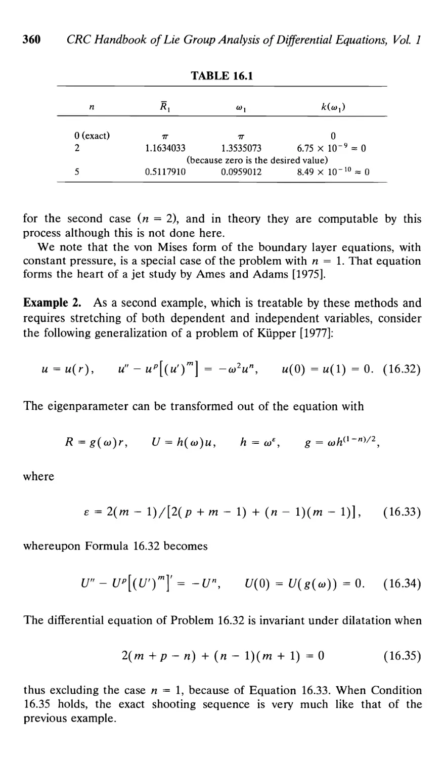
/


Похожие


Текст
CRC HANDB*
LIE GROUP
ANALYSIS OF
IFFERENTIAL
EQUATIONS
VOLUME 1
YMMETRIES
T SOLUTIONS
CONSERVATION LAWS
EDITED BY
N. PL 1BRAG1MOV
W. F. AMES, R. L. ANDERSON
V. A. DORODNITSYN
E. V. FERAPONTOY R. K. GAZIZOV
N. H. IBRAGIMOV
S. R. SVIRSHCHEVSKII
(g)
CRC Press
Boca Raton Ann Arbor London Tokyo
Library of Congress Cataloging-in-Publication Data
CRC handbook of Lie group analysis of differential equations/editor,
N. H. Ibragimov.
p. cm.
Includes bibliographical references and indexes.
Contents: v. 1. Symmetries, exact solutions, and conservation laws/
W. F. Ames... [et al.]
ISBN 0-8493-4488-3 (v. 1)
1. Differential equations—Numerical solutions. 2. Lie groups.
I. Ibragimov, N. Kh. (Nail' Khairullovich)
QA372.C73 1993 92-46289
515\35—dc20 CIP
This book represents information obtained from authentic and highly regarded sources.
Reprinted material is quoted with permission, and sources are indicated. A wide variety of
references are listed. Every reasonable effort has been made to publish reliable data and
information, but the author and the publisher cannot assume responsibility for the validity of all
materials or for the consequences of their use.
Neither this book nor any part may be reproduced or transmitted in any form or by any
means, electronic or mechanical, including photocopying, microfilming, and recording, or by any
information storage and retrieval system, without prior permission in writing from the publisher.
All rights reserved. Authorization to photocopy items for internal or personal use, or the
personal or internal use of specific clients, may be granted by CRC Press, Inc., provided that $.50
per page photocopied is paid directly to Copyright Clearance Center, 27 Congress Street, Salem,
MA 01970 USA. The fee code for users of the Transactional Reporting Service is ISBN
0-8493-4488-3 $0.00 + $.50. The fee is subject to change without notice. For organizations that
have been granted a photocopy license by the CCC, a separate system of payment has been
arranged.
CRC Press, Inc.'s consent does not extend to copying for general distribution, for promotion,
for creating new works, or for resale. Specific permission must be obtained in writing from CRC
Press for such copying.
Direct all inquiries to CRC Press, Inc., 2000 Corporate Blvd., N.W., Boca Raton, Florida
33431.
© 1994 by CRC Press, Inc.
No claim to original U.S. Government works
International Standard Book Number 0-8493-4488-3
Library of Congress Card Number 92-46289
Printed in the United States of America 1234567890
Printed on acid-free paper
CRC HANDBOOK OF LIE GROUP ANALYSIS
OF DIFFERENTIAL EQUATIONS
Editor N. H. Ibragimov
ABSTRACT FOR THE HANDBOOK
With the recent advances in group analysis of differential equations, it is
timely to make available to scientists as well as students this first extensive
compilation of the results of Sophus Lie and related modern developments.
The material is presented in separate volumes.
These volumes reflect the research interests and biases of the coauthors
and hence there is no claim that the presentations are either complete or
exhaustive. In this regard, the editor will entertain any proposal for inclusion
of material in any future Volumes.
in
PREFACE TO VOLUME I
With the veritable explosion of advances in group analysis of differential
equations, it is timely to make available to applied scientists as well as
students this first extensive compilation of the results of Sophus Lie and
related modern results, which span a period of over one hundred years. They
exist in many diverse books and journal articles and are written in many
languages, both in the literal and technical sense. We have attempted to
collect and unify the presentation of these results. There will be inevitable
shortcomings in this first attempt and we apologize for omissions. Subsequent
volumes will allow us to redress errors and omissions. In this regard, the
editor will entertain proposals for inclusion of materials in any subsequent
volumes.
Volume I consists of three parts: A—Apparatus; В—Body of Results;
С—Computer Aspects.
The purpose of Part A is as follows: to systematize the relevant results of
Lie and natural generalizations; to guide the reader through the totality of
group theoretic methods with a minimum number of theoretical
constructions; to prepare the reader to access the results tabulated in Part B; to assist
the reader in developing skills in applying these results and methods to new
problems.
Part B, which makes up the body of results of the Handbook, is devoted to
the group classification and characterization of differential equations. Their
Lie point and contact symmetries, Lie-Backlund and nonlocal symmetries,
Backlund transformations, exact solutions, and conservation laws are
tabulated.
Part С deals with numerical considerations.
The intention is to cover in subsequent volumes at least the following
topics: similarity, elasticity and glacial mechanics, differential constraints and
partial (conditional) symmetries, Backlund transformations, approximate
symmetries, superposition principles, recursion operators, classification
schemes, the Huygens principle, and fundamental and Green-Riemann
functions.
Chapters 1-4 were prepared by Ibragimov and Anderson by condensing
lecture and book manuscript material of Ibragimov.
Chapters 5 and 6 were written by Anderson and Ibragimov as a part of a
project funded by a NATO Collaborative Research Grant (#930117).
Chapter 7 was prepared by Gazizov, condensing research papers of
Akhatov, Gazizov, and Ibragimov.
Chapter 16 was written by Ames.
Chapter 17 was written by Dorodnitsyn.
The Body of Results was prepared by Ibragimov (Chapters 8 and 9),
Gazizov (Chapters 9, 11, and 13), Svirshchevskii (Chapter 10), and Ferapon-
tov (Chapters 14 and 15).
We benefitted from the help of many colleagues in collecting materials for
the Handbook. We would like especially to thank A. V. Aksenov (parts of
v
Preface
VI
Chapter 15), V. A. Baikov (major portion of Chapter 12), S. P. Konovalov
(Section 8.2), and S. P. Tsarev.
We would like to acknowledge Professor A. Samarskii, Director of
Institute of Mathematical Modeling of Russian Academy of Science for his
encouragement and financial support of this project.
We acknowledge financial support from the University of Georgia and, in
particular, we would like to thank Professor William J. Payne, Sr. (while
Dean of the Franklin College of Arts and Sciences) and Associate Vice
President for Research John Ingle for arranging for this support.
We would also like to thank, for their technical help in the preparation of
this volume of the Handbook, Mrs. T. I. Petrova and Miss E. V. Eremina.
Nail Ibragimov
TABLE OF CONTENTS
Preface to Volume I v
Part A. APPARATUS OF GROUP ANALYSIS
I. LIE THEORY OF DIFFERENTIAL EQUATIONS 3
1. One-Parameter Transformation Groups 7
1.1. Local one-parameter point transformation groups 7
1.2. Prolongation formulas 12
1.3. Groups admitted by differential equations 14
1.4. Integration and reduction of order 16
1.4.1. Integrating factor 17
1.4.2. Method of canonical variables 19
1.4.3. Invariant differentiation 21
1.5. Determining equation 22
1.6. Lie algebras 24
1.7. Tangent transformations 26
2. Integration of Second-Order Ordinary
Differential Equations 29
2.1. Solvable Lie algebras and successive reduction
of order 29
2.2. Method of canonical variables 30
2.2.1. Canonical forms of L2 31
2.2.2. Integration algorithm 32
2.2.3. Example 34
3. Group Classification of Second-Order Ordinary Differential
Equation 36
3.1. Lie's classification of equations admitting
three-dimensional algebras 36
3.2. Summary of Lie's general classification 38
3.3. Linearization 38
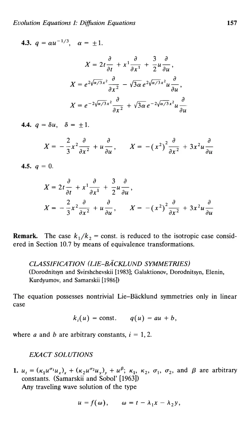
4. Invariant Solutions 42
4.1. Notion of an invariant solution 42
4.2. Optimal systems 44
vii
Contents
49
5. Lie-Backlund Transformation Groups 51
5.1 Steps toward a theory 51
5.1.1. Lie and Backlund 51
5.1.2. Generalization of Lie's infinitesimal
operators 52
5.1.3. Key applications 54
5.1.4. Imposition of the group structure
on infinite-order tangent transformations 54
5.2. Formal Lie-Backlund transformation groups 56
5.3. Lie-Backlund symmetries of differential equations .... 57
6. Noether-Type Conservation Theorems 60
6.1. Conservation laws 60
6.2. Noether theorem 63
7. Nonlocal Symmetry Generators via Backlund
Transformations 68
7.1. Quasilocal symmetries 71
7.2. Example 72
Part B. BODY OF RESULTS
8. Ordinary Differential Equations 77
8.1. Some first-order equations with a known symmetry .... 77
8.2. First-order equations with symmetries linear in
the dependent variable 79
8.3. Some second-order equations with a known
symmetry 82
8.4. Lie group classification of second-order equations 84
9. Second-Order Partial Differential Equations with Two
Independent Variables 86
9.1. Linear equation 86
9.1.1. Lie's classification 86
9.1.2. Ovsiannikov's classification 88
9.1.2.1. Hyperbolic normal form 88
9.1.2.2. Parabolic normal form 90
9.2. Chaplygin equation 91
9.2.1. Ш)фвв + фаа = 0 91
9.2.2. <рв = -фа, <ра = К(а)фв 92
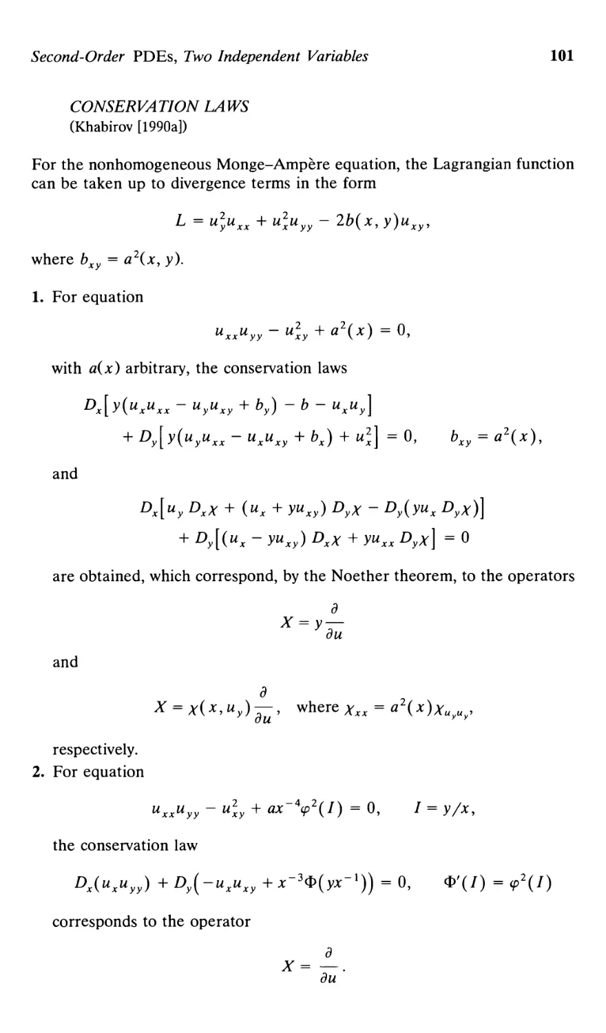
9.3. Homogeneous Monge-Ampere equation 94
9.4. Nonhomogeneous Monge-Ampere equation 95
IX
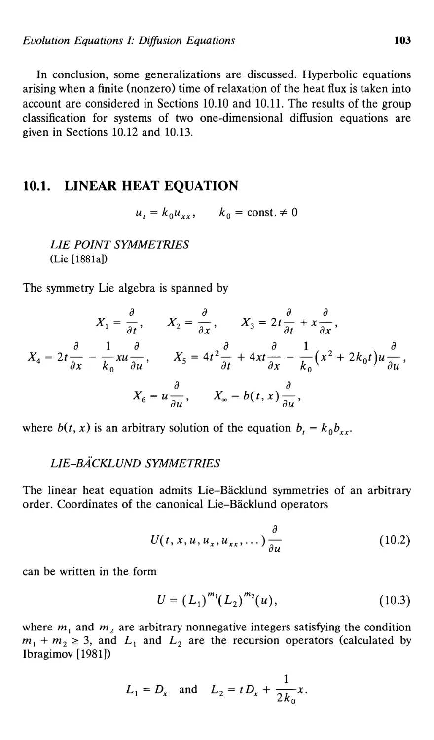
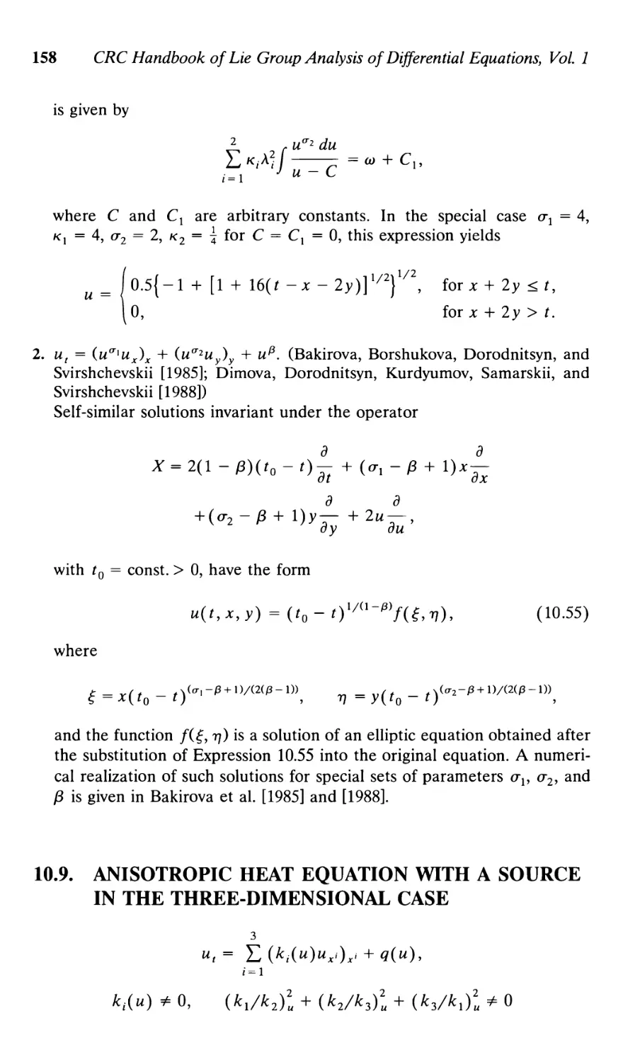
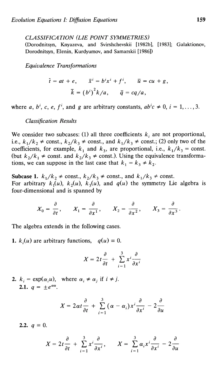
Evolution Equations I: Diffusion Equations 102
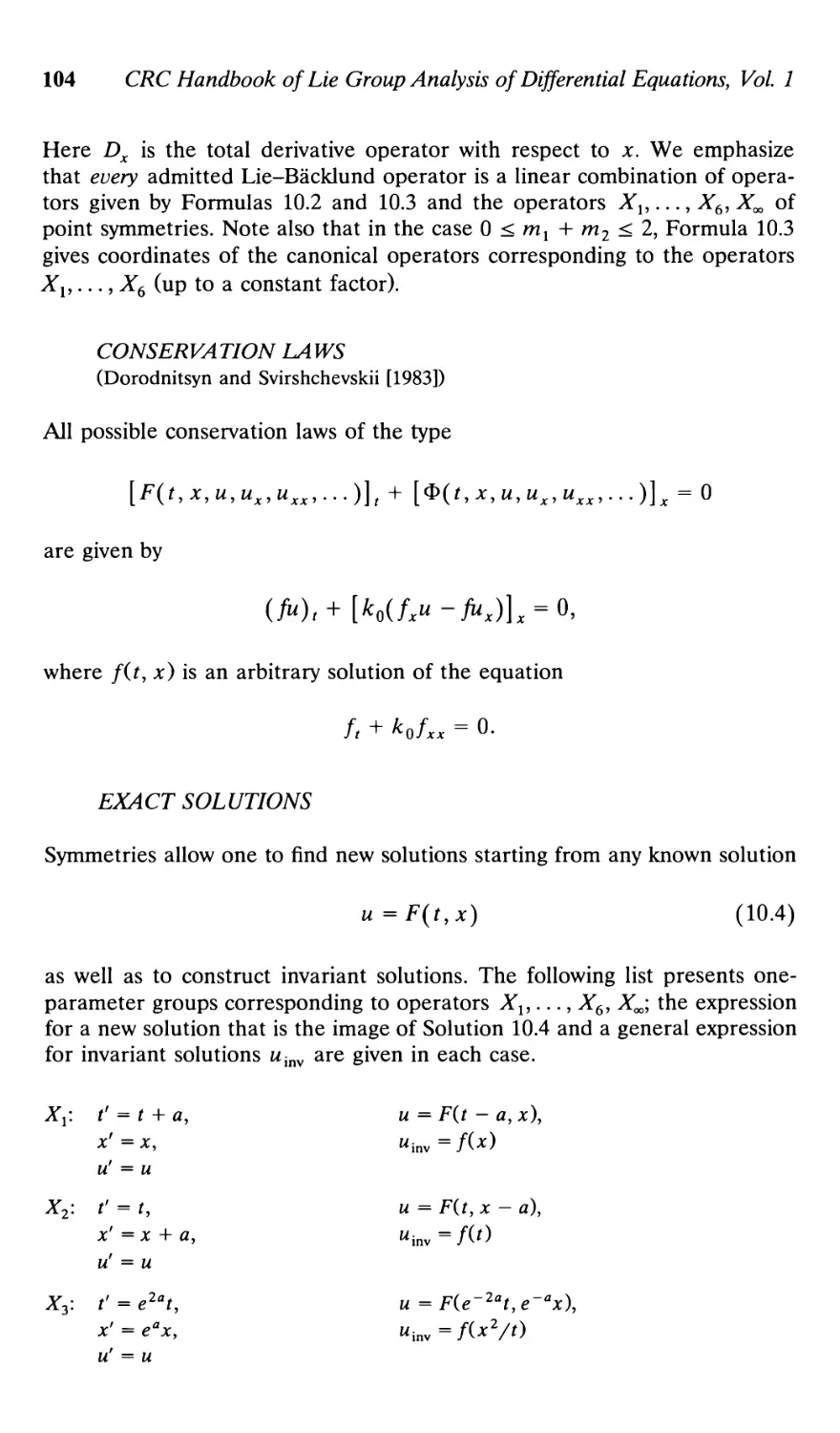
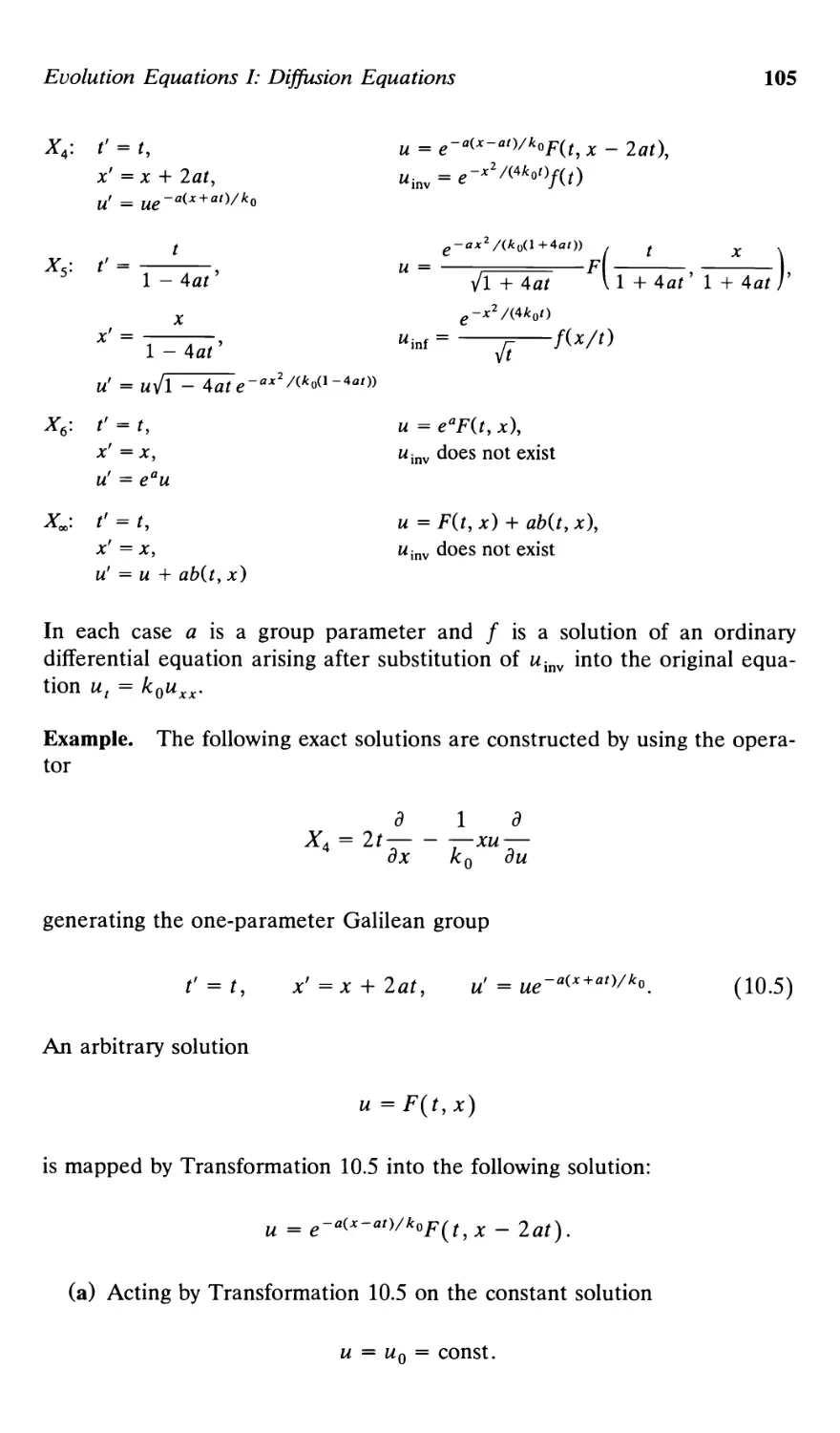
10.1. Linear heat equation 103
10.2. Nonlinear heat equation 110
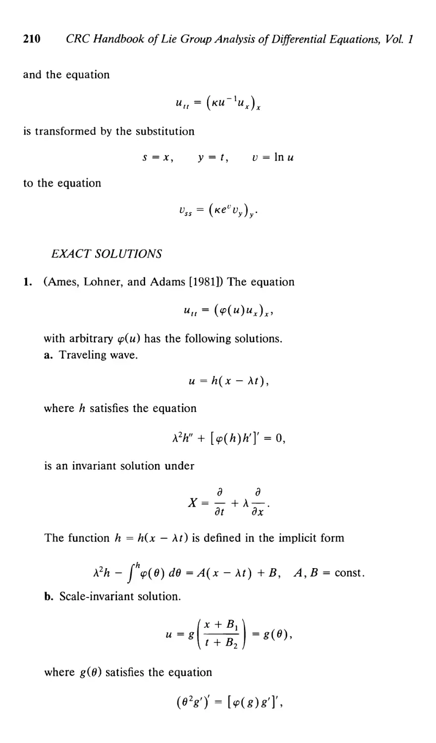
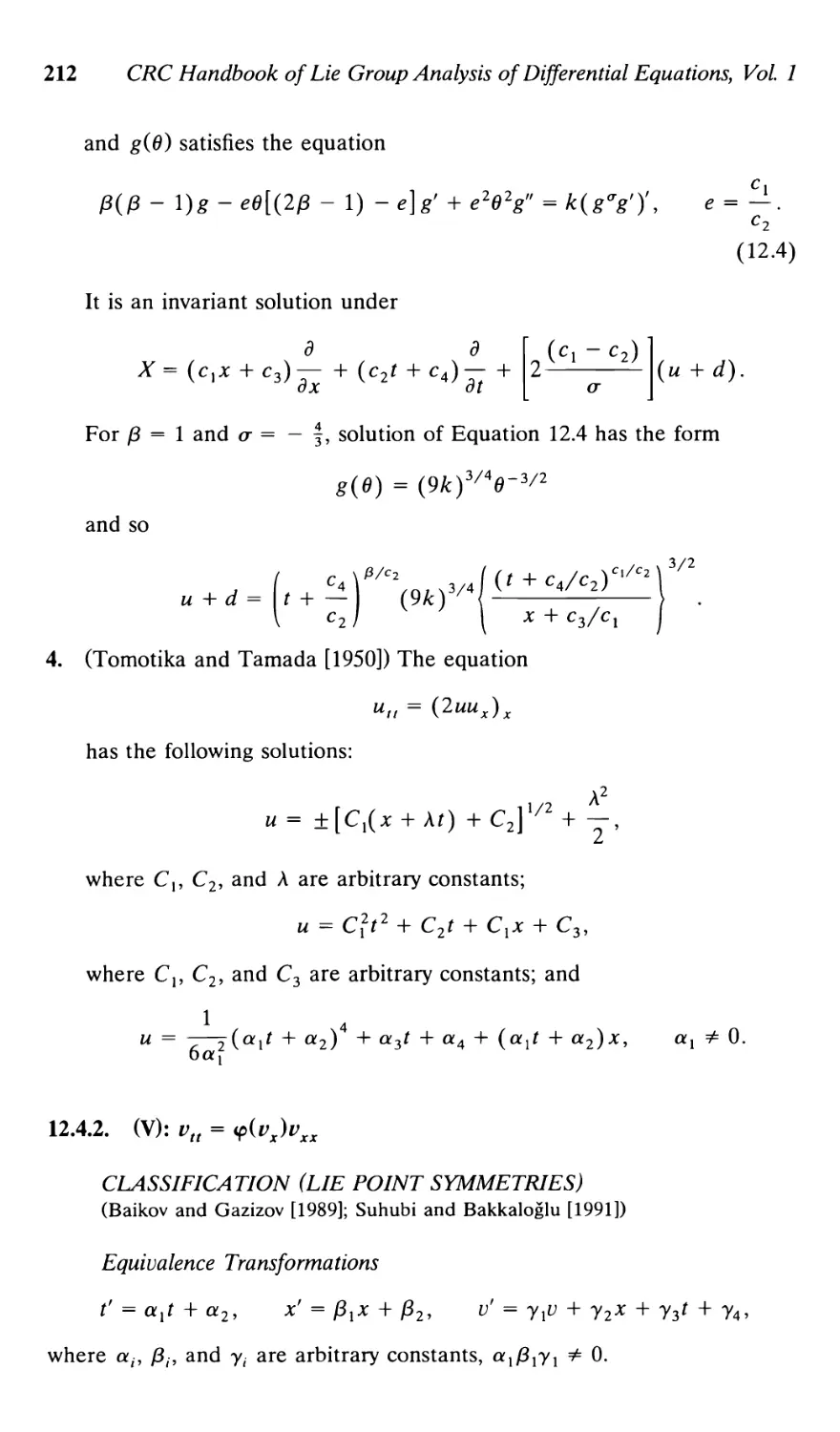
10.3. Nonlinear filtration equation 129
10.4. Potential filtration equation 131
10.5. Nonlinear heat equation with a source 133
10.6. Heat equations in nonhomogeneous medium
admitting nontrivial Lie-Backlund group 143
10.7. Nonlinear heat equation with a source,
in the Af-dimensional case 144
10.8. Anisotropic heat equation with a source,
in the two-dimensional case 155
10.9. Anisotropic heat equation with a source,
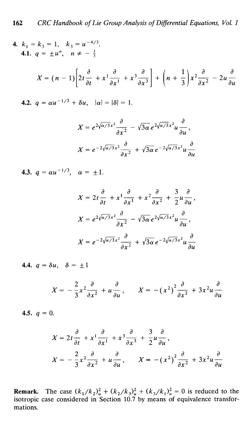
in the three-dimensional case 158
10.10. Potential hyperbolic heat equation 163
10.11. Hyperbolic heat equation 169
10.12. A system of two linear diffusion equations 170
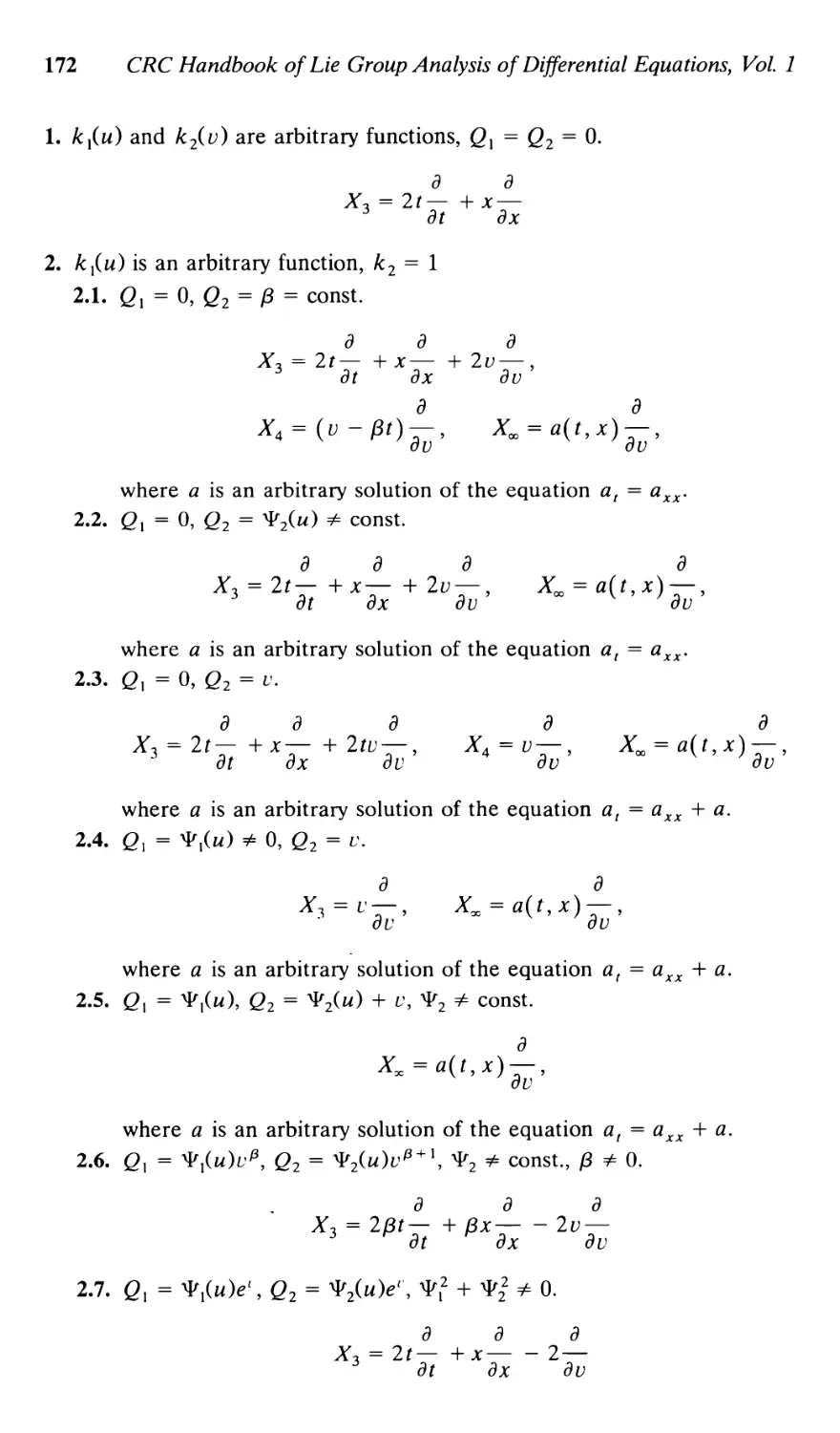
10.13. A system of two diffusion equations 171
Evolution Equations II: General Case 177
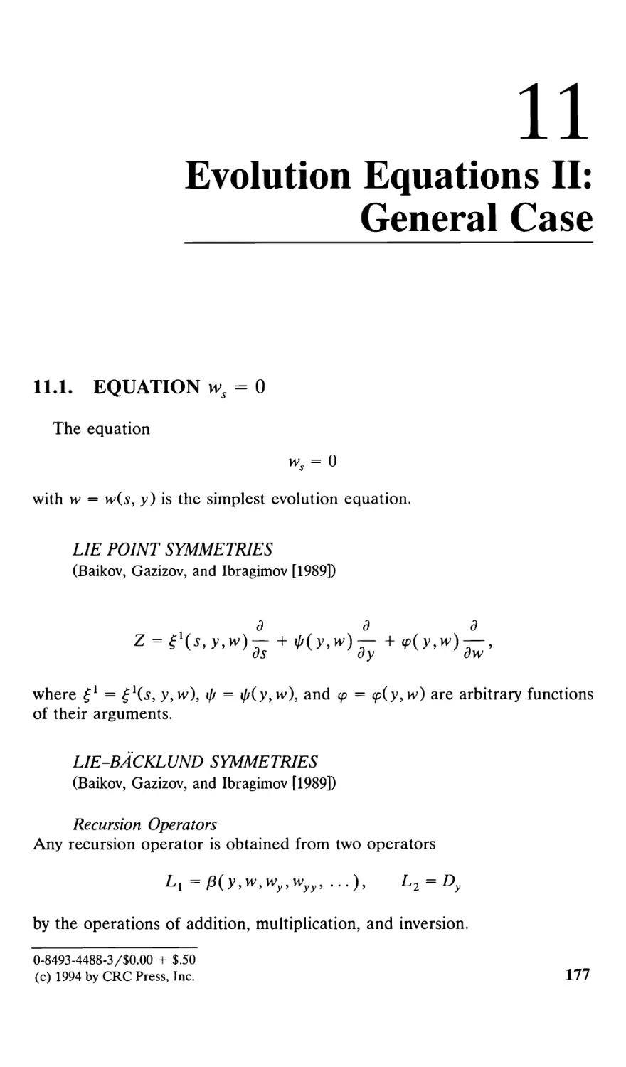
11.1. Equation ws = 0 177
11.2. Simplest transfer equation 178
11.3. Transfer equation 179
11.4. Burgers equation 180
11.5. Potential Burgers equation 183
11.6. Generalized Hopf equation 184
11.7. Korteweg-de Vries equation 185
11.8. Generalized Korteweg-de Vries-Burgers
equation 192
11.9. BBM equation 194
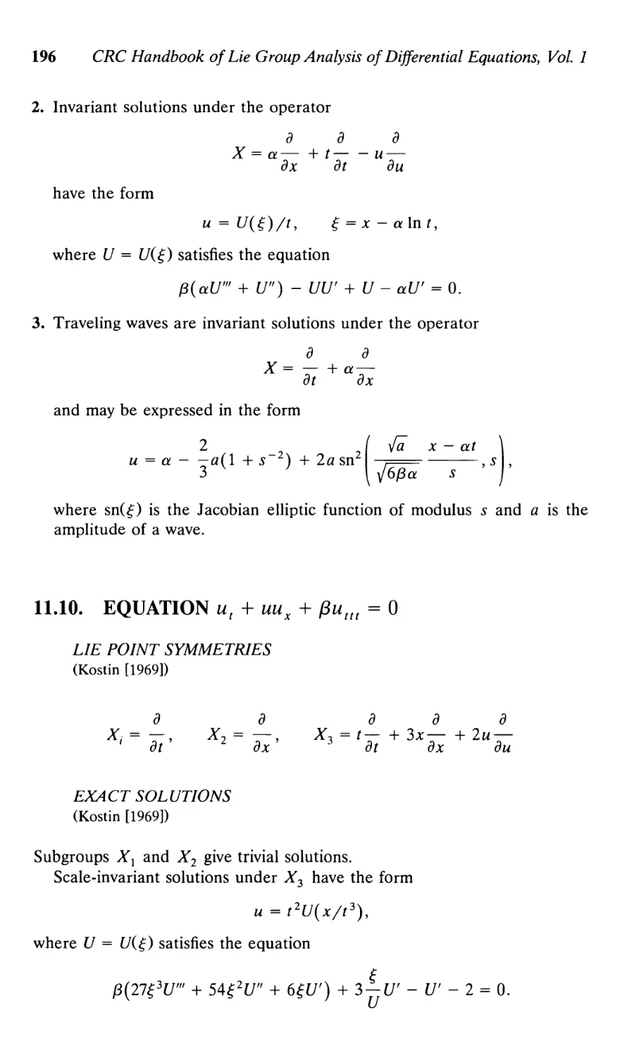
11.10. Equation ut + uux + $uttt = 0 196
Wave Equations 197
12.1. One-dimensional linear wave equations 197
12.1.1. ий7] = 0 197
12.1.2. utt-uxx = 0 198
12.2. One-dimensional linear wave equations
with variable coefficients 198
12.2.1. utt - c\x)uxx = 0 199
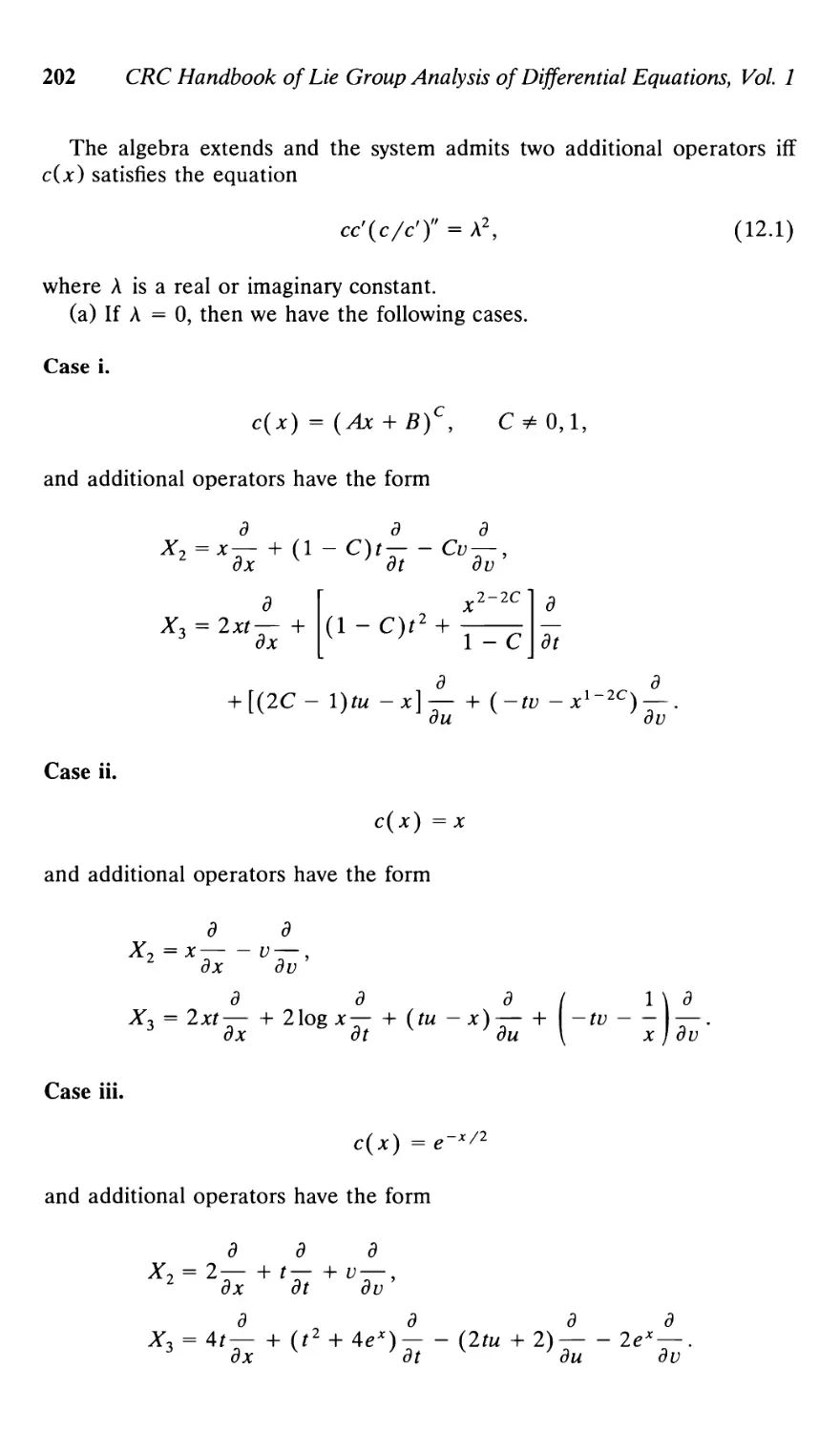
12.2.2. vt = ux, ut = c\x)vx 201
12.3. Equation zxy = F(z) 204
12.3.1. Bonnet equation 206
X
Contents
12.4. One-dimensional nonlinear wave equations 208
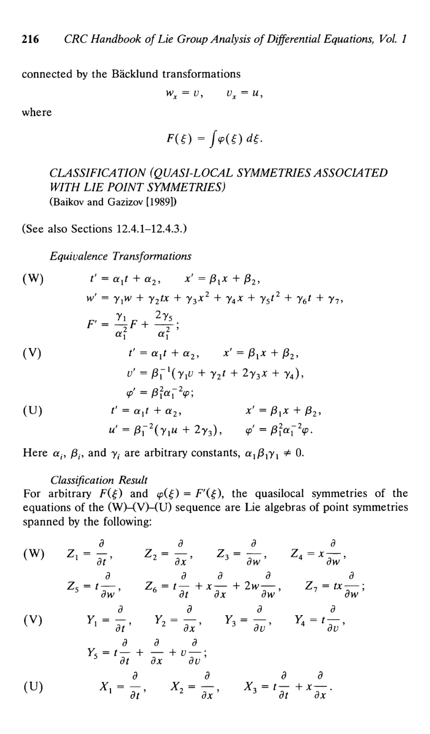
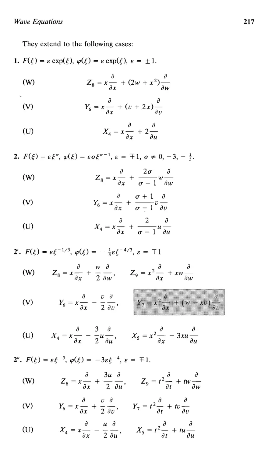
12.4.1. (U): utt = (cp(u)ux)x 208
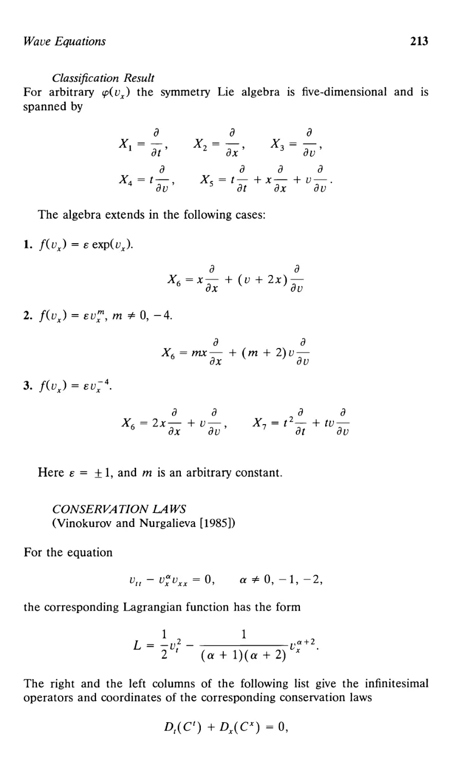
12.4.2. (V): vtt = <p(vx)vxx 212
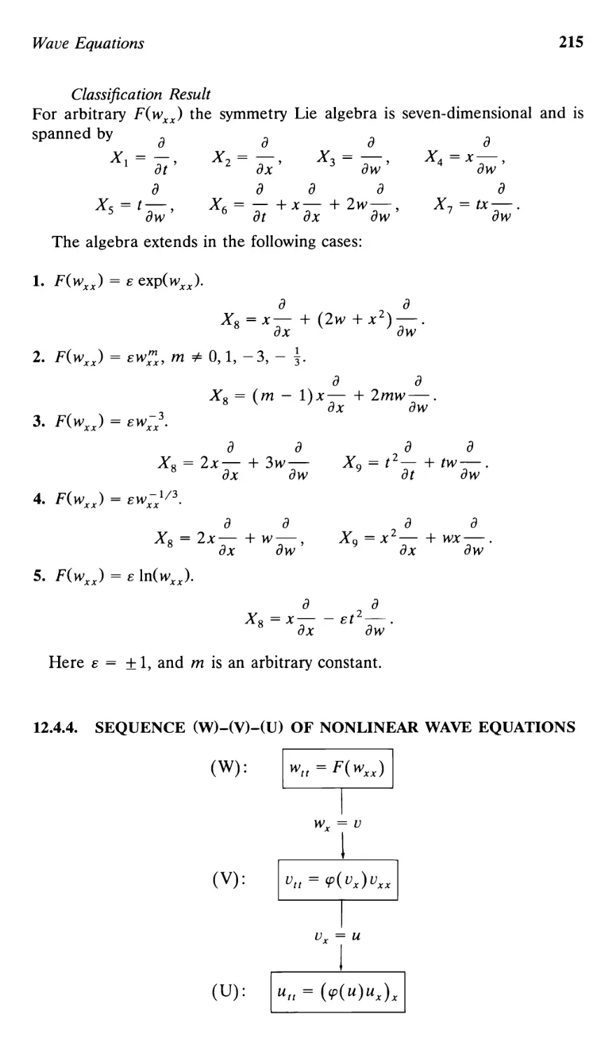
12.4.3. (W): w(( = F(wxx) 214
12.4.4. Sequence (W)-(V)-(U) of nonlinear
wave equations 215
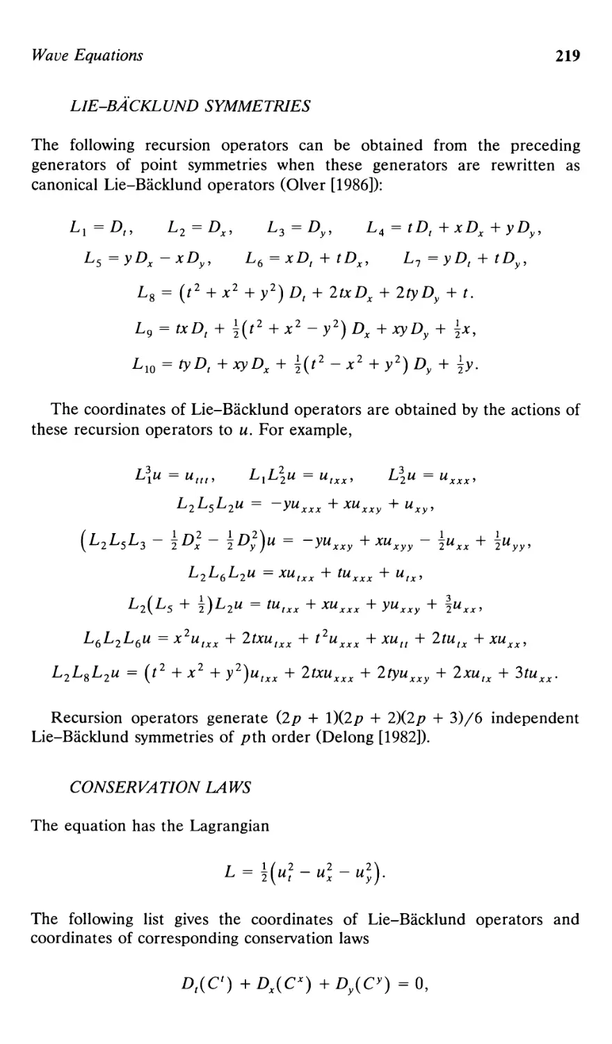
12.5. Two-dimensional linear wave equation 218
12.6. Two-dimensional nonlinear wave equations 222
12.7. Three-dimensional linear wave equation 226
12.8. Three-dimensional nonlinear wave equations 232
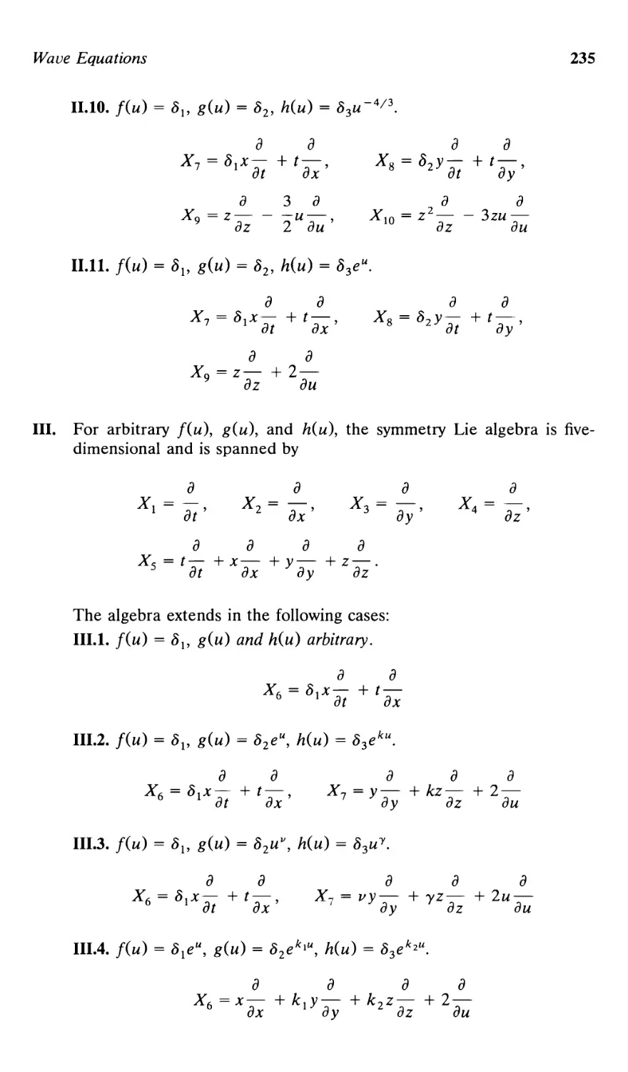
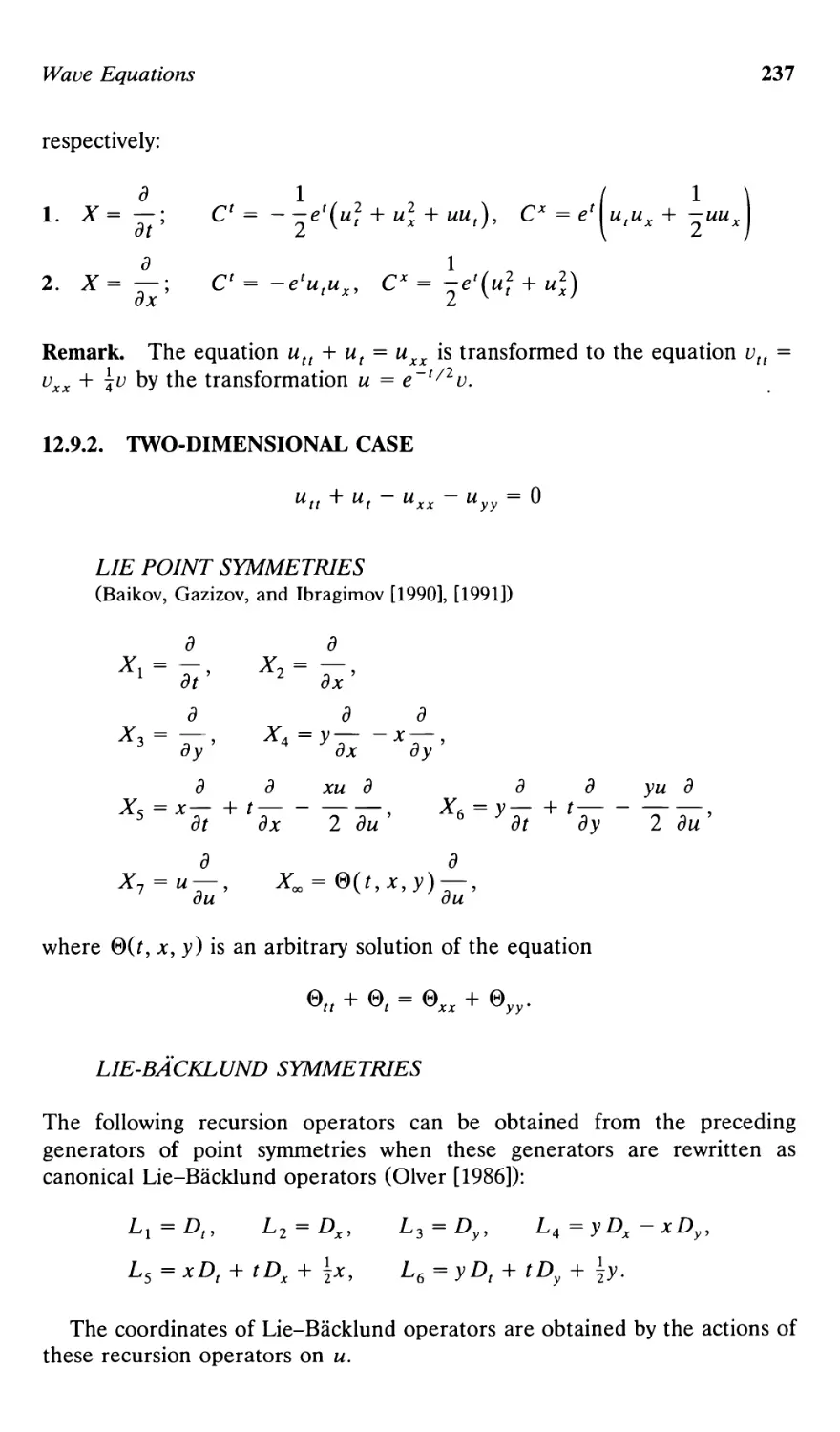
12.9. Linear wave equations with dissipation 236
12.9.1. One-dimensional case 236
12.9.2. Two-dimensional case 237
12.9.3. Three-dimensional case 239
12.10. Nonlinear wave equations with dissipation 243
12.10.1.One-dimensional case 243
12.10.2.Two-dimensional case 244
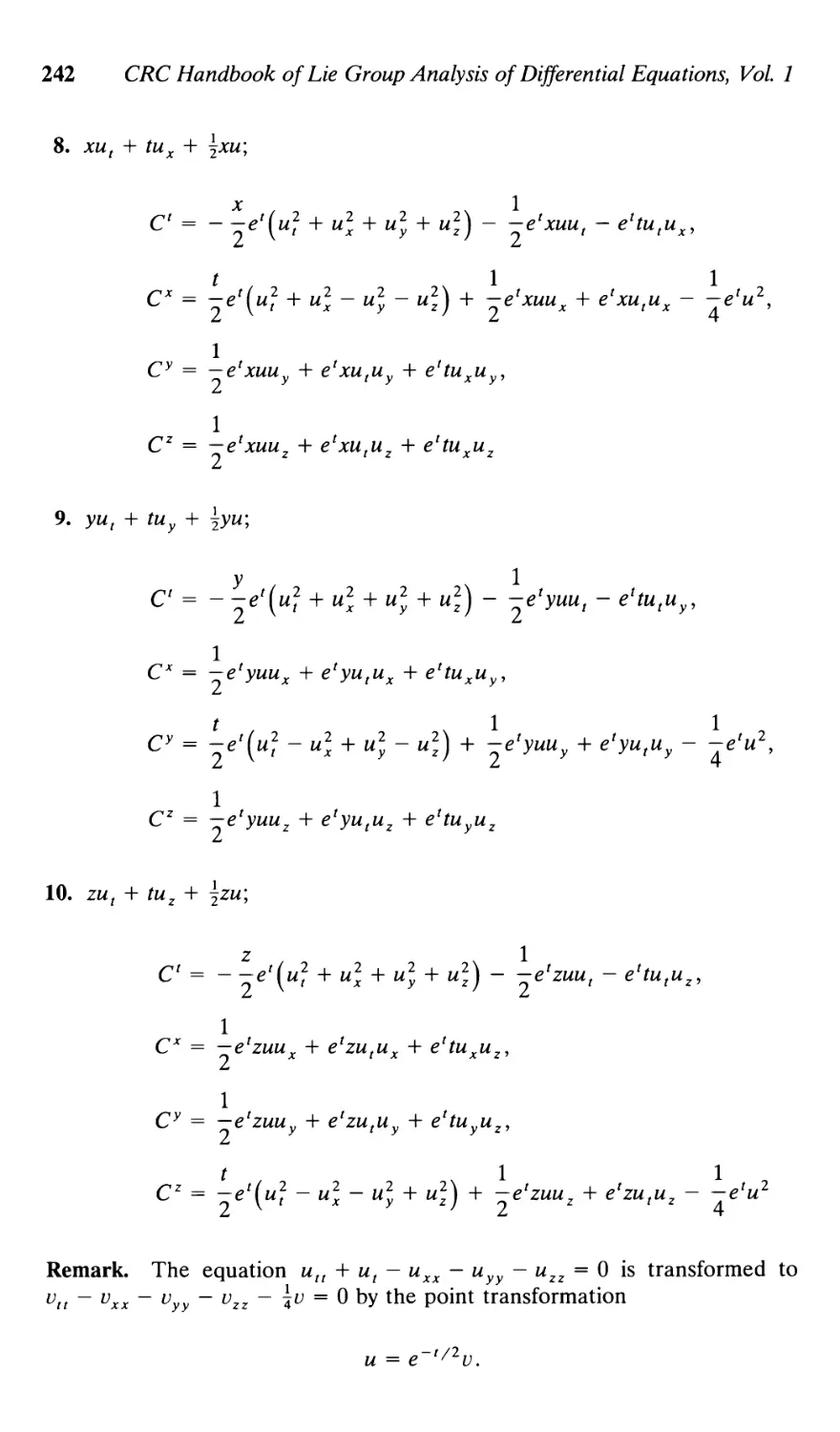
12.10.3.Three-dimensional case 246
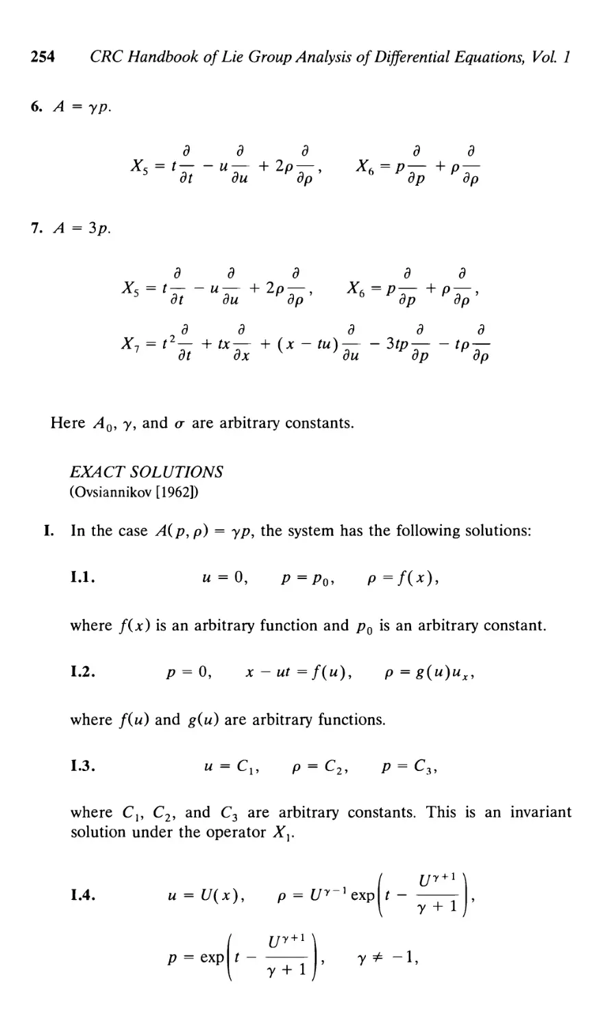
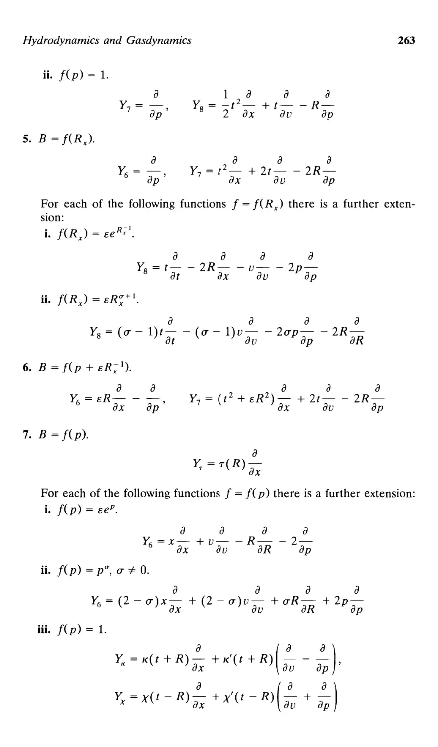
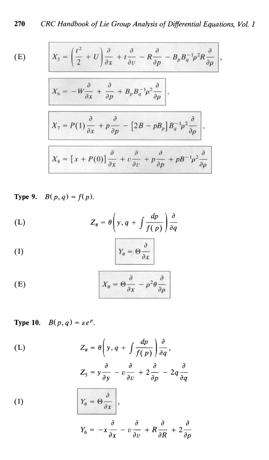
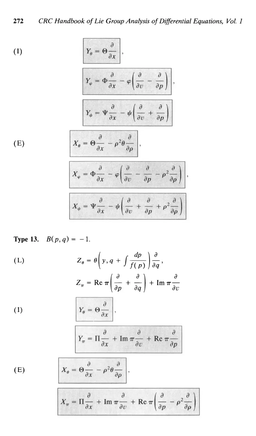
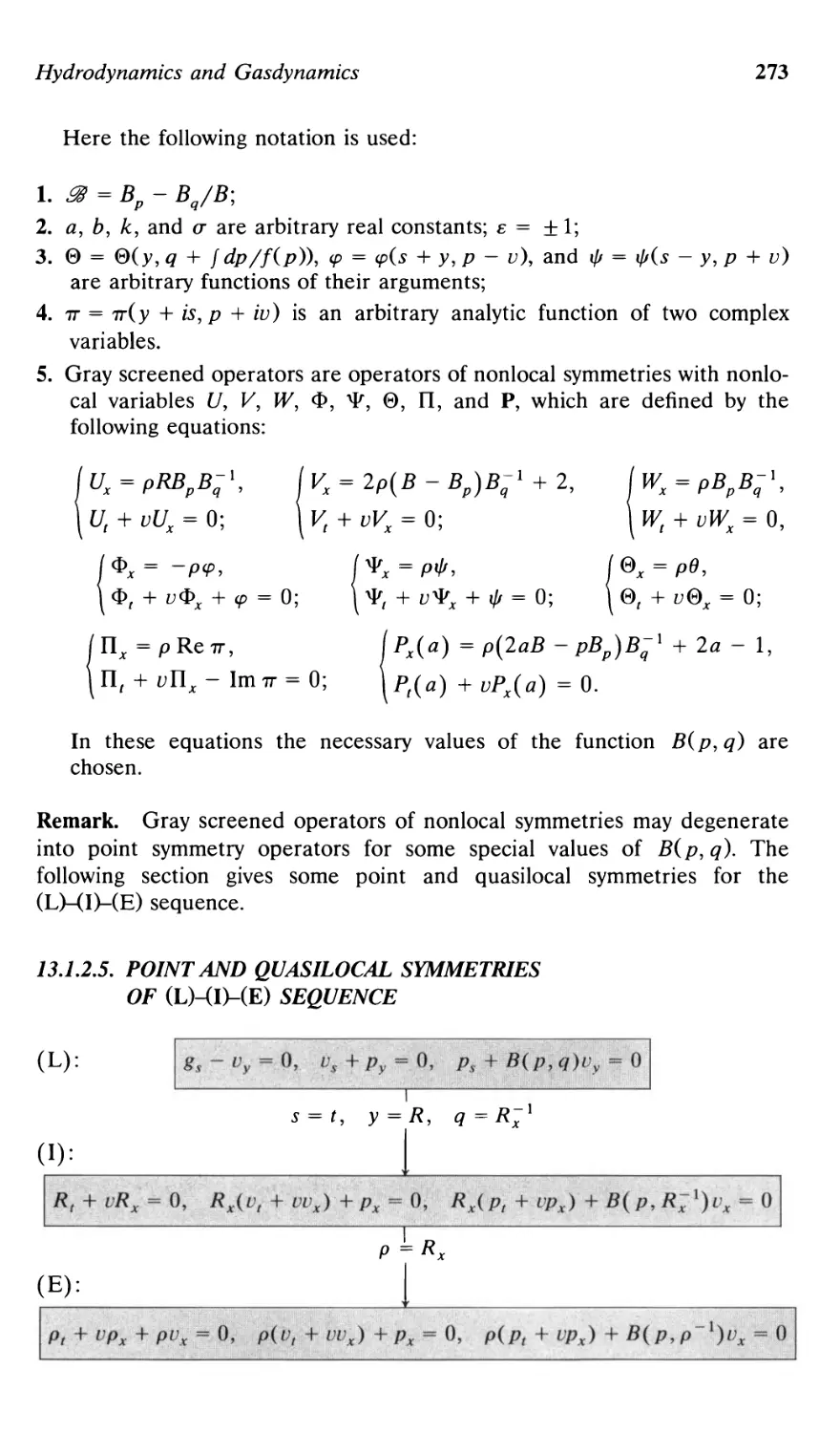
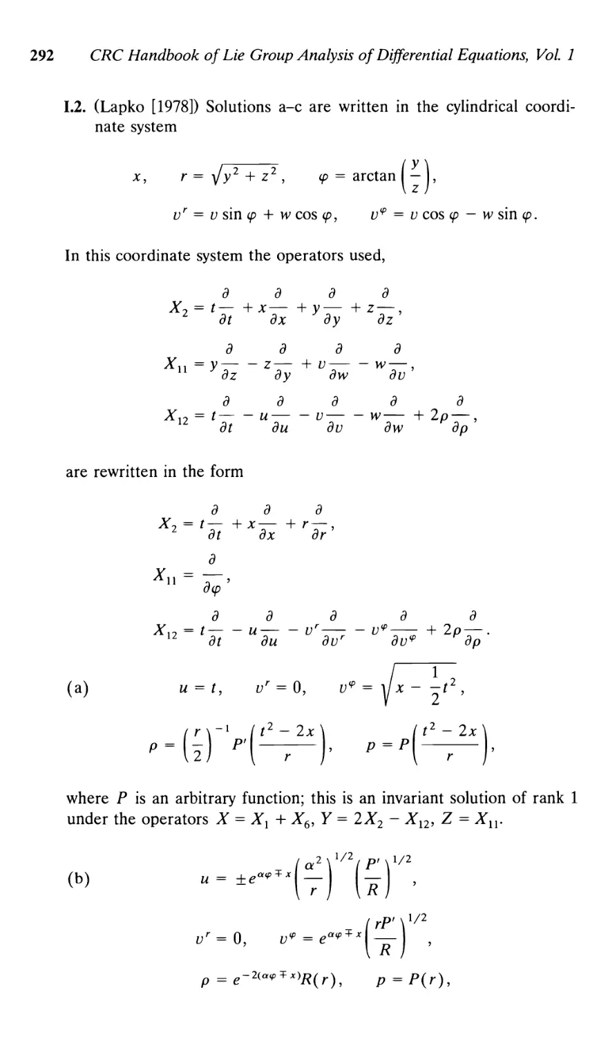
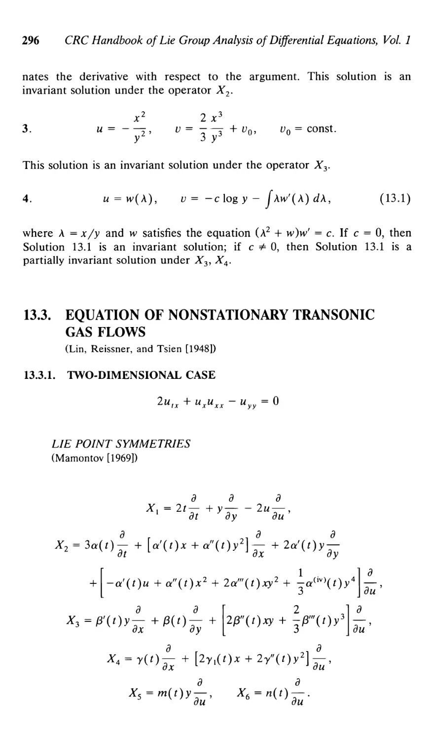
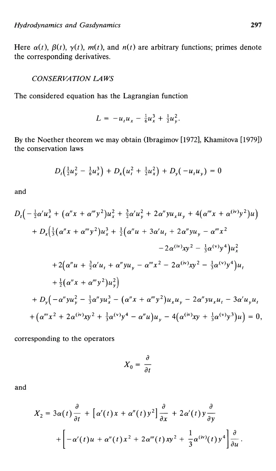
13. Hydrodynamics and Gasdynamics 249
13.1. Adiabatic gas motion 249
13.1.1. General case 249
13.1.2. One-dimensional case 252
13.1.2.1. Euler coordinates 252
13.1.2.2. Lagrangian coordinates 258
13.1.2.3. Intermediate system 261
13.1.2.4. (L)-(D-(E) sequence of equations
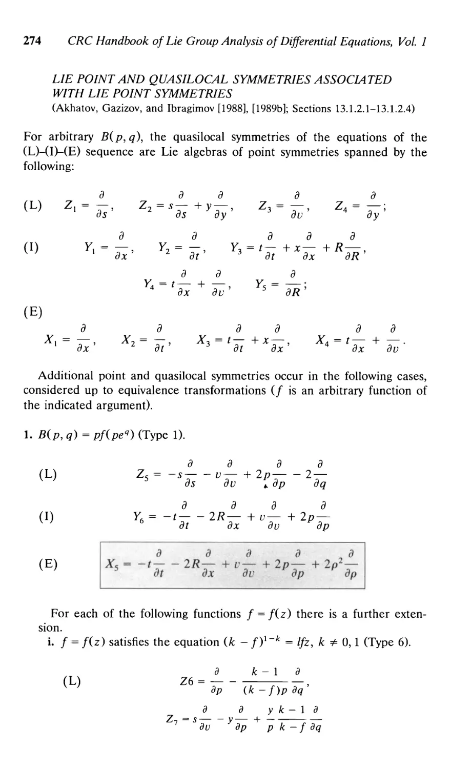
of adiabatic gas motion 264
13.1.2.5. Point and quasilocal symmetries
of (L)-(D-(E) sequence 273
13.1.3. Two-dimensional case 285
13.1.4. Three-dimensional case 289
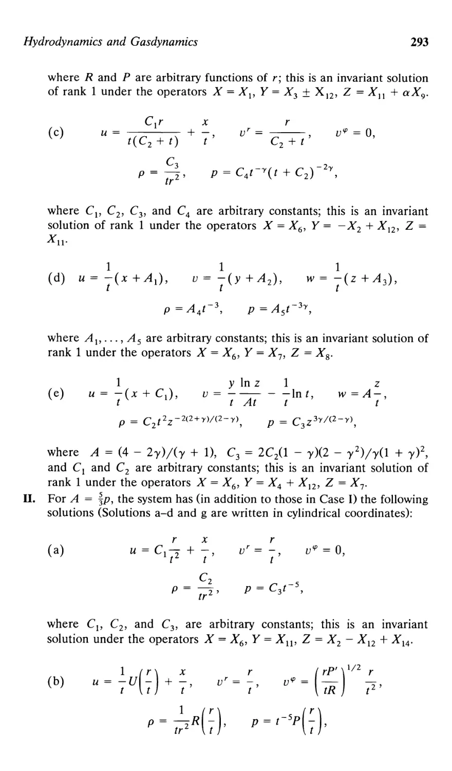
13.2. Equations of stationary transonic plane-parallel
gas flows 295
13.3. Equation of nonstationary transonic gas flows 296
13.3.1. Two-dimensional case 296
13.3.2. Three-dimensional case 298
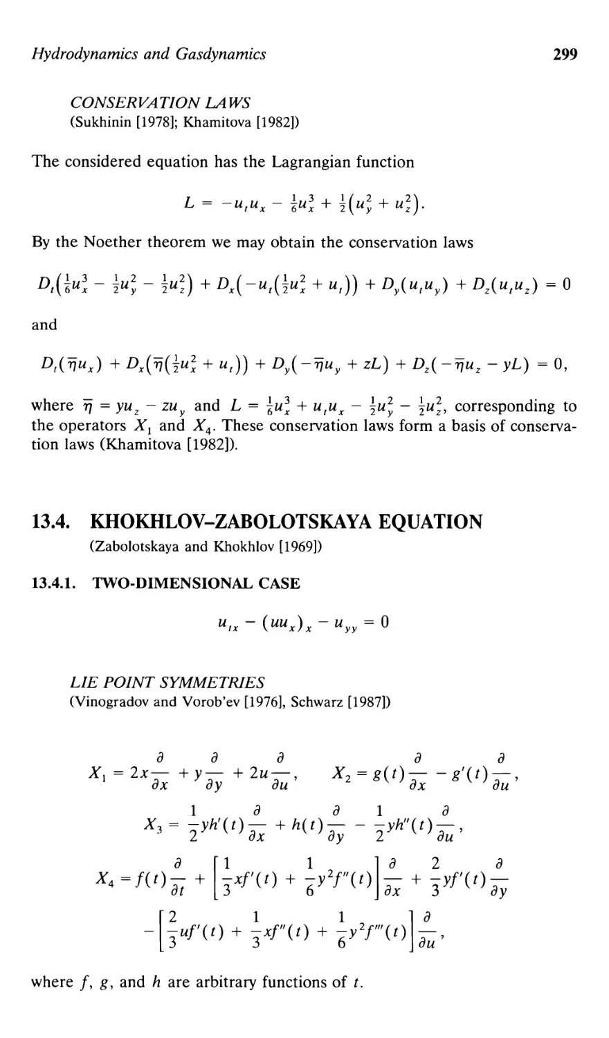
13.4. Khokhlov-Zabolotskaya equation 299
13.4.1. Two-dimensional case 299
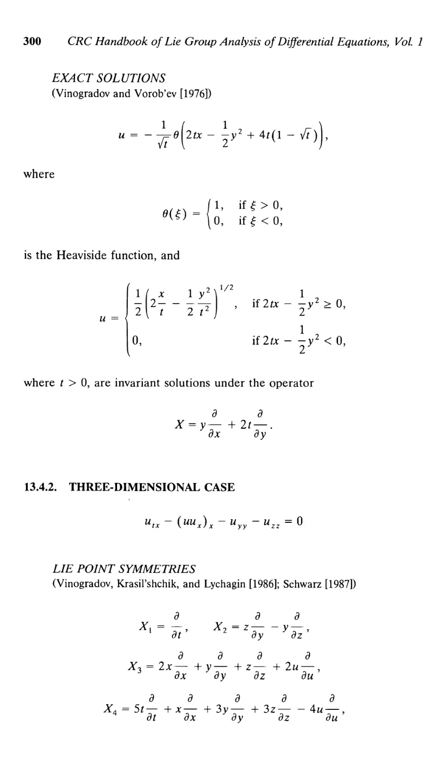
13.4.2. Three-dimensional case 300
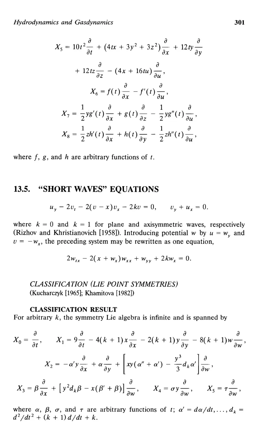
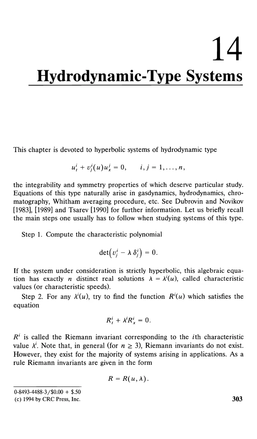
13.5. "Short waves" equation 301
xi
Hydrodynamic-Type Systems 303
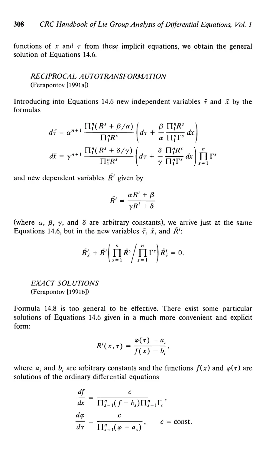
14.1. Equations of chromatography 306
14.1.1. Langmuir isotherm 306
14.1.2. Generalized Langmuir isotherm 310
14.1.3. Power isotherm 313
14.1.4. Langmuir isotherm with dissociation 316
14.1.5. Exponential isotherm 317
14.2. Systems of Temple class 317
14.3. Isotachophoresis equations 320
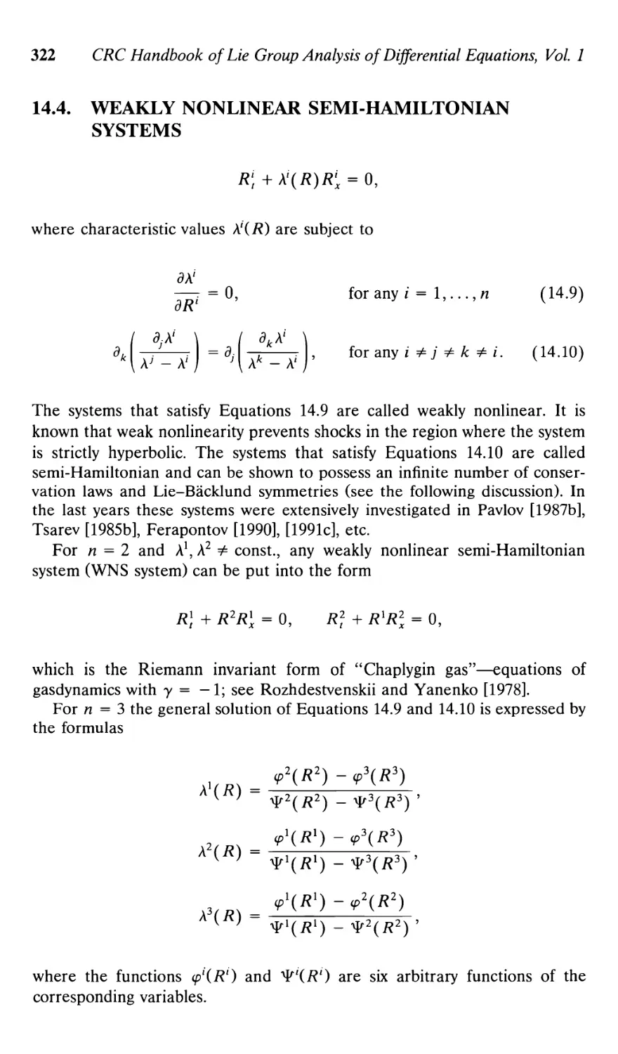
14.4. Weakly nonlinear semi-Hamiltonian systems 322
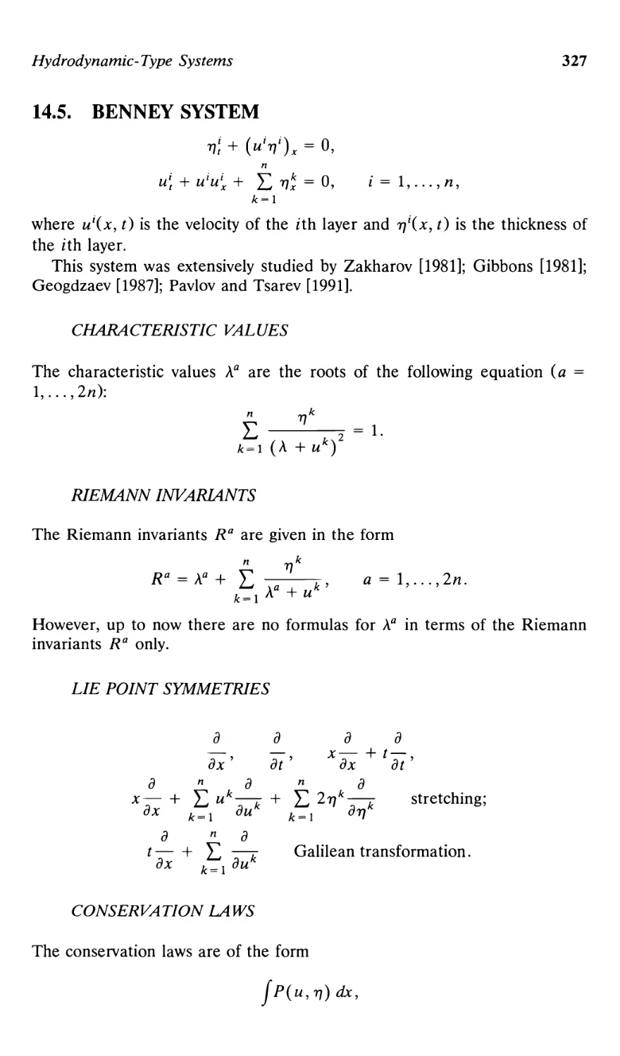
14.5. Benney system 327
14.6. Averaged nonlinear Schrodinger equation 328
14.7. Averaged KdV equation 330
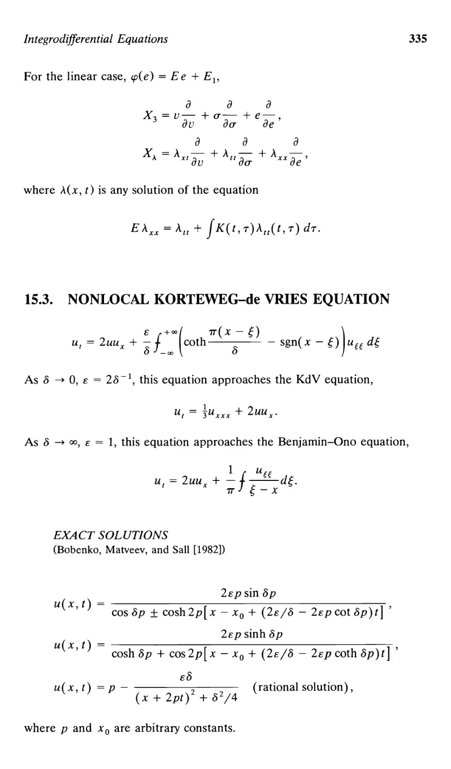
Integrodifferential Equations 332
15.1. PseudodifFerential Schrodinger equation 332
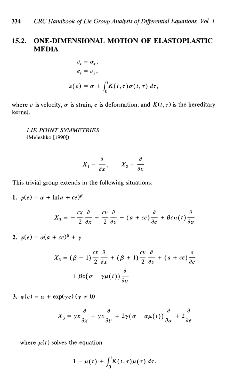
15.2. One-dimensional motion of elastoplastic media 334
15.3. Nonlocal Korteweg-de Vries equation 335
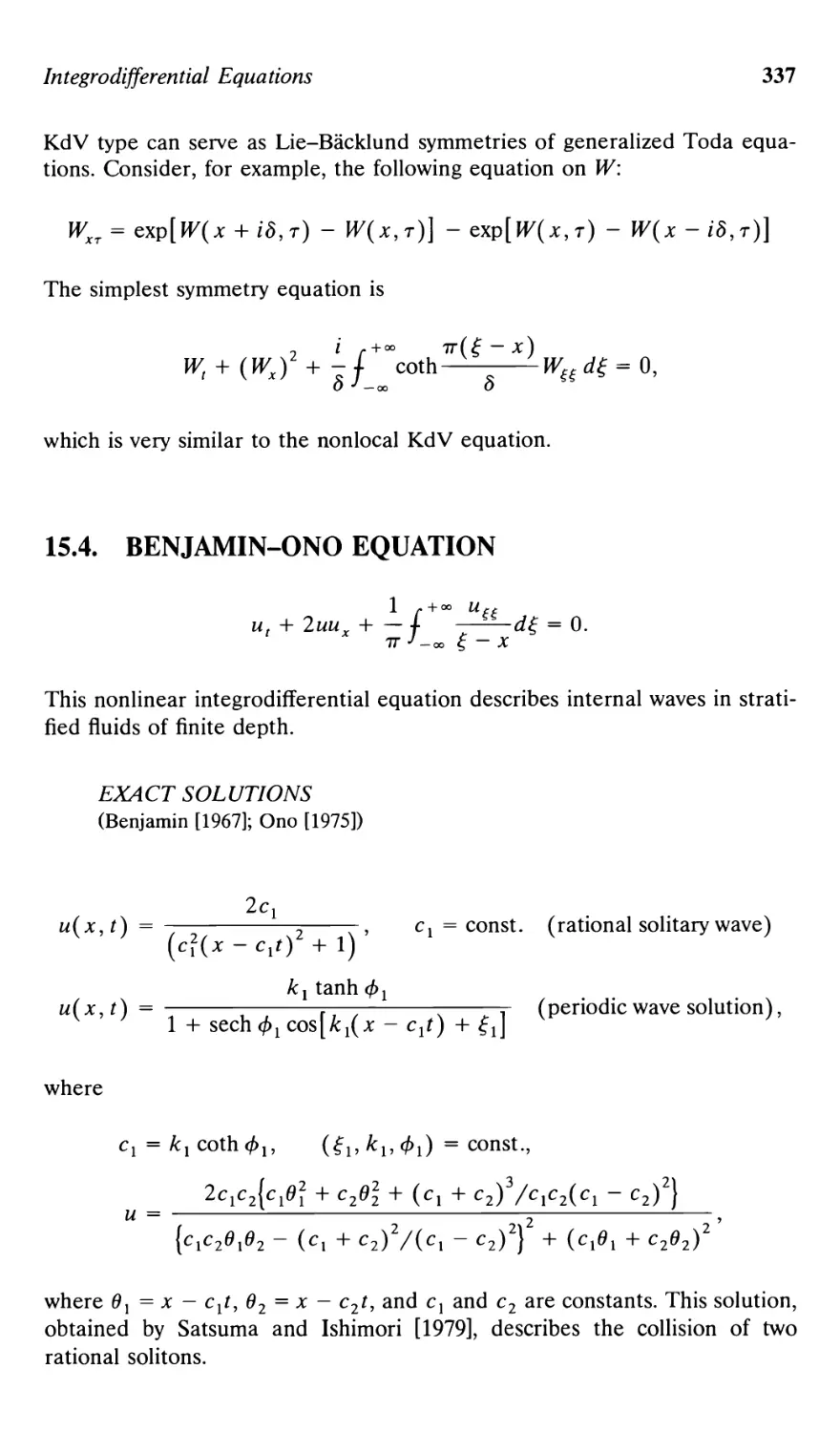
15.4. Benjamin-Ono equation 337
15.5. Conformal-invariant integrodifFerential equation 340
15.6. IntegrodifFerential Boltzmann equation 341
15.7. Spacially homogeneous Boltzmann equation
for Maxwell molecules 342
15.8. Exactly solvable kinetic equation describing
"very hard" particles 343
15.9. Maxwell-Vlasov equations 344
15.10. Long nonlinear waves 344
Part С COMPUTER ASPECTS
Applications of Group Theory in Computation—A Survey. . . . 349
16.1. Conversion of boundary value to initial value
problems 350
16.2. Calculation of eigenvalues 355
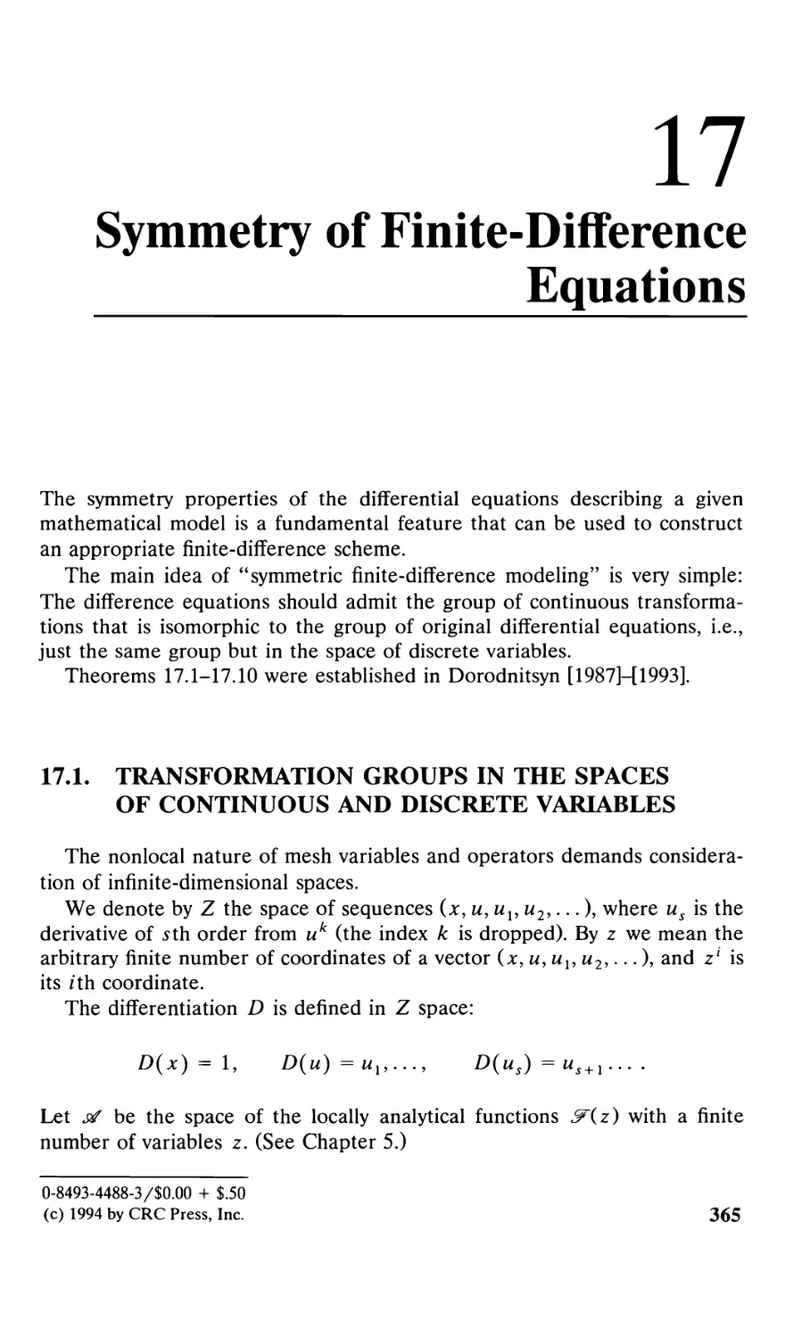
16.3. Some miscellaneous applications 361
16.3.1. Calculation near a singularity 361
16.3.2. Finite-difference equations 362
16.3.3. Invariant algorithms 364
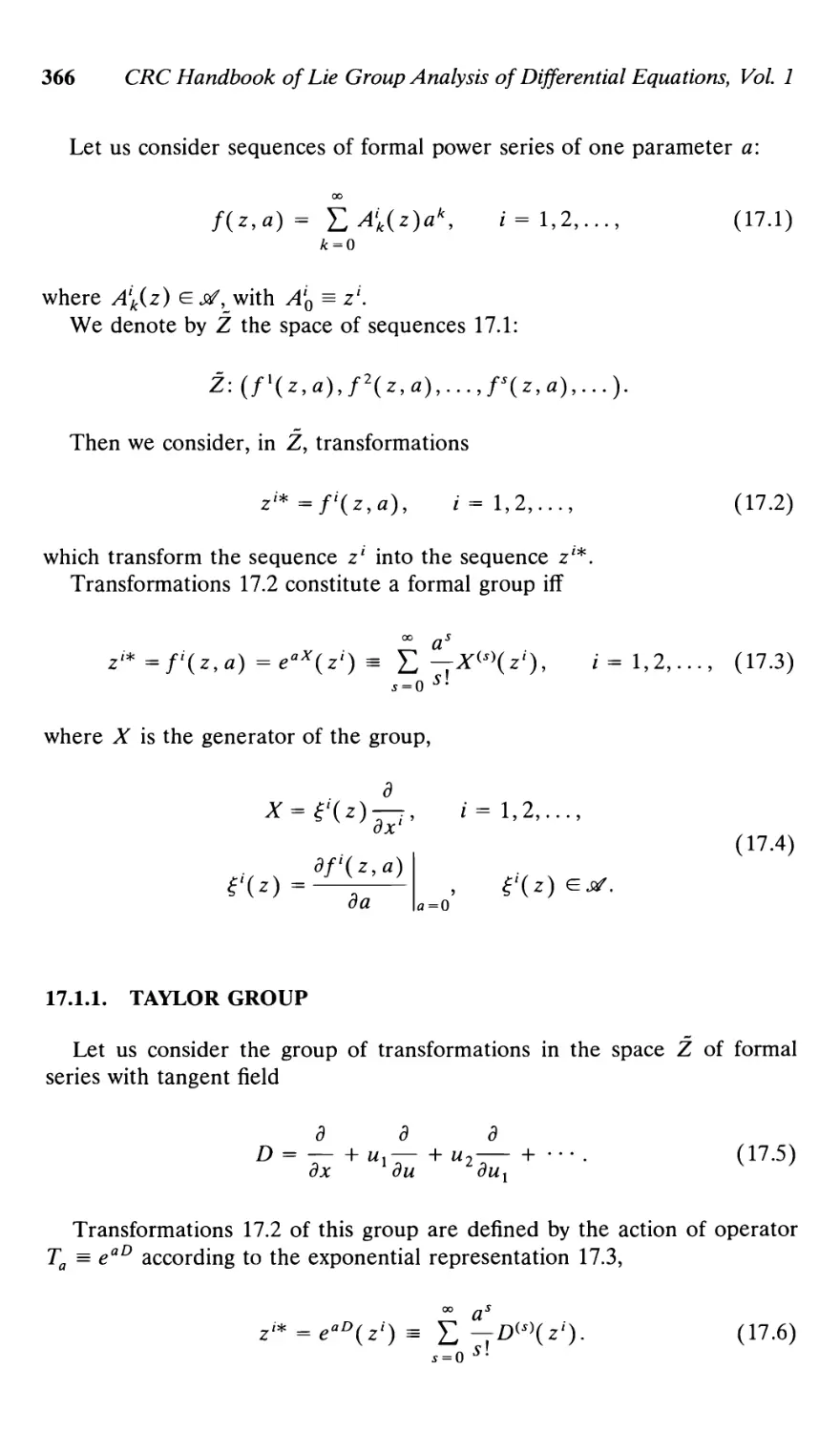
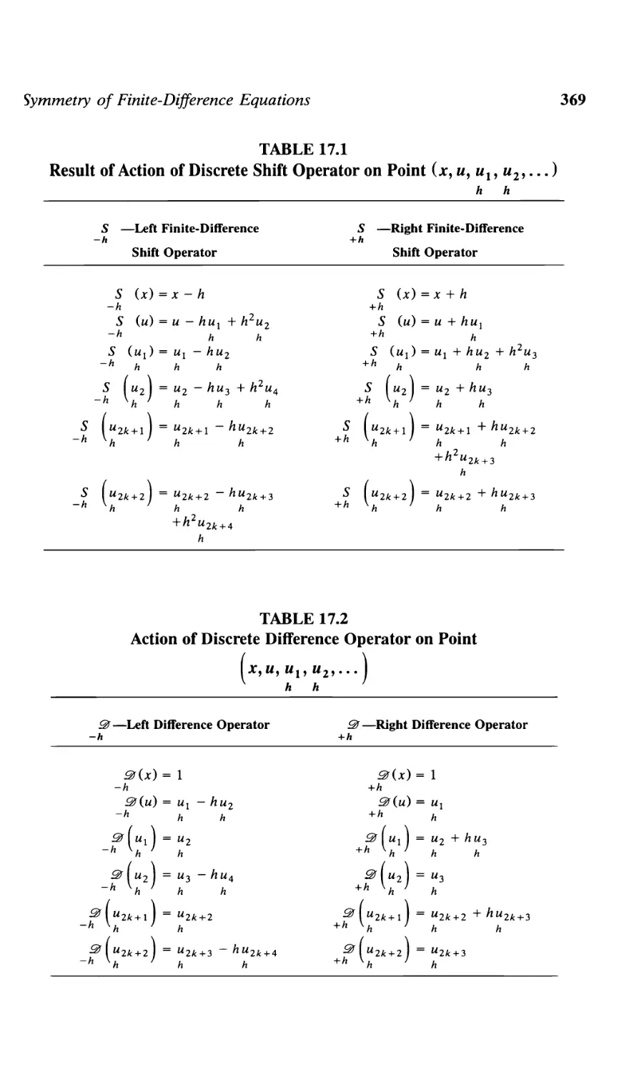
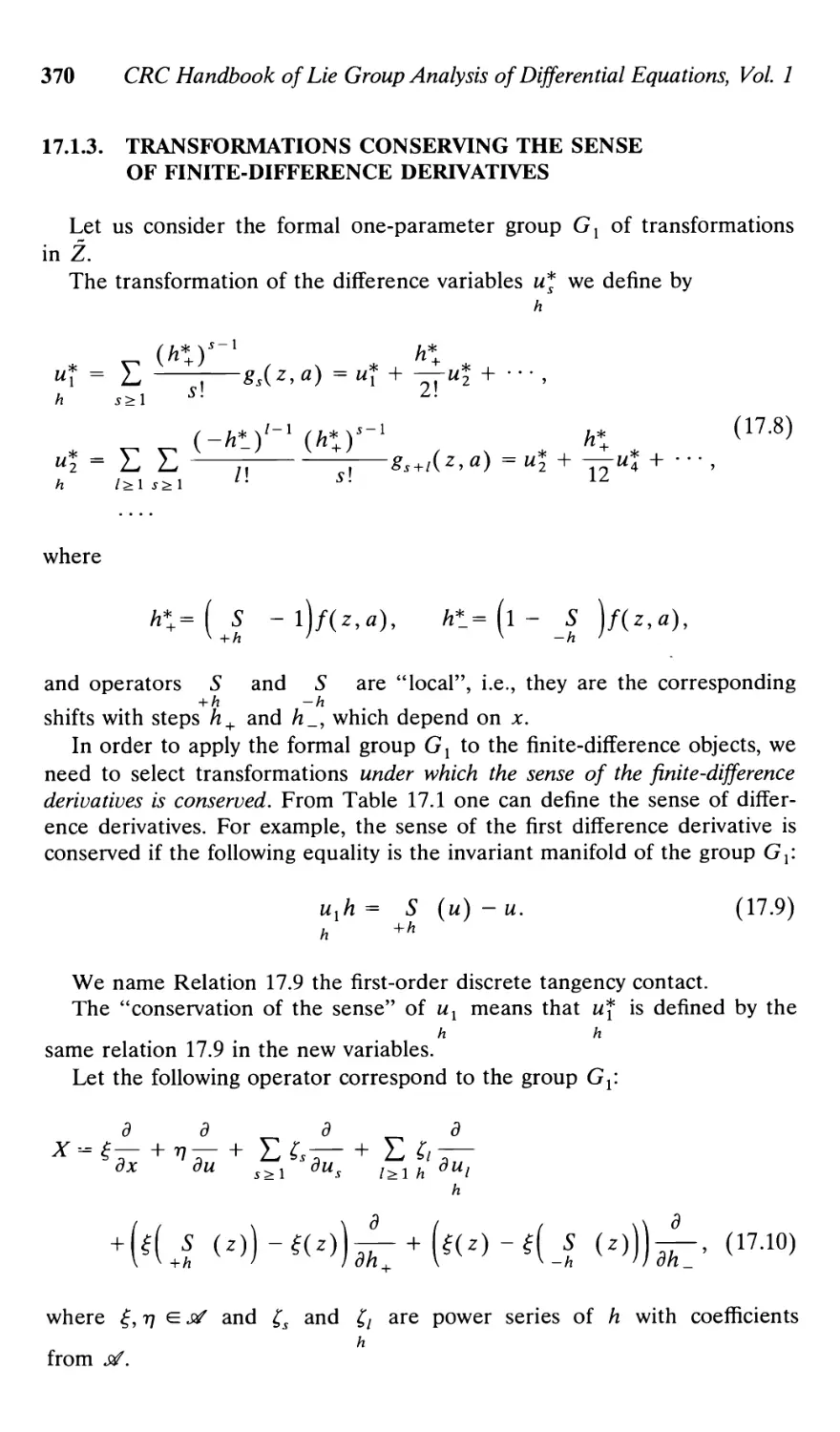
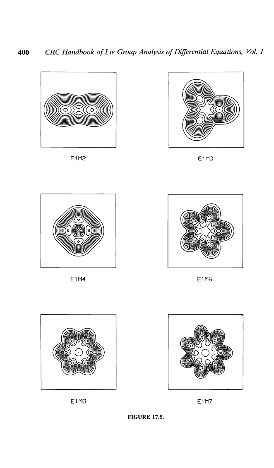
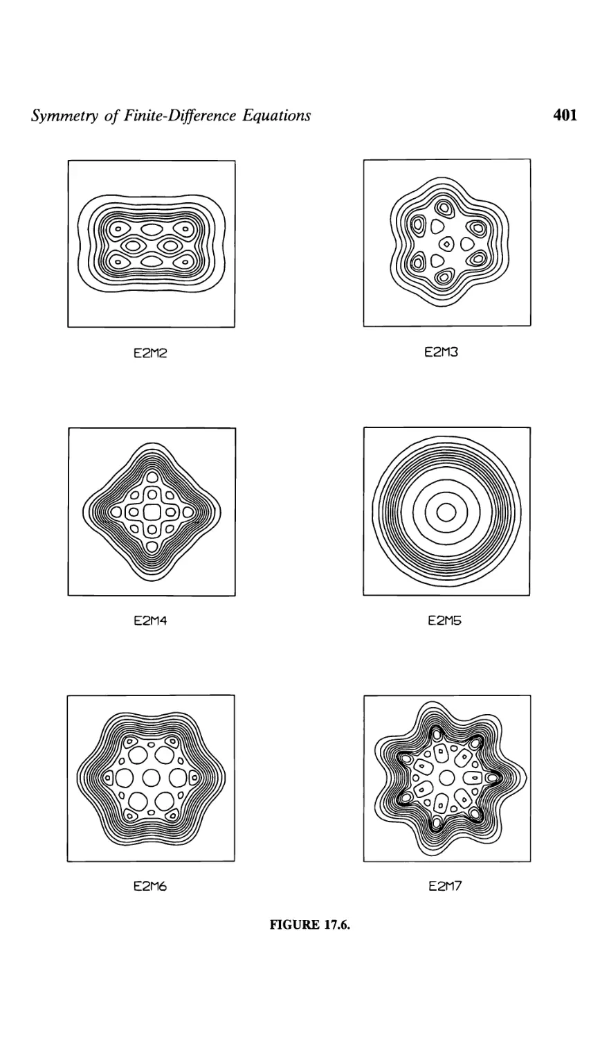
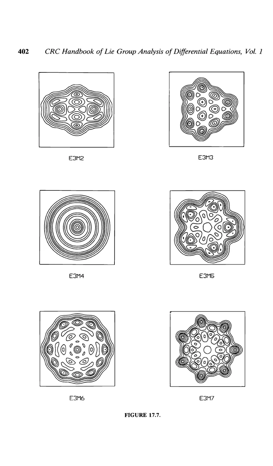
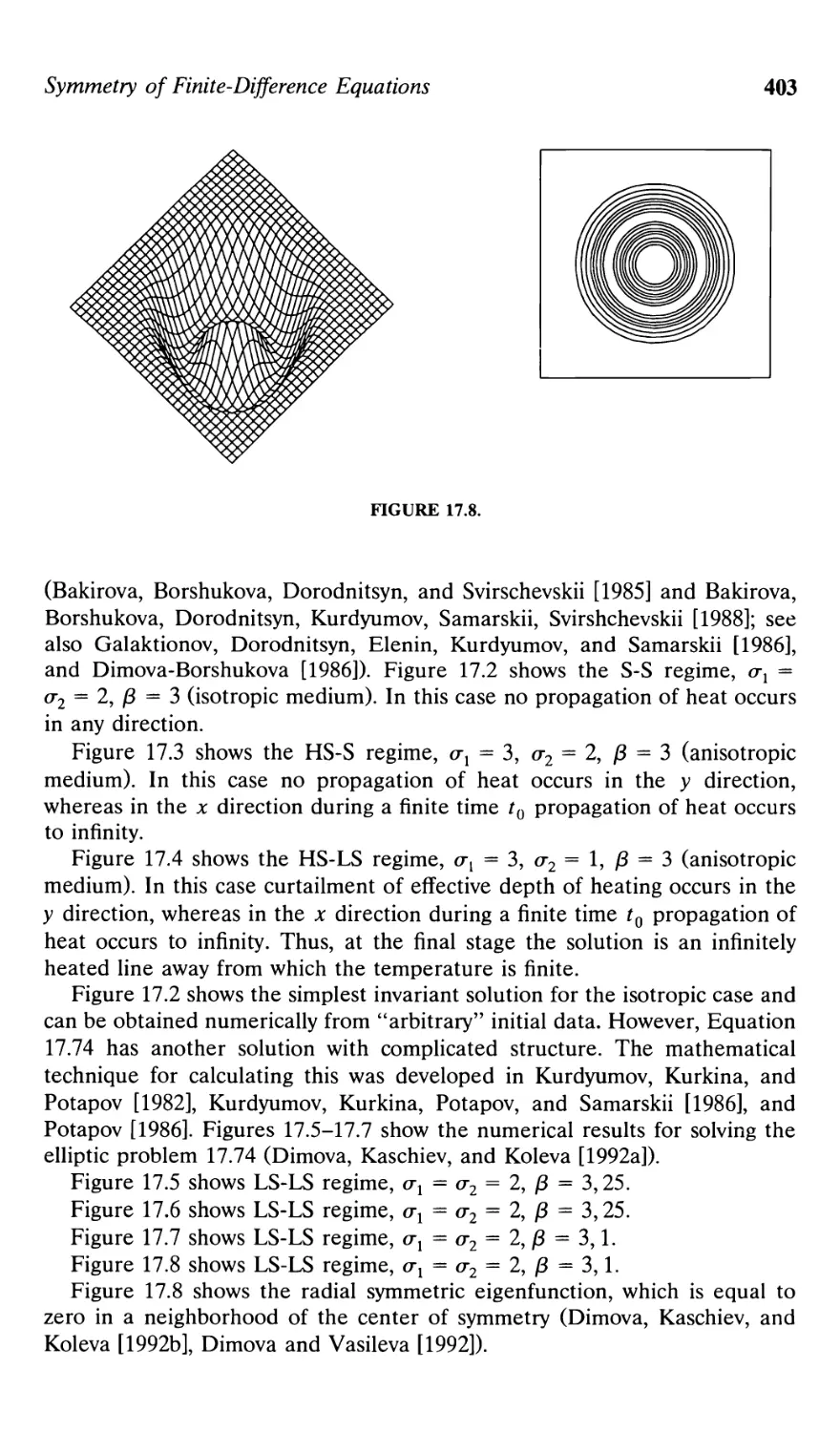
Symmetry of Finite-Difference Equations 365
17.1. Transformation groups in the spaces
of continuous and discrete variables 365
17.1.1. Taylor group 366
Xll
Contents
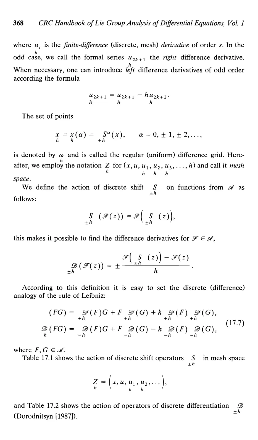
17.1.2. Introduction of finite-difference
derivatives 367
17.1.3. Transformations conserving the sense
of finite-difference derivatives 370
17.1.4. Continuation formulas for a group operator
in a grid space 371
17.1.5. Discrete representation of differential
equations 373
17.2. Invariance of finite-difference grids and finite-
difference equations 376
17.2.1. Criterion of invariance of finite-difference
equations on a grid 376
17.2.2. Invariance of finite-difference grids 377
17.2.3. Method of finite-difference invariants 378
17.3. Invariant variational problems in discrete spaces 379
17.3.1. Discrete representation of Euler's operator ...379
17.3.2. Invariance of mesh functional 381
17.3.3. Condition of invariance of a difference Euler
equation: quasiextremals of a mesh
functional 382
17.3.4. Quasi-invariance of a mesh functional and
invariance of a difference Euler equation 383
17.3.5. Conservation laws for quasiextremals
of an invariant mesh functional 383
17.3.6. The difference analogy of the Noether
theorem 385
17.4. Discrete models admitting symmetry groups 387
17.4.1. Ordinary finite-difference equations
(OFDEs) 387
17.4.1.1. Some classes of first-order
OFDEs admitting a one-
parameter group 387
17.4.1.2. Some first-order OFDEs admitting
a one-parameter group 388
17.4.1.3. Some classes of second-order
OFDEs admitting a one-
parameter group 390
17.4.1.4. Some classes of second-order
OFDEs admitting a two-
parameter group 391
17.4.1.5. Some second-order OFDEs
admitting a group 392
17.4.2. Partial finite-difference equations
(PFDEs) 394
17.4.2.1. Nonlinear difference heat
equation 394
Contents xiii
17.4.2.2. Difference equation of heat
transfer with relaxation
of a heat flow 395
17.4.2.3. Finite-difference wave equation .... 396
17.5. Numerical realization of invariant solutions
of heat transfer 397
References 405
Author Index 421
A. Apparatus of Group Analysis
I
Lie Theory
of Differential Equations
Lie, in his group theoretic investigations of differential equations, found it
necessary to distinguish clearly between two approaches: One is natural and
deals with the totality of solutions of a given differential equation. The other
is based on regarding the differential equation as a surface in the space of
independent and dependent variables together with the derivatives involved
in the given equation. To illustrate this, consider a first-order ordinary
differential equation [ODE],
F(x,y,y') =0. (i)
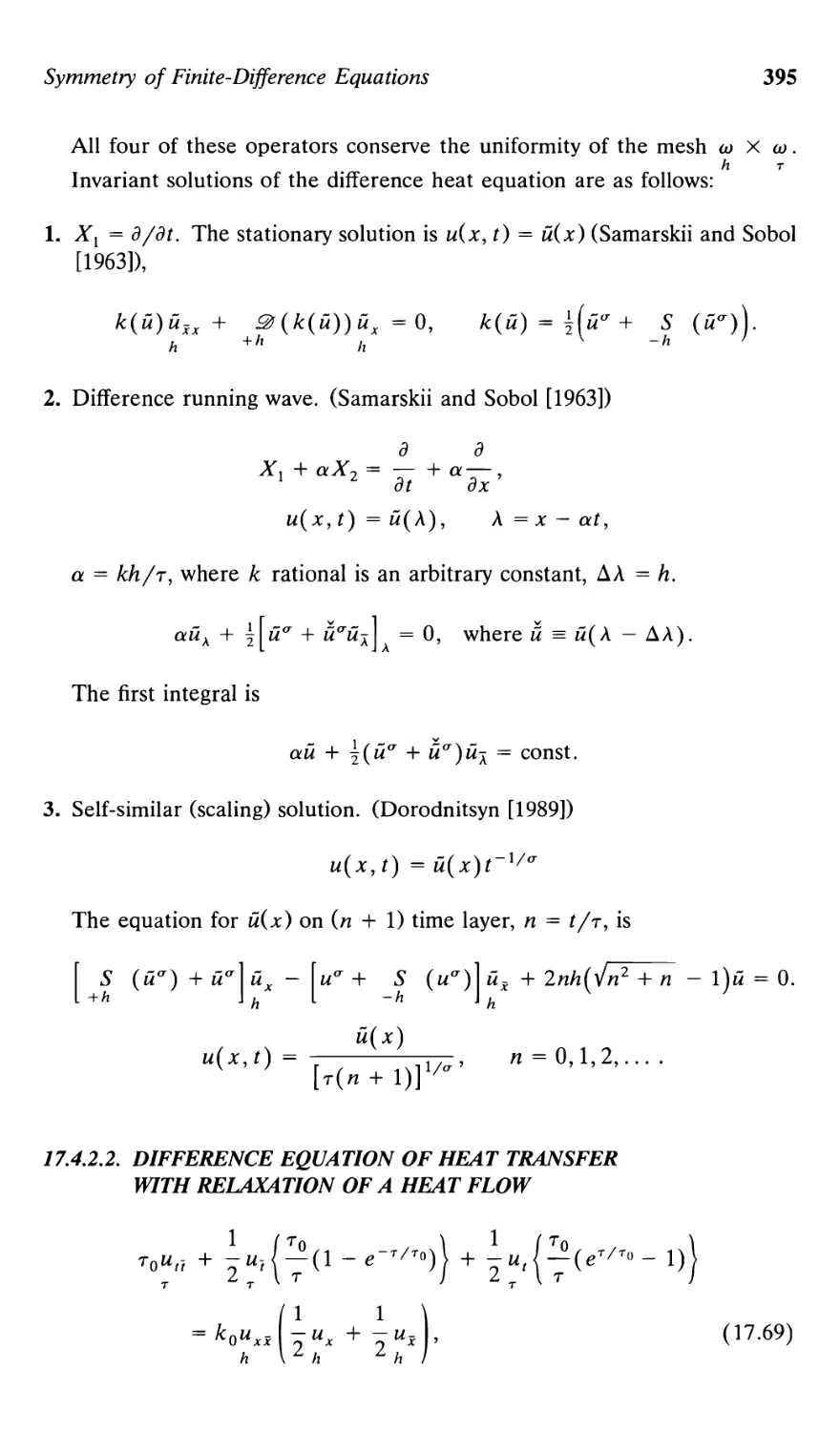
In the first approach, the symmetry group of Equation i is regarded as a
one-parameter group (with parameter a) of point transformations of the
(x, y) plane,
x = <p(x,y,a), у = ф(х,у,а), (ii)
such that any solution h(x) of Equation i (i.e., F(x, h(x\ h'(x)) = 0,
identically in x from some interval) is converted into a solution of Equation i in the
following way. Consider the integral curve
(x, у =h{x)). (iii)
Fix the parameter a in Equation ii and apply the Transformation ii to the
integral curve iii. This yields a curve given by
(x = <p(x,h(x),a), у = ф(х,к(х),а)), (iv)
which, according to the first approach, is an integral curve. This integral
3
4 CRC Handbook of Lie Group Analysis of Differential Equations, Vol. 1
curve, after elimination of x from Equations iv, can be rewritten in the form
y=H(x,a). (v)
Because x is arbitrary we can again denote it by x. Hence, the original
solution h(x) of Equation i is converted by the symmetry group into a
one-parameter family of solutions H(x, a) of Equation i.
In the second approach, the differential equation is considered as a
surface in the three-dimensional space of variables x, у, р given by
F(x,y,p) = 0. (vi)
Here x, y, and p are considered to be three independent variables that
transform as
x = <p(x,y,a), у = ф(х,у,а), р = Dilf/D<p, (vii)
where D = д/дх + p д/ду. This is, in fact, a one-parameter group and is
called the first prolongation of the group of point transformations. A
symmetry group, in the sense of this second approach, is defined as a group of
transformations such that its first prolongation leaves invariant the surface
given by Equation vi. The constraint on the transformation law for p that
appears in Equation vii provides a connection with the first approach because
the prolongation is consistent with the transformation law for first derivatives
with the identification p = y'. Equally important is the fact that this
constraint provides an algorithm for finding symmetry groups.
It is clear from the second approach that the symmetry group of Equation
i is identical to the invariance group for the surface given by Equation vi and
does not depend on the existence of solutions of the differential equation.
Because of this fundamental role played by the surface given by Equation vi,
it is called the frame of the differential equation.
In integrating differential equations, a decisive step is that of simplifying
the frame. For such a purpose, it is sufficient to "straighten out" the
one-parameter symmetry group i.e., to reduce its action to a translation by a
suitable change of the variables x and y. This automatically simplifies the
equation by converting its frame into a cylinder, i.e., the explicit dependence
on one of the variables x or у has been eliminated.
For illustration, we give the following example.
Example. The Riccati equation, y' + y2 - 2/x2 = 0, admits the group G
of point transformations x = xea and у = уе~а because the frame of this
equation, p + y2 — 2/x2 = 0, is invariant under the dilations in the space of
three variables (x, y,p) x = xea, у =уе~а, р = pe~2a. These dilations are
obtained by the prolongation of G. The group is straightened out by the
Lie Theory of Differential Equations
5
change of variables t = In x, и = ху. In these variables the transformations
of the group G are written 1 = t + а, й = и. Its prolongation to the frame
space (t, w, q) is given by t = t + а, й = w, q = q, which is obtained by
setting p = q in Formula vii. In the new variables the frame of the Riccati
equation becomes the parabolic cylinder q + u1 — и — 2 = 0. As a result we
have transformed the original Riccati equation into the following integrable
one: u' + u2 - и - 2 = 0.
Central to this book is the remarkable discovery by Lie that the group
approach provides a unified explanation for the seemingly disparate (diverse
and ad hoc) integration methods used to solve ordinary differential
equations. Moreover, Lie [1883], [1884] gave a group classification of all arbitrary-
order ordinary differential equations. In this way he identified all equations
that can be reduced to lower-order equations or completely integrated by the
application of group theoretic methods.
The purpose of Part I is as follows: (1) to systematize the relevant results
of Lie; (2) to guide the reader through the totality of Lie group methods with
a minimum number of theoretical constructions; (3) to assist the reader in
developing skills in applying these results and methods.
1
One-Parameter
Transformation Groups
1.1. LOCAL ONE-PARAMETER POINT
TRANSFORMATION GROUPS
We shall consider invertible transformations of the (x,y) plane
x = <p(x,y,a), у = ф(х,у,а), (1.1)
depending upon a real parameter a, where we impose the conditions
<p\a=0=X, ф\а=0=У- (1.2)
We say that these transformations form a one-parameter group G if the
successive action of two transformations is equivalent to the action of another
transformation of the form 1.1. This group property can always be recast, by
a suitable choice of parameter, as follows:
<p(x,y,b) =<p(x,y,a +ft),
ф(х,у,Ь) = ф(х,у,а + Ъ).
In practice, it often happens that the group property is valid only locally, i.e.,
only for a and b sufficiently small. In this case G is referred to as a local
one-parameter transformation group. If the group property is valid for all a
and b from some fixed interval, G is referred to as a global group. It is local
groups that are used in group analysis. For brevity, we simply call them
groups.
Transformations 1.1 are called point transformations (unlike contact
transformations, where the transformed values also depend on the derivative y'\
and the group G is called a group of point transformations. It is readily seen
0-8493-4488-3/$0.00 + $.50
(c) 1994 by CRC Press, Inc.
7
8 CRC Handbook of Lie Group Analysis of Differential Equations, Vol. 1
from Formulas 1.2 and 1.3 that the inverse transformation can be obtained by
changing the sign of the group parameter:
x = <p(x,y,-a), у = ф(х,у,-а). (1.4)
Let Ta denote the transformation 1.1 of a point (x, y) into a point (x, y), I
the identity transformation, T~] the transformation inverse to Ta, and TbTa
the composition of two transformations. Then one may summarize properties
1.2-1.4 as follows.
Definition 1.1. The set G of transformations Ta is a local one-parameter
group if the following hold:
1. 70 = /eG
2. TbTa = Ta+h e G
3. T~] = T_a^G
where a and b are sufficiently small.
We shall represent the functions <p and ф via their Taylor series
expansions with respect to the parameter a in the neighborhood of a = 0 and write
the infinitesimal Transformation 1.1 as follows:
x ~x + £(х,у)я, у ~y + 7i(x,y)a, (1.1')
where
дф(х,у,а)
дср(х,у,а)
a = 0
. (1.5)
z„ I ' V(x,y) =
da \a=o oa
For example, in the case of rotations
x = x cos a + у sin а, у = у cos a — x sin a,
the infinitesimal transformation is given by
x ~ x + ya, у ~ у — xa.
The vector (£, 77) given by Formula 1.5 is a tangent vector (at the point
(x, y)) to the curve determined by the totality of transformed points (x, y).
That is why it is called a tangent vector field of the group G.
Given an infinitesimal transformation 1.Г, a one-parameter group can be
completely determined by the following Lie equations with appropriate initial
One-Parameter Transformation Groups
9
conditions:
dcp
— = £(<P,<A), (p\a = 0 = *,
—- = 7](<р,ф), ф\а=0 =у.
da
A tangent vector field can be written in terms of the first-order differential
operator
X = £(x,y)-+V(x,y) — . (1.7)
Unlike the vector (£, 77), X transforms as a scalar under a change of
variables. Lie called the operator 1.7 a symbol of the infinitesimal
Transformation 1.Г. The terms infinitesimal operator, group operator, Lie operator,
and group generator came into use later. All these terms will be used
interchangeably.
Definition 1.2. A function F(xy y) is an invariant of the group of
transformations 1.1 if for each point (x, y) it is constant along the trajectory
determined by the totality of transformed points (x, y):
F(x,y) = F(x,y).
Theorem 1.1. The function F(xy y) is an invariant of the group G with the
symbol X given by Formula 1.7 iff it satisfies the partial differential equation
dF dF
XF = Z{x,y)— + r){x,y)— = Q. (1.8)
ox oy
Hence any one-parameter group of point transformations of the plane has
only one independent invariant. One can take this invariant to be the
left-hand side of a first integral J(x, у) = С of the characteristic equation
dx dy
(1.8')
Нх>у) v(x,y)'
Then any other invariant is a function of /.
The concepts just stated can be readily generalized to the
multidimensional case, where instead of transformation groups of the plane one
considers transformations
Г =/''(*, *), i = l,...,л, (1.9)
10 CRC Handbook of Lie Group Analysis of Differential Equations, Vol. 1
of the л-dimensional space of points x = (jc1, ..., xn). Let us focus on this
multidimensional case and consider the system of equations
Fx(x) = 0,...,Fs(x) = 0, s <n. (1.10)
We suppose that the rank of the matrix lldi^/dx1!! equals s at every point x
that satisfies System 1.10. Then System 1.10 determines an (n — s)-
dimensional surface M.
Definition 1.3. System 1.10 is invariant under the transformation group G
(or admits G) if any point x of the surface M moves along this surface under
the action of G, i.e., x e M if x e M.
Theorem 1.2. The system of Equations 1.10 is invariant under the group G
of Transformations 1.9 with the symbol
(l.ii)
a = 0
iff
XFk\M = 0, * = 1,...,*, (1.12)
where the notation \M means evaluated on M.
This theorem is useful for finding the group admitted by a given system of
equations. When the functions Fk(x) are known, the coordinates ijl(x) of
Operator 1.11 are determined from Equations 1.12. Then one may obtain
Transformations 1.9 of the group admitted by solving the Lie equations
-—=£'(*), х'\а=о = х', / = l,...,n.
da
Conversely, in order to find an invariant system of equations for a given
group G, it is convenient to use the following theorem on the representation
of invariant equations via group invariants. Each one-parameter group G of
Transformations 1.9 has exactly n — 1 functionally independent invariants.
Any set of n - 1 functionally independent invariants is called a basis of
invariants for G. A basis of invariants for a group G with symbol 1.11 can, in
principle, be constructed by solving the characteristic system
dxl dxtl
X = t'(x)^>
?(*) =
df{x,a)
da
One-Parameter Transformation Groups
11
Theorem 1.3. Let the system of equations 1.10 admit the group G, and
assume its tangent vector £ix) is not equal to zero on the surface M
determined by Equations 1.10. Then there exist functions Ф such that one
may rewrite System 1.10 equivalently as follows:
ф*(Л(дО,...,/„_!(*)) = °> * = l,..., j, (1.Ю')
where J{ix), ..., Jn_xix) is a basis of invariants of the group G (i.e., a set of
all functionally independent invariants). Equations 1.10 and 1.10' are
equivalent in the sense that they determine the same surface M.
Example. Consider the paraboloid given by
x2 + y2 - z = 0
with the origin excluded. This paraboloid is equivalently given by
x2 + y2
1 = 0.
z
The group G of inhomogeneous dilations x = xea, у = yea, and z = ze2a
moves points along this parabolic surface, hence both equations describing
the paraboloid are invariant under G. However, it can be easily verified that
the function Fix, y, z) = x2 + y2 — z under the action of G becomes
Fix, y, z) = e2aFix, y, z). Hence F is not invariant under G, whereas the
function Ф(х, у, z) = ix2 + y2)/z - 1 is invariant under G.
In integrating ordinary differential equations we shall use the following
simple theorem on what is called similarity of one-parameter groups. Here,
we formulate this theorem only in the case of transformation groups on the
plane.
Theorem 1.4. Any one-parameter group G of Transformations 1.1 can be
reduced under a suitable change of variables
t = tix,y), и = u(x,y)
to the translation group ~t = t + a and й = и with the symbol X = d/dt.
Such variables t and и are referred to as canonical variables.
This can be seen by the following argument. By a change of variables, the
differential operator given by Formula 1.7 is transformed according to the
formula
X = X(t)-+X(u) — , (1.13)
ot ou
12 CRC Handbook of Lie Group Analysis of Differential Equations, Vol 1
where X(t) and X(u) denote the action of the differential operator X on the
functions t(x, y) and u(x, y), respectively. In order that Operator 1.13
becomes X = д/dt, the equations
X(t) = 1 and X(u)=0 (1.14)
must be satisfied.
For example, for the dilation group x = xe and у = уе2а with the
operator X = хд/дх + 2у д/ду, Equations 1.14 are readily solved and yield t =
hut + g(yx~2) and и = h(yx~2), where g and h are arbitrary functions.
One has the freedom to choose the functions g and h. We take g = 0 and
h = yx~2, i.e., the change of variables t = In x, и = y/x2. This reduces the
dilation group to the group of translations
- i-i У y
t = \nx = \nx + a = t + a, и = ^z = -^ = u.
xL xL
1.2. PROLONGATION FORMULAS
Now we write the transformation formulas for the derivatives y',y"
corresponding to the point transformations. It is convenient to use the
operator of total differentiation
д д д
D = — + у'— + у"— + • • • ,
дх ду ду
where D is used to distinguish this operator from the operator of partial
differentiation д/дх. Then the derivative transformations are given by
dy Иф фх + у'фу
У = ~р = 7Г~ = —~--^ =Р(х,у,у ,а),
dx Dcp <рх + У(ру
-«^^-BL- ?x + yPy + у"Ру'
dx D<p ipx+ y'ipy
If we start from a group G of transformations 1.1 and add Formula 1.15,
we obtain the first prolongation G acting on the space of three variables
l
(я. У, У'У, after adding Formula 1.16, we obtain the second prolongation G
2
acting on the space (jc, у, у\ у").
Substituting the infinitesimal transformation x = x + at; and у = у + ar\
into Formulas 1.15 and 1.16 and neglecting the terms up to o(a), we obtain
(1.15)
(1.16)
One-Parameter Transformation Groups
13
the infinitesimal transformations of the derivatives
y' + aD(r\)
»/+ [D(V) - уЩ^а ш у'+ a(u
y" + aD(L)
?,-тт^"1,,+ад111'ад1
* у" + [D{Cx) ~ y"DU)]a « y" + a£2.
Hence the symbols of the groups G and G are equal to
1 2
f = 4 + *^ + ^' f.-^)-^(f). (1-17)
X = X + Z2—, t2 = D(C1)-y"D(a- (1.18)
They are referred to as the first- and the second-order prolongations of
Operator 1.7. Sometimes we shall also call the expressions for the additional
coordinates £x and £2,
Cx = D(V) - y'D(t) = r,x + (Vy ~ £,)У' - У'%, (1.17)
£г = D{Cx) ~ y"D{U) = Vxx + (2vxy " €xx)y' + (vyy " Пху)у'2
- y%y + (Vy - 2£x - 3y'iy)y", (1.18')
prolongation formulas.
In dealing with the multidimensional situation (with independent variables
x\ i = 1,..., n, and dependent variables u", a = 1,..., m, instead of x and
y) one may recast Prolongations 1.17 and 1.18 of the operator
as follows:
ь дх' диа
д д
X = X + ff , X = X + £»
1 'Зи?' 2 1 "dufj
where
tf - DW) ~ ufDfci), (1.17")
f* = DjiCT) ~ "°k4tk)> (1-18")
14 CRC Handbook of Lie Group Analysis of Differential Equations, Vol. 1
and
д д д
D:= Г + U0 + Uf: + ' ' ' .
1 дх1 ' диа lJduJ
The convention of summation over repeated indices is adopted here.
1.3. GROUPS ADMITTED BY DIFFERENTIAL EQUATIONS
Let G be the group of point transformations and let G and G be the first
1 2
and the second prolongations defined in Section 1.2.
Definition 1.4. A first-order ordinary differential equation
F(x,y,y') = 0
admits the group G if the frame of the given equation, i.e., a
two-dimensional surface F(x, y, p) = 0 in the three-dimensional space of variables x,
y, and p = y' is invariant (see Definition 1.3) under the first prolongation G
of G. Analogously a second-order differential equation
F(x,y,y',y") = 0 (1.19)
admits a group G if its frame (a three-dimensional surface in the space
x, у, у', у") is invariant under the second prolongation G.
2
Evidently this definition can be generalized to higher-order differential
equations as well as to systems of partial differential equations.
The terms "groups admitted by differential equations" and "symmetry
groups" are used interchangeably in the literature.
Under the action of a group admitted by a differential equation, any
solution of the equation is converted into a solution of the same equation.
Often in the literature one finds the converse statement taken as the
definition for symmetry groups, namely:
Definition 1.4'. A symmetry group of a differential equation is a group that
converts every solution of the equation under consideration into a solution of
the same equation.
Under conditions of solvability, Definitions 1.4 and 1.4' are equivalent (see
Lie [1891], Chapter 6, Section 1; for a recent treatment of locally solvable
systems see Olver [1986], Section 2.6). However, because of the work of
One-Parameter Transformation Groups
15
H. Lewy [1957], we know there are exceptional cases of equations without
solution. In these cases the two definitions are not equivalent.
The construction of differential equations admitting a given group can be
readily realized with the help of Theorem 1.3 on the representation of
invariant equations in terms of group invariants.
If we fix our attention on constructing the most general form of second-
order ODEs that admit a given group with generator X, then one must find a
basis of invariants for X, i.e., solve
2
XJ(x,y,y',y") = 0.
2
The theory of characteristics says there are three functionally independent
invariants. It is convenient to find these invariants successively by solving the
sequence of equations
Щх, у) = 0, XJ(x, у, у') = 0, XJ(x, у, у', у") = 0. (1.20)
1 2
The first equation has one functionally independent solution, which we
denote by u(x, y). The second equation has two functionally independent
solutions; we select one of them to be u(x, y) (because Xu = 0) and we
denote the second one by v(x, y, y'X Note that v(x, у, у') must depend on
y', otherwise the first of Equations 1.20 would have two functionally
independent invariants. The solution v(x, у, у') is called a first-order differential
invariant of the group G. Similarly, we find from the third of Equations 1.20
exactly one additional functionally independent (of и and v) invariant
w(x, у, у', у"), which is called a second-order differential invariant of the
group G. The choice of invariants is unique up to functional dependence. If
one looks for the most general form of first-order ODEs then it is only
necessary to consider the first two equations from Equations 1.20.
Example. Let G be the group of Galilean transformations x = x + ay and
у = у with generator X = у д/дх. This group has the invariant и = у. The
first and second prolongations of the operator X are easily calculated by
Formulas 1.17 and 1.18 and turn out to be
д д д д д
X = у— - у'2—, X = у— - у'2— - Зу'у"—-.
1 дх ду' 2 дх ду' ду"
From the characteristic equations
dx dy' dy"
У У'1 Зу'у"
16 CRC Handbook of Lie Group Analysis of Differential Equations, Vol 1
we obtain the first- and second-order differential invariants:
У У"
In accordance with Theorem 1.3 the most general invariant equation (except
singular ones) for prolongations G and G can be written as v = F(u) and
12
w = F(u, v), respectively. Substituting here the expressions for the invariants
w, v, and w, we obtain the following general first- and second-order
differential equations admitting the Galilean group:
У' = /gn, У" =У'ър[у, A " -).
x + F(y) \ у у)
In more complex cases the following theorem (Lie [1891] , Chapter 16,
Section 5) simplifies calculation of the second- and higher-order differential
invariants.
Theorem 1.5. Let the invariant u(x, y) and the first-order differential
invariant v(x, у, у') be known for a given group G. Then the derivative
dv vx + y'vy + y"vy. Dv
du ux + y'uy Du
is a second-order differential invariant. As a result of subsequent
differentiation one may obtain the higher-order differential invariants d2v/du2,
d3v/du3,....
Several differential equations of the first and second orders are listed in
Sections 8.1 and 8.3 along with the operators they admit. These results are
obtained with the help of Theorems 1.3 and 1.5.
1.4. INTEGRATION AND REDUCTION OF ORDER
Group theory elucidates many methods and results on the integration of
equations that are widely used in practice. This permits one to understand
connections between different methods and to unify them. Here we discuss
the simplest applications of one-parameter groups to the problems of
integration and reduction of order for ordinary differential equations.
For the integration of first-order equations, two group theoretical methods
are presented. The first provides a method for finding an integrating factor
(Section 1.4.1). The second, the method of canonical variables (Section 1.4.2),
provides a method for finding a suitable change of variables. This last
One-Parameter Transformation Groups
17
method, in the case of higher order equations, becomes a method for
reducing the order of the equation.
For these and more general group theoretic methods of integration of
ODEs see the exhaustive presentation by Lie [1891]. Helpful presentations
can also be found in Bianchi [1918] and Dickson [1924] as well as in more
recent books by Olver [1986], Bluman and Kumei [1989] Ibragimov [1989a],
[1991], and Stephani [1989].
1.4.1. INTEGRATING FACTOR
This method is applicable to first-order equations only. Consider a first-
order ordinary differential equation written in the symmetric form
Q(x,y)dx-P(x,y)dy = 0. (1.21)
It is equivalent to the following partial differential equation:
dF dF
P— + Q— = 0. (1.22)
дх ду
The left-hand side of any integral F(x, y) = const, of Equation 1.21 is a
solution of Equation 1.22 and, conversely, any solution F(x, y) of Equation
1.22 equated to an arbitrary constant determines an integral of
Equation 1.21.
Theorem 1.6 (Lie [1875]). Equation 1.21,
Q(x,y)dx-P(x,y)dy = 0,
admits a one-parameter group with generator 1.7,
д д
* = £— + ?7 —
дх ду
iff the function
€Q-vP
is an integrating factor for Equation 1.21.
First Example. Consider again the Riccati equation
/* = T7, Ъ (L23)
2
v'+y2=^. (1.24)
18 CRC Handbook of Lie Group Analysis of Differential Equations, Vol 1
This equation admits the one-parameter group of dilations x = xea and
у = уе~а with the generator
x-xk-yh- (L25)
Rewriting Equation 1.24 as
dy + \y2 ^\dx = 0 (1.24')
and using Formula 1.23, we obtain the integrating factor
Д =
x2y2 - xy - 2 '
After multiplying by this factor, Equation 1.24' becomes
xdy + (xy2 — 2/x) dx I 1 xy — 2
V ; =d \]nx + -]n- -I =0.
x2y2 — xy — 2 " \ 3 * xy + 1
Thus we find the general solution of Equation 1.24 in the form
2jc3 + С
У =
x(x2 - С)
Second Example—A Group Theoretical Basis for the Method of Variation of
Parameters. Let us apply Lie's formula to integrate the inhomogeneous
linear equation
y'+R(x)y = Q(x). (1.26)
In this case a symmetry group is given by the superposition principle.
Namely, if z0(x) = exp[fR(x)dx] is a particular solution of the
homogeneous equation
z'+/?(x)z = 0, (1.26')
then the one-parameter family of transformations
x=x, y=y+azQ(x)
converts any solution of Equation 1.26 into a solution of the same equation.
One-Parameter Transformation Groups
19
These transformations form a one-parameter group G with the symbol
X = z0(x)-.
Here, one can use Definition 1.4' and conclude that G is a symmetry group
for Equation 1.26. Now we rewrite Equation 1.26 in the form
(Q - Ry) dx - dy = 0,
and, using Formula 1.23, we find the integrating factor /x = - l/z0(x), or
fi = -e^x)dx.
Therefore
[dy + (Ry - Q) dx] efRix)dx = dF,
for some function F. It follows that
dF dF
= em*)dx^ = R(x)yeIR(x)dx __ Q(x)em*)dx
dy dx
By integrating the first equation one may obtain the expression F =
у cxp[fR(x)dx] +/(jc). The substitution of this expression into the second
equation yields
f'(x) = -Q(x)eJR(x)dx, or f(x) = -fQ(x)e^x)dxdx.
Substituting this back into the expression for F(x, y) and setting F = C, we
find
yeJR(x)dx _ jQ(x)emx)dx fa = C
By solving this equation with respect to у one obtains the general solution of
Equation 1.26:
у = e-}Rdx(fQefRdxdx + C).
1.4.2. METHOD OF CANONICAL VARIABLES
First we note that if a differential equation admits a group G in one
coordinate system, it admits the group in any other coordinate system.
Therefore, we simplify the group by choosing canonical variables t and и
according to Theorem 1.4 and reduce the action of G to translations in one
of these variables, say, t. Then our equation written in terms of t and и will
be invariant with respect to translations in t. This means that the trans-
20 CRC Handbook of Lie Group Analysis of Differential Equations, Vol. 1
formed equation does not depend explicitly on t. Therefore, in canonical
variables, we can integrate this equation by quadratures if it is first-order, or
if it is of higher-order, reduce the order by 1.
First Example. Consider equation 1.24. For the group with generator 1.25,
the canonical variables are
t = In x and и = xy.
In these variables Equation 1.24 is written as
u' + u2 - и - 2 = 0. (1.24")
This equation is readily integrated and yields
и + 1
In 3t = const.
и — 2
After substituting the expressions for t and и in terms of x and y, we
reproduce the solution given in Section 1.4.1.
Second Example. The second-order linear equation
yn+f(x)y = 0 (1.27)
admits the group of dilations in у with the generator
X = y — . (1.28)
by
Here the canonical variables are и = x and t = In y. In these variables
Equation 1.27 becomes
u" - u' + /(w)w'3 = 0.
It does not depend explicitly on t. That is why its order can be reduced by
the standard substitution u' = p{u) and the problem becomes one of
integrating the Riccati equation
dp
s+/<«),'-i-o.
The method of canonical variables gives a second group theoretic basis for
the method of variation of parameters (see, e.g., Ibragimov [1989a]). In this
way, in contrast to the integrating-factor method, one is provided with a
group theoretic approach to the method of variation of parameters for
higher-order equations.
One-Parameter Transformation Groups
21
1.4.3. INVARIANT DIFFERENTIATION
If a second- or higher-order equation admits a one-parameter group, one
can reduce the order of the equation with the help of Theorems 1.3 and 1.5.
Here we focus on second-order ODEs admitting a one-parameter group
G. Denote by и an invariant of G and by v its first-order differential
invariant. According to Theorem 1.5 a second-order differential invariant can
be chosen in the form w = dv/du. Then by Theorem 1.3 the differential
equation can be rewritten as
dv
-b=n»,v). (1.29)
By this we have reduced the order. If we find an integral of Equation 1.29
(e.g., of the original second-order equation) in the sense
Ф(и,и,С) =0 (1.30)
then the solution of our second-order equation automatically reduces to
quadratures. Indeed, the substitution of the known expressions for invariants
u(x, y) and v(x, у, у') into Equation 1.30 results in a first-order differential
equation that admits the group G. This is the consequence of the fact that и
and v are invariants.
Example. Let us reduce the order of Equation 1.27 by the method of
invariant differentiation. The first prolongation of operator 1.28 is
д д
X =y— +y'—.
1 ду ду
Its invariants are и = x and v = y'/y. In accordance with theorem 1.5, we
calculate the second-order differential invariant w = dv/du:
du у у2 у
It follows that y"/y = dv/du + v2. The substitution of this expression into
Equation 1.27 gives Equation 1.29 in the form of the following Riccati
equation:
dv
— + u2 +f(u) = 0.
22 CRC Handbook of Lie Group Analysis of Differential Equations, Vol. 1
1.5. DETERMINING EQUATION
Now we consider the problem of constructing the group admitted by a
given second-order Equation 1.19. In accordance with Definition 1.4 and
Theorem 1.2, the infinitesimal criterion for invariance is
X^F\F=0 = (£FX + VFy + CxFy. + £2iy)lF=o = 0 (1.31)
where f, and £2 are calculated by the prolongation formulas (Equations 1.17'
and 1.18'). Equation 1.31 is referred to as the determining equation for the
group admitted by Equation 1.19.
Furthermore, we shall treat differential equations written in the form
y"=f(x,y,y'). (1.32)
In this case the determining equation, becomes
Vxx + (2rlxy ~ €хх)У' + (Ъу ~ 2Ly)y'2 ~ У'Чуу
+ (т7у - 2{x - 3y%)f - [Vx + (Ъ - Zx)y' - y%\fy.
-Sfx-Vfy = 0. (1.33)
Here fix, у, у') is a known function and the coordinates £ and r\ are
unknown functions of x and y. Because the left-hand side of Equation 1.33
includes (besides x and у) у' considered as an independent variable, the
determining equation can be split into several independent equations. As a
result we obtain an overdetermined system of differential equations for £ and
77. Solving this system of determining equations, we find all operators
admitted by Equation 1.32.
First Example. Let us find all operators
д д
ox ay
admitted by
1
y" + -y' - ey = 0. (1.34)
x
Here f = ey — (l/x)y' and Equation 1.33 becomes
Vxx + (2Vxy ~ ixx)y' + (Vyy ~ Чху)У'2 ~ У%у
+ (Vy - Цх - 3y'{y)[e> - iL) + ![„, + (Vy - Qy' - y%\
йУ— ~ vey = 0.
x
One-Parameter Transformation Groups
23
The left-hand side of this equation is a polynomial of third degree in y'. That
is why the determining equation is split into the following four equations:
(yf: €yy = o;
.'\2
(/) : vyy-2ixy+-iy = 0;
y': 2r,x-ixx+\-\ -3^ = 0;
(1.35)
t\0.
(У'У- V**+-Vx + (vy-2tx-v)ey = 0.
It follows from the first two equations that
£=p(x)y +*(*) and v = (p' + ^)у2 + Ыа1' - -J + <?(*)
У +Ъ(х).
We substitute these expressions for £ and 77 into the last two of Equations
1.35. Because £ and 77 depend on у polynomially and the left-hand sides of
these last two equations contain ey, it follows that
£y = 0 and <ny-2£x-v= 0.
The solution of these equations is given by
f = a(x) and 17 = -2«'(jc).
After this the third equation of Equations 1.35 becomes
(•■-i)'-0-
which gives a = Cxx In x + C2jc. The last equation of Equations 1.35 is valid
identically.
As a result we obtain the general solution of Equations 1.35:
£ = Сгх In x + C2jc and 17 = —2[C1(1 + In jc) + C2],
with constant coefficients Cx and C2. By virtue of the linearity of the
determining equations the general solution can be represented as a linear
combination of the following two independent solutions:
£2 =jclnx, r)l= -2(1 4- lnx);
£2 =x> 712= ~2-
24 CRC Handbook of Lie Group Analysis of Differential Equations, Vol. 1
This means that Equation 1.34 admits two linearly independent operators
/9 /9 Я Я
X]=x\nx 2(1 + 1пл:)— and X2 = x 2—. (1.36)
дх ду дх ду
Hence the set of all operators admitted by Equation 1.34 is a
two-dimensional vector space with the basis given by operators 1.36.
For partial differential equations (PDEs), the construction of an admitted
group parallels the ODE development previously described. In the PDE case,
one utilizes the prolongation Formulas 1.17 and 1.18 in place of Formulas
1.17' and 1.18'. We illustrate this by the following example.
Second Example. Consider the following second-order partial differential
equation:
uxx + uyy = e\ (1.37)
We seek a symmetry operator
д д д
x = £l— + £2— + v —,
дх ду ди
where g\ £2, and 77 are unknown functions of three variables x, y, and u.
Solution of the determining equation gives that £] and £2 depend only on x
and у and satisfy the Cauchy-Riemann system
£-# = 0, #+# = 0, (1.38)
while
v = -1С
So, Equation 1.37 admits the infinite-dimensional vector space of operators
д д д
X=£l(x,y)— +£2(x,y) 2£| —, (1.39)
where £l and ^2 are defined by Equations 1.38.
1.6. LIE ALGEBRAS
Now we return to the general properties of the determining equation. It
can be seen from Equation 1.33 that the determining equation is a linear
partial differential equation with unknown functions £ and 77 of two variables
x and y. It follows that the set of all its solutions is a vector space. However,
One-Parameter Transformation Groups
25
there is another property that is intrinsic to determining equations. A set of
solutions of any determining equations forms what is called a Lie algebra.
(This term was introduced by H. Weyl; S. Lie himself used the term
infinitesimal group.)
We define a commutator (Lie bracket) [XY,X2\oi operators
д д д д
*i = £iT- +?7i^- and X2 = £2—- +7]2--
дх ду дх ду
by the formula
[Xl,X2]=XlX2-X2Xx, (1.40)
or
[XltX2] = (*,(&) -ХгЦ,))— + (Х^ъ) -Хг{щ)) — . (1.40')
It follows that the commutator
1. Is bilinear,
[X, cxXx + c2X2] = cx[X, Xx] + c2[X, X2]
[cxXl+c2X2,X]=cx[Xx,X]+c2[X2,X]
2. Is skew-symmetric, [Xv X2] = -[X2, Xx]
3. Satisfies the Jacobi identity,
[Xl9[X29X3]] + [X2,[X3,XX]] + [Х39[Хг,Х2]] =0
Definition 1.5. A Lie algebra of operators 1.7 is a vector space L that
includes the commutator [Xx, X2] along with any two operators Xx, X2 e L.
This Lie algebra is denoted by the same letter L, and the dimension of the
Lie algebra is the proper dimension of the vector space L.
Remark 1. Let Lr be an r-dimensional vector space with a basis Xx,..., Xr,
i.e., any IeLr can be decomposed as follows:
r
X = £ СМАГМ, С» = const. (1.41)
Then it follows from Definition 1.5 that Lr is a Lie algebra iff
г
[**,*„] = Е<Да> ^=1,..-,/-, (1.42)
Л = 1
where c*„ are real constants called structure constants of Lr.
26 CRC Handbook of Lie Group Analysis of Differential Equations, Vol. 1
Remark 2. A Lie algebra Lr generates an r-parameter group of
transformations 1.1 with a vector-parameter a = (я1,..., ar). To construct the
transformations corresponding to this group, it is sufficient to solve the Lie
equations for each basis operator of Lr and take compositions of these r
one-parameter groups.
One of the general results for second-order equations is the following one
due to Lie [1891].
Theorem 1.7. For any Equation 1.32, the set of all solutions of the
determining equation forms a Lie algebra Lr of dimension r < 8. The maximum
dimension r = 8 is realized if and only if Equation 1.32 is linear or can be
linearized by a change of variables.
Example. The commutator of operators 1.36 equals
[XUX2]=-X2. (1.36')
So property 1.42 is valid and therefore the vector space spanned by the
operators Xx and X2 is a two-dimensional Lie algebra. According to the
First Example in Section 1.5, Xl and X2 are two linearly independent
solutions of the determining equation for Equation 1.34, and any X admitted
by Equation 1.34 is a linear combination of them. It follows from Theorem
1.7 that equation 1.34 cannot be linearized.
Although we discuss above only groups admitted by second-order
differential equations, all concepts and algorithms can be generalized to higher-
order equations. Moreover, Lie gave a classification of all ordinary differential
equations of arbitrary order according to their admitted groups. This
classification is based on enumeration of all possible groups of transformations of
the plane. A treatment of this classification is given in Lie [1883] and [1884].
Finally, we are in a position to see why the method of the determining
equations is not effective for first-order ODEs y' = fix, y). In this case we
have the determining equation
*(/-/)!, =vx + (vy-e*)f-£yf2-£fx-vfy = 0- (i-43)
1 ly =f
This does not contain the variable y'\ that is why the split into an overdeter-
mined system does not occur here.
1.7. CONTACT TRANSFORMATIONS
In the theory of differential equations as well as in mechanics and
geometry along with point transformations, groups of contact (or tangent)
One-Parameter Transformation Groups
27
transformations are widely used (Lie [1896a], [1896b]). Here we will discuss at
once the multidimensional case with an arbitrary number n of independent
variables x = (x1,..., xn) and the one dependent variable u. (It is
worthwhile to mention that for the greater number of the dependent variables
there are no contact transformations different from a point ones; the proof
can be found, e.g., in Ovsiannikov [1978], Section 28.3, in Anderson and
Ibragimov [1979], Section 9, or in Ibragimov [1983], Section 14.10.)
Let u' denote the set of first derivatives ui = ди/дх\ and consider a
one-parameter group of transformations
xl = cpl(x, u, u!, a), U = ф(х,и,и',а), й( = а)((х, и, и', а) (1.44)
in the (2n + l)-dimensional space of variables (x,u,uf). Transformations
1.44 are referred to as contact transformations when Ui = дй/дх1. In terms
of infinitesimal transformations,
xl ~ xl + £'(*> u-> u')a-> и ~ и + r\(x,u,u')a,
bLt ~ ui + £i(x, u, u')a
(1.44')
this condition can be rewritten as the prolongation formula
£, = АЫ - UjD^). (1.45)
Theorem 1.8. The operator
Хш(,>? + ч*; + 1-щ (1-46)
is a symbol of a contact transformation group iff
dW dW dW dW
Г'=- —, 4 = ^-11,— , £-= — +11,.— (1.47)
dut dut дх1 ди
for some function W = W(x, w, u'). The function W occurring in this theorem
was called by Lie [1896a] the characteristic function of the contact
transformation group. For ordinary differential equations formulas 1.46 and 1.47
become
A A A
where W = W(x, y, p) with p = y'.
28 CRC Handbook of Lie Group Analysis of Differential Equations, Vol. 1
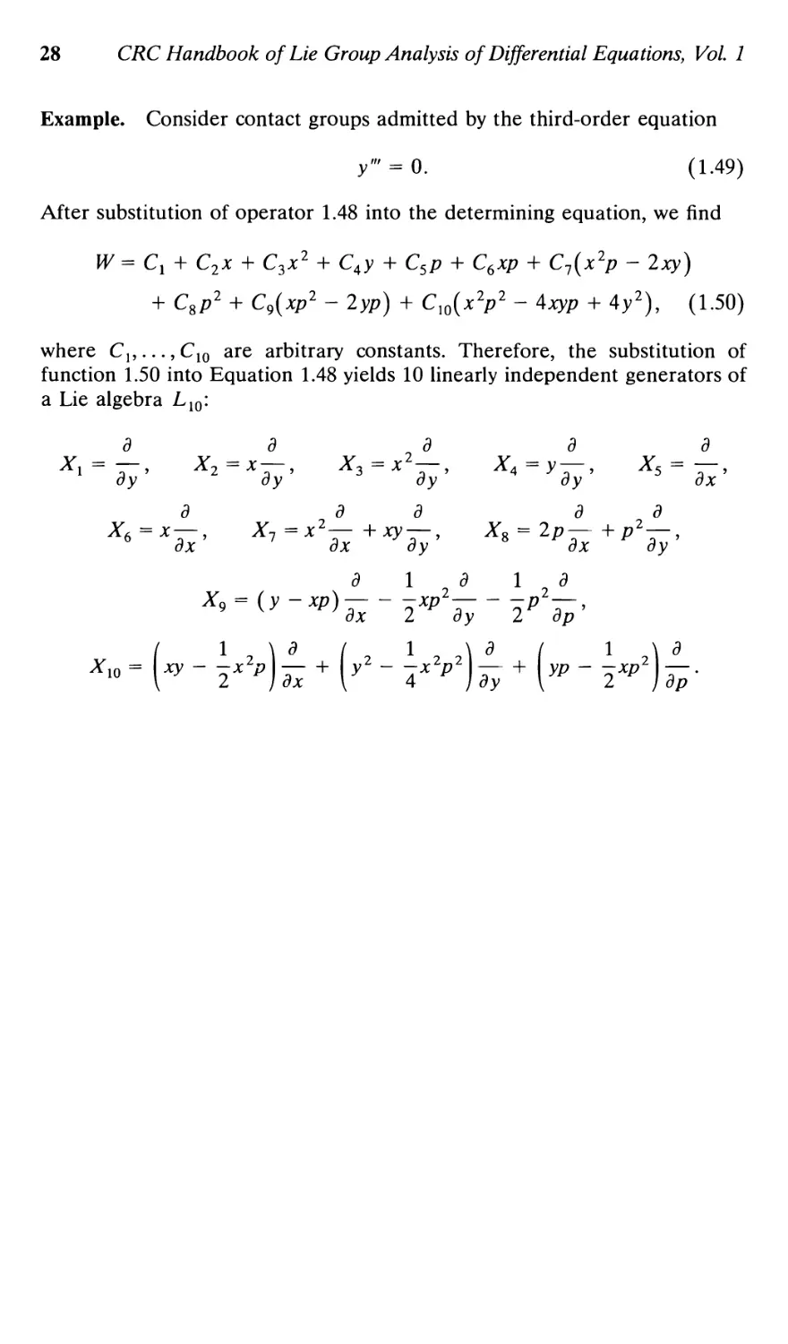
Example. Consider contact groups admitted by the third-order equation
y'" = 0. (1.49)
After substitution of operator 1.48 into the determining equation, we find
W = Cx + C2x + C3x2 + C4y + C5p + C6xp + C7(x2p - 2xy)
+ Csp2 + C9(xp2 - 2yp) + C10(xV - 4xyp + 4y2), (1.50)
where C1?...,C10 are arbitrary constants. Therefore, the substitution of
function 1.50 into Equation 1.48 yields 10 linearly independent generators of
a Lie algebra L10:
д д 2д д д
1 ay' 2 ay' 3 ду' 4 ay' 5 ах
а а а а а
Аг6=х—, Х7=х2—+ху —, Xs = 2p— +Рг—,
ах ах ay ax ay
а 1 а 1 а
^9 = (у-хр)---хр2---р2-,
2
Integration of Second-Order
Ordinary Differential Equations
2.1. SOLVABLE LIE ALGEBRAS AND SUCCESSIVE
REDUCTION OF ORDER
As stated in Section 1.4 (see also Dickson [1924], Ovsiannikov [1962],
Olver [1986], Bluman and Kumei [1989], Stephani [1989], and Ibragimov
[1989a], [1991]), a one-dimensional symmetry algebra can be used to reduce
by one the order of a second-order equation. So it is natural to expect that
given a two-dimensional algebra the order can be reduced twice, which
means we have integrated the equation.
We begin by discussing the properties of Lie algebras that we need in this
chapter. Let Lr be an r-dimensional Lie algebra with any r < oo and let N
be a linear subspace of Lr.
Definition 2.1. The subspace N is referred to as a subalgebra if [X, Y] e N
for all X,Y e N (i.e., this subspace is an algebra itself), and as an ideal if
[X,Y] e N for all X e TV and all Y e Lr.
If N is an ideal, then one can introduce an equivalence relation:
Operators X and Y from Lr are said to be equivalent if Y - X e N. The set of all
operators that are equivalent to a given operator X is referred to as a coset
represented by the operator X; any element У of this coset has the form
Y = X + Z for some Z e N. The set of all cosets is naturally endowed with a
Lie algebra structure and is called the quotient algebra of the Lie algebra Lr
by its ideal N. It is denoted by Lr/N. One may consider the representatives
of appropriate cosets as elements of this quotient algebra.
If all constructions are considered in the complex domain, then the
following theorem is valid.
0-8493-4488-3/$0.00 + $.50
(c) 1994 by CRC Press, Inc.
29
30 CRC Handbook of Lie Group Analysis of Differential Equations, Vol. 1
Theorem 2.1. In any algebra Lr, r > 2, there exists a two-dimensional
subalgebra. Moreover, any operator X ^ Lr can be included in a
two-dimensional subalgebra.
Definition 2.2. A Lie algebra Lr is solvable if there is a sequence
Lrz>Lr_xz> ... dL, (2.1)
of subalgebras of dimensions r, r — 1,..., 1, respectively such that Ls_x is
an ideal in Ls (s = 2,..., r).
A convenient criterion of solvability is formulated in terms of derived
algebras.
Definition 2.3. Let Xx,..., Xr be a basis of an algebra Lr The linear span
of the commutators [X^ Xv] of all possible pairs of the basis operators is an
ideal denoted by Lr and called the derived algebra. The higher-order derived
algebras are defined recursively: L(rn + l) = (L(/°)', n = 1,2,... .
Theorem 2.2. An algebra Lr is solvable if and only if the derived algebra of
some order equals zero: L(/° = 0 for some n > 0.
Corollary. Any two-dimensional algebra is solvable.
To construct Sequence 2.1 in the case of a two-dimensional algebra L2,
one may choose a basis Xx, X2 so that the equality [Xu X2] = aXx is valid.
Then the one-dimensional algebra Lx spanned by Xx is an ideal in L2, and
the quotient algebra L2/Lx can be identified with the algebra spanned by
X2. If this algebra L2 is admitted by a second-order ODE, one can use the
ideal Lx to reduce the order of this equation by 1 (Sections 1.4.2 and 1.4.3).
Further, the resulting first-order equation admits the quotient algebra L2/Lx
and hence it can be integrated by any of the methods discussed in
Section 1.4.
It is clear that an ordinary differential equation of order n > 2 can be
integrated by this method of successive reduction of order if it admits a
solvable п-dimensional Lie algebra. For detailed discussions, see Olver
[1986], Theorems 2.60, 2.61, and 2.64.
2.2. METHOD OF CANONICAL VARIABLES
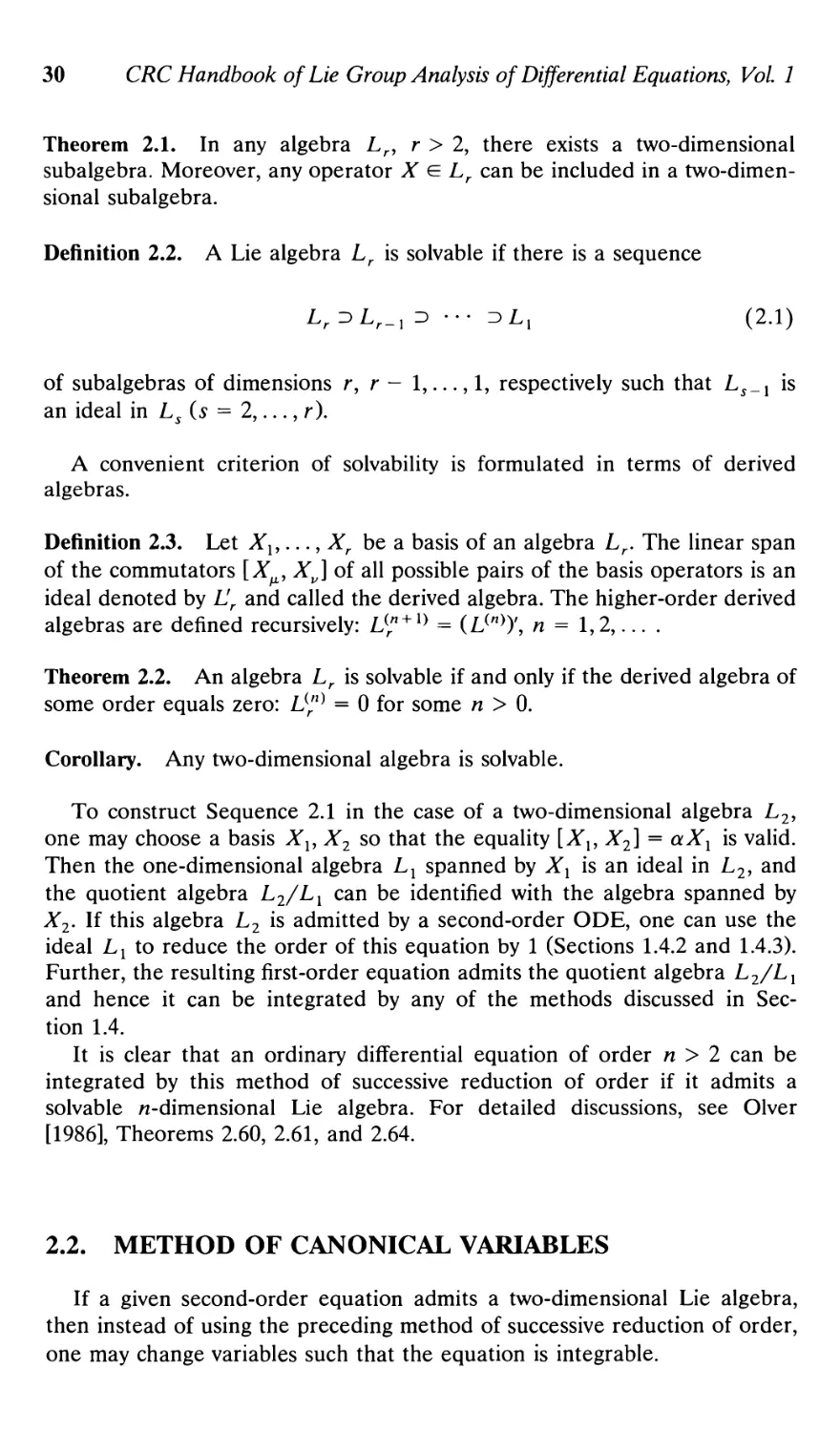
If a given second-order equation admits a two-dimensional Lie algebra,
then instead of using the preceding method of successive reduction of order,
one may change variables such that the equation is integrable.
Integration of Second-Order ODEs
31
2.2.1. CANONICAL FORMS OF L2
To state the basic theorems of this section we need, together with
Commutator 1.40, the pseudoscalar (skew) product
Х^Х2 = £м2-щ£2, (2.2)
A classification of two-dimensional Lie algebras according to their structural
properties is based on the fact that the equations [A",, X2] = 0, and A', V
X2 = 0 are invariant under both changes of bases in L2 and changes of the
variables x and y. Based on this, the set of all two-dimensional Lie algebras
is divided into the following inequivalent types:
I. [XUX2] = 0, Xx vA-2#0;
U.[Xl,X2]=0, X1vX2 = 0;
III. [XUX2] #0, Xx VX,*0;
IV. [XltX2] Ф0, X, V X2 = 0.
(2.4)
The following theorem states that in each type is only one inequivalent
algebraic structure.
Theorem 2.3. By a suitable choice of the basis XVX2, any two-dimensional
Lie algebra can be reduced to one of four different types, which are
determined by the following canonical structural relations:
I. [XlyX2] =0, XXV Х2Ф0
II. [Х1УХ2] =0, Xx V X2 = 0
III. [Xu X2] = Xu XXV Х2Ф0
IV. [Xl,X2]=Xl, XlVX2 = 0.
These structural relations are invariant under any change of variables.
Using this invariance one can simplify the form of the basis operators Xx and
32 CRC Handbook of Lie Group Analysis of Differential Equations, Vol 1
X2. This leads to the following:
Theorem 2.4. The basis of an algebra L2 can be reduced by a suitable
change variable of to one of the following forms:
I.
II.
III.
IV.
*1
*1
*1
*1
д
= Ty>
д
д
= Ty'
д
ду
д
ду
д д
х2 = х— + у—;
дх ду
д
*2=у—.
ду
(2.5)
The variables x and у are called canonical variables.
2.2.2. INTEGRATION ALGORITHM
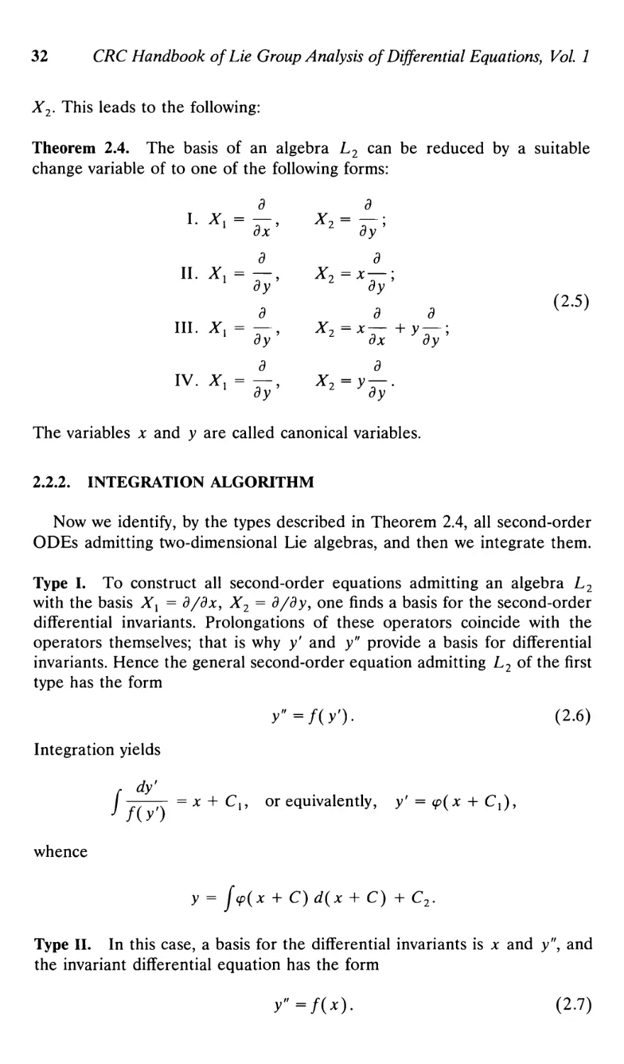
Now we identify, by the types described in Theorem 2.4, all second-order
ODEs admitting two-dimensional Lie algebras, and then we integrate them.
Type I. To construct all second-order equations admitting an algebra L2
with the basis Xx = д/дх, Х2 = д/ду, one finds a basis for the second-order
differential invariants. Prolongations of these operators coincide with the
operators themselves; that is why y' and y" provide a basis for differential
invariants. Hence the general second-order equation admitting L2 of the first
type has the form
У" -/(/)• (2-6)
Integration yields
, dy'
I = x + C1? or equivalently, y' = cp(x + C\),
whence
у = fcp(x + C) d(x + C) + C2.
Type II. In this case, a basis for the differential invariants is x and y", and
the invariant differential equation has the form
y"=f(x).
(2.7)
Integration of Second-Order ODEs
33
Integration yields
у = /(//(*) dx\ dx + Cxx + C2.
Type III. In this case, a basis for the differential invariants is y' and xy",
and the invariant differential equation has the form
y" = -f(y'). (2.8)
Integration yields
, dy'
]jr— = lnx + Cl9 or y' = <p{\nx + Cx),
then
у = \<p{\n x + C\) dx + C2.
Type IV. In this case, a basis for the differential invariants is x and y"/y\
and the invariant differential equation has the form
y"=f(x)y'. (2.9)
Integration yields
у = Cxf e!f{x)dxdx + C2.
The preceding results can be implemented in the following five-step
algorithm for the integration of second-order ODEs (for details, see
Ibragimov [1991], [1992]).
First Step. Calculate an admitted Lie algebra Lr.
Second Step. If r > 2, determine subalgebra L2 с Lr If r < 2, the ODE
cannot be completely integrated by the Lie group method.
Third Step. Calculate the commutator 1.40' and the pseudoscalar product
2.2 for a basis of L2; if necessary, change the basis in accordance with
Theorem 2.3.
Fourth Step. Introduce canonical variables in accordance with Theorem
2.4. Rewrite your differential equation in canonical variables and integrate it.
Fifth Step. Rewrite the solution in the original variables.
34 CRC Handbook of Lie Group Analysis of Differential Equations, Vol. 1
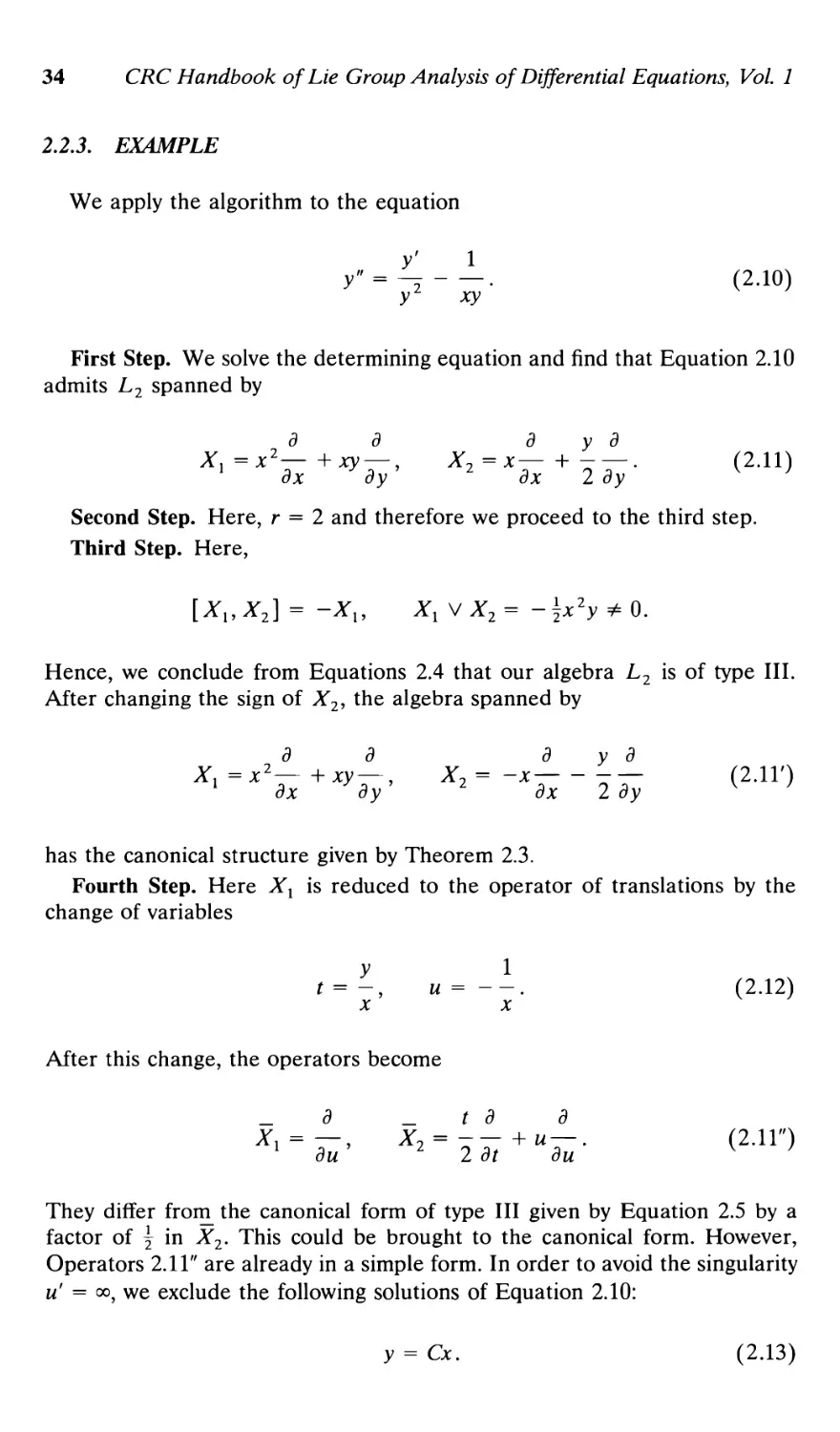
2.23. EXAMPLE
We apply the algorithm to the equation
У' 1
У" = ^--. (2.10)
У ХУ
First Step. We solve the determining equation and find that Equation 2.10
admits L2 spanned by
д д дуд
X,=x2— +*y —, X2 =x— + - —. (2.11)
дх ду дх 2 dy
Second Step. Here, r = 2 and therefore we proceed to the third step.
Third Step. Here,
[Xl9X2] = -Xl9 X,VX2 = -\хгуФЪ.
Hence, we conclude from Equations 2.4 that our algebra L2 is of type III.
After changing the sign of X2, the algebra spanned by
д д дуд
Xx=x2—+xy—, X2= -x—--— (2.1Г)
дх ду дх 2 ду
has the canonical structure given by Theorem 2.3.
Fourth Step. Here Xx is reduced to the operator of translations by the
change of variables
У 1
t = -, u= --. (2.12)
x x
After this change, the operators become
д t д д
Хг = —9 Х2 = + w—. (2.1Г)
1 ди 2 2 dt ди v }
They differ from the canonical form of type III given by Equation 2.5 by a
factor of \ in X2. This could be brought to the canonical form. However,
Operators 2.11" are already in a simple form. In order to avoid the singularity
u' = oo, we exclude the following solutions of Equation 2.10:
у = Cx.
(2.13)
Integration of Second-Order ODEs
35
After the change of variables, Equation 2.10 becomes
u" 1
Si V - О- (2.10Г)
Integration of Equation 2.10' gives the following two solutions:
t2
u=-- + C (2.14)
and
t 1
и = — + T^ln |Cjr - 1| + C2. (2.15)
Fifth Step. After we substitute Expressions 2.12 into Equations 2.14 and
2.15 and take into account Equation 2.13, then we obtain the following
general solution of the nonlinear Equation 2.10:
у = Сх, (2.13)
у = ±y/2x + Cx2, (2.16)
Cxy + C2x +xln\Cl- - 1| + Cf = 0, (2.17)
where the Cs are arbitrary constants.
3
Group Classification
of Second-Order Ordinary
Differential Equations
In Chapter 2 we discussed group theoretical methods for integrating second-
order ODEs. The conclusion is that if a second-order equation admits a
one-dimensional Lie algebra Lv then we can reduce its order by 1 and if it
admits a two-dimensional algebra L2, we can completely integrate the
equation by group methods. This conclusion led to the classification of
second-order equations admitting an L2. This classification is accomplished
by Theorem 2.4. As a result of this classification we obtain four inequivalent
types of equations, Formulas 2.6-2.9. Each of these four types involves one
arbitrary function of one variable. Further, if one takes into account the
allowed arbitrary changes of variables, each type involves two additional
arbitrary functions of two variables each. Hence the totality of second-order
ODEs integrable by Lie group methods is infinite in the sense just described.
Some of equations appearing in this classification admit
higher-dimensional Lie algebras Lr or r-parameter local Lie groups, 2 < r < 8 (see
Theorem 1.7). So we come to the problem of the complete group
classification of ODEs. Lie [1883] solved this problem for equations of arbitrary order.
Here, we only present this classification for second-order equations. This
permits us to present the essence of his method and at the same time to be
exhaustive.
3.1. LIE'S CLASSIFICATION OF EQUATIONS ADMITTING
THREE-DIMENSIONAL ALGEBRAS
The group classification of ordinary differential equations is based upon
the enumeration of all possible Lie algebras of operators acting on the plane
36
0-8493-4488-3/$0.00 + $.50
(c) 1994 by CRC Press, Inc.
Group Classification of Second-Order ODEs
37
(jc, y). The basis operators of each algebra are simplified by a suitable change
of variables. Algebras connected by a change of variables are called similar.
Equations that admit similar algebras are also similar (equivalent) in the
sense that they can be transformed into one another by a change of variables.
The classification happens to be of an especially simple form in the case of
second-order equations (see Lie [1889], Section 3). In this case the dimension
of a maximal admitted algebra has only the values 1, 2, 3, and 8. The
dimensions 1 and 2 were discussed in the previous chapters. Here we
summarize results for second-order equations admitting a three-dimensional
algebra.
Lie gave his classification in the complex domain. The results on the
enumeration of all nonsimilar (under complex changes of variables) three-
dimensional algebras and of invariant equations are given, e.g., in Lie [1891].
For three-dimensional algebras L3, the construction of invariant equations
is accomplished by solving the determining equation 1.33 with respect to the
unknown function fix, у, у'). We illustrate this construction for L3 spanned
by
д д д д д д
*! = — + —, Х2=х— + у —, Хх =х2— +у2—. (3.1)
дх ду дх ду дх ду
For the operator Xx we have £ = 1, 77 = 1. After substitution of these
values, Equation 1.33 becomes df/дх + df/ду = 0, so that
f = f(x-y,y').
Substitution of this expression for / and the coordinates £ = x and 77 = у for
X2 into the determining equation yields zfz+f= 0, where z = x - y. It
follows that
t-^-. 0.2)
x - у
Finally, substitution of Function 3.2 and the coordinates f = x2 and rj = y2
of X3 into Equation 1.33 yields
2y'— -3g + 2(y'2-y') = 0.
It follows that
g = -2(y' + C'3/2 + у'2), С = const. (3.3)
38 CRC Handbook of Lie Group Analysis of Differential Equations, Vol. 1
Thus the algebra L3 is admitted by the equation
y, + суЗ/2 + а
y" + 2 =0, С = const.
x - у
3.2. SUMMARY OF LIE'S GENERAL CLASSIFICATION
Lie demonstrated that if a second-order equation admits an algebra Lr
with r > 4, then it necessarily admits an eight-dimensional algebra. However,
all such equations are linearized (Theorem 1.7) and they are equivalent to
the equation y" = 0. This completes Lie's classification of second-order
ODEs, y" = fix, y, y'). Namely, if an equation admits Lv the action of Lx
can be transformed into translations in x. Therefore, the canonical form of
an equation admitting an Lx can be taken to be
y"=f(y,y')- (3.4)
In the case of L2, the corresponding four canonical forms of the invariant
equations are given by Equations 2.6-2.9. In the case of L3, they are given by
the four canonical forms listed in Section 8.4, Equations iv-vii. In the case of
higher dimensions, as discussed previously, the only canonical form is
y" = 0. (3.5)
Recall that Lie made his classification in the complex domain. If one deals
with the real domain only, some of the equations given in Section 8.4 will
split into two inequivalent equations (in the sense of real changes of
variables). For example, the equations
У" = С(1 +y'^3/2^arctan/
and
y" = Qj'(*-2)/(*-l)
are inequivalent in the real domain. However, the first equation is converted
into the second with к = (q + i)/(q - i) via the complex change of variables
x = \{y - ix), у = j(y + ix).
3.3. LINEARIZATION
One can extract, from several results of Lie ([1883], [1891]), the following
statement (Ibragimov [1991], [1992]).
Group Classification of Second-Order ODEs
39
Theorem 3.1. The following assertions are equivalent:
i. A second-order ODE
y"=/(*,y,y') (3.6)
can be linearized by a change of variables.
ii. Equation 3.6 has the form
y" + F3(x, y)y'3 + F2(xy y)y'2 + F}(x, y)y' + F(x, y) = 0, (3.7)
with coefficients F3, F2, F{, and F satisfying the integrability conditions
of an auxiliary overdetermined system,
dz dF
— = z2 - Fw - Fxz + — + FF2,
dx l dy 2
dz 1 dF2 2 dF,
— = -zw + pp £ + L
dy 3 3 dx 3 dy
dw 1 dFx 2 dF2
— = zw — FF3 — — h — ,
dx 3 dy 3 dx
(3.8)
dw dF3
— = -w2 + F2w + F3z + F,FV
^y 2 3 dx ] 3
iii. Equation 3.6 admits an L8.
iv. Equation 3.6 admits an L2 with a basis A^, A"2 such that their pseudo-
scalar product (Equation 2.2) Xx V X2 vanishes.
First Example. Consider equations of the form (2.6)
У"=/(У')- (3-9)
In accordance with Theorem 3.1(ii), it is necessary that the function f(y') is a
polynomial of the third degree, i.e., Equation 3.9 has the form
у" +^зУ'3 +A2ya +Axy' 4- A0 = 0 (3.10)
with constant coefficients. One can easily verify that the auxiliary system 3.8
for Equation 3.10 is integrable. Therefore Equation 3.10 is linearized.
40 CRC Handbook of Lie Group Analysis of Differential Equations, Vol. 1
Second Example (see also Mahomed and Leach [1989]). Consider equations
of the form,
r-l-nn
(3.11)
Again, by Theorem 3.1(H), we have to consider only equations of the form
у" + -(А3у'3+А2у'2+А1У'+А0) = О,
with constant coefficients At. In this case, the integrability conditions of
Equations 3.8 yield
A2{2 - Ax) + 9A0A3 = 0 and 3A3(1 + Ax) -A22 = 0.
We put A3 = -a and A2 = -b and obtain
At--\l + -\ and л0--.А + ^1
Hence, Equation 3.11 is linearized iff it is of the form
У = ~
x
7 . b2\ b b3
ay'3 + by'2 +1 + -— y' + -— +
Ъа ] За 27а2
(3.12)
A linearizing change of variables can be found via Theorem 3.1(iv).
For example, we find a linearization of Equation 3.12 in the case a = 1,
b = 0, i.e., of the equation
1
X
(3.13)
This equation admits L2 with the basis
*i =
1 д
X дх '
2 x дх
(3.14)
which satisfies the condition Xl V X2 = 0 of Theorem 3.1 (iv). These
operators are of type II from Equations 2.4. Therefore a linearization is obtained
by employing the canonical variables
x = у and у = \x2
Group Classification of Second-Order ODEs
41
so that
_ д _ д
1 dy 2 dy
Then, excluding the special solution у = const., Equation 3.13 becomes the
following linear equation:
y" + 1 = 0.
Third Example. Consider the equation
y" = F(x,y), (3.15)
where F(x, y) is nonlinear in y.
Equation 3.15 is a particular case of Equation 3.7 with Fl = F2 = F3 = 0.
System 3.8 is written
zx = z2 + Fw - Fy, wx = zw,
zy = —zw, wy = —w2.
One of the integrability conditions of this system is
It gives the necessary condition for linearization:
Fyy = 0.
Hence Equation 3.15 is not linearizable.
4
Invariant Solutions
Lie's investigations were centered on problems of general integrability of
differential equations by means of group theory. This is why many of his
papers deal with ordinary differential equations or with linear partial
differential equations of first order. In his paper on higher-order partial
differential equations, Lie [1895] considered solutions invariant under groups
admitted by these equations. With the help of these invariant solutions, he
returned to the problem of general integrability. However, the majority of the
partial differential equations that appear in mathematical physics are not
completely integrable by means of group theoretic techniques. In our
opinion, this is one of the main reasons why Lie's approach was not widely used
and taught in applied mathematics and mathematical physics for a long time.
On the other hand, special types of exact solutions of differential
equations were known and successfully used in mechanics and physics. These
solutions were found by ad hoc methods. As the result of the efforts of many
people, these special solutions are now identified as invariant solutions in the
sense of Lie. This connection with group theory led to the increased activity
in group analysis of partial differential equations that occurred after 1950
(strongly influenced by the books of Birkhoff [1950], Sedov [1957], Petrov
[1961], Ovsiannikov [1962], and Ames [1965], [1972]) and eventually to the
explosion of activity starting in about 1970.
This chapter provides an introduction to the notion of an invariant
solution and the construction of sets of independent invariant solutions
(optimal systems in the sense of Ovsiannikov [1962]). It is sufficient, for
purposes of illustration, to consider ordinary differential equations.
4.1. NOTION OF AN INVARIANT SOLUTION
In order to explain the notion of an invariant solution, we consider the
simple example of the Riccati equation from Section 1.4.1,
y' +y2 = 2/x2. (4.1)
42
0-8493-4488-3/$0.00 + $.50
(c) 1994 by CRC Press, Inc.
Invariant Solutions
43
One of its symmetry groups is given by
x=xea, y=ye'a. (4.2)
We choose a particular solution of Equation 4.1, say,
2x3 + 1
"'Тй^Ту <4J)
Transformation 4.2 converts this solution into a one-parameter family of
solutions
2x3 + С
»= iji^c) (4 4)
with С = е3й. Here С > 0 because — oo < я < oo.
How general is the solution given by Equation 4.4? The solutions with
С < О and С = oo are missing. Is it possible to recover those with С < 0 by
using the reflection x *+ —x, у •-» -у, which is a discrete symmetry of
Equation 4.1.
What about the limiting cases С = О and С = oo? It turns out that the
solutions
yx = 2/x and y2 = — 1/x, (4.5)
which correspond to С = 0 and С = oo, respectively, have a special property
with respect to the dilations. Namely, each one is converted into itself, i.e.,
yx = 2/x and у 2 = —1/x, (4-5')
and hence they are invariant in the sense of Definition 1.3. So, Solutions 4.5
are called invariant solutions. More precisely, Solutions 4.5 are invariant
solutions of Equation 4.1 under the action of the dilation group given by
Equations 4.2.
In general, if a solution is invariant, in the sense of Definition 1.3, under
the action of any symmetry group, it is called a group invariant solution or,
for brevity, an invariant solution.
Now, we illustrate a technique for constructing all invariant solutions
corresponding to a symmetry group when its infinitesimal operators are
known. We do this for Equation 4.1, using the infinitesimal operator
д д
дх ду
of Transformations 4.2.
44 CRC Handbook of Lie Group Analysis of Differential Equations, Vol. 1
By Theorem 1.3, any invariant solution can be written in terms of
invariants. In our case the only independent invariant is J = xy. Therefore all
invariant solutions can be written as
/ = const., i.e., xy = С
Substitution of the expression у = C/x into Equation 4.1 yields C2 — С —
2 = 0. Thus we have С = 2 and С = — 1. As a result we obtain two
solutions,
yx = 2/x and y2 = -1/x.
These are precisely the two invariant solutions given by Equations 4.5 and
there are no other invariant solutions of Equation 4.1 with respect to the
dilations 4.2.
4.2. OPTIMAL SYSTEMS
In the preceding section, we considered invariant solutions with respect to
a given one-parameter group or one-dimensional Lie algebra. If a differential
equation admits a Lie algebra Lr of dimension r > 1, one could in principle
consider invariant solutions based on one, two, etc., dimensional subalgebras
of Lr. However, there are an infinite number of subalgebras, e.g.,
one-dimensional subalgebras. This problem becomes manageable by recognizing that if
two subalgebras are similar, i.e., they are connected with each other by a
transformation from the symmetry group (with Lie algebra Lr), then their
corresponding invariant solutions are connected with each other by the same
transformation. Therefore, it is sufficient to put into one class all similar
subalgebras of a given dimension, say s, and select a representative from each
class. The set of these representatives of all these classes is called an optimal
system of order s (Ovsiannikov [1962], [1978]). In order to find all invariant
solutions with respect to s-dimensional subalgebras, it is sufficient to
construct invariant solutions for the optimal system of order s. The set of
invariant solutions obtained in this way is called an optimal system of
invariant solutions. Of course the form of these invariant solutions depends
on the choice of representatives.
It is sufficient to illustrate this construction for r = 2. Let us return to the
example in Section 2.2.3. It was shown there that the equation
У2 xy
(4.7)
Invariant Solutions
45
admits a two-parameter group G2 with the Lie algebra L2 spanned by
д д дуд
*i = *V +xy —, X2=x— + - —. (4.8)
дх ду дх 2 dy .
We will also use the fact that Equation 4.7 has the reflection symmetry
у >-> -у. Let us find the optimal system of one-dimensional subalgebras and
the corresponding invariant solutions.
Because we are interested in one-dimensional subalgebras, we determine
how an arbitrary operator
2
X = E C^ (4.9)
/x = l
of the algebra L2 transforms under G2. Transformations of G2 can be
obtained as a composition of two one-parameter groups, one generated by Xx
and the other by X2. Therefore, we need only consider transformations of
Operators 4.9 under the action of these two one-parameter groups
separately.
The operator Xx generates the group of projective transformations
(4.10)
1 ' * 1 >
1 — axx 1 — axx
with parameter av Using Equation 1.13, we find that under these
transformations Operator 4.9 becomes
_ 2 _
*= E^, (4.11)
/1=1
where
Xx = Xl9 X2=X2- агХх. (4.12)
In the original basis, Operator 4.11 is rewritten as
_ 2 _
*= E C^. (4.13)
/x = l
It follows from Equations 4.11-4.13 that
Cx = Cl - axC2, C2 = C2. (4.14)
46 CRC Handbook of Lie Group Analysis of Differential Equations, Vol. 1
Similar calculations with the group of dilations
x = a2x, у = yfa^y (a2 > 0) (4.15)
generated by the operator X2 yield
Xx=a2Xl9 X2=X2, (4.16)
or, equivalently,
C1 = a2C\ C2 = C2. (4.17)
To construct the optimal system of order 1, we must partition Operators
4.9, or equivalently, their coordinate vectors
C= (C\C2), (4.18)
into similarity classes with respect to Transformations 4.14 and 4.17.
Following Ovsiannikov [1962], we proceed to solve this problem in a way that is
particularly effective for low-dimensional algebras.
In our case we first observe that C2 is invariant with respect to
Transformations 4.14 and 4.17. Further, the transformation of the coordinate C1 in
Transformation 4.14 suggests that we distinguish the cases С2 = О and
C2#0.
All Vectors 4.18 with С2 = О are spanned by the unit vector
(1,0). (4.19)
Any vector with С2 Ф 0 can be transformed to the form (0, C2) by
applying Transformation 4.14 with ax = Cl/C2. These latter vectors are
spanned by the unit vector
(0,1). (4.20)
Hence any Operator 4.9 is similar to Xl or X2. Thus the optimal system of
order 1 is
{XUX2}. (4.21)
In order to find the corresponding optimal system of invariant solutions we
have only to construct the invariant solutions for Xx and X2. These solutions
are further simplified by using Dilations 4.15 and the reflection symmetry
у •-> — у of Equation 4.7. As a result we obtain the following optimal system
of invariant solutions:
yx=x, y2 = Jlx~. (4.22)
Invariant Solutions
47
The application of Transformations 4.10, 4.15, and reflection to Solutions
4.22 yields the totality of invariant solutions of Equation 4.7:
у = Cx (4.23)
and
у = ±)/2x + Cx2 . (4.24)
According to the terminology of Lie group theory, the action of the group
G2 on L2 given by Equations 4.12 and 4.16 (or, equivalently, by Equations
4.14 and 4.17) is called the adjoint representation of G2.
The fact that the number of elements in the optimal system of Subalgebras
4.21 and the optimal system of Solutions 4.22 is equal to the dimensionality
of the symmetry algebra is an accident of this example and is not true in
general. For example, consider the equation
У"=У"3. (4.25)
It admits the three-parameter group G3 with the Lie algebra L3 spanned by
д did д д
X{ = —, X2=x— + -y —, X3=x2— + xy —.
дх дх 2 ду дх ду
In this case the optimal system of order 1 is
{Xl9 X29 X39 Xx + X39 Xx - X3), (4.26)
whereas the corresponding optimal system of invariant solutions consists only
of one element, namely,
у = ]/l+x2. (4.27)
Furthermore, application of the group G3 and the reflection symmetry
у -» — у to Solution 4.27 yields the following two-parameter family of
invariant solutions:
у = — у 1 + b4(x + a)2 , a, b arbitrary constants. (4.28)
b
Moreover, this is the general solution of Equation 4.25; hence all solutions
are invariant solutions (see Ibragimov [1991] and [1992] for details).
II
Generalizations
The question of generalizing Lie's theory of point and contact transformation
groups led naturally to developments in two directions: group actions and
their generators (vector fields).
This problem was raised by Lie himself in his fundamental work (Lie
[1874], page 223) on contact transformations and was formulated as follows:
1. Are there transformations, other than contact transformations, for which
tangency of higher order is an invariant condition?
2. Do partial differential equations of order higher than one admit
transformations that are not contact transformations?
One positive answer to Lie's questions lies in the introduction of formal
transformation groups that act necessarily on infinite-dimensional spaces.
These formal groups are called Lie-Backlund transformation groups.
Another positive answer to the second question (not the first) is based on
the introduction of transformations that act only on the family of solutions of
a given differential equation and are called in the literature Backlund
transformations. These transformations do not have the group property and
are not connected in general with Lie-Backlund transformation groups.
Nevertheless, for evolution equations and those that can be rewritten in this
form. Backlund transformations can be represented as invariants of
Lie-Backlund groups defined by the evolution equations (considered as Lie
equations) (Fokas and Anderson [1979]; Anderson and Ibragimov [1978]).
For the purposes of applications, what has proven to be most expedient
are Backlund transformations and infinitesimal generators of Lie-Backlund
groups.
In Part II, we give a concise presentation of a theory of Lie-Backlund
transformation groups as well as closely related generalizations.
49
5
Lie-Backlund
Transformation Groups
5.1. STEPS TOWARD A THEORY
In this section we attempt to sketch the crucial ideas and key applications
that led to a theory of Lie-Backlund transformation groups. The subsections
reflect a chronological ordering. We also point out the importance of the
order of influence, which starts with key applications, on the development of
a theory. However, the main emphasis is on results.
5.1.1. LIE AND BACKLUND
In order to explain the work of Lie and Backlund, it is important to
distinguish between those requirements placed on transformations that arise
from tangency conditions alone and those that follow from the group
properties. Hereafter, we employ the notation и, и,..., for the sets of first-order,
1 2
second-order, etc. partial derivatives {ы,}, Ыи), ....
Lie contact transformations discussed in Section 1.7 can be considered as
transformations
xl = fl[ x, и, и ], й = fix,u, u\, w, = <p\ x, и, и J (5.1)
that leave invariant the first-order tangency condition
du - uidxi = 0. (5.2)
In the case of one-parameter groups of contact transformations 1.44, this is
0-8493-4488-3/$0.00 + $.50
(c) 1994 by CRC Press, Inc.
51
52 CRC Handbook of Lie Group Analysis of Differential Equations, Vol. 1
equivalent to the prolongation formula 1.45 or Lie's formulas 1.47.
Higher-order tangency conditions are obtained by replacing Equation
5.2 by
du - ut dxl = 0, du^ is — Uji i dxj = 0, s = 1,..., к — 1, (5.3)
for any fixed k.
Lie's first question, which is formulated in the Introduction to Part II,
concerns the existence of transformations
x1 = fl\x,u, и ,..., и), U = <p\x,u, и ,..., и),
v 1 к' v 1 к'
(5.4)
that leave invariant the tangency conditions 5.3 for 1 < к < oo.
Backlund [1874], [1876] proved the following negative result.
Theorem 5.1. Any invertible /cth-order tangent transformation 5.4 is a
prolongation to A:th-order derivatives of a Lie contact transformation 5.1.
The analogous result was proved within the framework of one-parameter
transformation groups by Ibragimov [1967].
The considerations of Lie and Backlund demonstrated that the only
generalization of contact transformation groups lies with the possible
existence of infinite-order tangent transformation groups (k = oo in Equations
5.3), acting on an intrinsically infinite-dimensional space. They themselves
did not pursue this possibility.
Noether [1918] demonstrated that if such groups exist, they have
applications in her theory of conservation laws.
A detailed discussion of the considerations of Lie and Backlund is given in
Anderson and Ibragimov [1979].
5.1.2. GENERALIZATION OF LIE'S INFINITESIMAL OPERATORS
Another possibility is to generalize Lie's infinitesimal operators. Johnson
([1964a], [1964b]) did this in one way by studying a new type of vector field. In
local coordinates, this type of vector field is an infinitesimal operator of the
form
/ \ д
X= 7]a[x,u, «,..., и \——, к < oo. (5.5)
v 1 k'dua
Lie-Backlund Transformation Groups
53
Note that in Lie-Backlund theory this is what is called a canonical Lie-
Backlund operator, and any generator
X = £*(х,и, и,..., и)—т + т?а(*,и, и,..., и)— (5.6)
of a formal one-parameter Lie-Backlund group can be reduced to the
canonical form 5.5 (see Section 5.3).
The results of Johnson's first paper that are relevant to our considerations
are as follows: (i) prolongations of Operators 5.5,
X=r1a +Д-(т7а) +■••+£> •••Д.(т7а) , (5.7)
диа ,v ' ' ди? ll 'л ' ' ди
ii.-.i,
where Д. is the total derivative with respect to x\ i.e.,
я л д
— + и? + и?.
ajc1 ' диа 1]диа:
D= —г + и? + uf: + ■ • • ; (5.8)
(ii) the definition of the Lie bracket [X^X^oi these operators; and (iii) the
proof of the theorem that the linear space of all operators 5.7 is a Lie algebra
(see Johnson [1964a], Definition 2 and Lemma 1, and Definition 3,
Theorem 1).
He also notes in this paper that the Lie equations
дйа / _ _ _\
—— = rja[x,u,u,...,u), a = l,...,m, (5.9)
да \ i k *
are not generally solvable for k > 1 even in the analytic case. This is in
contrast to Lie's point and contact transformation groups, where k = 0 or 1
and Equations 5.9 are locally solvable.
In his second paper, Johnson [1964b] defines invariance of systems of
partial differential equations under Operators 5.5 and derives the
determining equation for this invariance. Furthermore, he generalizes Lie's result that
the totality of solutions of the determining equation is a Lie algebra (Johnson
[1964b], Theorem 2).
Johnson treated this generalization in the framework of Ehresmann's
[1953] jet bundles in order to formulate his results in a
coordinate-independent form. He used the concept of formal tangent vectors introduced by
Hermann [1961] and called the generalized operator 5.5 a k-vector field.
Note that Johnson uses the Kuranishi symbol df for Dt given by Equation
5.8. For an exposition in the context of infinite jet bundles, see Vinogradov
[1979] and Kupershmidt [1980].
54 CRC Handbook of Lie Group Analysis of Differential Equations, Vol. 1
5.1.3. KEY APPLICATIONS
Interest in explaining so-called hidden and dynamical symmetries of
physical systems and their consequences within the framework of Lie theory of
differential equations led Khukhunashvili [1971] and Anderson, Kumei, and
Wulfman [1972a], [1972b], independently, to the introduction of higher
derivatives in Lie's infinitesimal techniques and to the rediscovery of
Johnson's к -vector fields. For example, in both papers the Runge-Lenz vector in
the so(4) symmetry algebra of the hydrogen atom (Fock [1935]) was identified
as a non-Lie operator 5.5. The so(4, 2) dynamical symmetry of the
hydrogen atom (Barut and Kleinert [1967], Fronsdal [1967]) was identified by
Anderson, Kumei, and Wulfman ([1972a], [1972b]), in their study of the time-
dependent Schrodinger equation, as a non-Lie symmetry.
Widespread interest in generalized group analysis of differential equations
came from a distinctly different direction, namely, from soliton physics
(Zabusky and Kruskal [1965]). It was recognized early that non-Lie
symmetries account for the infinite number of conservation laws that the first
soliton-type equations possessed, as well as providing a characterization of
their soliton solutions as invariant solutions under the action of these
symmetries. This led to a flurry of activity in generalized group analysis as a
tool to search for more soliton-type equations.
For our purposes it is important to understand that Lie's infinitesimal
techniques apply when using the generalization with one caveat, namely, one
must a priori fix the order к < oo (see, e.g., Kumei [1975], [1977]). A new
technique that was not in Lie's theory has proved to be particulary effective
for constructing hierarchies of symmetries. It is based on the notion of a
recursion operator discovered by Lenard for the Korteweg-de Vries equation
(see Gardner, Greene, Kruskal, and Miura [1974], Olver [1977], and Magri
[1978], [1980]). These recursion operators can be precisely associated with the
linear part of Lie-Backlund symmetries for evolution equations (Ibragimov
and Shabat [1980a], [1980b]; see also Ibragimov [1983], Section 19). This
latter association provides a test whether a given evolution equation
possesses nontrivial Lie-Backlund symmetries.
5.1.4. IMPOSITION OF THE GROUP STRUCTURE
ON INFINITE-ORDER TANGENT TRANSFORMATIONS
Now we return to the central problem of this chapter: How do we wed
infinite-order tangency with group properties? These are two different
requirements to impose upon any transformation. The problem is not with the
existence of infinite-order tangent transformations. Many examples are given
by transformations of the type
x =/(*,и,..., w), й = (p[x,u,..., w) (5.10)
Lie-Backlund Transformation Groups
55
together with their prolongation to all derivatives according to Formulas 1.15,
1.16, etc. The difficulty lies in imposing the group property. For example, in
the case of Transformations 5.10 we know transformation groups of this type
only for k, s < 1 (these are Lie point and contact transformations). However,
for к and/or s > 1, we do not know of any example of groups given by
Equations 5.10. This brings us to a fundamental difficulty. Namely, the
problem of wedding infinite-order tangency with the group property leads,
for Operators 5.6, to Lie-Backlund equations
d*1 (- - -\
— = £'(^,w,..., u),
da
дйс
da
дйа ,_ _ _ч (5.11)
-— = ria[x,u,..., и ,
да V k i
which are not of the Cauchy-Kovalevskaya type and hence their integrability
is not assured.
However, there are examples, beyond Lie's point and contact
transformation groups, for which one can prove the existence and uniqueness for the
Lie-Backlund Equations 5.11. For instance, examples are provided by taking
€* arbitrary and rja = £1и? in Operator 5.6, i.e.,
X=eDt, (5.12)
where Dt is given by Equation 5.8. The resulting Lie-Backlund Equations
5.11 are not of the Cauchy-Kovalevskaya type. However, there is a
generalization of the Cauchy-Kovalevskaya theorem, namely, Ovsiannikov's theorem
in scales of Banach spaces (Ovsiannikov [1971]), that is applicable to this
example (Ibragimov [1977], Anderson and Ibragimov [1977]). Another class of
examples is provided by Operators 5.5 of the form
д
X= u—.
P du
Here, e.g., for p = 2, the solvability of the corresponding Lie-Backlund
equations can be provided only for functions u(x) from the Jevrey class C1/2
(Anderson and Ibragimov [1979]), Section 12; for arbitrary p see Ibragimov
[1983], Section 16.3).
These examples, as well as those from quantum mechanics, make it clear
that there is no hope of proving, in general, the local solvability of the
Lie-Backlund equations as is the case with the Lie equations. Therefore the
problem is divided into two parts. First, candidates for Lie-Backlund groups
must be identified by using formal power series. The algebraic part was done
by Ibragimov [1979] (see also Ibragimov [1983]) for all Lie-Backlund
Operators 5.6 in a universal space [[s/]] and is described next, in Section 5.2. The
56 CRC Handbook of Lie Group Analysis of Differential Equations, Vol. 1
second part, i.e., the convergence of these formal power series, cannot be
universally solved and must be treated separately for each type of
Lie-Backlund operator.
5.2. FORMAL LIE-BACKLUND
TRANSFORMATION GROUPS
Consider functions f(x,u, w,..., u) of a finite number of arguments
l к
(к < ос) that are locally analytic in the sense that / is locally expandable in a
Taylor series with respect to all arguments. These functions are
generalizations of Ritt's differential polynomials (Ritt [1950]) and are called differential
functions of finite order (Ibragimov [1981], [1983]), where the order refers to
the highest derivative appearing in /. The space of all differential functions
of all finite orders is denoted by s/. This space is a vector space with respect
to the usual addition of functions and becomes an associative algebra if
multiplication is defined by the usual multiplication of functions.
Furthermore, it has the important property of being closed under the derivation
given by Equation 5.8.
Consider operators of the form
Х=?—+Г—, ?,-Пае*. (5-13)
ox ou
Their prolongation to all derivatives is again denoted by X and is given by
д д д д
X = f'"—г + г]а + if + f", + • • • , (5.14)
Ь дХ1 ' д^ l dU? bhl2duf: V '
I l{l2
where
Definition 5.1. An operator given by Equations 5.14 and 5.15, where £' and
r]a are differential functions of finite order, i.e., £', rja e s/, is called a
Lie-Backlund operator. The abbreviated operator 5.13 is also referred to as a
Lie-Backlund operator.
Denote by [[j/]] the space of formal power series in one symbol a with
coefficients in s/. The following theorem due to Ibragimov [1979], [1983]
Lie-Backlund Transformation Groups
57
states that any Lie-Backlund operator generates a formal one-parameter
group of tangent transformations acting in [[sf]].
Theorem 5.2. Given any Lie-Backlund operator 5.13, there exists a unique
solution of the Lie-Backlund equations
£4 x, U,..., й J, xl\a=o = xl,
, ' , (5-16)
ria[x,u,..., wj, ua\a=o = ua,
in the space [[ssf]]. This solution
Г =
5" =
with coefficients A's, B" e j/, where у4\ = £4*, и,..., и) and £" =
77а(л:, и,..., и). It is a formal one-parameter group that leaves invariant the
к
infinite-order tangency conditions
dua - uj dxj = 0, duf - ufj dxJ; = 0, ... . (5.18)
Definition 5.2. The formal groups obtained in Theorem 5.2 are called
formal Lie-Backlund transformation groups. Any formal Lie-Backlund
transformation group is given by a formal power series and is generated by a
Lie-Backlund operator (Definition 5.1).
Definition 5.3. The formal Lie-Backlund transformation group in
Definition 5.2 is a local one-parameter group if the series in Equations 5.17
converge, and is called a one-parameter Lie-Backlund transformation group.
5.3. LIE-BACKLUND SYMMETRIES
OF DIFFERENTIAL EQUATIONS
Lie's determining equations (see Section 1.5) naturally generalize to
formal Lie-Backlund symmetry groups (see Johnson [1964b], Ibragimov and
dxl
~da
дйа
~Ja~
is given by formal power series, i.e.,
00
= *'+ E^x,
(5.17)
= ua+ £#X>
5=1
58 CRC Handbook of Lie Group Analysis of Differential Equations, Vol 1
Anderson [1977], and Ibragimov [1983]). However, it is important to note that
one must use Definition 1.4 of an admissible group. This is because
Definition 1.4' is not applicable for Lie-Backlund transformation groups because
they are given by formal power series and do not convert classical solutions
into classical solutions. This is not to be confused with the fact that in
particular cases where one can prove convergence of the power series in
Equations 5.17, Definition 1.4' is also applicable.
Theorem 5.3 (Ibragimov [1979], [1983]). Consider a A:th-order differential
equation
F[x,u, w,..., u) = 0, (5.19)
^ 1 к '
where F e s/ is a differential function of order k. Denote by [F] the frame
of Equation 5.19 given by this equation and all its differential consequences
(cf. Introduction to Part I). Then Equation 5.19 admits, in the sense of
Definition 1.4, a formal Lie-Backlund transformation group generated by a
Lie-Backlund operator X iff
XF\[F] = 0. (5.20)
Equation 5.20 is called the determining equation of the Lie-Backlund
symmetry group.
It is an immediate consequence of the determining equation that every
Lie-Backlund operator of the form
X*=?Di9 f'^, (5.21)
is admitted by any differential equation. We remark that Lie-Backlund
equations for operators 5.21 are solvable (in suitable scales of Banach
spaces), as was noted in Section 5.1.4. Moreover the set of all Operators 5.21
is an ideal in the Lie algebra of all Lie-Backlund operators. Therefore, it is
sufficient to consider the quotient algebra, i.e., to consider Lie-Backlund
operators with £' = 0,
X=Va — , Va<=tf, (5.22)
which are called canonical Lie-Backlund operators. In particular, every
Operator 5.13 is transformed to the canonical form by the prescription
X = X-FDi.
Lie-Backlund Transformation Groups
59
All of these considerations obviously generalize to systems of differential
equations.
Example. The time-independent Schrodinger equation for the bound states
of the hydrogen atom
- Au + I E\u = 0,
where E is a positive constant, admits three nontrivial Lie-Backlund
operators (the Runge-Lenz vector mentioned in Section 5.1.3)
*(/) " dxl
-xl + £ (xluu - х1ин)
r 1Ф1
д
ди '
/=1,2,3,
or, in the canonical form,
x(i) ~
-xl - M/ + £ {xluu - xluii)
i*l
д
ди
6
Noether-Type
Conservation Theorems
6.1. CONSERVATION LAWS
The concept of a conservation law for a differential equation
F(x,u,u,...,u)=0 (6.1)
v 1 к '
is motivated by the conservation of such quantities as energy, linear and
angular momentum, etc. for equations that arise in classical particle
mechanics. These quantities (here denoted by T) are conserved in the sense that
they are constant on each trajectory, i.e., if t denotes time, q(t) a trajectory,
and q(t) the corresponding velocity, then T(t) = T(t, q(t), q(t)) satisfies the
equation
dT
- - 0. (6.2)
The conservation law given by Equation 6.2 generalizes to continuum
mechanics in the form
дт
— + divp = 0, (6.3)
where t is again time and div is the divergence operator with respect to
spatial variables x = (jc1, ..., xp). The function r is called a conserved
density. The terminology "conserved density" is used because its integral,
T = J т dx,
60
0-8493-4488-3/$0.00 + $.50
(c) 1994 by CRC Press, Inc.
Noether-Type Conservation Theorems
61
also satisfies
dT
under the usual assumption that p vanishes at infinity. The conserved density
т is a function of t, x, dependent variables, and their partial derivatives up to
some order, whereas p = (p1,..., pp) is a vector with the same arguments as
r. Because the differentiation with respect to t and x must be understood as
a total differentiation, Equation 6.3 means
D,(r)+ EAV) = °- (6.3')
/ = 1
For an arbitrary differential equation, we do not distinguish space and
time variables and denote by x = (xl,..., xn) all independent variables. In
this case a conservation equation is written in the form
Д(Г) = О, (6.4)
where Г gj/ (i.e., each Tl is a differential function of finite order, see
Section 5.2).
Definition 6.1. Equation 6.4 is called a conservation law for Equation 6.1 if
the equation
(*))
= 0 (6.5)
is satisfied for all solutions u(x) of Equation 6.1. The vector T = (Г1,..., Tn)
is called a conserved vector.
Immediately the question arises, how does one find conservation laws for a
given Equation 6.1, namely, how does one find Г? Although Definition 6.1
follows naturally from physical considerations, technically its applicability
depends on knowledge of the solutions of Equation 6.1. Here we arrive at the
same situation we encountered in the definition of symmetry groups (cf.
Introduction to Part I and the passage from Definition 1.4' to Definition 1.4
in Section 1.3). Namely, we make these considerations algorithmic if we
replace the notion of "all solutions" in this definition with the notion of the
frame of the differential equation. Because of the presence of higher
derivatives in the 7's, we must use the frame mentioned in Theorem 5.3, which is
given by Equation 6.1 together with its differential consequences.
In order not to get into an extremely technical discussion of what is meant
by the frame of Equation 6.1 in the general case, let us consider only
62 CRC Handbook of Lie Group Analysis of Differential Equations, Vol. 1
conservation laws of a fixed order /. By this we mean that / is the maximum
of the orders of all the Tl in Equation 6.4. As a result, the left-hand side of
Equation 6.4 involves derivatives of order < / + 1. Further, let us restrict
ourselves to the case of one equation (the generalization to systems of
differential equations is obvious). It follows that if s is defined by
s = max{&, / + 1}, (6.6)
then all constructions take place in the finite-dimensional space of variables
(jc, и, и ,..., и ). (6.7)
^ 1 s '
More precisely, the frame [F], in this case, is a surface given by the following
equations
F = 0, if s = k,
F = 0, AF = 0,...,A ••£> F=0, if s > k. (6*8)
' l ' ' 'l ls-k '
Definition 6.2. Equation 6.4 is called a conservation law for Equation 6.1 if
D,(T%F] = 0. (6.9)
Definition 6.2 brings us to the same situation we encountered when
calculating symmetries by using determining equations (see Section 1.5 and
compare Equation 6.9 with Equation 5.20). Namely, Equation 6.9 is linear in
the unknowns Tl and splits because it contains derivatives of higher order
than those in the Tl. In principle, we can solve Equation 6.9 and find all /th
order conservation laws for Equation 6.1. Hence we call Equation 6.4 the
determining equation for /th order conservation laws obeyed by
Equation 6.1.
This algorithmic possibility was employed by Laplace some 200 years ago.
He (see Laplace [1798], Livre II, Chapitre III no. 18) used an analog of
Equation 6.9 to derive conservation laws quadratic in velocities for the
Kepler problem. In particular he found three new conserved quantities,
xk
Ak = m(\v\2xk - (x • v)vk) + a—, 1,2,3, (6.10)
for the equation of motion
x
mx = a^r, a = const. (6.П)
r*
Here x = (jc1, x2, jc3), r = \x\, v = x = dx/dt, and x • v = E3=1 xlvl. The
Noether-Type Conservation Theorems
63
conserved quantities are the components of the vector
x
A = v X M + a-, where M = m(x X v). (6.12)
The quantum mechanical version of this Laplace vector is also known in
quantum mechanics as the Runge-Lenz vector.
6.2. NOETHER THEOREM
It has been known for a long time that the conservation laws of classical
mechanics are connected with symmetry properties of the physical system.
This connection was clearly described in the course of mechanics by С
Jacoby. Although Equation 6.9 provides, in principle, a direct and exhaustive
method for calculating conservation laws of finite order for any differential
equation, it sheds no light on this connection. Noether [1918] was the first to
combine the methods of the variational calculus with the theory of Lie groups
and to formulate a general approach for constructing conservation laws for
Euler-Lagrange equations when their symmetries are known. It is this
connection that is exhibited by the Noether theorem.
As a consequence, the rest of this chapter deals with conservation laws for
differential equations of the form
8L
— = 0, a=l,...,m, (6.13)
ou
where
L = L\x,u, и ,..., и) gj/
v l к)
is a Lagrangian. Equation 6.13 is called an Euler-Lagrange equation. It is
derived by the usual variation of an integral of the form (action)
fbdx, flcR". (6.14)
The operator 8/8ua denotes the variational derivative (or the Euler-Lagrange
operator) defined by
8 д ^ s д
= + £(-l)A "D: . (6.15)
8ua dua ctv ' ЖЩ : K }
64 CRC Handbook of Lie Group Analysis of Differential Equations, Vol. 1
It is convenient to rewrite any Lie infinitesimal operator (infinitely
prolonged) and the Lie-Backlund operator 5.14 in the form
д д
x = ^— + va—
dxl dua
+ E[A-'-A/^)+^1...Jt^-, (6.16)
-M
where
Wa = va - £>uj. (6.17)
The following operators are associated with any operator 6.16:
Nl = e + Wa + ЕД --• DAW") , (6.18)
OUi s>\ ouiil...is
where 8/8uf, etc. denote the corresponding variational derivatives (cf.
Equation 6.15), e.g.,
8 д ^ д
= + E(-l) Д •• D, . (6.19)
8ua dua h Jsdua-
oui oui s>\ ouiJl...js
Operators 6.18 were introduced and called Noether operators by Ibragimov
(see, e.g., Ibragimov [1983], Section 22.1).
Even though the three operators (6.15), (6.16), and (6.18) are represented
as infinite formal sums they act properly on the space srf. Namely, they
truncate while acting on any differential function.
Further and most importantly they are connected by the following
theorem.
Theorem 6.1 (Ibragimov [1983]). Operators 6.15, 6.16, and 6.18 satisfy the
identity
X + D,.(f'') = W°— + D,JV'. (6.20)
ou
This operator identity is called the Noether identity.
With this identity in hand, the content and proof of the Noether theorem
as well as related results become transparent.
For simplicity we first consider a one-parameter group G of point
transformations
xl =fl(x,u,a), Ua = <pa(x,u,a). (6.21)
Noether-Type Conservation Theorems
65
Let
X = ^(x,u)—+Va(x,u)— (6.22)
be its infinitesimal operator. Under the action of the group G, any function
u(x) is transformed into U(x) and a domain ftcR" is transformed into a
domain ft с Rn.
Definition 6.3. Integral 6.14 is said to be invariant under the action of a
group G of transformations 6.21 if
I L\ x, u(x), и(x),..., и(x)\ dx
= f_L\x, U(x), U(x),..., U(x)) dx (6.23)
Ja v i к >
for every domain fl and for all smooth functions u(x) such that the integral
exists.
Theorem 6.2 (Ibragimov [1969], [1983]). Integral 6.14 is invariant under the
action of a group G of point transformations with infinitesimal operator
6.22 iff
X(L) + Щ(£'') = 0. (6.24)
The following particular case of the Noether theorem (Noether [1918]) is a
direct consequence of formulas (6.20) and (6.24).
Theorem 6.3. If integral 6.14 is invariant under the action of a group G with
infinitesimal operator 6.22 then the vector T = (Г1,..., Tn) defined by
Tl = Nl(L) (6.25)
is a conserved vector for the Euler-Lagrange equation 6.13. In the case of an
r-parameter invariance group, Formula 6.25 applies to each of the r
generators of this group.
Noether [1918] assumed the existence of groups of transformations that
involve derivatives, and formulated her theorem for this case. This
generalization of Theorem 6.3 is what is understood today as Noether's theorem
(more precisely, Noether's first theorem, as distinguished from her second
theorem, which is not discussed here).
66 CRC Handbook of Lie Group Analysis of Differential Equations, Vol. 1
It is clear that Definition 6.3 and Theorem 6.3 can be directly extended to
contact transformation groups. However, in the case of transformations
involving higher derivatives, the realization of the general theorem is
problematic. The problem, as discussed in Chapter 5, is in the solvability of
Lie-Backlund equations. In order to deal properly with this general case and
not lose Noether's results, it is convenient to replace the invariance of the
integral 6.14 by the invariance of the differential л-form (elementary action)
Ldx. (6.26)
Then Theorems 6.2 and 6.3 are generalized to the following, which includes
Noether's theorem.
Noether's Theorem (Ibragimov [1983]). Given a formal Lie-Backlund
transformation group with the Lie-Backlund operator
х = ^ + ^ + -"' ^aej/' (6-27)
the differential «-form 6.26 is invariant with respect to this formal group iff
X(L) + ££,.(£') = 0. (6.28)
The vector T = (T\ ...,Tn) defined by
T = Nl{L) (6.29)
is a conserved vector for Equation 6.13.
Remark. It directly follows from the Noether identity 6.20 that if Operator
6.27 satisfies, on the frame of Equation 6.13, the divergence condition
X{L) + LDt(?) = D,(B'), В1 е sf, (6.30)
rather than the invariance condition 6.28, then the conserved vector is given
by
Г = N'(L)-B'. (6.31)
Example. We illustrate the Noether theorem by applying it to Equation
6.11 with Lagrangian
m , a
L = y|i|2--. (6.32)
Noether-Type Conservation Theorems
67
This is a one-dimensional case (n = 1), where the independent variable is t
and the three dependent variables are xl. So, Operator 6.27 is written as
Further, because Lagrangian 6.32 depends only on first derivatives, we need
only consider a truncated form of Noether operator 6.18, namely,
& = ? + (г,а-?и?)-^. (6.34)
In our example Operator 6.34 becomes
*-f+(V-£i')^7-
Equation 6.11 admits a five-parameter group consisting of time translation,
dilation, and rotations in space. An element of its Lie algebra, written in
canonical form, is X = rfld/dxl, where
V = (3At + B)xl + (Clk - 2A8lk)xk (6.35)
with constant coefficients A, B, Clk such that Clk + Ck = 0. If one looks for
additional symmetries linear in velocity, i.e., by replacing Equation 6.35 by
Vl=rt(t,x)xk + h!(t,x), (6.36)
then the solution of the determining equation gives three additional
Lie-Backlund operators,
X{k) = (2xkxl-xlxk - {x-x)8lk)—n к = 1,2,3. (6.37)
In this case the divergence Equation 6.30 is satisfied, hence the conserved
quantity for each operator 6.37 is given by Formula 6.31. This formula yields
Laplace's conserved quantities, or equivalently the Laplace vector 6.12
(Ibragimov [1983], page 346).
For more detailed discussions of the Noether theorem and related results,
applications, and generalizations, see Ibragimov [1983].
7
Nonlocal
Symmetry Generators
via Backlund Transformations
The theory of Lie-Backlund groups gives an algorithmic method for
constructing all local symmetries of differential equations, i.e., formal groups
generated by the canonical Lie-Backlund operators
д
X = f(x,u9ul9u2,...,uk)— + •••
ou
with coordinates / belonging to the space s/ of differential functions
(analytic functions of an arbitrary finite number of local variables jc, w,
uv и2,...). However, in practice differential equations are encountered that
admit an operator X = fd/ди + • • • whose coordinates / depend not only
on a finite number of local variables, but also on expressions of the type
involving integrals of u. Such symmetries are called nonlocal.
In a number of cases nonlocal symmetries may be easily obtained by a
recursion operator.
Example 1 (Ibragimov and Shabat [1979]). For the Korteweg-de Vries
(KdV) equation
ut = из + uu\->
the recursion operator has the form
L =D2 + \u + \uxD~\
68
0-8493-4488-3/$0.00 + $.50
(c) 1994 by CRC Press, Inc.
Nonlocal Symmetry Generators
69
(i)
Acting by it on the coordinate / = 1 4 tux of the canonical operator of the
Galilean group, we get a new admissible operator with coordinate
(3) (1)
f = L f = t(u3 4- uux) + \xux 4 \u.
(1) (3)
Here /, / e s/, but further action of the recurrence L leads to the
nonlocal symmetry operator
(5)
/ = t(u5 4 \ииъ 4 ^■ulu2 + fw2"i) + jx(u3 4 uux) 4 \u2 4 fw2 + !«!<£>,
where <p is a nonlocal variable defined by the integrable system of differential
equations
u2
<px = u, (pt = u2+ —.
This symmetry can also be found by direct calculation if one permits
dependence of / on a nonlocal variable u_1 such that D(u_x) = u.
Developing this observation, one could introduce instead of s/ the space sf of
analytic functions of any finite number of local (jc, w, ux,...) and "natural"
nonlocal («_!, w_2,...) variables and seek operators with coordinates from
sf. However, problems arise quickly. For example, the action of the operator
L leads to nonlocal symmetry
(7)
/ = t{un 4- \ииъ 4- luxuA 4- Ци2иъ 4- ffw2w3 + ™uuxu2 4- ffwj 4- ffw3^)
+ i(w3 4- wwj^ 4- ±игф
with the nonlocal variable ф satisfying the equations
фх = и2, фг = 2uu2 — u\ + \иъ.
The nonlocal variable ф found does not belong to s/ because in "natural"
variables it is represented as an infinite sum:
ф = D~](u2) = uu_x — uxu_2 4- u2u_3 — • • • .
Thus, the use of "natural" nonlocal variables in the present case would be
unsuccessful. The same thing is true for the symmetry
(9) (7)
70 CRC Handbook of Lie Group Analysis of Differential Equations, Vol. 1
which depends on q>, ф, and another nonlocal variable в defined by the
system
w3 u4
6X = u\, 6t = —2u1u2 + u\ + u2u2 — 2uu\ H .
Generally speaking a closed theory of nonlocal symmetries can be
constructed by the introduction of functions of an infinite number of variables
w, wl5 u_u ... (as is done, for example, in Kaptsov [1982]); however, here one
loses the possibility of a constructive calculation of nonlocal symmetries.
Thus, for the construction of nonlocal symmetries a basic problem is the
proper choice of nonlocal variables. They are defined by integrable systems
of differential equations that relate the nonlocal variables to the original
differential variable u. The choice of these differential equations is made on
the basis of some additional considerations. In the example just considered,
such an additional consideration was the principle of recursive construction
of the symmetry operators.
Another choice is based on the observation (cf. Examples 2 and 3) that the
existence of Backlund transformations can lead to extension of the admissible
group due to nonlocal symmetries.
We note that the nonlocal variables obtained turn out to be connected
with conservation laws (generally speaking, nonlocal ones). In Example 1 they
are connected with the familiar series of conservation laws for the KdV
equation; in fact, the compatibility conditions of the system of equations for
<p, ф, and в give, respectively, the first three conservation laws of this series:
Dt(u) +Dxl-u2- у =0,
Dt(u2) + Dx[u2 - 2uu2 u3\ = 0,
DA — u\ + Dx\2u1u3 — u2 — и u2 + 2uu\ — = 0.
Example 2 (Ibragimov [1983]). The equation
utt -uxx = 0
is invariant with respect to the Backlund transformation
vt-ux = 0 vx - ut = 0.
It has the nonlocal symmetry
/=ту(и + y)
with arbitrary function ту.
Nonlocal Symmetry Generators
71
Example 3. The linear diffusion equation
ut — u2 = 0,
due to its invariance with respect to differentiation and integration, has
nonlocal symmetries
/i = v> fi = ^tu + w>
where vx = u, vt = ux, and wx = xu, wt = xux — u.
An approach was developed in Akhatov, Gazizov, and Ibragimov [1987c]
for equations having Backlund transformations and used (Akhatov, Gazizov
and Ibragimov [1987b], [1987d]) for constructing nonlocal symmetries of a
special type, namely, quasilocal symmetries. It is important for applications
that the Lie equations corresponding to the nonlocal operators can be
integrated. This circumstance lets one again come to the classical problem of
group classification of differential equations. Here new possibilities for the
construction of group-invariant solutions are revealed.
Other approaches to nonlocal symmetries are considered in Fushchich
[1979], Fushchich and Kornyak [1985], Kaptsov [1982], Khor'kova [1988],
Kiso [1989], Konopel'chenko and Mokhnachev [1979], Svinolupov and Sokolov
[1990], and Vinogradov and Krasil'shchik [1980], [1984].
7Л. QUASILOCAL SYMMETRIES
(AKHATOV, GAZIZOV, AND IBRAGIMOV [1989b])
Let the systems of evolution equations
ut = F, F e ssf[x, и],
and
vs = G, G<Esf[y,v],
be connected by a Backlund transformation
s = t, у = (p(x,u,uu...,uk), ua = Фа(х,и,ии...,ик),
a = l,...,ra, (р,Фа <ejz?[x,u].
Here x and у are scalar independent variables; и and и are vector-valued
differential variables with successive derivatives
such as
(7.1)
(7.2)
72 CRC Handbook of Lie Group Analysis of Differential Equations, Vol 1
Let System 7.1 admit an algebra of local symmetries, i.e., a Lie-Backlund
algebra
*fUM = {/« ej*[x,u]:^ - {F,fu} = oj,
where the Lie bracket {F, /} is defined as the га-dimensional vector from
s?[x, u] with the components
{F,f}a = Fl •/-/« F,
/3 = 1 />0 dUi
After the Backlund transformation given by Equations 7.3, if fu ^sfF[x,u]
goes over into fv ^s/[y,u], then fu and /„ are connected by the transition
formula (Ibragimov [1981]),
Dx(<p)K = (Dx(<p)<bl - Dx(4>«)<p*)fu. (7.4)
The extension of Formula 7.4 to arbitrary fv (in the general case fv £ ssf[y, v])
may lead to the introduction of new, nonlocal, variables QJ, which are
defined from Formula 7.4 and the corresponding conditions of tangency of
the vector field fv(y, u, vv ..., Q) to the differential manifold [G]. The
function fv, calculated in this way, is a nonlocal symmetry; it is called a
quasilocal symmetry associated with the local symmetry /u.
Definition. A quasilocal symmetry fv of Equation 7.2 associated with fu e
sfF[x,u] is a vector-valued function fv that is connected with fu by the
transition formula 7.4 and depends not only on the local variables
s, y, v, vv... but also depends on certain new variables Q},..., Ql such that
^-{G,/J+ L^Qls = 0. (7.5)
ds i=\dQ
In computing the bracket {G, fv) we use differentiation Dy extended to the
nonlocal variables Ql in the same way as to the usual differential variables.
It is possible to use Equations 7.4 and 7.5 to obtain quasilocal symmetries
fu for Equation 7.1 associated with local symmetries fv for Equation 7.2.
7.2. EXAMPLE
Let us consider the equations
v, = У;*/зу (7.6)
Nonlocal Symmetry Generators
73
and
u, = {u-^ux)x, (7.7)
connected by the Backlund transformation vx = u, and translate the operator
д д
X = x2 Ъхи—, (7.8)
дх ди v }
admitted by Equation 7.7, into the corresponding operator admitted by
Equation 7.6.
In this case the transition formula has the form
/„ = Dx{fr), (7.9)
where fu and fv are coordinates of the canonical Lie-Backlund operator for
Equations 7.7 and 7.6, respectively. For Operator 7.8 the coordinate fu has
the form
fu = —Ъхи — x2ux.
Substituting this function into Equation 7.9 and using the Backlund
transformation, we get the following equation with respect to the unknown
function /,:
Dx(fv) = ~3xu ~x2ux s -3xvx -x2uxx.
After integration, the solution of this equation may be written in the form
fv = ~x2vx ~ xv + w,
where w is a nonlocal variable, satisfying the equation
Dxw = v.
Hence, the corresponding operator for Equation 7.6 has the form
д д
Y = x2 (- (w — xv) — .
dx v } dv
The dependence of the nonlocal variable w on t is determined by the
equation
D,(w) = -Ъь~У\
which is the condition of invariance of Equation 7.6 with respect to the
operator Y.
В. Body of Results
8
Ordinary Differential
Equations
8.1. SOME FIRST-ORDER EQUATIONS WITH A
KNOWN SYMMETRY
I. У' = F(y).
У' = Fix).
y' = Fikx + ly).
t у +xF(r)
д
x = —
дх
д
"'Ту
д д
Х = 1 к —
дх ду
у -г л,1 1/1 I— —
II. У'= ?K'r=V^r+^.
х - yF(r)
III. у' = F(y/x).
д д
Х = у х —
дх ду
д д
X = х— +у —
дх ду
0-8493-4488-3/$0.00 + $.50
(с) 1994 by CRC Press, Inc. 77
78 CRC Handbook of Lie Group Analysis of Differential Equations, Vol 1
IV. y' =xk~lF(y/xkl
V. xy' = F{xe~y).
VI. y' =yF(ye~x).
VII. y' = y/x + xF(y/x).
VIII. xy' = у + Я у А).
IX. у' =
x + F(y/x)
д д
X = х— + ку —
дх ду
д д
Х = х— + —
дх ду
д д
Х= — +у —
дх ду
д уд
Х= — +
дх jc ду
д д
X = х2— + ху —
дх ду
д д
Х = ху—+у2—
дх ду
X. у'
x+F(y)
Х = у
дх
XI. ху' = у + Л*).
* = х-
ду
XII. ху' =
In jc + F(y)
Х = ху
дх
Ordinary Differential Equations
XIII. xy' = y[ln у + Fix)].
8
X =
худу
XIV. у' = P{x)y + Q(x).
dy
XV. y' = P(x)y + QU)y".
dy
XVI. y' = P(x)y.
д
X = y —
dy
8.2. FIRST-ORDER EQUATIONS WITH SYMMETRIES
LINEAR IN THE DEPENDENT VARIABLE
Consider a first-order ODE
y'=f(x,y). (8.1)
The determining equation (Equation 1.43)
vx + (vy - L)f-Zyf2 ~ tfx -vfy = o
does not split into an overdetermined system. Therefore Equation 1.43 has
an infinite set of solutions. That is why we can hope to find solutions of
certain forms only. For instance, there is a sufficiently wide class of Equations
8.1 that admit operators of the form
X = (a(x)y + b(x))— + (c(x)y + d(x)) — , (8.2)
ox dy
in other words components £ and 17 are linear in у (see Section 8.1).
80 CRC Handbook of Lie Group Analysis of Differential Equations, Vol. 1
Example 1 (Konovalov [1992b]). Let us find Operators 8.2 admitted by the
equation
/=/n(^)y"+/p(^)yP+/i(^)y- (83)
This equation admits an Operator 8.2 in the following cases.
Case 1. fp = 0 (The Bernoulli equation). The Bernoulli equation admits
two (n Ф 2) or three (n = 2) linearly independent operators 8.2, for example,
1 Id д .
*,,.-««*.». _+/ir_i.
Case 2. n, p Ф 2 (One may consider Equation 8.3 as a perturbation of the
Bernoulli equation). In this case Equation 8.3 admits an Operator 8.2 iff the
function z = (fp/fn)l/(n~p) satisfies the equation
z'=fxz + Cfnz" (8.4)
for some constant С
The set of Operators 8.2 admitted by Equation 8.3 is a one-dimensional
vector space spanned by
1 1 д 1 1 д
X= —z1-"— + — z'zl~ny —.
fn dX fn дУ
In the canonical variables t = ffnzn~l dx, и = y/z, Equation 8.3 is
written as
u' = un - Си + up.
Remark. If n = 3 and p = 2 (the special case of the Abel equation), then
Condition 8.4 turns into a less strict condition.
Case 3. n = 2, p = 0 (The Riccati equation). The space of Operators 8.2 is
three-dimensional, i.e.,
X = b < — у Н —
{hb)' +fh
Ji
Ту' (8-5)
Ordinary Differential Equations
81
where b(x) is any solution of the equation
fob +
1 \fh+{hb)'
щл'+— r/or+~/r
The reduced Riccati equation
У'=У2+Го
admits the operator
X = b —
dx
b"\ д
b'' + i)ry-
where b is any solution of the equation
b'" + 4f0b' + 2f'0b = 0.
(8.6)
(8.7)
(8.8)
In the canonical variables t = / dx/b, и = by + b'/2, Equation 8.6 is
written as и! = и2 + С, where the constant С is
C=f0b2 + \bb" -\ba.
We cannot find solutions of Equation 8.8 in the case of arbitrary function
/0, but an analysis of Equation 8.8 may be useful. The following example
confirms this statement.
Example 2 (Konovalov [1992a]). Consider the special Riccati equation,
y' = y2 + axxSl + • • • +apxsp.
Let us find the solutions of Equation 8.8 in the form
b =Axxr* + ••• +Anxr». (8.9)
Here we consider only two cases, p = 1 and p = 2.
p = l: y' =y2 + axs.
(8.10)
Equation 8.10 admits a generator given by Equations 8.7 and 8.9 in the two
cases (a) s = -2 and (b) s = -2 ± 2/(2n - 1), n = 1,2,.... In the first
82 CRC Handbook of Lie Group Analysis of Differential Equations, Vol. 1
case, b = x. In the second case,
+ _ 2(fc-l) ._ 2(2n-k)
Tk~ 2n-l ' Tk 2n-l ' k-l-->n>
Л / 2
П \2rm-2±——
Л - 1, Л±= (-2a)*"1 -^ £"_^ k = ^ ^
П rm(rm - l)(rm - 2)
m = 2
/? = 2: / = y2 + я^1 + я2х*2. (8.11)
Equation 8.11 admits a generator given by Equations 8.7 and 8.9 in the
following two cases:
a. y' =y2 + axx~2 + a2x~2±{2yll-^)/{2n~l\ where ax and a2 are arbitrary
constants
b. y' = y2 + axx~2±{l/n) + Ня,и)х~2±(2/'1), where ax is an arbitrary
constant and a2 = F(av n) is obtained from the equation det(c/;) = 0, where
(cu) is a three-diagonal matrix,
ckk=^(4k-4n-2),
ckk+l = ^(* " 1)(* " 1 " n)(k - 1 - 2n),
4a2
c^_! = — (* -n)
For example, the equation у' = у2 + ах~г/г - 4a2x~l admits Operator
8.7 with b = 1 + Saxl/2 (n = 2).
8.3. SOME SECOND-ORDER EQUATIONS WITH A
KNOWN SYMMETRY
:. y" = F(y, y'l
y" = Fix, y').
y" = F{kx + ly,
y'l
X
д
x = —
дх
д
X= —
ду
д д
= 1 к —
дх ду
Ordinary Differential Equations
II. y"={\+y'2f/2F\r/-——,
v ; \ x + yy
у - xy
д д
X = y x —
дх ду
III. y" = y'JF y,
Z = y
djt
«"(y) /3 ( 1 в'(У)
IV. у" + —г^ху" = У' F\ y, - - ——x
X = q(y)
dx
V. y" = Fix, у - xy').
X = x-
dy
VI. p(x)y" - p"(x)y = Fix, pix)y' - p'ix)y).
VII. p2ix)y" + pix)p'ix)y' = Fiy,pix)y').
X = p(x)
dx
VIII. xy" = Fiy/x, y').
д д
X = x— + у —
дх ду
IX. у" =xk-2Fix~ky,xx-ky').
д д
Х = х— + ку —
дх ду
X. у" = yFiye-*, у'/у).
д д
84 CRC Handbook of Lie Group Analysis of Differential Equations, Vol. 1
XL / = yF(x, y'/yl
д
X = y —
dx
y'2 + q(y)F[x,^—\.
9(У)
X'^Ty
XIII. yy" = y'2 + y2F(x, jty'/y - In y).
* = *y —
dy
XIV. ;ty"+ y'+x2y'V(y,y/(jty') - In x).
* = *y —
dx
XV. ;cV = HyA,y-JcyO.
а d
X = x2— +jcy —
dx dy
XVI. ;cV=y,JF(y/x,(y -xy')/y'\
в в
X = xy— + y2—
dx dy
XVII. ** + y + (1 - k)xk+ly = F(x~ky, xy' - ky).
, д d
X = xk\x— + ky —
1 dx dy
XVIII. xy2y" + (k - \)xyy'2 = y'3F(*y~*, y/y' - kx).
I d d
X = yk\kx— +y —
I d* dy
8.4. LIE GROUP CLASSIFICATION OF SECOND-ORDER
EQUATIONS
i. у"=/(у,у').
d
Gx\ Xx = —
1 * ax
Ordinary Differential Equations
85
II. /'=/(/)•
д d
G2: X\ = —, X2 = —
dx
dy
III. y" = (!/*)/(/).
д д d
G2- x\ = —> x2 = x— +У-
dy
dx dy
y' + Cy'3/2 + y'2
TV. y" + 2 = 0.
x -y
G3: X, = — + —,
3 l dx dy
d d
X2=Xd-x+yd-y
X3 =x2— + y2
д д
- +у2—
дх ду
V. у" = Су
G3:
VI. у" = Се~у\
д д д
Хх = —, Х2 = 2х— +у —
1 дх 2 дх ду
д д
дх ' ду
Х3 =Х2— + ху —
G3: Хл — —,
3 1 дх
д д д
ду дх ду
VII. у" = Су,{
\кФ0,\,1,2.
д д д д
G3\ Х, = —, Х2=—, Х3=х— +ку —
3 * дх ду 3 дх ду
VIII. у" = 0.
дх
д
2 Эу'
д
ду
Х4=х—, Х5=у — , Хв=у — ,
дх дх ду
д д д д
Х7 =х2—- + ry — , Xs =ху— +у2—
дх ду дх ду
9
Second-Order Partial
Differential Equations with
Two Independent Variables
9.1. LINEAR EQUATION
R(x, y)zxx + S(x, y)zxy + T(x, y)zyy
+ P{x,y)zx + !2(x,y)zy + Z(x,y)z = 0
9.1.1. LIE'S CLASSIFICATION
CLASSIFICATION (LIE CONTACT SYMMETRIES)
(Lie [1881a])
Equivalence Transformations
*=/(*,У), y=g(x,y), z = a(x,y)z,
where /, g, and a are arbitrary functions.
Classification Result
For arbitrary R, S,T, P, Q, and Z the symmetry Lie algebra is infinite and is
spanned by
*0 = z-, x.-rtx.y)-
where ф(х, у) is an arbitrary solution of the equation.
0-8493-4488-3/$0.00 + $.50
86 (c) 1994 by CRC Press, Inc.
Second-Order PDEs, Two Independent Variables
The algebra extends in the following cases.
1. zxy + Y(y)zy + z = 0.
д
1 dx
2. zxv + Q(x - y)zv + Z(x - y)z = 0.
д д
1 dx dy
3. zxv + Cyzv + z = 0.
д д д д д
—, Х2 = Ccz—, Х3 = х у —
dx dy dz дх ду
А В
х-у (х-у)
д д д д
Хх= — + —, Х2=х— + у—,
дх ду дх ду
д д д
— +у2 Axz —
дх ду dz
Х3 = х2— + у2— - Axz —
5. zxx + zy + Z{x)z = 0.
6. zxx + zy = 0.
д
1 dy
1 дх ду
X3 = 2y— + xz—, *a=x— +2y —,
dx dz dx dy
д д /1 1 \ d
— + y2— + -x2 - -y\z—
dx dy \4 2y) dz
7. zxx + z + (A/x2)z = 0.
d d d
X\ = т~, *2 = x— +2y —,
dy ^JC dy
д 2д /1 1 \ a
88 CRC Handbook of Lie Group Analysis of Differential Equations, Vol. 1
9.1.2. OVSIANNIKOV'S CLASSIFICATION
anzxx + 2al2zxy + a22zyy + blzx + b2zy + cz = 0, (9.1)
where a, b, and с are analytic functions of x and y.
Equivalence Transformations
x = <p(x,y), у = ф(х,у), z = co(x,y)z, (9.2)
where <p, ф, and со are arbitrary functions.
Equation 9.1, by the corresponding equivalence transformations, may be
transformed to one of the normal forms:
• Hyperbolic normal form
zxy +Azx+Bzy + Cz = 0 (9.3)
• Elliptic normal form
Zxx + Zyy + Azx + Bzy + Cz = 0 (9.4)
• Parabolic normal form
zxx + Azx + Bzy + Cz = 0
or
zxx - zy - Hz = 0, (9.5)
where A, B, C, and H are functions of x and y.
Remark. Equation 9.4 may be written in the form of Equation 9.3 by the
complex change of variables
x = x + iy, у = x — iy, z = z.
9.7.2.7. HYPERBOLIC NORMAL FORM
zxy + A(x, y)zx + В(дс, y)zy + C(x, y)z = 0. (9.3)
Second-Order PDEs, Two Independent Variables
89
CLASSIFICATION (LIE POINT SYMMETRIES)
(Ovsiannikov [I960])
Equivalence Transformations
1°: x = <p(x), у = ф(у), z=z;
2°: x=x, y=y, z = co(x,y)z.
Here <p, ф, and oj are arbitrary functions.
Classification Result
For arbitrary A(x, у), B(x, y), and C(x, y), the symmetry Lie algebra is
infinite and is spanned by
д д
xo=z^-> X«>=z0(x,y) — ,
oz oz
where z0 = z0(x, y) is any solution of Equation 9.3.
The algebra extends in the following cases:
Case 1. If Laplace's invariants
h = Ax + AB - C, k = By+AB -C (9.6)
(they are invariants under the transformations 2°) are equal to zero, i.e.,
ft = 0, k = 09
then Equation 9.3 is equivalent to the wave equation
zxy = 0.
(see Section 12.1).
Case 2. Let h Ф 0 (or к Ф 0). Then Equation 9.3 admits more than one
additional operator iff the functions
к 1
are constants.
If p and q are constants, then Equation 9.3 is equivalent to either the
Euler-Poisson equation (q Ф 0)
2/q 2p/q Ap/q2
:z* ~ ггтт.2у + ~, 7iz = ° (9-7)
x+y x+y ' (x+yy
90 CRC Handbook of Lie Group Analysis of Differential Equations, Vol. 1
or the equation (q = 0)
zxy + xzx + pyzy + pxyz = 0. (9.8)
Equations 9.7 and 9.8 admit three additional operators:
д д д д
Equation9.7: Х{ = —, Х,=х—+у — ,
дх ду дх ду
д д 2 д
дх ду q dz
д д д д
Equation 9.8: X, = х у—, Х2 = yz—,
дх ду дх dz
д д
ду dz
Remark. Any equation admitting one additional operator may be rewritten,
in some coordinate system, as an equation with coefficients that do not
depend on one of the variables.
9.7.2.2. PARABOLIC NORMAL FORM
zxx=zy + Hz, (9.5)
where H = H(x, y).
CLASSIFICATION (LIE POINT SYMMETRIES)
(Ovsiannikov [1978])
Equivalence Transformations
r I a' b" \
x' = ax + b, у = Ia2dy, z = z exp -r—x + ——x + с \,
J \4a 2a j
aa" - 2a'2 ab" - Ъа'Ъ'
a2H(x, y) = H(x, y) + —j x2 +
4a2 Aa1
a' b'2
2a 4a2j'
where a = a(y), b = b(y), and с = c(y) are arbitrary functions of y; a', V
and a", b" are first and second derivatives with respect to y, respectively.
Second-Order PDEs, Two Independent Variables
91
Classification Result
For arbitrary H(x, y) the symmetry Lie algebra is infinite and is spanned by
д д
dz dz
where z0(x, y) is any solution of Equation 9.5.
The algebra extends in the following cases:
1. H = tf(y).
2. H = H(x).
3. H = mx , m Ф 0.
1 dx
д
x\ = —
1 dy
4. H = 0.
д д д
Хг=—, Х2=х— + 2у—,
ду дх ду
8 д д
Хъ = -4ху— - 4у2— + (х2 + 2y)z—
дх ду v J dz
д д д д
дх ду дх ду
д д д д /1 1 \ д
Хл = 2у xz—, Хс = ху К у2 —х2 Н у z —
4 У дх dz' 5 У дх У ду \4 2У) dz
9.2. CHAPLYGIN EQUATION
9.2.1. К(а)фвв + фаа = 0 (9.9)
LIE POINT SYMMETRIES
(Ovsiannikov [I960])
For arbitrary K(a) the symmetry Lie algebra is infinite and is spanned by
where ф0(в, a) is an arbitrary solution of Equation 9.9.
92 CRC Handbook of Lie Group Analysis of Differential Equations, Vol 1
Equation 9.9 admits three additional operators iff the function K(a) is
given in the following parametric form:
K = £\s), «7=-^-, (9.10)
where £(s) and £0(s) are two linearly independent solutions of the linear
second-order differential equation
d
ds
1 dC
-(*' + ClS + C2)-
= £, 4 = const., (9.11)
with Ct and C2 arbitrary constants.
The transformations
M I aa + b\
KW = 7 ^4 ^r—~A \> (9Л2)
M =£ 0, ad — be Ф 0, are the equivalence transformations on the set of all
functions #(<г) that are defined by Equations 9.10 and 9.11.
Functions K(a) defined by Equations 9.10 and 9.11 and nonsimilar up to
Equations 9.12 are as follows:
1. K(a) = l/o-2
2. K(a) = /04(\/27), a = Y0(i/27)//0(i/57), where у = J0(x) and у = Y0(x)
are Bessel functions of first and second kinds, respectively, satisfying the
equation
1
у" + -у' + у = 0
x
3. K(a) = a-4v^2v+l\ where 2/$ = v{v + 1)
4. ЯЫ = e"
5. K(cr) = Pu\s\ a = Q„(*)/W> where £ = Pp(s) and £ = Qv(s) are Leg-
endre functions of the nth degree, of first and second kinds, respectively,
satisfying the equation [(1 - s2)£'] + v(v + 1)£ = 0
9.2.2. <рв=-фа, <ра = К(а)фв (9.13)
CLASSIFICATION (LIE POINT SYMMETRIES)
(Ovsiannikov [1962])
Equivalence Transformations
a _ _ 1
6=-re, a = aa + b, <p = -j=<p, Ф = Ф,
vc vc
K(a) =cK(aa + b),
where a, b, and с are constants.
Second-Order PDEs, Two Independent Variables
93
Classification Result
For arbitrary K{a) the symmetry Lie algebra is infinite and is spanned by
д д д
xo = <P— + Ф-, Xx =
д(р оф
дв' ^ = ^Ро(0,сг)-+ф0(в,сг)-,
where <po(0, о-), ф0(в, a) is an arbitrary solution of Equations 9.13.
System 9.13 admits two additional operators iff K(a) satisfies the equation
К \" K2
K' I = P~K7' P = const-
(9.14)
Additional operators have the following form:
a. p Ф 0,
1
2l£l' + l
2K
N'^Te + lcN^
д
dip
I KY K2
д
^ф
Ь. р = 0,
х =
К2
1 К \' \ К^
2К д
+
\к 1
д
~дв
iky к2
\-^)Щв)(р+—ы'(в)ф
(f) + 1)nW
д
~дф'
д
д(р
where N(6) is a solution of the equation
JV"(0) +pN(d) =0.
94 CRC Handbook of Lie Group Analysis of Differential Equations, Vol. 1
The set of all solutions of Equation 9.14 contains the following nonequiva-
lent solutions:
1. К = l/o-2
2. K = e2t, a = fie-'/Odt
3. K = a(l~2u)/u, v Ф 0
4. К = еа
5. К = ((г - l)/(z + l))1"2", a= f(z- 1У~1(г + 1)"" dz.
9.3. HOMOGENEOUS MONGE-AMPERE EQUATION
Uxy ~ UxxUyy = 0
LIE POINT SYMMETRIES
(Chupakhin [1979], Ibragimov [1983])
д д д д
Хх=Тх' Хг=^' Хз=^и~' Ха=ХТх'
Х5=у — , Х6 = и — , Х7 = у — , Х8=х—,
ду ди дх ду
д д д д
Х$ = х — , Х10 = у — , Хх j = и ——, X12 = и — ,
ди ди дх ду
д д д д д д
Х1Ъ =х2— + *У — +хи —, Х14 =ху— +У2— + уи —,
дх ду ди дх ду ди
д д д
Х,5 = хи V уи— + и1 —
дх ду ди
LIE CONTACT SYMMETRIES
(Chupakhin [1979], Khabirov [1984])
ди
where £, 17, and £ are arbitrary functions of ux, uy, and и - xux - yuy.
Second-Order PDEs, Two Independent Variables
95
LIE-BACKLUND SYMMETRIES
(Chupakhin [1979], Ibragimov [1983], Section 21.1, and Khabirov [1984])
M д M n
X= /— + •", where / =fQ+yh + E Qk~lxfk,
ди k = l
where /0, A, and fk are arbitrary functions of the variables ux, uy, со = и —
xux - yuy, Rkuy, and Rkco (k = 1,..., n - 1); differential operators Q and
Я are defined by the formulas
Q = и;У2и1/у2 Dx-Dy, R = u\'fu-xZ'A Dx = u-y*u'l'* Dy.
9.4. NONHOMOGENEOUS MONGE-AMPERE EQUATION
и**иуу - u2xy + a2(x,y) = 0
CLASSIFICATION (LIE POINT SYMMETRIES)
(Khabirov [1990a])
Equivalence Transformations
Г : x = bux + bl2y + ft1? у = ft21* + ft22^ + ^2?
w = Ъхфг1аи + ft31Jt + ft32y + ft3, 5 = afl
2°: Jc = x(l - fix - yyy\ y=y(l-px- yy)"1,
й = u(\ — fix - yy)~ , a = a(\ — fix - yy) ,
where ft,, ft/y, a, /3, and у are constants.
This 12-parametric equivalence transformation group is a projective group
with the Lie algebra spanned by
д д д д
Xx = Yx' Xl=Yy' Хз=^и~' Ха = уТх'
д д д
5 ay' 6 dw 7 7ам
а а д д д д
дх да ду да ди да
д д д д
1 h ху Ь xu 2ах—
дх ду ди да
д д д д
Хп = ху h у2 h ум 2яу —.
дх ду ди да
96 CRC Handbook of Lie Group Analysis of Differential Equations, Vol. 1
Classification Result
For arbitrary a = a(x,y) the symmetry Lie algebra is three-dimensional and
is spanned by
д д д
*1=^' Xl=XTu> Хъ=УТи
The algebra extends in the following cases (а Ф 0).
1. a = xP(p(xay\
д д д
XA = x- ay— + (/3 - a + 1)и —
дх ду ди
2. a = х?уу.
д д д д
дх dw ду ди
3. а= х*.
д
Х4 — , Xз — х ,
ду ду
а а а а
dy dw дх dw
4. а = х Зуу.
a a a д д д
Х4 =х2— + ху — + хи—, *5 = ху — +У2^- +У« —
дх <9у дм дх ду ди
д д д д
Х6=х— -2и — , Х1=У^ + (? + ^«r
дх дм ду aw
5. я = 1.
дх ду дх ду
д д д д
Хо=х V и —, Х9 = у V и —
дх ди ду ди
Second-Order PDEs, Two Independent Variables
97
6. a = ya<p(yfi exp(x/y)).
*4 = (*-Ду)-+У-+(« + 2)И-
7. a = yaexp(jc/y).
Хл = у h и—
дх ди
д д д
Х5=х — + у — + (а + 2)и —
дх ду ди
8. а = у 2 ехр(х/у).
дх aw
X: = X2 Ь Ху Ь ХМ
6 дх 'ду
дх ду
д д д д
—, Х; = ху—+у2—+ум —
дм дх ду дм
9. а = ехср(у).
10. я = <р(у).
11. я = в'.
Х4 = — + и—
дх ди
Хл= —, Х5 = у —, Х6=х \-и —
дх дх дх ди
д д д
Хл = х—, Х5 = \-и —
ду дх ди
Х6 ~~ л >
ду
Хп = у— + и—
7 ду ди
12. а = (у2 + у)-1ехр(5/(у2 + уУ1 dy).
д д д д
Х4=—, Х5=у--, Х6=х— +и — ,
дх дх дх ди
д д д
Х7=ху— + (у2 + у)— + (у + 8)и —
*v / ду ди
дх
13. а=у 2(р(ху l + ay 2)ехр(-уу 1).
Х4 = (ху + 2а)— + у2— + (у + у)и —
дх ду ди
98 CRC Handbook of Lie Group Analysis of Differential Equations, Vol. I
14. a = у 2 ехр(— у l).
X4=—, X5=y — , Xe = x — + и — ,
ox ox ox ди
д д д
Xi=*y— +У2— + (У 1)и —
дх ду dw
15. я = у-2 ехр( —yy-1 + дху-1 + аду-2).
д д д д д
ХА=у — +MW —, Х5 = (*у+ 2а) — +y2— + (у+ у)и—-
дх ди дх ду ди
16. я = (ху + ду2 + а) 1.
д д д
ХА = {ху + 2а)— + у2— +уи —,
ох ду ди
д д д
Х5 = (х + 2fiy)- у- и —
дх ду ди
17. а = y-*v+l\xy + /ху2 + аУ.
д д д
Х4 = (ху + 2а) — +У2— +У« —,
дх ду ди
г) /) Я
*5 = (х + 2ду) — -у— + (2i/+ 1)и —
дх ду ди
CLASSIFICATION (LIE CONTACT SYMMETRIES)
(Khabirov [1990a], [1990b])
Equivalence Transformations
The equivalence contact transformation group reduces to the 12-parameter
projective group:
Г : x = bux + bny + fe1? у = b2lx + b22y + b2,
й = bnb22au + b3lx + b32y + b3, a = aa
2°: x =x(l - px - yy)"1, у =y(l - px - yy)~\
i 2
й = u(\ - Px - yy) , a = a(\ - Px - yy)
(see classification of the considered equations with respect to point
symmetries).
Second-Order PDEs, Two Independent Variables
99
Classification Result
The Lie algebra of contact transformations is defined by the characteristic
function W(x, y, u, uXJ uy) (see Section 1.7; here we set v = и - xux - yuy).
1. a = 0.
w= wo(ux>uyiv) + xWl(ux,uy,v) +yW2(ux,uy,v)
2. a = 1.
W = 2u — xux — yuy + Wx(uy — x, ux + y) + W2(uy -\- x,ux — y)
3. a = a(x) is an arbitrary function.
W = u -ywy + *(x,wy) + Cy, where Xxx = a2(x)xUyUy
For each of the following functions a = a(x) there is a further extension:
i. a = \/x.
W = Axux + uy(xux — v) — 2y ln|x|
ii. a = \x\p, /3 ¥= 1,2.
W = A[xux-(P + \)yuy]
+ (/3 + l)uy(pu + 2joix - (2)3 + l)ywy) -yx2/3+2
iii. я = e*.
Ж = ^4(w — wx) + 2uxuy — 2yu2y + wwy — ye2x
iv. a = (x2 + y)_1.
W = xv — yux + Ay— yx + "y((*2 + у)"* + луМу — *м)1,
_ r dx
v. a = (jc2 + y)-lexp(8x), 82 + 4y # 0, 8 Ф 0.
W = xv — yux + 5уиу
+ л[-у5_1ехр(28х) + uy((S - 2x)" + 2(д:2 + y)ux
+ 2y(x - 8)uy)],
100 CRC Handbook of Lie Group Analysis of Differential Equations, Vol. 1
4. a = x~2<p(I), I = y/x, where <p(7) is an arbitrary function.
W = xux + yuy + xa)(v, I) + C,
where ш satisfies the equation (p2(I)o)uv = o>/7.
For each of the following functions <p = <p(I), there is a further extension:
i. <p(I) satisfies the equation ±<р2ф = <//', ф =\2<р<р"<р'~2 - 3|"1/2.
W = ф[хих +уиу + 2<р(р'~1хиу}т(и) ± 2т'(и)(2ф + ср(ф<р'~1)),
where m = m(u) satisfies the equation m" = ±m
ii. а =у2ах-2а~2, а Ф -1/2.
W= -(2a + l)~l I4a + 2 + v((4a + 3)yuy + (4a + l)xux- (2a + 1)и)
+ Л((2а+ 1)и -ywy)
iii. я = (xy)~l.
W = 21n|/| + i;(xwx -ywy) + Луму
Here Л, С, о:, /З, y, and 5 are arbitrary constants and W{ are arbitrary
functions.
BACKLUND TRANSFORMATIONS
The equation
"xxUyy -u2xy + a2(x,y) = 0,
by Martin substitution
w(t,q) =ux(x,y), t = uy(x,y), x = q, y=p(t,q),
is connected with one-dimensional gas dynamics equations written in
Lagrange coordinate system
wt+pq = 0, Tt-wq = 0.
Here t, q, p, r, and w are time, Lagrange coordinate, pressure, specific
volume, and velocity, respectively (Martin [1953]).
Second-Order PDEs, Two Independent Variables 101
CONSERVATION LAWS
(Khabirov [1990a])
For the nonhomogeneous Monge-Ampere equation, the Lagrangian function
can be taken up to divergence terms in the form
L = u]uxx + u\uyy - 2b(x, y)uxy,
where bxy = a2(x, y).
1. For equation
"xxUyy- uly + a2(x) =0,
with a(x) arbitrary, the conservation laws
Dx[y{uxUxx ~ "yUxy + by) -b- uxuy\
+ Dy[y(uyuxx - uxuxy + bx) + u2x] = 0, bxy = a2(x),
and
Dx["y DxX + ("x + У"ху) DyX ~ Dy(yux DyX)\
+ Dy[(ux - yuxy) DxX + yuxx DyX\ = 0
are obtained, which correspond, by the Noether theorem, to the operators
д
X = y —
du
and
д
X = x(x,uy) — , where *** = «2(*)*w
respectively.
2. For equation
Uxxuyy ~ uly + ax-4(p2(I) = 0, / = y/x,
the conservation law
Dx(uxuyy) + Оу(-ихиху+х~Щух-1)) = 0, Ф'(/) = <Р2(1)
corresponds to the operator
д
X = —.
du
10
Evolution Equations I:
Diffusion Equations
This chapter presents a survey of symmetries and exact solutions for diffusion
equations of the type
ut = V • (jfc(n) Vu) + q(u), x e UN, (10.1)
as well as for some generalizations of this type. Such equations are widely
used as mathematical models of heat conduction and diffusion, filtration of
gases and fluids in porous media, processes of chemical kinetics and
biological processes. A variety of applications of diffusion equations is given, for
example, in Crank [1975], Ames [1965], Berezovskii [1976], Murray [1977],
and Fife [1979]. One can find a rich variety of exact solutions with a detailed
discussion in Samarskii, Galaktionov, Kurdyumov, and Mikhailov [1987];
many examples considered in this chapter are presented as they appear in
their book.
The first two sections deal with one-dimensional equations such as
Equation 10.1 without a source: N = 1, q(u) = 0. Closely related to them are the
equations for potentials и and w: ux = u, wx = u, which are treated in
Sections 10.3 and 10.4. One-dimensional equations with a source are
considered in Section 10.5. The more general case of nonhomogeneous media,
к = k(x, u) and q = q(x, u), is discussed in Section 10.6.
Equation 10.1 for N > 1 is considered in Section 10.7. For the most part
the results presented in this section (classification with respect to point
symmetries, exact solutions) remain valid for the case N = 1. Even though
there is some duplication we have included an independent presentation of
the one-dimensional case in Sections 10.1, 10.2, and 10.5 because of its
significance for applications. In Sections 10.8 and 10.9 anisotropic diffusion
equations are considered for N = 2 and N = 3, respectively.
102
0-8493-4488-3/$0.00 + $.50
(c) 1994 by CRC Press, Inc.
Evolution Equations I: Diffusion Equations
103
In conclusion, some generalizations are discussed. Hyperbolic equations
arising when a finite (nonzero) time of relaxation of the heat flux is taken into
account are considered in Sections 10.10 and 10.11. The results of the group
classification for systems of two one-dimensional diffusion equations are
given in Sections 10.12 and 10.13.
10.1. LINEAR HEAT EQUATION
ut = k0uxx, k0 = const. Ф 0
LIE POINT SYMMETRIES
(Lie [1881a])
The symmetry Lie algebra is spanned by
d d д д
1 dt 2 dx 3 dt dx
did d d 1 д
XA = It — хи —, X: = At2— + Axt —(x2 + 2knt)u —,
4 dx k0 du' 5 dt dx k0 V ° ' du
X6 = u — , Xco = b(t,x) — ,
du du
where b(t, x) is an arbitrary solution of the equation bt = k0bxx.
LIE-BACKLUND SYMMETRIES
The linear heat equation admits Lie-Backlund symmetries of an arbitrary
order. Coordinates of the canonical Lie-Backlund operators
d
U(t,x,u,ux,uxx,...)— (10.2)
can be written in the form
{/-(L.A^A»), (юз)
where mx and m2 are arbitrary nonnegative integers satisfying the condition
m, +m2> 3, and Lx and L2 are the recursion operators (calculated by
Ibragimov [1981])
1
L, = DY and L7 = tDY + —— x.
2k0
104 CRC Handbook of Lie Group Analysis of Differential Equations, Vol. 1
Here Dx is the total derivative operator with respect to x. We emphasize
that every admitted Lie-Backlund operator is a linear combination of
operators given by Formulas 10.2 and 10.3 and the operators Xx,..., X6, Хж of
point symmetries. Note also that in the case 0 < mx + ra2 < 2, Formula 10.3
gives coordinates of the canonical operators corresponding to the operators
Xl9..., X6 (up to a constant factor).
CONSERVATION LAWS
(Dorodnitsyn and Svirshchevskii [1983])
All possible conservation laws of the type
[F(t,x,u,ux9uxx9...)],+ [<b(t,x,u,ux,uxx,...)]x = 0
are given by
(fu),+ [k0(fxu-fux)]x = 0,
where fit, x) is an arbitrary solution of the equation
ft + k0fxx = 0.
EXACT SOLUTIONS
Symmetries allow one to find new solutions starting from any known solution
и =F(t,x) (10.4)
as well as to construct invariant solutions. The following list presents one-
parameter groups corresponding to operators Xv ..., X6, X^; the expression
for a new solution that is the image of Solution 10.4 and a general expression
for invariant solutions uinw are given in each case.
X{. t' = t + а, и = F(t - a, x\
X'=X, Minv=/(*)
и! = и
X2: t' = t, и = F(t, x - a),
x'=x + a, "inv=/(')
u' = и
X3: t' = e2at, и = F(e~2at, e~ax\
x' = eax, Minv = f(x2/t)
u' = и
Evolution Equations I: Diffusion Equations
105
X4:
X5:
*6-
X„:
t'
x'
u'
t'
x'
u'
tf
x'
u'
t'
x'
u'
= t,
= x + 2at,
= ue~a(x*at)/k°
t
1 - 4at'
X
l-4at'
= uy/\ - 4ate~
= t,
= x,
= eau
= t,
= x,
= и + ab(t, x)
u = e-a<*-°'VkoF(t,x-2cit),
"i„v = е-2/^о')/(г)
e
-ax2/(k0(l+4at)) t
U = j=
vT
v~ov, , ™.„ it x \
+ Aat ll + 4л*' 1 + 4atr
e-x2/(4k0t)
«inf = T /(*/Г)
и = eeFO, x\
winv does not exist
и = F(f, x) + ab(t, x\
winv does not exist
In each case a is a group parameter and / is a solution of an ordinary
differential equation arising after substitution of uinw into the original
equation ut = kQuxx.
Example. The following exact solutions are constructed by using the
operator
д l д
— xu —
дх к0 ди
X4 = 2t- —xu
generating the one-parameter Galilean group
t' = t, x' = x + 2at, u' = ue-«x+at)/k°. (10.5)
An arbitrary solution
и = F(t, x)
is mapped by Transformation 10.5 into the following solution:
и = e-^x-at)/k°F(t,x- 2at).
(a) Acting by Transformation 10.5 on the constant solution
и = u0 = const.
106 CRC Handbook of Lie Group Analysis of Differential Equations, Vol I
yields the "traveling wave" solution
и = uQe~a{x-at)/k\
where a is the speed of the wave. The most general expression for the
traveling wave solution has the form
и = u0e-a(x-at)/k° + uly
with arbitrary constants u0 and uv
(b) In a similar way, starting with the stationary solution
и = u0x, u0 = const.,
one can obtain the solution of the more complicated type
и = и0(х-2ш)е-«х-а1)/к°,
with arbitrary constants u0 and a.
(c) The invariant solution corresponding to X4 has the form
и =e~x2^k^f{t).
Substitution into the heat equation yields
2(f,+/=0
and hence
и = (C/i/f>-x2/(4*°'\ t > 0,
where С = const. This is the well-known fundamental solution of the linear
heat equation (up to a constant factor).
OPTIMAL SYSTEM OF ONE-DIMENSIONAL SUBALGEBRAS,
ALL POSSIBLE TYPES OF INVARIANT SOLUTIONS
(Olver [1986])
In order to enumerate all essentially different invariant solutions, it is
necessary to use the optimal system of one-dimensional subalgebras (see Part
A, Section 4.2). The optimal system of one-dimensional subalgebras of the
Lie algebra spanned by Xv ..., X6, Хж consists of the operators
^•2 > X6 , Aj + CX6 , Aj + A4 , A j — X4 ,
Xx + X5 + CX6, Хг + СХ6 (С е R),
Evolution Equations I: Diffusion Equations
107
and operators of the X^ type. These last operators do not give any invariant
solution and can be omitted. The discrete symmetry (t,x,u) -> (t, -x,u)
maps Xx - X4 to Xx + X4 and hence this list is reduced by one.
The corresponding invariants, factor equations (in Ovsiannikov's
terminology; also called reduced equations, Olver [1986]), and invariant solutions for
the case /c0 = 1 have the following form.
д д д
(a) X3 + 2CX. = It— +x— +2Cu — .
3 6 dt dx du
• Invariants
у = x/yft, и = t~cu
• Factor equation
Vyy + \У»у ~ С» = 0
• Invariant solution
u = tce-xl/^t){CxU(2C + \, x/yJTt) + C2V(2C + \, x/y/Ii)},
where U(b, z) and V(b, z) are parabolic cylinder functions (a fundamental
system of solutions of Webers equation's equation wzz = (b + z2/4)w; see
Abramowitz and Stegun [1970], Section 19.17), and where Cx and C2 are
arbitrary constants. The factor "2" in the linear combination X3 + 2CX6 is
introduced to simplify calculations.
For some particular values of the parameter С the solution can be
expressed in more simple form. For example, if С = 0, then
и = CxQrf(x/2]ft) + C2,
where erf is the error function:
erf(z) = -j= fe"2'2dz'.
If С = —(и + 1)/2 and n is a nonnegative integer, then
и = г-<"+1)/2е-*г/(4г)Яя(х/2^)>
where Hn is the nth Hermite polynomial:
tf„(z) = (-l)V— (e-).
108 CRC Handbook of Lie Group Analysis of Differential Equations, Vol 1
For n = 0 it yields the fundamental solution of the heat equation. The case
С = (n + l)/2 leads in particular to the solutions
и = t"/2H?(x/2y[t) = t"/2(-i)nHn(ix/2y[t)y
which are known as heat polynomials and can be written as
x, x2 + It, x3 + 6xt, etc.
(see Widder [1975]).
я я г)
(b) Xx + X5 + CX6 = {At2 + 1)— + 4tt (jc2 + 2r - С)и —.
dt дх ди
• Invariants
y = (4t2+iyl/2x,
,4r2+l ' 2
Factor equation
1/4 / '*2 С
v = {At2 + 1) exp| At2 i i + — arctan(2/)
vyy + (C + y2)v = 0
Invariant solution
/ С \/2Jc \ / С -i/2jc
•=(4'!+,,'"рЬ'ЖтГс'Ь'ЖТ
-rx2 С
4r2 + 1 " T
Xexpj ^2,1— ^T ^rctan(2r)
where W(fc, г) and W(b, -г) are parabolic cylinder functions forming a
fundamental system of solutions of the equation wzz = (b - z2/4)w (see
Abramowitz and Stegun [1970], Section 19.17), and where C\ are C2 are
arbitrary constants.
а я я
(c) Xl-X4=--2t-+xu — .
dt дх ди
• Invariants
у = x + t2, v = и exp( -xt — ft3)
Evolution Equations I: Diffusion Equations
109
• Factor equation:
Vyy = yv
• Invariant solution
и = [Cl Ai(;c + t2) + C2 Bi(;c + t2)}exp(xt + |r3)
where Ai(y) and Bi(y) are Airy functions (a fundamental system of
solutions of the Airy equation vyy = у v. see Abramowitz and Stegun [1970],
Section 10.4) and where Cx and C2 are arbitrary constants.
The corresponding invariant solutions for Xx + Хл can be obtained by
replacing x by — x.
(d) i, + a6=- + a*—.
1 6 dt du
• Invariants
Factor equation
Invariant solution
X,
— Ct
v = e и
»xx = CV
{CxeCt cosh(\/Cjc + C2), C> 0,
Cxx + C2, C = 0,
iC1e°cos(v/- Cjc + C2), С < 0,
with arbitrary constants Cx and C2.
For the remaining operators of the optimal system, namely, Xx = д/dt and
X6 = и д/ди, the invariant solutions are constant for the first operator and do
not exist for the second.
Any other invariant solution of the equation
can be found by transforming one of these solutions by a suitable
transformation from the admitted group.
110 CRC Handbook of Lie Group Analysis of Differential Equations, Vol. 1
10.2. NONLINEAR HEAT EQUATION
ut = (k(u)ux)x, k(u) Ф const.
CLASSIFICATION (LIE POINT SYMMETRIES)
(Ovsiannikov [1959], [1978])
Equivalence Transformations
- b2
1 = at + e, x = bx+f, u = cu+g, k = —k,
a
where a, b, c, e, /, and g are arbitrary constants, abc Ф 0.
Classification Results
For arbitrary k(u) the symmetry Lie algebra is three-dimensional and is
spanned by
д д д д
1 dt 2 дх 3 dt дх
The algebra extends in the following cases.
1. к = eu.
д д
2. к = иа,аФ 0,
з*
Х4 =х— + 2 —
4 дх ди
а д д
Х4 = —х Ь и —
2 дх ди
3. к = и~4/3.
2 д д д д
Хл = х Ь и —, Х5 = -х2 Ь Ъхи —
3 дх ди дх ди
CLASSIFICATION (LIE-BACKLUND SYMMETRIES)
(Bluman and Kumei [1980])
Classification Results
Nontrivial Lie-Backlund operators are admitted only in the case
k(u) = a(u + b)~ ,
where a and b are arbitrary constants.
Evolution Equations I: Diffusion Equations
111
In the case a = 1, b = 0, the coordinates of the canonical Lie-Backlund
operators have the form
U<k + 2) = (L)kB,
where L = (Dx)2 • (w_1) • (Д^)-1 is the recursion operator, В = Dx(u~2ux)
is the right-hand side of the given equation, к is a natural number, and
к + 2 is the order of the Lie-Backlund symmetry. For example,
jjO) = u~3u3 — 9u~4ulu2 + 12w~5(w1) ,
t/W = u~4u4 - Uu~5ulu3 - 10u-5(u2)2 + 95u-\uxfu2 + 90W-7(Wl)4,
where
dlu
LINEARIZATION
(Storm [1951]; Rosen [1979]; Bluman and Kumei [1980]; Ibragimov [1981];
Munier, Burgan, Gutierrez, Fijalkow, and Feix [1981])
The previously considered case к = a(u + b)~2 is remarkable also as the
case when linearization is possible. For simplicity it is assumed that a = 1,
b = 0. The equation
u,= (u-2ux)x (10.6)
is mapped by the one-to-one contact transformation
dx = udx + u~2ux dt,
di = dt, (Ю-7)
й = и'1,
(Rosen [1979], Bluman and Kumei [1980]) into the linear heat equation
Щ = й-хх. (10.8)
The transformation can be written in the following integrated form:
x=fudx'~f\—u~x\ dt', ~t = t - t0, й = и~\ (10.9)
where (t{], x{]) is a fixed point.
112 CRC Handbook of Lie Group Analysis of Differential Equations, Vol. 1
The corresponding inverse transformation has the form
dx = Udx + Ux eft,
dt = di,
и = (w)"1,
or
x = f'udx' + f\ux)x=X()di', t = t-t0, и = (й)~\
x0 *0
for some fixed point (f0, x0).
For a special case, this linearization was obtained in Storm [1951]. In the
notation used here, Storm's result can be formulated as follows. The
transformation
x = f u(t,x') dx', 1 = t - Г0, й = и~1 (10.10)
maps Equation 10.6 into the equation
where fit) denotes the heat flux at the boundary x = x0, i.e.,
f(t) = -u~2ux\x=Xo-
So if the function f(t) is known, then Transformation 10.10 maps Equation
10.6 into the linear equation given by Formula 10.11. In the special case
/ = 0 this transformation is identical with Transformation 10.9.
Note that Transformation, 10.10 allows one to obtain Transformation 10.9
in a simple way. Indeed, the transformation
x=x+ ft+t°f(t')dt', t = t, й = й (10.12)
maps Equation 10.11 into the linear heat equation 10.8. The superposition of
Transformations 10.10 and 10.12 yields Transformation 10.7.
The linearization can be realized also as the differential substitution
x = v(t,y), u(t,x) = (vy)~l
(Ibragimov [1981]; Munier, Burgan, Gutierrez, Fijalkow, and Feix [1981]). It
Evolution Equations I: Diffusion Equations
113
maps the equation ut = (u 2ux)x into the equation
So if v(t, y) is a solution of the linear heat equation vt = vyy, then u(t, x)
satisfies the nonlinear equation ut = (u~2ux)x.
It is interesting to note that the "remarkable equation"
ut = (a(u +b)~2ux)x
(as it was called in Bluman and Kumei [1980]) finds applications in some
physical problems such as heat conduction in simple metals (Storm [1951]),
diffusion in polymer-solvent systems (Fujita [1952]) and heat conduction in
solid H2 (Rosen [1979]).
NONLOCAL EQUIVALENCE TRANSFORMATION
(Strampp [1982], Burgan, Munier, Feix, and Fijalkow [1984])
The one-to-one contact transformation
dx = udx + k{u)ux dt,
dt = dt, (10.13)
U{i, x) = u(t, x)~
maps the equation
", = (*(«)«x)x (Ю.14)
into the equation
Щ=(й-2к{й-')й;)-х. (Ю.15)
The corresponding inverse transformation has the form
dx = udx + й~2к(й~1)йх di,
dt = dt,
и = (й)"1.
Transformation 10.13 can be written also in the following integrated form
x = f u(t, x') dx' + Ck(u{t', x0))\ —u(t', x) dt',
x0 tQ \ OX ) x=x0
I — I In, U ^ U ,
where (t0, x0) is a fixed point.
114 CRC Handbook of Lie Group Analysis of Differential Equations, Vol. 1
In particular, the equations
wr = ("X)* and ut = (ubux)x
are connected by means of Transformation 10.13 if
a + b = -2.
Note that in the case a = -2 this condition yields b = 0 in full
correspondence with the preceding results concerning the problem of linearization.
The cases
k(u)=eu and k(u) = u~4/\
to which the admitted Lie point group extends, lead to the new coefficients
k(u) = u~2el/u and k(u) = u~2/\
respectively, which are not distinguished from either the Lie or the
Lie-Backlund symmetries point of view. As is shown below, these and some
other coefficients arise when the class of considered symmetries is enlarged
by the nonlocal symmetries.
If the function k(u) satisfies the condition
k(u) =u~2k(u-1) (10.16)
then Equations 10.14 and 10.15 are identical. This means that
Transformation 10.13 is a symmetry. The general form of such k(u) is
k{u) = Ф(и)/и,
where function Ф(и) is invariant under the transformation и -> 1/w.
Examples of such functions are
Ф0 = const., Фг = In2 и, Ф2 = (и2 + l)/w,
Ф3 =f(u) +/(1/и), Ф4 =f(u)f(l/u),
where f(u) is an arbitrary function.
Remark 1. Transformation 10.13 can be extended to equations of the more
general type. For example, as shown in Strampp [1982], the transformation
dx = udx + cp(u, ux) dt,
dt = dt,
U(t, x) = u(t, x)
Evolution Equations I: Diffusion Equations 115
maps the equation
ut= [<p(u,ux)]x
into the equation
щ = -[й(р(й-\ -u~3Ux)]_.
Some generalizations were considered also by Pukhnachev [1987].
Remark 2. As shown in Akhatov, Gazizov, and Ibragimov [1987b], nonlocal
transformation given by Equations 10.13 corresponds to the local point
equivalence transformation
t = t, x = u(t,x), v(~t,x)=x (10.17)
connecting the equations
vt = k(vx)vxx and vt = (ux)~2k(l/ux)uxx,
and also to the local contact equivalence transformation
t = t, x = wx(t, x), w(~t, x) = xwx — w (10.18)
connecting the equations
Щ = K(wxx) and wf = -K(l/wxx).
NONLOCAL (QUASILOCAL) SYMMETRIES
(Akhatov, Gazizov, and Ibragimov [1987b], [1987d], [1989b]; Kirnasov [1987])
The original equation
u, = (k(u)ux)x (10.19)
is closely related to the following "potential" equations:
v, = k(vx)vxx (10.20)
and
Wt = K{wxx), (10.21)
where dK(z)/dz = k(z). Indeed, if v(t, x) satisfies Equation 10.20, then
116 CRC Handbook of Lie Group Analysis of Differential Equations, Vol. 1
u(t,x) = ux is a solution of Equation 10.19 and if w(t, x) satisfies Equation
10.21, then u(t, x) = wxx is also a solution of Equation 10.19. Moreover,
every local symmetry (Lie or Lie-Backlund) of Equation 10.20 (or of
Equation 10.21) can be considered as a symmetry of Equation 10.19. In general,
these last symmetries depend on "nonlocal variables" и and w and are called
nonlocal or quasilocal symmetries.
Invariance properties of Equation 10.21 with respect to Lie point
symmetries are represented in the following text. In order to use these results for
Equations 10.20 and 10.19 all equivalence transformations are extended on
variables v = wx, и = wxx, and k{z) = dK(z)/dz, as well as the infinitesimal
operators are extended on variables v = wx and и = wxx. Only nonlinear
case is considered which implies d2K(z)/dz2 Ф 0. Symmetries of Equations
10.20 and 10.21 are also discussed in Section 10.3 and 10.4, respectively.
Equivalence Transformations for Equation 10.21
~t = at + yly x = plx + p2v + y2>
vv = j8J j84w + -jS3x2 + y3x\ + y4t + y5
Рз + 04"
v =/33x + /V + y3, и
Pi + PlU '
P,P4 - P2P3 ^ 74 l(a+a x2.
/C = К H , k = — (/3i + /32w) A:,
a a
where a, /3,, and yi are arbitrary constants, а Ф 0, and /3^4 - Р2Ръ ^ 0.
Note that only point equivalence transformations of the space (t,x,w) are
taken into account in the following classification. Therefore if one restricts
the consideration only to the case of Equation 10.21, then p2 should be zero
in the preceding expressions.
Classification Results for Equation 10.21
For arbitrary K(wxx) the symmetry Lie algebra is five-dimensional and is
spanned by
д д д
1 bt 2 дх 3 dw
д д д д д д
Х4 = It— -hjc— + 2w— + v—, Х5 =х— + —.
dt дх dw dv dw dV
Evolution Equations I: Diffusion Equations
111
The algebra extends in the following cases (functions k(u) = dK(u)/du are
presented in curly brackets)
1. К = ew" {k = eu).
did d d
X6 = t x2 x
dt 2 dw dv ди
2. К = (l/a)(wxxr, а Ф 0, 1, ± \ {k = ua~1}.
d d д д
Хв = (1 - a)t— + w— + и— + и —
6 v J dt dw ди ди
3. K=3(wxxy/3 {k = u~2/3}.
2 д д д д д д д
Хс. = —t h W h V h U , Xn = W V2 Ъии
3 dt dw dv du dx du du
4. K= -3(wxx)-1'3 {k = u-^\
4 d d d d
X6 = —t h W h V h U ,
3 dt dw du du
X7 = x h xw— + (w - xv) Ъхи
dx dw
5. K= \n(wxx) {k = u~1}.
du
du
6 dt v Jdw dv du
There is a reason to include in this list two more cases when Equation
10.21 admits contact transformations. Extension of these contact
symmetries on the variables v and и leads to the point symmetries for Equation
10.20 and some nonlocal symmetries for Equation 10.19.
6. К = arctan(wXJC) {k = 1/(1 + u2)}.
X6= -v— +
6 dx
t + -(x*-v2)
d d d
+ X + (1 + U2)
dw dv
du
1 1
7. К = — exp[A arctan(wXJC)], A > 0 {k = j exPU arctan(w)] }.
A 1 ■+■ и
d d 1 d d d
Xe = -kt v— + -(x2 - v2)— +*— + (1 + u2) —
6 dt dx 2K } dw dv V } du
118 CRC Handbook of Lie Group Analysis of Differential Equations, Vol. 1
Projection of these results on the subspace (t9 x, u) yields in addition to
Ovsiannikov's classification given for the equations
ut = (k(u)ux)x
some new cases with outstanding symmetry properties, namely,
u, = (u-^ux)x
and
/ 1
и — ^Aarctan(w)..
' \l+U2
where Л is an arbitrary constant. Whereas the first equation is equivalent to
the equation ut = (u~4/3ux)x with Transformation 10.13, the second
equation is really new.
In a similar way, projection of the results on the subspace (t, x, v) yields
the full Lie point symmetry picture for the equations
ut = k(ux)uxx9
which were investigated in Akhatov, Gazizov, and Ibragimov [1987a]. Note
that the cases к = v~2/3 and к = vx4/3 arise here only from the nonlocal
symmetry point of view.
Remark 3. As shown in Gazizov [1987], group classification of the equations
w, = K(wxx) with respect to Lie contact symmetries (see also Section 10.4)
does not lead to new cases of extension of the admitted group. The main
reason for this is that the equivalence group contains the contact
transformation given by Formula 10.18, which reduces each "new" case (for example,
w, = -expd/vv^)) to the known one.
In the case of the equation vt = k(ux)uxx, the full Lie contact group
includes only point transformations (see Section 10.10, Remark 3).
CONSERVATION LAWS
(Dorodnitsyn and Svirshchevskii [1983])
The equation
ut = (k(u)ux)x, k(u) Ф const.,
is already in the form of a conservation law. The only additional linear
independent conservation law of the type
(10.22)
(F(t,x,u9ux9uxx9...))t + (<b(t9x,u,ux9uxx9...))x = 0
Evolution Equations I: Diffusion Equations
119
has the form
(xu)l + (K(u)-x(K(u))x)x = 0,
where K(u) is such that к = dK(u)/du.
OPTIMAL SYSTEM OF ONE-DIMENSIONAL SUBALGEBRAS,
ALL POSSIBLE TYPES OF INVARIANT SOLUTIONS
(Ovsiannikov [1959], [1978])
For arbitrary functions k(u) the optimal system of one-dimensional subalge-
bras consists of the operators
*■"*
д
2 дх
д
ЯГ, = It —
3 dt
д
+ X2 = — +
2 dt
+ JC
д
дх
д
дх
{и =f(x)},
{"=/(0).
(-'(т))-
{«-/(*-г)},
where the terms in brackets are the general forms of corresponding invariant
solutions. In the cases of symmetry extensions the optimal system widens and
includes the following additional operators (represented also with the
corresponding invariant solutions in brackets).
1. к = eu.
r) r) r)
Xl +X4 = — +x— + 2— [u ~2t +f(xe-')},
dt ox du
Я Я Я
CX, +X. = 2Q— + (C + l)x— + 2—
34 dt v J дх du
u = C-1\n(x) +Я»(1-2С)/С), {отСФОА
и = ln(f) +f(x), for С = 0 /'
*2-I(*3-*4)-J--,l + A {«-x+fite'))
120 CRC Handbook of Lie Group Analysis of Differential Equations, Vol 1
2. k = ua, а Ф 0, - f
д а д д
X{ + XA = — + -x— +u— {u = e'f(xe-at/2)},
dt 2 dx
д
ди
о ( a\ a d
CX3 +X4 = 2Ct— + С + - he— + и —
3 4 dt \ 2) дх ди
lu=xlAC + */2)f(tx-2CAC + */2)^ {отСф _ |
u = rl"f(x),
for С = -
a
х^-^ + х^Тх-^ + и1 (" = ''/(*")}
3. к = и"4/3.
a 2 a a
Xx + X, = x— + и— [и = e'f(xe2'/3)},
1 4 dt 3 dx ди l JK П
2\ д d
СХЪ + XA = 2Ct— + \C--\x— + u —
3 4 dt \ 3 dx du
u = длдс-г/зу^-гелс-г/з)^ for c ^ _> |
u = t^f(x),
X* = —x \- Ъхи-
5 дх
ди
X2 + X5 = x h Ъхи —
дх дх ди
д д д
Хъ+ Х5 = 2t— + (jc - х2)— + Ъхи —
dt v ' дх
Here С is an arbitrary constant.
ди
for С = -
3
{u=x-*f(t)},
u =X-3f\t - -
\u=x-'f\
txl
(x+lY
EXACT SOLUTIONS
1. ut = (k0uaux)x, a = const. Ф 0. Examples of invariant solutions.
(a) Stationary solutions are invariant under the operator X = д/dt and
are given by
и =
{Cxx + C2)1/(a+1\ if аФ -1,
C2ec*x,
where C\ and C2 are arbitrary constants
C2ec,x, if o-= -1,
Evolution Equations I: Diffusion Equations
121
(b) Traveling wave solutions are invariant under the operator. X = д/dt +
Л д/дх, where Л Ф 0 is a constant speed of the wave, and are given by
the implicit formula
ru ya dy A
where Cx and C2 are arbitrary constants and u0 is any fixed number.
For C{ = 0 this yields the explicit expression
и =
о-Л
— (Af -*) + С
-|1/<Г
(10.23)
where С is an arbitrary constant.
(c) The simplest self-similar solution can be constructed as invariant
under the operator
ад д
X = —X h U
2 дх ди
and has the form
и =
-|1/<T
2(<r + 2)
С- — -t
(10.24)
where С is an arbitrary constant.
(d) A more complicated self-similar solution can be constructed as
invariant under the operator
Я 1 Я Я
X = (t - Г0)— + -{Act + l)x— + Ли —,
v 07(9Г 2V ; дх ди
where T0 is an arbitrary constant, A = —l/(cr + 2), о- ^ -2 (see
Section 10.7). Setting N = 1 in Equation 10.52 (Section 10.7), one can
obtain a solution of the form
и = {C\t
-0-/(0-+ 2)
2(o- +2) T0 - t
l/a
, (10.25)
where С is an arbitrary constant.
The preceding expressions for the invariant solutions are written formally
without any discussion of the range of variables and parameters where these
122 CRC Handbook of Lie Group Analysis of Differential Equations, Vol. 1
expressions are meaningful. In the following Examples 2 and 3 the solutions
of initial boundary value problems are obtained by sewing these formal
solutions and the trivial (identically zero) solution. We emphasize that we are
dealing here with weak solutions: They are continuous everywhere but
nondifferentiable at some points. However, the heat flux W(x, t) = —k(u)ux
remains continuous at these points.
2. ut = (uaux)x, a = const. > 0; t > 0, x > 0.
Using Expressions 10.23 and 10.24, one can obtain the following solutions,
(a) The solution satisfying the initial boundary conditions
u(0,x) =0, x > 0,
w(/,0) = (a\2t)1/(r, t > 0 (Л = const. > 0),
is given by
M(,;X) = (M(A'-*)]1/<7, 0<*<A/, (1Q26)
\0, x>Xt.
This is a wave traveling over zero background with a finite speed Л. А
simple generalization can be obtained after jc-translation:
I [a\(\t - x + х0)]1/а, 0<x<x0 + Xt,
10, x > x0 + Xt.
The corresponding initial boundary conditions are obvious.
(b) The solution
u(t,x) =
2 "I1/^
a(x-x0)
2(<г + 2)(Г0-0
0, x>x0,
' °^*^*o> (102?)
where x0 and T0 are arbitrary positive constants, exists on a finite
time interval [0, Г0) only. It describes a blowup boundary value regime
(u -> oo as t -» T0 for any x e [0, jc0)) with a static wave front. The
corresponding initial and boundary conditions can be found from
Formula 10.27 by setting t = 0 and x = 0, respectively.
Evolution Equations I: Diffusion Equations
123
3. ut = (u(rux)x, a = const. > 0, а Ф -2; t > 0, x e U.
The following solutions are obtained from Expression 10.25 after a
suitable choice of the constants С and T0:
(a) Solution of instantaneous source type. (Zel'dovich and Kompaneets
[1950])
-<r/(a + 2)
U =
2(<7 + 2)
vl
( 2/(оЧ-2)
I/"
W<77o',/<<7+2).
(10.28)
where
^o
-n-
-1/2
2(o- + 2)
li/"-
Г(1/<7 + 3/2)
o-/(o- + 2)
Г(1/сг+1) uj
this is the solution of the initial-value problem with initial function
w(0, x) = E08(x), x <еШу
satisfying the condition of constant energy,
I u(t, x) dx = E0 = const. > 0.
•'id
(b) Blowup solution. (Galaktionov and Posashkov [1988])
{(T-o-0-4(1 - iL)2- (i - ^p+1} , о***х,(о,
и = <
X > X*(t),
(10.29)
where
t e [0,Г0), **(') =*o[l - (1 - t/T0)wi"+2)\,
2(<r+2)
Xn
1/2
T0 is a positive constant (the time of the solution existence). The
corresponding initial and boundary conditions are obtained by setting
t = 0 and x = 0, respectively, in Expression 10.29. When t tends to
T0, the solution tends asymptotically to the solution given by
Expression 10.26.
124 CRC Handbook of Lie Group Analysis of Differential Equations, Vol. 1
The solutions given by Expressions 10.26-10.29 are considered in more
detail, for example, in Samarskii, Galaktionov, Kurdyumov, and Mikhailov
[1987].
4. ut = (u~2ux)x. (Bluman and Kumei [1980])
The linearizing transformation 10.7 gives a possibility of constructing
solutions for this nonlinear equation using solutions of the linear heat
equation.
(a) The source solution of the equation щ = йхх, i.e.,
й = 0(1, x) =a(47r~0_1/V*2/4?,
on the domain — oo < x < o°? t > 0, is mapped into the following
separable solution of the equation ut = (u~2ux)x:
и = 6(t,x) =a-l(4irt)l/2eu\
on the domain — \a < x < \a, t > 0, where v(x) is defined by
a rv _ г
x = -j= I e y dy.
Л/ТГ J(\
0
Note that Итх_ ±a/2 6(x, t) = +oo.
(b) The dipole solution of the equation U-t = uxx,
й = 0(1,х) = -—[a(4iriyl/2e-*2'A1],
on the domain 0 < x < oo, ~t > 0, is mapped into the following self-
similar solution of the equation ut = (u~2ux)x:
i."1/2
1/2|
и = 0(t,x) =x~l(2t)
on the domain 0 < x < a(4wt)~l/29 t > 0.
( al
Some more examples of solving the initial boundary value problems for
the equation ut = (u~2ux)x using the linearizing transformation 10.7 are
presented in Storm [1951], Rosen [1979], Bluman and Kumei [1980],
Munier, Burgan, Gutierrez, Fijalkow, and Feix [1981], and Strampp [1982].
5. ut = (ue~uux)x. (Samarskii, Galaktionov, Kurdyumov, and Mikhailov
[1987])
The function
v ' \0, x>\t.
Evolution Equations I: Diffusion Equations
125
satisfies the equation for any (r, jc) e [О, Л 2)xR and the initial
boundary conditions
w(0,Jt) = 0,jc e R,
w(f,0) = -ln(l - A20, 0 < f < A-2.
In spite of unbounded growth of the solution at x = 0 the perturbation
penetrates the medium only on a finite distance L = A-1.
6. и, = (ux/(l + w2)),. (10.30)
(Akhatov, Gazizov, and Ibragimov [1987b], [1989b])
In addition to point symmetries generated by operators
1 dt9 2 dx 3 dt dx'
Equation 10.30 possesses a nonlocal symmetry with the operator
д д
X4= -v— + (1 +w2) —,
дх ди
where vx = и and v(t, x) satisfies the equation
"'-T^r (10J,)
Every invariant solution u(t, x) of Equation 10.30 can be written as
и = vx with the appropriate invariant solution u(t, x) of Equation
10.31. The point symmetry Lie algebra of Equation 10.31 is spanned by
У, = —, У2 = —, У, = 2t— +jc— + z; —,
1 dt 2 dx' 3 ^r dx du
d d d d
У4= —, У5= -w— +*— + (l + w2) —,
5d dx dv du
and the corresponding optimal system of one-dimensional subalgebras
consists of the operators
У„ Y2, У, + У2, Y5, Yl + Y5, Yx-Y5, Y3 + aY5,
where a is an arbitrary constant. Using these operators one can find
126 CRC Handbook of Lie Group Analysis of Differential Equations, Vol. 1
the following invariant solutions v(t, x) of Equation 10.31 as well as
the associated invariant solutions u{t, x) = vx of Equation 10.30:
(a) Yx + Y2.
v = C, — arcsin(C2e'_jr),
_,„ (10-32)
и = Ce'-'(1 - C2e*'-X)) ' , С = const.
(b) У,
5'
v = (C-2t-x2)1/2,
(Ю.ЗЗ)
и = -x(C - It - x1) 1/2, С = const.
(c) Yx + sY5 (e = ±1).
v = tan(<p(z) + st), z = x2 + v2,
^V ' ; (10.34)
и = tan(<p(z) + arctan(A(z)) -f st), z = x2 + u2,
where <p(z) and A(z) satisfy the system
A 1 / A
(d) Y3 + аУ5, а = const.
JC2 + V2
z =
1 (10.35)
x2 + z;2
у = xtan(<p(z) + -ln(m,
и = x tan(<p(z) + arctan(A(z)) -f st), z =
where <p(z) and A(z) satisfy the system
A 1 / A
9'=^", A'= -(1+A2) is--
Zz Z \ z
Solutions 10.32 and 10.33 of Equation 10.30 can be obtained as solutions
invariant under the operators
X,+X2 = — + — and CX, -X, = (C-2t) x—,
1 2 dt dx i3V ' dt dx
respectively, whereas Solutions 10.34 and 10.35 cannot be found via the
point symmetry operators Xv X2, and Хъ.
Evolution Equations I: Diffusion Equations 127
7. ut = | 7eAarctan(M)w J , Л = const. (10.36)
' \ 1 + U2 X)x
(Akhatov, Gazizov, and Ibragimov [1987e], [1989b])
The solution invariant under the operator of quasilocal symmetry
д д д
X, = -kt v— + (1 + и2) —,
4 dt дх v Jdu'
where ux = и and u(t, x) satisfies the equation
1
^AarctanCO^ (10.37)
' 1+V
can be obtained from the solution of Equation 10.37 invariant under the
operator
д д д
Yc = -Xt v— + x—
ь dt дх dv
after differentiation by x. This last solution has the form
v = x tan cp(z) ln(r) I, z = x2 + v2,
where q>(z) satisfies an ordinary differential equation of the second order,
which after one integration and substitution
/1 C-z
ф = tanl jln— <p
takes the form
ф' ф 2
+ — + -; г = 0,
1 + <A2 2z A(C-z)
where С is a constant of integration. The associated invariant solution
u(t,x) = vx is given by
и = tan cp(z) + arctan(2z<p') ln(0 , z = x2 + v2.
8. ut = (u~2/3ux)x. (10.38)
(Akhatov, Gazizov, and Ibragimov [1989b])
The solution invariant under the operator of quasilocal symmetry
X5 = w 3uv —, (10.39)
5 дх ди v '
128 CRC Handbook of Lie Group Analysis of Differential Equations, Vol. 1
where wxx = vx = u, can be found via nonlocal equivalence
transformation 10.13, which can be written in the following form:
t = ?, x = v, и = 1/й. (10.40)
This transformation maps Equation 10.38 into the equation
щ = {й-*'Щ-х (10.41)
and Operator 10.39 into the operator
X5 = (1 + x2) Ъш —.
5 v J дх дй
The corresponding invariant solution of Equation 10.41 is given by
й = (а2-41)3/\\+х2у3/2.
The associated solution of Equation 10.38 (invariant under Operator
10.39) has the form
u = (a2 - 4t)3/2[(a2 - 4r)V2 - x2] ~^\
This solution is also invariant under the point symmetry operator
д д д
(a2 - At) 3jc— + Ъи—.
v ' dt дх ди
9. ut = (u~lux)x. (Pukhnachev [1987])
As mentioned previously, the equation is invariant under nonlocal
transformation 10.13. It maps the solution
и = 2r(cos(jc))
invariant under the operator
д д
X =t— +и —
dt ди
into the solution
и = 2t(x2 + 4t2) l
invariant under the operator
д д д
X = t \- x и —.
dt дх ди
Evolution Equations I: Diffusion Equations
129
10.3. NONLINEAR FILTRATION EQUATION
Vt = KVx)Vxx> k(Vx) * COnSt.
CLASSIFICATION (LIE POINT SYMMETRIES)
(Akhatov, Gazizov and Ibragimov [1987a], [1987d], [1989b])
Equivalence Transformations
~t = at + yj, x = /^x + fi2v + y2, Z; = j83x + >S4^ + y3,
where a, /3,, and yt are arbitrary constants, а Ф 0, and >81y84 — /32/33 ^ 0.
Classification Results
For arbitrary A:(^) the symmetry Lie algebra is four-dimensional and is
spanned by
d d д д д д
1 dt 2 дх 3 dv 4 <9r <9х 5у
The algebra extends in the following cases:
1. к = eL\
d d
X5 = t x —
5 dt dv
2. к = (vx)n, n> -1, n Ф 0.
X: = tt£ V
5 <9f dv
1
3. fc = -^ епатс1*Щох) n>Q
vl + 1
a a a
X. = nt hD X
3 <9f <9jc dv
130 CRC Handbook of Lie Group Analysis of Differential Equations, Vol. 1
Remark 1. The equivalence group contains in particular the transformation
x = v, v=x, (10.42)
which connects the equations
v, = k{vx)vxx (10.43)
and
vt= Ю 2k(l/vx)vxx.
Some examples of the pairs of equivalent equations are
(1) vt = e°-vxx and vt-(vxy2el">'vxx
(2) vt = (vx)"vxx and vt = (vx)~n~2vxx
(2a) vt = (vx)~2uxx and vt = vxx
(2b) vt = (vx)~4/3vxx and vt = (vx)~2/3vxx
(3) vt = (avx + b)\x and vt = (vx)~n~\bvx + a)\
1 C
en*ctotvx) and »=——
У? + 1 У? + 1
(4) U/= ——^aictan^)^ and щ= ___e-narctanK)^
where С = e™/2 if z;x > 0 and С = е_7ГП/2 if z;x < 0. Here n, a, and b are
arbitrary constants. The equivalence of Equations 2a was established in
Chernous'ko [1969]; Crank [1975], page 323.
Transformation 10.42 becomes a symmetry if k(vx) satisfies the condition
k(vx) = (vxy2k(l/vx).
Examples of such invariant equations are
1 + K)2
-v„
See also the section "Nonlocal Equivalence Transformation" in Section 10.2.
Remark 2. It can be shown that group classification with respect to Lie
contact transformations does not yield anything new: At any k(vx) the
equation vt = k(vx)vxx has no contact symmetries other than point
symmetries.
Evolution Equations I: Diffusion Equations
131
10.4. POTENTIAL FILTRATION EQUATION
w, = K(wxx), dK(wxx)/dwxx Ф const.
CLASSIFICATION (LIE CONTACT SYMMETRIES)
(Gazizov [1987])
Equivalence Transformations
~t = at + y1? jc = pxx + /32*; + y2,
iv = /BJ/S^fv + -Дз*2 + y3x + у4Г + y5
p3(xwx - w) + y3v + -j84z;2
z; = 03jc + (34v + y3, /С = /С + —,
a a
where a, fih and y- are arbitrary constants, а Ф 0, /3,/34 - /32/33 # 0, and the
designation v = wx is used.
Classification Results
For arbitrary Жи^) the symmetry Lie algebra is five-dimensional and is
spanned by
д д
X =
dt9 2 dx' "3 dw'
^1 ~~ ;u ' ^2 - . > Х3 -
X, = It— + x— + 2w— + v —, Xs =x— + —
dt dx dw dv dw dv
The algebra extends in the following cases:
1. К = ew*\
d 1 d
X6 = t x2—
6 dt 2 dw
2. К = (l/a)(wxxr, а>0,аФ\,1
Хв = (1 - a)t— + w —
6 V } dt dw
132 CRC Handbook of Lie Group Analysis of Differential Equations, Vol. 1
3. К = 3(и> )1/3.
4. К = 1п(и> ).
5. К = arctan(u> ).
2 д д д
X. = -t— + w—, Xn = w—
6 3 dt dw 7 dx
X6 = -v— +
dx
6. К = (l/A)eAarctan(H;4 A > 0.
Г+ -(x2-v2)
2V '
d d
— + jc—
dw dv
d d 1 а d
X. = -\t v— + -(jc2 - u2)— +jc—
6 dr <9лг 2V } dw dv
Here the operators of essentially contact (non-point) transformations are
given in the form extended on the variable v = wx.
Remark. The equivalence group contains the following transformation
t = t, x = wx, w = xwx - w
(wx=x, vv?=-w,), (10.44)
which connects the equations
^t = K(wxx) and wt= ~K(l/wxx).
Using this transformation, one can obtain from the cases of the classification
just presented some new cases, such as
К = -eV»xx. K = ~{wxx)\ a < 0;
a
K= -3(wxx)
Note that the equation
■1/3 K= _eAarctan(^) Д < 0.
Л
W, = ~ko/Wx
is equivalent to the linear equation
W/ = *0W**«
Evolution Equations I: Diffusion Equations 133
10.5. NONLINEAR HEAT EQUATION WITH A SOURCE
ut = (k(u)ux)x + q(u), q(u) Ф 0
CLASSIFICATION (LIE POINT SYMMETRIES)
(Dorodnitsyn [1979], [1982];
Galaktionov, Dorodnitsyn, Elenin, Kurdyumov, and Samarskii [1986])
Equivalence Transformations
1 = at + e, x = bx + /, и = си + g,
_ b2 с
к = —к, q = -q,
a a
where a, b, c, e, /, and g are arbitrary constants, abc Ф 0.
Classification Results
For arbitrary k(u) and q(u) the symmetry Lie algebra is two-dimensional and
is spanned by
1 dt 2 dx
The algebra extends in the following cases.
1. к = eu.
1.1. q = ±e(3u, p Ф 0.
д (p - 1) д д
Хъ = fit — + ^ x
dt 2 дх ди
1.2. q = ±eu + 8, 8 = ±1.
д д
Хъ = e~8t— + 8e~8t—
3 dt du
1.3. q = 8 = ±1.
(9 (9 a a
— + Se"5'—, A^4 = jc— + 2 —
134 CRC Handbook of Lie Group Analysis of Differential Equations, Vol. 1
2. к = и*7, а Ф 0, - \.
2.1. q = ±uu
X, = 2(n - l)t— + (n - a - l)x 2u —
3 v ' dt K } dx du
2.2. q = ±u(7+1 + Su, 8 = ±1
d d
X~ =e-8at— + 8e'8trtu —
3 dt du
2.3. q = 8u, 8 = ±1
d d
— + 2u —
dx du
X3 = ax— + 2w —, *4 = e~8(Tt — + 8e~8(Ttu —
д
Jt
d
du
3. k = u~^\
3.1. g = + м", я Ф
3-
1\ d
A\ = 2(n - \)t— + \n + - jc 2w —
3 v y dr \ Ъ) dx du
3.2. q = au~l/3 + 8u, \a\ = \8\ = 1.
^з = е45./з_+5в45г/зм_>
dt
du
XA = e2^x y[3^e2^xu—,
dx
du
dx du
3.3. q = au 1/3, а = ±1.
4 <9 <9
X* = —t— + м —,
3 3 <9f du
XA = e2^7Jx y[b^e2^xu —,
dx
dw
,— d , ,— a
v =е-Ч«/Ъх— + V3oV2va/3*M —
5 dx <9w
Evolution Equations I: Diffusion Equations
3.4. q = 5u, 8 = ± 1.
2д d
X3= X h U ,
3 дх ди
Хл = е48"3- + 8еш'ъи —
4 dt ди
X5 = -x2- h Ъхи
д д
h Ъхи
дх ди
4. к = 1.
4.1. q = ±еи.
4.2. q = ±ип.
д д д
Х2 = 2t— +х- 2—
dt дх ди
X, = 2(п - \)t— + (п - 1)х 2и —
3 v } dt v ' дх ди
4.3. q = 8и\пи, 8 = ± 1.
д 8 д д
Хъ = е*'— - i;e8txu — , Х4 = estu —
дх 2 ди ди
4.4. q = 8и, 8 = ±1.
д д д
X, = 2t— +jc— + 28tu —,
3 dt дх ди
ХА = At2— + Axt (2t +x2 - 48t2)u — ,
dt дх ди
д д д
X5 = 2t хи —, Х6 = и —,
дх ди ди
д
Хх = b(t, х) —, where bt = bxx + 8b
du
4.5. q = 8, 8 = ±1.
d d d
X3 = 2t— +x— + 28tu —,
dt dx du
X4 = At2— + Axt— + [8(6t2 + tx2) - (л;2 + 2t)u\
dt dx
d d d
X5 = 2t— + (8xt -xu) —, X6= (u-8t) — ,
ox du du
d
Xoa = b(t,x) — , where bt = bxx
du
136 CRC Handbook of Lie Group Analysis of Differential Equations, Vol. 1
Remark. Equations a-e with b Ф 0,
(a) u, = k0(uaux)x + aua+l + bu, а Ф 0,
(b)
(c)
(d)
(e)
= k0(u-^ux)x + bu-^,
= k0uxx + bu,
= k0uxx + b,
= K(eu)xx + aeu + b,
where a, a, b, and k0 are arbitrary constants, can be mapped into the same
equations with b = 0 by using the transformations
(*')
(»>')
x,
t> = —eb(Tt,
ba
u' = e btu,
xf = е~^ь/ък0х
t = t,
U' = e3jb/3k0xu^ if > o,
x' = tan(^-fo/3A:0jc), t' = t, u' = cos3(^- b/3k0x) -и, if — < 0,
(C)
(e')
x'=x, t' = t, u' = e btu,
x' = x, V = t, и! = и - bt,
x' =x, t' = -ebt, и' = и - bt,
b
respectively. This fact allows one to simplify the preceding classincaiton
excluding the cases 1.2, 1.3, 2.2, 2.3, 3.2, 3.3, 3.4, 4.4, and 4.5. Transformation
b' was found in Kurdyumov, Posashkov, and Sinilo [1984].
CLASSIFICATION (LIE-BACKLUND SYMMETRIES)
(Dorodnitsyn and Svirshshevskii [1983]; Galaktionov, Dorodnitsyn, Elenin,
Kurdyumov, and Samarskii [1986])
Classification Results
Nontrivial Lie-Backlund (LB) symmetries are admitted only in the case
k(u) = ax(u + a2)~ , q(u) = b,
where av a2, and b are arbitrary constants, a( Ф 0, b Ф 0.
In the case ax = 1, a2 = 0, the coordinates of the canonical LB-operators
X= U(t,x,ux,uxx,...)
du
Evolution Equations I: Diffusion Equations
137
have the form
£/(*+2)= (L)kB,
where L = (Dk)2(u~l Dx — \bx)(Dx)~l is the recursion operator, B =
Dx(u~2ul) + b is the right-hand side of the given equation, A: is a natural
number, and (k + 2) is the order of LB-symmetry. It can be written in the
following more simple form:
U™--{Dx)Xu-*Dx-kbx)k+\x).
When b = 0 it yields the LB-symmetries given by G. Bluman and S. Kumei
(see Section 10.2).
LINEARIZATION
(Dorodnitsyn and Svirshchevskii [1983])
The linearizing transformation can be written in the form
2(vy\ b \
x = - — I — , u(t,x) = —.
b\vr У ' ) 2 (vy/v)y
It maps the equation ut = (u~2ux)x + b into the equation
Ч(т)>(^)Н-
So if v(t, y) is a solution of the linear heat equation vt = vyy, then u(t, x)
satisfies the nonlinear equation ut = (u~2ux)x + b.
CONSERVATION LAWS
(Dorodnitsyn and Svirshchevskii [1983])
The equation
ut = (k(u)ux)x + q(u)
has nontrivial conservation laws of the type
(F(t,x,u,ux,uxx,...)), + (<b(t,x,u,ux,uxx,...))x = 0
138 CRC Handbook of Lie Group Analysis of Differential Equations, Vol 1
only in the following two cases:
(а) к = k0 = const., q = au + b, where a and b are arbitrary constants.
Then the conservation laws are given by
(ju)t+ [k0(fxu-fux)-bcp]x = 0,
where f(t, x) is an arbitrary solution of the equation
and
<p(t,x) = f f(t,x')dx'.
(b) к = dK(u)/du, q = aK(u) + bu + с, where K(u) is an arbitrary
function and a, b, and с are arbitrary constants. Then the conservation laws
are given by
(e-b'f{x)u)t + {e-»>(f(x)xK(u) -f(x)(K(u))x + <p(x)))x = 0
or in equivalent form
(e-»'f(x)u)t+{e
-bt
-/w'l^i ♦♦<*>
-o,
where
Cx sm{4ax) + C2 cos{y[ax), if a > 0,
/(*) = { Схе^х + C2<r^*, if a < 0,
i CjA: + C2, if я = 0;
C\ and C2 are arbitrary constants,
l с
4>(x) =
-^[ —C\ cos(Jax) + C2 sm^Jax)], if a > 0,
if л < 0,
/
■[c1^-e* + c2e-^-ex]
!_• i ~r \^") X
if a = 0,
so that ip = cf(x).
Evolution Equations I: Diffusion Equations
139
For example, the only (up to jc-translations) conservation law for the
equation
is given by
ut = (W+l)xx + u*+l
(sin(jc)w), + (cos(x)ua+l - sin(x)(u<r+l)x)x = 0,
or
(sin(x)w), = </c0sin2(x) —
sin(x)
EXACT SOLUTIONS
1. ut = (uaux)x +ua+l, cr > 0. (Zmitrenko, Kurdyumov, Mikhailov, and
Samarskii [1976])
The solution
и = {
\(т0-
o,
V
-0"1/<r
"2(cr+l) ,
———cos2(irx/L)
cr^cr + z)
I/O"
L
w>|.
where Г0 is a positive constant (the life span of the solution), L =
2tt((t + l)1/2/c7, and t e [0, Г0), is invariant under the operator
д 1 a
Z= (f- Г0) u—.
v o;ar a du
It describes a blowup regime: и -» oo as Г -> Г0 for any x e (-L/2, L/2).
The perturbation is localized on a segment of length L.
2. и, = (w^ - Си2-», С = const. > 0, /x = const. > 1. (Kersner [1978])
The noninvariant solution
u= \f(t)-l/(»-»\Af(tf^-Bf(tf-x*]lA»-l\ [■■■]> 0,
A
[•••]<o,
140 CRC Handbook of Lie Group Analysis of Differential Equations, Vol. 1
where
2fi(/i + 1)
A =
/* - 1
c(ti- i)V + V/2
в = с
(м-i)2
and a and / are arbitrary positive constants, has compact support. When
llifc
the support grows at the beginning and then decreases with time. When
a > a0 the support decreases.
3. ut = uxx + 8u In u. (Dorodnitsyn [1979])
(a) u(t, x) = exp
(b) u(t, x) = exp
1 8
x + I In и
08t
8 _, 1
--x2(l + e~8t) + -e5'ln
4 v } 2
и0(1 +*"*')
(c) w(r, jc) = expj - -x2(l + se~8t) l + e5' In
1 + ее
1 + в
-8t\*/2*
Here e and w0 are arbitrary constants, w0 =£ 0. Solutions a and b are
special cases of solution c, when e -> 0 or e = 1, respectively. These
solutions are invariant under the operator
X= (e8t + e)
д 8 д
e8txu —
дх 2 ди
4. и, = (wm)XJC - Cwm, С = const. > 0.
(Bertsch, Kersner, and Peletier [1985])
и =
1 / cosh(ax) - 1
/C)
*(')
where a and p are arbitrary positive constants, and /(0 and git) are any
Evolution Equations I: Diffusion Equations 141
solutions of the system
/' = C(m-l)p +
f'8+f8' = (pg+l)
ma2
g
C(m2 - 1)
m
5. ut = uxx + (1 + w)ln2(l + u). (Galaktionov and Posashkov [1988])
The transformation
и = ev - 1
yields the equation
vt = vxx+ K)2 + ^2>
which has special solutions of the form
v(t,x) = (p(t){ijj(t) + cosx),
where cp(t) and \f/(t) are any solutions of the system
(p' = —cp + 2cp ф,
ф' = Ф + (p — (рф2.
The corresponding solutions of the original equation are noninvariant.
6. ut = (uaux)x + ul~a((ua - l)2 + (a/a)(ua - 1) + /З/оО.
(Galaktionov and Posashkov [1988])
The transformation
u = (i + z;)1^
yields the equation
vt = (1 + у)ухх + (1/сг)(^)2 + <™2 + av + /3,
which has special solutions of the form
v(t, x) = (p(t)^(t) + cos(Ajc)),
A = a/ylo- + 1 ,
142 CRC Handbook of Lie Group Analysis of Differential Equations, Vol. 1
where <p(t) and ф(0 are any solutions of the system
(срфУ = ——-<p2 + а<р2ф2 + асрф + /3,
сг + 1
о-2 (г((г+2)
^' = —<р + ——ц> ф + а<р.
сг + 1 а + I
The corresponding solutions of the original equation are noninvariant.
7. u, = uxx - u(a - u){\ - u), -1 < a < 1. (Kawahara and Tanaka [1983])
(a) Constant solutions, (a.l) и = 0; (a.2) и = 1; (а.З) и = a. Linear
stability analysis shows that и = 1 and w = л are stable while и = 0 is
unstable when — 1 < a < 0, whereas w = 1 and и = 0 are stable
while w = д is unstable when 0 < a < 1.
(b) Traveling wave solutions.
1 1 ( ±)/2x + (I - 2a)t
(b.l) и = - + -tanh '
2 2 4
(b.2) w = - 4- -tanh
±]/2ax + (a2 - 2a)t
2 2 4
1 +я 1 -a / ±\/2(l -«) + (1 -tf2)f
(b.3) u = —— + ^—tanh
The solutions represent the wave fronts connecting two constants: 0
and 1; 0 and a; and a and 1, respectively.
(c) Noninvariant solution.
exp(I\) + а ехр(Г2)
и =
1 + exp(rj) + ехр(Г2)
where
Г' = 7Г + (^Н' + '"1' Г2 = 7Г + (^Н' + '"2'
r j and r2 are arbitrary constants, describes the coalescence of two
fronts. Note that both the initial two fronts and a front after
coalescence have the tanh profiles given in Solutions b.l-b.3. The
coalescence of two fronts connecting stable and unstable constant states
leads to a front connecting two stable constant states.
8. ut = uxx + и - 2u3. (Cariello and Tabor [1989])
This is a special case of the previous equation obtained by setting a = — 1
and replacing и by ]/2u, known as a real version of the Newell-Whitehead
Evolution Equations I: Diffusion Equations
143
equation. Kawahara and Tanaka's solution can be written in this case in
the form
и = +
1 Acxp(x/y/2) -£exp(-x/\/2)
]/2 Aexp(x/}f2) + Bexp(-x/}/2) + Cexp(-ff)
with arbitrary constants A, B, and С (А2 + В2 + С2 Ф 0).
10.6. HEAT EQUATIONS IN NONHOMOGENEOUS
MEDIUM ADMITTING NONTRIVIAL
LIE-BACKLUND GROUP
dk
ut = (k(x,u)ux)x + q(x,u), — Ф 0
CLASSIFICATION (LIE-BACKLUND SYMMETRIES)
(Svirshchevskii [1984]; Galaktionov, Dorodnitsyn, Elenin, Kurdyumov, and
Samarskii [1986])
Nontrivial Lie-Backlund transformations are admitted if and only if the
equation has the form
ut = (ku~2ux)x + au + b}fk - }/к(}/к)ххи~1, (10.45)
where k(x) is an arbitrary function and a and b are arbitrary constants such
that a b = 0. After the transformation
и -> yk(x)u
the equation takes the form
w, = (u~2ux)x + au + b, ab = 0,
considered in Section 10.5.
A special case of Equation 10.45, with a = b = 0 and /: = (Ajc + /jl)2,
Ax + fi
au -V b
was considered in Munier, Burgan, Gutierrez, Fijalkow, and Feix [1981],
144 CRC Handbook of Lie Group Analysis of Differential Equations, Vol. I
where linearizing transformation was obtained. After the change of variables
1 A2
x -> —ln|x + /i|, t -> — t,
У У
the last equation transforms into the equation
ut = [(au + P)~2ux)x + y(au + P)~2ux
occurring in two-phase flow in porous media, which was considered in Fokas
and Yortsos [1982].
Note that in the case
dk
— =0
du
the nontrivial Lie-Backlund symmetries can be admitted only if the equation
is linear, i.e.,
dlg
du
— = 0;
see Svirshchevskii [1984].
10.7. NONLINEAR HEAT EQUATION WITH A SOURCE
IN THE N-DIMENSIONAL CASE
N
и, = E(*(«K/)*'+ *(")> k(u) *°
CLASSIFICATION (LIE POINT SYMMETRIES)
(Dorodnitsyn, Knyazeva, and Svirshchevskii [1982a], [1983]; Galaktionov,
Dorodnitsyn, Elenin, Kurdyumov, and Samarskii [1986])
Equivalence Transformations
1 = at + e, xl = bxl + fl, й = си + g,
_ b2
к = - /с, q = -q,
a a
where a, b, c, e, fl and g are arbitrary constants, abc Ф 0, / = 1,..., N.
Evolution Equations I: Diffusion Equations
145
Classification Results
For arbitrary k(u) and q(u) the symmetry Lie algebra is [(N2 + N + 2)/2]-
dimensional and is spanned by
d d д д
dt' l дх1' ч дх1 dxJ
Х0=—, Х:= Г, X::=XJ Г ~ JC' Г, | , j = 1 , . . . , TV, / > I .
The algebra extends in the following cases.
1. k(u) is an arbitrary function, q(u) = 0.
д d
X = It— +xl—г
dt dxl
2. к = eu.
2.1. q = ±eau, аФО.
X = 2at— + (a - l)xl—г - 2 —
dt v ) дх1 ди
2.2. q = ±eu + 8, 8 = ±1.
d d
X = e~st— + 8e~8t —
dt du
2.3. q = 8 = ±1.
2.4. 0 = 0.
*=e~5'— + 8e~St —, JT = *'—г + 2 —
df dw dxl du
d d d d
X=2t—+xl—r, X=t
dt dxl dt du
3. к = иа, а Ф 0.
3.1. q = ±un, пФ\.
X = 2(n - \)t— + (n- a- l)xl—г - 2w —
v ' dt v ' dxl du
3.2. q = ±ua+1 + 8u, 8 = ±1.
<9 /9
Х=<Гг<г'— +5e"s<r'u —
146 CRC Handbook of Lie Group Analysis of Differential Equations, Vol 1
3.3. q = 8u, 8 = + 1.
д д д д
X = ах1—г + 2и —, X = е~Ъа1 — + 8e~8<Ttu—
дх1 ди dt ди
In the case a = —4/(N + 2), there are additional operators.
(a) If N Ф 2, there are N additional operators:
X= \2xlxj - 8''|*|21—r - (N+ 2)xlu — ,
J dxJ du
where \x\2 = L"=](x1)2; 8ij is the Kronecker symbol.
(b) If N = 2 (i.e., a = -1), there is an additional
infinite-dimensional subalgebra genertaed by operators
д д д
X = A(x\x2)—г + B(x\x2)—=• - 2Ахш — ,
v 'дх1 v } дх2 х ди
where A(x\ x2) and B(xl, x2) are any solutions of the system
Ax\ = Bxi, Axi = -Bx\.
Note that the operator X = ax1 д/дх1 + 2и д/ди belongs to this
infinite-dimensional subalgebra.
3.4. q = 0.
д д д д
X = 2t— + xl—г, X = ах1—г + 2и —
dt дх1 дх1 ди
In the case о- = — 4/(7V + 2), there are additional operators.
(a) If N Ф 2, there are N additional operators:
*= 2xV - 8"|*|2 —r - (W + 2)x'u — ,
where |jc|2 = EfL^*1)2; 8'y' is the Kronecker symbol.
(b) If N = 2 (i.e., o- = -1), there is an additional
infinite-dimensional subalgebra generated by operators
д д д
X = A(x\x2)—г + B(x\x2)—~ - 2Ахш —,
v ' ' дх1 у ' дх2 х ди
where A(xl, x2) and B(xl, x2) are any solutions of the system
Axi = Bxi, Ax2 = -Bx\.
The operator X = ax'д/дх1 + 2u д/ди belongs to this infinite-
dimensional subalgebra.
Evolution Equations I: Diffusion Equations
147
4. к = 1.
4.1. q = ±eM.
а д д
X= It— -h л:'—г - 2 —
dt дх1 ди
4.2. # = ±un.
X=2(n - \)t— + (л - 1)jc'— -2w —
4.3. q = 8u In w, 6 = ± 1.
Z=e5'—r e8txu —, ЛГ = е*'и —
djt' 2 dw dw
4.4. g = 5u, 5 = ±1.
Z= It— + x'1—г + 28tu—,
dt дх1 ди
A r) Я
X=4t2— + 4txl — + (48t2- 2Nt - \x\2)u —,
dt dxl v ; dw
X = 2t—г — xlu —, X = и —,
дх1 ди ди
д
Хх = b(t,x) — , where bt = АЬ + 8b
ди
4.5. q = 8 = const.
X=2t— +Jt''— +2<5f—,
я я я
* = 4f2 — + 4tt'"—г + \2S(N + 2)r2 + S|*|2f - (2M + |jc|2)i*1 —
dt дх l A ди
А А Я
X=2t— +x\8t-u) — , X=(u-8t) — ,
дх1 ди ди
д
X^ = b(t, x) —, where bt = Ab
ди
The usual summation convention over the repeated indices is adopted
here. It is supposed that indices i and ; run the values from 1 through N.
148 CRC Handbook of Lie Group Analysis of Differential Equations, Vol. I
Remark 1. The classification presented in Dorodnitsyn, Knyazeva, and
Svirshchevskii [1982a] was done for the cases N = 2 and N = 3. However, it
seems to be realistic that it is valid for arbitrary natural N. At least it is easy
to verify that all operators listed above are admited in this general case.
Furthermore this classification remains valid for N = 1, too. Thus the
classification results formulated in Sections 10.2 and 10.5 are included in this
classification.
The symmetries for the linear multidimensional case were calculated by
Goff [1927].
CLASSIFICATION (LIE-BACKLUND SYMMETRIES)
(Dorodnitsyn and Svirshchevskii [1983]; Galaktionov, Dorodnitsyn, Elenin,
Kurdyumov, and Samarskii [1986])
For N > 2 nontrivial Lie-Backlund symmetries are admitted only in the
linear case
/cz(w) = const. q(u) = au + b,
where a and b are arbitrary constants, i = 1,..., N.
Remark 2. The result was obtained in Dorodnitsyn and Svirshchevskii
[1983] for the cases N = 2 and TV = 3, but it also seems to be valid for
arbitrary natural N > 3.
EXACT SOLUTIONS
1. ut = V • (ua Vw), a = const. ^ 0; x e RN. Examples of invariant
solutions: Radially symmetric case.
In the radially symmetric case the equation is written as
ut = r]-N(rN~]u(rur)r, (10.46)
where
Some examples of invariant solutions of this equation are given next,
(a) Stationary Solutions are invariant under the operator X = д/dt and
are given by
((C]r2-N + C2yA'r+n, К<тФ-\,ЫФ2,
I (С, lnr + C2)1/("+1), if <гФ -\,N = 2,
C2 exp(C1r2"A/), if a = - 1, N Ф 2,
\C2rc>, if a= -\,N = 2,
where Cx and C2 are arbitrary constants.
Evolution Equations 1: Diffusion Equations
149
(b) The self-similar solutions invariant under the operator
ад д
X = —r— + и —
2 dr du
are given by
2(Na + 2)
С - — -t
1 /a
(10.47)
where С is an arbitrary constant.
(c) A general form of the self-similar solution invariant under the
operator
д 1 д д
X= it -ТЛ— + -(Aa+ l)x— + Ли—,
v o;dt 2V ; dx du
where T0 and A are arbitrary constants, is the following:
u = U-T0\Af(€), £ =
\t- T<
UAa+\)/2 '
(10.48)
Substitution into Equation 10.46 yields the equation for /(£):
Ac + 1 df~
— uN-1/— I =
AtN~lf
2 £ du
sign(r- Г0). (10.49)
Consider the case when the expression in the square brackets is
proportional to the complete derivative d(gNf)/dtj. It is possible iff
A =
N
No-+ 2'
(10.50)
where the condition
cr Ф
N
(10.51)
is assumed to be valid. Integration of Equation 10.49 in this case
yields
м df sign(f - T0) Kr
150 CRC Handbook of Lie Group Analysis of Differential Equations, Vol 1
where Cx is an arbitrary constant. Assuming Cx = 0 we can integrate
the last equation and obtain
С -
asignjt - T0) 2
2(Mr + 2) *
l/cr
С = const.
Substituting this expression into Solution 10.48, we obtain the
following solution of Equation 10.46:
и = lC\t - Tn
-No-/(No- + 2)
(J
2 \ l/°-
2(Na + 2) Г0 - t
, (10.52)
where С is an arbitrary constant. Note that Expression 10.47 is a
special form of this solution with С = 0.
In Solution 10.52, setting С = 1 + In C0 and passing to the limit as
a -> 0, we obtain
и =
iN/2
exp
4(*-Г0)
Up to a constant factor this is (for t > T0) the fundamental solution
of the linear diffusion equation
ut = Am,
The preceding expressions for the invariant solutions are written formally
without any discussion of the range of variables and parameters where these
expressions are meaningful. In the following example, the solution of an
initial-value problem is obtained by sewing together the formal solution 10.52
and the trivial (identically zero) solution. We emphasize that we are dealing
here with a weak solution: It is continuous everywhere but nondifferentiable
on some surface. The heat flux W(x,0 = -k(u)Vu remains continuous on
that surface.
2. ut = V • (mct Vm), a = const. > 0; t > 0, x e UN. Solution of the
instantaneous source type. (Zel'dovich and Kompaneets [1950], for N = 1;
Barenblatt [1952], for N > 1)
Evolution Equations I: Diffusion Equations
151
The following solution can be obtained from Expression 10.52 at a suitable
choice of the constants С and Tn:
и = <
I f-Na/(Na + 2)
(J
2(Mr + 2)
Vo
f2/{N€r + 2)
1\ 1/(r
у Г < Vo*
o,
Г > 7]Qt
1 /(No- + 2)
1 /(No- + 2)
(10.53)
where
Vo= \tt
-N/2
2(Na + 2)
1 At \ a-/(No-+ 2)
l/T(N/a+l + l/a) \
Ц1/СГ+1) L°
EQ = const.
This is the solution of the initial-value problem with initial function
u(0,x) =E08(x), x G UN,
satisfying the condition of constant energy:
/ u(t, x) dx = E0 = const. > 0.
3. ut = V • (ua Vu) - ум, a = const. > 0, у = const. > 0; t > 0, x e [RN.
(Martinson and Pavlov [1972])
The transformation
1
f = —(1 - e~y(rt), u(t, x) = e-ycrtu(t\ x),
t' e [0,1/ycr), maps the equation into the one considered in the previous
example. Choosing, for instance, u(t\ x) = u{\ + t\ jc), where u(t, x) is
given by Formula 10.53, and returning to the original variables we obtain
the following solution:
\ e-*'[g(t)]-N/iN<r+2)
0,
■(vl
2(Mr + 2)\ ,u [g(t)]2/(N(T+2)
-il/o-
, r<r*(t),
r>rJ|e(0,
(10.54)
152 CRC Handbook of Lie Group Analysis of Differential Equations, Vol. 1
where
KO = i +
r*(0 = T|0 1 +
1 - e~yat
уст
уст
As well as in the previous example the diameter of the support of this
solution is monotonically increasing but is bounded now by the constant
L = lim|r*(OI = 77o 1 +
уст
l/CNa+2)
< oo.
The perturbation is localized in a ball of radius L.
4. ut = V • (иа Vu) - ul-a, ct e (0,1); t > 0, x e UN.
(Kersner [1978], for N = 1; Martinson [1979], for TV > 1)
2(Na + 2)
и = \ \ a
[0,
Л/а
(Mr+ 2)
At2/(Ncr + 2) _ ± >_t2 _ r2
Na + 1
l/a
, [-1^0,
[]<0,
where A = const. > 0.
The solution has compact support. The diameter of the support
increases with t on the time interval (0, t *), where
t* = \A{Ncr+\)/(NcT + 2f\
3UNa + 2)/(Na+l)
and decreases on the interval (t*y T0), where
T0 = \a{Nct + \)/{Ncr + 2)2]
2-|(М7- + 2)/(2(Мт-+1))
The solution becomes zero at t = TQ.
Examples 1-4 are considered in more detail in Samarskii, Galaktionov,
Kurdyumov, and Mikhailov [1987].
Evolution Equations I: Diffusion Equations
153
5. ut = Aw 4- и In u, t > 0, x e [RN. (Dorodnitsyn [1979], for N = 1;
Samarskii, Galaktionov, Kurdyumov, and Mikhailov [1987], for N > 1)
(a)
(b)
u(t, x) = exp
N 1 о
r2 + £e'
2 4
w(r,x) = exp{ -~r2(l - a0e ')"
+ e'
TV
Я-—ln(l-e0e-')
2я
where a0 and В are arbitrary constants, a0 < 1. Solution a is a special
case of Solution b, when aQ -> 0.
6. ut = А и - и In w, t > 0, jc g RN.
(Samarskii, Galaktionov, Kurdyumov, and Mikhailov [1987])
u(t, x) = exp| - — r2(a0e' - l) +e '
* - ^;ln^' -!)
where я0 and В are arbitrary constants, a0 > 1.
7. w, = (ux/u)x + (uy/u)y + Sw2.
(Galaktionov and Posashkov [1988], [1989])
(а) w(r, jc, y) = [<K0*A(0 + cos * + ^(Ocosh у] ~\
where functions <p(r), «K'X and P(r) satisfy the system of ordinary
differential equations
(срф)' = ср2(Р2-1)-8,
<P
-ср2ф, (срР)' = ср2фР.
The system can be reduced to the form
1
vV2
Ф^) = ±-(28 ln\<p\ + C2<p~2 + <p2 + C2) ' ,
P(0 =Cl9-2, <p' = -ср2ф,
where Cx and C2 are arbitrary constants,
(b) u(t,x,y)-{<p(t)[4,(t) + cos(2x) + Р(1)е2У
+ <&(t)eycosx]}~ ,
where <p(/), </fO), PO), and Ф(?) satisfy the system
(<рф)' = -4<p2 -5, <p' = -А<р2ф, (<pP)' = <рг(4фР - Ф2).
154 CRC Handbook of Lie Group Analysis of Differential Equations, Vol. 1
The system can be reduced to the form
1 (S
Ф = C2(p~] ехр(срф + 8t), <p' = -4<р2ф, P' = -2—P - срФ2,
<P
where Cx and C2 are arbitrary constants.
Remark 3. After the transformation и = u~l, the original equation takes
the form
»t = V(Vxx + »уу) ~ {»х + Vy) ~ «•
8. ut = A(eu) + e~u(eu - l)2 + ae~u(eu - 1) + fie'", a, /3 = const.
(Galaktionov and Posashkov [1988], [1989])
The transformation
и = ln(L> + 1)
yields the equation
vt= (1 + v) Av + v2 + av + /3,
which has special solutions of the form
v(t,x) =<p(t)[ilt(t) +0(x)]9
where 8{x) is any solution of the elliptic equation
Ав + в = О,
and where cp(t) and ф(0 satisfy the system
(<рф)' = <р2ф2 + асрф + /3, <pf = -<p + ср2ф + e*<p.
For a = 0 and (3 > 0, the system has the following solution:
exp(~0 i— / /— \
9(0 = cQ / гп л * <K0 = Vi8 exp(0sin(V/8f).
Evolution Equations I: Diffusion Equations 155
9. ut = V • (|Vw|Vw) + u2, t > 0, x e UN.
(Galaktionov and Posashkov [1988]; see also [1989])
1
u(t,x) = — r(#(x) - Ct - 1),
v ' } t(Ct + 1) v v } }
where С is any constant and #(*) is any solution of the elliptic equation
V(|V#|V#) + d2 = #.
10.8. ANISOTROPIC HEAT EQUATION WITH A SOURCE
IN THE TWO-DIMENSIONAL CASE
2
щ= E(^(«K<)*' + 4(W)>
k{(u) Ф 0, kx/k2 Ф const.
CLASSIFICATION (LIE POINT SYMMETRIES)
(Dorodnitsyn, Knyazeva, and Svirshchevskii [1982b], [1983]; Galaktionov,
Dorodnitsyn, Elenin, Kurdyumov, and Samarskii [1986])
Equivalence Transformations
1 = at + e, xl = blxl + fl, U = cu + g,
— -2 _
к = (bl) k/a, q = cq/a,
where a, b\ c, e, f\ and g are arbitrary constants, ablc Ф 0, i = 1,2.
Classification Results
For arbitrary kx(u), k2(u), and q(u) the symmetry Lie algebra is three-
dimensional and is spanned by
д д д
The algebra extends in the following cases.
156 CRC Handbook of Lie Group Analysis of Differential Equations, Vol. 1
1. k^u) are arbitrary functions, q(u) = 0.
д 2 д
x = 2t— + E*'"—
dt r; dxl
2. kt = expCc^w), where ax Ф a2.
2.1. q = ±eau.
д 2 д д
X = 2at— + У (а - ql:)x1—г - 2 —
dt ,_/ l) dxl du
i=\
2.2. q = 0.
д 2 д 2 д д
X=2t— + £jc''—, X= Г¥!--2-
dr .— dxl r' ' dxl du
3. ki = w% where ctj Ф a2.
3.1. <7 = ±un, n Ф 1.
з 2 /9/9
* = 2(n - l)f— + E (« - ^i - 1)*'"—^ " 2w —
V 7 dt ^ dxl du
3.2. q = 0.
д 2 д 2 д д
x = it—+ E*'—г. * = Е^'"—г + 2м
dt
dxl
i=\
dxl
du
4. kx = 1, *2 = u~4/\
4.1. <? = ±ия, n Ф - \.
X=(n-l)
д д
2t— +X1—г
dt dxl
l\ д д
n + — \x —~ — 2w—
3 I ax2 aw
4.2. q = au~]/3 + 8u, \a\ = \8\ = 1.
A' = <? W3^
dx2
3ae2^x2u — ,
du
Evolution Equations I: Diffusion Equations
157
4.3. q = аи~1/3, а = +1.
д д З д
X = It— + xl—г + -и —,
dt дх 2 ди
X = е2^х2^ - у[Ъае2^х1и — ,
дх ди
г) г)
X = е"2^*2—- + yjb^e-2^x2u —
дхА ди
4.4. q = 8и, 8 = ±1.
2 д д 2 д д
X = --х2—т + и—, Х= -(х2) —~ + 3jc2w —
Ъ дх2 ди к J дх2 ди
4.5. q = 0.
а аза
Z= 2r— +JC1—г + -и —,
dt дх 2 ди
2 д д 2 д д
Х= --х2—^ + и — , Х= -(х2) ^ + Зх2м —
3 ах2 aw v ' дх2 ди
Remark. The case кх/к2 = const, is reduced to the isotropic case
considered in Section 10.7 by means of equivalence transformations.
CLASSIFICATION (LIE-BACKLUND SYMMETRIES)
(Dorodnitsyn and Svirshchevskii [1983]; Galaktionov, Dorodnitsyn, Elenin,
Kurdyumov, and Samarskii [1986])
The equation possesses nontrivial Lie-Backlund symmetries only in linear
case
/c,(w) = const. q(u) = au + b,
where a and b are arbitrary constants, / = 1,2.
EXACT SOLUTIONS
1. ut = (k1u(Tiux)x + (к2иа2иу)у + u&\ kv к2, (тх, (72, and (3 are arbitrary
constants. (Samarskii and Sobol' [1963])
Any traveling wave solution of the type
и = f(co), со = t — Aljc — A2y,
158 CRC Handbook of Lie Group Analysis of Differential Equations, Vol. 1
is given by
. u*2 du
—7
«=1 u~c
= (o + C,,
where С and Cx are arbitrary constants. In the special case ax = 4,
к1 = 4, cr2 = 2, к2 = ^ for С = С, = 0, this expression yields
lo.5{-l + [l + 16(t -x- 2y)]1/2}1/2, forjc + 2y <r,
|o, forjc + 2y>r.
2. u, = (m^m^)^ + (ua2uy)y + w^. (Bakirova, Borshukova, Dorodnitsyn, and
Svirshchevskii [1985]; Dimova, Dorodnitsyn, Kurdyumov, Samarskii, and
Svirshchevskii [1988])
Self-similar solutions invariant under the operator
* - 2(1 - p)(t0 _ /)- + (o-, - 0 + \)x —
+ (<72-£ + l)y — + 2a —,
dy дм
with r0 = const. > 0, have the form
u(t,x,y) = (t0-ty/(1-l3)f(t,v), (10.55)
where
|=x(/0-O(<r'"" + 1)/<2(/3"1)), г, =у(Г0-0<<Г2^ + 1)/(2("_1)),
and the function /(£, ту) is a solution of an elliptic equation obtained after
the substitution of Expression 10.55 into the original equation. A
numerical realization of such solutions for special sets of parameters av a2, and
p is given in Bakirova et al. [1985] and [1988].
10.9. ANISOTROPIC HEAT EQUATION WITH A SOURCE
IN THE THREE-DIMENSIONAL CASE
3
kt(u) Ф 0, (k./k^l + (k2/k3fu + (ki/k^l Ф 0
Evolution Equations I: Diffusion Equations
159
CLASSIFICATION (LIE POINT SYMMETRIES)
(Dorodnitsyn, Knyazeva, and Svirshchevskii [1982b], [1983]; Galaktionov,
Dorodnitsyn, Elenin, Kurdyumov, and Samarskii [1986])
Equivalence Transformations
~t = at + e, xl = blxl + /', й = си + g,
— ■ 2 _
к = (bl) к/a, q = cq/a,
where a, b\ c, e, /', and g are arbitrary constants, ablc Ф 0, / = 1,... ,3.
Classification Results
We consider two subcases: (1) all three coefficients ki are not proportional,
i.e., kx/k2 Ф const., k2/k3 Ф const., and kx/k3 Ф const.; (2) only two of the
coefficients, for example, kx and k3, are proportional, i.e., kx/k3 = const,
(but k2/kx Ф const, and k2/k3 Ф const.). Using the equivalence
transformations, we can suppose in the last case that kx = k3 Ф k2.
Subcase 1. kx/k2 Ф const., k2/k3 Ф const., and kx/k3 Ф const.
For arbitrary kx(u), k2(u), k3(u), and q(u) the symmetry Lie algebra is
four-dimensional and is spanned by
д д д д
X*=Tt> *1=^' *2=^' Хз=^'
The algebra extends in the following cases.
1. kt{u) are arbitrary functions, q(u) = 0.
д 3 д
X= It— + Yxl—г
dt ^x dxl
2. kt: = ехр(а,и), where at Ф aj if / Ф j.
2.1. q = ±eau.
д 3 д д
X = 2at— + У (а - azU'"— - 2
dt i=x дх1 ди
2.2. q = 0.
д 3 д 3 д д
X=2t— + Ух1—, Х= Е¥'--2-
dt _x dxl ^x l дх1 ди
160 CRC Handbook of Lie Group Analysis of Differential Equations, Vol. 1
3. кi = ua', where at Ф o-j if / Ф j.
3.1. q = ±un, n Ф 1.
д ± . д д
dt /=1 ' дх1 ди
X=2(n-l)t—+ E (n - o;: - 1)^— - 2u
3.2. ^ = 0.
a 3 д 3 д д
X=2t—+ Txl—г, Х= У,(Т:Х1—r+2u —
dt f.ri <9jc' ^ ' dxl du
Subcase 2. kx(u) = k3(u) Ф k2(u).
For arbitrary kx(u), k2(u), and q(u) the symmetry Lie algebra is
five-dimensional and is spanned by
*o =
и
д
—
dt'
*i
1
д
=
дх1'
д
Ai := г-,
2 дх2
д
■S±i == Т ,
3 дх3
д 2 д
■Л* л X Т X т .
4 5л:1 5л:3
The algebra extends in the following cases.
1. fc,(w) are arbitrary functions, q(u) = 0.
д 3 д
x = 2t-+ Ел-'—
dt i=l dxl
2. fcf- = ехр(агм), a^ = a3 Ф a2.
2.1. <? = ±eau.
д 3 д д
df •_/ '' дх1 ди
2.2. ^ = 0.
д ъ д ъ д д
x = 2t—+ Е*'—> * = Еа,*''—-2—
дг ._! ta1 ^ ' дх1 ди
3. &, = uai, сгх = сгъ Ф а2.
3.1. q = ±ип, п Ф 1.
3 3 г) г)
* = 2(и - l)f- + Е (" " о-* " 1)*''Т7 " 2м
5/ ." 5л:' дм
Evolution Equations I: Diffusion Equations
161
3.2. q = ±u.
X = It— + £ (<r + 1)jc1"—7 + lu-
St ^ } дх1 ди
In the case cr1 = cr3 = — 1, cr2 = 0 (i.e., /с2 = k3 = u~x, k2 = 1),
there is an additional infinite-dimensional subalgebra generated by
operators
X = A(x\x2)—г + B(x\x2)—T - 2Ахш — ,
v ' J dxl y ' J dx2 x du
where ^(jc1, x2) and £(jc\ jc2) are any solution of the system
Ax\ = Bxi, Axi = -Bxi.
Note that the operator
3 д д
X = У,о-:Х1—г + 2u —
•t^ l дх1 ди
belongs to this infinite-dimensional subalgebra.
3.3. q = 0.
д 3 д 3 д д
X=2t—+ E*1" —^ X= V (Т:Х1— + lu-
St ." дх1 .~ ' dxl du
In the case ax = a3 = — 1, cr2 = 0 (i.e., kx = k3 = и-1, fc2 = 1),
there is an additional infinite-dimensional subalgebra generated by
operators
д д д
X = A(x\x2)-1 +B{x\x2)—^ -2Axiu — ,
дх1 dxz ди
where A(xl, jc2) and B(xl, х2) are any solution of the system
Ax\ = Bxi, Ax2 = -Bx\.
The operator
3 д д
•t^ l dxl du
belongs to this infinite-dimensional subalgebra.
162 CRC Handbook of Lie Group Analysis of Differential Equations, Vol. 1
4. k}=k3 = 1, k3 = и~4/3.
4.1. q = ±un, n Ф - j
X=(n-1)
д д д
It— +JC1 г + X3 г
df дх1 дх3
1\ д д
+ \п -\ х—=■ — 2и —
3/ дх2 ди
4.2. q = аи~х/3 + 8и, \а\ = \8\ = 1.
X = е2^*2—; - ^е2№х2и — 9
дх ди
X = е-2^73*2—у + у/З^е^У^^и —
дх ди
4.3. <? = аи~]/3, а = ±1.
а а а з а
ЛГ= 2r— + Х1—г + х2—~ + —и—>
дг ах1 ах2 2 ди
дх ди
дх дм
4.4. q = 8и, 8 = ±1
2 д
*= --Х2 =■ +W— , Х = -(Х2Г =■ + 3X2W
Ъ дх2 ди у } дх2 ди
4.5. 0 = 0.
а а д з д
X=2t— -Ьх1—г -Ьх3—т + -и —,
дг дх1 дх3 2 дм
2 д д 2 д
Х= --Х2—г + u—, * = -(х2) —=■ + 3х2м —
3 дх2 ди у ' дх2 *"
д
дм
Remark. The case (&i/&2)u 4- (k2/k3)l + (&3/^i^ = 0 is reduced to the
isotropic case considered in Section 10.7 by means of equivalence
transformations.
Evolution Equations I: Diffusion Equations
163
CLASSIFICATION (LIE-BACKLUND SYMMETRIES)
(Dorodnitsyn and Svirshchevskii [1983]; Galaktionov, Dorodnitsyn, Elenin,
Kurdyumov, and Samarskii [1986])
The equation possesses nontrivial Lie-Backlund symmetries only in the
linear case
k((u) = const., q(u) = au + b,
where a and b are arbitrary constants, i = 1,2,3.
10.10. POTENTIAL HYPERBOLIC HEAT EQUATION
r(ux)utt + ut = k(ux)uxx, (10.56)
к(их)Ф0, т(их)Ф0
Remark 1. The models of heat conduction considered in previous sections
were based, along with balance of energy
дт d\v
c^ = -^ (10-57>
on the Fourier law, postulating that the heat flux is proportional to the
gradient of the temperature: W = -кдТ/дх. Here T is the temperature, W
is the heat flux, p is the density, cL is the specific heat at constant volume,
and к is the thermal conductivity. Another relation between W and T was
proposed by Cattaneo [1948], [1958] to account for the finite speed of
propagation of thermal disturbances, namely,
дт dw
W= -k r—, (10.58)
dx dt y ;
were r is the time of relaxation of the heat flux. This hyperbolic model occurs
in different physical problems, such as heat transfer in rare gases (see Lykov
[1965]), thermoelasticity (Podstrigach and Koljano [1976]), and plasma physics
(Choi and Wilhelm [1976]). For more references on this subject see, for
example, Levanov and Sotskii [1987] and Morro and Ruggeri [1988].
Assuming that cvp = const. = 1, т and к are some functions of the
temperature, and introducing the new function u(t, x), such that ux = T and
ut = —W, we reduce the system given by Equations 10.57 and 10.58 to
Equation 10.56.
164 CRC Handbook of Lie Group Analysis of Differential Equations, Vol. I
CLASSIFICATION (LIE CONTACT SYMMETRIES)
(Svirshchevskii [1986], [1988])
Equivalence Transformations
~t = t, x = x, й = и + Cx,
т = т, к = к,
where С is an arbitrary constant.
Classification Results
The results are formulated in terms of the function U(t, x,u,unux) (the
coordinate of the canonical Lie-Backlund operator) connected with the
infinitesimal operator
д д д д д
х = £'— + %х— + г]— + с1— + Г—
dt дх ди ди ди
of the contact transformation by the formulas
dU 3U dU dU
£ = , Zx = , V = "/ Ь ux U,
ди{ дих ди{ дих
dU dU dU dU
dt ' ди дх х ди
For arbitrary k(ux) and r(ux) the equation possesses three-dimensional
Lie algebra with the basis functions
t/, = un U2 = ux, U3 = 1
(translations by t, x, and u, respectively). The algebra extends in the
following cases.
1. т = т0(ихУ (l ФО), к = k{){uxY.
U4 = (21 — n — 2)u — 2ltut — (21 - n)xux
2. т = r() ехр(/м^) (/ ^=0), к = k0 exp(mux).
U4 = (21 — m)u — 2x — 2ltut — (21 — m)xux
3. т = r0 = const.
3.1. k(ux) is an arbitrary function.
U4 = e-"T
Evolution Equations I: Diffusion Equations
165
3.2. к = k0 = const.
U5 = u, Ua= 2rxut + 2kQtux + xw, L^ = F(r, x),
where F is any solution of the equation rFtt + Ft = k0Fxx.
«3*«3* rC — K, r\U x
U5 = xwx, [4 = 2/c0r ■+■ (xux — rut)s,
U^ = uxF(r, s), where r = t + т ln|uj, 5 = w + тмр
and F(r, s) is any solution of the equation rFrr + Fr = k0Fss.
3.4. k = k0(ux)n, пФ 0,-2.
U5 = nxux — (n -\- 2)u
3.5. к = k0emu<, m Ф 0.
t/5 = гаш^ - mu — 2x
3.6. к = *оаО-(л+2)(их + С)л, п Ф 0, -2; С Ф 0.
/ n \ / п + 2 \ п
и5 = т1 их ~ ~^C)ut + I u + ~2TCx)Ux ~ ~2Си
3.7. А: = -; —т exp(n ак*ап(и ,/С)), С Ф 0.
/ я \ / п \ п
U5 = т\их + —C\ut+ \и — —Сх\их+ —Си Л- С х
3.8. к = k0u;2em/u*, m Ф 0.
/ т \ ( т \ т
Us = г\их - —yt + \и + у*]"* " у"
Here m, n, I, and С are arbitrary constants satisfying the hypothesis given
previously; kQ is a nonzero constant.
A CONTACT EQUIVALENCE TRANSFORMATION FOR THE CASE
r = r0 = const.
(Svirshchevskii [1986], [1988])
The contact transformation
1 = t + r0 lnluj, x = w + r0ut, й = x + rQut/ux,
Ux = l/ux, щ = —ut/ux, (10.59)
166 CRC Handbook of Lie Group Analysis of Differential Equations, Vol 1
maps the equation
т0ип + и, = k(ux)uxx
into the form
r0utt + u, = u;2k(u;l)uxx,
Using Transformation 10.59 one can obtain Cases 3.3 and 3.6-3.8 of the
previous classification from the following:
(3.2) к = k0; (3.4) к = k0(ux)n; (3.5) к = k0emu*.
Thus the equation
rutt + ut= k0u;2uxx
is transformed into the linear telegraph equation
r0utt + ut = k0uxx.
Transformation 10.59 admits the inversion
t = ~t + T0 1п|Й^|, X = U + T0W?, W=H To"//"jf'
wx = 1/Wjf, w, = — й}/йх, (10.60)
provided that the Jacobian
is nonzero.
Remark 2. In the case r = r0 = const., the system given by Equations 10.57
and 10.58 is also equivalent to the equation
T0Ttl + Tt = (k(T)Tx)x. (10.61)
The equivalence transformations given by Formulas 10.59 and 10.60 in this
case assume the form
1
* = f+ т01п|Г|, dx = k(T)Txdt + (T+r0Tt)dx, T=J (Ю.62)
Evolution Equations I: Diffusion Equations
167
and
t = t + т01п|Г|, dx = T-2k(T-l)Tfdi + (Г+ т0Г?) <й, 7= =,
respectively. They connect Equation 10.61 and the equation
rJtt + Tt = {T-4{T-')Tx)x.
Contrary to Transformation 10.59, defined for arbitrary functions u,
Transformation 10.62 is defined only on the solutions of Equation 10.61.
The linearizing transformation
t = t + r0ln|7|, dx = k0T~2Txdt + (7 + r0Tt)dx, 7 = -,
for the equation
rjtt + Tt = k0(T-2Tx)x
was obtained by Rogers and Ruggeri [1985]; see also Rogers and Ames
[1989], page 53.
Remark 3. The preceding results (classification and equivalence
transformations) concerning the equation
r0utt + ut = k(ux)uxx, т0 Ф 0, (10.63)
remain valid also for the case r0 = 0 with the only remark that the group
admitted in the case of arbitrary function k(ux) widens to the dilatation with
U4 = 2tut + xux — и (the earlier function U4 = e~t/T° becomes identically
zero), and in each of the cases к = k0 and к = kQu~2 one more operator is
added. Note that every contact symmetry transforms into the point symmetry
(compare with Section 10.3).
CONSERVATION LAWS FOR THE CASE т = r0 = const.
(Svirshchevskii [1986], [1988])
Equation 10.63 is the Euler-Lagrange equation for the variational functional
fL(t, x, u, un ux) dx with the Lagrangian
L = e'/T°("T(M')2 + ^(^))'
where ^ is an arbitrary solution of the equation d2i¥(ux)/du2xx = k(ux). By
168 CRC Handbook of Lie Group Analysis of Differential Equations, Vol 1
the Noether theorem there are the following conservation laws associated
with the symmetry operators listed previously.
1. k(ux) is an arbitrary function. The conservation laws corresponding to
U2 = ux, U3 = 1, and U4 = e~t/T have, respectively, the form
(r0e"*°utux)t + e"4¥-
dv
{rQe^ut)t+\-e^—\ = 0
d^
In the case of Ux = ut there are no conservation laws because the
condition of invariance of the variational functional does not hold.
2. к = k0(ux)n, n Ф 0, — 2. There is an additional conservation law,
Ъп + 4
т0е""о
,0 -и* + и,((л + 2) и - юшх) + (Ъп + 4)*
+ е'/т°
Tq—хщ + ——(njcwx — т0(3п + 4)w, — (n + 2)w)
dw¥
-/1х¥ + Ф
= 0,
where
*
(л + 1)(л + 2)
¥ = Л0их(1п|их|- 1),
i*;+2, Ф = 0, if п Ф -1,
Ф = 2А:0ы, if w = -1.
It corresponds to the linear combination (Ъп + 4)т0£/1 — £/5 of functions
Uy = ut and U5 = nxux — (n + 2)w.
3. A: = /c0eWM*, m Ф 0. There is an additional conservation law,
rne'/'o
3 ? 3fc0
Trs—mu, + u,(mu + 2x - mxur) + еш"л
°2 ' 'v x/ m
+ e
,'Ao
ml 3
rQ—xut — \u H jc - jcm^ + 3t0w, \kCiemUx
2 \ m
,0ut л,о
0,
Evolution Equations I: Diffusion Equations
169
corresponding to the linear combination 3mr0U{ — U5 of functions Ux = ut
and U5 = mxux - mu - 2x.
Conservation laws for the other cases of this classification can be written
down in a similar way.
10.11. HYPERBOLIC HEAT EQUATION
utt + ut = (k(u)ux)x, k(u) Ф const.
CLASSIFICATION (LIE POINT SYMMETRIES)
(Oron and Rosenau [1986])
Equivalence transformations are not taken into account in this classification.
Classification Results
For arbitrary k(u) the symmetry Lie algebra is two-dimensional and is
spanned by
д д
Xl=Jt> Xl=Tx'
The algebra extends in the following cases.
1. к = kevu, Л * 0, v Ф 0.
д д
X3 = vx— + 2 —
дх ди
2. к = Л(и + /хУ, ХФО, v Ф 0, - |, -2.
X3 = vX— + 2(и + /0 —
дх ди
3. к = Л(и + д)-4/3, Л # 0.
аза д д
Х3 =х- -(и + /х) —, Z4 = -*2— + Злг(ы + /г) —
а* 2 aw аде aw
4. к = Л(и + д)"2, Л ^ 0.
а а а а
Неге Л, д and, z^ are arbitrary constants.
170 CRC Handbook of Lie Group Analysis of Differential Equations, Vol. 1
LINEARIZATION
(Rogers and Ruggeri [1985]; Rogers and Ames [1989])
The transformation
1 = t + In |w|, dx = kQu~2uK dt + (u + ut) dx, U = 1/u,
maps the equation
utt + и, = k0(u-2ux)x
into the linear telegraph equation
Щ-t + Щ = kQu-x-x.
The inverse transformation has the form
t = ~t + In |w|, <& = k0Ux di + (и + щ) dx, и = 1/U.
See also Section 10.10, Remark 2.
10.12. A SYSTEM OF TWO LINEAR
DIFFUSION EQUATIONS
ut = kxuxx,
vt = k2vxx,
where kx and k2 are nonzero constants.
CLASSIFICATION (LIE CONTACT SYMMETRIES)
(Danilov [1980])
Classification Results
For arbitrary kx and k2 the symmetry Lie algebra is spanned by
д д д д
Хх=—, Х2=—, X3 = 2t— +jc—,
1 dt 2 dx 3 a* <9х
д д а 1 а 1 а
Л"4 = и —, Х5 = v—, Х6 = 2t хи —- xv —
ди ди дх кх ди к2 ди
д д 1 д 1 д
*'= t2Vt + txTx - лГУ + 1к^иТи - «ГУ + 2k*>Tv>
Evolution Equations I: Diffusion Equations
111
where fit, x) and (pit, x) are arbitrary solutions of the equations /, = kxfxx
and (pt = k2(pxx, respectively. The algebra extends in the case kx = k2 only,
with additional operators
д д
XR = v — , Xo = и — .
8 ди 9 dv
10.13. A SYSTEM OF TWO DIFFUSION EQUATIONS
ut = {kxiu)ux)x + Qxiu,v),
vt = {k2iv)vx)x + Q2iu,v),
where кг(и) Ф const, and/or k2iv) Ф const.
CLASSIFICATION (LIE CONTACT SYMMETRIES)
(Knyazeva and Popov [1986])
Equivalence Transformations
1 = at + e,
U = cu + g,
_ b2
x = bx + /.
v = dv + h,
_ с
d
k\ — k\9 k2 = k2, Q\ — ~Q\, Q2 = — Qi->
a a a a
where a, b, c, d, e, /, g, and h are arbitrary constants, abed Ф 0.
The discrete equivalence transformation
~t = t, x=x, u = v, v = u,
kl = k2, k2 = kl, QX = Q29 Q2 = Qi
is also taken into account.
Classification Results
For arbitrary kt and Qi9 i = 1,2, the symmetry Lie algebra is
two-dimensional and is spanned by
д д
Xl = 7t> Xl=Tx'
The algebra extends in the following cases (^ and Ф2 denote arbitrary
functions of indicated arguments; and /3 and at are arbitrary constants).
172 CRC Handbook of Lie Group Analysis of Differential Equations, Vol. 1
1. kx(u) and k2(v) are arbitrary functions, Qx = Q2 = 0
д d
X, = 2t h x —
3 dt dx
2. kx(u) is an arbitrary function, k2 = 1
2.1. £>! = 0, Q2 = p = const.
d d д
X, = 2t \-x h 2v—,
3 dt dx dv
X4 = (u ~pt) —, X00 = a(t,x) — ,
01) 01)
where a is an arbitrary solution of the equation at = axx.
2.2. Qx = 0, Q2 = Ъ2(и) Ф const.
d d д д
X3 = 2t- + х — + 2v —, XO0 = a(t,x) — ,
dt dx dv dv
where a is an arbitrary solution of the equation at = axx.
2.3. Qi = 0, Q2 = r.
d d d d d
X, = 2t- +x— +2tv —, X4 = u —, X00 = a(r,x) —,
<9? dx 3l' di; dv
where a is an arbitrary solution of the equation at = axx + л.
2.4. Q, = *,(и) # 0, Q2 = l\
X3 = v — , X^ = a(t,x) — ,
dv dv
where a is an arbitrary solution of the equation a( = axx + a.
2.5. Q, = %Ы, Q2 = Ъ2{и) + v, ЧГ2 Ф const.
X. = ait, x) —,
v } dv
where a is an arbitrary solution of the equation at = axx + a.
2.6. Q, = %Ы)иР, Q2 = ЧГ2Ы)иР + 1, % Ф const., p Ф 0.
Z, = 20f— + /Зх 2*;—
dt dx dv
2.7. Qx = %(u)el, Q2 = %(u)el\ V? + ^22 # 0.
d d d
X, = 2t— +jc 2 —
-3 dt dx dv
Evolution Equations I: Diffusion Equations 173
2.8. <2, = %(u), Q2 = %(u)v + v In v
д
X, = e'v —
3 dv
3.1. £>, = еР"%(и - v), Q2 = e^v%(u - v).
(V? + ^22 Ф 0, (%)2 + (% - %)2 + /З2 Ф 0)
a 1 d d d
*г = Pt— + -(/3 - 1)х— - w— - у —
dt 2 дх ди dv
3.2. 2i = «^(и - i>) + 5, Q2 = e"^2(" - w) + 5.
(^j2 + ¥22 # 0, 8 = ± 1)
5 a a
Z3 = e"s'— + S<TS' — + 8e~s' —
dt du dv
3.3. e, = G2 = s (a = +1).
a a a l а д д
X3 = e~s'— + 8е~а' — + 5е"г'—, X. = -x— + — + —
at du dv 2 dx du dv
3.4. Gi = Q2 = 0.
а а а д д
х3 = г , Хл = it— + х—
3 dt ди dv 4 dt дх
4. кх = и°\ к2 = v°\ (о-^ Ф 0, (о-, + f)2 + (сг2 + f)2 Ф 0)
4.1. б! = u^iu^/v"2), Q2 = i;(tr2(^"1)+tr,)/tr,^(wtr,/z;tr2).
(*!2 + *| # 0, (¥2 - (о-,/о-2)%)2 + (^;)2 + ()8 - I)2 # 0)
а 1 а д (ах \ д
4
а 1 а э (<гл з
(%2 + ^22^ 0, о = ±1)
а а / о-, \
X = е'8^1— + 8е~8^— + 5 — <
-3 аг ди \а2
а а / о-, \ а
аг;
174 CRC Handbook of Lie Group Analysis of Differential Equations, Vol 1
4.3. Qx = 8u, Q2 = (ax/a2)8v (8 = ± 1).
v = e-^t— + ge-*v_ + д
dt
du
a?
dv'
(ax \ d d I ax \ d
x4 = Иг U— + w— + —\v —
\ 2 J ox du \cr2 J dv
4.4. Qx = Qi = 0.
d d (ax \ д д I ах \ д
Х3 = It— +х—, Х4 = \ — \х— + и— + — \и —
dt дх \ 2 ) дх ди \а2 J dv
5. кх =и~4/\ k2 = v~4/3.
5.1. Qx = 8и + u~x/34fx{u/v\ Q2 = 8v + v~1/3^2(u/v).
(№J)2 + (% - %)2 Ф 0, 8 = ±1)
X = в(4/3)в/_ + 5e(4/3)Srw_ + 8e(4/3)8<v_
3 ar aw а у
5.2. Qx = uVx(u/v) + au~l/3, Q2 = v%(u/v) + av~l/3.
№[)2 + (¥2 - %)2 # 0, a = ±1)
,— а , ,— д , j— d
X^ = е2^а/Ъх ylb^e2va/3xu ylb^e2^a/3xv —,
дх ди dv
f\ Pi r)
дх ди dv
5.3. d = 8u + aw'1/3, G2 = S" + аг;~1/3. (5 = ±1, a = + 1)
X = e«/W — + 5e(4/3)5rw_ + Se«/3>8tv_9
dt
du
dv
X = ег^7ъх ][з^е2У^3хи Jb^e2^xv —,
dx
du
dv
, d , - d , , d
X, = е-2У1а/3х— + у[Ъ^е-2Уа/3хи— + yfb^e-2va/3xv —
dx du dv
5.4. Qx = u*%{u/v\ Q2 = vp%(u/v).
((%)2 + (% - Vx)2 ф 0, )8 Ф 1)
^-O-fl^-2 *+3 Xto+Mto+^
Evolution Equations I: Diffusion Equations
175
5.5. Qx = u%(u/v\ Q2 = v%(u/v). ((%)2 + (% - %)2 Ф 0)
2d d d
X, = X h U + V-
3 дх ди dv '
5.6. Qx = аи~1/3, Q2 = av'l/\ (a = ± 1)
Хл = —X- h Ъхи h 3XV~
dx
du
dv
Ad d d
X3 = —t h U h V ,
3 dt du dv
X4 = e2^x y[3^e2^xu fbxe2^xv —,
dx
du
dv
ri r) f)
dx dw dv
5.7. £>! = 5m, Q2 = 5u. (5 = ±1)
2 d d d d d d
X3 = л:— +w l-y—, X4 = —x2 h 3jcw Ь Злх>—,
3 dx du dv dx du dv
3 Г\ П
V = в(4/3)в/_ + 8е(4/3)8<и_ + 5e(4/3)5^_
<9f dw дг;
5.8. б! = Q2 = 0.
3 dt dx
2d d d
X4 = x V и — + v —,
3 dx du dv
Xc = -x2— + Ъхи— + 3xv —
dx
du
dv
6. kx = eu, k2 = va. О Ф 0)
6.1. Qx = Q2 = 0.
d d d d d
X3 = 2t- +x—, X4 = (a/2)x— +C7— + v —
dt dx dx du dv
6.2. Qx = 0,Q2 = efiu%(e-uva). (ЧГ2 Ф 0)
d \ d d d
Хъ = (Pa - \)t- + -((j8 - l)a - \)x— - a— - v-
dt 2 dx du dv
6.3. Qx = epu%(e-uva\ Q2 = e^a+l)/a^%(e-uva). (% Ф 0)
d \ d d d
X3 = pat- + -(p - \)(тх— - a— - v —
dt 2 dx du dv
176 CRC Handbook of Lie Group Analysis of Differential Equations, Vol 1
6.4. Qx = еиЧГг(е-ииа) + 5, Q2 = e«a+l)/a)u4r2(e-uva) + (8/a)v.
(8Ф ±1)
f) f) Я
X, = ere"6'— + crSe3' — + 8e~St —
3 dt du dv
Remark. Symmetries of the system of two semilinear diffusion equations
Ui = kl"xx + Q\(U,V),
Vt = k2Vxx + £?20>^)>
with constant kx and /c2 (kx Ф k2), were considered in Danilou [1980]. The
problem of the group classification for the systems
и, = uxx + Q(u),
where w e К", g(w) e Rn, was initiated in Zulehner and Ames [1983].
11
Evolution Equations II:
General Case
11.1. EQUATION ws = 0
The equation
with w = w(s, y) is the simplest evolution equation.
LIE POINT SYMMETRIES
(Baikov, Gazizov, and Ibragimov [1989])
д д д
Z = €l(s,y,w)— + ф(у,ы)— + <p(y,w) — ,
ds dy dw
where £l = £;l(s, y,w), ф = ф(у,м), and <p = <p(y, w) are arbitrary functions
of their arguments.
LIE-BACKLUND SYMMETRIES
(Baikov, Gazizov, and Ibragimov [1989])
Recursion Operators
Any recursion operator is obtained from two operators
Lx =/3(y,w,wy,wyy, ...)> L2 = Dy
by the operations of addition, multiplication, and inversion.
0-8493-4488-3/$0.00 + $.50
(c) 1994 by CRC Press, Inc. 177
178 CRC Handbook of Lie Group Analysis of Differential Equations, Vol. I
Lie-Bdcklund Operators
д
Z = a(y,w,wy,wyy, • ••) — + ' " ,
where a(y, w, wy, wyy, ...) is an arbitrary function from s/[y, w].
11.2. SIMPLEST TRANSFER EQUATION
LIE POINT SYMMETRIES
(Katkov [1965])
д д
Y = 6(t,x,v) — + [<p(v, x + tv) - t*lt(v,x + tv) - v6(t,x,v)] —
dt OX
д
+ *I*(V,X + W) — ,
dv
where <p, ф, в are arbitrary functions of their arguments.
LIE-BACKLUND SYMMETRIES
(Baikov, Gazizov, and Ibragimov [1989])
Recursion Operators
Any recursion operator is obtained from two operators
/ 1 Vxx \ 1
Lx =P\v,x + tv,t + —,—3-, ... , L2 = DX- —,
\ vx vl J vx
where (3(v, x + tv, ...) is an arbitrary function, by the operations of
addition, multiplication, and inversion.
Lie-Bdcklund Operators
1 vrr \ о
^ XX
Z = vxa\v,x + tv,t + —, —5-, ... — +
VY Vt dv
where oi(l>, x + a>, ...) is an arbitrary function from sf[x,v].
Evolution Equations II: General Case 179
LINEARIZATION
The considered equation reduces to
w5 = 0, where w = w(s, y),
by the point transformation
s = t, у = v, w = x + tv
EXACT SOLUTIONS
The general solution of the considered equation may be presented in the
form
v = cp(x + tv)
with an arbitrary function q>.
11.3. TRANSFER EQUATION
ut = h{u)ux
LIE POINT SYMMETRIES
(Baikov, Gazizov, and Ibragimov [1989])
д
X = 9(t, x, u) h [(p(u, x + th(u)) - М'(и)ф(и, x + th(u))
dt
д д
— h(u)6(t,x,u)] 1- ф(и, x + th(u)) —,
дх ди
where <p, ф, and в are arbitrary functions of their arguments.
LIE-BACKLUND SYMMETRIES
(Baikov, Gazizov, and Ibragimov [1989])
Recursion Operators
Any recursion operator is obtained from two operators
Mx = /3\h(u),x 4- th(u),t + ———, ... , Мг = В
h'(u)ux""y 2 x h'(u)u/
180 CRC Handbook of Lie Group Analysis of Differential Equations, Vol 1
where p(h(u), x + th(v), ...) is an arbitrary function, by operations of
addition, multiplication, and inversion.
Lie-Backlund Operators
X = uxa й(и),х + th(u),t + , ...—+•••,
\ h'{u)ux J du
where a(h(u), x + th(u), ...) is an arbitrary function from s/[x, u].
LINEARIZATION
The considered equation reduces to
ws = 0, where w = w(s, y),
by the point transformation
s = t, у = h(u), w=x + th(u).
EXACT SOLUTIONS
The general solution of the considered equation may be presented in the
form
и = cp(x + th{u))
with an arbitrary function ср.
11.4. BURGERS EQUATION
ut - uux -uxx = 0
LIE POINT SYMMETRIES
(Katkov [1965])
д
д
д д
Evolution Equations II: General Case
LIE-BACKLUND SYMMETRIES
Recursion Operators
Lx= Dx + \u + \ux Dxl (Asano and Kato [1977], Olver [1977])
L2 = 2tDx + О + tu) + (1 + tux) Dxx (Ibragimov [1983])
Lie-Backlund Operators
(Olver [1977])
0) д
X = f(t,x,u,ul9u29...)—+ •• • , ut = Dxu,
du
e.g.,
(3)
/ = u3 + \ииг + \u\ + \u2ux.
(4)
f = u4 + 2uu3 + 5^^ -f fw2w2 + Зшг2 -f ^w3wx,
(5)
f = u5 + \uuA + Ц;ихиъ + 5^2 + fw2w3 + 2juuxu2
NONLOCAL SYMMETRIES
1. (Akhatov, Gazizov, and Ibragimov [1989b])
+
du
*=(йи + 2Ах)ехр(^)-
where <p is a nonlocal variable satisfying the equations
<px = u, <pt = ux - —,
and h = h(x, t) is an arbitrary solution of the heat equation ut = ux
2. (Tian [1988])
{ l _, \ д
X = и ехр — — DY u\ — + • • • ,
F\ 2 x Jdu
X= (2-и)ехр\t+x- -D;xu\— + ••• .
182 CRC Handbook of Lie Group Analysis of Differential Equations, Vol. I
BACKLUND TRANSFORMATION
The Burgers equation is connected with the heat equation
u\ = u'xx
by the Backlund transformation
u'x — \uu' = 0, ut — \{uu') x = 0.
The first equation is known as the Hopf-Cole transformation (Hopf [1950],
Cole [1951]).
EXACT SOLUTIONS
1. The general solution of the Burgers equation
ut - uux - fiuxx = 0
with initial condition u(x,0) = u0(x) has the form
д
и = 2 — ln<p(*,f),
дх
where
1 л°° I (X - Tj) 1 Г7]
(Hopf [1950]).
2. и = 2 — , A = const.
A — e cos x
/-4-exp(-*7(4Q)
3. w = i/ ;==r, £ = const.
V тгГ В + <p(x/{At)
and
«p(z) = -r\Ze-"'dv
is the error integral.
4. и = u0 tanh — (jc — jc0), xQ and w0 are constants.
1 77JC
5. w = [— x + 77 tanh — -], —77 < x < 77.
1 +f 2(1+0
Evolution Equations II: General Case
183
11.5. POTENTIAL BURGERS EQUATION
ut = uxx + u\
LIE POINT SYMMETRIES
д д д
1 dt 2 dx 3 du 4
д д д д
X. = It— 4- х—, Хв = 4t2— 4- 4ta
aw
where (pit, x) is an arbitrary solution of
<Pt = <Pxx-
д д
= It x —,
дх ди
-(*2 + 2'^'
LIE-BACKLUND SYMMETRIES
Recursion Operators
Lx = Dx + ux (Ibragimov and Shabat [1979])
L2 = tDx + tux 4- \x (Ibragimov [1983])
Lie-Backlund Operators
(Ibragimov [1983])
(О д
X= f(t,x,u,ux,u2, ...)— + ••• , ui = Dlxu,
ou
e.g.,
(О
f =u3 + 3ulu2 4 u\,
(2)
/ = t(u3 4- 3ulu2 4- w3) 4- \x{u2 4- w2),
(3)
/ = r2(w3 4- Зи^г 4 u\) 4 Дс(и2 4- w2) 4- (t 4- i*:2)^,
(4)
/ = f3(w3 4 Зи^ 4 и3) 4 \t2x{u2 4 и2)
4(f/2 4 |а2)«! + (\tx 4 jx3),
(5)
f = uA + 4uxu3 4- 3«2 + bu\u2 4- mJ,
(6)
/ = w5 4 би^ 4 10u2u3 4 10w2w3 4 \buxu\ 4 10м3м2 + "i-
184 CRC Handbook of Lie Group Analysis of Differential Equations, Vol. I
NONLOCAL SYMMETRIES
(Kaptsov [1982])
The operators of nonlocal symmetry
A- = e-"Dx-'(e«-l) —, p > 1,
are obtained by the actions of the operator
L =e-uD~{eu
on the symmetry fx = 1 — eu.
TRANSFORMA TION
The Burgers equation is connected with the heat equation
U't = U'xx
by the point transformation
u! = exp(w).
11.6. GENERALIZED HOPF EQUATION
ut + uux = (k(u)ux)x
CLASSIFICATION (LIE POINT SYMMETRIES)
(Katkov [1965])
Equivalence Transformations
1. t' = t, x' = x + at, uf = и + a,
2. t' = b2t, x' = hx, u! = ^,
b
where a and b are constants, b Ф 0.
Classification Result
For arbitrary k(u) the symmetry Lie algebra is two-dimensional and is
spanned by
д д
Evolution Equations II: General Case 185
The algebra extends in the following cases:
1. k(u) = exp(w).
д д д
x, = t— + (t +x)— + —
3 dt v } dx du
2. k(u) = u2m.
d d д
X, = 2(m - l)t— + (2m - l)x— + и —
3 v } dt v } dx du
3. k(u) = 1. (The Burgers equation [see also, Section 11])
д д
X3 = t— + —,
dx du
d d d
X4 = It V x и—,
dt dx du
d d d
X. = t2— + tx— + (x - tu) —
5 dt dx y J du
4. k(u) = 0. (The simplest transfer equation [see also Section 11.2])
d d
Хж = il/(t, x,u) h [uty(t, x,u) + tf(u, x — tu) + (p(u, x — tu)\ —
dt dx
d
+ f(u,x - tu) —
ou
with arbitrary functions /, cp, and ф
11.7. KORTEWEG-DE VRIES EQUATION
ut = uxxx + uux
LIE POINT SYMMETRIES
(Kostin [1969])
1 dt 2 dx 3 dx du
X4 = 3t— + x 2u—.
dt dx du
186 CRC Handbook of Lie Group Analysis of Differential Equations, Vol. 1
The corresponding group transformations and transformations of an
arbitrary solution и = f(x, t) of the KdV equation are given as follows.
X{. t' = t + flj, x' = x, u' = u; w(1) = f(x, t + ax)
X2: t' = t, x' = x + a2, u! = u; u(2) = f(x + a2, t)
X3: t' = t, x' = x + a3t, и! = и — a3; w(3) = f(x + a3t, t) + a3
X4: t' = еЪаЧ, x' = ea<x, u' = e~2a*u; w(4) = e2a<f(ea<x, еЪач)
The optimal system of one-dimensional subalgebras is
X\, X2, X3, A4, Aj + л3, Xl -A3.
LIE-BACKLUND SYMMETRIES
Recursion Operators
(A. Lenard—see Gardner, Greene, Kruskal, and Miura [1974])
l = d2x + \u + \uxd;1
Lie-Backlund Operators
(Lax [1968], Gardner [1971])
(0
X= f(t,x,u,ul9u2,
e.g.,
(5)
/ = u5 + \uu3 + ^-uxu2 + \u2ux,
(7)
f = u7 + \ииъ + luxuA + Ц-и2и3 + ffw2w3
+ ™uuxu2 + Им? + ffw3^.
Remark 1. The symmetries X3, X4, and X = Lnux д/ди + • • • , n > 0,
define all local symmetries of the KdV equation (Ibragimov and Shabat
[1979]; Magadeev and Sokolov [1981]).
Remark 2. For the potential Korteweg-de Vries equation
w* + Wx + wxxx = 0>
the recursion operator is
L = D2 + \wx-\D-xwxx
"'ди +
ut=Dxu,
Evolution Equations II: General Case
187
and the Lie-Backlund operators are
(О д
X= f(t,x,w,wl9w2, ...)—+ ••• , wi = Dxw,
ow
where, for example,
(5)
/ = w5 + lwxw3 + fw2 + ^w3,
(7)
f =w7 + \wxw5 + f w2w4 + >f + §w2w3 + f wxw\ + ^wf
(Ibragimov and Shabat [1979]).
For the modified Korteweg-de Vries equation
ut = uxxx + u2ux,
the recursion operator is
l=d2x + \u2 + \uxd;xu
and the Lie-Backlund operators are
(О д
X = f(t9x,u,ul9u2,...)—+ ••• , ut = D'xu,
ou
where, for example,
(5)
f = u5 + \и2иъ + Щ-иихи2 + f«i + fw4"i,
(7)
/ = u7 + \и2иъ + 14ииги4 + 21и2и3 + ™uu2u3 + Ц-ихи\ + yfw4w3
+^W3W1W2 + ^W3^ + Ifw6wl
(Olver [1977])
NONLOCAL SYMMETRIES
Actions of recursion operator L on local symmetry / = 1 + taj give
the following nonlocal symmetries (Ibragimov and Shabat [1979]; Akhatov,
Gazizov, and Ibragimov [1987]; Khor'kova [1988]):
g = L2/ = r(w5 + f ww3 + ™ulu2 + 1"2"0 + }*("з + uu\)
+ \u2 + fw2 + \их(р,
188 CRC Handbook of Lie Group Analysis of Differential Equations, Vol. 1
where nonlocal variable cp is defined by the equations
u2
<px = w> <pt = u2 + у;
g = L g = L3f = t[un 4- \ииъ 4- 7wjW4 4- Ци2иъ 4- ffw2«3
-\-^§-uulu2 4- ffwj 4- |fw3Wi)
4- 2w4 4- \ииг 4- ^w3 4- |(w3 4- uuY)(p 4- ~^ихф,
where new nonlocal variable 1Д is defined by the equations
фх = и2, ф{ = 2uu2 — и2 + \иъ.
Remark 3. The modified Korteweg-de Vries equation
has the following nonlocal symmetries:
1. /= sinw_1? where u_x = D~\u) (Kaptsov [1982]).
M
2. / = L"(t(u3 4 u2ux) 4- ^х«! 4- з-w), where L = D2 4 |w2 4- fwx D~lu is
the recursion operator (Khor'kova [1988]).
CONSERVATION LAWS
"3 «x
— 4- uuxx —
3 2
= 0
(Whitham [1965]);
и
DA-
+ £>
и
T
= 0
(Miura, Gardner, and Kruskal [1968]);
DAt— +xu\ + DX
t\ — uu2
и
T
4 w, — xu~> — x —
Evolution Equations II: General Case
189
For other conservation laws, the conserved density is written as follows:
u4 2
Тл = — Ъии\ + — u\'
4 5
и5 _ _ 36 108 9
w6 108 120 36
Г3 = у - 10w3w2 - 5w* + lSu2u2xx - —uu2xxx + — w3x + —uxxxx.
BACKLUND TRANSFORMATION
The Korteweg-de Vries equation
is connected with the modified Korteweg-de Vries equation
by the transformation (Lamb [1974])
vx = s(u + z;2), vt = suxx + 2(vu)x, s = + 1.
The first relation is known as the Miura transformation (Miura [1968]).
The Korteweg-de Vries equation has the auto-Backlund transformation
(Ibragimov [1989b])
v*+ Wx = vT^ ~ W^D ~v ~ W^/2'
EXACT SOLUTIONS
A. Invariant Solutions under Operators of Optimal System of One-
Dimensional Subalgebras (Kostin [1969])
1. Xx = д/dt—stationary solutions. The invariant solutions have the form
и = <p(x),
where cp satisfies the equation
<p'" + cpcp' = 0,
190 CRC Handbook of Lie Group Analysis of Differential Equations, Vol. 1
or
<p'2 = -{-cp3 + kcp + /, (11.1)
obtained from the previous equation by two integrations, where к and /
are constants of integration. The general invariant solution is written in
the form
и = -12Ф(», (11.2)
where Ф(х) is the Weierstrass elliptic function, satisfying the equation
Ф'\х) = 4Ф3(х) - 82Ф(х) - g3.
For real roots r,, r2, and r3 of the cube polynomial on right-hand side
of Equation 11.1, Solutions 11.2 may be rewritten in the following forms:
a. If л-j < r2 < r3, then и = u(x) is a limited function and
2a _/ / a
6?
и = — dn2( ^ ^^ x, 5 | + y,
a cnoidal wave (Korteweg and de Vries [1895]), where dn(x, s) is the
Jacobian elliptic function with modulus s = ]/(r3 - r2)/(r3 - rx) ,
a = (r3 - r2)/2 is the amplitude of a wave, and у = rv
b. If rl = r2 < r3, then и -> r1? и', w" -> 0 when |jt| -> oo5 and
и = (r3 - rx) szch2(y/{r3-rx)/\2) + rl9
a soliton wave (Korteweg and de Vries [1895]).
с If rx = r2 = r3, then
-12
и =
(x-cf
2. X2 = д/дх. Invariant solutions have the form
и = с, с = const.
3. X3 = t д/дх — и д/ди. Galilean invariant solutions have the form
с - x
и = , с = const.
t
4. X4 = 3t д/dt + хд/дх — 2ид/ди. Scale-invariant solutions have the form
и = Г2/3и(хГ1'3),
Evolution Equations II: General Case 191
where v = v(y) satisfies the equation
vyyy + vvy - \yvy - f v = 0.
In particular,
-36x(x3 + 24t)
и = —x/r and и = 5—.
(x3 + 120
If w = w(y) is defined by
dw 1
then it satisfies the equation
Wyy = l^W3 + Ь™ + ^>
which is known as Painleve-II.
5. Xx + e^3 = д/dt + 6 d/dx — ей ди, e = ± 1. Invariant solutions have the
form
и = et + v(y), у = x — \et2,
where и = u(y) satisfies the equation
vT + w/ + e = 0.
If v(y) = —l23/5w and у = el2l/5z, then w = w(z) satisfies the
equation
w" = 6w2 + z,
which is known as Painleve-I.
B. Some Physically Relevant Solutions
1. Traveling waves. These are invariant solutions under
д д
192 CRC Handbook of Lie Group Analysis of Differential Equations, Vol. 1
and have the form
и = ср(х — ct),
where cp = cp(y) satisfies the equation
\v2 = - \v3 + \cv2 + kv + /,
where к and / are arbitrary constants. Corresponding solutions are
obtained from stationary solutions by the change x •-> x - ct (see A.l).
2. Soliton solutions.
a. One-soliton solution. (Korteweg and de Vries [1895])
u(x, t) = 3c sech2[\yfc(x — ct) + 8\
b. Two-soliton solution. (Hirota [1971], [1972])
d2
и = 12—j l°g(l + exP(0i) + exp(02) +Atxp(0l + 02)),
where 0i = a{x + a]t + 5f-, Л = ((al — a2)/(a1 + я2)Х and я, and 5, are
constants.
11.8. GENERALIZED KORTEWEG-DE VRIES-BURGERS
EQUATION
J и
y = o
; = i
j = 2
plane geometry
cylindrically symmetric geometry
spherically symmetric geometry
m, у, ц, and /3 are constants.
LIE POINT SYMMETRIES
(Korobeinikov [1983]; Zakharov and Korobeinikov [1980])
Certain special cases are given next.
I. j = 0 {ii Ф 0, p Ф 0).
LI. m = 1.
д д д д
Xi=—> Xi=—> X3 = yt— + —
dt дх дх ди
Evolution Equations II: General Case
193
1.2. m = 0. The admitted algebra is infinite and involves the following
finite subalgebra:
Xl~dt' Xl~ dx
X4 = 3t— +
4 dt
* + 2|r--|,
X3 = и —,
ди
д fi(x + yt) д
U
дх 3/3 ди
1.3. т Ф 0, т Ф 1.
-У, =
аг
^0
ах
И. w = 1.
11.1. у = 1, /х = О, У = 0. Korteweg-de Vries equation (see Section 11.7)
11.2. 7= 1, /x = 0, ; = 1. Cylindrical Korteweg-de Vries equation
Xx = —, X2 = 3t h x 2u —,
dx dt дх ди
d Id
3 dx yft du'
X4 = 2x{t— + 4t]/t + I-pr - 4м\/м—
dx \ yjt J du
II.3. 7 = 1, /x = О, У = 2. Spherical Korteweg-de Vries equation
d d d d did
Xx= —, X2 = 2t — +x и —, X3 = \nt— +
dx dt dx du dx t du
И.4. 7 = 0, fx = 0, /3 Ф 0. Linearized Korteweg-de Vries equation; the
admitted algebra is infinite and involves the following finite
subalgebra:
d
~dt
U d
It du
Xl ~ *+ ^ n* a» ' Xl ~ dx '
d d
X4 = u — , X5=xrj/2—,
4 du 5 du
d d
X, = 3t— + x —
3 dt dx
Х. = Г"2-
du
194 CRC Handbook of Lie Group Analysis of Differential Equations, Vol. I
II.5. у = I, jjl Ф 0, /3 = 0. Burgers equation
j = 0: AT, = —, *2 = — , X, = t— +—,
а д д
XA = It— +x- и —,
д д д
Xc = t2— + cc— + (x - m) —
У = 1:
d£ дх ди
д д д
1 дх 2 dt дх
,. д 1 д
\ = 2y/t— + -=- —
а
- и —,
ди
/ = 2: Ху = —, Хэ = 2t h x и —,
1 дх 2 dt дх ди
д 1 д
X, = In t— + .
3 дх t ди
11.9. ВВМ EQUATION
ut = иих + wfJCJC
(Peregrine [1966]; Benjamin, Bona, and Mahony [1972]). This equation is also
known as the regularized long-wave equation.
LIE POINT SYMMETRIES
(Kostin [1969])
1 dt 2 дх 3 dt ди
The optimal system of one-dimensional subalgebras (Kostin [1969]) is
x\> x2> хз> aX2 + X3, Xi+aX2.
Evolution Equations II: General Case
195
CONSERVATION LAWS
(Benjamin, Bona, and Mahony [1972])
Dtu+Dx(-utx-\u2)=0,
Dt{W + \u\) + Dx(-uutx - V) = 0, (11.3)
Dt(W) + Dx(u* - u]x - u2utx - >4)
The only nontrivial, independent conservation laws of the BBM equation in
which the conserved density depends smoothly on x, u, and the various
spatial derivatives of и are Equations 11.3 (Olver [1979]).
EXACT SOLUTIONS
(Kostin [1969])
The BBM equation of the type
ut + uux + fiutxx = 0
has the following invariant solutions under operators from the optimal system
of one-dimensional subalgebras.
Operators Xx = д/dt and X2 = д/дх give only trivial solutions,
и = с, с = const.
1. Scale-invariant solutions under the operator
д д
X, = t и —
3 dt ди
have the form
и = U(x)/t,
where U = U(x) satisfies the equation
pU" - UU' + U = 0.
Parametric solution of this equation has the form
1 f (p + l)dp
U= y/2p(p + lnp + c)x/1.
196 CRC Handbook of Lie Group Analysis of Differential Equations, Vol. 1
2. Invariant solutions under the operator
д д д
X = a— + t и —
дх dt ди
have the form
и = U(£)/t, £=x-alnt,
where U = U(£) satisfies the equation
p(aU"f + U") - UUf + U - aUf = 0.
3. Traveling waves are invariant solutions under the operator
д д
X= — +a —
dt dx
and may be expressed in the form
2 / {a x - at \
и = a a{\ + s ) + 2a sn , , s ,
3 v } \{b№ s у
where sn(£) is the Jacobian elliptic function of modulus s and a is the
amplitude of a wave.
11.10. EQUATION ut + uux + &иш = О
LIE POINT SYMMETRIES
(Kostin [1969])
д д д д д
X: = —, Х2 = —, X, = t— + Зх— + 2и —
' dt 2 дх 3 dt дх ди
EXACT SOLUTIONS
(Kostin [1969])
Subgroups Xx and X2 give trivial solutions.
Scale-invariant solutions under X3 have the form
и = t2U(x/t3),
where U = £/(£) satisfies the equation
0(27£3£/'" + 54£2t/" + 6ft/') + 3 —[/' - U' -2 = 0.
12
Wave Equations
12.1. ONE-DIMENSIONAL LINEAR WAVE EQUATIONS
12.1.1. и4„ = 0
LIE POINT SYMMETRIES
(Ovsiannikov [1978], Section 9.5; Ibragimov [1983])
Xm = a(i) — + p(V)— + [Си + a(i) + b(v)]—,
where a, /3, a, and b are arbitrary functions of their arguments, and С is an
arbitrary constant.
LIE-BACKLUND SYMMETRIES
(Ibragimov [1983])
д
X = [Си + g(x,ui9...,uni) + h(y,uv,...,unri)]— + ••• ,
where С is an arbitrary constant; un^ = дпи/д£п and uny] = dnu/dr]n; and g
and h are arbitrary functions of their arguments.
GENERAL SOLUTION
"=/(£) +g(v),
where / and g are arbitrary functions.
0-8493-4488-3/$0.00 + $.50
(c) 1994 by CRC Press, Inc.
197
198 CRC Handbook of Lie Group Analysis of Differential Equations, Vol. 1
12.1.2. и„ - uxx = 0
LIE POINT SYMMETRIES
(Ibragimov [1983])
X„= [ax(t+x) +a2{t-x)\— + [ax{t+x) - a2{t - x)] —
д
where av a2, j3j, and /32 are arbitrary functions of their arguments, and С is
an arbitrary constant.
CONSERVATION LAWS
The considered equation has the Lagrangian
The right and the left columns of the following list give the infinitesimal
operators and coordinates of the corresponding conservation laws
respectively:
A(C')+Dx(C*)=0,
1
1. X, = —; C'= (m? + u2r), Cx = u.ur
1 dt 2V '
д 1
2. X2 = —; С = -u,ux, Cx = -(и,2 + u2x)
д д t
3' X3 = t~dt +XJx'' C' = --(u^ + ux)-xutux,
x
Cx= 2(M'2 + M^) +tu,u*
Я Я 1
4. JT4 = a(t, x)— + j8(r, x) —; С = - -а(и? + u\) - (3utux,
dt ox I
where at = px and ax = /3, Cx = —&{u] + u2x) + aw^^
Wave Equations
199
GENERAL SOLUTION
и =f(x +y) + g(x -y),
where / and g are arbitrary functions.
Remark. The equations u^ = 0 and w„ — uxx = 0 are connected by the
point transformation
f = * + y, T7 = * -y.
12.2. ONE-DIMENSIONAL LINEAR WAVE EQUATIONS
WITH VARIABLE COEFFICIENTS
12.2.1. utt - c2(x)uxx = 0
CLASSIFICATION (LIE POINT SYMMETRIES)
(Bluman and Kumei [1987])
Classification Result
For arbitrary c(x) the symmetry Lie algebra is infinite and is spanned by
д д д
x0 = u--, xi = t:> xoe = u0(x,t) — ,
ди ot ди
where u0(x, t) is any solution of the considered equation.
The algebra extends in the following cases:
1. с = c(x) satisfies the system of equations
c'(x)
a2(x) = \2H'(x) +#2(x)] \ tf(jc)
2 /aa^2
c(x) '
(a' -Hay-I— =K9 K= const.,
for any a (zero or nonzero).
(a) If a = 0, then we have the following cases.
Case i.
c(x) = (Bx2 + Cx +£>)ехр((Л - C)f(Bx2 + Cx + D)~l dx J,
200 CRC Handbook of Lie Group Analysis of Differential Equations, Vol. 1
and additional operators have the form
X2 = [Bx2 + Cx +£>]— + [C -A]t— + -[A + 2Bx]u — ,
dx
X3 = t[Bx2 + Cx + £>]— +
df
dw
1
dx
d
1 .Дх2 + Ос + Z>
-2(C-A)t> + f c4x) dx
+ -t\A + 2Bx]u-
2 L J aw
Remark. This group is isomorphic to SO(2,1) when A — С Ф 0.
Case ii.
c(x) = {Ax + B)c, C#0,l,2,
and additional operators have the form
д
~dt
X2=(Ax + B)— +A(1 - C)t- + -ACu — ,
ox ot Z ou
д 1
X, = (Ax + B)t— + -
3 v ' dx 2
2-2C
A(l -C)t2 +
(Ax +B)
A(l-C)
Case Hi.
c{x) = Ax + B,
and additional operators have the form:
д l д
X2 = (Ax + B)— + -Au —,
2 v J dx 2 du
д 1 д
— + -ACtu —
at 2 au
X, = (Ax + B)t— +
3 V J dx
—log(Ax+B)
д 1 д
— + -Atu —.
dt 2 du
Case iv.
c(x) =AeBx
and additional operators have the form
д did
X0 =A- ABt— + -ABu —,
dx
d 1
3 dx 2
dt
du
ABt2 + e~2Bx
AB
d l d
— + -ABtu —.
dt 2 du
Wave Equations
201
Remark. Cases ii-iv are limits for certain values of constants А, В, С,
and D appearing in Case i.
(b) If а Ф 0, then additional operators have the form
X2 = eat
d did
a— + o-~\a' - Ha) — + -aHu
дх
dt 2 ди
X3 = e~at
д did
a a l(a' — Ha) 1 aHu
dx
dt 2
du
2. c(x) = (Ax + B)2. In this case the admitted group becomes infinite.
Remark. The equation
(Ax + Я) uxx- utt = 0
can be mapped into the linear wave equation
^ = °
by the transformation
1
£ =
+ At, V =
1
-At,
Ax + В Ax + В Ax + В
Hence, its general solution is
u = (Ax+B)[F(£) + G(ri)],
where F and G are arbitrary functions of their respective arguments.
12.2.2. vt = ux, ut = c2(x)vx
CLASSIFICATION (LIE POINT SYMMETRIES)
(Bluman and Kumei [1987])
Classification Result
For arbitrary c(x) the symmetry Lie algebra is infinite and is spanned by
Xo = UV + г;^~' Zi = 17' Xoo = u0(x,t)— +v0(x,t) — ,
du dv dt du dv
where (u0, u0) is any solution of the system.
202 CRC Handbook of Lie Group Analysis of Differential Equations, Vol. 1
The algebra extends and the system admits two additional operators iff
c(x) satisfies the equation
cc'(c/c,Y = Л2,
where Л is a real or imaginary constant.
(a) If Л = 0, then we have the following cases.
Case i.
c(x) = (Ax + B)c, СФ 0,1,
and additional operators have the form
(12.1)
dx
+ (1 - C)t Cv
X3 = 2xt — +
3 dx
dt
(1 -C)/2 +
dv'
r2-2C
1 - С
d
~dt
д д
+ [(2C- l)tu -x\— + {-tv -xl~2C)
dv
Case ii.
c(x) = x
and additional operators have the form
д д
X2 = x v —
dx dv
д д д I 1 \ д
X, = 2xt— + 21ogJC— + (tu - x)— + -tv —.
dx dt du \ X ) dv
Case Hi.
c(x) = e~
and additional operators have the form
д д д
X2 = 2— + t— + v —.
1 dx dt dv
x/2
C3 = At— + (t2 + 4ex) (Itu + 2) 2ex—.
3 dx v ' dt v ' du dv
Wave Equations
203
(b) If Л Ф 0, then, by appropriate scaling of с and jc, Equation 12.1
reduces to two cases.
Case i. Л2 > 0,
c' = v l sinh(^ logc)
(12.2)
or
c' = v sin(y log c),
(12.3)
where v is an arbitrary real constant. Additional operators have the form
X2 = 2e'C-
+ e'
X3 = -2e'
д г/су
— + 2e' - - 1
dX [\c'j
НЯ)"-?]
С д Г/ С
1 д
\Vt
ди
м-
С \ 1
- у+ —
с / ее
(9
— е
НЯ)м+^+е~'[(Яу-^
Case ii. Л2 < 0,
с' = v l cosh(^ log с),
where v is an arbitrary real constant.
Remark 1. The equation from Section 12.2.1 and the system from Section
12.2.2, for the same c(x), admit a four-parameter Lie group of point
transformations if and only if
c(x) = (A + Bx) ,
or the limiting case
c(x) =AeBx,
where A, B, and С are arbitrary constants.
204 CRC Handbook of Lie Group Analysis of Differential Equations, Vol. I
12.3. EQUATION zxy = F(z)
CLASSIFICATION (LIE CONTACT SYMMETRIES)
(Lie [1881b]; Pucci and Salvatori [1986])
Equivalence Transformations
x' = axx + a2, y'=j81y+j82, z' = yxz + y2,
where a,, /3,, and y- are arbitrary constants, a^/?^ # 0.
Classification Result
For arbitrary F(z) the symmetry Lie algebra is three-dimensional and is
spanned by
д д д д
Хх = —, Х2=—, Х3=х у—.
1 дх ду 3 дх ду
The algebra extends in the following cases:
1. F(z) = z.
я я
XA = z—, X„ = p{x,y) — ,
dz OZ
where (3(x, y) is any solution of zxy = z.
2. F(z) = zl~5, s Ф0.
д д д
Xd = SX h Sy h 2z
4 дх ду dz
3. F(z) = ez (Liouville equation).
A. = f(*) — + т,(у)— - (f(*) + V(y))^,
where £(x) and rj(y) are arbitrary functions.
In Case 3 the corresponding transformations have the form
x' = X(x), y' = Y(y), z' = z-\n X\x) - InY'(y),
where X{x) and Y(y) are arbitrary functions satisfying the nondegeneracy
condition X'{x)Y'{y) Ф 0.
Wave Equations
205
Remark. For the equation zxy = F(z), the admitted group of contact
transformations reduces to point transformations of the form
x'=X(x), y' = Y(y), z' = Z(x,y,z)
or
х' = Ф(у), y' = V(x), z' = tl(x,y,z).
The equation zxy = F(z) also admits the discrete transformation x -> y,
у -*x.
CLASSIFICATION (LIE-BACKLUND SYMMETRIES)
(Zhiber and Shabat [(1979])
If the equation zxy = F(z) admits Lie-Backlund symmetry of the type
д
^ = f(zl9z29...9zn)— + •••, z( = Dlxz,
where n > 3, then this equation may be transformed by point transformation
to one of the standard form (the corresponding functions / are indicated in
square brackets):
1. F(z) = 0—the linear wave equation (see Section 12.1)
2. F(z) = ez—the Liouville equation (Liouville [1853])
[/= (Dx + z1)<p(x,w,w1,w2,...), where w = z2 - \z\,w.t = Dxw]
3. F(z) = sin z—the Bonnet equation (Bonnet [1867]) (see Section 12.3.1)
4. F(z) = ez 4- e~2z—the Tzitzeica equation (Tzitzeica [1910a], [1910b])
[(5) 1
/ = z5 + 5(z2z3 - z\zz - zxz\) + z\\
BACKLUND TRANSFORMATIONS
1. The Liouville equation
z = ez
is transformed into the linear wave equation
206 CRC Handbook of Lie Group Analysis of Differential Equations, Vol. 1
by the Backlund transformation
zx-z'x + ae(z+z')/2 = 0,
2
zv+z' + -e(z~z)/2 = 0.
y y a
This linearization is obtained also by any of the differential substitutions
z - ln(2«
z'2
= ln[2(l + tan2 z')z'xz'y\
(Liouville [1853]).
2. The Backlund transformation for the Bonnet equation is considered in
Section 12.3.1.
3. For the Tzitzeica equation of the type
d2 log b 1
dudv b2'
b = b(u,u), the pseudopotential auto-Backlund transformation has the
form
1 dR dR
b, = -b + —т ,
1 R2 du dv
where R = R(u, v) satisfies the equations
d2R 1 db dR 1+cl dR d2R
= bR,
du2 b du du 1 — С Ь du ' dudv
d2R 1 + с 1 dR 1 db dR
+
dv2 1 — С Ь du b du du
where с is an arbitrary constant (Tzitzeica [1910a], [1910b]).
12.3.1. BONNET EQUATION
zxy = sin z
LIE POINT SYMMETRIES
(Lie [1881b])
Wave Equations
207
LIE-BACKLUND SYMMETRIES
Recursion Operator
(Olver [1977])
L=D2 + z2x-zxD~lzxx
Lie-Backlund Operators
(Kumei [1975])
(/) д
x=f- + ---,
where, for example,
(1) (3) (5)
f =Z\> f = Zs + \A> f = *s + fz2z3 + \zxz\ + fzf,
(7)
/ = Z7 4 fzfe 4 14Z!Z2Z4 4 f ZiZf
4—727 4 —747 4- — Z3Z2 4 — 77
-Г 2Z2Z3 ^ 8Z1Z3 ^ 4Z1Z2 ^ 16zl
NONLOCAL SYMMETRIES
(Khor' kova [1988])
For the Bonnet equation nonlocal symmetries have the form
f=L"{xzx-yzy),
where L is the recursion operator.
BACKLUND TRANSFORMATION
The Bonnet equation
urv = sin и
has the auto-Backlund transformation (Darboux [1894], Chapter 12; Bianchi
[1922], Section 262)
и - и
(и 4 v)x = 2л sin —-—,
2 и + v
(и -v)y = -sin—-—,
a 2
with a arbitrary.
208 CRC Handbook of Lie Group Analysis of Differential Equations, Vol. 1
The Bonnet equation
zxy = sin z,
and the equation
z;y = z'(i-z<2)1/2
are connected by the transformation
z' = zx, z'y = sin z.
EXACT SOLUTION
z = 4tan-1[exp(ox + a~ly + ft)],
where a and b are arbitrary constants.
12.4. ONE-DIMENSIONAL NONLINEAR
WAVE EQUATIONS
12.4.1. (U): utt = (<p(u)ux)x
CLASSIFICATION (LIE POINT SYMMETRIES)
(Ames, Lohner, and Adams [1981])
Equivalence Transformations
t' = axt + a2, x' = fixx + /32, u' = yxu + y2
where ai9 /3Z, and yi are arbitrary constants, a1p1yl Ф 0.
Classification Result
For arbitrary (p(u) the symmetry Lie algebra is three-dimensional and is
spanned by
д д д д
1 dt' 2 дх' 3 dt дх
Wave Equations 209
The algebra extends in the following cases:
1. cp(u) = eu.
д д
X4 =x— + 2 —
4 дх du
2. <p(u) = eua, e = + 1, a = const.
д 2д
X4 = x 1 и —
дх (Т du
3. (p(u) = SU~4/3, £ = +1.
д З д д д
Х4 = х — и —, Х5 = х2 Зхи —
дх 2 ди дх ди
4. ср(и) = ей 4, г = +1.
д д д д
dt ди ъ дх ди
Remark. The class of equations
utt = (<p(u)ux)x
is preserved under the substitution
s = x, у = t, v = Ф(м) = l<p(u) du
(which is not the equivalence transformation) and assumes the form
Vss= {F'(V)Vy)y>
where F(v) is the inverse function for Ф(и). In particular, the equation
utt = (киаих)х, а Ф — 1,
is reduced by the substitution
s = x, у = t, и = w°"+1
to the equation
vss = (Kvyvy)y, where у = ~^T^Y'
210 CRC Handbook of Lie Group Analysis of Differential Equations, Vol. 1
and the equation
utt = {ku~xux)x
is transformed by the substitution
s = x, у = t, v = In и
to the equation
EXACT SOLUTIONS
1. (Ames, Lohner, and Adams [1981]) The equation
utt = (<p(u)ux)x,
with arbitrary <p(u) has the following solutions.
a. Traveling wave.
и = h(x — \t),
where h satisfies the equation
A2/z" + [<p(h)h']f = 0,
is an invariant solution under
д д
X= — +Л —.
dt dx
The function h = h(x — \t) is defined in the implicit form
X2h - JH<p(0) dS =A(x - Xt) +5, А, В = const.
b. Scale-invariant solution.
where g(6) satisfies the equation
Wave Equations 211
is an invariant solution under
д д
X = (ax + ЬЛ— + (at + b2) —.
In particular, the partial solution of (0 V)' = [<?(#)#']' has the form
g(6)=cp-\e2),
where <p_1 is the inverse function to (p.
2. (Ames, Lohner, and Adams [1981]) The equation
u„ = (kexp(mu)ux)x
has the solution
w = ln|f + — | +g(6),
where
x + c3/cx _ (c{-c2)
Т7Г i a = 2
(r + c4/c2)Cl/C2
6 = „ , , ,^cl/C2> * = 2 " * 0-
It is an invariant solution under
д д Сх — C2 д
X = (cxx + c,)— + (c2t + c4)— + 2
3. (Ames, Lohner, and Adams [1981]) The equation
utt= (k(u + rf)\),
has the solution
/ с \P/C2
u + d= f+ — g(0),
where
* + c3Ai л „(ci_c2)
(* + с*/с2У
0 = / > 0 = 2 — — *0,
212 CRC Handbook of Lie Group Analysis of Differential Equations, Vol. 1
and g(6) satisfies the equation
j8(jB - l)g - ев[(2р - 1) - e]g' + e2d2g" = fc(*V)\ e = -.
C2
(12.4)
It is an invariant solution under
X = (c,jc + с,)— + (c2t + c4)— +
v l 3/d;c v 2 4J dt
(C\ ~Cl)
a
(u + d).
For /3 = 1 and a = — j, solution of Equation 12.4 has the form
g{6) = (9Jt)3/V3/2
and so
/3/c2
w -H ^ = I r _h _l I (9^)
3/4
(f + c4/c2)
C1A2
3/2
c2 J ' ^ x + c3/cl j
4. (Tomotika and Tamada [1950]) The equation
utt = (2uux)x
has the following solutions:
Л2
u= ±[Cx(x + \t) +C2]1/2+y,
where C,, C2, and Л are arbitrary constants;
и = C\t2 + C2r + Cxx + C3,
where C,, C2, and C3 are arbitrary constants; and
и = 2 (axt + a2) + a3t + a4 + (a^ + a:2)x, a^ =£ 0.
12.4.2. (V): *„ = <p(vx)vxx
CLASSIFICATION (LIE POINT SYMMETRIES)
(Baikov and Gazizov [1989]; Suhubi and Bakkaloglu [1991])
Equivalence Transformations
t' = axt + a2, x' = fixx + /32, v' = yxv + y2x + y3t + y4,
where at, /3,, and y, are arbitrary constants, ах/Зхух Ф 0.
Wave Equations
213
Classification Result
For arbitrary cp(vx) the symmetry Lie algebra is five-dimensional and is
spanned by
d d д
Xl = it' Xl=Tx> *3 = ^'
d d д д
Х4 = t—, Xs = t— + x— + v — .
dv dt dx dv
The algebra extends in the following cases:
1. f(vx) = гехр(^).
X6=x- + (v + 2x)-
2. f(vx) = evxn, тФО, -4.
3. f(vx) = ev-x\
д д
X6 = mx— + (m + 2)v —
dx dv
д д д д
Х6 = 2х— + v —, Х7 = t2— + tv —
6 дх dv 7 dt dv
Here e = +1, and m is an arbitrary constant.
CONSERVA TION LA WS
(Vinokurov and Nurgalieva [1985])
For the equation
vtt-vyxx = 0, a #0,-1,-2,
the corresponding Lagrangian function has the form
/ = _n2 va+2
2 ' (a+ l)(a + 2) * '
The right and the left columns of the following list give the infinitesimal
operators and coordinates of the corresponding conservation laws
D,(C) + DX(C*) = 0,
214 CRC Handbook of Lie Group Analysis of Differential Equations, Vol. 1
respectively:
д 1 2 1 a+2
5? 2 (a + l)(a + 2)
a + 1 ' *
3 1,1,
2. *2 = —; с =-v,vx, cx = —-u;+2 + -i),2
2 dx a + 2 * 2 '
д 1
3. ^з=—; C'-u„ Cx = u"+1
3 3y' " a + 1 *
4. *4 = 'r"; C = tv,-v, C*=-—— <+1
<?u a + 1
Remark 1. The equation
is linearized by the Legendre transformation
s = v,, у = vx, w = tvt + xvx - v
and assumes the form
Wyy =f(y)Wss>
if u„vxx - v?x = 0.
Remark 2. The equation
"yy + UXUXX = 0
is known as the equation of stationary transonic gas flow (see also Section
13.2).
12.4.3. (W): w„ = F(wxx)
CLASSIFICATION (LIE POINT SYMMETRIES)
(Baikov and Gazizov [1989])
Equivalence Transformations
t' = axt + a2, x' = Plx + (32,
w' = ylW + y2tx + y3x2 + y4x + y5t2 + y6t + y7,
where ah (3t, and y- are arbitrary constants, alplyl Ф 0.
F = —F +
2 2
«1 al
Wave Equations
215
Classification Result
For arbitrary F(wxx) the symmetry Lie algebra is seven-dimensional and is
spanned by ^ д д ^ д
Xx = Jt> Xl=Tx' *3 = ^> X*=X^>
д д д д д
Xs = t—, Хв= — +х— + 2и>—, Хп = tx—.
5 dw 6 dt дх dw 7 dw
The algebra extends in the following cases:
1. F(wxx) = в expOXJC).
я я
Xs =x— + {2w + x2)—.
dx
dw
2. F(wxx) = ew™, m Ф 0,1, -3, - f
3. F(wYr) = swrr3
Xo = (m — l)x 1- 2mw—
8 v J dx dw
XX7 ~'TXX
д д
дх ' dw
Хя = 2x — + Зи> — X9 = t2— + tw
д д
— + tw —
dt dw
4. F(wrr) = ewrr1/3.
XX' ^ XX
д d
дх dw
X8 = 2x-—h w—, X9 = x2-—h wx—.
d d
h WX
dx dw
5. F(wxx) = s \n(wxx).
д d
Xo =x et2—.
ox dw
Here e = + 1, and m is an arbitrary constant.
12.4.4. SEQUENCE (W)-(V)-(U) OF NONLINEAR WAVE EQUATIONS
(W): \wtt=F(wxx)
Wr = V
(V):
(U):
k,
= 9{vx)vxx\
vx = u
1
u„ --
= (<P(U)Ux)x
216 CRC Handbook of Lie Group Analysis of Differential Equations, Vol. 1
connected by the Backlund transformations
wx = u, vx = u,
where
F(£) =f<p(£)d£.
CLASSIFICATION (QUASI-LOCAL SYMMETRIES ASSOCIATED
WITH LIE POINT SYMMETRIES)
(Baikov and Gazizov [1989])
(See also Sections 12.4.1-12.4.3.)
Equivalence Transformations
(W) t'= axt + a2, x'= ргх + p2,
W = yxw + y2tx + y3x2 + y4x + y5t2 + y6t + y7,
У\ 27s
F' = — F + —-•
2 2 '
«г «г
(V) ^ = «^ + «2, *' = (3{X + fi2,
v' = ^ГЧг^ + У2* + 2Уз* + У4)>
^ = Э?«Г V;
(U) t'= axt + а2, х'= рхх + Р2,
uf = p-2(7lu + 2y3), <p' =p2ai2cp.
Here ah /3,, and у. are arbitrary constants, афхух Ф 0.
Classification Result
For arbitrary F(£) and <p(£) = F'(£), the quasilocal symmetries of the
equations of the (WMVMU) sequence are Lie algebras of point symmetries
spanned by the following:
(W)
(V)
(U)
д
1 dt9
д
z5 = r—,
dw
д
1 dt
д
5 dt
*i =
>
+
д
it
д
dx
д
Ze = t— + x
6 dt
д
dx
д д
— + и —;
dx dv
д
> *2 —
дх
z3 =
д
д
dw '
д
— + 2и>—,
дх dw
Y3
>
д
= ^'
д
x3 = t—
3 dt
з
Z*=Xiw~>
д
Zl = tX~dw~'
д
Y4 = f—,
dv
д
+ x—.
дх
Wave Equations
217
They extend to the following cases:
1. F(0 = e exp(f), <рЦ) = e exp(£), e = ± 1.
Я Я
(W) Z8 = x— + (2w + x2)—
dx dw
(V) Y6 = x— + (v + 2x) —
dx dv
(U) Z4=*— +2—
OX OU
2. F(0 = еГ, <РШ = sa^~\ e = +1, а Ф 0, -3, - f
a 2o- a
(W) Z8 = x— + -w—
dx a — 1 dw
a 0-+1 a
(v) y6 = ^^ + гут-
dx a — I ov
d 2д
(U) X4=x— + -w —
ox a — I ou
2'. Hf) = eC1/3, <рШ = ~ \еГ*/3, е=+\
d w d d д
(W) Z8 = x 1 , Z9 = x2 1- xiv —
dx 2 dw dx dw
(V) Y6=x
d v d
dx 2 dv '
аза d d
(U) *4=*^ ^W^~> *5=*2^ 3XW —
dx 2 dw dx dw
2". F(0 = еГ\ <рф = -ЗеГ4, е = =F1.
d 3w d d d
,— + , Zn = Г2— + tW
dx 2 du dt dw
dud d d
.— + , У7 = t2 — + tv —
dx 2 dv dt dv
dud d d
, X; = t2— + tu
dx 2 du dt du
(W) Z8=x— + — —, Z9 = r2— + m>:
(V) ^6=*— + 77—> У1 = *2— +tV~
(U) X4=x , X5 = t2— +tu-
218 CRC Handbook of Lie Group Analysis of Differential Equations, Vol. 1
3. FU) = elnt,<p(t) = sCl-
(W) Zs=x—-st2—
ox ow
(V) Y6=x—-u —
ox ov
(U) X4=x—-2u —
OX OU
Remark. Gray screened operator in Case 2! is the operator of quasilocal
symmetry with nonlocal variable w, satisfying the equations
w* = *>> Wtt = F(Vx)'
12.5. TWO-DIMENSIONAL LINEAR WAVE EQUATION
"« - Uxx -Uyy = °
LIE POINT SYMMETRIES
Xl~ dt' *2~ dx> *3~ dy>
а а а д д
ХА = t Ь х \- у —, X* = у х—,
4 dt дх ду9 5 дх ду
X. = х— + t—, Хп = у— + t—,
6 dt дх 7 dt ду'
д д д д
Xs = (f2+x2 + y2)- +2tt— + 2/у — ~tu — 9
' dt дх ду ди
д 1 д д д
Х9 = tx— + -it2 + x2 - у2)— + ху- хи —,
9 dt 2v ; a* ay ^w
a a i a a
ar a* 2v ay aw
*n =u — , XQO= e(t,x,y) — 9
ди ди
where 0(r, x, y) is an arbitrary function satisfying the equation
вц = вхх + вуу.
Wave Equations
219
LIE-BACKLUND SYMMETRIES
The following recursion operators can be obtained from the preceding
generators of point symmetries when these generators are rewritten as
canonical Lie-Backlund operators (Olver [1986]):
L{=Dn L2 = DX, L3 = Dy, LA = tDt+xDx+yDy,
L5 =yDx-xDy, L6 = xDt + tDx, L7=yDt + tDy,
L8 = (t2 + x2 + y2) Dt + 2txDx + 2tyDy + t.
L9 = txDt + \{t2 + x2 - y2) Dx + xyDy + \x,
L10 = tyDt + xyDx + \{t2 - x2 + y2) Dy + \y.
The coordinates of Lie-Backlund operators are obtained by the actions of
these recursion operators to u. For example,
L\u = utit, LxL\u = utxx, L\u = uxxx,
L2L5L2u = -yuxxx + xuxxy + uxy,
(L2L5L3 - \D2X - \D2)u = -yuxxy +xuxyy - \uxx + \uyy,
L2L6L2u = xutxx + tuxxx + utx,
Li{Ls + ^)L2U = tutxx + *"*** + Уихху + |ихх,
L6L2L6u = x2utxx + 2йги,хх + t2uxxx + xw„ + 2tutx + хихх,
L2L8L2u = (t2 + x2 + y2)w,xx + 2*шххх + 2tyuxxy + 2xw„ + 3tuxx.
Recursion operators generate (2p + l)(2p + 2)(2/? + 3)/6 independent
Lie-Backlund symmetries of pth order (Delong [1982]).
CONSERVATION LAWS
The equation has the Lagrangian
L = \{u]-u\-u2y).
The following list gives the coordinates of Lie-Backlund operators and
coordinates of corresponding conservation laws
D,(C) + DX(C) + Dy(C>) = 0,
220 CRC Handbook of Lie Group Analysis of Differential Equations, Vol. 1
respectively:
1. ut;
С = -|(w,2 + u2x + w2), Cx = u(ux, Cy = utuy
2. ux;
С = -utux, Cx = \{u] + u2x- u2y), Cy = uxuy
3. uy\
С1 = -utuy, Cx = uxuy, Cy = \{u] -u2x + u2y)
4. tut + xux + yuy + \u\
С = t(u2 + u2x + u2\ — uut — 2xutux - 2yutuy,
Cy = -(u2 - u2x - u2y) + uyy- + tut +xux + yuy}
5. -ywx + xu ;
С = -yutux + xutuy,
(u2 — u2 — i
2
у
Cx = -^{u2-u2x- u2y) +ux(yux-xuy),
X
СУ = ~ тК 'и2' Ul) + иу(УЫх - XUy)
6. xut + tux;
С = --(u2 + u2x + u2y) -tutux,
t
7. yut + tuy\
Cx = ~(u2 + u2x- u2y) + xutux,
Cy = xutux + tuxuy
у
С1 = ~^(u2 + "* + u2y) - tutuy,
Cx =yutux + yuxuy,
Cy = -{u2t-u2x + u2y) +yutuy
Wave Equations 221
8. (t2 + x2 + y2)ut + 2txux + 2tyuy + tu\
C=-l(t2 + x2 + y2)(u2 + u2x + u2y)
+ \u2 — tut{u + 2xux + 2yuy),
Cx = tx[u2 + u\- w2) + ux[tu + (t2 + x2 + y2)ut + 2tyuy\,
Cy = ty[u] -U2X + U2y) + Hy[fM + (t2 + X2 + y2)w, + 2*ШХ]
9. 2/xw, + (t2 + x2 — y2)ux + 2xywy + xu;
С = -tx[u2 + u2 + u2y) - ut[xu + (t2 + x2 - y2)ux + 2xywy],
C*=\(t2+x2-y2)(u2t+u2x-u2y)
— \u2 + ux(2txut + 2xywy + xw),
Cy = xy(w,2 - w2 + w2) + wy[xw + 2йш, + (t2 + x2 - y2)ux]
10. 2tyut + 2хуг^ + (Г2 - x2 + y2)uy + yu;
С = -ty[u2 + u2x + u2y) - ut[yu + 2xywx + (t2 - x2 + y2)wy],
Cx = xy(u2 + u2x- u2) + uy[2tyut + (t2 - x2 + y2)wy + yw],
C^ = I(/2-x2+y2)(W2-^ + ^)
- ^w2 + uy{2tyut + 2xywy + yw)
И. w,„;
12. и,хх;
^' Uxxx>
С = \(uj, + u]x + u%)
С = \(u2tx + u2xx + u2xy)
c' = u,xuxx
14- -Wxxx + XUxxV + "x
С = u,x( -yuxx + xuxy)
15. — yuxxy + XUxyy — 2Uxx + 2Uyy>
С = uxx(yuty + \ut) - uyy(xutx + \ut)
222 CRC Handbook of Lie Group Analysis of Differential Equations, Vol. 1
16. xutxx + tuxxx + ulx;
С = jx(u*x + u2xx + u2xy) + tu,xuxx
17. tulxx + xuxxx + yuxxy + \uxx;
С = xu,xuxx + yulyuxx + \u,uxx + \t{u2x + u2xx + u2xy)
18. x2uux + 2txutxx + t2uxxx + xu„ + 2tulx + xuxx;
C'=\{t2 + x2)(u2x+uxx + uxy)
+ \u2y + t(2xu„ulx- uyu,y)
19. (f2 + x2 + y2)ulxx + 2txuxxx + 2tyuxxy + 2xu,x + 3tuxx;
C' = -2(t2+x2 + y2)(ul + u2xx + u2xy)+u2x
+ 2t(™tx»xx + yUtyUxx + \^tUxx)
12.6. TWO-DIMENSIONAL NONLINEAR
WAVE EQUATIONS
"// = (f(U)Ux)x + {S{u)uy)y
CLASSIFICATION (LIE POINT SYMMETRIES)
(Baikov, Gazizov, and Ibragimov [1990], [1991])
Equivalence Transformations
u' = au + b, t' = ct + d, x' = Ix + m, y' = ny + q,
where a, b, c, d, I, ra, n, and q are arbitrary constants acln Ф 0.
Classification Result
I. For arbitrary f(u) = d^iu), g(u) = 82<p(u), the symmetry Lie algebra
is five-dimensional and is spanned by
д д д
*1=^' X2=Tx> *3=V
д д д д д
хл = t— +х— + у—, х. = 82у 8Х х—.
4 dt дх ду' 5 2 дх 1 ду
Wave Equations
223
The algebra extends in the following cases:
1.1. f(u) = 8{eu, g(u) = 82eu.
д д д
X6 = x— + y— + 2 —
6 дх ду ди
1.2. f(u) = 8хиа, g(u) = 82ua.
д д 2и д
X6 = X + у +
дх ду а ди
1.3. f(u) = 8xu~4, g(u) = 82и~4.
д д и д д д
Х6 =Х +у — , Х7 = t1— + Ш
дх ду 2 ди dt ди
1.4. f(u) = 8xu-\ g(u) = 82u-\
д д д
Х6 = х \- у 2и —,
дх ду ди
д д д
Хж = а1(х,у)— +а2(х,у)- 2иа\(х, у) —,
ох оу ои
where al(x, у) and a2(x, у) are arbitrary functions satisfying the
equations a\(x, y) = a2y(x, y), aly(x, y) = -8x82a2x(x, y).
II. For arbitrary f(u) and (gu), the symmetry Lie algebra is
four-dimensional and is spanned by
д д д д д д
х, = —, Х7 =—, х,= —, xA = t— +х—+у—.
1 dt 2 дх ду' 4 dt дх ду
The algebra extends in the following cases:
II.l. f(u) = 8V g(u) is an arbitrary function.
д д
X5 = 8гх— + t —
5 l dt дх
224 CRC Handbook of Lie Group Analysis of Differential Equations, Vol. 1
11.2. f{u) = 8V g(u) = 82e\
д д д д
X. = 8.x— + t—, X. =у— + 2—,
5 l dt дх 6 ду ди
д д й
X00 = al(t,x) — + a2(r,x) — -2a](t,x) — ,
дх ду ди
where а1(х, у) and a2(x, у) are arbitrary functions satisfying the
equations a](t, x) = a2{t, x), a\{t, x) = 8га2и, х).
11.3. f{u) = 8U g(u) = 82u\
д д д 2и д
X* = 8}x— + t —, Хв = у— +
5 x dt дх 6 ду у ди
НА. f(u) = 8l9 g(u) = 82u~A/\
д д д 3 д
X* = 8}х — + t —, X* = у —и — ,
5 l dt дх 6 ду 2 ди
д д
Х7 = у2—-3уи —
ду ди
11.5. Дм) = 8хеи, g(u) = 82еки.
д д д
Х5 =х— + ку— + 2—
дх ду ди
11.6. Дм) = дхиа, g(u) = 82иу.
д д д
Х5 = ах Ь у у V 2и —
дх ду ди
Неге 515 82 = +1, and <х, у, and к are arbitrary constants.
EXACT SOLUTIONS
(Baikov [1990])
-■-£),♦£),
Wave Equations
225
Consider the subalgebra (X4 - X6, Хж), where
X4-X6 = t-+2u-,
Xm = a\t,x) — +a2(t,x)- 2a\u —,
дх ду ди
a\ = a], a\ = -a2x.
(A)
Consider the example when System A has the partial solution a1 =
e*cos y, a2 = ex sin y. In this case the invariants of the subalgebra (X4 -
X6> *J are
Ix
ue
sin у
the corresponding solution has the form
u(t,x, y) = tzv(X)e , A =
sin у
when l>(A) is defined from the equation
e)
+ 2—A3 - 2v = 0.
A V
After the substitution v(\) = 2ev^\ A = l//z, the last equation assumes
the form u^ = eu. The invariant solution is then reduced to the following
three-parameter family:
u(t,x9y)
u(t,x,y)
u(t,x,y)
v2 '
(sin у + C2ex)
C\t2 ехр(С1(е_д: sin у + C2))
e2x[l - exp(C1(g"j:siny + C2))]2'
Cft
2,2 Г
4e
2x
tan'
Cx I sin у
+ С, + 1
where C\ and C2 are arbitrary constants.
226 CRC Handbook of Lie Group Analysis of Differential Equations, Vol 1
12.7. THREE-DIMENSIONAL LINEAR WAVE EQUATION
Utt ~ Uxx - Uyy -»zz = Q
LIE POINT SYMMETRIES
д d д д
1 dt 2 дх ду' 4 dz
д д д д д д
Хг = t \г х \- у V z —, Х*= у х —,
5 dt дх ду dz' 6 У дх ду'
д д д д
Хп = z х —, Хо = z у —,
7 дх dz 8 dy dz
d d d d d d
xg=x—+t—, xl0 = y— +t—, xu=z—+t—,
9 dt dx 10 dt dy n dt dz
l d d d d d
Xl2 = -(t2 + x2 +y2 + z2) — + tx— + ty— + tz tu—,
12 2v Jdt dx dy dz du
3 l о о о о д д д д
Хх% = tx— + -It2 + х2 - у2 - z2)— + ху— +xz хи —
13 dt 2V ' } dx У dy dz du
д д 1 d d d
xu = tyv< + д^;г + ^(t2~x2 + y2-z2)^ +yz^ -yu^
dt dx 2 / dy dz du
d d d 1 o o o o d d
Z15 = tz— + xz— +yz— + -it2 - x2 -y2 + z2) zu —
15 dt dx dy 2v ;<9z Зи
d d
Xl6 = u — , X00 = @(t,x,y,z) — ,
du du
where 00, x, y, z) is an arbitrary function satisfying the equation
0=0 +0 +0
^tt ^xx ~ ^yy ' ^zz-
LIE-BACKLUND SYMMETRIES
The following recursion operators can be obtained from the preceding
generators of point symmetries when these generators are rewritten as
Wave Equations
111
canonical Lie-Backlund operators (Olver [1986]):
L,=D„ L2 = DX, L3 = Dy, L4 = DZ,
L5 = tDt 4 xDx 4 yDy 4 zDz,
L6 = yDx- xDy, L7 = zDx - xDz, L8 = zDy - yDz,
L9 = xDt 4- tDx, L10 = yDt 4 tDy, Lu = z Д 4- rZ)z,
Li2 = \{*2 + *2 + У2 + z2) £>, 4 txDx 4 /y£>y + tzDz 4 f,
L13 = txDt 4 ^(r2 4 x2 - y2 - z2) D, 4 xyDy 4 xzD2 4 x,
L14 = fy D, 4 xyDx 4 |(r2 - x2 4 y2 - z2) Dy 4 yzZ)z 4- y,
L15 = fzD, 4 jczD, 4 yzDy 4 ^(r2 - x2 - y2 4 z2) Dz 4 z.
The coordinates of Lie-Backlund operators are obtained by the actions of
these recursion operators on u.
CONSERVATION LAWS
(Baikov [1992])
The equation has the Lagrangian
L = \(u2 - u\- u) - u\).
The following list gives the coordinates of Lie-Backlund operators and
coordinates of corresponding conservation laws
D,(C) 4 CX(CX) 4 Dy(Cy) 4 DZ(C*) = 0,
respectively:
1. ut;
С = -\{u2t 4 w2 4 w2 4 w2),
C* = utux, Cy = w,wy, Cz = w,wz.
2. Wjc;
С = -utux, Cx = \{u] 4 w2 - w2 - w2),
Cy = и^иу, Cz = uxuz.
228 CRC Handbook of Lie Group Analysis of Differential Equations, Vol 1
3. uy\
С = -utuy,
Cx = uxuy,
4. u-
Cy=\{u2t-u2x + u2y-u2z\ Cz = uyuz.
С = — utuz, Cx = uxuz,
Cy = uyuz, Cz = \{u] -u2x-u2y + u\)
5. tut + xux 4- yu + zw2 H- w;
С = — —t(u2 + u2x + u2y + u2z\ — uut — xutux — yutuy — zutuz,
X
Cx = —(u2 + u2x- u2y - и2Л + uux + й*,ил 4- уихиу 4- zuxuz,
у
Cy = —[u2 - u2x + u2 — wz) 4- wwy 4- ta,wy 4- xw^Wy 4- zuyuz,
z
Cz = — (u2 — u2x — u2 4- wz) + wwz + tutuz 4- xwA.wz 4- ywywz
6. yw^ -xw ;
7. zw^ - xw,;
С = —yutux 4- xutuy,
у
Cx = 2 (и? + "x - "у - «z) ~xuxuy,
X
Cy = --{u2t-u2x + u2y- u\) 4- yuxuy9
Cz = yuxuz — xuyuz
С = -zutux 4- xutuz,
Cx = ~(u2 + u2x-u2y -u\) -xuxuz,
Cy = zuxuy - xuyuz,
Cz = - -(и? - u2x - u2y 4- и*) 4- zw,w2
Wave Equations
229
8. zuv - yu-
9. xut + tux;
10. yut + tay;
С = -zutuy + yw,w2,
C* = zw^Wy — yuxuz,
z
C2= -^(ы2-и2-ы2 + ы2)+2ыуы2
C' = --(и? + u2x + u2y + u2z) - tutux9
Cx = ~(u2 + u2x- u2- u2z) + xutux,
Cy = xutuy + tuxuy,
Cz = jtM,w2 + toxwz
С = - -(w2 + u\ + w2 + w2) - ta,wy,
C* = yutux + tuxuy,
Cy = -(w2 - w2 + w2 - u2z) + yw,wy,
Cz = yw,w2 H- Ш w2
11. zut + tuz\
С = - -[и2 + u2x + и2 + w2) - tutuz,
Cx = zutux + tuxuz,
Cy = zw,wy 4- tuyuz,
Cz = —(u2 - u2x - u2 + u2z\ + zutuz
230 CRC Handbook of Lie Group Analysis of Differential Equations, Vol. 1
12. \(t2 + x2 + y2 + z2)u, + txux + tyuy + tzuz + tu;
С = -\{t2 +x2+y2+ z2)(u2 + u2x + u2y + u2z)
u2
- tuut — txutux — tyutuy — tzutuz 4 ,
Cx = \tx[u2 + u\ — u2y — w2) 4- tuux
4 \{t2 4- x2 4 y2 4- z2)utux 4- tyuxuy 4- tzuxuz,
Cy = \ty[u] - u2x + u2y- u2z) 4- tuUy
4 \(t2 4- x2 4 y2 4- z2)utuy 4- txuxuy 4- tzuyuz,
Cz = ^z(w2 - w2 - w2 4- w2) 4- йш2
4-|(f2 4- x2 4- y2 4 z2)utuz 4- rxwjcw2 4- ty"yw2
13. /xw, + \{t2 + x2 — y2 — z2)ux 4- xywy 4- xzwz 4- xu;
С = - \tx[u2 + u2x + u2y + u\) - xuut
— \{t2 4-х2 —y2 — z2)utux — xyutUy 4- xzutuz,
C* = \{t2 + x2-y2- z2)(u2 + u\-u\- u2z)
u2
4- xuux 4- txutux 4- xyuxuy 4- xzw^w., —,
Cy = —xy[u2t - u2x 4- u2 - w2) 4- хшгу 4- txutuy
+ —(t2 + x2 — y2 — z2)uxuy 4- xzuyuz,
Cz = —xz(u2 - u2x - u2 4- w2) 4- xuuz 4- fxw,w2
4- -(t2 4-х2 - y2 - z2)uxuz 4- xywywz
Wave Equations
14. tyut + xyux + ^(^2 — x2 4- y2 — z2)uy 4- yzwz 4- yw;
С = ty[u2 + u2x + u2 + u2^ - yuut
— —{t2 — x2 4- y2 — z2)utuy — xyutux 4- yzutuz,
Cx = —xy(u2 + u2x- u2y - и2Л + уии^ 4- tyutux
+ -(r2 -x2 +y2 - z2)uxuy +yzuxuz,
Су = -(t2 - x2 + y2 - z2)(u2 -u2x + u2y- u\)
u2
4- yuUy 4- *yw,"y 4- xyuxuy 4- yzuyuz —,
CZ = 2^Z(M? " Wx - "y + Wz) + Уииг + ^W/Wz
4- -(r2 - x2 4- y2 - z2)wyw2 4- Jtyw^w.,
If,2 _ v-2 _ „2 , ^2Л
15. tew, 4- xzux 4- yzwy 4- -^t — x — у 4- z )wz 4- zw;
1
fz(w2 4- w? 4- ul 4- w?) - zww,
С = - -te(w2 4- u\ 4- w2 4- w2)
— — {t2 — x2 — y2 4- z2)utuz — yzutuy 4- xzutux,
Cx = —xz(u2 + u2x- u2 - u2z\ 4- zww^ 4- fzw,^
4—(r2 — x2 — y2 4- z2)uxuz 4- yzw^Wy,
Cy = —yz[u2 - u2 + u2 - w2) 4- zwwy 4- rzw,wy
4- -(r2 - x2 - y2 4- z2)uyuz 4- xzuxuy,
C* = -(t2 - x2 - y2 + z2)(w2 - w2 - w2 + w2)
4
4- zww2 4- tzutuz 4- yzuyuz 4- xzuxuz
u2
232 CRC Handbook of Lie Group Analysis of Differential Equations, Vol. 1
12.8. THREE-DIMENSIONAL NONLINEAR
WAVE EQUATIONS
и« = (/(u)ux)x + {s(u)uy)y 4 (h(u)uz)z
CLASSIFICATION (LIE POINT SYMMETRIES)
(Baikov, Gazizov, and Ibragimov [1990], [1991])
Equivalence Transformations
u' = au 4 b, t' = ct 4 d, x' = be 4 m,
y' =ny+q, z'=pz + r,
where a, b, c, d, /, m, n, q, p, and r are arbitrary constants, aclnp Ф 0.
Classification Result
I. For /(w) = 5j<p(w), g(w) = 82cp(u), h(u) = 83cp(u), and arbitrary <p(w),
the symmetry Lie algebra is eight-dimensional and is spanned by
д д д д
Х\ = —, Х2 = —, А'з = —, А^4 = -—,
дГ дх ду dz
д д д д д д
Xc = t Ь х V у V z —, X. = 8?у 8хх—,
5 dt дх ду dz 6 2 дх 1 ду'
д д д д
Хп = 8^z— — 5,jc—, Х„ = 8^z— — 8?у—.
7 3 дх х dz 8 3 ду 2У dz
The algebra extends in the following cases:
1.1. f(u) = 8xe\ g(u) = 82e\ h(u) = 83eu.
д д д д
Х9 = х— 4 у— 4- z— 4- 2 —
дх ду dz ди
1.2. /(и) = V, g(u) = 82иа, h(u) = 83иа.
д д д 2и д
Х9 = х \- у V z 1
дх ду dz а ди
1.3. f{u) = 5jW-4, g{u) = 82и~4, h(u) = 83и~4.
д д д U д
Wave Equations
233
1.4. /(и) = 8lu~4/\ g(u) = 82u~4/\ h(u) = 83u~4/3.
d d д 5 д
Х9 = х \-у Yz — и —,
дх ду dz 2 ди
1 д д д 5 д
Хю = ^(х2 - S\52y2 - 8,83z2) — + ху— + xz- -zxu — ,
10 2v l 2 ] 3 J дх ду dz 2 ди
д 1 д д 5 д
Хлл = ху 1 (у2 — 8,87х2 — 8?8.z2) V yz yu —,
11 дх 2уУ 1 2 2 3 ) ду dz 2 ди
д д д 5 д
Х}7 = xz Ь yz Ь (z2 - 8,8.x2 - 8283у2) — zu —
12 дх ду v l 3 2 3 } dz 2 ди
II. For f(u) = 8х(р(и), g(u) = 82(p(u), and arbitrary q>(u) and h(u), the
symmetry Lie algebra is six-dimensional and is spanned by
д д д д
Xl = 7t> Xl=Tx> Хъ=Ту' x^Tz'
д д д д д д
dt дх ду dz дх ду
The algebra extends in the following cases:
ILL f(u) = 8xeu, g(u) = 82eu, h(u) = 83eku.
д д д д
Хп = х— + у— + kz— 4- 2 —
дх ду dz du
П.2. f(u) = 8xuv, g(u) = 82uu, h(u) = 83uy.
d d d d
X7 = vx— + vy 1- yz 1- 2w —
dx dy dz du
H.3. f(u) = 8гср(и), g(u) = 82(p(u), h(u) = 83.
II.4. f(u) = 8xuv, g(u) = 82uv, h(u) = 83.
d d 2 d
CRC Handbook of Lie Group Analysis of Differential Equations, Vol 1
11.5. /(«) = 8xu \ g(u) = 82u \ h(u) = 83.
d d
X7 = 8,z — + t — ,
7 3 dt dz
д д д
Xoa = a\x,y) — + a2(x,y)- 2alx(x, y)u —,
ox dy du
where al(x, y) and a2(x, y) are arbitrary functions satisfying the
equations a\ = a2, 8xa2x = -82a\.
11.6. f(u) = 8xe\ g(u) = 82eu, h(u) = 83.
д д д
X7 = x— +y— + 2—,
дх ду ди
г) г) г)
XO0 = a1(t,z) — + a2(f,z) — -2a](t,z) — ,
dt dz du
where al(t, z) and a2(t, z) are arbitrary functions satisfying the
equations a) = a2, a2 = 8ъа\.
H.7. f(u) = 8V g(u) = 82, h(u) arbitrary.
d d д д
Хп = 8}х— + t—, Хо = 82у— + t —
7 l dt дх 8 2 dt ду
П.8. /(и) = 8„ g(w) = S2, А(м) = 8ъиу.
д д д д
д 2 д
— + —и —
dz у ди
П.9. /(и) = Sp g(n) = 82, Мм) = S3w4.
лг7 = s,jc— + t—, Хо = 82у— + г—,
7 * df ал: 8 2 dt ду
д ид
Х9 = Z— + ,
dz 2 ди
д д д д
Xl0 = (t2 + 8хх2 + 82у2)- + 2tx— + 2ty— - tu — ,
v / dt dx dy du
d \ d d 1 d
x\\ = tx— + -(8xt2 + x2 - 8l82y2)—- +xy- -хм-,
dt 2 ч J dx dy 2 du
d d i а l а
X9 = z- 1 u-
Wave Equations
235
11.10. f(u) = 8X, g(u) = 82, h(u) = 83u~4/3.
d d д д
Х7 = 8хх- + t — , Xs = 82у- + t—,
dt dx dt dy
д 3 д д д
Xq = z — и—, Xw = z2 Зги —
9 dz 2 ди 10 dz ди
11.11. /(и) = 51? g(n) = 52, й(и) = 83ем.
а а д д
Х7 = 8хх- 4- t—, Xs = S2y- + t—,
dt дх dt ду
д д
X9=z— 4- 2—
dz dw
III. For arbitrary f(u), g(u), and /i(w), the symmetry Lie algebra is five-
dimensional and is spanned by
X\ — , X2 — , X3 — ^ , A,
д д д д
Х5 = t— + х— + у— 4z—.
5 dt дх ду dz
The algebra extends in the following cases:
111.1. f(u) = 8U g(u) and h(u) arbitrary.
д д
X6 = 8.x— 4- t—
6 x dt дх
111.2. /(и) = 8V g(u) = 82eu, h(u) = 83eku.
д д д д д
Х6 = 8<х— 4 t—, Хп =у— 4- kz— 4- 2 —
6 l dt dx dy dz du
111.3. /(и) = Sx, g(w) = 82u\ h(u) = 83uy.
Xe = 8}x— 4 Г—, X- = vy— 4- yz— 4- 2u —
6 l dt dx ' dy r dz du
VIA. f(u) = 8xeu, g(u) = 82ek>u, h(u) = 83ek*u.
X6 = x h kxy h k2z h 2 —
dx dy dz du
236 CRC Handbook of Lie Group Analysis of Differential Equations, Vol. I
III.5. f(u) = 8xua, g(u) = 82u\ h(u) = 83uy.
д д д д
Хь = ах Ь vy V yz h 2u —
дх ду dz ди
Неге 8Х, 82,83 = +1, and a, v, у, к, к}, and k2 are arbitrary constants.
12.9. LINEAR WAVE EQUATIONS WITH DISSIPATION
12.9.1. ONE-DIMENSIONAL CASE
utt + ut = uxx
LIE POINT SYMMETRIES
(Baikov, Gazizov, and Ibragimov [1987], [1988a])
1 д
dt9 "2 dx' ~3 ~ dt ' * dx 2*"du
Л.^ — , Л.2 — j ^з — X ^ ~\~ t ^ ~XU ^ ,
x4 = u—, xQO = e(t,x) — ,
ди ди
where 0(t, x) is an arbitrary solution of the equation
0tt + St = 0XX.
LIE-BACKLUND SYMMETRIES
Recursion operators
L, = D„ L2 = DX
The coordinates of Lie-Backlund operators are obtained by the actions of
these recursion operators on u.
CONSERVATION LAWS
The equation has the Lagrangian
The right and left columns of the following list give the infinitesimal
operators and the coordinates of the corresponding conservation laws
Z),(C')+D,(C*)=0,
Wave Equations
237
respectively:
д 1 / 1 \
1. *=^; C<= --е'(и2 + и2х + ии(), Сх = е<\и(их + -uuxj
д 1
2. X=—; С'=-е<и(их, Сх= -е'(и1 + и2х)
Remark. The equation utt + ut = «^ is transformed to the equation vtt
vxx + ^ by the transformation и = e~t/2v.
12.9.2. TWO-DIMENSIONAL CASE
utt + ut- uxx - uyy = 0
LIE POINT SYMMETRIES
(Baikov, Gazizov, and Ibragimov [1990], [1991])
Xl~ аГ Хг~ дх>
д д д
X3=—, Х4=У- x—,
ду дх ду
д д хи д д д уи д
— + t , Х6 = у— + t ,
dt дх 2 ди dt ду 2 ди
Х7 = и — , Xao = @(t,x,y) — ,
ди ди
where ®(t, x, у) is an arbitrary solution of the equation
© + © = © + ©
LIE-BACKLUND SYMMETRIES
The following recursion operators can be obtained from the preceding
generators of point symmetries when these generators are rewritten as
canonical Lie-Backlund operators (Olver [1986]):
Lx=Dn L2 = DX, L3 = Dy, L4=yDx-xDy,
L5 = xDt + tDx + \xy L6 = yDt + tDy + \y.
The coordinates of Lie-Backlund operators are obtained by the actions of
these recursion operators on u.
238 CRC Handbook of Lie Group Analysis of Differential Equations, Vol. 1
CONSERVA TION LA WS
The equation has the Lagrangian
L = {e'(u*-u\-u\).
The following list gives the coordinates of Lie-Backlund operators and
coordinates of corresponding conservation laws
D,(C) + DX(C*) + Dy(C>) = 0,
respectively:
1. ut\
С = -\е\и] + и\ + и]) - \uute\
Cx = elutux + \eluux,
Cy = e*utuy + \eluuy
2. ux\
С = -e'utux, Cx = \el{u] + u\- u]) Cy = eluxuy
3. uy\
С = e'utuy9 Cx = -e'uxuy, Cy = \г\и] -и\- u2y)
4. yux - xuy\
С = erut(-yux + xuy),
Cx = е'[\у(и2 -u\- u2y) - ux{xuy - yux)\,
Су = e\-\x{u2t -u\- u2y) - uy( -yux + xuy)\
5. xut + tux + \xu\
С = - \е1\х(и2 + u\ + w2,) + 2tutux + xuut],
Cx = je'[t(u* + u2x — u2} + 2xutux + xuux — {w2],
Cy = e{(xutuy + tuxuy + \xuuy}
Wave Equations
239
6. yut + tux + \yu\
С1 = -\е1[у(и* + u2x + u]) + 2ta,wy +yuut],
Cx = e*(yutux + tuxuy + ^yuux),
Cy = \el[t(u2 - u\ + My) + 2yutuy + ywwy - ^w
Remark. The equation
!„2
M„ + И, " Ихх " Myy = 0
is transformed to the equation
»tt ~ vxx -vyy- \v = 0
by the point transformation
u = e't/2v.
12.9.3. THREE-DIMENSIONAL CASE
utt + ug- uxx - uyy -uzz = 0
LIE POINT SYMMETRIES
(Baikov, Gazizov, and Ibragimov [1990], [1991])
д d д д
Тг Хг = Тх' *3=з? x^Tz
д д д д д д
Х5 = у х—, Х6 = z х—, Х7 = z у—,
дх ду дх dz ду dz
д д \ д д д \ д
Хо = X \~ t XU , Ха = у — + t — УЫ ,
8 dt дх 2 ди 9 dt ду 2 du
д did
ХлП = z Ь t — zu —,
10 dt dz 2 du
d d
Xn = u — , X^ = ®(t,x,y,z) — ,
du du
where &(t, x, y, z) is an arbitrary solution of the equation
в + в = в +(h) + (h)
\Jtt -r \Jt \jxx -r \jyy -r w2z.
240 CRC Handbook of Lie Group Analysis of Differential Equations, Vol. 1
LIE-BACKLUND SYMMETRIES
The following recursion operators can be obtained from the preceding
generators of point symmetries when these generators are rewritten as
canonical Lie-Backlund operators (Olver [1986]):
L}=DI9 L2 = DX, L3=Dy, L4 = DZ, L5=yDx-xDy,
L6 =zDx -xDz, L7 = zDy -yDz, L8 = xDt + tDx + \x,
L9=yD, + tDy + \y, Lm = zDt + tDz + \z.
The coordinates of Lie-Backlund operators are obtained by the actions of
these recursion operators on u.
CONSERVATION LAWS
The equation has the Lagrangian
L = \e\u2t-u2x-u2-u\).
The following list gives the coordinates of Lie-Backlund operators and
coordinates of corresponding conservation laws
Dt{C) + DX{CX) + Dy(Cy) + DZ(CZ) = 0,
respectively:
1. ut\
С = - —е1{иг + ux + u2y + u2z} - —eluun
I UUt\ I UUv\
C* = e*\utux + — , СУ = e'\[utuy + -f),
/ uuz \
C* = e-[u,u2+-f}
2. u-
С = -e'u,ux, Cx = \e'{u2t + u2x - u2y - u2z),
Cy = e'uxuy, Cz = e'uxuz
гп*тгд + (*я + {п - \п - г'я);з = zj
гп*пА,9 - (\п -{п + \п- г'я),Д = ,D
2
iZnxn6}9 - *ПхП2}д = XJ
iZnltl6}9 + *П}П2гд- = jj
\znti - *т т,
znxn2Jd 4 (*я + {п - *я - г'я),э = ZJ
с2п*пх,э — *пхтгд = tj
iZnXnXj9 - (*Я - £я - ХгП 4 zn)jd~ = *3
iZnlnx}d 4. xn'nZj9— = jj
znl{nXjd — znxn£}d = z3
!^77Jf — ХП2 *9
•y
апхпА,э + (*я - £я 4- \n - ггп)гэ- - = &Э
ипхпх}э — (*я - zn — xzn 4- }zY\)}d— = гэ
'^n'nXjd 4- хп1п£гд- = }j
(zzn + *zn-xzn- 1гп)гэ\ = zj iZn*n}9 = &j
iZnxnjd = xj '2п*п,э- = jj
{nx - XM *g
\zn p
гп*пгд = zj l(zzn -*n + *n- ггп)гэ\ = <j
апхп,э = XJ
anJfl}9- = }J
\*П •£
\fl
suopvnbg dciVM
242 CRC Handbook of Lie Group Analysis of Differential Equations, Vol. 1
8. xut 4 tux + \xu\
x 1
С = — —e'(u2 + u2x + u2y + u2z\ elxuut — eltutux,
t 1 1
Cx = —e'(u2 + u2 — u2y — u2\ 4 —elxuux 4- elxutux e'w2,
Cy = — elxuuy 4- elxutuy + eltuxuy,
1
C2 = —elxuuz + elxutuz 4- eltuxuz
9. ум, + ta 4- ^yw;
У 1
С = е'(и? + ux + uj + w2) - -elyuut - eltutuy,
Cy = —e'(u2 - u2x -\- u2 - и2Л H elyuuy + elyutuy - —e'u2,
Cz = —elyuuz 4- elyutuz 4- eltuyuz
10. zw, 4- taz 4- {zw;
z 1
С = e'(w2 + u2x + u2 + u2z\ e*zuut - eltutuz,
1
C* = —elzuuY 4- elzutuY 4- e'tuYu7J
2
Cy = —elzuuy 4- elzutuy 4- e'tuyuz,
t 1 1
C2 = —el[u2t - u2 - u2 4- w2) 4- —elzuuz 4- elzutuz e'w2
Remark. The equation w„ 4- w, - w^ - wyy - w22 = 0 is transformed to
y// ~~ yjfx ~ ^yy — ^zz ~~ iy = 0 by the point transformation
w = e~'/2t;.
Wave Equations
243
12.10. NONLINEAR WAVE EQUATIONS
WITH DISSIPATION
12.10.1. ONE-DIMENSIONAL CASE
utt + <p(u)ut = (f{u)ux)x
CLASSIFICATION (LIE POINT SYMMETRIES)
(Baikov, Gazizov, and Ibragimov [1988b], [1988c])
Equivalence Transformations
u' = au + b, t' = ct + d, x' = be + m,
where a, b, c, d, I, and m are arbitrary constants, acl Ф 0.
Classification Result
For arbitrary f(u) and <p(u)y the symmetry Lie algebra is two-dimensional
and is spanned by
д д
x^Jt' Xl=Yx'
The algebra extends in the following cases:
I. f(u) = 1.
1.1. <p(u) = u.
1.2. <p(u) = ua.
1.3. <p(u) = eu.
II. f(u) = кеи, к = +1
ILL <p(u) = 1.
X3 = t \- x и —
dt дх ди
X, = t— + x-
д ид
dt дх а ди
д д д
Х2 = t— + х
dt дх ди
Х3 =Х— + 2
дх ди
244 CRC Handbook of Lie Group Analysis of Differential Equations, Vol. 1
II.2. <p(u) = eku.
д ( 1 \ д Id
X2 = t— + 1 \x
3 dt \ 2k J дх к ди
III. f(u) = киа, к = + 1.
111.1. <p(u) = 1.
д 2d
X3 = x 1 и —
дх а ди
111.2. <p(u) = u\
д 2v — а д ид
X* = t— + — x-
L3
dt 2v дх v ди
IV. /(и) = KM"4/3, к = +1.
IV.1. <р(и) = 1.
аза д д
Х2 = х— — —и —, Хл = х2 Ъхи —
дх 2 ди дх ди
IV.2. <р(и) = и".
д 2 + Ъу д ид
X, = t— + — х-
dt Ъу дх V ди
V. /(и) = ки~\ к = + 1.
V.l. <р(и) = и".
а а д
X, = vt— + (v + 2)jc и —
Here о-, ^ and k are arbitrary constants.
12.10.2. TWO-DIMENSIONAL CASE
CLASSIFICATION (LIE POINT SYMMETRIES)
(Baikov, Gazizov, and Ibragimov [1990], [1991])
Equivalence Transformations
u' = au + b, t' = ct + d, x' = be + m, y' = ny + q,
where a, b, c, d, I, m, n, and q are arbitrary constants, acln Ф 0.
Wave Equations
245
Classification Result
I. For f(u) = 8х<р{и), g(u) = 82<p(u\ and arbitrary <p(u), the symmetry Lie
algebra is four-dimensional and is spanned by
д д д д д
Xi = 77' Х2 = T~i хъ = т~ > Х4 = &2у- 8ixT~'
dt дх ду дх ду
The algebra extends in the following cases:
1.1. /(и) = 8геи, g(u) = 82e\
д д д
X5 = x— + y— + 2—
дх ду ди
1.2. /(и) = 8xua, g(u) = 82иа.
д д 2и д
Х5 = х— + у— +
дх ду а ди
1.3. /(и) = 8хи\ g(u) = 82и2.
д д д д _ д
Х5 = х \- у V и —, Х6 = е ' ие * —
дх ду ди dt ди
1.4. f(u) = S^-1, g(u) = 82u~l.
д д д
Х5 =х \-у 2и —,
дх ду ди
д д д
Х„ = а\х,у)— + а2(х,у)- 2иа1х(х,у) —
ох оу ои
where ax(x, у) and a2(x, у) are arbitrary functions satisfying the
equations a\{x, y) = a2(x, у), а\(х, у) = -8l82a2.(x, у).
II. For arbitrary f(u) and g(w), the symmetry Lie algebra is
three-dimensional and is spanned by
д д д
1 dt дх ду
The algebra extends in the following cases:
ILL f(u) = 8U g(u) = 82eu.
д д
X,=y— + 2—
ду ди
246 CRC Handbook of Lie Group Analysis of Differential Equations, Vol. I
II.2. /(m) = S„ g(u) = 82u-4/\
д 2 д д д
х*=уТу--ъиТи> х^у2Ту~ЪуиТи
113. /(и) = S^", g(n) = S2eku.
д д д
Х4 = х— + ку— + 2 —
дх ду ди
ИЛ. f(u) = V, g(u) = 82и\
д д д
Х4 = ах Ь уу Ь 2и —
дх ду ди
Неге к, a, and у are arbitrary constants, and 5,, 82 = +1.
12.10.3. THREE-DIMENSIONAL CASE
Utt + "t= (/(«)«x)x + (*(М)МУ)у + (MWK)2
CLASSIFICATION (LIE POINT SYMMETRIES)
(Baikov, Gazizov, and Ibragimov [1990], [1991])
Equivalence Transformations
u' = au + b, t' = ct + d, x' = be + m,
y' = ny + q, z' = pz + r,
where л, Ь, с, d, /, га, n, #, p, and r are arbitrary constants, aclnp Ф 0.
Classification Result
I. For /(w) = 8x(p(u), g(u) = 82(p(u), h(u) = 83(p(u), and arbitrary <,p(w),
the symmetry Lie algebra is seven-dimensional and is spanned by
а д д д
Xx = 7r Xl=Tx' Хъ = Уу' Xa=Tz'
д д д д
дх ду дх dz
д д
Хп = 83z 89у—.
7 3 ду 1У dz
The algebra extends in the following cases:
1.1. f(u) = 8геи, g(u) = 82eu, h(u) = 83eu.
д д д д
Х8 =х— +у— + z— + 2 —
дх ду dz ди
Wave Equations
247
1.2. /(и) = 8xua, g(u) = 82ua, h(u) = 83ua.
д д д 2и д
Xo = x— 4 у— 4- z— 4
dx dy dz a du
1.3. f(u) = 8xu2, g(u) = 82u2, h(u) = 83u2.
д д д д д _ д
\-у Yz \-и—, Х9 = е ' е 'и —
дх ду dz du dt du
1.4. /(и) = 8хи~А/\ g(u) = 82и~4/\ й(и) = 83и"4/3.
д д д 3 д
Х8=х \-у \-z — и—,
дх ду dz 2 ди
1 д д д 5 д
Х9= -(х2 - 8{82у2 - 8{83z2)- +xy- +xz- - -хи-,
д 1 д д 5 д
хю=хУт- + ^(У2 ~ 8х82х2 - 8283z2) — + yz- тУ" —,
дх 2 v ; ду dz 2 ди
д д д 5 д
Хи = xz ь yz Ь (z2 - 8}8~>х2 - 8?8~>у2) — zu —
11 дх ду v 1 3 2 ъ } dz 2 ди
II. For f(u) = 8x(p(u), g(u) = 82<p(u\ and arbitrary h(u) and <p(w), the
symmetry Lie algebra is five-dimensional and is spanned by
д д д д
Vr Xl=Jx~' Хъ=^' X4=Tz>
д д
Хс = 8?у 8лх—.
5 2У дх х ду
The algebra extends in the following cases:
11.1. f(u) = V"> *(") = 82eu, h(u) = 83eku.
д д д д
Х6 = х— + у— 4 кх— 4 2—
дх ду dz du
II.2. /(и) = 8xuv, g{u) = 82и\ h{u) = 83и\
d d d d
X6 = vx 1- vy V yz V 2u —
dx dy dz du
248 CRC Handbook of Lie Group Analysis of Dijferential Equations, Vol. 1
11.3. f(u) = 8xu \ g(u) = 82u l, h(u) = 83.
д д д
Xx = al(x, у) 1- a2(x, y) 2a\(x, y)u —,
v } dx V Jду хУ У) du
where al(x, y) and a2{x, y) are arbitrary functions satisfying the
equations a\(x, y) = a2y(x, y), aly(x, y) = -8{82a2(x, y).
11.4. f(u) = 8xeu, g(u) = 82eu, h(u) = 83.
д д д
Хь = х— -У у— + 2 —
дх ду ди
11.5. /(и) = <5„ g(u) = 82, h(u) = «3"~4/3.
д 3 д д д
X, = z — и —, Хп = z2 Ъги —
6 dz 2 ди 7 дг ди
П.6. /(и) = Sl9 g(u) = 82, h(u) = 83еи.
Х6 = z— + 2 —
6 dz ди
III. For arbitrary /(гД g(u), and h{u), the symmetry Lie algebra is four-
dimensional and is spanned by
^1 ~~ rw ' ^2 — n ' ^3 ~~ n > X4 — .
dt дх ду dz
The algebra extends in the following cases:
111.1. f(u) = Sl9 g(u) = 82e\ h(u) = 83eku.
д д д
X5 = у— + kz— + 2 —
ду dz ди
111.2. /(и) = 8}еи, g(u) = 82ек>", h{u) = 83ек*.
д д д д
Хс = х— + кху— + k2z— + 2 —
5 дх 1 ду 2 dz ди
Ш.З. f(u) = 8хиа, g(u) = 82и\ h{u) = 83иу.
д д д д
Х5 = ах У vy У yz У 2и —
дх ду dz du
Here 8{,82,83 = + 1, and к{, к2, а, р, and у are arbitrary constants.
13
Hydrodynamics and
Gasdynamics
13.1. ADIABATIC GAS MOTION
13.1.1. GENERAL CASE
p dtu + grad p = 0, dtp + p divu = 0, dtS(p, p) = 0,
where u = (и1, ...,un) is velocity, df = d/dt + uld/dxl, р is density, p is
pressure, 5 = S(p, p) is entropy, / = 1,..., n, and, n = 1,2,3. Introducing
dS IdS dul dp
A( p, p) = —p— / — and ul„ = , л = ,
yy,HJ Hdp J dp a dxa a dxa
the preceding system can be rewritten as
u\ + uaula + p~lPi = 0,
Pt + uaPa + pw^ = 0,
p,+ иара+Л(р,рК = 0, а = l,2,3,i = 1,2,3.
Hereafter, summation on repeated indices is assumed.
CLASSIFICATION (LIE POINT SYMMETRIES)
(Ovsiannikov [1962])
Equivalence Transformations
p = ap + y, p = ар, Л = аА, а Ф 0.
0-8493-4488-3/$0.00 + $.50
(c) 1994 by CRC Press, Inc.
249
250 CRC Handbook of Lie Group Analysis of Differential Equations, Vol. 1
Classification Result
For arbitrary A(p, p) the symmetry Lie algebra is [\n(n + 3) + 2]-
dimensional and is spanned by
д д д д д д
Хг=—, X2 = t—+Xl г, Х'= г, X" = t : + —г,
1 dt 2 dt дх1 1 дх1 ' дх1 ди1
д д д д
Xik = хк—г - х1—т н- ик—г - и1—г, i,k = l,...,n, i < к.
1к дх1 дхк ди1 дик '
The algebra extends in the following cases (/ is an arbitrary function of
the indicated argument).
1. A =pf(pi+2>"p-4
д д д д
X* = mt mul—г + p— + (1 + 2m)p —
dt dul dp v )Hdp
2. A =f(pe-2n.
3. A= /(p).
4. A=f(p).
д д в в
X* = t и1— + — + 2р —
dt ди1 dp dp
d
X* = —
dp
d d d
X* = t ul—г + 2p —
dt dul dp
5. А =А0рт,Ы Ф0).
d d d d d
X1 = —, X" = (m- \)t- - (m - l)ul— - Imp— - 2p —
dp dt dul dp dp
6. A = yp.
d d d d d
Hydrodynamics and Gasdynamics
251
7. A = [{n + 2)/n]p.
X' = t ul—г + 2p—, X" = p— + p—,
dt dul dp dp dp
д д д д д
X'" = t2— + txl—г + (xl - tul)—г - (n + 2)tp ntp —
dt dxl V J dul У J dp H dp
Here A0, y, and m are arbitrary constants.
CONSERVATION LAWS
The equations governing the motion of an ideal polytropic gas are
p dtu + grad p = 0,
dtp + p divu = 0,
dtp + yp divu = 0.
In hydrodynamics, conservation laws may be written in the differential form
Dt(r) + div(ru + |) = 0
or in the integral form
— / т dx = — f %v dS,
dt -чк/) Jsu)
where 11(0 is an arbitrary n-dimensional volume, moving with the fluid; S(t)
is the boundary of the volume H(0; v is the unit (outer) vector normal to the
surface S(t).
Conservation of mass:
dt Jo.it)
Conservation of energy:
d f
— / p dx = 0
dt Jn(t\
— f \-p\u\2 + —P— \dx = - \ puvdS
at Ja(o\ 2 у - 1 ] Js(t)
252 CRC Handbook of Lie Group Analysis of Differential Equations, Vol 1
д
~dt-
Conservation of momentum:
/ pudx = — I pv dS
Jn(t) JSU)
Conservation of angular momentum:
[ p(x X u) dx = - f p(x X v) dS
Jnu) hu)
d
~dt
Center-of-mass theorem:
— / p(tu — x) dx = — / tpv dS
dt Jna) Jsu)
In the case у = (n + 2)/n, there are two additional conservation laws
(Ibragimov [1973]), which have the following integral form:
— / Г(p|u|2 + np) — pxu dx = — I p(2tu — x)v dS,
dt Jnur Jsu)
— f [/2(p|u|2 + np) - px(2tu - x)l dx = - f 2tp(tu - x)v dS.
dtJauy J hit)
13.1.2. ONE-DIMENSIONAL CASE
13.1.2.1. EULER COORDINATES
pt + upx + pux = 0, p{ut + uux) + px = 0,
pt + upx +A(p,p)ux = 0
CLASSIFICATION (LIE POINT SYMMETRIES)
(Ovsiannikov [1962])
Equivalence Transformations
~ a2 Pi
t = axt + Ji, x = a2x + pxt + y2, и = —и +
*i ai
p = a3p + y3, p =
ax a
1"3
Hydrodynamics and Gasdynamics
253
where at, /3,, and yi are arbitrary constants satisfying a nondegeneracy
condition.
Classification Result
For arbitrary A(p, q), the symmetry Lie algebra is four-dimensional and is
spanned by
д д д д д д
1 dt 2 дх 3 dt дх 4 дх ди
The algebra extends in the following cases (/ is an arbitrary function of
the indicated argument).
l+2o->i
1. A =pf((l/p)pl+2n
д д д д
Хс = at аи V р V (1 + 2а)р —
5 dt ди dp y ;ндр
2. A =f(pe-2p\
д д д д
Х5 = t и— + 2р— + —
dt ди dp dp
3. A=f(p).
5 dp
4. А=А0р°
д д д д д
Х5 = —, Х6 = -(а - \)t- + (а - 1)и— + 2ар— + 2р —
dp dt ди dp dp
5. A=f(p).
д д д
Xc = t и— + 2р —
5 dt ди др
254 CRC Handbook of Lie Group Analysis of Differential Equations, Vol. 1
6. A = yp.
д д д д д
at ou dp dp dp
7. A = Ър.
д д д д д
х^гЪ-иТи+1рТр' Хо=рТр+рТр>
д д д д д
Х-, = t2 ь tx— + (х - tu) 3tp tp —
7 dt дх v ' Ьи dp Hdp
Here AQ, у, and a are arbitrary constants.
EXACT SOLUTIONS
(Ovsiannikov [1962])
I. In the case A(p, p) = yp, the system has the following solutions:
1.1. и = 0, P=P0, p=f(x),
where fix) is an arbitrary function and p0 is an arbitrary constant.
1.2. p = 0, x — ut=f(u), p = g(u)ux,
where f(u) and g(u) are arbitrary functions.
1.3. и = C1? p = C2, p = C3,
where C{, C2, and C3 are arbitrary constants. This is an invariant
solution under the operator Xv
ljy +
1.4. u = U(x), p = Uy-'exp\t -
у + 1 Г
p = ™v Г-7ТТ ' y*-1'
Hydrodynamics and Gasdynamics 255
where U = U(x) is given by the equalities
1
;Uy+2 - yU = x, if уф -2,
у + 2
or
log£/+ 2t/ = jc, if у = -2.
This is an invariant solution under X = Xx + A^.
1
1.5. и = *-1/(А), p= ——, /> = 1Г*(А),
where the function U(\) is given by the equations
2y
2A + f/2 + f/1-^ = 0, if у Ф 1,
у - 1
or
2Л + £/2 + 2 log (7 = 0, if у = 1.
This is an invariant solution under X = Xx + X4.
1.6. u = t, p=-P'(A), p=P(A), Л=х-^Г,
where P(A) is an arbitrary function. This is an invariant solution under
the operator X = Xx + X4.
1.7. и = *+ £/(A), p = exp^ + J t/y + i-cu dUy
1 7
p = cU2p, \=x- -t2, уф -1,
where £/(A) is defined from the equation
rUy + l - yc
= / dU, с = const.
J с - Uy
The solution is invariant under the operator X = Xx + Хл + X6.
256 CRC Handbook of Lie Group Analysis of Differential Equations, Vol 1
1.8. и = — 2t, p = exp(x -f t2), p = 2exp(x + t2).
This is an invariant solution under the operator X = X2 + X6.
2 x 1
1.9. и=—г-, у=-Д(Л), p=x-*P(\),
у T 1 f X
A=tt-(r+D/2>
where f(A) is an arbitrary function and R(A) is denned by the formula
(У + !)2 ,/У + 1
The solution is invariant under the operator
y-_\
2
X = X3 + —^-Xs-jXe-
X \^ j ^2
1.10. и = — + —, p = —, p = C?t~y,
t t t *
where C,, C2, and C3 are arbitrary constants. The solution is invariant
under the operator X = X4.
x \ 1 / tl~y
1.11. и = - + -rf,_T, P = ex/l - exp
This is an invariant solution under the operator X = X4 + Xb.
II. In the case у = — 1, i.e., Л = —p, the system has the following
solutions:
11.1. u = U(x), p = , p=-ClU(x),
U(X)
where U{x) is an arbitrary function. This is an invariant solution under
the operator Xv
Hydrodynamics and Gasdynamics
257
U.2. "=—T7> p=*"-V, p = X e',
*> + 1 */(*/ + 1)
where j/ is an arbitrary constant. This is an invariant solution under the
operator X = Xx + X6.
II.3. w = Г ± \Л/(*2 - 2x) , p = ±
P
yjv(t2 - 2x) '
1 - * / ;
where v is an arbitrary constant. This is an invariant solution under the
operator X = Xx + X4.
11.4. и = Г - 1, p = ехр(д: + Г - \t2),
p = — exp(x + £ — |^2).
This is an invariant solution under the operator X = Xx + Хл + X6.
11.5. u=x, p=x~1R(\),
p =xj\R(X) dX, A =xe~l,
where ЖА) is an arbitrary function. This is an invariant solution under
the operator X = Хг + X3 - Xs + X6.
III. In the case у = 1, i.e., A = p, the system has the following solutions:
III.l. и = - + 1, p = exp(--]P'(A)>
p= yP(A), A = fexp(-y),
where P(A) is an arbitrary function. This is an invariant solution under
the operator X = X3 + X4 - Xb.
III.2. u=-— p=-, P=~-
2t x x
This is an invariant solution under the operator X = X3 + Xe.
258 CRC Handbook of Lie Group Analysis of Differential Equations, Vol. 1
x 1 t x \ 1
in.3. и-7, р-7л(7), P--t,
where R(\) is an arbitrary function. This is an invariant solution under
the operator X = X3 — X6.
III.4. и = с, p = exp — \tc~l, p = с exp — Wc_1,
where с is an arbitrary constant. This is an invariant solution under the
operator X = X4 + X6.
TV. In the case у = 2, i.e., Л = 2р, the system has the solution
x log t
t t
(X\ 1 / log t + 1 \
p = expl7j' 7expl — j'
JC \ 1 / log t + 1
w
р = ехр17]'7ехр\
which is an invariant solution under X = X4 + X6.
V. In the case у = 3, i.e., Л = Зр, the system has the solution
2 H t2 - 4/3
which is an invariant solution under the operator A' = A"3 — X5 + /ЗА^.
73.7.2.2. LAGRANGIAN COORDINATES
qs-uy = 0, vs+py = 0, ps+B(p,q)vy = 0,
where g, u, and /? are specific volume, velocity, and pressure, respectively,
and B(p, q) is the condition equation.
CLASSIFICATION (LIE POINT SYMMETRIES)
(Akhatov, Gazizov, and Ibragimov [1988], [1989b])
Equivalence Transformations
а\аъ „ a2 Pi
s = axs + yv у = у + y2, v = —и + —,
l
2
«i «1
a2 alPl
p = a3p + y3, q = —j—q + -j—
Hydrodynamics and Gasdynamics
259
where a/? /3/? and y, are arbitrary constants satisfying a nondegeneracy
condition.
Classification Result
For arbitrary B(p,q)y the symmetry Lie algebra is four-dimensional and is
spanned by
д д д д д
Zl = Ts' Z2 = 5^+)V z^Yv' Z"=Ty'
The algebra extends in the following cases.
1. B(p, q) satisfies the equation p(Bp&q - Bq&p) + (2a - l)Bqi
*, = 0.
Z5 = ay- + (l-a)v- +P- + <2aB - pBjB;* -
2. В = B(p,q) satisfies the equation Bp3Sq - Bq&p+ Bq& - B&q = 0.
z<-y£-^ + 2£ + 2<*-*')*«'£
3. В = B(p,q) satisfies the equation 33 = Bf(p\ f'(p) Ф 0.
д д д
v— + 2BB~1 —
ду ди ч dq
4. В = В(р, q) satisfies the equation 3S = kB/p, к Ф 0.
д д д д д д
Z5=y— -v— +2BB;1—, Z6 = v— +p— -pBpBql —
ду ди dq ди др р ч dq
5. В = В(р, q) satisfies the equation Bp3Bq - Bq&p = 0.
д д д д д
260 CRC Handbook of Lie Group Analysis of Differential Equations, Vol. 1
6. В = B(p, q) satisfies the equation & = Б(1_Ь)/2.
д д д д д
z*=srv-yirP+yB>B;lvq> г'-тР-в>в;1ъ>
zTyTy+ bvTv + (b+*>ph+ {2ВВ^1"(b+l)pB>B^h
7. В = В(р, q) satisfies the equation {% = 0.
д д д д д
zs = s У— +уВпВ~1 —, Z6 = ВпВ~{ —,
5 ди др У р q dq dp p q dq
Z-,=y— + bv— + (b + \)p— + (2BBZ1 - (b + \)pBDB-1) — ,
1 dy dv v 'dp v q v )И " q > dq
д д д
z8 = v— +р~л—pB ' —
dv dp dq
8. B(p,q)=f(p).
dp \d_
]dq
z--®[y-q+(£))
9. B(p,q) = ее".
d d d d
'~-*[*<+lm)h-
Z* = 0\y,q + I-—- —, Zc = y y— + 2 2q—
0 ' "4 i « -4 i - ' s уду dv др 4dq
10. B(p, q) = ер", О-Ф0.
d d d д
Z5 = ay— + (2 - <r)v— + 2p- 2{a - l)q —
dy dv dp dq
11. B(p,q)= 1.
Z& = @\y,q +
r dp \d
Zv = cp(s+y,P-v)\--- + - ,
Z, = t(s-y,p + v)\- + ---
Hydrodynamics and Gasdynamics 261
12. B(p,q)= -1.
/ , dp \ д
д д \ д
Z^ = Re7r(— + — +1ттг—
dp av J ov
Here the following notation is used:
\.3S = Bp- Bq/B.
2. a, b, k, and a are arbitrary real constants; e = + 1.
ie-e('W/£))-
<P = <p(s +y,p - v), ф = i//(s -y,p + v)
are arbitrary functions of their arguments.
4. 77 = 7r(y + is, p + ш) is an arbitrary analytic function of two complex
variables.
13.1.2.3. INTERMEDIATE SYSTEM
Rt + vRx = 0, Rx(vt + wj +px = 0, Rx{pt + црх) + ^(p,/?;1)^ = 0
CLASSIFICATION (LIE POINT SYMMETRIES)
(Akhatov, Gazizov, and Ibragimov [1988], [1989b])
Equivalence Transformations
<*2 P\
t = axt + yj, i = a2x + /3^ + /32Л + y2, ^ = —^ + —
a\a3 ~ а\аЪ
p = a3p + y3, R= Д + У4> B= ——B,
a2 a2
where ai9 fih and y- are arbitrary constants satisfying a nondegeneracy
condition.
262 CRC Handbook of Lie Group Analysis of Differential Equations, Vol. 1
Classification Result
For arbitrary B(p, R~l), the symmetry Lie algebra is five-dimensional and is
spanned by
д д д д д
У = —, У2= —, Y* = t — +x— +R—,
1 дх 2 dt 3 dt дх dR
д д д
Y4 = t— + —, У5 = —.
4 дх ди 5 dR
The algebra extends in the following cases (/ is an arbitrary function of
the indicated argument).
1. В =pf(peR^{).
д д д д
Yb = t— + 2R и 2p —
dt дх ди dp
2. B=px~(rf{Rxp(T\
У6 = -(a + l)r— + (a + l)v 2aR— H- 2p —
6 V ; dt V } ди dR У dp
3. В = Rxf{R;le>).
4.B= RJ(p).
Ye = x— + и R 2—
6 дх ди dR dp
d d d
У6 = x— + v R —
6 дх dv dR
For each of the following functions / = f(p) there is a further extension:
i. f(p) = УР-
lv у = 3.
d d d
Y7 = x — + v — + p —
дх dv dp
d d d d
У8 = t2— + tx— + (x- to)— - 3tp —
dt dx dv dp
Hydrodynamics and Gasdynamics
263
ii. f(p) = 1.
э l д д д
Y7 = —, У8 = -/2— + t R —
Э/7 2 Эх ди др
5. B=f(Rx).
д д д д
У6 = —, У7 = t2— + 2/ 2Л —
Эр Эх Эг; Эр
For each of the following functions f = f(Rx) there is a further
extension:
i. f(Rx) = eeR;\
д д д д
Y8 = t 2R v 2p —
dt dx dv dp
ii. f(Rx) = eR*
= o/?0-+l
y,-(,-1),1 -(,-.)„!-2,,^ -2«^
6. 5 =f(p + eRxl).
d d д д д
У, = sR , Y7 = (t2 + eR2)— + 2r 2Д —
6 Эх Эр 7 v } dx dv dp
7. Я=/(р).
Y=t(R) —
y ) dx
For each of the following functions / = /(p) there is a further extension:
i. /(p) = eep.
d d d d
Ye =x— + у Л 2 —
6 dx dv dR dp
". f(p)=Pa, <r*0.
d d d d
Y6 = (2 - cr)x — + (2 - <r)z;— + aR— + 2p —
Эх Эг; ЭД Эр
iii. /(p) = 1.
Э I д д
Y=K(t +R)— +K'(t + Я), .,
V 7Эх V МЭг; а/7 Г
Э ( д д
- +X'(t-R) — + -
Эх 1 Эг; Эр
*;=*('-*)-+*'('-*)(-+ 77
264 CRC Handbook of Lie Group Analysis of Differential Equations, Vol. 1
iv. f(p) = -1.
Y = oj(t,R)— + a)t(t,R)— + (oR(t,R) —.
v ' ' dx tK } du Ry } dp
Here the following notation is used:
1. a and у are arbitrary real constants; s = + 1.
2. т = t(R), к = kU + Л), and д' = xU - R) are arbitrary functions of their
arguments.
3. со = co(t, R) is an arbitrary harmonic function.
13.1,2,4. (LMIME) SEQUENCE OF EQUATIONS OF ADIABATIC GAS
MOTION
(L):
(I):
gs ~Vy = 0,
vs + py = 0,
1
p, + B(p,q)vy-0
s = г, у = Л, я = Rx
Rt + vRx = 0, Дх(*;, + vux) + px = 0, Лх(р, + црх) +В(р,Л;1)^ = 0
P=RX
(E):
P/ + rP* + pux = 0, p(r, + vvx) + px = 0, p(p, + up J + Я(р,р l)vx = 0
CLASSIFICATION (QUASILOCAL SYMMETRIES ASSOCIATED
WITH LIE POINT SYMMETRIES)
(Akhatov, Gazizov, and Ibragimov [1988], [1989a])
(See also Sections 13.1.2.1-13.1.2.3.)
Equivalence Transformations
at a
1«3
(L) s = axs + y{, y= У+У4,
_ <*2 /8,
L> = V H ,
«1 «1
p = a3p + y3, <? = ~^<7 +
a2/3
и2л2
2^2
Л
■В.
arc^ a.a-,
Hydrodynamics and Gasdynamics
265
(I) f = a1f + y1, x = a2x + fixt + /32Я + y2,
у = — у + — > P = <x3p + y3,
2 2 2
Я = Л + У4, # = —=-Б.
«7 a.
(E) ? = a1f + y1, x = a2x + /V + y2,
- «2 01
у = —^ + —> P = «зР + Уз>
a2a3p afa?
p= +y4, B=^B.
..2 <*9
Here af, j8£-, and y, are arbitrary constants satisfying a nondegeneracy
condition.
Remark. Grey screened terms lead to nonlocal transformations for
Equations E.
Classification Result
For arbitrary B(p,q), the quasilocal symmetries of the equations of the
(U-O)-(E) sequence are Lie algebras of point symmetries spanned by the
following:
(L) Z, = —, Z7 = s — + у —, Z-,= —, Z4 = — ;
v } l ds 2 ds ду' 3 ди dy'
(I)
(E)
д
Y' = TX- *
д д
Y4 = t— + —,
дх ди
д
дх
д
-*■ y>
д
Ys= ~dR]
д
*2= — >
2 dt
д
= t—
dt
*ъ =
д
дх д
д д
■- t— + х—,
dt дх
dR'
Х4 = t— + —.
дх ди
Classification of the equations of the (LMIME) sequence leads to the
identification of 13 basic types of functions B(p,q) for which the admitted
algebras extend (/ is an arbitrary function of the indicated argument).
266 CRC Handbook of Lie Group Analysis of Differential Equations, Vol. 1
Type 1. B(p, q) satisfies the equation p(Bp&q - Bq&p) + (2a - \)Bq
- 2aB&q = 0.
(L) Zc = ay— + (1 - а)и— + p— + (2aB - pBn)B~l —
y ' 5 dy v } dv dp v p) q dq
(I)
(E)
Type 2. В = B(p, q) satisfies the equation Bp3Sq - Bq38p + Bq±
B&q = 0.
d d д д
(L) Z, = у и— + 2— + 2(В - Вп)В~1 —
К } 5 У ду dv dp У р) q dq
(I)
(Е)
Type 3. В = В(р, q) satisfies the equation & = Bf(p\ f'(p) Ф 0.
дд д
dy dv ч dq
(О
(E)
Hydrodynamics and Gasdynamics
267
Type 4. В = B(p, q) satisfies the equation <% = кВ/р, к Ф 0.
д д д
ду ди ч dq
д д д
Z6 = v— +р рВпВ~1 —
6 ди др У р q dq
(I)
(Е)
Type 5. В = В(р, q) satisfies the equation Bp&q - Bq38p = 0.
д д д
Tv-yYP^B^Tq
(L) Zs = s--y^+yBpB;x—,
Zo=^-B»B^ Tq
(I)
(E)
268 CRC Handbook of Lie Group Analysis of Differential Equations, Vol. 1
Type 6. В = B(p, q) satisfies the equation 3S = B(l ~b)/2.
д д д
(L) Z, = s у— +yBDB7l—,
v ' 5 ди dp У р q dq'
д д
Z"=Tp~BpB^Tq'
Z7=y— +bv— + (b + \)p— + (25- (b + \)pB„)B-1 —
1 by dv v 'dp y v >r p) я dq
(I)
(E)
Type 7. В = Ър/q.
d 3 д
(L) Z5= -у — +v— + 2q —,
ду dv dq
д д д
— + p— + q—,
ди dp dq
Z6 = "— +P— +4
Hydrodynamics and Gasdynamics
269
d d д
(I) Y6 =х— +у R—,
w 6 dx dv dR
Y7 = x \- v \- p —,
dx dv dp
д д д д
Yo = t2 — + tx 3tp— + (x - to)—
8 dt dx dp V } dv
д д д
dx dv dp
3
dx dv dp dp '
Xe = X- hy- h p— — p
d d d d d
Xn = t2— + tx 3tp— + (x - to) tp —
7 dt dx dp v } dv Hdp
Type 8. В = B(p,q) satisfies the equation & = 0.
(L) Z5 = s— -y— +yBpBq
d d d
Z7 =y— +p— + (IB - pBn)B7l —,
7 dy P dp y * p) q dq'
d d d
dv dp dq
(I)
270 CRC Handbook of Lie Group Analysis of Differential Equations, Vol. 1
(E)
Type 9. B(p,q)=f(p).
(L)
, dp \ д
(I)
(E)
Type 10. B(p,q) = eep.
I , dp \ д
<L) '•'T'^lmW
д д д
Z5 = у v h 2 2q —
(i)
dy dv dp
dq
д д д д
У6 = -х v— + R— + 2 —
6 дх dv dR dp
Hydrodynamics and Gasdynamics
271
(E)
(5 = -x— + v— + 2— + 2p —
dx dv dp dp
Type 11. B(p,q) = spa, а Ф 0.
I , dp \ д
(L) z° = e[y>« + fjU)k>
(о
(E)
д д д д
Z, = ay 1- (2 - a)v 1- 2p 2(a - \)q—
5 dy V ' dv dp V )H dq
Уб = (2 - <t)x— + (2 - a)v— + aR— + 2p —
6 v ' dx v ' dv dR и dp
f\ 3 3 Q
X5 = (2 - <r)x— + (2 - o> — + 2p — + 2(cr - \)p —
ал: az; а/? ар
Type 12. B(p,q)=l.
(L)
=0h+/7^y)^
a a a
Z, = 9(s+y,p-i;)|--- + -
a a a
^ ! du ap dq
272 CRC Handbook of Lie Group Analysis of Differential Equations, Vol 1
(О
(E)
Type 13. B(p,q)= -1.
/ r dp \ д
(L) z.-,[,., + fm)-.
(д д \ д
Z = Re тг — + — + Im тг—
\др dqj dv
(I)
(E)
Hydrodynamics and Gasdynamics
273
Here the following notation is used:
1. Я = Bp - Bq/B;
2. a, b, k, and a are arbitrary real constants; e = + 1;
3. 0 = ®(y,q + fdp/f(p)), <p = <p(s + y,p - v), and ф = i/Ks - y,p + v)
are arbitrary functions of their arguments;
4. 77 = тг(у + is, p + w) is an arbitrary analytic function of two complex
variables.
5. Gray screened operators are operators of nonlocal symmetries with
nonlocal variables U, V, W, Ф, Ф, 0, П, and P, which are defined by the
following equations:
I Ux = pRBpB~\ I Vx = 2p(B - Bp)Bql + 2, (\VX = PBpB~\
\ Ut + vUx = 0; \ Vt + vVx = 0; ]Wt + vWx = 0,
(Фх= -рср, (% = рФ, 1®Х = Р0,
\ Ф( + иФх + <р = 0; ^ + u4rx + <A = 0; \ ©, + *;©* = 0;
/П^рЯетг, (Рх(а) = p(2aB - pBp)B~x + la - 1,
\п,+ ^П,- 1ттг = 0; |/>(fl) + z^(a) =0.
In these equations the necessary values of the function B(p,q) are
chosen.
Remark. Gray screened operators of nonlocal symmetries may degenerate
into point symmetry operators for some special values of B(p,q). The
following section gives some point and quasilocal symmetries for the
(LMI)-(E) sequence.
13.1.2.5. POINT AND QUASILOCAL SYMMETRIES
OF (L)-QME) SEQUENCE
(L):
s = t, у = R, q = R~l
(I): |
(E): I
274 CRC Handbook of Lie Group Analysis of Differential Equations, Vol I
LIE POINT AND QUASILOCAL SYMMETRIES ASSOCIATED
WITH LIE POINT SYMMETRIES
(Akhatov, Gazizov, and Ibragimov [1988], [1989b]; Sections 13.1.2.1-13.1.2.4)
For arbitrary B(p,q), the quasilocal symmetries of the equations of the
(LMD-(E) sequence are Lie algebras of point symmetries spanned by the
following:
d
(D Z,--
(i) ^ =
(E)
d
1 dx'
d d d
ds dy dv
d d d d
—, Y2=—, Y, = t— + jc—
dx 2 dt 3 dt dx
d d d
Y4 = t — + —, У5 = —;
4 dx dv 5 dR'
d d d
2 dt' 3 dt dx
d
dy
d
+ Л—,
dR'
d d
x4 = t— + —.
4 ax dy
Additional point and quasilocal symmetries occur in the following cases,
considered up to equivalence transformations (/ is an arbitrary function of
the indicated argument).
1. B(p,q)=pf(pe«) (Type 11
d d d d
(L) Zz = —s— — v h 2p 2 —
v ) 5 ds dv \.dp dq
d d d d
(I) У6 = -t 2R— + v— + 2p —
v J 6 dt dx dv dp
(E)
For each of the following functions / = /(z) there is a further
extension,
i. / = /(z) satisfies the equation (k - f)x~k = lfz9 к Ф 0,1 (Type 6).
д к - 1 д
(L) Z6 =
dp (k - f)p dq
д д у к - 1 д
Zn = s — — у I - —
dv dp Р к - f dq
Hydrodynamics and Gasdynamics
275
(I)
(E)
ii. / = /(z) satisfies the equation /_1 + In / = / + (k - l)ln z, к Ф 0
(Type 5).
д д (2 - k)f - 1 д
^ Z*=yTy+PJp+ (k-l)f Та
(О
(E)
ii,. к = 0, i.e., / = f(z) satisfies the equation el/f = l/(zf) (Type 8).
д 1 д д д у д
(L) Z7=^~^V z% = sTv~yTP*' JfYq
(I)
(Е)
276 CRC Handbook of Lie Group Analysis of Differential Equations, Vol. 1
2. B{p,q)=px-'Tf(p''/q) (Type 1).
Я Я Я
(L) Zc = -(a + 1)5 lay — + (a + l)u —
v } 5 v ' ds dy V 7 <9г;
+ 2p— + 2o-^ —
dp dq
Я Я Я Я
(I) Y6= -(<т+ \)t- + {a+ \)v- - 2<tR— + 2p—
at dv dR dp
!) f) !) !)
(E) X5= -(o-+ l)t- + (a+l)v— +2p— -lap —
at dv op op
For each of the following functions f = f{z) there is a further
extension.
i. / = /(z) is defined by the equalities
/ \a+k f
k- - 1 =//*,* #0,-1 or ln/+o—=/ (Type 5).
d d {k + \)af+{\-a)z d
(L) Zt = v V p 1 — — q—
V ' 6 dv dp (k + <r)f dq
(I)
(E)
ii. f = f{z) satisfies the equation
/'
o-zf + z2— = &/"/<--'> + (a - 1)/, к Ф 0 (Type 6).
d q k<rfaAa-l) + (1 -a)z d
K) 6 dp p kr/l°-» + (<r-l)f dq'
d d yq kcrf"^-» + (1 - a)z d
dv dp p kf/(a-" + {a- - 1)/ dq
(I)
Hydrodynamics and Gasdynamics
111
(E)
ii,. к = 0, i.e., /(z) is defined by the equality /(1 + f/zY'x = I
(Type 8).
д д <rf+(l-a)z д
(L) Zs = v— +p— + a —
dv dp af dq
(О
(E)
3. B(p, q) = (l/q)f(qep) (Type 2).
д д д д
(L) Z5 = -у— + V—-2— + 2q —
ду dv dp dq
д д д д
(I) Y6=x— + v R 2 —
w 6 dx dv dR dp
д д д д
(Е) X5=x—+v—-2—-2p —
дх dv dp dp
For each of the following functions / = /(z) there is a further
extension.
i. f = f(z) is defined by the equality /(1 - к/У1~к)/к = Iz, * # 0,1
(Type 6).
d q 1 - kf d
(L) Zb = ^~~fT^kJq'
d d yq 1 - kf d
Z7 = S у h
dv dp f 1 - к dq
(i)
278 CRC Handbook of Lie Group Analysis of Differential Equations, Vol 1
(E)
i,. к -» 0, i.e., / = /(z) is defined by the equality fe f = Iz
(Type 8).
д д 2- p - 2f д
dy dp f dq
(I)
(E)
4. B(p,q) =
(L)
(I)
(E)
= (1/<7)/(р)(ТуреЗ).
д д д
Z5 = -у h V h 2g
dy <9l> dq
д д д
К = jc— + у R —
6 <9x 5y dR
д д д
X5 = x— + и 2p —
дх dv dp
For each of the following functions f = f(p) there is a further
extension.
i. f(p) = УР + 8piy+])/\ уФ 0,-1 or f(p) = -p In p (Type 4).
д д (у + 1 p\ д
(L) Z6 = y— +p— + -\q —
dv dp \ у f) dq
(I)
(E)
Hydrodynamics and Gasdynamics
279
ii. /(/?) = 1 + 8ep (Type 6).
d
(L)
6 dp + 1 + 8epH dq'
8ep d
d д
8ef
dv
yq-
dp 1 + 8ep dq
(I)
(E)
Hi. /(/?) = 3/? (Type 7).
(L)
z6 = ^v + ^V~ + <?—,
<9l> dp
^
(I)
d d д
Y7 = x V v V p—,
дх dv dp
Yo = t2— + tx— + (x - to) 3tp —
8 dt dx v J dv dp
(E) x*=xTx+vTv+pTp-9T9'
Xi = t2— + tx — + (x - tu)— - 3tp— - tp —
dt dx dv dp dp
280 CRC Handbook of Lie Group Analysis of Differential Equations, Vol. 1
iv. f(p) = -p (Type 8).
(L)
d d д д q д
Zb = v— + р— + q—, Z7 = — + - —
dv
dp dq
dp p dq
Z8 =S~, У',
yq д
dv
dp P dq
(I)
d d d
Y7 = x V v V p —,
dx dv dp
(E) xb = xTx+vTo+pJp-pTP>
5. B(p,^)=/U)(Type5).
(L)
(I)
Z5 = ^'
z6 = s- У^Г
dv
dp
d д д д
Yh=—, Y-, = t2— + 2t 2R —
6 dp 7 dx dv dp
(E)
dp
Hydrodynamics and Gasdynamics
281
For each of the following functions / = f(q) there is a further
extension.
i. f(q) = eeq (Type 6).
d d д д
(L) Z7 = -s— + v— + 2^— + 2 —
ds dv dp dq
d d д д
(I) У8 = -Г— + 2R— + у— + 2р
w 8 <9f дх dv dp
(Е)
И. /(<7) = г<^ + 1)(Туре6).
А А А
(L) Z7 = (a-1)5 --2y— -(or-l)i; —
ds dy dv
d d
- lap— + 2q —
op dq
A AAA
(I) y„ = (cr-l)f (a-l)v 2R lap —
v ' 8 v ' dt y ' dv dR и dp
(E) *7 = (.-!),- -(„-!)„- -2.P--2P-
6. B(p,q)=f(p + *■$) (Type 5).
a a
(L) z5 = з e^~> Z6 = 5^ УЧ~+£УТ~
dp dq dv dp dq
d d t2 + eR2 d d d
(I) У6 = -eR — + —, Yn = + t R —
w 6 <9x dp 7 2 <9jc at' dp
(E)
282 CRC Handbook of Lie Group Analysis of Differential Equations, Vol. 1
For each of the following functions f = fip + eq) there is a further
extension.
i. / = fip + eq) is defined by the equality e In / + f~l = kip + eq) + /
(Type 6).
(L)
d <9 2 a
dy dv kf dq
(i)
(E)
ii. / = fip + eq) is defined by the equality ef — In / = &(p + eg) + kl
(Type 6).
5 5 д ( 2e 2e \ д
(i)
(E)
iii. f = fip + eq) is defined by the equality
e 1
_^_p+«__r = k{p + eq)+kh ^ o.-l (Type 6).
1 + a a
r) r) r)
(L) Z7 = у— + (2(7 + lb— + 2(c7 + l)p —
v ; 7 dy y } dv v ; <9p
+
2г
2(<r+l)(« + e/) + —/°
КСГ
д
Tq
(I)
Hydrodynamics and Gasdynamics
283
(E)
7. B(p,q)= f(p) (Type 9).
= a\ v.n + (
fiP))dq
^ z»H^ + /7^t)^
(I)
(E)
For each of the following functions f = f(p) there is a further
extension.
i. f(p) = eep (Type 10).
д d д д
(L) Z5 = у v — + 2 2q —
v ; 5 dy dv dp dq
d d д д
(I) Y6 = -x v— + R— + 2 —
w 6 dx dv dR dp
д д д д
(Е) Х5 = -х и— + 2— + 2р —
v } 5 dx dv dp F dp
и. /(р) = вр^, о- * 0 (Туре 11).
д д д д
(L) Z5 = cry— + (2 - сг)и— + 2р— - 2(сг - 1)<? —
ay dv op dq
Я Я Я Я
(I) У6 = (2 - o-U— + (2 - о-)*;— + сгЛ—- + 2р —
w 6 v ; <9х v ; dv dR и dp
(Е) *5 = (2 - ст)х^- + (2 - сг) Д + 2/Д
ах dv dp
+ 2(сг-1)р —
dp
284 CRC Handbook of Lie Group Analysis of Differential Equations, Vol. 1
Hi. f(p) = 1 (Type 12).
(L)
г9 = ф + у,р-иц--- + д,,
Z*-*('-y>P + v)\- + ---
(I)
(E)
iv. f(p)= -KType 13).
id д \ д
(L) Z =Reir— + — +1ттг—
V ' v \dp dq dv
(I)
(E)
Here the following notation is used:
1. Я = Bp - Bq/B.
2. a, b, k, and a are arbitrary real constants; e = ±1.
3. 0 = 0(y, q + i[dp/f(p)]\ <p=<p(s+y,p-v), and ф = ф(з-у,р + и) are
arbitrary functions of their arguments.
4. it = 7r(y + /5, /? + zl) is an arbitrary analytic function of two complex
variables.
Hydrodynamics and Gasdynamics
285
5. Gray screened operators are operators of nonlocal symmetries with
nonlocal variables U, V, W, Ф, ¥, ©, П, and P, which are defined by the
following equations:
I Ux = pRBpB~\ ( Vx = 2p(B - Bp)B-1 + 2, l\Vx = pBpB~\
\ Ut + vUx = 0; \Vt + vVx = 0; \ Wt + vWx = 0;
(Фх=-р<р, 1% = рФ, (вх = рв,
| Фг + уФх + 9 = 0; | Ф, + у*х + ^r = 0; \ в, + z;0x = 0;
(Пх = рКстг, (Рх(а) =Р(2аВ-рВр)В;1 + 2а- 1,
\П, + г;Пх- 1ттг = 0; \i,(e) + vPx(a) = 0.
In these equations the necessary values of the function B(p, q) are
chosen.
13.1.3. TWO-DIMENSIONAL CASE
ut + uux + шу + p~lpx = 0,
u, + иых + Wj, + p~1/?y = 0,
Pt + "Px + ^Py + P(Ux + ^y) = 0>
Pi + WP* + VPy +A(P>P)(Ux + ^y) = 0
CLASSIFICATION (LIE POINT SYMMETRIES)
(Ovsiannikov [1962])
Equivalence Transformations
p = ар + у, р = ар, Л = аЛ, а =£ 0
Classification Result
For arbitrary Жр, р), the symmetry Lie algebra is seven-dimensional and is
spanned by
д д д д д д
X, = —, Х? =—, Х,=—, X4 = t— +х— + у—,
1 dt 2 дх ду' 4 dt дх у ду'
д д д д
X. = t— + —, X. = t— + —,
5 дх ди 6 ду ди
д д д д
Хп = х у V и и —.
ду дх ди ди
286 CRC Handbook of Lie Group Analysis of Differential Equations, Vol. 1
The algebra extends in the following cases (/ is an arbitrary function of
the indicated argument).
1. A =p/(p1+2>-1).
д d д д д
Хо = mt ти ти Ь р Ь (1 + 2т)р—
8 dt ди dv dp v ^ dp
2. A =f(pe-2pl
д д д д д
Х% = t и и 1 Ь 2р —
dt ди dv dp dp
3. А =/(р).
д
др
4. А =/(/А
д д д д
Хо = t и v Ь 2р —
dt ди dv dp
5. A =AQpm, (т Ф 0).
x*~h' ^=(--i)4-(m-i)M^-(m-i)4
д д
- 2тр- 2р —
др др
6. А = 1.
д д д д д
Хо = —, Хо = t и и V 2р —
8 др 9 dt ди ди др
7. А = ур.
д д д д д д
X» = t и v V 2р —, Хя = р Ьр^—
8 dt du dv dp 9 dp dp
Hydrodynamics and Gasdynamics
287
8. A = 2p.
а а д д д д
Хо = t и и Ь 2р —, Х9 = р Ь р —
dt du dv dp dp dp
д д д д
Хю = t2— + tX— + ty— + (х - ft*) —
d£ djt dy du
д д д
+ {y-tv)— -4tp— -Up —
du dp dp
Here A0, m, and у are arbitrary constants.
CONSERVATION LAWS
(see Section 13.1.1)
EXACT SOLUTIONS
I. For arbitrary A(p, p), the system has the following solutions (Ibragimov
[1967]):
1.1. w=/(y), у = 0, P = C,, p = C2,
where Cj and C2 are arbitrary constants and / = /(y) is an arbitrary
function. This is a partially invariant solution under the operators
д д д
1 dt 2 dx dy'
d d d d
Хл = аГ— + (Г + ax)— + ay— + —.
4 dt y Jdx dy du
1.2. p = Cl9 p = C2,
with w and у defined from the equations
jtw 4- yu — ct = F(v) and w2 + г;2 = С,
where С is an arbitrary constant and F(v) is an arbitrary function. This
is a partially invariant solution under the operators
d
1 <Эг'
d d d d d
X4 = at— + (^+y)- + (ay-x)-+^- w —
df dx dy du du
д
x2= —,
2 dx
д
*з = —,
3 ду'
288 CRC Handbook of Lie Group Analysis of Differential Equations, Vol. 1
Other partially invariant solutions are considered in Men'shikov [1969].
tx - у - a b у + а с
1.3. U= ~2 + y, f>=——, P = y2> P=P(0>
where a, b, and с are arbitrary constants and P = P(t) satisfies the
equation
dP 2 I с
— + -A P,-
dt t \ t
— + -A\P,-2\ = 0.
It is an invariant solution under the operators
д д д д д
хх = — + t— + —, х? = t— + —.
1 dt ду ди 2 дх ди
И. For А(р, р) = 2р, the system has the following solutions written in polar
coordinates (r, cp), (un w^),
r = yx2 + y2 , (p = arctan — ,
wr = г; sin cp + w cos cp, u^ = v cos cp - w sin (p
(Ibragimov [1966]):
rt
IL1- ur = YTt27' U(p = 0'
rt I 2 r2 \ 1
A ~ , , ,2 > P = TP ,
2(1 + r) \ 1 + f
where a is an arbitrary constant
rt a
II.2. ur = =-, ы =
r i + r2' ~* /Г
+ r
2
1 / >*2 Г \ 1
where С and a are arbitrary constants.
Hydrodynamics and Gasdynamics
289
These solutions are invariant solutions under the operators
д д д д
Хх = у х V и и—,
дх ду ди ди
д д д д
Х2 = (1 + t2)- + tx— + ty— + (х - tu) —
dt дх ду ди
д д д
+ (у - to) — - Мр— - 2tp—.
ди dp dp
13.1.4. THREE-DIMENSIONAL CASE
ut + иих + ииу + wuz + p~lpx = 0,
ut + uux + vuy + wuz + p~lpy = 0,
W, + M^ + L>Wy + WIV2 + p_1/?2 = 0,
pt + wp, + upy + wpz + p(wx + uy + wz) = 0,
pt + wpx + upy + wpz +y4(p,p)(wx + z;y + wz) = 0
CLASSIFICATION (LIE POINT SYMMETRIES)
(Ovsiannikov [1962])
Equivalence Transformations
p = ар + у, р = ар, у4 = аА, а Ф 0
Classification Result
For arbitrary Жр, р), the symmetry Lie algebra is 11-dimensional and is
spanned by
д д д д д
X* = —, Х2 = t— + х— + у— +z—,
1 dt 2 dt дх ду dz
d d d
Хъ = Тх> *4=^> *5 = ^'
d d d d d d
x6 = t— + —, x7 = t— + —, Xo = t— + —,
dx du dy dv dz dw
d d d d
X9 = x у V и и —,
dy dx du du
d d d d
XlQ = X Z hW W ,
dz dx dw du
d d d d
Xn = у z V v w—.
dz dy dw du
290 CRC Handbook of Lie Group Analysis of Differential Equations, Vol. 1
The algebra extends in the following cases (/ is an arbitrary function of
indicated argument).
1. A =pf(pl+2mp-1).
d d д д д д
ЛГ19 = mt ти ти mw Ь р Ь (1 + 2т)р —
12 dt ди dv dw dp v 'dp
2. A =f(pe-2n.
3. A=f(p).
4. A=f(pl
д д д д д д
Х12 = t и и w 1 Ь 2р —
dt ди ди dw dp dp
12 dp
д д д д д
ХХ2 = t и v w (- 2р —
dt du dv dw dp
5. A =A0pm,(m Ф0).
d
Xn=Jp'
Xl3 = (m-l)t--(m-l)u--(m-l)v-
d d d
-(m - l)w- Imp- 2p —
dw dp dp
6. A = 1.
d d d d d d
Xn = —, X]3 = t и v w h 2p —
dp dt du du dw dp
7. A = у p.
d d d d d
Xn = t и v w h 2p —,
dt du dv dw dp
d d
x«=pJp+pTP
Hydrodynamics and Gasdynamics
291
8. A = fp.
д д д д д
Хп = t и v w Ь 2р —,
dt ди dv dw dp
д д
Х«=РТР+РТР'
д д д д д
Хы = t2— + tx— + ty— + tz— + (x - tu) —
14 dt dx dy dz v ;du
+ (y - tv)— + (z - tw)- 5tp- 3tp —
dv dw dp dp
Here A0, m, and у are arbitrary constants.
CONSERVATION LAWS
(see Section 13.1.1)
EXACT SOLUTIONS
I. In the case A = yp, the system has the following solutions:
1.1. (Ovsiannikov [1956])
dM 1 1
U=^TM x' P = W\F{M x)' ^=wG(M x)'
where x = (x, y, z), u = (u, u, w); the functions F = F(%) and G = G(^)
and the fixed square third-order matrix L satisfy the equality
\G = FLZ, £eR3;
and the nonsingular square third-order matrix M = M(t) is the solution
of the equation
d2M
M*—-^ -h\M\1~yL = 0,
dt
where M* is the transposed matrix M, and \M\ is the modulus of the
determinant of M.
292 CRC Handbook ofLie Group Analysis ofDifferential Equations, Vol 1
1.2. (Lapko [1978]) Solutions a-c are written in the cylindrical
coordinate system
x, r = yy2 + z2 , <p = arctan — ,
vr = v sin <p 4 w cos cp, v9 = v cos 9 - w sin <p.
In this coordinate system the operators used,
д d д д
Х2 = t— + х— 4- у— 4- z—,
dt дх ду dz
д д д д
Хи = у z Ь v w—,
dz ду dw dv
д д д д д
Хп = t и v w \- 2р —,
dt ди dv dw dp
are rewritten in the form
д
X2 = t —
2 dt
d
dcp
d
Xl2 = t —
d d
dx dr
>
d d
— и vr—
• v* • + 2p —
dvr dv* dp
(a) u = t, vr = 0, v*=)Jx--t2,
/r\-1 [t2-2x\ (t2-2x
where P is an arbitrary function; this is an invariant solution of rank 1
under the operators X = Xx + X6, Y = 2X2 - Xn, Z = Xn.
(b) и-±в— [-) [-
, (rP'V/2
i/ = 0, V'> = ec"i' + x\ —
, R
Hydrodynamics and Gasdynamics
293
where R and P are arbitrary functions of r; this is an invariant solution
of rank 1 under the operators X = X{, Y = X3 + X12, Z = Xn + aX9.
C\ v x v
v ; r(C2 + r) r C2 + r
P = ^|, p-C4r^(r + C2)-2y,
where C1? C2, C3, and C4 are arbitrary constants; this is an invariant
solution of rank 1 under the operators X = X6, Y = —X2+Xl2, Z =
Xn.
1 1 1
(d) u=-(x+Ax)9 v=-(y+A2), w=-(z+A3),
p =А4Г\ р=А5Г3у,
where A{,...,A5 are arbitrary constants; this is an invariant solution of
rank 1 under the operators X = X6, Y = X7, Z = Xs.
1 у In z 1 z
(e) и = — (x + C), l> = In f, н>=у4-,
p = c2r2z-2(2+*>/<2-4 p = C3z3^<2"4
where A = (4 - 2y)/(y + 1), C3 = 2C2(1 - y)(2 - y2)/y(l + y)2,
and Cj and C2 are arbitrary constants; this is an invariant solution of
rank 1 under the operators X = X6, Y = X4 + Xl2, Z = X7.
П. For A = §/?, the system has (in addition to those in Case I) the following
solutions (Solutions a-d and g are written in cylindrical coordinates):
(a) u = Cl£ + y, vr=-r ^ = 0,
С
2
5
P = ~^2> Р = СЪ* >
where Cv C2, and C3, are arbitrary constants; this is an invariant
solution under the operators X = X6, Y = Xn, Z = X2 - Xl2 + Xl4.
1 / r \ x r I rP' \l/1 r
"-Mi)- """ii)-
294 CRC Handbook of Lie Group Analysis of Differential Equations, Vol. 1
where U, R, and P are arbitrary functions; this is an invariant solution
under the operators X = Xb, Y = Xu, Z = Xl4.
(c)
1 / t \ X <p Г
u=-U\- + , ur=-, v* = 0,
t \r t t t
p = r3R\-\, Р = СГ5,
where U and R are arbitrary functions and С is an arbitrary constant;
this is an invariant solution under the operators X = X6, Y = X3 - Xu,
z = *14.
(d) и = y
u\z)+x+ j -<p
V = -, v"
'--^(t)- "'r'P(Lr^
where U and P are arbitrary functions; this is an invariant solution
under the operators X = X6, Y = X3 — Xn, Z = X3 + XX4.
(e)
z x у z
Ч2 t t t
p = С2Г\ p = СЪГ\
where C,, C2, and C3 are arbitrary constants; this is an invariant
solution under the operators X = X6, Y = X7, Z = X3 + XX4.
I x \ у z \
(f) и = -U(\) + -, v= -K(A) + -, w = - + —,
t
t
1
р = Г3Р'(\), р = Г5Р(Х); A= T|z+ —I,
1
where £/, F, and P are arbitrary functions; this is an invariant solution
under the operators X = X6, Y = X7, Z = X5 + Xu.
(g) " =
P =
x/
rr
1 + r2'
1+r2'
u* = +
(r2+x2)1/2
1 4- t2 :
' r£). ,-(. + ,',-,(i).
*r(l + Г)
where /> = P(x/r) is an arbitrary function; this is an invariant solution
under the operators X = X2 — X]2, Y = Xu, Z = Xx + XX4.
Hydrodynamics and Gasdynamics
295
13.2. EQUATIONS OF STATIONARY TRANSONIC PLANE-
PARALLEL GAS FLOWS
uy = vx, vy = -uux
LIE POINT SYMMETRIES
(Ovsiannikov [1962])
д д д ( 2 3 \ д
Xx = (-xv + yu2) (xu + 2yv)— + 2uv— + u3 + -v2\—,
dx dy du \ 3 2 / dv
д д д д д д
Х2=х h 2и h Зи —, Хъ = х Ну —, Хл = —,
дх ди dv dx dy dv
X„ = S(u,v)-+V(u,v)-,
where £(u, v) and rf(u, v) satisfy the equations
d£ drj d% drj
— = — and — = — и — .
dv ди ди dv
Remark. The considered system may be rewritten as a single equation,
uxuxx + uyy = 0.
This equation is known as the equation of stationary transonic gas flow and
admits a six-parameter Lie point group (see Section 12.4.2).
EXACT SOLUTIONS
(Ovsiannikov [1962])
1. (a) x = 3v(4u3 + 9v2)~5/\ у = -2u(4u3 + 9v2)~5/6;
(b) x = 2u2{Au3 + 9v2)~V\ у = 3u(4w3 + 9v2)'V\
These two linear independent solutions are invariant solutions under the
operator Xv
1 л 1
За
2. и = -— x2p0(ay + b), v = -— x3p'0(ay + b),
where p0(z) = p(z,0,4) is the Weierstrass elliptic function; the prime desig-
296 CRC Handbook of Lie Group Analysis of Differential Equations, Vol. 1
nates the derivative with respect to the argument. This solution is an
invariant solution under the operator X2.
3.
x2 2 x3
и = r, v = r- + y0, v0 = const.
у 3 yJ
This solution is an invariant solution under the operator X3.
4. и = w(A), v = — с log у — /Avv'(A) d\,
(13.1)
where A = x/y and w satisfies the equation (A2 + w)w' = c. If с = 0, then
Solution 13.1 is an invariant solution; if с Ф 0, then Solution 13.1 is a
partially invariant solution under X3, X4.
13.3. EQUATION OF NONSTATIONARY TRANSONIC
GAS FLOWS
(Lin, Reissner, and Tsien [1948])
13.3.1. TWO-DIMENSIONAL CASE
2ulx + uxuxx - uyy = 0
LIE POINT SYMMETRIES
(Mamontov [1969])
XY = It— + у 2u—,
dt dy
du
X2 = 3a(t)- + [a'(t)x + a"(t)y2] — + 2a'(t)y-
dt
dx
+
1
-a'(t)u + a"(0*2 + 2o"'(0^2 + ^^\t)y4
д
du
*з = /з'(0у— +/3(0— +
2p'(t)xy + -p'"(t)y3
д
du '
X4 = y(t)^ + [2yi{t)X + 2yV)y^,
Hydrodynamics and Gasdynamics
297
Here a(t), /3(0, y(0, m(t)y and n(t) are arbitrary functions; primes denote
the corresponding derivatives.
CONSERVATION LAWS
The considered equation has the Lagrangian function
L = -utux- \иъх+ \и2у.
By the Noether theorem we may obtain (Ibragimov [1972], Khamitova [1979])
the conservation laws
D,{Wy ~ K) + Dx(u2 + \u2x) + Dy{ -utuy) = 0
and
Dt[-\a'u\ + (a"x + a'"y2)u2x + \a'u] + 2a"yuxuy + 4(a'"x + a°v)y2)u)
+ Dx(\(a"x + a'"y2)ul + \{a"u + За'и, + 2a"yuy - a'"x2
-2a°v)xy2 - }a(v)y4)«2
+ 2(a"u + \a'ut + a"yuy - a'"x2 - 2a(ivV - \а^ул)и,
+ \(a"x + a'"y2)u2y)
+ Dy[-a"yu2y - \а"уиъх - (a"x + a'"y2)uxuy - 2a"yuxu, - 3a'uyu,
+ (a'"x2 + 2a°v)xy2 + }a(v)y4 - a"u)uy - 4(a(ivV + ^a(v)y3)") = 0,
corresponding to the operators
д
0 dt
and
я яд
X2 = 3a(t)- 4 [a\t)x 4 a"{t)y2] - 4 2a'{t)y-
dt
dx
1
-a'(t)u 4 a"(t)x2 4 2a'"(0*V2 4 -aClv\t)y4
д
ди
298 CRC Handbook of Lie Group Analysis of Differential Equations, Vol. 1
The general conservation law obtained by the Noether theorem from the
point symmetries has the conserved density (Ibragimov [1983])
C1 = -\au\ + (ax + ay2 + fi'y + y)u\ + faw2 + (2a'y + )3)wxw>
+ (a'w - a"*2 - 2a'"jcy2 - ja(iv)y4 - 2/Г*у
-fjB'V-2/*-2y'y2)Mx
+ 2(a"x + a'"y2 + pTy + y>.
13.3.2. THREE-DIMENSIONAL CASE
L/£ /WTVr SYMMETRIES
(Kucharczyk [1967]; Sukhinin [1978])
Xx = —, X2 = 5Г— 4- jc— + 3y— + 3z 3w—,
1 dt 2 dt dx dy dz du
д д д д д
X, = f х Ъи —, Х4 = z у —,
dt дх ди ду dz
5 д ( 3 \ д д д д
x^V2Vt + \tx+2{y2 + z2)h+ZtyTy+3tzTz+{x2-Ztu)^
д д ( 1УЪ \\ д
X7 = h'z— +h— + \2h"xz + К"\— +zy2\\—,
7 дх dz \ \ 3 }] ди
X* = о— + \2а'х + <т"(у2 +z2)l—, ЯГ9 =/(f,y,z) —,
8 ах L V л ди 9 JK } ди
where g(t), h(t), a(t), and f(t, y, z) are arbitrary functions; f(t, y, z) is a
harmonic function with respect to у and z, i.e., it satisfies the equation
(D2 + Ц2)/ = 0; g', g",... denote the first, second,... derivatives.
Hydrodynamics and Gasdynamics
299
CONSERVATION LA WS
(Sukhinin [1978]; Khamitova [1982])
The considered equation has the Lagrangian function
L = -utux - \u\ + {{u2y + u2z).
By the Noether theorem we may obtain the conservation laws
Dt{\u\ - \uy - \u2z) + Dx(-ut{\u2x + u,)) + Dy(u,uy) + Dz(u,u2) = 0
and
Dt(rjux) + Ar(*?(K + "r)) +Dy(-rjuy +zL) + Dz(-^uz-yL) = 0,
where rj = yuz - zuy and L = \ux + utux - \u2y - \u\, corresponding to
the operators Xx and X4. These conservation laws form a basis of
conservation laws (Khamitova [1982]).
13.4. KHOKHLOV-ZABOLOTSKAYA EQUATION
(Zabolotskaya and Khokhlov [1969])
13.4.1. TWO-DIMENSIONAL CASE
Utx~ (Uux)x-Uy
LIE POINT SYMMETRIES
(Vinogradov and Vorob'ev [1976], Schwarz [1987])
д д д
1 dx dy
1
du '
X* = *WTX-*^'
X-x = -yh'(t)— +h(t) —
3 2 K ' dx y ' dy
1 д
2yh"^lTu>
x*-K)Tt +
\*f'{t) + 7y2/"(0
д 2 д
дх 3 ду
luf'(t) + l-xf"{t) + l-y2f'"(t)
д
ди
where /, g, and h are arbitrary functions of t.
300 CRC Handbook of Lie Group Analysis of Differential Equations, Vol. I
EXACT SOLUTIONS
(Vinogradov and Vorob'ev [1976])
и = --^eiltx - -y2 + 4f(l - yft)\,
where
0Ш
1, iff>0,
0, if £ < 0,
is the Heaviside function, and
и = <
1(2*
2 t
0,
-^J , if2tt--y^0,
if2fcc y2 < 0,
2
where Г > 0, are invariant solutions under the operator
5 d
X = y— + 2f—.
<9jc dy
13.4.2. THREE-DIMENSIONAL CASE
Wr*" (uUx)x~Uyy ~Uzz = Q
LIE POINT SYMMETRIES
(Vinogradov, Krasil'shchik, and Lychagin [1986]; Schwarz [1987])
d d д
dt ay dz
X3 = 2x V у V z \- 2u —,
dx dy dz
du
X4 = 5t— + x— + 3y— + Ъz Au —
dt dx
dy
dz
du
Hydrodynamics and Gasdynamics
301
д д д
X5 = 10t2— + Utx + 3y2 + 3z2)— + Ylty —
** Uv dy
dt
dx
д д
+ Yltz (4x + 16m) —,
dz du
^-г/,ч«)^+ад^-Г""(')^,
where /, g, and A are arbitrary functions of t.
13.5. "SHORT WAVES" EQUATIONS
uy — 2vt — 2(v — x)vx — 2ku = 0, vy + мл
0.
where /с = 0 and к = 1 for plane and axisymmetric waves, respectively
(Rizhov and Khristianovich [1958]). Introducing potential w by и = wy and
v = -wx, the preceding system may be rewritten as one equation,
2wtx -2(x + wx)wxx + wyy + 2fovx = О.
CLASSIFICATION (LIE POINT SYMMETRIES)
(Kucharczyk [1965]; Khamitova [1982])
CLASSIFICATION RESULT
For arbitrary k, the symmetry Lie algebra is infinite and is spanned by
dt'
Zj = 9 4(k + \)x 2(k + l)y 8(Jfc + l)w —,
dt
dx
dy
dw
X2 = -a'y— + a— +
2 dx dy
xy(a" + a') - —dka'
d
dw
X^fi^ + iy^fi-xVr + fi)]^, X^ay^, X5 = r±,
where a, /3, a, and r are arbitrary functions of t; a' = da/dt,.. .,dk =
d2/dt2 + Ok + \)d/dt + к.
302 CRC Handbook of Lie Group Analysis of Differential Equations, Vol. 1
The algebra extends in the cases к = \ and к = 2, and additional
operators have the form
Xb = 9y- + {[ЗУ - 4(* + \)y\x - [Зу" -(к + 1)Г']У2}^
+ [6y'-2(k + \)y]y —
dy
I x2
+ -[3y' + 8(k + l)y]w - y[3y" + (5 -4k)y']
+ [3y'" + (2-k)y" - (k + \)y']xy2
- у [3y(iv> + 2(* + l)y'" - (k2 - к + l)y" - k(k + 1)У]|^,
where у is an arbitrary function of /.
CONSERVATION LAWS
(Khamitova [1982])
The considered equation has the Lagrangian function
L = {w,wx ~ \wl - xw2 + >y2)e2<* + 1".
A basis of conservation laws is defined by the conservation law
D,(r}iEwx + 9L) + Dx(^xE{wt - w2 - 2xwx) - 4(k + \)xL)
+ Dy(l\xEwy - 2(k + \)yL) = Ъ,
where 771 = -Ш + IV - 9w, + 4(k + \)xwx + 2{k + \)ywy, E = e2(k + l)',
and L is the Lagrangian function. It corresponds to the operator Xx.
14
Hydrodynamic-Type Systems
This chapter is devoted to hyperbolic systems of hydrodynamic type
u\ + v'(u)ujx = 0, ij = 1,..., л,
the integrability and symmetry properties of which deserve particular study.
Equations of this type naturally arise in gasdynamics, hydrodynamics,
chromatography, Whitham averaging procedure, etc. See Dubrovin and Novikov
[1983], [1989] and Tsarev [1990] for further information. Let us briefly recall
the main steps one usually has to follow when studying systems of this type.
Step 1. Compute the characteristic polynomial
det(uj - A5j) = 0.
If the system under consideration is strictly hyperbolic, this algebraic
equation has exactly n distinct real solutions Л = A'(w), called characteristic
values (or characteristic speeds).
Step 2. For any A'(m), try to find the function Rl(u) which satisfies the
equation
R\ + klRlx = 0.
Rl is called the Riemann invariant corresponding to the /th characteristic
value A*. Note that, in general (for n > 3), Riemann invariants do not exist.
However, they exist for the majority of systems arising in applications. As a
rule Riemann invariants are given in the form
R = R(u,\).
0-8493-4488-3/$0.00 + $.50
(c) 1994 by CRC Press, Inc.
303
304 CRC Handbook of Lie Group Analysis of Differential Equations, Vol 1
This formula has to be understood as follows. Suppose that Л = A' is a root
of the characteristic polynomial. Then Rl = R(u, A') is the corresponding
Riemann invariant.
Step 3. Having obtained both A' and Rl, try to rewrite the system in
diagonal form
R\ + X(R)Rlx = 0,
i.e., try to express A' as a function of Riemann invariants Rl only. (Note that
initially A' are functions of и and not of R.) This step appears to be not so
trivial as it may seem. Even if one has explicitly obtained R(u, A), it turns out
sometimes to be completely impossible to exclude initial variables ul and to
rewrite the system in Riemann invariants (see Sections 14.1.4, 14.1.5, and
14.5). However, from now on we shall suppose that our system is written
down in Riemann invariants explicitly:
R\ + kl{R)Rlx = 0, i = l,...,w. (14.1)
Step 4. Check the following identity (Tsarev [1985a]):
Jk
(V^)=d\j^)' '«any/*/***/, (14.2)
where dk = d/dRk. If these conditions are identically satisfied, the system is
called semi-Hamiltonian and can be shown to possess an infinite number of
commuting flows (or Lie-Backlund symmetries) and conservation laws.
Step 5. The system
Rlr + w\R)Rlx = 0, i = l,...,w, (14.3)
is called a commuting flow of System 14.1 if RltT = RlTt. This means that
r-evolution commutes with т-evolution, where т is the supplementary second
"time." The condition R'tT = RlTl is equivalent to
By d.A'
wJ — w
j—, forany/^;. (14.4)
If System 14.1 is semi-Hamiltonian, this linear system is compatible. Hence
any semi-Hamiltonian system possesses an infinite number of commuting
flows, depending on n arbitrary functions of one variable. Note that the
property for System 14.3 to be a commuting flow is equivalent to the property
for the vector field
д
,. i y ' xdR'
to be a Lie-Backlund symmetry of System 14.1.
Hydrodynamic-Type Systems
305
Hence any semi-Hamiltonian system possesses an infinite number of
first-order Lie-Backlund operators. In general it is not easy to solve the
linear system 14.4. However, it is possible for some particular classes (e.g.,
weakly nonlinear systems, Temple systems, and so on).
Step 6. The function H(R) is called the conserved density of System 14.1,
if the condition
д д
—H(R) = — G(R)
dt y } dx y }
is a consequence of Equations 14.1, for some appropriate G(R). Densities
H(R) can be easily shown to satisfy the linear system
д2Н дН djX dH dtXj
dRldRj ~ ~д& Aj - X ~dRJ A1" - kj'
For any semi-Hamiltonian system 14.1, these equations are again compatible
and define an infinite number of densities depending on n arbitrary functions
of one variable.
Step 7. Suppose wl(R) solve the linear system 14.4. Write down
wl(R) =x- \l(R)t, i = 1,...,л, (14.5)
and express Rl as a function of x and t from these implicit relations. It was
shown in Tsarev [1985a], that Rl(x,t) is an exact solution of System 14.1.
Moreover, any solution can be obtained after the suitable choice of wl(R).
Hence, to integrate nonlinear System 14.1 one has to solve linear System
14.4. This beautiful and simple construction, known as a generalized hodo-
graph transform (Tsarev [1985a]), can be given a purely group-theoretic
interpretation.
Indeed, System 14.1 has an obvious scaling symmetry
*o= Е(*-л'(л)0^Д.
Consider another symmetry
1=1 дк
where wl(R) is any solution of System 14.4. Their linear combination
x = xx-x0= Х>'-(х-А<0}л',—
306 CRC Handbook of Lie Group Analysis of Differential Equations, Vol. 1
is again a symmetry. Now it is clear that Formula 14.5 is the expression of the
solution, invariant under X. Hence any solution of a semi-Hamiltonian
system 14.1 is an invariant solution.
14.1. EQUATIONS OF CHROMATOGRAPHY
cu\ + [w' + ^'(w)] = 0, / = l,...,n,
where ul(x, t) is the concentration of the ith component of the compound in
the moving phase, al(x, t) is its concentration in the sorbent, and с = const.
is the velocity of the moving phase. After introducing т = ct — x, the
equations of chromatography can be rewritten in the form
u\ + a\u)T = 0.
Different models are obtained after different choices of al(u), called isotherms
of adsorption; see e.g., Kuznetsov [1967] and Rozhdestvenskii and Yanenko
[1978].
14.1.1. LANGMUIR ISOTHERM
/ Г>' \ Г>'
where the Г, = const, are Henri (or adsorption) coefficients.
CHARACTERISTIC VALUES
The characteristic values A' are the roots of the equation
n r2w5 Д
£ — = V, where V = 1 + £ Tsus.
5=1 LS AV S=\
RIEMANN INVARIANTS
The Riemann invariants R' are given by (Kuznetsov [1967])
Rl = XlV.
Hydrodynamic-Type Systems
307
There exist simple formulas that connect Riemann invariants Rl with
"physical" variables ul\
1 JL / Г
"'-^ш^-те-1-
DIAGONAL FORM OF CHROMATOGRAPHY EQUATIONS
(Tsarev [1989])
5=1 / S=\
K + Rl1nWnH*; = o
(14.6)
LIE-BACKLUND SYMMETRIES
(Pavlov [1987a])
where the w4/?) are solutions of the linear system
dw'l/dRj 1
wj - w' ~ (RJ - Rl)
Its general solution has the form
, for any / Ф j.
/(Я)
dRl
£ Ak(Rk)
: = 1 Пт#^(Лт - Л*)
where Ak(Rk) are л arbitrary functions of one variable.
(14.7)
GENERAL SOLUTION
The general solution of the chromatography equations (Equations 14.6) can
be obtained by the generalized hodograph transform:
(14.8)
Inserting here wl(R) given by Equation 14.7 and expressing the Rl as
308 CRC Handbook of Lie Group Analysis of Differential Equations, Vol. I
functions of x and r from these implicit equations, we obtain the general
solution of Equations 14.6.
RECIPROCAL AUTOTRANSFORMATION
(Ferapontov [1991a])
Introducing into Equations 14.6 new independent variables f and x by the
formulas
, Y\1(RS + P/a) I p nn,Rs
di = a" + l „— -\cLt + --r—dx
_. П1(Я' + 8/у) I 8 U1RS \"
U1RS \ уЩГ j/H
and new dependent variables R' given by
aW + /3
Rl =
yRl + 5
(where a, /3, y, and 8 are arbitrary constants), we arrive just at the same
Equations 14.6, but in the new variables f, x, and Rl:
R't + R'lUV ППЩ = 0.
EXACT SOLUTIONS
(Ferapontov [1991b])
Formula 14.8 is too general to be effective. There exist some particular
solutions of Equations 14.6 given in a much more convenient and explicit
form:
<р(т) - at
where a, and b{ are arbitrary constants and the functions f(x) and <р(т) are
solutions of the ordinary differential equations
df с
dcp с
с = const.
Hydrodynamic-Type Systems
309
It is possible to write down some explicit solutions even in the "physical"
variables ul. Consider, for example, the two-component case (n = 2):
Ux+\l + Tlul + T2u2jr °'
1 + Tjir + Г2и
The desired solutions are given by
u\x,r) = Ц?-[а0 + ^{YJix) - <p(r)) + a2(YJ(x) - <p(r))2},
и\х,т) = Ц^-[Ь0 + b^TJix) - <р(т)) + b2(T2f(x) - <p(r))2],
where a0, au a2, b0, bv and b2 are arbitrary constants subject to the
constraint
a2Tl + b2T2 = 0,
whereas f(x) and <р(т) are solutions of the ordinary differential equations
1
2\r2
= с + aQ + bQ + (в,Г, + bxY2)f + (а2Г2 + b2Y\)p,
df/dx
-—~d~ = с + (a, + &!)<P - (a2 + fc2)<p2.
Analogous formulas can be obtained in the n-component case for arbitrary
n > 2:
u,(x,r) = ^P-gi[rif(x)-(p(r)].
Here £,(•) are some polynomials of nth order in [FJix) - <p(r)] with certain
restrictions on their coefficients, and the functions fix) and <р(т) satisfy
ordinary differential equations.
CONSERVATION LAWS
The conservation laws are of the form
JH(R)dx,
310 CRC Handbook of Lie Group Analysis of Differential Equations, Vol. 1
with densities H(R) satisfying the linear system
d2H дН/dR1 - 3H/dRJ
3RldRj Rj - R*
One obvious solution is
**;.
H(R)= Yl(Rs-a),
where a is an arbitrary constant.
The general solution can be represented in the form
Н(Ю= [RlTl(Rs-«)<PMda+ ••• + [RnTl(Rs-a)<pn(a)da,
J l J l
where <px(a),..., <pn(a) are n arbitrary functions of one variable.
14.1.2. GENERALIZED LANGMUIR ISOTHERM
(Ferapontov and Tsarev [1991])
u' +
Y:U
1[1 + ЦГ,И')1/г]г]т
= o,
ry
at{u) = —pr, r = const.
[l + E(I>'),/r]
For r = 1 we recover the classical Langmuir case.
CHARACTERISTIC VALUES
The characteristic values Л' are the roots of the equation
E p ' lv = W\ where V- 1 + E (Г,«')1/Г.
RIEMANN INVARIANTS
The Riemann invariants Л' are given by
R1 = A'V.
Hydrodynamic-Type Systems 311
There exist simple formulas that connect Riemann invariants Rl with
"physical" variables ul:
DIAGONAL FORM
^ + ^nWflr5| K = o.
LIE-BACKLUND SYMMETRIES
A • ■ д
X= Y,wl(R)Rlx r,
where wl(R) are solutions of the linear system
dwl/dRJ r
wj-wl (Rj-Rl)
Its general solution has the form
for any / Ф j.
where H(R) satisfies the linear system
d2H dH/dR> - dH/dR1
IWdR' ~Г R> - Rl
One particular solution is
H(R) =
Yl(R'-a)
5 = 1
a = const.
For r < 0 the general expression for H(R) can be written in the form
where <р,(д),..., (pn(a) are n arbitrary functions of one variable.
312 CRC Handbook of Lie Group Analysis of Differential Equations, Vol. I
GENERAL SOLUTION
The general solution can be obtained by the generalized hodograph
transform
(П?Р)Г
R'iTllR')
TT-x = w'(R).
RECIPROCAL AUTOTRANSFORMATION
Introducing new independent variables f and x by the formulas
di =
dx =
U1(aRs +p)
TllR*
YlKyR5 + 8)
T\1RS
and new dependent variables Rl given by
Rl
aRl + j8
yRl + 8
(where a, /3, y, and 8 are arbitrary constants), we arrive at the same
equations, but in the new variables f, x, and Rl:
n in
5=1 / 5=1
&х +ЯЧ П^/ПГ5 R'i = 0
EXACT SOLUTIONS
R'(x,t) =
<Р(т) -at
where ai and bi are arbitrary constants and the functions f(x) and <p(r) are
Hydrodynamic-Type Systems
313
solutions of the ordinary differential equations
df
d* [nU(f-bs)UUr\
dip с
For r = - \, both fix) and cpir) become hyperelliptic integrals.
CONSERVATION LAWS
The conservation laws are of the form
JHiR)dx,
with the densities HiR) satisfying the linear system
d2H 3H/dRl - dH/dRj
dRl dRJ
One obvious solution is
= r-
R} - Rl
, for any / Ф j.
H(R)
s=\
The general solution can be represented in the form (for r > 0)
H{R) = fR'
Yl(R'-a)
/Rn
Tl(Rs-°)
<P„(a)da,
where (p^a),..., <p„(a) are n arbitrary functions of one variable.
14.1.3. POWER ISOTHERM
(Ferapontov and Tsarev [1991])
u' +
IV
n;.,(r/)"',
a,(u)
T,u'
П,Я.,(ГХ)
S\P,'
= 0,
j8j = const.
314 CRC Handbook of Lie Group Analysis of Differential Equations, Vol. I
CHARACTERISTIC VALUES
The characteristic values A' are the roots of the equation
£77^ = 1, where V= П(ГХЛ
л-=1 Ал - KV s=\
Hence A' can be represented in the form
A' = /x'/K,
where the constants /1/ are solutions of the equation
RIEMANN INVARIANTS
The Riemann invariants R' are given by
" P.
R'= £—L_^nI>*.
DIAGONAL FORM
^ + /i'exp - Ер'Л'к = 0,
where the constants pJ are solutions of the linear system
ps
,=1 ГУ"М
LIE-BACKLUND SYMMETRIES
*=1>'(ВД^-,
Hydrodynamic-Type Systems
315
where wliR) are solutions of the linear system
dwl/dRj /?V
GENERAL SOLUTION
The general solution can be obtained by the generalized hodograph
transform
т-м'ехр - YJpsRs\x = wi{R),
wl(R) being an arbitrary solution of the linear system defining the
Lie-Backlund symmetries.
EXACT SOLUTIONS
The exact solutions are of the form
#(*,т)=*,.(?(т) -,#(*)),
where #,(•) are certain polynomials of nth order and the functions <pir) and
fix) satisfy ordinary differential equations. Let us illustrate this construction
in the two-component case in = 2):
R\ + /x1exp(-/71/?1 -p2R2)R\ = 0,
R2X + n2exp(-plRl -p2R2)R2T = 0.
The desired solutions are given in the form
R1(x,t) = a0 + ах((р{т) - nlf(x)) + а2((р(т) - filf(x)) ,
R\x,t) =b0 + bfoir) - »2f(x)) + b2(<p(r) - n2f(x)f,
where the constants a0, ax, a2, b0, bv and b2 are subject to the constraint
а2р1/л1 + Ь2р2/л2 = 0.
Here (p(r) and fix) satisfy the ordinary differential equations
\n(d(p/dr) = [p'a^fi1)2 + р2Ь2(ц2)2]<р2 - [р1аФ1 + p2blti2]<p
+ P^o + P2b0 + c,
\n(df/dx) = -\pla2+p2b2\f2- [/>1*1+/>261]/+c.
(both <р(т) and fix) may be expressed through /exp(-£2)d£).
316 CRC Handbook of Lie Group Analysis of Differential Equations, Vol. I
14.1.4. LANGMUIR ISOTHERM WITH DISSOCIATION
(Ferapontov and Tsarev [1991])
u\ +
(ry)'A I =o
«,-(")
(ГУ)'
,Л1А
1 + Ц.^ГУ)
[/г-
where the constant r is the dissociation coefficient.
After introducing v' = (Г,м')|/г and у = те, these equations assume the
form
»; + (»'')
l-r
IV
1 + Eu*
= 0.
CHARACTERISTIC VALUES
The characteristic values A' are the roots of the equation
r,(i>')
2-r
s-irs(v')l-'-\V
= K, where К = 1 + £ г;5.
5 = i
RIEMANN INVARIANTS
In the case r = 2, the Riemann invariants are given by
5=1
Г - v5klV
ln-5-^ +
Г - г/Л'К
For r = 3,4,... the formulas for Riemann invariants become more
complicated.
This system possesses an infinite number of Lie-Backlund symmetries and
conservation laws. Difficulties in writing them down explicitly are due to the
fact that we cannot find the diagonal form of our equations (i.e., we cannot
express the A' as functions of Riemann invariants Rl as was done for
generalized Langmuir and power isotherms).
Hydrodynamic-Type Systems
317
14.1.5. EXPONENTIAL ISOTHERM
(Ferapontov and Tsarev [1991])
«• . ( <*,e*p(ry) \ =
oij ехр(Г/м')
1 + Е;.1а,ехр(Г,и*)
a-(") = 1 ^ v» „ ^^/r.,54 » <*s = const-
After introducing v' = a, ехр(Г,м'), these equations assume the form
(the exponential isotherm is a limiting case of the Langmuir isotherm with
dissociation as the dissociation coefficient r approaches zero).
CHARACTERISTIC VALUES
The characteristic values A' are the roots of the equation
^I>*-AK " —
RIEMANN INVARIANTS
The Riemann invariants /?' are given by
5=1
ln(r7^J
; к — i -г / , и
А'У 1
+ rsvs - A'Vj
The difficulties here are just the same as in the previous case: We cannot
write this system explicitly in Riemann invariants.
14.2. SYSTEMS OF TEMPLE CLASS
(Pavlov, Ferapontov, and Tsarev [1993])
R't + \l(R)R'x = 0,
318 CRC Handbook of Lie Group Analysis of Differential Equations, Vol. 1
dkau = dj(zik,
diaki
aki
where the \l(R) are subject to the following constraints:
for any к Ф i Ф j,
+ aki, for any к Ф i Ф j,
djdi In an + djUji - д(аи = ацап, for any i Ф j,
where аи = (dj\l)/(\j - A1") and dj = d/dRj.
The most interesting example is
n
Rlt + Rl П RkRix = °?
k = l
which coincides with the Riemann invariant form of the chromatography
equations with Langmuir isotherm of adsorption. Other examples and
applications may be found in Temple [1983].
LIE-BACKLUND SYMMETRIES
А д
X= У Wl(R)Rlx—r.
;=! dRl
To give the general form of Wl(R) it is convenient to introduce the
quantities Hl(R) being any solutions of equations
djH1 = -аиН1
(one needs only quadratures to recover Hl(R)) and the quantities b-(R),
given by
b; = a(JHJ, for iФj,
■ ldiaji
b\ =diHl +#4-^ +an
\ an
(Note that the last formula does not depend on the particular choice of /.)
Now the general form of Wl(R) may be written as follows:
W\R) = H\R)d-£-+ tbj(R)<pJ,
where the <pJ(RJ) are n arbitrary functions of one variable.
Hydrodynamic-Type Systems
319
CONSERVATION LA WS
The conservation laws are of the form
fH(R)dx,
where the densities H(R) are solutions of the linear system
dJdiH = aijdiH + ajidjH, гФ).
Among them any Temple system has exactly n linearly independent
densities H(R) that are solutions of the overdetermined system
djdiH = aljdiH + ajidjH,
This linear system on Я is compatible and defines H(R), depending on n
arbitrary constants. Let ЯД/?),..., Hn(R) be n linearly independent
solutions. Introducing H{(R\ ..., Hn(R) as new dependent variables, we may
rewrite our system
Rlt + Xi(R)Rix = 0
in the equivalent conservative form
(Я'), + (Р(Я)), = 0.
This form is usually adopted for systems of Temple class, because in
coordinates Hl the surfaces Rl = const, can be easily shown to be hyperplanes
(this peculiar property was the reason for B. Temple to introduce such
systems in 1983). In coordinates Hk any Riemann invariant Rl satisfies the
equation
Е/'(Я')Я* = 1, « = l,...,/i.
k = \
Indeed, this condition is necessary and sufficient for the surfaces Rl =
const, to be hyperplanes. Hence the expression
H(R) = fR'f!(a)Hk(R)<pl(a)da+--- + jR"fZ{a)Hk{R)<p"{a) da
defines the density H(R\ depending on n arbitrary functions (pl(a),..., cpn{a).
320 CRC Handbook of Lie Group Analysis of Differential Equations, Vol. 1
14.3. ISOTACHOPHORESIS EQUATIONS
(Babskii, Zhykov, and Yudovich [1983])
u\ + I I = 0,
where ul(x, t) is the concentration of the /th electrolyte in the solute and the
constants pl are electrophoretic mobilities (/ = 1,..., n).
CHARACTERISTIC VALUES
The characteristic values A' are the roots of the equation
/ A Ps"s \ A
A ' E Г7> = 0, where P = £ psus.
\S = X P ~ ЛГ ] s = 1
Hence A1 = 0 is one of the characteristic values.
RIEMANN INVARIANTS
The function Rl = ul + • • • +un is obviously Riemann invariant,
corresponding to A1 = 0, i.e., R\ = 0.
Riemann invariants Rl, i = 2,..., n, corresponding to nonzero
characteristic values A', are given by
Rl = A' • P.
Note, that P may be expressed in the form
P= Up5 Rl T\Rs
s=l / s=2
DIAGONAL FORM
The diagonal form of isotachophoresis equations is given by
R) = 0, R\+ \RlYlRs R1Ups\K = 0, i = 2,...,n.
From the first equation it immediately follows that Rl = Rx(x) does not
depend on t (this property is known as electrophoretic memory). Inserting
Hydrodynamic-Type Systems
321
Rl = Rl(x) in the last (n — 1) equations for R* and introducing new
independent variable x by the formula
dx/dx = Rl(x),
we arrive at the equations
R' + U,'nWflp5)/?i = 0, i = 2,...,n,
which identically coincide with the chromatography equations when the
isotherm of adsorption is the classical Langmuir one. This coincidence
explains the similarity between chromatography and isotachophoresis
equations, observed earlier.
LIE-BACKLUND SYMMETRIES
д п д
X=Wl(R)R\—r+ ЕИ^)^—?,
'dR1
'dR'
where Wl = W\Rl) is an arbitrary function of R1, whereas the W'(R) for
i = 2,..., n are of the form
rRxWHR)
Wl(R) = J £—i- dR - W'(R) In R\
where
R
Y,W\R)KX—
is an arbitrary Lie-Backlund symmetry of the chromatography equations
i.e.,
s = 2 °R
R'FlUiR* ■
» Ak(Rk)
k = 2 ^m*k(Rm ~ R )
i = 2,..., n.
In fact, all formulas for electrophoresis may be easily recovered from the
corresponding formulas for chromatography equations.
322 CRC Handbook of Lie Group Analysis of Differential Equations, Vol. 1
14.4. WEAKLY NONLINEAR SEMI-HAMILTONIAN
SYSTEMS
R\ + Xi{R)Rix = 0,
where characteristic values \'(R) are subject to
<ЭЛ'
—j = 0, foranyi-l,...,n (14.9)
uK
d* TT—J \=d'\ Ijrrij I > for апУ i*J*k* i. (14.10)
The systems that satisfy Equations 14.9 are called weakly nonlinear. It is
known that weak nonlinearity prevents shocks in the region where the system
is strictly hyperbolic. The systems that satisfy Equations 14.10 are called
semi-Hamiltonian and can be shown to possess an infinite number of
conservation laws and Lie-Backlund symmetries (see the following discussion). In
the last years these systems were extensively investigated in Pavlov [1987b],
Tsarev [1985b], Ferapontov [1990], [1991c], etc.
For n = 2 and А1, А2 Ф const., any weakly nonlinear semi-Hamiltonian
system (WNS system) can be put into the form
R) + R2R\ = 0, Rj + RlR2x = 0,
which is the Riemann invariant form of "Chaplygin gas"—equations of
gasdynamics with у = — 1; see Rozhdestvenskii and Yanenko [1978].
For n = 3 the general solution of Equations 14.9 and 14.10 is expressed by
the formulas
Л>(Л) =
A2(*) =
А3(Я) =
<p\Ri) - <p\R>)
V2(R2) - V3(R3) '
<p\R*) - <p3(R3)
V*(Rl) -^3(Я3)'
У'(Я!)-Р2(Я2)
^'(Д1) - V2(R2) '
where the functions (p'(R') and V(R') are six arbitrary functions of the
corresponding variables.
Hydrodynamic-Type Systems
323
To give the general solution of Equations 14.9 and 14.10 for any n > 3, it
is convenient to introduce the (n X n) matrix
Д =
1
l
<pln(Rn)
where the <pj(Rl) are arbitrary functions of the corresponding variables
(j = 1,..., n - 1, / = 1,..., n). Let Д1 be the (n - 1) X (n - 1) matrix
obtained from A after we cancel its (n - l)th row and ith column. Let A be
the (n — 1) X (n — 1) matrix obtained from A after we cancel its nth row
and ith column. Now the general solution of Equations 14.9 and 14.10 is
given by (Ferapontov [1990], [1991c])
det A'
v ' det A'
(However, all methods given next do not appeal to this general formula.)
CONSERVATION LAWS
(Pavlov [1987b])
The conservation laws are of the form
д д
—P+ —Q = 0,
dt dx
where
P= L /,(*'•) H,(R),
Q= Е/,(л')А'(л)я,(л).
i=l
Here the /,(^0 are n arbitrary functions of the corresponding variables, and
the H({R) are any solutions of the system
Wt = — r,
i*j.
(14.11)
Note that one needs only quadratures to solve Equations 14.11.
324 CRC Handbook of Lie Group Analysis of Differential Equations, Vol 1
A METHOD TO SOLVE INITIAL VALUE PROBLEM
(Tsarev [1985b])
Let H;(R) be any solutions of System 14.11. We write
R'x =fi{R')Hi(R), R' = -/,(Л')А'(Я)Я,.(Л), (14.12)
where the f;(Rl) are n arbitrary functions of one variable. These equations
are completely integrable (i.e., /?^ = Rltx) for any choice of fi(Rl), and their
solutions Rl(x, t) are automatically solutions of the system Rlt + Xl(R)Rlx = 0.
Given the initial data Rl(x,0), we insert them in the x part of Equations
14.12 to find fi(Rl). After that the t part of Equations 14.12 gives the time
evolution of Rl(x,0). This solves the initial value problem.
LINEARIZATION BY RECIPROCAL TRANSFORMATION
(Ferapontov [1991c])
For any WNS system
Rlt + Л/(Д)Д;С = 0
there are exactly n — 2 WNS systems
Ка + К(Я)Я!х = 0, a= 1 л - 2,
commuting with it. (Two systems Rl( + Л'ШД! = 0 and RlT + Wl(R)Rx = 0
commute if R\T = Rlrr) Let us write down all these commuting systems
together:
R' +A'(fl)/^ = 0,
<+^(Я)Д1 = 0, a = 1 л - 2.
The Rl are regarded now as functions depending not only on x and t, but
also on ra.
It is convenient to rewrite these equations in the equivalent exterior form:
dRl A(dx -Kdt - W[drx - ••• - W*_2drn_2) = 0.
Let us introduce new independent variables jjl1, i = l,...,n, by the formula
drf = Ht(R)[dx - X dt - W(drl - ••• - W*_2dTn_2\,
where the H^R) are again any solutions of System 14.11.
Hydrodynamic-Type Systems
325
Transformations of this type are known as reciprocal. In the new
independent variables /x' our system becomes linear:
dRlA d\£ = 0,
or
dW/diL* = 0, for any / Ф].
The complete integral is Rl = R1(ij!). Returning to the "old" variables
x, Г, та, we obtain a complete integral of the initial system.
ONE MORE METHOD OF INTEGRATION
(Separation of Variables)
(Ferapontov, [1990], [1991c])
Let us begin with the example
Rlt + IE Rk -&)Ях = °> i = l,...,n. (14.13)
(This system may be easily shown to be WNS.)
The complete integral is given by the formulas
1-Ш- + -+1 W- (14Л4)
where the functions /ХЦ),..., /„(£) are arbitrary. Some special solutions are
obtained when
Ш)= ••• =Ш=НП(^-£')1 . £* = const.
In this case our formulas become a Jacobi inversion problem, and the
function
u(x,t)= E Es-2ERs(x,t)
s=l s=\
326 CRC Handbook of Lie Group Analysis of Differential Equations, Vol. I
solves the KdV equation:
2n + \
4u, + uxxx - Ьшх + 2 £ Esux = 0.
j=i
(Solutions of the KdV equation obtained by the procedure just described are
called n-zone solutions.)
Formula 14.14 of the complete integral of System 14.13 can be generalized
to an arbitrary WNS system (Ferapontov [1990], [1991c]):
j Ш) j Ш)
f -Щ)~ + -+/ ~1Л)- = 1' (14Л5)
I -m- + '"+f 1J^ = 0' «-0---3-
where /\(£),..., /„(£) are arbitrary functions, whereas the <pj(£) are fixed
and completely determined by the WNS system under study (e.g., for System
14.13, ф) = П
LIE-BACKLUND SYMMETRIES
For any WNS system, the Lie-Backlund symmetries are of the form
(Ferapontov [1990], [1991c])
where
n-2
Wl{R) = An - A/(/?)An"1 - £ WJ(R)ka,
a = \
where Wla are the characteristic values of (n - 2) WNS systems R\ +
wiRix = °> commuting with the initial system #', + AT^ = 0, and the Д* "are
given by
Д'
fRitf ld£ fR»ipkn ld£
Ш) J Ш)
(where the cp) are just the same as in 14.15).
Hydrodynamic-Type Systems
327
14.5. BENNEY SYSTEM
7,; + (My), = o,
n
u\ + ululx + £ 17* = 0, / = 1,..., л,
A:=l
where w'(jc, f) is the velocity of the ith layer and rfix, t) is the thickness of
the ith layer.
This system was extensively studied by Zakharov [1981]; Gibbons [1981];
Geogdzaev [1987]; Pavlov and Tsarev [1991].
CHARACTERISTIC VALUES
The characteristic values \a are the roots of the following equation (a =
l,...,2w):
E —■ = *
* = i (Л + w*)2
RIEMANN INVARIANTS
The Riemann invariants Ra are given in the form
Ra = \a+T r, a = l,...,2n.
However, up to now there are no formulas for Afl in terms of the Riemann
invariants Ra only.
LIE POINT SYMMETRIES
д
— +
дх
д
t—
дх
д
Jx
п
*«1
п
+ Е
>
дик
д
~дй*
д
Yt
+
а а
дх dt
п д
£ 277*—г stretchin
Galilean transformation.
CONSERVATION LA WS
The conservation laws are of the form
Jp(u,t]) dx,
328 CRC Handbook of Lie Group Analysis of Differential Equations, Vol 1
with density P(u, in). Some particular densities are given by
P = v",
u~ - w
\ тФк
P = uk,
k2
P =U— + TjMllTJ* + £ J]m\Xi{uk - Um),
2 тФк
etc.
LIE-BACKLUND SYMMETRIES
The Lie-Backlund symmetries are given by
д i дР \
э i эр\
< + — —г =o,
т 5л: \ ату' /
where P(u, r)) is an arbitrary conserved density.
14.6. AVERAGED NONLINEAR SCHRODINGER
EQUATION
R', + \'(R)R'x = 0, i=l,...,4,
where
i, „ (R'-R^R'-R^Kis)
K ' t\ (R1-R4)K(s)-(R2-R4)E(s)'
( ' hx (R2-R3)K(s)-(Ri-R*)E(s)>
MR) - У Л* + 2 (^2-^3)(^-^)ВД
4 _ f * (л1 -R4)(R4-R3)K(s)
Hydrodynamic-Type Systems
329
with
(Rl -R2)(R3 -R4)
(Rl -R3)(R2-R4) '
s
and K(s) and E(s) are complete elliptic integrals of the first and second
kind, respectively. This hydrodynamic system describes modulation of a
one-phase solution of the nonlinear Schrodinger equation (Pavlov [1987c]).
LIE-BACKLUND SYMMETRIES
(Kudashev and Sharapov [1990b])
The Lie-Backlund symmetries are of the form
i ■ 3
k = l
where the Wk{R) are given by
X= У Wk(R)Rk—r,
^ v } xdRk
and the function V(R) satisfies the linear system
d2v dv dv
liRt-R')—= r + г r = 0, /,; = 1,2,3,4 (14.16)
v JdRldRJ dRJ dRl ' ,J ' v }
It is surprising, that elliptic integrals have disappeared from equations on V,
System 14.16 possesses the following symmetry operators (Kudashev and
Sharapov [1990b]):
4 д 4 д
3 tA 3Rk J
Moreover, Equations 14.16 are invariant under the transformation
Д' = \/R\ V = V/^RlR2R3R4 .
For example, starting from V0 = 1 and applying the last transformation, one
330 CRC Handbook of Lie Group Analysis of Differential Equations, Vol. 1
arrives at
V= l/]/R{R2R3R4 .
Applying the transformation Rl -> Rl — A, one obtains
V= l/}J(Rl - X)(R2 - А)(Д3 - Л)(Д4 - Л) .
Expanding K(A)in the form
K(A) = RWRiR^1 + Vl(R)X + Vl{R)K2 + ''' )
we arrive at the infinite family of polynomial solutions Vk(X).
Let us give some more solutions:
1. V=v(s)}/(Ri-Ri)(R2-R<), where, = ((*, " ^^ " *4)}
and v(€) satisfies hypergeometric equation
2. K=K(s), K=K(l-s2),
where К is the elliptic integral of the first kind.
Remark. Let us put R4 = r = const., x = x — rt, and 1 = t. After this
transformation, taking the limit r -> oo one arrives at the averaged KdV
equation.
14.7. AVERAGED KdV EQUATION
Rlt + \i(R)Rix = 0, i = 1,2,3,
where
A , (л3-л2)вд
Hydrodynamic-Type Systems
331
with s = (R2 - Rl)/(R3 - Rl\ and K(s) and E(s) are complete elliptic
integrals of the first and second kind, respectively. This hydrodynamic system
describes modulation of a one-phase solution of the Korteveg-de Vries
equation (Whitham [1965]) and was extensively investigated in Dubrovin and
Novikov [1989], Tsarev [1990], Kudashev and Sharapov [1990a], Levermore
[1988], etc; (see also references therein).
LIE-BACKLUND SYMMETRIES
The Lie-Backlund symmetries are of the form
X= ZWk{R)Rkx^-k,
k = \ dR
where the Wk(R) are given by (Kudashev and Sharapov [1990a])
and the function V(R) satisfies the linear system
d2v dv dv
2(Rl - RJ)—:—: + г г = 0, ij = 1,2,3,
v JdRlRJ 8R} 3Rl ' '
which is identical with that obtained in the nonlinear Schrodinger case.
Hence we shall not repeat its properties here.
15
IntegrodifFerential Equations
In this chapter we include some recent results on group analysis of integro-
differential equations. Despite their wide applicability in physical problems,
equations of this type have only recently drawn the attention of specialists in
group analysis. The main reason is the difficulty one faces when solving the
defining equation. Some approaches to overcome these difficulties were
proposed by Meleshko [1990] and Bobylev [1993].
15.1. PSEUDODIFFERENTIAL SCHRODINGER
EQUATION
д
i y/\ - A \u = 0,
dt
where
д д
д = —7 + • • • +—=-, ;2=-i.
**? dXn
This equation describes in dimensionless form the motion of a free relativis-
tic particle.
LIE POINT SYMMETRIES
(Aksenov and Samarov [1989], [1990])
This equation admits the Lorentz group,
д д
д д
332
0-8493-4488-3/S0.00 + $.50
(с) 1994 by CRC Press, Inc.
Integrodifferential Equations
333
EXACT SOLUTIONS
(Aksenov and Samarov [1989], [1990])
Up to rescaling и -* const. • u, there is only one Lorenz-invariant solution
1 .„ exp[/(fct - \l\ + k2t)\
J(n\x,t) = Л L V , ^dk,
(2ir)'
Vl + &2
where kx = kxxx + • • ■ +knxn, k2 = k2 + • • • + k2, and dk = dkx... dkn.
For n = 1,2 this expression can be rewritten in special functions as follows:
1
Jw{x,t) J j
Y0(^2-*2) - ^sgntJ0(y/t2-x2), \x\ < \t\,
-K0Nx2-t2), \x\>\t\,
77"
I / exp(-/sgn t\t2 - x2\
/(2)(jc,0 =
-— sgnt
LIT
4^.
1 exp(-Vx2 - t2)
2^ 7x=2=7
-, \x\<\t\,
W>\t\,
where Y0, J0, and KQ are special Bessel functions. For n > 3 analogous
expressions for /(n)(x, t) can be obtained by applying the following recursion
formula:
2тг\х\ д\х\
FUNDAMENTAL SOLUTION
U(x,t)=i-J<n\x,t)
ot
The function U(x, t) is a solution of the following Cauchy problem:
д
('5-H"4
U\,.„-S(x).
334 CRC Handbook of Lie Group Analysis of Differential Equations, Vol. 1
15.2. ONE-DIMENSIONAL MOTION OF ELASTOPLASTIC
MEDIA
<p(e) =<r+ ('K(t,T)(r(t,T)dT,
where v is velocity, a is strain, e is deformation, and K(t, r) is the hereditary
kernel.
LIE POINT SYMMETRIES
(Meleshko [1990])
д 3
хг = —, x2 = —
1 дх 2 ди
This trivial group extends in the following situations:
1. <p(e) = a + ln(a + ce)p
CX д CU д д д
Х3 = --- + — — + (а +се)— +pcv.(t) —
2 дх 2 dv де да
2. (р(е) = а{а + сеУ + у
сх д си д
Х3 = (р- 1) —— + (/3 + 1) —— + (а + се) —
3 кн ' 2 дх v ' 2 дг; v 7 <9е
+ j8c(o--y/i(0) —
оа
3. <р(е) = а 4- ехр(уе) (у =£ 0)
*з = У*^ + ?^ + 2у((7-ад(0)— +2—
dx dv да де
where fi(t) solves the equation
1 =/i(f) + CK{t,T)ii(r)dT.
Integrodifferential Equations 335
For the linear case, (p(e) = Ее + Ex,
д д д
X3 = и 1- a h e—,
до да де
д д д
A x'dv "до- ххде
where \(x, t) is any solution of the equation
E\xx = Att + JK(t,T)An(t,r)dT.
15.3. NONLOCAL KORTEWEG-de VRIES EQUATION
e r + »/ тг(х - f) \
ut = 2uux + — + coth sgn(x - £) w^ d£
As 8 -> 0, s = 28~l, this equation approaches the KdV equation,
ut = lUxxx + luUx-
As 8 -» oo? g = l? this equation approaches the Benjamin-Ono equation,
ut = 2uux H f at,.
тг J t — X
EXACT SOLUTIONS
(Bobenko, Matveev, and Sail [1982])
2ep sin 8p
u(x, t)
u(x,t) =
cos 8p ± cosh2p[x — x0 + (2e/8 — 2spcot 8p)t\
2sp sinh 8p
cosh 8p + cos2p[;t — л:0 4- (2e/8 — 2sp coth 5p)f]
e5
w(x,0 = p ~ (rational solution),
V (x + 2/tf) 2 + S2/4 V '
where /? and x0 are arbitrary constants.
336 CRC Handbook of Lie Group Analysis of Differential Equations, Vol. 1
BACKLUND TRANSFORMATION
(Satsuma, Ablowitz, and Kodama [1979])
Let us introduce и = -Wx and put e = 1. Then the equation can be
rewritten in the form
where
T(f)=f
W, + W2 + T(WXX) = 0,
i n(x-i) i
ICOth 8 + 5"Sgn(* ~ ^
f(€)d€.
The desired Backlund transformation is given by
{W + W)x = A + iT{W - W)x - 2iS-\W - W) + ,xei(-w'-W)
(W - W), = - (25"1 + \)(W - W)x + i(W + W)xx
-i(W - W)XT(W - W)x + 2i8-\W - W)(W - W)x,
where A and /a are arbitrary constants. If W(x, t) is a solution, then W(x, t)
is another solution of the same equation.
CONSERVATION LAWS
The conservation laws are of the form (Satsuma, Ablowitz, and Kodama
[1979])
JP(u,ux,...) dx.
where the first five densities P(u, ux,...) are given by (again, we put e = 1)
Pi = u, P2 = u2, P3 = u3 - \uT(ux),
P4 = u*- 3u2T(ux) + \u\ + \{Tux)2 + Ъ8~'иТ{их),
P5 = u5- fu'T(ux) + luuxT(u2) + \uu\ + lu(Tux)2
+ l"2T2(uxx) + luT(uxxx) + \uT\uxxx)
+ 2S-'[f u2T(ux) - fAu2x - f(Tux)2} - f8-2uT(ux).
As was recently observed by Degasperis et al. [1991], nonlocal equations of
Integrodifferential Equations
337
KdV type can serve as Lie-Backlund symmetries of generalized Toda
equations. Consider, for example, the following equation on W\
WXT = exp[W(x + i8,r) - W(x,t)] - exp[W(x,r) - W(x-i8,r)]
The simplest symmetry equation is
7 / r+°° irfij - x)
w, + W) + g / w coth^—^ ^ = °>
which is very similar to the nonlocal KdV equation.
15.4. BENJAMIN-ONO EQUATION
1 /-+00 Urt
ut + 2uux + — I ——d£ = 0.
' x irJ-^i-x
This nonlinear integrodifferential equation describes internal waves in
stratified fluids of finite depth.
EXACT SOLUTIONS
(Benjamin [1967]; Ono [1975])
2cx
u(x,t) = - 5 -, cx = const, (rational solitary wave)
[c\{x - cxt) + 1)
kx tanh фх
u(x,t) = r— =- (periodic wave solution),
v ' 1 + sech^cosfifc^jc - cxt) + £j '
where
q = /cj coth фх, (£1? kx, фх) = const.,
2схс2[схв\ + c20\ + (q + c2) Ai^2(ci ~ ci) }
и = j >
[cxc2exe2 - (cx + c2)2/(q - c2)2} + (c^! + c2e2)2
where вх = x — cxt, в2 = x — c2t, and cx and c2 are constants. This solution,
obtained by Satsuma and Ishimori [1979], describes the collision of two
rational solitons.
338 CRC Handbook of Lie Group Analysis of Differential Equations, Vol 1
A more general solution describing the collision of two periodic waves is
given by (Satsuma and Ishimori [1979])
u(x, t) = i — In
g(x,t)
where
/ = 1 + exp(/^! + фг) + exp(/f2 + ф2) + exp(/£, + /£2 + фх + ф2 + An)
g = 1 + exp(/^ - фх) + exp(/£2 - Фг) + exp(/f, + /£2 ~ Ф\~ Фг+ А\г)
where £y = A:;(jc — CyO + gf, c} = A:y coth фр and (&y, фу, £?) = const.
Moreover, Л12 is given by
exp Al2 = {(c, - c2f - (k{ - k2)2}/((c{ - c2f - (k{ + k2)2}
In general these solutions are complex, but may become real under a
particular choice of the parameters (Satsuma and Ishimori [1979]).
These formulas can be generalized to describe the interaction of N
periodic waves:
u(x, t) = i — In
v } dx
where
/ N N \
f= E expЕму('£у + Фу) + Е^ДуЛу >
M = 0,1 \j=\ i<j J
( N N \
g = E exp E MyO'f/ " Фу) + Е^/МуЛу •
M = 0,1 \У=1 /<У /
Where £y = kj(x - Cjt) + £?, cy = fcy coth фу, (fcy, фу, f?) = const., and
"interaction" constants Au are given by
exp Au = {(c,- - Cj)2 - (*, - kj)2}/{(Ci - Cj)2 - (*,. + *,)2}.
The notation EM=0,i indicates the summation over all possible combinations
of /it, = 0,1,...,/хя = 0,1.
Integrodifferential Equations
339
BACKLUND TRANSFORMATION
(Satsuma, Ablowitz, and Kodama [1979])
Introduce и = Wx. Then the equation can be rewritten in the form
1 , + »/(£)
Wt + Wx2 + H(WXX) = 0, Hf(x) = -f d€,
77 •'-00 Z; - X
where H denotes the Hilbert transform.
The Backlund transformation has the form
(W + W)x = A +iH(W - W)x + fiei(W'-w\
(W - W)t = -k{W - W)x + i(W + W)xx - i(W - W)XH{W - W)}
SOLUTIONS OBTAINED BY THE POLE EXPANSION METHOD
(Chen, Lee, and Pereira [1979])
Let us look for solutions of the form
n I l l \
u(x,t) = i £ —
k-o\x-ak x-akj
(the bar means complex conjugation), where the ak(t) are the complex poles
to be determined. (Note that u(x, t) is real for any choice of ak) Inserting
this ansatz in the equation, we arrive at the following dynamical system:
id Д 1 " 1
2 dt k*jak-aj k = \aj-ak
This system is completely integrable: After differentiation upon t it assumes
the form of the well-known Calogero-Moser л-body problem,
d2 Д 1
dt J кФ](Л]-акУ
In the periodic case we have to consider solutions of the form
n
u(x, t) = ia Y, {cot a(x - ak) - cot a(x - dk)).
k = Q
This solution is real and has period 2тг/а, where a is an arbitrary real
constant.
340 CRC Handbook of Lie Group Analysis of Differential Equations, Vol. I
The dynamics of the complex poles ak is governed by the system
i d n n
^Ttai = a £cotHfl* ~ ai)\ + <* E со1[а(лу-л*)],
L ai кФ) k = i
which after differentiation upon t converts into the integrable Moser-
Sutherland many-body problem
d2
—^aj = Sa3 £ csc[a(fly - ak)\coi2[a{aj - ak)\.
ai кФ]
15.5. CONFORMAL-INVARIANT INTEGRODIFFERENTIAL
EQUATION
// \3-a , \4-a
u(x) u(y) , 9
-^ \^ G(\x - y\2u(x)u(y)) dy = 0,
\x - y\
where
д2 З д2
or, A1? and A2 are constants, and G() is an arbitrary function.
LIE POINT SYMMETRIES
(Fushchich, Stelen, and Serov [1989])
This equation possesses conformal group c(l, 3) with generators
д д
P0=—, Рд=-—, £1 = 1,2,3,
<9x0 <9xfl
JtL* =xnpv ~ xvp^ P,v = 0,1,2,3,
D=xvPv + l,
K^ = 2x^D-x2P^ д = 0,1,2,3.
This equation turns out to be the only one that is conformal-invariant in the
class of integrodifferential equations of the form
D и + \xF(u) + \2ik(x,y,u(x),u(y)) dy = 0.
Integrodifferential Equations
341
15.6. INTEGRODIFFERENTIAL BOLTZMANN EQUATION
ft + vfx = I{f,f)
f = f(x,v,t), (x,v)^RnxR«,
'(/,/)= fdwdncr(v-w,n){f(v')f(w')-f(v)f(w)},
where u' = \{v + w + \v — w\n\ w' = \(u + w — \v — w\n\ \n\ = 1, n e
Sn, dn is a volume form of S", and cr(i; - w, n) is a cross section.
LIE POINT SYMMETRIES
(Bobylev [1993])
1. a(v — w, n) is an arbitrary function
д д
Z= —, ZJ = —г simple shifts,
' dt dxl
д д
Zni = t—- Л г Galilean transformations,
G dxl dvl
id д \ i д д \
Z('\J) = xl—r - xJ—г + и1—г - vJ—г rotations,
rot \ dxJ dxl) \ dvJ dvl)
д д п д
Z = f V t h Y, xk—т scaling transformation
df ^ /P1 dxk
2. a(v — w,n) = \v — w\2(l~n)/mg(9) where в is the scalar product of (v -
w)/\v — w\ and n; additional operator:
where pm = m/[m + 2 + n(m — 2)]
3. cr(v — w, n) = \v — w\(l~n)g(0), i.e., m = 2. Additional operator (Bobylev
and Ibragimov [1989]):
д 3 3
Z1 = t2 h tTxk—т + У\(хк - vkt)—г projective operator
dt к дх к dv
The corresponding one-parameter group of point transformations is given
by
t x'
t' = - -, jc'"=- -, v1' = v'(\-at) +axl, f=f.
1 — at 1 — at
342 CRC Handbook of Lie Group Analysis of Differential Equations, Vol. 1
15.7. SPATIALLY HOMOGENEOUS BOLTZMANN
EQUATION FOR MAXWELL MOLECULES
Tt = \dwdn\
(v — w)
\u - w\
■>n
{f(v')f(^)'f(v)f(w))9
where v' = \(v + w + \v — w\n), w' = \{v + w — \v — w\n), n e S2, \n\ = 1,
dn is the volume of a two-dimensional sphere, and g(-) is an arbitrary
function.
INTEGRAL INVARIANCE TRANSFORMATIONS
(Bobylev [1975], [1976])
1- STf(v,t)=
(477-r)
3/2
jdwf(w, t)txp
(u — w)
0 < T < oo
The infinitesimal generator of ST is the Laplacian d2/dv2, i.e., ST
exp(rd2/dv2).
2. RTf(v,t) = [2тг(1 -е~2т)] V1 fdwf(w,t)exp
(v — we T)
2(1 - e~2r)
The infinitesimal generator of RT is the operator
5 / 5
-\- + v, i.e., Лт = ехрТ- - + «,
^ / д
EXACT SOLUTIONS
(Bobylev [1975], [1976])
1 + /3 \3/2
1+/3 , 3
L>
2 2
exp
1+P
where
/3 = /3(0 = i „„,чГ„ ZT^T and /Lt = const. = — / dO g(cos 0)sin3 в.
I 2 •'n
1 + j3(0)[l -е~^]
Integrodifferential Equations
343
The action of RT on this exact solution results in the r-shift:
2тг'
Rrf(v,0 =f\V,t +
M
0 < T < oo.
Some other (more complicated) solutions f(v,t), satisfying
RTf(v,t) = /^,; + -j,
for appropriate Л = const., were constructed by Bobylev [1976] in the form of
convergent series. It turns out that the only possible values of Л = const, are
given by
77 Г1 \ I 1 +X\P / 1 -X\P]
/7 = 2,3,...
15.8. EXACTLY SOLVABLE KINETIC EQUATION
DESCRIBING "VERY HARD" PARTICLES
(Ernst and Hendriks [1979])
I- +x+ llF(*,0 = jyujyyF{y,t)F{u-y,t),
where Fix, t) is the energy distribution function.
Applying the Laplace transform
G(z,t) = fdxe-zxF{x,t)
yields the first-order nonlinear partial differential equation
д д \ 1
+ 1G=-(1- G2),
,dt dz J zy '
which can be integrated in a closed form
Ф(г +Г) + (z - \)e~'
G(z,t)
(z + 1)Ф(2 + t) - e~
344 CRC Handbook of Lie Group Analysis of Differential Equations, Vol. 1
where the function Ф(г + t) can be recovered from the initial data G(z,0):
G(z,0)+z-\
^Z) (z + l)G(z,0) - Г
The distribution function F(x, t) is obtained by Laplace inversion:
/ZOO -4- £ UZ,
—e"G(z,t).
-ioo + e £TTl
15.9. MAXWELL-VLASOV EQUATIONS
f, + vfx-Efv = 0,
E, = jvfdv, Ex = 1 - jfdv,
where / = fit, x, v) and E = E(x, t).
LIE POINT SYMMETRIES
(Taranov [1978])
д
1 «
1 dt
д
хг = —,
2 дх
д д д
Хъ =х— + v— + Е —
дх ди дЕ
д
~f—r>
9f
ХА = cos t sin t h cos t —,
4 дх ди дЕ
д д д
X. = sin t h cos t h sin t —
5 дх ди дЕ
15.10. LONG NONLINEAR WAVES
ut + uux - и I uxdy + ghx = 0,
ht + — udy = 0,
dx->o
where u(x, y, t) is the horizontal velocity, h(x, t) is a height of a free surface,
Integrodifferential Equations
345
and g is a constant. The main guess was to introduce "moments" An
$un(x, y,t)dy (Benney [1973]). In these variables we have
ВАЯ
дАг
h + ngAn_x = 0, n = 0,1,.,
CONSERVATION LAWS
(Benney [1973])
The conservation laws are of the form
— + — = o,
dt dx
« = 0,1,...,
where Pn and Qn are some functions of A0, Ax... . The first few are given
by
*2 ~ lA2 + -2&40,
Qo=A1,
Qx=A2 + \gA\,
Q2 = \Аг + gA0Au
Q3 = \A, + gA0A2 + \zA\ + \%гА\,
e4 = \A5 + gA0A3 + gA}A2 + \g2A\Ax,
and so on.
To obtain the infinite number of conservation laws it is convenient to
introduce the generating function
со
f(x,t,z) = ^An(x,t)z\
n = 0
Then the following identity holds:
д
~dt
n+lrn+l
lf
RL\(n^v.
д
+ —
dx
znfn
У Ln
-f(x,t,0)
= 0,
where L = gz1 d/dz.
Each power of z yields a distinct conservation law.
There exists another infinite sequence of conservation laws (Miura [1974])
of the form
д д д
— Tn + —Хп + —У =0, п = 1,2,...,
dt n dx n ду п
346 CRC Handbook of Lie Group Analysis of Differential Equations, Vol 1
where
Tx=u, Xl = u2 + gh, Yx=uv,
T2 = \u2, X2 = \u3 + ghu, Y2 = (\u2 + gA)i;,
73 = \u3 + *Ли, X3 = ^4 + g/ш2 + gAxu + ^g2A2, У3 = (У + g/iw + *4,)i
and so on, where
гУ
v = — I uxdy.
There exist also conservation laws
д д д
— Tn + — Хп + — Yn = О,
dt n дх п ду п
with the following explicit (x, O-dependence (Miura [1974]):
Tx = tu, Xx = t(u2 + gh) -xu,
T2 = t(u2 + gh) - xu, X2 = t(u3 + Ighu + gAx) - x(u2 + gh),
T3 = t2(u2 + gh) - 2xtu, X3 = t2(u3 + Ighu + gAx) - 2xt(u2 + gh) + x2u,
Yv = {tu -x)v,
Y2=[t(u2 + 2gh) -xu]v9
Y3 = [t2(u2 + 2gh) - 2xtu + x2]u.
С. Computer Aspects
16
Applications
of Group Theory
in Computation—A Survey
During the past three decades, research on and application of the group
properties of differential equations has generated a substantial literature. As
evidenced by the literature in book form (Ovsiannikov [1962], [1972], [1978];
Ames [1965], [1972]; Bluman and Cole [1974]; Ibragimov [1983]; Seshadri and
Na [1985]; Sattinger and Weaver [1986]; Olver [1986]; and Rogers and Ames
[1989]) and a great variety of papers, which will not be cited here, most of the
work is of an analytical nature. Because of the versatility of Lie's ideas, it is
not surprising that group analysis would also find applications in numerical
analysis.
Perhaps the first to realize such an application, but not in the present
modern context, was Toepfer [1912]. He discovered a scaling transformation
that successfully converts the Blasius boundary value problem into two initial
value problems. The successive solution of two problems provides a solution
for the original problem. Klamkin [1962], [1970] and Na [1979] realized that
the success of Toepfer's transformation hinged upon the invariance of the
Blasius equation under the one-parameter scaling group. Major extensions
have been made by Klamkin [1970] and Na [1979] to boundary value
problems on finite and infinite domains. In a recent paper, Ames and Adams
[1976a] demonstrated a further extension to eigenvalue problems. Upon
introducing other groups the procedure can be applied to many types of
equations. For certain groups Klamkin [1970] and Ames and Adams [1976b]
have characterized those classes for which the method is applicable. All of
these studies have been restricted to ordinary differential equations although
they can be generalized.
0-8493-4488-3/$0.00 + $.50
(c) 1994 by CRC Press, Inc.
349
350 CRC Handbook of Lie Group Analysis of Differential Equations, Vol. 1
In his book Numerical Methods for Partial Differential Equations Ames
([1977], pages 236-237) discusses the "removal" of a troublesome boundary
singularity by means of similarity transformations. These singularities,
created by differences in the function values at the corner where the initial line
meets the vertical boundary, are expanded into a line or curve. Then the
sudden jump becomes a smooth transition along the line or curve in the new
variables.
The passage from a partial differential equation to a difference scheme
inhibits a group analysis because the difference operators do not usually have
the same group properties as the differential operators. It was therefore
thought advisable by Janenko and Shokin, in a series of papers begun in 1968
(see Janenko and Shokin [1976] and Shokin [1983] for details and the
complete bibliography), to conduct a group classification of difference schemes
based on the first differential approximation. This approximation occupies an
intermediate position between the original equation and the approximating
difference scheme. In addition it is a fruitful device for studying the stability
and dissipative properties of difference schemes. For the equations of gas
dynamics these authors have shown how to formulate conditions under which
the system of equations of the parabolic form of the first differential
approximation admits the entire group of the original system. Thus a whole family of
dissipative difference methods is generated.
A related approach to that of Janenko and Shokin has been introduced by
Postell [1990] and Ames, Postell, and Adams [1993]. In addition to classical
optimal finite-difference schemes, they introduce invariant algorithms in
which the terms added to a basic finite-difference scheme are selected to
make the method high order and also to preserve some or all of the original
equation's symmetry group. Examples include both hyperbolic and parabolic
partial differential equations.
A third approach, that of Dorodnitsyn [1989] is presented in the next
chapter.
16.1. CONVERSION OF BOUNDARY VALUE TO INITIAL VALUE
PROBLEMS
In the early part of this century it was recognized that invariance under
scaling transformations permitted the reduction of the Blasius problem
(y =y(rf))
у» + yy» = o, y(0) = /(0) = °> /(°°) = 2
into a pair of initial value problems. This follows from the observation that
the Blasius equation is invariant under the scaling yi-q) = AF(rj), rj = \~lrj.
Consequently, if F(tj) is a solution of the equation so is \F(\rj)—which
constitutes a nonlinear superposition of solutions. So the procedure, now
Applications of Group Theory in Computation
351
called exact shooting, is as follows:
Solve the initial value problem for F,
F>» + ff» = o, F(0) = F(0) = 0, F"(0) = 1
(or any nonzero value) followed by
У'" + yy" = 0, y(0) = y'(0) = 0, /'(0) = [2/F'(oo)]v\
In principle there is no need to solve the second problem. However, if
у = kF(\ri) is to be obtained at the same uniformly spaced values of 77 as
F(rj), then it is easier and more accurate to solve the second problem rather
than to interpolate the values of AF(At7) from F(rj). An easy calculation
provides the value of F(oo) ~ 1.6551828....
Klamkin [1962], [1970] was probably the first to realize the connection of
the Blasius idea to group theory. In his first paper all the boundary
conditions were specified to be homogeneous at the origin with some finite value at
infinity. Such problems arise quite often in fluid mechanics. Subsequently, Na
[1979] noted that the method was applicable to finite intervals and also
applied to some equations that are invariant under other groups of
transformations. Klamkin [1970] also removes the homogeneity required on the initial
condition. We describe his analyses for a general second-order equation over
an infinite domain and over a finite domain.
Let a second-order equation over 0 < 77 < 00 be
LAmnrs(yT(y')"yrVs = 0, (16.1)
m, n
r, s
subject to the boundary conditions
У'(0) = ay(0) + b, y(e)(oo) = k. (16.2)
Here ra, n, r, and s are arbitrary indices, Amnrs are arbitrary constants, and
e is an arbitrary integer (usually 0, 1, or 2). In what follows, we are tacitly
assuming the existence and uniqueness of the initial value problems that will
have implications for the basic boundary value problem. If Equation 16.1 is
multiple-valued for y", a particular branch is specified and the analysis is
carried through for that branch.
Let A and fi be two parameters and assume that у can be expressed in the
form
y=XF(fJL71), (16.3)
where F(tj) also satisfies Equation 16.1 but is subject to initial conditions
F(0) =F(0) = 1.
352 CRC Handbook of Lie Group Analysis of Differential Equations, Vol. 1
For both у and F{rf) to satisfy Equation 16.1, the equation must be invariant
under the simple two-parameter group
rj=VVi У = А_1у. (16.4)
This implies certain restrictions on the indices m, n, r, and s, which are
obtained by putting Equation 16.3 into Equation 16.1, that is,
E Amnrs[F"(nv)]m[F'(ni)]n[Fr(vi)}S^dVs = 0, (16.5)
m,n
r,s
where
с = m + n + r, d = 2m + n — s. (16.6)
For invariance under Transformations 16.4, с and d must be constant for all
sets of indices m, n, r, and s. Then Equation 16.1 reduces to
ZAmn{y")m{y')nyc-m-"y]2m+"-d = 0. (16.7)
m, n
It now follows that
y(0) = A, y'(0) = ak + b = Лд, £ = Л^(е)(°°). (16.8)
After solving the initial value problem for F, thereby obtaining F(e)(°°)
(perhaps using an analysis similar to that of Rubel [1955]), Л and jjl are
determined from the simultaneous equations 16.8, which then provide the
information to specify y(0) and y'(0). Thus we have converted the boundary
value problem into two initial value problems. Both can be calculated, or we
can determine у from у = AHju-tj) by interpolation of F{t}).
The existence and uniqueness of И17), 0 < 77 < 00, has been tacitly
assumed. Consequently, from Equation 16.3, the existence and uniqueness of
у depends upon that for д and Л. Eliminating Л in Equations 16.8, it follows
that the equation for jjl is
k'{ii - a) = jjie,
where k' = k/bF{e\^>). Depending upon the relative values of a, e, and k',
there can be zero, one, or two solutions for fi. Once fi has been determined,
Л is obtained from Л = b/(fi — a). Clearly, у may not have a unique
solution.
If the interval is finite, a similar analysis is possible. Thus, if the second
boundary condition in Equation 16.2 is
y(e)(L) =k,
Applications of Group Theory in Computation
353
then we have two equations in Л and /л,
y'(0) = ak + b = A/i, k = XfieF(e)(fiL),
as before. From these, we find A = b/(fi — a) and
[k/bF«\vL)](fi - а) =це.
If we replace the boundary condition, 16.2, by
v(0) =a, y«\*>)=k,
then we can employ one parameter jjl. With у = F(jjlt]), the requirement that
F also satisfy Equation 16.1 leads to the invariance condition
2m + n - s = const.
Because y(0) = a, F(0) = a. If we now take F'(0) = 1, then y'(0) = jjl, which
is found from
& = ^F(£)(oo), e Ф 0.
For e = 0, an anomaly occurs, probably due to impossible boundary
conditions.
For a finite interval, with
у(0)=я, y^(L) =k,
we can proceed as in the immediately preceding paragraph. The boundary
condition at the terminal point, r\T (L or oo)? can be replaced by
ЕЯ,У(;>(Т7Г) = к.
i
Klamkin [1970] and Na [1979] also consider third-order equations of the form
E Amnrst(y"')m(y")n(y'Y(yyv' = o,
m, n, r
s,t
with у = XFifjLT]). The analysis is essentially the same as that described
previously.
There are many variations of the approach discussed here. We shall
illustrate some of those with examples.
Example 1. The energy equation for steady heat conduction, with linear
heat generation, is described by
+ ЬГ=0, Г(0)=0, 7(L)=0, (16.9)
d
dx
Г dT]
'-rn
dx \
354 CRC Handbook of Lie Group Analysis of Differential Equations, Vol. 1
where b is constant. Equation 16.9 is invariant under the scaling
transformation x = aax, T(x) = a^T(x), provided a = n/3/2. If our first initial value
problem is to be
d /_ df\
*Г*)+и,-°' г(0)=0' r(0) = 1'
the scaling gives the second problem 16.9 subject to
dT df
7X0) = 0, — (0) =a'3-a— (0) =al}~a. (16.10)
The choice of a = /3 in Equations 16.10 forces n to take the specific value 2,
an undesirable situation. For any other choice, say (3 — a = 1, the derivative
initial condition will depend upon a. With /3 — a = 1 there results
n Ф 2.
2 — n ' 2 — n
The value of the parameter a is then obtained by transformation of the
boundary condition at x = L, which gives
T = 0 at axQ = L,
that is,
a=[L/x0]i2-")/n, (16.11)
where x0 > 0 is the value of x (if it exists), where T = 0 in the first initial
value problem. The second initial value problem is then computed using this
value of a. In the special case n = 2, the solution of the first problem is the
required result. Some numerical results are listed in the following table:
n
b
2
0.1
6.544
2
1
1.167
2
5
0.354
2
3
0.3
5.55
2
3
3
3.12
2
3
15
2.085
Example 2. The equation
d
It
du
dt
+ ЛЫ = 0, ы'(0)=0, w(oo) = 0 (16.12)
is invariant under the screw (spiral) transformation t = jjl l~t, и = и + Л,
provided fi = ехр(Л/(/3 — a + 2)). Exact shooting proceeds as follows: Let
Applications of Group Theory in Computation
355
u(j) be a solution of the first initial value problem
+ a(iyeu = О, й(0) = О, й'(0) = О. (16.13)
The second initial value problem consists of и satisfying the differential
equation of Problem 16.12 subject to
и'(0) =0, и(0) =А.
To evaluate A, we use the condition u(p°) = 0; thus
0 = w(oo) = й(оо) + Л,
so Л = — w(o°) (the compared result) and the second initial value problem
can be obtained.
Additional examples can be found in the cited literature and, for diffusion
problems of various types, in Ames and Adams [1976a].
16.2. CALCULATION OF EIGENVALUES
The calculation of eigenvalues employing ideas from group analysis was
begun by Belford [1969], who gave some simple examples. This was extended
by Ames and Adams [1976b] to general situations using "exact shooting."
Let со be the (positive) eigenvalue(s) sought, and consider the general
problem
u"=f[r,u,u',a>] (16.14)
and, usually, three auxiliary conditions (see Moroney [1962] for details) of the
type
aiu{Pi) + biU\Pi) = 0, i = 1,2,3, (16.15)
where f ^ С, и,и' <е Ш, со <e U+, 0 < x < 1, and 0 < pi■ < 1. The form of /
is further restricted so that under the general scaling transformation
R=g(<*>)r, U = h(a))u,
the eigenvalue со is eliminated from Equation 16.14, but does appear in the
d
It
du
i
d't
356 CRC Handbook of Lie Group Analysis of Differential Equations, Vol. 1
auxiliary conditions. For this restriction to hold, / must have the property
R
U
g(a>) ' h(a>) '
g(e>)
A(«)
dU
~d~R
,a>)
g»
h(a>)
dU
R,U,-r~
dR
, (16.16)
as well as a condition found subsequently. In general / and F may be
distinct. With Condition 16.16, Equation 16.14 becomes
d2U
~d~R2
= F
R,U,
dU]
~dR
(16.17)
and the boundary conditions are
dU
a,U(g(a>)Pl) + big(a>) — (g(a>)Pi) = 0,
(16.18)
which now include the parameter.
Second, for Equation 16.17 to be invariant under the one-parameter group
coaR,col3U,(ol3-a
R = waR, U = a>pU,
dU
dR
= coP-^F
dU
(16.19)
a functional equation. Upon differentiating Equation 16.19 with respect to со
and setting со = 1, we obtain the generating first-order equation for F,
dF dR 8F
where p = dU/dR. Integrating this, by the theory of characteristics, gives
F = R^/^-2G[UR-P/a, pR-^/«)+l], а Ф 0, (16.20)
where G is an arbitrary but differential function of its arguments. (This
provides all but those solutions called special.) Applying Condition 16.16 to
Equation 16.20, we find that the admissible functions / of Equation 16.14 are
f[r,u,u\co]=h-lg^ar^/a)-2G
hu
P/<*' / „„\P/<*-1
(Sr)p/a (gr)
where u! = du/dr.
Applications of Group Theory in Computation 357
To simplify the details of the auxiliary conditions, we treat only two special
cases
f/(0) =0, U(g(co)) =0 (16.21)
and
(dU\ (dU\
(«)(0)-0. («)(«(-)) "О, (16.22)
with, in each case, the third condition being /3 — a = 1 to fix the eigenvalue
uniquely (see Equation 16.24).
So that we can guarantee the existence of positive eigenvalues со, assume
f(R,U,U')<0 for U<E[0,Umax] and Ue[-a,a], that is, U is concave
downward. For Conditions 16.21, using exact shooting, the first initial value
problem (IVP) is
U(R) satisfies Equations 16.17, 16.20,
dU
U(0) = 0, -= = 1, (16.23)
V } dR(0) У }
and the second IVP is
U(R) satisfies Equations 16.17, 16.20,
where the last condition 16.24 follows from the relation (dU/dR) =
a)P~a(dU/dR). From the first IVP, because of the_ requirement
U(g(a>)) = 0 in Equations 16.21, take the first zero of U(R), say, Rl9
whereupon
coaRl =g(co) (16.25)
yields an equation for со. Under the assumption that a smallest positive
solution col exists, that value is used to solve the second IVP (Formula 16.24),
generating U = U(R). Because R = g((o)r and U = h(a))u, the solution
и = u(r) is directly obtainable by transformation and thus the first zero of
u(r) is found for r e (0,1). Correspondingly, Equation 16.25 may possess a
second, third, etc. root for со.
358 CRC Handbook of Lie Group Analysis of Differential Equations, Vol. 1
For Condition 16.22 the first IVP is
U(R) satisfies Equations 16.17, 16.20,
B(0)-i, (±)«4-o,
and the second IVP is
u(R) satisfies Equations 16.17, 16.20,
ы(о)=йЛ Ш(о)=о-
From the first IVP take the first positive zero, Sl9 of du/dR, assuming it
exists, whereupon со is determined from
co^lSx=g{co).
Solving for col > 0, the second IVP is calculated with this value.
Example 1. A number of problems in fluid mechanics and diffusion (Ames
[1965], [1972]; Ames and Adams [1976a]) are modeled by nonlinear equations
of the power type. The nonlinear diffusion equation used here is
ut = (unur)r, n Ф 0, 0 < r < 1, t > 0,
и(0,Г) =м(1,0 = 0,
together with an induced initial condition. When a separable solution и =
T(t)S(r) is sought, T satisfies V = ПТп + 1 and S satisfies
(SnS')' = nS (16.26)
with arbitrary П e (R and with
S(0) =S(1) =0. (16.27)
In the usual physical problem и and 5 are positive, n > -1. So with these
set к = Sn + l > 0, whereupon Condition 16.26 becomes
к" = П(л + l)fc1/(" + 1) (16.28)
with
fc(0) =k(l) =0. (16.29)
Unless fl < 0, k" is positive. However, such nontrivial real solutions cannot
satisfy k{\) = 0. With П = — со2 and R = cor (no stretching of к is required),
Applications of Group Theory in Computation
359
Equations 16.28 and 16.29 become
k" = -{n + l)kl^n + l\ к = k(R) (16.30)
k(0) = k(co) = 0. (16.31)
Equation 16.28 is invariant under the simple group, with parameter со
(eigenvalue),
R = coaR, к = coPk,
if
2a(n + 1) = pn.
The first initial value problem requires \ = lc(R) to satisfy Equation 16.30
with Ш) = 0, Ш) = 1. The second IVP requires к = k(R) to satisfy
Equation 16.30 with k(0) = 0, k'(0) = со, where со is yet to be determined
and we have used the relation /3 — a = 1 as an alternative to a third auxiliary
condition. From these two conditions there follows
2(n + 1) n
n + 2 n + 2
Finally, to determine со, the condition k(co) = 0, hitherto ignored, is used.
The function lc(R) is to be zero at
coaRx = со,
that is, find a value(s) Rx where ~k = 0 (this is done by observing the solution
of the first IVP. Then*
cox = (R^
thus permitting the second IVP to be computed, generating k(R). With
R = cor the desired solution is obtained.
Two sample computations were solved by using a fourth-order Runge-
Kutta method. These are compared with the linear case (n = 0) in Table
16.1. Convergent sequences of upper and lower bounds for this problem are
given in Ames and Adams [1976a]. The linear problem has the countable
infinity of eigenvalues ктг, к = 1,2,3,.... A similar result probably holds
*When n is an odd integer and к goes negative, for R > o>1? /^/(л + О becomes complex. Only
one real positive eigenvalue results. If n is an even integer, the existence of a countable infinity
of eigenvalues cannot be excluded.
360 CRC Handbook of Lie Group Analysis of Differential Equations, Vol. 1
TABLE 16.1
n Rl o>j /c(a>j)
0 (exact) 7г 7г О
2 1.1634033 1.3535073 6.75 X 10"9 = 0
(because zero is the desired value)
5 0.5117910 0.0959012 8.49 X 10"10 « 0
for the second case (n = 2), and in theory they are computable by this
process although this is not done here.
We note that the von Mises form of the boundary layer equations, with
constant pressure, is a special case of the problem with n = 1. That equation
forms the heart of a jet study by Ames and Adams [1975].
Example 2. As a second example, which is treatable by these methods and
requires stretching of both dependent and independent variables, consider
the following generalization of a problem of Kupper [1977]:
u = u(r), u" -up[(u')m] = -co2uny и(0)=и(1)=0. (16.32)
The eigenparameter can be transformed out of the equation with
R=g(a>)r, U = h(a))u, h = u)\ g = totf1'""2,
where
e = 2(m - l)/[2(p + m - 1) + (n - l)(m - 1)], (16.33)
whereupon Formula 16.32 becomes
U" - Up[(U')m\ = -Un, f/(0) = U(g(co)) = 0. (16.34)
The differential equation of Problem 16.32 is invariant under dilatation when
2(m +p - n) + (n - l)(m + 1) = 0 (16.35)
thus excluding the case n = 1, because of Equation 16.33. When Condition
16.35 holds, the exact shooting sequence is very much like that of the
previous example.
Applications of Group Theory in Computation
361
16.3. SOME MISCELLANEOUS APPLICATIONS
(Ames and Ibragimov [1978])
16.3.1. CALCULATION NEAR A SINGULARITY
A common form of a singularity arises at the corners of the integration
domain where the initial line meets the vertical boundary. To describe the
removal of a singularity, consider
ut = (F(u)ux)x (16.36)
with initial data
lim u(x,t) =f(x), 0 <x < 1,
r->0
and boundary data
such that
lim u(x, t) = g(t), x > 0, t > 0,
lim u(x, t) = h(t), x < 1, t > 0,
x-*\
lim f(x) Ф lim g(t).
The singularity creates no difficulty in analysis but in numerical computation
there is a region of infection in the neighborhood of the origin. Fortunately,
as t increases any stable numerical method will dissipate the error
introduced by this singularity. In some problems, such as boundary layer
situations, precise solutions near the singularity may be of sufficient interest to
warrant "removal" of the singularity by a transformation that changes the
sudden jump into a smooth variation along the line of the new variable.
It is well known that Equation 16.36 is invariant under the group of
magnifications
x' = ax, t' = a2t, u' = u,
whose invariants are xt'l/2 and u. With
e=xt~l/2y fji = t (16.37)
Equation 16.36 becomes
/xwM - |@w0 = (F(u)u@)e. (16.38)
From Transformation 16.37, it is clear that the boundary line x = 0, t > 0,
362 CRC Handbook of Lie Group Analysis of Differential Equations, Vol. 1
becomes the line в = 0 in the (0, /x) plane. The singular point x = 0, t = 0
(interpreted as x -> 0, t -> 0) becomes the line tt = 0, and the line t = 0,
x > 0, becomes the point at infinity on the line /x = 0. The effect of the
mapping is to expand the origin into a line and the jump from /(0) to g(0)
becomes a smooth change along this line.
Along /x = 0 the initial values (/x is now the propagation variable) are
given by the solution to the boundary value problem for w(0,0),
d I du \ 0 du
~de[F{u)d®} + Td0 =°' (16.39)
u(0)=g(0), и(оо)=/(0).
With F(u) = 1, Problem 16.39 has an exact solution,
и(в) = [/(0) -g(0)]77"1/2 /V*2/4A+s(0),
'о
so the initial data can be easily determined. In more complicated cases a
numerical solution of Problem 16.39 may be required by some shooting
technique. In some cases the methods of the previous sections may be
applicable.
Having determined the initial values we can use a finite difference
procedure for Equation 16.38 and march a few steps in the /x direction. We are
then safely removed from the neighborhood of the singularity and can return
to the original variables for the remainder of the computation.
16.3.2. FINITE-DIFFERENCE EQUATIONS
We shall discuss some applications of group properties to computational
algorithms for the linear diffusion equation
(16.40)
Equation 16.40 admits the group G generated by the operators
д д д д
1 дх 2 dt 3 дх dt
д д
Хл = 2t хи —,
дх ди
д д II 1 \д
X. = xt— + г -х1и + -ш —,
5 дх dt \4 2 )ди'
д д
Х6 = и — , Х7 = b(x,t) — ,
ди ди
where b is a solution of Equation 16.40.
Applications of Group Theory in Computation
363
Equation 16.40 is invariant under space and time translation and under
the "similarity" transformation
x = aX, t = a2T, (16.41)
derived from Xx, X2, and X3, respectively. The invariant of Transformation
16.41 is x/ 4t. Our first application to computation will utilize
Transformation 16.41.
One of the simple methods for obtaining numerical solutions of Equation
16.40 is based upon explicit formulae (see, e.g, Ames [1977]), an example of
which is
K|,y+i = r(ui+1J + ut_XJ) + (1 - 2r)uij9 (16.42)
where /,; = 0,1,2,... and uij = u(iAx,jAt), r = At/(Ax)2, 0 < r < \,
for stability and the local truncation error [te] is
[te] = 6>[(A/)2 + (A0(A*)2].
Let a e R+ and let us study Equation 16.42 under the transformation
(compare Transformation 16.41)
i = al, j = a2J. (16.43)
In transformed variable form, Equation 16.42 becomes
u[laAx,(J + l)a2At] = (1 - 2r)u[Ia Ax, Ja2 At]
+ г{и[(/+ l)aAx,Ja2At]
+ u[(I - l)aAx,Ja2At]). (16.44)
With a Ax = AX, a2 At = AT, Equation 16.44 can be written
И/./+1 = r{uI+ltJ + "/_!,/} + (1 " 2r)Ujj,
where / and / need not be integers. Of course, the net in the (x, t) plane is
not invariant but the form of the finite-difference equation is invariant.
Further,
1 At AT
2>r=JKxY= (AX)2'
so that numerical stability is preserved and the truncation error in the capital
letter coordinate system becomes
[ТЕ] = -^o[(AT)2 + (AT)(AX)2].
364 CRC Handbook of Lie Group Analysis of Differential Equations, Vol 1
Thus a simple group property of the original equation provides for the
automatic generation of a natural mesh refinement whose stability properties
and truncation error order are left invariant. Most of the explicit and implicit
schemes for Equation 16.40 can be treated in an analogous manner.
Of course Transformation 16.43 is not the correct discrete form of
Transformation 16.41. It was convenient to use that form to generate new
algorithms. The correct discrete form of Transformation 16.41 should probably
be
iAx = aIAX, jAt = a2JAT,
where we might wish I and /, as well as / and j, to be nonnegative integers.
16.3.3. INVARIANT ALGORITHMS
(Ames, Postell, and Adams [1993])
To develop invariant finite-difference algorithms for equations such as
ut = [f(u)]x, a term of the form (cux)x is added to the equation that
preserves as much of the original group properties as possible. A typical
finite-difference algorithm is {u}-k = u(j Ax, к At))
At " 2Ajc
At
+ 2(д,2[П(*;+1/2> *к> И/+1/2,*) Al
-a(Xj-\/2>h>Uj-l/2,k) b-\]Uj,k
[fj + 2,k ~ 2fj+l,k + ^fj-\,k /} —2, A: J '
4Д*
where П = f(u) + c(x, t, u) and Ax and A_Y are forward and backward
differences, respectively.
17
Symmetry of Finite-Difference
Equations
The symmetry properties of the differential equations describing a given
mathematical model is a fundamental feature that can be used to construct
an appropriate finite-difference scheme.
The main idea of "symmetric finite-difference modeling" is very simple:
The difference equations should admit the group of continuous
transformations that is isomorphic to the group of original differential equations, i.e.,
just the same group but in the space of discrete variables.
Theorems 17.1-17.10 were established in Dorodnitsyn [1987H1993].
17.1. TRANSFORMATION GROUPS IN THE SPACES
OF CONTINUOUS AND DISCRETE VARIABLES
The nonlocal nature of mesh variables and operators demands
consideration of infinite-dimensional spaces.
We denote by Z the space of sequences (x, t* , lib ^ 9 ' * * *
), where us is the
derivative of sth order from uk (the index к is dropped). By z we mean the
arbitrary finite number of coordinates of a vector (x,u,ul,u2,---\ and zl is
its /th coordinate.
The differentiation D is defined in Z space:
D(x) = 1, D(u) =и, D(us) =us+l... .
Let sf be the space of the locally analytical functions 5<~{z) with a finite
number of variables z. (See Chapter 5.)
0-8493-4488-3/$0.00 + $.50
(c) 1994 by CRC Press, Inc.
365
366 CRC Handbook of Lie Group Analysis of Differential Equations, Vol. 1
Let us consider sequences of formal power series of one parameter a:
CO
f(z,a) = LA'k(z)ak, /=1,2,..., (17.1)
A = 0
where A'k(z) e j/,_with A'0 = z'.
We denote by Z the space of sequences 17.1:
Z:(/'(z,a),/2(z,a),...,r(z,a),...).
Then we consider, in Z, transformations
zi*=fi{z,a), / = 1,2,..., (17.2)
which transform the sequence z' into the sequence z'*.
Transformations 17.2 constitute a formal group iff
z''*=/''(z,e)=ee*(z')a E-r*W(z')> <" = 1,2,..., (17.3)
where X is the generator of the group,
* = |'(z) —, /=1,2,...,
<?/'(z,a)
V{z) =
da
a=0
(17.4)
17.1.1. TAYLOR GROUP
Let us consider the group of transformations in the space Z of formal
series with tangent field
D = — + ux— + u2 + • • • . (17.5)
дх ди дих
Transformations 17.2 of this group are defined by the action of operator
Ta = eaD according to the exponential representation 17.3,
z<* = eaD(zl) = £ — D(s\zl). (17.6)
,-n Si
Symmetry of Finite-Difference Equations
367
Transformations 17.6 are the expansion of the function и = и(х) at the
point (x + a) in the formal Taylor series, and thus the group with Operator
17.5 is called the group of Taylor's shift or the Taylor group. The Taylor
group is the simplest nontrivial Lie-Backlund group, i.e., it is not the
continuation in Z of the group of point or contact transformations, and the
decompositions in formal Taylor series form the one-parameter group only in
the infinite-dimensional space Z.
The Taylor group is a very convenient tool in studying the invariant
properties of the finite-difference objects in Z.
We fix the arbitrary value of parameter a = h > 0 and form the pair of
operators with the help of the Taylor group tangent field Formula 17.5. Such
operators will be called operators of discrete shift to the right and to the left,
respectively:
00 hs °° (-hY
S = ehD = E — £>*, S = e~hD = E ~DS.
+h s=0sl -h s = 0 s\
With the help of S and S , we construct the following pair of operators
+ h -h
of discrete (finite-difference) differentiation to the right and to the left:
+h /l V +h ' c=1 S\
s = \
3 = -[\- S U У- D'.
-h
-*('-.')-£
?!
Operators S, S, 3, 3, and Ta commute in every combination, whereas
+ h -h +h -h
2J = 3 S , 9 = & S .
+ h -h +h -h +h -h
17.1.2. INTRODUCTION OF FINITE-DIFFERENCE DERIVATIVES
We introduce the following special type of formal power series:
ux = 3f{u),
h +h
u2 = 3 &(u),
h -h +h
u3 = 2J 9J 9f(u),
и +h -h +h
368 CRC Handbook of Lie Group Analysis of Differential Equations, Vol. 1
where us is the finite-difference (discrete, mesh) derivative of order s. In the
h
odd case, we call the formal series u2k + x the right difference derivative.
h
When necessary, one can introduce left difference derivatives of odd order
according the formula
U2k+\ — U2k+l nU2k + 2-
h h h
The set of points
x = x(a)= Sa(x), a = 0, ± 1, ± 2,...,
h h +h
is denoted by со and is called the regular (uniform) difference grid. Here-
h
after, we employ the notation Z for (x, u, ux, u2, u3,..., h) and call it mesh
h h h h
space.
We define the action of discrete shift S on functions from j/ as
±h
follows:
S (7{z))=M 5 (z)),
±h v ±h '
this makes it possible to find the difference derivatives for & e j/,
r( S (z))-f(z)
f (*•(*)) = ±^^ 7 •
±h П
According to this definition it is easy to set the discrete (difference)
analogy of the rule of Leibniz:
(FG) = 3(F)G+F 3(G) +h 3(F) 3(G),
+ h +h +h +h ,
(17.7)
9(FG)= 9{F)G + F 9(G)-h 9(F) 9(G),
h -h -h —h -h
where F, G ej/.
Table 17.1 shows the action of discrete shift operators S in mesh space
±h
= х,и, ux, w2,... ,
\ и и I
h h
and Table 17.2 shows the action of operators of discrete differentiation 3
(Dorodnitsyn [1987]).
Symmetry of Finite-Difference Equations
369
TABLE 17.1
Result of Action of Discrete Shift Operator on Point (x, и, ul9 u2,...)
h h
S —Left Finite-Difference
-h
Shift Operator
5 —Right Finite-Difference
+л
Shift Operator
S (x) = x-h
-h
S (и) = и — hux + h2u2
~h h h
S (иг) = ul — hu2
~h h h h
S I u2 I = u2 — hu3 + h2u4
~h yh ' h h h
S \u2k + i) = u2k + i ~ hu2k+2
-h \l /
h h
*2k + 4
S (x) = x + h
+h
S (и) = и + hu]
+h h
S (иг) = ux + hu2 + h2u2
+ h h h h
S I u2 = u2 + /zm3
+h yh J h h
S U2k + \ = W2A:4-1 + hu2k + 2
'h Xh } h h
+ h2u0]f + .
S (u2k + 2) = u2k + 2 ~ hu2k + 3 S ("гЛ + г) = "2Л+2 + hu2k + 3
TABLE 17.2
Action of Discrete Difference Operator on Point
[x,u,ul9u2,...j
f —Left Difference Operator
У —Right Difference Operator
^00= 1
-h
&(u) = ux - hu2
~h h h
pf"i) = "2
9$\u2\ = иъ - hu4
~h Kh J h h
&(U2k + l) = "2k + 2
&\u2k + 2) = "2* + 3 -^"2* + 4
9{x)= 1
+h
9i(u) = ux
+h h
2! \ul I = u2 + /z«3
+h Kh } h h
&(u2) = u3
^(U2k+l) = «2* + 2 + ^M2* + 3
2>\u2k + 2) = "2*+3
370 CRC Handbook of Lie Group Analysis of Differential Equations, Vol. 1
17.1.3. TRANSFORMATIONS CONSERVING THE SENSE
OF FINITE-DIFFERENCE DERIVATIVES
Let us consider the formal one-parameter group Gx of transformations
in Z.
The transformation of the difference variables w* we define by
h
(ft*)*-1 ft*
и* = E —n—^(z'a) = w*+ ^fw* + •■•,
(-/j*)'-1 (ft*)5"1 ft*
"* = E E —» ^—*,+/(*>*) = и* + -туи* + • •
Л />15>1 Z* 5' 1Z
(17.8)
where
ft*=(j> -l)/(z,fl), ft*_=(l- _S )/(z,fl),
and operators 5 and 5 are "local", i.e., they are the corresponding
+ h -h
shifts with steps ft+ and ft_, which depend on x.
In order to apply the formal group Gx to the finite-difference objects, we
need to select transformations under which the sense of the finite-difference
derivatives is conserved. From Table 17.1 one can define the sense of
difference derivatives. For example, the sense of the first difference derivative is
conserved if the following equality is the invariant manifold of the group G{.
uxh = S (и) -и. (17.9)
h +h
We name Relation 17.9 the first-order discrete tangency contact.
The "conservation of the sense" of ux means that u\ is defined by the
h h
same relation 17.9 in the new variables.
Let the following operator correspond to the group G{.
д д д д
дх ди s^ dus ^1И дщ
h
+Hi <*>)-«*>)*;+(*('WU ^))ж-_-^М)
where £, 77 е s/ and £s and t>l are power series of ft with coefficients
h
from sf.
Symmetry of Finite-Difference Equations
371
Theorem 17.1. Let Gx be the formal one-parameter group with Operator
17.10. Let Equation 17.9 be the invariant manifold of Gx at every point of Z.
Then the following series of relations for the coordinates of Operator 17.10 is
true:
^=^(tj-|Mi)+^ + 1, 5 = 1,2,..., (17.11)
i.e., the formulas of Lie-Backlund groups.
The invariance of Equation 17.9 ensures the conservation of the sense of
the first difference derivative under transformations Gv The following
theorem pointed out the conservation of the sense of the second, third, etc.
derivatives.
Theorem 17.2. Let the formal one-parameter group Gx with Operator 17.10
be given. For every point in Z, let Relation 17.9 be invariant. Then Gx
conserves the discrete tangency contact of every finite order (i.e., Table 17.1 is
conserved).
17.1.4. CONTINUATION FORMULAS FOR A GROUP OPERATOR
IN A GRID SPACE
We shall prolong the formulas for coefficients of a group operator for
finite-difference derivatives which can be obtained by sequential action of the
Operator 17.10 on the rows of Table 17.1 (Dorodnitsyn [1987]):
Cx = &(V) - ux &(£),
h +h h +h
C2= arleA -u2 &(£),
h ~h xh } h ~h
: (17.12)
h ~h yh } h ~h
h +h ки J h +h
where к = 1,2,... .
Let us consider the many-dimensional case. Let Z be the space of the
sequences (x, w, ub u2,...), x = {xl: i = 1, 2,..., n}, и = {ик: к =
1,2,..., m}, let ux = {ulk) be the set of mn first-order partial derivatives and
let u2 = {и*.} be the set of second-order derivatives, etc.
The previously obtained continuation formulas are easily extended in the
case of many dependent variables uk. It is only necessary to interpret them as
a component wise record of the vector u. Major changes take place in the
372 CRC Handbook of Lie Group Analysis of Differential Equations, Vol 1
case of many variables xl. We shall study the case n = 2: x\ x2 without
large formulas. The index к in uk is dropped.
As in the one-dimensional case we introduce the following difference
derivatives:
&(u), ulT = 31 &(u), uX2 = 2 &(u),
-И, и -hx + Л, и -h +h{
u2 = 3f(u), ul2 = 5$ &(u), etc.
u +h7 h +h2 + Л.
Analogously to the one-dimensional case, conservation of the discrete
contact leads to the following prolongation formulas in Z:
h
Cx= 3(r,)-Ul ?(f)~ S(u2) 3(f), (17.13)
where S(u2) is the "continuous" derivative u2 = ди/дх2 at the point
shifted to the right along xl to hl (the discrete representation of
"continuous" derivatives in Z will be discussed later.
h
h +h2 +h2 +h2 h +h2
£lT = 2 3f(V)-2uri &{ZX)-T S(u2) 9f(?)
Пх —hx —Л,
£25 = 3 3(V)-2u22 3(f)-— 5(m.) 3(f)
h ~h +h2 и +hi h2 +h2 +h2 (17.14)
П2 — h2 —h
f12= 3 3(r,)-uJ 3(f)- 3(f)) + - S(ut) 3(f)
h +h2 +/ij h \ +/zj +/ij / rlx +h2 +h2
+ — S(u2) 3(f),
h2 -A, + A,
etc.
(Dorodnitsyn [1987], [1989]).
Symmetry of Finite-Difference Equations
373
17.1.5. DISCRETE REPRESENTATION OF DIFFERENTIAL
EQUATIONS
Every finite difference equation (or system)
F(z) = 0, F e s/, (17.15)
h h h
can be written with the help of the Taylor representation of mesh variables
in Z:
F(z) = 0, (17.16)
where F is the locally analytical function with finite number of formal series
of special type. So we have three objects in Z and Z: a differential equation
(system), a difference equation, and the continuous representation of the
difference equation. Because of symmetry, the presence of a fourth object
is needed, i.e. the exact expression of the differential equation in mesh
space Z.
h
The representation for the operator of the Taylor group in mesh space
was obtained in Dorodnitsyn [1987]:
r) r\ r)
r±=_+ 3f(u)—+ 3f(us\ +•••, (17.17)
dx ±h V ; du ±h \,.s)du, V }
h
h
where
2= £- " &• (17.18)
±h n = l П ±h
The finite transformations of the one-parameter group with operator 17.17
can be represented in exponential form as
a* \ л (-h)"-1
+ ns / *
E- E -—— f"\ (z%
>0 S- \n = \ П +h
~ X ' (17.19)
(~a)s I - A""1 ^
*>o sl U-i " ~h I
374 CRC Handbook of Lie Group Analysis of Differential Equations, Vol. 1
or, with the help of the Newton series (Dorodnitsyn [1988]),
5! -h
ос /,-1 \ j
, = 1 U = 0 ) Si +h
(17.20)
The discrete representation (Equations 17.9 and 17.20 of the Taylor group in
Z was called (Dorodnitsyn [1988], [1989]) the group of Newton's shift or the
h
Newton group.
The correspondence between the differential variables and
finite-difference variables is given by the formulas of Lagrange (Lagrange [1783]):
' £ (-h)-1
2$ <-> <
n = \
П +h
oo hn-\
(17.21)
>2=1
П -h
Formula 17.21 gives us the opportunity to represent the finite-difference
variables in Z and since every difference equation F(z) = 0 when Fei
(see also Gelfond [1967].)
Example. The ordinary differential equation u2 = u2 can be written in
mesh space Z with the help of the Lagrange formula:
(+ИУ
(ТА)'
'(и) = и2
s-l
In more detailed form,
"« ~ huxxx + 0(h2) = u2,
h h
(17.22)
"Л + hu— + 0(h2) =u2,
h h
"« + ^("J^ - uxxx) + 0(h2) = u2.
(17.23)
Symmetry of Finite-Difference Equations
375
The space of continuous
variables
Z.' (x ,u,u ,u , . . . „ft)
The space of discrete
variables
£; (x,u,u <u ,
h h h
,h)
-isomorphic transformation-
differential
equation
Lagrange
transformation]
discrete representation
of differential
equation
first differential
approximation of
difference
equation
truncation of
series
continuous
representation
of difference
equation
I
Taylor
transformation
(
difference -
-differential
equations
I
truncation of
series
first difference
approximation of
differential
equation
finite-difference
equation
FIGURE 17.1.
The finite-difference equations
uxx ~huxxx =m2>
h h
U-x + hux~Tx ="2>
h h
(17.24)
UXX rj ^XXXX U
h z h
376 CRC Handbook of Lie Group Analysis of Differential Equations, Vol 1
were called (Dorodnitsyn [1992]) a first difference approximation to the
corresponding differential equation in mesh space Z.
h
Any difference approximation of some differential equation is the finite-
difference equation of finite order and can be used for approximating
difference modeling of the given equation (see Figure 17.1). The vertical
arrows signify truncation of the corresponding series of continuous or
difference variables. Performing the truncation on the different orders, one can
obtain the first, second, etc. approximations of the corresponding objects.
The combined models—differential approximations of difference schemes
(see Janenko and Shokin [1973]) and difference approximations of differential
equations—demand consideration from the point ^f view of approximate
groups, and they need not inherit groups Gr and Gr of exact models. The
differential-difference equations (see Jamilov [1980], [1982] and Levi and
Winternitz [1991]) have their own group properties and they are not
considered here.
17.2. INVARIANCE OF FINITE-DIFFERENCE GRIDS
AND FINITE-DIFFERENCE EQUATIONS
17.2.1. CRITERION OF INVARIANCE OF FINITE-DIFFERENCE
EQUATIONS ON A GRID
Let Z be the space of the sequences of the mesh variables
h
(jc, u, w,,...,A + ), and let s/ be the space of analytical functions with a
h h h h
finite number of elements z from Z. Then the finite-difference equation on
h
the mesh со is written in the form
h
F(z) = 0, /ej/. (17.25)
h
This equation is written on the finite number of points (difference stencil) of
difference mesh со, which may be uniform or nonuniform. Let the mesh be
h
defined by the equation
fl(z,/z + )=0, flej/. (17.26)
h
The function П is defined by discretization of the space of independent
variables that is obtained as the result of the action of the operator Sa on
±h
the some "initial" point x0. Thus the surface given by Equation 17.26 is
invariant with respect to the operator of the discrete shift S in Z.
±h h
The difference equation 17.25 admitting S is called homogeneous.
±h
Symmetry of Finite-Difference Equations
377
Function ft(z, h + ) depends on a finite number of variables and explicitly
depends on /i+.
In contrast to the continuous case, Equation 17.26 should be included in
the invariance condition in the case of group transformations in Z because
h
the arbitrary mesh со need not admit the given group.
h
Theorem 17.3. Let the one-parameter group Gx be given with the help of
Operator 17.10.
For Equation 17.25 to admit the group Gx on the mesh given by Equation
17.26 it is necessary and sufficient that the following condition be fulfilled:
X^i z) |(17.25),(17.26) = 0,
Za(z,/Z + )|(17.25),(17.26) = 0.
The pioneering work in this direction was done by S. Maeda (Maeda
[1980], [1987]), who considered the transformations that do not change the
independent variables (£ = 0) and hence invariant regular grids. He
investigated a symmetry of first-ordinary ordinary difference equations,
й1 = Ф1(и), where ul!= S (V).
+ h
In this partial case Criterion 17.27 is
дФ1
V(0("))=V(")^7-
Levi and Winternitz [1991] extended this approach to apply to differential-
difference equations.
17.2.2. INVARIANCE OF FINITE-DIFFERENCE GRIDS
Uniform difference mesh со is one of the most widespread methods of
h
discretization of the space of independent variables. The transformation of
formal one-parameter group alternating x can change the mesh, i.e., it may
not be uniform after group transformations and this can influence
finite-difference equations on со. Thus we select the class of admitted transformations
conserving the mesh uniformity.
378 CRC Handbook of Lie Group Analysis of Differential Equations, Vol 1
It is clear that when the independent variable is the invariant of a group
(/(z, a) = x; £ = 0), then such a class of transformations does not change
the difference mesh and also the uniform mesh. However, this condition is
not necessary.
Theorem 17.4. For the mesh со to be uniform under the transformations of
h
the group G1? i.e., h*+= h*_, it is necessary and sufficient that, at each point
of Z,
h
2) 3fU(z))\ =0 (17.28)
+ h -h Wz) = 0,n(z,/i + ) = 0
be fulfilled.
The most widespread symmetries satisfy this criterion: translations, self-
similar transformations, rotations, Lorentz transformations, etc. For other
transformations it was proposed to construct invariant nonregular grids, using
a set of finite-difference invariants.
17.2.3. METHOD OF FINITE-DIFFERENCE INVARIANTS
Conditions 17.27 can be used for invariance check of difference equations
together with grid. Immediately the question arises: How does one construct
difference models according to the given differential model and its known
symmetry?
Let us have the system of differential equations
Fa(z) = 0, a= l,...,m,
admitting the known group Gr.
We construct the system of difference equations
Fa(z) =0, a = l,...,m,
h
on the difference mesh
Clp(h?,z) =0, j8 = l,...,/i,
p h
(17.29)
(17.30)
(17.31)
admitting the same group Gr in Z. Notice that the dimensions of surfaces
h
given by Equations 17.30 and Equations 17.30 and 17.31 coincide.
Symmetry of Finite-Difference Equations
379
Because System 17.29 admits the group Gn the full set of functional
independent differential invariants of order к is known: U{(z),
/2(z),...,/T(z)), Ja <=A.
Then System 17.29 can be written in the invariant form
<ba(Jl(z),J2(z),...,r(z)) = 0, a=l,...,m. (17.32)
Group Gr in Z has т + п functionally independent difference invariants
h
I\z),l\z),...,r+n{z), Ia(z) ey.
h
The next step is to construct the set of r invariants with the necessary
approximation, i.e., for each invariant Ia in continuous space Z the following
is true:
Ia{z) =Ja{z) +o(A?), a = 1,...,т,/ = 1,...,я. (17.33)
In practice we often need fewer than r invariants.
Finally, we have
o>/3(/1(z),/2(z),...,r+"(z)) = 0,
where w^ = 0 is the invariant representation of the difference mesh 17.31.
Because the functions Фа(/2,/2,...,/T) are locally analytical on their
arguments, we get from Formula 17.33 that difference equations Фа = О
simulate the corresponding fcth-order differential.
This method of constructing invariant difference equations was called
(Dorodnitsyn [1989], [1992]) the method of finite-difference invariants.
17.3. INVARIANT VARIATIONAL PROBLEMS IN
DISCRETE SPACES
17.3.1. DISCRETE REPRESENTATION OF EULER OPERATOR
Let us first consider the case of the single independent variable x and one
or several dependent variables (и1, w2, w3,..., um).
It is well known that the Euler operator in the "continuous" space Z can
be written in the following form (see Section 6.2):
8 д Д s l д \
___ + £(_l)D. . (17.35,
380 CRC Handbook of Lie Group Analysis of Differential Equations, Vol. 1
Let us represent the Euler operator in Z on the uniform mesh. We
h
suppose that it acts on the following functions:
Sf\xyuy uA Gi,
which are determined on the regular mesh со.
h
Operator 17.35 can be represented in Z in the form (Dorodnitsyn [1989])
h
8 3
8u du
' з *
dux
(17.36)
where
3f
-h
E -—-—d'
s>\
Si
is the operator of the left difference differentiation.
The Euler equation on the nonuniform mesh со is
h
~3u
Q}
(3^
3ux
h
= 0.
(17.37)
In the many-dimensional case where the Lagrangian depends on the first
"right" and "left" difference derivatives щ ,
h
5? = 5?\x\ u, ux, ux, u2, u2,... ,
\ и и и и I
h h h h
Euler's equation can be written in the following form:
35? hj
du hi _h
<3^
3u{
h
л;
з,
i +h
85?
h
0, i = l,2,... (17.38)
(Dorodnitsyn [1992]).
Symmetry of Finite-Difference Equations
381
17.3.2. INVARIANCE OF MESH FUNCTIONALS
Let the mesh (finite-difference) functional be given on the
one-dimensional mesh со,
h
L = Y,&(x,u,uAh+- (17.39)
Let the one-parameter group Gx be given in Z with Operator 17.10.
h
The mesh functional L will be called invariant with respect to the group
Gj on the uniform mesh if, for each transformation of the group Gx and
every domain П, the following equalities are fulfilled:
Y,5?(x,u,ul)h + = £^(jc*,w*,w?U+*, й+*=/Г*. (17.40)
Theorem 17.5. In order that the mesh functional be invariant with respect
to the formal one-parameter group Gx with Operator 17.10 on the uniform
mesh, it is necessary and sufficient that the fulfillment of the equalities
д5? д&
f 4- 7] +
дх ди
+ h
r(v)~ux &(£)
— +& ®{£) =0,
дих +И
h (17.41)
9f 3fU)\ = 0.
-h +h |Ш2,А+) = 0
Let us formulate the conditions of invariance of the mesh functional
L = Y,Mx\x2,...9u,ul9u29...)hth2 .../*+. (17.42)
a V h h }
h
Theorem 17.6. The necessary and sufficient condition of invariance of
Functional 17.42 in the case of nonuniform quadrilateral mesh
V=<P,(z) (17.43)
382 CRC Handbook of Lie Group Analysis of Differential Equations, Vol. 1
is the following:
X(2) + 2 &№) = 0,
+ /l
S^') - ? ~ Х(<р£)
+h
o,
И+ = <р{г)
where the operators Si and ^ are defined on the mesh given by
+h +h
Formula 17.43.
17.3.3. CONDITIONS OF INVARIANCE OF A DIFFERENCE EULER
EQUATION: QUASIEXTREMALS OF A MESH FUNCTIONAL
For convenience we shall treat the case of the one-dimensional uniform
mesh.
Theorem 17.7. In order that the Euler equations of Functional 17.39 be
invariant on the uniform mesh со, it is necessary and sufficient that the
following condition be true on its solutions:
/
L
32 32 32
3x h 3u h 3ul -h
h
= 0,
(17.44)
2 &((■) = 0.
-h +h
The following question necessarily arises: Let Condition 17.44 not be
satisfied; on what manifold will the constant value of the functional be
reached?
The answer is (Dorodnitsyn [1991]) "On the solutions of the equations (for
regular grids)
32 '
+ 3f
3x -h
32
W,
h
\
-2\
1
\
+ r,\
1 \
32
3u
-h
32
3ux
h
\\\
= 0." (17.45)
Equation 17.45 was called the quasiextreme and each of its solutions, quasiex-
lrentals.
Symmetry of Finite-Difference Equations
383
Notice that the coefficients £(xy u) and r](x, u) are in the quasiextreme
Equation 17.45. So the equations for quasiextremals for one and the same
invariant functional for different groups will have different forms.
So, generally speaking, in the difference variational problems the invari-
ance of a mesh functional does not mean the invariance of an Euler
equation. The set of solutions where the mesh functional is stationary
depends on the group orbit. If £ Ф 0, i.e., the group transformations change
the independent variable (and the difference mesh), then the stationarity of
the action is reached on the quasiextremals, not on the extremals.
17.3.4. QUASI-INVARIANCE OF A MESH FUNCTIONAL AND
INVARIANCE OF A DIFFERENCE EULER EQUATION
Definition . The mesh functional 17.39 that satisfies, on the
invariant-uniform mesh, the condition
[V -ЙТ- + 9 \V -f"i — = &(B(z)), with any B(z) e stf,
\ h ) du +h V h ) dul +h h
h
(17.46)
is called quasi-invariant.
Theorem 17.8. Let the variational functional 17.39 satisfy Condition 17.46
with some function 5(z) e i on the invariant-uniform mesh со. Then the
h h
Euler equation admits the operator
X= £— + v— +
dx du
&(r))-ux &(£V)
д л 8
h
(17.47)
17.3.5. CONSERVATION LAWS FOR QUASIEXTREMALS
OF AN INVARIANT MESH FUNCTIONAL
During the finite-difference modeling of the original invariant problem
two cases arise: (1) the mesh functional admits the same group as the original
and quasiextremals equation where the functional is stationary; (2) the mesh
functional is quasi-invariant and its stationary position is reached on the
invariant Euler equation.
384 CRC Handbook of Lie Group Analysis of Differential Equations, Vol 1
The following operator identities are true (Dorodnitsyn [1991]):
1. For the one-dimensional uniform difference meshes,
dS? dS?
£ + 77— +
дх ди
+ h
2J{y))-ux 9f({)
+h
dux +h
d& dS?
и
д&
дх h ди h дих -И
+
(*? ~£щ)
^
ди -И
1 д&^
+
+ Л
h
dj?
дих
\ h I }
(17.48)
where /= S (/)
-л
2. For one-dimensional nonuniform meshes,
dS? dS
<7JC <7W
3(i»)«i 3(f)
<9^
aul +И
(
= f
/
+
(v -£щ)
dS? (h
ди \h J -h
\
d&
dux
h П
+ 3f
+ h
{£+ (77 -guj)
AS*
ди
\ h >
(17.49)
Theorem 17.9. Let the difference equation (or the system)
F(z) = 0, F €ES/,
h
(17.50)
Symmetry of Finite-Difference Equations
385
be given on the mesh со,
h
ft(z, h) = 0, where Oej/
h
(17.51)
Let the solutions of Equation 17.50 on the mesh 17.51 be quasiextremals of
Functional 17.39 that are connected with the coordinates £, 17 of Operator
17.10.
Then the invariance of Functional 17.39 on Quasiextremals 17.45 is the
necessary and sufficient condition of the conservation law
i = l +h
= 0,
(17.52)
(17.50M17.51)
where
h^
dU:
^ h '
1Ф]. (17.53)
17.3.6. THE DIFFERENCE ANALOGY OF THE NOETHER THEOREM
The following identities, classified according to their dimension, are true
(Dorodnitsyn [1991]):
1. For one-dimensional meshes,
h-fnj — + зи-£щ)— + з(&)
\ и ' du +h \ , / du} +h
= (v -€щ)
h ' ""l
h
du \ h+ ) -JT
t9*^
дил
h 4
3
+ h
£&+ (77 -fMl)
du1
V h I
(17.54)
where/= S (/), B(z) e j/, and h + = h for uniform meshes; for the
-h h
nonregular meshes the operators 3 and 3 are "local"; and
+/1 -h
( \ h~
3 ЗФ 3 3, where 3\ S (/) = 7T" 3(f).
+h -h -h +h +h v-л v " h+ -h v y
386 CRC Handbook of Lie Group Analysis of Differential Equations, Vol 1
2. For two-dimensional meshes,
dS?
h -€1Щ -£2u-2\— + 3U -glu-{ -£2u-2\ —
\ h h I du +h \ h h )dul
h
j.1. V и и I OU1 ,. \ _. / _,_. \ _. /
h ' uu2 +h
h
[v ~ £ХЩ - ^2"2
\ и и '
dS? ftf
dS?
+ 2fx
+ h
+ ^2
+ h
du h^ _h
Bl + L -£хщ -£гиЛ Sx
v h h ' -h
ди1
h
~h+ 2
П2 -h
1^
du2
h ' )
'as^
du
v h 'I
<as^
du>)
(17.55)
h ' )
where Bl,B2 e j/.
h
If this mesh is uniform, then hx= hx~ and h2 = h2, for the
two-dimensional nonregular meshes the operators 3fx and &2 are "local", and in
±л ±л
the general case ^ ^ =£ ^ ^,
+ h -h -h +h
3ft st = wA s;., 1 = 1,2.
+h -h \ ni J -h
Identities 17.54 and 17.55 make it possible to state the difference analogy
of the Noether theorem.
Theorem 17.10. Let the difference equation (or system)
F(z)=0,
be given on the difference mesh со
h
n(z,/*+) = o,
(17.56)
(17.57)
where F,(lej/.
h
Symmetry of Finite-Difference Equations
387
Let Formula 17.56 be the Euler equations of Functional 17.42 on the mesh
17.57 and let them define the manifold invariant with respect to the group Gx
with Operator 17.10. Then the quasi-invariance of Functional 17.42 on the
solutions of the Euler equation 17.38, on the mesh Formula 17.57 with some
functions Bl(z\ i = 1,2, is the necessary and sufficient condition of
conservation law on the mesh 17.57 with vector
At = e sI.(^) + h-finI -еи-л sA —
/ = 1,2 (17.58)
(See also Maeda [1981]).
17.4. DISCRETE MODELS ADMITTING SYMMETRY
GROUPS
17.4.1. ORDINARY FINITE-DIFFERENCE EQUATIONS (OFDEs)
17АЛЛ. SOME CLASSES OF FIRST-ORDER OFDEs ADMITTING
A ONE-PARAMETER GROUP
(Dorodnitsyn [1992])
1. ux = F(u, й). F is an arbitrary smooth function; the admitted operator
h
is X = д/дх. Regular grid со is invariant.
h
2. ux = F(x, x). The admitted operator is X = д/ди. Regular grid со is
h h
invariant.
3. ux = F(mx + nu, mx + пй), п,т = const. The admitted operator is
h
X = n д/дх — m д/ди. Regular grid oo is invariant.
h
4. ux = F(u/x, u/x). The admitted operator is X = x д/дх + и д/ди. Reg-
h
ular grid со is invariant.
h
5. ux = xm~1F(u/xmy й/хт). The admitted operator is Х = хд/дх +
h
mu д/ди. Regular grid со is invariant.
h
6. ux = uF(x, x). The admitted operator is X = и д/ди. Regular grid со is
h h
invariant.
388 CRC Handbook of Lie Group Analysis of Differential Equations, Vol 1
7. ux = uF{ue x,ue x). The admitted operator is X = д/дх 4- ид/ди.
h
Regular grid со is invariant.
h
8. xux = F(xe~u, xe~u). The admitted operator is X = x д/дх + д/ди.
h
Regular grid со is invariant.
h
9. ux = xF(u/x, й/х). The admitted operator is X = д/дх 4- {и/х)д/ди.
h
Regular grid w is invariant.
h
10. xw^ = и 4- F(jc, f). The admitted operator is X = хд/ди. Regular grid
o> is invariant.
h
11. jcmx = {u — F(u/x, u/x)). The nonregular grid family is
h
X2 U U
Мгт+*;-;т|=о
(for example, h + = x2/(L0 — x), L0 = const., 0 < x < L0). The admitted
operator is X = x2 д/дх + хи д/ди.
12. ux = u/[x + F(u/x, й/х)]. The nonregular grid family is
h
(x(x 4- /г + ) и й\
и — и хх)
The admitted operator is X = хид/дх 4- и2д/ди.
17.4.1.2. SOME FIRST-ORDER OFDEs ADMITTING A ONE-PARAMETER
GROUP
(Maeda [1987])
1. Finite-difference Riccati equation.
au 4- b
й= -, й = S (и), (17.59)
си + a +h
where a, b, c, and d are constants, с Ф 0, ad — be Ф 0; regular grid со
h
with step h = 1 is considered (Maeda [1987]). The admitted operator is
X=v(u)-+V(u)-,
Symmetry of Finite-Difference Equations
389
where rj(u) = cu2 + (d — a)u — b. The following transformations
linearize Equation 17.59 to the form и = и + A, A = const.:
i. (a - d)2 + Abe > 0.
1
и =
а(щ -и2)
V("i) = V("2) = °
ii. (a - d)2 + Abe = 0.
1
v = —
log
и — w.
и — и*,
a(u — ux) '
i?K)=0
Hi. {a - d)2 + Abe < 0.
i
v = — tan l
aco
CO —
f b I
[ с (
\l (
— \u +
d - a \\
~
ы \ lc 1
a- d\2'
2c )\
1/2
2. The discrete logistic equation.
й = au{\ — u),
(17.60)
where a = const., 0 < a < 4, and initial value u0 is defined on [0,1]. The
determining equation is solved in the form
ту(Ф) = Вг](и)ФиУ Ф = au{\ - и),
where В = const., В Ф 0, В Ф 1.
i. a = 2.
т]{и) = \ - w, В = \.
For the new variable и = — log(| — и), v = 2v — log2, hence
Sn(v) =c2n + log2,
+h
or, in initial term w,
+h
S"(u) = \-\A2, A = \ -2u0, n = 0,1,.
390 CRC Handbook of Lie Group Analysis of Differential Equations, Vol. 1
ii. a = 4.
V(u) = [u{\-u)]X/\ B=l
v = cos_1(l — 2u), и = ^(1 — cost;)
Equation 17.60 may be transformed to cost) = cos2l>, and for small и
(and v) v = 2v, hence rewritting the solution
S"(v) = 2"A, n = 0,1,...,
+ h
we have, in initial term u,
S"(u) = \ - \zos(2nA),
+ h
A = cos_1(l — 2w0), n = 0,1,... .
17.4.1.3. SOME CLASSES OF SECOND-ORDER OFDEs ADMITTING
A ONE-PARAMETER GROUP
(Dorodnitsyn [1992]
1. ux- = F w, w, w, ux, Uj . F is an arbitrary smooth function. The ad-
h ^ h h '
mitted operator is X = д/дх. Regular grid со is invariant.
h
2. ux- = Fix, ux , ux I. The admitted operator is X = д/ди. Regular grid со
и \ и и ' h
h h h
is invariant.
3. ux- = Flmx + nu, ux, ux I, n, m = const. The admitted operator is
h h h
X = n д/дх — m д/ди. Regular grid to is invariant.
h
4. xuxx = Fi u/x, ux , ux \. The admitted operator is X = x д/дх + и д/ди.
h h h
Regular grid to is invariant.
h
5. uxx = Flx,u - xux,u - xuA. The admitted operator is X = xд/ди.
h x . h h
Regular grid со is invariant.
h
6. uxx = uFl x, ux/u, ux/u\. The admitted operator is X = хд/ди. Regu-
h h h
lar grid to is invariant.
h
1. uxx = uFlue x, ux/u, ux/u . The admitted operator is X = д/дх +
h h h
и д/ди. Regular grid со is invariant
h
Symmetry of Finite-Difference Equations 391
1 / и и й \
8* u™ = < 2^F ~ >7'7'M -xux,u -xu-A,
h (x2x) \x x x h h J
where ux-x = —\ux - uX
h n Kh h '
The nonregular grid family is
(for example, h + = x2/(L0 — x), L0 = const., 0 < x < L0). The admitted
operator is X - x2 д/дх + хи д/ди.
9. ux-x = ^-F
h и и
where
и и
и - xuY и - хи \
> А >
X
их
h
«г
А
The nonregular grid family is
/ x(x + /i + ) w w
f, -Ц -;-;-|=o.
\ и — и xxx
The admitted operator is A" = ;шд/<9х + и2 д/ди.
ПАЛА. SOME CLASSES OF SECOND-ORDER OFDEs ADMITTING
A TWO-PARAMETER GROUP
(Dorodnitsyn [1992])
1. uxx = F\ux, ux\. The admitted operators are Xx = д/дх and X2 = д/ди.
h 4 h '
Regular grid со is invariant.
h
2. uxx = F(x). The admitted operators are Xx = д/ди and X2 = x д/ди.
h
Regular grid со is invariant.
h
3. uxx = Fx(x)ux + F2(x)ux. The admitted operators are Xx = д/ди and
h h h
X2 = и д/ди. Regular grid w is invariant.
h
4. xuxx = f\ ux, ux . The admitted operators are A^ = д/ди and ^2 =
h ^h h j
x д/дх + и д/ди. Regular grid со is invariant.
h
392 CRC Handbook of Lie Group Analysis of Differential Equations, Vol. 1
17.4.1.5. SOME SECOND-ORDER OFDEs ADMITTING A GROUP
(Dorodnitsyn [1991], [1992], [1993])
1. Ordinary finite difference equation.
"xX-eu (17-61)
The admitted operators are Xx = д/дх and X2 = x д/дх — 2 д/ди.
Regular grid a) is invariant. Equation 17.61 is the Euler equation for
h
h
2> = \u\ + eu.
The quasiextremal equation for Xx is
1 - expl -hu^
ux-x = - h—eu. (17.62)
h h
The conservation law is
= 0.
(17.62)
h
The exact solution of Equation 17.62 is й = и ± h^2eu + C0, C0 = const.
2. Ordinary finite-difference equation.
uxx = u2
The admitted operators are Xx = д/дх and X2= x д/дх - 2и д/ди. The
Lagrangian is
&= Ъи\ + 2u3.
h
The quasiextremal equation for Xx is
2wP
2 i v i v2
. и + uu + и
ux-x = г -, • (17-63)
h h
Symmetry of Finite-Difference Equations
393
The conservation law is
+ h
2w3 - 3w?
= 0.
(17.63)
3. Ordinary finite-difference equation.
(17.64)
The admitted operators are Xx = д/дх and X2 = 2x д/дх + и д/ди.
Regular grid со is invariant. Equation 17.64 is the euler equation for
S?=\u-2-\u2x.
The quasiextremal equation for Xx is
W-
h
и + и
ux + и= и2й2
, where й = S (и). (17.65)
— h
h h
The conservation law is
+f(""2+"-)
-0,
(17.65)
The quasiextremal equation for X2 is
1
1 XI / \ U T U 1
h U U\h \ h J h И И /
The conservation law is
+h
\хй 2 + xw? - uu^\
= 0.
(17.66)
4- "** = "TT>
Л WW
where
Mu- - uA
394 CRC Handbook of Lie Group Analysis of Differential Equations, Vol 1
The nonregular grid family is F(h*/uu) = 0 (for example, h + = еий,
s = const., e <^ 1). The admitted operators are
д д д д д
Хх= —, Х2 = 2х \-и —, Хт>=х2 Ухи—.
дх дх ди * дх ди
17.4.2. PARTIAL FINITE-DIFFERENCE EQUATIONS (PFDEs)
77.4.2.7. NONLINEAR DIFFERENCE HEAT EQUATION
Finite-difference heat equation of order 0(r + h2) is given by
u, = &(к(и)йЛ-к(и)йЯх+ 3f{k{u))ux (17.67)
+h X h ' h +h h
where z = S (z) is the value of z on the "upper layer" in the t direction
and k(u) is a difference approximation of the heat transfer coefficient u".
If
k(u) = j(u"+ S (и*)),
then
+ h In v -h >
and Equation 17.67 is
ut = Uu°+ S (M*))fl_, + i-( 5 (и')- 5 (u*))us. (17.68)
2V -л /. 2n\+h -h '.
Equation 17.68 admits the four-parameter group G4, defined by the
operators
Xx = —, X2 = —, X, =2t— +x—, XA = at w —
h dt h дх' h3 dt дх h4 dt ди
(Dorodnitsyn [1989]).
Symmetry of Finite-Difference Equations 395
All four of these operators conserve the uniformity of the mesh со Х со .
h т
Invariant solutions of the difference heat equation are as follows:
1. Xx = д/dt. The stationary solution is u(x, t) = й(х) (Samarskii and Sobol
[1963]),
к(й)йхх + ®Шй))йх = О, к(й) = Uua + S (йа)).
h +h h V ~h J
2. Difference running wave. (Samarskii and Sobol [1963])
д д
Xx + aX2 = — + a—,
1 2 dt dx
u(x,t) = w(A), A = x — at,
a = kh/т, where к rational is an arbitrary constant, AA = h.
айк + \\йа + йайЛ = 0, where и = й(А — AA).
The first integral is
aw + \{йа + й°")йд = const.
3. Self-similar (scaling) solution. (Dorodnitsyn [1989])
u(x,t) =й(х)Г1/<т
The equation for й(х) on (n + I) time layer, я = t/r, is
5 (й^) + йЛйх - \ua + S {ua)\ йх + InhNn2 + n - l)u = 0.
*-* J j. [ -л J л
w(jc)
[r(^TT)]1
A
и(*»0 = ——, <x,1/o., /1 = 0,1,2,...
17.4.2.2. DIFFERENCE EQUATION OF HEAT TRANSFER
WITH RELAXATION OF A HEAT FLOW
r0utl + 2«-,{y(l -e-T/Tffl)} + 2M'{?(eT/T°_ 1}}
= M«ik«. + t«s . (17.69)
h \ L h z h I
396 CRC Handbook of Lie Group Analysis of Differential Equations, Vol. 1
where k0 and r0 are positive constants. The admitted operators (Dorodnitsyn
[1992]):
д д д
УЛ. 1 == . У\ Л "■ . УЛ. о —■ .
1 dt 2 дх' 3 ди '
а д д
Х4= -<Г'/Т—, Х5 = х — +3и—.
All five operators satisfy to the conditions of invariant uniformity so one
can use the quadrilateral mesh a) X a), which is regular in each direction.
r h
The finite-difference equation 17.69 approximates the corresponding
differential equation of order (r2 + h2) on the uniform mesh со Х со.
T /l
77.4.2.3. FINITE-DIFFERENCE WAVE EQUATION
ua - ux-x = 0 (17.70)
л л
admits the same group as in the continuous case (Dorodnitsyn [1991]).
Consider the subgroup generated by
д д д д
Л. л = , У\ л = , У\ т = / Т" X .
1 <9f 2 дх 3 дх dt
Equation 17.70 is the extremal Euler equation for the Lagrangian
The quasi-invariant conditions for Sf and conservation laws for Xx, X2, and
X3 are as follows:
1. a = 1.
Vt= -ut - ul9
т h
B\ = 0,
B2 = ux SA ux I — ut u-t
h —t h т т
r h i +h \ h т т '
= 0
(17.70)
Symmetry of Finite-Difference Equations
397
2. a = 2.
3. a = 3.
A A
B\
= uxux - u, Sx\u,y
A A
A -A h
B\ = 0;
3t \-u}(ux + u-x) + 3x\u\-ut Sx(u,))
+т \ A VA A ' + A \A t -A t '
= 0
(17.70)
V3= -t(ux + uxj -x(u, + и,),
h h т т
B\ = tuxux - (1 + т)и, 5х(ы,)-ы, 5,(и),
/z /z т — h т т —h
B\ = —xutut + (x + h)ux SA ux I — ux St(u);
т т h —т h h —t
Я?Ахи*+(х + И)их sAut\+tu-Aux + ux-\ + St(u)ux\
+ r \ т h —т т т h h —т ' h '
+ 9xl-tu2x-(t + T)ut Sx(ut) - xux(u, + и;)
+ A * А т —Л т h т т
- Sx{u)u,
= 0
(17.70)
17.5. NUMERICAL REALIZATION OF INVARIANT
SOLUTIONS OF HEAT TRANSFER
The following equation is considered:
u, = (ua>ux)x + {и°гиу)у + up,
(17.71)
where al > 0, <r2 > 0, and В > 0. Self-similar (scaling-invariant) solutions
invariant relative to the subgroup of dilatations defined by the operator
д д
+ (сг2 + 1 - В)у— + 2u —
v 2 И,Уду ди
(17.72)
are considered.
The parameter t0 > 0 determines the time interval [0, t0) on which the
solution exists (a solution does not exist globally), so-called blow-up regimes.
398 CRC Handbook of Lie Group Analysis of Differential Equations, Vol 1
FIGURE 17.2.
To Operator 17.72 there corresponds the invariant solution
u(t,x,y) = (t0 - 0171 Pu(£,ti),
where
(17.73)
€ = x{t{) - 0<-1 + i-*>/w-i>]f , =y(,o _ 0(^+i-/»/w-D]e
Substitution of Solution 17.73 into Equation 17.71 yields the following
equation for the function w(£, ту):
a2 + 1
{й'1йе)( + {й*йч)ч + Ц±^ейе+ 2(/?_i}
+ и
P _
1
/3-1
0.
(17.74)
Blow-up regimes corresponding to the case ft > 1 are considered next.
The dependence of the direction of heat propagation on the relations among
the parameters /3, al9 and a2 follows easily from Equation 17.73.
There we used the index characterizing the initial approximation of the
invariant solution: EjMm, where ; is the number of circle lines (where
maxima are localized) and m is the number of maxima on every circle line in
the initial approximation of the solution of the elliptic problem Equation
17.74.
Figures 17.2-17.4 present the numerical realizations of invariant blowup
regimes of Equation 17.71 (starting from "arbitrary" initial conditions). The
relation among the quantities {ax + 1), (a2 + 1), and [3 affects the character
of the heat propagation, as is evident from the representation of invariant
solution Formula 17.73. Figures 17.2-17.4 show three types of solutions
FIGURE 17.3.
FIGURE 17.4.
399
400 CRC Handbook of Lie Group Analysis of Differential Equations, Vol 1
E1M2
E1M3
E1M4
E1M5
IIP
wsk
щ
X)
Ш
ч
гЯ1Р
ШГ
Е1МБ
E1M7
FIGURE 17.5.
Symmetry of Finite-Difference Equations
401
E2M2
E2M3
E2M4
E2M5
E2M6
E2M7
FIGURE 17.6.
402 CRC Handbook of Lie Group Analysis of Differential Equations, Vol. 1
E3M2
E3M3
E3M4
E3M5
E3M6
E3M7
FIGURE 17.7.
Symmetry of Finite-Difference Equations
403
FIGURE 17.8.
(Bakirova, Borshukova, Dorodnitsyn, and Svirschevskii [1985] and Bakirova,
Borshukova, Dorodnitsyn, Kurdyumov, Samarskii, Svirshchevskii [1988]; see
also Galaktionov, Dorodnitsyn, Elenin, Kurdyumov, and Samarskii [1986],
and Dimova-Borshukova [1986]). Figure 17.2 shows the S-S regime, стх =
a2 = 2, /3 = 3 (isotropic medium). In this case no propagation of heat occurs
in any direction.
Figure 17.3 shows the HS-S regime, al = 3, a2 = 2, /3 = 3 (anisotropic
medium). In this case no propagation of heat occurs in the у direction,
whereas in the x direction during a finite time t0 propagation of heat occurs
to infinity.
Figure 17.4 shows the HS-LS regime, a{ = 3, a2 = 1, /3 = 3 (anisotropic
medium). In this case curtailment of effective depth of heating occurs in the
у direction, whereas in the x direction during a finite time t0 propagation of
heat occurs to infinity. Thus, at the final stage the solution is an infinitely
heated line away from which the temperature is finite.
Figure 17.2 shows the simplest invariant solution for the isotropic case and
can be obtained numerically from "arbitrary" initial data. However, Equation
17.74 has another solution with complicated structure. The mathematical
technique for calculating this was developed in Kurdyumov, Kurkina, and
Potapov [1982], Kurdyumov, Kurkina, Potapov, and Samarskii [1986], and
Potapov [1986]. Figures 17.5-17.7 show the numerical results for solving the
elliptic problem 17.74 (Dimova, Kaschiev, and Koleva [1992a]).
Figure 17.5 shows LS-LS regime, ax = a2 = 2, /3 = 3,25.
Figure 17.6 shows LS-LS regime, ax = a2 = 2, /3 = 3,25.
Figure 17.7 shows LS-LS regime, ax = a2 = 2, /3 = 3,1.
Figure 17.8 shows LS-LS regime, al = a2 = 2, /3 = 3,1.
Figure 17.8 shows the radial symmetric eigenfunction, which is equal to
zero in a neighborhood of the center of symmetry (Dimova, Kaschiev, and
Koleva [1992b], Dimova and Vasileva [1992]).
References
Abramowitz, M. and Stegun, I.
[1970] Handbook of Mathematical Functions. National Bureau of Standards Appl. Math. Ser.
No. 55, U.S. Government Printing Office, Washington, D.C.
Akhatov, I. Sh., Gazizov, R. K., and Ibragimov, N. H.
[1987a] Group classification of nonlinear filtration equations, Dokl. Akad. Nauk S.S.S.R.,
293(5), 1033. (English translation in Soviet Math. Dokl., 35(2), 384, 1987.)
[1987b] Quasi-local symmetries of equations of type of nonlinear heat conduction, DokL Akad.
Nauk S.S.S.R., 295(1), 75.
[1987c] Backlund transformations and nonlocal symmetries, Dokl. Akad. Nauk S.S.S.R., 297(1),
11. (English translation in Soviet Math. Dokl., 36(3), 393, 1988.)
[1987d] Quasi-local symmetries of equations of mathematical physics, in Mathematical
Modelling. Nonlinear Differential Equations of Mathematical Physics, Samarskii., A. A.,
Kurdyumov, S. P., and Mazhukin., V. I., Eds., Nauka, Moscow, 22.
[1987e] Group properties and exact solutions of equations of nonlinear filtration, in Numerical
Methods for Solving Problems of Nonlinear Filtration of a Multiphase Incompressible
Fluid, Fomin, V. M., Ed., Nauka, Novosibirsk, 24.
[1988] Basic types of invariant equations of one-dimensional gas dynamics. Preprint 49,
Institute of Applied Mathematics, Academy of Sciences, U.S.S.R., Moscow.
[1989a] Thirteen basic types of invariant equations in gas-dynamics, in Mathematical Modelling.
Modern Problems of Mathematical Physics and Computational Mathematics, Tikhonov,
A. N., Plokhotnikov, К. Е., and Priymak, V. G., Eds., Nauka, Moscow, 37.
[1989b] Nonlocal symmetries. Heuristic approach, in Itogi Nauki i Tekhniki, Ser. Sovremennye
Problemy Matematiki, Noveishie Dostizheniya, 34. VINITI, Moscow, 3. (English
translation in J. Soviet Math. 55(1), 1401, 1991.)
Aksenov, A. V. and Samarov, K. L.
[1989] Lorentz-invariant solutions of Schrodinger equation of the free relativistic particle, in
Modern Group Analysis. Methods and Applications, Elm, Baku, 14.
[1990] Lorentz-invariant solutions of pseudodifferential Schrodinger equation. Differents.
Uraun. 26(2), 268.
Ames, W. F.
[1965] Nonlinear Partial Differential Equations in Engineering, Vol. 1, Academic Press, New
York.
0-8493-4488-3/$0.00 + $.50
(c) 1994 by CRC Press, Inc.
405
406 CRC Handbook of Lie Group Analysis of Differential Equations, Vol 1
[1972] Nonlinear Partial Differential Equations in Engineering, Vol. 2, Academic Press, New
York.
[1977] Numerical Methods for Partial Differential Equations, 2nd ed., Academic Press, New
York.
Ames, W. F. and Adams, E.
[1975] Jets and other planar perturbations of the parallel basic flows. Ing. Archiu., 44, 385.
[1976a] Monotonically convergent two-sided bounds for some invariant parabolic boundary
value problems, Z. Angew. Math. Mech., 56, T242-T243, 1976.
[1976b] Exact shooting and eigenparameter problems. Nonlinear Anal.: Theory, Methods Appl.,
1,75.
Ames, W. F. and Ibragimov, N. H.
[1978] Utilization of group properties in computation, in Proc. Joint IUTAM/IMU Symp.
Group Theoretical Method in Mechanics, Ibragimov, N. H. and Ovsiannikov, L. V., Eds.,
Institute Hydrodynamics and Computing Center, Academy of Sciences, U.S.S.R.,
Siberian Branch, Novosibirsk, 9.
Ames, W. F., Lohner, R. J., and Adams, E.
[1981] Group properties of utl = [f(u)ux]x. Int. J. Nonlinear Mech., 16(5-6), 439.
Ames, W. F., Postell, F. V., and Adams, E.
[1993] Optimal numerical algorithms, Appl. Numer. Math., in press.
Anderson, R. L. and Ibragimov, N. H.
[1977] Lie-Backlund tangent transformations, J. Math. Anal. Appl., 59, 145.
[1978] Bianchi-Lie, Backlund, and Lie-Backlund transformations, in Proc. Joint IUTAM/IMU
Symp. Group Theoretical Method in Mechanics, Ibragimov, N. H. and Ovsiannikov, L. V.,
Eds., Institute Hydrodynamics and Computing Center, Academy of Sciences, U.S.S.R.,
Siberian Branch, Novosibirsk, 34.
[1979] Lie-Backlund Transformations in Applications, SIAM Stud. Appl. Math., SIAM,
Philadelphia.
Anderson, R. L., Kumei, S., and Wulfman, С. Е.
[1972a] Generalizations of the concept of invariance of differential equations. Results of
applications to some Schrodinger equations, Phys. Rev. Lett., 28, 988.
[1972b] Invariants of the equations of wave mechanics, Rev. Мех. Fis., 21(1) (Papers I and II), 1.
Asano, N. and Kato, Y.
[1977] Spectrum method for a general evolution equation, Progr. Theor. Phys., 58(1), 161.
Babskii, V. G., Zhykov, M. Yu., and Yudovich, V. I.
[1983] Mathematical Theory of Electrophoresis, Naukova Dumka, Kiev. (English translation
published by Plenum Press, New York, 1988.)
Backlund, A. V.
[1874] Einiges iiber Curven- und Flachen-Transformationen, Lunds Universitets Ars-skrift, X,
Afdelningen for Mathematik och Naturetenskap, 12.
[1876] Ueber Flachentransformationen, Math. Ann., IX, 297.
Baikov, V. A.
[1990] Approximate group analysis of nonlinear models of continuum mechanics, Ph.D. thesis
(Doctor of Science), Keldysh Institute of Applied Mathematics, 1.
[1992] Conservation laws of wave equations, unpublished.
Baikov, V. A. and Gazizov, R. K.
[1989] Quasilocal symmetries of nonlinear wave equations, unpublished.
Baikov, V. A., Gazizov, R. K., and Ibragimov, N. H.
[1987] Approximate symmetries of equations with a small parameter, Preprint 150, Institute of
Applied Mathmatics, Academy of Sciences, U.S.S.R., Moscow.
[1988a] Approximate symmetries, Mat. Sbornik, 136(3), 435. (English translation in Math.
U.S.S.R. Sbornik, 64(2), 427, 1989.)
References
407
[1988b] Approximate group analysis of nonlinear equation Uu - (f(u)ux)x + e(p(u)ut = 0. Dif-
ferents. Uraun., 24(7), 1127.
[1988c] Approximate group analysis of the equation utl - (f(u)ux)x + s(p(u)ut = 0. Preprint
68, Institute of Applied Mathematics, Academy of Sciences, U.S.S.R., Moscow.
[1989] Perturbation methods in group analysis, in Itogi Nauki i Tekhniki, Seriya Souremennye
Problemy Matematiki, Noueishie Dostizheniya, Vol. 34, VINITI, Moscow, 85. (English
translation in J. Sou. Math., 55(1), 1450, 1991.)
[1990] Classification of multi-dimensional wave equations with respect to exact and
approximate symmetries, Preprint 51, Institute of Applied Mathematics, Academy of Sciences,
U.S.S.R., Moscow.
[1991] Approximate symmetries and conservation laws, in Number Theory, Algebra, Analysis
and Their Applications, Proc. Steklou Math. Inst. Academy of Sciences, U.S.S.R., Vol.
200, Nauka, Moscow, 35.
Bakirova, M. I., Borshukova, S. N., Dorodnitsyn, V. A., and Svirshchevskii, S. R.
[1985] On a directed heat propagation in nonlinear anisotropic medium, Preprint 182, Keldysh
Institute of Applied Mathematics, U.S.S.R. Academy of Sciences, Moscow.
Bakirova, M. I., Dimova, S. N., Dorodnitsyn, V. A., Kurdyumov, S. P., Samarskii, A. A., and
Svirshchevskii, S. R.
[1988] Invariant solutions of heat equation describing the directed propagation of combustion
and spiral waves in nonlinear medium, Dokl. Akad. Nauk S.S.S.R., 299, 346.
Barenblatt, G. I.
[1952] On nonsteady motions of gas and fluid in porous medium, Prikl. Mat. Mekh., 16, 67.
Barut, A. O. and Kleinert, H.
[1967] Transition probabilities of the hydrogen atom from noncompact dynamical groups,
Phys. Rev., 156, 1541.
Belford, G. G.
[1969] An initial value problem approach to the solution of eigenvalue problems, SIAM J.
Numer. Anal., 6, 99.
Benjamin, T.
[1967] Internal waves of permanent form in fluids of great depth, J. Fluid Mech., 29, 559.
Benjamin, Т. В., Bona, J. L., and Mahony, J. J.
[1972] Model equations for long waves in nonlinear dispersive systems, Philos. Trans. R. Soc.
London Ser. A, 272, 47.
Benney, D. J.
[1973] Some properties of long nonlinear waves, Stud. Appl. Math., LII(l), 45.
Berezovskii, A. A.
[1976] Lectures on Nonlinear Boundary Value Problems in Mathematical Physics, Parts I and II.
Naukova Dumka, Kiev.
Bertsch, M., Kersner, R., and Peletier, L. A.
[1985] Positivity versus localization in degenerate diffusion equations, Nonlinear Anal.: Theory,
Methods Appl., 9, 977.
Bessel-Hagen, E.
[1921] Uber die Erhaltungssatze der Elektrodynamik, Math. Ann., 84, 258.
Bianchi, L.
[1918] Lezioni sulla Teoria dei Gruppi Continui Finiti di Trasformazioni, Spoerri, Pisa.
[1922] Lezioni di Geometria Differenziale, Vol. I, Spoerri, Pisa.
Birkoff, G.
[1950] Hydrodynamics, Princeton University Press, Princeton.
Bluman, G. W. and Cole, J. D.
[1974] Similarity Methods for Differential Equations, Springer-Verlag, New York.
408 CRC Handbook of Lie Group Analysis of Differential Equations, Vol. 1
Bluman, G. W. and Kumei, S.
[1980] On the remarkable nonlinear diffusion equation d[a(u + b)~2ди/дх]/дх - ди/dt = 0,
/. Math. Phys., 21(5), 1019.
[1987] On invariance properties of the wave equation, J. Math. Phys., 28(2), 307.
[1989] Symmetries and Differential Equations, Springer-Verlag, New York.
Bobenko, A. I., Matveev, V. В., and Sail', M. A.
[1982] Nonlocal Korteweg-de Vries equation, Dokl. Acad. Nauk S.S.S.R., 265(6), 1357.
Bobylev, A. V.
[1975] On certain properties of Boltzmann equation for Maxwellian molecules, Preprint 51,
Institute of Applied Mathematics, Academy of Sciences, U.S.S.R., Moscow.
[1976] On one class of invariant solutions of Boltzmann equation, Dokl. Acad. Nauk S.S.S.R.,
231(3), 571.
[1977] Exact solutions of the nonlinear Boltzmann equation and the theory of relaxation of the
Maxwell gas, Teor. Mat. Fiz., 60(2), 280.
[1993] The Boltzmann equation and the group transformations, Math. Mod. 3(4), 443.
Bobylev, A. V. and Ibragimov, N. H.
[1989] On the interrelation between symmetry properties of equations of dynamics, kinetic
theory of gases and hydrodynamics, Mat. Model., 1(3), 100.
Bonnet, O.
[1867] Memoire sur la theorie des surfaces applicables sur une surface donnee, /. VEcole
Imperiale Poly tech., XXV, 1.
Burgan, J. R., Munier, A., Feix, M. R., and Fyalkow, E.
[1984] Homology and the nonlinear heat diffusion equation, SIAM J. Appl. Math., 44(1), 11.
Cariello, F. and Tabor, M.
[1989] Painleve expansions for nonintegrable evolution equations, Phys. D, 39, 77.
Cattaneo, С
[1948] Sulla conduzione del calore, Atti Sem. Mat. Fis. Univ. Modena, 3, 83.
[1958] Sur une forme de l'equation de la chaleur eliminant le paradoxe d'une propagation
instantanee, C. R. Academy of Sciences, Paris, 247, 431.
Chen H. H., Lee Y. C, and Pereira N. R.
[1979] Algebraic internal wave solitons and the integrable Calogero-Moser-Sutherland «-body
problem, Phys. Fluids, 22, 187.
Chernous'ko, F. L.
[1969] Solution of nonlinear problems of heat conductivity in a medium with phase transitions,
Zh. Prikl. Mekh. Tekhn. Fiz., No. 2, 6. (English translation in Int. Chem. Eng., 10, 42,
1970.)
Choi, S. H. and Wilhelm, H. E.
[1976] Similarity transformation for explosions in two-component plasmas with thermal energy
and heat-flux relaxation, Phys. Rev. A, 14, 1825.
Chupakhin, A. P.
[1979] On the Lie-Backlund group for the equation of developable surface, Dinamika Splosh.
Sredi, 43, 141.
Cole, J. D.
[1951] On a quasilinear parabolic equation used in aerodynamics, Quart. Appl. Math., 9, 225.
Crank, J.
[1975] The Mathematics of Diffusion, Clarendon Press, Oxford.
Danilov, Yu. A.
[1980] Group analysis of Turing systems and their analogs, Preprint 3287, Institute of Atomic
Energy, U.S.S.R. Academy of Sciences, Moscow.
References
409
Darboux, G.
[1894] Leqons sur la Theorie Generate des Surfaces, Vol. Ill, Gauthier-Villars, Paris.
Degasperis, A., Lebedev, D., Olshanetsky, M., Pakuliak, S., Perelomov, A., and Santini, P.
[1991] Nonlocal integrable partners to generalized MKdV and two-dimensional Toda lattice
equation in the formalism of a dressing method with quantized spectral parameter.
Comm. Math. Phys., 141(1), 133.
Delong, R. P., Jr.
[1982] Killing tensors and Hamilton-Jacoby equations, Ph.D. thesis, University Minnesota.
Dickson, L. E.
[1924] Differential equations from the group standpoint, Ann. Math., 25, 287.
Dimova-Borshukova, S. N.
[1986] Numerical analysis of the directed heat diffusion in nonlinear anisotropic medium, in
Proc. ICCM '86, Tokyo, North-Holland, Amsterdam.
Dimova, S. N., Kaschiev, M. S., and Koleva, M. G.
[1992a] Investigation of eigenfunctions for combustion of nonlinear m edium in polar
coordinates with finite element method, Mathematical Modeling, 4(3). (See also Preprint
PI 1-91-552, Joint Institute for Nuclear Research, Dubna, Russia.)
[1992b] Unpublished.
Dimova, S. N. and Vasileva, D. P.
[1992] Unpublished.
Dorodnitsyn, V. A.
[1979] Group properties and invariant solutions of a nonlinear heat equation with a source or a
sink. Preprint 57, Keldysh Institute of Applied Mathematics, U.S.S.R. Academy of
Sciences, Moscow.
[1982] On invariant solutions of a nonlinear heat equation with a source. Zh. Vychisl. Mat. i
Mat. Fiz., 22, 1393.
[1987] Taylor's group and transformations conserving finite-difference derivatives. Preprint 67,
Keldysh Institute of Applied Mathematics, Academy of Sciences, U.S.S.R., Moscow, 1.
[1988] Newton's group and commutative properties of Lie-Backlund operators in mesh spaces.
Preprint 175, Keldysh Institute of Applied Mathematics, Academy of Sciences,
U.S.S.R., 1.
[1989] Transformation groups in mesh spaces, in Itogi Nauki i Tekhniki, Seriya Souremennye
Problemy Matematiki, Noueishie Dostizheniya, Vol. 34, VINITI, Moscow, 95. (English
translation in /. Soviet Math., 55(1), 1490, 1991.)
[1991] Invariant variational problems and conservation laws for finite difference equations.
Preprint 121, Keldysh Institute of Applied Mathematics, 1.
[1992] Group analysis of finite-difference equations, Ph.D. thesis, Keldysh Institute of Applied
Mathematics, 1.
[1993] The finite-difference analogy of the Noether theorem. Dokl. Rus. Akad. Nauk, 328(6),
678.
Dorodnitsyn, V. A., Elenin, G. G., and Kurdyumov, S. P.
[1980] On invariant solutions of heat equation with a source. Preprint 31, Keldysh Institute of
Applied Mathematics, Academy of Sciences, U.S.S.R., Moscow.
Dorodnitsyn, V. A., Knyazeva, I. V., and Svirshchevskii, S. R.
[1982a] Group properties of the nonlinear heat equation with a source in two and three space
dimensions, Preprint 79, Keldysh Institute of Applied Mathematics, Academy of
Sciences, U.S.S.R., Moscow.
[1982b] Group properties of the anisotropic heat equation with a source, Preprint 134, Keldysh
Institute of Applied Mathematics, Academy of Sciences, U.S.S.R., Moscow.
410 CRC Handbook of Lie Group Analysis of Differential Equations, Vol. 1
[1983] Group properties of the heat equation with a source in two and three space dimensions,
Differents. Uraun., 19, 1215.
Dorodnitsyn, V. A. and Svirshchevskii, S. R.
[1983] On Lie-Backlund groups admitted by the heat equation with a source, Preprint 101,
Keldysh Institute of Applied Mathematics, Academy of Sciences, U.S.S.R., Moscow.
Dubrovin, B. A. and Novikov, S. P.
[1983] Hamiltonian formalism of one-dimensional systems of hydrodynamic type, and the
Bogolyubov-Whitman averaging method, Dokl. Acad. Nauk. S.S.S.R., 270, 781.
(English translation in Soviet Math. Dokl., 27, 1983.)
[1989] Hydrodynamics of weakly deformed soliton lattices. Differential geometry and
hamiltonian theory, Uspekhi Mat. Nauk., 44, 29.
Ehresmann, C.
[1953] Introduction a la theorie des structures infinitesimales et des pseudogroupes de Lie, in
Geometrie Differentielle, Colloq. Int. Centre Nat. Recherche Sci., Strasbourg, 97.
Ernst, M. H. and Hendriks, E. M.
[1979] An exactly solvable non-linear Boltzmann equation, Phys. Lett. A, 70, 183.
Ferapontov, E. V.
[1990] Integration of weakly nonlinear semihamiltonian hydrodynamic systems by web
geometry methods, Mat. Sbornik, 181, 1220.
[1991a] Reciprocal autotransformations and hydrodynaqmic symmetries, Differents. Uraun.,
27(7), 1250.
[1991b] Equations of hydrodynamic type from the viewpoint of web geometry, Mat. Zametki,
50(5), 97.
[1991c] Integration of weakly nonlinear hydrodynamic systems in Rieman invariants, Phys. Lett.
A, 158, 112.
Ferapontov, E. V. and Tsarev, S. P.
[1991] Equations of hydrodynamic type, arising in gas chromotography. Riemann invariants
and exact solutions, Mat. Model., 3(2), 82.
Fife, P. С
[1979] Mathematical Aspects of Reacting and Diffusing Systems, Springer-Verlag, New York.
Fock, V. A.
[1935] Zur Theorie des Wasserstoffatoms, Z. Phys., 98, 145.
Fokas, A. S. and Anderson, R. L.
[1979] Group theoretical nature of Backlund transformations, Lett. Math. Phys., 3, 117.
Fokas, A. S. and Yortsos, Y. С
[1982] On the exactly solvable equations St = (((3S + y)'2Sx)x + a((3S + y)"2^ occurring in
two-phase flow in porous media, SIAM J. Appl. Math., 42, 318.
Fronsdal, С
[1967] Infinite multiplets and the hydrogen atom, Phys. Rev., 156, 1665.
Fujita, H.
[1952] The exact pattern of a concentration-dependent diffusion in a semi-infinite medium.
Part II, Textile Res. J., 22, 823.
Fushchich, V. I.
[1979] A new method of study of group properties of the equations of mathematical physics,
Dokl. Acad. Nauk S.S.S.R., 246(4), 846.
Fushchich, V. I. and Kornyak, V. V.
[1985] Realization on a computer of an algorithm for calculating nonlocal symmetries for
Dirac-type equations, Preprint 20, Institute of Mathematics, Academy of Sciences,
Ukr.S.S.R., Kiev, 85. 20.
Fushchich, V. I., Stelen, V. M., and Serov, N. I.
[1989] Symmetry Analysis and Exact Solutions of Nonlinear Equations of Mathematical Physics,
Naukova Dumka, Kiev.
References
411
Galaktionov, V. A., Dorodnitsyn, V. A., Elenin, G. G., Kurdyumov, S. P., and Samarskii, A. A.
[1986] A quasilinear heat equation with a source: peaking, localization, symmetry, exact
solutions, asymptotics, structures, in Modern Mathematical Problems, New Achievements,
Vol. 28, VINITI, Moscow, 95. (English translation in /. Soviet Math. 41, 1222, 1988.)
Galaktionov, V. A. and Posashkov, S. A.
[1988] Exact solutions of parabolic equations with quadratic nonlinearities, Preprint 115,
Keldysh Institute of Applied Mathematics, Academy of Sciences, U.S.S.R., Moscow.
[1989] On new exact solutions of parabolic equations with quadratic nonlinearities, Zh. Vychisl.
Matem. i Matem. Fiz., 29, 497.
Gardner, С S.
[1971] Korteweg-de Vries equation and generalizations, VI. The Korteweg-de Vries equation
as a Hamiltonian system, /. Math., 12(8), 1548.
Gardner, С S., Greene, J. M., Kruskal, M. D., and Miura, R. M.
[1974] Korteweg-de Vries equation and generalizations. VI. Methods for exact solution,
Comm. PureAppl. Math. 27, 97.
Gazizov, R. K.
[1987] Contact transformations of equations of the type of nonlinear filtration, in Physicochem-
ical Hydrodynamics (Inter-University Scientific Collection), Bashkir State Univ., Ufa, 38.
Gelfond, A. O.
[1967] The Calculus of Finite Difference, Fizmatgiz, Moscow, 1.
Geogdzaev, V. V.
[1987] Solving Benney equations by the inverse spectral transform method, Teor. Mat. Fiz.,
73(2), 255.
Gibbons, J.
[1981] Collisionless Boltzmann equations and integrable moment equations, Physica D, (3),
503.
Goff, J. A.
[1927] Transformations leaving invariant the heat equation of physics, Amer. J. Math., 49, 117.
Grigoriev, Yu. N. and Meleshko, S. V.
[1987] Group analysis of integrodifferential Boltzmann equation, Dokl. Acad. Nauk S.S.S.R.,
297(2), 323.
Hermann, R.
[1961] Formal Tangency of Vector Fields in Function Spaces, mimeographed notes, Univ.
California, Berkeley.
Hirota, R.
[1971] Exact solution of the Korteweg-de Vries equation for multiple collisions of solutions,
Phys. Rev. Lett., 27, 1192.
[1972] Exact solution of the Korteweg-de Vries equation for multiple collisions of solutions,
/. Phys. Soc. Jpn., 33(3), 1455.
Hopf, E.
[1950] The partial differential equation ut + uux = цихх, Comm. Pure Appl. Math., 3, 201.
Ibragimov, N. H.
[1966] Classification of invariant solutions of equations of two-dimensional gas motion. Zh.
Prikl. Mekh. Tekh. Fiz., 4, 19.
[1967] Group Properties of Some Differential Equations, Nauka (Siberian Branch), Novosibirsk.
[1969] Invariant variational problems and conservation laws, Teor. Mat. Fiz., 1(3), 350.
(English translation in Theor. Math. Phys., 1(3), 1969, 267.)
[1972] Lie Groups in Some Problems of Mathematics, Novosibirsk Univ., Novosibirsk.
[1973] Conservation laws in hydrodynamics, Dokl. Acad. Nauk, 210(6), 1307. (English
translation in Soviet Phys. Dokl., 18, 1973/1974.)
[1977] Group theoretical nature of conservation theorems, Lett. Math. Phys., 1, 423.
412 CRC Handbook of Lie Group Analysis of Differential Equations, Vol. 1
[1979] Theory of Lie-Backlund transformation groups, Mat. Sbornik, 109(2), 229. (English
translation in Math. U.S.S.R. Sbornik, 37(2), 205, 1980.)
[1981] Sur l'equivalence des equations devolution qui admettent une algebre de Lie-Backlund
infinie, C. R. Academy of Sciences, Paris, Ser. 1, 293(14), 657.
[1983] Transformation Groups Applied to Mathematical Physics, Nauka, Moscow. (English
translation published by D. Reidel, Dordrecht, 1985.)
[1989a] Primer on Group Analysis, Znanie, Moscow.
[1989b] Backlund transformations for evolution equations, in Choquet-Bruhat, Y. and DeWitt-
Morette, C, Eds. Analysis, Manifolds and Physics, Part II: 92 Applications, North-
Holland, Amsterdam, Chapter IV, Section 10.
[1991] Essay on Group Analysis of Ordinary Differential Equations, Znanie, Moscow.
[1992] The group analysis of ordinary differential equations and the invariance principle in
mathematical physics, Uspekhi Mat. Nauk, 47(4), 83.
Ibragimov, N. H. and Anderson, R. L.
[1977] Lie-Backlund tangent transformations, /. Math. Anal. AppL, 59(1), 145.
Ibragimov, N. H. and Shabat, A. B.
[1979] Korteweg-de Vries equation from the group point of view., Dokl. Acad. Nauk S.S.S.R.,
244(1), 57. (English translation in Soviet Phys. Dokl., 24(1), 15.)
[1980a] Infinite Lie-Backlund algebras, Func. Anal. AppL, 14(4), 313.
[1980b] L-A pairs and infinity of L-B groups and integrals for nonlinear evolution equations,
Workshop on Nonlinear Evolution Equations and Dynamical Systems, Chania (Crete),
9-23 July, 1980.
Jamilov, R. I.
[1980] On the conservation laws for the difference KdV equation, in Dynamics of Nonhomoge-
neous Liquids, IG SO Akal. Nauk. S.S.S.R., Novosibirsk, 164.
[1982] On the classification of discrete equations, in Integrable System, Bashkir Philos. Akad.
Nauk S.S.S.R., Ufa, 95.
Janenko, N. N. and Shokin, Ju. I.
[1973] On the group classification of difference schemes for gas dynamics, Trudy MI Akad.
Nauk S.S.S.R., 122, 85.
[1976] Group classification of difference schemes for a system of one-dimensional equations of
gas dynamics, Amer. Math. Soc. Transl. (2), 104, 259.
Johnson, H. H.
[1964a] Bracket and exponential for a new type of vector field, Proc. Amer. Math. Soc, 15, 432.
[1964b] A new type of vector field and invariant differential systems. Proc. Amer. Math. Soc,
15, 675.
Kaptsov, O. V.
[1982] Extension of symmetries of evolutional equations, Dokl. Acad. Nauk S.S.S.R., 262(5),
1056.
Katkov, V. L.
[1965] Group classification of solutions of Hopf's equations, Zh. Prikl. Mekh. Tekh. Fiz., 6,
105.
Kawahara, T. and Tanaka, M.
[1983] Interactions of traveling fronts: an exact solution of a nonlinear diffusion equations,
Phys. Lett. A, 97, 311.
Kersner, R.
[1978] On some properties of weak solutions of quasilinear degenerate parabolic equations,
Acta Math. Academy of Sciences, Hung., 32, 301.
Khabirov, S. V.
[1984] Computation of the Lie-Backlund algebra for second-order equations, Mat. Zametki,
35(3), 435.
References
413
[1990a] Nonisentropic one-dimensional gas motions constructed by means of the contact group
of the nonhomogeneous Monge-Ampere equation, Mat. Sbornik, 181(12), 1607.
(English translation in Math. U.S.S.R. Sbornik, 71(2), 447, 1992.)
[1990b] Application of contact transformations of nonhomogeneous Monge-Ampere equation
in one-dimensional gas dynamics. Dokl. Acad. Nauk S.S.S.R., 310(2), 333.
Khamitova, R. S.
[1979] On a basis of conservation laws of mechanics equations, Dokl. Acad. Nauk S.S.S.R.,
248(4), 798.
[1982] Group structure and a basis of conservation laws, Teor. Mat. Fiz., 52(2), 244. (English
translation in Theor. Math. Phys., 52(2), 777, 1982.)
Khor'kova, N. G.
[1988] Conservation laws and nonlocal symmetries, Mat. Zametki, 44(1), 134.
Khukhunashvili, Z. V.
[1971] The symmetry of the differential equations of field theory, Izu. Vyssh. Uchebn. Zaued.
Fiz., 3, 95. (English translation in Soviet Phys. J., 14, 1971.)
Kirnasov, E. G.
[1987] On the Wahlquist-Estabrook type covering for the heat conductivity equation, Mat.
Zametki, 42(3), 422.
Kiso, K.
[1989] Pseudopotentials and symmetries of evolution equations, Hokkaido Math. J., 18(1), 125.
Klamkin, M. S.
[1962] On the transformation of a class of boundary value problems into initial value problems
for ordinary differential equations, SLAM Rev., 4, 43.
[1970] Transformation of boundary value into initial value problems, /. Math. Anal. Appl., 32,
308.
Knyazeva, I. V. and Popov, M. D.
[1986] Group classification of diffusion equations, Preprint 6, Keldysh Institute of Applied
Mathematics, Academy of Sciences, U.S.S.R., Moscow.
Konopel'chenko, B. G., Mokhnachev, V. G.
[1979] Group analysis of differential equations, Yadernaya Fiz., 30(2), 559.
Konovalov, S. P.
[1992a] First-order differential equations with symmetries polynomial in the dependent variable,
unpublished.
[1992b] On integration of the Riccati equation, in Problemi Matem. v Zadachakh Fiziki i
Tekhniki, Kudryavtfev, L. D., Ed., Moscow Inst. Phys. Tech. Moscow, 79.
Korobeinikov, V. P.
[1983] Some exact solutions of Korteweg-de Vries-Burgers' equation for plane, cylindrical and
spherical waves, in Nonlinear Deformation Waves, Nigul, U. and Engelbrecht, J., Eds.,
IUTAM Symp. Tallinin, 1982, Springer-Verlag, Berlin, 149.
Korteweg, D. J. and de Vries, G.
[1895] On the change of form of long waves advancing in a rectangular canal, and on a new
type of long stationary waves, Philos. Mag., 39, 422.
Kostin, V. M.
[1969] Some invariant solutions of Korteweg-de Vries equations, Zh. Prikl. Mekh. Tekh. Fiz.,
4,69.
Кгоок, М. and Wu, Т. Т.
[1977] Exact solutions of the Boltzmann equation, Phys. Fluids, 20(1), 1589.
Kucharczyk, P.
[1965] Group properties of the "short waves" equations in gas dynamics, Bull. Acad. Polon.
Sci., Ser. Sci. Techn., XIII(5), 469.
414 CRC Handbook of Lie Group Analysis of Differential Equations, Vol 1
[1967] Teoria Grup Liego w Zastosowaniu do Rowman Rozniczkowych Czastkowych, I PPT
Polish Academy of Sciences, Warsaw, 65.
Kudashev, V. R., Sharapov, S. E.
[1990a] Legacy of KdV symmetries under Whitham averaging and hydrodynamic symmetries of
Whitham equations, Preprint IAE-5263/6, I. V. Kurchatov Inst. Atomic Energy,
Moscow.
[1990b] Hydrodynamic symmetries for Whitham equations for nonlinear Schrodinger equation
(NSE), Preprint IAE-5263/5, I. V. Kurchatov Inst. Atomic Energy, Moscow.
Kumei, S.
[1975] Invariance transformation, invariance group transformations, and invariance groups of
the sine-Gordon equations, /. Math. Phys., 16, 2461.
[1977] Group theoretic aspect of conservation laws of nonlienar dispersive waves: KdV-type
equations and nonlinear Schrodinger equations, /. Math. Phys., 18, 256.
Kupershmidt, B. A.
[1980] Geometry of jet bundles and the structure of Lagrangian and Hamiltonian formalisms,
Lecture Notes in Math. Vol. 775, Springer-Verlag, Berlin, 162.
Kiipper, T.
[1977] A singular bifurcation problem, /. Math. Anal. Appl., 60, 292.
Kurdyumov, S. P., Kurkina, E. S., and Potapov, A. B.
[1982] Investigation of many-dimensional structures of eigenfunctions of nonlinear media,
Preprint 75, Keldysh Institute of Applied Mathematics, Acad. Sci. U.S.S.R., Moscow.
Kurdyumov, S. P., Kurkina, E. S., Potapov, А. В., and Samarskii, A. A.
[1986] Complicated many-dimensional structures of heating in nonlinear media, Vychisl. Mat. i
Mat. Phys., 26(8), 1189.
Kurdyumov, S. P., Posashkov, S. A., and Sinilo, A. V.
[1989] On invariant solutions of the heat equation with the coefficient of heat conduction
allowing the widest group of transformations, Preprint 110, Keldysh Institute of Applied
Mathematics, Acad. Sci. U.S.S.R., Moscow.
Kuznetsov, N. N.
[1967] Some mathematical problems of chromatography, Vychisl. Metody i Progr., Moscow
State Univ., Moscow, 6, 242.
Lagrange, J. L.
[1783] Memoire sur la methode d'interpolation, Oeuures V, 663.
Lamb, G. L., Jr.
[1974] Backhand transformations for certain nonlinear evolution equations, /. Math. Phys., 15,
1257.
Lapko, B. V.
[1978] Invariant solutions of three-dimensional nonstationary gas motion, Zh. Prikl. Mekh.
Tekh. Fiz., 1, 45.
Laplace, P. S.
[1798] Traite de Mechanique Celeste, Vol. 1, Paris. (English translation published by Dover,
New York, 1966.)
Lax, P. D.
[1968] Integrals of nonlinear equations of evolution and solitary waves, Comm. Pure Appl.
Math., 21, 467.
Lenskii, E. V.
[1966] A group analysis of the equations of motion for a viscoplastic medium, Vestnik Moskov.
Gos. Uniu. (MGU), Ser. Mat. Mekh., 5, 116.
Levanov, E. I. and Sotskii, E. N.
[1987] Heat transfer with regard to the heat-flux relaxation, in Mathematical Modeling,
Nonlinear Differential Equations of Mathematical Physics, Samarskii, A. A., Kurdyumov,
S. P., and Mazhukin, V. I., Eds., Nauka, Moscow, 155.
References 415
Levermore, С. D.
[1988] The hyperbolic nature of the zero dispersion KdV limit, Comm. Partial Differential
Equations, 13, 495.
Levi, D. and Winternitz, P.
[1991] Continuous symmetries for discrete equations, Phys. Lett. A, 152(7), 335.
Lewy, H.
[1957] An example of a smooth linear partial differential equation without solution, Ann.
Math., 66, 155.
Lie, S.
[1874] Begriindung einer Invariantentheorie der Beriihrungs transformationen, Math. Ann.,
Vol. VIII, Heft 3, 215. (Reprinted in Lie, S., Gesammelte Abhandlungen, Vol. 4.)
[1875] Zur Theorie des Integrebilitatsafctor, Christ. Forh., Aar 1874, 242. (Reprinted in Lie, S.,
Gesammelte Abhandlungen, Vol. 3, Paper XIII.)
[1881a] Uber die Integration durch bestimmte Integrale von einer Klasse linearer partieller
DifTerentialgleichungen, Arch, for Math., Vol. VI, Heft 3, 328. (Reprinted in Lie, S.,
Gesammelte Abhandlungen, Vol 4, Paper XXXV.)
[1881b] Discussion der Differentialgleichung d2z/dxdy = F{z), Arch, fur Math., Vol. VI, Heft
1, 112.
[1883] Klassifikation und Integration von gewohnlichen DifTerentialgleichungen zwischen x, y,
die eine Gruppe von Transformationen gestatten, Arch, fur Math., Vol. VIII, 187.
(Reprinted in Lie, S., Gesammelte Abhandlungen, Vol. 5, Papers X, XI, XIV.)
[1884] Klassifikation und Integration von gewohnlichen DifTerentialgleichungen zwischen x, y,
die eine Gruppe von Transformationen gestatten, Arch, fur Math., Vol. IX, 187.
(Reprinted in Lie, S., Gesammelte Abhandlungen, Vol. 5, Paper XVI.)
[1889] Die infinitesimalen Beruhrungstransformationen der Mechanik, Leipz. Berichte.
(Reprinted in Lie, S., Gesammelte Abhandlungen, Vol. 6, Paper XXIV.)
[1891] Vorlesungen uber Differentialgleichungen mit bekannten infinitesimalen Transformationen
(Bearbeitet und herausgegeben von Dr. G. SchefTers), B. G. Teubner, Leipzig.
[1895] Zur allgemeinen Theorie der partiellen DifTerentialgleichungen beliebiger Ordnung,
Leipz. Berichte, I. 53. (Reprinted in Lie, S., Gesammelte Abhandlungen, Vol. 4, Paper
IX.)
[1896a] Geometrie der Beruhrungstransformationen {Dargestellt von Sophys Lie und Georg
Scheffers), B. G. Teubner, Leipzig.
[1896b] Die infinitesimalen Beruhrungstransformationen der Optik, Leipz. Berichte, I. 131.
(Reprinted in Lie, S., Gesammelte Abhandlungen, Vol. 6, Paper XXIV.)
Lin, С. С, Reissner, E., and Tsien, H. S.
[1948] On two-dimensional non-steady motion of a slender body in a compressible fluid,
/. Math. Phys., 27(3), 220.
Liouville, J.
[1853] Sur l'equation aux differences partielles d2(\og k)/(dudv) ± K/(2a2) = 0, J. Math.
Pures AppL, 18, 71.
Lykov, A. V.
[1965] Utilization of irreversible thermodynamics methods to investigation of heat and mass
exchange, Inzh.-Fiz. Zh., 9, 287.
Maeda, S.
[1980] Canonical structure and symmetries for discrete systems, Math. Japan, 25, 405.
[1981] Extension of discrete Noether theorem, Math. Japan., 26, 85.
[1987] The similarity method for difference equations, J. Inst. Math. AppL, 38, 129.
Magadeev, B. A. and Sokolov, V. V.
[1981] On the complete Lie-Backlund algebra of the Korteweg-de Vries equation, Dinamika
Splosh. Sredi, 52, 48.
416 CRC Handbook of Lie Group Analysis of Differential Equations, Vol. 1
Magri, F.
[1978] A simple model of the integrable Hamiltonian equations, /. Math. Phys., 19, 1156.
[1980] A geometrical approach to the nonlinear solvable equations, in Nonlinear Evolution
Equations and Dynamical Systems, Boiti, M, Pempinelli, F., and Soliani, G., Eds.,
Lecture Notes in Phys., Vol. 120, Springer-Verlag, New York.
Mahomed, F. M., Leach, P. G. L.
[1989] Lie algebras associated with scalar second-order ordinary differential equations,
J. Math. Phys., 30(12), 2770.
Mamontov, E. V.
[1969] On the theory of nonstationary transonic flows, Dokl. Acad. Nauk S.S.S.R., 185(3), 538.
Martin, M. H.
[1953] The Monge-Ampere partial differential equation rt - s2 + A2 = 0, Pacific J. Math.,
165.
Martinson, L. K.
[1979] Propagation of a heat wave in a nonlinear medium with absorption, Zh. Prikl. Mekh.
Tekhn. Fiz., 4, 36.
Martinson, L. K. and Pavlov, К. В.
[1972] On the spatial localization of the heat perturbations in theory of heat conduction,
Zh. Vychisl. Mat. i Mat. Fiz., 12, 1048.
Meleshko, S. V.
[1990] Classification of the solutions with degenerate hodograph of the equations of gas
dynamics and plasticity, Doctoral thesis, Novosibirsk.
Men'shikov, V. M.
[1969] Solutions of two-dimensional gasdynamics equations of the simple wave type, Zh. Prikl.
Mekh. Tekh. Fiz., 3, 129.
Miura, R. M.
[1968] Korteweg-de Vries equation and generalizations, I. A remarkable explicit nonlinear
transformation, J. Math. Phys., 9(8), 1202.
[1974] Conservation laws for the fully nonlinear long wave equations, Stud. Appl. Math.,
LIII(l), 45.
Miura, R. M., Gardner, C. S., and Kruskal, M. D.
[1968] Korteweg-de Vries equation and generalizations, II. Existence of conservation laws and
constants of motion, J. Math. Phys., 9, 1204.
Moroney, R. M.
[1962] A class of characteristic-value problems. Trans. Amer. Math. Soc, 102, 446.
Morro, A. and Ruggeri, T.
[1988] Non-equilibrium properties of solids obtained from second-sound measurements,
J. Phys. С Solid State Phys., 21, 1743.
Munier, A., Burgan, J. R., Gutierrez, J., Fyalkow, E., and Feix, M. R.
[1981] Group transformations and the nonlinear heat diffusion equation, SIAM J. Appl. Math.,
40(2), 191.
Murray, J. D.
[1977] Lectures on Nonlinear-Differential-Equation Models in Biology, Clarendon Press, Oxford.
Na, T. Y.
[1979] Computational Methods in ENgineering Boundary Value Problems, Academic Press, New
York.
Noether, E.
[1918] Invariante Variathionsprobleme, Konig. Gesell. Wissen., Gottingen, Math.-Phys. KL,
Heft 2, 235. (English translation in Transport Theory and Statistical Physics, 1, 186,
1971.)
References
417
Olver, P. J.
[1977] Evolution equations possessing infinitely many symmetries, J. Math. Phys., 18(6), 1212.
[1979] Euler operators and conservation laws of the BBM equation, Math. Proc. Cambridge
Philos. Soc, 85, 143.
[1986] Applications of Lie Groups to Differential Equations, Springer-Verlag, New York.
Ono, H.
[1975] Algebraic solitary waves in stratified fluids, /. Phys. Soc. Jap., 39, 1082.
Oron, A. and Rosenau, P.
[1986] Some symmetries of the nonlinear heat and wave equations, Phys. Lett. A, 118(4), 172.
Ovsiannikov, L. V.
[1956] New solution of hydrodynamics equations, Dokl. Acad. Nauk S.S.S.R., 111(1), 47.
[1958] Groups and group-invariant solutions of differential equations, Dokl. Acad. Nauk
S.S.S.R., 118(3), 439.
[1959] Group properties of nonlinear heat equation, Dokl. Acad. Nauk S.S.S.R., 125(3), 492.
[1960] Group properties of Chaplygin equation, Zh. Prikl. Mekh. Tekh. Fiz., 3, 126.
[1962] Group Properties of Differential Equations, Izdat. Sibirsk Otdel. Akad. Nauk S.S.S.R.,
Novosibirsk. (English translation by G. Bluman, 1967.)
[1971] Nonlinear Cauchy problem in a scale of Banach spaces. Dokl. Acad. Nauk S.S.S.R.,
200(4), 789. (English translation in Soviet Math. Dokl., 12(5), 000.)
[1972] Analytic Groups, Novosibirsk University, Novosibirsk.
[1978] Group Analysis of Differential Equations, Nauka, Moscow. (English translation, Ames,
W. F., Ed., published by Academic Press, New York, 1982.)
Pavlov, M. V.
[1987a] Hamiltonian formalism of the electrophoresis equation. Integrable equations of
hydrodynamics, Preprint 17, Landau Inst. Theoret. Phys., Moscow.
[1987b] Hamiltonian formalism of weakly nonlinear hydrodynamic systems, Teor. Mat. Fiz., 11,
316.
[1987c] Nonlinear Schrodinger equation and averaging method of Bogoliubov-Whitman, Teor.
Mat. Fiz., 71(3), 351.
Pavlov, M. V., Ferapontov, E. V., and Tsarev, S. P.
[1993] Systems of conservation laws of Temple class, to appear.
Pavlov, M. V. and Tsarev, S. P.
[1991] On conservation laws of the Benney equations, Uspekhi Mat. Nauk, 46(4), 169.
Peregrine, D. N.
[1966] Calculations of the development of an undular bore, J. Fluid Mech., 25, 321.
Petrov, A. Z.
[1961] Einstein Spaces, Fizmatgiz, Moscow. (English translation published by Pergamon Press,
Oxford, 1969.
Podstrigach, Y. S. and Koljano, U. M.
[1976] Generalized Thermomechanics, Naukova Dumka, Kiev.
Postell, F. V.
[1990] High order finite difference methods, Ph.D. dissertation, Georgia Inst. Technology,
Atlanta, GA, U.S.A.
Potapov, A. B.
[1986] The construction of 2-D eigenfunctions of nonlinear media, Preprint 8, Keldysh
Institute of Applied Mathematics, Academy of Sciences, Moscow.
Pucci, E. and Salvatori, M. C.
[1986] Group properties of a class of semilinear hyperbolic equations, Int. J. Nonlinear Mech.,
21, 147.
418 CRC Handbook of Lie Group Analysis of Differential Equations, Vol. 1
Pukhnachev, V. V.
[1987] Equivalence transformations and hidden symmetry of evolution equations, Dokl. Acad.
Nauk S.S.S.R., 294(3), 535.
Ritt, J. F.
[1950] Differential Algebra, AMS Coll. Publ. 33, New York.
Rizhov, O. S. and Khristianovich, S. A.
[1958] On nonlinear reflection of weak shock waves, Prikl. Mat. Tekh., 22(5), 586.
Rogers, C. and Ames, W. F.
[1989] Nonlinear Boundary Value Problems in Science and Engineering, Academic Press, New
York.
Rogers, С and Ruggeri, T.
[1985] A reciprocal Backlund transformation: application to a nonlinear hyperbolic model in
heat conduction, Lett. Nuovo Cimento, 44, 289.
Rosen, G.
[1979] Nonlinear heat conduction in solid H2, Phys. Rev. B, 19(4), 2398.
Rozhdestvenskii, B. L. and Yanenko, N. N.
[1978] Systems of quasilinear equations and their applications to gas dynamics, 2nd ed., Nauka,
Moscow. (English translation published by Amer. Math. Soc, Providence, RI, 1983.)
Rubel, L. A.
[1955] An estimate of the error due to the truncated boundary in the numerical solution of the
Blasius equation, Quart. Appl. Math., 13, 203.
Samarskii, A. A., Galaktionov, V. A., Kurdyumov, S. P., and Mikhailov, A. P.
[1987] Blowing-up in Problems for Quasilinear Parabolic Equations. Nauka, Moscow. (English
translation published by Walter de Gruyter, Berlin [to appear].)
Samarskii, A. A. and SoboP, I. M.
[1963] Examples of a numerical investigation of temperature waves, Zh. Vychisl. Mat. i Mat.
Fiz., 3(4), 702.
Satsuma, J., Ablowitz, M. J., and Kodama, J.
[1979] On an internal wave equation describing a stratified fluid with finite depth, Phys. Lett.
A, 73(4), 283.
Satsuma, J. and Ishimori, Y.
[1979] Periodic wave and rational soliton solutions of the Benjamin-Ono equations, /. Phys.
Soc. Jpn., 46(2), 681.
Sattinger, D. H. and Weaver, O. L.
[1986] Lie Groups and Algebras with Applications to Physics, Geometry and Mechanics,
Springer-Verlag, New York.
Schwa rz, F.
[1987] Symmetries of the Khokhlov-Zabolotskaya equation, /. Phys. A: Math, and Gen., 20(6),
1613.
Sedov, L. I.
[1957] Similarity and Dimensional Methods in Mechanics, Nauka, Moscow. (English translation,
Similarity and Dimensional Analysis, Academic Press, New York, 1959.)
Seshadri, R. and Na, T. Y.
[1985] Group Invariance in Engineering Boundary Value Problems, Springer-Verlag, New York.
Shokin, Ju. I.
[1983] The Method of Differential Approximation (English translation), Springer-Verlag, New
York.
Stephani, H.
[1989] Differential Equations'. Their Solution Using Symmetries, Cambridge Univ. Press,
Cambridge.
References
419
Storm, M. L.
[1951] Heat conduction in simple metals, /. Appl. Phys., 22, 940.
Strampp, W.
[1982] Backlund transformations for diffusion equations, Physica D, 6, 113.
Suhubi, E. S. and Bakkaloglu, A.
[1991] Group properties and similarity solutions for a quasi-linear wave equation in the plane,
Int. J. Nonlinear Mech., 26(5), 567.
Sukhinin, S. V.
[1978] Group property and conservation laws of the equation of transonic motion of gas,
Dinamika Splosh. Sredi, 36, 130.
Svinolupov, S. I. and Sokolov, V. V.
[1990] Weak nonlocalness in evolution equations, Mat. Zametki, 48(6), 91.
Svirshchevskii, S. R.
[1984] Group properties of the models of heat conductivity, Ph.D. thesis, Moscow, Phys.-Techn.
Inst., Moscow.
[1986] Group properties of the hyperbolic system of heat transfer, Preprint 20, Keldysh
Institute of Applied Mathematics, Academy of Sciences, U.S.S.R., Moscow.
[1988] Group properties of the heat equation accounting the heat-flux relaxation, Preprint 105,
Keldysh Institute of Applied Mathematics, Academy of Sciences, U.S.S.R., Moscow.
Taranov, V. B.
[1978] Group properties of the system of Vlasov-Maxwell equations for longitudinal motion of
collisionless plasma, in Proc. Joint IUTAM/IMU Symp. Group Theoretical Method in
Mechanics, Ibragimov, N. H. and Ovsiannikov, L. V., Eds., Inst. Hydrodynamics and
Computing Center, U.S.S.R. Academy of Sciences, Siberian Branch, Novosibirsk.
Temple, B.
[1983] Systems of conservation laws with invariant submanifolds, Trans. Amer. Math. Inst.,
280(2), 781.
Tian, C.
[1988] New strong symmetry, symmetries and Lie algebra of Burgers equation, Sci. Sinica A,
31(2), 141.
Toepfer, K.
[1912] Bemerkung zu dem Aufsatz von H. Blasius, Grenzschichten im Flussigkeiten mit kleiner
Reibung, Z. Math. Phys., 60, 397.
Tomotika, S. and Tamada, K.
[1950] Studies on two-dimensional transonic flows of compressible fluid, Part I, Quart. Appl.
Math., 1, 381.
Tsarev, S. P.
[1985a] On Poisson brackets and one-dimensional Hamiltonian systems of hydrodynamic type,
Dokl. Acad. Nauk S.S.S.R., 282(3), 534.
[1985b] Integration of chromatography equations for Langmuir isotherm of adsorption, in
Tomographical Methods in Physical-Technical Measurements, WNIIFTR, Moscow, 120.
[1989] Hamiltonian formalism of diagonal systems of hydrodynamic type, in Modern Group
Analysis, Methods and Applications, Preprint 106, LIIAN, 30.
[1990] The geometry of Hamiltonian systems of hydrodynamic type. The generalized hodo-
graph method. Izv. Akad. Nauk S.S.S.R., 54(5). (English translation in Math. U.S.S.R.
Izv. 37(2), 397, 1991.)
Tzitzeica, G.
[1910a] Sur une nouvelle classe de surface. I, C. R. Academy of Sciences, Paris. 150, 955.
[1910b] Sur une nouvelle classe de surface. II, C. R. Academy of Sciences, Paris, 150, 1227.
420 CRC Handbook of Lie Group Analysis of Differential Equations, Vol. 1
Vinogradov, A. M.
[1979] The theory of higher infinitesimal symmetries of nonlinear partial differential equations,
Dokl. Akad. Nauk S.S.S.R., 248(2), 274. (English translation in Soviet Math. Dokl.,
20(5), 985, 1979.)
Vinogradov, A. M. and KrasiPshchik, I. S.
[1980] A method of calculation of higher symmetries of nonlinear evolution equations and
nonlocal symmetries, Dokl. Akad. Nauk S.S.S.R., 253(6), 1289.
[1984] Theory of nonlocal symmetries of nonlinear partial differential equations, Dokl. Akad.
Nauk S.S.S.R., 275(5), 1044.
Vinogradov, A. M., KrasiPshchik, I. S., and Lychagin, V. V.
[1986] Introduction to geometry of nonlinear differentrial equations, Nauka, Moscow.
Vinogradov, A. M. and Vorob'ev, E. M.
[1976] Application of symmetries for finding of exact solutions of Zabolotskaya-Khokhlova
equation, Akust. Zh., 22(1), 23.
Vinokurov, V. A. and Nurgalieva, I. G.
[1985] Research of nonlinear equation of adiabatic motion of an ideal gas, in Nonclassical
Equations of Mathematical Physics, Vragov, V. N., Ed., Novosibirsk, 53.
Whitham, G. B.
[1965] Non-linear dispersive waves, Proc. Roy. Soc. London Ser. A, 283, 238.
Widder, D. V.
[1975] The Heat Equation, Academic Press, New York.
Zabolotskaya, E. A. and Khokhlov, R. V.
[1969] Quasi-plane waves in nonlinear acoustics of bounded bundles, Akust. Zh., 15(1), 40.
Zabusky, N. J. and Kruskal, M. D.
[1965] Interaction of "solitons" in collisionless plasma and the recurrence of initial states,
Phys. Rev. Lett., 15, 240.
Zakharov, V. E.
[1981] On the Benney equations, Physica D, 3(1 + 2), 193.
Zakharov, N. S. and Korobeinikov, V. P.
[1980] Group analysis of the generalised Korteweg-de Vries-Burgers' equation, /. Appl. Math.
Mech., 44, 668.
Zel'dovich, Ya. B. and Kompaneets, A. S.
[1950] On the theory of heat propagation with heat conductivity dependent on temperature, in
Collection Dedicated to the 70-th Anniversary of A. F. loffe, Moscow, 61.
Zhiber, A. V. and Shabat, A. B.
[1979] Klein-Gordon equations with a nontrivial group, Dokl. Akad. Nauk S.S.S.R., 247(5),
1103. (English translation in Soviet Phys. Dokl., 24(8), 607, 1979.)
Zmitrenko, N. V., Kurdyumov, S. P., Mikhailov, A. P., and Samarskii, A. A.
[1976] Occurrence of structures in nonlinear media and the nonstationary thermodynamics of
blow-up regimes, Preprint 74, Institute of Applied Mathematics, Academy of Sciences,
U.S.S.R., Moscow.
Zulehner, W. and Ames, W. F.
[1983] Group analysis of a semilinear vector diffusion equation, Nonlinear Anal., Theory,
Methods, Appl., 1, 945.
AUTHOR INDEX
Ablowitz, M. J., 336, 339
Abramowitz, M, 107-109
Adams, E., 208, 210, 211, 349, 350, 355,
358-360, 364
Akhatov, I. Sh., 71, 115, 118, 125, 127, 129,
181, 187, 258, 261, 264, 274
Aksenov, A. V., 332, 333
Ames, W. F., 42, 102, 167, 170, 176, 208, 210,
211, 349, 350, 355, 358-361, 363, 364
Anderson, R. L., 27, 49, 52, 54, 55, 58
Babskii, V. G., 320
Backhand, A. V., 51, 52
Baikov, V. A., 177-179, 212, 214, 216, 222,
224, 227, 232, 236, 237, 239, 243, 246
Bakirova, M. I., 158, 403
Barenblatt, G. L, 150
Barut, A. O., 54
Belford, G. G., 355
Benjamin, Т. В., 194, 195, 337
Benney, D. J., 345
Berezovskii, A. A., 102
Bertch, M., 140
Bianchi, L., 17, 207
Birkhoff, G., 42
Bluman, G. W,, 17, 29, 110, 111, 124, 137,
199, 201, 349
Bobenko, A. I., 335
Bobylev, A, V., 332, 341-343
Bona, J. L., 194, 195
Bonnet, O., 205
Borshukova, S. N., 158, 403
Burgan, J. R., Ill, 112, 124, 143
Cariello, F., 142
Cattaneo, C, 163
Chernous'ko, F. L., 130
Choi, S. H., 163
Chupakhin, A. P., 94, 95
Cole, J. D., 182, 349
Crank, J., 102, 130
Danilov, Yu. A., 170, 176
Darboux, G., 207
Degasperis, A., 336
Delong, R. P, Jr., 219
de Vries, G., 192
Dickson, L. E., 17, 29
Dimova, S. N., 158, 403
Dimova-Borshukova, S. N., 403
Dorodnitsyn, V. A, 104, 118, 133, 136, 137,
140, 143, 144, 148, 155, 350, 365-403
Dubrovin, B. A., 303, 331
Ehresmann, C, 53
Elenin, G. G., 133, 136, 143, 144, 148, 155,
403
Ernst, M. H, 343
Feix, M. R., 111-113, 124, 143
Ferapontov, E. V., 308, 310, 313, 316, 317,
322-326
Fife, P. C, 102
Fijalkow, E., 111-113, 124, 143
Fock, V. A., 54
Fokas, A. S., 49, 144
Fronsdal, C, 54
Fujita, H., 113
Fushchich, V. I., 71, 340
Galaktionov, V. A., 102, 123, 124, 133, 136,
141, 143, 144, 148, 152-155, 403
Gardner, С S., 54, 186, 188
Gazizov, R. K., 71, 115, 118, 125, 127, 129,
131, 177-179, 181, 187, 212, 214, 216,
222, 232, 236, 237, 239, 243, 246, 258,
261, 264, 274
Gelfond, A. O., 374
Geogdzaev, V. V., 327
Gibbons, J„ 327
Goff, J. A., 148
Greene, J. M, 54, 186
Gutierrez, J., Ill, 112, 124, 143
Hendriks, E. M., 343
Hermann, R., 53
Hirota, R., 192
Hopf, E., 182
Ibragimov, N. H., 17, 20, 27, 29, 38, 47, 49, 52,
54-58, 64-68, 71, 72, 94, 103, 111, 112,
115, 118, 125, 127, 129, 177-179, 182,
183, 186, 187, 189, 197, 222, 232, 236,
237, 239, 243, 246, 252, 258, 261, 264,
274, 287, 288, 297, 298, 341, 349, 361
Ishimori, Y., 337-339
Jamilov, R. I., 376
Johnson, H. H, 52, 53, 57
0-8493-4488-3/$0.00 + $.50
(c) 1994 by CRC Press, Inc.
421
422 CRC Handbook of Lie Group Analysis of Differential Equations, Vol. 1
Kaptsov, O. V., 70, 71, 184, 188
Kaschiev, M S., 403
Katkov, V. O., 178, 180, 184
Kawahara, Т., 142, 143
Kersner, R., 140, 152
Khabirov, S. V., 94, 95, 98, 101
Khamitova, R. S., 297, 299, 301, 302
Khokhlov, R. V., 299
Khor'kova, N. G., 71, 187, 188, 207
Khristianovich, S. A., 301
Khukhunashvili, Z. V., 54
Kirnasov, E. G., 115
Kiso, K., 71
Klamkin, M. S., 349, 351, 353
Kleinert, R, 54
Knyazeva, I. V., 144, 148, 155, 171
Kodama, J., 336, 339
Koleva, M. G., 403
Koljano, U. M, 163
Kompaneets, A. S., 150
Konopel'chenko, B. G., 71
Konovalov, S. P., 80, 81
Kornyak, V. V., 71
Korobeinikov, V. P., 192
Korteweg, D. J., 192
Kostin, V. M., 185, 189, 194-196,
Krasil'shchik, I. S., 71
Kruskal, M. D., 54, 186, 188
Kucharchyk, P., 298, 301
Kudashev, V. R., 329, 331
Kumei, S., 17, 29, 54, 110, 111, 124, 137, 199,
201, 207
Kupershmidt, B. A., 53
Kupper, Т., 360
Kurdyumov, S. P., 102, 124, 133, 136, 139, 143,
144, 148, 152, 403
Kurkina, E. S., 403
Kuznetsov, N. N., 306
Lioville, J., 205, 206
Lohner, R. J., 208,210, 211
Lykov, A. V., 163
Maeda, S., 377, 387, 388
Magadeev, B. A., 186
Magri, F., 54
Mahomed, F. M., 40
Mahony, J. J., 194, 195
Mamontov, E. V., 296
Martin, M. H., 100
Martinson, L. K., 151, 152
Matveev, V. В., 335
Meleshko, S. V., 332, 334
Mikhailov, A. P., 102, 124, 139, 152
Miura, R. M., 54, 186, 188, 189, 345, 346
Mokhnachev, V. G., 71
Moroney, R. M., 355
Munier, A., Ill, 112, 124, 143
Murray, J. D., 102
Na, T. Y., 349, 353
Newell, A. C, 142
Noehter, E., 52, 63, 65, 66
Novikov, S. P., 303, 331
Nurgalieva, I. G., 213
Olshanetsky, M., 336
Olver, P. J., 14, 17, 29, 54, 106, 107, 181, 187,
195, 207, 219, 227, 237, 240, 349
Oron, A., 169
Ovsiannikov, L. V., 27, 29, 42, 44, 46, 55,
88-92, 107, 110, 118, 119, 249, 252, 254,
285, 289, 291, 295, 349
Lagrange, J. L., 374
Lamb, G. L., Jr., 189
Lapko, B. V., 292
Laplace, P. S., 62, 67
Lax, P. D., 186
Leach, P. G. L., 40
Lebedev, D., 336
Lenard, A., 54, 186
Levanov, E. I., 163
Levermore, С D., 331
Levi, D., 376, 377
Lewy, H., 15
Lie, S., 3, 5, 9, 14, 16-18, 25-27, 36-38, 42,
49, 51, 52, 86, 103, 204, 206
Lin, С. С, 296
Pakuliak, S., 336
Pavolv, К. В., 151
Pavlov, M. V., 307, 317, 322, 323, 327, 329
Peletier, L. A., 140
Peregrine, D. N., 194
Perelomov, A., 336
Petrov, A. Z., 42
Podstrigach, Y. S., 163
Popov, M. D., 171
Posashkov, S. A., 123, 136, 141, 153, 154
Postell, F. V., 350, 364
Potapov, А. В., 403
Pucci, E., 204
Pukhnachev, V. V., 128
Author Index
423
Reissner, E., 296
Ritt, J. F., 56
Rizhov, O. S., 301
Rogers, C, 167, 170, 349
Rosen, G., Ill, 113, 124
Rosenau, P., 169
Rozhdestvenskii, B. L., 306, 322
Ruggeri, Т., 163, 167, 170
Sail', M. A., 335
Salvatori, M. C, 204
Samarov, K. L., 332, 333
Samarskii, A. A., 102, 124, 133, 136, 139, 143,
144, 148, 152, 395, 403
Santini, P., 336
Satsuma, J., 336, 337-339
Sattinger, D. H., 349
Schwarz, F., 299, 300
Sedov, L. L, 42
Serov, N. L, 340
Seshadri, R., 349
Shabat, А. В., 54, 62, 183, 186, 187, 205
Sharapov, S. E., 329, 331
Shokin, Ju. L, 350, 376
Sobol', I. M., 157, 395
Sokolov, V. V., 71, 186
Sotskii, E. N., 163
Stegun, I., 107-109
Stelen, V. M., 340
Stephani, H., 17, 29
Storm, M. L., 111-113, 124
Strampp, W., 113, 114, 124
Sukhinin, S. V., 298, 299
Svinolupov, S. I., 71
Svirshchevskii, S. R., 103, 118, 136, 137, 143,
144, 148, 155, 164, 403
Tabor, M, 142
Tamada, K., 212
Tanaka, M., 142, 143
Taranov, V. В., 344
Temple, В., 318
Tian, C, 181
Toepfer, K., 349
Tomotika, S., 212
Tsarev, S. P., 303, 304, 305, 307, 310, 313, 316,
317, 322, 324, 327, 331
Tsien, H. S., 296
Tzitzeica, G., 205, 206
Vasileva, D. P., 403
Vinogradov, A. M., 53, 71, 299, 300
Vinokurov, V. A., 213
Vorob'ev, E. M., 299, 300
Weaver, O. L., 349
Weyl, H, 25
Whitehead, J. A., 142
Whitham, G. В., 188, 331
Widder, D. V., 108
Wilhelm, H. E., 163
Winternitz, P., 376, 377
Wulfman, С E., 54
Yanenko, N. N., 306, 322, 350, 376
Yortsos, Y. C, 144
Yudovich, V. I., 320
Zabolotskaya, E. A., 299
Zabusky, N. J., 54
Zakharov, N. S., 192
Zakharov, V. E., 327
Zel'dovich, Ya. В., 150
Zhiber, A. V., 205
Zhykov, M. Yu., 320
Zmitrenko, N. V., 139
Zulehner, W., 176
SUBJECT INDEX
A
Abel equation, 80
Adiabatic gas motion
general case, 249-252
one-dimensional case
Euler coordinates, 252-258
intermediate system, 261-264
Lagrangian coordinates, 258-261
(L)-(D-(E) sequence, 264-273
(L)-(I)-(E) sequence: Lie point and
quasilocal symmetries, 274-285
three-dimensional case, 289-295
two-dimensional case, 285-289
в
Basis of invariants, 10
BBM (Benjamin-Bona-Mahony) equation,
194-196
Benjamin-Ono equation, 337-340
Benney hyperbolic system, 327-328
Bernoulli equation, 80
Blasius equation, 350-351
Boltzmann equation
integrodifferential, 341
spatially homogeneous for Maxwell
molecules, 342-343
Bonnet equation, 206-208
Boundary value-initial value conversions,
350-355
Burgers equation, 180-182
с
Canonical variables defined, 11-12
Canonical variables method
for first-order equations, 19-20
for second-order ordinary equations, 30-35
Chaplygin equation, 91-94
Chromatography equations
exponential isotherm, 317-319
Langmuir isotherm, 306-310
with dissociation, 316-317
generalized, 310-315
Commutator of operators, 24-25
Computer applications, see also Finite-
difference modeling
boundary value-initial value conversions,
350-355
calculation near singularity, 361-362
eigenvalue calculations, 355-360
finite-difference modeling, 365-403
finite-differences equations, 362-364
history, 349-350
invariant algorithms, 364
Conservation
laws of, 60-63
Noether theorem, 63-67
Contact transformations, 26-28
D
de Vries-Korteweg equation, 334-337
Differential equations
conservation
laws of, 60-63
Noether theorem, 63-67
determining equation, 21-24
first-order, 7-28, 14, see also Transformation
groups, one-parameter
with known symmetry, 77-79
with symmetries linear in dependent
variable, 79-82
integration and reduction of order, 16-17
canonical variables method, 19-20
integration factor, 17-19
invariant differentiation, 21
integro-, 332-346, see also
Integrodifferential equations
invariant solutions
defined, 42-44
optimal systems for, 44-47
point transformations admitted by, 14-16
second-order
with known symmetry, 82-84
Lie-group classification, 84-86
second-order ordinary
canonical variables method, 30-35
group classification, 36-41
solvable Lie algebras and successive
reduction of order, 29-30
425
426 CRC Handbook of Lie Group Analysis of Differential Equations, Vol. 1
Differential equations (Continued)
second-order partial
Chaplygin, 91-94
linear, 86-91
Monge-Ampere
homogeneous, 94-95
nonhomogeneous, 95-101
symmetry groups, 14-15
Diffusion equations
computer applications, 358-360
filtration
nonlinear, 129-130
potential, 130-132
heat
anistropic with source
three-dimensional, 158-163
two-dimensional, 155-158
hyperbolic, 169-170
linear, 103-109
in nonhomogeneous medium admitting
nontrivial Lie-Backlund group,
143-144
nonlinear, 110-128
nonlinear with source, 133-143
TV-dimensional case, 144-155
potential hyperbolic, 163-169
system of two, 171-176
system of two linear equations, 170-171
Discrete models, see Finite-difference
modeling
Eigenvalues, 355-360
Elastoplasticity: integrodifferential equations,
333-334
Euler coordinates, 252-258
Evolution equations
diffusion
filtration
nonlinear, 129-130
potential, 130-132
heat
anisotropic with source: three-
dimensional, 158-163
anisotropic with source: two-
dimensional, 155-158
hyperbolic, 169-170
in nonhomogeneous medium admitting
nontrivial Lie-Backlund group,
143-144
nonlinear, 110-128
nonlinear with source, 133-143
nonlinear with source in N-
dimensional case, 144-155
potential hyperbolic, 163-169
linear heat, 103-109
system of two diffusion equations,
171-176
system of two linear equations, 170-171
general case
basic equation, 177-178
BBM (Benjamin-Bona-Mahony)
equation, 194-196
Burgers equation, 180-182
equation ut + uux + fiullt = 0, 196
generalized Hopf equation, 184-185
Korteweg-de Vries-Burgers equation,
192-194
Korteweg-de Vries equation, 185-192
potential Burgers equation, 183-184
simplest transfer equation, 178-179
transfer equation, 179-180
Filtration
diffusion equations
nonlinear, 129-130
potential, 130-132
Finite-difference modeling
discrete models admitting symmetry groups
ordinary finite-difference equations,
387-394
partial finite-difference equations,
394-397
invariance of grids and equations, 376-379
invariant solutions of heat transfer, 397-403
invariant variations in discrete spaces
difference analogy of Noether theorem,
385-387
Euler operator representation, 379-381
mesh functional invariance, 381-382
quasiexternals, 382-385
transformation groups
conservation, 370-371
for continuous and discrete variables,
365-376
discrete representation of differential
equations, 373-376
for group operator in grid space, 371-372
introduction of finite-difference
derivatives, 367-369
Taylor group, 366-367
Finite-differences equations, 362-364
Subject Index
427
G
Gas dynamics
adiabatic gas motion
general case, 249-252
one-dimensional case
Euler coordinates, 252-258
intermediate system, 261-264
Lagrangian coordinates, 258-261
(L)-(D-(E) sequence, 264-273
(D-(I)-(E) sequence: Lie point and
quasilocal symmetries, 273-285
three-dimensional case, 289-295
two-dimensional case, 285-289
Khokhlov-Zabolotskaya equation
three-dimensional case, 300-301
two-dimensional case, 299-300
short waves equations, 301-302
transonic plane parallel gas flows
nonstationary, 296-208
three-dimensional, 298-299
stationary, 295-296
Gray screened operators, 253
H
Heat
diffusion equations
anisotropic with source
three-dimensional, 158-163
two-dimensional, 155-158
hyperbolic, 169-170
linear, 103-109
in nonhomogeneous medium admitting
nontrivial Lie-Backlund group,
143-144
nonlinear, 110-128
with source, 133-143
with source in N-dimensional case,
144-155
potential hyperbolic, 163-169
Heat transfer, 397-403
nonlinear difference equation, 394-395
with relaxation of heat flow, 395-396
Hopf evolution equation, 184-185
Hydrodynamics, see Gas dynamics
Hydrodynamic-type hyperbolic systems
averaged KdV equation, 330-331
averaged nonlinear Schrodinger equation,
328-330
Benney system, 327-328
chromatography equations
exponential isotherm, 317-319
Langmuir isotherm, 306-310
with dissociation, 306-310
generalized, 310-315
isotachophoresis equations, 320-321
principles, 303-306
weakly nonlinear semi-Hamiltonian systems,
322-326
Infinitesimal operator, see Lie operator
Integration of first-order equations, 16-21
Integrodifferential equations
Benjamin-Ono equation, 337-340
Boltzmann, 341
spatially homogeneous for Maxwell
molecules, 342-343
conformal-invariant type, 340
exactly solvable kinetic for very hard
particles, 343-344
long nonlinear waves, 344-346
Maxwell-Vlasov, 344
nonlocal Korteweg-de Vries equation,
335-337
one-dimensional motion of elastoplastic
media, 334-335
pseudodifferential Schrodinger equation,
332-333
Invariant computer algorithms, 364
Invariant solutions, 42-47
к
KdV averaged equation, 330-331
Korteweg-de Vries equation, 185-192
Khokhlov-Zabolotskaya equation, 299-301
Korteweg-de Vries-Burgers generalized
equation, 192-194
Korteweg-de Vries nonlocal equation,
335-337
Lagrangian coordinates, 258-261
Langmuir isotherm, 306-310
with dissociation, 316-317
generalized, 310-315
428 CRC Handbook of Lie Group Analysis of Differential Equations, Vol. 1
Lie algebras, for first-order differential
equations, 24-26
Lie-Backlund transformation groups
formal, 56-57
symmetry, 57-59
theoretical development, 51-56
Lie group classification
linearization and, 38-41
second-order differential equations, 84-86
summary of general, 38
of three-dimensional ordinary equations,
36-37
Lie operator, 9
Linear equations
Lie's classifications, 86-87
Ovsiannkov's classification, 87-91
wave, see also Wave equations
one-dimensional, 197-199
with dissipation, 236-237
with variable coefficients, 199-203
three-dimensional, 226-231
with dissipation, 239-242
two-dimensional, 218-222
with dissipation, 237-239
Linearization, 38-41
integration and reduction of order, 16-17
canonical variables method, 19-20
integrating factor, 17-19
invariant differentiation, 21
Lie algebras, 24-26
local one-parameter point, 7-12
prolongation formulas, 12-14
Ono-Benjamin equation, 337-340
Ordinary finite-difference equations (OFDEs),
387-394
Ovsiannkov's classification, 87-91
Partial finite-difference equations (PFDEs),
394-397
Prolongation formulas, 12-14
Pseudodifferential Schrodinger equation,
332-333
M
Maxwell molecules
Boltzmann equation, 342-343
very hard, 343-344
Maxwell-Vlasov equation, 344
Monge-Ampere equation
homogeneous, 94-95
nonhomogeneous, 95-101
N
Noether theorems, 60-67, 385-387
Quasilocal symmetries, 71-73
associated with Lie point, 274
of (D-(I)-(E) sequence, 273
R
Ricatti equations, 80-82, 388-390
О
One-parameter transformation groups
contact transformations, 26-28
determining equation, 22-24
groups admitted by differential equations,
14-16
Schrodinger equation
averaged nonlinear, 328-330
pseudodifferential, 332-333
Singularity calculations, 361-362
Symmetry
of finite-difference equations, 365-403, see
also Finite-difference modeling
first-order linear equations, 79-82
first-order equations with known symmetry,
77-79
Subject Index
429
local transformation groups, 14-15
Lie-Backlund, 57-59
nonlocal via Backlund transformations,
68-73
quasilocal, 71-73
Transformation groups
Lie-Backlund, 51-59
formal, 56-57
symmetry, 57-59
theoretical development, 51-56
one-parameter
contact transformations, 26-28
determining equation, 22-24
groups admitted by differential equations,
14-16
integration and reduction of order, 16-17
canonical variables method, 19-20
integrating factor, 17-19
invariant differentiation, 21
Lie algebras, 24-26
local one-parameter point, 7-12
prolongation formulas, 12-14
Transonic plane parallel gas flows
nonstationary, 296-308
three-dimensional, 298-299
stationary, 295-296
w
Wave equations, see also Integrodifferential
equations
finite-difference, 396-397
linear
with dissipation
one-dimensional, 236-237
three-dimensional, 239-242
two-dimensional, 237-239
one-dimensional, 197-199
with variable coefficients, 199-203
three-dimensional, 226-231
two-dimensional, 218-222
for long nonlinear waves, 344-346
nonlinear
with dissipation
one-dimensional, 243
three-dimensional, 246-249
two-dimensional, 244-246
one-dimensional, 208-218
three-dimensional, 231-236
two-dimensional, 222-225
short wave gas dynamic, 301-302
zxy = F (z), 204-206
Bonnet equation, 206-208
Weakly nonlinear semi-Hamiltonian systems,
322-326
Very hard molecules, 343-344
Vlasov-Maxwell equation, 344
Zabolotskaya-Khokhlov equation, 299-301
one-parameter
contact transformations, 26-28
theoretical development, 51-56