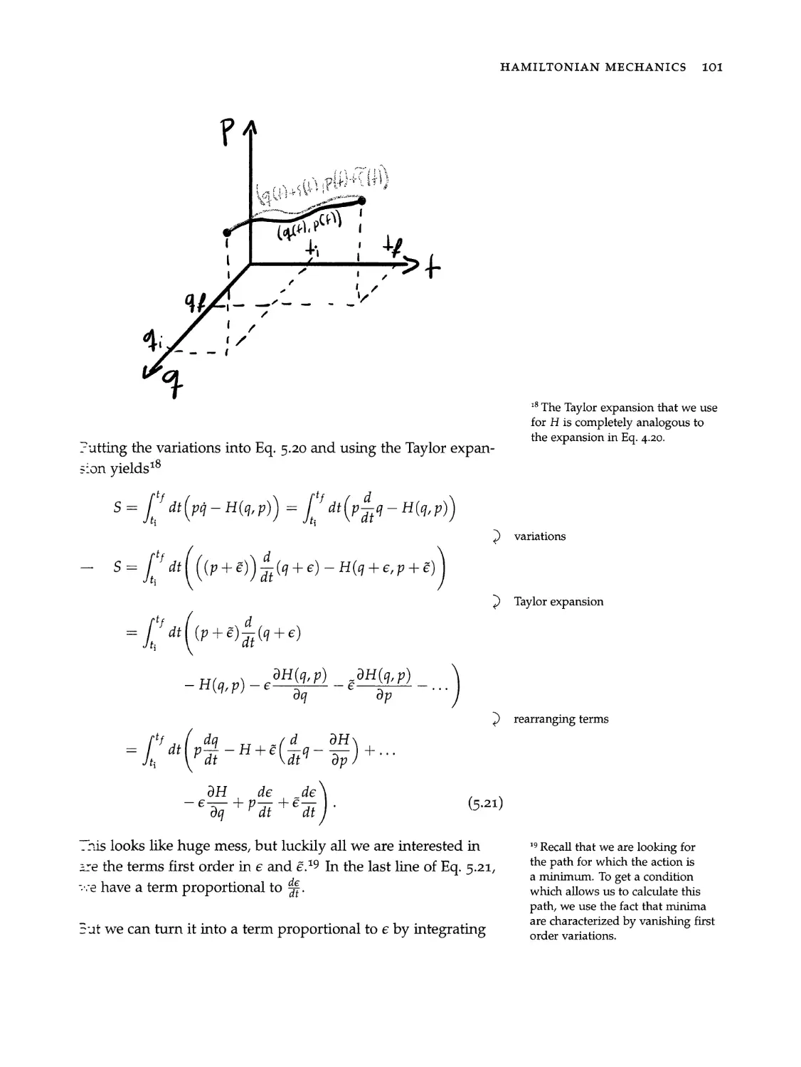
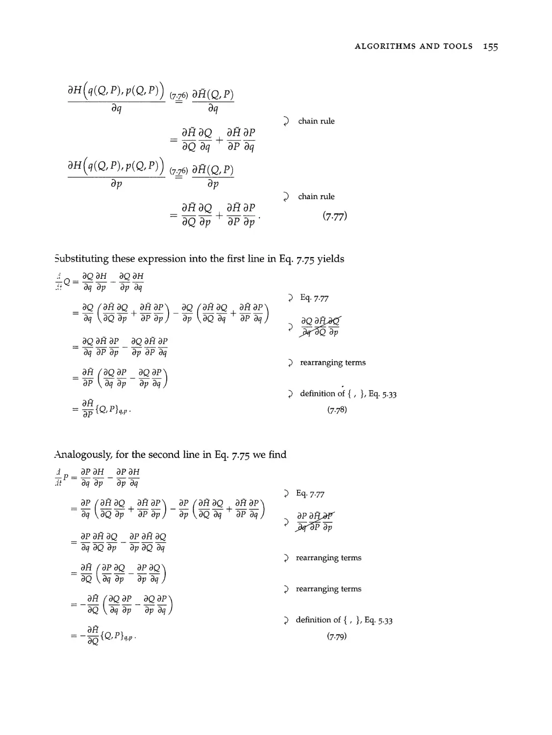
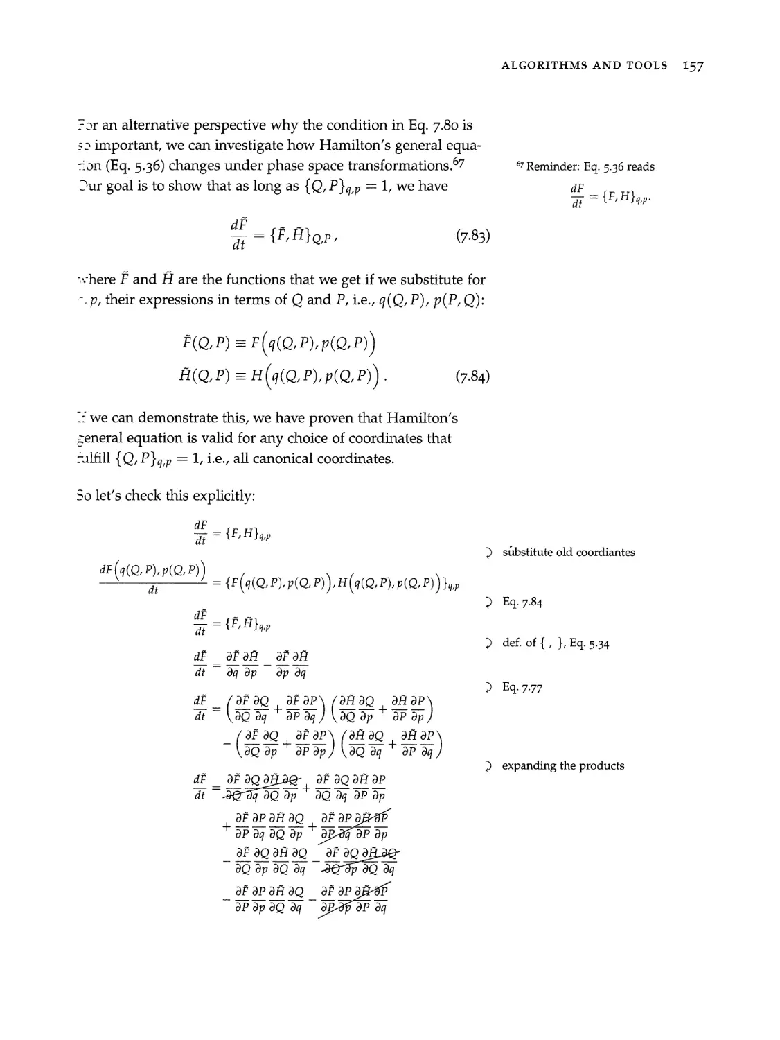
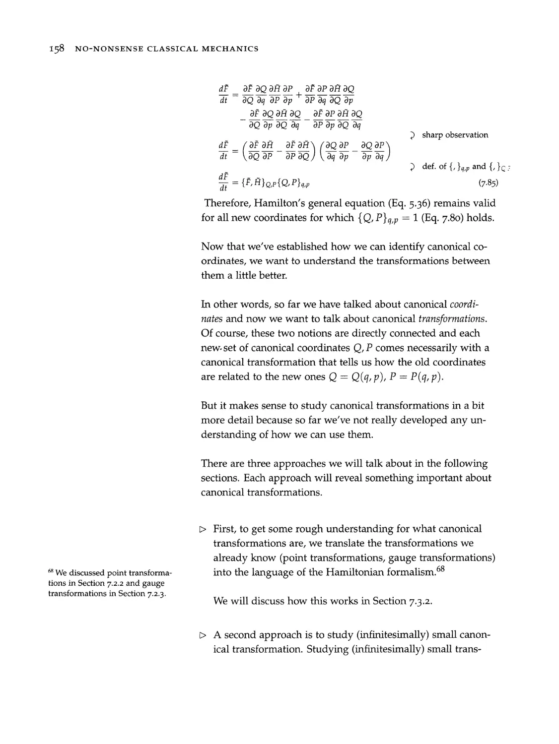
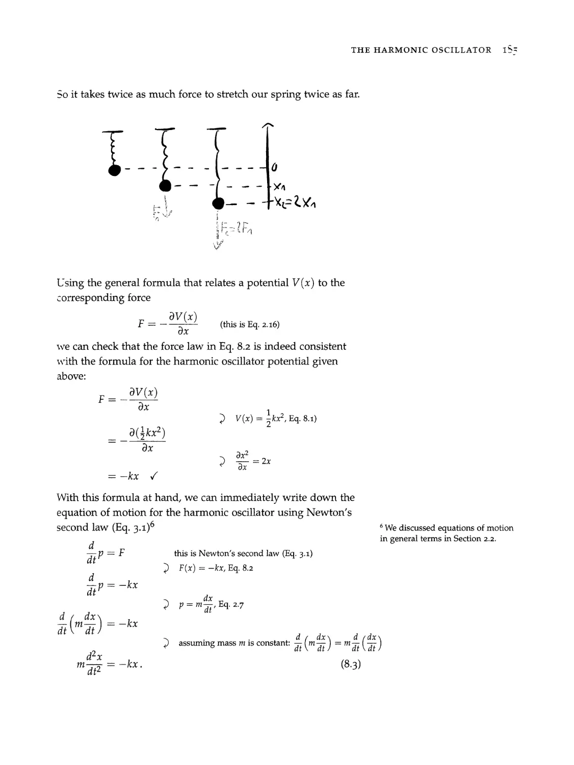
/


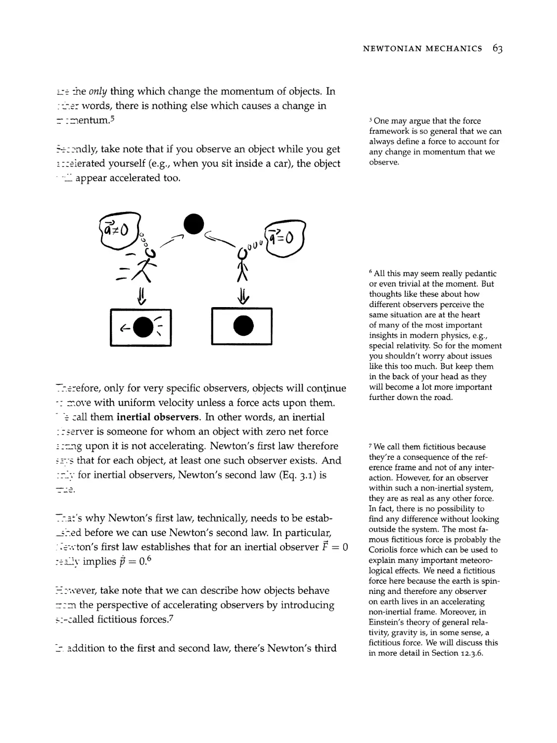


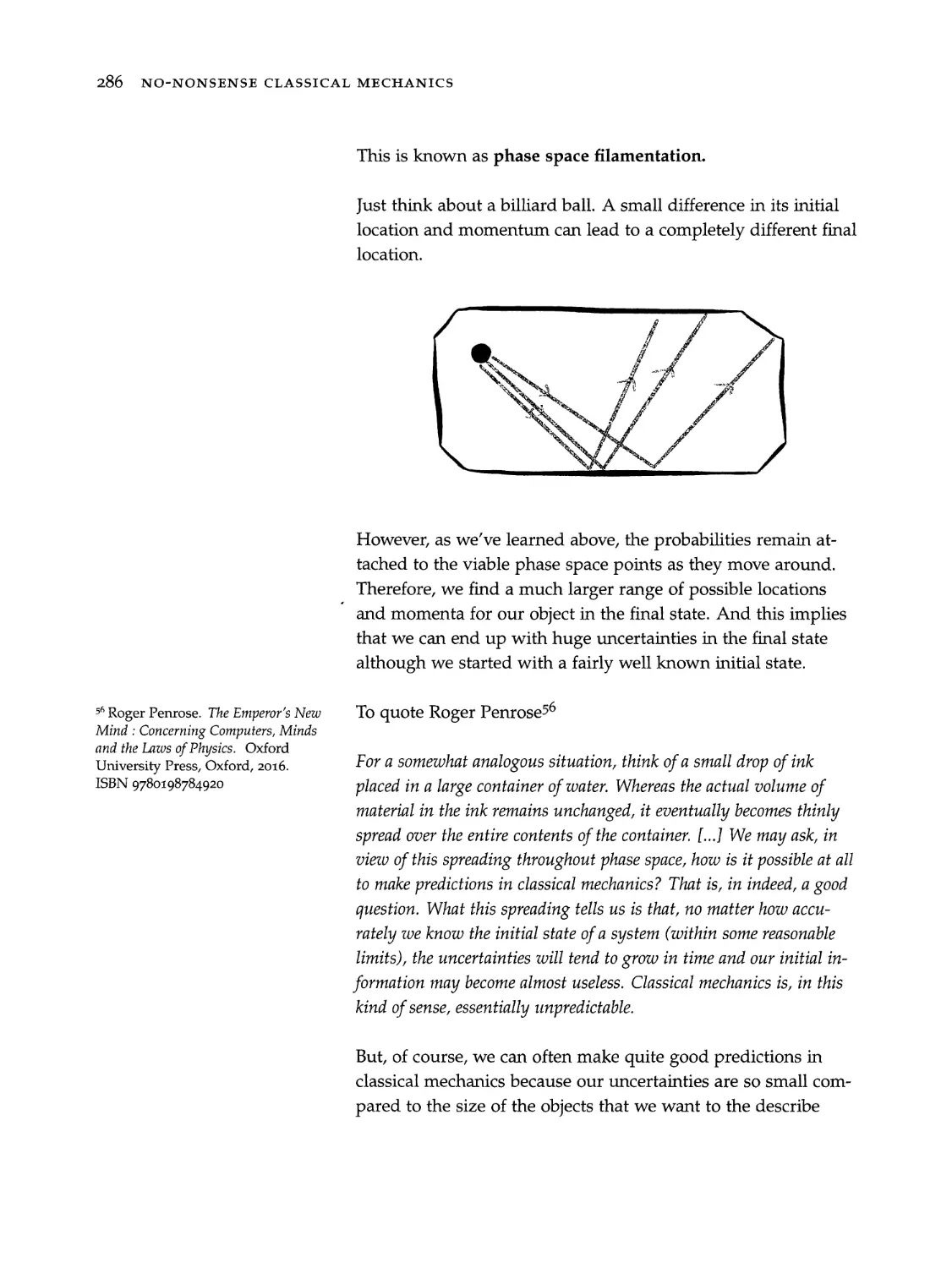


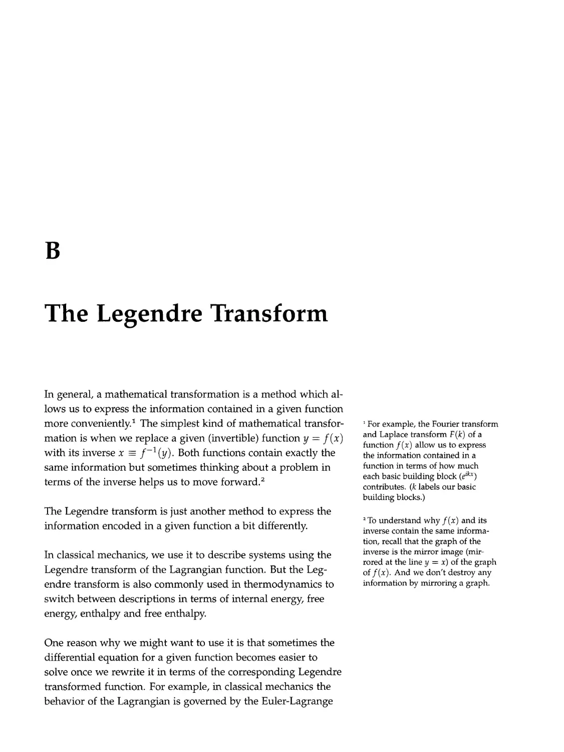


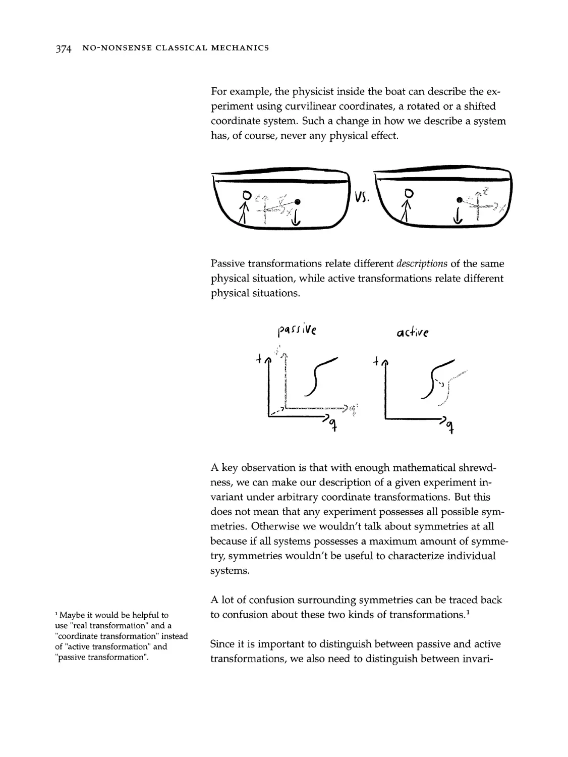
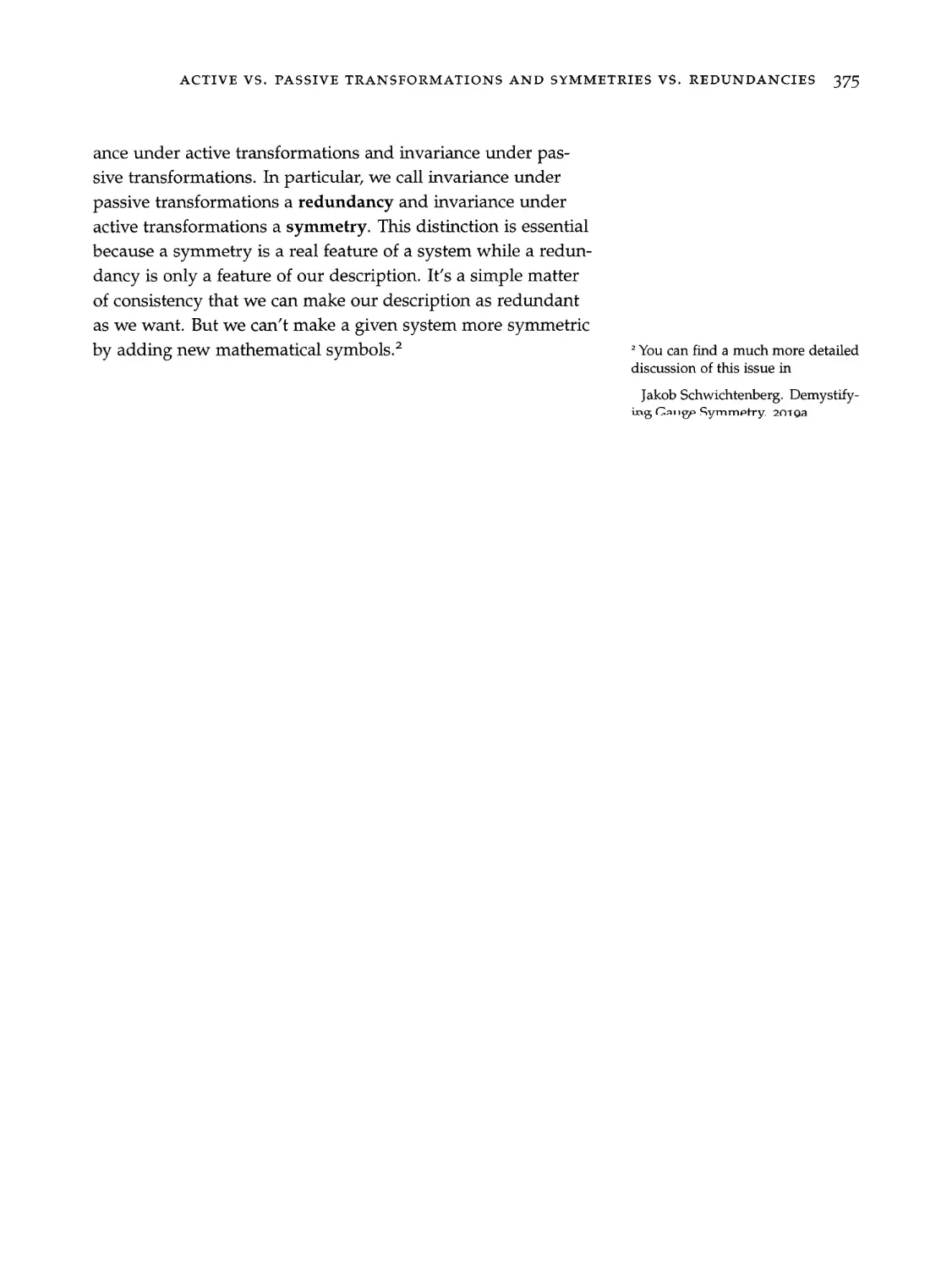


Текст
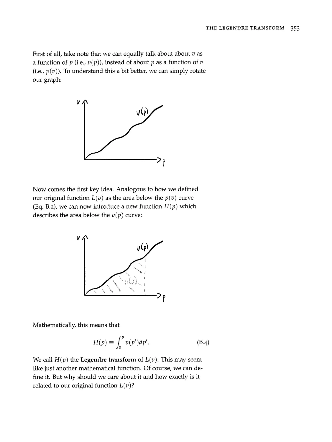
» ©
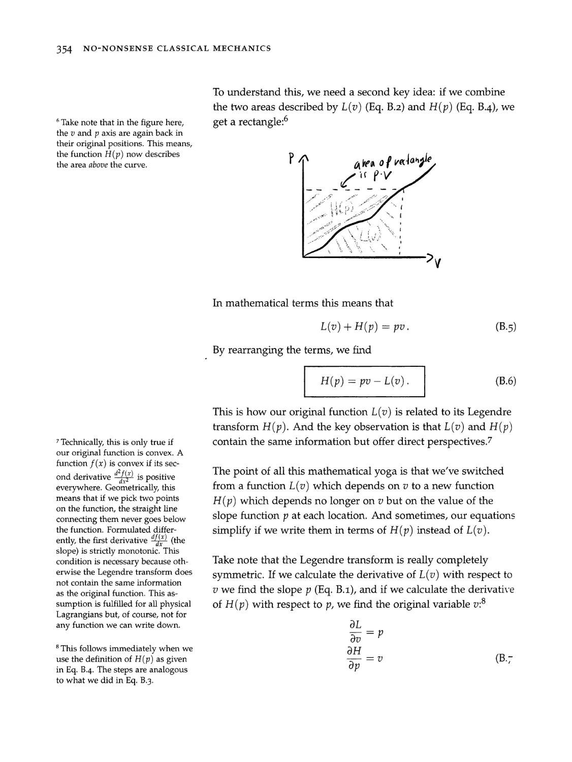
No-Nonsense
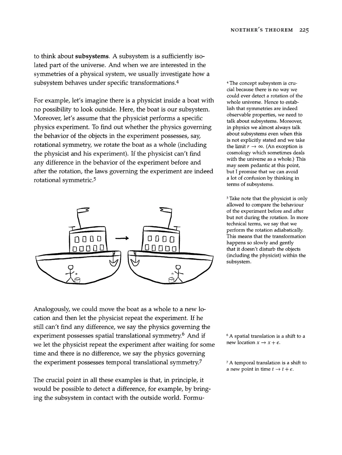
Jakob Schwichtenberg
Classical
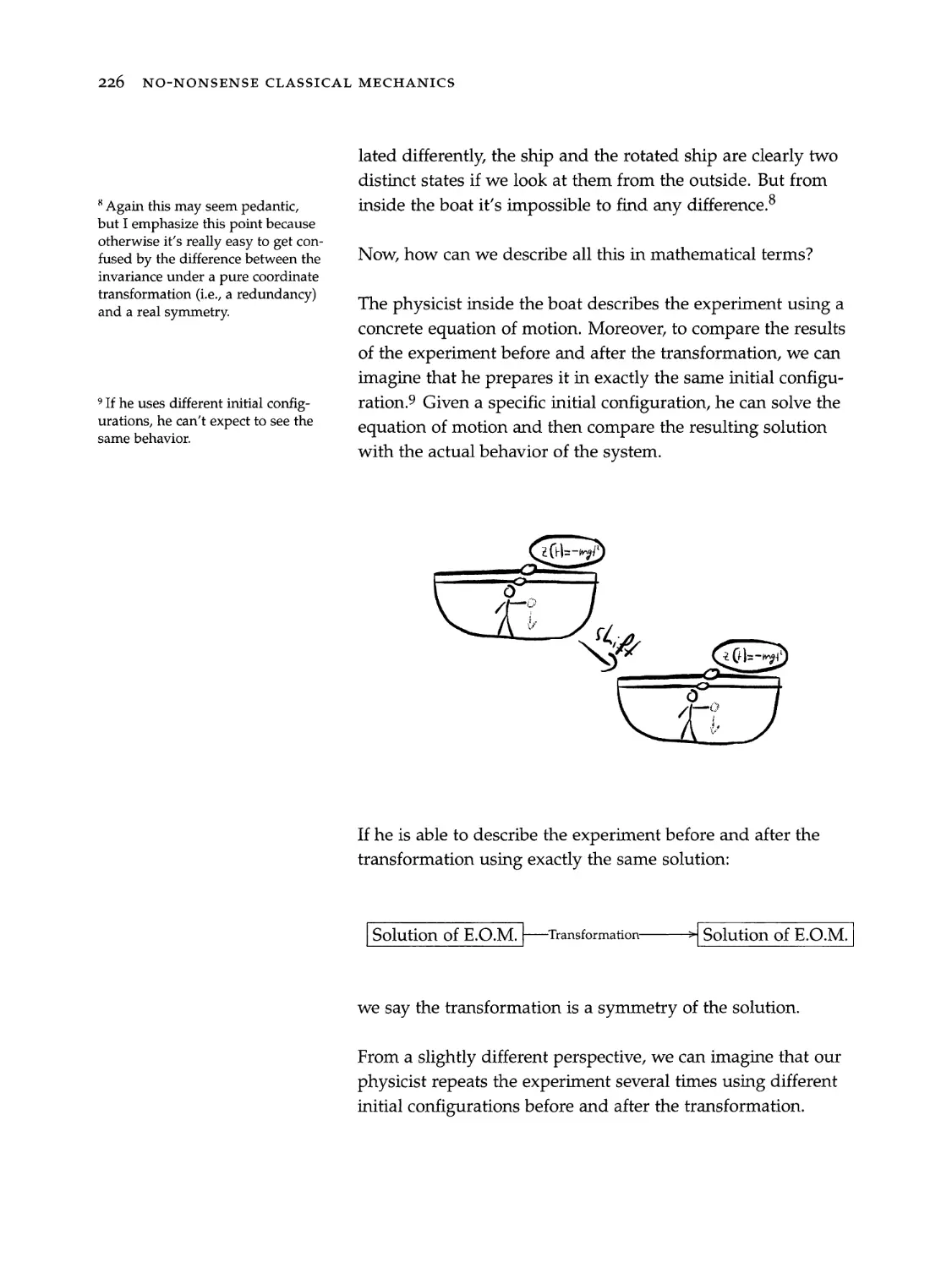
Mecnanics
CO Student- _—. ea
FROM THE AUTHOR OF THE BESTSELLING TEXTBOOK
PHYSICS FROM SYMMETRY
THE IMPORTANT THING IN SCIENCE IS NOT SO MUCH TO OBTAIN
NEW FACTS AS TO DISCOVER NEW WAYS OF THINKING ABOUT THEM.
SIR WILLIAM LAWRENCE BRAGG
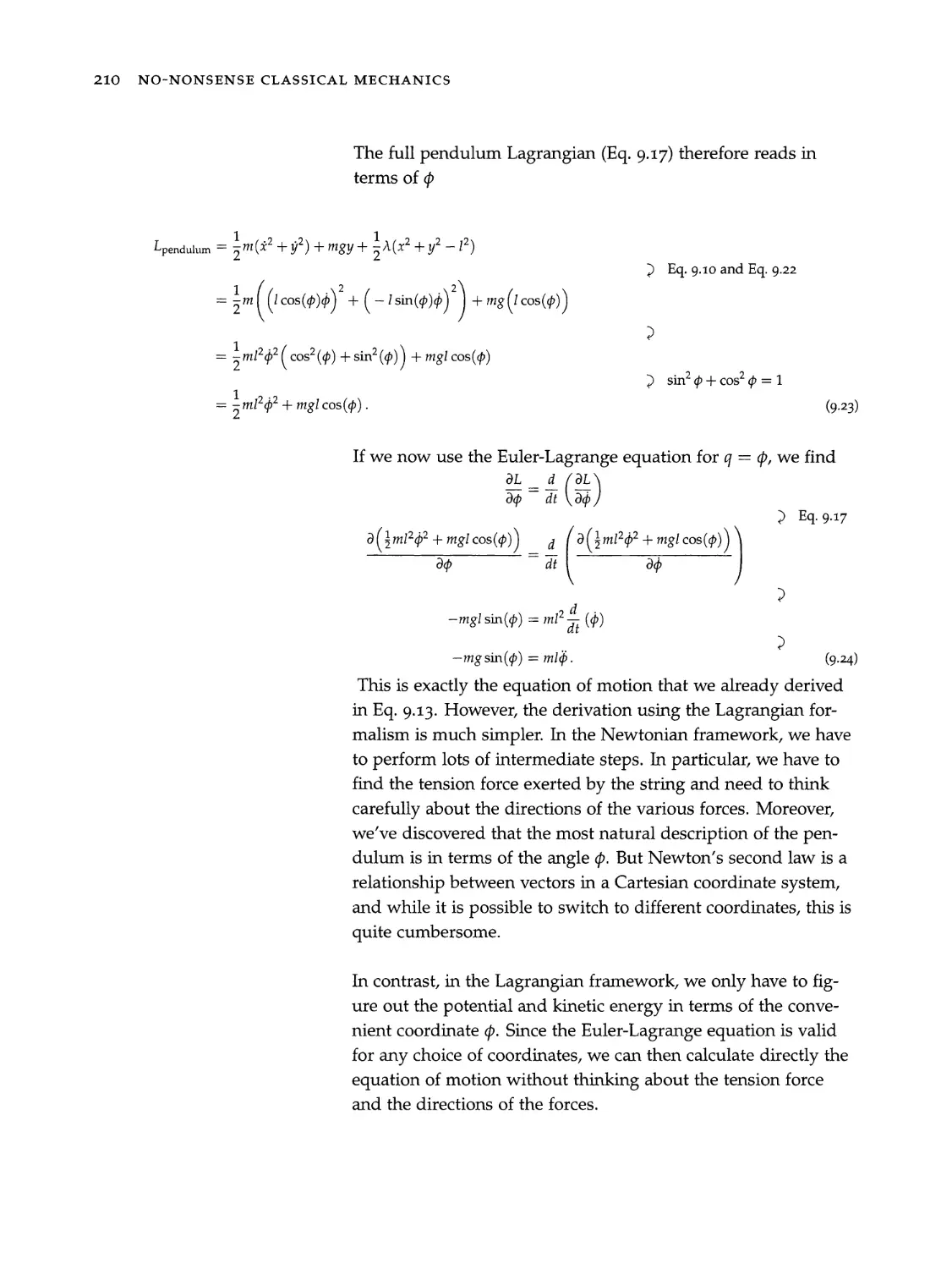
VE CANNOT SOLVE OUR PROBLEMS WITH THE SAME THINKING WE
~SED WHEN WE CREATED THEM.
~LBERT EINSTEIN
- YOU WANT TO IMPRESS PEOPLE, MAKE THINGS COMPLICATED. IF
“-3U WANT TO HELP PEOPLE, KEEP IT SIMPLE.
=-=ANK KERN
JAKOB SCHWICHTENBERG
NO-NONSENSE
CLASSICAL
MECHANICS
NO-NONSENSE BOOKS
no-nonsense
books: * °° "«*
First printing, May 2019
Copyright © 2019 Jakob Schwichtenberg
With illustrations by Corina Wieber
All rights reserved. No part of this publication may be reproduced, stored in, or introduced into
a retrieval system, or transmitted in any form or by any means (electronic, mechanical, photo-
copying, recording, or otherwise) without prior written permission.
UNIQUE ID: 5685DB256513FED14869E3E6AFE5FA1D65A6507E444198FC6D698F1 3A947930C
Each copy of No-Nonsense Classical Mechanics has a unique ID which helps to prevent illegal sharing.
EOI EDITION: 1.00
Dedicated to my parents
Preface
~.assical mechanics is more than 300 years old and dozens,
maybe even hundreds, of textbooks on the subject have already
ceen written. So why another one?
First of all, this book focuses solely on the fundamental aspects
of classical mechanics.* This narrow focus allows us to discuss
all important concepts several times from various perspectives.
In contrast, most other classical mechanics textbooks try to do
a lot at once. For example, it’s not uncommon that in addition
to the Newtonian, Lagrangian and Hamiltonian formulations,
dozens of applications, edge cases, advanced topics, historical
developments or even biographies of the most important con-
tributors are discussed. I think this is problematic because, as
the saying goes, if you try to be good at everything, you will not
be great at anything.
So a clear advantage of the approach used in this book is that
the reader has multiple chances to understand a given concept,
while in a "normal" textbook the reader immediately has a prob-
lem when a passage is not understood perfectly.2 A second
advantage of our narrow focus is that it minimizes the risk of
unnecessarily confusing the reader. Like all other fundamental
theories, classical mechanics is, at its heart, quite simple. How-
ever, using it to describe complicated systems is far from easy
and this is where most of the difficulties usually arise.
* Applications are only discussed
insofar as they help to deepen our
understanding of the fundamental
concepts and not as an end in it-
self. In addition, there are already
dozens of great books which dis-
cuss applications or, other special
topics in great detail. Some of the
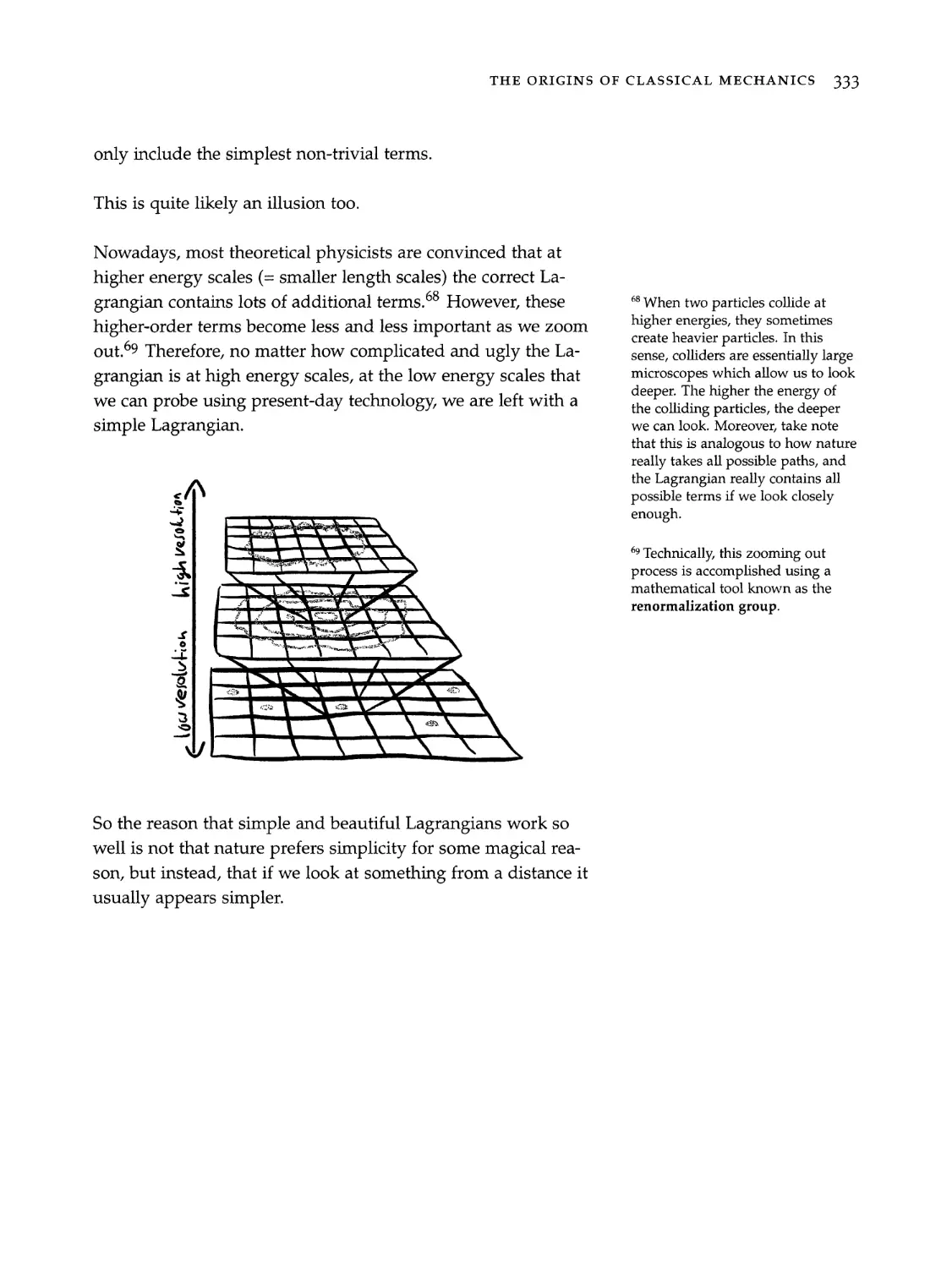
best ones are recommended in
Chapter 13.
*In a "normal" textbook each topic
is only introduced once. As a result,
later chapters become harder and
harder to understand without a
full understanding of all previous
chapters. Moreover, it’s easy to
become discouraged when a few
passages are not perfectly clear
since you know that you need the
knowledge to understand later
chapters.
3 Most of the difficulties are re-
ally math problems, not physics
problems anyway, e.g., solving a
difficult integral or solving a given
differential equation.
4 While advanced applications are,
of course, important, they are not
essential to understand the fun-
damentals of classical mechanics.
There are many great books which
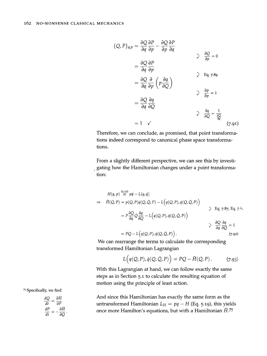
focus on specific applications. After
you've developed a solid under-
standing of the fundamentals, it’s
far easier to learn more about those
applications you're really interested
in.
5 This is known as the "Curse of
Knowledge."
® To quote C. Lanczos: "Many of
the scientific treatises of today
are formulated in a half-mystical
language, as though to impress
the reader with the uncomfortable
feeling that he is in the permanent
presence of a superman.”
In summary, restricting ourselves to the fundamentals allows us
to introduce classical mechanics as gently as possible.*
While this alone may already justify the publication of another
classical mechanics textbook, there are a few other things which
make this book different:
> First, it wasn’t written by a professor. As a result, this book
is by no means an authoritative reference. Instead, this book
is written like a casual conversation with a more experienced
student who shares with you everything he wishes he had
known earlier. I’m convinced that someone who has just
recently learned the topic can explain it much better than
someone who learned it decades ago. Many textbooks are
hard to understand, not because the subject is difficult, but
because the author can’t remember what it’s like to be a
beginner?.
[> Second, this book is unique in that it contains lots of idiosyn-
cratic hand-drawn illustrations. Usually, textbooks include
very few pictures since drawing them is either a lot of work
or expensive. However, drawing figures is only a lot of work
if you are a perfectionist. The images in this book are not as
pretty as the pictures in a typical textbook since I firmly be-
lieve that lots of non-perfect illustrations are much better than
a few perfect ones. The goal of this book, after all, is to help
you understand classical mechanics and not to win prizes for
my pretty illustrations.
> Finally, my only goal with this book was to write the most
student-friendly classical mechanics textbook and not, for
example, to build my reputation. Too many books are unnec-
essarily complicated because if a book is hard to understand
it makes the author appear smarter.° To give a concrete ex-
ample, nothing in this book is assumed to be "obvious" or
“easy to see’. Moreover, calculations are done step-by-step
and are annotated to help you understand faster.
Without any further ado, let’s begin. I hope you enjoy reading
7:5 book as much as I have enjoyed writing it.
s.2rlsruhe, June 2018 Jakob Schwichtenberg
='5: If you find an error, I would appreciate a short email to
=7zors@jakobschwichtenberg.com.
->S: You can discuss the content of the book with other readers,
23x questions and find bonus material at:
“44. nononsensebooks.com/cm/bonus.
Acknowledgments
srecial thanks to Stephan Lange for reporting several typos and
72 Dena Russell for carefully proofreading the manuscript.
10
7 We will talk about the relationship
of classical mechanics to modern
theories like quantum mechan-
ics and quantum field theory in
Section 12.1.
® To quote Roger Penrose: "In
modern attempts at fundamental
physics, when some suggested new
theory is put forward, it is almost
invariably given in the form of some
Lagrangian functional." [Penrose,
2016] This is discussed in more
detail Section 12.4.
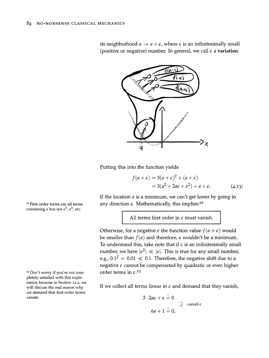
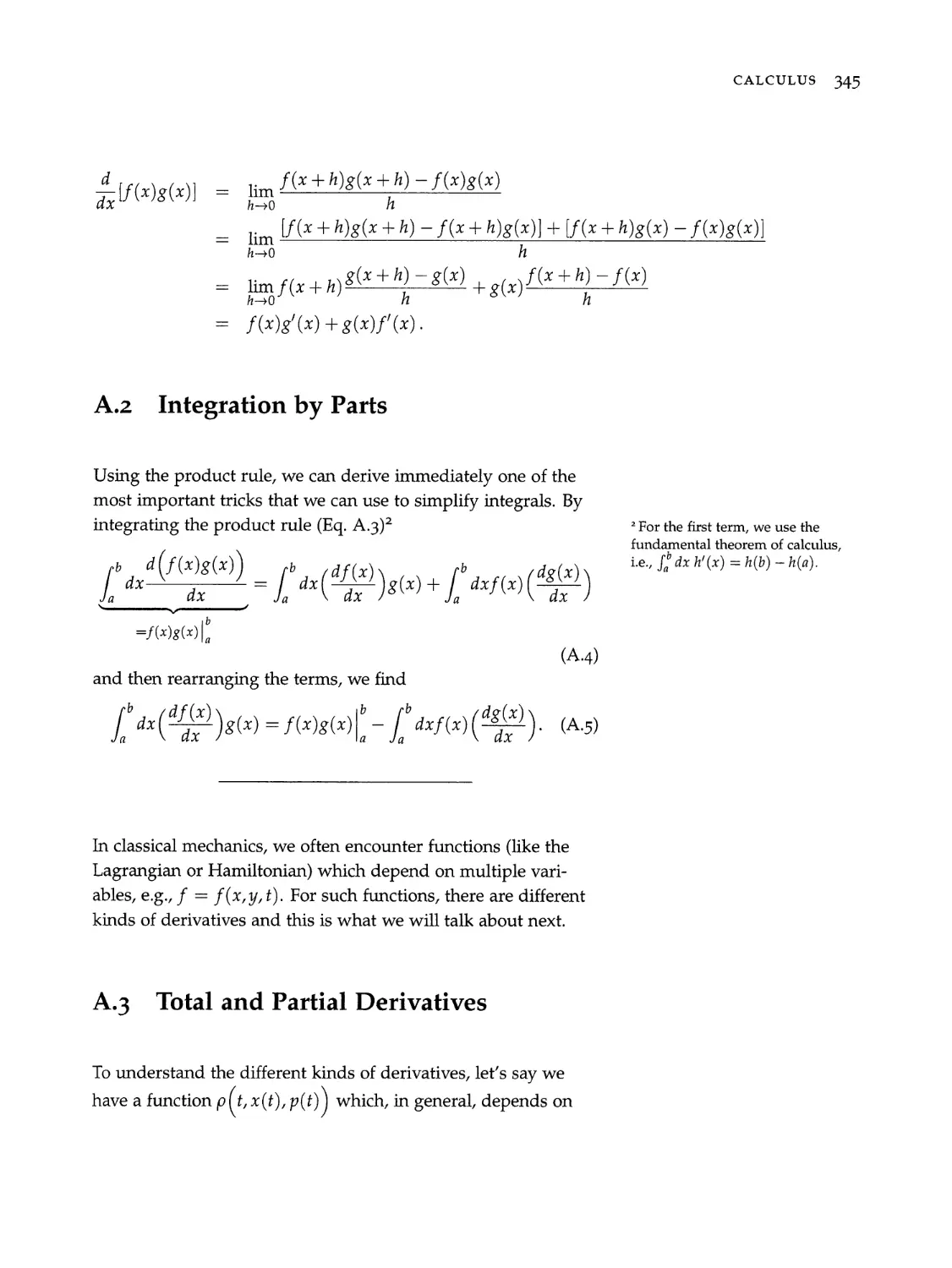
Before we dive in, we need to talk about two things. First, a
crucial question:
Why should you care about classical mechan-
ics?
First of all, classical mechanics is still the state of the art when
it comes to many problems. Modern theories like quantum
mechanics or quantum field theory do not help us when we
want to describe how a ball rolls down a ramp or how a rocket
flies. While classical mechanics does not help us to describe the
fundamental building blocks of nature, it’s still the best theory
of macroscopic objects that we have.”
This alone makes classical mechanics an invaluable tool in the
toolbox of any competent physicist.
But even if you only care about truly fundamental aspects of
physics, there are several reasons why learning classical me-
chanics makes sense:
> First, classical mechanics is an ideal playground to learn
many of the most important concepts which are used ev-
erywhere in modern physics. For example, the Lagrangian
formalism is presently our best tool to explore new mod-
els of nature, and there is no better way to learn it than by
studying how we can use it in classical mechanics. In addi-
tion, Noether’s theorem —a cornerstone of modern physics
—can be understood in beautiful and natural terms using the
framework of classical mechanics.
[> Second, by discussing the various formulations of classical
mechanics we can understand why there are usually multi-
ple ways to describe a given system, how these alternative
descriptions are related and why they studying multiple for-
mulations is often a smart thing to do. Understanding this
11
aspect of modern physics is especially important if we want
to think about new theories of fundamental physics.? °To quote Paul Dirac: "It is not
always so that theories which are
equivalent are equally good, because one
Finally, classical mechanics provides an intuitive arena to of them may be more suitable than the
study basic mathematical tools and basic mathematical are- other for future developments.
nas which we need all the time.
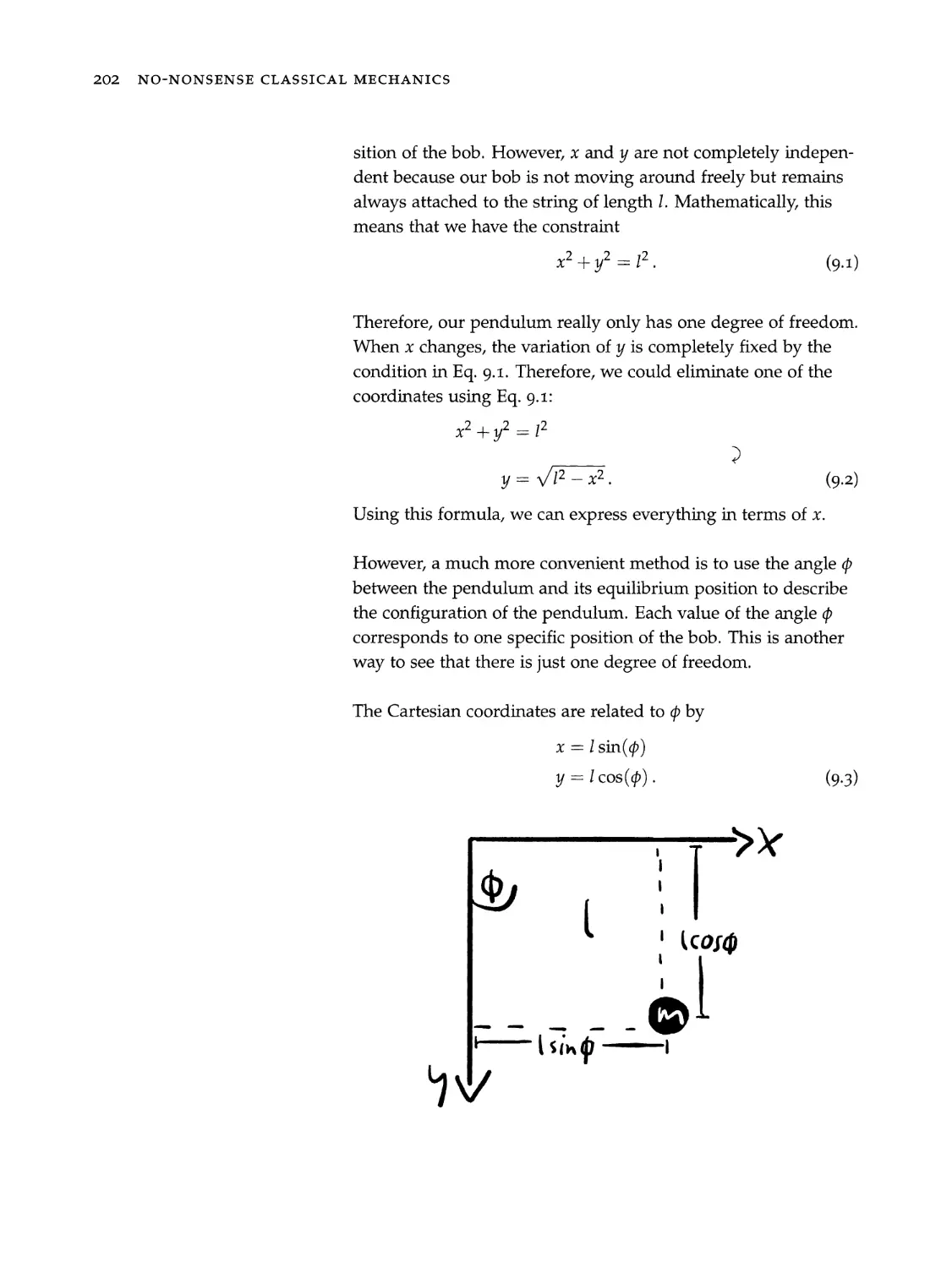
me second thing we need to talk about is the meaning of a few
srecial symbols which we will use in the following chapters.
Notation
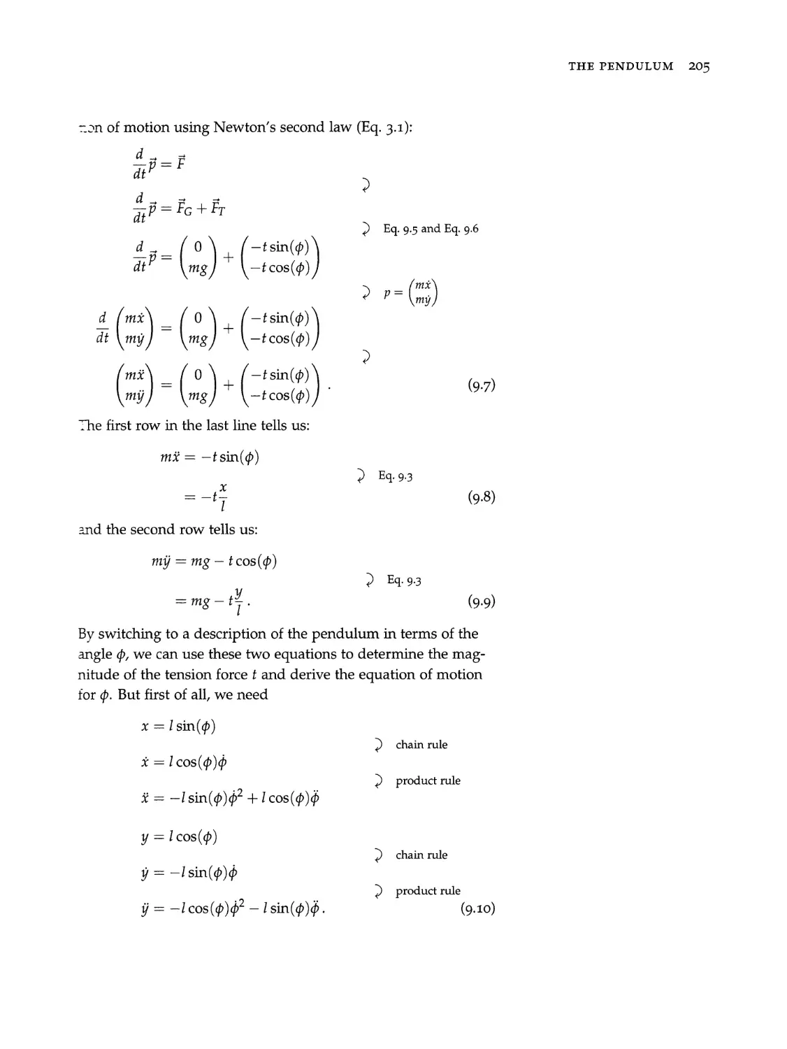
Three dots in front of an equation .., mean "therefore", Le.,
that this line follows directly from the previous one:
oul
oh
E=hw
This helps to make it clear that we are not dealing with a
system of equations.
» Three horizontal lines = indicate that we are dealing with a
definition.
!
The symbol = means "has to be", i.e., indicates that we are
dealing with a condition.
The most important equations, statements and results are
highlighted like this:
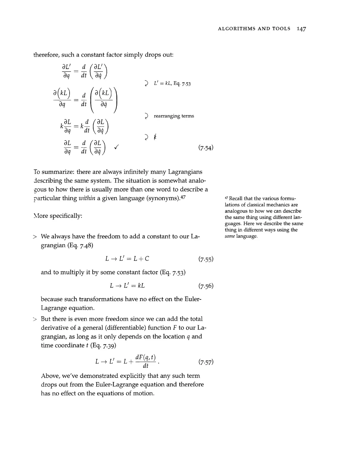
oL 4d fol
cm _£ (5) <9 (1)
og dt \ og
ofa et) denotes the partial derivative with respect to t,
while afxyzit) denotes the total derivative.*® © The difference between partial
and total derivatives is discussed in
Appendix A.3.
A dot above a function denotes the derivative with respect to
time q(t) = 4 and q(t) = 0.
12
> To unclutter the notation, we often use g as a shorthand for
all coordinates, i.e., q = (q1,...,q2). So for example, instead of
f (x,y,z), we write f(q).
That’s it. We are ready to dive in (after a short look at the table
of contents).
Contents
1 Bird’s-Eye View of Classical Mechanics 17
Part I What Everybody Ought to Know About Clas-
sical Mechanics
2 Fundamental Concepts 25
2.1 Basic Quantities .........0....0. 0000008 26
211 Mass ....... 0... 000.002. eee 28
2.1.2 Momentum and Angular Momentum .... 29
2.1.3 Energy... .. ee ee .. 32
2.2 Equations of Motion ...............048. 41
2.3 Mathematical Arenas..................4 49
2.3.1 Configuration Space .............. 50
2.3.2 PhaseSpace.............-.004. 54
3 Newtonian Mechanics 59
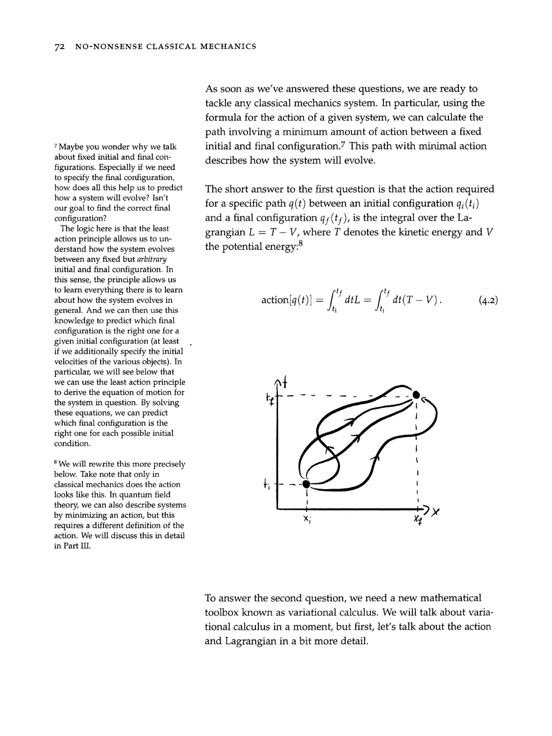
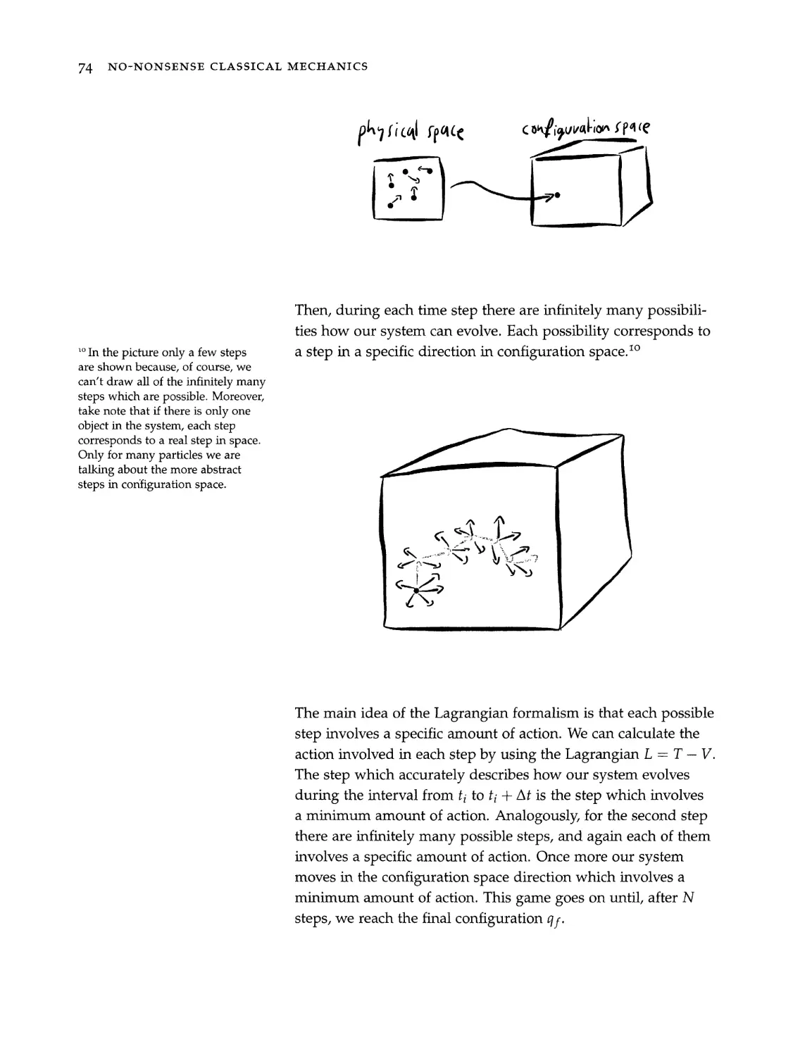
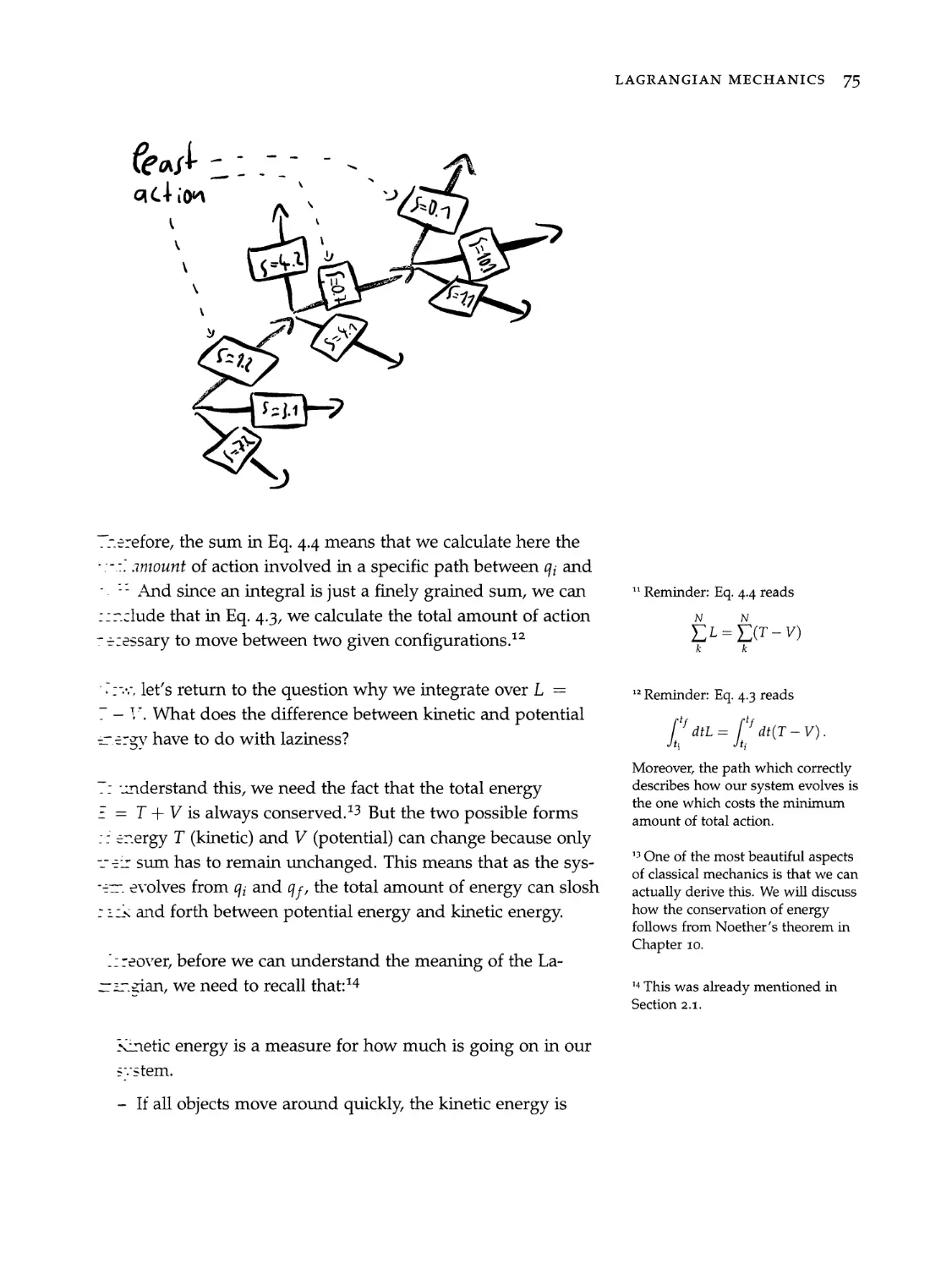
4 Lagrangian Mechanics 67
4.1 Action and the Lagrangian .............. 73
4.2 Variational Calculus ................044 81
4.3 The Euler-Lagrange Equation ............. 86
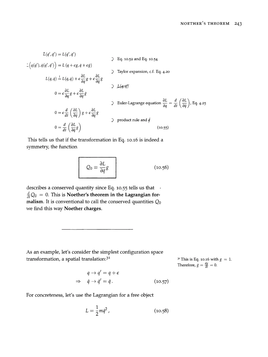
4.3.1 Meaning of the Euler-Lagrange Equation .. 90
5 Hamiltonian Mechanics 93
5.1 Hamilton’s Equations...............00, 95
5.1.1 Meaning of Hamilton’s Equations ...... 104
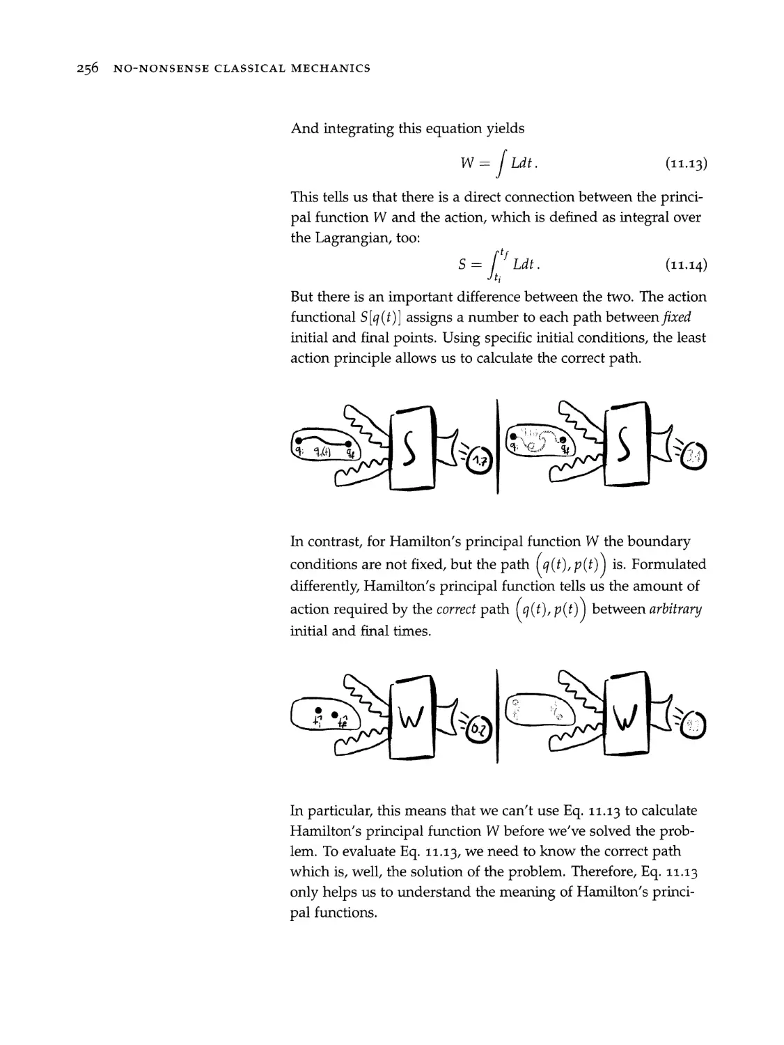
5.2 Hamilton’s General Equation ............., 107
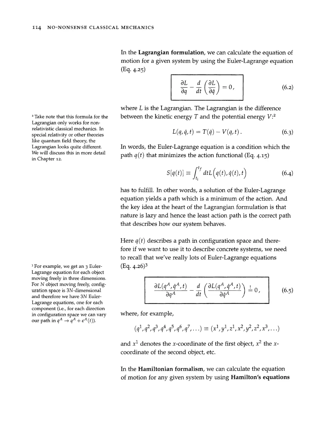
6 Summary 113
Part II Essential Systems and Tools
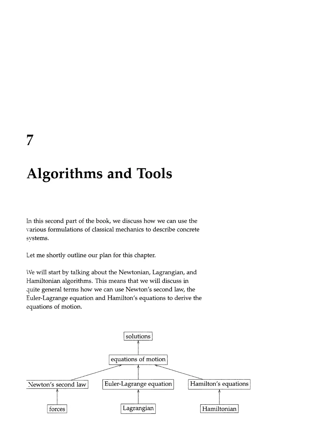
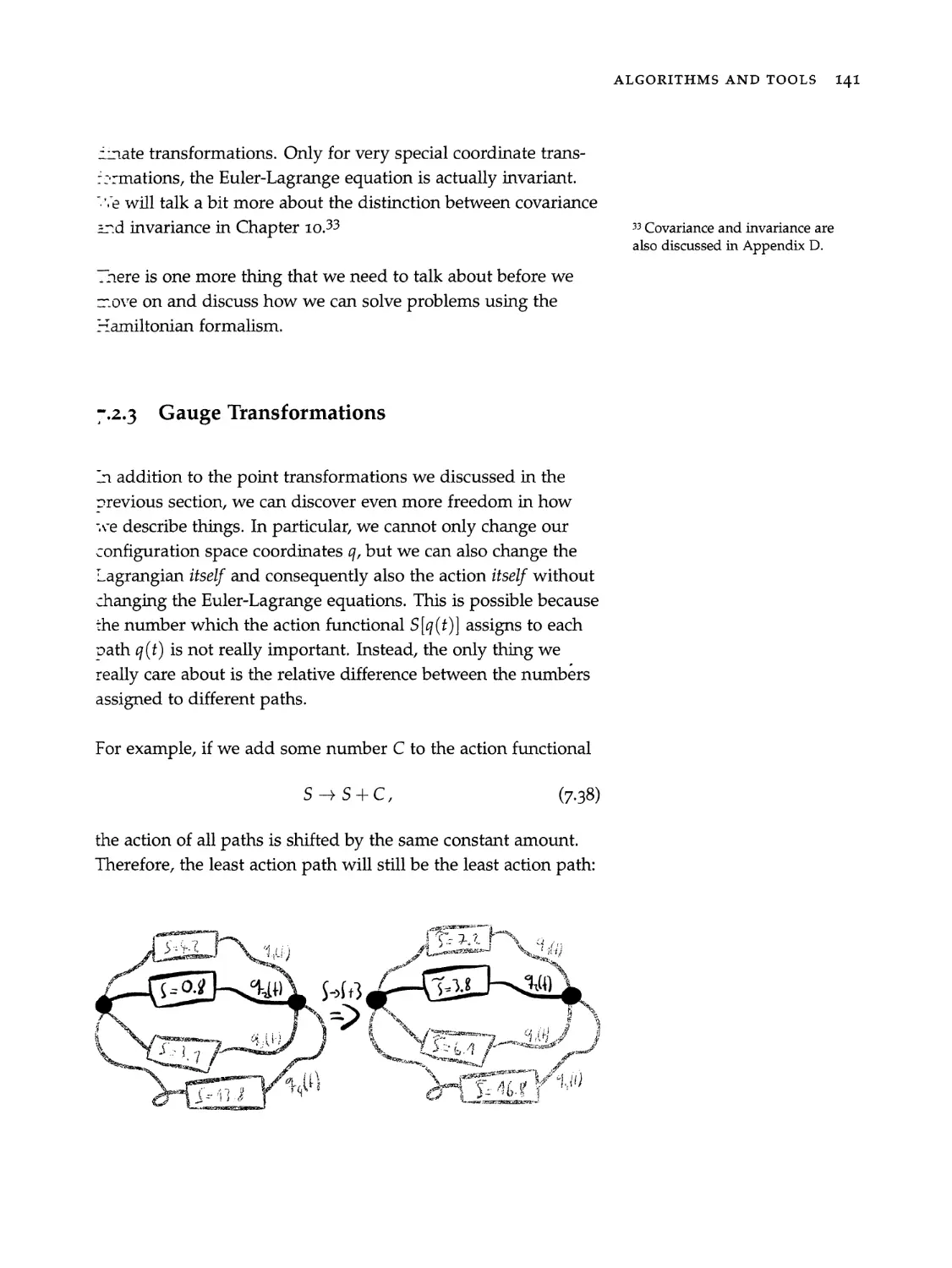
7 Algorithms and Tools 121
7.1 The Newtonian Algorithm. ............0.4. 125
7.2 The Lagrangian Algorithm .............. 127
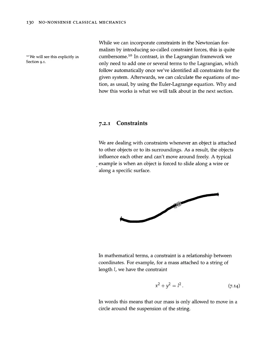
7.2.1 Constraints .......... 0.2.0. e ene 130
7.2.2 Point Transformations and Generalized Co-
ordinates... .... ee eee 134
7.2.3 Gauge Transformations ............ 141
7.3 The Hamiltonian Algorithm .............. 148
7.3.1 Canonical Transformations and Canonical Co-
ordinates... ...... cee ee ee 152
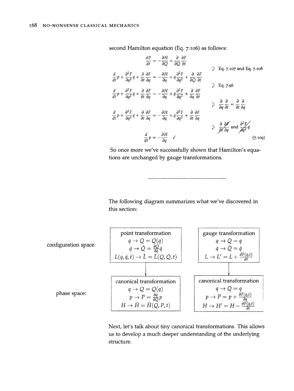
7.3.2 Canonical Point and Gauge Transformations 160
7.3.3 Infinitesimal Canonical Transformation ... 169
7.3.4 Generating Functions ............. 172
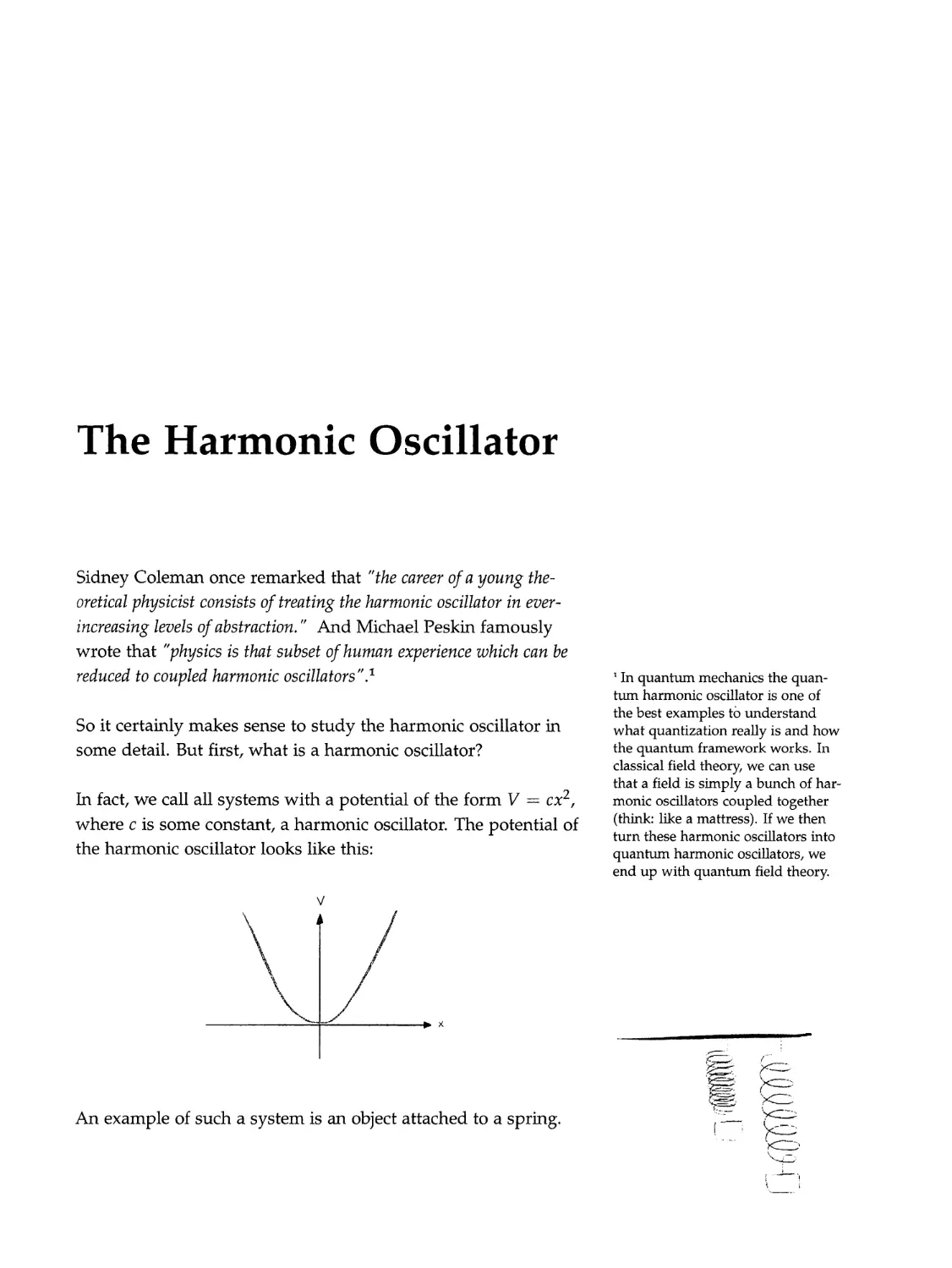
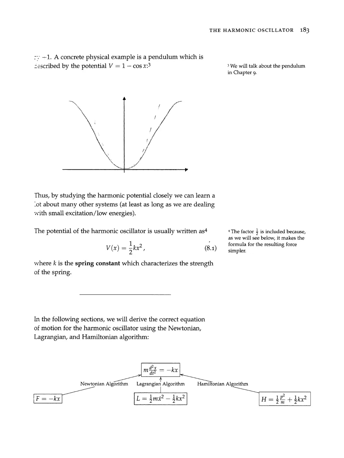
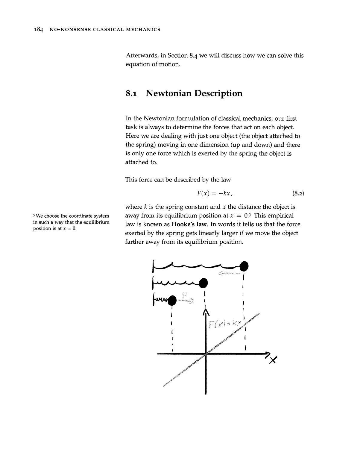
8 The Harmonic Oscillator 181
8.1 Newtonian Description. ...............0. 184
8.2 Lagrangian Description ..............4.. 187
8.3 Hamiltonian Description................ 188
8.4 Solving the Equation of Motion............ 190
8.5 Solving the Harmonic Oscillator Using a Canonical
Transformation ........... 000.00 bees 196
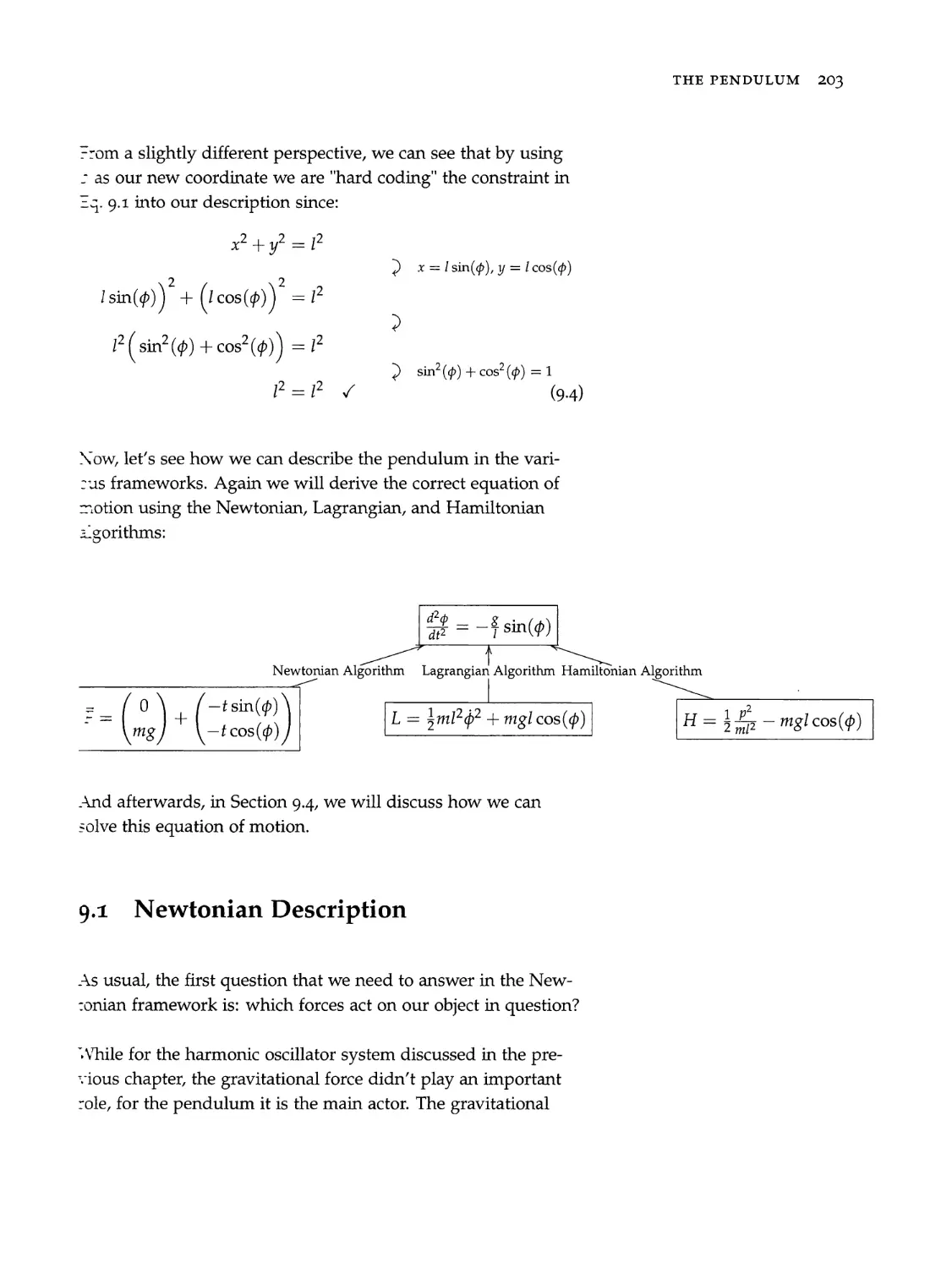
g9 The Pendulum 201
g.1 Newtonian Description... ...........00. 203
9.2 Lagrangian Description .............0-. 207
9.3. Hamiltonian Description................ 211
9.4 Solving the Equation of Motion. .... ae 213
Part III Get an Understanding of Classical Mechan-
ics You Can Be Proud Of
10 Noether’s Theorem 223
10.1 Symmetries ............ 0.02.00 0000. 224
10.1.1 Symmetries of PhysicalSystems ....... 224
10.2 Noether’s Theorem Intuitively ............ 228
10.3 Noether’s Theorem in the Hamiltonian Formalism 232
10.3.1 Noether’s Extended Theorem......... 239
10.3.2 Noether’s Converse Theorem......... 241
Noether’s Theorem in the Lagrangian Formalism . 241
10.4.1 Noether’s Extended Theorem......... 244
22.8 Summary... 2... ee ee 248
-: Additional Formulations of Classical Mechanics 251
71.1 Hamilton-Jacobi Mechanics .............. 252
11.1.1 Meaning of Hamilton’s Principal Function . 255
11.1.2 Harmonic Oscillator .............. 257
-7.2 Statistical Mechanics .................. 261
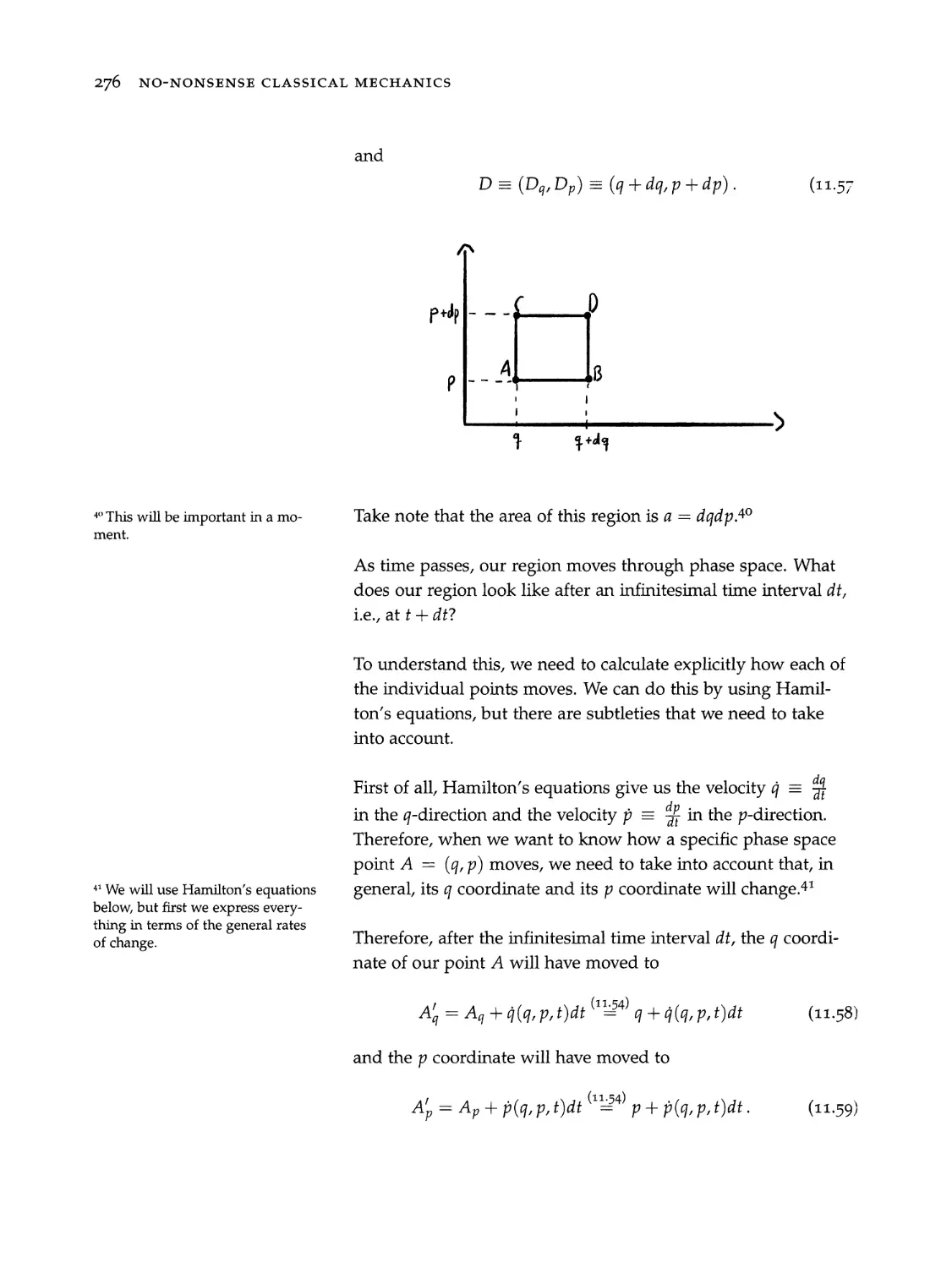
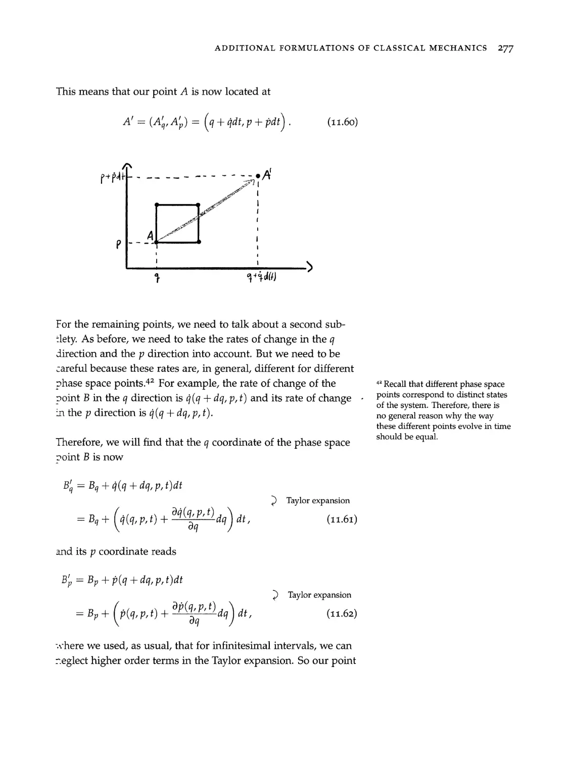
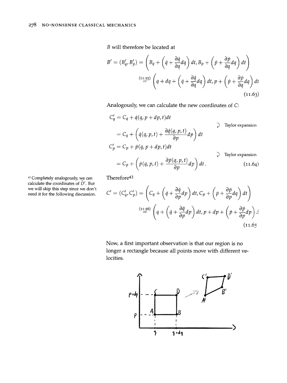
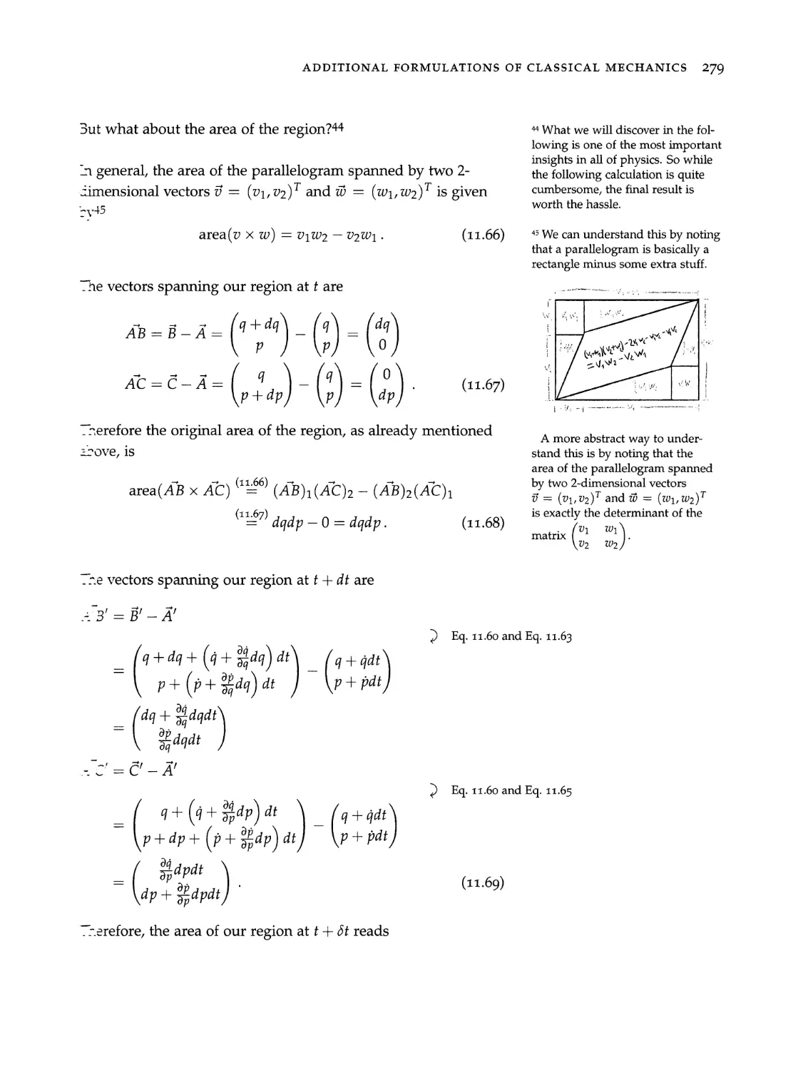
11.2.1 Probability Density. ............0.. 264
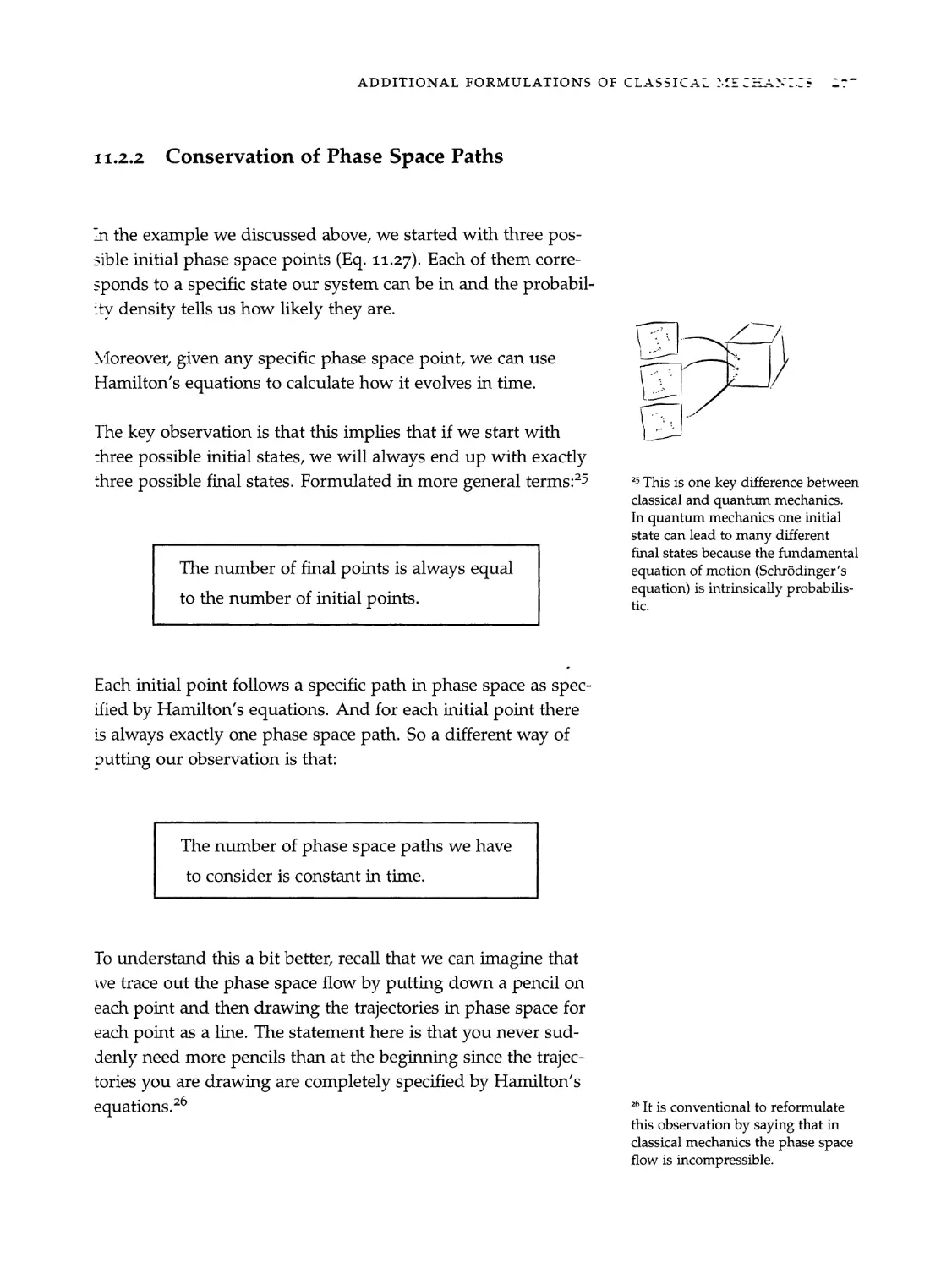
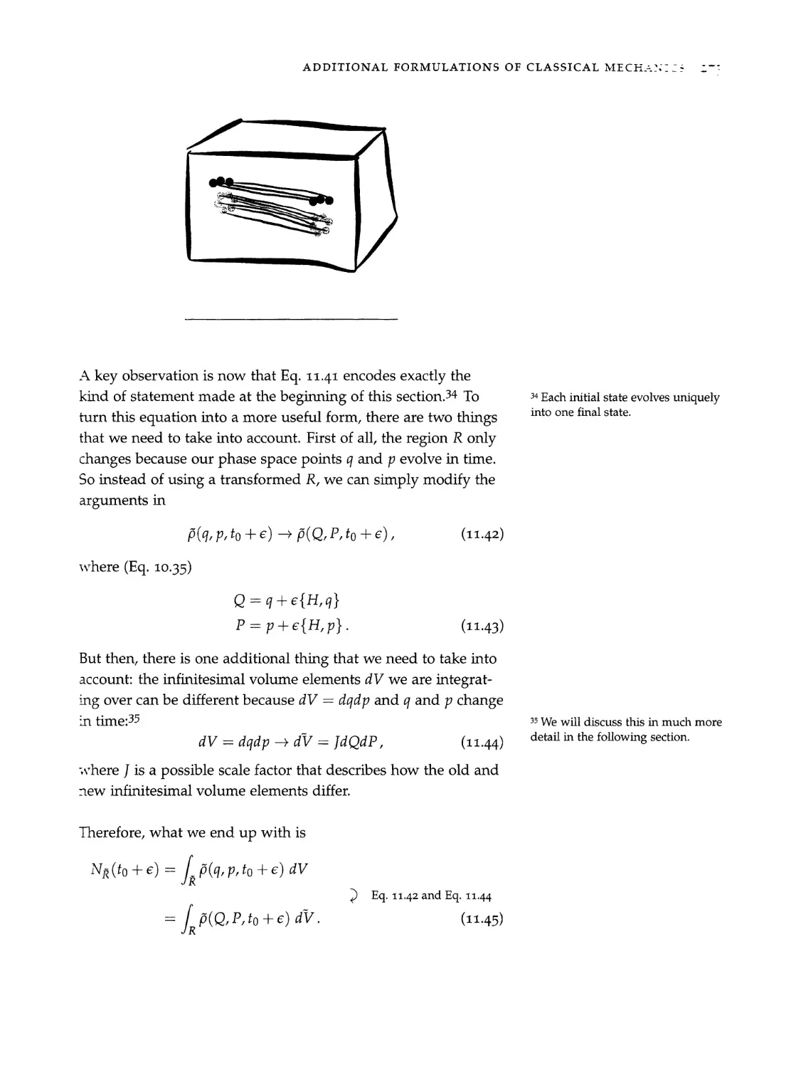
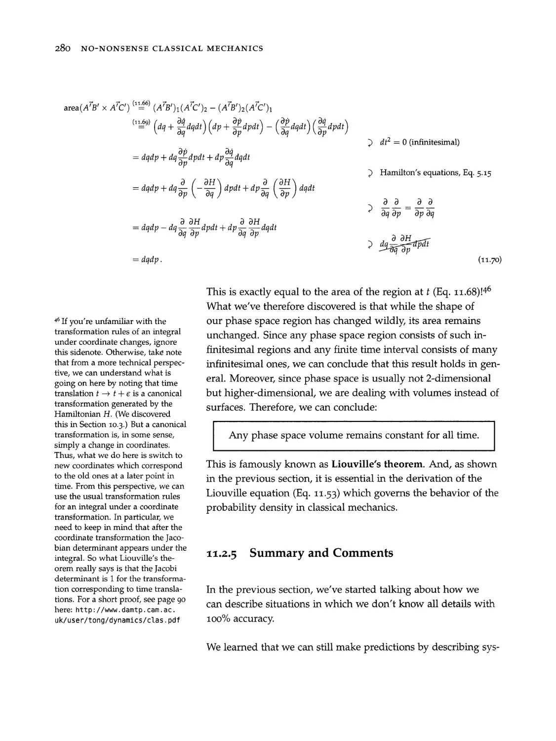
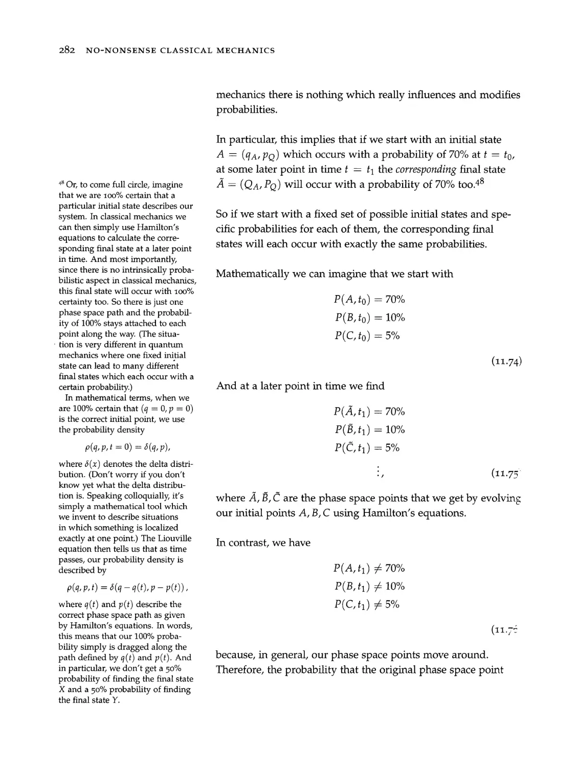
11.2.2 Conservation of Phase Space Paths ..... 267
11.2.3. Liouville’s Equation .............. 274
11.2.4 Liouville’s Theorem .............. 275
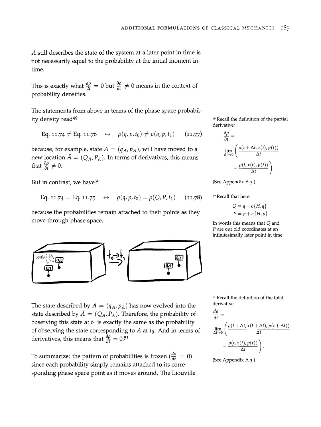
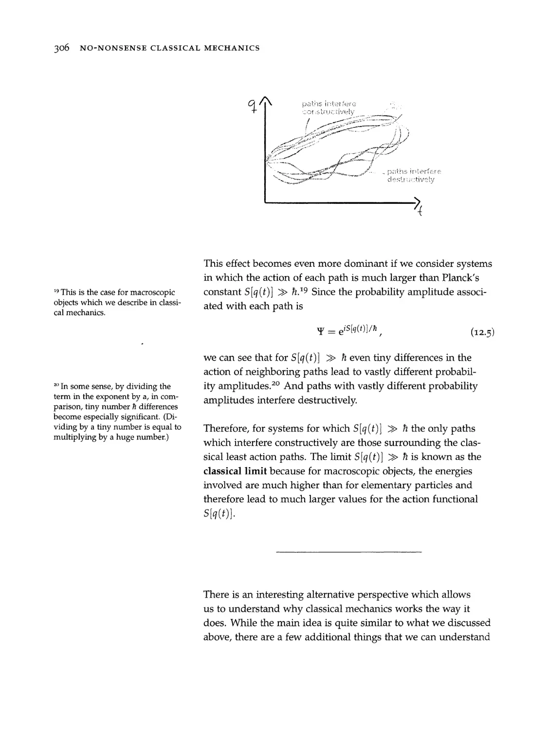
11.2.5 Summary and Comments ........... 280
-:.3 Koopmann-von Neumann Mechanics ........ 287
11.3.1 HilbertSpace ..............00.. 287
11.3.2 Koopman-von Neumann Equation...... 290
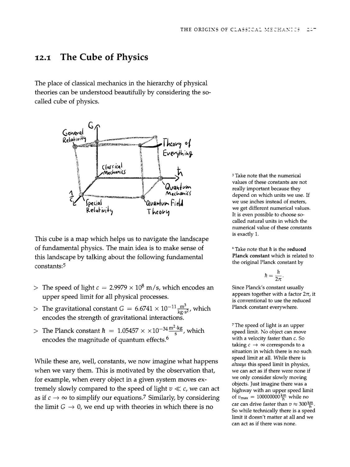
-: The Origins of Classical Mechanics 295
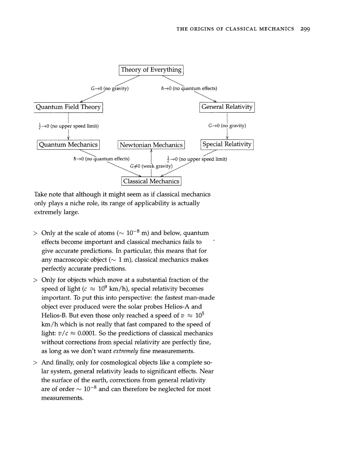
72.1 The Cube of Physics ................0.. 297
-2.2 The Origin of the Least Action Principle. ...... 300
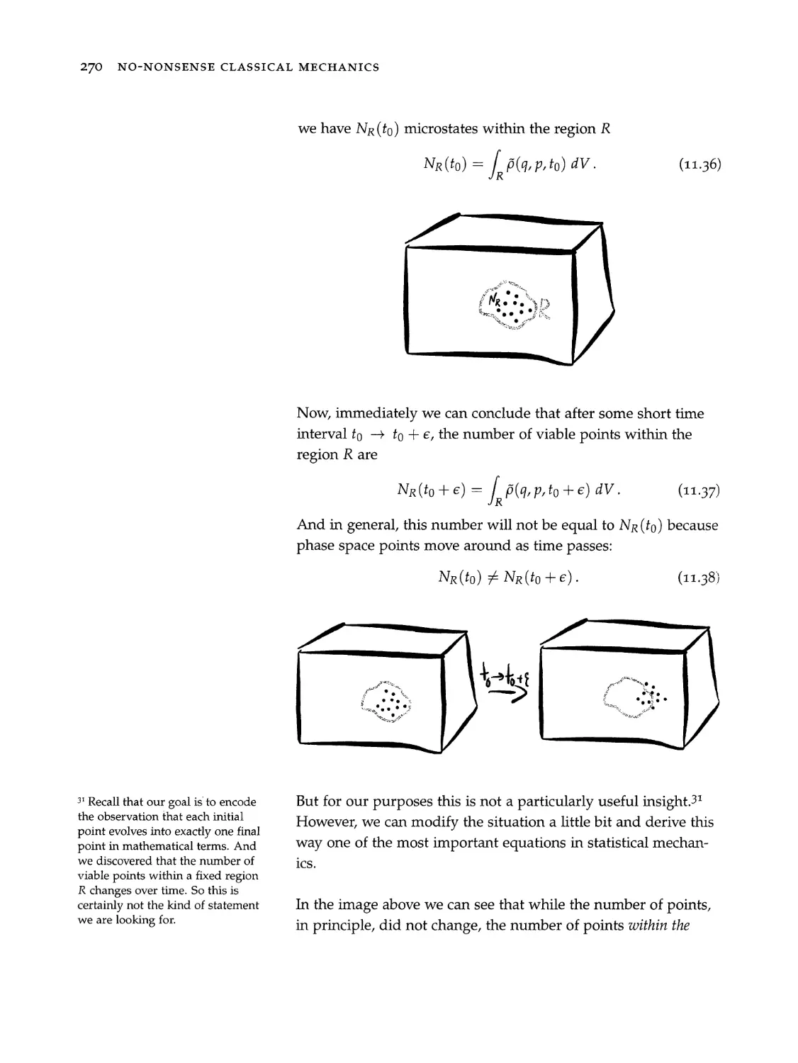
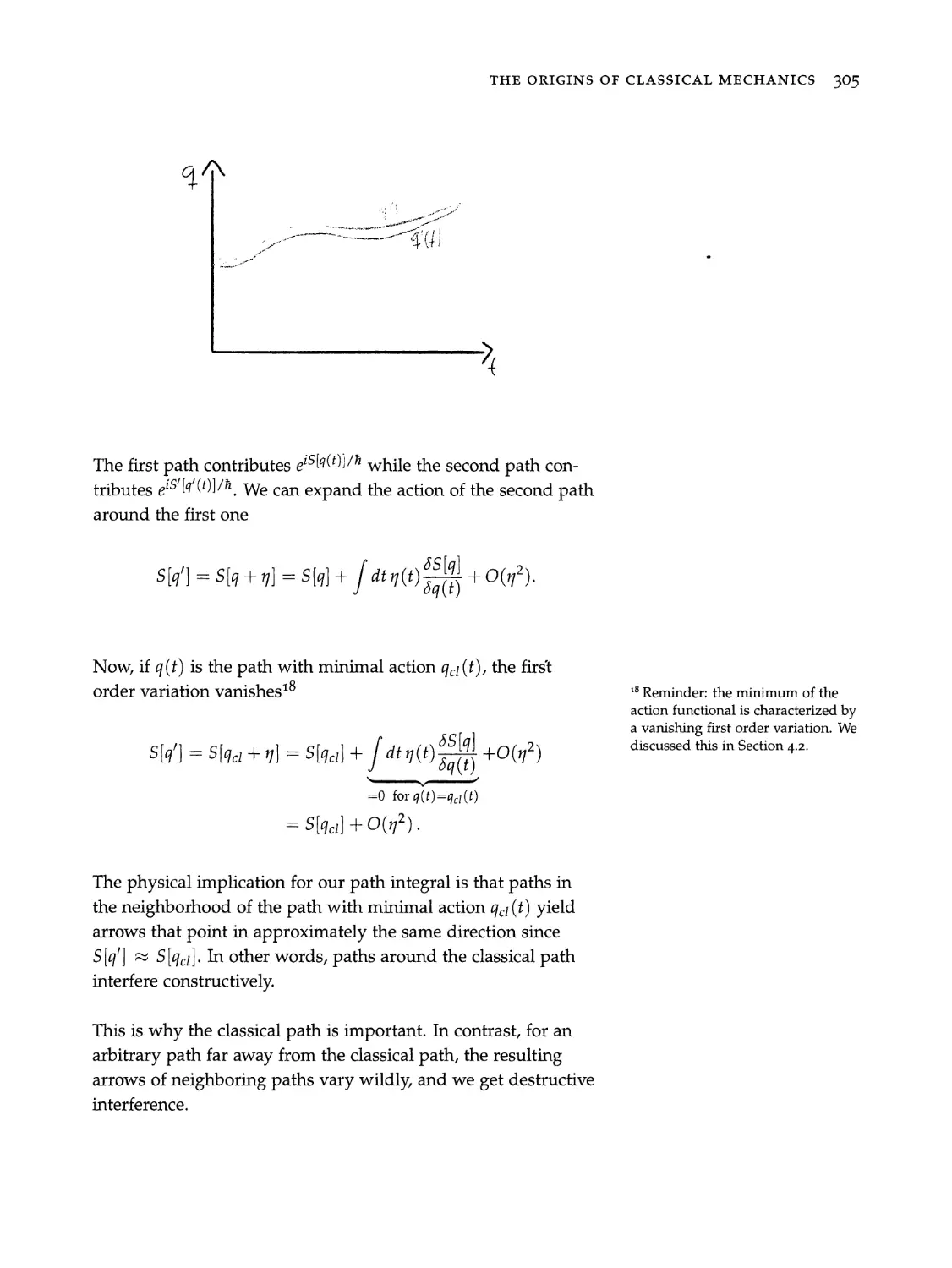
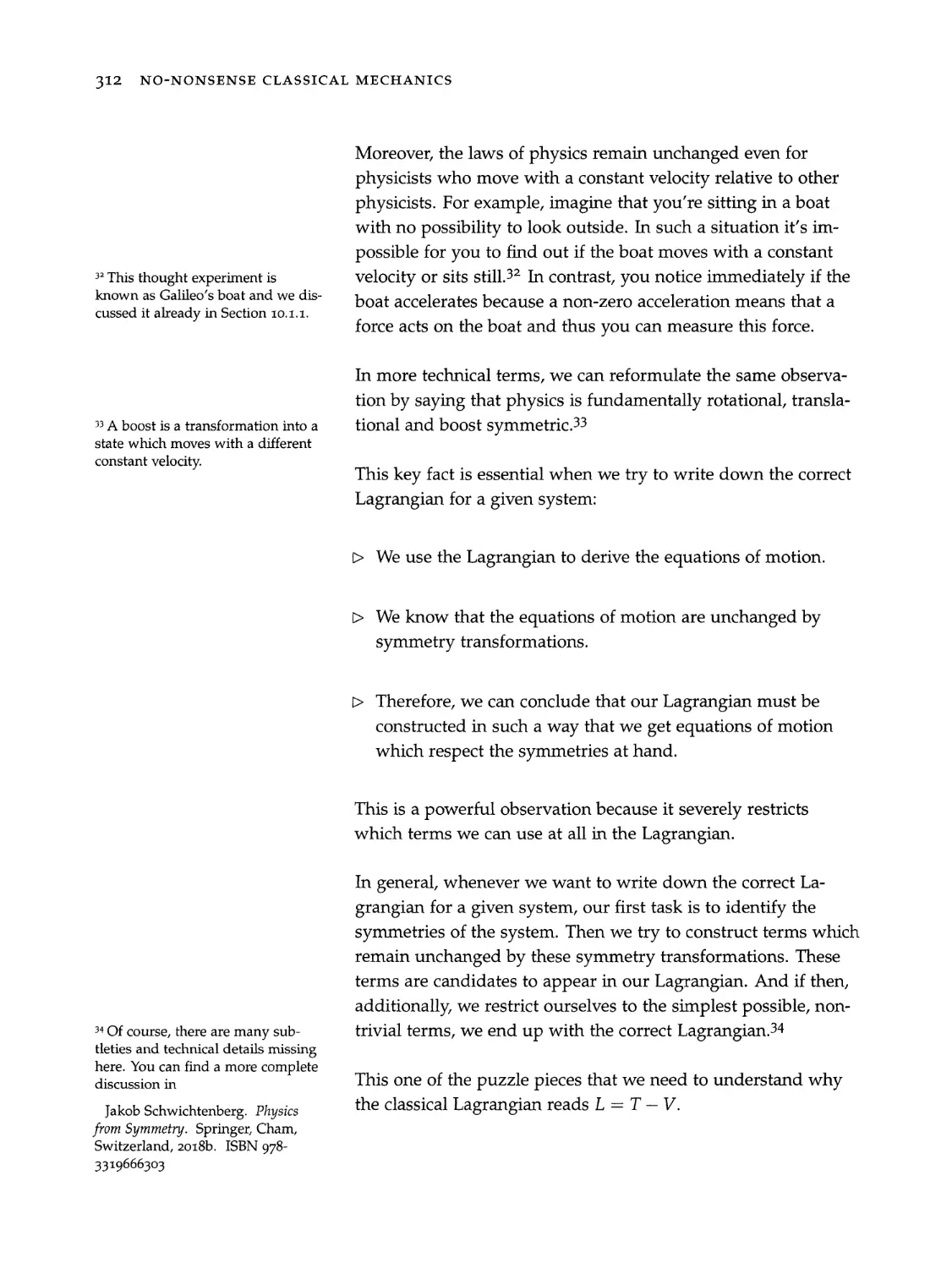
12.2.1 The Origin of the Classical Path ...... . 304
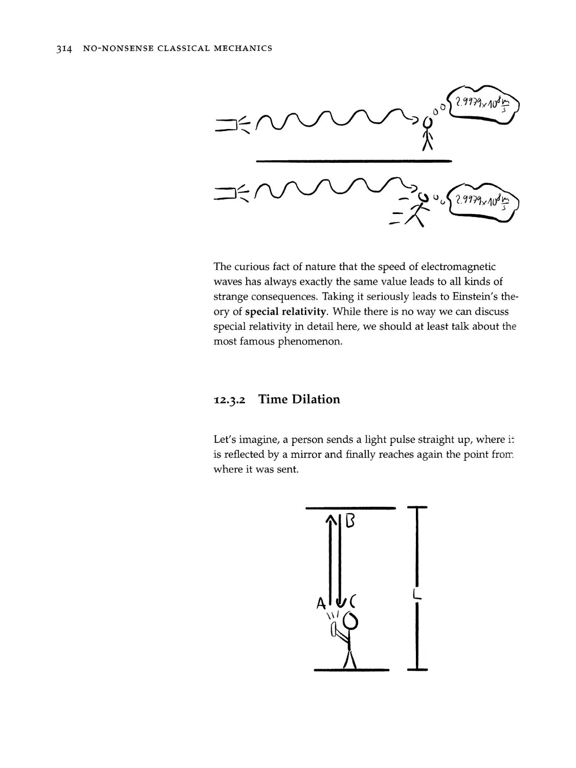
12.2.2 The Origin of the Hamilton-Jacobi Equation 308
-2.3 The Origin of the Classical Lagrangian ....... 311
12.3.1 Special Relativity .............0.. 313
12.3.2 Time Dilation ...............4.. 314
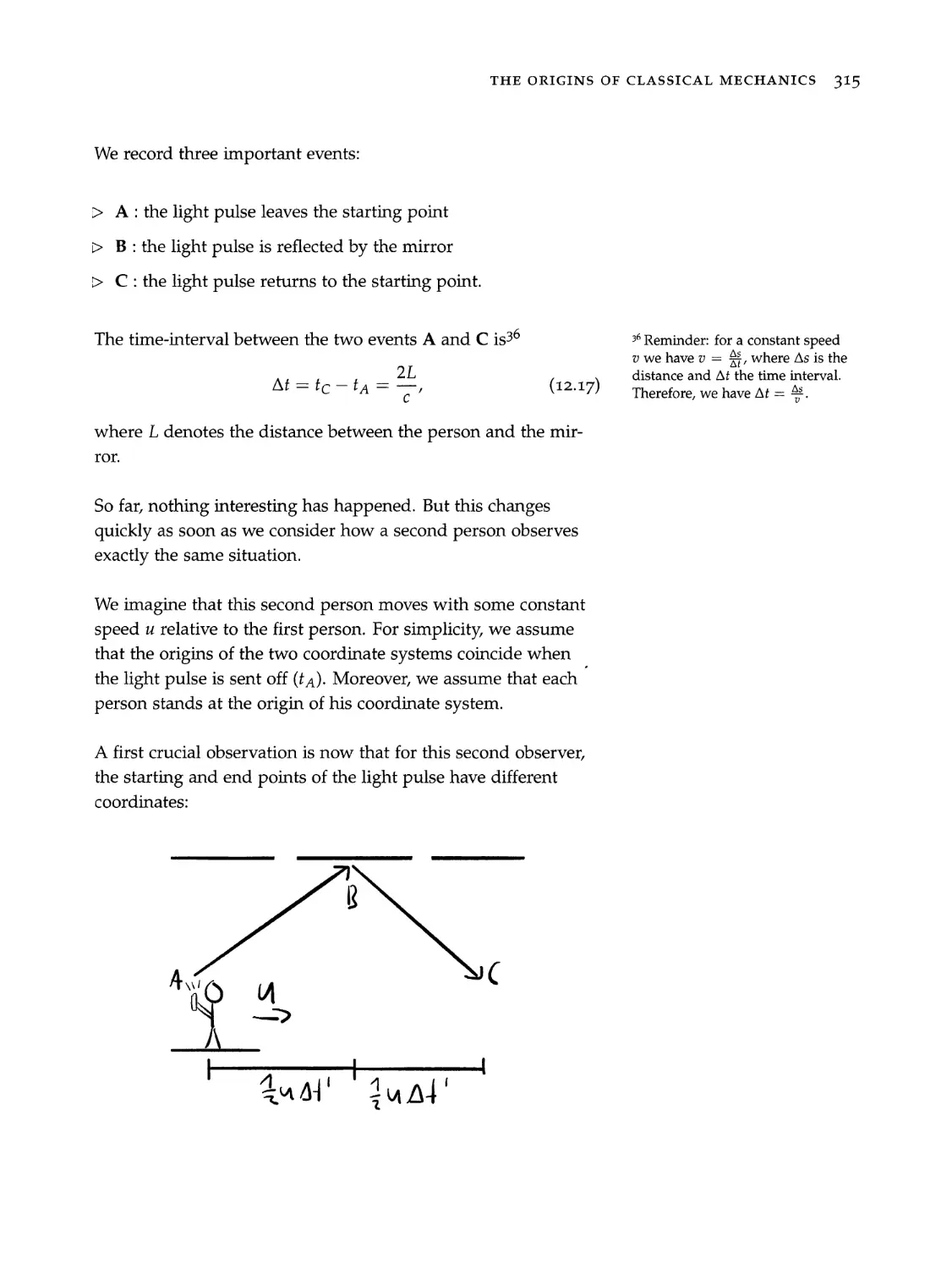
12.3.3 The Lagrangian of Special Relativity. .... 318
12.3.4 The Free Classical Lagrangian ........ 320
12.3.5 Understanding the Minus Sign ........ 322
12.3.6 General Relativity ............... 323
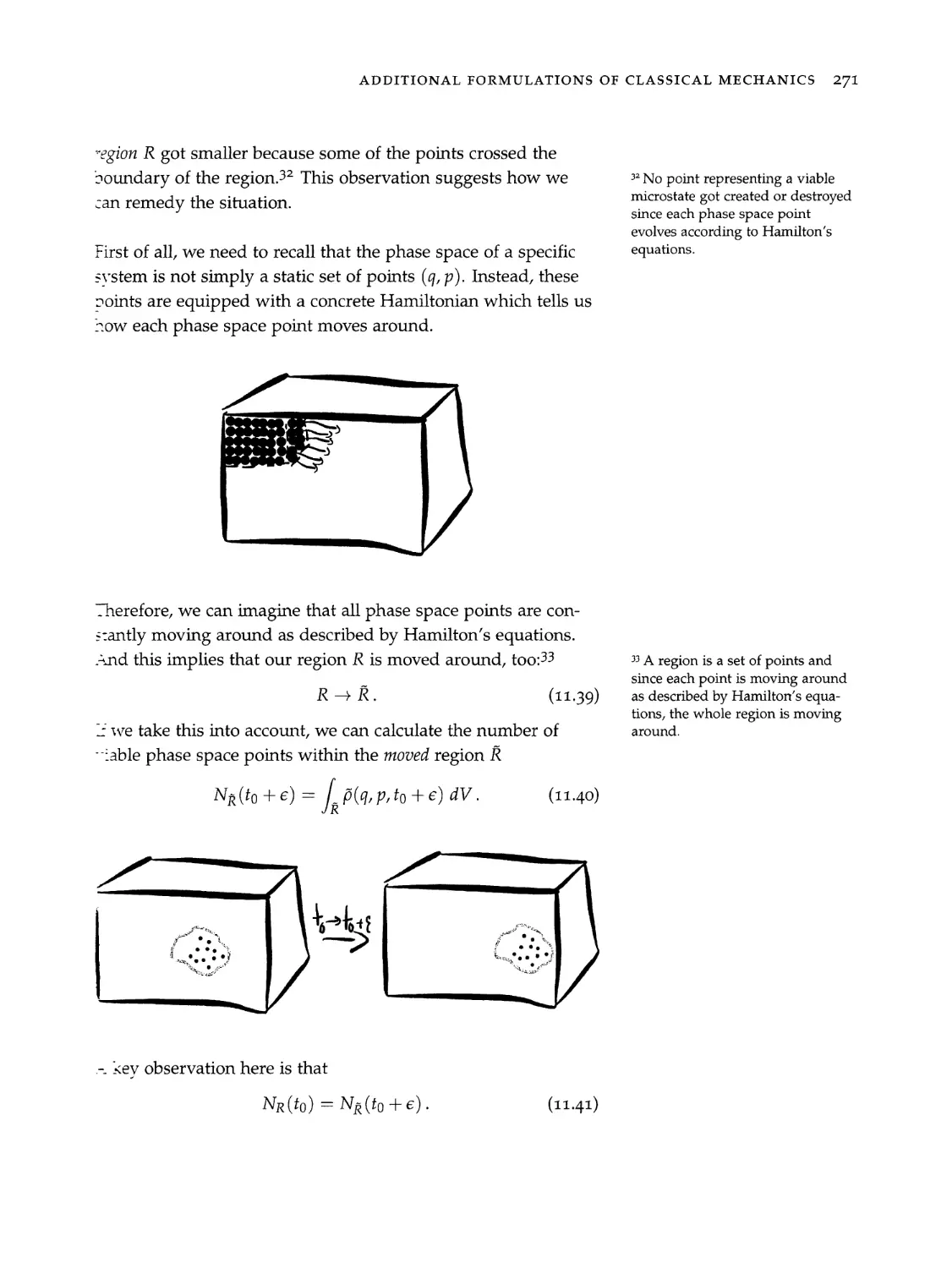
-2.4 Lagrangians in Modern Physics............ 332
-: Further Reading Recommendations 335
One Last Thing
Part V Appendices
4A Calculus 343
A.1 Product Rule..... 0.2... 0.2.0. 0.002 eae 344
15
16
A.2 Integration by Parts..............0004. 345
A.3 Total and Partial Derivatives.............. 345
A.44 ChainRule...... 0... 0.0.0.0. ee eee 348
B The Legendre Transform 351
C Lagrange Multipliers 359
D Invariance, Covariance and Functional Form 367
E Active vs. Passive Transformations and Symmetries vs. Re-
dundancies 373
F Taylor Expansion 377
G Vector Calculus 381
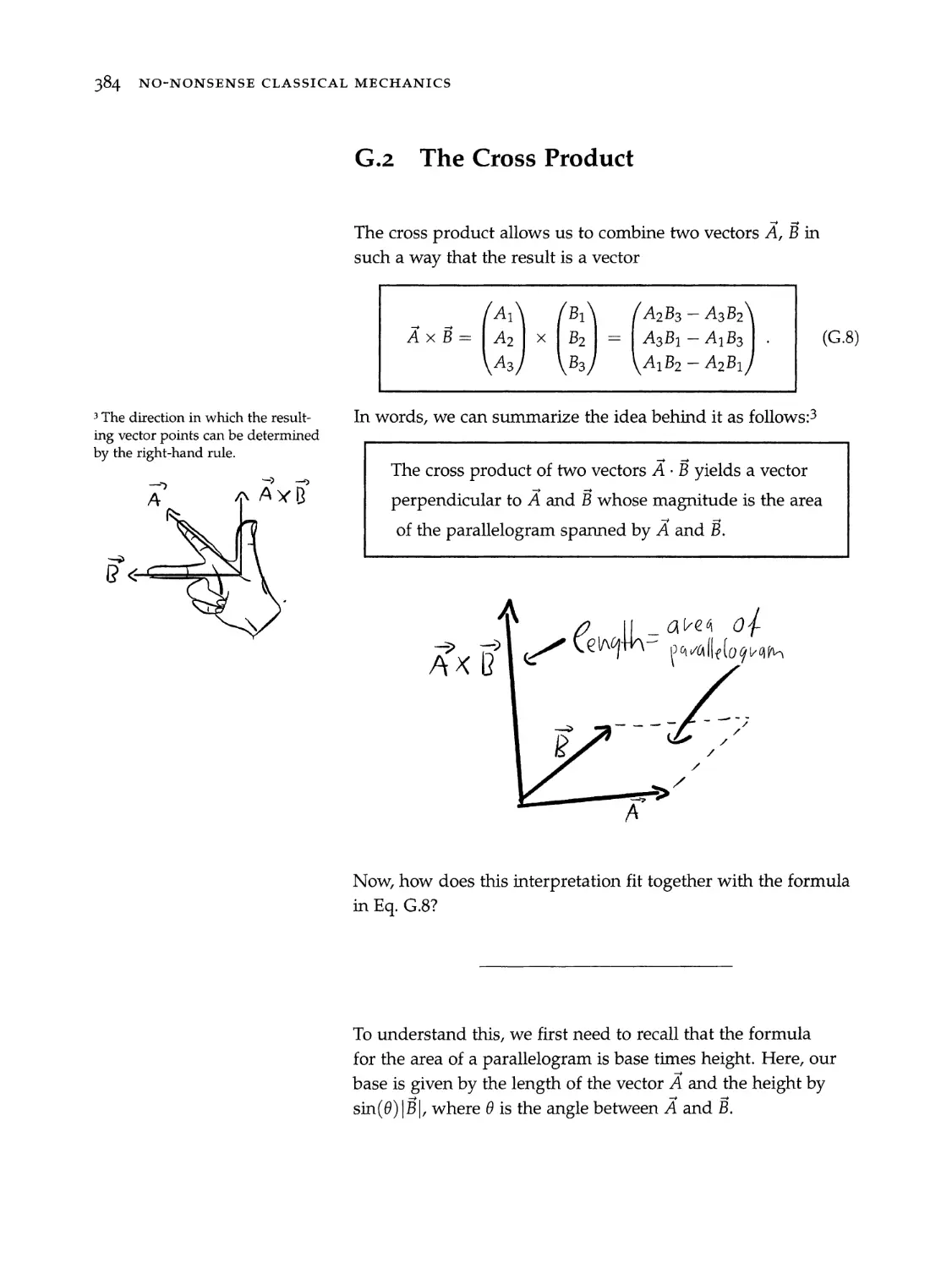
G.1 The Dot Product................-05000. 381
G.2 The Cross Product ...............-.004 384
Bibliography 387
. Index 391
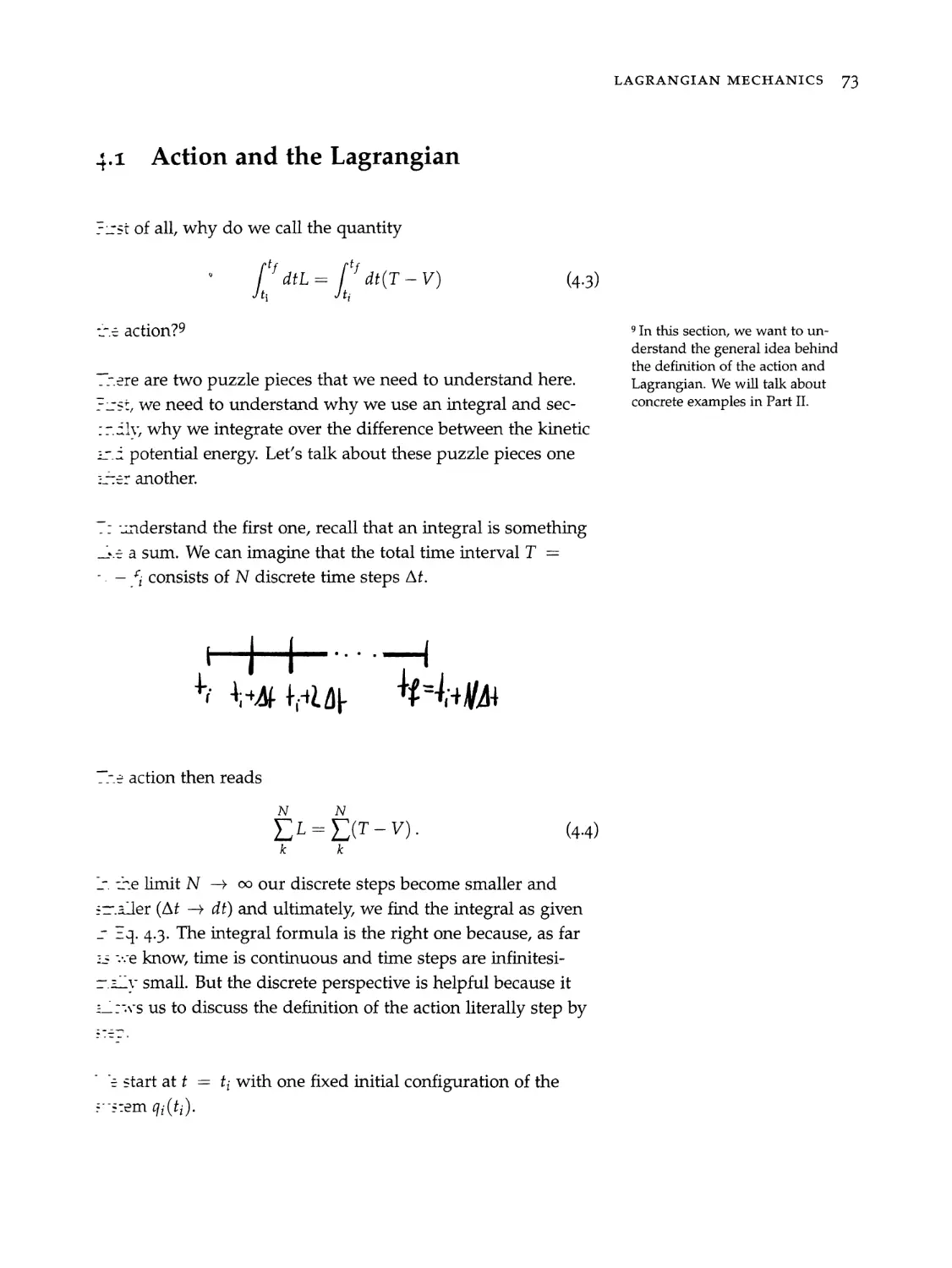
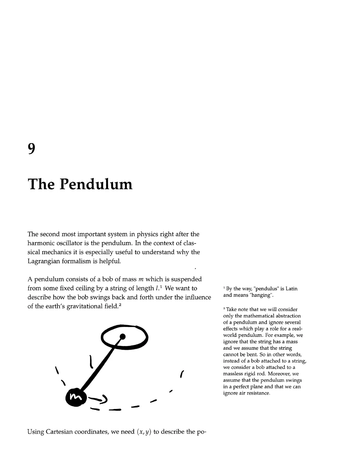
Bird’s-Eye View of Classical
Mechanics
As mentioned in the preface, classical mechanics is, at its heart,
quite simple. However, specific applications can be extremély
complicated. For this reason it’s easy to lose the forest for the
trees. To prevent this, we start this book with a quick overview.
Afterwards, we will talk about the various concepts in more
detail and gradually refine our understanding until we are
ready for concrete applications.
So don’t worry if not everything is immediately clear in this
chapter. Our goal is solely to get an overview and each idea
mentioned here will be discussed later in more detail.
Now first of all, what is our goal in classical mechanics?
~The short version is:* * Macroscopic means big enough
such that we don’t need quantum
mechanics or quantum field theory
to describe it.
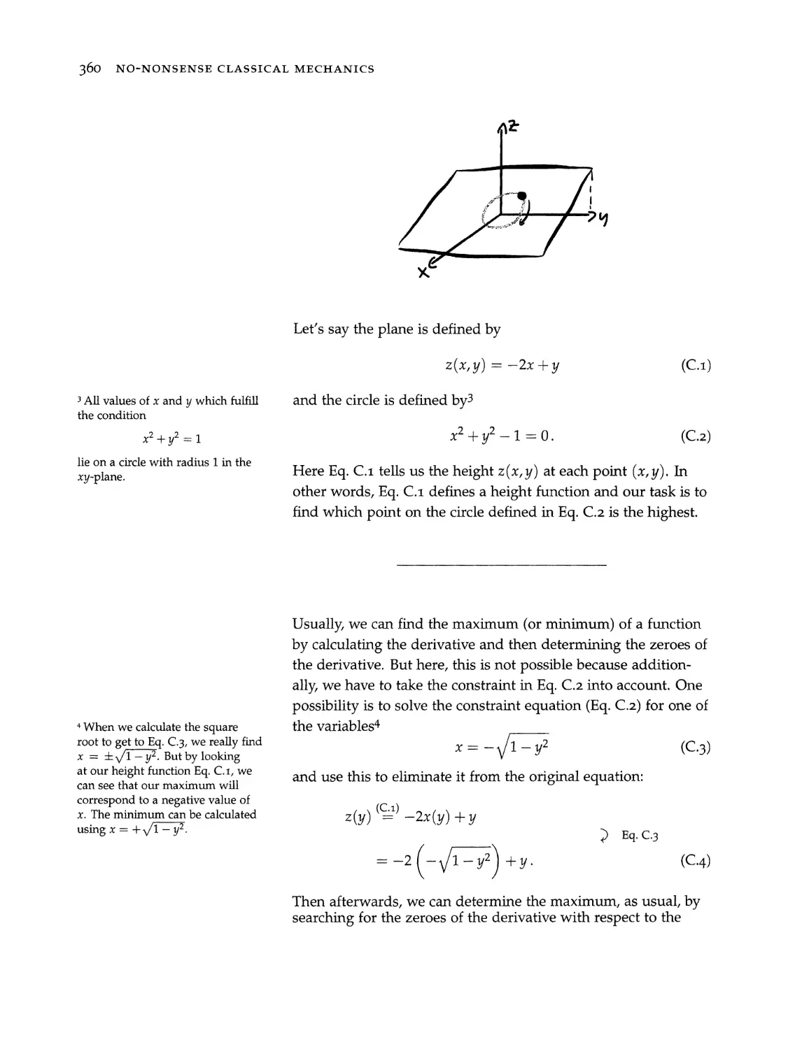
We want to describe how macroscopic objects behave.
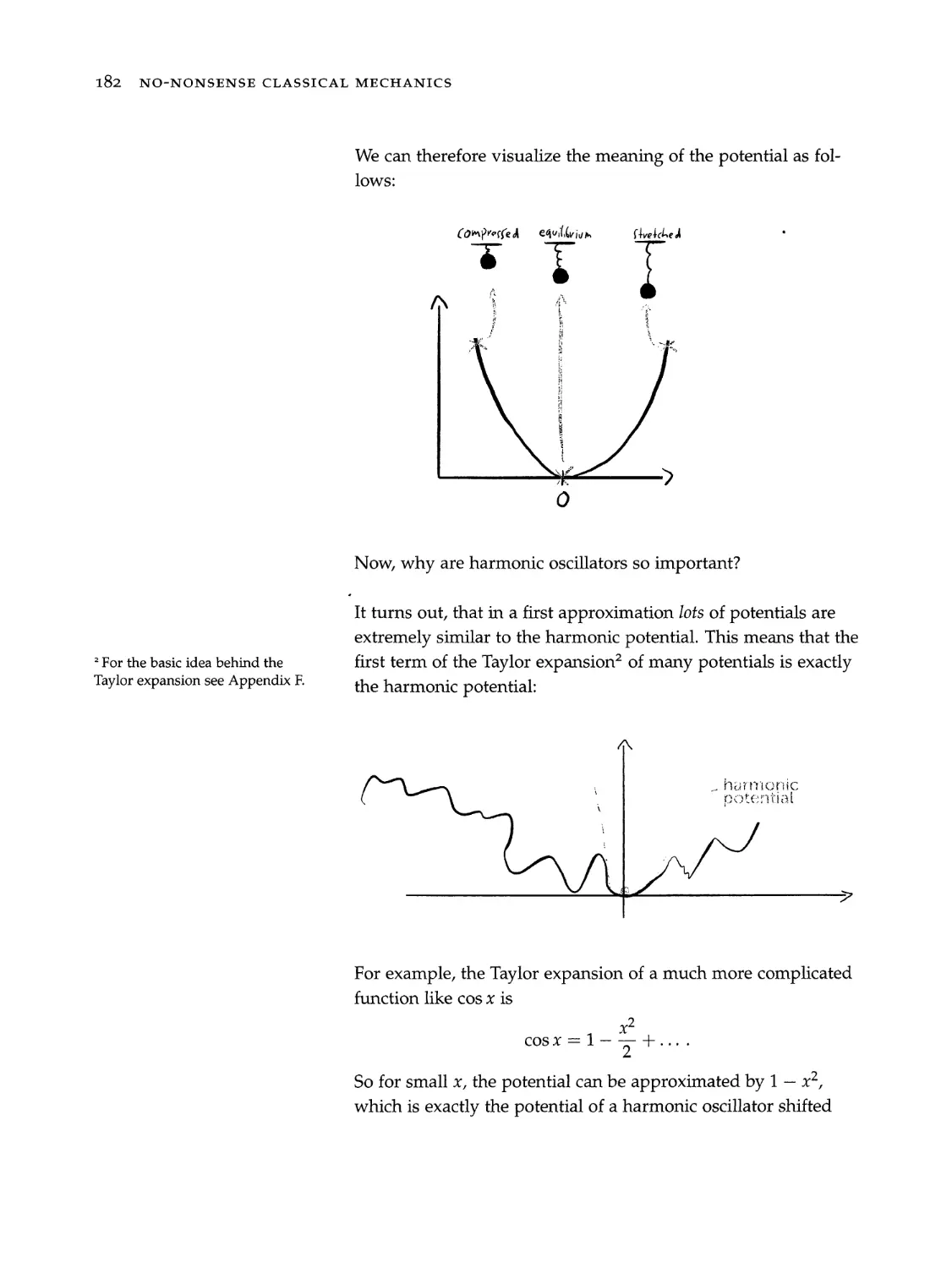
18 NO-NONSENSE CLASSICAL MECHANICS
2? We will talk about these arenas in
detail in Section 2.3.
3 It’s also possible to formulate
classical mechanics in Hilbert space.
This is known as the Koopman-von
Neumann formulation and we
will discuss it in Section 11.3. In
contrast, quantum mechanics was
originally formulated in Hilbert
space. But it’s equally possible
to formulate it in phase space,
configuration space or physical
space.
A bit more technically we can say that:
We want to derive and solve the equations of motion
for macroscopic systems.
One way to accomplish this is by using Newton’s second law
d, =
qe (1.1)
where 7? denotes the momentum of a given object and F is the
total force acting on it.
But one thing which makes classical mechanics (and physics
in general) extremely interesting is that physicists are quite
imaginative. Since it is so hard to discover a new theory, it is
often a huge step forward to find an alternative method to
describe an existing theory. And in fact, for each theory there
are different ways of how we can use it to describe a given
situation.
This is possible because there are different mathematical arenas
we can use as the stage on which we describe what happens.
The easiest one is the physical space we live in, but there are
also more abstract ones like configuration space, phase space
and Hilbert space. Each of these mathematical arenas has par-
ticular advantage.*
The laws of classical mechanics were originally written down
using vectors living in physical space. We can describe the be-
havior of these vectors by using Newton’s second law (Eq. 1.1).
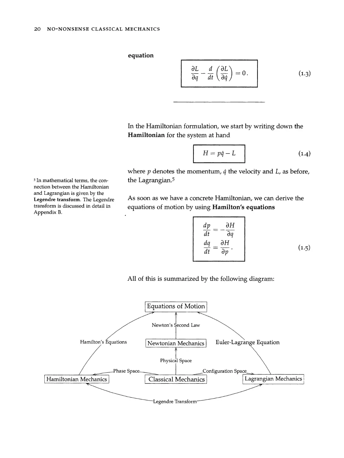
Nowadays this is known as the Newtonian formulation.
But it’s equally possible to describe macroscopic systems using
configuration space or phase space. If we write down the laws
of classical mechanics in configuration space, we end up with
the Lagrangian formulation of classical mechanics. And if
we use instead phase space, we end up with the Hamiltonian
formulation.
BIRD’S-EYE VIEW OF CLASSICAL MECHANICS 19
—. general, we call the description of a given theory in a particu-
_2r mathematical arena a formulation of the theory. So in other
~-ards, there are always different formulations of each theory.*
_cis is similar to how we can describe the number 1021 using
cre English word "one thousand twenty-one" or using the Ger-
an word "Eintausend Einungzwanzig" or "MXXI1" in Roman
~umerals or "1111111101" in the binary numbering system. Each
>: these descriptions has particular advantages depending on
zne problem at hand. For example, saying "1111111101" is ex-
<zemely awkward in everyday life but essential if we want to do
calculations using a computer.
Analogously, the Newtonian formulation of classical mechanics
‘s extremely useful for simple systems because all we have to
=0 is to specify a few vectors in physical space. But for more
complicated systems involving constraints, the Lagrangian for-
malism is a much better choice. And the Hamiltonian formula-
zion is awesome to understand the general structure of classical
mechanics and to describe systems consisting of lots of objects.
As mentioned above, in the Newtonian formulation, we use
Newton’s second law (Eq. 1.1) to derive the equations of mo-
‘ion.
In contrast, in the Lagrangian formulation, our first task is al-
ways to write down the appropriate Lagrangian for the system
at hand
where T denotes the kinetic energy and V the potential energy.
As soon as we have a concrete Lagrangian, we can derive the
corresponding equations of motion by using the Euler-Lagrange
L=T-V, (1.2)
4'To define what a theory is all
about we need to use a specific
formulation. But none of the for-
mulations is more fundamental
than the others. We can imagine a
theory as something abstract living
in "theory space". And to really
investigate it, we need to map this
abstract thing to something more
tangible, i.e., to a set of rules act-
ing on objects living in a specific
mathematical arena. Each such map
yields a different formulation. (See
the diagram below.)
20 NO-NONSENSE CLASSICAL MECHANICS
> In mathematical terms, the con-
nection between the Hamiltonian
and Lagrangian is given by the
Legendre transform. The Legendre
transform is discussed in detail in
Appendix B.
Hamilton’s Equations
equation
OL d fol
In the Hamiltonian formulation, we start by writing down the
Hamiltonian for the system at hand
H = pq—L (1.4)
where p denotes the momentum, g the velocity and L, as before,
the Lagrangian.°
As soon as we have a concrete Hamiltonian, we can derive the
equations of motion by using Hamilton’s equations
dp __0H
dt — ag
dq oH
dt op’ (1.5)
All of this is summarized by the following diagram:
| Equations of Motion
Newton’s Second Law
| Newtonian Mechanics} Euler-Lagrange Equation
Physical Space
Phase Space—___ ____ Configuration Space__. |
| Hamiltonian Mechanics | | Classical Mechanics | | Lagrangian Mechanics |
Legendre Transform
BIRD’S-EYE VIEW OF CLASSICAL MECHANICS 21
Now after this quick overview, let’s move on and discuss every-
thing mentioned here in more detail.
22 NO-NONSENSE CLASSICAL MECHANICS
Part I
What Everybody Ought to Know About
Classical Mechanics
"The action principle turns out to be universally applicable in physics. All
physical theories established since Newton may be formulated in terms of
an action. The action formulation is also elegantly concise. The reader
should understand that the entire physical world is described by one single
action.”
Anthony Zee
PS: You can discuss the content of Part I with other readers and give feedback at
www. nononsensebooks.com/cm/bonus.
Fundamental Concepts
Before we can start talking about classical mechanics, we should
talk about what exactly we want to describe.
In short, we want to describe macroscopic (big) objects and we
characterize them by using labels like their position, velocity, ac-
celeration, momentum, mass and energy. Since in this book we
only care about fundamental aspects, we will treat all objects as
it they were mass points. This means that we ignore all effects
which arise as a result of the size of objects. There are many im-
portant effects which only arise for extended objects, but since
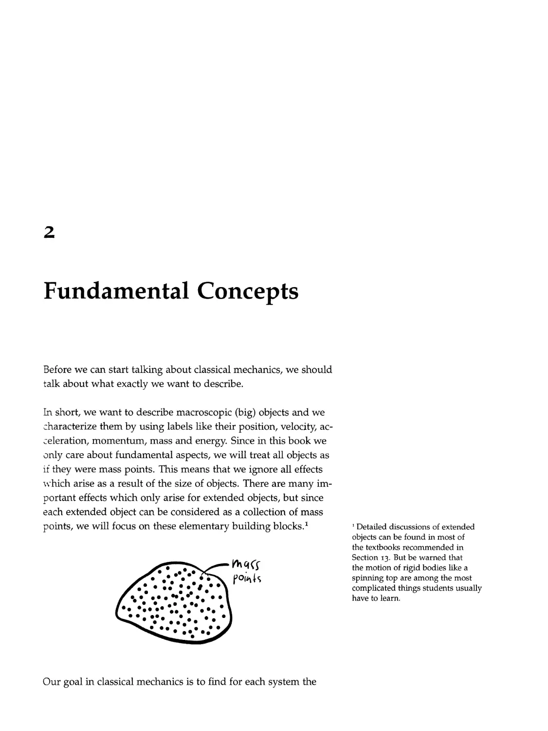
each extended object can be considered as a collection of mass
points, we will focus on these elementary building blocks.’ ' Detailed discussions of extended
objects can be found in most of
the textbooks recommended in
Section 13. But be warned that
the motion of rigid bodies like a
spinning top are among the most
complicated things students usually
have to learn.
Our goal in classical mechanics is to find for each system the
26 NO-NONSENSE CLASSICAL MECHANICS
*If you’re already familiar with the
notions mentioned above and don’t
need a refresher, feel free to skip
this chapter. But at least make sure
to skim Section 2.3 because a solid
understanding of configuration
space and phase space is essential
for everything that follows.
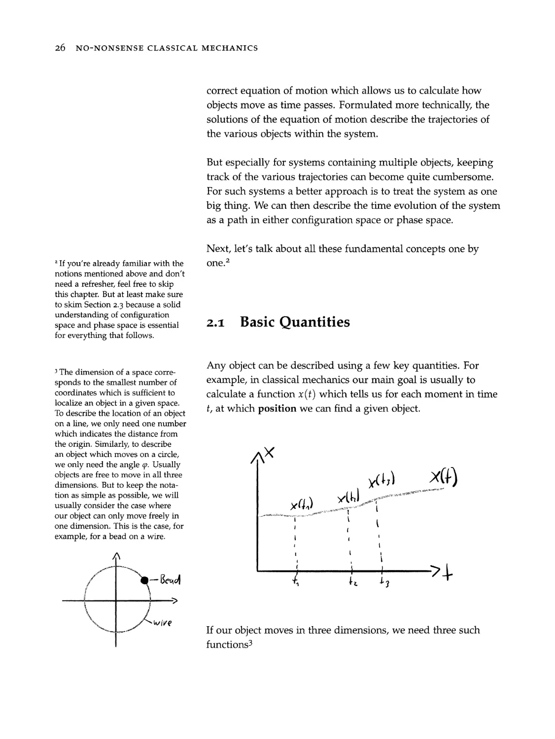
3 The dimension of a space corre-
sponds to the smallest number of
coordinates which is sufficient to
localize an object in a given space.
To describe the location of an object
on a line, we only need one number
which indicates the distance from
the origin. Similarly, to describe
an object which moves on a circle,
we only need the angle @. Usually
objects are free to move in all three
dimensions. But to keep the nota-
tion as simple as possible, we will
usually consider the case where
our object can only move freely in
one dimension. This is the case, for
example, for a bead on a wire.
AN
a psy
/ “ ‘e- Bead
i \
( }—
Se | aw Wwive
correct equation of motion which allows us to calculate how
objects move as time passes. Formulated more technically, the
solutions of the equation of motion describe the trajectories of
the various objects within the system.
But especially for systems containing multiple objects, keeping
track of the various trajectories can become quite cumbersome.
For such systems a better approach is to treat the system as one
big thing. We can then describe the time evolution of the system
as a path in either configuration space or phase space.
Next, let’s talk about all these fundamental concepts one by
one.*
2.1 Basic Quantities
Any object can be described using a few key quantities. For
example, in classical mechanics our main goal is usually to
calculate a function x(t) which tells us for each moment in time
t, at which position we can find a given object.
) vl t, eo eee SEE emenrsee
x ( \ we eee oe
|
, i— 7+
If our object moves in three dimensions, we need three such
functions?
FUNDAMENTAL CONCEPTS
Sut there are also additional quantities we often use to describe
“ciects. For example, we often want to know how quickly an
>riect moves around. This is described by the velocity function
- : which is defined as the rate of change of the location: -
v(t) = ra (2.2)
- words this means that v(t) tells us exactly how quickly the
zosition of the object changes as time passes. Since derivatives
«ith respect to t are so common in physics, we introduce the
snorthand notation
X(t) =. (2.3)
_ 72s means that whenever we write a function with a little dot
“z. top of it, we mean its rate of change.
-.2ain, if our object moves in three dimensions, we need three
~z.acity functions
d(t) = | vy(t) | . (2.4)
27
28 NO-NONSENSE CLASSICAL MECHANICS
+ We will see later why we care
about how quickly the velocity
changes. But to spoil the surprise:
the velocity of an object changes
whenever a force acts on it. And
describing how objects react when
forces act on them is what classical
mechanics (or really almost all of
physics) is all about.
5 This definition is circular because
a (mass) density is defined as an
object’s mass divided by its volume.
Using our shorthand notation, we can write this as
q(t) = | y(t) | . (2.5)
Sometimes, we not only care about how quickly a given object
moves around but also about how quickly its velocity changes.*
The rate of change of the velocity function is known as the
acceleration
d*x(t) ddx(t) d
de dt dt dt’ (2.6)
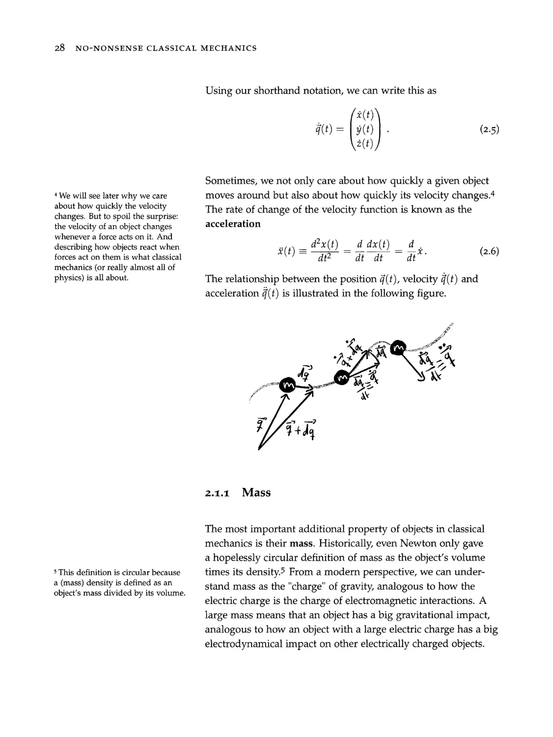
The relationship between the position 7(t), velocity g(t) and
acceleration g(t) is illustrated in the following figure.
2.1.1 Mass
The most important additional property of objects in classical
mechanics is their mass. Historically, even Newton only gave
a hopelessly circular definition of mass as the object’s volume
times its density.” From a modern perspective, we can under-
stand mass as the "charge" of gravity, analogous to how the
electric charge is the charge of electromagnetic interactions. A
large mass means that an object has a big gravitational impact,
analogous to how an object with a large electric charge has a big
electrodynamical impact on other electrically charged objects.
@
ihe<F,
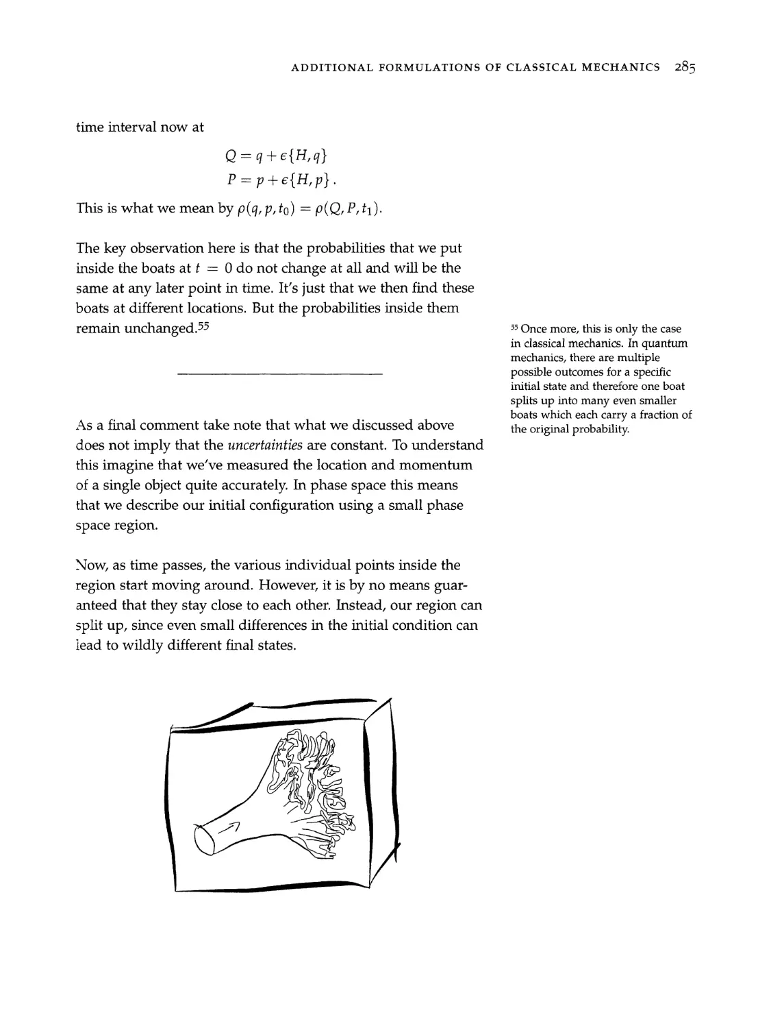
<6
be
5ut the main reason why we care about mass in classical me-
chanics is that it encodes the resistance of an object to being
moved or to having its velocity changed if it already moves with
aniform velocity.° In other words, the mass of an object is a la-
cel we use to describe how difficult it is to change its velocity
sarough a force.” For example, it’s much easier to push a ball
made of cork than a ball of equal size made of iron.
OOK
2.1.2 Momentum and Angular Momentum
_7nere are three further basic quantities that we regularly use
‘-. classical mechanics: momentum, angular momentum and
znergy. These quantities are useful because they are conserved.
_cis means that while everything within the system may change
2_ the time (in particular, the locations and velocities of the
>Sjects), these quantities remain unchanged. In this sense, con-
served quantities are like anchors which we can always cling to
>. an otherwise chaotic world.’ However, take note that the mo-
~entum, angular momentum and energy of individual objects
72 change. Only the total momentum, angular momentum and
=rergy within a closed system remains constant.?
~ne of the most beautiful aspects of classical mechanics is that
~-e can actually understand the origin of conserved quantities.
FUNDAMENTAL CONCEPTS 29
° You might rightfully wonder
how these two descriptions of
mass fit together. Historically,
physicists used the notions of
"gravitational mass” and “inertial
mass’ because they thought the
two roles played by mass mean
that there are actually two kinds
of mass that we need to keep
separate. However, the idea that
inertial mass and gravitational
mass are actually the same thing
(which we now simply call the
mass) was one of the key insights
which led Einstein to his famous
theory of general relativity. From
this perspective, the resistance
of an object to being moved is a
result of the gravitational pull of all
surrounding objects in the whole
universe.
This idea is known as Mach’s
principle. However, take note
that there are still lots of ongoing
discussions about the validity
of Mach’s principle and how to
formulate it properly.
7 Intuitively, we can define a force
as something which changes the
velocity of objects.
§ Mathematically, a conserved
quantity is something with a van-
ishing rate of change, for example,
ip _
qe = 0.
° A closed system is sufficiently
isolated such that we can ignore all
effects from the outside world. In
particular, no energy or momentum
is leaking out from a closed system.
30 NO-NONSENSE CLASSICAL MECHANICS
© To spoil the surprise: for each
symmetry of a system, we get a
conserved quantity. For example,
whenever it makes no difference
whether we perform an experiment
today or tomorrow, the energy
within the system is conserved.
This is known as Noether’s theo-
rem.
“If you’re unfamiliar with the cross
product, see Appendix G. We use
the cross product because it allows
us to multiply two vectors and get
another vector as a result. This is
what we need because angular mo-
mentum encodes information about
the direction in which an object
rotates. Therefore, we need a vector
to describe angular momentum.
And the cross product allows us
to combine the two vectors which
are relevant for angular momentum
(location and momentum) to get a
suitable vector. In contrast, the dot
product of two vectors d - b yields
a number and therefore cannot
encode any directional information.
’2 As mentioned above, this is
known as Newton’s second law and
we will discuss it in more detail in
Chapter 3 .
3 We can multiply by dt because dt
simply means a little bit of t, ie., a
really short time interval.
In other words, we do not need to introduce momentum, angu-
lar momentum and energy ad hoc as additional quantities but
we can actually derive them. In Chapter 10, we will talk about
this in detail.*° But the for the moment it is sufficient to use the
following rather rough definitions:
> Momentum is the velocity of an object times its mass
p(t) = mq(t).
[> Angular momentum is defined as the cross product of the
position vector and the momentum vector"
(2.7)
=>
L(t) = q(t) x p(t) = mat) x q(t). (2.8)
In intuitive terms, we can say that:
[> Momentum is the total "oomph" an object has behind it. To
understand how this interpretation comes about, we can use
the fact that the rate of change of the momentum of an object
is always equal to the force acting on it:**
d
Therefore, the total change in momentum Ap = p(tr) — p(ti)
during some time interval At = tr — t; is equal to the force F
times the time interval At:%3
(2.9)
d —
at? ~
» multiplication by dt and integrating
f '
dp = Fat
fj Ej
D assuming the force is constant
Ap = FAt.
In words, this means that the momentum of an object tells
us how long it takes a given force F to stop it. An object
with a large momentum is much harder to stop. Formulated
differently, we need a much bigger force to stop it quickly.
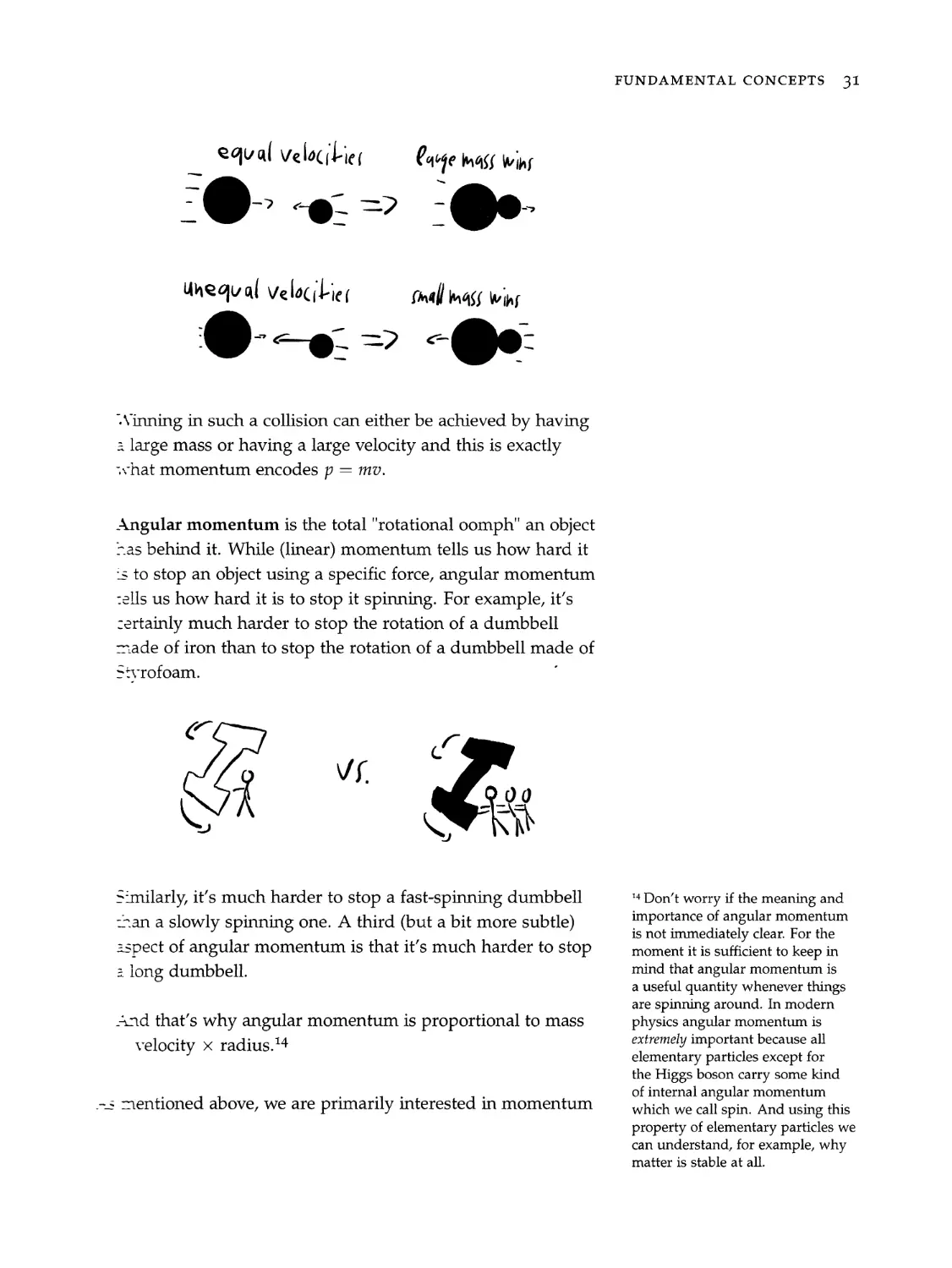
Alternatively, we can consider collisions of two objects. The
main point here is that the object with the larger momentum
tt ° wt
wins
equal veloc Lie Carge mass Wins
-@ -0.~ -@e
—_ —
Une qu al veloc i bie, Small mS, Wing
@--0.~ -@e
-Vinning in such a collision can either be achieved by having
2 large mass or having a large velocity and this is exactly
“what momentum encodes p = mv.
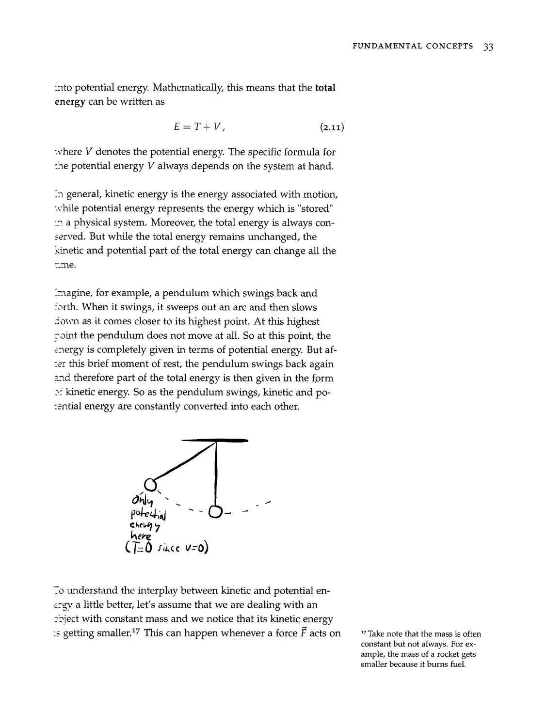
Angular momentum is the total "rotational oomph" an object
>as behind it. While (linear) momentum tells us how hard it
‘s to stop an object using a specific force, angular momentum
cells us how hard it is to stop it spinning. For example, it’s
certainly much harder to stop the rotation of a dumbbell
made of iron than to stop the rotation of a dumbbell made of
>*vrofoam.
999
Fit
>milarly, it’s much harder to stop a fast-spinning dumbbell
znan a slowly spinning one. A third (but a bit more subtle)
zspect of angular momentum is that it’s much harder to stop
z long dumbbell.
And that’s why angular momentum is proportional to mass
velocity x radius."
5 mentioned above, we are primarily interested in momentum
FUNDAMENTAL CONCEPTS 31
“4 Don’t worry if the meaning and
importance of angular momentum
is not immediately clear. For the
moment it is sufficient to keep in
mind that angular momentum is
a useful quantity whenever things
are spinning around. In modern
physics angular momentum is
extremely important because all
elementary particles except for
the Higgs boson carry some kind
of internal angular momentum
which we call spin. And using this
property of elementary particles we
can understand, for example, why
matter is stable at all.
32 NO-NONSENSE CLASSICAL MECHANICS
‘5 In more technical terms, this
means that the collision is com-
pletely inelastic. An elastic collision
is one in which both momentum
and kinetic energy are conserved.
In an inelastic collision some of
the kinetic energy is transferred
to internal degrees of freedom of
the objects, i.e., parts of the objects
crumple and bend. For the colli-
sion we consider here, a maximum
amount of kinetic energy is "lost" to
internal degrees of freedom. (This
is necessarily the case here because
otherwise, the two objects wouldn’t
stick together.)
6 Take note that 9° = 7-7, i.e., the
scalar product of the velocity vector
with itself.
and angular momentum because they are conserved. To under-
stand why conserved quantities are so helpful, let’s consider a
head-on collision of two objects. For simplicity, let’s assume that
the two objects stick together after the collision.*>
—? —?
VW. _—?
e--@ => <
Then, solely using the fact that momentum is conserved, we
can calculate the velocity the combined objects have after the
collision:
system system
P;
» definition of momentum
(1101 + m2v2) = (m1, + m2)v
D rearranging terms
M101 + M2V2
my, + ™D»
Next, let’s talk about one additional conserved quantity which
we use all the time in classical mechanics: energy.
2.1.3 Energy
Energy is a bit more tricky because it comes in different forms.
At first, physicists believed that energy can be described by the
formula’® 1
T = 5mq ,
But it was quickly noted that this quantity is not always con-
served. From a modern perspective, we say that energy comes
in two forms: kinetic and potential. The formula in Eq. 2.10
only describes kinetic energy and is therefore incomplete. The
total energy is always conserved and therefore, whenever the ki-
netic energy becomes smaller it doesn’t vanish but is converted
(2.10)
FUNDAMENTAL CONCEPTS 33
‘nto potential energy. Mathematically, this means that the total
energy can be written as
E=T+YV, (2.11)
‘where V denotes the potential energy. The specific formula for
cae potential energy V always depends on the system at hand.
-1 general, kinetic energy is the energy associated with motion,
“while potential energy represents the energy which is "stored"
-- a physical system. Moreover, the total energy is always con-
served. But while the total energy remains unchanged, the
xinetic and potential part of the total energy can change all the
Tme.
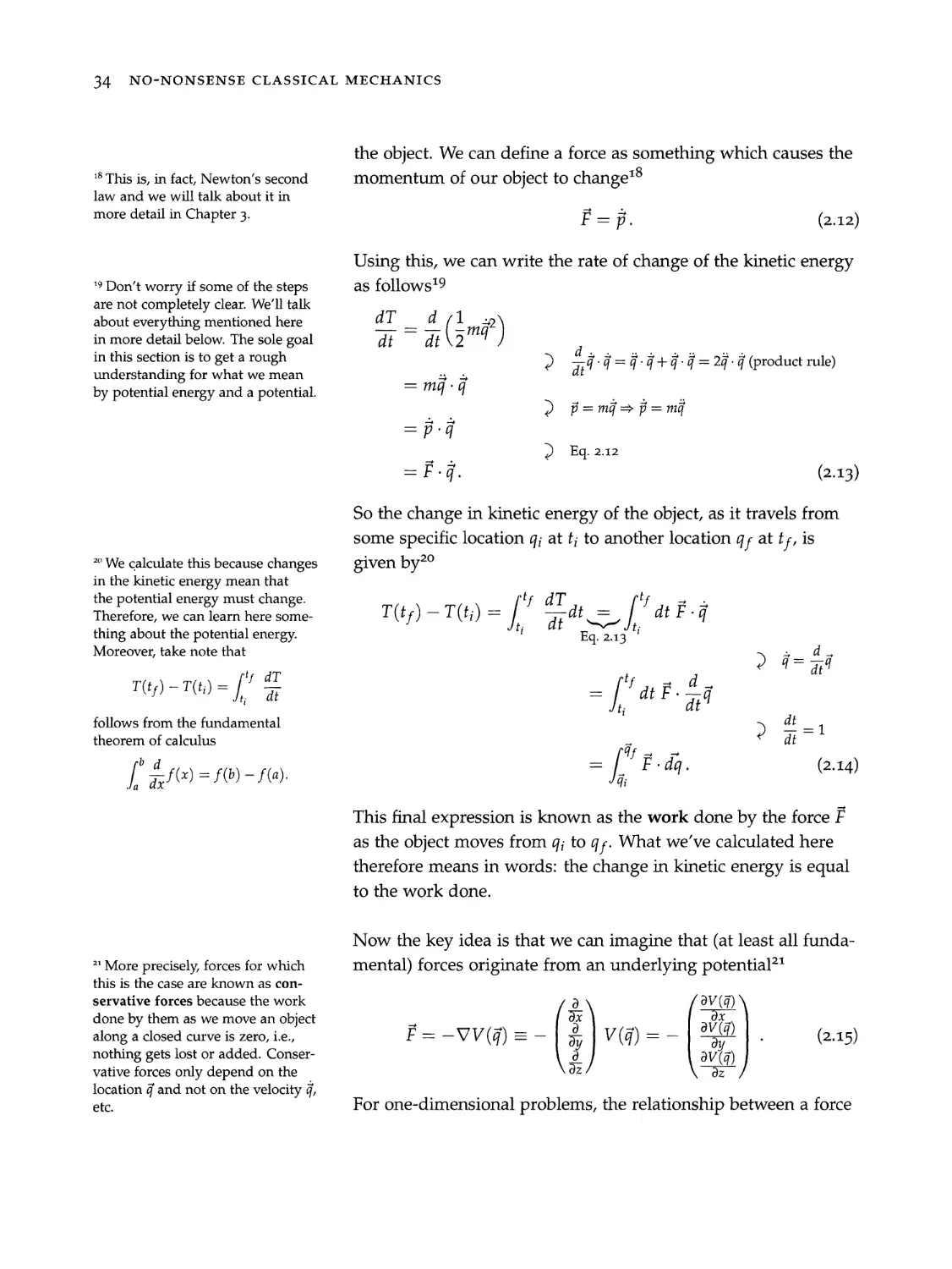
-magine, for example, a pendulum which swings back and
orth. When it swings, it sweeps out an arc and then slows
sown as it comes closer to its highest point. At this highest
roint the pendulum does not move at all. So at this point, the
<nergy is completely given in terms of potential energy. But af-
ter this brief moment of rest, the pendulum swings back again
and therefore part of the total energy is then given in the form
>: kinetic energy. So as the pendulum swings, kinetic and po-
zential energy are constantly converted into each other.
~o understand the interplay between kinetic and potential en-
<rgy a little better, let’s assume that we are dealing with an
saject with constant mass and we notice that its kinetic energy
-s getting smaller.*” This can happen whenever a force F acts on __” Take note that the mass is often
constant but not always. For ex-
ample, the mass of a rocket gets
smaller because it burns fuel.
34. NO-NONSENSE CLASSICAL MECHANICS
8 This is, in fact, Newton’s second
law and we will talk about it in
more detail in Chapter 3.
"2 Don’t worry if some of the steps
are not completely clear. We'll talk
about everything mentioned here
in more detail below. The sole goal
in this section is to get a rough
understanding for what we mean
by potential energy and a potential.
*° We calculate this because changes
in the kinetic energy mean that
the potential energy must change.
Therefore, we can learn here some-
thing about the potential energy.
Moreover, take note that
T(t) Tu) =f
follows from the fundamental
theorem of calculus
bd
| FI) =fO-FO.
** More precisely, forces for which
this is the case are known as con-
servative forces because the work
done by them as we move an object
along a closed curve is zero, i.e.,
nothing gets lost or added. Conser-
vative forces only depend on the
location 7 and not on the velocity 7,
etc.
the object. We can define a force as something which causes the
momentum of our object to change?®
F=@. (2.12)
Using this, we can write the rate of change of the kinetic energy
as follows*?
dT d/l.
En lam)
. 2 qi 4 = 4-944: 4 = 29-G (product rule)
= mq -G
Lo ) puma > p=mg
=P
» Eq. 2.12
=F G. (2.13)
So the change in kinetic energy of the object, as it travels from
some specific location q; at t; to another location q, at tf, is
given by*°
te AT ff ey
T(ty)—Th) = f Sats [akg
i g.2.13 |
1d,
) 9 a4
= [ak oq
7 tj dt 7
t
; oan!
qf 4
= [VF dj (2.14)
qi
This final expression is known as the work done by the force F
as the object moves from q; to gf. What we've calculated here
therefore means in words: the change in kinetic energy is equal
to the work done.
Now the key idea is that we can imagine that (at least all funda-
mental) forces originate from an underlying potential**
0 av (9)
: 4 ox 4 ata)
F=-VV@)=-| 5 | V@=— |S? (2.15)
0 —
32 oe
For one-dimensional problems, the relationship between a force
znd the corresponding potential simplifies to
rp —2V (4)
oq
~sing this, we can rewrite Eq. 2.14 as follows?
ff. 3
_ ty) — T(t;) = L / F. dq this is Eq. 2.14
i
p (-Vvv(q)) -dq
i
> Eq. 2-15
> [Fede = 0
> rearranging the terms, we can therefore conclude
T(t¢) + V(gp) = T(t) + VG).
)— f(a)
FUNDAMENTAL CONCEPTS = 35
(2.16)
* If you're confused by the steps
here, it may be helpful to consider
a one-dimensional problem. The
calculation then reads
T(t) — T(ti) = Fay
_ fa dV (q)
dg; (- og )aq
— —(V(q-) —V(q;)).
(2.17) (V(ar) - VG ))
(2.18)
>. words this means that the sum of kinetic and potential en-
=7zv at the initial moment in time (for which the object is at q;)
-s equal to the sum of kinetic and potential energy at the final
=.oment in time (for which the object is at 7 f). We've therefore
zerived that changes in the kinetic energy can always be ac-
->unted for by changes in the potential energy. The total sum
>: kinetic and potential energy stays always the same. In other
~ords, the total energy E = T + V is conserved.*3
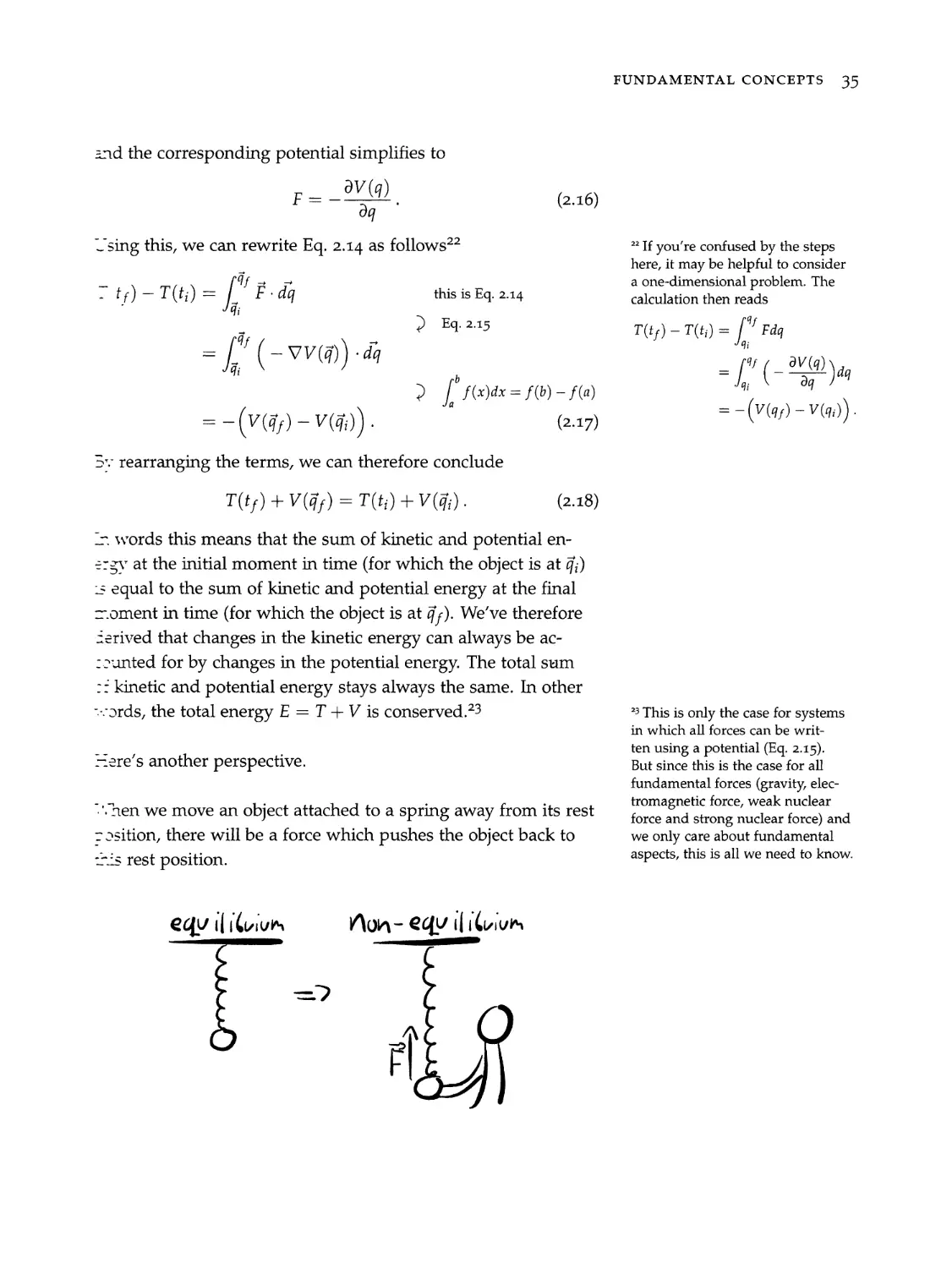
=ere’s another perspective.
“en we move an object attached to a spring away from its rest
> asition, there will be a force which pushes the object back to
77s rest position.
edu (Liviu Vion - equ (Liviu
*3 This is only the case for systems
in which all forces can be writ-
ten using a potential (Eq. 2.15).
But since this is the case for all
fundamental forces (gravity, elec-
tromagnetic force, weak nuclear
force and strong nuclear force) and
we only care about fundamental
aspects, this is all we need to know.
36 NO-NONSENSE CLASSICAL MECHANICS
4The constant C has units $
because then F = —2Cx has the
correct units of a force
kg-m
ve
One way to understand this is by describing the spring using
the potential V(x) = Cx?. This potential has its minimum at the
rest position, and any movement away from it results in a force
F= — 0) = —2Cx which pushes the object back to the rest
position.
For concreteness, we are dealing with a spring described by the
constant C = 1 S24, When we pull the object attached to this
spring to the x = 2 m location, there will be a force
ke -m
F=—-—2Cx = —4 7)
S
which is directed toward the equilibrium position at x = 0. And
if we push the object in the opposite direction to x = —2m,
there will be a force
kg +m
F=-—2Cx =4 7
S
which again points toward the equilibrium position.
equ i[ iduium N\on - edu i| (vive
—
=? yy
O7- -~=---- F- EF ka:
co] Se
Y \“
One final comment before we move on: we can’t measure the
potential or potential energy of an object directly. Instead, we
can only measure the resulting force F = — ove) This follows
because we can add an arbitrary constant V(x) > V(x) =
V(x) +c without changing the resulting force:
=> F(x)= ov)
5 Fx) = _oV(x) _ (V(x) +e) _ OVX) _
recause de = 0. This means that we can shift the potential
~owever we want.*> In geometrical terms, we can say that the
‘orce remains unchanged because the slope remains unchanged
zy constant shifts of the potential:?°
RO sqme
oh A (
ra wn
M * 5 ops
ay vn,
Rh “Ry, ite
a "Rn, ae
a tea, oe, rae
a “me Segre merger a=
. a
2.
we C
Nek,
“B,
Bios aa
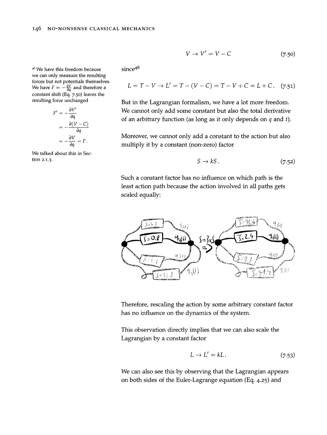
_ne freedom in how we define the potential for any system also
-mplies that we can’t measure the potential energy of an object
=<irectly. Instead, only differences between the potential energy
>t an object at one position and its potential energy at some
-2ference position, are physically important. We usually shift
<ne potential such that any object at the equilibrium position has
>otential energy zero and then specify the potential energy at
other positions relative to this position. For example, we usually
snift the earth’s gravitational potential such that it is zero when
zne ball lies on the ground, and we are then able to write the
>otential energy as V(z) = mgz, where z is the height above the
zround.*7 But we could equally shift the potential such that it
“3 non-zero at the ground, and then we would have to use the
-ormula V(z) = mgz +c, where c is the value of the potential
2? the ground (z = 0). For example, we could shift the potential
such that it is zero for z = 2 m. The potential energy would then
read V(z) = mgz — 2mg because then we get zero for z = 2 m:
+ 2) = mg(2) —2mg = 0.
~-lowever, everything we can measure in experiments remains
completely unaffected by such shifts of the potential. This fol-
-ows because only forces play a role in our equations of motion
FUNDAMENTAL CONCEPTS 37
* Historically, physicists used
this observation to conclude that
potentials are solely convenient
calculation devices which, however,
aren't really real because we can’t
measure them directly. Working
with a potential is much simpler
than working with a force because
a force is described by a vector
function F(x) while a potential is an
ordinary function $(x). Moreover,
the freedom to shift the potential
often allows important calculatory
simplifications. But from a modern
perspective, potentials are more
than purely mathematical tools. For
example, the famous Aharonov-
Bohm experiment demonstrated
that particles can be affected in
regions in which only the potential
is zero but nothing else. In other
words, it has been experimentally
verified that potentials are indeed
real. In some sense, potentials
are really at the heart of modern
physics and if you want to learn
more about how we understand
their role in nature, you might
enjoy:
Jakob Schwichtenberg. Physics
from Finance. No-Nonsense Books,
Karlsruhe, Germany, 2019b. ISBN
978-1795882415
© The slope of a potential corre-
sponds to the force since F = acre
77 Semantics: the potential here
reads ¢(z) = gz and an object
of mass m which is located at z
therefore has the potential energy
V(z) = mgz.
38
NO-NONSENSE CLASSICAL MECHANICS
(which we will discuss next), and all constant shifts leave the
resulting forces unchanged:
Viz)=mez => Fe= Ne) = —mg
V(z)=mez+co => F= ve) = —mg
V(z) =mgz—2mg => F= ve) = —mg
To summarize:
> Energy is defined as the sum of an object’s kinetic energy T
and its potential energy V
E=T+YV. (2.19)
- The kinetic energy is defined as
T= snip (2.20)
— There is no general formula for the potential energy be-
cause different systems are characterized by differential
potentials, and therefore, we need different formulas for
the potential energy. But take note that usually the for-
mula for potential energy of an object only depends on
its location q(t) and not on its velocity q(t) or accelera-
tion g(t). For example, the potential energy in the earth’s
gravitational field can be described by
V=mgz, (2.21)
where z is the height above sea level, m the mass and
g ~ 9.81 3, a constant which characterizes the earth’s
gravitational field.
In intuitive terms, we can say that:
FUNDAMENTAL CONCEPTS 39
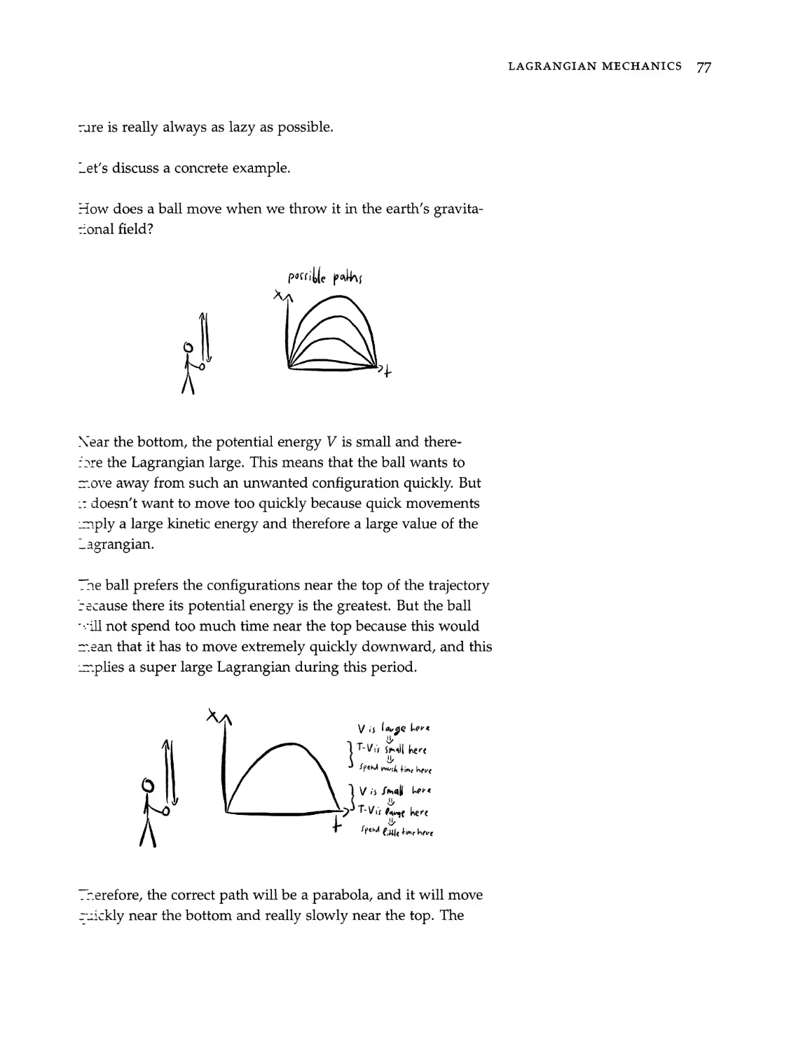
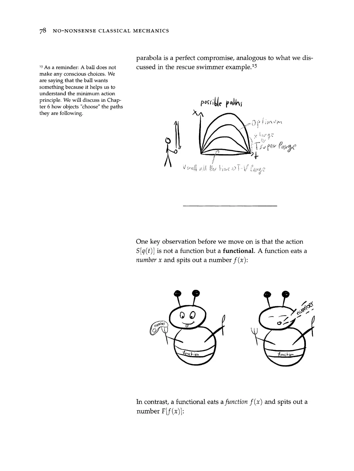
Kinetic energy is a measure for how much is going on in our
system.
— If all objects move around quickly, the kinetic energy is
high.
—- Incontrast, if all objects sit still, the kinetic energy is zero.
Potential energy is a measure for how much could happen,
out isn’t.
- If all objects are placed on the top of a mountain they have
a large (gravitational) potential energy and they could start
moving quickly by falling down. But currently they don’t.
In this sense, their large potential energy is unrealized
potential, which is why we use the word potential energy.
- In contrast, if all objects are placed on the floor, they have
zero potential energy since they can’t fall any further
down.
=inally, to demonstrate once more that conserved quantities
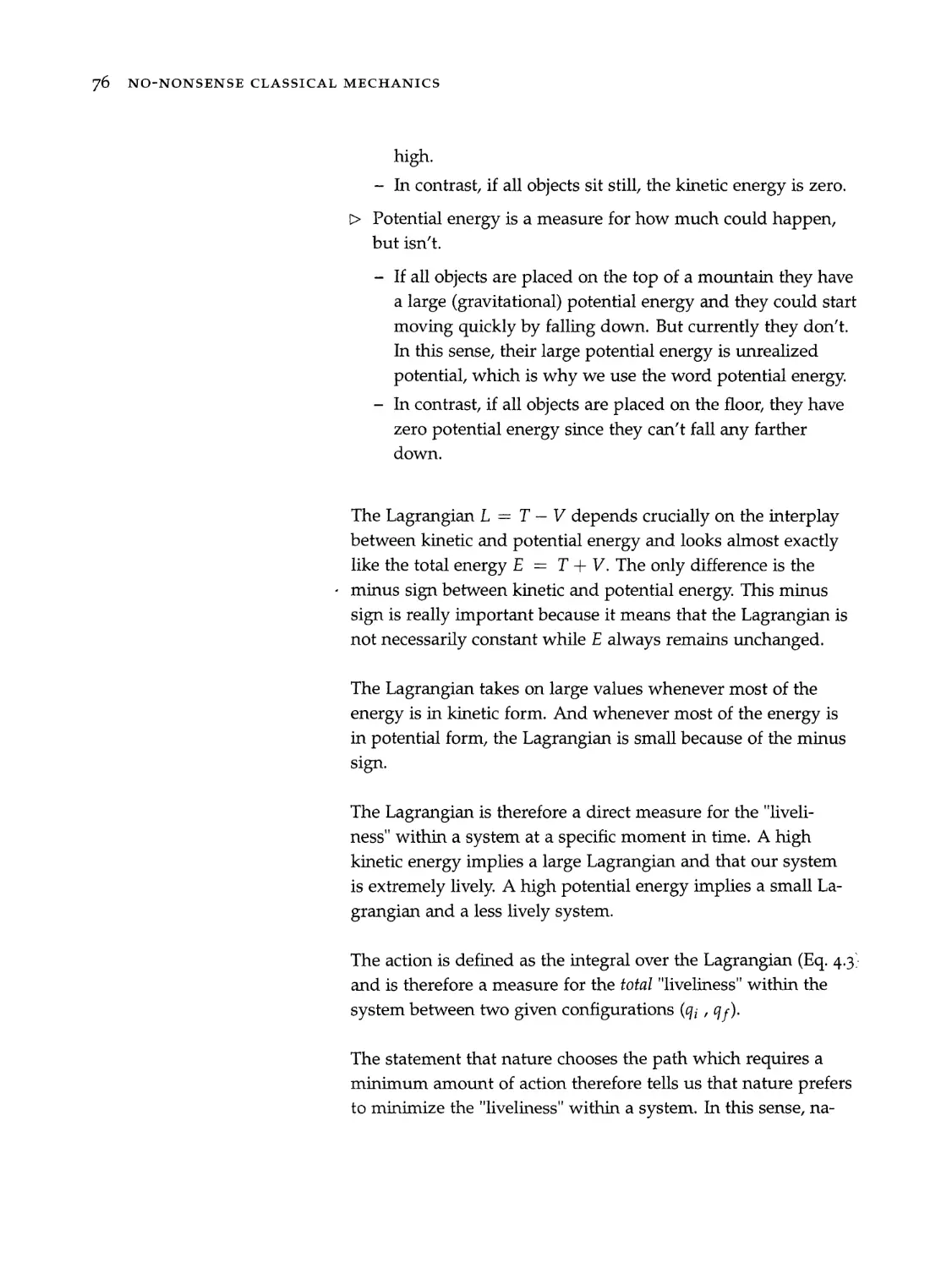
zre indeed useful, let’s try to describe a ball which is thrown
scraight up into the air. The ball’s total energy is
E=T+V
> T= sme, V = mez
1
= sme + MgQz
, » definition of momentum p = mz
p
= -— +Mgz.
2m s
=or concreteness, let’s assume that the ball’s mass is 1 kg and
ve throw it with z = 2 © starting from z = 2 m into the air.
kg-m
S
~herefore, the ball’s initial momentum is p = 2 . Moreover,
zne ball’s energy at the moment we throw it is
40 NO-NONSENSE CLASSICAL MECHANICS
1
E=~ yp?
rd + MZ
~ 2m
kg-m
,2=2m
) p=?
2
__ (22) + mg (2m)
d gz 981 a m= 1kg
— 1 kg-m)\? m
, , 2 simplifying
=2 8 4 19.62 SB
S S
kg +m?
= 21.62 so (2.22)
8 Maybe you wonder about the
conservation of momentum. While
the ball’s momentum is not con-
served (and even becomes zero at
point of maximum height), the total
momentum of the system consisting
of ball + earth is conserved.
9 In particular, to describe the
behavior of electrically charged
objects, we need electrodynamics. If
you want to learn about electrody-
namics, you might enjoy
Jakob Schwichtenberg. No-
Nonsense Electrodynamics. No-
Nonsense Books, Karlsruhe, Ger-
many, 2018a. ISBN 978-1790842117
Using only these numbers and that the ball’s energy is con-
served, we can directly predict the ball’s maximum height.?8
This is possible because when the ball reaches its maximum
height, it will stop moving upward. This means that z = 0
. and therefore that the kinetic energy vanishes T = 5mz* = 0.
But since the total energy is conserved, we know automatically
that at this point, the ball’s total energy must be in the form of
potential energy:
m2
Vinax = M&Zmax = 21.62 “$= =E
D ©9815, m=1kg
m ke -m
(1 kg) (9.81 —)2max = 21.62 os
Zmax —= 2.204 m.
This means that we can predict correctly how high the ball will
fly solely by using that energy is conserved.
Of course, there are additional properties of objects which can
be important in specific systems like, for example, the electric
charge. But since these are only important for specific systems,
we will not discuss them any further here.*?
Next, let’s talk about how we can describe objects at all times
(and not just at some extremal point like the point of maximal
height).
FUNDAMENTAL CONCEPTS 41
2.2 Equations of Motion
++ hile there are different formulations of classical mechanics,
>ur goal is usually to find for each system the correct equation
>= motion. Solutions of the equation of motion describe how the
>cjyects in our system move as time passes.
=-r simplicity, let’s restrict ourselves to one object moving in one
zrnension.>° 3° This means that we don’t need
vectors.
--. mathematical terms, an equation of motion is a differential
=juation. This means that we have the first or second derivative
>: a function which describes the position of the object x(t) on
>ne side of the equation and something else on the other side.
>or example, the equation of motion for a free object is3* 3" We will discuss in detail below
how we can derive the correct
equation for any system.
d*x(t)
dt?
= 0. (2.23)
Sut usually the equation of motion is more complicated. For
=xample, if a force F(x) = Cx(t) acts on the object, where C is
some constant, the equation of motion becomes?* 3? This is the equation of motion
for an object attached to a spring.
This system is known as a harmonic
oscillator and we will discuss it in
more detail in Chapter 8.
d* x(t)
dt?
= Cx(t). (2.24)
> either case, our goal is to find the correct function x(t) which
vields the same expression if we put it into the right-hand and
_<t-hand side of the equation. There are sophisticated methods
-or solving differential equations and big cookbooks full of
—.athematical recipes which you can try. But sometimes, we can
simply guess the right solution.
_2e equation of motion for the free object (Eq. 2.23) tells us that
ve need a function x(t) which yields zero if we differentiate it
~-ice. There are, in general, infinitely many such functions. In
rarticular, x(t) = a for any constant number a yields zero if
~-e differentiate it twice. Similarly, x(t) = bt for any constant
rvamber b yields zero. But higher order terms in ¢ do not vanish
42 NO-NONSENSE CLASSICAL MECHANICS
as we can check explicitly, e.g., for x(t) = ct?:
d?x(t) d?(ct*)
diz — dt?
where c is some constant.
=2c £0,
This means that the most general solution of the equation of
33 We will talk about the meaning of | motion for a free object (Eq. 2.23) reads?3
the constants a and b in a moment.
x(t) =a-+bt (2.25)
since for any value of the two constants a and D we find
d*x(t) d*(a+bt) | 0
dt2 “~— diz
Eq. 2.25
Finding solutions of the equation of motion for a non-free object
(e.g., Eq. 2.24) is a bit more difficult. Specifically, for Eq. 2.24 we
need a function x(t) which yields itself times some constant if
differentiated twice. Two functions with this special property
are’sin(wt) and cos(wt), where w is an arbitrary number. We
have
d .
Fi sin(wt) = wcos(wt)
=> a sin(wt) = wt cos(wt) = —w* sin(wt) (2.26)
dt? at —
© cos(wt = —wsin(wt)
=> a cos(wt) = wt sin(wt) = —w* cos(wt) (2.27)
dt ~ Ft ~ end
Therefore, we try the ansatz
x(t) = Acos(wt) (2.28)
in Eq. 2.24:
2
ae = Cx(t)
, » x(t) = Acos(wt), Eq. 2.28
d“ A cos(wt)
eT CA
7p CA cos(wt)
» & cos(wt) = —w* cos(wt), Eq. 2.27
—Aw* cos(wt) = CA cos(wt)
, > Ases(wt)
—w =C., (2.29)
FUNDAMENTAL CONCEPTS 43
cs tells us that our ansatz in Eq. 2.28 is indeed a solution
"I Eq. 2.24 ifw = Y—C. Analogously, we can check that
; = Bsin(wt) is a solution too. And we can construct fur-
er solutions by using linear combinations of the form*4 34 Take note that the constant w is
the same number in both terms
because its value is fixed through
the constant C appearing in the
equation of motion (Eq. 2.24). (In
2. f ~ /=¢6
x(t) = Acos(wt) + Bsin(wt). (2.30) F229 we found w = V—C)
_~2xe note that we haven’t used any proper solution techniques
-<te. Instead, we’ve guessed how the correct solutions could
ox like and then checked that they have the properties we are
_22xing for. This is often possible and if not, we usually need
7: ask a friend in the math department anyway. In other words,
sce solving a given equation of motion is a math problem,
-.21 a physics problem, we will often simply use the solutions
s7me mathematician found and then investigate its properties.
~zting down the correct equation of motion and understanding
_<s solutions are physics problems. But the technical task of
--.aing these solutions is a pure math problem. And for most
=Zuations we are interested in, we can either guess the right
s2 ution directly, the solution is complicated but well known, or
<2 equation can only be solved numerically.*> 35 You can recognize that a solution
is complicated whenever it is
_ named after some mathematician.
>t as an example, let me show you one of the most famous
:>_ution strategies which works for many simple equations. For
->mcreteness, let’s consider the equation
© x(t) = Cx(t), (2.31)
3° Tf you’re unsure why we are
allowed to do this, remember that
; . dt simply means "a little bit of
~-nere C is again some constant characterizing our system. We t. Moreover, In(x) is the natural
721 solve this equation by formally multiplying it by dt and logarithm which is the inverse
eer ; 6 of the exponential function, i.e.,
en integrating:3 aln(x) a x.
44 NO-NONSENSE CLASSICAL MECHANICS
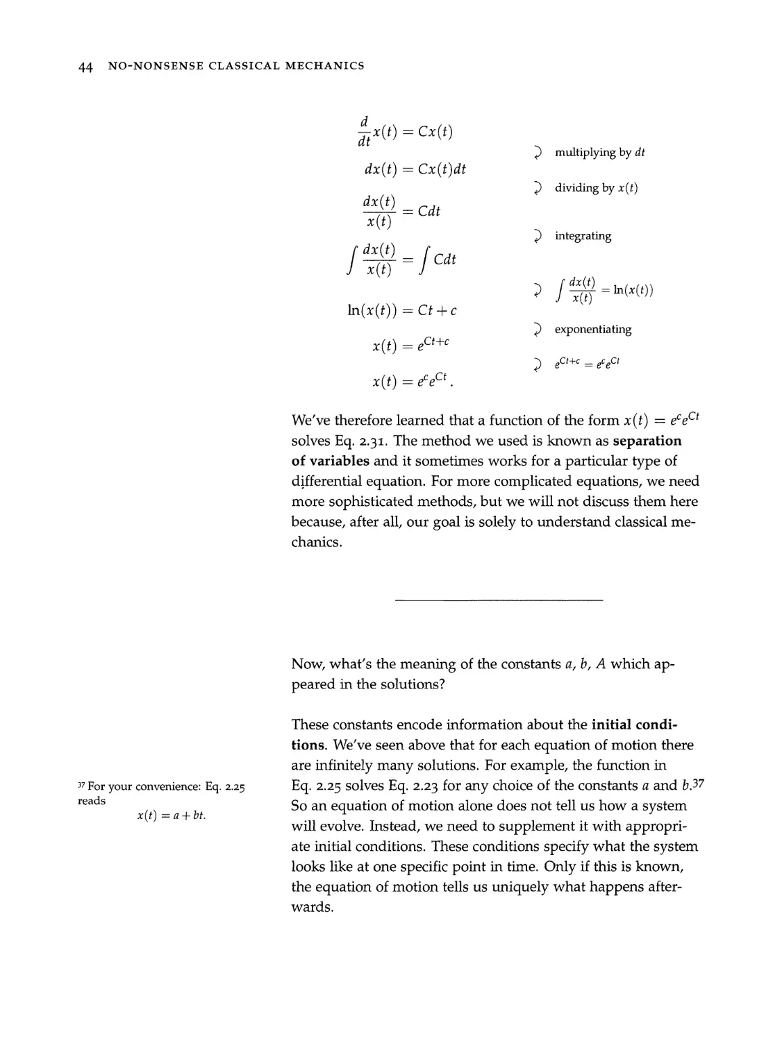
37 For your convenience: Eq. 2.25
reads
x(t) =a Ut.
» multiplying by dt
» dividing by x(t)
) integrating
> [SO =m
D exponentiating
> ectte — pC Ct
We've therefore learned that a function of the form x(t) = e°eC
solves Eq. 2.31. The method we used is known as separation
of variables and it sometimes works for a particular type of
differential equation. For more complicated equations, we need
more sophisticated methods, but we will not discuss them here
because, after all, our goal is solely to understand classical me-
chanics.
Now, what’s the meaning of the constants a, b, A which ap-
peared in the solutions?
These constants encode information about the initial condi-
tions. We've seen above that for each equation of motion there
are infinitely many solutions. For example, the function in
Eq. 2.25 solves Eq. 2.23 for any choice of the constants a and b.37
So an equation of motion alone does not tell us how a system
will evolve. Instead, we need to supplement it with appropri-
ate initial conditions. These conditions specify what the system
looks like at one specific point in time. Only if this is known,
the equation of motion tells us uniquely what happens after-
wards.
FUNDAMENTAL CONCEPTS 45
=cr the free object described by Eq. 2.23, we need to specify its
==tial position and velocity. We can see this because we have
70 constants in the general solution (Eq. 2.25) that we need to
=etermine. Mathematically, this follows because Eq. 2.23 is a
:=cond-order differential equation, which means that the second
zerivative of x(t) appears in it.
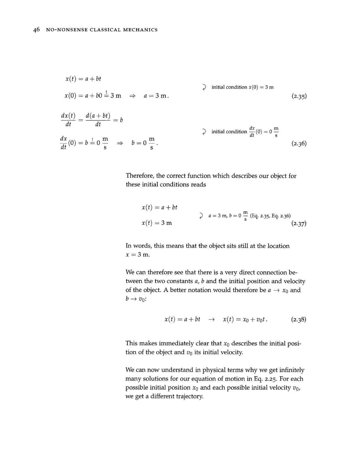
=>z concreteness, let’s say our object is att = Os atx = Om
2-d moves with ua (0) = 2 ©.38 This allows us to determine the
-2nstants a and b in Eq. 2.25:
t)=a+bt
» initial condition x(0) = 0
0)=a+bl0=0 > a=0. (2.32)
cx t) d(at+dt)
= = — b
at dt J
2 initial condition = (0) =2 =
= 0)=b=2— => b=2—. (2.33)
~2erefore, the correct function which describes our object reads
x(t) =atbt
> a=0,b=2 ~) (Eq. 2.32, Eq. 2.33)
m
x(t) =2 <t (2.34)
ve call the path described by such a concrete solution the tra-
‘ectory of the object.
—‘: course, we can also imagine that our object is att = 0 at
: = 3m and moves with some other initial velocity like (0) =
-. ~~
=. We can then again determine the constants a and b in
38 Take note that we do not neces-
sarily need to choose t = 0s as our
initial moment in time. We could
equally specify the location and
velocity at some other moment in
time like # = 2 s and then follow
the same steps to determine the
constants a and b. Butt = Osisa
convenient choice because it often
makes the equations simpler since
terms drop out if we put in a zero.
Moreover, we can always choose
t = 0s as our initial moment in
time because different choices sim-
ply correspond to a different choice
of the coordinate system. In other
words, we always choose when the
clock starts ticking. But choosing a
different coordinate system cannot
make any difference and hence,
specifying the position and velocity
att = 0 is a completely general
approach.
46 NO-NONSENSE CLASSICAL MECHANICS
x(t) =a+bt
» initial condition x(0) = 3m
x(0) =a+b0=3m > a=3m. (2.35)
dx(t) d(a+bdt)
= —____ =p
dt dt J
> initial condition =, (0) =0=
dx 1 om m
Therefore, the correct function which describes our object for
these initial conditions reads
x(t) =a+bt
) a4=3m,b=0 = (Eq. 2.35, Eq. 2.36)
x(t) =3m (2.37)
In words, this means that the object sits still at the location
x =3m.
We can therefore see that there is a very direct connection be-
tween the two constants a, b and the initial position and velocity
of the object. A better notation would therefore be a —+ xp and
b—- Vo:
x(t)=at+bt - x(t) =xo+v0t. (2.38)
This makes immediately clear that x9 describes the initial posi-
tion of the object and vg its initial velocity.
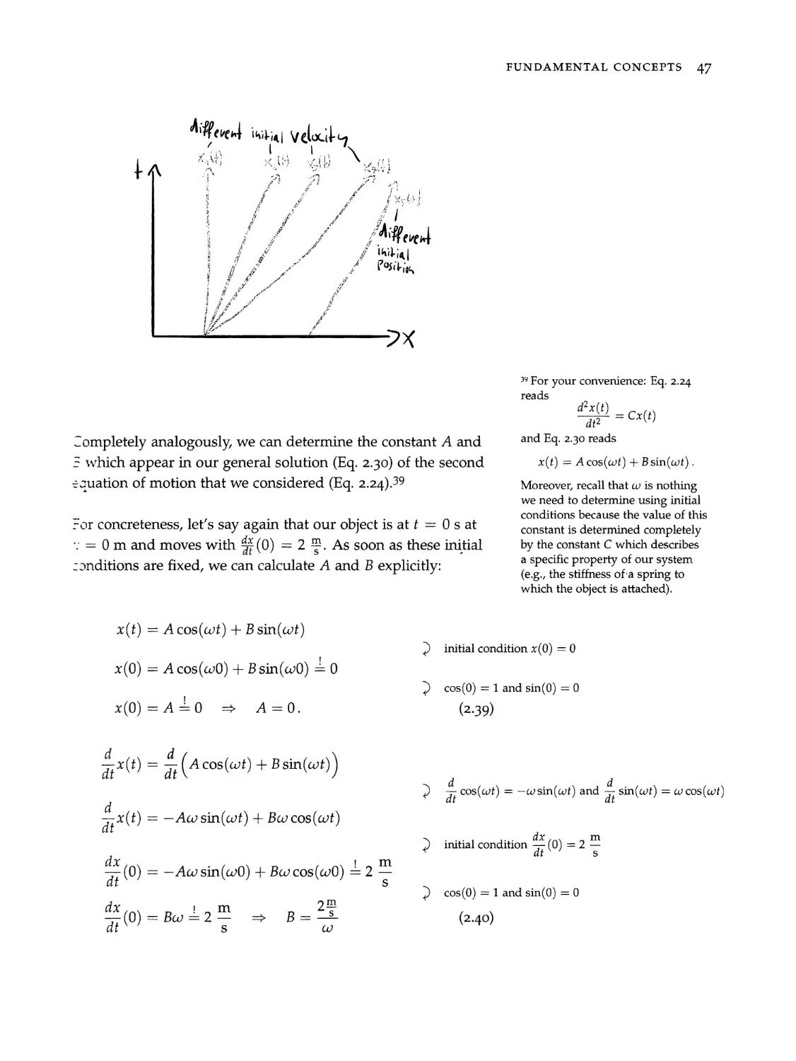
We can now understand in physical terms why we get infinitely
many solutions for our equation of motion in Eq. 2.25. For each
possible initial position x9 and each possible initial velocity vo,
we get a different trajectory.
FUNDAMENTAL CONCEPTS 47
NPP overt Inibia| velocity
yd
Rew ad ‘
sa 3
ies oy kes voah is VA to
: Mop ee Pe eG
yO “7 at ree
a re 2? we a
R f pe 2 we
4 , £ eo i
. 7 . 1
if é feb 3
5 ‘s rn ee)
* f ey
y f g a
2 } # a
5 a Z
. L ¢ oe .
i v ¢ o 1
i “L
‘i é f é ve
i : a a.
5 “ a ye
‘ : ini}
i ¥ e * fo Nhihia
: yg - & Pact:
a Posi,
i righ
i ; iF .
¥ £ s - /
4 " & ro of
. i ow . y
u ts wv ur
% Xv en" rad
N og ea
foo fe 7
Hy f wo 8
: a £ ; f
oes "
vs
Lf oe” 5
i ffs? ie
” vr
tga
39 For your convenience: Eq. 2.24
reads Px(t)
x(t
-ompletely analogously, we can determine the constant A and and Eq. 2.30 reads
= which appear in our general solution (Eq. 2.30) of the second x(t) = Acos(wt) + Bsin(wt).
=cuation of motion that we considered (Eq. 2.24).39 Moreover, recall that w is nothing
we need to determine using initial
_ let’ nth bi conditions because the value of this
ror concreteness, let's say again that our object is at? = 0s at constant is determined completely
= 0 mand moves with 4(0) = 2 @. As soon as these initial by the constant C which describes
conditions are fixed, we can calculate A and B explicitly: (eg. “the aitfness of a opt me to
which the object is attached).
x(t) = Acos(wt) + Bsin(wt)
» initial condition x(0) = 0
x(0) = Acos(w0) + Bsin(w0) = 0
» cos(0) = 1 and sin(0) = 0
x(0)=A=0 3 A=0O. (2.39)
£ _# (A cos(wt) + B sin(wt) J
> a cos(wt) = —wsin(wt) and Fi sin(wt) = w cos(wt)
© x(t) = —Awsin(wt) + Bw cos(wt)
» initial condition = (0) =2—
5
= (0) = —Aw sin(w0) + Bw cos(w0) =2
o | 5
» cos(0) = 1 and sin(0) = 0
(2.40)
dx
wo
|
m
—- =>
S
€ |B
48 NO-NONSENSE CLASSICAL MECHANICS
4° Eq. 2.24 is the equation of motion
of an object attached to a spring.
This solution therefore tells us that
the object bounces back and forth.
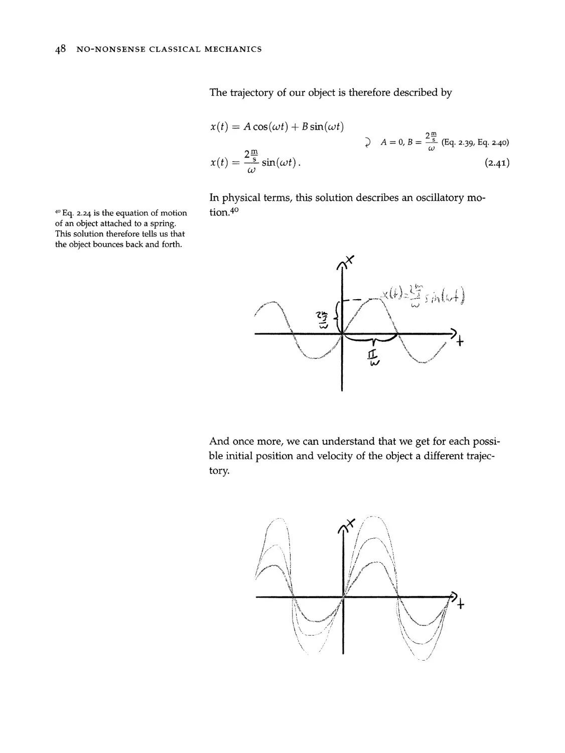
The trajectory of our object is therefore described by
x(t) = Acos(wt) + Bsin(wt) .
) A=0,B= os (Eq. 2.39, Eq. 2.40)
m
x(t) = a sin(wt). (2.41)
In physical terms, this solution describes an oscillatory mo-
tion.4°
And once more, we can understand that we get for each possi-
ble initial position and velocity of the object a different trajec-
tory.
FUNDAMENTAL CONCEPTS 49
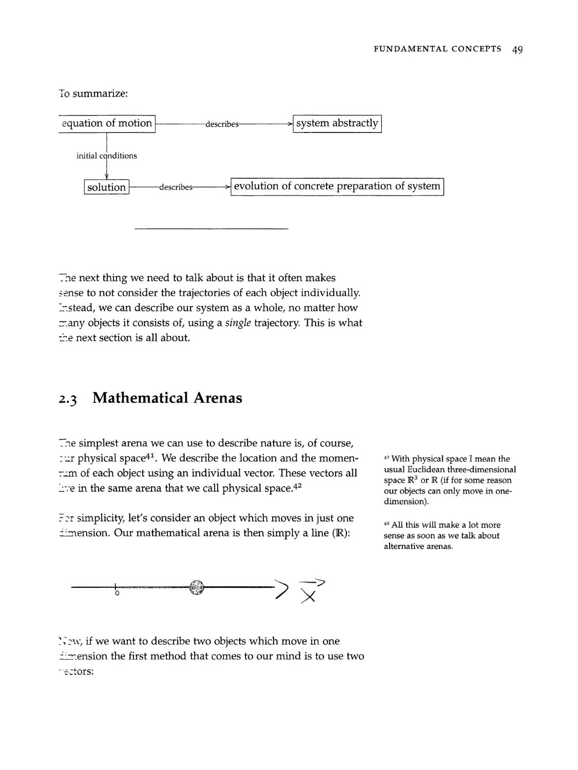
iO Summarize:
equation of motion }——-describes ————> system abstractly
initial c
onditions
describes ———> evolution of concrete preparation of system
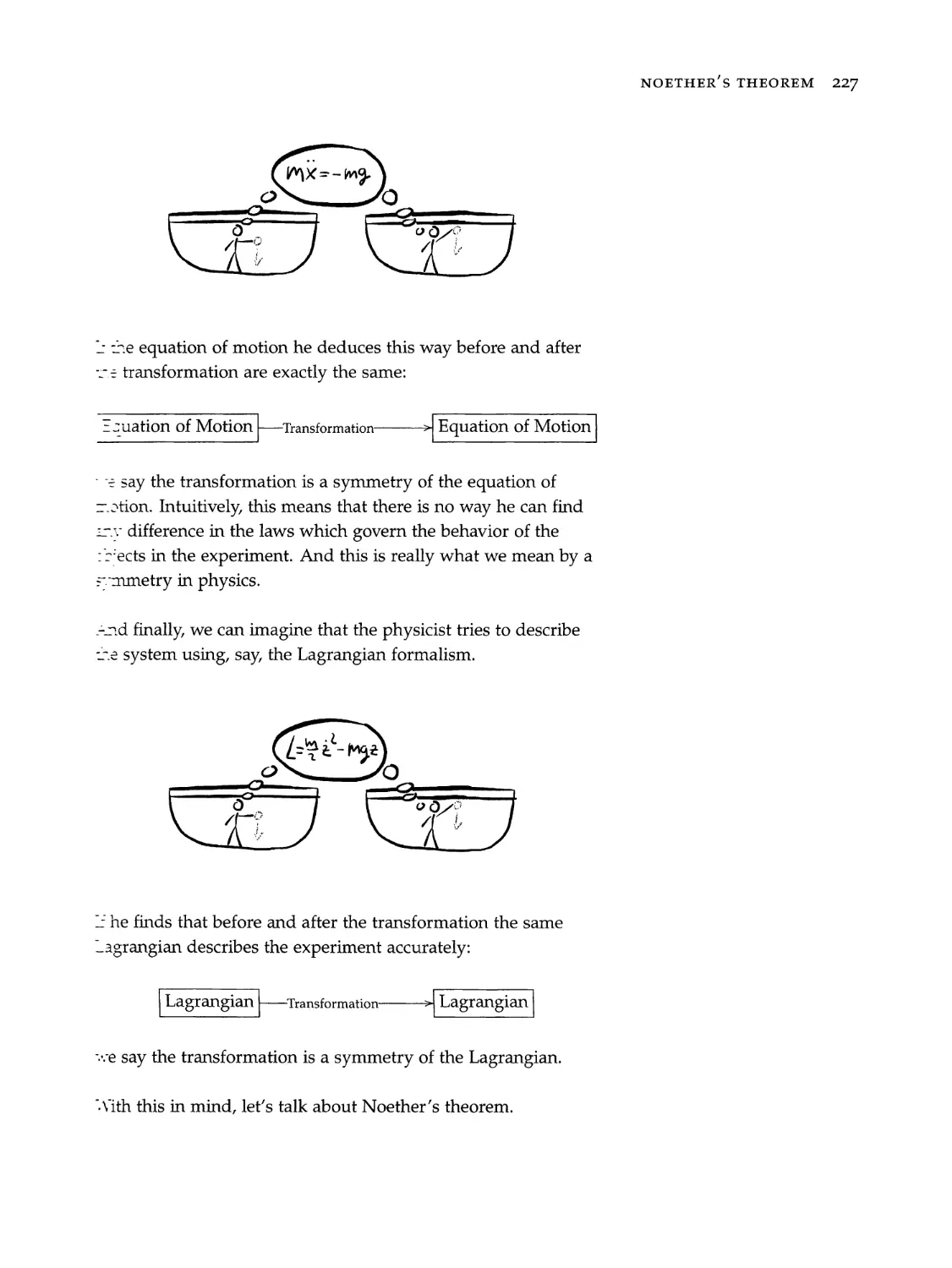
~he next thing we need to talk about is that it often makes
sense to not consider the trajectories of each object individually.
stead, we can describe our system as a whole, no matter how
any objects it consists of, using a single trajectory. This is what
tne next section is all about.
2.3 Mathematical Arenas
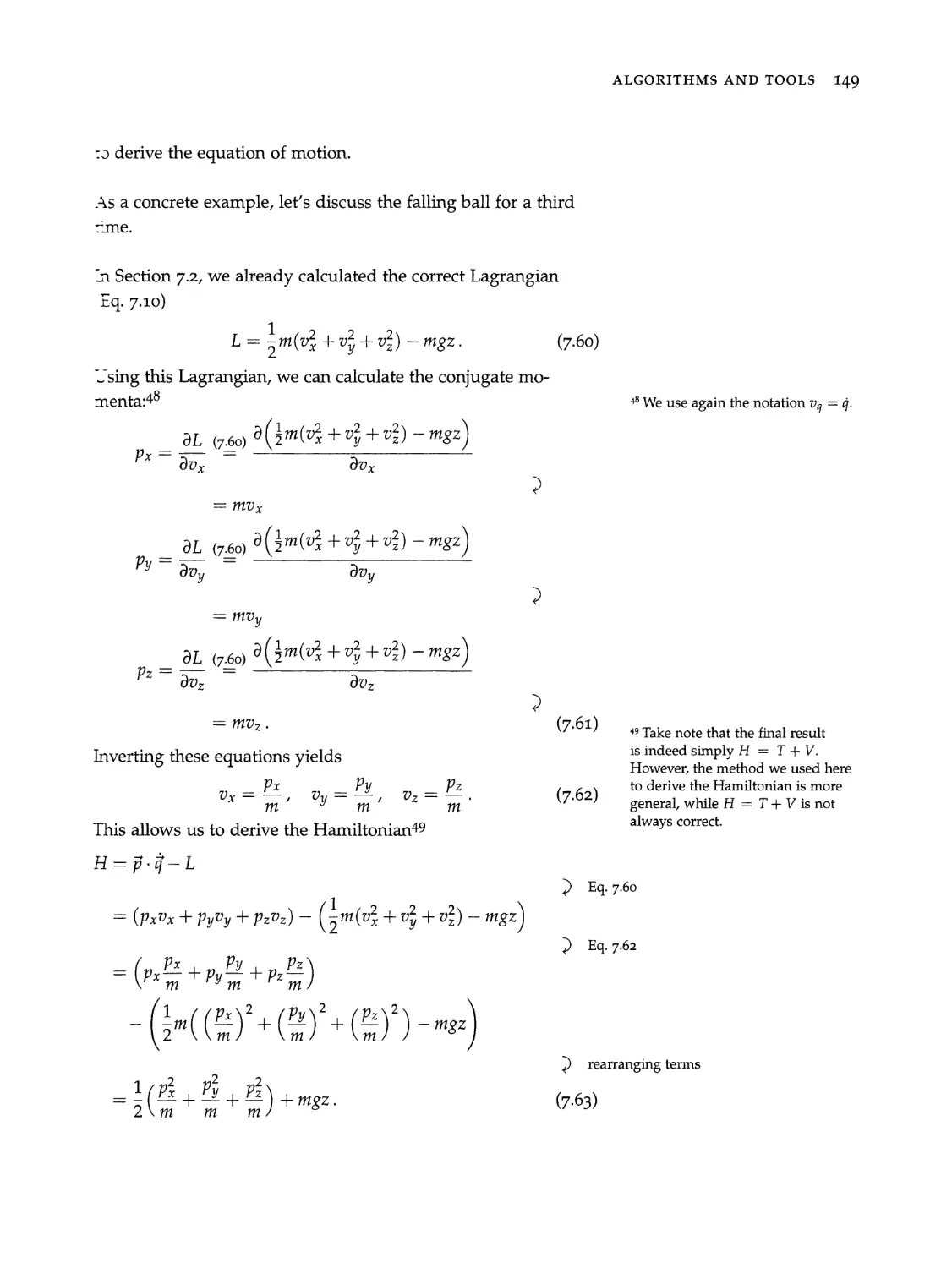
_ne simplest arena we can use to describe nature is, of course,
-ur physical space*+*. We describe the location and the momen- # With physical space I mean the
ram of each object using an individual vector. These vectors all usual Euclidean three-dimensional
; space IR” or R (if for some reason
re in the same arena that we call physical space.** our objects can only move in one-
dimension).
=2r simplicity, let’s consider an object which moves in just one #2 All this will make a lot more
WwW Yr
=:mension. Our mathematical arena is then simply a line (IR): sense as soon as we talk about
alternative arenas.
NW,
DPE ERS
ey x
or
*, sv, f we want to describe two objects which move in one
-‘~ension the first method that comes to our mind is to use two
2 7tors:
50 NO-NONSENSE CLASSICAL MECHANICS
43 We also need only two vectors if
there are three or more objects in
the system.
bo
In addition to two vectors that keep track of the locations, we
need two further vectors that keep track of the momenta.
This is what we do in the Newtonian formulation of classical
mechanics. Such a description in physical space is handy since
we can immediately understand everything that is going on in
the system. Each vector is simply an arrow that points from one
location to another. However, in practice, this approach is often
laborious —especially when we are dealing with lots of objects.
So how else can we describe our system consisting of, for exam-
ple, two objects that move along a line?
2.3.1 Configuration Space
What we need, mathematically, is a tool that allows us to keep
track of the locations and momenta of the two objects. In the
physical space description, we need four vectors to accomplish
this: two for the locations and two for the momenta.
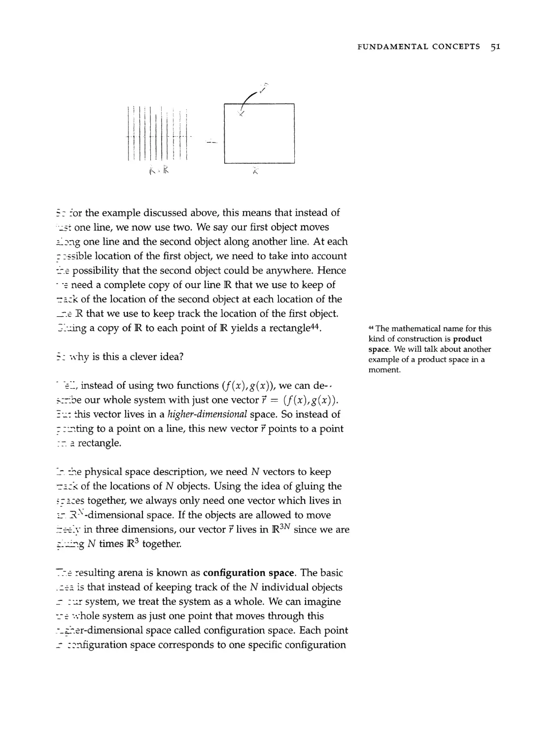
Using the following idea, we can describe the whole system
with just two vectors*3.
[> First, we act as if there were a separate arena for each object:
[> Then we glue these separate spaces together:
FUNDAMENTAL CONCEPTS 51
|
ce ee ef
ne
iia IR in
>> zor the example discussed above, this means that instead of
“2st one line, we now use two. We say our first object moves
2_2ng one line and the second object along another line. At each
zzssible location of the first object, we need to take into account
<2 possibility that the second object could be anywhere. Hence
"= need a complete copy of our line R that we use to keep of
zack of the location of the second object at each location of the
_>.< R that we use to keep track the location of the first object.
=.<ing a copy of IR to each point of R yields a rectangle*. 4 The mathematical name for this
kind of construction is product
space. We will talk about another
>: why is this a clever idea? example of a product space in a
moment.
=_, instead of using two functions (f(x), ¢(x)), we can de--
s:7-be our whole system with just one vector 7 = (f(x),g@(x)).
=..1 this vector lives in a higher-dimensional space. So instead of
—_— —_,
> Iinting to a point on a line, this new vector 7 points to a point
— om
“>. a rectangle.
>. tne physical space description, we need N vectors to keep
T2cx of the locations of N objects. Using the idea of gluing the
s>2ces together, we always only need one vector which lives in
i>. R-dimensional space. If the objects are allowed to move
=<:lv in three dimensions, our vector 7 lives in IR*% since we are
> ing N times IR? together.
"5
_-€ resulting arena is known as configuration space. The basic
222 is that instead of keeping track of the N individual objects
= iur system, we treat the system as a whole. We can imagine
>< whole system as just one point that moves through this
>_z-.er-dimensional space called configuration space. Each point
- :onfiguration space corresponds to one specific configuration
52 NO-NONSENSE CLASSICAL MECHANICS
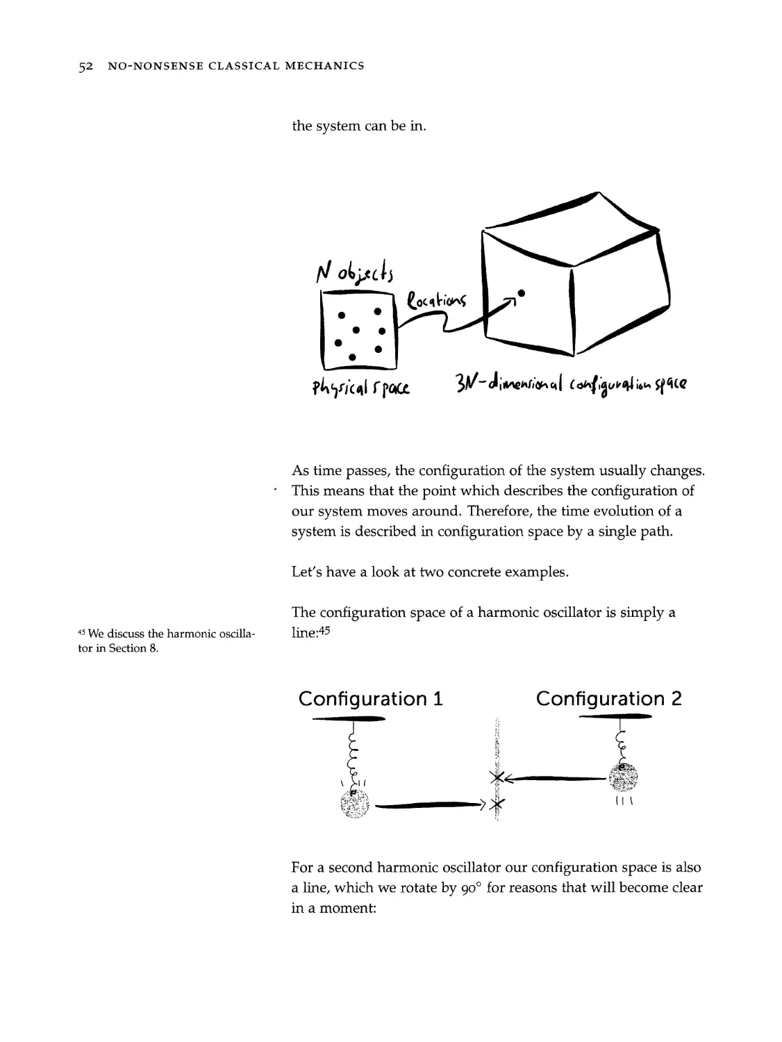
the system can be in.
N O ects
Cocatians n°
Phosical £ pace 3W- dimensional Cohfigural isn $740
As time passes, the configuration of the system usually changes.
This means that the point which describes the configuration of
our system moves around. Therefore, the time evolution of a
system is described in configuration space by a single path.
Let’s have a look at two concrete examples.
The configuration space of a harmonic oscillator is simply a
45 We discuss the harmonic oscilla- line:45
tor in Section 8.
Configuration 1 Configuration 2
For a second harmonic oscillator our configuration space is also
a line, which we rotate by 90° for reasons that will become clear
in a moment:
FUNDAMENTAL CONCEPTS 53
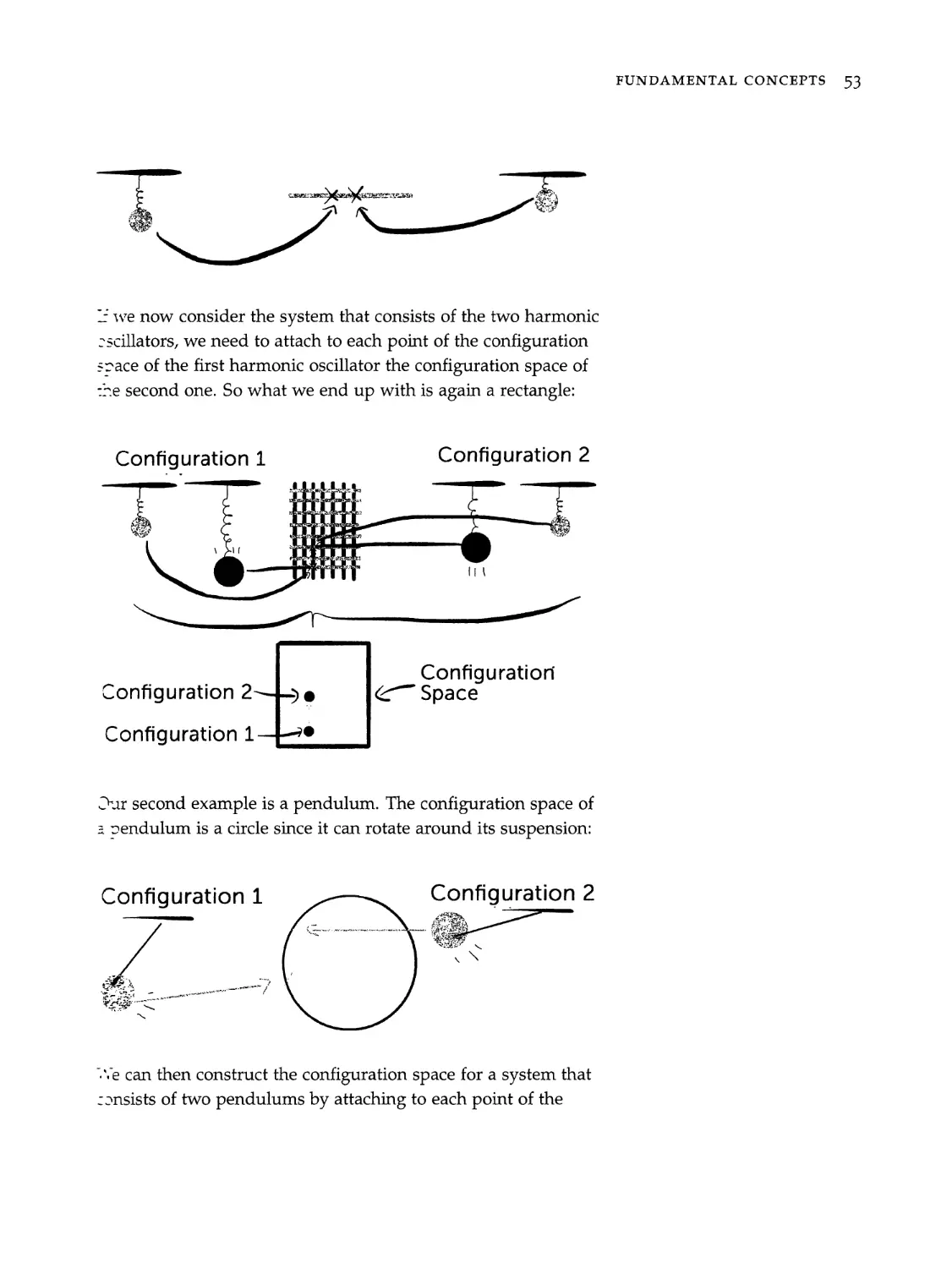
= we now consider the system that consists of the two harmonic
>scillators, we need to attach to each point of the configuration
space of the first harmonic oscillator the configuration space of
<ne second one. So what we end up with is again a rectangle:
Configuration 1 Configuration 2
err —
Configuration
Configuration 2—.-> @ @— Space
Configuration 1—++e
“ur second example is a pendulum. The configuration space of
2 pendulum is a circle since it can rotate around its suspension:
Configuration 2
WES
Configuration 1
“e can then construct the configuration space for a system that
-ansists of two pendulums by attaching to each point of the
54 NO-NONSENSE CLASSICAL MECHANICS
configuration space of the first pendulum the configuration
space of the second one. The result of this procedure is a torus:
Configuration 1 Configuration 2
Configuration 2 —
Configuration
Configuration 1 Space
To summarize: while individual objects move in the three-
dimensional physical space, the time evolution of a system
as a whole takes place in a higher-dimensional configuration
space. A single trajectory in configuration space describes the
evolution of a system as a whole.
2.3.2 Phase Space
An important observation is that configuration space only keeps
track of the locations of the various objects. But to describe the
state of a system completely, we need additionally to keep track
FUNDAMENTAL CONCEPTS 55
2 how the objects move. And mathematically, this means that
«ve need to keep track of their momenta. So in addition to a
actor 7 that keeps track of the locations, we need a vector # that
seeps track of the momenta.
_7is motivates the construction of the next mathematical arena
“nich works completely analogous to how we constructed
-2nfiguration space. However, this time we also act as if the
—.omenta live in a different space and then glue the momentum
spaces to our location spaces. As a result, we can describe the
->mplete state (not just the configuration) of our system with a
single vector.4® 4 By configuration of our system we
mean a complete description of all
_ . . . locations. In contrast, the state of a
~7e resulting mathematical arena is known as phase space. system corresponds to a complete
=ach point in phase space corresponds uniquely to one specific description of all locations and all
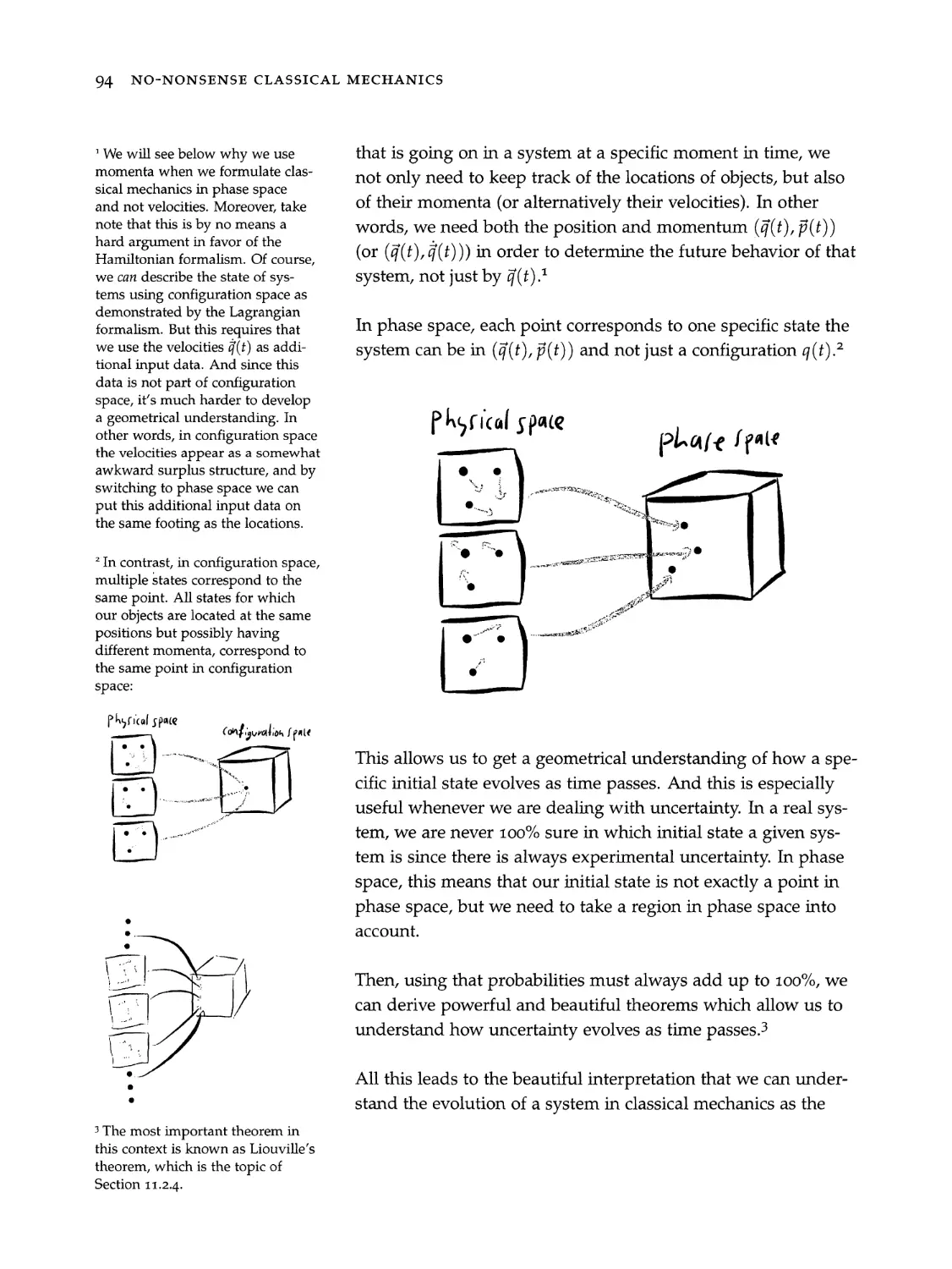
_2cation and momentum of each object. So everything that is go- momenta.
-.Z on in the system is described by just one vector (or equally
<2 point the vector points to) that moves through phase space.
“aww, the price we have to pay for this is that the vector we use
7: describe the system lives in a 2 x 3N-dimensional space for N
-z‘ects that move in three dimensions.
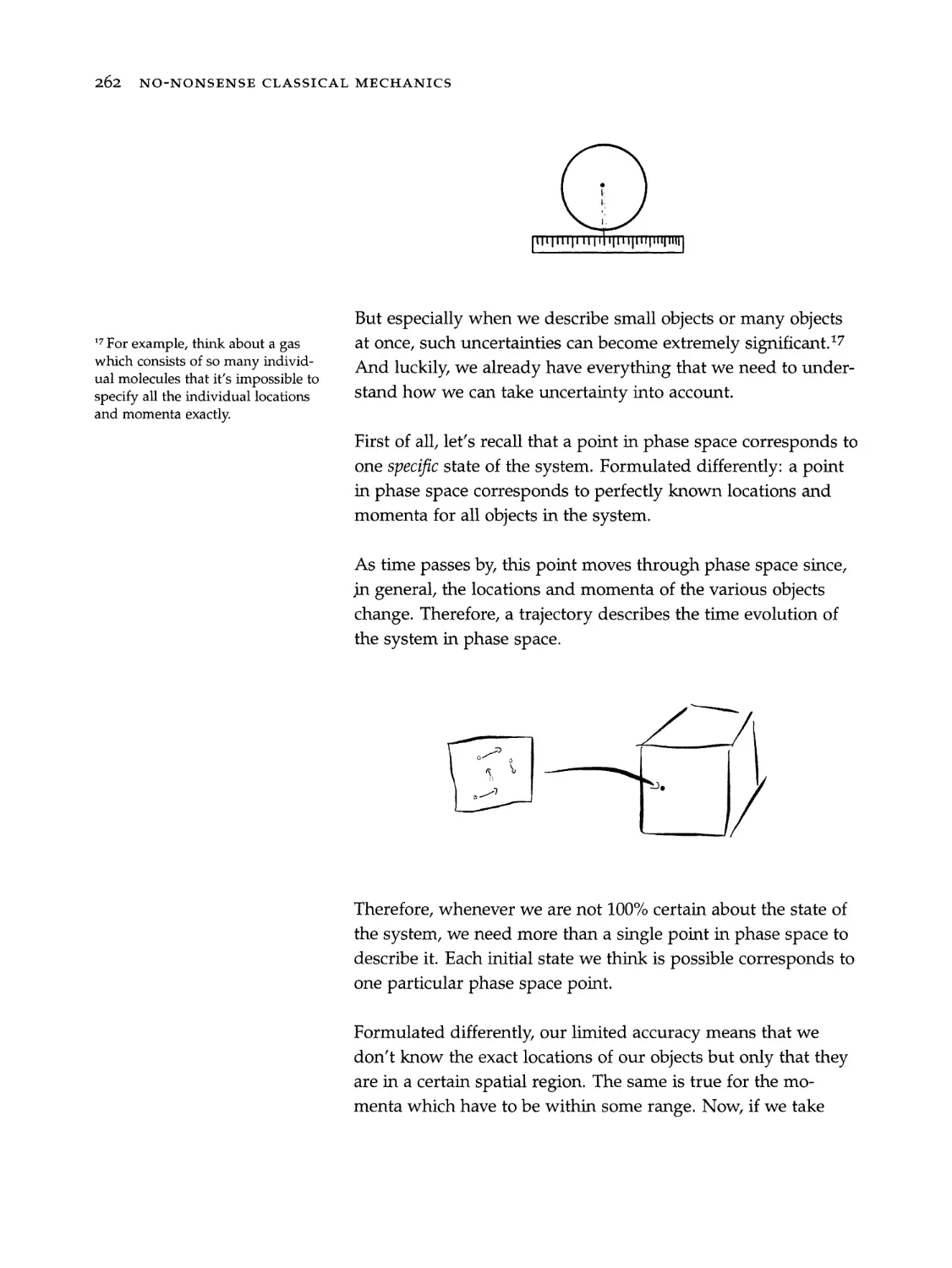
eee ) @
Physical £ pace GW - dimensional phase space
> 7.ase space is notoriously difficult to visualize since even for
37 two objects moving in one dimension, phase space is al-
-22dv four-dimensional. However, for just one object in one
=-—mension, it is possible.
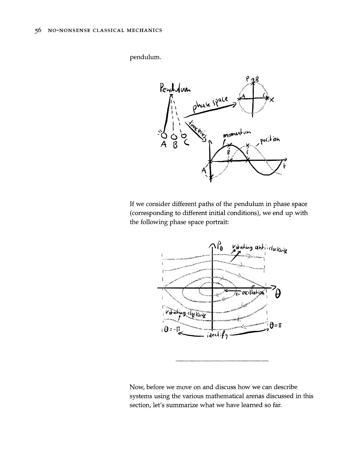
=<ze’s a concrete example: the phase space path of a swinging
56 NO-NONSENSE CLASSICAL MECHANICS
pendulum.
“©
NX
vY>
A
a
Ke udu UA a ov
galt a 3x
~
xo
a
%
IN
1\ ovate \ 4 ‘ | u
\ ‘ eg aw
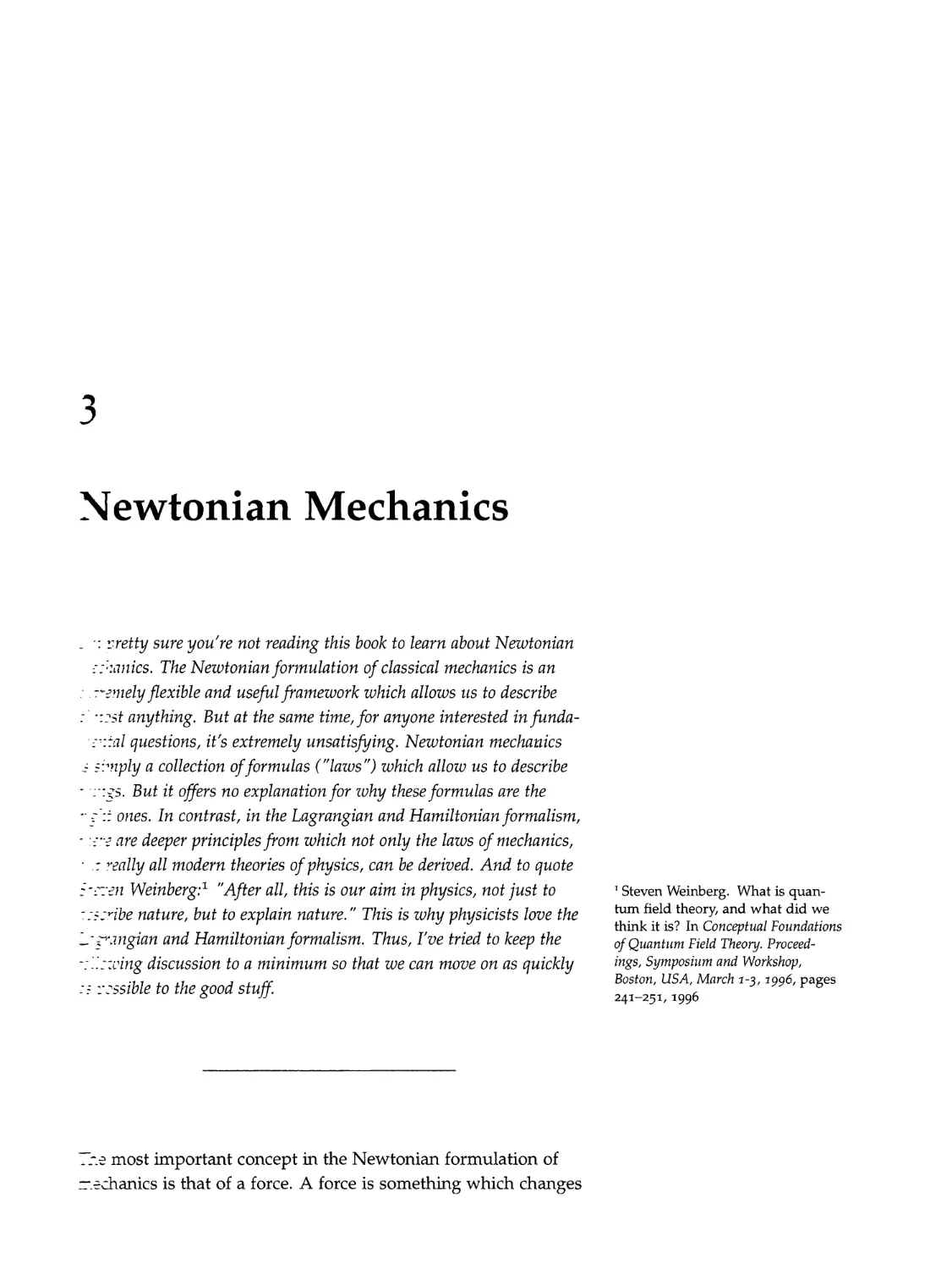
If we consider different paths of the pendulum in phase space
(corresponding to different initial conditions), we end up with
the following phase space portrait:
>
Nis ayn anki -clockvig
| gerne DEAE Sh . snes
nn ner TEI ve Sf “ +
eset PT aay .
\ “ere rE et oe ‘
eee an
we,
“en cee en ernie va
| concer pee > ee
aw Hing
ae | Ag a.
ee tt TOLLE . rate
se a a PS ll . Te,
| oe or . na, “,
- . ae “e
oe ae | “ahs, es ta
. a” aw Z
\ ie o P
' 72 y f Fo
ss z ,
*S x Nee, Oci a i oh
*e % 3 Frew ans :
{ ~,, ey, ws
Sa Teese, ingens aces econ
a I
a
A ne Ase Pe
a sult -
be 5 EO mo .
v va f ar C berms gers= 2 Pal |
9. wt vig] oe?
ge 5 {
~ Sat oy corp Ree ene RIE “ot ND
a
alesse | Q= il
a —_
eae gant? ees
- csc tunalfren scare
dest fs ———
Now, before we move on and discuss how we can describe
systems using the various mathematical arenas discussed in this
section, let’s summarize what we have learned so far.
> One possibility to describe nature is to keep track of every-
thing using various vectors living in physical space.
> A bit more convenient is a description in configuration space.
In configuration space, a single point is enough to keep track
of the locations of all objects in our system.
> Even better is a description in phase space. Each phase space
point corresponds to one specific state of the system (includ-
ing all locations and all momenta).
_ake note that these are really just different mathematical tools
znat allow us to describe a given system in different ways. It is
2D to you which one you like best.
=lowever, the crucial point is the following:
We can describe any given system
using any of these mathematical arenas.
_nis is why there are different formulations of classical mechan-
_—-
>,
specifically, we have the following well-known formulations:47
*> Classical mechanics in physical space is what we call the
Newtonian formulation.
‘> Classical mechanics in configuration space is what we call the
Lagrangian formulation.
> Classical mechanics in phase space is what we call the
Hamiltonian formulation.
Next, let’s talk about these formulations.
FUNDAMENTAL CONCEPTS 57
47 There is one additional important
arena known as Hilbert space,
and we can describe classical
mechanics in Hilbert space too.
The resulting formulation is known
as the Koopman-von Neumann
formulation and we will talk about
it in Section 11.3.
uJ
Newtonian Mechanics
_ ‘1 eretty sure you're not reading this book to learn about Newtonian
:suanics. The Newtonian formulation of classical mechanics is an
» .cremely flexible and useful framework which allows us to describe
: trast anything. But at the same time, for anyone interested in funda-
‘sital questions, it’s extremely unsatisfying. Newtonian mechanics
= sonply a collection of formulas (“laws”) which allow us to describe
“rigs. But tt offers no explanation for why these formulas are the
~ 2:2 ones. In contrast, in the Lagrangian and Hamiltonian formalism,
“itz are deeper principles from which not only the laws of mechanics,
‘2 really all modern theories of physics, can be derived. And to quote
>-zten Weinberg:* “After all, this is our aim in physics, not just to ‘Steven Weinberg. What is quan-
-:scribe nature, but to explain nature.” This is why physicists love the tum field theory, and what did we
_ , think it is? In Conceptual Foundations
_-zangian and Hamiltonian formalism. Thus, I’ve tried to keep the of Quantum Field Theory. Proceed-
-:izcving discussion to a minimum so that we can move on as quickly ings, Symposium and Workshop,
Boston, USA, March 1-3, 1996,
-: vossible to the good stuff. aioe s996 ATEN 73 19901 Pages
72 most important concept in the Newtonian formulation of
—chanics is that of a force. A force is something which changes
60 NO-NONSENSE CLASSICAL MECHANICS
2 We'll talk about Newton’s other
laws in a moment.
3 Take note that these examples
are especially simple because our
object moves effectively only in one
dimension, and therefore, we don’t
need vectors to describe the forces.
the momentum of an object. Mathematically, this means that
d
eat. (3.1)
This is Newton’s second law.” Formulated differently:
The rate at which the momentum of an object
changes is exactly equal to the force acting on it.
Newton’s little formula (Eq. 3.1) allows us to predict how any
object will move starting from some specific position and veloc-
ity (initial conditions).
The definition of a force given here is an extremely general one.
In Chapter 2, we’ve already discussed two simple examples.3
‘D The force a spring exerts on an object attached to it can be
described by F(x) = —kx, where k is known as the spring
constant and characterizes the spring in question.
> The (gravitational) force earth exerts on an object we throw
into the air can be described by F(x) = mg, where m is the
object’s mass and g ~ 9.81 & a constant
Historically, these formulas (and really most of the formulas we
use in classical mechanics to describe forces) were discovered
experimentally. We simply use them because we’ve discovered
that by putting them into Newton’s second law, we get the
correct equations of motion.
In general, we need to find all forces F;, F, ... that act on the
object in question. The total force F is then given by
F@)=LA@ =A@M+AM +... (3.2)
For example, an object attached to a spring will realistically not
only feel the force exerted by the spring but additionally will
feel a gravitational force.
NEWTONIAN MECHANICS 61
_ nis is what we use on the right-hand side of Newton’s second
aw (Eq. 3.1). On the left-hand side, we use the definition of the
omentum # = mi:
43 —Ff
dt .
7 » Eq. 3.2 and p = mq
= (m4) = Aa) + hq) +... (3:3)
_is is the equation of motion for the object, and its solutions
ze] us explicitly how the object moves around.
«shile this procedure may sound simple, for most systems it
-sm't. There are two major difficulties. Often it’s cumbersome to
verite down all the forces acting on a given object in a consistent
av. In particular, we need to take the various directions of the
=:-ferent forces into account. And secondly, solving the equation
~z motion is, for most realistic systems, an extremely difficult
~.ath problem.
»@ will see this explicitly in Part Il when we discuss various
stems in detail. But already here we take note that these dif-
=culties are one of the main reasons people use alternative -
->rmulations of classical mechanics.4 4 There are additional reasons to
consider these alternative formu-
_ ae lations of classical mechanics. The
-2ke note that if the mass of the object in question is constant, Lagrangian formulation not only
allows us to describe many systems
in much simpler terms, but is at the
same time conceptually beautiful
. and helps us to understand classical
do puma mechanics on a deeper level.
*ewton’s second law becomes
» product rule
d 4 d/s
> m= const. > 5m =Oandg= = (9)
mg = F. (3.4)
>. words, this means that whenever there is a non-zero acceler-
zzon of an object 7 # 0, this change in the velocity 7 = 4 (4)
-s directly proportional to the total force F acting on it. The pro-
> ortionality constant is what we call the mass of the object. And
=is is why it’s more difficult to push an object with large mass.
62 NO-NONSENSE CLASSICAL MECHANICS
Now you probably wonder, since Eq. 3.1 is Newton’s second law,
what are the remaining laws?
Newton’s first law states that, at least for one specific observer,
an object which moves with constant velocity will always con-
tinue to move with this constant velocity unless a force acts on
it. In particular, this implies that a particle at rest will stay at
rest unless a force acts upon it.
| objects at rest (v = 0 m/s) | | objects in motion (v # 0 m/s) |
no net force, a = 0 m/s? no net force, a = 0 m/s*
stay at rest | stay in motion |
So in other words, no object likes to have its state of motion
changed.
In this sense, Newton’s first law is often called the law of iner-
tia.
Although this law may seem really simple, it needs some ex-
plaining.
Newton’s second law tells us that forces can change the mo-
mentum of objects. But Newton’s first law tells us that forces
z= the only thing which change the momentum of objects. In
"<2 words, there is nothing else which causes a change in
= =mentum.?
>=: ondly, take note that if you observe an object while you get
::ceierated yourself (e.g., when you sit inside a car), the object
‘appear accelerated too.
_-.2zefore, only for very specific observers, objects will continue
-: move with uniform velocity unless a force acts upon them.
~ = call them inertial observers. In other words, an inertial
-Zserver is someone for whom an object with zero net force
:i=ng upon it is not accelerating. Newton’s first law therefore
:=.s that for each object, at least one such observer exists. And
"rv for inertial observers, Newton’s second law (Eq. 3.1) is
_7.2¢’s why Newton’s first law, technically, needs to be estab-
_:7ed before we can use Newton’s second law. In particular,
‘lewton’s first law establishes that for an inertial observer F = 0
-=2ly implies p = 0.
= =.vever, take note that we can describe how objects behave
=:m the perspective of accelerating observers by introducing
=--called fictitious forces.”
—~. addition to the first and second law, there’s Newton’s third
NEWTONIAN MECHANICS 63
> One may argue that the force
framework is so general that we can
always define a force to account for
any change in momentum that we
observe.
° All this may seem really pedantic
or even trivial at the moment. But
thoughts like these about how
different observers perceive the
same situation are at the heart
of many of the most important
insights in modern physics, e.g.,
special relativity. So for the moment
you shouldn’t worry about issues
like this too much. But keep them
in the back of your head as they
will become a lot more important
further down the road.
7 We call them fictitious because
they’re a consequence of the ref-
erence frame and not of any inter-
action. However, for an observer
within such a non-inertial system,
they are as real as any other force.
In fact, there is no possibility to
find any difference without looking
outside the system. The most fa-
mous fictitious force is probably the
Coriolis force which can be used to
explain many important meteoro-
logical effects. We need a fictitious
force here because the earth is spin-
ning and therefore any observer
on earth lives in an accelerating
non-inertial frame. Moreover, in
Einstein’s theory of general rela-
tivity, gravity is, in some sense, a
fictitious force. We will discuss this
in more detail in Section 12.3.6.
64 NO-NONSENSE CLASSICAL MECHANICS
, by y
Aiv , |
Awh
® This formula may look frightening.
But basically it only says that the
gravitational force between two
objects is directly proportional
to their masses and is inversely
proportional to their distance
r = |q1 — G2| squared. (The farther
they are away from each other, the
smaller the resulting force is). Thus,
the absolute magnitude of the force
can be written as
p=Gmy.
r
The remaining stuff in the formula
Gi —
lf — 92
yields a vector of length one which
points from the location of the first
object to the location of the second
object.
law. In Newton’s own words: “To any action there is always an
opposite and equal reaction; in other words, the actions of two bodies
upon each other are always equal and always opposite in direction.
Formulated differently, action = reaction.
In more concrete terms, this third law tells us that whenever
an object exerts a force F on another object, this second object
always exerts the force —F on the first.
yea chi
_/
“—
(xi 0” O
"ON.
XQ
This phenomenon is sometimes hard to believe. For example,
when we jump into the air there is a gravitational force F that
pulls us back toward the ground. However, at the same time, we
pull the earth a little bit upward through a gravitational force
of equal magnitude —F. Since the earth’s mass is so huge the
effects of this force are basically unnoticeable and the resulting
change in the earth’s velocity is tiny.
In practice, the equality of the forces two objects exert on each
other are directly encoded in the formulas which describe the
force in general. For example, the gravitational force an object
with mass M located at 9, exerts on an object with mass m
located at 92 is described by®
mM ~
E = G—— A, — ’ ’
Mm la _ 72/3 (41 G2) (3.5)
where G is a constant known as the gravitational constant.
NEWTONIAN MECHANICS 65
- we want to calculate the force the second object exerts on the
-—zst, we only need to switch their roles in the formula g, © 42,
° Take note that switching m & M
rrdimo M?
M makes no difference, but 7; ©
P m7» A he direction of the
E —G _ 6 gz changes the direc
m—M ldo — 9G \/° (92 — 91) (3.6) resulting vector.
_ris is a force of equal magnitude which points in the opposite
2-rection.
_o.at’s all we need to know for now about Newtonian mechanics
2-.d we are ready to discuss alternative formulations of classical
=. echanics.
4
Lagrangian Mechanics
_ 22 main idea of the Lagrangian formalism is that:
Nature is lazy.
~ 72s little fact allows us to derive the correct equations of mo-
-—>n for any system.! We will discuss how we can do this in ‘1 The idea is so general that we can
8
even use it to derive the correct
. equations of motion in quantum
-:zely demonstrates the laziness of nature. field theory.
: moment. But first, let’s talk about a simple example which
_t’s say we ask ourselves: how does light travel between two
zcints A and B?
ell, in a vacuum, light travels in a straight line:
68 NO-NONSENSE CLASSICAL MECHANICS
This is certainly an economical choice. But the laziness of nature
becomes even more obvious when A is in a vacuum and B in
some medium, say, water.
In such a situation, light no longer travels in a simple straight
line. Instead, its path looks roughly as follows:
\ no vacuum
* Vacuum
ON
Ny A
To understand this, imagine that you’re a rescue swimmer who
sees someone drowning in the water. Which path would you
choose to get to the swimmer as fast as possible? An impor-
tant factor you need to take into account is that you’re much
slower in water. So a straight path is certainly not the fastest
route. But minimizing the swimming distance isn’t the optimal
choice either because the total distance is quite long for this
path. Instead, the optimal path is a trade-off between these two
extremes.
x
\
i
DAN no vacuum
ee
~ . Vacuum
fs oS <taiglle,
Mining) ~ SoS
Nitkane — ~ 9
Ih Wed fun A
_7is is exactly the path light travels between two points. Light
2 ways travels the path between two points which requires the
.2ast travel time. And exactly for this reason we say that nature
‘3 _azy.
=owever, massive objects, in general, do not travel the path
z=ecween two points which requires the least travel time.? Never-
~eless, we can understand their behavior by using the idea that
>.ature is lazy. This requires a different definition of what we
~.ean by lazy. To that end, we introduce a new quantity called
<2 action which describes how much diligence is necessary for
=2ch possible path between two points. This is what we will talk
z7out next.
zzzst of all, we can reformulate the main idea of the Lagrangian
->rmulation in more technical terms by saying that:4
Any system evolves in such a way that
the action required is minimal.
~7e@ key observation which allows us to understand this is that
<nere are always infinitely many possibilities how a given sys-
7em_ can evolve from one initial state A to a specific final state
=. For example, there are infinitely many possible paths a given
-ziect could take between two specific locations:
LAGRANGIAN MECHANICS 69
* This observation is known as Fer-
mat’s principle, named after Pierre
de Fermat who first concluded that:
"Nature operates by means and ways
that are easiest and fastest."
3 However, this is only true for
slowly moving objects. Objects
which move extremely fast are
described by special relativity, and
we can understand that massive
objects follow the path which
requires the least travel time too.
But this fact gets hidden when
we consider the approximation of
slowly moving objects. We will
talk about this in more detail in
Chapter 6.
4 Take note that sometimes the
correct path is not the path with
minimal action, but the path with
maximal action or path for which
the action is a saddle point. So in
general, the correct path is always
the path with extremal action (or
stationary action). Please keep this
in mind, but in the following we
will always talk about minimums
of the action because it helps to
reinforce the idea that nature is lazy.
7O NO-NONSENSE CLASSICAL MECHANICS
And similarly, there are infinitely many paths two or more ob-
jects could take between a fixed set of initial positions (Aj, A2,...
and final positions (By, Bo,...):
\) x B,
K (
XN, Xf,
Since talking about lots of paths for several particles quickly
becomes cumbersome, we will switch perspectives and talk
5 We talked about configuration about paths in configuration space.” A point in configuration
space in Section 2.3. space corresponds to a specific configuration of the system.
Therefore, a path in configuration space between two fixed
points X and Y corresponds to one specific possibility how our
system evolves between two fixed configurations.
phgrical space Compig wat 1am f pace
eee
43, K
nC.
Kk, Khe
St
Using configuration space, we can therefore always talk about
individual specific paths which describe how our system
evolves as a whole.
Now, which path (in configuration space) is the right one?
LAGRANGIAN MECHANICS 71
72 correct answer is that it’s always the path with minimal ac-
=:n. This means that each of the infinitely many paths involve a
s>ecific amount of action. For example, we can imagine that one
ne
:>ecific path q(t) involves 8.73 “=
S
of action, while a second
722n g2(t) involves 9.21 kgemn of action. We usually denote the
zon by S and thus write these statements in mathematical
7=7™MS as:
kg +m?
S[qi(t)] = 8.73 3 —
kg +m?
=
S|qo(t)] = 9.21 (4.1)
_7~<erefore, we can visualize the situation here as follows:
kK .w
4%
E (4.0)
*.27ure prefers to minimize the action and hence, the path with
~->imal action (here q3(t)) is "chosen."© 6In this chapter, we will simply
use this as an almost magical
fundamental principle. But in
Chapter 6, we will talk about why
exactly the path with minimal
action is the right one.
=rore we can use this idea, we need to answer two crucial
>.estions:
stow can we calculate the action?
xlow can we find the least action path?
72 NO-NONSENSE CLASSICAL MECHANICS
7 Maybe you wonder why we talk
about fixed initial and final con-
figurations. Especially if we need
to specify the final configuration,
how does all this help us to predict
how a system will evolve? Isn’t
our goal to find the correct final
configuration?
The logic here is that the least
action principle allows us to un-
derstand how the system evolves
between any fixed but arbitrary
initial and final configuration. In
this sense, the principle allows us
to learn everything there is to learn
about how the system evolves in
general. And we can then use this
knowledge to predict which final
configuration is the right one for a
given initial configuration (at least
if we additionally specify the initial
velocities of the various objects). In
particular, we will see below that
we can use the least action principle
to derive the equation of motion for
the system in question. By solving
these equations, we can predict
which final configuration is the
right one for each possible initial
condition.
° We will rewrite this more precisely
below. Take note that only in
classical mechanics does the action
looks like this. In quantum field
theory, we can also describe systems
by minimizing an action, but this
requires a different definition of the
action. We will discuss this in detail
in Part HI.
As soon as we’ve answered these questions, we are ready to
tackle any classical mechanics system. In particular, using the
formula for the action of a given system, we can calculate the
path involving a minimum amount of action between a fixed
initial and final configuration.’ This path with minimal action
describes how the system will evolve.
The short answer to the first question is that the action required
for a specific path q(t) between an initial configuration q;(t;)
and a final configuration q (ts), is the integral over the La-
grangian L = T — V, where T denotes the kinetic energy and V
the potential energy:®
action(q(t)] = [’ dtL = [’ dt(T—V). (4.2)
To answer the second question, we need a new mathematical
toolbox known as variational calculus. We will talk about varia-
tional calculus in a moment, but first, let’s talk about the action
and Lagrangian in a bit more detail.
LAGRANGIAN MECHANICS 73
4.1 Action and the Lagrangian
=:zst of all, why do we call the quantity
£ f f f
/ dtL =| dt(T — V) (4.3)
ej tj
--= action?? 9Tn this section, we want to un-
derstand the general idea behind
_ the definition of the action and
_~.ere are two puzzle pieces that we need to understand here. Lagrangian. We will talk about
=:7st, we need to understand why we use an integral and sec- concrete examples in Part II.
"~alv, why we integrate over the difference between the kinetic
27.3 potential energy. Let’s talk about these puzzle pieces one
z<r another.
_: understand the first one, recall that an integral is something
_+=asum. We can imagine that the total time interval T =
-. — § consists of N discrete time steps At.
tj 44+At + AL AL tf “44 NA}
—
-= action then reads
(T—V). (4.4)
N
yL=
k
~[P]2
+. zne limit N — oo our discrete steps become smaller and
:=.aler (At — dt) and ultimately, we find the integral as given
> =. 4.3. The integral formula is the right one because, as far
zs +e know, time is continuous and time steps are infinitesi-
~2v small. But the discrete perspective is helpful because it
:_Iwvs us to discuss the definition of the action literally step by
_—
a
= start at t = ¢; with one fixed initial configuration of the
> stem gj (tj).
74 NO-NONSENSE CLASSICAL MECHANICS
*°In the picture only a few steps
are shown because, of course, we
can’t draw all of the infinitely many
steps which are possible. Moreover,
take note that if there is only one
object in the system, each step
corresponds to a real step in space.
Only for many particles we are
talking about the more abstract
steps in configuration space.
physical Space conf iguvakion space
—-
Fi
Then, during each time step there are infinitely many possibili-
ties how our system can evolve. Each possibility corresponds to
a step in a specific direction in configuration space.*®°
nN AN
Q Lee — ‘. a ~
SSNS
LA »
KH“
L
t_
The main idea of the Lagrangian formalism is that each possible
step involves a specific amount of action. We can calculate the
action involved in each step by using the Lagrangian L = T — V.
The step which accurately describes how our system evolves
during the interval from #; to t; + At is the step which involves
a minimum amount of action. Analogously, for the second step
there are infinitely many possible steps, and again each of them
involves a specific amount of action. Once more our system
moves in the configuration space direction which involves a
minimum amount of action. This game goes on until, after N
steps, we reach the final configuration 4 f
_—ezefore, the sum in Eq. 4.4 means that we calculate here the
“72, amount of action involved in a specific path between gq; and
-. -- And since an integral is just a finely grained sum, we can
::7clude that in Eq. 4.3, we calculate the total amount of action
7 =ressary to move between two given configurations.**
sry, let’s return to the question why we integrate over L =
. — \”. What does the difference between kinetic and potential
=-.<rgv have to do with laziness?
~: understand this, we need the fact that the total energy
= = IT + V is always conserved.*? But the two possible forms
:: energy T (kinetic) and V (potential) can change because only
~<iz sum has to remain unchanged. This means that as the sys-
"z=. evolves from q; and q,, the total amount of energy can slosh
>z:x and forth between potential energy and kinetic energy.
-ireover, before we can understand the meaning of the La-
=:ngian, we need to recall that:*4
sinetic energy is a measure for how much is going on in our
svstem.
— If all objects move around quickly, the kinetic energy is
LAGRANGIAN MECHANICS 75
“ Reminder: Eq. 4.4 reads
N N
yL=)(T-V)
k k
* Reminder: Eq. 4.3 reads
+t t
[oan = [Par -v).
tj ti
Moreover, the path which correctly
describes how our system evolves is
the one which costs the minimum
amount of total action.
*3 One of the most beautiful aspects
of classical mechanics is that we can
actually derive this. We will discuss
how the conservation of energy
follows from Noether’s theorem in
Chapter 10.
‘4 This was already mentioned in
Section 2.1.
76 NO-NONSENSE CLASSICAL MECHANICS
high.
~ In contrast, if all objects sit still, the kinetic energy is zero.
> Potential energy is a measure for how much could happen,
but isn’t.
- If all objects are placed on the top of a mountain they have
a large (gravitational) potential energy and they could start
moving quickly by falling down. But currently they don’t.
In this sense, their large potential energy is unrealized
potential, which is why we use the word potential energy.
- In contrast, if all objects are placed on the floor, they have
zero potential energy since they can’t fall any farther
down.
The Lagrangian L = T — V depends crucially on the interplay
between kinetic and potential energy and looks almost exactly
like the total energy E = T+ V. The only difference is the
- minus sign between kinetic and potential energy. This minus
sign is really important because it means that the Lagrangian is
not necessarily constant while E always remains unchanged.
The Lagrangian takes on large values whenever most of the
energy is in kinetic form. And whenever most of the energy is
in potential form, the Lagrangian is small because of the minus
sign.
The Lagrangian is therefore a direct measure for the "liveli-
ness" within a system at a specific moment in time. A high
kinetic energy implies a large Lagrangian and that our system
is extremely lively. A high potential energy implies a small La-
grangian and a less lively system.
The action is defined as the integral over the Lagrangian (Eq. 4.3:
and is therefore a measure for the total "liveliness" within the
system between two given configurations (9; , qf).
The statement that nature chooses the path which requires a
minimum amount of action therefore tells us that nature prefers
to minimize the "liveliness" within a system. In this sense, na-
LAGRANGIAN MECHANICS 77
care is really always as lazy as possible.
~et’s discuss a concrete example.
ow does a ball move when we throw it in the earth’s gravita-
xonal field?
posrible paths
AA
° >|
Near the bottom, the potential energy V is small and there-
-ore the Lagrangian large. This means that the ball wants to
ove away from such an unwanted configuration quickly. But
-- doesn’t want to move too quickly because quick movements
-mply a large kinetic energy and therefore a large value of the
_agrangian.
_ne ball prefers the configurations near the top of the trajectory
>ecause there its potential energy is the greatest. But the ball
-vill not spend too much time near the top because this would
—.ean that it has to move extremely quickly downward, and this
plies a super large Lagrangian during this period.
x
N V is large Leve
i
y
A prvi Small here
ly
Spend veurh time heve
\ V is Smal bere
uy
me? T-Vis Cava here
ly
Spend O-si1e time heve
O
_rerefore, the correct path will be a parabola, and it will move
=uzickly near the bottom and really slowly near the top. The
78 NO-NONSENSE CLASSICAL MECHANICS
*5 As a reminder: A ball does not
make any conscious choices. We
are saying that the ball wants
something because it helps us to
understand the minimum action
principle. We will discuss in Chap-
ter 6 how objects "choose" the paths
they are following.
parabola is a perfect compromise, analogous to what we dis-
cussed in the rescue swimmer example.”
potrible path,
One key observation before we move on is that the action
S|q(t)] is not a function but a functional. A function eats a
number x and spits out a number f(x):
In contrast, a functional eats a function f(x) and spits out a
number F\f(x)|:
LAGRANGIAN MECHANICS 79
>>cifically, the action functional S[q(t)| yields a number for
=222 path q(t). We call this number the action of the path.
LW Specific poth
2S amy
_-2 Lagrangian is what we see if we peek inside the action
--- ctional:1° © To unclutter the notation, here we
neglect the units of all quantities.
80 NO-NONSENSE CLASSICAL MECHANICS
L(q(o))
Lagrang lah
L(q(e))~%
ACHinn fui binna | ((a(\
L(q())
At each moment in time (e.g., £ = 7) we can use the explicit
formula for the specific path q(t) to calculate where exactly in
7 If configuration space is one- configuration space we are.*7 We then plug these numbers into
dimensional, a location in configu- the Lagrangian function L(q(t),q(t),t) and this yields a single
ration space is described by a single ;
number. Otherwise we get multiple number, say, L(q(7),q(7),7) = 5. The action functional S records
numbers q(t). these numbers (the values of the Lagrangian function) for each
moment in time between t; and tr. The final number the action
6 If we are dealing with multiple functional spits out is a single number, which is the sum over all
objects moving in three dimensions, —_the individual values of the Lagrangian function.
the Lagrangian is a function of the
various locations and velocities
L = L(q*,4*), where A is anindex A second key observation is that the Lagrangian is a function
which runs from 1 to ON for N of the location q and the velocity 1:18 L = L(q,q). In partic-
objects. For example q! can denote 4 Y at’ 94/4). 1p
the x coordinate of the first object, ular, this means that the Lagrangian does not depend on the
g* can denote the x coordinate lerati d2q hicher derivati
of the second object and q? can acceleration [> or even higher derivatives.
denote the y coordinate of the first
object, etc. But in the following, To understand this, we need to recall that the usual formula for
to unclutter the notation, we will oo,
simply write q(t) for the path in the kinetic energy of an object is
configuration space.
1 dq?
T= 5m— , (4.5)
2 dt
LAGRANGIAN MECHANICS 81
~vhere 4 is the velocity of the object and m its mass. To simplify
<re notation, in the following we again write derivatives with
~espect to time using a dot above the variable
__ a
gest. (4.6)
—he formula for the kinetic energy then reads
1.
T = 5mq°. (4.7)
‘.foreover, the potential energy V usually only depends on the
zosition of the object V = V(q). For example, the potential
=nergy in the earth’s gravitational field is
V=mgq, (4.8)
~chnere g denotes the height above the ground.
-- we combine these two observations, we end up with the con-
--asion that the Lagrangian L = T(q) — V(q) is a function which
=rly depends on the location g and the velocity 4:
L=L(q,q). (4.9)
~. addition, take note that the potential sometimes varies in
ame V = V(q,t). The Lagrangian then additionally depends on
L=L(q,4q,t). (4.10)
“aw, how can we find the path which involves a minimal
zmount of action?
4.2 Variational Calculus
=>z an ordinary function f(x), we can find the minimum by
:2_culating the zeroes of its derivative:
we) +0, (4.11)
82 NO-NONSENSE CLASSICAL MECHANICS
*9 Take note that the slope is zero at
a maximum or inflection point too.
If you’re unsure why the derivative
tells us something about the slope,
have a look at Appendix A.
For example, for f(x) = 3x? +x, we calculate af) = 6x +1 and
then find
6x+1=0
x=
==:
And indeed, a minimum of our function f(x) is located at x =
~1
“6°
(condition in Eq. 4.11)
(4.12)
. e
£
< ££ =
ee a f YR
4 & ” ra § 4 é :
\ i Ay OF Sey?
. GOP RAg” Ray
o Pia z é f ? -%
% &
x & c
hy coe
a Kg
Xs. we
Ne
wp
epee
Win:
This method works because the derivative tells us something
about the slope of f(x) and the slope at a minimum is necessar-
ily zero.'9
Slopes 2eva é
Sy ‘ “tt
Bey ag
7
—
flope=2eva
Now the bad news is that this simple method does not work
for functionals like the action S|q(t)]. Instead, we need a new
method to calculate the minimum of a functional.
To understand this alternative method, we need to take a step
-
>2cx and answer the question: what exactly characterizes a
> imum?
_27 S$ imagine that we have a function which describes the
-zizht of some terrain and want to find out where exactly the
-=7zain height is a minimum.
SD oes
we)
72 key observation is that if we stand at the minimum and
_> ok around, we will notice that it’s going upward in all direc-
=ons. This is necessarily the case because otherwise the point
“-2 are standing at wouldn’t be a minimum.
cP VE
— o~
nis means that a minimum is characterized by its neighbor-
~aod. If all neighboring points lie higher, the point in question
‘sa minimum.*°
_2t’s use this idea to once more find the minimum of the func-
zon f(x) = 3x* +x that we already considered above.?!
“Ye now pick one specific location x = a and start investigating
LAGRANGIAN MECHANICS 83
° Take note that this criterion only
tells us that we are dealing with
a local minimum. There can be
much deeper minima in some other
region.
21 We do this to demonstrate how
the method works. In the following
section, we will use it to derive the
minimum of the action functional.
84 NO-NONSENSE CLASSICAL MECHANICS
22 First order terms are all terms
containing € but not e*, €°, etc.
3 Don’t worry if you’re not com-
pletely satisfied with this expla-
nation because in Section 12.2, we
will discuss the real reason why
we demand that first order terms
vanish.
its neighborhood a — a+, where € is an infinitesimally small
(positive or negative) number. In general, we call € a variation.
4(A=5
—~"Ha) _)
Alas) \
Putting this into the function yields
f(at+e) =3(ate)+ (ate)
= 3(a* + 2ae + €7) +a+e., (4.13)
If the location a is a minimum, we can’t get lower by going in
any direction e. Mathematically, this implies:*?
All terms first order in € must vanish.
Otherwise, for a negative € the function value f(a +e€) would
be smaller than f(a) and therefore, a wouldn’t be a minimum.
To understand this, take note that if € is an infinitesimally small
number, we have |e*| < |e|. This is true for any small number,
e.g., 0.17 = 0.01 < 0.1. Therefore, the negative shift due to a
negative € cannot be compensated by quadratic or even higher
order terms in €.73
If we collect all terms linear in € and demand that they vanish,
3-2e+e=0
» cancel e
6a+1=0,
LAGRANGIAN MECHANICS 85
--2 find 4
a= —. (4.14)
_cs specific location has exactly the property we are looking
27 (in its neighborhood all first order variations vanish, and
-xerefore, it goes upward in all directions) and we can conclude
~.at we've found a minimum.
/\
ary, 5‘
wey
AL.
“tly
Sa
*
G@
,
a
abr
v3
a7
Jaf
fe
v
KY
\
%
yy
"y
Sh
4
4
Na
Nay
&
St, vp
VA
aN
wy
“A \ 0
oN
‘:
é
oe
7
ao
ein
ae
Ae
ee.
a
oa
oo
. e
SS ie
Sy | a
mn ; he “
Saray
~: course, the result here is exactly equal to what we calculated
<sing the standard method (Eq. 4.12). Thus, for ordinary func-
=ons what we've discovered is just another way of reaching the
same conclusion. However, the variational method of finding
=inima can also be applied to functionals like the action S/q(t)],
-.2t just functions. Take note that for functionals, our goal isn’t
72 tind a location like a which is the minimum of a function but
stead, to find a function q(t) which is the minimum of a func-
=onal. And this is what we will talk about in the next section.
>ut first, let’s summarize the main lessons learned in this sec-
sew ade
Minima are characterized by their neighborhood. If we are
dealing with a minimum, it has to go upward everywhere in
‘ts neighborhood.
Mathematically, this means that we can find minima by mak-
ing a specific choice x = a and then varying ita > a+e. Ifa
is aminimum, all first order variations € must vanish.
Through this condition, we can find locations a which are
minima.
86 NO-NONSENSE CLASSICAL MECHANICS
*4 As discussed at the end of Sec-
tion 4.1, the Lagrangian is in gen-
eral a function of the path q(t)
and its velocity g but not of higher
derivatives like g, i.e., does not
depend on the acceleration.
> As before, we write q(t) instead of
q(t), etc., everywhere to unclutter
the notation. In other words, we
use g(t) and q(t) as a convenient
notation for a path and the velocity
in the possibly high-dimensional
configuration space.
4.3. The Euler-Lagrange Equation
We learned above that the main idea of the Lagrangian for-
malism is that the least action path in configuration space cor-
rectly describes how a given system evolves. Moreover, we have
learned that the action functional*4 (Eq. 4.3)
Sia(t)] = [” ate (a(t),4) (4.15)
1
is a mathematical object which assigns a number to each possi-
ble path q(t) between two fixed configurations (q;(t;), q¢(tf)).79
Therefore, our task is to find a method which allows us to cal-
culate the path gm(t) for which the action functional is a mini-
mum. This path gm(t) correctly describes the evolution of our
system.
Luckily, we can derive a method which allows us to find gm(t)
for any system by repeating everything we did in the previous
section.
We start again with a concrete choice q(t) and consider small
variations around this specific path
q(t) > q(t) +e(#), (4.16)
where € is again an infinitesimally small variation.
C of yyration gpale
* foreover, since the Lagrangian not only depends on q(t) but
='so on the velocity q(t), we need to consider velocity variations,
“774°
g(t) + q(t) +é(¢). (4.17)
"2 consider variations between two fixed configurations (q;(t;),
". 7-)). Therefore, the variation € has to vanish at f; and t f
0=e(t;) =e(t,).
-==.alogous to what we did in the previous section, we use these
(4.18)
~-ariations explicitly
$= [’ dtL (q(t) +e(t),4(t) + é(t)) |
1
(4.19)
722 key idea is again that our specific path q(t) is indeed a
~=umum of the action if all terms first order in € vanish. This
“t<.ds a condition which allows us to identify the correct path
~ - which is a minimum of the action, analogous to how in the
rrevious section we were able to find the location for which a
zen function is a minimum.
“= could do this for each possible Lagrangian L individually.
2.t since this is quite cumbersome, it makes sense to try to
—.ave forward with a general Lagrangian. We can do this by
26
_sing the Taylor expansion
OL OL
Lig+e,g+é) =L(g,g)+e—+逗+4...,
34 ag (4.20)
~ “rere the dots indicate higher order terms in the expansion.
~ <tting this Taylor expansion of the Lagrangian into the action
=4. 4.19) yields
$= [’ dtL (a(t) + €(t), a(t) + e(t))
| » Taylor expansion
'f OL OL
= | dt(L(a,a) tex +e +...)
=_1 additional terms in the Taylor expansion are proportional to
=~. €* or even higher powers. Therefore, we have here already
=verything we need to use our idea that minima are character-
sed by vanishing first order variations.
LAGRANGIAN MECHANICS 87
* The Taylor expansion is explained
in Appendix F. In words it tells
us that the value of a function
at a neighboring point is given
approximately by the value of
the function at the original point
plus the rate of change times
the distance we are going. Fora
function which only depends on
one variable f = f(x), this means
that its value at the point x + € is
approximately
f(x te) = f(x) +e ,
Ox
If we are dealing with a function
which depends on multiple vari-
ables g = 9(x,y), we need to take
the rate of change in all directions
into account as we move from our
original point to the new point
O
g(xte,yté) = e(x,y) tel
0g
rea, .
Moreover, take note that to unclut-
ter the notation, we do not write the
arguments of a = a(t),€ =€ = e(t),
etc., explicitly.
88 NO-NONSENSE CLASSICAL MECHANICS
*7 In particular, we can get rid of the
nasty integral.
8 We will see in a moment, why
this is a clever idea. Integration
by parts is a direct consequence
of the product rule and derived in
Appendix A.2.
So again, we collect all terms first order in the variations and
demand that they vanish:
tf OL oL| 1
dt |e — +逗]| =0.
[ le og + oe
The path q(t) for which this is true is a minimum of the action.
(4.21)
The key idea is that we can rewrite this condition by using a
few mathematical tricks and derive this way a specific condition
for the function q(t).?” This condition is the equation of motion
which allows us to predict how systems evolves in general.
So, first of all, we integrate the second term on the right-hand
a.) a
dt) oq
to t
- [vat ef (55) ,
ty f. dt Og
1
side by parts”
t t
tat eck — [oa
t; Og t;
OL
= €=——
a4 (4.22)
Since the variation ¢(¢) vanishes for ¢ = ¢; and t = tr (Eq. 4.18),
the first term on the right-hand side in Eq. 4.22 vanishes:
OL
tf
“3g —
= 0. (4.23)
Ej
Therefore, we can write Eq. 4.21 as
E To
[Cale res =0
tj
oq = 0g |
tf OL d (oL\} |
ja Soa Gi). “0
ty oL od faL\) 1
I, ate |S 5 (53). = 0.
Now we’re almost finished. We only need to recall that if q(t) is
indeed the least action path that we are looking for, the condi-
tion must be correct for any possible variation € = e(t). But this
can only be correct, if in the last line of Eq. 4.24, the expression
between the two big square brackets vanishes:
a
0g dt\og/) —
) Eq. 4.22 and Eq. 4.23
> factoring out €
(4.24)
(4.25)
This equation is the famous Euler-Lagrange equation. We can
use it for any given Lagrangian L, to derive the correspond-
ing equation of motion.*? Solutions of this equation of motion
describe correctly how a system evolves.
Before we discuss a few concrete examples, take note that, in
general, our function g(t) describes a path in a high-dimensional
configuration space. This means that we get a condition like this
for each coordinate g 4 (t):3°
dL(q4,4*)
dg’
d
dt
|
aL (9, 4")
og4
|
= 0
Let’s try to understand the meaning of the Euler-Lagrange
equation by using a simple example.3*
(4.26)
LAGRANGIAN MECHANICS 89
29 We will discuss below how this
works concretely.
3° Recall that q(t) is only our short-
hand notation. In general, a path
in configuration space needs to be
described by multiple coordinates.
For example, for N freely-moving
objects, we need 3N coordinates,
i.e., the index A runs from 1 to 3N.
3? Further examples will be dis-
cussed in detail in Part II.
90 NO-NONSENSE CLASSICAL MECHANICS
4.3.1 Meaning of the Euler-Lagrange Equation
The easiest example is, of course, a system which consists of
just one object with no external potential V = 0. For such a free
object, the Lagrangian reads
L=T-V=T= mn? (4.27)
The Euler-Lagrange equation (Eq. 4.25) then tells us
d. .,. ;
a4 = g and assuming m = const.
This is exactly the equation of motion for a free object that we
also get by using Newton’s second law
F = 0 for a free object
p = m@q is the momentum for a single object
d. . ;
ad = g and assuming m = const.
LAGRANGIAN MECHANICS Qi!
~nis little calculation is not only an important consistency
“neck. It also allows us to understand the Euler-Lagrange equa-
zon a little better. In particular, we’ve seen that the first term
is vields zero if there is no potential because the kinetic energy
“rly depends on gq and not on q. Therefore, this term describes
--e forces F in the system because it is only non-zero if there are
-2zces. In particular, for a general potential V = V(q), this first
erm yields
IL a(T(@) — v(q)) oV(q) _
34 = oq = oq =F. (4.28)
*.oreover, we’ve seen that the second term f (2%) yields the
=me derivative of the momentum fp = img for a single object.
_7is motivates us to propose that the term between the brackets
zscribes, in general, the momentum:3? 32 Take note that this quantity is not
always the usual momentum. We
_ OL will talk about this subtlety below.
= 9 (4.29)
“~ith this in mind, we can rewrite the Euler-Lagrange equation
25 zollows
aL _d (aL\ _,
dg dt\dag/ —
d (ab) _ ab
dt\og/ 0g
D rearranging
o Eq. 4.28 and Eq. 4.29
d
—p=F., 30
_rés is exactly Newton’s second law!33 While there are many 33 Maybe it helps to recall that
=otleties we are glossing over here, it is very helpful to keep we can understand a force F as
OL _.: something which originates from an
>. mind that 34 yields the momentum (Eq. 4.29) and that the underlying potential V (Eq. 2.15):
=.er-Lagrange equation therefore says: aV(q)
pF-—otM
oq
The rate of change of the momentum equals the force. In a similar sense, we can argue
that Newton’s second law (or the
equation of motion in general)
originates from an underlying
Lagrangian.
*,>w, before we move on, we need to talk about one subtlety.
92 NO-NONSENSE CLASSICAL MECHANICS
34 Don’t worry if you don’t know
what a magnetic potential is.
This formula is only shown here
to emphasize that Eq. 4.29 does
not always yield what we call
momentum in the Newtonian
formulation.
35 A bit more abstractly, we can say
that a generalized force describes
the applied work done per unit dis-
placement in the direction defined
by the (generalized) coordinate q.
The quantity in Eq. 4.29 that we simply called the momentum,
is more properly called the conjugate momentum, canonical
momentum or generalized momentum. This is necessary to
emphasize that there is a close connection to a specific variable
q. For example, if we describe our system using angles instead
of Cartesian coordinates, the corresponding conjugate momenta
would be angular momenta. Moreover, for an object with elec-
tric charge e which moves in a magnetic potential A, Eq. 4.29
yields 4
B= mg+eA,. (4.31)
This is not just the usual momentum fp = mv. What we there-
fore learn is that to include the effects of the magnetic potential,
we need to replace our ordinary momentum with the more
general canonical momentum.
In general, the canonical momentum is a measure of how re-
sponsive a Lagrangian is to changes in the velocity.
Similarly, the quantity in Eq. 4.28 we simply called the force,
is more properly called the generalized force. Again this is
necessary because it clearly depends on which coordinates we
use. If we use angles instead of Cartesian coordinates, Eq. 4.28
does not yield an ordinary force but a torque.°
5
Hamiltonian Mechanics
--. the Newtonian formulation of classical mechanics, we de-
:-be a given system by using for each object and each force F
: vector in physical space 74(t). In the Lagrangian formulation,
- = describe the system using one big vector q(t) which de-
=:7ibes a path in configuration space and a Lagrangian function
.
=
+
_ =.g). This approach has the big advantage that everything
‘rich influences the dynamics within the system is described
.
=>
=. a single function L(g, q).
Phosical pace Cond quvation Space
AN
*,ow, as discussed in Section 2.3, there is another useful mathe-
~.2tical arena known as phase space which allows us to derive
: urd formulation of classical mechanics. The main observa-
=2n which motivates us to introduce this new space is that a
> 2int in configuration space only encodes information about
= 7
--2 locations of the various objects. But to describe everything
94 NO-NONSENSE CLASSICAL MECHANICS
"We will see below why we use
momenta when we formulate clas-
sical mechanics in phase space
and not velocities. Moreover, take
note that this is by no means a
hard argument in favor of the
Hamiltonian formalism. Of course,
we can describe the state of sys-
tems using configuration space as
demonstrated by the Lagrangian
formalism. But this requires that
we use the velocities 7(t) as addi-
tional input data. And since this
data is not part of configuration
space, it’s much harder to develop
a geometrical understanding. In
other words, in configuration space
the velocities appear as a somewhat
awkward surplus structure, and by
switching to phase space we can
put this additional input data on
the same footing as the locations.
* In contrast, in configuration space,
multiple states correspond to the
same point. All states for which
our objects are located at the same
positions but possibly having
different momenta, correspond to
the same point in configuration
space:
ho sical spac
Prfieal spate Configuration Spale
3'‘The most important theorem in
this context is known as Liouville’s
theorem, which is the topic of
Section 11.2.4.
that is going on in a system at a specific moment in time, we
not only need to keep track of the locations of objects, but also
of their momenta (or alternatively their velocities). In other
words, we need both the position and momentum (q(t), B(t))
(or (F(t), q(t))) in order to determine the future behavior of that
system, not just by q(t)."
In phase space, each point corresponds to one specific state the
>
system can be in (q(t), p(t)) and not just a configuration q(t).?
Phosical space phiafe fate
m,
cemearpiannan? @
e
#
gr
kel
This allows us to get a geometrical understanding of how a spe-
cific initial state evolves as time passes. And this is especially
useful whenever we are dealing with uncertainty. In a real sys-
tem, we are never 100% sure in which initial state a given sys-
tem is since there is always experimental uncertainty. In phase
space, this means that our initial state is not exactly a point in
phase space, but we need to take a region in phase space into
account.
Then, using that probabilities must always add up to 100%, we
can derive powerful and beautiful theorems which allow us to
understand how uncertainty evolves as time passes.
All this leads to the beautiful interpretation that we can under-
stand the evolution of a system in classical mechanics as the
- =1v of some kind of (incompressible) fluid in phase space.
_. 7.8, how can we describe classical mechanics in phase space?
s.1 Hamilton’s Equations
- rile there are various ways of deriving the fundamental equa-
=:zs which describe classical mechanics in phase space, we will
:-z7t with arguably the simplest one. The starting point for this
-=rvation is our results from the previous section.
—. zane Hamiltonian formulation of classical mechanics, we de-
:7.5e the evolution of our system as a path in phase space. The
-=.y thing about phase space is that we not only use the vari-
- zs locations q; to specify a point, but at the same time use the
~.2menta p; of the objects.
_ 72 first key idea is that we act as if g; and p; were completely
~.2ependent variables. Of course, for a single object we have
= mg;, and we will see in a moment that there is always a
7.>se connection between g; and p;. But for the moment, we
z:7 as if they were truly independent. Take note that this is not
zossible for the velocity q; because the velocity is always simply
—2 rate of change of the location £qi(t) = g;(t). In contrast,
=< relationship between the location and the (generalized) mo-
—<ntum is not always so direct. For example, as mentioned
2: che end of the previous chapter, for a charged object mov-
~z in a magnetic potential A, the (generalized) momentum
sF = m@+eA (Eq. 4.31). And this quantity certainly can be
-:mpletely independent of q(t) because A can change indepen-
zently.4
_ nis is, in some sense, what we mean when we say that in
7 nase space, we not only have an axis for each g; but also for
HAMILTONIAN MECHANICS 95
4 Again, the detailed form of this
formula and what exactly a mag-
netic potential is, is not important
for us here. The point to take
away is that when we speak of
momentum, we mean the general-
ized momentum that is defined in
Eq. 4.29:
_ OL
p= 4
If we evaluate this formula explic-
itly for certain Lagrangians, we
find a quantity which can be com-
pletely independent of g(t). And
that’s why we can treat q(t) and the
generalized momentum p(t) as in-
dependent variables. Moreover, take
note that the difference between a
partial derivative like sc and a total
derivative like ap is discussed in
detail in Appendix A.3.
96 NO-NONSENSE CLASSICAL MECHANICS
> For example, for a free object the
x coordinate of an object is inde-
pendent of the y and z coordinate.
That’s why we have three axis to
describe the location of a free object.
°It may seem strange why this
point is emphasized here. But we
will see below that we really need
this equation.
each p;.0 The momenta are on a completely equal footing with
the locations.
Secondly, we recall the definition of the momentum (Eq. 4.29)
_ OL
P= 3G (5.1)
Using this definition, we can write the Euler-Lagrange equation
° dp aL
AP _ oO
Moreover, the second defining equation in the Lagrangian for-
malism is the definition of the velocity as the rate of change of
the location®
4 (5.3)
Our goal is to rewrite these two equations (Eq. 5.2, Eq. 5.3) in
such a way that they only depend on p and no longer on q. We
can do this by using the explicit definition of the momentum.
First of all, we can invert Eq. 5.1 to get a formula for the velocity
in terms of the momentum g = g(q,p). We can then use this
result to derive an equation from which g has been eliminated.
But we need to be careful. The Lagrangian is a function which
depends on g and q: L = L(q,q). Therefore, in general, we don’t
get the same result when we take the derivative of L(q,q) and
when we take the derivative of the new function L(q, p):
oL(4,P) ee (5.4)
Og
where
L(q,p) =L(4,4(a.p)) (5.5)
In words, L(q, p) is the function that we get if we use the for-
mula g = 4(q, p) to eliminate g from L(q,q). In particular, take
note that, in general,
L(q,.p) #L(@p). (5.6)
For example, for the free Lagrangian (Eq. 10.58)
+2
; m
L(4,4) = (5.7)
2
HAMILTONIAN MECHANICS
2-2 the explicit formula for the momentum (p = m@), we find
Lqp) 21 (4.4(4-P))
2 Lad) ==
. 2
_ m(4(9.P))
a ae
0 gat
2
_ (i)
2
, d
P
oe (5.8)
~oerefore7 5 5 7If this is unclear, please have 2
m - look at A dix D.
Lap) = 4F =Lap). (5.9) NN PPene
>: when we calculate the derivative, we find
OL(q, p) (5.5) aL (4,4(4, p))
oq oq
_ chain rule
OL(9,p) _ 9L(9,4) , 2L(4,4) 24(9,p)
oq oq OG og
0
> p= 55 Ea. 5.
OL(g,p) _ OLG4) | ,24(4P)
SS | —- SOM) ———
oq Og Og
- D rearranging terms
oL(4,4) _ OL(4.p) _ ,24(4-P)
" " " a 9 9
Q 5, P4 = P54 because aq? =°
oL(q,4) _ 9 | 4 4
og — 5g (L(a-P) — p4(4,P)) (5.10)
—his is the equation that we need to use to eliminate g from the
=ght-hand side in Eq. 5.2
ip _ aL
dt Og
» Eq. 5.10
0 ,
- 3 (L(4,p) — pa(aP))
» definition H = pq(q,p) — L(g, p)
=—3y (5.11)
98 NO-NONSENSE CLASSICAL MECHANICS
® We will see in Section 5.1.1 why
we define the Hamiltonian function
like this. Moreover, take note that
mathematically, the Hamiltonian
and the Lagrangian are related
by a Legendre transform. The
Legendre transform is discussed in
Appendix B.
’ We will discuss the meaning of H
in more detail below.
'° For your convenience: Eq. 5.3
reads q
dq _.
dt 1
™ We will see in a moment why this
is useful.
We can see that the new function
H = pq(q,p) — L(4,p) (5.12)
which we defined here, determines the time-evolution of the
momentum p and is known as the Hamiltonian function or
simply the Hamiltonian.® While in the Lagrangian formulation,
the Lagrangian L is the most central object, in the Hamiltonian
formulation, the Hamiltonian H is central.?
Following similar steps, we can rewrite the second defining
equation of Lagrangian mechanics (Eq. 5.3).*° To do this, we
calculate the derivative of L(q,p) with respect to p:1
oL(q, p) (5.5) aL (4,4(4, p))
Op Op
_ chain rule
OL(q,p) _ 9L(4,4) 04
Op og op 51
> p= 39 Eq. 5.1
OL(q,p) _ p 04
Op Op
0 og
; d ap (r4) —q= P55
OL(q, p)
> rearranging terms
oL(q, O/..
Hao) 3
| 3
» factoring out >
0 /¢ , ,
op (L(q.p) — p4) = -4
2 H=pq(q.p)-Lp
oH (5.13)
ap
This result allows us to eliminate q from Eq. 5.3, which then
becomes
dq _.,
da q
1 5H D Eq. 5.13
aq _ Ott
—
_ 2.2 two equations (Eq. 5.11, Eq. 5.14) we derived by eliminating
‘>. favor of p from the two defining equations of Lagrangian
> =cnanics (Eq. 5.2, Eq. 5.3) are known as Hamilton’s equations.
--.2 since they are so important, we recite them here for further
>77enience:**
dp _ _oH
dt og
dq oH
a Op” (5.15)
72zs<e note how symmetrical these two equations are in how they
z=2¢ gq and p. As mentioned at the beginning of this chapter,
7 iting the locations and momenta on an equal footing is one of
<< main motivations behind the Hamiltonian formalism.
- “rile in the Lagrangian formalism, we also have a simple equa-
zim. for the rate of change of the location (Eq. 5.3): a = qg, there
= 7.0 similarly simple equation for a In other words, there is
>= general way to dig a out of the Euler-Lagrange equations
=<. 5.2). But in contrast, by switching variables we get a simple
+zuation for the time evolution of q and a simple equation for
7 time evolution of p.%3
-s defore, if there are multiple objects in the system moving
>. ree dimensions, we need to take all their locations and
—.2menta into account . Hamilton’s equations then read
dpi _ _9H
dt — 09;
dq; _ 0H
.7e index 7 is used to distinguish all the different momentum
>>ordinates p1, p2, p3,p4,-.. and all the different position coordi-
7 27€S X1,%X2,X3,X4,....
><fore we move on and discuss the meaning of Hamilton’s
=cuations in a bit more detail, let’s talk about an alternative way
>: deriving them.
HAMILTONIAN MECHANICS 99
*? Don’t worry if you didn’t like the
derivation of Hamilton’s equations
that we discussed above because
next, we will discuss a second way
to derive them.
3 Mathematically, we have in the
Hamiltonian formalism first-order
evolution equations, while in the
Newtonian and Lagrangian formu-
lations of classical mechanics, we
have second-order differential equa-
tions, i.e., equations containing q.
The price we have to pay is that we
have twice as many equations in the
Hamiltonian formalism since we’ve
doubled the size (dimensions) of
the space we are describing our
system in:
configuration space —> phase space.
For example, for N free parti-
cles configuration space is 3N-
dimensional but phase space is
6N-dimensional.
100 NO-NONSENSE CLASSICAL MECHANICS
4 As before, we restrict ourselves
to one object moving in one dimen-
sion. The derivation for a general
set of positions q;, velocities 9; and
momenta p; follows analogously.
"> Mathematically, the Hamiltonian
function is the Legendre transform
of the Lagrangian function. The
Legendre transform is discussed in
Appendix B.
© In Section 4.3, we used the least
action principle to derive the Euler-
Lagrange equation.
‘7 This is the key idea of variational
calculus which we discussed in
Section 4.2.
In the Lagrangian formalism our central object is the action
which is defined as the integral over the Lagrangian (Eq. 4.15)*4
tf
S =| L dt. (5.17)
bi
Above, we’ve already learned that the fundamental function in
the Hamiltonian formalism is the Hamiltonian, which is defined
as (Eq. 5.12)"
H=pg-—L. (5.18)
We can use this explicit relationship between the Hamiltonian
function H and Lagrangian L to derive Hamilton’s equations
completely analogous to how we derive the Euler-Lagrange
equation in Section 4.3.
When we rearrange the terms in Eq. 5.18, we find
L=pq—H. (5.19)
Using this, we can rewrite the action (Eq. 5.17) in terms of the
Hamiltonian:
i
s= |" att
Ej
» Eq. 5.19
- [’ dt (pq — H). (5.20)
This is useful because now we can once more use the least ac-
tion principle to derive the correct equations of motion.7©
Our goal is again to find the path which minimizes the action.
But take note that now, the functional S assigns a value to each
path in phase space Q(t) = (q(t), p(t)). In other words, we are
now searching for a path in phase space and not for a path in
configuration space. To find this path, we consider again small
variations around some arbitrary but fixed path (q(t), p(t)) -
(q(t) + e(t), p(t) + E(t)). The main idea is then once more that
we can find the correct path by demanding that all terms first
order in the variations must vanish.*”
HAMILTONIAN MECHANICS 101
‘8 The Taylor expansion that we use
for H is completely analogous to
soe vias the expansion in Eq. 4.20.
~utting the variations into Eq. 5.20 and using the Taylor expan-
sion yields™®
. t( pq - 1.P)) = [’ at(p<q—H(q,p))
1
» variations
)4
oo “ (p+é) ain
») Taylor expansion
» rearranging terms
Ej
=[' a( of —H+€ e(FI- 55) +
— eH ++ ae + gf (5.21)
ag. dt | dé >
~nis looks like huge mess, but luckily all we are interested in "9 Recall that we are looking for
the path for which the action is
de a minimum. To get a condition
~-e have a term proportional to 7. which allows us to calculate this
path, we use the fact that minima
are characterized by vanishing first
order variations.
re the terms first order in € and €.*? In the last line of Eq. 5.21,
Sut we can turn it into a term proportional to € by integrating
102 NO-NONSENSE CLASSICAL MECHANICS
*° Integration by parts is explained
in Appendix A.2. Moreover, we
will see in a moment why it makes
sense to use it here. The boundary
term
ep! = e(ty pte) — eC) PH)
vanishes because we are consider-
ing variations between fixed initial
and final configurations. And math-
ematically this means that e(t;) = 0
and e(t;) = 0 (Eq. 4.18).
21 We want to factor out € because
this tells us which terms have to
vanish.
*? All higher order terms are propor-
tional to e*, é2, e°, &, etc.
by parts”°
f 4, de yt dp ..
| aps = P|, — | 4 qa? Pe
e(t;) = e(t) = 0, (Eq. 4.18)
F gp (5.22)
=~ j, ae 5.
By using this, we can factor out € in the last line of Eq. 5.21:°*
_ ff dq d oH
s= | ato - <) +...
H+é(5q- op
this is Eq. 5.21
0H de _deé
89g Patt at
» Eq. 5.22
ai d 0H
= | ao _H+é (a ~ Fp) +
Og dt di eT Ee
_ [if dq
=|, (of -
- (HHP) +e)
oH ap . |
> factoring out —
A ba,
He (a - ap
(5.23)
Here, the dots indicate higher order terms in the Taylor expan-
sion. We can ignore them because we are only interested in
terms linear in € and €.**
The correct path describing our system is the one for which the
terms linear in € and € vanish. However, we need to be careful
because € and € are completely independent variations of the
path. While in Section 4.3 we also considered variations of the
velocity q —+ q-+é, this is not an independent variation because
é= ae In other words, the variation of the velocity function
is automatically fixed once we specify the variation of the path
q. But in phase space, we treat the position and momentum as
independent variables and therefore assume that we can vary €
and € independently.
This means that the terms linear in € and € only vanish, in gen-
=zal, if the following two conditions are fulfilled:3
dH
d
nr ad
on ak
Op dt)
HAMILTONIAN MECHANICS 103
*3 These are the terms proportional
to € and é in Eq. 5.23.
(5.24)
_ne path (q(t), p(t)) which fulfills these two conditions is the
~~ i
->rrect path which minimizes the action and therefore describes
—e evolution of our system. And these equations are exactly
=amilton’s equations (Eq.
_~> summarize:
5.15).
In the Hamiltonian formulation of classical mechanics, we
describe the evolution of a system as a path in phase space.
This requires that we eliminate the velocity q in favor of the
momentum p. When we do this in the defining equations of
the Lagrangian formulation (Eq. 5.2, Eq. 5.3) we get Hamil-
ton’s equations (Eq. 5.15).
Alternatively, we can start again from the action and elimi-
nate the Lagrangian in favor of the Hamiltonian (Eq. 5.19). If
we then calculate (using variational calculus) which condition
a path in phase space (q(t), p(t)) minimizing this new action
must fulfill, we find once more Hamilton’s equations.
_-2 following diagram illustrates the relationship between the
z<rivations discussed above.
tion: S[q(t)] = f,/ atl
4] —> D>
action: S[Q(t)] = I. at (p4 — H)
variational calculus
=.uer-Lagrange equation
| calculus
>| Hamilton's equations
Q
L
3
|
/ xt, let’s talk about the meaning of Hamilton’s equations.
104. NO-NONSENSE CLASSICAL MECHANICS
4 The formula
2
P 1 2
T —
am 24
describes exactly the kinetic energy,
where we used once more that
g = = (Eq. 5.26).
5 Take note that this is not correct
for open systems, i.e., systems in
which the energy is not conserved.
(A closed system is one for which
no energy is leaking out.) This is
the case, for example, whenever
the potential is time-dependent
V = V(q,t). For such systems the
Hamiltonian (like the Lagrangian) is
merely an abstract, but useful, func-
tion which allows us to describe the
system.
5.1.1 Meaning of Hamilton’s Equations
Again, the best way to get a feeling for the meaning of the
Hamiltonian function H and Hamilton’s equations is to con-
sider a simple example. Let’s consider a system which consists
of only one object and some general potential V = V(q). The
Lagrangian for this free object reads L = T — V = 4mq* — V(q).
We can calculate the corresponding Hamiltonian by using the
definition in Eq. 5.12 and the definition of the momentum in
Eq. 4.29. First of all, we need calculate the momentum explicitly
_ aL
p= a4 definition of the momentum, (Eq. 4.29)
d L= snd? - V(q)
+2
D oe = 0 and a = 24
= mq (5.25)
This implies that
, i?
f=. (5.26)
Using this result, we can derive the Hamiltonian:
H=pg-—L this is Eq. 5.12
> L=5mg*—V(@)
,-2
> 4= =, Eq. 5.26)
» rearranging terms
=5,7+ V(q). (5.27)
This is exactly the total energy of the object:*4
H= i +V(q) =T+V = kinetic energy + potential energy!
Similar results can be obtained for many systems and we can
therefore summarize that often:*>
HAMILTONIAN MECHANICS 105
The Hamiltonian represents the total energy.
Next, let’s try to understand the physical meaning of Hamil-
zon’s equations.
Once more it’s instructive to use the simple example that we
ziscussed above. Putting the explicit form of the Hamilto-
~ian we calculated in Eq. 5.27 into Hamilton’s first equation
Eq. 5.15) yields
dp 0H
at = — aq this is Hamilton’s first equation (Eq. 5.15)
2
_ Bo
) H= 5 +V(q), Eq. 5.27
dV(q) (5.28)
This is exactly Newton’s second law! Therefore, since the
Zerivative of the potential with respect to the location q yields
cne force (F = —), we can conclude that Hamilton’s first
=quation effectively tells us that:
The rate of change of momentum equals the force.
—lamilton’s second equation (Eq. 5.15) reads
dq oH
T (5.29)
dt dp’
-sing the explicit Hamiltonian we derived above, we can evalu-
106 NO-NONSENSE CLASSICAL MECHANICS
6 This is analogous to how the
second fundamental equation in
the Lagrangian formalism (Eq. 5.3)
a = q tells us how the velocity is
defined in terms of the location.
ate it explicitly:
dq _ 0H
dt op i
Q H = 57 +V(q), Bq. 5.27
2
—a(b5+Vq))
— xp
2
, > AD =oand Fo = 2p
=—. (5.30)
Therefore, we can now understand that the purpose of Hamil-
ton’s second law is to establish a relationship between the mo-
mentum and the rate of change of the position. In other words,
Hamilton’s second equation tells us what the momentum really
is for our system.”°
All this can be summarized perfectly as follows:
Hamilton’s Equations show how the q,’s and p,’s un-
dergo a ‘dance to the music of time’, a dance in which,
as some g;'s or p;'s increase in value, others decrease in
value, but always such as to keep the energy constant
(in conservative systems), and always such as to keep
the total action minimized, both instant by instant,
and over the whole path between ‘surfaces-of-common-
action’. This ‘dance’ is governed by one function, H, -
that is to say, while H is different for different systems
(orbiting planets, a statistical ensemble, an electrical
circuit, positrons orbiting an atomic antinucleus, a spin-
ning top, juggling pins, a flowing river and so on) yet
within any one system there is just one overarching
function (there is no need for individual functions, Hy,
Hp,...,Hy).
Jennifer Coopersmith, 2017, The Lazy Universe
HAMILTONIAN MECHANICS 107
>erore we summarize what we've learned in this and all previ-
-us chapters, let’s discuss one alternative way of how we can
<nderstand why the Hamiltonian is so important. What we
--Ll learn in the following section is a first glance at the deeper
scructure underlying classical mechanics.
5.2. Hamilton’s General Equation
>izst of all, we can imagine that sometimes we are not only in-
-ezested in the locations and momenta of the various objects in
<2 system but other quantities too. For instance, the temper-
:zare or how the kinetic energy evolves as time passes can be
—.ceresting things to investigate.
-.5 discussed at the beginning of this chapter, in the Hamilto-
~-2n formulation of classical mechanics, we describe our system
_sing phase space. This implies that quantities like the tem-
z<zature or kinetic energy are functions of the locations g; and
=.>menta pj.77 ° *7 Recall that the defining feature
of phase space is that we use the
~ . locations and momenta of all
=.t how can we calculate the time evolution of such functions objects as coordinates.
z=rending on the locations q;(t) and momenta p;(t)?
= zz simplicity, let’s restrict ourselves to one object moving in
"7.2 dimension. Then the total rate of change of a function F =
= = ¢),p(t)) along a single object’s trajectory reads?® 8 This is the total derivative of the
function F. If you’re unfamiliar
with the distinction between the
4 rg, p) = OF (4. P) aq + OF (GP) dp ; (5.31) total and partial derivative, see
dt oq at Op dt Appendix A.
~2.ng Hamilton’s equations (Eq. 5.15), we can rewrite this result
zs ollows
i= ay) OF(4,p) dq __ OF(q, p) dp
oF dq df dp dt
) dp __ 9H dq _
di oq’ dt
(5.32)
0H
op (Eq. 5.15)
_ 9F(q,p) 0H(q,p) _ 9F(q, p) 0H(q, p)
oq Op Op Og
108 NO-NONSENSE CLASSICAL MECHANICS
29 We will make this more concrete
in a moment.
3° If you don’t find this helpful, sim-
ply ignore this remark. Technically,
the Poisson bracket is not the prod-
uct but actually the (Lie) derivative
in phase space. So {A,B} yields the
phase space derivative of A with
respect to B,i.e.,dgA = {A,B}.
We will discuss in Section 11.2
that a phase space function, like
the Hamiltonian H, defines a flow
(a vector field) in phase space if
we put it into the Poisson bracket.
Therefore, by calculating the Pois-
son bracket {A,B}, we find the
derivative of A in the direction
defined by the flow of B.
3* We will see in Chapter 10 that any
function F for which
{F,H}=0,
where H is the Hamiltonian func-
tion, represents a conserved quan-
tity. Moreover, let’s assume we find
another function G for which
{G,H} =0
also holds (i.e., another conserved
quantity). The quantity we then get
by putting F and G into the Poisson
bracket
{F,G}=I
will be a conserved quantity, too:
{I,H}=0.
(This result is known as the Poisson
theorem.) In this sense, the natural
product that allows us to combine
conserved quantities in such a
way that we get new conserved
quantities is indeed given by the
Poisson bracket.
In words, this means that the time evolution of a general func-
tion in phase space is completely determined by the Hamilto-
nian function H!*9
Since the structure that appears on the right-hand side here is
so important, it is conventional to introduce a more compact
notation. We therefore introduce the Poisson bracket { , } of
two phase space functions A(q, p), B(g, p) by defining:
(5.33)
A helpful way of thinking about the Poisson bracket is that it
describes a natural product of two phase space functions:3°
JA0B dAQB
= (5.34)
This means that you can’t combine two functions in phase space
which describe properties of our system arbitrarily and ex-
pect to get something that describes another useful property of
the system. But if you calculate the Poisson bracket of the two
functions, you'll get something sensible. In this sense, the Pois-
son bracket is the natural product (the correct rule to combine
things) in the phase space of a specific system.>*
Using the definition of the Poisson bracket, we can write Eq. 5.32
more compactly
d
at = {F,H}
» check using Eq. 5.33
_oFaH aFaH | _
— 0g Op Op oq 7
This equation
4 {PHY (5.36)
qe 5.3
describes the time evolution of a general phase space function
and we call it Hamilton’s equation of motion.
We don’t introduce any new name for this equation because the
equations which we called Hamilton’s equations previously are
HAMILTONIAN MECHANICS 109
simply special cases of this general formula. For instance, one
of the simplest examples of a phase space function is certainly
simply q(t). For F = q, we find
d
74 = {q, H} this is Eq. 5.36 with F — q
40 OH bq aH o definition of Poisson bracket (Eq. 5.33)
oqart oq ort
dg dp op og
© 04 = land 24 = 0
dH 4 °
this is exactly Hamilton’s second equation (Eq. 5.15). Analo-
zously, for F = p we find
» — {p, H} this is Eq. 5.36
definition of Poisson bracket (Eq. 5.33)
_apaH apan *
0g op op aq
> oP = 0 and oP = 1
og op
0H
—= Og . (5.38)
~his is exactly Hamilton’s first equation (Eq. 5.15).
>0, to summarize:
General: aF = {F,H}
ea oN
F=p Faq
To understand our new equation (Eq. 5.36) a little better, we
rewrite it as follows:
oF = {E,H}
© multiplying by dt
dF = {F,H}dt
» switching to finite intervals
AF = {F,H}At. (5.39)
110 NO-NONSENSE CLASSICAL MECHANICS
32 From a more abstract perspective,
the Hamiltonian together with the
Poisson bracket yields a vector field
in phase space. This vector field
tells us how functions get pushed
along as time passes.
33 To spoil the surprise: we can un-
derstand other important quantities
like the momentum or angular
momentum analogously. In partic-
ular, momentum generates spatial
translations and angular momen-
tum generates rotations. And this
perspective leads us directly to
quantum mechanics. We will ex-
plore the connection between the
physical (conserved) quantities and
how they generate changes in more
detail in Chapter 10.
34 As an aside: mathematically, the
Poisson bracket and commutator
bracket are examples of a larger
category of brackets known as Lie
brackets.
The object on the left-hand side describes how much F changes
during the interval At. In other words, as time passes from ft to
t + At, our function F becomes F + AF. Therefore, {F,H} yields
the rate of change of F.
So one way to understand Hamilton’s general equation of mo-
tion is by imagining that we have a new kind of object { , H}
(an operator) which eats any function F on phase space ({F, H})
and spits out the correct time evolution of F.
For example, as we’ve just discovered, for F = p we get cor-
rectly Hamilton’s first equation and for F = p we get Hamilton’s
second equation.
So the Hamiltonian together with the Poisson bracket yields
something which allows us to calculate how functions evolve
as time passes.3* In this sense, it is conventional to say that
Hamilton’s equation of motion tells us that:
The Hamiltonian generates time evolution in phase space.
You'll probably still find this formulation somewhat strange and
it takes some time getting used to it. But be assured that this is
an extremely powerful perspective.33
In particular, in quantum mechanics this way of thinking is in-
credibly important. For example, the equation which describes
the time-evolution of observables in quantum mechanics reads
dei
d¢é oh
where [F, H] = FH — HF is known as the commutator bracket.
This equation is known as the Heisenberg equation. In some
[F, A], (5.40)
sense, the Heisenberg equation is completely analogous to
Hamilton’s general equation that we derived above. The main
difference is that we use a different bracket.34 In fact, many
textbooks introduce quantum mechanics by proposing the re-
placement rule
Poisson bracket {F,H} — Commutator [F, A].
HAMILTONIAN MECHANICS Iii
Here’s one final comment before we summarize everything
-ve’ve learned so far.
Sometimes we are dealing with a function in phase space which
~ot only depends on g and p, but also explicitly on t. For ex-
ample, this is necessarily the case if there is a time-dependent
rotential V = V(q,t). The total rate of change then reads35
_dgoF _dpoF | oF
d
dt
~. words, this means that we get an additional term which takes
zis additional explicit dependence on ¢ into account. Then,
->Howing exactly the same steps we can derive
d OF
qt (apt) = {F, H} + =. (5-42)
~ais is Hamilton’s equation of motion for a phase space general
~znction F = F(g, p,t).
35 This is the total derivative of a
general function. The difference be-
tween a total and partial derivative
is discussed in Appendix A.3.
Summary
~_et’s summarize what we’ve learned so far.
~~. the previous three chapters, we discussed three different for-
ulations of classical mechanics. In the Newtonian formulation,
“we Keep track of objects using vectors in physical space, in the
_~agrangian formulation we describe a system using a path in
configuration space, and in the Hamiltonian formulation, a path
- phase space. While the goal in classical mechanics is usually
72 derive (and solve) the equations of motion for a given system,
<ne way we derive them in the various formulations is quite
=itferent.
--. the Newtonian formulation, the equation of motion for any
sstem can be calculated by adding all forces acting on some
>aject to the right-hand side of Newton’s second law (Eq. 3.1)
d. 2
_~ words it tells us:
The rate at which the momentum of an object
changes is exactly equal to the force acting on it.
(6.1)
* Reminder: This law is supple-
mented by Newton’s first and
third law. The first law establishes
that there is always an observer
for whom Newton’s second law
holds. (We call observers for whom
Newton's second law holds inertial
observers. Speaking colloquially,
these inertial observers are ob-
servers which do not get accelerated
themselves.) Newton’s third law
tells us that for every force F ex-
erted by some object A on another
object B, there is necessarily a force
—F of equal magnitude but point-
ing in the opposite direction exerted
by B on A.
114. NO-NONSENSE CLASSICAL MECHANICS
? Take note that this formula for the
Lagrangian only works for non-
relativistic classical mechanics. In
special relativity or other theories
like quantum field theory, the
Lagrangian looks quite different.
We will discuss this in more detail
in Chapter 12.
3 For example, we get an 3 Euler-
Lagrange equation for each object
moving freely in three dimensions.
For N object moving freely, config-
uration space is 3N-dimensional
and therefore we have 3N Euler-
Lagrange equations, one for each
component (i.e., for each direction
in configuration space we can vary
our path in g4 — q4 + €4(t)).
In the Lagrangian formulation, we can calculate the equation of
motion for a given system by using the Euler-Lagrange equation
(Eq. 4.25)
OL ad foL
at ee (6.2)
where L is the Lagrangian. The Lagrangian is the difference
between the kinetic energy T and the potential energy V:*
L(q,4,t) = T(q)-V(qt). (6.3)
In words, the Euler-Lagrange equation is a condition which the
path q(t) that minimizes the action functional (Eq. 4.15)
‘f
Slq(#)] =f’ att (418), 40,1) (6.4)
has to fulfill. In other words, a solution of the Euler-Lagrange
equation yields a path which is a minimum of the action. And
the key idea at the heart of the Lagrangian formulation is that
nature is lazy and hence the least action path is the correct path
that describes how our system behaves.
Here q(t) describes a path in configuration space and there-
fore if we want to use it to describe concrete systems, we need
to recall that we’ve really lots of Euler-Lagrange equations
(Eq. 4.26)3
OL(q*,g*,t) d (OL(q*,4*,t)\ 1
aga aga =0, (6.5)
where, for example,
24,2 52 3
(q1,97,4°19°19°19°.9',---) = (x), yt, 2), x7, 97,27, 27,...)
VG GGG 1G reese
and x! denotes the x-coordinate of the first object, x* the x-
coordinate of the second object, etc.
In the Hamiltonian formalism, we can calculate the equation
of motion for any given system by using Hamilton’s equations
SUMMARY 115
=4. 5-15)
dp _ _ 0H
dt og
dq 0H
dt ap s (6.6)
-snere H is the Hamiltonian. The Hamiltonian is the sum of the
s<netic energy T and the potential energy V:4 + More generally, the Hamiltonian is
defined as the Legendre transform
H(q,p) = T(p) + V(q). (6.7) (see Appenidx B) of the Lagrangian.
For some systems, the Hamiltonian
function is not equal to the total
energy. This is the case because the
s-ribe concrete systems, we need to remember that we need to Hamiltonian always represents a
-2xe all coordinates of phase space into account conserved quantity, but the total
energy isn’t necessarily conserved
-.zain, whenever we want to use Hamilton’s equations to de-
within a given system, e.g., when
dp; oH energy is pumped from the outside
TE = _ 2g; into the system or energy is leaking
: out. We will discuss this in more
dqi _ 0H (6.8) detail in Chapter 10.
dt Op;
~e discussed two derivations of Hamilton’s equations. First,
“we derived it by switching from q to p in the Euler-Lagrange
=cuation by using the explicit formulas of the form 4 = 4(q, p).
and secondly, we derived it by switching variables in the action
“znctional (Eq. 5.20):
Sla(t),p(t)] =‘ at(H— pa). (69)
_- we use variational calculus to find the minimum of this func-
zonal, we find Hamilton’s equations.
‘.foreover, we derived the more general Hamilton equation
=q. 5.36):
oF = {F,H} (6.10)
“where { , } denotes the Poisson bracket (Eq. 5.34):
{A,B} = —— —- —— , (6.11)
116 NO-NONSENSE CLASSICAL MECHANICS
If we use F = g and F = p in Hamilton’s general equation, we
find once more Hamilton’s equations (Eq. 5.15). But (Eq. 5.36) is
more general because it allows us to calculate the time evolution
of any phase space function.
Now it’s time to see how all this works in practice. In the fol-
lowing chapters, we will talk about the most important classical
mechanics systems and how we can describe them using the
frameworks that we just talked about.
Part Il
Essential Systems and Tools
"The only way to learn it is to do it.”
Archimedes
PS: You can discuss the content of Part II with other readers and give feedback at
www. nononsensebooks.com/cm/bonus.
7
Algorithms and Tools
In this second part of the book, we discuss how we can use the
various formulations of classical mechanics to describe concrete
svstems.
Let me shortly outline our plan for this chapter.
We will start by talking about the Newtonian, Lagrangian, and
Hamiltonian algorithms. This means that we will discuss in
quite general terms how we can use Newton’s second law, the
Euler-Lagrange equation and Hamilton’s equations to derive the
equations of motion.
| solutions |
| equations of motion
f
Newton's second law | | Euler-Lagrange equation | Hamilton’s equations |
| forces | Lagrangian | Hamiltonian |
122 NO-NONSENSE CLASSICAL MECHANICS
1'We will discuss this in detail
below.
? Canonical transformation is really
the umbrella term for all trans-
formations that leave Hamilton’s
equations unchanged.
In addition, we will discuss several tools which allow us to
simplify problems. For example, one of the most powerful tools
that we can use to simplify problems is our freedom to choose a
suitable coordinate system.
However, especially in the Newtonian formalism, switching
coordinates can sometimes be more difficult than solving the
problem in an inconvenient one.
In contrast, in the Hamiltonian and Lagrangian formalism,
switching coordinates is easy because the fundamental equa-
tions (Hamilton’s equations, Euler-Lagrange equation) have the
same form no matter which coordinates we choose.*
In this context, it is important to recall that the main difference
between the various formalisms is that we use different mathe-
matical arenas.
While in the Newtonian formalism, we use coordinates to de-
scribe vectors in physical space, in the Lagrangian formalism,
we use coordinates for configuration space, and in the Hamilto-
nian formalism, we use coordinates for phase space. Since the
structure of these spaces is quite different, the transformations
which allow us to switch coordinates work quite differently.
For this reason, we introduce special names for these different
kinds of coordinate transformations:
> A switch of coordinates in physical space is an ordinary
coordinate transformation.
> A switch of coordinates in configuration space is a point
transformation.
> A switch of coordinates in phase space is a canonical trans-
formation.*
ALGORITHMS AND TOOLS 123
_712grammatically this means:
*“swrton’s second law | | Euler-Lagrange equation | | Hamilton’s equation |
\
ap _=- OL _ d fol d¢
de =F Lg (a) al = 1f,H}
|
-7 ardinate spsormation point transformation canonical eyestrain
dp’ = oL _ d fal dgle_seh
T+...=F aL = 4 (3) “f' = {fH}
~ere F, L and H denote the forces, Lagrangian, and Hamilto-
-:an, in new coordinates (p’, q’,q’), respectively. Moreover, f and
- are phase space functions.
_7e main point is that in the Newtonian formalism, depending
“7. the coordinate system, new terms appear on the left-hand
s.de and therefore Newton’s second law takes on a completely
=:*ferent form. Alternatively, these new terms can be under-
=700d as new (fictitious) forces.3 3 In non-inertial coordinate systems,
we need to take so-called fictitious
_ . . forces into account.
Sut we cannot only modify the coordinate systems we use to
=escribe the locations and momenta of objects. We can also
~.odify the coordinate systems we use to describe the somewhat
—ore abstract spaces the action and Lagrangian live in. To un-
zerstand this, recall that the action functional assigns a specific
~umber to each possible path. And mathematically, these num-
zers are points on the real line IR. However, it doesn’t matter
“where we put the origin of our real line coordinate system. In
-ther words, it doesn’t matter which absolute number we assign
<2 each path. Only the relative differences between the num-
cers for different paths are important because the only reason
“ve care about the action is to find the least action path. So if
“we shift all numbers assigned to individual paths equally by a
constant factor, it doesn’t make any difference because the least
action path stays the least action path.
\foreover, since the Lagrangian and Hamiltonian are directly
connected to the action functional, we have similar freedom
‘n how we choose the absolute numbers the Lagrangian and
124 NO-NONSENSE CLASSICAL MECHANICS
4 We will talk about gauge transfor-
mation in detail in Section 7.2.3 and
Section 7.3.2.
Action
S|q(t)]
gauge transformation
Slq(t)] +C
> We restrict ourselves to just two
examples but discuss them carefully
step by step. This should give you
a solid first idea how the various
formalisms are used in practice.
We will not discuss additional or
more advanced examples for two
reasons. First, you'll probably feel
obliged to go through all examples
presented here before you move on
to Part III. But the content of Part
III is extremely important, so I tried
to keep the hurdle to get there as
small as possible. And second, there
are usually no deep truths to be
learned in complicated applications.
It’s the same story but told in
more complicated terms. The only
thing you really learn by studying
many complicated problems is how
to solve complicated problems.
But there are no further deep
insights regarding the structure
and interpretation of classical
mechanics. Moreover, the skills you
get by studying lots of problems
usually don’t help when you
engage in research projects. Exactly
solvable problems are usually
only found in textbooks. So for
real research projects you need a
very different skillset. A great way
to learn about these real-world
problem solving skills is by reading
Street-Fighting Mathematics by
Sanjoy Mahajan. But, of course, if
your goal is to pass some university
exam you'll need to study a lot
more examples. You can find many
worked examples in the books
recommended in Chapter 11.
Hamiltonian function spit out. It is conventional to call these
kinds of transformations gauge transformations.*
Lagrangian Hamiltonian
L(q,4,t) H(q, p,t)
gauge transformation gauge transformation
L(q,4,t) + #F (qt) H(q, p,t) — $F (qt)
In addition, as concrete examples we will discuss the harmonic
oscillator and the pendulum.? We will derive the equation of
motion for both systems step by step using all three formula-
tions. Moreover, we will discuss how we can solve the resulting
equations.
Let’s now talk about all this in more detail.
~1 The Newtonian Algorithm
1 the Newtonian formalism our main task is to identify all
-orces which act on a given object. Afterwards, we need to write
=zown formulas which describe the strength and direction of the
-arious forces. Then, given these concrete formulas, we can use
Newton's second law (Eq. 3.1)
dp
dt = F, (7.1)
chere f = m7, to find the acceleration @ = @. Finally, using
=ne acceleration we can calculate how exactly the object in ques-
sion moves around. Formulated more technically, given the
acceleration a, we can derive its velocity ¢ and location 7 since
— —
T= U=*?.
“Vhile this procedure may sound straightforward, there are two
main difficulties:
> Finding all the forces acting on all the objects is not an easy
task. Usually, the forces point in various directions and it’s
quite easy to lose track of things.
> Solving the equation of motion can be challenging or even
impossible. Depending on the forces, the differential equa-
tion we end up with by using Newton’s second law can be
extremely difficult to solve exactly.
Let’s consider a simple example.
We stand at the top of the Leaning Tower of Pisa and let a ball
fall to the ground. How is the ball moving?
The only force acting on our ball (neglecting air resistance) is
gravity. Let’s choose our coordinate system such that the z-axis
points upward toward the sky and its origin is exactly at the
point from which we release the ball. The gravitational force can
ALGORITHMS AND TOOLS) 125
° The problems usually handed
to students are exactly those for
which the equation of motion
can be solved quite easily. But for
most real-world applications, the
equations need to be evaluated
numerically.
7Jn other words, our task is to
describe the movement of a free
falling object.
126 NO-NONSENSE CLASSICAL MECHANICS
then be described by the formula
F = 0 , (7.2)
Newton’s second law (Eq. 3.1) tells us
») Eq. 7.2 and p = mv
») m= const.
ow
d Vx 0
77 () = ( 0 ; (7.3)
Uz —8
Our task is to solve these three equations of motion. Luckily,
- we can simply integrate the equations twice since gravity is
constant:
t
> [ at andt
0
d
x(t x(0) Vx (O)t 0
(s (9) - oq = ( 0 : (7.4)
z(t z(0) vz(0)t —5eP
Next, we need to determine the integration constants
Vx (0), Vy (0), v2 (0), x(0), ¥(0),2(0)
ALGORITHMS AND TOOLS 127
using concrete initial conditions.
Since we don’t throw the ball, its initial velocity is zero
vx(0) 0
vy(0) | = | O] . (7.5)
vz(0) 0
Moreover, since we put the origin of our coordinate system
exactly at the spot from which we release the ball, we also have
x(0) 0
y(0)} = | 0] . (7.6)
z(0) 0
Therefore, for our concrete situation, Eq. 7.4 becomes
x(t) 0
y(t); =] O |]. (7.7)
z(t) —5et
hese three functions describe correctly how the ball falls down
70 the ground. Since there is no force acting in the x and y di-
-ection, the location on these axes remains constant. In addition,
zravity pulls the ball in the negative z-direction and that’s why °
=ne ball moves downward.
-.2 The Lagrangian Algorithm
-- we want to use the Lagrangian formalism to describe a given
system, our main task is to write down the correct Lagrangian
_. As discussed already in Part I, in classical mechanics the
_agrangian is simply the difference between the kinetic and
> otential energy:
L(4q,4) = T(q) — V(q). (7.8)
=or the kinetic energy of an object we use T = 4mq*. Therefore,
—e main difficulty is to specify the potential energy V(q) of the
-Ziect in question which possibly consists of various contribu-
zons V(q) = Vi(q) + Vo(q) +... analogous to how there can be
—.ultiple forces.
128 NO-NONSENSE CLASSICAL MECHANICS
® We use here and in the following Afterwards, we can use the Euler-Lagrange equation (Eq. 4.25)8
the notation vg = q.
OL d (ol (7.9)
dq. dt \du,) ’ v9
to derive the equation of motion. Our final task is then once
more to solve the equation of motion.
Again, as a concrete example let’s consider the ball that we drop
from the Leaning Tower of Pisa.
The Lagrangian for this system reads
L=T-V = md — MZ
1
— 5m(v; +04 + 0) — Mz (7.10)
where we used Eq. 2.21 for the potential energy of the ball in
the earth’s gravitational field.
The Euler-Lagrange equation (Eq. 4.25) for the x-coordinate tells
us
aL _ a (aL
ox dt \ dv
» £q.7.10
(fm (0% + 09 +02) — mgz) J (5m (oz + 03 + 02) — mgz)
ox dt OV»
Q
O= mv (7.11)
dt *
Following exactly the same steps, we find for the y-coordinate
d
O= Ma vy « (7.12)
And using the Euler-Lagrange equation (Eq. 4.25) for the z-
ALGORITHMS AND TOOLS 129
coordinate yields
aL _ d (aL
oz dt \ dv,
(5m (vz + 05 +02) — mgz) d ($m (oz + 03 + 02) ~ mgz)
» Eq. 7.10
OZ dt Vz
—m — mtv (7.13)
§ = dt Z° 7:13
These three equations (Eq. 7.11, Eq. 7.12, Eq. 7.13) are exactly
the equations of motion we derived already using the Newto-
nian formalism (Eq. 7.3). So it may seem as if the Lagrangian
formalism were merely another way of doing the same thing.
However, take note that in the derivations above, we didn’t
have to think about vectors at all. This is one advantage of the
Lagrangian formalism.
In addition, the Lagrangian formulation of classical mechanics
is always a good choice whenever we are dealing with a system
which is subject to constraints. This may sound abstract, but
constraints are really common. For example, if we want to de-
scribe a pendulum we need to take into account that the object
attached at the end of the string cannot move around freely. In-
stead, the object always remains attached to the string and this
‘s what we call a constraint.? Moreover, for any object which 9 We will discuss the pendulum in
slides along some surface we need to take the constraint into detail in Chapter 9.
account that it will not fall through the surface.
130 NO-NONSENSE CLASSICAL MECHANICS
*© We will see this explicitly in
Section 9.1.
While we can incorporate constraints in the Newtonian for-
malism by introducing so-called constraint forces, this is quite
cumbersome.*® In contrast, in the Lagrangian framework we
only need to add one or several terms to the Lagrangian, which
follow automatically once we’ve identified all constraints for the
given system. Afterwards, we can calculate the equations of mo-
tion, as usual, by using the Euler-Lagrange equation. Why and
how this works is what we will talk about in the next section.
7.2.1 Constraints
We are dealing with constraints whenever an object is attached
to other objects or to its surroundings. As a result, the objects
influence each other and can’t move around freely. A typical
_example is when an object is forced to slide along a wire or
along a specific surface.
In mathematical terms, a constraint is a relationship between
coordinates. For example, for a mass attached to a string of
length I, we have the constraint
ety =! (7.14)
In words this means that our mass is only allowed to move ina
circle around the suspension of the string.
(lume
More generally, a constraint is a formula of the form**
f(41/92,.++,t) = const. (7.15)
the trick which allows us to incorporate constraints in the La-
srangian formalism is known as the method of Lagrange multi-
dliers and works as follows.’
First of all, we rewrite our constraint equation such that we have
zero on the right-hand side:
f(91/92,+-+,t) = const.
(gn 1G2-- .,t) — const. = 0
(41 92,--.,t) =0,
where we defined a new function
(7.16)
S(4A 1 421+++7#) = f(91,92,.--,#) — const..
We then take the Lagrangian Lee that we would use if the
object could move around freely without constraints and add a
new term Leon which encodes the constraint
Lean = Léree + Leon
= Ltree + AQ (q,t).
This additional term has the form Loon = Ag(q,t), where ¢(q,t)
is the function that describes the constraint and A is something
new which we call a Lagrange multiplier.*3
(7.17)
This is a clever trick because if we treat A as a new coordinate,
the Euler-Lagrange equation (Eq. 4.25) for A tells us
ALGORITHMS AND TOOLS 131
11 It is conventional to call this
type of constraint a holonomic
constraint. Take note that there
are other types of constraints
which cannot be written like
this. Such constraints are called
non-holonomic constraints. One
example is when a constraint can
only be formulated in terms of an
inequality
f(91,42,---) 2 const..
We encounter this kind of con-
straint, for example, when we
want to describe an object moving
under the influence of gravity in
the region outside of some sphere
of radius R. Mathematically, this
implies
x? + y*+2* > R?,
Another instance when we en-
counter non-holonomic constraints
is when they depend on the rates of
change
f(q,4,t) = const.
in such a way that we can’t inte-
grate the equation to get something
of the form f(q,t) = const. How-
ever, since there is no general
method to solve systems with non-
holonomic constraints, we need to
evaluate them for each system in-
dividually, and we will not discuss
them any further. Additionally, take
note that it is conventional to call a
constraint which does not explicitly
depend on ¢ scleronomic (Greek
for "rigid") and a constraint with
explicit dependence on ¢t rheonomic
(Greek for "moving").
** Lagrange multipliers are dis-
cussed in more general terms in
Appendix C.
‘3 Here, as usual, g is a shorthand
notation for all coordinates q =
(91,42,-..). Moreover, the Lagrange
multiplier method are discussed in
more detail in Appendix C.
132 NO-NONSENSE CLASSICAL
MECHANICS
aL _ 4 (at)
dA dt \OA
) Eq. 7.17
0 (Ltree + Ag(q, t)) d d (Lie + Ag(q, t))
aA dt aA
») Aand A do not appear in Léree.
a(Ag(a, t)) _d a(Ag(a.t))
dA dt aA
> A appears nowhere.
a(Ag(a.t))
oA 7 5
g(q,t) =0. (7.18,
“4 Recall that Newton’s second law
reads F = ap
This is exactly our constraint formula (Eq. 7.16). Therefore,
we can see that by adding the constraint term Ag(q,t) to the
Lagrangian, the constraint becomes a part of our Lagrangian
description.
In addition, by using the Euler-Lagrange equation (Eq. 4.25) for
our ordinary coordinates g, we find
al _ 4 (ab
oq dt \ 0g
(Lites + Ag(q, t))
0g
» Eq.7-17
J (Live + Ag(q, t)
oq
=| S
2 &=38(qt)
(Lire + A8(4, t)) ad ( “se
Og dt
d rearranging
OL free 4 28(% t) _ d (“eee ) (7.19)
oq dg dt\ 2g
In Section 4.3.1, we’ve learned that the term on the right-hand
side g. ( “fe | is analogous to a in the Newtonian formalism.
Moreover, the first term on the left-hand side of describes the
forces.*4 Therefore, the last line in Eq. 7.19 tells us that the effect
of the constraint (Eq. 7.16) is to add new forces to the equation
of motion. In other words, ass yields exactly the constraint
forces, which are cumbersome to find in the Newtonian formu-
ration of classical mechanics. *>
This demonstrates nicely why the Lagrangian formalism is ex-
tremely powerful. But in the following section we will see that
it gets even better. By using a specific feature of the Lagrangian
formalism, the description of system involving constraints be-
comes even simpler.
To summarize: by using appropriate Lagrange multiplier terms,
we can reduce the variational problem with constraints to a free
variational problem without constraints.
As a final comment before we move on, take note that if there is
more than one constraint
gi(q,t) =0
go(q,t) = 0
(7.20)
we need to add a Lagrange multiplier term for each constraint:
Lean = Lfree + A191(9,t) + A281(9,t) +... (7.21)
Then using the Euler-Lagrange equation for each Lagrange mul-
tiplier Aj,A2,... yields the corresponding constraint equation.
Moreover, using the Euler-Lagrange equation for the regular co-
ordinate q yields the equation of motion including all constraint
forces:
OLegree 021 (q, t) 089 (g, t) _ d { OLfee
3g +A, 24 + A» aq +... Ai a4 . (7.22)
ALGORITHMS AND TOOLS) 133
*5 Once we've derived the equation
of motion including the constraint
forces, we can proceed as usual, i.e.,
search for solutions, etc.
134 NO-NONSENSE CLASSICAL MECHANICS
6 However, take note that the num-
ber of independent coordinates
must be at least equal to the num-
ber of degrees of freedom within
the system. For example, to de-
scribe a free particle moving freely
in three dimensions, you'll always
need three coordinates, say, (x, y,2Z)
or (r,¢,8). Moreover, the formulas
which tell us how the new and old
coordinates are related must be suf-
ficiently smooth and invertible. This
means that it must be possible to
switch back to the old coordinates.
For example, you can’t use x — 0,
y — 0, and z — 0. In other words,
you can’t use completely wild new
coordinates. But any reasonable
choice of new coordinates will do.
In technical terms, the condition
on the map from the old to new
coordinates is that it has to be a
diffeomorphism.
‘7 Take note that point transfor-
mations must be reversible, i.e., it
must be possible to switch back
without problems to the original co-
ordinates. In other words, nothing
is allowed to get lost through the
transformation. Moreover, the total
number of generalized coordinates
is fixed and determines the degrees
of freedom in the system. We need
a specific name because later we
will talk about transformations in
phase space, and like everything
else, coordinate transformations
work a little differently in phase
space. Thus, coordinate transforma-
tions in configuration space q — q’
are called point transformations
and coordinate transformations in
phase space (qg,p) — (q’,p’) are
called canonical transformations
(or alternatively contact transforma-
tions). We will talk about canonical
transformations in Section 7.3.1.
7.2.2 Point Transformations and Generalized Coordi-
nates
In the previous section, we’ve learned that whenever we want
to describe a system which is subject to constraints, we simply
need to add Lagrange multiplier terms to the Lagrangian. This
is already a lot easier than figuring out the constraint forces in
the Newtonian formalism. But there is one additional trick we
can use in the Lagrangian formalism which makes the whole
issue even simpler.
First of all, it’s a truism that:
Nature doesn’t care about how we describe her.
This means that we can describe any system in any formulation
of classical mechanics using any coordinate system.?®
But while we have the freedom to choose any coordinate sys-
tem, not all choices are equally good. In some coordinate sys-
tems, the description of a given system can appear incredibly
complicated, while in a better suited coordinate system, the
description becomes almost trivial.
For example, when we want to describe a pendulum we can,
of course, use the usual Cartesian coordinates (x(t), y(t)) to
describe the location of the bob at any given moment ¢. But
describing the pendulum is much easier using the angle ¢(t)
which parameterizes the distance from the equilibrium position.
We will see this explicitly in Chapter 9.
In general, we call a transformation from one set of coordinates
in configuration space q = (91,q2,...) to a new set of coordi-
nates q’ = (q1,95,...) a point transformation.*7
We can use the freedom to choose a suitable coordinate system
in any formulation of classical mechanics. However, switching
coordinate systems is not always easy. In particular, in the New-
tonian formalism, we need to transform Newton's second law
=q. 3.1) by using the transformation rules explicitly. This is
tten extremely cumbersome.
contrast, in the Lagrangian formalism switching coordinates
-s always much simpler no matter how complicated your coor-
<inate choice is. This is where the Lagrangian formalism shows
‘7s real strength. In particular:*?
The Euler-Lagrange equation (Eq. 4.25) is valid for any
choice of coordinates.
-or example, if we want to describe a given system using Carte-
sian coordinates (x,y), the equations
OL(x,x%,y,y) a (Seed)
Ox dt ax
OL(x,x,y,y) d (OL(x,x,y,¥)
oy—Ssdt ( oy (7-23)
-ield the correct equations of motion in terms of x(t) and y(t).
And if want to use polar coordinates (7, ¢), we can use?°
OL(r,¢,0,¢) d (ef)
Or dt or
dL(r,7,¢,o) _ d (aL(r,7,9,¢)
ap a (ap)
(7.24)
zo calculate the correct equations of motion in terms r(t) and
> t). In other words, no matter which coordinates we choose,
ze Euler-Lagrange equations always look exactly the same.7*
-2 is conventional to rephrase this by saying that in the La-
stangian formalism, we are free to use generalized coordinates.
1 particular, these generalized coordinates are not necessar-
~v quantities with dimension "length". For example, angles ¢
<0 not have dimension length. Moreover, they are coordinates
~shich we calculate through suitable combinations of the tradi-
onal Cartesian coordinates in configuration space. As a result,
ALGORITHMS AND TOOLS 135
8 For example, the acceleration
vector in Cartesian coordinates @
which appears in Newton’s second
law ma = F reads in spherical
coordinates:
a= (¥ — 6° — rp?sin’6) é,
+ @ + 2+ — r@ sin @ cos a) eo
+ (rg@siné + 2¢P sin 6 + 2769 cos 8) &.
Moreover, switching to a new
coordinate system which accelerates
relative to the old coordinate
system usually requires page-long
calculations.
*9 We will discuss why this is true
below.
*° Tn general, we have
Lg g’) = L4(q'),4(94),
where q’ and q’ represents our new
coordinates and q,q the old ones. If
you're unsure why and what this
means, have a look at Appendix D.
** Formulated differently, the Euler-
Lagrange equation maintains its
general form. In technical terms,
we say the Euler-Lagrange equation
is covariant under arbitrary point
transformations q — q’. Covariant
means that the form of the equation
remains unchanged, ie., no new
terms appear after the transforma-
tion. But take note that covariant
does not mean invariant. The Euler-
Lagrange equation is only invariant
under invariance transformations
for which
L(q’,q’) = 14,9’)
holds. Only then, not only the form
of the Euler-Lagrange equation
is preserved, but it’s actually
completely equivalent. We discuss
this in more detail in Chapter 10
and Appendix D.
136 NO-NONSENSE CLASSICAL MECHANICS
2 We will discuss in a moment
why we sometimes switch to such
strange coordinates. The main
idea is that often we use whatever
coordinates simplify the Lagrangian
as much as possible. Since the
Euler-Lagrange equations remain
unchanged, this is all we care about.
*3 Here, as usual, q is a shorthand |
notation for all coordinates gq =
(91,92,.--). Moreover, for example,
for a pendulum the function f
reads f(x,y) = x*+y*°-F
where / denotes the length of the
pendulum.
24 Tn words, this means that we use
the explicit formulas which express
q in terms of the new coordinates
q’ to eliminate them from f. Since
we can choose our new coordinates
q' cleverly such that f(g’) = 0,
we certainly have, in general,
f(q') # f(q’). The expression
f(q’) means that we use the old
formula for f in terms of the old
coordinates g and simply replace
them directly by q’ without using
the transformation formulas. For
some choices of q’ this is possible
but not in general. We will see this
explicitly in Section 9.2.
*5 Take note that many authors
call those coordinates for which
the constraint terms vanish the
generalized coordinates.
the generalized coordinates we construct this way are some-
times difficult to interpret because they are simply a convenient
way to characterize the whole system and there is no longer a
clear connection to individual objects within the system.
Before we check that this is true, let’s discuss why this is an
extremely powerful observation.
In the previous section, we've learned that in the Lagrangian
formalism, we describe constraints using Lagrange multiplier
terms. We use the Lagrangian that we would use if the object
in question could move around freely Lree and then add a new
term Leon Which encodes the constraint
Lean = “free + Leon. (7.25)
This additional term has the form Loon = Af(g), where A is
our Lagrange multiplier and f(q) a function that describes the
constraint.*3
An extremely clever idea is that we can use our freedom to
choose suitable coordinates to pick a specific coordinate system
for which the Lagrangian becomes especially simple.
In particular, we can choose new coordinates gq’ such that
f(q’) = f(q(q')) vanishes.?4 In words this means that in terms
of the new coordinates q' our object can move around freely.
There are no longer any restrictions when it comes to how our
object can move along the coordinate axis corresponding to
the new q’. Formulated differently, if we find such coordinates
for which the constraint term vanishes, we’ve found the most
natural coordinates to describe our system.*° And rather unsur-
prisingly, the description of the system in terms of these new
coordinates is as simple as it gets.
For example, when we want to describe an object which slides
along the surface of a sphere, mathematically, we have the con-
straint
R? = x*4+ y* +27, (7.26)
In words, this means that our object remains attached to the sur-
-32e of the sphere. If we now switch to spherical coordinates”®
x = Rsingcosé@
y = Rsingsin®@
z= Kcos¢ (7.27)
—-2 constraint equation becomes trivially true, as we can check
=«olicitly:
Fraxtty? +27
. 2 Eq. 7.27
=> = (Rsin¢cos 6)* + (Rsingsin6)* + (Rcos ¢)*
d
=> = R* sin? $(cos” 6 + sin? @) + (Rcos ¢)’
ALGORITHMS AND TOOLS 137
6 Take note that we do not switch
to arbitrary spherical coordinates
but keep r = R fixed, where R is
radius of our sphere. These are the
most natural coordinates for our
problem because only forr = R
the constraint becomes implicitly
encoded in the coordinates.
» cos?6+sin*@=1
=- = R*sin? @ + R* cos”
» sin dt+cos*¢=1
_2is means that if we switch to these coordinates, the otherwise
-ecessary constraint term Leon = A(x? + y* + 2% — R*) simply
--anishes. Therefore, in terms of our new coordinates (@ and
2 . our object can move around freely and we can describe it
~“ithout any constraint. This is possible because by choosing the
-30rdinates in Eq. 7.27, we’ve hard-coded the constraint into our
cescription of the system.
-4 second reason why the fact that the Euler-Lagrange equations
-old in any coordinate system is useful is that it allows us to
calculate quite easily what a given system looks like for a non-
-nertial observer.*” All we have to do is switch coordinates and
nen use, as usual, the Euler-Lagrange equation. In contrast, in
-nre Newtonian formalism, we need to introduce so-called fic-
tious forces to describe what observers in non-inertial frames
see,
To summarize:
*7 For inertial observer an object
with zero net force acting upon it is
not accelerating. This is Newton's
first law, which we discussed in
Chapter 3. Non-inertial observers
accelerate relative to inertial ob-
servers.
138 NO-NONSENSE CLASSICAL MECHANICS
® As usual, q is our shorthand
notation for all coordinates. This
means that our transformation
formulas read
9; = 9; (41/927 93) +++),
i.e., each new coordinate q; is possi-
bly a function of all old coordinates
G1,42,-+-
9 This is not trivial because there
could be additional terms through
the transformation q - q’.
3° We discussed this already in Sec-
tion 5.1. (See Eq. 5.5.) Moreover,
take note that in order to elimi-
nate the original coordinates q,4
from the Lagrangian, we need to
invert the transformation formulas
(Eq. 7.29). In other words, to substi-
tute for g,q in L we need to know
how exactly they are related to the
new coordinates
[> The Lagrangian formalism makes it particularly easy to
switch coordinates because the Euler-Lagrange equations
have exactly the same form in all coordinate systems. Our
only task when we want to use new coordinates is to rewrite
the Lagrangian.
[> This allows us to simplify problems involving constraints
because we can choose coordinates for which the constraint
terms vanish and the Lagrangian therefore becomes espe-
cially simple.
Now, why does the Euler-Lagrange equation look exactly the
same no matter which coordinates we choose?
The Euler-Lagrange equation reads (Eq. 4.25)
aL _d (aL) _ 4
og dt\og/ —
And we want to show that no matter which transformation
formulas we use,?®
(7.28)
q = 4 (9-4.t) (7.29)
the Euler-Lagrange equation in terms of the new coordinates
ala (at) _,
dq’ dt\oq')/ ~’
yields the correct equations of motion.?9 Here L is the La-
(7.30)
grangian that we get by using the replacement rules (Eq. 7.29) in
the original Lagrangian:3°
L(q',q',t) = L(4(q/,t),4(q1,4',t),t). (7.31)
ALGORITHMS AND TOOLS 139
Now, to show that the Euler-Lagrange equation holds for any
choice of the coordinates, we rewrite the left-hand side of the
"new" Euler-Lagrange equation (Eq. 7.30) in such a way that we
can see that this expression indeed vanishes provided that the
Euler-Lagrange equation in terms of the original coordinates
(Eq. 7.28) holds.
For this demonstration, we need a few puzzle pieces:? 31 We need these puzzle pieces to
translate the "new" Euler-Lagrange
equation (Eq. 7.30) into the lan-
First: guage of the old coordinates be-
d cause only then we can use Eq. 7.28
q = qa t) to show that it is indeed correct.
t We will see below that each of the
d chain rule
puzzle pieces below is essential.
oq dq’ | 09
~ Og! dt | Ot
dq’ _
5 5 d a“ 4
— 9F 4 , OF
~ aq! | + ot (7.32)
which implies
ot (2S, (Sy +
agi! _ og! aq! | ot
5 d
~ 5a (7.33)
secondly:
y OL / : / 2
OL (7.31) (4(q ,t), 4q(q 7G /t),t)
agi dq’
») chain rule
_ OL0qg OL og
= 9g aq! + 3g Bq! (7.34)
And thirdly:
aL (7.31) OL (4(q', t), q(q', q’, t), t)
aq! aq’
D chain rule
_ aL ay
09 04!
» Eq. 7-33
_ aL aq
140 NO-NONSENSE CLASSICAL MECHANICS
32 The product rule is derived in which implies:3°
Appendix A.1.
d oL (7.35) d (OL oq
dtog’ —s dit (ae dq!
» product rule
~ (424) a , aL (4 4)
dt og oq’ og \ dt dq’
doL\ oq , OL oq
~ (ai) dq’ 04 04! (7°39)
With these formulas at hand, let’s rewrite the "new" Euler-
Lagrange equation (Eq. 7.30)
pi Ob a (ab
0g’ — dt \ 0g!
— (2h 9. oh og) d oL 09, ok o4
0g 0q' 0g dq’ dt aq) dq! © Og dq!
_ OL og -(5 a) og
0g dq’ = \ dt 0g } oq!
2 Eq. 7.34, Eq. 7.36
OL 4
) a oq!
» rearranging terms
_ (ol dol\ og
7 (Ga dt 54) oq!
5 » Eq. 7.28
q
= (0) aq!
Q
—~0 ¥ (7.37)
We've therefore demonstrated that the "new" Euler-Lagrange
equation is indeed fulfilled provided that the Euler-Lagrange
equations for the original coordinates (Eq. 7.28) holds. There-
fore, Eq. 7.30 describes correctly the system in terms of the new
coordinates.
However, take note that we’ve only shown that the Euler-
Lagrange equation has the same form no matter which coor-
dinates we use. In technical terms, we say the Euler-Lagrange
equation is only covariant but not invariant under general coor-
ALGORITHMS AND TOOLS I4I1
=:nate transformations. Only for very special coordinate trans-
->rmations, the Euler-Lagrange equation is actually invariant.
~e will talk a bit more about the distinction between covariance
znd invariance in Chapter 10.73 33 Covariance and invariance are
also discussed in Appendix D.
_nere is one more thing that we need to talk about before we
move on and discuss how we can solve problems using the
“amiltonian formalism.
~.2.3 Gauge Transformations
-n addition to the point transformations we discussed in the
Drevious section, we can discover even more freedom in how
we describe things. In particular, we cannot only change our
configuration space coordinates g, but we can also change the
‘agrangian itself and consequently also the action itself without
changing the Euler-Lagrange equations. This is possible because
the number which the action functional S|q(t)] assigns to each
oath q(t) is not really important. Instead, the only thing we
really care about is the relative difference between the numbers
assigned to different paths.
For example, if we add some number C to the action functional
S3S+C, (7.38)
the action of all paths is shifted by the same constant amount.
Therefore, the least action path will still be the least action path:
142 NO-NONSENSE CLASSICAL MECHANICS
34 The symbol IR denotes the real
numbers.
» We will show this explicitly
below.
36 We did this explicitly in Sec-
tion 4.3.
For a slightly different perspective, recall that the action func-
tion assigns an ordinary number to each possible path. Mathe-
matically, these numbers live simply on a number line denoted
by IR.34 However, it doesn’t matter how we choose our coordi-
nate system for this space (in which the values the action as-
signs to paths live in). In particular, we can freely choose where
we put the origin of this space.
For the Lagrangian this freedom implies that we can add new
terms to the Lagrangian L + L + Lg as long as these terms Lc
fulfill a few special conditions.
In particular, the Euler-Lagrange equation does not change
when we add the total time derivative of any (differentiable)
function F which only depends on the location g and possibly
thé time coordinate ¢ to the Lagrangian?>
dE (q,t
pou =14+ S09. (7.39)
We call this kind of transformation a gauge transformation.
To understand why we have this freedom, recall that we derived
the Euler-Lagrange equation by invoking the principle of least
action.3° Solutions of the Euler-Lagrange equation yield the
least action path which correctly describes the time evolution of
ALGORITHMS AND TOOLS
“he system in question. Moreover, L and L’ differ by F = aF at)
—his allows us to calculate:
a(t) = [at L (g(t) a(t)
A(t] = fat! (9(0),40,1)
_ [’ dt (1(a00.400,4 + (0.4)
_ (/’ dt L) +F(a(tp), tr) ~ F(q(ti), ti)
=S+F(q(ty), tr) —F(q(ti),ti)
~
2
b
> nae
(7.40)
Sut F (a(t/), tr) = F(q(ti), ti) is a constant which only depends
on q(t¢),q(ti), t¢ and t;.37 The initial and final points are fixed.
~herefore, this additional term in S’ only provides an equal shift
>¢ the action for all paths. So the least action path of S will also
>e the least action path of S’.
herefore, we can conclude that the Euler-Lagrange equation
-ndeed does not change under gauge transformations (Eq. 7.39).
-n addition, we can also check explicitly that the Euler-Lagrange
=quation (Eq. 4.25) remains unaffected if we add the total time-
3erivative of a function F(q,t) to the Lagrangian:3°
OL! _ 4 (el
aq dt \ og
29 L=L+ “
a(L+%) gq [a(L+%)
Og at Og
> rearranging terms
aL , dF _d (aL) , d adr oo)
ag. dg dt dt\oq) | dtog dt’ 4
“Ve want to show that this is equal to
ag. di \ag)’ 74
143
= f(b) - f(a)
37 Take note that we are only able
to reach this conclusion because
F does not depend on q. If we use
a function G which additionally
depends on the velocities G =
G(q,q,t), the additional term we
get can be different for different
paths because the initial and final
velocities q(t;),q(t) are not fixed.
Only the initial and final position
in configuration space are fixed
when we consider all possible paths
between them. We discussed this in
Section 4.3.
38 As usual, feel free to skip the fol-
lowing somewhat lengthy demon-
stration.
144 NO-NONSENSE CLASSICAL MECHANICS
39 These are the additional terms in
Eq. 7.41 which need to vanish such
that we get Eq. 7.42.
4° The total derivative is explained
in Appendix A.3.
“| We use the product rule
8 aF dg
Og oq at
~ (2) 44 (2a)
og 0g/ dt og \og dt
dq , OF
= at a)
_oF
= 39°
The product rule is derived in
Appendix A.1.
4? G is simply the name we give to
the expression on the right-hand
side.
which is the Euler-Lagrange equation for the original La-
grangian. In other words, if we can show that??
adF doadF
dq di diag de’ (7.43)
we've proven that the Euler-Lagrange equation remains unaf-
fected by gauge transformations (L + L + arg t) ) , Eq. 7.39).
To show this, we use the general formula for the total derivative
of a function F(q, t):4°
dF OF dq OF
di ogdt ays (7.44)
This yields
adr sd adr .
oq dt dt og at T7249
» Eq. 7.44
9 (OFdg OF\ 1 do OF dq | oF (7.45)
aq \dq dt ot) dtdg\dqdt | at 740
We can use on the right-hand side that since F only depends on
g and ¢t but not on g, we have 5; oF = = 0 and 5 = = 0. Moreover,
ao = 1 since a = q. Therefore*’, oor = or and using this
our equation reads
0 (OF dq OF\ : dOF
aq & dt a) ~ dt oq (7-40)
To show that the left-hand and right-hand sides are indeed
equal, we use once more our "general formula for the total time
derivative, but this time for 36 = G(q,t) which appears on the
right-hand side:4?
general formula
oF
) Get
d OF 00Fdq 005
didq > dq aq dt + Dg (7.47)
-t we plug this into Eq. 7.46, we find:
5 (244 F) | d OF 7
= = this is Eq. 7.46
sq \aq dt + OF) dt aq
2) Eq. 7.47
9 (F dq, aF) 1 9 AF dq , AF
479 \dg dt ot) odgodgdt otog
» rearranging terms
00Fdg oO00F 1: 0OFdq OOF
dq 0q dt ' og ot dq dqdt otoq
q og q q q 9 0F 9 0F
° ag ar ~ aay
a aF dq, 9 OF 1 9 dF dq, BAF |
0g dgdt otog dgodgdt odtoq
In the final step, we used that partial derivatives commute,
which is a property that holds in general.43
We've therefore successfully demonstrated that the Euler-
Lagrange equation is completely unaffected by gauge trans-
formations.
As a final comment, take note that we can also add an arbitrary
constant C to the Lagrangian*4
LoL'=L+C (7.48)
because the Euler-Lagrange equation (Eq. 4.25) only involves
derivatives of the Lagrangian:
al! _ a (al!
og dt \ ag
») L=L+C
» rearranging terms
aL a. _ a (al), a
0g og dt\og dt ag
al _ (al
og dt \ og
This freedom to add constants to the Lagrangian is equiva-
lent to our freedom to shift any given potential by a constant
amount*>
D C is constant
(7.49)
ALGORITHMS AND TOOLS 145
43 The freedom to switch partial
derivatives is known as Schwarz’s
theorem.
44 This is, of course, a special case of
the more general transformation in
Eq. 7.39. For example, for F(q,t) =
Ct we have af =C.
45 We use a minus sign because
this allows us to see the equality
to what we did previously. But the
minus sign is not important because
we could always use a different
constant C = —C instead and then
we have
VoV=V-CH=VE4C.
146 NO-NONSENSE CLASSICAL MECHANICS
4° We have this freedom because
we can only measure the resulting
forces but not potentials themselves.
We have F = — x and therefore a
constant shift (Eq. 7.50) leaves the
resulting force unchanged
ov"
oq
a(V —C)
oq
Fl =
We talked about this in Sec-
tion 2.1.3.
VoVW=V-C (7.50)
since4®
L=T-V3U=T-(V-C)=T-V+C=L+C. (7.51)
But in the Lagrangian formalism, we have a lot more freedom.
We cannot only add some constant but also the total derivative
of an arbitrary function (as long as it only depends on q and f).
Moreover, we cannot only add a constant to the action but also
multiply it by a constant (non-zero) factor
So ks. (7.52)
Such a constant factor has no influence on which path is the
least action path because the action involved in all paths gets
scaled equally:
Therefore, rescaling the action by some arbitrary constant factor
has no influence on the dynamics of the system.
This observation directly implies that we can also scale the
Lagrangian by a constant factor
L—+L'=kL. (7.53)
We can also see this by observing that the Lagrangian appears
on both sides of the Euler-Lagrange equation (Eq. 4.25) and
therefore, such a constant factor simply drops out:
al’ _ d (al!
og dt \ ag
a(kL) —g { a(kL)
2 L'=kL, Eq. 7.53
og. dt \ og
oL d foL
“oq “at (Si)
aL _ a (aL
dg dt \og
To summarize: there are always infinitely many Lagrangians
describing the same system. The situation is somewhat analo-
zous to how there is usually more than one word to describe a
particular thing within a given language (synonyms).*7
D rearranging terms
2 &
\fore specifically:
> We always have the freedom to add a constant to our La-
erangian (Eq. 7.48)
LoL'=L+C (7-55)
and to multiply it by some constant factor (Eq. 7.53)
LL’ =kL (7.56)
because such transformations have no effect on the Euler-
Lagrange equation.
‘> But there is even more freedom since we can add the total
derivative of a general (differentiable) function F to our La-
grangian, as long as it only depends on the location g and
time coordinate t (Eq. 7.39)
dF (q,t
pov =14 94), (7.57)
Above, we’ve demonstrated explicitly that any such term
drops out from the Euler-Lagrange equation and therefore
has no effect on the equations of motion.
(7.54)
ALGORITHMS AND TOOLS 147
47 Recall that the various formu-
lations of classical mechanics are
analogous to how we can describe
the same thing using different lan-
guages. Here we describe the same
thing in different ways using the
same language.
148 NO-NONSENSE CLASSICAL MECHANICS
> In general, we call such transformations of the Lagrangian
itself a gauge transformation.
[> Additionally, we discussed this from a slightly different per-
spective. In Eq. 7.40 we demonstrated explicitly that a gauge
transformation leads to an equal shift of the action for all
paths. Therefore, the least action path is the same for the
original and shifted action functional. In physical terms, this
means that we find exactly the same (correct) path using the
original and the gauge transformed action functional.
Now, it’s time to move on and talk about how all this works in
the Hamiltonian formalism.
7.3 The Hamiltonian Algorithm
If we want to use the Hamiltonian formalism to describe a given
system, our main task is to write down the correct Hamiltonian
H. However, usually this requires a few intermediate steps.
> First of all, we write down the Lagrangian L = T — V.
> Then we calculate the corresponding generalized momenta
_ dL
P= 9G"
[> Afterwards we solve the formulas we found in the previous
step for q.
[> This allows us to eliminate g from L = L(q,g,t) and to use
the formula
H(q,p,t) = pq — L(9,4(q p,t),t). (7.58)
Finally, as soon as we’ve successfully calculated the Hamilto-
nian H, we can use Hamilton’s equations (Eq. 5.15)
dp _ _o
dt —« ag
dq oH
it dp’ (7.59)
70 derive the equation of motion.
As a concrete example, let’s discuss the falling ball for a third
=zme.
n Section 7.2, we already calculated the correct Lagrangian
£q. 7.10)
ALGORITHMS AND TOOLS 149
1
L= 5 ( Vy + Vy + 02) — Mgz. (7.60)
sing this Lagrangian, we can calculate the conjugate mo-
menta:48 4° We use again the notation v, = 4.
IL (7.60) a( pm(vz + vy +02) - mgz)
+ OvVx 7 OV
d
= MVx
aL (760) a( dm(o2 + vy +02) - mgz|
4 dy 7 OVy
d
= My
aL (760) a( fm(oz + vy +02) — mez
Pz = Ov, OU;
d
— Mz. (7.61) 49 Take note that the final result
is indeed simply H = T+ V.
Inverting these equations yields However, the method we used here
__ Px _ Py _ pz to derive the Hamiltonian is more
Ox = m’ vy = m’ Oz = Mm’ (7.62) general, while H = T+ V is not
This allows us to derive the Hamiltonian‘?9 always correct.
H=p-q-L
» Eq. 7.60
1
= (pxVx + PyVy + Pzdz) — (Gm (0% + vy + v2) — mgz)
» Eq. 7.62
_ Px Py Pz
= (Peg + PV mn + Pen)
2 2 2
~ (m( (Bs) + (22) + (%)*) - mee]
2 m m m
» rearranging terms
Ly pe, Py P2)
—o(rx Fy 4 Pz 6
(int t 1 M82 (7-63)
150 NO-NONSENSE CLASSICAL MECHANICS
Finally, we can put this Hamiltonian into Hamilton’s equations.
For the x-coordinate we find
dpx __0H
dt + ox
> Eq. 7.63
2
(4 + fy +) + mgs]
~ Ox
Q
= 0 (7.64)
dx 0H
dt dDy
» Eq. 7-63
2
a((B +B +8) +m)
= — Ops
» Q
_ Px
= (7.65)
We can then use Eq. 7.65 to eliminate py from Eq. 7.64:
Ps — 0 this is Eq. 7.64
d Eq. 7.65
d (m4z )
—~___+=(0
dt
» m=const.
dx
ma = (0. (7.66)
Analogously, for the y-coordinate we find
m—~-=0. (7.67)
ALGORITHMS AND TOOLS 151
Moreover, for the z-coordinate we find
dpz __0H
dt az
» Eq. 7.63
2.
(E+ 3 +2) + mgs
Oe Oz
Q
= —mg (7.68)
dz _ 0H
dt dp,
2 Eg. 7-63
a{ i Pe Py Pz
2 m tom +m + Mz
i op,
b; e
= mM (7.69)
“Ve can then use Eq. 7.69 to eliminate p, from Eq. 7.68:
as = —mg this is Eq. 7.68
» Eq. 7.69
d (mz |
d¢ 208
, » mm =const.
d
mo = —mg. (7.70)
dt
nese three equations (Eq. 7.66, Eq. 7.67, Eq. 7.70) are exactly
cre equations of motion we derived already using the Newto-
~ian formalism (Eq. 7.3) and Lagrangian formalism (Eq. 7.11,
=J. 7.12, Eq. 7.13). However, the Hamiltonian way to derive
<rem was far more cumbersome. So you'll probably not be
surprised when | tell you that the real advantage of the Hamil-
7anian method is not a practical but mostly a conceptual one.
_2 understand this, we need to talk once more about coordinate
znd gauge transformations.
152 NO-NONSENSE CLASSICAL MECHANICS
5° This was shown in Section 5.
>* We will show this explicitly
below.
> Formulated differently, in the
Hamiltonian formulation of me-
chanics, we have twice as many
variables and this widens the realm
of possible transformations. This is
one of the advantages of the Hamil-
tonian formalism. In Section 11.1,
we will see that it’s possible to use
this freedom to switch to coordi-
nates in which the equations of
motion are trivial to solve.
53 This is the general definition of
the conjugate momentum as given
in Eq. 4.29.
7.3.1 Canonical Transformations and Canonical Co-
ordinates
We discussed already in Section 7.2.2 that switching coordi-
nates is often a powerful tool. In particular, we’ve learned that
the Euler-Lagrange equation remains valid no matter which
coordinates we choose.
Now here is some good news: (almost) exactly the same state-
ment is true for the Hamiltonian formalism and Hamilton’s
equations. Since we end up with the Hamiltonian formalism by
modifying the Lagrangian formalism a little bit, this shouldn’t
be too surprising.*°
However, we need to be careful. In the Lagrangian formal-
ism, we describe any system using locations g in configuration
space, and the coordinates we use to describe them can be cho-
sen freely. In the Hamiltonian formalism, we describe systems
in terms of the locations g and momenta p. So the freedom to
choose coordinates for the locations q carries over to the Hamil-
tonian formalism.°* But additionally, a general coordinate trans-
formation in phase spaces intermingles location and momentum
coordinates while a transformation in configuration space only
mixes location coordinates.
In other words, in the Hamiltonian formalism we have even
more freedom to choose coordinates.°7
But we don’t have absolute freedom. Although we act as if q
and p are completely independent parameters, there is a close
connection between them since:?
ot (7.71)
In particular, there is a direct connection between each location
coordinate q (to be precise: its rate of change q) and each mo-
mentum coordinate p. For exactly this reason, we often call p in
this context conjugate momenta.
And since there is a close connection between the two, we can’t
transform our location and momentum coordinates completely
arbitrarily and still expect that Hamilton’s equations remain
valid. The interplay between the locations and momenta is
precisely what determines the dynamics within the system and
therefore we can’t change them too wildly.>*
In other words, there are important restrictions our coordinate
transformations q — Q(g,p) and p — P(g, p) must fulfill.>5
Good transformations respect the structure of the Hamiltonian
formalism and we call them canonical transformations.>°
Moreover, we call good coordinates which we can use in the
Hamiltonian formalism canonical coordinates.°’ Only if we
use canonical coordinates, we can use Hamilton’s equations in
their usual, simple form. In other words, a canonical transfor-
mation is a switch in coordinates which does not "break" our
Hamiltonian framework.
The term "canonical" is used because Hamilton’s equations are
often the starting point for advanced investigations in classical
mechanics and therefore so important that they are often called
the canonical equations.
Our task is therefore to calculate which conditions suitable
coordinates (and transformations between them) have to fulfill.
Let’s start by deriving the conditions canonical coordinates have
to fulfill. In a second step, we will then take a closer look at
canonical transformations.
We want to derive a condition on our new coordinates (Q, P)
which makes sure that Hamilton’s equations remain valid. In
particular, this means that we now investigate which properties
our new coordinates must have in order that the time evolution
of the system is described by the simple equations>®
dQ aH
dt oP
dP oH
dt — ~3O s (7.72)
ALGORITHMS AND TOOLS 153
4 From a slightly different per-
spective, we can imagine that if
we change to completely wild new
coordinates and then try to calcu-
late the dynamics as usual using
Hamilton’s equation, we find that
the system behaves completely
differently. Formulated differently,
if we switch to such coordinates
and don’t modify Hamilton’s equa-
tions appropriately, we end up with
new dynamical rules which no
longer describe our original system
appropriately.
55 Take note that transformations
in configuration space are of the
form q — Q(q). The corresponding
transformation of q follows auto-
matically since q is defined as the
time derivative of q.
56 Take note that sometimes the
word contact transformation is
used instead of canonical transfor-
mation.
57 With enough mathematical
shrewdness you can, of course,
use non-canonical coordinates. But
this requires a modification of the
Hamiltonian formalism.
5° We are only interested in co-
ordinates in which Hamilton’s
equations remain valid. What we
have here are Hamilton’s equations
(Eq. 5.15):
dp 0H
dt Og
dq 0H
dt Op’
in terms of the new coordinates.
The important thing is that the form
of the equations is exactly the same
and no new terms are necessary on
the left-hand or right-hand sides.
154 NO-NONSENSE CLASSICAL MECHANICS
°9 Once more it is important to keep
in mind that, in general, we have
H(Q,P) # H(Q,P). We discussed
this subtlety in Section 5.1 and you
can find a few more comments in
Appendix D.
6° In words this means that our new
coordinates are defined as some
function of the old coordinates.
For example, if we switch from
Cartesian coordinates to polar
coordinates, we have
r(xny)a=yxe+y?
x
g(x,y) = arccos (| ,
61
_dAdB dAOB
1A Bap = 35 Op Op 0g
This is the definition of the Poisson
bracket as given in Eq. 5.33.
°? For example, for the switch from
Cartesian to polar coordinates this
would mean that we use
x =rcos¢
y=rsingd.
°3 Recall that our goal is to calculate
the equations of motion for our
new coordinates Q and P which no
longer depend on the old coordi-
nates. See Eq. 7.72. The chain rule is
explained in Appendix A.4.
where H(Q,P) = H(q(Q,P), p(Q, P) is the original Hamiltonian
rewritten in terms of the new coordinates.??
In general, we have some formulas which relate the old coordi-
nates (g,p) to the new coordinates (Q, P):6°
Q=Q(4,p), P=P(q,p). (7.73)
In Section 5.1.1, we learned that the time-evolution of any phase
space function is described by Hamilton’s general equation of
motion (Eq. 5.36), which we recite here for convenience:
ftp Hy.
i (7.74)
Since our new coordinates (Q, P) are defined as functions of the
old coordinates (q, p) (Eq. 7.73), we have
d _ d0Q0H _ dQ 0H
aS 1Q, Hyp = 0g op op og
d OPd0H odPd0H
ae = {P, H}qy = aq op — Op oq” (7.75)
Here we’ve added subscripts to the Poisson brackets to remind
us that we need to evaluate them in terms of the old coordinates
(q,p).°! We are not finished, because we still have expressions
involving the old coordinates and the original Hamiltonian H
on the right-hand side.
To change this, we can invert the formulas in Eq. 7.73.°2 This
yields formulas which allow us to calculate what the Hamilto-
nian looks like in terms of the new coordinates:
Eq. 7.73
H(qp) = H(q(Q,P),p(Q,P)) =H(QP). (7-76)
This allows us to evaluate the partial derivatives that appear in
Eq. 7.75 using the chain rule:®3
9H (q(2P),PQP)) ine) AA(Q, P)
ALGORITHMS AND TOOLS 155
) chain rule
» chain rule
oq oq
_ 9H0Q | dHOP
~ 00 dq. OP og
aH(q(Q P), p(Q,P)) (7.76) JH(Q, P)
Op Op
_ 9HdQ | dHOP
~ OQdp OP op’
(7.77)
substituting these expression into the first line in Eq. 7.75 yields
ig _2QaH aan
it~ dg dp dap og
_ 8Q (8 9Q
dH OP\ aQ (220
= 3 (s0%p * Pa)
0HOP\ 0Q /(0H0Q , dHOP
OP dp dp \ dQ og
OP oq
_ dQoHaP aQoaHap
0g OP op dp OP ag
_ 0H (0Q OP _ aQoP
~ OP \ dg dp op ag
od Eq. 7.77
2Q vag
° Se
rearranging terms
definition of {, }, Eq. 5.33
= £2 {2P ay . (7.78)
Analogously, for the second line in Eq. 7.75 we find
i @Pd0H odPdH
it 0q Op = Op 04
. ; ; ; d Eq. 7-77
_ 0P (dH dQ dHeaP\ oP (aHaQ afar
= 53 (30 3p SP 3p) ~ 3p (30 35 3P 5) aP aft
> G50 Ip
_ O0Pd0HAQ dP dAHIQ
0g 0Q dp = dp AQ ag
» rearranging terms
_ 0H (dP dQ AP dQ
~ -aQ (55 3p Op mr)
» rearranging terms
_ 0H f/dQ0P dQOP
~ 0Q (35 op op aa)
») definition of {, }, Eq. 5.33
= -S5{Q,P hap (7-79)
156 NO-NONSENSE CLASSICAL MECHANICS
Now compare this to Eq. 7.72, which is what we want our
64 Ror your convenience: Eq. 7.72 equations of motion to look like.%4
y q q
reads
“ — an We can see that Eq. 7.78 and Eq. 7.72 are equal ifo5
iP __ afi
dt = dQ’ {Q,P}q» =1. (7.80
°5 Strictly speaking, we have
We can therefore conclude that only if our new coordinates
{Q,Phap =k, (Q,P) fulfill this condition, Hamilton’s equations remain valid.
where k is some arbitrary non-zero Therefore, this is the condition good new coordinates must
number, which would work, too, fulfill. Formulated differently, Eq. 7.80 is the defining condition
because we can always absorb such of canonical coordinates. Any set of coordinates which fulfills
a constant in our new Hamiltonian
H =k.
this condition is canonical. For this reason, we call Eq. 7.80 the
canonical Poisson bracket relation.
Therefore, such a constant would
not affect the form of the equations.
However, it is conventional to choose
k = 1 because usually we are not
interested in such a change of scale.
So whenever someone hands us some wild new coordinates
66 These are indeed extremely useful like, for example,
coordinates, at least when we want
to describe the harmonic oscillator. 2 p
aya: _ Q=,/—= sin
We will discuss this in Section 8.5. — q
mw
= \/2mwp cos gq (7.81)
we can check immediately if this is a valid choice by calculating
agap agar
oq Op op og
@
2p a 2p
_ a( mo sing d (./2mwp cos q) d (, mw sing d (,/2mwp cos q)
7 og op op oq
o
_ | 2p mw
= mw od Qp 84 Tamag IVR — sing)
Q
= cos*q+sin?q
o
—] J (7.82)
This tells us that the new coordinates in Eq. 7.81 are indeed
canonical and therefore a valid choice.
ALGORITHMS AND TOOLS 157
=or an alternative perspective why the condition in Eq. 7.80 is
$> important, we can investigate how Hamilton’s general equa-
on (Eq. 5.36) changes under phase space transformations.°7 67 Reminder: Eq. 5.36 reads
Sur goal is to show that as long as {Q,P},» = 1, we have dE
dt = {F, H} ap.
dF og
dt — {F, Hhop, (7.83)
“where F and H are the functions that we get if we substitute for
-.p, their expressions in terms of Q and P, ie., g(Q,P), p(P, Q):
F(Q,P) = F(q(Q,P), p(Q,P))
A(Q,P) = H(q(Q,P),p(QP)). (7.84)
x we can demonstrate this, we have proven that Hamilton’s
zeneral equation is valid for any choice of coordinates that
ralfill {Q,P}qy» = 1, ie., all canonical coordinates.
50 let’s check this explicitly:
dF
a hE Aba
) substitute old coordiantes
( dt = {F (q(Q,P), p(Q,P)),H(4(Q,P),p(Q,P)) tap
it » Eq. 7.84
F —
— = {F,H},»
; . ») def. of {, }, Eq. 5.34
if af an aPan
dt 0g op op oq
_ ; ; ; ; d Eq. 7-77
af _ (a 2Q , aF a) (aH ag , aap
dt \dQ0q dPdg/\0Q dp oP dp
~ (2620. 3 28) (28 90, 28 a”)
dQ 0p OPdp/ \AQ dq _ OP og
» expanding the products
dF _ oF 0Q oHag | of 0Q 0H oP
dt q9Qdp dQ oq OP op
af ap af aQ , af ap aner
OP 0g OQ Oop = daP-0G OP ap
_ af aQ aff aQ af aQariae
dQ dp AQ ag p 9Q oq
_ oF aP aH aQ _aF aP aeP
OP dp dQ og aAPdp OP ag
158 NO-NONSENSE CLASSICAL MECHANICS
* We discussed point transforma-
tions in Section 7.2.2 and gauge
transformations in Section 7.2.3.
at _ a aganap , af ap an.ag
dt 0Q0g OP op OP dg dQ op
sf dQ aH dQ af aPaftae
0Q Op OQ og = OP Op OQ Og
dF (= oH a5) (F> es)
dt \dQ0P dP dQ
» sharp observation
og Op op og
> def. of {, }yp» and {, }c:
dF
dt = {F, H}op{Q,P}ap (7.85)
Therefore, Hamilton’s general equation (Eq. 5.36) remains valid
for all new coordinates for which {Q, P}q = 1 (Eq. 7.80) holds.
Now that we’ve established how we can identify canonical co-
ordinates, we want to understand the transformations between
them a little better.
In other words, so far we have talked about canonical coordi-
nates and now we want to talk about canonical transformations.
Of course, these two notions are directly connected and each
new: set of canonical coordinates Q, P comes necessarily with a
canonical transformation that tells us how the old coordinates
are related to the new ones Q = Q(q, p), P = P(q,p).
But it makes sense to study canonical transformations in a bit
more detail because so far we’ve not really developed any un-
derstanding of how we can use them.
There are three approaches we will talk about in the following
sections. Each approach will reveal something important about
canonical transformations.
> First, to get some rough understanding for what canonical
transformations are, we translate the transformations we
already know (point transformations, gauge transformations)
into the language of the Hamiltonian formalism.
We will discuss how this works in Section 7.3.2.
[> A second approach is to study (infinitesimally) small canon-
ical transformation. Studying (infinitesimally) small trans-
ALGORITHMS AND TOOLS 159
formations is a standard approach in physics because un-
derstanding them is much easier than understanding large
ones.
Moreover, large transformations can be generated by combin-
ing many small ones. Often, a small set of small transforma-
tions is sufficient to understand all possible large transforma-
69
tions. 69 In mathematical terms, this means
that we study the corresponding
toa . . ; Lie algebra instead of the Lie group
Infinitesimal transformations are especially important in the itself.
context of Noether’s theorem which establishes a connection
between conserved quantities and symmetries. Noether’s
theorem is the topic of Chapter 10, and in Section 7.3.3, we
will talk about infinitesimal canonical transformations.
> Finally, there is a completely general method to construct
canonical transformations which is especially important for
practical applications. This method is based on so-called
generating functions and allows us to find exactly those
canonical transformations which simplify a given problem.
We will talk about generating functions and how they help us
to categorize canonical transformations in Section 7.3.4.
We will start by studying transformations that we already know.
In particular, we will see that point transformations in con-
figuration space correspond to a particular type of canonical
transformation in phase space.
Moreover, the second type of allowed transformation that we ” We discussed point transforma-
tions in Section 7.2.2 and gauge
discovered in the Lagrangian formalism (gauge transforma- non?
transformations in Section 7.2.3.
tions) corresponds to another type of canonical transforma-
tions:7°
All this is summarized in the following diagram:
160 NO-NONSENSE CLASSICAL MECHANICS
configuration space:
phase space:
71 As mentioned above, we'll talk
about a second class of canonical
transformations afterwards and
in Section 7.3.4 about canonical
transformations in more general
terms.
7 For example, when we switch to
polar coordinates, we have
r(x,y) =1/x*+y?.
point transformation
q+ Q= Q(q)
G7 Q= 954
L(q,q,t) + L = L(Q,Q,t)
gauge transformation
q7+Q=q
q>+Q=q
LoL =L+ 2H
canonical transformation
7+ Q= (4)
p+P= sap
H>H= H(Q,P,t)
canonical transformation
q>Q=4q
HH! =H — 2)
7.3.2 Canonical Point and Gauge Transformations
First of all, let’s check that point transformations in configura-
tion space do indeed correspond to a canonical transformation
in phase space. In addition, this allows us to understand how
exactly a change in coordinates (e.g., rectangular coordinates to
polar coordinates) affects our phase space description. In par-
ticular, we see that such a change in coordinates modifies the
Hamiltonian and the canonical momenta directly. Moreover,
this allows us to understand that point transformations are one
important class of canonical transformation.”*
A point transformation in configuration space reads
gq +> Q=Q(q). (7.86)
In words, this means that our new coordinates Q are defined as
some function of the old ones.72
If we now want to translate a point transformation into a phase
space transformation, we need to be careful. Naively, we could
think that since a point transformation only influences the loca-
tions q, we have for the momentum simply p — P = p. But this
is wrong, as we will see in a moment.
First of all, take note that a point transformation (Eq 7.86) di-
rectly modifies the velocities, too:
d _ 9Q(q)dq _ 0Q(4).
G7 Q=Q)=5 (1) = 3a at aq (7.87)
This tells us73
dQ (7.87) 0 (S2 ) _ 9Q(q) 38
jG \ Og " oq 78°)
And this, in turn, implies that the momentum p is also directly
modified whenever we perform a point transformation
p= 2k, p = 929)
0g aQ —
, ; L(Q,Q) = L(q(Q), p(Q, Q)
_ AL.(4(Q), 4(Q Q))
0
. D chain rule
_ OL(4,4) 94
og dQ
» Eq. 7.88 and p= mare
_ 4
~ FAQ (7.89),
This tells us that the new momentum P is not simply the old
one p. Instead, there is a factor os which directly depends on
the point transformation q > Q(q).
Now, with Eq 7.86 and Eq 7.89 at hand, we can check that point
transformations really correspond to a canonical transformation
in phase space.
In Section 7.3.1, we discovered that canonical coordinates are
characterized by the condition (Eq 7.80)
{Q,P}ap =1, (7.90)
where { , }q,» denotes the Poisson bracket evaluated with re-
spect to the old coordinates. Therefore, to check whether a point
transformation leads to a canonical phase space transformation,
we have to evaluate:/4
ALGORITHMS AND TOOLS 161
73 We will need this result in a
moment.
74'To get to the second line, we use
that the defining feature of a point
transformation is that q + Q(@q).
In words, this means that our new
location coordinates do not depend
on the momentum p.
162 NO-NONSENSE CLASSICAL MECHANICS
75 Specifically, we find
aQ
dt
dP
a
dH
~ OP
dH
30°
dQOP dQ oP
Q,P pp aa
{ tap Og ap op oq 10
d ay”
_ 8QaP
(0g Op
2 Eq. 7.89
_ 9Q 0 (+ so)
0g Op P30 5
> z=)
_ 9Q og
~ Og dQ 1
> 22
IQ” %
=1 Vv (7.91)
Therefore, we can conclude, as promised, that point transforma-
tions indeed correspond to canonical phase space transforma-
tions.
From a slightly different perspective, we can see this by investi-
_ gating how the Hamiltonian changes under a point transforma-
tion:
H(q,p) = pq - (4,4)
= (QP) = p(Q,P)4(Q,0,P) -L(4(,P),4(Q,0,P))
> Eq. 7.87, Eq. 7.>-
pee og ,
54 2a ~L(1(2P)4(2,0,P))
OQ oq _
° 8g 30
= PQ-L(q(Q,P),4(2,0,P)). (7-92)
We can rearrange the terms to calculate the corresponding
transformed Hamiltonian Lagrangian
L(q(QP),4(Q,0,P))=PQ-A(QP). — (7-93)
With this Lagrangian at hand, we can follow exactly the same
steps as in Section 5.1 to calculate the resulting equation of
motion using the principle of least action.
And since this Hamiltonian has exactly the same form as the
untransformed Hamiltonian Ly = pq — H (Eq. 5.19), this yields
once more Hamilton’s equations, but with a Hamiltonian H.75
ALGORITHMS AND TOOLS 163
Now secondly, let’s check what gauge transformations look like
= the Hamiltonian formalism.
—he first main observation is that the definition of the conjugate
momentum p = 4 (Eq. 4.29) directly involves the Lagrangian
_. Moreover, recall that in Section 7.2.3, we’ve discovered that
znere isn’t one unique Lagrangian for a given system. Instead,
cnere are infinitely many since we can always add the total time
ierivative of an arbitrary function F = F(q,t):7° 7 This is how we defined a gauge
transformation in Eq. 7.39.
' dF
L+L=L+—. (7.94)
-£ we combine these two puzzle pieces, we reach the conclusion
znat each such choice leads to a different conjugate momentum
Eq. 4.29):
/
r= 7 > P= a
Fan) ) Eq.7.94
a
— 3
» vearranging terms
og og. dt
_ al 0 (aF dg oF
0g | 0g \ dq dt * oF
eee 5 2 yang 2 at
og ot og dt
_ OL OF
Og | (Og
q q 5 aL
Og
=pt - (7.95)
oq
Moreover, the location coordinates remain completely unaf-
fected by a gauge transformation:77 7 This is, after all, one of the defin-
ing features of a gauge transforma-
q- Q( q) =. (7.96) tion. While a point transformation
modifies the location coordinates
, (plus conjugate momentum coordi-
Using these formulas we can check whether a gauge transfor- nates), a gauge transformation only
mation indeed corresponds to a canonical phase space transfor- modifies the Lagrangian and, as a
ti result, also the conjugate momenta.
mation:
164 NO-NONSENSE CLASSICAL MECHANICS
_ 9Q0P dQOP
(Q,Pr= og Op Op aq
_aq9(P+ 3%) aq 2(P +S)
» Eq. 7.89, Eq. 7.96
Og Op Op oq 3
q_,
) 3,715, =9
q Op
oF
_ Alp)
op
» rearranging terms
_ op , 0 OF
dp op oq oF
> 3p 3 = 0 since F = F(g,t)
op
Op
D .
“ty (7.97)
So we can conclude that the gauge transformations (which we
discovered in Section 7.2.3) are indeed canonical transforma-
tions.
Once more we can understand this from a slightly different
perspective by investigating how the Hamiltonian changes
under a gauge transformation:
(5.12)
= pq-L
oF aE » Eq. 7.94, Eq. 7.95, Eq. 7.96
— _ = _ / _
~ dQ 2 (E ~ F)
» rearranging
| OF. dF
—_— —_— fe —_—
=PQ-U~ 045
> Hl =PQ-L
_ py oF a, aF
=H! - 550+
dF dF dQ , OF
. sr4o > 0d * 8
_ py 2 6, (oF dQ , OF
=H 52+ (Soar t &
OF
OF * wat
=H'+— (7-98)
ot
~nerefore, we learn here that while the Lagrangian changes by
2 :otal derivative under a gauge transformation:
) dF
(7.
L— i! “2 L+—, (7.99)
-ne Hamiltonian changes by a partial derivative
_ OF
HoH! V2 yo
at
(7,100)
—. particular, this implies that our Hamiltonian is only modified
2+ all if F depends explicitly on t.7°
‘. foreover, we can rearrange the terms in
H'’ = PQ-L’ (7.101)
79 calculate the corresponding transformed "Hamiltonian La-
crangian'
L’= PQ-H'. (7.102)
“Vith this Lagrangian at hand, we can follow exactly the same
steps as in Section 5.1 to calculate the resulting equation of
motion using the principle of least action. And since the form
of this Hamiltonian only differs from the form of the untrans-
-ormed Hamiltonian Lagrangian L = pg — H (Eq. 5.19) by the
“otal derivative a (c.f. Eq. 7.94), this yields once more Hamil-
‘on’s equation but this time with Hamiltonian H’.79
Using these results, we can check explicitly that Hamilton’s
equations are unchanged under gauge transformation.®°
We can demonstrate the invariance of Hamilton’s first equation
‘Eq. 5.15)
dq 0H
de ap (7.103)
ALGORITHMS AND TOOLS 165
78 Maybe you find it puzzling that
we have can shift the Hamiltonian
since it usually represents the
total energy. To understand this,
recall that we can always shift any
potential by a constant amount
because the resulting force remains
unchanged. This, in turn, implies
that we can shift the potential
energy of an object analogously.
(In physical terms, this is possible
because only potential energy
differences are important and not
the absolute value of the potential
energy itself.) And therefore, we
’ can also shift the Hamiltonian.
79 Recall that in Section 7.2.3, we
discovered that a term of the
form a in the Lagrangian has no
influence on the resulting equations
of motion.
8° We’ve already shown this above.
But still it is instructive to see
how it works out if we simply
calculate everything by brute force.
Nevertheless, as usual, feel free
to skip the following calculation
because we are not really learning
something new.
166 NO-NONSENSE CLASSICAL MECHANICS
without major problems:
4 _ aH
dt oP
» Eq. 7-100
OF
aq _2(#-%)
dt “OP
» rearranging terms
dQ _ oH 0 (oF
dt oP oP \dt
10 3H » F = F(q,t) does not depend on P.
dt oP
» chain rule
iQ _ aHap
dt op oP
2 Q=4 Eq. 7.96
ay _ at ap
dt odpoP
>) P=pt 5q/ ES 7-95
dq 0H oO
OF
at > op ap? aq)
dq 0H
dt op
oP. @ OF(q,t)
2 hap ay 7°
(7.104)
Demonstrating the invariance of Hamilton’s second equation
(Eq. 5.15)
dp (90H
is a bit more difficult.
After the gauge transformation, the equation reads
dP
a= 7
aP _
dt
dP
aT
aH
dQ
» Egq.7.100
a(H- 3)
dQ
0H | a (aF
30+ ag (Ge)
) rearranging terms
(7.106)
and we need to be very careful when we evaluate the first term
on the right-hand side. The key observation is that P = p+ Sr
ALGORITHMS AND TOOLS 167
(Eq. 7.95) implies that p can also be a function of Q since F =
E (Q, t) depends on Q.8! Therefore:
dH'(Q, P) 9H (4(Q), p(Q, P), ¢)
0 3
R C d chain rule
_ 9H (4, p,t) 0q(Q) , 9H(y, p, t) dp(Q)
oq dQ dQ
Eq. 7.96, Eq. 7.95
_ 9H 0Q ae ( _ OF
0q9Q dap aQ Og 30 5p
d 30 1 and 30 = 0
_ oH _dH®F
04g «Op Og? 5
q. 7.103
2
= 0H oF (7.107)
oq og
Moreover, for the term on the left-hand side, we find
a al 1 OF
dt dt aq
_4,,49F
~ dP at dq
dd
~ ae t ae
_ 4, , 9Gdq
~ at?" Og dt
_4,,(99F
~ dP" \ 8g dq
~ deh" 9qz4
)
Te
ot
dq
\ae
0 OF
ot og-
0 OF
Ot Og
®t Maybe you are now a bit scared
because you would’ve made a
mistake here. So it will probably
make you feel better when I tell
you that a few years'ago there was
a little controversy because several
professional physicists missed this
rearranging terms subtlety. To learn more about this
story, see
_ OF o, Z. K. Silagadze. Gauge transfor-
G= aq (definition) mations are canonical transforma-
tions, redux, 2014
evaluating total derivative
substituting back
simplifying the notation
(7.108)
Using these two results we can rewrite our gauge transformed
168 NO-NONSENSE CLASSICAL MECHANICS
second Hamilton equation (Eq. 7.106) as follows:
dP OH oO OF
dt 0Q' dQ a
») Eq. 7.107 and Eq. 7.108
d OF, OOF _ 0H, oF 0 OF
dP aq" tq ~~ aq 7 Sq * 30 FF
© Eq. 7.96
d oF. OOF oH oF OOF
ai? ag" ot 9g ~~ Og * Taq? * 09 OE
09 da
° qt 3F 3g
d OF. OOF OH °F OOF
dP ag” ot dq ~~ Aq "8G? * OF Oy
oe 2
o aq and 49
aP=-Fy v (7.109)
So once more we’ve successfully shown that Hamilton’s equa-
tions are unchanged by gauge transformations.
The following diagram summarizes what we’ve discovered in
this section:
point transformation gauge transformation
. . q+ Q= Q(q) q-~Q=q
configuration space:
ee P G7 Q= FG G7 Q=4
L(q4,4,t) + L =1£(Q,,t) LoL =L+ 24
|
canonical transformation canonical transformation
phase space: q+ Q= Q(9) q7Q=49
p> P= 56p p>P=p+Ge
H + H = H(Q,P,t) H+ H! =H - 24)
Next, let’s talk about tiny canonical transformations. This allows
us to develop a much deeper understanding of the underlying
structure.
7.3.3. Infinitesimal Canonical Transformation
Mathematically, we can write a tiny transformation of our phase
space coordinates as®?
q—+>Q=q+eD(q,p)
p—+P=p+teE(q,p), (7.111)
where € is an infinitesimally small number.*3 In words, this
means that our new coordinates Q, P are defined as the old ones
plus a little change.
In the previous sections, we've already learned that we can’t
transform q and p completely independently. The relationship
between g and p contains important information about the
dynamics within the system. Therefore, we need to be careful to
keep it intact.
Thus, let’s see what the defining condition in Eq. 7.80
{Q,P hap =1
implies for our new objects D(q, p), E(g, p) which represent the
canonical transformation here:°4
(7.112)
ALGORITHMS AND TOOLS’ 169
82 Take note that if we include more
than one dimension, we have
qi + Qi = qj + €D;(9i, p;)
pia P=pit+ €E; (qi, pi) - (7.110)
By choosing the functions D; and
E; appropriately, we cannot only
write translations like this but also,
for example, rotations of our phase
space coordinate system.
83 In some sense, an infinitesimal
number is a very small quantity
which is greater than zero yet less
than any positive number. Formu-
lated differently, an infinitesimal
number is as small as possible but
not yet zero. This implies for an
infinitesimal number € that we have
e*? = 0.
*4 We will see below that this is a
smart thing to investigate.
_aQaP_aQap
{2 Phan = 3g Op — Bp 04
) Eq. 7.111
_ Og+eD) p+eE) 0(qt+eD) (pte)
Og Op op aq
aq 9%, @_5 ®_,
2 Op ag 3g Op
= (14657) (1405) - (ore?) (0+ 65)
7 oq Op op oq
= 146 4 PE 4 20D OF _ 29D OF
7 og Op Og Op Op 0g
> e€<1lse’n0
dD 0E
=1+ © 39 + °ap (7.113)
If the transformation in Eq. 7.111 is indeed canonical, {Q, P}4» =1
must hold and therefore by comparison with Eq. 7.113, we can
conclude
dD
oq
OE
{
(7.114)
170 NO-NONSENSE CLASSICAL MECHANICS
85 This is hardly surprising because
whenever we mix location and
momentum coordinates using a
canonical transformation, we must
be careful how we mix them. This
is how we ended up with the con-
dition in Eq. 7.80 ( {Q,P}y» = 1) in
Section 7.3.1 .
86 For instance, we’ve learned that
the Poisson bracket allows us to
calculate how functions evolve in
time (Eq. 5.36) and to determine
which coordinates are canonical
(Eq. 7.80).
This implies that there must be a connection between D and
E85 Specifically, we can conclude that Eq. 7.114 is fulfilled if
dG dG
D = op’ — ag’ (7.115)
where G = G(q, p) is some arbitrary function, because
pi 2? 9
oq Op
» Eq. 7.115
_00G 9d290G
Og op ap oq
qop op oq , 2a a2
dq 0p op oq
aac aac gq Op op oq
— Op oq = ap aq 5
=O Vv (7.116)
Motivated by this observation, it is conventional to say that the
new object G generates the transformation. Moreover, G is called
the generator of the canonical transformation.
Our infinitesimal transformation in Eq. 7.111 therefore reads
Ea. 7.1 0G
q+ Q=q+eD(q,p) Te ates
Eq. 7.11 dG
p-+P=p+eE(q,p) “2 are (7.117)
This result allows us to understand canonical transformations
from a completely new perspective.
We already learned in Section 5.1.1 and Section 7.3.1 that the
Poisson bracket is, in some sense, the natural product in phase
space.°© Therefore, if we consider an abstract phase space trans-
formation
p—>P=Top, (7.118)
it’s not a huge stretch to expect that in more concrete terms
q—>Q=Togq,
such a transformation reads
p—~-P=Top
= {T,p}.
q>Q=Togq,
= {Tq},
(7.119)
ALGORITHMS AND TOOLS 171
And this is exactly what we’ve discovered above! To see this, we
et our generator G act on the coordinates q, p via the Poisson
>racket. To that end, we define an infinitesimal transformation
zs a linear combination of the identity transformation Io X = X
which does nothing) and the generator action:
Tinp OX = (I+ eG)oX = X+eGoXx, (7.120)
“Ve can then calculate:
7-3 Q=Ting°Q, p—>P=Tp°p
» Eq. 7.120
=g+eGog, =pt+eGop
d
=q+e{q,G}, =p+i{G,p}
Eq. 5.33
ge a 224 9G a OpaG -oP 9G
AT Sa 8p “dp dq’ PT eS ap ap og
oq op
2 ap 9 ay = °
~ 9 4 0 9G _ oP 9G
Aaa Op’ Pop aq
09 op
© aM ap
4 <8G _ <8
= 9 Dp’ = p aq”
(7.121)
This is exactly what we discussed in Eq. 7.117. Therefore, our
zenerator G really acts on the phase space coordinates via the
Poisson bracket.
In words, this tells us that (at least infinitesimal) canonical trans-
-ormations are not really mysterious after all. We can transform
our phase space coordinates using any phase space function
G(q, p). We only have to make sure that G acts on our coordi-
nates via the appropriate phase space product, i.e., the Poisson
bracket. This alone makes sure that we end up with a canonical
transformation.
We will talk about the generators G in more detail in Chap-
ter 10. The most important discovery will be that some of the
generators are actually old acquaintances.®7 ’7 To spoil the surprise: we will
discover that the momentum p
generates spatial translations,
the Hamiltonian H generates
temporal translations and angular
momentum generates rotations.
172 NO-NONSENSE CLASSICAL MECHANICS
88.We will discuss in Section 11.1
that by performing a particularly
clever canonical transformation, we
can often solve the problem at hand
much easier.
*9 Take note that: generating func-
tion # generator.
”° As usual, Q, P and q,p represent
symbolically our 2N new and 2N
old coordinates. This means that we
really have here 2N such formulas
Q; = Qi (4i, Pi, t) ,
P; = Pi(Gis pit) .
In the previous sections, we’ve explored canonical transforma-
tion by translating the transformations that we discovered in
the Lagrangian formalism into the language of the Hamiltonian
formalism and by studying infinitesimal canonical transforma-
tions. However, there is also an alternative perspective which
allows us to understand and describe canonical transformations
in more general terms. This is what we’ll talk about in the next
section.
7.3.4 Generating Functions
In this section, we'll talk about canonical transformations from
yet another perspective. Most importantly, we will discover a
new method that allows us to construct transformations be-
tween canonical coordinates systematically. This allows us to
use canonical transformations as a powerful practical tool.5®
In the previous sections we’ve discovered that we can under-
stand infinitesimal canonical transformations using a single
function G. Therefore, it probably won’t surprise you when
I proclaim that we can understand finite canonical transfor-
mations using a single function too. In other words, the main
idea in this section is analogous to what we discussed in the
previous section. But this time we don’t restrict ourselves to
infinitesimal transformations.
So we assume that there is some function F which encodes all
information about one particular canonical transformation.
Starting from such a generating function, we can derive what
the corresponding canonical transformation looks like.°9
To understand how this is possible, we first need to talk about
what we really need to specify a canonical transformation. One
possibility is formulas which tell us how each new coordinate
Q,P is related to the old coordinates gq, p:9°
Q=Q(7,p,t), P=P(@,p,t).
But it would be equally sufficient to specify the inverse formu-
(7.122
ALGORITHMS AND TOOLS 173
as
=q(Q,P,t), p=p(QP,t). (7.123)
in addition, relations of the form
p=p(7,Q,t), P=P4,Q,t). (7.124)
work equally well because we can invert the formulas of the
‘orm P = P(g, Q,t) to find out how the old locations g are re-
iated to the new coordinates, i.e., to find q = q(Q,P,t). Then we
can use these formulas to substitute for q in p = p(q,Q,t) to get
the formulas that tell us how the old momentum coordinates
are related to the new ones
p = p(4, Qt) = p(q(Q,P,t),Qt) = p(QPrt).
So in other words, Eq. 7.124 is simply a little bit more indirect
way to relate the old to the new coordinates." * You might rightfully wonder, why
do we consider such an awkward
i. way to specify our new coordi-
With this in mind, I now claim that a canonical transforma- nates? Be assured that there is a
tion can be specified completely using a single function F = good reason we will learn below.
For the moment all we care about
92
F (q, Q, t) through the formulas: is that relations of this form are
equally sufficient.
9 For the moment simply assume
P= OF that someone really smart came up
7 dQ with these formulas that allow us to
dF specify a canonical transformation
p=—- a. (7.125) completely in terms of a single
Og function. We specify the new co-
ordinates rather indirectly because
Since F is a function of g, Q, and t, we know that ss will be only this way can we make sure
a function of g, Q, and t too. Therefore, the second line in that we actually end up with canon-
ical coordinates. Below we will
Eq. 7.140 is an equation of the form p = p(g,Q,t). We can discuss how these two formulas can
then invert this equation to get an expression of the form actually be derived.
Q = Q(q,p,t). So in other words, the second line tells us,
given some function F, what our new location coordinates look
like in terms of the original location and momentum coordi-
nates. The first line yields a formula of the form P = P(q,Q,t).
But we know already from the second line what Q looks like
in terms of the original coordinates. Therefore, we can use this
expression to get a formula that specifies the new momentum
coordinates P solely in terms of the original phase space coordi-
nates P = P(q,p,t).
174 NO-NONSENSE CLASSICAL MECHANICS
93 Feel free to skip the following
somewhat lengthy calculations on a
first encounter.
% This is the defining property
of canonical coordinates that we
discovered in Section 7.3.1.
35 Here | denotes that we hold
x fixed when we calculate the -
partial derivative. We spell this out
explicitly here because otherwise,
it’s really easy to get confused.
In this sense, the formulas in Eq. 7.125 are sufficient to establish
relations of the form given in Eq. 7.124. Therefore, Eq. 7.125
tells us everything that we need to know about how our old
coordinates are related to the new ones.
However, the main point we are interested in is that by us-
ing the formulas in Eq. 7.125, we end up not just with any
coordinates but with canonical coordinates for any function
F = F(q,Q). In other words, Eq. 7.125 allows us to write down
canonical coordinates and canonical transformations en masse.
Of course, we need to check such a grand claim.?3 As usual, we
do this by checking that the canonical Poisson bracket relation
remains valid for any choice of F = F(q,Q,t).94 But before we
can evaluate the canonical Poisson bracket relation explicitly, we
need two formulas which follow directly from Eq. 7.125. First,
we note that if we take the partial derivative of P with respect to
old momentum coordinates p, we find?
aP
Op
dQ
oP | dQ
Op
q q
= 0 (7.126)
q
because p appears only inQ = Q(q,p). Secondly, when we
take the partial derivative of P with respect to the old location
coordinates q, we find
oP) _ OP} AQ) | oP
dq; OQ\ oq) oq
p q p Q
» rearranging terms
oP oP| 0Q| _ OP
aq} 3Q| aq| ~ aq 7-127)
p q P Q
because P = oF (g,Q.t) and therefore directly in P
= —30 , 4 can appear directly in
and in Q = Q(q,p).
Using these two formulas, we can check that the coordinates
we get by using Eq. 7.125 are indeed canonical for any function
F = F(q,Q,t):
aQ| aP
(OP hap 33 a
Og » oP
_ 9Q|} oP
09 me
dQ
=l1 Vv
2 (
Pq
dQ
_ 9Q} oP
Op
oq
q q
AQ
Op
4 q
oP
Og
-2
04
p
Pp
9Q| aP
op! oO
Py, 04
oP
dQ
p
p
)
ALGORITHMS AND TOOLS 175
Eq. 7.126
rearranging terms
Eq. 7.127
Eq. 7.125
Eq. 7.125
(7.128)
Thus, as promised, the new coordinates we get through Eq. 7.125
are indeed canonical for any function F = F(q,Q).
As a concrete example, let’s calculate the canonical transforma-
“ion generated by
F(g,Q) =qQ.
(7.129)
176 NO-NONSENSE CLASSICAL MECHANICS
9 We discussed this in Chapter 5.
97 We discussed this already at the
end of Section 7.3.2. In particular,
see Eq. 7.102.
Using Eq. 7.125, we find
p— 9F _ 9(9Q) _
~ dQ. AQ
OF a
p= -F = 22) __9. (7.130)
This means that the canonical transformation generated by
F(q,Q) = qQ flips the role of the momentum and location
coordinates.
Now, you probably wonder why this method works.
Here’s why. First of all, recall that we are able to derive Hamil-
ton’s equations using the principle of least action.9° Hamilton’s
equations follow as a condition on the least action path for the
Hamiltonian action (Eq 5.20)
t t
s= |" Ldt= I’ (r4 — H) dt, (7.131)
fi fj
where
L=pq-—H (7.132)
is the "Hamiltonian Lagrangian’.
The defining feature of a canonical transformation is that the
form of Hamilton’s equations remains unchanged. This im-
plies that after the transformation q,p — Q, P, the least action
principle with an analogous Hamiltonian action
~ f E .
= [' iat= [' at(PQ-H') (7.133:
Ei Ej
must still be valid, where
L' = PQ-H'’ (7.134
is the transformed "Hamiltonian Lagrangian".?”
The original Lagrangian L and the transformed Lagrangian
differ by the total derivative of an arbitrary function F =
F(q,Q,t):
dF
, —
L-—L it (7.135)
In general, the total time derivative of a function F = F(q, Q,#)
reads:99
dF(q,Q) dF aq , OF AQ
dt dg at 20a
_ oF, 7
= + = 136
aq! +045 (7.136)
Using this, we can rewrite Eq. 7.135 as follows:
dF
, — 2
L-L Ti
ALGORITHMS AND TOOLS 177
%® See Eq. 7.94. Moreover, recall
that this is the case because only
the initial locations are fixed and
therefore, after the integration, this
total derivative term yields zero.
°° The total derivative of a gen-
eral function is discussed in Ap-
pendix A.3.
) Eg. 7.102, Eq. 5.12, Eq. 7.136
(PQ-H') - (pq-H) = 571+ 562+ 5
» rearranging
(P-=)o- (p+ 5g )4 =H H+ (7.137)
Now we can use that none of the functions in Eq. 7.137 depend
explicitly on g. Therefore, if we calculate the partial derivative
with respect to g, we find
° Fo 2 OF\. a
ag(P~ 3g) 2- ag (P+ 5p )4 = 5g (HH + Se)
“(P+ aa =0. (7.138)
Analogously, since none of the functions depend explicitly on
Q, we find
d OF\ . | }
55 (P ~ 50 )2- 3g (P+ 5p )4= 55 (H ~H+ =)
(P- 55) =0. (7.130)
Therefore, we can conclude:
OF
P= 55
oF
=, (7.140
p 4 7.140)
178 NO-NONSENSE CLASSICAL MECHANICS
10° This is exactly what we discov-
ered already in Eq. 7.100.
This is exactly Eq. 7.125.
We ended up with this somewhat indirect relationship between
the generating function F and the new coordinates because
only this way can we make sure that we end up with canonical
coordinates. We achieved this result because the least action
principle holds for the same path expressed in different coordi-
nates.
Moreover, we can also calculate how the Hamiltonian gets mod-
ified by the canonical transformation generated by F. If we use
Eq. 7.140 in Eq. 7.137, we find
(P+ 55)0-(p- SF )a=W-H+ 5, this is Eq. 7.137
D Eq. 7.140
(0)4- (0)O= H H+ S
O=H! H+ (7.141)
This tells us again that the new Hamiltonian H’ is related to
the old one H by the partial time derivative of the generating
function:?°° 5F
H'=H- oF (7.142)
To summarize, the algorithm to produce a canonical transforma-
tion goes like this:
1. Write down a specific generating function F = F(q,Q,t).
2. Use Eq. 7.140 to find the formulas which express the new
coordinates (Q, P) in terms of the old ones (gq, p).
3. Use Eq. 7.142 to calculate the new Hamiltonian H (Q,P,t).
Take note that we can also reverse this procedure. This means
that we can start with a given canonical transformation
Q=Q(4,p), P=P(q,p)
ALGORITHMS AND TOOLS 179
=~. 3 then look for the function which generates it. Specifically,
--e can use the equations which relate the new coordinates to
--< old ones to find formulas which relate p and P to q,Q and
- Ne can then use these formulas to eliminate p and P from
=<. 7.140. This is a system of differential equations that we need
-: solve for F = F(q,Q,t). If we find a solution, we’ve suc-
-essfully identified the function which generates the canonical
=ansformation we started with. Therefore, from a slightly dif-
"=zent perspective we can argue that as soon as we’ve found a
stable generating function for a given transformation, we can
-:nclude that the transformation is indeed canonical. In other
- -ords, searching for a suitable generating function F is another
~.ethod to check whether a given transformation is canonical.*°* —™ Alternatively, as discussed
above, we can check if the canonical
Poisson bracket relation {Q,P}y» =
1 is fulfilled by the new coordinates
QO,P.
*. aw, it’s finally time to talk about concrete systems.
The Harmonic Oscillator
Sidney Coleman once remarked that “the career of a young the-
oretical physicist consists of treating the harmonic oscillator in ever-
increasing levels of abstraction.” And Michael Peskin famously
wrote that “physics is that subset of human experience which can be
reduced to coupled harmonic oscillators” .*
So it certainly makes sense to study the harmonic oscillator in
some detail. But first, what is a harmonic oscillator?
In fact, we call all systems with a potential of the form V = cx?,
where c is some constant, a harmonic oscillator. The potential of
the harmonic oscillator looks like this:
An example of such a system is an object attached to a spring.
* In quantum mechanics the quan-
tum harmonic oscillator is one of
the best examples to understand
what quantization really is and how
the quantum framework works. In
classical field theory, we can use
that a field is simply a bunch of har-
monic oscillators coupled together
(think: like a mattress). If we then
turn these harmonic oscillators into
quantum harmonic oscillators, we
end up with quantum field theory.
CON
! | ‘i
ret
182 NO-NONSENSE CLASSICAL MECHANICS
* For the basic idea behind the
Taylor expansion see Appendix F.
We can therefore visualize the meaning of the potential as fol-
lows:
Compresved — eduiliviym Ctyedche A
Now, why are harmonic oscillators so important?
It turns out, that in a first approximation lots of potentials are
extremely similar to the harmonic potential. This means that the
first term of the Taylor expansion* of many potentials is exactly
the harmonic potential:
_ Manriaric
x wy be ye ee
potentia
For example, the Taylor expansion of a much more complicated
function like cos x is
2
cosx=1—-~— +
= 5 a
So for small x, the potential can be approximated by 1 — x’,
which is exactly the potential of a harmonic oscillator shifted
THE HARMONIC OSCILLATOR 183
> +1. A concrete physical example is a pendulum which is
-zscribed by the potential V = 1 — cos x3
V
Thus, by studying the harmonic potential closely we can learn a
ot about many other systems (at least as long as we are dealing
with small excitation/low energies).
The potential of the harmonic oscillator is usually written as4
V(x) = Ke , (8.1)
2
where k is the spring constant which characterizes the strength
of the spring.
In the following sections, we will derive the correct equation
of motion for the harmonic oscillator using the Newtonian,
Lagrangian, and Hamiltonian algorithm:
ax
may = —kx
, : aN
Newtonian Algorithm Lagrangian Algorithm
F = —kx L = mx? — 5kx?
neonian Aeon
3 We will talk about the pendulum
in Chapter 9.
‘The factor 5 is included because,
as we will see below, it makes the
formula for the resulting force
simpler.
184 NO-NONSENSE CLASSICAL MECHANICS
5 We choose the coordinate system
in such a way that the equilibrium
position is at x = 0.
Afterwards, in Section 8.4 we will discuss how we can solve this
equation of motion.
8.1 Newtonian Description
In the Newtonian formulation of classical mechanics, our first
task is always to determine the forces that act on each object.
Here we are dealing with just one object (the object attached to
the spring) moving in one dimension (up and down) and there
is only one force which is exerted by the spring the object is
attached to.
This force can be described by the law
F(x) = —kx, (8.2)
where k is the spring constant and x the distance the object is
away from its equilibrium position at x = 0.° This empirical
law is known as Hooke’s law. In words it tells us that the force
exerted by the spring gets linearly larger if we move the object
farther away from its equilibrium position.
THE HARMONIC OSCILLATOR
So it takes twice as much force to stretch our spring twice as far.
-|---46
XA
. —_ — +\22X,
Using the general formula that relates a potential V(x) to the
corresponding force
OV (x)
Ox
wwe can check that the force law in Eq. 8.2 is indeed consistent
with the formula for the harmonic oscillator potential given
above:
Fa—
(this is Eq. 2.16)
» V(x) = sk’, Eq. 8.1)
0(5kx?)
Ox
ax?
d ox = 2x
——kx Vv
With this formula at hand, we can immediately write down the
equation of motion for the harmonic oscillator using Newton’s
1
(ff)
" yy
second. law (Eq. 3.1)° ° We discussed equations of motion
in general terms in Section 2.2.
d
Fi p=F this is Newton’s second law (Eq. 3.1)
7 ) F(x) = —kx, Eq. 8.2
—p-—-—k
apP ~ "
d (m Ax )
at at dy ax d dx
2 » assuming mass m is constant: 7 (m= ) =m (=)
Xx
mz = —kx. (8.3)
dx
do p=m—, Eq. 27
—kx
186 NO-NONSENSE CLASSICAL MECHANICS
This is the equation of motion for an object attached to a spring.
Maybe you wonder why the gravitational force plays no role
here. To understand this, let’s include it in the equation of mo-
tion
ft
dt?
Now, we can simply shift our coordinate system
= Fepring + Feravity = —kx — mg. (8.4)
xx =x+meg/k (8.5)
and then find
d*x
m—, = —kx —mg
dt?
, ) x=x' ~—mg/k
/ —_
+ moe spe = —k(x' — mg/k) + mg
d* (mg/k)
Q 2 =0
dt
dx!
Te = —kx' + mg — mg
) DE
ax = —kx’ (8.6)
dt2 :
This is exactly the equation of motion that we already derived
above. In words, this means that the gravitational force indeed
has an effect, but not on the dynamics of the system. The only
thing the gravitational force does is to shift the equilibrium po-
sition. And that’s why we can ignore it here. We can always
shift our coordinate system such that the equilibrium position is
at the origin of the coordinate system (see Eq. 8.5). Intuitively,
this happens because the gravitational force Foravity = —mg is
constant. When our object is at the equilibrium position, the
gravitational force is balanced by the spring force. (Otherwise
the object would fall to the floor.) But the gravitational force
remains constant when the object is displaced from the equi-
librium position. Therefore, it yields no contribution to the
restoring force which pushes the object back to the equilibrium
position, and we can conclude that it has no further effect on the
movement of the object.
Next, let’s see how all this works in the Lagrangian formalism.
THE HARMONIC OSCILLATOR 187
8.2 Lagrangian Description
‘n the Lagrangian formulation of classical mechanics our first
‘ask is always to write down the correct Lagrangian L = T — V.
The potential energy of the object attached to a spring can be
described by (Eq. 8.1)
V(x) = skx? . (8.7)
The corresponding Lagrangian therefore reads
_ 1 3 lo
L=T V = 5mx a kx (8.8)
“ve can then calculate the correct equation of motion by putting
canis Lagrangian into the Euler-Lagrange equation (Eq. 4.25):
aL _ ad (a
ox dt\ox
_1 2 1,2
> L= smx* — skx’, Eq. 8.8
. _@
Ox dt Ox
ox ox
a( — kx”) _ d a( 5mx? )
Ox dt ox
1 d oF = ax and 2 = 24
—kx = m—x
dt de
, d t=
d*x
_rds is exactly the equation of motion that we already derived
=sing the Newtonian formalism (Eq. 8.3).
* ext, let’s derive this equation of motion one more time, using
-.¢ Hamiltonian formalism.
188 NO-NONSENSE CLASSICAL MECHANICS
8.3. Hamiltonian Description
In the Hamiltonian formalism our first task is always to deter-
mine the Hamiltonian H, which is defined as (Eq. 5.18)
H=px-—L, (8.10
where p denotes the generalized momentum (Eq. 4.29)
_ aL
p= >. (8.11
Using the Lagrangian that we’ve discovered in the previous
section, we find for the canonical momentum
_ aL
Pe Ox ; ;
> L= ame — ake", Eq. 8.8
a( 5mx — kx”)
— : x
Ox 5 592
d o* = 0 and on = 2x
ox Ox
= mx, (8.12)
This tells us
X= £ , (8.13)
And for the Hamiltonian we find
H=px—L
-»(2)-1
D X= Ee Kq. 8.13
—_ 1 2 1 2
D L= 5 x akx , Eq. 8.8
> t= E Eq. 8.13
» rearranging terms
F_4 Aky?, (8.14)
We can see here that for the harmonic oscillator, the Hamilto-
nian function H represents the total energy E=T+ V.
THE HARMONIC OSCILLATOR
Next, to derive the equation of motion we put this result into
Hamilton’s first equation (Eq. 5.15)
dp __ 0H
dt = ax
© Eq. 8.14
a($% + dkx?)
~ ox
d
= —kx. (8.15)
Moreover, Hamilton’s second equation (Eq. 5.15) tells us
dx 0H
dt ap
a($% + dkx?)
189
op
p d
Next, we can take the derivative of Eq. 8.167 7 We will see in a moment why this
is a smart idea.
dx p _
—_—_ = — this is Eq. 8.16
dt m
> 4
5 dp dt
ax _ Gt
dt?
, ” > xm
d*x dp
and use this result to eliminate p from Eq. 8.15:
dp 7
ra —kx this is Eq. 8.15
) Eq. 8.17
d*x
mz = —kx. (8.18)
So again, we find the correct equation of motion, but this time
we derived it using Hamilton’s equations.
190 NO-NONSENSE CLASSICAL MECHANICS
® Completely analogously, we can
check that x(t) = Bsin(wt) and
x(t) = Acos(wt) + Bsin(wt) solve
the equation of motion.
8.4 Solving the Equation of Motion
Now, let’s talk about the equation we derived three times
(Eq. 8.3)
d*x
Ty = —kx (8.19)
in a bit more detail.
In Section 2.2, we discussed already that, in general, solutions of
this equation read (Eq. 2.30)
x(t) = Acos(wt) + Bsin(wt). (8.20)
Let’s recall the main points. We get solutions like this because
Eq. 8.3 tells us that we need a function which yields itself if we
differentiate it twice. The trigonometric functions cos(wt) and
sin(wt) have exactly this property.
We can check?
2
mo = —kx
» ansatz x(t) = Acos(wt)
d? (A cos(wt)
m 7p = —kAcos(wt)
d T cost) = —w* cos(wt}
m( — Aw? cos (wt) = —kAcos(wt)
) rearranging terms and. 4
mu cos(wt) = kcos(wt). (8.21)
We can see that x(t) = Acos(wt) indeed solves our equation of
motion provided that
w= 1/— (8.22)
THE HARMONIC OSCILLATOR
tecause then
mu cos(wt) = kcos(wt) this is the last line in Eq. 8.21
m1 (VF) cos(wt) = kcos(wt)
: d
m— cos(wt) = kcos(wt)
> Mar
kcos(wt) =kcos(wt) Vv (8.23)
mntuitively, these solutions describe a periodic up-and-down
movement of the object attached to the spring. The constant A
‘5 the amplitude of the oscillation and depends on how far we
displace the object from its equilibrium position at t = 0:
x(0) = Acos(w0) = A. (8.24)
'f we don’t displace the object at all, we have A = 0 and there-
fore no oscillation at all. In other words, the object simply re-
mains at its equilibrium position.
o T ;
=
‘ 3
t :
$ {
t d
. : 5
pp nor § 4 ry a 3
4 oe Moke tm Ab coged i
: 4 ‘. s Si et ee F s . Z
j a a % 4 e Pott} S45 & (4 a 3
~
The constant w describes the frequency of the oscillation which
means how often per unit time our object passes a certain lo-
cation (e.g., the maximum position). In other words, w tells us
how many oscillations there are per second. This is a feature of
the system and does not depend on initial conditions. We can
see this because Eq. 8.22 tells us that w only depends on the
191
192 NO-NONSENSE CLASSICAL MECHANICS
’ The constant B plays no role
for the initial position because
sin(0) = 0.
dt
dx(0)
dt
'° Of course, if you’re not interested
in a mathematical derivation of
the solution, feel free to skip the
following paragraphs.
—x(t) =
l
mass of the object m and the spring constant k. This may be a
bit surprising because it means, no matter how far we displace
the object at t¢ = 0, the time the object needs to move one full
up-and-down cycle is always the same.
Moreover, if we consider the full solution (Eq. 2.30), there is an
additional constant B. This constant encodes information about
the initial velocity of the object (i.e., if we release the object from
its displaced position at rest or give it some initial push):?
e (A cos(wt) + B sin (wt)
») © cos(w#) = —wsin(wt), © sin(wt = wcos(wt)
—Aw sin(wt) + Bw cos(wt)
» initial condition
— Aw sin(w0) + Bw cos(w0)
» cos(0) = 1 and sin(0) = 0
dx(0)
Bu => B= a , (8.251
where ax(9) is the initial velocity.
Maybe you wonder how we can derive the solution of the equa-
tion of motion instead of guessing it. One possible clever ap-
proach works as follows.*°
First of all, we multiply the equation of motion (Eq. 8.3) by the
velocity x
d*x -
m— = —kx this is Eq. 8.3
dt?
> xx
met = —kxx (8.26)
dt2
This is clever because we can now rewrite the left-hand side
using the chain rule:
ox — Pues _id x2
di2 dt 2dt -
Moreover, we can rewrite the right-hand side analogously using
(8.27)
x. (8.28)
THE HARMONIC OSCILLATOR 193
Eq. 8.26 then reads
x
mk = —kxx
» Eq. 8.27 and Eq. 8.28
di
* 2\ __ _ * ( Zpy2
ga) = a (5")
» rearranging terms
dla ty)
= (sms + akx ) = 0. (8.29)
This means that the expression between the big brackets on
the left-hand side is constant in time. As already discussed in
Section 2.1.3, we usually call this conserved quantity the total
energy
E= smi -+- kx? =T+V, (8.30)
where T = 4mx? is the kinetic energy and V = 4kx? the
potential energy.
Equipped with this observation, we can use the separation of
variables method, which we already discussed in Section 2.2.
We now rewrite Eq. 8.30 as follows:
E= smi + sk?
1 1 » rearranging terms
E — <kx? = =mx*
2 2 5
d x
2E—kx*
™m
ov
[2E—kx?
— =X
__ ax
d t= dt
= dx
m dt
dt = spe
[= [ee
t= [lap pdx. (8.31)
» rearranging terms
» integrating
194 NO-NONSENSE CLASSICAL MECHANICS
“The main idea which motivates
this substitution is the trigonometric
identity cos*(%) + sin?(¢) = 1, as
we will see below.
We've therefore "reduced" the problem of solving the equation
of motion to the problem of solving the integral on the right-
hand side in Eq. 8.31.
Solving integrals is, like solving differential equations, some-
what of an art. The integral here can be solved by making the
substitution™
re sin(¢) , (8.32)
which implies
ax 2F cos )
do Vi OS?
» multiplying by dé
2E
dx = 4/—- cos(p)dp (8.33)
This is helpful because now, the term under the square root
simplifies dramatically.
t= | Eee
= ZF cos
I ae k(/3E Fans oe)
-(2/ a cos dp
-/"/ | sates cos(p)dg
= [26 +¢0).
where ¢ is the constant of integration. Solving for ¢ yields
this is the last line in Eq. 8.2:
» substitution, Eq. 8.32, Eq. $="
) 2E
) 1-sin’(¢) = cos*(¢)
2 sostpy
(8.34)
k
~=\7t- po. (8.35)
That’s our solution. All we need to do now is to put this result
THE HARMONIC OSCILLATOR 195
-nto Eq. 8.32:
x = ,/ — sin(¢) this is Eq. 8.32
2 Eq. 8.35
= [7 sin (x - | | (8.36)
“Ve can rewrite this result using the trigonometric identity
sin(a — b) = sin(a) cos(b) — cos(a) sin(b) (8.37)
70 bring it into the form given above:
— an (Ero
- (2 (sin ( (4s) cos( fo) — cos (+) si)
= Bsin | \/—t cos Ky
van(Vnr) ras (Ve'
= Bsin (wt) + Acos (wt) .
» Eq. 8.37
» definitions
2 we Jt (Eq. 8.22)
This is exactly the general solution that we already wrote down
‘n Eq. 2.30.
Now, before we move on and discuss how we can describe
the pendulum, we will discuss a second method to solve the
equations of motion of the harmonic oscillator. The idea be-
hind this second method is to use a canonical transformation
g,p) —> (Q,P) such that the equation of motion becomes much
easier to solve when rewritten in terms of the new phase space
coordinates (Q, P).
Let’s see how this works.
196 NO-NONSENSE CLASSICAL MECHANICS
*? We talked about generating
functions in Section 7.3.4. Moreover,
we will discuss in Section 11.1
how, in general, we can find clever
generating functions like this
which make a given problem much
simpler.
8.5 Solving the Harmonic Oscillator Using
a Canonical Transformation
First of all, we assume someone hands us the following generat-
ing function*+
1
F(q,Q) = —zmwq’ cot(Q), (8.38)
— /[k ‘on:
where w = 4/= and cot(x) denotes the cotangent function:
— 1 _ ©0s(x)
cot(*) = gaa) = sin(z)"
We can then use Eq. 7.125 to determine the corresponding
canonical transformation:
» Eq. 8.38
7 a( — 5mw¢q cot(Q)
00 dcot(x) 1
) 0 ax sin?(x)
_ _ mwg
~ Fein2(O) (8.39)
» = OF
0
4 » Eg. 8.38
a( — 5mw¢q cot(Q) }
~~ 54 .
Q oe = 2q
= mwgq cot(Q). (8.40)
These two formulas implicitly define the new coordinates Q, P
in terms of the old ones g, p. So our next task is to use these
formulas to rewrite the Hamiltonian (Eq. 8.14)
i p? a)
> w= *
1
= 5 (Pp + m*w*4°) (8.41)
THE HARMONIC OSCILLATOR 197
in terms of the new coordinates.
This requires that we solve Eq. 8.39 and Eq. 8.40 for q and p.
First of all, we can solve Eq. 8.39 for @:
mug?
2 sin*(Q)
5 D rearranging terms
_—* Dein2 — 72
Tot sit (Q) =4 Dy
(2... _
mot MQ) = 4: (8.42)
And putting this into Eq. 8.40 yields
p = mug cot(Q)
» Eq. 8.42
= mW (\ —-p (2) cot(Q)
_ cos(Q)
Q cot(Q) = sin(Q)
= V2mwP cos(Q). (8.43)
Using these two results, we can rewrite the Hamiltonian (Eg. 8.41)
in terms of the new coordinates:
H(q(Q,P),p(Q,P) “2? = (no P)) + mu? (4(Q P|
») Eq. 8.42 and Eq. 8.43
2
= 5 ( (V2marP cos(Q)) + mu y 2 Psin(Q))
d
= a (2muP cos*(Q) + m*w? (= Psin*(Q) )
mw?
2 nw =m
— = (2muwP cos*(Q) + 2mwP sin*(Q))
» 2m and factor out Pw
— Pwo ( cos*(Q) + sin*(Q))
. ) cos*(Q) +sin*(Q) = 1
= Pw = A(Q,P). (8.44)
We can see that the Hamiltonian looks much simpler in terms of
the new coordinates.
198
NO-NONSENSE CLASSICAL MECHANICS
Let’s see what Hamilton’s equations tell us if we use this new
Hamiltonian. Hamilton’s first equation (Eq. 5.15) reads
dP OH
dt 0Q
» Eq. 8.44
a( Pw)
=-—S5
Q
=0 (8.45)
This means that P is a constant.
Moreover, Hamilton’s second equation (Eq. 5.15) tells us
dQ 0H
dt oP
2 (Eq, 8.44)
a( Pw)
~ 9p 5
= WW, (8.46)
We can immediately integrate this equation to determine how Q
changes in time:
Q=wt+Qb), (8.47)
where Qo is a constant of integration.
Now, as a final step, we can substitute these results into Eq. 8.42
and Eq. 8.43 to determine the solution in terms of our original
coordinates:
(8.42) 20 .
q = 7 Psin(Q)
» Eq. 8.47
2 .
=4/ wae sin(wt + Qo)
p ©) /meoP cos(Q)
> Eq. 8.47
= V2mwP cos(wt + Qo), (8.48)
THE HARMONIC OSCILLATOR 199
where P is a constant that we need to determine using specific
initial conditions. This solution is exactly what we found in the
previous method using a more conventional approach.*? ‘3 Reminder: in Eq. 8.36 we found:
fe i (fa
I= VES m %0
/ 2E,
= moe (wt — oo) ,
Let’s now move on and talk about the pendulum, which is a where we used w = rE to get
bit more complicated because to describe it, we need to take a to the second line. To see the
a equivalence take note that the new
constraint into account. momentum coordinate P (which
we found out is just a constant) is
exactly equal to the total energy
E of the oscillator divided by the
frequency w: P = =.
9
The Pendulum
The second most important system in physics right after the
harmonic oscillator is the pendulum. In the context of clas-
sical mechanics it is especially useful to understand why the
Lagrangian formalism is helpful.
A pendulum consists of a bob of mass m which is suspended
from some fixed ceiling by a string of length /.t We want to
describe how the bob swings back and forth under the influence
of the earth’s gravitational field.
Using Cartesian coordinates, we need (x,y) to describe the po-
‘ By the way, "pendulus" is Latin
and means "hanging".
* Take note that we will consider
only the mathematical abstraction
of a pendulum and ignore several
effects which play a role for a real-
world pendulum. For example, we
ignore that the string has a mass
and we assume that the string
cannot be bent. So in other words,
instead of a bob attached to a string,
we consider a bob attached to a
massless rigid rod. Moreover, we
assume that the pendulum swings
in a perfect plane and that we can
ignore air resistance.
202 NO-NONSENSE CLASSICAL MECHANICS
sition of the bob. However, x and y are not completely indepen-
dent because our bob is not moving around freely but remains
always attached to the string of length J. Mathematically, this
means that we have the constraint
e+y=al, (9.1)
Therefore, our pendulum really only has one degree of freedom.
When x changes, the variation of y is completely fixed by the
condition in Eq. 9.1. Therefore, we could eliminate one of the
coordinates using Eq. 9.1:
x2 +? — |?
y= Vi2— x2. (9.2)
Using this formula, we can express everything in terms of x.
However, a much more convenient method is to use the angle ¢
between the pendulum and its equilibrium position to describe
the configuration of the pendulum. Each value of the angle ¢
corresponds to one specific position of the bob. This is another
way to see that there is just one degree of freedom.
The Cartesian coordinates are related to ¢ by
x =I sin(¢)
y = Icos(9). (9.3)
(cos@
THE PENDULUM
=rom a slightly different perspective, we can see that by using
> as our new coordinate we are "hard coding" the constraint in
=5- 9.1 into our description since:
ev+y=P
, > ») x=lsin(¢), y =1cos(¢)
Isin(#) + (1 cos() | =|?
d
( sin? (p) + cos*() J = [?
») sin*(¢) +cos*(p) = 1
P=P Vv (9.4)
Now, let’s see how we can describe the pendulum in the vari-
cus frameworks. Again we will derive the correct equation of
motion using the Newtonian, Lagrangian, and Hamiltonian
203
=.corithms:
fp ¢g..
qe = ~7sin(P)
Newtonian Arta Lagrangian Algorithm Hamiltonian Algorithm
— 1,,)242 1p
L= xml Pp + mgl cos(@) H= 5a — mgl cos(@)
=_[{ 0 —tsin(¢)
: ( r (“fen
And afterwards, in Section 9.4, we will discuss how we can
solve this equation of motion.
9.1 Newtonian Description
As usual, the first question that we need to answer in the New-
conian framework is: which forces act on our object in question?
‘While for the harmonic oscillator system discussed in the pre-
vious chapter, the gravitational force didn’t play an important
“ole, for the pendulum it is the main actor. The gravitational
204 NO-NONSENSE CLASSICAL MECHANICS
3In other words, the string provides
a constant centripetal force.
4 As shown in the images above, we
choose our coordinate system such
that the y-axis points downward.
Therefore, the gravitational force
points in the position y-direction.
> We can do this by using the
constraint that our bob remains
attached to the string of fixed length
l.
force Fc is what pushes the pendulum back to the equilibrium
position and therefore causes that it swings back and forth.
However, gravity is not the only force acting on our bob. Oth-
erwise the bob would simply fall to the ground. This does not
happen because the string our bob is attached to exerts a ten-
sion force Fr.3
Our next goal is to write down formulas which describe these
two forces.
The gravitational force always points downward and therefore
reads*
= 0
Fg —= | : (9.5:
What can we say about the tension force Fr?
Well, we know that it always points radially toward the sus-
pension of the pendulum. And mathematically, this means that
Fy = (“feni (9.6)
where ¢ describes the magnitude of the tension force which we
still need to figure out.°
Equipped with Eq. 9.5 and Eq. 9.6 we can write down the equa-
THE PENDULUM 205
zon of motion using Newton’s second law (Eq. 3.1):
45 _F
dt
7 Q
ae = Fa + Fr
» Eq. 9.5 and Eq. 9.6
d_ [0 —tsin(¢)
dt? (.) r (“ian
d[{mx\_ (0 —tsin(¢)
dt (m (| r (“rend |
(P)
mx\ [ 0 —tsin
(m 7 (| r (“fen (9-7)
the first row in the last line tells us:
mk = —tsin(¢)
2 Eq. 9.3
x
= TET (9.8)
and the second row tells us:
mi = mg — tcos(¢)
2 Eq. 93
y
— iT ,
By switching to a description of the pendulum in terms of the
angle @, we can use these two equations to determine the mag-
nitude of the tension force ¢ and derive the equation of motion
for d. But first of all, we need
= mg (9.9)
x =Isin(¢)
» chain rule
» product rule
x = 1cos()d
# = —Isin(¢)¢* + 1 cos()¢
y = Icos(¢)
y = —Isin(¢)¢
» product rule
i = —Icos()¢* —Isin($)¢. (9.10)
d chain rule
206 NO-NONSENSE CLASSICAL MECHANICS
6 We will discuss how this can be
done in a moment.
7 The explicit formula for the
tension force is useful, for example,
when we want to calculate how fast
the pendulum can spin before it
breaks.
® As usual, if you’re not interested
in mathematical details, feel free to
skip the following paragraphs.
Putting this into our equations of motion (Eq. 9.8, Eq. 9.9) yields
mk = —tsin(g)
» Eq. 9.10
m( —Isin(o)¢* +1 cos($) 6) = —tsin(@) (9.11)
my = mg —tcos(¢)
» Eq.9.10
m( — Icos(¢)¢? — Isin()¢ = mg —tcos(¢). (9.12)
These two equations can be combined cleverly such that we
find®
p= —5 sin(9)
t = mlg* + mgcos(¢). (9.13)
The first equation here is our correct equation of motion that
we need to solve for $(t) as soon as initial conditions are speci-
fied. This resulting function $(t) describes how our pendulum
swings. The second equation tells us exactly how large the
tension force is. However, often we are not really interested in
things like the tension force explicitly.7 Usually we only care
about how the object in question moves. That’s where the La-
grangian formalism comes in handy.
But first, let’s see how the formulas in Eq. 9.13 follow from
Eq. 9.11 and Eq. 9.12.
Multiplying Eg. 9.11 by sin(¢) and Eq. 9.12 by cos(@) and then
taking their sum:
(Eq, g.11 X sin ¢) + (Eq, 9.12 X cos ¢)
yields
m(Icos dsin @ — 16? sin* @) + m(—I¢ sin d cos p — 16” cos* p) = —tsin* @ — tcos* + mg cos
> cos* @ + sin? ¢ = 1
—ml¢* = —t+mgcos@.
Analogously, multiplying Eq. 9.11 by cos(¢) and Eq. 9.12 by
sin(~) and then taking their difference:
(Eq, 9.11 X cos ¢) — (Eq. 9.12 X sin ¢)
vields
THE PENDULUM 207
n(1b cos” o — 1¢" sin cos p) — m(—I¢ sin? ¢ — 1¢* cosgsing) = —tsin@cosd + tcososing — mgsing
mlp = —mgsing.
Next, let’s discuss how all this becomes much easier when we
use the Lagrangian formalism.
g.2 Lagrangian Description
The main new feature of the pendulum compared to the har-
monic oscillator is that we have to take a constraint (Eq. 9.1)?
ety al (9.14)
into account.
We can do this by using the method of Lagrange multipliers.’
So, to describe the pendulum, we use the Lagrangian for an ob-
ject moving freely in two dimensions in the earth’s gravitational
field
1
Lfree = T—V = 5m(x° + 9°) + mgy (9.15)
and add the Lagrange multiplier term:
12.42 7
Loon = a(x +y° —lT*) (9.16)
which yields
pendulum = Léree + Leon
1 1 °
=5m(x ty) +mgyt 5A t+y—P), (9.17)
where A is our Lagrange multiplier. This Lagrange multiplier
represents the pendulum constraint (Eq. 9.1) in the Lagrangian
formalism.
> cos*p+sin?¢ = 1
9 Strictly speaking this is not quite
true because our object attached
to a spring was not allowed to
move around freely either. We only
allowed up-and-down-movements
but no swinging etc. In other
words, our harmonic oscillator was
restricted to one dimension which
means mathematically that we
introduce the constraints
y=0
and
z=0.
Analogously, here we only allow
that the pendulum swings in two
dimensions, which means we have
the additional constraint z = 0.
We discussed Lagrange multi-
pliers in Section 7.2.1. Moreover,
the Lagrange multiplier method
is discussed in general terms in
Appendix C.
208 NO-NONSENSE CLASSICAL MECHANICS
Equipped with this Lagrangian for the pendulum, we can di-
rectly calculate the equations of motion by using the Euler-
Lagrange equation (Eq. 4.25)
OL d fol
an 7 at (ag) “
For g = x, we find
aL d (aL
ax dt (S)
d Eq. 9.17
a( 4m(i? +9?) + mgyt ha? +y¥—-P)) gq ( a(dm(a? + y?) + mgyt BAC? + -P))
Ox ~ dt ox
7 d
Ax = Fi (mx)
Ax = mk. (9.19)
And for q = y, we find
aL d (a
ay = a (3)
» Eq. 9.17
a(dm(2 +9) tmgyt BaP +y—-P)) — g [a(dm(? +9) +mgyt fA? +y-P))
oy ~ dt oy
d
mg + Ay = my. (9.20
These are the correct equations of motion for our pendu-
lum that we already derived using the Newtonian formalism
(Eq. 9.8,Eq. 9.9). By comparing our result here with our previ-
ous result, we can conclude that A = —}, which means that our
Lagrange multiplier A is directly proportional to the tension f.
Moreover, as a consistency check, we can evaluate the Euler-
THE PENDULUM 209
Lagrange equation for q = A
aL _ 4 (aL)
OA dt \OaA
d Eq. 9.17
3 ( $mm(x? +7) + mgy + 5A(x* +? - I*)) d a( dm(x? + 9°) +mgy + 5A(x? +y? - I7))
OA ~ dt OA
' Q
s(x ty? - 2) =0
2
x+y*—?=0. (9.21)
This is exactly our pendulum constraint (Eq. 9.1).
There is another cool thing we can do using the Lagrangian for-
malism. First of all, we need to recall that the Euler-Lagrange
equation is valid for any choice of the coordinates.** In addi- "1 We discussed this in Section 7.2.1.
tion, we are often not really interested in constraint forces like
the tension force Fr but only want to know how the object in
question moves. If this is the case, we can use our freedom to
choose suitable coordinates to make the Lagrangian description
even simpler.
In fact, we’ve seen this already at the beginning of this chapter.
When we switch from our Cartesian coordinates (x,y) toa
description in terms of the angle ¢, the constraint becomes
trivially true.** In particular, this means that our Lagrange '2 This was shown in Eq. 9.4.
multiplier term (Eq. 9.16) becomes as simple as it gets:
1
Leon = 54 (x* +y? —I*)
' 2 Fq.93
= 5A(( Ising)? + (lcos p)* -P)
2
= 5A(P( (sin? @ + cos 9) -P)
1 > sinrd+cos*¢=1
44/72 72
“(0-0 |
=0. (9.22)
210 NO-NONSENSE CLASSICAL MECHANICS
The full pendulum Lagrangian (Eq. 9.17) therefore reads in
terms of ¢
1, 1
Loendulum = 5x? +y) + mgy + 5 h(x" +y — I*)
» &q. 9.10 and Eq. 9.22
= 5m(( cos($)$) + (— sin) | +g (1cos(#)
= sml2g? ( cos*(¢) + sin? (¢)) + mgl cos(¢)
> sin?d+cos*¢=1
— sml2g? + mgl cos(¢). (9.23)
If we now use the Euler-Lagrange equation for q = ¢, we find
aL d (2
ap dt 53)
d Eq. 9.17
a( gmi2¢? + mel cos(¢) ) _d a( mi2¢? + mgl cos() J
ob ~ dt og
7 d
—meglsin(¢?) = ml = (p)
—mgsin(?) = ml¢. (9.24)
This is exactly the equation of motion that we already derived
in Eq. 9.13. However, the derivation using the Lagrangian for-
malism is much simpler. In the Newtonian framework, we have
to perform lots of intermediate steps. In particular, we have to
find the tension force exerted by the string and need to think
carefully about the directions of the various forces. Moreover,
we've discovered that the most natural description of the pen-
dulum is in terms of the angle ¢. But Newton’s second law is a
relationship between vectors in a Cartesian coordinate system,
and while it is possible to switch to different coordinates, this is
quite cumbersome.
In contrast, in the Lagrangian framework, we only have to fig-
ure out the potential and kinetic energy in terms of the conve-
nient coordinate ¢. Since the Euler-Lagrange equation is valid
for any choice of coordinates, we can then calculate directly the
equation of motion without thinking about the tension force
and the directions of the forces.
THE PENDULUM 211
In general, in the Lagrangian formalism, as soon as we have
found suitable coordinates which make the constraints trivially
true, we don’t have to care about the constraints at all. This hap-
pens because constraints are implemented in the Lagrangian
framework using Lagrange multipliers, and for a suitable choice
of the coordinates, the Lagrange multiplier terms vanish. There-
fore, as soon as we include these additional terms, we no longer
need to think about the constraints.
Next, let’s talk about the Hamiltonian description of a harmonic
oscillator.
9.3 Hamiltonian Description
As usual in the Hamiltonian framework, our first task is to
calculate the Hamiltonian H and the generalized momentum
p. Using the pendulum Lagrangian we derived in the previous
section (Eq. 9.23) and the general definition of the generalized
momentum p (Eq. 4.29), we can calculate
aL
pP~ 4 j
» Eq. 9.23
112 A2
a( pm op + mel cos(¢) |
7 od 3 Take note that this Hamiltonian
) has the usual form H = T+ V
4; where V = —melcos(@) is the
= mi'@. (9.25) bob’s potential energy in the earth’s
gravitational field and T = 4ml*¢*
This tells us is its kinetic energy.
f P tee te fy
=—- 77 26 ECE fe tea Ch pk
p mI2 (9.26) | A .
With this result at hand, we can derive the Hamiltonian using y i
the general definition in terms of the Lagrangian (Eq. 5.18)" a, 7 _ ap
% a
—_ Cag
212 NO-NONSENSE CLASSICAL MECHANICS
4 We will see in a moment why this
is a clever idea.
H = pd@-L
» Eq. 9.26
PL
m2
, » Eg. 9.23
1 .
= so — (;mi?@? + mel cos() |
» Eg. 9.26
PF aml? (Pe) + m 1 cos(@)
mi? 2 ml2 Bh COSLP
1 yp °
= 5712 mgl cos(@) . (9.27)
Then, we can use Hamilton’s first equation to calculate
dp 0H
dt ap
, » Eq. 9.27
a(325 —mgl cos(¢) |
op
DSO) — — sin(g)
= —melsin(¢). (9.28)
And Hamilton’s second equation tells us
dp 0H
dt op
» Eq. 9.27
a(5 fs — mel cos(¢) |
- xp
d
= on (9.29)
We can then take the derivative of Eq. 9.29%4
dp _ Pp o
dt me ™ is Eq. 9.29
d ° at
Px ie
2 2
ml > xml?
dx d
24x _ &P ;
m2 dt (9:30)
THE PENDULUM 213
and use this result to eliminate p from Eq. 9.28:
” = —megl sin(¢) this is Eq. 9.28
p » Eq. 9.30
me$ = —mel sin(¢)
d* g eo
Fz = 7 Sint?) - (9.31)
This is once more the correct equation of motion that we al-
ready derived above (Eq. 9.13).
We can therefore see that the Hamiltonian formalism does not
offer any further simplifications. It’s merely a different way of
doing the same thing.
9.4 Solving the Equation of Motion
Now, it’s finally time to talk about the equation
aap 8g.
qe = 7 Sin) (9.32)
that we derived three times in the previous sections, in a bit
more detail.
Although this equation seems really simple, it’s extremely diffi-
cult to solve.*> ‘5 To spoil the surprise, we can’t
write down a solution of Eq. 9.32 in
terms of elementary functions.
As a first step, we can use the same trick that we already used
tor the equation of motion of the harmonic oscillator.
So first of all, we multiply the equation of motion by the veloc-
ity @
d? ,
= —Ssin(g)
a go
> mo-$ = -$5 sin(?) . (9-33)
214 NO-NONSENSE CLASSICAL MECHANICS
** Tf we multiply the quantity we
find here by ml*, we get exactly the
Hamiltonian which describes the
total energy.
‘7 C is directly proportional to the
energy of the pendulum: C = .
This follows because if we multiply
the quantity on the left-hand side
by ml*, we get exactly the total
energy.
This is clever because we can now rewrite the left-hand side
using the chain rule:
d*¢ ,dp 1d,
Pa = OR = aH? (9.34)
Moreover, we can rewrite the right-hand side using
, d
psin(p) = —4 cos(#). (9.35)
Eq. 9.33 then reads
2 ,
Th = -$8 sin(p)
» Eq. 9.34 and Eq. 9.35
1d.» gd
oat? — Ta OS?)
») rearranging terms
d/l.
a (59? ~ $cos(#)) =o. 6.36
In words, this tells us that the quantity between the big brackets
on the left-hand side is constant in time.*®
Moreover, we can integrate Eq. 9.36 which yields
d (1,
a (5% ~ Fe0s(p)) =0
» integrating
1
a? —£ cos(p) =C, (9.37
]
where C is an integration constant.*7
Next, by taking the square root and separating the variables, w=
find
1.
192 £ oslp) =C
9 » rearranging terms
@? = 2C + “é cos(@)
a Vv
@ = 4/2C+ “8 cos(@)
2 =F
“ = 4/2C+ = cos(¢)
» separating variables
ag = dt
/2C + 28 cos(¢)
d
dp J
/ : =t. (9.38)
/2C + = cos(¢)
This type of integral is known as an elliptic integral and there
is no simple solution. But we can solve it, for example, using a
tool like Mathematica or Matlab.
To get at least some insight, we can evaluate the equation of mo-
tion in the limit that the pendulum only swings a little. Mathe-
matically, this means ¢ < 1. The equation of motion simplifies
dramatically in this limit which follows when we Taylor expand
sin(¢):7°
o° x?
sin(g) = $— E+ 759 ++ (9.39)
As long as the pendulum only swings a little (@¢ < 1), we can
safely ignore all higher order terms (¢° ~ 0,¢° ~ 0, etc.)'9 and
the equation of motion (Eq. 9.32) therefore reads:
d?
ae 780)
» Taylor expansion (Eq. 9.39)
> <i
& £9. (9.40)
THE PENDULUM 215
8 The Taylor expansion of sin(@) is
discussed in Appendix F.
9 This follows because for any
positive number smaller than 1,
higher orders are much smaller.
For example, for @ = 0.1, we find
¢°? = 0.001 and ¢° = 0.00001.
216 NO-NONSENSE CLASSICAL MECHANICS
This means that for small excitations of the pendulum, we can
describe it using solutions of the simpler equation of motion
dz
“$ = £9. (9.41)
But this is exactly the equation of motion of the harmonic os-
cillator (Eq. 8.3)! In words, this means that as long as the pen-
dulum only swings a little, its movement is analogous to the
movement of the harmonic oscillator. Therefore, in the small
excitation limit ¢ < 1, we can use again the solutions that we
discovered in Section 8.4.
Now that we’ve developed some understanding of how the
different formulations of classical mechanics work in practice,
it’s time to move on to the good stuff.
THE PENDULUM 217
Part Il
Get an Understanding of Classical
Mechanics You Can Be Proud Of
"There will come a time when you believe everything is finished. That will
be the beginning.”
Louis L’ Amour
PS: You can discuss the content of Part III with other readers and give feedback at
www. nononsensebooks.com/cm/bonus.
-2 this final part, we’ll elevate our understanding of classical
—echanics to a completely new level. In particular, we'll talk
25out three major topics: Noether’s theorem, additional for-
mulations of classical mechanics and the origin of classical
mechanics.
Let me outline shortly why these topics are interesting.
> Noether’s theorem is one of the most beautiful insights in
all of physics. It allows us to understand that there is a deep
connection between symmetries and conserved quantities.
In particular, it allows us to understand why the concepts
momentum, energy and angular momentum are so important
in all fundamental theories of physics.
> Alternative formulations like Hamilton-Jacobi mechanics
and Koopmann-von Neumann mechanics allow us to tackle
problems in completely new ways and help us to reveal deep
insights about the general structure of classical mechanics. In
addition, we will talk about statistical mechanics. We need
statistical mechanics whenever we are dealing with uncer-
tainty, which is necessarily the case when we want to de-
scribe lots of objects at once. Moreover, a solid understanding
of statistical mechanics is essential to understand the differ-
ence between classical mechanics and quantum mechanics.
> Finally, to really understand classical mechanics, we need to
talk about its origin. This means that we need to understand
how exactly classical mechanics is related to more fundamen-
tal theories like quantum mechanics and special relativity. By
discussing these connections, we will finally understand why
the least action principle works and why the Lagrangian has
the form it has in classical mechanics (L = T — V).
> In addition, we’ll talk about books you should read to learn
more about specific topics.
Without further ado, let’s dive in.
10
Noether’s Theorem
* There is also a converse Noether
"1 a nutshell, Noether’s theorem tells us that for each symmetry theorem which tells us how we
can find the symmetries related to
of a given system, there must be a conserved quantity:* specific conserved quantities:
oymmetry Noether’s theorem —>| Conserved Quantity | Conserved Quantity |
converse Noether theorem
| Symmetry
We will talk about the converse
Noether theorem in Section 10.3.2.
-n particular:
> If the system possesses rotational symmetry we know imme-
diately that angular momentum is conserved. In other words,
this means that if we can rotate our system without changing
anything, angular momentum is conserved.
> If the system is symmetric with respect to spatial translations
x — x +e, we know immediately that momentum is con-
served. This means that if we can change the position of the
whole system and nothing changes, momentum is conserved.
> If the system is symmetric with respect to temporal trans-
lations tf — t+ €, we know immediately that energy is
conserved. Formulated differently, if the system behaved
yesterday exactly as it does today, energy is conserved.
Before we can really understand about Noether’s theorem,
“ve need to understand what a symmetry is. Additionally, we
224 NO-NONSENSE CLASSICAL MECHANICS
In contrast, a redundancy takes
us from one description of a state
to another description of the same
state. We will talk a bit more about
this distinction below.
3 In particular, it is important to
not get confused by coordinate
transformations which are always
possible without physical conse-
quences. This is discussed in a bit
more detail in Appendix E.
need to find a way to describe in mathematical terms that a
physical system possesses a specific symmetry. So let’s talk
about symmetries in quite general terms first.
10.1 Symmetries
Imagine a friend stands in front of you and holds a perfectly
round red ball in her hand. Then you close your eyes, your
friend performs a transformation of the ball, and afterward you
open your eyes again. If she rotates the ball while your eyes are
closed, it is impossible for you to determine whether or not she
did anything at all. Hence, rotations are symmetries of the ball.
In contrast, if she holds a cube, only very special rotations can
be done without you noticing it. In general, all transformations
which, in principle, change something but lead to an indistin-
guishable result are symmetries. Formulated differently, a sym-
metry takes us from one state to a different one which happens
to have the same properties.*
10.1.1 Symmetries of Physical Systems
It’s important to take note that with the definition given in the
previous section, symmetries are observable properties of ob-
jects or systems. In other words, we can find out experimental
whether a given system or object possesses a specific symme-
try.
This point can be confusing especially when it comes to sym-
metries of physical systems. To understand it, it’s really helpf
to think about subsystems. A subsystem is a sufficiently iso-
lated part of the universe. And when we are interested in the
symmetries of a physical system, we usually investigate how a
subsystem behaves under specific transformations.*
For example, let’s imagine there is a physicist inside a boat with
no possibility to look outside. Here, the boat is our subsystem.
Moreover, let’s assume that the physicist performs a specific
physics experiment. To find out whether the physics governing
the behavior of the objects in the experiment possesses, say,
rotational symmetry, we rotate the boat as a whole (including
the physicist and his experiment). If the physicist can’t find
any difference in the behavior of the experiment before and
after the rotation, the laws governing the experiment are indeed
rotational symmetric.°
——=>
oo00
oooo0
nodo
ooo000
YU
2 t
O
Analogously, we could move the boat as a whole to a new lo-
cation and then let the physicist repeat the experiment. If he
still can’t find any difference, we say the physics governing the
experiment possesses spatial translational symmetry.° And if
we let the physicist repeat the experiment after waiting for some
time and there is no difference, we say the physics governing
the experiment possesses temporal translational symmetry.”
The crucial point in all these examples is that, in principle, it
would be possible to detect a difference, for example, by bring-
ing the subsystem in contact with the outside world. Formu-
NOETHER’S THEOREM 225
+The concept subsystem is cru-
cial because there is no way we
could ever detect a rotation of the
whole universe. Hence to estab-
lish that symmetries are indeed
observable properties, we need to
talk about subsystems. Moreover,
in physics we almost always talk
about subsystems even when this
is not explicitly stated and we take
the limit r — oo. (An exception is
cosmology which sometimes deals
with the universe as a whole.) This
may seem pedantic at this point,
but I promise that we can avoid
a lot of confusion by thinking in
terms of subsystems.
> Take note that the physicist is only
allowed to compare the behaviour
of the experiment before and after
but not during the rotation. In more
technical terms, we say that we
perform the rotation adiabatically.
This means that the transformation
happens so slowly and gently
that it doesn’t disturb the objects
(including the physicist) within the
subsystem.
° A spatial translation is a shift to a
new location x > x + €.
7 A temporal translation is a shift to
anew point in time t > t+.
226 NO-NONSENSE CLASSICAL MECHANICS
* Again this may seem pedantic,
but I emphasize this point because
otherwise it’s really easy to get con-
fused by the difference between the
invariance under a pure coordinate
transformation (i.e., a redundancy)
and a real symmetry.
° If he uses different initial config-
urations, he can’t expect to see the
same behavior.
lated differently, the ship and the rotated ship are clearly two
distinct states if we look at them from the outside. But from
inside the boat it’s impossible to find any difference.®
Now, how can we describe all this in mathematical terms?
The physicist inside the boat describes the experiment using a
concrete equation of motion. Moreover, to compare the results
of the experiment before and after the transformation, we can
imagine that he prepares it in exactly the same initial configu-
ration.? Given a specific initial configuration, he can solve the
equation of motion and then compare the resulting solution
with the actual behavior of the system.
If he is able to describe the experiment before and after the
transformation using exactly the same solution:
| Solution of E.O.M, |} —Transformatiom > Solution of E.O.M.
we say the transformation is a symmetry of the solution.
From a slightly different perspective, we can imagine that our
physicist repeats the experiment several times using different
initial configurations before and after the transformation.
NOETHER’S THEOREM 227
Gem)
Le
_ zne equation of motion he deduces this way before and after
= transformation are exactly the same:
= suation of Motion |—transformation——> Equation of Motion |
"= say the transformation is a symmetry of the equation of
~.otion. Intuitively, this means that there is no way he can find
i. difference in the laws which govern the behavior of the
“zects in the experiment. And this is really what we mean by a
=mmetry in physics.
and finally, we can imagine that the physicist tries to describe
<2 system using, say, the Lagrangian formalism.
Greens),
- he finds that before and after the transformation the same
~agrangian describes the experiment accurately:
“we say the transformation is a symmetry of the Lagrangian.
~\ith this in mind, let’s talk about Noether’s theorem.
228 NO-NONSENSE CLASSICAL MECHANICS
‘© As discussed in the previous
section, the symmetry of physical
systems is a quite different concept
than the symmetry of concrete
geometric shapes. In particular, a
system can posses a symmetry even
though a concrete configuration is
not invariant under the correspond-
ing transformation. Formulated
differently, there is a distinction
between the symmetries of physical
laws and the symmetries of things.
*t Take note that the total momen-
tum is always conserved. But, for
the sake of argument, we imag-
ine that the potential U(x) arises
from some unknown background
structure and simply absorbs the
momentum of the ball and then
leaks it to some object or structure
outside the spaceship. This means
that the momentum inside the
spaceship is not conserved. But
nevertheless the total momentum
in the whole universe is conserved.
In general, a quantity like energy or
momentum is only not conserved
if the subsystem we consider is not
really isolated and therefore some
energy or momentum can leak
out through interactions with the
environment.
10.2. Noether’s Theorem Intuitively
To get a rough feeling for why there is a connection between
conserved quantities and symmetries, it’s helpful to understand
when quantities are not conserved and when a system is not
symmetric.*?
Again it’s instructive to think about a physicist in a subsystem.
But this time let’s assume that our subsystem is a spaceship.
Moreover, let’s assume that the experiment our physicist carries
out is that he releases a ball and observes its trajectory.
Since we want to discuss a system in which a specific quantity,
say, momentum is not conserved and which is not translation
symmetric, we assume that there is a potential U(x) which
directly influences the ball. We assume that our physicist can
describe this potential in his specific coordinate system using:**
U(x) = ax’, (10.1)
where a is a constant that describes the potential strength.
Moreover, since we are in a spaceship there is no gravitational
pull or any other force acting on the ball.
Let’s assume that the physicist inside the box uses a coordinate
system with its origin exactly at the location of his shoulder
such that the ball’s initial position is x(0) = 1 m. This detail will
be important in a moment. In particular, it will be important
that our physicist uses (at least from his perspective) the same
coordinate system before and after the transformation.
In this setup our physicist quickly notices that the momentum
of the ball is not conserved. Even if he releases the ball without
giving it a push, it will start moving as a result of the potential
U(x):
The force resulting from U(x) is
—dUu(x) _ — d(ax*)
F(x) = int ie —2ax. (10.2)
Therefore Newton’s second law (Eq. 3.1) tells us
dp _ _
OT F(x) = —2ax. (10.3)
If momentum were conserved, we would have ap = 0, but
Eq. 10.3 tells us that this is not the case here.
Now, what about translational symmetry?
To answer this question, we shift the spaceship 3 meters. Since
we assume that the potential is due to some unspecified back-
ground structure, it stays where it is.
shidf
4
! &
/ \ 4 |
Therefore, the physicist inside the spaceship quickly notices that
we performed a shift because now, he has to use the formula
U(x) =a(x—3m)* (10.4)
NOETHER’S THEOREM 229
230 NO-NONSENSE CLASSICAL MECHANICS
to get the correct equation of motion describing the ball. The
resulting force is now
~ du (x d(a(x —3m)
F(a) = #02) __alatx—3 my
d(ax* —x6m+9 m7’)
dx
= —2ax+6m (10.5)
and the correct equation of motion after the shift therefore reads
" = F(x) = —2ax+6m. (10.6)
So we have here a system which is not invariant under spatial
translations and in which momentum is not conserved. But this,
of course, does not prove by any means that there really is a
direct connection. Nevertheless, it gives us a first hint why they
could be connected.
Next, let’s contrast the situation discussed above, with a new
one involving a system that is invariant under spatial transla-
tions. To construct such a system, all we have to do is to assume
that there is no longer any background structure which intro-
duced the spatial inhomogeneity in the example above. To get a
non-trivial situation, let’s assume that there is again a potential
V(x), but this time it originates from a second object which is
also located within the spaceship. For simplicity, let’s assume
this object is located exactly at the shoulder of our physicist, 1.e.,
directly at the origin of the coordinate system he is using.
So our new potential reads
V(x) = bx’, (10.7)
where b is again a constant that specifies the potential strength.
If we now shift the spaceship by 3 meters, it’s impossible for the
physicist inside the spaceship to find out that anything changed
because now the potential got shifted too.
(10.8)
and the equation of motion remains unchanged.
Now, what about the conservation of momentum in this second
situation?
if our physicist releases the ball without pushing it, it will start
moving again. Therefore, the momentum of this ball is still not
conserved. However, the source of the potential is now located
within the spaceship too. Thus, our physicist will observe that
as soon as ball he releases starts moving in one direction, the
second ball will move in the opposite direction. And if he calcu-
lates the total momentum of the two balls, he will find that it is
conserved.
To summarize:
Situation 1:
not conserved no translational symmetr
P y y
Situation 2:
| p conserved <-- translational symmetry |
So hopefully it now seems a bit more plausible that there is
a connection between conservation of momentum and trans-
lational symmetry and, more generally, between conserved
NOETHER’S THEOREM 231
*? From our outside perspective, the
old x is related to the new one by
X = x—3m. But this also implies
that the location of the second
object becomes Xo = 0 — 3. (This
is how the origin of the original
coordinate system the physicist
inside the spaceship uses is related
to the origin of the new coordinate
system after the shift, from our
outside perspective.) Therefore, the
potential reads after the shift
V(x(X)) = b(X +3 —3)* = bX?.
232 NO-NONSENSE CLASSICAL MECHANICS
3 PS: It’s really fun to think about
similar thought experiments which
connect conservation of energy
with temporal translational sym-
metry and the conservation of
angular momentum with rotational
symmetry.
14 This condition is discussed in a
bit more detail in Appendix D.
quantities and symmetries.*3 If not, don’t worry because in
the following section we'll discuss this connection a lot more
systematically.
10.3 Noether’s Theorem in the Hamiltonian
Formalism
To derive Noether’s theorem in the context of the Hamiltonian
formalism, we only have to recall a few things we learned in
previous chapters.
In Section 7.3.1, we’ve learned that Hamilton’s equations have
the same form no matter which canonical transformation q, p —
Q, P we perform. Hamilton’s equations before the transforma-
tion
dp oH dg _ 0H
dt 0g’ dt Op’ (10.9
read afterwards
dP 0H dQ oH
dt 30" DP’ (10.1¢
This is always true. But when it comes to Noether’s theorem
we only care about symmetries and about general canonical
transformations. Mathematically, we are only dealing with a
symmetry if*4
H(Q,P) = H(Q,P) (10.1:
where H(Q,P) = H(q(Q,P), p(Q,P)) because only then Hami-
ton’s equations not only have the same form but are actually
equivalent before and after the transformation. Formulated
differently, only when Eq. 10.11 holds, Hamilton’s equations
are invariant (and not just covariant) under the transformation.
g,p — Q,P. And, as discussed in detail in Section 10.1 this is
exactly our criterion for a symmetry.
To understand this, let’s consider again the situation discussed
in the previous section. The Hamiltonian for our system is
H=T+U= smn + ax*, (10.12)
which reads after the shift x — X = x-—s:
H = H(x(X)) = smX? +a(X +5). (10.13)
This is not equal to H(X) = 5mX? + aX? and therefore the shift
x + X =x —s isnot a symmetry.
In contrast, if there is no potential, the Hamiltonian reads’
dD
H=T=-=mx~*. (10.14)
1
2
This Hamiltonian reads after the shift x —~ X = x-=s:
Al = H(x(X)) =T = tmx.
5 (10.15)
This is equal to H(X) = 5mX? and therefore the shift x > X =
x — s is indeed a symmetry.
Next, we need to recall that we’ve learned in Section 7.3.3 that
we can describe infinitesimal canonical transformations using
so-called generators G(q, p) (Eq. 7.117):
dG
q7Q=qrez,
dG
p+P=p-ez. (10.16)
By using these transformation rules, we can rewrite the invari-
ance condition in Eq. 10.11 as follows:
NOETHER’S THEOREM 233
5 Take note that we have x(X) =
X+sandX = #(x+s) =
because s is a constant.
6 Alternatively, recall the second
situation described above. Here the
key difference was that the potential
is shifted, too, because the location
of the second object which causes
the potential is actively moved from
x=Otox=s:
V(x) = ax?
+ V(X) = a(x(X) — 5)
= a(X—s—s)?
= aX? = V(X)
and therefore the Hamiltonian is
indeed invariant:
234 NO-NONSENSE CLASSICAL MECHANICS
=H(qte
2 H(Q,P) = H(q(Q,P),p(Q,P))
» Eq. 10.16
dG S)
ap’? aq
») Taylor expansion, c.f. Eq. 4.20
») Herp)
oe oH IG _ 0H IG
dq op = op oq
») def. of. {, }, Eq. 5.34
0= {H,G} (10.17)
To get to the last line, we used that for an infinitesimal trans-
formation (e€ < 1) all higher order terms vanish (7 =0e =
0,...). In words, the final result here tells us that the canonical
transformation generated by G is a symmetry if the Poisson
bracket of G with the Hamiltonian vanishes. This is how we can
check if the transformation generated by G is a symmetry.
Now comes the key observation.
In Section 5.1.1, we discovered that the time-evolution of any
phase space function F(q, p) is given by Hamilton’s general
equation (Eq. 5.36)
d
af = {F,H}. (10.18)
Therefore, the time-evolution of a generator G(q, p) is also given
by
d
Ae = {G, H} . (10.19)
If we now recall that in Eq. 10.17, we’ve learned that {H,G} = 0
if G generates a symmetry, we can learn something important
about G. But first, take note that the Poisson bracket is antisym-
metric:
{A,B} = —{B, A} (10.20)
which follows directly from its definition (Eq. 5.34):
(apy = 2488 _ 2A a8
"0g Op Op 0g
__ (2AaB aAen
Op oq og op
__ (@B0A_aBaA
(eq op ap 0g
= —{B,A}. (10.21)
Therefore, we can conclude that {H,G} = 0 implies
{G,H} = —{H,c} “2? 0 =0. (10.22)
And putting this into Eq. 10.19 tells us
d (10.22)
ae = {G,H}*="'0. (10.23)
—herefore, we learn here that if G generates a symmetry, it au-
zamatically describes a conserved quantity.” This is Noether’s
theorem.
_oO summarize:
NOETHER’S THEOREM 235
‘7 In general, a conserved quantity
is defined as something with a
vanishing rate of change, i.e.,
d
at = 2
{H,G}=0 (symmetry)
\
£G = {G, H} = 0 (conserved quantity)
As a concrete example, let’s consider the simplest system there
-s: a single free object. The Hamiltonian for this system reads’®
1 p?
H=-—. 10.2
- (10.24)
‘ur first task is to find a symmetry of this system. Above we’ve
.carned that mathematically a symmetry is a canonical transfor-
mation generated by some phase space function G = G(q,p)
*® Here the Hamiltonian is equal to
the kinetic energy because there is
no potential.
236 NO-NONSENSE CLASSICAL MECHANICS
which has a vanishing Poisson bracket with the Hamiltonian
(Eq. 10.17):
{H,G}=0. (10.25)
Let’s try the arguably simplest phase space function
G(q.p) =p. (10.26)
Using the explicit definition of the Poisson bracket (Eq. 5.34), we
find
(5.34) 0H dp dH dp
(HP) ar ap” ap dq
. 2 02 Eq. 10.24
2G) ap 2 (Br) ap
oq op Op og 5
> Bao
=0. (10.27)
Therefore, G(q,p) = p indeed generates a symmetry. But what
kind of transformation is generated by this generator?
To understand this, we need to recall that a generator acts on
the phase space coordinates via the Poisson bracket (Eq. 7.121)
dG
q+>Q=q+e{G,q} =q+eq,
p>P=pt+e{G,p}= pes (10.28:
Therefore, we calculate
dG (10.26) Op _ 1
Op op
OG (10.26) Op _
9 OW 0. (10.2g
And using Eq. 10.28 this tells us that the phase space coordi-
nates transform as follows
0G (10.
gr Quqres USM gre
OG (10.29)
poP=p-ew
pt+e0=p. (10.3¢
NOETHER § T==72772 [iT
In words this means that the location coordinate q gets shifted
by a constant amount, while the momentum coordinate p re-
mains unchanged. We can therefore conclude that p generates
spatial translations.
Finally, it’s time to recall the punchline of Noether’s theorem:
{H,G} = Oimplies directly £G = 0 (Eq. 10.23). For our
concrete example here this implies that the momentum p is
conserved: i
P=0
— =0. 10.31
rr (10.31)
To summarize: momentum p is conserved whenever the system
is invariant under spatial translations because spatial transla-
tions are generated by p.
As a second example, let’s consider the canonical transforma-
tion generated by the phase space function H (ie., the Hamilto-
nian itself)*9 . 9 We discovered in Section 7.3.3
G(g,p) =H. 10.22 that we can use any phase space
4 P ) (10.32) function to generate an infinitesimal
This is an interesting choice because H certainly generates a canonical transformation.
symmetry since*® 20 Reminder: the criterion that a
specific phase space function G
{H, H} = 0H 0H _ OH 0H generates a symmetry is {G,H} = 0
’ 0g Op op a (Eq. 10.17).
=0. (10.33)
Now what kind of transformation is generated by H?
As before, we can understand this by recalling that our genera-
tors act on the phase space coordinates via the Poisson bracket
(Eq. 7.121). We find
aH
op
38) OH
{H, p} 62 aq. (10.34)
{H, q} (5.37) 7
238 NO-NONSENSE CLASSICAL MECHANICS
71 For your convenience: Hamilton’s
equations (Eq. 5.15) read
dq 0H
dt op
dp 0H
dt — aq"
Therefore, our coordinates after the infinitesimal transformation
generated by H read (Eq. 10.28)
oH
q—>Q=q+te{H,g} =q-—e—
op
oH
p>P=prettp}=pres. (10.35)
And this implies
~n ne _ 0H (5.15) dq
Ag =Q-q=e{H,q}= eo = eS
OH (5.15) 4p
og at
where in the last step we used Hamilton’s equations (Eq. 5.15).7*
On the left-hand side, we have the total change in the coor-
dinates Aq, Ap. On the right-hand side, we have their rates
of change uF a times some interval —e. This means that the
Ap=P—p=et{H,p} =e (10.36)
change we get by using the transformation generated by H, is
exactly the same that we get by waiting for —e seconds. We can
therefore conclude that H generates temporal translations, i.e.,
shifts to a later point in time!
And once more, we can recall the punchline of Noether’s theo-
rem: {H,G} = 0 implies directly £G = 0 (Eq. 10.23). For our
concrete Hamiltonian this implies
dH
a 0. (10.37)
To summarize: the Hamiltonian H represents a conserved quan-
tity whenever the system is invariant under temporal transla-
tions because temporal translations are generated by the Hamil-
tonian. For many systems the conserved quantity represented
by H is exactly the total energy.
Before we move on and discuss how we can derive Noether’s
theorem in the Lagrangian formulation, it makes sense to talk
about two slight modifications of Noether’s theorem in the
Hamiltonian formulation.
10.3.1 Noether’s Extended Theorem
In the previous sections, we’ve used the condition (Eq. 10.11)
A(Q, P) = H(Q,P) (10.38)
to define which transformations are symmetries. However, this
condition is a bit too strict. In Section 7.3.2, we learned that after
a gauge transformation we have (Eq. 7.100)**
H'(Q,P) = H(Q,P)- (10.39)
since
H'(Q,P) "=" PQ-L(Q,P)
H(Q,P) =" PQ -L(Q,P) (10.40)
and
L'(Q,P) "2 (QP) + = (10.41)
Additionally, we’ve learned in Section 7.3.2 that gauge trans-
-ormations have no influence on Hamilton’s equations and are |
*herefore always symmetries.*? Therefore, it seems reasonable
‘o relax our symmetry condition a little bit~4
dF
A(Q,P) = H(Q,P)-—. (10.42)
Equipped with this new condition, we can follow once more
exactly the same steps as in Eq. 10.17:
rs dF
H(Q,P) = H(Q,P) — dt
| dF
0 = {H,G}- or
dE » {H,G}=-{G,H}, Eq. 10.21
0= —{G,H} — Fp (10.43)
This means that even if {H,G} is non-zero, the transformation
zenerated by G can be a symmetry as long as {H,G} is equal to
‘he total derivative of an arbitrary function F = F(Q,t).
NOETHER’S THEOREM 239
2 Take note that in Eq. 7.98, we also
derived that
H(4(Q.P),p(QP)) =H'(Q.P)-S
ot
This is how the original Hamil-
tonian is related to the gauge
transformed Hamiltonian.
3 Recall that a gauge transforma-
tion is a shift in the abstract "action
space", i.e., a constant shift of the
action functional. But the only thing
we care about is the least action
path and if we shift the action as-
sociated with all paths equally, the
least action path will remain the
least action path. We discussed this
at the beginning of Section 7.2.3.
*4 It is conventional to call trans-
formations which fulfill the stricter
condition in Eg. 10.11 symmetries,
and transformations which only
fulfill the more generous condi-
tion (Eq. 10.42) quasi-symmetries.
Moreover, take note that the minus
sign is not important because we
can simply absorb it into a redefi-
nition of the arbitrary function F.
240 NO-NONSENSE CLASSICAL MECHANICS
Now let’s assume that we have found a function G for which
Eq. 10.43 holds, i.e.
dF
0= iG, H} +=. (10.44)
We can then use, analogous to what we did in Section 10.3, that
the time-evolution of the function G(q, p) is given by Hamilton’s
general equation of motion (Eq. 10.19)
d |
ae = {G,H}. (10.45;
Substituting this into Eq. 10.44 yields
dF
0={G,H}+ a
1 ir » Eq. 10.45
» Tearranging terms
0= (G+F) , (10.46
This means that we find once more a conserved quantity
d d
_ & (10.46) _
aS a (G+ F) 0. (10.47
This is the extended Noether theorem. We can see that if we
are dealing with a transformation that does not fulfill the strict
symmetry condition (Eq. 7.98) but instead only the extended
condition (Eq. 10.42), the corresponding conserved quantity is
the sum of the generator of the point transformation G and the
additional function F. From a slightly different perspective this
means that the corresponding conserved quantity is described
solely by the function F if we are dealing with a pure gauge
transformation.
There is one final interesting aspect of Noether’s theorem that
we can discuss using the Hamiltonian formalism.
10.3.2 Noether’s Converse Theorem
In the previous sections, we derived that we find a conserved
quantity for each symmetry. But now we want to investigate
whether the converse statement is true too.*>
To that end, we start with a specific phase space function G
which describes a conserved quantity:?°
dG
an 0. (10.48)
Using Hamilton’s equation of motion (Eq. 5.36), this tells us:
do (10.48)
He = 1G, A} = 0.
The key idea is that in Section 7.3.3, we discovered that we can
(10.49)
use any phase space function to generate an infinitesimal canon-
ical transformation. Moreover, in Section 10.3.1 we discovered
that the transformation generated by a specific function G is a
symmetry if (Eq. 10.44)?7
{G, H} =0, (10.50)
Therefore, our goal is to check if this condition is fulfilled
for any function that describes a conserved quantity. Using
Eq. 10.49 we can check this explicitly:
{G,H}=0
» Eq. 10.49
0=0 Vv (10.51)
Therefore, each phase space function which describes a con-
served quantity indeed generates a symmetry. This is the con-
verse Noether theorem.
10.4 Noether’s Theorem in the Lagrangian
Formalism
In the previous sections, we discussed Noether’s theorem in
the context of the Hamiltonian formalism. We discovered that
NOETHER’S THEOREM 241
*5 Take note that the inverse state-
ment would be: G does not gen-
erate a symmetry — G is not
conserved. In contrast, the converse
statement is: G is conserved — G
generates a symmetry.
6 For simplicity, we assume that
G is not explicitly time depen-
dent. But the proof for the time-
dependent case works completely
analogously.
*7 ‘Take note that the following
reasoning also works if we use the
relaxed condition in Eq. 10.43:
dF
-a
This follows because for F = const.,
we have af = 0. Formulated
differently, the condition is fulfilled
because we can write zero as the
total derivative of a function.
{G,H} =
242 NO-NONSENSE CLASSICAL MECHANICS
28 This distinction is discussed in
more detail in Appendix D.
72 Take note that this condition
is completely equivalent to our
condition in the Hamiltonian
formalism, i.e., Eq. 10.11.
3° We discussed this explicitly in
Section 7.2.2.
Noether’s theorem is an extremely natural consequence of the
general structure of the formalism. Now we want to understand
how Noether’s theorem manifests itself in the Lagrangian for-
malism. While the derivation is not particularly difficult, be
warned that the whole discussion will be a bit more abstract
because, well, the Lagrangian formalism itself is a bit abstract.
First of all, we need to clarify what we mean by a symmetry in
the context of the Lagrangian formulation of mechanics.
In Section 7.2.2, we introduced the following notation
L(g, q’) =L(4(q'),4(q',4)), (10.52)
for the Lagrangian after a point transformation 4,4 — q',q'. So
L is the Lagrangian that we find if we replace all coordinates in
the old Lagrangian with our new coordinates using the explicit
transformation rules.?8
The special kind of transformations for which?9
L(q',q’) = L(q',¢’) (10.53)
holds are called invariance transformations and describe sym-
metries of the system. We can understand this definition by
noting that under arbitrary point transformations gq — q’, the
Euler-Lagrange equation only keeps its form but is not neces-
sarily invariant.3° If Eq. 10.53 holds, the resulting equation of
motion is actually invariant, i.e., completely unchanged. As dis-
cussed in detail in Section 10.1, this is exactly our criterion for a
symmetry.
Next, we consider again an infinitesimal transformation
qq =qteg
> gGrgaqreg, (10.54)
where g = g(q) is a configuration space function that describes
the infinitesimal transformation in question. By using these
transformation rules, we can rewrite the symmetry condition in
Eq. 10.53 as follows:
NOETHER’S THEOREM 243
L(q', 4’) =L(q',4’)
» Eg. 10.52 and Eq. 10.54
(4(q'),4(q',4')) =L (q+ 68,4 + €8)
» Taylor expansion, c.f. Eq. 4.20
OL
1 t dL
L(q,4) =L(q,4) + e538 t e558
> Lherqy
o= ett pecs
~ Oqe | ag?
Q0= ef ob + ek
~ “aE \ ag J 8 age
2 product rule and ¢
d faL
This tells us that if the transformation in Eq. 10.16 is indeed a
_ OL 4d fal
» Euler-Lagrange equation a9 di (5): Eq. 4.25
symmetry, the function
Qo = G (10.56)
describes a conserved quantity since Eq. 10.55 tells us that
Qo = 0. This is Noether’s theorem in the Lagrangian for-
malism. It is conventional to call the conserved quantities Qo
we find this way Noether charges.
As an example, let’s consider the simplest configuration space
transformation, a spatial translation:3* # This is Eq. 10.16 with g = 1.
Therefore, ¢ = ag = 0.
qq =qte
> Grq =q. (10.57)
For concreteness, let’s use the Lagrangian for a free object
L= snd? , (10.58)
244 NO-NONSENSE CLASSICAL MECHANICS
which is invariant under translations:
L( 4’) (10.58) md
D Kq. 10.57
—_ 1 2
d
= L(q,4). (10.59)
Therefore, Noether’s theorem tells us that (Eq. 10.56)
OL
Qo = 3g
2 g=lhere
_ OL
a)
4 » Eq. 10.58
0 (5mq?
— “a
= mg (10.60
is a conserved quantity. We can see that the conserved quantity
we get from the invariance of the Lagrangian under translations
is once more exactly the momentum.
Before we summarize what we’ve learned in this chapter, there
is one important generalization of Noether’s theorem that we
need to talk about.
10.4.1 Noether’s Extended Theorem
In the previous section, we used the condition (Eq. 10.53)
L(q',4’) = L(q',q'), (10.6:
to define a symmetry. This definition is motivated by the obsez-
vation that if this equation holds, the Euler-Lagrange equatior.
NOETHER’S THEOREM 245
remains unchanged. However, this condition is actually a bit
too strict. In Section 7.2.3, we learned that the Euler-Lagrange
equation also remains unchanged when the Lagrangian changes
by a total derivative (Eq. 7.39):
dF(q,t)
Po —
L>~L=L ie
(10.62)
where F is an arbitrary function which only depends on the
locations g and t, and we introduced a conventional minus
sign.3? 32 This minus sign is not important
because we could simply absorb it
into the definition of the function F,
This means that we can relax our symmetry condition a little i.e., F = —F and then
bit: ;
Lol =L+ Oat) ,
~ . { . dF , t!
L(q',q’) = L(q', 4) — ag) d (10.63)
Using this modified condition, we can repeat the steps that we
performed in Eq. 10.55:
ret yy _ aF(g’,t
L(q’.g’) = L994’) - ae)
0= of OL — dF
~<a age)” at
» rearranging terms
d foL 1
0= ai es =F ; (10.64)
This is the generalized Noether theorem. In words it tells us
that if our Lagrangian changes at most by a total derivative of
some function F = F(q,t), we get a conserved quantity
_ OL 1 |, (10.56) il
Q= 558 =F =" Qo oF. (10.65)
In this context it is conventional to call Q the full Noether
charge and Qp the bare Noether charge.
246 NO-NONSENSE CLASSICAL MECHANICS
A great example where we need the extended Noether theorem
33 We need the extended Noether is infinitesimal time translation symmetry:73
theorem here because, in general,
the Lagrangian is not invariant ;
under time translation. (In contrast t—>f =t+e. (10.66)
to the Hamiltonian, the Lagrangian
does not describe a conserved
quantity). But still we can find a
Our first task is to calculate how such a shift influences the
conserved quantity associated with configuration space coordinates:
time-translation symmetry which,
in fact, we already discovered at
dq
the end of Section 10.3 using the t) > g(t) =qg(t+e) =g(t) +e—, 10.6
Hamiltonian version of Noether’s q( 1 ( ) q( q( ) at ( 7)
theorem.
where we used the Taylor expansion and that all higher order
terms vanish since € is infinitesimal. By comparing this result
with Eg. 10.16, we can conclude that the function which de-
34 For your convenience: Eq. 10.16 scribes the transformation is*4
reads
q>qg=qteg = aq (10.68)
> gg = Gteg. at
Below, we need g to calculate the For the velocity coordinates we find analogously
resulting conserved quantity using °
Noether’s theorem. -
, ; ; , q
q(t) > g(t) = q+) = q(t) tee. (10.69)
L
So in words, our new coordinates are the original ones at an
infinitesimally later point in time.
For the Lagrangian an infinitesimal time translation therefore
implies:
dq dq
(10.67) aq . aq
= L(qted greg tre]
(q',4',#)
> Taylor expansion and e” = 0, etc.
_ , OL0q oOLodg OL
» factoring out €
_ , OL0q _ OLQqg , OL
=Lad-+e (Sa af + ay at * a)
» terms are exactly the total derivative
dL
= L(q,g,t)+e (=) (10.70°
Substituting this result into our relaxed symmetry condition
NOETHER’S THEOREM 247
Fq. 10.63) yields
L(q'd',t') + Lgl 4',t') — 5
» Eq. 10.70
= roar gy be , aL _ dF
Sag t) +L dt) +e (F) at /
ALY GF D> Lg) = Lg t),4(4 Ft), HE)
= iat) +L (gat) +e (FE) a: (10.71)
“Ve can see that the condition is indeed fulfilled for
F=eL. (10.72)
--. other words, since the Lagrangian changes under an infinites-
al time translation by at most a total derivative term a we
-2ve time translation symmetry.7> We therefore don’t need to 35 Recall that in the Hamiltonian
formalism we reached the same
say cs oo, conclusion because {H, H} = 0, for
~-2 will find in the following is conserved for all Lagrangians. any Hamiltonian H.
->nsider a specific Lagrangian because the conserved quantity
_7e extended Noether theorem (Eq. 10.64) tells us that the asso-
-=2ted conserved quantity is
OL
Q= age ae
Eq. 10.68 and Eq. 10.72
Lay ;
og dt : 1
| > p= 24 and g = =
= pq-b
29 H=pq-L, (Eq. 5.12)
=H. (10.73)
-. zne final step we used that pq — L is exactly the definition
7: ne Hamiltonian. So the conserved quantity that we find by
:imsidering time translation symmetry is exactly the Hamilto-
-237,36 36 We discovered this already in
Eq. 10.37 using the Hamiltonian
version of Noether’s theorem.
248 NO-NONSENSE CLASSICAL MECHANICS
37 Just for the record: what we
talked about in this chapter is
known as Noether’s first theorem.
Her second theorem deals with
infinite-dimensional "symmetries"
which are commonly discussed in
the context of certain field theories.
The theorem tells us that these
infinite-dimensional "symmetries"
do not give rise to conserved quan-
tities but to constraints. However,
these infinite-dimensional "symme-
tries" are not really symmetries but
rather redundancies which can’t be
observed and are only part of the
formalism. Therefore it shouldn't be
too surprising that they don’t lead
to new conserved quantities.
38 Most importantly, while any
point transformation leaves the
form of the equation of motion
unchanged, only a few specific ones
leave the equation itself completely
unchanged.
39 In my humble opinion, this
beautiful insight alone justifies the
introduction of Hamilton formal-
ism. Moreover, if we try to apply
the same idea to a new mathemat-
ical arena (Hilbert space) we end
up with quantum mechanics. In
this sense, Noether’s theorem can
act as a bridge between classical
and quantum mechanics. For a
discussion of this perspective, see
Jakob Schwichtenberg. No-
Nonsense Quantum Mechanics. No-
Nonsense Books, Karlsruhe, Ger-
many, 2018c. ISBN 978-1719838719
10.5 Summary
In this chapter we discovered that whenever a system possesses
a specific symmetry, there is a corresponding conserved quan-
tity. This beautiful insight is commonly known as Noether’s
theorem.37
We started by talking about symmetries. In general, a symmetry
is a transformation that leaves a given object unchanged.
The symmetries in which we are interested in physics are trans-
formations that leave the equations of motion or the Lagrangian
unchanged.3®
We then discussed that in the Hamiltonian formalism, we can
understand Noether’s theorem beautifully by noting that many
important phase space functions play a double role.
On the one hand, they represent conserved quantities. On the
other hand, they generate symmetry transformations.3? In gen-
eral, a phase space function G generates a symmetry if its Pois-
son bracket with the Hamiltonian can be written as the total
derivative of a function F = F(q,t) (Eq. 10.44):
1 dF
1G, H} =——.. (10.74)
In particular, this implies that we are dealing with a symmetry
when the Poisson bracket {G,H} yields zero since for
F = const. we have a = 0. Moreover, sometimes transforma-
tions which fulfill the more strict condition
{G,H} =0
are called real symmetries, while transformations which only
fulfill
dF
dt
but not the more strict condition, are called quasi-symmetries.
{G,H} =-
=5 soon as we’ve found a function which fulfills this condi-
2m, Noether’s theorem tells us there is a conserved quantity
=3. 10.47):4°
Q=G-+F. (10.75)
~>ncrete examples are the momentum p which (in some sys-
sms) is a conserved quantity and, at the same time, generates
<> atial translations.
«=. second example is the Hamiltonian H itself which represents
= conserved quantity and, at the same time, generates temporal
<anslations.4*
. the Lagrangian formalism, we were able to derive similar
:onclusions although the interpretation of Noether’s theorem is
2 dit less transparent.
“ve defined a symmetry as a transformation which at most
-nanges the Lagrangian by a total derivative (Eq. 10.63):4*
~ nt dF (q’,t’ "
L(q',q’) = L(q’,q') — art) . (10.76)
Again, as soon as we’ve found a transformation which fulfills
-Ais condition, Noether’s theorem tells us there is a conserved
suantity (Eq. 10.65):73
€
Q= 4° — —F. (10.77)
Concrete examples are again the conservation of momentum,
which follows if the Lagrangian is invariant under spatial trans-
lations, and the conservation of the Hamiltonian, which follows
if the Lagrangian only changes by a total derivative under tem-
poral translations.44
NOETHER’S THEOREM 249
4° Tf {G,H} = 0 the conserved
quantity is simply G.
41 As mentioned above, the con-
served quantity described by the
Hamiltonian is often the total
energy.
42 Transformations which fulfill the
more strict condition
¥ t\ ! .
L(q', 4’) = L144’)
are sometimes called a real sym-
metry while transformations which
only fulfill
~ al dF(q',t!
L(q!,q’) £ L(g, 4’) - Be)
but not the more strict condition are
called quasi-symmetries.
43 Here € is the infinitesimal pa-
rameter which parameterizes the
transformation.
44 Take note that it’s also possible to
derive the conservation of electric
charge using Noether’s theorem.
This is usually discussed in the
context of quantum field theory.
11
Additional Formulations of
Classical Mechanics
So far we've talked about the three most famous formulations
of classical mechanics.* Additionally there are further not-so-
‘amous formulations and in this chapter we will talk briefly
about three of them. However, strictly speaking, only one of
them is a completely new formulation. The other two are better
described as methods which can be useful to simplify problems.’
To understand this remark, recall that the defining feature of the
three formulations we talked about so far is that each of them
describes classical mechanics using a different mathematical
arena:
> The Newtonian formulation describes classical mechanics
using trajectories in physical space.
> The Lagrangian formulation describes classical mechanics
using paths in configuration space.
> The Hamiltonian formulation describes classical mechanics
using paths in phase space.
* Newtonian, Lagrangian, Hamilto-
nian.
? There are further alternative
"formulations" like Routhian me-
chanics, which is a hybrid of the
Lagrangian and Hamiltonian for-
malism. However, since it doesn’t
reveal any new facets of classical
mechanics and is only useful in
engineering applications, we will
not discuss it here.
252 NO-NONSENSE CLASSICAL MECHANICS
3 For example, for 2 free particles
physical space is, as always, 3-
dimensional, configuration space is
2 x 3 = 6-dimensional and phase
space is 2 x 2 x 3 = 12-dimensional.
4 The Hilbert space for a free single
particle is infinite-dimensional!
To quote Carlton Caves: “Hilbert
space is a big place!” Nevertheless,
Hilbert spaces are not the end of the
ladder. For example, in quantum
field theory we use so-called Fock
spaces to describe various quantum
particles at once. In some sense,
a Fock space is a product of the
Hilbert spaces of the individual
particles and therefore even larger.
> We will discuss the origin of
classical mechanics in Chapter 12
In this sense, a completely new formulation of classical mechan-
ics requires a description in terms of some new mathematical
arena. And there is exactly one such arena which is used all
the time in modern physics: Hilbert space. To understand how
we end up with Hilbert space, recall that the "trick" which we
used as we progressed from physical space via configuration
space to phase space was to make our mathematical arena "big-
ger'.3 From this perspective we can say that Hilbert space is the
logical next step in this direction.* The formulation of classi-
cal mechanics in Hilbert space is known as the Koopman-von
Neumann formulation.
One of the remaining other "formulations", known as Hamilton-
Jacobi mechanics, does not require any new mathematical
arena and is therefore really just alternative perspectives on the
existing formulations. Similarly, the second alternative "formu-
lation" we will talk about, known as statistical mechanics, is
more accurately described as a tool that allows us to describe
uncertainty in the context of the Hamiltonian formalism.
Be warned that we will not discuss any details. We will focus on
the fundamental ideas, and one of the main points you should
take away is simply that these alternative formulations exist.
Moreover, while these alternatives are often not really useful
for practical applications, they allow us to develop a deeper
understanding of classical mechanics. This will be especially
important when we want to understand the origin of classical
mechanics.?
Let’s start by talking about Hamilton-Jacobi mechanics which,
in some sense, is a clever strategy to solve Hamilton’s equations.
11.1 Hamilton-Jacobi Mechanics
While Hamilton-Jacobi mechanics is a useful tool for some
applications (especially chaotic systems and geometrical optics),
from a more fundamental perspective we are mainly interested
ADDITIONAL FORMULATIONS OF CLASSICAL MECHANICS 253
in it because it provides a bridge to quantum mechanics.®
To put it in a nutshell, a German mathematician called Carl
Gustav Jacob Jacobi came up with a clever method to simplify
classical mechanics problems using canonical transformations.”
And although it’s a method to simplify problems and not a
real new formulation of mechanics like the Newtonian or La-
grangian formulations, it’s conventional to call this method the
Hamilton-Jacobi formulation of classical mechanics or simply
Hamilton-Jacobi mechanics.
The key idea is to simplify the Hamiltonian by using that it isn’t
invariant under canonical transformations. If we use a canonical
transformation generated by some function F = F(q,Q,t), the
Hamiltonian becomes (Eq. 7.142)®
HH =H+SF (11.1)
But this means that we can try to find a specific function
W = W(q, Q,t) for which the Hamiltonian becomes zero:
d
H>H =0=H+—=W. "(11.2)
It is conventional to call this special function W Hamilton’s
principal function. If we can find such a function, Hamilton’s
equations become trivial to solve
dp __9H dP __ 90H’ (12)
dt og dt o0Q
dq 7 0H dQ _ OH!’ (11.2)
This implies that P and Q are constant! Because these constants
will be important, we give them concrete names:
Q=a
P=B8. (11.4)
Therefore, finding the generating function W(q, Q,t) for which
Eq. 11.2 holds is really our only job because once we've found it,
we can write down the new coordinates directly by using?
° We will see in Chapter 12 that
Hamilton-Jacobi mechanics is
invaluable when we want to un-
derstand the connection between
classical and quantum mechanics.
7 We discussed canonical transfor-
mation in Section 7.3.1.
®In Eq. 7.142, we derived
Ho~H'=H- or
ot
Therefore, we introduce an addi-
tional minus sign here. We do this
to derive the conventional form
of the Hamilton-Jacobi equation.
However, this additional minus sign
has no deeper significance since it
simply corresponds to a redefinition
of the function F > F = —F.
° This is how, in general, we can
calculate the new coordinates
using a given generating function,
i.e., Eq. 7.125. However, since we
now work with a new generating
function which is related to the
original one by F = —F, we have
switched signs in the equations
here.
254 NO-NONSENSE CLASSICAL MECHANICS
° Take note that the « and B are
integration constants which we
need to determine by using specific
initial conditions.
ow
dQ
aw
= 09 (11.5)
P=—
To find the differential equation which allows us to find W, we
substitute Eq. 11.5 into Eq. 11.2:
ow ow
0 = (aot) +a: (11.6)
This is the famous Hamilton-Jacobi equation.
If we are dealing with a Hamiltonian of the usual form
y
H(q,p,t) = T(p) + V(q) = = + V4), (11.7)
the Hamilton-Jacobi equation reads in more explicit terms:
oW oW
» Eq. 11.7 with p = ae
1 (aw)? aw
So to write down the Hamilton-Jacobi equation, we take the
given Hamiltonian H and use Eq. 11.5 to substitute the momen-
tum coordinates by derivatives of the function W. This yields
a differential equation that we need to solve for W. Moreover,
since our new coordinates Q are constant, the generating func-
tion W is really only a function of the old coordinates q:*°
W = W(q,Q,t) “2 W(q,a,8).
This is a clever approach because finding the solution of the
Hamilton-Jacobi equation for a specific Hamiltonian is equiva-
lent to finding the solution of Hamilton’s original equations. In
other words, we’ve replaced the problem of finding a solution
of Hamilton’s equations with the problem of finding a solution
of the Hamilton-Jacobi equation. A solution of the Hamilton-
Jacobi equation yields a generating function that allows us to
"trivialize" Hamilton’s equations (see Eq. 11.3).
ADDITIONAL FORMULATIONS OF CLASSICAL MECHANICS) 255
As soon as we’ve found the solution W(q,«,t) of the Hamilton-
Jacobi equation, we can calculate the momenta directly using
the second line in Eq. 11.5. Moreover, we can calculate the con-
stant values of our new momenta P by using the first line in
Eq. 11.5:
(11.4) , (115) OW (114) OW(q,«,t)
P=" p= 30 7 om (11.9)
This, in turn, allows us to determine our original coordinates
g, p in terms of the constants «, B:
q=q(a,B,t), p=p(a,B,t). (11.10)
This is the solution of Hamilton’s equations we’ve been looking
for.
Here we are primarily interested in the Hamilton-Jacobi formal-
ism as a theoretical framework and not so much as a practical
tool." Therefore, let’s try to understand the principal function "Using the Hamilton-Jacobi for-
W a little better. malism in practice is quite compli-
cated and we will not discuss any
details. Moreover, for the majority
of examples, the Hamilton-Jacobi
approach is not particularly useful.
11.1.1 Meaning of Hamilton’s Principal Function Instead, we are mainly interested
in it because it reveals a deep
connection between classical me-
chanics and quantum mechanics.
First of all, let’s calculate the total time derivative of But if you're interested in how the
W = W(q, KX, t) 12 Hamilton-Jacobi formalism is used
in practice, you can find numerous
dW OWdq . oW examples and applications in the
ZF aT TT books listed in Chapter 11.
at og dt ot
29 H+ OW’ — 0, Eq. 11.6
ab *? Here it is crucial to recall that « is
— ow dq _ constant in time (Eq. 11.4).
Og at
4 OW
D p= Og” Kq. 11.5
d
= Pa H., (11.11)
But this is exactly what the Lagrangian L looks like in terms of
the Hamiltonian (Eq. 5.12)! We can therefore conclude:
aw
Gt =L, (11.12)
256 NO-NONSENSE CLASSICAL MECHANICS
And integrating this equation yields
W = [ tat. (11.13)
This tells us that there is a direct connection between the princi-
pal function W and the action, which is defined as integral over
the Lagrangian, too:
t
f
S= Ldt . (11.14)
t;
But there is an important difference between the two. The action
functional S|q(t)| assigns a number to each path between fixed
initial and final points. Using specific initial conditions, the least
action principle allows us to calculate the correct path.
6
In contrast, for Hamilton’s principal function W the boundary
conditions are not fixed, but the path (a(t), p(t)) is. Formulated
differently, Hamilton’s principal function tells us the amount of
action required by the correct path (a(t), p(t)) between arbitrary
initial and final times.
Ew hte
In particular, this means that we can’t use Eq. 11.13 to calculate
Hamilton’s principal function W before we’ve solved the prob-
lem. To evaluate Eq. 11.13, we need to know the correct path
which is, well, the solution of the problem. Therefore, Eq. 11.13
only helps us to understand the meaning of Hamilton’s princi-
pal functions.
ADDITIONAL FORMULATIONS OF CLASSICAL MECHANICS 257
All this probably makes little sense to you at this point. But this
will change as soon as we talk about the origin of classical me-
chanics and, in particular, its relationship to quantum mechanics
in Chapter 12.
To understand how the Hamilton-Jacobi method works in prac-
tice, let’s consider once more the harmonic oscillator.
11.1.2. Harmonic Oscillator
In Section 8.3, we derived already the correct harmonic oscilla-
tor Hamiltonian (Eq. 8.14):
_ip? 1.)
H= aa to , (11.15)
To simplify the following calculations, we rewrite the Hamilto-
nian a little bit
_ i 2 2.2.2
H= = (p +nPwr4?) , (11.16)
where we introduced w = V/k/m.
Substituting this Hamiltonian into the Hamilton-Jacobi equation
(Eq. 11.6) yields
aw ow
0 = H(q,—,t) +
| Og ot
» Eq. 11.16 with p = = (Eq. 11.5)
1 aw \2 a aw 3 We will see in a moment why
= —— = + mw" q +e. (11.17) this ansatz is clever. As mentioned
2m oq ot before, solving differential equa-
tions is somewhat of an art. Here
This is a differential equation that we need to solve for W. the key observation is that such a
separation ansatz will be successful
because one term only contains
This is possible by making the ansatz’? derivatives with respect to t, and
the remaining terms only involve
W(q,t) _ A(q) 4 B(t) (11.18) q. But for our purposes here, it is
only important to take note that the
. equation can be solved.
If we rearrange the terms in Eq. 11.17 and then use this ansatz,
we find
258 NO-NONSENSE CLASSICAL MECHANICS
4 Take note that what we have
on the left-hand side is really just
the Hamiltonian. Therefore, the
constant « is actually simply the
energy of the harmonic oscillator.
>) Eq. 11.18
2
2) ad _ (AG) +B)
ot
OB(t) _ 9A) _
y Og” =0 3 = 0
2
oe + ntare? = 2B) (11.19)
Now we can see why the ansatz in Eq. 11.18 is clever. The ex-
pression on the left-hand side only depends on q and the ex-
pression on the right-hand side only on ¢. But g and ¢ are com-
pletely independent.
Still, both sides must be equal. This is only possible if both
sides are constant. If, for example, the right-hand side is non-
constant, this would mean that we could change its value by
varying t. But since the left-hand side does not depend on t at
all, there is then no way that both sides are still equal. This ob-
servation allows us to convert our quite complicated differential
equation into two simpler ones.
Let’s call the constant both sides of the equation are equal to «
because we know that our principal function depends not only
on q and t but also on Q, and the whole point of the Hamilton-
Jacobi method is that this new location coordinate is actually
a constant that we conventionally call «. With this in mind we
find:14
1 dA(q)\* oo oo) tt OBE)
x (( a4 +m wg? | =H = or
t dA(q)\* > 2)
=> 1.) m (32 + m*w*q* ) =«
=> 2.) 9B) La. (11.20
ADDITIONAL FORMULATIONS OF CLASSICAL MECHANICS 259
“ve can integrate the equation for B(t) directly:
_ OB(t)
ot
» jae
ot
d
—B(t) = at. (11.21)
he equation for A(q) is solved by
A(q) = / \/ 2ma — m*w*q? dq (11.22)
25 we can check explicitly:
1 ((9A@)\* , 2 22) _
mi ((“a) tne!) =
» Eq. 11.22
2C2G2 ;
1 ee “) , “)
a + mw gq? | =«K
ai Og
d
2
io ( (an — mate?) +: mat? =a
, d
a pry 272 2,,2,2\ _
=o (2ma mW" G + mwa?) aX
) wort
A=aA Vv
(11.23)
Therefore, our full solution of the Hamilton-Jacobi equation
zeads
‘V(g,t) = A(q) + B(t) this was our ansatz, Eq. 11.18
») Eg. 11.22 and Eq. 11.21
= / i) 2me — mwq? dq — at. (11.24)
Next, we can use this solution to determine the solutions we are
really interested in, i.e., q(t) and p(t). Specifically, we now use
Eq. 11.5 and recall that our new coordinates Q, P are actually
constants (a, 6).7> Then, the first line in Eq. 11.5 tells us ‘5 Recall that these are constants
that we need to determine using
specific initial conditions.
260 NO-NONSENSE CLASSICAL MECHANICS
*© Specifically, in Eq. 8.36 we found
Using the definition w = Vk/m this
is equal to
x=4/ 2E sin (wt — go)
Vv mw? Po) -
By comparing this to Eq. 11.26, we
can conclude that a is indeed equal
to the total energy. Moreover, B
is directly connected to the initial
configuration as specified by ¢o.
p=
_ OW
on » Eq. 11.24
0 (/ /2ma — mewq? dq — at
7 On
on d
— dg+t
/ /2ma — m*wq? 4 7
D an sin! (cx) =
—1 iy mw?
oO sin (4 on +f
And finally, we can solve this equation for @:
q= ~\/ sin (wt + wB).
(11.26
This is the solution of Hamilton’s equation we’ve been looking
for and exactly the same result that we obtained in Chapter 8.1°
Next, let’s talk about statistical mechanics.
ADDITIONAL FORMULATIONS OF CLASSICAL MECHANICS 261
11.2 Statistical Mechanics
In this section, we’ll discuss how we can describe situations in
classical mechanics in which we don’t know all the details. This
may seem like an additional complication we can safely ignore
if we are only interested in fundamental aspects, analogous
to how we usually ignore friction. But this couldn’t be further
from the truth.
Many of the most important discoveries in modern physics
are about how we can describe situations without absolute
knowledge. For example, in quantum mechanics and quantum
field theory we are exclusively calculating probabilities because
there is a fundamental uncertainty we seemingly can’t get rid
of.
But statistical mechanics is not only a great way to get famil-
iar with probabilistic concepts in a familiar context. Statistical
mechanics is also essential to understand the fundamental dif-
ference between quantum mechanics and classical mechanics.
So far, we’ve always assumed that we are dealing with perfectly
known initial conditions. But whenever we perform a real ex-
periment, there is at least some uncertainty.
We never know the location or momentum of a given object
with 100% accuracy because there are always technical limits
to how precisely we can measure them. Of course, for many
applications this uncertainty is so small that we can safely ig-
nore it. For example, if we want to describe a big ball, it usually
doesn’t really matter whether its center is at x = 1.0 mor at
x = 1.0000001 m.
262 NO-NONSENSE CLASSICAL MECHANICS
‘7 For example, think about a gas
which consists of so many individ-
ual molecules that it’s impossible to
specify all the individual locations
and momenta exactly.
But especially when we describe small objects or many objects
at once, such uncertainties can become extremely significant.*7
And luckily, we already have everything that we need to under-
stand how we can take uncertainty into account.
First of all, let’s recall that a point in phase space corresponds to
one specific state of the system. Formulated differently: a point
in phase space corresponds to perfectly known locations and
momenta for all objects in the system.
As time passes by, this point moves through phase space since,
in general, the locations and momenta of the various objects
change. Therefore, a trajectory describes the time evolution of
the system in phase space.
LZ /
Therefore, whenever we are not 100% certain about the state of
the system, we need more than a single point in phase space to
describe it. Each initial state we think is possible corresponds to
one particular phase space point.
Formulated differently, our limited accuracy means that we
don’t know the exact locations of our objects but only that they
are in a certain spatial region. The same is true for the mo-
menta which have to be within some range. Now, if we take
ADDITIONAL FORMULATIONS OF CLASSICAL MECHANICS 263
uncertainty into account, our time evolution is no longer just a
trajectory in phase space but a collection of trajectories.
Imagine you put a pencil down on each possible initial state of
the system. Then, as time passes by, each of these pencils traces
out the path in phase space that describes the time evolution
if the system was in the corresponding initial state. Taken to-
gether all of these pencils trace out what we call a flow in phase
space. Formulated differently, while in the previous chapters
we always considered the trajectories of individual phase space
points, we are now interested in the trajectories of a swarm of
points in phase space.
in practice we will usually not deal with a finite set of points
Dut instead consider a whole region in phase space as our initial
state. Each point within this region corresponds to a specific
rossible initial state of the system. In other words, this means
<nat we assume that a whole range of locations and momenta is
cossible and not just a finite set.
_o understand this, let’s imagine we want to describe a single
>dject but are somewhat uncertain about its location. We can
“Aen split up the possible locations into discrete boxes. Each
such box corresponds to a range of possible locations. And in
chase space, each box corresponds to a specific region.
Figure 11.1: In general, for a contin-
uous set of possible initial states, we
get a region in phase space.
264 NO-NONSENSE CLASSICAL MECHANICS
8 We will see why below.
‘9 An alternative name for a prob-
ability density is probability
distribution. For example, the
probability distribution for a regu-
lar die is
x(1) = 1/6
x(2) = 1/6
x(3) = 1/6
x(4) = 1/6
x{5) = 1/6
x(6) = 1/6.
But we can also imagine that we are
dealing with an oddly shaped die.
Then, our probability could look as
follows
x(1) = 1/2
x(2) = 1/6
x(3) =1/12
x(4) =1/12
x(5) = 1/12
x(6) = 1/12
In words this means that for this
die it is much more likely to get a 1
than, say, a 6.
phase space
Physical me aA
§rac @ veg 104
—_ ie
yarcertart locate
Of course, usually not all points in such an initial region are
equally likely. For example, often we are somewhat certain
that one particular initial state is much more likely than the
other ones. But even if we are 99% certain, it can make sense to
include all less likely states into our considerations too.'®
Mathematically, we can take this into account by using a so-
called probability density.*9
11.2.1 Probability Density
A probability density p(x, p,t) is a function which eats a phase
space point (x, p) plus a specific point in time ¢ and spits out
the probability that this point corresponds to the correct state o:
the system.
ADDITIONAL FORMULATIONS OF CLASSICAL MECHANICS 2c
Before we discuss this in more technical terms, maybe the fol-
-owing idea helps: If we have definite knowledge about the
state of the system, we have just one point. If we are not exactly
sure, this one point splits up into many points. And we can
imagine that now, instead of one perfectly black point (prob-
ability = 100%), we have lots of points which are all a little bit
‘ransparent (probability < 100%). In other words, the level of
transparency indicates how confident we are to find the system
in this state. More transparency corresponds to a smaller proba-
dility to find the system in the corresponding state. The crucial
point is then that if we add up all the points we get a com-
pletely non-transparent point which is identical to the definite
xnowledge point. In physical terms, this means that probability
is conserved. In the definite knowledge case, we have just one
Point since we are 100% certain that the system is in this state.
If we are not sure, the 100% gets distributed among all possible
states.*° ? We will discuss this using an
explicit example in a moment.
To understand the concept "probability density" a bit better, let’s
imagine a one-dimensional system with two objects and for a
moment that (for some unspecified reason) only very specific
positions and momentum values are possible. This means that
only a few initial states are viable and not a continuous set.
Further, let’s say we are pretty certain that our system is in the
state A where g; = 2m, pi = 3 kg-m/s and q2 =3m, po = 4
kg -m/s. However, we can’t exclude the state B where gq; = 3 m,
9, =4kg-m/s and q2 = 4m, po = 5 kg- m/s or state C where
jy = 1m, py = 2ke-m/s and q2 = 2m, pp = 3 kg-m/s. Our
(now discrete) initial probability density is then?* 7 To unclutter the notation we
dropped all units.
o(t =0,A) = 0.7
o(t =0,B) =0.2
o(t =0,C) =0.1 (11.27)
In words this means that we are 70% certain to find the system
in state A, 20% certain to find it in state B, and 10% certain to
find it in state C.** An important property is that the probabili- 2 From a slightly different perspec-
tive we can imagine that when we
prepare a given experiment mul-
the outcomes must happen and a total probability of more than tiple times, we expect to find it at
t = 0 in 70% of all runs in state A,
in 20% of the runs in state B and
only in 10% of the runs in state C.
ties add to 1 = 100 %. This is necessarily the case because one of
266 NO-NONSENSE CLASSICAL MECHANICS
*3 Take note that the state C is not in
our region and therefore does not
appear in the sum.
P(t =0, (41,42) € {2..
4 As usual, x is our shorthand °
notation for all phase space loca-
tion coordinates x;,X2,... and p
represents all momentum coordi-
nates x1,X2,.... In particular, this
means that dx = dx,dx2... and
dp =dpidp2....
.3,3...4}, (pr, po) € {3...4,4..
100% doesn’t make sense.
To get the probability at = 0 to find our two objects in the
regions (91,92) € {2...3,3...4} and with momenta in the
range (p1,p2) € {3...4,4...5}, we have to "integrate" over the
corresponding volume. Since we are dealing with a discrete set
of possible states, our "integration" is simply a sum?
94 =3,42 =4,p1 =4,p2=9
.5}) = e(t = 0, pi, 941, P2,42)
9, =2,42=3,p, =3,p2=4
= p(t =0,A) + p(t = 0,B)
=0.74+0.2=0.29.
If we are dealing with a continuous set of possible states (which
is usually the case), the probability to find our objects with
positions within the region R, and momenta within the range
Rim at a specific moment in time ¢ is*4
P(Rim, Rp, t) =|, ax | dp p(x, p,t). (11.28)
p m
Usually, we will use a shorthand notation for this kind of in-
tegral and simply talk about a region R in phase space and a
phase space volume dV = dqdp:
(11.26
P(R, t) = | elxp.t)av.
Now, what we are really interested in is, given such an initial
probability density describing our system at t = 0, what does
the system look like after some time (i.e., at t # 0)? In other
words, our main goal is, as usual, to calculate the time evoluticz
of some given initial data.
But first, we need to talk about an important general propertv ::
phase space in classical mechanics.
ADDITIONAL FORMULATIONS OF CLASSICAL SE CTR ANIT IS ItT7
11.2.2 Conservation of Phase Space Paths
-n the example we discussed above, we started with three pos-
sible initial phase space points (Eq. 11.27). Each of them corre-
sponds to a specific state our system can be in and the probabil-
‘ty density tells us how likely they are.
Moreover, given any specific phase space point, we can use
Hamilton’s equations to calculate how it evolves in time.
The key observation is that this implies that if we start with
three possible initial states, we will always end up with exactly
chree possible final states. Formulated in more general terms:*? 5 This is one key difference between
classical and quantum mechanics.
In quantum mechanics one initial
state can lead to many different
; final states because the fundamental
The number of final points is always equal equation of motion (Schrédinger’s
equation) is intrinsically probabilis-
to the number of initial points. He.
Each initial point follows a specific path in phase space as spec-
ified by Hamilton’s equations. And for each initial point there
is always exactly one phase space path. So a different way of
putting our observation is that:
The number of phase space paths we have
to consider is constant in time.
To understand this a bit better, recall that we can imagine that
we trace out the phase space flow by putting down a pencil on
each point and then drawing the trajectories in phase space for
each point as a line. The statement here is that you never sud-
denly need more pencils than at the beginning since the trajec-
tories you are drawing are completely specified by Hamilton’s
equations.”° 26 Tt is conventional to reformulate
this observation by saying that in
classical mechanics the phase space
flow is incompressible.
268 NO-NONSENSE CLASSICAL MECHANICS
7 We will see that by putting the
simple observation discussed above
in mathematical terms, we can
derive one of the most important
statistical mechanics equations,
which is known as the Liouville
equation.
** A microstate corresponds to a
specific choice of locations and
momenta for all individual gas
molecules. In contrast, a macrostate
is defined by macroscopic observ-
ables like temperature and pressure.
In general, there are lots of mi-
crostates which corresponds to the
same macrostate.
milvg-
State
<.—_EEee..,
9 We will clarify how this density is
related to the probability density we
discussed above.
XA
> P
Let’s try to understand what this implies in mathematical
terms.?7
For simplicity, let’s assume that, in total, N different states of
our system are possible and we think each of them occurs with
the same probability. This kind of situation is very common in
statistical mechanics. For example, when we try to describe a
gas there is no way we can determine the locations and mo-
menta of all gas molecules at the same time. The best we can de
is to determine macroscopic properties like the temperature anc
pressure of the gas and then collect all microstates of the syster-.
which are compatible with these macroscopic properties.?°
Since we want to think about the behavior of individual phase
space points, it is helpful to introduce a new density 6(g, p,t)
which tells us how many viable phase space points are within
some given region.*? So when we integrate 6 all over phase
space, we get the total number of micostates which are compat-
ible with our specific macrostate at a particular moment in time
E:
N(t) = [ eG. p,t) dV. (11.3¢
And in general, if we integrate 6 over some phase space region
R, we find out how many viable phase space points there are
ADDITIONAL FORMULATIONS OF CLASSICAL MECHANICS ite
‘within this region:
Nr(t) = | 6a, p,t) dV. (11.31)
Since we assume that each microstate occurs with equal proba-
dility, the corresponding probability to find our system in a state
described by a point in the phase space region R is3° 3° Take note that the probability
N to find our system in any state
P( R,t) = R( ) . (11.32) described by a phase space point is
N(t) N(t)
P(all, t) = NG = 1 = 100%.
This allows us to relate the original probability density (q, p,t)
to our new number density 6(4, p,t):
p(q pt) = ao : (11.33)
But using this definition we find the correct probability for any
region R by integrating over p(q, p,t):
(11.33) f 6(9,p,t)
,p,t)dV = jp Abra
he (4. PE) r N(b)
» N(t) does not depend on q and p
— frP(qp,t)dV
7 N(t)
(11.31) Nr(t)
— N(#)
(11.32) P
=" P(R,t) Vv. (11.34)
Equipped with these new tools, we can finally discuss what
it really means that each initially possible phase space point
evolves into exactly one final phase space point.
First of all, we can conclude that the total number of viable
microstates N(t) will always be the same because each initial
state evolves into exactly one final state:
N(t) = const. =N. (11.35)
But what about the number of microstates within an arbitrary
ziven phase space region R?
We need to be very careful when we answer this question be-
cause there are multiple aspects we can easily miss. For con-
creteness, let’s say that at some specific moment in time t = fo,
—
270 NO-NONSENSE CLASSICAL MECHANICS
3* Recall that our goal is to encode
the observation that each initial
point evolves into exactly one final
point in mathematical terms. And
we discovered that the number of
viable points within a fixed region
R changes over time. So this is
certainly not the kind of statement
we are looking for.
we have Nr(tg) microstates within the region R
Nr(to) = [owe to) dV. (11.36)
Now, immediately we can conclude that after some short time
interval fp — to + €, the number of viable points within the
region K are
Nr(to +€) = [ bla.p.to+e) dV. (11.37)
And in general, this number will not be equal to Nr(tg) because
phase space points move around as time passes:
Nr (to) x Nr (to + €) . (11.38)
4»
gS t
«lh.
ofa
*,
i
;
é
|
But for our purposes this is not a particularly useful insight.”
However, we can modify the situation a little bit and derive this
way one of the most important equations in statistical mechan-
ics.
In the image above we can see that while the number of points,
in principle, did not change, the number of points within the
ADDITIONAL FORMULATIONS OF CLASSICAL MECHANICS 271
“egion R got smaller because some of the points crossed the
soundary of the region.>* This observation suggests how we 32 No point representing a viable
-an remedy the situation microstate got created or destroyed
since each phase space point
evolves according to Hamilton’s
First of all, we need to recall that the phase space of a specific equations.
system is not simply a static set of points (q, p). Instead, these
Doints are equipped with a concrete Hamiltonian which tells us
now each phase space point moves around.
~herefore, we can imagine that all phase space points are con-
stantly moving around as described by Hamilton’s equations.
«nd this implies that our region RK is moved around, too:73 33 A region is a set of points and
. since each point is moving around
ROR. (11.39) as described by Hamilton's equa-
tions, the whole region is moving
-- we take this into account, we can calculate the number of around.
table phase space points within the moved region R
Ng(to +€) = [ola p,to te) dv. (11.40)
fs
. 2S.
oe? oy.
SJ Be wt So
ee” * “ey, : ac” e ty .
e %
y
Sy @Ce *%
Ch +
e oe? a %ee @ PF
3, @ @ eo Ty © Ss
Be wr Ma esd
YO et “A oe
Vez RR”
ot
oe
ma
“ty
°
°
o
a
;
&
-. sev observation here is that
Nr(to) = Ng(to +e). (11.41)
272 NO-NONSENSE CLASSICAL MECHANICS
This follows because the evolution of each point within the
region K is uniquely fixed by Hamilton’s equations. And the
viable phase space points we are interested in are simply phase
space points in the region K too.
As time passes, all these points get "dragged" around by the
Hamiltonian. Analogously, all points outside the region KR get
dragged around. But no new point will ever enter our moving
region.
This is necessarily the case because:
The paths of different phase space points never
intersect each other.
Otherwise we would have a situation in which the time-evolutior.
of at least one specific state of the system (corresponding to the
phase space point where the paths intersect) wouldn’t be fixed.
Instead, there would be two possibilities how our state evolves
as time evolves. Each possibility would be described by one of
the paths.
In other words, if paths in phase space would intersect, the time
evolution of at least one initial state wouldn’t be unique.
But we can put any phase space point (9, p) into Hamilton’s
equations and get a specific phase space path as a result. There-
fore, we never run into such a situation in which the further
time evolution is not uniquely fixed. Translated into phase
space language this means that paths cannot intersect each
other.
Therefore, the paths of all phase space points at the boundary
of our region are like a shield that prevents new phase space
points from entering our moving region.
ADDITIONAL FORMULATIONS OF CLASSICAL MECHANI2: 17°
~~ = _
A key observation is now that Eq. 11.41 encodes exactly the
kind of statement made at the beginning of this section.3+ To 34 Each initial state evolves uniquely
turn this equation into a more useful form, there are two things into one final state.
that we need to take into account. First of all, the region R only
changes because our phase space points q and p evolve in time.
So instead of using a transformed R, we can simply modify the
arguments in
0(4, p,to +€) > P(Q,P,to+e), (11.42)
where (Eq. 10.35)
Q=4qt+etH,4}
P=p+e{H,p}. (11.43)
But then, there is one additional thing that we need to take into
account: the infinitesimal volume elements dV we are integrat-
ing over can be different because dV = dqdp and g and p change
in time:39 35 We will discuss this in much more
dV = dgqdp > dV = JdQdP, (11.44) detail in the following section.
where J is a possible scale factor that describes how the old and
new infinitesimal volume elements differ.
Therefore, what we end up with is
Nea(fo +e) = |, 6a p,ty +e) dV
») Eg. 11.42 and Eq. 11.44
= | (QP,to+e) dV. (11.45)
274 NO-NONSENSE CLASSICAL MECHANICS
3° Eq. 10.35:
Q=q+e{H,q}
P=p+t+e{H,p}.
3? Take note that the partial deriva-
tive op would vanish if instead of
Fq. 11.48, we would have
6(4, p,to) = P(9. p, ta +),
which, in general, is not the case
as we've seen above (Eq. 11.38).
The difference between the partial
and total derivative is discussed
in Appendix A.3. Moreover, we
will discuss this from a different
perspective in Section 11.2.5.
Using this formula, we can rewrite our key observation from
above (Eq. 11.41) as follows:
Nr (to) = Ng(to + €)
> Eq. 11.31 and Eq. 11.45
[6a P; to) dV = | (QPrto + €) dV. (11.46)
Now, you probably wonder why this is useful at all. So to avoid
that you get too bored, let’s discuss the punchline first and the
details afterwards.
11.2.3. Liouville’s Equation
In the previous section, we’ve simply put the statement that
the number of viable initial and final states is always equal
into a mathematical form. In the following section, we will
derive that dV = dV. This is known as Liouville’s theorem and
tells us that the infinitesimal phase space volume elements we
are integrating over remain unaffected by the time-evolution.
This result allows us to rewrite the main result of the previous
section (Eq. 11.46) as:
| (ap.to) dV = J (QPito+e) dV
» dV =AV, see next secti:-
| 64. Peto) av = | (QP.to+e) dV. (11.47)
By comparing the left-hand and right-hand side we can con-
clude:
P(q,p, to) = P(Q,P,to + €). (11.48)
Now this is really interesting because 6(Q, P, tg + €) is our num-
ber density 6 at an infinitesimally later point in time since Q
and P are the phase space coordinates at an infinitesimally later
point in time.3° But when our phase space density does not
change during an infinitesimal interval, it never does. After all,
we made no assumptions about the initial moment in time fo
and therefore the equality holds in general. So what we learn
here is that the total derivative of 6 vanishes:37
dp(4, Pit) _ 5
it (11.49)
ADDITIONAL FORMULATIONS OF CLASSICAL MEcCn As IIs I
Moreover, we can use the relationship between the number
density 6 and the probability density p (Eg. 11.33) to conclude:38
do(q,p,t) _
Tk =0. (11.51)
Next, by recalling that Hamilton’s general equation (Eq. 5.42)
nolds for any phase space function, we can rewrite Eq. 11.51 as
-ollows:
dp _
aT 0
2 Eq. 5.42
dp
(pe, H} + 5. =0. (11.52)
3v rearranging the terms, we find:
0
= = —{p,H} (11.53)
This is the famous Liouville equation which describes how the
orobability density p evolves in time.
-n the following section we will discuss why infinitesimal phase
space volume elements remain unaffected as we move forward
“n time.
11.2.4 Liouville’s Theorem
,Ve now consider one of the smallest possible regions in phase
space: an infinitesimal rectangle spanning from3?
A = (Aq, Ap) = (4) (11.54)
via
B = (By, By) = (q+ 4q,p) (11.55)
ZO
C = (Cy,Cp) = (4, p + ap) (11.56)
o-- ee ~—e -_
38 For your convenience Eq. 11.33
reads:
(4, p, t)
,pt) = ——
p(4. pt) N
where N is constant because the
total number of viable states does
not change since each initial state
evolves into exactly one final state.
Therefore:
ap(q.p,t) _ 9
dt
_ d(No(q,p.t))
dt
. vy F0G Pt) _ 9
dt
. 49(q. pt) _
a =0. (11.50)
39 We are simply giving convenient
names to the coordinates of the
various points.
276 NO-NONSENSE CLASSICAL MECHANICS
4° This will be important in a mo-
ment.
4* We will use Hamilton’s equations
below, but first we express every-
thing in terms of the general rates
of change.
and
D = (Dy, Dp) = (9 +4q,p + 4p). (11.57
I
P+dp --—- y
A
p|---
! S
t q+4q
Take note that the area of this region is a = dqdp.*°
As time passes, our region moves through phase space. What
does our region look like after an infinitesimal time interval dt,
Le.,att+dt?
To understand this, we need to calculate explicitly how each of
the individual points moves. We can do this by using Hamil-
ton’s equations, but there are subtleties that we need to take
into account.
First of all, Hamilton’s equations give us the velocity q = a
in the q-direction and the velocity p = ap in the p-direction.
Therefore, when we want to know how a specific phase space
point A = (g,p) moves, we need to take into account that, in
general, its g coordinate and its p coordinate will change.**
Therefore, after the infinitesimal time interval dt, the g coordi-
nate of our point A will have moved to
11.54)
; ( ,
Ag = Aq + 4(4,p,t)at q+4(q,p,t)dt (11.58)
and the p coordinate will have moved to
(11.54) |
Al, = Ap + p(q.p,t)dt 2" p+ p(q p,tdt. (11.59)
ADDITIONAL FORMULATIONS OF CLASSICAL MECHANICS 277
This means that our point A is now located at
Al = (Aj, Ay) = (q+ ddt,p + pat) | (11.60)
4s (
ptpat - -- --- ----- 73°
_ eo eS | ES | eM ee
4 a+4 d(t)
For the remaining points, we need to talk about a second sub-
‘lety. As before, we need to take the rates of change in the q
direction and the p direction into account. But we need to be
careful because these rates are, in general, different for different
phase space points.4* For example, the rate of change of the *? Recall that different phase space
Doint B in the g direction is 4 dq, p,t) and its rate of change points correspond to distinct states
- 4 . q(9 1 44 P ) 6 of the system. Therefore, there is
in the p direction is q(q + dq, p,t). no general reason why the way
these different points evolve in time
should be equal.
Therefore, we will find that the g coordinate of the phase space
Doint B is now
» Taylor expansion
0q(g,p,t
= By + (44, p,t) + “MAP. ay dt, (11.61)
and its p coordinate reads
B, = By + p(q +4q,p,t)dt
» Taylor expansion
Op(g,p,t
= By + (rts p,t) + oP aa | dt, (11.62)
“where we used, as usual, that for infinitesimal intervals, we can
~eglect higher order terms in the Taylor expansion. So our point
278 NO-NONSENSE CLASSICAL MECHANICS
B will therefore be located at
B’ = (B/, BL) = ( B,+ + 244 dt, B 5 4 Pg dt
= \Pqr Pp) = \ Pq q aq q } at, Bp + \ p aq q
(11.55) . 94 . Op
a (aaa (4+ Shae dt,p+ (p+ seas dt
(11.63)
Analogously, we can calculate the new coordinates of C:
Cy = Cy + 4(q,p + ap, t)dt
» Taylor expansion
0q(q,p,t
=C,+ (4 p,t)+ “NP. ay dt
5 = Cpt pgp + ap, tat
» Taylor expansion
Op(q, p,t |
= Cy+ (va p,t) + PP ap dt. (11.64)
43 Completely analogously, we can Therefore*?
calculate the coordinates of D’. But
we will skip this step since we don’t
., 0G _ OF
need it for the following discussion. C= (Cy, C,) — (< + (4 + sap dt, Cy + (¢ + Py) a)
11.56) . , OF . Op, \.
“3 (a4 (4+ sid) dt,p+dp+t+ (p+ Pap | 3
(11.65
—~“_-
Now, a first important observation is that our region is no
longer a rectangle because all points move with different ve-
locities.
p+dp|- — - ) wee B
ADDITIONAL FORMULATIONS OF CLASSICAL MECHANICS 279
3ut what about the area of the region?44
-n general, the area of the parallelogram spanned by two 2-
simensional vectors @ = (01,02)! and ® = (w},w2)! is given
oy
area(v X W) = 0jW2 — V2W}. (11.66)
_ne vectors spanning our region at ¢ are
ante (04)-()-(8
p p 0
AC=C-A= (ap) = (7 — () | (11.67)
_nerefore the original area of the region, as already mentioned
z>ove, 1S
area(AB x o)"® °°) (AB), (AC)2 — (AB)2(AC),
B
” agdp — 0 = dqdp. (11.68)
.ne vectors spanning our region at t + dt are
2B! = BA’
44 What we will discover in the fol-
lowing is one of the most important
insights in all of physics. So while
the following calculation is quite
cumbersome, the final result is
worth the hassle.
45 We can understand this by noting
that a parallelogram is basically a
rectangle minus some extra stuff.
ili. yr’ 4 fee
Paes (wen L U Wh 3 nyt
a7 No
= 4
i
Peek ee,
a ae ee eh ee
i uy ~ i sweeter ere Ly
A more abstract way to under-
stand this is by noting that the
area of the parallelogram spanned
by two 2-dimensional vectors
v= (v1, 02)! and @ = (wy, we)?
is exactly the determinant of the
. v w
matrix 1 1 .
02 2
» Eq. 11.60 and Eq. 11.63
i (4+ Sea) dt
sedq) dt
— (aq sedqdt
- 2h
~! =
-c=C- A!
_ g + gat
p+ pat
» Eq. 11.60 and Eq. 11.65
_ sidp | dt - en
sie (pe Say) p+ pat
- spat
7 ip 1? 554 pat
_cerefore, the area of our region at t + dt reads
(11.69)
280 NO-NONSENSE CLASSICAL MECHANICS
area(A'B’ x A'C’) 189)
34
(11.69)
7 (4q + og
(A'B’)1(A'C’)> _ (A’B')2(A'C’)
dqdt ) (ap +
4 apat)
pat) ~ (SP gat) ( >
dt? = 0 (infinitesimal)
= dqdp + dP pat + ap Shana
0 oH
way (8)
= dqdp — 445,
= dgdp.
4° If you’re unfamiliar with the
transformation rules of an integral
under coordinate changes, ignore
this sidenote. Otherwise, take note
that from a more technical perspec-
tive, we can understand what is
going on here by noting that time
translation t + t+ is a canonical
transformation generated by the
Hamiltonian H. (We discovered
this in Section 10.3.) But a canonical
transformation is, in some sense,
simply a change in coordinates.
Thus, what we do here is switch to
new coordinates which correspond
to the old ones at a later point in
time. From this perspective, we can
use the usual transformation rules
for an integral under a coordinate
transformation. In particular, we
need to keep in mind that after the
coordinate transformation the Jaco-
bian determinant appears under the
integral. So what Liouville’s the-
orem really says is that the Jacobi
determinant is 1 for the transforma-
tion corresponding to time transla-
tions. For a short proof, see page go
here: http: //www.damtp.cam.ac.
uk/user/tong/dynamics/clas.pdf
a aH
Op
» Hamilton’s equations, Eq. 5.15
0 (0H
99 99
° 8g dp ~ Op ay
dpdt +d 2 0H dt
Pp PG ap 4
0 0H
(11.70)
This is exactly equal to the area of the region at t (Eq. 11.68)!4°
What we've therefore discovered is that while the shape of
our phase space region has changed wildly, its area remains
unchanged. Since any phase space region consists of such in-
finitesimal regions and any finite time interval consists of many
infinitesimal ones, we can conclude that this result holds in gen-
eral. Moreover, since phase space is usually not 2-dimensional
but higher-dimensional, we are dealing with volumes instead of
surfaces. Therefore, we can conclude:
Any phase space volume remains constant for all time.
This is famously known as Liouville’s theorem. And, as shown
in the previous section, it is essential in the derivation of the
Liouville equation (Eq. 11.53) which governs the behavior of the
probability density in classical mechanics.
11.2.5 Summary and Comments
In the previous section, we've started talking about how we
can describe situations in which we don’t know all details with
100% accuracy.
We learned that we can still make predictions by describing sys-
ADDITIONAL FORMULATIONS OF CLASSICAL MECHANICS 281
tems in terms of probability densities. In general, if we integrate
a probability density over a phase space region R, we get the
probability of finding our system in a state described by a phase
space point within the region (Eq. 11.29):
P(R, t) = | olx,p.t)av. (11.71)
We then used the key observations that each possible initial
state evolves into exactly one final state, that phase space paths
never intersect each other, and that phase space volumes are
constant in time (Liouville’s theorem) to derive the Liouville
equation (Eq. 11.53)47 47 We discussed Liouville’s theorem
in Section 11.2.4.
0
20 _ _fo,H}. (11.72)
Of course, we’ve barely scratched the surface. Statistical me-
chanics is a vast and beautiful branch of physics. But for the
modest goals of this book we have everything that we need to
move forward.
Nevertheless, there is one additional perspective on Liouville’s
equation I would like to talk about because so far it may appear
a bit nebulous. In particular, you might find it puzzling that we
first discovered that, in general, the total time derivative of the
probability density vanishes (Eq. 11.51)
dp
a (11.73)
but then, using Hamilton’s general equation of motion (Eq. 5.36),
we derived that the corresponding partial time derivative oe
does not vanish in general (Eq. 11.53).
The observation which allows us to understand this is that the
key fact encoded in the Liouville equation is that in classical
282 NO-NONSENSE CLASSICAL MECHANICS
4 Or, to come full circle, imagine
that we are 100% certain that a
particular initial state describes our
system. In classical mechanics we
can then simply use Hamilton’s
equations to calculate the corre-
sponding final state at a later point
in time. And most importantly,
since there is no intrinsically proba-
bilistic aspect in classical mechanics,
this final state will occur with 100%
certainty too. So there is just one
phase space path and the probabil-
ity of 100% stays attached to each
point along the way. (The situa-
‘ tion is very different in quantum
mechanics where one fixed initial
state can lead to many different
final states which each occur with a
certain probability.)
In mathematical terms, when we
are 100% certain that (g = 0,p = 0)
is the correct initial point, we use
the probability density
e(q,p,t =0) = 6(q,p),
where 6(x) denotes the delta distri-
bution. (Don’t worry if you don’t
know yet what the delta distribu-
tion is. Speaking colloquially, it’s
simply a mathematical tool which
we invent to describe situations
in which something is localized
exactly at one point.) The Liouville
equation then tells us that as time
passes, our probability density is
described by
0(4,p,t) = 6(q — q(t), p — plt)),
where q(t) and p(t) describe the
correct phase space path as given
by Hamilton’s equations. In words,
this means that our 100% proba-
bility simply is dragged along the
path defined by q(t) and p(t). And
in particular, we don’t get a 50%
probability of finding the final state
X and a 50% probability of finding
the final state Y.
mechanics there is nothing which really influences and modifies
probabilities.
In particular, this implies that if we start with an initial state
A = (Ga, Pq) which occurs with a probability of 70% at t = to,
at some later point in time t = ¢, the corresponding final state
A = (Qa4, Pg) will occur with a probability of 70% too.4®
So if we start with a fixed set of possible initial states and spe-
cific probabilities for each of them, the corresponding final
states will each occur with exactly the same probabilities.
Mathematically we can imagine that we start with
P(A, to) = 70%
P(B, to) = 10%
P(C, to) = 5%
(11.74)
And at a later point in time we find
P(A, t1) = 70%
P(B, ty) = 10%
P(C,t1) = 5%
7 (11.75
where A,B,C are the phase space points that we get by evolving
our initial points A, B,C using Hamilton’s equations.
In contrast, we have
P(A, t1) 4 70%
P(B, ty) & 10%
P(C,t) £ 5%
(11.77
because, in general, our phase space points move around.
Therefore, the probability that the original phase space point
ADDITIONAL FORMULATIONS OF CLASSICAL MECEAN IIS lt:
A still describes the state of the system at a later point in time is
not necessarily equal to the probability at the initial moment in
time.
This is exactly what ap = 0 but $e ~ 0 means in the context of
probability densities.
The statements from above in terms of the phase space probabil-
ity density read*?
Eq. 11.74 # Eq. 11.76 © (9,p,to) #e(4,p,t1) (11.77)
because, for example, state A = (g4,p,), will have moved to a
new location A = (Qz, P,). In terms of derivatives, this means
that 6 # 0.
But in contrast, we have>°
Eg. 11.74 = Eq.11.75 © p(9,p,to) =p(Q,P,ti) (41.78)
because the probabilities remain attached to their points as they
move through phase space.
The state described by A = (q4,p,) has now evolved into the
state described by A = (Quy, P,4). Therefore, the probability of
observing this state at t; is exactly the same as the probability
of observing the state corresponding to A at tg. And in terms of
derivatives, this means that p = 0.91
To summarize: the pattern of probabilities is frozen (4 = 0)
since each probability simply remains attached to its corre-
sponding phase space point as it moves around. The Liouville
49 Recall the definition of the partial
derivative:
op _
ot
_ { plt+ At, x(t), p(t))
jim, ( At
At
_ mero |
(See Appendix A.3.)
5° Recall that here
Q=4q+e{H,q}
P=pte{H,p}.
In words this means that Q and
P are our old coordinates at an
infinitesimally later point in time.
31 Recall the definition of the total
derivative:
do _
dt
lian (ee + At, x(t + At), p(t + At))
At
(See Appendix A.3.)
284 NO-NONSENSE CLASSICAL MECHANICS
>? The pattern of probabilities is
fixed by the initial probabilities.
3 Take note that the zero probabil-
ities which are now found at the
original locations, moved there from
some other location. To understand
this, take note that there is really a
probability assigned to all points.
But for most points, the probability
is zero. Nevertheless, as time moves
on, all these probabilities (zero or
not) move around as described by
Hamilton’s equations.
4 In this analogy, the time evolution
as given by Hamilton’s equations
yields a flow which drags our boats
in certain directions.
equation allows us to keep track of how the fixed probabilities
get dragged around as time passes.°*
On the other hand, this also implies that the probabilities at a
fixed phase space point change all the time (ie., oe # 0) because
all points drag their probabilities with them as time moves on.??
Maybe it helps to imagine that we place a little boat at each
phase space point which has a real chance to describe the sys-
tem in question accurately. Inside each such boat we put the
probability that the corresponding phase space point describes
our system. All points without a boat have a probability of zero
to describe our system.
Then, as time passes, our little boats get dragged around phase
space as a result of the Hamiltonian flow.*4
So when we wait some time and then check the original loca-
tions of the boats, we will most likely not find any boats there.
And if we don’t find any boat at a given phase space point at a
specific moment in time, the probability that this point describes
our system is zero. Usually, our boats have moved on and there-
fore the probabilities are now found elsewhere. This is what
0(4,p,to) # (4, p,ti) means.
But on the other hand, we know exactly where we can find
our boats since their movement is determined completely by
Hamilton’s equations. We will find the boat which was located
at the specific phase space point (q, p), after an infinitesimal
ADDITIONAL FORMULATIONS OF CLASSICAL MECHANICS 285
time interval now at
Q=4q+e{H,4q}
P=p+e{H,p}.
This is what we mean by 0(g, p, to) = p(Q, P,t1).
The key observation here is that the probabilities that we put
inside the boats at t = 0 do not change at all and will be the
same at any later point in time. It’s just that we then find these
boats at different locations. But the probabilities inside them
remain unchanged.>> 35 Once more, this is only the case
in classical mechanics. In quantum
mechanics, there are multiple
possible outcomes for a specific
initial state and therefore one boat
splits up into many even smaller
boats which each carry a fraction of
As a final comment take note that what we discussed above the original probability.
does not imply that the uncertainties are constant. To understand
this imagine that we’ve measured the location and momentum
of a single object quite accurately. In phase space this means
that we describe our initial configuration using a small phase
space region.
Now, as time passes, the various individual points inside the
region start moving around. However, it is by no means guar-
anteed that they stay close to each other. Instead, our region can
split up, since even small differences in the initial condition can
lead to wildly different final states.
286 NO-NONSENSE CLASSICAL MECHANICS
5° Roger Penrose. The Emperor’s New
Mind : Concerning Computers, Minds
and the Laws of Physics. Oxford
University Press, Oxford, 2016.
ISBN 9780198784920
This is known as phase space filamentation.
Just think about a billiard ball. A small difference in its initial
location and momentum can lead to a completely different final
location.
However, as we’ve learned above, the probabilities remain at-
tached to the viable phase space points as they move around.
Therefore, we find a much larger range of possible locations
~ and momenta for our object in the final state. And this implies
that we can end up with huge uncertainties in the final state
although we started with a fairly well known initial state.
To quote Roger Penrose5®
For a somewhat analogous situation, think of a small drop of ink
placed in a large container of water. Whereas the actual volume of
material in the ink remains unchanged, it eventually becomes thinly
spread over the entire contents of the container. [...] We may ask, in
view of this spreading throughout phase space, how is tt possible at all
to make predictions in classical mechanics? That is, in indeed, a good
question. What this spreading tells us is that, no matter how accu-
rately we know the initial state of a system (within some reasonable
limits), the uncertainties will tend to grow in time and our initial in-
formation may become almost useless. Classical mechanics is, in this
kind of sense, essentially unpredictable.
But, of course, we can often make quite good predictions in
classical mechanics because our uncertainties are so small com-
pared to the size of the objects that we want to the describe
ADDITIONAL FORMULATIONS OF CLASSICAL MECHANICS 287
so that a moderate growth in the uncertainties doesn’t make a
huge difference.
Now, let’s move on to a final formulation of classical mechanics
which is as close to quantum mechanics as it gets.
11.3 Koopmann-von Neumann Mechanics
At the beginning of this chapter, I’ve already mentioned that
Koopmann-von Neumann mechanics, in some sense, is the logi-
cal next step after the Newtonian, Lagrangian and Hamiltonian
-ormulations of classical mechanics. We climbed this ladder by
successively increasing the number of dimensions of the math-
ematical arena that we use. In Newtonian mechanics, we have
physical space with just 3 dimensions. In configuration space
we add 3 dimensions for each object moving around freely. And
‘n phase space, we add 6 dimensions for each object because
we not only introduce new axes to keep track of the location of
zach individual object, but also new axes for the momenta of
-he various objects.
So how can we construct a space that is even larger than phase
space?
11.3.1 Hilbert Space
“Vell, we can add one axis for each possible state a given object
can be in. This certainly yields a huge space, but why would
anyone want to do that? And what does an “axis for each possi- 57 Possible reasons for such an
uncertainty are that there is always
a limit to how precisely we can
measure the location of objects,
To answer these questions, we need to talk again about uncer- and when it comes to elementary
particles, there is a fundamental
uncertainty we seemingly can’t get
Dosition and momentum of a particular object with 100% cer- rid of. This, in fact, is the defining
cainty.°” In such a scenario it’s not too stupid to introduce an feature of quantum mechanics and
we will talk more about it in the
next chapter.
>le state” mean?
zainty. Let’s imagine that for some reason, we don’t know the
288 NO-NONSENSE CLASSICAL MECHANICS
58 We will discuss how this works
below.
9 In general, an object can be in
infinitely many states.
individual axis for each possible state. We can then describe
how likely a given state is by using a particular point on the
corresponding axis.5®
For simplicity, let’s assume that our object can only be in four
different states (91, Pi), (G2, P2) (93, P3) (G4, Pa)? Mathematically,
we describe these four possible states using four different basis
vectors @1, 2, @3,é4 because we now introduce an individual axis
for each possible state.
If we are 100% certain to find our object in the first state, we
would describe this situation by the vector
T= é. (11.79)
Analogously, if we are 100% certain to find it in the second
state, we would use
Y=@. (11.80)
But this kind of framework is only useful when we are dealing
with uncertainties. So let’s assume that each of the four states is
equally likely. We can then describe the situation by the vector
1, 1, ,1, ,1, |
Y= 561 + 5 o2 + 583 + 5 eh: (11.81:
Analogously, if we think there is a 50% chance that our object is
in the first state and a 50% that we find it in the second state, we
use the vector
Y= 1s + t é
v2 V2”
So the numbers in front of the basis vectors encode the corre-
sponding probabilities. And in this sense, the projection of a
state onto a specific axis tells us how likely the corresponding
(11.82
state is.
But how exactly are the numbers in front of the basis vectors
related to probabilities?
ADDITIONAL FORMULATIONS OF CLASSICAL MECHANICS 289
The basic rule is that the absolute value squared of the number
in front of a basis vector yields the corresponding probabil-
ity.°° So for our vector in Eq. 11.81, the probability of each of 6° We will see later how this comes
. . 1 2 1 about.
the four states is (3) = {= 0.25 = 25%. And for the vector
2
in Eq. 11.82, we have a 45 = § = 0.5 = 50% probabil-
ity for each of the two states and a probability of zero for the
remaining two states because we can rewrite our vector as
Y €y + 063 + 024. (11.83)
1 1
= —é, + —
Jz 2
So in general, if there are N possible states, we describe a spe-
cific state of the system using the vector
cjé; = cy) + Co@o +0363 +..., (11.84)
Me
~
|
_—
Y=
where c; are the coefficients in front of the basis vectors @; which
encode the corresponding probabilities.
Usually, there are infinitely many possible states, and we then
have to replace our sum with an integral
¥ (x, p,t) = Jets, p, tex,» dxdp, (11.85)
where our coefficients depend on the time c = c(x, p,t) because
the probability to find an object in a specific state changes over
time.
In general, we call the space spanned by the basis vectors é,,y,
which we introduce for each possible state, a Hilbert space.
Moreover, we call the vectors which describe a specific physical
situation 'f a state vector.
A key feature of basis vectors is that they are orthogonal and
normalized. So, for example,
WY
3
>
|
—- ©
(11.86)
©)
—
o>
—
|
290 NO-NONSENSE CLASSICAL MECHANICS
* Take note that Hilbert space is an
essential tool to describe things in
quantum mechanics.
*? We discussed probability densities
in Section 11.2.1.
and we have, in general,
é;-e; =0 for ifx-j
é;-é; =1 for i=j. (11.87)
This allows us to extract the concrete probability that a specific
state, say state 3, is the right one by multiplying the correspond-
ing state vector by the corresponding basis vector:
P(3) = |é3-¥/?
2
N
(11.84) |, ~
=" |és- («ei
i=1
N 2
= |) cies Bi |
i=]
> 3: é =0 unless i = 3, Eq. 11.87
= Ie3|?. (11.88)
_ As mentioned above, |c3|* is exactly the probability that we find
our system in the state 3.
So far, we’ve simply constructed a new mathematical arena
which you can find useful or awkward depending on your per-
sonal preferences.°! In any case, the crucial next step is to find
a way to describe classical mechanics in this new mathematical
arena.
11.3.2. Koopman-von Neumann Equation
There are two key ideas which allow us to describe classical
mechanics in Hilbert space:
1. The probability density p(x, p,t) is related to the state vectors
Y by®?
p(x, p,t) = [¥(x,p,t)|*. (11.89)
This follows directly if we recall what we’ve learned in the
previous section. By evaluating Eq. 11.89 explicitly using the
lJ
ADDITIONAL FORMULATIONS OF CLASSICAL MECHANICS
general form of our state vector (Eq. 11.85) and that our basis
vectors are ortogonal, we find:®3
o(x, p, t) = [¥ (x, p,t)|? = |e(x, p,t)|?. (11.90)
Moreover, as mentioned in the previous section, the absolute
value squared of the coefficients c(x, p) yields exactly the
probability to measure a specific state (x, p). Therefore if we
integrate c(x, p) over a specific phase space region R, we get
the probability to find our system in a state described by a
phase space point within this region. This is exactly how we
defined the probability density in the first place (Eq. 11.29).
The time-evolution of our state vectors is described by the
equation
24 (2, p,t) = LY¥(x,p,t), (11.91)
where [. is the so-called Liouville operator:
_.f OHO dH
Lai(-$o+os| . (11.92)
We call Eq. 11.91 the Koopman-von Neumann equation.
We can understand why the Koopman-von Neumann equation
‘s the right choice by noting that if it holds, the corresponding
probability density p(x, p,t) = |¥(x, p,t) 2 automatically fulfills
the Liouville equation (Eq. 11.53). Let’s check this explicitly.
We need two puzzle pieces here. The first one is that we rewrite
the Koopman-von Neumann equation a little bit and then multi-
ply it by ¥*:6
291
63 Reminder: Eq. 11.85 reads
Y(x,p,t) = Jet, p,t)éx» dxdp.
The integral vanishes because basis
vectors are orthogonal. This is
analogous to what we discussed in
Eq. 11.88.
64 Reminder: Eq. 11.29 reads
P(R,t) = I, o(x, p,t)dV.
®5 An operator is a mathematical
object which eats a particular kind
of object and spits out a possibly
different object of the same kind.
A simple example is a differential
operator like dy = 2. which eats a
function f(x) and spits out a new
function
, i.e., its derivative. Another exam-
ple would be a matrix M, which
acts on vectors @ and yields as a
result a new vector
o = Mid.
Moreover, take note that we intro-
duce an additional factor 7 because
it makes our operator Hermitian.
This is a requirement on all physical
operators in Hilbert space because it
guarantees that the corresponding
eigenvalues are real. You'll un-
derstand this once you learn more
about quantum mechanics.
292 NO-NONSENSE CLASSICAL MECHANICS
joy = LY
» Eg. 11.92
ae
ot Op ox ox ap
2 cancel i
ay __aHaY , HAY
ot § op ox ox ap 5
multiplying by ¥*
0 dH oF dH OY
x — _ xT aT TF
¥ aE Y dp ox Y dx Op’ (11.93)
The second puzzle piece is that we take the complex conjugate
of the Koopman-von Neumann equation and multiply it by Y:
0 OHOY dHOY
dt| Op ox Ox Op
0.\" dHd¥ dHdY\*
—Y = (| —-——— + _—
ot Op ox Ox ap
Oye __ OH OY" | aH a"
ot § dp ox dx dp
O yx _woH OF" | dH OF" (31.0:
ot sap: ax Ox Op” a
» complex conjguate
» only ¥ is complex
> multiplying by Y
Y
If we calculate the sum of Eq. 11.93 and Eq. 11.94, we find
9 Jue wrOHd¥ .,0HO¥Y dHdY* _ dHaY*
YE tat =P att ie of oe Op
» product rule
£ (vy) - _aHa(¥¥) 1 aH o(¥"¥)
ot Op ax ox op
> p=l¥? = ¥*Y, Eq. 11.89
9 (0) _ 0H a(p) : ax 9(p)
atv) op ox | ax ap
») definition of {, }, Eq. 5.33
0
x0 = tHe}
») antisymmetry: {A,B} = —{B, A}, Eq. i: 2:
0
xe = ~ {0H}. (E252
This is exactly the Liouville equation (Eq. 11.53)! Therefore,
we can conclude that the Koopman-von Neumann equation is
indeed the correct choice because the corresponding probabi:-
density will fulfill the correct equation of motion.
ADDITIONAL FORMULATIONS OF CLASSICAL MECHANICS 293
Now unfortunately, I have to tell you that our journey into the
wonderful world of Koopman-von Neumann mechanics will
end here already before it really started.
I don’t think it makes much sense to study Koopman-von Neu-
mann mechanics (= classical mechanics in Hilbert space) be-
fore you study Schrédinger mechanics (= quantum mechanics
in Hilbert space). Hilbert space, in some sense, is really the
natural arena of quantum theories and while we can study a
non-quantum theory like classical mechanics in Hilbert space,
the resulting formalism is quite awkward.°7 It’s much easier to
learn how physics in Hilbert space really works in the context of
quantum mechanics.©
Nevertheless, I think it’s really important that at this stage you
take note that, in principle, we can formulate classical mechan-
ics in Hilbert space. The resulting formalism is not very pretty
but the main point to take away is that it is possible at all.°9
To quote Nobel laureate Frank Wilczek in his "Notes on Koop-
man von Neumann Mechanics, and a Step Beyond":
Classical mechanics, as usually formulated, seems to inhabit a dif-
ferent conceptual universe from quantum mechanics. Koopman and
von Neumann developed a mathematical formulation of classical me-
chanics using concepts usually associated with quantum theory. [...]
It deserves to be better known among physicists, because it gives a
new perspective on the conceptual foundations of quantum theory, and
it may suggest new kinds of approximations and even new kinds of
theories.
So in summary, it makes a lot more sense to study Koopman-
von Neumann mechanics in more detail once you've learned
a thing or two about quantum mechanics. Great resources to
learn more about Koopman-von Neumann mechanics are:
67 Similarly, we can study quantum
mechanics in physical space but
end up with something quite
awkward. The formulation of
quantum mechanics in physical
space is known as pilot wave
mechanics. Moreover, take note
that we can also formulate quantum
mechanics in configuration space,
which is known as the path integral
formulation, and also in phase
space, which is known as the phase
space formulation of quantum
mechanics.
8 In a sense, we automatically end
up with quantum mechanics if we
apply to Hilbert space the lessons
we've learned in Section 10.3
regarding the double role certain
objects play as conserved quantities
plus generators of symmetries. This
is discussed, for example, in my
book
Jakob Schwichtenberg. No-
Nonsense Quantum Mechanics. No-
Nonsense Books, Karlsruhe, Ger-
many, 2018c. ISBN 978-1719838719
69 As a final side remark, take note
that the Koopman-von Neumann
equation (Eq. 11.91) is strikingly
similar to the Schrédinger equation
ine ¥(2, t) = HY¥ (x,t),
which describes the time-evolution
of state vectors ‘Y in quantum me-
chanics. The main difference is
how the Hamiltonian acts on the
state vector. In quantum mechanics
it acts as an ordinary "product”
(H¥ (x, t)) while in classical me-
chanics it acts via the Poisson
bracket. (This is what the Liouville
operator describes, c.f. Eq. 11.92.)
Additionally, in quantum mechan-
ics our state vectors only depend
on either the location or momen-
tum but not both. The reason for
these differences is that in quantum
mechanics we can’t determine the
momentum and location of a given
object with arbitrary precision at
the same time. Instead, there is
always a fundamental uncertainty
we seemingly can’t get rid of.
(11.96)
2904 NO-NONSENSE CLASSICAL MECHANICS
[> "Topics in Koopman-von Neumann Theory" by Danilo
” https://arxiv.org/abs/ Mauro”?
quant - ph/0301172
[> "Notes on Koopman von Neumann Mechanics, and a Step
™ http: //frankwilczek.com/2015/ Beyond" by Frank Wilczek”*
koopmanVonNeumann02. pdf
12
The Origins of Classical Me-
chanics
Let me paraphrase a famous quote by the Danish philosopher
Soren Kierkegaard:* "Physics can only be understood backwards; but —_‘* The original quote is "Life can only
be understood backwards; but it must
it must be discovered forwards."
b f be lived forwards."
And in fact, I’m not really sure how anybody could understand
classical mechanics before quantum mechanics, special relativity
and general relativity were discovered. There are just so many
mysteries which we cannot explain within the framework of
classical mechanics. For example:
> Why is the Lagrangian exactly the difference between kinetic
and potential energy (L = T — V)?
> How does an object know which path is the least action path?
Why does the principle of least action work so remarkably
well? ? Recall that the least action prin-
ciple states that a given system
follows the path in configuration
Luckily, nowadays we can beautifully answer these questions. space which minimizes the time
This ; hat this ch ‘s ab integral of the difference between
is 1s what this chapter 1s about. the kinetic and potential energies,
i.e., the action.
296 NO-NONSENSE CLASSICAL MECHANICS
3'Take note that here we always start
with a more fundamental theory
(quantum mechanics, etc.) and then
derive how classical mechanics
emerges in a specific limit. In con-
trast, in many textbooks you'll find
attempts to derive, for example,
quantum mechanics by starting
with classical mechanics. But this is
not a very fruitful endeavor because
usually it’s simply impossible to
derive a more fundamental theory
by starting from a less fundamental
one ("zooming in"). In fact, there is
still research going on about how
we can properly "quantize" a given
classical theory. But the reverse pro-
cedure ("zooming out") is usually
possible without problems. This
shouldn't be too surprising because
if we zoom out we lose information,
e.g., about the quantum behavior of
individual atoms. But if we try to
zoom in purely by using theoretical
(not experimental) tools there is no
unique way how we can recover
this information. If there were a
method that allowed us to system-
atically derive more fundamental
theories, we would use it immedi-
ately to derive the correct theory of
quantum gravity or the theory of
everything. The fact that no one has
successfully done this so far shows
that we can’t zoom in purely by
using theoretical tools.
40=T-—V=T forV =0.
But these answers require some knowledge of quantum me-
chanics, special relativity and general relativity.3 And, of course,
we can’t discuss these topics properly here. So instead my goal
is to give you a rough overview so that you know what to look
out for as you continue your journey in physics.
We will start by talking about the general relationship of classi-
cal mechanics to these more fundamental theories. Then we will
learn how quantum mechanics allows us to understand why
the least action principle works at all. Afterwards, using special
relativity we will discuss why the Lagrangian for a free object
is equal to the kinetic energy.* And finally, we understand how
general relativity helps us to understand why the potential
energy V enters the Lagrangian with a relative minus sign.
As usual here’s a diagram which summarizes our plan for this
chapter:
Minimize {(T — V)dt
Quantum Mechanics Special Relativity General Relativity
THE ORIGINS OF CLASSICAL MECHANICS
12.1. The Cube of Physics
The place of classical mechanics in the hierarchy of physical
theories can be understood beautifully by considering the so-
called cube of physics.
Geneval _
lativ: cacrteonstmnrceane ont
Re 3 ee eiSes Ae TT RCN MOR a mB dre ore 3 oe | heovy of
5 .
4 AG Evertth ing
4 : (ass ical e ‘
: | CneciaaniCs H 4 h
| 7 ‘Quantum
4 ments i Mechanils
Gpecial Quartuin Field
Relativity Theovy
This cube is a map which helps us to navigate the landscape
of fundamental physics. The main idea is to make sense of
this landscape by talking about the following fundamental
constants:?
> The speed of light c = 2.9979 x 10° m/s, which encodes an
upper speed limit for all physical processes.
> The gravitational constant G = 6.6741 x me which
encodes the strength of gravitational interactions.
> The Planck constant # = 1.05457 x x107 ~34 mi kg
encodes the magnitude of quantum effects.°
8 which
While these are, well, constants, we now imagine what happens
when we vary them. This is motivated by the observation that,
for example, when every object in a given system moves ex-
tremely slowly compared to the speed of light v < c, we can act
as if c — oo to simplify our equations.” Similarly, by considering
the limit G — 0, we end up with theories in which there is no
5 Take note that the numerical
values of these constants are not
really important because they
depend on which units we use. If
we use inches instead of meters,
we get different numerical values.
It is even possible to choose so-
called natural units in which the
numerical value of these constants
is exactly 1.
®° Take note that ft is the reduced
Planck constant which is related to
the original Planck constant by
h
h= —
270
Since Planck’s constant usually
appears together with a factor 271, it
is conventional to use the reduced
Planck constant everywhere.
7 The speed of light is an upper
speed limit. No object can move
with a velocity faster than c. So
taking c — oo corresponds to a
situation in which there is no such
speed limit at all. While there is
always this speed limit in physics,
we can act as if there were none if
we only consider slowly moving
objects. Just imagine there was a
highway with an upper speed limit
of Umax = 1000000004@ while no
car can drive faster than v ~ 30042.
So while technically there is a speed
limit it doesn’t matter at all and we
can act as if there was none.
298 NO-NONSENSE CLASSICAL MECHANICS
* Again, while there are always
gravitational interactions even
between elementary particles, we
can often ignore them because
gravity is much weaker than all
other kinds of interactions. So by
taking the limit G — 0 we consider
systems which only contain objects
which are so light that gravity plays
no important role.
9 While quantum effects are ex-
tremely important for elementary
particles, they have no notable
effects on everyday objects. Such
everyday objects consist of so many
elementary particles that the quan-
tum effects average out and we end
up with no quantum effects at all,
1.€., Umax — ©.
© The remaining corner point
is at (ht 7 0 and 4 — 0) and
corresponds to Non-Relativistic
Quantum Gravity which, so far, is
a speculative topic that we will not ~
discuss here.
" Take note that we can, of course,
take gravitational effects in classical
mechanics into account as long
as these are not too wild (black
holes, etc.) So the distinction
between classical mechanics and
Newtonian mechanics is really
just semantics. Here we define
Newtonian mechanics as classical
mechanics including gravity.
gravity at all. And by considering the limit 4 — 0, we end up
with a theory in which quantum effects play no role.?
90 the most accurate theory of physics takes the upper speed
limit (c 4 co), gravitational interactions (G # 0) and quantum ef-
fects (f #0) into account. This would be a theory of everything
and, so far, no one has succeeded in writing it down.
While this is certainly a big problem, it doesn’t stop us from
making astonishingly accurate predictions. Depending on the
system at hand, we can act as if certain effects don’t exist at all.
And this is how we end up with the various theories which live
at the corner points of the cube of physics:*°
[> Whenever it is reasonable to ignore gravitational interactions
G — 0(e.g., for elementary particles), we can use quantum
field theory.
> For systems in which it is reasonable to ignore quantum
effects i — 0 (e.g., planets), we can use general relativity.
> If we can ignore quantum effects and gravitational interac-
tions (h — Oand G — OQ), we can use special relativity.
[> Moreover, when it is reasonable to ignore gravitational inter-
actions and that there is an upper speed limit (G — 0 and
= —> 0), we can use quantum mechanics.
> For systems in which we can ignore quantum effects and that
there is an upper speed limit (2 — 0 and : — 0), we can use
classical mechanics with Newton’s laws to describe gravity.
(The resulting model is often called Newtonian gravity.)
> And finally, if we can ignore quantum effects, the upper
speed limit, and gravitational interactions (h — 0, : —> 0
and G ->+ 0), we can use non-relativistic classical mechanics
without gravity.
If you still find the cube of physics confusing, here’s an alterna-
tive perspective:**
THE ORIGINS OF CLASSICAL MECHANICS 299
Theory of Everything |
G— 0 (no gravity) h—0 (no quantum effects)
Quantum Field Theory | General Relativity
1_,9 (no upper speed limit) G0 (no gravity)
| Quantum Mechanics | | Newtonian Mechanics | Special Relativity
h—0 (no quantum effects) 4-0 (no upper speed limit)
G0 (weak gravity)
| Classical Mechanics |
Take note that although it might seem as if classical mechanics
only plays a niche role, its range of applicability is actually
extremely large.
> Only at the scale of atoms (~ 107° m) and below, quantum
effects become important and classical mechanics fails to
give accurate predictions. In particular, this means that for
any macroscopic object (~ 1m), classical mechanics makes
perfectly accurate predictions.
> Only for objects which move at a substantial fraction of the
speed of light (c ~ 10? km/h), special relativity becomes
important. To put this into perspective: the fastest man-made
object ever produced were the solar probes Helios-A and
Helios-B. But even those only reached a speed of v ~ 10°
km/h which is not really that fast compared to the speed of
light: v/c ~ 0.0001. So the predictions of classical mechanics
without corrections from special relativity are perfectly fine,
as long as we don’t want extremely fine measurements.
> And finally, only for cosmological objects like a complete so-
lar system, general relativity leads to significant effects. Near
the surface of the earth, corrections from general relativity
are of order ~ 10~° and can therefore be neglected for most
measurements.
300 NO-NONSENSE CLASSICAL MECHANICS
*2 Cureau de la Chambre was a
friend of Fermat and talked about
Fermat’s principle which states that
light always takes the shortest path.
(We discussed Fermat’s principle
at the beginning of Chapter 4.)
But exactly the same philosophical
objection can be and was raised
against the least action principle.
Now after this big picture overview, let’s talk about the origin of
classical mechanics in more detail.
12.2 The Origin of the Least Action Princi-
ple
For a long time, the principle of least action was something
magical. How exactly does nature "know" which path is the
least action path? Unsurprisingly, many shared the skepticism
of people like Cureau de la Chambre who argued:’”
“The principle which you take as the basis for your proof, namely that
Nature always acts by using the simplest and shortest paths, is merelv
a moral, and not a physical one. It is not, and cannot be, the cause of
any effect in Nature.”
But this changed quickly when in 1948 Richard Feynman devel-
oped the configuration space formulation of quantum mechan-
ics. The key idea is that really every path between a fixed initial
and final point in configuration space is possible in principle.
wos,
rest,
ao per ae.
eo
., SS
: 4,
% , ,
o ‘ ee a \
ome N “ame ; Z ™ Penne” “- aoe
aa \ - ws, ™_
- af Or i Feng ee eating 5
: ” yom sy a ~. wwe
Poy ee “i a ey gyn OUST
Pe Se es ~
; 3
/ £ a ~ 25
“ “o “fy at OF mys 9 oe, eet af :
et i r ae cargan 1 a
FS ve roe «
me NT, Pome f ?
- 17 te . Weta Me, sf
Tee he mk ee SENS tertey ON Ne th ite So e
ee set es a
% ae ae i Poe fi
‘ = SpE a Ae sw
‘ way , Lf
* of o ‘ * So €
= cae ce ON, a
XY ra . ae 4 e
S, ? ie : 3
However, the probability of each path is a different one. Specii-
ically, we can calculate a probability amplitude for each path
q(t)
wy — elSla(t)|/h (12:
where S|q(t)| is the action associated with the path, and h is
a fundamental constant known as Planck’s constant which
THE ORIGINS OF CLASSICAL MECHANICS 301
encodes the strength of quantum effects.*?
To calculate the total probability that our system evolves from
a specific initial point A to a specific final point B we sum over
the probability amplitudes for all possible paths:
N .
YPa+B = S- el lai(t)]/% (12.2)
i=1
and then take the absolute square:™4
P(A — B) = |pasa/’. (12.3)
But usually there are infinitely many paths possible, so we need
to replace our sum with an integral:
Paso = [ Dales i
The expression on the right-hand side is known as the path
integral. The total probability is given by the absolute square of
this total probability amplitude.
Let’s try to understand all this a little better.
First of all, recall that the action is just a number for any given
path. Some paths require a lot of action (i.e., S{q(t)] is large
for these paths between A and B) while others require only a
little action. The action here appears as the argument of the
complex exponential function: e’5!4(4)!, In general, since the
action for a specific path (S[q(t)]) is an ordinary number, e594)!
is a complex number with absolute value 1. In the complex
plane, these numbers lie on the unit circle.7®
13 As an aside, take note that we can
see here that Planck’s constant h has
the same units as our action S[q(t)].
This is necessarily the case because
the argument of the exponential
function has to be dimensionless.
This follows if we recall that we can
define the exponential function in
terms of a series:
x
xl
e = —.
n!
12
n=0
(This is discussed in Appendix F.)
So if the argument of the expo-
nential function X wouldn’t be
dimensionless, we would have a
sum over objects with different
dimensions which doesn’t make
sense.
‘4 In this sense, the probability
amplitudes are analogous to the
coefficients in front of the basis vec-
tors we discussed in Section 11.3. To
get the corresponding probability,
we need to calculate the absolute
value squared of these coefficients
too.
'S The following visual interpreta-
tion of the path integral was mainly
popularized by Richard Feynman,
for example, in his excellent book
Richard Feynman. QED: the
Strange Theory of Light and Matter.
Princeton University Press, Prince-
ton, NJ, 2014. ISBN 978-0691164090
6 We can understand this using
Euler’s formula
z= el?
= cos(?) +isin(¢)
= Re(z) + ilm(z).
302 NO-NONSENSE CLASSICAL MECHANICS
‘7 On a real clock it would point to
the 3.
_ pia cea meaner oon
ee “ %
The contribution of each path to the total path integral is there-
fore simply a unit complex number. The total path integral is a
sum over infinitely many unit complex numbers. Therefore, it
is useful to imagine that there is a little stopwatch attached to
the particle as it travels a given path. At the beginning of each
path, the dial points directly to the right.*”7 which in our com-
plex plane corresponds to z = 1 = e”®. The clocks move as our
configuration space point traces out a specific path. At the end
of each particular path, the dial points to one specific number
on the clock. For example, for one path the situation may look
like this:
While for another path we have:
THE ORIGINS OF CLASSICAL MECHANICS 303
To calculate the path integral, we have to add the little arrows
for each path like we would add vectors. The total value of the
path integral is then the resulting arrow.
e .
’ eh
\ fe A
7 é a
o on f 2 a“ a
j a G7
iD Af:
A =
eo
Since the resulting arrows do not necessarily all point in the
same direction, the resulting arrow can be quite small. Here, we
nave three paths, but to get the final result we have to include
all possible paths, not just three. The final result depends on the
starting locations A and B. For some final point B’ most of the
arrows cancel each other. The resulting arrow is tiny. In physical
304. NO-NONSENSE CLASSICAL MECHANICS
terms, this means that the probability to find the particle here
is tiny. In addition, we can imagine that for another final point
B’’, lots of arrows point in the same direction and the resulting
arrow is large. This means that it is quite probable to find the
particle at B” at the end of our time interval.
The main point to take away, however, is that each path between
a fixed initial and final point is possible. And each path con-
tributes exactly one little arrow (one probability amplitude) to
the total path integral.
But why then is the least action path so important in classical
mechanics?
12.2.1 The Origin of the Classical Path
What we have learned above is that the probability of a given
final position depends crucially on the relative positions of the
final arrows. If the arrows point mostly in the same direction,
we get a long final arrow. We say that in such a situation we
have constructive interference. If the final arrows point wildly
in different directions, they mostly average out, and we end up
with a short total arrow. This is known as destructive interfer-
ence.
This observation allows us to understand why the least action
path is so important in classical mechanics.
In our quantum context, the classical path is just one path out
of many. But we can understand why the classical path is so
important in classical mechanics by exploring the contributions
of neighboring paths. For concreteness, let’s consider two neigh-
boring paths q(t) and q/(t) where the second path is a variation
of the first one g/(t) = q(t) + 4(t), and where y(t) denotes a
small variation.
THE ORIGINS OF CLASSICAL MECHANICS 305
The first path contributes e!5l4(!)//" while the second path con-
tributes e'$'17'()]/2, We can expand the action of the second path
around the first one
S{q/|=Siq+n) =Slal+ f dent + 007).
Now, if q(t) is the path with minimal action q,;(t), the first
order variation vanishes?® 8 Reminder: the minimum of the
action functional is characterized by
a vanishing first order variation. We
6S{q|
S{q’] _ Sle + 4 — Sige] + [atn(t 5q(H +O(n") discussed this in Section 4.2.
-
we
=0 for q(t)=4c1(t)
— S11] + O(n?)
The physical implication for our path integral is that paths in
the neighborhood of the path with minimal action q,;(t) yield
arrows that point in approximately the same direction since
S[q’| ~ S|q.)|. In other words, paths around the classical path
interfere constructively.
This is why the classical path is important. In contrast, for an
arbitrary path far away from the classical path, the resulting
arrows of neighboring paths vary wildly, and we get destructive
interference.
306 NO-NONSENSE CLASSICAL MECHANICS
9 This is the case for macroscopic
objects which we describe in classi-
cal mechanics.
*° In some sense, by dividing the
term in the exponent by a, in com-
parison, tiny number ft differences
become especially significant. (Di-
viding by a tiny number is equal to
multiplying by a huge number.)
at . . .
/\ patis iiterrerc
rae wheppotnyealys .
WPS GPL avery : .
ae Neamt
/ pen fe of
. venetTy la sorte n avmrmenwes «Ty
! a oa ee ee ee i? ‘
1 ge yA 8 jlo
age we = fo 4 ?
ar ato en éo¢ ra
On ye ee re
ng we re
ogi for
Mn saga = + perp ° w
for ak Sie. fo
we ge " wo We ee
Ue. aan a 5 aw ie
+ Bl mee , oe ee TOT. if
pie tot pee g
os Ns, Peg a - ¢
: Sey, ae Pr rating eeghapiere
Pre cane TEE Pats (WMeErere
s. Ta a" xa es eSys.ede yak i
“a Nene ge flee. cl a S iy G o ty to iy
ae oe zone ~
,
This effect becomes even more dominant if we consider systems
in which the action of each path is much larger than Planck’s
constant S[q(t)] >> 4.79 Since the probability amplitude associ-
ated with each path is
Y= elS|q(t)|/h , (12.5)
we can see that for S{q(t)| >> h even tiny differences in the
action of neighboring paths lead to vastly different probabil-
ity amplitudes.*° And paths with vastly different probability
amplitudes interfere destructively.
Therefore, for systems for which S|q(t)| >> h the only paths
which interfere constructively are those surrounding the clas-
sical least action paths. The limit S[{q(t)] >> % is known as the
classical limit because for macroscopic objects, the energies
involved are much higher than for elementary particles and
therefore lead to much larger values for the action functional
Siq(t)].
There is an interesting alternative perspective which allows
us to understand why classical mechanics works the way it
does. While the main idea is quite similar to what we discussed
above, there are a few additional things that we can understand
THE ORIGINS OF CLASSICAL MECHANICS 307
this way. In particular, we can understand why the Hamilton-
Jacobi equation (Eq. 11.6) plays an important role in classical
mechanics.
308 NO-NONSENSE CLASSICAL MECHANICS
** The Schrodinger equation was
already mentioned in Section 11.3
where we noted its similarity to the
Koopman-von Neumann equation
(Eq. 11.91):
0
2 Take note that in this context is
usually called the wave function.
*3 This is discussed in more detail
in my book No-Nonsense Quantum
Mechanics.
*4 It is conventional in the context
of quantum mechanics to factor out
1/h. But it would be equally possi-
ble to absorb it into the definition of
the function in the exponent
W=W/h.
The polar form follows if we use
Euler’s formula:
e'? = cos(p) + isin(¢).
75 We have
v|? = ere
_ (ReiW/n)" (ReiW/™)
= Re~iW/h ReiW/h
= R*.
To get to the last line, we used that
o-iW/hpiW/h — 6
—iW/h+iW/h — 0 — 7.
12.2.2. The Origin of the Hamilton-Jacobi Equation
The fundamental equation of motion in quantum mechanics is
the Schréddinger equation**
in ¥ (2, t) = HY¥ (x,t),
5 (12.6°
where ¥ is a complex function which we interpret as a probabil-
ity amplitude and
hn? 3
A ~ om dq? +V(q)
(12.7:
is the Hamiltonian operator.** Like in classical mechanics, the
Hamiltonian represents the total energy. We get the operator
form by using the classical Hamiltonian
yp
and then replacing the momentum p with the momentum oper-
ator p = ing. This identification can be motivated by consider-
ing Noether’s theorem in Hilbert space. The generator of trans-
lations in Hilbert space is i¢., and in Chapter 10, we learned
that the generator of translations is the momentum.*3 Moreover.
as mentioned above, /i is a fundamental constant which encodes
the magnitude of quantum effects.
In general, we can write a complex function in the so-called
polar form*4
(x,t) = R(x, pelMeb)/h (12.8
where R and W are real functions. In physical terms, R? is the
probability density and W is known as the phase.*?
If we now put the polar form of the probability amplitude
(Eg. 12.8) into the Schrédinger equation (Eq. 12.6), we discover
THE ORIGINS OF CLASSICAL MECHANICS 309
something remarkable:
inoy = HY¥
ot
a) he e¥
ing (Re'’/") _ Wh a (Rew)
E
age tHe
ih (5 R) gn" + AR (Sew) ~~ om aq? 0q og oq?
2 (ew oR 1 5 oR oelW/h azeiW/h
2m
ot 2m oq? og og
inei * © + ihelW/hR
+ V(q)ReiW/*
‘4 0 a7 d(iW/h) hy? . o7R . OR d(iW/h) .
iW/h iW/h iW/h iW/h iW/h
ifte oy R+ ihe R-— = — om (- age + 2e oq aq + Re (
2(;
+ Reiw/n? ee) + V(q)ReiW/*
» Eq. 12.7
» Eq. 12.8
» product rule
4 V(q)ReiW/*
» chain rule
; 2f 9 | , a( (iW/h)eiW/
o(iW/h) he piw/ndR 4. geiw/n OR OW /h) 4+R ( 54 )
») product rule
iW /h) \2
oS )
» rearranging
w/in PR winpOW awn PR _ jFt iw/nOR OW | 1p aiwsn (ey
oq
> gern
—i-—R+~,+V(q)R
the ‘ot ot Cm oq* =m 0g og = 2m
oh wa ew iW/h
in Re Og. + V(q)Re
oR dW fh eR .hORIW 1, /0W\2? .h WwW
in - RR = - 5 To i + R()
ot ot 2m og mdog oq 2m \ aq
(12.9)
since W and R are both real functions, we have here actually
two equations.”° One equation is given by the real part (i.e., all
terms without an 2):
ow he ?R 1 (ow
2
ow h oR 1 saWy2 oR
~ Ft = Sm ag? * im Gq) $Y): (12.10)
The second equation is given by the imaginary part (i.e., all
2m oq?
6 Since R and W are real, there is
no way the real and imaginary parts
of the equation can influence each
other. Hence, the imaginary part
and the real part of the equation
must be fulfilled independently.
310 NO-NONSENSE CLASSICAL MECHANICS
*7 The second equation (Eq. 12.11)
is the continuity equation for
the probability density p = R?.
Unfortunately, a proper discussion
of how this interpretation comes
about is far beyond the scope of this
book.
*8 For your convenience: Eq. 11.8
reads
1 (aw\? ow
*9 Like for any other potential, we
can calculate the force resulting
from this quantum potential.
The "quantum force" we find
this way allows us to include
quantum effects in the physical
space formulation of quantum
mechanics. Formulated differently,
the idea to take the force which
results from this quantum potential
seriously is the starting point for
the pilot wave formulation of
quantum mechanics. (The pilot
wave formulation of quantum
mechanics is quantum mechanics in
physical space.)
terms with an 1)
pK __,RORISW_,h R2W
ot mag og 2m dq?
D cancel i
paR __haRW _ h pPW
ot mog og ~ om oq?
OR h OROW hh
RS = ng Og Om Op
h oR? ho p2oW
2 ot 2m og og
R? o°W
» product rule
, g
OR 1 9 (Re | , (12.11)
ot |) mag Og
This is really interesting because fi is a constant which encodes
the magnitude of quantum effects. Therefore, if we assume that
we can ignore quantum effects for a moment (f# — 0), our first
equation (Eq. 12.10) becomes?
OL = om (12.12)
w= (=) +V(q).
But this is exactly the Hamilton-Jacobi equation (Eq. 11.8).?°
Therefore, we can conclude that in the classical limit # — 0, the
phase W of the probability amplitude Y obeys the Hamilton-
Jacobi equation. If we want to include quantum effects, we only
need to modify the Hamilton-Jacobi equation a little bit:
ow (12.10) 1 ;dW\2
“> = a (Sy) + V(q) + V,(q) (12.13)
where > 9
h- oOcR
Va(q) = ~ ImR Oq2 (12.14)
is the quantum potential.?9
What we’ve therefore derived is once more how classical me-
chanics emerges from quantum mechanics in the limit where we
THE ORIGINS OF CLASSICAL MECHANICS 311
can ignore quantum effects. But it also allows us to see Hamil-
ton’s principal function W in a completely new light.
In Section 11.1.1, we discovered that Hamilton’s principal func-
tion W tells us the amount of action required by the correct
path (a(t), p(t)) between arbitrary initial and final times. Here
we learned that W is equal to the phase of the wave function
Y = Re'W/", Therefore, as in the previous section, we reach the
conclusion that the action is really the phase of the probability
amplitude Y of quantum mechanics.3° 3°Tn the previous section we dis-
cussed this in the context of the
path integral formulation of quan-
tum mechanics. Each possible
ee ° e ath contributes the probabilit
12.3. The Origin of the Classical Lagrangian fnplitude ¥ = e510)" (Eq, 12.2),
In the previous section, we discussed why the least action prin-
ciple works at all. In general, the action is defined as the time
integral over the Lagrangian L:
S= [tat (12.15)
Moreover, in classical mechanics we end up with the correct
equations of motion if we use the Lagrangian
L=T-V, (12.16)
where T denotes the kinetic and V the potential energy.
But why is the Lagrangian given by such a strange formula?
To understand this, we need to discuss one crucial observa-
tion:3* 31 Speaking colloquially, an inertial
observer is a non-accelerating
oo, observer. Inertial observers are
Physics is the same for all inertial observers. moving with constant velocity
relative to each other.
This is the principle of relativity. In words it means that the
equations of motion must be the same for all physicists no mat-
ter where they are located at (e.g., Tokyo or New York), when a
given experiment is performed (e.g., 10 years ago or tomorrow)
or from which perspective they look at it.
312 NO-NONSENSE CLASSICAL MECHANICS
3? This thought experiment is
known as Galileo’s boat and we dis-
cussed it already in Section 10.1.1.
33 A boost is a transformation into a
state which moves with a different
constant velocity.
34 Of course, there are many sub-
tleties and technical details missing
here. You can find a more complete
discussion in
Jakob Schwichtenberg. Physics
from Symmetry. Springer, Cham,
Switzerland, 2018b. ISBN 978-
3319666303
Moreover, the laws of physics remain unchanged even for
physicists who move with a constant velocity relative to other
physicists. For example, imagine that you're sitting in a boat
with no possibility to look outside. In such a situation it’s im-
possible for you to find out if the boat moves with a constant
velocity or sits still.4* In contrast, you notice immediately if the
boat accelerates because a non-zero acceleration means that a
force acts on the boat and thus you can measure this force.
In more technical terms, we can reformulate the same observa-
tion by saying that physics is fundamentally rotational, transla-
tional and boost symmetric.33
This key fact is essential when we try to write down the correct
Lagrangian for a given system:
[> We use the Lagrangian to derive the equations of motion.
[> We know that the equations of motion are unchanged by
symmetry transformations.
> Therefore, we can conclude that our Lagrangian must be
constructed in such a way that we get equations of motion
which respect the symmetries at hand.
This is a powerful observation because it severely restricts
which terms we can use at all in the Lagrangian.
In general, whenever we want to write down the correct La-
erangian for a given system, our first task is to identify the
symmetries of the system. Then we try to construct terms which
remain unchanged by these symmetry transformations. These
terms are candidates to appear in our Lagrangian. And if then,
additionally, we restrict ourselves to the simplest possible, non-
trivial terms, we end up with the correct Lagrangian.44
This one of the puzzle pieces that we need to understand why
the classical Lagrangian reads L = T — V.
THE ORIGINS OF CLASSICAL MECHANICS 313
12.3.1 Special Relativity
The second puzzle piece that we now need is a curious fact of
nature which was discovered by the famous Michelson-Morley
experiment:
The velocity of light has the same value c
for all inertial observers.
This is a puzzling statement because, usually, the speed of an
object depends on how we move relative to it, ie., the frame of
reference we are using. For example, imagine that an observer
standing at a train station measures that a train moves at 50 ae
Cds
1
R
A second observer who runs at 15 <m parallel to the same train,
measures that the train moves at 35 sn
~~
=
hg eg ho”
~%* 30
Curiously, this does not happen for electromagnetic waves.
Electromagnetic waves always travel withe = 1/,/€9fio =
2.9979 x 10° m/s, no matter how you move.35
35 This is only true in free space and
not if our wave moves in matter.
The speed of electromagnetic waves
in matter is lower.
314 NO-NONSENSE CLASSICAL MECHANICS
=e hhVY» eg
~ \
AN\I\LS\fLIF»
—_—
The curious fact of nature that the speed of electromagnetic
waves has always exactly the same value leads to all kinds of
strange consequences. Taking it seriously leads to Einstein’s the-
ory of special relativity. While there is no way we can discuss
special relativity in detail here, we should at least talk about the
most famous phenomenon.
12.3.2 Time Dilation
Let’s imagine, a person sends a light pulse straight up, where 1:
is reflected by a mirror and finally reaches again the point frorr.
where it was sent.
AI [3 |
THE ORIGINS OF CLASSICAL MECHANICS 315
We record three important events:
> A: the light pulse leaves the starting point
> B: the light pulse is reflected by the mirror
> C: the light pulse returns to the starting point.
The time-interval between the two events A and C is?° 36 Reminder: for a constant speed
or v we have v = 4, where As is the
distance and At the time interval.
At=tc—ta= “oO” (12.17) Therefore, we have At = ©.
where L denotes the distance between the person and the mir-
ror.
So far, nothing interesting has happened. But this changes
quickly as soon as we consider how a second person observes
exactly the same situation.
We imagine that this second person moves with some constant
speed u relative to the first person. For simplicity, we assume
that the origins of the two coordinate systems coincide when
the light pulse is sent off (£4). Moreover, we assume that each ,
person stands at the origin of his coordinate system.
A first crucial observation is now that for this second observer,
the starting and end points of the light pulse have different
coordinates:
316 NO-NONSENSE CLASSICAL MECHANICS
37 It will become clear in a moment,
why this is an interesting question.
38 See the triangle in the figure
above.
Mathematically, we have
x, =04 x6 =udt! — Ax’ = ud’, (12.18
where we use primed coordinates for the coordinate system
associated with the second person. In words, this means that fo:
this second person the light apparently also has moved in the
x-direction. In contrast, for the first person
XA =XC > Ax = 0. (12.12
Now, what’s the time interval which the second person mea-
sures between the event A and the event C?37
As usual, the time interval At’ = t. — t', can be calculated as thz
distance | divided by the speed of the light pulse c.
]
At! = - (12.22
C
The distance | is for this second observer no longer simply L,
but we can calculate it using the Pythagorean theorem3®
1 2
1=2 (5uat'] + L?. (12.22
The time interval measured by this second person is therefore
y (12.20)
At
) Eq. 12.21
» L= aad Eq. 12.17
2 2
24/ (Juaw’) 4 Ga
Cc
_ VueAt? + c2Att
- .
(12.22
THE ORIGINS OF CLASSICAL MECHANICS 317
We can solve this equation for At’ by squaring it:
u2At2 + c2At?
At? =
c2
> rearranging terms
At’*c* — u* At? = eA
» factoring At*
At? (c* — u*) = c7At?
p12 ») dividing by (c* — u*)
c“At
At’? = ~—~
c2 — y2
ov
; 1
r
At = Le (12.23)
c2
So for u # O this new time interval At’ is different from the
time interval measured by the first observer: At! # At.39 In 39 Reminder: At = *£, Eq. 12.17.
words, this means that two observers moving relative to each
other do not agree on the time interval between the two events °
A and C! This phenomenon is usually called time dilation.
Clocks tick differently for different observers and they count a
different number of ticks between two events. However, take
note that this effect is usually unnoticeable because the size
of the effect depends crucially on e This implies that for all
velocities u which are significantly below the speed of light c,
we have us ~ 0 and therefore, At! = At.
Analogously, it’s possible to derive that different observers do
not necessarily agree on the length of objects. This is known
as length contraction and is another famous consequence of
‘he constant speed of light. A third incredibly important con-
sequence is that the speed of light c is an upper speed limit for
everything physical. Unfortunately, discussing all these conse-
quences in detail requires at least another book.
Now we are almost ready to understand the classical La-
zrangian. But first, we need to talk about the Lagrangian that
we use in special relativity.
318 NO-NONSENSE CLASSICAL MECHANICS
4° Take note that the constancy of
the speed of light is a symmetry
requirement too. As discussed
in Chapter 10, a symmetry is a
transformation which leaves a given
object unchanged.
4" In particular recall that we dis-
cussed in Section 4 that light always
follows the "least time” path.
4? For the moment, we only need to
know that it’s possible to find such
an interval. You can find a complete
derivation why all observers agree
on this particular time interval in
Jakob Schwichtenberg. Physics
from Symmetry. Springer, Cham,
Switzerland, 2018b. ISBN 978-
3319666303
12.3.3. The Lagrangian of Special Relativity
For simplicity, let’s focus on a single free object. Above we
discussed that our action must respect the symmetries of the
system at hand. Therefore, our task is now to find an action
functional which respects the symmetries of special relativity.4°
In general, the action is defined as time integral over the La-
grangian. Therefore, in some sense, we can understand the total
action as a time interval times some constants.*'
But in the previous section, we've learned that clocks tick dif-
ferently for different observers. So how can we write down an
action or time interval all observers agree on?
Well, there is exactly one such time interval:**
_ fj, #
r= / 1-5 dt,
where c denotes the (constant) speed of light and g is the speed
(12.24)
of the object that we want to describe as it follows some trajec-
tory g(t). This time interval t is known as the proper time. The
proper time is the time measured by a clock which is attached
to the object which we want to describe. And all observers agree
on the time interval such a clock measures.
proper time
\Y
Therefore, a reasonable guess for the action functional in special
relativity is
gq?
S|[q(t)| = Ct = c | 1— oa dt,
(12.25)
THE ORIGINS OF CLASSICAL MECHANICS 319
where C is a proportionality constant.
Let’s try to guess what this constant is. In general, the action
has units "Joule-seconds":43
[S} =J-s (12.26)
In terms of base units, a Joule can be written as
[= ke - m?
=~3
and therefore, we have
ke +m?
[5] = (12.27)
The integral in Eq. 12.25 yields something with units seconds
[yb =s
42
since the proper time tT = | \/1— 5 dt is a time interval.
(12.28)
If we combine these observations, we end up with the conclu-
sion that our constant C in Eq. 12.25 must have units:
c] = (12.29)
because
ic [vat] = (Cc) [rae
, » Eg. 12.28 and Eq. 12.29
_ ‘em s
d
_ kg m =(S] Vv (12.30)
Next, we need to recall that we want to describe a single free
object. The only property which comes naturally with every
free object is its mass m. That’s where the kilograms come from
in the constant C. The only other ingredient we have is the
43 We can understand this by re-
calling that the classical action for
a free particle is simply the time
integral over the kinetic energy.
The kinetic energy is measured
in Joules. Therefore the time inte-
gral over the kinetic energy yields
something with units Joules times
seconds. Moreover, we discussed in
Section 12.2 that the action appears
together with Plank’s constant in
the exponential function. Since
the argument of the exponential
function has to be dimensionless,
the action has necessarily the same
units as Planck’s constant which
happen to be [A] =J-s.
320 NO-NONSENSE CLASSICAL MECHANICS
44 We will see why below. Moreover,
recall that we discovered in Sec-
tion 7.2.3 that a numerical rescaling
of the Lagrangian
L—-sL,
where s is an arbitrary number,
makes no difference.
45 Take note of the similarity to
Fermat’s principle, which we
discussed at the beginning of
Chapter 4.
4© We discussed this in Section 12.1.
Moreover, take note that this is
analogous to how we can under-
stand classical mechanics as the
correct theory in the limit where
we can neglect quantum effects, i.e.,
in which our action is much larger
than fh.
fundamental constant c which describes the speed of light.
Since c is a velocity it has units
ic] =
m
a (12.31)
Therefore, we can construct a constant C with the correct units
as follows
C = mc? (12.32)
because
ke +m? (12.
[mc*] = — 12:29) IC] Vv. (12.33)
And indeed
(12.25) G2
Siq(t)] “2 c | 1-5 at
» Eq. 12.32
q?
= mc? | 1— oa at (12.34:
is (almost) the correct action functional for special relativity. The
only thing missing is a conventional minus sign:44
Siq(t)| = —me* | \/1— r dt.
So the main point to take away is that in special relativity, ob-
jects follow the minimum proper time path.
(12.35
Now, how is this Lagrangian related to the classical Lagrangian:
12.3.4 The Free Classical Lagrangian
We can understand classical mechanics as the theory which
emerges in the limit where all objects move slowly compared
to the speed of light.4° Mathematically, this implies that for
gq < c we should be able to recover the Lagrangian of classical
mechanics.
THE ORIGINS OF CLASSICAL MECHANICS 3214
By looking at the special relativity Lagrangian (Eq. 12.35), we
can see that in the limit 9 < c, the fraction which appears
under the square root (4) is a tiny number. Therefore, we can
approximate the square root by using the Taylor expansion‘
—..., (12.36)
where we can neglect all higher order terms for x < 1.
This means that as long as our object moves slowly compared to
the speed of light (¢ < c), we can rewrite the action functional
as follows:
2
S{q(¢)] 1239) —me? | \/1— 5 dt
7)
> Eq. 12.36 with x = 5
D rearranging terms
=— [me dt + / ms dt. (12.37)
If we recall that adding a constant to the Lagrangian has no
influence on the equations of motion4®, we can conclude that for
slowly moving objects, we can use the action functional:49
1»
Sia(t)] = | 5m? at. (12.39)
This is exactly the action functional that we introduced in Chap-
ter 4 for a free object since 4m” is the kinetic energy of the
object.>°
We’ve therefore discovered that in the limit q < c, the spe-
cial relativity Lagrangian reduces to the classical mechanics
Lagrangian. Thus we now understand that objects follow the
minimum proper time paths, but for slowly moving objects, the
corresponding integral looks like the integral over the kinetic
energy.
But so far, we’ve only derived the correct Lagrangian for a free
object. What if there is non-zero potential V?
47 The Taylor expansion is discussed
in Appendix F.
48 We discussed this in detail in
Section 7.2.3.
49 As an aside: the term mc? de-
scribes a third type of energy
known as the rest energy:
Erest = me? (12.38)
But it yields no significant contribu-
tion to the action functional in the
limit of slowly moving objects.
°° Recall that previously we always
used
$= / (T—V) dt
which for a free object (V = 0) reads
s= [Tat
and T denotes the kinetic energy.
322 NO-NONSENSE CLASSICAL MECHANICS
>' We derived this in Chapter 10.
> In a non-relativistic context,
we can neglect this additional
form of energy because it only
contributes a constant shift to the
action functional, and we showed
in Section 7.2.3 that such shifts have
no influence on the equations of
motion. In some sense, this rest
energy encodes the intrinsic amount
of energy a given object carries
in the absence of any movement
and external potential. For high-
energetic elementary particles this
additional form of energy becomes
important because these can scatter
to produce new particles or decay.
In each such process the total
energy needs to be conserved and
thus we need to take the rest energy
of the original particles and the rest
energy of the final particles into
account.
Q
12.3.5 Understanding the Minus Sign
One way to understand why we need to add —V to the free
Lagrangian Leree = T is by noting that only then we get, using
Noether’s theorem, the correct total energy E = IT +Vasa
conserved quantity.>*
From a slightly different perspective, we can say that the minus
sign in front of mc? in Eg. 12.40 is already a hint that different
forms of energy appear with a minus sign in the Lagrangian. To
understand why, recall that the full free Lagrangian, which we
derived in the previous section, reads
(12.40)
where T = 45mg? denotes the usual kinetic energy and
* another form of energy known as rest energy.>? Us-
Erest = mec
ing Noether’s theorem, we can derive that there is a conserved
quantity which follows from the invariance under temporal
shifts t + t + € (Eq. 10.73):
OL
» Eq.12.40 and p = 34
a( — mc? + 5mq?} , 14
= a q—- (— me + 5 ng
1 d
= mg? + mc? — =m
d
—1 tse
= mq" + mc
2
d
— T+ crest (12.42
We can see here that a relative minus sign between the kinetic
energy and other forms of energy in the Lagrangian leads to the
correct total energy.
THE ORIGINS OF CLASSICAL MECHANICS 323
But there is also another possibility to understand the relative
minus sign between the kinetic and potential energy in the clas-
sical Lagrangian which has to do with the fact that clocks tick
differently if there is a non-zero gravitational field. To under-
stand this, we need to talk about general relativity.
12.3.6 General Relativity
At the beginning of Section 12.3 we discussed already that it’s
impossible to find out from the inside whether a (soundproof)
boat (with no windows) is at rest or moves with a constant
velocity.
General relativity is based on a similar but more subtle idea.
While no one doubts that there is no difference between frames
of reference that move with constant speed relative to each
other, accelerating frames are special.
In a soundproof, perfectly smoothly moving train without win-
dows, there is no way to tell if the train moves at all. For exam-
ple, a glass of water is indistinguishable in a perfectly smoothly
moving train from a glass of water in a standing train. However,
we notice immediately when the train accelerates. For example,
it the train accelerates rapidly, the water in a glass spills over.
. SS
AA
Sut the key insight at the heart of general relativity is that it’s
324 NO-NONSENSE CLASSICAL MECHANICS
impossible to find out whether such an effect is due to an accel-
eration of the train or due to gravity.
To understand why, imagine a spaceship somewhere in the
universe far away from anything. Usually, the astronauts in a
spaceship float around if the spaceship isn’t accelerating. There
is no way to call one of the walls the floor and another one the
ceiling.
“be £
But what happens if another spaceship starts pulling the origi-
nal spaceship?
Immediately there is an "up" and a "down". The passengers of
the spaceship get pushed toward one of the walls. This wall
suddenly becomes the floor of the spaceship. If one of the pas-
sengers drops an apple, it falls to the floor.
/ |_|.
ae
a
/ | \™\
For an outside observer, this isn’t surprising. Through the
pulling of the second spaceship, the floor is moving toward
THE ORIGINS OF CLASSICAL MECHANICS 325
the floating pencil. This leads to the illusion for the passengers
inside the original spaceship that the pencil falls to the floor.
The key idea is now that if there is no window in the original
spaceship, there is no way how the astronauts can tell if they
are sitting still on some planet or if they are accelerating. If
their spaceship sits on a planet, the pencil and the passengers
themselves would be equally pulled to the floor. But in this
second case this happens because of gravity.>
An outside observer would call the force that pushes things
to the floor in the accelerating spaceship, a fictitious force. It
is merely a result of the floor moving toward the floating ob-
jects. However, for the passengers inside the spaceship, the force
would be very real. They experience a real floor and a real ceil-
ing and things really fall down if you let them drop. Without
getting an outside view, it would be impossible for them to dis-
tinguish this fictitious force caused by the acceleration of their
spaceship, from the force we call gravity. They can’t distinguish
between acceleration and being at rest in an appropriate gravita-
tional field.>4
To summarize:
Accelerating frames are indistinguishable from
resting frames immersed in a gravitational field.
This idea is at the heart of Einstein’s theory of general relativity
and is commonly known as the principle of equivalence.>-
To understand the principle of equivalence a little better, let’s
imagine another situation. Instead of a spaceship somewhere in
the middle of nowhere, let’s consider a spaceship floating 100
kilometers above the earth. The spaceship is pulled down by
the earth’s gravitational field, and for the moment let’s imagine
the spaceship is stationary. In this situation, the astronauts in
33 Take note that even if we try
to exploit some special possibil-
ity of gravity, there is no way to
distinguish these situations. For
example, a bowling ball and a
pencil that are released from the
same height would hit the floor
at the same moment. This is what
Galileo demonstrated for gravity
by throwing things down from
the Leaning Tower of Pisa. For an
observer outside of the original
spaceship, this fact would be by
no means mysterious. The floor
simply moves constantly toward
the floating bowling ball and pencil.
Hence, the floor touches the pencil
and the bowling ball at exactly the
same moment.
34 Of course, the situation is only
indistinguishable if the acceleration
has a precise value that mimics
the effect of the gravitational field.
If you want to mimic the earth’s
gravitational field, you need to
accelerate quicker than if you want
to mimic the weaker gravitational
field of the moon.
55 To clarify the different degrees of
relativity: Galilean relativity means
the observation that physics is the
same for all inertial observers (e.g.,
in a moving boat with constant
velocity vs. a boat at rest). Special
relativity means Galilean relativity
plus that the speed of light c has
the same value for all observers.
General relativity is special rela-
tivity plus the observation that it’s
impossible to find any difference
between a force due to acceleration
of the whole system and gravity.
326 NO-NONSENSE CLASSICAL MECHANICS
the spaceship are able to distinguish "up" and "down" without
problems. A pencil falls down, thanks to the earth’s gravita-
tional field.
Then suddenly the spaceship is released from whatever holds
it still 100 kilometers above the earth. What happens now? Of
course, the spaceship starts falling down, i.e., moves toward
the earth. At the same time the notions of "up" and "down"
start losing their meaning for the astronauts inside the space-
ship. Everything inside the spaceship falls down toward the
earth with exactly the same speed. This property of gravity was
demonstrated by Galileo through his famous experiments at the
Leaning Tower of Pisa. Thus, everything inside the spaceship
starts floating. They experience zero gravity. For them, without
the possibility to look outside of their spaceship, there is no
gravitational field and nothing is falling down.
©)
Therefore, gravity is nothing absolute. While for some observers
there is a gravitational field, for the free-falling observers inside
the spaceship, there is none. If we want, we can therefore al-
ways consider some frame where there is no gravity at all! The
gravitational force vanishes completely inside the free-falling
spaceship. In contrast, an observer standing on earth would de-
scribe the spaceship by taking the earth’s gravitational field into
account. To such an observer everything falls down because of
this gravitational field. However, for the astronauts inside the
spaceship, nothing is falling.
THE ORIGINS OF CLASSICAL MECHANICS 327
This situation is exactly the reversed situation compared to our
first scenario. In this first scenario, we considered a spaceship
somewhere in the middle of nowhere. Then the spaceship got
pulled by another spaceship, and suddenly the situation in-
side the original spaceship was as if they were immersed in a
gravitational field. In our second scenario, we started with a
spaceship immersed in a gravitational field. However, all ef-
fects of this gravitational field vanish immediately when the
spaceship starts falling freely toward the earth. Gravity has no
absolute meaning. For some frames of reference there is gravity,
for others, there isn’t.
Now, what does all this have to do with the relative minus sign
in front of the potential energy in the classical Lagrangian?
To understand this, we need to talk about a different kind of
acceleration.
So far, we only considered linear acceleration. But we are not
only dealing with acceleration when the absolute value of the
velocity is non-constant (42 # Q) but also when the direction of
the velocity vector changes in time.5° 5° In general, we are dealing with
a non-zero acceleration when the
. . velocity vector 0 changes in any
In this sense, when we are standing, for example, on a rotating way since = 43.
disk, we are constantly accelerating too. Formulated differently,
since the velocity of each point on the disk undergoes a change
in direction at every instant, each such point is accelerating all
the time.
Now for simplicity, let’s assume that the disk rotates with a
constant angular velocity ©, which implies that each point on it
moves with a constant absolute velocity
v=OQr, (12.42)
where 7 is the distance from the center of the disk.
328 NO-NONSENSE CLASSICAL MECHANICS
37 We discussed this in Sec-
tion 12.3.2.
Take note that the time intervals
recorded by these kinds of clocks
are proper time intervals because
they move with the points on the
disk.
59 For the first equality we use
the usual relationship between a
potential and the resulting force, c.f.
Kg. 2.15.
From special relativity we know that clocks tick differently for
different observers.°”7 Moreover, we know that the time interval
a particular clock records depends on its velocity. Therefore, if
we put a clock at the center of the disk (r = 0 and thus v = 0),
it will record something different than a clock located elsewhere
on the disk (r £ 0 and therefore v 4 0).58
G
©
We can calculate
2
At(r) "229 az(0)4/1 — ow)
» Eq. 12.42
?r2
= At(0)4/1— 2 (12.43
If we now imagine that an observer sits in a closed cabin on a
particular location r on the rotating disk, we can conclude that
he will notice a centrifugal acceleration a = ?r. However, ac-
cording to the equivalence principle discussed above, it’s impcs-
sible for such an observer to find out whether this acceleration
is due to an acceleration of his cabin or due to a gravitational
potential ¢.
Specifically, if such a potential causes the force??
(12.2
F (2-45) me = mO4r,
or
the effect inside the cabin would be exactly the same. We can
THE ORIGINS OF CLASSICAL MECHANICS 329
see this because Newton’s second law (Eq. 3.1) tells us
F=ma
» Eq. 12.44
mor = ma
we
O’r =a, (12.45)
which is exactly the centrifugal acceleration due to the spinning
of the disk.
By separating the variables in Eq. 12.44 and then integrating, we
can determine the appropriate gravitational potential explicitly:
mo = mOPr
or
5 ow
op = —O¢r
or
> xor
dp = —O?*rar
> |
Q2r2
o=- 7 (12.46)
Next, using the principle of equivalence, we can substitute this
into Eq. 12.43
ae(g) “22 ae(oyf1- 2
» Eg. 12.46
—2
= at(o),/1— ca
= At(0)4/1+ , (12.47)
In words, this means that not only a non-zero velocity changes
the flow of time, but a gravitational potential @ does too.°°
Therefore, we need to modify our time dilation formula (Eq. 12.23)
a little bit to take this into account:
(12.23) ve
» Eq. 12.47
1— oe 29 (12.48)
°° Analogously, we can derive one of
most surprising consequences of the
equivalence principle. By following
the same steps as before, we can
derive that a gravitational potential
leads to length contraction and
this, in turn, implies that gravity
can be understood as curvature of
spacetime.
To understand why, take note
that each point on our spinning
disk moves round and round, but
not inward or outward. Thus,
according to special relativity, there
is length contraction along the
circumference, but none along the
radius. Thus, when we measure
the circumference of a spinning
disk, we measure a different value
than an observer who sits on the
spinning disk. For the observer
sitting on the spinning disk, the
disk is at rest, and hence no length
contraction happens. But we agree
with this observer on the diameter
of the disk, since even for us there
is no radial movement of the
points on the disk. Now comes the
punchline.
The formula we all learned in
school for the relationship between
the radius r and circumference C
of a circle is C = 27r. Therefore
for an observer sitting on the disk
for whom the disk appears at rest,
we have C/r = 27. However, if we
look at the disk from the outside,
the disk spins, and therefore there
is length contraction along the
circumference. Therefore, what we
measure is not the same: C/r 4 271!
We can understand this by noting
that the formula C = 277 only
holds in a flat space but not if
the space in question is curved.
Moreover, using the equivalence
principle we can conclude that the
same phenomena should hold for a
disk at rest if there is a gravitational
potential. Einstein connected these
dots and concluded that gravity =
curvature of spacetime. This is the
key idea at the heart of Einstein’s
theory of general relativity.
330 NO-NONSENSE CLASSICAL MECHANICS
* Imagine that our disk would not
only rotate but also move with
a constant velocity in a specific
direction.
° The steps here are analogous to
what we did in Eq. 12.37. Moreover,
take note what we do here only
works if the gravitational potential
¢ is sufficiently weak <1.
This formula describes that, in general, the flow of time can
be modified by a non-zero velocity v and additionally by a
gravitational potential.®
Our discovery here implies that we also need to modify our
proper time formula (Eq. 12.24)
52
t= f1-Sat
» Eq. 12.48
+? 2
~ r= fyi-5+ Sat, (12.49}
And therefore, we also need to modify our action functional
(Eq. 12.35)
52
Siq(t)] = —me® | 4/1 - Fat
D Eq. 12.49
52
> Siq(t)) = —me? [1-5 +S at. (12.50:
If we now follow exactly the same steps that in Section 12.3.4
allowed us to derive the classical Lagrangian for a free object,
we find®?
» Eq. 12.36 with x = 5 — <<
1 /g 2
~ —mc2 q_ 4”
» rearranging terms
— — | me? at+ | (m5 — mg dt. (12.51
So if we ignore once more the constant term f[ mc* dt, we find
that (as long as all objects move slowly v < c and the gravi-
tational potential is sufficiently weak + <_ 1) we can use the
THE ORIGINS OF CLASSICAL MECHANICS 331
action functional
S{[q(t)| = / (m5? — mg dt = pt dt, (12.52)
where 1
L= m4? —mog=T-V (12.53)
is the Lagrangian.
We have therefore derived that the potential energy (here
V = m®@) indeed enters the Lagrangian with a relative minus
sign.
Let’s finish this chapter with a short comment on how La-
grangians are used generally in modern physics.
332 NO-NONSENSE CLASSICAL MECHANICS
°3 For example, in Section 12.3.1,
we learned that the Lagrangian in
special relativity is given by the
proper time (Eq. 12.35)
/ “2
L = —mc?*. 1-4.
C
*4'You can find a complete dis-
cussion in my book "Physics from
Symmetry”.
*5 As discussed in Section 12.2, we
find the correct classical equations
of motion by minimizing the
action. In a quantum context, the
action allows us to calculate the
probability amplitude for each
possible path.
6 A. S. Wightman. The usefulness
of a general theory of quantized
fields. In Conceptual foundations
of quantum field theory. Proceedings,
Symposium and Workshop, Boston,
USA, March 1-3, 1996, pages 41-46,
1996
67 We discussed this in detail in
Section 12.2.
12.4 Lagrangians in Modern Physics
In Section 12.3, we’ve learned that we can derive the Lagrangiar.
of special relativity by using that a Lagrangian must always
respect the symmetries of the theory in question. And in fact,
this trick seems to be working quite generally.
This means, we can start by identifying the symmetries of the
theory, then we write down a Lagrangian which only includes
terms which respect these symmetries, and if we finally restrict
ourselves to the simplest, non-trivial of these terms, we end up
with the correct Lagrangian.
As we've already seen above, not every Lagrangian is given by
the difference of kinetic and potential energy.°3 But the genera:
algorithm outlined above works if we broaden our definition
of what a Lagrangian is.°+ More generally, a Lagrangian is a
function which allows us to calculate the action, and which is
constructed such that nature chooses the trajectory for which
the corresponding action is minimized.°5
Our best model of elementary particles, known as the Standarc
Model, is defined in terms of a Lagrangian. And general rela-
tivity can be formulated using a Lagrangian too. Moreover, new.
models of fundamental physics are usually proposed using a
Lagrangian.
So quite appropriately, Arthur Wightman once summarized the
goal of most theoretical physicist as "the hunt for the Green Lion.
the ultimate Lagrangian of the world". ©
Now you properly wonder why all this works so well.
We already understand why the least action principle works.
The economical behavior of nature turned out to be an illusion
because really all paths are possible and it’s just that the min-
imal action path is the most probable path.°7 But still, nature
seems to prefer simple and beautiful Lagrangians because we
THE ORIGINS OF CLASSICAL MECHANICS = 333
only include the simplest non-trivial terms.
This is quite likely an illusion too.
Nowadays, most theoretical physicists are convinced that at
higher energy scales (= smaller length scales) the correct La-
grangian contains lots of additional terms.°® However, these
higher-order terms become less and less important as we zoom
out.°9 Therefore, no matter how complicated and ugly the La-
grangian is at high energy scales, at the low energy scales that
we can probe using present-day technology, we are left with a
simple Lagrangian.
e . Berry, par SEN we ”
TREE ry)
high vesok tien
lou verolubion
So the reason that simple and beautiful Lagrangians work so
well is not that nature prefers simplicity for some magical rea-
son, but instead, that if we look at something from a distance it
usually appears simpler.
°8 When two particles collide at
higher energies, they sometimes
create heavier particles. In this
sense, colliders are essentially large
microscopes which allow us to look
deeper. The higher the energy of
the colliding particles, the deeper
we can look. Moreover, take note
that this is analogous to how nature
really takes all possible paths, and
the Lagrangian really contains all
possible terms if we look closely
enough.
°? Technically, this zooming out
process is accomplished using a
mathematical tool known as the
renormalization group.
13
Further Reading Recommen-
dations
Let’s finish this book with a few comments on books you
should consult if you want to read a second opinion on a spe-
cific topic or simply want to dive deeper.
Great books to learn more about the basic ideas of classical
mechanics are
> Analytical Mechanics by Louis N. Hand and Janet D. Finch’.
Introduction to Classical Mechanics by David Morin’.
Lagrangian and Hamiltonian Mechanics by Melvin G.
Calkin?.
- you want to dive deeper, try
Classical Mechanics by Herbert Goldstein‘.
* Louis Hand and Janet Finch.
Analytical Mechanics. Cambridge
University Press, Cambridge New
York, 1998. ISBN 9780521573276
David Morin. Introduction to
Classical Mechanics : With Problems
and Solutions. Cambridge University
Press, Cambridge, UK New York,
2008. ISBN 9780511808951
3M. G. Calkin. Lagrangian and
Hamiltonian mechanics. World
Scientific, Singapore River Edge, NJ,
1996. ISBN 9810226721
4 Herbert Goldstein. Classical
Mechanics. Pearson, Essex, England,
2014. ISBN 9781292026558
336 NO-NONSENSE CLASSICAL MECHANICS
> Alexei Deriglazov. Classical Me-
chanics : Hamiltonian and Lagrangian
Formalism. Springer, Switzerland,
2016. ISBN 9783319441467
6V. I. Arnold. Mathematical Methods
of Classical Mechanics. Springer New
York, New York, NY, 1989. ISBN
978-1-4757-2063-1
7Jerrold Marsden. Introduction to
Mechanics and Symmetry : a Basic
Exposition of Classical Mechanical
Systems. Springer, New York, 1999.
ISBN 978-0-387-21792-5
Jorge Jose and Eugene Saletan.
Classical Dynamics. Cambridge
University Press Textbooks, 1998.
ISBN 9781299859579
° Jennifer Coopersmith. The Lazy
Universe : An Introduction to the
Principle of Least Action. Oxford
University Press, Oxford New York,
NY, 2017. ISBN 9780198743040
*© Jakob Schwichtenberg. No-
Nonsense Electrodynamics. No-
Nonsense Books, Karlsruhe, Ger-
many, 2018a. ISBN 978-1790842117
“ Jakob Schwichtenberg. No-
Nonsense Quantum Mechanics. No-
Nonsense Books, Karlsruhe, Ger-
many, 2018c. ISBN 978-1719838719
> Classical Mechanics by Alexei Deriglazov?.
However, be warned that these books aren’t as student-friendly
as the books mentioned above.
To learn more about mathematical aspects related to classical
mechanics consult
[> Mathematical Methods of Classical Mechanics by Vladimir
Arnold?.
> Introduction to Mechanics and Symmetry by Jerrold E.
Marsden and Tudor S. Ratiu’.
> Classical Dynamics by Jorge V. JosAl and Eugene J. Saletan’.
And if you want to learn more about the history and philoso-
phy of classical mechanics, a good starting place is
[> The Lazy Universe by Jennifer Coopersmith?.
Moreover, the two topics students usually study after classical
mechanics are electrodynamics and quantum mechanics. So if
you want to move on and learn more them, you might enjoy mv
books
[> No-Nonsense Electrodynamics””,
[> No-Nonsense Quantum Mechanics".
In addition, you might want to learn more about special rela-
tivity and general relativity. Good books on special relativity
are
FURTHER READING RECOMMENDATIONS 337
[> Special Relativity by Anthony French”,
[> Special Relativity for Beginners by Jiirgen Freund’3,
[> Spacetime Physics by Edwin F. Taylor and John A. Wheeler’.
And if you want to understand Einstein’s theory of general
relativity try
> Relativity, Gravitation and Cosmology by Ta-Pei Cheng”.
> Einstein Gravity in a Nutshell Anthony Zee’®.
2 A. P. French. Special relativity.
Norton, New York, 1968. ISBN
9780393097931
Juergen Freund. Special rela-
tivity for beginners : a textbook for
undergraduates. World Scientific, Sin-
gapore, 2008. ISBN 9789812771599
*4 Edwin Taylor. Spacetime Physics
: Introduction to Special Relativity.
W.H. Freeman, New York, 1992.
ISBN 9780716723271
5 Ta-Pei Cheng. Relativity, Gravita-
tion and Cosmology: A Basic Introduc-
tion. Oxford University Press, 2nd
edition, 1 2010. ISBN 9780199573646
© Anthony Zee. Einstein Gravity
in a Nutshell. Princeton University
Press, 1st edition, 5 2013. ISBN
9780691145587
One Last Thing
It’s impossible to overstate how important reviews are for an
author. Most book sales, at least for books without a marketing
budget, come from people who find books through the recom-
mendations on Amazon. Your review helps Amazon figure out
what types of people would like my book and makes sure it’s
shown in the recommended products.
I’d never ask anyone to rate my book higher than they think it
deserves, but if you like my book, please take the time to write
a short review and rate it on Amazon. This is the biggest thing
you can do to support me as a writer.
Each review has an impact on how many people will read my
book and, of course, I’m always happy to learn about what
people think about my writing.
So on that note, if you buy my book on Amazon and leave a
review, I will send you a free gift. Simply send me a link to your
review on Amazon or a screenshot to
mail@jakobschwichtenberg.com.
Part V
Appendices
A
Calculus
Of course, we can’t discuss calculus in detail here. We will focus on
1 few key aspects which we need throughout the book. If you want
‘o learn calculus, I highly recommend "Calculus Made Easy” by
Silvanus P. Thompson which 1s available for free at
Attp://calculusmadeeasy.org/.
In physics, we are mostly interested in how things change. So
et’s talk about derivatives.
In general, the derivative of a function f(x) is defined by the
difference quotient:
df(x) _ 5. f(x+h) — fl) (A.1)
intuitively, the derivative of a function tells us how it changes as
we move along the x-axis.
344 NO-NONSENSE CLASSICAL MECHANICS
* Take note that technically this
formula is only correct if € is
infinitesimal. Infinitesimal means
as small as possible but still not
zero. This implies that «* = 0,
e? = 0 because for any positive
number a smaller than 1, we have
a’ < a,e.g.,0.17 = 0.01 < 0.1. But
if, by assumption, € is already as
small as possible (but non-zero), the
only possibility how e? and e? can
be even smaller is if they are exactly
zero. If we want to find the value
of f at a point which is not only
infinitesimally away, the correct
formula is given by the Taylor series
which is discussed in Appendix F.
ao .
at ( “eh,
a Sa, a
war 5, oe "
it hy, 2
ea | ye ae
PH rca SF
Imagine that we know the value of a function f(x) at a specific
location xp. If we then want to know the value of the function
as we move a little bit to the right on the x-axis x9 —> x9 + €, we
can calculate it by using the derivative’
f(xo +e) = fxo) +e“ f(x). (A.2)
This formula is correct because aft) describes the rate of
change of f, and therefore by multiplying it by the distance e
we are moving along the x axis, we get the total change in f.
One of the most important rules when it comes to derivatives is
the product rule.
A.1 Product Rule
The product rule
22) a(x) + f(x) (S82) = fist fe
a(f(n)g(x))
* * (A.3;
dx
follows directly from the definition of the derivative
CALCULUS 345
= f(z)g(x)] _ lim f(x +h)g(x oY — f(x)g(x)
— jm Stale +h) — fet ats) + [f(x + h)g(x) — f(x)g(x)]
h-0
= fim f(x+h) g(x + ") = (x) a(x) f(x+ 2 — f(x)
= f(x)g'(x) + g(x) fi(x).
A.2 Integration by Parts
Using the product rule, we can derive immediately one of the
most important tricks that we can use to simplify integrals. By
integrating the product rule (Eq. A.3)? * For the first term, we use the
fundamental the of calculus,
» Hf@8@)) _ po pata b dg) ie Fe eH) = 80) HC)
| ax Ax =f ax( Ax a+ f dxf(x)( Ax
oY oll
b
a
=f (x)g(x)|
(A.4)
and then rearranging the terms, we find
[x(Z2 Jew = post! - Parry (82). as)
In classical mechanics, we often encounter functions (like the
Lagrangian or Hamiltonian) which depend on multiple vari-
ables, e.g., f = f(x,y,t). For such functions, there are different
kinds of derivatives and this is what we will talk about next.
A.3 Total and Partial Derivatives
To understand the different kinds of derivatives, let’s say we
have a function 0 (t, x(t), p(t)) which, in general, depends on
346 NO-NONSENSE CLASSICAL MECHANICS
3 The symbol p is typically used
in physics to denote densities. We
discuss the probability density
e(t, x(t), p(t)) in a physical context
in Section 11.2.
4 We will derive this formula below.
> The symbol d means "a little bit
of". For example, dx means a little
bit of x and dy means a little bit of
y.
the location x(f) and momentum p(t) plus the time ¢.3 A key
observation is that the location x(t) and momentum p(t) are
functions of tf too. Therefore, we need to be extremely careful
what we mean when we calculate the derivative with respect to
the time t.
In such a situation, we use the symbol ae to denote the total
derivative which is defined in terms of a difference quotient:
do... e(t + At x(t + At), p(t + At)) — p(t x(t), p())
—- = lim
dt At—30 At
(A.6)
The result is the total rate of change of p.
But it’s also possible to consider to partial derivative, which is
denoted by 6 and defined as follows:
Op _
a, PUE* SE x(H),P) (tx), P))
Ot At+0 At (07)
The key difference is that we only vary t if it appears explicitly
in ep but not if it only appears implicitly because x(t) and p(t)
also depend on t. Formulated differently, when we calculate
partial derivatives we hold all other variables fixed. In contrast,
if we calculate the total derivative we let changes in variables
affect each other.
The total derivative of a function o (t, x(t), p(t) can be calcu-
lated by using the formulat
dp _apdx | apap , ap
dt oxdt opdt ot’
By using this formula we take the change of p in all “directions”
(here x,p and ft) into account.
(A.8)
We can see this more explicitly by multiplying our formula,
formally, by dt:
P ay Pay 4 P
== = — at. A.
do q ax + ap iP + 5 at (A.9)
Now each term on the right-hand side is of the form "rate of
change times distance” and therefore yields the total change
of p in the corresponding direction. So the total change in p
is the sum over the changes due to changes in position x, of
momentum p, or time t itself. We have here a sum, because the
whole point of the total derivative is that when we move in the
t direction, we automatically also move in the x and p direction
because x = x(t) and p = p(t).
To understand what this means in intuitive terms, recall that
one possible arena we can use to describe physics is phase
space.° Our phase space coordinates are x and p. If we calculate
the partial derivative e we act as if phase space is a static back-
ground structure. This means that we hold x and p fixed and
then only consider how our function p (t, x(t), p(t) | changes in
time.”
But if we calculate the total derivative e we take into account
that each point in phase space actually moves around as de-
scribed by Hamilton’s equations of motion (Eq. 5.15).°
In general, the total derivative of a function f(x(t),y(t),z(t),t)
reads
df ofdx ofdy ofdz of
dt oxdt | oydt | ozdt ot (A-10)
Let’s consider as a concrete example the function
Os (4, x(¢), p(¢) = x2 +4ct, (A.11)
where x(t) = at? and c and a are constants. The partial deriva-
tive of this function with respect to t reads
dps _ 9(x? + ct)
of ot
_ dx? d(ct)
at ot
=C. ot (A.12)
CALCULUS 347
® Phase space is discussed in Sec-
tion 2.3.
7You might wonder why we want
to do that. One important reason is
that this partial change is part of the
total change which we find when
we calculate the total derivative.
We can see in Eq. A.8 that the
partial derivative is part of the total
derivative. Moreover, take note
that many important equations
in physics like the Schrédinger
equation or the Liouville equation
contain solely a partial derivative
with respect to time.
8 This is discussed in more detail in
Section 11.2.5.
348 NO-NONSENSE CLASSICAL MECHANICS
In contrast, the total derivative reads
dps (a8) Ops dx | Ops dp , ape
at ox dt opdt at
ax dt op dt ot
= (2) 5+ OF8*(©
= 2(at) ae) +¢
= Aq’ Pe.
O(x*+ct)dx d(x*+ct)dp | d(x? +ct
Oe Te OP OA Te)
Kq. A.11
Kq. A.12
x(t) = at?
d(at?) _ oat
(A.13)
Now, why is the general formula (Eq. A.8) for the total deriva-
tive correct?
To understand this, we first need to talk about the chain rule.
A.q Chain Rule
The chain rule
if(s@)) _ agag
ie = 3e 3x
(A.14)
CALCULUS 349
follows directly from the definition of the derivative
f(g(x+h)) — f(g(x))
é (g(x)) = lim
h30 h
— lim F(sx+")) ~F(8@)) g(x+m) gC)
0 h g(x+h) — g(x)
= gg LSE HM) ~S(8@)) g(x +h) - 9H
h—0 g(x+h) — g(x) h
_ Of ag
= Fe ax
Completely analogously, we can derive that for a function f
which depends on multiple functions f = f (g(x), h(x)), we
have
df (s(x), d(x)) afag af ad
dx = agax | adax’ (A.15)
To see this explicitly, we use once more the definition of the
derivative
d
* (g(x) d(x) — lim f (a(e +h), d(x +h)) — f (g(x),d(x))
ax ’ =
h-0 h
pee tate) Neer)
h
+
Hse ni) Heer)
h
f(g(z +h),d(x+ h) ) — f (g( + h), d(x))
= lim
h-0 h
— f(g(x+h),d(z)) - £(g(x),4(2))
+ i
_ af dd . Of ag
~ Od ox * Og ax’
where in the last step, we used that the two terms are analo-
gous to what we considered in the derivation of the chain rule
above.
If instead, we consider a function which depends explicitly on x
itself, ie., f = f(g(x),x), we have
df (g(x),x) _ af ag | af
dx — agax Ox’ (A.16)
350 NO-NONSENSE CLASSICAL MECHANICS
which follows directly from Eq. A.15 if we substitute d(x) for x:
af(s(2)x) _ afag | afax
dx ~ agax | dx OX’
ox
afag , af oa
— es , OF
— ogaox ax (4.17)
If we combine these puzzle pieces, we end up with the full
formula for the total derivative of a general function f =
f(x(t),y(€),2(¢), #):
df _afdx afdy , afdz , af
di dxdt | dydt | ozdt Of (A.18)
B
The Legendre Transform
In general, a mathematical transformation is a method which al-
lows us to express the information contained in a given function
more conveniently.* The simplest kind of mathematical transfor-
mation is when we replace a given (invertible) function y = f(x)
with its inverse x = f—!(y). Both functions contain exactly the
same information but sometimes thinking about a problem in
terms of the inverse helps us to move forward.*
The Legendre transform is just another method to express the
information encoded in a given function a bit differently.
In classical mechanics, we use it to describe systems using the
Legendre transform of the Lagrangian function. But the Leg-
endre transform is also commonly used in thermodynamics to
switch between descriptions in terms of internal energy, free
energy, enthalpy and free enthalpy.
One reason why we might want to use it is that sometimes the
differential equation for a given function becomes easier to
solve once we rewrite it in terms of the corresponding Legendre
transformed function. For example, in classical mechanics the
behavior of the Lagrangian is governed by the Euler-Lagrange
* For example, the Fourier transform
and Laplace transform F(k) of a
function f(x) allow us to express
the information contained in a
function in terms of how much
each basic building block (e!**)
contributes. (k labels our basic
building blocks.)
* To understand why f(x) and its
inverse contain the same informa-
tion, recall that the graph of the
inverse is the mirror image (mir-
rored at the line y = x) of the graph
of f(x). And we don’t destroy any
information by mirroring a graph.
352 NO-NONSENSE CLASSICAL MECHANICS
3 The Legendre transform some-
times helps but certainly not al-
ways.
+In general, the function we want to
Legendre transform can depend on
multiple variables, e.g., L(q,v,...).
But this makes no difference for
what we consider here, and every-
thing works analogously. Moreover,
a bit more context: L is the symbol
that we typically use for the La-
grangian function (see Chapter 4).
The Lagrangian is, in general, a
function of the location q, velocities
g = v and can additionally depend
ont: L = L(q,q,t). In this context
the slope function p = ote) is
known as the conjugate momentum.
We use the symbol v = g for the
velocity because the connection to g
is not important.
> While this may seem awkward,
we will see in a moment that
it’s actually helpful to write the
function like this.
equation (Eq. 7.28) while the behavior of its Legendre transform
(called the Hamiltonian) is governed by Hamilton’s equations
(Eq. 5.15). For some specific applications, Hamilton’s equations
are more convenient than the Euler-Lagrange equation.’
To understand how the Legendre transform works, let’s say we
start with a concrete function L(v).4 We can then calculate the
corresponding slope function
p(v) = one
ne
(B.1)
An overly complicated way to write our original function L(v)
is therefore?
L(v) = [ p(v' )dv’ (B.2)
because integrating and differentiating are inverse procedures:
OL B20 [?
a0 22 = f p(v')do’ =p v
We can understand this in geometrical terms by plotting the
slope function p(v) as a function of v:
(B.3)
PA
p(v)
Eq. B.2 tells us that our function L(v) is the area below the p(v)
curve.
So far nothing interesting has happened. But now let’s switch
perspectives.
THE LEGENDRE TRANSFORM 353
First of all, take note that we can equally talk about about v as
a function of p (i.e., v(p)), instead of about p as a function of v
(i.e., p(v)). To understand this a bit better, we can simply rotate
our graph:
V 4\
vp
?P
Now comes the first key idea. Analogous to how we defined
our original function L(v) as the area below the p(v) curve
(Eq. B.2), we can now introduce a new function H(p) which
describes the area below the v(p) curve:
vp)
Mathematically, this means that
H(p) = [ u(p')dp’. (B.4)
We call H(p) the Legendre transform of L(v). This may seem
like just another mathematical function. Of course, we can de-
fine it. But why should we care about it and how exactly is it
related to our original function L(v)?
354 NO-NONSENSE CLASSICAL MECHANICS
° Take note that in the figure here,
the v and p axis are again back in
their original positions. This means,
the function H(p) now describes
the area above the curve.
7 ‘Technically, this is only true if
our original function is convex. A
function f(x) is convex if its sec-
ond derivative Hf) is positive
everywhere. Geometrically, this
means that if we pick two points
on the function, the straight line
connecting them never goes below
the function. Formulated differ-
ently, the first derivative afta) (the
slope) is strictly monotonic. This
condition is necessary because oth-
erwise the Legendre transform does
not contain the same information
as the original function. This as-
sumption is fulfilled for all physical
Lagrangians but, of course, not for
any function we can write down.
® This follows immediately when we
use the definition of H(p) as given
in Eq. B.4. The steps are analogous
to what we did in Eq. B.3.
To understand this, we need a second key idea: if we combine
the two areas described by L(v) (Eq. B.2) and H(p) (Eq. B.4), we
get a rectangle:®
Pa” area of vedangle
uw pV
— —_— ws lc
In mathematical terms this means that
L(v) + H(p) = pv. (B.5)
By rearranging the terms, we find
H(p) = pu—L(v). (B.6)
This is how our original function L(v) is related to its Legendre
transform H(p). And the key observation is that L(v) and H(p)
contain the same information but offer direct perspectives.”
The point of all this mathematical yoga is that we’ve switched
from a function L(v) which depends on v to a new function
H(p) which depends no longer on v but on the value of the
slope function p at each location. And sometimes, our equations
simplify if we write them in terms of H(p) instead of L(v).
Take note that the Legendre transform is really completely
symmetric. If we calculate the derivative of L(v) with respect to
v we find the slope p (Eq. B.1), and if we calculate the derivative
of H(p) with respect to p, we find the original variable v:®
OL
“=
dH
op
|
THE LEGENDRE TRANSFORM 355
To summarize: when we want to calculate the Legendre trans-
form of a function L(q,4,t), we start by calculating the corre-
sponding slope function
p (B.8)
lI
Q| Q
2.)
Then, we calculate the Legendre transform of L(q,q,t) using the
formula (Eq. B.6)
H(q,p,t) = pq(p) — L(q,4(p),t), (B.9)
where we use the explicit relationship between q and p to get a
function H(q, p,t) which only depends on p but not on @.
Take note that if we are dealing with a function that depends on
multiple variables (like L = L(q,q,t)), we can, in principle, per-
form a Legendre transformation with respect to each variable.
In classical mechanics, we usually only consider the Legendre
transform with respect to gq. But we can equally consider a Leg-
endre transform with respect to q.
This means that we can consider the slope function? 9 We will talk about the physical
meaning of this alternative slope
oL function below.
f= (B.10)
oq
= oL
instead of p = 5 j (Eq. B.8). The corresponding Legendre trans-
form of the Lagrangian L = L(q,q) then reads
G(f,q,t) = fq—Lg(f),4#). (B.11)
Therefore, we end up with a new function which no longer
depends on g but on the new variable f.
In addition, we can even Legendre transform the Lagrangian
356 NO-NONSENSE CLASSICAL MECHANICS
‘© The additional minus signs here
are just conventions that make sure
that we end up with the correct
functions if we derive K(f, p,t)
by using G(f,q,t) or by using
H(q, p,t). They have no deeper
significance.
™ The names "Kamiltonian" and
“Gamiltonian" are jokes and, as
mentioned below, no one uses
them. Moreover, take note that
f= = = —oE We will discuss this
in more detail below.
twice such that we end up with a function:
K(f, pt) = pa — (fa -L(a(f),4#))
"2" pg — G(f,4,t).
Alternatively, we can calculate K(f, p,t) by using H(q, p,t):*°
K(f,p,t) = pa — (fa —L(a(f)-4-#))
= (-f)a— ((=pa) — Lal f),4,4))
= (-f)q - H(q,—p,t)
w
To summarize:!?
| Lagrangian L(q, q, t)
— —
125 wa NN (P=
a frq=F pga
ao —
Gamiltonian G(f, 4, t) | | Hamiltonian H(q, p,t)
4
Nye fo ce eG
=p T= — FF
oN NZ _—
Kamiltonian K(f, p, t) |
** Reminder: the slope function
p= % (Eq. B.8) we use to calculate
the Hamiltonian represents the
canonical momentum.
However, the only Legendre transform of the Lagrangian which
is actually useful is the Hamiltonian H(q, p,t), while the "Gamil-
tonian" G(f,qg,t) and the "Kamiltonian" K(f, p,t) are rarely
considered. To understand why, we need to understand what
our new variable f represents.**
The Euler-Lagrange equation (Eq. 4.25) reads
d (aL) _ al
dt \ ag) oq’
And we discovered in Section 4.3.1 that if we use p = oa and
(B.12)
the definition of a force F = — we can rewrite it as (Eq. 4.30):
4 =F.
Ti (B.13)
THE LEGENDRE TRANSFORM 357
This suggests that our new slope function f = on describes the
(generalized) force acting on the object in question.
We can also understand this by invoking Hamilton’s equation
(Eq. 5-15)
dp oH
dq oq (B.14)
and then recalling that in Section 5.1.1, we discovered that this
equation essentially also states (Eq. 5.28)
d
AP = F, (B.15)
Therefore, we can again conclude that our slope function f =
— describes the (generalized) force.
This allows us to understand why the "Gamiltonian" G(f, 4, t)
and "Kamiltonian” K(f, p,t) are almost never considered, while
the Hamiltonian H(q, p,t) can, in principle, always be used. The
key observation here is that there is always a proper (bijective)
relation between the velocity q and the momentum p.*? But for . * Bijective mean one-to-one and
most systems, there is no such relation between the location onto. This means that each value of
j the velocity function q is mapped
g and the force f. Mathematically, this implies that while the to exactly one unique momentum
Hamiltonian is always well-defined, the Legendre transforms value p. In contrast, a formula for
G(f,q,t) and K(f, p,t) are ill-defined for most systems.™4 a force of the form f(x) = bx’ is
not bijective since f(—x) = f(x),
and therefore pairs of x values are
mapped to the same value of f.
0°
_
~
nt”
Sn oops S Pate
NO Darang peepee A TEE
i ee eee ne uae .
4 An exception is an object attached
to a spring (harmonic oscillator), for
which f = kx (Hooke’s law). We
discuss the harmonic oscillator in
Chapter 8.
C
Lagrange Multipliers
The Lagrangian multiplier method is an extremely powerful
tool which allows us to find the maxima or minima of functions
which are subject to constraints.* In Chapter 4, we discuss that
we can find the correct path in configuration space by mini-
mizing the action. But for many applications, we are not just .
looking for any path that minimizes the action but for very spe-
cific ones. Quite often there are constraints which define which
kind of paths are allowed. For example, the mass at the end of a
pendulum cannot move around freely but needs to stay fixed to
the string. This is a constraint.* And therefore, we need the La-
grangian multiplier method all the time in classical mechanics.
Let’s start with concrete example.
Suppose we have a marble which, for some unspecified reason,
always remains attached to an inclined plane and moves on this
plane only along a circle. What’s the highest point the marble
can reach?
* A typical example would be: find
the path of minimum action under
the condition that our path does
not leave a fixed surface. But also:
find a way to minimize the material
costs to enclose a fixed volume.
* We discuss this application of
Lagrange multipliers in more detail
in Section 7.2.1. In particular we
learn in this section that the La-
grangian multiplier method allows
us to reduce a variational problem
with constraints to a free varia-
tional problem without constraints.
Moreover, we discuss the pendulum
in detail in Chapter 9. In this ap-
pendix, we focus on the method as
a general mathematical tool.
360 NO-NONSENSE CLASSICAL MECHANICS
3 All values of x and y which fulfill
the condition
e+y=1
lie on a circle with radius 1 in the
xy-plane.
+ When we calculate the square
root to get to Eq. C.3, we really find
x = +,/1—y?. But by looking
at our height function Eq. C.1, we
can see that our maximum will
correspond to a negative value of
x. The minimum can be calculated
using x = +,/1— y’.
Let’s say the plane is defined by
z(x,y) = —2x+y (C.1)
and the circle is defined by
x7 +y*-1=0. (C.2)
Here Eq. C.1 tells us the height z(x,y) at each point (x,y). In
other words, Eq. C.1 defines a height function and our task is to
find which point on the circle defined in Eq. C.2 is the highest.
Usually, we can find the maximum (or minimum) of a function
by calculating the derivative and then determining the zeroes of
the derivative. But here, this is not possible because addition-
ally, we have to take the constraint in Eq. C.2 into account. One
possibility is to solve the constraint equation (Eq. C.2) for one of
the variables*
x= —/1—y? (C.3)
and use this to eliminate it from the original equation:
(C.1)
z(y) = —2x(y)+y
2 Eq.C3
=-2(-y1-¥)+y (C4)
Then afterwards, we can determine the maximum, as usual, by
searching for the zeroes of the derivative with respect to the
LAGRANGE MULTIPLIERS 361
remaining variable:
dz(y)
dy
» Eq. C4
» chain rule
1—y?
» rearranging
Psa sy
20 1- y?
» rearranging
1-y* | ;
> =
© squaring
1-y* |
~ +
1:5 °
1°,2
4 44
, d
soo
ov
11
vw (C.5)
This tells us that the maximum is located at yy, = ee We-can 5 The subscript m denotes the
coordinates of our maximum.
then use Eq. C.3 to determine the x-coordinate of the maximum
Moreover, again, when we calculate
and minimum: the square root in Eq. C.5, we really
(C3) _ 1_ 2 get te = y since minima are
Xm = Yn characterized by a vanishing first
>) Eq.Cs5 derivative too. The maximum is
1 9 aty = +75 and the minimum at
--yt-(%) me
4
=—\VE- (C.6)
Using these coordinates, we can calculate the maximum height
by plugging them into the height function (Eq. C.1)
Zm (Xm, Ym) = —2Xn + Ym
-2(-ff)+4
= V5. (C.7)
») Eq. C.5 and Eq. C.6
362 NO-NONSENSE CLASSICAL MECHANICS
° Although this may sound stupid,
we will see in a minute that this is
actually a smart thing to do.
While here this is possible without major problems, this ap-
proach quickly becomes cumbersome when we are dealing with
a large set of variables. Eliminating all but one variable is often
a lot of work.
The Lagrange multiplier method approaches this problem the
other way around. Instead of eliminating variables, we intro-
duce new ones.®
We replace the function that we want to maximize with a new
function A which combines the original function and the con-
straint into a single function:
A(x,y,A) = z(x,y) +A(x* +y* —1)
> Eq. C.1
= -2x+ty+A(x*+y?-1) (C.8
where we introduced a new variable A. In general, A is known
as a Lagrange multiplier.
Now, let’s see what happens when we try to find the maximum
of this new function by determining its zeroes:
0+ A(zy,A)
1 » Eq. C8
0= = (-2x+y+A(P? +¥—-1))
* ) dy _o ar _4
| dx’ dx
O= —2+2Ax
» rearranging
Il -
eR
(C.c
SI
LAGRANGE MULTIPLIERS 363
Analogously, we can calculate the y-coordinate of the maximum
O= ae
i > Eq.C8
0= - (-2x+y +A? + -1))
, D dx — 0 dA — 0
| dy dy
O=1+42Ay
1 > rearranging
I
yy = y. (C.10)
And for A we find:
0O= £ Az y,)
i » Eq.C8
O= aA (-2x +y$ AQP +? - 1)
) dx. dy _¢
| ar 7° ax >
O=x*+y -1
» rearranging
(C.11)
The last line is exactly our constraint equation (Eq. C.2). This
means that adding the new term A(x? + y* — 1) to our height
function (as we did in Eq. C.8) allows us to describe the height
and the constraint at the same time using a single function
A(x,y,A).
The key observation is that the coordinates of the maximum
(Xm, Ym) of our new function A depend on A. This gives us the
freedom to choose A cleverly such that the constraint is fulfilled.
And this particular value for A allows us to find the correct
maximum of our original function z(x,y).
We solve the constraint equation for one of the variables (e.g.,
for x as we did in Eq. C.3) to solve Eq. C.g for A:7 7 As before, the subscript m denotes
the coordinates of our maximum.
For your convenience: Eq. C.3 reads
x=-,/1-y?.
364 NO-NONSENSE CLASSICAL MECHANICS
® We calculated this explicitly in
Eq. C.6.
9 We calculated this in Eq. C.7.
(C9) 1
Xm —= _
A
» Eqg.C3
—V1- Yin = 5
A
o rearranging
A= _ i (C.12:
Vi-#
And this, in turn, allows us to calculate the y-coordinate of our
maximum:
(C9) 1
fm OH
> Eq. C12
1—y2
Vin = 5 Yin
12 » squaring
Yin ~ on
1 ) rearranging
Yn — 5
> Vv
1
Ym = 2. (C.13,
This is exactly the same result that we found previously (Eq. C.=
Moreover, we can again determine the x-coordinate of the max-
imum by using Eq. C.3.5 Therefore, we find once more that the
maximum height our marble can reach is 2, = 5.9
Let’s summarize: We start with a function f(x,y,...) whose
maximum (or minimum) we want to determine, and a con-
straint ¢(x,y,...) = 0. We combine them into a single function
A(x,y,...,A) = f(x, y,...) HAg(%yY,...), (C.14
where A is a new variable we call the Lagrange multiplier. If
we now determine the maximum (or minimum) of this new
function, we automatically take the constraint into account and
therefore, find the correct result.
LAGRANGE MULTIPLIERS 3605
So far, you might not be particularly impressed by the Lagrange
multiplier method. But here’s what makes it so useful. If there
are multiple constraints 91(x,y,...) = 0, 92(x,y,...) =0,..., we
simply have to use
A(x,Y,...,A1,A2,...) = flvy,.. JtA E(t Yy,...) +A (LYy,.. Je...
In words, this means that we introduce a new term and a La-
grange multiplier A; for each constraint. The rest of the method
works completely analogously.*® © PS: If you want to understand in
geometric terms why the Lagrange
multiplier method works, have a
look at this iluminating video by
Grant Sanderson: https://ww.
youtube. com/watch?v=yuqB- d5Mj ZA
D
Invariance, Covariance and
Functional Form
First of all, it’s essential to understand that when we switch
coordinates gq —> q’, in general, the functional form of a function
which depends on q will be changed.
For example, the transformed Lagrangian is defined as
L(q',q') = L(4(a'),4(q,4))
In words, this means that L is the Lagrangian that we get when
we replace in the old Lagrangian all coordinates with our new
ones using the explicit transformation rules.
But in general, we have
Loa, q') L(G 4)
) Eq. D.1
L(4(q'),4(q,4')) ALG! 4). (D.1)
To understand this, let’s assume our original Lagrangian reads
L(x,y) =x? -y’, (D.2)
368 NO-NONSENSE CLASSICAL MECHANICS
‘Symmetries are discussed in detail
in Section 10.
and. we switch to polar coordinates
x=rcos(p), y=rsin(¢). (D.3)
Our Lagrangian becomes
L(r,p) = (rcos(p))* — (rsin())?. (D.4)
So the functional dependence on 1, ¢ is clearly a different one.
In other words, the tilde is necessary because, in general, the
Lagrangian will look quite different in terms of the new coordi-
nates.
We wouldn’t need a tilde if
L(q',4') = L(q,4'), (D.5)
which in words means that we can replace gq > q’ and q — qj’
and get the correct Lagrangian. For our example
L(r,¢) =r —-¢ (D.6)
is wrong and therefore we need a tilde.
The special kind of transformations for which
L(q',q’) = (4,4) (D.7)
holds are called invariance transformations and describe sym-
metries of the system.’
For example, let’s consider the Lagrangian
L(x) = (“) (D8
and that we want to switch to a coordinate system which is
shifted related to the old one
x =x4d, (D.c
where d is the distance that we shift the new coordinate system
relative to the old one.
INVARIANCE, COVARIANCE AND FUNCTIONAL FORM 369
Since d is a constant, we have
dx’ d(x+d)_ dx
de dt dt (D.10)
and therefore the Lagrangian after the transformation in Eq. D.9g
reads
er IY dx(x") ;
L(x’) = (a
D Eq. D.10
1\ 2
= (= | , (D.11)
We can therefore conclude that our Lagrangian in Eq. D.8 is
unchanged by such shifts. Mathematically, this means
L(x’, 2) = L(x’, 2’). (D.12)
We cannot only talk about how functions change under coordi-
nate transformations, but also about how equations change.
In Section 7.2.2, we check explicitly that no matter which co-
ordinates we choose, the Euler-Lagrange equation (Eq. 4.25)
OL d (oL
oa 7 (aa) (D-13)
always keeps its form. This means that if we switch coordinates,
g — g' such that L > L, we can still calculate the correct
equation of motion using
oL od (OL
ap = a (ay) me
Whenever an equation has this property, we say it is covariant.
However, take note that while the Euler-Lagrange equation is
covariant, the equations of motion usually aren't.
To understand this, let’s consider the Lagrangian
L(x,x) = x2 +x. (D.15)
370 NO-NONSENSE CLASSICAL MECHANICS
We can calculate the corresponding equation of motion by using
the Euler-Lagrange equation (Eq. 4.25):
aL _ 4 (a
ox dt \oax
» Eq. Ds5
a(x2+22) gy [a(a2 +2?)
Ox ~ dt ox
d
2x = of (D.16)
qe
If we switch to a shifted coordinate system
x! = x— d (D.17)
the Lagrangian becomes
L(x!,x') "2 L(x(x', 2"), 2(2',2'))
= (x(x',2')) + (x(x"))
=x +4 (x+d)*
» Eq. D5
» Eq. D.17 using x’ = 4, c.f. Eq. D.10
d
= x7 47% 42x/d +2. (D.18)
We can then calculate what the equation of motion looks like
in terms of our new coordinate x’ by using again the Euler-
Lagrange equation, but this time for the new Lagrangian L:
aL _ a (ab
ox’ — dt: \ ox!
0 (x” + x!? +2x'd + a) qg {a (x” +x! + 2x'd + a)
dx! ~ dt ox!
» Eq. D.18
2x’ + 2d’ = 2s . (D.19)
INVARIANCE, COVARIANCE AND FUNCTIONAL FORM 371
The form of this equation is clearly different from the form of
the original equation of motion (Eq. D.16). Therefore, while the
Euler-Lagrange is indeed always covariant, this is not true for
the equations of motion.
To understand this even better, let’s write the original equation
of motion (Eq. D.16) in the following form
f(x,x) =0, (D.20)
where
f(x,x) =2x- 2a, (D.21)
The equation of motion would only be covariant if after the
transformation it reads
f(x’, x) =0. (D.22)
But we can calculate immediately
f(x!, 2") =0
7 » Eq. D.21
2x" — 27% =0 (D.23).
which is not the correct transformed equation of motion (Eq. D.19).
In contrast, if we start with the Lagrangian
L(x,x) = x? (D.24)
instead, we get equations of motion which are indeed covariant
under shifts of the coordinate system. This follows because the
Lagrangian is unchanged by such shifts (Eq. D.12) and there-
fore, the equation of motion remains unaffected too.
E
Active vs. Passive Transfor-
mations and Symmetries vs.
Redundancies
In Chapter 10, we only considered active transformations. For
example, we discussed what happens when we rotate the ship.
This is a real physical transformation.
However, there is also a different kind of transformation, called
passive transformation. A passive transformation is a change in
how we describe a given system.
vy
Pascive
Active
374 NO-NONSENSE CLASSICAL MECHANICS
* Maybe it would be helpful to
use "real transformation" and a
“coordinate transformation" instead
of "active transformation” and
“passive transformation”.
For example, the physicist inside the boat can describe the ex-
periment using curvilinear coordinates, a rotated or a shifted
coordinate system. Such a change in how we describe a system
has, of course, never any physical effect.
Passive transformations relate different descriptions of the same
physical situation, while active transformations relate different
physical situations.
(74 Ss iVe active
1 t
+¢
2
a
%
precectinsaurs, AS Sern ee
\
vJ
\
Ny
A key observation is that with enough mathematical shrewd-
ness, we can make our description of a given experiment in-
variant under arbitrary coordinate transformations. But this
does not mean that any experiment possesses all possible sym-
metries. Otherwise we wouldn’t talk about symmetries at all
because if all systems possesses a maximum amount of symme-
try, symmetries wouldn’t be useful to characterize individual
systems.
A lot of confusion surrounding symmetries can be traced back
to confusion about these two kinds of transformations.1
Since it is important to distinguish between passive and active
transformations, we also need to distinguish between invari-
ACTIVE VS. PASSIVE TRANSFORMATIONS AND SYMMETRIES VS. REDUNDANCIES 375
ance under active transformations and invariance under pas-
sive transformations. In particular, we call invariance under
passive transformations a redundancy and invariance under
active transformations a symmetry. This distinction is essential
because a symmetry is a real feature of a system while a redun-
dancy is only a feature of our description. It’s a simple matter
of consistency that we can make our description as redundant
as we want. But we can’t make a given system more symmetric
by adding new mathematical symbols.* 2-You can find a much more detailed
discussion of this issue in
Jakob Schwichtenberg. Demystify-
ing, Gage Symmetry. 201Qa
F
Taylor Expansion
The Taylor expansion is one of the most useful mathematical
tools, and we need it in physics all the time to simplify compli-
cated systems and equations.
We can understand the basic idea as follows:
Imagine you sit in your car and wonder what your exact loca-
tion I(t) will be in 10 minutes: I(t9 + 10 minutes) =?
> A first guess is that your location will be exactly your current
location
I(to +10 minutes) = I(t).
‘Here 0; is a shorthand notation
Given how large the universe is and thus how many possible for &, and 0;1(t) yields the velocity
locations there are, this is certainly not too bad. (rate of change). After taking
the derivative, we evaluate the
> If you want to do a bit better than that, you can also include velocity function /(t) = 9;1(t) at to:
your current velocity (tg) = 0;,1(t) lio’ The total distance M(to) = 3Hl()L,
you will travel in 10 minutes if you continue to move at your
current velocity is this velocity times 10 minutes: I(t9) x
10 minutes . Therefore, your second estimate is your current
location plus the velocity you are traveling times 10 minutes
I(t9 +10 minutes) ~ /(t9) + 1(fo) x10 minutes. (F.1)
378 NO-NONSENSE CLASSICAL MECHANICS
? The factor 4 and that we need to
square the 10 minutes follows since,
to get from an acceleration to a
location, we have to integrate twice:
/ at [ dtz(to) =
| atz(to =
1
= ¥(tg)t?
5 * (to)
where <(to) is the value of the
acceleration at t = to (= a constant).
3 Here the superscript 1 denotes
the n-th derivative. For example
fO = f and fF is dxf.
> If you want to get an even better estimate you need to take
into account that your velocity can possibly change. The rate
of change of the velocity I(to) = d?1(t)| 1p 18 what we call
acceleration. So in this third step you additionally take your
current acceleration into account?
I(t +10 minutes) ~ I(tg) + 1(to) x 10 minutes
+ 5i(to) x (10 minutes)*,
> Our estimate will still not yield the perfect final location
since, additionally, we need to take into account that our
acceleration could change during the 10 minutes. We could
therefore additionally take the current rate of change of our
acceleration into account.
This game never ends and the only limiting factor is how pre-
cisely we want to estimate our future location. For many real-
world purposes, our first order approximation (Eq. F.1) would
already be perfectly sufficient.
The procedure described above is exactly the motivation behind
the Taylor expansion. In general, we want to estimate the value
of some function f(x) at some value of x by using our knowl-
edge of the function’s value at some fixed point a. The Taylor
series then reads3
0 £(1)(q)(x — a)”
f(x) = Fe LO le=a
n=0
(0) _ y0 (1) _ yl (2) (a) (x — a)2
_f te a) ff ts a) if ot )
pL@a- (F.2)
3!
where f(a) is the value of the function at the point a we are
expanding around. Moreover, x — a is analogous to the 10-
minute timespan we considered above. If we want to know the
location at x = 5:10 pm by using our knowledge at 4 = 5:00 pm,
we get X — a = 5:10 pm — 5:00 pm = 10 minutes. Therefore, this
equation is completely analogous to our estimate of the future
location we considered previously.
TAYLOR EXPANSION 379
To understand the Taylor expansion a bit better, it is helpful to aS / <— e*
look at concrete examples.
ad >
We start with one of the simplest but most important examples: x
the exponential function. Putting f(x) = e* into Eq. F2 yields
_ 3 (2) (x — 0)"
Oe n! IN
Cec AX
The crucial puzzle pieces that we need are therefore (e*)’ = e” __ 7 >
and e° = 1. Putting this into the general formula (Eq. F.2) yields WA x
oe (x-0)P OS xn
n=0 M n=o " /N.
This result can be used as a definition of e*.
NOX 14+x+%
Next, let’s assume that the function we want to approximate —— >
is sin(x) and we want to expand it around x = 0. Putting
f(x) = sin(x) into Eq. F2 yields
sin") (0) (x — 0)" |
12
sin(x) =
0
nN
The crucial information we therefore need is (sin(x))’ = cos(x),
(cos(x))’ = —sin(x), cos(0) = 1 and sin(0) = 0. Because
sin(0) = 0, every term with even n vanishes, which we can use
if we split the sum. Observe that
oO
yr = y"( (2n+1)+ Len
n=0 n=0
14+24+34+44+5+6...=14+34+5+... +24+4+6+....
(F.4)
Therefore, splitting the sum into even and odd terms yields
Co in(2"+1) (9 Q)2n+1
sin(x) = Lu OT 7
1 x sin'*") (0) (x — 0)2"
= (2n)!
X ~ Y
_ 3 sin (27 +1) (0)(x — Q)2n+1 Fs)
= (2n+1)! °
380 NO-NONSENSE CLASSICAL MECHANICS
4sin) (x) = sin?) (x) =
)) is again
sin(x) or — sin(x). Therefore the second term vanishes since
sin(0) = 0. The remaining terms are odd derivatives of sin(x),
which are all proportional to cos(x). We now use
Moreover, every even derivative of sin(x) (ie., sin'2”
sin(x)) = cos(x)
sin(x)) = cos’(x) = — sin(x)
sin(x) 9) = — sin’(x) = —cos(x)
sin(x)“) = — cos’ (x) = sin(x)
sin(x)) = sin’ (x) = cos(x).
The general pattern is sin'?"+1) (x) = (—1)" cos(x), as you can
check by putting some integer values for 1 into the formula‘.
(—1)° cos(x) = cos(x), sin®) (x) =
sin'*142)(x) = (—1)! cos(x)
— cos(x)
SS XZ
Thus, we can rewrite Eq. F.5 as
sin2"+1) (0) (x —
(2n +1)!
(—1)” cos(0) (x —
(2n +1)!
(—1)"(x)20+1
(Qn+1)! —
Q\antt
gyan+t
(F.6)
This is the Taylor expansion of sin(x), which we can also use as
a definition of the sine function.
G
Vector Calculus
G.1 The Dot Product
The dot product allows us to combine two vectors U, @ in sucha
way that the result is a number?
1
S
WwW)
W. | = Vz{W + V2W2 + U3W3.
W3
In words, we can summarize the idea behind it as follows:
(G.1)
times the length of the second vector.
The scalar product of two vectors @ - w yields the projection of
the first vector 0 onto the axis defined by the second vector w
How does this interpretation fit together with the formula given
in Eq. G.1?
To understand this, we need to talk about the projection of some
vector d onto the axis defined by a second vector w.*
1 Tf we combine two vector func-
tions, we get a scalar function.
* The easiest way to understand
projections in general is to consider
projections onto the coordinate axis
Ex, €y,€z. The projection of some
vector d onto a coordinate axis like
éy is simply what we usually call
the first component 7. In words,
the meaning of this component is
how much our vector @ spreads out
in the x-direction. Analogously, the
projection of d onto é, is what we
call the second component v2 and it
tells us how much @ spreads out in
the y-direction.
AT
This allows us to write any vector in
terms of basis vectors as follows
382 NO-NONSENSE CLASSICAL MECHANICS
(<7| oC)
By looking at the figure above, we can see that the correct for-
mula for the projection of d onto W is
projection of |7| onto the axis defined by @ = |d\cos@, (G3)
where @ denotes the angle between the two vectors. The state-
ment from above in mathematical form therefore reads
0-W = |d| cos O|w) . (G.4)
Therefore, the question we now need to answer is: How is this
formula related to the usual formula in Eq. G.1?
To answer this question, we write our two general vectors in
terms of our basis vectors:
v = Vrex + Dyey ++ Uzex
iw = Wye + Wyey +- We,
We can then rewrite our dot product in terms of dot products of
the basis vectors:
~
d+: @ = |B||w| cos(@)
= [vx@, + vy + 028] + [wre + wyey + wzé,|
= UxWy (@y - @x) + Ux Wy (@x - @y) + Vx Wz (Ex - Ez)
+ VyWy (ey + &x) + VyWy (@y - ey) + vywz (ey - &)
+ UzWy (Ez + Cy) + VzWy (ez - ey) + VzWz (Ee; - ez).
Next we use that our basis vectors are normalized (é, -é, = 1)
and orthogonal (é, - é, = 0):
D+ W = VxWy(1) + VyWy(O) + 0xwz (0)
+ VyWx(0) + vywy(1) + vywz(0)
+ VzW,x(0) + vzWy(0) + vzwz(1)
= Ux Wy + Vy Wy + UzWz v.
VECTOR CALCULUS 383
We can visualize this calculation as follows:
GC
7)
7,
®
SS I
A
> an \
——?__ > * —_— _»* _, |
Vics My Vr We 0) Ver l= 0) Mae %
This tells us that we really can understand the result of the dot
product as the projection of 3 onto w times the length of w.
An important example is the dot product of a vector with itself
d-v. In words, the result is the projection of @ onto itself times
the length of v. Since the projection of d onto itself simply yields
the full vector length, we get simply the length of the vector
squared
0-3 = |B|cosO0|a| = |a/?. (G.5)
Example: dot product of two vectors
The dot product of
1 2
g=—|4 and w= {2 (G.6)
9 1
2
(2). (2) <2+8r9=, (G.7)
1
is given by
384 NO-NONSENSE CLASSICAL MECHANICS
3 The direction in which the result-
ing vector points can be determined
by the right-hand rule.
rAXR
G.2 The Cross Product
The cross product allows us to combine two vectors A, B in
such a way that the result is a vector
Aj By A2B3 — A3B2
AxB={|A)|x | Bo] = | A3B, — A1B3 | . (G.8)
A3 B3 A1By — A2B,
In words, we can summarize the idea behind it as follows:3
The cross product of two vectors A - B yields a vector
perpendicular to A and B whose magnitude is the area
of the parallelogram spanned by A and B.
A
Ax.
aves of
7 Cenglh= parallel Ogvan
Now, how does this interpretation fit together with the formula
in Eq. G.8?
To understand this, we first need to recall that the formula
for the area of a parallelogram is base times height. Here, our
base is given by the length of the vector A and the height by
sin(0)|B|, where 6 is the angle between A and B.
VECTOR CALCULUS 385
height 7
“=(Plon(0) — 7
7 = IBIS JY
The area of the parallelogram spanned by A and B is therefore
area = Asin(6)|B]. (G.9)
Therefore, the question we now need to answer is: How is this
formula related to the usual formula in Eq. G.1?
To answer this question, we write our two general vectors in
terms of our basis vectors:
v = Vylx + Vyly + Vzez
wW = Wy bx + Wyey + Wrex
We can then rewrite our cross product in terms of dot products
of the basis vectors:
|d x @| = | [over + vyey + 0zé,] x [Wry + Wye + We] |
=> =>
— |VxWx (ey x ex) + Uy Wy (Ex x ey) + OxWz (ey x éz)|
=> =
ot VyWx (ey x éy) + Dy Wy (ey x ey) - VyWz (Ey x @;)
=> >
+ UzWy(@z X x) + VzWy (Ez X &y) + vzWz (ez X ez)|.
Next we use that the cross product of a vector with itself yields
zero (@, X €, = 0) and that the cross product of two basis vectors
yields the third basis vector (€, x @y = éz):4 4 This is necessarily the case since
the resulting vector if we take the
3 x | — lo Ww (0) + 0,W (é ) 4+ 0yW (—é ) cross product of two vectors is
xWx xWy\ Ez x Wz y
orthogonal to them.
+ VyW x (—@z) + VyWy (0) + VyWz (Ex)
= || (vywz — vzwy) & + (Vzwy — VxWz) by + (VxWy — VyWx) &)]
386 NO-NONSENSE CLASSICAL MECHANICS
Therefore, we can conclude that the cross product really yields a
vector whose length is the area of the parallelogram spanned by
A and B.
Example: cross product of two vectors
The cross product of
1 2
A= | and B= (| (G.10)
9 1
1 2 4 — 18 —14
AxB= ‘| x (= = [2-3] =| 17}. (G.11)
9 1 2—8 —~6
is given by
Bibliography
V. I. Arnold. Mathematical Methods of Classical Mechanics.
Springer New York, New York, NY, 1989. ISBN 978-1-4757-
2063-1.
M. G. Calkin. Lagrangian and Hamiltonian mechanics. World
Scientific, Singapore River Edge, NJ, 1996. ISBN 9810226721.
Ta-Pei Cheng. Relativity, Gravitation and Cosmology: A Basic
Introduction. Oxford University Press, 2nd edition, 1 2010.
ISBN 9780199573646.
Jennifer Coopersmith. The Lazy Universe : An Introduction to the
Principle of Least Action. Oxford University Press, Oxford New
York, NY, 2017. ISBN 9780198743040.
Alexei Deriglazov. Classical Mechanics : Hamiltonian and La-
grangian Formalism. Springer, Switzerland, 2016. ISBN
9783319441467.
Richard Feynman. QED: the Strange Theory of Light and Matter.
Princeton University Press, Princeton, NJ, 2014. ISBN 978-
0691164090.
A. P. French. Special relativity. Norton, New York, 1968. ISBN
9780393097931.
Juergen Freund. Special relativity for beginners : a textbook
for undergraduates. World Scientific, Singapore, 2008. ISBN
9789812771599.
388 NO-NONSENSE CLASSICAL MECHANICS
Herbert Goldstein. Classical Mechanics. Pearson, Essex, Eng-
land, 2014. ISBN 9781292026558.
Louis Hand and Janet Finch. Analytical Mechanics. Cam-
bridge University Press, Cambridge New York, 1998. ISBN
9780521573276.
Jorge Jose and Eugene Saletan. Classical Dynamics. Cambridge
University Press Textbooks, 1998. ISBN 9781299859579.
Jerrold Marsden. Introduction to Mechanics and Symmetry : a
Basic Exposition of Classical Mechanical Systems. Springer, New
York, 1999. ISBN 978-0-387-21792-5.
David Morin. Introduction to Classical Mechanics : With Problems
and Solutions. Cambridge University Press, Cambridge, UK
New York, 2008. ISBN 9780511808951.
Roger Penrose. The Emperor's New Mind : Concerning Comput-
ers, Minds and the Laws of Physics. Oxford University Press,
Oxford, 2016. ISBN 9780198784920.
Jakob Schwichtenberg. No-Nonsense Electrodynamics. No-
Nonsense Books, Karlsruhe, Germany, 2018a. ISBN 978-
1790842117.
Jakob Schwichtenberg. Physics from Symmetry. Springer, Cham,
Switzerland, 2018b. ISBN 978-3319666303.
Jakob Schwichtenberg. No-Nonsense Quantum Mechanics.
No-Nonsense Books, Karlsruhe, Germany, 2018c. ISBN 978-
1719838719.
Jakob Schwichtenberg. Demystifying Gauge Symmetry. 20192.
Jakob Schwichtenberg. Physics from Finance. No-Nonsense
Books, Karlsruhe, Germany, 2019b. ISBN 978-1795882415.
Z. K. Silagadze. Gauge transformations are canonical transfor-
mations, redux, 2014.
Edwin Taylor. Spacetime Physics : Introduction to Special Relativ-
ity. W.H. Freeman, New York, 1992. ISBN 9780716723271.
BIBLIOGRAPHY 389
Steven Weinberg. What is quantum field theory, and what
did we think it is? In Conceptual Foundations of Quantum Field
Theory. Proceedings, Symposium and Workshop, Boston, USA,
March 1-3, 1996, pages 241-251, 1996.
A. 5. Wightman. The usefulness of a general theory of quan-
tized fields. In Conceptual foundations of quantum field theory.
Proceedings, Symposium and Workshop, Boston, USA, March 1-3,
1996, pages 41-46, 1996.
Anthony Zee. Einstein Gravity in a Nutshell. Princeton Univer-
sity Press, 1st edition, 5 2013. ISBN 9780691145587.
Index
acceleration, 28
action, 73
action functional, 86
angular momentum, 30, 31
canonical coordinates, 153
canonical momentum, 91
canonical Poisson bracket relation,
156
canonical transformation, 122, 134,
153
infinitesimal, 169
classical limit, 304, 306, 310
classical mechanics, 298
classical path, 304
commutator bracket, 110
configuration space, 18, 50, 52
conjugate momentum, 91
conservative forces, 34
constraint, 130
constructive interference, 305
contact transformation, 153
coordinate transformation, 122
covariant, 135, 369
cross product, 384
cube of physics, 297
destructive interference, 305
difference quotient, 343
dot product, 381
energy, 38
equation of motion, 41
Euler-Lagrange equation, 20, 89,
114
meaning, 91
formulation, 18
functional, 78
Galilean relativity, 325
gauge transformation, 124, 141,
142 .
canonical transformation, 160
general relativity, 298
generalized coordinates, 135
generalized force, 92
generalized momentum, 91
generating function, 172
generator, 170
Hamilton’s equation, 95
meaning, 105
Hamilton’s equation of motion,
108
Hamilton’s equations, 20, 99, 115
Hamilton’s general equation, 107
Hamilton’s principal function, 253
Hamilton-Jacobi equation, 254
Hamilton-Jacobi Mechanics, 252
Hamiltonian, 20, 98
meaning, 105
Hamiltonian formalism, 115
algorithm, 148
392 NO-NONSENSE CLASSICAL MECHANICS
Hamiltonian formulation, 18, 57
Hamiltonian mechanics, 93
harmonic oscillator, 181
Hamiltonian description, 188
Lagrangian description, 187
Newtonian description, 184
Heisenberg equation, 110
Hilbert space, 18, 289
holonomic constraint, 131
Hooke’s law, 184
inertial observer, 63
infinitesimal, 344
initial conditions, 44
invariance transformation, 242
invariance transformations, 368
kinetic energy, 33, 38
Koopman-von Neumann equa-
tion, 291
Koopman-von Neumann formula-
tion, 18, 252
Lagrange multiplier, 131, 362
Lagrangian, 19
Lagrangian formalism
algorithm, 127
Lagrangian formulation, 18, 57,
114
Legendre transform, 20, 353
length contraction, 317
Liouville equation, 275
Liouville operator, 291
Liouville’s theorem, 280
mass, 28
mathematical arenas, 49
momentum, 30
Newton's second law, 60
Newtonian formalism
algorithm, 125
Newtonian formulation, 18, 57,
113
Newtonian mechanics, 59
Noether charge, 243
bare, 245
full, 245
Noether theorem
converse, 241
extended, 240
generalized, 245
intuitively, 228
Lagrangian, 243
Noether’s theorem
Hamiltonian, 235
non-holonomic constraint, 131
partial derivative, 346
path integral, 301
pendulum, 201
Hamiltonian description, 211
Lagrangian description, 207
Newtonian description, 203
phase space, 18, 55
filamentation, 286
flow, 263
physical space, 18, 49
Planck constant, 297, 300
reduced, 297
point transformation, 122, 134
point transformation, 160
Poisson bracket, 108
position, 26
potential energy, 38
principle of equivalence, 325
principle of relativity, 311
probability amplitude, 300
probability distribution, 264
product space, 51
proper time, 318
quantum field theory, 298
quantum mechanics, 298
phase space, 293
pilot wave formulation, 293, 310
quantum potential, 310
quasi-symmetries, 239
quasi-symmetry, 239
redundancy, 375
renormalization group, 333
rest energy, 321
rheonomic, 131
Schwarz’s theorem, 145
scleronomic, 131
separation of variables, 44
special relativity, 298, 314
state vector, 289
subsystem, 225
symmetry, 224, 375
Taylor expansion, 377
Taylor series, 378
theory of everything, 298
time dilation, 317
total derivative, 346
total energy, 33
trajectory, 45
variation, 84
variational calculus, 81
velocity, 27
wave function, 308
work, 34
INDEX 393
CPSIA information can be obtained
at www.ICGtesting.com
Printed in the USA
LVHW101540110619
620865LV00007B/391/P
781096 195382
@ What if there was a non-boring way to learn
classical mechanics without all the usual fluff?
© What if there was a book that allowed you to see the
© whole picture and not just tiny parts of it?
What's inside?
Get to know all fundamental concepts
Grasp why we can describe classical mechanics using the
Lagrangian formalism, the Newtonian formalism, or the
Hamiltonian formalism and how these frameworks are
connected.
Learn how to describe classical mechanics mathematically
Understand the meaning and origin of the most important
equations: Newton's second law, the Euler-Lagrange
equation and Hamilton's equations.
Master the most important classical mechanics systems
Read fully annotated, step-by-step calculations and
understand the general algorithm that we use to describe
aaloaen
Get an understanding you can be proud of ©
Learn about beautiful and deep insights like Noether's
theorem or Liouville’s theorem and how classical mechanics
emerges in a proper limit of special relativity, quantum
mechanics and general relativity. Ps ©
NO-NONSENSE
DOOKSs *% se ve
9" 781096 © 195382