INTERNATIONAL SERIES OF MONOGRAPHS IN
NATURAL PHILOSOPHY
General Editor: D. ter Haar
Volume 31
COLLECTION OF PROBLEMS IN
CLASSICAL MECHANICS

COLLECTION OF PROBLEMS
IN CLASSICAL MECHANICS
BY
G. L. KOTKIN and V. G. SERBO
Novosibirsk State University
TRANSLATION EDITOR
D. TER HAAR
PERGAMON PRESS
OXFORD • NEW YORK • TORONTO
SYDNEY • BRAUNSCHWEIG

Pergamon Press Ltd., Hcadington Hill Hall, Oxford
Pergamon Press Inc., Maxwell IIouno, Fulrviow Purk, hlmsford, New York 10523
Pergamon of Canada Ltd., 207 Queen's Quay West, Toronto 1
Pergamon Press (Aust.) Pty. Ltd., 19a Boundary Street, Riishcutters Bay,
N.S.W. 2011, Australia
Vieweg & Sohn GmbH, Burgplatz 1, Braunschweig
Copyright © 1971 Pergamon Press Ltd.
All Rights Reserved. No part of this publication may be reproduced,
stored In a retrieval system, or transmitted. In any form or by any
means, electronic, mechanical, photocopying, recording or otherwise,
without the prior permission of Pergamon Press Ltd.
First edition 1971
Based on a translation from the Russian
book Sbornik Zadach po Klassicheskoi
Mekhanike, Nauka, 1969
Library of Congress Catalog Card No. 78-124061
PRINTED IN HUNGARY
08 015843 9

Contents
I'KLFACE Vii
PROBLEMS
1. Integration of One-dimensional Equations of Motion 3
2. Motion of a Particle in Three-dimensional Potentials 6
3. Scattering in a Given Field. Collisions between Particles 10
4. Lagrangian Equations of Motion. Conservation Laws 13
5. Small Oscillations of Systems with One Degree of Freedom 19
6. Small Oscillations of Systems with Several Degrees of Freedom 24
7. Oscillations of Linear Chains 34
X. Non-linear Oscillations 36
9. Rigid-body motion. Non-inertial Coordinate Systems 38
10. The Hamiltonian Equations of Motion 42
11. Poisson Brackets. Canonical Transformations 44
12. The Hamilton-Jacobi Equation 50
13. Adiabatic Invariants 53
ANSWERS AND SOLUTIONS
1. Integration of One-dimensional Equations of Motion 63
2. Motion of a Particle in Three-dimensional Potentials 73
3. Scattering in a Given Field. Collisions between Particles 110
4. Lagrangian Equations of Motion. Conservation Laws 125
5. Small Oscillations of Systems with One Degree of Freedom 137
6. Small Oscillations of Systems with Several Degrees of Freedom 152
7. Oscillations of Linear Chains 183
8. Non-linear Oscillations 197
9. Rigid-body Motion. Non-inertial Coordinate Systems 206
10. The Hamiltonian Equations of Motion 219
v

Contents
11. Poisson Brackets. Canonical Transformations 221
12. The Hamilton-Jacobi Equation 236
13. Adiabatic Invariants 253
References 275
Index 277
Other Titles in the Series in Natural Philosophy 279
VI

Preface
This collection is meant for physics students. Its contents correspond
roughly to the mechanics course in the textbooks by Landau and Lifshitz
(I960), Goldstein (1950), or ter Haar (1964).
We hope that the reading of this collection will give pleasure not only
to students studying mechanics, but also to people who already know it.
We follow the order in which the material is presented by Landau and
Lifshitz, except that we start using the Lagrangian equations in § 4.
The problems in§§ 1-3 can be solved using the Newtonian equations of
motion together with the energy, linear momentum and angular
momentum conservation laws.
As a rule, the solution of a problem is not finished with obtaining the
required formulae. It is necessary to analyse the results and this is of
great interest and by no means a "mechanical" part of the solution.
In particular, it is very desirable to study limiting cases. This is useful not
only for checking purposes and for an understanding of the solution
obtained, but also for a preliminary analysis of the problem which can be
used to learn how to find the motion of a system by intuition. It is also
very useful to investigate what happens to a solution, if the conditions of
the problem are varied. We have, therefore, suggested further problems
at the end of several solutions.
Apart from a few exceptions, we have used the notation of the
Mechanics volume by Landau and Lifshitz (1960) and this is often not
specifically stated. In problems on electrical circuits we use SI units and for
problems about the motion of particles in electromagnetic fields, gaussian
units.
A large part of the problems were chosen for the practical classes with
students from the physics faculty of the Novosibirsk State University for
a course in theoretical mechanics given by Yu. I. Kulakov. We want
especially to emphasise his role in the choice and critical discussion of a
large number of problems. We owe a great debt to I. F. Ginzburg for
vii

Preface
useful advice and hints which we took into account. We are very grateful
to V. D. Krivchenkov whose active interest helped us to persevere until
the end.
We wish to express our indebtedness to A. A. Drozdov, G. I. Frolova,
K. G. Gan, Yu. N. Kafiev, V. N. Limanskii, V. L. Maksimov, N. M.
Matveeva, T. A. Panshina, N. A. Serbo, A. B. Shvachka, A. A. Sysoletin,
and A. S. Vaisman, who helped us in formulating the text.
We are grateful to E. A. Kravchenko and A. L. Kotkin whose part
in helping us with translating this book into English cannot be
overestimated. We are extremely grateful to D. ter Haar for his help in
organising an English edition of our book.
We would be grateful for being told of any errors which are still
present.
viii

PROBLEMS

Problems
1. Integration of One-dimensional Equations of Motion
1.1. Describe the motion of a particle in the following potentials
U(x):
(a) U(x) = A(e~2ax-2e~ax) (Morse potential Fig. la);
(c) U(x)= C/0tan2ax (Fig. lc).
(a) (b) (c)
Fig. 1
1.2. Describe the motion of a particle in the potential U(x) =—Ax*,
for the case where its energy is equal to zero.
1.3. Give an approximate description of the motion of a particle in a
potential U(x) near the turning point x = a (see Fig. 2).
Hint: Use a Taylor expansion of U(x) near the point x = a. Consider
the cases U'(a) * 0 and U\a) = 0, U"(a) * 0.
3

Collection of Problems in Classical Mechanics
1.4
Fig. 2
Fig. 3
1.4. Determine how the period of a particle moving in the potential
drawn in Fig. 3 tends to infinity as its energy E approaches Um.
1.5. Estimate the period of a particle moving in the potential U(x) given
in Fig. 4, when its energy is close to Um (E— Um <sc Um—Umin).
Determine how long the particle stays in the range x, x+dx.
1.6. A point particle m moves along a circle of radius / in a vertical
plane under the influence of the field of gravity (mathematical pendulum).
Describe its motion for the case when its kinetic energy E in the lowest
point is equal to 2mgl.
Estimate the period of the pendulum when E—2mgl <sc 2mgl.
1.7. Describe the motion of a mathematical pendulum for an arbitrary
value of the energy.
4

1.11
Problems
Fig. 4
Hint: The time dependence of the angle the pendulum makes with the
vertical can be expressed in terms of elliptic functions (see, for instance,
Landau and Lifshitz, 1960, § 37).
1.8. Determine the change in the motion of a particle moving along a
section which does not contain turning points when the potential U(x) is
changed by a small amount dU(x). Consider the applicability of the results
obtained for the case of a section near a turning point.
1.9. Find the change in the motion of a particle caused by a small
change dU(x) in the potential U(x) in the following cases:
(a) U(x) — jmcoV (harmonic oscillator), dU(x) = ymouc3;
(b) U(x) = a*"*, x < a; U(x) = ~, x > a, dU(x) = F(x).
1.10. Determine the change in the period of a finite orbit of a particle
caused by the change in the potential U(x) by a small amount dU(x).
1.11. Find the change in the period of a particle moving in a potential
U(x) caused by addipg to the potential U(x) a small term dU(x) in the
following cases:
(a) U(x) = \mo?x\ dU(x) = |m£x4;
(b) U(x) = ±ma)2x29 dU(x) = ^wax3;
(c) U(x) = A(e-2ax-2e-*x), dU(x) = - Ve*x (V <£ A).
5

Collection of Problems in Classical Mechanics
2.1
2. Motion of a Particle in Three-dimensional Potentials
2.1. Describe qualitatively the motion of a particle in the potential
U = —oL/r—y/r* for different values of the angular momentum and of the
energy.
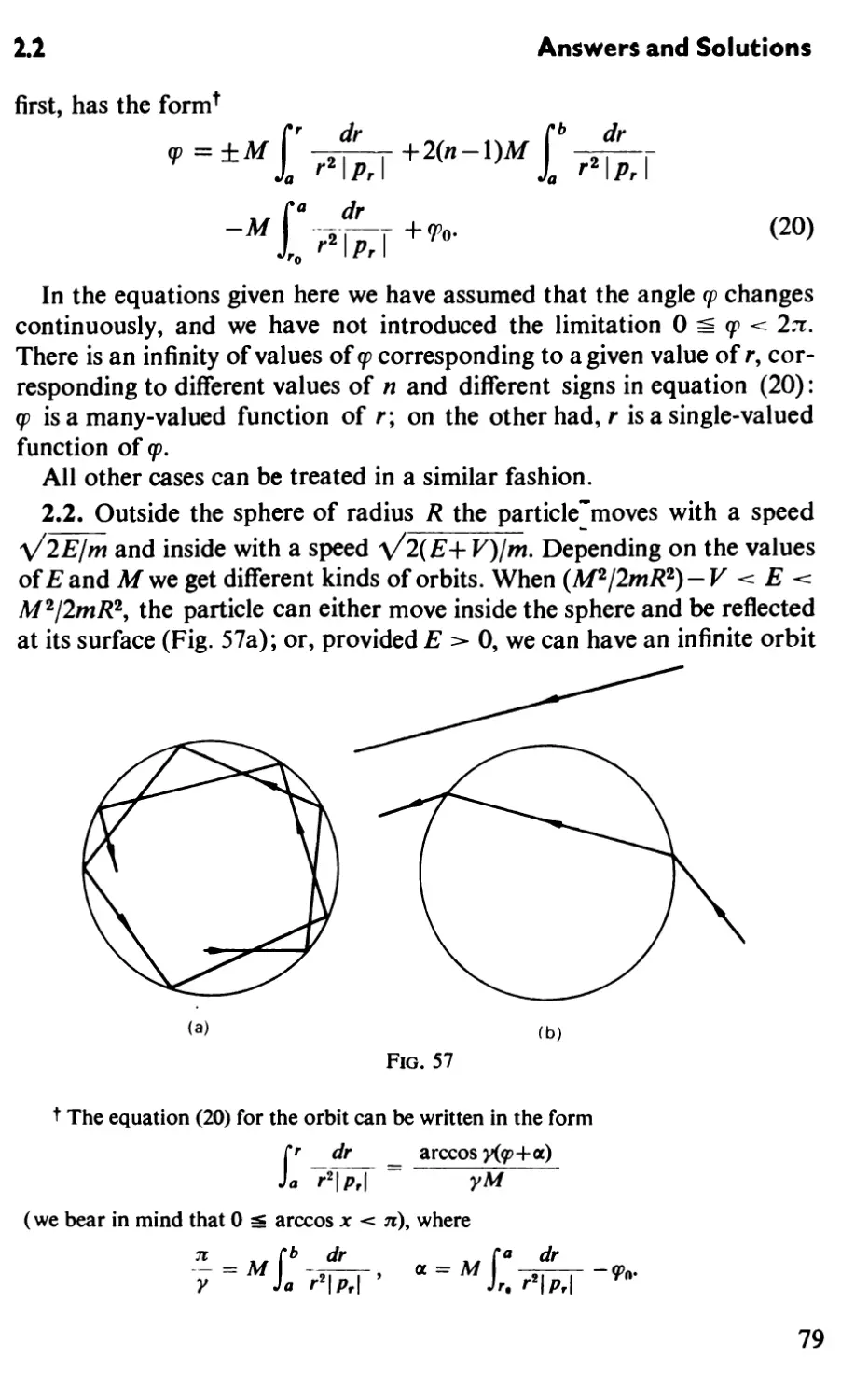
2.2. Find the trajectories for a particle moving in the potential
(/(r) = -K, r^R; U(r) = 0, r > R
(Fig. 5: "spherical rectangular potential well") for different values of the
angular momentum and of the energy.
ui
Fig. 5
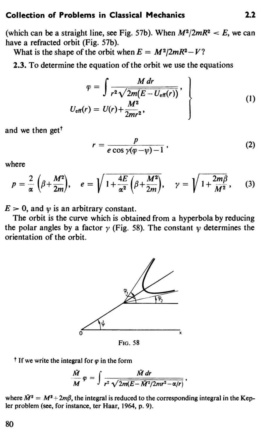
2.3. Determine the trajectory of a particle in the potential U = a/r-h/S/r2.
Give an expression for the change in the direction of the velocity when the
particle is scattered as a function of angular momentum and energy.
2.4. Determine the trajectory of a particle in the potential (/ =
a/r—(i/r2. Find the time it takes the particle to fall to the centre of the
potential from a distance r. How many revolutions around the centre
will the particle then make?
2.5. Determine the trajectory of a particle in the potential U =
— a/r-f-/9/r2. Find the angle Acp between the directions of the radius
vector at two successive passages through the pericentre (that is, when
6

2.14
Problems
r=rmin); find also the period of the radial oscillations, Try and the
period of revolution, T^. Under what conditions will the orbit be a
closed one?
2.6. Determine the orbit of a particle in the potential U = — a/r—/?/r2.
2.7. For what values of the angular momentum M is it possible to have
finite orbits in the potential U(r) for the following cases:
(b) U = -Ve-**rn
2.8. A particle falls from a finite distance towards the centre of the
potential U = —ar~n. Will it make a finite number of revolutions around
the centre? Will it take a finite time to fall towards the centre? Find the
equation of the orbit for small r.
2.9. A particle in the potential U(r) flies off to infinity from a distance
r t* 0. Is the number of revolutions around the centre, made by the
particle, finite for the following cases:
«" = £.
(b)tf = -£?
2.10. How long will it take a particle to fall from a distance R to the
centre of the potential U = — a/r? The initial velocity of the particle is
zero. Treat the orbit as a degenerated ellipse.
2.11. Determine the minimum distance between two particles, the one
approaching from infinity with an impact parameter q and an initial
velocity v and the other one initially at rest. The masses of the particles are m\
and w2, and the interaction law is U = ar~n.
2.12. Determine in the centre of mass system the finite orbits of two
particles of masess wi and /w2, and an interaction law U = —a/r.
2.13. Determincthe position of the focus of a beam of particles close to
the beam axis, when the particles are scattered in a potential U(r) under
the assumption that a particle flying along the axis is turned back.
2.14. Find the inaccessible region of space for a beam of particles
flying along the z-axis with a velocity v and being scattered by a potential
U = a/r.
7

Collection of Problems in Classical Mechanics
2.15
2.15. Find the inaccessible region of space for particles flying with a
velocity v from a point A in all directions and moving in a potential
U = -a/r.
2.16. Use the integral of motion A = [v/\M]—&(r/r) to find the orbit of
a particle moving in the potential U = —a/r.
2.17. Determine the change in the angular momentum and energy
dependence of the period of radial oscillations of a point particle moving
in a potential U(r) when this potential is changed by a small amount
dU(r).
2.18. Show that the orbit of a particle in the potential U = —ae~r/D/r
is a slowly precessing ellipse when rmax <sc D. Find the velocity of
precession.
2.19. Find the precessional velocity of the orbit in the potential U =
—a/r1+e, when \e\ «: 1.
2.20. Find the change in the period of the radial oscillations, in the
period of revolution, and in the angle between the radius vectors at two
successive passages through the pericentre
(a) when the energy is changed by a small amount dE, and
(b) when the potential is changed instantaneously by a small amount
dU(r).
2.21. Find the equation of motion of the orbit of a particle moving in
the potential U(r) = - a/r+y/r3, assuming y/r3 to be a small correction to
the Coulomb field.
2.22. Show that the problem of the motion of two charged particles in
a uniform electrical field E can be reduced to the problem of the motion of
the centre of mass and that of the motion of a particle in a given potential.
2.23. Under what conditions can the problem of the motion of two
charged particles in a uniform magnetic field be separated into the
problem of the centre of mass motion and the relative motion problem?
Take the vector potential in the form A = \[H/\r],
2.24. Express the kinetic energy, the linear momentum, and the angular
momentum of a system of N particles in terms of the Jacobi coordinates
_ m1r1+...+mJrJ
*'- Wl+...+„,, r'+i> 7-1,2,...,7V 1,
t _ miriH-.. .+m^r^
^N " mi+...+mN '
8

2.32
Problems
2.25. A particle with a velocity v at infinity collides with another
particle of the same mass m which is at rest. Their interaction potential is
U = cajf1 and the collision is a central one. Find the point where the first
particle comes to rest.
2.26. Prove that
(M.#) + ^([rA#]HrA#]), where M = m[rAv],
is an integral of motion for a charged particle moving in a uniform
magnetic field //.
2.27. Give a qualitative description of the motion and the shape of the
orbit of a particle moving in the field of a magnetic dipole Jtl in the plane
perpendicular to the dipole. Take the vector potential in the form A =
M/Ar]/r>.
2.28. (a) Give a qualitative description of the motion of a charged
particle in the potential U = ymAr2, where r is the distance from the z-axis
(the field of a uniformly charged cylinder), for the case where there is a
uniform magnetic field //parallel to the z-axis present.
(b) Find the orbit of a charged particle moving in the potential
U(r)=oc/r2 in a plane perpendicular to a constant uniform magnetic field H.
2.29. A charged particle moves in the Coulomb field U = — a/r in a
plane perpendicular to a uniform magnetic field //.
Find the orbit of the particle. Study the case where the potential U(r) is
a small perturbation and the case when His small.
2.30. Describe the motion of two identical charged particles in a
uniform magnetic field H for the case when their orbits lie in the same plane
which is perpendicular to H and where we may consider their interaction
energy U = e2/r to be a small perturbation.
2.31. Show that the quantity
(F,[pAM])-a(F^l^jfFArHFAr])
is a constant of motion in the potential U(r) = — a/r—(F«r). Give the
meaning of this integral of motion when F is very small.
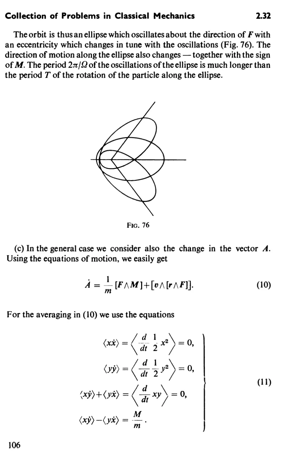
2.32. Study the effect of a small extra term dU = -(F-r) added to the
Coulomb potential on the finite orbit of a particle.
(a) Find the average rate of change of the angular momentum, averaged
over one period;
PCM2
9

Collection of Problems in Classical Mechanics 2.32
(b) Find the time-dependence of the angular momentum, the size, and
the orientation of the orbit for the case when the force Flies in the orbital
plane;
(c) Do the same as under (b) for the case when the orientation of F is
arbitrary.
2.33. Find the systematic displacement of a finite orbit of a charged
particle moving in the potential U(r) = —oLJr and in the field of a
magnetic dipole JIL, if the effect of the latter may be considered to be a small
perturbation. Take the vector potential in the form A = [J/f /\r]/r*.
Hint: Write down the equations of motion for the vectors M =
m[rf\v] and B = [v/\M]—ccr/r averaged over one period, and solve
them.
3. Scattering in a Given Field. Collisions between Particles
3.1. Find the differential cross-section for the scattering of particles
with initial velocities parallel to the z-axis by smooth elastic surfaces of
revolution g(z) for the following cases:
z
(a) q = b sin — , 0 ^ z ^ na\
a2 a2
(b)g = 6- —, -^-^z<oo.
(c) q = Azn, n > 0, n ^ 1;
3.2. Find the surface of revolution which is such that the cross-section
for elastic scattering by this surface is the same as the Rutherford
scattering cross-section.
3.3. Find the differential cross-section for the scattering of particles by
a spherical "potential barrier":
U(r)=V, r^a; U(r) = 0, r > a.
3.4. Find the cross-section for the process where a particle falls towards
the centre of the potential U(r) when U(r) is given by:
(» W = 7--£;
10

3.12
Problems
3.5. Calculate the cross-section for a particle to hit a small sphere of
radius R placed at the centre of the potential U(r) for the cases:
(a) u(r) = ~, «S2;
(b) tf(r) = -£--£.
3.6. Find the differential cross-section for the scattering of particles by
the potential U(r) = <x/r-<x/R, r < R; U(r) = 0, r > R.
3.7. Find the differential cross-section for the scattering of fast particles
(£»K) by the potential U(r) = F(l-r2/*2), r < R; U(r) = 0, r > R.
3.8. Calculate the differential cross-section for small angle scattering in
the potential U(r) = Plr*-*lr2.
3.9. Find the differential cross-section for the scattering of particles by
the potential U(r) = -air2.
3.10. Find the differential cross-section for the scattering of fast parti
cles (E:» V) by the following potentials U(r):
(a) C/(r) = Ver^%\
Study in detail the limiting cases when the deflecting angle is close to
its minimum or to its maximum value.
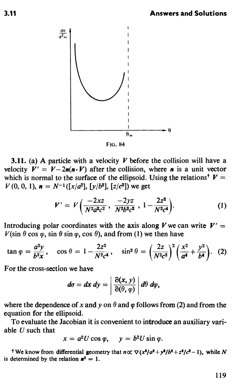
3.11. A beam of particles with their velocities initially parallel to the
z-axis is scattered by the fixed ellipsoid
a2 + b2^ C2 '•
Find the differential scattering cross-section for the following cases:
(a) the ellipsoid is smooth and the scattering elastic;
(b) the ellipsoid is smooth and the scattering is inelastic;
(c) the ellipsoid is rough and the scattering elastic.
3.12. Find the differential cross-section for small-angle scattering by
the following potentials U(r) (a is a constant vector):
(a) U(r) = ^fi- ;
(b)C/(r)=^.
2*
11

Collection of Problems in Classical Mechanics
3.13
3.13. Find the change in the differential cross-section for the
scattering of a particle by the potential U{r) when U(r) is varied by a small
amount dU(r) for the following cases:
(a) U(r) = " , dU(r) = -£ ;
(b)C/(r)=", *£/(r) =-£-;
(c) U(r) = £ , 6U(r) = -£ .
3.14. Find the differential cross-section as function of the energy
acquired by fast particles (E:» Vlt 2) due to their scattering in the
potential U(r,t) = [Vi(r)+V2(r)sino)i]e-**r2.
3.15. A particle with velocity V decays into two identical particles. Find
the distribution of the secondary particles over the angle of divergence,
that is, the angle between the directions at which the two secondary
particles fly off. The decay is isotropic in the centre-of-mass system and the
velocity of the secondary particles is Vo in that system.
3.16. Find the energy distribution of secondary particles in the
laboratory system, if the angular distribution in the centre-of-mass system is
3 sin2 0o rf2<o/87t (d2<o = sin 0O dd0 d<p), where 0O is the angle between the
velocity V of the original particle and the direction in which one of the
secondary particles flies off in the centre-of-mass system. The velocity of
the secondary particles in the centre-of-mass system is V0.
3.17. An electron moving at infinity with velocity V collides with
another electron at rest; the impact parameter is q. Determine the
velocities of the two electrons after the collision.
3.18. Find the range of possible values for the angle between the
velocity directions after a moving particle of mass mi has collided with a
particle of mass m2 at rest.
3.19. Find the differential cross-section for the scattering of inelastic
smooth spheres by similar ones at rest.
3.20. Find the change in the intensity of a beam of particles travelling
through a volume filled with absorbing centres; their density is n cm-3,
and the absorption cross-section is a.
3.21. Find the number of reactions occurring during a time dt in a vo 1-
12

4.5
Problems
ume element d3r when two beams with velocities V\ and V2 and densities
«i and n2, respectively, collide. The reaction cross-section is a.
3.22. A particle of mass M moves in a volume filled with particles of
mass m (<sc M) which are at rest initially. The cross-section for the
scattering of M by m is dcr/d2^ = f(0), and the collisions are assumed to be
elastic.
(a) Find the "frictional force" acting on M,
(b) Find the average of the square of the angle over which M is deflected.
4. Lagrangian Equations of Motion. Conservation Laws
4.1. A particle, moving in the potential U(x) = —Fx, travels from the
point x = 0 to the point x = a in a time r. Find the time-dependence
of the position of the particle, assuming it to be of the form x(t) =
At2+Bt+C, and determining the constants A,B, and C such that the
action is a minimum.
4.2. A particle moves in the xy-plane in the potential U(x, y) = 0,
x < 0; U(x, y) = V, x > 0, and travels in a time r from the point ( — a, 0)
to the point (a9 a). Find its position as a function of time, assuming that it
satisfies the equations
X\t 2 = A\% 2t-\-B\% 2,
yi, 2 = Cit2t+Dit2.
The indices 1 and 2 refer, respectively, to the left-hand (x < 0) and
right-hand (x > 0) half-planes.
4.3. Prove by direct calculation the invariance of the Lagrangian
equations of motion under the coordinate transformation
<li = 4i(Qu (?2, ..., Ci, 0, / = 1, 2, ..., s.
4.4. What is the change in the Lagrangian in order that the Lagrangian
equations of motion retain their form under the transformation to new
coordinates and "time":
4/ = 4t(Qu (?2, ..., Qs, t), i = 1, 2, .. .9s;
t = t(QuQ2, ...,0.,t).
4.5. Write down the Lagrangian and the equations of motion for a
particle moving in a potential U(x), introducing a "local time" r = t—lx.
13

Collection of Problems in Classical Mechanics 4.6
4.6. How does the Lagrangian
transform when we change to the coordinate q and "time" t through the
equations:
x = #cosh A+rsinh A,
t = q sinh X + r cosh A?
4.7. How do the energy and the generalised momenta change under the
coordinate transformation
qi=fiQu ...,&, o, /= i, ...,*?
4.8. How do the energy and the generalised momenta which are
conjugate to (a) the spherical polar and (b) the Cartesian coordinates transform
under a change to a coordinate system which is rotating around the z-axis?
(a) (p = (p'+Qt, r = r'\
(b) x = x' cos Qt -y' sin Qt,
y = x' sin Qt+y' cos Qt.
4.9. How do the energy and momenta change when we change to a
frame of reference which is moving with a velocity VI Take the Lagrangian
L' in the moving frame of reference in either of two forms:
(a) L[ = L(r'+ Vt, r'+ V, f), where L(f, r, /) is the Lagrangian in the
original frame of reference;
(b) L'2 = £ \mav'*- U(r' + Vt9 t). Here L'2 differs from L[ by the total
a
derivative with respect to the time of the function / V* £ mjr'a\ + \ V2tY,ma-
4.10. Consider an infinitesimal transformation of the coordinates and
the time of the form
q\ = qi + eW£q91\ t' = t+eX(q, t), e - 0.
Show that if the action is invariant under this transformation,
14

4.15
Problems
the quantity
is an integral of motion.
4.11. Generalise the theorem of the preceding problem to the case when
under the transformation of the coordinates and the time the action
changes in the following way:
4.12. Find the integrals of motion if the action remains invariant under:
(a) a translation;
(b) a rotation;
(c) a shift in the origin of the time;
(d) a screw shift;
(e) the transformation of problem 4.6.
4.13. Find the integrals of motion for a particle moving in
(a) a uniform field U(r) = — (F*r);
(b) a potential U(r)9 where U(r) is a homogeneous function,
U(ocr) = ocnU(r);
specify for what values of n the similarity transformation leaves
the action invariant;
(c) the field of a travelling wave U(r, i) = U(r— Vt), where V is a
constant vector;
(d) a magnetic field specified by the vector potential A(r), where A(r) is
a homogeneous function;
(e) an electromagnetic field rotating with a constant angular velocity Q
around the z-axis.
4.14. Find the integral of motion corresponding to the Galilean
transformations.
Hint: Use the result of problem 4.11.
4.15. Find the integrals of motion of a particle moving in a uniform
magnetic field H, if the vector potential is given in the form
(a) A = l[Hhr];
(b) Ax = Az = 0, Av = Hx.
15

Collection of Problems in Classical Mechanics
4.16
4.16. Find the integrals of motion of a particle moving in
(a) the field of a magnetic dipole, A = [Jfl/\r]/r*9 JH = constant;
(b) the Rubenchik field, Av = /i/r, Ar = A2 = 0.
4.17. Find the equations of motion of a system with the following
Lagrangian:
(a) L(x,x) = e-*(e-** + 2x V e~at do\ ;
(b) L(x, x, t) = ie*'(x2-a)*x2).
4.18. Write down the components of the acceleration vector for a
particle
(a) in the system of spherical polars;
(b) for the case of orthogonal coordinates qh if the line element is
given by the equation
ds* = h\dq\+h\dq\ + h\dq\,
where h( = h,{qu q2, q$) are the Lam6 coefficients.
4.19. Write down the equations of motion of a point particle using
arbitrary coordinates qt which are connected with the Cartesian coordinates
xt by the relations:
(a) x( = Xi(qu q2, qs), i= 1, 2, 3;
(b) xt = Xi(qu q2, qs, t), i = 1, 2, 3.
4.20. Verify that one can use the Lagrangians
L1=iM-Uql9
*» = -#+"«».
where q\ = / is the current flowing through the inductance J2 in the
solenoid from A to B (Fig. 6a), q2 the charge on the upper plate of the
capacitor (Fig. 6b), and C/the voltage between A and B (U = (Pb—<Pa)>
to find the correct "equations of motion" for the qi and the correct energies.
\¥
\ .1
) u
(3)
(b)
Fig. 6
16

4.23
Problems
4.21. Use the additivity property of the Lagrangians and the results of
the preceding problem to find the Lagrangians and the Lagrangian
equations of motion for the circuits of Figs. 7a, b, c.
My
u
o
ft
Hh
(a)
(b)
Fig. 7
(c)
4.22. Find the Lagrangians for the following systems :
(a) a circuit with a variable capacitor, the movable plate of which is
connected to a pendulum of mass m (Fig. 8a), and the capacitance
of which is a known function C(cp) of the angle y the pendulum
makes with the vertical. The mass of the capacitor plate may be
neglected;
(b) a core suspended from a spring with elastic constant x inside a
solenoid with inductance J2(x) which is a given function of the
displacement x of the core (Fig. 8b).
(b)
Fig. 8
4.23. A perfectly conducting square frame can rotate around a fixed
side AB of length a (Fig. 9). The frame is placed in a constant uniform
magnetic field H at right angles to the AB-axis. The inductance of the
frame is -£, the mass of the side CD is m, and the masses of the other sides
may be neglected. Describe qualitatively the motion of the frame.
17

Collection of Problems in Classical Mechanics
4.24
Fig. 9
Fig. 10
4.24. Use the method of the Lagrangian or undetermined multipliers to
obtain the equations of motion for a particle in the field of gravity when it
is constrained to move
(a) along a parabola z = ax2 in a vertical plane;
(b) along a circle of radius / in a vertical plane.
Determine the forces of constraint.
4.25. A particle moves in the field of gravity along a straight line
which is rotating uniformly in a vertical plane. Write down the equations
of motion and determine the moment of the forces of constraint.
4.26. One can describe the influence of constraints and friction on the
motion of a system by introducing generalised constraint and friction
forces into the equations of motion:
d_ 9L_ 9L
dt dqt dqt
(a) How does the energy of the system vary with time?
(b) What is the transformation of the Ri which leaves the equations of
motion invariant under a transformation to new generalised coordinates:
qt = qtQu ...,0«O?
4.27. Let the constraint equations be of the form
s
tip = Z bpnqn* /3 = 1, ..., r,
n = r + 1
while the Lagrangian L(qr+1, ..., qS9 qu ..., qs, 0 and the coefficients
bpn do not depend on the qfi.
Show that the equations of motion can be written in the form
d dL dL ' dL * / 3bfim dbpn\
* 3^» 3?» 0=1 99/>
18

5.1
Problems
where L(qr+l, ..., qs, qr+1, ..., qs, t) is the function obtained fromL by
using the constraint equations to eliminate the velocities 4u ..., qr.
4.28. A continuous string can be thought of as the limiting case of a
system of N particles (Fig. 10) which are connected by an elastic thread, in
the limit as N — °°, a — 0, Na = constant. The Lagrangian for a discrete
system is
N+l
Hqu — -9qN94u-"94N>t)= £ L„(qn,qn-q„_i,4n,t), (q0=qN+1 = 0)
n = 1
where qn is the displacement of the n\h particle from its equilibrium
position.
(a) Obtain the equations of motion for a continuous system as the
limiting case of the Lagrangian equations of motion for a discrete system.
(b) Obtain an expression for the energy of a continuous system as the
limiting case of the expression for the energy of a discrete system.
Hint: Introduce the coordinate x of a point on the string together
with the expressions obtained as a result of taking the limit as a -* 0,
n = xja -* oo:
-* (*•*!!• -?!-•')= *mU9m*-*-u4mt).
4.29. A charged particle moves in a potential U(r) and a constant
magnetic field H(r)9 where U(r) and H(r) are homogeneous functions of
the coordinates of degrees k and n, respectively, that is, U(<xr) =■ ockU(r),
H(ocr) = ocnH(r). Develop for this system the similarity principle,
determining for what value of n it holds.
4.30. Generalise the virial theorem for a system of charged particles
in a uniform magnetic field H. The potential energy U of the system is a
homogeneous function of the coordinates, U(<xr\,.. .,ocrs)=akU(ri, ..., rs)
and the system moves in a bounded region of space with velocities which
remain finite.
5. Small Oscillations of Systems with One Degree of Freedom
5.1. Find the frequency of the small oscillations for particles moving in
the following potentials:
(a) U(x) = V cos QLx-Fx\
(b) U(x) = F(a2x2-sin2ax).
19

Collection of Problems in Classical Mechanics
5.2
5.2. Find the frequency of the small oscillations for the system depicted
in Fig. 11. The system rotates with an angular velocity Q in the field of
gravity around a vertical axis.
5.3. A point charge q of mass m moves along a circle of radius R in a
vertical plane. Another charge q is fixed at the lowest point of the circle
(Fig. 12). Find the equilibrium position and the frequency of the small
oscillations for the first point charge.
CD"
Fig 11
5.4. Describe the motion along a curve close to a circle for a point
particle in the central field U(r) = - a./rn (0 < n < 2).
5.5. Find the frequencies of the small oscillations of a spherical
pendulum (a particle of mass m suspended from a string of length /), if the angle
of deflection from the vertical oscillates about the value 0o.
5.6. Find the correction to the frequency of the small oscillations of a
diatomic molecule due to its angular momentum M.
5.7. Determine the eigen-oscillations of the system shown in Fig. 13
for the case when the particle moves (a) horizontally, and (b) vertically.
How does the frequency depend on the tension in the springs in the
equilibrium position ?
x m x
Fig. 13
20

5.10
Problems
5.8. Find the eigen-oscillations of the system in Fig. 14 in a uniform field
of gravity for the case when the particle can only move vertically.
5.9. Find the stable small oscillations of a pendulum when its point of
suspension moves uniformly along a circle of radius R with frequency Q
(Fig. 15). The pendulum length is / (/:» R).
Fig. 14
Fio. 15
P
-o u o-
Fig. 16
5.10. Find the stable oscillations in the voltage across a capacitor and
the current in a circuit with an e.m.f. U(i) = U0 cos cot (Fig. 16).
21

Collection of Problems in Classical Mechanics
5.11
5.11. Describe the motion with friction of an oscillator which initially
is at rest and which is acted upon by a force F(t) = F cos yt.
5.12. Determine the energy E acquired by an oscillator under the action
of a force F(t) = Fe~0/T^ during the total time it acts
(a) if the oscillator was at rest at / = — <»;
(b) if the amplitude of the oscillator at / = — oo was a.
5.13. Describe the motion under the action of a force F(t)
(a) of an unstable system described by the equation
x-fi2x= l F(t);
m
(b) of an oscillator with friction:
x + 2kx + colx = F(t).
5.14. Find the differential cross-section for an isotropic oscillator to be
excited to an energy £ by a fast particle (E^> V) if the interaction between
the two particles is through the potential U(r) = Ve~*trl. The energy of
the oscillator is zero initially.
5.15. An oscillator can oscillate only along the z-axis. Find the
differential cross-section for the oscillator to be excited to an energy e by a fast
particle (E^> V\ if the interaction between the particles is through the
potential U(r) = Ve~xlr*. The particle moves along the z-axis with
velocity Voo, and the initial energy of the oscillator is £o.
5.16. A force F(t), for which F(— oo) = 0, F(oo) = F0, acts upon an
harmonic oscillator. Find the energy gained by the oscillator during the
total time the force acts, and the amplitude of the oscillator as t-+ + oo, if
it were at rest at / = — «>.
5.17. Find the energy acquired by an oscillator under the action of the
force
F(t) = iFoe*', t < 0; F(t) = |F0(1 -*-*), / > 0.
At / = — oo the energy of the oscillator was E0.
5.18. Estimate the change in the amplitude of the vibrations of an
oscillator when a force F(t) is switched on slowly and smoothly over a period
22

S.19
Problems
r so that (ox » 1. Assume F{i) = 0 for / < 0, F(t) = F0 for / > t, while
F<k\t) ~ Folrk (k = 0, 1, ..., n+1) for 0 < / < r and F<*>(0) = F(*>(r)
= 0 (s = 1, 2, ...,«— 1), while the /rth derivative of the force has a
discontinuity at / = 0 and at t = r.
5.19. Find the stable oscillations of an oscillator which is acted upon by
a periodic force in the following two cases:
(a) F(t) = (t/r-n)F, when m ^ / < (w+ 1)t (Fig. 17);
(b)F(0 = (l-*~a'V. r' = r-/iT, when m ^ /< (w+1)t (Fig. 18).
FA
Fio. 17
Fig. 18
23

Collection of Problems in Classical Mechanics 5.19
(c) Find the stable current through the circuit of Fig. 16 in which
there is an e.m.f. U(t) = V{tjx-n) for nx ^ / < (h+1)t. The internal
resistance of the battery is zero.
5.20. An oscillator with eigen-frequency co0 and with a friction force
acting upon it given by/fr = — 2mXx has an additional force F{i) acting
upon it.
(a) Find the average work done by F(i) when the oscillator is vibrating
in a stable mode for the case when
F(t) =fi cos cot +f2 cos 2cot.
(b) Repeat the calculations for the case when
H0= ~E aneinMt, a_n = a*n.
n= — oo
(c) Find the average over a long time interval of the work done by the
force
F(t) = f\ cos co it +/2 cos co2t,
when the oscillator performs stable vibrations.
(d) Find the total work done by the force
F(t) = y)(co) eio,t dco, y>(-co) = y)*(co)
for the case where the oscillator was at rest at / = — oo.
6. Small Oscillations of Systems with Several Degrees of Freedom
6.1. Find the normal oscillations of the system of Fig. 19 for the case
when the particles can move only vertically.
6.2. Three masses which are connected by springs move along a circle
(Fig. 20). The point A is fixed. Find the eigen-vibrations of the system.
Find the normal coordinates and express the Lagrangian in terms of
those coordinates.
24

6.5 Problems
6.3. Find the eigen-vibrations of a system described by the Lagrangian
What is the trajectory of a point with Cartesian coordinates x, yl
6.4. Find the normal coordinates of the systems with the following
Lagrangians :
(a) L = i(^2+f)-lKx2+^2)+ax};;
(b) L = Ur"ix2+m2y2)+Pxy-i(x*+y*).
6.5. Find the eigen-oscillations of a system of coupled circuits (Figs.
21a and b).
'/m'///<
Fig. 19
i 'TRKRRP-
*2
-'WWP 1
(a)
Fig. 21
^2
(b)
PCM 3
25

Collection of Problems in Classical Mechanics
6.6
6.6. Find the normal coordinates of a system of particles which are
connected by springs (Fig. 22). The masses can move only along the straight
line AB. Find the eigen-vibrations of the system.
'/A
VA mi m2
:aJVWWW\AA/WWWW^
g4 *1 *2 *3
Fig. 22
//
I
1
B-
'AVWWWWWWWWWWWWWWVWWWWVWWWtB'
% X1 V/
Fig. 23
6.7. Find the eigen-vibrations of the system of Fig. 23 where the
particles can move only along the straight line AB
(a) if at / = 0 one of the particles moves with velocity v while the second
particle is at rest and the displacements from the equilibrium
positions of both particles are zero;
(b) if at / = 0 one of the particles is displaced from its equilibrium
position over a distance a, while the other is at its equilibrium position
and both particles are at rest.
6.8. Determine the flux of energy from one particle to the other in the
preceding problem.
6.9. Find the eigen-vibrations of the system of Fig. 23 if each of the
particles is acted upon by a frictional force which is proportional to its
velocity.
6.10. Find the eigen-oscillations of three identical particles which are
connected by identical springs and which move along a circle (Fig. 24).
Determine the normal coordinates which reduce the Lagrangian to a
sum of squares.
6.11. Find the normal vibrations of the system of particles considered in
the preceding problem, if at / = 0 one of the particles is displaced from its
equilibrium position. The initial velocities are zero.
6.12. Find the normal coordinates of a system of four identical particles
moving along a circle (Fig. 25).
26

6.13 Problems
Fig. 25
6.13. Find the eigen-vibrations[of the system of particles of Fig. 26 such
that the particles do not move out of the plane of the figure. All particles
and springs are identical. The tensions in the springs at equilibrium are
equal to/ = xl, where / is the equilibrium distance between the masses.
3#
27

Collection of Problems in Classical Mechanics 6.14
Fig. 26
6.14. Consider a system with Lagrangian
L = i £ mU*iXj ~i E *UxixJ> mU = ™jh *U = *ji •
US I. J
Let their eigen-oscillations be given by the equations
jtf>(t) = A\° cos ((Oit+tpj).
Prove that the amplitudes corresponding to oscillations with different
frequencies ty and cos satisfy the relations
i.J i>J
6.15. (a) Find the eigen-vibrations of the system of Fig. 27. All particles
and springs are identical. The tension in the springs at equilibrium is
/ = «/, where / is the equilibrium distance between the particles.
(b) Find the eigen-vibrations of the system of four identical particles of
Fig. 27 for the case where the mass of particle 5 is put equal to zero. The
elasticity coefficients and the tensions at equilibrium are the same as
before.
28

6.16
Problems
Fig. 27
Hint for both (a) and (b): several of the eigen-vibrations are obvious.
The determination of the others can be simplified by using the relations of
the preceding problem.
6.16. Find the eigen-vibrations of the systemof particles of Fig. 28a;
the particles move along a circle.
2m
29

Collection of Problems in Classical Mechanics 6.17
M
Fig. 28b
6.17. Find the eigen-vibrations of a system of four particles moving
along a circle (Fig. 28b). All springs are identical and the masses of
particles 1 and 3 are m, while those of particles 2 and 4 are M.
6.18. Which of the eigen-vibrations of the system of Fig. 24 remain
practically unchanged when the following small changes are made in the
system:
(a) the elasticity of the spring AB is changed by a small amount bx\
(b) a small mass dm is added to particle C;
(c) a small mass dmi is added to particle C and 6w2 to particle B?
6.19. Describe the eigen-vibrations of the system of the preceding
problem for the cases (a) and (b) if initially the particles A and C are displaced
over equal distances in opposite directions so as to decrease their mutual
distance. All velocities are initially zero.
6.20. Find the eigen-vibrations of the system of Fig. 25 which are
practically the same as the eigen-vibrations of the system which is obtained
(a) by adding identical small masses to particles A and B;
(b) by changing the elasticity coefficients of the springs AB and CD by
equal amounts;
(c) by adding an extra mass to particle A.
30

6.25
Problems
6.21. The masses A and C of the system described in problem 6.20(b)
are at time / = 0 displaced by the same amount from their equilibrium
positions in opposite directions so as to decrease their distance apart. Ini"
tially all velocities are equal to zero. Describe the eigen-vibrations of the
system.
6.22. Determine the eigen-vibrations of the system of Fig. 27 if at / = 0
the masses 1 and 4 are displaced over equal distances in the horizontal
direction in such a way that their distance apart decreases. At / = 0 the
velocities of all particles are equal to zero. The tension in the springs is
/= */i, l—li<^l, where / is the equilibrium distance between the
particles (compare problem 6.21).
6.23. Determine the eigen-vibrations of an anisotropic charged
harmonic oscillator moving in the potential U(r) = \m(w\x2+(o\y2+to\z2') and
in a uniform magnetic field H which is parallel to the z-axis. Consider in
particular the following limiting cases:
(a) \oH\ « |g)i-co2|;
(b) \o)H\ »colt2;
(c) cot = co2:» \coH\,
where coH = eH/mc.
6.24. Determine the eigen-vibrations of an anisotropic charged harmonic
oscillator moving in a potential U(r) = ^(cof^H-co^-l-co^andina
weak magnetic field H = (Hx, 0, Hz\ considering the effect of the
magnetic field to be a small perturbation.
6.25. A mathematical pendulum is part of an electric circuit (Fig. 29).
A constant, uniform magnetic field H is applied at right angles to the
plane of the figure. Find the eigen-vibrations of this system.
y/////y
Fig. 29
31

Collection of Problems in Classical Mechanics
6.26
6.26. Find the stable oscillations of the system of particles of Fig. 19,
if the point of suspension A moves vertically according to the equation
(a) a cos cor,
(b) a(t)
= al Ail for nr ^ / < (h4-1)t.
Plot a diagram of the frequency-dependence of the amplitude of the
vibrations for the case (a). What is the change in the diagram when there
is friction present?
6.27. Determine the stable oscillations of the system of Fig. 23 if the
point A moves according to the relation a cos cot.
6.28. Determine the stable oscillations of the mass m in Fig. 30 moving
in a variable uniform field described by the potential U(r) = — (F(t) «r) for
the following cases:
(a) F(t) = F0 cos cot;
(b) the vector F rotates with constant absolute magnitude with a
frequency co in the plane of the figure.
££^
Fig. 30
6.29. Find the stable oscillations of a system of two particles which
move along a circle (Fig. 31) for the case when the point A moves along
the circle according to the relation a cos cot. Study the way the amplitude
of the oscillations depends on the frequency of the applied force.
6.30. Find the stable oscillations of the system of particles of Fig. 20
for the case when the point A moves along the circle according to the
relation a cos cot.
32

6.32
Problems
Fig. 31
6.31. We can write the stable oscillations of a system described by the
Lagrangian
L = i £ rriijXiXj —i- £ xtjXiXj+ £ Xifi cos cot
ij
i.j
in the form
xfc) = YtX°40 c°s cot
i
(see problem 6.14). Why?
Express the coefficients A(/) in terms of the/) and the A\l).
Study the co-dependence of the A(/).
Show that A(*> = 0, if Y*fiA¥* = ° for the ^h oscillation.
6.32. The system of particles of Fig. 32 is symmetric with respect to
the line CD.
^^ ^^
+- -
Fig. 32
33

Collection of Problems in Classical Mechanics 6.32
(a) Show that if the eigen-oscillations of the system are non-degenerate,
the amplitudes of the oscillations of the different particles are distributed
either symmetrically or antisymmetrically with respect to the centre.
(b) Show that if there is degeneracy, one can always choose the normal
oscillations such that they are either symmetrical or antisymmetrical.
6.33. Show that if the points A and B (Fig. 33) move symmetrically or
antisymmetrically, several of the eigen-vibrations of the system of Fig. 33
will not be excited.
6.34. Use symmetry considerations to find the vectors of the normal
vibrations of the system of particles of Fig. 26.
6.35. Find the stable oscillations of the system of Fig. 23, if the point
A moves according to a cos cot. Assume that there are frictional forces
acting upon the particles proportional to their velocities.
6.36. Describe the motion of the system of Fig. 22 if at / = 0 the
particles are at rest at their equilibrium positions while the point A moves
according to a cos cot. Take the masses to be equal (nti = m2 = m).
6.37. Determine the eigen-vibrations in a plane of a molecule which has
the shape of an equilateral triangle. Assume that the potential energy
depends only on the distances between the atoms and that all atoms are
the same. The angular momentum is equal to zero up to terms of first
order in the amplitude of the oscillations.
6.38. Use symmetry arguments to determine the degree of degeneracy of
various frequencies for the case of a "molecule" consisting of four
identical atoms which has the form of a regular tetrahedron at equilibrium.
7. Oscillations of Linear Chains
Chains of particles connected by springs are the simplest model used in
the theory of solids (see, for example, Wannier, 1959, or Kittel, 1968). The
electrical analogues of such lines are r.f. lines employed in radio
engineering.
7.1. Determine the frequencies of the normal oscillations of a system of
N identical particles with masses m connected by identical springs with
elastic constants x and moving along a straight line (Fig. 33a).
Hint: Express the normal oscillations in terms of standing waves.
7.2. Repeat this for the system of Fig. 33b with one free end.
34

7.7
Problems
4 ^wwvwwvw aaaa*wvt a Ja/vwwaaaa/wv*-—'vwvaaaa*
ni m M m M k \i i
HaAA*WWW*AAAA- - >W\^/W!\A>V\AAAMAAA^WWWV^ - -AA/WNAAAA*
1 I^ixkxKKx*
(d> , ,e) <c>
lA/WV\MAAA/WWWW\Ar MAAAAAA/1.
^ x K x K x K '
(f)
Fig. 33
7.3. Find the eigen-vibrations of N particles which are connected by
springs and which can move along a circle (Fig. 33c). All particles and the
elastic constants of all springs are the same. Check that if the motion is
that of a wave travelling along the circle, the energy flux equals the
product of the linear energy density and the group velocity.
7.4. Determine the frequencies of the eigen-vibrations of a system of
particles moving along a straight line for the following cases (take the hint
of problem 7.1 into account):
(a) 2N particles, alternating with masses m and M connected by springs
of elastic constant x (Fig. 33d);
(b) 2N particles of mass m connected by springs with alternating elastic
constants x and K (Fig. 33e);
(c) 2N+1 particles of mass m connected by springs with alternating
elastic constants x and K (Fig. 33f).
7.5. (a) Determine the eigen-vibrations of the system of Fig. 33a if the
point A moves according to a cos cot.
(b) Do the same for the system of Fig. 33b.
7.6. Do the same for the system of Fig. 33d.
7.7. Determine the eigen-vibrations of a system of AT particles which
move along a straight line for the following cases:
(a) mt = m ?± mN, i = 1,2, ..., N— 1; the elastic constants of all the
springs are the same (Fig. 34). Discuss the cases when mNy>m and
(b) xt = x ^ xN+l, i = 1,2, ...,#; all the masses are the same
(Fig. 35).
Study the cases when xN+l:» x and when xN+l <sc x.
35

Collection of Problems in Classical Mechanics
7.8
^wvwwwwwwwww\w wwwwwwwwwwwwvp
Fig. 34
^WWWWVS^/WWVWWVWWWWV ^WWWW\A^\AA/WVW\^WW\AAp
Fig. 35
7.8. Consider an elastic rod to be the limiting case of the system of N
particles of Fig. 33a in the limit as N — «>, a -» 0, m — 0, where m and a
are, respectively, the mass of the particles and the distance between
neighbouring particles at equilibrium, while Na and Nm are kept constant.
Write down the equations of motion for the oscillations of the rod as the
limiting case of the equations of motion of the discrete system.
Hint: Introduce the coordinate of a point of the rod at equilibrium
I = na and consider the following quantities
*(|, 0 = lim x„(t), |£ = lim *"E>-*-i(0 .
7.9. Write down the equations of motion for the oscillations of the rod
of the preceding problem, taking into account the first non-vanishing
correction due to a finite distance a between neighbouring particles.
8. Non-linear Oscillations
8.1. Determine the distortion in the oscillations of a harmonic oscillator
which is caused by the presence of anharmonic terms in the potential
energy for the following cases:
(a) bU = >£x4;
(b) bU = Iwax3.
8.2. Determine the distortion in the oscillations of a harmonic oscillator
which is caused by the presence of an anharmonic term, bT = \myxx2,
in the kinetic energy.
8.3. Determine the anharmonic corrections to the oscillations of a
pendulum whose point of suspension moves along a circle (Fig. 15; R<zl).
8.4. Determine the oscillations of a harmonic oscillator when there is a
force/i cos coi/+/2 cos a)2t acting upon it, taking anharmonic corrections
into account for the case when bU = j/wax3.
36

8.8
Problems
8.5. Find the amplitude of the stable oscillations of an anharmonic
oscillator which satisfy the equations of motion
x + 2Xx + colx+(ix* =/ cos cot
(a) in the resonance region, \co—co0\ <s: co0;
(b) in the region where there is resonance with the tripled frequency of
the force, \3co—co0\ <zcoo (frequency tripling).
8.6. (a) Determine the amplitude and phase of the stable vibration of a
harmonic oscillator under conditions of parametric resonance:
x + 2Xx + coftl+h cos 2cot)x+fix3 = 0
(h <3C 1, j CO —COq | <SC CO0, (ill2X <$C C00).
(b) Determine the amplitude of the third harmonic in the stable
vibration.
8.7. Determine the vibrations of the harmonic oscillator
x + g)o(1+/j cos 2cot)x = 0, h «: 1, | co—co0 | «: coq
(a) in the region where instability for parametric resonance occurs;
(b) close to the region of instability.
8.8. Let the frequency of a harmonic oscillator co(t) change as is
indicated in Fig. 36. Find the region where instability against parametric
resonance'occurs.
w(t)
2t 3t 4t
Fig. 36
37

Collection of Problems in Classical Mechanics 8.9
8.9. Find the frequency of the small vibrations of a pendulum whose
point of suspension performs vertical oscillations with a high frequency Q
(Q»VJJl)-
8.10. Find the effective potential energy for the following cases:
(a) a particle of mass m moving in the potential
a a
\r— a cos cot | |r + acos cot \
(b) a harmonic oscillator moving in the potential
= (it) cos cot
r^>a;
8.11. Determine the motion of a fast particle entering the potential field
U(r) = A(x2-y2) sin kz at a small angle to the z-axis (k2E:» A).
9. Rigid-body Motion. Non-inertial Coordinate Systems
9.1. At the vertices of a square with side lengths 2a masses m and M are
located (Fig. 37a). Find the components of the moments of inertia tensor
(a) relative to the x-, y-, and z-axes;
(b) relative to the x'- and j>'-axes which are the diagonals of the square.
f
Tm
Im
4—
2a
M
m
<
2b
> m
(b)
Fig. 37
(c)
9.2. Find the principal axes and the principal moments of inertia for the
following systems:
(a) masses m and M at the vertices of a rectangle with side lengths 2a
and 2b (Fig. 37b);
38

9.7
Problems
(b) masses m and 2m at the vertices of a right-angled triangle with side
lengths 2a and 4a (Fig. 37c).
9.3. Give an expression for the moment of inertia In with respect to an
axis parallel to a unit vector n and passing through the centre of mass in
terms of the components of the moment of inertia tensor.
9.4. Determine the principal moments of inertia of a sphere of radius R
inside of which there is a spherical cavity of radius r (Fig. 38).
Fig. 38
9.5. Express the components of the mass quadrupole moment tensor,
Dtk= f e(?XiXk-r2dtk)(Pr
(q is the density), in terms of the components Iik of the moment of inertia
tensor.
9.6. Determine the frequency of the small vibrations of a uniform
hemisphere which lies on a smooth horizontal surface in the field of
gravity.
9.7. A particle moving parallel to the >>-axis with a velocity v and with
impact parameters q\ and q2 is incident upon a uniform ellipsoid with
semi-axes a,b(= a), and c (Fig. 39), and sticks to it. Describe the motion
of the ellipsoid assuming its mass to be much larger than that of the
particle.
39

Collection of Problems in Classical Mechanics
9.8
S?2
Fig. 39
9.8. An isotropic ellipsoid of revolution of mass m moves in the
gravitational field produced by a fixed point of mass M. Use as generalised
coordinates the spherical polar coordinates of the centre of mass and the Euler
angles and determine the Lagrangian of this system. Assume the size of the
ellipsoid to be small compared to the distance from the centre of the field.
Hint: The potential energy of the system is approximately equal to
U(R) = ni(p(R)+
1
a./9
3
E
= 1
9M*)
A*~^B
3 Xa dXp'
where R = (XuX2, Xs) is the radius vector of the centre of the ellipsoid,
Dap the mass quadrupole moment tensor (see problem 9.5), and y(R)
= —yM/R is the potential of the gravitational field (compare Landau and
Lifshitz, 1962, §41).
9.9. Write down the equations of motion for the components of the
angular momentum along moving coordinate axes which are chosen to lie
along the principal axes of the moment of inertia tensor.
Integrate these equations for the case of the free motion of a symmetric
top.
9.10. Use the Euler equations to study the stability of rotations around
the principal axes of the moment of inertia tensor of an asymmetric top.
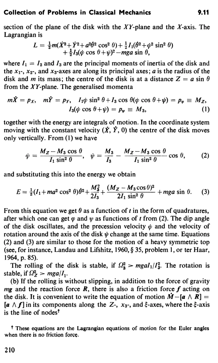
9.11. (a) A plane disk, symmetric around its axis, rolls over a smooth
horizontal plane without friction. Find its motion in the form of
quadratures.
40

9.14
Problems
Answer in detail the following questions:
Under what conditions does the angle of inclination of the disk to the
plane remain constant?
If the disk rolls in such a way that its axis has a fixed (horizontal)
direction in space, at what angular velocity will the rotation around this
axis be stable?
If the disk rotates around its vertical diameter, at what angular velocity
will the motion be stable?
(b) A disk rolls without slipping over a horizontal surface. Find the
equations of motion, and answer for this case the same questions as
under (a).
(c) Repeat this for a disk which rolls without slip over a horizontal
plane, without rotation around a vertical axis.*
(d) A disk rotates, without slipping, around its diameter which is at
right angles to an inclined plane, which makes a small angle a with the
horizontal, on which the disk is placed. Find the displacement of the
disk over a long time interval.
9.12. (a) Find in terms of quadratures the law of motion of an inhomo-
geneous sphere which is slipping without friction on a horizontal plane.
The mass distribution is symmetric with respect to the axis passing through
the geometric centre and the centre of mass of the sphere.
Study the effect of small dry friction forces for the case when the motion
of the sphere, if the dry friction forces are neglected, would be such that
the angle between the vertical and the axis of symmetry remained
constant.
(b) Find the equations of motion for the sphere of (a) if it rolls without
slipping over a horizontal plane.
(c) Find the equations of motion of this sphere for rolling without
slipping down an inclined surface.
9.13. A particle is dropped from a height h with zero initial velocity.
Find its displacement from the vertical in the directions of the West and
the South.
9.14. A particle moves in a central field potential U(f). Find the
equation for its trajectory and describe its motion in a coordinate system which
is rotating uniformly with an angular velocity Q parallel to its angular
momentum M.
t This means that the cohesion of the disk to the plane at the point of contact is so
firm that the area of contact neither slips not rotates. The energy loss due to rolling
friction can be neglected.
PCM 4
41

Collection of Problems in Classical Mechanics 9.15
Fig. 40
9.15. Find the small oscillations of a mass m which is fastened to a
frame by springs with elastic constants «i and x2. The frame rotates in its
own plane with an angular velocity Q (Fig. 40). The mass moves in the
plane of the frame.
9.16. Determine the eigen-oscillations of the three-atomic molecule
described in problem 6.37 for the case where its angular momentum Af is
non-vanishing. Consider the case where the angular momentum is at right
angles to the plane of the molecule and where the angular velocity Q is
small: Q <sc \/xlm, where x is the elastic constant of the binding.
10. The Hamiltonian Equations of Motion
10.1. Let the Hamiltonian H of a system of particles be invariant under
an infinitesimal translation (rotation). Prove the linear (angular)
momentum conservation law.
10.2. Use the Euler angles to find the Hamiltonian of a symmetric top
for the case when there is no external field acting on the top.
10.3. Determine the Hamiltonian of an anharmonic oscillator, if the
Lagrangian is given by the equation
10.4. Describe the motion of a particle with a Hamiltonian
H(P, *) = if + fr^ + Kif + iafr*?.
42

10.7 Problems
10.5. Find the equations of motion for the case when the Hamiltonian
is of the form (a beam of light)
n(p,r)
Determine the trajectory for the case when n(r) = ax.
10.6. Find the Lagrangian for the case when the Hamiltonian is
(a) H(j>, r) = f^-(a-P)> a = constant;
10.7. Describe the motion of a charged particle in a uniform magnetic
field H by solving the Hamiltonian equations of motion; take the vector
potential in the form Ay = xH, Ax = Az = 0.
In problems 10.8 to 10.12 we are dealing with the motion of electrons
in a metal or semiconductor. Electrons in a solid form a system of
particles which interact both with themselves and with the ions which form the
crystalline lattice. Their motion is described by quantum mechanics. In
solid state theory one is often able to reduce the problem of many
interacting particles which form the solid to the problem of the motion of
separate free particles (the so-called quasi-particles: electrons or holes,
depending on the sign of their charge) for which, however, the momentum
dependence e(p) ("dispersion law") of the energy is complicated.* In many
cases it turns out that it is possible to consider the motion of the quasi-
particles using classical mechanics. The function e(p) is periodic with a
period which is equal to the period of the so-called reciprocal lattice.!
Otherwise one can assume that e(p) has an arbitrary form.
t For instance, for "holes" in germanium and silicon crystals
e(p) = {Ap*±[B*p*+C\plp\+p\p*+plpl)]*)l2m,
where the coordinate axes are chosen to coincide with the crystal symmetry axes,
m is the electron mass, and the constants A, B, and C have the values
Ge
Si
A
-13.1
-4.0
B
8.3
1.1
C
12.5
4.1
t For instance, for a crystal the lattice of which has a smallest period a in the jc-
direction, we have e(pXi pwi pz) = e(p, + 2^/r/a, pw, /?,), where 2nk is Planck's constant
(/us Dirac's constant).
4#
43

Collection of Problems in Classical Mechanics 10.8
10.8. Obtain the equations of motion using the Hamiltonian H(P, r) =
e(P—(e/c)A) fe<p (the electron charge e is taken to be negative).
Hint: Introduce the electron quasi-momentum p = P—(e/c)A.
10.9. It is well known that e(p) is a periodic function ofp with a period
which is equal to that of the reciprocal lattice, multiplied by Inch; for
instance, for a simple cubic lattice with lattice constant a, the period of e(p)
is equal to 2nhja.
Describe the motion of an electron in a uniform electric field E.
10.10. Determine the integrals of motion of an electron moving in a
solid in a uniform magnetic field. What does the "orbit" in momentum
space look like?
10.11. Prove that the projection of an electron orbit in a uniform
magnetic field onto a plane at right angles to H in coordinate space can be
obtained by rotation and change of scale of the orbit in momentum
space.
10.12. Express the period of revolution of an electron in a uniform
magnetic field in terms of the area S(E, pn) of the section cut off by the plane
Ph — (P'H)/H= constant of the surface e(p) = E in momentum space.
11. Poisson Brackets. Canonical Transformations
11.1. Evaluate the Poisson brackets
(a){M/}4 {MhPj}, {Mi9Mj};
(b) {(«•/>),(A-r)}, {(fl.A/),(A-r)}, {(a-Af),(A-M)};
(c){Af,(r •/>)}, {p,r% {p,(*-rf};
where x^/j^and M,are the Cartesian components of the vectors r,pt and
M, while a and b are constant vectors.
11.2. Evaluate {Ah Aj\ where
Ax = }(x2+p2x -y2 -p% A2 = \(xy+pxpy\
A2 = \{xpy-ypx\ AA = x2+y2+p2+p2.
11.3. Evaluate {Mi9 Ajk) and {Ajk, Au) where Aik = XiXk+PiPk.
11.4. Show that {Mz, cp) = 0 where <p is an arbitrary function of the
coordinates and momenta of a particle.
Show also that {Mz,f} = [k/\f], where /is a vector function of the
coordinates and momenta of a particle and k the unit vector along the
z-axis.
44

11.13
Problems
11.5. Evaluate the Poisson brackets {/, (a-A/)} and {(/-M), (/-A/)},
where/and / are vector functions of r and p while a is a constant vector.
11.6. Evaluate {Afc, M^}, where Mc and M$ are the components of the
angular momentum along the Cartesian £- and |-axes which are fixed in a
rotating rigid body.
11.7. Write down the equations of motion for the components of the
angular momentum along the axes fixed in a freely rotating rigid body.
The Hamiltonian is of the form
11.8. Write down the equations of motion for the vector M (M =
[r/\P]9 where P is the generalised momentum), for the case when the
Hamiltonian is H = — y(M'H)+P2/2m, where y and H are constant.
This Hamiltonian is equal to the energy of a magnetic moment yM in a
magnetic field H.
11.9. Evaluate {vi9 Vj} for a particle in a magnetic field.
11.10. Prove that the value of any function/(/?(/), q{t)) of the
coordinates and momenta of a system at time / can be expressed in terms of
the values of the p and q at t = 0 as follows:
f{p(t),4(t)) =fo+tl]{H,f0} + £{H9 {H,f0}} +
where/o = f(p(0), q(0)) while H = H(p(0), q(0)) is the Hamiltonian.
Assume that the series converges.
Apply this formula to evaluate p(t), q(t), p2(t), and q\t) for the
following cases:
(a) a particle moving in a uniform field of force;
(b) a harmonic oscillator.
11.11. Evaluate v{t) for the case of a particle moving in a uniform
magnetic field using the results of problems 11.9 and 11.10 and writing the
Hamiltonian in the form H = \mv2.
11.12. Prove by direct calculation that the Poisson brackets are
invariant under canonical transformations.
11.13. Determine the canonical transformations defined by the
following generating functions:
(a) F(q,Q,t) = \mco(t)q*coiQ.
45

Collection of Problems in Classical Mechanics
11.13
Write down the equations of motion of a harmonic oscillator with
frequency co(t) in terms of the variables Q and P;
(b) F(g9 Q9 t)=±mco \q-^VCot Q.
Write down the equations of motion for a harmonic oscillator which is
acted upon by a force F{t) in terms of the variables Q and P.
11.14. Determine the generating function W{p, Q) which produces the
same canonical transformation as the generating function F(q, P) = #V\
11.15. What is the condition that a function &(q, P)can be used as a
generating function for a canonical transformation?
Consider in particular the example 0(q9 P) = q2+P2.
11.16. Prove that a rotation in q, p-phase space is a canonical
transformation for a system with one degree of freedom.
11.17. Consider the small oscillations of an anharmonic oscillator with
Hamiltonian
H = ip2 + ico2x2+*x?+pxp2
under the assumption that olx <sc co2, fix <sc 1.
Find the parameters a and b for the canonical transformation produced
by the generating function 0 = xP+ax2P+bP3 such that the new
Hamiltonian does not contain any anharmonic terms up to first-order terms in
(xQ/co2 and jiQ. Determine x(t).
11.18. Determine the parameters a and b for the canonical
transformation produced by the generating function 0 = xP+ax*P+bxI* in such a
way that the small oscillations of an anharmonic oscillator described by
the Hamiltonian
H = ip2 + W0x2+px*
can be reduced to harmonic oscillations in terms of the new variables Q
and P. Neglect terms of second order in f}Q2/co2 in the new Hamiltonian.
11.19. Prove that the following transformation is canonical:
P P
x = A" cos Ah—^-sin A, v = Ycos Ah—^sin A,
mco mco
px = —mcoY sin X+Px cos A, py = — mco X sin X+Py cos A.
Determine the new Hamiltonian H'(P9 Q), if the old Hamiltonian is
H{p, g) = ^-±& + ~ ma>Kx*+y*).
46

11.26
Problems
(Compare problem 11.29.) Describe the motion of a two-dimensional
harmonic oscillator for which Y = Py = 0.
11.20. Use the transformation of the preceding problem to reduce the
Hamiltonian of an isotropic harmonic oscillator in a magnetic field
described by the vector potential A = (0, Hx, 0) to a sum of squares and
determine its motion.
11.21. Use a canonical transformation to diagonalise the Hamiltonian
of an anisotropic charged harmonic oscillator with potential energy
U(r) = |m(cofx2+co|v2+co2z2)
which is situated in a constant uniform field determined by the vector
potential A = (0, Hx, 0).
11.22. Apply the canonical transformation of problem 11.19 to pairs
of normal coordinates corresponding to standing waves in the system of
particles on a circle considered in problem 7.3 to obtain the coordinates
corresponding to travelling waves.
11.23. Prove that the following transformation is a canonical one:
x = —}=(V2Pi sin Q1+P2), y = !=-=(V2Pi cos Q1 + Q2),
ymco ymco
Px= i V^^(V2PiCOsQi-Q2), py = \ Vmco(-\/2PisinQi + P2)-
Find the Hamiltonian equations of motion for a particle in a magnetic
field described by the vector potential A = ( — \yH, \xH,0) in terms of
the new variables introduced through the above transformation with
co = eHjmc.
11.24. What is the meaning of the canonical transformations produced
by the generating function &(q9 P) = &qP1
11.25. Prove that a gauge transformation of the potentials of the
electromagnetic field is a canonical transformation for the coordinates and
momenta of charged particles, and find the corresponding generating
function.
11.26. It is well known that replacing the Laplacian L(q, q, t) by
LXq9q,t) = L(q,q,t) + ^^,
where/(#, /) is an arbitrary function, leaves the Lagrangian equations of
motion invariant. Prove that this transformation is a canonical one and
find its generating function.
47

Collection of Problems in Classical Mechanics
11.27
11.27. Find the generating function for the canonical transformation
which consists in changing q(t) and p{t) to Q{i) = q(t+r) and P{t) =
p(t+t\ where r is constant for the following cases:
(a) a free particle;
(b) motion in a uniform field of force, U = —Fq;
(c) a harmonic oscillator.
11.28. Discuss the physical meaning of the canonical transformations
produced by the following generating functions :
(a) 0(r,P) = (r.P) + (5«.P);
(b) 0(r,P) = (r.P) + (8cp.[rAP]);
(c) «Kq,P,t) = qP+&tH(q9P9t);
(d) 0(r, P) = (r .P) + (r2+P2)6a,
where r is the Cartesian radius vector while 5a, 8cp, frr, and <5a are
infinitesimal parameters.
11.29. Prove that the canonical transformation produced by the
generating function &(x9y9 PX9 Py) = xPx+yPy + e(xy+PxPy) with e — 0 is a
rotation in phase space.
11.30. Write down the generating functions for the infinitesimal
canonical transformations corresponding to
(a) a screw motion;
(b) a Galilean transformation;
(c) a change to a rotating system of reference.
11.31. A canonical transformation is produced by the generating
function &(q, P) = qP+XW(q, P\ where A — 0. Determine up to first-order
terms the change in value of an arbitrary function/(#,/>) when we change
arguments: df(q, p) = f(Q, P) -f(q, p).
11.32. For the case when the Hamiltonian is
determine {//, (r •/?)} and use the result to obtain an integral of the
equations of motion. Use the results of problem 11.24. The vector a is
constant.
11.33. Determine how the r- and /^-dependence of M, p2, (p*r), and
H(r, p, t) change under the canonical transformations of problem 11.28.
48

11.36
Problems
11.34. Show that if
{W1(q9p),W2(q,p)} = 09
the result of applying two successive infinitesimal transformations which
are produced by the generating functions
0i(g9 P)=qP+ XfVfa n i=l,2f A, - 0,
will be independent of the order in which they are taken, up to and
including second-order terms.
11.35. Determine the canonical transformation which is the result of
N successive infinitesimal canonical transformations produced by the
generating function 0(q, P) = qP-\- (A/AT) W(q, P) for the case where A =
constant and N — «, while W(q, P) is given by the equations
(a) W(r,P) = ([r/\P] -a), a = constant;
(b) W(r,P)=([rhP]-[rAP]);
(c) W(q, P) = qP.
Hint: Construct—and solve for the different concrete forms of W—
differential equations which Q(X) and P(A) must satisfy.
11.36. (a) What is the change with time in the volume, the volume in
momentum space, and the volume in phase-space which are occupied by
a group of particles which move freely along the x-axis? At t = 0 the
particle coordinates are lying in the interval x0 < x < xq+Axq, and their
momenta in the range po < p < p0+Ap0.
(b) Do the same for particles which move along the x-axis between two
walls. Collisions with the walls are absolutely elastic. The particles do not
interact with one another.
(c) Do the same for a group of harmonic oscillators.
(d) Do the same for a group of harmonic oscillators with friction.
(e) Do the same for a group of anharmonic oscillators.
(f) We shall describe the particle distribution in phase space at time t
by the distribution function w(x, p, t) which is such that w(x, p, t) dx dp is
the number of particles with coordinates in the interval from x to x+dx
and momenta in the range from p to p+dp. Determine the distribution
function of a group of free particles and of a group of harmonic
oscillators, if at t = 0
, m 1 f (*-*o)2 (P-Po)2\
w(x> P> °) = ^^ a- exP I " -S-^T- - W"J-
2n dxQApQ K| 2Ax% 2Ap%
49

Collection of Problems in Classical Mechanics
12.1
12. The Hamilton-Jacobi Equation
12.1. Describe the motion of a particle moving in a potential U(r) by
using the Hamilton-Jacobi equation for the following cases:
(a) U(r) = -Fx',
(b) C/(r)=|mKx2 + co|>^).
12.2. Describe the motion of a particle which is scattered in the field
of the potential U(r) = (a-r)//-3. Express the equation of the trajectory in
terms of quadratures; express it analytically for the case when Eg2:» a,
where q is the impact parameter. Before the scattering the velocity of the
particle is parallel to —a.
12.3. Find the cross-section for the small-angle scattering of particles
with velocities before the scattering antiparallel to the z-axis for the cases
where the scattering is caused by the following potentials:
(a) U(r)= —^ *
(c)l/(r) = ^.
12.4. Find the cross-section for a particle to fall into the centre of one
of the following force fields with potential U(r):
(a) U(r) = ^- ;
(b)l/(r)-^- + A;
(c)«*r)-*£>--£;
(d) U(r) = W> .
Assuming that all directions of a are equally probable, evaluate the
averages of the cross-sections obtained.
50

12.11
Problems
12.5. Find the cross-section for particles to hit a sphere of radius R
placed at the centre of the potential U(r) = (a • r)jt*.
12.6. Describe the motion of particles which are scattered by and fall
towards the centre of the potential field in the following cases:
(a) m = ^l :
(b)f/(r) = _*l±!i^.
Give an expression for the trajectories in terms of quadratures, and also
analytically for the case when Eg2 :» a. For the case (a) find also an
analytical expression for the case when Eg2 <c a. The quantity g is the impact
parameter. Take the initial velocity parallel to the z-axis.
12.7. Describe the motion of a particle falling towards the centre of the
potential U(r) = (a • r)/r3 for the case when at infinity the particle moved
along the straight line x = — z tan a, y = g, where g is the impact
parameter. The vector a is along the z-axis and the initial spherical coordinates
of the particle are r =«>, 0 = n — a, y = 0. Express the trajectory in
terms of quadratures, and for the case when a2 < 2Eg2/a «: 1 also
analytically.
12.8. (a) Determine in terms of quadratures the finite orbit of a particle
moving in the potential U(r) = (fl'rj/r3—a/r for the case when Mz = 0,
where the z-axis is taken along the direction of a.
(b) Do the same for the potential U(r) = (a'r)lr3+y/rA.
12.9. Under what condition is the orbit in the preceding problem a
closed one?
12.10. Describe qualitatively the motion of a particle in the potential:
CM = ££-•.
r3 r
12.11. Find the values of M for which the orbits in the following
potentials are finite:
(a)l«r) = £-*^;
(b) </(,)= <^-f
Describe the orbits in both cases.
51

Collection of Problems in Classical Mechanics 12.12
12.12. Describe the motion in terms of parabolic coordinates for a
particle moving in the potential U(r) for the following cases:
(a) U(r) = -y ;
(b) u(r) = -"r—(F.r).
In the case (b) consider only finite orbits and express the orbit in terms
of quadratures.
12.13. A particle starts from the origin at an angle a to the z-axis
inside a smooth elastic ellipsoid of revolution
^ . Z2. t = i
a2 a2+62
Find the region inside the ellipsoid which cannot be reached by the
particle.
12.14. Describe in terms of quadratures the trajectory of a particle
moving in the field of two Coulomb centres,
U(r) = ^-±9
ri r2
(see Fig. 41). At infinity the velocity of the particle was parallel to the axis
O2O1Z. Describe the motion of a particle falling onto a "dipole" formed
by these centres.
Fig. 41
12.15. A short magnetic lens is produced by a field governed by the
vector potential
A9 = y H(z), Ar = A2 = 0,
52

13.2
Problems
where H(z) is non-vanishing in the interval | z | < a. A beam of electrons
close to the z-axis is incident onto the lens from the point 0,0, z0. Find the
point 0, 0, Z\ onto which the beam is focused. Assume that | z01, z\ y> a.
Hint: Find the solution of the Hamilton-Jacobi equation in the form
of an expansion of S(r, <p, z, t) in powers of r:
S(r, <p9 z, 0 = -£/+<p/v+/(z)+r^(z) + |rMz)+ ....
12.16. A magnetic lens is produced by a field governed by the vector
potential
A9 = \rH{z\ Ar = A2 = 0,
where
1+K2Z2
A beam of electrons close to the z-axis is incident onto the lens from the
point 0, 0, z0. Find the points where it will be focused.
Hint: Find a solution of the Hamilton-Jacobi equation as an expansion
in r.
12.17. How can one find the action as a function of the coordinates and
the time, if the solution of the Hamilton-Jacobi equation is known ?
12.18. Formulate and prove the theorem about integrating the equations
of motion using the complete solution of the equation
dS rr/ dS \ A
where H(q, p, i) is the Hamiltonian (Hamilton-Jacobi equation in the
momentum representation).
12.19. Use the Hamilton-Jacobi equation in the momentum
representation to find the trajectory of a particle moving in a uniform field.
13. Adiabatic Invariants
13.1. A mass m is suspended from a string which passes through a small
ring (Fig. 42). Determine the average force exerted upon the ring A by the
string when the pendulum performs small oscillations. Find the change in
the energy of the pendulum when the ring is slowly displaced vertically.
13.2. A particle moves in a rectangular potential well of width /.
Consider the collisions of the particle with the "wall" of the well to find how
the energy of the particle will change when / is changed slowly.
53

Collection of Problems in Classical Mechanics
13.3
Fig. 42
13.3. A small ball is jumping up and down on an elastic plate in a lift.
What is the change in the maximum height the ball reaches if the
acceleration of the lift is slowly changed? How does the height vary, if the plate
is raised slowly?
13.4. How does the energy of a particle moving in a potential U(x)
change when the parameters of the potential change slowly for the
following cases:
U0
(a) U(x)=-
cosh2 ocx
(b) U(x)= C/0tan2ax;
(c) U(x) = A\x\nl
Hint: Use the formula (see, e.g., ter Haar, 1964, § 6.2) T = 2n(dI/dE).
13.5. A particle moves down an inclined plane AB (Fig. 43) and is
reflected elastically by a wall at the point A. How does the maximum
height the particle reaches change when the angle a changes slowly?
Fig. 43

13.8
Problems
Fig. 44
13.6. A pendulum is placed upon an inclined plane (Fig. 44). How does
its amplitude change, when the angle a is changed slowly?
13.7. Determine the adiabatic invariants for a mathematical pendulum
for the case when the amplitude of the oscillations is not small.
13.8. (a) Two elastic spherical particles of small radius and with masses
m and M, respectively, (m <$c M) move along the straight line OA (Fig. 45).
At O the particle m is reflected elastically by a wall. Assume that the
velocity of the lighter particle at / = 0 is much larger than that of the heavier
particle and determine the motion of the heavier particle averaged over
the period of motion of the lighter particle.
Fig. 45
(b) Two particles of mass M each and one of mass m (m <sc M) move
along a straight line. The light particle interacts with each of the heavy
ones according to a potential
tfi,2(l*i,2-*l) = 0, |*i,2-*I > a,
where Xi and x2 are the coordinates of the heavy particles and x is the
coordinate of the light particle. Describe the motion of the system, if at
/ = 0
1*1 I ~ 1*2 I <^ |*| •
55

Collection of Problems in Classical Mechanics 13.9
13.9. Use the method of successive approximations to solve the
equations for P and Q of problem 11.13(a) for the case when the frequency
changes slowly (ax^co2, co «coco) up to and including terms of first order
in cb/co2.
What is the advantage of the variables P, Q over/?, q in this case?
13.10 Check that up to terms of first order in co/co2 the expression
q = co~l exp ill codt\ satisfies the equation q+co\t)q = 0, where
co/co2 ~ co/coco «: 1.
13.11. A force F(t) acts upon a harmonic oscillator. Find the time-
dependence of the adiabatic invariant I(t) = (l/ln) <ppdq.
Find I(t) in particular for the following cases:
(a) F(t) = at
(b) F(t) = F0 sin Qt, 0 < / < ^ ; F(t) = 0, t < 0 and^ < t.
(c) F(t) = F0 sin2 Qt, 0 < t < ^; F(i) = 0, I < 0 and -^ < I.
13.12. Find the connection between the volume and the pressure of a
"gas" consisting of particles which move parallel to the edges and inside
an elastic cube, when the size of the cube changes slowly.
13.13. A particle moves inside an elastic parallelepiped. How does its
energy change
(a) if the size of the parallelepiped changes slowly;
(b) if the parallelepiped rotates slowly?
13.14. A particle moves inside an elastic sphere, the radius of which
changes slowly. How does its energy change and how does the angle at
which it hits the sphere change?
13.15. Determine the change in the energy and in the trajectory of a
particle in the following cases:
(a) a finite orbit in the potential
U(r) = -?„ (0 < n < 2)
when y changes slowly;
56

13.23
Problems
(b) a finite orbit in the potential
u(r) = -r<r + T*>
when y changes slowly.
13.16. The string of a spherical pendulum is slowly shortened. How
does this affect the motion of the pendulum?
13.17. Determine the change in the energy of a particle moving in a
central field potential U(r) when a small extra potential W(r) is slowly
"switched on".
13.18. Determine the time-dependence of the energy of a system of two
coupled harmonic oscillators with a Lagrangian
L = \m{x2+y2 — co\ x2 —co%y2 + 2ocxy),
when coi changes slowly.
What is the change in the orbit of the point x, yl
13.19. Let the coupling between the oscillators in the preceding
problem be small (a <zco2t 2). Prove that if we are far from degeneracy, where
coi = co2, the adiabatic invariants calculated neglecting the coupling are
conserved, but that they change rapidly when we pass slowly through the
region of degeneracy.
13.20. In which range of frequencies coi(t) will the adiabatic invariants
of the harmonic oscillators in problem 13.19 change sharply, if the
coupling is bU = fix2y7
13.21. Determine the shortest distance a particle approaches the edge of
a dihedral angle a after being reflected elastically from its faces. The angle
at which the particle is incident on one of the faces at a distance / from
the edge is <po.
Solve this problem by two methods: either by using a reflection method
and solving it directly, or by using adiabatic invariants assuming that a
and <po are small.
13.22. Determine the boundaries of the region in which a particle
moves between two elastic surfaces y = 0 and y = a cosh ax/cosh 2ax.
The particle starts at the origin in the xy-plane at an angle (p to the >>-axis in
the xy-plane and a and y are small compared to unity. Also determine
the period of the oscillations along the x-axis.
13.23. What is the change in the radius and the centre of the orbit of a
charged particle moving in a uniform magnetic field which is slowly
PCM 5
57

Collection of Problems in Classical Mechanics 13.23
changing its strength. Take the vector potential in one of the following two
forms:
(a) Ax = 0, Ay = xH{t\ Az = 0;
(b) Ar = A2 = 0, Av = \rH{t).
Explain why the result depends on the form of A.
13.24. Calculate the adiabatic invariants for a charged isotropic
harmonic oscillator moving in a uniform magnetic field.
13.25. Consider the following cases of the motion of a charged
anisotropic harmonic oscillator in a uniform magnetic field. The potential
energy of the harmonic oscillator is of the form
U(r) = \m((olx2+coly2+colz2),
and the magnetic field is along the z-axis. Take the vector potential in the
form A = (0, xH, 0) and consider the following cases:
(a) Determine the adiabatic invariants for the harmonic oscillator.
(b) Let initially H = 0 and let the trajectory of the orbit fill the
rectangle \x\^a,\y\^b. Find the motion of the oscillator after the
magnetic field has slowly increased its strength up to a value which is so high
that coH = eHjmc ^>col2.
(c) Let the magnetic field be weak (coH<£coi—co2) and let the oscillator
originally oscillate nearly along the x-axis. What happens to its motion
when the value of a>i decreases slowly to reach a value co[ < co2 such that
13.26. A particle performs a finite motion in a plane at right angles to
a magnetic dipole Jtl. What is the change in the energy of the particle
when the magnitude of JH changes slowly?
13.27. Determine the period of the oscillations along the z-axis of an
electron moving in a magnetic trap. The magnetic field of the trap is
symmetric with respect to the z-axis and we have H^ = 0, Hz = H(z), Hr =
— \rH '(z). Consider the following two cases:
(a) H(z) = Ho(l + A tanh2 ^\ ;
(b)//(z) = Wl+Jl
58

13.32
Problems
13.28. How does the energy and the period of oscillations of an electron
moving in the magnetic trap of problem 13.27 change when the field
parameters //o, A, and a change slowly?
13.29. Determine the change in energy of a particle moving in a central
field potential U(r) when a weak uniform magnetic field H is slowly
"switched on".
13.30. It is well known that the number of single-valued integrals of
motion is increased when the motion becomes degenerate. Find the
integrals of motion for the case where a particle moves in the following
potentials :
(a) U(r) = >•*;
(b) U(r)= ima)\x2 + 4y2).
13.31. Find the action and angle variables for the following systems:
(a) a harmonic oscillator;
(b) a particle moving in the potential U(x) = «>, x ^ 0; U(x) = Fx,
x > 0.
13.32. Use the generating function
S(x,P) = \/2m[E- U(x)] dx
Jo
to perform a canonical transformation for the case of a particle moving in
the periodic potential
U(x) = 0, na < x < (n+\)a\
U(x) = V, (n+\)a < x < (n+ l)a, n = 0, ± 1, ±2, ...,
for the case when E > V, and where E in the expression for S(x, P) can be
derived as function of P from the equation
P= p <\/2m[E-U(x)]dx.
s»
59

ANSWERS
AND
SOLUTIONS

Answers and Solutions
1. Integration of One-dimensional Equations of Motion
1.1. (a) The energy of the particle E is determined by the initial values
x(0) and x(0). The motion follows from the energy conservation law
$mx2+ U(x) = E. (1)
When E ^ 0 the particle can move in the region x ^ xi: the motion is
infinite (E = E in Fig. 46). When E ^ 0 (E = E") the particle moves
in the interval x2 ^ x ^ x3: the motion is finite. The turning points are
determined from (1) through U(xi) — E:
= i_lQVA(A+E)-At when £>0>
E
xi = —
a
xi = —
In 2
when E = 0,
1 ^TV^U-I^I)
X2'3=a b LEI
when E < 0.
(2)
From (1) we obtain
r 2 •wi
rfx
whence
x(r) = — In
2 A© y/E-U(x) '
A - VA(A-\E\) cos (at V2\E\fm+C)
x(t) =
-Hi
+ ^«+C)i],
w
when
when
£<0,
£ = 0,
1 , V^G* +E) cosh (a/ ^/lEjm + C) - A
x(t) = In -— ±—Z , when E :
a is
(3)
(4)
(5)
0.(6)
63

Collection of Problems in Classical Mechanics
1.1
Ui
l\
1 \
1 \ *2
\ 1
\ 1
E'
X3
1
1 ^
1 ^^
E y/^
i-A
Fig. 46
The constants C are determined by the initial values x(0). For example
in (4), when x(0) > 0
A-\E\e«xW
C = arccos
Va(a-\e\)
The turning points (2) are easily found from (4) to (6).
When E < 0 the motion is periodic according to (4) with a period
_ n if2m
~^V \E]'
When E is close to the minimum value of U(x\ Umin =-A, that is, when
A—\E\ « A, the period
^T^if)
is nearly independent of E. In that case we can write (4) in the form
(7)
64

1.3
Answers and Solutions
The particle now performs harmonic oscillations near the point a_1x
In (A/\E\) with an amplitude determined by the difference £— t/min and
with a frequency which is independent of the energy. This kind of motion
for an energy close to Umin occurs in nearly every potential (compare
the discussion in § 1.5).
When E ^ 0 the particle coming from the right reaches the turning
point xi (see (2)), turns back, and goes to infinity. Its velocity approaches
the value y/lEjm from above.
(b)
«,„J--[ff.,(.Yf+c)],
when E < 0,
m = ±l- arsinh [][*±^ sinh («, ][f+c)].
when E > 0,
— + C), when E = 0,
m J
where arsinh x = In (jc+ \/*^+') is the inverse of the hyperbolic sine.
*)-i—[/^*(-/^+c)]- —•
Explain why in some of the formulae two signs occur.
1.2.
X(t) = i ^ *°/^7T- > ^o = x(0).
l±/Xo\/2^//w
The sign in the denominator is the opposite of that of x(0). To fix our
ideas, let x(0) > 0. When x(0) > 0, the particle reaches infinity after a
time y/m\2Ax%. Of course, for real systems the particle only reaches finite,
though long, distances, corresponding to the distance over which the
potential has the given form. When x(0) < 0, the particle asymptotically
approaches the point x = 0.
1.3. Near the turning point U(x) ^ E-(x-a)F, where F = -U'{a\
that is, the motion of the particle can be considered to occur under the
65
x(t) = ± arsinh
H

Collection of Problems in Classical Mechanics 1.3
action of a uniform constant force. Assuming that x(0) = a, we get
Ft2
The further away from the point of x = a we go, the less accurate this
formula becomes.
It takes a time r oc s to traverse a short path length s if it is far from a
turning point. However, if this path length is at the turning point, r %
V'2msI\F\, that is> T ^ Vs.
If U'(a) = 0 (see Fig. 47) one must extend the expansion of U(x) to the
next term
U(x) = E+\U"{a) (x-df.
E
Fig. 47
In that case x(t) = a f se±Xt with ^ = x(0)-a9 A2 = - U"(a)/m, where
m is the particle mass, and where the sign in the index is determined by the
direction of the velocity at t = 0. It takes an infinite time to reach the
turning point.
1.4. If U'\a) 9*0, Joe ln£; where e = Um-E. If U"(d) = ... =
U^n~l\a) = 0, U^\a) * 0, we have Joe exp. {[(\/ri) -|] In e}.
1.5. The particle moves most slowly near the point x = a. Let us first
consider the interval a— b<x<a+d(d<KL = x2—*i). To estimate
the time Ti the particle spends in that interval we write U(x) in the form
U(x) = U{a)-\x{x-af, wherex=-U"(a). We find
l-i VE-U(x) Y x \l f l21
66

T.S
Answers and Solutions
where / — \^2e/x 2nd e = E—Um. Assuming that e is so small that
I « 6 « L
can be satisfied, we find
The time T2 spent by the particle along the intervals Xi < x < a— d and
a+6 < x < x2 satisfies the relation r2 ^ L/v, where \mv2 ~ -|-k<52, that is
T2 £
When e decreases, 7\ increases so that, for sufficiently small e, !T2 <sc 7*i
and we can then use equation (1) to estimate the period of the motion.
This formula is asymptotically exact. As e -* 0, its relative error tends to
zero as (In e)_1.
If U"(a) = 0, but U^\a) = K * 0, we have
\ eK J J0 \Zi+x* \eKj
If we observe the motion of the particle over a long period / ■» T,
the probability to find the particle between x and x+dxis
... „ dt \/2m dx
w(x) dx = 2 — = y, •
T Ty/E-U(xY
67

Collection of Problems in Classical Mechanics 1.5
The x-dependence of the probability w to find the particle at a point x
is drawn in Fig. 48. The probability w(x) dx is represented by the hatched
area (the total area under the curve is unity). For small e the area under
the central maximum gives the main contribution T\\T to the total area
under the curve. In spite of the fact that w(x)-+ » as x < xlt 2 the
contribution from the regions near the turning points is relatively small.
1.6. We put the value of the potential energy at the lowest point equal
to zero. If E = 2mgl, we have
(p(t) = n+4 arctan [exp ( ±2t \/gfl) tan \(<p(0)-n)\
where y is the angle between the pendulum and the vertical. The sign in
the index is the same as that of <p(0). The pendulum asymptotically
approaches its upper position.
In the case 0 < E—2mgl <z 2mgl the pendulum rotates, slowly crossing
its upper position. One can estimate the period of rotation applying the
result of the preceding problem:
1.7. We again put the value of the potential energy at the lowest point
equal to zero. We then have
t
The substitution x =
t
whence
x
(For a definition of the sn function and the other elliptic functions see,
for instance, Abramovitz and Stegun, 1965.) The oscillation period is
r 2 Jo \/E—mgl(\—cosy)
= x sin y(jp, x = \/E/2mgl changes the integral to
= }[11* *
r g Jo Vo -*2)0 -x2*2)'
= 2arcsin — sn If 1/ y + ^,xl .
68

1.8 Answers and Solutions
T= 4 \/l/g K(x)9 where K(x) is the complete elliptic integral of the
first kind,
K{x) = ^ - .
Jo y/\ -x2 sin2 f
If x > 1, we get from the substitution xx = y
-m-.
dy
g x Jo Vo-^Hi-yv*2)'
and (p = 2 arcsin -^ sn [xty y + V*—)•
The rotation period of the pendulum is T = (2/x)\/l/gK(llx).
The following formulae allow us to obtain the period in certain limiting
cases:
K(.
x) = - I1 4- d x2\, when x «: 1;
K(x) = -- In - —„ , when 1 — x <sc 1.
2 1 —?r
In particular, when E—2mgl <c 2wg/, we have
where eo = 32mgl. This result differs from the rather crude evaluation
made in the preceding problem in the value of e0, that is, in a quantity
which does not depend on E—2mgl. This difference is small when
E-2mgl n*
-—f- «: -— ^ 0.2.
2wg/ 64
1.8. The motion in the potential U{x)+ 6U(x) is governed by the
equation
dx
-m
\/E-U(x)-dU(x),
(1)
where we have assumed that at / = 0, x = a. Expanding the integrand in
(1) in powers of dU(x), we obtain
t=to(x)+dt(x), (2)
69

Collection of Problems in Classical Mechanics
1.8
where
dx
2 I y/E-U(x)'
t*x) = ^jj*-7^==, (3)
&t(x) = 2\Tl [E-uw (4)
Let the orbit for the case when dU(x) = 0, which is determined by / =
t0(x)9 be x = x0(t). We then have from (2)
x = x0{t-dt(x)), (5)
where in dt(x) we substitute for x the function x0(t). Expanding (5) in
terms of dt, we finally obtain
x = x0(t)-x'0(t)6t(x0(t)). (6)
Near a turning point one has to be careful, as the small parameter in
the problem so far has been bUj{E— U(x)) which becomes large near the
turning point. Near the turning point x = x\ we may assume
6U(x) = 6U(Xll U(x) = E-(x-Xl)F,
where F= — U'(xi). We assume that | dU'(xi)\ <sc \F\. The expansion is
applicable as long as \x—xi\ <> dxi, where dxi = — dU(xi)/F. We then
have
\/2F*(x-Xi)
where the constant 6/0 determines the delay of the particle suffered along
its path far from the turning point. When | x—Xi \ > dxi, the first term on
the right-hand side of (7) is small; however, when \x—xi\ < dxi it
becomes large according to (7) so that it ceases to be a small correction, and
(2) is no longer applicable.
We note, however, that equation (6) remains valid right up to the
turning point. Indeed, the change in the motion in the vicinity of the turning
point consists in a shift of the latter. This result is obtained when we
substitute (7) into (6):
*(0 = *b(0 + A*i-*o(0*'o = *o('-«'o) + «*i, (8)
where dxi satisfies the equation for a turning point,
70

1.10 Answers and Solutions
with the required accuracy. This is connected with the fact that near an
extremum x is nearly independent of/, even though dt increases when we
approach the turning point.
1.9. (a) For the unperturbed motion we have
x0(t) = a sin cot, E = \mdlco2. (1)
(2)
For the correction we have
dt(x) = — (\/a2-x2 + ,al -2a\.
3co*V \A*2-*2 /
Substituting (1) and (2) into (6) of the preceding problem, we get
x(t) = a sin cot — -—r cos cot |cos cot-f —2).
3co2 \ cos cot J
Up to terms of first order in cca2/co2 we have
x(t) = a sin (cot + cp)- ^ - —¥ cos 2(cot+cp),
where <p = — 2aa2/3co2 (compare problem 8.1b).
1.10. The change in period is
w-i^rrv * -p * i. a)
One cannot expand the integrand in (1) in terms of dU(x) since the
requirements of the theorem about differentiating improper integrals with
respect to a parameter are violated, as the resulting integral diverges.
However, we can expand the integrand in terms of dU(x) up to terms of first
order in bU(x) if we write dT in the form
bT=\/2m-%\\ ' l\/E-U(x)-bU(x)dx- \ * y/E-U{x)dA> (2)
oh Uxl+dXl JXl J
whence
\/E-U{x) dE
(8U) = ± jT6U(x(t))dt (4)
is the time-average of dU.
71
v—fe A. £' jp^L . _ JL (7W), (3)
where

Collection of Problems in Classical Mechanics 1.10
The time spent near the turning point contributes little to the period,
provided, of course, that U'(xh2) ^ 0 (compare problem 1.3). Equation
(3) can therefore give a good approximation.
We note that sometimes even small extra terms 6U(x) may strongly
affect the motion (see, for example, problems 1.11(b) and (c)).
Higher-order terms in the expansion of dT in terms of dU can be
obtained by similar means:
T = ifi". f (~l)n JL f"iwtoir* (5)
r 2 n=o n\ dEn J*, \/E-U(x)'
The formal expansion (5) may be an asymptotic or even a convergent
series.
1.11. (a) According to equation (5) of the preceding problem the
correction to the period Ijijco is — 37r,pE/2ma)5 which is small, provided E is
sufficiently small,
(b) In Fig. 49 we have given the potential energies U(x) and t/(x)+
6U(x). When E=E' > Um = wcofl/6a2 the extra term clearly means that the
particle can move to infinity. When E is close to Um, the period of
oscillation increases without bound (as \ln(Um—E)\; see problem 1.4) so that
one cannot determine the change in period just by a few terms in the series
(5) of the preceding problem.
Fio. 49
72

2.1 Answers and Solutions
When E <sc Um the correction to the period is bT = 5nEj\%(oUm.
(c) bT = 3nAy/ml2ctE~*y/2\ the formula is applicable when \E\ »
\Um\*V8AV, (£<0).
2. Motion of a Particle in Three-dimensional Potentials
2.1. To study the orbits of the particle we use the energy and angular
momentum conservation laws:
■j7ii(r.r)+C/(r) = £, (1)
m[r Mr] = M. (2)
It follows from (2) that the orbit lies in a plane. Introducing polar
coordinates in that plane (see Fig. 50) we get
\mr2 + imr2<p2 + U(r) = Ey (3)
mr2(p = M. (4)
Fio. 50
Using (4) to eliminate <p from (3) we get
imr*+UeS(r) = E, (5)
where
M2
UeS(r) = U(r)+
2mr2'
The radial motion can thus be considered as a one-dimensional motion
in the potential t/eff(r).
PCM 6
73

Collection of Problems in Classical Mechanics
2.1
For a qualitative discussion of the character of the orbits we use
diagrams of
l/eir(r) =
r r
T+ 2wr2
(6)
for different values of M (Fig. 51).
When M4 > 12m2ay, C/eff has two extrema (for
VM4-12m2ar]/2ma), where Ueff(r2) = Umi]
either positive, when M4 > 16m2ay (Fig. 51a), or negative, when \2m2ccy <
M4 < \6m2(x.y (Fig. 51b). If M4 < 12w2ay, the function C/eff(r) will be
monotonic (Fig. 51c).
i,2=[M2 +
0, while C/max can be
Mil*
(a)
(b)
Fig. 51
(c)
Fig. 52
Let us consider the case of Fig. 5 la in somewhat more detail. If E> Umax
the particle coming from infinity falls into the centre of the potential. The
quantity <p then increases according to (4). This is all we need to sketch the
orbit (see Figs. 52a, b).
At large distances such that yr~3<scar_1, the main term in U is —a/r
and the orbit differs little from a hyperbola. For the form of the orbit
74

2.1
Answers and Solutions
as r — 0, we refer to problem 2.8. If the energy is close to C/max, the
particle passes very slowly through the range of values of r which are close to
ri. At the same time the radius vector turns round with a velocity cp ^ M/mr*
so that the particle may perform many revolutions around the centre
before it passes through this range of values (Fig. 52b).
If E = Umax the particle approaches the point r = r\ asymptotically
during its radial motion (compare problem 1.3). The orbit is a spiral
approaching the circle of radius n and centre O (Fig. 53a). If, on the other hand,
the particle starts in the region r < r\ and is moving away from the centre,
its orbit also approaches this circle, but this time from the inside (Fig.
53b). Finally, motion along the circle r = rx is possible when E = C/max *
•^ c
Fig. 53 Fig. 54
The motion along this circle is an unstable one, as any change in E or
M will bring the particle onto an orbit which moves away from the circle.
If 0 < E < C/max a particle coming from infinity will be reflected from
the potential barrier C/eff and again move off to infinity. Examples of such
orbits are given in Fig. 54a, b. If the energy is close to C/maxthe particle
makes many revolutions around the centre before r changes sign. The
closer the energy is to zero (for a fixed value of M this corresponds to
larger values of the impact parameter) the less twisted the orbit of the
particle.
When E < C/max, the case is also possible of the particle falling towards
the centre, when it is moving in the region r < a. The orbit for that case is
given in Fig. 55.
When Umin < E < 0 the particle can also perform radial oscillations in
the range c ^ r ^d. If the energy is close to zero, the amplitude of the
radial oscillations will be large; their period can also become large and the
6#
75

Collection Of Problems in Classical Mechanics
2.1
radius vector may perform several revolutions during one radial oscillation
(Fig. 56a). When the energy is close to Umin the orbit is close to a circle
with radius r2 (Fig. 56b) while the angle over which the radius vector
turns during one period of the radial oscillation depends on the quantities
Fig. 55
(a) (b)
Fig. 56
a, y, and M (compare problem 5.4). When E = Umin the particle moves
along the above-mentioned circle.
One can analyse the motion of the particle in a similar way for the other
cases.
What are the particular features of the orbit when M4 = 12w2ay?
Let us now consider the orbits in more detail. One can obtain the
equation for the orbit from equations (4) and (5). From (5) we get
r = ±yi(E-UeS), (7)
76

2.1
Answers and Solutions
or
' dr
-*m
, -+C. (8)
Using (4) to eliminate dt from (7) we find the equation of the orbit:
M Cr dr
<P = ± ~^= +C. (9)
Let us consider the case M4 > 12m2ay. If the particle moves towards
the centre we must take in (7), and of course also in (8), the lower sign.
If at / = 0, r = r0, we can rewrite (8) in the form
V 2 Jr.VE-Ucff(r)
Equation (10) is an implicit equation for r as a function of /. If the orbit
passes through the point r = r0,(p = <po, the equation of the orbit
becomes
* = -Ml^P-;\^ (11)
where we have taken once again the lower sign, and where \pr\ =
\/2m[E- Ucff(r)]. In particular, if the velocity of the particle at infinity
makes an angle ip with the x-axis, we must put r0 = ^, (?* = n—ip.
If E> Umdx, equations (10) and (11) completely determine the orbit
and the time when the particle passes through each point of the orbit.
However, if 0 < E < C/max, these equations correspond only to the section
AB of the orbit (see Fig. 54a). At B the radial component of the velocity
r vanishes and then changes sign. The section BC of the orbit is thus
described by equation (9) with the upper sign and we must redetermine the
constant C. It is convenient to write (9) in the form
? = M .!T^ + C/- (»2)
As long as C is not determined, we can choose the lower limit of the
integral arbitrarily. According to (12) we now have
C = <p(rmi„). (13)
77

Collection of Problems in Classical Mechanics 1.1
Determining <p(rmin) from (11) we get the following equation for the sefction
BC of the orbit:
w fr dr w frmin dr
Similarly we can determine the time dependence of r along BC:
'=im f /* -i- P",dr • 05)
If ^min < £ < 0, a < r0 < fc, r(0) < 0, (p|,=0 = (p0, equation (11)
describes the section AB of the orbit in Fig. 54b. The section BC is
described by the equation
'-*f*£r+*- (l6)
where the angle <pi can be obtained by putting r = a in (16). The equation
for the section CD is
'--"f^*- (,7)
where (p2 is determined from (16) with r = b, and so on. Substituting the
values of (jpi and (p2 into (16) and (17) we get the equations for BC and CD
in the form
Cr dr Ca dr
*-Ml^-Ml.*I¥A- (l8)
*, fr dr %, Cb dr %, Ca dr
^-Mi-r^K\ + M[-^¥A -"I'M
Ja r2\pr\ Ja r2\p,\ Jr> r*\pr\
One verifies easily that the equation for that section of the orbit which
corresponds to the nth radial oscillation, taking the section BC to be the
78

2.2
Answers and Solutions
first, has the form*
-"tufa+"" <20)
In the equations given here we have assumed that the angle (p changes
continuously, and we have not introduced the limitation 0 ^ cp < 2tc.
There is an infinity of values of cp corresponding to a given value of r,
corresponding to different values of n and different signs in equation (20):
(p is a many-valued function of r; on the other had, r is a single-valued
function of cp.
All other cases can be treated in a similar fashion.
2.2. Outside the sphere of radius R the particle~moves with a speed
\f2E\m and inside with a speed \/2(E+ V)jm. Depending on the values
of £and M we get different kinds of orbits. When (A/2/2/n/P)-K < E <
M2/2mR2, the particle can either move inside the sphere and be reflected
at its surface (Fig. 57a); or, provided E > 0, we can have an infinite orbit
<a) (b)
Fig. 57
t The equation (20) for the orbit can be written in the form
J'r dr _ arccos yiy+a)
(we bear in mind that 0 ^ arccos x < n\ where
71 a* [b dr ** [a dr
- = M \ -T.—- , a = M \ -i-—■ <p0.
y Ja r2\pr Jr. r2 pr\
79

Collection of Problems in Classical Mechanics
2.2
(which can be a straight line, see Fig. 57b). When M2/2mR2 < E, we can
have a refracted orbit (Fig. 57b).
What is the shape of the orbit when E = M2/2mR2-Vl
2.3. To determine the equation of the orbit we use the equations
*=!?
Mdr
rW2m(E-UeK(r)y
and we then get*
where
r =
ecosy((p—y)) — \ '
(i)
(2)
2s > 0, and ip is an arbitrary constant.
The orbit is the curve which is obtained from a hyperbola by reducing
the polar angles by a factor y (Fig. 58). The constant ip determines the
orientation of the orbit.
Fig. 58
t If we write the integral for q> in the form
M f
— y = _
Mdr
y/2m{E-KP/2mr*-OLlr)'
where tif2 = M2+2mfit the integral is reduced to the corresponding integral in the
Kepler problem (see, for instance, ter Haar, 1964, p. 9).
80

2.4
Answers and Solutions
The direction of the asymptotes is determined by the condition r — oo,
or e cos y{<p1%2—y))= 1. The directions of the velocity before and after
the scattering are at an angle
rt—iSpl—tp?) = 7T"
2 1
— arccos — ■ = n ■
Y e
arctan
i[4E/. M*\
to one another.
2.4. It is useful to study first of all the character of the orbit using a graph
of Uef{(r). This graph is given in Fig. 59 for the case where /? < M2/2m.
In that case all orbits are infinite and lie in the region r > rm, when E > 0.
Fig. 59
The equation of the orbit is the same as in problem 2.3, equation (2),
except that in equations (3) we must substitute —/? for ft. The main
difference with the orbits found in problem 2.3 occurs because now y < 1. An
example of an orbit is shown in Fig. 60^
The form of UeS(r) for the case when ft > M2/2m is shown in Fig. 61.
If
_ a2
E>U>»= 4(p-M*/2m) '
t The inflection point A is determined from the condition dU/dr=0, that is, r=2(J/ai.
81

Collection of Problems in Classical Mechanics
2.4
Uen|
Fig. 61
the particle coming from infinity will fall into the centre. The equation of
the orbit can be obtained from the equations of problem 2.3. We must
then replace 0 by -/?_and y by y+rc/2y, and also use the formulae
sin ix = i sinh x, \/-x = i y/x. As a result we get
r =
<-\{f-
2m)'
e' sinhy'(<p—f)+l
Y r a/2
(i)
(2)
The orbit for this case is shown in Fig. 62a. We note that as r - 0, <p -«.
This means that a particle coming from infinity and falling into the centre
makes an infinite number of revolutions around the centre.
82

2.4
Answers and Solutions
Fig. 62a
Fig. 62b
If E < Um, we see from Fig. 61 that the particle can either move in the
region b ^ r < «> (scattering), or in the region 0 < r ^ a (falling into the
centre). We obtain the equation for the orbit, using the relation cos i'jc =
cosh x, and for the second case again the substitution of y+njy for y>:
r =
1 HF e" cosh y\(p —yi)
'-/--£('-£)■ <3>
For the case E = C/m it is not possible to use equation (2) of problem
2.3, as we have assumed in its derivation that e ^ 0 and we must start
again from the integral (1) of problem 2.3. We find
r =
that is,
P'
1± exp[-/(?>-yO]
or r = /?
depending on the initial value of r. The orbit is either a spiral starting at
infinity and approaching asymptotically the circle with radius r = /?', or a
spiral starting near the centre and approaching the same circle
asymptotically, or it is this circle itself (Fig. 62b).
Finally, for the case ft = APjlm it is also simplest to start again from
the original integral. In that case scattering occurs and the equation for
the orbit is
2M%c
r =
2M2E—moc2((p—y))2
83

Collection of Problems in Classical Mechanics 2.4
The time it takes the particle to fall into the centre is found from the
equation
F 2 Jo ^/E-UeS(r)
For instance, when the orbit has the form given by equations (1) and
(2) of the present problem, the time to fall into the centre from a distance
r is given by
a -if m~\ . (2£r/a)-l . 1 1
+ 2E\ IE I2™11 J' arCSin e' [
2.5. The equation of the orbit is
r =
1 + e cos y((p —xp)
where p, e, and y are defined in problem 2.3. When E < 0, the orbit is a
finite one, and*
Ttoc y/m A _ In
T' = Trrsrss • A(P = — • T* = yT>-
The orbit is closed, if y is a rational number. In Fig. 63 we show the orbit
for y ~ 4.
2.6. When P < M2/2m we have
p s = 1(ML-r\
l-ecosy((p-f) ' p a \2m p)'
ifE < 0, Acp = 2ji/y, Tv = yTr9 and Tr will be the same as in the preceding
problem.
t The period Tr is the same as in the potential U0 = -oc/r. To determine Tr it is
sufficient to note that adding a term P/r2 to the potential U0 has the same effect on the
radial motion as increasing M. However, the period Tr is independent of M in the
Coulomb potential C/0.
84

2.7
Answers and Solutions
Fig. 63
When /S > M2/2m, we have (using the notation of problem 2.4)
r = ———?7 r—r, when E > 0;
, when E < 0.
r =
esinh/(<p—y)+l
ecosh/(<p— y>)+ 1
2.7. (a) A finite orbit is possible if the function UcS(r) has a minimum.
The equation U'cfs(r) = 0 can be reduced to the form f(x) = xfrP/owi,
where/(x) = x(x+ l)e~x, x = xr. Using a graph of/(x) one sees easily
that this equation has real roots only when xfrP/czm is less than the
maximum value of /(*), for x > 0. This maximum value is equal to
(2+\/5)exp[-|(l + \/5)]^0-84. A finite orbit is thus possible,
provided M2 < 0-84 am/x.
(a) (b)
Fig. 64
85

Collection of Problems in Classical Mechanics
2.7
(b) A finite orbit is possible provided M2 < SmV/e2x2.
2.8. In the equation for the orbit (equation (1) of problem 2.3) we can
neglect for small values of r the quantity E, when n = 2, and also the term
M2/2mr2, when n > 2. We obtain then
M In (r/ro) , ~ , ^. , - x
cp = + <po, when « = 2 (see Fig. 64a),
V2wa-M2
(jp = —= r~ 2\ when n > 2 (see Fig. 64b).
V 2wa (2 -«)
It turns out that the number of revolutions is infinite only when n = 2.
The time it takes the particle to fall into the centre is finite as the radial
velocity increases when the centre is approached.
2.9. The number of revolutions of the particle around the centre is
infinite only in the case
(b)£=0, »^2.
2.10. The time it takes the particle to fall into the centre is n \/mR3/2<x.
2.11. The relative motion is characterised by the angular momentum
M = [tvQ and the energy E = \/j,v29 where p = mim2/(mi + m2) is the
reduced mass. The distance to be determined follows from the
condition C/eff(rmin) = E. Solutions can be obtained easily for n = 1,2, and 4.
2.12. The particle orbit is
where
JL.
mi,2
u9
P
P =
= 1±<
M2
[J,0C
ecos
e =
<P>
■^
2EM*
9 '
E and M are the total energy and angular momentum of the system. The
particles move in similar conical sections with a common focus and their
radius vectors are at any moment in opposite directions (Fig. 65).
86

2.13
Answers and Solutions
€D
Fig. 65
2.13. One sees easily from Fig. 66 that
OS = e(cot (po —cot 2cpo).
Fio. 66
Here
As q -+ 0, (jpo — 0, and
(i)
«po = e \ —. . (2)
os = [2 (°° —. dr \ Voce2). (3)
The point S is the virtual focus of the beam of scattered particles so that
up to and including terms of first order in q the position of the points
87

Collection of Problems in Classical Mechanics 2.13
where the asymptote of the orbit intersects the axis of the beam is
independent of q.
2.14. The equation of the orbit is
= e cos ((p-(po)-l,
where p = M2/ma, e = \/l+2EM2/moL2, while <p0 is determined from
the condition that <p — 0, as r — <~, so that cos <p0 = l/e. The region which
cannot be reached by the particles is bounded by the envelope of the
family of orbits. To find it we differentiate the equation for the orbit,
M2 t M *[~2E .
hi— cos op 1/ — sin w = 0, (1)
mocr T oc i m
with respect to the parameter M:
2M *[2E . n n.
V — sin cp = 0, (2)
and eliminate M from (1) and (2). The result is
2a
-g- = 1+COSqp.
The inaccessible region is thus
2a
£(l+cos<p)
which is bounded by a paraboloid of revolution (Fig. 67).
2.15.
lab
Q ^ l-<52-(l-6)2cos<p '
where b = mav2/2a., OA = a.
2.16. We take the scalar product of the equation
[vAM]-ocr = A
r
88

2.18
Answers and Solutions
Fig. 67
with r. Denoting by (p the angle between r and A, we get
M2 Pi
—ocr = Ar cos <p, or — = \-\-ecosw,
m r
where p = M2lmcc, e = A/a. We note that the vector A is directed from
the centre of the potential field to the point r = rmin.
2.17.
8T = -
ddl
where 61 = T < 6U
=>fif:
bU(r)dr
^/E-Ueff(r)
(compare problem 1.10).
Similarly we can write for the change in the angular distance between
successive pericentre passages (r = rmin) in the form dAy = 8//6M
(compare problem 3 of§ 15 and§ 49 of Landau and Lifshitz, 1960).
2.18. The potential U(r) differs little from the Coulomb potential U0(r) =
—oLJr in the region r <sc D. Therefore a finite orbit which is close to an
ellipse with a parameter/? and an eccentricity e determined by the integrals
PCM 7
89

Collection of Problems in Classical Mechanics 2.18
of motion E and M will retain its shape, but will change its orientation.
The velocity of rotation Q of the ellipse is determined by the
displacement of the pericentre over a period Q = bA<p/T0 which we can evaluate
using the equations from the preceding problem with bU = <z/D—ar/2Z>2,t
while To is the period in the Coulomb potential. The result is Q =
M/2mD2. We can write the equation for the orbit in the form
^ = l+ecosyy, y=1-"27T ^
The deviation of the curve (1) from the actual orbit is of first order in bU,
that is, during one period equation (1) describes the orbit with the same
degree of accuracy as the equation for the fixed ellipse. However,
equation (1) retains the same accuracy during many periods. It is therefore just
this equation which we can call the "correct zeroth approximation".
In other words, only secular first order effects have been taken into
account in equation (1).
2.19. The potential U = -a/r1+c differs little from the Coulomb
potential so that the orbit of a particle in this potential will be a slowly precessing
ellipse. Expanding U in terms of e we can write it in the form U= U0+ bU,
where
U0 = - * -, dU = £0C In r , i = olR%
T f R
while R is a constant which characterises the size of the orbit. We can
evaluate the shift of the pericentre bAy = (d/dM)JlbUdt (see problem
2.17) by making the substitution (see Landau and Lifshitz, 1960, § 15)
a T
r = --2£ (1 -e cos I), f = ~ (I -e sin I),
^f\ 2EM2 „ _i/" m
t It is convenient to change to an integration over the eccentric anomaly £, where
r = (a/2|£|)(l -e cos ft (see ter Haar, 1964, p. 131).
90

2.21 Answers and Solutions
The result is
bA<p _ eo^ 8_ C2n a(l-ecosg)
T"" 2JT 8MJ0 2|£|J?
__*£ jte_ f2* coslrfl jreJE!
~ 2tt 9A/J^ 1 -e cos T ~ M
The condition for the applicability of the calculations made, bU <sc Uo,
can most easily be satisfied by taking R = V^mii/max = M/y/2 \E\
(discuss why this is so). The condition that bU be small leads to
\e]n(l-e*)\ «1.
Simultaneously we must satisfy the condition bAcp « 2n leading to the
requirement \e\ « 1— e2, which is more restrictive.
2.20. We have the following expressions for the changes in the period
of radial oscillations and in the period of revolution:
85/ . __i*L
dE ' 01* ~ A<p
*Tr = - tTF- . dT<P = -
d Tr 8 lx. XA dbl
(a) bI = -TrbE;
(b) bI=Tr< bU>-TrbU(r<>\
whererois the distance of the particle from the centre at the moment bU
is "switched on" (compare problem 2.17).
2.21. If we expand the integrand in the equation for the orbit,
Mdr
-k
(i)
ri\/2m(E-M2/2mr2+oc/r-y/rs)'
in terms of 51/ = y//-3, we can write this equation in the form
7> = <*>o(r)+fy>C)> (2)
Mdr
where
<P«ir) = j -
W = J -
2\/2m(E-Mi/2mr2+x/r)'
yMdr
5 V2m(E-M2/2mr2+x/rf
(3)
(4)
If we neglect in (2) the correction bq>(r), we obviously get the equation of
the orbit in a Coulomb potential (see Landau and Lifshitz, 1960, § 15)
- = 1 + e cos (p> (5)
T
91

Collection of Problems in Classical Mechanics
2.21
where p = M2/ma., e = V [1 +(2£Af2//wa2)]. If we take into account the
correction bcp{r) in (2), we get, in place of (5),
P = \ + e cos {(p-d(p(r)). (6)
In the right-hand side of (6) we can expand in terms of txp(r) and use in
dcp(r) for r the relation r = r0((p) which follows from (5). The result is
— = 1 +e cos y + e dq)(r0((p)) sin y. (7)
Integrating (4), we find*
M^co^ o J
e2sinqp J
Substituting (8) into (7) gives a result which is accurate up to and
including first-order terms in C = m2ay/M4:
^= l+ecos[(l + 3C)<p] + C 2*2+1 sin2<p
v 1 + e cos op r/% / o i x
- C [2e + (e2+ 1) cos <p].
(9)
t We can rewrite (4) in the form
6 C y/lm y dr
&p
■/;
8A/ J rWE-M2/2mr2+0L/r
and use (5) to change the integration into one over <p:
6 m2ya
s 9 m2ya f ,t
69' = €M--\p-)(X+ecos<p)d(p
3m2ya. . . . m2yoL de . m2ya ,. . 8a>
From (5) we find
2Af 8* 8© . de e2-\
and substituting this into (8'), we obtain (8).
(8')
92

2.22
Answers and Solutions
In the vicinity of y = 0 and (p = n, the expansion (2) can no longer be
applied as d<p increases indefinitely. Equation (9) for the orbit remains,
however, valid also in those regions (compare problem 1.8).
In the case of an infinite orbit (E ^ 0) equation (9) is the solution of the
problem. If E < 0, equation (9) remains the equation for the orbit only
during a few revolutions,* namely, as long as 3C<p <c 1. Taking only the
secular part dy = —3£(p in (8) into account, we obtain the equation
P = l+ecosA<p, X= 1 + 3C, (10)
which describes the path over a long section of the orbit; this is a "correct"
zeroth approximation (as distinct from (5); compare problem 2.18). It is
obviously easy to transform equation (9) also in such a way that it
describes the orbit over a long stretch with an accuracy up to and
including first-order terms, and we have
P = \+e cos A<p-f f(2e2+ 1) sin2 hp
-C--^^ [2e+(e2 + 1) cos hp\. (11)
2.22. It is sufficient to prove that the Lagrangian can be split into two
parts when expressed in terms of the centre of mass coordinates, R =
(wiri + m2r2)/(wi + W2), and the relative coordinates, r = r2 — r\\
L = Ll(R,R) + L2(r,r),
LX(R9 R) = i(nn + m2)fl2 + (ex + **) (£•/?),
L2(r> 0 = ^ , ^ r« ----- + —-^ -(----- (£ .r).
m\m2 .2 eie2 , m1m2
2(mi+m2) r mi + m2
The function Li(R, R) determines the motion of the centre of mass which is
the same as the motion of a particle of mass mi + m2 and charge ei + e2 in
a uniform field E. The relative motion, determined by L2(r, r), is the same
as the motion of a particle of mass mim2j{m1-\-m2) (the reduced mass) in
a Coulomb field as well as in a uniform field.
One could, of course, have obtained the same result starting from the
equations of motion of the particles.
t In particular, the radius vector r must be a periodic function of <p.
93

Collection of Problems in Classical Mechanics 2.23
2.23.
L = J W + ^)+' (A(r^i) + -c;(A(r2).r2).
The Lagrangian can be split into two parts depending only on R, R and
r, r (using the notation of problem 2.22), if ei/mi = e2\m2\
2.24.
where
^ n=l n=l
111 N
= -—" + (/! = 1, ...,#-1), UN = Y, mk'
* = 1
2.25. Let the coordinates of the incident particle and of the particle
initially at rest be x\ and x2, respectively, and let at / = 0, jci = — R,
x2 = 0. The centre of mass of the system moves according to the equation
X = — Rj2+vtj2. The relative motion (jc = x2 — xi) follows from the
equation
.—Vs-j' , "" .
r 4 Jr y \mvK—0LX~n
The first particle thus has the following position:
_ Y_x _ R 1 CR dx_
x
jmv2xn) 2
The distance between the particles decreases until it becomes xmin =
(mv2/4*)lln and then increases again. When it is again equal to R, the
first particle has come to the point
^Hf^T^"1)^-1}-
(i)
The point where the first particle comes to rest is the limit of xv, as R -* °°.
If n =s 1, Xif — oo, as R — °°, that is, both particles go to infinity after
the collision.
94

2.27
Answers and Solutions
2.27. The motion of a charged particle in an electromagnetic field is
determined by the Lagrangian
L = ~mv2-eq)+-(o.A), (1)
where cp and A are the scalar and vector potentials (see, for instance, ter
Haar, 1964, p. 113).
Using cylindrical coordinates we have
L=\ m(r>+r*<p>+z>)+ec jg^ ■ (2)
We see from the equation of motion for z,
.. 3e JMr2z(p
WZ+-27FT^ = 0' (3)
that for z = 0 the component of the force along the z-axis vanishes. The
orbit thus lies in the plane z = 0 when z(0) = z(0) = 0.
As (p is a cyclic coordinate, we have
9L 9. eJt
^—- = mr2w-\ = Pa> = const. (4)
o<jp cr
From this equation it follows that pv is the value of JHZ as r — «>, in the
case of an infinite orbit. Moreover, the energy conservation law is satisfied
(since 9L/3/ = 0):
im(r2+r2<£2) = £. (5)
Using (4) to eliminate (p from (5) we get
1tmr2+Ueff(r) = E, (6)
where
/ eM\2
^eir(r)=^-^-j/2mr2. (7)
The radial motion thus takes place as in the one-dimensional potential
CUM.
We have drawn UcS(r) given by (7) for the case p9 < 0 and for the case
pv > 0 in Figs. 68a and b.
95

Collection of Problems in Classical Mechanics
2.27
Fig. 68
In the case when pv < 0 the orbit is always infinite fori? > 0. In order
to give a qualitative description of the orbit it is useful to use (4) to write
~.r2 mcr3
mr'
(8)
The velocity with which the radius vector of the particle turns round has
all the time the same direction and increases when the particle approaches
the dipole. Curve 1 in Fig. 69 shows such an orbit. The orbit is symmetric
with respect to the straight line connecting the centre of the field with the
point r = rmin.
When Py > 0, scattering can occur for any energy E > 0, but if E <
Vm = c2p*/32 me^Jl2 (E = Ex in Fig. 68 b), there is also the possibility
of finite orbits. From the equation
• _ _Pv e^
mr2 mcr3
it follows that q? > 0 when r > ri = eJK/cp^andq) < 0 when r < rx. For
r = n there is a "sticking point" in <p. A particle with an energy E > Um
(E = E2in Fig. 68b) is scattered while in two points (where r = n) its
velocity is parallel to its radius vector (curve 2 in Fig. 69). When E
= £3 < Um there can occur scattering without sticking points (curve 3 of
Fig. 69) or a finite orbit in the annulus a^ r ^ b (Fig. 70). In the latter
case the particle can perform both a direct (section AB) and a "counter"
(section BC) motion as far as cp is concerned.
2.28. (a) It is convenient to use cylindrical coordinates and to take the
vector potential in the form Av=\Hr, Az = Ar=0. In the z-direction the
96

Answers and Solutions
Fig. 69 Fig. 70
motion is uniform, while in a plane perpendicular to the z-axis we have a
finite motion. In Fig. 71 we show the projection of the orbit on this plane.
The orbits (a), (b), and (c) correspond, respectively, to the cases p^ > 0 (to
fix our ideas we assume that H > 0; p^ is the generalised momentum
corresponding to the coordinate^)and Ui<E±< U2,E± = C/2,and U2 < E±,
where E± = E-\mv% Ux = (Q-Q)p<p, U2 = Z-PJ2Q, Q = eHjlmc,
(a)
(c)
97

Collection of Problems in Classical Mechanics
2.28
An orbit for the case when p^ < 0 is given in Fig. 71d, while Fig. 71e
depicts the orbit for the case where p^ = 0.
The orbit for the particle in the jcy-plane can easily be determined once
we know the motion of a free isotropic harmonic oscillator of frequency Q
(see problem 3 of § 23 in Landau and Lifshitz, 1960):*
r2 = a2cos2Qt + b2s\n2Qt,
(p = -£>/+ arctan J tan Qt j.
The maximum and minimum radii (a and b) are determined by the
energy E = ymff(fl2+62)-^fl and the angular momentum p^ = mQab; the
origins for / and <p are chosen such that <p(0) = 0, r(0) = a.
Note that the period of the radial oscillations, T = njQ is independent
ofisand/Jr The angle over which the radius vector turns during this
period is
where the sign is the same as that of p^, and
Q
A<p = —7t — 9 when p^ = 0.
The angle Ay is independent of the energy EX
What will be the motion when A < 0?
It is interesting to compare the motion of the particle in this problem
with the motion in crossed electrical and magnetic fields (see Landau and
Lifshitz, 1962, §22).
2.29. The equation of the orbit is
t The branches of arctan(a/6 tan Qt) should be chosen such that the angle q> is a
continuous function of t.
% Another way to solve the problem is given in problem 6.23.
98

2.29
Answers and Solutions
where Q = eHjlmc and
By looking at a graph of C/eff(r) one can study the character of the motion
qualitatively. One must then pay attention to the fact that (p changes sign
when r passes through the value r0 = \ZpJmQ. The result is orbits such
as the ones shown in Figs. 71a—e.1" The different orbits occur when
(a) pv > 0, Umln < E < Uo where Umin is the minimum value of C/cff (r)
and C/0 = ^cff^o);
(b)/>,=><>,£ = £/0;
(d)p,<0;
(e)^ = 0.
In the last case the particle falls into the centre in the first loop.
Let us consider in somewhat more detail two limiting cases. Equation
(1) can be written in the form
<P = -£- f ^ -Qt- (2)
We may thus describe the effect of the magnetic field as a change in the
energy to E' = E+p^Q and an extra term in the potential U = —oc/r
which is bU = \mifir2, each of which leads to a precession of the orbit,
and also as an additional precession with an angular velocity —Q. If the
magnetic field H is sufficiently small, the term S(/can be considered to be
a small correction to Uo = (pl/2mr2) — a/r, provided the following
condition is satisfied,
6U(r)«\U0(r)U (3)
for the whole range of the motion. The precession velocity caused by bU
can be found from
Q' = .dA^ = -L-^(T(6U)), (4)
where the averaging of b U is over the motion of the particle in the
potential Uo with an energy E' and an angular momentum p^ while T is the
t As we are only interested in a qualitative study, using the shape of Uttl(r) we can
use the same approximate treatment as in problem 2.28. Of course, the exact form of the
orbits is different in the two problems.
99

Collection of Problems in Classical Mechanics
2.29
period of that motion (compare problems 2.17 and 2.18). If we perform
the calculation (to evaluate (dU) it is convenient to use the variables
used in problems 2.18 and 2.19; since the period in the potential Uo is
independent of p^ we can take Tfrom under the differentiation sign in (4)),
we get
Q'=-3Q*P(p[2\E'\; (5)
we can assume d U to be a small correction if apart from (3) also the
condition dAcp <c 2ti is satisfied, or
Q2pq,x\/m\E'\ 2«1. (6)
It is, of course, impossible to consider dU to be a small correction when
E' ^ 0, as in that case neglecting dU may introduce a qualitative change
in the character of the orbit. The quantity Q' may turn out to be either
small compared to Q or large. The sign of £?' is the opposite of that otp^
that is, the direction of this velocity is the opposite of that of the motion
of the particle in its orbit. The direction off?, though, is determined by the
magnetic field. The orbit is thus an ellipse processing with the angular
velocity
fiprec = -& + £'. (7)
To be more exact: the orbit is a fixed ellipse, if the system of reference
rotates with an angular velocity ^prec> because it is possible that QT ^ 1.
It is interesting to compare the result obtained with the Larmor theorem
(see Landau and Lifshitz, 1962, § 45, and also problem 9.14).
Is there a case when although E is positive we can consider bU to be a
small correction ?
Let us now consider the case when the field U = —0LJr can be
considered to be a small correction. If U were not present, the motion would be
along a circle. Its radius a and the distance b of its centre from the centre
of the potential field can be expressed in terms of the maximum and
minimum distances of the particle from the centre of the potential,
o _ E+P<pQ±ViE+2PlfQ)E
ri'»" ^* • {)
There are now two possibilities (see Fig. 72), depending on how the circle
is placed with respect to the origin. If pvQ < 0, case (a) occurs, and if
pvQ > 0, case (b) occurs. In both cases we have
b* = (E+ Ip^jlmQ1, a* = EjlmQ^. (9)
100

2.30
Answers and Solutions
(a) u (b)
Fig. 72
Taking U into account leads to a systematic displacement of the circle
(the so-called drift) while its radius and the distance from the origin which
are determined by a and b do not change, that is, its centre moves along a
circle of radius b. The angular velocity of the displacement of the centre of
the circle is
where the averaging of U is over the uniform motion along the circle. Let
us restrict ourselves to the case when a <sc b. In that case we may simply
assume that
(U) = -ocfb, (10)
so that
y = (x/lmQb3.
We note that in this case the linear drift velocity is equal to cE/H, where
eE = a/62 is the force acting upon the particle at a distance b (compare
Landau and Lifshitz, 1962, § 22).
2.30. The problem of the motion of two identical charged particles in
a uniform magnetic field can be reduced to the problem of the motion of
the centre of mass and the problem of the relative motion (see problem
2.23).
For the centre of mass coordinates we have
X= R cos cot, (1)
Y = —R sin cot,
where a) = eHjmc.
The relative motion is the same as that of a motion of a particle of mass
jw/2 and charge e/2 in the potential U = e*/r and in a uniform magnetic
101

Collection of Problems in Classical Mechanics
2.30
field H. This motion is similar to the one considered in the preceding
problem (we need only change m to w/2, e to e/2, and a to — e2 in the formulae).
Let us restrict ourselves to the case where the radius a of the orbit is small
compared to the distance b from the centre of the potential (Fig. 72b). We
can easily find thefrequency of the radial oscillations to a higher degree of
accuracy than was done in the preceding problem, by expanding
in a series in the vicinity of the minimum where r = b (see Landau and
Lifshitz, 1960, §21).
From the condition U'cfi(b) = 0 we get
p = \ fw2r/)2/)2 mp^h ^ — mh% I — m —v I v =
1 1 / 1 \ 2e2
.ntoW-jnutovjmP^w-y), y = -^ , (2)
and we thus get finally for cor = \/2U'eff(b)/m the result cor = co- \y,
and for the separation of the particles
r = b + a cos (cort+a). (3)
To find <p(/) we apply the principle of conservation of generalised
momentum to Py = ^mr2((p + \co). Using (2) and (3) we get
<K0= -yf--r-sin(a>r/+a) + qPo. (4)
Using (3) and (4) we get for the relative coordinates (/? = a — <p0)
x = rcosqp = bcos(yt — <p0) + a cos (cot + \yt+/?),
y = r sin<p = — bs'm(yt — <p0)— asm(tot+\yt+fi).
The first terms here correspond to the motion of the centre of the circle
with a drift velocity by, and the second terms to the motion along this
circle with an angular velocity co + ^y. The coordinates of the particles,
*i, 2 = ^± tx> yi, 2 = Y ± \y can be written in the form
*i,2 = ±\bcos(yt-(po) + Qit2cos((Dt+y)it2),
yi,2 = T \b cos (yt -<po) -pi, 2 sin (cot+tplt 2),
(6)
where
tan ^1,2
Qi,2=V*2+W±<iRcos(}yt+p)f
±asin(lyf+/?)
2/?±acos(yyf+/?)
102

2.30
Answers and Solutions
The centres of the circles along which the particles move rotate thus
around the origin with an angular velocity y (a drift velocity by 12) while
their radii oscillate with a frequency y/2 (Fig. 73).
Fig. 74
Another limiting case when a » b (distance of the centre of the orbits to
the origin small compared to the radii of the orbits; Fig. 74) may give a
clear insight into the mechanism of energy "exchange". The work carried
out by the force of the interaction on the second particle is clearly positive,
while the work carried out on the first particle is negative, when taken over
many periods.
103

Collection of Problems in Classical Mechanics
2.31
2.31. One can easily prove that the given quantity is a constant, by using
the equation of motion (compare Landau and Lifshitz, 1960, § 15), and
writing this quantity in the form (A *F) + ^([F/\r]'[F/\r]), where A =
[v/\M]—<xr/r. For small values of F the orbit will be close to an ellipse
with its semi-major axis along the direction of the vector A and with an
eccentricity e = \A |/a. In this case (A *F) 9z constant, or ecos y ^
constant, where y) is the angle between A and F.
2.32. When there is a small extra term dU(r) in the potential energy, the
quantities characterising the motion of the particle, such as the angular
momentum, the pencentre position, ..., change, although they do not
change their values appreciably over a short time interval (a few periods
of the unperturbed motion). However, these changes may add up over an
extended time, so that some of the quantities may happen to change by
large amounts.
In particular, the orbit remains elliptical for a short time interval. Its
semi-major axis, a = a/2 \E\, which is determined by the energy, does not
change over a long time, while the eccentricity e = \/l — [M2/m(x.a] and
the orientation of the orbit are both liable to secular changes.
(a) The change in the angular momentum is determined by the equation
M = [rAF]. (1)
Averaging (1) over one period, we obtain
<Af>=[<r>AF], (2)
where
Tr(t)dt. (3)
"-if
For the averaging we use a coordinate system with the z-axis parallel to
M and the x-axis parallel to A (Fig. 75). (Here .4 = [o AAf ]—ar/r is an
additional integral of motion in the Kepler problem. The vector A is
directed from the centre of the potential to the pericentre, and \A\ = cue.)
Clearly, — <r> is parallel to the positive jc-axis.
Making the substitution x=a (cos !j-e), t = (T/2n)(^—e sin |), we get
«-sJ[
2* 3
(cos I-e)(l -cos I) d£ = —-- ae. (4)
Therefore
/ \ 3 A 3aA
<r>—2"m = ---2-« • (5)
104

2.32 Answers and Solutions
Fig. 75
(b) If F is at right angles to M, it is obvious from symmetry
considerations that the orbit lies in a plane and the vector M retains its direction
— apart possibly from the sign.
Omitting the averaging sign we can write (2) and (5) in the form
M = %ae Fsinip, (6)
where \p is the angle between A and F. Using the fact that
e cos \p = e = constant (7)
(see problem 2.31) and eliminating e and ip from (6) we find
M = *aFV 1-e2- -. (8)
2 \ moca v J
Integrating equation (8) we get
M=M0cos(flf+/?),
e=\/l -(1 -e2) cos2(&'+/?)>
where
Q = ^Fy/ajmaL, M0 = y/m<xa(\ -e2).
PCM 8
105

Collection of Problems in Classical Mechanics
2.32
The orbit is thus an ellipse which oscillates about the direction of F with
an eccentricity which changes in tune with the oscillations (Fig. 76). The
direction of motion along the ellipse also changes — together with the sign
of M. The period 2njQ of the oscillations of the ellipse is much longer than
the period T of the rotation of the particle along the ellipse.
Fig. 76
(c) In the general case we consider also the change in the vector A.
Using the equations of motion, we easily get
A = ^[FAM] + \ph[rhF)l
(10)
For the averaging in (10) we use the equations
/vv\ _ /A.. \ x2\ = 0 I
{XX} \dt 2 / ' '
(yy)
dt 2
0,
{xy)+(yx) = /-^xy\=0,
<«*>-o*> =—•
(11)
106

2.32
Answers and Solutions
As a result we get
C4> = ~[fAM]. (12)
We have thus for M and A, averaged over one period (in the following
we omit the averaging sign), the following set of equations
(13)
The components of these vectors along the direction of Fare conserved:
(M-F) = constant, (A -F) = constant. (14)
(The same result could also easily be obtained from other considerations.)
For the transverse component of M,
w „ F(F-M)
M± = M — , (15)
we obtain from (13)
M±+Q*M± = 0. (16)
In a coordinate system OX1X2X3 with the AVaxis parallel to F we have
for the solution of (13):
Mi = Bi cos Qt+ Ci sin Qt,
M2 = Bz cos Qt+ C2 sin Qt.
We then obtain from (13):
3F
Ai = - D (Bi sin Qt - d cos Qt),
(17)
3F
A2= ~—q (B2 sin Qt -C2cos Qt).
(18)
As we should expect, the constants Blt 2and Clt 2 are determined by the
intitial values of the vectors A/and A.
The end point of the vector M describes an ellipse with its centre on the
AVaxis and lying in a plane \i which is parallel to the AriAr2-plane (Fig. 77).
s- 107

Collection of Problems in Classical Mechanics
2.32
The end point of the vector A also describes an ellipse with its centre on
the AVaxis and lying in a plane a which is parallel to /x; this second ellipse
is similar to the first one, but rotated over an angle tt/2: A remains thus at
right angles to M all the time. The plane of the orbit is perpendicular to M,
and the vector A determines the direction to the pericentre of the orbit.
Fig. 77
The plane of the orbit thus rotates (precesses) around F. The angle
between the plane of the orbit q and F oscillates about its mean value. The
eccentricity and the angle between the projection of F upon the plane q
and the direction to the pericentre also oscillate about their mean values.
All these motions occur with a frequency Q.
We should bear in mind that we have neglected those corrections in F
which are of first order but which do not lead to secular effects. Our
solution is valid for a time interval of the order of several periods of the orbital
precession.
The reader should check whether the inclusion of the next
approximations will lead to a qualitative change in the character of the motion (for
instance, to a possible departure of the particle to infinity).1 The exact
solution of the problem of the motion of a particle in the potential
U = — cajr—(F-r), which can be given [in parabolic coordinates (see
t Such a case is possible in quantum mechanics and is called "field emission",
108

2.33 Answers and Solutions
problem 12.12b) shows that such effects do not take place if E is fixed
and negative and if F is sufficiently small.
It should be emphasised that the appearance of secular changes of the
orbit under the action of infinitesimal constant perturbations is connected
with a degeneracy of the unperturbed motion.
See problem 12.12b for a solution of this problem for arbitrary F.
2.33. The Lagrangian of the system,
L = —mr2+ — + —[r ^—I, (1)
2
a e /. [MAr]\
7+71 jr-):
is the same—apart from the notation—as the one considered in the
problem of § 103 of Landau and Lifshitz (1962).
The equation of motion of M is the following one
M=—T[MAJf]. (2)
mcr2
To average equation (2) over one period of the unperturbed motion, we
introduce again the eccentric anomaly (ter Haar, 1964, p. 131):
T
r = a(\ -e cos I), t = —- (I -e sin |),
where a and e are again the semi-major axis and the eccentricity of the
unperturbed ellipse.
We then find
T J0 r3 2na3 J0
^ d£ 1
!o (l-ecos|)2 a3(i-e2)t
and hence
(M)= e[M^\ , (3)
mccP(\ —e2)*
that is, the vector M rotates with constant magnitude around the
direction of the dipole.
A similar calculation for the vector B gives
B = —^ [BhJt] + -¥-i(M-JD[MAr]9 (4)
mcr3 m2crb
109

Collection of Problems in Classical Mechanics
2.33
(B)=[B/\Sl],
^--{»'-3«(«.»')}
mca\\ -e2Y
(5)
(6)
and averaging this equation leads to
where
Sl =
with
n = Mf\M\, ri = MI\M\.
In deriving (5) we have used the fact that (r/r5) will be along the major
axis of the ellipse, that is, parallel to B. From (5) we see that the vector B
rotates with constant magnitude with an angular velocity SI.
Equation (3) can be written in *he form
<M>=[AfAfl], (7)
that is, SI is the precessional velocity of the orbit.
3. Scattering in a Given Field. Collisions between Particles
3.1.(a) It can be seen from Fig. 78 that the angle of deflection of a
particle is twice the angle of the slope of the tangent to the surface of
revolution at the point of collision. We have therefore
Hence we have
1 n do b z
tan - 0 = , = cos
2 dz a a
o2 = b2-a2tan2i^
Fig. 78
110

3.4
and thus
do =n\dq2\ =na2l2in\d
dd
Answers and Solutions
a2d2t»
cos2y0 4cos4^0
The possible deflections of the particle lie within the range of angles from
zero, as q -► b, to dm = arctan (b/a), as q -► 0. We have thus
da
|a2 sec4 \B d*ta, when 0 < 0 < 0m;
when 0m «= 0.
(b)
</<7 = 1
16(0 \Aan (0/2) -b) </2co/sin2 j 0 sin 0,
/b\2
when 0 < 0 < 0m = 2 arctan
0, when 0m < 0.
(«)
(c) </<r = ^-2/("-1)(«tani0)(n+W"-1)rf2co/2(«-l)sin0cos2i0.
3.2. It is the paraboloid of revolution q2 = olzjE. The reader should
check whether the trajectories of the particles scattered by the potential
U = — a/r and those of the particles scattered by the paraboloid
approximate one another asr-oo.
3.3.
dfar =
a2n2 (ttcosl0-l)(tt-cosj0)
+ i*2]
rf2CO,
4cosy0 (l-h«2-2/2Cosi0)2 ' 4
when 0 < 0 < 0m = 2 arccos «,
0, when 0m < 0 < tt,
where « = Vl — (VIE). Why is there a difference between this scattering
cross-section and the one for scattering by a potential well (see Landau
and Lifshitz, 1960, § 19, problem 2)?
3.4. (a)
'0 "2
a = <
n(e1&)' when £>a2/2'3'
0, when E < a2/2/9.
How does the cross-section change, when a changes sign ?
Ill

Collection of Problems in Classical Mechanics
3.4
(b)
a =
L(2J^-|), when E^f/Ay;
0, when E < £2/4y.
3.5. (a) We first of all consider the motion of a particle in the potential
U = -<xlrn. The behaviour of C/eff(r) = (Eq2/^)-^/^) for different
values of the impact parameter q is shown in Fig. 79. The function Ueff(r)
reaches its maximum value,
when
\2Eq*)
r= rm =
nix \i/(»-2>
When E<Um (curve 1 in Fig. 79) the particles are scattered in the
potential U = —(x./rn9 and the minimum distance from the centre rmin which is
determined by the equation UcS(r) = £ decreases with decreasing p. When
q is further decreased the condition Um < E is satisfied (curve 3 in Fig. 79)
and the particle can fall into the centre of the potential. This condition is
Fig. 79
112

3.8
Answers and Solutions
satisfied when
02 < 02 = /,(n_2)(2-n)/n(a/2£)2/».
The cross-section for particles to hit a small sphere with its centre
located in the centre of the potential is determined by different conditions,
depending on the ratio of the radius of the sphere, R,and the value of rmin
reached when E = Um (curve 2 in Fig. 79). This latter value, r0, satisfies
the equation
rmin = r0=[2E(n-2)l*yi".
If R < r0, only those particles which fall into the centre of the potential
U = —air" will hit the sphere, and the cross-section will be a = tiqI.
However, if R > r0 all particles for which rmin ^ R will hit the sphere
and in that case
a =tiR2
(■♦*)•
(b) a = 7t[2VyfE-(P/EJ\ provided both ly/yE > p and ER* > y;
otherwise
*=^(1+m<-^)
3.6.
* = _!_* (»+*>*»
4 (1+Asin2y0):
2 '
where X = 4ER(RE+a)/a.2. How can one explain the result which one
obtains when a/RE = - 2 ?
2 \ F/ -\/\-(E6IVY E
3.8. One can easily evaluate the angle of deflection of a particle, using
a general formula (it is simplest to use the result of problem 2 in § 20 in
Landau and Lifshitz, 1960), and we have
4Eq* 2Eq2 u'
113

Collection of Problems in Classical Mechanics
3.8
— p
Fig. 80
The function 6(q2) is shown in Fig. 80. From (1) we find
Qla =
net.
4E0
not.
~4E6
where 0m = na?l\2Ep.
For the cross-section we have
* = »(l</e!l + |</e8l + l</e5l) = »</(-ei+ei-e2)
not, f l + dl20m , 2-0/0m A
4E63
\Vi
+e/e„
\/i -e/fl« J
</2U>.
(2)
This result is valid provided each of the terms in (1) is much less than unity.
An estimate shows that the condition 0 <«: 1 is sufficient for this.
Equation (2) is obtained when 0 < 0m. If Bm « 1 and 0m < 0 <k 1, we have for
the cross-section
to.
Figure 81 shows how do/d2<» depends on 0. The differential cross-section
becomes infinite both as 0 - 0 and as 0 -* 0m. The total cross-section for
scattering into a range of angles adjoining 0 = 0 is infinite as the small-
angle scattering corresponds to large impact parameters.
114

3.9
Answers and Solutions
Fig. 81
The total cross-section for scattering into a range of angles 0m--b ^ 0
In sin 0 clO = r
) d2to o rti*
is finite, and tends to zero as b -* 0.
What is the relation between the number of scattered particles reaching
a counter and its size, if the counter is located at an angle 0m?
3.9. The velocity of the particle after scattering is at an angle
0 = :
y/\ -a2/g*
(*-i)
a)
to its original direction. A counter registers particles scattered over an
angle 101 < it together with those particles which have made several
revolutions around the scattering centre (Fig. 82a). The observed angle of
deflection % lies in the range 0 ^ % ^ n and satisfies the relation
-0 = 2nl±x,
(2)
where / = 0, 1,2,3, ... corresponds to the upper sign in (2) and / = 1,
2, 3, ... to the lower sign in (2). From (1) and (2) we have (see Fig. 82b)
e2(z,/, ±) = «2 +
na*
1
1
2i/±£ 2tiI+2ji±x
115

Collection of Problems in Classical Mechanics
3.9
The cross-section is
/=0 1=1
Using the fact that
116

3.10
Answers and Solutions
we find that
da = nd\
I Q2(X, U +)+ I Q\X, U -)} = ~ d( 1 +-^—\
1=0 1=1 J 2 \ x 2n-x J
ncPiltf-lnx + X2)
2x\2n-x)2smx
d2<*.
3.10. (a) One sees easily that the condition Ey>V means that the angle
over which the particle is deflected during the scattering is small. The
change in momentum is
a 9 f+°°r,/i ,xj 2V\fn
P = ~dgL00 U(\f>+Vt\)clt= ^— xe >
where x = xg. The angle of deflection is
e =
Ap Vy/n
xe~
(1)
We cannot solve equation (1) for x in analytical form. However, from the
graph of the function xe~xt (Fig. 83) we see that equation (1) has two
xe x
117

Collection of Problems in Classical Mechanics
3.10
roots when
0<0,
= Hl/jL
E \ 2e
2e
Using equation (1) and the relation
V\/Ht
dO = ~—{\ -2&)er*dx
we can write the expression for the cross-section
In
da = n( | dq\\ + I dq\ \) = ~r (*i dxx -x2 dx2),
in the form
= </2co / x\ x?_ \
xW \2x|-f \-2xlJ'
When 0 <c dm, it turns out that xx <sc 1 and x2 «: 1, so that </<r = rf2co/2«2f92.
When 0m—6<s£6mv/e can solve (1) by expanding xe~*8 in a series near
the maximum. We then get
\/2
and hence
</2co
e/rr = —
2Vwo%Vom-o'
Figure 84 shows da/d2i* as a function of 0. The singularity at 0 = 0m is
integrable (compare problem 3.8). Discuss whether the presence of the
singularity in the cross-section at 0 = dm is connected with the
approximations made in the solution of the problem.
(b) da-^w \T=2^+YxV-i I
where
0+*i. 2)3 \nV)'
When 6 <k6„ = - — we have da =
3Ey/3 WE6* ■
V'id2**
When 6m—d<ziOm, we have da =
ro^Vl-•(**/««)
118

3.11
Answers and Solutions
e*
Fig. 84
3.11. (a) A particle with a velocity V before the collision will have a
velocity V = V—2n(n*V) after the collision, where n is a unit vector
which is normal to the surface of the ellipsoid. Using the relations* V =
V(0, 0, 1), n = N~H[x/a*], [y/b*l [zl<?]) we get
""(■
F' =
-2x2
N2a2c2 ' N*b2c2 '
-2yz
2z*
i-^V
(1)
Introducing polar coordinates with the axis along V we can write V =
K(sin 0 cos (p, sin © sin <p, cos 0), and from (1) we then have
a2y
tan op = j^-, cos © = 1
b2x
2z2
For the cross-section we have
da = dxdy =
W,?)
where the dependence of x and >> on 0 and q> follows from (2) and from the
equation for the ellipsoid.
To evaluate the Jacobian it is convenient to introduce an auxiliary
variable U such that
x = a2U cos <p9 y = b2U sin <p.
t We know from differential geometry that /ioc V^/oP+yt/tf+zt/c*-1), while N
is determined by the relation »2 = 1.
119

Collection of Problems in Classical Mechanics 3.11
From (I) and (2) it then follows that
. a 2zU 2z2 t 6 z
Sin6=N?' 1-cose=^' tan2 = t^'
and from the equation of the ellipsoid we find
U~2 = a2 cos2 y+b2 sin2 y+c2 tan2 |0.
Moreover, we have
d(x,y) d(x,y) d(U, g>) _ aW dU2
8(0, qp) " d(U,(p) 8(0, qp) " ~2 80 '
We thus get, finally,
a2b2c2d2i»
da =
4 sin4 ±0[a2 cos2 y+b2 sin2 q> + c2 tan2 |0]2
What is the limit which we must take to obtain from this result the
cross-section for scattering by a paraboloid?
(b)
a2b2c2d2u>
cos3 0 [a2 cos2 <p+b2 sin2 <p+c2 tan2 0]2 "
(c)
cos 0 a2b2c2d2u*
da =
sin4 0 [a2 cos2 y + b2 sin2 q>+c2 cot2 0]2 *
3.12. (a) The change in momentum due to scattering is
+ -["¥* o)
For small angle scattering we can substitute in the right-hand side of (1):
r(t) = p + vt (q±v) and thus we have1
9 ffocn/ x , 8 rc(a-p)
(2)
t Differentiation with respect to p rather than with respect tor (where P-LiO
means that the formula obtained for Ap determines only its components perpendicular
tot?,*,.
120

3.13 Answers and Solutions
Let the z-axis be parallel to v and the >>-axis at right angles to a. We then
have
4>* = —*-4> 4*=^-^. (3)
The direction of the velocity after the scattering can be characterised by
two spherical polar angles:
fonm Ap, . Ap
Apx p
It is clear from (3) that scattering only occurs when \n < <p < |-7t.
From (3) and (4) we then have
nax sin op cos w _ rca* cos2 <p , _x
e' = ±2£ 0~~' e* = :F2£-0~- (5)
For the cross-section we find
d(Qx, Qy)
do = X *fec <% = £
8(0, <p)
</0</<p
The summation in (6) is over the two possible values of p (see (5)).
(b)
, | a± | cPt*
The cross-section turns out to be symmetrical with respect to v^, although
the potential is by no means symmetric with respect to this direction; a±
is the component of a at right angles to v^.
3.13. The change in the angle of deflection of the particle is given by the
equation (see problem 2.17)
± <^C°° dU(r)dr
EdeL»Vl-Q2/r2-U(r)/E
"(e> = -^ ,. :.V" „- (0
We then find from the equation 0 = 0o(e)+<$0(e):
PCM 9 121

Collection of Problems in Classical Mechanics 3.13
(see problem 1.8). The function 0o(e) and hence the function go(0)are the
expressions obtained when bU = 0. We then get for the cross-section:
da
W\= n\ -w—W ^o(e)«e(eo(e)) -^-j |
The sign in (2) is the opposite of that of dg^d)!dd.
(a)
do _ 7T/3 d in-d+2cos\0\
He ~ ~e 'dd \ sltTe j;
(c)
d—- 2y d \ (rc-fl)2
dd ~ jrVP dB i y/Q{2n-0)
3.14. The energy acquired by the particle,
{p+Apf p*
e = --- — ^ (0*A#>)>
2m 2m v "*
is to first order determined solely by the change in the longitudinal
component of the momentum. As we assume that the deflection of the particle
is small, we can (after differentiating) put r = g + o(t —r) in the expression
for the force F acting upon the particle,
F= -s7U(r,t).
Here g is the impact parameter and r the time when the particle is at its
smallest distance from the centre. Therefore we have
e = (0-J+~F(/)rfO = eme-*^ cos q,
£m = \JnVi— e-wl'4xlvi, w = cor,
XV
and the scattering cross-section for particles with a given value of r is
when cos y > 0 (cos y < 0)
da _ fjr/«2|e|,
*l 0,
when 0 < e < em cos cp (0 > e > em cos <p) ;
when | e | > em | cos <p |.
122

3.18 Answers and Solutions
In the incident beam there are particles with different values of r.
If we average the cross-section over the phase <p, using, for example, for
/da\ 1 f* da e
e > 0 the formula (-j- ) = -tt- -j-de9oc = arccos —, we get
3.15.
dA = Jarccos (| e\/em)/x2\e\9 when | e | < em\
de/ [0, when \e\ > em.
dN _ k2 sin Odd V2-V%
N " cos30Vl-*2tan20' " 2KK0 '
0 ^ 0 ^ arctan A"1, if V > K0; ^-arctan | A |_1 ^ 0 ^ tt, if K < F0.
3.16.
*V _ 3(Tm&x-T)(T-Tmin) ^t^t
*t — /rp rp x3 *»i, i miii — * — imax>
^ V-* max — ■■ minj
^in = im(Vo- V)\ Tmax = \m(V*+ V)2.
3.17. tan 0i = cot 02 = a/Ep; E = |wK2(see the problem in § 17 of
Landau and Lifshitz, 1960).
3.18. \n ^ 0 ^ n, when m\ < m2;
0 = ^r, when m\ = m2;
0 ^ 0 < -|i7r, when mi > m2.
3.19. The velocity component normal to the sphere's surface at the
point of impact becomes zero in the centre-of-mass system while the
tangential component V'0 is conserved (see Fig. 85). The scattering cross-
section as function of the angle of deflection % of the particle in the
centre-of-mass system is
da = n | dq2 | = Ana2 \ d cos2 % | = 4a2 cos % </2co.
To transform to the laboratory system we use the equation
tan9= **** =S;n*C°2S*
Kocos*+K0 1+cos2*
to find the equation
cos2 xi,2 = 1 cos2 0 -1 ±i cos 0 \/9cos20-8.
o. 123

Collection of Problems in Classical Mechanics
3.19
Fig. 85
Taking into account the fact that there are two possible connections
between x and 0, we get
do = 47ia2(\ d cos2 xi 14-1 d cos2 #21) = 4jwz2 */(cos2 xi —cos2 #2)
5 -9 sin2 0
= 4a2
\/l -9 sin2 0
rfko, where 0 < 0 < arcsin -§-
If the spheres impinging upon those at rest are identical with them so
that there are no means of distinguishing between them after the collision,
we must add to the cross-section which we have just obtained the cross-
section
do' = 4a2 cos 0<Pto, 0 < 0 < \n,
which refers to the spheres which were originally at rest flying off at an
angle 0.
3.20. I=Ioe-nax.
3.21. dN = onm* \ Vx - V2 \ cPr dt.
3.22. (a) FfT = lnmv2n J*/(0) (1 -cos 0) sin 0 d6?
(b) 02 = In l^fnl f 7(0) sin30 dO,
where / is the path travelled by M, v its velocity, and n the concentration of
light particles.
t The quantity J (da/d2oi) (1 -cos 0) </2<o is called the transport cross-section — as
distinct from the total cross-section j(do/d2<»>) </2<o.
124

4.3
Answers and Solutions
4. Lagrangian Equations of Motion. Conservation Laws
4.1. Assuming that / = 0 when the particle is at x = 0, we find C = 0,
and from the condition that x = a at / = r we find that B = {a\x) — Ax.
Substituting the function x{i) = At2+(al%—Ax)t into the action, we find
S = jTQL(x9x)dt = jT0(imx* + Fx)dt
= {mAH>+\™--^FAr>+X-Far.
O Z T O 1
From the condition that the action be a minimum, dS/dA = 0, it follows
that A = Fjlm. It is clear that in the present case the orbit
Ft2 /a Fr\
is exact. However, the only thing the solution given here allows us to state
is that this orbit in some sense is the best one among all possible orbits of
this kind.
In order that we can be certain that this orbit indeed gives a smaller
value for S than any other x(t)9 that is, that it is the true orbit, we must
verify that it satisfies the Lagrangian equations of motion.
4.2. x = vxt—a9 0 < / < t0 = a/vx;
x = y/v%-2Vjm{t -r)+a, U<t<%\
y = at\x\
where vx = (2aV/mtf .
4.3. From the relation
L(Q, Q, t) = Uq(Q, t\ q(Q, Q9 $), t) = L (q{Q, /); || Q + ff ■ ')
we get
d_dL__^q_d_^L_ <^d_?Sq_ dL^d^d^ dL dq
dt dQ ~ dQ dt dq dq dt dQ ' dQ ~ dq dQ dq dQ '
Bearing in mind that
dq _ d dq
dQ ~~di^dQ9
125

Collection of Problems in Classical Mechanics
4.3
we get
f* M_8^ _ S!5_( d_*h 9L\
<// 8Q 3g ~ 3g \A 3/ 3*7/'
The validity of the equation
d dL 3L
dt dq dq ~
thus leads to the validity of the analogous equation
d dL dL
(1)
dt 9g 8g
= 0.
If there are several degrees of freedom, we get instead of (1) the
following equation:
d dL dL v dqk I d dL dL
4.4.
L _ dL^ _ y dqk_ ld_ dL _ dL \
dt 36, 36* ~ T 36/ \dt dqk ?qk )'
Here
_ dq _ dq dr dq _ dq dQ dq
q = rtQ^h dt - d- -dr dx - qq dx + fa >
dt _ dt_dQ_ dt
dx ~ dQ dr + dr '
4.5.
This problem is a purely formal one. However, both this Lagrangian
and the transformation considered ("improved" by the introduction of
dimensional factors) have a simple physical meaning in the theory of
relativity (see, for instance, Landau and Lifshitz, 1962, §§ 4 and 8).
126

4.10
Answers and Solutions
4.7. From
we find
96/
^/* _ E" _ I? V _ 3/*.
F"m^ *-'-?
A
4.8. Applying the formulae of the preceding problem, we obtain
(a) p'r = mf' = pr, p'v = mr,2(<p'+Q) = pv, E' = E-Qpv\
(b) p'x = px cos Qt —py sin Qt, (1)
Py — Px sin Qt+py cos Qt.
It follows from (1) that p' = p, while (1) also gives the rules for the
transformation of vector components when we are changing to a
coordinate system which is rotated over an angle Qt. Note that p' y± mv'
(compare Landau and Lifshitz, 1960, § 39).
4.9.
(a) E[ = E-iV-P), where P[ = Pi = 2>fl;
a
(b) E^ = E-(V.P)-\V*l,ma, P'2 = P- V£m..
a a
The two expressions for the energy differ by a constant. Usually, we
employ the second formula, as it agrees with the definition of the energy
in the theory of relativity.
4.10. Let qt = <pfj) describe the motion of the system (trajectory AB
in Fig. 85a). As the form of the action is invariant when we change to the
variables q\, /', the motion is also described by the equations q\ = (p\(t').
If we express these equations in terms of the variables qi9 t, we have
up to first order in e:
qi(t-dt) = (Pl{t)-6qh
with
bqt = eVfo(t),t), 6t = eX(<p(t),t)
(trajectory A'B' in Fig. 85a). Small changes in the coordinates and the
time at the beginning and the end of the motion, when we change from
the orbit AB to the orbit A'B', lead to the following change in the action:
W-SAB=[g(-*0 + E|(-^)]°.
127

Collection of Problems in Classical Mechanics
4.10
Here we have (see Landau and Lifshitz 1960, § 43)
95 _ v 9L . „ , 95 9L
On the other hand, according to the conditions of the problem 5AB =SA,B,
so that
E(tA)eX(qA, /a)-Z^a)^i(^a, >a)
i
- E(tB)eX(qB, tj^-Y.pMsWiiqB, tB),
or,
EX-J^PiWf = constant.
Fig. 85a
4.11.
£ -|r- (4iX- Yd -LX+f = constant.
4.12. (a) The linear momentum;
(b) the angular momentum;
(c) the energy;
(d) Mz+h/2jip2 = constant, where h is the pitch of the screw;
(e) Ex—pxt = constant: the integral of motion of the centre of inertia
of the system (see Landau and Lifshitz, 1962, § 14).
4.13. (a) The potential energy is U = — (F-r), and this energy and at
the same time the action remain unchanged under translations in direc-
128

4.15
Answers and Solutions
tions at right angles to F or under rotations around axes parallel to F.
Integrals of motion are thus the linear momentum components at right
angles to F and the angular momentum component parallel to F. As the
Lagrangian is independent of the time, the energy is an integral of
motion.
The statement that different points in some region of space are
"interchangeable" means that the value of the potential energy (but not of the
force) is the same in all those points. The space in which there is a
uniform field is by no means itself uniform.
(b) The similarity transformation leaves the form of the action invariant
when n = 2. In that case
(p*r)—2Et = constant,
For instance, in the central force potential U = a/r2, if we write this
integral in the form mrr—2Et = constant, and take the relation
' = Vm r"72~2^J
into account, we obtain the functional dependence r{i) (compare Landau
and Lifshitz, 1960, § 15, problem 2);
(c) E-(V'p) = constant;
(d) (r-P)-2Et = constant, where P = mo+e/cA, if A(ar) = a_1^(r);
(e) E—p^i = constant.
4.14. (Compare problem 4.12 (e).) mr—pt = constant. Is this integral
of motion the eighth independent integral for a closed system (apart
from£, M, and/?)?
4.15. (a) Let the z-axis be parallel to//. A translation along the z-axis
or a rotation around it leaves the form of A, and hence also the form of
the action, invariant. We have thus the following integrals of motion:
p2 = dL/di = mi and Mz = xPy-yPx = m(xy-yx) + (e/2c)H(x2+y2).
Moreover, the energy, E = \m(x2+y2+z2) is an integral of motion.
(b) E = \m(x2+y2+z2\ P'y = my + eHx/c9 p'z = mi (compare
problem 10.7).
Symmetry considerations allow us to determine various integrals of
motion depending on the choice of a vector potential for a given field H.
However, the quantities E, pz = pz, Mz, and Py are all integrals of motion,
independent of the choice of A.
129

Collection of Problems in Classical Mechanics 4.16
4.16. (a) E= |m(x2+j>2+z2),
eJL
Mz = m(xy—yx)-\ , , where the z-axis is taken
eV*2+y2
parallel to JH (compare problem 2.27).
(b) From the symmetry properties of the given field we can obtain the
following integrals of motion:
pz = mz, Mz = p(p = mr2(p-\-efi/c9 E = \m(r2 + r2q? + z2).
However, the motion in this "field" is free-particle motion. Indeed, the
Lagrangian, L= \mv2+eti<plc, differs from the Lagrangian of a free
particle only by the total derivative with respect to time of the function
efxp/c.*
We note that in the case when p, is a function of the time, pz and Mz
remain integrals of motion.
4.17. (a) x+x = 0. The same equation could have obtained from the
Lagrangian Li(x, x) = x2—x2. It is well known that if two Lagrangians
differ by a total derivative of a function of the coordinates and the time,
they lead to the same Lagrangian equations of motion. The reverse
statement is incorrect.
(b) x+ax+co2x = 0.
4.18. (a) In spherical polars the Lagrangian equations of motion for a
particle moving in a potential (/are:
m(f -r<p* sin2 0 -r62)+?- = 0,
or
mirtf + 2nd - r2(p2 sin 6 cos 0) + ^ = 0,
m{ryp sin2 6 + 2rr<p sin2 0 + 2r2 6<j> sin d cos 9) + -- = 0.
ocp
We can easily write them in the form
mbi = Ft
where the components of the force are the components of — v U:
p-JE F=_l™ F= L_^
r~ dr' ' r 80' * rsind dp'
t Of course, in this case we have H = curl A = 0.
130

4.20
Answers and Solutions
Hence we have
br = r-ry* sin2 d-r6\
be = r6+2rd-r(p2 sin 0 cos 0,
vv = rep sin 6 + 2r<p sin 6 + 2r6<p cos 0.
(b)
. _ \_ld_ _8 B\<^
"' - 2^ ^A 89, 3?,/ dt*
4.19. (a) The Lagrangian
3
L = \™ Z gu4i4j-U(q)9
i.j = 1
with
leads to the equations
3 3 qu
m £ gskfik + m Z A.*#*?/ = —5- ($=1,2,3), (1)
A: = i Ar./^= 1 Oqs
where the
r 1 figsk , 3g/5 Sg*/^
= i rgsk 8g/5 8g*;\
are the so-called Christoffel symbols of the first kind.
(b) Using the notation qA(x, t) = t we can proceed as under (a) and
3 4
obtain the same formulae, merely replacing £ by J\
i i
What is the meaning of the terms in (1) which contain rltkA(k = 1, 2,
3, 4), if the qt are Cartesian coordinates in a rotating frame of reference
(see problem 4.8)?
4.20. The equations of motion are
-«£/ = tpA -<pB, qi\C = q)B -q>A •
We shall assume that the potential source is a capacitor with a very large
capacitance C0 and that its charge at the time when qi = 0 is Q. The
energy of the system including the potential source and the inductance is
131

Collection of Problems in Classical Mechanics 4.20
Shifting the zero of the energy and considering the limit as C0-* °°,
lim QICo = U, we get
E= E0-Q*/2C0 = Uqx + \£q\ •
This is the form of the energy which leads to the Lagrangian given in
the problem.
Similar to this, the energy of a particle of mass m in a uniform force
field -F(t) is ±mx2+Fx.
The same Lagrangian may be obtained from that of an electromagnetic
field including interactions between potentials and charges (Landau and
Lifshitz, 1962, §§27, 28):
L = j- ((E*-&)& + - f (A.j)d*r- [ <pqd*r = -L f (H*-E*)d*r.
(using Gaussian units).
Generally speaking the electromagnetic field is a system with an infinite
number of degrees of freedom. However, the fields inside the capacitor
and inductance are specified by the charge q* or the current q\.
Therefore the Lagrangian can be expressed in terms of the electric field
energy inside the capacitor as
if
_ <&
8, I ^ - 2C
and in terms of the magnetic field energy inside the inductance as
J_ f „. „ 1
8tt
JHWr = ~£q\
(Landau and Lifshitz, 1960a, §§ 2, 32).
4.21. (a) L = ><7?-(<7!/2C)+ l/(fc-*i);
(b)L=-£q2-q2/2C;
4.22.
1 1 a2
(a) L = T ml2?2 + =- JS.q2+mgl cos q> — *
(b) L = j mx2+ j £{x)q2 -±xx2+ mgx - f-
132

4.23
Answers and Solutions
4.23. Let cp be the angle of rotation of the frame around the AB-axis,
such that cp = 0 gives the direction of the magnetic field; let q be the
current in the frame (the positive direction is the one from A to D). The
Lagrangian for the system is
L = \ma2y2+\Jlq2+Ha2q sin <p.
The integrals of motion are the energy,
E = \ma2<p2+\£q\ (1)
and the momentum conjugate to the cyclic coordinate q which is
associated with the total magnetic flux through the frame,
dL
dq
= Mq +Ha2 sincp = 0O.
The current through the frame is thus uniquely determined by its
position:
q = (0o-Ha2 sin <p)/4.
Substituting q into (1) we obtain
E = \ma2<p2+ t/offfoO, UM<P) = (®o-Ha2 sin q>)2/2M. (2)
The problem of the system's motion is thus reduced to a
one-dimensional one.
[Uett
Fig. 86
Let us consider the case 0 < 0O < Ha2 in more detail. The function
^effW for this case is given in Fig. 86. One sees that when E > C/max =
(0o +■ Ha2)2/2-£ the frame rotates and <p is a periodic function with period
J-„i-tVE-U<,ft(<p)
(0o- HdflUS. = Um, the frame performs periodic
When C/_ > E
oscillations within the angular interval <pi < q> < n—<pi, where
(pi = arcsin
0o-A/2^£
Ha2
133

Collection of Problems in Classical Mechanics 4.26
the period tends to infinity as E -*• C/max (see problem 1.5). When 0<E<Um
one can have oscillations either in the interval cpi < cp < <p2 or in the
interval n—<p2 < (jp < a—q>i, where
V2 = arcsin ^ .
How will the character of the frame's rotation change if one assumes it
to have a small resistance?
4.24. (a) The equation of motion for the system can be obtained using
a Lagrangian with an additional term responsible for the constraints
(Goldstein, 1950, §§2-4)
L* = \m(x2+z2)-mgz + X(z-ax2\
where A is a time-dependent Lagrangian multiplier.The equations of motion
mx = —2Xax9 (1)
mz-mg = A, (2)
together with the equation of constraint z = ax2> completely determine the
motion of the particle.
On the right-hand side of equations (1) and (2) there are the
components of the reaction force along the two axes: Rx = — 2Xax and Rz = A.
They can be rewritten in terms of the coordinate and velocity of the
particle with the help of the equation of constraint as follows:
Rx = — 2axR2, Rz = . 2 2— .
(b) mr—mg cos (p—mr(p2 = A,
mr2(jp + 2mrf(p + mgr sin <p = 0,
r = /.
The reaction force, A = mg cos cp+ml(p2 lies along r.
4.25.
L* = \m(r2<p2+r2) + mgr cos tp+X((p-Qt);
A = 2mrrQ + mgr sin Qt is the generalised force (torque) corresponding to
the coordinate <p.
at s
4.26. (a)£=--— +Y,q,Ri.
Of i=l
(b) Using the transformation which is the inverse of the one for the
velocities
134

4.28
Answers and Solutions
we obtain
R'~LmRk-
Therefore one can find the forces R; in terms of any generalised coordinates
if the constraint and friction forces are known in Cartesian coordinates.
In particular, if the friction forces are given in terms of a dissipative
function, Rt = —dF/dq^ the transformation of F is reduced to a change of
variables.
4.27. The equations stated in this problem can be obtained by
eliminating the Xp from the following equations:
d dL dL ^
dt dqn dqn fa
The following relations must be taken into account:
dqn~ dgn+fadqp *""
dL^ _ dL j, A dL^ dbPm .
dq„ dqn fa mti+\ dqfi dqn
Thus, the equations of motion for a system with non-holonomous
constraints differ from the Lagrangian equations of motion although the
constraint equations permit one to eliminate certain coordinates and
velocities from the Lagrangian.
4.28. (a) Taking into account that qn occurs both in Ln and in Ln+l9 we
obtain the Lagrangian equations of motion
-?n-i, (1)
whence
d
dt
we
9L
find
1
a
9<7»
as a — 0
I 8A». _
a dq„
r 9l„
9L„
8W
9.e
' d(dqidt]
9(^„+i) '
1
dLa+1 1
d(dqn+1)\
dL„
dq«
8
"8*
Mn = qn
9^
" 99 '
9.2
8(9?/9jc) '
135

Collection of Problems in Classical Mechanics
4.28
so that the equations (1) are reduced to the following equations:
dt d(dq/dt) r dx 8(84/8*) dq '
Here 8/6/ and d/dx should be applied to the function q(x, /) and its
derivatives. For a continuous system the variable x indicates a fixed point
on the string.
We do not consider the physical consequences of the equations (2)
since systems with an infinite number of degrees of freedom are the subject
of field theory, but not of mechanics (see ter Haar, 1964, Ch. 8; Landau
and Lifshitz, 1962, §32).
4.29. The Lagrangian is
L = ±mv*-U(r)+^(A(r).v)9
where A(r) is the vector potential of the magnetic field, H = curl A (of
course, A(r) can always be taken as a homogeneous function of the
coordinates of degree n+ 1). If as a result of the similarity transformation,
r — ar, f -* a i /, the transformation of the vector potential is the same
as that for the velocity, that is, n = \k, we have L — cckL. Therefore, the
equations of motion remain invariant after this transformation and the
principle of mechanical similarity holds (see Landau and Lifshitz, 1960,
§10).
It is clear that the principle of mechanical similarity remains valid for a
magnetic field if it is constant in space and if its value changes by a factor
a2 under a similarity transformation (see, for example, the following
problems about an oscillator in a magnetic field: 2.27-2.29, 6.23).
4.30. The kinetic energy of the system is
a
so that
2T = £ i^- • oa\ = -j- (X mfl(pfl. rfl)) - £ (rfl -mava).
136

5.2 Answers and Solutions
The term (dldt)(£ma(va'ra)) which is the total time derivative with
respect of time of a bounded function becomes zero after averaging over
large time interval (Landau and Lifshitz, 1960, § 10). Substituting
dU ea T A rF1
mava = -^— + —[oaMI]
dra c
into the second term and averaging over the time we obtain
2r+(j/.£^[r.A*j)\ = k(U),
where the pointed brackets indicate the time averaging. In particular, if
the magnetic field H does not change with time and ejma = e/m9 we have
2(T)+^c(H.(M)) = k(U),
where
is the angular momentum of the system.
5. Small Oscillations of Systems with One Degree of Freedom
5.1.
(a) co2 =
Ka2
m
/-$■'
a minimum in U occurs when F < Vol.
(b) " ~ 3 m X°\r(\l4))'
where the amplitude x0 is determined from the equation
E = ±mx2 + iVx*x* = iV**x&.
5.2. The Lagrangian of the system is (see Landau and Lifshitz, 1960,
§5, problem 4):
L = ma2[62(l +2 sin2 0)+fl» sin2 0 + 2f2§ cos2 0],
where we have introduced Q\ = 2gja.
pcm 10 137

Collection of Problems in Classical Mechanics
5.2
When Q > Q0 the potential energy of the system, U = — ma2(Q^ sin2 0
+ 2Q§ cos 0) has a minimum when cos 0O = jQg/jQ2. Expanding U in the
neighbourhood of 0O, and in the kinetic energy putting
1 + 2 sin2 0=1 + 2 sin2 0O = 3 -2 (£0/£)4 = M/2ma2,
we get
L= \Mx2-\xx\
where n = U"(d0), x = 0—0O. Hence we get
AT " 3-2^/^'
When Q ^> Q0, the oscillation frequency is proportional to the angular
velocity, co ^ Q/\/3 and 0O » tt/2; when f2-*f20, small oscillations
occur with a frequency co—0 and 0O-*O.
If Q < i30, one can consider oscillations near 0O = 0 for elastic
collisions of the lateral particles; co2 = Q\—Q2 (Q < £?0).
If jQ = £?o, f/ has a minimum at 0O = 0 and in the neighbourhood of it,
we can write U = ma2Ql(—2 + \d% that is the oscillations are non-linear
in an essential way. Retaining also in the kinetic energy terms up to the
fourth order, we get
2jr ^ o f*m aA + 202</0
= T= 8 f
Jo
w Jo V«.-04)
Here 0m is the amplitude of the oscillations (see Landau and Lifshitz,
1960,§ 11, problem 2a).
5.3. co2 = (3glR)(\ -x2), where jc0 = y/(q2l%mgRf. When a0 > 1,
the point A is a position of stable equilibrium, but for x0 < 1, it is
unstable. The position of stable equilibrium (p0 for x0 < 1 is determined
by the condition sin \(po = *o-
5.4. r = r0+a cos co(t-t0\
cp = <po+£(f-to)-(2tf/r0)(&/co)sinco(f-fo),
where r0, <po, 0, and t0 are integration constants (a «: r0), and
Q = 1/—r0 , co = si V 2-/i.
138

5.6
Answers and Solutions
5.5. At the point 0 = 0O the effective potential energy
(Landau and Lifshitz, 1960, § 14, problem 1) has a minimum, so that
U'eS(do) = 0.
We thus obtain
2 m2Pg sin4 d0
2 " cos 0O '
and the frequency of small oscillations is
g 1 + 3 cos2 0O
For this calculation to be applicable the condition
i£/e'ff(0o) W » -J-|£/eff (0o)| (A6)\
with Ad the oscillation amplitude, must be satisfied. If 0O ~ 1, it is
satisfied for Zl0 <sc 1. If, however, 0O"<^ 1, we have £/eff(0o)°c 1/0O, and the
oscillations in 0 can be considered to be small only when Ad <c 0O. The
result obtained, co = 2\/gjl, is nevertheless valid also for Ad ~ 0O, when
the oscillations in x and y are no longer harmonic. Indeed, in this case
small oscillations with frequency \/g/l occur along the x- and >>-axes,
that is, the pendulum moves along an ellipse executing two oscillations
in 0 for each revolution (Landau and Lifshitz, 1960, § 23, problem 3).
5.6. The effective potential energy for radial oscillations of the molecule
is
C/eff = imcog(r-r0)2 + M2/2mr2,
where r is the distance between the atoms and m the reduced mass. The
extra term which is assumed to be a small correction leads to a small shift
in the equilibrium position dr0 = Af^/w^grJ. We determine the shift in
the frequency by expanding C/eff in a series near r0+ dr0:
1 M2 3Af2
We get from this a correction to the frequency:
b(o = 3M2/2w2ft)0'"o-
o*
139

Collection of Problems in Classical Mechanics
5.7
5.7. (a) We get for the displacement from the equilibrium position: x =
x0 cos cot-\-(xQjco) sin cot = \/[xl+(x0lco)2]cos(cot+(p),tan cp = — x0/ft>*o,
co2 = 2x/m.
(b) Let the tension in each spring be /. For small displacements
\y | <sc \/fl/x, where / is the separation between the points where the springs
are fixed, the oscillations are harmonic, y = A cos (cot+<p\ and
co2 = Ifjinl. When / = «/, the oscillation frequency is equal to that in
part (a). In the case of springs in which there is no tension (/ = 0) the
oscillations are non-linear, the restoring force is F = — xy*/!2, and the
frequency (compare problem 5. lb) is co = [V^^f )/^(j)]\/2x/w W)»
where ym is the amplitude of the oscillations.
If the mass can move in the xy-plane, its motion—for the case when
/ ?* 0 and x and y are small—consists of harmonic oscillations along the
x- and >>-axes with frequencies co2 = 2xjm and co2 = 2f/ml, respectively
(see problem 6.3).
5.8. Let y be the coordinate of the mass reckoned from the upper
suspension point, and 2/ the distance between the two suspension points. The
Lagrangian of the system,
1 / mg\2
my2—x(y—l)2 + mgy = -^my2—xly—l—-—J ^constant,
describes a harmonic oscillator with frequency co2 = 2x/m and
equilibrium position>>o = /+w#/2k, sothat y =y0+A cos (cot+cp). If we take
the displacement from the equilibrium position as coordinate, we can
eliminate the gravity potential from the Lagrangian.
5.9. For the angle between the pendulum and the vertical we have
aQ2 cos Qt n2 in2.
5.10. The result
da Uq sin (cot —w) x cojg. -1 jcoC
J - -j- = . , tan <p = jr1 ,
* V*2+(o>-£-l/ft>C)2 *
can be obtained by solving the Lagrangian equations of motion for q. The
Lagrangian of the system is (see problem 4.21) L = \j2.q2—q2l2C, and
the dissipative function is equal to \Rq2 (compare Landau and Lifshitz,
1960a, §§48, 32).
140

5.11 Answers and Solutions
5.11. The general solution of the equation of motion (see Landau and
Lifshitz, 1960, §26)
F
x + 2Xx + o&x = — cos yt,
m
under such conditions that co2 = co\—X2 > 0, has the form
x(t) = e~Xt{a cos cot+b sin cot)
+ m[W-f)*+4lY] M"^ C°S r'~1%Y Sin 7tl
where a and b are constants to be determined from the initial conditions.
If we put jc(0) = x(0) = 0, we find finally
x(t) = m[(coi-fy+UY] {K~y2)(cosyt~e~XtcosC°°
+ 2Ay[sin Vt-°\^ e~Xl^sin co/]l. (1)
Let us study this solution in the region near resonance, y = co + e,\e\<za).
If there is no friction at all, that is, X = 0, the motion of the oscillator
near resonance will show beats:
p
x = sin \et sin co0t9 (2)
m(o0e
where the amplitude and the frequency of the beats are determined by
how near resonance we are (Fig. 87a). However, when y = coo, that is, at
exact resonance, we get by letting e — 0:
x = —(FI2mco0)t sin co0t, (3)
that is, we get oscillations with an amplitude a(t) which increases
indefinitely as a{i) = (FI2mco0)t (see Fig. 87b).
When there is even a small amount of friction (A <$c a>0) the character of
the motion changes qualitatively. From (1) we get easily in the case when
A <sc |e| instead of (2)
p
x{t) = \/l -2e~Xt cos et-e~2Xi cos ((o0t+<pi(t)). (4)
141

Collection of Problems in Classical Mechanics
S.11
x
F
mcjolel
,
/ M 1
/M 1 1 1
\ 1J If
\ \J
1 \ ~
1 A /fl
An 'II
I J 11 \ 1 I
U7 n
| /
2t:
le 1
(a)
(b)
Fig. 87
Here (pi(i) is the phase of the oscillations which changes slowly with time.
The amplitude of the oscillations oscillates slowly with a frequency \e\
about the value Fj2m(o0 \ e \, gradually approaching that value (see Fig. 88a).
It is interesting that during the transient stage the amplitude may reach
twice the value of the amplitude of the steady-state oscillations.
When |e| <sc A«c co0,
x(t) = lm^>k (1 -e~xt) cos (co0f+ <p2(0)- (5)
In that case we have a transient process with a smoothly increasing
amplitude which asymptotically approaches the value FjlmcooX which
is determined by the friction coefficient X (see Fig. 88b). Finally, if the
quantities e and X are of the same order of magnitude, |e| % X < co09 we
get oscillations of the amplitude around the value F/2mco0\e\^/2 which
corresponds to the steady-state oscillations which are reached very
'a)
(b)
Fig. 88
142

5.12
Answers and Solutions
slowly (see Fig. 89 for the case when e = A). The system thus proceeds
to steady-state oscillations for these three cases (Figs. 88 and 89) over a
time of the order of / ~ 1/A, as is clear from (1).
Fig. 89
^maxl
Fig. 90
One can use a vector diagram (see Fig. 90) to study qualitatively how
the oscillations proceed to a steady state (transient process). The forced
oscillation is depicted by the component of the vector OA9 which rotates
with an angular velocity y, onto the x-axis. The vector of the free
oscillation, AB, rotates with angular velocity co, and its length decreases as e~Xt.
Att = 09OA+AB % 0.
What is the nature of the transient process, if x(0) = 0, x(0) ^ 0?
5.12. (a) The energy acquired by the oscillator,
TlF2
2m
.±{a>Ty
143

Collection of Problems in Classical Mechanics
5.12
depends on how fast the force is switched on (that is, on the parameter
cor). For an instantaneous impact, cor <sc 1, or a very slow switching on,
cor :» 1, the energy transfer is small, while the maximum energy transfer,
Em = nF^/meco2, is reached when rm = y/ljco (see Fig. 91).
(b) If x — a cos (cot + <p\ as / — «> ,f we have
TtF2 -ic^r)2 /- —l(<my
AE = E(+ <*>)—E( — oo) = —— r2e —acorFyne 4 sin <p.
Depending on the value of <p, the oscillator gains or loses energy. This
change in energy is similar to the absorption or stimulated emission of
light by an atom. When we average over the phase y we get the same result
as under (a).
5.13. (a) *f) =-^\Ut)+Ut)\,
where
!i,2 = e±»' I" f'-^e***dr + xoTiuco\.
(b) x(t) = -^ Im \e**>t-u I" p F(T)_e*T-i^dt+xo + (iu + fyXo\\
where co = y/co\—)?.
5.14. The force
F(/) = -vt/(|r-ro(OI) (1)
is acting upon the oscillator; here r{i) is the deflection of the mass of the
oscillator and r0(t) the radius vector of the impinging particle. Assuming
that the particle is little deflected, we can put r0(t) = p + ot with p being
the impact parameter (p _L v). Assuming also that the amplitude of the
vibrations of the oscillator is small we can put r=0 in (1) (after
differentiating) and then
F(t) = 2K2K(p+0Oe"*2p2-*w. (2)
t The meaning of <p is that of the "impact phase", that is, the phase which the
oscillator would have had at t = 0, if there were no force acting upon it.
144

5.14
Answers and Solutions
The oscillations along p and o are independent and the corresponding
energy excitations are equal to
1
2m
lf.>
(t)-Uotdt
and
1 I C+°°
V— OO
(t)e~iai'dt
where FQ and Fv are the components of F in the directions of p and v. The
total energy excitation of the oscillator is*
e = --^-(*+fl)e~(JC+fl),
2£
(3)
where
a = l(^)' * = W' E = \m#.
The cross-section for exciting the oscillator to an energy between e
and e + de is
7T de y,
l-0-x*(e)
(4)
where the xk(e) are the roots of equation (3). For a further consideration
it is most convenient to solve (3) graphically, in the same way as was done
in problem 3.10(a). When e « ex = (7iV2l2E)ae~a, we get da = (n/2x2)
(de/e) (in equation (4) we assume that xk(e) y> 1, a). For large e the result
depends on the value of a. If a > 1, we can only have e < ei (see Fig. 92a;
/Tn%
-a+1
(a)
Fig. 92
t It is interesting to note that e(a>) is the same function of a> as the spectral radiation
density of a fast electron in a potential U(r).
145

Collection of Problems in Classical Mechanics
5.14
do 4
de
(a)
(b)
Fig. 93
for the cross-section see Fig. 93a). However, if a < 1 we can have e < e2 =
(nV2l2Ee) (see Fig. 92b) and at e = ex the function dajde will have
a discontinuity while for e2—e <?c e2 it has an integrable singularity,
de 1
da =
71
x2\/2 e2 \f\-e\e2
(see Fig. 93b).
5.15. If the oscillator has an "impact phase" <p (see problem 5.12(b)),
we get, by repeating the calculations of the preceding problem, for the
energy of the oscillator the expression (e0 is the initial energy of the
oscillator)
e = e1e-2^)t + 2\/^o^"(^)icoS(jP + eo, (1)
where
71 /VC0\2 f 1 /C0\21
When cos <p > 0, we have e > e0 for all q, while we can also have values
glt 2 such that e < e0, if cos <p < 0. Solving equation (1) for q2 we find
p2 = — In
x2
01.2 =
1
In
si/fo 1
—cos(jp+\/e/eo—sin2(jp J '
Vfil/gQ 1
I cos <p I ± \Ze/e0 —sin2 9? J '
when e > e0;
when cos q> < 0 and £0 > £ > emin = eo sin2 <p.
146

5.15
Hence we have
dq1
Answers and Solutions
da =n
ds
ds =
1
when s > e0, and
<fa ^-ej+eg) ^, _ _», jfe
• jr ■
7i de
2x2 e0 e/e0—sin2<p—cos(p\/e/e0—sin2(p
| cos q>\
de =
de x2 e0 (\-e/eo)\/e/eo—sm2(p
when e0 > e > e0 sin2 <p and cos cp < 0.
Averaging over all possible phases <p for a given e, we get
(2)
(3)
do\ _ n
~de / ~ ~2& \eQ-e\
(4)
Co *
Fig. 94
(see Fig. 94). The averaging is performed, using the formulae
%2n da
/ *\ = i_ f *
\«fe/ 2^J0
<fe
dip, when e =► e0;
/«*r\ 1 C+'da
when
£0- Here a = arcsin
-/!■
The singularity of the cross-sections (2), (3), and (4), as e—e0, is connected
with the fact that the oscillator is excited for any, however large, g. What
is the cause of the additional singularity in (3) and why does it not appear
in (4)?
147

Collection of Problems in Classical Mechanics
5.16. We have the Lagrangian
L = imx2-$mco2x2+xF(t).
We then have for the energy of the system
5.16
E(t) = IwCRel^+lwaml)2- ^ Im| = \m
l-
iF(t)
mco
where
| = x + icox = eiwi y_^e-imt{F{x)lm)dx
2mco2
(1)
(see Landau and Lifshitz, 1960, § 22). Although the expression for the
energy has a well-defined limit as / — °°, the integral defining £(/) has no
limit as / — oo (since F(x) -+F0 as r — oo). Integrating (1) by parts, we get
1(0 =
iF(t) ieiwt
mco0 mco
\x)e~iuiXd%,
(2)
where F'(%) -* 0, as r — oo and the integral converges as / — oo. It is clear
from (2) that as / — «> the motion of the oscillator is in this case a
harmonic oscillation (the second term in (2)), around a new equilibrium position
xo = Fo/mco2 (the first term in (2)). The energy transferred to the
oscillator is in accordance with this given by
n
E{+oo)-~2^+2mo^
1 I f+~
**
m
(r)e-iujrdx\ .
aX2F0 cos <p
2mco2 2mco2(X2+co2)2 k2 + co2
5.17.
zJ£ = £(oo)+-£(-oo)
E0 = \mco2a2,
<p is the impact phase.
5.18. If in the formula (see Landau and Lifshitz, 1960, § 22)
|(T) = !(0)e"«+_ Fify-'^dt
m
148

5.19
Answers and Solutions
we integrate by parts n times, we get
mco m(ico)n+1
pia>T p X
m(io>)n+1 J0
Here |£(0)| = a^co, where a0 is the amplitude of the oscillations at
the moment the force is switched on. The penultimate term in this formula
is of order of magnitude (Fo/mco)(cox)-n, while the last term is, generally
speaking, considerably smaller—provided F(n+1)(/) changes smoothly.
The square of the amplitude of the oscillations ||—(iF0/mo))\2/co2 is for
/ > r of order of magnitude [a0+{F0(cox)-n/mco2}]2. If the force F(t) is
switched on slowly and smoothly, the energy transferred is thus very
small.
5.19. (a) During the time interval 0 ^ / ^ r the oscillations have the
form
F t
x(t) = —s —h B sin cot+ C cos cot.
mco2 x
The oscillations will be stable if x(x) = x(0) and x(x) = jc(0). This
condition leads to the following set of equations
F
„ +i? sin cor+C(cos cor — 1) = 0,
mco2
B(coscox — \) — C sin cox = 0, (1)
which determines the constants B and C. Thus we have for 0 ^ / ^ r
mco2 |_ r 2 sin \ cox J
(2)
However, if/ lies in the interval nx ^ / ^ («+ l)r, where n is an integer,
we must replace / on the right-hand side of (2) by /' = /—nx (0 ^ /' ^ r).
When cox is close to an integral number times 2jt the second term in (2)
turns out to be very large—a case which is close to resonance. When
cox = 2nl (/ an integer), there can be no stable oscillations—the set (1) is
inconsistent.*
t If we write the force as a Fourier series
we see that each harmonic term in the force which is acting can cause a resonance
build-up. When r = 2jiI/(o we have for sufficiently large / (how large?), x(t) ~
- (Ftjlnmoil) sin mt.
149

Collection of Problems in Classical Mechanics 5.19
(b)
x(t) = -Im [—+ nF . , e-f+Ae**'],
^ = -
m(A+/co) l-elW '
when 0 ^ t ^ r, while for «t^/^(«+l)twe must replace on the right-
hand side t by /' = /—mr.
(c) When co0 = 1/\/^?C > A = /*/2j2 the stable current is
/(/)= . Im + — ,
a = _A+r\A>o-A2, (0
for 0 ^ f ^ r. When n-^tjx ^ w+1, we must in the formula for the
current replace / by /' = t—nz.
Can one use (1) to obtain an expression for the stable current when
coo < A or when coo = A?
5.20. (a)
A = -2-j mm*
= *& r a2 , 4/i
m [(<o»-«aj),+4A\»»+(fl)j-4a)»),+ 16A\o»
that is, the two harmonics in the force both transfer energy, independently
of one another (the period T is equal to 2ji/co).
(b)
A 4ko2 £ rt2 I a |2
A = ~zr 1
(c)
m »=i K -«2co2)2+4AV<» 2'
K ' m [(ft)2-co2)2+4A2ft)2r (o)2-a)2)2+4A2co2
When we average over a large time interval, T^s>2nj(oi% 2, it turns out that
each of the two forces/i cos <oit and/2 cos co2t acts independently on the
oscillator. This is connected with the fact that only the squares of trigono-
150

5.20 Answers and Solutions
metric functions have non-vanishing averages,
CT 11 1
-I sm2co1tdt = j + -^r^(l-sm2co1T)-*-^9
]_ CT
T
as T — oo, while the averages of cross-products such as sin coit cos oh/,
sin coxt cos co2t, ..., vanish: for instance,
1 CT .
, 1 —cos (coi—co2)r 1 — cos (coi + co2)5p
sin coi/ cos co2t dt = —^—± ^— + — \ ' - 0,
2(o)i-o)2)r 2(o)i + o)2)r
as T - oo.
(d) The displacement of the oscillator is
x(t) - ■ yv '
-\:
o)g—o)2 + 2/Ao) '
so that the total work done by the force F(i) is equal to
8ttA f°° co2 \y)(co)\2 dco
/;;*«)-"/;
,0 (ft)§-co2)2+4A2ft)2
To prove this equation one uses the inverse Fourier transform
0)
L
F(t)eiwtdt= 2jzy)*(co).
When A«co0 the main contribution to the integral (1) comes from the
vicinity of the eigen-frequency of the oscillator co = co0. We have thus
4rc|y(cPo)|\Po [of00 <fa>2 1
in l Jo K-^2)2 + 4A2o)2J-
The factor inside the square brackets can easily be evaluated and turns
out to be independent of A:
_ \2ny>(coo)\*
A ~~^hn
(compare Landau and Lifshitz, 1960, equation (22.12)).
151

Collection of Problems in Classical Mechanics 6.1
6. Small Oscillations of Systems with Several Degrees of Freedom
6.1. Two normal vibrations are possible in the system, namely
oscillations where the two masses move with the same frequency in phase or in
antiphase (xt are the displacements from the equilibrium position;
compare problem 5.8):
2A
(1) xi = A cos (coit+cp), x2 = —7= cos (coif+<p);
y5-l
—2B
(2) xi = Bcos (co2f+<p), *2 = —7= cos (co2f+a>).
V5+1
The eigen-frequencies are here given by
31 a/5 x
°A, 2 = ^r (compare problem 7.2).
6.2. Let xt (i = 1, 2, 3) be the displacement of the ith mass along the
circle. The Lagrangian of the system is
L = im(jcf+i|+Jci)-H*! + (*2-*i)2 + (^-*2)2 + ^)-
The equations of motion,
mxi+x(2xi— X2) = 0,
mx2+x(2x2—X3—Xi) = 0, (1)
mx3+K(2x3-x2) = 0,
can be reduced to a set of algebraic equations through the substitution
xt = AiCos(cot+<p):
(—mco2 + 2x)Ai—xA2 = 0,
-«^i+(-mco2 + 2«)^2-^3 = 0, (2)
—xA2+(—mco2+2x)Az = 0.
The set of equations (2) has a non-trivial solution only when its determinant
vanishes:
(-*-£)[H+f)'-3H
We get thus for the eigen-frequencies
2x
m ~* ~ m
<3 = (2*^/2)^. o>i = --. (4)
152

6.1 Answers and Solutions
Of the three equations (2) only two are independent, because of (3) and (4).
Substituting the values of co*(s = 1,2, 3) from (4) into (2) we get the ratios
of the amplitudes:
A\ = —— Ai = Az= A for co = a>i;
A\ = — Az = B, A2 = 0 for co = co2;
A\ = — A2 = Az = C for co = co$.
y/2
The eigen-vibrations of the system are thus:
xi = A cos(coif + <pi) + Z?cos(co2/+<p2) + Ccos (co3f + <p3),
X2 = V2 A cos (o>i/+(pi) — y/l Ccos (co3f+<p3), (5)
xz = A cos (o>if+(fi)—Bcos (co2f + ^2) + Ccos (co3t + 993).
The constants ^4,5, C, 991,992, and 993 are determined by the initial
conditions. The eigen-vibrations (5) describe the motion of the system
completely. However, for solving many problems (for instance, problems with
extra forces (see problems 6.26(b), and 6.27) or when developing
perturbation theory or quantising the system) it is more convenient to use normal
coordinates. This is connected with the fact that the normal coordinates,
9i. 3 = i(*i±\/2*2+*3),
q2 = —7=-(*i-*a),
V2
reduce the Lagrangian to a sum of squares:
L = \m{q\ -co\q\ + q\ -co\q\ + q\ -eof ?f ),
while the equations of motion become one-dimensional:
Qi + tfqi = 0, 1 = 1, 2, 3.
This is similar to the way the problem of the motion of two interacting
bodies is reduced to the problem of the centre-of-mass motion and the
motion of a particle with the reduced mass in the given field of force.
PCM 11
153

Collection of Problems in Classical Mechanics 6.3
6.3. The motion is described by the equations
x = a cos (coif+ <pi), y = b cos (co2/ + $2).
The constants a, b, <pi, and <p2 are determined by the initial conditions. The
orbit lies inside the rectangle — a^x^a, — b^y^b (see Fig. 95).
Fig. 95
Generally speaking, the orbit "fills" the whole rectangle. More precisely,
if the ratio €0x10)2 is irrational, the orbit comes arbitrarily close to any
point inside this rectangle. The motion of the point is in that case not
periodic, although the motion of its components along the two
coordinate axes is period. However, if the ratio is rational (/coi — rtco2 with /
and n integers) the orbit is a closed curve, a so-called Lissajous figure.
The motion is periodic in this case—with period 27r//co2.
6.4. (a) The transformation to normal coordinates is for this system
simply a rotation in the xy-plane (Fig. 96) :
x = Qi cos (p-Q2 sin cp, y = gisin <p + g2cos<p. (1)
Indeed, the kinetic energy does not change its form under the rotation
while the coefficient of Q1Q2 in the potential energy, which is equal to
— \(°°\—00%) sin 2<p—a cos 2<p,can be made to vanish, if we determine the
parameter cp from the condition cot 2<p = (co\—co\)/2a. The way (p depends
on ool is shown in Fig. 97; the region where cp changes from 0 to 2jt has a
154

Answers and Solutions
Fig. 96
Fig. 97
width of the order of a/a>. When the coupling is weak, a<sc|cof—co||,the
normal oscillations are localised, that is, when co1 < co2, we have <p ^ 0
and x ^ gi, >> % (?2, while for (ox > co2, <P « rc/2 and x % -g2, J> ~ (?i-
When <ox = co2 the normal vibrations are no longer normalised, whatever
thevalueofa:()P = 7r/4,x = (Qi-Q2)lV2,y = (Q1 + Q2VV2 (see Landau
and Lifshitz, 1960, § 23, problem 1).
The normal frequencies,
flf.2 = i(^MT VK~^)2 + 4a2),
(2)
!!•
155

Collection of Problems in Classical Mechanics 6.4
lie outside the range of partial frequencies, * that is, Qi < a>i and Q2 > co2
(to fix the ideas we assume that a>i < co2). Relations of this kind for
systems with many degrees of freedom are known as "Rayleigh's theorem"
(Rayleigh, 1890). Figure 98 shows how the Qlt 2 depend on cov It is clear
from Fig. 98 that the Qlt 2 differ little from the partial frequencies (just as
x and y differ little from the normal coordinates Q\ and Q2) when a is
small, everywhere, except the degeneracy region, where \co\ —co2\ < a.
When a>i becomes sufficiently small, one of the frequencies becomes
imaginary: the system ceases to be stable.
Fig. 98
In terms of Q\ and Q2 the motion and the orbits are the same as in the
preceding problem.
(b) The normal coordinates can in this case be obtained from the results
of the preceding problem, simply by replacing co\t 2 by ml 12, while the
normal frequencies are the reciprocal of the frequencies £2lt 2 of the preceding
problem. Why is this the case?
Can one see from the form of the Lagrangian that the normal
frequencies are independent of the sign of a (or ft) without finding£lt 2 explicitly?
6.5. (a) The Lagrangian of the system is (see problem 4.21)
where q\ and q2 are the charges on the upper plates of the capacitors d
and C2. Introducing new variables x = q\\JJl\ and y = q2\/^2 we get
t We follow Mandel'shtam in calling those frequencies which are obtained from
the original system when x = constant (or y = constant) partial frequencies.
156

6.7
Answers and Solutions
the Lagrangian of problem 6.4(a), with the parameters
1/1 1 \ 1/1 1 \ 1
j2i\C d) M2\C C2J CVM
(b) By the change of variables x = qi/\/Ci and y = q2/\/C2 we can
change the Lagrangian of this system to the Lagrangian of problem 6.4(b)
with the parameters
iwi, 2 = U+^i, 2)Ci, 2, 0 = & A/C1C2.
Can this system become unstable?
6.6. Let Xi and x2 be the displacements of the masses Wi and m2 from
their equilibrium positions. Writing x = Xi\/mi and y = x2\^m2 we get
for the system the same Lagrangian as in problem 6.4(a).
We can obtain the answer to the problem in various limiting cases
without solving it. For instance, if all x{ = x and m\ = m <c m2 = M, we can
have a normal vibration with a very low frequency Q\ = 3x/2M, Xi = \x2
(the mass m is, so to say, part of the spring, while the mass M vibrates
between springs of stiffness x/2 and x) and one with a very high frequency
Q\ = 2x/m (when the mass Mis almost at rest). One can find the amplitude
of the oscillations of the second mass by considering its motion as being
under the influence of an extra force xx\ with a high frequency (see
Landau and Lifshitz, 1960, equation (22.4)): x2 = —mx\\2M.
It is of interest to consider in a similar way the cases
(a) mi = m2, xx = x2 = x <sc «3 = K;
(b) all stiffnesses are different, but of the same order of magnitude, and
mi «: m2;
(c) x2 y> xi = «3 and the masses mx and m2 are of the same order of
magnitude.
6.7. (a)
1 f 1 . 1 . I
= wv\ sin fl>i* H sin co2t ;
2 [ coi ~ oo2 J
*1, 2
when xi <sc x, the oscillations have the form of beats:
v
x\ = — cos et sin cox/,
v .
x2 = sin et cos w.t.
(b) jci, 2 = ^a(cos coit ± cos co2t);
157

Collection of Problems in Classical Mechanics
6.7
when x\ <sc x, we have
X\ = a cos et cos o^f,
x2 = a sin £f sin cox/.
Everywhere in this problem a>i = \/x/m and co2 = \/(2xi + x)/m,
e = x^o^lx.
6.8. The energy transferred from the first to the second mass during
a time dt is equal to the work done by the force Flt2 = x{x\ —x2):
dE = x{x\—x2)dx2 = x(xi—x2)x2dt9 and the energy flux is dE/dt =
x(xi—x2)x2. In the limiting case when x\ <?c x the flux of energy averaged
over the fast oscillations is in problem 6.7a equal to \v2 \/xm sin et
and changes sign with the frequency of the beats.
6.9. The equations of motion,
mxi + xxi+x^xi— x2)+<xxi = 0,
mx2+xx2+x1(x2— xi)+<xx2 = 0,
split into two equations for the normal coordinates, when we use the
substitution xlt 2 = (qi ± q*)l V2:
where co\ = x/m, co2 = (k+2«1)/w, 2A = a/m.
We have thus, when A < a>it 2 (see Landau and Lifshitz, 1960, § 25):
xi, 2 = e~*'[a cos (yit + cpi)±b cos (y2t+(p2)],
where yh2 = \/coft2— A2.
The characteristic equation for the system of Fig. 23 is no longer
biquadratic when there is friction present, but of fourth degree, and it is
therefore considerably more complicated to find the eigen-vibrations.
6.10. Let Xj be the displacement of the ith mass along the circle. The
Lagrangian of the system is
L = ^mW+xl+xl)-^ [(xl-x2fHx2-x^Hx^-xin (1)
The three masses can rotate with a constant angular velocity:
xx = x2 = x3 = cxt+c2 = /-^(O, <*>i = 0. (2)
158

6.10
Answers and Solutions
The oscillations, where the masses A and B move towards one another
with equal amplitude,
*1 = ~*2 = 7^ ft(0 = C3 COS (<*¥+<*), *3 = °> ^2 = 3*/™> 0)
have the same frequency as the oscillations where the masses B and C
move towards one another:
x2 = —x3 = —/- 93(0 = ^5 cos(co3f+ c6), jci = 0, co3 = co2. (4)
V2
We introduce the "displacement vector" r = (jci, x2, x3) and we can then
write the three oscillations (2), (3), and (4) as three vectors*
'2 (-;)"• "=7i(_;)*"<5>
The normal coordinates must diagonalise simultaneously two quadratic
expressions—the kinetic energy and the potential energy. As in (1) the
kinetic energy is proportional to the sum of the squares of the velocities,
the transformation from the xt to the normal coordinates which does not
change its form must be an orthogonal transformation, and the vectors of
the normal oscillations must be mutually orthogonal. The vectors r, are
independent, but not mutually orthogonal: (r\*r2) = (»vr3) = 0, but
(»V3) y* 0. To obtain the normal coordinates we must orthogonalise the
vectors r2 and r3. We note that a superposition of the oscillations ar2+j8r3
s again an oscillation with the frequency co2 = 0)3. The oscillations
H.h
Ri = ru R2 = r2, and R3 = ar2+£r3 = —j= ( 11 ^, (6)
where a = l/\/3and/? = 2/ \/3 are found from the condition (i?3 • R2) =0
and the condition that /?3 be normalised, are thus the normal oscillations.
t The factors l/V^and 1/V2are introduced in order that the vectors ri are
normalised by the condition (v*) = dikq\.
159

Collection of Problems in Classical Mechanics
6.10
The coordinates qt found from
reduce (1) to the form
L = \m{q\^ql^ql-colql-o^ql). (8)
Of course, any coordinates q'2 and qz obtained from q2 and q3 by an
orthogonal transformation are normal coordinates—and, correspondingly, any
vectors R'2 and R^ obtained from R2 and R3 simply by a rotation around
/?i are vectors of the normal oscillations.
6.11. The initial conditions for the displacements xt along the circle are
xi(0) = a, x2(0) = x3(0) = x,(0) = 0. We have thus for the normal
coordinates qt (see formula (7) of the preceding problem) the initial conditions
qi(0) = n/V3, ?2(0) = aly/% q3(0) = a\y/l, qffS) = 0. Therefore, we
find qi = fl/\/3, q2 = (ajy/2) cos co2t, qs = (a/\/6) cos corf, and taking
into account the fact that co2 = (0$, we get finally
a 2 a a
xi= ~^acos(o2t, x2 = —— H—cos co2t9
33 V3 3
a a
*3 = T + T cos (°2tm
6.12. The Lagrangian of the system is
L = im^xf-ix[(x1-x2f+(x2-x^ + (x^-xA)2^-(x4-x1n
1
The vectors of the normal oscillations are (see problem 6.10)
qiit), r2 = —=\ A q2(t),
93,4(0, (1)
160

6.13
Answers and Solutions
where qt = Atcos (co^+qp,), i = 1, 2, 3; coi = co2 = a/2h//w, co3 =
2y/xjm\ qk = AAt + A5, coA = 0.
This is, of course, not the only possible choice. Any vectors obtained
from the ones given here through a rotation in the plane determined by
the vectors ri and r2 will also be vectors of the normal oscillations. For
instance: r[t2 = 2~i(rl±r2)\ r^A = r3f 4 (rotation over rc/4). However,
the vectors rl9 r2, r3, r4 will not reduce the Lagrangian to a sum of squares,
although they also are independent.
6.13. Let x{ and >>, be the displacements of the ith mass from its
equilibrium position. The Lagrangian of the system (see problem 5.7) can be
reduced to the form
L(x,y) = Ll(x)+L1(y),
1 r 4 4x 4 2x
Lx(x) = --mJ] *?—=r Z ** + — (*i + *3>(*2 + *4>
2 [,=i m if 1 m
(1)
The orthogonal transformation which reduces the quadratic cross-term
(xi + xs)(x2+xA) to a sum of squares must be the same as the
transformation in problem 6.12 in which the Lagrangian has the same form so that
we have
1 1 1
xi = —=q1+- ?3+-<74,
V2 2 2
1 1 1
x2 = —=q2- qa+ --q*9
V2 2 2
-1 1 . (2>
V2 2 2
-1 11
x4 = -7=q2---qz + -qA.
V2 2 2
The term (xi+xs)(x2 + X4) is through the transformation (2) reduced to
q\—q\ and we have
Li(x) = -0-m(ql~qi + qi- %l + qi~qi + ql~qU .
Z y m m m m J
The term Li(y) has a similar form in the coordinates q5, q6, q?, and q%.
The normal frequencies are a>i = co2 = 005 = eo6 = \/iy/m,co^ = a>7 =
\/2x/m, and 04 = co% = \/6x/m. The vectors of the normal
oscillations in the x, have the same form as the vectors r, of problem 6.12.
161

Collection of Problems in Classical Mechanics 6.14
6.14.. The amplitudes of the normal oscillations satisfy the equations
-a)?2^0+Z^^/) = 0, (1)
J J
-co?Xm^f+ZM)5) = 0. (2)
J J
Multiplying (1) by A\5) and (2) by A\l) and summing both equations over i
we get instead of (1) and (2)
-oifX^^^+lMM^O, (3)
-^z^rf+j;^!0 = o. (4)
i.J I.J
Subtracting (4) from (3) and using the fact that m0 = mn and xu = xjh
we get
that is, when cos ^ eo7,
x^'^y^o, (5)
and at the same time from (3)
l*„y|{^y) = 0. (6)
/,y
It is convenient to use the terminology from linear algebra. We shall call
the set of amplitudes of a given oscillation the amplitude vector A(l) =
(A*p, A%\ ..., A*P). The relations (5) and (6) which we have just proved
mean that the amplitudes A{s) and A{1) are mutually orthogonal,
provided the scalar product is defined by means of the metric tensors nty or xi}.
In the case of degeneracy (if cos = co,) the amplitudes A(l) and A(s) do not
necessarily satisfy equations (5) and (6). However, one can in that case
always choose—indeed, in several ways—such amplitudes that they
satisfy (5) and (6) and also reduce the Lagrangian to a sum of squares.
6.15. (a) Let xi9 yiy and z, be the displacements of the ith mass from its
equilibrium position. The Lagrangian of the system has the form (see
problem 5.7)
L(x9y9 z) = LiW + Li^ + L^z),
5
I,
+ (*.-*5>, + (*»-*4>, + *il.
162
Lx(x) = \m £ xf-ix[xl-\-(xl-x5)2 + (x5-x3f-\-xl-\-xl

6.15 Answers and Solutions
So that the oscillations in the x-, y-, and z-directions proceed
independently. We can easily guess three of the normal vibrations in the x-direc-
fion:
n = gi(l, 0, -1, 0, 0), r2 = q2(09 1, 0, -1, 0),
r3 = q3(\, -1,1, -1,0),
q&t) = AfaOit+<p,)9 cox = co2 = co3 = \flx\m. (1)
The other two normal vibrations must be orthogonal to the vector (1)
and r4f 5 thus has the form1
r4>5 = (a,a,a9a,d)qAt5. (2)
Substituting this vector into the equations of motion for the first and
fifth particle,
mxi + x(2xx— Xs) = 0,
mx5 + x(4x5—xi— x2— X3— X4) = 0,
we get two equations to determine the unknown parameter d and the
frequencies co4f 5:
\ m J m
^^a+(-(^+—)d=0. (3)
m \ m J
Solving (3) we find cof f 5 = (3 ^ \/5)(x/m) and </4> 5 = (-1 ± V5)a4,5,
and finally
'4,5 = 04,5(1, 1,1,1, -1±V5). (4)
The results for the oscillations along the y- and z-axes are the same as
for those along the x-axis. There are thus altogether three different
frequencies in the system: col = 2x/m which is ninefold degenerate and o>4f 5 =
(3 if \/5)(xlm) which are threefold degenerate (see problem 6.22 about the
lifting of the degeneracy).
t Let r4, 5 = (a, by c, ey d) = r. The orthogonality conditions (r -rj = 0 = (r-r2) =
('••''3) = 0 leads to the equations a = b = c = e.
163

Collection of Problems in Classical Mechanics
6.15
(b) The oscillations along the z-axis can easily be guessed: rx =
(1, 0, -1, Ofci, r2 = (0, 1, 0, -l)g2, r3,4 = 0> TU U TOfti, ?/ =
Ai cos {<Dtt+(pd, coi = co2 = (Os = \/(2flml)9 coA — \/(flml), where
/* is the tension in the springs, and / the length of one of the springs at
equilibrium.
Iff = «/, the oscillations in the x- or ^-directions will have the same form
as those in the z-direction, if we put r = (xi, x2, jc3, jc4) or r = (y2, yi,
yi, ^3). If, however, / 7^ «/ the degeneracy is lifted. Two of the normal
oscillations with frequencies eoi = \/(2x/m) and a>2 = \/(2//m/)are the
same as rj and r2. The two other ones must have the form (a, b, a, b) x
cos (cot+cp) because of the orthogonality condition. To find them it is
sufficient to consider the equations of motion of two particles:
f
mxi + *(2*i — x5) = 0, mx2 + — (2x2 - x5) = 0.
Here
*5
*(*i + *3)+-t(*2 + *4)
is the coordinate of the point where the springs are joined together which
is determined from the condition that the potential energy be a minimum
for given values of xu 2, 3, 4-
Solving these equations we get
°% = ^nr> *3=-^a3'andw' = 7*7^0' bi=7at-
6.16. Let xt be the displacement of the ith mass along the circle. We can
easily guess two normal vibrations:
ri = (1, 1, 1, \)qi(t\ qi(t) = d(t) + c2, (ox = 0;
r2 = (1,0, -1, 0)q2(t)9 q2(t) = A2 cos (co^+yj, (o\ = 2x/m. (1)
The two other vectors must be orthogonal to the vectors (1) in the metric
determined by the coefficients of the quadratic form of the kinetic energy
(see problem 6.14), that is, they must have the form
r = (a,b,a9 -a-\b)q(t). (2)
164

6.18
Answers and Solutions
Substituting (2) into the equations of motion for the first and the second
mass,
mx\ + x{2x\ — x*—x2) = 0, mx2-\-x(2x2—x\ — x3) = 0,
we get two equations to determine the quantities a and b and the
frequencies:
2>x\
-2r'+(-"+£)*"°- <3>
Solving (3), we find a)|t 4 = i(5 =F V5)(*/m), fc3,4 = 0 ± V5)tf3.4, or
'3,4= (1, 1 ± A/5, 1, —1-^1^/5)^3(0, ?3,4 = ^3. 4 COS (G>3,4f + <P3, 4>-
6.17. The normal oscillations are
(1, 1,1, l)<7i,(l,0, -1,0)^2, (0, 1,0, -1)<73, and (1, -m/M, -m/M, \)q„
where q\ = At+B, q{ = ^ cos (oy+qp,) (/ = 2, 3, 4), <o\ = 2x/m,
col ~ 2x/M, to\ = 2x(M+m)/mM. The first three oscillations can easily
be guessed, while the last one is found from the condition that it be
orthogonal to the first three. As the masses of the particles are different
the orthogonality condition for two oscillations a and b has the form:
maibi + Ma2b2+ma3b3+MaJ?i = 0 (see problem 6.14).
6.18. It is convenient to use for the solution the method explained
in problem 6.16.
(a) The normal vibrations are
ri = (1, 1, \)(Cit+C2)9 r2(l, -l,0M2cos(a)2f+<p2),
r3 = (1, 1, -2)^3 cos (cost+cps), (1)
co| = (3 + 2e)x/m9 <o\ = 2>xjm, e = dx/x;
for small e they are close to the oscillations (6) of problem 6.10: the
amplitudes of the oscillations are the same, but all frequencies are different.
Therefore, although in problem 6.10 any superposition of the vectors R2
and J?3 again gave normal vibrations, now the choice of the vectors rx, r2,
and r3 is completely unambiguous.
(b) The normal vibrations
*-! = (1, 1, l)(Cif+C2), r2 = (l, -1,0)^2cos (V3*7>w'+<P2),
r3 = I1, *' 1+7) A* C°S ^t+(p^9 ^ = (3 + e)*/0 + e)m, (2)
6 = dm/nty
165

Collection of Problems in Classical Mechanics 6.18
are for small e close to the oscillations (6) of problem 6.10. If the extra
mass had been added to the particle B, the normal oscillations,
ri = (1, 1, l)(Cif+C2), r2 = (1,0, -l)^2cos(v/3«7^^+^2)v
r3 = I1' JT7' M^scostcosf + qps),
would be close to the following superposition of the normal oscillations
(6) of problem 6.10:
R[ = Rl9 R'2 = (tf2 + /?3 V3)/V2, *3 = (3/?2-/?3V3)/\/2.
(c)ri = (lf 1, l)(d/ + C2),
r2,3= Ksfl, -l,0) + 62, s(l, 1, -2)} cos (o)2t 3/+<p2.3),
where (et = <5m//m,)
^2,3 ei €2i v €i « €2 — €i€2
a2.3 €2 + ei T V€i + ei -£i€2 '
6.19. (a) We expand the initial displacement r(0) = (a, 0, - a) in terms
of the vectors rt (see equation (1) of the preceding problem), taken at
/ = 0:
r(0) = rxCOHr^OH^O). (1)
We do the same for the vector of the initial velocities:
r(0) = r1(0) + r2(0) + f3(0). (2)
From the set of equations (1) and (2) we find for the constants the
following values: A2 = A3 = \a9 d = C2 = <p2 = 993 = 0, or
r = ^-a(cos co2t + cos corf, —cos co2t + cos co3f, —2 cos cost)
^ a(cos (yaosO cos corf, sin (y£eo3f) sin cotf, —cos co3f).
The motion of the particles A and B thus shows beats with a frequency
which is determined by the perturbation dx, while the particle C performs
166

6.22
Answers and Solutions
a simple oscillation with frequency eo3. We emphasise that even a very
small perturbation bx leads to secular changes which become appreciable
after sufficiently long times (compare problem 2.32).
6.20. (a, b)
ri = (1, - 1, - 1, l)?i(0, r2 = (1, 1, - 1, - \)q2(t),
r3,4 = (i, ±i, i, ±1)^3,4(0;
(c) the same as in problem 6.12, equation (1).
6.21. jq 2 = -*3t4 = ±±acos[\/(2x+2bx)/mt] + ±acos[\/2x/m /]:
the oscillations of the particles show beats (compare problem 6.19).
6.22. When the tension is changed but little, (/—/A)// = e <sc 1, the non-
degenerate oscillations r4t 5 (see (4) in problem 6.15) change little. We can
easily guess two more oscillations :
rx = (1,0, —1,0, 0)AX cos (aV + <Px), (o\ = 2x/m,
r2 = (0, 1, 0, -1, 0)^2 cos ((D2t + (p2), col = 2xl1/ml = (2x/m)(\ -e).
They are close to two of the vectors (1) of problem 6.15. The last normal
oscillation which is orthogonal to all the others must thus necessarily be
close to the third of the vectors (1). We find the secular changes by taking
for the amplitudes the zeroth and for the frequencies the first order
approximation in e, that is, by taking1
r3 = (1, -1, 1, -1, 0)^3 cos (ay+y>3), a>§ = (2x/m)(\ -^e).
Expanding the vector of the initial displacement, r0 = (a, 0, 0, — a, 0) in
terms of the vectors ru r2, and r3, taken at / = 0, and the vector of the
initial velocity r0 = 0 in terms of the vectors f, at / = 0, we find A\ =
A2 = A3 = \a, A4 = A5 = <p, = 0, or
*i, 3 = ia(±cosco1t-\-coso)st), x2,4= \a(±cosco2t— cos(D$t), x5 = 0;
the oscillations show beats (compare problem 6.19).
t The vector r3 must be orthogonal to rY and rt and thus be of the form r3 = (a, 6, a,
by c) cos (<o3t + <p3). Substituting this expression into the equations of motion, we get
only three independent equations. The cubic equation to determine the frequencies,
(-x + 2)[(-x + 2-2e)(-x + 4-2e)-2([-ey]-2(-x + 2-2e) = 0, x = mco2/*,
can easily be solved approximately, by putting x = 2 + dx and retaining only terms
which are linear in dx and e.
167

Collection of Problems in Classical Mechanics 6.23
6.23. We choose the vector potential to be A = \H (—y, x, 0); the
Lagrangian is then
L = |m(;c2+j>H22)-im(a^^
where coH = eH/mc. For x and y we get the equations
x+(o\x-(DHy = 0,
y + G%y+a>Hi = 0.
It is convenient to look for oscillations in the form
x = Re(Aeio% y = Re (Be™).
The set of equations
{<£>\-a*)A-mHQB = 0,
ia)HQA + (col-£P)B = 0,
leads to the oscillations
x = Re(Akei0^) = ak cos(Qkt+(pk),
Ak = ake^, k= 1,2,
with frequencies
A?.i = i(a>2 + col + co?,)±|[(a)? + c^
To fix our ideas let (ox > co2, coh > 0. The first of the oscillations which
we have found is then a clockwise motion along an ellipse with its major
axis along the x-axis, while the second oscillation is a counterclockwise
motion along an ellipse with its major axis along the >>-axis.
The motion along the z-axis turns out to be a harmonic motion which is
independent of the magnetic field,
z = tf3cos(co3f+<p3).
The free motion of the oscillator is a superposition of the oscillations
obtained. We can call these oscillations normal oscillations, thus
generalising the concept of normal oscillations: the motion in the x- and
^-directions occurs with the same frequency, but with a shift in phase. It is
impossible to reduce the Lagrangian to diagonal form using only a linear
transformation of the coordinates as the transition to normal coordinates
168

6.23
Answers and Solutions
is in the present case connected with a canonical transformation (see
problem 11.21).
If the magnetic field is weak, coH «: cox —co2, the ellipses of the normal
vibrations are strongly elongated, and the frequencies Qlt 2 % cox 2
±co2Hcox 2l2(0)i—(02) are cl°se to ^i, 2- The orbit of the oscillator without
a magnetic field fills a rectangle with sides parallel to the coordinate axes
(see problem 6.3); the influence of a weak magnetic field is merely to
deform slightly the region filled by the orbit. (The Larmor theorem
is here not applicable as the field U is not symmetric with respect to the
z-axis.)
In a strong magnetic field, coH > cox 2, the normal oscillation with
frequency Qx % coH takes place along a circle, and the normal oscillation
with frequency Q2 % coxco2lcoH along an ellipse with axes which are in the
x- and ^-directions and which stand in the ratio cozjcoi. The motion is thus
along a circle with a centre which moves slowly along an ellipse. It is well
known that if a charged particle moves in a strong uniform magnetic
field in a plane at right angles to the field, the occurrence of a weak,
quasi-uniform potential U(r) (that is, a potential such that the force
F = — V U changes little within the circular orbit) leads to a slow
displacement (drift) of the centre of the orbit in a direction at right angles to F
(that is, along the equipotential lines of U(r); see Landau and Lifshitz,
1962, § 22). We note that in our case a similar drift occurs also in a
strongly inhomogeneous oscillator field.
If co i = co2, the normal oscillations in the xy-plane correspond to
motions along a circle in opposite senses with frequencies Qlt 2 =
co±\coH, where co = <>Jco\+\co2H. In a system rotating with frequency
—\coH the frequencies of both motions thus turn out to be equal to co.
Such motions are the normal oscillations of an isotropic oscillator with
frequency co. Indeed, the sum and difference of such oscillations with
equal amplitudes,
coscoA /coscoA
— sin cot J \sm cot/9
are linear oscillations in the x- and ^-directions (if we neglect the motion
in the direction of the magnetic field). If the magnetic field is weak,
coH <c cov we have co % cov and the whole eflFect of the field on the motion
of the oscillator reduces to a rotation ("precession") around the z-axis
with a frequency —\coH (Larmor theorem; compare Landau and Lifshitz,
1962, § 45). If, however, coH > cov there is no longer any obvious use for
the rotating system which we have employed.
PCM 12
169

Collection of Problems in Classical Mechanics
6.23
Note that the time-dependence of x and y in this problem is similar to
the way the x- and ^-components of the electrical induction D of a wave
propagating through an anisotropic, optically active medium depend
on the distance along the direction of propagation (see Landau and
Lifshitz, 1960a, §82).
6.24. We can solve the equations of motion,
jc + co\x = co2y9
y + coly= -a)2x + coxz,
z + co\z = -coxy,
with
cox = eHx/mc, co2 = eHJmc,
by the method of successive approximations. We look for the coordinates
in the form* = x(1) + x(2), y = y(1)+y(2\ z = z(1) + z(2), where x(2), y<2\
and z(2) are small compared to x(1\ y(1\ and z(1). In first approximation
we neglect small terms in the right-hand sides of the equations:
x(1) = A cos(a>if+a), ya) = B cos(co2t+£), z(1) = C cos(a)3f+ y).
The corrections x(2\ y(2\ and z(2) are determined by the equations
jc(2) + a>?x(2) = co2y(1\
<V(2) + co2v(2)= -co2x(1) + coxz(1\ (1)
z(2) + a)§z(2) = -a>xy(1\
We get
-co2(o2 B sin(co2t+fi)
coi
(2) <Qi<q2A sin(a>i/+a) _ o)^o3 C sin(co3/ + y) m
(2) = a)xa>2Bsin(co2t+p)
~ Col-CD2
The corrections turn out to be small, provided \co2\ <?c IcOj— co2\ and
\cox\ <c |co2— co3|. The normal oscillations are oscillations along ellipses
which are strongly elongated along the coordinate axes.
If, however, for example, | co2 \ > |cOj —co2|, \cox\ <?c \co2-coz\, according
to (2) x(2) and y(2) are no longer small. This is connected with the fact that
the frequencies of the "forces" co2y(l) and -co2x(1) in (1) turn out to lie
170

6.25
Answers and Solutions
close to the eigen-frequencies of the oscillator. In that case we must retain
the resonance terms in the first approximation equations:
x(1) + colx(1)-o)2y^= 0,
<y(1) + co|y(1) + co2x(1) = 0,
z(1) + o>2z(1) = 0,
(3)
that is, it is necessary to take the effect of Hz on the motion exactly into
account. We considered the set (3) in problem 6.23. For the second order
corrections we have the equations
x(2> = 0,
y™ + a)ly™ = coxz(1\
z(2) + co2z(2) = -a>xy(1).
For the sake of simplicity we restrict ourselves to the case coi = o)2 and we
have then the following normal oscillations:
Re I
Ail
1
i
Q>iQ>x
C02-C02
L*e1+iO' + i4
(4)
In the approximation used, the normal oscillations (4), with
frequencies o)1±yO)JC, take place along a circle in planes which make angles
^0)^/(0)2—0)2) with the xy-plane, while the oscillation with frequency
o)3 is along an ellipse in the >>z-plane which is strongly elongated in the
z-direction.
6.25. We assume that the oscillations of the pendulum are small
oscillations : we reckon the angle <p counterclockwise from the vertical, and as
the second coordinate we choose the charge q on the left-hand plate.
When the pendulum is deflected over an angle <p, the magnetic flux through
the circuit is equal to 0 = constant — \l2q>H. This leads to an emf in the
circuit which is equal to E = —d&/dt = \Hl2<p, corresponding to an
12*
171

Collection of Problems in Classical Mechanics
6.25
external force, so that the Lagrangian of the system is equal to (see
Landau and Lifshitz, 1960a, § 48; see also problem 4.20)
L = Um^-mgkf+jeq*-^ + HPyqY
If we introduce the coordinates x = lep and y = y/'Jljmq, the
Lagrangian of our system differs from the one considered in problem 6.23 (with
parameters co\ = g//, co\ = 1/J2C, coH = Hljly/mJB. and z = 0) only by
a total derivative with respect to the time: \<oH d(xy)/dt. The equations of
motion of problem 6.23 and their solutions are thus also valid in the
present case.
6.26. (a) The Lagrangian of the system is (compare problem 6.1)+
L = \m(x\ + x$) -\x[{xx -a cos cotf + (xx -x2f],
while the equations of motion,
mxi + x(2xi— x2) = x a cos cot, (1)
mx2+x(x2 — Xi) = 0,
can be reduced to a homogeneous linear set of two equations to determine
A and B through the substitution X
x\ = A cos cot, x2 = B cos cot. (2)
We get thus
__ ax(—mco2+x) _ ax2
m\co2-col)(co2-co$)' m2(co2-col)(co2-co$) '
where co\2 = \@TV$)(xlm) are the eigenfrequencies of the system.
The frequency dependence of the amplitudes A and B is shown in Fig.
99a.
When the frequency goes through the resonance values co = colt2, the
amplitudes A and B change sign; this corresponds to a change of rr in the
t It can also be written in the form L=\m(x\ + x|) - \x[x\ + (xx - x%)2] + xxyta X cos o>ty
the difference, — \xaz cos2 <ot being a total derivative with respect to the time. This
way of writing the Lagrangian is more convenient as it enables us to write down at
once the external force vector: F = (xa cos cot, 0)
t The general solution of the set of equations (1) is a superposition of free and forced
oscillations. As soon as there is even the smallest amount of friction present, the free
oscillations are damped so that after a long time interval the solution of equations (1)
is independent of the initial conditions and consists of the forced oscillations (2).
172

6.27
Answers and Solutions
A,B
V B
\
(a)
Fig. 99
(b)
phase of the oscillations. At the frequency co = \/x/m the oscillations of
the upper mass are completely damped: A = 0. In Fig. 99b we have
shown qualitatively how | A | depends on the frequency of the applied
force when there is friction present.
At what frequency co will the oscillations of the upper mass be damped,
if we suspend from the lower mass another mass on the same spring?
(b) Introducing the[normal coordinates (see problem 6.1)
2 2
*i = ?i+?2, x2 = -/=--- gi 7=—-42,
V5-1 V5+1
we can write the Lagrangian of the system in the form
L = Li(qu qi)+L2(q2, q2),
Lh2 = -m(5±V5) |gi,2-<2?i,2+(5 **1 v ^1,2] •
The problem is thus reduced to finding the stable oscillations of two
independent harmonic oscillators on each of which a sawtoothed force acts
(see problem 5.19(a)).
6.27.
ax(xi+x — mco2)
Xi =
m2(co2 —co\) (co2 —col)
where co2 = xjm, co2 = («+2«1)/m
^t- cos cot, x2
ir 1
axxi cos cot
m2(co2 —cof) (co2 —col)
,2\ '
173

Collection of Problems in Classical Mechanics
6.20
F0 sin cp cos cot
m(co\ -co2) '
where co\ = xjm, col = xlm> <P *s the angle between F and the x-axis
(AB), and x and y are the displacements from the equilibrium position
along AB and CD. The particle oscillates along a straight line through the
centre. It is interesting that when co2 = co\ sin2<p+coi*cos2<p this straight
line is at right angles to the vector F0. In that case the work done by the
applied force vanishes. Therefore, it seems that even the smallest amount
of friction must lead to a damping of the oscillations. Explain this
situation.
(b)
_ F cos cot _ F sin cot
m{co\—co2) ' m{co\—co2)
The trajectory is an ellipse with semi-axes a = Fjm(co\—co2) and
b = Fjm\co\—co2\. If the quantities co\—co2 and co\—co2 have opposite
signs, the particle moves clockwise along the ellipse, while the force
vector rotates counterclockwise.
How does the picture given here of the motion of the particle change
when the tension in the springs in the equilibrium position differs from
zero?
6.29. xi = x2 = ax cos cot I (x—nuo2), where the x, are the displacement
along the circle from the equilibrium position of the two particles.
Resonance is possible only at one of the normal frequencies when co2 = xjm
(see problem 6.31).
6.30. Using the notation of problem 6.2 we have
_ _ ax(co\ -co2) cos cot _ lax2 cos cot
m(co2—col)(co2—col) ' 2 m2(co2—a)l)(co2—col)
We draw attention to the fact that if co = co29 x\ = x$ = 0, and x2 =
— a cos cot. Why is the number of resonance frequencies less than that
of eigen-frequencies ?
6.31. Substituting x} = £ A(/)^j7) cos cot into the equations of motion,
E W/yXy + £ HtjXj = fi COS COt9 (1)
j j
6.28. (a)
Fq COS W COS COt
X =
m(co\ -co2)
174

6.32 Answers and Solutions
we get the following equations to determine the coefficients A(/):
-co^m^A^^^^f =ft. (2)
j. i J. i
The simplest way to solve these equations is by using the orthogonality
relations (5) and (6) of problem 6.14. To do this we multiply equations
(2) by A\5^ and sum over i; we get then
A(J) = ,FtM ~> where ^ = £4%
ms(co2-co2) r
m5 = I m<,4*>4*\ co2 = xjms, xs = £ x^Af.
The quantity co, is the .yth eigen-frequency of the system, in accordance
with equation (4) of problem 6.14.f The co-dependence of the X(s) shows
resonances.
For the normal coordinates qS9 introduced by the equations
*i = W}*(0, (3)
we have instead of equations (1) the following equations of motion:
msqs + xsqs = Fs cos cot. (4)
It is clear from (4) that if the force vector/ is orthogonal to the amplitude
vector of the .yth normal vibration,
E4JV; = o,
the corresponding normal coordinate satisfies the equation for free
oscillations and there is no resonance for co = cos. We note that the work done
by the applied force is in this case equal to zero:
i i
Consider the case where the force vector is parallel to the amplitude
vector of one of the normal oscillations, fi!A\5) = constant (i = 1, 2,
..., N). Can such a force excite other normal vibrations?
6.32. Let us to simplify matters consider only the motion of the particles
along AB. Let N be the number of particles in the system, and xt the dis-
t If some of the eigen-frequencies are degenerate we shall assume that the amplitudes
of the eigen-vibrations corresponding to them are chosen in such a way that they satisfy
the orthogonality relations (5) and (6) of problem 6.14.
175

Collection of Problems in Classical Mechanics 6.32
placement of the ith particle from its equilibrium position. Let us consider
one of the normal vibrations
r = (Au A2, ..., AN) cos (cot+cp). (1)
As the substitution xt-+ xN_i+l leaves the Lagrangian invariant, there must
be together with (1) a normal vibration of the form
i-! = (ANAN-l9 ..., Ax) cos (wt + cp). (2)
(a) If the frequency co is non-degenerate, the solution (2) can differ from
(l)only by its sign, so that either A t= AN_i+1, that is, masses at the same
distance from the centre of the system move in phase, or Aj = — A^_i+i9
that is, corresponding masses move in antiphase,
(b) If the frequency co is degenerate, the vibrations (1) and (2) need not
be the same. However, their sum and difference
(*i, *2, • • •, xN) = r±ri
= (Ai±AN, A2±AN-u ...9AN±A1)cos (cot + (p)
are also normal vibrations with the same frequency and they have the
required symmetry properties.
What are the symmetry properties of the normal vibrations of systems
with a centre of symmetry (see, for example, Fig. 28)?
6.33. Let the points A and B oscillate in phase with an amplitude a(i)\
the force vector, acting on the system, then is of the form/*(/) = (1, 0, 0,
..., 0, \)xa(t). It is clear that it is orthogonal to those normal vibrations
for which masses which are equidistant from the centre move in antiphase,
that is, x( = —xN_i+l. According to the results of problem 6.31 these
normal vibrations will not be excited. One can show similarly that if/(/) =
(1, 0, 0, ..., 0, - \)xa(t\ the normal vibrations with x, = xN_i+l will
not be excited.
6.34. It is clear that the motions of the particles in the horizontal and
the vertical directions are independent. We shall consider the motion in
the horizontal direction. Displacements to the left for the first and
fourth, and to the right for the second and third particle shall be taken
to be positive. According to the result of the preceding problem we can
choose the normal oscillations to be symmetric or antisymmetric with
respect to the lines AA and BB. For an oscillation which is symmetric
with respect to AA, we have Xi = xv x2 = x3. If this oscillation is also
symmetric with respect to BB we have x\ = x2, x3 = x4 so that for
this doubly symmetric oscillation we have rss = (1,1, 1, 1) ^ss.
176

6.35 Answers and Solutions
For the oscillation which is symmetric with respect to AA and
antisymmetric with respect to BB we have x± = xv x2 = x3 and jci = — x2,
x4 = — x3 so that rsa = (1, —1, —1, 1) qs&. Similarly we find ras =
(1, 1, -1, -l)?as>raa = 0, -1» 1» -l)?aa- In the same way we can
find the normal oscillations in the vertical direction. The frequencies of
the oscillations can be found by substituting the eigen-vectors into the
equations of motion.
If the normal oscillations are degenerate, they cannot have these
symmetry properties (see problem 6.13).
6.35. We shall look for solution of the equations of motion (see
problem 6.27)
mxi+odci + xxi + xi(xi— x2) = xa Re eiv}\
mX2 + OLX2 + XX2 + X\(x2 — Xi) = 0,
in the form
jci = Re Aeiv,i9 x2 = Re Be1"".
For A and B we get the equations
( — mco2+2mXico + x + xi)A —x\B = xoc, 2Xm = oc,
-x1A + (-mco2-\-2mtico+x + Xi)B = 0,
whence
ax(x -f x i — mco2 + 2iXmco)
A =
B =
m2(co2 -2tixo -co2) (co2 -2ifoo -co2)
axx\
m\(o 2 -2iko -co2) (co2 -2iko -co2)
_ ax\/(co2 — \co\ — \oy$f + 4A2co2 cos (cot + cp i + y2 + y>)
Xl~ m\/[(co2 -o>lf + 4A2co2] [(co2 -co2)2 + 4X2co2]
axxi cos (cot + q)\+(p2)
x2 =
m2\f[(co2-co2)2 + Wco2] [(co2-co2)2 + 4k2co2] '
9 x „ « + 2«i A 2ko
*>?=-, <»2=—-—, tan <p i,a= ,
mm co' —C0it 2
4Aw
tany> =
<of+a>l-2ft>2 '
177

Collection of Problems in Classical Mechanics
6.35
There is a phase difference ip between the oscillations of the two masses;
the oscillations of the first mass are never completely damped. As functions
of the frequency of the applied force, co, the amplitudes of the oscillations
have either one or two maxima, depending on the ratios of the quantities
coi, a>2, and A.
6.36. If x and y are the displacements from the equilibrium position of
the first and the second mass, respectively, we have for the Lagrangian of
the system
L = m \xz+yz xl yz-\ xy \-\-xiax cos cot;
/.« . .2 *l + *2 2 *2 + *3 o *2 \
(jC2 + V2 X2 V2H XVI
\ m m m )
it differs from the Lagrangian considered in problem 6.4a only in the term
xixa cos co/, corresponding to a force x\a cos cot acting upon the first mass.
We shall use here the notation of problem 6.4a. The partial frequency
^1,2 = (*i,3 + «2)/w corresponds to the eigen-frequency of a system which
we obtain by fixing the second (first) mass, that is, by putting y = 0
(respectively, x = 0).When we change to the normal coordinates (?iand(?2,
the Lagrangian becomes
L = \m{Q\— Q1Q1 + Q2—Q2QD+Qixia cos <P cos cot—Q^a sin cp cos cot.
For the coordinate Q\ ((?2) we get the equation of motion of a harmonic
oscillator with frequency Q\ (£?2) under the action of an applied force
xia cos cp cos cot (respectively, — K\a sin cp cos cot). The initial conditions
are &(0) = £),{()) = 0. We get
Fi, 2(cos cot — cos £?i, 2O
01.2 =
m(£2f2 — co2)
where Fi = «itf cos <p and F2 = -*itf sin cp are the components of the
amplitude of the force F = xxa along the normal coordinates Q\ and £>2
(see Fig. 96). It is interesting to consider resonance at the second
eigen-frequency for the system in the weak coupling approximation,
e = k<l\{k\—«3)<c 1 (to fix the ideas we have assumed that «i > K3).
If we put co = Q2(\ + £1) and | £11 <sc 1, we have
Qi = (cos co2t— cos co it);
X1—X3
02 = 1~o— sin (i £iCo2f) sin co2f, when | ei | <c 1,
Qi = -^ £/ sin co2f when £1 = 0.
2mco2
178

6.37
Answers and Solutions
We see thus that for even the smallest coupling the amplitude Q2 can
become large or even steadily increase with time, although the rate of
change will then be small. Since the angle of rotation is small (sin y = e),
we have for the displacements x = Qi—eQ2, and y = Q2.
What is the rate of change of the amplitude of the vibrations for
resonance near the first frequency co = £?i?
How will the character of the vibrations change if on both particles we
have acting a small frictional force, proportional to the velocity (compare
problem 5.11)?
6.37. The Lagrangian is
L = |-/fi(^+^+^)-i«{(|r10-r>0 + ir1-ir2|-/)8
+ (|r2o-r3o + tt2-tt3|-/)2+(|r3o-rio+tt3-tti|-/)2}, (1)
where / = |ri0— r2o| = l^o— fsol = kso—riol; ua is the displacement of
the ath atom from its equilibrium position, which is determined by the
radius vector rfl0. Since \ua\ <z /, we have
L = im(il + ul^il)-\x{(el2'[u1-u2]f + (e23'[u2-u3]^
+ (ezi-[uz-ui])2},
where
In the system of reference where the total momentum m{u\ + i2+ ws) = 0,
the condition
W1 + W2+03 = 0 (2)
is satisfied. Moreover, we impose upon the ua the condition
[rio A «i]+ [r2o A u2]+ [r30 A 03] = 0, (3)
which is equivalent to requiring that the angular momentum of the
molecule,
M = WZ [{r*O + 0a} A 0a], (4)
a
vanishes up to and including terms of first order in the ua.
It turns out to be convenient for the description of the motion to
introduce for each atom its own Cartesian system of coordinates
179

Collection of Problems in Classical Mechanics 6.37
Fig. 100
(Fig. 100), thus retaining symmetry in the description of the system.
Equations (2) and (3) give in terms of those coordinatest
yi+(-h2-ix2Vi) + (-hs+iW3) = o, (5)
h + (-TJ'» + W3) + (-TJ'i"T*iA/3) = 0, (6)
J'i+J^+J's = 0,
and hence
X2—X3 X3—X1 X\— X2
nd
L = ^(xf+xl+xl)-^*!^
t For instance, multiplying equation (2) by e2a, we get (5). One must bear in mind
that the vector e23 in the different coordinate systems has the coordinates e23 = (0, l)j =
= (jV3, -j)2 = (-|v% -y)3 while «« = (xa,ya)a. Equation (6) follows from (5)
through a cyclic permutation.
180

6.37 Answers and Solutions
The equations of motion are
ym(5x1-x2-x3)+3«Xi = 0,
\m(5x2 -Xz -xi) + 3xx2 = 0, (7)
ym(5x3— xi— x2) + 3xx3 = 0.
One normal oscillation is obvious:
*<!>= *«> = 41) = qim (8)
Substituting (8) into (7) we find the frequency of this oscillation,
a>i = \/3x/m. The two other normal oscillations are orthogonal to the
first one which, using the metric xij9 leads to the condition
jcf+ *£>+*£> = 0, s = 2, 3. (9)
Substituting (9) into (7) we find cos = y/3xj2m\ this frequency turns out
to be twofold degenerate.
The substitution (compare eq. (7) in problem 6.10)
*i = ?i+i?2AA+i?3, *2 = q\-\qi\/3 + \q^ x3 = qi-q*
leads to a Lagrangian of the form
L = \m(cfi + ql + ql)-\x{2q\+ql+ql). (10)
The normal coordinates corresponding to these coordinates are shown in
Fig. 101.
(a) (b) (c)
Fig. 101
The form of the Lagrangian (10) is retained under a rotation in the
?2, ^3-plane.
181

Collection of Problems in Classical Mechanics
6.37
If we include terms which are quadratic in the ua9 the angular
momentum
\M\ = m£[ifa A «a] = m\q2q3-q3q2\ (12)
a
can be non-zero, if there is a phase difference between the oscillations q2
and qz.
It is interesting to analyse what changes are introduced if we consider
now the possibility that the potential energy may depend on the angles
between the bonds. It is clear that such a dependence will not affect the
frequency of the qi oscillation. The frequencies of the q2 and q3 oscillation
will be changed, but a twofold degeneracy will remain. Indeed, together
with a ^-oscillation we can also have another oscillation obtained from
the original ^-oscillation by a rotation over 120°. Its frequency must be
the same as that of the original oscillation. On the other hand, the
^-coordinate will differ (only the q\ oscillation remains the same under a rotation
over 120°). We find thus two independent oscillations with the same
frequency. The normal coordinates must in this case satisfy only one
condition: they must be orthogonal to q\\ in particular, q2 and q3 remain
normal coordinates.
6.38. Let the oscillation for which the molecule retains its shape (Fig.
102a) have a frequency o>i.
Fig. 102
182

7.1
Answers and Solutions
The frequency co2 of the oscillation which retains its form under
rotations around OD over 2jt/3 (Fig. 102b) is, in general, different from o>i.
One can obtain another displacement of the atoms by taking a reflection
in the plane BCO; we obtain oscillations which differ from the second
one only in that atoms A and D change roles. The frequency of that
oscillation co3 = co2. Similarly, in the reflection in the plane AOC the roles
of atoms B and D are changed, while the frequency remains the same,
0)4 = a)2. This fourth oscillation cannot be reduced to a superposition
of the previous ones as, in contrast to those, it is not symmetric with
respect to the plane AOD.
The oscillation which is symmetric with respect to the planes AOB
and DOC (Fig. 102c) has a frequency co5 which is different from a>i and
co2. A rotation over an angle 2jt/3 around OD which results in a cyclic
permutation of A, B, and C, leads to an oscillation which is symmetric
with respect to the planes COA and DOB, and its frequency co3 = co5.
The molecule has thus three eigen-frequencies which are, respectively,
non-degenerate and twofold and threefold degenerate.
In conclusion we note that the molecules considered in problems 6.37
and 6.38 are, clearly, not to be found in nature. However, a similar
approach can be used also for real molecules.
7. Oscillations of Linear Chains
7.1. The Lagrangian of the system is
L(x9 x) = ±m£ x*-\y\x\+ £ (xn-x^{f+xk]9 0)
«=i L w=2 J
where the xware the displacements of the nth mass from its equilibrium
position. We also introduce the coordinate of the equilibrium position of
the nth mass, yn = na, where a is the equilibrium length of one spring.
The Lagrangian equations of motion
mxi + x(2xi— x2) = 0,
mxn + x(2x„-xn_i-xn + i) = 0, n = 2, 3, . ..,N-\,
mxN + x(2xN-xN_i) = 0,
(2)
are equivalent to the set
mxn + x(2xn-x„_i-xn+i) = 0, n = 1, 2, ..., N, (3)
with the additional condition
*o = xN+i = 0. (4
183

Collection of Problems in Classical Mechanics
7.1
We expect from physical considerations that the normal oscillations of
the system will be standing waves. It is, however, convenient to consider
xn = Ae'i**"*). (5)
The set of N equations (3) then reduces to the one equation
x 1
co2 = 4 — sin2 — cp, (6)
in 2
which determines the relation between the frequency co and the difference
in the phase of neighbouring particles (p. The meaning of the substitution
(5) consists in the choice for the xn of a solution in the form of a travelling
wave with a wave vector/? = (p/a such that ncp = nap = pyn. Equation (6)
thus establishes the relation between the frequency and the wave vector.
Conditions (4) can be satisfied by taking a superposition of waves
travelling in two directions,
xn = yl £»■(«"-«?) + Be^wt+n(p\
The condition x0 = 0 gives A = — B, or x = 2iB sin ncp eiui\ that is, a
standing wave. From the condition at the other end, xN+l = 0 we
determine the spectrum of possible frequencies. The equation sin (N+ l)<p = 0
has N independent solutions
^=j^V s=h2,...,N. (7)
In fact, s = 0 and s = N+1 give vanishing solutions; for s = N+l the
phase (pN+! = — (pN-i+2 + 2?r> that is, the solution corresponding to s = N+1
can be expressed in terms of the solution for s = N—l+2. From (6) and
(7) we find N different frequencies:
1 / v I "\ I 7t TtS
(8)
The different frequencies are shown in Fig. 103 by the discrete points on
the sine curve. The vector of the normal oscillation corresponding to the
.sth frequency is
where
= (*i, *2, • •., xN) = V ----- (sin (pS9 sin 2(pS9 ..., sin N(ps) qs(t), (9)
qs(i) = Re (2iBselm*) = cs cos (cost+ois)
184

7.2
Answers and Solutions
is the sih normal coordinate while the factor
f]vTT=[isin2^]
is introduced to get the normalisation (rs-rs.) — f>ss-q*.
/"
/'
s
/
y
\L
S
1 2 N N + 1
Fig. 103
The general solution is a superposition of all normal oscillations:
xn = Z y - — sin ncps qs(t). (10)
The matrix giving the transition from the xn to the qs9
a \\ 2 - nns
is an orthogonal matrix which reduces the Lagrangian to a sum of squares
corresponding to a set of N different oscillators:
N
L(x,x) = £ Ls(qs, qs); Ls(qs, qs) = \m Mi-cofrf].
5 = 1
7.2. The equations of motion for the given system are the same as
equations (3) of the previous problem but now with the additional conditions
PCM 13
185

Collection of Problems in Classical Mechanics 7.2
xo = 0, xN = xN+l. We get thus
V* = ~2tf+T~ ■ ' = L 2, ..., JV; c», = 2 y - sin 2(2yv+1) \
x„ = Y<AS sin ntps cos (co5f+a5).
For the particular case when N = 2, see problem 6.1.
7.3. The equations of motion are the same as equations (3) of problem
7.1 but now with the conditions x0 = xN and jcyv+i = *i- We get thus
2fltf - , .. , . l f x . ns
<ps = hr- , s = 0, 1, ..., N-1; co5 = 2 1/ - sin
-N- , *-„,.,...,„ ., «,,-*„ -w„- ,
the frequencies cos and co/v- s are the same and the wave vectors
corresponding to them differ only in sign: ys = 2ji—cpN_s. The frequency co0 = 0
corresponds to the motion of all masses along the ring with a constant
velocity. In this system oscillations of the form
j#> = Re A^''-^ (1)
are possible, that is, waves which travel along the ring. The above-
mentioned twofold degeneracy of the frequencies corresponds to waves
moving in opposite directions. The presence of two such waves with equal
amplitudes gives a standing wave:
^>±^-) = 2M,| I^s^cosK/+a ) j
n ^ n sl [ sin ncps sin (cost+as)\ v
This is also a normal oscillations (all points move either in phase or in
antiphase).
In terms of the appropriate normal coordinates,
R
*n = £ (fti cos n(ps + qs2 sin n(ps) + q0, R = ^(N-\) (N: odd), (3)
5=1
the Lagrangian is reduced to diagonal form:
L = \Nm{ql+ £ [& +&-«#«?! + «&)]}. (4)
5=1
(If the number of particles is even, equations (3) and (4) must be
somewhat changed as the frequency coN/2 is non-degenerate; equation (1) at
once defines a standing wave for s = \N.)
186

7.4 Answers arid Solutions
It is interesting to note that rotations in the qsl, #52-planes,
fti = q'si cos ft - q's2 sin ft, qs2 = q'sl sin ft-h^2 cos ft,
which leave the Lagrangian (4) invariant, correspond to a displacement
of the nodes of the standing waves:
R
x» = <7o+ £ [q'si cos (n<ps -ft) + ^2 sin in<P* -ft)]-
The average energy flux along the ring is for the travelling waves (1)
given by (compare problem 6.8)f
— I *(xn+1-x„)x„dt = -x\A\2co sin (p,
while the group velocity is
dco ,/"x 1
where a is the equilibrium length of one spring, while p = (p/a is the wave
vector. The energy is
E = \-my£xl+ \ *£(*„-*„-!)* = 2N\A |2* sin J y,
and we have thus EvvjNa = S^.
7.4. (a) The equations of motion are (n = 1,2, ..., N)
WX2w-1+«(2X2w_i-X2W-X2w-2) = 0,
MX2n + x(2X2n-X2„-l-X2n + \) = 0.
Here
*0 = X2N+\ = 0. (1)
We shall look for a solution in the form of travelling waves with different
amplitudes
•*2«-l ^*c » I /y\
To determine A and 5 we get a set of homogeneous equations,
(-m(D2+2x)A-x(e-i*> + ei(f,)B = 0,1
-«(e-'9, + el>)^ + (-Mco2+2«)J8 = 0, J
(3)
t In the following we drop for the sake of simplicity the index s. The calculation of 5af
and of the energy E is most conveniently carried out using complex variables (compare
Landau and Lifshitz, 1962, § 48).
13*
187

Collection
of Problems in Classical Mechanics
7.4
1 2 3
Fig. 104
(a)
\kl
j t\9 10 -11 12 13 14 15 16 17
1 2 3 4 5 6 7 8Vk I I I I I T~J
(b) ^
Fig. 105
188

7.4
Answers and Solutions
which have a non-trivial solution only if its determinant vanishes. This
condition determines the relations between the frequency and the
difference in phase of neighbouring particles:
a* = -41TK1-«&-u,,4 "-*+*• (4)
The boundary condition (1) is satisfied only by well-defined linear
combinations of the travelling waves (2), namely,
x2n-s = As sin(2/2-l)(jp, cos (cost+ocs),
Xin = Bs sin 2nq)s cos (cost+ocs),
for which ys = snj{2N+ 1). Since (p2N+i-s = n~<Ps we get different
frequencies, having chosen one of the two signs in (4), only for s= 1, 2, ..., N.
These are indicated (for the case when M > m) in Fig. 104 by distinct
dots on the two different branches, one of which, the lower one, co_ , is
usually called the acoustic, and the other, the upper one, co+ , is called the
optical branch.
The general solution has the form
N
*2n-i = Z sin(2/2-l)(jP5[^(+)5cos(co(+)5/+a5) + ^(_)5cos(co(_),/+j55)],
5=1
N
*2/i = Z sin 2n<Ps[B(+)s cos (co(+)5/-ha5) + B(_)s cos (co(_)5/+jS5)],
5 = 1
where the A and 5 are according to (3) connected by the relation
-mco(2±)5 + 2*
KJZ' KZL' 2«cos(jp5
It is noteworthy that B(_) and A{_) which correspond to the acoustic
frequencies have the same sign while B(+) and A(+) for the optical
frequencies have the opposite sign (that is, neighbouring masses m and M
move in antiphase). The amplitude of the oscillations for the case N = 8,
s = 2 is shown in Fig. 105 where the ordinate gives the number of the
masses and the abscissa gives the amplitude (a gives an optical and b an
acoustic mode).
How can one obtain from the results obtained here the limiting case
when m = M (see problem 7.1)?
189

Collection of Problems in Classical Mechanics
(b) The normal oscillations are
*g = A5 sin 2n<ps cos (cost 4- a5),
,5) A: sin 2rt<p5 4- x sin (2a* -2)<p,
**?-i = As 1 x v 2 *— cosfof+a,),
7.4
x + K — mo£
where
m
is determined from the equations
tan(2iV-f \)(ps = --^—— tan<p5, s = 1, 2, ..., N, 0 ^ <p5 < yjr.
Figure 106a shows the optical and acoustic branches of the frequencies
for the case K > x.
What happens in the limiting case when x — Kl
(c) We have cps = tts/2(N+ 1); for s = 1, 2, ..., N we get 2N normal
oscillations and normal frequencies which have the same form as under
0)1
z.
/
N N + 1
(a)
(b)
Fig. 106
(b) (see Fig. 106b). How does one find the necessary and very interesting
normal oscillation for which x2n = 0, Kx2„-i = xx2n+i, the frequency of
which, co2 = (x + K)/m, lies in the forbidden band between the optical
and acoustic branches? The distribution of the amplitudes of this oscil-
190

7.5
Answers and Solutions
lation is shown in Fig. 107 where the ordinate and abscissa show
respectively the number of the masses and their amplitudes. Masses with an even
number are not moving while neighbouring masses with odd numbers are
moving in antiphase with exponentially damped amplitudes, when we
move away from the left-hand end of the chain ("surface phonon").
7.5. We look for a solution of the equations of motion,
mxn + x(2xn-xn-i-xn+i) = 0,
1,2, ...,W,
(1)
with the boundary conditions xo = 0 and xN+1 = a cos cot in the form
xn = A sin ncp cos cot, so that the first boundary condition is immediately
satisfied. From the second boundary condition we find A = a/sin (N+ \)cp,
while from equations (1) we get for the "wave vector" cp of the standing
wave
*2
sin2 \y =
mco'
4x
When co2 < 4x/m the stable oscillations
sin nw ,_x
xn = a ——,.. \. cos cot (2)
sin (N+\)<p v '
have a large amplitude when sinC/V+ l)<p is close to zero. But this is just
■t
/ \
/ \
/ \
/ *
/ \
/ \
\ i
\
\ I \ ' - - -
Fig. 107
191

Collection of Problems in Classical Mechanics
7.5
the condition which determined the spectrum of the eigen-frequencies cos of
the system (see problem 7.1), that is, we have then a near-resonance
situation, co % cot. When co «: co\ = 2\/xfm sin[rc/2(#+ 1)] the oscillations
(2) correspond to a slow extension and compression of all springs:
xn = (anj[N+ 1]) cos cot.
If co2 > 4x/m, we change (p ion—ixp in (2) and get
xn = (-\)N+l+na . . /mr ,x cos co/,
where sinh(^+l)^
cos «24 w = —i— •
4x
The oscillations are (exponentially when nip y> 1) damped towards the left-
hand end of the chain. The reasonableness of this result is particularly
clear when co2:» 4xjm when the frequency of the applied force lies
appreciably above the limit of the spectrum of the norma frequencies. In that case
the mass on the extreme right oscillates with a small amplitude in
antiphase with the applied force while the (N— l)st mass is in first
approximation at rest. Then we can consider the motion of the (N— l)st mass as a
forced oscillation caused by an applied force ot high frequency arising
from the Mh mass, and so on.
We note that a similar damping of the wave occurs in the phenomenon of
complete internal reflection (for instance, when short wavelength radio-
waves are reflected by the ionosphere).
What is the form of the stable oscillation when co2 = 4x\m ?
cos (N-n+\)y . 2l mco2 4x
*n = a tt-j—r^r-11 cos <*>t9 sin2-kw= —t— , when co2 < —;
cos (N+\)<p 2r 4x' m'
xn = ( — \)na —. , ,mT—,~- cos cot, cosh2iw = -i— > when co2 >—.
7.6. If the frequency of the applied force lies in the range of the acoustic
normal frequencies, 0 < co2 < 2xjM or in the region of the optical normal
frequencies 2xjm <co2 < Ixjii (see problem 7.4 (a)) the stable oscillations
are
sin (2n — \)w
sin (2W+l)<p
i fix —mco2 sin 2nw
x2n = + 1/ z-r-i. a——,__. 1X cos cot.
-\ 2x-Mco2 sm{2N+\)<p '
192

7.7 Answers and Solutions
where
cos2 cp = j-2 0-x ~ma)2) @x ~ Mof)y
while the upper (lower) sign corresponds to co lying in the range of the
acoustic (optical) frequencies.
For frequencies lying in the "forbidden band" 2x/M < co2 < 2x/m, we
have
/ nvx. cosh (2/2-1W
*»-i = (-l)»+* cosh(2jV+1); coscor;
i A 2x—mco2 sinh2/jw
*■ = (-1)A,+"fl y^^cosh(2^7l>/°S^;
sinh2 ^ = 2 (2k — Afco2) (2k —/wco2),
while for frequencies co2 > «//i, which lie above the limit of the optical
branch,
sinh (2/2 —l)y
*2w-i = 0 . t ,* w—rr^ cos cot;
2 sinh(2N+l)£
-=-a ii-
2x—mco2 sinh2/2y
*2» = "* 1/ *»- -Mco2 sinh (2*+1)* COS ^
cosh2 Z = xr (Mfi)? ~ 2*) (mco2 ~ 2*)»
the vibrations are damped exponentially towards the left-hand side end of
the chain.
7.7. (a) We look for the solution of the equations of motion,
mxn + x(2xn-xn-i-xn+i) = 0, n= 1,2, ...,#-1; (1)
mNxN + x{2xN -xN-1) = 0 (2)
(with the boundary condition x0 = 0), in the form of standing waves:
xn = A sinncpcos(cot+a), /* = 1, 2, .. .,N—\; )
jew = i?cos(cof+a). J
From (1) we get the relation
0,2= 4^™*i<p. (4)
193

Collection of Problems in Classical Mechanics
7.7
Using (3) and (4) we get from (1) and (2) the set of equations
A sinN<p-B = 0,
-As\n(N-\)<p+(- 4m" sin2 \<p+l\B = 0.
Hence B = A sin N(p, while the parameter (p is determined as the solution
of the transcendental equation
sinNcp
4w/v . o i
sinz4<p— 2 + cosop
m T
= cos N<p sin (p. (5)
When mN » m, we have apart from the obvious normal oscillations,
x^ = As sin n<ps cos (<ost + 0Ls), n = 1,2, ..., N— 1,
xff = As sin N(ps cos (eo,/ + a,),
tan N(ps % -—cos|^, ^ = 1,2, ..., JV-1,
2mN
when the mass w^is practically stationary (sin N<ps <sc 1), also a normal
vibration with an amplitude which increases linearly to the right-hand side
of the chain:
xiN) = Bn COs(co^+aN), co% = — (l +—) .
TV W/v
The mass m^ then oscillates between springs of stiffness x (to the right)
and xjN (to the left). The fact that equation (5) has such a solution can be
seen as follows. Assuming cp to be small and retaining only the main terms
we get from (5): cp2 = (mjmN){\ +N'1) completely in accordance with the
assumptions made.
When mN<szmwe have the usual oscillations characteristic for a system
of N— 1 masses with a spring of stiffness x/2 at the right-hand end (the
parameters q^and the frequencies cos,s = 1,2, .. .,N— 1, are determined
from the equation tan N<p = —sin (pi {2 —cos (p)). Apart from those there
is also a normal oscillation with an amplitude which decreases towards
the left-hand side of the chain:
,,i m 2 2x
cosh2 *y = =- =*> 1, coN = —.
ZrriN iris
194

7.7 Answers and Solutions
Formally, the value of the parameter \p can be obtained from equation (5)
using the substitution cp = n—iy), assuming ^ to be large. This normal
vibration can in first approximation be considered to be the simple oscillation
of the small mass mN while the other masses are at rest, while we afterwards
consider the motion of the other masses as forced oscillations under the
action of a high-frequency force,
XXN = KB COS
(lA^+4
acting upon the right-hand side of the chain of N— 1 identical masses
(compare problem 7.6).
(b) When xN+1<zx the solution is the same as the solution of problem
7.2. When xN+ x» x there are normal oscillations for which the Nth mass is
practically at rest:
xis) -
Xn —
a>* =
As:
As\
Ax
m
sin nq)s cos
sin N<ps cos
sin2 \(ps,
(a)st+oc
,);
\(cost+<zs);
(fs «
71S
(6)
s= 1,2, ...,W-1.
The parameter cps is determined from the equation
j2sin2y(jp *L±L\ sinAty = cos N<p sin <p,
which in the approximation considered has the form
x
tan Nq> = sin<p.
XN+l
Equation (6) has yet one more solution which we can obtain by putting
cp =7t—iy) and assuming \p to be large. In that case we have
*m = (_!)"+.*„ *^ cos («>„,+«„), cosh* h> = -^!-,
m
that is, the amplitude of this oscillation decreases towards the left-hand
side of the chain.
How can we obtain this last oscillation by using the results of problem
7.5)?
195

Collection of Problems in Classical Mechanics
7.8
7.8. The equations for the oscillations of the discrete system (see
equation (3) of problem 7.1) can be written in the form
xn-xa — r^±lZ^_^-^-^ll = o. (1)
m l a a \a
The quantity mja = NmjNa becomes in the limit the linear density of
the rod q. The relative extension of the section a, that is, the quantity
(xn— xn_^)ja is proportional to the force acting upon it, F =
xa(xn —xn_i)la, and xa thus becomes in the limit the elastic modulus Yof
the rod. Equation (1) in the limit thus becomes the wave equation
8/2 -8£2 ' K)
where v = \Z{Yjq) is the phase velocity of the wave.
Instead of a set of N coupled differential equations we have obtained
one partial differential equation (compare problem 4.26).
We note that in our derivation we had to make the important
assumption that the function xn{t) tends to a well-defined limit jc(|, t) which is
a sufficiently smooth function.
7.9. If a is small we can approximately write the displacement in the
form
xn = x(£, t),
xH±i = x(£±a,t) = x(|, t)±a ^ ' + |a2 gv ' '±\a* ^ '+ ...
Equation (2) of problem 7.8 then changes to the equation
dt2 q 8I2 \2q 8|4 " ( }
While each of equations (1) of problem 7.8 contains the displacements
of three neighbouring points (long-range interaction), equation (1) here
contains the displacement x in a given point I (short-range interaction).
The term — (yia2/12p)(84x/8|4) in equation (1) corresponds to taking
approximately into account the small difference between the system
considered and a continuous one (see, for instance, Landau and Lifshitz,
1960a, § 83, for a discussion of spatial dispersion in electrodynamics).
196

8.2
Answers and Solutions
8. Non-linear Oscillations
8.1. (a)
x(t) = acoscot—^772- cos 3cot, co = co0-\-
32co§
8coft
(see Landau and Lifshitz, 1960, § 28). In Fig. 108 we have depicted the
function x(t). When /? > 0 there is a "limitation" of the oscillations, when
/? < 0, the maxima become sharper. These properties of the oscillations
and also the sign of the correction to the energy can easily be considered
by looking at the graph of U(x) (Fig. 109).
Fig. 108
(b)
x = a cos coQt —
oca'
M
oca'
6c^g
cos 2o)0t.
The distortion of the oscillations is non-symmetric (Fig. 110). The shift in
the equilibrium position caused by the influence of the anharmonic
corrections plays an important role in the theory of the thermal expansion of
crystals (see, for instance, Haug, 1971, or Kittel, 1968).
8.2.
x = a cos cot 4- -\-ya2 cos 2cot —ifificP cos 3cot, co = co0+^y2a2co0.
197

Collection of Problems in Classical Mechanics
8.3
Fig. 109
Fig. 110
8.3.
f = IP5T COS Qt +
a2Q*
g-l& \Hg-ia*)(g-AlQF)
sin 2Qt
(the notation is that of problem 5.9).
8.4.
,0) = h cos (Qit J"2 cos (Out .
m(a)g-cof) m(a)g-fo§) '
198

8.6 Answers and Solutions
yn = ~«/g a/i
2wcog(cog —cof)2 2mcog(cog — co§)2
a/f cos 2co{t ocfl cos 2co2f
2m(col -4<o2)(co2 -co?)2 2w(co2 -4co2)(co2 -co\f
a/i/2cos(coi-co2)/
w[co2 -(cox -col)2](cog -a>2)(cog -a>l)
a/i^cosCcOi + coa^
mlcol-ico^co^icol-coDicol-col)
What combinations of frequencies will occur when we take an anhar-
monic correction of the form bU = \mftx* into account?
8.5. (a) We look for a solution in the form
x = Aeiwt + A*e-io".
Equating the coefficients of eiu,i> we get
[co2-co2 + 2/Aco + 3£M|2],4 = if,
and hence
[(cog-co2 + 3i3M|2)2+4AW]M|2= \p.
A study of this equation which is cubic in | A |2 can be done in the same way
as the study of the analogous equation (29.4) in Landau and Lifshitz
(1960).
8.6. (a) We look for a solution of the oscillations equation
x + 2Xx + a%(\+h cos 2a>t)x+fSx? = 0 (1)
in the form
x = Ae!at + A*e-iwt9 (2)
and we retain only the terms containing e±iwtJ Putting the coefficients of
e±ia>t eqUaj t0 zero, we find
\hto\A + (co*-co2 -licoX-30\A \*)A* = 0, 1
|/ico2^* + (co2-co2 + 2/coA-3i3M|2)^ = 0. J
t Assuming that the terms in e±3twt are appreciably smaller will be compensated by
the contribution to x from the third harmonic, as will become clear in the following.
199

Collection of Problems in Classical Mechanics
8.6
We can only have a non-vanishing A, if
\ho&
co2-c>l-2ia)k-3p\A\2\
co2 -cog+2/coA -3/?| A |2 i/ico2,
= 0.
Hence
\A\2 =
1
3/SL
CO'
(4)
(5)
From (3) we gett
A -4A
sin 2<p = Im
Thus,
A*
hd)n
-<ol±^{^hco2J-(2(oX)2Y
cos 2q> = ? ^ ]/ ( 2 K)2 -(2oA)2. (6)
where ;4 = yfl^'9'.
x = a cos (cor + (p),
(7)
Figure 111 shows how | A |2 depends on co2 (to fix the ideas we have
assumed that /? > 0). In some frequency ranges two or three (including
zero values) different amplitudes of stable oscillations are possible.
Fig. Ill
The amplitudes corresponding to the sections AD and CD are not
realised in actual cases since those oscillations are unstable (for a proof of this
for the section AD compare the next problem; for a study of the stability
of the oscillations along the sections ABC and CD see Bogolyubov and
Mitropolskii, 1958).
t Equations (6) determine the phase apart from a term nn. There is no sense in
determining the phase with greater precision as a change in the phase by n corresponds simply
to a shift in the time origin.
200

8.7 Answers and Solutions
(b) When we take the third harmonic into account, x has the form
x = Aeiwt-\-A*e-il')t + Be3ii°t + B*e-^h)t. (8)
We assume that | B | <sc | A |, which will be confirmed by the results.
Substituting (8) into (1) we split off the terms containing e3'"'; we then drop
the product of B with small parameters. It turns out that
„ / , 1 BA* \ A
(9)
and, indeed, \B\ <sc \A\.
Therefore
x = a cos (cot+y) + b cos (3cot + y)\ (10)
where b = 2\B\, \p = arg/?.
One notes easily that the fifth harmonic turns out to be small of second
order (~/*M),the seventh ^hzA, and so on. The even harmonics do not
occur. This is the basis of the method used to evaluate the amplitudes.
8.7. (a) We look for a solution of the equation of motion in the form
x(t) = a(t) cos cot+ b(t) sin cot, (1)
where a(t) and b(t) are slowly changing functions of the time. To determine
a(i) and b{t) we get the following set of equations (compare Landau and
Lifshitz, 1960, §27):
d + [co -coo+ihco0]b = 0, 1
b — \co — coo—\hco0~]a = 0. J
If | co—co01 < \hco0, its solution is
a(t) = <zi(c1e-s' + c2est),
= <xl{cle-st + c2es% 1
= a2(cie-J/-c2es'), J
v . (3)
b(t) - '- —' - -A ' V ;
where
s = \ \/(hcoo)2 -16(co -a>o)2, ax, 2 = \/hco0 ± 4(co -co0).
Hence
x = c'est cos (cot —<p) + C"e~st cos (cot+(p), (4)
where tan cp = a2/ai (see Fig. 112).
The oscillations thus increase, generally speaking, without limit. The
rate of their increase which is characterised by the quantity s is, indeed,
small. In actual cases the increase in the amplitude of the oscillations is
cut off, for instance, if the influence of the anharmonic terms becomes
PCM 14
201

Collection of Problems in Classical Mechanics
8.7
important (see problem 8.6) or the reaction of the oscillations on the
device which periodically changes its frequency becomes important.
It is useful to draw attention to the analogy between the result obtained
and the particular solution of the problem of the normal oscillations of a
chain of masses connected by springs of different stiffness (problem 7.4c).
An inhomogeneity with period 2a along the chain leads to a build-up
along the chain of the amplitude of the stable oscillations, when the
"wavelength" is equal to 4a (see Fig. 107) in a similar way as a periodic
change with time of the frequency of an oscillator will lead to an increase
in the amplitude with time. An even more complete analogy can be
observed with problem 7.6. The region of instability with respect to
parametric resonance corresponds to the forbidden zone in the spectrum of the
oscillations of the chain.
I V. I
Fig. 112 Fig. 113
Similar equations are obtained in quantum mechanics in the problem of
the motion of a particle in a periodic field. In that problem we also meet
with "forbidden bands" and "surface states".
(b) If | co — co01 > \hco0, we have
x = c/?i sin (Qt+\p) cos cot - c/?2 cos (fit+ip) sin cot,
where
Q = iVl6(co-co0)2-(/zco0)2,
p1 f 2 = \/4(co -co0) ± hco0, when co> co0,
= ± \/4(g>o -co) ± hco0, when co < co0.
The oscillations are beats:
x = c\/4(co -co0) -hco0 cos (2Qt+y>) cos (cot+<p),
202

8.8 Answers and Solutions
where <p is a slowly varying phase (see Fig. 113). If the frequency
approaches the limit of the instability region the depth of the modulation of
the oscillations approaches the total amplitude and their period increases
without limit.
What is the form of the oscillations when \co—co0\ = J-/ico0?
8.8. Let
x = eh^,
when 0 < / < r. We then have in the interval r < / < 2%
x = ae^'+be-1™*',
where a and b are determined from the "matching" condition for t = r:
x(r - 0) = x(r 4- 0), x(r - 0) = x(x 4- 0).
Hence we have
a — —*
2ft)2
0)2-0)!
v — —^
2ft)2
Similarly we find that for 2% < / < 3r:
^/(o>1-(u,)T
where
/? = / sin co2r e3'"**
, . co? 4- o)\ . \
0L — e~/c"iT (cos co2r 4-1 -~ sin co2t
0)?—OJ%
2o)iO)2
It is clear that oscillations of the form
Aeia>xt + Be- hut for 0<r<r, (1)
after a period 2% will become
Aiae1^14- /fe~ /rOl0 4- £(a\>~ ''"I' 4- /J V'°*')
We now look for such a linear combination (1) that it retains its form
—apart from a multiplying factor—after a period 2%:
(olA +p*B)eiaii* 4- (fiA +a*£)e-'<v = ii(Aeiui^ 4- Be~iw^)9 (2)
w 203

Collection of Problems in Classical Mechanics 8.8
where
t' = t-2x,
oiA+p*B = /Lie-2iu,irA,
(lA+a*B = [ie2iwirB.
The set (2) has a non-trivial solution, provided
(<x-/j,e-2iu'iT)(oi*-iLie2h'iT)-pp* = 0,
whence
where
« / o; x o)2 + o)l .
y = Re (pce2tU)iT) = cos o)\t cos o)2r — -^ sin coAr sin o)2r.
20)\0)2
After n periods the oscillation
e-2ii»lr _(X
*i,2 = AK lie^' + X^e-^'X 0 < t < r; A1>2 = /*i,2 ^
has changed to
*i,2(0 = 1^1,2 Ai,2(eiuilt' + *i,2*~K0» 0 < f' = f-2«r < r.
Any oscillation is a superposition of oscillations such as xlt 2; in'particu-
lar, a real oscillation (which is the only one which has a direct physical
meaning)
x(t) = Aeiw*t + A*e-imit9 0 < f < r,
is the sum *i(f)+*2(0 with
_ A*-hA _ XxA-A*
A\ — A.2 /l — A>2
If y < 1, |/j1i2| = 1 and the oscillations *1>2(0 (an^ at the same time
x(t)) remain bounded.
If, however, y > 1, we have fii > 1, and the amplitude of the
oscillations increases without bound. This is the case of the onset of parametric
resonance. One verifies easily that if the frequency difference is small,
\coi— co2| <s:coi, this condition is satisfied if the frequencies lie close to
rm/r:
\(»1+»2)T-2xn\ < fo-*!* .
0)1 + 0)9
204

8.11
Answers and Solutions
Fig. 114
We show in Fig. 114 the regions of instability against parametric
resonance.
8.9.
(0* =
a2& *
2/2
/
(compare problem 1 in § 30 of Landau and Lifshitz, 1960).
8.10. (a)
'2 3(a-r)2
(b)
a2 [a2 3(a-r)2 ]
Utg = 4^ [7* + r« J ;
_ a2 [a2 3(a-r)2 ]
UtB = 4/«(co2-a)2) |/r« + ^ J
(1)
(2)
We draw attention to the fact that the .relation C/eff oc r ~fl is
characteristic for intermolecular forces. If we substitute into (1) the values a = e2 ~
(5X 10-10esu)2, w ~ 10"27g, 0 ~ 10"8 cm, co ~ 10lfl Hz, which are typical
for atoms, we get C/eff ~ 10"fl0 erg cm6//*8 which is close to the correct
value for van der Waals interactions, as far as order of magnitude is
concerned. This result may serve as an indication of the physical nature of
this interaction. A complete calculation of the van der Waals forces is only
possible using quantum mechanics.
8.11. The motion along the z-axis is nearly uniform, z = vt. In the xy-
plane there acts upon the particle a fast oscillating force
fx = 2 Ax sin kvt, fy = —2 Ay sin kvt.
205

Collection of Problems in Classical Mechanics 8.11
The corresponding effective potential is
l/eff = \mQ\x2+y2) where Q = A \mkv.
According to the initial conditions, we have for the frequency of the force
oscillations kv y> Q so that the force is, indeed, fast oscillating. The
particle thus performs in the xy-plane a harmonic oscillation with frequency
ii around the z-axis.
This problem illustrates the principle of strong focusing of particle
beams in accelerators.
9. Rigid-body Motion. Non-inertial Coordinate Systems
9.1. (a)
||2tf2(m + M) 2a\m-M) 0 II
|| 0 0 4a2(m+M)||
(b)
\\4ma2 0 0 ||
|| 0 4Ma2 0
|| 0 0 4(m+M)a2\\
9.2. For both cases one of the principal axes is the axis perpendicular to
the plane of the figure going through the centre of mass of the figure
(z-axis). The principal x-axis is orientated at an angle y with respect to
OV of each of the two figures. The principal >>-axis is perpendicular to the
x-axis. Both these axes pass through the centre of mass of the figures.
(a) The coordinates of the centre of mass in the O'x'y' system are: b, a;
2(M+m)(a2 + 62);
(A/+m)(a2+62)+ \/(M+m)2(b2-a2)2+4(M-m)2a2b2;
(M+m)(a2+b2)-V(M+m)2(b2-a2)2+4(M-m)2a2b2;
(M+m)(b2-a2)
2ab(M-m)
(b) The coordinates of the centre of mass in the O'x'y' system are: a, a;
I22 = \6ma2; Ixx = 4(2+ \/~2)ma2; Iyy = 4{l-\T2)ma2\
tan 2<p = — 1; cp = ~^ti.
9.3.
h = ^IikHkHi.
'xx =
Iyy =
tan 2<p
206

9.7
Answers and Solutions
9.4. The centre of mass is a point on the axis of symmetry at a distance
(R — r^KJP — r3) to the left of the centre of the sphere. The body is a
symmetric top. With respect to the axis of symmetry we have (q: density of
the body)
and with respect to any two perpendicular axes passing through the centre
of mass:
jx = iy = — nq
2 ,nK ^ (R-r)2r*R3
CR5-r5)-- J
5V ' R*-r3
]•
9.5.
A* = 3/* ]£///—3//*
I
(see Landau and Lifshitz, 1962, § 96).
9.6. The centre of mass lies on the axis of the hemisphere at a distance
\R from the centre of the sphere, where R is the radius of the sphere. The
moment of inertia around any axis perpendicular to the axis of symmetry
is
/ = \m&-(\?m& = i*>mR\
where m is the mass of the hemisphere. The centre of mass can only
move along the vertical. Let <p be the angle over which the hemisphere is
turned, and z the height of the centre of mass above the plane so that
z = /*—-§-/* cos (p.
The Lagrangian of the system is
L = il(p2 + ^mz2-mgz,
or when <p is small,
The frequency of the small oscillations is thus given by
*»= ,2°*
S3R
9.7. The moment of inertia of the ellipsoid with respect to the axis of
symmetry is 73 = \Ma2\ with respect to any axis perpendicular to that axis
and passing through the centre of mass, we have I\ = }M(fl2+i2), where
M is the mass of the ellipsoid. The impinging particle of mass m<scM
transfers to the ellipsoid a momentum p = (px, py, pz) = mv(0, — 1, 0)
and an angular momentum M = mv (qu 0, —^2). In the system of refer-
207

Collection of Problems in Classical Mechanics
9.7
ence moving with a velocity p/(M+m), we find (compare Landau and
Lifshitz, 1960, § 33) that the ellipsoid will rotate around the c-semi-axis
with an angular velocity
n _ Mz _ 5mvQ2
"8 " Is " " ~2Ma2 '
while at the same time processing around the direction of M with an
angular velocity
n= \M\ = 5rnvx/Q*+Ql
h M(a2 + b2) '
9.8. Let a = b ^ c be the semi-axes of the ellipsoid; R, 0, and <t> the
spherical coordinates of the centre of mass of the ellipsoid, and 0, qp, and y)
the Euler angles, and let the x3-axis of the moving system of reference be
along the c-semi-axis. The kinetic energy of the body is (see ter Haar,
1964, Ch. 4)
T = \m{R2+R202 + R?<1>2 sin2 6)
+ ih(<p2 sin2 6 + 02) + ih((p cos 0 + v>)2, (1)
where h = h = \m{a2 + c2) and h = \rna2 are the moments of inertia
of the ellipsoid with respect to the jci, x2, and x3 axes.
The potential energy for the interaction of the ellipsoid with the
gravitational centre is, up to and including the quadrupole terms (compare
Landau and Lifshitz, 1962, § 41; a = GmM, where G is the gravitational
constant),
£/ = ---- (c2-a2) 3cos2^~1 (2)
r 10 l ; R* ' K '
where /? is the angle between the radius vector R and the x3-axis. The
unit vector ex% which determines the direction of the x3-axis has the
components
eXz = (sin 6 sin <p, —sin 0 cos <p, cos 6).
Hence we have
cos P = - ^^ = cos 6 cos 0 + sin 6 sin 0 sin (<p - 0). (3)
R
From (1), (2), and (3) we get finally the expression for the Lagrangian,
L = T-U.
208

9.11
Answers and Solutions
9.9.
Mi+ (---~\m*Mz = K19
M2+ lr r- \M3Ml = K2,
(/7 7i)
^3+ (/x -72)M1M2=^3.
When /1 = 72, we get
Af 1 = B cos (cof 4- <p),
M2 = 5 sin (co/+99) |co = [~r - J) Ms)>
M3 = constant
(compare ter Haar, 1964, Ch. 4, and also problem 11.7).
9.10. Let us consider the motion around an axis which lies close the the
principal Xi-axis. From the Euler equations (ter Haar, 1964, eq. (4.206))
fli+^f^2-0203 = 0,
h
we get Qi = constant, neglecting terms of order Q2t 3/Qi«: 1. The two
other equations become then linear in Q2 and £?3- Assuming that
02.»oce"f 0)
we get for s the equation
2 = _(h-h)(h-h)
hh
Q\.
When 72 < h < /3 or 73 < /1 < 72, equation (2) has real roots so that
according to (1) the rotation around the xi-axis is unstable.
If, however, h is either the largest or the smallest moment of inertia,
equation (2) has imaginary roots, that is, the changes in Q2 and Q$ are in
the nature of oscillations and rotation around the Xi-axis is stable.
9.11. (a) We use as our generalised coordinates the X- and
^coordinates of the centre of the disk and the Euler angles <p, 0, and ip (see ter
Haar, 1964, § 4.1). We take the Z-axis to be the vertical and the (moving)
^3-axis along the axis of the disk. The angle cp is the one between the inter-
209

Collection of Problems in Classical Mechanics
9.11
section of the plane of the disk with the AT-plane and the A'-axis. The
Lagrangian is
L = Im^+yHfl2^2 cos2 0) + |/i(02+<p2 sin2 0)
+ \h(<p cos 0+y))2—mga sin 0,
where h = h and /3 are the principal moments of inertia of the disk and
the *i-, x2-, and x3-axes are along its principal axes; a is the radius of the
disk and m its mass; the centre of the disk is at a distance Z = a sin 6
from the AT-plane. The generalised momenta
m£ = px, fnY = pr, I\(p sin2 d + h cos 0((p cos 0+tp) = p? = Afz,
h(<p cos 0+yO = pv = M3, (1)
together with the energy are integrals of motion. In the coordinate system
moving with the constant velocity (£, f, 0) the centre of the disk moves
only vertically. From (1) we have
Mz - Ms cos 0 Ms Mz-Ms cos 0 t. ,..
V = 1—^~fl ' V = 1 1—"~Y~n cos ^' (2)
h sin2 0 r h h sin2 0
and substituting this into the energy we obtain
E=Uh+ma> cos* W+g+W*-"^ sin 0. (3)
2/3 2/i sin^ u
From this equation we get 6 as a function of f in the form of quadratures,
after which one can get <p and ip as functions of f from (2). The dip angle
of the disk oscillates, and the precession velocity q> and the velocity of
rotation around the axis of the disk ip change at the same time. Equations
(2) and (3) are similar to those for the motion of a heavy symmetric top
(see, for instance, Landau and Lifshitz, 1960, § 35, problem 1, or ter Haar,
1964, p. 85).
The rolling of the disk is stable, if Q\ > mgal\\l\. The rotation is
stable, if Qz > mgallv
(b) If the rolling is without slipping, in addition to the force of gravity
mg and the reaction force R, there is also a friction force / acting on
the disk. It is convenient to write the equation of motion A/—[a A R] =
[a A /] in its components along the Z-, *3-, and |-axes, where the J-axis
is the line of nodest
t These equations are the Lagrangian equations of motion for the Euler angles
when there is no friction force.
210

9.11
Answers and Solutions
Mz=fnacosO, M3=fsa, (4)
d 8L 81 . ...
<ft8T-80 = =/*flSin<?- (5)
Here a is the vector from the centre of the disk to the point of contact.
If we take the components of the equation mV = f+R + mg along the
l-and ry-axes (the ry-axis is horizontal and at right angles to the £-axis)
we have the following equations for/^ and/^:
h = ™Vs = mibs-yv,,), fn = mVn = m{vn-q)v^). (6)
The condition of rolling without slipping, v+[£l A a] = 0, leads to the
equations
Vf = —a(rp + (p cos 0), vv = a6. (7)
Substituting (1), (6), and (7) into (4) and (5) we obtain a set of
equations for the Euler angles. The disk can move along the plane without
slipping and without leaving the plane, provided
\f\^[im(g+Z), g+Z^O,
where [i is the friction coefficient.
If we put 6 = 0, we get <p = ip = 0, and there exists the following
relation between 0, <p, and rp:
I$(<p cos d+yf) sin d — h<p2 sin 6 cos d + mga cos 6 = 0 (8)
(we put from now on I'U3 = IU3 + ma2). The centre of the disk moves
with a velocity, which has a constant absolute magnitude V = a\Q3\ =
a\ip + <p cos 0|, along a circle with radius R = V/\<p\.
Condition (8) can also be expressed as follows:
FtRV* = \haV* cos 0 + mga2 R? cot 0|.
In particular, if the mass of the disk is concentrated in the centre
(/i = h = 0) we get the elementary relation
V2 = gR\col 0|.
Gyroscopic effects which appear when 713 differ from zero may turn
out to be important. For example when R » a, we have \ V2 = gR jcot 0\
for a uniform disk (2/A = 73 = \ma2\ but 2V2 = gR |cot 0| for a hoop
(2/x = h = ma>).
If the disk is rolling vertically we have
71
0 = —, </> = 0, f = Q3 = constant. (9)
211

Collection of Problems in Classical Mechanics
9.11
In order to study the stability of this motion we put
0 = - — /?, /?<scl, <5p^/?<cfl3, 9?~^~i53^<jp&3
into equations (1) and (4) to (7), retaining only the first-order terms. We
then get
Mz=h(p + hQ3p=constant, £?3=constant, I^-\-I^Q3(p-mgaP= 0, (10)
and hence
If
/;j8+ \^Ql-mgah = I1±MzQ3.
flJ-^P"-, (11)
'3'3
small oscillations in /? and (p occur with the angle 0 differing from7r/2:
j8 = 3/a)2 -h/So cos (co*+6), 99 = -pj 2-^— sin (cot+d),
where
(02-IS_Q2_nl^
MM M
The direction of motion also executes small vibrations; the motion is
not about a straight line, but about a circle of radius aQ3I\co2lmgaMz.
Therefore, if there are small deviations in the initial conditions from (9),
we may have either small oscillations near an "equilibrium" motion along
a straight line—if Mz = 0, (t0 ^ 0—or a new "equilibrium" motion—if
Mz^0,/?0 = 0.
If inequality (11) is not satisfied, the motion is not stable.
One can say that motion with d = constant can occur, if in the 0-, <p-,
^-space the representative point lies on the surface determined by
equations (10). It can easily be seen that, if (11) holds, the motion is stable
with respect to perturbations which remove the representative point from
the surface (10) while it is neutral with respects to perturbations shifting
the point along the surface. A similar situation holds for the stability of
the motion of the disk along a smooth plane; we must merely replace
^,3 by A,3.
212

9.11 Answers and Solutions
Rotation of the disk around its vertical diameter is stable, if Qz >
mga/rv
(c) If there can be no rotation around a vertical axis, the following
condition must be satisfied:
Qz = (p + y, COS 0 = 0. (12)
In this case there is an additional, "frictional torque" N, which is
directed along the vertical, acting on the disk. Instead of (4) we then have
Mz = fa cos 0 + N, M3 = fa+N cos 0. (13)
The integration of the equations of motion can easily be reduced to
quadratures (in contrast to the equations under (a)).
Motion with a constant angle of inclination is possible if (12) is satisfied
as well as (8), which means that <p and y> are completely determined by the
angle 0.
In this case
R = a\ sin 6 tan 6\, ** = __.
Rolling of the disk in a vertical position is stable, if Q\ > mgajl^.
(d) If there is a small inclination, the term dL = —mgocX must be
added to the Lagrangian; the 7-axis lies in the plane and is horizontal,
the Z-axis lies in the place at right angles to the F-axis, pointing
upwards, and the Z-axis is at right angles to the plane. Substituting
0 = — —/?, /J<acl, y)~(i<z:Qz, y)^p ^ &z «yfiz
into (1) and (4) to (7), and adding the contribution from dL, we get
I$+(h-Iz)Qzp-IzQzy)-mgap = mgaoL sin Qzt,
I$ + (h+2ma2) Qzfi = —mgaoc cos Qzt9
and hence
/. 2ma2 mga\ ~ a <-» ^
y> = - I 2+-JT- + yq^\ a cos iizU P = ~2a sin Qzt.
\ 3 3 ZJ
Substituting (7) and 0, <p, and ip into the equations
X = V£ cos <p — vn sin <p, Y = v$ sin <p+ vv cos <p,
and averaging over one period of rotation, we find
that is, the disk is displaced without losing height.
213

Collection of Problems in Classical Mechanics 9.12
9.12. (a) The position of the sphere is determined by the coordinates of
its centre of mass, X, Y, Z, and the Euler angles 0, op, \p which determine
the orientation of the principal axes of the sphere. Let the Z-axis be
vertical, and the x3-axis be directed from the centre of mass to the geometric
centre of the sphere; let x3 = b be the position of the geometric centre of
the sphere and a be its radius. The analysis of the motion of the sphere is
analogous to the analysis in the preceding problem.
If Mz ^ Af3, there is a minimum in Ucff(0) when 0 ^ 0, n9 and if the
energy E = C/eff(0o) we can have a steady rotation of the sphere with a
constant angle 0 = 60 and Z = a— b cos 0o. The instantaneous point of
contact of sphere and plane has a velocity v = {by+ay) sin 0O along the
direction of the line of nodes. Let us now take into account the dry
friction force/. It is directed antiparallel to v and causes a change in 0O,
when v ^ 0, we have
Mz = qp fb sin 0, M3 = + fa sin 0o. (1)
Hence
Mza-M3b = C = constant. (2)
If the sphere is rotating fast, M % Af3, Mz % M cos 0O, or, of we take
(2) into account,
M(a cos 0o-b) = C. (3)
It follows that the angular momentum decreases due to friction, while
the angle 0O decreases, if a cos 0o > b, while it increases, if a cos 0o < b.
From (1) and (3) we see that
aC(a cos d-b)2 '
The centre of mass moves slowly in the Z-direction while in the XY-
plane the effect of the variable friction force fx=—f cos y, fx =
—/sin (p is to produce a rotation of the centre of mass along a small circle
with an angular velocity (p. Of course, even the smallest friction force will
eventually lead to a vanishing of the slipping so that the velocity of the
lowest point of the sphere becomes zero.
(b) Let
Rc = (X+b sin 0 sin <p, Y—b sin 0 cos <p, a)
be the coordinates of the geometrical centre of the sphere, and let
n = (QX9QY9Qz)
= (6cos(p+ysin&sin<p90s\n(p—y>sin0cos(p, (p+y> cos 0)
214

9.13
Answers and Solutions
be the angular rotational velocity of the sphere, while a = (0, 0, —a) is
the radius vector from the geometric centre of the sphere to the point where
the sphere is in contact with the plane. The condition that the sphere rolls
without slipping,
Rc+[Sl Afl] = 0,
is the non-holonomic constraint
X = 0(a—b cos 0) sin (p—(aip + b(p) sin 0 cos <p,
f = —6(a—b cos 6) cos (p—(aip + b(p) sin 0 sin <p. (4)
The equations of motion are (compare the preceding problem)
mX = Ai, mY = A2, (5)
Mz = (Ai cos <p+A2 sin cp) b sin 0, (6)
Ms = (Ai cos <p+A2 sin <p) a sin 0, (7)
~didfr~W= ^~^1 Sin V+*2 C°S ^a~b cos e); W
they contain the friction forces and the torques produced by these forces
on the right-hand sides. Using (4) we can express the Lagrangian
multipliers Ai and A2 in terms of the Euler angles. Indeed, the components
of the friction force along the line of nodes, /„, and at right angles to it,
f±9 are given by
fw = mfcp (a—b cos 0)—m -j [(a\p + b<p) sin 0], (9)
d
f± = —m—j- [6(a—b cos 0)]—m(p(ay) + b(p) sin 0. (10)
Note that equations (6) and (7) are the same as (1), if one substitutes
into (1) the friction force /„ instead of the dry friction force qp/. The
quantity Mza—Mzb = C is an integral of motion, as before.
9.13. To solve this problem it is necessary to assume that that the height
of the particle above the Earth, h, is small compared with the radius R of
the Earth and that the centrifugal acceleration, QPR (ft is the angular
velocity of the Earth), is small compared to the acceleration of free fall, g,
towards the surface of the Earth. There are thus two small parameters
in the problem:
£i=*—-0.01, s2 = -^. (1)
215

Collection of Problems in Classical Mechanics 9.13
The equation of motion has the following form, if we take into account
the dependence of g on the height r (up to second order in e2):
(R-r) 15 8(*t)8 3r2
Rh + 2 h RW 2h2
y - S 1 —3C2 m + o £2 do/,2 ^U2~ £2
(tf-r)\ , [ft A[*AQ]], [ftA[rA«]]
Q*h
r I, » (R-n \ " A /cA«J]
+ 2gV 2e^2 [^^-]Q + o(£2> V2). (2)
K0) = *; r(0) = 0. (3)
We choose the z-axis along the radius of the Earth, the jc-axis along the
meridian towards the Pole, and the >>-axis along the latitude to the west.
The (northern) latitude is denoted by A. We then have
g = (0,0, -g); R = (0,0, R); SI = Q(cos A, 0, sin A);
h = h(\ex sin 2A, 0, 1 -\e\ sin2 2A);
[&AR] = -flflcos A(0,1,0);
[fl A [* A SI]] = Q*R cos A( -sin A, 0, cos A). (4)
The equation can be solved by the method of successive approximations:
, [OA^Afl]] 1 .„.. /, , g<2\ /. ff (»-*)\ g'2 ,«
+ flfli 2g/eie,i1 + _6*r)-(*-Jr_ip-)8s"2A-- (5)
We then find for the time it takes to fall, t, and for the displacement:
x = —^E\h sin 2A(4e2+ fii cos2 A); y = —\/2E\e2\h cos A. (6)
The minus signs show that the displacement is towards the east and the
south.
216

9.16
Answers and Solutions
9.14.
', 1 ifin f dr w = \[^[ (Mr~2-®dr
\ 2 J y/E+MQ-U^ V 2 J V^+^^-^eff'
where E is the energy, M the angular momentum in the rotating system of
reference, UeS = U(r)+M2/2mr2. We bear in mind that E = E0-MQ,
M = Mo, where E0 and M0 are the energy and angular momentum in the
inertial system.
It is interesting to note that the centrifugal potential energy —wi22r/2
does not enter into UeS.
9.15. In the system of reference, which is fixed in the frame, the Lagran-
gian of the problem is the same as the one considered in problem 6.23, with
z = 0 and with the parameters coH= —2Q, co\ 2 = — (*i,2+-y) —Q2*
When G)ff 2 > 0 the motion of the particles is the same as the motion of an
anisotropic harmonic oscillator with a magnetic field H = —2mcQ/e.
The orbits of the particle for the case o)i = o)2 were shown in Fig. 71 of
problem 2.28. In particular, if o)i = o)2 = 0, the motion of the particle is
the same as the motion of a free particle in a magnetic field:
x = x0+a cos coHt, y = y0— a sin coHt,
that is, the particle moves uniformly along a circle with radius a and
centre x0, ^o. It is interesting to investigate what is the motion of the
particle in the rest system which corresponds to the latter case, especially
for a = 0 or for x0 = y0 = 0.
If the centrifugal force is larger than the restoring forces along the
two springs, colt2 < 0, but the particle still executes small oscillations.
Although the potential energy has a maximum at x = y = 0, the
equilibrium position is stable because of the Coriolis force.
If a)i and 0)2 have opposite signs so that the point x = y = 0 is a
saddle point of the potential energy, the equilibrium position is unstable.
Comparing these results with those of problem 5.4 one sees that in a •
system rotating with angular velocity Q the point r0, <po lies on a ridge of
the potential energy U = —(<x.lrn)—\mQ2r2 which has a maximum in the
direction of the radius vector but which does not change in the direction
of the azimuth. In this case one of the eigen-frequencies is co, but the other
one vanishes: the equilibrium position is neutral with respect to some
perturbations (for instance, a change in <p0).
9.16. We shall consider the oscillations in a frame of reference which
rotates together with the molecule. We obtain the Lagrangian from (1)
PCM 15
217

Collection of Problems in Classical Mechanics 9.16
of problem 6.37 by replacing ua by ua+ [Si A {rao+ua}] while the angular
velocity SI of the system of reference is chosen to be equal to the angular
rotational velocity of the molecule when there are no oscillations, that is,
a= M
™£ar$o
Instead of equation (3) of problem (6.37) we get
Z{[rfl0Aiia] + 2(rfl0.Wfl)fl} = 0, (1)
a
or
2
yi+^2+^s+—^Q/(*i+x2+x8) = a <2>
A/3
Introducing qA = \(yx+y2+y^ and neglecting terms* quadratic in Q we
can write the Lagrangian in the form
L = \m(q\ + q\ + q\ + eft) - \xq\ - \x{ql + ql) + mQ(q2qz - qzq2)
+ 3mQ(qlqt-q4q1l(3)
and condition (2) in the form
qA + 2Qgi = 0. (4)
The equations of motion lead to the following normal vibrations—
which also satisfy condition (4):
q\D = Aicos(a>it + q)i), a>i = \/3>t\m\ q^ = — 2 -— A\ sin (a>it+(pi);
q!?>z) = A2t3 cos (co2f3f+<p2f3), o)23 = \/3x/2m±Q;
^(2,3) = ±A2tZ sin (co2tzt+<p23).
Moreover, the equations of motion and condition (4) are satisfied by
qx = C,qA = —2Q Ct + D, but we must put C = D = 0 since this motion
would move the atoms far from their equilibrium positions. The six
arbitrary constants Ah (p-, correspond to three vibrational degrees of
freedom.
Describe the oscillations, when the initial displacements in the rotating
system are those shown in Fig. 101, while the initial velocities are zero.
t If we take these corrections into account, we should make the substitution
x -* x- \mQ\ I -* /(l + mQyix), Q -* £(1 - mQ*/x).
218

10.5 Answers and Solutions
10. The Hamiltonian Equations of Motion
10.1. Let € be a vector of an infinitesimal displacement; we then have
ra - r'a = ra+ e, pa - p'a = pa, H(ra, pa) = H(ra, p'a).
Hence £ v„# = 0. Using the Hamiltonian equations we get
a
P = YPo = -£ Vfl// = 0,P = constant.
a a
For an infinitesimal rotation 8<p we have
ra^r'a = ra+ [5<p A rj, pa - p'a = pa+ [8<p A Pal H(r„ pa) = H(ra, p'a\
I {(vfl//.[8cp A r.])+ (|^-[5<P A p.]\\ = 0
= I {-(Pa-[&<P A rmD + (K- [6cp A Pa])} = - UvZ ~ [ra A pA
or, M = £ [ra A Pa] = constant.
a
10.2. H = 4- + ^-p^-^-.
2/i 2/i sin2 0 2/3
[n particular, for small oscillations (|ax| <?c co2, \($x\ «: 1)
H = h2-Wx2+<*x*-Pxp2+2P2x2P2---.,
and up to and including terms linear in a and /? the extra term in the
Hamiltonian of the harmonic oscillator is connected with the extra term
in the Lagrangian through the equation bH = — bL (see Landau and
Lifshitz, 1960, § 40).
10.4. x = a cos (cof+<p), p = — co^a sin (cot + y),
where
co = (l + 2A£0)co0, E0 = \co2a2.
^ _ . cp cp dn cp , ,
The given Hamiltonian describes the propagation of light in a transparent
medium with refractive index n(r) in the geometric optics approximation
is* 219

Collection of Problems in Classical Mechanics 10.5
(see Landau and Lifshitz, 1960a, § 65). The "particle" is a wave packet,
and r(i) gives the way it moves, r its group velocity, while the vector p
which is perpendicular to the wave front determines the wave vector.
When n(r) = ax, the trajectory is
x = c\ cosh
(',-)•
where the c, are determined by the initial and final points of the trajectory.
10.6. (a)
L = \m(v-a)2\
(b) L = 0: such "particles" cannot be described using a Lagrangian
(compare Landau and Lifshitz, 1962, § 53).
10.7. The given vector potential determines a magnetic field H in the
z-direction.
The Hamiltonian is
H(x,y,z,px,py,pz) = -^^+ — hy--Hx\ .
Since H does not depend on y or z, we have py = constant and pz =
constant. If we write H in the form
where co = eH/mc, x0 = cpyjeH, we see that x and px are obtained from
the same Hamiltonian as that of a harmonic oscillator. Therefore we have
x = a cos (tot+q>)+x0, px = — mcoa sin (cot+cp).
To determine y and z we use the equations
67/
dp,
Pz
y = —^- = Ipy— Hx\ = coa cos (cot+<p), >
z =
m
whence
y = a sin(ft)f+<p)+>>o, z = —L/+z0.
The particle moves along a spiral with its axis parallel to H. The
generalised momentum /^determines the distance of that axis from the ^z-plane.
220

11.1 Answers and Solutions
10.8.*
p = eE+-[v/\H].
c
10.9.
P = Po+eEt; e(p) — e(E • r) = constant;
([r-r0]-eE) = e(p0+eEt)-e(p0).
10.10. e(p) = E, pH = constant, pH is the component of the
momentum along the magnetic field H. The trajectory in momentum space is
determined by the intersection of the two surfaces e(p) = constant and
Ph = constant.
10.11. From the equation of motion,
p=e [r A//],
c
it is clear that the projection of the electron orbit on a plane perpendicular
to the magnetic field //is obtained from the orbit in momentum space by a
rotation over n/2 around H and by changing the scale by a factor c/eH.
10.12.
where o± is the component of the vector dE/dp which is orthogonal to H.
11. Poisson Brackets. Canonical Transformations
ll.l.t (a)
~YeUkXk', -Y,eUkPk', —Y,eUkMk\
k k k
(b) («.*); {(«.Af),(A.r)}= {I>M/, !>*,} = |>W> *,}
= -Y,aibjeiJkxk = -{[aAb]-r); -([aAb]-M);
(c) 0; nrrn~2; 2a(a-r).
t For details about the motion of electrons in a metal (problems 10.8 to 10.12)
see, for instance, Haug 1971.
t eyt is the completely antisymmetric tensor: el23 = e23l = e3l2 = 1, e132 = etl3 =
^321 = -1, all other components of eijk vanish.
221

Collection of Problems in Classical Mechanics 11.2
11.2.
{Aif Aj) = - £ eijkAk\ {AJf AA} = 0,
k
where i,j, and k take on the values 1, 2, and 3 (compare problem 11.1a).
11.3.
{A/,-, Alk) = -£ eijiA^-Y, eiklAu\
i i
{AJki An] = dijMik + dikMij + djiMik + dkiMjj,
where
Mkl = Pk*i-PiXk-
11.4. When the system as a whole is rotated around the z-axis over an
infinitesimal angle e, the change by in any function of the coordinates and
momenta is in first order in e given by
6<p = (p(x-ey, y+ex, z, px-epy, py+epX9 pz)-(f(x,y, z,pX9py9p2)
If (jp is a scalar, this change under rotation must vanish, and thus {<p, Mz)
= 0. If (p = fx is the component of a vector function, its change under
rotation is bfx = — efy, and thus
{M2i fx) = -/,, or, {Mz, /} = [k A f]
(compare problems 3 and 4 of § 42 of Landau and Lifshitz, 1960).
What is the value of the Poisson bracket {M2, Txx), where Txx is a
component of a tensor function ?
11.5.
{/, («.M)} = [/a«];
{(/.M), (/• M)} = ([/A/]-M)+ Z M,Mk{fh /*}.
it k
11.6. Substituting into the second formula of the preceding problem
f=ec and / = e$ where ec and e$ are unit vectors along the C- and |-axes
of the moving system of reference, we have
{A/c, M,)=Mn. (1)
This equation differs in the sign of the right-hand side from the analogous
relation for the components of the angular momentum along the axes of
the fixed system of coordinates,
{M2, Mx) = -My. (2)
222

11.8
Answers and Solutions
As was shown in problem 11.4 (see also ter Haar, 1964, § 5.3, and
Goldstein, 1950, § 8.7) the Poisson bracket (2) characterises the change in the
component Mx when the coordinate system is rotated as a whole over an
infinitesimal angle e (see Fig. 115a):
bMx = e{M2, Mx) = -eMy.
The Poisson bracket (1), which is equal to
{(ez-M\ (M-ed) = ({^:, *}-A#),
characterises the change in the component of the fixed vector M along the
axis e$ when the moving coordinate system is rotated over an infinitesimal
angle around the C-axis (see Fig. 115b; in the figure the f, r)9 C-axes are the
same as the x, y9 z-axes before the rotation).
IVL \
(b)
Fig. 115
11.7.
fly*
In particular, if we choose the moving system of coordinates such that the
inertial tensor 1^ is diagonal, we obtain the Euler equations (see ter Haar,
1964, §4.2, using the relation Ma = 1rJia).
11.8.
M = -y[HAM],
223

Collection of Problems in Classical Mechanics
11.8
that is, the vector M processes around the direction of H with an angular
velocity — yH (compare the Larmor theorem; see § 45 of Landau and
Lifshitz, 1962).
11.9.
K*>> = -^£ *«*"*•
11.10. (a) p{i) = p+Ft,
(b) p(t) = p cos cot —mcoq sin cot,
q(t) = q cos cot+ — — sin cot.
mco
Of course, these quantities can more simply be evaluated without using
Poisson brackets. However, this method can easily be taken over in
quantum mechanics (see, for instance, problem 3.20 in ter Haar, 1964a).
11.12. We can for the proof use, for instance, a generating function of
the form &(q, P) (see Landau and Lifshitz, 1960, § 45, or ter Haar, 1964,
§ 5.2):
tfa\ 9(/,g) d(f,g) d(P,Q) ld(p,q)
v, it,.«- d(Pt q) d(Py 0 d(Py q) J d(P> q)
9(/,g) (W\ H_8p_\
9(i>, 0 \ dq Jp=comt I \ dP /,=COnst
9(/, g) 92# / 92<Z>
9(^,0 9g9i> / dPSq
11.13. (a)
9(/,g)
~9(i>, 0
= {f,g}p.Q-
f
2p
~£t.- sin Q, p = \/2mco(t)Pcos Q,
Q = co+~ sin 20, P = -P — cos2Q.
2to co
In this case P and Q are action and angle variables. These variables are
more convenient than p and q for solving the problem by the method of
224

11.17 Answers and Solutions
successive approximations, if the frequency co{t) changes slowly, ch/co2 <^c 1
(see problem 13.9).
(b)
2p
sin Q, p = \/2mcoPcosQ,
ma2 y
Q = a>+f 1/ ~ cos Q, P= f y/lmaf sin Q.
11.14.
V(P, Q) = -Q
1+,%eJ
11.15. The function &(qi, q^ ..., qs, Pi, • • •, Ps) determines a
canonical transformation, provided
920
dqidPk
11.16. Let
Q = #cosa — /?sina,
and P = qs\n<x+pcos<x.
Then we have
{P* Q}p, g = -{V* P)p. q si"2« + {p, q}Pt q cos2a = 1.
For a system with one degree of freedom this is sufficient for the
transformation to be canonical.
11.17. One sees easily (and subsequent calculations verify) that the
canonical transformation must be close to the identity transformation,
and that the terms ax2P and bP3 in the generating function are small.
To solve the equations
p = i>+ 2axP, Q = x+ax2+ 3bP2,
which determine the canonical transformation, for x and p, we replace x
by Q andp by P in the small terms:
p = P+ 2aQP, x = Q -aQ2 - 3bP2.
225

Collection of Problems in Classical Mechanics 11.17
We proceed in a similar fashion when we express the Hamiltonian in
terms of the new variables:
H'(Q, P) = ±P2+ico*Q2+oiQ*+PQP2+2aQP2-aQ*-3bQP2
+ terms of fourth degree in P and Q.
Putting a— a = 0, (}+2a—3b = 0, the third-order terms are made to
vanish. Tn the approximation indicated in the problem we have thus
Q = A cos cot, P = —coA sin cot, and from (1) (compare Landau and
Lifshitz, 1960, § 28)
x = A cos cot —ocA2 cos2 cot — (/?+ 2a) co2 A2 sin2 cot.
11.18. Reducing the Hamiltonian to the form considered in problem
10.4 we get (compare Landau and Lifshitz, 1960, § 28)
x= 0-—0*- —OP2
X * 8co2^ Sco^ 9
where Q = A cos cot, P = —co0A sin cot, o = (o0+-I—A2.
2coo
11.19. H'(P, Q) = H(P, Q); when X = A sin(co*+<p), Y = 0 the
oscillator performs a motion along an ellipse:
x = A cos A sin(co/+<p), y = A sin X cos (cot+(p).
11.20. In order to make the notation less cumbersome it is convenient
to put for the time being m = co = e = c= 1. One can easily reintroduce
these factors in the final expressions. The transformation of problem 11.19
is a rotation in the x, py- and y, /vplanes, which therefore leaves the form
of that part of the Hamiltonian which is equal to \(x2+y2+pl+p2y)
invariant. On the other hand, the correction due to the terms \FPx2—Hxpy
is equal to
\H\X2 cos2 A+P2 sin2;i+2A7V sin A cos k) + H(X2-P2) sin X cos X
-H{cos2X-sm2X)XPY.
The off-diagonal term XPY vanishes, if we put
sin2 X —cos2 X+H sin X cos X = 0, that is, cot 2X = y//.
After a few simple transformations the Hamiltonian is reduced to the
form
j_
2my
H = ^_(p2+i>2 cot2 X) + \mCo2{X2 tan2 X+ Y2). (1)
226

11.22
Answers and Solutions
The variables X and Y thus perform harmonic oscillations with
frequencies which are, respectively, equal to
0,2=0,001 A=[ft,2+(S)2]i+^
(compare Landau and Lifshitz, 1962, § 21). Each of the coordinates X and
Y corresponds to a motion along an ellipse; an arbitrary oscillation is a
superposition of two such motions (compare problems 6.23, 11.19).
It is interesting to note that when H -* 0, it turns out that X = n/4
(and not X = 0). This means, that even for very weak fields H the
"normal" oscillations turn out to be "circularly polarised". On the other hand,
oscillations corresponding to the coordinates A" or Y with X = 0 which if
there were no field H would be linearly polarised, slowly change their
direction of polarisation, as soon as there is a field H present.
If the magnetic field is variable, we must add to the Hamiltonian (1)
the partial derivative with respect to the time of the generating function
0 = -moxycotk- ^ tan X+ xPx+f*
mco cos /
(expressing it in terms of X, Y, Px, and PY\ see also the footnote to
problem 13.25).
11.21. Putting into the canonical transformation of the preceding
problem
_„ 2coH(o2
co = co2, tan 2X = —=-—„- o >
coh2+cdI-(4
we get
where fli, 2 was defined in problem 6.23.
11.22. The transformation (X = n/4)
227

Collection of Problems in Classical Mechanics 11.22
leaves the form of the Hamiltonian
invariant (compare problem 11.19). The oscillation corresponding to
Xs = A cos (coj+fi) is
xn = —— sin (cDst + n(ps+P)9
and the one corresponding to Ys = B cos(ay+/?) is
x = —— sin (—(ost + n(ps—(i).
V2
11.23. The new Hamiltonian is W = coPi, and in the new variables the
equations of motion have the form
Pi = P* = Q* = 0, Qi = co.
What is the change in the Hamiltonian H\ if //depends on the time?
11.24. The transformation is p = ocP, r = Q/ot, which is a similarity
transformation.
11.25. The gauge transformation
1 ?)f
A' = A + vf(r,t), q>' = f—-~
can be written as a canonical transformation,
r' = r, P'=P-~vf(r,t), H' = H~%-,
c c at
if one uses the generating function
0(r,P') = (r.P')-^f(r,t).
11.26.
<P{q,P) = qP-f{q,t).
228

11.31
Answers and Solutions
11.27.
(b) FT{q, Q) = 2 F<1+Q)+-£ (*-Q?->
(c) FT(q,Q)= 2™— [2?e-(92+e2)coscor]
11.28. (a)
Q = r + ba, P = p:
a shift of the system as a whole over 8« (or a shift of the coordinate system
over — 6a).
(b) Up to and including first-order terms, we have
Q = r+[S<?Ar], P = p+[S<pAp].
The transformation is a rotation of the coordinate system over an angle
— 5tp.
(c)
Q(t) = g(t+6t), P(t) = p(t+dr),
H'(P,Q,t)=H(p,q,t+dr).
The transformation is a shift in the time by 8r (compare Landau and
Lifshitz, 1960, §45).
(d) Q = r+2pdx, P = p-2rSoc.
The transformation is a rotation over an angle 26a in each of the xtpr
planes (i = 1,2,3) in phase space.
11.30. (a)
<Hr,P) = (r-P) + (n.P)da+(n.[rAP])6cp,
where da is the displacement along the direction of n while dcp = 2nda/h
js the angle of rotation around n; h is the pitch of the screw;
(b) 0(r,P) = (r>P)+(V'P)t-m(r'Vy,
(c) 0(r,P) = (r.P)-t(Sl.[rAP]).
11.31.
Indeed, substituting the values of the new variables,
P = p-Xl)a-> Q = t*+Xl)P>
229

Collection of Problems in Classical Mechanics 11.31
into f(Q, P) and expanding the expression obtained in powers of X we get
up to and including first-order terms
•/Vf,^/ dq dp dp dq
11.32. Putting
0 = (r.P) + X(r-P)
in the preceding problem, we get a similarity transformation with a =
1 + X (see problem 11.24). The given Hamiltonian is such that H'(P, Q) =
a2/7(P, Q) and therefore X {H, (r-p)} = H'-H = 2XH(X - 0). On the
other hand,
{H,{r'P)) = jtir.p\
and hence
(p*r)—2E = constant
(compare problem 4.13(b)).
11.34. Let 6xq and dip be the changes in the coordinates and momenta
connected with the transformation defined by 0i.f Then we have
/(?+*#, P + tiP) = f(q,P) + li{Wi(q,P)Jto>P)}p.q + fai(q,P). 0)
We now apply to each of the terms on the right-hand side of (1) another
transformation, defined by the function 02:
f(q+d2iq,P + d2ip) = f+X2{W2,f} + X1{W1,f}
+ X1X2{W2, {fVuffi + Xfri+XIfpt. (2)
The transformation of X\q)x{qy p) gives a correction of higher than second
order. If we apply these transformation in the reversed order, the result is:
f(q+di2q, p + dltp) = f+X^Wu f) + X2{W2i f)
+ X1X2{WU {*F2,/}} +Afyx+%2. (3)
The difference between (2) and (3) lies only in the second-order terms
which are proportional to X±X2. Subtracting (3) from (2) we get
AiA2[{^2, {Wu f}}-{Wly {W2, /}}] = XJ2 {f9 {Wly W2}}.
t Let us as an example indicate the change in the momentum up to second-order
terms:
230

11.36
Answers and Solutions
Therefore, we see that, in particular, shifts XW = (da-P) (see problem
11.28(a)) commute, while this is not the case for rotations around different
axes, XW = (Scp-foA^l).
Is the statement, which is the inverse of the one in the problem, correct?
11.35. (a) A canonical transformation with a variable parameter X can
be considered to be a "motion" where X plays the role of the time and
W(q, p) the role of the Hamiltonian (compare problem 11.28c). The
equations of "motion" are
dQ _ %W(Q,P) dP _ _ dW(Q, P)
dX dP ' dX~~ dQ '
One can also easily obtain these equations formally from the result of
problem 11.31.
(b) The infinitesimal change in the coordinates and momenta under
the given canonical transformation has the form
dr = ^ {W, r) = ~ M{(M.m),r} = [nAr]d<p,
dp = [n/\p]d(p, (1)
where
M = [r/\p] = Mn, bcp = -2--M.
The transformation (1) is a rotation of the coordinate system over an
angle 6<p around the direction of M, that is, in the plane of the vectors r
and/?. The vector M does not change under the transformation. If we take
the z-axis along M, we get finally
x((p) = Xq cos (p —yo sin <p, y(y) = j>0 sin y -h x0 cos <p, z(<p) = z0,
and similar equations for the components of the momentum.
(c) q(y) = q^ p{cp) = p0e~*.
11.36. (a) The volume specified in momentum space and in phase
space does not change with time, but in coordinate space the volume is
spread out. Thus, if at f = 0 the state of the system is represented by the
rectangle ABCD (Fig. 116) it goes over to the parallelogram A'B'C'D'
(AD = A'D') after a time f, and the distance in the x-direction between
the points A' and C is equal to Ax = Ax0+Ap0t/m. As time goes on this
parallelogram degenerates into a narrow, very long strip.
231

Collection of Problems in Classical Mechanics
11.36
Po+APo
B C
Li
A
D
|
/
I
I
J
B
'/
~^D
C
71
x0 x0+Ax0 x0+p0t/m x +Ax Pq+APq
0 0m
Fig. 116
(b) If there is a wall at the point x = L, the state of the system can no
longer be represented by the parallelogram A'B'C'D', but must have
the form shown in Fig. 117a. When time marches on the initial phase
volume ABCD changes into a number of very narrow parallel strips
which are almost uniformly distributed inside two rectangles 0 ^ x ^ L,
Po^p ^Po+dpo and 0 ^ x ^ L, -p0-Ap0 ^ p ^ —p0 (Fig. 117b).
(c) The phase orbit of an oscillator with energy E and frequency co is
the ellipse (x2/a2)+(p2/b2) = 1 with semi-axes a = ^(2Efmco2)9 b =
y/(2E/m). All points of the specified phase volume move along such
ellipsis and return to their initial state after a period T = 2n/co. The
dimensions of the specified "volume" in coordinate space, Ax, and in
momentum space, Ap, oscillate with frequency 2co. In contrast to the case
sub (b) there is no spreading out of the specified phase volume into the
whole of the available phase space.
1
P<3+ APo [
Por
Po
- PerAPo
B (
U
D A'^
B C
//
|L x
A -
(a)
p0+aP(
Po
PcTAPo
Fig. 117
L *
(b)
232

11.36
Answers and Solutions
(d) For an oscillator with friction (friction force Ffr = —2mXx) we
have
x = ae~Xt cos(cot + (p), p — mx = —mae~Xt[co sin (cot + (p) + Xcos(a)t + (p)],
and the oscillations are damped so that the phase orbit is a spiral,
a2 m2a2co2
The specified phase volume decreases until it vanishes. The
non-conservation of phase volume is here connected with the fact that the system is not
canonical: to describe it fully we need know not only the Lagrangian
L = \m{x2— c6qX2) but also the dissipative function F = \mXx2 (see
Landau and Lifshitz, 1960, § 25).
If we choose for this system a "Lagrangian" in the form
V = \me™{x2-(o2x2)
(compare problem 4.17), the phase volume specified will be conserved
for the appropriate canonical variables x and p' = dL'/dx; however, in
that case the generalised momentum p' = mxe2U will not have a simple
physical meaning, as before.
(e) Since the period of the motion in this case depends on the energy,
the phase space volume is spread out with time, "filling" the whole of the
available region of phase space (compare sub (b)).
Let the initial specified region be x0 < x < x0+Ax,p0 < p < p0+Ap.
One can easily estimate the time which is such that during that period the
fastest particles have made one more oscillation than the slowest ones:
T2 4T dT p0Ap
Af> AT^TEAE> AE^ W +
dU(x<>)
dx
Ax.
(f) Let there be N particles such that the points in phase space
which represent their state are at time f = 0 distributed with a density
Nw(xo, po9 0) and that they move about according to the equations
x = f(x0, Po, t), p = <p(x0, Po, t). (1)
Here
f(x0, Po, t) = x0+ — t, (p(x0, po, t) = po,
m
for free motion and
f(xo,po, t) = Xo cos a)t+-^- sin cot, (p(xo,Po, 0 = —mcoxosin tot+po cos cot,
WICO
PCM 16
233

Collection of Problems in Classical Mechanics
11.36
for harmonic oscillators. The number of particles in the specified region
of phase space, all points of which move according to the same law,
remains constant; in particular, for an infinitesimal phase volume dx dp
we have
Nw(x, p9t)dx dp = Nw(x0, p0, 0) dx0 dp0.
According to the Liouville theorem (see, for instance, ter Haar 1966,
§ 5.1) d(x, p)/d(xo, po) = 1, and therefore
w(x, p9t) = w(x0, p0, 0). (2)
Using (1) to get expressions for x0 and /?0>
*o =f(x, -p, -t\ po = (f(x, -/?, -t\
and substituting this into (2), we get
w(x,p, t) = w(f(x, -p, -t), q>(x, -p, -t), 0),
or
where X = f(XQ, PQ, t), P = (p(Xo9 PQ, t) while the coefficients a, /?, y are
for free particles
_ 1 _ _ -j_ _ 1 t2
a ~~ *> A„2 > P ~~ ~.A~ A- > y ~ "> A~2 + "
2Axy K mAx0Ap09 r 2Apl T 2m2 Ax*'
and for oscillators
cos2 cot mko2 sin2 cot
a =
cosz cot TYrco* sinz cot n / mco 1 \
cos2 cot sin2 cot
■ + -
r 2Ap2 ^ 2m2co2Ax2 '
We show in Figs. 118 and 119 how the regions in phase space in which
w(x,p, t)^\ (for free particles and for harmonic oscillators, respectively)
move about. These regions are ellipses which are deformed as time
marches on.* Their centres are displaced according to the same law (1) as
the particles. In the case of free particles this ellipse is spread out
without limit, but in the case of the oscillators, it only pulsates. We note
t If the scales along the/?- and Jt-axes in the phase space of the harmonic oscillators
are chosen such that mm = 1, the phase orbits are circles, and the specified region in
phase space rotates around the origin without being deformed.
234

11.36
Answers and Solutions
-4-
:^?
Fig. 118
Fig. 119
that the distributions in coordinate and in momentum space are no
longer independent (w(x9 p9 t) cannot be split into two factors of the
form h>i(x, t)w2(py t)).
It is interesting to consider the coordinate distribution function
(independent of the values of the momenta)
r+oo
w(x,t) = w(x,p, t)dp9
or the momentum distribution function
w(p,t) = w(x9p9t)dx.
v-oo
These distributions turn out to be Gaussian with maxima at X and P9
respectively,
w(x, t) = JL , e-(*-W**o\ ft(Pi t) = —L- e-i'-******,
<\/2jiAx
where for the free motion
IjtAp
{Ax? = (Axof + (^ t\ (Apf = (Ap0)\
m*
and for the oscillators
(Ax)2 = (Axo)2 cos2 cot + *-j^- sin2 cot,
(Apf = (Apof cos2 cot+mWiAxo)2 sin2 cot.
16*
235

Collection of Problems in Classical Mechanics
12.2
12. The Hamilton-Jacobi Equation
12.2. It is clear that the trajectory is a curve in a plane. If we use polar
coordinates we can separate the variables in the Hamilton-Jacobi
equation, provided we take the polar axis Oz along a. The complete integral
of the Hamilton-Jacobi equation is
S = -Et± J \/p-2macose dd±\ \/2mE-pr~2 dr. (1)
To fix the signs in (1) we use the relations
85 .
pr = mf = -Qfr = ± ^2mE-(ir-\ (2)
Pe = mr26 = ^ = ± ^p-2macosd. (3)
On the initial section of the trajectory1 r < 0, 6 > 0. We must thus take
the upper sign in front of the first radical in (1) and the lower sign in front
of the second radical. The equation dS/dfi = B is the equation of the
trajectory:
Jo VP-2macosd .L r*y/2mE-$r-*
(4)
one can choose the lower limits of the integrals arbitrarily as long as the
constant B is not determined. From our choice of lower limits and the
condition that 6-* 0 as r-+ °°, it follows that B = 0.
The constant /? is an integral of motion of our problem and from (3)
we have
(3 = p%+2macos0.
t We assume that the trajectory lies above the z-axis (see Fig. 120).
236

12.2 Answers and Solutions
It can be expressed in terms of the particle parameters when r-+ °° and
0-^0, that is, before the collision, when p0 = rnvq (g is the impact
parameter) :
p = 2m(Eg2+a), E = \mv2.
When r changes from «> to
which is determined by the condition pr = 0,0 changes from 0 to a value
0m which is such that
Ce*» dd Cr>» dr
Jo \/fS-2macos6 J^ r2\/2mE-pr~2
A further increase in 0 is accompanied by an increase in r; pr then changes
sign. The equation for the part LM of the orbit is
Ce dd f' dr_
)em \/B-2macosd J. r2\/2mE-
= 0; (6)
Um s/fS-2macosd Jfm r2\/2mE-pr~2
it is more convenient to use (5) and (6) and write it in the form
Ce dd f~ dr Cr dr
Jo \/fS-2maco$Q )fm r2\/2mE-pr~2 Jfm r2\/2rnE-pr~2 ~
(7)
As r— oo the trajectory asymptotically approaches a straight line
parallel to ON. The angle 0max can be found from the equationf
r<W dO _ f°° dr _ n
Jo V£-2macos0 ~ )Tm r2\Z2mE-pr~2 ~ \Z]}
(8)
The equation dS/dE = A determines r as function of /. If we choose A
such that r(0) = rm, we get
r= y/vW + rl = V Q2+_^ + v2t2
(9)
The integrals over r in (4) and (7) can be evaluated elementarily, but those
over 0 reduce to elliptical integrals.
t We draw attention to the following method to avoid the calculation of the integral
over r in (8). This integral is independent of a and must therefore equal the left-hand
side of (8) also when a = 0. But in that case, clearly, 0max = ny and the integral over 0 is
trivial.
237

Collection of Problems in Classical Mechanics
12.2
If Eg2:» a, we can expand the integrand in (4) and (7) in powers of
2ma/p % a/Eg2. Up to and including first-order terms we get
ma [arcsin (rm/r), O<0<0m,
0-\ sin0 = { (10)
p [n-arcsin (rmjr\ 6m < 0 < 0max,
or, with the same accuracy,
rsinO = rm/l—^l^cosOJ (11)
(see Fig. 121). In this approximation, the angle over which the velocity of
the particle is deflected after the scattering is equal to zero. This can be
explained by the fact that the action of the force along different sections of
the orbit (which to first approximation is the straight line K'M') partially
(and in first approximation completely) is self-cancelling.
o
Fig. 121
12.3. (a) To determine the angle over which the particle is deflected we
must expand in equation (8) of the preceding problem in powers of a/Eg2
up to second order. We get the equation
ma . n 3 /ma\2/n 1 ... \
0max + -g-Sin0max + -:4 1-pJ I0max + y Sin20max] = n' 0)
Solving this equation up to order (majpf, we find the angle of deflectionf
3 (ma\2 . / a \2
Z = »-8« = T»(T) =3*(W)- (2)
t We look for 0max in the form 0max = 6o + 6l + 0t+ ..., where 6t ~ (malp)60. In
zeroth approximation we get from equation (1) 0O = n\ in first approximation
^ ma ,. _
0i + -g-sm0o = 0,
whence Bx = 0; in second approximation
ei+™ 0t cosO.+A {^f (».+! sin 20.) = 0,
whence follows (2).
238

12.3
Answers and Solutions
The scattering cross-section is
tb=7l\d?\= 6 .
l6Ex*
The dependence on % which we have obtained is the same as for small-
angle scattering in the potential a/r4, which decreases much faster than
U(r).
One obtains easily the result that when v^ is parallel to Oz the small-
angle scattering cross-section is the same as (3).
In problem 3.12(b) we considered the scattering cross-section for
particles for which v^ made an angle a with the dipole axis. For small a we
can apply for some scattering angles % (which ones?) equation (3), but for
others we must use the equation from problem 3.12b.
(b) da=~*Ef-
(c) When Eg2^>\b(d)\ for all 0 we have instead of equation (10) of
problem 12.2
m C0 3 m2 C6
»+JjnW>,0+-2--j(W,*
_ farcsin (rm/r), 0 < 0 <= 0„M
Vr-arcsin (rfn/r)9 0m < 0 < 0inax,
up to and including second-order terms.
If rb(0)d0=7i(b)^0,
Jo
we can limit ourselves to the first approximation for which
and the small-angle scattering cross-section, da = 7t(b)d2ia/4E^9 is the
same as in the central-field potential U = (b)/r2.
If, however, (b) = 09 we must take the second-order terms into account
and we get
3 m* Tarawa 3 ™2<*2>
239

Collection of Problems in Classical Mechanics 12.3
and the cross-section,
is the same as the scattering-cross-section in the central-field potential
U = air* with a = (b2)/2E.
Why can we neglect the possible contribution from small impact
parameters?
12.4. (a) We can separate the variables in the Hamilton-Jacobi
equation, if we choose spherical polars with the z-axis parallel to a. The
canonical momenta are
pr = mr = -<\/2mE-pr-2, 1
p9 = mr26 = ± \/p-2ma cos 6 -(/?2/sin2 0), \ 0)
Py = mr2<p sin2 6 = constant. j
One finds the constant
P=P2e + ^l7r + 2macose
r sin20
easily by noting that
p2
n2_L ^ = JU2
where M is the total angular momentum of the particle; it is convenient
to evaluate it for r—oo and d-+n—a (a is the angle between p*, and a), that
is, before the collision.
According to (1) the particle can fall into the centre when /? < 0, or
q2 < — cos a. (2)
This is thus possible if a < tt/2, and in that case the cross-section is
na
a = —— cos a.
E
Averaging over all possible values of a gives
«-±l
2 TTfl _ , TTfl
—=- 2ti cos a sin ocaoc = -r-=
o £ 4E
It is interesting that the area defined by (2) is a circle with centre on the
axis of the particle beam, although the potential is not symmetric with
respect to that axis.
240

12.6
(b)
a =
na n A2
-£COSa-4£^
0
a <a„
Answers and Solutions
A2
arccos
AaE '
0,
<<x>
jra
am < a < re;
AE T 64a£3 8£2 '
(c) ff =
<<7>:
(d)
12.5.
zra
cos
0
na
4E'
a + 27r|/-^-, 0<a<am=?r-
y-^
-arccos
2\/yE m
ocm <ot <tt;
7rfe(7r —a)
provided b{n—<x) < 0.
(7 =
TTfl
tt/?2 + -=- cos a, a cos a > — ER2;
is
0 , a cos a < — ER2>
where a is the angle between p*, and a.
12.6. (a) We use the same notation as in problem 12.2. The equation for
the first part of the orbit (r-* °°, 6-+71) is
r
Je
with
e \/p—2macosd
/5 = 2m(EQ2-a)
r *
(1)
(2)
When /? > 0, the angle 0 decreases when r changes from 00 to rm and
then again increases to <».* The equation for the part of the orbit after
t The fact that there is no "stopping point" for 0 is due to the inequality
dd
where
r ,...
( 0, 0 < A < 1,
A> 1
0=1 1
I arccos
(this inequality can easily be checked when X < 1 and can be checked in a rather
complicated way when A > 1).
241

Collection of Problems in Classical Mechanics
12.6
r has passed through the minimum distance from the centre is
f" dd _ n fr dr
Je VP-^macosO " 2y/~fi )rm r^y/lntE-fr-* '
It is clear that when Eq2 » a the orbit equations (1) and (3) are the same
as equation (11) in problem 12.2.
When ft < 0 the particle can fall into the centre (we note that it follows
from (2) that only values /? ^—2maare admissible). In that case r
decreases monotonically from *> to 0. The angle 6 decreases from n to the
27X-9
*-Z
Fig. 122
value 6 for which p9 vanishes (the section AB of the orbit, see Fig. 122).
We have then fi—2ma cos 0 = 0. After that the angle increases until it
reaches the value 2k—d (the section BC of the orbit):
r.
dr
" a
dO
+
r
do
2\/2mE-Pr-2 J5 ^/^-ImacosO J-e \Z^-2macosO '
(4)
In the point C, pe again changes sign and 0 decreases until it reaches the
value 0 in the point D, it then increases again, and so on.
242

12.6 Answers and Solutions
The equation of the complete orbit can be written in the form
r dr -{o-r
J, rV2w£-/9r-2 J, y/fi-
2ma cos 6
dO
e \//3—2/nacos 6
+ 2»r-7==p==-, « = 0,1,2, .... (5)
A single value of 0 (0 < 0 < 2:r—0) corresponds to an infinite number of
values of r (n can take on any non-negative integral value since the
integral on the left-hand side of (5) increases without bound as r—0). The
particle performs thus infinitely many oscillations between the lines BD and
CE before it falls into the centre.
In the case of small impact parameters, Eq2 <$c a, it turns out that
7t— 0 <?c 1 so that we can write in (5) cos 0 % — 1 +-1(^—0)2 The flnaj
result is (arsinh x = In (x+ y/\ +x2))
6 = „-9 ^sin [^arsinh (-' ]/|)]. (6)
The orbit r(/) is determined in the same way as in problem 12.2, when
P > 0 which justifies the relation (9) from problem 12.2. If ft < 0, we have
r(t) = vVi*=*, --</<* =-^M-, (7)
and the particle falls into the centre at time r.
(b) If fi > 0 (££2 > a), we have
IE
0m < 0 < 7T,
(see Fig. 123a), where / is the number of complete oscillations in angle
(from 0i to 02 and back again) performed by the particle, and the +sign
243
f- dd
Je \/l+(2ma/0)(l + sin0)
Tm
arcsin — ,
r
tt—arcsin —
r
If/?< 0(£e2 < a), we have
I J*, -V J* J VP+2ma
(l+sin0) J

Collection of Problems in Classical Mechanics
12.6
Fig. 123
(—sign) corresponds to counterclockwise (clockwise) motion, and
0i = — arcsin——
rc+arcsin
Eg2
If p = 0(Eq2 = a\ we have
g_lptan(|jr+j[7r--0])
tan -$n
71
2
e
The particle moves along the orbit of Fig. 123b, and we have r =
- V2E/m t (t < 0; the particle falls into the centre at / = 0).
12.7. The complete integral of the Hamilton-Jacobi equation is (see
Landau and Lifshitz, I960, § 48)
i i
S= -Et+p(p<p±
Jl'-
2ma cos 0 —
sin20
j2rf0-J[2m£-Aj2rfr.
The generalised momenta are the same as in problem 12.4a. The particle
can fall into the centre, if /? = 2m(Eg2—a cos a) < 0 (which is clearly
satisfied if a2 < 2Eg2/a <?c 1). In that case r decreases monotonically from
oo to 0 (compare equation (7) of the preceding problem), and the angle <p
increases monotonically from 0 to °°. On the initial section of the orbit
the angle 0 decreases from a value 02 = n— a to a value 0i where pe
vanishes (if a2 < 2Eg2/a <c 1, it turns out that di=n — y/{^Eqla)) after
which it again increases to the value 02, and so on.
244

12.8
Answers and Solutions
The equations for the orbit,
<p=± f
J !
(1)
sin2 0 \/fi -2 ma cos 0 -(/>2/sin2 0)
r = qp r0 sinh J -7=^ v ]r^"\ .== , rj = ^, (2)
VjS -2ma cos 0 -(/?2/sin2 0)' ° 2mE'
can in general not be integrated to produce elementary functions.
However, one can easily describe the motion qualitatively if one notes that
equation (1) which gives a relation between the angles 0 and <p is, apart
from the notation, the same as the equation for the motion of a spherical
pendulum (see problem 1 of § 14 of Landau and Lifshitz, 1960). The
particle thus moves in such a way that the point where its radius vector
intersects the surface of a sphere of radius / describes the same curve as does a
spherical pendulum of length /, energy jl/2ml2, and angular momentum
Py in the field of gravity g = —a/mP. This curve is enclosed between two
"parallel" circles on the sphere corresponding to 0 = 0i and 0 = 02.
If a2 < 2EQ2/a <c 1, one can easily integrate equations (1) and (2):
0 = n - y/(e - |a2) cos [2 y/\mal\p |) arsinh (r0/rj\ + e + |a2,
0 = rc 2a ^S e = E?/a. (3)
V 2e + a2 + (2e - a2) cos 2(p
It is clear from (3) that a particle when falling into the centre moves in the
region between two conical surfaces 0i ^ 0 ^ 02 rotating around the
z-axis, while one complete rotation around the z-axis corresponds to two
complete oscillations in the angle 0. In this approximation the orbit is
closed for a spherical pendulum (it is an ellipse).
12.8. (a) If the particle does not fall into the centre, the equation for a
finite orbit is
Py = 1+e cos [/(»)], (1)
where
L-'-f
x + 2Il f(0) =
mot? . ., 4 «,„.
cos 6
while the constants E and /? satisfy the inequalities E < 0 and /? > 0.
If 0 < (1 < 2iwfl, the orbit fills the region ABCDEF (Fig. 124),
ri^r^ r2, ri,2 = jj— , 0i ^ 0 ^ 02, 0i = arcsin ^- , 02 = 2ti- 0u
l±e 2ma
that is, it approaches any point in this arbitrarily closely.
245

Collection of Problems in Classical Mechanics
12.8
/
c f
A E
Fig. 124
Fig. 125
If/5 = 2ma,
f(6)= V2 1ntan|e + ci,
(2)
and the orbit lies inside the ring n ^ r ^ r2 (Fig. 125).
If/? > 2ma, the orbit fills the ring r\ ^ r ^ r2. In particular, if/? » 2wa,
we have
/(0) = 0 + C sin 0 + ft«0 + ft* sin 20 + c2, (3)
where C = ma/(}. This is a slightly deformed ellipse, the nature of the
deformation being determined by its orientation. Equation (3) can also
be applied when 0 ^ C~2. It is interesting to make a comparison with the
results of problem 2.21.
12.9. If the motion lies inside the ring rx ^ r ^ r2, when
J*2*
0
= 2jt
Jo y/\ -(2ma/p) cos 0 / '
and if the motion lies in the region ri ^ r ^ r2, 0i ^ 0 ^ 02, when
f'■ dd __ n
)ex Vl-(2""*//5)cos0 ~ * /
(« and / are integers).
12.10. One can separate variables in the Hamilton-Jacobi equation,
if we take the z-axis along the vector a (see equation (48.9) of Landau and
Lifshitz, 1960). The radial motion,
-a)
dr
y/E-(*lr)-W2mr*)'
246

12.12
Answers and Solutions
is, when ft ^ 0, the same as the motion of a particle in a Coulomb
potential —oc/r with angular momentum /J and energy E. When /? < 0 the
particle can fall into the centre. The equations of the orbit are dS/dp^ =
constant, dS/df} = constant. The first of these,
J si
/y»
sin2 0 \f$-2ma cos 9 -(/?2/sin 0)'
is the same as the equation for the orbit of a spherical pendulum with
energy (}/2ml2 and angular momentum M2 = p^ in the field of gravity
g = —a/mP (see problem 1 of § 14 in Landau and Lifshitz, 1960). The
second equation connects r and 0. One can also use the analogy with a
spherical pendulum for the analysis of that equation.
12.11.
(a) \M2\ ^^\mb;
(b) A finite orbit is possible for any value of Mz.
12.12. (b) The complete integral of the Hamilton-Jacobi equation is
(see Landau and Lifshitz, 1960, § 48, problem 1)
S = -Et+pjp+ J />«(««/{ + J pM*l>
where
Pt=±y/ \m[E - U^)], Pn = ± \/\m\E - U^rj)]
motion is determined by the equations
3/? dpq> dE
9
that is,
J &«© J W?)
247

Collection of Problems in Classical Mechanics 12.12
When studying the character of the motion we must determine the region
admissible for the values of £ and rj for given values of E, p^ and /?. Figure
126 gives the shape of the effective potential energies C/^l) and C/^(ry). If
F = 0, and when -ma < ft < ma (see curves a) and E < 0, the motion in
both £ and r\ is finite, but for E > 0 it is infinite. When a small force
(a) (b)
Fig. 126
B
Fig. 127
F > 0 appears, the curve C/^(|) shows a maximum (see curve b); when
Ur, min < £ < ^ max»the motion is finite, as before. The motion is restricted
to the region li < | < |2, ^i < V < ry2 (see Fig. 127) in the pz-plane,
while the pz-plane itself rotates around the z-axis with an angular velocity
(p. The orbit fills the region of space formed by rotating the figure ABCD
around the z-axis (see also problem 2.32). When C/$ max< E, the motion is
infinite.
248

T2.t J Answers and Solutions
When F increases the quantity U$mgLX decreases and C/,,min increases.
When t/fmax becomes less than C/^min finite motion becomes impossible
(when {} < -/wa+y(F/n/7*)¥ there are no extrema in U^)).
12.13. In elliptical coordinates we have
q = a V(l2-l)(l-^2), z = afy, a = y/tf^tf .
The potential,
U =
oo , when I > lo = —
a
0, when I < lo,
depends only on I and we can separate the variables in the Hamilton-
Jacobi equation (see Landau and Lifshitz, 1960, § 48).
The complete integral is
S = -*+W± J f^E.l^>- -3p «
W
2nwȣ-?--1 - (J^ dr,,
where
^(l) = (|2-^)C/(l)=C/(l).
For a particle projected from the origin, p^ = 0. From the above it
follows that
P* = ±\-
2mo*E- P - "«P-™
1 -7J2 1 -*}«
In the origin (t) — 0,1 = 1) we have
and from the condition
i-
IE ^Ima^E-B
— cos a = — -
m ma
PCM 17
249

Collection of Problems in Classical Mechanics
12.13
we find
/3 = 2ma2E sin2 a.
The region of the admissible values of rj is determined by the condition
P
2ma2E-
\-r?
0,
or
1771 > | cos a |.
The motion thus takes place in the region
\r]\ < |cosa|, 1 < I < f0
(shaded region in Fig. 128).
Fig. 128
Fig. 129
12.14. One can separate the Hamilton-Jacobi equation in elliptical
coordinates (see problem 2 of § 48 of Landau and Lifshitz, 1960, with
ai = —a2 = a). For a particle coming from infinity along the z-axis,
the constant /? = —2mEQ2+4m<xo9 where q is the impact parameter.
If /? < 0, the orbit is qualitatively the same as the orbit of a particle
which is scattered in the potential of a point dipole (see problem 12.6b).
If /? > 0 the particle "falls" onto the dipole (that is, it passes in its
motion through the section O1O2) and then goes off again to infinity.
If moreover p^rji) = 0 when 971 < 0, the particle moves in the region
bounded by the hyperbola rj = rji (Fig. 129).
12.15. In the Hamilton-Jacobi equation,
85 1 r/9S\2 /9S\2
■8T+2srKar)+(ar)+l
/1 85 e __, , .
2c
)'-*
(i)
250

12*15 Answers and Solutions
we can separate off the time and the angle y:
S = -Et+pjp+S(r9z). (2)
Considering in the following only orbits which intersect with the z-axis,
we put pv = 0. It is not possible to separate the variables r and z and we
shall look for the integral approximately, in the form of an expansion in r:
S(r, z) = 50(z) + rip(z) + \r*o{z) + ... . (3)
Since the radial momentum,
/?, = — = y,(z) + ro(z)+ ..., (4)
for a particle flying along the z-axis (with r = 0) vanishes, for the particle
beam considered we have \p(z) = 0. Substituting (3) into (1) and
comparing coefficients of the same powers of r (compare Landau and Lifshitz,
1962, § 56, problem 2), we get
So(z) = pz, (5)
/7^(z) + (T2 + ^2//2(z) = 0. (6)
Outside the lens (where \z\ > a, H(z) = 0) we have from (6)
< -a, (7)
> a. (8)
«z) =
a(z) =
The equation of the orbit,
85
P
Z+Ci '
P
Z+C2 '
when
when
Pr2
8ci,2 2(z + cif2)2
is an equation of straight lines intersecting the z-axis in the points
- Ci, 2 ,f that is, z0 = — ci and z\ = — c2. From (6) we get
po(a)-pa(-a)+ V°o*dz+~ V°H\z)dz = 0.
(10)
t When z is close to — cu t9 a-*oo so that the expansion (3) becomes inapplicable.
However, the equations (9) for the orbit remain valid also for that region.
17. 251

Collection of Problems in Classical Mechanics 12.15
Since |z0, i| » a, it follows from (7) and (8) that
a{±a) = -^- (11)
r+a
Let us estimate a2 dz. According to (6), g(z) is a monotonic function.
J—a
Therefore we have
'+« lap2
72
Zl,0
It thus follows from (10) that
11 e2 C+a 1
£
(T2rfz £ -^«pa(±a).
The condition |zo, i| y> a is, indeed, satisfied when a <?c cpjeH.
12.16. The whole of the calculation of the preceding problem up to
equation (6) is applicable also to this problem. The substitution a = f'/pf
reduces (6) to the form
(l+AT'(z)+-^l-/=0,
and after that the substitution
gives
rf'M+Xhfg) = 0,
where
e2H2
12=1 + -
^ 4cV/>2 '
Hence
<r = sin 1 +A cos2 I cot (A£ -I-a),
and the equation for the orbit becomes
85 _ pr2X cos21
8a " 2sin2(A|+a)~ '
or
r cos | = 5' sin (A£+a).
When r = 0,
4£n+a = W*,
252

13.1
Answers and Solutions
and thus
oc = —Aarctan «zo,
so that the points where the beam is focused are given by
xz„ = tan arctan xz0-\—y .
Depending on the magnitude of A there will be one or several points of
focusing.
12.17.
S(q, q, ty to) = f(q, oc(q, q0, t, t0), t) -f(q0, <*(q, qo, ty to), t0),
where f(q, a, /) is the complete integral of the Hamilton-Jacobi equation,
while the function a(#, qo, t, t0) is determined by the equation (or set of
equations for the case of several degrees of freedom)
df(q,<x,t) _ df(qo,*,to)
doc
doc
13. Adiabatic Invariants
13.1. On the ring A there acts a force determined by the tension in the
string. From Fig. 130 we see that for small <p, Fx = mgy, Fy = \mg<p2.
Since the length of the string AB changes slowly, we can average the force
y
i
Flo. 130
253

Collection of Problems in Classical Mechanics
13.1
over a period of the oscillations,
cp = cpo cos cot, co =
assuming the length of the string to be constant. We get
Fx = 0, Fy = \mg(pl.
displaced over a distance dy = dl, the energy decreases
Fydy = \mgy\dl.
E = \mglyl,
dE = -\ E{dl
Hence we have El2 = constant.
13.2. After the particle has collided with both walls its velocity v is
changed by 21. The condition that the change is slow means that 12.1 jv | <?c 1.
We choose a time interval At such that At^>2l/v and At<szl/l. Such a At
exists because of the slowness condition. During such a time interval there
are v At/21 pairs of collisions with the walls and the velocity is changed by
Av = -vl^. (1)
Hence vl = constant or El2 = constant.
It is interesting to study in somewhat more detail how the product vl
changes. This is easily done by studying the functions l(t) and v(t) (see
Fig. 131a, b). In Fig. 131c we have drawn the function / = vl. The
quantity vl oscillates around the practically constant value (vl) while the
amplitude of the oscillations has the relative magnitude AIjI ~ Ijv.
The deviation of (vl) from a constant value is of higher order:
jt¥) - '*•
13.3 If g{t) = g—a were constant, the motion of the ball would be
described by
11
When the ring is
by
Since
we have
254

13.3
Answers and Solutions
(a)
12/
v(
(b)
Kr^vrNNh^vh^vT^vhvhvM
(c)
Fig. 131
255

Collection of Problems in Classical Mechanics
133
A change in g(i) by Ag leads to a change in the potential energy by mzAg,
and over a period by m(z)Ag, where <z> = ^h is the time average of z.
There is a slow change in the total energy, A{mgh\ due to the change in
the potential energy. Therefore
mAg.^h = A(mgh\
or
gAh+ihAg = 0,
whence
hocg'^.
In this proof we have essentially followed the same method which in the
general case is applied to prove that j>p dq is constant (see Landau and
Lifshitz, 1960, § 49, or ter Haar, 1964, § 6.3).
Of course, we could directly have used in this problem (and in the two
preceding problems) the results of the general theory.
If the plate is raised, h = constant. This is clear when the velocity of the
plate is constant (it is sufficient to change to a system of reference fixed
in the plate). If the velocity changes the result cannot change as it depends,
according to the general theory, only on the height of the support of the
plate. It is assumed that the relative change in velocity during a time
V(2h/g) is small.
13.4. (a)
oc
(b) I=^[x/E+u0-VUoh
ft
fc) / -2 v^ A-k Eh\ nmi\\) oc te.
13.5.
13.6.
13.7.
_2
h oc sin8a.
x oc sin 4«.
I = \E I sin (pof -cos2 tp0K I sin <p0l •
256

13.9
Answers and Solutions
13.8. (a) Let the coordinates of the particles m and M, reckoned from
O be x and X. The motion of the light particle can be considered
approximately as the motion between two walls, one of which is moving. As the
condition
1*1 » 1*1 (1)
is satisfied, the average over one period of the product \x\X = C is
conserved (see problem 13.2). Eliminating x from the energy
conservation law,
\mx2+\MX* = E,
we find that the effect of the light particle upon the motion of the heavy
one is equivalent to the appearance of a potential energy U(X) = mC2/2X2.
The equation
\MX2+ U(X) = E
leads to the following equation for the orbit:
x=f
mC* IE, ..
The constants E, C, and r can be determined from the initial values of X,
% and x (they are independent of x(0)). This method of solving the
problem becomes inapplicable when condition (1) is not satisfied.
Similar approximations (which are called adiabatic approximations)
are widely applied, for instance, in the theory of molecules.
(b) If at the moment of contact of the heavy particles (xi = x2) the
energy of the light particle E < — \V, a "molecule" may exist.
13.9. We expand the frequency in a series in / in the equations for P
andg,
Q = C0+-"*- sin 2Q, P = -P — cos 2Q.
Restricting ourselves to first-order corrections we get for P and Q the
equations
(On
Q = o)0+mot+-2^- sin 2Q, (1)
P = -P(°-cos2Q, (2)
(Oft
where (Oo and cb0 are the values of the frequency and its derivative at time
257

Collection of Problems in Classical Mechanics 13.9
t0 - 0, and we have <o0 = A»l with *• <k 1. From (1) and (2) we get
Q = <0Ot + <p + iaiot2 +
_wo_ f'
sin 20(/) <//,
'-'•f'-^r"-20*]-
(3)
(4)
that is, the phase Q and the amplitude A = y/2P/nuo of the perturbed
motion differ relatively little from their initial values Qo = a>ot+(p and
A0 = \/2P0/mcoo even for time intervals which are much longer than the
(a)
(b)
Fig. 132
period 2ti/(d of the oscillations (see Fig. 132). Thus for a time / ~ 1 /fco0 the
second term in (3) is of order unity, and the third one of order f, and thus
Q = C0ot + <p + i(t)ot2, P = Po.
However, this change in phase leads to the fact that the perturbed motion
in terms of the variables p and q,
q{t) = A0 cos (coot+y + ^coot2),
will differ appreciably from the unperturbed motion,
q0(t) = Ao cos (coot + cp),
258

13.11 Answers and Solutions
in such a way that
q(0-qo(t)~ qoO).
When one tries to construct a perturbation theory for the variables q and
p one obtains for the first-order correction q\(t) the equation
<7i + a>o<7i = -2co0cb0M0 cos (co0/+<p),
which has a resonance force which increases with time. The solution
obtained in such a theory is thus applicable only for small time intervals of
the order of a few periods of the oscillations 2n/a>o <?c l/fa>0.
13.10.
/(/) = /(-«)+ ^ | f' F\x)e-^ dr\2-^j' F(r) sin (cot -cp)dr,
J(— oo) = \mcod1.
13.11. We transform the Hamiltonian of the system,
to the form
\ mco2)
Wx-^J+^-^E.
From this it is clear that the orbit in phase space is an ellipse which is
displaced along the x-axis over a distance F/mco2 with semi-axes
if IE F2 . ,/" ^ F2
y AWCO2 AW2C04 |f CO2
Apart from a factor 1 /2jrthe adiabatic invariant is the area of this ellipse
I=jab=E+PI2nK". (2)
2 CO
Here the meaning of E+ F2\2mco2 is that of the energy of oscillations near
the displaced equilibrium position (compare problem 5.16). Substituting
the value of E from (1) into (2) we can write the result in the form
ml . . / F \
2co \ moj2J
m I 1 C iF(t) I2
HL\-L eia<i-r)F^r+ei'"[x(0)+icox(0)]--^\ .
2co \ m /„ mco i
259

Collection of Problems in Classical Mechanics 13.11
We can use here equations (22.9) and (22.10) from Landau and Lifshitz,
1960, for the quantity x+tiox.
Integrating by parts we get
/(0 = /(0) + ^£f(0 sin Mdt~ p(0)-^l J'ity) cos cotdt
f I2
P(tWmidt\ .
Jo
2mco\
If the force changes slowly, I(t) will thus oscillate near 7(0). If F(t) —
constant as t -* «>, the total change in the adiabatic invariant, /(«>) —7(0),
can be very small (see problem 5.18).
13.12. PV3 = constant.
13.13. (a)
E=2*L\ji_L_n__L_n;
m
[a** 62 + c2 y
where a, b, and c are the lengths of the edges of the parallelepiped, and
Ik — constant. The dependence of the energy on a, b, and c is determined
not only by their initial values, but also by the initial distribution of energy
over the different degrees of freedom.
(b) The position of the parallelepiped is determined by three angles (for
instance, the Euler angles). These angles will occur as parameters in the
Hamiltonian and will change slowly when the parallelepiped is rotated. In
a system of coordinates with axes parallel to its edges, we can separate the
variables in the Hamilton-Jacobi equation. The form of the Hamiltonian
is in that system of coordinates independent of the above-mentioned
parameters. The invariance of the appropriate adiabatic invariants thus leads
to the invariance of the absolute magnitudes of the components of the
velocity along each of the edges. The angles of incidence of the particle on
each of the sides are also invariant.
13.14. In spherical coordinates the variables separate. The angular
momentum M is strictly conserved. (Moreover, Mz is an adiabatic invariant
corresponding to the angle <p.) The adiabatic invariant for the radial
motion is
*r
\/2mE-M2r~2dr. 0)
/rmln
r-1- f
' 2n 1
260

13.18 Answers and Solutions
We can find the function E(R) without evaluating the integral (1). The
substitution r = Rx gives
Ir = ^-\ V2mER2-M2x~2 — - = Ir(ER\ M\
whence ER2 = constant. We get thus for the angle of incidence
''mill M
sin a = = —; — = constant.
R \/2mER
13.15.(a)£ocy2/<2-">;
^
(b) Eocy 2.
13.17. Equating the values of the adiabatic invariant before and after
the switching on of the field,
•''■mill
\/E-(M2/2mr2)-U(r)dr
y/E+ dE-(M2/2mr2) - (J(r)-dU(r) dr9
-I'
we get
bU(r)dr
2 rrm»x dm
8E = (6U) = ^
(M2/2mr2)-U]
(compare problem 13.3).
13.18.
E = I1U1+I2Q2
(in the notation of problem 6.4a). The orbit fills the rectangle
\Qi\*VhlQi, 1021 ^ VI2IQ2.
The condition that the theory of adiabatic invariants is applicable is
Qi^zQf, Qi«Qii2i9 1 = 1,2.
Outside the region of degeneracy these conditions reduce to the same ones
for ci>i(f). In the region of degeneracy |o>f—o>|| ~ a, and the second
condition is more restrictive and gives a>i <?c a (the region of degeneracy is
traversed during a time which is considerably longer than the period of the
beats).
261

Collection of Problems in Classical Mechanics
13.19
13.19. When the coupling caxy is not present, the system splits into two
independent oscillators with coordinates x and y. The corresponding
adiabatic invariants are Ix = EJcoi and Iv = Ey/co29 where island is,,are
the energies of these oscillators.
When the coupling is taken into account the system consists of two
independent oscillators with coordinates Q\ and Q2. If the frequency
changes sufficiently slowly, the quantities h = Ei/Qi and 72 = E2IO2 are
invariant.
Outside the region of degeneracy the normal oscillations are strongly
localised, and when coL < co2 it turns out that Q\ = x,Q2 = y, while when
\
Iy
Fig. 133
Fig. 134
262

13.20
Answers and Solutions
coi > co2, we have Q\ = y, Q2 = — x. Thus, when a>i < co2, Ix = Iv
Iy = h, while when a>i < co2, we have /^ = 72, /,, = 7i (see Fig. 133).
We shall illustrate this by the following example. Two pendulums, the
length of one of which can be changed slowly, are coupled by a spring
with a small stiffness (Fig. 134). When the lengths /and L of the pendulum
are appreciably different, the normal oscillations are practically the same
as the oscillations of one or the other pendulum. Let the pendulum AB
initially oscillate with amplitude <p0, and the pendulum CD with a very small
amplitude. When L is decreased the amplitude of the oscillations of the
pendulum CD remains small until its length becomes almost equal to /.
When L % /, its amplitude increases (and when I = L both pendulums
will oscillate with the same amplitude, q)0/\/29 in antiphase). When L is
decreased further, practically all the energy transfers to the pendulum CD
3_
and its amplitude becomes <pi = <p0(//£)4, as for a separate pendulum.
If we traverse the degeneracy region relatively fast, a <cd)i, such a
transfer of energy between the oscillators will not take place. If, moreover,
coi <?c cof, coi <k cbicoi, Ix and Iy will be invariant.
13.20. From the equations of motion,
x + a>lx+2pxy = 0, (1)
y + (4y+0x* = O, (2)
we see easily that the coupling between the oscillators leads to a large
energy transfer when 2co\ ^ a)2.
Let
x = a(t) cos (coif+<p), y = b{t) cos ((»2t+\p).
If a ^> 6, the term
fix2 = ±pa2+ipa2 cos (2a>i+2<p)
in (2) will play the role of an applied force, leading to a resonance increase
in y. If, however, a <?c fc, the term
2(ixy = 2(ibx cos (co2+y>)
leads to a parametric building-up of the oscillations in x.
The region of resonance interaction (see problem 8.7) is
|2C0!—0>2| <, Pb/COL
In general, a strong resonance interaction between the oscillators occurs
when ncoi = mco2, where n and m are integers. However, the width of the
263

Collection of Problems in Classical Mechanics
13.20
regions of frequencies in which these resonances occur is for not too small
n and m extremely small (see Landau and Lifshitz, 1960, § 29). We can
therefore neglect their influence on the motion of the oscillators for not
too small values of coi (provided they are sufficiently small that we can use
the theory of adiabatic invariants).
13.21. Let the particle moving in the xy-plane at a small angle to the
>>-axis (|;t | « |>>|)be reflected from the x-axis and from the curve yo(x)
(Fig. 135). If we assume that we know how the particle moves in the x-direc-
tion, we can study the motion in the ^-direction by taking x(t) to be a slowly
Fig. 135
changing parameter. The adiabatic invariant,
j>pydy = \py\yo(x) = 2jt/,
will remain constant and that equation determines the function py(x). To
determine x(t) we can use the energy conservation law
m2x2+p*(x) = 2mE.
The minimum distance xmin is determined by the condition
P%xmin) = 2mE.
Substituting
yo(x) = x tan a, 2jiI = \/2mE I tan a cos <p0i
we get
*min = /cOSqPo-
264

13.23 Answers and Solutions
EC A
Fig. 136
The solution by means of the reflection method is clear from Fig. 136.
This method gives an exact solution applicable to any angles a and gp0 but
it cannot be generalised to the case when ^o(^) is not a straight line.
In
13.22. tan ccxm = tan <p, T = 1== •
avy cos 2<p
13.23. (a) The problem of the motion of a particle in a magnetic field
reduces for the given choice of vector potential to the problem of the
motion of a harmonic oscillator (see problem 10.7). The adiabatic invariant is
. E-p\\2m v\
I = — oc —v oc 7ta2H,
(o H
where a = cnw±/eH is the radius of the electron orbit (compare Landau
and Lifshitz, 1962, § 21). The relation / oc na2H can be interpreted simply:
the radius of the orbit changes in such a way that the magnetic field flux
through the area circumsciibed by it remains constant. The distance of
the centre of the orbit from the >>z-plane is equal to x = cpy/eH, and
decreases with increasing H.
The occurrence of a drift of the orbit is connected with the appearance
of an electric field,
E = -1 A =(0, --xi/,0),
c c
PCM 18
265

Collection of Problems in Classical Mechanics
13.23
v
El |
m I
E
Fig. 137
when the magnetic field changes (compare Landau and Lifshitz, 1962,
§ 22) (the electrical field vector E and the drift velocity v6r are shown in
Fig. 137 for different orbit positions).
(b) The Hamiltonian is in cylindrical coordinates
» = -£h-^h- l
2m 2m 2mr2
(»-£*)'■
The quantities pz and p^ are integrals of motion. The adiabatic invariant
for the radial motion is
_ i_
which after the substitution r = H 2 S becomes
nlf = i" y(2mE±iH)-*-2(p<p- 2c ")2j| = n,r(p^EJH)
Therefore, EJH = constant, that is, the energy of the transverse motion
changes in the same way as under (a). The distance r0 of the centre of the
orbit to the origin is
_ 1 *
?0 — (''max T rminj —
2 2\/H
smaxrsmin *
Vh
When H increases, the centre of the orbit approaches the origin (Fig. 138).
266

13.24 Answers and Solutions
Fig. 138
When H changes there occurs an electric field
Eq> = — y H9 Er = E2 = 0,
the field lines of which are closed circles (Fig. 138).
In real conditions a uniform magnetic field can exist only in a limited
region of space. The electrical field occurring when the magnetic field is
changed depends very strongly on the shape of that region and the
conditions at its boundaries (compare Landau and Lifshitz, 1962, § 21). For
instance, the field considered under (a) could occur near a conducting plane
in which there was a current, while the field under (b) could be produced
in a solenoid.f
The strong dependence of the nature of the motion of the particle on
the weak field E even in the case of infinitesimal //can be explained by the
presence of degeneracy (when H = constant the periods in the two
coordinates x and y, or r and (p are the same).
We note that the quantity E±/H turned out to be anadiabatic invariant
in both cases. One can prove that this result is independent of the choice
of the form of A (see Landau and Lifshitz, 1962, § 21, or Bogolyubov and
Mitropolskii, 1958, §25).
13.24. Choosing the vector potential in the form
A9 = \rH{t\ Ar = Az = 0, (1)
t The change in the electric field E connected with the change in the choice of the form
of A would not occur if we had simultaneously changed the scalar potential by Aq> =
c~v{<dl^t)(\Hxy) (gauge transformation).
18#
267

Collection of Problems in Classical Mechanics 13.24
we get the adiabatic invariants
Iz = E2/co9 Iv = p(p9
Therefore
£,occo, ^{"cP^[^{~)y. 0)
As we showed in the preceding problem, if we give H(r, t) in the region
where the motion of the particle takes place, we have not determined
uniquely the physical conditions of the problem: E(r, t) is not determined
uniquely. However, if we give the vector potential A(r9 t) (we assume
that the scalar potential is equal to zero) the fields E and H are
completely determined.
The vector potential (1) gives a magnetic field which is symmetric with
respect to the z-axis going through the centre of the oscillator. If we make
a different choice for A,
AX = A2 = 0, Ay = xH{t\ (4)
we get practically a different physical problem. The Lagrangians for these
two problems differ by
bL=ddi{hHxy)-ikxy' (5)
that is, their difference is very small, if we drop in (5) the inessential total
derivative with respect to time. In the preceding problem, where the
motion was degenerate, just this extra term led to a complete change in the
direction and drift velocity of the orbit. In the present case, however, the
motion of the oscillator is not degenerate when H ^ 0 and we can neglect
the extra term bL (compare problem 13.19). The relation (3) is thus valid
also for a different choice of A. When one passes through the degeneracy
region (H = 0) equation (3) remains valid only when we choose the axially
symmetric field (1). For instance, the behaviour of the oscillator in the
field (4) when H passes through zero requires additional study.
Would Ir from (2) and Iz = Ezj(oz for an harmonic oscillator with an
elastic constant in the z-direction different from the constants mco2 in the
268

13.25
Answers and Solutions
.vj>-plane be invariant when the magnetic field passes through values such
that one of the frequencies of the transverse oscillations,
turns out to be equal to co2l
13.25. (a) Using a canonical transformation one can reduce the Hamil-
tonian to a sum of two independent oscillator Hamiltonians (for X and
Y\ see problem 11.21). For each of the oscillators the ratio of the energy
to the frequency is an adiabatic invariant. We remind ourselves that the
oscillations of each of them corresponds to motion along an ellipse (see
problem 6.23). In terms of the amplitudes ak of the oscillations in the
x-direction, for instance, the adiabatic invariants are equal to
_ ma\ Qi — co\co\ _
Ik ~ 2Qk Q2k-cof k ~ 1'2'
When the parameters of the system are changing we must also add to
the new Hamiltonian the partial derivative with respect to the time of the
generating function which is equal to A(mco2AT+ PxPYlmco^).^ This
correction term is small (A < Qk) and can be neglected provided the
eigen-frequencies are not the same (compare problem 13.19). One must
consider separately the degenerate case when coi = co2 and a magnetic
field which can vanish.
If we choose a different vector potential which leads to the same
magnetic field, but to a different electric field, as E = — c _1 dA/dt, the adiabatic
invariants turn out to be unchanged (we must again exclude the case
when coi = co2 and H = 0).
(b) To fix the ideas let cox > co2. The motion is along a circle of radius
a \/o)ila>H with a frequency coH, but the centre of the circle moves
t One can simplify the calculation of this partial derivative by the following
considerations. When we go from / to t f St we must perform an additional canonical
transformation corresponding to changing from A to A+ 6X. Such a transformation is
produced by the generating function (see problem 11.29)
&(X9 Y, P'xP'y) = XPx+YP'Y+dA(m(DtXY+PxPy/m<ot).
Therefore
= i.(m<DtXY+PxPy/m<ot).
Yt
269

Collection of Problems in Classical Mechanics
13.25
along an ellipse with semi-axes in the x- and ^-directions and equal to
bco2\/coiO)H and b\Zcoi/coH9 with a frequency o)iO)2lo)H.
(c) The oscillation will proceed almost in the ^-direction; its amplitude
is increased by a factor \/coi/co2 (compare problem 13.19).
13.27. (a) The motion of the particle in the xy-plane takes place under
the action of a magnetic field which is slowly varying as the particle moves
along the z-direction. The adiabatic invariant I± = E±l(eH(z)/mc)is then
conserved (see problem 13.23). From the energy conservation law we have
yAWZ2-h/_L = E.
mc
The particle moves in the z-direction as if it moved in a potential U(z) =
I±eH(z)/mc. The period of the oscillations is (compare problem 2b from
Landau and Lifshitz, 1960, § 12)
2na
v \/X sin2a—cos2a'
where a is the angle between the velocity v of the particle and the z-axis.
Particles for which cot2 a > A are not contained in the trap. The condition
for the applicability of the theory of adiabatic invariants consists in the
requirement that the change in the magnetic field during one period of
revolution of the particle be small. This gives mcAvz <sc aeH0.
The motion of a particle the centre of the orbit of which is not on the
z-axis is more complicated. The centre of its orbit both moves in the z-
direction and slowly rotates around the z-axis at a constant distance.
As an example of a magnetic trap we can mention the radiation belts of
the Earth.
(b) T= ^
v sin a
13.28. (a) (A£± -E2)a2 = constant, E±/H0 = constant,
E = E±+EZ;
(b) E±/Ho = constant, Ez\ZHo/a = constant.
13.29. If we neglect in the Hamiltonian
H = eL + eL + _& eHw + eH2r2 sin2 °
2m 2mr2 2wr2sin20 2mc %mc2
270

13.31 Answers and Solutions
the last term which is quadratic in H we can separate the variables in the
Hamilton-Jacobi equation. The adiabatic invariants have the form
71 J e
--:j>h'£,-«*>]-£}'*-''H£4
Iq> — Pq» h —
When H is slowly changed, the quantities p^ /?, and E+eHpJlmc
thus remain constant.
13.30. (a) Apart from the obvious integrals of motion E and M the
following quantities are also conserved (we consider at once planar
motion):
*« = £+** ^ = £+i«*
The number of independent integrals (three, when we bear in mind that
Ex+Ey = E) is larger than the number of degrees of freedom (two).
Of course, there are yet other integrals of motion—such as, for
instance, {Mz, Ex}—but they are not independent.
(b) Apart from
|i +imco*x* = E„ & +imt*y* = Ey,
the quantity B= tan(2wx — wy) is also a unique integral of motion;
wx = arctan(pxlmcox)9 wy = 2Lrctan(pyl2mcoy) are angle variables (Landau
and Lifshitz, 1960,§ 50; ter Haar, 1964,§ 6.2):
_ 4m2co2xypx—m2co2x2py+p2py
13.31. (a)
2m3co3x2y —2mcoyp2 + 2mcoxpxpy'
w = arctan — , / = \-i-mcoq2.
mcoq 2mco
These variables are convenient, for instance, to develop perturbation
theory (see problem 13.9; see also ter Haar, 1964, Ch. 7).
(b) Let initially the particle move to the right from the point x = 0;
we shall choose S such that S = 0 for x = 0.
271

Collection of Problems in Classical Mechanics
In that case
13.31
rx r//\2'3 i3'2
5= \p\dx = nI-na\[-\ -Fx\ ,
where
71 Jq
If the motion is to the left
S =
and so on. For the nth oscillation
2\/2m E , , /-—— —-
v Xm = j,\p\ = V2m(E-xF).
"{t-i\Wx""+"W-FxT-
/\2/3 -13/2
r//\2/3 Hi
S= (2/1-1) 7=f jra (-) -Fx\
(the upper (lower) sign corresponds to motion to the right (left); Fig.
139).
Fig. 139
One can use S(x, I) as a generating function to change to new canonical
action and angle variables (see Landau and Lifshitz, 1960, § 49). The new
variables are connected with the old ones in the following way:
1 //\2/3 - /A2/3
= *F \a) {n*"l(2"~l>t~W]2]' P = % ° [a) l(2"~l)n~w]'
where w is a periodic function of x (but w is a multivalued function of x;
Fig. 140).
x =
272

13.32
13.32. From the relation
Answers and Solutions
we find
The action is
Jo
pdx \
P = \/2m(E-U)clx
Jo
L~2ma^ + 2V+ 8i>2 *
/\/2mEx+(n — \)P, when na < x < (/i + ^)a,
V2m(£-K)(x-^)+ y/2mE^ + (n-\)P,
when (Ai + y)fl < jc < (/!+ 1) a.
Eliminating £ we get the generating function for the canonical
transformation under consideration
So(x,P)= <
(P amV\ . t.n , , lx
- + ^«-J x+(n-\)P, whenra < * < (n + i)a,
ma2V IP amV\ , t.n
-2T + [a- -2F)*+to-\V.
when (n + \) a<x<(n+ \)a.
From the equations Q = 350/3P, /> = dSo/dx we get
-a+£a,when/t—2-= (?«=«.
pc.eH
P__amV x(p>Q)z
a~ 2P '
l+(ma2Vl2P2)'
The variables P and 0 are analogous to action and angle variables and
the quantity aQ is the average particle velocity.
273

References
Abramowttz, M. and Stegun, I. A. (1965) Handbook of Mathematical Functions,
Dover, New York.
Bogolyubov, N. N. and Mitropolskii, Yu. A. (1958) Asymptotic Methods in the
Theory of Non-linear Oscillations, Noordhoff, Groningen.
Goldstein, H. (1950) Classical Mechanics, Addison-Wesley, Reading, Mass.
ter Haar, D. (1964) Elements of Hamiltonian Mechanics, North Holland, Amsterdam.
ter Haar, D. (1964a) Selected Problems in Quantum Mechanics, Academic Press, New
York.
ter Haar, D. (1966) Elements of Thermostatistics, Holt, Rinehart, & Winston,
New York.
Haug, A. (1971) Theoretical Solid State Physics, Pergamon, Oxford.
Kittel, C. (1968) Introduction to Solid State Physics, Wiley, New York.
Landau, L. D. and Lifshitz, E. M. (1960) Mechanics, Pergamon, Oxford.
Landau, L. D. and Lifshitz, E. M. (1960a) Electrodynamics of Continuous Media,
Pergamon, Oxford.
Landau, L. D. and Lifshitz, E. M. (1962) Classical Theory of Fields, Pergamon,
Oxford.
Rayleigh, Lord (1890) Theory of Sound.
Wannier, G. H. (1959) Elements of Solid State Theory, Cambridge University Press.
275

Index
The numbers refer to the problems;
Acoustic branch 7.4, 7.6
Adiabatic approximation 13.8
Anomaly, eccentric 2.33
Barrier, spherical 3.3
Beam focusing 2.13, 8.11, 12.15, 12.16
Christoffel symbol 4.19
Circuits 4.20-4.22, 5.10, 5.19, 6.5
Conservation law
angular momentum 4.12,10.1
energy 2.1,4.12
momentum 2.1, 4.12, 10.1
Constraints 4.24-4.27
Continuous systems 4.28, 7.8, 7.9
Curvilinear coordinates 4.18, 4.19
Dissipative function 5.10,11.36
Electric field, motion in 2.22, 2.32,
4.13,6.28, 10.9, 11.10, 11.27, 12.1,
12.19
Electron motion in periodic lattices
10.9, 10.10
Euler angles 9.8, 9.11, 10.2, 13.13
Euler equations 9.10,11.7
Frequency tripling 8.5
Friction 5.11,5.13,5.20, 11.36
Gauge transformation 11.25,13.23
Gravity, motion under 4.24, 4.25, 5.2,
5.8, 9.12
instance, 4.12 is problem 12 of § 4.
Holes 10.8
Inertial tensor 9.1-9.4
Jacobi coordinates 2.24
Kepler problem 2.3, 2.33
Lagrangian multipliers 4.24
Larmor theorem 2.29, 6.23, 11.8
Light, propagation of 10.5
Lissajous figures 6.3
Magnetic dipole 2.27, 2.33, 4.16, 11.8
Magnetic field, motion in 2.23, 2.26,
2.28-2.30, 4.13, 4.15, 4.16, 4.29,
4.30, 6.23^6.25, 10.7, 10.8, 10.10-
10.12, 11.9, 11.20, 11.23, 12.15,
12.16, 13.23-13.29
Magnetic trap 13.26, 13.27
Molecules
diatomic 5.6
four-atomic 6.38
triatomic 6.37,9.15
Noether's theorem 4.10
Optical branch 7.4, 7.6
Orthogonality relations 6.14
Oscillator
anharmonic 1.11, 8.1, 8.2, 8.4-8.6,
10.2, 11.17, 11.18, 11.36
277

Index
Oscillator (continued)
harmonic 1.9, 1.11, 5.11-5.19, 5.20,
6.23, 6.24, 8.7, 8.8, 8.10, 11.10,
11.13, 11.19-11.21, 11.27, 11.36,
12.1, 13.9-13.11, 13.23-13.25,
13.30, 13.31
Oscillators, coupled 11.17,13.18-13.20
Pendulum 1.6,1.7,4.22, 5.5, 5.9, 6.25,
8.3, 8.9, 12.10, 13.1, 13.6, 13.7,
13.16
Pendulums, coupled 13.19
Perturbation theory 1.8-1.10, 2.17,
2.20, 2.21, 2.30, 2.32, 3.13, 6.18,
6.20, 13.9, 13.13, 13.14, 13.17
Phase-space distributions 11.36
Potential
Coulomb 2.6,2.18,2.21,2.22,2.29,
2.33, 12.14
Morse 1.1
perturbed 1.8-1.10,2.17
Yukawa 2.7,2.18
Precession of orbit 2.1
Quadrupole moment tensor 9.5, 9.8
Quasi-momentum 10.8
Quasi-particles 10.8
Rayleigh's theorem 6.4
Resonance 5.11, 5.19, 8.5, 13.20
Resonance, parametric 8.7, 8.8
Rotating frame, motion in 9.12-9.15
Scattering § 3, 5.14, 5.15, 12.3-12.5
Rutherford 3.2
small angle 3.8,3.10,3.12,12.3
Solids, motion in 10.8-10.10
Top
asymmetric 9.10
symmetric 9.4, 10.2
Transformations
Galilean 4.14, 11.30
gauge 11.25,13.23
infinitesimal 11.34, 11.35
similarity 4.13
Transport cross-section 3.22
van der Waals forces 8.10
Virial theorem 4.30
Well
spherical 2.2
square 13.2
278

OTHER TITLES IN THE SERIES IN NATURAL PHILOSOPHY
Vol.1. Davydov-Quantum Mechanics
Vol. 2. FoKKER-Time and Space, Weight and Inertia
Vol. 3. Kaplan - Interstellar Gas Dynamics
Vol.4. Abrikosov, Gor'kov and Dzyaloshinskii-Quantum Field Theoretical
Methods in Statistical Physics
Vol. 5. Okun' - Weak Intraction of Elementary Particles
Vol. 6. Shklovskii- Physics of the Solar Corona
Vol. 7. Akhiezer et al. - Collective Oscillations in a Plasma
Vol. 8. Kirzhnits- Field Theoretical Methods in Many-body Systems
Vol. 9. Klimontovich - Statistical Theory of Non-equilibrium Processes in a Plasma
Vol. 10. Kurth-Introduction to Stellar Statistics
Vol. 11. Chalmers - Atmospheric Electricity (2nd Edition)
Vol. 12. Renner-Current Algebras and their Applications
Vol. 13. Fain and Khanin-Quantum Electronics, Volume 1 -Basic Theory
Vol. 14. Fain and Khanin - Quantum Electronics, Volume 2- Maser Amplifiers and
Oscillators
Vol. 15. March-Liquid Metals
Vol. 16. Hori - Spectral Properties of Disordered Chains and Lattices
Vol. 17. Saint James, Thomas and SARMA-Type II Superconductivity
Vol. 18. Margenau and Kestner- Theory of Intermolecular Forces
Vol. 19. Jancel-Foundations of Classical and Quantum Statistical Mechanics
Vol. 20. TAKAHASHi-An Introduction to Field Quantization
Vol. 21. Y von -Correlations and Entropy in Classical Statistical Mechanics
Vol. 22. Penrose - Foundations of Statistical Mechanics
Vol. 23. Visconti- Quantum Field Theory, Volume 1
Vol. 24. Furth-Fundamental Principles of Theoretical Physics
Vol. 25. ZHELEZNYAKOV-Radioemission of the Sun and Planets
Vol. 26. GRiNDLAY-An Introduction to the Phenomenological Theory of Ferroelec-
tricity
Vol. 27. Unger-Introduction to Quantum Electronics
Vol. 28. Koga - Introduction to Kinetic Theory Stochastic Processes in Gaseous
Systems
Vol. 29. Galasiewicz - Superconductivity and Quantum Fluids
Vol. 30. Constantinescu and Magyari - Problems in Quantum Mechanics