PENGUIN BOOKS
CLASSICAL MECHANICS
Leonard Susskind has been the Felix Bloch Professor in Theoretical Physics at
Stanford University since 1978. The author of 11:Jt BIa&Ie Holt war and The Comdt
undtttlfH, he lives in Palo Alto, California. He is widely considered to be one of the
fathers of string theory.
George Hrabovsky is the president of Madison Area Science and Technology
(MAST), a non-profit organization dedicated to scientific and technological
research and education. He lives in Madison, Wisconsin.

LEONARD SUSSKIND AND
GEORGE HRABOVSKY
Classical Mechanics
The Theoretical Minimum

PENGUIN BOOKS

PENGUIN BOOKS
Published by the Penguin Group
Penguin Books Ltd, 80 Strand, London WCIR ORL, England
Penguin Group (USA) Inc., J" Hudson Street, New York, New York 10014, USA
Penguin Group (Canada), 90 Bg1inton Avenue Bast, Suite 700, Toronto, Ontario, Canada M4P 11'J
(a division of Pearson Penguin Canada Inc.)
Penguin Irdand, l' St Sttphcn's Green, Dublin 1, Ireland (a division of Penguin Boob Ltd)
Penguin Group (Australia), 707 Collins Street, Melbourne, Victoria J008, Australia
(a division of Pearson Australia Group Pty Ltd)
Penguin Boob India Pvt Ltd, II Conununity Centre, Panchsheel Park, New Delhi - 110017, India
Penguin Group (NZ), 67 Apollo Drive, Roscda1c, Auckland 06'1, New Zealand
(a division of Peamon New Zealand Ltd)
Penguin Boob (South Africa) (Pty) Ltd, Block D, RDeebank Office Park,
181 Jan Smuts Avenue, Parktown North, Gautcng 119', South Africa
Penguin Boob Ltd, Registered Offices: 80 Strand, London WCIR on. England
wwwpenguin.com
Pint published, under the tide 17H 11Norr1W/ Mi1IiI1nmt,
in the United Statn of America by Basic Boob 10lJ
Pint published in Great Britain by Allen Lane 10 I J
Published under the current tide by Penguin Boob 1014
010
Copyright C Leonard Susskind and George Hrabovaky, 10 I J
The moral right of the authon has been asserted
Allrighmrcecrved
Except in the United States of America, this book is sold sublect
to the condition that it shall not, by way of trade or otherwise, be lent,
re-lold, hired out, or otherwise circulated without the publisher's
prior consent in any form of binding or cover other than that in
which it is pubUahed and without a similar condition including this
condition being imposed on the subecquen t purchaser
Printed in Great Britain by Clays Ltd, St lves pic
A CIP catalogue record for this book is available £rom the British Library
ISBN: 978-o-14176u-8
www.greenpenguin.co.uk
A- MIX
"vJ ,..., flam
r'IIPOfIIIIII.."..
!!S Fee- 0011171
Penguin Books Is committed to a sustalnablt
future for our business, our readers and our planet
This book is made from Forest Stewardship
CouncllTM certified paper.

To our spouses-
those who have chosen to put up with us,
and to the students of Professor Susskind's
Continuing Education Courses

CONTENTS
Preface ix
LECTURE 1 The Nature of Classical Physics 1
Interlude 1 Spaces, Trigonometry, and ctors 15
LECTURE 2 Motion 29
Interlude 2 Integral Calculus 47
LECTURE 3 Dynamics 58
Interlude 3 Partial Differentiation 74
LECTURE 4 Systems of More Than One Particle 85
LECTURE 5 Energy 95
LECTURE 6 The Principle of Least Action 105
LECTURE 7 Symmetries and Conservation Laws 128
LECTURE 8 Hamiltonian Mechanics and
Time- Translation Invariance 145
LECTURE 9 The Phase Space Fluid and the
Gibbs-Liouville Theorem 162
LECTURE 10 Poisson Brackets, Angular
Momentum, and Symmetries 174
LECTURE 11 Electric and Magnetic Forces 190
Appendix 1 Central Forces and Planetary Orbits 212
Index 229

Preface
I've always enjoyed explaining physics. For me it's much more
than teaching: It's a way of thinking. Even when I'm at my desk
doing research, there's a dialog going on in my head. Figuring out
the best way to explain something is almost always the best way
to understand it yourself.
About ten years ago someone asked me if I would teach a
course for the public. As it happens, the Stanford area has a lot of
people who once wanted to study physics, but life got in the way.
They had had all kinds of careers but never forgot eir one-time
infatuation with the laws of the universe. Now, after a career or
two, they wanted to get back into it, at least at a casual level.
Unfortunately there was not much opportunity for such
folks to take courses. As a rule, Stanford and other universities
don't allow outsiders into classes, and, for most of these grown-
ups, going back to school as a full-time student is not a realistic
option. That bothered me. There ought to be a way for people .to
devdop their interest by interacting with active scientists, but
there didn't seem to be one.
That's when I first found out about Stanford's
Continuing Studies program. This program offers courses for
people in the local nonacademic community. So I thought that it
might just serve my purposes in finding someone to explain
physics to, as well as their purposes, and it might also be fun to
teach a course on modern physics. For one academic quarter
anyhow. .
It was fun. And it was very satisfying in a way that
teaching undergraduate and graduate students was sometimes

x
C/asslcsl Mechsnlcs
not. These students were there for only one reason: Not to get
credit, not to get a degree, and not to be tested, but just to learn
and indulge their curiosity. Also, having been "around the block"
a few times, they were not at all afraid to ask questions, so the
class had a lively vibrancy that academic classes often lack. I
decided to do it again. And again.
What became clear after a couple of quarters is that the
students were not completely satisfied with the layperson's
courses I was teaching. They wanted more than the S cientiji,
American experience. A lot of them had a bit of background, a bit
of physics, a rusty but not dead knowledge of calculus, and some
experience at solving technical problems. They were ready to try
their hand at learning the real thing-with equations. The result
was a sequence of courses intended to bring these students to the
forefront of modem physics and cosmology.
Fortunately, someone (not I) had the bright idea to video-
record the classes. They are out on the Internet, and it seems that
they are tremendously popular: Stanford is not the only place
with people hungry to leam physics. From all over the world I get
thousands of e-mail messages. One of the main inquiries is
whether I Will ever convert the lectures into books? Classical Mechanics: The
Theoretical Minimllm is the answer.
The term theoretical minimum was not my own invention. It
originated with the great Russian physicist Lev Landau. The TM
in Russia ment everything a student needed to know to work
under Landau himself. Landau was a very demanding man: His
theoretical minim um meant just about everything he knew, which
of course no one else could possibly know.
I use the term differendy. For me, the theoreticaJ
minimum means just what you need to know in order to proceed
to the next level. It means not fat encyclopedic textbooks that

Preface
xl
explain everything, but thin books that explain everything
important. The books closely follow the Intemet courses that you
will find on the Web.
Welcome, then, to Classical Mechanics: The Theoretical Minimllm, and
good luck!
Leonard Susskind
Stanford, California, July 2012
I started to teach myself math and physics when I was eleven.
That was forty years ago. A lot of things have happened since
then-I am one of those individuals who got sidetracked by life.
Still, I have leamed a lot of math and physics. Despite the fact
that people pay me to do research for them, I never pursued a
degree.
For me, this book began with an e-mail. After watching
the lectures that fonn the basis for the book, I wrote an e-mail to
Leonard Susskind asking if he wanted to turn the lectures into a
book. One thing led to another, and here we are.
We could not fit everything we wanted into this book, ot
it wouldn't be Classical Mechanic!.. The Theoretical Minimllm, it would
be A-Big-Fat-Mechanics-Book. That is what the Internet is for: Taking up
large quantities of bandwidth to display stuff that doesn't fit elsewhere!
You can find extra material at the website madscitech.org,ltm. This
material will include answers to the problems, demonstrations, and
additional material that we couldn't put in the book.
I hope you enjoy reading this book as much as we
enjoyed writing it.
George Hrabovsky
Madison, Wisconsin, July 2012

Lecture 1: The Nature of Classical
Physics
Somewhere in Steinbeck country two tired men sit down at the
side of the road. Lenny combs his beard with his fingers and says,
''Tell me about the laws of physics, George." George looks down
for a moment, then peers at Lenny over the tops of his glasses.
"Okay, Lenny, but just the minimum."
What Is Classical Physics?
The tenn classical pf!ysics refers to physics before the advent of
quantum mechanics. Classical physics includes Newton's
equations for the motion of particles, the Maxwell-Faraday theory
of electromagnetic fields, and Einstein's general theory of
relativity. But it is more than just specific theories of specific
phenomena; it is a set of principles and rules-an underlying
logic-that governs all phenomena for which quantum
uncertainty is not important. Those general rules are called
classical mechanics.
The job of classical mechanics is to predict the future.
The great eighteenth-century physicist Pierre-Simon Laplace laid
it out in a famous quote:
We m'!] regard the present state of the universe as the effect of its pasl
and the cause of its future. An intellect which at a certain moment
would know all forces that set nature in motion, and all positions
of all items of which nature is composed, if this intellect were also vast
enough to submit these data to analYsis, it would embrace in a single
formula the movements of the greatest bodies of the universe and those

2
Classical Mechanics
of the tiniest atom; for such an intellect nothing would be uncertain
and the future just like the past would be present befo.re its f:Jes.
In classical physics, if you know everything about a system at
some instant of time, and you also know the equations that
govern how the system changes, then you can predict the future.
That's what we mean when we say that the classical laws of
physics are deterministic. If we can say the same thing, but with the
past and future reversed, then the same equations tell you
everything about the past. Such a system is called reversible.
Simple Dynamical Systems and the Space of States
A collection of objects-particles, fields, waves, or whatever-is
called a system. A system that is either the entire universe or is so
isolated from everything else that it behaves as if nothing else
exists is a closed system.
Exercise 1: Since the notion is so important to
theoretical physics, think about what a closed system is
and speculate on whether closed systems can actually
exist. What assumptions are implicit in establishing a
closed system? What is an open system?
To get an idea of what deterministic and reversible mean,
we are going to begin with some extremely simple closed systems.
They are much simpler than the things we usually study in
physics, but they satisfy roles that are rudimentary versions of the
laws of classical mechanics. We begin with an example that is so
simple it is trivial. Imagine an abstract object that has only one
state. We could think of it as a coin glued to the table-forever
showing heads. In physics jargon, the collection of all states

The Nature of Classical Physics
3
occupied by a system is its space of states, or, more simply, its
s.tate-space. The state-space is not ordinary space; it's a
mathematical set whose elements label the possible states of the
system. Here the state-space consists of a single point-namely
Heads (or just H)-because the system has only one state.
Predicting the future of this system is extremely simple: Nothing
ever happens and the outcome of any observation is always H.
The next simplest system has a state-space consisting of
two points; in this case we have one abstract object and two
possible states. Imagine a coin that can be either Heads or Tails
(H or T). See Figure 1.
Figure 1: The space of two states.
In classical mechanics we assume that systems evolve
smoothly, without any jumps or intermptions. Such behavior is
said to be continuous. Obviously you cannot move between Heads
and Tails smoothly. Moving, in this case, necessarily occurs in
discrete jumps. So let's assume that time comes in discrete steps
labeled by integers. A world whose evolution is discrete could be
called stroboscopic.
A system that changes with time 1S called a
4Jnamical system. A dynamical system consists of more than a space
of states. It also entails a law of motion, or 4Jnamical law. The
dynamical law is a role that tells us the next state given the
current state.

41
Classical Mechanics
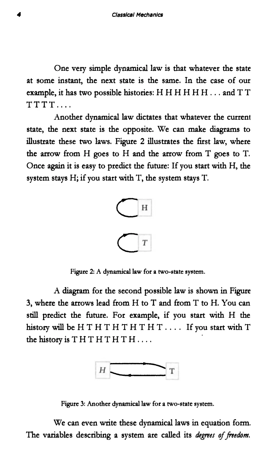
One very simple dynamical law is that whatever the state
at some instant, the next state is the same. In the case of our
example, it has two possible histories: H H H H H H . . . and T T
TTTT....
Another dynamical law dicta.tes that whatever the current
state, the next state is the opposite. We can make diagrams to
illustrate these two laws. Figure 2 illustra.tes the first law, where
the arrow from H goes to H and the arrow from T goes to T.
Once again it is easy to predict the future: If you start with H, the
system stays H; if you start with T, the system stays T.
c
c
Figure 2: A dynamical law for a two-state sY8tem.
A diagram for the second possible law is shown in Figure
3, where the arrows lead from H to T and from T to H. You can
still predict the future. For example, if you start with H the
history will be H T H T H T H T H T . . .. If you start with T
the history is T H T H T H T H . . . .
. 
.............. .
Figure 3: Another dynamical law for a two-state system.
We can even write these dynamical laws in equation fonn.
The variables describing a system are called its degrees of freedom.

The Nature of ClassIcal Physics
5
Our coin has one degree of freedom, which we can denote by the
greek letter sigma, u. Sigma has only two possible values; u = 1
and u = -1, respectively, for Hand T. We also use a symbol to
keep track of the time. When we are onsidering a continuous
evolution in time, we can symbolize it with t. Here we have a
discrete evolution and will use n. The state at time n is described
by the symbol u(n), which stands for u at n.
Let's write equations of evolution for the two laws. The
first law says that no change takes place. In equation fonn,
u(n+ 1) = u(n).
In other words, whatever the value of u at the nth step, it will
have the same value at the next step.
The second equation of evolution has the form
u(n+1) = -u(n),
implying that the state flips during each step.
Because in each case the future behavior is completely
determined by the initial state, such laws are deterministic. All the
basic laws of classical mechanics are deterministic.
To make things more interesting, let's generalize the
system by increasing the number of states. Instead of a coin, we
could use a six-sided die, where we have six possible states (see
Figure 4).
Now there are a great many possible laws, and they are
not so easy to describe in words-or even in equations. The
simplest way is to stick to diagrams such as Figure 5. Figure 5
says that given the numerical state of the die at time n, we
increase the state one unit at the next instant n + 1. That works
fine until we get to 6, at which point the diagram tells you to go
back to 1 and repeat the pattern. Such a pattern that is repeated

I
Classical MechanIcs
endlessly is called a 'Ycle. For example, if we start with 3 then the
history is 3, 4, 5, 6, 1, 2, 3, 4, 5, 6, 1, 2, . . . . We'll call this pattern
Dynamical Law 1.
Figure 4: A six-state system.
'" '-
t I
, I
Figure 5: Dynamical Law 1.
Figure 6 shows another law, Dynamical Law 2. It looks a
little messier than the last case, but it's logically identical-in each
case the system endlessly cycles through the six possibilities. If
we relabel the states, Dynamical Law 2 becomes identical to
Dynamical Law 1.
Not all laws are logically the same. Consider, for example:
the law shown in Figure 7. Dynamical Law 3 has two cycles. If
you start on one of them, you can't get to the other.
Nevertheless, this law is completely detenninistic. Wherever you
start, the future is determined. For example, if you start at 2, the

The Nature of Classical Physics
7
history will be 2, 6, 1, 2, 6, 1, . . . and you will never get to 5. If
you start at 5 the history is 5, 3, 4, 5, 3, 4, . . . and you will never
get to 6.
1
Figure 6: Dynamical Law 2.
I' "
.
.
, ,I
Figure 7: Dynamical Law 3.
Figure 8 shows Dynamical Law 4 with three cycles.
c

I
,,-
Figurc 8: Dynamical Law 4.

8
Classical Mechanics
I t would take a long time to write out all of the possible
dynamical laws for a six-state system.
Exercise 2: Can you think of a general way to classify the
laws that are possible for a six-state system?
Rules That Me Not Allowed: The Minus-First Law
According to the roles of classical physics, not all laws are legal.
It's not enough for a dynamical law to be deterministic; it must
also be reversible.
The meaning of reversible-in the context of physics--can
be described a few different ways. The most concise description
is to say that if you reverse all the arrows, the resulting law is still
deterministic. Another way, is to say the laws are deterministic into the
past as well as the future. Recall Laplace's remark, "for such an
intellect nothing would be uncertain and the future just like the
past would be present before its eyes." Can one conceive of laws
that are deterministic into the future, but not into the past? In
other words, can we fonnulate irreversible laws? Indeed we can.
Consider Figure 9.
/
Figure 9: A system that is irreversible.
The law of Figure 9 does tell you, wherever you are, where to go
next. If you are at 1, go to 2. If at 2, go to 3. If at 3, go to 2.

The Nature of Classical Physics
I
There is no ambiguity about the future. But the past is a different
matter. Suppose you are at 2. Where were you just before that?
You could have come from 3 or from 1. The diagram just does
not tell you. Even worse, in terms of reversibility, there is no state
that leads to 1; state 1 has no past. The law of Figure 9 is
imversible. It illustrates just the kind of situation that is prohibited
by the principles of classical physics.
Notice that if you reverse the arrows in Figure 9 to give
Figure 10, the corresponding law fails to tell you where to go in
the future.
/
Figure 10: A system that is not detenninistic into the future.
There is a very simple role to tell when a diagram
represents a deterministic reversible law. If every state has a
single unique arrow leading into it, and a single arrow leading out
of it, then it is a legal deterministic reversible law. Here is a
slogan: There must be one arrow to tell you where you're going and one to
tell you where you came from.
The role that dynamical laws must be deterministic and
reversible is so central to classical physics that we sometimes
forget to mention it when teaching the subject. In fact, it doesn't
even have a name. We could call it the first law, but unfortunately
there are already two first laws-Newton's and the first law of
thennodynamics. There is evan a zeroth law of thennodynamics.
So we have to go back to a minus-first law to gain priority for what
is undoubtedly the most fundamental of all physical laws-the
conservation of information. The conservation of infonnation is

JO
Classical Mechanics
simply the rule that every state has one arrow in and one arrow
out. It ensures that you never lose track of where you started.
The conservation of infonnation is not a conventionaJ
conservation law. We will return to conservation laws after a
digression into systems with infinitely many states.
Dynamical Systems with an Infinite Number of States
So far, all our examples have had state-spaces with only a f1nite
number of states. There is no reason why you can't have a
dynamical system with an infinite number of states. For example,
imagine a line with an infinite number of discrete points along
it-like a train track with an infinite sequence of stations in both
directions. Suppose that a marker of some sort can jump from
one point to another according to some role. To describe such a
system, we can label the points along the line by integers the
same way we labeled the discrete instants of time above. Because
we have already used the notation n for the discrete time steps,
let's use an uppercase N for points on the track. A history of the
marker would consist of a function N(n), telling you the place
along the track N at every time n. A short portion of this state-
space is shown in Figure 11.
Figure 11: State-space for an infinite system.
A very simple dynamical law for such a system, shown in Figure
12, is to shift the marker one unit in the positive direction at each
time step.

The Nature of Classical Physics
II
-4
..
 --- .... ..... ....
-...
Figure 12: A dynamical rule for an infinite system.
This is allowable because each state has one arrow in and one
arrow out. We can easily express this role in the form of an
equation.
N(n+ 1) = N(n) + 1
(1)
Here are some other possible rules, but not all are allowable.
N (n + 1) = N (n) - 1 (2)
N (n + 1) = N (n) + 2 (3)
N (n + 1) = N (n)2 (4)
N(n+ 1) = _I N (n) N(n) (5)
Exercise 3: Determine which of the dynamical laws
shown in Eq.s (2) through (5) are allowable.
In Eq. (1), wherever you start, you will eventually get to
every other point by either going to the future or going to the
past. We say that there is a single infinite cycle. With Eq. (3), on
the other hand, if you start at an odd value of N, you will never
get to an even value, and vice versa. Thus we say there are two
infinite cycles.
We can also add qualitatively different states to the
system to create more cycles, as shown in Figure 13.

12
ClasslCllI Mechanics
-4
...
.... .... .... ..... ....
.....
==
Figure 13: Breaking an infmite configuration space into
fmite and infinite cycles.
If we start with a number, then we just keep proceeding through
the upper line, as in Figure 12. On the other hand, if we start at
A or B, then we cycle between them. Thus we can have mixtures
where we cycle around in some states, while in others we move
off to inf1nity.
Cycles and Conservation Laws
When the state-space is separated into several cycles, the system
remains in whatever cycle it started in. Each cycle has its own
dynamical rule, but they are all part of the same state-space
because they describe the same dynamical system. Let's consider
a system with three cycles. Each of states 1 and 2 belongs to its
own cycle, while 3 and 4 belong to the third (see Figure 14).
(  J 
C  . -
Figure 14: Separating the state-space into cycles.
Whenever a dynamical law divides the state-space into
such separate cycles, there is a memory of which cycle they
started in. Such a memory is called a conseroation law; it tells us that

The Nature of Classical Physics
11
something is kept intact for all time. To make the conservation
law quantitative, we give each cycle a numerical value called Q. In
the example in Figure 15 the three cycles are labeled Q = + 1,
Q = -1, and Q = O. Whatever the value of Q, it remains the
same for all time because the dynamical law does not allow
jumping from one cycle to another. Simply stated, Q is conserved.
(  . -
( -  -
Figure 15: Labeling the cycles with specific values of a
conserved quantity.
In later chapters we will take up the problem of
continuous motion in which both time and the state-space are
continuous. All of the things that we discussed for simple
discrete systems have their analogs for the more realistic systems
but it will take several chapters before we see how they all play
out.
The Limits of Precision
Laplace may have been overly optimistic about how predictable
the world is, even in classical physics. He certainly would have
agreed that predicting the future would require a perfect
knowledge of the dynamical laws governing the world, as well as
tremendous computing power-what he called an "intellect vast
enough to submit these data to analysis." But there is another
element that he may have underestimated: the ability to know the
initial conditions with almost perfect precision. Imagine a die
with a million faces, each of which is labeled with a symbol

14
Classical Mechanics
similar in appearance to the usual single-digit integers, but with
enough slight differences so that there are a million
distinguishable labels. If one knew the dynamical law, and if one
were able to recognize the initial labe one could predict the
future history of the die. However, if Laplace's vast intellect
suffered from a slight vision impairment, so that he was unable to
distinguish among similar labels, his predicting ability would be
limited.
In the real world, it's even worse; the space of states is
not only huge in its number of points-it is continuously infinite.
In other words, it is labeled by a collection of real numbers such
as the coordinates of the particles. Real numbers are so dense
that every one of them is arbitrarily close in value to an infinite
number of neighbors. The ability to distinguish the neighboring
values of these numbers is the "resolving power" of any
experiment, and for any real observer it is limited. In principle we
cannot know the initial conditions with infinite precision. In most
cases the tiniest differences in the initial conditions-the starting
state-leads to large eventual differences in outcomes. This
phenomenon is called chaos. If a system is chaotic (most are), then
it implies that however good the resolving power may be, the
time over which the system is predictable is limited. Perfect
predictability is not achievable, simply because we are limited in
our resolving power.

Interlude 1: Spaces, Trigonotnetry, and
Vectors
"Where are we, George?"
George pulled out his map and spread it out in front of
Lenny. "We're right here Lenny, coordinates 36.60709N,
-121.618652W."
"Huh? What's a coordinate George?"
Coordinates
To describe points quantitatively, we need to have a coordinate
system. Constructing a coordinate system begins with choosing a
point of space to be the origin. Sometimes the origin is chosen to
make the equations especially simple. For example, the theory of
the solar system would look more complicated if we put the
origin anywhere but at the Sun. Strictly speaking, the location of
the origin is arbitrary-put it anywhere-but once it is chosen,
stick with the choice.
The next step is to choose three perpendicular axes.
.A.gain, their location is somewhat arbitrary as long as they are
perpendicular. The axes are usually called x, y, and Z but we can
also call them X1, X2, and X3' Such a system of axes is called a
Cartesian coordinate system, as in Figure 1.

l'
C/ass/1 Mechanics
y
x
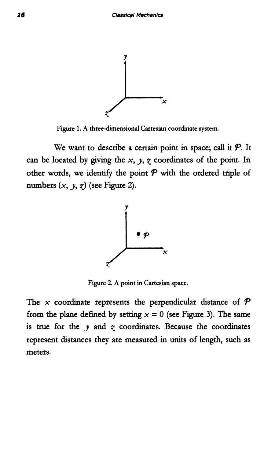
Figure 1. A three-dimensional Cartesian coordinate system.
We want to describe a certain point in space; call it 'P. It
can be located by giving the x, y, Z coordinates of the point. In
other words, we identify the point 'P with the ordered triple of
numbers (x, y, z) (see Figure 2).
y
-tp
x
Figure 2. A point in Cartesian space.
The x coordinate represents the perpendicular distance of tp
from the plane defined by setting x = 0 (see Figure 3). The same
is true for the y and Z coordinates. Because the coordinates
represent distances they are measured in units of length, such as
meters.

Spaces, Trigonometry, and Vectors
17
'Y
tp
x
i:
Figure 3: A plane defined by setting x = 0, and the distance
to tp along the x axis.
When we study motion, we also need to keep track of
time. Again we start with an origin-that is, the zero of time. We
could pick the Big Bang to be the origin, or the birth of Jesus, or
just the start of an experiment. But once we pick it, we don't
change it.
Next we need to fix a direction of time. The usuaJ
convention is that positive times are to the future of the origin
and negative times are to the past. We could do it the other way,
but we won't.
Finally, we need units for time. Seconds are the
physicist's customary units, but hours, nanoseconds, or years are
also possible. Once having picked the units and the origin, we can
label any time by a number t.
There are two implicit assumptions about time in classicaJ
mechanics. The first is that time runs unifonnly-an interval of 1
second has exactly the same meaning at one time as at another.
For example, it took the same number of seconds for a weight to
fall from the Tower of Pisa in Galileo's time as it takes in our
time. One second meant the same thing then as it does now.
The other assumption is that times can be compared at

18
Classical Mechllnlcs
different locations. This means that clocks located in different
places can be synchronized. Given these assumptions, the four
coordinates-x, y, Z, t--define a reference frame. Any event in the
reference frame must be assigned a value for each of the
coordinates.
Given the function f(/) = t 2 , we can plot the points on a
coordinate system. We will use one axis for time, t, and another
for the function, f(t) (see Figure 4).
f(t)
15 .
.
.
10 .
.
.
5 .
.
.
..
.. t
1 2 3 4
Figure 4: Plotting the points of I(t) = t 2 .
We can also connect the dots with curves to fill in the spaces
between the points (see Figure 5).
f(t)
15
10
5
t
1
2
3
4
Figure 5: Joining the plotted points with curves.

Spaces, Trigonometry, and Vectors
1.
In this way we can visualize functions.
Exercise 1: Using a graphing calculator or a program
like Mathnnotica, plot each of the following functions.
See the next section if you are unfamiliar with the
trigonometric functions.
f (I) = t 4 + 3 t 3 - 12 t 2 + t - 6
g(x) = sin x -cosx
9 (a) = P + alna
x (I) = sin 2 x - cos x
Trigonometry
If you have not studied trigonometry, or if you studied it a long
time ago, then this section is for you.
We use trigonometry in physics all the time; it is
everywhere. So you need to be familiar with some of the ideas,
symbols, and methods used in trigonometry. To begin with, in
physics we do not generally use the degree as a measure of angle.
Instead we use the radian; we say that there are 211' radians in
360°, or 1 radian = 11' /180°, thus 90 ° = 11' /2 radians, and
30 ° = 11' /6 radians. Thus a radian is about 57° (see Figure 6).
The trigonometric functions are defined in terms of
properties of right triangles. Figure 7 illustrates the right triangle
and its hypotenuse c, base b, and altitude a. The greek letter theta,
9, is defined to be the angle opposite the altitude, and the greek
letter phi, l/J, is defined to be the angle opposite the base.

20
C/asslCllI Mechanics
Figure 6: The radian as the angle subtended by an arc equal
to the radius of the circle.
a
b
Figure 7: A right triangle with segments and angles
indicated.
We define the functions sine (sin), cosine (cos), and tangent (tan),
as ratios of the various sides according to the following
relationships:
a
sin (J = -
c
b
cos (J = -
c
a sin (J
tan (J = - =
b co s (J

Spaces, Trigonometry, and Vectors
21.
We can graph these functions to see how they va.ry
(see Figures 8 through 10).
sinB
1
8
1r
2
-1
Figure 8: Graph of the sine function.
cas 8
1
B
21r
-1
Figure 9: Graph of the cosine function.
tan 8
Figure 10: Graph of the tangent function.
There are a couple of useful things to know about the
trigonometric functions. The first is that we ca.n draw a triangle
within a circle, with the center of the circle located at the origin
of a Cartesian coordinate system, as in Figure 11.

22
Classical Mech.nlcs
y
x
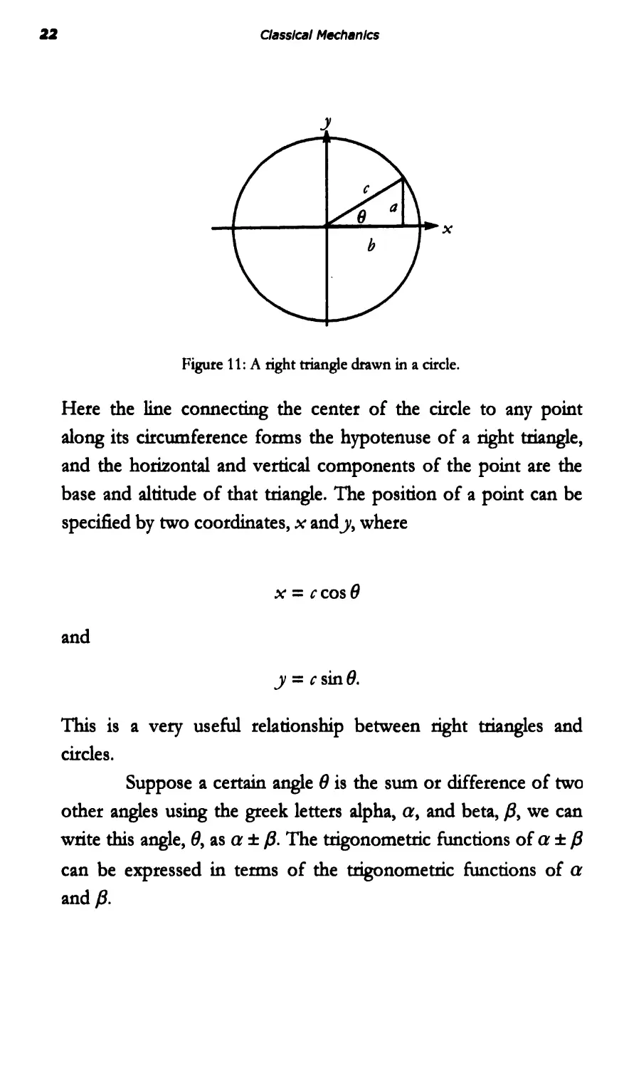
Figure 11: A right triangle drawn in a circle.
Here the line connecting the center of the circle to any point
along its circumference fonns the hypotenuse of a right triangle,
and the horizontal and vertical components of the point are the
base and altitude of that triangle. The position of a point can be
specified by two coordinates, x andy, where
x = c cos 8
and
y = c sin 8.
This is a very useful relationship between right triangles and
circles.
Suppose a certain angle 8 is the sum or difference of two
other angles using the greek letters alpha, a, and beta, {3, we can
write this angle, 8, as a :t: {3. The trigonometric functions of a :t: {3
can be expressed in tenns of the trigonometric functions of a
and {3.

Spaces, Trigonometry, and Vectors
23
sin {a + {3) = sin a cos {3 + cos a sin {3
sin (a - {3) = sin a cos {3 - cos a sin {3
cos (a + {3) = cos a cos {3 - sin a sin {3
cos (a - {3) = cos a cos {3 + sin a sin {3.
A final-very useful-identity is
sin 2 8 + cos 2 8 = 1.
(1)
(Notice the notation used here: sin 2 8 = sin 8 sin 8.) This equation
is the Pythagorean theorem in disguise. If we choose the radius
of the circle in Figure 11 to be 1, then the sides a and b are the
sine and cosine of 8; and the hypotenuse is 1. Equation (1) is
the familiar relation among the three sides of a right triangle:
rJ2 + b 2 = c2.
Vectors
Vector notation is another mathematical subject that we assume
you have seen before, but-just to level the playing field-let's
review vector methods in ordinary three-dimensional space.
A vector can be thought of as an object that has both a
length (or magnitude) and a direction in space. An example is
displacement. If an object is moved from some particular starting
location, it is not enough to know how far it is moved in order to
know where it winds up. One also has to know the direction of
the' displacement. Displacement is the simplest example of a
vector quantity. Graphically, a vector is depicted as an arrow with
a length and direction, as shown in Figure 12.

24
Classical Mechanics
y
x

'\.
Figure 12: A vector r in Cartesian coordinates.
Symbolically vectors are represented by placing arrows over

them. Thus the symbol for displacement is r. The magnitude, or
length, of a vector is expressed in absolute-value notation. Thus
the length of -: is denoted 1-:1.
Here are some operations that can be done with vectors.
First of all, you can multiply them by ordinary real numbers.
When dealing with vectors you will often see such real numbers
given the special name scalar. Multiplying by a positive number
just multiplies the length of the vector by that number. But you
can also multiply by a negative number, which reverses the

direction of the vector. For example - 2 r is the vector that is

twice as long as r but points in the opposite direction.
 
Vectors may be added. To add A and B, place them as
shown in Figure 13 to fonn a quadrilateral (this way the
directions of the vectors are preserved). The sum of the vectors is
the length and angle of the diagonal.

Spaces, Trigonometry, and Vectors
25
-+
B
...
/
/
/
/
/
... /
... ... /
..../
...
...
Figure 13: Adding vectors.
If vectors can be added and if they can be multiplied by negative
numbers then they can be subtracted.
Exercise 2: Work out the rule for vector 8ubtraction.
Vectors can also be described in component fonn. We
begin with three perpendicular axes x, y, . Next, we define
three unit vectors that lie along these axes and have unit length. The
unit vectors along the coordinate axes are called basis vectors. The
three basis vectors for Cartesian coordinates are traditionally
A A A
called i, j, and Ie (see Figure 14). More generally, we write '1, '2,
and '3 when we refer to (x1, X2, x3), where the symbol A (known
as a carat) tells us we are dealing with unit (or basis) vectors. The
-+
basis vectors are useful because any vector V can be written in
terms of them in the following way:
-+  1\ A
V = V x t + V y J + V z Ie.
(2)

28
Classical Mechanics
y
1\
J
I).
t
x
'Y
'\.
Figure 14: Basis vectors for a Cartesian coordinate system.
The quantities V x , V y , and V z are numerical coefficients that

are needed to add up the basis vectors to give V. They are also

called the components of V. We can say that Eq. (2) is a linea,
combination of basis vectors. This is a fancy way of saying that we
add the basis vectors along with any relevant factors. Vector
components can be positive or negative. We can also write a
vector as a list of its components-in this case (V x , V y , V).
The magnitude of a vector can be given in terms of its
components by applying the three-dimensional Pythagorean
theorem.
v = ...J V x 2 + Vi + Vl
(3)

We can multiply a vector V by a scalar, a, in terms of
components by multiplying each component bya.

a V = (a V x , a V Y ' a V z )
We can write the sum of two vectors as the sum of the

Spaces, Trigonometry, and Vectors
27
corresponding components.
(A+BL = (Ax+Bx)
(A + Bt = (Ay + By)
(A + B)Z = (AZ + BZ)'
Can we multiply vectors? Yes, and thete is more than one
way. One type of product-the cross product-gives another
vector. For now, we will not worry about the cross product and
only consider the other method, the dot prodNct. The dot product

of two vectors is an ordinary nwnber, a scalar. For vectors A and

B it is defined as follows:
  -. 
A · B = A B cos 8.
Here 8 is the angle between the vectors. In ordinary language, the
dot product is the product of the magnitudes of the two vectors
and the cosine of the angle between them.
The dot product can also be defined in terms of
components in the form
 
A · B = Ax Bx + A y By + Az Bz.
This makes it easy to compute dot products given the
components of the vectors.

28
Classical Mech.nlcs
Exercise 3: Show that the magnitude of a vector satisfies
-+2 -+-+
A =A.A.
Exercise 4: Let (Ax = 2, Ay = -3, AZ = 1) and
(Bx = -4, By = -3,Bz = 2). Compute the mag- nitude of
.... -+
a A and B, their dot product, and the angle between
them.
An important property of the dot product is that it is
zero if the vectors are orthogonal (perpendicular). Keep this in
mind because we will have occasion to use it to show that vectors
ate orthogonal.
Exercise 5: Detennine which pair of vectors are
orthogonal. (1, 1, 1) (2, -1, 3) (3, 1, 0) (-3, 0, 2)
Exercise 6: Can you explain why the dot product of two
vectors that are orthogonal is O?

Lecture 2: Motion
Lenny complained, "George, this jumpy stroboscopic stuff makes
me nervous. Is time really so bumpy? I wish things would go a
little more smoothly."
George thought for a moment, wiping the blackboard,
"Okay, Lenny, today let's study systems that do change
smoothly."
Mathematical Interlude: Differential Calculus
In this book we will mostly be dealing with how various
quantities change with time. Most of classical mechanics deals
with things that change smoothly-continuouslY 1S the
mathematical term-as time changes continuously. Dynamical
laws that update a state will have to involve such continuous
changes of time, unlike the stroboscopic changes of the first
lecture. Thus we will be interested in functions of the
independent variable t.
To cope, mathematically, with continuous changes, we
use the ma.thematics of calculus. Calculus is about limits, so let's
get that idea in place. Suppose we have a sequence of numbers,
1 1 '' '3,"" that get closer and closer to some value L. Here is
an example: 0.9, 0.99, 0.999, 0.9999, . . . . The limit of this
sequence is 1. None of the entries is equal to 1, but they get
closer and closer to that value. To indica.te this we write
 1,. = L.
'-'00
In words, L is the limit of  as i goes to infinity.

30
C/asslc.' Mech.nlcs
We can apply the same idea to functions. Suppose we
have a function, f(t), and we want to describe how it varies as t
gets closer and closer to some value, saya. If f(t) gets arbitrarily
close to L as t tends to a, then we say that the limit of f(t) as t
approaches a is the number L . Symbolically,
lim f(t) = L.
I-+a
Let f(t) be a function of the variable t. As t varies, so will
f(t). Differential calculus deals with the rate of change of such
functions. The idea is to start with f(t) at some instant, and then
to change the time by a little bit and see how much f(t) changes.
The rate of change is defined as the ratio of the change in f to
the change in t. We denote the change in a quantity with the
uppercase greek letter delta, 4. Let the change in t be called 4t.
(This is not 4 x t, this is a change in t.) Over the interval 6t, f
changes from f(t) to f(t + 4t). The change in f, denoted 6f, is
then given by
6f = f(t + 4t) - f(t).
To define the rate of change precisely at time t, we must
let 4t shrink to zero. Of course, when we do that 4f also shrinks
to zero, but if we divide 4 f by 6t, the ratio will tend to a limit
That limit is the derivative of f( t) with respect to t,
df(t) 6f f(t + 6t) - f(t)
= lim - = Jim . (1)
d t 4/-+0 4t 4/-+0 4t
A rigorous mathematician might frown on the idea that
d1(1) is the ratio of two differentials, but you will rarely make a
dl I
mistake this way.

Motion
3J
Let's calculate a few derivatives. Begin with functions
defined by powers of t. In particular, let's illustrate the method by
calculating the derivative of f(t) = t 2 . We apply Eq. (1) and begin
by defining f( t + dt) :
f(t + dt) = (t + dt)2.
We can calculate (t + dt)2 by direct multiplication or we can use
the binomial theorem. Either way,
f(t + dt) = j2 + 2tdt + dt 2 .
We now subtract f(t):
f(t + dt) - f(t) =  + 2tdt + dP - P
= 2tdt + dP.
The next step is to divide by dt:
f(t + dt) - f(t)
dt
2tdt + dt 2
dt
= 2t +dt.
Now it's easy to take the limit dt --. O. The first term does not
depend on dt and survives, but the second term tends to zero
and just disappears. This is something to keep in mind: Terms of
higher order in dt can be ignored when you calculate derivatives.
Thus
f(t + dt) - f(t)
lim = 2t
4/-+0 dt
So the derivative of t 2 is

32
Classical Mechanics
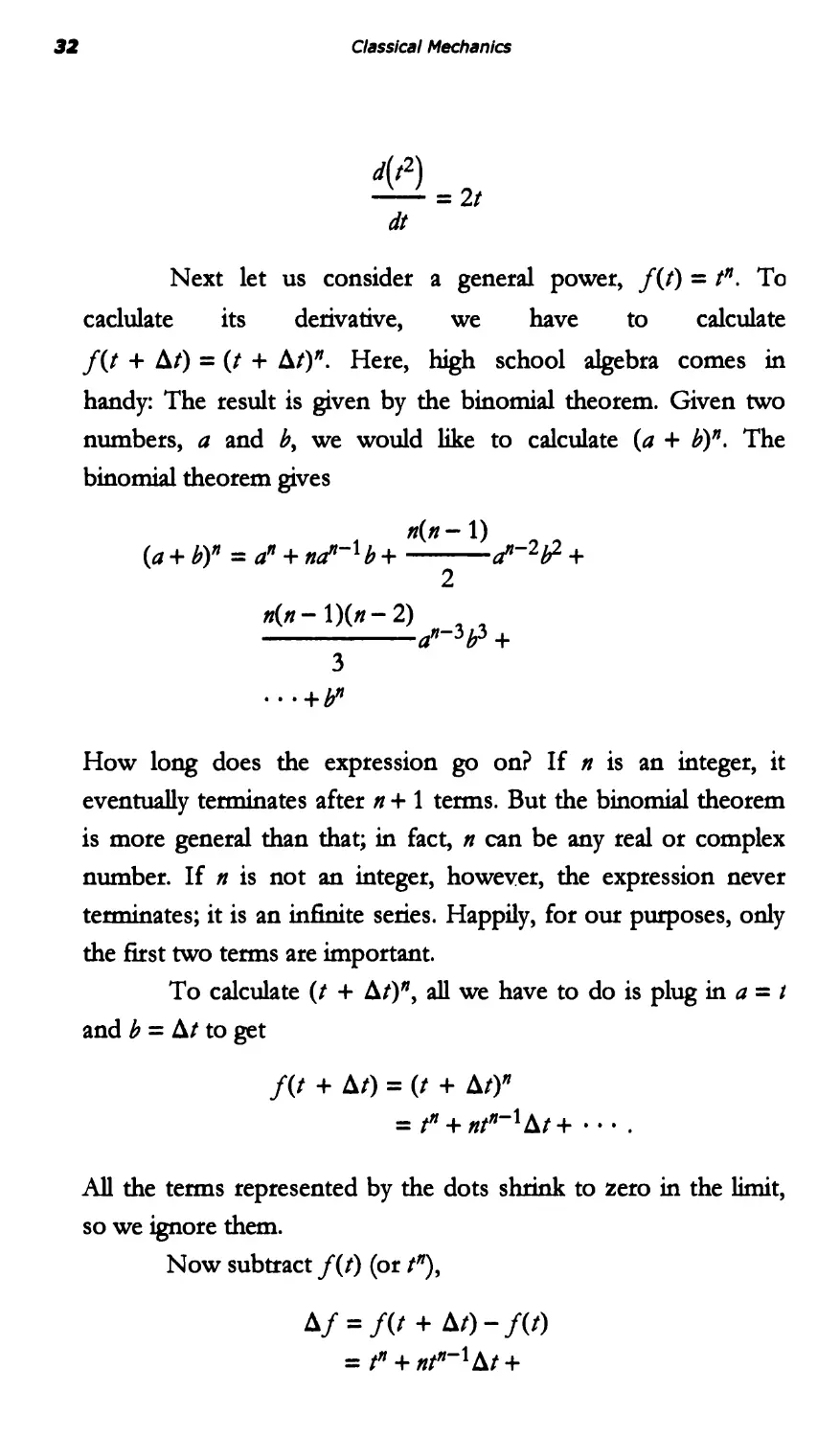
d(t 2 )
-=2t
dt
Next let us consider a general power, f(t) = tn. To
caclulate its derivative, we have to calculate
f(t + dt) = (t + dt)n. Here, high school algebra comes 111
handy: The result is given by the binomial theorem. Given two
numbers, a and b, we would like to calculate (a + b)n. The
binomial theorem gives
n(n - 1)
(a + b)n = an + na»-1 b + a»-2 +
2
n(n - l)(n - 2)
a n - 3 b3 +
3
. . . + b n
How long does the expression go on? If n is an integer, it
eventually terminates after n + 1 terms. But the binomial theorem
is more general than that; in fact, n can be any real or complex
number. If n is not an integer, however, the expression never
terminates; it is an infinite series. Happily, for our purposes, only
the first two terms are important.
To calculate (t + dt)n, all we have to do is plug in a = I
and b = dt to get
f(t + dt) = (t + dt)n
= t n + nt n - 1 dt + · · · .
All the terms represented by the dots shrink to zero in the limit,
so we ignore them.
Now subtract f(t) (or t n ),
df = f(t + dt) - f(t)
= t n + nt n - 1 dt +

Motion
33
n(n - 1)
t n - 2 d t 2 + . . . - t n
2
= nt"-1 dt +
n(n - 1)
t n - 2 dP + . . . .
2
Now divide by dt,
df n(n-1)
- = nt n - 1 + t n - 2 dt + . . . .
dt 2
and let dt --. 0. The derivative is then
d( t n )
- = nt n - 1 .
dt
One important point is that this relation holds even if n is not an
integer; n can be any real or complex number.
Here are some special cases of derivatives: If n = 0, then
f(t) is just the number 1. The derivative is zero-this is the case
for any function that does't change. If n = 1, then f(t) = t and
the derivative is 1-this is always true when you take the
derivative of something with respect to itself. Here are some
derivatives of powers
d(tl)
-=2t
tit
d( t3 )
-=3P
dt
d( t 4 )
-=4
dt

34
Classical Mechanics
d(t n )
- = nt n - 1 .
dt
For future reference, here are some other derivatives:
d(sin t)
= cos t
dt
d( cos t)
= - sint
dt (2)
d(/) -=1
dt
d(log t) 1
- -
dt t
One comment about the third formula in Eq. (2), d{l) = I. The
dt
meaning of I is pretty clear if t is an integer. For example,
e3 = e X eX 6. Its meaning for non-integers is not obvious.
Basically, I is defined by the property that its derivative is equal
to itself. So the third formula is really a definition.
There are a few useful roles to remember about
derivatives. You can prove them all if you want a challenging
exercise. The first is the fact that the derivative of a constant is
always O. This makes sense; the derivative is the rate of change,
and a constant never changes, so
de
- _ 0
- .
dt
The derivative of a constant times a function 1S the
constant times the derivative of the function:

Motion
35
d( c f)
dt
df
= c-.
dt
Suppose we have two functions, f(t) and g(t). Their sum
is also a function and its derivative is given by
d(f + g) d(j) d(g)
= -+-.
dt dt dt
This is called the sum rule.
Their product of two functions is another function, and
its derivative is
d(jg) d(g) d(j)
- = f(t)- + g(t)-.
dt d t d t
Not surprisingly, this is called the product rule.
Next, suppose that g(t) is a function of t, and f(g) is a
function of g. That makes f an implicit function of t. If you want to
know what f is for some t, you first compute g(t). Then,
knowing g, you compute f(g). It's easy to calculate the t-
derivative of f:
df df dg
----
dt dg dt
This is called the chain rule. This would obviously be true if the
derivatives were really ratios; in that case, the dg's would cancel in
the numerator and denominator. In fact, this is one of those
cases where the naive answer is correct. The important thing to
remember about using the chain role is that you invent an
intennediate function, g(t), to simplify f(t) making it f(g). For
example, if

.
Classical Mechanics
f (t) = In t 3
and we need to fmd , then the t 3 inside the logarithm might
dt
be a problem. Therefore, we invent the intennediate function
g = /3, so we have f(g) = In g. We can then apply the chain rule.
df df dg
----
- .
dt dg dt
We can use our differentiation fonnulas to note that  = 1 and
dg g
dg ?
- = 3. so
dt '
3 t 2
df
dt
-
.
g
We can substitute g = t 3 , to get
df 3 t 2 3
dt
t 3
t
That is how to use the chain role.
U sing these roles, you can calculate a lot of derivatives.
That's basically all there is to differential calculus.

Motion
37
Exercise 1: Calculate the derivatives of each of these
functions.
f (t) = t 4 + 3 t 3 - 12 t 2 + t - 6
g (x) = sin x - cos x
lJ(a) = e a +alna
x(t) = sin 2 x - cos x
Exercise 2: The derivative of a derivative is called the
d d ,. d .. d 2 (I) T k th d
secon envative an IS wntten d,2 . a e e secon
derivative of each of the functions listed above.
Exercise 3: Use the chain rule to find the derivatives of
each of the following functions.
g(t) = sin(t 2 ) - cos(t 2 )
lJ(a) = e 3a + 3aln(3a)
x(t) = sin 2 (t 2 ) - cos(t 2 )
Exercise 4: Prove the sum rule (fairly easy), the product
rule (easy if you mow the trick), and the chain rule
(fairly easy).
Exercise 5: Prove each of the formulas in Eq.s (2). Hint:
Loole up tr"go"otn8hic ,.t/8"t"t"es and h'm"t propert"es ,." a
reference boole.

38
Classical Mechanics
Particle Motion
The concept of a point particle is an idealization. No object is so
small that it is a point-not even an electron. But in many
situations we can ignore the extended structure of objects and
treat them as points. For example, the planet Earth is obviously
not a point, but in calculating its orbit around the Sun, we can
ignore the size of Earth to a high degree of accuracy.
The position of a particle is specified by giving a value fo!
each of the three spatial coordinates, and the motion of the
particle is defined by its position at every time. Mathematically,
we can specify a position by giving the three spatial coordinates
as functions of t: x(t), y(t), z(t).
-+
The position can also be thought of as a vector r (t)
whose components are x, y, Z at time t. The path of the
-+
particle-its trt!Jectory-is specified by r (t). The job of classical
-+
mechanics is to figure out r (t) from some initial condition and
some dynamical law.
Next to its position, the most important thing about a
particle is its velocity. Velocity is also a vector. To define it we
need some calculus. Here is how we do it:
Consider the displacement of the particle between time t
and a little bit later at time t + dt. During that time interval the
particle moves from x(t), y(t), z(t) to x(t + dt), y(t + dt),
-+ -+
if...t + dt), or, in vector notation, from r (t) to r (t + dt). The
displacement is defined as
dx = x(t + dt) - x(t)
dy = y(t + dt) - y(t)
dZ = Z(t + dt) - Z(t)

Motion
3.
or
-+ -+ -+
d r = r (t + dt) - r (t).
The displacement is the small distance that the particle moves in
the small time dt. To get the velocity, we divide the displacement
by dt and take the limit as dt shrinks to zero. For example,
dx
Vx = lim -.
4/-+0 dt
This-of course-is the definition of the derivative of x with
respect to t.
dx
Vx = - = x
dt
dy
v y = - = Y
dt
dZ
V z = - = z.
dt
Placing a dot over a quantity is standard shorthand for taking the
time derivative. This convention can be used to denote the time
derivative of anything, not just the position of a particle. For
example, if T stands for the temperature of a tub of hot water,
then T will represent the rate of change of the temperature with
time. It will be used over and over, so get familiar with it.
It gets tiresome to keep writing x, y, Z, so we will often
condense the notation. The three coordinates x, y, Z are
collectively denoted by Xi and the velocity components by vi:

40
Classical Mechanics
dx.
t
V. = - = X,
t dt t
where i takes the values x, y, Z, or, in vector notation
-+
-+ dr 
v = - = r.
dt
The vdocity vector has a magnitude r;;l.
1';;1 2 = v x 2 + vi + vr/.
this represents how fast the particle is moving, without regard to
the direction. The magnitude r;;1 is called speed
Acceleration is the quantity that tells you how the velocity
is changing. If an object is moving with a constant velocity
vector, it experiences no acceleration. A constant velocity vector
implies not only a constant speed but also a constant direction.
You feel acceleration only when your velocity vector changes,
either in magnitude or direction. In fact, acceleration is the rime
derivative of velocity:
dv.
t
ai = - = Vi
dt
or, in vector notation,
.
-+ -+
a = v.
Because vi is the time derivative of Xi and ai is the time
derivative of Vb it follows that acceleration is the second time-
derivative of Xi,

Motion
4J
d 2 x.
t
ai = - = xi
dt 2
where the double-dot notation means the second time-derivative.
Examples of Motion
Suppose a particle starts to move at time t = 0 according to the
equations
x(t) = 0
yet) = 0
1
z(t) = z(O) + v(O)t - - gfl
2
The particle evidently has no motion in the x and y directions
but moves along the Z axis. The constants Z(O) and v(O) represent
the initial values of the position and velocity along the Z direction
at t = O. We also consider g to be a constant.
Let's calculate the velocity by differentiating with respect
to time.
Vx(t) = 0
vy(t) = 0
vz(t) = v(O) - gt.
The x and y components of velocity are zero at all times. The Z
component of velocity starts out at t = 0 being equal to v(O). In
other words, v(O) is the initial condition for velocity.

42
Classical Mechanics
As time progresses, the - gt term becomes nonzero.
Eventually, it will overtake the initial value of the velocity, and the
particle will be found moving along in the negative Z direction.
N ow let's calculate the acceleration by differentiating with
respect to time again.
ax(t) = 0
ay(t) = 0
az(t) = - g.
The acceleration along the Z axis is constant and negative. If the Z
axis were to represent altitude, the particle would accelerate
downward in just the way a falling object would.
Next let's consider an oscillating particle that moves back
and forth along the x axis. Because there is no motion in the
other two directions, we will ignore them. A simple oscillatory
motion uses trigonometric functions:
x(t) = sin w t
where the lowercase greek letter omega, w, is a constant. The
larger w, the more rapid the oscillation. This kind of motion is
called simple harmonic motion (see Figure 1).
x
t
Figure 1: Simple hannonic motion.
Let's compute the velocity and acceleration. To do so, we need to
differentiate x(t) with respect to time. Here is the result of the

Motion
..
first time-derivative:
d
V x = - sinwt.
dt
We have the sine of a product. We can relabel this product as
b = wt:
d
V x = - sin b.
dt
U sing the chain role,
d db
v = -sinb-
x db dt
or
d
V x = cos b - (w t)
dt
or
V x = w cos w t .
We get the acceleration by similar means:
ax = -w 2 sinwt.
Notice some interesting things. Whenever the position x is at its
maximum or minimum, the velocity is zero. The opposite is also
true: When the position is at x = 0, then velocity is either a
maximum or a minimum. We say that position and velocity are
90 0 out of phase. You can see this in Figure 2, representing x(t),
and Figure 3, representing vet).

44
Classical Mechanics
x(t)
1
(J
1r
2
-1
Figure 2: Representing position.
v(t)
1
(J
21r
-1
Figure 3: Representing velocity.
The position and acceleration are also related, both being
proportional to sin w t. But notice the minus sign in the
acceleration. That minus sign says that whenever x is positive
(negative), the acceleration is negative (positive). In other words,
wherever the particle is, it is being accelerated back toward the
origin. In technical terms, the position and acceleration are 180 0
out of phase.
Exercise 6: How long does it take for the oscillating
particle to go through one fun cycle of motion?
Next, let's consider a particle moving with uniform
circular motion about the origin. This means that it is moving in a

Motion
45
circle at a constant speed. For this purpose, we can ignore the !(:
axis and think of the motion in the x, y plane. To describe it we
must have two functions, x(t) and y(t). To be specific we will
choose the particle to move in the counterclockwise direction.
Let the radius of the orbit be R.
It is helpful to visualize the motion by projecting it onto
the two axes. As the particle revolves around the origin, x
oscillates between x = - R and x = R. The same is true of the y
coordinate. But the two coordinates are 90° out of phase; when x
is maximum y is zero, and vice versa.
The most general (counterclockwise) uniform circulat
motion about the origin has the mathematical form
x(t) = Rcoswt
y(t) = Rsinwt.
Here the parameter w is called the angular frequenry. It is defined as
the number of radians that the angle advances in unit time. It also
has to do with how long it takes to go one full revolution, the
period of motion-the same as we found in Exercise 6:
21r
T=-
w
Now it is easy to calculate the components of velocity and
acceleration by differentiation:
v x = - R w sin w t
v Y = R w cos w t
ax = -Rw 2 coswt
a y = -Rw 2 sinwt
(3)
This shows an interesting property of circular motion that
Newton used in analyzing the motion of the moon: The

4'
Classical Mechanics
acceleration of a circular orbit is parallel to the position vector,
but it is oppositely directed. In other words, the acceleration
vector points radially inward toward the origin.
Exercise 7: Show that the position and velocity vectors
are orthogonal.
Exercise 8: Calculate the velocity, speed, and
acceleration for each of the following position vectors. If
you have graphing software, plot each position vector,
each velocity vector, and each acceleration vector.
-+
r = (cos w t, eW t )
-+
r = (cos (w t -lfJ), sin (w t - lfJ»
-+
r = (c cos 3 t, c sin 3 t)
-+
r = (c(t-sint),c(l-cost»

Interlude 2: Integral Calculus
"George, I really like doing things backward. Can we do
differentiation backward?"
"Sure we can, Lenny. It's called integration."
Integral Calculus
Differential calculus has to do with rates of change. Integral
calculus has to do with sums of many tiny incremental quantities.
It's not immediately obvious that these have anything to do with
each other, but they do.
We begin with the graph of a function f(t), as in Figure 1.
1(1)
15
10
5
1
12345
Figure 1: 'rhe behavior of f(t).
The central problem of integral calculus is to calculate the area
under the curve defined by f(t). To make the problem well
defined, we consider the function between two values that we call
limits of integration, t = a and t = b. The area we want to calculate is
the area of the shaded region in Figure 2.

48
Classical Mechanics
f(/)
15
10
5
a b
t
1 2 3 4 5
Figure 2: The limits of integration.
In order to do this, we break the region into very thin rectangles
and add their areas (see Figure 3).
f(t)
15
10
5
a b
t
1 2 3 4 5
Figure 3: An illustration of integration.
Of course this involves an approximation, but it becomes
accurate if we let the width of the rectangles tend to zero. In
order to carry out this procedure, we fust divide the interval
between t = a and t = b into a number, N, of subintervals-each
of width b. t. Consider the rectangle located at a specific value of
t. The width is b. t and the height is the local value of f(t). It
follows that the area of a single rectangle, 6 A, is
6 A = f(t) b. t.
Now we add up all the areas of the individual rectangles to get an
approximation to the area that we are seeking. The approximate

Integral Calculus
..,
answer 1S
A = L:f(tj)'
i
where the uppercase greek letter sigma, 1:, indicates a sum of
successive values defined by i. So, if N = 3, then
3
A = L:f(ti) 1
i
= j(t1) b. t + j(tz) b. t + j(t3) b. t.
Here ti is the position of the ith rectangle along the taxis.
To get the exact answer, we take the limit in which b. J
shrinks to zero and the number of rectangles increases to infinity.
That defines the definite integral of Jet) between the limits t = a
and t = b. We write this as
A = (b f(/) d 1 = lim L:f(tj)  I.
Ja 4 '....0 .
t
The integral sign, called summa, 1: replaces the summation sign,
and-as in differential calculus-4 t is replaced by d t. The
function J(t) is called the integrand.
Let's make a notational change and call one of the limits
of integration T. In particular, replace b by T and consider the
integral
[ f(/) d 1
where we are going to think of T as a variable instead of as a
definite value of t. In this case, this integral defines a function of
T, which can take on any value of t. The integral is a function of

50
Classical Mechanics
T because it has a definite value for each value of T.
F(T) = f j(l) d t.
Thus a given function jet) defines a second function F(T). We
could also let a vary, but we won't. The function F(T) is called
the indefinite integral of jet). It is indefinite because instead of
integrating from a fixed value to a fixed value, we integrate to a
variable. We usually write such an integral without limits of
integration,
F(t) = f j(l) d t.
(1)
The fundamental theorem of calculus is one of the simplest and
most beautiful results in mathematics. It asserts a deep
connection between integrals and derivatives. What it says is that
if F(T) = f J(t) d t, then
J(t) =
d F(t)
dt
To see this, consider a small incremental change in T from T to
T + 4 t. Then we have a new integral,
f +f1t
F(T +  t) = a jet) d t.
In other words, we have added one more rectangle of width b. t
at t = T to the area shaded in Figure 3. In fact, the difference
F(T + b. t) - F(T) is just the area of that extra rectangle, which
happens to be J(T) b. t, so
F(T + 4 t) - F(T) = J(T) 4 t.

Integral Calculus
5J
Dividing by  t,
F(T +  t) - F(T)
= j(T)
t
we obtain the fundamental theorem connecting F and j, when
we take the limit where  t -+ 0:
dF
-=lim
d T 1:1 '.....0
F(T +  t) - F(T)
= f(T).
4t
We can simplify the notation by ignoring the difference between t
and T,
dF
- = f(t).
dt
In other words, the processes of integration and differentiation
are reciprocal: The derivative of the integral is the original
integrand.
Can we completely determine F(t) knowing that its
derivative is f(t)? Almost, but not quite. The problem is that
adding a constant to F(t) does not change its derivative. Given
f(t), its indefinite integral is ambiguous, but only up to adding a
constant.
To see how the fundamental theorem is used, let's work
out some indefinite integrals. Let's fmd the integral of a power
f(t) = tn. Consider,
F(t) = f jet) d t.
It follows that

52
Classical Mechanics
d F(t)
f(t) =
dt
or
d F(t)
t n =
dt
All we need to do is find a function F whose derivative is tn, and
tha t is easy.
In the last chapter we found that for any fII,
d (t 11l )
= fII f'I-1.
dt
If we substitute fII = n + 1, this becomes
d (t n + 1 )
= (n + 1) t n
dt
or, dividing by n + 1,
d (t n + 1 / n + 1)
= tn.
dt
Thus we find that t" is the derivative of I n +1 . Substituting the
n+1
relevant values, we get
J tn+1
F(t) = t n d t = -.
n+1
The only thing missing is the ambiguous constant that we can
add to F. We should write

Integral Calculus
5'
J t,,+1
t"dt= -+c
n+l
where c is a constant that has to be determined by other means.
The ambiguous constant is closely related to the
ambiguity in choosing the other endpoint of integration that we
earlier called a. To see how a determines the ambiguous constant
c, let's consider the integral
[ 1(1) d t.
in the limit where the two limits of integration come together-
that is, T = a. In this case, the integral has to be zero. You can
use that fact to determine c.
In general, the fundamental theorem of calculus is written
L iJ b
f(t) d t = F(t) = F(b) - F(a).
a a
(2)
Another way to express the fundamental theorem is by a
single equation:
I df
- d t = f(t) + c.
dt
(3)
In other words, integrating a derivative gives back the original
function (up to the usual ambiguous constant). Integration and
differentiation undo each other.
Here are some integration formulas:
Ie d t = e t

54
Classical Mechanics
Ie f (t) d t = elf (t) d t
J t2
tdt=;+e
J t3
t 2 dt="3+ e
J t,,+1
t"dt= + c
n + 1
ISintdt=-cost+e
I cos t d t = sin t + e
Ii d t = r
I dt
-; = Int + e
I U(t):tg(t)]dt= If(t)dt:t Ig(t)dt.
Exercise 1: Determine the indefinite integral of each of
the following expressions by reversing the process of
differentiation and adding a constant.
f(t) = t 4
f(t) = cos t
f(t) = t 2 - 2

Integral Calculus
55
Exercise 2: Use the fundamental theorem of calculus to
evaluate each integral from Exercise 1 with limits of
integration being t = 0 to t = T.
Exercise 3: Treat the expressions from Exercise 1 as
expressions for the acceleration of a particle. Integrate
them once, with respect to time, and detennine the
velocities, and a second time to determine the
trajectories. Because we win use t as one of the limits of
integration we win adopt the dummy integration
variable t'. Integrate them from t' = 0 to t' = t.
v(t) = £ t'4 d t'
v(t) = £cos t' d t'
v(t) = £(t'2 - 2) d t'
Integration by Parts
There are some tricks to doing integrals. One trick is to look
them up in a table of integrals. Another is to learn to use
Mathematical But if you're on your own and you don't recognize
the integral, the oldest trick in the book is integration by paris. It's
just the reverse of using the product rule for differentiation.
Recall from Lecture 2 that to differentiate a function, which itself
is a product of two functions, you use the following rule:
d[f(x) g(x)] d g(x) d f(x)
= f(x) + g(x)
dx dx dx
Now let's integrate both sides of this equation between limits a

56
Classical Mechanics
and b.
L b d[f(x) g(x)] L b d g(x)
= f(x) +
a dx a dx
L b d f(x)
g(x)
a dx
The left side of the equation is easy. The integral of a derivative
(the derivative of f g) is just the function itself. The left side is
f(b) g (b) - f(a) g(a)
which we often write in the form
f(x) g (x)I:.
Now let's subtract one of the two integrals on the right side and
shift it to the left side.
L b d g(x) L b d f(x)
f(x) g (x)l: - f(x) = g(x) ·
a dx a dx
(4)
Suppose we have some integral that we don't recognize, but we
notice that the integrand happens to be a product of a function
f(x) and the derivative of another function g(x). In other words,
after some inspection, we see that the integral has the form of the
right side of Eq. (4), but we don't know how to do it. Sometimes
we are lucky and recognize the integral on the left side of the
equation.
Let's do an example. Suppose the integral that we want to
do is
Tr
1'2 xcosxd x.

Integral Calculus
57
That's not in our list of integrals. But notice that
d sin x
cos x =
dx
so the integral is
L  d sin x
x dx.
o dx
Equation (4) tells us that this integral is equal to
!. L !. d x
x sin xlg - 2 - sin x d x
o dx
or just
1r 1r r!.
2 sin;- J o 2 sinxdx.
Now it's easy. The integral f sin x d x is on our list: it's just cos x.
I'll leave the rest to you.
Z£
Exercise 4: Finish evaluating -'2 Jt cos Jt d Jt.
You might wonder how often this trick works. The answer is
quite often, but certainly not always. Good luck.

Lecture 3: Dynatnics
Lenny: ''What makes things move, George?
.George: "Forces do, Lenny."
Lenny: ''What makes things stop moving, George?"
George: "Forces do, Lenny."
Aristode's Law of Motion
Aristode lived in a world dominated by friction. To make
anything move-a heavy cart with wooden wheels, for example-
you had to push it, you had to apply a force to it. The harder you
pushed it, the faster it moved; but if you stopped pushing, the
cart very quickly came to rest. Aristode came to some wrong
conclusions because he didn't understand that friction is a force.
But still, it's worth exploring his ides in modem language. If he
had known calculus, Aristode might have proposed the following
law of motion:
The velocity of any object is proportional to the total applied force.
Had he known how to write vector equations, his law would have
looked like this:
-+ -+
F = mv.
-+
F is of course the applied force, and the response (according to
-+
Aristode) would be the velocity vector, v. The factor m relating
the two is some characteristic quantity describing the resistance
of the body to being moved; for a given force, the bigger the m of

Dynamics
58
the object, the smaller its velocity. With a little reflection, the old
philosopher might have identified m with the mass of the object.
It would have been obvious that heavier things are harder to
move than lighter things, so somehow the mass of the object has
to be in the equation.
One suspects that Aristode never went ice skating, or he
would have known that it is just as hard to stop a body as to get it
moving. Aristode's law is just plain wrong, but it is nevertheless
worth studying as an example of how equations of motion can
determine the future of a system. From now on, let's call the
body a particle.
Consider one-dimensional motion of a particle along the
x axis under the influence of a given force. What I mean by a
given force is simply that we know what the force is at any time.
We can call it F(t) (note that vector notation would be a bit
redundant in one dimension). Using the fact that the velocity is
the time derivative of position, x, we find that Aristode's
equation takes the form
dx(t)
F(t)
dt
m
Before solving the equation, let's see how it compares to the
deterministic laws of Chapter 1. One obvious difference is that
Aristode's equation is not stroboscopic-that is neither t nor x is
discrete. They do not change in sudden stroboscopic steps; they
change continuously. Nevertheless, we can see the similarity if we
assume that time is broken up into intervals of size 4t and
I thd ' . b 4x D " .
rep ace e envat1ve y -. 0111g so gives
4/

.0
Classical Mechanics
F(t)
x(t + I::.t) = x(t) + I::.t -.
m
In other words, wherever the particle happens to be at time t, at
the next instant its position will have shifted by a definite
amount. For example, if the force is constant and positive, then
in each incremental step the particle moves forward by an
amount I::.t (t) . This law is obviously deterministic. Knowing that
111
the particle was at a point x(0) at time t = 0 (or xo), one can
easily predict where it will be in the future. ,So by the criteria of
Chapter 1, Aristorle did not commit any crime.
Let's go back to the exact equation of motion:
dx(t)
F(t)
-
.
dt
111
Equations for unknown functions that involve derivatives are
called differential equations. This one is a first-order differential
equation because it contains only first derivatives. Equations like
this are easy to solve. The trick is to integrate both sides of the
equation:
f dx(t) f F(t)
dt = -dt.
dt fII
The left side of the equation is the integral of a derivative. That's
where the fundamental theorem of calculus comes in handy. The
left side is just x(t) + c.
The right side, on the other hand, is the integral of some
specified function and, apart from a constant, is also determined.
For example, if F is constant, then the right side is

Dynamics
..1
J F F
-dt = -t + c.
m m
Note that we included an additive constant. Putting an arbitrary
constant on both sides of the equation is redundant. In this case,
the equation of motion is satisfied by
F
x(t) = -t + c.
m
How do you ftx the constant c? The answer is by the initial
condition. For example, if we knew that the particle started at
x = 1, at time t = 3 we would plug these values in, obtaining
F
1 = -3 + c,
m
and solve for c:
F
c = 1 - 3-.
m
Exercise 1: Given a force that varies with time according
to F = 2t2, and with the initial condition at time zero,
(O) = 1r, use Aristode's law to find ""(1) at aU times.
Aristode's equations of motion are deterministic, but are
they reversible? In Lecture 1, I explained that reversible means that
if all the arrows were reversed, the resulting new law of motion
would also be deterministic. The analogous procedure to
reversing the arrows when time is continuous is very simple.
Everywhere you see time in the equations, replace it with minus
time. That will have the effect of interchanging the future and the

.2
Classical Mechanics
past. Changing t to - t also includes changing the sign of small
differences in time. In other words, every dt must be replaced
with - dt. In fact, you can do it right at the level of the
differentials dt. &versing the af'f'OWS means changing the differential
dt to - dt. Let's go back to Aristode's equation
dx
F(t) = m-
dt
and change the sign of time. The result is
dx
F(-t) = -m-.
dt
The left-hand side of the equation is the force, but the force
evaluated at time - t, not at time t. However, if F(t) is a known
function, then so is F( - t). In the reversed problem, the force is
also a known function of reversed time.
On the right-hand side of the equation we've replaced dJ
with -dt, thereby changing the sign of the whole expression. In
fact, one can shift the minus sign to the left-hand side of the
equation:
dx
-F(-t) = m-.
dt
The implication is simple: The reversed equation of motion is
exacdy like the original, but with a different role for the force as a
function of time. The conclusion is clear: If Aristode's equations
of motion are deterministic into the future, they are also
dete rmini stic into the past The problem with Aristode's
equations is not that they are inconsistent; they are just the wrong
equations.

Dynamics
.3
It is interesting that Aristode's equations do have an
application-not as fundamental laws, but as approximations.
Frictional forces do exist, and in many cases they are so
important that Aristode's intuition-things stop if you stop
pushing-is almost correct. Frictional forces are not
fundamental. They are a consequence of a body interacting with a
huge number of other tiny bodies-atoms and molecules-that
are too small and too nwnerous to keep track of. So we average
over all the hidden degrees of freedom. The result is frictional
forces. When frictional forces are very strong such as in a stone
moving through mud-then Aristode's equation is a very good
approximation, but with a qualification. It's not the mass that
determines the proportionality between force and velocity. It's
the so-called viscous drag coefficient. But that may be more than
you want to know.
Mass, Acceleration, and Force
Aristode's mistake was to think that a net "applied" force is
needed to keep an object moving. The right idea is that one
force-the applied force-is needed to overcome another
force-the force of friction. An isolated object moving in free
space, with no forces acting on it, requires nothing to keep it
moving. In fact, it needs a force to stop it. This is the law of inertia.
What forces do is change the state of motion of a body. If the
body is initially at rest, it takes a force to start it moving. If it's
moving, it takes a force to stop it. If it is moving in a particular
direction, it takes a force to change the direction of motion. All
of these examples involve a change in the velocity of an object,
and therefore an acceleration.

N
Classical Mechanics
Prom experience we know that some objects have more
inertia than others; it requires a larger force to change their
velocities. Obvious examples of objects possessing large and
small inertia are locomotives and Ping-Pong balls, respectively.
The quantitative measure of an object's inertia is its mass.
Newton's law of motion involves three quantities:
acceleration, mass, and force. Acceleration we studied in Lecture
2. By monitoring the position of an object as it moves, a clever
observer-with a bit of mathematics--can determine its
acceleration. Mass is a new concept that is actually defmed in
terms of force and acceleration. But so far we haven't defmed
force. It sounds like we are in a logical circle in which force is
defined by the ability to change the motion of a given mass, and
mass is defined by the resistance to that change. To break that
circle, let's take a closer look at how force is defined and
measured in practice.
There are very sophisticated devices that can measure
force to great accuracy, but it will suit our purposes best to
imagine a very old-fashioned device, namely, a spring balance. It
consists of a spring and a ruler to measure how much the spring
is stretched from its natural equilibrium length (see Figure 1).
.-.
Pull
Scale
A
Figure 1: A spring balance.
The spring has two hooks, one to attach to the massive body
whose mass is being measured, and one to pull on. In fact, while
you are at it, make several such identical devices.

Dynamics
65
Let's define a unit of force by pulling on one hook, while
holding the other hook fixed to some object A, until the pointer
registers one "tick" on the ruler. Thus we are applying a unit of
force to A.
To define two units of force, we could pull just hard
enough to stretch the spring to two ticks. But this assumes that
the spring behaves the same way between one tick and two ticks
of stretching. This will lead us back to a vicious circle of
reasoning that we don't want to get into. Instead, we define two
units of force by attaching two spring balances to A and pulling
both of them with a single unit of force (see Figure 2).
In other words, we pull both hooks so that each pointe!
records a single tick. Three units of force would be defined by
using three springs, and so on.
When we do this experiment in free space, we discove!
the interesting fact that object A accelerates along the direction in
which we pull the hook. More exacdy, the acceleration is
proportional to the force-twice as big for two units of force,
three times as big for three units, and so on.
Figure 2: Twice the force.
Let us do something to change the inertia of A. In
particular, we will double the inertia by hooking together two
identical versions of object A (see Figure 3).

66
Classical Mechanics
Figure 3: Twice the mass.
What we find is that when we apply a single unit of force (by
pulling the whole thing with a single spring stretched to one tick)
the acceleration is only half what it was originally. The inertia
(mass) is now twice as big as before.
The experiment can obviously be generalized; hook up
three masses, and the acceleration is only a third as big, and so on.
We can do many more experiments in which we hook
any number of springs to any number of A's. The observations
are summarized by a single formula, Newton's second law of
motion, which tells us that force equals mass times acceleration,
 
F = mal
(1)
This equation can also be written in the form

 dv
F = m-.
dt
(2)
In other words, force equals mass times the rate of change of
velocity: no force-no change in velocity.
Note that these equations are vector equations. Both
force and acceleration are vectors because they not only have
magnitude but also direction.

Dynamics
.7
An Interlude on Units
A mathematician might be content to say that the length of a line
segment is 3. But a physicist or engineer--or even an ordinary
person-would want to know, ''Three what?" Three inches, three
centimeters, or three light years?
Similarly, it conveys no information to say that the mass
of an object is 7 or 12. To give the numbers meaning, we must
indicate what units we are using. Let's begin with length.
Somewhere in Paris rests the defining platinum mete!
stick. It is kept in a sealed container at a fixed temperature and
away from other conditions that might affect its length.1 Prom
here on, we will adopt that meter stick as our unit of length.
Thus we write
[x] = [length] = meters.
Despite its appearance, this is not an equation in the usual sense.
The way to read it is x has units of length and is measured in meters.
Similarly, t has units of time and is measured in seconds.
The def1nition of a second could be given by the amount of time
it takes a certain pendulum to make a single swing:
[t] = [time] = seconds.
The units meters and seconds are abbreviated as m and s,
respectively.
1. There is a more modem definition of the meter in tenns of the
wavelength of light emitted by atoms jwnping from one quantum level
to another. For our purposes the Paris meter stick will do just fme.

II
Classical Mechanics
Once we have units for length and time, we can constroct
units for velocity and acceleration. To compute the velocity of an
object, we divide a distance by a time. The result has units of
kngth per time, or-in our units-meters per second.
[ length ] m
[v] = . = -.
tune s
Similarly, acceleration is the rate of change of velocity, and its
units are velocity per unit time, or length per unit time per unit
time:
[ length ][ 1 ] [ length ] m
[a] - - - - -
- time time - time 2 - 52'
The unit of mass that we will use is the kilogram; it is
defined as the mass of a certain lump of platinum, that is also
kept somewhere in France. Thus
[m] = [mass] = kilogram = kg.
Now let's consider the unit of force. One might define it
in terms of some particular spring made of a specific metal,
stretched a distance of 0.01 meter, or something like that. But in
fact, we have no need for a new unit of force. We already have
one-namely the force that it takes to accelerate one kilogram by
one meter per second per second. Even better is to use Newton's
law F = mal Evidendy, force has units of mass times acceleration,
[F] = [force]
= [ma]

Dynamics
61
= [ mass,X length ]
ttme 2
kgm
--
- .
S2
There is a name for this unit of force. One kilogram meter per
second squared is called a Newton, abbreviated N. Newton,
himself, being English, probably favored the British unit, namely
the pound. There are about 4.4 N to a pound.
Some Simple Examples of Solving Newton's Equations
The simplest of all examples is a particle with no forces acting on
it. The equation of motion is Eq. (2), but with the force set to
zero:
-+
dv
m- = 0,
dt
or, using the dot notation for time derivative,
.
-+
m v = o.
We can drop the factor of mass and write the equation 111
component fonn as
.
v x = 0
.
v y = 0
.
V z = 0

70
Classical Mechanics
The solution is simple: The components of velocity are constant
and can just be set equal to their initial values,
vx(t) = vx(O).
(3)
The same goes for the other two components of velocity. This,
incidendy, is often referred to as Newton's first law of motion:
Every object in a state of uniform motion tends to remain in that state oj
motion unless an external force is applied to it.
Equations (1) and (2) are called Newton's second law ofmotion,
The relationship between an object's mass m, its acceleration a, and the
applied force F is
F = mal
But, as we have seen, the first law is simply a special case of the
second law when the force is zero.
Recalling that velocity is the derivative of position, we
can expres s Eq. (3) in the form
.
x = vx(O).
This is. the simplest possible differential equation, whose solution
(for all components) is
x(t) = Xo + vx(O)t
y(t) = Yo + vy(O)t
Z(t) =  + vz(O)t
or, in vector notation,
-+ -+ -+
r (t) = r a + vat.

Dynamics
7J.
A more complicated motion results from the application
of a constant force. Let's fust carry it out for just the Z direction.
Dividing by m, the equation of motion is
Fz
"z = -.
m
Exercise 2: Integrate this equation. Hi"t.' Use d8ji"ite
i"tegrals .
Prom this result we deduce
F
z
"z(t) = "z(O) + - t,
m
or
. Fz
t) = vz(O) + -to
m
This is probably the second simplest differential equation. It is
easy to solve:
Fz
Z{t) = iD + "z(O)t + -?-.
2m
(4)
Exercise 3: Show by differentiation that this satisfies the
equation of motion.
This simple case may be familiar. If Z represents the height above
F
the surface of the Earth, and  is replaced with the acceleration
",
F
due to gravity,  = - g, then Eq. (4) is the equation describing
",

72
Classical Mechanics
the motion of an object falling from height in with an initial
velocity tJz(O):
1
Z{t) = in + vz(O)t - - gt 2 .
2
(5)
Let's consider the case of the simple harmonic oscillator.
This system is best thought of as a particle that moves along the
x axis, subject to a force that pulls it toward the origin. The force
law is
Fx = -lex.
The negative sign indicates that at whatever the value of x, the
force pulls it back toward x = O. Thus, when x is positive, the
force is negative, and vice versa. The equation of motion can be
written in the form
Ie
x = - -x,
m
or, by def1ning ! = w 2 ,
",
; = -w 2 x.
(6)
Exercise 4: Show by differentiation that the general
solution to Eq. (6) is given in terms of two constants A
and B by
t) = A cos (J) t+B sin (J) t.
Determine the initial position and velocity at time t = 0
in terms of A and B.
The harmonic oscillator is an enormously important
system that occurs in contexts ranging from the motion of a

Dynamics
73
pendulum to the oscillations of the electric and magnetic fields in
a light wave. It is profitable to study it thoroughly.

Interlude 3: Partial Differentiation
''Look out there, Lenny. Ain't those hills and valleys pretty?"
"Yeah George. Can we get a place over there when we
get some money? Can we?"
George squinted. "Exacdy where are you looking Lenny?"
Lenny pointed. "Right over there George. That locaJ
. . "
muumum.
Partial Derivatives
The calculus of multivariable functions 1S a straightforward
generalization of single-variable calculus. Instead of a function of
a single variable t, consider a function of several variables. To
illustrate, let's call the variables x, y, z, although these don't have
to stand for the coordinates of ordinary space. Moreover, there
can be more or fewer then three. Let us also consider a function
of these variables, Vex, y, Z). For every value of x, y, Z, there is
a unique value of Vex, y, z) that we assume varies smoothly as
we vary the coordinates.
Multivariable differential calculus revolves around the
concept of partial derivatives. Suppose we are examining the
neighborhood of a point x, y, z, and we want to know the rate at
which V varies as we change x while keeping y and Z fixed. We
can just imagine that y and Z are fixed parameters, so the only
variable is x. The derivative of V is then defined by
dV t1V
-= 1im -
d x !:i x-+O t1 x
(1)

Partial Differentiation
75
where t1 V is defmed by
t1 V = V([x + t1 x], y, V - V(x, y, V. (2)
Note that in the defininition of t1 V, only x has been shifted; y
and Z are kept f!Xed.
The derivative defined by Eq. (1) and Eq. (2) is called the
partial derivative of V with respect to x and is denoted
av
ax
or, when we want to emphasize that y and Z are kept fixed,
( :: Lz'
By the same method we can construct the partiaJ
derivative with respect to either of the other variables:
av t1 V
-- Jim -
- .
a y  y.....O t1 y
A shorthand notation for the partial derivatives of V with
respect to y is
av
- = a y v.
ay
Multiple derivatives are also possible. If we think of av
ax
as itself being a function of x, y, Z, then it can be differentiated.
Thus we can define the second-order partial derivative with
respect to x:

78
Classical Mechanics
iJ2 V = OX ( OV ) = Ox,x V.
oXl OX
Mixed partial derivatives also make sense. For example, one can
differentiate 0 y V with respect to x:
0 2 V ( OV )
= Ox - = Ox y v.
oxoy oy ,
It's an interesting and important fact that the mixed derivatives
do not depend on the order in which the derivatives are carried
out. In other words,
(J2 V (J2 V
oxoy oyox
Exercise 1: Compute aU first and second partial
derivatives-including mixed derivatives-of the
following functions.
Xl + .I = sin (x y)
 r+ ,;
y
eX cos Y
Stationary Points and Minimizing Functions
Let's look at a function of y that we will call F (see Figure 1).

Partial Differentiation
77
F(y)
y
Figure 1: Plot of the function F(y).
Notice that there are places on the curve where a shift in y in
either direction produces only an upward shift in F. These points
re called local minima. In Figure 2 we have added dots to indicate
the local minima.
F(y)
y
Figure 2: Local minima.
For each local minimum, when you go in either direction along y,
you begin to rise above the dot in F(y). Each dot is at the
bottom of a litde depression. The global minimum is the lowest
possible place on the curve.
One condition for a local minimum is that the derivative
of the function with respect to the independent variable at that
point is zero. This is a necessary condition, but not a sufficient
condition. This condition defines any stationary point,
d
-F(y) = O.
dy
The second condition tests to see what the character of the
stationary point is by ex amining its second derivative. If the

78
Classical Mechanics
second derivative is larger than 0, then all points nearby will be
above the stationary point, and we have a local minimum:
d 2
-F(y) > O.
d 2 Y
If the second derivative is less than 0, then all points nearby will
be below the stationary point, and we have a local maximum:
d 2
- F(y) < O.
d 2 Y
See Figure 3 for examples of local maxima.
F(y)
y
Figure 3: Local maxima.
If the second derivative is equal to 0, then the derivative changes
from positive to negative at the stationary point, which we call a
point of inflection:
d 2
- F(y) = O.
d 2 Y
See Figure 4 for an example of a point of inflection.

Partial Differentiation
7.
F(y)
y
Figure 4: Point of inflection.
These are collectively the results of a second-derivative test.
Stationary Points in Higher Dimensions
Local maxima, local minima, and other stationary points can
happen for functions of more than one variable. Imagine a hilly
terrain. The altitude is a function that depends on the two
coordinates-let's say latitude and longitude. Call it A(x, y). The
tops of hills and the bottoms of valleys are local maxima and
minima of A(x, y). But they are not the only places where the
terrain is locally horizontal. Saddle points occur between two
hills. You can see some examples in Figure 5.
Local PtJaxbna
Sid.
Pota..
Local rdinin..
Figure 5: A function of several variables.
The very tops of hills are places where no matter which
way you move, you soon  down. Valley bottoms are the

80
Classical Mechanics
opposite; all directions lead up. But both are places where the
ground is level.
There are other places where the ground is level. Between
two hills you can fmd places called saddles. Saddle points are leve
but along one axis the altitude quickly increases in either
direction. Along another perpendicular direction the altitude
decreases. All of these are called stationary points.
Let's take a slic along the x axis through our space so
that the slice passes through a local minimum of A, see Figure 6.
Figure 6: A slice along the x axis.
It's apparent that at the minimum, the derivative of A
with respect to x vanishes, we write this:
oA
-- 0
- .
ox
On the other hand, the slice could have been oriented along the
y axis, and we would then conclude that
oA
-- 0
- .
oy
To have a minimum, or for that matter to have any stationary
point, both derivatives must vanish. If there were more directions
of space in which A could vary, then the condition for a
stationary point is given by:

Partial Differentiation
81
8A
-- 0
- .
ax.
t
(3)
for all Xi'
There is a shorthand for summarizing these equations.
Recall that the change in a function when the point x is varied a
little bit is given by
aA
6A = L: - 6x i'
i aXi
The set of Equations (3) are equivalent to the condition that
c5A = 0
(4)
for any small variation of x.
Suppose we found such a point. How do we tell whethef
it is a maximum, a minimum, or a saddle. The answer is a
generalization of the criterion for a single variable. We look at the
second derivatives. But there are several second derivatives. For
the case of two dimensions, we have
a 2 A
8 Xl'
a 2 A
a y.'
a 2 A
,
axay
and

82
Classical Mechanics
a 2 A
,
ayax
the last two being the same.
These partial derivatives are often arranged into a speciaJ
matrix called the Hessian matrix.
H=
a2A
-
8x2
a2A
8y8x
a2A
8x8y
a2A
-
8Y.
Important quantities, called the determinant and the trace, can be
made out of such a matrix. The determinant is given by
a 2 A 8 2 A a 2 A IJ2A
DetH= ---
ax'2 ay2 8yax ax8y
and the trace is given by
8 2 A If2A
TrH=-+-.
ax'2 ay2
Matrices, determinants, and traces may not mean much
to you beyond these definitions, but they will if you follow these
lectures to the next subject--quantum mechanics. For now, all
you need is the definitions and the following roles.
If the determinant and the trace of the Hessian is positive then the point is a
local minimum.
If the determinant is positive and the trace negative the point is a Ioca
maximum.
If the dete1'1'1Jinant is negative, then imspective of the trace, the point is a
saddle point.
However: One caveat, these roles specifically apply to functions
of two variables. Beyond that, the roles are more complicated.

Partial Differentiation
II
None of this is obvious for now, but it still enables you to test
various functions and find their different stationary points. Let's
take an example. Consider
P(x, y) = sin x + siny.
Differentiating, we get
ap
- = cos x
ax
ap
- = cosy.
ay
Take the point x = l!., Y = l!.. Since cos [ = 0, both derivatives
2 2 2
are zero and the point is a stationary point.
Now, to find the type of stationary point, compute the
second derivatives. The second derivatives are
a 2 p
- = -S1nX
ax2
a 2 p
- = -S1nY
ay2
If2p
=0
axay
a 2 p
= o.
ayax
Since sin ! = 1 we see that both the determinant and the trace of
2

84
Classical Mechanics
the Hessian are positive. The point is therefore a minimum.
Exercise 2: Consider the points (=;, .Y = - ;),
(=-;,'y=;),
(= -;,,Y = - ;). Are these points stationary points of
the following functions? Is so, of what type?
F(x, y) = sin x + siny
F(x, y) = cos x + cos y

Lecture 4: Systetns of More Than One
Particle
It's a lazy, wann evening. Lenny and George ate lying in the grass
looking up at the sky.
"Tell me about the stars George. Are they particles?"
"Kind 0 f, Lenny."
"How come they don't move?"
''They do, Lenny. It's just that they're very far away."
''There's an awful lot of them, .George. Do you think that
guy Laplace could really figure them all out?"
Systems of Particles
If-as Laplace believed-natural systems are composed of
particles, then the laws of nature must be the dynamical laws of
motion that determine the motion of those systems of particles.
Again, Laplace: "An intellect which at a certain moment would
know all forces . . . and all positions . . . ." What is it that
determines the force on a given particle? It is the positions of all
the other particles.
There are many types of forces-such as friction, the
drag force exerted by the wind, and the force exerted by the floor
that keeps you from falling to the basement-that are not
fundamental. They originate from the microscopic interactions
between atoms and molecules.
The fundamental forces are those that act between
particles, like gravity and electric forces. These depend on a
number of things: Gravitational forces between particles are

8.
Classical Mechanics
proportional to the product of their masses, and dectric forces
are proportional to the product of their electric charges. Charges
and masses are considered to be intrinsic properties of  particle,
and specifying them is part of specifying the system itself.
Apart from the intrinsic properties, the forces depend ot]
the location of the particles. For example, the distance between
objects determines the electric and gravitational force that one
particle exerts on another. Suppose that the locations of all the
particles are described by their coordinates: X1, Y1, i:1 for the first
particle, X2, Y2, i:2 for the second particle, X3, Y3, Z3 for the third
particle, and so on up to the last, or the Nth, particle. Then the
force on anyone particle is a function of its location as well as
the location of all the others. We can write this in the fonn
F i = Fi(F}).
What this equation means is that the force on the ith particle is a
function of the positions of all the particles. The symbol F}
stands for the collective location of every particle in the system.
Another way of saying this is that the symbol represents the set
of all position vectors.
Once we know the force on any particle-for example
particle number 1-we can write Newton's equation of motion
for that particle:
F.({;}) = "'t ;10
-+
where m1 and a 1 are the mass and acceleration of particle 1.
When we express the accderation as the second derivative of the
position, the equation becomes

Systems of More Than One Particle
81
-+
Ft{{;}) = 1111 d: 1
In fact, we can write such an equation for each particle:
2-+
-+ ({ -+ }) d r 1
F 1 r = 1111 d?
-+
-+ -+ d 2 r 2
F 2 ( { r }) = 1112 d 1 2
-+
-+ -+ d 2 r 3
F3({r}) = 1113 dt 2
-+
-+ -+ d 2 r N
FN({r})=1IIN 412
or, in condensed fonn,
-+
-+ d 2 r .
F;({;}) = 111; d t 2 ' .
We can also write these equations in component fonn:
d 2 x.
t
(Fx)i ({x}) = mi -
d t 2
d 2 Yi
(Fy).({y}) = mi-
t d t 2
d 2 i
(Fz). ({i:}) = mj -.
t d t 2
(1)
In this set of equations, (FX)i, (}4-Y)i' and (FZ)i mean the x, y, and
i: components of the force on the ith particle, and the symbols

88
Classical Mechanics
{X}, {y}, and {i:} represent the sets of all the X coordinates, all the
y coordinates, and all the i: coordinates of all the particles.
This last set of equations makes it clear that there is at']
equation for each coordinate of every particle, which would tell
Laplace's vast intellect how every particle moves if the initial
conditions were known. How many equations are there in all?
The answer is three for each particle, so if there are N particles
the grand total is 3N equations.
The Space of States of a System of Particles
The formal meaning of the state of a system is, "Everything you
need to know (with perfect accuracy) to predict its future, given
the dynamical law." Recall from Lecture 1, that the space of
states, or state-space, is the collection of all possible states of the
system. In the examples of Lecture 1, the state-space was typically
a discrete collection of possibilities: H or T for the coin, 1
through 6 for the die, and so forth. In Aristotelian mechanics,
assuming that the forces on an object are known, the state is
specified by simply knowing the location of the object. In fact,
from Aristode's law, the force determines the velocity, and the
velocity tells you where the particle will be at the next instant.
But Newton's law is different from Aristode's: It tells you
the acceleration, not the velocity. This means that to get started,
you need to know not only where the particles are but also their
velocities. Knowing the velocity tells you where the particle will
be at the next instant, and knowing the acceleration tells you what
the velocity will be.
All of this means that the state of a system of particles
consists of more than just their current locations; it also includes
their current velocities. For example, if the system is a single

Systems of More Than One Particle
8'
particle, its state consists of six pieces of data: the three
components of its position and the three components of its
velocity. We may express this by saying that the state is a point in
a six-dimensional space of states labeled by axes x, y, Z, v x , v y, vZ'
Now let's consider the motion of the particle. At each
instant of time, the state is specified by the values of the six
variables x(t), y(t), i:(t), vx(t), v y(t), vz(t). The history of the
particle can be pictured as a trajectory through the six-
dimensional state-space.
Next, consider the space of states of a system of N
particles. To specify the state of the system, we need to specify
the state of every particle. This obviously means that the space of
states is 6N -dimensional: three position components and three
velocity components for each of the N particles. One may even
say that the motion of the system is a trajectory through a 6N-
dimensional space.
But wait. If the state-space is 6N-dimensional, why is it
that 3N components in Equations (1) are enough to determine
how the system evolves? Are we missing half the equations? Let's
go back to a system of a single particle with specified forces and
write Newton's equations, using the fact that acceleration is the
rate of change of velocity:
-+
d v -+
m - = F.
dt
Since there is no expression for the velocity here, let's add to this
another equation expressing the fact that velocity is the rate of
change of position:

gO
Classical Mechanics

d r 
- = v.
dt
When we include this second equation, we have a total of six
components that tell us how the six coordinates of the state-
space change with time. The same idea, applied to each individual
particle, gives us 6N equations governing the motion through the
space of states:
d v.
t
m.-=P.
t d t t
d r:
t
- = Vi'
dt
(2)
Thus, in answer to the question posed above, we were missing half
the equations.
Wherever you happen to be in the 6N -dimensional space
of states, Equations (2) tell you where you will be next. They also
tell you where you were an instant ago. Thus, Equations (2) are
suitable dynamical laws. We now have our 6N equations for the
N particles.
Momentum and Phase Space
If you are struck by a moving object, the result depends not only
on the velocity of the object but also on its mass. Obviously, a
Ping-Pong ball at 30 miles per hour (about 13 meters per second)
will have much less of a mechanical effect than a locomotive
moving at the same speed. In fact, the effect is proportional to
the momentum of the object, which for now we shall define as the
product of the velocity and the mass. Since the velocity is a

Systems of More Than One Particle
,J
vector, so is the momentum, denoted by the letter p. Thus
P . =m.v.
t t t
or
... ...
p = m v.
Since velocity and momentum are so closely linked, we
can use momentum and position instead of velocity and position
to label the points of the state-space. When the state-space is
described this way, it has a special name-phase space. The phase
space of a particle is a six-dimensional space with coordinates Xi
and Pi (see Figure 1).
p
(x, p)
.
 x
Figure 1: A point in phase space.
Why didn't we call this space configuration space? Why
the new term phase space? The reason is that the term
configuration space is used for something else, namely, the three-
dimensional space of positions: Just the ,./s. It might have been
called position space; then we could have said, "Position space
plus momentum space equals phase space." In fact, we do say
that, but we also use the term configuration space
interchangeably with position space. Therefore the slogan is
Configuration space plus momentum space equals phase space.
You may wonder why we go to the trouble of replacing
the intuitive concept of velocity with the more abstract concept

.2
C/sslcal Mechnlcs
of momentum in describing the state of a particle. The answer
should become clear as we develop the basic framework of
classical mechanics in later chapters. For now, let's just reexpress
Equations (2) in terms of momentum instead of velocity. To do
so, we first note that
...
dv
m-
dt
is nothing but the time rate of change of momentum-that is,
...
!J:.., or in the condensed dot notation,
dt
...
d v ...
m - = p.
dt
\
The full set of equations becomes
.
Pi = Fi({'Z.})
Pi
r. . --
t - ·
111
(3)
This simple, elegant set of equations is exacdy what Laplace
imagined the laws of nature to be: For each coordinate of phase
space we have a single equation to tell you how it changes over an
infinitesimal interval of time.
Action, Reaction, and the Conservation of Momentum
The principle of the conservation of momentum is a profound
consequence of abstract general principles of classical mechanics
that we have yet to formulate. But it can also be understood at an
elementary level ftom Newton  third law of motion:

Systems of More Than One Particle
..1
For every action there is an equal and opposite reaction.
The simplest way to think of the third law is to suppose first that
particles interact in pairs. Each particle j exerts a force on each
other particle i, and the total force on any particle is the sum of
the forces on it exerted by all the other particles. If we denote the
....
force on particle j due to particle j by the symbol f ii' then the
total force acting on particle i is
 
Pi = f fi'
j
(4)
The left side represents the total force on particle i, and the right
side is the sum of the forces acting on j due to all the other
particles.
Newton's . law of action and reaction is about the force

between pairs of particles, f g' What it says is simple: The force
due to one particle j on another particle j is equal and opposite to
the force due to particle j acting on particle}. As an equation, the
third law says that for every i and j,
- -
f g = - f ji'
(5)
Let's rewrite the first of Equations (3), plugging in Eq. (4):
. 
Pi = f Ii'
j
In other words, the rate of change of the momentum of any
particle is the sum of the forces due to all the other particles.
Now let's add up all these equations 'to see how the total
momentum changes.

,,,
Classical Mechanics
I)i = L:L:J U
i i j
The left-hand side of this equation is the sum of the rates
of change of all the momenta (the plural of momentum). In other
words, it is the rate of change of the total momentum. The right-
hand side of the equation is zero. That's because when you write
it out, each pair of particles contributes two terms: the force on i
due to j, and the force on j due to i. The law of action and
reaction, Eq. (5), ensures that these cancel. Thus we are left with
an equation that we can write in the form
d
- p.=O.
dt  t
t
This equation is precisely the mathematical expression of the
"conservation" of momentum: The total momentum of an
isolated system never changes.
Let's consider the 6N-dimensional space of p's and x's.
At every point the entire collection of momenta are specified, so
it follows that every point in the phase space is (partially)
characterized by a value of the total momentum. We could go
through the phase space, labeling each point with its total
momentum. Now imagine starting the system of particles at some
point. As time evolves, the phase point sweeps out a path in
phase space. Every point on that path is labeled with the same
value of total momentum; the point never jumps from one value
to another. This is entirely similar to the idea of a conservation
law that we explained in Lecture 1.

Lecture 5: Energy
"Old timer, what are you looking for under the locomotive?"
Lenny loved the big steam locomotives, so now and
then, on their days off, George took him down to the train yard.
Today, they found a confused old man who looked as if he had
lost something.
''Where's the horse that pulls this thing?" the old timet
asked George.
'We'll, it don't need no horse. Here, I'll show you how it
works. You see this place over here," he said, pointing. ''That's
the fire box where they burn the coal to get out the chemical
energy. Then this, right next to it, is the boiler where the heat
boils the water to make steam. The steam pressure does work
against the piston in this here box. Then, the piston pushes
against these rods, and they make the wheels turn." The old timer
grinned, shook George's hand, and took his leave.
Lenny had been standing aside while George explained
the locomotive. Now, with a look of sheer admiration, he came
over to George and said, "George, I loved the way you explained
things to that guy. And I understood all of it. The fire box, the
boiler, the piston. Just one thing I didn't get."
''What's that, Lenny?"
'Well, I was just wondering. Where's the horse?"
Force and Potential Energy
One often learns that there are many fonns of energy (kinetic,
potential, heat, chemical, nuclear, . . . ) and that the sum total of

,.
Classical Mechanics
all of them is conserved. But when reduced to the motion of
particles, classical physics really has only two forms of energy:
kinetic and potential. The best way to derive the conservation of
energy is to jump right into the formal mathematical principles
and then step back and see what we have.
The basic principle-call it the potential energy principle-
asserts that all forces derive from a potential energy function
denoted V({x}). Recall that {x} represents the entire set of 3N
coordinates-the configuration space---{)f all particles in the
system. To illustrate the principle, let's begin with the simplest
case of a single particle moving along the x axis under the
influence of a force F(x). According to the potential energy
principle, the force on the particle is related to the derivative of
the potential energy, V(x):
d V(x)
F(x) = -
dx
(1)
In the one-dimensional case, the potential energy principle is
really just a definition of V(x). In fact, the potential energy can
be reconstructed from the force by integrating Eq. (1):
V(x) = - fF(X)dX.
(2)
We can think of Eq. (1) in the following way: The force is always
directed in a way that pushes the particle toward lower potential
energy (note the minus sign). Moreover, the steeper V(x), the
stronger the force. The slogan that captures the idea is J:torce pushes
you down the hill.
Potential energy by itself is not conserved. As the particle
moves, V(x) varies. What is conserved is the sum of potential
energy and kinetic energy. Roughly speaking, as the particle rolls

Energy
'7
down the hill (in other words, as it moves toward lower potential
energy), it picks up speed. As it rolls up the hill, it loses speed.
Something is conserved.
Kinetic energy is defined in terms of the velocity v and
mass m of the particle. It is denoted by T:
1
T=-mtl-.
2
The total energy E of the particle is the sum of the kinetic and
potential energies:
1
E = - m';' + Vex).
2
As the particle rolls along the x axis, the two types of energy
individually vary, but always in such a way that the sum is
conserved. Let's prove it by showing that the time derivative of E
1S zero.
First let's calculate the rate of change of the kinetic
energy. The mass is assumed constant, but ,)2 can vary. The time
derivative of ,;. is
d,)2 dv .
- = 2 v - = 2 v v.
dt dt
(3)
Exercise 1: Prove Eq. (3). Hi"t.. Use the product rule for
djfferentiation.
I t follows that the time derivative of the kinetic energy is
.
T=mvv=mva
,
where the time derivative of the velocity has been replaced by the
acceleration.

,.
Classical Mechanics
N ext, let's calculate the rate of change of potential energy.
The key is to realize that V(x) changes with time because x
changes. Here is the fonnula that expresses this:
dV dV dx
dt dx dt
(It's okay to think of derivatives as ratios and to cancel the factors
of d x in the numerator and denominator.) Another way to write
this equation is to replace d x with the velocity v:
dt
dV dV
- =  v.
dt dx
(Be careful to not confuse V and v.)
Now we can calculate the rate of change of the totaJ
energy:
E=T+V
dV
=mva+-v.
dx
Note that since both terms contain a factor of v, we can factor it
out:
· { d V )
E= ma+ dx ·
N ow look at the expression in parentheses. Use the fact
that the derivative of V is related to the force. Recalling the
minus sign in Eq. (1), we see that the rate of change of E is given
by

Energy
"
E = v{m a - F(x» .
We now have what we need to prove energy conservation:
Newton's law, F = m a, is exacdy the condition that the factor in
parentheses vanishes, which in turn tells us that the total energy is
constant.
One point before we go on to many-dimensional motion.
We have shown that energy is conserved, but why is it that
momentum is not conserved in this case? After all, in the
previous chapter we showed that for an isolated system of
particles, Newton's third law implies that total momentum does
not change. The answer is that we have left something out of the
system-namely, the object that exerts the force on the one-
dimensional particle. For example, if the problem has to do with
a particle falling in a gravitational field, the gravitational force is
exerted by the Earth. When the particle falls, its momentum
changes, but that change is exacdy compensated for by a tiny
change in the motion of the Earth.
More Than One Dimension
It is a fact that the components of force are derivatives of
potential energy, but it is not a definition. This is so when there is
more than one x to worry about-because space has more than
one dimension, or because there is more than one particle, or
both. It is quite possible to imagine force laws that do not come
from differentiating a potential energy function, but nature does
not make use of such nonconservative forces.
Let's be a little more abstract than we have so far been.
Call the coordinates of configuration space Xi (remember,
confiw,tration space is the same as position space). For now, the

JOO
C/ss/c.' Mechnlcs
subscript j will not refer to which particle we are talking about or
which direction of space. It runs over all these possibilities. In
other words, for a system of N particles there are 3N values of i.
Let's forget where they come from; we are simply considering a
system of abstract coordinates labeled j.
Now let's write the equations of motion:
II
mi Xi = Fi({X}) ·
(4)
For each coordinate, there is a mass mi and a component of force
F i . Each component of force can depend on all positions {x}.
We have seen in the one-dimensional case that the force
is minus the derivative of the potential energy, as in Eq. (1). This
was a definition of V, not a special condition on the force. But
when there is more than one dimension, things get more
complicated. It is generally not true . that if you have a set of
functions F,{{x}), that they can all be derived by differentiating a
single function V({x}). It would be a brand-new principle if we
asserted that the components of force can be described as
(partial) derivatives of a single potential energy function.
Indeed this principle is not hypothetical. I t is a basic
mathematical expression of one of the most important principles
of physics:
For any system there exists a potential V({x}) such that
oV({x}}
Fi({x}) =-
ox.
,
(5)
What law of nature does Eq. (5) represent? You may have already
guessed that it is the conservation of energy. We'll see that
shortly, but first let's try to visualize what it means.
Picture a terrain with the function V( {x}} representin

Energy
JOJ
the height or altitude at each point. First of all, the minus sign in
Eq. (5) means that the force points in the downhill direction. It
also says that the force is greater along directions where the slope
is steeper. For example, on a contour map, there is no force
pushing along the contour lines. The force vector points
perpendicular to the contours.
Now let's come back and derive energy conservation. To
do that, we plug Eq. (5) into the equations of motion (4):
a v({x}}
111,. x,. = -
ax.
t
(6)
The next step is to multiply each of the separate equations in Eq.
.
(6) by the corresponding velocity x,. and sum them all,
 11I'';' = _ . av({x})
L..J t t t L..Jt a ·
,. i 
(7)
Now we have to manipulate both sides of the equation in the
same way that we did in the one-dimensional example. We define
the kinetic energy to be the sum of all the kinetic energies for
each coordinate:
1  · 2
T = - L..Jm,.xi .
2 .
t
Here is what the two sides of Eq (7) give. First the left-
hand side:
 . II dT
L..Jm,.x,.xi = -.
. dt
t

!02
C/sslcal Mechnlcs
Now the right-hand side:
_ L:i av({x}}
; ax;
dV
---
- .
dt
Thus we can rewrite Eq. (7) as
dT dV
- + - = O.
d t d t
(8)
Precisely as in the one-dimensional case, Eq. (8) says that the
time derivative of the total energy is zero--energy is conserved.
To picture what is going on, imagine that the terrain has a
frictionless ball rolling on it. Whenever the ball rolls toward a
lower altitude it picks up speed, and whenever it rolls uphill it
loses speed. The calculation tells us this happens in a special way
that conserves the sum of the kinetic and potential energies.
You might wonder why the forces of nature are always
gradients (derivatives) of a single function. In the next chapter we
will reformulate classical mechanics using the principle of least
action. In this formulation, it is ''built in" from the very
beginning that there is a potential energy function. But then why
the principle of least action? Ultimately, the answer can be traced
to the laws of quantwn mechanics and to the origin of forces in
field theory-subjects that, for the moment, are still out of range
for us. So, why quantum field theory? At some point we have to
give up and say that's just the way it is. Or, not give up and push
on.

Energy
!03
Exercise 2: Consider a particle in two dimensions, Jt and
J'. The particle has mass m, equal in both directions.
The potential energy is V = ; k(x2 + y). Work out the
equations of motion. Show that there are circular orbits
and that all orbits have the same period. Prove explicidy
that the total energy is conserved.
Exercise 3: Rework Exercise 2 for the potential
V = 2 (x2 Is + .;) · Ide there circular orbits? If so, do they all
have the same period? Is the total energy conserved?
Before moving on to the principle of least action, I want
to list a few of the different kinds of energy that we talk about in
physics, and review how they fit into the picture. Let's consider
. mechanical energy
. heat
. chemical energy
. atomic/nuclear energy
. electrostatic energy
. magnetic energy
. radiation energy
Some, but not all, of these distinctions are a bit old-fashioned.
Mechanical energy usually refers to the kinetic and potential energy
of large visible objects such as planets or weights being hoisted
by a crane. It often refers to gravitational potential energy.
The heat contained in a gas or other collection of
molecules is also kinetic and potential energy. The only difference
is that it involves the large and chaotic motion of so many

!04
C/asslClJI Mechanics
particles that we don't even try to follow it in detail. Chemical
energy is also a special case: The energy stored in chemical bonds
is a combination of the potential energy and kinetic energy of the
constituent particles that make up the molecules. It's harder to
understand because quantum mechanics has to replace classical
mechanics, but nonetheless, the energy is the potential and
kinetic energy of particles. The same goes for atomic and nuclear
energy.
Electrostatic enetgy is just another word for the potentia]
energy associated with the forces of attraction and repulsion
between electrically charged particles. In fact, apart from
gravitational energy, it is the primary form of potential energy in
the ordinary, classical world. It is the potential energy between
charged particles in atoms and molecules.
Magnetic energy is tricky, but the force between the poles
of magnets is a form of potential energy. The tricky part comes
when we think about the forces between magnets and charged
particles. Magnetic forces on charged particles are a new kind of
beast called velocity-dependent forces. We will come back to this
later in the book.
Finally, there is the energy stored in electromagnetic
radiation. It can take the form of heat from the sun, or the energy
stored in radio waves, laser light, or other forms of radiation. In
some very general sense, it is a combination of kinetic and
potential energy, but it is not the energy of particles (not until we
get to quantum field theory, anyway) but, of fields. So we will set
electromagnetic energy aside until a later book.

Lecture 6: The Principle of Least Action
Lenny was fmstrated-not a good sign considering his size and
strength-and his head hurt. "George, I can't remember all this
stuffl Forces, masses, Newton's equations, momentum, energy.
You told me that I didn't need to memorize stuff to do physics.
Can't you make it just one thing to remember?"
"Okay, Lenny. Calm down. I'll make it simple. All you
have to remember is that the action is always stationary."
The Transition to Advanced Mechanics
The principle of least action-really the principle of stationary
action-is the most compact form of the classical laws of
physics. This simple rule (it can be written in a single line)
summarizes everythingl Not only the principles of classical
mechanics, but electromagnetism, general relativity, quantum
mechanics, everything known about chemistry-right down to
the ultimate known constituents of matter, elementary particles.
Let's begin with a general observation about the basic
problem of classical mechanics, namely this problem is to
determine the trajectories (or orbits) of systems from their
equations of motion. We usually express the problem by
postulating three things: the masses of the particles, a set of
forces F({x}) (or, even better, a formula for the potential energy),
and an initial condition. The system begins with some values of
the coordinates and velocities and then moves, according to
Newton's second law, under the influence of the given forces. If
there are a total of N coordinates, (x1, X2, ..., XN), then the

JIM
C/sslcal Mechanics
initial conditions consist of specifying the 2N pOS1tions and
velocities. For example, at an initial time to, we can specify the
positions {x} and velocities {,:.} and then solve the equations to
find out what the positions and velocities will be at the later time
t1' In the process, we will usually determine the whole trajectory
between 10 and t1 (see Figure 1).
,
'1
"
'0
Figure 1: A trajectory from time to to time t1 .
But we can fonnulate the problem C?f classical mechanics
in another way that also involves specifying 2N items of
infonnation. Instead of providing the initial positions and
velocities, we provide the initial and final positions. Here is the
way to think about it: Suppose that an outfielder wants to throw a
baseball (from Xo at time to) and he wants it to arrive at second
base (X1) after exacdy 1.5 seconds (t1)' How does the ball have to
move in between? Part of the problem in this case will be to
determine what the initial velocity of the ball has to be. The initial
velocity is not part of the input data in this way of posing the
question; it is part of the solution.
Let's draw a space-time picture to illustrate the point (see
Figure 2). The horizontal axis shows the position of a particle (or
the baseball), and the vertical axis denotes the time. The
beginning and end of the trajectory are a pair of points on the

The Principle of Least Action
107
space-time diagram, and the trajectory itself is a curve connecting
the points.
I
11
X(/1 )
x
Figure 2: A trajectory of the baseball.
The two ways of posing the problem of motion are
analogous to two ways of fonnulating the problem of fixing a
straight line in space. One thing we could ask is to construct a
straight line from the origin that begins in some particular
direction. That's like asking for the trajectory given the initial
position. and velocity. On the other hand, we could ask to
construct a straight line that connects two particular points. That
is like finding the trajectory that begins at one position and
arrives at another position after a specified time. In this form, the
problem is similar to asking how we have to aim a line from
some initial point so that it passes through another point. The
answer: Find the shortest path between the points. In the
problems of classical echanics, the answer is to find the path of
stationary action.
Action and the Lagrangian
Fonnulating the actiqn principle involves exacdy the same
parameters as formulating Newton's equations. You have to
know the masses of the particles, and you have to know the

JOB
C/ssIClJI Mechanics
potential energy. The action for a trajectory is an integral from
the start of the trajectory at to to the end of the trajectory at 11'
I'll just tell you what the integral is-no motivation-and then
e'll explore the consequences of minimizing it. 1 We'll end up
with Newton's equations. Once we see how that works, any
fUrther motivation will be unnecessary. If it's equivalent to
Newton's equations, what more motivation do we need?
Before being general, let's illustrate the idea for a single
particle moving on a line. The position of the particle at time t is
x(t), and its velocity is x(t). The kinetic and potential energies are
1 '2
T = - mx
2
V = V(x),
respectively. The action of a trajectory is written
..91 = £1 (T - V) d 1
('1 ( 1 · 2 )
= Jto 2 11IX - V(x) d 1.
(1)
You might think that there is a typo in Eq. (1). The energy is the
sum of T and V, but the integral involves the difference. Why
the difference and not the sum? You can try the derivation with
T + V, but you'll get the wrong answer. The quantity T - V is
1. I use the term minimizing because, to my knowledge, there is no verb
to express making a quantity stationary. I tried stationaryizing,
stationizing, and a few others, but I eventually gave up and took the
path of least action. But remember, least action really means
stationary action.

The Principle of Least Action
.10.
called the LAgrangian of the system, and it's denoted by the
symbol L. The things you need to know to specify L are the
mass of the particle (for the kinetic energy) and the potential
V(x). It is, of course, no accident that these are the same things
you need to know to write Newton's equation of motion.
Think of the Lagrangian as a function of the position "
.
and the velocity x. It's a function of position because the
potential energy depends on x, and it's a function of velocity
because the kinetic energy depends on x. So we write
L = L(x, ).
We can rewrite the action as the integral of the Lagrangian:
i 1 ·
-.91 = L(x, x) d t.
to
(2)
The principle of stationary action is really very remarkable. It
almost seems that the particle must have supernatural powers to
feel out all the possible trajectories and pick the one that makes
the action stationary. Let's pause to consider what we are doing
and where we are going.
The process of minimizing the action is a generalization
of minimizing a function. The action is not an ordinary function
of a feu. variables. It depends on an infJ.nity of variables: All the
coordinates at every instant of time. Imagine replacing the
continuous trajectory by a "stroboscopic" trajectory consisting of
a million points. Each point is specified by a coordinate x, but
the whole trajectory is specified only when a million x's are
specified. The action is a function of the whole trajectory, so it is

.1.10
Classical Mechanics
a function of a million variables. Minimizing the action involves a
million equations.
Time is not really stroboscopic, and a real trajectory is a
function of a continuously infinite number of variables. To put it
another way, the trajectory is specified by a function x (t), and the
action is a function of a function. A function of a function-a
quantity that depends on an entire function-is called a functional.
Minimizing a functional is the subject of a branch of mathematics
called the calculus of variations.
Nevertheless, despite the differences from ordinary
functions, the condition for a stationary action strongly resembles
the condition for a stationary point of a function. In fact, it has
exacdy the same form as Eq. (4) in Interlude 3, namely
c5 A = o.
Now, however, the variations are not just small shifts of a few
coordinates, but all the possible small variations of a whole
tra jectory.
Later in this lecture we will work out the equations fOI
minimizing the action. They are called the Euler-Lagrange
equations. For the case of a single degree of freedom, there is one
equation at each point along the trajectory. In fact, the equations
become differential equations that tell the system how to move
from one instant to the next. Thus the particle does not have to
have supernatural powers to test out all future trajectories-at
least no more so than it needs to follow Newton's equations of
motion.
We will derive the Euler-Lagrange equations later in this
lecture. To do you a flavor, I will write down their fonn. If you

The Principle of Least Action
111
are the independent type, you can try to plug in the Lagrangian
and see if you can derive Newton's equation of motion. Here,
then, is the Euler- Lagrange equation for a single degree of
freedom:
d aL aL
----- 0
- .
d t a ax
Derivation of the Euler-Lagrange Equation
Let's see if we can derive the Euler-Lagrange equation for a single
degree of freedom. Start by replacing continuous time with
stroboscopic time. The instants can be labeled by integers n. The
time between neighboring instants is very small. Call it J1 t. The
action is an integral, but, as always, an integral is the limit of a
sum. In this case, we are going to think of the sum as being over
the intervals between successive instants. '
Here are the replacements that we do when we
approximate the integral by the sum:
fLdt=l:Lt
x n +1 - X n
X=
J1t
The first replacement is just the usual approximation of replacing
the integral by a discrete sum of terms, each weighted with the
small time interval J1 t. The second is also familiar. It replaces the
.
velocity x with the difference of neighboring positions divided by
the small time interval.
The last replacement is a bit more subtle. Since we are

J1
Classical Mechanics
going to think of the sum as being over the small intervals
between neighboring instants, we need an expression for the
position halfway between the instants. That's easy. Just replace
x (t) with the average position between neighboring instants:
X n + X n +1
x(t) = ·
2
.
Notice that everywhere x occurred in the Lagrangian I replaced it
with XII+1-Xn , and everywhere that x occulted I substituted
f:&t
xn+ x lI+1
2
The total action is found by adding up all the incrementaJ
contributions:
 ( Xn+1 - Xn X n + Xn+1 )
A = L ,  t.
n  t 2
(3)
I have very explicitly taken the action apart into its components,
almost like writing a computer program to evaluate it.
Now suppose we want to minimize the action by varying
anyone of the Xn and setting the result equal to zero. Let's pick
one of them, say xa. (Any other one would have been just as
good.) This sounds very complicated, but notice that xa appears
only in two of the terms in Eq. (3). The two tenns that contain xa
are
( X9 -Xa Xa +X9 )
A=L , t+
t 2
( xa - x-, x-, + xa )
L ,  t.
t 2
Now all we have to do is differentiate with respect to xa. Notice
that Xs appears in two ways in each tenn. It appeals through the

The Principle of Least Action
JJ3
velocity dependence and through the x dependence. The
derivative of A with respect to X8 is
aA 1 ( aL aL )
{}XB = 11 t - {} n=9 + {} n=B +
1 ( aL aL )
- - +-
2 ax n=8 ax n=9 ·
The symbol I n=8 is an instruction to evaluate the function at the
discrete time n = 8.
To minimize the action with respect to variations of X8:
we set d A / d x equal to zero. But before we do, let's see what
happens to d A / d x in the limit when J1 t tends to zero. Start
with the first tenn,
1 ( aL aL )
11 t - {} n=9 + {} n=B ·
This has the form of the difference between a quantity evaluated
at two neighboring times, n = 8 and n = 9, divided by the small
separation between them. This obviously tends to a derivative,
namely
1 ( aL aL ) d aL
11 t - {} n=9 + {} n=B -+ -;; {} .
The second tenn,
1 ( aL aL )
- - +-
2 ax n=8 ax n=9 '
also has a simple limit. It is half the sum of  evaluated at
ax
neighboring times. As the separation between the points shrinks

J14
Classical Mechanics
. aL
to zero, we Just get -.
ax
The condition that aA = 0 becomes the Euler-Lagrange
axs
equation,
d aL aL
----- 0
- .
d t a ax
(4)
Exercise 1: Show that Eq. (4) is just another form of
Newton's equation of motion F = ma.
The derivation is essentially the same for many degrees of
freedom. There is' an Euler-Lagrange equation for each
coordinate Xi:
d aL aL
----- 0
- .
d t a. aXi
t
What this derivation shows is that there is no magic
involved in the ability of the particle to feel out the entire path
before deciding which way to go. At each stage along the
trajectory, the particle has only to minimize the action between a
point in time and a neighboring point in time. The principle of
least action just becomes a differential equation at each instant
that determines the immediate future.
More Particles and More Dimensions
All together, let there be N coordinates that we call Xi' The
motion of the system is described by a trajectory, or orbit, through
an N-dimensional space. For an even better description we can
add time, thinking of the orbit as a path through N + 1

The Principle of Least Action
1J5
dimensions. The starting point of the trajectory is the set of
points xi(Io), and the endpoint is another set of points xi(tt). The
orbit through the (N + 1)-dimensional space is described by
giVing all the coordinates as functions of time xi(t).
The principle of least action for more degrees of freedom
is essentially no different than the case with only a single degree
of freedom. The Lagrangian is the kinetic energy minus the
potential energy:
L = G mi/) - V({x)).
t
The action is also exacdy as before, the integral of the Lagrangian,
.91 = !1 {x}, (}) d I,
(5)
and the principle of least (stationary) action is that the trajectory
minimizes this action.
When there are many variables, we can vary the trajectory
in many ways, for example we can vary X1 (t), or x2(t), and so on.
It's like minimizing a function of many variables: There is an
equation for each variable. The same is true for the Euler-
Lagrange equations: There is one for each variable Xi' Each one
has the same general form as Eq. (4)
:1 [ ;: J = : .
(6)
Exercise 2: Show that Eq. (6) is just another form of
..
Newton's equation of motion P; = m,' Je,'.

218
Classical Mechanics
What's Good about Least Action?
There are two primary reasons for using the principle of least
action. First, it packages everything about a system in a very
concise way. All the parameters (such as the masses and forces),
and all the equations of motion are packaged in a single
function-the Lagrangian. Once you know the Lagrangian, the
only thing left to specify is the initial conditions. That's really an
advance: a single function summarizing the behavior of any
number of degrees of freedom. In future volumes, we will fwd
that whole theories-Maxwell's theory of electrodynamics,
Einstein's theory of gravity, the Standard Model of elementary
particles-are each described by a Lagrangian.
The second reason for using the principle of least action
is the practical advantage of the Lagrangian fonnulation of
mechanics. We'll illustrate it by an example. Suppose we want to
write Newton's equations in some other coordinates, or in some
frame of reference that is moving or accelerating.
Take the case of a particle in one dimension that, from
e point of view of someone standing at rest, satisfies Newton's
laws. The physicist at rest-call him Lenny-uses the coordinate
x to locate the object.
A second physicist-George-is moving relative to
Lenny, and he wants to know how to describe the object relative
to his own coordinates. First of all, what does it mean to talk
about George's coordinates? Because George moves relative to
Lenny, the origin of his coordinate frame moves relative to
Lenny's origin. This is easily described by changing coordinates
from Lenny's x to George's coordinate system X.
Here is how we do it. At any time t, Lenny locates
George's origin at x + f(t), where f is some function that
describes how George moves relative to Lenny. An event (at time

The Principle of Least Action
1.1.7
t) that Lenny assigns a coordinate x, George assigns coordinate
X where
X = x- f(t).
When Lenny sees a particle moving on the trajectory x(t),
George sees the same particle moving on the trajectory
X = x(t) - f(t). If George does not want to keep asking Lenny
what the trajectory is, then he wants his own laws of motion to
describe the object from his coordinates. The easiest way to do
this is to transfOrm the equations of motion from one coordinate
system to another is to use the principle of least action, or the
Euler- Lagrange equations.
According to Lenny, the action of a trajectory is
(11 ( 1 · 2 )
..9{ = Jto 2: 111 X - V(x) d t.
[l)
But we can also write the action in terms of George's
.
coordinates. All we have to do is to express x in terms of X:
.
x = X + f.
So we plug this into Eq. (T) to get
(11 1 ( . · ) 2
..9{ = J to 2: 111 X + f - V(X) d t.
The potential energy V(X) simply means the potential energy
that Lenny would use, evaluated at the object's location, but
expressed in George's coordinates-same point, different label.
And now we know the Lagrangian in the X frame of reference,

218
Classical Mechanics
1 .J' · ) 2
L = 2 ",\ X + f - V(X),
where we can expand the square:
1 .J . 2 .. . 2 )
L = 2"'\ X + 2 X f + f - V(X).
(8)
What does George do with Eq. (8)? He writes the Euler-Lagrange
equation. Here is what he gets:
dV
mX+mf=--
dX'
or, with a small rearrangement,
dV
m X = - - - m f.
dX
The result is nothing surprising. George sees an extra, "fictitious"
force on the object equal to - m f. What is interesting is the
procedure: Instead of transforming the equation of motion, we
worked directly with the Lagrangian.
Let's do another example. This time George is on a
rotating carousel. Lenny's coordinates are x and y. George's
coordinate frame is X and Y, and it rotates with the carousel.
Here is the connection between the two frames:
x = X cos w t + Y sin w t
y = - X sin w t + Y cos w t.
(9)
Both observers see a particle moving in the plane. Let's assume
that Lenny observes that the particle moves with no forces

The Principle of Least Action
JJ,
acting on it. He describes the motion using the action principle
with Lagrangian
fII ( · 2 · 2 )
L=;x+ y .
(10)
What we want to do is express the action in George's
rotating frame and then use the Euler-Lagrange equations to
figure out the equations of motion. Since we already know the
action in Lenny's frame, all we need to do is express the velocity
in his frame in tenns of George's variables. Just differentiate
Equations (9) with respect to time:
.
x = Xcoswt -wXsinwt+ Ysinwt
+ w Y cos w t
y = - X sin w t - w X cos w t + Y cos w t
-wYsinwt.
After a little bit of algebra using sin 2 + cos 2 = 1, here is what we
· 2 · 2
get for x + y
'2 '2 '2 '2
x + y = X + Y + w 2 (X2 + y2) +
2W(XY-YX).
(11)
Now all we have to do is plug Eq. (11) into Lenny's Lagrangian,
Eq. (10), to get George's Lagrangian. It's the same Lagrangian
except expressed in George's coordinates:

220
Classical Mechanics
m ( . 2 · 2 ) m w 2
L = '2 X + Y + 2 (X2 + y2) +
mw(Xy - Y X).
(12)
( · 2 · 2 )
Let's examine the various terms. The first term, ; X + Y , is
familiar-it's just what George would call the kinetic energy.
Notice that if angular velocity were zero, that's all there would be.
The next term, mw 2 (X2 + y2), is something new due to the
rotation. What it looks like to George is a potential energy,
v = -mw 2 (X2 + y2),
which can easily be seen to create an outward force proportional
to the distance from the center of rotation:

F=mw 2 r.
This is nothing but the centrifugal force.
The last term in Eq. (12) is a little less familiar. It is called
the Coriolis force. To see how it all works, we can work out the
Euler-Lagrange equations. Here is what we get:
.. .
mX=mw 2 X-2mwY
mY = mw 2 Y +2mwX.
This looks exacdy like Newton's equations with centrifugal and
Coriolis forces. Notice that there is something new in the form of
the force law. The components of the Coriolis force,

The Principle of Least Action
121
F x =-2mwY
F y = 2mwX,
depend not only on the position of the particle but also on its
velocity. The Coriolis force is a velocity-dependent force.
Exercise 3: Use the Euler-Lagrange equations to derive
the equations of motion from this Lagrangian.
The main point of this exercise was not so much to
derive the centrifugal and Coriolis forces as to show you how to
transfonn a mechanics problem from one coordinate system to
another by simply rewriting the Lagrangian in the new
coordinates. This is, by far, the easiest way to do the
transfonnation-a lot easier than trying to transfonn Newton's
equations directly.
Another example, which we will leave to you, is to
transfonn George's equations to polar coordinates:
x = Rcos8
Y = Rsin8.
Exercise 4: Work out George's Lagrangian and Euler-
Lagrange equations in polar coordinates.
Generalized Coordinates and Momenta
There is really nothing very general about Cartesian coordinates.
There are many coordinate systems that we can choose to
represent any mechanical system. For example, suppose we want
to study the motion of an object moving on a spherical surface-

122
C/ssICllI Mechanics
say, the Earth's surface. In this case, Cartesian coordinates are
not of much use: The natural coordinates are two angles,
longitude and latitude. Even more general would be an object
rolling on a general curved surface like a hilly terrain. In such a
case, there may not be any special set of coordinates. That's why
it is important to set up the equations of classical mechanics in a
general way that applies to any coordinate system.
Consider an abstract problem in which a system is
specified by a general set of coordinates. We usually reserve the
notations Xj for Cartesian coordinates. The notation for a general
system of coordinates is called qj' The qj could be Cartesian
coordinates, or polar coordinates, or anything else we can think
of.
We also need to specify the velocities, which in the
abstract situation means the time derivatives of the qj generalized
coordinates. An initial condition consists of the set of generalized
coordinates and velocities (qj, qj)'
In a general coordinate system, the equations of motion
may be complicated, but the action principle always applies. All
systems of classical physics--even waves and fields-are
described by a Lagrangian. Sometimes the Lagrangian is
calculated from some previous knowledge. An example is
calculating George's Lagrangian, knowing Lenny's. Sometimes
the Lagrangian is guessed on the basis of some theoretical
prejudices or principles, and sometimes we deduce it from
. experiments. But however we get it, the Lagrangian neatly
summarizes all the equations of motion in a simple package.
Why are all systems described by action principles and
Lagrangians? It's not easy to say, but the reason is very closely
related to the quantum origins of classical physics. It is also
closely related to the conservation of energy. For now, we are

The Principle of Least Action
12
going to it take as given that all known systems of classical
physics can be described in terms of the action principle.
The Lagrangian is always a function of the coordinates
and the velocities, L = L(q,., q,.), and the action principle is always
£ 1 ·
«5 = «5 L(q,., q,.) d t = O.
to
This means that the equations are of the Euler-Lagrange form.
Here, then, is the most general form of classical equations of
motion. There is an equation for each q,.
d [ 8L ] 8L
;; oq; = oq; '
(13)
That's it, all of classical physics in a nutshelll If you know what
the q/s are, and if you know the Lagrangian, then you have it all.
Let's look a little closer at the two sides of Eq. (13). Begin
with the expression 8 . Suppose for a moment that the q/s are
8qj
the ordinary Cartesian coordinates of a particle and L is the usual
kinetic energy minus potential energy. In this case, the Lagrangian
., 8L ·
would contain !!!. x- and then -:- would just be m x-in other
2 lJq,.
words, the component of momentum in the x direction. We then
all lJL th Ii d " th .
c  e genera ze momentum cOnjugate to q,. or Just e cofl}ugate
lJq,.
momentum to q,..
The concept of conjugate momentum transcends the
simple example in which momentum comes out to be, mass times
velocity. Depending on the Lagrangian, the conjugate momentum
may not be anything you recognize, but it is always defined by

224
C/sslcal Mechnlcs
8L
P --
,. - .'
8qi
The notation for generalized momentum is Pi'
With that deftnition, the Euler-Lagrange equations are
d Pi 8L
---
- .
d t 8qi
Let's do a couple of examples starting with a particle in polar
coordinates. In this case the q/s are the radius, r, and the angle, 6.
We can use the result from Exercise 4 to get the Lagrangian:
m ( · 2 · 2 )
L="2 r +,.20 ·
The generalized momentum conjugate to r (the r momentum) is
8L
P - - - ... r
r - . - ,, ,
8r
and the corresponding equation of motion is
d Pr 8L · 2
- = - = mr8 .
d t 8r
. II
Using P = m r and canceling m from both sides, we can write this
equation in the form
'2
r = r6 .
The equation of motion for the angle 6 is especially
interesting. First consider the conjugate momentum to 8:

The Principle of Least Action
225
8L ·
Pe = -:- = m,2 (J.
8(J
This quantity should be familiar. It is the angular momentum of the
particle. Angular momentum and Pe are exactly the same thing.
Now consider the equation of motion for (J. Since (J itself
does not appear in the Lagrangian, there is no right-hand side,
and we have
dpe
-- 0
- .
dt
(14)
In other words, angular momentum is conserved. Another way to
write Eq. (14) is
 ( HI r2 6) = o.
(15)
We can see that r2 (J is a constant. That's why angular velocity
increases as a particle gets closer to the origin.
Exercise 5: Use these results to predict the motion of a
pendulum of length I.
Cyclic Coordinates
As we've just seen, it sometimes happens that some coordinate
does not appear in the Lagrangian though its velocity does. Such
coordinates are called tyclic (I don't know why.)
What we do know is that the Lagrangian does not change
when you shift the value of a cyclic coordinate. Whenever a
coordinate is cyclic, its conjugate momentum is conserved.

22.
Classical Mechnlcs
Angular momentum is one example. Another is ordinary Qinear)
momentum. Take the case of a single particle with Lagrangian
m ( . 2 · 2 · 2 )
L='2 x + y + Z .
None of the coordinates appear in the Lagrangian, so they are all
cyclic. Again, there is nothing particularly cyclic about them-it's
just a word. Therefore, all of the components of momentum are
conserved. This would not be true if there were a potential energy
that depended on the coordinates.
Let's take another case: two particles moving on a line
with a potential energy that depends on the distance between
them. For simplicity I'll take the masses to be equal, but there is
nothing special about that case. Let's call the positions of the
particles X1 and X2' The Lagrangian is
m ( . 2 · 2 )
L = '2 Xt +X2 - V(Xt -X2)'
(16)
Now the Lagrangian depends on both X1 and X2, and neither is
cyclic. Neither momentum is conserved.
But that's missing an important point. Let's make a
change of coordinates. Define x+ and x_ as
(X1 + x2)
x+ =
2
(x1 - x2)
X -
- -
2
We can easily rewrite the Lagrangian. The kinetic energy is
( . 2 · 2 )
T = m x+ + x- .

The Principle of Least Action
127
Exercise 6: Explain how we derived this.
The important point is that the potential energy depends only on
x -. The Lagrangian is then
..1' 2 · 2 )
L = T"\X+ + X- - V(x-).
In other words, there was a hidden cyclic coordinate, namely X+.
This means that the conjugate momentum to X+ (call it p+) is
conserved. It is easy to see that P+ is. nothing but the total
momentum,
. . .
P+ = 2mx+ = mX1 + mx 2'
The real point that we will come to in the next lecture is not so
much about cyclic coordinates but about symmetries.

Lecture 7: Synunetries and Conservation
Laws
Lenny had trouble reading maps. It always seemed like whichever
way he was facing must be north. He wondered why he had more
trouble with NSEW than he did with up and down. He could
almost always get up and down right.
Preliminaries
The relationship between symmetries and conservation laws is
one of the big main themes of modern physics. We're going to
begin by giving some examples of conservation laws for some
simple systems. At first, the fact that certain quantities are
conserved will seem somewhat accidental-hardly things of deep
principle. Our real goal, however, -is not to identify accidental
conserved quantities, but to identify a set of principles connecting
them to something deeper.
We'll begin with the system that we studied at the end of
Lecture 6 in Eq. (16), but let's free it from the interpretation of
particles moving on a line. It could be any system with two
coordinates: particles, fields, rotating rigid bodies, or whatever.
To emphasize the broader context, let's call the coordinates q
instead of x and write a Lagrangian of similar-but not quite
identical-form:
1 ( . 2 · 2 )
L = 2' qt + q2 - V(qt - q2)'
(1)

Symmetries and Conservation Laws
129
The potential is a function of one combination of variables,
namely (q1 - Q2)' Let's denote the derivative of the potential V
by V'. Here are the equations of motion:
.
P1 = - V' (q1 - Q2)
.
P2 = + V' (q1 - q2)'
(2)
Exercise 1: Derive Equations (2) and explain the sign
difference.
Now add the two equations together to see that the sum P1 + P2
is conserved.
Next, let's do something slightly more complicated.
Instead of the potential being a function of (q1 - q2), let's have it
be a function of a general linear combination of q1 and q2' Call
the combination (a q1 - b q2)' The potential then has the form
V(Q1, Q2) = V(a Q1 - b Q2).
(3)
For this case the equations of motion are
.
P1 = -a V' (aQ1 - bQ2)
P2 = + b V' (a Q1 - b Q2)'
I t seems that we've lost the c<?nservation law; adding the
two equtions does not give the conservation of P1 + P2'
But the conservation law has not been lost; it just
changed a little bit. By multiplying the first equation by b and the
second by a and then adding them, we can see that b P1 + a P2 is
conserved.

130
Classical Mechanics
Exercise 2: Explain this conservation.
On the other hand, suppose the potential is a function of
some other, more general combination of the q's, such as
q1 + q22. Then there is no conserved combination of the p's. So,
then, what is the principle? \Vhat determines whether there are
conservation laws and what they are? The answer has been
known for almost 100 years from the work of the German
mathematician Emmy Noether.
Examples of Symmetries
Let's consider a change of coordinates from q; to a new set q;'.
Each q;' is a function of all of the original q coordinates:
q,.' = q,.' (q,.).
There are two ways to think about a change of coordinates. The
first way is called passive. You don't do anything to the system-
just relabel the points of the configuration space.
For example, suppose that the x axis is labeled with tick
marks, x = ..., -1, 0, 1, 2, . .. and there is a particle at x = 1.
Now suppose you are told to perform the coordinate
transformation
x'=x+ 1.
(4)
According to the passive way of thinking, the transfonnation
consists of erasing all the labels and replacing them with new
ones. The point formerly known as x = 0 is now called x' = 1.
The point fonnerly known as x = 1 is now called x' = 2, and so

Symmetries and Conservation Laws
J3J
on. But the particle is left where it was (if it was at x = 1, then the
new labeling puts it at x' = 2); only the label has changed.
In the second way of thinking about coordinate
transformations, which is called active, you don't relabel the points
at all. The transformation x' = x + 1 is interpreted as an
instruction: \Vherever the particle is, move it one unit to the
right. In other words, it is an instruction to actually move the
system to a new point in the configuration space.
In what follows, we will adopt the active point of view.
\Vhenever I make a change of coordinates, it means that the
system is actually displaced to the new point in the configuration
space. In general, when we make a transformation, the system
actually changes. If, for example, we move an object, the
potential energy-and therefore the Lagrangian-may change.
N ow I can explain what a symmetry means. A symmetry is
an active coordinate transfonnation that does not change the
value of the Lagrangian. In fact, no matter where the system is
located in the conf1gUlation space, such a transformation does
not change the Lagrangian.
Let's take the simplest example: a single degree of
freedom with Lagrangian
1 '2
L=-q.
2
Suppose we make a change in the coordinate q by shifting it an
amount 6. In other words, any conf1gUlation is replaced by
another in which q has been shifted (see Figure 1).

12
Classical Mechanics
6

_ e
q q+6
Figure 1: Shifting the coordinate of a point, q, by 6.
If the shift 6 does not depend on time (as we will assume), then
.
the velocity q does not change, and-most important-neither
does the Lagrangian. In other words, under the change
q -+ q + 6,
(5)
the change in the Lagrangian is 6 L = O.
In Eq. (5) the quantity 6 can be any number. Later, when
we consider transformations by infinitesimal steps, the symbol 6
will be used to represent infinitesimal quantities, but for now it
doesn't matter.
We could consider a more complicated Lagrangian with a
potential energy V(q). Unless the potential is a constant
independent of q, then the Lagrangian will change as q is shifted.
In that case there is no symmetry. The symmetry of moving a
system in space by adding a constant to the coordinates is called
translation symmetry, and we will spend a lot of time discussing it.
Now look at Equations (2). Suppose we shift q1 but not
Q2' In that case the Lagrangian will change because the potential
energy changes. But if we shift both coordinates by the same
amount so that q1 - q2 does not change, then the value of the
Lagrangian is unchanged. We say that the Lagrangian is invariant
under the change
q1 -+ q1 + 6
Q2 -+ Q2 + 6.
(6)
We say that the Lagrangian is symmetric with respect to the
transfonnation in Equations (6). Again this is a case of translation

Symmetries and Conservation Laws
1.33
symmetry, but in this case, to have a symmetry we must translate
both particles so that the distance between them is unchanged.
For the more complicated case of Eq. (3), where the
potential depends on a q1 + b q2, the symmetry is less obvious.
Here is the transformation:
q1 -+ q1 + b 6
q2 -+ q2 - a 6.
(J)
Exercise 3: Show that the combination a '/1 + b '/2, along
with the Lagrangian, is invariant under Equations (7).
If the potential is a function of a more complicated
combination, it is not always clear that there will be a symmetry.
To illustrate a more complex symmetry, let's revert to Cartesian
coordinates for a particle moving on the x, y plane. Let's say this
particle is under the influence of a potential energy that depends
only on the distance from the origin:
111 ( · 2 · 2 )
L = '2 x + y - v(xl + .I).
(8)
It's pretty obvious that Eq. (8) has a symmetry. Imagine rotating
the configuration about the origin by an angle (J (see Figure 2).
Figure 2: Rotation by 9.
Since the potential is a function only of the distance from the
origin, it doesn't change if the system is rotated through an angle.

J34
Classical Mechanics
Moreover, the kinetic energy is also unchanged by a rotation. The
question is how we express such a change. The answer is
obvious: Just rotate coordinates
x -+ x cos (J + Y sin (J
y -+ - x sin (J + y cos (J.
(9)
where (J is any angle.
Now we come to an essential point about the
transformations of translation and rotation. You can do them in
small steps-infinitesimal steps. For example, instead of moving
a particle from x to x + 1, you can move it from x to x + 6. Now
I am using 6 to denote an infinitesimal. In fact, you can build up
the original displacement x -+ x + 1 by many tiny steps of size 6.
The same is true for rotations: You can rotate through an
infinitesimal angle 6 and, by repeating the process, eventually
build up a finite rotation. Transformations like this are called
continuous: They depend on a continuous parameter (the angle of
rotation), and, moreover, you can make the parameter
infinitesimal. This will prove to be a good thing, because we can
explore all the consequences of continuous symmetries by
restricting our attention to the infinitesimal case.
Since finite transformations can be compounded out of
infinitesimal ones, in studying symmetries it's enough to consider
transformations with very small changes in the coordinates, the
so-called infinitesimal transftrmations. So let's consider what happens
to Equations (9) when the angle (J is replaced by an infinitesimal
angle 6. To first order in 6,
cos 6 = 1
sin 6 = 6.
(Recall that for small angles, sin 6 = 6 and cos 6 = 1 - 1 6 2 , so
2

Symmetries and Conservation Laws
135
the first-order shift in the cosine vanishes and the first-order shift
in sine is 6.)
Then the rotation represented by Equations (9) simplifies
to
x -+ x + y6
y -+ y - x6.
(10)
You can also see that the velocity components change. Just
differentiate Equations (10) with respect to time:
. . .
x -+ x + y6
. . .
y -+ y - x6.
(11)
Another way to express the effect of the infinitesimal
transformation is to concentrate on the changes in the
coordinates and write
6x = y6
6y=-x6.
(12)
Now it's a simple calculus exercise to show that the Lagrangian
does not change to first order in 6.
Exercise 4: Show this to be true.
One thing worth noting is that if the potential is not a
function of distance from the origin, then the Lagrangian is not
invariant with respect to the infinitesimal rotations. This very
important point should be checked by examining some explicit

J3.
Classical Mechanics
examples. A simple example is a potential that depends only on x
and not on y.
More General Symmetries
Before we get to the connection between symmetries and
conservation laws, let's generalize our notion of symmetry.
Suppose the coordinates of an abstract dynamical system are qi'
The general idea of an infinitesimal transformation is that it is a
small shift of the coordinates, that may itself depend on the value
of the coordinates. The shift is parameterized by an infinitesimal
parameter 6, and it has the form
6 qi = fi(q) 6.
(13)
In other words, each coordinate shifts by an amount proportional
to 6, but the proportionality factor depends on where you are in
configuration space. In the example of Equations (6) the value of
fi and of h are both 1. In the example of Equations Cl) the f-
functions are fi = a and h = - b. But in the more complicated
example of the rotations of Equations (12), the f's are not
constant:
fx=y
fy = -x.
If we want to know the change in velocities-in order, for
example, to compute the change in the Lagrangian-we need
only to differentiate Eq. (13). A little calculus exercise gives
. d
6 q,. = - (6 q,).
dt
(14)

Symmetries and Conservation Laws
J37
For example, from Equations (12),
. .
6x = y6
. .
6 y '= -x6.
(15)
Now we can re-state the meaning of a symmetry for the
infinitesimal case. A continuous symmetry is an infinitesimal
transformation of the coordinates for which the change in the
Lagrangian is zero. It is particularly easy to check whether the
Lagr ng;n is invariant under a continuous symmetry: All you
have to do is to check whether the first order variation of the
Lagrangian is zero. If it is, then you have a symmetry.
Now let's see what the consequences of a symmetry are.
The Consequences of Symmetry
Let's calculate how much L(q, q) changes when we do a
transformation that shifts q,. by the amount in Eq. (13) and, at the
.
same time, shifts qi by the amount in Eq. (14). All we have to do
.
is compute the change due to varying the q's and add it to the
change due to varying the q's:
[ 8 L . 8 L ]
6L = 1: -:-6qj+ -6qj ·
i 8 q,. 8 q,.
(16)
Now we do a bit of magic. Watch it carefully. First, we remember
that lJ is the momentum conjugate to qb which we denote Pi'
lJqj
.
Thus the first term in Eq. (16) is Li Pi 6 qi' Hold on to that while

238
Classical Mechanics
we study the second term, 8 L 6 q,.. To evaluate terms of this
8qi
type, we assume the system is evolving along a trajectory that
satisfies the Euler-Lagrange equations
{J L d Pi
---
- .
{J q,. d t
Combining the terms, here is what we get for the variation of the
Lagrangian:
oL= L:(p,.oq;+p;oq;).
i
The final piece of magic is to use th product role for derivatives:
d (F G)
= FG+FG.
dt
Thus we get the result
d
oL = - L:p,. 0 q;.
dt .
t
\Vhat does all of this have to do with symmetry and
conservation? First of all, by deftnition, symmetry means that the
variation of the Lagrangian is zero. So if Eq. (13) is a symmetry,
then 6 L = 0 and
d
- L:p;oq; = O.
dt .
t
But now we plug in the form of the symmetry operation, Eq.
(13), and get

Symmetries and Conservation Laws
J39
d
- L:Pi f;(q) = O.
dt .
t
(17)
That's it: The conservation law is proved. What Eq. (17) states is
that a certain quantity,
Q = L:Pi f;(q),
i
(18)
does not change with rime. In other words, it is conserved. The
argument is both abstract and powerful. It did not depend on the
details of the system, but only on the general idea of a symmetry.
Now let's turn back to some particular examples in light of the
general theory.
Back to Examples
Let's apply Eq. (18) to the examples we studied earlier. In the
first example, Eq. (1), the variation of the coordinates in
Equations (12) defines both fi and h to be exactly 1. Plugging
fi = 12 = 1 into Eq. (18) gives exacdy what we found earlier:
(P1 + />2) is conserved. But now we can say a far more general
thing: For any system of particles, if the Lagrangian is invariant under
simultaneous translation of the positions of all particles, then momentum
is conserved. In fact, this can be applied separately to each spatial
component of momentum. If L is invariant under translations
along the x axis, then the total x component of momentum is
conserved. Thus we see that Newton's third law-action equals
reaction-is the consequence of a deep fact about space: Nothing
in the laws of physics changes if everything is simultaneouslY shifted in space.

J40
Classical Mechanics
Next let's look at the second example, in which the
variations of Equations (12) imply It = b, 12 = -a. Again,
plugging this result into Eq. (18), we find that the conserved
quantity is b P1 + a P2'
The last example-rotation-is more interesting. It
involves a new conservation law that we haven't met yet. From
Eq. (14) we obtain Ix = y, I y = -x. This time the conserved
quantity involves both coordinates and momenta. It is called I, or
angular momentum. From Eq. (18) we get
I = y Px - X P Y'
Again, as in the case of translations, there is a deeper thing
involved than just the angular momentum of a single particle:
For any system of particles, if the ugrangian is invariant unde,
simultaneous rotation of the position of all particles, about the origin, then
angular momentum is consented.
Exercise 5: Determine the equation of motion for a
simple pendulum of length 1 swinging through an arc in
the x, y plane from an initial angle of 8.
So far, our examples have been very trivial. The
Lagrangian formulation is beautiful, elegant, blah blah, but is it
really good for solving hard problems? Couldn't you just use
F = ma?
Try it. Here is an example: the double pendulum. A
pendulum swings in the x, y plane supported at the origin. The
rod of the pendulum is massless, and the bob (weight at the end)
is M. To make it simple, let the rod be 1 meter in length and let
the bob be 1 kilogram in mass. Next, take another identical

Symmetries and Conservation Laws
J4J.
pendulum, but suspend it from the bob of the first pendulum, as
shown in Figure 3. We can study two cases: with and without a
gravita tional field.

I ". r
I '-.., M
I 
I ""
I '" r
"-
I '
I "eM
Figure 3: The double pendulum.
Our goal will not be to solve the equations of motion.
That we can always do, even if we have to put them on a
computer and do it numerically. The goal is to f1t1d those
equations. It's a tricky problem if you try to do it by F = M a.
Among other things, you have to worry about the forces
transmitted through the rod. The Lagrangian method is much
easier. There is a more or less mechanical procedure for doing it.
The steps are the following:
1. Choose some coordinates that uniquely specify the
conftguration of the components.. You can choose them
however you like-just make sure that you have just
enough to determine the configuration-and keep them
as simple as possible.
In the double pendulum example, you need two
coordinates. I will choose the first one to be the angle of
the first pendulum from the vertical. Call it 8. Next, I have
a choice. Should I choose the secod angle (the angle of
the second rod) also to be measured from the vertical, or
should I measure it relative to the angle of the first rod?
The answer is that it does not matter. One choice may
make the equations a little simpler, but either will get you

J42 Classical Mechanics
to the answer. I will choose the angle a to be measured
relative to the first rod rather than to the vertical.
2. Work out the total kinetic energy. In this case it is the
kinetic energy of the two bobs.
The easiest way to do this is to refer temporarily
to Cartesian coordinates x, y. Let X1, Y1 refer to the first
bob and X2, Y2 to the second bob. Here are some
relations among the angles 8, a and x, y: For bob 1,
x1 = sin 8
Y1 = cos (J
and for bob 2,
x2 = sin 8 + sin (a + 8)
Y2 = cos 8 + cos (a + 8).
Now, by differentiating with respect to time, you can
compute the Cartesian velocity components in tenns of
the angles and their time derivatives.
F ' all k th kin . ", ( · 2 · 2 )
10 y, wor out e ettc energy "2 x + Y
for each bob and add them. It should take a couple of
minutes. Remember that we have chosen the masses and
rod lengths to be 1.
Here is the result: The kinetic energy of the first
bob is:
'2
8
T 1 =-
2
and the kinetic energy of the second bob is
· 2 ( · ) 2
(J + 8+a ..
T 2 = 2 + 9+ ) cos a.

Symmetries and Conservation Laws
143
If there is no gravitational field, then the kinetic
energy is the Lagrangian:
. 2 · 2 ( · ) 2
8 8 + 8+a .. .
L=Tt+ T 2=2+ 2 +(J+a)cosa.
If there is gravity, then we have to calculate the
gravitational potential energy. That's easy: For each bob
we add its altitude times 111 g. This gives a potential energy
V(8, a) = - g [2 cos 8 + cos (8 - a)].
3. Work out the Euler-Lagrange equations for each degree
of freedom.
4. For later purposes, work out the conjugate momenta for
h din lJL
eac coor ate, p,. = -:-.
lJq,.
Exercise 6: Work out the Euler-Lagrange equations for (J
and a.
There is more that you may want to do. In particular, you
may want to identify the conserved quantities. Energy is usually
the first one. The total energy is just T + V. But there may be
more. Finding symmetries is not always a mechanical procedure;
you may have to do some pattern recognition. In the double
pendulwn case without any gravity, there is another conservation
law. It follows from rotation symmetry. Without a gravitational
field, if you rotate the whole system about the origin, nothing
changes. This implies conservation of angular momentum, but to
find the form of the angular momentum, you have to go through
the procedure that we derived. That involves knowing the
conjugate momenta.

1."
Classical Mechanics
Exercise 7: Work out the form of the angular
momentum for the double pendulum, and prove that it
is conserved when there is no gravitational field.

Lecture 8: HaoUltonian Mechanics and
Ti01e- Translation Invariance
Doc was sitting at the bar drinking his usual-a beer milk shake-
and reading the paper, when Lenny and George walked in. ''What
ate you reading about, Doc?"
Doc looked up at Lenny over his glasses. "I see where
this guy Einstein says, 'Insanity is doing the same thing over and
over and expecting different results.' What do you think about
that?"
Lenny thought for a minute. ''You mean like every time I
eat here I order chili, and then I get a stomachache?"
Doc chuckled, ''Yeah, that's the idea. I see you're
beginning to understand Einstein."
Time-Translation Symmetry
You may wonder what happened to energy conservation and
whether it fits the pattern relating symmetries to conservation
laws. Yes, it does, but in a slighrly different way than the
examples in Lecture 7. In all of those examples the symmetry
involved shifting the coordinates qj' For instance, a translation is
a symmetry that simultaneously shifts the Cartesian coordinates
of all the particles in a system by the same amount. The
symmetry connected with energy conservation involves a shift of
time.
Imagine an experiment involving a closed system fat
from any perturbing influences. The experiment begins at time to

1.41
Classical Mechanics
with a certain initial condition, proceeds for a definite period, and
results in some outcome. Next, the experiment is repeated in
exacdy the same way but at a later time. The initial conditions are
the same as before, and so is the duration of the experiment; the
only difference is the starting time, which is pushed forward to
to + /:1 t. You might expect that the outcome will be exacdy the
same, and that the shift /:1 t would make no difference. Whenever
this is true, the system is said to be invariant under time translation.
Time-translation invariance does not always apply. Fox
example, we live in an expanding universe. The effect of the
expansion on ordinary laboratory experiments is usually
negligible, but it's the principle that counts. At some level of
accuracy, an experiment that begins later will have a slighdy
different outcome than one which begins earlier.
Here is a more down-to-earth example. Suppose the
system of interest is a charged particle moving in a magnetic field.
If the magnetic field is constant then the motion of the particle
will be time-translation invariant. But if the current that generates
the field is being slowly increased, then the same initial condition
for the particle-but starting at different times-will result in a
different outcome. The description of the particle will not be
time-translation invariant.
How is time-translation symmetry, or the lack of it,
reflected in the Lagrangian formulation of mechanics? The
answer is simple. In those cases where there is such symmetry,
the Lagrangian has no explicit dependence on time. This is a
subde point: The value of the Lagrangian may vary with time, but
onlY because the coordinates and velocities vary. Explicit time
dependence means that the JOrm of the Lagrangian depends on
time. For example, take the harmonic oscillator with Lagrangian

Hamiltonian Mechanics and Time. Translation In variance 147
1 ( .2 )
L = 2 11IX - lex'2 ·
If m and Ie are time-independent then this Lagrangian is time-
transla tion invariant.
But one can easily' imagine that the spring constant k
might, for some reason, change with time. For example, if the
experiment took place in a changing magnetic field, this could
have a subde effect on the atoms of the spring, which in turn
could cause k to vary. In that case, we would have to write
1 [ '2 ]
L = 2' 11IX - k(t)x'2 ·
This is what we mean by an explicit time dependence. More
generally, we can write
L = L(q,., q,., t),
(1)
where the t dependence is due to the time variation of all the
parameters controlling the behavior of the system.
With this idea in hand, we can now give a very succinct
mathematical criterion for time-translation symmetry: A .rystem is
time-translation invariant if there is no explicit time dependence in its
Lagrangian.
Energy Conservation
Let's consider how the actual value of the Lagrangian, Eq. (1),
changes as a system evolves. There are three sources of time
dependence of L. The fust and second are due to the time
.
dependence of the coordinates q and the velocities q. If that were
all, we would write

J48
Classical Mechanics
d L L:[ {JL. {JL .. J
-- - q +- q
d - {J ,. · j'
t ,. q,. {Jq,.
But if the Lagrangian has explicit time dependence, then
there is another term:
 = L: [ qi+ qi J +.
d t j {Jqj {Jqj {Jt
(2)
Let's exanune the vanous terms in Eq. (2) using the Euler-
Lagrange equations of motion. The first type of term, oL qj, can
oqj
be written
{JL . '.
- {J qj = p,. q,..
qj
IJL ..
The second type of tenn,  q,., takes the form
oq,.
{JL ..
-:- q,. = pj qj'
(Jqj
If we combine everything, we get
d L L:( " .. ) {JL
- = p.q.+ p,.q. +-.
dt . t t I {Jt
t
The first two terms can be simplified. We use the identity
(j,iqi+ Piqi) = :1 (Piqi)
I t

Hamiltonian Mechanics and Time- Translation In variance 14'
to get
d L d . oL
- = - L:(p;q.) + -.
dt dt. t ot
I
(3)
Notice that even if there is no explicit time dependence in L, the
Lagrangian will nevertheless depend on time through the first
term . ..!L. (Pi q,). The upshot is that there is no such thing as
dt
conservation of the Lagrangian.
Inspection of Eq. (3) reveals something interesting. If we
define a new quantity H by
L:(p;q;)-L=H
i
(4)
then Eq. (3) has a very simple form:
d H oL
dt ot
(5)
-----
- .
The steps leading to Eq. (5) may seem a bit complicated
but the result is very simple. The new quantity H varies with time
onlY if the Lagrangian has an explicit time dependence. An even
more interesting way to say it is if a system is tiflle..translation
invariant, then the quantity H is conserved.
The quantity H is called the Hamiltonian, and, as you
might expect, it is important because (among other reasons) it is
the energy of a system. But it is more than important; it is the
central element in an entirely new formulation of mechanics
called the Hamiltonian ftrmulation. But for now, let's consider its
meaning by returning to a simple example, the motion of a
particle in a potential. The Lagrangian is

1.50
Classical Mechanics
111 '2
L = - X - V(x )
2 '
(6)
and the canonical momentum is just the usual momentwn
p = 111 X.
(J)
Let's plug Eq. (6) and Eq. (l) into Eq. (4), the def1nition of H:
· · 111'2
H=(11Ix)x--x +V(x)
2
'2 111'2
= 111 X - - X + V(x)
2
111 '2
= -X + V(x).
2
Notice what happens: Two terms proportional to 111 2 combine
to give the usual kinetic energy, and the potential term becomes
+ V(x). In other words, H just becomes the usual total energy,
kinetic pINs potential.
This is the general pattern that you can check for any
number of particles. If the Lagrangian is kinetic energy minus
potential energy, then
.
H = P q - T + V.
= T + V.
There are systems for which the Lagrangian ha$ a more intricate
form than just T - V. For some of those cases, it is not possible
to identify a clear separation into kinetic and potential energy.
Nonetheless, the role for constmcting the Hamiltonian is the
same. The general definition of energy for these systems is

Hamiltonian Mechanics and Time-Translation In variance 1.51.
Energy equals Hamiltonian.
Moreover, if there is no explicit time dependence 1n the
Lagrangian, then the energy H is conserved.
If, however, the Lagrangian is explicidy time-dependent
then Eq. (5) implies that the Hamiltonian is not conserved. What
happened to the energy in that case? To understand what is going
on, let's consider an example. Suppose that a charged particle,
with unit electric charge, is moving between the plates of a
capacitor. The capacitor has a uniform electric field E due to the
charges on the plates. (fhe reason we are using E for electric field,
instead of the more conventional E, is to avoid confusing it with
energy.) You don't have to know anything about electricity. All
you need to know is that the capacitor creates a potential energy
equal to EX. The Lagrangian is
m .,
L= -X--EX.
2
As long as the field is constant, the energy is conserved. But
suppose the capacitor is being charged up so that E is also
ramping up. Then the Lagrangian has an explicit time dependence:
m '2
L = - x - E(t) x.
2
Now the energy of the particle is not conserved. Depending on
the momentary location x of the particle, the energy varies
according to
dH dE
- = - x.
d t d t
Where did that energy come from? The answer is that it
came from the battery that was charging the capacitor. I won't go

152
Classical Mechanics
into details, but the point is that when we defined the system to
consist of just the particle, we narrowed our focus to just a part
of a bigger system that includes the capacitor and the battery.
These additional items are also made of particles and therefore
have energy.
Consider the entire experiment, including the battery:
capacitor, and particle. The experiment begins with an uncharged
capacitor and a particle at rest, somewhere between the plates. At
some moment we close a circuit, and current flows into the
capacitor. The particle experiences a time-dependent field, and, at
the end of the experiment, the capacitor is charged and the
particle is moving.
What if we did the entire experiment an hour later? The
outcome, of course, would be the same. In other words, the
entire closed system is time-translation invariant, so the entire
energy of all items is conserved. If we treated the entire collection
as a single system, it would be time-translation invariant, and the
total energy would be conserved.
Nevertheless, it is often useful to divide a system into
parts and to focus on one part. In that case, the energy of part of
the system will not be conserved if the other parts are varying
with time.
Phase Space and Hamilton's Equations
The Hamiltonian is important because (among other reasons) it is
the energy. But its significance is far deeper: It is the basis for a
complete revamping of classical mechanics, and it is even more
important in quantum mechanics.
In the Lagrangian-or action-formulation of
mechanics, the focus is on the trajectory of a system throh the

Hamiltonian Mechanics and Time-Translation In variance 153
conftguration space. The trajectory is described in terms of the
coordinates q(t). The equations are second-order differential
equations, so it is not enough to know the initial coordinates; we
also have to know the initial velocities.
In the Hamiltonian formulation, the focus is on phase
space. Phase space is the space of both the coordinates q,. and the
conjugate momenta p,.. In fact, the q's and p's are treated on the
same footing, the motion of a system being described by a
trajectory through the phase space. Mathematically, the
description is through a set of functions q,.(t), p,.(t). Notice that
the number of dimensions of phase space is twice that of
conftguration space.
What do we gain by doubling the number of dimensions?
The answer is that the equations of motion become first-order
differential equations. In less technical terms, this means that the
future is laid out if we know only the initial point in phase space.
The first step in constructing the Hamiltonian
.
formulation is to get rid of the q's and replace them with the piS.
The goal is to express the Hamiltonian as a function of q's and
piS. For particles in ordinary Cartesian coordinates, the momenta
and velocities are almost the same thing, differing only by a factor
of the mass. As usual, the particle on a line is a good illustration.
We start with the two equations
p=mx
. 2
mx
H = - + V(x).
2
(8)
When we replace the velocity with p / m the Hamiltonian
becomes a function of p and x:

154
Classical Mechanics
f2
H = - + V(x).
2m
One last point before we write the equations of motion in
Hamiltonian form: The partial derivative of H with respect to x
'. dV . th £ Th th · f ·
1S Just -, or nunus e orce. us e equation 0 motion
dx
(F = m a) takes the form
8H
P ---
- .
8x
(9)
We noted earlier that in the Hamiltonian fonnulation, the
coordinates and momenta are on the same footing. From that
you might guess that there is another equation similar to Eq. (9),
with P and x interchanged. That is almost true, but not quite. The
correct equation is
8H
x=-
8p'
(10)
with a plus sign instead of a minus sign.
To see why Eq. (10) is true, just differentiate the
expression for H with respect to p. Prom the second of
Equations (8) we get
8H P
8p
,
m
which from the first equation is just x.
So now we see a very simple symmetric packaging of the
equations. We have two equations of motion instead of one, but
each is of first-order:

Hamiltonian Mechanics and Time-Translation In variance
:I. 55
aH
P=--
ax
aH
x=-.
ap
(11)
These are Hamilton's equations for a particle on a line. Soon we
will derive the general form for any system, but for now I will tell
you what it is. We start with a Hamiltonian that is a function of
all the q's and p's:
H = H(q,., Pi)'
We can use this to generalize Equations (11),
aH
p ---
,. - a q,.
aH
IJ --
'7 i-a Pi ·
(12)
So we see that for each direction in phase space, there is a single
first-order equation.
Let's stop to consider how these equations are related to
the very first chapter of this book, in which we described how
deterministic laws of physics predict the future. What Equations
(12) say is this:
If at any time you know the exact values of all the coordinates and momenta,
and you know the form of the Hamiltonian, Hamilton 1 equations
will tell you the corresponding quantities an infinitesimal time later. By a
process of successive updating, you can determine a trcyectory through phase
space.

158
Classical Mechanics
The Harmonic Oscillator Hamiltonian
The harmonic oscillator is by far the most important simple
system in physics. It describes all sorts of oscillations in which
some degree of freedom is displaced and then oscillates about an
equilibrium position. To see why it is so important, let's suppose
a degree of freedom q has a potential energy V(q) that has a
minimum. The minimum describes a stable equilibrium, and
when the degree of freedom is displaced, it will tend to return to
the equilibrium position. Without any real loss of generality, we
can locate the minimum at q = o. The generic function that has a
minimum at this point can be approximated by the quadratic
function
V(q) = V(O) + c rj.
(13)
where V(O) and c are constants. The reason why there is no
lin . al . th th d . · dV b
ear term proportton to q 1S at e envattve - must e
dq
zero at the minimum. We can also drop the term V(O) since
adding a constant to the potential energy has no effect.
The form of Eq. (13) is not very general; V could
contain terms of all orders-for example, q3 or q4. But as long as
the system deviates from q = 0 by only a small amount, these
higher-order terms will be negligible compared to the quadratic
term. This reasoning applies to all sorts of systems: springs,
pendulums, oscillating sound waves, electromagnetic waves, and
on and on.
I will write the Lagrangian in what may seem like a speciaJ
form involving a single constant called w:

Hamiltonian Mechanics and Tlme- Translation In variance J57
1 '2 w
L= -q --rl. (14)
2w 2
'2
Exercise 1: Start with the Lagrangian ", - 4  and
2 2
show that if you make the change in variables
q = (k ",)1/4 x, the Lagrangian has the form of Eq. (14),
What is the connection among Ie, "', and (UP
Exercise 2: Starting with Eq, (14), calculate the
Hamiltonian in terms of p and q.
The Hamiltonian corresponding to Eq. (14) is very
simple:
w
H = - (p2 + rl).
2
(15)
It was in order to get H into such a simple fonn that we changed
variables from x to q in Exercise 1.
One of the hallmarks of the Hamiltonian fonnulation is
how symmetric it is between the q's and p's. In the case of the
harmonic oscillator, it is almost completely symmetric. The only
asymmetry is a minus sign in the first of Equations (12). For a
single degree of freedom, Hamilton's equations are Equations
(11). If we plug our Hamiltonian, Eq. (15), into Equations (12),
we get,

:I."
Classical Mechanics
Pi = -w q
.
q,. = w p.
(16)
How do these two equations compare with Lagrange's equations
that we woul4 derive from Eq. (14)? First of all, there is only one
Lagrangian equation:
q = -w 2 q.
(17)
Second, this equation is second-order, meaning that it involves
second time-derivatives. By contrast, the Hamiltonian equations
are each first-order. This somehow means that two first-order
equations are equivalent to one second-order equation. We can
see this by differentiating the second equation in Equations (16)
with respect to time,
q = w P,
and then using the first equation in Equations (16). This enables
.
us to replace p with - w q, which gives us Eq. (17): The Euler-
Lagrange equation of motion.
Is one formulation better than the other? Did Lagrange
have the final word or did Hamilton? You can decide for
yourself, but wait a while before you do. We still have a couple of
courses on relativity and quantwn mechanics before the real
meanings of the Lagrangian and Hamiltonian become completely
clear.
Let's return to Equations (16). We usually "think" in
configuration space. The harmonic oscillator is a system that
moves back and forth along a single axis. But it is also an
excellent starting point for getting used to "thinking" in phase
space. Phase space (for the oscillator ) is two-dimensional. It is

Hamiltonian Mechanics and Time-Translation Invarlance 151
easy to see that the trajectories of the oscillator in phase space are
concentric circles about the origin. The argument is very simple.
Go back to the expression for the Hamiltonian, Eq. (15). The
Hamiltonian, being the energy, is conserved. It follows that
q2 + p2 is constant with time. In other words, the distance from
the origin of phase space is constant, and the phase point moves
on a circle of fixed radius. In fact Eq. (16) is the equation for a
point moving with constant angular velocity w about the origin.
Especially interesting is the fact that the angular velocity in phase
space is the same for all orbits, independent of the energy of the
oscillator. As the' phase point circles the origin, you can project
the motion onto the horizontal q axis, as shown in Figure 1. It
moves back and forth in an oscillatory motion, exacdy as
expected. However, the two-dimensional circular motion through
phase space is a more comprehensive description of the motion.
By projecting onto the vertical p axis, we see that the momentum
also oscillates.
q
Figure 1: The hannonic oscillator in phase space.
The harmonic oscillator is especially simple. In general
the motion of a system through phase space is more complicated
and less symmetric. But the fact that the phase point stays on a
contour of constant energy is universal. Later we will discover
more general properties of motion in phase space.

J80
Classical Mechanics
Derivation of Hamilton's Equations
Let's complete a piece of business that we left unfinished: the
general derivation of Hamilton's equations. The Lagrangian is
some general function of the coordinates and velocities,
L = L({q}, {q}),
and the Hamiltonian is
H = L)Pi qi) - L.
j
The change in the Hamiltonian is
oH= )PiOqi+qiOPi)-OL
I
 [ .. 8L 8L. ]
=  Pi 6 qi + qj 6 Pi - - 6 qj - --:- 6 qi .
i 8 8
Now if we use the definition of P,., namely Pi = 8 , we see that
8qi
the first and last terms exacdy cancel, leaving
o H = L: ( qi 0 Pi - '!!:.. 0 qi ) .
j 8qj
Let's compare this with the general role for a small
change in a function of several variables:
( 8H 8H )
o H({q), (p» = L: - 0 Pi + - 0 qi ·
i 8 Pi 8qj

Hamiltonian Mechanics and Time-Translation In variance 1.1
By matching the terms proportional to 6 qj and 6 Pb we arrive at
8H
--q
8 Pi - j
8H 8L
(18)
-=--
8qj
.
8qj
There is only one last step, and that 1S to write Lagrange's
equations in the form
8L
-- P
. - ,. .
8qi
Inserting this in the second of Equations (18) we get Hamilton's'
equations,
8H
--q
8 Pi - ;
8H
---P
8q; - ;'
(19)

Lecture 9: The Phase Space Fluid and
the Gibbs-Liouville Theorem
Lenny loved watching the river, especially watching little bits of
floating debris making their way downstream. He tried to guess
how they would move between the rocks or get caught in eddys.
But the river as a whole-the large-scale current, the volwne of
water, the shear, and the divergence and convergence of the flow
were beyond him.
The Phase Space Fluid
Focusing on a particular initial condition and following it along
its specific trajectory through phase space are very natural things
to do in classical mechanics. But there is also a bigger picture that
emphasizes the entire collection of trajectories. The bigger
picture involves visualizing all possible starting points and all
possible trajectories. Instead of putting your pencil down at a
point in phase space and then following a single trajectory, try to
do something more ambitious. Imagine you had an infinite
nwnber of pencils and used them to fill phase space uniformly
with dots (by uniformly, I mean that the density of dots in the
q, p space is everywhere the same). Think of the dots as particles
that make up a fictitious phase-space- f1111ng fluid.
Then let each dot move according to the Hamiltonian
equations of motion,

The Phase Space FluId and the Gibbs-Liouville Theorem
1"
8H
q --
i - 8 Pi
8H
P ---
. - ,
t 8 qj
(1)
so that the fluid endlessly flows through the phase space.
The harmonic oscillator is a good example to start with.
In Lecture 8 we saw that each dot moves in a circular orbit with
uniform angular velocity. (Remember, we are talking about phase
space, not coordinate space. In coordinate space, the oscillator
moves back and forth in one dimension.) The whole fluid moves
in a rigid motion, unifonnly circulating around the origin of
phase space.
Now let's return to the general case. If the nwnber of
coordinates is N, then the phase space, and the fluid, are 2N-
dimensional. The fluid flows, but in a very particular way. There
are features of the flow that are quite special. One of these special
features is that if a point starts with a given value of energy-a
given value of H(q, p)-then it remains with that value of energy.
The surfaces of fiXed energy (for example, energy E) are defmed
by the equation
H(q, p) = E.
(2)
For each value of E we have a single equation for 2N phase-
space variables, thus defming a surface of dimension 2N -1. In
other words, there is a surface for each value of E; as you scan
over values of E, those surfaces fill up the phase space. You can
think of the phase space, along with the surfaces defined in Eq.
(2) as a contour map (see Figure 1), but, instead of representing
altitude, the contours denote the value of the energy. If a point of

J.4
Classical Mechanics
the fluid is on a particular surface, it stays on that surface forever.
That's energy conservation.

q
Figure 1: Contour plot of energy surfaces of a hannonic
oscillator in phase space.
For the harmonic oscillator, the phase space 1S two-
dimensional and the energy surfaces are circles:
w
2" (q2 + p2) = E.
(3)
For a general mechanical system, the energy surfaces are far too
complicated to visualize, but the principle is the same: The enefgY
surfaces fill the phase space lilee layers and the flow moves so that the points
sttrJ on the surface that they begin on.
A Quick Reminder
We want to stop here and remind you of the very first lecture,
where we discussed coins, dice, and the simplest idea of a law of
motion. We described those laws by a set of arrows connecting
dots that represented the states of the system. We also explained
that there are allowable laws and unallowable laws, the allowable

The Phase Space Fluid and the Gibbs-Liouville Theorem 1..5
laws being reversible. \Vhat is it that characterizes an allowable
law? The answer is that every point must have exacdy one
incoming arrow and one outgoing arrow. If at any point the
number of incoming arrows exceeds the number of outgoing
arrows (such a situation is called a convergence), then the law is
irreversible. The same is true if the number of outgoing arrows
exceeds the number of incoming arrows (such a situation is called
a divergence). Either a convergence or divergence of the arrows
violates reversibility and is forbidden. So far we have not
returned to that line of reasoning. Now is the time.
Flow and Divergence
Let's consider some simple examples of fluid flow in ordinary
space. Forget about phase space for the moment, and just
consider an ordinary fluid moving through regular three-
dimensional space labeled by axes x, y, Z. The flow can be
-+
described by a velocity field. The velocity field v (x, y, Z) is defined
by going to each point of space and specifying the velocity vector
at that point (see Figure 2).
y
z
x
Fie 2: Ve10city field.

1..
Classical Mechanics
Or we may describe the velocity field to be the components of
the velocity: vx(x, y, z), v y(x, y, Z), vz(x, y, Z). The velocity at a
point might also depend on time, but let's suppose that it doesn't.
In that case the flow is called stationary.
Now let's suppose the fluid is incompressible. This
means that a given amount of the fluid always occupies the same
volwne. It also means that the density of the fluid-the nwnber
of molecules per unit volwne-is uniform and stays that way
forever. By the way, the term incompressible also means in-
decompressible. In other words, the fluid cannot be stretched
out, or decompressed. Consider a small cubic box defined by
Xo <x < xo+dx
Yo <y < yo+dy
iD < Z < iD + d Z.
Incompressibility implies that the number of fluid points in every
such box is constant. It also means that the net flow of fluid into
the box (per unit time) must be zero. (As many points flow in as
flow out.) Consider the number of molecules per unit time
coming into the box across the face x = xo. It will be
proportional to the flow velocity across that face, vx(xo).
If V x were the same at Xo and at Xo + d x, then the
flow into the box at x = Xo would be the same as the flow out of
the box at x = Xo + d x. However, if V x varies across the box,
then the two flows will not balance. Then the net flow into the
box across the two faces will be proportional to
av x
-- dxdydZ'
ax
Exacdy the same reasoning applies to the faces at Yo and
Yo + d y, and also at iD and in + d Z. In fact, if you add it all up,

The Phase Space Fluid and the Glbbs-Uouvll1e Theorem 1.7
the net flow of molecules into the box (inflow minus outflow) is
given by
( Ov x OVy OV t )
- -+-+- dxdydZ'
ox oy OZ
The combination of derivatives in the parentheses has a name: It
-+
is the divergence of the vector field v(t) and is deaoted by
-+ ( 0 V x 0 v y 0 v t )
V.v= -+-+-.
ox 0 y oZ
(4)
The divergence is apdy named; it represents a spreading out of
the molecules, or an increase in the volume occupied by the
molecules. If the fluid is incompressible, then the volume must
not change, and this implies that the divergence must be zero.
One way to think about incompressibility is to imagine
that each of the molecules, or points, of the fluid occupies a
volume that cannot be compromised. They cannot be squeezed
into a smaller volume, nor can they disappear or appear from
nowhere. With a little bit of thought, you can see how similar
incompressibility is to reversibility. In the examples that we
examined in Lecture 1, the arrows also defined a kind of flow.
And in a sense the flow was incompressible, at least if it was
reversible. The obvious question that this raises is whether the
flow through phase space is incompressible. The answer is yes, if
the system satisfies Hamilton's equations. And the theorem that
expresses the incompressibility is called Liouville's theorem.
Liouville's Theorem
Let's go back to the fluid flow in phase space and consider the
components of the velocity of the fluid at every point of the

JIB
Classical Mechanics
phase space. Needless to say, the phase-space fluid is not three-
dimensional with coordinates x, y, z. Instead it is a 2N-
dimensional fluid with coordinates Ph q,.. Therefore, there are
2N components of the velocity field, one for each q and one for
each p. Let's call them v q ,. and vPi .
The concept of a divergence 1n Eq. (4) is easily
generalized to any number of dimensions. In three dimensions it
is the StuD of the derivatives of the velocity components in the
respective directions. It's exacdy the same in any number of
dimensions. In the case of phase space, the divergence of a flow
is the StuD of 2N terms:
-+  ( OVqi OVPi )
V'V= -+-.
i oqi 0 Pi
(5)
If the fluid is incompressible, then the expression in Eq. (5) must
be zero. To ftnd out, we need to know the components of the
velocity field-that being nothing but the velocity of a particle of
the phase space fluid.
The flow vector of a fluid at a given point is identified
with the velocity. of a fictitious particle at that point. In other
words,
V qi = q,.
VPi = Pi ·
Moreover, q,. and Pi are exacdy the quantities that Hamilton's
equations, Equations (1), give:

The Phase Space Fluid and the Gibbs-Liouville Theorem
Jlt
8H
v =-
fJi 8 Pi
8H
vp. = --I
t 8qi
(6)
All we have to do is plug Equations (6) into Eq. (5) and see what
we get:
-+ ( 8 8H 8 8H )
V'v=L -----,
i 8qi 8 Pi 8 Pi 8qi
(T)
Recalling that a second derivative like .E... 8H does not depend
8fJj 8 Pi
on the order of differentiation, we see that the terms in Eq. (1)
exacdy cancel in pairs:
-+
V · V = o.
Thus the phase space fluid is incompressible. In classical
mechanics, the incompressibility of the phase space fluid is called
Uouvilk  theorem, even though it had very little to do with the
French mathematician Joseph Liouville. The great American
physicist Josiah Willard Gibbs first published the theorem in
1903, and it is also known as the Gibbs-Liouville theorem.
We defined the incompressibity of a fluid by req uiring
that the total amount of fld that enters every small box be zero.
There is another definition that is exacdy equivalent. Imagine a
volume of fluid at a given time. The volume of fluid may have
any shape-a sphere, a cube, a blob, or whatever. Now follow all
the points in that volume as they move. After a time the fluid
blob will be at a different place with a different shape. But if the
fluid is incompressible, the volume of the blob will remain what it

1.70
Classical Mechanics
was at the beginning. Thus we can rephrase Liouville's theorem:
The volume occupied by a blob of phase space fluid is conserved with time.
Let's take the example of the harmonic oscillator in
which the fluid moves around the origin in circles. It's obvious
that a blob maintains its volume since all it does is rigidly rotate.
In fact, the shape of the blob stays the same. But this latter fact is
special to the harmonic oscillator. Let's take another example.
Suppose the Hamiltonian is given by
H = P q.
You probably don't recognize this Hamiltonian, but it 1S
completely legitimate. Let's work out its equations of motion:
q=q
p = - p.
What these equations say is that q increases exponentially with
time, and p decreases exponentially at the same rate. In other
words, the flow compresses the fluid along the p axis, while
expanding it by the same amount along the q axis. Every blob
gets stretched along q and squeezed along p. Obviously, the blob
undergoes an extreme distortion of its shape-but its phase space
volwne does not change.
Liouville's theorem is the closest analogy that we can
imagine to the kind of irreversibility we discussed in Lecture 1. In
quantum mechanics, Liouville's theorem is replaced by a
quantum version called unitariry. U nitarity is even more like the
discussion in Lecture 1-but that's for the next installment of The
Theoretical Minimum.

The Phase Space FluId and the GIbbs-Liouville Theorem 171
Poisson Brackets
What were the nineteenth-century French mathematicians
thinking when they invented these extremely beautiful-and
extremely formal-mathematical ways of thinking about
mechanics? (Hamilton himself was an exception-he was Irish.)
How did they get the action principle, Lagrange's equa tions,
Hamiltonians, Liouville's theorem? Were they solving physics
problems? Were they just playing with the equations to see how
pretty they could make them? Or were they devising principles by
which to characterize new laws of physics? I think the answer is a
bit of each, and they were incredibly successful in all these things.
But the really astonishing degree of success did not become
apparent until the twentieth century when quantum mechanics
was discovered. It almost seems as if the earlier generation of
mathematicians were clairvoyant in the way they invented exact
parallels of the later quantum concepts.
And we are not finished. There is one more formulation
of mechanics that seems to have been very prescient. We owe it
to the French mathematician Poisson, whose name means "fish"
in French. To motivate the concept of a Poisson bracket, let's
consider some function of qi and Pi' Examples include the kinetic
energy of a system that depends on the p's, the potential energy
that depends on the q's, or the angular momentum that depends
on products of p's and q's. There are, of course, all sorts of other
quantities that we might be interested in. Without specifying the
particular function, let's just call it F (q, p).
We can think of F (q, p) in two ways. First of all, it is a
function of position in the phase space. But if we follow any
point as it moves through the phase space-that is, any actual
trajectory of the system-there will be a value of F that varies
along the trajectory. In other words, the motion of the system

1.72
Classical Mechanics
along a particular trajectory turns F into a function of time. Let's
compute how F varies for a given point as it moves, by
computing the time derivative of F:
·  ( OF. OF. )
F = LJ - qi + - Pi ·
i oqi 0 Pi
By now the routine should be obvious-we use Hamilton's
equations for the time derivatives of q and p:
F = 1: (  ?!!. -  ?!!. ) .
i oqi 0 Pi 0 Pi oqi
(8)
I don't know exacdy what Poisson was doing when he invented
his bracket, but I suspect he just got tired of writing the right
hand side of Eq. (8) and decided to abbreviate it with a new
symbol. Take any two functions of phase space, G (q, p) and
.F (q, p). Don't worry about their physical meaning or whether
one of them is the Hamiltonian. The Poisson bracket of F and G
is defined as
( oF oG of OG )
{F, G} = 1: - - - - - ·
i oqi 0 Pi 0 Pi oqi
(9)
Poisson could now save himself the trouble of writing Eq. (8).
Instead, he could write
F = {F, H}.
(10)
The amazing thing about Eq. (10) is that it summarizes so much.
The time derivative of anything is given by the Poisson bracket of
that thing with the Hamiltonian. It even contains Hamilton's

The Phase Space Fluid and the Gibbs-Liouville Theorem .173
equations themselves. To see that, let F (q, p) just be one of the
q's:
.
qle = {qle, H}.
Now, if you work out the Poisson bracket of qi and H, you 'Will
discover that it has only one term-namely, the one where you
differentiate q/e with respect to itself. Since oqlr. = 1, we find that
8qle
the Poisson bracket {qle, H} is just equal to 8H , and we recover
8p .
the first of Hamilton's equations. The second equation is easily
seen to be equivalent to
P k = {Pie, H}.
Notice that in this formulation the two equations have the same
sign, the sign difference being buried in the definition of the
Poisson bracket.
The French obsession with elegance really paid off. The
Poisson bracket turned into one of the most basic quantities of
quantum mechanics: the commutator.

Lecture 10: Poisson Brackets, Angular
Motnentutn, and Sytntnetries
Lenny asked, "Hey George, can we hang fish on a Poisson
Bracket?"
George smiled. "Only if they're theoretical."
An Axiomatic Formulation of Mechanics
Let's abstract a set of roles that enable one to manipulate Poisson
Brackets (from now on I'll use the abbreviation PB) without all
the effort of explicitly calculating them. You can check (consider
it homework) that the rules really do follow from the definition
of PB's. Let A, B, and C be functions of the p's and q's. In the
last lecture, I defmed the PB:
( lJA lJC lJA lJC )
{A, C} = L: - - - - - ·
i lJqi lJPi lJPi {Jqi
(1)
. The fust property is anti symmetry: If you interchange the
two functions in the PB it changes sign:
{A, C} = -{C,A}.
(2)
In particular, that means that the PB of a function with
itself is zero:
{A, A} = O.
(3)
. Next is lineariry in either entry. Linearity entails two
properties. First, if you multiply A (but not C) by a
constant Ie, the PB gets multiplied by the same constant:

Poisson Brackets, Angular Momentum, and SymmetrIes 1.75
{leA, C} = Ie {A, C}. (4)
Second if you add A + B and take the PB with C, the
result is additive:
{(A + B), C} = {A, C} + {B, C}.
(5)
Eq.s (2) and (3) define the linearity property of PB's.
. Next we consider what happens when we multiply A and
B and then take the PB with C. To figure it out, all you
need to do is go back to the def1nition of the PB and
apply the role for differentiating a product. For example,
o(AB) oB oA
=A-+B-.
oq oq oq
The same thing is true for derivatives with respect to p.
Here is the role:
{(A B), C} = B {A, C} + A {B, C}.
(6)
. Finally, there are some specific PB's that you need in
order to get started. Begin by noting that any q or any pis
a function of the p's and q's. Since every PB involves
derivatives with respect to both p's and q's, the PB of any
q with any other q is zero. The same is true for the PB of
two P's:
{q,-, qj} = 0
{p,., Pj} = o.
(7)
But a PB of a q with a p is not zero. The role is that
{q,., Pj} is one if i = j and zero otherwise. Using the
Kronecker symbo
{q,., Pj} = 6#.
(8)

1.7.
Classical Mechanics
Now we have everything we need to calculate any PB. We can
forget the definition and think of Eq.s (2, 3, 4, 5, 6, 7, and 8) as a
set of axioms for a formal mathematical system.
Suppose we want to compute
{qn, p},
(9)
where for simplicity I have assumed a system with just one q and
one p. I 'Will tell you the answer and then prove it. The answer is
{qn, p} = n q(n-1).
(10)
The way to prove this kind of formula is to use mathematicat
induction. That takes two steps. The first step is to assume the
answer for n (assume the induction hypothesis, Eq. (10)) and
show that it follows for n + 1. The second step is to explicitly
show that the induction hypothesis holds for n = 1.
Thus, replacing n with n + 1, we can write Eq. (9) using
Eq. (6):
{ q(n+ 1), p} = {q. qn, p}
= q {qn, p} + qn {q, pl.
Next use Eq. (8), which in this case is just {q, p} = 1:
{q(n+1), p} = {q' qn, p}
= q {qn, p} + qn .
We now use the induction hypothesis-Eq. (10)-and get
{q<n+1), p} = {q. qn, p}
= q nq(n-1) + qn
= (n + 1) qn.
(11)
Equation (11) is exactly the induction hypothesis for n + 1.
Therefore, all we need to do is show that Eq. (10) holds for

Poisson Brackets, Angular Momentum, and Symmetries 177
n = 1. But all it says is that {q, p} = 1, which is of course true.
Thus Eq. (10) is true.
We can write this example in another way that has far-
reaching consequences. Notice that n q(1I-1) is nothing but the
derivative of q". Thus, for this case,
d(q")
{q", p} = .
dq
(12)
Now take any polynomial (even an infinite power series) of q. By
applying Eq. (12) to each term in the polynomial and using
linearity to combine the results, we can prove
d F(q)
(F(q), p} = .
dq
(13)
Since any smooth function can be arbitrarily well approximated
by a polynomial, this enables us to prove Eq. (13) for any
function of q. In fact, it even goes further. For any function of q
and P, it is easy to prove that
of(q, p)
(F(q, p), Pi} = a ·
q,.
(14)
I Exercise 1: Prove Eq. (14).
Thus we have discovered a new fact about Poisson Brackets:
T aleing the PB of any function with Pi has the effict of diffirentiating the
function with respect to qi' We could have proved that directly from
the definition of the PB, but I wanted to show you that it follows
from the formal axioms.

1.78
Classical Mechanics
What about taking the Poisson bracket of F (q, p) with
q,.? You may be able to guess the answer from the symmetric way
in which the p's and q's enter all the roles. By now you may even
guess the sign of the answer:
lJF(q, p)
(F(q, p) q,.} = - lJ ·
Pi
(15)
Exercise 2: Hamilton's equations can be written in the
. .
form q = (q, H) and p = (p, H). Assume that the
Hamiltonian has the form H = ..L p2 + V(q). Using
2m
only the PH axioms, prove Newton's equations of
motion.
Angular Momentum
In Lecture 7, I explained the relationship between rotation
symmetry and the conservation of angular momentum. Just to
remind you, I will briefly review it for the case of a single particle
moving in the x, y plane. We wrote the formula for an
infinitesimal rotation in the form
6x= efx=-ey
6 y = e fy = ex.
(16)
Then, ass nm1n g that the Lagrangian is invariant, we derived a
conserved quantity
Q = Px fx + p y fy;
with a change of sign, we call it the angular momentum L,

Poisson Brackets, Angular Momentum, and Symmetries .171
L = x P y - Y Px. (17)
Now I want to go to three-dimensional space, where
angular momenttun has the status of a vector. Equation (16) is
still true, but it takes on a new meaning: It becomes the role for
rotating a system about the Z axis. In fact, we can fill it out with a
third equation that expresses the fact that Z is unchanged by a
rotation about the Z axis:
6x= e/ x = -ey
6y=el y =ex
6 Z = o.
(18)
Equation (17) is also unchanged, except that we interpret the left-
hand side as the Z component of the angular momentum. The
other two components of angular momentum are also easily
computed, or you can guess them just by cycling the equation
x -+ y, y -+ Z, Z -.. x:
LZ = x P y - y Px
Lx = y Pz - z P y
L y = Z Px - X PZ'
-+
As you might expect, each component of the vector L 1S
conserved if the system is rotationally symmetric about every axis.
Now let's consider some Poisson Brackets involving
angular momentum. For example, consider the PB's of x, y, and
Z with Lz:

J80
Classical Mechanics
{x, LZ} = {x, (x Py - y Px)}
{y, LZ} = {y, (x Py - y Px)}
{z, Lz} = {z, (x P y - y Px)}'
(19)
You can work out these PB's using the definition Eq. (1), or you
can use the axioms.
Exercise 3: Using both the definition of PH's and the
axioms, work out the PH's in Equations (19). Hint.. In
each eJtjJression, look for thi"gs in the parentheses that have
nontero Poisson Brackets ",ith the coordinate x, y, or t.
For examp18, in the first PB, x has a "O"tno PB ",ith p:Jt.
Here are the results:
{x, Lz} = - Y
{y, Lz} = x
{z, Lz} = o.
If we compare this with Equations (18) we see a very interesting
pattern. By taking the PB's of the coordinates with Lz we
reproduce (apart from the e) the expressions for the infinitesimal
rotation about the Z axis. In other words,
{x, Lz} 6 x
{y, Lz} 6 y
{Z, Lz}  6 z.
where -- means "apart from the factor e."
The fact that taking a PB with a conserved quantity gives
the transfonnation behavior of the coordinates under a

Poisson Brackets, Angular Momentum, and Symmetries 1.:1.
symmetry-the symmetry related to the conservation law-is not
an accident. It is very general and gives us another way to think
about the relationship between symmetry and conservation.
Before we pursue this relationship further, let's explore other
PB's involving angular momentum. First of all, it is easy to
generalize to other components of L. Again, you can do it by
cycling x .... y, y .... Z, Z -. x. You'll get six more equations, and
you might wonder whether there is a nice way to summarize
them. In fact there is.
Mathematical Interlude-The Levi-Civita Symbol
A good notation can be worth a lot of symbols, especially if it
appears over and over. An example is the Kronecker delta
symbol 6 g .. In this section I will give you another one, the lJvi-
Civita symbol, which is also called the E symbol Eg'k' As in the
Kronecker case, the indices i, j, k represent the three directions
of space, either x, y, Z or 1, 2, 3. The Kronecker symbol takes
on two values: either 1 or 0, depending on whether i = j or
i :/:. j. The E symbol takes on one of three values: 0, 1, or -1. The
roles for Eg'k are a little more complicated than those for 6 g"
First of all, Eg'k = ° if any two indices are the same.-fot
example, Elll and E223 are both zero. The only time Eg'k is not
zero is when all three indices are different. There are six
possibilities: E123, E23l' E3l2, E213' E132, E321' The first three have
value 1, and the second three have value -1.
What is the difference between the two cases? Here is
one way to describe it: Arrange the three numbers 1, 2, 3 on a
circle, like a clock with only three hours (see Figure 1).

182
Classical Mech.nlcs
Figure 1: A circular arrangement of the numbers 1,2, and 3.
Start at any of the three numbers and go around
clockwise. You get (123), (231), or (312), depending on where
you start. If you do the same going counterclockwise, you get
(132), (213), or (321). The role for the Levi-Civita symbol is that
Elilt. = 1, for the clockwise sequences, and Eglt. = - 1 for the
counterclockwise sequences.
Back to Angular Momentum
Now, with the aid of the E symbo we can write the PB's for all
....
the coordinates and all the components of L:
{x;.Lj} = L:EgkXk'
It.
(20)
For example, suppose that you want to know {y, Lx}. Identifying
1, 2, 3 with x, y, Z and plugging these into Eq. (20) we get
{X2' Lt} = E213 x3'
Since 213 is a counterclockwise sequence, E213 = -1, so
{X2, Lt} = -x3'
Let's consider another set of PB's-namely, the PB's of
....
Pi with the components of L. They are easy to work out, and
with the aid of the E symbo we get

Poisson Brackets, Angular Momentum, and Symmetries 183
{Pb L j } = Egle Pie'
For example,
{Px, Lz} = - Py'
The thing to notice is that the PB's of the p's and L's have
exacdy the same form as those of the x's and L's. That is
interesting because the p's and x's transform exacdy the same
way under a rotation of coordinates. Just as 6 x'" - y for a
rotation about Z, the variation of Px is proportional to - P Y'
The meaning of this is quite deep. It says that to compute
the change in any quantity when the coordinates are rotated, we
compute the Poisson bracket of the quantity with the angular
momentum. For a rotation about the ith axis,
6F = {F,4J.
(21)
The angular momentum is the generator of rotations.
We will come back to this theme, and to the intimate
relationship connecting symmetry transformations, Poisson
Brackets, and conserved quantities, but first I want to explain
how PB's can be useful in formulating and solving problems.
Rotors and Precession
One thing we haven't done yet is to compute the PB's between
different components of the angular momentum. The PB of
anything with itself is always zero, but the PB of one component
-.
of L with another is not zero. Consider

J84
Classical Mechanics
{Lx, Ly} = {(y Pz - Zpy), (ZPx -x PZ)}'
Either by using the definition of PB's or by using the axioms, we
will get
{Lx, Ly} = Lz.
Try it.
The general relation can be read off by cycling through
x, y, Z. Here it is using the Levi-Civita symbol:
{4,LA = L:Eij,tL,t.
k
(22)
That's very pretty, but what can we do with it? To illustrate the
power of relations such as Eq. (22), let's consider a small, rapidly
spinning ball in outer space. Call it a rotor. At any instant there is
an axis of rotation, and the angular momentum is along that axis.
If the rotor is isolated from all influences, then its angular
momentum will be conserved, and the axis of rotation will not
change.
Now suppose the rotor has some electric charge. Because
the rotor is rapidly spinning, it behaves like an electromagnet with
its north and south poles along the rotation axis. The strength of
the dipole is proportional to the rate of rotation-or, better yet-
to the angular momentum. This won't make any difference unless
-+
we put the whole thing in a magnetic field B. In that case, there
-+
will be some energy associated with any misalignment between L
....
and B (see Figure 2).

Poisson Brackets, Angular Momentum, and Symmetries 185
B L
Figure 2: A rotor aligned at an angle to
a magnetic field.
That energy is proportional to the cosine of the angle
between the two vectors and to the product of their magnitudes.
In other words, the alignment energy is proportional to the dot
product
.... ....
H-B .L.
(23)
I've used the notation H for energy because later we will identify
it with the Hamiltonian of the system.
Let's take the magnetic field to be along the Z axis so that
....
H is proportional to the Z component of L. Lwnping the
magnetic field, the electric charge, the radius of the sphere, and
all the other unspecified constants into a single constant w, the
energy of alignment takes the form
H = w Lz.
(24)
Let's pause for some perspective on what we are doing and
where we are going. It's obvious that without the magnetic field,
the system is rotationally symmetric in the sense that the energy
does not change if you rotate the axis of the rotor. But with the
magnetic field, there is something to rotate relative to. Therefore,
the rotational symmetry is ruined. Eq.s (23) and (24) represent

18'
Classical Mechanics
the rotational asymmetry. But what is the effect? The answer is
obvious: The angular momentum is no longer conserved-no
symmetry, no conservation. That means the direction of the spin
will change with time, but exacdy how?
One can try to guess the answer. The rotor is a magnet-
like a compass needle-and intuition suggests that the angular
-+
momentum will swing toward the direction of B, like a
pendulum. That's wrong if the spin is very rapid. What does
happen is that the angular momentum precesses, exacdy like a
gyroscope, around the magnetic field. (A gyroscope would
precess about the gravitational field.) To see that, let's use the
Poisson Bracket fonnulation of mechanics to work out the
-+
equations of motion for the vector L.
First, recall that the time derivative of any quantity is the
PB of that quantity with the Hamiltonian. Applying this role to
-+
the components of L gives
.
Lz = {Lz, H}
Lx = {Lx, H}
.
Ly = {Ly, H}.
or, using Eq. (24)
.
Lz = W {Lz, Lz}
.
Lx = W {Lx, Lz}
.
Ly = W {Ly, Lz}.
Now we can see the point. Even if we know nothing about the
material that the rotor is made of, where the char resides, or

Poisson Brackets, Angular Momentum, and Symmetries J.87
how many particles are involved, we can solve the problem: We
....
know the PB's between all components of L. First we take the
equation for L: Since it involves the PB of Lz with itself,
Lz = o.
-.
The Z component of L does not change. That immediately
-+ -+
precludes the idea that L swings like a pendulum about B.
Next we use Eq. (22) to work out Lx and L y:
Lx = -wLy
Ly = wLx.
This is exacdy the equation of a vector in the x, y plane rotating
uniformly about the origin with angular frequency w. In other
....
words, L precesses about the magnetic field. The magic of
Poisson Brackets allows us to solve the problem knowing very
.... ....
little other than that the Hamiltonian is proportional to B · L.
Symmetry and Conservation
Let's go back to Eq. (21), the meaning of which is that the
variation of any quantity, under the action of a rotation, is
proportional to the PB of that quantity with 4. Moreover, 4
happens to be the quantity that is conserved by virtue of
invariance with respect to rotation. That's an' interesting
connection, and one wonders how general it is. Let me give a
couple of other examples of the same thing. Consider a particle

1..
Classical Mechanics
on a line. If there is translation invariance, then the momentum P
is conserved. Now take the PB of any function of x with p:
dF
{F(x), p} = -.
dx
What is the change in F (x) under an infinitesimal translation by
distance e? The answer is
dF
c5F=e-,
dx
or
c5 F = e {F(x), pl.
Here's another example: If a system has time-translation
invariance, then the Hamiltonian is conserved. What is the small
change. in a quantity under a time translation? You guessed it-
the time derivative of the PB of the quantity with H.
Let's see if we can generalize the connection. Let G (q, p)
be any function of the coordinates and momenta of a system. I
use the letter G because I am going to call it a generator. What it
generates is small displacements of the phase space points. By
definition, we will shift every point in phase space by the amount
c5 q,., c5 p,., where
c5 qi = {q b G}
c5 Pi = {p,., G}.
(25)
Equations (25) generate an infinitesimal transformation of phase
space. The transfonnation generated by G mayor may not be a
symmetry of the system. What exactly does it mean to say that it
is a symmetry? It means that no matter where you start, the

Poisson Brackets, Angular Momentum, and Symmetries 181
transformation does not change the energy. In other words, if
6 H = 0 under the transformation generated by G, then the
transformation is a symmetry. We can therefore write that the
condition for a symmetry is
{H, G} = O.
(26)
But Eq. (26) can be read another way. Since interchanging the
order of the two functions in a PB changes only the sign, Eq. (26)
may be expressed as
{G,H} =0.
(27)
which is exacrly the condition that G is conserved. One can say it
this way: The same Poisson Bracket that tens us how H changes
under the transformation generated by G also tens us how G
changes with time.

Lecture 11: Electric and Magnetic Forces
He kept a magnet in his coat pocket. How it attracted nails and
other bits of metal was an endless source of fascination, and the
way it spun the needle of his compass, round and round the
world. What magic was inside that horseshoe-shaped bit of iron?
Whatever it was, Lenny never tired of playing with his favorite
toy.
What he didn't know was that the whole Earth is a magnet.
Or that. the earth-magnet was a providential force, that protected
him from deadly solar radiation, bending the paths of charged
particles into safe orbits. For the moment such things were
beyond Lenny's imagination.
"Tell me about magnets, George."
Vector Fields
A field is nothing but a function of space and time that usually
represents some physical quantity that can vary from point to
point and from time to time. Two examples taken from
meteorology are the local temperature and the air pressure. Since
the temperature can vary, it makes sense to think of it as a
function of space and time, T (x, y, z, t)2 or, more simply,
T (x, t). The temperature and air pressure are obviously not
vector fields. They have no sense of direction, nor do they have
components in different directions. Asking for the y component
of temperature is nonsense. A field that consists of only one
number at each point of space is called a scalar field. The
temperature field is a scalar.

Electric and Magnetic Forces
1.1
There are, however, vector fields such as the local wind
velocity. It has a magnitude, a direction, and components. We can

write it as v (x, t), or we can write its components Vj(x, t). Other
examples of vector fields are the electric and magnetic fields
created by electric charges and currents.
Because such fields vary in space, we can construct new
fields by differentiating the original fields. For example, the three
rtial d .. f aT aT aT b . d d
pa envatlves 0 temperature, -, - , -, can e conS1 ere
ax a y az
to be the components of a vector field called the temperature
gradient. If the temperature increases from north to south then the
gradient points toward the south. Let's spend a little time going
over the tricks used to create new fields from old ones by
differentiating.
Mathematical Interlude: Del
-+
Let's invent a fake vector called V. The verbal name of V is "de"
standing, I suppose, for delta, although an honest delta is written

as . The components of V are not numbers. They are derivative
symbols:
a
V x =-
ax
a
V y =-
ay
a
V z = -
az
(1)
At first sight Equations (1) look like nonsense. The components
of vectors are numbers, not derivative symbols. And anyway the

1.2
Classical Mechanics
derivative symbols don't make sense-derivatives of what? The
point is that V never stands alone. Just like the derivative symbol
.!L, it must act on something-it must have a function of some
dx
sort to differentiate. For example, V can act on a scalar such as
the temperature. The components of V Tare
8T
VxT= -
8x
8T
VyT: -
8y
8T
VzT:-.
8Z
and they indeed form the components of a genuine vector field-
the gradient of the temperature. In a similar way, we can form the
gradient of any scalar field.
Next, let's define the dive'l,ence of a vector field. The
divergence is defined in analogy with the dot product of two
-+ -+
vectors V. A = V x Ax + V y A y + V z Az' which, by the
way, is a scalar. The divergence of a vector is also a scalar. Let the
-+ -+
vector field be A(x). The divergence of A is the dot product of
-+ -+ -+ -+
V and A-in other words, V · A. The me n1ng of this symbol is
easy to guess by analogy with the usual dot product:
-+ -+ 8Ax 8Ay
V.A=-+
8x 8y
8AZ
+-.
8Z
(2)

Electric and Magnetic Forces
1'3
-+ 
Then consider the cross product of two vectors V and A
which gives another vector. The components of the cross
product are
(v x At = VyAZ- VZAy
(v x At = VZAx- VxAZ
(v x A)z = VxAy- VyAZ'
Here is another way to write them using the Levi-Civita symbol:
( V x A ) . = LLEgk VjAk'
t A:}
(3)
Exercise 1: Confinn Eq. (3). Also prove that
V:. A J - V. A. = - EOOJ.. ( V )( :4 )
, J'  '.JIG . .
,
-+ 
Now let's substitute the fake vector V for V in Eq. (3):
( -+ -+ ) 8AA:
V x A . = LLEgk -.
t A:} 8x}
More explicitly
( -+ -+ ) 8Az 8A y
VxA =---
x 8y 8Z
( -+ -+ ) 8Ax 8Az
VxA =---
y 8Z 8x

1...
Classical Mechanics
(   ) BAy BAx
VxA =-- .
z Bx By

What we have done is to start with a vector field A(x) and
 
generate another vector field V x A by differentiating A in a
  
particular way. The new vector field V x A is called the curl of A.
Here is a theorem that takes a few seconds to prove. Fot

any starting field A(x), the curl of A has no divergence,
 [   ]
V. V x A = O.
The theorem actually has a stronger form that is harder to prove.
A field has zero divergence if and only if it is the curl of another
field.
Here is another theorem that is easy to prove. Let a
vector field be defined by the gradient of a scalar field:
 
E(x) = V V(x)

where V is the scalar. Then it follows that the curl of E is zero:
v x [v V(X)] = o.
(4)
I Exercise 2: Proy-e Eq. (4).
Magnetic Fields
 .
Magnetic fields (called B (x») are vector fields, but not just any
vector field can represent a magnetic field. All magnetic fields

Electric and Magnetic Forces
J'5
have one characteristic feature: Their divergence is zero. Thus it
follows that any magnetic field can be expressed as a curl of some
auxiliary field:
-+ -+ -+
B=VxA
(5)
-+
where A is called the vector potential. In component form,
8Az 8Ay
Bx=---
8y 8Z
8Ax 8Az
By=---
8Z 8x
8A y 8Ax
Bz= ---I
8x 8y
(6)
The vector potential is a peculiar field. In a sense it does not have
the same reality as magnetic or electric fields. It's only definition
is that its curl is the magnetic field. A magnetic or electric field is
something that you can detect locally. In other words, if you want
to know whether there is an electric/magnetic field in a small
region of space, you can do an experiment in that same region to
find out. The experiment usually consists of seeing whether there
are any forces exerted on. charged particles in that region. But
vector potentials cannot be detected locally. First of all, they are
not uniquely defmed by the magnetic field they are representing.
-+
Suppose B is given by a vector potential, as in Eq. (5). We can
-+
always add a gradient to A to define a new vector potential
-+
without changing B. The reason is that the curl of a gradient is
always zero. Thus if two vector potentials are related by

J"
Classical Mechanics
 
At = A + V s
for some scalar s, then they produce identical magnetic fields and
cannot be distinguished by any experiment.
This is not the first time we have seen an ambiguity
having to do with one thing being defined by a derivative of
another. Remember that the force on a system is minus the
gradient of the potential energy:

F(x) = - V U(x).
The potential energy is not unique: You can always add a
constant without changing the force. This means that you can
never directly measure the potential, but only its derivative. The
situation is similar with the vector potential; indeed, that's why it
is called a potential.
Let's consider an example of a magnetic field and its
associated vector potential. The simplest case is a uniform
magnetic field pointing, say, along the Z axis:
Bx =0
By = 0
B = b,
(7)
where b is a nwnber representing the strength of the field. Now
define a vector potential by
Ax=O
Ay = bx
Az = O.
(8)

When the curl of A is computed, there is only one term, namely

Electric and Magnetic Forces
1..7
oA y _ _
b. Thus the only component of the magnetic field is the Z
ox
component, and it has value b.
Now, there is something funny about Equations (8). The
uniform magnetic field seems to be completely symmetric with
respect to rotations in the x, y plane. But the vector potential has
only a y component. However, we could have used a different

vector potential A '-one with only an x component-to
generate the very same magnetic field:
A'x = -by
A'y = 0
A'z = O.
(9)
Exercise 3: Show that the vector potentials in Equations
(8) and Equations (9) both give the same unifonn
magnetic field. This means that the two differ by a
gradient. Find the scalar whose gradient, when added to
Equations (8), gives Equations (9).
The operation of changing from one vector potential to another
to describe the same magnetic field has a name. It is called a gauge
transformation. Why "gauge"? It's a historical glitch. At one time it
was wrongly thought to reflect ambiguities in gauging lengths at
different locations.
If the vector potential is ambiguous but the magnetic
field quite def1nite, why bother with the vector potential at all?
The answer is that without it, we could not express the principle
of stationary action, or the Lagrangian, Hamiltonian, and Poisson
formulations of mechanics for particles in magnetic fields. It's a

1.8
Classical Mechnlcs
weird situation: The physical facts are gauge invariant, but the
formalism requires us to choose a gauge (a particular choice of
vector potential).
The Force on a Charged Particle
Electrically charged particles are influenced by electric and
 
magnetic fields E and B. The force due to the electric field is
simple and of the form that we studied in earlier chapters;
specifically, it is the gradient of a potential energy. In terms of the
electric field,
 
F = e E,
where e is the charge of the particle. It is a role of electromagnetic
theory that a static (not time-dependent) electric field has no curl
so it mus t be a gradient. The usual notation is
 
E = - V V,
so we can write the force as
 
F = - e V V.

The potential energy is e V V, and everything is completely
conventional.
Magnetic forces on charged particles are different and a
little more complicated. They depend not only on the position of
the particle through the value of the magnetic field, but also on
the velocity of the particle. They are referred to as veloci!'J-dependent
forces. The magnetic force on a charged particle was first written
down by the great Dutch physicist H. A. Lorentz and is called the

Electric and Magnetic Forces
1"
Lorentzforce. It involves the velocity vector of the particle and the
speed of light c:
.... e........
F=-vxB.
c
(10)
Notice that the Lorentz force 1S perpendicular to both the
velocity and the magnetic field. Combining Eq. (10) with
.... -+
Newton's F = m a, we find that the equations of motion for a
particle in a magnetic field are
.... e........
ma=-vxB.
c
(11)
The Lorentz force is not the first velocity-dependent force we
have encountered. Recall that in a rotating frame, there are two
so-called fictitious forces: The centrifugal force and (more to the
point) the Coriolis force. The Coriolis force is given by
.... ........
F = 2m v xw,
(12)
....
where w is the vector representing the angular velocity of the
rotating frame. The Coriolis and Lorentz forces are very similar,
with the magnetic field and the angular velocity playing the same
role. Of course, not all magnetic fields are uniform, so the
magnetic situation can be far more complex than the Coriolis
case.
The Lagrangian
All of this raises the question of how to express magnetic forces
in the action, or Lagrangian, form of mechanics. One source of
confusion is that the symbol for action and the symbol for vector

200
Classical Mechanics
potential are both A. In what follows, we will use A for the

action, and A, or A,., as the vector potential. Let's ignore or set
equal to zero the electric field and concentrate on the magnetic,
or Lorentz force. Begin with the action for a free particle with no
forces:
('1 ·
A = Jfo L(x, x)d t
with
111 · 2
L = - (Xi) .
2
Here i refers to the direction of space, and the summation sign
for summing over x, y, Z has been left implicit. Get used to it.
What can we add to the action or to the Lagrangian to
give rise to a Lorentz force? The answer is not obvious.
However, we know that whatever the additional ingredient is, it
should be proportional to the electric charge, and it should also
involve the magnetic field in some form.
You can experiment around with it and get frustrated.

There is nothing you can do direcdy involving B that will give the
Lorentz force. The key is the vector potential. The simplest thing
we can do with the vector potential is to dot it into the velocity
vector. Remember that the Lagrangian involves only the
positions and the velocities. You might also try dot products of

the position vector with A, but that doesn't work very well. So
let's try adding to the Lagrangian the term

Electric and Magnetic Forces
20J
e -+ -+ e [ . ]
- V .A(x) = - L: (x,.A,.(x) ·
c c .
t
(13)
The reason for including the speed of light is that it
occurs together with the charge in Lorentz force. Thus we try out
the action:
i 1  [ m · 2 e. ]
A = L...J - (Xj) + - Xj' Ai(x) d t.
to i 2 c
(14)
Now you might object that the equation of motion 1S not
supposed to involve the vector potential, but only the magnetic
field. We know that the vector potential is not unique, so won't
we get another answer if we make a gauge transfonnation
-+ -+ -+
At = A + V s? Let's see what happens to the action if we do so.
The important part of the action is the tenn arising from
Eq. (13):
A L =:. r t L: [,,:.,. A,. (x) ] d t.
C Jto ,.
or, more explicitly,
e i 1 [ dXi ]
A L = - L: A,.(x) - d t.
C to i d t
In this equation, A L is the part of the action that we are adding
to try to account for the Lorentz force-hence the subscript L.
-+ -+
Suppose we change A by adding V s. At first sight, it would seem
to change A L by adding the tenn

202
Classical Mechanics
e J: 1  ( as d Xi )
- LJ-- dt
C to i a xi d t ·
If you look at this carefully, you will see that it all boils down to a
simple expression. The d t's in the numerator and denominator
cancel:
e  (J: 1 as )
- LJ - d x.
C i to a Xi t'
And then the whole thing is just the difference between the value
of S at the beginning and its value at the end of the trajectory. In
other words, the gauge transfonnation added a tenn S1 - So to the
action, where So and St are the values of s at the initial and final
positions of the trajectory, respectively. In other words, the
change in the action due to the gauge transfonnation is
S1 - So.
(15)
Does such a change make any difference to the equations of
motion? Let's recall exacdy what the action principle actually says.
Given any two points in space and time, Xo, 10 and X1, t1, there
are many trajectories that connect them, but only one is the true
trajectory taken by a particle. The tme trajectory is the one that
minimizes, or makes stationary, the action. So what we do is
explore all trajectories that connect the points until we find the
stationary-action solution. From that principle we derived the
Euler-Lagrange equations of motion.
As we see in Eq. (15), a gauge transformation changes the
action, but only if we vary the endpoints. If the endpoints are
kept ftxed, the change in the action has no effect. The stationary
point has to do only with changing the trajectory without moving

Electric and Magnetic Forces
203
the endpoints. Though the action changes, the equations of
motion do not, and neither do the solutions. We say that the
equations of motion and their solutions are gauge invariant.
One more bit of jargon: Since there are many possible
choices of vector potentials that describe the same physical
situation, a specific choice is simply called a gauge. For example,
Equations (8) and Equations (9) are two different gauges
describing the same unifonn magnetic field. The physical
principle that the result of any experiment should not depend on
the gauge choice is called gauge invariance.
Equations of Motion
Let's return to the action, Eq. (14). And let's be very explicit
about the Lagrangian:
m ( · 2 . 2 · 2 ) e. · .
L= - x +y +z +-(xAx+yAY+ZAz).
2 c
(16)
Starting with x, the Lagrange equation of motion is
aL
P --
x - ax'
(17)
First the canonical momenta: You might think that the momenta
are just the usual mass times velocity, but that's not right. The
correct definition is that the momenta are the derivatives of the
Lagrangian with respect to the components of velocity. This does
give p = m v with the usual particle Lagrangians, but not with a
magnetic field. From Eq. (16) we get
. e
Px = 111 X + - Ax.
c
(18)
This may worry you. It indicates that the canonicaJ
momentum is not gauge invariant. This is true, but we are not

204
C/asslcsl Mechanics
finished yet We have two more things to do. We must compute
the time derivative of Px and also compute the right-hand side of
Eq. (17). Maybe, if we are lucky, all the gauge-dependent stuff will
cancel.
The left-hand side of Eq. (17) is
e d
p = m ax + - - Ax
x c d t
e ( OAx. oAx. oA x . J
=ma x +- -x+- y+-Z,
c ox oy oZ
where ax is the x component of acceleration.
The right-hand side side of Eq. (17) is:
oL e ( OAx. oAy. oAz . )
-=- -x+ y+-Z'
ox c ox ox ox
N ow let's combine the left and right sides:
e ( OA Y OAx ) . e ( OA z OAx ) .
111 ax = - - - y + - - - - z.
c ox 0 y c ox oZ
(19)
Equation (19) looks complicated, but note that the combinations
or derivatives
oA y
ox
oA x
--
oy
and
oAz oA x
---
ox oZ
are things we saw U1 Equations (7)-namely, the Z and y

Electric and Magnetic Forces
205
components of the magnetic field. We can rewrite Eq. (19) in a
much simpler fonn:
e . .
ma x = -(Bzy-ByZ)'
c
(20)
Take a careful look at Eq. (20). You should be impressed by a
number of things. First of all, the equation is gauge invariant: On
the right-hand side, the vector potential has completely
disappeared in favor of the magnetic field. The left-hand side is
the mass times the acceleration-that is the left-hand side of
Newton's equation. In fact, Eq. (20) is nothing but the x
component of the Newton-Lorentz equation of motion, Eq. (12).
One might wonder why We bothered introducing the
vector potential at all. Why not just write the gauge-invariant
Newton-Lorentz equation? The answer is that we can, but then
we lose any possibility of formulating the equations as an action
principle, or as Hamilton's equations of motion. That might not
be such a tragedy for the classical theory, but it would be a
disaster for quantum mechanics.
The Hamiltonian
Before discussing the Hamiltonian of a charged particle in a
magnetic field, let's go back to the deftnition of the particle's
momentum. You may still find it confusing. The reason is that
there are two separate concepts: mechanical momentum and
canonical momentum. Mechanical momentum is what you learn
about in elementary mechanics (Momentum equals mass times velocity)
and in advanced mechanics (Canonical momentum equals derivative oj
the LAgrangian with respect to velocity). In the simplest situations
where the Lagrangian is just the difference of kinetic and

2,.
C/asslc41 Mechanics
potential energy, the two kinds of momentum are the same.
That's because the only dependence on velocity is 1 m ,)1..
2
But once the Lagrangian gets more complicated, the two
kinds of momentum may not be the same. In Eq. (18) we see
such an example. The canonical momentum is the mechanical
momentum plus a term proportional to the vector potential. We
can write it in vector notation:
-+ -+ e-+
p = m v + - A(x).
c
(21)
The mechanical momentum is not only familiar; it is gauge
invariant. It is direcdy observable, and in that sense it is "real."
The canonical momentum is unfamiliar and less "real"; it changes
when you make a gauge transformation. But whether or not it is
real, it is necessary if you want to express the mechanics of
charged particles in Lagrangian and Hamiltonian language.
To pass to the Hamiltonian, we recall the definition
H = 2:(p; qi) - L,
i
which in this case is
 { · [ 111. 2 e. ]}
H =  Pixi- 2(Xi) + ;xi'Ai(x) ·
t
(22)
Let's work it out. First we will need to get rid of the velocities;
the Hamiltonian is always thought of as a function of coordinates
and momenta. That's easy. We just solve Eq. (21) for velocity in
terms of p:

Electric and Magnetic Forces
207
. 1 [ e ]
Xj = ;; Pi - ; Aj(x) ·
(23)
Now wherever you see a velocity component 1n Eq. (22),
substitute Eq. (23) and then do a little rearranging. Here is what
you will get:
H =  {i;;[Pi - ; Aj(X)][Pi -; Aj(X)]} (24)
Exercise 4: Using the Hamiltonian, Eq. (24), work out
Hamilton's equations of motion and show that you just
get back the Newton-Lorentz equation of motion.
If you carefully look at Eq. (24), you will see something a little
surprising. The combination [pj - ; Aj(x)] is the mechanical
momentum m Vj' The Hamiltonian is nothing but
1
H=-mtl-.
2
In other words, its numerical value is the same as the naive
kinetic energy. That proves (among other things) that the energy
is gauge invariant. Since it conserved, the naive kinetic energy is
also conserved, as long as the magnetic field does not change
with time. But that does not mean the particle motion does not
sense the magnetic field. If you want to use the Hamiltonian to
find the motion, you must express it in tenns of the canonical
momentum, not the velocity, and then use Hamilton's equations.
Alternatively, you can work with velocities and use the
Lagrangian fonn of the equations, but in that case the Lagrangian
is not the naive kinetic energy. In either case, if you work it all

208
Classics I Mechanics
out, you will discover that the charged particle expenences a
gauge-invariant Lorentz magnetic force.
Motion in a Uniform Magnetic Field
Motion in a unifonn magnetic field is easy enough to solve, and it
illustrates a lot of the principles we have been discussing. Let's
take the field to lie in the Z direction and to have magnitude b.
This is the situation described in Equations (6, 7, 8). The choice
between the vector potentials in Equations (7, 8) is an example of
the ambiguity associated with gauge transfonnations. Let's fust
choose Equations (7) and write the Hamiltonian, Eq. (24), using
(Ax = 0, Ay = bx, Az = 0). We get
H = i;[<Px)2 + (pzf + (h -.  bXY).
As always, the first thing to do is to look for conservation laws.
We already know one: energy conservation. As we've seen, the
energy is the old-fashioned kinetic energy 1 111 ,)1.. It follows that
2
the magnitude of the velocity is constant.
Next, notice that the only coordinate that appears in H is
x. This means that when we work out Hamilton's equations, we
will fmd that Px is not conserved but that both Pz and p yare
conserved. Let's see what the implications are. First the Z
component. Since Az = 0, Pz = 111 v z , and the conservation of
Pz tells the familiar story that the Z component of velocity is
constant.
Next look at the conservation of p y' This time p y is not
equal to m v y but, rather, to 111 v y + !. b x. The conservation of p y
c

Electric and Magnetic Forces
201
then tells us that
e
may + - b V x = 0,
c
or
eb
a y = - - v x .
mc
(25)
Notice that the conservation of p y does not imply that the y
component of velocity is conserved.
What about Px? It does not seem to be conserved since
H has explicit dependence on x. We could use Hamilton's
equations to determine the x component of acceleration, but I'm
going to do it another way. Instead of using Equations (8) I'm
going to change the gauge in midstream and use Equations (1).
Remember that the physical phenomena should not change. The
new Hamiltonian that goes with Equations (7) is,
1 [( e ) 2 2 2 ]
H = 2", Px + ; b y + (Py) + (P.J ·
Now the Hamiltonian does not depend on x, which implies that
Px is conserved. How can that be? We previously showed the x-
component of momentum Px is conserved when we used
Equations (8). The answer is that when we make a gauge
transfonnation the components of p change. In the two cases, Px
does not have the same meaning.
Let us see the implication of Px conservation in the new
gauge. Using Equations (7) we find that Px = m V x - ! by. Thus
t
the conservation of Px is expressed as

2JO
Classical Mechanics
eb
ax = - v y'
mc
(26)
By now you may have already realized that Eq. (25) and Eq. (26)
are familiar. They are the Newton-Lorentz equations for motion
in a unifonn magnetic field.
Exercise 5: Show that in the :It, .y plane, the solution to
Eq. (25) and the solution to Eq. (26) are a circular orbit
with the center of the orbit being anywhere on the plane.
Find the radius of the orbit in terms of the velocity.
Gauge Invariance
The reason why I left magnetic forces for the last lecture is that I
want you to remember the lessons when, in future study, we
come to quantum mechanics and field theory. Gauge fields and
gauge invariance are not minor artifacts of writing the Lorentz
force in Lagrangian fonn. They are the central guiding principles
that underlie everything, from quantum electrodynamics to
general relativity and beyond. They play a leading role in
condensed matter physics-for example, in explaining all sorts of
laboratory phenomena such as superconductivity. I will close
these lectures on classical mechanics by reviewing the meaning of
the gauge idea, but its real importance will become clear only in
later lectures.
The simplest meaning of a gauge field-the vectot
potential is the most elementary example-is that it is an auxiliary
device that is introduced to make sure certain constraints are
-+
satisfied. In the case of a magnetic field, not any B(x) is allowed.

. Electric and Magnetic Forces
211

The constraint is that B(x) should have no divergence:
 
V.B=O
To ensure that, we write the magnetic field as the curl of

something-A(x)-because curls automatically have no
divergence. It's a trick to avoid having to worry explicitly about

the fact that B(x) is constrained.
But we soon discover that we cannot get along without

A(x). There is no way to derive Lorentz's force law from a
Lagrangian without the vector potential. That is a pattern: To
write the equations of modern physics in either Lagrangian or
Hamiltonian form, auxiliary gauge fields have to be introduced.
But they are also nonintuitive and abstract. Despite theu
being indispensable, you can change them without changing the
physics. Such changes are called gauge transformations, and the fact
that physical phenomenal do not change is called gauge invanance.
Gauge fields cannot be "real," because we can change them
without disturbing the gauge invariant physics. On the other
hand, we cannot express the laws of physics without them.
I am not about to give you a sudden insight that will
resolve this tension. I will just say that's the way it is: The laws of
physics involve gauge fields, but objective phenomena are gauge
invariant
Good Bye for Now
We are now finished with classical mechanics. If you have
followed along, you know the Theoretical rvfinimum-all you
need to know about classical mechanics to move on to the next
thing. See you in Quantwn Mechanicsl

Appendix 1: Central Forces and
Planetary Orbits
Lenny stooped and peered through the eyepiece of the telescope.
It was the first time he had ever done that. He saw the rings of
Saturn and whistled at their beauty. "George, have you seen the
rings?"
George nodded and said, ''Yup, I seen 'em."
Lenny looked up and pressed his friend. "Where do they
come from?"
George said, "It's like the Earth goin' round the Sun."
Lenny nodded. "How does it go around?"
The Central Force of Gravity
A central force field is a force that points toward a center-in
other words, toward a point of space (see Figure 1). In addition,
for a force to be a central force, the magnitude of the force must
be the same in every direction.
l/
.. 
/I
Figure 1: A central force.
Other than the obvious symmetry-rotational symmetry-there
is nothing very special about central forces from a mathematical

Appendix-Central Forces and Planetary Orbits
213
viewpoint. But their role in physics and in the history of physics
is very special. The first problems solved by Newton-the
problems of planetary orbits-were central force problems. The
motion of an electron orbiting a hydrogen nucleus is a central
force problem. Two atoms orbiting one another to form a simple
molecule can be reduced to a central force problem in which the
center is the center of mass. Since there was not enough time to
cover this subject in the lectures, we'll add it here as a supplement.
Let's focus on the motion of the Earth as it orbits the
much heavier Sun. According to Newton's laws, the force exerted
by the Sun on the Earth is equal and opposite to that exerted by
the Earth on the Sun. Moreover, the direction of those forces is
along the line connecting the two bodies. Because the Sun is so
much heavier than the Earth, the motion of the Sun is negligible,
and it can be considered to be at a fixed location. We can choose
our coordinates so that the Sun is at the origin, x = y = z = O.
The Earth, by contrast, moves in an orbit about the origin. Let's
....
denote the location of the Earth by the vector r with
components x, y, Z. Since the Sun is located at the origin, the
force on the Earth points toward the origin, as shown in Figure
1. Moreover, the magnitude of the force depends only on the
distance r from the origin. A force with these properties-
pointing toward the origin and depending only on the distance-
is called a central force.
Let's rewrite the unit vector from Interlude 1:
A.
r --
- .
....
r
r
In equation fonn, the definition of a central force is

2:14
Classical Mechsnlcs
F=f(;),
where f(;) determines two things. First, the magnitude of 1(;)
is the magnitude of the force when the Earth is at distance r.
Second, the sign of f(;) determines whether the force is toward
or away from the Sun-in other words, whether the force is
attractive or repulsive. In particular, if 1(;) is positive the force
is away from the Sun (repulsive), and if it is negative the force is
toward the Sun (attractive).
The force between the Sun and the Earth is of course
gravitational. According to Newton's law of gravitation, the
gravitational force between two objects of mass mt and m2 has
the following properties.
Nt: The fOrce is attractive and proportional to the product of the
objects' masses and a constant called G. Today we refer to G as
Newton's constant. Its value is G  6.673 m 3 kg-1 8- 2 .
N2.' The fOrce is inverselY proportional the square of the distance
between the masses.
T . th £ . . d h . d G 1111 111,
o summame, e orce 1S attractive an as magwtu e ,2 .....
In other words, the function f(;) is given by
(  ) Gm1 m2
f r = ,
,.2
and

Appendix-Central Forces and Planetary Orbits
21.5
-+ G m1 m2 1\
F gray = - ,.z r ·
For the case of the Earth-Sun .system let's denote the Sun's mass
by M and the Earth's mass by m. The force on the Earth is
-+ GM m
Fgrav = - P.
,.2
The equation of motion for the Earth's orbit is the usual F = m a,
or, using the gravitational force,
d 2 -; GMm
m-=-
d t 2 ,.2
1\
r.
Notice an interesting fact: The mass of the Earth cancels from
both sides of the equation, so the equation of motion does not
depend on the mass of the Earth:
-+
d 2 r G M
1\
----r
d t 2 - ,.2 ·
(1)
An object of very different mass, such as a satellite, could orbit
the Sun in the same orbit as the Earth. One caveat about this
fact: It is true only if the Sun is so massive, compared with the
Earth or satellite, that its motion can be ignored.
Gravitational Potential Energy
The gravitational force can be derived from a potential energy
function. Recall that the force associated with a potential energy
is minus the gradient of the potential:

2:18
Classical Mechanics
F = - V V.
It's not too hard to guess the fonn of V for the gravitational
case. First of all, since the force is proportional to the constant
G M m, one expects the potential energy also to have this factor.
Next, because the magnitude of the force only depends
on the distance r, one may expect the potential energy V(r) also
to depend only on r. Finally, since we have to differentiate V(r)
to get the force, and since the force is proportional to 1 / ,.2, the
potential energy must be proportional to -1 / r. Thus it is natural
to try
GMm
V (r) = -
r
In fact, this is exactly right.
The Earth Moves in a Plane
Earlier, we mentioned that the central force problem has a
symmetry. You probably recognize it as rotational symmetry
about the origin. The implication of the symmetry, explained in
Lecture 7, is the conservation of angular momentwn. Suppose
 
that at some instant the earth has location r and velocity v. We
can place these two vectors and the position of the Sun in a
plane-the momentary plane of the Earth's orbit.

The angular momentwn vector L is proportional to the
   
cross product r x v, so it is perpendicular to both r and v (see
Figure 2). In other words, the angular momentwn is
perpendicular to the plane of the orbit. This is a powerful fact
when combined with the conservation of angular momentwn.

Appendix-Central Forces and Planetary Orbits
21.7

The conservation tells us that the vector L never changes. From
that we conclude that the orbital plane never changes. To put it
simply, the Earth's orbit and the Sun pennanently lie in a fixed
plane that does not vary. Knowing this, we may rotate our
coordinates so that the orbit is in the x, y plane. The entire
problem is then two-dimensional, the third coordinate Z playing
no role.

L

r

v
Figure 2: The relationship among the angular momentum
  
L, the position vector r, and the velocity II.
Polar Coordinates
We could work with the Cartesian coordinates x, y, but central
force problems are much easier to solve in polar coordinates r, 8:
r= .J x2+J
x
cos 8 = -
r

2J8
Classical Mechanics
In polar coordinates the kinetic energy of the earth is simple
enough:
m ( . 2 · 2 )
T=;: r +,.20.
(2)
The potential energy is even simpler-it does not involve (J at all:
GMm
V(r) = -
(3)
r
Equations of Motion
As is usually the case, the easiest route to the equations of motion
is through the Lagrangian method. Recall that the Lagrangian is
the difference of the kinetic and potential energies, L = T - V.
Using Eq. (2) and Eq. (3), the Lagrangian in polar coordinates is
m ( '2 '2 ) GMm
L=;:r+,.20 + r ·
(4)
The equations of motion,
d aL aL
dt a; ar
d aL aL
- - = -,
dt a6 a(J
take the explicit fonn
II GM
r = r,(J - -
r
(5)
and

Appendix-Central Forces and Planetary Orbits
2J'
f ( m r2 0) = o.
(6)
This last equation has the fonn of a conservation law. Not
surprisingly, it is conservation of angular momentwn. (To be
precise, it is the conservation of the Z component of angular
momentum.) It is traditional to denote the angular momentum by
the symbol L, but we are using that as the Lagrangian, so we will
use P8 instead. If we know P8 at any particular instant, then we
know it for all time. We may write
m ,2 () = Pe
(1)
and just treat P8 as a known constant.
This enables us to express the angular velocity in tenns of
the distance of the Earth from the Sun. We just solve the
equation for ():
· P8
()- -
- ".
mr-
(8)
We will come back to this relation between angular velocity and
radial distance, but first let's return to the equation for r, namely
Of .2 GMm
mr=mr() -
,.2
(9)
In Eq. (9) the angular velocity appears, but we can use Eq. (8) to
replace it:
P8 2 G M m
mr = --
m ,.3 ,.2
(10)

220
Classics I Mechsnlcs
The equation for r has an interesting interpretation. It looks like
the equation for a single coordinate r under the influence of a
combined "effective" force:
P8 2 G M m
Peffective = m,.3 - ,.2
(11)
The tenn - G ", is just the gravitational force, but at first sight
the second term may be a surprise. It is, in fact, nothing but the
fictitious centrifugal force experienced by any particle that has an
angular motion about the origin.
It's useful to pretend that Eq. (11) really does describe a
particle moving under a total force that includes both the real
gravitational force and the centrifugal force. Of course, for each
value of the angular momentwn, we must readjust P8, but since
P8 is conserved, we may regard it as a fIXed number.
Given the effective force, one can also construct an
effective potential energy function that includes the effect of
gravity and the effect of centrifugal force:
P8 2
Veffective = 2 m ,.2
GMm
(12)
r
You can easily check that
d Veffective
Feffective = -
dr
For all practical purposes, we can pretend the r motion is
just that of a particle whose kinetic energy has the usual fonn,
'2
, whose potential energy is Veffective' and whose Lagrangian
2
.
1S

Appendix-Central Forces and Planetary Orbits
22J
'2
!II r P9 2
4ffective = -;- - 2111,.2 +
GMm
(13)
r
Effective Potential Energy Diagrams
In getting a feel for a problem, it is often a good idea to make a
graph of the potential energy. For example, the equilibrium
points (where the system may be at rest) can be identified as the
stationary points (minima, maxima) of the potential. In
understanding central force motion, we do exactly the same,
except that we apply it to the effective potential. Let's first plot
the two terms in Veffective separately, as shown in Figure 3. Note
that the two terms are of opposite sign; the centrifugal term is
positive and the gravitational term negative. The reason is that
the gravitational force is attractive, whereas the centrifugal force
pushes the particle away from the origin.
'i:'

V(r) = P9 2
2 111 ,.2
Gm
V(r) = - -
r
r
Figure 3: The potential energy diagram for the centrifugal
and gravitational terms.
Near the ortgm the centrifugal term is the most

222
Classical Mechanics
important, but at large values of r the gravitational term has the
larger magnitude. When we combine them, we get a graph of
Veffective that looks like Figure 4.


P9 G 111
V(r) = --
2111,2 r
r
Figure 4: The potential energy diagram for the combination
of centrifugal and gravitational terms.
Note that when the two terms are combined, the graph has a
minim um. That may seem odd; we don't expect an equilibrium
point where the Earth can stand still. But we have to remember
that we are discussing only the behavior of r and ignoring the
angular coordinate 6. The point is that for each angular
momentum, there are orbits that maintain a constant radial
distance while moving around the Sun. Such orbits are circular.
On the graph of Veffective a circular orbit is represented by a
fictitious particle sitting at rest at the minimum.
Let's compute the value of r at the minimum. All we have
to do is differentiate Veffective and set the derivative equal to
zero. It's an easy calculation that I will leave to you. The result is
that the minim um occurs at

Appendix-Central Forces and Planetary Orbits
223
P9 2
r=
G M "J2
(14)
Equation (14) yields the radius of the Earth's orbit (assuming it is
circular, which is not quite right) given its angular momentum.
Kepler's Laws
Tycho Brahe was a sixteenth-century Danish astronomer before
the age of telescopes. With the help of a long rod and some
instnlments to measure angles, he made the est tables and
records of the motion of the Solar System before telescopes were
invented. As a theoretician, he was somewhat confused. His
legacy was his tables.
It was Tycho's assistant Johannes Kepler who put the
tables to good use. Johannes Kepler took those records and fit
the observed data to simple geometric and mathematical facts.
He had no idea why the planets moved according to his laws-by
modern standards, his theories of wI?) were at best, odd-but he
got the facts right.
Newton's great achievement-in a sense the start of
modem physics-was to explain Kepler's laws of planetary
motion through his own laws of motion, including the inverse-
square law of gravity. Let's recall Kepler's three laws.
K 1.' The orbit of every planet is an ellipse with the Sun at one of the
two foct:
K2: A line joining a planet and the Sun sweeps out equal areas
during equal interoals of time.
K3: The square of the orbital pen"od of a planet IS directlY
proportional to the ''Nbe of the radius of its orbit.

224
Classical Mechanics
Begin with K1, the ellipse law. Earlier we explained that circular
orbits correspond to being in equilibrium at the minimum of the
effective potential. But there are motions of the effective one-
dimensional system in which it oscillates back and forth near, but
not at, the minimum. A motion of this type would have the Earth
periodically getting closer to and farther from the Sun.
Meanwhile, because it has angular momentum L, the Earth must
also be moving around the Sun. In other words the angle 6 is
increasing with time. The resulting trajectory, in which the
distance oscillates and the angular position changes, is elliptical.
Figure 5 shows just such an elliptical orbit. If you follow the orbit
and keep track only of the radial distance, the position of the
Earth periodically moves in and out as if it were oscillating in the
effective potential.
e
Figure 5: The elliptical orbit of the Earth around the Sun.
To prove the orbit is exactly an ellipse is a bit difficult, and we
will not prove it now.
Let's take another look at the motion of a particle in the

Appendix-Central Forces and Planetary Orbits
225
effective potential. Imagine a particle with so much energy that it
would completely escape from the dip in the potential energy. In
such an orbit the particle comes in from infinity, bounces off the
potential near r = 0, and goes back out, never to return. Such
orbits certainly exist; they are called unbounded hyperbolic orbits.
Now let's move on to K2. According to Kepler's second
law, as the radial vector sweeps out the ellipse, the area that it
sweeps per unit time is always the same. This sounds like a
conservation law, and indeed it is-the conservation of angular
momentum. Go back to Eq. (1) and divide it by the mass m:
,.2 6 = P9 .
m
(15)
Imagine the radial line as it sweeps out an area. In a small time
6 t, the area changes by 66.
Figure 6: The area swept out by the line connecting the
Earth to the Sun in a short time 0 t.
The small triangle swept out in Figure 6 has area

228
Classical Mechanics
1
6 A = -,2 6 6.
2
You can check this using the fact that the area of a triangle is one-
half the base (r} times the height (r 66). If we divide by the small
time interval 6 t, we get
dA ,.2.
--- 6
- .
d t 2
But now we use angular momentum conservation in the form of
Eq. (15), and we get the final equation
dA Po
dt 2111
(16)
Since Po (and also 111) do not vary, we see that the rate of swept-
out area is constant,' and, moreover, it is just proportional to the
angular momentum of the orbit.
Finally, we come to K3: The square of the orbital period of (4
planet is directlY proportional to the cube of the radius of its orbit.
Kepler's formulation was very general, but we will work it
out only for circular orbits. There are a number of ways we can
do this, but the simplest is just to use Newton's law, F = 111 a. The
force on the orbiting Earth is just the gravitational force, whose
magnitude is
GM11I
F=-
r 2
On the other hand, in Lecture 2 we calculated the acceleration
of an object moving in a circular orbit,

Appendix-Central Forces and Planetary Orbits 227
a = W 2 r (17)
where w is the angular velocity.
Exercise 1: Show that Eq. (17), above, is a consequence
of Equations (3) from Lecture 2.
Newton's law becomes
GM11I
= 111 w 2 r.
r2
We can easily solve this for w 2 :
GM
w 2 = -.
,J
The last step is to note that the period of the orbit-the time to
make one circuit-is simply related to the angular velocity.
Denoting the period by the Greek letter tau, T, we have
1
"'P - _
I - .
2rrw
Traditionally we would use T for the period, but we are already
using T for the kinetic energy. Putting it all together we get
1
T 2 = ,.3 .
4rrGM
Indeed, the square of the period is proportional to the cube of
the radius.

Acceleration
of circular orbit, 45-46
due to gravity, 71-72
mass, force, and, 63-66, 70
of particle, 40-41, 42, 43-44,
45-46
position and, 44, 46
state-space of system of particles
and, 88, 89
units ot 68
Action, 108-110, 115
reaction and, 92-94, 139
total, 112
&t also Principle of least action
Active change of coordinates, 131
Addition, of vectors, 24-25, 26-27
Advanced mechanics, 105-107
Angle, measure of, 19-20
Angular frequency, 45
Ang\:1lar momentum, 124-125
conservation ot 140, 143-144,
219,225-226
Earth's orbit and, 216-217
Poisson brackets and, 178-181,
182-187
Angular velocity, radial distance and,
219-221
An tisymmetry of Poisson Brackets,
174
Aristode's (false) law of motion,
58-63
Atomic energy, 103, 104
Axes, 15-16
Index
Basis vectors, 25-26
Binomial theorem, 31, 32
Brahe, Tycho, 223
Calculus
fundamental theorem of, 50-53
of variations, 110
Stt also Differential calculus;
Integral calculus
Canonical momentum, 203-204,
205-207
Carat, 25
Cartesian coordinates, 15-19,
121-122
vectors for, 23-24, 25-27
Central forces, 212-215
equations of motion and,
218-221
gravitational potential energy and,
215-216
planetary orbits and, 213-215
polar coordinates and, 217-218
Centrifugal force, 120
in effective potential energy
diagrams, 221, 222
effective potential energy function
and, 220,221
Chain rule, 35-36
Chaos, 14
Charges, 85-86
Chemical energy, 103, 104
Circle, right triangle drawn in, 21-22
Circular motion, 44-46

230
Circular orbit, 222-223, 226-227
velocity and acceleration of, 45-46
Classical mechanics, 1-2
Classical physics
assumptions about time in, 17-18
cycles and conservation laws and,
12-13
def1ned, 1-2
dynamical systems with infinite
number of states and, 10-12
limits of precision and, 13-14
minus-first law and, 8-10
systems and state-space and, 2-8
Closed systems, 2
Commutator, 173
Components, of vectors, 26
Condensed matter physics, 210
Configuration space, 91
Conjugate momentum, 123-125,
126-127
Conservation, symmetry and,
178-181,187-189
Conservation laws
cycles and, 12-13
for simple systems, 128-130
symmetry and, 139-144
Conservation of angular momentum,
140,216-217,219,225-226
Conservation of energy, 101-103,
145-152
Conservation of information, 9-10
Conservation of momentum, 92-94,
139-140
Constant, derivative of a, 34
Continuous evolution, 3
Continuous transformations, 134, 137
Convergence, 165
Coordinates, 15-19
Cartesian, 15-17, 121-122
Index
cyclic, 125-127
generalized, 121-125
polar, 124, 217-218
Coordinate system, Cartesian,
15-17
Coordinate transformation, 117-120,
130-135
CorioUs force, 120-121, 199
Cosine (cos), 20, 21, 23
Cross product, 27, 193
Curl, 193-194
Cycles, 5-6
conservation laws and, 12-13
Cyclic coordinates, 125-127
Definite integral, 49
Degrees of freedom, 4-5
Euler-Lagrange equation for a
single, 110-111
Del, 191-194
Delta (), 30
Derivatives
calculating, 31-36
deflned,30-31
of a constant, 34
integrals and, 50-53
of powers, 32-34
rules for, 33-36
second,79,82,83-84
second-order partial, 76
special cases, 33-34
time, 38-39
Determinant, 82
Deterministic, 2
dynamical laws and, 8-9
laws of classical physics and, 5
Differential calculus, 29-37
partial derivatives and
multivariable, 74-84

Differential equations
first-order, 60-63
second-order, 69-72
Direction of time, 17
Displacement, 23, 38-39
Distance
angular velocity and radial,
219-221
coordinates and, 16
electric and gravitational forces and,
85-86
Divergence, 165
flow and, 165-167
of magnetic fields, 195
of vector field, 167, 192
curl and, 194
Dot product, 27
Double pendulum, angular
momentum and, 140-144
Drag force, 85
Dynamical laws, 3-8
reversible and deterministic, 8-10
Dynamical systems, 3
with infinite number of states,
10-12
Dynamics
Aristotle's law of motion, 58-63
mass, acceleration, and force,
63-66
Newton's equations, 69-73
Earth, angular velocity and distance
from Sun, 219-220
Earth's orbit, 224
cen tral forces and, 213-215
equation of motion for, 215
gravitational force and, 214-215
as movement in a plane, 216-217
radius of, 222-223
Index
231
Effective potential energy diagrams,
221-223
Electric field, 198
Electric forces, 85-86
Electromagnetic energy, 103-104
Electrostatic energy, 103, 104
Ellipse law, 223-225
Elliptical orbit, 223-225
Energy, 95-104
atomic/nuclear, 103, 104
chemical energy, 103, 104
conservation of (see Energy
conservation)
electrostatic 103, 104
heat, 103-104
nerlc,97, 101-102
magnetic, 103, 104
mechanical, 103
multiple dimensions and, 99-102
potential, 95-99
radiation, 103, 104
rate of change of, 97-99
total, 97
Energy conservation, 97-99, 147-152
motion in uniform magnetic field
and, 208-210
phase space fluid and, 162-164
symmetry and, 145-152
Equations of motion, 203-205,
218-221
determining trajectories from,
105-108
for Earth's orbit, 215
generalized coordinates and,
121-125
Lagrange and the vector potential,
203-205
Newton-Lorentz, 204-205, 207, 209
New1ons,69-73,86-88

232
Euler-Lagrange equations, 110-114,
202
conjugate momentum and,
123-125
derivation of, 111-114
use of, 116-121
Fictitious forces, 118, 199
Fields
electric, 198
gauge, 210-211
magnetic (Stt Magnetic fields)
scalar, 190-191, 194
vector (Stt Vector fields)
First-order differential equations,
60-63
Flow
divergence and, 165-167
in phase space, 162-164
stationary, 166
Forces, 58-59, 96
cen tral (Stt Cen tral forces)
centrifugal (Stt Centrifugal force)
on charged particle, 198-199
CorioUs, 120-121, 199
defining, 63-66
electric, 85-86
fictitious, 199
friction, 58, 63, 85
fundamental, 85-86
gravi tational (Stt
Gravity/gravitational force)
Lorentz, 198-199
magnetic (stt Magnetic forces)
mass, acceleration, and, 63-67, 70
nonconservative, 100
potential energy and, 95-99
types of, 85
units ot 68-69
Index
velocity and, 58-60
velocity-dependent, 198
Friction, 58,63,85
Functional, 110
Functions
graphing, 18-19
implicit, 35
minimizing, 76-79
trigonometric, 19-23
Fundamental forces, 85-86
Fundamental theorem of calculus,
50-53
Gauge, 197, 203
Gauge fields, 210-211
Gauge invariance, 203, 210-211
Gauge invariant, 198, 203-205, 208
Gauge transformation, 197, 201, 202,
211
Generalized coordinate system,
121-125
Generalized coordinates, 121-125
Generalized momentum, 123-125
Generator, 183, 188
Gibbs, Josiah Willard, 169
Gibbs-Liouville theorem, 169
Global minimum, 77
Gradient, 191-192
Graph
of functions, 18-19
of harmonic oscillator in phase
space, 163-164
of integration, 47-48
of local maxima, 78
of local minima, 77
of simple harmonic motion, 42
of trigonometric functions, 21
of vector, 24
of velocity field, 165

Gravitational potential energy,
215-216
Gravity/gravitational force, 85-86,
212-216
acceleration due to, 71-72
in effective potential energy
diagrams, 221-222
effective potential energy function
and,220-222
inverse-square law o£ 222-223
on orbiting Earth, 214-215,
226-227
properties of: 214
Gyroscope, 185-187
Hamiltonian, 149-152
charged particle in magnetic field
and, 205-208
gauge fields and, 210-211
harmonic oscillator, 156-159
phase space and, 152-155
symmetry o£ 157
Hamilton's equations, 153-155
derivation of, 160-161
Poisson brackets and, 178
Harmonic oscillator, 72-73
Liouville's theorem and, 170
phase space fluid and, 162-164
time-translation symmetry and,
145-147
Harmonic oscillator Hamiltonian,
156-159
Heat energy, 103-104
Hessian matrix, 82-84
Implicit function, 34
Incompressibility of fluid, 166-167
Liouville's theorem and, 167-170
Indefinite integral, 50, 51-54
Index
233
Inertia, law ot 63
Inf1ni tesimal transformations,
134-136, 137
Inflection, point of: 78-79
Information, conservation of, 9-10
Initial conditions, 13-14
Integral calculus, 47-57
in tegration by parts, 55-57
In tegrals
definite, 49
derivatives and, 50-53
indefinite, 50, 51-54
integration by parts and, 55-57
Integrand, 49
Integration
formulas, 53-54
graph of, 48
by parts, 55-57
Inverse-square law of gravity, 223
Irreversible, 8-9
Kepler, Johannes, 223
Kepler's laws, 223-227
Kilogram (kg), 68
Kinetic energy, 97-98, 101
defined,97
Kronecker delta, 175, 181
Lagrange equation of motion for a
charged particle, 203
Lagrangian (L), 107-111
cyclic coordinates and, 125-127
energy conservation and, 147-152
gauge fields and, 210-211
in generalized coordinate system,
123-125
Hamiltonian and, 149-152
Lorentz forces and, 199-203
in polar coordinates, 218-219

234
Lagrangian (continued)
symmetry and, 130-136, 137-139
time-translation symmetry and,
146-147
use o£ 116-121
Laplace, Pierre-Simon, 1-2, 13, 85
Law of inertia, 63
Law of motion, 3-10
Length, units o£ 67
Levi-Civita symbol, 181-182,
183-184, 193
Limits, 29-30
oflntegration,47-48
of precision, 13-14
Linear combination, of basis vectors,
26
Linearity of Poisson Brackets,
174-175
Liouville, Joseph, 169
Liouville's theorem, 167-170
Local maximum(a), 78
Hessian and, 82
in higher dimensions, 80, 82
Local minimum{a), 77-78
Hessian and, 82
in higher dimensions, 80-82
Lorentz, H.A, 198
Lorentz forces, 198-199
Lagrangian and, 199-203
Magnetic fields, 194-198
equations of motion and, 203-205
gauge invariance and, 210-211
Hamiltonian of charged particle in,
205-207
motion in uniform, 208-210
Magnetic forces
on charged particles, 198-199
Lagrangian and, 199-203
Index
Magnitude, of vector, 23. 26
Mass, acceleration, force, and, 63-66,
70
Mathematica, 19, 55
Mathematical induction, 176
Matrix, Hessian, 82-84
Maximum, local. Set Local
maximum(a)
Mechanical energy, 103
Mechanical momentum, 205-206
Mechanics, axiomatic formulation of,
174-178
Meter (m), 67
Meters per second (m/s), 68
Minimizing functions, 76-79
Minimum
global, 77
local (see Local minimum(a))
Minus-first law, 8-10
Mixed partial derivatives. 76
Momentum{a)
angular (see Angular momentum)
canonical. 203-204,205-207
conjugate, 123-125, 126-127
conservation of, 92-94, 139-140
defined, 90-91
generalized, 123-125
mechanical, 205-206
phase space and, 90-92
Momentum space. 91
Motion
Aristotle's law of, 58-63
circular, 44-46
examples o£ 41-46
oscillatory, 41-42
particle, 38-41
simple harmonic, 42-44
in uniform magnetic field, 208-210
See Dynamics; Equations of motion

Multiplication, of vectors, 24, 27
Multivariable differential calculus,
partial derivatives, 74-76
N -dimensional space
orbit through, 114-115
principle of least action and,
114-115
6N -dimensional space
conservation of momentum in, 94
motion of system through, 90-92
Newton, 'Isaac, Kepler's laws and, 223
Newton-Lorentz equation of motion,
204-205,207,210
Newton (N), 69
Newton's equations of motion, 86-88
solving, 69-73
Newton's Brst law of motion, 63-64,
70
Newton's law of gravitation, 214
Newton's second law of motion, 66,
70
Newton's third law of motion, 92-93,
139
Noether, Emmy, 130
Nonconservative forces, 99
Nuclear energy, 103, 104
Open systems, 2
Orbit, 114-115
circular, 222-223, 226-227
elliptical, 223-225
Origin, 15
Orthogonal vectors, 28
Oscillatory motion, 41-42
Partial derivatives, 74-76
Hessian matrix and, 82
Partial differentiation
Index
235
minimizing functions and, 79-84
partial derivatives, 74-76
stationary points and, 76-84
Particle motion, 38-41
examples of: 41-46
Particles
force on charged, 198-199
gravi tational force on, 214
Hamiltonian of charged, 205-208
on a line, Hamilton's equations for,
155
rate of change of momentum of,
93-94
See Systems of particles
Passive change of coordinates,
130-131
Period of motion, 45
Phase space, 90-92
Hamiltonian and, 152-155
harmonic oscillator in, 158-159
inBnitesimal transformation of: 188
Phase space fluid, 162-164
flow and divergence, 165-167
Liouville's theorem and, 167-170
Phi (), 19
Plane
Earth's orbit in, 216-217
Planetary orbits
central forces and, 212-215
Kepler's laws and, 223-227
See Earth's orbit
Plotting points, 18
Point(s), 16
of inflection, 78-79
plotting, 18
stationary, 76-79
Poisson brackets, 171-173
angular momentum and, 179-181,
182-187

23'
Poisson brackets (continued)
rotors and precession and, 183-187
rules for, 174-178
symmetry and conservation and,
187-189
Polar coordinates, 124, 217-218
Euler-Lagrange equations in,
124-125
Lagrangian in, 121, 218-219
Position
acceleration and, 44, 46
in phase space, momentum and, 91
representing,38
velocity as rate of change of, 39-40
Potential energy
effective potential energy diagrams,
221-223
force and, 95-99
gravitational, 215-216
in more than one dimension,
99-103
Potential energy principle, 96
Pound (lb), 69
Powers, derivatives ot 33-34
Precession, 183-187
Principle of least action, 102,
105-127
advanced mechanics, 105-107
cyclic coordinates, 125-127
derivation of the Euler-Lagrange
equation, 111-114
generalized coordinates and
momenta, 121-125
Lagrangian and, 107-111
N-dimensional space and,
114-115
reasons for using, 116-121
Product rule, 35, 138
Pythagorean theorem, 23, 26
Index
Radian, 19, 20
Radiation energy, 103-104
Radius, of planet's orbit, 222-223,
226-227
Rates of change, 30
of momentum of particles, 93-94
of potential energy, 98
of total energy, 98-99
See also Differential calculus
Reaction, action and, 93-94, 139
Reference frame, 18
Relative motion, 116-121
Resolving power of an experiment, 14
Reversed time, 61-62
Reversible, 2, 8
dynamica1laws and, 8-10
Right triangle
drawn in circle, 21, 22
relation among three sides of, 20
trigonometric functions and, 20
Rotation
of frames of reference, 118-121
transformations of, 134-135
Rotation symmetry
about the origin, 216
conservation law and, 139, 140
conservation of angular momentum
and, 178-179, 184
Rotors, 183-187
Saddle point, 80, 82
Hessian and, 82
Scalar, 24, 26
Scalar flcIds, 190-191, 194
Second derivatives, 82
stationary points and, 83-84
Second-derivative test, 79
Second-order partial derivative, 75-76
Second (s), 17, 67

Sigma (0'), 5
Sigma (I), 49
Simple harmonic motion, 42
Sine (sin), 20, 21, 23
Speed, 40
Spring balance, 64-66
State-space
defined, 2-3
dynamical systems and, 3-8
inflni te systems and, 10-12, 14
system of particles and, 88-90
Stationary flow, 166
Stationary points, 77-79
in higher dimensions, 79-84
Stroboscopic, 3
Subtraction, of vectors, 25
Suma (J), 49
Sum rule, 34
Symmetry
antisymmetry of Poisson Brackets,
174
consequences ot 137-139
conservation and, 178-181,
187-189
conservation law and, 139-144
defined, 131
examples of, 130-136
general, 136-137
rotation, 136, 140, 143, 178-181,
184-185
time-translation, 145-147
translation. 132-133
Systems, 2-8
closed, 2
dynamical, 3, 10-12
open,2
Systems of particles, 85-88
action, reaction, and conservation
of momentum and, 92-94
Index
237
momentum and phase space and,
90-92
space of states ot 88-90
Tangent (tan), 20, 21, 23
Theta (9), 19
Time
Aristode's equations of motion and,
60-63
assumptions about, 17-18
direction ot 17
reversed, 62
units ot 17, 67
time derivative, 39-41
Time translation, 146
Time-translation invariance, 146-147
Time-translation symmetry, 145-147
Trace, 82
Trajectory
determining from equations of
motion, 105-107
Lagrangians and, 107 -Ill
of particle, 38
throughN -dimensional space,
114-115
through phase space, 155
Transformations
continuous, 134, 137
coordinate, 130-135
gauge, 197,201,202,211
infinitesimal, 134-136, 137
Translation, transformations ot 134
Translation symmetry, 132-133
Trigonometric functions, 19-23
oscillatory motion and, 41-42
Unitarity, 170
Units
of acceleration, 68

238
Units (continued)
of distance, 16
of force, 68-69
of length, 16, 67
of mass, 68
of time, 17, 67
of velocity, 67
Unit vectors, 25
Vector equations, 66
Vector fields, 190-191
divergence of, 167, 192-194
magnetic fields and, 194-195
Vector potential, 195-197
equation of motion and,
204-205
Lagrangian and, 200
Lorentz force and, 201
Vectors, 23-28
addition ot 24-25, 27
basis, 25, 26
dot product, 27
in component form, 25-26
linear combinations, 25-26
magnitude, 24
multiplication by a scalar, 24, 26
orthogonal, 28
Index
subtraction ot 25
unit, 25
Velocity
acceleration and, 40-41, 42-46
of circular orbit, 44-45
Coriolis force and, 120
force and, 58-60
Lagrangian and, 109, 122
momentum and, in phase space,
90-92
of particle, 38-41, 42-46
representing, 39-40
state-space of system of particles
and, 88-90
units of, 68
Velocity-dependent forces, 198
Velocity field, 165-166
Viscous drag coefficient, 63
x-axis. 15
x-coordinate, 16
y-axis, 15
y-coordinate, 16
z-axis, 15
z-coordinate, 16

ALLEN LANE
an imprint of
PENGUIN BOOKS
Recently Published
Geoff Dyer, Contest of the Century: The New Era of Competition
with China
Mai Jia, Decoded: A Novel
Yaron Matras, I Met Lucky People: The Story of the Romani Gypsies
Larry Siedentop, Inventing the Individual: The Origins of Western
Liberalism
Dick Swaab, We Are Our Brains: A Neurobiography of the Brain,
from the Womb to Alzheimer's
Max Tegmark, Our Mathematical Universe: My Quest for the
Ultimate Nature of Reality
David Pilling, Bending Adversity: Japan and the Art of Survival
Hooman Majd, The Ministry of Guidance Invites You to Not Stay:
An American Family in Iran
Roger Knight, Britain Against Napoleon: The Organisation of
Victory, 1793-1815
Alan Greenspan, The Map and the Territory: Risk, Human Nature
and the Future of Forecasting

Daniel Lieberman, Story of the Human Body: Evolution, Health and
Disease
Malcolm Gladwell, David and Goliath: Underdogs, Misfits and the
Art of Battling Giants
Paul Collier, Exodus: Immigration and Multiculturalism in the 21St
Century
John Eliot Gardiner, Music in the Castle of Heaven: Immigration and
Multiculturalism in the 2 1St Century
Catherine Merridale, Red Fortress: The Secret Heart of Russia's
History
Ramachandra Guha, Gandhi Before India
Vic Gatrell, The First Bohemians: Life and Art in London's Golden
Age
Richard Overy, The Bombing War: Europe 1939-1945
Charles Townshend, The Republic: The Fightfor Irish Independence,
1918-1923
Eric Schlosser, Command and Control
Sudhir Venkatesh, Floating City: Hustlers, Strivers, Dealers, Call Girls
and Other Lives in Illicit New York
Sendhil Mullainathan Be Eldar Shafir, Scarcity: Why Having Too
Little Means So Much
John Drury, Music at Midnight: The Life and Poetry of George
Herbert
Philip Coggan, The Last Vote: The Threats to Western Democracy
Richard Barber, Edward 111 and the Triumph of England
Daniel M Davis, The Compatibility Gene
John Bradshaw, Cat Sense: The Feline Enigma Revealed

Roger Knight, Britain Against Napoleon: The Organisation of
Victory, 1793-1815
Thurston Clarke,JFK's Last Hundred Days: An Intimate Portrait
of a Great President
Jean Dreze and Amartya Sen, An Uncertain Glory: India and its
Contradictions
Rana Mitter, China's War with Japan, 1937-1945: The Struggle for
Survival
Tom Burns, Our Necessary Shadow: The Nature and Meaning of
Psychiatry
Sylvain Tesson, Consolations of the Forest: Alone in a Cabin in the
Middle Taiga
George Monbiot, Feral: Searching for Enchantment on the
Frontiers of Rewilding
Ken Robinson and Lou Aronica, Finding Your Element: How to
Discover Your Talents and Passions and Transform Your Life
David Stuckler and Sanjay Basu, The Body Economic: Why
Austerity Kills
Suzanne Corkin, Permanent Present Tense: The Man with No
Memory, and What He Taught the World
Daniel C. Dennett, Intuition Pumps and Other Tools for Thinking
Adrian Raine, The Anatomy of Violence: The Biological Roots of
Crime
Eduardo Galeano, Children of the Days: A Calendar of Human
History
Lee Smolin, Time Reborn: From the Crisis of Physics to the Future
of the Universe
Michael Pollan, Cooked: A Natural History of Transformation

David Graeber, The Democracy Project: A History, a Crisis, a
Movement
Brendan Simms, Europe: The Struggle for Supremacy, 1453 to the
Present
Oliver Bullough, The Last Man in Russia and the Struggle to Save a
Dying Nation
Diarmaid MacCulloch, Silence: A Christian History
Evgeny Morozov, To Save Everything, Click Here: Technology,
Solutionism, and the Urge to Fix Problems that Don't Exist
David Cannadine, The Undivided Past: History Beyond Our
pifferences
Michael Axworthy, Revolutionary Iran: A History of the Islamic
Republic
Jaron Lanier, Who Owns the Future?
John Gray, The Silence of Animals: On Progress and Other Modern
Myths
Paul Kildea, Benjamin Britten: A Life in the Twentieth Century
Jared Diamond, The World Until Yesterday: What Can We Learn
from Traditional Societies?
Nassim Nicholas Taleb, Antifragile: How to Live in a World We
Don't Understand
Alan Ryan, On Politics: A History of Political Thought from
Herodotus to the Present
Roberto Calasso, La Folie Baudelaire
Carolyn Abbate and Roger Parker, A History of Opera: The Last
Four Hundred Years
Yang Jisheng, Tombstone: The Untold Story of Mao's Great Famine