Classical
MECHANICS


THIRD EDITION


Goldstein
Poole & Safko




CLASSICAL MECHANICS
THIRD EDITION
Herbert Goldstein
Columbia Uniersity
Charles Poole
University of South Carolina
John Safko
University of South Carolina
II
San FrancIsco BOSlor New York
Capetown Hong Kong London Madrid MeXIco City
Montreal MUnich Pam Smgapore Sydney Tokyo Toronto

Contents
1 . Survey of the Elementary Principles
I. I Mechanics of a Particle I
1.2 Mechanics of a System of Particles 5
I .3 Constraint.. 12
1.4 D' Alembert's Principle and Lagrange's Equations 16
1.5 Velocity-Dependent Potentials and the Dissipation Punction 22
1.6 Simple Applications of the Lagrangian Formulation 24
2 . Variational Principles and lagrange's Equations 34
2.1 Hamilton's Principle 34
2.2 Some Techniques of the Calculus of Variations 36
2.3 Derivation of Lagrange's Equations from Hamilton's Pnnciple 44
2.4 Extension of Hamilton's Principle to onholonomic Systems 45
2.5 Advantages of a Variational Principle Formulation 51
2.6 Conservation Theorems and Symmetry Properties 54
2.7 Energy Function and the Conservation of Energy 60
3 . The Central Force Problem 70
3.1 Reduction to the Equivalent One-Body Problem 70
3.2 The Equations of Motion and First Integrals 72
3.3 The Equivalent One-Dimensional Problem, and
Classification of Orbits 76
3.4 The Virial Theorem 83
3.5 The Differential Equation for the Orbit, and Integrable
Power-Law Potentials 86
3.6 Conditions for Closed Orbits (Bertrand's Theorem) 89
3.7 The Kepler Problem: Inverse-Square Law of Force 92
1J The Motion in Time in the Kepler Problem 98
3.9 The Laplace-Runge-Lenz Vector 102
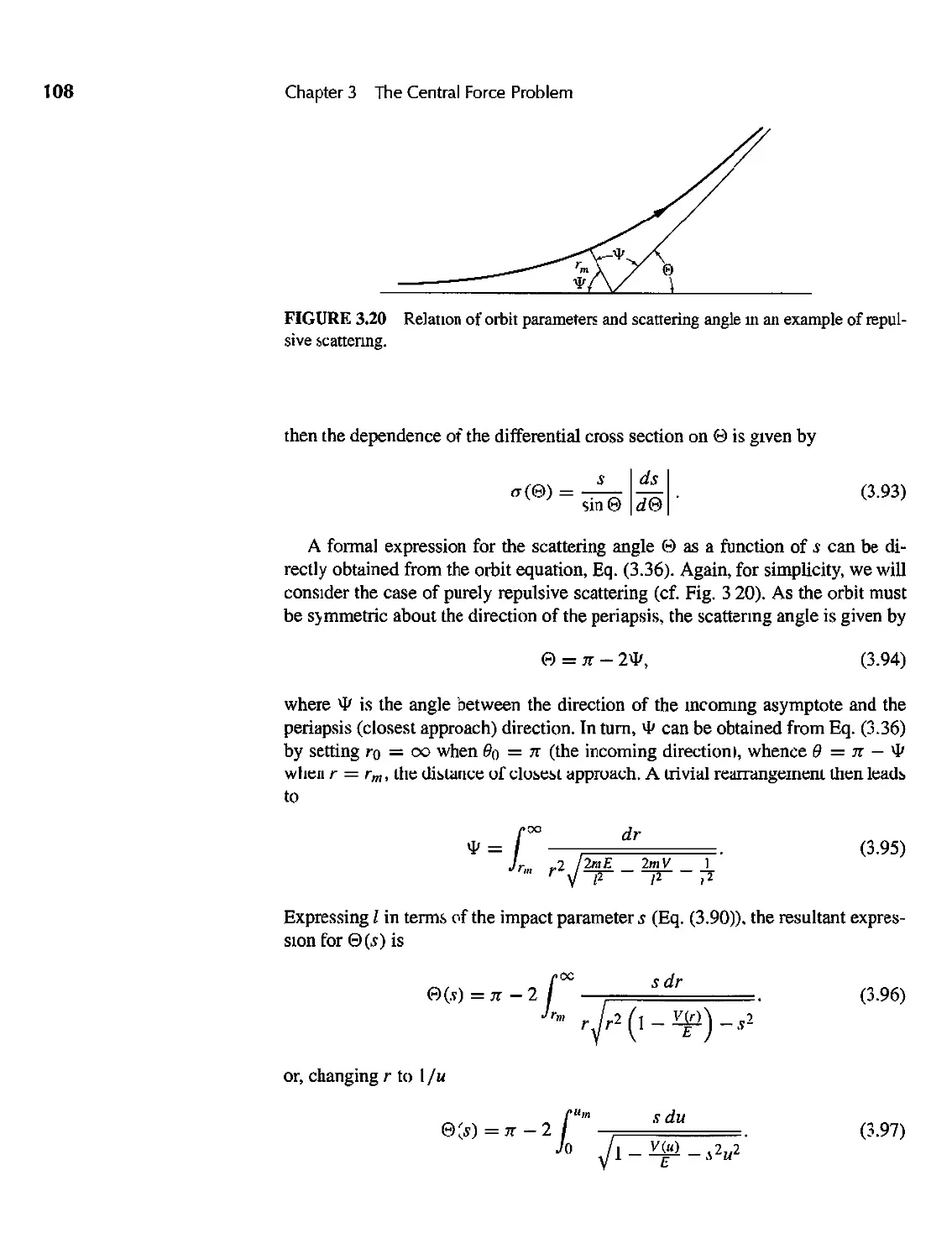
3.10 Scattering in a Central Force Field 106
3.11 Transformation of the Scattering Problem to Laboratory
Coordinates 114
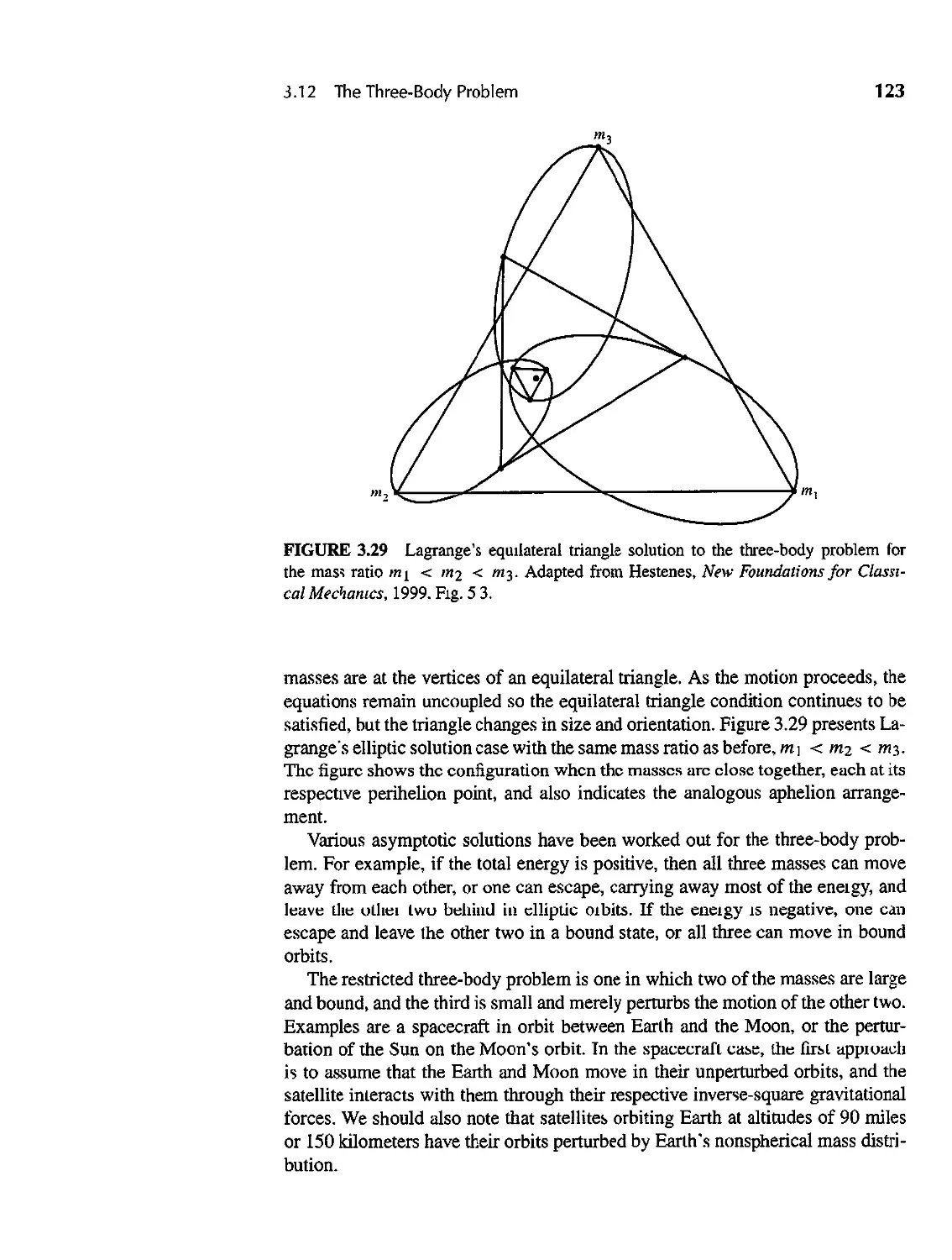
3.12 The Three-Body Problem 121
v

vi
Conterts
4 . The Kinematics of Rigid Body Motion 134
4.1 The Independent Coordinates of a RIgid Body 134
4.2 Orthogonal TranstonnatlOns UY
4.3 Fonnal Properties of the Transfonnation Matrix 144
4.4 The Euler Angles 150
4.5 The Cayley-Klein Parameters and Related Quantities 154
4.6 Euler's Theorem on the Motion of a Rigid Body 155
4.7 Finite Rotations 161
4.8 Infinitesimal Rotations 163
4.9 Rate of Change of a Vector 171
4.10 The Coriolis Effect 174
5 . The Rigid Body Equations of Motion 184
5.1 Angular Momentum and KInetIc Energy ot MotIon
about a Point 184
5.2 Tensors 188
5.3 The Inertia Tensor and the Moment ofInertia 191
5.4 The Eigenvalues of the Inertia Tensor and the Principal
Axis Transfonnation 195
5.5 Solving Rigid Body Problems and the Euler Equations of
Motion 198
5.6 Torque-free Motion of a Rigid Body 200
5.7 The Heavy Symmetrical Top with One Point Fixed 208
5.8 Precession of the Equinoxes and of Satellite Orbits 223
5.9 Prccession of Systems of Charges in a Magnetic Field 230
6 . Oscillations 238
6.1 Fonnulation of the Problem 238
6.2 The Eigenvalue Equation and the Principal Axis Transfonnation 241
6.3 Frequencies of Free Vibration, and Nonnal Coordinates 250
6.4 Free Vibrations of a Linear Triatomic Molecule 253
6.5 Forced Vibrations and the Effect of Dissipative Forces 259
6.6 Beyond Small Oscillations: The Damped Driven Pendulum and the
Josephson Junction 265
7 . The Classical Mechanics of the
Special Theory of Relativity
7.1 Basic Postulates of the Special Theory 277
7.2 Lorentz Transformations 280
7.3 Velocity Addition and Thomas Precession 282
7.4 Vectors and the Metric Tensor 286
276

Contents
vii
7.5 1-Fonns and Tensors 289
7.6 Forces in the SpecIal Theory; Electromagnetism 297
7.7 Relativistic Kinematics of Collisions and Many-Panicle
Systems 300
7.8 Relativistic Angular Momentum 309
7.9 The Lagrangian Fonnulation of Relativistic Mechanics 312
7.10 Covariant Lagrangian Fonnulations 318
7.11 Introduction to the General Theory of Relativity 324
8 . The Hamilton Equations of Motion 334
8.1 Legendre Transfonnations and the Hamilton Equations
of Motion 334
8.2 Cyclic Coordinates and Conservation Theorems 343
8.3 Routh's Procedure 347
8.4 The Hamiltonian Fonnulation of Relativistic Mechanics 349
8.5 Derivation of Hamilton's Equations from a
Variational Principle 353
8.6 The Principle of Least Action 356
9 . Canonical Transformations 368
9.1 The Equations of Canonical Transformation 368
9.2 Examples of Canomcal Transfonnations 375
9.3 The Harmonic Oscillator 377
9.4 The Symplectic Approach to Canonical Transformations 381
9.5 Poisson Brackets rnd Other Canonical Invariants 388
9.6 Equations of Motion, Infinitesimal Cmonical Transformations, and
Conscrvation Theorems in the Poisson Bracket Fonnulation 396
9.7 The Angular Momentum Poisson Bracket Relations 408
9.8 Symmetry Groups of Mechanical Systems 412
9.9 Liouville's Theorem 419
10 . Hamilton-Jacobi Theory and Action-Angle Variables 430
10.1 The Hamilton-Jacobi Equation for Hamilton's Principal
Function 430
10.2 The Harmonic Oscillator Problem as an Example of the
Hamilton-Jacobi Method 434
10.3 The Hamilton-Jacobi Equation for Hamilton's Characteristic
Function 440
10.4 Separation of Variables in the Hamilton-Jacobi Equation 444
10.5 Ignorable Coordinates and the Kepler Problem 445
10.6 Action-angle Variables in Systems of One Degree of Freedom 452

..
Contents
10.7 Action-Angle Variables for Completely Separable Systems 457
10.8 The Kepler Problem in Action-angle Variables 466
11 . Classical Chaos 483
11.1 Periodic Motion 484
11.2 Perturbations and the Kolmogorov-Amold-Moser Theorem 487
11.3 Attractors 489
11.4 Chaotic Trajectories and Liapunov Exponents 491
11.5 Poincare Maps 494
11.6 Henon-Heiles Hamiltonian 496
11.7 Bifurcations, Driven-damped Hannonic Oscillator, and Parametric
Resonance 505
11.8 The Logistic Equation 509
11.9 fractals and Dimensionality 516
12 . Canonical Perturbation Theory 526
12.1 Introduction 526
12.2 Time-dependent Perturbation Theory 527
12.3 Illustrations of Time-dependent Perturbation Theory 533
12.4 Time-independent Perturbation Theory 541
12.5 Adiabatic Invariants 549
13 . Introduction to the Lagrangian and Hamiltonian
Formulations for Continuous Systems and Fields 558
13.1 The Transition from a Discrete to a Continuous System 558
13.2 The Lagrangian Formulation for Continuous Systems 561
13.3 The Stress-energy Tensor and Conservation Theorems 566
13.4 Hamiltonian Formulation 572
13.5 Relativistic Field Theory 577
13.6 Examples of Relanvistic Field Theorie') 583
13.7 oether"s Theorem 589
Appendix A . Euler Angles in Alternate Conventions
and Cayley-Klein Parameters 601
Appendix B . Groups and Algebras 605
Selected Bibliography 617
Author Index 623
Subject Index 625

Preface to the Third Edition
The first edition of this text appeared in 1950, and it was so well received that
it went through a second printing the very next year. Throughout the next three
decades it maintained its position as the acknowledged standard text for the intro-
ductory Classical Mechanics course in graduate level physics cUITicula through-
out the United States, and in many other countries around the world. Some major
institutions also used it for senior level underw:aduate Mechanics. Thirty years
later, in 1980, a second edition appeared which was "a through-going revision of
the first edition." The preface to the second edition contains the following state-
ment: "1 have tried to retain, as much as possible, the advantages of the first edition
while taking into account the developments of the subject itself, its position in the
curriculum, and its applications to other fields." This is the philosophy which has
guided the preparation of this third edition twenty more years later.
The second edition introduced one additional chapter on Perturbation Theory,
and changed the ordering of the chapter on Small Oscillations. In addition it added
a significant amount of new material which increased the number of pages by
about 68%. This third edition adds still one more new chapter on Nonlinear Dy-
namics or Chaos, but counterbalances this by reducing the amount of material in
severa) of the other chapters, by shortening the space allocated to appendices, by
considerably reducing the bibliography, and by omitting the long lists of symbols.
Thus the third edition is comparable in size to the second.
In the chapter on relativity we have abandoned the complex Minkowski space
in favor of the now standard real metric. Two of the authors prefer the complex
metric because of its pedagogical advantages (HG) and because it fits in well with
Clifford Algebra fonnulations of Physics (CPP), but the desire to prepare students
who can easily move forward into other areas of theory such as field theory and
general relativity dominated over personal preferences. Some modem notation
such as I-fonns, mapping and the wedge product is introduced in this chapter.
The chapter on Chaos is a necessary addition because of the current interest
in nonlinear dynamics which has begun to play a significant role in applications
of classical dynamics. The majority of classical mechanics problems and apph-
cations in the reaJ world lOclude nonlineanues, and It IS important for the student
to have a grasp of the complexities involved, and of the new properties that can
emerge. It is also important to realize the role of fractal dimensionality in chaos.
New sections have been added and others combined or eliminated here and
there throughout the book, with the omissions to a great extent motivated by tbe
desire not to extend the overall length beyond that of the second edition. A section
ix

x
Preface to the Third Edition
was added on the Euler and Lagrange exact solutions to the three body problem.
In several places phase space plots and Lissajous figures were appended to ilJus-
trate solutions. The damped driven pendulum was discussed as an example that
explains the workings of Josephson junctions. The symplectic approach was clar-
ified by writing out some of the matrices. The harmonic oscillator was treated
with anisotropy, and also in polar coordinates. The last chapter on continua and
fields was fonnulated in the modern notation introduced in the relativity chap-
ter. The significances of the special unitary group in two dimensions SU(2) and
the special orthogonal group in three dimensions SO(3) WE're presentf".d in more
up-to-date notation, and an appendix was added on groups and algebras. Special
tables were introduced to clarify properties of ellipses, vectors, vector fields and
l-fol1l1s, canonical transformations, and the relationships between the spacetime
and symplectic approaches.
Several of the new features and approaches in this third edition had been men-
tiont".rl AS possihilities in the preface to the second edition. such as properties of
group theory, tensors in non-Euclidean spaces, and "new mathematics" of theoret-
ical physics such as manifolds. The reference to "One area omitted that deserves
special attention-nonlinear oscillation and associated stability questions" now
constitutes the subject matter of our new Chapter 11 "Classical Chaos." We de-
bated whether to place this new chapter after Perturbation theory where it fits
more logically. or before Perturbation theory where it is more likely to be covered
in class, and we chose the latter. The referees who reviewed our manuscript were
evenly divided on this question.
The mathematical level of the present edition is about the same as that of the
first two editions. Some of the mathematical physics, such as the discussions
of hermitean and unitary matrices, was omitted because it pertains much more
to quantum mechanics than it does to classical mechanics, and little used nota-
tions like dyadics were curtailed. Space devoted to power law potentials, Cayley-
Klein parameters, Routh's procedure, time independent perturbation theory, and
the stress-energy tensor was reduced. In some cases reference was made to the
second edition for more details. The problems at the end of the chapters were
divided into "derivations" and "exercises;' and some new ones were added.
The authors are especially indebted to Michael A. Unseren and Forrest M.
Hoffman of the Oak Ridge National laboratory for their 1993 compilation of
errata in the second edition that they made available on the Internet. It is hoped
that not too many new errors have slipped into this present revision. We wish to
thank the students who used this text in courses with us, and made a number of
useful suggestions that were incorporated into the manuscript Professors Thomas
Sayetta and the late Mike Schuette made helpful comments on the Chaos chapter,
and Professors Joseph Johnson and James Knight helped to clarify our ideas
on Lie Algebras. The following professors reviewed the manuscript and made
many helpful suggestions for improvements: Yoram Alhassid, Yale University;
Dave Ellis, University of Toledo; John Gruber, San Jose State; Thomas Handler,
University of Tennessee; Daniel Hong, Lehigh University; Kara Keeter, Idaho
State University; Carolyn Lee; Yannick Meurice, University of Iowa; Daniel

Preface to the Third Edition
xi
Marlow, Princeton University; Julian Noble, University of V1l'ginia; Muhammad
Numan, Indiana University of Pennsylvania; Steve Ruden. University of Califor-
nia, Irvine; Jack Semura, Portland Srate Univenrity; Tammy Ann Smecker-Hane,
Utriversity of California, Irvine; Daniel Stump, Michigan State University; Robert
WaId, University of Chicago; Doug Wells, Idaho State University.
It has indeed been an honor for two of us (CPP and JLS) to collaborate as
co-authors of this third edition of such a classic book fifty years after its first ap-
pearance. We have admired this text since we first studied Classical Mechanics
from the first edition in our graduate student days (CPP in 1953 and JLS in 1960),
and each of us used the first and second editions in our teaching throughout the
years. Professor Goldstein is to be conunended for having written and later en-
hanced such an outstanding contribution to the classic Physics literature.
Above all we register our appreciation and ack:nolwedgement in the words of
Psalm 19,1:
01 ovpavo£ 8£7JyoVVTa£ 8oav E)EOV
Flushing, New York
Columbia, South Carolina
Columbia, South Carolina
July, 2000
HERBERT GOLDSTEIN
CHARLES P. POOLE, JR.
JOHN L. SAFKO

CHAPTER
1
Survey of the
Elementary Principles
The motion of material bodies formed the subject of some of the earliest research
pursued by the pioneers of physics. From their efforts there has evolved a vast
field known as analytical mechanics or dynamics, or simply, mechanics. In the
present century the term "classical mechanics" has come into wide use to denote
this branch of physics in contradistinction to the newer physical theories, espe-
cially quantum mechanics. We shall follow this usagE', intetpreting the name to
include the type of mechanics arising out of the special theory of relativity. It is
the purpose of this book to develop the structure of classical mechanics and to
outline some of its apphcations of present-day interest in pure physics. Basic to
any presentation of mechanics are a number of fundamental physical concepts,
such as space, time, simultaneity, mass, and force. For the most part, however,
these concepts will not be anaJY7ed critically here; rather, they will be assumed as
undefined terms whose meanings are familiar to the reader.
1.1 . MECHANICS OF A PARTICLE
T .et r be the radiu vector of a particle from some given ongin and v its vector
velocity:
dr
v=-.
dt
The linear momentum p of the particle is defined as the product of the particle
mass and its velocity:
OJ)
p=mv.
(1.2)
In consequence of interactions with external objects and fields, the particle may
experience forces of various types, e.g., gravitational or electrodynamic; the vec-
tor sum of these forces exerted on the particle is the total force F. The mechanics
of the particle is contained in Newton's second law oj motion, wmch states that
there exist frames of reference in which the motion of the particle is described by
the dIfferential equation
F = dp == p,
dt
( 1.3)

2
Chapter 1 Survey of the Elementary Principles
or
d
F = di(rnv).
(1.4 )
In most instances, the mass of the particle 1S constant and Eq. (1.4) reduces to
F = m dv = ma.
dt
(15)
where a is the vector acceleration of the particle defined by
d 2 r
a = dt 2 '
(1.6)
The equation of motion is thus a differentiJ! equation of second order, assumiTtg
F does not depend on higher-order derivatives.
A reference frame in which Eq. (1.3) is valid is called an inertial or Galilean
system. Even within classical mechanics the notion of an inertial system is some-
thing of an idealization. In practice, however, it is usually feasible to set up a co-
ordinate system that comes as close to the desired properties as may be required.
For maTty purposes. a reference frame fixed in Earth (the "laboratory system") is
a suffic1ent approximation to an inertial system, while for some astronomical pur-
poses it may be necessary to construct an inertial system by reference to distant
galaxies.
Many of the important conclusions of mechanics can be expressed in the fonn
of conservation theorems: which indicate under what conditions various mechan-
ical quantities are constant in time. Equation (1.3) directly furnishes the first of
these, the
Conservation Theoremfor the Linear Momentum of a Particle: lfthe tota/force,
F, is lero. then p = 0 and the linear momel'tum. p, is conserved.
The angular momentum of (he particle about point 0, denoted by L, is defined
as
L = r x p,
(1.7)
where r is the radius vector from 0 to the particle. Notice that the order of the
factors is important. We now define the moment of force or torque about 0 as
N = r x F.
(1.8)
The equation analogous to (1.3) for N is obtained by fonning the cross product of
r with Eq. (1.4):
d
r x F = N = r x di(mv).
( 1.9)

1.1 Mechanics of a Particle
3
Equation (1.9) can be written in a different form by using the vector identity:
d d
dt"(r x mY) = v x mv + r x di(mv), (1.10)
where the first term on the right obviously vanishes. In consequence of this iden-
tity, Eq. (1.9) takes the form
d dL.
N = di(r x my) = dt == L. (1.11)
Note that both Nand L depend on the point 0, about which the moments are
taken.
As was the case for Eq. (1.3), the torque equation, (1.11), also yields an imme-
diate conservation theorem, this time the
Conservation Theorem for the Angular Momentum of a Particle: If the total
torque, N, if Zf'T"O th"n t = O. and the angular momentum L is conserved.
Next consider the work done by the external force F upon the particle in going
from point 1 to point 2. By definition, this work is
Wl2 = {2 F 0 ds.
1 1
( 1.12)
For constant mass (a will be assumed from now on unless otherwise specified),
the integral in Eq. (1.12) reduces to
f Fods=m f dv ovdt =  f !!.-(v2)dt.
dt 2 dt
and therefore
WI2 = (vi - vf).
2
The scalar quantity m u Z f2 is called the kinetic energy of the particle and is de-
noted by T, so that the work done is equal to the change III the kinetic energy:
(1.13)
WI2=Tz- T l'
(1.14)
If the force field is such that the work WI2 is the same for any physically
possible path between points 1 and 2, then the force (and the system) is said to be
conservative. An alternative description of a conservative system is obtained by
imagining the particle being taken from point I to point 2 by one possible path
and then being returned to point 1 by another path. The independence of W12 on
the particular path implies that the work done around such a closed circuit is zero,
i.e.
f F . ds = O.
(1.] 5)

4
Chapter 1 Survey of the Elementary Principles
Physically it is clear that a system cannot be conservative if friction or other dis-
sipation forces are present, because F . ds due to friction is always positive and
the integral cannot vanish.
By a well-known theorem of vector analysis, a necessary and sufficient condi-
tion that the work, WJ2, be independent of the physical path taken by the particle
is that F be the gradient of some scalar function of position:
F = -VV(r),
(1.16)
where V is called the potential, or potential energy. The eXIstence of V can be
mferred mtullJvely by a simple argument. If W12 is independent of the path of
integration between the end points 1 and 2. it should be possible to express WIZ
as the change in a quantity that depends only upon the positions of the end points.
This quantity may be designated by - V, so that for a differential path length we
have the relation
F. ds = -dV
or
av
F = - as '
which is equivalent to Eq. (1.16). Note that in Eq. (1.16) we can add to V any
quantity constant in space, without affecting the results. Hence the zero level of V
is arbitrary.
For a conservative system, the work done by the forces is
W12 = VI - Vz.
Combining Eq. (1.17) with Eq. (1.14), we have the result
T] + VI = Tz + V2,
(1.17)
(1.18)
which states in symbols the
Energy CUflMtrvutiun Theorem for a Panicle: If the forces acting on a panicle
are conservative, then the total energy of the panicle, T + V, is conserved.
The force applied to a particle may in some circumstances be given by the
gradient of a scalar function that depends explicitly on both the position of the
particle and the time. However, the work done on the particJe when it travels a
distance d s ,
F. ds = _ av ds
as '
is then no longer the total change in - V during the displacement, since V also
changes explicitly with time as the particle moves. Hence, the work done as the

1.2 Vlechanics of a System of Particles
5
particle goes from point 1 to point 2 is no longer the difference in the function V
between those points. While a total energy T + V may still be defined, it is not
conserved during the course of the particle's motion.
1.2 . MECHANICS OF A SYSTEM OF PARTICLES
In generalizing the ideas of the previous section to systems of many particles,
we must distinguish between the external forces acting on the particles due to
sources outside the system. and internal forces on, say, some particle i due to all
other particles in the system. Thus, the equation of motion (Newton's second law)
for the ith particle is written as
" F F (e) .
 )1 + I = P"
)
(119)
where Fe) stands for an external force, and F), is the internal force on the ith
particle due to the jth particle (F", naturally, is zero). We shall assume that the
F,) (like the Fe)) obey .;\lewton's third law of motion in its original form: thatthe
forces two particles exert on each other are equal and opposite. This assumption
(which does not hold for an types of forces) is sometimes refelTed to as the weak
law of action and reaction
Summed over all particles, Eq. (1.19) takes the form
d 2 " "(e),,
- d 2 m,r, = F, + FJI'
t .
, I I,}
i:j:.}
(1.20)
The first sum on the right is simply the total external force F(e) , while the second
term vanishes, since the law of action and reaction states that each pair F,} + F),
is zero. To reduce the left-hand side, we define a vector R as the average of the
radii vectors of the particles, weighted in proportion to their mass:
R _ Emir, = Em/r i .
Em; M
( 1.21)
The vector R defines a pomt known as the center ofmaJs, or more loosely as the
center of gravity, of the system (cf. Fig. 1.1). With this definition, (1.20) reduces
to
M d2R = '" F(e) == F(e)
dt2 L.. I '
,
(1.22)
which states that the center of mass moves as if the total external force were
acting on the entire mass of the system concentrated at the center of mass. Purely
internal forces, if the obey Newton's thIrd law, therefore have no effect on the

b
Chapter 1 Survey of the Elementary Principles
mJ
o
FIGURE 1.1 The center of ma!- of a system of particles.
mutiun uf the center of mass. An oft-quoted example IS the motIon ot an exploding
shell-the center of mass of the fragments traveling as if the shell were still in a
single piece (neglecting air resistance). The same principle is involved in jet and
rocket propulsion. In order that the motion of the center of mass be unaffected,
the ejection of the exhaust gases at high velocity must be counterbalanced by the
forward motion of the vehicle at a slower velocity.
By Eq. (1.21) the total hnear momentum of the system,
"drj dR
p= L.Jm'di = Mdt,
(1.23)
is the total mass of the system times the velocity of the center of mass. Conse-
quently, thE' E'quation of motion for the center of mass, (1.23), can be restated as
the
ConselVation Theoremfor the Linear Momentum of a System of Particles: lfthe
total external force is zero, the total linear momentum is conserved.
We obtain the total angular momentum of the system by forming the cross
product r, X p, and summing over i. If this operation is performed in Eq. (1.191,
there results, with the aid of the identity, Eq. (1.10),
)r, x PI) = L !!..-(r, x PI) = t = I>, x Fe) + I>, x FJi' (1.24)
dt .
I I-  I.}
i#J
The last term on the right in (1.24) can be ,::onsidered a sum of the pairs of the
form
r , x Fj, + rJ x F,j = (r, - rJ) x FJI'
(1.25)

1.2 Mechanics of a System of Particles
7
. .
.
FIGURE 1.2 The vector rij between the ith and jth particles.
using the equality of action and reaction But ri - r] is identical with the vector
r!j from j to i (cf. Fig. 1.2), so that the right-hand side ofEq. (1.25) can be wntten
as
r!] x FJ!'
If the internal forces between two particJes, in addition to being equal and oppo-
site, also lie alung lhe line joining the particles-a condition known as the strong
law of action and reaction-then all of these cross products vanish. The sum over
pairs is zero under this assumption and Eq. (1.24) may be written in the fonn
dL = N(e).
dt
(1.26)
The time derivative of the total angular momentum is thus equal to the moment
of the external force about the given point. Corresponding to Eq. (1.26) is the
Conservation Theoremfor Total Angular Momentum: L is constant in time if the
applied (external) torque is zero.
(It is perhaps worthwhile to emphasize that this is a vector theorem; i.e., Lz
will be conserved if N?) is zero, even if Ne) and Ne) are not zero.)
Note that the conservation of linear momentum in the absence of applied forces
assumes that the weak law of action and reaction is valid for the internal forces.
The conservation of the total angular momentum of the system in the absence of
applied torques requires the validity of thc strong law of action and reaction-that
the internal forces in addition be central. Many of the familiar physical forces,
such as that of gravity, satisfy the strong form of the law. But it if. possible to
find forces for which action and reaction are equal even though the forces are not
central (see below). In a system involvmg moving charges, the forces between
the charges predicted by the Biot-Savart law may indeed violate both forms of

8
Chapter 1 Survey of the Elementary Prrnclples
the action and reaction law. * Equations (1.23) and (1.26), and their corresponding
conservation theorems, are not applicable in such cases, at least in the form given
here. Usually it is then possible to find some generalization of P or L that is
conserved. Thus, in an isolated system of moving charges it is the sum of the
mechanical angular momentum and the electromagnetic "angular momentum" of
the field that is conserved.
Equation (1.23) states that the total linear momentum of the system is the same
as if the entire mass were concentrated at the center of mass and moving with it.
The analogous theorem for angular momentum is more complicated. With the
ongin 0 as reference point, the total angular momentum of the system is
L = L r, x P"
I
Let R be the radius vector from 0 to the center of mass, and let r; be the radius
vector from the center of mass to the Ith particle. Then we have (cf. Fig. 1.3)
r, = r; + R
(1.27)
and
V, = v; + v
where
dR
v=-
at
Center
of mass
o
FIGURE 1.3 The vector involved in the sluft of reference pOInt for the angular momen-
tum.
*If two charge are movmg umfonnly with parallel velocity vecto!s that are not perpendicular to the
line Joining the charge, then the net mutual forces are equal and opposite but do not he along the
vector between the charges. ConsIder, further, two charges moving (instanuneously) o as to "cross
the T:' I.e.. onc charge moving directly at the other, which in turn I moving at right angle to the first
Then the second charge exert 3 nonvanihlng mdgnetic force on the firt, without cxpenencmg my
magnetic reaction torce at that mstant.

1.2 Mechanics of a S'lstem of Particles
9
is the velocity of the center of mass relative to 0, and
 = dr;
, dt
is the velocity of the ith particle relative to the center of mass of the system. Using
Eq. (1.27), the total angular momentum takes on the form
L= 'ER x m,v+ 'Er; x m, + ( 'Emir: ) x v+R x  'Em,r;.
.. dt
, , , ,
The last two terms in this expression vanish, for both contain the factor L m1r;,
which, it will be recognized, defines the radius vector of the center of mass in the
very coordinate system whose origin is the center of mass and is therefore a null
vector. Rewriting the remaining terms, the total angular momentum about 0 is
L=R x Mv+ I>; x p;.
,
(1.28)
In \'Yords, Eq. (1.28) says that the total angular momentum about a point 0 is
the angular momentum of motion concentrated at the center of mass, plus the
angular momentum of motion about the center of mass. The form of Eq. (1.28)
emphasizes that in general L depends on the origin 0, through the vector R. Only
if the cente1 of mass 1:) at rest with respect to 0 will the angular momentum be
independent of the point of reference. In this case, the first term in (1.28) vanishes,
and L always reduces to the angular momentum taken about the center of mass.
Finally, let us consider the energy equation. As in the case of a single particle,
we calculate the work done by all forces in moving the system from an initial
configuration 1, to a final configuration 2:
W12 = 'E {2 F, . dS I = 'E (2 Fe) . ds, + L / 2 FJ' . ds,. (1.29)
i 11 i 11 '.J 1
I*J
Again, the equations of motion can be used to reduce the mtegraIs to
L {2 Fl' ds = L i 2 m,v / . v,dt = 'E {2 d ( miV ) .
1 11 1 1 , 11
Hence, the work done can still be written as the difference of the final and initial
kinetic energies:
W12 = T2 - Tl.
where T, the total kinetic energy of the system, is
T =  Lm,v;.
1
(1.30)

10
Chapter I Survey of the I::lementary Principles
Making use of the transformations to center-of-mass coordinates, given in Eq.
(1.27), we may also write T as
1
T =:2 Lm,(v+v,). (v+v,)
,
1 " 2 1 "r2 d ( " , )
= 2m,v + 2m,vi +v. di m!r, '
, I ,
and by the reasoning already employed in calculating the angular momentum, the
last tenn vanishes, leaving
1 1
T = 2 Mv2 + 2 Lm,v
,
( 1.31)
The kinetic energy, like the angular momentum, thus also consists of two parts:
the lane tIC energy obtained if all the mass ere concentrated at the center of mass,
plus the kinetic energy of motion about the center of mass.
Consider now the right-hand side of Eq. (1.29). In the pecial case that the
external. forces are derivable in terms of the gradient of a potential, the first term
can be written as
1 2 {2 1 2
L Fe) . ds , = - L JI V, V, . ds , = - L V, ,
! 1 I ] , 1
where the subscript i on the del operator mdicates that the derivatives are with
respect to the components of r,. If the internal forces are also conservative, then
the mutual forces between the ith and jth particles, Fil and F '" can be obtained
from a potentlal function V,}, To satisfy the strong law of action and reaction, V;J
can be a function only of the distance between the particles:
Vz j = V'J(I r, - r j I).
(1.32)
The two forces are then automatically equal and opposite,
FJ' = -V, Vz J = +V'j VI} = -FIJ'
( 1.33)
and lie along the line joining the two particles,
VVzj(l ri - r j I) = (ri - rJ)J,
(1.34)
where j is some scalar function. If v,J were also a function of the difference of
some other pair of vectors associated with the particles, such as their velocities
or (to step into the domain of modem physIcs) their intrinsic "spin" angular mo-
menta, then the forces would still be equal and opposite, but would not necessarily
lie along the direction between the particles.

1.2 Mechanics of a System of Particles
11
When the forces are all conservative, the second term m Eq. (1.29) can be
rewritten as a sum over pairs of particles, the terms for each pair being of the
form
- [2 (V, Vij . ds, + V] V,] . dSj).
If the difference vector r. - r] is denoted by r,], and if Vij stands for the gradient
with respect to r'J' then
V, v,] = V,} V iJ = -V] V,],
and
ds, - ds} = dr, - dr] = dr,j.
so that the term for the . pair has the form
- f V,] V,} . dr,].
The total work arising from internal forces then reduces to
1 1 2 1 1 2
- - L 'V'J Y.j . dr,} = - - L v'J .
2 '.} 1 2 i,} 1
'J ,j
(1 35)
The factor! appears in Eq. (1.35) because in sununing over both i and j each
member of a given pair ;s included twice, first in the i summation and then in the
1 summation.
From these considerations, it is clear that it the external and mternal forces are
both derivable from potentials it is possible to define a total potential energy, V,
of the system,
1
V = LVi + 2 L v']'
, i';)]
such that the total energy T + V is conserved, the analog of the conservation
theorem (1.18) for a single particle.
The second term on the right in Eq. (1.36) will be called the internal potential
energy of the system. In general, it need not be zero and, more important, it may
vary as the system changes with time. Only for the particular class of system.;;
known as rigid bodie:. will the internal potential always be constant. Formally,
a rigid body can be defined as a system of particles in which the distances r,]
are fixed and cannot vary with time. In such case, the vectors drij can only be
perpendicular to the corresponding r,], and therefore to the Fij. Therefore, m a
rigid body the internal forces do no work. and the internal potential must remain
(1.36)

12
Lhapter 1 urvey of the Elementary Principles
constant. Since the total potential is in any case uncertain to within an additive
constant, an unvarying internal potential can be completely disregarded in dis-
cussing the motion of the system.
1.3 . CONSTRAINTS
From the previous sections one might obtain the impression that all problems in
mechanics have been reduced to solving the set of differential equations (1.19):
" F (e) " F
m,r, = , - L J"
J
One merely substitutes the various forces acting upon the particles of the system,
tum... the mathematical crank., and grinds out the answers! Even from a purely
physical standpoint, however, this view is oversimplified. For example, it may be
necessary to take mto account the constraints that limit the motion of the system.
We have already met one type of system involving constraint!., namely rigid bod-
ies, where the constraints on the motions of the particles keep the distances r'J
unchanged. Other examples of constrained systems can easily be furnished. The
beads of an abacus are constrained to one-dimensional motion by the supporting
wires. Gas molecules within a container are constrained by the walls of the ves-
sel to move only inside the container. A partIcle placed on the surface of a solid
sphere is subject to the constraint that it can move only on the surface or in the
region exterior to the sphere.
Constraints may be classified in various ways, and we shall use the following
system. If the conditions of constraint can be expressed as equations connecting
the coordinates of the particles (and possibly the time) having the form
f(rl' rz, r3,..., t) = 0,
( 1.37)
then the constraints are said to be holonomic. Perhaps the simplest example of
holonomic constraints is the rigid body, v.,here the constraints are expressed by
equations of the form
(r, - rJ)Z -c = O.
A partide constrained to move along any curve or on a given surface is another
obvious example of a holonomic constraint, wIth the equations defining the curve
or surface acting as the equations of a constraint.
COl1stJ.aints nul exprible in this fashion are caned nonholonomic. The walls
of a gas container constitute a nonholonomic constraint. The constraint involved
in the example of a particle placed on the surface of a sphere i!. also noOOolo-
nomic, for it can be expressed as an inequality
r Z - a Z ::: 0

1 .3 Constramts
13
(where a is the radius of the sphere), which is not in the form of (1.37). Thus, in
a gravitational field a particle placed on the top of the sphere will slide down the
surface part of the way but will eventually fall off.
Constraints are further classified according to whether the equations of con-
straint contain the time as an explicit variable (rheonomous) or are not expl1cltly
dependent on time (scleronomous). A bead sliding on a rigid curved wire fixed
in f.pace is obviously subject to a scleronomous constraint; if the wire is moving
in some prescribed fashion, the constramt is rheonomous. Note that if the wire
moves, say, as a reaction to the bead's motion, then the tune dependence of the
constraint enters in the equation of the constraint only through the coordinates
of the curved wire (which are now part of the system coordinates). The overall
constraint is then scleronomous.
Constraints introduce two type of difficulties in the solution of mechanical
problems. First, the coordinates r 1 are no longer all independent, since they are
connected by the equations of constraint; hence the equations of motion (1.19)
are not all independent. Second, the forces of constraint, e.g., the force that the
wire exerts on the bead (or the wall on the gas particle), is not furnished a pri-
ori. They are among the unknowns of the problem and must be obtained from the
solution we s.eek. Indeed, imposing constraints on the system IS simply another
method of stating that there are forces present in the problem that cannot be spec-
Ified directly but are known rather in termf. of their effect on the motion of the
system.
In the case of holonomic constraints, the first difficulty is solved by the intro-
duction of generalized coordinates. So far we have been thinking implicitly in
terms of Cartesian coordinates. A system of N particles. free from constraints,
has 3N independent coordinates or degrees offreedom. If there exist holonomic
constraints, expressed in k equations in the form (1.37), then we may use these
equations to eliminate k of the 3N coordinates, and we are left with 3N - k inde-
pendent coordinates, and the system is said to have 3N - k degrees of freedom.
Thif. elimination of the dependent coordinates can be expressed in another way,
by the introduction of new, 3N - k, independent variables qI, q2, ..., q3N-k in
tentls of which the old coordinatef. rl, r2, . . . , rN are expressed by equations of
the form
r = r} (qj, qz, . . ., q3N-I., t)
(1.38)
rN = rN(ql, Q2, ..., q3N-ko t)
containing the constraints in them implicitly. These are transformation equations
from the set of (rt) variables to the (q{) set, or alternatively Eqs. (1.38) can be con-
sidered as parametric representations of the (rt) variables. It is always assumed
that we can also transform back flOm the (qt) to the (rt) set, Le., that Eqs. (1.38)
combined with the k equations of constraint can be inverted to obtain any ql as a
function of the (rt) variable and time.

14
Chapter 1 urvey ot the Elementary Prmciples
Usually the generalized coordinates, q{, unlike the Cartesian coordinates, will
not divide into convenient groups of three that can be associated together to fonn
vectors. Thus, in the case of a particle constrained to move on the surface of a
sphere, the two angles expressing position on the sphere, say latitude and longi-
tude, are obvious possible generalized coordinates. Or, in the example of a double
pendulum moving in a plane (two particles connected by an inextensible I.1ght
rod and suspended by a similar rod fastened to one of the particles), satisfactory
generalized coordinates are the two angles 91, 92. (Cf. Fig. 1.4.) Generalized co-
ordinates, in the sense of coordinates other than Cartesian, are often useful in
systems without constraints. Thus, in the problem of a particle moving in an ex-
ternal central force field (V = V (r ) ), there is no constraint invol ved, but It is
clearly more convenient to use spherical polar coordinates than Cartesian coordi-
nates. Do not, however, think of generalized coordinates in terms of conventional
orthogonal position coordinates. All sorts of quantities may be impressed to serve
as generalized coordinates. Thus, the ampJitudes in a Fourier expansion of r J may
be used as generalized coordinates, or we may find it convenient to employ quan-
tities with the dimensions of energy or angular momentum.
If the constraint is nonholonomic, the equations expressing the constraint can-
not be used to eliminate the dependent coordinates. An oft-quoted example of
a nonholonomic constraint is that of an object rolling on a rough surface with-
out slipping. The coordinates used to describe the system wilt generally involve
angular coordinates to specify the orientation of the body. plus a "et of coordi-
nates describing the location of the point of contact on the surface. The constraint
of "rolling" connects these two sets of coordinates; they are not independent. A
change in the position of the point of contact inevitably means a change in its
orientation. Yet we cannot reduce the number of coordinates, for the "rolling"
condition is not expressible as a equation between the coordinates, in the manner
of (1.37). Rather, it is a condition on the vp/ncities (i e , the point of contact is
stationary), a differential condition that can be given in an integrated form only
after the problem is so!\.ed.
FIGURE 1.4 Double pendulum.

I.J Constraints
15
FIGURE 1.5 Vertical disk rollmg on a horizontal plane.
A simple case will illustrate the point. Consider a disk rolling on the horizontal
xy plane constrained to move so that the plane of the disk is always vertical.
The coordinates used to describe the motion might be the x. y coordinates of the
center of the disk, an angle of rotation </> about the axis of the disk, and an angle
e between the axis of the disk and say, the x axis (cf. Fig 1.5). As a result of the
constraint the velocity of the center of the disk, v, has a magnitude proportional
to <P,
v = a<p,
where a is the radius of the disk, and its direction is perpendicular to the axis of
the disk:
x = v sin e
y = -v cose.
Combining these conditions, we have two differential equations of constraint:
dx - a sinedlj) = 0,
dy + a cosed</> = O.
( 1.39)
Neither of Eqs. (1.39) can be integrated without in fact solving the problem; i.e.,
we cannot find an integrating factor f (x, ), e, </» that will turn either of the equa-
tions into perfect differentials (cf. Derivation 4). * Hence, the constraints cannot
be reduced to the form of Eq. (1.37) and are therefore nonholonomic. Physically
we can see that there can be no direct functional relation between </> and the other
coordinates x, y, and e by noting that at any point on its path the disk can be
*In prinlple. an mtegratmg factor can always be found for a first-order di:Ierential equation of con-
btraint ill systems involving only two coordinates and such constraints are therefore holonomic. A
familiar example IS the two-dimensional motion of a cIrCle rolling on an inclmed plane.

16
Chapter 1 urvey ot the Elementary PrinCiples
made to roll around in a circle tangent to the path and of arbitrary radius. At the
end of the process, x, }, and () have been returned to their original values, but <I>
has changed by an amOJnt depending on the radius of the circle.
Nonintegrable differential constraint" of the fonn of Eqs. (1.39) are of course
not the only type of nonholonomic constraintf.. The constraint conditions may
involve higher-order derivatives, or may appear in the fonn of inequalities, as we
have seen.
Partly because the dependent coordinates can be eliminated, problems involv-
ing holonomic constraints are always amenable to a fonnal solution. But there is
no general way to attack nonholonomic examples. True, if the constraint is non in-
tegrable, the differential equations of constrdint can be introduced into the prob-
lem along with the differential equations of motion, and the dependent equations
eliminated, in effect, by the method of Lagrange multipliers.
We shall return to this method at a later point. However, the more vicious cases
of nonholonomic constraint must be tackled individually, and consequently in the
development of the more formal aspects of classical mechanics, it is almost invari-
ably assumed that any constraint, if present, is holonomic. This restriction does
not greatly limit the applicability of the theory, despite the fact that many of the
constraints encountered in everyday life are nonholonomlc. The reason is that the
entire concept of constrdintc; imposed in the system through the medium of wires
or surfaces or walls is particularly appropriate only in macroscopic or large-scale
problems. But today physicists are more interested 10 atomic and nuclear prob-
lems. On this scale all objects, both in and out of the system, consist alike of
molecules, atoms, or smaller particles, exerting definite forces, and the notion of
constraint becomes artificial and rarely appears. Constraints are then used only
as mathematical idealizations to the actual physical case or as classical approxi-
mations to a quantum-mechanical property, e.g., rigid body rotations for "spin."
Such constraints are always holonomic and fit smoothly into the framework of the
theory.
To sunnount the second difficulty, namely, that the forces of constraint are
unknown a priori, we should like to so fonnulate the mechanics that the forces
of constraint disappear. We need then deal only with the known applied forces. A
hint as to the procedure to be followed is provided by the fact that in a particular
system with constraints i f" a rigid body, the work done by internal forces (which
are here the forces ot constraint) vanishes. We shall follow up this clue in the
ensuing sections and generalize the ideas contained in it.
1.4 . D'ALEMBERT'S PRINCIPLE AND LAGRANGE'S EQUATIONS
A virtual (infinitesimal) displacement of a system refers to a change in the con-
figuration of the system af. the result of any arbitrary infinitesimal change of the
coordinates or " consistent with the forces and constraints imposed on the sy.tem
at the given instant t. The displacement is called virtual to distinguish it from an
actual displacement of the system occurring in a time interval dt, during which

1.4 0' Alembert's Principle and Lagrange's Equations
17
the forces and constrdints may be changing. Suppose the system is in equilibrium;
i.e., the total force on each particle vanishes, F, = O. Then clearly the dot product
F, . or" which is the virtual work of the force F, in the displacement or" also
vanishes. The sum of these vanishing products over all particles must likewise be
zero:
LF, . or, =0.
j
(1.40)
As yet nothing has been said that has any new physical content. Decompose F,
into the applied force, Fa), and the force of constraint, f"
F, = Fa) + f j .
(1.41)
so that Eq. (1.40) becomes
EFa). r, + EF,. r, = 0
, ,
(1 42)
We now restrict ourselves to systems for which the net virtual work of the
forces of constraint is zero. We have seen that this condition holds true for rigid
bodies and it is valid for a large number of other constraints. Thus, if a particle is
constrained to move on a surface, the force of constraint is perpendicular to the
surface, while the virtual displacement must be tangent to it, and hence the virtual
work vanishes. This is no longer true if sliding friction forces are present, and
we must exclude such systems from our fonnulation. The restriction is not un-
duly hampering, since the friction is essentially a macroscopic phenomenon. On
the other hand, the forces of rolling friction do not violate this condition, since the
forces act on a point that is momentarily at rest and can do no work in an infinites-
imal dtsplacement consistent with the rolling constraint. Note that if a particle is
constrained to a surface that is itself moving in time, the force of constraint is
instantaneously perpendlcular to the surface and the work during a virtual dis-
placement is still zero even though the work during an actual displacement in the
time dt does not necessarily vanish.
We therefore have as the condition for equilibrium of a system that the virtual
work of the appliedforees vanishes:
LFa) . or, = O.
j
(1.43)
Equation (1.43) is often called the principle of virtual work. Note that the coef-
ficient of Sr, can no longer be set equal to zero; Le., in general Fa) I- 0, since
the or, are not completely independent but are connected by the constraint. In
order to equate the coefficients to zero, we must transfonn the principle into a
fonn involving the virtual displacements of the q" which are independent. Equa-
tion (1.43) satisfies our needs in that it does not contain the fl> but it deals only
with statics; we want a condition invol ving the general motion of the system.

18
Chapter 1 Survey of the Elementary Principles
To obtain such a principle, we use a device first thought of by James Bernoulli
and developed by D' Alembert. The equation of motion,
F, =P"
can be written as
F, - P, = 0,
which states that the particles in the system will be in equilibrium under a force
equal to the actual force plus a "reversed effective force" -pj. Instead of (1.40),
we can immediately write
L(Fi - P,) .lSr , = 0,
j
(1.44)
and, making the same resolutIon toto applied torces and forces of constraint, there
results
)F}a) - p;) . ISr , + L f , . or; = O.
i I
We again rcstrict ourselves to systems for which the virtual work of the forces of
constraint vanishes and therefore obtain
)Fa) - Pi) .lSr , = 0,
i
(1.45)
which IS often called D'Alembert's principle. We have achieved our aim. in that
the forces of constraint no longer appear. and the superscript (a) can now 
dropped without ambiguity. It is still not in a useful fonn to furnish equations
of motion for the system. We must now transfonn the principle into an expression
involving virtual displacements of the generalized coordinates, which are then in-
dependent of each other (for holonomic constraints), so that the coefficients of the
}iq, clln be set separately equal to zero.
The translation from r, to qJ language starts from the transformation equations
(1.38),
r , = rj(qt, q2,..., qn, t)
(1.45')
(assummg n independent coordinates), and is carried out by means of the usual
"chain rules" of the calculus of partial differentiation. Thus, Vi is expressed in
tenns of the qk by the formula
drj " or , . ar,
V, == - = £...J -qk + -.
dt k aqk at
(1.46)

1 .4 LJ' Alembert's Principle and Lagrange's I:quatlons
19
Similarly, the arbitrary virtual displacement or, can be connected with the virtual
displacements oq, by
" dr,
8r, =  -lIq)
) 8q}
(I 47)
Note that no variation of time, 8t, is invoved here, since a virtual displacement
by definition considers only displacemenl<; of the coordinates. (Only then is the
virtual displacement perpendicular to the force of constraint if the constraint itself
is changing in time.)
In tenns of the generalized coordinates. the virtual work of the F, becomes
" "ar l
Fj .8rj = F" a-0q}
, 10 
= L Q)oq).
}
(1.48)
where the Q} are called the components of the generalized force, defined as
" or,
Q} = F, . .
i aq)
(1.49)
Note that just as the q's need not have the dimensions of length, so the Q's do
not necesf.arily have the dimensions of force, but Q)8q) mu&t always have the
dimemions of work. For example, Q} might be a torque N) and dq} a differential
angle de), which makes N) de} a differential of work.
We turn now to the other other term Involved m Eq. (1.45). which may be
written as
LP,.8r, = Lmjrj' or,.
I
Expressing or, by (1.47), this becomes
" .. ar l
m,r,. -8q).
',} i3q)
Consider now the relatIOn
" .. ar, " [ d ( . or, ) . d ( ari )]
L..Jm,r, .  = L..J - mlr l .:-- - mrr,' -:-- .
, aq), dt oq} dt oq)
( 1.50)
In the last tenn of Eq. (1.50) we can interchange the differentiation with respect
to t and q), for, in analogy to (1.46).

20
Chapter 1 Survey of the Elementary Principles
d ( ar, ) ar, a 2 r!. a 2 r,
- - =-=L-qk+-.
dt a{fj aq) k aq)aqk aqJat
_ aVi
aq/
by Eq. (1.46). Further, we also see from Eq. (1.46) that
av, ar,
aq) = aqj
Substitution of these changes in (1.50) leads to the result that
(1.51)
" .. ar, " [ d ( av, ) av, ]
Lm,ri . :-- = L - m,v,':-:- - mjv! .:-- ,
, aqj, dt aq) aq)
and th second tenn on the left-hand side ofEq. (1.45) can be expanded into
I d [ a ( 1 2 ) ] a ( 1 2 ) }
 di aq)  zm,v, - aq)  zmivj - Qj 8q).
Identifying Ll 4m,v with the system kinetic energy T, D'Alembert's principle
(cf. Eq. (1.45)) becomes
L {[ ( : ) - : ] - Q)} 8q) =0.
(1.52)
Note that in a system of Cartesian coordinates the partial derivative of T \\rith
respect to q) vanishes. Thus, speaking in the language of differential geometry,
this term arises from the curvature of the coordinates q). In polar coordinates,
e.g., it is in the partial derivative of T with respect to an angle coordinate that the
centripetal acceleration tenn appears.
Thus far, no restriction has been made on the nature of the constraints other
than that they be workless in a virtual displacement. The variables q) can be any
set of coordinates used to describe the motion of the system. If, however, the con-
straints are holonomic, then it is possible to find sets of independent coordinates
q) that contain the constraint conditions implicitly in the transfonnation equations
(1.38). Any virtual displacement oq) is then independent of oqk, and therefore the
only way for (1.52) to hold is for the individual coefficients to vanish:
d ( aT ) aT
di aq) - aq) - Q).
(1.53)
There are n such equations in all.
When the forces are derivable from a scalar potential function v,
F! = - V, v.

1.4 D' Alembert's Prmciple and Lagrange's Equations
21
Then the generalized forces can be written as
" ari " ar!
Q) = F,.:-- = -  'V, V.:--,
I aqj I aq]
which is exactly the same expression for the partial derivative of a function
- V (rl, r21 . . . I rN I t) with respect to qr
av
Q j = - aq, .
Equations (1.53) can then be rewritten as
(1.54)
 (  ) _ C!( - V) = o.
dt aqj aq,
The equations of motion in the form (1.55) are not necessanly restricted to conser-
vative systems, only if V is not an explicit function of time is thc system conscrva-
tive (cf. p. 4). As here defined, the potential V does not depend on the generalized
velocities. Hence, we can include a term III V in the partial derivative with respect
to q):
( 1.55)
 ( a(T  V) ) _ a(T - V) = o.
dt oq] oqj
Or, defining a new function, the Lagrangian L, as
L = T - V,
(1.56)
the Eqs. (1.53) become
d ( aL ) aL
di aqj - oqj = 0,
(1.57)
expressions referred to as "Lagrange's equations."
Note that for a particular set of equations of motion there is no unique choice
of Lagrangian .;;uch that Rqc;; (1 57) lead to the equations of motion in the given
generalized coordinates. Thus, in Derivations 8 and 10 it is shown that if L(q, q I t)
is an approximate Lagrangian and F(q, t) is any differentiable function of the
generalized coordinates and time, then
,. . dF
L (q, q, t) = L(q. q, t) + dt
( 1.57')
is a Lagrangian also resulting in the same equations of motion. It is also often
possIble to find alternative Lagrangians beside those constructed by this prescrip-
tion (see Exercise 20). While Eq. (1.56) is always a suitable way to construct a
Lagrangian for a conservative system, it does not provide the only Lagrangian
suitable for the given system.

22
Chapter 1 Survey of the Elementary Principles
1.5 . VELOCITY-DEPENDENT POTENTIALS AND
THE DISSIPATION FUNCTION
Lagrange's equations can be put in the fonn (1.57) even if there is no potential
function, V, in the usual sense, providing the generalized forces are obtained from
a function U(qJ' qJ) by the prescription
au d ( au )
QJ = - aqJ + dt aqj .
In such case, Eqs. (1.57) still follow from Eqs. (1.53) with the Lagrangian given
by
( 1.58)
L = T - U.
( 1.59)
Here U may be called a "generalized potential," or "velocity-dependent poten-
tial." The possibility of using such a "potential" is not academic; it applies to one
very important type of force field, namely. the electromagnetic forces on mOVlng
charges. Considering its importance, a digression on this subject is well worth-
while.
Consider an electric charge, q, of mass m moving at a velocity. v, in an other-
wise charge-free region containing both an electric field. E. and a magnetic field.
B, which may depend upon time and position. The charge experiences a force,
called the Lorentz force, given by
F = qrE + (V x B)].
( 1.60)
Both E(t, x, y, z) and B(t, x, y, z) are continuous functions of time and positlOn
derivable from a scalar potential </>(t, x, y, z) and a vector potential A(t, x, y, z)
by
aA
E= -\1</>- at
(1.61 a)
and
B = \1 x A.
(1.61b)
The force on the charge can be derived from the following velocity-dependent
potential energy
U=q</>-qA.v,
( 1.62)
so the Lagrangian, L = T - U, is
L = !mv 2 - q1J + qA . v.
(1.63)

1.5 Velocity-Dependent Potentials and the Dissipation Function
23
Considering just the x-component of Lagrange's equations gives
.. ( a At aA y a A z ) ( all> dA x )
mx = q vxa;- +Vy +vz -q ax + dt .
(1.64)
The total time derivative of Ax is related to the particle time derivative through
dAx aA x
dt = at + v . \l Ax
aA x aA x aA x aA x
= _ a + v X - a + vY- a + v z --;-.
t X Y oZ
(1.65)
Equation (1.61b) gives
B) ( aAy aAx ) ( aAz aAx )
(v x x = v y _ a - _ a + V z - - _ a .
x y ax z
Combining these expressions gives the equation of motion in the x-direction
mx = q [Ex + (v x B)xJ.
(1.66)
On a component-by-component comparison, Eqs. (1.66) and (1.60) are identical,
showing that the Lorentz force equation is derivable from Eqs. (1.61) and (1.62).
Note that if not all the forces acting on the system are derivable from a poten-
tial, then Lagrange's equations can always be written in the form
d ( aL ) aL
di aqJ - aqJ = Qj,
where L contains the potential of the conservative forces as before, and Q J rep-
resents the forces not arising from a potential. Such a situation often occurs when
frictional forces are present. It frequentl)' happens that the frictional force is pro-
portional to the velocity of the particle, so that its x-component has the form
Ff.. = -kxv".
Frictional forces of this type may be denved in terms of a function :F, known as
Rayleigh's dissipation function, and defined as
1,, ( 2 2 2 )
:F = 2"  kxv,x + kyV,y + kzVjz '
I
(1.67)
where the summation is over the particles of the system. From this definition it is
clear that
a:F
FIx = -- a .
V x

24
Chapter 1 Survey of the Elementary Principles
or, symbolically,
Ff = -VvF.
(I.68)
We can also give a physical interpretation to the dissipation function. The work
done by the system again.r;t friction is
dWf = -F f . dr = -F f . vdt = (kxv; + kyv - kzV;) dt.
Hence. 2F is the rate of energy dissipation due to friction. The component of (he
generalized force resulting from the force of friction is then given by
'"' ar; '"' ar;
Q = L...,FJ. . - = - L..., VvF.-
] ,raq] aq,
'"' ar,
= - L..., VvF. ail J '
aF
- - 8qJ .
by (1.51),
(1.69)
An example is Stokes' law, whereby a sphere of radius a moving at a speed
v, in a medium of viscoMty 11 experiences the frictional drag force F f = 6:n:11av.
The Lagrange equations with dissipation become
!!.- (  ) _  + 8F = 0
dt 8q] 8qJ 8q] ,
so that two scalar functions, Land F, must be specified to obtain the equations
of motion.
(1. 7 0)
1.6 . SIMPLE APPLICATIONS OF THE LAGRANGIAN FORMULATION
The previous sections show that for systems where we can define a Lagrangian,
i.e., holonomic &ystems with applied forces derivable from an ordinary or gen-
eralized potential and workless constraints, we have a very convenient way of
setting up the equations of motion. We were led to the Lagrangian formulation
by the desire to eliminate the forces of constraint from the equations of motion,
and in achieving this goal we have obtained many other benefits. In setting up the
original form of the equations of motion, Eqs. (1.19), it is necessary to work with
many vector forces and accelerations. Wit't the Lagrangian method we only deal
with two scalar functions, T and V, which greatly simplifies the problem.
A straightforward routine procedure can now be established for all problems
of mechamcs to which the Lagrangian formulation is applicable. We have only to
write T and V in generalized coordinates, form L from them, and substitute in
(1.57) to obtain the equations of motion. The needed transformation of T and V
from Cartesian coordinates to generalized coordinates is obtained by applying the

1.6 Simple Appl ications of the Lagrangian Formulation
25
transformation equations (1.38) and (1.45'). Thus, T is given in general by
( ) 2
I 2 1 ar , . ar,
T= 2mlvl = L 2 m, La-qj+a;-
I I ] q]
It is clear that on carrying out the expansion, the expression for T in generalized
coordinates will have the form
I
T = Mo + L Mil.] + 2 LMjkqi;k.
] ],k
(1.71)
where Mo, MJ' Mjk are definite functions of the r's and t and hence of the q's
and t. In fact, a comparion shows that
1 ( art ) 2
Mo= L 2 m, at '
I
M. = "m ar, . ar;
J ' at aq] ,
(1.72)
and
Or; Or;
M k= Lm,-.-.
] I aqJ aqk
Thus, the kinetic energy of a system can always be written as the sum of three
homogeneous functions of the generalized velocities,
T = 1\) + TJ + T]..
(1.73)
where To is independent of the generalized velocities, Tl is linear in the velocitJes,
and T2 is quadratic in the velocities. If the transformation equations do not contain
the time explicitly, as may occur when the constraints are independent of time
(scleronomous), then only the last term in Eq. (1.71) is nonvanishing, and T is
always a homogeneous quadratic form in the generalized velocities.
Let us now consider simple examples of this procedure:
I. Single particle in space
(a) Cartesian coordinates
(b) Plane polar coordinates
2. Atwood's machine
3. Time-dependent constraint-bead sliding on rotating wire
1. (a) Motion of one particle: using Cartesian coordinates. The generalized
forces needed in Eq. (1.53) are obviously Fx, F)', and Fz. Then

26
Chapter 1 Survey of the Elementary Prine pies
T=!m(x2+l+Z2),
aT = aT = aT = o.
ax ay 8z
aT .
ax = mx,
aT .
aj> = my,
aT .
at = mz,
and the equations of motion are
d .
di(mx) = Fx.
rl .
di(m y ) = Fy,
d .
di(mz) = Fz.
(1.74)
We are thus led back to the original Newton's equations of motion.
(b) Motion of one particle: using plane polar coordinates. Here we must ex-
press T in tenns of f and e. The equations of transfonnation, i.e., Eqs. (1.38), in
this case are simply
x = rcose
y = rsine.
By analogy to (1.46), the velocities are given by
x = ;- cos e - rO sin e,
y = ;- sin e + re cos e.
The kmetic energy T = !m(x 2 + ),2) then reduces fonnally to
T = !m [;-2 + (rO)2] .
(1.75)
An alternative derivation ofEq. (1.75) is obtained by recognizing thatthe plane
polar components of the velocity are ;- along r, and re along the direction per-
pendicular to r, denoted by the unit vector n. Hence, the square of the velocity
expressed in polar coordinates is simply ,2 + (rO)2. With the aid of the expression
dr = rdr + r9de + kdz
for the differential position vector, dr, in cylindrical coordinates, where r and
8 are unit vectors in the rand 8-directions, respectively, the components of the
ge;:IIe;:laliz [un.;e can be ubtained from the definition, Eq. (1.49),
Qr =F.  =F.r= Fr,
ar
ar A
Qe = F. ae = F. r8 = rF(J,

1.6 Simple Applications of the Lagrangian Formulation
27
FIGURE 1.6 Derivative of r with respect to e.
since the derivative of r with respect to G is, by the definition of a derivative, a
vector in the direction of e (cf. Fig. 1.6). There are two generalized coordinates.
4m.llhi;:ldult: lwu Laglange equations. The derivativel> occumng in the r equation
are
aT '2
a;: = mre ,
aT .
ai- = mr.
 ( a T ) = mr
dt ai- '
and the equation itself i,
mr - mr0 2 = Fr,
the second term being the centripetal acceleration term. For the e equation, we
have the derivatives
01'
ar;=O.
01 .
 = mr 2 e
oe '
d ( 2 . ) 2" .
di mr e = mr e + 2mrN3,
o that the equation becomes
d ( 2 . ) 2" .
di mr e =mr e+2mrre=r F e.
Note that the left side of the equation is just the time derivative of the angular
momentum, and the right side is exactly the applied torque, so that we have simply
rederived the torque equation (1.26), where L = mr 2 e and N(f,) = r Fe.
2. Atwood's machine-(See Fig. 1.7) an example of a conservative system
with holonomic. scleronomous constraint (thc pulley is assumed frictionless and
massless). Clearly there is only one independent coordinate x, the position of
the other weight being determined by the constraint that the length of the rope
between them is 1. The potential energy is
v = -Mlgx - M2g(l - x),

28
Chapter 1 Survey of the Elementary Principles
x
1
I-x
Mj
FIGURE 1.7 AtwDod's machine.
while the kinetic energy is
T =! (MI + M2)X 2 .
Combining the two, the Lagrangian has the form
L = T - V = ! (Ml + M2) i 2 + Mlgx + M2g(l - x).
There is only one equatIon of motion, involving the derivatives
8L
ax = (Ml - M2)g,
oL
ai = (Ml + M2)i,
so that we have
Mj +M2)X = (Ml - M2)g,
or
.. Ml - M2
x = Mj +M2 g ,
which is the familiar result obtained by more elementary means. This trivial prob-
lem emphasizes that the forces of constraint-here the tension in the rope-
appear nowhere in the Lagrangian fonnulation. By the same token, neither can
the tension in the rope be found directly by the Lagrangian method.
3. A bead (or ring) shding on a uniformly rotating wire in af01u-free space.
The wire is straight, and is rotated uniformly about some fixed axis perpendicular
to the wire. This example has been chosen as a simple illustration of a constraint

Derivations
29
being time dependent, with the rotation axis along z and the wire in the xy plane.
The transformation equations explicitly contain the time.
y = r sin wt.
(w = angular velocity of rotation)
(r = distance along wire from rotation axis)
x = r cos wt.
While we could then find T (here the same as L) by the same procedure used to
obtain (1.71), it is simpler to take over (1.75) directly, expresing the constraint
by the relation e = w:
T = !m (;2 + r 2 ( 2 ).
Note that T is not a homogeneous quadratic function of the generalized velocities,
since there is now an additional term not involving;. The equation of motion is
then
mr = mrw 2 = 0
or
., ,
r = rw-,
which 1S the familiar simple harmonic oscillator equation with a change of sign.
The solution r = e W / shows that the bead moves exponentially outward because
of the centripetal acceleration. Again, the method cannot furnIsh the force of con-
straint that keeps the bead on the wire. Equation (1.26) with the angular momen-
tum, L = mr 2 w 2 e u.>I. provides the force F = Nlr, which produces the constraint
force, F = mrw 2 e wt , acting perpendicular to the wire and the axis of rotation.
DERIVATIONS
1. ShL'w that for a single partlcle with constant mass the equation of motion imphe the
following differential equation for the kinetic energy:
dT =F.v,
dr
while if the mass varie with time the corresponding equation i
d(mT)
---;jf = F . p.
2. Prove that the magnitude R of the position vector for the center of mass from an
arbiIrary origin is gIven by the equation
M 2 R 2 = Mm!r; -  mlm]r.

30
Chapter 1 Survey of the Elementary Principles
3. Suppose a system of two particles is known to obey the equations of motion, Eqs.
(1.22) and (1.26). From the equations of the motion of the individual particles show
that the internal forces between particles satisfy both the weak and the strong laws
of action and reaction The argument ma) be generalized to a ystem with arbitrary
number of particles, thus proving the converse of the argument leading to Eqs. (1.22)
and (1.26).
4. The equations of constramt for the rolling dISk, Eqs. (1.39), are special cases of gen-
erz.1 hnear differential equations of constraint of the form
n
E8, (xl. ..., x,,)d."¥;, = O.
1=1
A constramt condition of thi type is holonomlc only if an integrating functIon
f (x I . . . . . xn) can be found that turn it bto an exact differential. Clearly the func-
tion must be such that
a (fg,) _ iJ (I8])
ax] - ax,
for all i ;6 j. Show that no such mtegratmg factor can be found for either of Eqs.
(1.39).
5. Two wheels of radius a are mounted on the ends of a common axle of length b such
that the wheels rotate independently. The whole combmatlon rolls without slipping on
a plane. Show that there are two nonholonomic equations of constraint,
cos Bdx + sin Bdy = 0
sinBdx - cosBdv = !a (dcp + dcp') ,
(where (), cp, and cp' have meanings similar to those in the problem of a single vertical
lhk., and (x. y) are the coordinates of a point on the axle mIdway between the two
wheels) and one holonomic equation of constraint,
a ,
B = C - b (cp - cp ).
where C is a constant.
6. A particle moves m the xy plane under the constramt that it!; velocity vector is al-
ways directed towards a point on the x axis whose abscIssa is some given function of
time f(t). Show that for f(t) differentiable, but otherwise arb.I.Tary, the constraint is
nor.holonomic.
7. Show that Lagrange's equations in the form of Eq. (1.53) can also be written as
at aT
_ a ' -2- a = Q].
qj q]
These are sometImes known as the Nielsen form of the Lagrange equations.
8. If L is a Lagrangian for a system of n degrees of freedom satisfying Lagrange's equa-
tIons, show by direct substitution that

Exerci ses
31
L' = L + dF(ql...., qn, t)
dt
aho atisfies Lagrange's equations where F is any arbitral), but differentiable. func-
tion of it:. arguments.
9. The electromagnetic field is invanant under a gauge transfonnation of the scalar and
vector potential gIven by
A -+ A + V1/1(r, t),
<P -+ <P _  a1/1 ,
c at
where 1/1 IS arbItrary (but differentiable). Vvhat effect does this gauge transfonnation
have on the Lagrangian of a particle moving in the electromagnetic field? Is the motion
affected?
10. Let q 1 ' . . . . qn be a set of independent generalized coordinates for a system of n
degrees of freedom, wi:h a Lagrangian L(q. q, t). Suppose we transfonn to another
set of mdependent coordinates Sl. . . . . Sn by means of transformation equatIOns
q, = q, (s). ... . n. I).
1= 1,...,n.
(Such a transfonnatlon i<; called a pomt transformation.) Show that If the Lagrangian
function is expressed as a function of s], S J' and t through the equations of transfOl-
mahon. then L satisfies Lagrange's equatio"1s with respect to the s coordinates:
d ( iJL ) aL
di as] - as] = o.
In other words, the form of Lagrange's equations is invariant under a pomt transfor-
mation.
EXERCISES
11. ConMder a unifonn thin disk that rolls without slippmg on a horizontal plane. A hori-
zontal force is applied to the center of the dIsk and in a direction parallel to the plane
of the disk.
(a) Denve Lagrange's equations and find the generalized force.
(b) Discuss the motion If the force is not applied parallel to the plane of the disk.
12. The escape velocity of a partlcle on Earth is the minimum velocIty required at Earth's
sur.ace in order that the particle can escape from Earth's gravitational field. Neglecting
the resistance of the atmosphere, the system i conservative. From the conservation
theurem fUl pUlenli,,1 plus kinetic energy :.how Ihal the escape velocity for Earth,
Ignoring the presence of the Moon, is 11.2 kmls.
13. Rockets are propelled by the momentum reaction of the exhaust gases expelled from
the tail. Since these gases anse from the reaction of the fuels carried in the rocket, the
mas of the rocket is not conMant, but decreases a the fuel is expended. Show that the
eqJ.:ation of motion for a rocket projected vertically upward in a un1.fonn gravitational

32
Chapter 1 Survey of the Elementary Principles
field, neglectIng atmospheric frictlon, IS
dv ,dm
mdi = -v dt -mg,
where m I the mass of the rocket and v'is the velocity of the escaping gases relative to
the rocket. Integrate this equation to obtain vas a function ofm, assuming a cons'ant
time rate of loss of mass. Show, for a rodet starting inItially from ret, with v' equal
to 2.1 rnls and a mass los pel second equal to 1/6Oth of the initial mass, that in order
to reach the escape velocity the ratio of the weight of the fuel to the weight of the
empty rocket must be almost 300!
14. Two points of m& fIi are Jomed by a ngld weightles rod of length l, the center of
\¥hich is constrained to move on a circle of radius a. Express the kInetic energy In
generahzed coordinates.
15. A point particle moves in space under the influence of a force derivable from a gener-
alized potentIal of the fonn
U(I, v) = VCr) + (T. L.
where r is the radius vector from a fixed point, L IS the angular momentum about that
point, and (T is a fixed vector in space.
(al Find the components of the force on the particle In both CartesIan and phencal
polar coordinates, on the basIs of Eq. 11.58).
(b) Show that the component<; In the two coordinate system ue related to each other
as In Eq. (1.49).
(c) Obtain the equatIons of motion in phenca1 polar coordinate<;.
16. A particle moves in a plane under the influence of a force, acting toward a center of
force, whose magniluce IS
I ( ;.2 - 2" )
F=-;:J. l- '
where r IS the distance of the particle to the center of force. Find the generaliled
potential that will result in such a force, and from that the Lagrangtan for the motion
III a plane. (The expression for F represents the force between Lwo charge in Weber's
electrodynamics.)
17. A l1ucleus. originally at rest, decays radioactlVely by enutting an electron of mom en-
turn 1.73 MeV/c, and at right angle<; to the direction of the electron a neutrmo \¥lth
momentum 1.00 MeV/c. (The MeV, milhon electron volt, is a unit of energy used
In modem phYSICS, equal to 1.60 x 10- 13 J. Correspondingly, MeVIc IS a urut of
lInear momentum equal to 5.34 x 10- 22 kg.rnls.) In what direction does the nu-
cleus recoil? What is .Is momentum In MeV/c? If the ma% of the residual nucleus
is 3.90 x 10- 25 kg what is its kinetic energy. in electron volts?
18. A Lagrangian for a particular physical system can be wntten as
L ' =  (ai 2 + 2biy + c y2 ) -  (ax 2 + 2bxy + c y2 ) ,
where a, b, and c are arbitrary con<;tants but ubJect to the condillon that b 2 - ac ;6 O.

Exercises
33
What are the equations of motion? Examme particularly the two cases a = 0 = c
and b = 0, c = -a. What is the physical system described by the above Lagrangian?
Show that the usual Lagrangian for this system as defined by Eq. (1.57') is related
to L' by a point transformation (cf. Derivation 10). What is the significance of the
condition on the value of b 2 - ac?
19. Obtain the Lagrange equations of motion tor a !>pherical pendulum, Le., a mass point
sru.pended by a rigid weightless rod.
20. A particle of mass m moves in one dimension such that It has the Lagrangian
m 2 i 4
L = - + my2V(x) - V2(X),
12
where V is some differentiable function of x. Find the equatIOn of motion for x (t) and
describe the phYMcal nature of the system on the basis of this equation
21. Tho mass points of mass mI and m2 are connected by a smng passing through a
hole in a smooth table so that mI rests on the table surface and m2 hangs !>u!>pended.
A<tnminE m2 move.. only in a vertical line. what are the generalized coordinates for
the system? Write the Lagrange equations for the system and, if possible, discus!>
the physical significance any of them might have. Reduce the;' problem to a single
second-order differential equation and obtain a first llltegral of the equation. Wha: is
its physical significance? (Consider the motion only until m 1 reaches the hole.)
22. Obtam the Lagrangian and equations of moUon for the double ?endulum dlustratec In
Fig 1.4. where the lengths of the pendula are It and [2 With corresponding masses m I
and m2.
23. Obtain the equation of motion for a particle falling vertically under the influence of
gravity when frictional force!> obtainable from a dissipation function !kv 2 are present.
Integrate the equation to obtain the velocity as a function of ame and show that the
maxilllUm possible velocity for a fall from rest is v = mg / k.
24. A spring of rest IengtJ-. La (no tension) is connected to a support at one end and has
a mass M attached at the other. Neglect the mass of the spring, the dimension of the
mass M, and assume that the motion IS confined to a vertical plane. Also, assume that
the spring only stretches without bendmg but it can swing III the plane.
(a) USlllg the angular displacement of the mass from the vertical and the length that
the string has stretched from its rest length (hanging with the mass m), find La-
granEe' eqnatiom.
(b) Solve these equatu:ms for small stretching and angular displacement!>.
(C) Solve the equatIOns in part (a) to the next order in both stretching and angular
di!>placement. This part is amenable to hand calculations. Using some reasonable
assumptions about the spnng con!>tanl, the mass, and the rest length, discu!>s the
motion. I!> a resonance likely under the assumptions statec. in the problem?
(d) (For analytic computer programs.) Consider the spring to have a total mass
m « M. Neglecting the bending of the spring, set up Lagrange's equations
correctly to first order in m and the angular and linear displacements.
(e) (For numencal computer analysIs.) Make sets of rea.<,onable assumptions of the
constants m part (a) and make a single plot of the two coordinates as functions of
time.

CHAPTER
2
34
Variational Principles and
lagrange's Equations
2.1 . HAMILTON'S PRINCIPLE
The derivation of Lagrange's equations presented in Chapter I started from a
consideration of the instantaneous state of the system and s:11all virtual displace-
mentf.. about the instantaneous state, i.e., from a "differential principle" such as
D' Alembert's principle. It is also possible to ohtain T .:!grAnge's equations from a
principle that considers the entire motion of the system between times tl and 12,
and small virtual variations of this motion from the actual motion. A principle of
this nature is known as an "integral principle."
Before presenting the integral principle, the meaning attached to the phrase
"motion of the system between times tl and t2" must first be stated In more pre-
cise language The in<:tl1ntaneol1s configuration of a system is described by the
values of the n generalized coordinates ql, . . ., qn, and corresponds to a particu-
lar pOint in a Cartesian hyperspace where the q's form the n coordinate axes. This
n-dimensional space is t1erefore known as configuration space. As time goes on,
the state of the system changes and the system point moves in configuration space
tracing out a curve, desc:ibed as "the path of motion of the system." The "motion
of the system," as used above, then refers to the motion of the system point along
this path in configuratio'1. spac.e. Time can be considered fonnally as a parame-
ter of the curve; to each point on the path there is associated one or more values
of the time. Note that configuration space ha!. no necessary connection with the
physical tIu-ee-dimensional space, just as the generalized coordinates are not nec-
essarily position coordinates. The path of motion in configuration space has no
resemblance to the path in space of any actual particle; each point on the path
represents the entire system configuration at some given instant of time.
The integral Hamilton's principle describes the motion of those mechanical
systems for which all forces (except the forces of constraint) are derivable from a
generalized scalar potential that may be a function of the coordinates, velocities,
and time. Such systems will be denoted as monogenic. Where the potential is an
ex.plicit function of position coordinates only, tht:n a munugenic system is also
conservative (cf. Section 1.2).
For monogenic systems, Hamilton's principle can be stated as
The motion of the system from time ij to time t2 is such that the line
integral (called the action or the action integral),

2.1 Hamilton's Principle
35
1 "
1= Ldt,
tl
(2.1)
where L = T - V, has a stationary value for the actual path of the
Motion.
That is, out of all possible paths by which the system point could travel from
its position at time t1 to its position at time t2, it will actually travel along that
path for which the value of the integral (2.1) is &tationary. By the term "station-
ary value" for a line integral, we mean that the integral along the given path has
the same value to within first-order infinitcsimals as that along all neighboring
paths (1.e., those that differ from it by infimtesimal displacements). (Cf. Fig. 2.1.)
The notion of a stationary value for a line integral thus correspond., in ordinary
function theory to the vanishing of the first derivative.
We can summarize Hamilton's principle by saying that the motion is such that
the variation of the line integral! for fixed t1 and t2 is zero:
j t 2
OJ = 8 L(ql...., %,(11,..., qn, t) dt = O.
II
(2.2)
Where the system constraints are holonomic, Hamilton's principle, Eq. (2.2),
is both a necessary and '\ufficient condition for Lagrange's equations, Eqs. (1.57).
Thu'\, it can he shown that Hamilton's principle follows directly from Lagrange's
equations. Instead, however, we shall prove the converse, namely, that Lagrange's
equations follow from Hamilton's principle, as being the more important theorem.
That Hamilton's principle is a sufficient condition for deriving the equations of
motion enable us to construct the mechanics of monogenic systems from Hamil-
ton's principle as the basic postulate rather than Newton's laws of motion. Such
a fOITl'lulation has advantages; e g , "inee the integral T is ohviously invariant to
the system of generalized coordinates used to express L, the equations of motion
must always have the Lagrangian fonn no matter how the generalized coordinates
y
x
FIGURE 2.1 Path of the system point in configuration !>pace.

36
Chapter 2 Variational Principles and Lagrange's Equations
are transformed. More important, the fonnulation in terms of a variational prin-
ciple IS the route that is general1y fo11owed when we try to describe apparently
nonmechanical systems in the mathematical clothes of classical mechanics, as in
the theory of fields.
2.2 . SOME TECHNIQUES OF THE CALCULUS OF VARIATIONS
Before demonstrating that Lagrange's equations do follow from (2.2), we must
first e1{amine the methods of the calculus of variations. for a chief problem of this
calculus is to find the curve for which some given line integral has a stationary
value.
Consider first the problem in an essentially one-dimensional fonn: We have a
function f(y. y, x) defined on a path y = y(x) between two values Xl and X2,
where y is the derivative of y with respect to x. We wish to find a particular path
y(x) such that the line integral J of the function I between Xl and X2,
. dy
y= dx '
J = r X2 I(y, y, x) dx,
JXI
(2.3)
has a stationary value relative to paths differing infinitesimally from the correct
function y(x). The variable X here plays the role of the parameter t, and we con-
sider only such varied paths for which y(xd = YI, y(X2) = Y2. (Cf. Fig. 2.2.)
Note that Fig. 2.2 does not represent configuration space. In the one-dimensional
configuration space, both the correct and varied paths are the segment of the
straight line connecting YI and Y2; the paths differ only in the functional rela-
tion between y and x. The problem is one-dimensional. V is a function of x not a
coordinate.
y
(x 2 . Y2)
{XI'YI)
x
FIGURE 2.2 Varied paths of the function of y(x) in the one-dimensional extremum
problem.

2.2 Some Techniques cf the Calculus of variations
37
We put the problem in a fonn that enables us to use the familiar apparatus of
the differential ca1culus for finding the stationary points of a function. Since J
must have a stationary value for the correct path relative to any neighboring path,
the variation must be zero relative to some particular set of neighboring paths
labeled by an infinitesirr.al parameter a. Such a set of paths might be denoted by
y(x, a), with y(x, 0) representing the correct path. For example, if we select any
function 7J(x} that vanishes at x = Xl and x = X2, then a possible set of varied
paths is given by
y(x, a) = y(x, 0) + a7J(x).
(2.4)
For simplicity, it is assumed that both the correct path y(x) and the auxiliary
function 7J(x) are well-behaved functions--continuous and nonsingular between
Xl and X2, with continuou first and second derivatives in the same interval. For
any such parametric family of curves, J in Eq. (2.3) is also a function of a:
l X2
J(a) = f (y(x, a), j(x, a), x) dx.
XI
(2.5)
and the condition for obtaining a stationary point is the familiar one that
( dJ ) _ 0
dO! 00=0 - .
(2.6)
By the usual methods of differentiating under the integral sign, we find that
dJ = r 2 ( Of oy + of OJ ) dx.
dO( JXI oy oCt oj oa
(2.7)
Consider the econd uf lht:t: inlt:grah..
l X2 of oj [ X2 of o2y
--dx = --dx
XI oj aa l oj' ox oa .
Integrating by parts, the integral becomes
r 2 of 02y dx = of oy \ Xl _ [X2.!!..- ( Of ) oy dx. (2.8)
JXl oj ox oa oj aa Xl JXl dx oj' oct
The conditions on all the varied curves are that they pass through the po:nts
(x}, Yl), (X2, Y2), and hence the partial derivative of y with respect to a at Xl and
X2 mUf..t vanish. Therefore. the first tenn of (2.8) vanishes and Eq. (2.7) reduces to
dJ = [X 2 ( of _.!!..- of ) oy dx.
da JXl oy dx oj aD!
The condition for a stationary value, Eq. (2.6), is therefore equivalent to the equa-
tion

38
Chapter 2 Variational Principles and lagrange's Equations
l X2 ( of d af ) ( Oy )
XI oy - dx aj' act 0 dx = O.
Now, the partial derivative of y with respect to ct occwTing in Eq. (2.9) is a
functIon of x that is arbitrary except for continuity and end point conditions. For
example, for the particular parametric family of varied paths given by Eq. (2.4),
it is the arbitrary function 1}(x). We can therefore apply to Eq (2.9) the so-caned
"fundamental lemma" of the calculus of variations, which says if
(2.9)
l x,
M (x) 17 (x) dx = 0
XI
(2. 10)
for all arbitrary functions 1}(x) continuous through the second derivative, then
M(x) must identically vanish in the interval (Xl. X2). While a fonnal mathemat-
ical proof of the lemma can be found in texts on the calculus of variations, the
validity of the lemma is easily seen intuitively. We can imagine constructing a
function 1} that is positIVe in the lmmedtate VIClllity ot any chosen pomt in the
interval and zero everywhere else. Equation (2.10) can then hold only if M (x)
vanishes at that (arbitrarily) chosen point which shows M must be zero through-
out the interval. From Eq. (2.9) and the fundamental lemma, it therefore follows
that J can have a stationary value only if
af _.:!:.... ( fJ f ) = o.
oy dx aj
(2 11)
The differential quantity,
( a y ) da=8y,
aCt 0
(2 12)
represents the infinitesimal departure of the varied path from the correct path} (x)
at the point x and thus corresponds to the "irtual displacement introduced in Chap-
ter 1 (hence the notation 8y). Similarly, the infinitesimal variation of J about the
correct path can be designated
( dJ ) da == 8J.
dct 0
The assertion that J is stationary for the correct path can thus be written
(2.13)
81 = {X2 ( a f _  o ) 8ydx _ O.
lx, oy dx ay
requiring that y(x) satisfy the differential equation (2.11). The 8-notation, intro-
duced through Eqs. (2.12) and (2.13), may be used as a convenient shorthand
for treating the variation of integrals, remembering always that it stands for the
manipulation of parametric families of varied paths such as Eq. (2.4).

2.2 Some Techniques of the Calculus of Variations
39
Some simple examples of the application of Eq. (2.11) (which clearly
resembles a Lagrange equation) may now be considered:
1. Shortest distance between two points in a plane. An elment of length in a
plane is
ds = ; dx 2 + dy2
and the total length of any curve going between points 1 and 2 is
[2 [X2 I ( d y ) 2
1= JI ds = JXl Vi + dx dx.
The condition that the curve be the shortest path is that I be a minimum. This is
an example of the extremum problem as expressed by Eq. (2.3), with
f = ; I + y2 .
Substitutmg in (2.11) with
of =0,
oy
of y
oy = vi + 5'2 '
we have
d ( Y )
- --0
dx ""1 + j2 -
or
y
-=c,
Vi + y2
where c is constant. This solution can be valid only if
y =a,
where a is a constant related to c by
L
a--
-.
But this is clearly the equation of a straight line,
)' = ax + b,

40
Chapter 2 Variational Principles and Lagrange's Equations
where b is another constant of integration. S1rictly speaking, the straight line has
only been proved to be an extremum path, but for this problem it is obviously also
a minimum. The constants of integration, a and b, are detennined by the condition
that the curve pass through the two end points. (Xl, Yt), (X2, Y2).
In a similar fashion we can obtain the shortest distance between two points
on a sphere, by setting up the arc length on the surface of the sphere in tenus of
the angle coordinates of position on the sphere In general, curves that give the
shortest distance between two points on a given surface are called the geodesics
of the surface.
2, Minimum surface of revolution. Suppose we fonn a surface of revolution
by taking some curve passing between two fixed end points (XI, Yl) and (X2, Y2)
defining thexy plane, and revolving it about the Y axis (cf. Fig. 2.3a). The problem
then is to find that curve for which the surface area is a minimum. The area of a
strip of the surface is 2Jrx ds = 2Jrx ";l + y2 dx, and the total area is
2Jr [2 x Jl + y2 dx.
The extremum of this integral is again given by (2.11) where
f = x J 1 + y2
and
af =0,
3y
af _ xy
ay - ";1 + y2 '
Equation (2.11) becomes in this case
y
;- I' -.
z
FIGURE 2.38 Mmimum surface of revolution. Note that this figure is drawn for Yl and
Y2 having the same sign relative to the rotation axis. This is not assumed in the generdl
solution.
(x2' Y 2 )

2.2 Some Techniques of the Calculus of Variations
41
!£ (  ) -o
dx Jl + y2 -
or
xy
-=a,
Jl + y2
where a is some constant of integration clearly smaller than the minimum value
of x. Squaring the above equation and factoring terms, we have
y2(x 2 _ a 2 ) = a 2 ,
or solving.
dy _
dx-.
The general solution of this differential equation, in light of the nature of a, is
f dx x
y = a  + b = a arc cosh - + b
v x 2 - a- a
or
y-b
x =acosh-,
a
which is the equation of a catenary. Again the two constants of integration, a and
b, are determined in principle by the requirements that the curve pass through the
two given end points, as shown in Fig. 2.3b.
Curves satistying the preceding equation all scale as x/a and y/a WIth one
independent parameter bfa. This suggests that when the solutions are examined
in detail they turn out to be a great deal more complicated. than these considera-
y
b
a
x
FIGURE 2.3b General catenary solutIon for minimum surface of revolutIon.

42
Chapter 2 Variational Pnnciples and Lagrange's Equations
tions suggest. For some pairs of end poinh, unique constants of integration a and
b can be found. But for other end points, it is possible to draw two different cte-
nary curves through the end points, while for additional case no possible values
can be found for a and b. Further, recall that Eq. (2.1l) represents a condition
for finding curves y(x) continuous through the second derivative that render the
integral stationary. The catenary solutIons therefore do not always represent min-
imum values, but may represent "inflection points" where the length of the curve
is stationary but not minimum.
For certain combinations of end points (an example is XI and X2 both posi-
tive and both much smaller than Y2 - Yl), the absolute minimum in the surface
of revolution is provided (cf. Exercise 8) by a curve composed of straight line
segments-from the first end point parallel to the X axis until the Y axis is reached,
then along the y axis until the point (0, Y2.) and then out in a straight line to the
second end point corresponding to the area Jl'(xf + xi). This curve results when
a = 0, forcing either X = 0 or Y = constant. Since this cwve has discontinuous
first derivatives. we should not expect to find it as a solution to Eq. (2.11).
This example is valuable in emphasizing the restrictions that surround the
derivation and the meaning of the stationary condition. Exercises 7 and 8 eXam-
ine the conditions fOf the pathological behavior for a symmetric example. More
infonnation can be found in many texts on the calculus of variations.
3. The brachistochrone problem. (See Fig. 2.4a.) This well-known problem is
to finu the curve joining two points, along which a particle falling from rest under
the influence of gravity travels from the higher to the lower point in the least time.
If v is the speed along the curve. then the time required to fall an arc length ds
is ds IV, and the problem is to find a minimum of the integral
tl2 = j2 d: .
x_
y
l
FIGURE 2.4a The brachi!.tochrone problem.

2.2 Some Techniques of the Calculus of Variations
43
If y is measured down from the initial point of release, the conservation theorem
for the energy of the particle can be written as
!mv 2 = ragy
or
v = fiiY.
Then the expression for t12 becomes
1 2 vI + y2
1]2 =  dx,
1 V 2gy
and f is identified as
f = J 1 + y2 .
2gy
The integration of Eq. (2.11) with this form for f is straightforward and is left as
an exercise.
The solution in terms of its one parameter, a, given by
y [ X + "; y(2a - y) ]
-=l-cos ,
a a
is sketched in Fig. 2.4b for the first cycle (0 :::: x :::: 21t a) and the beginning of the
second cycle. Three cases of solutions are indicated. A power-series expansion of
the solution for the limit)' « a gives
x 2
Y=2"a.
The brachistochrone problem is famous in the history of mathematics, for it
was the analysis of this problem by John Bernoulli that led to the formal founda-
tion of the calculus of vanations.
1m 21ra
2<,
"
X2 = I Y2
3a
FIGURE 2.4b Catenary solutIOn to the brach1stochrone problem showing positions on
the curve tor the three case x2 « Y2, x2 = if Y2, and X2 » Y2

44
Chapter 2 Variational principles and Lagrange's Equations
2.3 . DERIVATION OF LAGRANGE'S EQUATIONS
FROM HAMILTON'S PRINCIPLE
The fundamental problem of the calculus of variations is easily generalized to the
case where f is a function of many independent variables };, and thetr denvatives
j;. (Of course, all these quantities are considered as functions of the parametric
variable x.) Then a variation of the integral J,
8J = 8 /2 fey) (x); Y2(X), . . .,)11 (x); Yz(x), . . . ,x) dx, (2.14)
is obtained, as before, by considering J as a function of parameter a that labels a
possible set of curves YI (x, a). Thus, we may introduce a by setting
Yl (x, a) = y) (J., 0) + aT/I (x),
Y2(X, a) = Y2(X, 0) + aT/2(x),
(2.15)
where Yl (x, 0), Y2 (x, 0), etc., are the solutions of the extremum problem (to be
obtained) and 171, 172, etc., are independent functions of x that vanish at the end
points and that are continuous through the second derivative, but otherwise are
completely arbitrary.
The calculation proceeds as before. The vanatton ot J 18 gIVen in terms of
oj da = [2 L ( of oy, da + of aj, da ) dx. (2.16)
aa JI, oy, aa aj, aa
Again we integrate by parts the integral involved in the second sum of Eq. (2.16):
[2 8f a 2 y, dx = of ay, 1 2 _ [2 ay, !£ ( ' a f ) dx
Jl oS,; oaox ay, oa 1 JI oa dx ,oS,; ,
where the first term vani!.hes because all curves pass through the fixed end points.
Substituting in (2.16), H becomes
1 2 ( af d af )
8J= L -- d _ a ' l>y,dx,
1 , VY, X y,
(2.17)
where, in analogy with (2.12), the variation 8Yi is
8Yi = ( y, ) da.
aa 0
Since the y variables are independent, me variations 8Yi are independent (e.g.,
the functions T/, (x) will be independent of each other). Hence, by an obvious
extension of the fundamental lemma (cf. Eg. (2.10», the condition that 8J is zero

2.4 cxtE'nSlon of Hamllt01's Principle to Nonholonomlc ystems
45
requires that the coefficients of the 8Yi separately vanish:
af _  of = 0
oy, dx oy, '
Equations (2.18) represent the appropriate generalization of (2.11) to several
variables and are known as the Euler-Lagrunge differential equations. Their so-
lutions represent curves for which the variation of an integral of the form given
in (2.14) vanishes. Further generalizations of the fundamental variational problem
are easily po!.sible. Thus, we can take f as a function of higher derivatives y, ).,
etc., leading to equations different from (2.18). Or we can extend it to cases where
there are several parameters x] and the integral is then multiple, with f also in-
volving as variables derivatives of y, with respect to each of the parameters x].
Finally, It is possible to consider variations in which the end points are not held
fixed.
For present purposes, what we have derived here suffices, for the integral in
Hamilto"1's principle,
i = 1, 2, . . . , n.
(2.18)
1= j2 L(q" q,. t)dt,
(2.19)
has Just the form stipulated in (2.14) with the transformation
x-+t
y, -+ q,
f(y" y" x) -+ L(q" q,. t).
In deriving Eqs. (2.18), we assumed that the y, vaIiables are independent. The
correspondmg condition In connectIOn wIth HamIlton's pnncJple is that the gen-
eralized coordinates qi be independent, which requires that the constraints be
holonornic. The Euler-Lagrange equations corresponding to the integral I then
become the Lagrange equations of motion,
:!.... oL _ &L = 0,
dt aib aq,
and we have accomplished our original ann, to show that Lagrange's equations
follow from Hamilton's principle-for monogenic systems with holonomic Con-
straints.
i = 1,2,..., n,
2.4 . EXTENSION OF HAMILTON'S PRINCIPLE
TO NONHOLONOMIC SYSTEMS
It is possible to extend Hamilton's principle, at least in a formal sense, to cover
certain types of nonholonornic systems. In deriving Lagrange's equations from

46
Chapter 2 Variational Principles and Lagrange's Equations
either Hamilton's or D' Alembert's principle, the requirement of holonomic con-
straints does not appear until the last step, when the variations q, are considered
as independent of each other. With nonholonomic systems the generalized coor-
dinates are not independent of each other, and it is not possible to reduce them
further by means of equations of constraint of the form f(q1, q2, ..., qn, t) = O.
Hence, it is no longer true that the q, 's are all independent.
Another difference that must be considered in treating the variational principle
is the manner in which the varied paths are constructed. In the discussion of Sec-
tion 2.2, we pointed out that 8)' (or 8q) represents a virtual displacement from a
point on the actual path to some point on the neighboring varied path. But, with
independent coordinates it is the final varied path that is significant, not how it is
constructed. When the coordinates are not independent, but subject to constraint
relations, it becomes important whether the varied path is or is not constructed by
displacements consistent with the constraints. Virtual displacements, in particular,
mayor may not satisfy the constraints.
It appears that a reasonably straightforward treatment of nonholonomic sys-
tems by a variational principle is possible only when the equations of constraint
can be put in the fonn
fa(q] , . . ., qn; q1 .. .. qn) = 0,
(2.20)
when this can be done the constraints are called semi-holonomic. The index ex
indicates that there may be more than one such equation. We will assume there
are m equations in all, i.e., ex = 1, 2, . . . . m. Equation (2.20) commonly appears
in the restricted form
L a,k dqk + ai' dt = O.
k
We might expect that the varied paths, or equivalently, the displacements con-
structing the varied path, should satisfy the constraints of Eq. (2.20). However, it
has been proven that no such varied path can be constructed unless Eqs. (2.20)
are integrable, in which case the constraints are actually holonomic. A variational
principle leading to the correct equations of motion can nonetheless be obtained
when the varied paths are constructed from the actual motion by virtual displace-
ments.
The procedure for eliminating these extra virtual displacements is the method
of Lagrange undetermined multipliers. If Eqs. (2.20) hold, then it is also true that
(2.20')
m
LAafa = 0,
a::]
(2.21)
where the Aa, ex = I, 2. . . . , m, are some undetermined quantities, functions in
general of the coordinates and of the time t. In addition, Hamilton's principle,
1 /2
8 Ldt=O,
1(
(2.2)

2.4 Extension of Hamilton's Principle to Nonholonomic Systems
47
is assumed to hold for this semiholonomic system. Following the development of
Section 2.3, Hamilton's principle then implies that
1 2 ( oL d aL )
dt L _ a - d - - a . 8qk = o.
1 k qk t qk
(2.22)
The variation cannot be taken as before since the qk are not independent; however,
combining (2.21) with (2.2) gives
8 ['2 ( L + t Aafa ) dt = 0
111 c:t=1
(2.23)
The variation can now be performed with the n 8q, and m Aa for m+n independent
variables. For the simplifying assumption that Aa = Aa(t), the resulting equations
from oq, become*
d ( 8L ) aL
di aqk - oqk = Qb
(2.24)
where
Qk = t { A a [ oJa _  ( aa )] _ dAa aa } , (2.25)
a=l 8qk dt oqk dt oqk
while the 8Aa give the equations of constraint (2.20). Equations (2.24) and (2.20)
together constitute n + m equations for n + m unknowns. The system can now
be interpreted as an m + n holonomic system with generalized forces Qk. The
generalization to Aa = Aa (q1, . . . , qn; q) , . . . , qn; t) is straightforward.
As an example, let us consider a particle whose Lagrangian is
L = !m (x2 + 5'2 + Z2) - V(x, Y, z)
(2.26)
subject to the constraint
J(x, y, y) = xy + ky = 0
(2.27)
with k a constant. The resulting equations of motion are
.. .. '. av 0
mx + AY + AY + ox = ,
.. .. k '. av 0
mY+Ax- A+A.x+-ay='
mz + 8 V = o.
az
(2.28)
(2.29)
(2.30)
"'J. Ray, Amer. J. Phy. 34 (406-8).1996.

48
Chapter 2 Vanational Principles and Lagrange's Equations
and the equation of constraint, (2.20), becomes
)1.x+ky=0.
In this process we have obtained more information than was originally sought.
Not only do we get the qk's we set out to find, but we also get mAl's. What is
the physical significance of the AI'S? Suppose we remove the constraints on the
system, but instead apply external forces Q in such a manner as to keep the
motion of the system unchanged. The equations of motion likewise remain the
same. Clearly these extra applied forces must be equal to the forces of constraint,
for they are the forces applied to the system so as to satisfy the condition of
constraint. Under the influence of these forces Q, the equations of motion are
!!.- -  = Q.
dt aqk oqk
But these must be identical with Eqs. (2.24). Hence, we can identify (2.25) with
Q, the generalized forces of constraint. In this type of problem we realIy do not
eliminate the forces of constraint from the formulation. They are supplied as part
of the answer.
Although it is not obvious, the version of Hamilton's principle adopted here
for semiholonomic systems also requires that the constraints do no work in virtual
displacements. This can be most easily seen by rewriting Hamilton's principle in
the form
(2.31 )
1 12 1 '2 1 12
o L dt = 0 T dt - 0 U dt = O.
II I) '1
(2.32)
If the variation of the integral over the generalized potential is carried out by the
procedures of Section 2.3, the principle takes the form
1 12 1 t? [ au d ( au )]
o T dt = - L ;- - d -;- oqk dr ;
I) tl k uqk r aqk
(2.33)
or, by Eq. (1.58),
1 '2 1 12
o T dt = - L Qkoqk dt .
tl I. k
(2.34)
In this dress, Hamilton's principle says that the difference in the time integral of
the kinetic energy between two neighboring paths is equal to the negative of the
time integral of the work done in the virtual displacements between the paths.
The work involved is that done only by the forces derivable from the generalized
potential. The same Hamilton's principle holds for both holonomic and semiholo-
nomic !'ystems, it must be required that the additional forces of semiholonomic
constraints do no work in the displacements oqk. This restriction parallels the ear-
lier condition that the virtual work of the forces of holonomic constraint also be

2.4 Extension of Hamilton's Pnnciple to Nonholonomic Systems
49
zerO (cf. Section 1.4). In practice, the restriction presents little handicap to the
applications, as many problems in which the semiholonomic formalism is used
relate to rolling without slipping, where the constraints are obviously workless.
Note that Eq. (2.20) is not the most general type of nonholonomic constraint;
e.g., it does not include equations of constraint in the form of inequalities. On
the other hand, it does include holonomic constraints. A holonomic equation of
constraint,
!(q!, q2, q3,..., q/l, t) = 0,
(2.35)
is equivalent to (2.20) with no dependence on qk. Thus, the Lagrange multiplier
method can be used also for holonomic constraints when (1) it i<; inconvenient to
reduce all the q's to independent coordinates or (2) we might wish to obtain the
forces of constraint.
As another example of the method, let u!, consider the following somewhat
trivial illustration-a hoop rolling, without slipping, down an inclined plane. In
this example, the constraint of "rolling" is actually holonomic, but this fact will
be immaterial to our discussion. On the other hand, the holonomic constraint that
the hoop be on the inclined plane wi\l be contained implicitly in our choice of
generalized coordinate.
The two generalized coordinates are x, e, as in Fig. 2.5, and the equation of
rolling constraint is
rde = dx.
The kinetic energy can be resolved into kinetic energy of motion of the center
of mass plus the kinetic energy of motion about the center of mass:
T = Mx2 + Mr2fj2.
The potentIal energy is
v = Mg(l - x) sinq"
where l is the length of the inclined plane and the Lagrangian is
FIGURE 2.5 A hoop rolling down an inclined plane.

50
Chapter 2 Variational Principles and Lagrange's Equations
L=T-V
Mi 2 Mr 2 (p
= 2 +  - Mg(l-x)sinljJ.
(2.36)
Since there is one equation of constraint, only one Lagrange multiplier A is
needed. The coefficients appearing in the constraint equation are:
a{J = r,
ax = -I.
The two Lagrange equations therefore are
Mi - MgsinljJ + A = 0,
Mr 2 jJ - Ar = 0,
(2.37)
(2.38)
which along with the equation of constraint,
rB =i,
(2.39)
constitutes three equations for three unknowns, e, x, A.
Differentiating (2.39) with respect to time, we have
rjJ = x.
Hence, from (2.38)
Mx = A,
and (2.37) becomes
.. g sinljJ
X=-.
2
along with
MgsinljJ
A=-
2
and
., g sinljJ
e=.
Thus, the hoop rolls down the incline with only one-half the acceleration it would
have slipping down a frictionless plane, and the friction force of constraint is
A = Mg sinljJj2.

2.5 Advantages of a Variational Principle Formulation
51
2.5 . ADVANTAGES OF A VARIATIONAL PRINCIPLE FORMULATION
Although we can extend the original formulation of Hamilton's principle (2.2) to
include some nonholonomic constraints, in practice this formulation of mechan-
ics is most useful when a Lagrangian of independent coordinates can be set up
for the system. The variational principle formulation has been justly described as
"elegant," for in the compact Hamilton's principle is contained all of the mechan-
ics of holonomic systems with forces derivable from potentials. The principle has
the further merit that it involves only physical quantities that can be defined with-
out reference to a particular set of generalized coordinates, namely, the kinetic
and potential energies. The formulation is therefore automatically invariant with
respect to the choice of coordinates for the system.
From the variational Hamilton's principle, it is also obvious why the La-
grangian is always uncertain to a total time derivative of any function of the
coordinates and time, as mentioned at the end of Section 1.4. The time integral
of such a total derivative between point,> I and 2 depends only on the values of
the arbitrary function at the end points. As the variation at the end points is zero,
the addition of the arbitrary time derivative to the Lagrangian does not affect the
variational behavior of the integral.
Another advantage is that the Lagrangian formulation can be easily extended
to describe systems that are not normany considered in dynamics-such as
the elastic field, the electromagnetic field, and field properties of elementary
particles. Some of these generalizations will be considered later, but as three
simple examples of its applicatIOn outside the usual framework of mechanics, let
us conider the cases of an R L circuit, an LC circuit, and coupled circuits.
We consider the physical system of a battery of voltage V in series with an
inductance L and a resistance of value R and choose the electric charge q as
the dynamical variable. The inductor acts as the kinetic energy term since the
inductive effect depends upon the time rate of change of the charge. The resistor
provides a dissipative term and the potential energy is q V. The dynamic terms in
Lagrange's equation with dissipation (1.70) are
T = !Lq2, :F = ! Rq 2,
and potential energy = q V. The equation of motion is
V = Uj + Rq = Li + RI.
(2.40)
where 1 = q is the electric current. A solution for a battery connected to the
circuit at time t = 0 is
1= 10(1 - e- R1 / L ),
where 10 = V / R is the final steady-state current flow.
The mechanical analog for this is a sphere of radius a and effective mass m'
falling in a viscous fluid of constant density and viscosity 1'/ under the force of

52
Chapter 2 Variational Principles and Lagrange's Equations
gravity. The effective mass is the difference between the actual mass and the mass
of the displaced fluid, and the direction of motion is along the y axis. For this
system,
T = !m'j.2, F = 37r1]ay2,
and potential energy = m' gy, where the frictional drag force, F f = 67r1]ay, caIled
Stokes' law, was given at the end of Section 1.5.
The equation of motion is given by Lagrange's equations (1.70) as
m'g = m'.y + 67r1]ay.
Using v = y, the ')olution (if the motion starts from rest at 1 = 0), is
v = v,,(] - e-I/r:)
where T = m'/(67r1]a) is a measure of the time it takes for the sphere to reach
1/ e of its terminal speed of vo = m' g 167r 1]a.
Another example from electrical circuits is an inductance, L, in series with a
capacitance, c. The capacitor acts as a source of potential energy given by q2 Ie
where q is the electric charge. The Lagrangian produces the equation of motion,
Lei + i. = 0,
C
(2.4] )
which has the solution
q = qOcOS(VOl,
where qO is the charge stored in the capacitor at 1 = 0, and the assumption is that
no charge is flowing at 1 = O. The quantity
1
(VO = JLC
is the resonant frequency of the system.
The mechanical analog of this system is the simple harmonic oscillator de-
scribed by the Lagrangian L = !mx 2 -  kx 2 , which gives an equation of motion,
mx + kx = 0,
whose solution for the same boundary conditions is
x = xo coswot
with wo = .jkJiii..
These two examples show that an inductance is an inertial term, the electrical
analog of mass. Resistance is the analog of Stokes' law type of frictional drag,
and the capacitance term II C represents a Hooke's law spring constant. With this

2.5 Advantages of a Variational Principle Formulation
53
(J E'
Ll
OOE'
C 2 R 2 M 23 R3 C 3
FIGURE 2.6 A system of coupled circuits to which the Lagrangian fonnulatlon can be
applied.
background, a system of coupled electrical circuits of the type shown in Fig. 2.6
has a Lagrangian of the fonn
1 .? 1 . . q;
L= 2LLjq;+2LMjkqjqk- L2C"+ Le/t)qj'
j Jk j j j
J¥,k
and a dissipation function
:F I  .2
= 2 RJqJ'
J
where the mutual inductance tenns, MJkiJAk. are added to take into account the
coupling between inductors. The Lagrange equations are
d 2 qJ  d 2 qk dqJ qJ
L j - d 2 + Mjk- d 2 + R J - d + - c = EJ(t).
t k t t J
j#
where the EJ (t) tenns are the external emf's.
This description of two different physical systems by Lagrangians of the same
fonn means that all the results and techniques devised for investigating one of the
systems can be taken over immediately and applied to the other. In this particular
case, the '$tudy of the behavior of electrical circuits has been pursued intensely
and some special techniques have been developed; these can be directly applied
to the corresponding mechanical systems. Much work has been done in fonnulat-
ing equivalent electrical problems for mechanical or acoustical systems, and vice
versa. Tenns hitherto reerved for electrical circuits (reactance, susceptance, etc.)
are now commonly found in treatises on the theory of vibrations of mechanical
systems.
(2.42)

54
Chapter 2 Variational Pnnclples and Lagrange's Equations
Additionally, one type of generalization of mechanics is due to a subtler fonn
of equivalence. We have seen that the Lagrangian and Hamilton's principle to-
gether form a compact invariant way of obtaining the mechanical equations of
motion. This possibility is not reserved for mechanics only; in almost every field
of physics variational principles can be used to express the "equations of motion,"
whether they be Newton's equations, Maxwell's equations, or the Schr6dinger
equation. Consequently, when a variational principle is used as the basis of the for-
mulation. all such fields will exhibit. at least to some degree, a structural analogy.
When the results of experiments show the need for alterating the physical content
in the theory of one field, this degree of analogy has often indicated how similar
alterations may be carried out in other fields. Thus, the experiments perfonned
early in this century showed the need for quantization of both electromagnetic
radiation and elementary particles. The methods of quantization, however, were
first developed for particle mechanics, starting essentially from the Lagrangian
fonnulation of classical mechanics. By describing the electromagnetic field by a
Lagrangian and corresponding Hamilton's variational principle, it is possible to
carry over the methods of particle quantization to construct a quantum electrody-
namics (cf. Sections 13.5 and 13.6).
2.6 . CONSERVATION THEOREMS AND SYMMETRY PROPERTIES
Thus far, we have been concerned primarily with obtaining the equations of mo-
tion, but little has been said about how to solve them for a particular problem
once they are obtained. In general, this is a question of mathematics. A system
of n degrees of freedom will have n differential equations that are second order
in time. The solution of each equation will require two integrations resulting, all
told, in 2n constants of integration. In a specific problem these constants will be
determined by the initial conditions, Le., the initial values of the nqj's and the
nq} 's. Sometimes the equations of motion will be integrable in terms of known
functions, but not always. In fact, the majority of problems are not completely
integrable. However, even when complete solutions cannot be obtained, it is often
possible to extract a large amount of information about the physical nature of the
system motion. Indeed, such information may be of greater interest to the physi-
cist than the complete solution for the generalized coordinates as a function of
time. It is important, therefore, to see how much can be stated about the motion
of a given system without requiring a complete integration of the problem. *
In many problems a number of first integrals of the equations of motion can be
obtained immediately; by this we mean relations of the type
f(ql. q2. ..., 'h. in, ..., t) = constant.
(2.43)
'loIn this and succeedmg ectlOns It will be <I&sumed. unless otherwise specified, the ytem IS such that
its motion IS completely described by a Hamilton' principle of the fonn (2.2).

2.6 Conservation Theorems and Symmetry Properties
55
which are first-order differential equations. These first integrals are of interest
because they tell us something physically about the system. They include, in fact,
the conservation laws obtained in Chapter I.
Let us consider as an example a system of mass point under the influence of
forces derived from potentials dependent on position only. Then
a a == a a - a a: = a a: = a . L _ 2 1m , ( x;+yl+i )
XI XI XI XI XI
= miX, = PIX'
which is the x component of the linear momentum associated with the ith
particle. This result suggests an obvious extension to the concept of momentum.
The generalized momentum associated with the coordinate qJ shall be defined as
aL
PJ = ---;-.
aqJ
(2.44)
The tenns canonical momentum and conjugate momentum are often also used for
PJ. Notice that if qJ is not a Cartesian coordinate, PJ does not necessarily have
the dimensions of a linear momentum. Further, if there is a velocity-dependent
potential, then even with a Cartesian coordinate qJ the associated generalized
momentum will not be identical with the usual mechanical momentum. Thus,
in the case of a group of particles in an electromagnetic field, the Lagrangian is
(cf. 1.63)
L = L m,r; - Lqlc!>(x,) + Lq,A(x,). r l
, I ,
(q, here denotes charge) and the generalized momentum conjugate to x, is
aL .
PIX =  =m,x, +q,A x ,
ax,
(2.45)
i.e., mechanical momentum plus an additional tenn.
If the Lagrangian of a system does not contain a given coordinate q J (although
it may contain the correponding velocity qJ)' then the coordinate is said to be
cyclic or ignorable. This definition is not universal, but it is the customary one
and will be used here. The Lagrange equation of motion,
:!:.. -  = 0,
dt aqJ aqJ
reduces, for a cyclic coordinate, to
:!:..=O
dt aq J

56
Chapter 2 Variational Principles and Lagrange's Equations
or
dPl = 0,
dt
which mean that
P J = constant.
(2.46)
Hence, we can state as a general conservation theorem that the generalized mo-
mentum conjugate to a t:.}oclic coordinate is conserved.
Note that the derivation of Eq. (2.46) assumes that qj is a generalized coordi-
nate; one that is linearly independent of all the other coordinates. When equations
of constraint exist, all the coordinates are not linearly independent. For exam-
ple. the angular coordinate e is not present in the Lagrangian of a hoop rolling
without slipping in a honzontal plane that was previously discussed, but the angle
appears in the constraint equations rde = dx. As a result, the angular momentum,
pe = mr 2 e, lS not a constant of the motJ.on.
Equation (2.46) constitutes a first integral of the fonn (2.43) for the equations
of motion. It can be used fonnally to eliminate the cyclic coordinate from the
problem, which can then be solved entirely in tenns of the remaining general-
ized coordinates. Briefly, the procedure, originated by Routh, consists in modify-
ing the Lagrangian so that it is no longer a function of the generalized velocity
corresponding to the cyclic coordinate, but instead involves only its conjugate
momentum. The advantage in so doing is that p J can then be considered one of
the constants of integration, and the remaining integrations involve only the non-
cyclic coordinates. We shall defer a detailed discussion of Routh's method until
the Hamiltonian formulation (to which it is closely related) is treated.
Note that the conditions for the conservation of generalized momenta are more
general than the two momentum conservation theorems previously derived. For
example, they furnish a conservation theorem for a case in which the law of ac-
tion and reaction is violated, namely, when electromagnetic forces are present.
Suppose we have a single particle in a field in which neither cP nor A depends on
x. Then x nowhere appears in L and is therefore cyclic. The corresponding canon-
ical momentum P must therefore be conserved. From (1.63) this momentum now
has the fonn
px = mx + q Ax = constant.
(2.47)
In this case, it is not the mechanical linear momentum mx that is conserved but
rather its sum with q Ax. '" Nevertheless, it should still be true that the conservation
theorems of Chapter 1 are contained within the general rule for cyclic coordinates;
with proper restrictions (2.46) should reduce to the theorems of Section 1.2.
"It can be hown from cl.u.ical eleclrodynamlc that under thee eondltlon. I.e.. neither A nor tp
dependmg on x, that q Ax is exactly the x-component ot the electromagnetic linear momentum of the
field associated with the charge q.

2.6 Conservation Theorems and Symmetry Properties
57
We first consider a generalized coordinate qJ' for which a change dqJ repre-
sents a translation of the system as a whole in some given direction. An example
would be one of the Cartesian coordinates of the center of mass of the system.
Then clearly q} cannot appear in T, for velocities are not affected by a shift in the
origin, and therefore the partial derivative of T with respect to qj must be zero.
Further, we will assume conservative systems for which V is not a function of the
velocities. so as to eliminate such complications as electromagnetic forces. The
Lagrange equation of motion for a coordinate so defined then reduces to
d 8T _ . _ 8V_
di 8qJ = p} - - 8qJ = Q}.
We WIll now show that (2.48) is the equation of motion for the total linear
momentum, i.e., that Q, represents the component of the total force along the di-
rection of translation of q" and PJ is the component of the total linear momentum
along this direction. In general, the generalized force QJ is given by Eq. (1.49):
(2.48)
" 8r ,
QJ = L..,F; . -.
, 8qJ
Since dq} corresponds to a translation of the system along some axis, the vectors
r , (q}) and r, (q) + dq J) are related as shown in Fig. 2.7. By the definition of a
derivative, we have
8r, = lim r, (qJ + dqJ) - r, (q}) = dqj n = n,
8q} dqJ-'>O dq.l dqJ
where n is the unit vector along the direction of the translation. Hence,
QJ = LF, .n=n.F,
w hich (as was stated) is the component of the total force in the direction of n. To
prove the other half of the statement, note that with the kinetic energy in the fonn
(2.49)
FIGURE 2.7 Change in a position vector under translation of the system.

58
Chapter 2 VanatIonal Principles and Lagrange's Equations
T =  Lm'rT,
the conjugate momentum is
aT" . art
p} = ----;- = m,rl . :-:-
aq}, oq}
= Lm,v, . art ,
I aq}
using Eq. (1.51). Then from Eq. (2.49)
p} = n. Lm,vt>
,
which again, as predicted, is the component of the total system linear momentum
along n.
Suppose now that the translation coordinate q} that we have been discussing is
cyclic. Then q} cannot appear in V and therefore
av
-- = QJ = O.
aq}
But thi is simply the familiar conservation theorem for linear momentum-that
if a given component of the total applied force vanishes, the corresponding com-
ponent of the linear momentum is conserved.
In a similar fashion, it can be shown that if a cyclic coordinate q} is such that
dqJ corresponds to a rotation of the system of particles around some axis, then
the conservation of its conjugate momentum corresponds to conservation of an
angular momentum. By the same argument used above, T cannot contain q}, for
a rotation of the coordinate system cannot affect the magnitude of the velocities.
Hence, the partial derivative of T with respect to qJ must again be zero, and since
V is independent of qj, we once more get Eq. (2.48). But now we wish to show
that with qJ a rotauon coordinate the generalized force is the component of the
total applied torque about the axis of rotation, and P J is the component of the total
angular momentum along the same axis.
The generalized force QJ is again given by
" art
Q} = .LJF, . -,
, aqJ
only the derivative now has a different meaning. Here the change in qJ must cor-
respond to an infinitesimal rotation of the vector rj, keeping the magnitude of
the vector constant. From Fig. 2.8, the magnitude of the derivative can easily be
obtained:
Idr, I = n sine dqJ

2.6 Conservation Theorems and Symmetry Properties
59
n
----- -----.....
I' ....,
\, ,)
......
.......------
FIGURE 2.8 Change of a position vector under rotatlon of the system.
and
I ar, I .
- =r , sm8,
8qJ
and its direction is perpendicular to both r, and n. Clearly, the derivative can be
written in vector form as
8r,
i1qJ = n x r l .
With this re..'mlt, the generalized force becomes
QJ = L F, . n x r l
(2.50)
= Ln.r , xF "
I
reducing to
Qj =0' LN; =n.N,
which proves the first part. A similar manipulation of P J with the aid ofEq. (2.50)
provides proof of the second part of the statement:
Pi = 8 = Lm,v,.  = Ln.r, x mev, =n. LL; =n.L.
8QJ, 8Q];

60
Chapter 2 Variational Principles and Lagrange's Equations
Summarizing these result." we see that if the rotation coordinate q] is cyclic,
then Q}, which is the component of the applied torque along n, vanishes, and
the component of L along n is constant. Here we have recovered the angular
momentum conservation theorem out of the general conservation theorem relating
to cyclic coordinates.
The significance of cyclic translation or rotation coordinates in relation to the
properties of the system deserves some comment at this point. If a generalized co-
ordinate corresponding to a displacement is cyclic, it means that a translation of
the system, as if rigid, has no effect on the problem. In other words, if the system
is mvariant under translation along a given direction, the corresponding linear
momentum is conserved. Similarly, the fact that a generalized rotation coordinate
is cyclic (and therefore the conjugate angular momentum conserved) indicates
that the system is invariant under rotation about the given axis. Thus, the momen-
tum conservation theorems are cloc;ely connected with the symmetry properties
of the system. If the system is spherically symmetric, we can say without further
ado that all components of angular momentum are conserved. Or, if the system is
symmetric only about the z axis, then only Lz will be conserved. and so on for
the other axes. These symmetry considerations can often be used with relatively
complicated problems to determine by inspection whether certain constants of the
motion exist. (cf. Noether's theorem-Sec. 13.7.)
Suppose, for example, the system conslsts of a set of mass points moving in
a potential field generated by fixed sources unifonnly distributed on an infinite
plane, say, the z = 0 plane. (The sources might be a mass distribution if the forces
were gravitational, or a charge distribution for electrostatic forces.) Then the sym-
metry of the problem is such that the Lagrangian is invariant under a translation
of the system of particles in the x- or y-directions (but not in the z-direction) and
also under a rotation about the z axis. It immediately follows that the x- and y-
components of the total linear momentum, Px and Py, are constants of the motion
along with Lz, the z-component of the total angular momentum. However, if the
sources were restricted only to the half plane, x ::: 0, then the symmetry for trans-
lation along the x axis and for rotation about the z axis would be destroyed. In that
case, Px and Lz could not be conserved, but Py would remain a constant of the
motion. We will encounter the connections between the constants of motion and
the symmetry properties of the system several times in the following chapters.
2.7 . ENERGY FUNCTION AND THE CONSERVATION OF ENERGY
Another conservation theorem we should expect to obtain in the Lagrangian for-
mulation is the conservation of total energy for sY1.tems where the forces are
derivable from potentials dependent only upon position. Indeed, it is possible to
demonstmte a conservation theorem for which conservation of total energy repre-
sents only a special case. Consider a general Lagrangian, which will be a function
of the coordinates q] and the velocities q} and may also depend explicitly on the
time. (The explicit time dependence may wise from the time variation of external

2.7 Energy Function and the ConservatIon of Energy
61
potentials, or from time-dependent constraint.,.) Then the total time derivative of
Lis
dL = L  dqj + L 8 dqj + 8L .
dt j 8qj dt j 8qJ dt at
(2.51)
From Lagrange's equations,
8L d ( 8L )
8qJ = di 8qj ,
and (2.51) can be rewritten as
dL = L  (  ) q + L  dqj + 8L
dt j dt 8qj j J aqJ dt at
or
dL d ( . 8L ) aL
dt = L dt qj 8qJ + at.
j
It therefore follows that
d ( . 8L ) aL
dt  qJ 8qj - L + at = o.
(2.52)
The quanttty in parentheses is oftentimes called the energy function * and will be
denoted by h:
h(qI.....qn; q\,...,qn;
. 8L
t) = LqJ:-:- - L,
oqJ
.I
(2.53)
and Eq. (2.52) can be looked on as giving the total time derivative of h:
dh aL
dt =-at
(2.54)
If the Lagrangian is not an explicit function of time, i.e., if t does not appear
in L explicitly but only implicitly through the time variation of q and q, then
Eq. (2.54) says that h is conserved. It is one of the first integrals of the motion and
i& sometimes referred to as Jacobi's integral. t
*The energy function h is Identical in value wIth the Hamiltonian H (See Chapter 8) It I given
a different name and ymbol here 10 emphasize that h IS considered a function of n mdependent
vanables q] and their time derivatives q] (along with the lime), wherea the Hanultonian will be
treated as a function of 2n mdependent van ables, q], p] (and possibly the tune)
tThi delgnatlOn I mot otten confined to a first integral In the retncted three-body problem. How-
ever. the integral there is merely a special cae of the energy functIOn h, and there is some hhtoI1cal
precedent to apply the name Jacobi integral to the more general situation

62
Chapter 2 Vanational PrincIples and Lagrange's Equations
Under certain circumstances, the function h is the total energy of the system.
To determine what these circumstances are, we recall that the total kinetic energy
of a system can always be written as
T = To + TI + T2,
(1.73)
where To is a function of the generalized coordinates only, TI (q, q) is linear in the
generalized velocities, and T2 (q, q) is a quadratic function of the q's. For a very
wide range of systems and sets of generalized coordinates, the Lagrangian can be
similarly decomposed as regards its functional behavior in the q variables:
L(q, q, t) = Lo(q, t) + LI (q, q, t) + L2(q, q, t).
(2.55)
Here L2 is a homogeneous function of the second degree (not merely quadratic)
in q, while L 1 is homogeneous of the first degree in q. There is no reason intrinsic
to mechanics that requires the Lagrangian to conform to Eq. (2.55), but in fact it
does for most problems of interest. The Lagrangian clearly has this form when the
forces are derivable from a potential not involving the velocities. Even with the
velocity-dependent potentials, we note that the Lagrangian for a charged particle
in an electromagnetic field, Eq. (1.63), satisfies Eq. (2.55). Now, recall that Euler's
theorem states that if f is a homogeneous function of degree n in the variables Xl'
then
af
LXi:- = nf.
I ax;
(2.56)
Applied to the function h, Eq. (2.53), for the Lagrangians of the form (2.55), this
theorem implies that
h = 2L2 + LI - L = L2 - Lo.
(2.57)
If the transformation equations defining the generalized coordinates, Eqs. (1.38),
do not involve the time explicitly, then by Eqs. (1.73) T = h. If, further, the
potential does not depend on the generalized velocities, then L2 = T and Lo =
- V, so that
h = T + V = E,
(2.58)
and the energy function is indeed the total energy. Under these circumstances,
if V does not involve the time explicitly, neither will L. Thus, by Eq. (2.54), h
(which is here the total energy), will be conserved.
Note that the conditions for conservation of h are in principle quite distinct
from those that identify h as the total energy. We can have a set of generalized
coordinates such that in a particular problem h is conserved but i not the total
energy. On the other hand, h can be the total energy, in the form T + V, but not
be conserved. Also note that whereas the Lagrangian is uniquely fixed for each

Derivations
63
system by the prescription
L==T-U
independent of the choice of generalized coordinates, the energy function h de-
pends in magnitude and functional form on the specific set of generalized co-
ordinates. For one and the same system, various energy functions h of different
physical content can be generated depending on how the generalized coordinates
are chosen.
The most common case that occurs in classical mechanics is one in which the
kinetic energy terms are all of the tonn mid 12 or PF 12m and the potential energy
depends only upon the coordinates. For these conditions, the energy function is
both conserved and is also the total energy.
Finally, note that where the system is not conservative, but there are frictional
forces derivable from a dissipation function F, it can be easily shown that F is re-
lated to the decay rate of h. When the equations of motion are given by Eq. (1. 70),
including dissipation, then Eq. (2.52) has the fonn
dh aL _ '" aF .
d + a -  a' q].
t t ] q]
By the definition of F, Eq. (1.67), it is a homogeneous function of the q's of
degree 2. Hence, applying Euler's theorem again, we have
dh = -2F _ aL .
dt at
(2.59)
If L is not an explicit function of time, and the system is such that h is the same
as the energy, then Eq. (2.59) says that 2F is the rate of energy dissipation,
dE
- = -2F,
dt
(2.60)
a statement proved above (cf. Sec. 1.5) in less general circumstances.
DERIVATIONS
1. Complete the solution of the brachistochrone problem begun in Section 2.2 and show
that the de!oired curve is a cycloid with a cusp at the initIal point at which the particle
is released. Show also that if the particle is projected with an initial kinetic energy
!mv6 that the brachistochrone is still a cycloid passing through the two points with a
cusp at a height z above the initial point given by vij = 2g l.
2. Show that if the potenual in the Lagrangian contams velocity-dependent tenns. the
canonical momentum corresponding to a coordinate of rotaUon (J of the entire system

64
Chapter 2 Variational Principles and Lagrange's Equations
is no longer the mechanical angular momentum Le but IS given by
pe = Le - Ln. r, x "il v , V,
,
where "ilv ]s the gradient operator in which the derivatives are with respect to the
velocity components and II is a unit vector in the direction of rotation. If the forces are
electromagnetic in character. the canonical momentum is therefore
PO =LO + Lll.r , x Ai'
. c
I
3. Prove that the !;hortet distance between two points In pace is a straight line.
4. Show that the geodes]c of a spherical surface are great circles, i.e., cIrcles whose
centers he at the center of the sphere.
EXERCISES
S. A part]cle ]S subjected to the potential V (x) = - F x, where F ] a constant. The
particle travels from x = 0 to x = a In a time interval to. Assume the motIon of the
partIcle can be expressed III the fonn x(t) = A + B t + C t 2 . Find the values of A, B,
and C such that the actlon is a minimum.
6. Find the Euler-Lagrange equatlon describmg the brachistochrone curve for a partlcle
movmg inside a sphencal Earth of unifonn mas denity. Obtain a first integral for
this d]fferential equation by analogy to the Jacob] Integral h. WIth the help of this
mtegral, show that the desired curve ]s a hypocycloid (the curve described by a point
on a circle rolling on the inside of a larger circle). Obtain an expression for the time
of travel along the brachistochrone between two points on Earth's suIface. How long
would]t take to go from New York to Los Angele (assumed to be 4800 km apart on
the surface) along a brachistochrone tunnel (assuming no friction) and how far below
the surface would the deepet point of the tunnel be?
7. In Example 2 of Section 2.1 we considered the problem of the rrunimum surface of
revolutlon. Examine the symmetric case Xl = X2, Y2 = -YI > 0, and eXpre& the
condition for the parameter a as a transcendental equation in tenns of the dImenSIon-
less quantities k = X2/a, and a = Y2/X2. Show that for a greater than a certaIn value
ao two values of k are poss]ble, for a = ao only one value of k is possible, while if
a < ao no real value of k (or a) can be found, so that no catenary solution exiSI1> m
this region. Find the value of ao, numerically if necessary.
8. The broken-segment &olution described in the text (cf. p. 42), In which the area of
revolution is only that of the end c]rcles of radius YI and )'2, respectively, is known as
the Goldschmidt solution. For the symmetric situation discussed in Exercise 7, obtain
an expression for the ratIO of the area generated by the catenary solutions to that gIVen
by the Goldschmidt solution. Your result should be a functIOn only of the parameters
k and a. Show that for sufficiently large values of a at least one of the catenarIes
gives an area below that of the Goldschmidt solution. On the other hand, show that if
a = ao, the Goldschmidt solution gives a lower area than the catenary.

Exerci ses
65
9. A chain or rope of indefinite length passes freely over pulleys at heights YI and yz
above the plane surtace of Earth, wIth a horizontal distance X2 - xl between them. If
the chain or rope has a umfonn linear mass density, show that the problem of finding
the curve assumed between the pulIey is Idenocal with that of the problem of mini-
mum surface of revolution. (The transition to the Goldschmidt solution as the heIghts
YJ and yz are changed makes for a !otrikmg lecture demonstration. See Exercise 8.)
10. Suppose it is known expenmentally that. a particle fell a gIVen distance YO m a orne
to = /2)'01 g , but the times of fail for distances other than YO IS not known. Suppose
further that the Lagrangian for the problem is known, but that instead of solvmg the
equatton of motlon for y as a function of t, it is guessed that the functional form is
y = at + bt z .
If the constants a and b are adjusted alway so that the time to fail YO is correctly
gIVen by to, show directly that the integral
to
Jo L dt
IS an extremum for real values of the coefficients only when a = 0 and b = g 12.
11. When two billiard balls colhde, the instantaneou forces between them are very large
but act only in an infimtesunal time £:.t, in such a manner that the quantity
r Fdt
h,
remams fimte. Such forces are described a& impulsive forces, and the mtegral over
£:.t !s known as the impulse of the force. Show that if impulsive forces are present
Lagrange's equations may be transformed into
( 8L ) ( iJL )
8qJ f - 8qJ i = SJ'
where the subscripts i and f refer to the tate of the system before and after the
unpulse, SJ is the impule of the generalized Impulsive force corresponding to qJ'
and L is the Lagrangian including ail the nonimpulsive forces.
12. The tern! generalized mechanicr has come to designate a variety of classical mechan-
ics in which the Lagrangian contains time derivatives of q, higher than the first. Prob-
lems for wluch x = f(x, X. ii, t) have been referred to  ')erky" mechanics. Such
equations of motion have intereting applications in chaos theory (cf. Chaptel 11). By
applying the methods of the calculus of variation, show that If there IS a Lagrangian
of the form L(q" qi. q, ' t), and Hamilton's principle hold with the zero variation of
both q, and q, at the end points, then the corresponding Euler-Lagrange equations are
d Z ( 8L ) d ( 8L ) 8L
dt Z iJq, - di 8q, + 8q, = O.
Apply tlm result to the Lagrangian
i = 1,2, .. ,n.

66
Chapter 2 Variational PnnClples and Lagrange's Equations
L = _!!!..qij _ q2
2 2
Do you recognIze the equations of motIOn?
13. A heavy particle I placed at the top of a vertical hoop. Calculate the reactIon of
the hoop on the particle by means of the Lagrange's undetennined multipliers and
Lagrange's equations. Find the height at which the particlc falls off.
14. A umfonn hoop of ma m and radius r rolls without slipping on a fixed cylinder
of radius R as shown in the figure. The only external force is that of gravity. If the
r,maller cylmder starts rolling from rest on top of the bigger cylinder, use the method
of Lagrange mulipliers to find the point at which the hoop falls off the cylmder.
15. A fonn of the Wheal<;tone impedance bndge h, in addinon to the usual four reSIS-
tances. an inductance in one ann and a capacitance in the OppOSite arm. Set up Land
:F for the unbalanced bndge. with the charges III the elements as coordinates. Using
the KIrchhoff juncnon conditions as constraints on the cumml<;, obtam the Lagrange
equation of monon, and show that elmrinating the A'S reduces these to the u<;ual net-
work equation.
16. In certam Mtuatlons, particularly one-dimensIOnal systems, It IS possIble to mcorpo-
rate fnctional effects without mtroducing the dissipation function. As an example. find
the equations of motion for the Lagrangian
t ( m q2 kq2 )
L = e Y 2 - 2 .
How would you descnbe the system? Are there any constants of motion? Suppose a
point transfonnation is made of the fOnTI
s=eytq.
What I the effecnve Lagrangian in terms of s? Find the equation of motIOn for .\.
What do these results say about the conserved quantities for the system?
17. It sometimes occurs that the generalized coordinate<; appear separately in the kmetlc
energy and the potential energy in such a manner that T and V may be written in the
fonn
T = L f,(q,)q;
and
V = L V, (q,)

Exercises
67
Show that Lagrange's equatIons then eparate, and that the problem can always be
reduced to quadratures.
18. A point mas is contrlllned to move on a massless hoop of radius a fixed III a vertical
plane that rotate about its vertIcal symmetry axis with constant angular speed w.
Obtain the Lagrange equations of motion assuming the only external force arie fTOm
gravity. What are the contants of motion? Show that if w IS greater than a critical
value WO, there can be a olution III which the particle remains stationary on the hoop
at a point other than at the bottom, but that If w < wo, the only stationary point for the
particle i at the bottom of the hoop. What is the value of wo?
19. A partIcle move:" without tiiction in a conservative field of force produced by variou
mas wstnbutlons. In each lIJstance, the force generated by a volume element of the
distribution is deIived from a potential that IS proportional to the mass of the volume
element and I a functIOn only of the scalar distance from the volume element. For the
following fixed, homogeneou mass distributions, state the conserved quantities in the
motion of the particle:
(a) The mass IS unifonnly ditributed III the plane z = O.
(b) The mass IS uniformly distributed in the half-plane z = 0,) > O.
(c) The mas IS umfonnly dbtrlbuted in a cIrcular cylinder of Illfimte length, with
axis along the z axis.
(d) The mass I umfonnly w:"trlbuted in a circular cylinder of finite length, Wlth axis
along the z aXIs.
(e) The mass IS umtonnly distributed In a right cyhnder of elliptical cross sectIOn and
mhmte length. With axis along the Z aXIs.
(f) The ma:" I umtonnly distributed In a dumbbell whose axis is oriented along the
z axi.
(g) The mass IS III the form of a uniform wire wound in the geometry of an infimte
helical solenoid, with axis along the Z aXIs
20. A particle of mass m slides without friction on a wedge of angle ex and mass M that can
move without friction on a smooth honzontal surface, as shown in the figure. Treating
the constraint of the particle on the wedge by the method of Lagrange multipliers,
find the equatJon of motion for the particle and wedge. Also obtam an expression for
the forces of contrainl. Calculate the work done lIJ time t by the forces of constraint
acting on the particle and on the wedge. What are the constants of motion for the
ystem? Contrast the results you have found with the situation when the wedge I
fixed. ISuggesnon: For the particle you may eithel use a Cartesian coordinate system
with y vertical, or one With y normal to the wedge or. even more instructively, do it in
both ytem.]


68
Chapter 2 Variational Principles and Lagrange's Equations
21. A carriage run along rails on a rigid beam, as shown in the figure below. The carriage
is attached to one end of a spring of equilibrium length ro and force constant k, whose
other end is fixed on the beam. On the carnage, another set of rails IS perpendicular to
the first along which a partIcle of mass m moves, held by a pring fixed on the beam,
of force contant k and zero equilibrium length. Beam, rail, springs, and carriage are
assumed to have 7ero mass. The whole system is forced to move in a plane about the
point of attachment of the fir<>t pnng, with a constant angular speed w. The length of
the second spring is at all tImes considered small compared to roo
(a) What i the energy of the system? Is It conserved?
(b) Using generalized coordmates in the laboratory system, what i the Jacobi integral
for the system? Is it conserved?
(c) In tenus of the generah7ed coordinates relative to a system rotating with the angu-
lar speed w. what is the Lagrangian? What is the Jacobi integral? Is It conserved?
Discuss the relationship between the two Jacobi integrals.
m
22. Suppoe a particle moves in space subject to a conservative potential VCr) but IS
constrained to always move on a surface whose equation is Q"(r,l) = O. (The exphcit
dependence on t indicates that the urface may be moving.) The mstantaneous force of
constraint is taken as always perpendicular to the urface. Show analytically that the
energy of the partIcle is not conserved If the surface moves in time. What physically
i the reason for nonconervatIon of the energy under this circumstance?
23. Consldertwo particles of masses m} and m2. Let mJ be confined to move on a circle
of radius a III the z = 0 plane, centered at x = y = O. Let m 1 be confined to move
on a circle of radlU!> b in the z = c plane, centered at x = y = O. A light (massless)
spring of spring constant k IS attached between the two particles.
(a) Find the Lagrangian for the ystem.
(b) Solve the problem using Lagrange multipliers and gIVe a physical interpretation
for each multiplier.
24. The one-dimensional harmonic oscIllator has the Lagrangian L = mx 2 /2 - kx 2 /2.
Suppose you did not know the solution to the motIon, but reahzed that the motion
must be penodlc and therefore could be de.cribed by a Founer o;enes of the fonn
x(t) = La] cOJwt,
)=0

Exercises
69
(taking t = 0 at a turning poinl) where w is the (unknown) angular frequency of the
motion. This representation for x(t) defines a many-parameter path for the system
point in configuration space. Consider the action integral I for two point, tJ and 12
eparated by the period T = 2Jf Iw. Show that with thi fonn for the system path, I is
an extremum for nonvanishing x only if a] = 0, for j ¥' 1, and only if w 2 = klm.
25. A disk of radiUs R rolls without slipping inside the statIOnary parabola y = ax 2 . Find
the equatlons of constraint. What condition allows the disk to roll so that it touche
the parabola at one and only one point independent of its position?
26. A partlcle ot mass m IS suspended by a massless spnng of length L. It hangs, without
miual motton, in a gravitatIonal field of strength g. It is struck by an lIllpulsive hor-
Izontal blow, which mtroduces an angular velocity w. If w IS sufficIently smaIl, it is
obvious that the mass moves as a &Imple pendulum. If w is sufficiently large, the mass
will rotate about the support. Use a Lagrange multipher to detenmne the conditions
under which the string becomes slack at some point m the motion.

CHAPTER
3
The Central Force Problem
In this chapter we shall discuss the problem of two bodies moving under the in-
fluence of a mutual central force as an application of the Lagrangian formulation.
Not all the problems of central force motion are integrable in terms of well-known
functions. However, we shall attempt to explore the problem as thoroughly as is
pOf)sible with the tools already developed. In the last section of this chapter we
consider some of the complications that follow by the presence of a third body.
3.1 . REDUCTION TO THE EQUIVALENT ONE-BODY PROBLEM
Consider a monogenic system of two mass points, m 1 and mz (cf. Fig. 3.1), where
the only forces are those due to an interaction potential U. We will assume at first
that U is any function of the vector between the two particles, rz - r) , or of their
relative velocity, rz - r] , or of any higher derivatives of rz - r}. Such a system
has six degrees of freedom and hence six independent generalized coordinates.
We choose these to be the three components of the radius vector to the center of
mass, R, plus the three components of the difference vector r = rz - r!. The
Lagrangian will then have the form
L = T(It, r) - U(r, r, . . .).
(3.1 )
ml
FIGURE 3.1 Coordinates for the two-body problem.
70

3.1 Reduction to the Equivalent One-Body Problem
71
The kinetic energy T can be written as the sum of the kinetic energy of the
motion of the center of mass, plus the kinetic energy of motion about the center
of mass, T':
T = 1 (ml + m2) R 2 + T'
with
T' = !mJr1 + tm2r.
Here  and ri are the radii vectors of the two particles relative to the center of
mass and are related to r by
 = -r,
ml +m2
, ml
r 2 = m! + m2 r
(3.2)
Expressed in terms of r by means of Eq. (3.2), T' takes on the form
T' =  m[m2 r 2
2m! +m2
and the total Lagrangian (3.1) is
ml+m2'2 1 mJm2 .,. .
L=-R +--r-U(r,r,...).
2 2ml +m2
(3.3)
It is seen that the three coordinates R are cyclic, so that the center of mass
is either at rest or moving uniformly. None of the equations of motion for r will
contain terms involving R or R. Consequently, the process of integration is par-
ticularly simple here. We merely drop the first term from the Lagrangian in all
subsequent di&cussion.
The rest of the Lagrangian is exactly what would be expected if we had a fixed
center of force with a single particle at a distance r from it, having a mass
mlm2
jJ---
- ml +m2'
(3.4)
where IJ, is known as the reduced ma.v.v. Frequently, Eq. (3.4) is written in the form
1 1 1
- = - + -.
IJ, m! m2
(3.5)
Thus, the central force motion of two bodies about their center of mass can always
be reduced to an equivalent one-body problem.

72
Chapter 3 The Central Force Problem
3.2 . THE EQUATIONS OF MOTION AND FIRST INTEGRALS
We now restrict ourselves to conservative central forces, where the potential is
VCr), a function of r only, so that the force is always along r. By the results of
the preceding section, we need only consider the problem of a single particle of
reduced mass m moving about a fixed center of force, which will be taken as the
ongin ot the coordinate system. Since potential energy involves only the radial
distance, the problem has spherical synunetry; Le., any rotation, about any fixed
axis, can have no effect on the solution. Hence, an angle coordinate representing
rotation about a fixed axis must be cyclic. These synunetry properties result in a
considerable simplification in the problem.
Since the problem is spherically synunetric, the total angular momentum vec-
tor,
L = r x p,
is conserved. It therefore fo])ows that r is always perpendicular to the fixed direc-
tion of I" in space. This can be true only if r always lies in a plane whose normal
is parallel to L. Whi Ie this reasoning breaks down if L is zero, the motion in that
case must be along a straight line going through the center of force, for L = 0
requires r to be parallel to r, which can be satisfied only in straight-line motion. *
Thus, central force motion is always motion in a plane.
Now, the motion of a single particle in space is described by three coordinates;
in spherical polar coordinates these are the azimuth angle e, the zenith angle (or
colatitude) ¥/" and the radial distance r. By choosing the polar axis to be in the
direction of L, the motion is always in the plane perpendicular to the polar axis.
The coordinate ¥/' then has only the constant value 1'(/2 and can be dropped from
the subsequent discussion. The conservation of the angular momentum vector fur-
nishes three independent constants of motion (corresponding to the three Carte-
sian components). Tn effect, two of these, expressing the constant derection of the
angular momentum, have been used to reduce the problem from three to two de-
grees of freedom. The third of these constants, corresponding to the conservation
of the magnitude of L, remains still at our disposal in completing the solution.
Expressed now in plane polar coordinates, the Lagrangian is
L=T-V
= m(r2 + r 2 e 2 ) - VCr).
(3.6)
As was forseen, () is a cyclic coordinate, whose corresponding canonical momen-
tum is the angular momentum of the system:
aL 2'
PB = ae = mr e.
"'Formally r = rDr + rline. hence r x r = 0 reqUIres iJ = o.

3.2 The Equations of Motion and First Integrals
73
One of the two equations of motion is then simply
. d ( 2 . )
P8 = di m1' () = O.
(3.7)
with the immediate integral
mr 2 e = l.
(3.8)
where 1 is the constant magnitude of the angular momentum. From (3.7) is also
follows that
 ( 1'2e ) = O.
dt 2
(3.9)
The factor t is inserted because 11'2e is just the areal velocity-the area swept
out by the radius vector per unit time. This interpretation follows from Fig. 3.2,
the differential area swept out in time dt being
dA = 11'(1' de),
and hence
dA _ 1'2 d()
dt - 2 dt'
The conservation of angular momentum is thus equivalent to saying the areal
velocity i constant. Here we have the proof of the well-known Kepler's second
law of planetary motion: The radius vector sweeps out equal areas in equal times.
It should be emphasized however that the conservation of the areal velocity is a
general property of central force motion and is not restricted to an inverse-square
law of force.
FIGURE 3.2 The area swept out by the radius vector III a time dt.

74
Chapter 3 The Central Force Problem
The remaining Lagrange equation, for the coordinate r. is
d. '2 av
di(mr) - mr8 + or = O.
Designating the value of the force along r, -a V jar, by fer) the equation can be
rewritten as
(3.10)
mr - mre 2 = fer).
(3.11)
By making ue of the first integral. Eq. (3.8), e can be eliminated from the equa-
tion of motion, yielding a second-order differential equation involving r only:
.. [2 f
mr - - = (r).
mr 3
(3.12)
There is another first integral of motion available, namely the total energy,
since the forces are conservative. On the basis of the general energy conservation
theorem, we can immediately state that a constant of the motion is
E = 1m(r2 + r 2 (j2) + V(r).
(3.13)
where E is the energy of the system. Alternatively, this first mtegral could be
derived again directly from the equations of motion (3.7) and (3.12). The latter
can be wntten as
.. d ( 1 1 2 )
mr = - dr V + 2 mr2 .
(3.14)
If both sides ofEq. (3.14) are multiplied by r the left .,ide become!>
... d ( 1 '2 )
mrr = - -mr .
dt 2
The right side similarly can be written as a total time derivative, for if g(r) is any
function of r, then the total time derivative of g has the form
d dg dr
dig(r) = dr dt '
Hence, Eq. (3.14) is equivalent to
!!.- ( mr2 ) = _!!.- ( V +  )
dt 2 dt 2 mr 2
or
d ( 1 .2 1 [2 ' )
- -mr + - - + V = 0,
dt 2 2 mr 2

3.2 The Equations of Motion and First Integrals
75
and therefore
1 I 1 2
2 mr2 + 2. mr2 + V = constant.
(3.15)
Equation (3.15) is the statement of the conservation of total energy, for by us-
ing (3.8) for I, the middle tenn can be written
1 [2 I 2 4'2 mr 2 e 2
2 mr 2 = 2mr 2 m r e 2
and (3.15) reduces to (3.13).
These fir!.t two integrals give us in effect two of the quadratures necessary to
complete the problem. As there are two variables, rand e, a total of four inte-
grations are needed to solve the equations of motion. The first two integrations
have left the Lagrange equations as two first-order equations (3.8) and (3.15); the
two remaining integrations can be accomplished (formally) in a variety of ways.
Perhaps the simplest procedure starts from Eq. (3.15). Solving for r, we have
r= j  ( E-V- ) ,
m 2mr 2
(3.16)
or
dt =
/ 1. ( E - V - ...JL )
m 2mr 2
dr
(3.17)
At time t = 0, let r have the initial value roo Then the integral of both sides of the
equation from the initial state to the state at time f takes the fonn
r dr
t = fro ; 1. ( E _ V _ 1 2 )
m 
(3.18)
As it stands, Eq. (3.18) gives t as a function of r and the constants of integration
E, T. and roo However, it may be inverted, at least formally, to give r as a function
of t and the constants. Once the solution for r is found, the solution e follows
immediately from Eq. (3.8), which can be written as
de=.
mr 2
(3.19)
If the initial value of e is eo, then the integral of (3.19) is simply
1 , dt
e = I ----y- ( ) + eo.
o mr t
(3.20)

76
Chapter 3 The Central Force Problem
Equations (3.18) and (3.20) are the two remaining integrations, and fonnally
the problem has been reduced to quadrature,>, with four constants of integration E,
I, ro, eo. These constants are not the only ones that can be considered. We might
equally as well have taken ro, eo, Yo, eo, but of course E and I can always be deter-
mined in terms of this set. For many applications, however, the set containing the
energy and angular momentum is the natural one. In quantum mechanics, such
constants as the initial values of rand e, or off and e, become meaningless. but
we can still talk in terms of the system energy or of the system angular momen-
tum. Indeed, two salient differences between classical and quantum mechanics
appear in the properties of E and I in the two theories. In order to discuss the
transition to quantum theories, it is therefore important that the classical descrip-
tion of the system be in terms of its energy and angular momentum.
3.3 . THE EQUIVALENT ONE-DIMENSIONAL PROBLEM,
AND CLASSIFICATION OF ORBITS
Although we have solved the one-dimensional problem formally, practically
speaking the integrals (3.18) and (3.20) are usually quite unmanageable, and in
any specific case it is often more convenient to perform the integration in some
other fashion. But before obtaining the solution for any specific force laws, let
us see what can be learned about the motion in the general case, usmg only the
equations of motion and the conservation theorems, without requiring explicit
solutions.
For example, with a system of known energy and angular momentum, the mag-
nitude and direction of the velocity of the particle can be immediately determined
in tenns ofthe ditance r. The magnitude v follows at once from the conservation
of energy in the form
E = !mv 2 + V(r)
or
v = j  (E - V(r)).
(3.21)
The radial velocity-the component of r along the radius vector-has been given
in Eq. (3.16). Combined with the magnitude v, this is sufficient information to
furnish the direction of the velocity. * These results, and much more, can also be
obtained from consideration of an equivalent one-dimensional problem.
The equation of motion in r, with e expressed in terms of I, Eq. (3.12), involves
only r and its derivatives. It is the same equation as would be obtained for a
*Alternatlvely, the conservation ot angular momemum furnIshes &, the angular velocity. and this to-
gether with I' gtve both the magnitude and direction of r.

3.3 The Equivalent One-Dimensional Problem
77
fictitious one-dimensional problem in which a particle of mass m is subject to a
force
[2
t'=I+.
mr
(3.22)
The significance of the additional term is clear if it i!> written as mdj2 = mv/ r,
which is the familiar centrifugal force. An equivalent statement can be obtained
from the conservation theorem for energy. By Eq. (3.15) the motion of the particle
in r is that of a one-dimensional problem with a fictitious potential energy:
I [2
y'=Y+--.
2mr 2
(3.22')
As a check, note that
ay' [2
I' =-- = I(r) + -,
ar mr 3
which agrees with Eq. (3.22). The energy conservation theorem (3.15) can thus
also be written as
E = V' + !mr 2 .
(3.15')
As an illustration of this method of examining the motion, consider a plot of
V' against r for the specific case of an attractive inverse-square law of force:
k
1=--;:'2'
(For positive k, the minus sign ensures that the force is toward the center offorce.)
The potential energy for this force is
y--
- r'
and the corresponding fictitious potential is
k [2
y'=--+-.
r 2mr 2
Such a plot is shown in Fig. 3.3; the two dashed lines represent the separate com-
ponents
k
and
[2
2mr 2 '
r
and the solid line is the sum V'.

78
Chapter 3 The Central Force Problem
t
v'
,
, 1 2
1-
\ 2mr 2
I
\
\
\
\
\
\
,
,
'.....
.............----
E,
v'
/
/
I
I _ k
/ v-- r
/
I
FIGURE 3.3 The equivalent one-dimenlOnal potent1al for attract1ve mverse-square law
of force.
Let us consider now the motion of a particle having the energy E 1. as shown in
Figs. 3.3 and 3.4. Clearly this particle can never come closer than r1 (cf. Fig. 3.4).
Otherwise with r < r1, V' exceeds £1 and by Eq. (3.15 / ) the kinetic energy would
have to be negative, corresponding to an imaginary velocity! On the other hand,
there is no upper limit to the possible value of r, so the orbit is not bounded. A
particle will come in from infinity, strike the "repulsive centrifugal barrier," be
repelled, and travel back out to infinity (cf. Fig. 3.5). The distance between £ and
V' is mr2, i.e., proportional to the square of the radial velocity, and becomes
zero, naturally, at the turning point '1. At the same time, the distance between E
and V on the plot is the kinetic energy mv2 at the given value of r. Hence, the
distance between the V and V' curves is mr21;j2. These curveS therefore supply
the magnitude of the particle velocity and fts components for any distance r, at the
given energy and angular momentum. This information is sufficient to produce an
approximate picture of the form of the orbit.
For the energy E2 = 0 (cf. Fig. 3.3), a roughly similar picture of the orbit
behavior is obtained. But for any lower energy, such as £3 indicated in Fig. 3.6,
we have a different story. In addition to a lower bound r), there is also a maximum
value r2 that cannot be exceeded by r with positive kinetic energy. The motion is
then "bounded," and there are two turning points, '1 and '2, also known as apsidal
distances. This does not necessarily mean that the orbits are closed. All that can
be said is that they are bounded, contained between two circles of radius r) and
r2 with turning points always lying on the circles (cf. Fig. 3.7).

3.3 The EquIvalent One-Dimensional Problem
79
Vi
E
1
i- mr 2
FIGURE 3.4 Unbounded motion at positive eneTgie for Inverse-square law of fOlce.
FIGURE 3.5 The orbit for E 1 correspondmg to unbounded motion.

80
Chapter 3 The Central Force Problem
t
v'
'.
'2
FIGURE 3.6 The equivalent one-dimensional potential for invere-quare law of force,
JllutratJ.ng bounded motion at negative energies.
If the energy is E4 at the minimum of the fictitious potential as shown in
Fig. 3.8, then the two bounds coincide. In such case, motion is possible at only
one radius; r = 0, and the orbit is a circle. Remembering that the effective "force"
is the negative of the slope of the V' curve, the requirement for circular orbits is
sImply that f' be zero, or
[2 .2
f(r) = - mr 3 = -mrO .
We have here the familiar elementary condition for a circular orbit, that the ap-
plied force be equal and opposite to the "reversed effective force" of centripetal
FIGURE 3.7 The nature of the orbits for bounded motion.

3.3 The Equivalent One-Dimensional Problem
81
t
v'
'1
,-
FIGURE 3.8 The equivalent one-dimensional potential of mver&e-square law of force.
illustrating the condition for circular orbit.
acceleration. * The properties of circular orbits and the conditions for them will
be studied in greater detail in Section 3.6.
Note that all of thi1> discussion of the orbits for various energies has been at
one value of the angular momentum. Changing 1 changes the quantitative details
of the V' curve, but it does not affect the general classification of the types of
orbits.
For the attractive inver!.e-square law of force discussed above, we shall see
that the orbit for E1 is a hyperbola, for E2 a parabola, and for E3 an ellipse.
With other forces the orbits may not have such simple forms. However, the same
general qualitative division into open, bounded, and circular orbits will be true
for any attractive potential that (1) falls off slower than l/r 2 as r  00, and
(2) becomes infinite slower than 1/1'2 as r  O. The first condition enures that
the potential predominates over the centrifugal ternl for large r, whi Ie the second
condition is such that for small r it is the centrifugal term that is important.
The qualitative nature of the motion will be altered if the potential does not sat-
isfy these requirements, but we may still use the method of the equivalent poten-
tial to examine features of the orbits. As an example, let us consider the attractive
potential
a
V(r) = -;3'
3a
with f = - r 4 .
The energy diagram is then as shown in Fig. 3.9. For an energy E, there are two
possible types of motion, depending upon the initial value of r. If ro is less than
rl tbe motion will be bounded, r will always remain less tban Y], and the particle
will pass through the center of force. If r is initially greater than 1'2, then it will
*The case E < E4 doe& nol correspond to physically possIble motion, for then i. 2 would have to be
negative, or ; imaginary.

82
Chapter 3 The Central Force Problem
v
\ 1 2
\ 2rn,2
\
\
\
\
\
\
"-
"
E
';.---
/
I
/
V' Iv
I
FIGURE 3.9 The eqUlvalent one-dimenlOnal potential for an attractIve invere-fourth
law offorce
always remain so; the motion IS unbounded, and the particle can never get inside
the "potential" hole. The initial condition r1 < ro < r2 is again not physically
possible.
Another interestmg example of the method occur!> for a linear restoring force
(isotropic harmonic oscillator):
f = -kr,
v = !kr 2 .
For zero angular momentum, corresponding to motion along a straight line, V' =
V and the situation is as shown in Fig. 3.lO. For any positive energy the motion is
bounded and, as we know. simple harmonic. If I 1= 0, we have the state of affairs
shown in Fig. 3.11. The motion then is always bounded for all physically possible
t
v'
1 = 0
FIGURE 3.10 Effective potential for zero angular momentum.

3.4 The Vinal Theorem
83
t
v'

!\. /'
I ",,/
V=.lk,2: ........x;.....
.-.,J..'" .........._
'. , _ '2
I  0
FIGURE 3.11 The equivalent one-dimensional potential for a linear restonng force.
energies and does not pass through the center of force. In this particular case, it is
easily seen that the orbit is eJliptic, for if f = -kr, the x- and y-components of
the force are
Ix = -kx,
I y = -ky.
The total motion IS thus the reultant of two simple harmonic oscillations at right
angles, and of the same frequency, which III general leads to an elliptic orbit.
A well-known example is the spherical pendulum for smaIl amplitudes. The
familiar Lissajous figures are obtained as the composition of two sinusoidal os-
cillations at right angles where the ratio of the frequencies is a rational number.
For two oscillations at the same frequency, the figure is a straight line when the
oscillations are in phase, a circle when they are 90° out of phase, and an elliptic
!:>hape otherwise. Thus, central force motion under a linear restoring force there-
fore provides the simplest of the Lissajous figures.
3.4 . THE VI RIAL THEOREM
Another property of central force motion can be derived as a special case of a
general theorem valid for a large variety of systems-the virial tfu!orem. It differs
in character from the theorems previously dIscussed in being statistical in nature;
i.e., it h concerned with the time averages of various mechanical quantities.
Consider a general system of mass points with position vectors r, and applied
forces F, (including any forces of constraint). The fundamental equations of mo-
tion are then
Pi =F,.
(1.3)
We are interested in the quantity

84
Chapter 3 The Central Force Problem
G= LPI .r , .
i
where the summation is over all particles in the system. The total time derivative
of this quantity is
dG " . " .
dt = Lr, 'P, + LP, .r , .
I I
(3.23)
The first tenn can be transfonned to
Lr"p, = Lmlr , .rj = Lm , v;=2T,
I I I
while the second tenn by (1.3) is
LPI .r , = LF, °r , .
I I
Equation (3.23) therefore reduces to
d
di LPI or, =2T+ LF, or,.
I ,
(3.24)
The time average of Eq. (3.24) over a time interval. 1S obtained by integrating
both side!:> with respect to t from 0 to., and dividing by.:
1 1 'dG dG - -
- -dt =: - = 2T + L For
1: 0 dt dt ,"
or
- I
2T + LF, . rj = - [G(.) - G(O)].
.
I
(3.25)
If the motion is periodic, i.e., all coordinates repeat after a certain time, and if.
is chosen to be the period, then the right-hand side of (3.25) vanishes. A similar
conclusion can be reached even if the motion is not periodic, provided that the
coordinates and velocities for all particles remain finite so that there is an upper
bound to G. By choosing. sufficiently long, the light-hand side ofEq. (3.25) can
be made as small as desired. In both cases, it then follows that
I-
T = -2:LFi or,.
I
(3.26)
Equation (3.26) is known as the virial theorem, and the right-hand side is called
the virial of Clausius. In this fonn the theorem is imporant in the kinetic theory

1.4 The Vlrial Theorem
85
of gases loince it can be used to derive ideal gas law for perfect gases by means of
the following brief argument.
We consider a gas consisting of N atoms confined within a container of vol-
ume V. The gas is further assumed to be at a Kelvin temperature T (not to be
confused with the symbol for kinetic energy). Then by the equipartition theorem
of kinetic theory, the average kinetic energy of each atom is given by kBT, kB
being the Boltzmann constant, a relation that in effect is the definition of temper-
ature. The left-hand side of Eq. (3.26) is therefore
NkBT.
On the right-hand side of Eq. (3.26), the forces Fj include both the forces of
interaction between atoms and the forces of constraint on the system. A perfect
gas is defined as one for which the forces of interaction contribute negligibly to
the virial. This occurs, e.g., if the gas is so tenuous that collisions between atoms
occur rarely, compared to collisions with the walls of the container. It is these
walls that constitute the constraint on the system, and the forces of constraint, Fe,
are localized at the wan and come into existence whenever a gas atom collides
with the wall. The sum on the right-hand side of Eq. (3.26) can therefore be re-
placed in the average by an integral over rhe surface of the container. The force
of constraint represents the reaction of the waIl to the collision forces exerted by
the atoms on the wall, i.e., to the pressure P. With the usual outward convention
for the unit vector n in the dIrection of the nonnal to the surface, we can therefore
write
dF, = -PndA,
or
1 P J
2LF,.rj=-2 n.rdA.
I
But, by Gauss's theorem,
f n.rdA = f V.rdV =3V.
The virial theorem, Eq. (3.26), for the system representing a perfect gas can there-
fore be written
NkBT = PV,
which, cancelling the common factor of  on both sides. is the familiar ideal
gas law. Where the interparticle forces contribute to the virial, the perfect gas
law of course no longer holds. The virial theorem is then the principal tool, in
classical kinetic theory, for calculating the equation of state corresponding to such
imperfect gases.

86
Chapter 3 The Central Force Problem
We can further show that if the force F, are the sum of nonfrictional forces F'
and frictional forces fj proportional to the velocity, then the virial depends only
on the F;; there is no contribution from the f" Of course, the motion of the system
must not be allowed to die down as a result of the frictional forces. Energy must
constantly be pumped into the system to maintain the motion; otherwise all time
averages would vanish as T increases indefinitely (cf. Derivation 1.)
If the forces are derivable from a potential, then the theorem becomes
- I"
T = 2"L., VV. r/,
/
(3.27)
and for a single particle moving under a central force it reduces to
- lav
T = --r.
2 or
(3.28)
If V is a power-law function of r,
v = ar n + 1 ,
where the exponent is chosen so that the force law goes as r n , then
oV
a;:r = (n + l)V,
and Eq. (3.28) becomes
- n + 1-
T=-V.
2
(3.29)
By an application of Euler's theorem for homogeneous functions (cf. p. 62), it is
clear that Eq. (3.29) also holds whenever V is a homogeneous function in r of
degree n + I. For the further special case of inverse-square law forces, n is -2,
and the virial theorem takes on a well-known fonn:
T = -!"V.
(3.30)
3.5 . THE DIFFERENTIAL EQUATION FOR THE ORBIT,
AND INTEGRABLE POWER-LAW POTENTIALS
In treating specific details of actual central force problems, a change in the orien-
tation of our discussion is desirable. Hitherto solving a problem has meant finding
rand () as functions of time with E, I, etc., as constants of integration. But most
often what we really seek is the equation of the orbit, i.e., the dependence of r
upon (), ehminating the parameter t. For central force problems, the elimination is
particularly simple, since t occurs in the equations of motion only as a variable of
differentiation. Indeed, one equation of motion, (3.8), simply provides a definite

3.5 The Differential Equation for the Orbit
87
relation between a differential change dt and the corresponding change de:
I dt = mr 2 de.
(3.31)
The corresponding relation between derivatives with respect to t and e is
did
di - mr 2 de .
These relations may be used to convert the equation of motion (3.12) or (3.16) to
a differential equation for the orbit. A substitution into Eq. (3.12) gives a second-
order differential equation, while a substitution into Eq. (3.17) gives a simpler
first-order differential equation.
The substitution into Eq. (3.12) yields
(3.32)
1 d ( 1 dr ) [2
-- -- ---f(r)
1'2 de mr 2 de mr 3 - ,
(3.33)
which upon substituting u = l/r and expressing the results in tenns of the poten-
tial gives
d 2 u +u = -V ( .!. ) .
de 2 1 2 du u
(3.34)
The precedmg equation is such that the resulting orbit is symmetric about two
adjacent turning points. To prove this statement, note that if the orbit is symmet-
rical it should be possible to reflect it about the direction of the tuming angle
without producing any change. If the coordinates are chosen so that the turning
point occurs for e = 0, then the reflection can be effected mathematically by
substituting -e for e. The differential equation for the orbit, (3.34), is obviously
invariant under such a substitution. Further the initial conditions, here
u = u(O),
( ; )o = 0,
for e = 0,
will likewise be unaffected. Hence, the orbit equation must be the same whether
expressed in tenns of e or -e, which is the desired conclusion. The orbit is there-
fore invariant under reflection about the apsidal vectors. In effect, this means that
the complete orbit can be traced if the portion of the orbit between any two turning
points is known. Reflection of the given portion about one of the apsidal vectors
produces a neighboring stretch of the orbit, and this process can be repeated in-
definitely until the rest of the orbit is completed, as illustrated in Fig. 3.12.
For any particular force law, the actual equation of the orbit can be obtained by
eliminating t from the solution (3.17) by means of (3.31), resulting in
ldr
de =
mr 2 J  ( E - V (r) - 2:,2 )
(3.35)

88
Chapter 3 The Central Force Problem
FIGURE 3.12 Extension of the orbit by reflection of a portion about the apsldaI vector&.
With slight rearrangements, the integral of (3.35) is
() = l r dr + ()O,
ro r2 / 2mE _ 2m V _ 1-
V f2 /2 ,2
(3.36)
or, if the variable of integration is changed to u = 1/ r,
1 "
()=()o-
"0 /21nE _ 2m V _ U 2
1 2 1 2
du
(3.37)
As in the case of the equation of motion, Eq. (3.37), while solving the problem
fOlmally, is not always a practicable solution, because the integral often cannot be
expressed in tenns of well-known functions. In fact. only certain types of force
laws have been investigated. The most important aJ e the power-law functions of r,
v = ar"+ 1
(3.38)
so that the force varies at the nth power of r. * With this potential, (3.37) becomes
i ll du
()=- .
III) /2111£ _ 2ma u -1I-1 _ U 2
1 2 1 2
(3.39)
This again is integrable in tenns of simple functions only in certain cases. The
particular power-law exponents for which the results can be expressed in tenns of
trigonometric function are
n = 1, -2, -3.
"The case n = -I IS to be excluded from the dIscussion. In the potCntlal (3.38), It corresponds to a
contant pOlenti,d, J.e , no force at all It IS an equally anomalou Cd!>e jf the exponent is ubed in the
force law dIrectly, mce a force varying as r- 1 corresponds to a loganthmlc potential, which is not a
power law at all. A loganlhrrnc potential is unusual for motion about a point, it is more characleristic
of a line source. Further detail of thee cascs are given Ifi the second edition of this text.

3.6 Conditions for Closed Orbits (Bertrand's Theorem)
89
The results of the integral for
n = 5, 3, 0, -4, -5, -7
can be expressed in terms of elliptic functions. These are all the possibilities for an
integer exponent where the formal integrations are expressed in terms of simple
well-known functions. Some fractional exponents can be hown to lead to elliptic
functions, and many other exponents can be expressed in tenns of the hyperge-
ometric function. The trigonometnc and elliptical functions are special cases of
generalized hypergeometric function integrals. Equation (3.39) can of course be
numerically integrated for any nonpathological potential, but thiio is beyond the
scope of the text.
3.6 . CONDITIONS FOR CLOSED ORBITS (BERTRAND'S THEOREM)
We have not yet extracted all the information that can be obtained from the equiv-
alent one-dimen<;ional problem or from the orbit equation without explicitly solv-
ing for the motion. In particular, it is possible to derive a powerful and thought-
provoking theorem on the types of attractive central forces that lead to closed
orbits, i.e., orbits in which the particle eventually retraces it." own footsteps.
Conditions have already been described for one kind of closed orbit, namely a
circle about the center of force. For any given Z, this will occur if the equivalent
potential V' (r) has a minimum or maximum at some distance ro and ifthe energy
E is just equal to V'(ro). The requirement that V' have an extremum is equiva-
lent to the vamshing of f' at ro, leading to the condition derived previously (cf.
Section 3.3).
[2
f(ro) = -,
mro
(3.40)
which says the force must be attractive for circular orbits to be possible. In addi-
tion, the energy of the particle must be given by
Z2
E = V(ro) +.
2mro
(3.41)
which, by Eq. (3.15), corresponds to the requirement that for a circular orbit r is
zero. Equations (3.40) and (3.41) are both elementary and familiar. Between them
they imply that for any attractive central force it is possible to have a circular
orbit at some arbitrary radius ro, provided the angular momentum [ is given by
Eq. (3.40) and the particle energy by Eq. (3.41).
The character of the circular orbit depends on whether the extremum of V'is
a minimum, as in Fig. 3.8, or a maximum, as if Fig. 3.9. If the energy is slightly
above that required for a circular orbit at the given value of [, then for a minimum
in V' the motion, though no longer circular, will stil] be bounded. However, if

90
Chapter 3 The Central Force Problem
v' exhibit a maximum, then the slightest raising of E above the circular value,
Eq. (3.34), results in motion that is unbounded, with the particle moving both
through the center offorce and out to infinity for the potential shown in Fig. 3.9.
Borrowing the terminology from the case of static equilibrium, the circular orbit
arising in Fig. 3.8 is said to be stable; that in Fig. 3.9 is unstable. The stability
of the circular orbit is thus detennined by the sign of the second derivative of V'
at the radius of the circle, bemg stable for positive second derivative (V' concave
up) and unstable for V' concave down. A stable orbit therefore occurs if
02V' I of I 312
---z = --;- + ---;j" > O.
or 1'=1'0 or 1'=1'0 mro
(3.42)
Using Eq. (3.40). this condition can be written
::. II'=/'o
3f(ro)
<--
ro '
(3.43)
or
 11'=1'0 > -3
where f(ro)/ ro is assumed to be negatIve and given by dividing Eq. (3.40) by roo
If the force behaves like a power law of r in the vicinity of the circular radius roo
(3.43')
f = -kr n ,
then the stability condition, Eq. (3.43), becomes
-knr n - 1 < 3kr n - 1
or
n> -3,
(3.44)
where k is assumed to be poitive. A power-law attractive potential varying more
slowly than 1/ r 2 is thus capable of stable circular orbits for all values of roo
If the circular orbit is stable, then a small increase in the particle energy above
the value for a circular orbit results in only a slight variation of r about roo It can
be easily shown that for such small deviations from the circularity conditions, the
particle executes a o;;imple harmomc motion m u(= l/r) about uo:
u = uo + a cos f3e.
(3.45)
Here a is an amplitude that depends upon the deviation of the energy from the
value for circular orbits, and f3 is a quantity arising from a Taylor series expansion

3.6 Conditions for Closed Orbits (Bertrand's Theorem)
91
of the force law f (r) about the circular orbit radius ro. Dire'-'t substitution into the
force law gives
{32 = 3 +  df I .
f dr r=ru
(3.46)
As the radius vector of the particle sweeps completely around the plane, u goes
through f3 cycles of its oscillation (cf. Fig. 3.13). If {3 is a rational number, the
ratio of two integers, p / q, then after q revolutions of the radius vector the orbit
would begin to retrace itself <;0 that the orbit is closed.
At each ro such that the inequality in Eq. (3.43) is satisfied, it is possible to
establish a 'Stable circular orbit by giving the particle an initial energy and angular
momentum prescribed by Eqs. (3.40) and (3.41). The question naturally arises as
to what fonn the force law must take in order that the slightly perturbed orbit about
any of these circular orbits <;hould be closed. It is clear that under thee conditions
f3 must not only be a rational number, it must also be the same rational number at
all distances that a circular orbit is possible. Otherwise, since f3 can take on only
dicrete values, the number of oscillatory periods would change discontinuously
with "0, and indeed the orbits could not be closed at the discontinuity. With f32
everywhere constant, the defining equation for f:J2, Eq. (3.46), becomes in effect
a differential equation for the force law j in terms of the independent vanable roo
We can indeed conider Eg. (3.46) to be written in tenns of r if we keep in
mind that the equation is valid only over the ranges III r for which stable circular
orbits are possible. A slight rearrangement of Eq. (3.46) leads to the equation
dlnf = f;2 - 3,
dlnr
(3.47)
FIGURE 3.13 Orblt for motion in a central force deviating slightly from a circular orbit
for t3 = 5.

92
Chapter 3 The Central Force Problem
which can be immediately integrated to give a force law:
k
f(r) = - r 3 -ft2 .
(3.48)
All force laws of this form, with f3 a rational number, lead to closed stable orbits
for initial conditions that differ only slightly from conditions defining a circular
orbit. Included within the possibilities allowed by Eg. (3.48) are some familiar
forces such as the inverse-square law (f3 == 1), but of course many other behaviors,
such as f = -kr- 2/9 (f3 = i), are also permitted.
Suppose the initial conditions deviate more than slightly from the requirement"
for circular orbits; will these same force laws still give circular orbits? The ques-
tion can be answered directly by keeping an additional tenn in the Taylor series
expansion of the force law and solving the resultant orbit equation.
1. Bertrand solved this problem in 1873 and found that for more than first-order
deviations from circularity. the orbits are closed only for f32 = I and f32 = 4. The
first of these values of f32, by Eq. (3.48), leads to the familiar attractive inverse-
square law; the second is an attractive force proportional to the radial distance-
Hooke's law! These force laws, and only these, could possibly produce closed
orbits for any arbitrary combination of I and E(E < 0), and in fact we know
from direct !o,olution of the orbit equation that they do. Hence, we have Bertrand's
theorem: The only central forces that result m closed orbits for all bound particles
are the inverse-square law and Hooke 'slaw.
This is a remarkable result, weIl worth the tedious algebra required. It is a com-
monplace astronomical observation that bound celestial objects move in orbit"
that are in first approximation closed. For the most part, the small deviations from
a closed orbit are traceable to perturbations such as the presence of other bodies.
The prevalence of closed orbits holds true whether we consider only the solar sys-
tem, or look to the many examples of true binary stars that have been observed.
Now, Hooke's law is a most unrealistic force law to hold at all distances, for it
implies a force increasing indefinitely to infinity. Thus, the existence of closed
orbits for a wide range of initial conditions by itself leads to the conclusion that
the gravitational force varies as the inverse-square of the distance.
We can phrase this conclusion in a slightly different manner, one that is of
somewhat more significance in modem physics. The orbital motion in a plane
can be looked on as compounded of two oscillatory motions, one in r and one
in () with the same period. The charaLter of orbits in a gravitational field fixes
the form of the force law. Later on we shall encounter other formulations of the
relation between degeneracy and the nature of the potential.
3.7 . THE KEPLER PROBLEM: INVERSE-SQUARE LAW OF FORCE
The inverse-square law is the most important of all the central force laws, and it
deserves detailed treatment. For this case, the force and potential can be written

3.7 The Kepler Problem: Inverse-Square Law of Force
93
as
k
/=-;:2
k
v= --.
r
(3.49)
There are several ways to integrate the equation for the orbit, the simplest being to
substitute (3.49) in the differential equation for the orbit (3.33). Another approach
is to start with Eq. (3.39) with n set equal to -2 for the gravitational force
8 - 8' _ ! du
- /2mE + 2mku _ U 2 '
V f2 /2
(3.50)
where the integral is now taken as indefinite. The quantity 8' appearing in (3.50)
is a constant of integration detennined by the initial conditions and will not nec-
essarily be the same as the initial angle 80 at time t = O. The indefinite integral is
of the standard fonn,
! dx 1 /3 + 2yx
Ja+/3x+yx2 = .J=Y arccos- .;q ,
(3.51)
where
q = /32 - 4ay.
To apply this to (3.50), we must set
2mE
a=T'
and the discriminant q IS therefore
2mk
/3=y
y = -1,
(3.52)
= ( 2mk ) 2 ( 2EZ2 )
q [2 1 + mk 2 .
(3.53)
With these sub<;titutef>, Eq. (3.50) becomes
&-1
8 = e' - arc co.. mk .
/1 + 2E/2
mk 2
(3.54)
Finally, by solving fm u, == l/r, the equation of the orbit is found to be
1 mk (
;:={2 1+
2E Z2 )
1 + mk 2 cos(8 - e') .
(3.55)
The constant of integration e' can now be identified from Eq. (3.55) as one of the
turning angles of the orbit. Note that only three of the four constants of integration
appear in the orbit equation; this is always a characteristic property of the orbit. In

94
Chapter 3 The Central Force Problem
effect, the fourth constant locates the initial position of the particle on the orbit. If
we are interested solely in the orbit equation, this information is clearly irrelevant
and hence does not appear in the answer. Of course, the missing constant has to
be supplied if we wish to complete the solution by finding rand () as functions
of time. Thus, if we choose to integrate the conservation theorem for angular
momentum,
mr 2 d() = I dt,
by means of (3.55), we must additionally specify the initial angle ()o.
Now, the general equation of a conic with one focus at the origin is
1
- = C[l + ecos«() - ()')],
r
(3.56)
where e is the eccentricity of the conic section. By comparison with Eq. (3.55), it
follows that the orbit is always a conic section, with the eccentricity
e=
2£[2
1 + mk 2 .
(3.57)
The nature of the orbit depends upon the magnitude of e according to the follow-
ing scheme:
e> 1. £ >0: hyperbola,
e = 1, £=0: parabola,
e < 1, E <0: ellipse,
mk 2 circle.
e=O, E = -2{2:
This classification agrees with the qualitative discussion of the orbits on the
energy diagram of the equivalent one-dimensional potential V'. The condition for
circular motion appears here in a somewhat different form, but it can easily be
derived as a consequence of the previous conditions for circularity. For a circular
orbit, T and V are constant in time, and from the virial theorem
v V
E == T + V = -"2 + V = "2.
Hence
E--
- 2 r o.
But from Eq. (3.41), the statement of equilibrium between the central force and
the "effective force," we can write
(3.58)
k Z2
r5 mrJ '

3.7 The Kepler Problem: Inverse-Square Law of Force
95
or
[2
rO = mk '
With this formula for the orbital radius, Eq. (3.58) becomes
(3.59)
mk 2
E = -2]2'
the above condition for circular motion.
In the case of elliptic orbits, it can be shown the major axi depends solely
upon the energy, a theorem of considerable importance in the Bohr theory of the
atom. The semimajor axis is one-half the sum of the two apsidal distances q and
r2 (cf. Fig. 3.6). By definition, the radial velocity is zero at these points, and the
conservation of energy implies that the apsidal distances are therefore the rooLo; of
the equation (cf. Eq. (3.15»
[2 k
E--+-=O,
2mr 2 r
or
k [2
r 2 + -r - - = O.
E 2mE
(3.60)
Now, the coefficient of the linear term in a quadratic equation is the negative of
the um of the roots. Hence, the semimajor axis is given by
r1 + r2 k
a==- 2E '
(3.61)
Note that in the circular limit, Eq. (3.61) agrees with Eq. (3.58). In terms of the
semimajor axis, the eccentricity of the ellipse can be written
e = J I _ [2 ,
mka
(3.62)
(a relation we will have use for in a later chapter). Further, from Eq. (3.62) we
have the expression
[2
- = a(1 - e 2 ),
mk
in terms of which the e1liptical orbit equation (3.55) can be written
(3.63 )
a(l - e 2 )
r=
1 + ecos(e - e')
(3.64)

96
Chapter 3 The Central Force Problem
1;=0
E= 0.9
FIGURE 3.14 Ellipses with the same major axes and eccentncities from 0.0 to 0.9.
From Eq. (3.64), It follows that the two apsidal distances (which occur when e _eJ
is 0 and 7i, respectively) are equal to a(1 - e) and a(l + e), a is to be expected
from the properties of an ellipse.
Figure 3.14 shows sketches of four elliptical orbits with the same major axis
a. and hence the same energy, but with eccentricities s = 0.0, 0.5, 0.75, and 0.9.
Figure 3.15 shows how,] and r2 depend on the eccentricity e.
The velocity vector vII of the particle along the elliptical path can be resolved
into a radial component VI' = r = Pr 1m plu!> an angular component V9 = riJ =
llmr
VII = vrf + V9 9 .
The radial component with the magnitude Vr = SVo sine 10 - e 2 ) vanishes
at the two apsidal distances, while V9 attains its maximum value at perihelion
and its minimum at aphelion. Table 3.1 lists angular velocity values at the ap-
sidal distances for several eccentricities. Figure 3.16 presents plots of the ra-
dial velocity component VI' versu<; the radius vector r for the half cycle when
VI' points outward, i.e., it is positive. During the remaining half cycle Vr is nega-
J::l
FIGURE 3.15 Dependence ofnormaJized ap<;ldal di<;tances r] (lower line) and'2 (upper
line) on the eccentrIcity s.

3.7 The Kepler Problem: Inverse-Square Law of Force
97
TABLE 3.1 Nonnalit:ed angular speeds iJ and v9 = rO at perihelion (rt) and aphelion
(r2), repeClively, ill Keplerian orbits of vanou:. eccentrIcittes (1':). The nonnalized radial
distances at penhelion and aphelion are lIsted m columns 2 and 3, re:.pectIvely. The
nonnalization IS with respect to motion in a circle with the radius a and the angular
momentum I = mavo = ma 2 iJo.
Eccentricity Penhellon Aphelion Angular :.peed Linear angular speed
rJla r21a 8] 180 ihl80 V/J] Ivo v92/ v o
1-," 1 1 1 1
1+8 (1 - 8)2 (1 + sp I-s l+s
0 1 I 1 1 1 1
0.1 0.9 l.l 1.234 0.826 l.lll 0.909
0.3 0.7 1.3 2041 0.592 1.429 0.769
0.5 0.5 1.5 4000 0.444 2.000 0.667
07 0.3 1.7 11.111 0.346 3.333 0.588
0.9 0.1 1.9 100.000 0.277 10.000 0.526
tive, and the plot of Fig. 3.16 repeats itself for the negative range below V r = 0
(not shown). Figure 3.17 shows analogous plots of the angular velocity com-
ponent ve versus the angle e. In these plots and ill the table the velocitIes are
normalized relative to the quantities vo and 80 obtained from the expressions
l = mr 2 iJ = mrv9 = ma 2 iJo = mavo for the conservation of angular momentum
in the elliptic orbits of semimajor axis a, and in the circle of radius a.
0.6
0.4
v r W
V o
02
8=01
0 1\
0.5 ] 15
;:
FIGURE 3.16 Nonnalized rad1al velocity, Vr. versus r for three valuel> of the eccentric-
ity 8.

98
Chapter 3 The Central Force Problem
Ve ] 5
Va
o
100
200
e
300
FIGURE 3.17 Nonnahzed orbital velocity, VB, versus e for three values of the eccen-
tricity 8.
3.8 . THE MOTION IN TIME IN THE KEPLER PROBLEM
The orbital equation for motion in a central inverse-square force law can thus be
solved in a fairly straightforward manner with results that can be stated in simple
closed expressions. Describing the motion of the particle in time a<; it traverses the
orbit is however a much more involved matter. In principle, the relation between
the radial distance of the particle r and the time (relative to some f..tarting point)
is given by Eq. (3.18), which here takes on the fonn
IRL JL+E
r Zmr 2
(3.65)
Similarly, the polar angle B and the time are connected through the conserva-
tion of angular momentum,
mr 2
dt = ide,
which combined with the orbit equation (3.51) leads to
[3 {fJ de
t = mk2 190 [1 + e cos(B - B')]2 .
(3.66)
Either of these integrals can be carried out in tenns of elementary functions. How-
ever, the relations are very complex, and their inversions to give r or e as func-
tions of t pose fonnidable problems, especially when one wants the high precision
needed for astronomical observations.
To illustrate some of these involvements, let us consider the situation for
parabolic motion (e = 1), where the integrations can be most simply carried
out. It is customary to measure the plane polar angle from the radius vector at

3.8 The Motion in Time in the Kepler Problem
99
the point of closest approach-a point most usually designated as the perihe-
lion.* This convention corresponds to setting ()' in the orbit equation (3.51) equal
to zero. Correspondingly, time is measured from the moment, T, of perihelion
passage. Using the trigonometric identity
()
1 + cos () = 2 cos 2 -,
2
Eg. (3.66) then reduces for parabolic motion to the form
[3 1 9 ()
t = - sec 4 - d().
4mk 2 0 2
The integration is easily performed by a change of variable to x
leading to the integral
tan«() /2),
[3 1 tan(8/2)
t = -z (1 +x 2 )dx,
2mk 0
or
[3 ( () 1 , () )
t = 2mk 2 tan 2: + 3 tan 2: .
(3.67)
In thIS equatIOn, -T( < () < T(, where for t -+ -00 the particle starts ap-
proaching from infinitely far away located at () = -T(. The time t = 0 corre-
sponds to () = 0, where the particle is at perihelion. Finally t -* +00 corresponds
to () -+ T( as the particle moves infinitely far away. This is a straightforward rela-
tion for t as a function of e; inversion to obtain () at a given time requires solving
a cubic equation for tan(e /2), then finding the corresponding arctan. The radial
distance at a given time is given through the orbital equation.
For elliptical motion, Eq. (3.65) is most conveniently integrated through an
auxiliary variable 1/1, denoted as the eccentric anomaly, * and defined by the rela-
tion
r = a(l - e cos 1/1).
(3.68)
By comparison with the orbit equation, (3.64), it is clear that 1/1 also covers the
interval 0 to 2T( as () goes through a complete revolution, and that the perihelion
occurs at 1/1 = 0 (where () = 0 by convention) and the aphelion at 1/1 = T( = ().
'l<Lnerally, the tenn hould be restnctcd to orblt around the Sun, whIle the more gener<ll tenn hould
be periapsis. However, It has become customary to use penhel10n no matter where the center of force
IS Even for space craft orbiting the Moon, official descnptionb of the orbltdl parameter<; refer to
perihelion where pericynthion would be the pedantic tenn
"'Medieval astronomers expected the angular motion 10 be constant. The angle calculated by multi-
plying tills average angular velocity (211' Iperiod) by the time since the la.t perihelion passage was
called the medII .mom<lly From the me<ll1 anomaly Ihe eccentnc anomaly could be calculated and then
used 10 calculate the true anomaly. The angle e I called thc true anomaly Just as it was in medieval
astronomy.

100
Chapter 3 The Central Force Problem
Expressing E and f. in terms of a, e, and k, Eq. (3.65) can be rewritten for
elliptic motion as
F i r rdr
t = -y 2k ro j r _ i!.. _ a(l-e 2 ) ,
2a 2
(3.69)
where, by the convention on the starting time, ro is the perihelion distance. Substi-
tution of r in terms of 1fr from Eq. (3.68) reduces this integral, after some algebra,
to the simple form
r;;;;;3 {'IF
t = Yk 10 (l-ecos1fr)d1fr.
(3.70)
First, we may note that Eq. (3.70) provides an expression for the period, ., of
elliptical motion, if the integral is carried over the full range in 1fr of 21l':
. = 27ra 3 / 2 E
'IT'
(3.71 )
This important result can also be obtained directly from the properties of an el-
lIpse. From the conservation of angular momentum, the areal velocity is constant
and is gIven by
dA = !r 2 e = .
dt 2 2m
(3.72)
The area of the orbit, A, is to be found by integrating (3.72) over a complete
period .:
r dA dt = A = .
10 dt 2m
Now, the area of an ellipse is
A =1l'ab,
where, by the definition of eccentricity, the semiminor axis b is related to a ac-
cording to the formula
b=a.
By (3.62), the semi minor axis can also be written as
b = a l / 2 [i2
Y ;;;k'

3.8 The Motion in Time in the Kepler Problem
101
and the period is therefore
'r = 2m TCa3/Z fl2 = 2TCa3/Z f!i
I V;k Vk'
as was found previously. Equation (3.71) states that, other things being equal,
the square of the period is proportional to the cube of the major axis, and this
conclusion is often referred to as the third of Kepler's laws.'" Actually, Kepler
was concerned with the specific problem of planetary motion in the gravitational
field of the Sun. A more precise statement of this third law would therefore be:
The square of the periods of the various planets are proportional to the cube of
their major axes. In this form, the law is only approximately true. Recall that the
motion of a planet about the Sun i a two-body problem and m in (3.71) must be
replaced by the reduced mass: (cf. Eq. (3.4»
mlmZ
f..t=-,
ml +mz
where ml may be taken as refetring to the planet and mz to the Sun. Further, the
gravitational law of attraction is
f - _G m1mz
- r Z '
so that the constant k is
k = Gmlmz.
(3.73)
Under these conditions, (3.71) becomes
2TCa 3/2 2TCa '/Z
t'- -
- .j G(ml + mz) .jGm2 '
(3.74)
if we neglect the ms of the planet compared to the Sun. It is the approximate
version of Eq. (3.74) that is Kepler's third law, for it states that 'r is proportional
to a 3/Z , with the same constant of proportionality for all planets. However, the
planetary mass ml is not always completely negligible compared to the Sun's; for
example, Jupiter has a mass of about 0.1% of the mass of the Sun. On the other
hand, Kepler's third law i rigorously true for the electron orbits in the Bohr atom,
since f..t and k are then the same for all orbit in a given atom.
To return to the general problem of the position in time for an elliptic orbit, we
may rewrite Eq. (3.70) slightly by introducing the frequency of revolution w as
tKepler's three laws of planetary motion, publbhed around 1610, were the rebult of Ius plOneenng
analysis ofplcUletary obervations and laId the groundwork for Ncwton' great advances The second
law, the conservation ot are,d VelOCIty. I a general theorem for central force motion, as h been
noted previously. However, the first-that the planets move In elliptIcal orbiu. about the Sun at one
focus-and the third are restricted specifically to the inverse-bquare law offoree.

102
Chapter 3 The Central Force Problem
w= 2Jr = J k3 '
r ma
(3.75)
The integration in Eq. (3.70) is of course easily performed, resulting in the relation
wt = 1/1 - e sin 1/1,
(3.76)
known as Kepler's equation. The quantity wt goes through the range 0 to 21l',
along with 1/1 and e, in the course of a complete orbital revolution and is therefore
also denoted as an anomaly, specifically the mean anomaly.
To find the position in orbit at a given time t, Kepler's equation, (3.76), would
first be inverted to obtain the corresponding eccentric anomaly 1/1. Equation (3.68)
then yields the radial distance, while the polar angle e can be expressed in terms
of 1/1 by comparing the defining equation (3.68) with the orbit equation (3.64):
1 - e 2
l+ecose= .
I - e cos 1/1
With a little algebraic manipulation, this can be simplified, to
cos 1/1 - e
cose =
1 - e cos 1/1
(3.77)
By successively adding and subtracting both sides of Eq. (3.77) from unity and
taking the ratio of the resulting two equations, we are led to the alternative form
tan = Jt +e tanto
2 l-e 2
(3.78)
Either Eq. (3.77) or (3.78) thus provides e, once 1/1 is known. The solution of
the transcendental Kepler's equation (3.76) to give the value of 1/1 corresponding
to a given time is a problem that has attracted the attention of many famous math-
ematicians ever since Kepler posed the question early in the seventeenth century.
Newton, for example, contributed what today would be called an analog solution.
Indeed, it can be claimed that the practical need to solve Kepler's equation to ac-
curacies of a second of arc over the whole range of eccentricity fathered many
of the developments in numerical mathematics in the eighteenth and nineteenth
centuries. A few of the more than 100 methods of solution developed in the pre-
computer era are considered in the exercises to this chapter.
3.9 . THE LAPLACE-RUNGE-LENZ VECTOR
The Kepler problem is also distinguished by the existence of an additional con-
served vector besides the angular momentum. For a general central force, New-

3.9 The Laplace-Runge-Lenz Vector
103
ton's second law of mol:1on can be written vectoria)]y as
p = f(r).
r
(3.79)
The cross product of p with the constant angular momentum vector L therefore
can be expanded as
. mf(r) .
p x L = - [r x (r x r)]
r
mf(r) [ . 2, ]
= ----;:- r(r. r) - r r .
Equation (3.80) can be further simplified by noting that
. 1 d .
r.r=2dt(r.r)=rr
(or, in less fonnal tenns, the component ofthe velocity in the radial direction is r).
As L is constant, Eq. (3.80) can then be rewritten, after a little manipulation, as
(3.80)
d 2 ( r r r )
-(p x L) = -mf(r)r - - - .
dt . r r 2
or
d 2 d ( r )
-(p x L) = -mf(r)r - - .
dt dt r
(3.81)
Without specifying the fonn of f(r), we can go no further. But Eq. (3.81) can be
immediately integrated if f(r) is inversely proportional to r 2 -the Kepler prob-
lem. Writing f (r) in the fonn prescribed by Eq. (3.49), Eq. (3.81) then becomes
d d ( mkr )
-(p x L) = - - ,
dt dt r
which says that for the Kepler problem there exists a conserved vector A defined
by
A = p x L - mk.
r
(3.82)
The relationships between the three vectors in Eq. (3.82) and the conservation of
A are illustrated in Fig. 3. 1 8, which shows the three vectors at different positions
in the orbit. In recent times, the vector A has become known amongst physicists
as the Runge-Lenz vector, but priority belongs to Laplace.
From the definition of A, we can easily see that
A.L=O,
(3.83)
since L is perpendicular to p x Land r is perpendicular to L = r x p. It follows
from this orthogonality of A to L that A must be some fixed vector in the plane of

104
Chapter 3 The Central Force Problem
p
A mk
--
pxL
A
FIGURE 3.18 The vectors p, L, and A at three positions m a Keplenan orbit. At penhe-
lion (extreme left) Ip x LI = mk(1 +e) and at aphelion (extreme right) Ip x LI = mk(1-e).
The vector A always points In the same directLon with a magll1tude mke.
the oroit.li & 'is used to denote the angle "between r and the fixed direction or A,
then the dot product of r and A is given by
A . r = Ar cos e = r. (p x L) - mkr.
(3.84)
Now, by permutation of the terms in the triple dot product, we have
r. (p x L) = L. (r x p) = /2,
so that Eq. (3.84) becomes
Ar case = [2 - mkr.
or
l mk \ A 0
- = - ') + -cosl1 .
r [2 mk
\':»
The Laplace-Runge-Lenz vector thus provides stilJ another way of deriving the
orbit equation for the Kepler problem! Comparing Eq. (3.85) with the orbit equa-
tion in the form of Eq. (3.55) shows that A is in the direction of the radius vector
to the perihelion point on the orbit, and has a magnitude
A = mke.
(3.86)
For the Kepler problem we have thus identified two vector constants of the
motion L and A, and a scalar E. Since a vector must have all three independent
components, this corresponds to seven conserved quantities in all. Now, a system
such as this with three degrees of freedom has six independent constants of the
motion, corresponding, say to the three components of both the initial position

3.9 The Laplace-Runge-Lenz Vector
105
and the initial velocity of the particle. Further, the constants of the motion we
have found are all algebraic functions of rand p that describe the orbit as a whole
(orientation in space, eccentricity, etc.); none of these seven conerved quantities
relate to where the particle is located in the orbit at the initial time. Since one
constant of the motion must relate to this information, say in the form of T. the
time of the perihelion passage, there can be only five independent constant of the
motion describing the size, shape, and orientation of the orbit. We can therefore
conclude that not all of the quantities making up L, A, and E can be independent;
there must in fact be two relations connecting these quantities. One <;uch relation
has already been obtained as the orthogonality of A and L, Eq. (3.83). The other
follows from Eq. (3.86) when the eccentricity is expressed in terms of E and l
from Eq. (3.57), leading to
A 2 = m 2 k 2 + 2mEZ 2 ,
(3.87)
thus confirming that there are only five independent constants out of the seven.
The angular momentum vector and the energy alone contain only four inde-
pendent constants of the motion: The Laplace-Runge-Lenz vector thus adds one
more. It is natural to ask why there should not exist for any general central force
law some conserved quantity that together with L and E serves to define the orbit
in a manner similar to the Laplace-Runge-Lenz vector for the special case of the
Kepler problem. The answer seems to be that such conserved quantities can in
fact be constructed, but that they are in general rather peculiar functions of the
motion. The constants of the motion relating to the orbit between them define the
orbit. i.e., lead to the orbit equation giving r as a function of e. We have een
that in general orbits for central force motion are not closed; the arguments of
Section 3.6 show that closed orbIts imply rather stringent conditions on the form
of the force law. It is a property of nonclosed orbits that the curve will eventually
pass through any arbitrary (r, e) point that lies between the bounds of the turning
points of r. Intuitively this can be seen from the nonclosed nature of the orbit; as
e goes around a full cycle, the particle must never retrace its footsteps on any pre-
vious orbit. Thus, the orbit equation is such that r is a multivalued function of e
(modulo 27r); in fact, it is an infinite-valuedfunction of e. The corresponding con-
served quantity additional to Land E defining the orbit must similarly involve an
mfinite-valued function of the particle motion. Suppose the r variable is periodic
with angular frequency W r and the angular coordinate e is periodic with angular
frequency W8. If these two frequencies have a ratio (W r /W8) that is an integer or
integer fraction, periods are said to be commensurate. Commensurate orbits are
closed with the orbiting mass continually retracing its path. When W8 > W r the
orbit will spiral about the origin as the distance varies between the apsidal (max-
imum and minimum) values, Closing only if the frequencies are commensurate.
If, as in the Kepler problem, W r = We, the periods are said to be degenerate. If
the orbits are degenerate there exists an additional conserved quantity that is an
algebraic function of rand p, such as the Runge-Lenz vector.
From these arguments we would expect a simple analog of such a vector to
exist for the case of a Hooke's Jaw force, where, as we have seen. the orbits are

106
Chapter 3 The Central Force Problem
also degenerate. This is indeed the case, except that the natural way to formulate
the constant of the motion leads not to a vector but to a tensor of the second
rank (cf. Section 7.5). Thus, the exh,tence of an additional constant or integral of
the motion, beyond E and L, that is a simple algebraic function of the motion
is sufficient to indicate that the motion is degenerate and the bounded orbits are
closed
3.10 . SCATTERING IN A CENTRAL FORCE FIELD
Historically, the interest in central forces arose out of the astronomical problems
of planetary motion. There is no reason, however, why central force motion must
be thought of only in tenns of such problem!'; mention has already been made
of the orbits in the Bohr atom. Another field that can be imestigated in terms of
classical mechanics is the scattering of particles by central force fields. Of course,
if the partJ.cles are on the atomic scale, it must be expected that the specific results
of a classical treatment will often be incorrect physically, for quantum effects
are usually large in such regions. Nevertheless, many classical predictions remain
valid to a good approximation. More important, the procedures for describing
scattering phenomena are the same whether the mechanics is classical or quan-
tum; we can learn to speak the language equally as well on the basis of classical
physics.
In its one-body fonnulation, the scattering problem is concerned with the scat-
tering of particles by a center of force. We consider a uniform beam of particles-
whether electrons, or a-particles. or planets is irrelevant-all of the same mass
and energy incident upon a center of force. It will be assumed that the force falls
off to zero for very large distances. The incident beam is characterized by speci-
fying ill) internity I (all)u calld ilux dnsily), which gives the number of particles
crossing unit area normal to the beam in unit time. As a particle approaches the
center of force, it will be either attracted or repelled, and its orbit will deviate
from the incident straight-line trajectory. After passing the center of force, the
force acting on the particle will eventually diminish so that the orbit once again
approaches a straight line. In general, the final direction of motion is not the sa-ne
as the mcident direction. and the particle is said to be scattered. The cross section
for scurtering in a given direction, 0"(0), is defined by
!l number of particles scattered into solid angle d Q per unit time
0"( ) dQ. = . 'd . . ,
lOCI ent mtenslty
(3.88)
wheredQ is an element of solid angle in the dl1t:ctioll O. Ofl1I a (0) il) dlsu dt:l)-
ignated as the differential scattering cross section. With central forces there must
be complete symmetry around the axis of the incident beam; hence the element
of solid angle can be written
dQ. = 2Jr sin ede,
(3.89)

3.10 Scattering in a Central Force Field
107
tis
-
-
FIGURE 3.19 Scattering of an inc1dent beam of particles by a center of force.
where e is the angle belwet:ulht: 1>callered and incident directions, known as the
scattering angle (cf. Fig. 3.19, where repulsive scattering is illustrated). Note that
the name "cross section" is deserved in that (F (0) has the dimensions of an area.
For any given particle the constants of the orbit, and hence the amount of scat-
tering, are detennined by its energy and angular momentum. It is convenient to
express the angular momentum in tenns of the energy and a quantity known as
lhe impact parameter, s, defined as the perpendIcular distance between the center
of force and the incident velocity. If Vo is the incident speed of the particle, then
1= mvos = s -J2mE .
(3.90)
Once E and s are fixed, the angle of scattering Eo> is then detennined uniquely.1<
For the moment, it will be assumed that different values of s cannot lead to the
same scattering angle. Therefore, the number of particles scattered into a solid
angle dn lying between e and e + de must be equal to the number of the
incident particles With impact parameter lying between the corresponding .I' and
s +ds:
2:Jr lsldsl = 21rC7(B)I sin e I del.
(3.91)
Absolute value signs are introduced in Eq. (3.91) because numbers of particles
must of course always be positive, while s and e often vary in opposite directions.
If s is considered as a function of the energy and the corresponding scattering
angle,
s = see, E),
(3.92)
"It 1 at lhl> point ill the fonnulcJ.tlOn that classical and quantum mechanics part company. Indeed,
it is fundamentally characterilic of quantum mechamcb that we cannOl unequivocally predict the
trajectory of any particular paT(ide. We can only gIVe prcbabilities tor caltering in variou directions.

108
Chapter 3 The Central Force Problem
FIGURE 3.20 Relation of orbit parameter5 and scattering angle 111 all example of repul-
sive catter1!lg.
then the dependence of the differential cross section on e is given by
s I ds I
a(B)=- -
sin 19 dB .
(3.93)
A formal expression for the scattering angle E-) as a function of s can be di-
rectly obtained from the orbit equation, Eq. (3.36). Again, for simplicity, we will
consJder the case of purely repulsive scattering (cf. Fig. 320). As the orbit must
be s)mmetric about the direction of the periapsis, the scattermg angle is given by
8 = 1r - 2\11,
(3.94)
where \II is the angle between the direction of the mcommg asymptote and the
periapsis (closest approach) direction. In turn, \II can be obtained from Eq. (3.36)
by setting ro = 00 when eo = 1r (the incoming direction I, whence e = 1r - \II
wht:1I r = 'm. tht: ili1>tanct: uf cIU1>t:M approach. A trivial rt:arrangt:IIlt:nt tlIt:n It:ad1>
to
1 00
\11-
- T", r2 j2mE _ 2m V _ J...
[2 /2 /2
dr
(3.95)
Expressing 1 in termr. {\f the impact parameter s (Eq. (3.90». the resultant expres-
Sion for 8(s) is
i OC s dr
8(s) = 1r - 2
rIll r J r2 (1 - Yfl) -s2
(3.96)
or, changing r to I ju
1 "", sdu
es) = 1r - 2
o J I- VI) -.\2U2
(3.97)

3.10 Scattering In a Central Force Field
109
Equations (3.96) and (3.97) are rarely used except for direct numerical compu-
tation of the scattering angle. However, when an analytic expression is available
for the orbits, the relation between e and s can often be obtained almost by in-
spection. An historically important illustration of such a procedure is the repulsive
scattering of charged particles by a Coulomb tield. The scattering force field is that
produced by a fixed charge -Ze acting on the incident particles having a charge
- ZI e so that the force can be written as
ZZI e 2
f = --;:r- I
i.e., a repulsive inverse-square law. The results of Section 3.7 can be taken over
here with no more change that writing the force constant as
k = -ZZ'e 2 .
(3.98)
The energy E is greater than zeIO, and the orbit is a hypel bola with the eccentlicit)
given by"
E=
2£/2
1+ =
m(ZZ'e 2 )2
( 2Es ) 2
1+ ZZ'e '
(3.99)
where use has been made of Eq. (3.90). If (JI in Eq. (3.55) is chosen to be 1r.
periapsis cOlTesponds to (J = 0 and the orbit equation becomes
1 mZZ'e
;: = ----z2(ECOS(J - 1).
(3.100)
TIri hyprbolic orbit equation ha.... the same form as the elliptic orbit equa-
tion (3.56) except for a change in sign. The direction of the incoming asymptote.
'II, is then determined by the condition r -+ 00:
1
cos IV = -
f
or, by Eq. (3.94),
e 1
sin - = -.
2 E
Hence,
cot 2  = E 2 - 1,
2
and using Eq. (3.99)
*To avoId confimon wIth the electron charge e, the eccentnclty wIll temporanly be denoted by €.

110
Chapter 3 The Central Force Problem
e 2Es
cot "2 = Z Z' e .
The desired functional relationship between the impact parameter and the scatter-
ing angle is thelef01e
ZZ'e 2 8
s=cot2'
(3.101)
so that on carrying through the manipulation required by Eq. (3.93), we find that
0"(8) is given by
( ) 2
I ZZ'e 2 4e
a(8) = - - csc-.
4 2E 2
(3.102)
Equation (3.102) gives the famous Rutherford scattering cross section, orig-
inally denved by Rutherford for the scattering of a particles by atomic nuclei.
Quantum mechanics in the nonrelativistic limit yields a cross section identical
with this classical result.
In atomic physics, the concept of a total scattering cross section aT, defined
as
aT = [ a (0) dr.! = 2n- (7r a(8) sin (") de.
.41< 10
is of considerable importance. However, if we attempt to calculate the total cross
section for Coulomb scattering by substituting Eq. (3.102) in this definition, we
obtain an infinite result! The physical reason behind this behavior is not diffi-
cult to discern. From its definition the total cross section is the number of parti-
cles scattered in all directions per unit time for unit incident intensity. Now, the
Coulomb field is an example of a "long-range" force; its effects extend to infinity.
The very small deflections occur only for particles with very large impact param-
eters. Hence, all particles in an incident beam of infinite lateral extent will be
scattered to some extent and must be included in the total cattering cross sectlOn.
It is therefore clear that the infinite value for O"T is not peculiar to the Coulomb
field; it occurs in classical mechanics whenever the scattering field is different
from zero at all distances, no matter how large.... Only if the force field "cut off,"
i.e., h zero beyond a certain distance, will the scattering cross section be finite.
Physically, such a cut-off occurs for the Coulomb field of a nucleus as a result of
the presence of the atomic electrons. which "creen" the nucleu!> and effectively
cancel its charge outside the atom.
*UT l alo mhmLe for the Coulomb held In quantum mechanics. smce It has been stated that
Eq (3 102) remams vahd there. However, not all "Iong-r,mge" forces give me LO mfimte Lotal cro
ections in quantum mechanicb. It turns out that all pOLentiab that fall off faster at larger distances
than 1/r 2 produce a finite quantum-mechanic,1i total scattering cross section

3.10 Scattering in a Central Force Field
111
In Rutherford scattering, the scattering angle 8 is a smooth monotonic func-
tion of the impact parameter s. From Eq. (3.101) we see that as s decreases from
infinity, e increases monotonically from zero, reaching the value 1r as s goes to
zero. However, other types of behavior are possible in classical systems. requiring
some modification in the prescription, Eq. (3.93), for the classical cross section.
For example. with a repulsive potential and particle energy qualitatively of the
nature shown in Fig. 3.21(a), it is easy to see physically that the curve of 8 ver-
sus s may behave as indicated in Fig. 3.211b). Thus, with very large values of
the impact parameter, as noted above, the particle always remains at large radial
distances from the center of force and :mffen; only minor deflection. At the other
extreme, for s = 0, the particle travels in a straight line into the center of force,
and if the energy is greater than the maximum of the potential, it will continue
on through the center without being scattered at all. Hence, for both limits in s,
the scattering angle goes to zero. For some intermediate value of s, the scatter-
ing angle must pass through a maximum 8m. When 8 < 8m, there will be two
vallit'o;: of  thl1f can givf' riSf' to the samf' scattf'ring anglf' Each will contribute
to the scattering cross section at that angle, and Eq. (3.93) should accordingly be
modified to the form
L s, I ds I
a(8) = --:-- - ,
SIn e de
I I
(3.103)
where for 8 f. 8m the index i takes on the values 1 and 2. Here the subscript I
distinguishes the various values of s giving nse to the same value of (M).
Of particular interest is the CrOSS section at the maximum angle of scattering
8m. As the derivative of 8 with respect to s vanishes at this angle, it follows from
Eq. (3.93) or (3.103) that the cross section must become infinite at 8  8m. But
for all larger angles the cross section is zero, since the scattering angle cannot
exceed em. The phenomenon of the infinite rise of the cross section followed by
abrupt disappearance is very similar to what occurs in the geometrical optics of the
scattering of sunlight by raindrops. On the basis of this similarity, the phenomenon
is called rainbow scattering.
7r
E
t
V
r-
5-
(a)
(b)
FIGURE 3.21 RepulsIve non!>Jngular scattenng potentIal and double-valued curve of
scattenng angle e versus impact parameter So for sufficIently high energy.

112
Chapter 3 The Central Force Problem
So far, the examples have been for purely repulsive scattering. If the scattering
involves attractive forces, further complications may arise. The effect of attraction
will be to pull the particle in toward the center instead of the repulsive deflection
outward shown in Fig. 3.20. In consequence, the angle IV between the incoming
directlon and the periapsis direction may be greater than 1r /2, and the scattering
angle as given by Eq. (3.94) is then negative. This in itself is no great difficulty
as clearly it is the magnitude of e that is involved in finding the cross sectlon.
But, under circumstances Eo) as calculated by Eq. (3.96) may be greater than 21r.
That is, the particle undergoing scattering may circle the center of force for one
or more revolutions before going off finally in the scattered direction.
To see how this may occur physically, consider a scattering potential shown as
the s = 0 curve in Fig. 3.22. It is typical of the intermolecular potentials assumed
in many kinetic theory problems-an attractive potential at large distances falling
off more rapidly than 1/1'2, with a rapidly rising repulsive potential at small dis-
tances. The other curves in Fig. 3.22 show the effective one-dimensional potential
V' (1'), Eq. (3.22'), for various values of the impact parameter s (equivalently' var-
ious values of l). Since the repulsive centrifugal barrier dominates at large I' for
all values of s > 0, the equivalent potential for small s will exhibit a hump.
Now let us consider an incoming partlcle with impact puameter s] and at the
energy E, corresponding to the maximum of the hump. As noted in Section 3.3,
the difference between El and V' (I') is proportional to the square of the radial
velocity at that di"tance When the incoroing particle reaches r(, the location of
the maximum in V', the radial velocity is zero. Indeed, recall from the discussion
t
V'er)
EI
E 2
FIGURE 3.22 A combined attracl.1ve and repulsive scattering potentIal, and the corre-
sponding equi valent one-dimensi onal potential at several value of the lmpact parameter s.

3.10 Scatterrng in a Central Force Field
113
in Section 3.6 that we have here the conditions for an unstable circular orbit at the
distance "I. In the absence of any perturbation, the incoming particle with param-
eters Eland S1, once having reached r, would circle around Ihe center of force
indefinitely at that distance without ever emerging! For the same impact param-
eter but at an energy E slightly higher than E), no true circular orbit would be
established. However, when the particle is in the immediate vicinity of rl the ra-
dial speed would be very small, and the particle would spend a disproportionately
large time in the neighbourhood of the hump The angular velocity, iJ, meanwhile
would not be affected by the existence of a maximum, being given at r, by (3.90)
iJ== fiE
mr? rrV-;;'
Thus, in the time it takes the particle to get through the region of the hump, the
angular velocity may have carried the particle through angles larger than 2Jt or
even multiples thereof. In such mstances, the classIcal scattenng IS smd to exhIbIl
orbiting or spiraling.
As the Impact parameter is increased, d:e well and hump in the equivalent
potential V' tend to flatten out, until at some parameter Sz there is only a point
of inflection in V' at an energy E2 (cf. Fig. 3.22). For particle energies above
Ez, there will no longer be orbitmg. But the combined effecls of the attractive
and repulsive components of the effective potential can lead even in such cases to
zero deflection for some fimte value of the impact parameter. At large energies and
small impact parameters, the major scattering effects are caused by the strongl}
repulive potentials at small distances, and the scattering qualitatively resembles
the behavior of Rutherford scattering.
We have een that the scattered particle may be deflected by more than 7i when
orbiting takes place. On the other hand, the observed cattering angle in the lab-
oratory lies between 0 and Jt. It is therefore helpful in such ambiguous cases to
distinguih between a deflection angle <1>, as calculated by the right-hand sides of
Eqs. (3.96) or (3.97), and the observed scattering angle e. For given <1>, the angle
e is to be determined from the relation
e = ::1:4> - 2m7i,
m a positive integer.
The sign and the value of m are to be chosen so that B lies between 0 and 7i. The
sum in Eq. (3.103) then covers all values of <t> leading to the same e. Figure 3.23
shows curves of C., versus s for the potential of Fig. 3.22 at two different energies
The orbiting that takes place for E = E I shows up as a singularity in the curve at
s = oS 1. When E > E2, orbiting no longer takes place, but there is a rainbow effect
at (oj = -<1>' (although there is a nonvanishing cross section at higher scattering
angles). Note that e vanishes at s = S3, which means from Eq. (3.93) that the
cross section becomes infinite in the forward direction through the vanishing of
sin e. The cross section can similarly become infinite in the backward direction

114
Chapter 3 The Centrall-orce Problem
7T
<I-
4>'
FIGURE 3.23 Curves of deflection angle <f> versus of, for the potentIa! of Fig. 3.22 at two
dIfferent energies.
providing
I d' 1
s d(=')
remams finite at e = ;r. These infimties in tIlt: [urwdfd or backward scattering
angles are referred to as glory scattering. again in analogy to the corresponcing
phenomenon III meteorological optics. *
A more general treatment would involve quantum corrections, but in some in-
stances quantum effects are small, as in the scattering of low-energy ions in crystal
lattices, and the classical calculations are directly useful. Even when quantum-
mechanical cOITectionl> ate impmluul, it uften suffices to use an approximatlOn
method (the "semiclassical" approximation) for which a knowledge of the c!as-
sicat ttajectory is required. For almost all potentials of practical interest, it is im-
possible to find an anal}tic fOml for the orbit, and Eq. (3.96) (or variant fOmls) is
either approximated for particular regions of s or integrated numerically.
3.11 . TRANSFORMATION OF THE SCAlTERING PROBLEM
TO LABORATORY COORDINATES
In the previous section we were concerned with the one-body problem of the
scattering of a particle by a fixed center of force. In practice, the scattering always
involved two bodies; e.g., in Rutherford scattering we have the IX particle and the
atomic nucleus. The second particle, m2, is nut fixed but recoils from its initial
position as a result of the scattering. Since it has been shown that any two-body
*The backward glory IS raIIII.iar to aITplane travelers <II> the nng of hght observed to encircle the
hadow of the plane projected on clouds underneath

3.11 Transformation of the Scattering Problem
115
FIGURE 3.24 Scattering of two particles as viewed in the labomtory system.
central force problem can be reduced to a one-body problem, it might be thought
that the only change is to replace m by the reduced mass f.k. However. the matter
is not quite that simple. The scattering angle actually measured in the laboratory,
which we shall denote by 'D, is the angle between the final and incident directions
of the scattered particle in laboratory coordinates. t On the other hand, the angle
e l.:akulc1lt:d [WIll tht: t:l{uivcllt:l\l unt:-budy plublt:m i::. llit: anglt: bt:twt:t:1I tilt: final
and initial directions of the relative vector between the two particles in the cen-
ter of mass coordinatef-. These two angles, () and e, would be the same only if
the second particle remains stationary through the scattering process. In general,
however, the econd particle, though initially at rest, is itself set in motion by the
mutual force between the two particles, and, as is indicated in Fig. 3.24, the two
angles then have different values. The equivalent one-body problem thus does
not directly furnish the scattering angle as measured in the laboratory coordinate
system.
The reJationship between the scattering angles e and 'D can be determined
by examining how the scattering takes place in a coordinate system moving with
the center of mass of both particles. In such a system the total linear momentum
IS zero, of course, and the two particles always move with equal and Opposite
momenta. Figure 3.25 illustrates the appearance of the scattering process to an
observer in the center of mass system. Before the scattering, the particles are
moving directly toward each other: after, they are moving directly away from each
other. The angle between the initial and final directions of the relative vector, B,
must therefore be the same as the scattering angle of either part1cle in the center-
of-mass system. The connection between the two scattenng angles (':9 and I'} can
thus be obtained by considering the transformation between the center-of-mass
system and the laboratory system.
'"The $calterng angle iJ must not be confused wIth the angle coordmate () of the relative vector, r,
between the two partic1e

116
Chapter 3 The Central Force Problem
-)£
r
FIGURE 3.25 Scattering of two particles as viewed in the center of mass system.
It is convenient here to use the tenninology of Section 3.1, with slight modifi-
cations:
rl and VI are the position and velocity, after scattering. of the incident particle,
ml, in the laboratory system,
r; and v are the position and velocity, after scattering, of particle m I In the
center of mass system, and
R and V are the position and (constant) velocity in the center of mass in the
laboratory system.
At any instant, by definitlon
rl = R + r '
and consequently
VI = V + V; .
(3.104)
FIgure 3.26 graphically portrays this ve::tor relation evaluated after the scattering
has taken place; at which time VI and ,, make the an?;les f) and B, respectively,
v=Lvo

FIGURE 3.26 The relation!> between the velocitle!> In the center of mass and laboratory
coordmates.

3.11 Transformation of the Scattering Problem
117
with the vector V lying along the initial direction. Since the target is initially sta-
tionary in the laboratory system, the incident velocity of particle 1 in that system,
vo, is the same as the initial relative velocity of the particles. By conservation of
total linear momentum, the constant veloclty of the center of mass is therefore
given by
(ml +m2)V = mlvO,
or
v = .!!:.-vQ,
m2
(3.105)
where fJ.- = mlm2/(ml + m2). From Fig. 3.26, it is readily seen that
VI sin'D = vi sin e
and
VI cos'D = v cos e + v.
(3.106)
The ratio of these two equations gives a relation between 'D and e:
smG
tan'D=-,
cos e + p
(3.107)
where r- is defined a
f.L vo
p == m2 ;r'
(3.108)
An alternative relation can be obtained by expressing VI in tenns of the other
speeds through the cosine law as applied to the triangle of Fig. 3.26:
vr = v? + V 2 + 2v; V cos c.,.
(3.109)
When this is used to eliminate VI from Eq. (3.106) and V is expressed in tenns of
Vo by Eq. (3.105), we find
cos e + p
cos 'D =
J 1 + 2p cos e + p2
(3.110)
Both these relations !It ill involve a ratio of speeds through f). By the definition
of center of mass, the speed of particle I in the center-of-mass system, vi, is con-
nected with the relative speed v after the collision, by the equation (cf. Eq. (3.2»,
where V = I i"l:
I f.L
vI =-v.
ml

118
Chapter 3 The Central Force Problem
Hence, p can also be written as
m) vo
p=--,
m2 v
(3.108')
where v, it should be emphasized. is the relative speed after the collision. When
the collision is elastic, dle total kinetic energy of the two particles remains unal-
tered and v must equal Vo so that p is simply
m)
p= m2 '
(elastic collision)
n 111)
independent of energies or speeds. If the collision is inelastic, the total kinetic
energy of the two particles is altered (e.g., some of the kinetic energy goes mto
the form of internal excitation energy of the target). Since the total energy is con-
served and momentum is conserved, the energy change resulting from'the colli-
sion can be expressed as
IJ-V 2 IL v 5
2 = 2 + Q.
(3.112)
The so-called Q value of the melastic collisIon is clearly negative in magnitude,
but the sign conventlon is chosen to conform to that used in general for atomic
and nuclear reactions. From Eq. (3.112) the ratio of relative speeds before and
after collision can be written
v
m) +m2 Q
1+--,
m2 E
(3.113)
Vo
where E = 1mv5 is the energy of the incoming particle (m the laboratory sys-
tem). Thus, for inelastic scattering p becomes
m)
p=
m2 j l + ml+md l
1tI2 E
(inelastic scattering)
(3.114)
Not only are the scattering angles t} and e in general different in magnitude,
but the values of the differential scattering cross section depend upon which of
the t\\oo angles is used as the argument of a. The connection between the two
functional fonns is obtained from the obsrvation that in a particular experiment
the number of particles scattered into a given element of solid angle must be the
same whether we measure the event in terms of '0 or e. As an equation, this
statement can be written
2]( 10'(8) sin el del = 2]( Ia'(t}) sin '01 (/t}I,

3.11 Transformation of the Scattering Problem
119
or
sine I de I I d(COS9) I
a/(rr) = a«(-) - = a(8) - d '
sm1 drr (cosrr)
(3.115>
where a/(rr) is the differential scattering cross section expressed in tenns of the
scattering angle in the laboratory system. The derivative can easily be evaluated
from Eq. (3.110), leading to the result
(1 + 2p cos e + p2)3/2
aiel?) = a(8)
1 + p cos e
(3.116)
Note that ace) is not the cross section an observer would measure in the
center-of-mas!; system. Both a(8) and a/err) are cross sections measured in the
laboratory system; they are merely expressed in tenn!; of different coordinates. An
observer fixed in the center-of-mass system would see a different flux density of
incident particles from that measured in the laboratory system. and this transfor-
mation of flux density would have to be included if (for some reason) we wanted
to relate the cross sections as measured in the two different systems.
The two scattering angles have a particularly simple relation for elastic scat-
tering when the two masses of particles are equal. It then follows that p = 1, and
from Eq. (3.110) we have
I I +cosE> 8
cosrr =.f- =cos-
V 2 2'
or
8
rr = 2'
(r- = 1).
Thus, with equal masses, scattering angles greater than 90° cannot occur in the
laboratory system; all the scattering is in the forward hemisphere. Correspond-
ingly, the scattering cro!>s section is given in tenns of e from Eg. (3.116) as
a/(rr) = 4COS1' a(8),
rr <  ( 1 )
- 2' p= .
Even when the scattering is isotropic in terms of 8, i.e., a(8) is constant, in-
dependent of e. then the crof,S section in teID1S of rr varies as the cosine of the
angle! When, however, the _cattering mass m2 is very large compared to the inci-
dent parlidt: llla:,:, m) and the scanering is elastic, then from Eq. (3.111) p  0,
so a/err)  aCe) fromEq. (3.116).
We have seen that even in elastic collisions, where the total kinetic energy
remains constant, a collision with an initially _tationary target results in a transfer
of kinetic energy to the target with a corresponding decrease in the kinetic energy
of the incident particle. In other words, the collision slows down the incident

120
Chapter 3 The Central Force Problem
particle. The degree of slowing down can be obtained from Eq. (3.109) if vI and
V are expressed in tenns of vo by Eqs. (3.108) and (3.105), respectively:
 = (  ) 2 (1 + 2p cos (_) + p2)
v) m2P
For elastic collisions p = m 1 / m2, and Eq. (3.117) can be simplified to
E 1 _ 1 + 2p cos B + p2
Eo - (I + p)2
(3.117)
(elastic collision)
(3.117')
where Eo is the initial kinetic energy of the incident particle in the laboratory
system and E I the corresponding energy after scattering. When the particles are
of equal mass. this relation becomes
EI 1 +cosB
Eo =  = costJ.
Thus, at the maximum scattering angle (E-) = T(, tJ = T( /2), the incident particle
loses all its energy and is completely stopped in the laboratory system.
This transfer of kinetic energy by scattering i.., of course, the principle behind
the "moderator" in a thennal neutron reactor. Fa..t neutrons produced by fission
make successive elastic scatterings until tileir kinetic energy is reduced to theID1al
energies, where they  more liable to cause fission than lo be captured. Clearly
the best moderators will be the light element." ideally hydrogen (p = I). For a
nuclear reactor, hydrogen is plactical only when contained as part of a lllixture
or compound, such as water. Other light elements useful for their moderating
properties include deuterium, of mass 2, and carbon, of mass 12. Hydrogen, as
present III paraffin, water, or plastics, is frequently used in the laboratory to slow
down neutrons.
Despite theIr current useful applications, these calculations of the transfoID1a-
tion from laboratory to center of mass coordinate!), and of the transfer of kinetic
energy, are not particularly "modem" or "quantum" in nature. Nor is the classi-
cal mechanics involved particularly advanced or difficult. All that has been used,
essentially, is the conservation of momenmm and energy. Indeed, similar calcula-
tions may be found in freshman textbooks, usually in terms of clastic collisions
between, say, billiard balls. But it is their elementary natLlre that results in the
widespread validity ofthe..e calculations. So long as momentum is conversed (and
this will be true in quantum mechanics) and the Q value is known, the details of
the scattering process are irrelevant. In effect, the vicinity of the scattering par-
ticle IS a "black box," and we are concerned only with what goes in and what
comes out. It matters not at all whether the phenomena occurring inside the box
are "classical" or "quantum." Consequently, the fonnulae of this section may be
used in the experimental analysis of phenomena essentially quantum in nature,
as for example, neutron-proton scattering, so long as the energies are low enough
that relativistic effects may be neglected. (See Section 7.7 for a discussion of the
relativistic treatment of the kinematics of collisions.)

3.12 The Three-Body Problem
121
3.12 . THE THREE.BODY PROBLEM
Thus far, we have treated integrable problems in which the equations of motion
can be integrated to give a closed-form solution. For the two-body case of the
inverse-square law, we found solutions involving motion in elliptic, parabolic,
and hyperbolic orbits, the fonner of which constitute closed orbits. Solutions can
also be found for some additional power laws of the form V (r) = ar n . Neverthe-
less, for almost all other possible central force potentials, the equations of motion
cannot be mtegrated. When one more mass is added, the situation becomes much
more complex. Even for inverse-square law forces, this three-body Kepler-type
problem has no known general solution. In the present section we shall examine
some simple examples of what happens when this third mass is added.
The Newtonian three-body problem involves three masses ml, m2, and m3 at
the respective positions rI, rz, and r3, interacting with each other via gravitational
forces. We assume that the position vectors f1, rz, and r3 are expressed in the
center of mass system. It is easy to write the equation of motion of the first mass
since by Newton's second law mlrl equals the gravitational forces that the other
two masses exert on m 1 :
rI = -G m 2 rI - rz _ Gm3 rI - r3
IrI - r21 3 Irl - r31 3
(3.118)
and analogously for the other two masses. If 'he make use of the relative-posItion
vectors defined by
8, = r J - r
(3.119)
in Fig. 3.27, then c1early
SI + 8Z + S3 = o.
(3.120)
m 1
m)
S3
r
FIGURE 3.27 Po!>ition vectors 8, = rJ - rk for the three-body problem. Adapted from
Hestenes, lvew FoundatIOns jor Classical Mechanics, 1999. Fig. 5.1.

122
Chapter 3 The Central Force Problem
After a little algebra, tne equations of motion assume the symmetrical form
.. G Si G
S, = -m "3 + m,
05;
(3 121)
where i = 1,2,3, the quantity m is the sum of the three masses
m = m I + m2 + m3
(3 122)
and the vector G is ghen by
( S) S2 S) )
G=G 3"+3"+3" .
s I s2 s3
(3 123)
The three coupled equation in the symmetrical form, (3.121), cannot be sol ved in
general, but they do provide solutions to the three-body problem for some simple
case.
There is a solution due to Euler in which mass m2 always lies on the straight
line between the other two masses so (hat r), r2, r3, S), S2, S3, and G are all
collinear. Figure 3.28 shows Euler's negative-energy (i.e., bound-state) solution
for the mass ratio m) < m2 < m3 in which the masses move along confocal
ellipses with the same period r. During each period, the masses pass through
bUlb i:1 pt:riht:liull L:UUfigufi:1liuIl, iu whkh lht:y lit: du:.t: lUgt:lht:l wung lht: i:1J1.h uf
the ellipses. and an aphelion configuration, in which they lie along this same axis
but far apart. The aphelion positIons in the orbits are indicated in Figure 3.28.
If the vector G = O. the equations of motion decouple, t.nd Eq. (3.121) reduces
to the two-body form of the Kepler problem,
.. . S,
S, = -mv;J'
I
(3.124)
with each mass moving along an elliptical orbit lying in the same plane with the
same focal point and the same period. This decoupling occurs when the three
In,
.
FIGURE 3.28 Euler's collinear solution to the three-body problem for the mass ra-
tio m) < m2 < m3. Three of the dots show aphelion positions. Adapted from Hes-
tenes, New FoundatlOnsfor Classical Mechamcs, 1999, Fig. 5.2

3.12 The Three-Body Problem
123
m 1
111 2
FIGURE 3.29 Lagrange's eqUIlateral triangle solution to the three-body problem for
the mas ratio ml < m2 < m3. Adapted from Hestenes. New Foundations for CLassI-
cal Mecantcs. 1999. Eg. 5 3.
masses are at the vertices of an equilateral triangle. As the motion proceeds, the
equations remain uncoupled so the equilateral triangle condition continues to be
satisfied, but the triangle changes in size and orientation. Figure 3.29 presents La-
grange.s elliptic solution case with the same mass ratio as before, m] < m2 < m3.
The figure shows the configuration when the musses ure close together, eueh at its
respectIve perihelion point. and also indicates the analogous aphelion arrange-
ment.
Various asymptotic solutions have been worked out for the three-body prob-
lem. For example, if the total energy is positive, then all three masses can move
away from each other, or one can escape, carrying away most of the enelgy, and
leave the othel twu behillll in elliptic olbits. If the enelgy IS negative, Qne can
escape and leave the other two in a bound state, or all three can move in bound
orbits.
The restricted three-body problem is one in which two of the masses are large
and bound, and the third is small and merely perturbs the motion of the other two.
Examples are a spacecraft in orbit between Earth and the Moon, or the pertur-
bation of the Sun on the Moon's orbit. In the spacecraft cat:, the rlIt applUal:h
i.. to assume that the Earth and Moon move in their unperturbed orbits, and the
satellite interacts with them through their respective inver..e-square gravitational
forces. We should also note that satellite!) orbiting Earth at altitudes of 90 miles
or 150 kilometers have their orbits perturbed by Earth's nonspherical mass distri-
bution.

124
Charter 3 The Central Force Problem
A complicating factor in the restricted three-body problem is the distribution
of gravitational potential energy in the vIcinity of the Earth-Moon system. Close
to Earth, we experience a gravitational force directed toward Earth, and close to
the Moon, the force is directed toward the Moon. This means that the equipoten-
tials, or curves of constant gravitational energy, are closed curves that encircle
the Earth, (mJ) and Moon, (m2), respectively, as shown in Fig. 3.30. In contrast
to thiS, far from the Earth and Moon, the equipotentials encircle the Earth-Moon
pair, as <;hown in the figure. At some point, called Lagrange point L2, along the
horizontal line in the figure between the Earth and Moon, the attraction to the two
bodies is equal in magnitude and opposite in direction so the force experienced by
a small mass placed there is zero. In other words, L2 is a local potential minimum
along this line. More precisely, this point is a saddle poin because the potential
energy is a minimum only along the Earth-Moon axis, and decreases in directions.
perpendicular to tlus axis. Two other Lagrange points, L] and L3, along this same
axis between the Earth and Moon are located at the transition points between or-
bItS that encircle the Earth and the Moon individually, and orbits that encircle the
FIGURE 3.30 Contour map of equipotential curves of two masses m J > m2 plottet! In
a reference system rotating with the two masses around each other. From Hestenes, New
FoundaJionsfor Classica' Mechanics, 1986, Fig. 5.5.

3.12 The Three-Body Problem
125
two together as a pair. These are also saddle points. The fourth and fifth Lagrange
points, L4 and Ls, which are not collinear with the other three, correspond to lo-
cal miOlma in the gravitational potential energy. Masses in the vicinity of these
two points experience a force of attraction toward them, and an find themselves
in stable elliptical-shaped orbits around them.
We can venfy the preceding statements by considering the c;olutions found
in Sections 3.7 and 3.8 for two massive bodies in the center-of-mass frame and
asking if there are locations where a small test body will remain at rest relative to
the two bodies. By a test body we mean one whose mass is sufficiently Fomall that
we can neglect its effect on the motions of the other two bodies. For simplicity,
we will limit our attention to the restricted case where the bodies undergo circular
motion about the center of mass. The Lagrangian for the motJ.on of the test mass,
m, can be wlitten, in general, as
L = !m(r 2 + r 2 tP) - V(r. (), t),
(3.125)
where VCr, (), t) i the time-dependent potential due to the two massive bodies.
As a consequence of the circular motion. the radius vector, r, between the two
bodies is of constant length and rotates with a constant frequency, w, in the inertial
frame. If we go to a coord mate system rotating at the frequency, the two massive
bodies r..ppear to be at rest and we can write the LagrangIan in terms of the rotating
ytl"m hy using 8' = 8 +(,)1 <: thf' trn<:formtion to the rotting frame TIm" the
Lagrangian in the rotating coordinates can be written in terms of the cylindrical
coordinates, p, (} = ()' - WI, and z, with p being the distance from the center
of mass and () the counterclockwise angle from the line joining the two masses
shown in Fig. 3.30. So
L = m (.0 2 + p2(iJ' - w)2 + Z2) - V'(p, e, z),
(3.126)
or
L = !m(p2 + p2 e t2 + Z2) - ( mwp 2 e ' - mp2w2 + V'(p, (), z»). (3.127)
The fifth and sixth terms are the potentials for the Coriolis effect (cf. Section 4.10)
and the centrifugal effect, respectively.
The procedure then is to find the Lagrange equations and look for solutions
with the conditions that p = Z = e = O. The solutions are the five Lagrange
points shown in Fig. 3.30. Stability can be determined by investigating the ef-
fe('t of mall displacempnt<: from the<:e position<: Il,ing the methods discussed In
Chapters 6 and 12. Only L4 and Ls are stable.
Even though the L2 point is not stable against displacements along the line
between the masses, it has been useful for studier. of the Sun. The L2 between the
Earth and Sun ir:. the approximate location in the 1990s for the solar and helio-
spheric observatory, SORa, which orbits the L2 point m a plane perpendicular to

126
Chapter 3 The Central Force Problem
the Earth-Sun line. The satellite cannot be exactly at the L2 point, or we could
not receive its transmissions against the bright Sun. Small steering rockets correct
for the slow drift toward, Or away from, L2.
DERIVATIONS
1. COIl!.lder a system in which the lotal forces acting on the parades consist of conserva-
live forces F and frictional forces f, proportional to the velocity. Show that for such
a system the virial treorem holds m the form
- l
T = -2F, . f,.
I
provldmg the motion reaches a leady !.tate and is not allowed to die down as a result
of the fnctional forces.
2. By expanding e sm Vr in a Fourier eries in wt, !.how that Kepler's equation has the
fonnal solutIOn
00 2
1/1 = w/ + L ;"/n(ne) SInwt,
n=l
where I n I!. the Bessel function of order n. tor small argument, the Bessel tunchon
can be approxill1ated in a power series 01 the argument. Accordingly, from thiS re!.ult
derive the first few lerms in the expansIOn of 1/, in powers of e.
3. If the difference 1/1 - wi is represented by p, Kepler'!. equation can be written
P = e sin(wt + p).
Succe!.!.lve approxunations to P can be obtained by expanding sin P in a Taylor series
In p, and then replacing P by its expression given by Kepler's equation. Show that the
fir!.t approximation by p is PI, given by
e sin wt
tanPI = ! _ e co!. wt '
and that thc next approximation IS found from
sm(p2 - PI) = -e 1 sin(wt + PI)(1 + ecoswt),
an expression that is accurate through teImS of order e 4 .
4. Show thar for repulsive scattering, Eq. (3.96) for the angle of cattering a a functIon
of the impact parameter, s, can be rewntten as
[ 1 P dp
e = 7r: - 4s 10
o Jr ;, (1 - t) - s2(1 - p2)

Derivations
127
or
(1 dp
8=-h '
o J ilE (V(rm) - V(r» + s2(1- p2)
by changing the variable of integration to some function per). Show that for a re-
pullve potentIal the integrand is never smgular in the limit r -+ rm. Because of
the definite limits of integration, these fonnulations have advantages for numencal
calculatIons of 8(s) and allow naturally for the use of Gauss-Legendre quadrature
schcmes.
5. Appl)' the fonnulatIon of the preceding exercise to compute numencally e (s) and the
differential cross ection of (T(8) for the repulsive potential
V=
1 +1
and for a total energy E = 1.2Vo. It i suggested that 16-point Gauss-Legendre
quadrature will give adequate accuracy. Does the scattering exhibit a rainbow?
6. If a repulsive potential drops ot monotonically with r, then for energies high com-
pared:o V(rm) the angle of scattering will be small. Under these cDnditions show that
Eq. (3 97) can be manipulated so that the deflection angle IS given approximately by
0-..!.. (1 (V(um) - V(u))dy
- E 10 (1 - y2)3/2 '
where y, obvIOusly, IS ufum.
Show further, that 1f V(u) IS of the fonn CU'l, where n is a posItive integer, then in
the high-energy limit the crn<;s see-tion is proportional to e-20+1/n).
7. (a) Show that the angle of recoil of the target particle relative to the incident direction
of the scattered particle is simply CP =  (:1r - E».
(b) It IS observed that in elastic scattering the scattering cross section is isotropic in
teons of E>. What are the corresponding probability distributions for the scattered
energy of the incident particle. E 1, and for the recoil energy of the target particle,
Ez'?
8. Show that the angle of scattering in the laboratory system, TJ, is related to the energy
before scattering, Eo, and the energy after scattering E 1, according to the equation
mz + ml {E; m2 - ml (E;; m2Q
cosTJ =  V  -  V E; + 2ml-JEOE1 '
9. Show iliat the central force problem IS soluble in terms of elIiptic functions when the
force IS a power-law function of the distance with the following fractional exponents:
3 5 157
n = -2' -2' -3' -3' -3'

128
Chapter 3 The Central Force Problem
EXERCISES
10. A planet of mass M IS in an orbIt of eccentricity e = I - a whele a « 1, about the
Sun. Assume the motion of the Sun can be neglected and that only gravitational forces
a::t. When the planet IS al its greatest distance from the Sun, It is struck by a comet of
mass m. where m « M traveling in a tangential direction. Assunung the collision is
completely inelastic, find the minimum klnetic energy the comet must have to change
the nevv orbit to a parabola.
11. Two partlcle move "bout each other m clIcular orbIts under the influence of gravIta-
tIonal forces, WIth a Jeriod i. ThelI motion is uddenly stopped at a gIven Instant of
time, and they are then released and allowed to fall into each other. Pro"e that they
collide after a time i 14../2.
12. Suppose that there are long-range lIlteractions between atoms in a gas III the form of
central forces derivable from a potential
V(l) - ..!:-.
r m
where r I lhe dI!.tanc..e between any pair of atom!. and m ilo> a pOSitive integer. Assume
further that relative to any gIven atom the other atom are distributed in space uch
lhal theIr volume density IS gIVen by lhe Boltzmann faclor:
per) = e-Tl(r)/kT,
V
where N I!. the total number of atoms m a volume V. Find the addttion to the vinal of
ClaUSlU1> resultIng from these force1> between pair!. ot atom!., and compule the reulting
CoJrrection to Boyle\ law. Take N !.o large that sum!. may be replaced by integrals
While closed results can be found for any posilIVe m, If desired, the mathematics can
be sImplIfied by taking m = + 1
13. (a) Show thaltl a particle describes a ClTcular orbit under the influence of an attractive
cenlral force directed loward a point on the circle, then the force varies as the
invere-fifth power of the distance.
(b) Show that for the orbit described the total energy of the pmlIcle b zero.
(c) Find the period of the motion.
(d) Find x, .y, and vas a functIon of angle around the clIcIe and show that all three
quantities are mr.mte as the particle goelo> through the center of force.
14. (a) For circular and parabolic orbits in an attractive 1/ r potential havmg the same
angular momentum, show that the perihelion distance of the parabola IS one-half
the radius of the circle.
(b) Prove that m the !>UIDe central force us In part (a) the speed of a particle at an)
poinl in a parabolic orbll is ../2 lIme!. lhe speed in a circular orbit passing through
the same point.
15. A meteor is observed to strike Earth WIth a speed v. making an angle ifJ witl' the
zenith. Suppose that far from Earth the meteor's speed wa!. v' and it wa procee::hng
in a direction making a zenith angle ifJ', the etfect ot Earth's gravIty being to pull it Into

Exercises
129
a hyperbolic orbit intersecting Earth's surface. Show how Vi and r// can be detennined
from v and rP In tenns of known constant1>.
16. Prove that in a Kepler elliptic orbit with small eccentricity e the angular motion of
n particle IlS viewed from the empty foeus of the ellipse is uniform (the empty focus
is tile focus that is nO! the center of attracton) to first order in e. It is this theorem
that enables the Ptolemaic picture of planetary motion to be a reasonably accurate
approximation. On this picture the Sun is aS1>umed to move unifonnly on a circle
whose center IS shifted from Earth by a distance called the equant. If the equant is
taken as the distance between the two focI of the correct elliptIcal orbit, then tile
angular motion is thus described by the Ptolemaic picture accurately to first order in
e.
17. One classic theme in science fiction is a twin planet ("Planet X") to Earth that is
identical in mass, energy, and momentum but is located on the orbit 90° out of phw.e
with Earth 1>0 that It is hIdden from the Sun. However, because of the elliptical nature
of the orbit, it IS not alwaY1> completely hidden. Assume this twin planet 11> III the
!-ame Keplenan orbit a1> Earth in such a manner than it is in aphehon when Earth
IS in perihelion. Calculate to first order in the eccentricity e the maximum angular
separatIOn of the twin md the Sun as viewed from the Earth. Could such a twin be
visible from Earth? Suppose the twin planet IS m an elliptical orbit havmg the same
size and shape as that of Earth, but rotated 180 0 from Earth's orbit, so that Earth and
the twin are In perihelion at the same time. Repeat your calculatlon and compare the
visibility in the two situations.
18. At pengee of an elhptic gravitational orbit a particle expenences an Impulse S (cf.
Exerci1>e 11, Chapter 2) in the f'ddtal directIon, sending the particle into another elhptIc
orbit. Determine the new semimaJor axIS, eccentricity, and orientatlon in tenns of the
old
19. A particle moves in a force field described by
F(r) = - exp (-S).
where k and a are posItive.
(a) Wnte the equatlom ot motion and reduce them to the equivalent one-dimensional
problem. UM: the effectIve potential to dicuss the qualitative nature of the orbits
for different value of the energy and the angular momentum.
(b) Show that if the orbit is nearly circular, the apsides will advance approximately
by Tt P / a per revolution, where p is the radius of the circular orbit.
20. A uniform distribution of dust ill the solar system adds to the gravitational attraction
of the Sun on a planet an additional force
F = -'11Cr,
where m is the mass of the planet, C is a con1>tant proportIOnal to the gravitational
Con1>tant and the density of the dust, and r is the radms vector from the Sun to the
planet (both considered as points). This additional force is very small compared to the
direct Sun-planet gravitational force.

130
Chapter 3 The Central Force Problem
(a) Calculate the period for a circular orbit of radius '0 of the planet in this combhed
field.
(b) Calculate the period of radial oscillations for slight disturbances from this circular
orbit.
(c) Sho\1\' that nearly circular orbIts can be approximated by a precessing ellipse and
find the precel>slo;J frequency. Is the precession in the same or opposite direction
to the orbital angular velocity?
21. Show that the motion of a particle in the potential field
VCr) = - + !!..
r r 2
IS the same a that of the motion under the Kepler potential alone when expre1>sed in
terms of a coordinate ystem rotating or precessing around the center of force.
For negative total energy, show that if the additIOnal potential tenn IS very small
compared to the Kepler potential. then the angular speed of precession of the elliptical
ortllt jc;
. 2Ttmh
Q=.
The penhelion of Mercury is observed to precess (after correctIon for known planetary
perturbations) at the rate of about 40" of arc per century. Show that this precession
could be accounted for clasically if the dimensIOnless quantIty
h
1]=-
ka
(which is a measure of the perturbing inverse-square potential relative to the gravita-
tional potential) were as small as 7 x 10- 8 . (The eccentricity of Mercury's orbit IS
0.206, and its period is 0.24 year.)
22. The additional tenn ill the potential behaving a ,-2 in Exercise 21 looks very much
like the centrifugal barrier tenn in the equivalent one-dimensional potential. Why IS it
then that the additional force tenn causes a precession of the orbit, while an addil10n
to the bamer, through a change in I, does not'!
23. Evaluate approximately the ratio of mass of the Sun to that of Earth, using only the
lengths of the year and of the lunar month (27.3 days), and the mean radii of Earth's
orbit (1.49 x 10 8 km) and of the Moon's orbit (3.8 x H)-'S km).
24. Show that for elliptical motiOn ill a gravitatIonal field the radial speed can be written
as
r = wa v a2e2 - (r - a)2.
,
Introduce the eccentnc anomaly variable 1/1 in place of r and show that the resulnng
differential equation in 1/1 can be integrated immediately to give Kepler's equation.
25. If the eccentricity e is small, Kepler's equatIon for the eccentnc anomaly 1/1 as a func-
tion of wt, Eq. (3.76), is easily solved on a computer by an iterative technique chat
treats the e sin 1/1 tenn a of lower order than 1/1. Denoting 1/1/1 by the nth iteratJve

Exercises
131
l>olutIon, the obvious Iteration relation is
1/In = WI + e sin 1/In-J.
Using this iteration procedure, find the analytic fonn for an expansion of 1/1 in powers
of e at least through terms in e 3 .
26. Earth' penod between successive perihelion transits (the "anomalistic year") I
365.2596 mean solar days, and the eccentricity of its orbit is 0.0167504. A!'suming
motion in a Keplerian elhptical orbit, how far does the Earth move in angle in the
orbit, startmg from perihelion, in a time equal to one-quarter of the anomaIistic year?
GIVe your result in degrees to an accuracy of one second of arc or better. Any method
may be used, including numencal computation with a calculator or computer.
27. In hyperbolIc motiOn in a 1/ r potential, the analogue of the eccentric anomaly IS F
defined by
,. = a(ecoshF - 1),
where aCe - 1) i the distance of closest applOach. Find the analogue to Kepler's
equation givmg I from the time of closest approach as a function of F.
28. A magnetic.. monopole i defined (if one exists) by a magnetlc field I>mgularity of the
fonn B = br / r " where b is a constant (a measure of the magnetic charge, as it were).
Suppose a particle of mass m moves in the field of a magnetic monopole and a central
force field derived from the potential VCr) = -k/r.
(a) Fmd the fonn ot Newton'!> equation of mOllon, usmg the Lorentz force given by
Eq. (1.60) By locking at the product r x p show that while the mecharucal angular
momentum is not conserved (the field of force il> noncentral) there is a conserved
vector
D=L- .!:.
c r
(b) By parallelmg the steps leading from Eq. (3.79) to Eq. (3.82), show that for some
fer) there IS a conl>erved vector analogous to the Laplace-Runge-Lenz vector in
which D plaYI> the same role as L in the pure Kepler force problem.
29. If all the momentum vectors of a particle along its trajectory are translated so as to
start from the center of force, then the heads of the vectors trace out the particle's
hodograph, a locus curve of considerable antiquity in the history of mecharucs, with
!>omcthmg of a rcviv<L in conncction with spacc vehiclc dynlU1\1cs. By tuking the C'oss
product of L with the Laplace-Runge-Lenz vector A, show that the hodograph for
elliptical Kepler motion is a circle of nWlUI> mk / I with origin on the y axis displaced
a distance A / I from the center of force.
30. "''hat changel>, if any, would there be in Rutherford scattering if the Coulomb force
were attractive. instead of repulsive'!
31. E'lamme the scatteril1g produced by a repulsive central force f = kr-. i . Show that
the differential cross section is given by
cr(e)de= k (1-x)dx ,
2£ x 2 (2 - x)2 s inn-x
where x is the ratio of e /n- and E IS the energy.

132
Chapter '3 The Central Force Problem
32. A central force potential fTequently encountered in nuclear physics IS the rectang.llar
well, defined by the potenttal
v =0
=-Vc
r>a
r :::: a.
Show that the scattering produced by such a potenlial in classIcal mechanics is Iden-
tical wIth the refraction of light rays by a sphere of radius a and relative index of
refractton
n = J F. ; Vo .
(This equivalence demonstrates why it wa possible to explain refraction phenomena
both by Huygen's wave and by Newton's mechamcal corpuscles.) Show also that the
dIfferential cross section I
n2a2 (n cos  - I) (n - C()',)
u«(o:») = e 2
4cos"2 (I + n 2 - 2n cos )
What is the total cros ectJon?
33. A particle of mas m is constrained to move under gravity without fnction on the
Inside of a paraboloid of revolution whos aXIs IS vertical Fmd the one-rljmt"nlOnal
problem eqUivalent to its motion. What is the condition on the particle's initial velocity
to produce circular motton? Fmd the penod of I>mall oscIllattons about thIS circuhu
motion.
34. Consider a truncated repull>IVe Coulomb potential defined as
k
v= r>a
k
r :::: a.
a
For a particle oftota! energy E > kia, obtain expressIons for the scattering angle e
as a function of s I so' ",here .10 is the Impact parameter for which the periapMs occurs
at the point r = a. (The fonnulas can be given In closed fonn but they are not simple!)
Make a numencal plot of e versus sl.lo for the special case E = 2kla. What can you
deduce about the angular scattenng cross section from the dependence of e on s I So
for this particular case'?
35. Another version of the truncated Coulomb potential has the fann
k "
V=---
r a
r>a
=0
r < a.
Obtain closed-fonn expreSSIOn for the scattering angle and the differential scattering
crObS l>ection. These are most convenientl) expressed in tenns of a parameter measur-
ing the distance of closest approach in units of a. What il> the total cross section?

ExerCIses
133
36. The restncted three-body problem consist of two masse1> ill clfcular orbits about each
other and a tlurd body of much smaller mass whose effect on the two larger bodies
can be neglected.
(a) DefinE' IIn effE'.divf' pnte'ntial V (I;, y) for thi problem where the x axis is the Ine
of the two larger masse1> Sketch the function V (x, 0) and show that there are two
"valleys" (points of stable equilibrium) corresponding to the two masses. Also
show that there are three "hills" (three points of unstable equilibrium).
(b) U1>illg a computer program, calculate some orbits for the restncted three-body
problem. Many orbit will end with eJe::t.ion of the smaller mass. Start by assum-
ing a position and a vector velocity for the small mass.

CHAPTER
4
134
The Kinematics of
Rigid Body Motion
A rigid body was defined prevIOusly as a system ot mass pomts subject to the
holonomic constraints that the distances between an pairs of points remain con-
stant throughout the motion. Although something of an idealization, the concept
is quite useful, and the mechanics of rigid body motion deserves a full exposition.
In this chapter we shan discuss principally the kinematics of rigid bodies, I.e.,
the nature and characteristics of their motions. We devote some time to develop-
mg the mathematlcal technIques involved, which are of considerable interest in
themselves, and have many Important applications to other fields of physics.
Of essential importance is the rotational motion of a rigid body. These consid-
erations lead directly to the relation between the time rate of change of a vector
in an Inertial frame and the time rate of change of the same vector in a rotating
frame. Since it is appropriate at that point, we leave kinematics and develop the
description of the dynamics of motion in a rotating frame. In the next chapter we
discuss, using the Lagrangian formulation, how the motion of extended objects is
generated by applied forces and torques.
4.1 . THE INDEPENDENT COORDINATES OF A RIGID BODY
Before discussing the motion of a rigid body, we must first establish how many
independent coordinate1' are necessary to specify it.;; configuration. From experi-
ence, we expect that there should be six independent coordinates. Three external
coordinates are needed to specify the position of some reference point in the body
and three more to specify how the body is oriented with respect to the external
coordinates. In this section we show that these intuitive expectations are correct.
A rigid body with N particles can at most have 3N degrees of freedom, but
these are greatly reduced by the constraints, which can be expressed as equations
of the form
n] = Cij.
(4.1)
Here r , ] is the distance between the ith and jth particles and the c's are constants.
The actual number of degrees of freedom cannot be obtained simply by subtract-
ing the number of constraint equations from 3N, for there are ! N (N -1) possible
equations of the form or Eq. (4.1), which is far greater than 3N for large N. In
truth, the Eqs. (4.1) are not all independent.

4.1 The Independent Coord mates of a Rigid Body
135
FIGURE 4.1 The location of a point in a ngid body by its dIstances from three reference
points.
To fix a point in the rigid body, it is not necessary to specJfy its distances to
all other points in the body; we need only state the distances to any three other
noncolIinear points (cf. Fig. 4.1). Thus, once the positions of three of the particles
of the rigid body are determined, the constraints fix the positions of all remaining
particles. The number of degrees of freedom therefore cannot be more than nine
But the three reference pOInts are themselves not independent; there are in fact
three equations of rigid constraint imposed on them,
r12 = C]2,
r23 = 1:"23,
YI3=Q3,
that reduce the number of degrees of freedom to six. That only six coordinate
are needed can also be seen from the following considerations. To establish the
position of one of the reference points, three coordinates must be supplied. But
once point 1 is fixed, point 2 can be specified by only two coordinates, since it is
constrained to move on the surface of a sphere centered at point 1. With these two
points dt:Lt:lll1ille::d, point 3 has only one degree of freedom, for it can only rotate
about the axis joining the other two points. Hence, a total of six coordinates is
sufficient.
A rigid body in space thus needs six independent generalized coordinates to
specify its configuration, no matter how many particles it may contain--even in
the limit of a continuous body. Of course, there may be additional constraints on
the body besides the constraint of rigidity. For example, the body may be con-
strained to move on a surface, or with one point fixed. In such case, the additional
constraints will further reduce the number of degrees of freedom, and hence the
number of independent coordinates.
How shall these coordinates be assigned'! Note that the set of configuration
of a rigid body is completely specified by locating a Cartesian set of coordinates

136
Chapter 4 The Kinematics of Rigid Body MotIon
FIGURE 4.2 Unpnmed axe,> repreent an external reference set of axes: the pnmed axes
are fixed In the rigid body.
fixed in the rigid body (the primed axes shown in Fig. 4.2) relative to the coor-
dinate axes of the external space. Clearly three of the coordinates are needec to
specify the coordinates of the origin of this "body" set of axes. The remaining
three coordinates must then specify the orientation of the primed axes relative to
a coordinate system parallel to the external axes, but with the same origin as the
primed axes.
There are many ways of specifying the orientation of a Cartesian set of axes
relative to another set with common origin. One fruitful procedure is to state the
direction cosines of the primed axes relative to the unprimed. Thus, the x' axis
could be specified by its three direction cosines aI, a2, a3, with respect to the x,
y, Z axes. If, as customary, i, j, k are three unit vectors along x, y, z, and i', j'. k'
perform the same function in the primed system (cf. Fig. 4.3'1, then these direction
cosines are defined as
z = X3
y = X 2
FIGURE 4.3 Direction co,>ines of the body set of axes relath.e to an external ,>et of axes.

4.1 The Independent Coord mates of a Rigid Body
137
cas ell = cos(i' 0 i) = i' 0 i = j 0 i'
cos 012 = cos(i' 0 j) = i' 0 j = j 0 i'
coslhl = cosy' 0 i) - j' 0 i - i oj'
cos 022 = cosy' 0 j) = j' 0 j = j 0 j'
(4.2)
and similarly for cos e13, cos 031, etc. Note that the angle e'l is defined so that
the first index refers to the primed system and the second index to the unprimed
system. These direction cosines can also be used to express the unit vector in the
primed system in tenns of the umt vectors of the unprimed system giving
i' = cos ell i + cos e12.i + cos 013k
j' = cos e2J i + cos B22.i + cos e23k
k' = cos e3l i + cos B32.i + cos e33 k.
(4.3)
These sets of nine directions cosines then completely specify the orientation of
the x', y', z' axe.;; relative to the x, y. Z set. We can equally wen invert the process,
and use the direction cosmes to express the i, j, k unit vectors in terms of their
components along the primed axes. Thus, V\>e can write
r - xi + yj + zk = x'i' + y'j' + z'k'
(4.4)
by
x' = (r . i') = cos ell x + cos e12Y + cos eI3Z
y' = (r 0 j') = cos e2 J x + cos £h2Y + cos e23Z
z' = (r 0 k') = cos e3lX + cos e32Y + cos e33Z
(4.5)
with analogous equations for i, j and k.
The direction cosines also furnish directly the relations between the coordl-
nates ot a given point in one system and the coordinates in the other system.
Thus, the coordinates of a point in a given reference frame are the components of
the position vector, r, along the primed and unprimed axes of the system, respec-
tively. The primed coordinates are then given in tenns of x, y, and z, as shown in
Eq. (4.5). What has been done here for the components of the r vector can obvI-
ously be done for any arbitrary vector. If G is some vector, then the component of
G along the x' axis will be related to its X-, y-, z-components by
G x ' = G 0 i' = cos ell G x +COSeI2Gy +COSe13Gz, (4.6)
and so on. The set of nine direction cosines thus complete]y spells out the trans-
fonnation between the two coordinate systems.
If the primed axes are taken as fixed in the body, then the nine direction cosines
will be functions of time as the body changes its orientation in the course of the

138
Chapter 4 The Kmematlcs of RIgid Body Motion
motion. In this sense, the direction cosines can be considered as coordinates de-
scribing the instantaneous orientation of the body, relative to a coordinate system
fixed in space but with origin in common with the body system. But, clearly, they
are not independent coordinates. for there are nine of them and it has been shown
that only three coordinates are needed to pecify an orientation.
The connections between the direction cosines arise from the fact that the basis
vectors in both coordinate systems are orthogonal to each other and have unit
magnitude; in symbols,
and
i . j = j . k = k . i = O.
i . i = j . j = k. k = 1,
(4.7)
with imilal relations fori', j', and k'. We can obtain the conditions satisfied by the
nine coefficients by forming all possible dot products among the three equations
fori.j, and k in terms ofi',j', and k' (as inEq. (4.4», making use of the Eqs. (4.7):
3
L cos elm' cos elm = 0
1=1
m =1= m'
3
LcoS2elm = I.
1=1
These two sets of three equations each are exactly sufficient to reduce the number
of independent quantities from nine to three. Formally, the six equations can be
combined into one by Lsing the Kronecker D-symbol 151m, defined by
(4.8)
151m = I
l=m
=0
l i= m.
Equations (4.8) can then be written as
3
L cos elm' cas elm = Om'm
'=1
(4.9)
It is therefore not possible to set up a Lagrangian and subsequent equations
of motion with the nine direction cosines as generalized coordinates. For this
purpose, we must use some set of three independent functions of the direction
cosines. A number of such sets of independent variables will be described later.
the most important being the Euler angles. The use of direction cosines to de-
sCribe the connections between two Cartesian coordinate systems nevertheless has
a number of important advantages. With their aid. many of the theorems about the
motion of rigid bodies can be expressed with great elegance and generality, and in
a form naturally leading to the procedures used in special relativity and quantum
mechanics. Such a mode of description therefore merits an extended discussion
here.

4.2 Orthogonal Transformations
139
4.2 . ORTHOGONAL TRANSFORMATIONS
To study the properties of the nine direction cosines with greater ease, it is con-
venient to change the notation and denote all coordinates by x, distinguishing the
axes by subscripts:
X XI
y --+ X2
(4.10)
Z --+ X3
as shown in Fig. 4.3. We also change the notation for the direction cosines to
a'l = COS (j1J
(4.11)
Equations (4.5) and (4.6) constitute a group of transformation equations from
a set of coordinates Xl> X.l, XJ to a new set XI' X, x3' In particular, they fonn an
example of a linear or vector transfonnation, defined by transformation equations
of the form
XI = al JXI + aJ 2 X 2 + al3X3
x = aZIXl + a22X2 + a23X3
x3 = a31 x I + a32 x 2 + a33 x 3,
(4.12)
where the all, 012, . . ., are any set of constant (independent of X, x') coeffi-
cients. * To simplify the appearance of many of the expressions, we will also make
use of the !>ummation convention first introduced by Einstein: Whenever an index
occurs two or more times in a tenn, it is implied, without any further symbols, that
the terms are to be summed over all possible values of the index. Thus, Eqs. (4.12)
can be written most compactly in accordance with this convention as
,
x, = a,]x],
i = 1,2,3.
(4.12')
The repeated appearance of the index j indicates that the left-hand side of
Eq. (4.12') is a sum over the dummy index j for all possible values (here, j = 1,
2,3). Some ambiguity is possible where powers of an indexed quantity occur, and
for that reason, an expression such as
L>t
,
appears under the summation convention as
X, Xi.
"'EquatJons (4.12) of course are not the most general set of transfonnal1on equal1ons. d.. for example,
those from the r's to the q's (1-38).

140
Chapter 4 The Kinematics of Rigid Body Motion
For the rest of the book the summation convention should be automatically
assumed In reading the equations unless otherwise explicitly indicated. Where
convenient, OJ to remove ambiguity, the summation sign may be occasionally
displayed explicitly, e.g., when certain values of the inde1{ are to be excluded
from the summation.
The transfonnation represented by Eqs. (4.11) is only a special case of the gen-
erallinear transfonnation, Eqs. (4. I 2), since the direction cosines are not all inde-
pendent. The connections between the coefficients, Eqs. (4.8) ate rederived here
in tenns of the newer notation. Since both coordinate systems are Cartesian, the
magnitude of a vector is given in tenns of the sum of squares of the components.
Further, since the actual vector remains unchanged no matter which coordinate
system is used, the magnitude of the vector must be the same in both systems In
symbols, we can state the invariance of the magnitude as
I I
X,X, = X,x,.
(4.13)
Tilt: lefl-hand !)ide of Eq. (4.13) is therefore
a'ja,kXJXk,
and it will reduce to the right-hand side of Eq. (4.13), if, and only if
a'la,k = 1
=0
j=k
) :j= k,
(4.14)
or, in a more compact fonn, if
a'jaik = 8jk,
j,k= 1,2,3.
(4.15)
When the a'l coethclents are expressed in terms of the direction cosines, the six
equations contained in Eq. (4.15) become identical with the Eqs. (4.9).
Any linear transfonnation, Eq. (4.] 2), that has the properties required by
Eq. (4 15) is called an orthogonal transformation, and Eq. (4.15) itself is known
as the orthogonality condition. Thus, the transition from coordinates fixed in
space to coordinates fixed in the rigid body (with common origin) is accom-
plished by means of an orthogonal transfonnation. The array of transfonnatlon
quantities (the direction cosines), written as
[ all
aZI
a31
al2 a13 ]
aZ2 a23 ,
a32 a"
(4.16)
is called the matrix of tram.jormation, and will be denoted by a capital letter A.
The quantities a'j are correspondingly known as the matrix elements of the trans-
fonnation.
To make these formal considerations more meaningful, consider the simple ex-
ample of motion in a plane, so that we are restricted to two-dImensional rotations,

4.2 Orthogonal Transformations
141
and the transfonnation matrix reduces to the [onn
[ all
a21
°
a)2 0 ]
a22 0 .
o 1
The four matrix elements, a'j' are connected by three orthogonality conditions:
a'ja,k = 8jk,
j, k = 1, 2,
and therefore only one independent parameter is needed to specify the transfor-
mation. But this conclusion is not surprising. A two-dimensional transfonnation
from one Cartesian coordinate system to another corresponds to a rotation of the
axe in the plane (cf. Fig. 4.4), and such a rotation can be specified completely by
only one quantity, the rotation angle cp. Expressed in tenns of this single parame-
ter, the transfonnation equations become
x =.t) cos cp + X2 sin cp
x = -x) sin cp + X2 cos cp
x = X3.
The matrix elements are therefore
a)) = coscp
a21 = -sincp
a31 =0
C/12 = sin cp
a22 = cos cp
C/32 = 0
a)3 =0
a23 =0
a33 = 1,
(4.17)
so that the matrix A can be written
Xl
FIGURE 4.4 Rotation of the coordinate axe, as equIvalent to two-dimensional orthog-
onal tramfonnation.

142
Chapter 4 The Kinem<:tics of Rigid Body Motion
[ cos 4J sin 4J
A = - sin 4J cos 4J
o 0
]
(4.17')
The three nontrivial orthogonality conditions expand mto the equatlOns
allan +a21a21 = 1
al2al2 + a22a22 = 1
allal2 + a21a22 = O.
These conditions are obviously satisfied by the matrix (4-17'), for in terms of the
matrix elements (4.17) they reduce to the identities
cos 2 4J + sin 2 4J = 1
sin 2 4J + cos 2 4J = 1
cos 4J sin 4J - sin 4J cos 4J = o.
The transformation matrix A can be thought of as an operator that, acting
on the unprimed system, transforms it into the primed system. Symbolically, the
process might be written
(r)' = Ar,
(4.18)
which is to be read: The matrix A operating on the components of a vector in the
unprimed system yields the components of the vector in the primed system. Note
that in the development of the subject so far, A acts on the coordinate system only,
the vector is unchanged, and we ask merely for its components in two different
coordinate frames. Parentheses have therefore been placed around r on the left in
Eq. (4.18) to make clear that the same vector is involved on both sides on the equa-
tion. Only the components have changed. In three dimensions, the transformation
of coordinates, as shov.n earlier, is simply a rotation, and A is then identical with
the rotation operator in a plane.
Despite this, note that without changing the formal mathematics, A can also be
thought of as an operator acting on the vector r, changing it to a different vector r':
r' = Ar,
(4.19)
with both vectors expressed in the same coordinate system. Thus, in two dimen-
sions. instead of rotating the coordinate system counterclockwise, we can rotate
thc vector r clockwise by an angle 4J to a new vector r', as shown in Pig. 4.5. The
components of the new vector will then be related to the components of the old
by the same Eqs. (4.12) that describe the transformation of coordinates. From a
formal standpoint, it is therefore not necessary to use parentheses in Eq. (4.18);
rather, it can be written as in Eq. (4.19) and interpreted equally as an operation on
the coordinate system or on the vector. The algebra remains the same no matter

4.2 Orthogonal Transformations
143
X 2
XI
FIGURE 4.5 Interpretation of an orthogonal transformation as a rotation of the vector,
leavmg the coordinate system unchanged.
which of these two points of view is followed. The interpretation as an operator
acting on the coordinates is the more pertinent one when using the orthogonal
transformation to specify the orientation of a rigid body. On the other hand, the
notion of an operator changing one vector into another has the more widespread
application. In the mathematical discussion either interpretation will be freely
used, as suits the convenience of the situation. Of course, note that the nature
of the operation represented by A will change according to which interpretation
is selected. Thus, if A corresponds to a counterclockwise rotation by an angle if!
when applied to the coordmate system, it will correspond to a clockwise rotation
when applied to the vector.
The same duality of roles often occurs with other types of coordinate transfor-
mations that are more general than orthogonal transfonnations. They may at times
be looked on as affecting only the coordinate system, expressing some given quan-
tity or function in terms of a new coordinate system. At other times, they may be
considered as operating on the quantity or fJnctions themselves, changing them to
new quantities in the same coordinate system. When the transformation is taken
as acting only on the coordinate system, we spcak of thc passive role ofthc trans-
formation. In the active sense, the transformation is looked on as changing the
vector or other physical quantity. These alternative interpretations of a transfor-
mation will be encountered in various formulations of classical mechanics to be
considered below (cf. Chapter 9) and indeed occur in many fields of physics.
To develop further the kinematics of rigid body motion about a fixed origin, we
shall make much use of the algebra governing the manipulation of the transfonna-
tion matrix. The following section is therefore a brief summary of the elementary
aspects of matnx algebra with specific application to orthogonal matrices. For
those unacquainted with this branch of mathematics, the section should provide
an introduction adequate for the immediate purpose. The material also details the
particular terminology and notation we will employ. Those already thoroughly fa-

144
Chapter 4 The KmemalCs of Rigid Body Motion
miliar with matrix algebra may however omit the section a.'1d proceed directly to
Section 4.4.
4.3 . FORMAL PROPERTIES OF THE TRANSFORMATION MATRIX
Let us consider what happens when two successive transformations are made-
corresponding to two uccessive displacements of the rigid body. Let the first
transformation from r to r' be denoted by B:
x£ = bjxj'
(4 20)
and the &ucceeding transformation from r' to a third coordinate set r" by A:
/I ,
X, = alkxk.
(421)
The relation between x:' and x j can then be obtained by combining the two Eqs.
(4.20) and (4.21):
x:' = alkbkjXj.
This may also be written as
x;' = e.jxj' (4.22)
where
e 'j = a,kbkj' (4.23)
The successive application of two orthogonal transfOimations A, B IS thus
equivalent to a third linear transformation C. It can be shown that C is also an
orthogonal transformatIon in consequence of the orthogonality of A and B. The
detailed proof will be left for the exercises. Symbolically, the resultant operator C
can be considered as the product of the t\\>o operators A and B:
C=AB,
and the matrix elements e lj are by definition the elements of the square matrix
obtained by multiplying the two square matrices A and B.
Note that this "matrix" or operator muJtiplication is not commutative,
BA =1= AB,
for. by definition, the elements of the transformation D = BA are
dij = bikakj,
(4.24)

4.3 Formal Properties ot the Transtormatlon Matrix
145
which generally do not agree with the matrix elements of C, Eq. (4.23). Thus, the
final coordinate system depends upon the order of application of the operators A
and B, i.e., whether first A then B, or first B and then A. However, matrix mul-
tiplication is associative; in a product of three or more matrices the order of the
multipliwtions is unimportant:
(AB)C = A(BC).
(4.25)
In Eq. (4.19) the juxtaposition of A and r, to indicate the operation of A on
the coordinate system (or on the vector), was said to be merel} symbolic. But, by
extending our concept of matrice, it may ahu be taken as indicating an actual
matrix multiplication. Thus far, the matrices used have been square, i.e., with
equal number of rows and columns. However, we may also have one-column
matrices, such as x and x' defined by
x un
x'  [;!]
(4.26)
The product Ax, by definItion, shall be taken as a one-column matrix, with the
elements
(Ax), = ai}x} = x;.
Hence, Eq. (4.19) can also be written as the matrix equation
x' = Ax.
The addition of two matrices, while not as important a concept as multipHca-
tion, is a frequently used operation. The sum A + B IS a matnx C whose elements
are the sum of the corresponding elements of A and B:
e 'J = a,j + hi)'
Of greater importance is the transfonnation inverse to A. the operation that
changes r ' back to r. Thh Inm:sfUIIIIal!un will be called A-l and its matrix ele-
ments designated by a;). We then have the set of equations
x, = a:Jx,
(4.27)
which must be consistent with
x" = QkIX"
(4.28)
Substitttting x, from (4.27), Eq. (4.28) becomes
, "
x k = ak,aijx;,
(4.29)

146
Chapter 4 The KinematICs of Rigid Body Motion
Since the components of r' are independent, Eq. (4.29) is correct only if the sum-
mation reduces identically to x£. The coefficient of xj must therefore be 1 for
j = A and 0 for j i= k; in symbols,
akl a;j = Okj.
(4.30)
The left-hand side of Eq. (4.30) is easily recognized as the matrix element for the
product M -[, while the right-hand side is the element of the matrix known as
the unit matrix 1:
1[ ! l
(431)
EquatIon (4.30) can therefore be written as
AA- 1 = 1.
(4.32)
which indicates the rea&On for the designation of the inverse matrix by A -1. The
transformation corresponding to 1 is known as the identity transformation, pro-
ducing no change in the coordinate system:
x = 1x.
Similarly multiplying any matrix A by 1, 10 any order, leaves A unaffected:
1 A = A 1 = A.
By slightly changing the order of the proof of Eq. (4.28), it can be shown that A
and A -I commute. instead of substituting x, in Eq. (4.29) in terms of x', we could
equally as well demand consistency by eliminating Xl from the two equations,
leading in analogous fashion to
aja Jk = Olk.
In matrix notation, this reads
A-I A = 1,
(4.33 )
which proves the statement.
Now let us consider the double sum
aklak'C;j'
which can be written either as
cz,a;j with CJ/ = aklakt

4.3 Formal Properties of the TransformatIOn Matrix
147
or as
akldkj
withdkj = ak,a: j .
Applying the orthogonality conditions, Eq. (4.15), the sum in the first form re-
duce., to
81z a;j = aIr
On the other hand, the same sum from the econd point of view, and with the help
of hq. (4.3U), can be wntten
akZ8kj = a jl.
Thus, the elements of the direct matrix A and the reciprocal A-I are related by
a' j =a j /.
(4.34)
In general, the matrix obtained from A by interchanging rows and columns is
known as the transposed matrix, indicated by the tilde thus A. Equation (4.34)
therefore states that for orthogonal matrices the reciprocal matrix is to be identi-
fied as the transposed matrix; symbolically.
A-I =A.
(4.35)
If this result is substituted in Eq. (4.33), we obtain
AA= 1,
(4.36)
which IS identical with the set of orthogonality conditions, Eq. (4.15), written in
abbreviated form, as can be verified by direct expansion. Similarly, an alternative
form of the orthogonality conditions can be obtained from Eg. (4.30) by substi-
tuting (4.34):
ak,a j , = 8kj'
(4.37)
In symbolic form, (4.37) can be wntten
M=1
and may be derived directly from (4.36) by multiplying it from the left by A and
from the right by A-I.
A rectangular matrix IS said to be of dimension m x n if it has m rows and n
columns; Le., if the matrix element is aij, then i runs from I to m, and j from 1
to n. Clearly the transpose of such a matrix has the dimension n x m. If a vector
column matrix is considered as a rectangular matrix of dimension m x I, the
transpose of a vector i of dimension I x m, i.e., a one-row matrix. The product

148
Chapter 4 The Kinematics of Rigid Body Motion
AD of two rectangular matrices exists only if the number of columns of A is the
same as the number of rows of D. This is an obvious consequence of the definition
of the multipJication operation leading to a matrix element
C,j = a,kbk) .
From this viewpoint, the product of a vector column matrix with a square matrix
does not exist. The only product between these quantities that can be formed is
that of a square matrix wIth a single column matrix. But note that a single row
matrix, Le., a vector transpose, can indeed pre-multiply  square matrix. For a
vectul, huwever, the distinction between the column matnx and Its transpose is
often of no consequence. The symbol x may therefore be used to denote either
a column or a row matrix, as the situation warrants..j< Thus in the expression Ax,
where A is a square m::trix, the symbol x stands for a column matrix, whereas in
the expression xA it represents the same elements arranged in a single row. Note
that the ith component of Ax can be written as
A,)x) = "()(A));.
Hence, we have a useful commutation property of the product of a vector and a
square matrix that
Ax = xA.
A square matrix that is the same as its transpose,
A,) = Aj"
(438)
is said (for obvious reasons) to be symmetric. When the tran&pose is the negative
of the original matrix,
AI) = -A)I>
(4.39)
the matrix is antisymmetric or skew symmetric. Clearly in an anti symmetric ma-
trix, the diagonal elements are always zero.
The two interpretations of an operator as transforming the vector, or alterna-
tively the coordinate system, are both involved if we find the transformation of an
operator under a change of coordinates. Let A be considered an operator acting
upon a vector F (or a single-column matrix F) to produce a vector G:
G=AF.
If the cOlJluinate 1>Y1>tem is transformed by a matrix B, the components ot the
vector G in the new system will be given by
BG = BAF,
"'The tr4nspose sIgn on vector matnces will occasionally be retained where It l useful to emphdlZe
the distincTIon between column and row matrice

4.3 Fo'mal Properties of the Transformation Matrix
149
which can al!'.o be written
BG = BAB-IBF.
(4.40)
Equation (4.40) can be stated as the operator BAB- I acting "Jpon the vector F,
expressed in the new system, produces tbe vector G, likewise expressed in the
new coordinates. We may therefore consider BAB- 1 to be the fonn taken by the
operator A when transforlT_ed to a new set of axes:
A' = BAB- I .
(4.41 )
Any transfonnation of a matrix having the fonn of Eq. (4.41) is known as a .vimi.
larity traf1jormation.
It is appropriate at lhi point to consider the propertie of the determinant
formed from the elements of a quare matri1!:. As is customary, we shall denote
such a detenninant by vertical bars, thus: IAI. Note that the definition of matrix
multlphcatlOn IS identical with that for the multiplication of detenninants
IABI = IAI °IBI.
(4.41')
Since the detenninant of the unit matrix 1<' 1, the determinantal fonn of the or-
thogonality conditions, Eq. (4.36), can be written
IAlolAI = 1.
Further, c.S the value of a determinant is unaffected by interchanging rows and
columns, we can wnte
IAI2 = 1.
(I] .42)
which implies that the determinant of an orthogonal matrix can only be + I or -I.
(The geometrical significance of these two values will be considered in the next
section.)
When the matrix is not orthogonal, the determinant does not have these simple
values, of course. It can be !ohown however that the va 1m- of the determinant is
invariant under a similarity trdnsfonnation. Multiplying Eq. (4.41) for the trans-
fonned matrix from the right by B. we obtain the relation
AIB = BA,
or in determinantal form
IA'loIBI = IBI'IAI.
Since the Jetenninant of B IS merely a number, and not zero,* we can divide by
*If It were zero. there could be no mverse operator B-1 (by Cramer's rule), ",Inch 1 requIred for
Eq. (441) to make ene.

150
Chapter 4 The Kinematics of Rigid Body Motion
181 on both sides to obtain the desired result:
IA'I = IAI.
In discussing rigid body motion later. all these propertIes of matrix transfor-
mations, especially of orthogonal matrices, wiIl be employed. In addition, other
properties are needed, and they will be derived as the occasion requires.
4.4 . THE EULER ANGLES
We have noted (cf. p. 137) that the nine elements a'j are not suitable as generalized
coordinates because they are not independent quantities. The six relations that
express the orthogonality conditions, Eqs. (4.9) or Eqs. (415), of course reduce
the number of independent elements to three. But in order to characterize the
motion of a rigid body, there i an additional requirement the matrix elements
must satisfy, beyond those implied by orthogonality. In the previous section we
pointed out that the detenninant of a real orthogonal matrix could have the value
+ 1 or -I. The following argument shows however that an orthogonal matrix
whose detenninant is - I cannot represent a physical displacement of a rigid body.
Consider the simplest 3 x 3 matrix with the detenninant -1:
[ -I 0 0 ]
S= 0 -1 0 =-1.
o 0-1
The transfonnation S has the effect of changing the sign of each of the components
or coordinate axes (cf. Fig. 4.6). Such an operation transfonns a right-handed
coordmate system into a left-handed one and is known as an inversion of the
coordmate axes.
One method of performing an inversion is to rotate about a coordinate axis by
180 0 and then reflect in that coordinate axis direction. For the z-direction, this
gives
( rotate ) ( reflect )
by 180 0 in the = inversion.
about z xy plane
)--yy'-{"
FIGURE 4.6 Inversion of the coordinate axes.

4.4 The Euler Angles
151
In matri'!: notation, this has the form
[ - -  ] [    ] = [ - -  ] .
o 0 1 0 0 -1 0 0-1
where the 180 0 rotation is obtained by setting if! = 180 0 in Eq. (4.17).
From the nature of this operation, it is clear that an inversion of a right-handed
system into a left-handed one cannot be accomplished by any rigid change in the
orientRtion of the c.oordinate axes An inversion therefore never corresponds to a
physical displacement of a rigid body. What is true for the inversion S is equally
valid for any matrix whose detenninant is -1, for any such matrix can be writ-
ten as the product of S with a matrix whose determinant is + 1, and thus includes
the inversion operation. Consequently, it cannot describe a rigid change in on-
entation Therefore, the transfonnations representing rigid body motion must be
restricted to matrices having the determinant + 1. Another method of reaching this
conclusion starts from the fact that the matrix of transfonnation must evolve con-
tinuously from the unit matrix, which of course has the determinant + 1. It would
be incompatible with the continuity of the motion to have the matrix determinant
suddenly change from its initial value + 1 to -1 at some given time. Orthogonal
transformations with determinant + 1 are said to be proper, and those with the
determinant -1 are called improper.
In order to describe the motion of rigid bodies in the Lagrangian fonnulation
of mechanics, it will therefore be necessary to seek three independent parameters
that specify the orientation of a rigid body in such a manner that the correspond-
ing orthogonal matrix of transfonnation has the determinant + 1. Only when such
generahzed coordinates have been found can we write a Lagrangian for the sys-
tem and obtain thc Lagra:J.gian equations of motion. A number of such sets of
parameters have been described in the literature, but the most common and useful
are the Euler or Eulerian angles. We shall therefore define these angles at this
point, and show how the elements of the orthogonal transfonnation matrix can be
expressed in tenns of them.
We can carry out the transfonnation from a given Cartesian coordinate sys-
tem to anothe! by lIIeal\ uf llire<;: i)ucceive wtatiun!> perfonned in a specific
sequence. The Euler angles are then defined as the three successive angles of rota-
tion. Within limits, the choice of rotation angles is arbitrary. The main convention
that will be followed here is used widely in celestial mechanics, applied mechan-
ics, and frequently in molecular and solid-state physics. Other conventions will
be descnbed below and in Appendix A.
The sequence employed here is started by rotating the initial system of axes,
xyz, by an angle if! counterclockwise about the z axis, and the resultant coordinate
system is labeled the  17 c; axes. In the second stage, the intermediate axes,  17 c; ,
are rotated about the  axis counterclockwise by an angle () to produce another in-
tennediate set, the ' 17' c;' axes. The ' axis is at the intersection of the x y and '17'
planes and is known as the line of nodes. Finally, the '17'c;' axes are rotated coun-