/


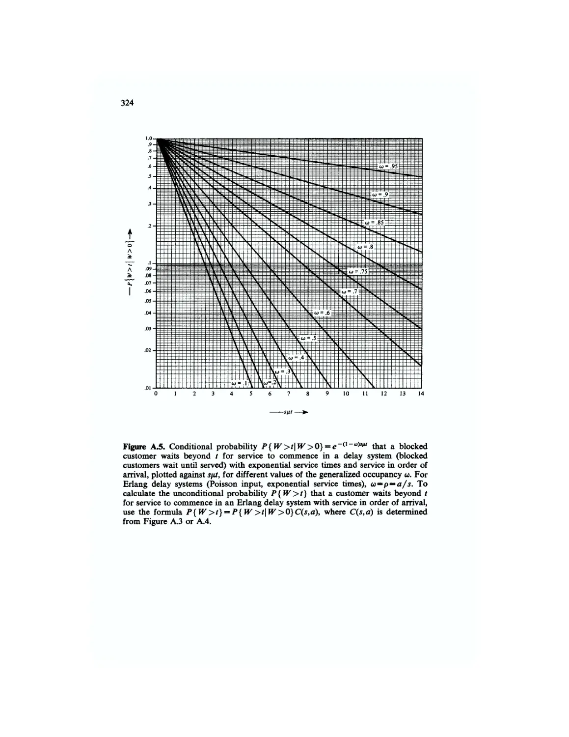


Текст
Introduction to
QUEUEING
THEORY
Second Edition
ROBERT R COOPER _
Introduction to
Queueing Theoiy
Second edition
Drawing by McCaJlister; © 1977 The New Yorker Magazine, Inc.
Introduction to
Queueing Theory
Second Edition
Robert B. Cooper
Computer Systems and Management Science
Florida Atlantic University
Boca Raton, Florida
It*
North Holland
New York • Oxford
Elsevier North Holland. Inc.
52 Vanderbilt Avenue, New York, New York 10017
Distributors outside the United States and Canada:
Edward Arnold (Publishers) Limited
41 Bedford Square
London WC1B 3DQ, England
© 1981 by Elsevier North Holland, Inc.
Library of Congress Cataloging in Publication Data
Cooper, Robert B
Introduction to queuelng theory.
Bibliography: p.
Includes index.
1. Queueing theory. I. Title.
T57.9.C66 1981 519.8'2 80-16481
ISBN 0-444-00379-7
Copy Editor Joe Fineman
Desk Editor Louise Calabro Schreiber
Design Edmee Froment
Art Editor Glen Burris
Cover Design Paul Agule Design
Production Manager Joanne Jay
Compositor Science Typographers, Inc.
Printer Haddon Craftsmen
Manufactured in the United States of America
For
my son
Bill
Contents
List of Exercises xi
Preface to the Second Edition xiii
1 Scope and Nature of Queueing Theory 1
2 Review of Topics from the Theory of Probability
and Stochastic Processes 9
2.1 Random Variables 9
2.2 Birth-and-Death Processes 14
2.3 Statistical Equilibrium 19
2.4 Probability-Generating Functions 26
2.5 Some Important Probability Distributions 34
Bernoulli Distribution 34
Binomial Distribution 34
Multinomial Distribution 35
Geometric Distribution 36
Negative-Binomial (Pascal) Distribution 37
Uniform Distribution 38
Negative-Exponential Distribution 42
Poisson Distribution 50
Erlangian (Gamma) Distribution 64
2.6 Remarks 71
3 Birth-and-Death Queueing Models 73
3.1 Introduction 73
3.2 Relationship Between the Outside Observer's Distribution and the
Arriving Customer's Distribution 77
3.3 Poisson Input, s Servers, Blocked Customers Cleared: The Erlang
Loss System 79
viii • Contents
3.4 Poisson Input, s Servers with Exponential Service Times, Blocked
Customers Delayed: The Erlang Delay System 90
3.5 Quasirandom Input 102
3.6 Equality of the Arriving Customer's «-Source Distribution and the
Outside Observer's («- 1)-Source Distribution for Birth-and-Death
Systems with Quasirandom Input 105
3.7 Quasirandom Input, s Servers, Blocked Customers Cleared: The
Engset Formula 108
3.8 Quasirandom Input, s Servers with Exponential Service Times,
Blocked Customers Delayed 111
3.9 Summary 116
4 Multidimensional Birth-and-Death Queueing Models 123
4.1 Introduction 123
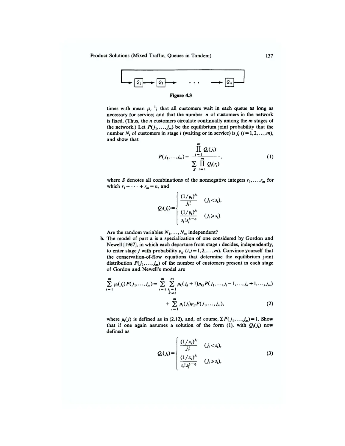
4.2 Product Solutions (Mixed Traffic, Queues in Tandem) 126
Infinite-Server Group with Two Types of Customers 126
Finite-Server Group with Two Types of Customers and Blocked
Customers Cleared 128
Queues in Tandem 132
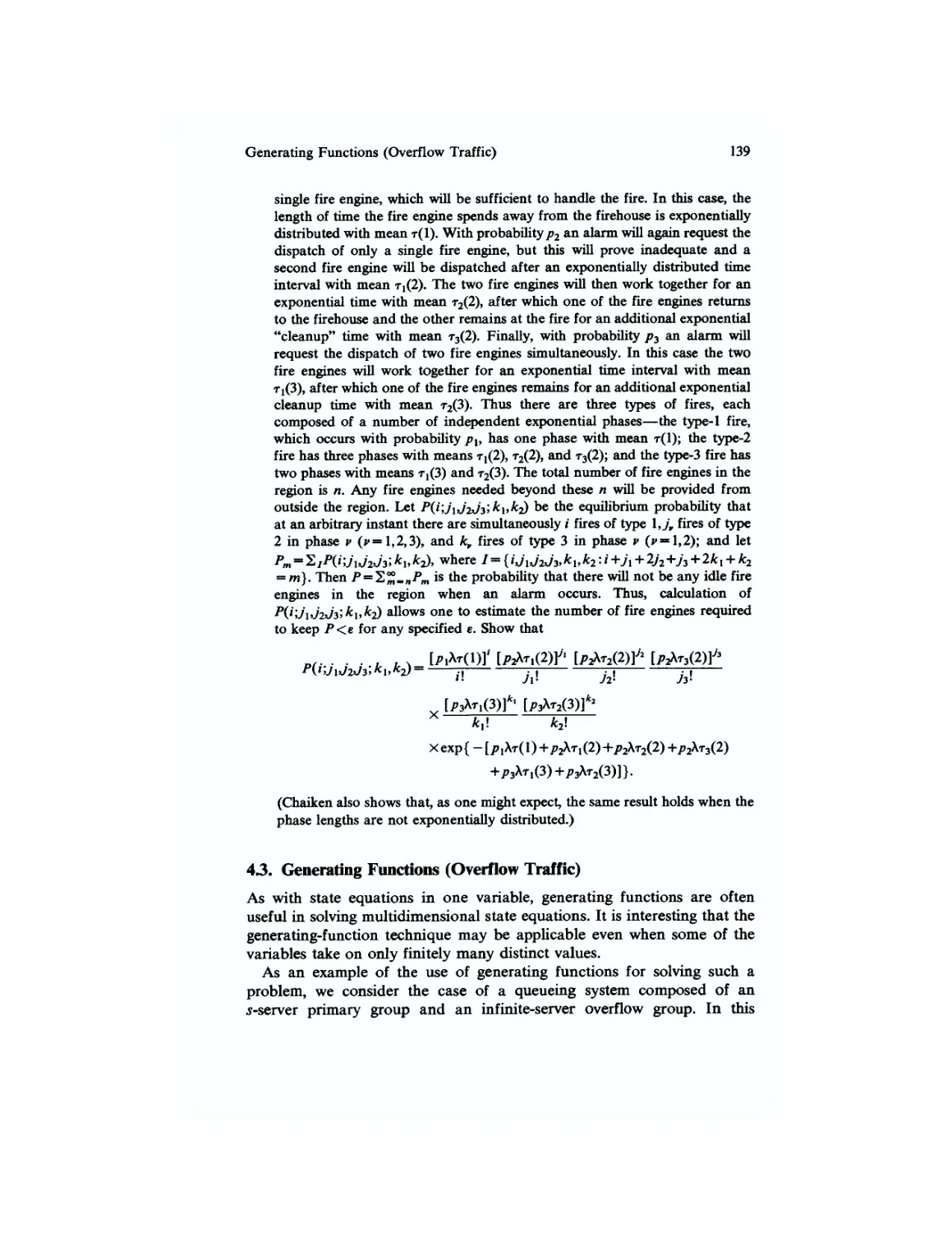
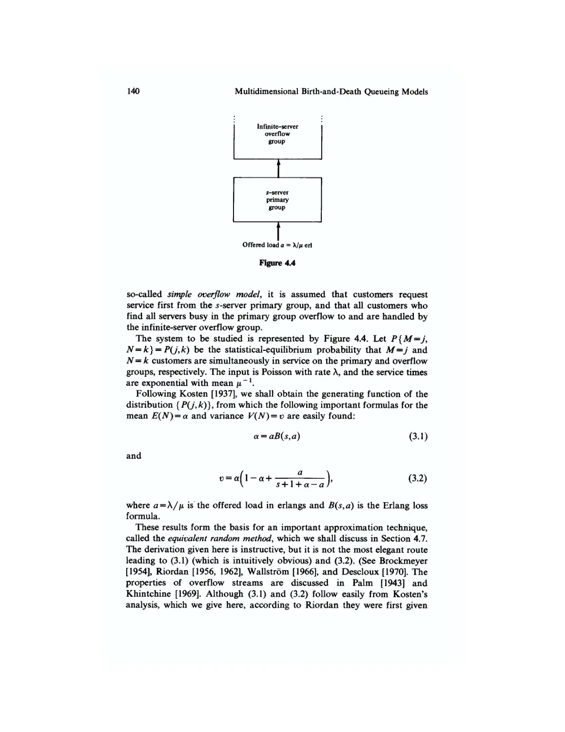
4.3 Generating Functions (Overflow Traffic) 139
4.4 Macrostates (Priority Reservation) 150
4.5 Indirect Solution of Equations (Load Carried by Each Server of an
Ordered Group) 153
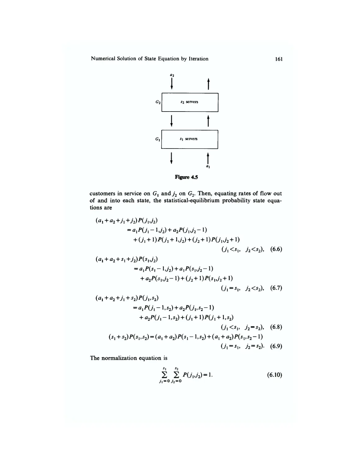
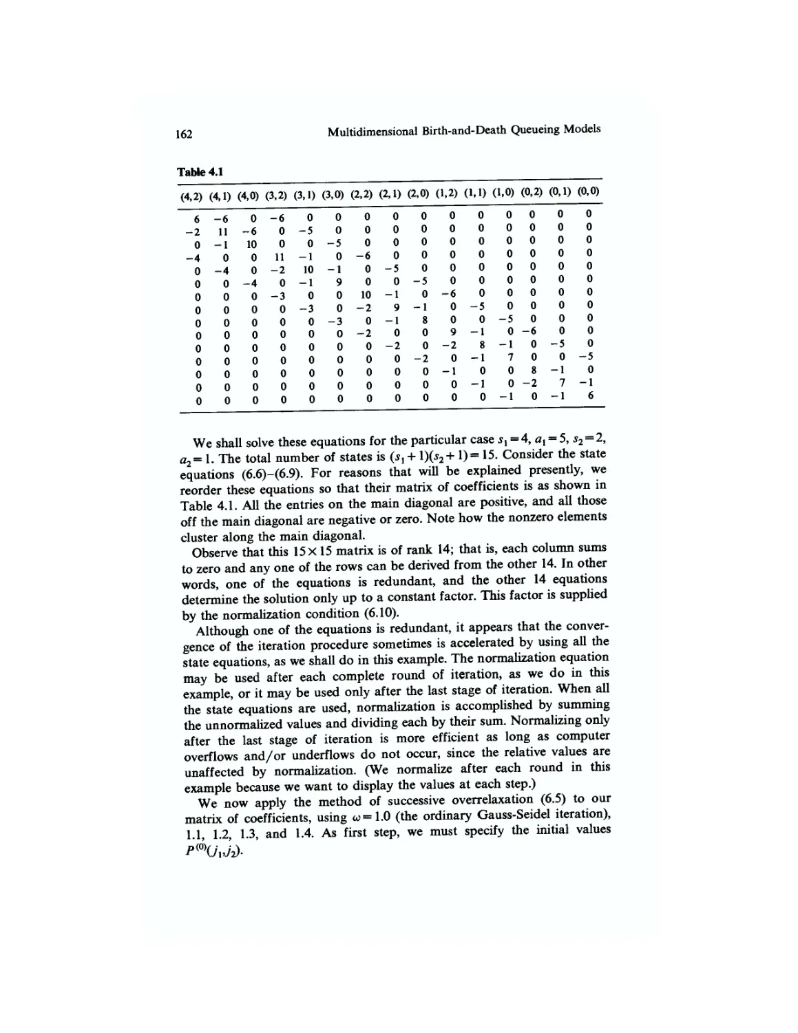
4.6 Numerical Solution of State Equations by Iteration (Gauss-Seidel and
Overrelaxation Methods) 158
4.7 The Equivalent Random Method 165
4.8 The Method of Phases 171
5 Imbedded-Markov-Chain Queueing Models 176
5.1 Introduction 176
5.2 The Equation L = KW ( Little's Theorem) 178
5.3 Equality of State Distributions at Arrival and Departure Epochs 185
5.4 Mean Queue Length and Mean Waiting Time in the M/G/l Queue 189
5.5 Riemann-Stieltjes Integrals 192
5.6 Laplace-Stieltjes Transforms 197
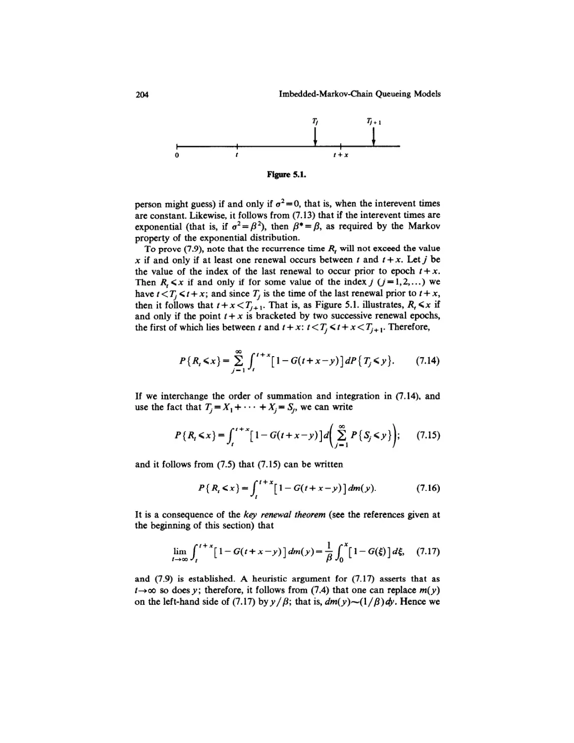
5.7 Some Results from Renewal Theory 200
5.8 The M/G/l Queue 208
The Mean Waiting Time 209
The Imbedded Markov Chain 210
The Pollaczek-Khintchine Formula 216
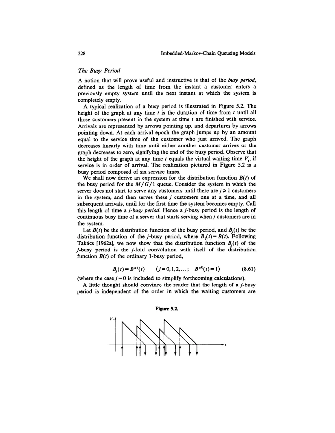
The Busy Period 228
5.9 The M/G/l Queue with Finite Waiting Room 235
5.10 The M/G/l Queue with Batch Arrivals 241
5.11 Optimal Design and Control of Queues: The N-Policy and the
T- Pol icy 243
5.12 The M/G/l Queue with Service in Random Order 253
5.13 Queues Served in Cyclic Order 261
5.14 The GilMjs Queue 267
5.15 The Gil Mis Queue with Service in Random Order 275
Contents ix
6 Simulation of Queueing Models 281
6.1 Introduction 281
6.2 Generation of Stochastic Variables 284
6.3 Simulation Programming Languages 287
6.4 Statistical Questions 288
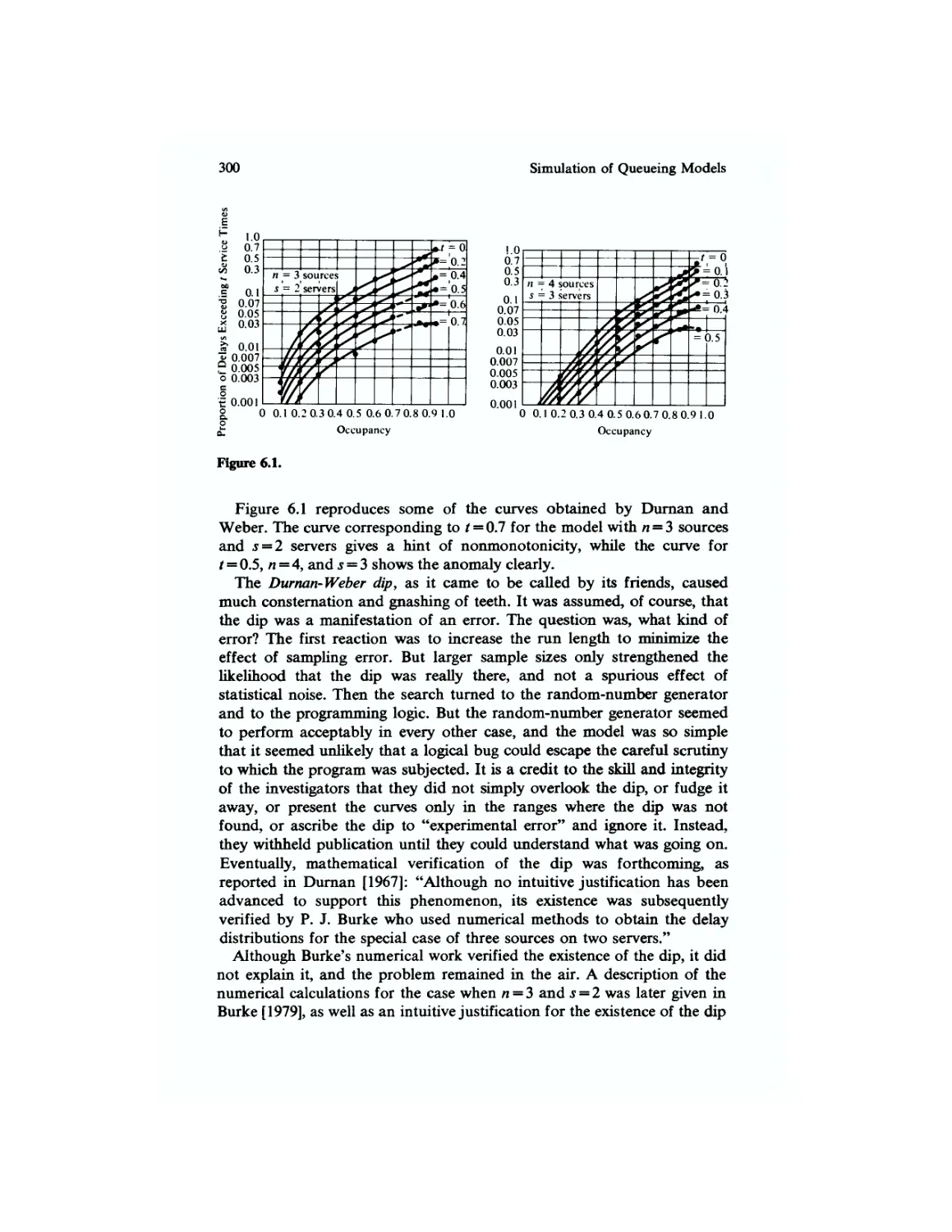
6.5 Examples 298
Waiting Times in a Queue with Quasirandom Input and Constant
Service Times 298
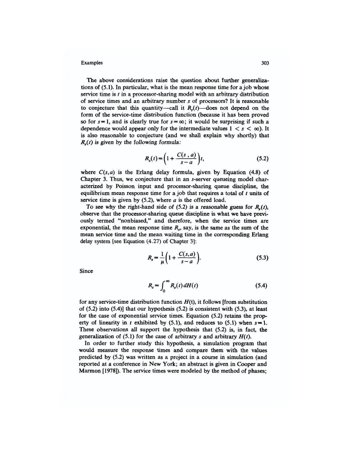
Response Times in a Processor-Sharing Operating System 30!
7 Annotated Bibliography 308
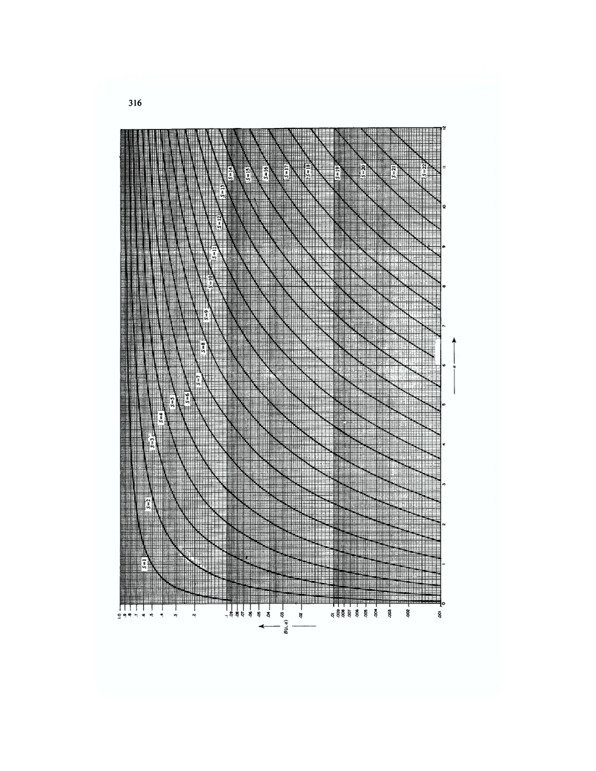
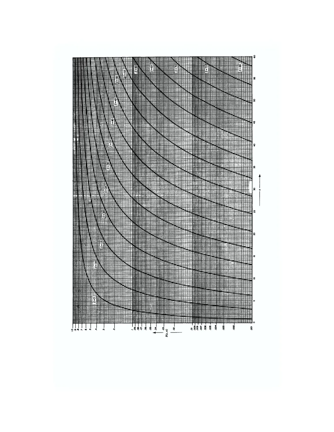
Appendix 315
References 325
Index 341
List of Exercises
Chapter 1
1
2
3
4
5
6
6
6
6
6
7
8
Chapter 2
1
2
3
4
5
6
7
8
9
10
11
12
13
14
17
24
30
31
34
35
38
38
41
49
49
49
Chapter
2
(continued)
14
15
16
17
18
19
20
21
22
23
24
25
26
49
49
49
51
56
56
59
62
63
63
63
70
71
Chapter 3
1
2
3
4
5
78
79
81
82
82
Chapter 3
(continued)
6
7
8
9
10
11
12
13
14
15
16
17
18
19
20
21
22
23
24
25
26
82
82
82
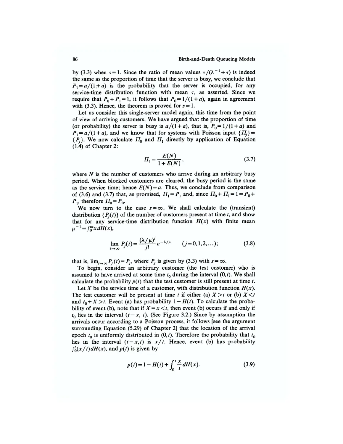
83
85
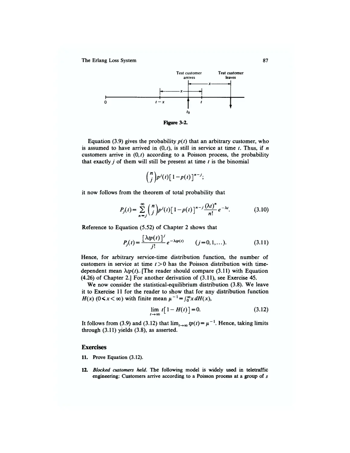
87
87
89
90
90
92
92
93
95
95
95
98
98
98
98
98
Xll
Chapter 3
(continued)
27
28
29
30
31
32
33
34
35
36
37
38
39
40
41
42
43
44
45
46
99
99
99
99
99
101
102
110
111
114
116
116
116
116
118
118
118
119
119
120
Chapter 4
1
2
3
4
5
6
7
125
129
130
130
130
131
131
Chapter 4
(continued)
8
9
10
11
12
13
14
15
16
17
18
19
135
136
138
138
148
153
157
170
170
171
175
175
Chapter 5
1
2
3
4
5
6
7
8
9
10
tl
12
13
14
15
188
188
196
199
199
199
203
203
206
206
207
222
223
224
227
List of Exercises
Chapter 5
(continued)
16
17
18
19
20
21
22
23
24
25
26
27
28
29
30
31
32
33
34
35
36
233
233
233
233
234
238
240
240
243
250
252
258
259
260
267
267
273
273
273
273
279
Chapter 6
1
2
3
4
285
285
298
298
Preface to the Second Edition
This is a revised, expanded, and improved version of my textbook, Introduction
to Queueing Theory. As before, it is written primarily for seniors and graduate
students in operations research, computer science, and industrial engineering;
and as before, the emphasis is on insight and understanding rather than either
cookbook application or fine mathematical detail. Although it has been struc-
structured for use primarily as a textbook, it should be a useful reference for re-
researchers and practitioners as well. The second edition reflects the feedback of stu-
students and instructors who have used the first edition (which began as a set of
notes for an in-house course I taught at Bell Laboratories), as well as my own
experience teaching from the book at the Georgia Institute of Technology (in the
School of Industrial and Systems Engineering and the School of Information and
Computer Science), the University of Michigan (in the Department of Industrial
and Operations Engineering), the New Mexico Institute of Mining and Technol-
Technology (in the Department of Mathematics), and Florida Atlantic University (in the
Department of Computer and Information Systems). The objective of the second edi-
edition is to improve on the first edition with respect to clarity, comprehensiveness, cur-
currency, and, especially, its utility both for teaching and, self-study.
In particular, improvements over the first edition include
1. the availability from the publisher of an instructor's manual containing de-
detailed solutions, by Bprge Tilt, to essentially all of the many exercises;
2. a new chapter, on simulation of queueing models;
3. an expanded and more complete treatment of background mathematical
topics, such as Laplace-Stieltjes transforms and renewal theory;
4. an annotated bibliography of almost all of the English language books on
queueing theory in existence;
5. the placement of exercises in the text just after the discussion they are
xiv Preface
designed to illuminate, rather than all together at the end of each chapter,
and the addition of new exercises, including numerical exercises that
reflect engineering and economic concepts;
6. the presentation in the text of some of the more difficult and important
material that was left to the exercises in the first edition;
7. the integration of the material of Chapter 6 of the first edition f "Waiting
Times") into the other chapters;
8. the inclusion of new material and references published after the first edi-
edition;
9. revision throughout to improve clarity and correct errors;
10. arrangement of the material so that the book can be used either for a
course that emphasizes practical applications, or for a course that em-
emphasizes more advanced mathematical concepts with an eye toward more
sophisticated applications or research.
The first chapter illustrates the nature of the subject, its potential for applica-
application, and the interplay between intuitive and mathematical reasoning that makes
it so interesting, Chapter 2 contains a review of topics from applied probability
and stochastic processes. Since the reader is presumed to have had a course in
applied probability, some of the material (such as the discussion of common
probability distributions) may well be familiar, but other topics (such as elemen-
elementary renewal theory) may be less familiar. The instructor can decide which topics
to emphasize and which to assign for review or self-study. Chapter 3 covers the
basic one-dimensional birth-and-death queueing models, including the well-
known Erlang B, Erlang C, and finite-source models. Care is taken to distin-
distinguish between the viewpoint of the arriving customer and that of the outside
observer. Chapter 4 discusses multidimensional birth-and-death models. This
chapter is organized by model, each of which exemplifies a different method of
solution of the multidimensional birth-and-death equations. The methods include
product solutions, probability-generating functions, inspection, the method of
phases, and numerical analysis. The models include networks of queues (with
many examples and references), systems with alternate routing, and systems with
multiple types or classes of traffic. Little's theorem, Kendall's notation, and the
Pollaczek-Khintchine formula are mentioned, but detailed discussion and deriva-
derivations are left to Chapter 5; the instructor can refer ahead or not as he sees fit.
Relatively "advanced" mathematical concepts, such as Laplace-Stieltjes trans-
transforms and imbedded Markov chains, are not used until Chapter 5. The intention
is that an elementary course, requiring no knowledge of "advanced" applied
mathematics but nevertheless conveying the main results and the essence of the
subject, can be constructed from topics covered in the first four chapters. For the
very practical-minded, a course can be constructed using only Chapters 1 and 3.
Chapter 5, which is the longest chapter, uses more advanced mathematics and
is more rigorous in its arguments than the preceding chapters. It covers much of
the material of classical queueing theory, as well as some more specialized top-
topics, such as queues with service in random order, which can be skipped without
Preface xv
toss of continuity. Also, it includes a summary treatment of Riemann-Stieltjes
integration and Laplace-Stieltjes transforms, tools that are often used but rarely
explained in textbooks on queueing theory or applied stochastic processes. An
intermediate-advanced course for students with prior knowledge of elementary
queueing theory can be built around Chapter 5. Chapter 6, which is completely
new, surveys the field of simulation as applied to queueing models. It contains,
among other things, one of the first textbook treatments of the regenerative
method in the context of simulation of queueing models, and discussions of two
structurally simple but nevertheless sophisticated simulation studies. Chapter 7
concludes with an annotated bibliography of (almost) all the books on queueing
theory and its application that have been published in the English language. (The
reader may well turn to Chapter 7 first.)
Colleagues who have contributed to this book, either directly by their reading
and commenting on the manuscript or indirectly by their personal and profes-
professional influence, include Carl Axness, Paul J. Burke, Grace M. Carter, Ralph
L. Disney, Hamilton Emmons, Carl M. Harris, Philip Heidelberger, Daniel P.
Heyman, Marcel F. Neuts, Stephen St. John, Donald G. Sanford, Bruce W.
Schmeiser, Samuel S. Stephenson, Shaler Stidham, Jr., Ryszard Syski, and
Eric Wolman. Special thanks go to B0rge Tilt who read the manuscript in its
entirety (through several versions), made many excellent suggestions, and wrote
the solutions manual (whose existence is surely one of the major attractions of
this book). Finally, I want to thank Elizabeth Fraissinet and Dora Yates, who typed the
manuscript, and Louise Calabro Gruendel of Elsevier Science Publishing Company,
who oversaw the editing and production.
Robert B. Cooper
Scope and Nature
of Queueing Theory
This text is concerned with the mathematical analysis of systems subject to
demands whose occurrences and lengths can, in general, be specified only
probabilistically.
For example, consider a telephone system, whose function is to provide
communication paths between pairs of telephone sets (customers) on
demand. The provision of a permanent communications path between
each pair of telephone sets would be astronomically expensive, to say the
least, and perhaps impossible. In response to this problem, the facilities
needed to establish and maintain a talking path between a pair of tele-
telephone sets are provided in a common pool, to be used by a call when
required and returned to the pool when no longer needed. This introduces
the possibility that the system will be unable to set up a call on demand
because of a lack of available equipment at that time. Thus the question
immediately arises: How much equipment must be provided so that the
proportion of calls experiencing delays will be below a specified acceptable
level?
Questions similar to that just posed arise in the design of many systems
quite different in detail from a telephone system. How many taxicabs
should be on the streets of New York City? How many beds should a
hospital provide? How many teletypewriter stations can a time-shared
computer serve?
The answers to these questions will be based in part on such diverse
considerations as politics, economics, and technical knowledge. But they
share a common characteristic: In each case the times at which requests
for service will occur and the lengths of times that these requests will
occupy facilities cannot be predicted except in a statistical sense.
2 Scope and Nature of Queueing Theory
The purpose of this text is to develop and explicate a mathematical
theory that has application to the problems of design and analysis of such
systems. Although these systems are usually very complex, it is often
possible to abstract from the system description a mathematical model
whose analysis yields useful information.
This mathematical theory is a branch of applied probability theory and
is known variously under the names traffic theory, queueing theory,
congestion theory, the theory of mass service, and the theory of stochastic
service systems. The term traffic theory is often applied to theories of
telephone and communications traffic, as well as to theories of vehicular
traffic flow. These two areas share some common ground, and the material
we shall develop will be useful in both fields. The term queueing theory is
often used to describe the more specialized mathematical theory of waiting
lines (queues). But some of the most interesting and most useful models are
based on systems in which queues are not allowed to form, so that the term
queueing theory does not seem completely appropriate. The subject of this
text is perhaps better described by the broader terms congestion theory
and stochastic service system theory. However, the name queueing theory
has become most widely used to describe the kind of material presented in
this text, and therefore I chose to entitle the book Introduction to Queueing
Theory.
Historically, the subject of queueing theory has been developed largely
in the context of telephone traffic engineering. Some of our examples will
be drawn from this area, but it should be kept in mind that the theory is
widely applicable in engineering, operations research, and computer sci-
science. Also, it is worth noting that the mathematics underlying queueing
theory is quite similar to that underlying such seemingly unrelated subjects
as inventories, dams, and insurance.
Consider the following model. Customers request the use of a particular
type of equipment (server). If a server is available, the arriving customer
will seize and hold it for some length of time, after which the server will be
made immediately available to other incoming or waiting customers. If the
incoming customer finds no available server, he then takes some specified
action such as waiting or going away. Such models often can be defined in
terms of three characteristics: the input process, the service mechanism,
and the queue discipline.
The input process describes the sequence of requests for service. Often,
for example, the input process is specified in terms of the distribution of
the lengths of time between consecutive customer arrival instants. The
service mechanism includes such characteristics as the number of servers
and the lengths of time that the customers hold the servers. For example,
customers might be processed by a single server, each customer holding the
server for the same length of time. The queue discipline specifies the
disposition of blocked customers (customers who find all servers busy).
For example, it might be assumed that blocked customers leave the system
Scope and Nature of (Jueueing Theory 3
immediately or that blocked customers wait for service in a queue and are
served from the queue in their arrival order.
We now use a model of this type to illustrate some important points
about queueing theory: A) The subject matter is of great practical value.
B) Heuristic and intuitive reasoning is often useful. C) Mathematical
subtleties abound.
Consider two cities interconnected by a group of s telephone trunks
(servers). Suppose that arrivals finding all trunks busy do not wait, but
immediately depart from the system. (Technically, no "queueing" occurs.)
What proportion of incoming calls (customers) will be unable to find an
idle trunk (and thus be lost)?
We wish to derive a formula that will predict the proportion of calls lost
as a function of the demand; that is, we wish to derive a formula that
allows estimation of the number of trunks required to meet a prespecified
service criterion from an estimate of the telephone traffic load generated
between the two cities. The great practical value of any model that leads to
such a formula is obvious. The fact that such models have been success-
successfully employed has spurred continuing investigations by industrial and
academic researchers throughout the world.
We shall now give a heuristic derivation of the required formula, using a
concept of great importance in science and engineering, that of conserva-
conservation of flow. It is important for the reader to realize that since the following
derivation is heuristic, he should not expect to understand it completely;
our "derivation" is really a plausibility argument that, as will be demon-
demonstrated later, is correct in certain circumstances. With this disclaimer, let us
now proceed with the argument.
When the number of customers in the system isy, the system is said to
be in state Ej (J=Ofli..,,s). Let Pj be the proportion of time that the
system spends in state Ey, Pj is therefore also the proportion of time thaty
trunks are busy. Denote by X the call arrival rate; X is the average number
of requests for service per unit time. Consider first the case j<s. Since calls
arrive with overall rate A,, and since the proportion of time the system
tpends in state Ej is PJf the rate at which the transition Ej->EJ+X occurs
(the average number of such transitions per unit time) is therefore XP*.
Now consider the case when j = s. Since the state Es+l represents a
physically impossible state (there are only s trunks), the transition Es-*
?,+ 1 cannot occur, so the rate of transition Es->Ea+l is zero. Thus the rate
at which the upward transition Ej~*EJ+1 occurs is XPj wheny = 0,1,..., s — 1
d is zero when 7=$.
Let us now consider the downward transition
suppose that the mean holding time (the average length of time a call
holds a trunk) is t. Then, if a single trunk is busy, the average number of
4 Scope and Nature of Queueing Theory
calls terminating during an elapsed time t is 1; the termination rate for a
single call is therefore 1/t, Similarly, if two calls are in progress simulta-
simultaneously and the average duration of a call is t, the average number of calls
terminating during an elapsed time r is 2; the termination rate for two
simultaneous calls is therefore 2/t. By this reasoning, then, the termina-
termination rate fory'+l simultaneous calls is 0 + l)/T- Since the system is in
state EJ+X a proportion of time PJ+V we conclude that the downward
transition Ej+x-^Ej occurs at rate (J+1)t~1P/+i transitions per unit time
We now apply the principle of conservation of flow: We equate, for each
value of the index j, the rate of occurrence of the upward transition
Ej^>EJ+l to the rate of occurrence of the downward transition ?^+]—>?,-.
Thus we have the equations of statistical equilibrium or conservation of
flow.
0,1,...,j-I). A.1)
These equations can be solved recurrently; the result, which expresses each
Pj in terms of the value Po, is
p (At/ „ / • i -j \ fn\
Since the numbers {Pj} are proportions, they must sum to unity:
P + P + • • + P — 1 (iVi
Using the normalization equation A.3) together with A.2), we can de-
determine Po:
/ s s\ \k \ -I
A.4)
U-
o *! /
Thus we obtain for the proportion Pj of time thaty trunks are busy the
formula
0 = 0,1,....). A.5)
An important observation to be made from the formula (L5) is that the
proportions {/*,} depend on the arrival rate A and mean holding time r
only through the product At. This product is a measure of the demand
made on the system; it is often called the offered load and given the symbol
a (a = At). The numerical values of a are expressed in units called erlangs
(erl), after the Danish mathematician and teletraffic theorist A. K. Erlang,
who first published the formula A.5) in 1917.
Scope and Nature of Queueing Theory 5
Wheny = s in A.5), the right-hand side becomes the well-known Erlang
loss formula, denoted in the United States by B(sta) and in Europe by
B{s,a)= f/s' . A.6)
2 ak/kl
We shall derive these results more carefully later in the text. The point to
be made here is that some potentially useful mathematical results have
been derived using only heuristic reasoning. The question we must now
answer is: What, if any, are the conditions under which these results are
valid?
More precisely, what assumptions about the input process and service
mechanism are required for the validity of the formulas A.5) and A.6)?
[We have described the input process by giving only the arrival rate;
similarly, the service times have been specified only through their mean
value. It turns out that our conclusion A.5) is valid for a particular type of
input process called a Poisson process and, surprisingly, for any distribution
of service times whatever.] Can the assertion that the downward transition
fate is proportional to the reciprocal of the mean holding time be justified?
What is the relationship between the proportion Pj of time thaty calls are
in progress and the proportion IIp say, of arriving calls that find j other
calls in progress? [It turns out that for systems with Poisson input these
two distributions are equal. Thus, the Erlang loss formula A.6) gives the
proportion of customers who will be denied service, that is, lost, when the
arrivals occur according to a Poisson process.] How widely applicable is
the conservation-of-flow analysis? How does one handle processes for
which this type of analysis is inapplicable?
Questions of this nature sometimes require highly sophisticated mathe-
mathematical arguments. In this text we shall take a middle ground with regard
to the use of advanced mathematics. We shall attempt to impart an
understanding of the theory without recourse to the use of abstract and
measure-theoretic tools; the material is presented in a mathematically
informal manner with emphasis on the underlying physical ideas. Mathe-
Mathematical difficulties and fine points will be noted but not dwelled upon. The
material should be accessible to a student who understands applied proba-
probability theory and those areas of mathematics traditionally included in
undergraduate programs in engineering and the physical sciences.
A word about the range of applicability of these models is in order here.
The example discussed above is based on a telephone traffic application,
but it should be clear that the identification of the customers as "calls" and
the servers as "trunks" in no way limits the generality of the model.
As mentioned previously, telephone applications have provided the
context for the development of much of queueing theory (and this example
6 Scope and Nature of Queueing Theory
illustrates why). We shall occasionally refer to telephone applications,
thereby illustrating the general principles of the theory with a coherent
class of authentic examples. Of course, no technical knowledge of tele-
telephony is required.
In summary, this is a text and reference in queueing theory, a subject of
both practical importance and theoretical interest. Although the book is
directed primarily toward the student, some of the lesser-known concepts
and results from telephone traffic theory should prove of interest, apart
from their value in illustrating the theory, to engineers and researchers.
The material is presented with an emphasis on the underlying physical
processes and the interplay between physical and mathematical reasoning.
Heuristic and intuitive approaches are used where helpful. Mathematical
subtleties are observed and are explored where it is profitable to do so
without recourse to methods of abstract analysis.
Since the publication of Erlang's first paper in 1909 (which is regarded
by many as marking the birth of queueing theory), and especially since the
renewed interest in queueing theory that accompanied the f ormalization of
the field of operations research after World War II, about 2000 papers and
at least 35 books on this subject have been published. It is hoped that the
reader will find the present book a useful and interesting addition to the
literature.
Exercises
1. In what ways are telephone traffic theory and vehicular traffic theory similar,
and in what ways are they different?
2. List some applications of the Erlang loss model.
3. Discuss ways in which queueing models might be used in the following:
a. Highway design.
b. City planning.
c. Hospital management.
d. Airport design.
e. Reliability engineering.
f. Computer design.
4. Extend the heuristic conservation-of-flow argument to include the case in
which all customers who find all servers busy wait until served.
a. Argue that
pJ-
A)
Scope and Nature of Queueing Theory
where
b. What restriction must be placed on the magnitude a of the offered load in
order for B) to be correct? Give a physical interpretation of this restriction.
c Show that the proportion of time that all servers are busy (which, in this
case, turns out to equal the proportion of customers who find all servers
busy and therefore must wait for service) is given by
s\(\-a/s)
This is the well-known Erlang delay formula, also denoted by E^a), which
we shall discuss in detail in Chapter 3.
d. What assumption, if any, have you made about the order in which waiting
customers are selected from the queue when a server becomes idle? Is such
an assumption necessary? Why?
e. Show that, if all servers are busy, the probability p} that j customers are
waiting for service is given by
/>, = (i-pV 0=o,i,...), D)
where p = a/s. [The probabilities defined by D) constitute the geometric
distribution.]
f. Suppose it is known that at least k > 0 customers are waiting in the queue.
Show that the probability that the number of waiting customers is exactly
j + kis pp given by D). Note that this probability is independent of the value
of the index k.
g. Show that Pj=Pj 0=0.U-O when$= 1. Show that C(l,a) = a.
Consider the so-called loss-delay system, which is one with a finite number n of
waiting positions: An arrival who finds all servers busy and at least one waiting
position unoccupied waits as long as necessary for service, while an arrival who
finds all n waiting positions occupied departs immediately (and thus is lost).
a. Using the conservation-of-flow argument, show that the probability Pj thaty
customers are present simultaneously is given by the formula A) of Exercise
4, where now the largest value of the index j is s + n, and
b. Use these results to obtain the Erlang loss formula A.6) and the Erlang
delay formula C) of Exercise 4.
Scope and Nature of Queueing Theory
c What restrictions, if any, must be placed on the magnitude a of the offered
load when n < oo? When n — oo?
Consider a queueing model with two servers and one waiting position, and
assume that if an arriving customer finds both servers busy and the waiting
position unoccupied, then with probability p the customer will wait as long as
necessary for service, and with probability 1 —p he will depart immediately.
(As usual, all customers who arrive when there is an idle server enter service
immediately, and all customers who arrive when the waiting position is
occupied depart immediately.)
a. Let Py 0 = 0,1,2,3) be the probability that j customers are present simulta-
simultaneously; let A be the arrival rate and t be the average service time; and write
the conservation-of-flow equations that determine the probabilities Pj (J =
0,1,2,3).
b. Solve the equations of part a.
c Find the fraction B of arriving customers who don't get served.
d. Suppose A—2 customers per hour, t= 1 hour, and/> = {. Evaluate i% Px, P2,
i>3, and B.
e. Suppose the manager receives $2.00 for every customer who gets served
without waiting and $1.00 for every customer who gets served after having
to wait. How many dollars per hour will she receive?
f. If the manager pays a rental fee of $.50 per hour per server (whether the
server is busy or idle), and each server when busy consumes fuel at the rate
of $.25 per hour, what is the manager's total operating cost in dollars per
hour? What is her profit in dollars per hour?
f21
Review of Topics
From the Theory of Probability
and Stochastic Processes
This chapter reviews and summarizes some aspects of the theory of
probability and stochastic processes that have direct application to elemen-
elementary queueing theory. The material given here is intended not only as a
reference and refresher in probability and stochastic processes but also as
an introduction to queueing theory. It is assumed that the reader is already
familiar with the basic concepts of probability theory as covered, for
example, in ^inlar [1975], Feller [1968], Fisz [1963], Neuts [1973], and Ross
[1972], Specifically, we assume of the reader working knowledge of the
basic notions of event, probability, statistical dependence and indepen-
independence, distribution and density function, conditional probability, and
moment. These concepts will be used freely where required. Familiarity
with the theory of Markov chains is helpful, but not essential. Birth-and-
death processes, generating functions, and the properties of some im-
important distributions will be reviewed in some detail. Examples will be
drawn largely from queueing theory. The reader who feels no need for
review is advised to skim, but not skip, this chapter before proceeding to
the next.
2.1. Random Variables
If an experiment could be performed repeatedly under identical condi-
conditions, then, experience seems to tell us, each of the different possible
outcomes of the experiment will occur with a long-run relative frequency
that remains constant. Probability theory represents an attempt to model
this "observed" behavior of long-run frequencies with a formal mathemati-
mathematical structure. As a mathematical theory, of course, probability theory need
10 Review of Probability and Stochastic Processes
only be internally consistent. As a model of reality, however, the theory
needs also to be consistent with the observed properties of the phenomena
it purports to describe. To be a useful model, moreover, the theory should
be capable of exposing facts about reality that were previously hidden
from view.
Probability theory is now a well-developed mathematical theory, and has
proved also to be an excellent model of frequencies in repeated experi-
experiments. We will take advantage of this fact and apply probability theory to
the analysis of the phenomenon of queueing. Characteristic of applied
probability, and queueing theory in particular, is the interaction between
the mathematical and intuitive (that is, interpretive) aspects. All mathe-
mathematical results should be understandable in physical terms; and all intui-
intuitive results should be capable of rigorous mathematical proof. Unfor-
Unfortunately, neither of these conditions can always be met. In this text
intuitive arguments and interpretations will be emphasized, with the tacit
understanding that, of course, one is never safe until a rigorous argument
is proffered.
We begin with a brief discussion of random variables in the context of
queueing theory, and we follow with an example that illustrates the
intuitive "frequency" approach to the calculation of probabilities.
The mathematical definition of event involves the notions of sample
space and Borel field, but for most practical purposes, intuitive notions of
event are sufficient. Examples of the kinds of events of interest in queueing
theory are (an arbitrary customer finds all servers busy}, (an arbitrary
customer must wait more than three seconds for service}, and (the number
of waiting customers at an arbitrary instant isy}.
In each of these examples, the event can be expressed in numerical terms
in the following ways. Define N to be the number of customers in an
j-server system found by an arbitrary arriving customer. Then the event
(an arbitrary customer finds all s servers busy} can be written {N>s},
and the probability of occurrence of this event can be represented by
P{N>s}.
Similarly, let W be the waiting time of an arbitrary customer, and let Q
be the number of waiting customers (queue length) at an arbitrary instant.
Then these events are { W>3) and {(?=/}, with probabilities P{ W>3)
and P{Q=j), respectively.
The quantities N, W, and Q defined above are random variables. Each
of them has the property that it represents an event in terms of a numerical
value about which a probability statement can be made. More formally: A
random variable is a function defined on a given sample space, and about
whose values a probability statement can be made.
The question of precisely which functions can qualify as random vari-
variables is, like that of the notion of event, a mathematical one. For our
purposes, it will be sufficient to consider the use of random-variable
Random Variables 11
notation as simply a device for describing events without explicit concern
for the underlying probability space.
A random variable is defined by assigning a numerical value to each
event. For example, in a coin-tossing experiment, the event {head} can be
assigned the value 1, and the event {tail} the value 0. Call the describing
random variable X. Then at each toss a head will occur with probability
P{X=l] and a tail with probability P{X=0). This use of the random-
variable notation may seem artificial, since the association of the event
{head} with the value X— 1 is arbitrary, and the value X=2.6 might just as
well have been chosen. But it will be seen that judicious choices of the
random-variable definitions often lead to simplifications. For example,
observe that any random variable X that takes only the values 0 and 1 has
expected value E(X) = 0P{X = 0} + \P{X= \} = P{X=\); that is, the
mean value of a zero-one random variable is equal to the probability that
the random variable takes on the value 1.
Suppose, for example, that we wish to study the random variable Sn,
which we define to be the number of heads occurring in n tosses. Let the
random variable Xj describe theyth toss; let Xj=\ if theyth toss results in a
head, and Xj=0 for a tail. Then the random variable Sn can be interpreted
as the sum Sn = Xl+ • ¦ ¦ +Xn. The interpretation of Sn as a sum of random
variables allows its study in terms of the simpler component random
variables Xx,...,Xn, without further regard to the physical meaning of Sn.
We shall return to this example later.
In most of the queueing-theory problems we shall encounter, however,
the assignment of random-variable values to events is quite natural from
the context of the problem. Only a malcontent would choose to assign the
value Q = 4.2 to the event {six customers are waiting}.
We now consider an example that will illustrate the intuitive
"frequency" approach to the calculation of probabilities, while simulta-
simultaneously providing us with a result that will prove useful in queueing
theory. Consider a population of urns, where an urn of typey (y = 1,2,...)
contains n, balls. Let the random variable X be the type of an urn selected
at random; that is, P{X=j) is the probability that an arbitrary urn is of
typey. We interpret P{X=j) as the frequency with which urns of typey
occur in the general population of urns. Let us say that a ball is of typey if
it is contained in an urn of typey, and let Y be the type of a ball selected at
random; we interpret P{Y=j) as the frequency with which balls of typey
occur in the general population of balls. Our objective is to derive a
formula that relates the frequencies (probabilities) of occurrence of the
urns to the corresponding frequencies (probabilities) of occurrence of the
balls.
Suppose first that m urns are selected "at random" from the (infinite)
parent population, and let w, be the number of urns of typey among the m
urns selected. Then the relative frequency of occurrence of urns of typey
12 Review of Probability and Stochastic Processes
among the m urns selected is rrij/m. We now assume that this ratio has a
limit as m tends to infinity, and we call this hypothesized limiting value the
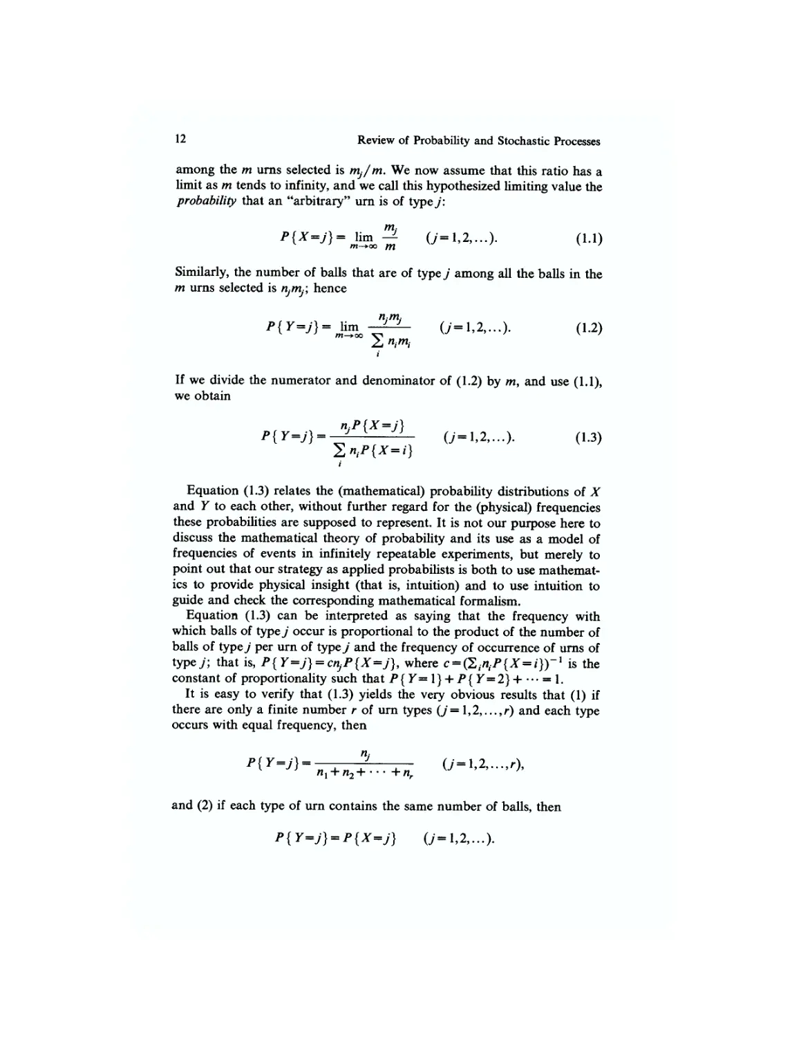
probability that an "arbitrary" urn is of typey:
Similarly, the number of balls that are of typey among all the balls in the
m urns selected is rijiny, hence
P{y=y} = mlim^- (y=l,2,...). A.2)
If we divide the numerator and denominator of A.2) by m, and use A.1),
we obtain
niP{X=j)
P{Y=j} = ^— (y=l,2,...). A.3)
}
2
Equation A.3) relates the (mathematical) probability distributions of X
and Y to each other, without further regard for the (physical) frequencies
these probabilities are supposed to represent. It is not our purpose here to
discuss the mathematical theory of probability and its use as a model of
frequencies of events in infinitely repeatable experiments, but merely to
point out that our strategy as applied probabilists is both to use mathemat-
mathematics to provide physical insight (that is, intuition) and to use intuition to
guide and check the corresponding mathematical formalism.
Equation A.3) can be interpreted as saying that the frequency with
which balls of type j occur is proportional to the product of the number of
balls of typey per urn of typey and the frequency of occurrence of urns of
typey; that is, P{ Y=j) = crijP{X=j), where c = (ZiniP{X = i})~1 is the
constant of proportionality such that P{Y=l} +P{Y=2}+ ¦¦¦ = \.
It is easy to verify that A.3) yields the very obvious results that A) if
there are only a finite number r of urn types (j= 1,2,...,r) and each type
occurs with equal frequency, then
and B) if each type of urn contains the same number of balls, then
Random Variables 13
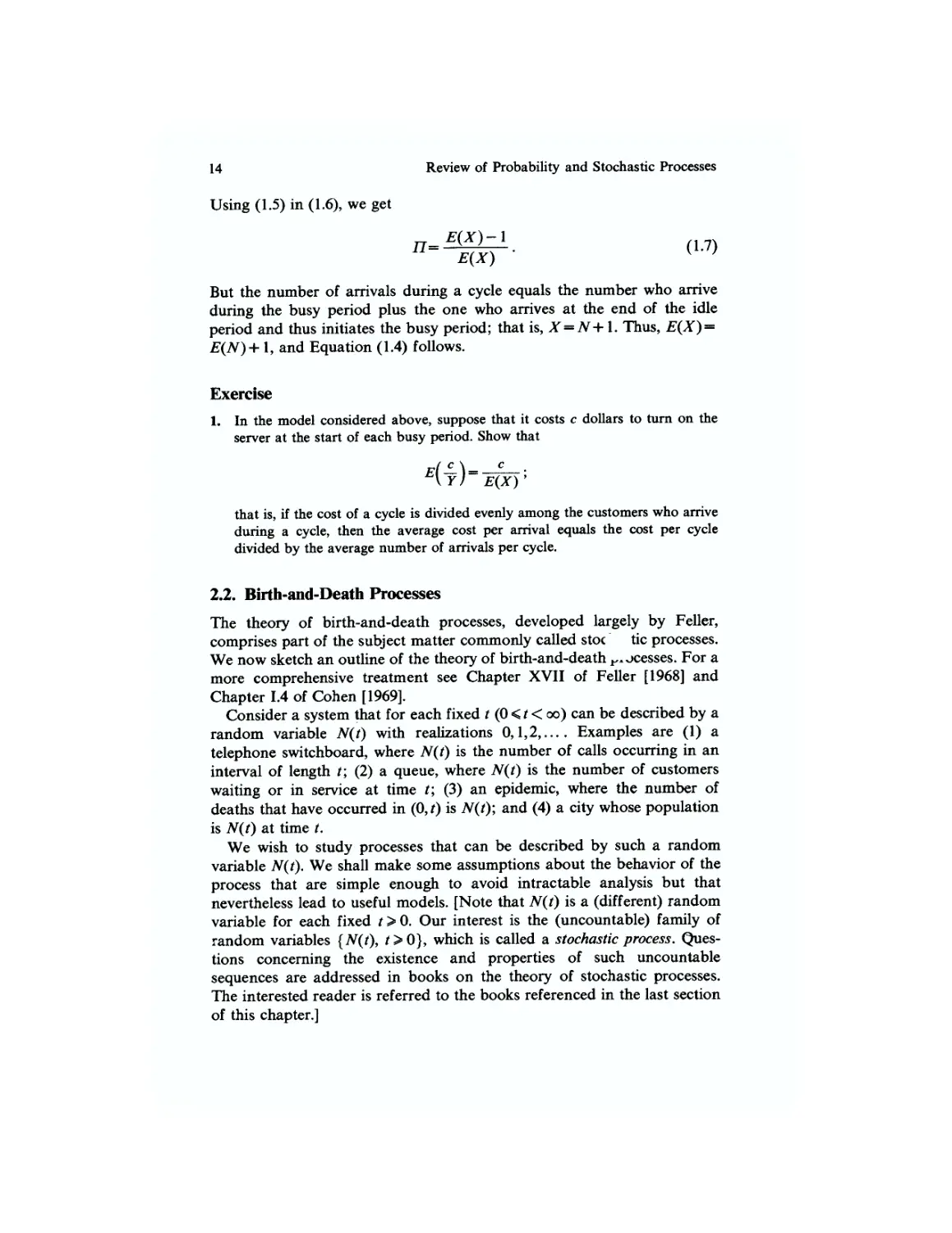
As an example of the application of A.3) in queueing theory, we
consider a single-server system. We view time as being decomposed into a
sequence of cycles, where each cycle consists of an idle period (during
which there are no customers present and the server is idle) and an
adjacent busy period (during which the server is continuously busy). In
many important queueing models the cycles are independent and statisti-
statistically identical; that is, each cycle represents an independent trial in a
sequence of infinitely repeatable experiments. Now suppose that the num-
number of customers who arrive during a busy period is N, with mean value
E(N). [The calculation of E(N) depends on other assumptions of the
model, such as whether customers who arrive during a busy period, and
thus are blocked, wait for service or leave immediately or take some other
action.] We shall show that the proportion H of customers who are
blocked is given by
l + E(N)- { '
According to A.4) the probability of blocking equals the ratio of the
mean number of customers who are blocked per cycle, E(N), to the mean
number of customers who arrive during a cycle, 1 + E(N). This result has
great intuitive appeal, and will also be useful when E(N) is easy to
calculate.
To prove A.4), let X be the number of customers (balls) who arrive
during an arbitrary cycle (urn), and let Y be the number of customers who
arrive during the cycle that contains an arbitrary customer (called the test
customer) whose viewpoint we shall adopt. Also, let a customer be of typey
if exactly j customers (including himself) arrive during his cycle. Then
Equation A.3) applies, with rij—j:
Now, if the test customer is one of j arrivals during a cycle, the probability
that he is not the first of those j, and therefore is blocked, is (J— \)/j. It
follows from the theorem of total probability* that the probability II that
the test customer is blocked is
A.6)
•If the events Bt,B2,... are mutually exclusive (that is, BtBj=<t> for all i?j) and exhaustive
(that is, Bx\jB2\j--- . where Q is the sample space), then, for any event A,P{A}~
P{A\Bl}P{Bl} + P{A\B2}P{B2} + ¦ ¦ ¦. (See, for example, p. 15 of ?inlar [1975].)
14 Review of Probability and Stochastic Processes
Using A.5) in A.6), we get
But the number of arrivals during a cycle equals the number who arrive
during the busy period plus the one who arrives at the end of the idle
period and thus initiates the busy period; that is, X = N +1. Thus, E(X) =
E(N)+1, and Equation A.4) follows.
Exercise
1. In the model considered above, suppose that it costs c dollars to turn on the
server at the start of each busy period. Show that
E(X)'
that is, if the cost of a cycle is divided evenly among the customers who arrive
during a cycle, then the average cost per arrival equals the cost per cycle
divided by the average number of arrivals per cycle.
2.2. Birth-and-Death Processes
The theory of birth-and-death processes, developed largely by Feller,
comprises part of the subject matter commonly called stoc tic processes.
We now sketch an outline of the theory of birth-and-death ^ocesses. For a
more comprehensive treatment see Chapter XVII of Feller [1968] and
Chapter 1.4 of Cohen [1969].
Consider a system that for each fixed t @ < t < oo) can be described by a
random variable N(t) with realizations 0,1,2,.... Examples are A) a
telephone switchboard, where N(t) is the number of calls occurring in an
interval of length t; B) a queue, where N(t) is the number of customers
waiting or in service at time t; C) an epidemic, where the number of
deaths that have occurred in @,0 is N(t); and D) a city whose population
is N(t) at time t.
We wish to study processes that can be described by such a random
variable A^@- We shall make some assumptions about the behavior of the
process that are simple enough to avoid intractable analysis but that
nevertheless lead to useful models. [Note that N(t) is a (different) random
variable for each fixed t > 0. Our interest is the (uncountable) family of
random variables [N(t), t>0}, which is called a stochastic process. Ques-
Questions concerning the existence and properties of such uncountable
sequences are addressed in books on the theory of stochastic processes.
The interested reader is referred to the books referenced in the last section
of this chapter.]
Birth-and-Death Processes 15
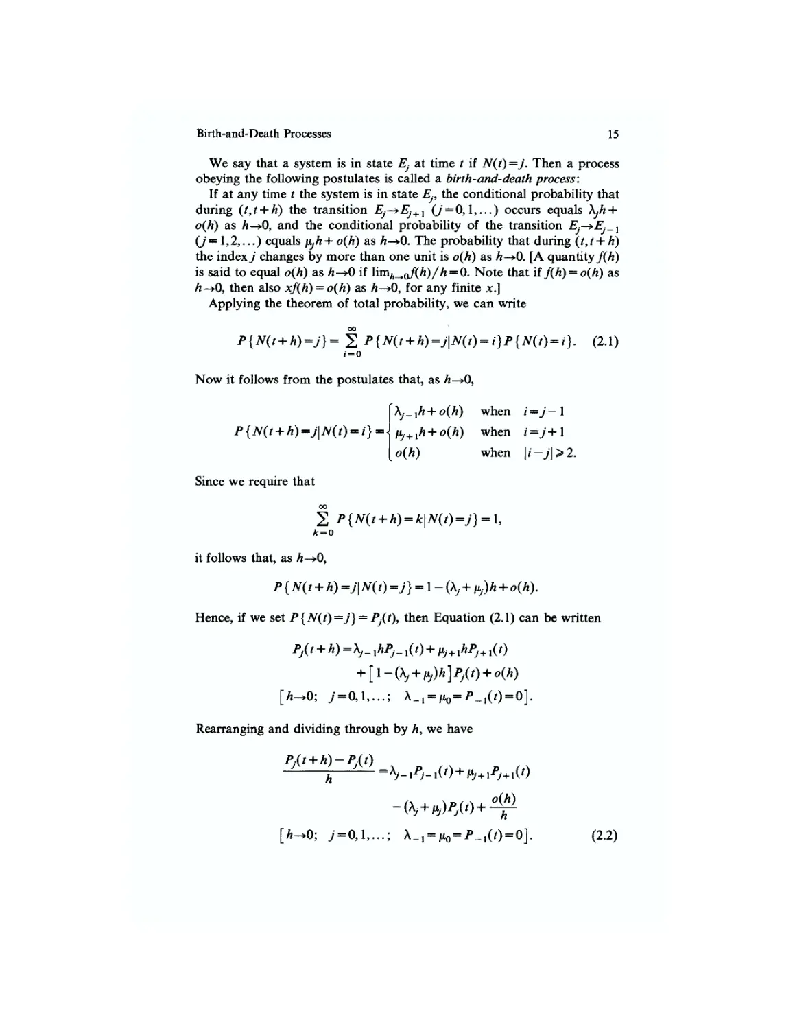
We say that a system is in state Ej at time t if N(t) =j. Then a process
obeying the following postulates is called a birth-and-death process:
If at any time t the system is in state Ej, the conditional probability that
during (t,t + h) the transition Ej-*EJ+1 (J = 0,l,...) occurs equals Xjh +
o(h) as h—>0, and the conditional probability of the transition Ej—*EJ_i
G=1,2,...) equals \ijh + o{h) as A-»0. The probability that during (t, t + h)
the index 7 changes by more than one unit is o(h) as h-*0. [A quantity/(A)
is said to equal o(h) as A-»0 if \imh^ofih)/h=0. Note that itf(h) = o{h) as
h—>0, then also xf(h) = o(h) as A-»0, for any finite x.]
Applying the theorem of total probability, we can write
= i}. B.1)
1=0
Now it follows from the postulates that, as h—*0,
when /=y —1
when i=j+\
[o(h) when \i-j\>2.
Since we require that
it follows that, as h—*0,
P{N(t + h) =j\N(t) =7} = 1 - (A, + fj)h + o(h).
Hence, if we set P{N(t)=j} = Pj(t), then Equation B.1) can be written
P/t + h)=Xj_ xhPj_,(/) + iiJ+lhPJ+1(t)
Rearranging and dividing through by h, we have
; 7 = 0,1,...; \_1 = [lo=p_l(t) = 0]. B.2)
16 Review of Probability and Stochastic Processes
We now let h—*0 in Equation B.2). The result is the following set of
differential-difference equations for the birth-and-death process:
[y-0,1,...; A_1 = ^o=P_1@=0]. B.3)
If at time / = 0 the system is in state Et, the initial conditions that
complement Equation B.3) are
The coefficients {A,} and {j^} are called the birth and death rates,
respectively. When jUy = 0 for ally, the process is called a pure birth process;
and when ^ = 0 for ally, the process is called a pure death process.
In the case of either a pure birth process or a pure death process, it is
easy to see that the differential-difference equations B.3) can always be
solved, at least in principle, by recurrence (successive substitution).
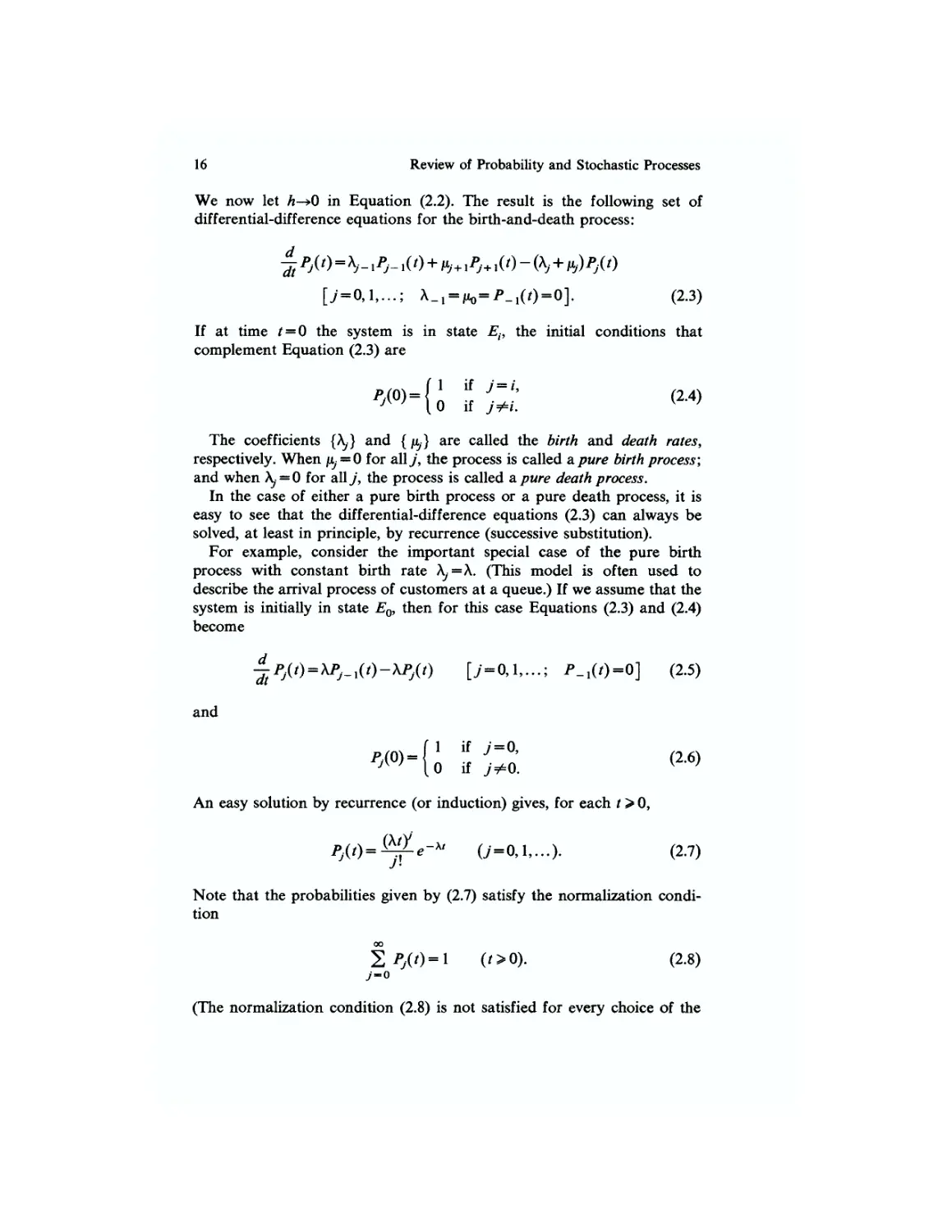
For example, consider the important special case of the pure birth
process with constant birth rate A,=A. (This model is often used to
describe the arrival process of customers at a queue.) If we assume that the
system is initially in state Eo, then for this case Equations B.3) and B.4)
become
ji/ JJ [y = 0,l,...; /»_,(/)-0] B.5)
and
An easy solution by recurrence (or induction) gives, for each t > 0,
PjiO-Qjfe-* 0=0,1,...). B.7)
Note that the probabilities given by B.7) satisfy the normalization condi-
condition
W B.8)
(The normalization condition B.8) is not satisfied for every choice of the
Birth-and-Death Processes 17
birth coefficients. For a more extensive treatment, see Chapter XVII of
Feller [1968].)
According to Equation B.7), N(t) has the Poisson distribution with mean
\t; we say that {N(t), t > 0} is a Poisson process. Since the assumption
\j=X is often a realistic one in the construction of queueing models, the
simple formula B.7) is important in queueing theory. The Poisson distribu-
distribution possesses important theoretical properties and plays a central role in
queueing theory.
Another important example is the special case of the pure death process
with death rate /x, proportional to the index of the state Ey that is, /i,=y)t.
(A real system that might fit this model is a population in which only
deaths occur and where the death rate is proportional to the population
size.) If we assume that the system is in state En at / = 0, then Equations
B.3) and B.4) become
j-tPn(t)=-npPn(t) [/»„(<>)-1], B.9)
dt J /r*j+i / j
[Pj@) = 0; j-n-l,n-2,...,2,1,0]. B.10)
Solving these equations by recurrence, it is easy to verify that the general
form of the solution Pj(t) is
¦e-")"-J O = 0,l,...,«). B.11)
We remark that the probabilities defined by B.11) constitute a binomial
distribution, and therefore sum to unity.
Exercise
2. Consider a population modeled as a pure birth process in which the birth rates
are proportional to the population size, that is, \,=j\ (J = 0,l,...). Write the
differential-difference equations that determine the probability P,(t) that N(t)
=j for7=1,2,... and all t>0; and show that if N@)=l, then
e-Xiy-1 0=1,2,...).
We have observed that in the case of the pure birth process (ju, = 0), the
differential-difference equations B.3) can always be solved recurrently, at
least in principle. Therefore, even though the number of equations is, in
general, infinite, there is no question about the existence of a solution,
since the solution can be exhibited. On the other hand, it is not necessarily
true that the solution {Py(t)} is a proper probability distribution. In any
18 Review of Probability and Stochastic Processes
particular case, a good strategy may be to find the solution first, and then
determine if the solution is a proper probability distribution, rather than
vice versa.
In the case of the pure death process (Xj = 0), the differential-difference
equations B.3) offer less theoretical difficulty, since not only can they be
solved recurrently, but also they are finite in number.
In contrast, in the general case, the equations B.3) of the birth-and-
death process do not yield to solution by recurrence, as one can easily
verify. Also, in general, these equations are infinite in number. Therefore,
both practical and theoretical difficulties present themselves.
The questions of existence and uniqueness of solutions are difficult and
will not be discussed here. Suffice it to say that in almost every case of
practical interest, Equations B.3) and B.4) have a unique solution that
satisfies
^ Pj(t) = l [0<Pj(t)<l; 0<t<oo]. B.12)
The question is discussed in some detail in Chapter XVII of Feller [1968],
who also gives several pertinent references.
As an example of the use of the birth-and-death process in a queueing-
theory context, we consider a model of a queueing system with one server
and no waiting positions. Specifically, we assume that the probability of a
request in (t,t+h) is \h + o(h) as h—>0, and assume that if the server is
busy with a customer at t, the probability that the customer's service will
end in (t,t + h) is nh + o(h) as h—*0. Assume further that every customer
who finds the server occupied leaves the system immediately and thus has
no effect upon it.
In terms of the postulates for the birth-and-death process, this queueing
model corresponds to a two-state birth-and-death process. Eo corresponds
to the state {server idle}, and El corresponds to the state {server busy}.
Since, by assumption, an arrival that occurs when the server is busy has no
effect on the system, an arrival will cause a state transition if and only if it
occurs when the server is idle. Therefore, the effective arrival rates are
X0=X and ^ = 0 for y^O. Similarly, no customers can complete service
when no customers are in the system, so that /^=0 wheny'^1, and, by
assumption, fix = ft. The birth-and-death equations B.3) for these particular
choices of the birth-and-death coefficients are
-^Po@ = /iA@-^o@ B-13)
and
/iP,@- B.14)
Statistical Equilibrium 19
Standard techniques exist for the solution of sets of simultaneous linear
differential equations, but we shall solve this simple set by using its special
properties.
First note that when Equations B.13) and B.14) are added, we obtain
so that the sum of the probabilities is constant for all t > 0,
l(t) = c. B.15)
We require that the system initially be describable by a probability
distribution, so that
1. B.16)
Then Equations B.15) and B.16) require c= 1, and hence
P0(t)+P1(t) = l C>0). B.17)
Substitution of B.17) into B.13) yields
which has the general solution
By symmetry, Equations B.17) and B.14) yield
Equations B.18) and B.19) comprise the transient solution, which de-
describes the system as a function of time. In most applications, interest
centers not on the values of these probabilities at a specific point in time,
but rather on their long-run values. This topic is discussed in the next
section.
23. Statistical Equilibrium
Suppose that we are interested in the behavior of the system just described
for large values of t, that is, after it has been in operation for a long period
of time. The state probabilities as functions of time are given by Equations
20 Review of Probability and Stochastic Processes
B.18) and B.19). Letting f-»oo in B.18) and B.19), we obtain
Po = limPo@=^- C.1)
and
P,= lim/»,(/)- j^_. C.2)
/—»0O ATjU
Observe that
^0+^1 = 1- C-3)
so that the limiting distribution is proper. Note that the limiting values of
the probabilities are independent of the initial values Po@) and /^(O). In
other words, after a sufficiently long period of time the state probabilities
are independent of the initial conditions and sum to unity; the system is
then said to be in statistical equilibrium or, more simply, equilibrium.
An important characteristic of the statistical-equilibrium distribution is
that it is stationary; that is, the state probabilities do not vary with time.
For example, if our system were assumed to be in equilibrium at some time
t, say t = 0, so that ^@) = ju/(A + ju.) and ^,@) = \/(\ + ju), then Equations
B.18) and B.19) make it clear that these initial values will persist for all
t>0. In other words, when a system is in statistical equilibrium no net
trends result from the statistical fluctuations.
Another important property of a system possessing a statistical
equilibrium distribution is that it is ergodic, which means that in each
realization of the process, the proportion of the time interval @,x) that the
system spends in state Ej converges to the equilibrium probability Pj as
x-»oo.
Note carefully that the concept of statistical equilibrium relates not only
to the properties of the system itself, but also to the observer's knowledge
of the system. In our example, if an observer were to look at the system at
any time t, then he would find the system in either state Ex or Eo, say Eo. If
he were to look again at any later time x = t +1', the probability that he
would then find the system in state Ev say, is given by B.19) with t = t'
and 7^@) = 0; whereas the corresponding probability would be given by
C.2) if equilibrium had prevailed at time t and the observer had not
looked. Thus, the value of the probability Pj(t +1') depends on whether or
not an observation was made at t, even though the system itself is not
physically affected in either case.
Clearly, practical applications of queueing theory will be largely con-
concerned with the statistical-equilibrium properties of a system. Therefore, it
would be useful to be able to obtain the equilibrium distribution directly
Statistical Equilibrium 21
(when it exists), without having to find the time-dependent probabilities
first. In our example, since the limiting probabilities lim,^^ Pj(j) = Pj have
been shown directly to exist, it follows from Equations B.13) and B.14)
that lini,^^ (d/dt)Pj(t) = 0. This suggests that the equilibrium probabilities
might follow directly from Equations B.13) and B.14) when the time
derivatives are set equal to zero. That is, letting t—*oo in B.13) and B.14),
we obtain
0 = ,iP1-XP0 C.4)
and
0=X^0-M^i- C-5)
Equations C.4) and C.5) are identical; they yield
i>,= ^o- C.6)
Since the initial conditions B.16), which led to the normalization equation
B.17), no longer appear, we must specify that
P0+Pt-l. C.7)
We then obtain from Equations C.6) and C.7) that Po= ju/(A + ju) and
Pt=\/(\ + n), in agreement with the previous results C.1) and C.2). Thus
we have obtained the statistical-equilibrium solution by solving the linear
difference equations C.4) and C.5) instead of the more difficult linear
differential-difference equations B.13) and B.14).
We have shown that, in this simple example at least, the statistical-
equilibrium distribution can be obtained in two different ways:
1. Solve the differential-difference equations B.3), with appropriate ini-
initial conditions, to obtain Pj(t), and then calculate the limits
2. Take limits as f-»oo throughout the basic differential-difference equa-
equations B.3), set lim^nid/dt)Pj(t)=0 and limt^o0PJ(t) = Pp solve the
resulting set of difference equations, and normalize so that 2JL0^
= 1.
Method 2 is clearly the easier way to obtain the equilibrium distribution,
since the problem is reduced to solving a set of difference equations
instead of a set of differential-difference equations.
Let us now move from this simple motivating example to the general
birth-and-death process. One might hope that method 2 applies to the
general birth-and-death equations B.3). In essentially all birth-and-death
22 Review of Probability and Stochastic Processes
models of practical interest, it does. The following informal theorem,
which we state without proof, is useful in this regard.
Theorem. Consider a birth-and-death process with states EO,EV... and
birth and death coefficients Xj >0 (J = 0,1,...) and fij>0 (J=l,2,...); and
let
^ M ^lZVi+.... C.8)
Then the limiting probabilities
Pj=HmPj(t) (y=0,l,...) C.9)
/—>O0
exist, and (for the models considered in this book) do not depend on the
initial state of the process. If S <°°, then
Since the probabilities C.10) sum to unity, they constitute the statistical-
equilibrium distribution. If S= oo, then i^ = 0 for all finite j, so that, roughly
speaking, the state of the process grows without bound and no statistical-
equilibrium distribution exists. If the process has only a finite number of
allowed states E0,El,...,En, then put \, = 0 in C.8); in this case we shall
always have S< oo, and hence C.10) is the statistical-equilibrium distribu-
distribution, where, of course, P,=0 for allj>n.
For example, consider again the (finite-state) system described by C.1)
and C.2), for which the birth coefficients and death coefficients are \)=A,
A,=0, and ju, = ju. In this case, S= 1 +X/fi< oo, and therefore the statisti-
statistical-equilibrium distribution exists and is given by C.10), in agreement with
C.1) and C.2).
As a second example, consider the birth-and-death process in which
Xj_l = nJ>0 for j= 1,2 Then 5=1 + 1 +•••-oo; hence Py = 0 (/ =
0,1,...) and no equilibrium distribution exists.
A third example is provided by the three-state birth-and-death process
characterized by \,=0, A, = ju, > 0, and X2 = ju2 = 0. Our theorem is inappli-
inapplicable, because the condition p.j > 0 (j!= 1,2,...) is violated [causing S, given
by C.8), to be undefined]. However, it is clear from physical considerations
that a limiting distribution does exist: If the initial state is E, and i?=\,
then P, = l; and if the initial state is Ex, then Po=P2 = { (and, again,
Pj—0). In other words, the system is not ergodic, because if it ever
occupies state Eo it will remain there forever, and similarly for E2. Thus,
the limiting distribution depends on the initial conditions and is therefore
not a statistical-equilibrium distribution.
Statistical Equilibrium 23
It is instructive to assume the existence of lim,,,^ Pj(t) = PJt and then
derive C.10). Observe first that, by B.3), the existence of Xim,^ Pft) = Pj
for ally implies the existence of lim^^d/ dt)Pj(t) for ally. Consequently,
limt^oo(d/dt)PJ(t) = 0, because any other limiting value would contradict
the assumed existence of lim^^P^/)- Thus, taking limits throughout the
equations B.3) and rearranging, we have:
(y-0,l,...;A_,-/io-0). C.11)
Wheny = 0, Equation C.11) is
Ao'o-iM'i. C-12)
and wheny = 1, Equation C.11) is
(Xl + ,i1)Pl = X0P0 + lx2P2. C.13)
Equations C.12) and C.13) together yield
C.14)
Similarly, C.14) and C.11) fory=2 together yield X.2P2 = H3P3I continuing
in this way we derive the following set of equations, which are equivalent
to C.11) but much simpler in form:
HJ+lPJ+l (y = 0,l,...). C.15)
If j^+I>Ofory = 0,1,..., then C.15) yields
PJ+1 = -^Pj (y = 0,l,...), C.16)
or, equivalently,
AftA I * ' ' Ay _ I
0-1,2,...).
In the cases of practical interest for our purposes, it will always be true
that j^+1>0(/= 0,1,...) and either (i) Ay>0 for ally = 0,1,... or (ii) A,>0
for y' = 0, \,...,n — 1 and \, = 0. In both cases, the probability Po is de-
determined formally from the normalization condition
|p, = 1. C.18)
24 Review of Probability and Stochastic Processes
In case (i) the sum on the left-hand side of C.18) may fail to converge
when C.17) is substituted into it unless ^0=0. This would imply that i^=0
for all finite j, and therefore no statistical-equilibrium distribution would
exist. In case (ii) this sum will always converge, because it is composed of
only a finite number of terms [because, from C.17), i^ = 0 for allj>n].
Therefore, if the initial state is is, and /<«, then the statistical-equilibrium
distribution exists and is given by C.17), with Po calculated from C.18).
Thus we see that in both cases we obtain results that agree with C.10).
If ^>0 for ally, and ^ = 0 for somey = A:, then, as Equation C.15)
shows, Pj=0 forj = 0,l,...,k—l. An extreme example is provided by the
pure birth process, where fy = 0 for all values of the index j. Thus Py = 0
0 = 0,1,...,) for the pure birth process; that is, no proper equilibrium
distribution exists. In the particular case of the Poisson process, for
example, whereXj = X(J = 0,l,...), the time-dependent probabilities {Pj(t)}
are given by Equation B.7), from which we see that these probabilities are
all positive and sum to unity for all finite t > 0, but that each probability
approaches zero as t—>oo.
Exercise
3. Consider a birth-and-death process with ju* = 0 and ^ >0 when./ >k, and X,- > 0
for ally. Show that when S<oo,
0 0 = 0,1 A;-l),
S-1 (J-k),
where
5=1+ f f[ ^i;
j~k+\ i-k+l Ml
and
i>=0 0=0,1,...) when S=oo.
Equation C.11) admits of a simple and important intuitive interpreta-
interpretation: To write the statistical-equilibrium state equations (sometimes also
called the balance equations), simply equate the rate at which the system
leaves state Ej to the rate at which the system enters state Ej. Similarly,
Equation C.15) can be interpreted as stating that the rate at which the
system leaves state Ej for a higher state equals the rate at which the system
leaves state Ej+l for a lower state.
Equations C.11) and C.15) are statements of conservation of flow.
Recall that in Chapter 1 we gave a heuristic derivation of an important
Statistical Equilibrium 25
queueing formula using this concept. Specifically, we appealed to this
concept to derive the statistical-equilibrium equation A.1) of Chapter 1:
xPj=U+i)t-1pj+1 0=0,1,...,.*-1).
Observe that this equation is the special case of the statistical-equilibrium
state equation C.15) with A^ = A and /x?+, = (y+1)t-1 for j=0,l,...,s— 1
and^ = 0 for j>s, and that the heuristic conservation-of-flow argument of
Chapter 1 is identical with the intuitive interpretation of Equation C.15).
Thus far our discussion has been limited to birth-and-death processes
for which the ordering of states EQ,EVE2,... arises quite naturally. As we
shall see, however, this is not always the case. Quite often problems arise in
which the natural definition of states requires two variables, for example,
Ey (/ = 0,1,2,...; y = 0,1,2,...). We have shown that for the one-dimen-
one-dimensional case, the "rate out equals rate in" formulation C.11) is equivalent to
the algebraically simpler "rate up equals rate down" formulation C.15). Of
course, these two-dimensional states can always be relabeled so that the
problem reduces to a one-dimensional case, but in general the result is no
longer a birth-and-death process. Thus, the "rate up equals rate down"
formulation, as exemplified by C.15), is in general inapplicable in the
multidimensional case. However, as we will show in Chapter 4, multidi-
multidimensional birth-and-death models can be described by "rate out equals
rate in" equations that are analogous to C.11).
To summarize, from a practical point of view, it is assumed that a
system is in statistical equilibrium after it has been in operation long
enough for the effects of the initial conditions to have worn off. When a
system is in statistical equilibrium its state probabilities are constant in
time, that is, the state distribution is stationary. This does not mean that
the system does not fluctuate from state to state, but rather that no net
trends result from the statistical fluctuations. The statistical-equilibrium
state equations are obtained from the birth-and-death equations by setting
the time derivatives of the state probabilities equal to zero, which reflects
the idea that during statistical equilibrium the state distribution is constant
in time. Equivalently, the statistical-equilibrium state probabilities are
defined by the equation "rate out equals rate in," which reduces in the
one-dimensional case to "rate up equals rate down." A system with a
statistical-equilibrium distribution is ergodic, and hence the probability Pj
can be interpreted as the proportion of time that the system will spend in
state Ej (J = 0,1,2,...), taken over any long period of time throughout
which statistical equilibrium prevails.
It should be apparent that a deep understanding of the theory of
birth-and-death processes requires extensive mathematical preparation. We
emphasize that the present treatment is informal; the interested reader
should consult more advanced texts on stochastic processes and Markov
26 Review of Probability and Stochastic Processes
processes, such as Qnlar [1975], Cohen [1969], Feller [1968], Karlin [1968],
and Khintchine [1969]. (Roughly speaking, a Markov process is a process
whose future probabilistic evolution after any time t depends only on the
state of the system at time t, and is independent of the history of the
system prior to time t. It should be easy for the reader to satisfy himself
that a birth-and-death process is a Markov process.) Hopefully, it is also
apparent that the birth-and-death process has sufficient intuitive appeal so
that useful insights can be gained from the preceding cursory summary.
We shall return to the birth-and-death process in Chapter 3, where we shall
develop queueing models by judiciously choosing the birth-and-death
coefficients.
2.4. Probability-Generating Functions
Many of the random variables of interest in queueing theory assume only
the integral values j=0,1,2,.... Let AT be a nonnegative integer-valued
random variable with probability distribution {/>,}, where pj = P{K=j)
(J = 0,1,2,...). Consider now the power series g(z),
g(z)=Po+Plz+p2z2+---, D.1)
where the probability pj is the coefficient of zJ in the expansion D.1). Since
{Pj) is a probability distribution, therefore g(l)= 1. In fact, g{z) is conver-
convergent for \z\ < 1 [so that the function D.1) is holomorphic at least on the
unit disk—see any standard text in complex-variable or analytic-function
theory]. Clearly, the right-hand side of D.1) characterizes K, since it
displays the whole distribution {/>,-}. And since the power-series repre-
representation of a function is unique, the distribution {pj} is completely and
uniquely specified by the function g{z). The function g(z) is called the
probability-generating function for the random variable K. The variable z
has no inherent significance, although, as we shall see, it is sometimes
useful to give it a physical interpretation.
The notion of a generating function applies not only to probability
distributions {Pj), but to any sequence of real numbers. However, the
generating function is a particularly powerful tool in the analysis of
probability problems, and we shall restrict ourselves to probability-generat-
probability-generating functions. The generating function transforms a discrete sequence of
numbers (the probabilities) into a function of a dummy variable, much the
same way the Laplace transform changes a function of a particular
variable into another function of a different variable. As with all transform
methods, the use of generating functions not only preserves the informa-
information while changing its form, but also presents the information in a form
that often simplifies manipulations and provides insight. In this section we
summarize some important facts about probability-generating functions.
For a more complete treatment, see Feller [1968] and Neuts [1973].
Probability-Generating Functions 27
As examples of probability-generating functions, we consider those for
the Bernoulli and Poisson distributions. A random variable X has the
Bernoulli distribution if it has two possible realizations, say 0 and 1,
occurring with probabilities P {X = 0} = q and P {X = 1} =p, where p + q =
1. As discussed in Section 2.1, this scheme can be used to describe a coin
toss, with X=l when a head appears and X=0 when a tail appears.
Referring to D.1), we see that the Bernoulli variable X has probability-
generating function
g(z) = q+pz. D.2)
(If this seems somewhat less than profound, be content with the promise
that this simple notion will prove extremely useful.)
In Section 2.2 we considered the random variable N(t), defined as the
number of customers arriving in an interval of length t, and we showed
that with appropriate assumptions this random variable is described by the
Poisson distribution
= 0,1,...).
If we denote the probability-generating function of N(t) by g(z), then
j — 0 ¦/• y-0 J'
and this reduces to
g(z)-e-W-*\ D.3)
Having defined the notion of probability-generating function and given
two important examples, we now discuss the special properties of such
functions that make the concept useful. Since the probability-generating
function g(z) of a random variable K contains the distribution {pj}
implicitly, it therefore contains the information specifying the moments of
the distribution {pj}. Consider the mean E(K),
D.4)
It is easy to see that D.4) can be obtained formally by evaluating the
derivative (d/dz)g(z) = '2JlljpJzJ~1 at z= 1:
= g\\). D.5)
28 Review of Probability and Stochastic Processes
From D.2) and D.5) we see that the Bernoulli random variable X has
mean
E(X)=p, D.6)
and from D.3) and D.5) we see that the Poisson random variable N{t) has
mean
E(N(t))=Xt. D.7)
Similarly, it is easy (and we leave it as an exercise) to show that the
variance V(K) can be obtained from the probability-generating function as
V(K) = g"(l) + g'(l)-[g'(l)]2. D.8)
This formula gives for the Bernoulli variable
V{X)=pq D.9)
and for the Poisson variable
V{N(t))=Xt. D.10)
Sometimes, as we shall see, it is easier to obtain the probability-generat-
probability-generating function than it is to obtain the whole distribution directly. In such
cases, the formulas D.5) and D.8) often provide the easiest way of
obtaining the mean and variance. The higher moments can also be calcu-
calculated in a similar manner from the probability-generating function, but the
complexity of the formulas increases rapidly. If primary interest is in the
moments of a distribution rather than the individual probabilities, it is
often convenient to work directly with the moment-generating function or
the related characteristic function, which generate moments as D.1) gener-
generates probabilities. These topics are covered in most texts on mathematical
statistics, such as Fisz [1963].
Another important use of probability-generating functions is in the
analysis of problems concerning sums of independent random variables.
Suppose K= Kx + K2, where Kx and K2 are independent, nonnegative,
integer-valued random variables. Then P{K=k) (k = 0,1,2,...) is given by
the convolution
P{K=k} = 2 P{Kx=j)P{K2 = k-j). D.11)
j-0
Let ATj and K2 have generating functions g,(z) and g2(z), respectively:
g,(z)= f P{Kx=j}zJ
j-0
Probability-Generating Functions 29
and
Then term-by-term multiplication shows that the product g\(z)g2(z) is
given by
If K has generating function g(z) = '2^0P{K=k}zk, then D.11) and
D.12) show that
g(z) = gl(z)g2(z). D.13)
Thus we have the important result: The generating function of a sum of
mutually independent random variables is equal to the product of their
respective generating functions.
For a more concise proof of D.13), observe that for any random variable
K with probability-generating function g(z), the random variable zK has
expected value E(zK) given by
E{zK) = g{z). D.14)
Then if K=Kl + K2, it follows that E(zK) = E(zK'+K*) = E(zK>zK*). If #,
and K2 are independent, then the random variables zK> and zK* are also
independent, and thus E(zK>zKl) = E(zKl)E(zK*), from which D.13)
follows.
Consider again the coin-tossing experiment described in Section 2.1. A
coin is tossed n times, with Xj — l if a head appears and Xy=0 if a tail
appears on they'th toss. We wish to determine the probability that k heads
appear in n tosses. Let
Sn = Xl+---+Xn, D.15)
so that the value of the random variable Sn is the number of heads
appearing in n tosses. Sn is the sum of n mutually independent, identically
distributed Bernoulli variables {Xj}, each with generating function g(z)
given by D.2). Therefore, Sn has generating function [g(z)]n; hence
- 2 P{Sn = k}zk. D.16)
30 Review of Probability and Stochastic Processes
Expanding the left-hand side of D.16) by the binomial theorem, we obtain
(*+/«)"= 2 (;)(/«)**"-*. D-17)
Equating coefficients of zk in D.16) and D.17) yields
(^A,..,n), Dl8)
0 )
which is, of course, the binomial distribution.
The result D.18) could have been obtained by direct probabilistic
reasoning. (Any particular sequence of k heads and n — k tails has proba-
probability pkqn~k, and there are (?) such sequences.) In this example, the
direct probabilistic reasoning concerning the possible outcomes of n tosses
is replaced by the simpler probabilistic reasoning concerning the possible
outcomes of one toss and the observation D.15) that leads to the use of
probability-generating functions. In a sense, probabilistic or intuitive rea-
reasoning has been traded for more formal mathematical manipulation. In the
present case both approaches are simple, but this is not always true.
Roughly speaking, the difficulties encountered in the generating-function
approach, when applicable, are not extremely sensitive to the underlying
probabilistic structure. Thus the use of generating functions tends to
simplify hard problems and complicate easy ones.
Another example is provided by the Poisson distribution. Let N=Nl +
N2, where N( is a Poisson random variable with mean A,; that is, P{Ni='j}
= (k(/j\)e~\ Then N has probability-generating function
g(z)_e-x,(i-.Oe-A2(i-*)_e-(Xi+x2Xi-z) D-19)
Equation D.19) shows (with no effort) that the sum of two independent
Poisson variables with means A, and A2 is itself a Poisson variable with
mean A=A,+A2.
Exercise
4. Compound distributions. Let Xl,X2,... be a sequence of independent, identically
distributed, nonnegative, integer-valued random variables with probability-gen-
probability-generating function /(z); and let N be a nonnegative, integer-valued random
variable, independent of Xl,X2,.--, with probability-generating function g(z).
Let SN denote the sum of a random number of random variables: SN = Xl
H + XN. (In general, the distribution of the sum of a random number of
independent random variables is called a compound distribution.)
a. Show that SN has probability-generating function g(f(z)).
b. Show that E(SN) = E(N)E(X) and V(SN) = E(N)V(X)+ V(N)E2(X).
Probability-Generating Functions 31
It was mentioned previously that the variable z in the generating func-
function has no inherent significance, but that it is sometimes useful to give it a
probabilistic interpretation. This may allow us to obtain the generating
function directly from probabilistic considerations and, in so doing, to
replace tedious arguments by elegant ones. This probabilistic interpreta-
interpretation, suggested by D. van Dantzig and called by him the method of
collective marks, is: Imagine that the random variable whose probability-
generating function we seek has been observed to have realization K=j,
say. Now suppose we perform j Bernoulli trials, where at each trial we
generate a "mark" with probability 1 — z (and no mark with probability z).
Then zJ is the probability that none of the j trials resulted in a mark.
Hence, '2°°m0P{K=j}zJ = g(z) is the probability that no marks are gener-
generated by the realization of K.
For example, consider Exercise 4a, where we wish to determine the
probability-generating function of the sum SN of a random number of
random variables. The probability that the realization of Xx, say, generates
no marks is equal to its probability-generating function /(z). Thus, the
probability that the realization of Xl + • • • + Xn generates no marks is
[/OOF- Hence, the probability that the realization of SN generates no
marks is 2»_ XP{N= «}[/(z)f = g(/(z)).
We shall appeal to the method of collective marks to eliminate messy
calculation at various points in the text. For further discussion see Neuts
[1973] and Runnenburg [1965] (as well as the accompanying discussion of
Runnenburg's paper by van der Vaart).
Exercise
5. Let JVi and N2 be independent, identically distributed, nonnegative integer-val-
integer-valued random variables. We consider two different procedures for distributing
JVj + N2 balls into two cells. In procedure (a), we place Nt balls in the first cell
and N2 balls in the second cell. In procedure (b), we consider the Nt + N2=N
balls together, and independently place each of the N balls in a cell, with each
ball having probability ± of being placed in the first cell and probability { of
being placed in the second cell. Define the generating functions
y-o
and show that if procedures (a) and (b) are equivalent, then
32 Review of Probability and Stochastic Processes
Perhaps the most important use of probability-generating functions in
queueing theory is the solution of probability state equations. Consider, for
example, the birth-and-death equations B.3) with Xj=X, \ij=j\i 0 =
0,1,2,...), and initial condition P0@)= 1. The equations are
j-t Pj(t)=\Pj_M
[f-i@ = 0; 7 = 0,1,...]. D.20)
These equations describe the following important queueing model.
Customers request service from an infinite-server group. The probability
that exactly one customer arrives in (t,t + h) is Xh + o(h) as A-*0. If there
are j customers in service at time t, the probability that exactly one
customer will complete service in (t,t + h) is jyh + o(h) as h—>0, and the
probability that more than one change (arrivals and/or service comple-
completions) occurs in (t,t + h) is o(h) as A-*0. (As we shall see, these assumptions
are true if the customers arrive according to a Poisson process with rate X,
and the service times are mutually independent, identically distributed
exponential random variables, each with mean p~l.) Pj(i) is the probability
thaty customers are in service at time t.
Although this model is an important one in queueing theory, we shall
defer discussion of it to later chapters. Our present concern' is simply the
application of the theory of probability-generating functions to the solu-
solution of the probability state equations D.20).
We emphasize that D.20) is an infinite set of simultaneous linear
differential-difference equations, an apparently hopeless case. Undaunted,
we define the probability-generating function P(z, t),
P(z,t)= f PjW- D-21)
y = 0
Now multiply each equation in (d/dt)Pj(t) of the set D.20) by zJ and add
all the equations. The result is
2 ^PjW-xt ^..(O^+mS U+i)pj+M*j
-X 2 PjW-p 2 JPj{t)zJ, D.22)
j=o j-\
which in view of D.21) can be written
j-( P(z, t) = XzP{z, t) + VYz p(z> 0 - Mi*, t) - /iz A P(z,,). D.23)
Probability-Generating Functions 33
When rearranged into standard form, Equation D.23) reads
f^t). D.24)
Thus we have transformed the infinite set of simultaneous linear dif-
differential-difference equations D.20) for Pj(j) into the single linear first-
order partial differential equation D.24) for the generating function P(z, t).
It remains to solve D.24) for P(z, t) and invert.
Equation D.24) can be solved in general by well-known techniques (see
any standard text, such as Garabedian [1964]). The solution that satisfies
P(z,0)= 1, corresponding to the initial condition P0@)= 1, is
D.25)
as is readily verified by substitution into D.24). The state probabilities Pj(t)
are easily found by recognizing D.25) as the probability-generating func-
function for the Poisson distribution with mean (A//i)(l — e~>u):
D.26)
Several observations are in order. As in Section 2.2, we have solved the
birth-and-death equations B.3) completely for a particular choice of birth
and death rates and a parti&ular initial condition. The normalization
requirement B.12) is satisfied, since for any t, Pj(t) is a Poisson probability.
Equivalently, P(\,i)=\, as D.25) shows. The statistical-equilibrium distri-
distribution can be obtained directly by taking limits in D.26):
D.27)
The limiting distribution is the Poisson distribution with mean \/ \i.
The limiting distribution D.27) can also be obtained by taking limits in
the probability-generating function D.25). In general, it is true that a
sequence of probability distributions converges to a limiting distribution if
and only if the corresponding generating functions converge (see Chapter
XI.6 of Feller [1968]).
Finally, note that D.27) can be obtained directly from the statistical-
equilibrium state equations and the normalization condition, that is, from
C.17) and C.18) with A/=A, ^=j)i 0=0,1,2,...).
34 Review of Probability and Stochastic Processes
Exercise
6. For the model of Exercise 2, Section 2.2, define the generating function
a. Show directly from the birth-and-death equations that P(z,t) satisfies the
partial differential equation
b. Verify that this equation has solution
P(*,»=T ZS~
satisfying the initial condition N@) = 1 [and, of course, the normalization
condition 2JLoiy(O= 1]> and verify that P(z,t) generates the distribution
found in Exercise 2.
c Verify that the solution Pn{z,i) of the partial differential equation corre-
corresponding to the initial condition N(O)=n> 1 is given by Pn(z,f) = P"(z,t).
Give a physical interpretation of this result. [It can be shown by expansion
of P"(z,t) that for N(O) = n > 1,
and Pj(t) = O when j<n.]
2.5. Some Important Probability Distributions
We consider several distributions that are important in queueing theory.
Bernoulli Distribution
A random variable X has the Bernoulli distribution if it has two possible
outcomes, say X=l and X=0 (often called success and failure, respec-
respectively) occurring with probabilities P{X=l}=p and P{X=0} = q, where
p + q = 1. As mentioned previously, this scheme is often used to describe a
coin toss, with X = 1 when a head occurs. The Bernoulli variable has
probability-generating function q +pz, mean p, and variance pq.
Binomial Distribution
The binomial distribution describes the number of successes in n Bernoulli
trials, which, by definition, are a sequence of n independent experiments,
each of which results in either "success," with probability p, or "failure,"
with probability 1 — p = q. If Sn is the number of successes in n Bernoulli
trials, then Sn can be represented as the sum Sn = Xl A + Xn, where Xj
Some Important Probability Distributions 35
is the Bernoulli variable with value Xj, = 1 if the yth trial results in success
and Xj = 0 for failure. Since the {Xj} are mutually independent, identically
distributed random variables, each with probability-generating function
q+pz, then Sn has generating function (q+pz)". Expansion of the generat-
generating function shows that Sn has the binomial distribution
As mentioned previously, Equation E.1) can be derived directly by
probabilistic reasoning: Since the trials are mutually independent, each
trial having probability/? of success, any sequence of k successes and n — k
failures has probabilitypk{\ —p)"~k- There are
n\
k\{n-k)\
ways to choose the k locations of the successes in a sequence of k successes
and n — k failures. Thus there are altogether (?) different sequences of k
successes and n — k failures, and E.1) follows.
The binomial distribution is often used to describe the number of busy
telephone lines in a line group. This use of E.1) is based on the implicit
assumptions that each line has equal probability p of being busy, and that
the lines become busy and idle independently of each other. These implicit
assumptions are often not true, in which case E.1) provides only a rough
approximation.
The random variable Sn with distribution E.1) has mean np and vari-
variance npq, which follows directly from the interpretation of Sn as a sum of n
identical, mutually independent Bernoulli variables.
Exercise
7. Suppose SB] has the binomial distribution E.1) with n=nu and Sn2 has the
binomial distribution E.1) with n = n2. Show that if SHt and Sni are indepen-
independent, then Sni + Sn2 has the binomial distribution E.1) with n = nl + n2-
Multinomial Distribution
Suppose that we have a sequence of n independent trials, but at each trial
the number of possible outcomes is r > 2. That is, at the7th trial there are r
possible outcomes with respective probabilitiespv...,pr (subject, of course,
to/), + • • • +pr= 1). Let N( be the number of times the ith outcome occurs
in n trials. The joint probability that in n trials the ith outcome occurs k,
times, where kt + • • • + kr = n, is
1
36 Review of Probability and Stochastic Processes
Equation E.2) defines the multinomial distribution, which is a multivariate
distribution, and for which probability-generating functions can be defined
in a manner analogous to that presented for univariate distributions. We
shall not go into this subject further, but simply call attention to E.2),
which we shall have occasion to use later. Note that E.2) reduces to the
binomial distribution when r = 2.
Geometric Distribution
In a sequence of Bernoulli trials, the probability that the first success
occurs after exactly k failures is A —p)ftp, where p is the probability of
success at any particular trial. Let N be the number of failures preceding
the first success. (N is often called the waiting time to the first success.)
Then N has the geometric distribution
Notice that N has an infinite number of possible realizations, in contrast
with the Bernoulli, binomial, and multinomial distributions, which are
defined on finite sample spaces. For any 0</>< 1 we have 2?_0(l —p)kPz=:
1, so that the distribution E.3) is proper and there is no need to assign a
positive probability to the realization N=co.
The random variable N has probability-generating function
°° _
y qkzk=z_P__
k-o !-«*'
mean q/p, and variance q/p2, where q=\ —p.
From E.3) the probability that the waiting time to the first success is at
least k is
flqJp=^=qk, E.4)
j-k l 1
which is just what we should expect: cf is the probability that each of the
first k trials results in failure.
The formula E.3) gives the probability that exactly k failures precede
the first success in a series of independent trials, where each trial has the
same probability p of success. Since the probability of success at each trial
is independent of the number of preceding trials, it should be clear that the
conditional probability that N will equal j + k, given that N is at least j
(/=0,1,2...), is exactly the same as the unconditional probability E.3)
Some Important Probability Distributions 37
that N equals k. The definition of conditional probability yields
1-*?-* <">
or equivalently,
qk. E.6)
Comparison of E.6) and E.4) shows that if N has a geometric distribution,
then
P{N>j + k\N>j} = P{N>k). E.7)
This property of independence of past history, called the lack-of-memory
or Markov property, plays an important role in queueing theory.
The geometric distribution may be used to describe the duration of
service of a customer. For the service time might be viewed as the waiting
time for the first success in a sequence of Bernoulli trials, one trial
performed per unit of time. (Failure means service continues; success
means service is completed.) This crude model will prove to be surprisingly
useful.
Negative-Binomial (Pascal) Distribution
The number N of failures preceding the first success in a sequence of
Bernoulli trials has the geometric distribution E.3). Let Sn be the number
of failures preceding the «th success. En + n is the number of trials up to
and including the «th success.) Then Sn = Nl+ ••• + Nn, where Nj (y =
1,2,...,«) is the number of failures occurring between the (j — l)th andyth
successes. The {Nj} are mutually independent, identically distributed ran-
random variables, each with the geometric distribution E.3) and probability-
generating function p/(\ — qz). Hence, Sn has probability-generating func-
function [p/{\ — qz)]n. The distribution of Sn, the total number of failures
preceding the nth success in a sequence of Bernoulli trials, is called the
negative-binomial or Pascal distribution. Expansion of the probability-gen-
probability-generating function shows that the negative-binomial distribution is given by
p» (*-0,l,...). E.8)
When n= 1, Equation E.8) reduces to E.3).
38 Review of Probability and Stochastic Processes
Equation E.8) is perhaps more easily derived through direct probabilis-
probabilistic reasoning. The nth success will be preceded by exactly k failures if there
are exactly k failures and n — 1 successes in any order among the first
n + k — 1 trials, and the (n + k)th trial results in success. Any such sequence
has probability qkp"~p. There are ("+*-1) ways of choosing the k failures
out of the first n + k- 1 trials, and E.8) follows.
Since Sn can be interpreted as a sum of n mutually independent,
identically distributed geometric random variables, Sn has mean nq/p and
variance nq/p2.
Exercises
8. Verify the parenthetical statement of part c of Exercise 6.
9. Repeat Exercise 7, with the phrase "binomial distribution E.1)" replaced
everywhere with "negative-binomial distribution E.8)."
Uniform Distribution
Let U be a continuous random variable that takes values in @,/)» with
distribution function P { U < x } = F(x),
0 (*<0),
E.9)
and corresponding density function f(x) = (d/dx)F(x),
E.10)
Then U has the uniform distribution, with mean value
and variance
[In general, the uniform distribution is defined over an arbitrary interval
(tut2)> but for simplicity we have taken tl = 0. The standard definition,
Some Important Probability Distributions 39
however, uses the interval @,1). Of course, all these definitions are equiv-
equivalent, corresponding only to changes in scale and location.]
According to E.9), U takes on values between zero and t, and the
probability that U lies in any subinterval of @,0 is proportional by \/t to
the length of the subinterval. The random variable U is said to be uniformly
distributed on @, t). Since there is no tendency to prefer one point over any
other when sampling is performed according to E.9), a point chosen from
a uniform distribution is often said to be chosen at random.
The probability is x/t that a point chosen at random in @,0 will lie in a
subinterval of length x, and the probability is 1 — (x/t) that a randomly
chosen point will lie outside the designated subinterval. Thus, if n points
are independently chosen at random from @,/), the probability is (x/t)k-
[l — (x/0]n * that k specific points will fall in the designated subinterval
of length x and « — & specific points outside it. Since there are (?) ways of
specifying k points out of n, then k out of n points chosen at random from
@,0 will fall in any prespecified subinterval of length x with probability
CXt)'(-7)
n-k
Reference to E.1) shows that this is the binomial probability vnth.p = x/t.
Similarly, suppose that @,/) is divided into r subintervals of respective
lengths Xj, such that *, + ••• +xr=t. Choose n points at random from
@,0, and let N, be the number of points that fall within the ith subinterval
(of length x,). Then the joint distribution of the numbers of points falling
in each subinterval is given by the multinomial probabilities E.2), with
p,-x,/t.
In the special case xx = x2 = • • • = xr = t/r, each subinterval has the same
probability of containing k points (k = 0, \,2,...,ri) as each other subinter-
subinterval. Although the numbers of points falling in each subinterval of equal
length are in general unequal, there is no tendency for any particular
subinterval to be favored over any other. Thus the uniform distribution has
the properties one would desire from any distribution so named.
Let us consider more deeply the question of points uniformly distributed
over an interval @,0- We have shown that when the interval @,0 is
divided into subintervals, the probability that a randomly chosen point will
lie in a given subinterval is proportional to the subinterval's length; the
probability that k of n randomly chosen points will all lie in a subinterval
of length x is given by E.1). Let us now turn our attention from the
discrete distribution describing the number of points in a subinterval to the
continuous distribution describing the distances between successive points.
We shall find the distribution of the distance between any two consecutive
points of n points uniformly distributed over @,t).
Suppose that n points U{,...,Un are chosen at random from @,0- Let
U(k) be the kth smallest; Um < l/B) < • ¦ • < U(n). ( U(k) is called the kth order
40 Review of Probability and Stochastic Processes
statistic.) What is the distribution of the distance t/(Jl+1)— ?/(Jt) between two
arbitrary successive points?
We have argued previously that points distributed uniformly over an
interval are spread evenly throughout the interval in the sense that the
probability that a particular point will lie in any given subinterval is
proportional to the subinterval's length, regardless of the relative location
of the subinterval within the interval @, t). This suggests that the distribu-
distribution of the distance between any two successive points should be the same
for every pair of consecutive points, even when one of the pair is an end
point. Thus, if we take ?/@) = 0 and U^n+l) = t, then the probability
P{U^k+iy— U(k)>x} should be independent of the index k. Hence it is
necessary to evaluate P{U(k+l^ — U^>x) for only one value of k. The
evaluation for k = 0 is particularly easy: f/A) will exceed x if and only if all
n points fall in (x, t). The probability of this occurrence for any one point
is 1 —(x/t), and since the points are selected independently of each other,
the required probability is P{ ?/A)>x} = [1 — (x/t)]". Therefore, the proba-
probability that any two consecutive points are separated by more than x when n
points are selected at random in @, t) is
= 0, U(n+l)=t; & = 0,l,...,«). E.11)
The result E.11) has been obtained through intuitive reasoning. Its
validity rests on the truth of the symmetry argument that the distribution
of ?/{*+1)— t/(t) is independent of k, even for the end points ?/@)=0 and
We shall now verify E.11) by a more mathematical argument that is of
interest in itself. Choose n points at random in @, i). We wish to calculate
the probability that, of these n points, exactly one point lies in the
differential element (?,?+</?), exactly k— 1 points lie in @,?)> and exactly
n-l-(k-l) points lie in (? + x,t). The simple diagram in Figure 2.1
shows that this particular arrangement implies Uik+V)— Uw>x.
The probability that any particular point lies in (?,?+ dg) is f(?)di- =
(\/t)d?. The probability that any particular point lies in @,?) is i/t, so
that the probability that any particular k — 1 (independently chosen) points
all lie in @,?) is therefore (?/*)*"'• Similarly, for any particular choice of
n-k points, the probability that all lie in (?+x,t) is {[t-(?+x)]/t}"~k.
Figure 2.1
k — 1 points I n — k points
1
l+x
Some Important Probability Distributions 41
Therefore the probability that, out of n points, a particular point lies in
(?,?+ dg), k-\ particular points lie in @,?), and n — k particular points lie
in (? + x,t) is given by the product
This expression represents the required probability for a particular choice
of the points falling in each interval. Since there are n points, there are n
different choices for the point that falls in (?, ? + dQ. And for each such
choice, there are ( "~') different choices for the k — 1 points falling in @,?).
Once these k points are specified, then the remaining n — k points falling in
(?+x,i) are automatically specified. Thus the probability that, out of n
points, any one lies in (?,? + d?), any k-\ lie in @,0, and any n —k lie in
(?+x,i) is given by
Finally, the value ? can be anywhere from zero to t — x, so that
(*-l,2,...,n; ?/(n+i)= 0- E-12)
We have already shown that P{Um>x} = [\-{x/t)f. Evaluation of
E.12) for &=1 easily shows that P{U{2)- Um>x}=[l-(x/t)]n. It would
now be surprising if our intuitive derivation of E.11) were incorrect.
Further straightforward (although complicated) calculations would show
that the result E.11) is indeed correct.
Exercise
10. (Feller [1971].) Find the distribution function of the length of the arc covering
a fixed point xona circle of circumference c when the endpoints of the arc
are independently uniformly distributed over the circumference of the circle.
Show that the mean length of the covering arc is \c. [Observe that this latter
result is the same as would be obtained if the point x were not fixed, but were
itself chosen randomly. To the extent that this observation could have been
made a priori on grounds of symmetry, our conclusion (that the mean length
of the covering arc is fc) is intuitively obvious (because three randomly
chosen points would "on the average" partition the circumference into three
equal arcs).]
42 Review of Probability and Stochastic Processes
Finally, we note for future reference that if Ux,U2,...,Un are indepen-
independent and uniformly distributed on @, t), then the joint distribution function
of the order statistics f/A) < f/B) < • • • < f/(n) is given by
P{Uw<Xl,...,U(n)<xn)
where 0<Xi<jc2< •••<xn<t, and the summation is extended over all
those sets of nonnegative integers {jx,j2,.--,jn) for which
J1+J2 + ¦•• +J« = n and Ji+J2+ ••¦ +Jk>k (k=l,2,...,n-l).
To prove E.13), observe that its right-hand side is simply a sum of
multinomial probabilities, each being the probability that, out of n inde-
independent realizations, exactly jx values fall in the interval @,xx), and jointly
j2 values fall in (x,,*^, and so on. The sum is taken over all values of the
indices such that, simultaneously, the number of values in @, xx) is at least
one (that is,y, > 1), the number of values in (O.Xj) is at least two (that is,
j\ +J2 ** 2), and so on.
Negative-Exponential Distribution
Let A' be a continuous random variable with distribution function P{X <
x} = F(x),
and with corresponding density function f(x) = (d/dx)F(x). Thus
E.15)
Then X has the negative-exponential distribution with mean E(X) = ji~1
and variance V(X) = \i~2. (For convenience, the adjective "negative" is
often omitted from the name.)
In the discussion of the geometric distribution, we showed [see Equation
E.4)] that in a sequence of Bernoulli trials, each trial having probability of
success p, the first k trials will all result in failures with probability A —p)k.
That is, A —p)k is the probability that the waiting time (number of trials)
preceding the first success is at least k.
The mean number of successes in k independent Bernoulli trials is kp.
Hence, if k trials are conducted in a time interval of length x, then the
success rate—that is, the mean number of successes per unit time, say
ji—is
Some Important Probability Distributions 43
Now let/>-»0 (and therefore k^co) in such a way that the rate n remains
constant. That is, we envision an experiment with an infinite number of
trials performed in a finite length of time x, each trial taking vanishingly
small time and each trial with vanishingly small probability of success, but
with the mean number of successes being equal to the constant fix > 0. We
have
lim A -/>)*- lim (l--^)-*-**. E.16)
p-*0 V ' A:—ooV k ) V '
k—tao
This equation shows that the geometric distribution approaches the
negative-exponential in the limit as the trials are taken infinitesimally close
together, each with vanishingly small probability of success, but with the
average number of successes per unit time remaining constant. Thus,
if X is the random variable representing the (continuous) time to the
first success, rather than the (discrete) number of trials preceding the first
success, then P{X >x} = e~'vc, where jw is the mean time to the first
success.
We mentioned previously that the number of trials preceding the first
success in a sequence of Bernoulli trials provides a crude but suggestive
model for the description of service times. This assertion is further sup-
supported by the fact that in the limit the geometric distribution approaches
the negative-exponential distribution, and observation has shown the nega-
negative-exponential distribution to provide a good statistical description of
some service-time distributions. For example, it has long been known that
telephone-call durations are well described by the negative-exponential
distribution. As we shall see, it is indeed fortunate that this is so; the
special properties of the exponential distribution greatly simplify what
might otherwise be intractable mathematics. Because of these simplifying
mathematical properties, and because data support its use in some im-
important applications such as telephony, it is common in the construction of
queueing models to assume exponential service times. We shall now
investigate some of these important mathematical properties.
A continuous nonnegative random variable X is said to have the Markov
property if for every t> 0 and every x > 0,
P{X>t + x\X>t} = P{X>x}. E.17)
A random variable with the Markov property E.17) is often said, for
obvious reasons, to have no memory.
Recall from Equation E.6) that a random variable with a geometric
distribution has this characteristic property of lack of memory. As pointed
out in the discussion of E.6), the existence of the Markov property is
self-evident in that case. It is easy to show that the Markov property of the
44 Review of Probability and Stochastic Processes
(discrete) geometric distribution carries over to the (continuous) exponen-
exponential distribution. Using the definition of conditional probability, we have
>t} = ^r=e-»*. E.18)
This equation implies, for example, that a call with duration distributed
according to E.14) has the same distribution of remaining holding time
after it has been in progress for any length of time t > 0 as it had initially at
t = 0. (This does not mean, of course, that an individual call does not "age,"
but only that the statistical properties of the population of all calls are such
that one can draw no inference about the future duration of an arbitrary
call from this population based on only its past duration.)
Although at first glance one might find the property E.18) to have little
intuitive appeal, it should immediately be stocked in one's inventory of
intuition, since the simplifications to which it leads are enormous.
Consider, for example, a two-server system with one waiting position,
and suppose that at some time t there are three customers in the system. If
the waiting customer waits as long as required for a server to become idle,
what is the probability that the waiting customer will be the last of the
three to complete service?
We assume that service times are mutually independent random vari-
variables, each with the negative-exponential distribution E.14). The waiting
customer will complete service last if and only if his service time exceeds
the remaining service time of the customer still in service when the first
customer leaves. But because of the Markov property, this remaining time
is independent of the previously elapsed time. Therefore, the last two
customers have the same distribution (exponential) of time left in the
system; that is, there is no bias in favor of either of the customers, so that
the required probability is \.
The problem was solved without knowledge of the instants at which the
various customers seized the servers. Even the mean service time was not
used in the calculation. It should be clear that without the assumption of
negative-exponential service times this problem would have been much
more difficult.
We now turn to the relationship between the exponential distribution
and the birth-and-death process. Let a random variable X represent the
duration of some process, and assume that X has the exponential distribu-
distribution function given by E.14). Suppose that at some time / the process is
uncompleted. (For example, if X is the duration of a telephone call, then
we suppose the call to be in progress at time t.) Then the Markov property
E.18) implies that the process will complete in (t,t + h) with probability
[h) (h->0).
Some Important Probability Distributions 45
Conversely, suppose that if a process whose duration is given by a
continuous random variable X is still in progress at time t, then the
probability of completion in (t, t + h) is ju/i + o{h) as /i-»0 for all / > 0. That
is, assume that
(t>0, h^>0). E.19)
Then, using the definition of conditional probability in the form
in E.19) rearranging, and letting A-»0, we obtain the differential equation
jiP{X>t)=-liP{X>t},
which has the unique solution
satisfying P{X >0} = 1. Thus X is exponentially distributed.
Finally, note that the Markov property P{X>x+y\X>x} = P{X>y)
and the definition of conditional probability,
together give the functional equation
P\X>x+y}=P{X>x}P{X>y}.
It can be shown that the Markov property, as expressed by this functional
equation, uniquely characterizes the negative-exponential distribution.
More precisely, it can be shown (see, for example, p. 459 of Feller [1968])
that if u(x) is defined for x > 0 and bounded in some interval, then the
only nontrivial solution of the functional equation
u(x+y) = u(x)u(y) E.20)
is u(x) = e~'tx for some constant ji. It follows from this theorem (which is
stronger than necessary for our conclusion) that if a continuous random
variable has the Markov property, then it must be exponentially distrib-
distributed.
Suppose now that Xl,X2,...,Xn are independent, identical, exponential
random variables, and consider the corresponding order statistics Xw<
46 Review of Probability and Stochastic Processes
) () Observe that Xm = min(Xl,X2,..,,Xn) will exceed x if and
only if all Xt (/= l,2,...,n) exceed x. Hence P{Xm>x} = (e~'uc)'' = e-niiX.
We have proved the important fact:
P{mm(Xl,X2,...,Xtt)>x} = e-'"iX; E.21)
that is, the distribution of the minimum of n independently chosen values
from a negative-exponential distribution is again a negative-exponential
distribution, with mean \/n times the mean of the original distribution.
For the sake of example, let us identify the random variables Xv...,Xn
with the durations of n independent simultaneously running time intervals,
so that A"w is the duration of the 7th shortest interval. We have just shown
that the distribution of the duration of the shortest of the n time intervals is
exponential with mean (np)~l; that is, P{Xw>x) = e~">lx. At the point of
completion of the shortest interval, the distribution of remaining duration
for each of the n — 1 uncompleted intervals is, by the Markov property,
unchanged. Hence, P{Xm-X0)>y} = e~(n~l)liy. The general rule should
now be obvious.
Suppose that we are given a number of time intervals whose durations
Xv...,Xn are identically distributed, mutually independent, exponential
random variables with common mean \i~x, and all durations are longer
than x. We seek the probability that exactly j of these intervals are longer
than x +1. Because of the Markov property, the value of x is irrelevant.
Therefore, let us take time x as the origin: x = 0.
Now let N(t) be the number of these intervals still uncompleted at time
t, and let P {N(t)=j} = P/J). Since the ith (unordered) interval has dura-
duration Xt with the exponential distribution function E.14), the probability
that any particular one of these intervals is still uncompleted after an
elapsed time t is
PiX^-e-i" (/= 1,2,...,«).
Since the {A',} are also mutually independent, it follows that the distribu-
distribution {Pj(t)} is the binomial distribution,
e-TJ 0 = 0,1,...,«). E.22)
This problem can also be viewed in the framework of the pure death
process. If the system is in state Ej at time t, then the same reasoning that
led to E.22) shows that the conditional probability of transition Ej-^Ej in
(t,t + h) is given by
P {N(t + h)=j\N(t)=j) = e-JtA=l-Jiih + o(h)
Some Important Probability Distributions 47
Similarly, the conditional probability of transition EJ^>Ej_l in (t,t + h) is
given by
o(h)
Since we must have
it follows that
P{N(t + h)<j-2\N(t)=j} = o(h) (*->0).
Thus we have shown that N(t) obeys the postulates of the pure death
process with death coefficients ^=j)i (J=0,l,...,n) and initial condition
N@) = n. This is precisely the case we considered in Section 2.2 as an
example of the pure death process. The corresponding equations are given
by B.9) and B.10), and the solution by B.11). The solution B.11) is
identical, of course, with that just obtained by more direct reasoning, the
binomial distribution E.22). [This should not be surprising, since we
implicitly assumed E.22) when we specified the transition probabilities.]
We have thus also shown that if N(t) obeys the postulates of the pure
death process with ^ =jfi, then the aggregate death process is the same as
if it were composed of j mutually independent processes whose durations
are identically distributed negative-exponential random variables each with
mean n~l. (But it does not necessarily follow that the aggregate process is
in fact such a superposition of independent exponential processes.)
We can calculate from E.22) the distribution function of the length of
time required for all n simultaneously running time intervals to complete.
The time required for all the intervals to complete is the time required for
N(t) to reach zero; that is, {Xw<t}^{N(t) = 0}. Hence P{Xw<t} =
) = (l-e~fl')". Since X(n) = ma.x(Xl,X2,...,Xn), we have proved
this result should be compared with E.21). [Note that max(Xi,X2,...,Xn) is
not exponentially distributed.]
To calculate E(X^n)) without performing any integration, let Yj be the
elapsed time between the7th and the (J — l)th completions,
48 Review of Probability and Stochastic Processes
Then XM=Yl+Y2+--- + Yn, and since Yj is exponentially distributed
with mean [(n-j+ l)n]~\ it follows that
[Thus we have deduced that
For example, consider a queueing system with n customers in service
and no customers waiting at time zero, and assume that no new customers
are allowed into the system. If the service times are independently ex-
exponentially distributed according to E.14), then we let N(t) be the number
of servers busy at time t, and XM be the length of time until all servers
become idle.
In another common application, reliability theory, a device depends on n
independent components, each assumed to have a length of life distributed
according to E.14). The device continues to operate as long as at least one
of the n components is functioning. Then we can let N(t) be the number of
components still functioning at time t, and -Y(n) be the time at which the
device fails.
Finally, suppose that Xx and X2 are independent nonnegative random
variables with distribution functions Fx(t) and F2(t). Then the probability
that X2 exceeds Xx is
•'0
If we assume further that Xx and X2 are exponential with means ju, ' and
fij, then the integral on the right-hand side becomes
r
o
We conclude that
•We are using here the notation of the Riemann-Stieltjes integral, which will be discussed
in Chapter 5. For the present, the reader should simply interpret the Riemann-Stieltjes
integral /g{t)dh(t) as the ordinary Riemann integral with dh(t) = h'(t)dt; that is, / g(t)dh(t)
= Jg{t)h'(t)dt.
Some Important Probability Distributions 49
that is, the probability that one exponential variable "wins a race" with
another equals the ratio of the winner's rate to the sum of the two rates.
Exercises
11. Let Xx,...,Xn (w>2) be mutually independent, identically distributed, ex-
exponential random variables. Define the range R = max{Xl,X2,...,Xn) —
mm(Xi,X2,...,Xn). Show, with no calculation, that the distribution function
P{R <x) of the range is given by P{R<x}=(l-e~'u')"-1.
12. Let Xu...,Xn be a sequence of mutually independent random variables, and
let Xj be exponentially distributed with mean (Jv)~x- Let Sn = JfiH + Xn.
Show that Sn has distribution function P{Sn<t}=(l-e~'uy'. [Hint: No
calculation is necessary; compare with the maximum of n exponential vari-
variables.]
13. In reliability theory Hoe failure rate function r(t) is defined such that r{i)dt can
be interpreted as the probability that a component that is still operational at
time / will fail in (t,t + di). Show that if f(t) is the density function of
component lifetimes, with corresponding distribution function F\t), then
l-F(t)'
Conclude that if component lifetimes are exponentially distributed, then the
failure rate is constant.
14. Let XltX2 Xn be independent exponential random variables with means
/Kf'.Mf'. — .ftT1- Show that
, = min(X1,X2,...,Xn)}= ^^^ -+^ (/= 1,2,...,«).
15. Let Ar, and X2 be independent exponential random variables. Show that
P {min(XuX2)>t\Xl<X2} = P {min(Xl,X2)>t}
or, equivalently,
P{Xi>t\Xi = tnin(Xl,X2)}=P{min(XuX2)>t} 0 = 1,2)
[even when E(Xi)^=E(X2)].
16. At t — 0 a customer (the test customer) places a request for service and finds all
s servers busy and_/ other customers waiting for service. All customers wait as
long as necessary for service, waiting customers are served in order of arrival,
and no new requests for service are permitted after f = 0. Service times are
50 Review of Probability and Stochastic Processes
assumed to be mutually independent, identically distributed, exponential
random variables, each with mean duration /t~'.
a. Let Xx be the elapsed time from (=0 until the customer at the head of the
queue enters service, and let X, (»=2,3,...J+ 1) be the length of time that
the ith customer spends at the head of the queue. (XJ+X is the test
customer's time spent at the head of the queue.) Show that XX,X2,...,XJ+X
are mutually independent exponential random variables, each with mean
(spy1.
b. Find the expected length of time the test customer spends waiting for
service in the queue.
c. Find the expected length of time from the arrival of the test customer at
t = 0 until the system becomes completely empty (all customers complete
service).
d. Let X be the order of completion of service of the test customer; that is,
X=m if the test customer is the /nth customer to complete service after
t = 0. Find P{X=m) (w= 1,2,...,.*+./"+1).
e. Find the probability that the test customer completes service before the
customer immediately ahead of him in the queue.
Poisson Distribution
Thus far we have discussed the exponential distribution mainly with
respect to its use as a description of service times. But just as it may be
useful as a description of durations of service, likewise it may be useful as
a description of durations of elapsed time between customer arrival
epochs. More generally, we consider points on a line (or customers arriving
in time), and we make the assumption that the distances between succes-
successive points are independently, identically, exponentially distributed. That
is, we label these points TX,T2,..., and assume that the random variable
Xj= Tj- TJ_l (j=l,2,...; To = 0) has the exponential distribution
i>{*/>/} = e-A' 0 = 1,2,...'). E.24)
We ask the question: If the distances (lengths of time) XJ=Tj—Tj_l
between successive points are independently distributed according to
E.24), what is the distribution of the number of points occurring in a fixed
interval of length tl
Let N(t) be the number of points occurring in @,t), with P{N(t)=j} =
Pj(t). [More formally, we say that {N(t), t>0} is a counting process.] Let
the lengths of time between successive points be independent and have the
exponential distribution E.24). Then the probability that at least one point
will occur in (t,t + h) is 1 — e~Xh=)di + o(h) as h—*0. And the probability
that exactly one point will occur in (t, t + h) is
/:
Some Important Probability Distributions 51
Thus the probability of occurrence of two or more points in (t,t + h) is
1 -e~™-Xhe'™ = o(h) as A->0.
Hence, N(t) satisfies the postulates of the pure birth process with Xj = X
(J=0,1,2,...). This case has already been discussed in Section 2.2. The
problem formulation is given by B.5) and B.6), and the solution by B.7):
jjf-^ 0 = 0,1,...). E.25)
The probabilities given by E.25) constitute the ubiquitous Poisson distribu-
distribution. N(t) has probability-generating function g(z) given by D.3),
g(z) = e-W->\ E.26)
with mean and variance given by D.7) and D.10):
E(N(t))=V(N(t))=Xt. E.27)
Because of the Markov property of the exponential distribution, it is not
necessary that counting start at any special point To=0; the formula E.25)
gives the distribution of the number of points occurring in any interval or
set of disjoint subintervals of total length t.
Conversely, when the distribution of the number of points occurring in
any interval of length t (regardless of the number of points occurring in
any preceding interval) is given by the Poisson distribution E.25), then the
distances between successive points are mutually independent, identically
distributed, exponential variables, with common mean A.1 Setting^ = 0 in
E.25) shows that the distance to the first point is exponentially distributed.
Suppose that the first point is located at Tx = t. Since E.25) is assumed to
hold for any interval of length /, then the probability of j points in (t,t + t)
is again given by E.25). Thus the distance between the first point and the
second point is independent of and has the same distribution as the
distance to the first point. Repeated use of this reasoning proves the
assertion.
Thus Equations E.24) and E.25) are equivalent: In a pure birth process
with parameter X (called a Poisson process with rate X), the number of
points occurring in a fixed interval of length t has the Poisson distribution
E.25), or equivalently, the lengths of the intervals separating successive
points are independent and have identical, negative-exponential distribu-
distributions E.24).
Exercise
17. Suppose customers arrive at instants T\,T2,..., where the interarrival times
are independent and have common distribution function P{Tj— 7}_1<jc} =
G(x) 0 = 1.2,...; ro=O). (This is called recurrent or renewal input) Let P/t)
52 Review of Probability and Stochastic Processes
be the probability of j arrivals in an interval of length t. Use the fact that
Pj(t)= ['Pj-^t-OdGtt) 0 = 1,2,...)
•'o
with
/»„(') = l-
to prove again: When customer interarrival times are mutually independent
random variables, each with the negative-exponential distribution with mean
interarrival time A~', then the number of customers arriving in a fixed
interval of length / has the Poisson distribution with mean Xt.
The Poisson process is often used as a description of the input process in
queueing systems. That is, E.24) is assumed to describe the customer
interarrival-time distribution, and E.25) to describe the distribution of the
number of customers arriving in a fixed interval of length t. An input
process obeying E.24) and E.25) is called, naturally enough, Poisson input.
Because of its mathematical properties, the assumption of Poisson input in
the analysis of queueing systems often leads to the easiest mathematics.
Specifically, we have, as a consequence of the Markov property, the
following important facts:
With Poisson input at rate X, the distribution of the length of time from
an arbitrary instant until the next arrival epoch is the same as the
distribution of the length of time between successive arrival epochs, that is,
exponential with mean A. Similarly, looking backward from an arbitrary
instant, the distribution of the length of time separating an arbitrary
instant and the preceding arrival epoch is also exponentially distributed
with mean X ~' (assuming, of course, that the process is not measured from
a finite origin).
We now use the Markov property to illustrate a point that may be
confusing to the beginner. Suppose that, at an arbitrary instant, one begins
to observe a Poisson process, and asks for the mean length of time that will
elapse until the next arrival epoch. According to the Markov property, the
distribution of the length of time preceding the next arrival is the same as
the interarrival-time distribution. Therefore, the observer will wait a mean
length of time X ~l for the occurrence of the next arrival. But the observer's
waiting time is, in general, less than the time between the two bracketing
arrival epochs (see Figure 2.2). Hence the mean time separating the
Figure 2.2
Observer's sampling
point
'/-I
Some Important Probability Distributions 53
bracketing arrival epochs has mean value larger than X~l, in apparent
contradiction to the assumption that X~l is the mean duration of an
arbitrary interarrival interval.
Of course, there is no contradiction. The answer lies in the realization
that the interval during which the observer samples is not an arbitrary
interval. A little reflection should convince the reader that an observer
sampling at arbitrary instants is more likely to sample during a long
interarrival interval than a short one. Thus the act of observing introduces
a bias; the mean length of the sampling interval exceeds that of the
arbitrary interarrival interval. This phenomenon, the biasedness of the
sampling interval, is true in general, not just for Poisson input. We have
mentioned it here because the use of the Markov property makes the
existence of the phenomenon clear. We shall discuss the general problem
in some detail in Chapter 5.
The geometric distribution describes the waiting time preceding the first
success in a sequence of Bernoulli trials; the binomial distribution de-
describes the number of successes in a fixed number of Bernoulli trials.
Similarly, the exponential distribution describes a length of time preceding
an event, while the Poisson distribution describes the number of such
events occurring during a fixed time interval. We have shown [see Equa-
Equation E.16)] that the geometric distribution function approaches the nega-
negative exponential in the limit as the trials are taken infinitely close together,
each with vanishingly small probability of success, but with the average
number of successes per unit time remaining constant. We should not be
surprised, then, that a similar limiting process produces the Poisson distri-
distribution from the binomial:
Urn (n.y{l-py~J=M-e-^ 0=0,1,...). E.28)
Arrivals occurring according to a Poisson process are often said to occur
at random. This is because the probability of arrival of a customer in a
small interval of length h is proportional to the length h, and is indepen-
independent of the amount of elapsed time from the arrival epoch of the last
customer. That is, when customers are arriving according to a Poisson
process, a customer is as likely to arrive at one instant as any other,
regardless of the instants at which the other customers arrive. This is
similar to the property noted previously for points chosen independently
from a uniform distribution on @, t). However, in that case, the length t of
the interval containing the points is known. One might conjecture, there-
therefore, that when it is known that a given number n of arrivals generated by
a Poisson process have occurred in an interval @, f), these arrival epochs
are (conditionally) uniformly distributed throughout the interval. This is
indeed true.
54 Review of Probability and Stochastic Processes
More precisely, we shall now prove that if the number N(t) of Poisson
arrivals in @,/) is n, then the joint distribution of the arrival epochs
TuT2,...,Tn is the same as the joint distribution of the coordinates
arranged in increasing order of n independent points, each of which is
uniformly distributed over the interval @, t).
Let 0 < x1 < x2 < • • • < xn < t. Then, using the definition of conditional
probability,
P{T1<xl,T2<x2,...,Tn<xn\N(t) = n)
_ P{Tl<xuT2<x2,...,Tn<xn,N(t) = n)
P{N(t) = n
we can write, with x0 = 0,
P{Tl<xl,T2<x2,...,Tn<xn\N(t) = n)
I 7!i
where the summation is extended over all those sets of nonnegative
integers {jj2,...,jn) for whichy, +j2 + • • • +jn-n and jl +j2 +¦•¦ +jk>
k (k= 1,2,...,« — 1). Comparison with Equation E.13) shows that our
assertion is proved.
As an application of this result, let us return to the observer who
samples a Poisson process at an arbitrary time, say t, and finds that the
mean time from t until the next arrival epoch is the mean interarrival time.
We consider the problem in more depth: Let TQ=0, Tlt T2,... be the arrival
epochs of the Poisson process, and define the forward recurrence time Rt as
the time duration from t until the next arrival epoch; define the backward
recurrence time or age A, as the time duration between t and the last arrival
epoch prior to t; and define the covering interval It = A, + Rr I, is thus the
duration of the interarrival interval that contains (covers) the sampling
point t. We know from the Markov property that Rt is exponential, that is,
) = e~Xx; E.30)
and further, At and R, are independent.
Some Important Probability Distributions 55
Now consider At. It follows from the theorem of total probability that
for t>x,
P{At>x}= 2 P{t-Tn>x\N(t) = n
By assumption
and also, since TQ = 0 and t>x, we have P{t- T0>x\N(t)<=0} = 1. There-
Therefore,
. E.31)
n\
From E.29) we know that, conditional on the event N(t) = n, the joint
distribution of Tl,T2,...,Tn is exactly the same as that which we would
obtain if n values were chosen independently from a uniform distribution
over @,t). Therefore, we can apply E.11). In particular, we have P{t—Tn
>x\N(t) = n} = P{f/(n+1)- ?/(n)>x} where U(n+1)=t; thus
E.32)
Insertion of E.32) into E.31) easily yields P{A, >x} = e~Xx (when x<t).
Hence, we conclude that
and therefore,
lim P{Al>x} = e~Xx. E.34)
t
Equation E.33) could have been obtained with no calculation, simply by
observing that A, >x if and only if no arrival epochs occur in the interval
(t-x,t). Equation E.34) has already been anticipated (at the start of this
discussion, in the second paragraph following Exercise 17) on intuitive
grounds.
Thus we have shown that
lim P{At>x] = P{Rt>x] ( = e~Xx) E.35)
56 Review of Probability and Stochastic Processes
for the Poisson process. We shall later show that
lim P {A, >x} = lim P { R, >x] E.36)
I—>00 f-»00
for more general arrival processes (that do not possess the Markov prop-
property), a result that one might anticipate on grounds of symmetry.
Let us now consider the covering interval I, = At + Rt. We leave it to
Exercise 18 for the reader to show that
)e-Xy, E.37)
and therefore
lim P{It <y} = \-e-Xy-\ye~Xy. E.38)
Observe that according to E.37) and E.38), the interarrival interval /, that
covers the sampling point does not have the same distribution as does an
arbitrary interarrival interval. This is in agreement with the observation of
the "paradox" that motivated the above analysis.
Exercises
18. Prove Equation E.37).
19. Let F(x,y) be the limiting joint distribution function of the lengths of the
forward recurrence time and the covering interval, that is, F(x,y) =
]iml^,xP{R,<x, /,<>>}. We shall show later (without invoking the Markov
property) that for a Poisson process
F(x,y) = l-e-Xx-Xxe-hy @<x<y).
Using this result,
a. Prove Equation E.38).
b. Prove that liml^xP{Rl>x} = e'Kx. [This result is weaker than E.30),
which we proved using the Markov property.]
c Prove that Umt^xP{R,>x, At>y} = e'Xxe~Xy.
d. Prove Equation E.34) and thereby show that
lim P{Rt>x,A,>y}= lim P{Rt>x}P{At>y}.
(This proves independence in the limit; in the text we used the Markov
property to prove the stronger result that A, and R, are independent for
any/.)
e. Prove that, in the limit as <—»oo, the sampling point t is uniformly
distributed throughout the covering interval; that is, hmt^<x>P{Rl<x\Il =
Some Important Probability Distributions 57
Let us now consider a property of the Poisson process that turns out to
be one of the most important in the context of queueing theory. Consider a
"system" with states that occur according to some distribution {Pj(t)};
that is, Pj(t) is the probability that, at time t, the system is in state Er
Stated differently, Pj(t) is the probability that an outside observer who
observes the system at time t will find the system in state Ej. Now consider
the state distribution as seen by the arriving customers. That is, if Tx, T2,...
are the instants at which customers arrive, let JZJ-(f) be the probability that
the system is in state Ej just prior to time t, where t is now an arrival
epoch. {Ilj(t)} is thus the distribution that represents the viewpoint of the
arriving customer at time t. In general, these two distributions are different:
Ilji^^Pjit). However, if the arrival epochs TVT2,... follow a Poisson
process, then ni(t) = PJ(t) for all t>0 and all7 = 0,1,.... In other words,
when the input process is Poisson, the arriving customer's distribution
{IIj{t)} and the outside observer's distribution {Pj(i)} are equal:
nj(t) = Pj(t) (t>0; 7 = 0,1,...). E.39)
For the reader who does not think that the equality E.39) is remarkable,
we give the following counterexample. Suppose that a single server is
reserved for the exclusive use of a single customer, who uses the server
intermittently. Let Eo represent the state "server idle" and El denote the
state "server busy." Then if at time t the customer makes a request for
service, he will necessarily find the server idle; hence, IT0(f)=l. However,
if an outside observer looks at the server at time t, he may find that the
server is busy serving the customer; hence PQ(t)< 1. Thus, no(t)?=Po(t) in
this example.
To prove E.39) we need the following result: If Tt,T2,... are the arrival
epochs in a Poisson process and N(t) is the number of arrivals in @,0,
then
E.40)
Before proving E.40), we show that E.40) implies E.39): Equation E.40)
says that the joint distribution function of the arrival epochs TvT2,...,Tn
preceding the point / is the same whether t is an arrival epoch (Tn+, = t) or
an arbitrary point. Now the state of any system at any epoch t is
completely determined by the sequence of arrival times prior to t and the
realizations of other random variables, such as service times, that do not
depend on the arrival process. Therefore, when E.40) is true, the system
looks the same to arrivals as it does to an outside observer; that is, for any
system with Poisson arrivals, Equation E.39) is true. Note that E.39) holds
without regard to whether all, some, or none of the customers in the
Poisson arrival stream join the system (thereby causing a change of state).
58 Review of Probability and Stochastic Processes
We shall give further discussion and an alternate proof of E.39) in
Chapter 3. To complete the present proof, it remains only to prove E.40).
An expression for the right-hand side of E.40) is given in E.29), namely,
P{Tl<xl,...,Tn<xn\N(t) = n}
jj [ [Hx,-Xi-i)]Jl
; E.41)
e
n\
where x0 = 0 and the summation is extended over all those sets of nonnega-
tive integers {jit...Jn} for which j\ + • • • +jn = n and j\ + • • • +jk>k
(k=l,2,.-.,n-l).
Now consider the probability on the left-hand side of E.40). If we agree
that
P{Tl<xl,...,Tm<xm\Tm+l-t)
= limP{T1<x1,...,Tn<xn\t<Tn+l<t + h},
h—»0
then it follows from the definition of conditional probability that
P{Tl<xl,...,Tn<xn\Tn + 1 = t)
P{Tl<x1T<xt<T l<t + h}
Since the arrival epochs TVT2,... follow a Poisson process, the denomina-
denominator in E.42) can be written
Q?f E.43)
and the numerator in E.42) can be written
P{T1<xi,...,Tn<xn,t<Tn+l<t+h}
(h-*0). E.44)
Substitution of E.43) and E.44) into E.42) yields the right-hand side of
Some Important Probability Distributions 59
E.41); Equation E.40) has been established, and consequently, so has
E.39).
Exercise
20. A bus shuttles back and forth between two stations. At each station the bus
unloads and all passengers waiting at the station board the bus, which is
assumed to be of sufficient capacity so that all passengers can board. Let Pj
be the probability that,/ passengers board the bus at a station; that is, Pj
(y' = 0,1,2,...) is the distribution of the number of passengers on the bus from
the viewpoint of an outside observer (the bus driver, say). Let Uj be the
probability that an arbitrary passenger shares the bus withy other passengers;
that is, IIj G = 0,1,2,...) is the distribution of the number of (other)
passengers on the bus from the viewpoint of one of the passengers. Show that
Pj = IIj (that is, the bus driver's viewpoint and the passenger's viewpoint are
equivalent) if and only if PJ = (aj/jl)e~a 0 = 0,1,2,...). [The "if" part of the
statement provides a discrete analogue of E.39).]
Finally, we consider the questions of superposition and, decomposition of
a Poisson process. We have already shown [see Equation D.19)] that if
JV1(/),...,iVn(;) are mutually independent random variables, and JV,-(O has
the Poisson distribution with mean \f (i= 1,2,...,«), then the sum N^t)
+ ¦ • • + Nn(t) also has the Poisson distribution, with mean Xtt + ¦ ¦ • +\t.
This implies that the superposition of n streams of Poisson arrivals is again
a Poisson stream with mean equal to the sum of the means of the
component streams.
The question naturally arises: Can a Poisson process conversely be
viewed as the superposition of any number of mutually independent
component Poisson processes? That is, can a Poisson stream be decom-
decomposed into any number of independent Poisson streams? The answer is yes,
as we now show.
Suppose for example, that telephone calls arrive according to a Poisson
process with parameter X at a device that distributes the calls to n
machines for processing. If each arrival is directed to machine j randomly
with probability Xj/X, where A=X, H H\,, then the probability that a
call will arrive at machine j in (t,t + h) is (XJ/X)[Xh + o(h)]=Xjh + o(h) as
h^O; and likewise the probability of two or more arrivals at machine./ is
o(h) as A—»0. Hence machine j sees arrivals occurring according to a
Poisson process with parameter Xj. And because of the Markov property,
the arrival processes at the different machines are mutually independent.
Let us consider more formally the question for the case of decomposi-
decomposition into two streams. Let {N(t), t > 0} be the original Poisson process with
rate X; and suppose that whenever this process generates an arrival, with
probability X//X (/= 1,2) that arrival is counted as having been generated
by the process {N,(t), t > 0}, independently of the assignments of all other
arrivals. (Thus, a sequence of assienments is a realization of a sequence of
60 Review of Probability and Stochastic Processes
Bernoulli trials.) We now show that
M-XrfC^-* E.45)
from which it follows that {#,(/), t > 0} and {N2(t), t > 0} are independent
Poisson processes. (The extension to include an arbitrary number of
processes is straightforward.)
Now we can write
P{Nx{t)=j,N2{t) = k)
= P{Nl(t)=j,N2(t) = k\N(t)=j + k}P{N(t)=j + k], E.46)
and, by assumption,
e-». E.47)
Since the assignments of arrivals from {N(t), t>0} to be counted as
belonging to {Nt(t), t>0} constitute a sequence of Bernoulli trials, it
follows that the first probability on the right-hand side of E.46) is the
binomial:
±yffi. E.48)
Insertion of E.47) and E.48) into E.46) yields E.45).
We conclude: A Poisson process can be decomposed into any number of
mutually independent component Poisson processes. A process with this
property is called infinitely divisible (see Feller [1968]).
The fact that the processes {#,@, t > 0} and {N2(t), t > 0} are indepen-
independent of each other may seem surprising. Suppose, for example, that \= 100
customers per hour, and X, =\2. One might argue that if during an hour 99
customers have been observed to have been assigned to stream 1, then one
would expect only a small number of customers to have been assigned to
stream 2 (because there will be about 100 customers generated on the
average, and 99 of them have been assigned to stream 1). On the other
hand, one might argue that the number assigned to stream 2 should be
relatively large (because a large number have been assigned to stream 1,
and each stream receives an equal number of customers on the average).
Since one can argue with equal force for either of two opposite conclu-
conclusions, neither should be believed without further analysis. In this case,
"further analysis" shows that the correct conclusion lies precisely midway
Some Important Probability Distributions 61
between these two extremes: knowledge of the number of customers
assigned to stream 1 tells us nothing about the number assigned to
stream 2.
The process of decomposition can be viewed#as a compound Poisson
process: Let XUX2,... be a sequence of independent, identically distributed
random variables, and let SN = Xl + • • • + XN, where N is a random
variable, independent of XUX2,... ¦ If N has a Poisson distribution, then
SN (SQ = 0) is said to be a compound Poisson process.
According to Exercise 4, if XX,X2,... are discrete random variables with
probability-generating function f(z), then, in light of E.26), SN has proba-
probability-generating function g(/(z)) = e~>Jli~-^2)]. In particular, if XVX2,...
are Bernoulli random variables with P{X, = \}=p, then SN has probabil-
probability-generating function e-V»(i-*). that is, SN also has a Poisson distribu-
distribution:
P{SN=j} = ^-e-^». E.49)
(To see the connection with decomposition of a Poisson process, observe
that if we take p=\i/\, then we can interpret N as the number of
customers generated by the original stream during an interval of length t,
and SN as the number of customers assigned to stream / during that
interval. However, further argument is needed to show that the streams are
independent.)
To derive E.49) directly, observe that
P{Sn~J}- 2 P{SN=j\N=n}P{N=n}, E.50)
n-j
where, by assumption,
"} = ^fe~X'- E-51)
From the assumption that Xl,X2>... are Bernoulli variables it follows that,
for fixed n, the sum Xx + • • • + Xn has the binomial distribution:
E.52)
Insertion of E.51) and E.52) into E.50) yields
a result that the reader can easily verify.
62 Review of Probability and Stochastic Processes
We have shown that the Poisson distribution possesses many elegant
properties. The simplifications resulting from the exploitation of these
properties permit the solution of many problems that might otherwise be
intractable.
Exercises
21. Suppose customers arrive according to a Poisson process, with rate A. Let M
be the number of customers that arrive during an interval of length X, where
X is a nonnegative random variable, independent of the arrival process, with
distribution function H{f) = P{X</}, and mean t and variance a2.
a. Show that
= 0,1,...),
E{M)=\t,
?(M2)=At+A2(o2
F(M) = At + A V.
b. Show that
c. Show that E(X\M=j) = E(X) if and only if
/} = Te"XT O=o,i,...).
Note: It can be shown, using the theory of Riemann-Stieltjes integration,
which will be discussed in Chapter 5, that
if and only if H(t) = 0 when t <t and H(t)= 1 when t>r; that is, when the
random variable X always takes the (constant) value t. Thus, we have
proved that if arrivals follow a Poisson process, then E(X\M=j) = E(X) if
and only if X is constant.
d. Show that, if the service time is not a constant, then for all t such that
P{X<t\M=j+\)<P{X<t\M=j) 0 = 0,1,...);
and furthermore, this property of stochastic dominance implies that
E(X\M=j+l)>E(X\M=j) 0 = 0,1,...).
Some Important Probability Distributions 63
e. Suppose H(t) =\-e~'u. Show, with no calculation, that M has the geomet-
geometric distribution,
f. Conclude that if X is exponential with mean (i l, then
E(X\M-/)-j±± 6 = 0,1,...).
Show how this result could have been obtained with no calculation.
22. Customers request service from a group of s servers according to a Poisson
process with mean interarrival time X. Service times are mutually indepen-
independent, exponentially distributed, random variables with common mean /w~'. At
time t = 0 an observer samples the system and finds all s servers occupied and
no customers waiting.
a. Find the probability that the next arriving customer is blocked.
b. Let N be the number of customers that arrive prior to the first completion
of a customer in service. Find P{N=j}.
c. Find the probability that the next arriving customer finds at least two idle
servers.
23. Continuation of Exercise 5 (Section 2.4). Conclude that procedures (a) and (b)
are equivalent if and only if N, has a Poisson distribution.
[Hint: Make the substitution x = x+y,y=0 to obtain Equation E.20) of the
text.]
24. Consider the single-server queue with an unlimited number of waiting posi-
positions. Assume that the input process is Poisson with rate X. Let the service-
time distribution function H(Q be arbitrary, with mean t and variance a2, and
let
) = r
Jo
[r](s) is called the Laplace-Stieltjes transform of H(Q.] Let N* be the number
of customers remaining in the system just after a service completion epoch,
with IIf = P{N*=j} and probability-generating function g(z) = I.jLonfzJ. It
can (and in Chapter 5 will) be shown that the distribution {II*} satisfies the
equations
n?=Pjns+y2Pj-i+1nr 0=0,1,...), (i)
/¦-1
where
fX?f 0=0,1,...) B)
is the distribution of the number of arrivals during a service time.
64 Review of Probability and Stochastic Processes
a. Show that
where
c
y-o "
b. Show that
c Show that the normalization equation,
l, E)
implies
ns=i-P, F)
where p = At < 1, so that Equation D) becomes
d. Show that
e. Show that when service times are exponential, then
I3? = (l-pV 0 = 0,1,...), (9)
which is a geometric distribution.
This model, sometimes called the M / G/1 queue, will be discussed in detail in
Chapter 5.
Erlangian (Gamma) Distribution
Again we consider points on a line (or customers arriving in time) and
assume that the distances between successive points are independently,
identically, exponentially distributed. That is, we label these points
Tl,T2,..- and assume that the random variable Xj=TJ—Tj_l (J = 1,2,...;
ro = O) has the exponential distribution, P{Xj>t} = e~Xt (y = 1,2,...) [and
therefore the number of points occurring in @, t) has the Poisson distribu-
distribution with mean Xt]. We wish to find the distribution of the distance
Some Important Probability Distributions 65
spanning n consecutive points, that is, the distribution of the sum Sn — Xx
+ 1- Xn of n mutually independent, identically distributed exponential
random variables.
Because Sn is the sum of n interarrival times when the arrivals occur
according to the process {N(t), t>0}, it follows that the events {Sn <x}
and {N{x)>n} are equivalent; therefore,
P{Sn<x}=P{N(x)>n}~ f $
where the second equality follows from the assumption that { N(t), t > 0} is
a Poisson process. Hence, if we define F(x) = P{ Sn <x), then we have
^-** (x>0). E.53)
j-o J-
The distribution defined by E.53) is called the Erlangian distribution of
order n (n = l,2,...). [Observe that the right-hand side of E.38) is an
Erlangian distribution function of order 2.] The component variables
Xl,X2,... are sometimes considered to be phases or stages, and conse-
consequently F(x) is often called the n-phase or n-stage Erlangian distribution
function.
The Erlangian density function f(x) = (d/dx)F(x) can also be written
down directly as was the distribution function E.53). Interpret f(x)dx as
the probability that the nth point lies in the differential element about the
point x. The probability that exactly n — 1 points lie in @,x) is [(Ax)"~'/(w
-l)!]e~**; the (conditional) probability that a new point occurs at x is
then Xdx. Hence the probability that n—\ points lie in @,x) and that the
nth point occurs in (x,x + dx) is f(x)dx = [(\x)"~l/(n-l)l]e~Xx\dx; the
density function is
[Note that this is essentially the same argument that was made in support
of Equation E.43).] A graph of the density function E.54) is given in
Figure 2.3. Of course, E.54) follows directly from E.53) by differentiation.
From the interpretation of Sn as a sum of n mutually independent,
identical, exponentially distributed phases, each with mean X~l (and
variance A), we immediately obtain the mean E(Sn) = n\~i and variance
V(Sn)=n\~2. As might be expected, the Erlangian distribution is easier to
handle than are distributions in general, but not so easy as the exponential.
As the number of phases increases and the mean phase length decreases
in such a way that E(Sn) remains constant [E(Sn) = c], the variance V(Sn)
66
Review of Probability and Stochastic Processes
1.5 r
Figure 23. Graphs of the Erlangian density function of order n, for n= 1,2,..., 10.
The densities have been normalized to have mean unity by taking \=n. Adapted
from L. Kosten, Stochastic Theory, of Service Systems, New York: Pergamon Press,
1973.
goes to zero:
Urn V(Sn)= lim n\-l\~l=0.
X—>oo A—*oo
Thus, in the limit, the random variable Sn becomes a constant, 5^ = 0.
Hence, the Erlangian distribution provides a model for a range of input
processes (or service times) characterized by complete randomness when
n = 1 and no randomness when n = oo.
Observe that the Erlangian distribution is the continuous analogue of
the negative-binomial distribution, just as the exponential is the continuous
analogue of the geometric.
The M-phase Erlangian distribution, where n is a positive integer, is
actually a special case of the gamma distribution, defined by the density
Some Important Probability Distributions 67
function
^Xe~Xx (p>0' A>0> x>0)-
The gamma distribution can be viewed as the generalization of the/?-phase
Erlangian, where the number p of phases is no longer required to be an
integer. As expected, we have E(Sp)=pX~l and V(Sp)=p\~2. Thus the
gamma distribution provides a potentially useful generalization of the
Erlangian distribution. In particular, the gamma distribution extends the
"sum" Sp to include the case of a fraction of a phase, since p can be less
than unity. Hence the gamma distribution provides a model for a range of
input processes (or service times), characterized by an arbitrarily large
variance when/?—»0 and A—»0 butp\~l = c, and zero variance when/?—»oo
and A-»oo, again holding pX ~ x = c. The term hyperexponential is sometimes
used to describe this distribution, but this term is most descriptive if
applied only when 0<p < 1. (The term hyperexponential has also been used
by Morse [1958] to describe a distribution function that is a weighted sum
of exponential distribution functions.)
The n-phase Erlangian distribution arises quite naturally in the consider-
consideration of input processes. Suppose, for example, that a device distributes
incoming requests for service to two groups of servers on an alternating
basis. Then the input to each group of servers is Erlangian with n = 2
phases. (But these input processes are not independent.)
Similarly, the Erglangian distribution E.53) can be used to describe
service times that are assumed to be composed of independent phases,
each with the same exponential distribution. These phases may correspond
to reality in the sense that each phase represents an identifiable component
of the service, or they may be hypothesized in order to fit a theoretical
distribution to data. In the former case, the number n of phases is equal to
the number of components of the service time, whereas in the latter case,
the number n of phases is determined from the data.
For another example of the use of the Erlangian distribution in queueing
theory, consider again the premise of Exercise 16: At / = 0 an arbitrary
customer (called the test customer) arrives (places a request for service) and
finds all s servers busy and j > 0 other customers waiting for service.
Customers are served in order of arrival, and all customers wait as long as
necessary for service. Service times are assumed to be exponentially
distributed with mean ju. We wish to find the distribution of the test
customer's waiting time. To this end, let Xl be the elapsed time from t = 0
until the customer at the head of the queue enters service; and let Xt
(i = 2,3,...,j+ 1) be the length of time that the ith customer spends at the
head of the queue. (Xj+l is the time that the test customer spends at the
head of the queue.) Clearly, the test customer's waiting time is the sum
68 Review of Probability and Stochastic Processes
Xx+ • • • +Xj+V Now, the length of time that each customer spends at the
head of the queue is the elapsed time from his arrival at the head of the
queue until the completion of the shortest of the s service times then in
progress. Because the service times are independent, identical, exponential
variables with mean ju, the duration of time from an arbitrary instant
until the completion of the shortest remaining service time is also exponen-
exponentially distributed, with mean (sn)~l. Hence, Xl,X2,...,Xj+1 are all identi-
identical, exponential variables, with mean (sn)~l; furthermore, they are inde-
independent. We conclude that the test customer's waiting time W, given that
A) the number Q of customers that he finds waiting ahead of him in the
queue is j and B) W > 0 (because he finds all servers busy), has the
(J+ l)-phase Erlangian distribution:
P{W>t\W>0, Q=j} = P{Xl + --- +XJ+l>t)
= 2 ^p-e-*. E.55)
i=o '•
Also of importance in applications is the case where the number of
exponential variables in the sum is itself a random variable; that is,
SN = Xl + • • • +XN, where XX,X2,... are independent, identical, exponen-
exponential variables, and N is a nonnegative discrete random variable, indepen-
independent of XVX2, (SN differs from the compound random variables we
have considered previously in that XVX2,... are no longer required to be
discrete. In a later chapter we shall develop appropriate transform tech-
techniques, analogous to the use of generating functions as in Exercise 4, for
studying this kind of compound random variable. For the present we use
only direct calculation.) In particular, suppose that N—\ has the geometric
distribution,
P{N=l + k}=(l-p)ph (k = 0,l,...). E.56)
Then, applying the theorem of total probability,
P{SN>t}=fl P{SN>t\N=j}P{N=j},
7=1
we can write
oo 7-1
j=\ , = 0 '¦
or, equivalently,
E.57)
7=0 i = 0 '•
Some Important Probability Distributions 69
If we interchange the order of summation in E.57) we have
i=0j = i '•
and this easily reduces to
P{SN>t} = e-V-p*. E.58)
Thus we conclude that if SN — Xl + ¦ • ¦ + XN, where Xl,X2,... are inde-
independent, identical, exponential variables with mean X, and N is a
random variable with the geometric distribution E.56), independent of
XVX2,..., then SN has the exponential distribution with mean [A — p)X]~1.
For example, consider a queueing system with high-priority customers
and low-priority customers: High-priority customers will preempt the
server from low-priority customers, so that no low-priority customer is ever
served when a high-priority customer is present. We wish to find the total
length of time a low-priority customer spends in service under two dif-
different priority disciplines, preemptive resume and preemptive repeat. Under
the discipline of preemptive resume, whenever a preempted customer
reenters service he simply continues his service where he left off. Under the
discipline of preemptive repeat, a preempted customer draws a new value
of service time from the service-time distribution each time he reenters
service.
Clearly, when the priority discipline is preemptive resume, the total
service time of a low-priority customer is not affected by the number of
times he is preempted, and thus is unaffected by the existence of the
high-priority customers.
Now consider the case when the priority discipline is preemptive repeat.
We assume that service times of low-priority customers are exponential
with mean n~l, and also that the high-priority customers arrive according
to a Poisson process with rate a. We shall show that the total time spent in
service by a low-priority customer is (again) exponentially distributed with
mean [x~l, independent of the stream of high-priority customers. Thus, in
this case, the total time spent in service by a low-priority customer has the
same distribution under both priority disciplines, and is not affected by the
existence of the high-priority stream. We now show that this surprising
result can be obtained by application of the argument leading to E.58).
Let Yj be the elapsed time between the start of service of a low-priority
customer after his (J — l)th preemption and the next arrival of a high-prior-
high-priority customer, and let Zj be the duration of the new service time drawn by
the low-priority customer when he begins service after his (j— l)th pre-
preemption. If we let Xj = min(Yj,Zj), then the total service time of the
low-priority customer is SN = Xl+ 1-XN, where the random variable
^— 1 is the total number of times he is preempted from the server by the
arrival of a high-priority customer.
ln Review of Probability and Stochastic Processes
It follows from Equation E.23) that P{Yj<Zj} = a/(a + [x); hence the
distribution of N is given by E.56), with p = a/(a + n). Now, observe that
P{Xj>t} = P{min(Yj,Zj)>t\YJ<ZJ}foTJ=l,2,...N-l;andP{XN>t} =
P{mm(YN,ZN)>t\YN>ZN}. It follows from Exercise 15 that when Yj and
Zj are independent, exponential random variables, the conditions Yj<Zj
(j=\,2,...,N— 1) and YN>ZN are irrelevant; thus XX,X2,... are indepen-
independent identical exponential variables with mean E(XJ) = (_a + n)~\ Exercise
15 further implies that N is independent of the random variables Xx,X2,...
(because no inference can be drawn about the value of Xj from knowledge
of whether j <N or j = N).
Therefore, Equation E.58) applies, with p = a/(a + ju) and X=a + /x;
hence, P{SN>t} = e~lU, and our assertion is proved.
This result could have been anticipated on intuitive grounds: Since the
service times are exponential, they have the Markov property, which
implies that it makes no difference whether a low-priority customer who
reenters service continues with his old service time (preemptive resume) or
selects a new one (preemptive repeat). Note that this intuitive argument
also shows that the assumption of a Poisson arrival process for the
high-priority customers is superfluous; regardless of the probabilistic struc-
structure of the process of preemption, the distribution function of the total
service time for the low-priority customers remains the same.
Exercises
25. An operations research consultant is retained to help a highway engineering
department study the relationship between the flow of vehicles on an express-
expressway and the delays suffered by other vehicles that want to merge onto the
expressway from an entrance ramp. The consultant proposes the following
model. Let Uj be the time from the instant the merging vehicle moves to the
head of the entrance ramp until the first car in the expressway stream passes
the entrance point, and let Uk (fc = 2,3,...) be the times between the (k— l)th
and kth vehicles in the expressway stream. The merging vehicle will start to
enter the expressway immediately if its required acceleration time Vu say, is
less than Ux; in that case his merging time is, by definition, Vx. If Vt > I/, the
merging vehicle waits until the first expressway vehicle passes, and then
begins to enter the expressway if its new required acceleration time V2 is less
than U2; in this case the merging time is Ut + V2. Thus, the merging time of
the vehicle on the ramp is ?/,+ ••• + ?/„_,+ Vn if Vk>Uk for all k=\,2,...,
n-\ and Vn<Un.
Further, asserts the consultant, we can assume that Ux, U2, ¦ ¦ ¦ are indepen-
independent, identical, exponential variables with mean a~', say, and VX,V2,... are
independent, identical, exponential variables with mean /?"', say. Of course,
the consultant admits, the accuracy of numerical values for the merging times
that will be derived from this model will depend on the accuracy of the
underlying assumptions; nevertheless, the model should give a good qualita-
qualitative picture of the functional dependence of merging times on the parameters
a and /?.
Remarks 71
A critic of the model argues that such qualitative information is not helpful,
since a qualitative description is intuitively obvious to even the most casual
observer: Merging times increase as a increases relative to /? ~'. The model
will not give useful qualitative information because the assumption that the
vehicles on the expressway can be described by a Poisson process is unrealis-
unrealistic. Clearly, asserts the critic, the Poisson assumption is valid only when the
expressway traffic is light; otherwise, a distribution that implies less variability
in the interarrival times Ut, U2,... is required. Therefore, concludes the critic,
the model will be useful only when a more accurate description of the
expressway traffic is provided.
Evaluate the arguments of the consultant and the critic.
26. In the model of Exercise 25, let X be the merging time of a vehicle; that is, X
is the time from the instant the vehicle reaches the head of the ramp until it is
merged into the mainstream of expressway traffic. Then, as a consequence of
the assumptions of the model of Exercise 25, X has the same distribution as
does the acceleration time V. Suppose now that each vehicle has a characteris-
characteristic acceleration time V; that is, the merging time is Ut + • ¦ • + Un-\+ V if
F>I/*forall k=\,2,...,n-\ and V<Un.
a. Show that
E(X\V=c) = c + (eac-l)E(U\U<c).
b. Assume that V is exponentially distributed with mean j8 ~', and show that
E(X) = (P-a)~1 when/? >a and E(X)=x when/?<<*.
c. Show, for the assumption of part b, that the variance V(X) of the merging
times is
when /} >2a, and V(X)= oo when @<2a.
Feller [1971] uses this model of "gaps" as an illustration in his exposition of
renewal theory. For further references and a discussion in the context of
vehicular traffic theory, see Ashton [1966] and Haight [1963]. It is interesting
to observe that if one were asked to make an a priori choice between the
hypotheses of this model and those of Exercise 25, one could make a good
argument in favor of either; nevertheless, the conclusions that follow from
these two sets of apparently similar hypotheses are radically different.
2.6. Remarks
We have reviewed some topics from the theory of probability and
stochastic processes that are particularly important in queueing theory.
There are many excellent books in which these and related topics are
covered. We mention a few for reference.
72 Review of Probability and Stochastic Processes
Feller [1968] is perhaps the most widely referenced book on probability.
It contains valuable material on discrete probability distributions, generat-
generating functions, and birth-and-death processes. The first chapter of a second
volume, Feller [1971], treats the uniform and negative-exponential distribu-
distributions. These two books comprise a most thorough and lucid treatment of
probability theory and its applications.
Fisz [1963] provides a firm background in probability, covering many
topics of interest to applied workers. A recent textbook in probability that
is especially recommended is Neuts [1973], which includes a good discus-
discussion of probability-generating functions and the method of collective
marks.
Some recent textbooks that treat the theory of stochastic processes with
an eye toward applications in queueing theory and related areas are Bhat
[1972], Cinlar [1975], Clarke and Disney [1970], Cox and Miller [1965],
Karlin [1968], and Ross [1970]. Another book by this last author, Ross
[1972], gives a good elementary treatment of probability and stochastic
processes.
Takacs [1960a] provides short summaries of some important topics in
stochastic processes, followed by problems with complete solutions.
Finally, Cohen [1969] and Syski [1960] are two important reference
books in queueing theory that contain substantial preliminary material on
probability and stochastic processes.
There are many other books on queueing theory that do not include
substantial preliminary material on probability and stochastic processes.
These books will be referenced in the present text when appropriate and
will be discussed briefly in an annotated bibliography in the final chapter.
Birth-and-Death Queueing Models
3.1. Introduction
In Chapter 1 we discussed the characteristics of a queueing model, and in
Chapter 2 we discussed the birth-and-death process. In this chapter we
shall develop a correspondence between certain queueing models and
certain birth-and-death processes, and then specialize the results of our
previous birth-and-death analysis to provide an analysis of these queueing
models.
Recall from Chapter 1 that a queueing model can be defined (roughly
speaking) in terms of three characteristics: the input process, the service
mechanism, and the queue discipline. The input process describes the
sequence of requests for service. For example, a common assumption for
the input process, and one that we shall make in this chapter, is that of
Poisson (or random) input, where the customers are assumed to arrive
according to a Poisson process. Another input process we shall study in
this chapter is called quasirandom input, where each idle source generates
requests independently and with the same exponentially distributed inter-
request time.
The service mechanism includes such characteristics as the number of
servers and the lengths of time that customers hold the servers. In this
chapter we shall study primarily models with an arbitrary number of
parallel servers and with independent, identically distributed exponential
service times. We shall also consider some variants, such as one in which
¦he servers are selected in a prespecified order.
The queue discipline specifies the disposition of blocked customers
(customers who find all servers busy). In this chapter we shall consider two
different queue disciplines. When blocked customers do not wait, but
74 Birth-and-Death Queueing Models
return immediately to their prerequest state, the queue discipline is said to
be blocked customers cleared (BCC). And when blocked customers wait as
long as necessary for service, the queue discipline is said to be blocked
customers delayed (BCD). In this latter case, it is sometimes necessary to
specify the order in which waiting customers are selected from the queue
for service. We shall concern ourselves primarily with service in order of
arrival, although we will also outline some results for service in random
order.
Our strategy is to exploit the fact that certain queueing processes can be
modeled as birth-and-death processes. Thus, if we let {N(t), t>0) be the
number of customers present at time /, then the statistical-equilibrium state
probabilities, PJ = lim,_ta0P{N(t)=j}, are given by Equation C.10) of
Chapter 2, which we repeat for convenience:
1 ,.„,
2 (\>i \fci/Mi/2/*)
*-l A.1)
^^o 0=1,2,...).
As we showed in Chapter 2, this equation is equivalent to the "rate
up = rate down" equations
l>.j+lPj+l 0 = 0,1,2,...), A.2)
augmented by the normalization equation
fp, = l. A.3)
The birth rates A, G = 0,1,2,...) and death rates fij (J= 1,2,...) must be
chosen to reflect the assumptions about the input process, the service
mechanism, and the queue discipline.
For example, consider an infinite-server system, and suppose that
arrivals occur according to a Poisson process, with rate A, and service times
are exponentially distributed, with mean ju~', independently of the arrival
process and each other. (That is, we have Poisson input and exponential
service times.) Suppose we observe the system at some time t, and suppose
N{t)=j. Interarrival times are exponential with mean X~l, and service
times are exponential with mean ju; thus the time from t until the next
event, whether an arrival or a service completion, is also exponentially
distributed, with mean (X+jix)'1. (This follows because the time to the
next event is the minimum of the exponential interarrival time and the j
Introduction 75
exponential service times.) Thus, the probability that an event will occur in
(t,t + h) is (X+j'n)h + o(h) as h—»0. When an event does occur, the proba-
probability that it will be caused by an arrival rather than a service completion is
\/(\+jn). [According to Exercise 15 of Section 2.5, the length of time
required for the event to occur and the type of the event (whether arrival
or service completion) are independent.] Therefore, the probability of
occurrence of the transition Ej^>Ej+l in (t,t + h) is
^ o(h)= M + o(h) (h^O),
where the second o(h) on the left-hand side of this equation is the
probability of multiple arrivals and service completions that could effect
this transition. Thus,
h)=j+l\N(t)=j}=Xh + o(h) (h-^0). A.4)
By a similar argument,
(A-h.0). A.5)
The probability that no event occurs in (t,t + h) is e~<^+Mh; and because
the probability that more than one event will occur in (t, t + h) is o(h) as
h-*0, it follows that
P {N(t + h)=j\N(t)=j) = e-^+Jli)h + o(h)
A.6)
Again, because the probability of more than one event occurring in
(t,t+h) is o{h) as h-^0, it follows that
P{N(t + h) = k\N(t)=j} = o(h) (h^O, \k-j\>2). A.7)
Thus, we have shown that in the infinite-server system having Poisson
arrivals with rate A and exponential service times with mean n, the
number N(t) of customers present at time / obeys the postulates of the
birth-and-death process with birth rates Xj=X (j=0,1,2,...) and death
rates j^^'ju (J= 1,2,...). [This model has been considered previously—
see Equation D.20) of Chapter 2.] Thus, Equation A.1) applies, and we
have
Pj=(h/±ie-xu 0 = 0,1,2,...). A.8)
We return our attention to the general j-server case. One of the quanti-
quantities of interest that can be calculated from the equilibrium probabilities
76 Birth-and-Death Queueing Models
A.1) is the carried load a', which is defined as the mean number of busy
servers at an arbitrary instant in equilibrium:
A-9)
The first sum on the right-hand side of A.9) reflects the assumption that if
the number of customers in the system is less than the number of servers,
then all these customers will be in service; the second sum reflects the fact
that all s servers will be busy if there are at least s customers in the system.
In view of the definition of carried load as the mean number of busy
servers, it can be shown (using Little's theorem, which is discussed and
proved in Section 5.2) that the carried load equals the product of the mean
service completion rate and the mean service time.
The server occupancy p is defined as the load carried per server in
equilibrium:
p~~. A.10)
s
The server occupancy p measures the degree of utilization of a group of
servers, and is therefore sometimes called the utilization factor. Clearly, we
must always have p < 1.
Another important quantity is the offered load a, which is defined as the
product of the arrival rate and the mean service time. Thus, if X is the
arrival rate and r is the mean service time, then
a = Xr. A.11)
The offered load is a dimensionless quantity whose numerical values,
which provide a measure of the demand placed on the system, are
expressed in units called erlangs (abbreviated erl).
In the case of Poisson input, the offered load a is equal to the mean
number of arrivals per service time. That is, let X be an arbitrary service
time, with distribution function P{X<t} = H(t) and mean value t =
f™tdH(t); and let M be the number of arrivals during the service time X.
If we letPj = P{M=j}, then
0 = 0,1,2,...). A.12)
Now E(M) = '2]^Jpj = }™XtdH(t), where the last equality follows after
using A.12) and interchanging the order of summation and integration.
Comparison with A.11) shows that E(M) = a for Poisson input, as
asserted.
Outside Observer's and Arriving Customer's Distribution 77
For example, consider again the infinite-server model with Poisson
arrivals, with rate X, and exponential service times, with mean ju. To
calculate the carried load, substitute A.8) into A.9). Note that in this case
(s = oo), the definition A.9) reduces to the mean value of the (Poisson)
distribution A.8); hence, a' = X/n. To calculate the offered load, use the
fact that when H{i) = 1 — e ~ *", the mean service time t is given by t = /x ~';
then A.11) yields a=X/\i. Thus we see that in this example a' = a. This
equality of carried and offered loads reflects the fact that in this model, all
arrivals are served (because s = oo), and therefore the mean number of
service completions per unit time equals the mean number of arrivals per
unit time.
Before proceeding to the application of Equation A.1) to queues with
particular choices of the input process, service mechanism, and queue
discipline, we direct our attention to the relationship between the probabil-
probabilities given by Equation A.1), which describe the system at an arbitrary
instant during equilibrium, and the probabilities that describe the system at
the instants at which the customers arrive.
3.2. Relationship between the Outside Observer's Distribution and
the Arriving Customers Distribution
In Section 2.5 we showed [see Equation E.39)] that for systems with
Poisson input, the arriving customer's distribution {1^@} and the outside
observer's distribution {Pj(t)} are equal:
(/>0; 7 = 0,1,...). B.1)
That is, when customers arrive in a Poisson stream, the probability that
there are j customers present in the system at any time t is the same
whether or not t is an arrival point. We also showed by counterexample
that B.1) is not true in general.
We now give an alternative argument in support of B.1) for systems
with Poisson input. Let C(t,t + h) be the event (a customer arrives in the
interval (t,t + h)}, and define
17,@= Km P{N(t)=j\C{t,t + h)}, B.2)
h—>0
where, as before, N(t) is the number of customers present at time /, and we
use the notation Pj(t) = P{N(t)=j). [Note that the occurrence of the event
{C(t,t + h)} does not imply that the arriving customer necessarily enters
the system; it includes the case where the arrival departs immediately,
without causing a state transition.]
Consider the probability P{C(t,t + h)\N(f)=j). By assumption, the
customers arrive according to a Poisson process; hence, the probability
that an arrival occurs in any interval of length h is Xh+o(h) as h—»0,
78 Birth-and-Death Queueing Models
regardless of the value of t, j, or anything else. Thus, for Poisson input,
that is, the events {C(t,t + h)} and {N{i)=j} 0 = 0,1,...) are independent.
It follows from the independence of these events that
P{N(t)=j\C(t,t + h)} = P{N(t)=j}.
Thus, for Poisson input, Equation B.2) reduces to B.1), as was to be
shown.
For the purpose of making calculations for systems with non-Poisson
input, it is often useful to express B.2) in the form commonly referred to as
Bayes' rule:
P (C(t,t + h)\N(t)=j}Ph)
lim x l " J yW • B.3)
Of interest in most applications is the equilibrium arriving customer's
distribution {IX}, which we define as
IL= lim 17,@ 0 = 0,1,...). B.4)
t—*oo
In particular, Equation B.1) yields (for systems with Poisson input)
nrp] 0=0,1,...). B.5)
An interpretation of B.5) [and B.1)] is: Since Poisson arrivals occur
randomly in time, the proportion IIj of arrivals that occur when the system
is in state Ej equals the proportion Pj of time that the system spends in
state Er
Note that we have nowhere assumed that the process {N(t), t>0) is
necessarily a birth-and-death process. If it is, and if P{C(t, t + h)\N(t)=j]
= \jh + o(h) as h^>0, then Equations B.3) and B.4) yield
nr J J 0 = 0,1,...), B.6)
2 V*
where Pj (j = 0yl,...) is given by A.1).
Exercises
1. a. A single-server queueing system with an unlimited number of waiting
positions is modeled as a birth-and-death process with \j = (J+ l)~l\ for
The Erlang Loss System 79
j>0 and (i) = n for_/> 1, where births correspond to arrivals and deaths to
service completions. Show that
pj=^jre~Xr 0=0,1,...)
and
nj=(\-e-^ylpJ+x o=o,i,...),
where r = p~1. Calculate the carried load a'. Convince yourself that the
arrival rate equals SJLo ^Pp and calculate the offered load a. Verify that
b. A single server with exponential service times with mean n~l serves
customers who arrive in a Poisson stream at rate X. An arriving customer
who finds j other customers in the system will, with probability j/(j + 1),
depart (renege) immediately; all customers who do not depart immediately
wait as long as necessary for service. Find {P,} and {TIj}. Find the carried
load a' and the offered load a, and verify that the probability that an
arbitrary arrival does not receive service equals the ratio (a —a')/ a.
c Customers arrive in a Poisson stream at a single server with an infinite
number of waiting positions. Observation indicates that the server works
faster as the queue size increases. If this system is described by a birth-and-
death model with X/=A and (i/=jn C' = 0, !,.-.)> find {Pj} and {TIj}. Calcu-
Calculate the carried load a'. By considering the queue discipline in which (i) each
arrival enters service immediately, preempting the customer in service (if
any) and moving him back to the head of the queue, and (ii) the customers
in the queue are served in reverse order of arrival, convince yourself that the
mean service time equals Sjio-^/V+i- Calculate the offered load a, and
verify that a = a'.
For a list of references and discussion of the models of this exercise from a
different point of view, see Conolly and Chan [1977], and also Brumelle [1978].
2. Customers arrive at a two-chair shoeshine stand at rate 10 per hour. The
average length of a shoeshine is 6 minutes. There is only one attendant, so that
one chair is used as a waiting position. Customers who find both chairs
occupied go away.
a. Assuming Poisson input and exponential service times, write and solve the
statistical-equilibrium probability state equations.
b. Find the mean number of customers served per hour.
c. Repeat the analysis to calculate the mean number of customers served per
hour when there are two attendants at the stand (and no waiting positions).
33. Poisson Input, 5 Servers, Blocked Customers Cleared:
The Erlang Loss System
In this model, we assume that customer arrivals follow a Poisson process
with rate X; that service times are exponentially distributed with mean
service time [x~l, independent of each other and the arrival process; and
that customers who find all s servers busy leave the system and have no
80 Birth-and-Death Queueing Models
effect upon it, that is, blocked customers cleared (BCC). (However, the
assumption of exponential service times will be seen to be unnecessary.)
An application of the BCC assumption arises in telephone traffic engineer-
engineering, where calls that find all trunks busy are given a busy signal. Other
applications should be apparent.
Since customers arrive at random with rate A, but effect state changes
only when^Xj (because blocked customers are cleared), we write
(A when j=0,\,...,s-\,
KJ~\0 when j = s. {3A)
Because service times are exponential, when there are j customers in
service the rate ^ at which service completions occur is
J">=7> 0 = 1,2,...,5). C.2)
The rates C.1) and C.2), in conjunction with A.1), give for the statisti-
statistical-equilibrium probability of j busy servers
C.3)
and Pj = 0 for j>s. The distribution C.3) is called the truncated Poisson
distribution. Note that the rates A and n appear in C.3) only through the
ratio X/n, which, according to Equation A.11), is the offered load a. We
call a system with Poisson arrivals and blocked customers cleared [whose
equilibrium-state probabilities are given by C.3) for any service-time
distribution] an Erlang loss system. (A. K. Erlang, 1878-1929, was a
Danish mathematician who laid the foundations of modern teletraffic and
queueing theory—see Brockmeyer et al. [1948].)
The probability that all s servers are busy is given by C.3) with j = s.
Formula C.3) withes is called the Erlang loss formula or Erlang B
formula in the United States and is denoted by
?(s,a) P^—. C.4)
2 ak/k\
k-0
Likewise, the truncated Poisson distribution C.3) is also known as the
Erlang loss distribution. In Europe, the right-hand side of C.4) is called
Erlang''s first formula and is denoted by Ex s(a). The formula C.4) was first
published by Erlang in 1917. As already suggested, the Erlang loss formula
has found extensive application in the field of telephone traffic engineer-
The Erlang Loss System 81
ing. Curves of C.4) for fixed values of s are plotted against increasing
values of a in Figures A.I and A.2 of the appendix. Equation C.4) is also
tabulated in Dietrich et al. [1966]. Further mathematical and numerical
properties of the Erlang loss formula are discussed in Jagerman [1974].
We emphasize that C.4) gives both the proportion of time that all s
servers are busy and the proportion of arriving customers who find all j
servers busy (and thus are lost). Note also that C.4), which we have
derived from first principles, is the same as A.6) of Chapter 1, which was
derived through a heuristic argument. We have now answered some, but
not all, of the questions raised in Chapter 1 about the validity of this
formula.
For the Erlang loss system, the carried load a', calculated directly from
the definition A.9) and the probabilities C.3), is easily shown (see Exercise
3) to be
a' = a[l-B(s,a)]. C.5)
This result can be interpreted to say that the carried load a' equals that
portion of the offered load a that is not lost. (In particular, when j = oo,
then a' = a; that is, the offered load is the load that would be carried if
there were no blocking.) Similarly, we can interpret aB(s,a) as the lost
bad. Then it follows (in this case) that the proportion of arrivals that is lost
equals the ratio of the lost load to the offered load.
Exercise
3. Derive C.5) from the definition A.9) and the probabilities C.3).
Investigation of C.4) and C.5) leads to the following important conclu-
conclusion: As the number of servers is increased and the offered load is
increased in such a way that the probability of blocking remains constant,
the server occupancy [defined by Equation A.10) as the carried load per
server] increases. In other words, large server groups are more efficient
than small ones.
Unfortunately, in practice hardware limitations sometimes preclude ex-
exploitation of this fact. Moreover, high-occupancy server groups are more
vulnerable to service degradation during periods of overload than are
smaller server groups with the same blocking probability but lower oc-
occupancy.
For a server group of fixed size, occupancy increases with increasing
load, thereby increasing server-group efficiency; unfortunately, the proba-
probability of blocking also increases with increasing load. Hence, efficient use
of equipment must be balanced against the provision of acceptable service
for the customers.
82 Birth-and-Death Queueing Models
Exercises
4. Consider an Erlang loss system with 10 servers. Measurements show that about
1% of the arriving customers are lost (denied service). It is estimated that the
rate of requests for service will double over the next year. How many servers
must be added so that the system will provide the same grade of service (that
is, the same probability that an arrival will find an idle server) to the customers
in the face of the increased demand?
5. An entrepreneur offers services that can be modeled as an i-server Erlang loss
system. Suppose the arrival rate is 4 customers per hour; the average service
time is 1 hour; the entrepreneur earns $2.50 for each customer served; and the
entrepreneur's operating cost c is $1.00 per server per hour (whether the server
is busy or idle). What is the optimal number of servers, and what is the hourly
profit earned when the optimal number of servers is provided? What is the
maximum value of c beyond which it is unprofitable for the entrepreneur to
remain in business?
6. Show that
B(sa)- aB{s-\,a)
s + aB(s — \,a) '
How might this recurrence be computationally useful?
7. Consider an Erlang loss system with retrials. Any customer who finds all s
servers busy will return and place another request for service at some later
time, and will persist in this manner until he receives service. Let a=\r, where
t is the average service time and X is the rate at which the original requests for
service occur. (That is, X is the arrival rate with retrials not counted.) Since all
customers are served, the carried load equals the original offered load a=\r.
Therefore, it can be argued, the probability of blocking (the probability that a
customer requesting service will find all servers busy and be forced to retry) is
given by B(s,d), where a satisfies the equation
d[l -B(s,a)] = a.
Discuss the strengths and weaknesses of this approximate analysis of the
Erlang loss system with retrials. (See Riordan [1962].)
8. Consider an equilibrium ^-server Erlang loss system with exponential service
times and offered load a erl. A statistician observes the system at a random
instant and waits until the next customer arrives. Show that the probability p
that this customer is blocked is
B(s,a).
r a + s
Explain why p =?B(s, a).
The Erlang Loss System 83
9. The Erlang loss system as a semi-Markov process. A (stationary) Markov chain
is a stochastic process {Xn, n =0,1,2,...} whose values are countable, and for
which the transition probabilities satisfy
*'o}
i}=PlJ; A)
that is, for each n, the conditional probability that the process will have value j
(be in state Ej) after the (n + l)th step depends only on the state of the process
after the nth step, and is independent of the past history of the process prior to
the nth step. If we define
Pf=lmioP{Xn=j\X0=i}, B)
then it is known that, under certain conditions, the limiting distribution Pf
0 = 0,1,2,...) exists and is the unique solution of the equations
PT=%PTPij 0=0,1,2,...) C)
J-0
and
2/y-i- D)
A semi-Markov process is a Markov chain in which the times between transi-
transitions are random variables. It can be shown that (a) if the Markov chain {Xn,
« —0,1,2,...} takes only the values 0,1,...,&, and (b) if, for each n, m, is the
mean length of continuous time that Xn = i before making a transition, then the
proportion Pj of time that the process spends in state Ej is the weighted average
of the probabilities {P*}:
m,Pf
Pj j^— C/-Q.1,...,*). E)
i-O
(These important topics are discussed in most books on probability and
stochastic processes, such as those referenced in Section 2.6.)
Now consider the equilibrium, ^-server Erlang loss system with exponential
service times. Then the distribution {Pj} above corresponds to the equilibrium
birth-and-death probabilities. Assume that the conditions required for the
above results are satisfied, and
a. findpjj (iJ = 0,l,...,s);
b. find m, (i=0,1,...,?);
c. show that Equation E) agrees with C.3).
An important theorem is that all of the results derived above are true for
any service-time distribution function with finite mean, even though the
Markov property of the exponential distribution function was used ex-
explicitly in the above derivation. [Specifically, in using the birth-and-death
84 Birth-and-Death Queueing Models
formulation we have assumed that if at any instant t there arey customers
in service, each with mean service time ju, then the probability that a
customer wiii complete service in (r, t + h) is jph + o(h) as «-h), indepen-
independent of the value of / and the lengths of time that the customers have been
in service.]
The remarkable fact that the truncated Poisson distribution C.3) is valid
for an arbitrary service-time distribution function was conjectured by
Erlang himself in 1917, and proved by Sevast'yanov [1957]. Subsequently,
many investigators studied this problem, and a variety of proofs have been
offered. (See pp. 271-278 of Syski [I960]; see also Takacs [1969], Cohen
[1976], Oakes [1976], and Brumelle [1978].) It is worthwhile at this point to
give proofs for the special cases s= 1 and s = oo. A proof for the case of
arbitrary s will be outlined in Chapter 4. Before proceeding with the
proofs, however, let us consider the following example, which illustrates
the utility of the theorem.
First, consider a server group that serves two independent streams of
Poisson traffic (for example, a telephone trunk group serving eastbound
and westbound traffic) on a BCC basis. That is, suppose that arrivals from
stream i occur according to a Poisson process with rate A,, and assume first
that the customers in each stream have a common (but arbitrary) service-
time distribution function with mean t. Then the two streams can be
viewed as composing a single Poisson stream with rate A, + X2, so that the
outside observer's distribution {Pj} is given by C.3) with X=A!+A2- Since
each stream is Poisson, each stream sees the (same) outside observer's
distribution, and hence each stream sees the same arriving customer's
distribution; thus the probability of blocking is the same for each stream.
Suppose now that the (arbitrary) service-time distribution functions of
the two Poisson streams are not identical, with stream i having mean
service time t,. Arrivals still occur according to a Poisson process with rate
Aj+A2- ^ follows from our theorem that, regardless of the form of the
composite service-time distribution function, the state probabilities are still
given by C.3), where the composite mean service time t remains to be
determined. Again, since each stream is Poisson, each stream sees the same
state distribution. Thus, the proportion of served customers who are from
stream / is the same as the proportion of arriving customers who are from
stream /, namely Xt/X. Therefore, the (composite) mean service time t for
all customers who are served is
T=_T1+_T2.
Multiplying through by X, we obtain
where a=Xr and a,=A,T,-.
The Erlang Loss System 85
We conclude that when two streams of Poisson traffic of magnitudes ax
and a2 erlangs, respectively, are offered to a single group of s servers on a
BCC basis, each stream suffers a blocking probability given by the Eriang
loss formula C.4) with a = al + a2. The generalization of this result to
include an arbitrary number of independent Poisson streams is clearly
true.
Exercise
10. Two independent Poisson streams of traffic, called low-priority and high-
priority traffic, are handled by a primary group of 10 servers. Low-priority
customers who are blocked on (overflow from) the primary group are cleared
from the system, whereas high-priority customers who overflow the primary
group are routed to a backup of overflow servers. According to measure-
measurements, the high-priority customers require an average of 12 minutes for
service and arrive at rate 20 per hour, of which about 2 per hour overflow.
a. If the arrival rate of low-priority customers doubles, by what factor will the
overflow rate of the high-priority customers increase?
b. If the overflow group handles the overflow traffic on a BCC basis, is it
legitimate to use the Erlang loss formula to decide how many servers to
provide in the overflow group?
We now give a heuristic argument for the case s= 1 of the theorem: For
a system with Poisson input and blocked customers cleared, the distribu-
distribution {Pj} of the number of customers present at an arbitrary point in
equilibrium is the Erlang loss distribution C.3).
We suppose that customers arrive according to a Poisson process with
rate A. An arrival who finds the server idle will hold it for a time interval
whose duration is a random variable with mean t. An arrival who finds the
server occupied will leave the system immediately. Hence the server
alternates between busy and idle states, each busy period of mean length t
and each idle period of mean length A". This is illustrated in Figure 3.1.
Consider a single cycle composed of an idle period and an adjacent busy
period. The cycle has mean length A~' + t, and thus the ratio of the mean
busy period to the mean cycle length is
C.6)
where the right-hand side follows from A.11). This is the same as Px, given
Figure 3-1.
Busy
Idle
86 Birth-and-Death Queueing Models
by C.3) when s = l. Since the ratio of mean values t/(X~1 + t) is indeed
the same as the proportion of time that the server is busy, we conclude that
Fl = a/(i + a) is the probability that the server is occupied, for any
service-time distribution function with mean t, as asserted. Since we
require that P0+Pl = l, it follows that P0=\/(\ + a), again in agreement
with C.3). Hence, the theorem is proved for s= 1.
Let us consider this single-server model again, this time from the point
of view of arriving customers. We have argued that the proportion of time
(or probability) the server is busy is a/(l + a), that is, Po= 1/A + a) and
Pl = a/(l + a), and we know that for systems with Poisson input {TIj} =
{Py}. We now calculate IT0 and IT] directly by application of Equation
A.4) of Chapter 2:
1 l + E(N)' { }
where N is the number of customers who arrive during an arbitrary busy
period. When blocked customers are cleared, the busy period is the same
as the service time; hence E(N) = a. Thus, we conclude from comparison
of C.6) and C.7) that, as promised, IT, = P, and, since JT0+ IT, = 1 = Po+
Px, therefore no=Po.
We now turn to the case s = oo. We shall calculate the (transient)
distribution {Pj(t)} of the number of customers present at time t, and show
that for any service-time distribution function H{x) with finite mean
0 = 0,1,2,...); C.8)
that is, lim,^^Pj(t) = Pj, where Pj is given by C.3) with s = oo.
To begin, consider an arbitrary customer (the test customer) who is
assumed to have arrived at some time t0 during the interval @, t). We shall
calculate the probability p(t) that the test customer is still present at time t.
Let X be the service time of a customer, with distribution function H(x).
The test customer will be present at time t if either (a) X >t or (b) X<t
and to + X>t. Event (a) has probability l-H(t). To calculate the proba-
probability of event (b), note that if X=x <t, then event (b) occurs if and only if
t0 lies in the interval (t — x, i). (See Figure 3.2.) Since by assumption the
arrivals occur according to a Poisson process, it follows [see the argument
surrounding Equation E.29) of Chapter 2] that the location of the arrival
epoch t0 is uniformly distributed in @, t). Therefore the probability that t0
lies in the interval (t — x,t) is x/t. Hence, event (b) has probability
f'0(x/t)dH(x), and p(t) is given by
)• C.9)
The Erlang Loss System
87
Test customer Test customer
arrives leaves
Figure 3-2.
Equation C.9) gives the probability p(t) that an arbitrary customer, who
is assumed to have arrived in @,f), is still in service at time t. Thus, if n
customers arrive in @,t) according to a Poisson process, the probability
that exactly j of them will still be present at time / is the binomial
{nj)pJ(t)[\-p{t)}'-J;
it now follows from the theorem of total probability that
n-j
n\
Reference to Equation E.52) of Chapter 2 shows that
C-10)
C.11)
Hence, for arbitrary service-time distribution function, the number of
customers in service at time t > 0 has the Poisson distribution with time-
dependent mean Xtp(t), [The reader should compare C.11) with Equation
D.26) of Chapter 2.] For another derivation of C.11), see Exercise 45.
We now consider the statistical-equilibrium distribution C.8). We leave
it to Exercise 11 for the reader to show that for any distribution function
H(x) @<x< oo) with finite mean n~l = JgxdH(x),
It follows from C.9) and C.12) that lim,_
through C.11) yields C.8), as asserted.
Exercises
11. Prove Equation C.12).
i]=0. C.12)
, tp{t) = fi ~1. Hence, taking limits
12. Blocked customers held. The following model is widely used in teletraffic
engineering: Customers arrive according to a Poisson process at a group of s
88 Birth-and-Death Queueing Models
servers. An arriving customer is willing to spend an amount of time T (called
the sojourn time) in the system, where T is a random variable, after which he
will depart regardless of whether or not at the expiration of his sojourn time
he is in service or is still waiting in the queue. In other words, a blocked
customer will wait for service as long as time T; if he receives service before
the expiration of T, he then holds the server for the remainder of the time T.
There is no limit to the number of customers who may be waiting for service.
a. Show that the distribution {P/0} of the number of customers present at
time / is given by C.11), where H(x) is the distribution function of the
sojourn times.
b. Show that if the sojourn times are exponentially distributed with mean /*"',
then so are the service times.
c Let q be the equilibrium probability that an arriving customer does not
receive service. Show that if the sojourn times are exponential, then
q = P(s,a)-±P(s+\,a),
where a=\/p is the offered load and P{s,a) = '2JL,Pj., Show that
q= 1 - a'/a, where a is the carried load, defined by A.9). (Can the exponentiality
assumption be relaxed?)
An interesting variation of the Erlang loss model is obtained with the
additional assumption of ordered hunt. That is, we assume that the servers
are numbered 1,2,...,s, and each arriving customer takes the lowest-num-
lowest-numbered idle server. As before, we assume that customers arrive according to
a Poisson process, blocked customers are cleared, and the system is in
statistical equilibrium. Again, it is not necessary to assume that service
times are exponentially distributed. For this model we calculate the load
carried by each server.
Real systems that might be described by such a model include a parking
lot in which the parking places are deemed less desirable as they get farther
from the exit, or a telecommunications system in which the trunks can be
financed on either a flat-rate or measured-rate (usage) basis (see Exercise
13).
Let Nk denote the number of servers among the first k (k=l,2,...,s)
ordered servers that are busy at an arbitrary instant in equilibrium.
Because blocked customers are cleared, the values realized by the random
variable A^ do not depend on the disposition of any customer who
overflows the first k ordered servers. Thus, for each value of the index k
the distribution of Nk is the Erlang loss distribution C.3); that is,
0=0,1,..., k; k=l,2,..-,s), C.13)
The Erlang Loss System 89
where a is the offered load. Also, it follows from C.5) that the mean
number E(Nk) of servers busy among the first k ordered servers is
E(Nk) = a[l-B(k,a)] (k= 1,2,...,*). C.14)
To find the load carried by the 7th ordered server in the Ac-server group,
let us first define the random variables Xj (J= 1,2,...,s), with Xj = 0 when
the 7th ordered server is idle and Xj = 1 when theyth ordered server is busy.
Then E{XJ) is the mean number of busy servers in the single-server group
that consists of only the7th ordered server; therefore, by definition E(Xj) is
equal to the load carried by the7th ordered server. If we define/, = P{Xj =
1}, then E(Xj)=py, that is, the load carried by a single server equals the
probability that the server is busy at an arbitrary instant (in equilibrium).
Now, clearly,
JV,. = *,+ ••• +Xj, C.15)
from which it follows that
Xj-Nj-Nj_v C.16)
Taking expected values in C.16) yields
E(XJ) = E(NJ)-E(NJ_l), C.17)
which, together with Equation C.14), implies that the load carried by the
y'th ordered server is given by
)]. C.18)
Equation C.18) can be interpreted to say that the load carried by the 7th
ordered server is the difference between the load that overflows the
(J— l)th ordered server and that which overflows the 7th ordered server. It
is intuitively obvious thatp~l>p2>p3> •••; for a proof see Messerli [1972].
Exercises
13. Suppose that a company with a private telephone network can choose from
two classes of telephone trunks, of which the first is paid for by a flat monthly
rental that is equivalent to $14 per hour, and the second is charged for
according to usage at the rate of $.50 per minute. (These numbers are for
illustrative purposes only, and were not chosen to reflect any existing rate
structure.) If it is required that the total number of trunks should be sufficient
to handle the offered load, estimated at 2 erlangs, with a loss no higher than
2%, what is the most economical division between measured-rate and flat-rate
trunks, and what is the associated cost?
90 Birth-and-Death Queueing Models
14. Prove that in an Erlang loss system with ordered hunt the equilibrium
probability that an arbitrary customer will be served by they'th ordered server
equals the ratio of the load carried by that server to the total offered load.
15. Prove that the variance v of the Erlang loss distribution C.3) is given by
where a' is the total load carried by an ^-server Erlang loss system and p, is
the load carried by the last ordered server in the group.
3.4. Poisson Input, s Servers with Exponential Service Times,
Blocked Customers Delayed: The Erlang Delay System
Consider now the case in which customers who find all s servers busy join
a queue and wait as long as necessary for service, that is, blocked customers
delayed (BCD). No server can be idle if a customer is waiting. The number
of waiting positions in the queue is assumed to be infinite. Applications of
this model should be self-evident. (We note for future reference that in the
terminology of queueing theory, the s-server BCD queue with Poisson
input and exponential service times is called the M/M/s queue. This
terminology will be discussed in Chapter 5.) Since customers arrive accord-
according to a Poisson process with rate A, and every arrival effects a change of
system state, we have
A,=A 0=0,1,...). D.1)
The assumption of exponential service times implies that if at any time all
the j customers in the system are in service, the rate at which service
completions occur isy/x; if all s servers are busy, only those customers that
are in service are eligible to leave, so that the service completion rate is sfi.
Hence
Using D.1) and D.2) in Equation A.1), we can write
PJ=J\P° C/-U,...,*-l) D.3)
and
Pj=-^—po (j = s,s+l,...), D.4)
The Erlang Delay System 91
where a — X/n and where Po is given by
I s-\ k oo ak \
D-5)
If a<s, the infinite geometric sum on the right-hand side converges, and
If a>s, the infinite geometric sum diverges to infinity. Then .P0 = 0 and
hence ^ = 0 for all finite j. For a > s, therefore, the queue length is infinite
(greater than any prespecified finite value) with probability 1. In this case,
we say that no statistical-equilibrium distribution exists.
Let C(s,a) denote the probability that all servers are occupied; C(s,a) =
2.JLsPj- It follows from D.4) that
hence
s\(l —a/s)
C(s,a)~ ,_, kK ^ @<a<s). D.8)
Formula D.8) is called the Erlang delay formula (because blocked
customers are delayed until service commences) or Erlang C formula in the
United States; in Europe it is called Erlang's second formula and is denoted
by E2<s(a). Like the Erlang loss formula C.4), the Erlang delay formula
D.8) was first published by Erlang in 1917 (see Brockmeyer et al. [1948]).
Curves for D.8) are given in Figures A.3 and A.4 of the appendix. See also
Dietrich et al. [1966] and Descloux [1962].
Since we have Poisson input, the arriving customer's distribution {JJj} is
identical to the calculated outside observer's distribution {Pj}. Thus, D.8)
gives both the proportion of time that all servers are busy and the
proportion of customers who find all servers busy.
Unlike the Erlang loss probabilities, the Erlang delay probabilities are
not valid for an arbitrary service-time distribution.
Again unlike the Erlang loss probabilities, the Erlang delay probabilities
constitute a proper distribution only when the offered load is less than the
number of servers. This restriction follows mathematically from the con-
convergence criterion for the infinite geometric sum and does not apply if the
92 Birth-and-Death Queueing Models
number of queue positions is finite (in which case customers finding all
queue positions busy are cleared from the system).
¦ From the definition A.9) of carried load we can easily calculate that
a' = a; D.9)
that is, the carried and offered loads are equal. This is intuitively clear,
because in the Erlang delay model all blocked customers wait as long as
necessary for service, and therefore all arriving customers are served.
Indeed, D.9) provides an intuitive partial explanation for the restriction
a<s (or, equivalently, p< 1), for a>s would require the carried load (the
mean number of busy servers) to exceed the number of servers, which is
clearly impossible.
Exercises
16. a. Show that for every integer s >a,
C(S'a) s-a[l-B(s,a)]'
and use this result to show that
C(s, a) > B(s, a) when a > 0.
b. Show that for every integer s>a,
C(s, a) = r
l + (s-a)[aB{s-l,a)]~l
where B@,a)=l.
c Show that for every integer s >a + 1,
C(s,a)--
fs — a\ s — l — aC(s — l,a)
How might these formulas be computationally useful?
17. Review and reconsider Exercises 4 and 5 of Chapter 1. In the loss-delay
system, what proportion of customers are denied service, what proportion
wait for service, and what proportion are served immediately?
Let us briefly consider the single-server case without the requirements of
Poisson input and exponential service times. We have argued that the
carried load equals the offered load by virtue of the assumption that all
arrivals get served (although some may have to wait), and this is true for
arbitrary interarrival-time and service-time distribution functions. Also, by
the definition A.9), in the single-server case the carried load equals the
The Erlang Delay System 93
proportion of time the server is busy, a'=*'2,™=lPj (where, in general, we
may not know how to calculate the {Pj})- We conclude that the proportion
of time that a single-server BCD system is busy is always equal to the
offered load; that is, \-P0=a=\r. [As a check, note that C(\,a) = a.]
A quantity of some interest for the single-server queue is the busy period,
defined as the length of time from the instant the (previously idle) server is
seized until it next becomes idle and there is no one waiting in the queue.
The calculation of this quantity is difficult in general, and we shall
investigate it in some detail in Chapter 5. But with the simple tools now at
hand, we can easily calculate the mean busy period for systems with
Poisson input (and arbitrary distribution of service times). Denote by b the
mean length of the busy period. Then the ratio of the mean busy period to
the total cycle time (contiguous idle period and busy period) is b/(\ ~x +
b), where A is the mean interarrival time. But this ratio, which is
independent of the form of the service-time distribution function, is simply
the proportion of time that the server is busy; therefore,
l-/»o=—f-. D.10)
A + b
Since we are assuming that all arrivals ultimately get served, it follows that
1-Po = a=\r. D.11)
We conclude from D.10) and D.11) that the mean busy period b is given
by
Observe that b increases rapidly as a approaches unity. Thus, for example,
when the server occupancy is 90%, the mean busy period is 10 service
times; when the server occupancy is 99%. the mean busy period is 100
service times.
Exercise
18. Is the analysis leading to D.12) valid for arrival processes other than the
Poisson? Why?
We now turn to consideration of the Erlang delay system with ordered
hunt: The servers are numbered 1,2,...,$, and each arriving customer
takes the lowest-numbered idle server. Blocked customers wait until
served, and no customers can be waiting in the queue if there is an idle
server. As usual, we assume Poisson input, exponential service times, and
statistical equilibrium.
94 Birth-and- Death Queueing Moc
Recall that we previously considered the Erlang loss system with orderec
hunt, and we obtained Equation C.18) for the probability/?, that the 7th
ordered server is busy at an arbitrary instant in equilibrium. (Equivalently,
pj is the load carried by the 7th ordered server.) The derivation of C.18)
depended critically on the assumption of blocked customers cleared. Even
though we are no longer making this assumption, it turns out, surprisingly,
that we can nevertheless solve the corresponding problem using only
elementary considerations. (However, in contrast with the Erlang loss
model, we must now require that service times be exponentially distrib-
distributed.)
To calculate the probability pj that the 7th ordered server is busy (under
the assumptions of the Erlang delay model) we partition time into two
mutually exclusive and exhaustive sets of intervals, namely, those time
intervals during which there is at least one customer waiting and those
time intervals during which there are no customers waiting.
We let N be the total number of customers in the system at an arbitrary
time (at which the system is assumed to be in statistical equilibrium) and
as before, define Xj, = 0 when the 7th ordered server is idle and Xj = \ when
it is busy. Then, from the theorem of total probability we can write
Pj=P{Xj=l\N<s}P{N<s}+P{Xj=l\N>s}P{N>s}
G=1,2,...,*). D.13)
If no server can be idle when customers are waiting, then clearly P{Xj =
\\N >s} = 1. We will now argue that, remarkably,
P{Xj=\\N<s}=pJ D.14)
where j?,, given by C.18), is the load carried by the7th ordered server in an
Erlang loss system.
To see the truth of D.14), observe that because of the Markov property
the behavior of the Erlang delay system during the time intervals when
N <s is unaffected by the behavior of the system when N >s; therefore,
the load carried by the 7th ordered server during the time intervals when
no customers are waiting is the same as that for the corresponding Erlang
loss system. This clever intuitive argument was first advanced by Vaulot
[1925]. We shall give a generalization and a more rigorous proof in Chap-
Chapter 4.
Now, it follows easily from D.4) that 2JLa+lPj = (a/s)C(s,a); hence
P{N>s} = -C(s,a). D.15)
s
Therefore, we conclude from Equations D.13)—D.15) and C.18) that the
load/?, carried by the7th ordered server in an j-server Erlang delay system
The Erlang Delay System 95
with ordered hunt is given by
p, = a[BU- l,a)-B{J,a)][l-pC(s,a)]+pC(s,a), D.16)
where p = a/s is the average load carried per server (the server occupancy).
Exercises
19. Consider again the premise of Exercise 13. Now, however, assume that (a)
sufficient waiting positions are provided so that no calls will be lost and (b)
the total number of trunks in the group is 4. What is the most economical
division between measured-rate and flat-rate trunks, and what is the
associated hourly cost?
20. Prove that for an ^-server Erlang delay system, the statistical-equilibrium
probability that_/ customers are in service, given that _/<•$, is the same as the
corresponding unconditional probability for the Erlang loss system. Gener-
Generalize this theorem so that it applies to general birth-and-death queueing
models.
21. Reconsider Exercise 14 with "Erlang loss system" replaced by "Erlang delay
system."
We now turn to the analysis of waiting times in the equilibrium Erlang
delay system in which the queue discipline is service in order of arrival. In
particular, we will calculate, for each t>0, the probability P{W>t) that
an arbitrary customer will wait in excess of t before entering service. To
this end, let us write
P{W>t} = P{W>0)P{W>t\W>0}. D.17)
We shall call a queue discipline nonbiased* if it is such that whenever a
customer is selected from the queue for service, his service time is a
random variable with the same distribution function as an arbitrary service
time. For example, nonbiased queue disciplines include service in order of
arrival (first come, first served), service in random order, and service in
reverse order of arrival (last come, first served). An example of a queue
discipline that is not nonbiased is one sometimes called shortest-process-
shortest-processing-time-first, in which the customer selected for service when a server
becomes available is that customer whose service time is least among all
those waiting (where, of course, it is assumed that these values can be
ascertained).
•In the first edition, we used the word nonscheduled instead of nonbiased; the latter seems to
be a more descriptive term.
96 Birth-and-Death Queueing Models
If two queueing models are the same except for their queue disciplines,
and if their queue disciplines are nonbiased, then they will have the same
distribution of state probabilities. Hence, all other things being equal, the
probability P{W>0} is the same regardless of the (nonbiased) queue
discipline. In particular, for the Erlang delay system in equilibrium we
have, for any nonbiased queue discipline, from D.7),
C(s,a)= s](ia_Sa/s)P0. D.18)
It follows that to find P{W>t) for the Erlang delay system with order-
of-arrival service, it is sufficient to calculate the conditional probability
Let Q be the number of customers waiting for service at the instant of
arrival of an arbitrary customer (the test customer). Then, it follows from
the theorem of total probability that (for any queueing system)
P{W>t\W>0}= 2 P{W>t\W>0,Q=j}P{Q=j\W>0}. D.19)
j-0
Recall from Equation E.55) of Chapter 2 that for exponential service
times,
P { W >t\ W > 0, Q =j} = 2 ^r"e"""• D2°)
;-o '!
Now, from the definition of conditional probability we can write
Note that although Q and W are defined from the viewpoint of the
arriving customer, we can (because the input process is Poisson) adopt the
viewpoint of the outside observer. Thus,
P{Q-J, W>0}-J»,+,--?(f J^o, D.22)
where the second equality follows from D.4). Substitution of D.22) and
D.18) into D.21) yields the geometric distribution
P{Q-J\W>0}-(l-p)p> 0 = 0,1,...), D.23)
where p = a/s is the server occupancy. Now substitute D.20) and D.23)
into D.19) and compare with Equations E.57) and E.58) of Chapter 2. We
The Erlang Delay System 97
conclude that
P{W>t\W>0} = e-^-<'^; D.24)
that is, for the equilibrium Erlang delay system with service in order of
arrival, the conditional (given that the customer is not served immediately)
waiting-time distribution function is the negative-exponential.
To summarize, we have argued that A) the waiting time for an arbitrary
customer who finds all servers busy is the sum Xl H + XJ+, of the times
that he and each of they customers ahead of him spend at the head of the
queue, that these times are independent exponential random variables with
mean (sn)~\ and hence their sum has the (J+ l)-phase Erlangian distribu-
distribution D.20). This is the analysis leading to Equation E.55) of Chapter 2.
The next step in our argument is that B) the number of customers that the
(assumed blocked) test customer finds ahead of him in the queue has the
geometric distribution D.23). Thus, the test customer's waiting time is a
sum of independent, identical, exponential random variables, where the
number of variables in the sum is geometric; therefore, as shown by
Equation E.58) of Chapter 2, the test customer's waiting time is exponen-
exponentially distributed.
Equation D.24) is particularly suited to graphical presentation; for each-
value of p, Equation D.24) gives a straight line when P{W>t\W>0) is
plotted against sfit on semilog paper, as in Figure A.5 of Appendix A. The
unconditional waiting-time probability P{W>t) is easily obtained from
Equations D.17), D.18), and D.24):
P{W>t} = C(s,a)e-A-p)^. D.25)
Numerically, we can easily calculate P{W>t) by evaluating the factor
e-(\-p)siit from jts graph in Appendix A, evaluating C(s,a) from its graph
in Appendix A or from one of the tabulations of the Erlang delay formula,
and forming the required product.
Since the conditional waiting time for blocked customers is exponen-
exponentially distributed according to D.24), it follows that the conditional mean
waiting time E(W\ W>0) (the mean wait suffered by those customers who
are blocked) is given by
and thus the overall mean waiting time E{ W) is given by
^k <427>
These formulas are tabulated or plotted in Dietrich et al. [1966] and
Descloux [1962].
98 Birth-and-Death Queueing Models
It is an important fact, which we shall prove later, that the formulas
D.26) and D.27) are valid for an Erlang delay system with any nonbiased
queue discipline, even though the derivation given here assumes service in
order of arrival.
Finally, a note on terminology: Some queueing theorists call the waiting
time that would be experienced by an outside observer, were he in fact to
join the system as a customer, the virtual waiting time; and they call the
waiting time experienced by an arriving customer the actual waiting time.
We have shown that the arriving customer's distribution {IIj} and the
outside observer's distribution {Pj} are equal for systems with Poisson
arrivals, from which it follows that the actual waiting times and the virtual
waiting times have the same distribution for systems with Poisson arrivals.
In particular, it follows that Equation D.25) describes both actual and
virtual waiting times in the equilibrium M/M/s queue.
Exercises
22. Repeat Exercise 5 with "Erlang loss system" replaced by "Erlang delay
system with order-of-arrival service," and with the additional requirement that
the entrepreneur must pay $10 for each customer whose wait for service
exceeds 5 hour. If the entrepreneur has control over the order of selection
from the queue, should he select in order of arrival?
23. Consider a 10-server Erlang delay system that handles an offered load of 6
erlangs. If the arrival rate increases by ±, what is the corresponding increase
in
a. the fraction of customers who must wait for service, and
b. the mean waiting time for those customers who must wait for service?
Repeat the exercise for the case where, instead, the mean service time
increases by a factor of 5.
24. In an Erlang delay system with service in order of arrival, what proportion of
those customers who are blocked wait longer than the average waiting time
for blocked customers?
25. Consider a telephone system in which the central office equipment that
provides dial tone (the dial-tone machines) can be modeled as an Erlang delay
system with service in order of arrival. (That is, the dial-tone machines are the
servers, and a subscriber who goes "off hook" to place a call is a customer.) If
a subscriber goes off hook and still has not received dial tone after 30
seconds, what should she do?
26. Show that in the Erlang delay system with order-of-arrival service, the
customer waiting-time distribution function has variance
(j/02O-pJ
The Erlang Delay System 99
27. Let W be the waiting time and T the sojourn time (waiting time plus service
time) of an arbitrary customer. Show that in the single-server Erlang delay
system with service in order of arrival,
p [T>t} = P {W>t\W>0}.
28. a. Consider an Erlang delay system, and denote by L the mean queue length,
W the mean waiting time for service, and X the arrival rate. Verify the
equation L = \W. (This well-known equation, often called Little's theorem,
is true under very general conditions and is often written using the present
symbols. See Section 5.2.)
b. Redefine L to be the mean number of customers in the system (waiting and
in service) and W to be the mean time spent in the system. ( W is the mean
sojourn time.) Verify L = X W using these redefinitions.
29. Prove that in an Erlang delay system with order-of-arrival service, the
equilibrium conditional probability that a blocked customer will still be
waiting in the queue when the next customer arrives is equal to the server
occupancy or utilization factor p. (This is a special case of a more general
result. See Exercise 33 of Chapter 5.)
30. Let N be the number of customers found by an arrival at an ^-server Erlang
delay system. Using the fact that the events {Q=j, W>Q} and {N-s+j}
are equivalent, show that Equation D.19) can be written (for any nonbiased
queue discipline)
P{W>t\fV>0}=(l-p) 2 PiP{W>t\N = s+j),
J-o
where p is the server occupancy.
1. Consider the differential-difference equations
^FJ(t)=cFJ_1(t)-cF/t)
[t>0; y-0,1,...; F_,@ = 0], A)
where c is an arbitrary constant. Define
F(x,0- 2 Fj{t)XJ. B)
7-0
a. Show that F(x,t) satisfies
^F(x,t) = c(x-l)F(x,t), C)
which has solution
F(x,t)<=F(x,0)e-<i-x)cl. D)
100 Birth-and-Death Queueing Models
b. Let N(t) be the number of events occurring in @,/) according to a Poisson
process with rate A. Then, according to Equation B.5) of Chapter 2, we can
set Fj(t)= P{N(i)=j} = Pj(t) and c=X in Equation A). Show that Equa-
Equation D) yields the Poisson distribution,
Wjf-* 0 = 0,1,...).
c. In an Erlang delay system with s servers, mean service time /i~', and
service in order of arrival, let N be the number of customers waiting or in
service when an arbitrary customer (the test customer) arrives, let W be the
test customer's waiting time, and define Wj(t) — P{W>t\N*=s+j}. Show
that
and therefore,
[t>0; .7 = 0,1,...; W_ ,(/)-<)]. E)
d. Define
W(x,t)- f W,(t)xJ, F)
and show by comparison with Equation D) that
W(x,t)= fr(x,0)e-A-x)-"". G)
e. Show that
W(x,0)=j^. (8)
f. Show that the result of Exercise 30 implies
P{lV>t\W>0}=(l-p)W(p,t). (9)
g. Deduce from Equations G)-(9) that
e-°'p)^. A0)
Compare with Equation D.24).
h. Show directly from Equations F)-(8) that
W/J)- 2 &$-€-«". A1)
Compare Equation A1) with Equation D.20).
The Erlang Delay System 101
32. Service in random order. Consider the equilibrium s-server Erlang delay sys-
system with service in random order. Let N be the number of customers wait-
waiting or in service when an arbitrary customer (the test customer) arrives, let W
be the test customer's waiting time, and define Wj(t) = P{ W>t\N=s+j}.
a. Show that
,/=0,l...; W_,@=0], A)
and therefore,
L/-0.1,...; W_ ,(/)-<>], B)
where
Wj{0)-\ 0=0,1,...).
b. Define
, o 0 J
and assume that Wj{i) has the Maclaurin series representation
*J\WJ 0-0,1,...). D)
Using the result of Exercise 30, show that
P{W>t\W>0} = l+(l-p) 2 ^ 2 ^j''- E)
c Show that the right-hand side of E) can be evaluated to give
P 1-p
For further discussion of this method see Riordan [1953]. Pollaczek [1946]
gives a closed-form solution for the probability P{W>t\W >0}.
Summaries of Pollaczek's and other studies are given in Riordan [1962] and
Syski [I960].
102 Birth-and-Death Queueing Models
33. Let B(t) be the distribution function of the busy period in the single-server
Erlang delay system, with mean b = /"/ dB(t); and let W be the equilibrium
waiting time of an arbitrary customer. Convince yourseif that when service is
in reverse order of arrival, then P{W<t\W>Q)*=B{i). Conclude, therefore,
that E(W\JV>Q) = b, where b is given by D.12). Note that this agrees with
D.26) when j"l, thereby providing an illustration of the theorem that the
mean waiting time does not depend on the (nonbiased) order of service.
3.5. Quasirandom Input
In all the birth-and-death queueing models considered so far, we have
assumed that requests for service occur according to a Poisson process
with rate A. With Poisson input, the probability that a request for service
will occur in any interval (t, t + h) is independent of the state of the system
at time t. This important property is at the heart of the proof in Section 3.2
of the equality of the outside observer's distribution {Pj} and the arriving
customer's distribution {IZ,.} for systems with Poisson input.
Consider now a system in which the requests for service are generated
by a finite number of sources. In such a system the probability of an
arrival in an interval (t, i + k) will not be independent of the system state
at time t, since it will, in general, depend directly on the number of sources
idle (and therefore available to generate new requests) at time t. Conse-
Consequently, the outside observer's and the arriving customer's distributions are
not equal.
These properties are illustrated by the finite-source system with an equal
number of sources and servers. When all the servers are occupied no new
requests can occur, since there are no idle sources to generate new
requests. Therefore the probability of blocking is zero, whereas the propor-
proportion of time all servers are busy can take any value between zero and one.
The particular kind of finite-source input we shall consider is often
called quasirandom input (as opposed to Poisson or completely random
input). We say that a finite number n of (identical) sources generate
quasirandom input if the probability that any particular source generates a
request for service in any interval {t, t + h)isyk + o(h) as /i->0 if the source
is idle at time t, and zero if the source is not idle (waiting or being served)
at time t, independently of the states of any other sources.
It follows from this definition that if a particular source is idle at time t,
the distribution of time from t until the source next generates a request for
service is exponential with mean y; that is, with probability e~yx the
source will not originate a request for service in (t, t + x).
If the number of sources idle at time t is n, the probability that exactly j
of them generate requests for service in (t, t + x) is
Quasirandom Input 103
Now let n—>oo and y—»0 in such a way that ny=A. Then, it can be shown
that
lim (n.)(l-e-^y(e-^)"-J=^-e-Xx. E.1)
y—»0
Thus, assuming that each idle source can generate at most one request in
(t, t + x), we have shown that the distribution of the number of requests
generated is, in the limit, Poisson. It should be intuitively clear that
because y->0 the restriction of at most one request per source can be
removed without affecting the conclusion. Then, more formally, we con-
conclude:
If the number n of independent sources generating quasirandom input
increases to infinity and the request rate y per idle source decreases to zero
in such a way that the overall idle-source request rate ny remains constant
(ny=X), then in the limit the input process is Poisson with rate A.
In the case of Poisson input the number of sources, or potential
customers, is infinite (and is therefore often called infinite-source input).
However, the sources affect the system only when they make requests for
service, that is, when they become customers. Therefore, with Poisson
input, there is no need to distinguish between sources and customers. This
is not true, however, in the case of finite-source input. With finite-source
input, a source assumes the role of a customer when it places a request for
service, and it remains a customer as long as it is either waiting for service
or in service. As soon as it becomes eligible to generate a new request for
service, it again assumes the role of a source. We shall refer to a source as
a customer only when we wish to stress that it is making a request for
service. Any source can become a customer more than once, so the
number of blocked customers is the number of requests (generated by
sources) that are blocked. To avoid this confusion, we shall say that a
source generates a request rather than that a source becomes a customer.
The meanings of the words customer, source, and request should be clear
from the context in which they are used.
Let us consider a system with n sources, s servers, exponential service
times, and quasirandom input, where each idle source generates requests
for service at rate y. If at any time t the number of idle sources is n —j,
then the probability that a request for service will occur in (/, t + h) is
(n-j)yh + o(h) as h->0. Thus queueing models with quasirandom input
and exponential service times can be studied in the framework of the
birth-and-death process, in a manner analogous to that used for the
corresponding systems with Poisson input; we simply have a different
specification of the birth coefficients {Ay}.
As with the infinite-source models considered previously, it is often
useful to think in terms of carried and offered loads. In Section 3.1 we
104 Birth-and-Death Queueing Models
defined the carried load a', for any input process, by Equation A.9). We
can also retain the definition of offered load a, given by Equation A.11) as
the product of the arrival rate (the mean number of requests per unit time)
A and the mean service time t. With Poisson input, the arrival rate A is
independent of the system to which it is offered and thus provides a simple
characterization of the amount of traffic that is to be handled by any
system that may be provided to handle it. The same is not true of
quasirandom input, because the instantaneous arrival rate A, depends on
the state of the system, and the proportion of time the system spends in
each state depends on the number of servers and the disposition of blocked
customers. Therefore, although the traffic can be characterized by the
number of sources n and the idle request y per source, independently of
the system to which it is offered, the mean number of requests per unit
time A (and hence also the offered load a) that a system receives depends
directly on the characteristics of the particular system that receives it.
For each of the quasirandom input models that we consider, we shall
derive a relationship between the offered load per idle source a = y/n and
the total offered load a. Unfortunately these relationships involve state
probabilities that depend on the number of servers. For this reason, it is
sometimes useful to consider the intended offered load a*, defined as the
load that the sources would offer to the system if there were enough servers
so that no blocking could occur (that is, s = n). Then, as we shall show
later, the intended offered load a* is given, for any «-source system, by
where a = y/n is the offered load per idle source.
Finally, let us note for future reference that for systems in which the
queue discipline is blocked customers cleared or blocked customers de-
delayed, the carried load a' can be calculated from the formula
To prove E.3), we sum both sides of the basic "rate up=rate down"
equations A.2), where we take
0=o,i,..., s),
[The death rates defined by E.4) describe both the delay model and the
loss model. In the latter case, the values for j>s are irrelevant because
Aj = 0, which implies that Pj = 0 fory>.y.] Using the fact that, for «-source
Quasirandom Input: n/n] = P/n — 1] 105
systems with quasirandom input, \=0 and Pj = 0 for j>n, we obtain
W-hZJPj + I* 2 ^. E.5)
Comparison of E.5) with A.9) proves E.3).
3.6. Equality of the Arriving Customer's rc-Source Distribution
and the Outside Observer's (n — 1)-Source Distribution for
Birth-and-Death Systems with Quasirandom Input
We have already shown by example that in systems with finite-source
input, in contrast to the infinite-source case, the outside observer's distri-
distribution {Pj} and the arriving customer's distribution {TIj} are, in general,
unequal. In the case of the birth-and-death queueing models with quasi-
random input, we can calculate {Pj} directly from the birth-and-death
probabilities A.1). But {IIj} is the distribution of direct relevance to one
concerned with the quality of service provided by the servers to the
customers. Hopefully, the two distributions will be simply related. Happily,
they are.
For example, consider the simple system composed of one source and
one server. Suppose that the source generates requests at rate y when idle
and rate zero when not idle, and let the mean service time be t. Let yr = a;
a is the load offered by the source when idle. The server alternates between
busy and idle states, with each busy period of mean length t. Consider a
single cycle composed of an idle period and an adjacent busy period. The
cycle has mean length y ~' + t, and thus the ratio of the mean busy period
to the mean cycle length is
As we did with a similar example for Poisson input, we interpret this ratio
as the proportion of time (or probability) that the server is busy when the
system is in equilibrium. This ratio is not the proportion of requests
blocked, which we have already argued is zero when (as in this example)
the number of sources does not exceed the number of servers. Let Pj[n]
and IIj[n] be the «-source outside observer's and arriving customer's state
probabilities, respectively. We then have Px[\] = a/(\ + a) and PJ[l] =
1/A +a) for the outside observer's distribution, in contrast with the
arriving customer's distribution, iT1[l] = 0 and iTo[l] = 1.
Consider now the same system with the addition of an identical source.
Since blocking can occur in this two-source, one-server system, we must
consider the disposition of blocked requests. Let us assume that blocked
106 Birth-and-Death Queueing Models
customers are cleared. (That is, any source that finds all servers busy when
placing a request returns immediately to its previous state as an idle
source.) The server again alternates between busy and idle states. The busy
period still has mean length r. But since there are now two sources, each
bidding for service at rate y when idle, the overall bid rate when both
sources are idle is 2y, and the idle portion of the cycle has mean length
B-y). Forming the ratio of the mean busy period to the mean cycle
length, we obtain
t la
Thus the outside observer's distribution is i'1[2] = 2a/(l+2a) and
Blocking can occur only when the server is occupied by one of the
sources. The number of requests blocked during a cycle is the number
generated by the idle source during the service time of the busy source.
Since we have assumed blocked customers cleared, the mean number of
requests generated by a source during the service time of the other source
is yr = a. On the other hand, the total number of requests generated during
a cycle is simply the sum of the number generated during the busy period
plus the number generated during the idle period. The latter number is 1,
namely, the arrival who finds the server idle, ending the idle period and
starting the busy period. Forming the ratio of the mean number of requests
blocked to the mean number generated per cycle, we obtain d/(l + a).
That is, 2T,[2] = d/(l + a) and 2TO[2] = 1/A + a).
Comparison with our calculations for the one-source case shows that
2T0[2] = i'0[l] and iT1[2] = /»,[l]. In other words, the state distribution seen
by a source in the two-source system when placing a request is the same as
the state distribution the source would see if it placed no requests but
instead acted the part of an outside observer of the one-source system.
It is true in general that for equilibrium /i-source birth-and-death sys-
systems with quasirandom input, the state distribution seen by a source when
placing a request is the same as if that source were not contributing load to
the servers, but instead were only observing the corresponding («— 1)-
source system continuously or at random instants. For many years the
(n — l)-source outside observer's viewpoint was considered only an ap-
approximation to the H-source arriving customer's viewpoint, since (it was
argued) no account is taken of the fact that the particular source places a
load on the system, interacting with other sources, and thus affecting the
state distribution. This argument neglects to mention that the requests
generated by any particular source do not follow a Poisson process (why?);
apparently these two effects cancel each other exactly.
We now give a formal proof of the general theorem: In any equilibrium
H-source birth-and-death queueing system with quasirandom input, the
Quasirandom Input: IIj[n] = Pj[n — 1] 107
arriving customer's distribution is the same as the outside observer's
distribution for the corresponding (« — l)-source system.
We consider a system with n sources, each source originating requests at
rate y when idle and rate 0 otherwise (quasirandom input). Then the
request rate when./' sources are busy (in service or waiting for service) is
\ = («-/>Y (j = 0,l,...,n). F.1)
To calculate the arriving customer's distribution {i^}, substitute F.1) into
B.6); this yields
F.2)
In order to emphasize the dependence on the number n of sources, we
write Pj = Pj[n] and IIj = IIJ{ri\. Then F.2) becomes
n["}= \ C/-0,l,...,n-l). F.3)
nj["} n-\ C/0,l,...,nl).
2 (n-k)Pk[n]
fc = 0
Now, according to Equations A.1) and F.1), the outside observer's distri-
distribution can be written
?0[n] 0=l,2,...,«) F.4)
and
/1+ | n(nl)...{nk+l^\\
Substitution of F.4) into F.3) yields
n{n-\)---{n-j+\)(n-j)yJ
p
[»]
nP0[n]+ 2 V ' v /v yf fo[/i]
/t=i V"\Vo.''' V"k
= 1,2,...,«-!). F.6)
108 Birth-and-Death Queueing Models
After cancellation of the factor nP^ri\ in F.6), we have
F.7)
1+-2!i»zlhi^L-*h*
Comparison of Equation F.7) with F.4) and F.5) shows that i3,[«]
Pj[n — 1] forj = 1,2,...,« — 1. Since we must have
,[],M
we conclude that
n^n] = Pj[n-\] 0 = 0,1,. ...h-1). F.8)
The theorem is proved. For further discussion, see Exercises 1 and 5 of
Chapter 4 and Exercise 1 of Chapter 5.
Taking limits through F.8) as «->oo and y-»0 while holding ny=X, the
dependence on n vanishes and, since quasirandom input becomes Poisson
input in the limit, we again illustrate the equality of the arriving customer's
distribution and the outside observer's distribution for systems with Pois-
Poisson input.
3.7. Quasirandom Input, 5 Servers, Blocked Customers Cleared:
The Engset Formula
We assume that the number of sources is n > s and that each source
independently generates requests at rate y when idle and rate zero other-
otherwise. Since blocked customers are assumed cleared, a new request will
effect a change of state only when at least one server is idle. Hence, we
have birth rates
o U=s).
Let us assume for the present that service times are exponential. Then we
have death rates
H-JH 0=1,2,- ..,5), G.2)
where ju is the mean service time. As with the Erlang loss model, the
assumption of exponential service times can be shown to be superfluous.
The Engset Formula 109
The rates G.1) and G.2), in conjunction with A.1), give for the statisti-
statistical-equilibrium probability olj busy servers (where d =
'"
0-0,1 ,) G.3)
and Pj[n] = O for j>s. If the substitution
«=T^ G)
is made in G.3), then, after multiplication of numerator and denominator
by A -p)", Equation G.3) takes the form of the truncated binomial distribu-
distribution
G.5)
1-/0"-*
Solving G.4) for p gives
P-?-&, W
which is immediately recognized as Pr[l]. In other words,/? is the probabil-
probability that an arbitrary source would be busy if there were no interaction
among the sources. If n = s, in which case each source assumes busy and
idle states unaffected by the states of the other sources, then the denomina-
denominator on the right-hand side of G.5) sums to unity, and the distribution of the
number of customers in service is the simple binomial. In this case the
mean number of busy servers is np; thus, the intended offered load a*,
defined as the load that would be offered (and carried) if s = n, is given by
E.2), as asserted.
Expression G.3)—or G.5)—gives the proportion of time the system
spends in each state ?,. The probability IIj[n] that one of the n sources
finds the system in state Ej when placing a request is obtained by replacing
n by n — 1 in G.3):
G.7)
}
=ov
K
110 Birth-and-Death Queueing Models
In particular, the proportion of requests that find all s servers busy is
IIs[n]; the right-hand side of G.7) withy = 5 is often called the Engset
formula.
Exercise
34. Show that
Y-»0
fly™ A
where I^[n] is given by G.7) and Pj is given by C.3).
To calculate the carried load a' we use Equation E.3). Substitution of
G.3) into E.3) gives, after some calculation,
] G.8)
where a* is the intended offered load, defined by E.2). In view of the fact
that the carried load a' is that portion of the offered load a that is not
cleared, we have
a' = a(l-ns[n]). G.9)
Equations G.8) and G.9) give the following relationship between the
offered load per idle source a = y/fi and the total offered load a:
a(l-ns[n])
d= n(l-Ps[n])-a(l-ns[n])
Thus we see that the offered load generated by a finite number of sources
cannot be specified without first calculating its effect on the particular
system to which it is offered.
Recall from Section 3.5 that we defined the intended offered load a* as
the load that the sources would offer to the system if there were as many
servers as sources (in which case no blocking would occur, and the carried
and offered loads would be equal). Clearly, when no blocking occurs the
queue discipline is irrelevant; therefore, we can make the calculation for
the model at hand (blocked customers cleared) and apply it to all systems
that differ from the present one only in the queue discipline. Thus, we have
established E.2) in general.
The point to be made here is simply that the offered load a is a most
useful and simple measure of demand for Poisson traffic, but not nearly so
useful or simple for quasirandom traffic. When blocked customers are
cleared, the offered load a is bounded from below by the intended offered
The Delay System with Quasirandom Input 111
load a* (why?); thus Equation E.2) provides a low-side estimate of the
offered load when the probability of blocking is small.
The results of this section were calculated here on the assumption
of exponential service times. But, as with Poisson input, when blocked
customers are cleared the birth-and-death equations (n—j)yPj =
(J+l)nPj+1(J = O,l,...,s—l) are valid for any service-time distribution
function with finite mean ju~'; and hence G.7) also remains valid. (Note
that in the heuristic discussion of single-server systems with one and two
sources, no assumption was made about the form of the service-time
distribution function.) Cohen [1957] (see also pp. 278-284 of Syski [I960])
has derived a "generalized Engset formula," which shows that for finite-
source BCC systems with nonidentical sources, the state probabilities
depend only on the mean service times and mean idle-source interarrival
times for each source, and not on the forms of their respective distribution
functions.
Exercise
35. Four sources share access to two servers. Assume that A) the input generated
by the sources can be described as quasirandom, with each source char-
characterized by a mean time between requests when idle of y ~' = 27 minutes and
a mean service time /i ~~' = 3 minutes, and B) blocked customers are cleared. If
an additional identical source is given access to the servers, by what per-
percentage will the probability of blocking increase? If a statistician were
observing the system and tabulating the total number of requests for service
per hour generated by the sources, what values would he obtain (when n = 4
andw = 5)?
3.8. Quasirandom Input, 5 Servers with Exponential Service Times,
Blocked Customers Delayed
We now turn to the finite-source analogue of the Erlang delay model: We
assume that n sources generate quasirandom input to a group of s ex-
exponential servers, and that blocked customers wait as long as necessary for
service. This model has found wide application. For example, Scherr [1967]
has used it to predict the performance of a computer system composed of a
central processing unit (server) and a number of teletypewriter terminals
(sources), using either batch processing or time sharing. Teletraffic en-
engineers have used it to describe systems in which a small number of lines
(sources) in a central office have access to a common outgoing trunk group
(servers). Another important example is provided by the so-called machine
interference or repairman models. Here the sources are machines that can
break down, thereby requiring the attention of a repairman (server).
References, numerical examples, and related models are given in Cox and
Smith [1961], Feller [1968], and Page [1972].
112 Birth-and-Death Queueing Models
In this model we have quasirandom input, where every request for
service effects a change of state; hence
0=o,i,...,«), (8.1)
where n is the number of sources and y is the request rate for an idle
source. The rate ju, at which busy sources become idle is
where ju ' is the mean service time.
With a = y/n the rates (8.1) and (8.2), in conjunction with Equation
A.1), give for the statistical-equilibrium probability of j customers present
("Mpo[»] (y = l,2,...,*-l),
(8.3)
n\
7=;**oM
(n-jy.slsJ-
where P^n] is given by
s-l , . n |
iy+ s , ":.>..*" ¦ (8-4)
*:=(
Note that, in contrast with the infinite-source Erlang delay model, the
number of terms in the second summation on the right-hand side of (8.4) is
finite. Therefore the equilibrium-state distribution (8.3) and (8.4) is nonde-
generate for all values of the parameters y and ju. Thatis, since the number
of sources n is finite, the number of customers waiting for service can
never exceed the finite value n — s, so that ever-increasing queue lengths
cannot occur. In effect, finite-source systems are self-regulating, since the
request rate gets smaller as the system gets busier, and the stream of
requests shuts off completely when there are no idle sources available to
generate new requests.
The probability P{W>0} that a customer must wait for service is the
probability that a source finds all servers busy when placing a request.
Therefore
j=s j=s
To calculate the waiting-time distribution function, we can write
n — 5— 1
P{W>t}= 2 P{W>t\N = s+j}P{N = s+j), (8.6)
7 = 0
where N is the number of customers present at (just prior to) an arrival epoch.
The Delay System with Quasirandom Input 113
P{N=s+j) is the probability that a source finds all s servers busy andy
other sources waiting for service when it places a request for service. Hence
P{N=s+j}=ns+J[n]=Ps+J[n-l]. (8.7)
If requests are served in order of arrival, the conditional probability
P{W>t\N=s+j) that a customer waits beyond / when placing a request,
given that he finds s +j other customers present, is exactly the same in a
finite-source system as in its infinite-source counterpart; the waiting time
of a customer who finds all s servers busy and j other waiting customers
ahead of him is the sum of the lengths of time that each of the j+\
customers spends at the head of the queue. Since these time intervals are
independent exponential variables with common mean (sfi)~1, we have [see
Equation D.20)]
'2l ^-. (8.8)
By the same argument
J±± (8.9)
Substituting (8.7) and (8.8) into (8.6) we obtain (see Exercise 36)
P{W>t} = c 2 L , J e-«'\ (8.10)
7 = 0 J-
where
and
C = i
Observe that the distribution of W is essentially Erlangian of order n — s.
The order-of-arrival waiting-time distribution function (8.10) and some
related quantities have been tabulated by Descloux [1962], who also gives a
concise discussion covering much of the same material presented here.
Tabulations are also available in Peck and Hazelwood [1958].
114 Birth-and-Death Queueing Models
Exercise
36. Verify Equation (8.10).
Using (8.9), we can directly calculate the mean wait for service (for
arbitrary order of service) suffered by an arbitrary customer when placing
a request:
n-s-l
E(W)= 2 E(W\N = s+j)P{N=s+j}. (8.13)
y-O
Although (8.13) may be computationally useful, unfortunately it does not
yield algebraically neat results, and we shall not pursue it further.
As was true in the BCC case, the offered load a cannot be specified in
the BCD case without first calculating its effect on the particular system to
which it is offered. With BCD, the right-hand side of Equation E.3)
becomes
Equations E.3) and (8.14) imply
a ^ . (8.15)-
In BCD systems, the carried load a' and the offered load a are equal:
a' = a. (8.16)
Equations (8.15) and (8.16) give the following relationship between the
offered load per idle source a = y/fi and the total offered load a:
a- ^ . (8.17)
Note that (8.17) could have been anticipated on intuitive grounds: The
total offered load a is the product of the offered load per idle source a and
the average number n — Y,jm.ljPj[n] of idle sources.
It can be shown (see Exercise 37) that
The Delay System with Quasirandom Input 115
Thus the offered load a per idle source, the total offered load a, the mean
wait E(W)/n~l for service in units of mean service time, and the number
n of sources are related according to the equation
(8.19)
The offered load a is bounded from above by the intended offered load
a* = n[a/{\ + a)] (why?), which provides an approximation to a when the
probability of blocking is small.
Further insight can be gained from Equation (8.19). Let T be the sojourn
time (the sum of the waiting time and the service time) of a source. Then
(8.19) can be written
n = X(y-1 + E(T)), (8.20)
where A = an is the actual rate at which requests for service are made by
the sources.
Equation (8.20) is especially useful when this model is used for computer
performance evaluation. In this application, n terminals (sources) request
the use of a computer (server) to process transactions. The length of time
that a terminal takes to generate a request for the computer to process a
transaction is called the think time; that is, in this application y is the
mean think time. The length of time from the instant a terminal generates
a transaction (that is, requests service from the computer) until the com-
computer completes the transaction (and instantaneously responds by com-
communicating this fact to the user at the terminal) is called the response time;
hence E(T) is the mean response time. The rate at which transactions are
processed (which equals the rate at which they are generated) is called the
throughput; hence X is the throughput, which is a measure of the computer
system's processing power. In this application, then, Equation (8.20) relates
the number of terminals, mean think time, mean response time, and
throughput to each other.
For example, suppose that 30 terminals with a mean think time of 20
seconds are serviced by a single central processing unit (CPU) whose mean
time to process a transaction is 1 second. A tedious but straightforward
calculation [using (8.13) or its equivalent, with « = 30, y~1=20, ju~1 = 1,
and s = l] gives for the mean response time E(T) = E(W) + n~l = 10.3
seconds. Substituting this value into (8.20), we calculate the throughput
A=30/B0+10.3) = .99 transactions per second (which, for 5=1 server
with mean service time unity, also equals the utilization of the CPU). If a
second CPU were added, then s = 2 and the mean response time would
drop to 1.68 seconds; simultaneously, according to (8.20), the throughput
would rise to 30/B0+ 1.68)= 1.38 transactions per second and the utiliza-
utilization of each of the CPUs would drop to 1.38/2 = 69%.
116 Birth-and-Death Queueing Models
The derivation of Equations (8.19) and (8.20) outlined here is based on
the assumption of quasirandom input and exponential service times; the
derivation of formulas (8.3) and (8.4) for the probabilities {.P,[nj} uses
these assumptions explicitly. Nevertheless, Equations (8.18) and (8.19) are
true whether or not these assumptions hold and, in fact, can be shown to
be true for very general models that describe a finite number of sources
circulating through a closed network. As we shall discuss in Chapter 5, and
as is hinted at in Exercise 37, Equation (8.18) can be written immediately
as a special case of the very general theorem known as Little's theorem. In
fact, Equation (8.20) can itself be written immediately from this theorem,
without any other analysis; that argument will be given as an example in
Section 5.2. (For an application of these results in the context of computer
performance evaluation, see Chapters 4.11 and 4.12 of Kleinrock [1976] and
Chapter 3.9 of Kobayashi [1978].)
Exercises
37. Verify Equation (8.18) by direct calculation. (This result can also be obtained,
immediately, by application of the Little's theorem L = \W; see Exercise 28
and Section 5.2.)
38. Reconsider Exercise 35, but instead of assumption B), assume that blocked
customers are delayed. For n = 4 and n = 5, find also the server occupancy, the
mean waiting time, the proportion of requests that wait more than 45 seconds
for service, and the proportion of time that an arbitrary source is idle (neither
waiting nor in service).
39. Using Equations F.3) and (8.17), show that
for systems with quasirandom input, exponential service times, and blocked
customers delayed. Does this equation remain valid for other queue disci-
disciplines?
40. Consider a single-server queueing system with quasirandom input and
blocked customers delayed, and assume that the service completion process is
a pure death process with rate ^ =jp (thus the server speeds up as the queue
size increases). Find Ifyri] C/=0, l,...,w— 1).
3.9. Summary
In this chapter we have shown that certain queueing models can be treated
within the framework of the birth-and-death process. In particular, we
have studied four queueing models, with two types of input (Poisson and
quasirandom), two different queue disciplines (BCC and BCD), and ex-
Summary 117
ponential service times. We have stated that although the assumption of
exponential service times was used to justify the formulation as a birth-
and-death process, the results derived for BCC are valid for any service-
time distribution function with finite mean. We have also derived the
waiting-time distribution function for the BCD case in which customers
are served in their order of arrival, and we have outlined the derivation for
service in random order. Each model was discussed in detail, and ways in
which the various models relate to each other were pointed out. (It should
be noted that in a common classification scheme, to be discussed later, the
s-server Erlang delay model is referred to as M/M/s.)
Systems with quasirandom input differ in some basic respects from
systems with Poisson input (even though every Poisson-input model can be
obtained, by a limiting process, directly from its quasirandom-input coun-
counterpart). In particular, in contrast to systems with Poisson input, A)
finite-source systems can admit only a finite number of states, so that
questions of convergence do not arise; B) the magnitude of the offered
load depends on the state probabilities of the system to which it is offered;
and C) the arriving customer's distribution and the outside observer's
distribution are unequal, but the former agrees with the latter for the
corresponding system with one less source.
Finite-source models are discussed in detail by Syski [i960], who covers
most of the material given here, including a summary of Cohen's paper on
the generalization of the Engset formula. (As previously mentioned, tabu-
tabulations of finite-source formulas are given in Descloux [1962] and Peck and
Hazelwood [1958].)
Poisson input models have been more widely studied. Several references
were given in this chapter, and many others are available. Of particular
historical interest, Fry [1928, second edition 1965] discusses both Poisson
and finite-source models in the context of teletraffic theory.
From a practical viewpoint, the Erlang loss and Erlang delay models are
the most important, and situations for which they may be realistic models
should be self-evident. Some interesting papers that are notable for their
integration of theoretical and practical (numerical) results concerning the
use of the Erlang loss model and some of its variants in teletraffic studies
are Benes [1959, 1961], Descloux [1965, 1973], Jagerman [1975], Kuczura
and Neal [1972], and Neal and Kuczura [1973]. The finite-source models
are more difficult to understand and calculate but, as noted above, have
found several important applications.
Some of the material presented in this chapter is not well known outside
of the literature of teletraffic theory. In particular, the concepts of offered
load and carried load, and the relationship between the arriving customer's
distribution and the outside observer's distribution, have not received the
attention in the general literature of queueing theory that they seem to
warrant.
118 Birth-and-Death Queueing Models
Exercises
41. Queue with feedback. Customers request service on a BCD basis from a group
of s servers according to a Poisson process with rate \. Upon seizing an idle
server, a customer holds it for an exponentially distributed length of time with
mean /i. Upon leaving the server, the customer rejoins the queue (as if he
were a new arrival) with probability/;, and leaves the system with probability
1 —p. Find the statistical-equilibrium probability that a new arrival finds all
servers busy.
42. A single server serves customers of two priority classes on a preemptive basis:
High-priority customers will preempt the server from low-priority customers,
so that no low-priority customer is ever served when a high-priority customer
is present. High-priority customers arrive according to a Poisson process at
rate A, and have exponential service times with mean /if1. Low-priority
customers arrive according to a Poisson process at rate \2, and have exponen-
exponential service times with mean p?l. Assume preemptive-repeat priority discipline
(a new value of the service time is chosen from the exponential distribution
each time a preempted customer enters the server). All customers wait as lqng
as necessary for service. '
a. Find the probability that a low-priority customer is preempted from the
server n times.
b. Find the distribution function of the total length of time that a low-priority
customer occupies the server.
c Find the mean length of time from the instant a low-priority customer first
enters service until he leaves the system, assuming that when a customer is
preempted no other low-priority customer can enter service until the
preempted customer completes his service.
d. Find the waiting-time distribution function for high-priority customers,
assuming service in order of arrival within priority classes.
e. What criteria must be met to ensure bounded delays for customers of each
class?
f. Repeat parts a-e assuming preemptive-resume priority discipline (preemp-
(preempted customers resume service where they left off)-
43. Priority reservation. A group of s telephone trunks is offered ax erl of
eastbound Poisson traffic and a2 erl of westbound Poisson traffic. Both
eastbound and westbound call holding times are exponentially distributed
with common mean. To give the eastbound traffic better service than the
westbound traffic, any westbound call that finds less than n+\ (n<s) trunks
idle is cleared, whereas eastbound requests are cleared only when all s trunks
are busy.
a. Write the state equations that determine Pj, the statistical-equilibrium
probability that j calls are in the system 0=0,1,2,...,s). Include all
boundary conditions.
b. Solve the equations for Pj 0=0, l,2,...,s).
c. Write the expressions (in terms of Pj) for the proportions of eastbound and
westbound calls lost.
Summary 119
44. In order to minimize its telephone bill, a company decides to investigate
leasing a number of flat-rate telephone trunks between two locations. Man-
Management has decided that nonadministrative personnei wiii be given access to
the flat-rate trunks only, while administrators will have access to the regular
toll network in addition to the flat-rate trunks. Suppose that the situation can
be described by the following model.
High-priority calls originate according to a Poisson process at rate \t
attempts per minute. These calls are first offered to the group of s flat-rate
trunks. If a high-priority call finds all s flat-rate trunks busy, it will im-
immediately be offered to the toll network where, it is assumed, there will always
be at least one idle trunk. Low-priority calls originate according to a Poisson
process at rate \2 attempts per minute. These calls are offered to the flat-rate
trunks only; if a low-priority call finds all flat-rate trunks busy, it waits in a
queue until a flat-rate trunk becomes available. The holding times for both
types of call are exponentially distributed with mean length /i ~' minutes.
Show that if the company leases the flat-rate trunks at a cost of c dollars
per trunk per minute, the overall cost per minute c(s) is given by
where r0 is the cost of a toll call for the first minute or any fraction thereof, r
is the cost of a toll call for each additional minute or any fraction thereof, and
sB(s,a, +a2)
B(S) =
2
s-a2[l-B(s,al+a1)]
where B (s,a) is the Erlang B formula, and B(s) = 1 when a2s=s, where a, = \,/|j, and
a 2 = \2/(j,. Find the mean waiting time for low-priority calls and the occupancy of the
flat-rate trunks.
45. Time-varying Poisson input.
a. Consider a generalization of the Poisson process in which the parameter \
can vary with time (time-varying Poisson input); that is, assume that as
h—*0 the probability of an arrival in any interval (x, x + h) is \(x)h + o(h)
and the probability of more than one arrival is o(h). Let Pj(t) be the
probability of exactly j arrivals in @, I), and show that
where
A(/)- f'\(x)dx. B)
A)
b. Consider the transient analysis of the infinite-server queue with (ordinary)
Poisson input; the probability Pj(t) that exactly j customers are present at
120 Birth-and-Death Queueing Models
any time / is given by Equation C.11). Show that the number of customers
present at time t can be interpreted as the number of arrivals in @,0
according to a time-varying Poisson process in which the effective arrival
rate at every time x @<x<t) is A(x)=A[l-H(t-x)]. Conclude that A)
applies; show that B) yields A(t)=\tp(t), where p(t) is given by C.9); and
compare with C.11).
This exercise was suggested by B/arge Tilt.
46. Transient analysis of the single-server Erlang delay model.
a. Show that if we adopt the time scale in which the mean service time is the
time unit, then the probability Pj(t) that exactly j customers are present at
time t satisfies the equations
A)
and
0=1,2,...), B)
where a is the offered load.
b. In order to solve the equations A) and B), consider the auxiliary system of
equations
^ l(t) (y=0, ±1, ±2,...) C)
and
aP_x{t), D)
and show that
P 0=0,1,2,...); E)
that is, any solution of C) and D) for j = 0, ± 1, ±2,... will also be a
solution of A) and B) for j = 0,1,2, (The values of P/J) for j =
— 1, — 2,... are irrelevant.)
c Define the generating function
H*>0- 2 fijC)'J, F)
J- -oo
and show that P(z, i) satisfies the differential equation
~P{z,t) = [az-(\ + a) + z-i]P{z,t), G)
the most general solution to which is
l)t], (8)
where G(z) is an arbitrary function of z.
Summary 121
d. Using the fact that the modified Bessel functions Ik(y) are given by the
well-known expansion
00
exp[j^(x + x~')]= 2 Ik(y)xk> (9)
k—-aa
show that
00
"\Z) 11 = Cz( Zj€ Si k\ tlCt Z • I L\J I
e. Now assume that G{z) can be represented by^an expansion of the form
<?(*)- 2 c.jzi, A1)
j- -oo
and show, by equating coefficients in F) and A0), that
*-<'+«>' | cka^+^IJ+k{2a^2t) A2)
(where the coefficients {ck} remain to be determined).
f. Show that Equation (9) implies that /0@)= 1 and 4@) = 0 when k^=0; and
therefore, if the number of customers present at f=0 is i, then c_,= 1 and
ck =0 when k < 0 and kj= — i. Thus, Equation A2) can be written
J\ A3)
g. Show that Equations A3) and D) imply
a-3'/_,+ f dklk = a-l>i+il_(i+l) + a1/2 f dklk_v A4)
*-l k-\
where we have written dk = ckak^2 and /fc = /fcBa1//2<).
h. Using the fact that Ik = I_k [as is easily verified by replacing xbyx in
both sides of (9)], show that A4) implies
122 Birth-and-Death Queueing Models
i. Conclude that
Pj(t) = aiv'-0e-d+«)»! /-._ .Ba!''2O + a
a) f a-*/2/>+,.+,Ba'/2ol. A5)
*-2 J
j. For what values of the offered load a is Equation A5) valid?
This derivation of A5) is that of Cox and Smith [1961]. For further discussion,
generalizations, and references, see also Cohen [1969], Riordan [1962], Syski
[1960], and Takacs [1962a].
f41
Multidimensional Birth-and-Death
Queueing Models
In this chapter we shall discuss methods of analysis of queueing models for
which the natural definition of a state requires more than one variable. Our
approach will be through the use of examples that illustrate various
techniques and often represent systems important in themselves.
4.1. Introduction
In Section 2.2 we studied the one-dimensional birth-and-death process, the
essential characteristic of which is that the system occupies "states" Eo>
Elt... and the rates at which changes of state occur depend only on the
instantaneous state of the system and not on the past history of the process
(the Markov property). In Section 2.3 we showed that, under appropriate
conditions often assumed to hold in practice, the state probabilities {Pj}
are related to each other according to the equations C.11) of Chapter 2,
which we restate for convenience:
= 0,1,...), A.1)
where {X,} and {ju^} are the rates of transition upward and downward,
respectively, and \_1 = ii0=Q.
We noted that the equations A.1) have the following simple and im-
important interpretation: For each state, the rate at which the system leaves
the state equals the rate at which the system enters the state. In other
words, these equations express a law of conservation of flow, that is, rate
124 Multidimensional Birth-and-Death Queueing Models
out = rate in. The equations A.1) are easily solved by recurrence [the
normalized solution is given by the equations C.10) of Chapter 2].
In this chapter we consider systems that have the Markov property, but
whose states require more than one variable for definition. For example,
consider the infinite-server queue with Poisson input at rate A and two
types of customers, where the service times of customers of type i (i= 1,2)
are independent, identically distributed, exponential random variables with
mean duration t,. If t, = t2 = t, then the equilibrium probabilities Pj
(/ = 0,1,...) that there are./ customers in the system satisfy the equations
A.1) with Xf=X and fXj=jr~l. However, if rli=T2, one cannot specify the
death rate ^ without knowledge of the composition of the state Ej. But if
we define the two-dimensional states {EJuJj}, where y, is the number of
customers of type / in the system, with corresponding equilibrium distribu-
distribution {P(JiJ2)}< then clearly the Markov property still holds, and the death
rate corresponding to the state EJxiJi is
Note that the one-dimensional equations A.1) are not incorrect in this
case; they are simply inapplicable because the death rates cannot be
specified.
In what follows, we consider systems that can be described by a
multidimensional analogue of the simple birth-and-death equations A.1).
More precisely, we assume that systems that have the Markov property
when the states are properly defined have equilibrium state distributions
that satisfy "rate out = rate in" equations analogous to A.1). Unlike the
equation for the one-dimensional case, however, the analogous set of
multidimensional difference equations cannot, in general, be solved by
recurrence. We shall devote this chapter to a discussion of queueing
models, many of practical importance, that can be formulated as multidi-
multidimensional birth-and-death processes, and to special techniques for solving
the equations of conservation of flow that are assumed to describe these
systems in equilibrium.
As an example of a multidimensional birth-and-death queueing model,
we consider a finite-source system with nonidentical sources. In particular,
imagine a single-server system with two sources. Assume that source i
generates requests at constant rate 7, when idle and rate 0 otherwise, and
has exponential service times with mean ju,. Assume that the queue
discipline is blocked customers delayed. Let 5, = 0 if source i is idle, 5, = 1
if source i is being served, and 5, =2 if source i is waiting for service.
Finally, let P{Sx=j, S2 = k} = P(J,k) Q',k = 0,1,2) be the statistical-
equilibrium state distribution. Now, the reader should be convinced that
the conservation-of-flow equations, which equate the rate the system leaves
Introduction 125
each state to the rate at which it enters that state, are
lx2PB,l)=y1P@,l).
Observe that the sum of the terms on the left-hand side is identical to the
sum of the terms on the right-hand side; thus any one of these equations is
redundant and can be ignored. The four remaining equations, together
with the normalization equation
l,O) + P@,1) + P(l,2) + PB,1) = 1,
uniquely determine the unknown probabilities.
Exercise
1. Finite-source systems with nonidentical sources. We proved in Section 3.6 that in
any equilibrium w-source (one-dimensional) birth-and-death queueing system
with quasirandom input (identical sources), the state distribution seen by a
source when placing a request is the same as would be seen by an outside
observer of the corresponding (n — l)-source system. This suggests that for
(multidimensional) birth-and-death systems with nonidentical sources, the state
distribution seen by a particular source when placing a request is the same as
that particular source would see if he placed no requests, but instead acted as
an outside observer of the system. Descloux [1967] has observed that this
generalization cannot always be made, and has given the necessary and
sufficient conditions for its validity. To illustrate this, consider a system
composed of a single server and two nonidentical sources, as above, but, unless
stated otherwise, make no assumption about the queue discipline.
a. Show that the probability b2 that source 2 is blocked (finds the server
occupied when placing a request for service) is given by
b. Show that if source 2 makes no requests for service but instead acts the part
of an outside observer, then the probability b'2 that source 2 sees the server
occupied is given by
126 Multidimensional Birth-and-Death Queueing Models
c Assume that blocked customers are cleared. Find the distribution {.PC/,/0}
and show that b2 = b'2.
d. Assume that blocked customers are delayed. Find the distribution {P(J,k)}
and show that
Show that b2= b'2 if and only if /ij = fi2.
This exercise was suggested by P. J. Burke.
4.2. Product Solutions (Mixed Traffic, Queues in Tandem)
Infinite-Server Group with Two Types of Customers
Consider an infinite-server group that receives two distinct types of Pois-
son traffic (such as ordinary telephone conversations and data) with arrival
rates \x and \2. Assume that customers of type 1 have exponentially
distributed service times with mean juf1, that customers of type 2 have
exponentially distributed service times with mean ju^1, and that each value
of a service time is obtained from its corresponding distribution indepen-
independently of all others and the arrival process. Let P(J\Ji) be the statistical-
equilibrium joint probability that at any instant there are jl customers of
type 1 andy2 customers of type 2 in service. Then, equating rate out to rate
in for each state, the statistical-equilibrium state equations are
(A,
=XlP(j1 -
+ {Ji + l)Mi^C/i + 1 Ji) + C/2 +
-l) = 0; y-,-0,1,...; y2 = 0,l,...]. B.1)
In addition, of course, the probabilities must satisfy the normalization
equation
I 2 n/u/2)-l- B-2)
71-0 72-0
In this case, we already know the answer. Since the server group is
infinite, the two types of customers do not affect one another. Thus the
marginal distribution of the number of customers of each type is that
which would be obtained by solving the corresponding one-dimensional
problem, namely the Poisson distribution:
PiU)- 2 P(j,k)=^^e-^'\ B.3)
/t=o J-
P2(J)= 2 P(kJ)=V^e-^\ B.4)
Product Solutions (Mixed Traffic, Queues in Tandem) 127
Since the number of customers present of each type is independent of the
number present of the other type, therefore PU1J2) = PxUxiPiUi)'* that is,
B.5)
Let us substitute the solution B.5) into the equations B.1). We see
immediately that, as far as B.1) is concerned, the factor
f [ \ K
exp - —+ —
I [ Mi \h.
is irrelevant, since it divides out. More importantly, each factor on the left
of B.1) corresponds to a single factor on the right and vice versa.
Specifically, it is easy to verify that B.5) satisfies the equations
*) = 0*2
J-^iPUi-lJi), B-6)
Jl V-2PtilJl) =^2PUvJ2 ~ !)¦
[Observe that the first and third equations of the set B.6) are identical, as
are the second and fourth.] Thus we have shown that, in this case, the
conservation-of-flow equation B.1) can be decomposed into the four
separate conservation-of-flow equations B.6). However, there seems to be
no intuitive reason to predict that this decomposition should be possible.
(For the reader interested in further theoretical considerations, we mention
that this decomposition property is related to Kolmogorov's criterion for
reversibility—see Keilson [1965, 1979] and Kelly [1979] for discussion and
references.) The important point to be made here is that, as we shall
demonstrate, the decomposition property holds for a very large variety of
models that do not appear similar at first glance; and as a practical matter,
this property of decomposition implies that a "simple" solution of the basic
conservation-of-flow equations exists.
For example, the first equation of the set B.6) shows that
similarly, it follows from the second equation of B.6) that
128 Multidimensional Birth-and-Death Queueing Models
Thus we see that the decomposition implies (and is implied by) the
statement that the solution PU1J2) *s a product of two factors, one
depending functionally on only the index./,, the other on onlyy2:
B-7)
or equivalently, in this case,
. .v (Vfti) (Vfa)
1J2) = —jj jj c<
where the constant c is determined from the normalization equation B.2).
In practice, a good strategy is to assume a product solution of the form
B.8) (or some other form) and see if it satisfies the original conservation-
of-flow equations. If it does, then the solution has been obtained, except
for a multiplicative constant required to make the probabilities sum to
unity. (That this solution is unique can be argued on physical grounds.) If
it doesn't, not much effort has been expended, and a different approach
can be undertaken. (The reader may recognize this strategy as the method
of separation of variables, widely used in solving partial differential equa-
equations.) The extension to models with more than two variables should be
clear. The question of exactly what form of product solution should be
tried is not easily answered, except to say that the examples of the
following sections should be helpful.
Finally, with regard to the particular model used as an example here, we
remark that although we have assumed that the service times for each type
of customer are exponentially distributed, we know from previous consid-
considerations that the marginal distributions are of the form B.3) and B.4) for
any distribution of service times with means juj and ju^. It is probably
true that in any system in which customers of a certain type are cleared
when blocked, or when no blocking can occur, the results are independent
of the form of the service-time distribution function for that type. (See
Fortet and Grandjean [1963].)
Finite-Server Group with Two Types of Customers and Blocked
Customers Cleared
As in the previous example, we assume two types of customers, with
customers of type i characterized by parameters \ and ju,-; but the number
of servers is now s < 00, and blocked customers are cleared. The system is
again described by B.1), which is valid now only for j1 +j2 <s. When
Ji+j2 — s, then the states EJi + l>Ji and EJitJi+l cannot occur. Therefore,
again equating the rate of flow out of state EJitJi to the rate of flow into
Product Solutions (Mixed Traffic, Queues in Tandem)
129
E, i, we have
C/i
B.9)
Observe that B.9) can be obtained from B.1) by deleting the first two
terms on the left and the last two terms on the right. It follows that the
product solution B.8) also satisfies B.9), since each term deleted (remain-
(remaining) on the left corresponds to a term deleted (remaining) on the right.
Thus, in this case the boundary conditions do not change the form of
the solution, which is again given by Equation B.8). The probability P(J)
that there are j customers in service is given by P(j) = 2j,+j2
which, with the help of the binomial theorem, reduces to
/• \ Mi H)
The normalization equation, 7>?k^P(k) = \, implies that
B.10)
o k\
to
We conclude that
aj
0 = 0,1,...,*),
B.11)
where a = (Xl/nl) + (X2/n2)- This result agrees, of course, with that ob-
obtained by different reasoning in Section 3.3: When two streams of Poisson
traffic of magnitudes al erl and a2 erl are simultaneously served by a group
of s servers on a BCC basis, each stream sees the state distribution, given
by the Erlang loss (truncated Poisson) probabilities with the parameter
Exercises
2. a. Three cities, A, B, and C, are interconnected by two trunk groups, group 1
consisting of sx trunks connecting A and B, and group 2 consisting of s2
trunks between B and C (Figure 4.1). A call between A and C simulta-
simultaneously holds a trunk in each group. Blocked calls are cleared. Write and
solve the equilibrium state equations for this network.
130 Multidimensional Birth-and-Death Queueing Models
Figure 4.1.
b. Consider the network of part a augmented by the addition of group of s
trunks directly connecting A and C. In the augmented network, all calls
between A and C are carried on the new group if a trunk is available. Calls
between A and C that find all s trunks in the new group busy are
alternate-routed via groups 1 and 2 if there is an idle trunk in each group,
and are cleared otherwise. Whenever a direct trunk between A and C
becomes available and there is at least one overflow call in progress, an
overflow call will be switched down from the alternate route to the direct
route, thus using one less trunk to complete the call. Write and solve the
equilibrium state equations for this network.
c Consider the same network as in part b, but without the capability of
switching alternate-routed calls down to the direct route. Is this system
easier or harder to analyze than that of part b? Why?
d. Suppose now that calls offered to any of the three direct groups can be
alternate-routed via the other two, and that any alternate-routed call can be
switched back to its direct route. Write and solve the equilibrium state
equations for this network.
3. A group of s trunks serves two types of Poisson traffic on a BCC basis. Type 1
is ordinary telephone traffic, with arrival rate \{ and exponential holding times
with mean /if1. Type 2 is "wideband" data traffic, with arrival rate \2 and
exponential holding times with mean /if1. Each wideband call requires the
simultaneous use of k trunks for transmission. If a wideband call finds less
than k idle trunks, it is cleared from the system. Find the proportion of
ordinary calls and the proportion of wideband calls that are lost.
4. A group of s servers handles n types of customers. A customer of type i is
cleared from the system if on arrival he finds all servers busy or ks <s other
customers of his own type in service (/= 1,2,...,«). Customers of type / arrive
in an independent Poisson stream at rate A,-, and have exponential service times
with mean /u,. Find the probability of blocking seen by customers of each
type.
5. A group of s servers handles two types of customers on a BCC basis. Type 1 is
Poisson traffic with arrival rate \. Type 2 is quasirandom traffic generated by n
sources, each bidding with rate y when idle. Service times are exponential with
means /if' and /tf1, respectively.
Product Solutions (Mixed Traffic, Queues in Tandem) 131
a. Find the equilibrium probability PJJ1J2) that there are./', type-1 customers
and y2 of the n type-2 customers simultaneously in service at an arbitrary
instant.
b. Define
where Nj(t) is the number of customers of type i that are in service at time t
and Cj(t,t + h) is the event {a customer of type i makes a request for service
in (t,t + h)); and let
\vax Wn{jxJ2;t).
t-KX
Show that
and
[Therefore, the probability of blocking suffered by customers of type 1 is
'EjI+j2-iPn(Ji>J2)> an<l that suffered by customers of type 2 is
2,-, +j2-sPn- iO'i Ji)-}
Calls arrive according to a Poisson process with rate X at a call distributor that
routes each call to one of two trunk groups, composed of st and s2 trunks,
respectively. Let Wj >sx and n2>s2 be integers. If an arrival occurs when./, calls
are in progress on group i (i = l,2), then with probability {rti—jl)/(nx + n2—
jx —j2) the new arrival is routed to group i. A call routed to group i that finds
all Sj trunks busy is cleared from the system. Call holding times are exponential
with mean /i, and \/n = a. If PU1J2) is the equilibrium probability that
there are./', calls on group 1 nndj2 calls on group 2, show that (see Appendix D
of Buchner and Neal [1971])
\J1+J2j
-low might one surmise a solution of this form?
Customers arrive according to a Poisson process with rate X at a group of s
xponential heterogeneous servers; that is, the servers are numbered 1,2,...,s,
nd the time required for server i to serve a customer is exponentially
distributed with mean pfl. All of the servers that are idle when a customer
arrives are equally likely to be selected by the customer, and blocked customers
are cleared. Define the random variables X, = 0 when the ith server is idle and
Xt= 1 when the ith server is busy (i = 1,2,...,$), and let P{xi,...,xs) — P{Xi =
xx,...,Xs = xs) be the equilibrium state probabilities (xt = 0,\ for each i =
1,2,...,s).
132 Multidimensional Birth-and-Death Queueing Models
a. Show, with no calculation, that if fit = • • • = fis = /i, then
P(xu...,xs) = l.\ Pj when x,H +xa=j,
and
2 P(xi,...,xs) = Pj 0 = 0,1 A
where {i}} is the Erlang loss distribution C.3) of Chapter 3.
b. Write the statistical-equilibrium state equations that determine the distribu-
distribution {P(xl,...,xs)} in the general case (the service rates are no longer
assumed to be equal), and show that the solution is
where
Verify that this solution can be specialized to yield the results of part a.
Queues in Tandem
Consider two sets of servers arranged in tandem, so that the output
(customers completing service) from the first set of servers is the input to
the second set. Assume that the arrival process at the first stage of this
tandem queueing system is Poisson with rate A, the service times in the first
stage are exponential with mean juf', and the queue discipline is blocked
customers delayed. The customers completing service in the first stage
enter the second stage, where the service times are assumed to be exponen-
exponential with mean juj. Customers leaving the first stage who find all servers
occupied in the second stage wait in a queue in the second stage until they
are served. The number of servers in stage i is s,.
Let PUvJi) be tne statistical-equilibrium probability that there are y,
customers in stage 1 andy2 customers in stage 2. To save rewriting the state
equations for each set of boundary conditions, let
(/=1,2). B.12)
Then the statistical-equilibrium state equations, obtained by equating the
Product Solutions (Mixed Traffic, Queues in Tandem) 133
rate the system leaves each state to the rate it enters that state, are
= XP(j\ - IJ
-l) = 0; y',-0,1,...; J2 = 0,l,...]. B.13)
The term nl(Jl + l)P(jl + lJ2—l) reflects the fact that a departure from
stage 1 constitutes an arrival at stage 2.
In the previous two examples, it has turned out that the joint probability
P(JiJ2) could be written as the product of two factors P\(jx) and P2(J2):
PUiJj-PiUi)PiUJ- B-14)
In the example under consideration, we can evaluate without calculation
the marginal distribution of the number of customers in the first stage; for,
the first stage of this tandem queueing system is precisely an Erlang delay
system, so that the marginal distribution of the number of customers in
stage 1 is given by the Erlang delay probabilities D.3), D.4), and D.5) of
Chapter 3.
Therefore, because of our previous success, and because it is certainly
worth a try, let us assume a product solution of the form B.14), with the
factor Pi(Ji) given by the Erlang delay probabilities:
B.15)
We shall substitute the assumed product solution B.14) and B.15) into the
equilibrium state equations B.13), with the hope that we will be left with a
one-dimensional set of equations that we can solve for the remaining
factor P2(J2) of our assumed product solution. [If our guess turns out to be
correct, then, since B.14) holds for ally, and_/2> it follows that the factors
on the right-hand side of B.14) are, in fact, the marginal probabilities for
each stage.]
It is readily verified that substitution of the assumed product solution
B.14) and B.15) into the state equations B.13) yields, after cancellation,
B.16)
134 Multidimensional Birth-and-Death Queueing Models
Inspection of the equations B.16) shows that these are precisely the
equilibrium state equations that, except for the normalization condition,
define the Erlang delay probabilities. We conclude that P2(J2) *s &w&n by
P2U2)
c2——
B.17)
Since
I />,.(/) = 1 0 = 1,2), B.18)
it follows that if we define at = X/jUj, then
This equation implies, as expected, that a proper joint distribution exists
only when X/ju, <sx and X/fi2 <s2.
Note that, as in the previous cases, each term on the left-hand side of
Equation B.13) corresponds to a single term on the right-hand side of
B.13) and vice versa. Specifically, we have the correspondences
/i Ji) = h(Ji + l)pOi Ji + 1),
i) = M1C/1 +1 Wi +1 Ji-1).
as can be easily verified by substitution. We have thus derived three
conservation-of-flow equations that hold in this particular problem. How-
However, there was no intuitive reason to predict that these conservation laws
would hold individually, but only that they would hold jointly [which, of
course, is the basis for Equation B.13)]. This must be viewed as an
enlightening and unexpected result.
We have shown that the equilibrium joint probability P(Jx,j2) factors
into a product of two Erlang delay probabilities, Px(Ji) and P2(j2). We
conclude that the number of customers in either stage of this tandem
queue is independent of the number of customers simultaneously present
in the other stage.
Product Solutions (Mixed Traffic, Queues in Tandem) 135
We have also shown that the marginal distribution of the number of
customers in the second stage is the Erlang delay distribution; that is, the
distribution of the number of customers in the second stage is exactly that
which would obtain if the first stage were not present and the customers
arrived according to a Poisson process directly at the second stage.
These remarkable results, which were first obtained by R. R. P. Jackson
[1954, 1956], suggest that the output process might, in fact, be the same as
the input process to the first stage, that is, a Poisson process. The truth of
this conjecture was proved by Burke [1956]; Burke's theorem states that
the sequence of departures from an Erlang delay system in equilibrium
follows a Poisson process and, further, the state of this Erlang delay system
at any arbitrary time t0 is independent of the departure process previous to
t0. (These results were also obtained by Reich [1957].) It easily follows
from Burke's theorem that the analysis given here for the case of two
queues in tandem can be extended to the case of an arbitrary number of
queues in tandem. A proof of Burke's theorem is outlined in Exercise 2 of
Chapter 5.
As one might guess, there are many other remarkable facts about
tandem queueing systems and departure processes to be uncovered. For
example, in single-server tandem queues with service in order of arrival,
the sojourn times (sojourn time is waiting time plus service time) of an
individual customer in the various stages of the tandem queueing systems
are independent random variables; however, the waiting times are not
independent. Surveys of results on departure processes and tandem queues
are given by Burke [1972] and Daley [1976].
The model of queues in tandem generalizes naturally into that of
networks of queues (see Exercises 8 and 9). This is an area of active
research, with important applications in telecommunications and computer
science. (The entire September 1978 issue of Computing Surveys, Vol. 10,
No. 3, pp. 219-362, is entitled "Queueing Network Models of Computer
System Performance.") Some recent works on networks of queues are
Barbour [1976]; Baskett, Chandy, Muntz, and Palacios [1975]; Beutler and
Melamed [1978]; Beutler, Melamed, and Ziegler [1977]; Boxma [1979a,b];
Chandy, Howard, and Towsley [1977]; Courtois [1977]; Disney [1975];
Kelly [1976, 1979]; Lemoine [1977, 1978, 1979]; Melamed [1979a,b];
Mitrani [1979]; Noetzel [1979]; Pittel [1979]; Schassberger [1978a,b];
Simon and Foley [1979]; Stoyan [1977]; and Vantilborgh [1978]. Addi-
Additional references are given in Exercises 8 and 9.
Exercises
8. Networks of queues.
a. Consider a network of queues, say Qx, Q2, Q3, and Q4, with input-output
structure as in Figure 4.2, where each departing customer from Qt is
136 Multidimensional Birth-and-Death Queueing Models
Pn
Figure 4.2
assigned, independently, to either Q2 or Q3, with probabilities pl2 andpl3
(=1 —pn), respectively; and similarly for departures from Q2. Assume also
that the input to Qt is Poisson, with rate X; that Qt is served by s,- servers,
with exponential service times with mean fif'; and that all customers wait
as long as necessary for service. Find the equilibrium distribution of the
number of customers present at each queue.
b. Consider the same network as in part a, except that now the portion of the
output from Q2 that does not go to Q4 feeds back as input to Qx instead of
leaving the system. Write and solve the equations that determine the
equilibrium distribution of the number of customers present at each queue.
(Networks of this type, with feedback, were first considered by J. R.
Jackson [1957], who observed that, as in part a, the results are the same as
one would obtain if the input to each queue were a Poisson process.
Jackson remarked that this was "far from surprising in view of recent
papers by P. J. Burke and E. Reich." However, as Burke [1972] points out,
Jackson's results are, in fact, quite astonishing, because the combined input
to any queue that receives feedback is not Poisson:
The point is that in networks without feedback not only are the states of the
component queues distributed as if the inputs are Poisson, these actually are
Poisson; whereas when feedback is present the only statement that can be made
is that these distributions are the same as those which would arise if the inputs
were in fact Poisson.
For example, the results of Exercise 41 of Chapter 3 can be obtained by
assuming (incorrectly) that Burke's theorem applies and therefore the
combined stream of new and fed-back arrivals is a Poisson stream. Burke
[1976] proves that this is not the case; nevertheless, the system behaves as if
it were the case. Recently, Beutler and Melamed [1978] and Melamed
[1979a] have shown that Burke's theorem can be generalized to apply to the
exit arcs of Jackson-type networks with single-server nodes. For additional
related results see Disney, McNickle, and Simon [1980], and the references
cited therein; see also Disney, Farrell, and de Morais [1973], and Foley
[1979].)
9. Closed networks of queues.
a. Consider a network of m queues, Qx, Q2,..., Qm, with the structure as in
Figure 4.3. Assume that Qt is served by st servers, with exponential service
Product Solutions (Mixed Traffic, Queues in Tandem)
137
Qm
Figure 43
times with mean ju,; that all customers wait in each queue as long as
necessary for service; and that the number n of customers in the network
is fixed. (Thus, the n customers circulate continually among the m stages of
the network.) Let P(Ji>---Jm) be the equilibrium joint probability that the
number N, of customers in stage i (waiting or in service) isj, (i = 1,2,..., m),
and show that
II QiUi
2 n &(#¦,)
S i-l
where S denotes all combinations of the nonnegative integers ru
which r, + • • • + rm = n, and
A)
..,rm for
Are the random variables Nu...,Nm independent?
b. The model of part a is a specialization of one considered by Gordon and
Newell [1967], in which each departure from stage / decides, independently,
to enter stagey with probability/>,-,¦ (*j= l,2,...,w). Convince yourself that
the conservation-of-flow equations that determine the equilibrium joint
distribution P(j\ jm) of the number of customers present in each stage
of Gordon and NewelPs model are
i,¦ ¦ ¦ Jm)
1-1
i-l k-l
k?-i
2 PtUl)PuPUl>---Jm)>
B)
where /u,(y) is defined as inB.12), and, of course,2/>Oi,...jm)= 1. Show
that if one again assumes a solution of the form A), with ??,¦(/•) now
defined as
0/*/)*
OA,/'
Ut<Si),
C)
138 Multidimensional Birth-and-Death Queueing Models
then it follows from substitution of the assumed solution A) and C) into
the equilibrium state equations B) that
-Hf'*/ 2 ***" V»J-o. D)
*-» J
Observe that if D) is to hold for every y,- @<y( <«), the term in brackets
must vanish for each i; that is,
m
2 Pki( VkXk ') = Mi*,~' (i -1,2,..., w). E)
t-1
It can be shown (see, for example, p. 153 of Cinlar [1975]) that if the matrix
Ipy] is that of an . irreducible aperiodic Markov chain, then the vector
(/iixf',...,nmx~x) is uniquely determined to within a multiplicative fac-
factor; furthermore, the components of this solution vector are all strictly
positive. Conclude, therefore, that the assumed solution A) and C) is
indeed the correct solution of Equation B), provided only that the finite
Markov chain defined by the matrix of transition probabilities [p,j] is
aperiodic and irreducible (which is not a severe restriction on the kinds of
transitions allowed among stages of the network).
Gordon and Newell's model subsumes as special cases the closed network
models of earlier authors, such as Koenigsberg [1958] and Finch [1959].
Gordon and Newell show also that the open models of Exercise 8 ("open" in
the sense that customers can enter and leave the system) and the closed
models of this exercise are equivalent. For a discussion of numerical methods
for computing the equilibrium distributions that describe networks of this
type, see Buzen [1973].
10. The following model can be used to study talking and dialing equipment
interactions in a modern private branch exchange telephone switching system.
Calls arrive at random to two groups of servers, H2 (time slots for talking) and Hi
(digit trunks for dialing). If an arrival finds all servers in H2 busy, the call is
cleared from the system. If an arrival finds at least one idle server in each of H2
and Hi, the call holds one server in each group simultaneously for an exponen-
exponentially distributed time interval with mean u-f' (dialing time); it then releases the
server in Hi but retains the server in H2 for an additional exponentially distributed
time with mean y^1 (conversation length). If an arrival finds all servers in Ht
busy and at least one idle server in H2, the call holds a server (waits) in H2 until it
gains access to an idle server in Hi; it then proceeds in the same manner as a call
that initially finds an idle server in both H2 and Ht. Write and solve an appropriate
set of equilibrium state equations for this system.
11. The following is a simplified version of a model that has been used to estimate
the number of fire engines needed in New York City (Chaiken [1971]).
Suppose that in a region of the city fire alarms occur according to a Poisson
process with rate X. With probability/>, an alarm will request the dispatch of a
Generating Functions (Overflow Traffic) 139
single fire engine, which will be sufficient to handle the fire. In this case, the
length of time the fire engine spends away from the firehouse is exponentially
distributed with mean tA). With probability p2 an alarm will again request the
dispatch of only a single fire engine, but this will prove inadequate and a
second fire engine will be dispatched after an exponentially distributed time
interval with mean t^). The two fire engines will then work together for an
exponential time with mean t2B), after which one of the fire engines returns
to the firehouse and the other remains at the fire for an additional exponential
"cleanup" time with mean t3B). Finally, with probability p3 an alarm will
request the dispatch of two fire engines simultaneously. In this case the two
fire engines will work together for an exponential time interval with mean
T!C), after which one of the fire engines remains for an additional exponential
cleanup time with mean t2C). Thus there are three types of fires, each
composed of a number of independent exponential phases—the type-1 fire,
which occurs with probability px, has one phase with mean tA); the type-2
fire has three phases with means t^), t2B), and t3B); and the type-3 fire has
two phases with means TjC) and t2C). The total number of fire engines in the
region is n. Any fire engines needed beyond these n will be provided from
outside the region. Let P(i;j\J2J3',k\,k? be the equilibrium probability that
at an arbitrary instant there are simultaneously i fires of type \,j, fires of type
2 in phase v {v= 1,2,3), and A^, fires of type 3 in phase v (v-1,2); and let
Pm = 2/P(i;7WW3; *i>k2>> where / = {iJt J2J3,kx,k2: i +j\ + %j2 +h + 2kl + k2
= m). Then P = 2"_ni>m is the probability that there will not be any idle fire
engines in the region when an alarm occurs. Thus, calculation of
p('JiJ2J3'ki,k2) allows one to estimate the number of fire engines required
to keep P<e for any specified e. Show that
[P3\r2C)]k>
k2\
(Chaiken also shows that, as one might expect, the same result holds when the
phase lengths are not exponentially distributed.)
43. Generating Functions (Overflow Traffic)
As with state equations in one variable, generating functions are often
useful in solving multidimensional state equations. It is interesting that the
generating-function technique may be applicable even when some of the
variables take on only finitely many distinct values.
As an example of the use of generating functions for solving such a
problem, we consider the case of a queueing system composed of an
j-server primary group and an infinite-server overflow group. In this
140
Multidimensional Birth-and-Death Queueing Models
Infinite-server
overflow
group
s-server
primary
group
Offered load a = X//i erl
Figure 4.4
so-called simple overflow model, it is assumed that customers request
service first from the .s-server primary group, and that all customers who
find all servers busy in the primary group overflow to and are handled by
the infinite-server overflow group.
The system to be studied is represented by Figure 4.4. Let P{M=j,
N=k} = P(J,k) be the statistical-equilibrium probability that M=j and
N= k customers are simultaneously in service on the primary and overflow
groups, respectively. The input is Poisson with rate A, and the service times
are exponential with mean n~l.
Following Kosten [1937], we shall obtain the generating function of the
distribution {P(J,k)}, from which the following important formulas for the
mean E(N) = a and variance V(N) = v are easily found:
aB(s,a)
and
= a(\-
V
a+
s + l + a — a
C.1)
C.2)
where a = X/n is the offered load in erlangs and B(s,a) is the Erlang loss
formula.
These results form the basis for an important approximation technique,
called the equivalent random method, which we shall discuss in Section 4.7.
The derivation given here is instructive, but it is not the most elegant route
leading to C.1) (which is intuitively obvious) and C.2). (See Brockmeyer
[1954], Riordan [1956, 1962], Wallstrom [1966], and Descloux [1970]. The
properties of overflow streams are discussed in Palm [1943] and
Khintchine [1969]. Although C.1) and C.2) follow easily from Kosten's
analysis, which we give here, according to Riordan they were first given
Generating Functions (Overflow Traffic) 141
explicitly in independent unpublished memoranda A941) by H. Nyquist
and E. C. Molina.) Also, despite the elementary nature of these calcula-
calculations, they are involved. If the reader is willing to accept C.1) and C.2), he
can skip the calculations without loss of continuity.
The equations for the probabilities {P(J,k}} when j<s — 1 are
, k) = aP(j -l,
[P(-l,k) = 0; j = O,l,...,s-l; fc-0,1,...], C.3)
where a = X/fi. When an arriving customer finds all s servers in the
primary group busy, he takes a server in the overflow group. Thus, for
[P(s,-l) = 0; fc-0,1,...]. C.4)
The system is completely described by Equations C.3), C.4), and
? 2 P(j,k)-l. C.5)
y = 0 /t=0
To solve these equations using generating functions, consider the aux-
auxiliary system of equations obtained from C.3) by ignoring the finiteness
of s:
(a+j+k)PU,k)-aPU- l,k) + (j+l)P(j+ \,k)
+ {k+\)P{j,k+\)
l,*)-0; 7 = 0,1,...; k = 0,l,...]. C.6)
We shall solve the set C.6) in such a way that
) (j = 0,l,...,s; fc-0,1,...)- C.7)
The values {P(j>k)} for j>s yielded by the equations C.6) are of no
consequence. (Observe that this is the same strategy used in Exercise 46 of
Chapter 3.)
Define the two-dimensional probability-generating function
+(*,y)- 2 2 PU,k)xfyk. C.8)
Substitution of equations C.6) into C.8) yields, after some straightforward
142
Multidimensional Birth-and-Death Queueing Models
manipulation, the partial differential equation
whose solution is
C.9)
C.10)
where G is an arbitrary function. (For discussions of partial differential
equations of the form C.9) see, for example, Garabedian [1964].)
We now determine the function G such that the coefficients {P(J,k)}
generated by }p(x,y), which satisfy the state equations C.3), also satisfy the
boundary condition implied by Equation C.4). Then Equation C.7) will be
satisfied. To this end, we first expand G in powers of A —y)/(l — x). Then,
from C.10),
C.11)
where the coefficients {cr} remain to be determined.
Let us expand the term e"**1"*^ — x)~' in Equation C.11) into a power
series in x:
y-o
C-12)
where, as is easily verified,
p+i-l
C.13)
Two useful identities are
y-o
and
C-14)
U+ 1KO+ 0- fl^C/) + »^+iC/). C-15)
To obtain Equation C.14), we simply equate coefficients on both sides of
Generating Functions (Overflow Traffic) 143
the identity
e-«l-'\l-x)-'>=e-«l-x\l-xylw+i)-e-«l-x\l-xri' + 1)x.
The result is
from which Equation C.14) follows directly by summing both sides of this
equation. Similarly, Equation C.15) follows after we equate coefficients on
both sides of the identity
-LeV\\- xy = ae(\l- Xy+ ve^Xl- x).
Now consider Equation C.7). Whenj=s, comparison of Equations C.4)
and C.6) shows that if C.7) is true, then
k) (k=l,2,...) C.16)
and/(j+l,0) = 0.
Let \pj(y) be the marginal generating function
i(y)= S Hj,k)yk, (in)
so that
+(x,y)~ 2 fay)**- C-18)
y-o
Then, introducing C.16) into C.17), we obtain
W.OO-Cj + OA+iGO. C.19)
From Equation C.18) we see that
C-20)
Using C.12) in C.11), we have
+(*>y) = 2 <vO ->-)" 2 fcC/V- C.2i)
r-0 y-0
144 Multidimensional Birth-and-Death Queueing Models
It follows from Equations C.20) and C.21) that
i(y)~ 2 MvUXI-jO". C.22)
«--0
In particular,
Uy)- 2 c,*,(s)(i-yy. C.23)
If we use the identity
we can write
y*,(y)- 2 c&OV-yY- 2 ^)(i-^)'+l. C.24)
«--<) «--0
Therefore, equating coefficients of A —y)r in Equation C.19) we have, by
virtue of Equations C.23) and C.24), for v= 1,2,...,
ac.+,{s) ~ acv_ ,</>,_ ,(*) = (s + l)c&{s +1). C.25)
Comparison of Equation C.25) with C.15) when j=s shows that
<V"<h,+iCs)= ~acv_ ,</>,_ x(s) (^=1,2,...)
or, solving recursively,
It remains to find c0.
Applying the binomial theorem to the factor A —y)v in Equation C.21),
we can write
00 V
2 «v 2 <-!)*(;>*2
*:-0 V/C/ 7-0
where we define
and which, after interchanging the orders of summation over v and k,
Generating Functions (Overflow Traffic) 145
becomes
Finally, interchanging the orders of summation over v and j, we have
i/W)- 2 2 f(-i)* 2 (I)m>XoW. C.27)
Comparison of Equations C.8) and C.27) shows that
which, in view of Equation C.26), can be written
We now determine c0 from Equation C.7) and the normalization equa-
equation C.5). Summing first with respect to the index k, we have
*-0 *-0 »-* U' ^ *,+ l(%W
which, after interchange of the order of summation, becomes
2 PU>k) = c0 2 (-1) -j--—/-U/,^0) 2 (-1) I fr). C-29)
The last summation on the right-hand side of C.29) is the binomial
expansion of A — 1)'; therefore
k-o
Since by definition I *r 1 = 1, Equation C.29) becomes
2 P(j,k) = c^0{j). C.30)
146 Multidimensional Birth-and-Death Queueing Models
Summing both sides of Equation C.30) with respecc toy, we have
2 2 nM)-*o?*oC/). C-31)
y = 0 fc —0 y-0
Using the normalization equation C.5), it follows that
1
2 *o(j)
j-o
and finally, using the identity C.14), we conclude that
1
C.32)
Thus, in view of Equation C.28), we have Kosten's explicit expression for
the distribution {P(j,k)}:
0=0,1,...,*; fc-0,1,...), C.33)
where {</vO)} is given by Equation C.13).
Note that, according to Equations C.30), C.32), and C.13), the marginal
distribution of the number of busy servers in the primary group is, of
course, the Erlang loss distribution
2 p{j,k)=??j-!- = ——- 0 = 0,1,...,*). C.34)
We are now prepared to derive the required formulas C.1) and C.2) for
the mean E{N) = a and the variance V(N) = v of the overflow distribution.
It follows from Equation C.17) that
U) 0 = 0,1,...,*)
and therefore
s I j . \
C.35)
Generating Functions (Overflow Traffic) 147
From Equation C.22) we see that
which, in view of C.26) and C.32), becomes
Using C.36) in C.35) we have, in light of the identity C.14),
The required result C.1), which of course could have been anticipated on
other grounds, follows from C.37).
To calculate v = V(N), note that
¦E(N2)-a.
Since V(N) = E(N2)-E2(N), we have
C.38)
7-0 \ dy
From Equation C.22), we see that
¦2c2*20) 0=0,1,...,*). C.39)
Therefore
C.40)
y-o
Using the identity C.14), we have
t; + a2-a = 2c2<^3(j). C.41)
Equation C.2) now follows directly from C.41).
The important concept to be digested here is in the use of probability-
generating functions to solve multidimensional state equations which, at
first glance, do not seem amenable to these techniques because of the
148 Multidimensional Birth-and-Death Queueing Models
existence of certain boundary conditions. The key steps are the extension
of the original state equations so that the generating-function technique
can be used, the expansion of the generating function in a power series,
and the calculation of the unknown coefficients by forcing the generating
function to agree with the previously ignored boundary conditions.
It is interesting to speculate whether the preceding results are valid
independently of the form of the service-time distribution function. In
particular, is the formula C.2) for the variance V(N)=v of the overflow
distribution valid in general for systems with Poisson input? One might
suspect so, since both the distribution of the number M of customers on
the primary group and the distribution of the total number M+N of
customers in the system are known to be independent of the form of the
service-time distribution function. Nevertheless, as Burke [1971] has de-
demonstrated in a study of the simple overflow model with constant service
times, this is not the case. Of course, C.1) remains true, since it gives the
mean number of customers per service time who find all primary servers
busy.
Overflow models are of both theoretical and practical interest, and have
received much attention throughout the past 50 years. Syski [1960]
summarizes most of this work, including practical applications. Riordan
[1962] and Khintchine [1969] also discuss and summarize various aspects
of overflow problems. Important papers not discussed or summarized in
these books include Burke [1971], Descloux [1963, 1970], Neal [1971], and
Wallstrom [1966]. (See also Section 4.7 and Exercise 12.)
Exercise
12. Apportioning the moments of the overflow distribution. Suppose that customers
arrive in n independent Poisson streams with rates \it...,\ at a single
primary group of servers and, if all servers in the primary group are busy, are
served on a single infinite-server overflow group. Let /t ~' be the mean service
time, and set a,=\//i (/= 1,2,...,«). Let Nt be the number of customers from
the ith Poisson stream present on the overflow group at an arbitrary instant in
equilibrium. Then, with a = ax H +an and N=Nx-\ + Nn,
A)
B)
^)[^)inN)-E(N)]. C)
For simplicity, we shall prove the results (l)-C) for the case n=2 only.
a. Assume exponential service times. Let M be the number of customers in
service on the primary group, and define h(J,kx,k^ = P{M=j, Nx = kl,
N2 = k2}. Write the equilibrium state equations for the distribution
Generating Functions (Overflow Traffic) 149
{h(J,kuk^)}, and show that the solution is
where P(j,k) is given by Equation C.33). [Hint: Substitute the above
expression for h(J,k1,k2) into the state equations, and show that Equations
C.3) and C.4) result.]
b. Show that
c Show that
/i.
E)
hk^. F)
d. Show that E) implies A).
e. Show that F) implies
f. Show that G) implies B). Define the peakedness factor for any stream as its
overflow-distribution variance-to-mean ratio, and show that Equation B)
can be written
z,-l=p,(z-l), (8)
where p{ is the proportion of customers in stream i, and z, and z are the
relevant peakedness factors.
g. Continue the argument of parts b-f to prove C).
h. Conclude that, for exponential service times, the moments of the overflow
distribution corresponding to the /th Poisson stream (at least for n = 2) are
given by Equations A), B), and C) with E(N)=*a given by C.1) and
V(N) = v given by C.2).
These results, which are useful in the application of the equivalent random
method, were originally obtained by A. Descloux [1962, unpublished] and
Lotze [1964]. The following argument shows that the assumption of exponen-
exponential service times is not necessary for the validity of Equation D), and
therefore the results (l)-C) are valid for arbitrary service-time distribution
function: Because the original streams of traffic are Poisson, each sees the
same probability of blocking on the primary group. Hence, given that a
customer is blocked, the probability that this customer is from stream i
is the ratio cii/a. Further, this probability is independent of the composition
of the other customers in service on the overflow group. Therefore, given the
150 Multidimensional Birth-and-Death Queueing Models
number of simultaneous customers in service on the overflow group, the
distribution of the number of customers of type i is the binomial with
proportion a,/ a, given by Equation D). It is interesting that the formulas
(l)-C) are valid for an arbitrary service-time distribution function, whereas
the moment V{N) [but not E{N)\ depends on the distribution of service times.
[If the service times are exponentially distributed, then V(N) = v is given
by Equation C.2).]
4.4. Macrostates (Priority Reservation)
In all the examples so far, the naming of the states of the system has been
quite natural in the context of the problem, and our attention has been
directed toward methods of solution of the corresponding equilibrium state
equations. In this section we observe that it is sometimes possible and
convenient to consider groupings of the "natural" states (microstates) into
macrostates.
For example, consider a system in which a group of 5 servers handles
two independent Poisson streams of traffic, where customers in stream 1
are designated high-priority customers, and those in stream 2 are desig-
designated low-priority customers. A high-priority customer will be cleared
from the system if on arrival he finds no idle servers, whereas a low-prior-
low-priority customer will be cleared from the system if on arrival he finds less than
n +1 idle servers. Service times for both high- and low-priority customers
are assumed to be exponentially distributed with the same mean. We wish
to find the probability of blocking experienced by the customers of each
priority class.
One approach to this problem is to describe the system by the two-
dimensional states Ej^, where y, and_/2 are, respectively, the numbers of
high-priority and low-priority customers in service; and then write and
solve the "rate out = rate in" state equations for the corresponding distribu-
distribution {P(JvJ2)}- ^ we define
Pj= 2 W1J2) C/-o,i »), D.1)
J1+J2-J
then Ps is the probability of blocking seen by the high-priority customers,
and 'E,j-s_nPj is the probability of blocking suffered by the low-priority
customers. The indicated calculations are tedious and, as the following
illustrates, unnecessary.
Consider now the grouping of all those two-dimensional microstates
Ej j with the property iha.tjl+j2s=j into a single one-dimensional macro-
state Ej. That is, we define the macrostate Ej as the set of all microstates
Ej^ that correspond to a total of j customers in service. It should now be
clear that the probability corresponding to the state Ej is Pp and that the
distribution {Pj} is easily found from the one-dimensional "rate up=rate
Macrostates (Priority Reservation) 151
down" state equations (where Xt and \2 are the arrival rates and ju is the
mean service time):
G = 1,2,... ,*-«), D.2)
jj (j = s-n + l,s-n+2,...,s). D.3)
The solution, found easily by recurrence, is
D.4)
where a,=\/ju is the offered load, in erlangs, from the ith stream, and
where, from the normalization requirement,
• D.5)
It is worth pointing out that the example considered here is identical to
Exercise 43 of Chapter 3. A reader with no knowledge of multidimensional
birth-and-death processes would not make the mistake of doing this
problem the hard way. Of course, if the mean service times of the
high-priority and low-priority customers were unequal, the one-dimen-
one-dimensional macrostate approach would not apply, and the advantage would lie
with the more advanced reader.
In the above example, the fact that a macrostate approach is possible is
almost obvious, and once the proposed macrostates are identified, the
validity of the results is clear. This is not always the case. When a valid set
of equilibrium macrostate equations exists, the macrostate equations can
always be derived from the ordinary equilibrium microstate equations. In
general, however, it is arguable whether it is easier to write down directly
an appropriate set of macrostate equations, or to derive them (if indeed
they exist) from the more detailed but sometimes conceptually simpler
ordinary microstate equations.
As an illustration of these difficulties, we consider a model that is a
generalization of the model considered above. Imagine a priority reserva-
reservation system with 5 identical exponential servers, where customers arrive in
5 independent Poisson streams, S,,S2,...,S'J. Customers in stream S, may
start service only when / — 1 or fewer servers are busy. All customers wait
as long as necessary to obtain service. (If we denote by A, the arrival rate
of the customers in stream S,, then this model reduces to the ^-server
Erlang delay model when A, —X2= • • • =XS_1 = 0.)
152 Multidimensional Birth-and-Death Queueing Models
Let Ej.„ „. be the (micro-) state corresponding to the event {j servers
are busy and «, customers from stream S, are waiting, /= 1,2, ...J, j —
1,2,...,s), and let P(J;«,,...,«,) be the corresponding equilibrium proba-
probability. It is tedious but straightforward to write the conservation-of-flow
equations that determine these probabilities; however, it is quite another
matter to solve them.
Now consider the macrostates Ej (j = 0,l,...,s), corresponding to the
events {j servers are busy}, and let {PC/)} be the corresponding
equilibrium distribution. Clearly,
and P(J) + P(J+ 1)+ • • • + P(s) is the blocking probability for stream S,.
We now argue that an appropriate application of the principle of
conservation of flow leads to the following equations for the macrostate
equilibrium probabilities:
(X,-*- ¦ ¦ ¦ +\)P(j-l) + \/[P(j)+ ¦ ¦ ¦ + P(s)]=j)iPU) 0=1,2,...,*).
D.6)
Equation D.6) and the normalization equation,
y-o
permit successive calculations of the distribution {P(J)} whenever the
offered loads ax,...,as (a^Xf/fi) are such that statistical equilibrium
obtains.
To see the truth of D.6), observe that the term on the right-hand side
equals the equilibrium rate of transition from Ej to Ej_x, including those
transitions that are instantaneously reversed because a waiting customer
seizes a just-released server. On the left-hand side of D.6), the term
Q^+ • ¦ • +\)P(J— 1) equals the equilibrium rate of transition from Ej_l to
Ej, including only those transitions that are not involved in instantaneous
reversal; the term X/[P(J)+ • • • + P(s)] equals the equilibrium rate of
transition from EJ_l to EJt including only those transitions that instanta-
instantaneously reverse previous transitions from Ej to Ej_v (The quantity \J[P(J)
+ • • • + P(s)] equals the rate at which arrivals from Sj join the queue.
Eventually, each such customer will seize a server whose release caused the
transition Ej-*EJ_l; the just-released server will be seized instantaneously
by a waiting customer from Sj, thereby causing the transition EJ_1-*EJ.)
Hence, the left-hand side of D.6) equals the equilibrium rate of transition
from EJ_l to Ep and the right-hand side equals the equilibrium rate of
transition from Ej to EJ_i; that is, rate up equals rate down.
Indirect Solution of Equations (Ordered Servers) 153
A. Descloux [1969, unpublished] has rigorously derived D.6) directly
from the conservation-of-flow equations that determine the microstate
probabilities {P(J;«,,...,«,)}. Descloux's complicated analysis further
yields the conditions that must be satisfied if statistical equilibrium is to
obtain (as we have tacitly assumed). Interestingly, the equilibrium condi-
conditions turn out to be polynomial functions of the offered loads, this
nonlinearity being a reflection of the interaction among the different
streams of traffic. For instance, when s = 3 the equilibrium condition for
stream S, is
+ ala3-6<0.
Exercise
13. Show that when at = a2 = • • ¦ = as_ x =0 and a* ~ a> the*1 Equation D.6) yields
P(s) = C(s,a),
where C(s,a) is the Erlang delay formula.
4.5. Indirect Solution of Equations (Load Carried by Each Server
of an Ordered Group)
We have seen that in many cases of practical interest, the probability state
equations are easy to specify but difficult to solve in closed form. Such
problems usually call for simulation (which we shall discuss in a subse-
subsequent chapter) or numerical methods (which we shall discuss in the next
section), but occasionally a closed-form solution can be obtained by
indirect means.
We consider again the question of systems with ordered hunt as de-
described previously in Section 3.3: The servers are numbered 1,2,...,s, and
each arriving customer takes the lowest-numbered idle server. As in
Chapter 3, we assume that customers arrive according to a Poisson process.
However, we replace the assumption that blocked customers are cleared by
the assumption that blocked customers may wait in the queue and defect
from it at any arbitrary rate; this necessitates (if the problem is not to be
intractable) the further assumption of exponential service times. For this
model we calculate, as before, the load carried by theyth ordered server
(j=l,2,...,s), which is the same as the equilibrium probability that they'th
ordered server is busy.
As a first step, let us review the results of Section 3.3 for the Erlang loss
model with ordered hunt. We defined the random variables Xj (J =
1,2,...,s), with Xj = 0 when theyth ordered server is idle and A^= 1 when
154 Multidimensional Birth-and- Death Queueing Models
the7th ordered server is busy. Then, defining pj = P{Xj = 1}, we showed
[Equation C.18) of Chapter 3] that
Pj-a[B(j-ha)-B(J,a)], E.1)
where a is the offered load and B{k,a) is the Erlang loss formula. Equation
E.1) was interpreted to say that the load pj carried by they'th ordered
server in an Erlang loss system is the difference between the load that
overflows the (J — l)th ordered server and that which overflows the jth
ordered server.
This model was extended in Section 3.4 to include the case where all
blocked customers wait until served. There we presented a clever intuitive
argument, first advanced by Vaulot [1925], that shows that the equilibrium
conditional probability P{Xj=l\N<s) that they'th ordered server is busy,
given that there are no customers waiting, is given, remarkably, by [see
Equation D.14) of Chapter 3]
P{Xj-l\N<s}-pj 0 = 1,2,...,*), E.2)
where pp given by E.1), is the corresponding probability for the system in
which no waiting is allowed. This result, combined with Equation D.13) of
Chapter 3, leads to the required result, namely,
Pj = a[B(j-\,a)-BU,a)]P{N<s} + P{N>s}, E.3)
which we used in Exercise 19 of Chapter 3 to calculate the most economi-
economical division between flat-rate and measured-rate trunks in an Erlang delay
system.
Our present objective is to give a more algebraic proof of E.2) that is of
some interest in itself. For the sake of generality, we no longer restrict
ourselves to the assumption that blocked customers wait until served, but
instead we allow any queue discipline that can be described in the
framework of a multidimensional birth-and-death process. (That Vaulot's
argument remains valid for any birth-and-death model with A,-=X and
fy-JP (/ —0>!»•••>¦*) was observed by P. J. Burke [1963, unpublished].) To
this end, we again begin by considering the Erlang loss system with
ordered hunt, and we define
P{xl,...,xt)-P{Xx-xl,...,X,-xt} E.4)
and
f? *T **' E-5)
when x—y. v '
Indirect Solution of Equations (Ordered Servers) 155
Then, using the principle of conservation of flow, we can write, for all
xt = 0 or 1 except xx = • • • =xs = l,
+ --- +xs)n]P(xv...,xs)
S
+ ju2 8@,xj)P(xl,...,xJ_1,xJ.+ l,Xj+v...,xs); E.6)
and when Xj = • • • = x, = 1,
E.7)
The 2* unknown probabilities {P(x,,...,xi)} can be found from the set
E.6) of 2s — 1 independent equations and the normalization equation
^P(xu...,xs) = l, E.8)
where the summation is carried out over all 2s probabilities. [Equation E.7)
can be obtained by adding all the equations in E.6), and is therefore
redundant.]
Our objective is to find pj, the load carried by the jth ordered server,
which is given by
Pj= 2 P(xv...,Xj_vl,xJ+ „...*,), E.9)
where the sum is taken over all values of the arguments xx,
...,Xj_1,xJ+1,...,xs. Observe, however, that it is not necessary to solve the
equations E.6) and evaluate the right-hand side of E.9) in order to
calculate py, we have already rigorously shown, in Chapter 3, that pj is
given by E.1). We now use this observation to prove that, as asserted,
Equation E.2) is valid for the more general model that allows queueing,
thereby proving E.3).
To this end, let Q be the number of customers waiting in the queue, and
define
xl,...,Xs = xs,Q = k). E.10)
Now observe that, for k=0 and not all xt= 1, the probabilities defined by
156 Multidimensional Birth-and-Death Queueing Models
E.10) satisfy the same conservation-of-flow equations E.6) that are satis-
satisfied by the probabilities E.4) for the Erlang loss system with ordered hunt.
When A: = 0 and all x, = 1, then the corresponding flow equation is
E.11)
It is also true (because "rate up=rate down") that
..,l;*+l) (*-<U,...)- E.12)
(Note that this model allows the departure rate ty to be arbitrary when
j>s. The Erlang delay model is the special case in which /^ = 5ju when
j>s.) Substitution of E.12) with k=0 into E.11) yields an equation
identical with E.7). Thus we have shown that the probabilities
{P(xv...,xs)} and {P(xl,...,xs;0)} satisfy the same equations (for all x,).
From this important observation we can conclude that the probabilities
{P} and {P} are proportional (by c, say) when A: = 0:
P(xl,...,x,;0)<-cP(xl,...,x,). E.13)
Now, applying the definition of conditional probability, we can write
But
P{XJ"l,N<s}-'2Pix1,...,Xj_l,l,xJ+l,...,xt;0) E.15)
and
P{N<s} = 2P(Xl,...,xs;0). E.16)
Substitution of E.13) into E.15) and E.16) yields
P{XJ-l,N<s}-c'2P(x1,...,Xj_1,l,Xj+l,...,xM) E.17)
and
'2,...,xs). E.18)
Indirect Solution of Equations (Ordered Servers) 157
Comparison of E.17) with E.9) shows that
cpJ; E.19)
and comparison of E.18) and E.8) shows that
P{N<s} = c. E.20)
Substitution of E.19) and E.20) into E.14) yields E.2), and the proof is
complete.
Note that nowhere did we solve any complicated set of conservation-of-
flow equations. The problem was solved by recognizing that the set of
equations whose solution we required had essentially the same solution as
another set, namely E.6) and E.7); and, further, the required information
could be extracted from E.6) and E.7) without solving these either, but
rather by applying an elegant argument [that of Section 3.3 to obtain E.1)]
that is valid only for the original Erlang loss model. For an analysis of a
similar model with heterogeneous exponential servers (exponential servers
with different rates) see Cooper [1976].
The moral of this section is that there is more than one way to skin a cat.
Exercise
14. Consider again the premise of Exercise 7 (heterogeneous exponential servers
selected in random order), but assume now that all blocked customers wait as
long as necessary for service. Let Q be the number of customers waiting in the
queue; define P(xi,...,xs;k) = P{Xi = x1,...,Xs = xs, Q = k} and p=X/(jn,
H + /i,); and show that if p< 1, then
and
where P(x1,...,xr) is given in part b of Exercise 7 and
These results were first obtained, in somewhat different form, by Gumbel
[I960].
158 Multidimensional Birth-and-Death Queueing Models
4.6. Numerical Solution of State Equations by Iteration
(Gauss-Seidel and Overrelaxation Methods)
Thus far we have seen that queueing problems often lead to sets of
multidimensional probability state equations. In each of the cases consid-
considered so far in this chapter, we have been able to solve these equations
without recourse to numerical methods. In most cases of practical interest,
however, product solutions, generating functions, or astute observations
will not lead to neat solutions. Fortunately, equations of the type we are
concerned with often yield easily to a simple numerical iteration scheme.
Convergence criteria are known, but are often difficult to apply in practi-
practical cases. However, real queueing problems in which this iteration tech-
technique fails rarely, if ever, occur. Because of its simplicity, its particular
suitability for digital-computer application, its apparent reliability, and the
lack of anything better, we shall briefly describe an iteration procedure
and its generalization and illustrate their application to the solution of
multidimensional probability state equations.
Numerical analysis is a subject in itself. The present discussion is
intended to provide only a starting point for one who is interested in the
theory of numerical solution of large systems of linear equations. Hope-
Hopefully, the following necessarily terse discussion will enable the reader to
"get numbers" from multidimensional probability state equations. It is
worth mentioning that the iteration procedure we shall describe is much
simpler to apply than might appear from the mathematical description.
The numerical example that follows the theoretical description should
make this clear.
Consider a general set of linear equations
Ax=b, F.1)
where A is a given square matrix, b is a given vector, and x is an unknown
vector. [In the case of interest here, the components of x are the
equilibrium state probabilities that are to be found; F.1) is the set of
equilibrium state equations.] Equation F.1) can be rewritten in the form
(I-L-U)x=d, F.2)
where L and U are, respectively, lower and upper triangular matrices with
zeros along the main diagonal, and I is the unit matrix, with ones along the
main diagonal and zeros everywhere else. Equation F.2) can be written
x = Lx + Ux+d, F.3)
Numerical Solution of State Equation by Iteration 159
which suggests the iteration scheme
where the vector x(w) is the nth iterate, « = 0,1,..., and x@) is an arbitrary
vector. Equation F.4) simply says calculate each component of the vector
x("+1) based on the latest calculated values available, which are all the
components of the vector x("+1)calculated thus far and the remaining
components of the vector xw calculated at the last stage of iteration. The
iteration procedure F.4) has associated with it the names Seidel, Gauss,
Liebmann, Nekrasov, and probably several others. The general technique
of solving equations by iteration is also called successive approximation and
relaxation. The most common name of the scheme F.4) is Gauss-Seidel
iteration.
It can be shown that a necessary and sufficient condition for the
convergence of the iteration procedure F.4) for arbitrary x@) is that all the
eigenvalues of the iteration matrix M = (I—L)~'U lie inside the unit circle;
that is, the iteration procedure F.4) converges independently of the initial
vector x@) if and only if the spectral radius of the iteration matrix is less
than unity.
This convergence criterion is ordinarily of theoretical interest only, since
finding the spectral radius of the iteration matrix is usually of the same
order of difficulty as solving the original equations F.1). It is desirable to
be able to predict behavior of the iteration scheme directly from inspection
of the original matrix A. This is possible in certain special cases. In
particular, a sufficient condition for convergence of the iteration scheme is
that the original matrix A be irreducible and exhibit weak diagonal domi-
dominance; that is, if atJ is the element in row / and column j of the irreducible
matrix A, then convergence is assured if
7=1
and for at least one /
where k is the number of rows (columns) of the matrix A. This condition is
not usually met by probability state equations, but it does suggest why this
iteration scheme has proven useful in this context. The greater the con-
concentration of "mass" of the matrix A along its main diagonal, the more
160 Multidimensional Birth-and-Death Queueing Models
likely (and faster) will the procedure converge. State equations of the type
we are concerned with are characterized by a large number of zero
elements off the main diagonal, making convergence likely, and simulta-
simultaneously making computer programming particularly easy.
A generalization of the Gauss-Seidel method that has proven useful is
the so-called method of successive overrelaxation, in which the overrelaxa-
tion values are obtained by weighting the most recent value by a factor
. F.5)
The Gauss-Seidel method is thus the special case of overrelaxation for
«=1. An intuitive feel for the reason overrelaxation sometimes speeds
convergence can best be gained by running through a numerical example.
Mathematically, the use of a weighting factor w will speed convergence if
the corresponding iteration matrix has a smaller spectral radius.
Experience indicates that overrelaxation with ««1.3 is often faster than
simple Gauss-Seidel iteration. Many fundamental questions about conver-
convergence and rates of convergence remain unanswered. The interested reader
should see Young [1971]. Recently, Brandwajn [1979] has proposed other
iterative methods that may be superior (with respect to assurance of
convergence and rate of convergence) to the Gauss-Seidel and overrelaxa-
overrelaxation methods. Related numerical methods are discussed in Buzen [1973]
and Wallace [1973].
From a practical point of view, it appears that the Gauss-Seidel, overre-
overrelaxation, and similar iterative methods (such as those proposed by Brand-
Brandwajn) are the most useful methods for numerical solution of large sets of
equations of the type that arises from analysis of multidimensional birth-
and-death processes. These methods are especially suitable for implemen-
implementation on a digital computer. (Also, a point that was of utmost importance
only a short time ago, when computers were relatively rare and expensive,
is that iteration schemes that converge for any starting vector x@) are
self-correcting; an error is "absorbed" by the method and results in only a
larger number of iterations. Anyone who has tried to solve systems of
equations on a calculator will surely appreciate this fact.)
We now give a simple illustration of the use of the Gauss-Seidel and
overrelaxation methods in the solution of multidimensional statistical-
equilibrium probability state equations.
Consider two server groups, each of which receives direct Poisson traffic
and also overflow traffic from the other group (see Figure 4.5). Let the
server groups Gx and G2 be of sizes sl and s2, with Poisson loads of
magnitudes ax erl and a2 erl, and exponential service times with mean fi~1.
Customers who find all st + s2 servers busy are cleared from the system.
Let PU1J2) be the statistical-equilibrium probability that there are j\
Numerical Solution of State Equation by Iteration
161
I t
I t
c,
I t
Figure 4.5
customers in service on Gx and_/2 on G2. Then, equating rates of flow out
of and into each state, the statistical-equilibrium probability state equa-
equations are
(Ji
\ + hj
> F-6)
+ sx+j2)P(<svj2)
= axP{sx - \,j2)
+ a2P(sl,j2-
0,
F-7)
= axPUx ~ \,s2) + a2P{jx,s2-
+ a2P(jt - l,s2) + (Jx
J2=s2), F.8)
s2-l)
Ji=si)- F.9)
The normaUzation equation is
s, s2
F.10)
162 Multidimensional Birth-and-Death Queueing Models
Table 4.1
D,2)
6
-2
0
-4
0
0
0
0
0
0
0
0
0
0
0
D,1)
-6
11
-1
0
-4
0
0
0
0
0
0
0
0
0
0
D,0)
0
-6
10
0
0
-4
0
0
0
0
0
0
0
0
0
C,2)
-6
0
0
11
-2
0
-3
0
0
0
0
0
0
0
0
C,1)
0
-5
0
-1
10
-1
0
-3
0
0
0
0
0
0
0
C,0)
0
0
-5
0
-1
9
0
0
-3
0
0
0
0
0
0
B,2)
0
0
0
-6
0
0
10
-2
0
-2
0
0
0
0
0
B,1)
0
0
0
0
-5
0
-1
9
-1
0
-2
0
0
0
0
B,0)
0
0
0
0
0
-5
0
-1
8
0
0
-2
0
0
0
A,2)
0
0
0
0
0
0
-6
0
0
9
-2
0
-1
0
0
A,1)
0
0
0
0
0
0
0
-5
0
-1
8
-1
0
-1
0
A,0)
0
0
0
0
0
0
0
0
-5
0
-1
7
0
0
-1
@,2)
0
0
0
0
0
0
0
0
0
-6
0
0
8
-2
0
@,1)
0
0
0
0
0
0
0
0
0
0
-5
0
-1
7
-1
@,0)
0
0
0
0
0
0
0
0
0
0
0
-5
0
-1
6
We shall solve these equations for the particular case sl = 4, a, = 5, s2=2,
a2= 1. The total number of states is (>, + I)(s2+ 1)= 15. Consider the state
equations F.6)-F.9). For reasons that will be explained presently, we
reorder these equations so that their matrix of coefficients is as shown in
Table 4.1. All the entries on the main diagonal are positive, and all those
off the main diagonal are negative or zero. Note how the nonzero elements
cluster along the main diagonal.
Observe that this 15 X 15 matrix is of rank 14; that is, each column sums
to zero and any one of the rows can be derived from the other 14. In other
words, one of the equations is redundant, and the other 14 equations
determine the solution only up to a constant factor. This factor is supplied
by the normalization condition F.10).
Although one of the equations is redundant, it appears that the conver-
convergence of the iteration procedure sometimes is accelerated by using all the
state equations, as we shall do in this example. The normalization equation
may be used after each complete round of iteration, as we do in this
example, or it may be used only after the last stage of iteration. When all
the state equations are used, normalization is accomplished by summing
the unnormalized values and dividing each by their sum. Normalizing only
after the last stage of iteration is more efficient as long as computer
overflows and/or underflows do not occur, since the relative values are
unaffected by normalization. (We normalize after each round in this
example because we want to display the values at each step.)
We now apply the method of successive overrelaxation F.5) to our
matrix of coefficients, using «=1.0 (the ordinary Gauss-Seidel iteration),
1.1, 1.2, 1.3, and 1.4. As first step, we must specify the initial values
Numerical Solution of State Equation by Iteration
163
Let us first consider ordinary Gauss-Seidel iteration («= 1.0) with the
initial values all equal. Then i>((\/1j2) = -^ = 0.06667. Following the order
indicated by the matrix, we first calculate PA)D,2) according to
6PA)D,2) = 6P(O)D,1) + 6P(O>C,2).
We next calculate PA)D,1) according to
We continue in this manner, calculating PA)D,0), PA)C,2),...,PA)@,0).
We may then normalize these values (divide each one by their sum) and
start the second round of iteration, or we may start the next round of
iteration immediately and normalize at completion of the iteration proce-
procedure. For this example, the normalized probabilities after k=0, 1, 2, 5, 11,
12, and 13 stages of iteration (<o= 1.0) are as shown in Table 4.2.
Observe that the probabilities change only slightly from the twelfth
iteration to the thirteenth. Somehow it must be decided when to stop
iterating, that is, when the procedure has converged (or shown that
convergence is not occurring). In the present example the convergence
criterion was taken to be
2 2 \P(kH\J2)-P(k-l\JiJ2)\<o.ooi.
That is, we assume that the process has converged when the sum of the
absolute changes of the probabilities from one iteration to the next is less
Table 4.2
Pik\4,2)
i»(*>D,1)
P(k)D,0)
i»<*>C,2)
i»(*>C,1)
i><*>C,0)
i><*>B,2)
i»<*>B,1)
i»(*>B,0)
i»(*>(l,2)
i»(*>(l, 1)
P<k\l,0)
P<*>@,2)
Pik\0,1)
/»<*>(<), 0)
k-0
0.0667
0.0667
0.0667
0.0667
0.0667
0.0667
0.0667
0.0667
0.0667
0.0667
0.0667
0.0667
0.0667
0.0667
0.0667
k-l
0.12500
0.08523
0.03977
0.08523
0.08864
0.06225
0.06932
0.08662
0.07323
0.06402
0.08543
0.07764
0.01581
0.02552
0.01719
k-2
0.16304
0.08893
0.03866
0.10316
0.10358
0.06761
0.07597
0.10412
0.08478
0.03595
0.05956
0.04448
0.00755
0.01301
0.00958
k = 5
0.23077
0.12338
0.04774
0.12751
0.12392
0.06623
0.05920
0.08036
0.05100
0.01954
0.03260
0.02312
0.00332
0.00639
0.00492
k-U
0.26404
0.12464
0.03978
0.13995
0.12059
0.05431
0.06067
0.07458
0.04162
0.01876
0.02925
0.01901
0.00305
0.00564
0.00411
k-U
0.26444
0.12455
0.03960
0.14019
0.12056
0.05410
0.06076
0.07455
0.04149
0.01878
0.02923
0.01896
0.00305
0.00563
0.00410
k-n
0.26466
0.12449
0.03949
0.14033
0.12054
0.05399
0.06082
0.07454
0.04141
0.01880
0.02922
0.01893
0.00305
0.00563
0.00409
164 Multidimensional Birth-and-Death Queueing Models
than 0.001. This criterion, which is completely arbitrary, is satisfied in our
example at k= 13.
If we had used an u different from the Gauss-Seidel value of unity, we
might have speeded up the convergence; that is, we might have satisfied
our arbitrary convergence criterion after less iterations. For this example
use of an overrelaxation factor w=1.3 will produce convergence (as
defined above) for the same initial values after k = 9 iterations, a saving in
computation time of about -^?»31%.
Another way to speed convergence is to start out with a set of initial
values closer to the solution. That is, use some intelligence in specifying the
initial values, instead of choosing them in a completely arbitrary fashion.
In the present example, we know that a product solution of the form
will satisfy the equilibrium state equations everywhere except on the
boundary. Therefore it seems reasonable that the true solution should not
differ numerically as much as from the product solution values as from the
arbitrary value -^.
For the example under consideration, using the product
P Oljd~jllj3l '
where c is the normalization factor, leads to convergence (with respect to
our criterion) in 10 iterations when u= 1.0, and in 6 iterations when u= 1.3
[as opposed to 13 and 9 when the initial values are P<P)(JiJ?) = -&]- Speeds
of convergence (numbers of iterations required) for this example for
various values of the overrelaxation factor w and different initial values are
summarized in Table 4.3.
The reason for ordering the equations as we have done, starting with the
boundary states, should now be apparent. If, when using the product
(a{'//i0(a22//20c as the initial vector, we had started the iteration proce-
procedure at interior states, then no change in the calculated values would have
Table 43
T5
1.0
10
13
1.1
8
11
1.2
6
9
1.3
6
9
1.4
8
11
The Equivalent Random Method 165
occurred until a boundary equation (where the product solution does not
hold) was reached. Thus the computation time of the first round of
iteration would have been largely wasted.
Another useful observation is that we know, in this example, that
^'j\+J2-jP(J^J2)~Pp where {pj} is the Erlang loss distribution C.3) of
Chapter 3. In particular, we can calculate P@,0)-Po and PD,2) = P6;
these can be used as starting values or, if they are not, can serve to indicate
the degree of convergence achieved after a finite number of iterations. For
example, PD,2) = P6 = 5F,6) = 0.26492; comparison with Table 4.2 shows
that |PD,2) - PA3)D,2)| = 0.00026.
These tricks may seem hardly worth the effort for the simple example
considered here. But for the solution of large sets of equations of the kind
likely to arise in practical problems, the computer needs all the help it can
get.
Finally, it should be mentioned that when mathematical or numerical
solution is impractical, simulation is often a useful tool for analysis. (This
topic will be addressed in Chapter 6.) Simulation can be used to study
processes that are much more complicated than those that can be studied
by mathematical and numerical analysis. However, if an appropriate
mathematical or numerical solution can be obtained, it is often more
useful than simulation data.
4.7. The Equivalent Random Method
Consider the following important queueing system. Customers arrive in n
independent Poisson streams, each stream directed at one of n different
primary groups of servers. All customers who find all servers busy in their
primary group are directed toward a single overflow group. The overflow
group thus provides a common backup for the n primary groups. The
service times on all groups are assumed to be independently and identi-
identically distributed negative-exponential random variables. Customers who
are blocked on the overflow group are cleared from the system. The
operations researcher might be interested in determining the numbers of
servers and the particular server arrangements that ensure that a prespeci-
fied probability of loss (overflow from both primary and overflow servers)
is not exceeded.
We shall describe a technique, called the equivalent random method, for
the approximate analysis of such a system. The theoretical basis of the
equivalent random method has already been discussed in Section 4.3. We
begin with a discussion of the simplest overflow system, which consists of a
single primary group with one server and an overflow group with one
server, as illustrated in Figure 4.6.
Let Pj be the proportion of time that the overflow server is busy. The
load carried on the overflow server is the difference between the load
aB(l,a) that overflows the primary server and the load aBB,a) that
166 Multidimensional Birth-and-Death Queueing Models
aBB,a)
Overflow server
aB{ I, a)
Primary server
a erl
Figure 4.6
overflows both the primary server and the overflow server. Since the load
carried on a single server equals the proportion of time that server is busy,
it follows that
)-5B,a)], G.1)
where B(s,a) is the Erlang loss formula.
Now consider the probability JT, that a customer who overflows the
primary server finds the overflow server busy. Since the customers arrive at
the two-server (primary and overflow) system in a Poisson stream, they see
the same distribution of states on the two-server system as would an
outside observer. It follows that JT, is the conditional probability that the
overflow server is busy, given that the primary server is busy. Applying the
definition of conditional probability, we have
which can be written
Ul aB{\,a) ¦
We can conclude from Equation G.3) that the proportion of overflow
customers who find the overflow server occupied, and thus are cleared
from the system, is the ratio of the load overflowing the second server to
the load overflowing the first server. Hence, viewing the overflow server as
a system by itself, whose input stream is the overflow stream from the first
server, the proportion of customers who find the overflow server busy is
the ratio of the load not carried (that is, overflowing the second server) to
the load offered (that is, overflowing the first server).
The Equivalent Random Method
167
Comparison of Equations G.1) and G.2) shows that
G.4)
from which we conclude that the overflow stream from the first server is
not a Poisson stream. This should also be apparent from the fact that the
probability that a customer will request service from the second server in
any interval (/, t + h) is Xh + o(h) as A—>0 if the first server is busy at time t,
and zero if the first server is idle at time t. If the overflow stream were
Poisson, then this probability would be Xh + o(h) as h^>0, independent of
any other considerations.
It should now be clear that the following analogous properties are true
for overflow systems composed of a single ^-server primary group and a
single c-server overflow group:
1. The overflow stream is not Poisson.
2. Of those customers who overflow the primary group, the proportion
Hc who are also blocked on the overflow group is the ratio
n_aB(s + c,a)
c aB{s,a)
G.5)
The situation can be represented by Figure 4.7. Property 1 implies that
overflow systems cannot, in general, be studied by the elementary methods
developed thus far in this text (except through the use of multidimensional
state equations, which is usually not practical). Property 2 is used in the
equivalent random method, which was developed by Wilkinson [1956] (a
aB(s + c,a)
a
Figure 4.7
a' — aB(s + c, a)
t
a = aB(s, a)
I
.nc =
aB(s + c,a)
aB(s,a)
168
Multidimensional Birth-and-Death Queueing Models
similar method is given by Bretschneider [1956]) to facilitate the approxi-
approximate analysis of more complicated overflow systems, and to which we now
direct our attention.
Consider the system on the left-hand side of Figure 4.8. In this system, a
group of c servers acts as the common overflow group for all traffic
overflowing the n primary groups. The ith primary group is assumed to
consist of Sj servers, and to receive a direct Poisson load of at erl. The
service times on all groups are assumed to be independently and identi-
identically exponentially distributed.
We shall analyze this system by means of an approximation technique
widely known in teletraffic engineering as the equivalent random method.
For the purposes of our approximate analysis, we represent the load that
overflows the ith primary group by two parameters, the mean a, and
variance v,, which are calculated according to Equations C.1) and C.2):
a, a,5(j,,a,)
v, = a, 11 - a, + r-^ 1
(i-1,2,...,«), G.6)
(/-1,2,...,«). G.7)
That is, the load overflowing a primary group is characterized by the mean
and variance of the equilibrium overflow distribution that would result if
the overflowing customers were handled by an infinite-server overflow
group. We denote by a' the mean value of the load that overflows the
c-server overflow group.
We wish to calculate the proportion of customers who overflow the
c-server overflow group, given that they overflow a primary group. That is,
we wish to calculate the probability that a customer who finds all j, servers
busy in his primary group will also find all c servers busy in the overflow
Figure 4.8
"\
t t
) (
1
1
*2
a2
The Equivalent Random Method 169
group. Although in reality the value of this probability will, in general, be
different for different values of index i, it seems reasonable that the value
of the ratio
should provide a meaningful approximation to this probability. It remains
to calculate a'.
To this end, we replace the n primary groups and their respective
Poisson loads with a single "equivalent random" primary group and a
single "equivalent random" load, as indicated on the right-hand side of
Figure 4.8. The number s of servers in the equivalent random group and
the size a (in erlangs) of the equivalent random load are chosen such that
the mean a and variance v of the total overflow load offered to the
overflow group remain constant. Thus, since the primary groups are
independent of each other, we have
« = «,+ ••• +ocn, G.8)
«=¦©,+ •••+©„. G.9)
Now the values of the equivalent random load a and the equivalent
random group size s are chosen to satisfy the following equations for the
(known) moments a and v:
a = aB(s,a), G.10)
G.11)
s+l+a-a
Then it follows that
a' = aS(s + c,a). G.12)
In summary, the equivalent random method is to replace the system on
the left-hand side of Figure 4.8 with the system on the right-hand side,
where the values a and s are chosen such that the resulting overflow
moments a and v remain constant. Then, in this new "equivalent random"
system, of those customers who overflow the j-server primary group, the
proportion who also find all c servers busy on the overflow group is,
according to Equation G.5),
c aB(s,a) a v '
We take the value Hc, calculated according to Equation G.13), as the
170 Multidimensional Birth-and-Death Queueing Models
probability of blocking on the overflow group suffered by overflow traffic
from the primary groups. Likewise, the proportion TI of all customers who
are blocked on both the primary and overflow groups is approximated by
aB(s + c,a)
It remains only to discuss how to solve Equations G.10) and G.11)
numerically for the values a and s that correspond to a given pair a and v.
Curves that effect this solution are given in Wilkinson [1956]. A useful set
of tables and curves, with accompanying text and examples, is given in
Wilkinson [1970].
An easy and fairly accurate approximate solution to Equations G.10)
and G.11), given by Rapp [1964], is (where z = v/a is the peakedness
factor)
a = v + 3z(z-l) G.15)
and, solving Equation G.11) for s,
±?-l. G.16)
a+z-1
(Note that z > 1; see Exercise 15.) These estimates of a and s are generally
on the high side of the exact values. By rounding s down to its integral part
[s], the corresponding value of a that produces the desired peakedness
factor z is then found by solving Equation G.16) for a:
(\s]+a+l)(a + z-l)
Exercises
15. Show that,
if
a>0,
u — —
then
v = a
v>a
a+z
when s = 0,
when s > 1,
where a and v are defined by Equations C.1) and C.2).
16. aj = 10 erl of Poisson traffic is offered to a group of 10 servers, and a2 = 5 erl
of Poisson traffic is offered to a group of 5 servers. An overflow group of c
servers handles the overflow from the two primary groups on a BCC basis.
Service times are independent, identically distributed, exponential variables.
a. Find the value of c that gives a loss of 10% on the overflow group.
b. Find the loss for the system as a whole.
c. Find the loss on the overflow group and the loss for the system as a whole
if a, and a2 axe each increased by 50%.
The Method of Phases 171
Suppose now that an overflow system is composed of a single primary
group to which two independent Poisson loads a, and a2 are offered, and
an overflow group that receives only the overflow from a,. To determine
the proportion of overflow customers (from a{) who are blocked on the
overflow group, one would calculate the overflow mean and variance
associated with only the load ax. These values a, and vu which can be
calculated according to the formulas A) and B) given in Exercise 12,
would then determine the equivalent random values a and s.
Exercise
17. Poisson traffic totaling 10 erl is offered to a group of 10 servers. This stream
of Poisson traffic is evenly divided between two types of customers, called
high- and low-priority customers. Both substreams of traffic are Poisson, and
service times have a common exponential distribution. The high-priority
customers who overflow the 10-server group are routed to an overflow group
of c servers (where they are handled on a BCC basis). The low-priority
customers who overflow the 10-server group are cleared from the system.
Determine the smallest value of c such that the proportion of high-priority
customers who do not receive service is no greater than 0.01.
The equivalent random method has proved to be very useful in tele-
traffic engineering, and doubtless will prove useful in other applications.
For extensions and further discussion on the equivalent random method
and its applications see, for example, Katz [1967] on the application of the
equivalent random method to analysis of large communication networks
with alternate routing, Neal [1971] on extending the equivalent random
method to allow analysis of correlated streams of overflow traffic, Holtz-
man [1973] on the accuracy of the equivalent random method, Fredericks
[1980] on a related method for the analysis of systems with overflow traffic,
and Kuczura [1973] on a method for approximating overflow streams.
4.8. The Method of Phases
The method of phases (or stages) is an approximation procedure according
to which a random variable with an arbitrary distribution is replaced by
either a sum, or a mixture, or a combined sum-mixture of independent (but
not necessarily identical) random variables (each being a phase or stage of
the lifetime of the original random variable). This technique allows trans-
transformation of the original model into a multidimensional birth-and-death
model, thus making it amenable to the powerful tools of analysis that have
been described in this chapter.
Consider, for example, the j-server Erlang loss system; we assume that
blocked customers are cleared, arrivals follow a Poisson process with rate
A, and service times are independent, identical, random variables with
172 Multidimensional Birth-and-Death Queueing Models
arbitrary distribution function H(t). In this example of the application of
the method of phases, we assume that the service time X can be approxi-
approximated by a sum of n independent, but not necessarily identical, exponen-
exponential random variables,
* = *¦,+ ••• + Xn; (8.1)
that is, we imagine that the service time X is composed of n independent
phases of service, the /th phase being exponentially distributed with
distribution function Fi(t) = P{Xl<t} = 1 -e~*'. Then E(X) = 2"_, n~'
and K(A') = 2"=i/i,~2- (In particular, when ju,= ¦ ¦ • = //.„, then X has the
Erlangian distribution of order n, whose density function is pictured, for
various values of n, in Figure 2.3.) Since it is true that B"_ i iu,~ 'J >
2"_i(jUj~'J (see Exercise 19), it follows that any service time described by
a random variable X, where E(X)> yV(X) , can be represented as a sum
of independent, exponential phases, as in (8.1), with the given mean and
variance. Furthermore, by judicious choice of the values n and /x, (/ =
1,2,..., n), other moments might also be fitted to better approximate the
given service-time distribution. Of course, the phases Xv...,Xn do not
necessarily correspond to any actual phases of service, but are only
artifices introduced for the purpose of approximating the original process
by a birth-and-death process.
Now suppose the service time X has greater variability than the ex-
exponential distribution prescribes; that is, assume E(X)< ~\/v(x) . In this
case, we can model the random variable lasa parallel arrangement of
exponential phases (Morse [1958]); that is, the realization of X is obtained
by choosing, with probability pf, the realization of the random variable Xt.
Thus, the distribution function of X is Fx(t) = 1,"m.1plFi(t), where, as
before, F,(t) = 1 - e"*'; then E(X) = 2?_, p^'1 and V(X) =
22"=1^,/Xj~2-B"_1^,/x1~1J. In this case, X is said to be a mixture of
exponentials, and Fx(t) is called the hyperexponential distribution function.
We leave it to Exercise 19 for the reader to show that E(X) > V V{X)
when X is modeled as a serial arrangement of exponential phases, and
E(X) < yJv{X) when X is modeled as a parallel arrangement of ex-
exponential phases.
Thus, as a practical matter, one may try to approximate an arbitrary
random variable J by a sum [when E(X) > ~\/v(X) ], a mixture [when
E(X) < yJv{X) ], or a combined sum-mixture (see, for example, Klein-
rock [1975]). In fact, as we shall discuss shortly, such an approximation can
be made with any desired degree of accuracy.
To continue with our example of the method of phases applied to the
j-server Erlang loss system, suppose that a representation of the form (8.1)
has been fitted to the original data or hypothesized service-time distribu-
distribution. For ease of exposition let us assume /i = 2. Now, if we let PU1J2) be
The Method of Phases 173
the equilibrium probability that simultaneously there arey'j customers in
phase 1 of service andy2 customers in phase 2, the corresponding conserva-
tion-of-flow equations are
(X +j\ /x, +j2 ih)P{jvj2) = \P(j\ - 1J2)
+ 0, + i)/i,^O'i +1J2- 0 + O2+ i)hP0\J2+ 0
U\+J2<s) (8.2)
and
t/i Mi +/z M2W1J2)=^0i - 1 j2) + 0\ + l)/t,7»0"i + hJ2~ 1)
U1+J2-')' (8-3)
Equations (8.2) and (8.3), together with the normalization equation,
1)=l, (8.4)
can now be solved, numerically or otherwise, for the probabilities P(JvJ2)
(y,+72<5), from which we can calculate the equilibrium probability Pj
that there are j customers in service:
Pj= 2 PUiJ2)= 2 P(kJ-k) 0 = 0, l,...,s). (8.5)
Ji+ji-j k = 0
It is interesting to note that the method of phases was originally
suggested by Erlang himself. A generalization of the method, using com-
complex-valued probabilities, has been given by Cox [1955]. Gaver [1954] has
proposed an extended method of phases, in which the number n of terms in
the sum (8.1) is itself a random variable (that is, X is a compound random
variable). Recently, Neuts [1975a] has greatly extended these ideas with his
introduction of the notion of probability distributions of phase type, of which
the Erlangian and hyperexponential distributions are very special cases.
Neuts has applied his theory to develop computational algorithms for the
solution of a wide variety of problems in queueing theory and related
areas; see, for example, Neuts [1975b, 1977, 1978a, 1978b, 1980, 1981].
A particularly interesting aspect of the method of phases is that it can
sometimes be used to obtain exact results by use of a limiting process. This
idea has been developed by Schassberger [1973, pp. 32-33], who proves a
theorem that states, roughly speaking, that any nonnegative random vari-
variable X can be represented as accurately as desired by a compound sum
174 Multidimensional Birth-and-Death Queueing Models
(that is, the number of terms in the sum is itself a random variable) of
independent, identical, exponential variables.
We now illustrate this idea by using the ordinary method of phases to
prove the important theorem that was asserted in Section 3.3, namely, that
the Erlang loss distribution, given by C.3) of Chapter 3 and repeated here
for convenience,
0=0,1,...,*), (8.6)
k-0 Kl
is valid for any service-time distribution function with finite mean fi~l.
To see this, observe that Equations (8.2) and (8.3), which describe an
Erlang loss system in which service times are composed of a sum of two
exponential phases with means /xj and /x^1, are satisfied by the product
solution
(8.7)
[Compare (8.2) with the equations B.13) that describe two queues in
tandem.] Substitution of (8.7) into (8.5) gives, after application of the
binomial theorem,
V
— c 0 = 0, l,...,j); (8.8)
if we set
in (8.8) and normalize, the result is (8.6), as promised. It is easy to see the
assumption that the service time is composed of n = 2 phases is irrelevant;
the same result (8.6) would be obtained for any number n of phases and
corresponding mean values /t, whose sum is fi~l.
Thus we have proved the theorem in the special case where the service
time is modeled as a serial arrangement of exponential phases. We leave it
to Exercise 18 for the reader to show that the Erlang loss distribution
results when the service time is modeled as a parallel arrangement of
exponential phases. These results strongly suggest that our result holds for
The Method of Phases 175
all service-time distributions. Schassberger's theorem shows that the argu-
argument made here can be sharpened to provide a rigorous proof. For other
proofs, see the references given in Section 3.3.
For an example of the application of the method of phases to the study
of networks of queues, see Kelly [1976] and Barbour [1976].
Exercises
18. Consider the Erlang loss system with hyperexponential service times; that is,
assume that each arrival is assigned a service time chosen randomly and
independently from one of (for simplicity) two different exponential distribu-
distributions. (Thus, if the two distributions have means /if' and /t2~', and are chosen
with probabilitiespx and/>2= l—p\, respectively, then the service-time density
function is plii}e~ll<'+P2lJ-2e~'1* and the mean service time is />iMf1 +
PiPa1-) Show that this system is described by the Erlang loss distribution
(8.6).
19. Show that if a random variable X is given by a sum of independent,
exponential random variables, then E(X) > Vv(X) ; whereas if A' is given by
a mixture of independent, exponential random variables, then
E(X)<VV(X) .
5
Imbedded-Markov-Chain Queueing Models
5.1. Introduction
In this chapter we investigate some important queueing models that cannot
be studied in the framework of the birth-and-death process.
Recall that a queue is characterized by the input process, the service
mechanism, and the queue discipline. In the preceding chapters we con-
concentrated mainly on queues with Poisson or quasirandom input and
exponential service times. These assumptions imply that the future evolu-
evolution of the system from some time t depends only on the state of the
system at time t, and is independent of the history of the system prior to
time /. In these models, the "state" of the system could always be specified
in terms of the number of customers present. (In the multidimensional
case, the state was specified in terms of the number of customers of each
type present at time t.)
Suppose that we are interested in a queue for which knowledge of the
number of customers present at any time t is not sufficient information to
permit complete analysis of the model. For example, consider the case in
which the service times are assumed exponential, but the customer's arrival
epochs are separated by a constant time interval. Then the future evolution
of the system from some time t would depend not only on the number of
customers present at time t, but also on the elapsed time since the last
customer arrival epoch (because the arrival epoch of the next customer is
strictly determined by the arrival epoch of the last customer).
Clearly, a new method of analysis is required. A powerful method for
the analysis of certain queueing models, such as the model in the above
example, is that of the imbedded Markov chain, introduced by Kendall
[1951, 1953]. As with the birth-and-death process, there is a vast theory of
Markov chains. More generally, both are subsumed under the heading
Introduction 177
Markov processes. As is our policy, we shall aim at as direct an approach
to the analysis of our queueing models as possible, without extended
excursions into the surrounding theoretical structure. Thus we shall in-
introduce the main ideas behind the theory of the imbedded Markov chain,
and show how these ideas facilitate the analysis of certain important
queueing models.
We will study two important basic models, and some of their variations,
which are easily analyzed by the method of the imbedded Markov chain.
These two models are, in the notation introduced by Kendall [1953], the
M/G/X queue and the GI/M/s queue. (We shall explain Kendall's
notation shortly.)
The M/G/l queueing model assumes that customers arrive according
to a Poisson process; the distribution of service times is arbitrary; there is
one server; and all blocked customers wait until served. This model differs
from the 1-server Erlang delay model we studied earlier only in that the
service times are no longer required to be exponentially distributed. This
increase in generality requires a corresponding increase in the complexity
of the mathematical apparatus needed for its analysis.
The second basic model we shall study, the GI/M/s queue, assumes
that the interarrival times are independent, identically distributed, non-
negative random variables; the service times are exponentially distributed;
there are s > 1 servers; and all blocked customers wait until served. This
model differs from the 5-server Erlang delay model we studied earlier only
in that the interarrival times are no longer required to be exponentially
distributed. As with the M/G/X queue, the increased generality of the
model requires mathematical tools beyond those required for birth-and-
death models. In both cases, the main new mathematical tool we shall use
is the imbedded Markov chain.
Kendall's shorthand notation a/b/c is now widely used to describe
queueing models. In this notation, a specifies the arrival process, b speci-
specifies the service time, and c is the number of servers. In every case, it is
assumed that all blocked customers wait until served. Of course, this
notation can't characterize every model, so extended versions have been
introduced to permit specification of other system characteristics, such as
the order of service or the number of waiting positions if there is a
maximum allowed queue length. However, these extensions are not univer-
universally accepted, and often seem to be clumsier than a simple longhand
characterization of the queueing model.
Some examples of Kendall's notation are
M/G/X—Poisson (Markov) input, General (arbitrary) service-time dis-
distribution function, 1 server;
GI/M/s—General, /ndependently distributed interarrival times, ex-
ponential(Markov) service times, s servers;
178 Imbedded-Markov-Chain Queueing Models
M/D/s—Poisson input, constant (Deterministic) service times, s
servers;
Ek/M/s—/t-phase ?rlangian interarrival-time distribution function, ex-
exponential service times, s servers;
MI' MI's—Poisson input, exponential service times, s servers (the Erlang
delay model).
Of course, each of the above models is only a special case of the model
GI/G/s. But it is often true that the more general the analysis, the less
specific (and useful) is the derived information. Such is the case here. The
models that appear to be optimal with respect to the tradeoff between
generality and specificity are the M/G/l and GI/ M/s models (and some
of their variations), to which we devote this chapter. References for these
models will be given in the text. For a discussion of the more general
model GI/G/s, which we shall not discuss, see De Smit [1973] and the
papers referenced therein. In preparation for the analyses of these models,
we start with a discussion of some important related results.
5.2. The Equation L = XW (Little's Theorem)
Consider a system in equilibrium in which customers arrive, remain in the
system for a length of time (called the waiting time), and then depart. Let X
be the arrival rate, W be the mean waiting time, and L be the mean
number of customers present. (We are adopting this notation to be
consistent with common practice.) Then, if the mean values X, W, and L
exist, they are related to each other according to the equation (which holds
for each realization of the process)
L=XW. B.1)
The well-known theorem embodied in Equation B.1) (which is often
referred to as Little's theorem, or simply as "the equation L=XW") is one
of the most general and useful results in queueing theory. It was first stated
in a rigorous manner by Little [1961]. Little's original statement of B.1)
required that the system under consideration possess certain conceptually
difficult mathematical properties (e.g., metric transitivity), and his proof
was similarly nonintuitive. Since the publication of Little's paper, many
authors have attempted to simplify the hypotheses under which B.1) holds,
or present proofs that are intuitively more appealing, or give heuristic
arguments that convincingly explain B.1) even though they lack rigor.
Recently, Stidham [1974] published a relatively simple yet rigorous proof
of B.1), which is exceedingly general in that it requires only the existence
and finiteness of the mean values X and W.
In this section we will give some examples to illustrate the range and
utility of B.1), followed by a simple heuristic argument to "explain" B.1)
and then an outline of Stidham's proof.
The Equation L=X W (Little's Theorem) 179
Consider, for example, the relationship between offered load and carried
load that has been used repeatedly throughout this text on heuristic
grounds, namely, carried load equals the portion of the offered load that is
carried. Offered load a, by definition, is the product of the arrival rate and
the mean service time; hence, in the language of B.1), the offered load
equals XW. Carried load a', by definition, is the mean number of busy
servers; hence, in the language of B.1), the carried load equals L. As an
application of this idea, consider the equilibrium s-server Erlang loss
system, where X is the parameter of the Poisson arrival stream [not the
same quantity as defined in B.1)], and t is the mean service time. We
define the "system" as the group of s servers. The left-hand side of B.1) is,
by definition, the carried load a'. To calculate the right-hand side of B.1),
note that the rate at which customers enter this system is X(l — B(s,a)), and
the mean time spent in the system by those who enter is the mean service
time t. Therefore, B.1) becomes
a'=[X(l-B(s,a))]-r, B.2)
where, by definition, a = Xt. Hence, B.2) becomes
a' = a(l-B(S,a)), B.3)
which is the same as Equation C.5) of Chapter 3.
For another example, consider again Exercise 28 of Chapter 3. In part a
of that exercise, the reader is asked to verify B.1) by direct calculation of L
and W, where L is the mean number waiting in the queue and W is the
mean waiting time for service. That is, in part a the "system" is defined to
include only the queue, not the servers. In part b of the same exercise, the
reader is asked to again verify B.1), this time defining the system to
include both the queue and the servers. In either case, the calculation is
routine.
Another example is given by Exercise 37 of Chapter 3, where the reader
is asked to verify Equation (8.18) of Chapter 3, which can be written
it B.4)
The left-hand side of B.4) equals the mean number of customers present
(waiting in the queue and in service) in an n-source equilibrium queueing
system with quasirandom input, exponential service times (with mean fi ~'),
and BCD queue discipline. Since a is the offered load, therefore a/x=X;
furthermore, the term in brackets on the right-hand side of B.4) equals the
mean time a customer spends in service or waiting in the queue. Hence,
Equation B.4) is simply a special case of B.1) and needs no further
verification.
180 Imbedded-Markov-Chain Queueing Models
As a final example, consider Equation (8.20) of Chapter 3,
which was obtained, after much calculation, for the model in which n
sources submit quasirandom input to s exponential servers, with the queue
discipline blocked customers delayed. We assert that this equation holds
not only for that model, but also for the more general model in which each
of n sources submits requests at rate y when idle, and experiences a
sojourn time T before returning to the idle state, regardless of the
complexity of the network through which the sources travel, and regardless
of the distributions that describe the service times and interarrival times.
To prove this assertion, simply observe that we can identify n as L and
(y-l + E(T))as W.
Of course, Equation B.1) is most useful when one wants to know W and
it is difficult to calculate it directly, but L is easy, or vice versa. This is
often the case, because L is a time-average of a discrete-valued random
variable, whereas If is a customer-average of a (in general) continuous-val-
continuous-valued random variable.
For example, we can use B.1) to prove easily an important assertion
made previously in this text: In any queueing system with a nonbiased queue
discipline, the mean wait for service suffered by an arbitrary customer is
independent of the order of service. (Recall that a nonbiased queue disci-
discipline is one in which customers are selected for service from among those
waiting without regard to the service times of the waiting customers; that
is, the next customer chosen for service has the same service-time distribu-
distribution function as does an arbitrary customer.)
To prove this assertion, note that according to B.1) the mean wait W is
proportional to the mean queue length L. But the state equations from
which one calculates the distribution of the number of customers in the
queue do not depend on the identity of the particular customer chosen for
service at any time; that is, the distribution of the number of customers
waiting in the queue does not depend on the order of service if the queue
discipline is nonbiased. Therefore, the mean queue length L is independent
of the order of service, and hence, by Equation B.1), so is the mean
waiting time W.
Note that, in general, the distribution function of waiting times does
depend on the order of service for nonbiased queue discipline, even though
its first moment W does not.
The following heuristic argument in support of B.1) was suggested by P.
J. Burke. Assume that the mean values L and W exist, and consider a long
time interval @,/) throughout which statistical equilibrium prevails. The
mean number of customers who enter the system during this interval is Xt.
Imagine that a waiting time is associated with each arriving customer; that
The Equation L=\W (Little's Theorem) 181
is, each arrival brings a waiting time with him. If the average waiting time
brought in by an arrival is W, then the average amount of waiting time
brought into the system during @,0 is \tW. On the other hand, each
customer present in the system uses up his waiting time linearly with time.
If L is the average number of customers present throughout @, t), then Lt
is the average amount of time used up in @,/). Now, as f-»oo the
accumulation of waiting time must equal the amount of waiting time used
up; that is, the ratio of the waiting time accumulated in @, t) to that used
up in @,/) must approach unity as t—>oo. Hence,
hm —-— = 1 (roughly speaking),
t—>» Lit
from which B.1) follows.
We conclude this section with Stidham's [1974] statement of the theorem
B.1) and an outline of his proof. For further discussion see Brumelle
11971], Heyman and Stidham [1980], and Miyazawa [1977].
Theorem. Let L(x) be the number of customers present at time x, and
define the mean number L of customers present throughout the time
interval [0, oo) as
L= Urn - f'L(x)dx; B.5)
/->oo t Jn
let N(t) be the number of customers who arrive in [0,t], and define the
arrival rate \ as
B.6)
/-»« t
and let Wt be the waiting time of the ith customer, and define the mean
waiting lime W as
1 "
W= lim - 2 Wt. B.7)
If X and W exist and are finite, then so does L, and they are related
according to B.1).
proof. Our strategy is first to show that for all t > 0,
U(t)> f'L(x)dx>V(t), B.8)
where U(t) is defined as the sum of the waiting times of the customers that
182 Imbedded-Markov-Chain Queueing Models
have arrived in [0, t], and V(t) is defined as the sum of the waiting times of
the customers that have (arrived and) departed in [0, t]. We then rewrite the
inequality B.8) as
t t
and establish that
}^D~~t~=XW ^2A(y)
and
lim —f~= lim ¦*-—. B.11)
Our theorem then follows from B.9)-B.11) and the definition B.5).
To prove B.8), let Tt, i= 1,2,..., be the arrival time of the ith customer
@ < Tl < T2 <¦¦¦), and write
U(t)=ZWi, B.12)
where 5,@ is the set of values of the index i for which Tt<t,
Sx(t)={i:Tt<t}; B.13)
and similarly, we write
nO- 2 W,, B.14)
•?2@
where S2(t) is the set of values of the index / for which Ti, + W,<t,
S2(t) = {i:T,+ Wi<t). B.15)
The truth of the inequality B.8) is now easy to see if we use the following
economic interpretation. Suppose that the system incurs a unit cost for
each unit of time spent in the system by each customer. Then U(i) is the
total cost incurred in [0, t] if each customer's cost is charged in a lump sum
at the instant of his arrival; f'0L(x)dx is the total cost incurred in [0,/] if
each customer's cost is charged (in the usual way) continuously at unit rate
while he is in the system; and V{i) is the total cost incurred in [0,/] if each
customer's cost is charged in a lump sum at the instant of his departure.
With this interpretation, B.8) becomes obvious. (Note that this argument is
The Equation L = \W (Little's Theorem) 183
essentially the same as the heuristic argument given earlier. Indeed, this
proof of L=\W is, in fact, a rigorous treatment of the earlier heuristic
argument.)
Our next step is to establish B.10). To this end, we calculate the product
XW using the definitions B.6) and B.7):
\W=( lim ?%&){ lim - 2 w). B.16)
Now replace the second limit on the right-hand side of B.16) by the
equivalent representation
1 « ,
lim - 2 W,- lim —- 2 Wlt B.17)
"^°° n ro JV(f)
and use the fact that (lima) (lim 6) = lim aft; then B.16) becomes
l "(o
\W= Urn - 2 Wf. B.18)
Observe that the sum on the right-hand side of B.18) is the same as that in
B.12). Hence, we have proved B.10).
It remains only to prove B.11). To this end, observe that
lim-^-0. B.19)
Equation B.19) becomes obvious when one realizes that the waiting times
Wf, i= 1,2,..., do not systematically increase with increasing /, whereas the
arrival times Tlt /=1,2,..., do become arbitrarily large as i-»oo. (For a
proof of B.19), see Lemma 4 of Stidham [1972].) It follows from B.19) that
for any e>0, there exists a number k such that Wt/Tt<.e for all / >k; that
is,
W,<Ttz for all i>k. B.20)
Now suppose t is large enough so that N(t) >k. Observe that the index set
S2@» defined by B.15), can be partitioned into the union of the two sets
S3(t) and S4(t), defined by
S3(t)={i:Ti+Wi<t and /<*} B.21)
and
54(/)-{/: T,+ W,<t andi >k). B.22)
184 Imbedded-Markov-Chain Queueing Models
(That is, S3(t) and S4(t) partition the set S2(t) of customers who arrive and
depart in [0,/] into those who arrive in [0, Tk] and those who arrive in
(Tk,t].) Hence, we can write B.14) as
V(t)= 2 W,+ 2 Wt. B.23)
Now consider the index set S5(t), defined by
Ss(t) = {i:T,+ Tie<t and i>k} B.24)
Since Tie>Wi by B.20), it follows that S4(t) contains at least as many
points as S5(t); that is, S5(t)QS4(t), and therefore
2 W,< 2 Wt. B.25)
It follows from B.23) and B.25) that
V(t)> 2^+2 Wr B.26)
By adding and subtracting the quantity 2S ^)^i> we can write B.26) as
F(/)> 2 ^1- 2 »^+ 2 ^+2 ^/. B-27)
s3(o s6(/) S6(/) s3@
where
S6(t) = {i: r,+ 7)e </ and i <k). B.28)
The last two sums on the right-hand side of B.27) can be combined, so
that B.27) can be written
V(t)> 2^-2^+2^. B.29)
s3@ s6(t) s7(t)
where S7(t) is the union of S6(t) and S5(t):
:Ti<j^-e]. B.30)
Comparison of B.13) and B.30) shows that
) B.31)
Equality of State Distributions at Arrival and Departure Epochs 185
and it then follows from B.12) and B.31) that B.29) can be written
V@> 2 W- 2 Wi+ui-!-); B.32)
that is,
B.33)
where the first inequality in B.33) follows from B.9).
Now let /—»oo in B.33). The sums in parentheses in B.33) are bounded
(by 2,<JtW,), and therefore
lim -\ 2 Wt- 2 w\-H. B.34)
Furthermore,
U(t/(l + e)) U(t') 1 U(t)
lim — lim — r—- = — hm . B.35)
Hence, if we take limits in B.33) we obtain
U(t) . V(t) 1 . U{t)
lim > lim > lim . B.36)
/-»oo t /-»oo t l + e <-»oo t
The statement B.36) is valid for any e>0, no matter how small; hence
B.11) follows from B.36), and the proof is complete. ?
53. Equality of State Distributions at Arrival and Departure Epochs
Often, queueing models are analyzed by writing equations that relate state
probabilities to one another at certain well-defined points in time (epochs).
The choice of the particular set of points with respect to which the
equations are written is governed by the mathematical properties of the
model under consideration, not by unfettered choice. For example, the
M/G/l model is easily analyzed by relating the system states to each
other at the instants at which customers finish service and leave the system.
Therefore, we define the state of the system to be the number of customers
left behind by a departing customer, and the corresponding departing
customer's distribution {Ilf} describes the system at this special set of
points. However, the quantities of interest are the state probabilities at a
different set of points, namely the arrival epochs. That is, from the point of
view of an arriving customer, the number of customers that he finds in the
186 Imbedded-Markov-Chain Queueing Models
system, not the number he leaves behind, is the quantity of interest.
Fortunately, for a wide range of processes that includes the important
ones, the state distributions at these two sets of points are identical.
We have already encountered some similar situations. In the M/M/s
(Erlang delay) model, the birth-and-death formulation led directly to the
outside observer's distribution {Pj(t)}. But it was shown in Chapter 3 that
the arriving customer's distribution {1^@} is identical to the outside
observer's distribution {Pj(t)} whenever the input is Poisson. Thus the
more relevant arriving customer's distribution had been found indirectly.
Likewise, the birth-and-death formulation for the case of quasirandom
input in Chapter 3 yielded the outside observer's distribution, which,
though not directly equal to, was easily translated into the arriving
customer's distribution.
We have the following important theorem relating the equilibrium
distribution {JJj) of the number of customers found by an arrival (the
arriving customer's distribution) and the equilibrium distribution {11/} of
the number of customers left behind by a departure (the departing
customer's distribution):
in any queueing system for which the realizations of the state process
are step functions with only unit jumps (positive and negative), the
equilibrium state distribution just prior to arrival epochs is the same as that
just following departure epochs: {-TZ,} = {Ilf}, (And, in addition, when the
input is Poisson, {Pj} = {IIj) = {11/}.)
Note that in this theorem, as in the theorem L — \W, the term "queueing
system" is not used in a restricted sense. For example, the "system" may
be defined as the servers and the queue, or it may be defined as the queue
alone. The essential characteristic is simply that the number of customers
present can increase and decrease by at most one customer at a time. Thus
the theorem holds for all systems (in statistical equilibrium) considered so
far in this text.
The theorem becomes intuitively obvious when one observes that during
any time interval the number of upward transitions Ej-*EJ+l cannot differ
by more than one from the number of downward transitions EJ+l—*Ej.
That is, for every customer whose arrival causes the transition Ej—*Ej+l,
there corresponds another customer whose departure causes the transition
Ej+i-*Ej. Thus, the proportion of customers for whom the system is in Ej
just prior to arrival approaches the same limit as the proportion of
customers for whom the system is in Ej just after departure.
Because of this theorem's importance (which will become obvious) and
because (strangely) it does not appear to be well known even among
experts, we now give a formal statement and proof. The theorem and proof
are taken from an adaptation by P. J. Burke [1968, unpublished] of a
corresponding result by L. Takacs for the M/ G/1 queue.
Equality of State Distributions at Arrival and Departure Epochs 187
Theorem. Let N(t) be a stochastic process whose sample functions are
(almost all) step functions with unit jumps. Let the points of increase after
some time t = 0 be labeled Ta, and let the points of decrease be labeled T'a,
a= 1,2, Let N(Ta—) be denoted Aa, and let N(T^ + ) be denoted Da.
(Thus, if idpward jumps correspond to arrivals and downward jumps corre-
correspond to departures, then Aa is the state of the system just prior to the ath
arrival epoch and Da is the state of the system just after the ath departure
epoch) Then if either ]imn_too P{An <k) or limn_>aoP{Dn<k} exists, so
does the other and these are equal. [Thus N(f) has the same limiting
distribution just prior to its points of increase as it does just after its points
of decrease, if this limiting distribution exists.]
proof. Let N@) = i. We first show that Dn+i<k => An+k+l<k. Suppose
Dn+i=j<k. Then there are n+j of the Ta preceding T'nJri. Thus An+J+l <
j, and, since k—j arrivals later than Tn+J+l the state can be at most k—j
greater, therefore An+k+l<k.
We will now show the converse, namely An+k+l<k => Dn+I<k.
Suppose An+k+l=j<k. Then there are n + i + k—j of the T'a preceding
Tn+k+l; that is, T;+l+k_j is the last T'a preceding Tn+k+l. Hence DH+l+k_j
<j&ndDn+i<k.
Therefore, P {Dn+i<k} = P{An+k+1<k}, and both sides must have the
same limit. Thus, for any k,
Jim P{Dn+I <k) = Urn P{An+k+,
that is,
limP{Dn<k}=limP{An<k),
rt—*QO /I—* 00
and the proof is complete. ?
Thus we have shown that, with the definitions
J}= UmP{JVG;-)=./} (y-0.1,2,...) C.1)
and
n?=limoP{N(T; + )=j] 0 = 0,1,2,...), C.2)
then
17. = J7* G = 0,1,2,...); C.3)
that is, when the state changes occur one at a time and statistical
188 Imbedded-Markov-Chain Queueing Models
equilibrium prevails, then the arriving customer's distribution {IJj} and the
departing customer's distribution {Ilf} are equal.
Exercises
1. (P. J. Burke [1968, unpublished].) Consider a birth-and-death process with
birth rate A,- and death rate y^ when the system is in state ?,. (J — 0,1,...; jiq = 0).
Let {Hj} be the state distribution just prior to arrival epochs (births).
a. Prove that
and compare with Equation C.15) of Chapter 2. [Hint: Show that
where {Ilf) is the state distribution just subsequent to departure epochs
(deaths) and P{EJ+1^>Ej} is the conditional probability that the next
transition will take the system into state EJt given that it is currently in state
?,+ ,-]
b. Use the result A) of this exercise to prove that in any system whose state process consti-
constitutes a (one-dimensional) birth-and-death process with birth coefficients depending only
on the number of idle sources (i.e., Xj[n] = Jin-j)), the arriving customer's
distribution is the same as the outside observer's distribution for a similar system
with one less source. [This proves, in particular, the result F.8) of Chapter 3 for
birth-and-death systems with quasirandom input.]
2. Burke's theorem. For the M/M/s queue in equilibrium, the sequence of
service completion epochs follows a Poisson process (with the same parameter
as the input process); that is, the output process is statistically the same as the
input process.
proof. Let r, be an arbitrary service completion epoch in equilibrium, and
let T2 be the next consecutive service completion epoch; and define F,(t) to be
the joint probability that the number of customers in the system just after time
T, + / equals j and T2 > Tx + t.
a. Obtain a set of differential-difference equations for /}(/), and show that the
unique solution satisfying the initial condition F/P) - Ilf is
FjW-IJfe-*. A)
b. Show that Equation A) implies that the time separating two successive
departures is exponentially distributed with the same mean as the inter-
arrival times.
c. To complete the proof of the theorem, show that the interdeparture intervals
are mutually independent. [Hint: Because of the Markov property of the
M/M/s queue, it is sufficient to show that the length of an interdeparture
interval and the number of customers in the system at the start of the next
interval are independent. To do this use the fact that the joint probability
Mean Queue Length and Mean Waiting Time in the M/G/l Queue 189
that the interdeparture interval length is in (tj + dt) and the number of
customers in the system at the start of the next interdeparture interval isj is
given by /}+,(/)/i(/+ 1)<*> where /i(y+ l) = 0'+ l)/i ifj+l <s and /i(y + 1) =
5/1 if y + 1 >s, and /i~' is the average service time.]
This theorem was proved independently by Burke [1956] (whose proof is
outlined here) and by Reich [ 1957]. For a related discussion and references, the
reader is referred back to the subsection "Queues in Tandem" in Section 4.2.
Question: Can the assumption about the form of [x.(j) be relaxed?
5.4. Mean Queue Length and Mean Waiting Time in the
M/G/l Queue
In this section we will apply the results of the last two sections to obtain
the following important results for the equilibrium M/G/l queue: The
expected value of the number Q of waiting customers found by an
arbitrary arrival and the expected value of the time W spent by an
arbitrary customer waiting in the queue for service to begin are given by
and
where t is the mean and a2 is the variance of service times, and p = Xr < 1
(where X is the arrival rate).
Note first that D.2), which is known as the Pollaczek-Khintchine formula,
follows immediately from D.1) and the equation L=\W. [Let "L" corre-
correspond to the mean number of customers waiting in the queue, from the
viewpoint of the outside observer; and let " W" be the mean waiting time.
Because the outside observer's viewpoint and the arriving customer's
viewpoint are identical in systems with Poisson input, it follows that
L=E{Q). Hence, E(Q) = \E(W).\ Before we establish D.1), however, let
us consider some ramifications of these results.
Suppose first that service Jtimes are exponentially distributed. Then
o2 = r2 and, if we denote by WM the mean waiting time in the M/M/X
queue, it follows from D.2) that
JfV=T^T. D.3)
Now suppose that service times are constant. Then a2 =0, and if we
similarly denote by WD the mean waiting time in the M/D/l queue, it
190 Imbedded-Markov-Chain Queueing Models
follows from D.2) that
That is,
WM=2WD D.5)
(and, similarly, the mean queue length in M/M/l is twice that in
M/ D/Y). This vividly illustrates the effect of the form of the service-time
distribution function on the queue length and waiting times in the M/ G/1
queue. [It is remarkable to observe, however, that although the time spent
waiting in the queue does depend on the service-time distribution function,
the probability that a customer will in fact wait in the queue does not; this
probability equals p for any equilibrium M/ G/1 queue. To see this, recall
Equation D.11) of Chapter 3: 1-P0=At. Now, Po=IIo because we have
Poisson input. Hence, 1 - IIQ=p, as asserted.]
The importance of the variance term in the formulas D.1) and D.2) is
underscored by the following observation: An M/G/l queue with finite
mean service time, no matter how small, will have infinite mean queue
length and infinite mean waiting time if the variance of the service-time
distribution function is not finite.
We now give the promised derivation of D.1), using a clever, though
nonintuitive, argument due to Kendall [1951]. The trick is to write the
equations from the viewpoint of the departing customer, and then interpret
the results to describe the arriving customer's viewpoint.
Let N? be the number of customers in the system (including any
customer in service) just after the service completion epoch of the Arth
departing customer, and let Xk be the number of customers that arrive
during the service time of this customer. Clearly the random variables Xlt
X2,...are mutually independent and identically distributed, and Xk is
independent of Nf, N%,..., N?_ l.
If the kih departing customer does not leave the system empty, then the
(k + l)th departure will leave behind those same customers in the queue
left by the A;th departure except for himself, plus all those customers who
arrived during the service time of the (k+ l)th customer. Thus
Nt+l-Ng-l + Xk+l (JVJ>0). D.6)
On the other hand, if the fcth customer leaves the system empty, then the
(k + l)th customer will leave behind just those customers who arrived
during his service time. Thus
^+l = Xk+l (A?-0). D.7)
Mean Queue Length and Mean Waiting Time in the M/G/l Queue 191
Equations D.6) and D.7) can be combined into a single equation
Nl+i-W-8W) + Xk+i> D-8)
where the random variable 8(N?) is defined as
;: %:*
We now square both sides of D.8):
*2 + 8 \N*) + X?+, + 2NgXk+l
. D.10)
It follows from the definition D.9) that
82(N^) = 8(N^ D.11)
and
= N*, D.12)
so that Equation D.10) can be written
D.13)
We now take expected values through D.13). Since N% and Xk+l are
independent, we have
+ 2E{N*)E{Xk+l) - 2E{Xk+ ,)
-2E(N*). D.14)
Now let k~>co in D.14). Assuming that a statistical-equilibrium distribu-
distribution exists, then in equilibrium the distribution of the number of customers
left behind by each customer is the same. Therefore lim^^ E(N^l,) =
ar*a) and D-14) becomes
Similarly, taking expectations and limits through D.8), we have
E(8(N*)) = E(X). D.16)
192 Imbedded-Markov-Chain Queueing Models
It remains to calculate E(X) and E(X2). E(X) is simply the mean number
of arrivals occurring during an arbitrary service time, that is, the offered
load:
= At = p. D.17)
Direct calculation of jE^2) gives (see Exercise 21a of Chapter 2)
E(X2)=X2(a2+r2) + p. D.18)
Substitution of Equations D.16), D.17), and D.18) into D.15) yields
Q is the number of customers waiting in the queue just prior to an arrival
epoch, and N* is the number of customers in the system just after a
departure epoch. Since the arrival and departure distributions are equal,
we can equate the mean number E(N*) of customers left by an arbitrary
departure to the mean number of customers found by an arbitrary arrival.
The latter quantity is the sum of the mean number p in service and the
mean number E(Q) waiting for service. Thus
E(N*) = p + E(Q). D.20)
Finally, comparison of D.19) and D.20) shows that D.19) is equivalent to
D.1).
5.5. Riemann-Stieltjes Integrals
Before we can proceed with our study of queueing theory, we need to
introduce (or review) a new tool, the Riemann-Stieltjes integral, along with
the Laplace-Stieltjes transform, which will allow us to discuss discrete and
continuous random variables within a single mathematical formalism. We
shall continue to adhere to our policy of reviewing only the minimal
theoretical background necessary to understand the applications in queue-
queueing theory. The material of this section is taken largely from Chapter 5 of
Widder [1961]; see also Widder [1941].
Consider an interval (a,b) and a set of points xo,xv...,xn (a = xo<xl<
x2< • • • <xn-b) that partition (a,b) into a subdivision A of n adjoining
subintervals (xo,xl),(xl,x2),..-,(xn_1,xn). The norm ||A|| of a subdivision A
is
(i - xQ, xz - xx,..., xn - xn_ J;
Riemann-Stieltjes Integrals 193
that is, it is the length of the largest of the subintervals. We are ready to
define the Riemann-Stieltjes (or, simply, Stieltjes) integral of a function
g(x) with respect to a function h(x) from a to b:
[
Ja
bg(x)dh(x)= Km 2 *&)[*(**)-*(*k-i)], E-1)
I|A||O
where J^-i^^t^** (*= 1,2, —,«).
The left-hand side of E.1) is the notation employed for the Riemann-
Stieltjes integral. When h(x) = x it reduces to the usual notation of the
ordinary (Riemann) integral; and, of course, the right-hand side of E.1)
reduces to the definition of the Riemann integral. The Riemann-Stieltjes
integral possesses many properties analogous to those of the Riemann
integral, including the fact that there is a method of calculation that is
much easier than the definition.
A sufficient condition for the existence of the limit on the right-hand
side L- E.1) is that g(x) be continuous on [a,b] and h(x) be nondecreasing
on [a, b]. This will be the case for all applications in this book.
Essentially all of the elementary properties of the Riemann integral are
retained by the Riemann-Stieltjes integral. In particular,
= h(b)-h(a); E.2)
also, the Riemann-Stieltjes integral is linear, that is,
E.3)
where cx and c2 are arbitrary constants; and for a<c<b,
fg(x)dh(x)= (Cg(x)dh(x)+ fg(x)dh(x). E.4)
(A table of the elementary properties of the Riemann-Stieltjes integral is
given on p. 155 of Widder [1961].)
Calculation of the Riemann-Stieltjes integral is facilitated by the follow-
following two results:
1. Suppose that g(x), h(x), and h\x) = dh{x)/dx are all continuous on
[a,b]. Then
(bg(x)dh(x)>= (bg(x)h'(x)dx. E.5)
J a •>n
194 Imbedded-Markov-Chain Queueing Models
[Note that the integral on the right-hand side of E.5) is an ordinary
Riemann integral. This theorem has, in fact, been assumed from the
beginning of this text.]
2. Suppose h(x) is a step function with jumps at the points ck of
amounts Ahk = h(ck + ) — h(ck — ) (k= 1,2,...,«), where a<ci<c2
< ... <cn<b; and suppose g(x) is continuous on [a,b]. Then
fbg(x)dh(x)= ? g(ck)Mk. E.6)
For example, consider again Exercise 27 of Chapter 3. There the reader
is asked to show that
P{T>t} = P{W>t\W>Q) E.7)
for the M/M/l queue with service in order of arrival, where T is the
sojourn time and W is the waiting time. It follows from Equation D.24) of
Chapter 3 that
Therefore, the problem can be restated as follows: Show that
jP{r>f} = e-A-°)'" (f>0), E.8)
where T= W+X (sojourn time equals waiting time plus service time) and
E.9)
P{W<t)-W{t)-[° .. , ('<0)> E.10)
Note that the waiting-time distribution function E.10), which follows from
D.25) of Chapter 3, has a jump of amount 1 — a at the origin.
From probabilistic considerations, we can write
P{T>t}= f°° \\-H(t-x)]dW(x) E.11)
or, equivalently,
P{T>t}= (°° [l-W(t-x)]dH(x). E.12)
Riemann-Stieltjes Integrals 195
A reader with no knowledge of Riemann-Stieltjes integration could have
solved the problem by rewriting E.12) as
P{T>t}= f'[l-W(t-x)]H'(x)dx+ (<X>H\x)dx
from which E.8) easily follows. However, in order to use E.11), one must
be cognizant of the theory of Riemann-Stieltjes integration to account for
the effect of the jump in the function W(x) at the origin. As an example,
we shall evaluate the right-hand side of E.11).
First, we break the integral on the right-hand side of E.11) into three
integrals, ranging over (—oo,0—e), [0—e,t], and (t, oo), where e is any
positive number. Observe that
f°^[l-H(t-x)]dW(x)-0 E.13)
because, according to E.10), W(x)=0 for — oo<jc<O, and therefore
dW(x)= W(x)dx=0. Now observe that
f°°[l-H(t-x)]dW(x) = f°°dW(x)=l- W(t) = ae-ll-a)i«, E.14)
where the first equality in E.14) follows from the fact E.9) that H(y)=0
when y < 0; the second equality follows from E.2); and the third follows
from E.10). Hence, we have reduced E.11) to
P{T>t}= I e->*'-x)dW(x) + ae-(x-a)l". E.15)
To evaluate the integral in E.15) we observe that W(x) has a jump of
amount I —a at x = 0, and dW{x)=W'{x)dx — a{\ — a)ii?~^~<f>liXdx for
x>0. Therefore
-a)+ Ve
J0
E.16)
It is now a simple matter to evaluate the ordinary Riemann integral on the
right-hand side of E.16), and to combine with E.15) and simplify to get
E.8).
It is perhaps worthwhile at this point to indicate a different proof of
E.7) that requires no integration. Let N be the number of customers found
by an arbitrary arrival in an equilibrium M/M/l queue with offered load
196 Imbedded-Markov-Chain Queueing Models
a. Then, from Equations D.3)-D.6) of Chapter 3, we have
P{N-j)-(\-a)ai 0 = 0,1,...). E.17)
Now
P{T>t}= f P{T>t\N=j}P{N=j} E.18)
and
P{W>t} = 2 />{^>^=y+l}i'{A^=y+l}. E.19)
,=0
P {W>t\W>0}= p{{^} =±P{W>t); E.20)
Also,
therefore, it follows from E.19) that E.20) can be written
P{W>t\W>0} = - 2 P{W>t\N=j+l}P{N=j + l}. E.21)
Substitution of E.17) into E.18) and E.21) gives, respectively,
P{T>t}= 2 P{T>t\N=j}(\-a)aJ E.22)
and
P{W>t\W>0}= 2 i>{PF>^=7+l}(l-a)^. E.23)
But
j+\), E.24)
because when N=j, then 7 is a sum of y'+l service times; and when
N=j+l, then W is a sum of j+1 service times. Therefore, the right-hand
sides of E.22) and E.23) are the same; hence E.7) is true, as asserted.
Exercise
3. Solve Exercise 18 of Chapter 2 by evaluating the integral
Laplace-Stieltjes Transforms 197
5.6. Laplace-Stieltjes Transforms
The ordinary Laplace transform should be familiar to every student of
engineering and applied mathematics. In this section we outline the prop-
properties of a generalization, called the Laplace-Stieltjes transform, which has
proven to be very useful in applied probability and queueing theory. For
an introduction to the theory of transforms, see Widder [1971]; and for a
comprehensive discussion in the context of probability theory, see Chapter
XIII of Feller [1971].
The Laplace-Stieltjes transform ^>(j) of a distribution function F(t) of a
nonnegative random variable [that is, F(t)=0 when t <0] is defined as
^(s)=fC°e-"dF(t) E>0). F.1)
Note that the lower limit of the integral F.1) is defined so as to include the
jump at the origin when F@)>0. For convenience, throughout the re-
remainder of the text we shall adopt the convention that /0 is to be
interpreted as /„_; that is, we shall always assume, unless stated otherwise,
that any jump at the origin is included. Thus, for example, from now on we
shall write F.1) as <Ks) =/>~*' dF(t). Observe that cb(o) = 1.
It turns out that the Laplace-Stieltjes transform of the distribution
function of an arbitrary nonnegative random variable shares many of the
properties of the probability-generating function of an arbitrary nonnega-
nonnegative integer-valued random variable, and this fact accounts for its useful-
usefulness in queueing theory. [The close analogy between the Laplace-Stieltjes
transform ${s) and the probability-generating function g(z) is illuminated
by Exercise 4, where the reader is asked to show that <^(j) differs from g(z)
only by the change of variable z = e~s; that is, <(>(s) = g(e~s).]
We first observe that if F(t) is differentiate, F'(t)=f(t), then </>($) is the
ordinary Laplace transform of f(t):
That is, the Laplace transform of a density function equals the Laplace-
Stieltjes transform of the corresponding distribution function. (We remark
that the names Laplace-Stieltjes transform and Laplace transform are not
used universally as we use them here.)
Like the ordinary Laplace transform (and the probability-generating
function), the Laplace-Stieltjes transform maps the object function, of a
variable /, into another function, of a dummy variable s. In order for any
transform to be useful, of course, its properties must be such that A)
manipulations in transform space are easier than in the original space, and
B) the answer in transform space determines uniquely the answer in the
original space. We will now list some properties of the Laplace-Stieltjes
transform that demonstrate requirement A); but we merely assert that
198 Imbedded-Markov-Chain Queueing Models
requirement B) is met [if 4>(s) is known for all s > 0] and refer the reader to
Feller [1971] and Widder [1971] for discussion of the uniqueness of the
inverse transformation. Jagerman [1978] discusses numerical inversion of
the Laplace transform, and illustrates his method with examples drawn
from queueing theory.
1. The moments of the distribution function F{t) can be obtained
directly from its Laplace-Stieltjes transform by differentiation:
o. F-3)
Equation F.3) is easily verified by formal differentiation of F.1).
2. If Fx(i) and F2(t) have Laplace-Stieltjes transforms <^,(j) and $2(s),
respectively, and F(t) is the convolution
F(t)= f'Fl(t-x)dF2(x)= CF2{t-x)dFl(x), F.4)
J0 •'0
then the Laplace-Stieltjes transform <j>(s) of F(t) is the product
. F.5)
Thus, if Xl and X2 are independent, nonnegative random variables whose
distribution functions have Laplace-Stieltjes transforms ^(j) and </>2(j),
then the distribution function of the sum Xi + X2 has Laplace-Stieltjes
transform <J>,(j)<J>2(.y). To prove this, observe that the transform F.1) can be
written as the expectation <f>(s) = E(e~sX), where F(t) is the distribution
function of X. Hence, if X = Xl+X2, then <K*) = E{e"s(Xi+x^) =
E(e~sX'e~sX2)=E(e~sX')E(e~sX2) = 4>l(sL>2(s), where the next to last
equality follows from the independence of X, and X2.
3. Of particular interest in queueing theory is the relationship between
the generating function of the number of events that occur according to a
Poisson process during a time interval whose length is a random variable
and the Laplace-Stieltjes transform of the distribution function of the
interval length. Thus, suppose that events occur according to a Poisson
process with rate X, and let Pj be the probability that exactly y events occur
during a time interval whose length is a random variable with distribution
function F(t). Then
0=0,1,...)- F.6)
If the distribution {Pj} has the probability-generating function g(z) =
1,JL0PjZJ, then it follows from F.6), after interchanging the order of
Laplace-Stieltjes Transforms 199
summation and integration, that
^^fe-^dF{t). F.7)
Observe that the integrand in F.7) is the probability-generating function of
a Poisson variable; hence, from Equation D.3) of Chapter 2, Equation F.7)
can be written
r
•'o
F.8)
Now, if F(t) has Laplace-Stieltjes transform <j)(s),
F.9)
then it follows from comparison of F.8) and F.9) that
\z). F.10)
Equation F.10) will prove to be a most useful result.
Exercises
4. Let TV be a nonnegative, integer-valued random variable with distribution
function F(t). If <l>(s) is the Laplace-Stieltjes transform of F(t) [<Kj) =
$™e~"dF(t)] and g(z) is the probability-generating function of N [g(z) =
], show that <t+s) = g(e-<).
5. Consider again the premise of Exercise 4 of Chapter 2, but assume now that
the distribution function of X, (/= 1,2,...) has Laplace-Stieltjes transform <f>(s)
(that is, Xj is no longer required to be discrete). Show that, in analogy with part
a, SN has Laplace-Stieltjes transform g(<M»), and that part b remains correct.
6. We shall show in Section 5.8 that the equilibrium waiting-time distribution
function W{t) in the M/G/l queue with service in order of arrival has
Laplace-Stieltjes transform w(j)=¦f™e~"dW(i) given by
where i\{s)-l^e~stdH(t) is the Laplace-Stieltjes transform of the service-time
distribution function H(t), with mean r = j^tdH(i), and p=\r<l, where \ is
the arrival rate.
a. Use the fact that the waiting time W has mean value E( W) given by
E(W)=-u'(Q) to obtain Equation D.2), which we restate here for con-
200 Imbedded-Markov-Chain Queueing Models
venience:
where a2 is the service-time variance.
b. We know that when service times are exponentially distributed with mean
/t, then the waiting-time distribution function W{i) is given by [see, for
example, Equation E.10) with a = p]
(/<0) C)
Calculate to(s) from C) and show that it agrees with A) when H(t)= \ — e~**
(t>0). Conclude that C) is the inverse of A) when service times are
exponential.
The Laplace-Stieltjes transform A) of the equilibrium waiting-time distribution
function in the M/G/l queue with order-of-arrival service is known as the
Pollaczek-Khintchine formula. The corresponding result B) for the mean wait-
waiting time (which is valid for any nonbiased queue discipline) is also often
referred to by the same name.
5.7. Some Results from Renewal Theory
During our discussion of the Poisson process in Section 2.5 the following
phenomenon was noted: If the mean time between adjacent arrival epochs
in a Poisson process is X, then an outside observer who samples
(observes) at a random instant will see that the forward recurrence time
(the elapsed time between his sampling point and the arrival epoch of the
next customer) also has mean X, instead of \\~x as one might naively
expect. That this mean value exceeds \\ ~x was interpreted as a reflection
of the fact that the observer would be more likely to sample during a long
interarrival interval than during a short one. In the particular case of a
Poisson process, where the interarrival times are exponentially distributed,
we obtained this result about the forward recurrence time directly from
consideration of the Markov property of the exponential distribution. In
the more general case where the distribution of interarrival times is not
restricted to the exponential, again an observer would tend to sample
during a long interarrival interval, but more sophisticated mathematical
tools are necessary for its analysis. In this section we review some results
from renewal theory that are applicable to the analysis of this and similar
questions for processes in which the interevent times are independent,
identically distributed, positive random variables, with an otherwise arbi-
arbitrary distribution function. Recommended references on renewal theory
are Cohen [1969], Feller [1971], Neuts [1973], and Ross [1970]. We note
that a rigorous treatment of the subject of this section requires some
Some Results from Renewal Theory 201
delicate arguments concerning limits that are outside the scope and spirit
of this text. The reader who requires a more precise treatment of this
subject should consult the references.
Suppose that Xx, X2,... is a sequence of independent, identically distrib-
distributed, positive random variables, with distribution function G(x)— P {Xt<
x} and mean value fi = SoXdG{x). The sequence {X,} is said to be an
ordinary renewal sequence. In a common queueing-theory application, the Xt's
are interarrival times, and the corresponding arrival process is called renewal
input or recurrent input.
Suppose we have a renewal process in which events or renewals
(customer arrivals, say) occur at epochs 7\, r2,...,with Xi=Ti-Ti_x
(/= 1,2,...; ro=0). Let N(i) be the number of renewals (arrivals) in @,/],
and let Sn = X1+--- +Xn=Tn. Then the events {N(t)>n} and {Sn<t}
are equivalent; hence
P{N(t)>n} = P{Sn<t}. G.1)
Of particular interest in renewal theory is the renewal function m(t), defined
as the mean number of renewals in @,/]:
m(t) = E(N(t)). G.2)
The elementary renewal theorem states the highly intuitive fact that the
renewal function m(t) satisfies
^ I G.3)
<-»oo t p
that is, in the language of asymptotic analysis, the mean number of
renewals in @,t] is asymptotic to t//?:
m(t)~j. G.4)
We shall also need the fact that
™(t)=i,r{Sj<t). G.5)
To prove G.5), note that
I P{Sj<t}= | P{N(t)>j}= | | P{N(t)-k), G.6)
j=\ j-\ j=l k-j
202 Imbedded-Markov-Chain Queueing Models
where the first equality in G.6) follows from G.1). Rearrangement of the
terms in the right-hand sum of G.6) yields
2 2 P{N(t) = k}= § iP{N(t) = i} = E(N(t)), G.7)
y-i k-j i-i
which establishes G.5).
Now let Pj{i) be the probability that exactly j renewals occur in the
interval (Tk, Tk +1]. Note that the point Tk is either a renewal point (k > 1)
or the starting point of the process (k = 0), and that Tk is not included in
the interval. In particular, Pj(t) is the probability of j renewals in @,f]. Let
G*J(t) be the j-iold convolution of G with itself, and define G*°(t)= 1 and
G*\t)-G(t). Then, since
and
it follows from G.1) that
G = 0,1,...). G.8)
For example, if the interarrival times are exponentially distributed,
G(t)=\ — e~Xt, then G*J{f) is the ./-phase Erlangian distribution function,
/-o '•
and G.8) gives, of course, the Poisson probabilities,
G=0,1,...).
Our main result of this section concerns the limiting distribution of the
forward recurrence time Rr defined as the elapsed time from an arbitrary
instant t to the next renewal epoch. If we define
lim P{R, <x} = F{x),
t—>OO
then we shall show that
fJ G.9)
Some Results from Renewal Theory 203
Thus, G.9) gives the distribution of the remaining time from an arbitrary
observation point t to the next renewal epoch in an equilibrium renewal
process (one that has been in existence infinitely long at time /)•
Exercise
7. Show that if G@-1 e~x* in G.9), then F(x)-l -<?"**; that is, if the
interevent times are exponentially distributed, the forward recurrence times
have the same distribution as the interevent times.
Before proceeding to a proof of G.9), let us consider some of its
ramifications. The distribution function F(x) defined by G.9) has
Laplace-Stieltjes transform <j>(s) = j™e~sx dF(x) given by
*(*L1Z7M' G10)
where y(s) = j™e~sx dG(x) is the Laplace-Stieltjes transform of the distribu-
distribution function of times between renewals. To prove G.10), note that from
G.9) we can write
G.11)
where we have used the fact that 1 - G(x) = J^dG(y). If we interchange the
order of integration on the right-hand side of G.11), we have
and G.10) follows from straightforward evaluation of G.12).
We leave it for the reader to calculate the mean p* = j?'xdF(x) of the
equilibrium forward recurrence time from the transform G.10): /?* =
-$'@), that is,
where a2 is the variance of the interevent times.
Exercise
8. Verify Equation G.13).
Equation G.13) shows, for example, that the mean equilibrium forward
recurrence time is one-half of the mean interevent time (as the naive
204 Imbedded-Markov-Chain Queueing Models
T, 7}+
1 . I
t + x
Figure 5.1.
person might guess) if and only if a2—0, that is, when the interevent times
are constant. Likewise, it follows from G.13) that if the interevent times are
exponential (that is, if a2 = /?2), then /?* = /?, as required by the Markov
property of the exponential distribution.
To prove G.9), note that the recurrence time R, will not exceed the value
x if and only if at least one renewal occurs between t and t + x. Letj be
the value of the index of the last renewal to occur prior to epoch t + x.
Then Rt<x if and only if for some value of the index j G = 1,2,...) we
have t <Tj < t + x; and since 7} is the time of the last renewal prior to t + x,
then it follows that t + x<TJ+l. That is, as Figure 5.1. illustrates, R,<x if
and only if the point t + x is bracketed by two successive renewal epochs,
the first of which lies between t and t + x: t<Tj<t + x<Tj+v Therefore,
[ ]{7}<7}. G.14)
j-\Jt
If we interchange the order of summation and integration in G.14), and
use the fact that TJ = XlH + Xj= Sj, v/e can write
P{R,<x} = f'+x[l-G(t + x-y)]d( 2 P{Sj<y}); G.15)
and it follows from G.5) that G.15) can be written
/t + x
[l-G(t + x-y)]dm(y). G.16)
It is a consequence of the key renewal theorem (see the references given at
the beginning of this section) that
*[l- G(t + x-y)]dm(y)= ± jf[l- <?(€)] rffc G.17)
and G.9) is established. A heuristic argument for G.17) asserts that as
t-*oo so does y; therefore, it follows from G.4) that one can replace m(y)
on the left-hand side of G.17) byy/fi; that is, dm(y)~(l/(i)dy. Hence we
Some Results from Renewal Theory 205
can write
±f'+X G.18)
Now, if we make the substitution t+ x-y=? in the right-hand integral of
G.18), we obtain G.17).
Thus far we have concerned ourselves with the forward recurrence time
Rt, which is the elapsed time from / until the next renewal. We now define
the covering interval I, as the interval defined by the renewal epochs that
bracket the point /, and the age A, of the covering interval at time t as the
elapsed time between / and the preceding renewal epoch. The age is
referred to also as the backward recurrence time. Clearly, /, = A,+ Rt;
however, the random variables A, and R, are not, in general, independent.
In Exercise 9 the reader is asked to verify that
lim dP {I, <x} = ^xdG(x). G.19)
f-»oo p
L. Takacs has given the following intuitive interpretation of the right-hand
side of G.19), which is the "density" function of the length of the
interval that covers an arbitrary point / in an equilibrium renewal process:
dG(x) is the frequency with which intervals of length x occur in the general
population of intervals defined by our renewal process. We imagine that
an observer chooses an interval by observing the process at time t and
selecting the interval that contains the observation point t. We have
already argued that an observer sampling without regard to the underlying
process is more likely to sample during a long interval than a short one;
that is, the point / is more likely to be contained in a long interval than a
short one. If the frequency dG(x), say, with which such an interval has
length x,is proportional to the product of the frequency of occurrence of
intervals of length x in the general population and the length x, then
dG(x) = cxdG(x), where c is a constant. If we require that J"dG(x)=l,
then c = p"x and G.19) follows.
Other interesting facts, which the reader is asked to verify in Exercise 9,
are
lim P{Rt<x,Il<y} = ^fX[G(y)-G@]d^ @<x<y), G.20)
t-KX>
lim P{R,<x\I,=y} = - @<x<y), G.21)
/-»» y
lim P { Rt >x,A, >y } - 1 f °° [ 1 - G(?) ]«/{. G.22)
<-»OO P Jx+y
206 Imbedded-Markov-Chain Queueing Models
Equation G.20) gives, for an equilibrium renewal process, the joint distrib-
distribution function of the forward recurrence time and the length of the
covering interval. Equation G.21) shows that the location of the point / is
uniformly distributed over the length of the covering interval. And G.22)
shows easily (by virtue of its symmetry in x and y) that, in an equilibrium
renewal process, the forward recurrence time and the backward recurrence
time are identically distributed.
Exercises
9. a. Show that
@<x<y<t).
[Hint: Let 7} be the time of occurrence of the last renewal prior to time t.]
b. Using the same kind of heuristic argument by which G.9) was derived from
G.14), show that
lim
t—>00
-\
and show that this implies G.20).
c. Show that the distribution function of the length of the covering interval in
an equilibrium renewal process, obtained by setting x —y in G.20), is given
by
P
and thereby deduce G.19).
d. Prove G.21).
e. Show that G.20) and G.22) are equivalent.
f. Use G.22) to show that if the equilibrium renewal process is a Poisson
process, then the forward recurrence time and the backward recurrence time
are independent.
10. Customers arrive at a single server according to a renewal process with
interarrival-time distribution function G(t). The service-time distribution
function is H(i), and blocked customers are cleared.
a. Define the cycle time as the time interval separating two successive epochs
at which the server becomes busy, and let F(x) be the cycle-time distribu-
Some Results from Renewal Theory 207
tion function. Show that
n*)-S C C[\-G(x-y)]dG*J{y)dH{t). A)
j-iJo Jt
[Hint: Define R, as the duration of time from a service completion epoch
(at time /) to the next arrival epoch, so that F(x) = }qP{R, <x-t)dH(t).]
In parts b-h, assume H(t)= 1 -e~** (t >0).
b. Let <^s) = S^e~"dF{x) be the Laplace-Stieltjes transform of F(x), and
show that
«•>-*$*$#¦ «
where y(s) = f™e~"dG(t) is the Laplace-Stieltjes transform of G(t), and
G@)=0.
c Let a denote the mean cycle time, and show that
d. Let P be the equihbrium probability that the server is busy, and show that
1 D)
e. Let JT be the equilibrium probability that an arbitrary arrival finds the
server busy, and show that
E)
f. Equations D) and E) imply
\-n)- F)
Interpret this result in terms of offered and carried loads.
g. Show that if G@= 1 ~e~u U> 0), then
i. i»-JT;
ii. the cycle time is the sum of two independent exponential random
variables, with parameters X and /i, respectively.
h. Argue from first principles that if the interarrival times are of constant
length r, then
/X*)-1-*"-*" [jr<x<(j+l)r; j-0,1,2,...]. G)
Calculate $(s) = j™e~sxdF(x) from G), and show that this agrees with B).
11. Customers arrive according to a renewal process at a group (finite or infinite)
of servers with exponential service times. The servers are numbered
1,2,...,and each arriving customer takes the lowest-numbered idle server
(ordered hunt). Thus, the input stream at the (i + l)th server is the overflow
208 Imbedded-Markov-Chain Queueing Models
stream from the ith server. (If the number of servers is finite, then blocked
customers are cleared.)
a. Show that if the arrival stream at a server is a renewal process, then the
overflow stream from that server is also a renewal process.
b. Let G,@ be the distribution function of times between successive overflows
from the ith server, and show that
1(jc) 0 = 1,2,...), A)
where Go(/) is the distribution function of interarrival times at the first
server, and jx~l is the mean service time.
c. If fi(s) is the Laplace-Stieltjes transform of G,@> show that
Equation B) was first derived by Palm [1943], and A) by Takacs [1959], who
extended Palm's work. (Jinlar and Disney [1967] have studied the more
general model in which there are n waiting positions; they obtain B) when
« = 0. Descloux [1970] has shown how systematic application of renewal
theory can further simplify and extend these results.
5.8. The M/G/l Queue
We have now developed sufficient mathematical machinery to derive
easily many results for the equilibrium M/G/l queue and some of its
variants, which may well be the most widely studied class of queueing
models.
A precise description of the M/G/l queueing model is this: A)
Customers arrive according to a Poisson process. B) There is a single
server. C) An arriving customer who finds the server idle begins service
immediately. D) All blocked customers wait until served. E) The server
cannot be idle when there is a waiting customer. F) Service times are
identically distributed, nonnegative random variables, independent of the
arrival process and each other.
We shall denote the arrival rate by A and the service-time distribution
function by H(t), with mean t = ffidH(t). Also, we define the traffic
intensity (or offered load) p as the product p — Xr. We shall assume
throughout that p<l; that is, the arrival rate is less than the service
completion rate. (A consequence of this assumption is that the system will,
for all practical purposes, attain statistical equilibrium after a sufficiently
long time.) Our objective is to obtain results that describe the statistical
characteristics of the M/ G/1 queue in equilibrium.
The Af/G/l Queue 209
The Mean Waiting Time
We begin with a direct derivation of the famous Pollaczek-Khintchine
formula for the expected value of the waiting time W experienced by an
arbitrary customer in the equilibrium M/G/l queue,
where a2 is the variance of the service-time distribution function. Equation
(8.1) is simply a rewriting of Equation D.2), which was derived by a rather
indirect method, and its ramifications discussed, in Section 5.4. It is the
purpose of the present derivation to show that one can "explain" the
presence of the mysterious and important variance term in the light of
renewal theory.
We begin by expressing the expected waiting time E( W) for an arbitrary
customer (the test customer) in terms of the conditional expected waiting
time, conditioned on whether or not the test customer is blocked:
E(W) = E(W\W>0)P{W>0} + E(W\W=O)P{W=0}. (8.2)
The second term in (8.2) is obviously zero. We have argued previously (in
Section 5.4) that 1 — iT0 = p, where 7T0 is the equilibrium probability that an
arriving customer finds the system empty. Hence P {W > 0} = p, and
Equation (8.2) reduces to
E(W)=PE(W\W>0). (8.3)
Now, conditional on the event { W > 0} that the test customer must wait
for service, the waiting time is given by
W=XX+--- +XQ + R (W>0), (8.4)
where Q is the number of customers (if any) waiting in the queue when the
test customer arrives, given that W >0; X, is the service time of the ith
customer in the queue; and R is the remaining service time of the customer
in service when the test customer arrives.
By assumption E(Xt) = r, and the X,'s are independent of Q. Therefore,
tE(Q\W>0). (8.5)
Hence, if we take expected values in Equation (8.4), we get
(8.6)
210 Imbedded-Markov-Chain Queueing Models
Now, by the same argument used to derive (8.3), we can also establish
E(Q)=pE(Q\W>0). (8.7)
Applying the equation L = XW as in Section 5.4, we know that E(Q) =
XE(W). Hence, it follows from (8.7) that
tE(Q\W>0) = E(W). (8.8)
Therefore, (8.6) can be written, interestingly, as
E(W\W>0) = E(W) + E(R), (8.9)
where, of course, E(R) = E(R\W>0); and thus (8.3) becomes
E(W)=T?—E(R). (8.10)
1-p
To evaluate E(R), we note that the renewal-theory argument of Section
5.7 is applicable. That is, the sequence of service times forms a renewal
process (ignoring any idle times between service times), and since the
system is assumed to be in equilibrium, R is the equilibrium forward
recurrence time from an arbitrary point (the arrival epoch of the test
customer) to the next renewal (end of the current service time). Thus
Equation G.13) is applicable; that is, E(R) = fi* with /J = t:
E(R)-% + ^. (8.11)
(For a rigorous justification of this argument, see Exercise 14.) Substitution
of (8.11) into (8.10) gives the PoUaczek-Khintchine formula (8.1); and the
variance term is seen to reflect the fact that the test customer tends to
arrive during a service time that is longer, on the average, than an arbitrary
service time.
The Imbedded Markov Chain
We shall now analyze the equilibrium M/G/l queue in more depth, using
the concept of the imbedded Markov chain, an idea of great importance in
queueing theory, which was introduced by Kendall [1951, 1953]. In par-
particular, we shall derive the following expression for the probability-
generating function g(z) of the number of customers left behind by an
arbitrary departing customer in an equilibrium M/ G/1 system:
The M) G) 1 Queue 211
where i\(s) is the Laplace-Stieltjes transform of the service-time distribution
function.
In Chapter 2 we saw that an important characteristic of a birth-and-
death process is that if at any instant t the system state E, is known, then in
principle the state probabilities for all t + x (x> 0) are also known, inde-
independent of whatever route the system may have followed in reaching state
Ej at time t. When this is true, we may write equations relating the state
probabilities at any time t to those at any other time t + x. We showed that
a necessary and sufficient condition for a system to have this property,
called the Markov property, is that the time between successive changes of
state be exponentially (but not necessarily identically) distributed. A pro-
process that has this characteristic Markov property is called (naturally) a
Markov process. An example is the number of customers in the M/M/s
(Erlang delay) system, which was discussed in Chapter 3.
Let us consider the birth-and-death process again, and see why the
M/G/l queue, unlike the M/M/s queue, cannot be modeled as a
birth-and-death process. Let N(t) be the number of customers in the
system at time t. Then, by the theorem of total probability,
P{N(t + x)=j}= 2 P{N(t + x)=j\N(t) = i}P{N(t) = i}
i-O
(t>0, x>0; i=0,l,...).
Note that this set of equations is valid for any queueing model. All that is
required is to evaluate the conditional probabilities P{N(t + x)=j\N(t) =
/'}, called the transition probabilities, and solve these equations for the state
probabilities P{N(t) =j) (J=0,1,...).
In the analysis of those queueing models that are birth-and-death
processes, we wisely chose x small and let x-»0. Since all the transition
probabilities except those representing a transition of step size 0 or ± 1 are
o(x) as x^O, we were saved from laboriously calculating the transition
probabilities, only to see most of them become irrelevant as x-»0. But the
fact remains that in principle we could have calculated the transition
probabilities first, simply because the birth-and-death process is a Markov
process; that is, the time separating successive transitions is exponentially
distributed, obviating the need to consider how long the system had been
in state Et at time t, or by what path state Et at time t evolved.
In the M/G/l queue this is not true; since the service-time distribution
function is not assumed to be exponential, in order to specify the transition
probabilities one must know not only what state the system is in at time t,
but also how long it has been there. Thus, the above equations are not
incorrect; they are just inapplicable to the analysis of the M/G/l queue.
A renewal point of a stochastic process with time parameter / is a time
epoch at which the Markov property holds. Thus, if / is a renewal point for
212 Imbedded-Markov-Chain Queueing Models
a given process, then the future evolution of this process depends only on
the state (appropriately defined) at time t. A Markov chain is a stochastic
process with a discrete state space, in which every point t in the parameter
space is a renewal point.
With regard to the M / Gf 1 queue, the service completion points, which
are those epochs at which customers complete service and leave the
system, are renewal points. For whenever a customer leaves the system,
either the system becomes empty or a previously waiting customer starts
service; in either case, because of the lack of memory in the (Poisson)
arrival process, the transition probabilities (and therefore the future evolu-
evolution of the system) depend only on the state, defined here as the number of
customers in the system at the service completion point. Hence, this
particular choice of time epochs (the service completion points) and
definition of state (the number of customers present) permits the applica-
application of the (well-developed) theory of Markov chains. This kind of Markov
chain, whose states are defined at a discrete set of renewal points that are
imbedded in the continuum of all nonnegative points, is called (naturally)
an imbedded Markov chain. Following Kendall, we now proceed to use the
concept of the imbedded Markov chain to study the M/G/l queue in
equilibrium.
Before beginning the analysis, we note that the theory of Markov chains
is widely known, and therefore we feel no need to treat it in this text. Also,
the only theorem we shall need from the theory of Markov chains is
intuitively reasonable, which further obviates the need for discussion here.
A more formal definition of Markov chain is given in this text in Exercise
9 of Chapter 3. For further discussion, see Cohen [1969], Cinlar [1975],
Feller [1968], Karlin [1968], Neuts [1973], Ross [1970], or one of the many
other books that treat this topic.
Proceeding with the analysis, we define N? to be the number of
customers in the system (including any in service, but excluding the
departing customer) at the instant the kth customer completes service.
That is, if Tv T2,... are the successive service completion points, then N? is
the state of the system at Tk + 0. Then, by the theorem of total probability
we can write
0=0,1,...; k=l,2,-..). (8.13)
Consider first the transition probability P{Nk+i=j[Nk =°}- If thG
customer leaves the system empty, then the (k + l)th customer necessarily
finds the server idle. Hence the number of customers left behind by this
customer will be all those who will have arrived during his service time.
Since with probability e~**(k$/jl exactly j customers will arrive during
The M/G/l Queue 213
any interval of length ?, we have
r2& 0>0), (8.14)
•'o
J-
where H(?) is the service-time distribution function. Similarly, when iV? = i
>0, the (/fc+l)th customer will leave behind those same customers left
behind by the kth customer except for himself, plus all those customers
who will have arrived during the service time of the (k+ l)th customer.
Therefore
(Z>0, j>i-\) (8.15)
and, of course,
Let us define
0=0,1,...). (8.17)
Then the transition probabilities are
\Pj if ' = 0,
i}—\pj_i+l if «>0 and7>»-l, (8.18)
0 if />0 and
Note that the transition probabilities are independent of the value of the
index k, that is, are the same for every pair of successive customers.
With the transition probabilities thus specified, we turn our attention to
Equation (8.13), which relates the distribution of the number of customers
left behind by the (k + l)th departing customer to the distribution of the
number left behind by the fcth departure, for each A: =1,2, From a
practical point of view, we are rarely interested in this distribution for any
particular value of k; rather we wish to know the distribution of the
number of customers left behind by an arbitrary departing customer.
Clearly, the distribution is different for each k, but it seems reasonable that
the dependence on k should diminish as k-*co. Intuitively, one would
expect that limk_,aoP{N^=j} = IIf should exist under the appropriate
conditions for the imbedded Markov chain, just as does lim,^,^P{N(t) =
214 Imbedded-Markov-Chain Queueing Models
j) = Pj for the Markov (birth-and-death) process studied in Chapter 2. The
distribution {1^*} is thus a statistical-equilibrium distribution; II? is the
probability that an arbitrary departing customer leaves behind j other
customers in a system that has been operating for a sufficiently long period
of time.
From a mathematical point of view, it can be shown using the theory of
Markov chains that a unique proper stationary distribution
n; = lim P { Ng =j} (j = 0,1,...), (8.19)
independent of the initial conditions, exists if and only if p<l. (If p> 1,
then 11/=0 for all finite j.) The proof of this statement is the only place
where the formal theory of Markov chains is relevant. Since both the
existence of the limiting distribution (8.19) and the requisite condition p< 1
are obvious in the queueing-theory context, we shall accept this intuitively
plausible statement without proof. (For a formal proof, see pp. 236-238 of
Cohen [1969].) Equation (8.13) becomes
?j2Pj-i+inr (j-M,...). (8.20)
1-1
The normalization equation is
fl? = l. (8.21)
We proceed to solve Equations (8.20) and (8.21) for the departing
customer's distribution {11/}.
Define the probability-generating function
Substituting (8.20) into (8.22), we
g(z) = IZJ 2 Pji
For simplicity let us denote by S
= 2 n/zJ.
7-0
have
00 /+1
j+ 2 2/» ,+i^T^7-
y-0i-l
the double sum in (8.23):
(8.22)
(8.23)
llPj-i+iB?*'- (8-24)
7-0i-l
The M/G/1 Queue 215
If we reverse the order of summation in (8.24), we have
s- 2 nr 2 pj-,+i*- 2 J? 2 A***'-1. (8.25)
where the second equality in (8.25) follows from the substitution k =j — i +
1. Hence, we can write (8.24) as
S-z-H ^nrz'U ^Pkzk\. (8.26)
\i=l /\k=0 I
If we now define the probability-generating function
h(z)= ^PjZJ, (8.27)
,-o
then, in light of (8.22) and (8.27), (8.26) can be written
S = z-1[g(z)-n*]h(z); (8.28)
and (8.23) can be written
g(z) = n%h(z) + z ~1 [ g(z) - nt ] h(z). (8.29)
Solving (8.29) for g(z) yields
-JI*; (8.30)
it remains only to find J7J. The normalization equation (8.21) implies
g(l) = l, (8.31)
and (8.30) and (8.31) yield, with a single application of L'HopitaFs rule,
n$-l-p. (8.32)
[We have previously argued that P(W>0)= 1 — no = p; the equality no=
n$ is consistent with the theorem of Section 5.3.]
Finally, we note that if we define t}(s) as the Laplace-Stieltjes transform
of the service-time distribution function,
re-*dH(Q, (8.33)
¦'o
216 Imbedded-Markov-Chain Queueing Models
then substitution of (8.17) into (8.27) gives [see Equation F.10)]
/t(z) = tj(X-Az). (8.34)
And substitution of (8.32) and (8.34) into (8.30) yields (8.12), as promised.
Thus we have derived an expression (8.12) for the probability-generating
function (8.22) of the number of customers left behind by an arbitrary
departure in an M/G/l system in equilibrium. It follows from the theo-
theorem of Section 5.3 that (8.12) also generates the corresponding probabili-
probabilities from the viewpoint of an arbitrary arrival; and it follows from the
assumption of Poisson input that these are also the outside observer's
probabilities:
n* = n. = P. (,--0,1,2,...). (8.35)
We emphasize that, clearly, the distribution generated by (8.12) depends
on the particular choice of the service-time distribution function; neverthe-
nevertheless, as (8.32) shows, the probability n% = II0=PQ does not. Thus, the
probability that an arrival will find the server busy does not depend on the
service-time distribution function; but if the arrival does find the server
busy, then the distribution of the number of other customers he finds
waiting in the queue does depend on the distribution of service times.
The mean number of customers present in the equilibrium M/G/l
system (at a departure point, an arrival point, or an arbitrary point) can be
found from (8.12) by a routine but tedious calculation (two applications of
L'Hopital's rule are required). The result, which we derived previously [see
D.19)] by a different argument, is
where o2 is the variance of the service-time distribution function. (The
reader is referred back to Exercise 24 of Chapter 2, where he was asked to
carry out these calculations.) Equation (8.36) shows, for example, that the
mean number of customers waiting in the queue, [which equals g'(\) — p,
the mean number in the system minus the mean number in service] is twice
as great in the M/M/l queue (where a2 = r2) as in the M/D/l queue
(where a2=0), even though the probability that there is a queue at all is the
same in both cases.
The Pollaczek-Khintchine Formula
We now turn to the waiting-time distribution function for the equilibrium
M/G/l queue when service is in order of arrival. Let W be the waiting
time of an arbitrary customer, with distribution function W(t) = P{W<t)
The M/G/l Queue 217
and Laplace-Stieltjes transform
«0)= Ce-*dW(t). (8.37)
Jo
We shall show that
The important result (8.38) is widely known as the Pollaczek-Khintchine
formula. Using the fact that E( W) = - w'@), it is a straightforward but
tedious task (requiring two applications of L'Hopital's rule) to establish
that
a result that is also often referred to as the Pollaczek-Khintchine formula.
[Equation (8.39) has been derived earlier in this chapter by two indepen-
independent arguments—see D.2) and (8.1)—and its ramifications discussed in
Section 5.4. The reader is also referred back to Exercise 6, where he was
asked to verify (8.39) by calculating — «'@)> and to invert the transform
(8.38) when the service times are exponential.] Finally, we shall invert
(8.38) to obtain the remarkable formula, first found by Benes [1957],
W{t) - A - P) 2 fSifrit), (8-40)
7-0
where H*\t) is the ./-fold self-convolution (with H*l = H and H*°=\) of
the distribution function H(t) defined by
(8.41)
We emphasize that Equations (8.38) and (8.40) require that the queue
discipline be service in order of arrival, but (8.39) remains valid for any
nonbiased queue discipline.
To obtain (8.38), let <K-s) be the Laplace-Stieltjes transform of the
distribution function of the sojourn time (the sum of the waiting time and
the service time) of an arbitrary customer (the test customer). Since the
waiting time and the service time of any customer are independent random
variables, the Laplace-Stieltjes transform of the distribution function of
their sum is the product of the Laplace-Stieltjes transforms of the compo-
component distribution functions; that is,
<t>(s) -«(*),( j). (8.42)
218 Imbedded-Markov-Chain Queueing Models
Now, <J>(j) is the Laplace-Stieltjes transform of the distribution function
of the total length of time (sojourn time) the test customer spends in the
system. The distribution of the number of customers left behind by the test
customer has probability-generating function g(z) given by (8.12). Since
service is in arrival order, the customers left behind by the test customer
must all have arrived during his sojourn time. And since the arrivals follow
a Poisson process with rate A, the generating function of the distribution of
the number of arrivals during this sojourn time is related to the Laplace-
Stieltjes transform of the distribution function of the length of the sojourn
time according to Equation F.10):
g(z) = <j>(\-\z). (8.43)
Equations (8.42) and (8.43) imply g(z) = «(A—\z)q(\-\z); when this ex-
expression is used in the left-hand side of (8.12) and the factor ij(A — \z) is
canceled, we get
The substitution s = \-\z in (8.44) yields (8.38).
To derive (8.40), we rewrite (8.38) in the form
which expands to
(ll?!i)' (8-45)
y_0
Referring back to Equation G.10), we observe that the factor in parenthe-
parentheses in (8.45) is the Laplace-Stieltjes transform, ij(s) say, of the function
H{t) defined by (8.41). That is, according to G.9) and G.10), if H(t) is
given by (8.41) and rj(s) = f^e-s'dH(t), then
lljtf?> (8.46)
Therefore, Equation (8.45) can be written
j-o
Finally, term-by-term inversion of (8.47) yields (8.40), because if ij(s) is the
The M/G/l Queue 219
transform of H(t\ then [¦»}(.$)}' is the transform of the ./-fold self-convolu-
self-convolution of H(t).
The rather mysterious appearance of the function H(J) in (8.40) is
noteworthy. One can interpret H{t) as the distribution function of the
elapsed time from the arrival of a customer until the end of the service
time of the customer (if any) in service when he arrives. In the case of
exponential service times, H(t)=\-e~>u) then H(t) = H(t), and (8.40)
yields easily to term-by-term interpretation: A -p)p^ is the probability that
the test customer, who arrives at t0, say, finds j customers present; and
H*\t) is the distribution function of the sum of the service times of the
customers ahead of him (including the remaining service of the customer,
if any, in service at f0). But, despite its simple form, (8.40) does not seem to
yield to similar term-by-term interpretation in the general case. This
provides a dramatic counterexample to the folk theorem (often true) that
simple results have simple explanations.
The Pollaczek-Khintchine formula (8.38) was first obtained by Pollaczek
[1930] and, independently, by Khintchine [1932]. Interestingly, it was also
obtained by Cramer [1930], in connection with a problem of insurance risk
(to which we shall return shortly).
The elegant derivation given here is due to Kendall [1951]. In Kendall's
derivation, we write equations for the state probabilities from the
viewpoint of the fcth customer, and let A:-»oo to yield the distribution {il*}
of the number of customers left behind by an arbitrary departing
customer, who leaves after the arrival and departure of an "infinite"
number of other customers have brought the system into statistical
equilibrium. Then the distribution function of the time waited by this
departure is calculated. An analogous (but much more complicated) argu-
argument that takes the viewpoint of an arriving customer is outlined in
Exercise 14.
Khintchine's [1932] method was to denote by Wn the waiting time of the
nth arriving customer and show that for p< 1,
lim P { Wn < t} = W(t), (8.48)
where W(t) has the Laplace-Stieltjes transform (8.38). Pollaczek [1930]
considered the model where n customers arrive in the interval @,x), with
the arrival times chosen independently from a distribution uniform over
@,x). He showed that the distribution function of the waiting time of an
arbitrarily selected customer from this group tends to W(t), with Laplace-
Stieltjes transform (8.38), when p< 1 and «-»oo and x->oo in such a way
that n/x~*X.
Another approach is to define the virtual waiting time Vy as the length of
time that a customer would have to wait for service to commence if he
were to arrive at time y. Takacs [1955, 1962a, 1967] has studied this in
220 Imbedded-Markov-Chain Queueing Models
detail and has shown, among other things, that for p<l, as one would
expect,
lirn^ P { Vy < t} = W(t), (8.49)
where W(t) is the distribution function whose Laplace-Stieltjes transform
is given by (8.38). A heuristic proof of (8.49) is outlined in Exercise 15.
Cohen [1969] has given a neat derivation of the Pollaczek-Khintchine
formula by using the method of collective marks; this procedure is out-
outlined in Exercise 13.
Finally, let us entertain a slight digression, namely, the insurance risk
problem alluded to earlier, in connection with which Cramer [1930] de-
derived a formula that, it turns out, is identical with the Pollaczek-
Khintchine formula. Suppose that at time u=0 an insurance company has
a reserve fund of amount t to cover claims made by its policyholders. We
assume that the instants at which the claims are made follow a Poisson
process with rate X, and that the amounts of the claims are mutually
independent, identically distributed, nonnegative random variables with
distribution function H(g); and we denote by X(u) the total amount of
claims made in @,u). We further assume that the policyholders pay their
premiums into the reserve fund linearly with time. Thus, if we denote by
R(u) the size of the reserve fund at time u, we can write
R(u) = t+cu-X(u), (8.50)
where c is the rate at which the policyholders increase the size of the
reserve fund through payment of their premiums. We can, without loss of
generality, define the monetary unit so that c = 1; then (8.50) can be
written
R(u) = t-[X(u)-u]. (8.51)
The insurance company would like to know the probability p(t) that there
will always be enough money in the reserve fund to cover the claims made
against it, when the initial size of the reserve fund is t. Hence, we seek the
probabilityp(t) that R(u) > 0 for all u > 0, when R@) = t; that is, p(t) is the
probability that the right-hand side of (8.51) will never become negative:
p(t) = P[ sup [X(u)-u]<t\. (8.52)
We now give an elegant argument, due to Takacs [1967, pp. 119-120], to
show that the right-hand side of (8.52) and the left-hand side of (8.48) are
equal; that is, the probability that an insurance company that starts with a
reserve fund of amount t will never run out of money equals the probabil-
probability that a customer will not wait a time in excess of t for service to
The M/G/l Queue 221
commence in an equilibrium M/G/l queue with service in order of
arrival:
p(t)=W(t). (8.53)
Denote by 7] (/= 1,2,...) the time of the /th arrival (claim), and let X(u)
be the sum of the service times (the total amount of claims) associated with
all the arrivals in @, u]. Then, clearly,
sup [X(u)-u]= sup [X(r, + 0)-7;.], (8.54)
0<u<oo 0<i<oo
where To=0. If we let Xt (/ = 1,2,---) be the service time of the ith
customer (the amount of the /th claim), then X(Tj + 0)=Xl + • • • +Xt and
(8.54) can be written
sup [X(u) - u] = sup (Xx + ¦ ¦ • + X, - T,), (8.55)
0<u<oo 0</<oo
where the empty sum is taken to be zero. It follows from (8.52) and (8.55)
that
sup (X1 + ---+Xl-T,)<t). (8.56)
0<i<oo ;
We now show that
Km P{Wn<t} = p{ sup (*,+ ••• +Xi-Ti)<t), (8.57)
/1->0° lo</<oo '
from which (8.53) follows [by comparison of (8.57) with (8.48) and (8.56)].
The random variables Wn (« = 1,2,...) satisfy the recurrence relation
^+1 = max@,^n + Xn-G;+1-7;)) (« = 1,2,...), (8.58)
where Wi=0 (because we assume that the server is idle at time u = 0).
Expansion of (8.58) yields
Xn+---+X2-(Tn+l-T2),Xn+--+X1-(Tn+l-T1)).
(8.59)
Now, consider the right-hand side of (8.59) with the random variables
Xn,Xn_j,...,Xx replaced by XvX2,...,Xn, respectively, and (Tn+1-Tn),
(^n+i-^n-O.-'-'C^n+i-^i) replaced by ^,^,...,7;, respectively; the
result is a new random variable that has exactly the same distribution as
222 Imbedded-Markov-Chain Queueing Models
(8.59). Therefore,
(8.60)
Now let /i-»oo in (8.60); the result is (8.57), and the proof of (8.53) is
complete. Note that the assumption of Poisson input was not used in the
proof; it follows that (8.53) remains correct for the case when the times at
which the arrivals (claims) occur follow an arbitrary renewal process,
where W(i) is now the equilibrium waiting-time distribution function for
the GI/G/l queue with service in order of arrival.
For more on insurance risk theory and its relationship to queueing
theory, see Halmstad [1974], Seal [1969], and Takacs [1967].
Exercises
12. The M/G/l queue with server vacation times. Consider the equilibrium
M/ G/1 queue with the following variation. The server works continuously as
long as there is at least one customer in the system. When the server finishes
serving a customer and finds the system empty, it goes away for a length of
time called a vacation. At the end of the vacation the server returns and
begins to serve those customers, if any, who have arrived during the vacation.
If the server finds no customers waiting at the end of a vacation, it im-
immediately takes another vacation, and continues in this manner until it finds
at least one waiting customer upon return from a vacation. Let X be the
arrival rate, ij(*) be the Laplace-Stieltjes transform of the service-tune distri-
distribution function, and
/(*)= 2 PO)**
j-o
be the probability-generating function of the number of customers waiting for
service at the end of a vacation.
a. Let Of 0 = 0,1,...) be the equilibrium probability that an arbitrary de-
departing customer leaves behind j other customers, and define the probabil-
probability-generating function
?(')- 2 n?*J-
j-o
Write the imbedded-Markov-chain equations that determine the distribu-
distribution {fl*}, and show that
/'(I)'
The Af/G/l Queue 223
that is,
where g(z) is given by (8.12).
b. Show that g(z) = g(z) if and only if f(z)-P@) + P(l)z. Explain this result.
c Find the equilibrium probability-generating function 2^zy of the number
of customers in the system found by an arbitrary arrival. Show that
d. Show that
^gl C)
e. Show that if the vacation lengths are independent of the arrival process,
then the Laplace-Stieltjes transform u(s) of the waiting-time distribution
function when service is in order of arrival is given by
f. If the vacation lengths are independent of the arrival process, find the
probability that an arriving customer must wait for service.
g. If W is the length of time an arbitrary customer waits for his service to
commence, show that
J^ E)
where E{W) is given by (8.39).
b. Suppose that f(z) = zJ. Show that Equation D) reduces to the Pollaczek-
Khintchine formula wheny=l. Is Equation D) correct wheny>2? Why?
What about B), C), and E)?
For more on this model, see Cooper [1970] and Levy and Yechiali [1975].
13. Derivation of the Pollaczek-Khintchine formula by the method of collective
marks {Cohen [1969]).
a. Let gk(z) be the probability-generating function of the number of
customers left behind by the fcth departing customer in the M/G/l queue
with order-of-arrival service. Show that gk(z) can be interpreted as the
probability that no marked customers arrive during the sojourn time of the
fcth customer, where it is assumed that arriving customers are marked (or
not marked) independently and each customer has probability z of not
being marked.
b. Define the random variables Tk and Wk as the sojourn time and waiting
time, respectively, of the fcth customer; and define the events Ck = {the fcth
224 Imbedded-Markov-Chain Queueing Models
customer is marked}, with complement Ck, and M'(X) = {no marked
customers arrive during X}, where X is a (random) time interval. Show
that
c Show that P{M'(Tk)} = <t>k(\-\z) and P{M'(Wk+l)} =uk+l(X-\z),
where <t>k(s) and o>k(s) are the Laplace-Stieltjes transforms of the distribu-
distribution functions of Tk and Wk, respectively.
d. Show that these results imply that
' P{W=0]>
"M-j-W -vis)]
where tj(j) is the Laplace-Stieltjes transform of the service-time distribution
function, W is the equilibrium waiting time of an arbitrary customer, and
uAjs) is the Laplace-Stieltjes transform of the distribution function of W.
e. Conclude that Equation (8.38), the Pollaczek-Khintchine formula, is cor-
correct.
14. The M/G/l queue from the viewpoint of arrivals. Let N be the number of
customers in the system just prior to an arbitrary arrival epoch Tc, and let R
be the time needed to complete the service of the customer (if there is one) in
service at Tc. Define
P{R<x,N=j}=nj(x) (x>0; 7 = 1,2,...) B)
and
J°°0 = 1,2,...). C)
Wishart [1961] (see also Takacs [1963]) has shown that for Xt = p<1 the
generating function u(s,z) of the Laplace-Stieltjes transform C),
is given by
u(sz)= E)
U(S>Z) z-r,(\-Xz) s-\(l-z) W
with
iT0=l-p, F)
The M/G/l Queue 225
where rj(s) is the Laplace-Stieltjes transform of the service-time distribution
function H(x), t is the mean service time, and \ is the customer arrival rate.
Finally, inversion of E) gives
. G)
a. Using the normalization equation
7-1
and E), prove Equation F).
b. Starting with Equation G), show that
j-i
and that this in turn implies
(8)
Observe that (8) further justifies the use of (8.11).
c. Show that
Compare Equations (9) and (8.12).
d. Let W(x) be the waiting-time distribution function for an arbitrary
customer when service is in order of arrival. Show that (Takacs [1963])
w(x)=no+ |
and that therefore W(x) has Laplace-Stieltjes transform «(.$):
Compare Equations A1) and (8.38).
In parts e-j, the derivation leading to E) is outlined.
226 Imbedded-Markov-Chain Queueing Models
e. Argue that
II0=n0(C°e-x'dH(t)+ f C re-X(*+*dIIk(y)dH*k(z), A2)
¦'0 k-lJ0 J0
+ 2 f" C'e-^
k-lJ0 J0
X [C°[H(t+x)-H(t)]\e-"dt, A3)
¦'o
2 f°°{C
-jJo Jo
f. Show that Equations A2), A3), and A4) yield, respectively,
2 +k(\)rik(\), A5)
fc-i
A6)
^(X) 0=2,3,...)- A7)
k-J
g. Show that substitution of A6) and A7) into D) yields
u(s,z)[s-\(l-z)] =
h. Take s = \—Xz in A8), and show
so that A8) becomes
i. Show that A5) implies
B1)
The M/G/X Queue 227
and deduce from B1) and A9) that
"(A'z) z-n(\-\2) ' B2)
j. Show that substitution of B2) into B0) yields E).
k. Verify by taking Laplace-Stieltjes transforms in G) that G) gives the
inverse of E).
15. The integrodifferential equation of Takacs. Let V, be the virtual waiting time in
the M/G/l queue with order-of-arrival service, and define the distribution
function V(t,x)= P{V,<x).
a. Show that, for h>0,
b. Show that
This is known as the integrodifferential equation of Takacs (see Takacs
[1955] and also Takacs [1962a] and Hasofer [1963]).
c It is not unreasonable to assume that in equilibrium Equation A) becomes
^l^l=\V(x)-\fXH(x-y)dV(y) (x>0), B)
ax Jo
where we have assumed that
and
lim V(t,x)=V(x).
Define the Laplace-Stieltjes transform 9(s) = j™e sxdV(x), and show that
Equation B) transforms to
- K@) - ) 9(s) - ± r,(sH(s). C)
d. Solve C) for 0(s) and compare with (8.38).
228
Imbedded-Markov-Chain Queueing Models
The Busy Period
A notion that will prove useful and instructive is that of the busy period,
defined as the length of time from the instant a customer enters a
previously empty system until the next instant at which the system is
completely empty.
A typical realization of a busy period is illustrated in Figure 5.2. The
height of the graph at any time t is the duration of time from t until all
those customers present in the system at time t are finished with service.
Arrivals are represented by arrows pointing up, and departures by arrows
pointing down. At each arrival epoch the graph jumps up by an amount
equal to the service time of the customer who just arrived. The graph
decreases linearly with time until either another customer arrives or the
graph decreases to zero, signifying the end of the busy period. Observe that
the height of the graph at any time t equals the virtual waiting time Vt, if
service is in order of arrival. The realization pictured in Figure 5.2 is a
busy period composed of six service times.
We shall now derive an expression for the distribution function B(t) of
the busy period for the M/ G/1 queue. Consider the system in which the
server does not start to serve any customers until there arey> 1 customers
in the system, and then serves these j customers one at a time, and all
subsequent arrivals, until for the first time the system becomes empty. Call
this length of time &j-busy period. Hence ay-busy period is the length of
continuous busy time of a server that starts serving wheny customers are in
the system.
Let B(t) be the distribution function of the busy period, and Bj(t) be the
distribution function of the y-busy period, where B^t) = B(t). Following
Takacs [1962a], we now show that the distribution function Bj{t) of the
y-busy period is the y-fold convolution with itself of the distribution
function B(t) of the ordinary 1-busy period,
Bj(t) = B*J(t) (y = 0,l,2,...; B*°(t) = l) (8.61)
(where the casey = 0 is included to simplify forthcoming calculations).
A little thought should convince the reader that the length of a y-busy
period is independent of the order in which the waiting customers are
v<\
Figure 5.2.
The M/G/l Queue 229
served. This being so, we choose to consider the following particular order
of service. Suppose the server is about to begin service on one of j > 1
waiting customers. When it finishes serving the first of these j customers, it
then serves all those customers, if any, who arrived during the service time
of the first customer, and then those customers, if any, who arrived during
these service periods, and so on. That is, it serves first all those customers
who arrive during the 1-busy period generated by the first of the original j
customers. When the 1-busy period generated by the first of the original
j customers terminates, the server starts on the next of the original j
customers, and serves all those customers who arrive during the 1-busy
period generated by him. The server continues in this manner, so that the
length of time during which it is continuously busy is the sum of j 1-busy
periods. These j 1-busy periods are clearly mutually independent and
identically distributed. Hence Equation (8.61) is true.
We shall now use (8.61) to obtain the Laplace-Stieltjes transform fi(s),
(8.62)
of the 1-busy-period distribution function B(t). Note that a 1-busy period
will not exceed a value / if and only if the first service time lasts a length
? < t and the j > 0 customers who arrive during the first service time
generate ay-busy period that does not exceed t—?. Thus we may write
B(t)= 2 ('Q&e-«Bfi-i)dH(i), (8.63)
j-oJo J1
where H(g) is the service-time distribution function.
Taking Laplace-Stieltjes transforms on both sides of (8.63), and noting
that (8.61) implies that the Laplace-Stieltjes transform /},($) of the ./-busy-
period distribution function Bj(t) is
pj(s) = [p(s)]J 0=0,1,...), (8.64)
we obtain
/»(*)- 2
y-O
Equation (8.65) reduces to
- 2 /
(8-66)
230 Imbedded-Markov-Chain Queueing Models
The integral on the right-hand side of (8.66) is the Laplace-Stieltjes
transform i)(x) of the service-time distribution function, with argument
x = s + \-\/3(s). Thus we have the functional equation
/3(s) = r,(s + \-\/3(s)). (8-67)
We can obtain the mean b of the busy period by differentiating Equa-
Equation (8.67) and using the fact that -/?'@) = 6 and -t)'@) = t, where t is
the mean service time:
[]) (8.68)
and therefore
or
[This result was derived earlier by a heuristic argument—see Equation
D.12) of Chapter 3.] Similarly, a second differentiation of (8.67) gives
0-p)
(8.70)
from which one can calculate the variance of the busy-period distribution
function.
It is interesting to consider directly the special case of the M/D/X
queue. Let Nj be the number of customers served during a y'-busy period,
and set
Following Prabhu [1965], we can write the following recurrence:
e~XTj (n=j),
V(MYw> (—- (8-71)
where t is the (constant) service time. It is easy to show (see Exercise 16)
The M/G/\ Queue 231
that the equations (8.71) have solution
-e
— Xrn
(n>j). (8.72)
The distribution (8.72) is often referred to as the Borel-Tanner distribution
or, wheny= 1, the Borel distribution (Borel [1942], Tanner [1953, 1961]).
It can be shown (see Prabhu [1965]) that 2"_^=1 when p< 1, and
2"_/n0)< 1 when P> 1; also E(NJ)=j(l-Pyi when p< 1, and E(Nj)- oo
when p > 1. Thus if p > 1 there is a positive probability that the busy period
will continue indefinitely, whereas if p < 1 it will terminate eventually;
however, the expected number of customers served during the ./-busy
period will be finite only if p is strictly less than one.
Note that the expression in brackets on the right-hand side of Equation
(8.72) is the probability that during a time interval of length m (which is
the time required to serve the n customers whose service times comprise
this ./-busy period) exactly n—j customers arrive. Evidently, the factor j/n
equals the probability that these n —j arrivals occur in such a way as to
make this a busy period.
In an exposition of the use of combinatorial methods and ballot theo-
theorems in the theory of queues and related subjects, Takacs showed that,
remarkably, the above interpretation of the factor j/n is valid in the
general case of the M/G/l queue (see Theorem 5, p. 102, of Takacs
[1967]). It follows, therefore, for the M/G/l queue that if Bj{n,t) is the
joint probability that the number of customers served during a ./-busy
period is n and the length of the ./-busy period does not exceed /, then
where H*"(g) is the «-fold convolution with itself of the service-time
distribution function. Since
*,(') = f Bj(n,t),
n—j
it follows that
(8-74)
In particular, Equation (8.74) withy = l provides us with the inversion of
the Laplace-Stieltjes transform /}($) defined by the functional equation
232
Imbedded-Markov-Chain Queueing Models
(8.67). Thus,
<8-75)
[Prior to his derivation of Equation (8.75) by combinatorial methods,
Takacs [1962a] obtained (8.75) by inversion directly from the functional
equation (8.67).]
We have observed that the transform /}($) can be inverted to obtain an
infinite-series representation for the distribution function 5@, as given by
Equation (8.75). With regard to numerical inversion of the transform /$(s),
it can be shown by using the monotonicity of the Laplace-Stieltjes trans-
transform that the iteration scheme
(8.76)
converges to /?(.$), x^s)-* /}($), for s > 0 whenever At < 1. This is illustrated
in Figure 5.3. Therefore one may calculate, for each s > 0, the value of the
Laplace-Stieltjes transform Pis'), and, at least in theory, invert numerically.
In practice, as we shall see, the quantity of interest may well be the
Laplace-Stieltjes transform /J(s) itself, not the original distribution function
5@-
The interesting point here is not so much the mathematics of solving
functional equations (although this is important if one wants to get an
answer), but the characteristic combination of mathematical and heuristic
reasoning that leads to the functional equation (8.67) and the explicit
solution (8.75).
Figure 53.
The M/G/l Queue 233
Exercises
16. Verify that (8.72) is the solution of (8.71).
17. a. Let Nk be the number of customers served during a /fc-busy period in the
M/G/l queue. Give an argument, similar to that following Equation
(8.61), to show that
A)
where Nt and Nj ore independent.
b. Show that
1-p-
c Show that the truth of Equation A) for the M/D/l queue implies the
identity
B)
In particular, when i-j=\ in Equation B), we obtain the interesting
identity
C)
fc-1
Equation C), which is difficult to derive from first principles, is a member
of a class of formulas related to Abel's generalization of the binomial
theorem (see, for example, pp. 18-23 of Riordan [1968]).
18. Let Nj be the number of customers served during a y-busy period in the
M/M/l queue, and show that
7
n-j
[Hint: Use (8.73).] Observe that the distribution of Nj depends on the form of
the service-time distribution function [as comparison with Equation (8.72)
shows], whereas ^A^) does not (see Exercise 17b).
19. The "polite" customer. Let us call a customer polite if she declines to enter
service whenever anyone else is waiting for service, and denote by Wp her
equilibrium waiting time. (Clearly, no queue is big enough for more than one
polite customer at a time.)
234 Imbedded-Markov-Chain Queueing Models
a. Argue that
^f A)
where B(t) is the distribution function of the busy period, and b is its
mean. [Hint: Use Equation G.9).]
b. Conclude fruin A) that
(See Takacs [1963].)
c Show that
where o\ is the variance of the busy-period distribution function.
d. Conclude that
E(Wp\Wp>0)-
2r(l-pJ
where a2 is the variance of the service-time distribution function,
e. Show that for the M/ M/s queue,
J(*W>o)- \2 ¦
20. Service in reverse order of arrival.
a. Let Tc be the arrival epoch of an arbitrary customer who arrives when the
server is busy, and let Tx be the first subsequent service completion epoch.
Let Pj(x) be the joint probability that./ customers arrive in {Tc, TJ and that
r,-7;<x. Argue that
where H(t) is given by (8.41).
b. Let W(t) be the equilibrium waiting-time distribution function, and argue
that
2 f'PJ(t-x)dBJ(x), A)
where Bj(x) is the distribution function of the/-busy period.
c Let w(s) be the Laplace-Stieltjes transform of W(t), and show by taking
The M/G/l Queue with Finite Waiting Room 235
transforms in A) that
aL^, B)
where i}(s) and fi(s) are the Laplace-Stieltjes transforms of the service-time
and busy-period distribution functions, respectively.
d. Show that Equation B) reduces to
For more on this model see Riordan [1961], Wishart [1960], and, especially,
Takacs [1963], who obtains formulas for the moments of the waiting-time
distribution function, and gives the inverse of C) as
r
j—i
5.9. The M/G/l Queue with Finite Waiting Room
In this section we discuss the single-server queue with Poisson input,
general service times, and a finite number n of waiting positions. [Hence
there are «+2 states Ej (J = 0,1,...,«,«+1), where the value of the index./
is the number of customers in the system.] In the analysis of this important
model we overcome a difficulty that has not appeared in any previous
model.
When the number of waiting positions is finite, a customer will depart
from the system either after he has completed service or, if he arrives when
all waiting positions are occupied, immediately upon arriving. Note that no
customer departing after having been served can leave behind him a
completely full system; at least one waiting position must be empty.
We consider first those states E0,Ei,...,En in which a customer who has
just completed service can leave the system. Let Uf (J=0,l,...,n) be the
equilibrium probability that a departing customer (after completing
service) leaves behind j other customers. Then, following the previous
analysis for the infinite-waiting-room model, we obtain again Equation
(8.20), this time valid only fory=0,1 n — 1, which can be written
Equation (9.1) can be solved numerically by recurrence; one can succes-
successively determine II*,II*,...,II* in terms of Fig.
236 Imbedded-Markov-Chain Queueing Models
If we are interested only in the distribution of the number of customers
left behind by a customer who gets served, then 27* is determined from the
normalization equation
flS + nf+--.+i?-l. (9.2)
Observe that since this distribution {rZJ,JTf,...,JT*} satisfies the same
equations (9.1) as does that of the infinite-waiting-room model, the finite-
waiting-room probabilities i7o,IZf,...,17* are proportional to the corre-
corresponding infinite-waiting-room probabilities. We assume in what follows
that the probabilities 23J, Iff,..., 27* are now known.
We wish to find the distribution of the number of customers found by
an arbitrary arrival (not just those arrivals that are served). That is, we
wish to find the arriving customer's distribution {JIq,IT,,...,Iln,IIn+l}. We
have found the distribution {12J,ITf,...,I^} of the number of customers
left in the system by a departing customer who is completing service. By
the theorem of Section 5.3, {J7J,nf,...,I7*} is also the distribution that
describes the viewpoint of the arrivals, excluding those who find the system
in state En+l; that is, Hf is the conditional probability that an arbitrary
arrival finds the system in state Ep given that ,/</! +1. Therefore, the
probabilities {22,} and {27j*} both satisfy the same equation (9.1) when
j<n + l, and it follows that they are proportional wheny<n + l:
nj=cn; 0=o,i,...,»). (9.3)
It remains to find a new equation that permits calculation of the probabil-
probability 2Tn+1 that an arriving customer finds all n waiting positions occupied.
The constant of proportionality c is then calculated from the normalization
equation
13^ + 21,+ ¦+nn + nn+1 = l. (9.4)
Observe that 2Tn+1 is the proportion of customers who are not served. If
one wished to design a system with sufficient number of waiting positions
so that only a given proportion of the arriving customers are turned away
(cleared), then he could determine the number n of waiting positions
required from a plot of iTn+1 versus n.
We return to consideration of the new equation required to calculate
nn+1. The carried load a' (the mean number of busy servers) is
«' = />,+ ••• +Pn+l = l-P0; (9.5)
therefore, for systems with Poisson input, it follows from the equality of
the outside observer's distribution {P0,Pv...,Pn,Pn+l} and the arriving
The M/G/l Queue with Finite Waiting Room 237
customer's distribution {iT0,n,,...,IZn,irn+1} that a' is given by
a'=l-H0. (9.6)
The probability that an arbitrary customer is served is 1 — IIn + l; therefore,
since a' is that portion of the offered load a(=\r = p) that is carried
(served), we have
a' = a(l-nn+1). (9.7)
(In what follows, we use this symbol a instead of p to emphasize its
interpretation as offered load.) Combination of (9.6) and (9.7) yields the
required equation:
Substitution of (9.3) and (9.8) into (9.4) yields
c= nz+a^n*- (9'9)
Substitution of (9.3) into (9.4) and use of (9.2) yields
c-l-H,+I; (9.10)
also, (9.9) becomes
c=TfT— • (9-11)
J-t0 TO
Hence, we conclude from (9.3) and (9.11) that
nf
nJ= n* + a O'-o.!.---.") (9-12)
and, from (9.10) and (9.11),
Thus we see that although the finiteness of the waiting room precludes
the writing of an equation for the probability II*+1 from the point of view
of a customer completing service, we can obtain the necessary equation
(9.8) independently from consideration of the carried load. (For a much
more detailed study of this model, see Chapter III.6 of Cohen [1969]; see
also Bhat [1973] and Hokstad [1977] for variations of this model.)
238 Imbedded-Markov-Chain Queueing Models
Exercise
21. It is required to calculate the arriving customer's equilibrium state distribution
{IIj) for the M/G/l queue with « waiting positions.
a. Show that {II,} can be calculated from the following algorithm:
1. Assume an arbitrary value for 11$, say J7J= 1, and calculate nj,...,nf
from Equation (9.1).
2. Set d= IIg + JTf + • • • + II* and calculate
IJf
nJ= ns + ad C/-o,i,...,«),
b. Suppose that the state distribution, say {II,}, for the corresponding in-
infinite-waiting-room queue has been previously calculated. Show that
r
no+a 2 n,
r-0
o=o,i,...,«),
n..
v-0
v-0
c Using the results of part b, calculate the distribution {IIj} for the particular
case of exponential service times. Compare with the corresponding proba-
probabilities {Pj} computed from the "rate up=rate down" equations for a
birth-and-death process.
Another approach to the analysis of the M/G/l queue with finite
waiting room is through use of the mean busy period. Let b(ri) denote the
mean busy period in the M/ G/1 queue with n waiting positions. Then the
probability 1 — Po that the server is occupied is the ratio b(n)/[X~1 + b(n)]
of the mean busy period to the mean cycle time. But this probability also
equals the carried load [see (9.5)]; hence
It follows from (9.14) and (9.7) that
n 1 (915)
therefore, one can calculate the loss probability 2Tn+1 if one can calculate
The M/G/l Queue with Finite Waiting Room 239
the mean busy period b(n). We now give a recurrence for the calculation of
bin).
We begin by writing
Kn)-r+Pj ? &(*)+ ?/>,?*(*) («-ai,...).
y-i *-»-y+i y-» fc=i
(9.16)
wherep- is defined by (8.17), and any undefined sum is taken to equal zero.
To prove (9.16) observe first that, clearly, b@) = t. Now assume «>1.
Observe that the busy period is composed of the service time of the first
customer plus some additional time if there are any new arrivals during the
first service time. Suppose that exactly7 A <J<n — 1) arrivals occur during
the first service time. Then, as the second service time begins, there will be
j—\ customers waiting in the queue. Since the length of the busy period
does not depend on the order of service of waiting customers, we can
imagine that none of these j — 1 waiting customers will enter service until
any and all new customers are served who enter the waiting room after the
start of the second service time. Thus, the mean time until the next (if there
is one) of the original j customers enters service is b(n—j + \) (because
only n—j+l waiting positions were available to new arrivals during this
time). Hence, with this queue discipline, the mean time required for the
system to become completely empty is b(n— j+ 1)+ ••• + bin); this ex-
explains the second term on the right-hand side of (9.16). Finally, if j>n
customers arrive during the first service time, then the mean time until the
system becomes completely empty is b(l)+ ••• +b{n); this explains the
third term on the right-hand side of (9.16).
Equation (9.16) can be rewritten
b(n) = r+ 2 1- I,Pj]b{n-k) (n = O,l,...). (9.17)
If we subtract the (n— l)th equation from the nth in (9.17), we get the
following system, which appears most suitable for calculation by re-
recurrence of 6A), bil),...:
b{n)-
,-i
(l-/>,)&(«-1)-
n-2
(n-2.3....).
(9.18)
Equation (9.18) thus provides an easy algorithm for the calculation of the
loss probability /Tn+1, given by (9.15). An attractive feature of this algo-
algorithm is that in the process of calculating the loss probability IIn+1 for the
240 Imbedded-Markov-Chain Queueing Models
M/G/l queue with n waiting positions, one obtains as a by-product the
corresponding loss probabilities for all the systems with smaller waiting
rooms.
We have given two methods for the calculation of the probability of loss
in the M/G/l queue with finite waiting room. For this model, the first
method is probably easier to implement. However, the busy-period method
is conceptually easier, and may be easier in practice if the number of
waiting positions is small and the model is not standard. An example is
provided by Exercise 22.
Exercises
22. A particle-counting device consists of three one-particle buffers and a re-
recorder that visits the buffers and counts the particles. Particles arrive at each
of the buffers in three independent Poisson streams, each with rate X. Any
particle that finds its particular buffer occupied is cleared from the system,
that is, not counted. A buffer is held by a particle both while waiting for the
counter and while being counted. The time required for the recorder to count
a particle (and empty a buffer) is a constant of length unity. Show that the
proportion p of particles not counted by this device is
23. Let B(j,k) be the duration of they-busy period in the M/G/l queue with
j+k-l waiting positions, with E{B(J,k)) = b(J,k); and let P(J,k) be the
probability that throughout the busy period there will always be at least one
unoccupied waiting position,
a. Show that
and thus
b. Show that
[Hint: Imagine that the customer (if there is such a customer) whose
arrival causes the waiting room to be fully occupied for the first time will
not enter service until there are no other waiting customers.]
c Conclude that
<*>»
The M/G/l Queue with Batch Arrivals 241
d. Show that when service times are exponential, then
l + a + a2+---+ak~1
, K a) -
where a is the offered load.
e. The classical ruin problem can be formulated as follows: A gambler with
initial capital j A <y< oo) dollars plays against an adversary whose initial
capital is k A <k< oo) dollars. The game consists of independent trials, at
each of which the gambler wins a dollar from his adversary with probabil-
probability/) or loses a dollar to his adversary with probability q= 1 —p. The game
continues until the gambler's capital either is reduced to zero or is in-
increased toy + k, that is, until one of the two players is ruined. Let P'(j,k,p)
denote the probability of the gambler's ruin, and show that P'(j,k,p) =
P(j,k,a), where p - a/(I + a); that is,
The relationship between combinatorial problems and stochastic processes, as
in part e, has been systematically studied by Takacs [1967]. This exercise is
adapted from a paper by Cooper and Tilt [1976], whose main theme concerns
the result of part c.
5.10. The M/G/l Queue with Batch Arrivals
An interesting variant of the M/G/l queueing model occurs when one
assumes batch arrivals. That is, each arrival epoch now corresponds to the
arrival of a batch of customers, where the batch sizes are independent,
identically distributed, random variables. The customers within a batch are
served one at a time, and, as before, the service times of the customers are
independent, identically distributed, random variables, with distribution
function H(x). (Thus, when the batch size is always one, this model
reduces to the ordinary M/G/l queue.) Let W be the equilibrium waiting
time for an arbitrary (test) customer. Then W= Wx + W2, where Wx is the
time from arrival to start of service of the test customer's batch, and W2 is
the remaining time until start of service of the test customer. We shall
show that
A0.1)
and
242 Imbedded-Markov-Chain Queueing Models
where r and a2 are, as before, the mean and variance of the service-time
distribution function; and m and a2 are the mean and variance of the
distribution of the number of customers in an arbitrary batch; and
This model is worthy of our attention here, not only because it is an
interesting variant of the ordinary M/G/l model, but also because, as
pointed out by Burke [1975], several treatments of this model that appear
in the literature give incorrect expressions for E( fF2).
Let N be the size of an arbitrary batch, and let SN be the sum of the
service times of the customers in an arbitrary batch. Then SN = Xj
+ • • • + Xtf, where Xt is the service time of the ith customer in the batch,
where E(Xi)=r and V(Xi) = o2. Now, if we view a batch as if it were a
single customer with service time SN, then, according to (8.39), we can
write
2[l-XE(SN)]
According to Exercise 5, the compound sum SN has mean
E(SN) = mr A0.4)
and variance
= mo2+r262. A0.5)
Substitution of A0.4) and A0.5) into A0.3) yields A0.1).
To obtain A0.2) observe that the discussion of Section 2.1 applies: Let
N' be the number of customers (balls) who arrive in the batch (urn) that
contains the test customer. Then, according to Equation A.5) of Chapter 2,
(where the "cycle" of that discussion corresponds to the "batch" in our
present discussion). Now,
E(W2)= f E(W2\N'=j)P{N'=j}, A0.7)
where, clearly,
Optimal Design and Control of Queues: JV-Policy and T-Policy 243
Substitution of A0.6) and A0.8) into A0.7) yields A0.2). (The error alluded
to earlier resulted from ignoring the difference between N, the size of an
arbitrary batch, and N', the size of the batch to which the test customer
belongs.)
Exercise
24. Consider the equilibrium M/ G/1 queue with batch arrivals, and assume that
the batches are served in order of arrival. Let u(s) be the Laplace-Stieltjes
transform of the waiting-time distribution function for an arbitrary customer,
and show that
where rj(s) = f™e~sxdH(x), and g(z) is the probability-generating function of
the number of customers in a batch.
5.11. Optimal Design and Control of Queues: The TV-Policy
and the T-Policy
So far in this text we have discussed only descriptive queueing models, that
is, models that are completely specified with regard to method of opera-
operation. One reason for studying descriptive models is that they permit one to
determine the values of the model parameters that result in the most
efficient (that is, optimal) operation. For example, if it is required to design
an Erlang loss system that is optimal according to the criterion that, for a
given offered load a, no more than p% of the arriving customers will be
blocked, then one simply chooses the number s of servers to be the
minimum value such that B(s,a)<p/100. (Here we are making the tacit
and reasonable assumption that the cost of operating the system is an
increasing function of the number of servers, and our objective is to meet
the stated blocking criterion at lowest cost.) Recently, much attention has
been directed to the problem of prescriptive queueing models, that is,
models in which the optimization is carried out over a class of operating
policies, rather than over a set of parameters for a single operating policy
that is fixed as part of the model. Of course, one might view a set of
possible operating policies as nothing more than a set of parameters for a
single (more general) operating policy; that is, one might claim that the
distinction between the static optimization of descriptive models and the
dynamic optimization of prescriptive models is merely semantic obfusca-
tion. It turns out, however, that the concept of dynamic optimization of
queues is a fruitful one.
There is now available a sufficient body of research in this area so that
one can talk about a general theory of optimal design and control (or
244 Imbedded-Markov-Chain Queueing Models
operation) of queues. This theory is an application and extension of other
theories and concepts such as dynamic programming, sequential decision
theory, and Markov and semi-Markov decision processes. In particular,
the theory of Markov and semi-Markov decision processes is discussed in
Ross [1970]. Four papers that complement each other and among them
provide a comprehensive explication and bibliography of research into
optimal design and control of queueing systems are Stidham [1977],
Stidham and Prabhu [1973], Sobel [1973], and Crabill, Gross, and Mag-
Magazine [1977].
In this section we shall illustrate these ideas by considering several
different types of optimal control policy for the M/ G/1 queue. However,
our methodology will not be in the framework of the (rather abstract)
general theory presented in Stidham and Prabhu [1973]; instead, we shall
exploit the particular structure of the model and rely on certain intuitive
arguments to obtain the optimal control policies.
We begin by considering the M/G/l queue with the following cost
structure. The server can be in either of two states, "off and "on," and
can be turned off or on at any time. The server can provide service only
when it is on. Customers who arrive when the server is off wait in the
queue. The running cost of keeping the server on is c0 dollars per unit time,
whether or not any customers are being served. To save money, the server
can be turned off when it is idle; however, a switching cost of cx dollars is
incurred each time the server is turned back on. Also, a (linear) holding cost
of c2 dollars per unit time is incurred for each customer present in the
system, whether waiting or being served. Our objective is to find the
optimal operating policy, that is, the rules for turning the server on and off
that result in the lowest long-run cost.
A stationary policy is defined as one that always prescribes the same
action whenever the system is in a given state. For obvious reasons,
attention is usually restricted to the class of stationary policies, and the
following three questions are asked: A) when does an optimal stationary
policy exist, and, if it exists, B) what is its structure, and C) what are the
values of its parameters? These are difficult questions to answer in general
(see Stidham and Prabhu [1973]), but we can often make some reasonable
guesses for specific problems. In particular, if we assume that an optimal
stationary policy exists, and can make a reasonable guess as to its struc-
structure, then it may not be difficult to obtain the values of the parameters of
the putative optimal policy.
For the particular problem at hand, let us assume that an optimal
stationary policy exists, and try to infer what the structure of such a policy
might be. It seems obvious that if the server is on and there are customers
present, there would be no advantage in turning it off, because to do so
would incur unnecessary holding costs. Likewise, if the server is off and
there are no customers present, there would be no advantage in turning it
Optimal Design and Control of Queues: JV-Policy and T-Policy 245
on, because to do so would incur unnecessary running costs. Therefore, we
conjecture that there is an optimal stationary policy and that it is one of
the following:
1. Turn the server off when there are no customers present, and turn it on
when there are n customers present. Such a policy is called an N-policy.
2. Leave the server on permanently. Such a policy is called a do-nothing
policy.
If there is indeed an optimal stationary policy, and if it is in fact of the
form conjectured, then our optimization problem reduces to finding the
value of the parameter n that produces the optimal iV-policy, and compar-
comparing this policy with the do-nothing policy. A proof that an iV-policy or a
do-nothing policy is, in fact, the optimal stationary policy (when the
control information available is the number of customers present at each
point in time) is given in Heyman [1968], using the same kind of dynamic-
programming argument that is formalized in Stidham and Prabhu [1973].
Of course, it makes sense to consider the iV-policy only if such a policy
can be implemented. For example, suppose that the server of our model
represents an electronic telephone switching machine that cannot directly
"see" if a customer has arrived, but must periodically "look" to determine
whether a customer is present. If we assume that each look corresponds to
turning the server on, then we might conjecture that there is an optimal
deterministic stationary policy that is one of the following:
1. Turn the server off at the end of a busy period (when there are no
customers present), and turn it on (that is, look) after an interval of
length t. If there are no customers present when the server looks, turn it
off and look again after another interval of length t. Repeat this
procedure until the server finds a customer waiting. Then, leave the
server on until the end of the busy period. Such a policy is called a
T-policy.
2. Leave the server on permanently.
Hence, optimization of this system reduces to finding the value of the
parameter t that yields the optimal 7"-policy, and comparing this policy
with the do-nothing policy. (The T-policy, motivated by the application
described here, has been studied by Heyman [1977].)
It is intuitively clear (and we will show it) that, all other things being
equal, the optimal T-policy is inferior to the optimal iV-policy (because the
T-policy uses less information about the status of the queue than the
iV-policy). The point to be made here is that the structure of the optimal
stationary policy depends upon the constraints built into the original
model.
We shall consider each of these policies in turn. Our approach is to
study the general case of the P-policy; specialize our results to obtain
246 Imbedded-Markov-Chain Queueing Models
formulas for the optimal iV-policy and the optimal T-policy; and prove
that, all other things being equal, the former is superior to the latter.
To this end, we denote by ap the expected value of the cost per customer
to turn the server on under policy P; and we denote by bP the expected
value of the waiting cost per customer under policy P in excess of that
which would be incurred under any policy according to which the server
can never be off when a customer is waiting. Let
cP = aP + bp. A1.1)
Define the random variable MP as the number of customers served, under
policy P, during the busy period of a particular customer (the test
customer) whose viewpoint we will adopt. If we let Y be the number of
times during a cycle that the server looks at the system and finds no
customers waiting (which may be always zero, as in the iV-policy), then
c,(l + Y) is the total cost per cycle of activating the server. (We are
assuming that the server must be turned on to look.) Therefore, e,(l +
Y)/MP is the test customer's share of the cost of turning on the server (to
implement the test customer's cycle). Now
where the first equality in A1.2) follows by definition, and the second
follows from the properties of the expected-value operator and the inde-
independence of Y and MP. To calculate E(l/MP), which is given by
E(-±-)-f\p{Mr-,}, 01J
observe that the discussion of Section 2.1 of Chapter 2 applies: Let NP be
the number of customers (balls) who are served during an arbitrary busy
period (urn) under policy P. Then, according to Equation A.5) of Chapter
2, it follows that
Substitution of A1.4) into A1.3) yields
1
E(NP) ¦
A1.5)
Optimal Design and Control of Queues: iV-Policy and T-Policy 247
To calculate E(NP), we write
E(NP) = | E{Np\AP=j)P{AP=j), A1.6)
j-i
where the random variable AP is the number of arrivals waiting when the
busy period begins, under policy P. It follows from Exercise 17b that
E(NP\AP=j)=jt-. A1.7)
Hence, it follows from substitution of A1.7) into A1.6) that
To calculate E(AP), observe that the vacation-time model of Exercise 12 is
applicable: If we say that when the server is off it is on vacation, then
where fP(z) is the probability-generating function of the number of
customers present at the end of a vacation, and P@) is the probability that
no customers arrive during a vacation. It now follows from A1.5), A1.8),
and A1.9) that A1.2) can be written
A1.10)
To calculate bp, let the random variable XP be the test customer's
sojourn time under policy P, and let X be the sojourn time that the test
customer would experience if the server can never be off when a customer
is waiting. Then the expected value of the test customer's excess waiting
cost is
bP = E[c2(XP-X)] = c2[E(XP)-E(X)], A1.11)
where the first equality in A1.11) follows from the definition of bP and the
assumption of a constant linear holding cost c2, and the second equality
follows from the properties of the expected-value operator. Now, using
L=*\W, it follows that E(X)=g'(l)/\ where g(z) is the equilibrium
probability-generating function of the number of customers present in the
ordinary M/G/l queue; similarly, we can write E(XP) = g'P(l)/\, where
248 Imbedded-Markov-Chain Queueing Models
gP(z) is the corresponding probability-generating function in the M/G/l
queue operating under policy P. If we again adopt the viewpoint that the
server's off periods correspond to vacations, then it follows from Equation
C) of Exercise 12 that
^y; 01.12)
therefore,
Finally, it follows from A1.10) and A1.13) that A1.1) becomes
(m4)
Equation A1.14) is the key result: To find the optimal policy of type P, it
suffices to find the value of the parameter associated with policy P that
minimizes the right-hand side of A1.14).
For example, consider the iV-policy. Then, clearly, E(Y)=0, P@) = 0,
and
and hence
fk(X)~n (H-16)
and
%{\)-n(n-\). A1.17)
Thus, for the ^V-policy Equation A1.14) becomes
,, Ci(l-P) . c2(n-l)
cN=cN(n) + 2^ («=1,2,...). A1.18)
Let n* be the value of the parameter n that minimizes the right-hand side
of A1.18):
cN(n*)= min cN(n). A1.19)
If we treat n as a continuous variable, call it x, and denote by x* the
Optimal Design and Control of Queues: iV-Policy and T-Policy 249
minimizing value of x, so that
cN(x*)=mincN(x), A1.20)
then x* can be obtained by the well-known method of calculus: If
Cn(x)>0, then x* is the root of the equation
It easily follows from A1.18) that
icCN{x)=~
and
Hence x*, which is the value of x for which the right-hand side of A1.21)
vanishes, is
A1.22)
n* is one of the two integers adjacent to x*; it is found by substituting
these two integers into A1.18), and taking as n* the integer that gives the
smaller value of cN.
Thus, we have found the value n* of the parameter n that gives the
optimal iV-policy. However, the optimal iV-policy is not necessarily better
than the do-nothing policy, which is the policy of never turning the server
off. To analyze this policy, we calculate the cost of running the server
during the idle period that precedes the test customer's busy period, and
distribute this cost equally among the customers served during the test
customer's busy period. Let c@) denote the expected value of this cost;
then
where Xo is the interamval time and Mo is the number served during the
250 Imbedded-Markov-Chain Queueing Models
test customer's (ordinary 1-) busy period. Then
and, by the same reasoning that led to A1.5),
1
where No is the number of customers served during an ordinary 1-busy
period. Now, E(N0) = 1/A —p), and therefore,
A1.23)
If we set c@) = cN(n*\ we obtain co = \cN(n*)/(l -p). We conclude that if
co>\cN(n*)/(\ —p) the optimal policy is the N-policy with parameter n*,
while if co<\cN(n*)/(l — p) the optimal policy is never to turn the server
off. Note that although the long-run operating cost depends, in general, on
the service-time distribution function, the optimal policy depends only on
the mean service time t (and the parameters c,, c2, and X).
For example, suppose \=|, t=1, cl = l2, and c2 = 2. Then it follows
from A1.22) that x* = V3 , and thus
1 if
2 if cN(l)>cNB).
We have from A1.18) that c^(l) = 6 and cNB)=5. Therefore, n* = 2 is the
parameter of the optimal iV-policy. If co>\cN(n*)/(l— p) = 5, then the
cheapest long-term operation is obtained with the iV-policy with n* = 2;
whereas if co<5, then the best operating policy is to leave the server on
permanently.
Exercise
25. Let c be the minimum mean operating cost per unit time in equilibrium for
the M/G/X queue operating either continuously or under an iV-policy, and
show that
coP + XcN(n*) + c2\p+ ^-^1 + ^I when
Optimal Design and Control of Queues: TV-Policy and T-Policy 251
where a2 is the variance of the service-time distribution function. Evaluate c
for the above example when service times are exponentially distributed and
(a) co=4, and (b) co = 6. Repeat the calculations for the case of constant
service times.
Let us now turn to consideration of the T-policy. We leave it to Exercise
26 for the reader to show that Equation A1.14) specializes to
cr-cr(,)-^ + f. (.1.24)
Let us define t* as the value of t that minimizes the right-hand side of
A1.24):
cT(t*)= min cT(t). A1.25)
Then, exactly the same arithmetic that led from A1.18) to A1.22) will lead
from A1.24) to
t*=-
Inspection of A1.22) and A1.26) shows that
A1.27)
Equation A1.27) shows that the mean number of customers present when
the server is activated (turned on to look) in the optimal ^-policy is
precisely the value of the parameter n* that would define the optimal
iV-policy if that value were not required to be an integer. Observe also that,
as with the JV-policy, the optimal T-policy does not depend on the form of
the service-time distribution function.
We stated earlier that it is intuitively clear that, all other things being
equal, the optimal ^-policy is inferior to the optimal iV-policy, because the
T-policy uses less information about the status of the queue. To prove this,
suppose first that x* happens to be an integer. Then cT(t*) — cN(n*) =
cT{t*) — cN(x*) = c1{t*)-cN(Kt*), where the last equality follows from
A1.27). Now application of A1.24) and A1.18) shows that Cjit^-c^Xt*)
= c2/2\>0; that is,
cT(t*)>cN(n*). A1.28)
Now suppose that x* is not an integer. We first show that
cT{t*)>cN{x*+\), A1.29)
252 Imbedded-Markov-Chain Queueing Models
and then that
cN(x*+l)>cN(n*); A1.30)
these two inequalities show that A1.28) is correct also when x* is not an
integer, which will prove our assertion.
To prove A1.29), we write
where the equality follows from A1.18), and the inequality follows from
the fact that
x*+l
But it follows from A1.27) and A1.24) that the right-hand side of the
inequality A1.31) equals Cj{t*y, we have established A1.29).
To prove A1.30), let us denote by /i, and n2 the integers adjacent to x*
on the left and right, respectively. Then, n2<x* + 1, which implies that
cN(n2)<cN(x* + \) A1.32)
[because, according to A1.21), cN(x) is an increasing function of x when
x>x*]. Thus, A1.30) is true when n* = n2. If n* = nx, then, of course,
Cjv(ni)<Cjv(n2)> and it then follows from A1.32) that c#(n1)<cN(x* + 1).
Thus, A1.30) is true also when «* = «,. The proof is complete.
Exercise
26. Consider the M/G/l queue operating under a T-policy, with parameter /.
a. Show that
b. Show that
c Conclude that A1.24) is correct.
The results x*, n*, and cN(n) for the ./V-policy were first derived by
Yadin and Naor [1963]. This model was extended and studied further by
Heyman [1968]. Other studies of this model are referenced in the three
survey papers mentioned at the start of this section. All of the results given
here for the T-policy were first derived by Heyman [1977]. An interesting
The M/G/l Queue with Service in Random Order 253
and related model is the D-policy, according to which the server is turned
off at the end of each busy period and turned back on only when the sum
of the service times of the waiting customers exceeds some fixed value d.
This model is more difficult to analyze, and cannot be handled by the
method given here. The interested reader is referred to Balachandran
[1973] and Balachandran and Tijms [1975].
5.12. The M/G/l Queue with Service in Random Order
In this section we consider the equilibrium M/G/l queue in which
whenever a customer completes service the next customer to begin service
is selected at random from among all the customers waiting in the
queue. Our objective is to derive algorithms for the numerical computa-
computation of the complementary conditional waiting-time distribution function
P{ W>t\ W >0}, which is the probability that an arbitrary customer who
is forced to wait in the queue will wait more than t (for any t>0) for
service to commence. The unconditional waiting-time distribution function
can then be calculated from the relation P{W>t} = P{W>t\W>0}
xP{W>0}; for the M/G/l queue, P{W>0}=p. This model has been
studied by LeGall [1962] and Kingman [1962], who used transform
methods. These yield formulas for the moments of the waiting-time distri-
distribution function (see Takacs [1963]), but numerical calculation of the
waiting-time distribution function requires the inversion (numerical or
otherwise) of transforms.
The algorithms given here, which are taken from Carter and Cooper
[1972], do not use transform methods. Nevertheless, numerical calculations
may be impractical except in certain special (but important) cases. We will
present the results of numerical calculation for the special case M/ Ek/\
with k= 1, 2, and 3. These results are in excellent agreement with those of
Neuts [1977], who used this model to compare with his method of using
phase-type approximations for numerical calculations.
The special case of the M/D/l queue with service in random order has
been studied by Burke [1959], who, by utilizing certain simplifying results
that apply only to the case of constant service times, obtained an expres-
expression suitable for the calculation of the waiting-time distribution function.
Burke's paper includes a useful set of curves. Additional discussion on the
numerical properties of the waiting-time distribution function for the
M/D/l random-service queue is given in Lee [1966],
Suppose that an arbitrary customer (the test customer) arrives at time Tc
and finds j > 1 other customers in the system (either in service or waiting
for service). Then the length of time that the test customer waits for service
to begin is the sum of
1. the elapsed time between the test customer's arrival epoch Tc and the
first subsequent service completion epoch Tx, and
254 Imbedded-Markov-Chain Queueing Models
2. the elapsed time between Tx and the instant at which the test
customer commences service.
The analysis of the total waiting time is complicated by two facts. First,
the time intervals A) and B) are not, in general, statistically independent.
Second, as we have pointed out, any customer in service at epoch Tc when
the test customer arrives does not, in general, have the same service-time
distribution function as does an arbitrary customer. Specifically, the rela-
relationship of the distribution function H(x) of the length of the service
interval containing the arrival epoch Tc to the distribution function H(x)
of the length of an arbitrary service interval is obtained by application of
Equation G.19), namely,
dH(x)=-xdH(x); A2.1)
T
likewise, the distribution function H(x) of the length of the remainder of
this service interval, from Tc to Tx, is obtained by application of G.9) [see
also Equation (8) of Exercise 14], namely,
A2.2)
Note that in the special case of constant service times these difficulties
disappear. When the service times are constant, the delay suffered by a
blocked customer between the instant of his arrived and the first postarrival
departure epoch is independent of the delay subsequent to this epoch, and
the distribution of the service interval containing Tc is the same as that of
an arbitrary service interval (that is, constant).
We are now ready to calculate for the case of general service times the
conditional probability P{W>t\W>Q), where W is the waiting time of
the test customer. We denote by Tc the test customer's arrival epoch, and
by Tx the first departure epoch subsequent to Tc. We also define N(T) as
the number of customers in the system (including service) at any time T,
and W(T) as the remaining waiting time for service to commence for any
customer who is waiting at time T. Then we may write
P{T1-Tc>t\W>0}
2 f
xdiP{N(T1+0)=j,T1-Tc<?\W>0).
A2.3)
Let us define
0 = 1,2,...). A2.4)
The M/G/l Queue with Service in Random Order 255
Now consider the service interval containing the test customer's arrival
epoch Tc. The probability that this interval has length between x and
x + dx is dH(x), given by Equation A2.1). The probability />,(*) that. m
addition to the test customer, exactly i other customers arrive during such
an interval of length x is, by assumption, the Poisson probability
A2.5)
Since the arrival process is Poisson, then for fixed x the length of the
interval G;, 7\) is uniformly distributed over @,x). It follows that Qffl has
density
given by
x) + 2 h?pj-i(x)O<*#(*) G=1,2,...),
/-I )x
A2.6)
(where {II?} is the equilibrium state distribution as seen by a departure),
which, in view of Equation A2.1), can be written
r[n$M+ 2 rz;vy-X^))^W 0 = 1,2,...).
1=1 /
A2.7)
Now let us define
0)-y} 0 = 2,3,...)
A2.8)
and W1(x) = 0. Then Equation A2.3) can be written
*j(t-OQ/'(&d?, A2.9)
where H(x) is given by Equation A2.2), <?/(?) is given by Equation A2.7),
and Wj(x) satisfies the following set of integral equations:
WJ{x)=\-H(x)+ %Ll±±rptf)#
0 = 2,3,...). A2.10)
256
Imbedded-Markov-Chain Queueing Models
It remains to solve Equation A2.10) before A2.9) can be used. One
formal approach is to assume that each function Wj(x) has a convergent
Maclaurin series expansion, and then use A2.10) to determine the
coefficients in the expansion. This method is outlined in Exercise 27.
Although numerical calculation by this algorithm may appear hopelessly
complicated, it has in fact been demonstrated for the M/ Ek/\ queue. The
results are reproduced in Table 5.1.
Another method for obtaining the functions Wj(x), suggested by P. J.
Burke [1967, unpublished], involves the introduction of an additional
conditioning variable (sometimes called a supplementary variable). Let Sk
be the sum of the first k service times commencing at epoch Tv and let the
additional conditioning variable X(x) be the value of the largest integer k
(& = 0,1,...) such that Sk<x. We define WJk(x) as follows:
Wlk{x) = P { W{ Tx + 0) >x\ W > 0, N(Tx + 0) -j, X(x) = k }
0 = 2,3,...; k = 0,l,...) A2.11)
and Wx k(x)=0, where, as before, !T, is the first service completion epoch
after the arrival of the test customer, N(TX +0) is the number of customers
in the system (including service) just after epoch 71,, and W(Tx + 0) is the
remaining waiting time for service to commence for a customer who is
waiting just after time Tv
Table 5.1. Sample Calculations by the Maclaurin-Series Method for
P {W > t\ W > 0} for the M/Ek/1 Random-Service Queue
r
0.0
0.2
0.4
0.6
0.8
1.0
1.5
2.0
2.5
3.0
3.5
4.0
4.5
*-l
1.0000
0.8487
0.7237
0.6199
0.5331
0.4602
0.3236
0.2319
0.1689
0.1248
0.093
0.070
0.054
p = 0.3
k = 2
1.0000
0.8364
0.6889
0.5365
0.4599
0.3758
0.2305
0.1455
0.0945
0.063
0.043
*-3
1.0000
0.8336
0.6766
0.5394
0.4261
0.3361
0.1894
0.112
0.072
*-l
1.0000
0.9254
0.8609
0.8045
0.7547
0.7102
0.617
0.544
0.483
0.433
0.39
0.35
0.33
p=0.8
k-1
1.0000
0.9166
0.8395
0.7709
0.7107
0.6578
0.551
0.470
0.407
0.358
0.33
Jfc-3
1.0000
0.9137
0.8312
0.7565
0.6908
0.6338
0.521
0.440
aIn units of mean service time.
The M/G/X Queue with Service in Random Order 257
We have that [see Equation G.8)]
(k = 0,l,...; H*°(x) = l; x>0), A2.12)
where H*k(x) is the it-fold convolution with itself of the service-time
distribution function. From the theorem of total probability it follows that
Wj(x)= f Wjlc(x)P{X{x) = k) (y=2,3,...), A2.13)
k = 0
and hence our problem will be solved if we can determine the conditional
probabilities WJJc(x) (J = 2,3,...; k = 0,1,...).
Clearly
^,o(*)=l 0 = 2,3,...). A2.14)
Let us define for it > 0
imk,x) = P{Sl<Z\X(x) = k}. A2.15)
It follows from the definition of conditional probability that
We now have the following recurrence for k > 1:
0=2,3,...; k-1,2,...). A2.17)
The required function P{W>t\W>0} can now be determined in
principle from Equation A2.9), complemented by Equations A2.7), A2.13),
and A2.14) and A2.17). This method has the advantage over the
MacLaurin-series method that it does not require any assumptions about
existence or convergence of a Maclaurin series expansion of Wj(x), but
whether it offers any computational advantages is problematical. For an
outline of the application of this method to the M/D/X queue, see
Exercise 29.
Clearly, reduction to practice of these algorithms is difficult except in
special cases. One may well argue that obtaining the kind of numerical
results that engineers need from the formulae produced by mathematicians
258 Imbedded-Markov-Chain Queueing Models
is often more an art than a science. Recent progress in computational
probability has been made by Neuts [1977] in utilizing phase-type ap-
approximations of arbitrary distributions to obtain numerical results, and by
Jagerman [1978] in methods for the numerical inversion of Laplace trans-
transforms. Of course, one can always resort to digital-computer simulation,
which we shall discuss in Chapter 6.
Exercises
27. The Maclaurin-series method for the M/ G/l random - service queue(Ca.rtcr and
Cooper [1972]). Assume that W/x), defined by Equation A2.10), has the
Maclaurin series expansion
*>(*)- S ^rfj" 0=2,3,...; rff> = l). A)
v —0
Set
h{x)"-^H{x) B)
and
?,(*)-*(*)/»,(*)• C)
Also, for any function f(x), define
a. Show that
l k-i
0=2,3,...; ir-1,2,...). D)
[Equation D) permits, in principle, evaluation of the sum on the right-hand
side of A).]
b. Let F(t)= P {W >t\W > 0}, and assume the representation
F@= I -^W (^0)=l). E)
Show that Equation A2.9) yields the following formula for the coefficients
{F(I°} in the expansion E):
/*')¦_?(.•>+ f t± '^'ef+O^-i-*) (p=l,2,...). F)
j-2 J k-0
The M/G/l Queue with Service in Random Order 259
c. Show that Equation A2.7) yields
Qy(l)-Q/(O)-|-i3r-i G=1,2,...) G)
and
1 *-' // i\ / j
(*-i,2,...; 7=1,2,...). (8)
Thus Equations D), F), G), and (8) permit calculation of the Maclaurin
series representation E) of the conditional waiting-time probability P { W
>/|ff>0}. Sample calculations according to this algorithm for the
M/Ek/l random-service queue are given in Table 5.1.
28. (Carter and Cooper [1972].) Suppose that
H(x)-l-e-*/\ A)
a. Show that for v=l, Equation F) of Exercise 27 becomes
FA)= —— + V Zlln(i) o\
j-2 J
b. Show that Equation B) reduces to
Fm— - -^^lnjJ—. C)
c. Show that for v = 2, Equation F) of Exercise 27 becomes
1 °° ; — 1
pB)—_+ V J -(QWfyt1) + Q&)). D)
T2 y_2 J J J J
d. Show that
1 / J \
J T l ^ -if
\ l—' /
and that this reduces to
Qj2) 3A-pV (y = 2,3,...). F)
e. Show that Equation D) of Exercise 27 yields
-7TTT G = 2,3,...). G)
260 Imbedded-Markov-Chain Queueing Models
f. Show that Equation D) reduces to
[l^^] (8)
g. Compare the results C) and (8) with the expansion F) of Exercise 32 of
Chapter 3.
29. The additional-conditioning-variable method for the M/D/l random-service
queue (Carter and Cooper [1972]). Suppose that
!| X<T>
when x>t.
a. Show that Equation A2.7) reduces to
[O when ?>t.
b. Show that for t<r, Equation A2.9) reduces to
@<t<r) C)
and, for t>r,
T 7-2 -^
. D)
c. Show that, since Wj(x) is a step function, the integrals on the right-hand
side of Equations C) and D) can be evaluated, giving
@<t<r) E)
and
_
), F)
where [jc] is defined as the largest integer not exceeding x.
Queues Served in Cyclic Order 261
d. Show that
H(S{k,x)-H(&. G)
e. Show that Equation A2.17) reduces to
»*/.*(*)- 2 7X7=rMT)Jf)+(-u-i(*-T)
0=2,3,...; A-1,2,...). (8)
f. Show that Equation A2.12) reduces to
l when k=\-]
LtJ (9)
(9)
0 otherwise.
g. Show that Equations (9) and A2.13) imply
Wj(x)=WMx/Tl(x) 0 = 2,3,...). A0)
h. Show that if we set k = [x/r] in Equation (8), we obtain
0 = 2,3,...; jc>t). A1)
i. Show that Equation A1) is complemented by
Wj{x)=\ 0=2,3,...; *<t). A2)
j. Show that the recurrence A1) follows immediately from Equation A2.10).
Equations A1) and A2) permit calculation of Equation F). It can be shown in
a straightforward manner that these results are equivalent to those of Burke
[1959], who gives several useful sets of curves for the Af/D/1 random-service
queue.
5.13. Queues Served in Cyclic Order
So far in this text we have been concerned with well-defined models. Quite
often, however, applications require models that do not fit into the stan-
standard molds and are not available in the literature in packaged form. Then
the reader must develop his own model if possible. We give here an
example of a model suggested by a practical problem that has received
some attention in the literature, but is not one that would usually be called
"standard." The point is that even though this model cannot be equated
directly to a standard queueing model, it can be analyzed by the same
techniques.
262 Imbedded-Markov-Chain Queueing Models
We shall first state the general problem, and then solve it for a particular
special case. In so doing we hope to illustrate the underlying concepts
while simultaneously avoiding inessential detail. The success of the method
in the special case then suggests its own generalization. It is interesting to
observe that in the literature, for reasons of economy and mathematical
"elegance," such problems are usually presented in the most general form
that the authors can handle. Such presentation often obscures the process
by which the solution was reached, leaving the reader with only the
answers and undue respect for the intelligence of the author.
We consider a system of queues served in cyclic order by a single server.
The /th queue is characterized by general service-time distribution function
H,(x) and Poisson input with parameter \. The process begins with the
arrival of a customer at some queue, say A, when the system is otherwise
empty. The server starts on this customer immediately, and continues to
serve queue A until for the first time the server becomes idle and there are
no customers waiting in queue A. The server then looks at the next queue
in the cyclic order, queue A + l, and serves those customers, if any, that
have accumulated during the serving period of queue A. The server
continues to serve A + l until for the first time the server becomes idle and
there are no customers waiting in queue A + l. The process continues in
this manner, with the queues being served in cyclic order, until for the first
time the system becomes completely empty. The process is then reinitiated
by the arrival of the next customer. No time is required to switch from one
queue to the next.
It should be pointed out that this description is quite precise, and, in
fact, itself constitutes a large chunk of the solution. The original question is
simply, how does one analyze a system in which queues are served in cyclic
order?
Systems in which a single server is shared among several queues are
common. For example, in a time-shared computer system the users have
access through teletypewriters to a central computer that is shared among
them. Similarly, in some electronic telephone switching systems, the central
control spends much of its time polling various hoppers and performing
work requests that it finds in these hoppers. Another possible application
of this model is in the design of a dynamically controlled traffic light at an
intersection.
These systems, of course, do not fit our model exactly. In particular, the
assumptions (or lack of assumptions) made with regard to the various
distributions, and the exact way in which the server moves among the
queues, are the result of a tradeoff between the model's closeness of fit to
reality and its mathematical tractability.
We shall solve the problem posed above for the very special case of two
queues, each characterized by the same general service-time distribution
function H(x) and Poisson input with the same parameter X. We start by
Queues Served in Cyclic Order 263
writing probability state equations for the Markov chain imbedded at the
instants at which the server finishes serving a queue. We call these time
instants switch points. At a switch point, all the customers in the system are
waiting in the queue other than that on which the server has just been
working (because the server switches from a queue at the first instant the
queue becomes empty). Since the two queues are identical, the "state" of
the system at a switch point can be defined as the number of waiting
customers, without regard for the identity of the queue in which they are
waiting.
Note that we have chosen to study this system at a particular set of
renewal points, the switch points, which is a "smaller" set than that of the
usual choice of renewal points, the set of all service completion points. It is
not clear, a priori, that this choice will yield as much information as would
a solution based on the set of all service completion points. (It turns out
that it does.) But if one were to imbed the chain at the latter set of points,
the definition of state would require two variables—one for the number of
customers in each queue at a service completion point.
Let P(k) be the probability that at an arbitrary switch point the number
of waiting customers is k (A: = 0,1,...). This event can occur through the
following exhaustive and mutually exclusive contingencies:
1. The server leaves a queue and finds j>\ customers waiting for
service in the other queue, and during the time that the server spends
at the latter queue, exactly k customers arrive at the first queue. This
length of time is precisely ay-busy period, with distribution function
Bj(t) = B*\t) and corresponding Laplace-Stieltjes transform [0(s)Y.
2. The server leaves a queue and finds no customers waiting in the other
queue. When the next arrival occurs (at either queue) the server
spends a 1-busy period there, and during that time k customers arrive
at the other queue.
These considerations lead directly to the imbedded-Markov-chain equa-
equations for the equilibrium state probabilities:
P{k)= f
¦P(O)f°
0,1,...). A3.1)
We now solve the equations A3.1) by the use of a probability-generating
function g(x):
*(*)- 2 P(k)xk. A3.2)
k-0
264 Imbedded-Markov-Chain Queueing Models
Substitution of A3.1) into A3.2) yields
00 ( 00
00 ( 00 r
*(*)- 2 2 P(J)f
k-o[j-i Jo
which becomes, after summing over k,
C A3.3)
J0
The second integral on the right-hand side of A3.3) is simply the Laplace-
Stieltjes transform 0(s) of the busy-period distribution function, with
argument s=\(\- x); similarly, the first integral on the right of A3.3) is
the Laplace-Stieltjes transform with argument j=\A — x) of the y-fold
convolution with itself of the busy-period distribution function. Since the
transform of ay-fold self-convolution is the original transform raised to the
y'th power, Equation A3.3) becomes
*(*)= 2 PU)[ ^-Xx)]J + P@)/i(\-Xx). A3.4)
i
But, with the addition of the term P@), the sum in A3.4) is simply the
generating function g(z) with argument z = /3(A — Xx). Hence, Equation
A3.4) may be written
g(P(\-\x))-g{x)-P(p)[l-p(\-\x)]. A3.5)
Equation A3.5) is a functional equation for the probability-generating
function A3.2). It remains to solve Equation A3.5) and find P@).
Let us now define the iteration procedure
tew) (r = O,l,...; zQ=x). A3.6)
[Notice that since zo = x, the rth iterate z, is a function of x; that is,
Queues Served in Cyclic Order 265
z» = zv(x).] Successive use of A3.6) in A3.5) gives
g(z2)-g(Zl) = P@)(l-z2),
which, when added together, give
g(zp)-g(x)=P@)±^-zJ). A3.7)
We shall now show that
hmzJx)=l (x<l). A3.8)
V—»00
From the definition A3.6) of zv as a Laplace-Stieltjes transform, we see
that for any zo = x< 1, the numbers z,,z2,••• all lie in @,1] and thus are
bounded (by 1). Since g(x) is a probability-generating function, the
sequence g(z{),g(z2),... is also bounded (by 1). Since r,,.z2,... all lie in
@,1], the sum on the right-hand side of A3.7) increases monotonically with
v. Therefore the left-hand side of A3.7), and in particular the sequence
g(z1),g(z2),..., increases monotonically with v. Thus the sequence
g(z!),g(z2),... is both bounded and monotonically increasing, and there-
therefore has a finite limit. Hence, the left-hand side of A3.7) has a limit, which
implies that the series of nonnegative terms on the right-hand side of A3.7)
converges. But a necessary condition for the convergence of a series of
nonnegative terms is that the »»th term must go to zero as v—»-oo. Hence
lim,,_,00(l — zr) = 0; that is, we have proved the assertion A3.8).
Returning from our digression, we see that taking limits as r-»oo in
Equation A3.7) gives, by virtue of A3.8),
. A3.9)
Using the normalization requirement g(l)= 1 in Equation A3.9), we have
g(*)-l-.P@) f [I-*/*)]- 03.10)
Setting x = 0 in Equation A3.10) and noting that g@) = P@), we obtain
. A3.11)
266 Imbedded-Markov-Chain Queueing Models
The functional equation A3.5) has now been solved in the sense that
g(x) can be evaluated [using A3.10) and A3.11)] for any x< 1. We can
now use this fact to obtain some important characteristics of our queueing
system.
To obtain the mean number n = g'(l) of customers in the system at a
switch point, we differentiate through the functional equation A3.5):
A3.12)
Setting x= 1 in Equation A3.12) gives
-A/8'@)n-«=\i>@)/8'@). A3.13)
Recall that ft(s) is the Laplace-Stieltjes transform of the M/G/l busy-
period distribution function, which has mean t/A -Xt). Hence, — /?'@) =
t/A-Xt), and Equation A3.13) yields
Note that A3.14) is meaningful only when 2Xr< 1. This is exactly what
one would intuitively expect: A statistical-equilibrium distribution for this
single-server system (of two queues) will exist if and only if the total load
offered to the server is less than unity. Numerical evaluation of Equation
A3.14) requires calculation of only one state probability, P@), which can
be computed to any desired degree of accuracy from Equations A3.11),
A3.6), and (8.76). Observe that although numerical values of the Laplace-
Stieltjes transform /3(s) are required for this calculation, inversion of the
transform is not. (Note also that, in general, P@)?=l — 2Xt. Why?)
Because of the symmetry in the special case we have considered here,
the mean wait E( W) for service to commence for a customer arriving at a
given queue is given by Equation (8.39) with p = 2Xr. In the general case,
however, the required formula is more complicated. It is worth mentioning
that this general formula does not require any iteration for its numerical
evaluation.
Models similar to this have been studied by many authors. In particular,
this model was used in a nontechnical article explaining queueing theory
for the layman (Leibowitz [1968]) as an example of an interesting and
important queueing model. For further discussion and references, see
Cooper and Murray [1969], Cooper [1970], Eisenberg [1972], Halfin [1975],
Kuehn [1979], and Stidham [1972]. (There is a subtle error in Cooper
[1970]; for the record, we give the correct result in Exercise 31.)
The Gl/M/s Queue 267
Exercises
30. The M/G/l queue with gating. An arriving customer who finds the server idle
causes a gate to close. When this customer's service is complete, the gate
opens and admits into a waiting room all those customers who arrived during
this service time, and then closes. When all the customers in the waiting room
have been served, the gate opens and admits into the waiting room all those
customers who arrived during the collective service times of the preceding
group of customers, after which it closes. The process continues in this
manner. When the gate opens and finds no waiting customers, it remains open
until it closes behind the next arrival. Show that the mean n of the number of
customers who enter the waiting room when the gate opens is given by
with
G = 0,1,...; xo=0),
where p is the utilization factor, X is the arrival rate, and tj(s) is the
Laplace-Stieltjes transform of the service-time distribution function.
31. Show that Equation D4) of Cooper [1970] is incorrect, and should be replaced
by
u,W = A_p)+__ *
where
[Hint:Thc error is introduced in Equation D2).]
5.14. The GI/M/s Queue
In Section 5.8 we studied the M/G/l queue by writing equations relating
the state probabilities to each other at successive renewal points, where, by
definition, a renewal point is an epoch at which the future evolution of the
system depends on the present state only, and not on the path by which
that state was reached. We showed that in the M/G/l queue the service
completion epochs, which are the instants at which customers leave the
server, constitute a set of renewal points. We then wrote an equation
268 Imbedded-Markov-Chain Qucucing Models
relating the state probabilities to each other at a pair of successive renewal
points, namely the service completion points of the kth and (A: + l)th
departing customers [Equation (8.13)]. Using a statistical-equilibrium argu-
argument, we obtained an equation [Equation (8.20)] defining the statistical-
equilibrium distribution {IIj*} of the number of customers left behind by
an arbitrary departing customer, from which blocking and waiting-time
information was subsequently obtained.
We shall analyze the GI/M/s queue by the same technique: Identify a
set of renewal points, relate the state probabilities at successive renewal
points to each other, assume the existence of a limiting stationary distribu-
distribution, and solve the resulting system of equations.
Suppose that customers arrive at epochs TVT2,---, and assume that the
interarrival times Tk +, — Tk (k = 0,1,...; To = 0) are mutually independent,
identically distributed, random variables, with common distribution func-
function G(x) = P { Tk + j — Tk < x} (k = 0,l,...), and mean interarrival time A ~'.
All customers wait as long as necessary for service. Let Nk be the number
of customers in the system just prior to the arrival of the kth customer; Nk
is the number of customers present at Tk-0. Since the input is recurrent,
and since the service times are by assumption identically distributed
exponential variables (with mean fi), independent of the arrival epochs
and each other, the arrival epochs TVT2,... are renewal points. Hence, by
the theorem of total probability,
x=J}= 2
i = 0
0=0,1,...; fc = l,2,...). A4.1)
As was true with the M/G/l queue, the transition probabilities
depend on the indices i and./, but not on the index k. It can be shown
using the theory of Markov chains that a unique stationary distribution
IIj = lim P{Nk-/} G = 0,1,...) A4.2)
fc-»oo
exists if and only if p=\/sn< 1. [Equation A4.2), for the GI/M/s queue,
is the analogue of (8.19), for the M/G/l queue.]
Therefore, after taking limits on both sides of Equation A4.1), it follows
that the equilibrium probability state equations that determine the distribu-
distribution A4.2) are
nj=flPijni (y = 0,l,...), A4.3)
i = 0
The GI/M/s Queue 269
together with the normalization equation,
fi^-1- 04.4)
We now proceed to specify the transition probabilities {py} and solve the
equations A4.3) and A4.4) that determine the equilibrium arriving
customer's distribution {IIj}- (Note that our analysis will yield the arriving
customer's distribution directly. This is in contrast to the models previ-
previously considered, in which the distribution originally obtained required
further analysis before it could be interpreted as or translated into the
distribution that corresponds to the viewpoint of the arriving customer.)
To obtain the transition probabilities, note first that any arrival can find
at most one more customer present than was found by the preceding
arrival; hence
Py = 0 (i + l-j<0). A4.5)
Now consider the case where the (& + l)th arrival finds all servers busy.
Then the kth arrival could have found at most one server idle, and all s
servers must have been continuously busy during the interarrival time
Tk+1— Tk. Since the service times are assumed to be exponentially distrib-
distributed, with mean t = h~1, it follows that
(suxY+1~J
i, Tk+l-Tk /
and, since the interarrival time Tk+l — Tk has distribution function G(x),
therefore
!-l, j>S, i+\-
A4.6)
It will turn out that for our purposes we need only the transition probabili-
probabilities A4.5) and A4.6); we leave it to Exercise 34 for the reader to show that
the remaining transition probabilities are given by
A4.7)
270 Imbedded-Markov-Chain Queueing Models
and
A4.8)
Let us now consider the equilibrium probability state equations A4.3)
for the values of the iadexj>s; then substitution of A4.6) into A4.3) yields
which, with a change of variable, becomes
C/--M+1,...). A4.9)
Equation A4.9) is most easily solved by a serendipitous guess; we assume a
solution of the simplest form that could conceivably be correct, namely, a
geometric distribution:
). A4.10)
Substitution of A4.10) into A4.9) yields the equation
. A4.11)
f
•'o
Observe that the right-hand side of A4.11) is the Laplace-Stieltjes trans-
transform y(z) of the interarrival-time distribution function, evaluated at z =
A — w)sju. Hence, Equation A4.11) can be written
«-y((l-«M. A4.12)
It can be shown (see, for example, Takacs [1962a]) that A4.12) has a
unique root in @,1) whenever p=\/sn< 1, and in this case the numerical
solution can be found using the iteration procedure
«,>ry@-«,W 0 = 0,1,...; 0<«0<l). A4.13)
Note that for Poisson input, the root w of Equation A4.12) equals the
server occupancy; w — X/sfi — p. For this reason, u> is sometimes referred to
as the generalized occupancy, although the true occupancy, defined to be
the carried load per server in erlangs, is still p=\/sfi, and in general
The GI/M/s Queue 271
We conclude that our guess A4.10) is indeed correct. It remains for us
to calculate the constant A and the remaining state probabilities
IIs_2,ns_3,...,n0. The determination of these probabilities, described now
by a finite number of equations, requires much labor. Since these probabil-
probabilities are not required explicitly for most applications, we content ourselves
here with the statement of a formula for the calculation of the constant A:
where
Y, = yO>) (y = 0,l,...,s) A4.15)
and
f^M G=1,2,...,*). A4.16)
A derivation following Takacs [1962a] of A4.14) and the probabilities
no,ni,...,IIs_2 is outlined in Exercise 35.
We now turn to calculation of the blocking probability and, for service
in order of arrival, the length of time W that an arbitrary customer spends
waiting in the queue for service to commence. An arriving customer will be
forced to wait for service if on arrival he finds at least s other customers in
the system, and this event has probability
Hence, it follows from A4.10) that the probability of blocking is given by
P{W>0} = T^—. A4.17)
[We leave it to Exercise 32 for the reader to verify that for Poisson input,
the right-hand side of A4.17) reduces, of course, to the Erlang delay
formula. This provides another illustration of the equality of the arriving
customer's distribution {II,} and the outside observer's distribution (Pj)
for systems with Poisson input.]
The calculation of the waiting-time distribution for the case of service in
order of arrival closely parallels the corresponding calculation for the
Erlang delay model, as done in Section 3.4. In particular, Equations
D.19)-D.21) of Chapter 3 all remain valid for the GI/M/s queue.
272 Imbedded-Markov-Chain Queueing Models
Corresponding to D.22) of Chapter 3 we have
P{Q=j,W>0}=ns+J = AuJ, A4.18)
where the second equality in A4.18) follows from A4.10). Substitution of
A4.18) and A4.17) into D.21) of Chapter 3 yields the analogue of D.23) of
Chapter 3, namely,
P{Q=j\W>0} = (l-w)<^ (y=0,l,...). A4.19)
Since A4.19) is the same as D.23) of Chapter 3 with p replaced by w, it
follows that D.24) of Chapter 3 will be valid for the GI/M/s queue when
p is replaced by u>; we conclude that
P{W>t\W>0} = e-V~u)stl'. A4.20)
Thus, for the equilibrium GI/M/s queue with service in order of arrival,
the conditional (given that the customer is not served immediately) wait-
waiting-time distribution function is the negative exponential, with mean value
It follows from A4.17) and A4.20) that the (unconditional) waiting times
are described by
T^—e'(l-u)siU, A4.22)
1 —w
and, from A4.17) and A4.21),
E(W)= A . A4.23)
A-w) sn
Of course, A4.21) and A4.23) are valid not only for the case of service in
order of arrival, but for any nonbiased queue discipline. Calculations with
A4.20) are facilitated by the use of the graph of Figure A.5 of the
appendix.
Finally, let us look at the relationship between the outside observer's
distribution {Pj} and the arriving customer's distribution {J2,}. Takacs
[1962a] proves that
h1 (y=1'2'-)' A424)
where \~l is the mean interarrival time, and n(J) =jn when j<s and
The GI/M/s Queue 273
H(J) = s[i whenj>s. If we write A4.24) as
0=1,2,...), A4.25)
then we can make the following interpretation. The left-hand side of
A4.25) equals the product of the arrival rate and the proportion of arrivals
who find j — 1 other customers present; hence it equals the rate at which
the system moves from state Ej_, to Er The right-hand side of A4.25) is
the product of the service completion rate when there are j customers
present (with exponential service times) and the proportion of time that
exactly j customers are present; hence, it equals the rate at which the
system moves from state Ej to EJ_l (just as we have argued previously for
birth-and-death processes). Thus, Equation A4.25) states that "rate up =
rate down." [For an interesting derivation of A4.25) using Little's theorem,
see Heyman and Stidham [1980].]
The development of this section follows that of Takacs [1962a], Chapter
2. The reader is referred to Chapter 5 of the same book for a treatment of
the corresponding model (renewal input, exponential service times) with no
waiting positions.
Exercises
32. Verify that for Poisson input, Equation A4.17) reduces to
33. Prove that in a GI/M/s queue with service in order of arrival, the
equilibrium conditional probability that a blocked customer will still be
waiting in the queue when the next customer arrives is equal to the gener-
generalized occupancy w. (See Exercise 29 of Chapter 3.)
34. Verify Equations A4.7) and A4.8).
35. Derivation o/A4.14) and the probabilities iT0,iT,,...,iTJ_2 (Takacs [1962a]).
a. Define the generating function
I/(z)=2 IIjzJ, A)
j-0
and show, by using A4.3), that
U(z)= (™(\-e
-Az*. B)
274 Imbedded-Markov-Chain Queueing Models
b. Show that
"(O-i-T^. C)
c. Define
and show that
and
Uj= ujyj+ u^yj-A^j) s?~_y?Zj C/-U *-
that is,
where y}, is defined by A4.15).
d. To solve the difference equations F), show that
uj-\
C, - Cy_, Cj{\ -yj) \j) s{\ -w)-j ' (l)
where Co= 1 and Cj (j > 1) is defined by A4.16). Add these equations for
j=i+l,...,s-l, and, using the fact that U,-i — n,-l=Aa~1, obtain
Now set i-O in (8), and show that (8) and E) together imply A4.14).
e. To obtain the unknown probabilities JT0,iTI,...,J^_2, show that
U{z)= 2 Uj(z-\)J; (9)
,-0
and use the fact that
The GI/M/s Queue with Service in Random Order 275
to deduce the final result, namely,
where Vj is defined by (8).
5.15. The GI/M/s Queue with Service in Random Order
The GI/M/s random-service queue has been studied by LeGall [1962],
Takacs [1962b], Burke [1967, unpublished], and Carter and Cooper [1972].
LeGall gives an expression for the characteristic function of the waiting-
time distribution function; Takacs gives a similarly complicated expression
for the corresponding Laplace-Stieltjes transform. Their results are quite
formidable, and reduction to practice (through either mathematical or
numerical inversion) does not appear simple.
As we did in Section 5.12 for the M/G/l queue with service in random
order, we shall here derive algorithms (the Maclaurin-series method and
the additional-conditioning-variable method) for the numerical computa-
computation of the complementary conditional waiting-time distribution function
P{ W>t\ W>0] for the GI/M/s random-service queue. Then the uncon-
unconditional waiting-time distribution can be found from the relation
P{W>t} = P{W>t\W>0}P{W>0}, A5.1)
where P{ W>0] is given, for any nonbiased queue discipline, by A4.17).
Let N be the number of customers present when an arbitrary customer
(the test customer) arrives, and define
Wj(t) = P{W>t\N=s+j} 0=0,1,...). A5.2)
The probability that the test customer's waiting time W will exceed t can
be written
P[W>t}= 2 P{W>t\N=i}P{N=i);
i-O
that is,
P{W>t}= f Wj(t)P{N=s+j), A5.3)
where P{N=s+j} = P{Q=j, W>0} = A(*>, as given by A4.18). Hence, it
follows from A5.1) and A5.3), together with A4.17) and A4.18), that
00
A-co) 2 ^WyW- A5.4)
j-0
276 Imbedded-Markov-Chain Queueing Models
[Note that A5.4), which is valid for any nonbiased queue discipline, is the
analogue of the result of Exercise 30 of Chapter 3. In particular, when
service is in order of arrival, then
fc-0 *•
and A5.4) yields A4.20).] It remains to calculate Wj{t) for service in
random order.
We shall first give a heuristic derivation of the Maclaurin series expan-
expansion of the conditional probability P{W>t\W>0}, and show that our
results include Equation F) of Exercise 32 of Chapter 3 (for the M/M/s
random-service queue) as a special case. This method, which we call the
Maclaurin-series method, results in an algorithm that may be computation-
computationally useful in some cases.
We begin with the Maclaurin-series method (Carter and Cooper [1972]).
Consider a test customer who, upon arrival at time Tc, say, finds all s
servers busy andy > 0 other customers waiting for service. Then one of the
following two events must occur: A) the next customer arrives after time
Tc + t, or B) the next customer arrives prior to time Tc +1.
In case A), the test customer will wait more than / for service to begin if
and only if he is one of the i A< i <y +1) customers still waiting for service
at time Tc + t. (If / = 0, the test customer will necessarily have begun
service.) Since service times are assumed to be independently exponentially
distributed with common mean ju, the probability pk(x) that exactly k
customers complete service in an interval of length x, given that all s
servers are continuously busy throughout this interval, is the Poisson
probability
A5.5)
Now N is the number of customers present when the test customer arrives
at Tc; let Tc, be the next arrival epoch after Tc. If Tc,- Tc>t, then the
(conditional) probability that the test customer waits in excess of t for
service to commence is
7+1 .
P{W>t\N-s+j, Tc,-Tc>t}= 2 7XT^+i-*('),
where the factor i/(J +1) is the probability that the test customer is not
among they'+l —» customers selected (according to the random selection
procedure) to begin service during the interval (Te,Tc+1). Since the
The GI/M/s Queue with Service in Random Order 277
interarrival-time distribution function is G(x), and since Tc is an arrival
epoch, event A) occurs with probability 1 — G(t).
Now consider event B); that is, suppose that the next customer arrives
at time Tc.= Tc+i-y where ?</. The probability that the test customer will
be among the remaining / waiting customers is
The test customer will now experience a total wait in excess of t for service
to begin if and only if he suffers an additional delay exceeding length t — ?.
But since waiting customers are selected for service in random order, the
probability that the test customer's additional waiting time will exceed t—?
(if he has not yet begun service) is the same as the probability that a new
arrival waits in excess of t —i for service to begin. The latter probability is
W,{t — Q. Thus, if the next customer arrives at time Tc, = Tc + ?, where ? < /,
then the test customer's waiting time will exceed t with probability
J+1 •
P{W>t\N = s+j, Tc,-Tc=i<t}= 2 -r-7Pj+i-i(?)Wi(.t-t)- A5-6)
Finally, the probability that the next arrival epoch Tc, will occur in an
infinitesimal interval about the point Tc + ? is dG(?).
Therefore, combining events A) and B), we have the following re-
recurrence for the conditional probability Wj{t) that the test customer waits
in excess of t for service to begin, given that on arrival he finds all j servers
busy andy>0 other customers waiting for service:
7 + 1 ,
where G{x) is the interarrival-time distribution function and pk(x) is given
by Equation A5.5).
We now assume that Wj(t) for the GI/M/s queue has the Maclaurin-
series representation
^@-2t7^f) 0=0,1,...; Wf>-\). A5.8)
Equation A5.8) is the same as Equation D) of Exercise 32 of Chapter 3,
except that A5.8) refers to the GI/M/s queue instead of the M/M/s
278 Imbedded-Markov-Chain Queueing Models
queue. In analogy with Equation E) of that exercise for the M/M/s
queue, we have the corresponding equation for the GI/M/s queue:
A5-9)
It remains to determine the derivatives { Wf-"'*} appearing on the right-hand
side of Equation A5.9) from the basic recurrence A5.7).
Differentiating v times on both sides of Equation A5.7), we have
0 = 0,1,...; v=\,2,...), A5.10)
where g(?) is the interarrival-time density function,
G{i). A5.11)
For convenience we set
«, + >(')= [1-G(')]'2 JTyPj+x-M 05.12)
and
bJ+l_i(t) = g(t)pJ+l_i(t). A5.13)
Now set f = 0 in Equation A5.10). The integral on the right-hand side
vanishes and we have
(y = 0,l,...; ^=1,2,...). A5.14)
The recurrence A5.14) permits evaluation of the sum on the right-hand
side of Equation A5.9). The problem is solved if the series converges and if
the assumed derivatives exist. If, in addition, the terms of the series are
easy to calculate, the solution is also useful.
The GI/M/s Queue with Service in Random Order 279
One might note the steps taken in the above development that are
mathematically questionable. In particular, we assumed the existence of
the Maclaurin series expansion A5.8) while ignoring possible effects on
convergence of the values of t and o>, the differentiability of WJify, and the
vanishing of the integral on the right-hand side of A5.10) at t=0. It is
because of these (not unreasonable) assumptions that we term this
derivation "heuristic." The fact that the method gives agreement with an
independently obtained result for the special case of Poisson input (see
Exercise 36) is encouraging, but proves little. Clearly, work remains to be
done.
Exercise
36. Show that for Poisson input this algorithm yields Equation F) of Exercise 32
of Chapter 3.
An algorithm that does not require that the interarrival-time distribution
function G(x) possess a density function has been proposed by P. J. Burke
[1967, unpublished]. This method, which is based on the introduction of an
additional conditioning (or supplementary) variable, is essentially the same
as the algorithm of Burke for the M/G/l random-service queue that we
discussed in Section 5.12. According to Burke, this method yields results
that appear to be well suited for computation on a digital computer. For
the particular case of Poisson input, Burke's method yields a power series
representation for P{W>t\W>0} that is easily shown to be convergent
for all sfit > 0. It follows from the uniqueness property of power series
representations that the Maclaurin series F) of Exercise 32 of Chapter 3
exists and converges for all sfit > 0.
We now briefly describe Burke's additional-conditioning-variable method
for the GI/M/s random-service queue. The Maclaurin-series method was
based on obtaining an expression for Wj(t) — P{W>t\N—s+j) lor j=
0,1,..., where W is the waiting time of the test customer, and N is the
number of customers present in the system just prior to the test customer's
arrival epoch Tc. Burke considers the additional random variable X(t),
defined as the number of customers who arrive in (Te,Te + i\, with t>0,
and AX0)=0 with probability 1. Instead of calculating W/j), Burke's basic
calculation is that of Wj k(t), which we define as
(y=0,l,...;fc=0,l,...). A5.15)
We have that
P{X{t) = k) = G*k(t)- G*ik+l\t)
[*-0,l,...; G*°(t) = l; t>0], A5.16)
280 Imbedded-Markov-Chain Queueing Models
where G*k(t) is the &-fold convolution of the interarrival-time distribution
function G(t) with itself. Also, from the theorem of total probability,
**,(') = 2 P{x(') = k}WM(t). A5.17)
k = 0
Since the conditional waiting-time distribution function is determined by
Equation A5.4), it follows from Equation A5.17) that it now remains only
to determine the conditional probabilities WJk(t).
First note that X(t)=0 if and only if Tc,-Tc>t. It follows from
Equation A5.5) and the definition A5.15) of WJ>k{t) that
^,o@ = i 7n7»y+1-,@ 0 = 0,1,...)- A5.18)
For k > 0, we define
G(Z\k,t) = P{Tc,-Tc<Z\X(t) = k}, A5.19)
which is the conditional distribution function of the elapsed time Tc, - Tc
between the arrival epoch Tc of the test customer and the next arrival
epoch Tc,, given that k arrivals occur in (Tc, Tc + t]. It follows from the
definition of a conditional probability density function that
Then, reasoning in a manner similar to that leading to Equation A5.7), we
have the following recurrence for k > 1:
; = 1 J T"
0 = 0,1,...; k=\,2,-..). A5.21)
Thus, using Equations A5.18) and A5.21) one can compute P{ W >t\ W>
0} to any desired degree of accuracy.
Complicated as these algorithms for the GI/M/s random-service queue
are, they are clearly less complicated than the corresponding algorithms for
the M/G/l random-service queue that are given in Section 5.12. This is a
consequence of the fact that we analyzed the GI/M/s queue directly from
the viewpoint of the arriving customer, whereas our analysis of the
M/G/l queue required a "translation" from the viewpoint of the depar-
departing customer to that of the arriving customer.
[6]
Simulation of Queueing Models
6.1. Introduction
One can define a model as a description that eliminates nonessential detail
and captures the essence of the system being described, and simulation as a
methodology whereby a system is studied by observing the response of its
model to artificially generated input. Our interest is in mathematical
models of queueing systems, in which the model is a logical, not physical,
representation of the system under study. Although the concept of simula-
simulation does not depend on the existence of a computer, it is the advent of the
high-speed digital computer that has made simulation a practical tool of
analysis. Simulation is a subject in its own right, but its application to the
analysis of queueing models is of sufficient importance and closeness to
queueing theory to warrant a chapter in this text. This chapter gives an
introduction to the subject, much more in the nature of a survey than the
other chapters of this book. Our intention is to raise the important
questions, suggest some answers, and provide references for the reader who
wishes to pursue the subject further.
The preceding chapters of this book have all been concerned with the
mathematical analysis of queueing models. These models were relatively
simple, and presumably could provide adequate descriptions of simple real
systems, or simple parts of complicated real systems. The construction of a
mode] to describe a particular system is an art, not a science, and requires
consideration of the tradeoff between the amount of detail about the real
system incorporated in the model and the simplicity of the model. Roughly
speaking, the inclusion of more detail will permit the analyst to draw more
accurate inferences about the real system from its model if the analyst can
solve the model, whereas the elimination of more detail will result in a
greater likelihood that the analyst will, in fact, be able to solve the model,
282 Simulation of Queueing Models
thereby obtaining information about the model from which inference
about the real system will be drawn. In other words, the analyst wants to
construct a mode! that strikes a balance between accuracy and tractability.
It is impossible to state in general which information about a real system
should be included in its model and which should not. Most readers would
probably agree, for example, that a model whose purpose is to predict the
proportion of patients who will be denied immediate service in a hospital
emergency room should not contain information on the positions of the
stars (although the arrival rate may well depend on the phase of the moon).
Less obvious to the naive observer is the assertion that the type of
treatment required is relevant only through the distribution of the lengths
of the treatment times. A more sophisticated observer would know that if
the arrivals can be said to follow a Poisson process, and if the blocked
patients do not wait but instead overflow to another facility, then only the
mean of this distribution is relevant to the system's performance. Clearly,
the type of modei chosen to describe any given real system will depend on
the knowledge, insight, and wisdom of the analyst.
Digital-computer simulation permits, in principle, the analysis of arbi-
arbitrarily complicated models of real systems. Conceptually, it is no more
difficult to simulate a complicated model than a simple one. This fact
reflects both the strength and the weakness of the methodology. For, on
the one hand, simulation provides a method of analysis that is applicable
when mathematical analysis is too hard, and it allows the analyst to model
a real system in a way that is more complicated (and therefore, presum-
presumably, more accurate) than mathematical analysis would permit. On the
other hand, all other things being equal, simulation does not yield any-
anywhere near the insight and information that a mathematical model will
yield if it can be solved. Because of the generality of simulation methodol-
methodology (analysis of queueing models is only one of many kinds of applica-
applications), and because of the difficulty of obtaining the specialized skills
required for the construction and solution of mathematical models, there is
a tendency for applied workers automatically to adopt simulation rather
than mathematical analysis, regardless of the merits of the different ap-
approaches with respect to the particular problem at hand. Of course, the
optimal situation is when the analyst has competence in both simulation
and mathematics, and can use either one or a combination of the two.
Historically, the earliest use of the concept of simulation is usually
credited to Count de Buff on, a French naturalist, who in 1777 stated what
is now known as Buff on's needle problem: A needle of length a is thrown at
random on a plane covered with parallel lines that are all a distance d
apart (a < d). What is the probability/? that the needle will intersect one of
the lines? The answer is p = 2a/-nd. Buffon is supposed to have performed
the experiment and, by setting the observed frequency equal to the
probability p, to have calculated the value of w. This remarkable idea, the
Introduction 283
calculation of a deterministic quantity from the data of a random experi-
experiment, became a practical methodology with the advent of digital com-
computers to carry out logical operations with artificially generated data at
high speed. This technique was first used during the development of the
atomic bomb, for the numerical evaluation of integrals, where it was called
the Monte Carlo method. It is not widely known, however, and therefore is
worth mentioning here, that the first application of the concept of simula-
simulation for the analysis of systems subject to stochastic demands, such as we
are discussing here, was done much earlier. In 1907 J. C. T. Baldwin
described, in an engineering report for the American Telephone and
Telegraph Company, what is probably the first modern simulation study.
Baldwin's study, entitled "Report of Engineering Studies for Semi-
Mechanical Switchboards," used artificial data to simulate telephone
traffic and determine the loads that could be handled by operators
providing service with a given average delay. Baldwin called his technique
the " "Throw Down' Method." Although it did not, of course, use a
computer, it embodied the essential concepts of a modern simulation
study. The throwdown became a standard tool of teletraffic engineers. With
the advent of computers, the concept of the throwdown became widely
applicable, and the term simulation has come to be the accepted one to
describe this methodology.
Our objective in this chapter is to provide an overview of the use of
simulation to construct and analyze models of real queueing systems.
Hence, our discussion will be restricted to discrete-event digital simulation,
which is concerned with models of systems whose states make only discrete
changes as time passes. We shall try to illustrate the relative strengths and
weaknesses of simulation as opposed to mathematical analysis of queueing
models. We assume that the reader is familiar with the basic concepts of
computers and computer programming.
A simulation model is a description of the structure of the system under
study. When the simulation program is run, the computer generates arrival
times, service times, and any other stochastic variables that correspond to
the demand on the system. In other words, each simulation run is an
experiment in which artificial, computer-generated input data are fed
through a logical structure whose response to the input data "simulates"
the response that the real system would make to the same input data.
Hence, the computer must have the capability of generating input data
with any prescribed statistical characteristics, which are supposed to mimic
the input to the real system. That is, digital-computer simulation requires
algorithms for generating realizations of customer arrival processes and
service times, such as Poisson input and exponential service times.
Of course, before a simulation run can be made, the simulation program
must be written. The details of the programming depend on the type of
computer, its operating system, and the programming language used. In
284 Simulation of Queueing Models
particular, the analyst may have a choice between a general-purpose
programming language, such as Fortran, and a simulation programming
language, such as gpss, subscript, or gasp.
Since a simulation run is an experiment in which the response (output) to
(artificial) data (input) is observed, this output will itself be statistical in
nature, and will therefore require some statistical analysis for its interpreta-
interpretation. This is the most critical part in the design and implementation of a
simulation model, because it is often difficult to draw general conclusions
and gain real insight (as opposed to merely noting what happened in a
particular case) from output data.
We shall discuss each of these issues in turn, emphasizing those points
most relevant to simulation of queueing models, and referring the reader to
other sources for further information on simulation in general.
6.2. Generation of Stochastic Variables
Suppose we wish to generate independent realizations of a random vari-
variable X whose distribution function is Fx(x); that is, we seek a computer
algorithm to select independent samples from a given distribution. As we
shall see, it is sufficient to be able to generate values of a random variable
U that is uniformly distributed on @,1).
First, observe that Fx(x) is a nondecreasing function of x, on a finite or
infinite interval. For 0 < u < 1 the "inverse" function Fx 1(u) is defined as
follows: If Fx(x) has a discontinuity at x = x0 and Fx(xQ—)<u <Fx(xQ),
then define Fx l(u) = x0; otherwise, let Fx l(u) be the realizable value of x
for which Fx(x) = u. Now define X according to the transformation
X = FX\U), B.1)
where U is a random variable uniformly distributed on @,1). We now
show that if the realization of X is generated by first realizing the random
variable U and then calculating the value of X from B.1), it will follow
that for all x,
P{X<x} = Fx(x); B.2)
that is, the values of X calculated according to this inverse-transformation
method will be samples from a population whose distribution function is
Fx(x). To prove B.2), note that
P{X<x} = P{Fxl(U)<x} = P{U<Fx(x)}, B.3)
where the first equality in B.3) follows from B.1). Now recall from
Equation E.9) of Chapter 2 that if U is uniform on @,1), then
<1). B.4)
Generation of Stochastic Variables 285
It follows from B.4) that the right-hand side of B.3) equals Fx(x); hence
B.2) has been proved.
For example, suppose it is required to generate a value of a random
variable X that is exponentially distributed with mean value t. Then
Fx{x) = \-e~x/r @<x<oo), B.5)
and therefore we take
solving this for X, as in B.1), we get
X=-T\n(\-U). B.6)
We leave it to Exercise 1 for the reader to show that if U is uniform on
@,1), then so is 1— U. Therefore, we can replace B.6) by the simpler
calculation
X=-r\nU. B.7)
Hence, we conclude from B.7) that to obtain a realization x of a random
variable X that is exponentially distributed with mean t as in B.5), it
suffices to obtain a realization u of a random variable U that is uniform on
@,1), and then calculate x from the formula
x=-T\nu. B.8)
In the simulation of queueing models, exponentially distributed random
variables play a central role. In particular, a Poisson arrival stream can be
generated by generating the (independent, identical) exponentially distrib-
distributed interarrival times. Similarly, various other distributions can be pro-
produced by the method of phases (see Section 4.8), according to which the
random variable in question is assumed to be composed of a sum of
independent exponential phases. (An example of this procedure will be
discussed in Section 6.5.)
Exercises
1. Show that if U is uniform on @,1), then so is 1 — U.
2. Let X have the Erlangian distribution function of order n,
y-o
286 Simulation of Queueing Models
If Uy, U2 Un are n independent samples, each uniformly distributed on
@,1), show that
-(i/A)ln( ?/,-••?/„)
has the same distribution as X.
It is convenient to consider separately the special case when X is a
discrete random variable, with probability distribution P{X=xi}=pi
(/= l,2,...,n). To generate a sample from this distribution, again simply
generate a value u of a random variable U that is uniform on @,1), and
take X = x( if
ipj<u< ipj (/=1,2,...,«), B.9)
where the empty sum is taken to be zero. For example, suppose we wish to
determine whether the next arrival occurs before or after the completion of
service of a customer presently being served. If the customers arrive
according to a Poisson process with rate X, and the service times are
exponentially distributed with mean n~\ then the probability that the
arrival occurs before the service completion is X/(X + ju). Therefore, we
say that the arrival occurs first if the realization u of the uniform random
variable U satisfies 0<m<X/(X + ju), and the service completion occurs
first if X/(X + ju)<«<1.
We have shown that if we can generate values of a random variable U
that is uniform on @,1), then we can calculate from these values another
set of values that represent samples from any distribution we want.
Therefore, we need concern ourselves only with the question of how to
generate the values of U. Fortunately, there are in existence easily accessi-
accessible subroutines that generate values that are uniformly distributed on
@,1). These subroutines, which are called random-number generators, are
generally included in scientific subroutine packages and simulation pro-
programming languages. Thus, they ought to be tightly written and well
tested. (However, reliance on this supposition can be costly.) It is interest-
interesting to note that most random-number generators use algorithms that
produce a deterministic string of numbers with the property that they
appear to be random, in that they can pass statistical tests for randomness
and independence. Because these "random" numbers are in fact a de-
deterministic sequence, they are often referred to as pseudorandom numbers.
Although the inverse-transformation method is, in principle, always
applicable, it is not necessarily the most practical way to generate sample
values from a particular given distribution. For more information on
random-number generation and its use in the inverse-transformation
method, and on other methods of stochastic-variable generation, see
Cheng and Feast [1980], Fishman [1973, 1978a], Knuth [1969], Lewis
[1975], Lewis and Shedler [1978], Schmeiser [1977], and Yakowitz [1977].
Simulation Programming Languages 287
6,3. Simulation Programming Languages
Simulation programming languages are high-level problem-oriented lan-
languages that have been designed to facilitate the writing of simulation
programs. They contain language statements and subroutines for certain
procedures that are common to simulation programs, like random-variable
generation and data collection, that are not as readily available in general-
purpose languages such as Fortran, pascal, and pl/i. General-purpose
languages are more flexible and can produce programs that run more
efficiently than those written in simulation languages. On the other hand, it
is much simpler to write a simulation in a simulation language. The choice
of the type of programming language, and the particular language within
that type, will depend on several factors, such as the availability and the
programmer's knowledge of the various languages, as well as the character-
characteristics of the model to be simulated.
The most widely used simulation language is probably gpss (General
.Purpose Simulation System), a language that is particularly well suited for
queueing problems, simscript is a widely available simulation language
that is particularly comprehensive, gpss compares favorably with
simscript in that it is simpler; on the other hand, it is less comprehensive.
Neither is uniformly better than the other, gasp (General Activity Simula-
Simulation .Program), which is a package of Fortran subroutines specially
written for simulation, has the advantage that it provides some of the
benefits of a simulation language without requiring a programmer who
knows Fortran to learn a completely new language. (Also, gasp iv has the
capability to handle models whose states change continuously, not just
discretely, in time.)
The subject of simulation languages is a substantial one, far removed
from queueing theory; the best we can do here is alert the reader to the
existence of this body of knowledge and identify some of the major
references. Fishman [1973, 1978a] discusses simulation programming lan-
languages in general and gives detailed descriptions of gpss, simscript, and
Simula, gpss is described in Schriber [1974], in Bobillier, Kahan, and
Probst [1976], and, by its originator, in Gordon [1975], and again, along
with simscript, in Gordon [1978]. simscript is described by its developers
in Kiviat, Villanueva, and Markowitz [1973]. gasp iv is described by its
originator in Pritsker [1974], and Pritsker and Pegden [1979] describe slam,
which extends gasp iv to include queueing network models. Mention
should be made of resq, which is a software package, consisting of an
analytic part and a simulation part, that is designed specifically for the
analysis of queueing networks of the type that arises in modeling for
computer performance evaluation, resq is described in Sauer and
MacNair [1977, 1978] and Reiser and Sauer [1978], but the program itself
is presently available only within the IBM company. A good survey paper
on simulation with some discussion of programming languages is Shannon
[1975].
288 Simulation of Queueing Models
6.4. Statistical Questions
A simulation run is a statistical experiment in which the response of a
logical model to artificial input data is observed. It differs from an
ordinary statistical experiment, such as observing the response of a real
system to real input, in that the simulation experimenter has more control
over the input data and the model. That is, in a simulation experiment, the
analyst can generate the input to have any specified statistical characteris-
characteristics; likewise, the model can (and should) be reduced to its essential
structure, without the extraneous factors that complicate understanding
but have no real effect. The first problem, of course, is for the analyst to
constuct a model that is optimally "clean" and yet captures the essence of
the real system under study. Assuming now that the appropriate model has
been constructed, the problem is to draw inference from the simulation
output about the response of the model to the input data. The design and
interpretation of any statistical experiment is a challenging task. In the
case of a simulation experiment, the fact that the analyst has a cleaner
model and greater control over the input would seem to promise that there
should be a corresponding increase in the quality of the inference that can
be drawn from the output data. One would expect, therefore, that simula-
simulation experiments will be more efficient and informative than real experi-
experiments with respect to drawing inference (about the model) from statistical
analysis of the output data. It is probably fair to say that the general
attempt to realize the potential of highly efficient and informative simula-
simulation output promised by the high degree of control over the simulation
model and input has not yet been realized. This is an area of active
research, but one that has not yet been especially productive in terms of
useful procedures for practitioners. In this section we shall discuss some
of these statistical questions (but, unfortunately, not much in the way of
answers).
In order to illuminate the kinds of statistical questions that arise, let us
consider a structurally simple model about which we already know,
through mathematical analysis, (almost) everything, namely, the Erlang
loss model. That is, for the sake of example, we consider the model
characterized by Poisson arrivals, s servers, and blocked customers cleared.
It is a simple matter to write a program, even in Fortran, to generate
Poisson arrivals with any given rate and service times from any given
distribution, and to keep records of the number of customers blocked and
the proportion of simulated time that all servers are busy.
Since we must make an assumption about the distribution of service
times, let us make the simplest assumption, namely, constant service times;
and suppose that we are interested in ascertaining only the equilibrium
load-loss relationship, that is, the fraction of arriving customers who find
all servers busy, as a function of the offered load, after statistical
equilibrium is attained.
Statistical Questions 289
The first question is obvious: How long will it take for statistical
equilibrium to be reached? In theory, of course, statistical equilibrium will
never be "reached," only approached asymptotically (unless the system is
in equilibrium at time zero, which is impossible in the context of a
simulation that must begin in some specified state, such as all servers idle).
Unfortunately, little more can be said without the help of mathematical
analysis (whose availability would probably preclude the necessity for the
simulation). The practitioner's solution is simple: Ignore the first 100 (or
1,000 or 10,000) arrivals in the final calculations.
Now suppose, for the sake of argument, that we have determined how
many arrivals are necessary to bring the simulation model to equilibrium.
How many additional arrivals should be simulated to ensure that the
observed fraction of blocked customers will be close to the "true" probabil-
probability of blocking? In other words, how large should the sample size be? And
is it better to make one long run or several short runs?
Let's suppose that we have answered these questions (as they must be
answered, whether rationally or not, in every actual simulation). What
have we got? If we call the service time unity, and generate the arrivals
according to a Poisson process with rate A [using B.7) with t=A-1 to
generate the interarrival times, for example], can we say that the observed
fraction of blocked customers is an estimate of B(s,A)l Or is it an estimate
of B(s,A), where A is the realized value of the arrival rate, that is, the ratio
of the total number of arrivals generated to the total duration of simulated
time? (Although A and A should be close, it is unlikely that they will be
exactly equal.)
Thus, we see that the numerical value generated by the simulation
confounds several types of error, including A) error caused by waiting only
a finite length of time before declaring the system to be in statistical
equilibrium (because no real system can ever attain statistical equilibrium),
B) sampling error caused by generating only a finite number of arrivals
after equilibrium has allegedly been attained, and C) error caused by any
departure from randomness of the pseudorandom-number generator. If we
adopt the pragmatic point of view that we have run our simulation long
enough and have a pseudorandom-number generator that is good enough
so that these errors are all negligible, then we will have obtained a single
point on the load-loss curve. It is an easy matter, but perhaps quite
expensive, to make enough runs to obtain enough points to construct the
load-loss curve—for one particular value of s. To obtain a set of curves,
such as those given in the appendix, would require repetition of this
process for each value of s. (Actually, in the present example of the Erlang
loss system, one could alleviate this problem somewhat by recognizing that
each realization for s servers contains another realization for s — 1 servers.
However, the results for each value of s would depend on the same stream
of pseudorandom numbers, so that any error in this regard would have
multiple effects.)
290 Simulation of Queueing Models
But suppose now that instead of wanting to obtain the load-loss curves
for the case of constant service times only, we also wanted to consider
exponential service times. One could then use the same simulation program
as before, except that now the service times would be generated according
to B.7) instead of assigning each service time the same (constant) value.
This would increase the variability of the response and thus, it seems
reasonable to suppose, would require a larger sample size to produce
results of equal accuracy. But, no matter how great the care and expense of
the simulation, it is highly unlikely that the load-loss curves for exponential
service times would be exactly the same as those for constant service times.
Simulation could never tell us with absolute certainty that, in fact, the two
sets of curves should be exactly the same and moreover, that the load-loss
curves should be identical no matter what kind of service-time distribution
we have.
In a similar vein, a simulation analysis would almost certainly give
different values for the proportion of customers who are blocked and the
proportion of time all servers are busy, even though these two probabilities
are equal. These examples illustrate the crudity of simulation analysis as
compared to mathematical analysis; simulation should be used only when
mathematical analysis is not feasible.
One promising technique for increasing the efficiency of simulation is
called the regenerative method. The idea is to identify an infinitely recur-
recurring state with the property that the future evolution of the system from
this state is independent of the system's past history. The evolution of the
system can then be viewed as consisting of a sequence of statistically
independent and identical cycles, each cycle bounded by a return to this
regenerative state. This method, when applicable, provides insight and
some of the answers to the questions raised above. The power of the
method lies in the fact that it creates a sequence of independent, identi-
identically distributed random variables from correlated random variables, and
thereby permits application of the central limit theorem (see any textbook
in statistics) and its variants.
According to the simplest version of the central limit theorem, if /?,, R2,
... are independent, identically distributed random variables, with_com-
mon mean E(R) and variance V(R), both finite, and if R(n) =
(/?! + ••• + Rn)/n is the average value of a sample of size n, then
VV(R)/n
as m-»oo, where <&(/) is the standard normal distribution function,
$@= f -^e-^'2dx. D.2)
J-<*> V2w
Statistical Questions 291
The standard normal distribution function <&(f) is widely tabulated, and
therefore, if the sample size n is sufficiently large so that the arrow in D.1)
can be replaced by an equals sign, useful information can be obtained
about the relationship between the size of a sample and the accuracy of
some inference made from the sample values.
We shall illustrate the use of the regenerative method and the applica-
application of the central limit theorem by considering a simulation analysis of
the simple single-server Erlang loss model. Our objective is to estimate^the
probability U that an arriving customer will find the server busy. Let II(ri)
be the observed ratio of the number of arrivals who are blocked to the
total number of arrivals in n cycles. Clearly, the state in which there are no
customers present is a regenerative state. Let Mt be the observed number
of customers blocked during the /th cycle; that is, A/, is the number of
customers who arrive during the ith service time. Then, by definition,
that is,
%^®. D-4)
where M(n) = (Mx + • • • + Mn)/n is the average (over n cycles) number of
customers blocked per cycle. If we denote the distribution function of II(n)
by FhM{t),
D.5)
then it follows from D.4) and D.5) that
^y D.6)
Now, according to the central limit theorem, the random variable
M (n)-E( M)
has the standard normal distribution when n is sufficiently large. It follows
from Exercise 21 of Chapter 2 that
E(M)=Xt D.7)
292
Simulation of Queueing Models
and
D.8)
where X is the rate of the Poisson input process, and t and a2 are the mean
and variance, respectively, of the service-time distribution function. Hence,
we can write
M(n)-a
(a+X2a2)
D.9)
where a = At is the offered load; that is,
D.10)
Finally, comparison of D.6) and D.10) yields
t
\-t
— a
-(a+X2a2)
D.11)
Equation D.11) gives some interesting information about how the sam-
sample size n or the service-time variance a2 affects the accuracy of the
inferences that can be drawn from the simulation output. For example,
suppose we wish to compare the sample sizes required to estimate H by
n(n) with the same degree of accuracy in the cases of two different
service-time distribution functions, with variances a2 and a2, say. Accord-
According to D.11), the statistical properties of the estimator TI{n) will be
the same in both cases if the argument of the standard normal distribution
function <&, on the right-hand side of D.11), is the same for all t. In that
case, it follows that
D.12)
where «, and n2 are the corresponding sample sizes. In particular, if we
compare constant service times (o2=0) with exponential service times
(o2 = t2), then D.12) implies that
D.13)
Statistical Questions
293
According to D.13), if a = 1 erlang, for example, then it requires exactly
twice as many cycles to simulate the exponential-service-time model as it
does to simulate the constant-service-time model with the same degree of
accuracy (even though the true value of II is the same in both cases).
If the analyst knew that the value of H is the same for every service-time
distribution function, but did not know how to find H except through
simulation, then he could conclude from D.12) that he should restrict his
attention to the case of constant service times, because it results in the
minimum variance of the estimator II(n). (This idea, choosing an estimator
that has a smaller variance than another estimator for the same parameter,
is called a variance-reduction technique.)
We can use D.11) to investigate how accurately the statistic I7(n)
estimates the true probability IT. In particular, if we consider the interval
of half-length 8 centered at IT, then the probability that the estimator TT(n)
lies within this interval can be calculated from D.11):
p{n-s<n(n)<n+s}
n+s
— a
n-s
i-(n-s)
— a
-(a+XV)
• D-14)
In our example we know that
II=B(l,a)--
+ a'
D.15)
it is instructive to use D.14) and D.15) to investigate numerically how the
sample size n and the service-time variance a2 affect the accuracy of the
estimator TT(n). (See, for example, Exercise 4.)
^ Another interesting question is whether it is better to estimate IT by
FI(n) or P(n), where the latter is defined as the observed proportion of
simulated time that the server is busy:
P{n)-
D-16)
where Xt and Y( are the observed values of the service time and the idle
time, respectively, of the ith cycle. If we define the average values X(n)
=(*( + ••• +Xn)/n and Y(n) = (Yl + ¦ • • + YJ/n, then D.16) becomes
X(n)
Y(n) + X(n)
D.17)
294
Simulation of Queueing Models
We leave it to Exercise 3 for the reader to show that the statistic P(n) has
distribution function
1-/
— a
D.18)
Equation D.18), which is the analogue of D.11), leads to the analogue of
D.14):
P{n-8<P(n)<n+8j
n+s
— a
n-s
i-(n-s)
— a
'i\(j^s)J^v]
D.19)
Numerical investigation of D.14) and D.19) shows that neither of the
statistics II(n) and P(n) is uniformly superior to the other. For example
(see Exercise 4), when n = 100 cycles and the service times are constant, it
turns out that
when a = 1; when a < 1, then
7>{n-O.O5<JT(lOO)<iT+O.O5}<7>{n-O.O5<JP(lOO)<n+O.O5};
and when a> 1, then
P{17-0.05< 11A00) < 17+ 0.05} >P{JT-0.05 <PA00) < 17+0.05}.
In other words, when a = 1, then the estimators 77A00) and P(IQO) axe
equally likely (about 95%) to lie within S = 0.05 of the true value of 17;
Statistical Questions 295
whereas IT is more accurately estimated by P(l00) than by 11A00) when
a< 1, and vice versa when a>\ (at least, when a2 = 0 and 8 = 0.05).
The statistical problems associated with the simulation of queueing
models are quite similar to those associated with traffic measurement and
performance measurement of real systems. For example, suppose that it is
required to determine by measurement the loss probability of a real
system. Is it better to estimate this loss probability by measuring the
proportion of arrivals that are lost or the proportion of time that all servers
are busy? If s = 1 and we are willing to agree that the arrivals follow a
Poisson process and the service times are constant, then the above results
imply that we should prefer IT to P if it appears that a > 1, and vice versa if
it appears that a < 1. Here, even though we may know that D.15) describes
this system, we presumably don't know the value of the offered load a;
and rather than measure a and then calculate U from D.15), we measure
IT directly. This question of whether IT or P is a better estimator of IT is
discussed from the viewpoint of traffic measurement by Descloux [1965]
for the case where the system being measured can be described by an
j-server Erlang loss model with exponential service times. It is interesting
that Descloux used simulation to^ verify an approximate formula he derived
for the variance of the statistic IT. Some related papers on traffic measure-
measurement that might be of interest from the viewpoint of simulation are Benes
[1961], Descloux [1973, 1975, 1976], Kuczura and Neal [1972], and Neal
and Kuczura [1973].
A more conventional use of the regenerative method is in assessing the
accuracy of a parameter's point estimate obtained from simulation output.
Suppose, for example, that a simulation has been written that calculates a
statistic whose value will be taken as an estimate of the mean waiting time
in a certain queueing model. The analyst would like to know how close this
point estimate is to the "true" mean value E( W) it is supposed to estimate.
One way is to construct a confidence interval, which is an interval whose
endpoints are calculated from the simulation output, and which will
contain the true value of the parameter being estimated [in this example,
E(W)] with a prespecified probability a.
Let Nk be the number of customers who are served during the kth cycle,
and let Sk be the sum of the waiting times_of those customers, and define
Rk = Sk - Nk E(W). Let N(n),S(n), and R(n) be die average values (over
n cycles) of these random variables. Then R(n) = S(n) — N(n)E( W), and
according to D.1),
r, S(n)-N(n)E(W)-E(Sk-NkE(W)) ^
\-V{Sk-NkE{W))
D.20)
296
Simulation of Queueing Models
as »-»oo. It can be shown (using the argument of Section 2.1 for example)
that
E(W) =
thus, E(Sk-NkE(W)) = 0 and D.20) becomes
D.21)
Pi
S(n)-N(n)E(W)
<t
D-22)
Expanding the variance term in D.22), we have
V(Sk - NkE( W)) = V(Sk) + E\W) V{Nk) - 2E{ W)O>v(Sk, Nk).
If we define
fe-i
^>-) -±^ 2 (Nk-N(n)f
N (n) ) n l k-\
-2-I^-It 2 {Sk-S{nj){Nk-N(n% D.23)
N(n) n l k-i
then V(n) is a consistent estimator (see any text in statistics) of V(Sk —
NkE(W)), and D.22) remains true when V(Sk-NkE(W)) is replaced by
V(n). Thus we can say that, for sufficiently large n,
Vv{n)/n
D.24)
It follows from D.24) that
[N(n) N(n) V n N(n) N(n) V « J
=2<f>(t)-l. D.25)
Therefore, if /„ is the value of t for which the right-hand side of D.25)
equals a, that is
Statistical Questions 297
then
S(n) S(n) , „ \
-^-^ - 8(n, a), -if^- + 8(n, a)
N(n) N(n) /
is a 100a% confidence interval for E(W), where
8{n,a)= [ ^ )Jm. D.26)
() V »
Thus, in an n-cycle simulation of a regenerative queue, the mean waiting
time E(W) is estimated as the ratio S(n)/N(n); and for any specified a,
the interval defined by
4 (,)
N(n)
will, with probability a, contain the true value of the mean waiting time (if
the number n of cycles is sufficiently large).
In summary, it is clear that the regenerative method, when applicable,
gives much insight and provides answers to several of the questions posed
earlier in this section. (In particular, note that with the regenerative
method the question of how many arrivals must be generated before
statistical equilibrium is attained is moot.) Unfortunately, as our examples
indicate, the method is often difficult to apply to those models that are not
simple enough for mathematical analysis. Some interesting progress in this
area has been made by Lavenberg and Sauer [1977], who use the regenera-
regenerative method to estimate confidence intervals for response variables for
relatively complicated queueing models, and give sequential stopping rules
that terminate a simulation run when the relative width of an estimated
confidence interval reaches a prespecified value. This is an area of active
and promising research. The interested reader should begin by consulting
the aforementioned paper, the following papers, and some of the other
papers referenced therein: Carson and Law [1980], Crane and Iglehart
[1974a, 1974b, 1975], Crane and Lemoine [1977], Gunther and Wolff
[1980], Heidelberger [1977, 1978a, 1978b], Heidelberger and Iglehart [1979],
Heidelberger and Lewis [1980], Heidelberger and Welch [1980], Iglehart
[1978], Iglehart and Shedler [1978], Lavenberg [1978], Lavenberg and Slutz
[1975], and Schruben [1980]. The regenerative method is not the only
method for predetermining run length and/or calculating confidence inter-
intervals from simulation output. For another approach (based on the method
of batch means), and also a list of references that discuss other methods,
see Fishman [1978b] and Law and Carson [1979].
298 Simulation of Queueing Models
Exercises
3. Derive Equation D.18).
4. Consider simulation of the single-server Erlang loss model with constant
service times.
a. Show that if the offered load is a •» 1 erlang, then for all values of 8,
asymptotically,
p {n- s < n(n) < n+ s} - p {n- s </(«) < n+ s},
where II is the loss probability, and II («) and P(ri) are the estimators of II
defined by Equations D.4) and D.17).
b. Tabulate the values of i>{iT-0.05<i7A00)<iT+0.05} and P{II-0.05<
/A00)<U+0.05} for 17=0.05,0.10,0.15,0.20,....0.95. On the same set of
axes plot the graph of each of these probabilities versus II.
6.5. Examples
In this section we discuss two examples of simulation studies of queueing
models. These particular examples were chosen because, despite their
structural simplicity, they illustrate some important points in simulation
methodology, and illuminate the characteristic strengths and weaknesses of
simulation analysis.
Waiting Times in a Queue with Quasirandom Input and Constant
Service Times
As the reader is by now well aware, queueing theory contains many results
that are, at first glance, puzzling and even absolutely counterintuitive. It is,
of course, a tautology that no truth is counterintuitive to one who under-
understands it. Nevertheless, it is probably safe to assume that even the reader
who has advanced this far in this book retains some naivete about
queueing theory, and therefore it is worthwhile to discuss a case in which
simulation analysis uncovered a very puzzling anomaly.
The model under consideration is characterized by n sources generating
quasirandom input with rate y per idle source, s servers with constant
service times, blocked customers delayed, and service in order of arrival.
This model has applications in teletraffic engineering. Of particular interest
in these applications is knowledge of the equilibrium waiting-time distribu-
distribution as a function of the server occupancy. (The server occupancy, of
course, is a strictly increasing function of y.) C. J. Durnan and J. H. Weber
[1961, unpublished] used simulation to study the waiting times in this
model. (Their results are discussed also in Durnan [1967].) We will briefly
Examples 299
describe the logic by which this model can be simulated, the validation of
the simulation program, and the results obtained by Durnan and Weber
and their consequences.
We begin with the programming logic. Let us suppose that an event,
either an arrival or a service completion, has just occurred in the simula-
simulation and all associated bookkeeping has been done. Let n—j @<j<n) be
the number of idle sources, and let y be the time remaining until the next
service completion is scheduled to occur. Now the simulation determines
the type of event and the elapsed time to the next event. To do this, the
simulation generates a value x from the exponential distribution with mean
[(n—j)y]~l (which can be implemented according to B.8), with r = [(n —
J)y]~ ')¦ ^ x <V> the event is an arrival: The simulation records are updated
to reflect this fact; the simulation clock is advanced by the amount x; and
a new value is drawn from the exponential distribution, now with the mean
l(n~j~ 1)y]~i- If x>y, the event is a service completion: The simulation
records are updated; the clock is advanced by the amount y; and a new
value x is drawn from the exponential distribution, now with mean
[(n—j+l)y]~l. This procedure is repeated (with obvious modifications
when j = 0 or j = ri) until the simulation is deemed to have run long
enough.
Durnan and Weber wrote such a simulation, with similar or equivalent
logic, to obtain information on waiting times when service is in order of
arrival. In order to validate their simulation, they ran it for some special
cases for which mathematical results were available, such as the case of
j=l server (Harrison [1959]). Also, the equilibrium distribution of the
number of customers in service when n = s is known [and is given by the
binomial distribution that results from setting s = n in G.5) of Chapter 3].
Furthermore, it would be easy (and wise) to write the simulation so that
the service times can be assigned values drawn from an exponential
distribution instead of being assigned a constant value. Then the simula-
simulation results can be checked against the formulas derived in Section 3.8. In
a similar fashion, Durnan and Weber checked their simulation results
against mathematical formulas for various models similar to the one they
were studying. Their results seemed to agree with theory in every case they
tried. They concluded that their model was valid (that is, there were no
logical bugs and the statistical procedures were satisfactory) and proceeded
to make simulation runs to study the original model.
In particular, they used their simulation output to plot curves of the
proportion (probability) of requests whose delay exceeded t service times
versus the observed server occupancy. It is intuitively obvious to even the
most casual observer that this probability must be a strictly increasing
function of the server occupancy. Nevertheless, their results indicated that
there were values of t,n, and s for which this probability decreases when
the server occupancy increases within a certain range.
300
Simulation of Queueing Models
1.0
> 0.7
: 0.5
! 0.3
? 0.1
1 0.07
i 0.05
j 0.03
I- o.oi
'< 0.007
1 0.005
i 0.003
; o.ooi
n = 3 source*
s = 2 servers
<
(f
'I i
r
7i
A
V
/ i
/,
/
>
^\
^^
f
f=
= 0
0.2
b=0.4
• =0.5
_
0.6
0 7
0 0.10.2 0.30.40.5 0.6 0.70.8 0.9 1.0
Occupancy
0.001
0 0.10.2 0.3 0.40.50.60.70.80.91.0
Occupancy
Figure 6.1.
Figure 6.1 reproduces some of the curves obtained by Durnan and
Weber. The curve corresponding to t = 0.1 for the model with n = 3 sources
and s = 2 servers gives a hint of nonmonotonicity, while the curve for
t = 0.5, n = 4, and s = 3 shows the anomaly clearly.
The Durnan-Weber dip, as it came to be called by its friends, caused
much consternation and gnashing of teeth. It was assumed, of course, that
the dip was a manifestation of an error. The question was, what kind of
error? The first reaction was to increase the run length to minimize the
effect of sampling error. But larger sample sizes only strengthened the
likelihood that the dip was really there, and not a spurious effect of
statistical noise. Then the search turned to the random-number generator
and to the programming logic. But the random-number generator seemed
to perform acceptably in every other case, and the model was so simple
that it seemed unlikely that a logical bug could escape the careful scrutiny
to which the program was subjected. It is a credit to the skill and integrity
of the investigators that they did not simply overlook the dip, or fudge it
away, or present the curves only in the ranges where the dip was not
found, or ascribe the dip to "experimental error" and ignore it. Instead,
they withheld publication until they could understand what was going on.
Eventually, mathematical verification of the dip was forthcoming, as
reported in Durnan [1967]: "Although no intuitive justification has been
advanced to support this phenomenon, its existence was subsequently
verified by P. J. Burke who used numerical methods to obtain the delay
distributions for the special case of three sources on two servers."
Although Burke's numerical work verified the existence of the dip, it did
not explain it, and the problem remained in the air. A description of the
numerical calculations for the case when n = 3 and s = 2 was later given in
Burke [1979], as well as an intuitive justification for the existence of the dip
Examples 301
and the following conjecture:
l wi;en >
O when f>0.5,
where F(y, i) is the equilibrium probability that an arbitrary request waits
more than t service times for service to commence when the request rate
per idle source is y. Half in [1979] proves that "Burke's conjecture is right
(except perhaps for / = 0.5), even under weaker assumptions about the
arrival process." Halfin's interesting paper is perhaps best summarized by
its abstract:
The behavior of queueing systems with two servers and one waiting room is
investigated. It is shown that if the service time is constant, then the difference
between the times to service completion of the two servers (phase difference)
tends to a constant, for increasing input intensities. This phenomenon holds
for a wide class of arrival processes, but not when the service time has even a
small variability. These results imply that the delay is not stochastically
monotone in the input intensity. In general, we conjecture that the behavior of
the phase differences, and delays, depends on whether the size of the waiting
room is even or odd.
In summary, this example illustrates a case where an entirely unsus-
unsuspected and mathematically interesting result was uncovered through a
simulation study of a simple model, conducted as part of an engineering
study of a real system. In this case simulation and mathematical analysis
worked together to yield results of both practical and theoretical interest.
One can only speculate on the number of counterintuitive facts that have
remained buried in simulation studies of more complicated models, or in
simulation studies performed by less competent investigators.
Response Times in a Processor-Sharing Operating System
The methodology of simulation is usually used to study (models of) real
systems that are deemed too complicated for mathematical analysis. That
is, a choice is made between what are assumed to be mutually exclusive
methodologies, with simulation being the methodology of choice to study
complicated, real systems, and mathematics being the methodology of
choice to study simple, abstract models. Of course, a certain amount of
mathematics is necessarily embodied in a simulation analysis, but it is
unusual for simulation methodology to be used for the stated purpose of
answering "mathematical" questions. In our discussion of the queue with
constant service times and quasirandom input, we saw that a simulation
study stimulated mathematical analysis of a particular model by uncover-
uncovering a counterintuitive fact, but this was inadvertent. We now turn to an
example in which simulation was used to investigate an essentially
302 Simulation of Queueing Models
mathematical question, namely, how the response times (sojourn times)
reflect the variability of the processing times (service times) in a model of a
computer operating system. An interesting point about this use of simula-
simulation is that the model in question, which provides an upper bound on the
performance of a real computer operating system, is obtained as a
mathematical limit of a sequence of models, each of which can, in
principle, be simulated; but the limiting model itself is not physically
realizable, and therefore cannot be simulated directly. We begin with a
description of the round-robin scheduling algorithm, which is one of the
best known and most widely used operating-system scheduling algorithms
for time-shared computer systems. According to this algorithm, the
processor allocates to each job a fixed amount of time, called a quantum or
time slice. If a job's service time (the total time required from the
processor) is completed in less than the quantum, it leaves; otherwise, it
feeds back to the end of the queue of waiting jobs, waits its turn to receive
another quantum of service, and continues in this fashion until its total
service time has been obtained from the processor.
This model, which has the pleasant property that it tends to yield a
shorter response time (the total time required for the job to receive its full
service time from the processor) for a job with a shorter service time, was
first analyzed by Kleinrock [1964]. An important advance was made when
Kleinrock [1967] studied the same model in the limiting case where the
quantum length goes to zero. (He called this model processor sharing,
because it is equivalent to the assumption that all k jobs in the mix are
being processed simultaneously at I/A: times the rate at which a single job
would be processed if it were the only job in the mix.) This greatly
simplified the mathematics, and led to the remarkable conclusion that in
the processor-sharing model, the mean response time for all jobs whose
total required service time is t is proportional to t. More precisely,
Kleinrock's 1967 paper showed that under the assumptions that A) the
jobs arrive in the mix according to a Poisson process, B) the service times
are exponentially distributed, and C) there is one processor, then the mean
value Rx(t) of the equilibrium response time for a job whose service time is
t is given by
Rl(t)=-^t, E.1)
where a is the product of the arrival rate and the mean service time. The
range of applicability of E.1) was considerably widened when Sakata,
Noguchi, and Oizumi [1971] showed that assumption B) is superfluous;
that is, E.1) is valid for any distribution of service times whatever. (For
further discussion see Kleinrock [1976], and also Coffman and Denning
[1973].)
Examples 303
The above considerations raise the question about further generaliza-
generalizations of E.1). In particular, what is the mean response time for a job whose
service time is t in a processor-sharing model with an arbitrary distribution
of service times and an arbitrary number s of processors? It is reasonable
to conjecture that this quantity—call it 11,@—does not depend on the
form of the service-time distribution function (because it has been proved
so for s= 1, and is clearly true for j = oo; it would be surprising if such a
dependence would appear only for the intermediate values 1 < s < oo). It
is also reasonable to conjecture (and we shall explain why shortly) that
/?,(/) is given by the following formula:
E-2)
where C(s,a) is the Erlang delay formula, given by Equation D.8) of
Chapter 3. Thus, we conjecture that in an j-server queueing model char-
characterized by Poisson input and processor-sharing queue discipline, the
equilibrium mean response time for a job that requires a total of t units of
service time is given by E.2), where a is the offered load.
To see why the right-hand side of E.2) is a reasonable guess for Rs(t),
observe that the processor-sharing queue discipline is what we have previ-
previously termed "nonbiased," and therefore, when the service times are
exponential, the mean response time Rs, say, is the same as the sum of the
mean service time and the mean waiting time in the corresponding Erlang
delay system [see Equation D.27) of Chapter 3]:
E.3)
f\ s-a
Since
R,= r Rs{t)dH{t) E.4)
•'o
for any service-time distribution function H(X), it follows [from substitution
of E.2) into E.4)] that our hypothesis E.2) is consistent with E.3), at least
for the case of exponential service times. Equation E.2) retains the prop-
property of linearity in t exhibited by E.1), and reduces to E.1) when s=l.
These observations all support the hypothesis that E.2) is, in fact, the
generalization of E.1) for the case of arbitrary s and arbitrary H(t).
In order to further study this hypothesis, a simulation program that
would measure the response times and compare them with the values
predicted by E.2) was written as a project in a course in simulation (and
reported at a conference in New York; an abstract is given in Cooper and
Marmon [1978]). The service times were modeled by the method of phases;
304 Simulation of Queueing Models
that is, if A" is the random variable that represents the total required service
time of an arbitrary job, then X has distribution function P{X<x} =
Hn(x) given by the Erlangian distribution function of order n:
Hn(x) = \- l??e-»«, E.5)
y=o J-
where n is the number of phases, each with mean n~l and variance fi~2.
Hence, if we take ju. = n we have
E{X) = \ E.6)
and
V(X) = \; E.7)
that is, as the parameter n is assigned the values 1,2,..., the mean service
time remains constant at one, while the variance of service times runs from
one to an arbitrarily small number. This corresponds to a spectrum of
service-time distributions, ranging from high variability (n= 1, exponential
service times) to no variability (n=oo, constant service times), all with a
mean value of unity. This model does not include all possible service-time
distributions, of course, but it does provide a wide range of variability of
service times. One might reasonably expect that if the mean response time
does indeed depend on the form of the service-time distribution function,
then the simulated response times will show a dependence on the value of
the parameter n used in that particular run. Besides providing an easy way
to describe a family of service-time distributions with different variances,
the use of the method of phases to describe the service times has another
important property in this application: It permits the adoption of a
particularly simple simulation algorithm, based on the properties of the
birth-and-death process. We emphasize that this algorithm gives an exact
representation of the processor-sharing model, not an approximation for a
"negligible" value of the time slice. This is consistent with the objective of
using simulation to test a mathematical formula that is conjectured to
describe exactly a mathematical model that is itself a physically unrealiz-
unrealizable idealization of the round-robin operating system.
We now describe the simulation algorithm. Suppose there are k jobs
present in the system. Then each job is receiving service at rate jit if k <s
and rate sfi/k if k >s, where n ~1 is the mean duration of an (exponentially
distributed) phase of service. If we define
li (k = 0,h...,s),
(k-s+l.s + 2,...), E"8)
Examples
305
then the probability p(k) that the next event is a phase completion is
<5-9>
and the probability q(k) that the next event is an arrival of a new job in the
mix is
q{k) = \-p{k) (A: = 0,1,...),
E.10)
where X is the rate of the Poisson arrival process. If the event is a phase
completion, then the probability that it corresponds to any given job is
\/k. Random numbers are generated and decisions as to the kind of event
generated are made according to these probabilities. Records are kept as to
the number of jobs present and the number of phases of service completed
by each job in the system. The time between events is calculated by
drawing a sample value x = x(k) from an exponential distribution with
mean [X + r(k)]~l, where k is the number of jobs in the mix during the time
between events. Thus, whenever an arrival or phase completion occurs, the
cumulative response time for each job present is increased by the amount
x(k). If k<s, each job's cumulative service time is also increased by the
same amount x; but if k>s, each job's cumulative service time is increased
by an amount xl = (s/k)x.
Thus, whenever a job leaves the system, it has two times associated with
it—the actual response time experienced by the job and the actual amount
of service time t that the job received. From these data the simulation
calculates, for a range of values of t,s, and a, the average value Rs(t) of the
response time for a job that received (required) t units of service.
Finally, the values of Rs(t) produced by the simulation are compared
with the hypothesized corresponding theoretical values of /?,(/) given by
E.2). Some examples of these comparisons are given in Figures 6.2, 6.3,
and 6.4, where R,(t) is plotted against /?,(*) for n = l,2, and 10 and s = 1, 2,
and 3. If the hypothesis E.2) is correct, each of these graphs should be the
Figure 6.2.
n = 1 phase
n ~ 1 phases
n = 10 phases
2 3
/?i@
2 3
R\(t)
306
Simulation of Queueing Models
Figure 63.
n = 2 phases
n = 10 phases
la;'
Figure 6.4.
n = 10 phases
R3(t)
straight line with unit slope, with any deviation attributable solely to
statistical sampling error and roundoff error. Figure 6.2 corresponds to the
case j = 1, for which case, according to Sakata, Noguchi, and Oizumi
[1971], Equation E.2) is correct. Inspection of Figures 6.3 and 6.4 shows
the same quality of agreement between simulation and theory that Figure
6.2 shows. This indicates that the deviations from the straight line with unit
slope in Figures 6.3 and 6.4 are manifestations of the same source of error
that appears in Figure 6.2, namely, statistical and roundoff error. In
summary, the simulation results support the conjecture that E.2) is correct.
In conclusion, this simulation study not only provides the usual kind of
engineering information about the performance of a system as a function
of the relevant parameters, but, more interestingly, illustrates the use of
simulation as a complement to mathematical analysis in the theoretical
study of mathematical models.
As an interesting postscript, we observe that even stronger evidence for
the hypothesis E.2) is available: In a relatively obscure paper, presented at
a conference in Hawaii, Sakata, Noguchi, and Oizumi [1969] proved
Equation E.2). (Surprisingly, these authors did not reference their 1969
Examples 307
paper in their 1971 paper, which is on the same subject and is much more
accessible.) In addition, J. W. Cohen presented a paper at a 1977 con-
conference in the Netherlands that, independently, also arrived at E.2) (an
abstract is given in Cohen [1978]). Finally, R. Schassberger has pointed out
to this author that formula (S.2) can be obtained after much calculation as
a special case of formula A2) of his unpublished paper, Schassberger
[1978c]. Needless to say, each author's work was done with no knowledge
of the work of any of the others.
Annotated Bibliography
To the casual observer, the very idea that so simple-minded a concept as
that of a queue should form the basis of a mathematical theory to which
otherwise rational people devote their professional lives may seem
ludicrous. Perhaps. But, as the reader will have recognized by now,
queueing theory is an unending subject to which this book provides only
an introduction. It is the purpose of this chapter to provide a guide to the
textbooks, reference works, tables, and research journals on queueing
theory.
We begin with a list of textbooks on queueing theory. The list includes,
to the best of the author's knowledge, every English-language hardcover
textbook devoted primarily to queues, as well as some other books that fall
outside this category. Each book is referenced by author, date, and title;
additional publishing information is given in the References.
Bear [1976], Principles of Telecommunication-Traffic Engineering. The appli-
application of probability (and queueing) theory in the engineering and
administration of telephone systems.
Beckmann [1968], Introduction to Elementary Queuing Theory and Telephone
Traffic. Short outline of basic formulas and applications to telephone
traffic engineering.
Conolly [1975], Lecture Notes on Queueing Systems. Lecture notes from a
graduate-level course.
Cox and Smith [1961], Queues. Short and elegant overview of the theory,
with an eye toward application. Especially valuable is the carefully
selected list of references in an appendix.
Fry [1928, 19651, Probability and Its Engineering Uses. Probably the first
reference and/or textbook to treat queueing theory (mainly in the
Annotated Bibliography 309
context of telephone traffic theory). Remarkable in 1928, but the
second edition, 1965, adds little.
Giffin [1978], Queueing: Basic Theory and Applications. A "primer on
queues... for practitioners rather than theoretical mathematicians."
Gross and Harris [1974], Fundamentals of Queueing Theory. Designed for a
graduate-level course in operations research.
Hillier and Stidham [1981, in preparation], Queueing Theory: Describing
and Optimizing Queueing Systems.
Kleinrock [1975], Queueing Systems, Volume I: Theory. Designed for a
graduate-level course. Prepares the reader for Volume II: Computer
Applications.
Kosten [1973], Stochastic Theory of Service Systems. Treats some of the
standard models and variants, some of which have a telecommunica-
telecommunications flavor.
Lee [1966], Applied Queueing Theory. Short exposition of theory followed
by illustrative case studies.
Mina [1974], Introduction to Teletraffic Engineering. A manual of telephone
traffic engineering practice, with examples, graphs, and tables.
Morse [1958], Queues, Inventories and Maintenance. Probably the first
widely used and influential book on the subject. Clear explanation of
mathematical concepts and applications. Still useful as a textbook.
Murdoch [1978], Queueing Theory: Worked Examples and Problems. "It is
designed to meet the needs not only of management science training
programmes, but also of mangement (sic) teaching programmes."
Page [1972], Queueing Theory in OR. Outlines the derivation of formulas
for some classical queueing models, gives numerical examples and
problems.
Panico [1969], Queuing Theory: A Study of Waiting Lines for Business,
Economics, and Science. Totally confused and confusing.
Ruiz-Pala, Avila-Beloso, and Hines [1967], Waiting-Line Models.
White, Schmidt, and Bennett [1975], Analysis of Queueing Systems. Well-
written textbook for applications-oriented students with an engineer-
engineering background.
The following are important reference works and monographs.
Benes [1963], General Stochastic Processes in the Theory of Queues. An
attempt to present the theory of single-server queues simultaneously to
mathematicians and engineers.
Benes [1965], Mathematical Theory of Connecting Networks and Telephone
Traffic. Reprints of papers originally published in The Bell System
Technical Journal.
Borovkov [1976], Stochastic Processes in Queueing Theory. "... an attempt
310 Annotated Bibliography
to set forth the contemporary state (as it appears to us) of the
mathematical theory of queues from the most unified and general
standpoint possible."
Brockmeyer, Halstrem, and Jensen [1948], The Life and Works of A. K.
Erlang. An especially interesting and important historical work, which
should be on the shelf of every afficianado.
Cohen [1969], The Single Server Queue. A massive, rigorous mathematical
treatment, relying heavily on complex-variable theory, of the classical
single-server models and some of their variants. Contains substantial
preliminary material on stochastic processes and an extensive bibliog-
bibliography.
Cohen [1976], On Regenerative Processes in Queueing Theory. Views the
classical models in the light of recent results in the theory of regenera-
regenerative processes.
Con way, Maxwell, and Miller [1967], Theory of Scheduling. About one-third
of this book concerns queueing theory.
Franken, Konig, Arndt, and Schmidt [1981], Queues and Point Processes.
Gnedenko and Kovalenko [1968], Introduction to Queueing Theory. Empha-
Emphasis on theory. References many Russian-language papers.
Jaiswal [1968], Priority Queues, "...addressed primarily to research stu-
students...."
Kelly [1979], Reversibility and Stochastic Networks. Discusses the concept
of reversibility, including its application to the analysis of networks of
queues.
Khintchine [1969], Mathematical Methods in the Theory of Queueing. A
short, rigorous, mathematical study of some classical models and the
properties of the underlying stochastic processes.
LeGall [1962], Les systemes avec ou sans attente et les processes stochas-
tiques, Tome 1.
Neuts [1981], Matrix-Geometric Solutions in Stochastic Models—An Al-
Algorithmic Approach.
Pollaczek [1957], Problemes stochastiques poses par le phenomene de forma-
formation d 'une queue d 'attente a un guichet etpar des phenomenes apparentes.
Foiiaczek [1961], Theorie analytique des problemes stochastiques relatifs a un
group de lignes telephoniques avec dispositif d 'attente.
Prabhu [1965], Queues and Inventories. "The purpose of this book is to give
a unified treatment of [their basic stochastic] properties."
Riordan [1962], Stochastic Service Systems. Queueing theory with an em-
emphasis on topics relating to teletraffic theory.
Saaty [1961], Elements of Queueing Theory. A text and summary of scattered
papers and monographs, with an extensive bibliography.
Schassberger [1973], Warteschlangen.
Annotated Bibliography 311
Syski [1960], Introduction to Congestion Theory in Telephone Systems. Encyl-
opedic. Treats standard queueing models and background probability
theory; contains summaries of a large number of papers relating to
teletraffic theory, extensive bibliography.
Takacs [1962a], Introduction to the Theory of Queues. A rigorous mathe-
mathematical treatment of some classical models. Contains exercises and
their solutions.
There are many textbooks on methods of operations research and manage-
management science, most of which devote at least a chapter to queueing theory
and its applications. These chapters might provide an overview, but in
most cases this is poorly done. Two exceptions are
Hillier and Lieberman [1980], Introduction to Operations Research, 3rd ed.
Wagner [1975], Principles of Operations Research, 2nd ed.
Some books concerned with applications of queueing theory in computer
science are
Allen [1978], Probability, Statistics, and Queueing Theory, with Computer
Science Applications. "... a junior-senior level textbook on applied
probability and statistics with computer science applications."
Coffman and Denning [1973], Operating Systems Theory. Chapter 4 treats
queueing theory.
Courtois [1977], Decomposability: Queueing and Computer System Applica-
Applications. A monograph on queueing networks and computer system
performance evaluation.
Ferrari [1978], Computer Systems Performance Evaluation. Chapter 4 dis-
discusses queueing models.
Kleinrock [1964b], Communication Nets: Stochastic Message Flow and De-
Delay. Probably the first application of queueing theory to the analysis of
store-and-forward communication networks.
Kleinrock [1976J, Queueing Systems, Volume II: Computer Applications.
Queueing theory applied to computer performance evaluation and to
the design and analysis of computer-communication networks.
Kobayashi [1978], Modeling and Analysis: An Introduction to System Perfor-
Performance Evaluation Methodology. Contains material on queueing theory
and its application to computer performance evaluation.
Sauer and Chandy [1981], Computer Systems Performance Modeling.
Queueing Network Models of Computer System Performance, a special
issue of ACM Computing Surveys (Vol. 10, No. 3, September 1978)
devoted entirely to performance evaluation of computer systems, with
focus on queueing network models.
312 Annotated Bibliography
Queueing theory with an eye toward application in transportation en-
engineering is presented in
Newell [1971], Applications of Queueing Theory.
Newell [1973], Approximate Stochastic Behavior of n-Server Service Systems
with Large n.
Newell [1979], Approximate Behavior of Tandem Queues.
Two books that are not nominally about queueing theory, but contain
substantial amounts of related material are
Takacs [1960a], Stochastic Processes: Problems and Solutions. A collection
of challenging problems imbedded in a small amount of text, with
complete and detailed solutions.
Takacs [1967], Combinatorial Methods in the Theory of Stochastic Processes.
An exposition of the author's original research in which he shows that
"for a wide class of random variables and for a wide class of
stochastic processes we can obtain explicit results in a simple and
elementary way using a generalization of the classical ballot theorem."
There are many textbooks on probability and/or stochastic processes that
present queueing theory in the context of illuminating and illustrating a
more general theory. Some notable ones are
Bhat [1972], Elements of Applied Stochastic Processes.
Cinlar [1975], Introduction to Stochastic Processes.
Cox and Miller [1965], The Theory of Stochastic Processes.
Feller [1971], An Introduction to Probability Theory and Its Applications,
Volume II, 2nd ed.
Heyman and Sobel [1982], Stochastic Models in Operations Research, Vol-
Volume 1 (Volume 2 in preparation).
Karlin [1968], A First Course in Stochastic Processes.
Ross [1970], Applied Probability Models with Optimization Applications.
Tables of queueing formulas are given in
Descloux [1962], Delay Tables for Finite- and Infinite-Source Systems.
Tables of formulas for the Erlang C model and its quasirandom-input
counterpart, prefaced by a concise derivation of these formulas.
Dietrich, Kruse, Michel, Ondra, Peter, and Wagner [1966], Teletraffic
Engineering Manual.
Frankel [1976], Tables for Traffic Management and Design: Book 1 —
Trunking. A manual for teletraffic engineering.
Hillier and Lo [1971], Tables for Multiple-Server Queueing Systems Involv-
Involving Erlang Distributions. Extensive tabulation of formulas relating to
the Em/Ek/s model, with a comprehensive introduction describing the
use of the tables and the numerical analysis underlying their construc-
construction.
Annotated Bibliography 313
Hillier and Yu [1981], Queueing Tables and Graphs.
Peck and Hazelwood [1958], Finite Queuing Tables.
The number of papers on queueing theory that have been published since
the seminal work of Erlang is enormous. One would think that there would
be little left to say, but it seems that new papers are appearing at an
ever-increasing rate. Following is a list of journals that regularly carry
papers on queueing theory or its application:
Advances in Applied Probability. Contains review and expository papers,
as well as mathematical and scientific papers of interest to probabilists.
Each issue invariably contains at least one paper on queueing theory.
The Bell System Technical Journal. Occasionally contains papers on
queueing theory, usually relating to teletraffic theory or engineering.
IBM Journal of Research and Development. Occasionally contains
papers on queueing theory and its applications in computer science.
IEEE Transactions on Communications. Regularly publishes papers on
queueing theory and its application to communication system analysis.
IEEE Transactions on Software Engineering. Regularly publishes papers
on queueing theory and its application to computer system analysis.
Journal of Applied Probability. A companion publication to Advances in
Applied Probability, it contains "research papers and notes on applica-
applications of Probability Theory to the biological, physical, social and
technological sciences." Each issue invariably contains several papers
on queueing theory. These papers are "applied" only in the sense that
the whole subject of queueing theory is an application of probability
theory; they are not case studies.
Journal of the Association for Computing Machinery. Often contains
papers on queueing theory and its applications in computer science.
Journal of the Operations Research Society of Japan. Often contains
papers on queueing theory.
Management Science. Emphasizes the methodological and practical
aspects of the development and implementation of management sci-
science models. Averages about one paper per issue related to queueing
theory.
Mathematics of Operations Research. Averages slightly less than one
paper per issue on the mathematics of queueing theory.
Naval Research Logistics Quarterly. Occasionally contains papers on
queueing theory.
Operations Research. Emphasizes practice, operational science and
methodologies. Averages about one paper per issue related to queueing
theory.
Opsearch. The journal of The Operational Research Society of India.
Often contains papers on queueing theory.
314 Annotated Bibliography
Proceedings of the International Teletraffic Congress. Held every third
year beginning in 1955. Many papers on the application of probability
and queueing theory to teletraffic theory and engineering. (Available
from several libraries throughout the world, including the Engineering
Societies Library, 345 East 47 Street, New York, New York 10017,
U.S.A.)
Studies in Congestion Theory. A continuing series of tables and reports
published by the Institute of Switching and Data Technics at the
University of Stuttgart.
Appendix
Engineering Curves for Systems
with Poisson Input
In the following figures, the number of servers is denoted by s, and the
magnitude in erlangs of the offered load is denoted by a (a=\/\i, where X
is the customer arrival rate, and ju is the mean service time).
316
Figure A.1. Erlang loss formula B(s,a) plotted against offered load a in erlangs for different values of the number s of servers. For
systems with Poisson input in which blocked customers are cleared, B(s,a) is the proportion of customers who find all servers
busy and are consequently cleared from the system without receiving service. The service-time distribution need not be
exponential.
1.0
•3.
.2, ;
.09— i
.08 —
-07_
.06—
.OS—
H
1 -03 —
B<s,a)
.01 _
¦009-
.007 _
.008-
.005-
-004 _
¦003-
¦002- :
0
Figure AJ. Erlang loss formula B(s,a) plotted against offered load a in erlangs for different values of the number s of servers. For
systems with Poisson input in which blocked customers are cleared, B(s,a) is the proportion of customers who find all servers
busy and are consequently cleared from the system without receiving service. The service-time distribution need not be
exponential.
320
Figure A3. Erlang delay formula C(s, a) plotted against offered load a in erlangs for different values of the number s of servers. For
systems with Poisson input and exponential service times in which blocked customers are delayed (blocked customers wait
until served), C(s,a) is the proportion of customers who find all servers busy and consequently wait until served. The order of
service of waiting customers is irrelevant.
322
Figure A.4. Erlang delay formula C(s,a) plotted against offered load a in erlangs for different values of the number s of servers. For
systems with Poisson input and exponential service times in which blocked customers are delayed (blocked customers wait
until served), C(s,a) is the proportion of customers who find all servers busy and consequently wait until served. The order of
service of waiting customers is irrelevant.
Slit *-
Figure A.5. Conditional probability P{W>t\W>O} = e~^-a^ that a blocked
customer waits beyond / for service to commence in a delay system (blocked
customers wait until served) with exponential service times and service in order of
arrival, plotted against sixt, for different values of the generalized occupancy «. For
Erlang delay systems (Poisson input, exponential service times), «=p = a/5. To
calculate the unconditional probability P{ W>t} that a customer waits beyond t
for service to commence in an Erlang delay system with service in order of arrival,
use the formula P{W>t} = P{W>t\W>O}C{s,a), where C(s,a) is determined
from Figure A.3 or A.4.
References
Allen, A. O. [1978]. Probability, Statistics, and Queueing Theory, with Computer
Science Applications. New York: Academic Press.
Ashton, W. D. [1966]. The Theory of Road Traffic Flow. New York: John Wiley
and Sons.
Balachandran, K. R. [1973]. Control Policies for a Single Server System. Manage-
Management Science 19, No. 9 (M/iy), 1013-1018.
, and H. Tijms. [1975]. On the D-Policy for the M/G/l Queue. Management
Science 21, No. 9 (May), 1073-1076.
Barbour, A. D. [1976]. Networks of Queues and the Method of Stages. Advances in
Applied Probability 8, No. 3 (September), 584-591.
Baskett, F., K. M. Chandy, R. R. Muntz, and F. G. Palacios. [1975]. Open,
Closed and Mixed Networks of Queues with Different Classes of Customers.
Journal of the Association for Computing Machinery 22, No. 2 (April), 248-260.
Bear, D. [1976]. Principles of Telecommunication-Traffic Engineering. England:
Peter Peregrinus Ltd.
Beckmann, P. [1968]. Introduction to Elementary Queuing Theory and Telephone
Traffic. Boulder, CO: The Golem Press.
BeneS, V. E. [1957]. On Queues with Poisson Arrivals. The Annals of Mathematical
Statistics 28, 670-677.
. [1959]. On Trunks with Negative Exponential Holding Times Serving a
Renewal Process. The Bell System TechnicalJournal 38, No. 1 (January), 211-258.
. [1961]. The Covariance Function of a Simple Trunk Group, with Applica-
Applications to Traffic Measurement. The Bell System Technical Journal 40, No. 1
(January), 117-148.
.. [1963]. General Stochastic Processes in the Theory of Queues. Reading, MA:
Addison-Wesley.
. [1965]. Mathematical Theory of Connecting Networks and Telephone Traffic.
New York: Academic Press.
326 References
Beutler, F. J., and B. Melamed. [1978]. Decomposition and Customer Streams of
Feedback Networks of Queues in Equilibrium. Operations Research 26, No. 6
(November-December), 1059-1072.
Beutler, F. J., B. Melamed, and B. P. Ziegler. [1977]. Equilibrium Properties of
Arbitrarily Interconnected Queueing Networks. In Proceedings of the Fourth
International Symposium on Multivariate Analysis (P. R. Krishniaih, ed.).
Amsterdam: North-Holland, pp. 351-370.
Bhat, U. N. [1972]. Elements of Applied Stochastic Processes. New York: John
Wiley and Sons.
. [1973]. Some Problems in Finite Queues. In (A. B. Clarke, ed.) Mathemati-
Mathematical Methods in Queueing Theory (Proceedings of a Conference at Western
Michigan University, May 10-12, 1973). Berlin and New York: Springer-Verlag
Lecture Notes in Economics and Mathematical Systems, Vol. 98, pp. 139-156.
1974.
Bobillier, P. A., B. C. Kahan, and A. R. Probst. [1976]. Simulation with GPSS
and GPSS V. Englewood Cliffs, NJ: Prentice-Hall.
Borel, E. [1942]. Sur l'emploi du theoreme de Bernoulli pour faciliter le calcul d'un
infinite de coefficients. Application au probleme de Fattente a un guichet.
Comptes Rendus Academie des Sciences, Paris 214, 452—456.
Borovkov, A. A. [1976]. Stochastic Processes in Queueing Theory. New York:
Springer-Verlag.
Boxma, O. J. [1979a]. On a Tandem Queueing Model with Identical Service Times
at Both Counters, I. Advances in Applied Probability 11, No. 3 (September),
616-643.
. [1979b]. On a Tandem Queueing Model with Identical Service Times at
Both Counters, II. Advances in Applied Probability 11, No. 3 (September),
644-659.
Brandwajn, A. [1979]. An Iterative Solution of Two-Dimensional Birth and Death
Processes. Operations Research 27, No. 3 (May-June), 595-605.
Bretschneider, G. [1956]. Die Berechnung von Leitungsgruppen fur uberfliessen-
den Verkehr in Fernsprechwahlanlagen. Nachrichtentechnische Zeitschrift 9, 533-
540.
Brockmeyer, E. [1954]. The Simple Overflow Problem in the Theory of Telephone
Traffic. Teleteknik 5 (December), 361-374.
, H. A. Halstrom, and A. Jensen. [1948]. The Life and Works of A. K.
Erlang. Trans. 2. Copenhagen: Danish Academy of Technical Sciences, pp.
1-277.
Brumelle, S. L. [1971]. On the Relation Between Customer and Time Averages in
Queues. Journal of Applied Probability 8, No. 3 (September), 508-520.
. [1978]. A Generalization of Erlang's Loss System to State Dependent
Arrival and Service Rates. Mathematics of Operations Research 3, No. 1
(February), 10-16.
Buchner, M. M., Jr., and S. R. Neal. [1971]. Inherent Load-Balancing in
Step-by-Step Switching Systems. The Bell System Technical Journal 50, No. 1
(January), 135-165.
References 327
Burke, P. J. [1956]. The Output of a Queuing System. Operations Research 4, No. 6
(December), 699-704.
. [1959]. Equilibrium Delay Distribution for One Channel with Constant
Holding Time, Poisson Input and Random Service, The Bell System Technical
Journal 38 (July), 1021-1031.
.. [1968]. The Output Process of a Stationary M/M/s Queueing System. The
Annals of Mathematical Statistics 39, No. 4, 1144-1152.
[1971]. The Overflow Distribution for Constant Holding Time. The Bell
System Technical Journal 50, No. 10 (December), 3195-3210.
.. [1972]. Output Processes and Tandem Queues. Proceedings of the Sym-
Symposium on Computer-Communications Networks and Teletraffic. New York: Poly-
Polytechnic Institute of Brooklyn Press, pp. 419-428.
.. [1975]. Delays in Single-Server Queues with Batch Input. Operations
Research 23, No. 4 (July-August), 830-833.
.. [1976]. Proof of a Conjecture on the Interarrival-Time Distribution in an
M/M/l Queue with Feedback. IEEE Transactions on Communications (May),
pp. 575-576.
.. [1979]. A Queuing-Theoretic Anomaly. Journal of Applied Probability 16,
No. 2 (June), 373-383.
Buzen, J. [1973]. Computational Algorithms for Closed Queueing Networks with
Exponential Servers. Communications of the Association for Computing Machinery
16, No. 9 (September), 527-531.
Carson, J. S., and A. M. Law. [1980]. Conservation Equations and Variance
Reduction in Queueing Simulations. Operations Research 28, No. 3, Part I
(May-June), 535-546.
Carter, G. M., and R. B. Cooper. [1972]. Queues with Service in Random Order.
Operations Research 20, No. 2 (March-April), 389-405.
Chaken, J. M. [1971]. The Number of Emergency Units Busy at Alarms Which
Require Multiple Servers. R-531-NYC/HUD. Santa Monica: The Rand Corpo-
Corporation. See also Chapter 7 of Fire Department Deployment Analysis (W. E.
Walker, J. M. Chaiken, and E. J. Ignall, eds.). New York: North Holland, 1979.
Chandy, K. M., J. H. Howard, Jr., and D. F. Towsley. [1977]. Product Form
and Local Balance in Queueing Networks. Journal of the Association for Comput-
Computing Machinery 24, No. 2 (April), 250-263.
Cheng, R. C. H., and G. M. Feast. [1980]. Gamma Variate Generators with
Increased Shape Parameter Range. Communications of the Association for Com-
Computing Machinery 23, No. 7 (July), 389-394.
Cinlar, E. [1975]. Introduction to Stochastic Processes. Englewood Cliffs, NJ:
Prentice-Hall.
, and R. L. Disney. [1967]. Stream of Overflows from a Finite Queue.
Operations Research 15, No. 1 (January-February), 131-134.
Clarke, A. B., and R. L. Disney. [1970]. Probability and Random Processes for
Engineers and Scientists. New York: John Wiley and Sons.
Coffman, E. G., Jr., and P. J. Denning. [1973]. Operating Systems Theory.
Englewood Cliffs, NJ: Prentice-Hall.
328 References
Cohen, J. W. [1957]. The Generalized Engset Formulae. Philips Telecommunication
Review 18, No. 4 (November), 158-170.
. [1969]. The Single Server Queue. Amsterdam: North-Holland.
. [1976]. On Regenerative Processes in Queueing Theory. Berlin and New
York: Springer-Verlag Lecture Notes in Economics and Mathematical Systems,
Vol. 121.
.. [1978]. On a General Class of Processor Sharing Service Facilities. Ab-
Abstract in Advances in Applied Probability 10, No. 2 (June), 334-335.
Conolly, B. W. [1975]. Lecture Notes on Queueing Systems. New York: Halsted (a
division of John Wiley and Sons).
, and J. Chan. [1977]. Generalised Birth and Death Queueing Processes:
Recent Results. Advances in Applied Probability 9, No. 1 (March), 125-140.
Conway, R. W., W. L. Maxwell, and L. W. Miller. [1967]. Theory of Scheduling.
Reading, MA: Addison-Wesley.
Cooper, R. B. [1970]. Queues Served in Cyclic Order: Waiting Times. The Bell
System TechnicalJournal49, No. 3 (March), 399-413.
. [1976]. Queues with Ordered Servers That Work at Different Rates.
Opsearch 13, No. 2 (June), 69-78.
and R. I. Marmon. [1978]. A Conjecture on a Generalization of a
Theorem Concerning Response Times in a Processor-Sharing Operating System,
and Its Investigation by Simulation. Abstract in the TIMS/ORSA Bulletin, No.
5, p. 211 (Joint National TIMS/ORSA Meeting, New York, May 1-3).
, and G. Murray. [1969]. Queues Served in Cyclic Order. The Bell System
Technical Journal 48, No. 3 (March), 675-689.
., and B. Tilt. [1976]. On the Relationship Between the Distribution of
Maximal Queue Length in the M/G/1 Queue and the Mean Busy Period in the
M/G/l/n Queue. Journal of Applied Probability 13, No. 1 (March), 195-199.
Courtois, P. J. [1977]. Decomposability: Queueing and Computer System Applica-
Applications. New York: Academic Press.
Cox, D. R. [1955]. A Use of Complex Probabilities in the Theory of Stochastic
Processes. Proceedings of the Cambridge Philosophical Society, 51, 313-319.
, and H. D. Miller. [1965]. The Theory of Stochastic Processes. London:
Methuen and Co.
, and W. L. Smith. [1961]. Queues. London: Methuen and Co.
Crabill, T. B., D. Gross, and M. J. Magazine. [1977]. A Classified Bibliography
of Research on Optimal Design and Control of Queues. Operations Research 25,
No. 2 (March-April), 219-232.
Cramer, H. [1930]. On the Mathematical Theory of Risk. Skandia Jubilee Volume,
Stockholm.
Crane, M. A., and D. L. Iglehart. [1974a]. Simulating Stable Stochastic Systems,
I: General Multiserver Queues. Journal of the Association for Computing Machin-
Machinery 21, No. 1 (January), 103-113.
. [1974b]. Simulating Stable Stochastic Systems, II: Markov Chains. Journal
of the Association for Computing Machinery 21, No. 1 (January), 114-123.
References 329
. [1975]. Simulating Stable Stochastic Systems, III: Regenerative Processes
and Discrete-Event Simulations. Operations Research, 23, No. 1 (Jan-
(January-February), 33-45.
Crane, M. A., and A. J. Lemoine. [1977]. An Introduction to the Regenerative
Method for Simulation Analysis. New York: Springer-Verlag.
Daley, D. J. [1976]. Queueing Output Processes. Advances in Applied Probability 8,
No. 2 (June), 395-415.
Descloux, A. [1962]. Delay Tables for Finite- and Infinite-Source Systems. New
York: McGraw-Hill.
. [1963]. On Overflow Processes of Trunk Groups with Poisson Inputs and
Exponential Service Times. The Bell System Technical Journal 42, No. 2 (March),
383-398.
[1965]. On the Accuracy of Loss Estimates. The Bell System Technical
Journal 44, No. 6 (July-August), 1139-1164.
. [1967]. On the Validity of the Particular Subscriber's Point of View.
Abstract in Proceedings of the Fifth International Teletraffic Congress, New York,
June 14-20, 309,
.. [1970]. On Markovian Servers with Recurrent Input. Proceedings of the
Sixth International Teletraffic Congress, Munich, September 9-15, 331/1-331/6.
.. [1973]. Traffic Measurement Biases Induced by Partial Sampling. The Bell
System Technical Journal 52, No. 8 (October), 1375-1402.
.. [1975]. Variance of Load Measurements in Markovian Service Systems.
The Bell System Technical Journal 54, No. 7 (September), 1277-1300.
.. [1976]. Some Properties of the Variance of the Switch-Count Load. The
Bell System Technical Journal 55, No. 1 (January), 59-88.
De Smit, J. H. A. [1973]. Some General Results for Many Server Queues. Advances
in Applied Probability 5, No. 1 (April), 153-169.
Dietrich, G., W. Kruse, R. Michel, F. Ondra, E. Peter, and H. Wagner.
[1966]. Teletraffic Engineering Manual. Stuttgart: Standard Elektrik Lorenz AG.
Disney, R. L. [1975]. Random Flow in Queueing Networks: A Review and a
Critique. AIIE Transactions 7, No. 3 (September), 268-288.
, R. L. Farrell, and P. R. De Morais. [1973]. A Characterization of
M/G/l Queues with Renewal Departure Processes. Management Science 19, No.
11 (July), 1222-1228.
, D. C. McNickle, and B. Simon [1980]. The M/G/l Queue with Instanta-
Instantaneous Bernoulli Feedback. Naval Research Logistics Quarterly (in press).
Durnan, C. J. [1967]. Estimates of the Delay Distributions for Queueing Systems
with Constant Server Holding Time and Random Order of Service. Proceedings
of the Fifth International Teletraffic Congress, New York, June 14-20, pp. 96-106..
Eisenberg, M. [1972]. Queues with Periodic Service and Changeover Time. Opera-
Operations Research 20, No. 2 (March-April), 440-451.
Feller, W. [1968]. An Introduction to Probability Theory and Its Applications, Vol. I,
3rd ed. New York: John Wiley and Sons.
. [1971]. An Introduction to Probability Theory and Its Applications, Vol. II,
2nd ed. New York: John Wiley and Sons.
330 References
Ferrari, D. [1978]. Computer Systems Performance Evaluation. Englewood Cliffs,
NJ: Prentice-Hall.
Finch, P. D. [1959]. Cyclic Queues with Feedback. Journal of the Royal Statistical
Society B21, No. 1, 153-157.
Fishman, G. S. [1973]. Concepts and Methods in Discrete Event Digital Simulation.
New York: John Wiley and Sons.
. [1978a]. Principles of Discrete Event Simulation. New York: John Wiley
and Sons.
.. [1978b]. Grouping Observations in Digital Simulation. Management Sci-
Science 24, No. 5 (January), 510-521.
Fisz, M. [1963]. Probability Theory and Mathematical Statistics, 3rd ed. New York:
John Wiley and Sons.
Foley, R. D. [1979]. The M/G/l Queue with Delayed Feedback. Dissertation
(Ph.D., Industrial and Operations Engineering), The University of Michigan,
Ann Arbor.
Fortet, R., and C. Grandjean. [1963]. Study of the Congestion in a Loss System.
Paper presented at the Fourth International Teletraffic Congress, London, July
15-21, 1964. Laboratoire Central de Telecommunications, 46 Avenue de Breteuil,
Paris (VIIC), as internal memorandum, February 12, 1963.
Frankel, T. [1976]. Tables for Traffic Management and Design: Book l—Trunking.
Geneva, IL: Lee's abc of the Telephone.
Franken, P., D. Konig, U. Arndt, and V. Schmidt. [1981]. Queues and Point
Processes. Berlin: Akademie-Verlag.
Fredericks, A. A. [1980]. Congestion in Blocking Systems—A Simple Approxima-
Approximation Technique. The Bell System Technical Journal 59, No. 6 (July-August),
805-827.
Fry, T. C. [1965]. Probability and Its Engineering Uses, 2nd ed. New York: Van
Nostrand. First edition published in 1928.
Garabedian, P. R. [1964]. Partial Differential Equations. New York: John Wiley
and Sons. Chapter 2, Section 1.
Gaver, D. P. [1954]. The Influence of Servicing Times in Queuing Processes.
Operations Research 2, 139-149.
Giffin, W. C. [1978]. Queueing: Basic Theory and Applications. Columbus, OH:
Grid Publishing.
Gnedenko, B. V., and I. N. Kovalenko. [1968]. Introduction to Queueing Theory.
Jerusalem: Israel Program for Scientific Translations.
Gordon, G. [1975]. The Application of GPSS V to Discrete System Simulation.
Englewood Cliffs, NJ: Prentice-Hall.
. [1978]. System Simulation, 2nd ed. Englewood Cuffs, NJ: Prentice-Hall.
Gordon, W. J., and G. F. Newell. [1967]. Closed Queuing Systems with Exponen-
Exponential Servers. Operations Research 15, No. 2 (March-April), 254-265.
Gross, D., and C. M. Harris. [1974]. Fundamentals of Queueing Theory. New
York: John Wiley and Sons.
Gumbel, H. [I960]. Waiting Lines with Heterogeneous Servers. Operations Research
8, No. 4, 504-511.
References 331
Gunther, F. L., and R. W. Wolff [1980]. The Almost Regenerative Method for
Stochastic System Simulations. Operations Research 28, No. 2 (March-April),
375-386.
Haight, F. A. [1963]. Mathematical Theories of Traffic Flow. New York: Academic
Press.
Halfin, S. [1975]. An Approximate Method for Calculating Delays for a Family of
Cyclic-Type Queues. The Bell System Technical Journal 54, No. 10 (December),
1733-1754.
. [1979]. A Singular Property of Multiserver Systems with Constant Service
Time. Journal of Applied Probability 16, No. 2 (June), 362-372.
Halmstad, D. G. [1974]. Actuarial Techniques and Their Relations to Nonin-
surance Models. Operations Research 22, No. 5 (September-October), 942-953.
Harrison, G. [1959]. Stationary Single-Server Queuing Processes with a Finite
Number of Sources. Operations Research 7, No. 4 (July-August), 458-467.
Hasofer, A. M. [1963]. On the Integrability, Continuity and Differentiability of a
Family of Functions Introduced by L. Takacs. The Annals of Mathematical
Statistics 34, 1045-1049.
Heidelberger, P. [1977]. Variance Reduction Techniques for the Simulation of
Markov Processes, I: Multiple Estimates. Technical Report 42, Stanford, CA:
Stanford University, Department of Operations Research, October.
. [1978a]. Variance Reduction Techniques for the Simulation of Markov
Processes, II: Matrix Iterative Methods. Technical Report 44. Stanford, CA:
Stanford University, Department of Operations Research, January.
.. [1978b]. Variance Reduction Techniques for the Simulation of Markov
Processes, III: Increasing the Frequency of Regenerations. Technical Report 45.
Stanford, CA: Stanford University, Department of Operations Research, January.
., and D. L. Iglehart [1979]. Comparing Stochastic Systems Using Regener-
Regenerative Simulation with Common Random Numbers. Advances in Applied Probabil-
Probability 11, No. 4 (December), 804-819.
, and P. A. W. Lewis. [1980]. Regression-Adjusted Estimates for Regenera-
Regenerative Simulations, with Graphics. To appear as IBM Research Report. Yorktown
Heights, NY: IBM Thomas J. Watson Research Center.
., and P. D. Welch. [1980]. A Spectral Method for Simulation Confidence
Interval Generation and Run Length Control. IBM Research Report RC 8264
(#35826), April 28. Yorktown Heights, NY: IBM Thomas J. Watson Research
Center.
Heyman, D. P. [1968]. Optimal Operating Policies for M/G/l Queuing Systems.
Operations Research 16, No. 2 (March-April), 362-382.
[1977]. The T-Policy for the MI G I 1 Queue. Management Science 23, No. 7
(March), 775-778.
., and M. J. Sobel [1982]. Stochastic Models in Operations Research,Vo\-
ume 1. New York: McGraw-Hill.
, and S. Stidham, Jr. [1980]. The Relation Between Customer and Time
Averages in Queues. Operations Research 28, No. 4 (July-August), 983-994.
Hillier, F. S., and G. J. Lieberman. [1980]. Introduction to Operations Research,
3rd ed. San Francisco: Holden-Day.
332 References
, and F. D. Lo. [1971]. Tables for Multiple-Server Queueing Systems Involv-
Involving Erlang Distributions. Technical Report No. 31, Dept. of Operations Research,
Stanford University.
and S. Stidham, Jr. [1981]. Queueing Theory: Describing and Optimizing
Queueing Systems. Englewood Cliffs, NJ: Prentice-Hall. (In preparation.)
and O. S. Yu. [1981]. Queueing Tables and Graphs. New York: North
Holland.
Hokstad, P. [1977]. Asymptotic Behavior of the Ek/G/\ Queue with Finite
Waiting Room. Journal of Applied Probability 14, No. 2 (June), 358-366.
Holtzman, J. M. [1973]. The Accuracy of the Equivalent Random Method with
Renewal Inputs. The Bell System Technical Journal 52, No. 9 (November),
1673-1679.
Iglehart, D. L. [1978]. The Regenerative Method for Simulation Analysis. In
Current Trends in Programming Methodology, Volume III: Software Modeling (K.
M. Chandy and R. T. Yeh, eds.). Englewood Cliffs, NJ: Prentice-Hall, pp.
52-71.
, and G. S. Shedler. [1978]. Regenerative Simulation of Response Times in
Networks of Queues. Journal of the Association for Computing Machinery 25, No.
3 (July), 449-460.
Jackson, J. R. [1957]. Networks of Waiting Lines. Operations Research 5, 518-521.
Jackson, R. R. P. [1954]. Queueing Systems with Phase Type Service. Operational
Research Quarterly 5 (December), 109-120.
. [1956]. Queueing Processes with Phase-type Service. Journal of the Royal
Statistical Society B18, No. 1, 129-132.
Jagerman, D. L. [1974]. Some Properties of the Erlang Loss Function. The Bell
System Technical Journal 53, No. 3 (March), 525-551.
. [1975]. Nonstationary Blocking in Telephone Traffic. The Bell System
Technical Journal 54, No. 3 (March), 625-661.
. [1978]. An Inversion Technique for the Laplace Transform with Applica-
Application to Approximation. The Bell System Technical Journal 57, No. 3 (March),
669-710.
Jaiswal, N. K. [1968]. Priority Queues. New York: Academic Press.
Karlin, S. [1968]. A First Course in Stochastic Processes. New York: Academic
Press.
Katz, S. S. [1967]. Statistical Performance Analysis of a Switched Communications
Network. Proceedings of the Fifth International Teletraffic Congress, Rockefeller
University, New York, June 14-20, pp. 566-575.
Keilson, J. [1965]. A Review of Transient Behavior in Regular Diffusion and
Birth-Death Processes. Part II. Journal of Applied Probability, 2, 405-428.
. [1979]. Markov Chain Models—Rarity and Exponentiality. New York:
Springer-Verlag.
Kelly, F. P. [1976]. Networks of Queues. Advances in Applied Probability 8, No. 2
(June), 416-432.
References 333
. [1979]. Reversibility and Stochastic Networks. Chichester: John Wiley and
Sons Ltd.
Kendall, D. G. [1951]. Some Problems in the Theory of Queues. Journal of the
Royal Statistical Society B13, 151-185.
. [1953]. Stochastic Processes Occurring in the Theory of Queues and Their
Analysis by Means of the Imbedded Markov Chain. The Annals of Mathematical
Statistics 24, 338-354.
Khintchine, A. Y. [1932]. Mathematical Theory of a Stationary Queue. (In
Russian.) Matematicheskii Sbornik 39, No. 4, 73-84.
. [1969]. Mathematical Methods in the Theory of Queueing, 2nd ed. New
York: Hafner.
Ktngman, J. F. C. [1962]. On Queues in Which Customers Are Served in Random
Order. Proceedings of the Cambridge Philosophical Society 58, 79-91.
Kiviat, P. J., R. Villanueva, and H. M. Markowitz. [1973]. In SIMSCRIPTII.5
Programming Language (E. C. Russell, ed.). Los Angeles: Consolidated Analysis
Centers.
Kleikrock, L. [1964a]. Analysis of a Time-Shared Processor. Naval Research
Logistics Quarterly 11, No. 10 (March), 59-73.
. [1964b]. Communication Nets: Stochastic Message Flow and Delay. New
York: McGraw-Hill. Reprinted by Dover Publications, New York.
. [1967]. Time-Shared Systems: A Theoretical Treatment. Journal of the
Association for Computing Machinery 14, No. 2 (April), 242-261.
. [1975]. Queueing Systems, Volume I: Theory. New York: John Wiley and
Sons.
.. [1976]. Queueing Systems, Volume II: Computer Applications. New York:
John Wiley and Sons.
Knuth, D. E. [1969]. The Art of Computer Programming: Seminumerical Algorithms,
Vol. 2. Reading, MA: Addison-Wesley.
Kobayashi, H. [1978]. Modeling and Analysis: An Introduction to System Perfor-
Performance Evaluation Methodology. Reading, MA: Addison-Wesley.
Koenigsberg, E. [1958]. Cyclic Queues. Operational Research Quarterly 9, No. 1,
22-35.
Kosten, L. [1937]. Uber Sperrungswahrscheinlichkeiten bei Staffelschaltungen,
Elektro Nachrichten-Technik 14, 5-12.
. [1973]. Stochastic Theory of Service Systems. New York: Pergamon Press.
Kuczura, A. [1973]. The Interrupted Poisson Process as an Overflow Process. The
Bell System Technical Journal 52, No. 3 (March), 437-448.
, and S. R. Neal. [1972]. The Accuracy of Call-Congestion Measurements
for Loss Systems with Renewal Input. The Bell System Technical Journal 51, No.
10 (December), 2197-2208.
Kuehn, P. J. [1979]. Multiqueue Systems with Nonexhaustive Cyclic Service. The
Bell System Technical Journal 58, No. 3 (March), 671-698.
Lavenberg, S. S. [1978]. Regenerative Simulation of Queueing Networks. IBM
334 References
Research Report RC 7087 (#30391), April 24. Yorktown Heights, NY: IBM
Thomas J. Watson Research Center.
, and C. H. Sauer. [1977]. Sequential Stopping Rules for the Regenerative
Method of Simulation. IBM Journal of Research and Development 21, No. 6
(November), 545-558.
., and D. R. Slutz. [1975]. Introduction to Regenerative Simulation. IBM
Journal of Research and Development 19, No. 5 (September), 458-463.
Law, A. M., and J. S. Carson. [1979]. A Sequential Procedure for Determining the
Length of a Steady-State Simulation. Operations Research 27, No. 5 (September-
October), 1011-1025.
Lee, A. M. [1966]. Applied Queueing Theory. New York: St. Martin's Press.
LeGaix, P. [1962]. Les systemes avec ou sans attente et les processes stochastiques,
Tome I. Paris: Dunod.
Leibowitz, M. A. [1968]. Queues. Scientific American 219, No. 2 (August), 96-103.
Lemoine, A. J. [1977]. Networks of Queues—A Survey of Equilibrium Analysis.
Management Science 24, No. 4 (December), 464-481.
. [1978]. Networks of Queues—A Survey of Weak Convergence Results.
Management Science 24, No. 11 (July), 1175-1193.
.. [1979]. On Total Sojourn Time in Networks of Queues. Management
Science 25, No. 10 (October), 1034-1035.
Levy, Y., and U. Yechiali. [1975]. Utilization of Idle Time in an M/G/l
Queueing System. Management Science 22, No. 2 (October), 202-211.
Lewis, P. A. W., and G. S. Shedler. [1978]. Simulation of Nonhomogeneous
Poisson Processes by Thinning. Technical Report NPS-55-78-014, Monterey, CA:
Naval Postgraduate School.
Lewis, T. G. [1975]. Distribution Sampling for Computer Simulation. Lexington,
MA: D. C. Heath and Company.
Little, J. D. C. [1961]. A Proof for the Queuing Formula: L=\W. Operations
Research 9, No. 3, 383-387.
Lotze, A. [1964]. A Traffic Variance Method for Gradings of Arbitrary Type.
Proceedings of the Fourth International Teletrafflc Congress, London, July 15-21,
Volume III.
Melamed, B. [1979a]. On Poisson Traffic Processes in Discrete-State Markovian
Systems with Applications to Queueing Theory. Advances in Applied Probability
11, No. 1 (March), 218-239.
. [1979b]. Characterizations of Poisson Traffic Streams in Jackson Queueing
Networks. Advances in Applied Probability 11, No. 2 (June), 422-438.
Messerli, E. J. [1972]. Proof of a Convexity Property of the Erlang B Formula. The
Bell System Technical Journal 51, No. 4 (April), 951-953.
Mina, R. R. [1974]. Introduction to Teletrafflc Engineering. Chicago: Telephony
Publishing Corporation.
Mttrani, I. [1979]. A Critical Note on a Result by Lemoine. Management Science
25, No. 10 (October), 1026-1027.
Miyazawa, M. [1977]. Time and Customer Processes in Queues with Stationary
Inputs. Journal of Applied Probability 14, No. 2 (June), 349-357.
References 335
Morse, P. [1958]. Queues, Inventories and Maintenance. New York: John Wiley and
Sons.
Murdoch, J. [1978]. Queueing Theory: Worked Examples and Problems. London:
The Macmillan Free Press Ltd.
Neal, S. R. [1971]. Combining Correlated Streams of Nonrandom Traffic. The Bell
System TechnicalJoumal 50, No. 6 (July-August), 2015-2037.
, and A. Kuczura. [1973]. A Theory of Traffic-Measurement Errors for
Loss Systems with Renewal Input. The Bell System Technical Journal 52, No. 6
(July-August), 967-990.
Neuts, M. F. [1973]. Probability. Boston: Allyn and Bacon.
. [1975a]. Probability Distributions of Phase Type, in Liber Amicorum
Professor Emeritus H. Florin, Louvain, Belgium: University of Louvain, Depart-
Department of Mathematics, pp. 173-206.
.. [1975b]. Computational Uses of the Method of Phases in the Theory of
Queues. Computers and Mathematics with Applications I, 151-166.
[1977]. Algorithms for the Waiting Time Distributions Under Various
Queue Disciplines in the M/G/X Queue with Service Time Distributions of
Phase Type. In Algorithmic Methods in Probability (M. F. Neuts, ed.). Amster-
Amsterdam: North-Holland/TIMS Studies in the Management Sciences 7, pp. 177-197.
[1978a]. Markov Chains with Applications in Queueing Theory, Which
Have a Matrix-Geometric Invariant Probability Vector. Advances in Applied
Probability 10, No. 1 (March), 185-212.
. [1978b]. Renewal Processes of Phase Type. Naval Research Logistics
Quarterly 25, No. 3 (September), 445-454.
. [1980]. Explicit Steady-State Solutions to Some Elementary Queueing
Models. Applied Mathematics Institute, Technical Report No. 53B, March. New-
Newark, DE: University of Delaware.
[1981]. Matrix-Geometric Solutions in Stochastic Models—An Algorithmic
Approach. Baltimore, MD: The Johns Hopkins University Press.
Newell, G. F. [1971]. Applications of Queueing Theory. London: Chapman and
Hall.
. [1973]. Approximate Stochastic Behavior of n-Server Service Systems with
Large n. Berlin and New York: Springer-Verlag Lecture Notes in Economics and
Mathematical Systems, Vol. 87.
.. [1979]. Approximate Behavior of Tandem Queues. Berlin and New York:
Springer-Verlag Lecture Notes in Economics and Mathematical Systems,
Vol. 171.
Noetzel, A. S. [1979]. A Generalized Queueing Discipline for Product Form
Network Solutions. Journal of the Association for Computing Machinery 26, No. 4
(October), 779-793.
Oakes, D. [1976]. Random Overlapping Intervals—A Generalisation of Erlang's
Loss Formula. Annals of Probability 4, No. 6, 940-946].
Page, E. [1972]. Queueing Theory in OR. New York: Crane Russak and Company.
Palm, C. [1943]. Intensitatsschwankungen im Fernsprechverkehr. Ericsson Technics
44, 1-189.
336 References
Panico, J. A. [1969]. Queuing Theory: A Study of Waiting Lines for Business,
Economics, and Science. Englewood Cliffs, NJ: Prentice-Hall.
Peck, L. G., and R. N. Hazelwood. [1958]. Finite Queuing Tables. New York:
John Wiley and Sons.
Pittel, B. [1979]. Closed Exponential Networks of Queues with Saturation: The
Jackson-Type Stationary Distribution and Its Asymptotic Analysis. Mathematics
of Operations Research 4, No. 4 (November), 357-378.
Pollaczek, F. [1930]. fiber eine Aufgabe der Wahrscheinlichkeitstheorie, I-II.
Mathem. Zeitschrift 32, 64-100, 729-750.
. [ 1946]. La Loi d'attente des appels telephoniques. Comptes Rendus A cademie
des Sciences, Paris 222, 353-355.
. [1957]. Problemes stochastiques poses par le phenomene de formation d'une
queue d'attente a un guichet et par des phenomenes apparentes. (Memorial de
Sciences Mathematiques No. 136.) Paris: Gauthier-Villars.
.. [1961]. Theorie analytique des problemes stochastiques relatifs a un groupe de
lignes telephoniques avec dispositif d'attente. (Memorial des Sciences Mathema-
Mathematiques, No. 150.) Paris: Gauthier-Villars.
Prabhu, N. U. [1965]. Queues and Inventories. New York: John Wiley and Sons.
Pritsker, A. A. B. [1974]. GASP IV Simulation Language. New York: John Wiley
and Sons.
, and C. D. Pegden. [1979]. Introduction to Simulation and SLAM. New
York: Halsted (a division of John Wiley and Sons).
Rapp, Y. [1964]. Planning of Junction Network in a Multiexchange Area. Ericsson
Technics 20, No. 1, 77-130.
Reich, E. [1957]. Waiting Times When Queues Are in Tandem. The Annals of
Mathematical Statistics 28, 768-773.
Reiser, M., and C. H. Sauer. [1978]. Queueing Network Models: Methods of
Solution and Their Program Implementation. In Current Trends in Programming
Methodology, Volume III: Software Modeling (K. M. Chandy and R. T. Yeh,
eds.). Englewood Cliffs, NJ: Prentice-Hall, pp. 115-167.
Riordan, J. [1953]. Delay Curves for Calls Served at Random. The Bell System
Technical Journal 32, 100-119.
. [1956]. Derivation of Moments of Overflow Traffic. (Appendix I of R. I.
Wilkinson, Theories for Toll Traffic Engineering in the U.S.A.) The Bell System
Technical Journal 35, No. 2 (March), 421-514.
.. [1961]. Delays for Last-Come First-Served Service and the Busy Period.
The Bell System Technical Journal 40, No. 3 (May), 785-793.
. [1962]. Stochastic Service Systems. New York: John Wiley and Sons.
. [1968]. Combinatorial Identities. New York: John Wiley and Sons.
Ross, S. M. [1970]. Applied Probability Models with Optimization Applications. San
Francisco: Holden-Day.
. [1972]. Introduction to Probability Models. New York: Academic Press.
Ruiz-Pala, E., C. Avtla-Beloso, and W. W. Hines. [1967]. Waiting-Line Models:
An Introduction to Their Theory and Application. New York: Reinhold.
References 337
Runnenburg, J. Th. [1965]. In Proceedings of the Symposium on Congestion Theory
(W. L. Smith and W. E. Wilkinson, eds.). Chapel Hill: University of North
Carolina Press, Chapter 13, On the Use of the Method of Collective Marks in
Queueing Theory, pp. 399-438.
Saaty, T. L. [1961]. Elements of Queueing Theory. New York: McGraw-Hill.
Sakata, M., S. Noguchi, and J. Oizumi. [1969]. Analysis of a Processor Shared
Queueing Model for Time Sharing Systems. Proceedings of the Second Hawaii
International Conference on System Sciences, University of Hawaii, Honolulu,
January, pp. 625-628.
. [1971]. An Analysis of the M/G/l Queue Under Round-Robin Schedul-
Scheduling. Operations Research 19, No. 2 (March-April), 371-385.
Sauer, C. H., and K. M. Chandy. [1981]. Computer Systems Performance Modeling.
Englewood Cuffs, NJ: Prentice-Hall.
, and E. A. MacNair. [1977]. Computer/Communication System Modeling
with Extended Queueing Networks. IBM Research Report RC 6654 (#28630),
July 22. Yorktown Heights, NY: IBM Thomas J. Watson Research Center.
_. [1978]. Queueing Network Software for Systems Modeling. IBM Research
Report RC 7143 (#30592), May 24. Yorktown Heights, NY: IBM Thomas J.
Watson Research Center.
Schassberger, R. [1973]. Warteschlangen. Vienna: Springer-Verlag.
. [1978a]. The Insensitivity of Stationary Probabilities in Networks of
Queues. Advances in Applied Probability 10, No. 4 (December), 906-912. See also
correction in the same journal, Vol. 12, No. 2 (June, 1980), 541.
.. [1978b]. Insensitivity of Steady-State Distributions of Generalized Semi-
Markov Processes with Speeds. Advances in Applied Probability 10, No. 4 (De-
(December ), 836-851.
. [1978c]. Mean Sojourn Times in Insensitive Generalized Semi-Markov
Schemes. Research Paper 380, Calgary, Alberta: The University of Calgary,
Department of Mathematics and Statistics, January, revised April.
Scherr, A. L. [1967]. An Analysis of Time-Shared Computer Systems. Cambridge,
MA: M.I.T. Press.
Schmeiser, B. W. [1977]. Methods for Modelling and Generating Probabilistic
Components in Digital Computer Simulation When the Standard Distributions
Are Not Adequate: A Survey. Proceedings of the 1977 Winter Simulation Con-
Conference, Gaithersburg, MD, December, pp. 51-57.
Schrjber, T. J. [1974]. Simulation Using GPSS. New York: John Wiley and Sons.
Schruben, L. W. [1980]. A Coverage Function for Interval Estimators of Simula-
Simulation Response. Management Science 26, No. 1 (January), 18-27.
Seal, H. L. [1969]. Stochastic Theory of a Risk Business. New York: John Wiley and
Sons.
Sevast'yanov, B. A. [1957]. An Ergodic Theorem for Markov Processes and Its
Application to Telephone Systems with Refusals. Theory of Probabilities and Its
Application 2, 104-112.
Shannon, R. E. [1975]. Simulation: A Survey with Research Suggestions. AHE
Transactions 7, No. 3 (September), 289-301.
338 References
Simon, B., and Foley, R. D. [1979]. Some Results on Sojourn Times in Acyclic
Jackson Networks. Management Science 25, No. 10 (October), 1027-1034.
Smith, W. L. [1953]. On the Distribution of Queueing Times, Proceedings of the
Cambridge Philosophical Society A9, 449-461.
Sobel, M. J. [1973]. Optimal Operation of Queues. In (A. B. Clarke, ed.) Mathe-
Mathematical Methods in Queueing Theory (Proceedings of a Conference at Western
Michigan University, May 10-12, 1973). Berlin and New York: Springer-Verlag
Lecture Notes in Economics and Mathematical Systems, Vol. 98, pp. 231-261.
1974.
Stidham, S., Jr. [1972]. Regenerative Processes in the Theory of Queues, with
Applications to the Alternating-Priority Queue. Advances in Applied Probability 4,
No. 3 (December), 542-577.
. [1974]. A Last Word on L=\W. Operations Research 22, No. 2 (March-
April), 417-421.
. [1977]. Optimal Control of Stochastic Service Systems. Abstract in Ad-
Advances in Applied Probability 10, No. 2 (June 1978), 277-278 (Seventh Conference
on Stochastic Processes and Their Applications, Enschede, The Netherlands,
August 15-19, 1977).
, and N. U. Prabhu. [1973]. Optimal Control of Queueing Systems. In (A.
B. Clarke, ed.) Mathematical Methods in Queueing Theory (Proceedings of a
Conference at Western Michigan University, May 10-12, 1973). Berlin and New
York: Springer-Verlag Lecture Notes in Economics and Mathematical Systems,
Vol. 98, pp. 263-294. 1974.
Stoyan, D. [1977]. Queueing Networks—Insensitivity and a Heuristic Approxima-
Approximation. Abstract in Advances in Applied Probability 10, No. 2 (June 1978), 318
(Seventh Conference on Stochastic Processes and Their Applications, Enschede,
The Netherlands, August 15-19, 1977).
Syski, R. [I960]. Introduction to Congestion Theory in Telephone Systems. London:
Oliver and Boyd.
Takacs, L. [1955]. Investigation of Waiting Time Problems by Reduction to
Markov Processes. Acta Math. Acad. Sci. Hungary 6, 101-129.
. [1959]. On the Limiting Distribution of the Number of Coincidences
Concerning Telephone Traffic. Annals of Mathematical Statistics 30, 134-142.
. [1960a]. Stochastic Processes: Problems and Solutions. New York: John
Wiley and Sons.
[1960b]. Transient Behavior of Single-Server Queuing Processes with
Recurrent Input and Exponentially Distributed Service Times. Operations Re-
Research 8, 231-245.
. [1962a]. Introduction to the Theory of Queues. New York: Oxford Univer-
University Press.
.. [1962b]. Delay Distributions for Simple Trunk Groups with Recurrent
Input and Exponential Service Times. The Bell System Technical Journal 41, No.
1 (January), 311-320.
.. [1963]. Delay Distributions for One Line with Poisson Input, General
Holding Times, and Various Orders of Service. The Bell System TechnicalJoumal
42, No. 2 (March), 487-503.
References 339
. [1967]. Combinatorial Methods in the Theory of Stochastic Processes. New
York: John Wiley and Sons.
. [1969]. On Erlang's Formula. The Annals of Mathematical Statistics 40,
71-78.
Tanner, J. C. [1953]. A Problem of Interference Between Two Queues. Biometrika
40, 58-69.
. [1961]. A Derivation of the Borel Distribution. Biometrika 48, 222-224.
Vantilborgh, H. [1978]. Exact Aggregation in Exponential Queueing Networks.
Journal of the Association for Computing Machinery 25, No. 4 (October), 620-629.
Vaulot, E. [1925]. Application du calcul des probabilites a l'exploitation tele-
phonique. Annales des Postes, Telegraphes et Telephones 14, No. 2, 135-156.
Wagner, H. M. [1975]. Principles of Operations Research, 2nd ed. Englewood
Cliffs, NJ: Prentice-Hall.
Wallace, V. L. [1973]. Algebraic Techniques for Numerical Solution of Queueing
Networks. In (A. B. Clarke, ed.) Mathematical Methods in Queueing Theory
(Proceedings of a Conference at Western Michigan University, May 10-12,
1973). Berlin and New York: Springer-Verlag Lecture Notes in Economics and
Mathematical Systems, Vol. 98, pp. 295-305. 1974.
Wallstrom, B. [1966]. Congestion Studies in Telephone Systems with Overflow
Facilities. Ericsson Technics, No. 3, pp. 190-351.
White, J. A., J. W. Schmidt, and G. K. Bennett. [1975]. Analysis of Queueing
Systems. New York: Academic Press.
Widder, D. V. [1941]. The Laplace Transform. Princeton, NJ: Princeton University
Press.
. [1961]. Advanced Calculus, 2nd ed. Englewood Cliffs, NJ: Prentice-Hall.
. [1971]. An Introduction to Transform Theory. New York: Academic Press.
Wilkinson, R. I. [1956]. Theories for Toll Traffic Engineering in the U.S.A. The
Bell System Technical Journal 35, No. 2 (March), 421-514.
. [1970]. Nonrandom Traffic Curves and Tables for Engineering and Ad-
Administrative Purposes. Holmdel, NJ: Bell Telephone Laboratories, Traffic Studies
Center.
Wishart, D. M. G. [I960]. Queuing Systems in Which the Discipline Is 'Last-Come,
First-Served.' Operations Research 8, 591-599.
[1961]. An Application of Ergodic Theorems in the Theory of Queues.
Proceedings of the Fourth Berkeley Symposium on Mathematical Statistics and
Probability, Vol. 2. Berkeley and Los Angeles: University of California Press,
581-592.
Yadin, M., and P. Naor. [1963]. Queueing Systems with a Removable Service
Station. Operational Research Quarterly 14, No. 4, 393-405.
Yakowitz, S. J. [1977]. Computational Probability and Simulation. Reading, MA:
Addison-Wesley.
Young, D. M. [1971]. Iterative Solution of Large Linear Systems. New York:
Academic Press.
Index
Abel's generalization of binomial theorem, 233
Actual waiting time, 98
Additional conditioning variable, 256, 260, 275,
279; see also Supplementary variable
Advances in Applied Probability, 313
Age, see Recurrence time, backward
Allen, A.O., 311, 325
Arndt, U., 310, 330
Arriving customer's distribution, 57, 77, 105,
185
Ashton, W.D., 71, 325
At random, 53
Avila-Beloso, C, 309, 336
Axness, Carl, xv
B
Balachandran, K.R., 253, 325
Balance equations, 24
Baldwin, J.C.T., 283
Ballot theorems, 231, 312
Barbour, A.D., 135, 175, 325
Baskett, F., 135, 325
Batch arrivals, 241
Batch means, 297
Bayes' rule, 78
BCC, see Blocked customers cleared
BCD, see Blocked customers delayed
Bear, D., 308, 325
Beckmann, P., 308, 325
Bell System Technical Journal, The, 313
Benes, V.E., 117, 217, 295, 309, 325, 326
Bennett, G.K., 309, 339
Bernoulli distribution, 34
Bernoulli trials, 34, 42
Bessel function, 121
Beutler, F.J., 135, 136, 326
Bhat, U.N., 72, 237, 312, 326
Binomial distribution, 17, 34, 46, 53
Binomial theorem, 30
Birth-and-death process, 14, 22, 24, 44, 74
Birth-and-death queueing models, 74
multidimensional, 123
Birth rate, 16
Blocked customers cleared, 74, 79, 108
Blocked customers delayed, 74, 90, 111
Blocked customers held, 87
Bobillier, P.A., 287, 326
Borel, E., 231, 326
Borel distribution, 231
Borel-Tanner distribution, 231
Borovkov, A.A., 309, 326
Boxma, O.J., 135, 326
Brandwajn, A., 160, 326
Bretschneider, G., 168, 326
Brockmeyer, E., 80, 91, 140, 310, 326
Brumelle, S.L., 79, 84, 181, 326
Buchner, M.M., Jr., 131, 326
Buffon's Needle Problem, 282
Burke, Paul J., xv, 126, 135, 136, 148, 154,
180, 186, 188, 189, 242, 253, 256, 26],
275, 279, 300, 327
Burke's theorem, 135, 136, 188
Busy period, 13, 93, 102, 228, 239
Buzen, J., 138, 160, 327
Carson, J.S., 297, 327
Carter, Grace M., xv, 253, 258, 259, 260, 275,
276, 327; see also Murray, G.
342
Index
Central limit theorem, 290 Do-nothing policy, 245
Chaiken, J.M., 138, 139, 327 Durnan, C.J., 298, 299, 300, 329
Chan, )., 79, 328 Durnan-Weber dip, 300
Chandy, K.M., 135, 311, 325, 327, 337
Cheng, R.C.H., 286, 327
Cinlar, E., 9, 13, 26, 72, 138, 208, 212, 312,
327 E
Clarke, A.B., 72, 327
Classical ruin problem, 241
Coffman, E.G., Jr., 302, 311, 327
Cohen, J.W., 14, 26, 72, 84, 111, 117, 122,
200, 212, 214, 220, 223, 237, 307, 310,
328
Collective marks, method of, 31, 220, 223
Combinatorial methods, 231, 241
Compound distribution, 30
Compound Poisson process, 61
Computer science, see Computer system
performance evaluation
Computer system performance evaluation, 2,
111, 115, 135, 301, 311
Confidence interval, 295
Congestion theory^ 2
Conolly, B.W., 79, 308, 328
Conservation of flow, 3, 4, 24, 123
Convolution, 28, 198
Conway, R.W., 310, 328
Cooper, Robert B., 157, 223, 241, 253, 258,
259, 260, 266, 267, 275, 276, 303, 327,
328
Counting process, 50
Courtois, P.J., 135, 311, 328
Covering interval, 54, 56, 205
Cox, D.R., 72, 111, 122, 173, 308, 312, 328
Crabill, T.B., 244, 328
Cramer, H., 219, 220, 328
Crane, M.A., 297, 328, 329 F
Cycle, 13 Failure rate, 49
Cycle time, 206 Farrell, R.L., 136, 329
Cyclic order, service in, 261 Feast, G.M., 286, 327
Feedback, 118, 136, 302
Feller, W., 9, 14, 18,22,33,41,45,60,71,72,
111, 197, 198, 200, 212, 312, 329
D Ferrari, D., 311, 330
D-policy, 253 Finch, P.D., 138, 330
Daley, D.J., 135, 329 Finite-source input, see Quasirandom input
Dams, 2 Finite-source systems, with nonidentical
De Buffon, Count, 282 sources, 125
Death rate, 16 Finite waiting room, 7, 92, 235, 238
Decomposition, of Poisson process, 59 Fishman, G.S., 286, 287, 297, 330
DeMorais, P.R., 136, 329 Fisz, M., 9, 28, 72, 330
Denning, P.J., 302, 311, 327 Flat-rate trunks, 88, 89, 95, 119
Descloux, A., 91, 97, 113, 117, 125, 140, 148, Foley, F.D., 135, 136, 330, 338
149, 153, 208, 295, 312, 329 Fortet, R., 128, 330
DeSmit, J.H.A., 178, 329 Fortran, 284, 287
Departing customer's distribution, 185 Frankel, T., 312, 330
Dietrich, G., 81, 91, 97, 312, 329 Franken, P., 310, 330
Disney, Ralph L., xv, 72, 135, 136, 208, 327, Fredericks, A.A., 171, 330
329 Fry, T.C., 117, 308, 330
js, 178
Eisenberg, M., 266, 329
Emmons, Hamilton, xv
Engset formula, 108, 117
Equilibrium, see Statistical equilibrium
Equivalent random method, 140, 165
Ergodic property, 20
Erl, 4; see also Erlangs
Erlang, A.K., 4. 80, 84, 91, 173, 309
Erlang B formula, see Erlang loss formula
Erlang C formula, see Erlang delay formula
Erland delay formula, 7, 91, 320, 322
Erlang delay system, 90, 156, 320, 324
Erlang loss distribution, 80, 90
Erlang loss formula, 5, 80, 316, 318
Erlang loss system, 79, 95, 117, 154, 171, 175,
179, 288
Erlangian distribution, 64, 97, 172
Erlangs, 4, 76; see also Erl
Erlang's first formula, see Erlang loss formula
Erlang's second formula, see Erlang delay
formula
Event, 10
Exponential distribution, see
Negative-exponential distribution
Exponential service times, 74
Index
343
Gambler's ruin problem, see Classical ruin
problem
Gamma distribution, 66; see also Erlangian
distribution
Gaps, in expressway traffic, 71
Garabedian, P.R., 33, 142, 330
gasp, 284, 287
gasp IV, 287
Gating, M/G/l with, 267
Gauss-Seidel iteration, 158
Gaver, D.P., 173, 330
Generalized Engset formula, 111
Generalized occupancy, 270
Generating function, see Probability-generating
function
Geometric distribution, 7, 36, 43, 63, 64, 96
Gl/G/s, 178
G//G/1, 222
GUM Is, 177, 267, 275
Giffin, W.C., 309, 330
Gnedenko, B.V., 310, 330
Gordon, G., 287, 330
Gordon, W.J., 137, 33O|
gpss, 284, 287
Grandjean, C, 128, 330
Gross, D., 244, 309, 328, 330
Gumbel, H., 157, 330
Gunther, F.L., 297, 331
H
Haight, F.A., 71, 331
Halfin, S., 266, 301, 331
Halmstad, D.G., 222, 331
Halstr0m, H.A., 310, 326
Harris, Carl M., xv, 309, 330
Harrison, G., 229, 331
Hasofer, A.M., 227, 331
Hazelwood, R.N., 113, 117, 313, 336
Heidelberger, Philip, xv, 297, 331
Heterogeneous servers, 131, 157
Heyman, Daniel P., xv, 181, 245, 252, 253,
273, 312, 331
Hillier, F.S., 309, 311, 312, 313, 331,332
Hines, W.W., 309, 336
Hokstad, P., 237, 332
Holding cost, 244
Holding times, 3; see also Service times
Holtzman, J.M., 171, 332
Howard, J.H., Jr., 135, 327
Hyperexponential distribution, 67, 172
I
IBM Journal of Research and Development, 313
Idle period, 13
IEEE Transactions on Communications, 313
IEEE Transactions on Software Engineering,
313
Iglehart, D.L., 297, 328, 329, 331, 332
Infinite-source input, see Poisson input
Infinitely divisible process, 60
Input process, 2, 73, 188
Institute of Switching and Data Technics at the
University of Stuttgart, see. Studies in
Congestion Theory
Insurance, 2, 219, 220
Integrodifferential equation of Takacs, 227
Intended offered load, 104, 110, 115
International Teletraffic Congress, Proceedings
of the, 314
Inventories, 2
Inverse-transformation method, 284
Iteration matrix, 159
y'-busy period, 228
Jackson, J.R., 136, 332
Jackson, R.R.P., 135, 332
Jagerman, D.L., 81, 117, 198, 258, 332
Jaiswal, N.K., 310, 332
Jensen, A., 310, 326
Journal of Applied Probability, 313
Journal of the Association for Computing
Machinery, 313
Journal of the Operations Research Society of
Japan, 313
Journals, 313
K
Kahan, B.C., 287, 326
Karlin, S., 26, 72, 212, 312, 332
Katz, S.S., 171, 332
Keilson, J., 127, 332
Kelly, F.P., 127, 135, 175, 310, 332, 333
Kendall, D.G., 176, 177, 190, 210, 212, 219,
333
Khintchine, A.Y., 26, 140, 219, 310, 333
Kingman,J.F.C.,253,333
Kiviat, P.J., 287, 333
Kleinrock, L., 116, 172, 302, 309, 311, 333
Knuth, D.E., 286, 333
Kobayashi, H., 116, 311, 333
Koenigsberg, E., 138, 333
Kolmogorov's criterion for reversibility, 127
Konig, D., 310, 330
Kosten, L., 66, 140, 146, 309, 333
Kovalenko, I.N., 310, 330
Kruse, W., 312, 329
Kuczura, A., 117, 171, 295, 333, 335
Kuehn, P.J.,266, 333
L-kW, see Little's theorem
Laplace transform, 197
344
Index
Laplace-Stieltjes transform, 63, 197
Lavenberg, S.S., 297, 333, 334
Law, A.M., 297, 327, 334
Lee, A.M., 253, 309, 334
LeGall, P., 253, 275, 310, 334
Leibowitz, M.A., 266, 334
Lemoine, A.J., 135, 297, 329, 334
Levy, Y., 223, 334
Lewis, P.A.W., 286, 297, 331, 334
Lewis, T.G., 286, 334
Lieberman, G.J., 311, 331
Liebmann iteration, 159
Little, J.D.C., 178, 334
Little's theorem, 76, 99, 116, 178, 273
Lo, F.D., 312, 332
Load
carried, 76, 104, 110, 114, 179
lost, 81
offered, 4, 76, 110, 114, 179, 208
Load carried by ordered server, 89, 94
Loss-delay system, see Finite waiting room
Lotze, A., 149, 334
M
MID Is, 178
M/D/\, 189, 230, 253, 257, 260
M/Ek/l, 253
M/GIl, 64, 177, 189,200,208,235,241,244,
253, 267
M/G/a>, 32, 86, 119
MIMIs, 90, 178
MIMI\, 120, 190
Machine interference model, 111
Maclaurin series (for waiting times), 256, 258,
275
MacNair, E.A., 287, 337
Macrostate, 150
Magazine, M.J., 244, 328
Management Science, 313
Management science, see Operations research
Markov chain, 9, 83, 138, 212
imbedded, 176, 210
Markov process, 26, 211
Markov property, 37, 43
Markowitz, H.M., 287, 333
Marmon, R.I., 303, 328
Mass service, theory of, 2
Mathematics of Operations Research, 313
Maximum, of independent random variables,
47, 49
Maxwell, W.L., 310, 328
McNickle, D.C., 136, 329
Mean queue length, 189
Mean waiting time, 97, 114, 189, 199,209, 272
Measured-rate trunks, 88, 89, 95, 119
Melamed, B., 135, 136, 326, 334
Merging, into expressway, 70, 71
Messerli, E.J., 89, 334
Michel, R., 312, 329
Microstate, 150
Miller, H.D., 72, 312, 328
Miller, L.W., 310, 328
Mina, R.R.,309, 334
Minimum, of independent random variables, 46,
49
Mitrani, I., 135, 334
Mixed traffic, 126
Mixture, 172, 175
Miyazawa, M., 181, 334
Molina, E.C., 141
Monte Carlo method, 283
Morse, P., 67, 172, 309, 335
Multinomial distribution, 35
Muntz, R.R., 135, 325
Murdoch, J., 309, 335
Murray, G., 266, 328; see also Carter, Grace M.
N
^-policy, 243, 245
Naor, P., 252, 339
Naval Research Logistics Quarterly, 313
Neal.S.R., 117, 131, 148, 171,295,326,333,
335
Negative-binomial distribution, 37
Negative-exponential distribution, 42, 50
Nekrasov iteration, 159
Networks of queues, 135, 136, 175
Neuts, Marcel F., xv, 9, 26, 31, 73, 173, 200,
212, 253, 258, 310, 335
Newell, G.F., 137, 312, 330, 335
Noetzel, A.S., 135, 335
Noguchi, S., 302, 306, 337
Nonbiased queue discipline, 95, 98, 180
Nonscheduled queue discipline, see Nonbiased
queue discipline
Normal distribution, 290
Numerical solution, 158
Nyquist, H., 141
o
o(h), 15
Oakes, D., 84, 335
Occupancy, see Server occupancy
Offered load per idle source, 104
Oizumi, J., 302, 306, 337
Ondra, F., 312, 329
Operations Research, 313
Operations research, 2, 311
Opsearch, 313
Optimal control, see Optimal design
Optimal design, 243
Optimal operating policy, 244
Order statistics
from uniform distribution, 39
from exponential distribution, 46
Ordered hunt, 88, 90, 93, 153, 207
Output process, 188
Outside observer's distribution, 57, 77, 105
Index
345
Overflow distribution
apportioning moments, 148
mean, 140, 169
variance, 140, 169
Overflow stream, 208
Overflow traffic, 139, 165
Overrelaxation iteration, 158
P
/•-policy, 245
Page, E., Ill, 309, 335
Palacios, F.G., 135, 325
Palm, C, 140, 208, 335
Panico, J.A., 309, 336
Particle-counting device, 240
pascal, 287
Pascal distribution, see Negative-binomial
distribution
Peakedness factor, 149, 170
Peck, L.G., 113, 117, 313, 336
Pegden, CD., 287, 336
Peter, E., 312, 329
Phase, 65
Phase type, 173
Phases, method of, 171, 303
extended, 173
Pittel, B., 135, 336
pl/i, 287
Point estimate, 295
Poisson distribution, 17, 50
Poisson input, 52, 73, 103, 117
time-varying, 119
Poisson process, 5, 17, 51, 136, 198, 200
Polite customer, 233
Pollaczek, F., 101, 219, 310, 336
Pollaczek-Khintchine formula, 189, 200, 209,
216
Prabhu, N.U., 230, 231, 244, 245, 310, 336,
338
Preemptive repeat, 69
Preemptive resume, 69
Priority queue, 69, 118, 119
Priority reservation, 118, 150
Pritsker, A.A.B., 287, 336
Probability, theory of, 9
Probability-generating function, 26, 139, 197
Probst, A.R., 287, 326
Processing times, 302
Processor sharing, 301
Product solutions, 126
Pseudorandom numbers, 286
Pure birth process, 16, 17, 51
Pure death process, 16, 17, 46
Q
Quantum, 302
Quasirandom input, 73, 102, 105, 117, 130,
188, 298
Queue discipline, 2, 74
Queueing theory, 2
R
Random input, see Poisson input
Random number generator, 286
Random variable, 9
Range, of sample from exponential distribution,
49
Rapp, Y., 170, 336
Recurrence time
backward, 54, 205
forward, 54, 56, 202
Recurrent input, 51, 201
Regenerative method, 290
Reich, E., 135, 136, 189, 336
Reiser, M., 287, 336
Reliability theory, 48, 49
Renege, 79
Renewal function, 201
Renewal input, see Recurrent input
Renewal point, 211
Renewal process, 201
equilibrium, 203
Renewal sequence, ordinary, 201
Renewal theorem
elementary, 201
key, 204
Renewal theory, 200
Repairman model, 111
Response time, 115, 301
resq, 287
Retrials, 82
Reversibility, 127
Riemann integral, 48
Riemann-Stieltjes integral, 48, 62, 192
Riordan, J., 82, 101, 122, 140, 148, 233, 235,
310, 336
Ross, S.M., 9, 72, 200, 212, 244, 312, 336
Round-robin, 302
Ruiz-Pala, E., 309, 336
Runnenburg, J. Th., 31, 337
Running Cost, 244
Saaty, T.L., 310, 337
St. John, Stephen, xv
Sakata, M., 302, 306, 337
Sanford, Donald G., xv
Sauer, C.H., 287, 297, 311, 334, 336, 337
Schassberger, R., 135, 173, 175, 307, 310, 337
Scherr, A.L., 111, 337
Schmeiser, Bruce W., xv, 286, 337
Schmidt, J.W., 309, 339
Schmidt, V., 310, 330
Schriber, T.J., 287, 337
Schruben, L.W., 297, 337
Seal, H.L., 222, 337
346
Index
Seidel iteration, 159
Semi-Markov process, 83
Separation of variables, 128
Server occupancy, 76
Service mechanism, 2, 73
Service times, 5
Sevast'yanov, B.A., 84, 337
Shannon, R.E., 287, 337
Shedler, G.S., 286, 297, 332, 334
Simon, B., 135, 136, 329, 338
Simple overflow model, 140
simscript, 284, 287
SIMULA, 287
Simulation, 281
slam, 287
Slutz, D.R., 297, 334
Smith, W. L., Ill, 122, 308, 328, 338
Sobel, M. J., 244, 312, 331, 338
Sojourn time, 88, 99
Stage, see Phase
Stages, method of, see Phases, method of
Stationary policy, 244
Stationary property, 20
Statistical equilibrium, 4, 19, 20
Statistical-equilibrium distribution, 22
Statistical-equilibrium state equations, 24
Statistical questions (in simulation), 288
Stephenson, Samuel S., xv
Stidham, Shaler, Jr., xv, 178, 181, 183, 244,
245, 266, 273, 309, 331, 332, 338
Stieltjes integral, see Riemann-Stieltjes integral
Stochastic dominance, 62
Stochastic process, 9, 14, 312
Stochastic service systems, theory of, 2
Stoyan, D., 135, 338
Studies in Congestion Theory, 314
Superposition, of Poisson process, 59
Supplementary variable, 256; see also
Additional conditioning variable
Switch point, 263
Switching cost, 244
Syski.Ryszard, xv,72, 84, 101, 111, 117, 122,
148, 311, 338
r-policy, 243, 245, 251
Tables, of queueing formulas, 312
Takacs, L., 72, 84, 122, 186, 205, 208, 219,
220, 222, 224, 225, 227, 228, 231, 232,
234, 235, 241, 253, 270, 271, 272, 273,
275, 311, 312, 338, 339
Tandem queues, 126, 132, 189
Tanner, J.C., 231, 339
Telephone traffic engineering, see Teletraffic
engineering
Teletraffic engineering, 2, 3, 80, 87, 89, 95, 98,
111, 117, 118, 119, 129, 130, 131, 138,
298
Test customer, 13
Think time, 115
Throughput, 115
Throwdown, 283
Tijms, H., 253, 325
Tilt, B0rge, xiii, xv, 120, 241, 328
Time slice, 302
Total probability, theorem of, 13
Towsley, D.F., 135, 327
Traffic intensity, 208
Traffic measurement, 295
Traffic theory, 2
Transaction, 115
Transient solution, 19, 86, 119, 120
Transportation engineering, 311; see also
Vehicular traffic theory
Transition probabilities, 211
Truncated binomial distribution, 109
Truncated Poisson distribution, see Erlang loss
distribution
u
Uniform distribution, 38, 54, 56
Utilization factor, 76
Vacation times, MlGI\, with, 222, 247
van Dantzig, D., 31
van der Vaart, 31
Vantilborgh, H., 135, 339
Variance reduction, 293
Vaulot, E., 94, 154, 339
Vehicular traffic theory, 71; see also
Transportation engineering
Villanueva, R., 287, 333
Virtual waiting time, 98, 219, 227, 228
w
Wagner, H., 312, 329
Wagner, H.M., 311, 339
Waiting times
service in order of arrival, 95, 113, 216, 225,
227, 271, 298, 324
service in random order, 101, 253, 275
service in reverse order of arrival, 102, 234
Wallace, V.L., 160, 339
Wallstrom, B., 140, 148, 339
Weber, J.H., 298, 299, 300
Welch, P.D., 297, 331
White, J.A., 309,339
Widder, D.V., 192, 193, 197, 198, 339
Wilkinson, R.I., 167, 170, 336, 339
Wishart, D.M.G., 224, 235, 339
Wolff, R.W., 297, 331
Wolman, Eric, xv
Index 347
Y Z
Yadin, M., 252, 339 Ziegler, B.P., 135, 326
Yakowitz, S.J., 286,339
Yechiali, U., 223, 334
Young, D.M., 160, 339
Yu, O.S., 313, 332