Probability with Martingales
David Williams
Statistical Laboratory, DPMMS
Cambridge University
11
i
The right of the
University of Cambridge
to print and sell
all manner of books
was granted by
Henry VIII in 1534.
The University has printed
and published continuously
since 1584.
CAMBRIDGE UNIVERSITY PRESS
Cambridge
New York Port Chester
Melbourne Sydney

Published by the Press Syndicate of the University of Cambridge
The Pitt Building, Trumpington Street, Cambridge CB2 1RP
40 West 20th Street, New York, NY10011, USA
10, Stamford Road, Oakleigh, Melbourne 3166, Australia
Cambridge University Press 1991
Printed in Great Britain at the University Press, Cambridge
British Library cataloguing in publication data available
Library of Congress cataloging in publication data available

Contents
Preface — please read! xi
A Question of Terminology xiii
A Guide to Notation xiv
Chapter 0: A Branching-Process Example 1
0.0. Introductory remarks. 0.1. Typical number of children, X. 0.2. Size
of nth generation, Zn. 0.3. Use of conditional expectations. 0.4. Extinction
probability, tt. 0.5. Pause for thought: measure. 0.6. Our first martingale.
0.7. Convergence (or not) of expectations. 0.8. Finding the distribution of
. 0.9. Concrete example.
PART A: FOUNDATIONS
Chapter 1: Measure Spaces 14
1.0. Introductory remarks. 1.1. Definitions of algebra, a-algebra. 1.2. Ex-
Examples. Borel cr-algebras, B(S), B = B(R). 1.3. Definitions concerning
set functions. 1.4. Definition of measure space. 1.5. Definitions con-
concerning measures. 1.6. Lemma. Uniqueness of extension, x-systems. 1.7.
Theorem. Caratheodory's extension theorem. 1.8. Lebesgue measure Leb
on (@, l],#@,1]). 1.9. Lemma. Elementary inequalities. 1.10. Lemma.
Monotone-convergence properties of measures. 1.11. Example/Warning.
Chapter 2: Events 23
2.1. Model for experiment: (O,^7, P). 2.2. The intuitive meaning. 2.3.
Examples of (Q^J7) pairs. 2.4. Almost surely (a.s.) 2.5. Reminder:
limsup,liminf,| lim, etc. 2.6. Definitions. limsupJ5n, B£n,i.o.). 2.7.

vi Contents
First Borel-Cantelli Lemma (BCl). 2.8. Definitions, liminf En,(En,ev).
2.9. Exercise.
Chapter 3: Random Variables 29
3.1. Definitions. S-measurable function, mS, (mS)+,bS. 3.2. Elementary
Propositions on measurability. 3.3. Lemma. Sums and products of mea-
measurable functions are measurable. 3.4. Composition Lemma. 3.5. Lemma
on measurability of infs, liminfs of functions. 3.6. Definition. Random
variable. 3.7. Example. Coin tossing. 3.8. Definition, cr-algebra generated
by a collection of functions on Q. 3.9. Definitions. Law, Distribution Func-
Function. 3.10. Properties of distribution functions. 3.11. Existence of random
variable with given distribution function. 3.12. Skorokod representation of
a random variable with prescribed distribution function. 3.13. Generated
a-algebras - a discussion. 3.14. The Monotone-Class Theorem.
Chapter 4: Independence 38
4.1. Definitions of independence. 4.2. The 7r-system Lemma; and the
more familiar definitions. 4.3. Second Borel-Cantelli Lemma (BC2). 4.4.
Example. 4.5. A fundamental question for modelling. 4.6. A coin-tossing
model with applications. 4.7. Notation: IID RVs. 4.8. Stochastic processes;
Markov chains. 4.9. Monkey typing Shakespeare. 4.10. Definition. Tail c-
algebras. 4.11. Theorem. Kolmogorov's 0-1 law. 4.12. Exercise/Warning.
Chapter 5: Integration 49
5.0. Notation, etc. /i(/) :=: J fdfi, fi(f\A). 5.1. Integrals of non-negative
simple functions, SF+. 5.2. Definition of//(/), / £ (mS)+. 5.3. Monotone-
Convergence Theorem (MON). 5.4. The Fatou Lemmas for functions (FA-
TOU). 5.5. 'Linearity'. 5.6. Positive and negative parts of /. 5.7. Inte-
grable function, C1 (S, S,//). 5.8. Linearity. 5.9. Dominated Convergence
Theorem (DOM). 5.10. Scheffe's Lemma (SCHEFFE). 5.11. Remark on
uniform integrability. 5.12. The standard machine. 5.13. Integrals over
subsets. 5.14. The measure ///, / £ (mS)+.
Chapter 6: Expectation 58
Introductory remarks. 6.1. Definition of expectation. 6.2. Convergence
theorems. 6.3. The notation E(X;F). 6.4. Markov's inequality. 6.5.
Sums of non-negative RVs. 6.6. Jensen's inequality for convex functions.
6.7. Monotonicity of Cp norms. 6.S. The Schwarz inequality. 6.9. C2:
Pythagoras, covariance, etc. 6.10. Completeness of Cp A < p < oo). 6.11.
Orthogonal projection. 6.12. The 'elementary formula' for expectation.
6.13. Holder from Jensen.

Contents vii
Chapter 7: An Easy Strong Law 71
7.1. 'Independence means multiply' - again! 7.2. Strong Law - first version.
7.3. Chebyshev's inequality. 7.4. Weierstrass approximation theorem.
Chapter 8: Product Measure 75
8.0. Introduction and advice. 8.1. Product measurable structure, Si X £2.
8.2. Product measure, Fubini's Theorem. 8.3. Joint laws, joint pdfs. 8.4.
Independence and product measure. 8.5. B(R)n = B(Rn). 8.6. The n-fold
extension. 8.7. Infinite products of probability triples. 8.8. Technical note
on the existence of joint laws.
PART B: MARTINGALE THEORY
Chapter 9: Conditional Expectation 83
9.1. A motivating example. 9.2. Fundamental Theorem and Definition
(Kolmogorov, 1933). 9.3. The intuitive meaning. 9.4. Conditional ex-
expectation as least-squares-best predictor. 9.5. Proof of Theorem 9.2. 9.6.
Agreement with traditional expression. 9.7. Properties of conditional ex-
expectation: a list. 9.8. Proofs of the properties in Section 9.7. 9.9. Regular
conditional probabilities and pdfs. 9.10. Conditioning under independence
assumptions. 9.11. Use of symmetry: an example.
Chapter 10: Martingales 93
10.1. Filtered spaces. 10.2. Adapted processes. 10.3. Martingale, super-
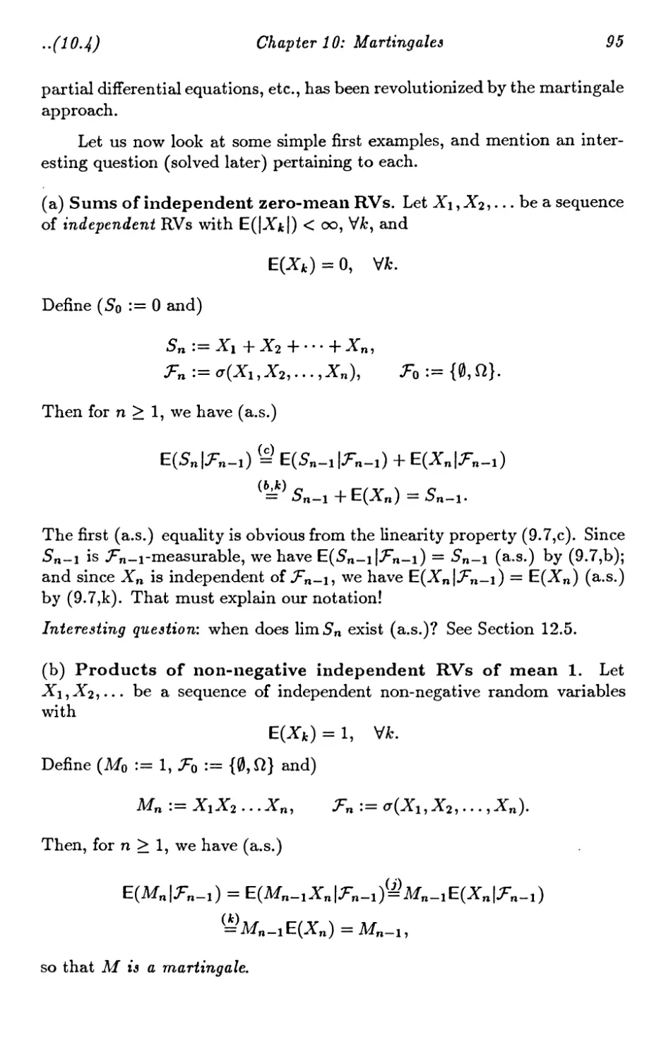
martingale, submartingale. 10.4. Some examples of martingales. 10.5. Fair
and unfair games. 10.6. Previsible process, gambling strategy. 10.7. A fun-
fundamental principle: you can't beat the system! 10.8. Stopping time. 10.9.
Stopped supermartingales are supermartingales. 10.10. Doob's Optional-
Stopping Theorem. 10.11. Awaiting the almost inevitable. 10.12. Hitting
times for simple random walk. 10.13. Non-negative superharmonic func-
functions for Markov chains.
Chapter 11: The Convergence Theorem 106
11.1. The picture that says it all. 11.2. Upcrossings. 11.3. Doob's Upcross-
ing Lemma. 11.4. Corollary. 11.5. Doob's'Forward'Convergence Theorem.
11.6. Warning. 11.7. Corollary.

viii Contents
Chapter 12: Martingales bounded in C2 110
12.0. Introduction. 12.1. Martingales in C2: orthogonality of increments.
12.2. Sums of zero-mean independent random variables in C2. 12.3. Ran-
Random signs. 12.4. A symmetrization technique: expanding the sample space.
12.5. Kolmogorov's Three-Series Theorem. 12.6. Cesaro's Lemma. 12.7.
Kronecker's Lemma. 12.8. A Strong Law under variance constraints. 12.9.
Kolmogorov's Truncation Lemma. 12.10. Kolmogorov's Strong Law of
Large Numbers (SLLN). 12.11. Doob decomposition. 12.12. The angle-
brackets process (M). 12.13. Relating convergence of M to finiteness of
(M)oq. 12.14. A trivial 'Strong Law' for martingales in £2. 12.15. Levy's
extension of the Borel-Cantelli Lemmas. 12.16. Comments.
Chapter 13: Uniform Integrability 126
13.1. An 'absolute continuity' property. 13.2. Definition. UI family. 13.3.
Two simple sufficient conditions for the UI property. 13.4. UI property
of conditional expectations. 13.5. Convergence in probability. 13.6. Ele-
Elementary proof of (BDD). 13.7. A necessary and sufficient condition for Cl
convergence.
Chapter 14: UI Martingales 133
14.0. Introduction. 14.1. UI martingales. 14.2. Levy's 'Upward' Theorem.
14.3. Martingale proof of Kolmogorov's 0-1 law. 14.4. Levy's 'Downward'
Theorem. 14.5. Martingale proof of the Strong Law. 14.6. Doob's Sub-
martingale Inequality. 14.7. Law of the Iterated Logarithm: special case.
14.8. A standard estimate on the normal distribution. 14.9. Remarks on ex-
exponential bounds; large deviation theory. 14.10. A consequence of Holder's
inequality. 14.11. Doob's Cp inequality. 14.12. Kakutani's Theorem on
'product' martingales. 14.13.The Radon-Nikodym theorem. 14.14. The
Radon-Nikodym theorem and conditional expectation. 14.15. Likelihood
ratio; equivalent measures. 14.16. Likelihood ratio and conditional expec-
expectation. 14.17. Kakutani's Theorem revisited; consistency of LR test. 14.18.
Note on Hardy spaces, etc.
Chapter 15: Applications 153
15.0. Introduction - please read! 15.1. A trivial martingale-representation
result. 15.2. Option pricing; discrete Black-Scholes formula. 15.3. The
Mabinogion sheep problem. 15.4. Proof of Lemma 15.3(c). 15.5. Proof
of result 15.3(d). 15.6. Recursive nature of conditional probabilities. 15.7.
Bayes' formula for bivariate normal distributions. 15.8. Noisy observation of
a single random variable. 15.9. The Kalman-Bucy filter. 15.10. Harnesses
entangled. 15.11. Harnesses unravelled, 1. 15.12. Harnesses unravelled, 2.

Contents ix
PART C: CHARACTERISTIC FUNCTIONS
Chapter 16: Basic Properties of CFs 172
16.1. Definition. 16.2. Elementary properties. 16.3. Some uses of char-
characteristic functions. 16.4. Three key results. 16.5. Atoms. 16.6. Levy's
Inversion Formula. 16.7. A table.
Chapter 17: Weak Convergence 179
17.1. The 'elegant' definition. 17.2. A 'practical' formulation. 17.3. Sko-
rokhod representation. 17.4. Sequential compactness for Prob(R). 17.5.
Tightness.
Chapter 18: The Central Limit Theorem 185
18.1. Levy's Convergence Theorem. 18.2. o and 0 notation. 18.3. Some
important estimates. 18.4. The Central Limit Theorem. 18.5. Example.
18.6. CF proof of Lemma 12.4.
APPENDICES
Chapter Al: Appendix to Chapter 1 192
Al.l. A non-measurable subset A of S1. A1.2. J-systems. A1.3. Dynkin's
Lemma. A1.4. Proof of Uniqueness Lemma 1.6. A1.5. A-sets: 'algebra'
case. A1.6. Outer measures. Al.7. Caratheodory's Lemma. A1.8. Proof of
Caratheodory's Theorem. Al.9. Proof of the existence of Lebesgue measure
on (@, l],#@,1]). A1.10. Example of non-uniqueness of extension. Al.ll.
Completion of a measure space. A1.12. The Baire category theorem.
Chapter A3: Appendix to Chapter 3 205
A3.1. Proof of the Monotone-Class Theorem 3.14. A3.2. Discussion of
generated a-algebras.
Chapter A4: Appendix to Chapter 4 208
A4.1. Kolmogorov's Law of the Iterated Logarithm. A4.2. Strassen's Law
of the Iterated Logarithm. A4.3. A model for a Markov chain.
Chapter A5: Appendix to Chapter 5 211
A5.1. Doubly monotone arrays. A5.2. The key use of Lemma 1.10(a).
A5.3. 'Uniqueness of integral'. A5.4. Proof of the Monotone-Convergence
Theorem.

x Contents
Chapter A9: Appendix to Chapter 9 214
A9.1. Infinite products: setting things up. A9.2. Proof of A9.1(e).
Chapter A13: Appendix to Chapter 13 217
A13.1. Modes of convergence: definitions. A13.2. Modes of convergence:
relationships.
Chapter A14: Appendix to Chapter 14 219
A14.1. The cr-algebra Tt<> T a stopping time. A14.2. A special case of OST.
A14.3. Doob's Optional-Sampling Theorem for UI martingales. A14.4. The
result for UI submartingales.
Chapter A16: Appendix to Chapter 16 222
A 16.1. Differentiation under the integral sign.
Chapter E: Exercises 224
References 243
Index 246

Preface - please read!
The most important chapter in this book is Chapter E: Exercises. I have
left the interesting things for you to do. You can start now on the 'EG'
exercises, but see 'More about exercises' later in this Preface.
The book, which is essentially the set of lecture notes for a third-year
undergraduate course at Cambridge, is as lively an introduction as I can
manage to the rigorous theory of probability. Since much of the book is
devoted to martingales, it is bound to become very lively: look at those
Exercises on Chapter 10! But, of course, there is that initial plod through
the measure-theoretic foundations. It must be said however that measure
theory, that most arid of subjects when done for its own sake, becomes
amazingly more alive when used in probability, not only because it is then
applied, but also because it is immensely enriched.
You cannot avoid measure theory: an event in probability is a measur-
measurable set, a random variable is a measurable function on the sample space,
the expectation of a random variable is its integral with respect to the prob-
probability measure; and so on. To be sure, one can take some central results
from measure theory as axiomatic in the main text, giving careful proofs in
appendices; and indeed that is exactly what I have done.
Measure theory for its own sake is based on the fundamental addition
rule for measures. Probability theory supplements that with the multipli-
multiplication rule which describes independence; and things are already looking
up. But what really enriches and enlivens things is that we deal with lots
of cr-algebras, not just the one cr-algebra which is the concern of measure
theory.
In planning this book, I decided for every topic what things I considered
just a bit too advanced, and, often with sadness, I have ruthlessly omitted
them.
For a more thorough training in many of the topics covered here, see
Billingsley A979), Chow and Teicher A978), Chung A968), Kingman and

xii Preface
Taylor A966), Laha and Rohatgi A979), and Neveu A965). As regards
measure theory, I learnt it from Dunford and Schwartz A958) and Halmos
A959). After reading this book, you must read the still-magnificent Breiman
A968), and, for an excellent indication of what can be done with discrete
martingales, Hall and Heyde A980).
Of course, intuition is much more important than knowledge of measure
theory, and you should take every opportunity to sharpen your intuition.
There is no better whetstone for this than Aldous A989), though it is a very
demanding book. For appreciating the scope of probability and for learning
how to think about it, Karlin and Taylor A981), Grimmett and Stirzaker
A982), Hall A988), and Grimmett's recent superb book, Grimmett A989),
on percolation are strongly recommended.
More about exercises. In compiling Chapter E, which consists exactly of
the homework sheet I give to the Cambridge students, I have taken into
account the fact that this book, like any other mathematics book, implicitly
contains a vast number of other exercises, many of which are easier than
those in Chapter E. I refer of course to the exercises you create by reading
the statement of a result, and then trying to prove it for yourself, before
you read the given proof. One other point about exercises: you will, for
example, surely forgive my using expectation E in Exercises on Chapter 4
before E is treated with full rigour in Chapter 6.
Acknowledgements. My first thanks must go to the students who have
endured the course on which the book is based and whose quality has made
me try hard to make it worthy of them; and to those, especially David
Kendall, who had developed the course before it became my privilege to
teach it. My thanks to David Tranah and other staff of CUP for their help in
converting the course into this book. Next, I must thank Ben Garling, James
Norris and Chris Rogers without whom the book would have contained more
errors and obscurities. (The many faults which surely remain in it are my
responsibility.) Helen Rutherford and I typed part of the book, but the vast
majority of it was typed by Sarah Shea-Simonds in a virtuoso performance
worthy of Horowitz. My thanks to Helen and, most especially, to Sarah.
Special thanks to my wife, Sheila, too, for all her help.
But my best thanks - and yours if you derive any benefit from the book
- must go to three people whose names appear in capitals in the Index: J.L.
Doob, A.N. Kolmogorov and P. Levy: without them, there wouldn't have
been much to write about, as Doob A953) splendidly confirms.
Statistical Laboratory, David Williams
Cambridge October 1990

A Question of Terminology
Random variables: functions or equivalence classes?
At the level of this book, the theory would be more 'elegant' if we regarded
a random variable as an equivalence class of measurable functions on the
sample space, two functions belonging to the same equivalence class if and
only if they are equal almost everywhere. Then the conditional-expectation
map
A' i-» E(X\g)
would be a truly well-defined contraction map from Lp(Cl, J7, P) to LP(Q, Q, P
for p > 1; and we would not have to keep mentioning versions (representa-
(representatives of equivalence classes) and would be able to avoid the endless 'almost
surely' qualifications.
I have however chosen the 'inelegant' route: firstly, I prefer to work
with functions, and confess to preferring
4 + 5 = 2 mod 7 to [4]7 + [5]7 = [2]7.
But there is a substantive reason. I hope that this book will tempt you to
progress to the much more interesting, and more important, theory where
the parameter set of our process is uncountable (e.g. it may be the time-
parameter set [0, oo)). There, the equivalence-class formulation just will
not work: the 'cleverness' of introducing quotient spaces loses the subtlety
which is essential even for formulating the fundamental results on existence
of continuous modifications, etc., unless one performs contortions which are
hardly elegant. Even if these contortions allow one to formulate results, one
would still have to use genuine functions to prove them; so where does the
reality lie?!
Xlll

A Guide to Notation
► signifies something important, ►► something very important, and
the Martingale Convergence Theorem.
I use ':=' to signify 'is defined to equal'. This Pascal notation is particularly
convenient because it can also be used in the reversed sense.
I use analysts' (as opposed to category theorists') conventions:
► N:= {1,2,3,...} C {0,1,2,...} =: Z+.
Everyone is agreed that R+ := [0, oo).
For a set B contained in some universal set S, Ib denotes the indicator
function of B: that is Ib : S —* {0,1} and
0 otherwise.
For a, b £ R,
a A b := min(a, 6), a V b := max(a, b).
CFxharacteristic function; DF: distribution function; pdf: probability den-
density function.
<7-algebra, a(C) A.1); a{Y1 : 7 G C) C.8, 3.13). 7r-system A.6); c?-system
(A1.2).
a.e.: almost everywhere A.5)
a.s.: almost surely B.4)
the space of bounded S-measurable functions C.1)
xiv

A Guide to Notation
B(S):
C»X:
dX/dfx:
dQ/dP:
E(X):
E(X; F):
E(X\g):
(En,ev):
(En,i.o.):
fx:
fx,Y:
fx\Y'-
Fx:
lim inf:
lim sup:
vis ——" I XJL xX Jl *a> j-j
log:
£x, Ax:
Cp, L*>:
Leb:
mS:
MT:
(M):
tif)'-
V^x:
<?:
$:
XT:
the Borel <r-algebra on S, 3 := 5(R) A.2)
discrete stochastic integral A0.6)
Radon-Nikodym derivative E.14)
Likelihood Ratio A4.13)
expectation E(X) := JQ X{uj)P(duj) of X F.3)
/FXcfPF.3)
conditional expectation (9.3)
liminf£?n B.8)
lim sup £n B.6)
probability density function (pdf) of X F.12).
joint pdf (8.3)
conditional pdf (9.6)
distribution function of X C.9)
for sets, B.8)
for sets, B.6)
xn f x in that xn < xn+\ (Vn) and xn —*• x.
natural (base e) logarithm
law of X C.9)
Lebesgue spaces F.7, 6.13)
Lebesgue measure A.8)
space of S-measurable functions C.1)
process M stopped at time T A0.9)
angle-brackets process A2.12)
integral of / with respect to /i E.0, 5.2)
fA fdfi E.0, 5.2)
CF of X (Chapter 16)
pdf of standard normal N@,l) distribution
DF of N@,l) distribution
X stopped at time T A0.9)

Chapter 0
A Branching-Process Example
(This Chapter is not essential for the remainder of the book. You can start
with Chapter 1 if you wish.)
0.0. Introductory remarks
The purpose of this chapter is threefold: to take something which is probably
well known to you from books such as the immortal Feller A957) or Ross
A976), so that you start on familiar ground; to make you start to think
about some of the problems involved in making the elementary treatment
into rigorous mathematics; and to indicate what new results appear if one
applies the somewhat more advanced theory developed in this book. We
stick to one example: a branching process. This is rich enough to show that
the theory has some substance.
0.1. Typical number of children, X
In our model, the number of children of a typical animal (see Notes below
for some interpretations of'child' and 'animal') is a random variable X with
values in Z+. We assume that
P(X = 0) > 0.
We define the generating function f o/Ias the map / : [0,1] —* [0,1],
where
f@) := E@x) =
Standard theorems on power series imply that, for 0 6 [0,1],
f'($) = E(X0x~1) =
and
fi := E(X) = /'(I) = ]T kP(X = k)<oo

2 Chapter 0: A Branching-Process Example
Of course, /'(I) is here interpreted as
lim MW = lim
9\\ 0-1 911
since /(I) = 1. We assume that
\x < oo.
Notes. The first application of branching-process theory was to the question
of survival of family names; and in that context, animal = man, and child
= son.
In another context, 'animal' can be 'neutron', and 'child' of that neu-
neutron will signify a neutron released if and when the parent neutron crashes
into a nucleus. Whether or not the associated branching process is super-
supercritical can be a matter of real importance.
We can often find branching processes embedded in richer structures
and can then use the results of this chapter to start the study of more
interesting things.
For superb accounts of branching processes, see Athreya and Ney A972),
Harris A963), Kendall A966, 1975).
0.2. Size of nth generation, Zn
To be a bit formal: suppose that we are given a doubly infinite sequence
(a) [xJm):m,reNJ
of independent identically distributed random variables (IID RVs), each
with the same distribution as X:
P(X(rm) =k) = P(X = k).
The idea is that for n £ Z+ and r £ N, the variable Xr represents the
number of children (who will be in the (n-f l)th generation) of the rth animal
(if there is one) in the nth generation. The fundamental rule therefore is
that if Zm signifies the size of the nth generation, then
(b) Zn+1 = Jf <"+« + • • • + X£+1).
We assume that Zo — 1, so that (b) gives a full recursive definition of
the sequence (Zm : m £ Z+) from the sequence (a). Our first task is

..@.8) Chapter 0: A Branching-Process Example 3
to calculate the distribution function of Zn, or equivalently to find the
generating function
(c) /„(*) := EFZ») = £ 6kP{Zn = k).
0.3. Use of conditional expectations
The first main result is that for n £ Z+ (and 9 £ [0,1])
(a) /„+!(<?) =/„(/(*)),
so that for each n £ Z+, /n is the n-fold composition
(b) fn=fofo...of.
Note that the 0-fold composition is by convention the identity map fo@) —
0, in agreement with - indeed, forced by - the fact that Zq — 1.
To prove (a), we use - at the moment in intuitive fashion - the fol-
following very special case of the very useful Tower Property of Conditional
Expectation:
(c) E(U) = BE(U\V);
to find the expectation of a random variable U, first find the conditional
expectation E(£/|F) of U given V, and then find the expectation of that.
We prove the ultimate form of (c) at a later stage.
We apply (c) with U = 0Zn^ and V = Zn:
Now, for fcG Z+, the conditional expectation of 0Zn+1 given that Zn = k
satisfies
(d) E(**«+* \Zn = Jfe)
But Zn is constructed from variables Xs with r < n, and so Zn is inde-
independent of X[n ,... ,X^n . The conditional expectation given Zn — k
in the right-hand term in (d) must therefore agree with the absolute expec-
expectation
(e)

Chapter 0: A Branching-Process Example @.3)..
But the expression at (e) is a expectation of the product of independent
random variables and as part of the family of'Independence means multiply*
results, we know that this expectation of a product may be rewritten as the
product of expectations. Since (for every n and r)
we have proved that
and this is what it means to say that
[If V takes only integer values, then when V — k, the conditional expectation
E(£/|F) of U given V is equal to the conditional expectation E({7|F = k) of
U given that V = k. (Sounds reasonable!)] Property (c) now yields
and, since
E(a*») = /„(<*), D
result (a) is proved.
Independence and conditional expectations are two of the main topics
in this course.
0.4. Extinction probability, -k
Let 7rn := P(Zn = 0). Then tt* = /n@), so that, by @.3,b),
(a) 7Tn+i =/GTn).
Measure theory confirms our intuition about the extinction probability:
(b) 7T := P(Zm = 0 for some m) =| Iim7rn.
Because / is continuous, it follows from (a) that
(C) 7T = /(,).
The function / is analytic on @,1), and is non-decreasing and convex (of
non-decreasing slope). Also, /(I) = 1 and /@) = P(X = 0) > 0. The slope
/'(I) of / at 1 is // = E(X). The celebrated pictures opposite now make
the following Theorem obvious.
THEOREM
E(X) > 1, then the extinction probability tt is the unique root of the
equation it = /(tt) which lies strictly between 0 and 1. If E(X) < 1,
then 7T = 1.

..@.4)
Chapter 0: A Branching-Process Example
V = /(*)
y — x
Case 1: subcritical, /i = /'(I) < 1. Clearly, ir = 1.
The critical case /i = 1 has a similar picture.
Case 2: supercritical, n — /'(I) > 1. Now, w < 1.

6 Chapter 0: A Branching-Process Example @.5)..
0.5. Pause for thought: measure
Now that we have finished revising what introductory courses on probability
theory say about branching-process theory, let us think about why we must
find a more precise language. To be sure, the claim at @.4,b) that
(a) 7r=flim7Tn
is intuitively plausible, but how could one prove it? We certainly can-
cannot prove it at present because we have no means of stating with pure-
mathematical precision what it is supposed to mean. Let us discuss this
further.
Back in Section 0.2, we said 'Suppose that we are given a doubly infinite
sequence {Xr : m,r £ N} of independent identically distributed random
variables each with the same distribution as X\ What does this mean? A
random variable is a (certain kind of) function on a sample space Q.. We
could follow elementary theory in taking Q to be the set of all outcomes, in
other words, taking Q to be the Cartesian product
r,8
the typical element uj of Q being
u> = (u>£r) : r £ N, s £ N),
and then setting Xb(uj) = a>« . Now Q is an uncountable set, so that
we are outside the 'combinatorial' context which makes sense of ?rn in the
elementary theory. Moreover, if one assumes the Axiom of Choice, one
can prove that it is impossible to assign to all subsets of ft a probability
satisfying the 'intuitively obvious' axioms and making the X's IID RVs
with the correct common distribution. So, we have to know that the set
of u corresponding to the event 'extinction occurs' is one to which one can
uniquely assign a probability (which will then provide a definition of tt).
Even then, we have to prove (a).
Example. Consider for a moment what is in some ways a bad attempt to
construct a 'probability theory'. Let C be the class of subsets C of N for
which the 'density'
p(C) := lim t{k : 1 < k < n; k £ C}
n\oo
exists. Let Cn := {1,2,..., n}. Then Cn £ C and Cn | N in the sense that
Cn C Cn+i,Vn and also \JCn = N. However, p(Cn) = 0,Vn, but /?(N) = 1.

..@.6) Chapter 0: A Branching-Process Example 7
Hence the logic which will allow us correctly to deduce (a) from the
fact that
{Zn = 0} | {extinction occurs}
fails for the (N,C,p) set-up: (N,C,p) is not ca probability triple'. □
There are problems. Measure theory resolves them, but provides a huge
bonus in the form of much deeper results such as the Martingale Conver-
Convergence Theorem which we now take a first look at - at an intuitive level, I
hasten to add.
0.6. Our first martingale
Recall from @.2,b) that
H h AZn ,
where the J\T(n+1) variables are independent of the values Z\, Z2,..., Zn. It
is clear from this that
= j\Zn = Zn),
a result which you will probably recognize as stating that the process Z
(Zn : n >Q) is a Markov chain. We therefore have
E(Zn+i\Z0 = zo,Zi = i'i,...,Zn =in) = ^jP(Zn+i =j\Zn = in
j
or, in a condensed and better notation,
(a) E(Zn+i |Z0, Zi,..., Zn) — E(Zn+i \Zn).
Of course, it is intuitively obvious that
(b) E(Zn+1\Zn) =
because each of the Zn animals in the nth generation has on average
children. We can confirm result (b) by differentiating the result
with respect to 0 and setting 0 = 1.

8 Chapter 0: A Branching-Process Example @.6)..
Now define
(c) Mn := Zn/fin, n > 0.
Then
which exactly says that
(d) M is a martingale relative to the Z process.
Given the history of Z up to stage n, the next value Mn+i of M is on average
what it is now: M is 'constant on average' in this very sophisticated sense
of conditional expectation given 'past' and 'present'. The true statement
(e) E(Mn) = l, Vn
is of course infinitely cruder.
A statement S is said to be true almost surely (a.s.) or with prob-
probability 1 if (surprise, surprise!)
P(S is true) =1.
Because our martingale M is non-negative (Mn > 0, Vn), the Martin-
Martingale Convergence Theorem implies that it is almost surely true that
(f) Jlfoo := UmMn exists.
Note that if M^ > 0 for some outcome (which can happen with positive
probability only when \i > 1), then the statement
is a precise formulation of 'exponential growth'. A particularly fascinating
question is: suppose that ji > 1; what is the behaviour of Z conditional on
the value o
0.7. Convergence (or not) of expectations
We know that M^ :— lim Mn exists with probability 1, and that E(Mn) = 1,
Vn. We might be tempted to believe that E(Moo) = 1. However, we already
know that if // < 1, then, almost surely, the process dies out and Mn is
eventually 0. Hence
(a) if fi < 1, then Moo - 0 (a.s.) and

..@.8) Chapter 0: A Branching-Process Example 9
This is an excellent example to keep in mind when we come to study
Fatou's Lemma, valid for any sequence (Yn) of non-negative random vari-
variables:
E(liminf Yn) < liminf E(Fn).
What is 'going wrong' at (a) is that (when \i < 1) for large n, the chances
are that Mn will be large if Mn is not 0 and, very roughly speaking, this
large value times its small probability will keep E(Mn) at 1. See the concrete
examples in Section 0.9.
Of course, it is very important to know when
(b)
and we do spend quite a considerable time studying this. The best gen-
general theorems are rarely good enough to get the best results for concrete
problems, as is evidenced by the fact that
(c) E(Moo) = 1 if and only if both, /i > 1 and E(X logX) < oo,
where X is the typical number of children. Of course 0 log 0 = 0. If \i > 1
and E(-YlogX) = oo, then, even though the process may not die out,
o = 0, a.s.
[oo
0.8. Finding the distribution of Mc
Since Mn —* Moo (a.s.), it is obvious that for A > 0,
exp(—XMn) —► exp(—AMoo) (a.s.)
Now since each Mn > 0, the whole sequence (exp( — XMn)) is bounded
in absolute value by the constant 1, independently of the outcome of our
experiment. The Bounded Convergence Theorem says that we can now
assert what we would wish:
(a) Eexp(—AMqo) = limEexp(—AMn).
Since Mn = Zn/fin and EFZ») = /n@), we have
(b) Eexp(-AMn) = /n(exp(-A//in)),
so that, in principle (if very rarely in practice), we can calculate the left-hand
side of (a). However, for a non-negative random variable Y, the distribution
function y i-> P(Y < y) is completely determined by the map
A h-* Eexp(—AF) on @, oo).

10 Chapter 0: A Branching-Process Example @.8)..
Hence, in principle, we can find the distribution of
We have seen that the real problem is to calculate the function
L(X) :~ Eexp(—AMqo).
Using (b), the fact that fn+i — f ° /n, and the continuity of L (another
consequence of the Bounded Convergence Theorem), you can immediately
establish the functional equation:
(c) L(\») = f{L(X)).
0.9. Concrete example
This concrete example is just about the only one in which one can calculate
everything explicitly, but, in the way of mathematics, it is useful in many
contexts.
We take the 'typical number of children' X to have a geometric distri-
distribution:
(a) P(X = k)=pqk (&G
where
0 < p < 1, q := 1 — p.
Then, as you can easily check,
*
and
To calculate / o / o ... o /, we use a device familiar from the geometry
of the upper half-plane. If
G
_ f 9\\ 9\2 \
\92\ 922/
is a non-singular 2x2 matrix, define the fractional linear transformation:
(c) G{0) =
+#22

..@.9) Chapter 0: A Branching-Process Example 11
Then you can check that if H is another such matrix, then
G(HF)) = (GH)(e),
so that composition of fractional linear transformations corresponds to ma-
matrix multiplication.
Suppose that p =fi q. Then, by the S *AS = A method, for example,
we find that the nth power of the matrix corresponding to / is
0 ]
-q \) -" " VI qJ\0
so that
q/in(l - 0) + qO - p'
If n = q/p < 1, then limn/n@) = 1, corresponding to the fact that the
process dies out.
Suppose now that /i > 1. Then you can easily check that, for A > 0,
L(X) : = Eexp(—AMoo) = lim/n(exp(—X/fin))
p
q-p
/•OO
from which we deduce that
P(Moo = 0) = 7T,
and
P(x < M^ < x + <&) = A - Trfe-^-^^a: (x > 0),
or, better,
> a?) = A - w)e-(l-*)x (x > 0).
Suppose that // < 1. In this case, it is interesting to ask: what is the
distribution of Zn conditioned by Zn =fi 0? We find that
Z"
where

12 Chapter 0: A Branching-Process Example @.9)..
so 0 < an < 1 and an -f /?„ = 1. As n -» oo, we see that
an -» 1 - //, /?„ -» //,
so (this is justified)
(e) lim P(Zn = k\Zn ^ 0) = A - /z)/ (A: G N).
Suppose that // = 1. You can show by induction that
and that
E{e-xz»'n\Zn ^ 0) - 1/A+A),
corresponding to
(f) P(Zn/n > x\Zn ^ 0) -> c"x, a: > 0.
'The Fatou factor'
We know that when fi < 1, we have E(Mn) = 1, Vn, but E(Moo) = 0. Can
we get some insight into this?
First consider the case when fi < 1. Result (e) makes it plausible that
for large n,
E(Zn\Zn ^ 0) is roughly A — /*)X)&/* = V(* ~
We know that
P(Zn ^ 0) = 1 - /n@) is roughly A -
so we should have (roughly)
n ^ 0)
which might help explain how the 'balance' E(Mn) = 1 is achieved by big
values times small probabilities.

..@.9) Chapter 0: A Branching-Process Example IS
Now consider the case when // = 1. Then
P(Zn + 0) = l/(n + 1),
and, from (f), Zn/n conditioned by Zn =^ 0 is roughly exponential with
mean 1, so that Mn = Zn conditioned by Zn =^ 0 is on average of size about
n, the correct order of magnitude for balance.
Warning. We have just been using for 'correct intuitive explanations'
exactly the type of argument which might have misled us into thinking that
= 1 in the first place. But, of course, the result
E(Mn) = E(Mn\Zn jt 0)P(Zn jt 0) = 1
is a matter of obvious fact.

PART A: FOUNDATIONS
Chapter 1
Measure Spaces
1.0. Introductory remarks
Topology is about open sets. The characterizing property of a continuous
function / is that the inverse image f~l(G) of an open set G is open.
Measure theory is about measurable sets. The characterizing property
of a measurable function / is that the inverse image f~1(A) of any measur-
measurable set is measurable.
In topology, one axiomatizes the notion of 'open set', insisting in par-
particular that the union of any collection of open sets is open, and that the
intersection of a finite collection of open sets is open.
In measure theory, one axiomatizes the notion of 'measurable set', in-
insisting that the union of a countable collection of measurable sets is measur-
measurable, and that the intersection of a countable collection of measurable sets
is also measurable. Also, the complement of a measurable set must be mea-
measurable, and the whole space must be measurable. Thus the measurable sets
form a <r-algebra, a structure stable (or 'closed') under countably many set
operations. Without the insistence that 'only countably many operations
are allowed', measure theory would be self-contradictory - a point lost on
certain philosophers of probability.
The probability that a point chosen at random on the surface of the unit
sphere S2 in R3 falls into the subset jP of S2 is just the area of jP divided
by the total area 4?r. What could be easier?
However, Banach and Tarski showed (see Wagon A985)) that if the
Axiom of Choice is assumed, as it is throughout conventional mathematics,
then there exists a subset F of the unit sphere S2 in R3 such that for
u

..A.1) Chapter 1: Measure Spaces 15
3 < k < oo (and even for k — oo), S2 is the disjoint union of k exact copies
of F:
where each r,- is a rotation. If F has an 'area', then that area must
simultaneously be 4?r/3,4?r/4,..., 0. The only conclusion is that the set F
is non-measurable (not Lebesgue measurable): it is so complicated that one
cannot assign an area to it. Banach and Tarski have not broken the Law of
Conservation of Area: they have simply operated outside its jurisdiction.
Remarks, (i) Because every rotation r has a fixed point x on S2 such that
t(x) = x, it is not possible to find a subset A of S2 and a rotation r such
that A U r(A) = S2 and A D r(A) = 0. So, we could not have taken k — 2.
(ii) Banach and Tarski even proved that given any two bounded sub-
subsets A and B of R3 each with non-empty interior, it is possible to decompose
A into a certain finite number n of disjoint pieces A = (JJLj A{ and B into
the same number n of disjoint pieces B — (J"=1 #,-, in such a way that, for
each i, A^ is Euclid-congruent to I?,!!! So, we can disassemble A and rebuild
it as B.
(iii) Section Al.l (optional!) in the appendix to this chapter gives
an Axiom-of-Choice construction of a non-measurable subset of S1.
This chapter introduces
0-algebraSj ir-systems, and measures
and emphasizes monotone-convergence properties of measures. We shall see
in later chapters that, although not all sets are measurable, it is always the
case for probability theory that enough sets are measurable.
1.1. Definitions of algebra, <r-algebra
Let S be a set.
Algebra on S
A collection So of subsets of S is called an algebra on S (or algebra of
subsets of S) if
0) S 6 So,
(ii) F 6 So => Fc := S\F 6 So,
(iii) -F,Ge So => FUG G So.
[Note that 0 = Sc € So and

Chapter 1: Measure Spaces A-1)~
Thus, an algebra on S is a family of subsets of S stable under finitely many
set operations.
Exercise (optional). Let C be the class of subsets C of N for which the
'density'
lim m~1}ji{k : 1 < k < m\ k £ C}
mfoo
exists. We might like to think of this density (if it exists) as 'the probability
that a number chosen at random belongs to C\ But there are many reasons
why this does not conform to a proper probability theory. (We saw one in
Section 0.5.) For example, you should find elements F and G in C for which
FOGgC.
Note on terminology ('algebra versus field'). An algebra in our sense is a
true algebra in the algebraists' sense with D as product, and symmetric
difference
AAB:=(Al)B)\(AnB)
as 'sum', the underlying field of the algebra being the field with 2 elements.
(This is why we prefer 'algebra of subsets' to 'field of subsets': there is no
way that an algebra of subsets is a field in the algebraists' sense - unless So
is trivial, that is, So = {5,0}.)
<r-algebra on S
A collection S of subsets of S is called a cr-algebra on S (or <r-algebra of
subsets of S) if S is an algebra on S such that whenever Fn 6 S (n £ N),
then
n
[Note that if S is a <r-algebra on S and Fn £ S for n £ N, then
n n
Thus, a cr-algebra on S is a family of subsets of S 'stable under any countable
collection of set operations'.
Note. Whereas it is usually possible to write in 'closed form' the typical
element of many of the algebras of sets which we shall meet (see Section
1.8 below for a first example), it is usually impossible to write down the
typical element of a <j-algebra. This is the reason for our concentrating
where possible on the much simpler '7r-systems'.
Measurable space
A pair E, S), where S is a set and S is a ^-algebra on 5, is called a
measurable space. An element of S is called a S-measurable subset of S.

..A.2) Chapter 1: Measure Spaces 11
, <7-algebra generated by a class C of subsets
Let C be a class of subsets of S. Then cr(C), the a-algebra generated by C,
is the smallest <j-algebra S on S such that CCS. It is the intersection of
all <7-algebras on S which have C as a subclass. (Obviously, the class of all
subsets of S is a cr-algebra which extends C.)
1.2. Examples. Borel cr-algebras, B(S), B = B(R)
Let 5 be a topological space.
B(S)
B(S)j the Borel cr-algebra on 5, is the cr-algebra generated by the family of
open subsets of S. With slight abuse of notation,
B(S) := cr(open sets).
B := B(R)
It is standard shorthand that B := #(R).
The a-algebra B is the most important of all cr-algebras. Every subset
of R which you meet in everyday use is an element of B\ and indeed it is
difficult (but possible!) to find a subset of R constructed explicitly (without
the Axiom of Choice) which is not in B.
Elements of B can be quite complicated. However, the collection
tt(R) := {(-oo,z] :x eR]
(not a standard notation) is very easy to understand, and it is often the
case that all we need to know about B is that
(a) B = <t(tt(R)).
Proof of (a). For each x in R, (—oo,a:] = flneis^"0^ "+" n~1)i so ^a^ as a
countable intersection of open sets, the set (—oo,ar] is in B.
All that remains to be proved is that every open subset G of R is in
<7(tt(R)). But every such G is a countable union of open intervals, so we
need only show that, for a, b £ R with a < 6,
(a, b) e <t(tt(R)).
But, for any u with u > a,
(a, u] = (-oo, u] D (—oo, a]c £ <j(tt(R)),
and since, for e = %(b — a),
(a, 6) = [j(a,b - en'1],
n
we see that (a, b) £ cr(?r(R)), and the proof is complete.

18 Chapter 1: Measure Spaces A.8)..
1.3. Definitions concerning set functions
Let 5* be a set, let So be an algebra on S, and let fiQ be a non-negative set
function
: So —► [0,oo].
Additive
Then fio is called additive if //o@) = 0 and, for F, G £ So,
Countably additive
The map hq is called countably additive (or cr-additive) if //@) = 0 and
whenever (Fn : n £ N) is a sequence of disjoint sets in So with union
F = IJ-Fn in So (note that this is an assumption since So need not be a
a-algebra), then
n
Of course (why?), a countably additive set function is additive.
1.4. Definition of measure space
Let (S, S) be a measurable space, so that S is a <j-algebra on S.
A map
\x : S —> [0, oo].
is called a measure on E, S) if ft is countably additive. The triple E, S,
is then called a measure space.
1.5. Definitions concerning measures
Let (S, S,//) be a measure space. Then /j, (or indeed the measure space
(S, S,//)) is called
finite
if fi(S) < co,
cr- finite
if there is a sequence En : n £ N) of elements of S such that
n(Sn) < oo (Vn £ N) and [J 5n = S.
Warning. Intuition is usually OK for finite measures, and adapts well for
<7-finite measures. However, measures which are not <7-finite can be crazy;
fortunately, there are no such measures in this book.

..A.6) Chapter 1: Measure Spaces 19
Probability measure, probability triple
Our measure \x is called a probability measure if
fi(S) = 1,
and E, S,//) is then called a probability triple.
//-null element of S, almost everywhere (a.e.)
An element F of £ is called fi-nullii p(F) = 0. A statement 5 about points
s of S is said to hold almost everywhere (a.e.) if
F := {s : S(s) is false} G S and fi(F) = 0.
1.6. LEMMA. Uniqueness of extension, 7r-systems
Moral: cr-algebras are 'difficult', but 7r-systems are 'easy'; so we
aim to work with the latter.
►(a) Let S be a set. Let X be a Tr-system on S, that is, a family of subsets
of S stable under finite intersection;
Let £ := cr(X). Suppose that fi\ and fi2 are measures on E, S) such
that fii(S) = fi2(S) < oo and /xi = //2 on X. Then
\i\ = fi2 on S.
►(b) Corollary. If two probability measures agree on a Tr-system,
then they agree on the <j-algebra generated by that Tr-system.
The example B = (t(tt(R)) is of course the most important example of
the S = cr(J) in the theorem.
This result will play an important role. Indeed, it will be applied more
frequently than will the celebrated existence result in Section 1.7. Because
of this, the proof of Lemma 1.6 given in Sections Al.2-1.4 of the appendix
to this chapter should perhaps be consulted - but read the remainder of
this chapter first.

20 Chapter 1: Measure Spaces
1.7. THEOREM. Caratheodory's Extension Theorem
Let S be a set, let So be an algebra on S, and let
S:=<j(S0).
If Ho is a countably additive map no : So —* [0,oo], then there exists a
( measure /i on E, S) such that
:= fio on
If fio(S) < oo, then, by Lemma 1.6, this extension is unique - an
algebra is a rc-system!
In a sense, this result should have more ► signs than any other, for
without it we could not construct any interesting models. However, once
we have our model, we make no further use of the theorem.
The proof of this result given in Sections Al.5-1.8 of the appendix is
there for completeness. It will do no harm to assume the result for this
course. Let us now see how the theorem is used.
1.8. Lebesgue measure Leb on (@, l],#@,1])
Let S = @,1]. For F C S, say that F £ So if F may be written as a finite
union
(*) F = (a1,61]U...U(ar,6r]
where r £ N, 0 < a\ < b\ < • • • < ar < br < 1. Then So is an algebra on
@,1] and
(We write 5@,1] instead of #(@,1]).) For F as at (*), let
k<r
Then fiQ is well-defined and additive on So (this is easy). Moreover, fiQ is
countably additive on So. (This is not trivial. See Section A1.9.) Hence,
by Theorem 1.7, there exists a unique measure fi on (@,1], 5@,1]) extend-
extending fio on So. This measure \i is called Lebesgue measure on (@, l],/?@,1])
or (loosely) Lebesgue measure on @,1]. We shall often denote fi by Leb.
Lebesgue measure (still denoted by Leb) on ([0, l],#[0,1]) is of course ob-
obtained by a trivial modification, the set {0} having Lebesgue measure 0. Of
course, Leb makes precise the concept of length.
In a similar way, we can construct (cr-finite) Lebesgue measure (which
we also denote by Leb) on R (more strictly, on (R, B(R)).

..A.10) Chapter 1: Measure Spaces 21
1.9. LEMMA. Elementary inequalities
Let (,!>,£,//) be a measure space. Then
(a) n(A U B) < n(A) + fi(B)
Furthermore, if fi(S) < oo, //ten
(c) /z(AUJ3)==/z(A) + /z(J3)-/z(An£) (A,JB 6 E),
(d) (inclusion-exclusion formula): for Fi, F2,..., Fn G E,
E £<</(*n
successive partial sums alternating between over- and under-estimates.
You will surely have seen some version of these results previously. Re-
Result (c) is obvious because A U B is the disjoint union A U (B\( A D B)). But
(c)=^(a)=^(b) - check that 'infinities do not matter'. You can deduce (d)
from (c) by induction, but, as we shall see later, the neat way to prove (d)
is by integration.
1.10. LEMMA. Monotone-convergence properties of measures
• These results are often needed for making things rigorous. (Peep ahead
to the 'Monkey typing Shakespeare' Section 4.9.) Again, let E, S, fi) be a
measure space.
►(a) If Fn £ E (n 6 N) and Fn | -F, then fi(Fn) | fi(F).
Notes. Fn T F means: Fn C Fn+1 (Vn £ N), \JFn = F. Result (a) is
2/ie fundamental property of measure.
Proof of (a). Write d := Fls Gn := Fn\Fn_i (n > 2). Then the sets
n (n G N) are disjoint, and
U G2 U ... U G») = Y, /*(G*) t
/:<oo
Application. In a proper formulation of the branching-process example of
Chapter 0,
{Zn — 0} I {extinction occurs}, so that ?rn f tt.
(A proper formulation of the branching-process example will be given later.)

22 Chapter 1: Measure Spaces A.10)..
►(b) If Gn £ E, Gn i G and n(Gk) < oo for some &, then fi(Gn) I
Proof of (b). For n £ N, let Fn := G|fc\Gjt+n, and now apply part (a). □
Example - to indicate what can 'go wrong'. For n £ N, let
n •= (n,oo).
Then Leb(tfn) = oo,Vn, but tfn | 0.
►(c) 77ie union of a countable number of ft-null sets is fi-null.
This is a trivial corollary of results A.9,b) and A.10,a).
1.11. Example/Warning
Let E, E,//) be ([0,1], B[Q, l],Leb). Let e(k) be a sequence of strictly posi-
positive numbers such that e(k) j 0. For a single point x of 5, we have
(a) {x} C(x - e(k), x + e(k)) f! 5,
so that for every k, //({#}) < 2e(k), and so //({#}) = 0. That {x} is ^E)-
measurable follows because {x} is the intersection of the countable number
of open subsets of S on the right-hand side of (a).
Let V = Q fl [0,1], the set of rationals in [0,1]. Since V is a count-
countable union of singletons: V = {vn : n £ N}, it is clear that V is #[0,1]-
measurable and that Leb(V) = 0. We can include V in an open subset of
S of measure at most 4e(k) as follows:
VCGk= |J [(vn - e(kJ-n, vn + e(*J-») n S] =: |J /„,*.
n
Clearly, H :— f)k Gk satisfies Leh(H) = 0 and V Q H. Now, it is a
consequence of the Baire category theorem (see the appendix to this chapter)
that H is uncountable, so
(b) the set H is an uncountable set of measure 0; moreover,
n n
Throughout the subject, we have to be careful about interchanging orders
of operations.

Chapter 2
Events
2.1. Model for experiment: (£l,f, P)
A model for an experiment involving randomness takes the form of a prob-
probability triple @,^*, P) in the sense of Section 1.5.
Sample space
H is a set called the sample space.
Sample point
A point lj of Q is called a sample point.
Event
The cr-algebra J~ on 0 is called the family of events, so that an event is an
element of J-', that is, an ^"-measurable subset of 0.
By definition of probability triple, P is a probability measure on (Q^J7).
2.2. The intuitive meaning
Tyche, Goddess of Chance, chooses a point cj of Q, 'at random' according to
the law P in that, for F in f, P(F) represents the 'probability' (in the sense
understood by our intuition) that the point u chosen by Tyche belongs to
F.
The chosen point uj determines the outcome of the experiment. Thus
there is a map
0 —> set of outcomes,
u; *-¥ outcome.
There is no reason why this 'map' (the co-domain lies in our intuition!)
should be one-one. Often it is the case that although there is some obvious
'minimal' or 'canonical' model for an experiment, it is better to use some
richer model. (For example, we can read off many properties of coin tossing
by imbedding the associated random walk in a Brownian motion.)
28

24 Chapter 2: Events B.8)..
2.3. Examples of (fi,^*) pairs
We leave the question of assigning probabilities until later.
(a) Experiment: Toss coin twice. We can take
Q = {HH, HT, TH, TT], f = V(tt) := set of all subsets of Q.
In this model, the intuitive event 'At least one head is obtained' is described
by the mathematical event (element of J-) {HH,HT,TH}.
(b) Experiment: Toss coin infinitely often. We can take
so that a typical point uj of Q is a sequence
We certainly wish to speak of the intuitive event 'u>n = W\ where W £
{Hy T}, and it is natural to choose
T = a{{u e a : un = W) : n 6 N,W 6 {H,T}).
Although T =fi V(£i) (accept this!), it turns out that T is big enough; for
example, we shall see in Section 3.7 that the truth set
\ n 2}
of the statement
number of heads in n tosses 1
n * 2
is an element of
Note that we>fcn use the current model as a more informative model
for the experiment in (a), using the map u; h-> (cji,^) of sample points to
outcomes.
(c) Experiment: Choose a point between 0 and 1 uniformly at random. Take
fi = [0,1], .F = #[0,1],uj signifying the point chosen. In this case, we
obviously take P =Leb. The sense in which this model contains model (b)
for the case of a fair coin will be explained later.

..B.5) Chapter 2: Events 25
2.4. Almost surely (a.s.)
A statement S about outcomes is said to be true almost surely (a.s.), or
with probability 1 (w.p.l), if
F := {a; : S(w) is true} G ^ and P(F) = 1.
(a) Proposition. If Fn € T (n € N) <md P(-F«) = l,Vn,
Pro©/. P(F^) = 0,Vn, so, by Lemma 1.10(c), PflJn^n) = °- But C\Fn =
(b) Something to think about. Some distinguished philosophers have tried to
develop probability without measure theory. One of the reasons for difficulty
is the following.
When the discussion B.3,b) is extended to define the appropriate prob-
probability measure for fair coin tossing, the Strong Law of Large Numbers
(SLLN) states that F € F and P(F) = 1, where F, the truth set of the
statement 'proportion of heads in n tosses —> \\ is defined formally in
B.3,b).
Let A be the set of all maps a : N —♦ N such that c*(l) < <*B) <... .
For a £ A, let
n f lt(fc < n : u>a(k) = H) 1\
I n 2}
the 'truth set of the Strong Law for the subsequence a'. Then, of course,
we have P(Fa) = 1, Va 6 A.
Exercise. Prove that
(Hint. For any given a>, find an a ... .)
The moral is that the concept of 'almost surely' gives us (i) absolute
precision, but also (ii) enough flexibility to avoid the self-contradictions
into which those innocent of measure theory too easily fall. (Of course,
since philosophers are pompous where we are precise, they are thought to
think deeply ... .)
2.5. Reminder: limsup, liminf, | lim, etc.
(a) Let (xn : n £ N) be a sequence of real numbers. We define
lim sup xn :— inf < sup xn > =J, lim < sup xn >
m ln>m J m [n>m )
£ [— oo, oo],

26 Chapter 2: Events B.5)..
Obviously, ym := supn>m xn is monotone non-increasing in m, so that the
limit of the sequence ym exists in [—oo, oo]. The use of flim or J,lim to signify
monotone limits will be handy, as will yn j y^ to signify yoo =1 limt/n.
(b) Analogously,
liminf xn := sup < inf xn > =| lim < inf xn > £ [—oo, oo].
m ^n>m J m ^n>m J
(c) We have
xn converges in [—00,00] <£=> limsupxn = liminf xn,
and then limxn = lim sup xn = liminf xn.
► (d) Note that
(i) if z > lim sup xn, then
xn < z eventually (that is, for all sufficiently large ri)
(ii) if z < lim sup xny then
xn > z infinitely often (that is, for infinitely many n).
2.6. Definitions. limsupi£n,(.En, i.o.)
The event (in the rigorous formulation: the truth set of the statement)
'number of heads/ number of tosses —► J'
is built out of simple events such as 'the nth toss results in heads' in a
rather complicated way. We need a systematic method of being able to
handle complicated combinations of events. The idea of taking lim infs and
lim sups of sets provides what is required.
It might be helpful to note the tautology that, if E is an event, then
E = {a; : w € E).
Suppose now that (En : n £ N) is a sequence of events.
► (a) We define
(En, i.o.) : = [En infinitely often)
: = limsup.En := Q [J En
= {u> : for every ro, 3n(u>) > m such that uj 6
= {a; : a; G En for infinitely many n}.

..B.8) Chapter 2: Events 27
►(b) (Reverse Fatou Lemma - needs FINITENESS of P)
P(limsup£n) > limsupP(JE;n).
Proof. Let Gm := Un>m En> Then (look at the definition in (a)) Gm 1 G,
where G := limsup£n7 By result A.10,b), P(Gm) 1 P(G). But, clearly,
P(Gm) > sup P(En).
Hence,
P(G) >i lim ( sup P(En)\ =: HmsupP(.En). □
m [n>m J
2.7. First Borel-Cantelli Lemma (BC1)
► Let (En : n £ N) be a sequence of events such that
£nP(£n)<oo. Then
P(limsup£n) = P(En, i.o.) = 0.
Proof. With the notation of B.6,b), we have, for each m,
P(G) < P(Gm) <
using A.9,b) and A.10,a). Now let m f oo. D
Notes, (i) An instructive proof by integration will be given later.
(ii) Many applications of the First Borel-Cantelli Lemma will be given
within this course. Interesting applications require concepts of indepen-
independence, random variables, etc..
2.8. Definitions, liminfEn, (En, ev)
Again suppose that (En : n 6 N) is a sequence of events.
► (a) We define
(Eny ev) : = (En eventually)
: = liminfEn:=\J f] En
m n">m
= {uj : for some ro(u;), u £ En,\/n > m(u>)}
= {io : uj £ En for all large n).
(b) Note that (£n, ev)c = (££, i.o.).
►(c) (Fatou's Lemma for sets - true fot ALL measure spaces)
P(liminf En) < liminf P(En).
Exercise. Prove this in analogy with the proof of result B.6,b), using
A.10,a) rather than A.10,b).

28 Chapter 2: Events B.9)
2.9. Exercise
For an event E, define the indicator function Ie on Q via
., ifweE,
Let (En : n G N) be a sequence of events. Prove that, for each u>,
IlimsuP£n(^) = limsupl£?n(a;),
and establish the corresponding result for lim infs.

Chapter 3
Random Variables
Let (Sy S) be a measurable space, so that S is a a-algebra on S.
3.1. Definitions. S-measurable function, mS,(mS)+,bS
Suppose that h : S —♦ R. For ACR, define
h-1(A):={seS:h(s)G A}.
Then h is called S-measurable if h~l :5-^S, that is, h~1(A) £ S, VA £
So, here is a picture of a S-measurable function h:
We write mS for the class of S-measurable functions on 5, and (mS)+ for
the class of non-negative elements in mS. We denote by bS the class of
bounded S-measurable functions on 5.
Note. Because lim sups of sequences even of finite-valued functions may be
infinite, and for other reasons, it is convenient to extend these definitions
to functions h taking values in [—00,00] in the obvious way: h is called
S-measurable if h~l : B[—00,00] —* S.
Which of the various results stated for real-valued functions extend to
functions with values in [—00, 00], and what these extensions are, should be
obvious.
Borel function
A function h from a topological space S to R is called Borel if h is B{S)-
measurable. The most important case is when S itself is R.
29

80 Chapter 8: Random Variables (8.2)..
3.2. Elementary Propositions on measurability
(a) The map h~1 preserves all set operations:
h-'iUa Aa) = U* ^KO. h^{Ac) = {h-\A)Y, etc.
Proof. This is just definition chasing. □
►(b) IfCCBand<T(C) = B,thenh-1:C->E => ft £ mE.
Proof. Let £ be the class of elements B in B such that h~1(B) £ E. By
result (a), £ is a <r-algebra, and, by hypothesis, S "DC. □
(c) If S is topological and h : S —* R is continuous, then h is Borel.
Proof. Take C to be the class of open subsets of R, and apply result (b). □
►(d) For any measurable space (Sy S), a function h : S —* R is S-measurable
if
{h < c) := {seS : h(s) <c}eS (Vc £ R).
Proof Take C to be the class tt(R) of intervals of the form (—oo, c], c € R,
and apply result (b). □
Note. Obviously, similar results apply in which {h < c] is replaced by
{h > c}, {h > c}, etc.
3.3. LEMMA. Sums and products of measurable functions are
measurable
► mS is an algebra over R, that is,
if A £ R and h,hi,h2 £ mS, then
hi + /12 € mS, /ii/i2€mS, Xh £ mS.
Example of proof. Let c £ R. Then for ^ € S, it is clear that hi(s)+h2(s) > c
if and only if for some rational q, we have
hi(s) > q > c — h2(s).
In other words,
+ /i2 > c} = (J ({/ij > q) fl {/*2 > c -
a countable union of elements of E. □

..(8.6) Chapter 8: Random Variables 81
3.4. Composition Lemma.
If h e mS and f £ mB, then f o h £ mS.
Proof. Draw the picture:
C ** D * v O
O ► rl r It
Note. There are obvious generalizations based on the definition (important
in more advanced theory): if (Si, Si) and (S2,S2) are measurable spaces
and h : Si —* S2, then h is called Si/S2-measurable if h~l : S2 —* Si.
From this point of view, what we have called S-measurable should read
SI'B-measurable (or perhaps S/#[—00,00]-measurable).
3.5. LEMMA on measurability of infs, lini infs of functions
► Let (hn : n £ N) be a sequence of elements o/mS. Then
(i) inf 7in, (ii) liminf/in, (iii) limsup/in
are Yt-measurable (into ([—00,00], ^[—00, 00]), but we shall still write
mihn £ mS (for example)). Further,
(iv) {s : limhn(s) exists in R} £ S.
Proof, (i) {inf hn > c} = Hnl^w — c}*
(ii) Let Ln(s) := inf {hr(s) : r > n}. Then Ln £ mS, by part (i). But
L(s) := liminf hn(s) =| limLn(s) = supLn(s),
(iii) This part is now obvious.
(iv) This is also clear because the set on which lim/in exists in R is
{limsup/in < 00} fl {liminf hn > —00} D ^"^({O}),
where
g := limsuphn — liminf hn. D
3.6. Definition. Random variable
►Let (Q^J7) be our (sample space, family of events). A random variable is an
element of m^*. Thus,
X : Q -> R, X'1 \B-*T.

32
Chapter 8: Random Variables
(8.7)..
3.7. Example. Coin tossing
Let n = {H,T}N, u =
£ {H,T}. As in B.3,b), we define
, T}).
Let
The definition of T guarantees that each Xn is a random variable. By
Lemma 3.3,
Sn := X\ + X2 + - • • + Xn = number of heads in n tosses
is a random variable.
Next, for p £ [0,1], we have
A
f
:= < a; :
number of heads
r r-
number of tosses
1
p\
J
= p}
r
: L
where L+ := limsupn~15n and L~ is the corresponding lim inf. By Lemma
3.5, A6f
► Thus, we have taken an important step towards the Strong Law: the
result is meaningful! It only remains to prove that it is true!
3.8. Definition. <r-algebra generated by a collection of functions
on Q
This is an important idea, discussed further in Section 3.14. (Compare the
weakest topology which makes every function in a given family continuous,
etc.)
In Example 3.7, we have
a given set 0,
a family (Xn : n £ N) of maps Xn : Q —> R.
The best way to think of the cr-algebra J- in that example is as
T = a(Xn : n £ N)
in the sense now to be described.
►Generally, if we have a collection (F7 : 7 £ C) of maps Y1 : Q -> R, then
: 7 € C)

..(8.10) Chapter 8: Random Variables 88
is defined to be the smallest a-algebra y onQ such that each map Yy G G C)
is y-measurable. Clearly,
G(K7 : 7 G C) = <r({u; G a : Y^w) 6 B} : 7 € C,B 6 B).
If X is a random variable for some (ft, J7), then, of course, cr(X) C T.
Remarks, (i) The idea introduced in this section is something which you
will pick up gradually as you work through the course. Don't worry about
it now; think about it, yes!
(ii) Normally, tt-systems come to our aid. For example, if (Xn : n G N) is a
collection of functions on ft, and Xn denotes a{Xk : k < n), then the union
(J Xn is a 7r-system (indeed, an algebra) which generates cr(Xn : n G N).
3.9. Definitions. Law, distribution function
Suppose that X is a random variable carried by some probability triple
(ft^P). We have
or indeed [0,1] 4^- a{X) £^B.
Define the law Cx of X by
Cx~P°X-\ £X : B-» [0,1].
Then (Exercise!) Cx is a probability measure on (R,H). Since ?r(R) =
{(—00, c] : c G R} is a 7r-system which generates B, Uniqueness Lemma 1.6
shows that Cx is determined by the function Fx : R —♦ [0,1] defined as
follows:
Fx(c) := £x(-oo,c] = P(X < c) = P{u; : X(cj) < c}.
The function Fx is called the distribution function of X.
3.10. Properties of distribution functions
Suppose thatF is the distribution function F = Fx of some random variable
X. Then
(a) F : R -> [0,1], F | (that is, x < y => F(x) < F(y)),
(b) limx_ooF(a:) = l, limx__ooF(a:) = 0,
(c) F w right-continuous.
Proof of (c). By using Lemma A.10,b), we see that
and this fact together with the monotonicity of Fx shows that Fx is right-
continuous.
Exercise! Clear up any loose ends.

Chapter S: Random Variables
(8.11)..
3.11. Existence of random variable with given distribution func-
function
If F has the properties (a,b,c) in Section 3.10, then, by analogy with Sec-
Section 1.8 on the existence of Lebesgue measure, we can construct a unique
probability measure C on (R, B) such that
£(—oo,x] = F(x),\/x.
Take (ft, T, P) = (R, B, £), X(w) = u>. Then it is tautological that
Note. The measure C just described is called the Lebesgue-Stieltjes measure
associated with F. Its existence is proved in the next section.
3.12. Skorokhod representation of a random variable with pre-
prescribed distribution function
Again let F : R —* [0,1] have properties C.10,a,b,c). We can construct a
random variable with distribution function F carried by
as follows. Define (the right-hand equalities, which you can prove, are there
for clarification only)
(al)
inf{z : F(z) > u} = sup{y : F(y) < a;},
:= inf{z : F(z) > u} = sup{y : F(y)
(al)
The following picture shows cases to watch out for.
1
0
By definition of X
X-{F{x)) x
X+(F(x))
(w < F(c)) =>
< c).

..(8.12) ChapterS: Random Variables 85
Now,
so, by the right-continuity of F, F(X~(u>)) > u>, and
fuj<F(X-(aj))<F(c)\
Thus, (w < F(c)) <=> (X-(w) < c), so that
P(X~ < c) =
(b) TTie variable X therefore has distribution function F, and the mea
sure C in Section 3.11 is just the law of X~.
It will be important later to know that
(c) X"*" also has distribution function F, and that, indeed,
P(X+ = X") = 1.
Proof of(c). By definition o
so that F(c) < P(X+ < c). Since X~ < X+, it is clear that
{X~ £ X+} = |J {X~ <c< X+}.
c€Q
But, for every c £ R,
P(Ar~ < c < X+) = P({X~ < c}\{X+ < c}) < F(c) - F(c) = 0.
Since Q is countable, the result follows. □
Remark. It is in fact true that every experiment you will meet in this (or
any other) course can be modelled via the triple ([0, l],#[0,1], Leb). (You
will start to be convinced of this by the end of the next chapter.) However,
this observation normally has only curiosity value.

SO Chapter 8: Random Variables (8.18)..
3.13. Generated cr-algebras - a discussion
Suppose that (ft,.?7, P) is a model for some experiment, and that the ex-
experiment has been performed, so that (see Section 2.2) Tyche has made her
choice of a;.
Let (Ky : 7 G C) be a collection of random variables associated with
our experiment, and suppose that someone reports to you the following
information about the chosen point u>:
(*) the values Yy(uj), that is, the observed values of the random variables
y-r G 6 C).
Then the intuitive significance of the cr-algebra y := <r(Y7 : 7 € C) is that it
consists precisely of those events F for which, for each and every a>, you can
decide whether or not F has occurred (that is, whether or not u; € F) on
the basis of the information (*); the information (*) is precisely equivalent
to the following information:
(**) the values IF(w) (F G y).
(a) Exercise. Prove that the <r-algebra cr(Y) generated by a single random
variable Y is given by
a{Y) = Y~l{B) := ({w : Y(u>) € B} : B £ B),
and that <r(Y) is generated by the 7r-system
tt(Y) := ({w : Y(w) < x} : x <E R) = F-1(tt(R)). D
The following results might help clarify things. Good advice: stop
reading this section after (c)! Results (b) and (c) are proved in the appendix
to this chapter.
(b) If Y : Q —* R, then Z : ft —> R is an <r(Immeasurable function if and
only if there exists a Borel function / : R —> R such that Z = f(Y).
(c) If Ki, yi,..., Yn are functions from Q to R, then a function Z : Q —> R
is cr(Yi, Y2,..., Yn)-measurable if and only if there exists a Borel function /
on Rn such that Z = f(Y\, Y2,..., Yn). We shall see in the appendix that
the more correct measurability condition on / is that / be '#n-measurable\
(d) If (F7 : 7 £ C) is a collection (parametrized by the infinite set C) of
functions from ft to R, then Z : ft -> R is <r(Yy : 7 € C)-measurable if and
only if there exists a countable sequence G,- : i G N) of elements of C and a
Borel function / on RN such that
Warning - for the over-enthusiastic only. For uncountable C, #(RC) is
much larger than the C-fold product measure space Yi-yec #(R)- ^ is tne
latter rather than the former which gives the appropriate type of / in (d).

..(8.14) ChapterS: Random Variables SI
3.14. The Monotone-Class Theorem
In the same way that Uniqueness Lemma 1.6 allows us to deduce results
about cr-algebras from results about 7r-systems, the following 'elementary'
version of the Monotone-Class Theorem allows us to deduce results about
general measurable functions from results about indicators of elements of n-
systems. Generally, we shall not use the theorem in the main text, preferring
'just to use bare hands'. However, for product measure in Chapter 8, it
becomes indispensable.
THEOREM.
Let H be a class of bounded functions from a set S into R satisfying
the following conditions:
(i) 7i is a vector space over R;
(ii) the constant function 1 is an element ofTi;
(iii) if (fn) is a sequence of non-negative functions in H. such that
fn T / where f is a bounded function on S, then f £ 7i.
Then if 7i contains the indicator function of every set in some tt-
system X, then 7i contains every bounded <r(T)-measurable function
on S.
For proof, see the appendix to this chapter.

Chapter 4
Independence
Let (fi,*F, P) be a probability triple.
4.1. Definitions of independence
Note. We focus attention on the cr-algebra formulation (and describe the
more familiar forms of independence in terms of it) to acclimatize ourselves
to thinking of cr-algebras as the natural means of summarizing information.
Section 4.2 shows that the fancy c-algebra definitions agree with the ones
from elementary courses.
Independent c-algebras
► Sub-<7-algebras ^i,&2»«-- of .F are called independent if, whenever G{ G
Qi (i £ N) and i\,..., in are distinct, then
n
Independent random variables
►Random variables X\,X29 • • • are called independent if the cr-algebras
are independent.
Independent events
►Events JE?i, £?2»• • • sxe called independent if the <j-algebras £1, £2,... are
independent, where
Sn is the cr-algebra {$,En,£l\En,Q}.
Since €n — °(lEn ), it follows that events E\, 2?2, • • • a^e independent if and
only if the random variables Iex , /£;2,... are independent.
88

..D-%) Chapter 4- Independence 89
4.2. The 7r-system Lemma; and the more familiar definitions
We know from elementary theory that events E\, E2,... are independent if
and only if whenever n £ N and i1?... ,zn are distinct, then
n
corresponding results involving complements of the JE7«, etc., being conse-
consequences of this.
We now use the Uniqueness Lemma 1.6 to obtain a significant general-
generalization of this idea, allowing us to study independence via (manage-
(manageable) 7r-systems rather than (awkward) cr-algebras.
Let us concentrate on the case of two cr-algebras.
►(a) LEMMA. Suppose that Q and 7i are sub-a-algebras of J-, and that
X and J are ft-systems with
cr(J) = G, a{J) = H.
Then Q and Ji are independent if and only ifX and J are independent
in that
P(/n J) = P(/)P(J), 1 el, J ej.
Proof Suppose that J and J are independent. For fixed / in J, the measures
(check that they are measures!)
H »-» P(J n H) and H 1-+ P(I)P(#)
on @,7^) have the same total mass P(/), and agree on J. By Lemma 1.6,
they therefore agree on <r(J) = 7i. Hence,
p(jnh) = p(/)P(#), /€ J, h en.
Thus, for fixed H in K, the measures
G 1-+ P(G n JI) and G 1-+ P(G)P(fT)
on @, ^) have the same total mass P(^), and agree on X. They therefore
agree on <r(J) = Q; and this is what we set out to prove. □

j@ Chapter 4-' Independence
Suppose now that X and Y are two random variables on (ft, T, P) such
that, whenever x,y € R,
(b) P(X < x\ Y < y) = P(X < x)P(Y < y).
Now, (b) says that the 7r-systems tt(X) and tt(Y) (see Section 3.13) are
independent. Hence cr{X) and <r(Y) are independent: that is, X and Y are
independent in the sense of Definition 4.1.
In the same way, we can prove that random variables Xi, X2,. • • ,Xn
are independent if and only if
n
P(Xk < xk : 1 < k < n) = JJ P(Xk < xk),
and all the familiar things from elementary theory.
Command: Do Exercise E4.1 now.
4.3. Second Borel-Cantelli Lemma (BC2)
If (En : n € N) is a sequence of independent events, then
= 00 =^ P(JEJn, i.o.) = P(limsup£n) = 1
Proof First, we have
(limsup£n)c = liminfEcn = (J f] Ecn.
m
With pn denoting P(£^n), we have
n>m
this equation being true if the condition {n > m} is replaced by condition
{r > n > m}, because of independence, and the limit as r f 00 being
justified by the monotonicity of the two sides.
For x > 0, 1 — x < exp(—x), so that, since Y!,Pn = °°>
n>m \ n>m
So, P[(limsuPjE;n)c]=0. D
Exercise. Prove that if 0 < pn < 1 and S := J2pn < 00, then Y[(l
0. Hint First show that if S < 1, then J](l - Pn) > 1 ~

..D-4) Chapter 4- Independence 41
4.4. Example
Let (Xn : n E N) be a sequence of independent random variables, each
exponentially distributed with rate 1:
P(Xn > x) = e"x, x > 0.
Then, for a > 0,
so that, using (BCl) and (BC2),
(aO) P(Xn > a logn for infinitely many n) = < '
Now let L := limsup(Xn/logn). Then
P(X > 1) > P(Arn > logn, i.o.) = 1,
and, for k E N,
P(Z > 1 + 2A:-1) < P (Xn > A + A;-1)logn, i.o.) = 0.
Thus, {L > 1} = \Jk{L > 1 + 2A:} is P-null, and hence
L — 1 almost surely.
Something to think about
In the same way, we can prove the finer result
(al) P(Xn > logn + a log logn, i.o. ) = \ l -f ^ < i'
or, even finer,
(a2) P(Xn > logn + log logn + a log log logn, i.o. )=\1 if ^ < i'
or etc. By combining in an appropriate way (think about this!) the se-
sequence of statements (aO),(al),(a2),... with the statement that the union of
a countable number of null sets is null while the intersection of a sequence
of probability-1 sets has probability 1, we can obviously make remarkably
precise statements about the size of the big elements in the sequence (Xn)-
I have included in the appendix to this chapter the statement of a
truly fantastic theorem about precise description of long-term behaviour:
Strassen's Law.

42 Chapter 4-' Independence D-4)-
A number of exercises in Chapter E are now accessible to you.
4.5. A fundamental question for modelling
Can we construct a sequence (Xn : n E N) of independent random variables,
Xn having prescribed distribution function Fn ? We have to be able to answer
Yes to this question - for example, to be able to construct a rigorous model
for the branching-process model of Chapter 0, or indeed for Example 4.4
to make sense. Equation @.2,b) makes it clear that a Yes answer to our
question is all that is needed for a rigorous branching-process model.
The trick answer based on the existence of Lebesgue measure given
in the next section does settle the question. A more satisfying answer is
provided by the theory of product measure, a topic deferred to Chapter 8.
4.6. A coin-tossing model with applications
Let (ft,^1*, P) be ([0, l],#[0,1], Leb). For u E ft, expand u in binary:
(The existence of two different expansions of a dyadic rational is not going
to cause any problems because the set D (say) of dyadic rationals in [0,1]
has Lebesgue measure 0 - it is a countable set!) An an Exercise, you can
prove that the sequence (£„ : n E N), where
is a sequence of independent variables each taking the values 0 or 1 with
probability \ for either possibility. Clearly, (£n : n E N) provides a model
for coin tossing.
Now define
and so on. We now need a bit of common sense. Since the sequence
has the same 'coin-tossing' properties as the full sequence (un : n E N), it
is clear that
Y± has the uniform distribution on [0,1];
and similarly for the other Y's.

..D-8) Chapter 4- Independence 4$
Since the sequences A,3,6,...), B,5,9,...), ... which give rise to Yi, F2,... are
disjoint, and therefore correspond to different sets of tosses of our 'coin', it
is intuitively obvious that
► Fi,Y2,--- are independent random variables, each uniformly dis-
distributed on [0,1],
Now suppose that a sequence (Fn : n £ N) of distribution functions
is given. By the Skorokhod representation of Section 3.12, we can find
functions gn on [0,1] such that
Xn := gn(Yn) has distribution function Fn.
But because the Y-variables are independent, the same is obviously true of
the X-variables.
► We have therefore succeeded in constructing a family (Xn : n € N) of
independent random variables with prescribed distribution functions.
Exercise. Satisfy yourself that you could if forced carry through these
intuitive arguments rigorously. Obviously, this is again largely a case of
utilizing the Uniqueness Lemma 1.6 in much the same way as we did in
Section 4.2.
4.7. Notation: IID RVs
Many of the most important problems in probability concern sequences of
random variables (RVs) which are independent and identically distributed
(IID). Thus, if (Xn) is a sequence of IID variables, then the Xn are inde-
independent and all have the same distribution function F (say):
P(*» < x) = F(x), V?2,Vz.
Of course, we now know that for any given distribution function F,
we can construct a triple (H,^*, P) carrying a sequence of IID RVs with
common distribution function F. In particular, we can construct a rigorous
model for our branching process.
4.8. Stochastic processes; Markov chains
►A stochastic process Y parametrized by a set C is a collection
Y = (K, : 7 6 C)
of random variables on some triple (Q,^*, P). The fundamental question
about existence of a stochastic process with prescribed joint distributions
is (to all intents and purposes) settled by the famous Daniell-Kolmogorov
theorem, which is just beyond the scope of this course.

Chapter 4-' Independence
Our concern will be mainly with processes X = (Xn : n G Z+) indexed
(or parametrized) by Z+. We think of Xn as the value of the process X at
time n. For u> G ft, the map ?i h-> Xn(u;) is called the sample path of X
corresponding to the sample point a;.
A very important example of a stochastic process is provided by a
Markov chain.
Let E be a, finite or countable set. Let P = (pij : z, j G E) be a stochastic
E x E matrix, so that for i,j G E, we have
Let fjt be a probability measure on E, so that fi is specified by the values
Hi :=z n({i}), (i G E). By a time-homogeneous Markov chain Z = (Zn : n G
Z~*~) on E with initial distribution fi and 1-step transition matrix P is meant
a stochastic process Z such that, whenever n G Z+ and z'o, ii,..., in € 22,
(a) P(Z0 = io;Zt = ii;...;Zn = in) = ^iQPioix •..?»„_!»„•
Exercise. Give a construction of such a chain Z expressing Zn{u>) explicitly
in terms of the values at w of a suitable family of independent random
variables. See the appendix to this chapter.
4.9. Monkey typing Shakespeare
Many interesting events must have probability 0 or 1, and we often show
that an event F has probability 0 or 1 by using some argument based on
independence to show that P(FJ = P(F).
Here is a silly example, to which we apply a silly method, but one
which both illustrates very clearly the use of the monotonicity properties
of measures in Lemma 1.10 and has a lot of the flavour of the Kolmogorov
0-1 law. See the 'Easy exercise' towards the end of this section for an
instantaneous solution to the problem.
Let us agree that correctly typing WS, the Collected Works of Shake-
Shakespeare, amounts to typing a particular sequence of N symbols on a type-
typewriter. A monkey types symbols at random, one per unit time, producing
an infinite sequence (^n) of IID RVs with values in the set of all possible
symbols. We agree that
e := inf {P(Xi = x) : x is a symbol} > 0.
Let H be the event that the monkey produces infinitely many copies of WS.
Let Hk be the event that the monkey will produce at least k copies of WS in

..D-9) Chapter 4-' Independence 4b
all, and let Hm^k be the probability that it will produce at least k copies by
time m. Finally, let #(m) be the event that the monkey produces infinitely
many copies of WS over the time period [m -f- l,oo).
Because the monkey's behaviour over [l,m] is independent of its be-
behaviour over [m + 1, oo), we have
P(Hm,k n
But logic tells us that, for every m, i/(m) = Hi Hence,
P{Hm,t n H) = P{Hm,k)P{H).
But, as m f oo, Hm<k T Hk, and (Hm,k nfl)| (Hk D H) = H, it being
obvious that Hk D H. Hence, by Lemma 1.10(a),
P(H) = P(Hk)P(H).
However, as k | oo, Hk I H, and so, by Lemma 1.10(b),
P(H) = P(H)P(H),
whence P(H) = 0 or 1.
The Kolmogorov 0-1 law produces a huge class of important events E
for which we must have P(E) = 0orP(E) = 1. Fortunately, it does not tell
us which - and it therefore generates a lot of interesting problems!
Easy exercise. Use the Second Borel-Cantelli Lemma to prove that P(H) =
1. Hint. Let E\ be the event that the monkey produces WS right away,
that is, during time period [l,iV]. Then P(E\) > eN.
Tricky exercise ( to which we shall return). If the monkey types only
capital letters, and is on every occasion equally likely to type any of the 26,
how long on average will it take him to produce the sequence
'ABRACADABRA'?
The next three sections involve quite subtle topics which take time to as-
assimilate. They are not strictly necessary for subsequent chapters. The
Kolmogorov 0-1 law is used in one of our two proofs of the Strong Law for
IID RVs, but by that stage a quick martingale proof (of the 0-1 law) will
have been provided.
Note. Perhaps the otherwise-wonderful Tg^- makes its T too like X. Below,
I use K, instead of X to avoid the confusion. Script X, X, is too like Greek
chi, x-) t°°; btrt we have to live with that.

46 Chapter 4- Independence D-10)..
4.10. Definition. Tail cr-algebras
Let X\, X2, • • • be random variables. Define
(a) Tn := <7(Xn+i,Xri+2? • • • )•> T := | |
n
The cr-algebra T is called the tail a-algebra of the sequence (Xn : n £ N).
Now, T contains many important events: for example,
(bl) F\ := (limX* exists) := {a; : limX*(a;) exists},
k
(b2) F2 := B__\ Xk converges),
,,ov c, fv X\ + X2-] h Xk . \
(b3) F3 := ( lim = exists ) .
\ A> /
\ /
Also, there are many important variables which are in mT: for example,
, , r .- IT" A2 i~ * ' ' + A.k
(c) fi:=hmsup ,
which may be ±00, of course.*
Exercise. Prove that JFi, JF2 and JF3 are are T-measurable, that the event
H in the monkey problem is a tail event, and that the various events of
probability 0 and 1 in Section 4.4 are tail events.
Hint - to be read only after you have already tried hard.
Look at Fz for example. For each n, logic tells us that F$ is equal to the set
Now, Xn+i, Xn+2, • • • are all random variables on the triple (fi, 7^, P). That
^3 E Tn now follows from Lemmas 3.3 and 3.5.
4.11. THEOREM. Kolmogorov's 0-1 Law
Let (Xn : n £ N) be a sequence of independent random variables,
and let T be the tail a-algebra of (Xn : n E N). Then T is P-trivial:
that is,
(i) FeT => P(F) = 0 or P(F) = 1,
(ii) if £ is a T-measurable random variable, then, £ is almost deter-
deterministic in that for some constant c in [—00,00],
Ptf = c) = 1.

..D-11) Chapter 4- Independence
We allow £ = d=oo at (ii) for obvious reasons.
Proof of (i). Let
Xn := a(X\,... ,Xn), Tn := <
/: We claim that Xn and Tn are independent.
Proof of claim. The class JC of events of the form
u : Xi(cj) <xi:l<k<n}, jr^RU {oo}
is a x-system which generates Xn. The class J of sets of the form
{u : Xj(lj) < xj : n + 1 < j < n + r}, r G N, Xj G R U {oo}
is a 7r-system which generates Tn. But the assumption that the sequence
(Xk) is independent implies that K and J are independent. Lemma 4.2(a)
now clinches our claim.
Step 2: Xn and T are independent.
This is obvious because T C Tn.
Step 8: We claim that Xqq := &(Xn : n E N) and T are independent.
Proof of claim. Because Xn C Xn+i, Vn, the class /Coo := U^" 1S a T~
system (it is generally NOT a <7-algebra!) which generates A^. Moreover,
/Coo and T are independent, by Step 2. Lemma 4.2(a) again clinches things.
Step 4>
Since T C Xqq, T is independent of T! Thus,
FeT => P(F) = P(F n F) = P(F)P(F),
and P(F) - 0 or 1. D
Proof of (ii). By part (i), for every x in R,
P(f < x) = 0 or 1.
Let c := sup{a: : P(^ < x) = 0}. Then, if c = —oo, it is clear that
P(£ = —oo) = 1; and if c = oo, it is clear that P(£ = oo) = 1.
So, suppose that c is finite. Then P(£ < c — 1/n) = 0, Vn, so that
while, since P(£ < c + 1/n) = 1, Vn, we have

48 Chapter 4- Independence D.11)~
Hence, P{( = c) = 1. □
Remarks. The examples in Section 4.10 show how striking this result is.
For example, ifX\,X2,... is a sequence of independent random variables,
then
either P(V^ Xn converges) = 0
or P(TJ Xn converges) = 1.
The Three Series Theorem (Theorem 12.5) completely settles the question
of which possibility occurs.
So, you can see that the 0-1 law poses numerous interesting questions.
Example. In the branching-process example of Chapter 0, the variable
Moo := lim Znj\in
is measurable on the tail <7-algebra of the sequence (Zn : n E N) but need
not be almost deterministic. But then the variables (Zn : n £ N) are not
independent.
4.12. Exercise/Warning
Let Yq , Y\, Y2,... be independent random variables with
P(Kn = +l) = P(Kn = -l)=i, Vn.
For n 6 N, define
Xn := 10Y1 ... Yn.
Prove that the variables X\,X2,... are independent. Define
y:=a(YlyY2>...), Tn := a(Xr : r > n).
Prove that
\ n
Hint. Prove that Yq 6 m£ and that Yo is independent of 71.
Notes. The phenomenon illustrated by this example tripped up even Kol-
mogorov and Wiener. The very simple illustration given here was shown to
me by Martin Barlow and Ed Perkins. Deciding when we can assert that
(for J> a a-algebra and (Tn) a decreasing sequence of cr-algebras )
n \ n /
is a tantalizing problem in many probabilistic contexts.

Chapter 5
Integration
5.0. Notation, etc. /i(f) :=: J/d/x, /i(f;A)
Let (S, £,//) be a measure space. We are interested in defining for suitable
elements / of mS the (Lebesgue) integral of / with respect to //, for which
we shall use the alternative notations:
/*(/) :==: Is f(sMds) :==: Is fd^'
It is worth mentioning now that we shall also use the equivalent nota-
notations for i6S:
(with a true definition on the extreme right!) It should be clear that, for
example,
tifl />*):= Kfr A)> where A = {s G S : f(s) > x).
Something else worth emphasizing now is that, of course, summation is
a special type of integration. If (an : n £ N) is a sequence of real numbers,
then with S = N, S = V(N), and fi the measure on E, S) with fi({k}) = 1
for every A: in N, then s t-* as is /i-integrable if and only if ^ |an| < oo, and
then
fln ==: / as/i(ds) = I ad/j,
Js Js
We begin by considering the integral of a function / in (mS)+, allowing
such an f to take values in the extended half-line [0, oo].
49

50 Chapter 5: Integration E.1).
5.1. Integrals of non-negative simple functions, SF+
If A is an element of S, we define
oo.
The use of fio rather than fi signifies that we currently have only a naive
integral defined for simple functions.
An element / of (mS)+ is called simple, and we shall then write / G
, if / may be written as a finite sum
m
(a)
where a* G [0, oo] and Ak G S. We then define
(b) ^o(/) = Vja*/i(Ajfc) < oo (with O.oo := 0 =: oo.O).
The first point to be checked is that fJ,o(f) is well-defined; for / will have
many different representations of the form (a), and we must ensure that
they yield the same value of Ho(f) in (b). Various desirable properties also
need to be checked, namely (c), (d) and (e) now to be stated:
(c) if f,g G SF+ and fi(f j= g) = 0 then /zo(/) =
(d) ('Linearity') if f,g £ SF+ and c > 0 then / + 9 and cf are in SF+,
and
(e) (Monotonicity) if /,# G 5F+ and / < g, then //o(/) 5:
(f) if /, # G SF+ then / A 0 and / V g are in SF+.
Checking all the properties just mentioned is a little messy, but it in-
involves no point of substance, and in particular no analysis. We skip this, and
turn our attention to what matters: the Monotone-Convergence Theorem.
5.2. Definition of//(/), / G (mE)+
►For / G (mS)+ we define
(a) fi(f) := sup{no(h) : h G SF+, h < /} < 00.
Clearly, for / G 5F+, we have //(/) =
The following result is important.

..E.8) Chapter 5: Integration 51
LEMMA
►(b) If f e (mS)+ and //(/) = 0, then
rtU > o}) = o-
Proof. Obviously, {/ > 0} =| lim{/ > n}. Hence, using A.10,a), we see
that if fi({f > 0}) > 0, then, for some n, //({/ > n}) > 0, and then
>O. D
5.3. Monotone-Convergence Theorem (MON)
►(a) If (fn) is a sequence of elements of (mS)+ such that fn j /,
then
KM t Kf) <
or, in other notation,
T
Js
This theorem is really all there is to integration theory. We shall see that
other key results such as the Fatou Lemma and the Dominated-Convergence
Theorem follow trivially from it.
The (MON) theorem is proved in the Appendix. Obviously, the the-
theorem relates very closely to Lemma 1.10(a), the monotonicity result for
measures. The proof of (MON) is not at all difficult, and may be read once
you have looked at the following definition of a(r\
It is convenient to have an explicit way given / € (mE)+ of obtaining
a sequence /(r) of simple functions such that /(r) | /. For r E N, define the
rth staircase function a^ : [0, oo] —► [0, oo] as follows:
(b)
f 0 if x = 0,
(i - lJ~r if (t - lJ"r < x < i2~r <r (i € N),
r if x > r.
Then /<r) = a^ o f satisfies /<r> 6 ST+, and /(r> | / so that, by (MON),
We have made a^ left-continuous so that if fn | / then a^(fn) | &(r

52 Chapter 5: Integration E.8)..
Often, we need to apply convergence theorems such as (MON) where
the hypothesis (fn | / m the case of (MON)) holds almost everywhere
rather than everywhere. Let us see how such adjustments may be made.
(c) If f,g e (mS)+ and f = g (a.e.), then fi(f) = fi{g).
Proof. Let /<r> = a<r> o /, g^ = a<r> o g. Then /<r> = g^ (a.e.) and so,
by E.1,c), /i(/(r)) = K9(r))- Now let r T oo, and use (MON). □
(d) If f £ (mS)+ and (fn) is a sequence in (m£)+ such that, except on
a fi-null set TV", fn | /. Then
Kfn) T /i(/).
Proo/. We have p(f) = fi(fls\N) and /i(/n) = A*(/nIs\iv). But fnls\N T
fls\N everywhere. The result now follows from (MON). □
From now on, (MON) is understood to include this extension. We do not
bother to spell out such extensions for the other convergence theorems,
often stating results with 'almost everywhere' but proving them under the
assumption that the exceptional null set is empty.
Note on the Riemann integral
If, for example, / is a non-negative Riemann integrable function on ([0,1],
#[0,1], Leb) with Riemann integral I, then there exists an increasing se-
sequence (Ln) of elements of SF+ and a decreasing sequence (Un) of elements
of SF+ such that
Ln T L < /, Un i U > f
and n(Ln) T I» M^n) 1 I. If we define
■{
- i L if L — c7,
0 otherwise,
then it is clear that / is Borel measurable, while (since fi{L) = n(U) = 1)
{/ ¥" /} ^s a subset of the Borel set {L ^ U} which Lemma 5.2(b) shows
to be of measure 0. So / is Lebesgue measurable (see Section Al.ll)
and the Riemann integral of / equals the integral of / associated with
([0, l],Le6[0, l],Leb), Le6[0,1] denoting the cr-algebra of Lebesgue measur-
measurable subsets of [0,1].
5.4. The Fatou Lemmas for functions
(a) (FATOU) For a sequence (/„) in (mS)+,
//(liminf fn) < limin

..E.6) Chapter 5: Integration 53
Proof. We have
(*) liminf/„ =f lim#jt, where gk := infn>jb fn.
n
For n > k, we have fn > gk, so that /i(/n) > /^(^fc), whence
< inf
and on combining this with an application of (MON) to (*), we obtain
^(liminf/n) =| lim//($*) <| lim inf //(/„)
n it It n>k
=: liminf/i(/n). D
n
Reverse Fatou Lemma
► (b) // (/n) is a sequence in (mS)+ such that for some g in (mS)+, we
have fn < g,Vn, and fi(g) < oo, then
/i(limsup/n) > lim sup//(/„).
Proof Apply (FATOU) to the sequence {g - /„). □
5.5. 'Linearity'
For a, $ e R+ andf.g 6 (mS)+,
fi(af + /?^) = a/i(/) + ^/i(flf) (< oo).
Proof Approximate / and g from below by simple functions, apply E.1,d)
to the simple functions, and then use (MON). □
5.6. Positive and negative parts of/
For / £ mS, we write / = /+ — /~, where
f+(s) := max(/(a), 0), f~(s) :=
Then /+,/-€ (mS)+, and |/| = /++/-.

54 Chapter 5: Integration E.7)..
5.7. Integrable function,
►For / E mS, we say that / is \i-integrable, and write
if
and then we define
Note that, for / 6 £J(S, S, /*),
• Hf)\ < K\f\),
the familiar rule that the modulus of the integral is less than or equal to the
integral of the modulus.
We write £X(S, S, /i)+ for the class of non-negative elements in £l(S, E, //).
5.8. Linearity
Fora,p e R and f,g G
and
Proof. This is a totally routine consequence of the result in Section 5.5. □
5.9. Dominated-Convergence Theorem (DOM)
► Suppose that /n, / E m£, that /n(«s) —► f(s) for every s in S and that
the sequence (/„) is dominated by an element g of Cl(S, £,//)+:
\fn{s)\<g(s), VsES,VneN,
where n(g) < oo. Then
fn-+f in £\S, S,/x): that is, /i(|/n - /|) -> 0,
whence
Kfn)
Command: Do Exercise E5.1 now.

..E.11) Chapter 5: Integration 55
Proof. We have \fn - f\ < 2#, where fiBg) < oo, so by the reverse Fatou
Lemma 5.4(b),
limsup/i(|/n - /|) < //(limsupl/n - /|) = /i@) = 0.
Since
IM/n) - Kf)\ = Hfn ~ f)\ < MI/» - /I),
the theorem is proved.
5.10. Scheffe's Lemma (SCHEFFfi)
►(i) Suppose that /„,/ 6 Cl(S, S,^)+; in particular, fn and f are non-
negative. Suppose that fn —> f (a.e.). Then
v(\fn - /I) -> 0 if and only if ji(fn)
Proof The 'only if part is trivial.
Suppose now that
0)
Since (/„ - /)" < /, (DOM) shows that
(b)
Next,
But
Hfn - /; /» < /)| < K(/n - /Dl - o
so that (a) and (b) together imply that
Of course, (b) and (c) now yield the desired result. □
Here is the second part of Scheffe's Lemma.
► (ii) Suppose that fn,f E £*(£, £,//) and that /n —> / (a.e.). TTten
i ~ /I) "* 0 if and only if »(\fn\) -
Exercise. Prove the 'if part of (ii) by using Fatou's Lemma to show that
^(Z^) ~* A£(/±)> an(l then applying (i). Of course, the 'only if part is
trivial.
5.11. Remark on uniform integrability
The theory of uniform integrability, which we shall establish later for proba-
probability triples, gives better insight into the matter of convergence of integrals.

56 Chapter 5: Integration E.12)..
5.12. The standard machine
What I call the standard machine is a much cruder alternative to the
Monotone-Class Theorem.
The idea is that to prove that a 'linear' result is true for all functions
/iina space such as Cl(S, H,fi),
• first, we show the result is true for the case when h is an indicator
function - which it normally is by definition;
• then, we use linearity to obtain the result for h in SF+;
• next, we use (MON) to obtain the result for h E (m£)+, integrability
conditions on h usually being superfluous at this stage;
• finally, we show, by writing h = h+ — h~~ and using linearity, that
the claimed result is true.
It seems to me that, when it works, it is easier to 'watch the standard
machine work' than to appeal to the monotone-class result, though there are
times when the greater subtlety of the Monotone-Class Theorem is essential.
5.13. Integrals over subsets
Recall that for / E (m£)+, we set, for A E D,
/
Ja
If we really want to integrate / over A, we should integrate the restriction
/| a with respect to the measure jia (say) which is fi restricted to the measure
space (A, £,4), Ha denoting the <7-algebra of subsets of A which belong to
E. So we ought to prove that
The standard machine does this. If / is the indicator of a set B in A, then
both sides of (a) are just fi(A fl B); etc. We discover that for f E mS, we
have J\a € mS^; and then
S\a € C^A^a^a) if and only if flA E
in which case (a) holds.

..E.14) Chapter 5: Integration 57
5.14. The measure //i, / G (m£)+
Let / e (mS)+. For AeS, define
(a)
A trivial Exercise on the results of Section 5.5 and (MON) shows that
(b) (//*) w a measure on E, £).
For h 6 (m£)+, and A G 2, we can conjecture that
(c)
If h is the indicator of a set in E, then (c) is immediate by definition. Our
standard machine produces (c), so that we have
Result (d) is often used in the following form:
00 if f e (mS)+ and h e (mS), then h e C^S^.ffi) if and only if
fh e Cl{S,Y,,ii) and then (ffi)(h) = fi(fh).
Proof. We need only prove this for h > 0 in which case it merely says that
the measures at (d) agree on 5. d
Terminology, and the Radon-Nikodym theorem
If A denotes the measure ffi on E, E), we say that A has density f relative
to /i, and express this in symbols via
dX/dfi = f.
We note that in this case, we have for F £ S:
(f) n(F) = 0 implies that X(F) = 0;
so that only certain measures have density relative to fi. The Radon-
Nikodym theorem (proved in Chapter 14) tells us that
*/ /•* and ^ are cr-finite measures on E, D) such that (f) holds, then
A = f/j, for some f £ (mS)+.

Chapter 6
Expectation
6.0. Introductory remarks
We work with a probability triple (Q, T, P), and write Cr for £r(£l, J7, P).
Recall that a random variable (RV) is an element of mj7, that is an T-
measurable function from fi to R.
Expectation is just the integral relative to P.
Jensen's inequality, which makes critical use of the fact that P@) = 1, is
very useful and powerful: it implies the Schvvarz, Holder, ... inequalities for
general (S, S,/i). (See Section 6.13.)
We study the geometry of the space £2(Q, T, P) in some detail, with a view
to several later applications.
6.1. Definition of expectation
For a random variable X 6 C1 = £1(Q,^r, P), we define the expectation
E(X) ofX by
E(X) := / XdP = [ X{u:)P{dw).
We also define E(X) (< oo) for X G (mJF)+. In short, E(X) = P(X).
That our present definitions agree with those in terms of probability
density function (if it exists) etc. will be confirmed in Section 6.12.
6.2. Convergence theorems
Suppose that (Xn) is a sequence of RVs, that X is a RV, and that Xn —> X
almost surely:
P(Xn -► X) = 1.
We rephrase the convergence theorems of Chapter 5 in our new notation:
58

..F.4) Chapter 6: Expectation 59
(MON) if 0 < In T X, then E(Xn) T E(X) < oo;
(FATOU) ifXn > 0, then E(X) < liminf E(Xn);
►(DOM) if \Xn(u>)\ < Y(u) V(n,u;), where E(F) < oo, then
so that
E(Xn) -+
►(SCHEFFE) ifE(\Xn\) -♦ E(\X\), then
E(\Xn - X\)-+0;
(BDD) if for some finite constant K, |Xn(u;)| < K, V(n,u;), then
E{\Xn - X\)-* Q.
The newly-added Bounded Convergence Theorem (BDD) is an imme-
immediate consequence of (DOM), obtained by taking Y(u>) = K, Vu;; because
of the fact that P@) = 1, we have E(F) < oo. It has a direct elementary
proof which we shall examine in Section 13.7; but you might well be able
to provide it now.
As has been mentioned previously, uniform integrability is the key con-
concept which gives a proper understanding of convergence theorems. We shall
study this, via the elementary (BDD) result, in Chapter 13.
6.3. The notation E(A"; F)
For X EC1 (or (m^*)+) and Fe/,we define
► E(X; F) := JF X{u:)P{duj) := E(XIF),
where, as ever,
1 if oj
if a;
Of course, this tallies with the /i(/; A) notation of Chapter 5.
6.4. Markov's inequality
Suppose that Z £ mj7 and that g : R —► [0, oo] is B-measurable and non-
decreasing. (We know that g{Z) = g o Z 6 (m.Jr)+.) Then
Eg(Z) > E(g(Z); Z>c)> g(c)P(Z > c).

Chapter 6: Expectation F-4)~
Examples: for Z G (m^)+, cP(Z > c) < E(Z), (c > 0),
eO, cP{\X\ > c) <
► Considerable strength can often be obtained by choosing the optimum 6 for
c in
► P(F > c) < e"*cE(e*y), @>O, c G R).
6.5. Sums of non-negative RVs
We collect together some useful results.
(a) If X £ (m.F)+ and E(Ar) < oo, then P(X < oo) = 1. This is obvious.
(b) If (Zk) is a sequence in (m^7)"^", then
This is an obvious consequence of linearity and (MON).
►(c) If(Zk) is a sequence in (m^*)+ such that 5ZE(Zjt) < oo, then
Y^Zk < oo (a.s.) and so Zk —» 0 (a.s.)
This is an immediate consequence of (a) and (b).
(d) The First Borel-Cantelli Lemma is a consequence o/(c). For suppose
that (Fk) is a sequence of events such that ^P{Fk) < oo. Take Zk = If*-
Then E(Zjt) = P(Fk) and, by (c),
If* = number of events Fk which occur
is a.s. finite.
6.6. Jensen's inequality for convex functions
►A function c : G —♦ R, where G is an open subinterval of R, is called
convex on G if its graph lies below any of its chords: for x,y £ G and
0<p=l-g<l,
c(px -f qy) < pc(x) + qc(y).
It will be explained below that c is automatically continuous on G. If c is
twice-differentiable on G, then c is convex if and only if c" > 0.
^Important examples of convex functions: \x\,x2 ,c6x{9 6 R).

..F.7) Chapter 6: Expectation 61
THEOREM. Jensen's inequality
► ► Suppose thai c : G —* R is a convex function on an open subinterval
G of R and that X is a random variable such that
< oo, P(X 6ff) = l, E|c(X)| < oo.
Then
Ec(X) > c(E(Ar)).
Proof. The fact that c is convex may be rewritten as follows: for u,v,w G G
with w < v < w, we have
A ^ A 1_ A C(V) ~ C(U)
A«,v < At,tU;) where AUtV :=
v — u
It is now clear (why?!) that c is continuous on G, and that for each v in
the monotone limits
(D-c)(v) :=T Hm A«flM B?+c)(u) :=| lim A
exist and satisfy (D-c)(v) < (J94_c)(v). The functions J9_c and J9+c are
non-decreasing, and for every v in G, for any m in [(J9_c)(v), (Z>4_c)(v)] we
have
c(x) > m(x — v) + c(v), x £ G.
In particular, we have, almost surely, for ji :=
c(X) > m(X -,i) + c(/i), m 6 [B
and Jensen's inequality follows on taking expectations. □
Remark. For later use, we shall need the obvious fact that
(a) c(x) = sup[(D_c)(q)(x - q) + c(q)] = sup(anx + bn) (x 6 G)
G
n
for some sequences (an) and (bn) in R. (Recall that c is continuous.)
6.7. Monotonicity of Cp norms
►For 1 < p < oo, we say that X e Cp = £'(ft,^", P) if
oo,

$2 Chapter 6: Expectation F.7).
and then we define
► ||X||, := {E(\X\')}i.
The monotonicity property referred to in the section title is the following:
►(a) if 1 < p < r < oo and Y G £r, then Y G Cp and
\\y\\p < w\\r.
► Proof. For n 6 N, define
Xn(u):={\Y(u)\An}'.
Then Xn is bounded so that Xn and Xn are both in C1. Taking c{x)
xrtp on @, oo), we conclude from Jensen's inequality that
A ny\ < E(\Y\r).
Now let n f oo and use (MON) to obtain the desired result. D
Note. The proof is marked with a ► because it illustrates a simple but
effective use of truncation.
Vector-space property of Cp
(b) Since, for a, b G R+, we have
(a + b)p < [2max(a, b)]p < 2p(a
Cp is obviously a vector space.
6.8. The Schwarz inequality
►(a) If X and Y are in £2, then XY G C1, and
Remark. You will have seen many versions of this result and of its proof
before. We use truncation to make the argument rigorous.
Proof. By considering \X\ and |F| instead of X and F, we can and do
restrict attention to the case when X > 0, Y > 0.

..F.9) Chapter 6: Expectation 68
Write Xn •*= X A n, Yn := Y A n, so that A"n and yn are bounded. For any
a,b € R,
2
= a2E(A'2) + 2a6E(Xny«) + *>2E(Fn2),
and since the quadratic in a/b (or 6/a, or...) does not have two distinct real
roots,
{2E(XnYn)}2 < 4E(A2)E(Fn2) < 4E(X2)E(F2).
Now let n f oo using (MON). □
The following is an immediate consequence of (a):
(b) if X and Y are in C2, then so is X +Y, and we have the triangle law.
Remark. The Schwarz inequality is true for any measure space - see Sec-
Section 6.13, which gives the extensions of (a) and (b) to Cp.
6.9. C2: Pythagoras, covariance, etc.
In this section, we take a brief look at the geometry of C2 and at its con-
connections with probabilistic concepts such as covariance, correlation, etc.
Covariance and variance
If X, Y 6 £2, then by the monotonicity of norms, A", Y 6 £*, so that we
may define
liX:=E(X), /iy:=E(r).
Since the constant functions with values fiXil^Y &re in £2, we see that
(a) X:=X-nx, Y :=Y -
are in C2. By the Schwarz inequality, XY G £*, and so we may define
(b) Cov(X, Y) := E(XY) =
The Schwarz inequality further justifies expanding out the product in the
final [ ] bracket to yield the alternative formula:
(c) Cov(X, Y) = E(XY) -
As you know, the variance of X is defined by
(d) Var(X) := E[(X - fixf] = E(X2) -& = Cov(X, X).

Chapter 6: Expectation F.9)..
Inner product, angle
For U, V 6 £2, we define the inner (or scalar) product
(e) (V, V) := E(UV),
and if ||17||2 and ||F||2 ^ 0, we define the cosine of the angle 9 between U
and V by
(f) cos*=
\Wh\\V\W
This has modulus at most 1 by the Schwarz inequality. This ties in with
the probabilistic idea of correlation:
(g) the correlation p of X and Y is cos a where a is the angle between X
and Y.
Orthogonality, Pythagoras theorem
C2 has the same geometry as any inner-product space (but see ' Quotient-
ing' below). Thus the 'cosine rule' of elementary geometry holds, and the
Pythagoras theorem takes the form
(h) \\U + V\\22 = \\U\U2 + \\V\\22 if (U, V) = 0.
If A7, V) — 0, we say that U and V are orthogonal or perpendicular, and
write U _L V. In probabilistic language, (h) takes the form (with 17, V
replaced by X, Y)
(i) Var(X + Y) = Var(X) + Var(F) if Cov(X,F) = 0.
Generally, for Xx, X2,..., Xn 6 C2,
(j) Var(Xa + X2 + • • • + Xn) = ^ V*r(Xk) + 2^ X]. Cov(X,-, Xj).
k
I have not marked results such as (i) and (j) with ► because I am sure that
they are well known to you.
Parallelogram law
Note that by the bilinearity of (•,•),
(k) \\U + V\\22 + \\U - F||22 = (U + V,U + V) +
= 2\\U\\22+2\\V\\22

..F.10) Chapter 6: Expectation 65
Quotienting (or lack of it!): L2
Our space C2 does not quite satisfy the requirements for an inner product
space because the best we can say is that (see E.2,b))
||J7||2 = 0 if and only if U = 0 almost surely.
In functional analysis, we find an elegant solution by defining an equiv-
equivalence relation
U ~ V if and only if U = V almost surely
and define L2 as '£2 quotiented out by this equivalence relation'. Of course,
one needs to check that if for t = 1,2, we have c, G R and 17,-, V{ G C2 with
Ui ~ V*, then
+ c2U2 ~ dVl + c2V2; (UUU2) = (VUV2);
that if Un -» U in C2 and Fn - I7n and V~U, then Vn -^ V in £2; etc.
As mentioned in *A Question of Terminology', we normally do not do
this quotienting in probability theory. Although one might safely do so at
the moderately elementary level of this book, one could not do so at a more
advanced level. For a Brownian motion {Bt : t G R+}, the crucial property
that t h* Bt(u)) is continuous would be meaningless if one replaced the true
function Bt on 0 by an equivalence class.
6.10. Completeness of Cp A < p < oo)
Let p G [1, oo).
The following result (a) is important in functional analysis, and will
be crucial for us in the case when p = 2. It is instructive to prove it as an
exercise in our probabilistic way of thinking, and we now do so.
(a) If (Xn) is a Cauchy sequence in Cp in that
sup ||Xr - X3\\p -+ 0 (k -+ oo)
r,s>k
then there exists X in Cp such that Xr —► X in Cp:
\\Xr - X\\p -> 0 (r -> oo).
Note. We already know that Cp is a vector space. Property (a) is important
in showing that Cp can be made into a Banach space Lp by a quotienting
technique of the type mentioned at the end of the preceding section.

C6 Chapter 6: Expectation F.10)..
Proof of (a). We show that X may be chosen to be an almost sure limit of
a subsequence (Xkn ).
Choose a sequence (kn : n 6 N) with kn f oo such that
Then
E(|X*n+1 -X*J) = ||X,n+1 - AT*m ||! < ||X*n+1 -Xk
so that
Hence it is almost surely true that the series
kn+i ~ Ar*B) converges
(even absolutely!), so that
limXjfcn(u;) exists for almost all u.
Define
Then X is ^"-measurable, and Xkn —■> A", a.s.
Suppose that n G N and r > /?„. Then, for N B t >n,
E (|Xr - Xit Y) = ||Xr - Xk, ||/ < 2-"',
so that on letting t f oo and using Fatou's Lemma, we obtain
Firstly, Xr — X G £p, so that X £ £p. Secondly, we see that, indeed,
Xr -+ X in £P. D
. For an easy exercise on £p convergence, see EA13.2.
6.11. Orthogonal projection
The result on completeness of £p obtained in the previous section has a
number of important consequences for probability theory, and it is perhaps
as well to develop one of these while Section 6.10 is fresh in your mind.
I hope that you will allow me to present the following result on orthog-
orthogonal projection as a piece of geometry for now, deferring discussion of its
central role in the theory of conditional expectation until Chapter 9.
We write || • || for || • ||2 throughout this section.

..F.11) Chapter 6: Expectation 67
THEOREM
Let K, be a vector subspace of C? which is complete in that whenever
(Vn) is a sequence in K, which has the Cauchy property that
sup
then there exists a V in K, such that
||V»-V||->0 (n->oo).
Then given X in C2 y there exists Y in K, such that
(i) \\X - r|| = A := inf{||X - W\\ : W G £},
(ii) X - Y ± Z, VZ e£.
Properties (i) and (ii) ofY in fC are equivalent and ifY shares either
property (i) or (ii) with Y', then
\\Y - Y|| = 0 (equivalent^, Y = Y, a.s.).
Definition. The random variable Y in the theorem is called a version of
the orthogonal projection of X onto IC. UY is another version, then Y = Y,
a.s.
Proof. Choose a sequence (Yn) in IC such that
By the parallelogram law F.9,k),
\\X - Yr\\2 + \\X - Ys\\2 = 2\\X - \{Yr + Fa)||2 + 2\\\(Yr - Y™2
But \(Yr + Y3) e £, so that \\X - \{Yr + y^,)||2 > A2. It is now obvious
that the sequence (Yn) has the Cauchy property so that there exists a Y in
K such that
\\Yn - Y\\ - 0.
Since F.8,b) implies that \\X - Y\\ < \\X -Yn\\ + \\Yn - Y\\, it is clear that
\\X - Y\\ = A.

$8 Chapter 6: Expectation F.11).
For any Z in £, we have Y + tZ G K for t 6 R, and so
whence
-2t(Z,X -Y) +t2\\Z\\2 >Q.
This can only be the case for all t of small modulus if
= 0. □
Remark. The case to which we shall apply this theorem is when K, has the
form £2(Q, £, P) for some sub-a-algebra Q of J7.
6.12. The 'elementary formula' for expectation
Back to earth!
Let X be a random variable. To avoid confusion between different £'s,
let us here write Ax on (R, B) for the law of X:
Ax(B) := P(X e B).
LEMMA
Suppose that h is a Borel measurable function from R to R. Then
h(X) e Cl(Sl,F,P) if and only if h G Cl(R,B,\x)
and then
(a) Eh(X) = Ax(h) = / h(x)Ax(dx).
Jr
Proof We simply feed everything into the standard machine.
Result (a) is the definition of Ax if h = Ib (B E B). Linearity then
shows that (a) is true if h is a simple function on (R, B). (MON) then implies
(a) for h a non-negative function, and linearity allows us to complete the
argument. □
Probability density function (pdf)
We say that X has a probability density function (pdf) fx if there exists a
Borel function fx : R —> [0, oo] such that
(b) P(X eB)= f fx{x)dx,
JB

..F.13) Chapter 6: Expectation 69
Here we have written dx for what should be Leb(dx). In the language of
Section 5.12, result (b) says that Ax has density fx relative to Leb:
dAx __ ,
dLeb JX'
The function fx is only defined almost everywhere: any function a.e. equal
to fx will also satisfy (b) 'and conversely'.
The above lemma extends to
E(\h(X)\) < oo if and only if / \h(x)\fx(x)dx < oo
and then
Eh(X) — I h(x)fx(x)dx.
Jr
6.13. Holder from Jensen
The truncation technique used to prove the Schwarz inequality in Section
6.8 relied on the fact that P(Q) < oo. However, the Schwarz inequality is
true for any measure space, as is the more general Holder inequality.
We conclude this chapter with a device (often useful) which yields the
Holder inequality for any E, E, fi) from Jensen's inequality for probability
triples.
Let (S, E, /i) be a measure space. Suppose that
► p > 1 and p~l -f q~l = 1.
Write / G £P(S, S,/i) if / G mS and //(|/|p) < oo, and in that case define
11/11, :=
THEOREM
Suppose thai f,g G £P(S, S, //), h G Cq(S, S, //). Then
►(a) (Holder's inequality) fh G £1E',E,/i) and
Mfh)\ < V(\fh\) < \\f\\p\\h\Ui
►(b) (Minkowski's inequality)

ft) Chapter 6: Expectation F.IS).
Proof of (a). We can obviously restrict attention to the case when
f,h >0 and//(/*)> 0.
With the notation of Section 5.14, define
P
"" tip)'
so that P is a probability measure on E", £). Define
0 if/(a)
The fact that P(«)» < P(w«) now yields
Proof of(b). Using Holder's inequality, we have
till + g\p) = ti\M + ar1) + ti\g\\f +
^ + \\9\\pA
where
and (b) follows on rearranging. (The result is non-trivial only if /, g 6 £p,
and in that case, the finiteness of A follows from the vector-space property
of £P.) D

Chapter 7
An Easy Strong Law
7.1. 'Independence means multiply' - again!
THEOREM
Suppose that X and Y are independent RVs, and that X and Y are
both in C1. Then XY e C1 and
E(AT) = E(X)E(F).
In particular, if X andY are independent elements of C2, then
Cov(X, Y) = 0 and Var(X + Y) = Var(X) + Var(F).
Proof Writing X = X"^ — X , etc., allows us to reduce the problem to the
case when X > 0 and Y > 0. This we do.
But then, if a^ is our familiar staircase function, then
= £ bjlB,
where the sums are over finite parameter sets, and where for each i and
Ai (in cr(X)) is independent of Bj (in cr(Y)). Hence
n B
= E E ^
Now let r f oo and use (MON). D
Remark. Note especially that if X and Y are independent then X 6 C1
and Y 6 C1 imply that AT G £J. This is not necessarily true when X and
71

72 Chapter 7: An Easy Strong Law G.0)..
Y are not independent, and we need the inequalities of Schwarz, Holder, etc.
It is important that independence obviates the need for such inequalities.
7.2. Strong Law - first version
The following result covers many cases of importance. You should note that
though it imposes a 'finite 4th moment' condition, it makes no assumption
about identical distributions for the (Xn) sequence. It is remarkable that
so fine a result has so simple a proof.
THEOREM
► Suppose that X\,X2, • • • are independent random variables, and that
for some constant K in [0, oo),
= 0, E(Xi)<K, Vk.
Let Sn = Xi + X2 + • • • + Xn. Then
or again, Sn/n —>■ 0 (a.s.).
Proof. We have
E(S*) = E[(A'j + Xt + • • • + Xnf]
k
because, for distinct i,j, k and /,
E(XiX]) = E(XiX]Xk) = EiXiXjXkXt) = 0,
using independence plus the fact that E(Arj) = 0. [Note that, for example,
the fact that E(Xf) < oo implies that E(X]) < oo, by the 'monotonicity of
£P norms' result in Section 6.7. Thus X{ and X] are in C1.]
We know from Section 6.7 that
[E(X?)]2 < E(Xf) < K, Vi.
Hence, using independence again, for i ^ j,
E(X?X]) = E(Xf)E(Xj) < K.

..G.8) Chapter 7: An Easy Strong Law 73
Thus
4) < nK + 3n(n - \)K < 3/vn2,
and (see Section 6.5)
]T/nL < ZK

so that ]C(*^n/nL < °°» a-s*> an<^
5*n/?i —♦ 0, a.s. D
Corollary. If the condition E(Xk) = 0 m the theorem is replaced by
E(-Y*) = // /or wme constant fi, then the theorem holds with n~1Sn —> //
(a.s.) a^ ita conclusion.
Proof. It is obviously a case of applying the theorem to the sequence
where Yk := X* — //. But we need to know that
(a) supE(yfc4) < oo.
This is obvious from Minkowski's inequality
(the constant function fil on Q having £4 norm \fi\). But we can also prove
(a) immediately by the elementary inequality F.7,b). □
The next topics indicate a different use of variance.
7.3. Chebyshev's inequality
As you know this says that for c > 0, and Ie£2,
c2P(|X - fi\ > c) < Var(X), fi := E(X);
and it is obvious.
Example. Consider a sequence (Xn) of IID RVs with values in {0,1} with
p = P(Xn = 1) = 1 - P(Xn = 0).

74 Chapter 7: An Easy Strong Law G.8).
Then E(Xn) = p and Var(Arn) = p(l - p) < J. Thus (using Theorem 7.1)
Sn := X\ 4- -^2 4- * *' 4- -X\»
has expectation np and variance np(l — p) < n/4, and we have
Ein^Sn) = P, V*s{rrlSn) = nVar(Sn) < l/Dn).
Chebyshev's inequality yields
7.4. Weierstrass approximation theorem
If f is a continuous function on [0,1] and e > 0, <&era tffoere exw^ a
polynomial B such that
sup |B(x) ~/(x)| < e.
x€[0,l]
Proof. Let (J\Tjt), S'n etc. be as in the Example in Section 7.3. You are well
aware that
P[5n = k] = (? V(l ~ PT~\ 0<k<n.
Hence
Bn(p) :=
the 4J?' being in deference to Bernstein.
Now / is bounded on [0,1], |/(y)| < K, Vy 6 [0,1]. Also, / is uniformly
continuous on [0,1]: for our given e > 0, there exists S > 0 such that
(a) |x — y| < 6 implies that \f(x) — f(y)\ < is.
Now, for pe [0,1],
\Bn(p) - f(P)\ = mfin-'Sn) - f(p)}\.
Let us write Yn := {/(n^Sn) - f(p)\ and Zn := {n^Sn-pl Then Zn < 6
implies that Yn < \e, and we have
2KP(Zn > S)
Earlier, we chose a fixed 8 at (a). We now choose n so that
2K/Dn62) < ie.
Then \Bn(p) - f(p)\ < e, for all p in [0,1]. □
Now do Exercise E7.1 on inverting Laplace transforms.

Chapter 8
Product Measure
8.0. Introduction and advice
One of this chapter's main lessons of practical importance is that an 'in-
'interchange of order of integration' result
S\
is always valid (both sides possibly being infinite) if / > 0; and is
valid for 'signed' / (with both repeated integrals finite) provided
that one (then the other) of the integrals of absolute values:
/ (/ \f(sus2)\fi2(ds2))fii(ds1)=
J S\ JS2 J S
/ (/
is finite.
It is a good idea to read through the chapter to get the ideas, but you are
strongly recommended to postpone serious study of the contents until a later
stage. Except for the matter of infinite products, it is all a case of relentless
use of either the standard machine or the Monotone-Class Theorem to prove
intuitively obvious things made to look complicated by the notation. When
you do begin a serious study, it is important to appreciate when the more
subtle Monotone-Class Theorem has to be used instead of the standard
machine.
8.1. Product measurable structure, £1 x £2
Let (Si,I]i) and E2, £2) be measurable spaces. Let S denote the Cartesian
product S := S\ x S2. For i = 1,2, let pi denote the ith coordinate map, so
that
75

76 Chapter 8: Product Measure (8.1).
The fundamental definition of S = Si x S2 is as the cr-algebra
►(a) E = <j(/>i,p2).
Thus S is generated by the sets of the form
together with sets of the form
p2~1(B2) = S1 xB2 E2 G S2).
Generally, a product cr-algebra is generated by Cartesian products in
which one factor is allowed to vary over the a-algebra corresponding to that
factor, and all other factors are whole spaces. In the case of our product of
two factors, we have
(b) (Bl x S2) 0 (Si x B2) = BlxB2
and you can easily check that
(c) X={J?i X B2:Bi;€£,}
is a 7r-system generating E = Ei x E2. A similar remark would apply for
a countable product fl^»»» but you can see that, since we may only take
countable intersections in analogues of (b), products of uncountable families
of cr-algebras cause problems. The fundamental definition analogous to (a)
still works.
LEMMA
(d) Let Ti denote the class of functions f : S —> R which are in bS and
which are such that
for each s\ in S\, the map s2 *-► f(s\^s2) is £2-measurable on S2,
for each s2 in S2y the map S\ \-* f(s\,s2) is Si -measurable on S\.
Then H = bS.
Proof. It is clear that if A G J, then IA G U. Verification that H satisfies the
conditions (i)-(iii) of the Monotone-Class Theorem 3.14 is straightforward.
Since E = a(I), the result follows. □

..(8.2) Chapter 8: Product Measure 77
8.2. Product measure, FubinPs Theorem
We continue with the notation of the preceding Section. We suppose that
for i = 1,2, m is a finite measure on E*,-, Et). We know from the preceding
Section that for / G bE, we may define the integrals
:= /
S2
LEMMA
Let 7i be the class of elements in bE such that the following property
holds:
{and l£(-) G
Then H = bE.
Proof. If A G X, then, trivially, 1^ G *%. Verification of the conditions of
Monotone-Class Theorem 3.14 is straightforward. □
For F G E with indicator function / := I/r, we now define
5! Js2
Fubini's Theorem
► The set function fi is a measure on E, S) called the product mea-
measure of fix and jjl2 and we write ji = jjl\ X fi2 and
X E2,S2,/x2).
Moreover, /j, is the unique measure on (S1, S) for which
(a) ti(Ai x A2) = tii{Ai)n2(A2), A{ G E,-.
If f G (mS)+, then with the obvious definitions ofif, 1^ we have
• fi(f)= I l{{sl)lH{ds1) = f lf2(s2)n2(dS2),

78 Chapter 8: Product Measure (8.2)..
in [0, oo]. // / 6 mS and fJ>(\f\) < oo, then equation (a) is valid (with all
terms in R).
Proof. The fact that /x is a measure is a consequence of linearity and (MON).
The fact that fi is then uniquely specified by (a) is obvious from Uniqueness
Lemma 1.6 and the fact that o~(Z) = S.
Result (b) is automatic for / = 1^, where A 6 T. The Monotone-Class
Theorem shows that it is therefore valid for / (E bS, and in particular for
/ in the SF+ space for (S, S, fi). (MON) then shows that it is valid for
G (m£)+; and linearity shows that (b) is valid if//(|/|) < oo.
Extension
► All of Fubini's Theorem will work if the (S,-,Et-,/it) are a-finite mea-
measure spaces:
We have a unique measure \i on (S, S) satisfying (a), etc., etc. We can prove
this by breaking up a-finite spaces into countable unions of disjoint finite
blocks.
Warning
The a-finiteness condition cannot be dropped. The standard example is the
following. For i = 1,2, take Si = [0,1] and E,- = #[0,1]. Let ji\ be Lebesgue
measure and let //2 just count the number of elements in a set. Let F be
the diagonal {(x,y) £ Si x S2 : x = y}. Then (check!) F G E, but
and result (b) fails, stating that 1 = 0.
Something to think about
So, our insistence on beginning with bounded functions on products of fi-
finite measures was necessary. Perhaps it is worth emphasizing that in our
standard machine, things work because we can use indicator functions of
any set in our a-algebra, whereas when we can only use indicator functions
of sets in a 7r-system, we have to use the Monotone-Class Theorem. We
cannot approximate the set F in the Warning example as
where each Fn is a finite union of Rectangles' A\ X ^2, each A{ being in
B[0,1].

..(8.3) Chapter 8: Product Measure 79
A simple application
Suppose that X is a non-negative random variable on (fi, T, P). Consider
the measure \i := P x Leb on (O,^7) x ([0, oo),#[0, oo)). Let
A := {(u>,z) : 0 < x < X(u>)}, h := 1^.
Note that A is the 'region under the graph of X\ Then
If H = X(u>), lh2(x) = P(X>x).
Thus
(c) fjt(A) = E(X) = / P(X > x)dx,
dx denoting Leh(dx) as usual. Thus we have obtained one of the well-known
formulae for E(X) and also interpreted the integral E(X) as ''area under the
graph of X\
Note. It is perhaps worth remarking that the Monotone-Class Theorem,
the Fatou Lemma and the reverse Fatou Lemma for functions amount to
the corresponding results for sets applied to regions under graphs.
8.3. Joint laws, joint pdfs
Let X and Y be two random variables. The (joint) law £x,Y of the pair
(X, Y) is the map
Cx,y : B(R) x B(R) -> [0,1]
defined by
CX,y(T) := P[(X, Y) e T).
The system {(—oo, x] X (—oo,y] : x,y G R} is a 7r-system which generates
x #(R). Hence £x,Y is completely determined by the joint distribution
of X and Y which is defined via
We now know how to construct Lebesgue measure
/i = Leb x Leb on (R, 5(R)J.
We say that X and Y have joint probability density function (joint pdf)
fx,Y on R2 if for T e B(R) x B(R),
p[(x,Y)er\ =
= / / h(x,
Jr Jr

SO Chapter 8: Product Measure (8.3)..
etc., etc., (Fubini's Theorem being used in the last step(s)). Fubini's The-
Theorem further shows that
fx(x) := / fx,y{x,
acts as a pdf for X (Section 6.12), etc., etc. You don't need me to tell you
any more of this sort of thing.
8.4. Independence and product measure
Let X and Y be two random variables with laws Cx, Cy respectively and
distribution functions Fx,Fy respectively. Then the following three state-
statements are equivalent:
(i) X and Y are independent]
n) ^x,y = Lx x Ly\
(iii) FXyy{x,y) = Fx(x)FY(y);
moreover, if (X, Y) has 'joint' pdf fx,Y then each of (i)-(iii) is equivalent to
(iv) fx,Y(x,y) = fx(x)fy(y) for Leb x Leb almost every (x,y).
You do not wish to know more about this either.
8.5. B(R)n = B(Rn)
Here again, things are nice and tidy provided we work with finite or count-
countable products, but require different concepts (such as Baire a-algebras) if
we work with uncountable products.
B(Rn) is constructed from the topological space Rn. Now, if pi : Rn —+
R is the iih coordinate map:
then pi is continuous, and hence #(Rn)-measurable. Hence
Bn :=: B(R)n = a(pi : 1 < i < n) C B{Rn).
On the other hand, #(Rn) is generated by the open subsets of Rn, and every
such open subset is a countable union of open 4hypercubes' of the form
l<k<n
and such products are in B(R)n. Hence, B(Rn) = B(R)n. D
In probability theory it is almost always product structures Bn which
feature rather than B(Rn). See Section 8.8.

..(8.7) Chapter 8: Product Measure 81
8.6. The n-fold extension
So far in this chapter, we have studied the product measure space of two
measure spaces and how this relates to the study of two random variables.
You are more than able to 'generalize' 'from two to n1 from your experi-
experience of similar things in other branches of mathematics. You should give
some thought to the associativity of the 'product' in product measure space,
something again familiar in analogous contexts.
8.7. Infinite products of probability triples
This topic is not a trivial extension of previous results. We concentrate on a
restricted context (though an important one) because it allows us to get the
main idea in a clear fashion; and extension to infinite products of arbitrary
probability triples is then a purely routine exercise.
Canonical model for a sequence of independent RVs
Let (An : n € N) be a sequence of probability measures on (R, B). We
already know from the coin-tossing trickery of Section 4.6 that we can con-
construct a sequence (Xn) of independent RVs, Xn having law An. Here is a
more elegant and systematic way of doing this.
THEOREM
Let (An : n 6 N) be a sequence of probability measures on (R,3).
Define
so that a typical element u> of £1 is a sequence (u>n) in R. Define
and let T := <j(Xn : n £ N). Then there exists a unique probability
measure P on (ft, .F) such that for r G N and B\, B2,..., Br G B,
* nR) = n
J
We write
,.F, P)=
Then the sequence (Xn : n £ N) is a sequence of independent RVs
on (ft,^*, P), Xn having law An.

82 Chapter 8: Product Measure (8.7)..
Remarks, (i) The uniqueness of P follows in the usual way from Lemma
1.6, because product sets of the form which appear on the left-hand side of
(a) form a 7r-system generating T.
(ii) We could rewrite (a) more neatly as
ns*)=n
To see this, use the monotone-convergence property A.10,b) of measures.
Proof of the theorem is deferred to the Appendix to Chapter 9.
8.8. Technical note on the existence of joint laws
Let (n,^*), (Si,Si) and (£2,^2) be measurable spaces. For i = 1,2, let
: n —> Si be such that X~l : S,- —* T. Define
S := Si x 52, S := Ei x S2, X(w) := (Xi(w),X2(u>)) G S.
Then (Exercise) X~l : S —* T, so that X is an E, S)-valued random
variable, and if P is a probability measure on fi, we can talk about the law
fi of X (equals the joint law of X\ and X2) on E, S) : /x = P o X~l on S.
Suppose now that Si and S2 are metrizable spaces and that S; =
(i = 1,2). Then £ is a metrizable space under the product topology. If Si
and S2 are separable, then S = B(S), and there is no 'conflict'. However,
if Si and S2 are not separable, then B(S) may be strictly larger than S, X
need not be an (S, #(S))-valued random variable, and the joint law of X\
and X2 need not exist on (S, B(S)).
It is perhaps as well to be warned of such things. Note that the sepa-
separability of R was used in proving that 3(Rn) C Bn in Section 8.5.

PART B: MARTINGALE THEORY
Chapter 9
Conditional Expectation
9.1. A motivating example
Suppose that (ft, T, P) is a probability triple and that X and Z are random
variables,
X taking the distinct values x\, #2, • • • > xm >
Z taking the distinct values z\, ^2,. •., zn.
Elementary conditional probability:
P(X = Xi\Z = Zj) := P(X = Xi;Z = zj)/P(Z = zj
and elementary conditional expectation:
E(X\Z = Zj) =
are familiar to you. The random variable Y = E(X|Z), the conditional
expectation of X given Z, is defined as follows:
(a) if Z(w) = jztj, then Y(u) := E(X|Z = ^) =: ^ (say).
Z = zx
Z — Z2
• • •
Z = zn
It proves to be very advantageous to look at this idea in a new way.
'Reporting to us the value of Z(cj)' amounts to partitioning Q into ^-atoms'
on which Z is constant:
Q
The a-algebra Q = cr(Z) generated by Z consists of sets {Z 6 B}, B 6 5,
and therefore consists precisely of the 2n possible unions of the n Z-atoms.
It is clear from (a) that Y is constant on Z-atoms, or, to put it better,
(b) Y is ^-measurable.
83

Chapter 9: Conditional Expectation (9.1)..
Next, since Y takes the constant value yj on the Z-atom {Z = zj], we have:
/ YdP = yjP(Z = *,-) = r*iP(X = s,-|Z = zj)P(Z = zj)
J{z=*rt j
XdP.
If we write Gj = {Z = zj}, this says E(YlGj) = E(XlGj). Since for every
G in £, /g is a sum of Igj 's, we have E(Y1g) = E(XIg), or
VG G
(c) / YdP = /
Results (b) and (c) suggest the central definition of modern probability.
9.2. Fundamental Theorem and Definition (Kolmogorov, 1933)
► Let (Q,^7, P) be a triple, and X a random variable with E(|-Y|) < oo.
Let Q be a sub-a-algebra of T. Then there exists a random variable
Y such that
(a) Y is G measurable,
(b) E(|F|) < oo,
(c) for every set G in Q fequivalently, for every set G in some
7r-system which contains ft and generates Q)y we have
JYdP= I XdP, VGeQ.
G G
Moreover^ ifY is another RV with these properties thenY = Y, a.s.,
that is, P[Y = Y] = 1. A random variable Y with properties (a)-(c)
is called sl version of the conditional expectation E(X\G) of X
given Q, and we write Y = E(X|£), a.s.
Two versions agree a.s., and when one has become familiar with the
concept, one identifies different versions and speaks of the conditional ex-
expectation E(X\G). But you should think about the 'a.s.' throughout this
course.
The theorem is proved in Section 9.5, except for the tt-system assertion
which you will find at Exercise E9.1.
►Notation. We often write E(X\Z) for E(A>(Z)), E(X|Z1,Z2,...) for
E(X\a(Zi,Z2,...)), etc. That this is consistent with the elementary usage
is apparent from Section 9.6 below.

..(9.5) Chapter 9: Conditional Expectation 85
9.3. The intuitive meaning
An experiment has been performed. The only information available to you
regarding which sample point u> has been chosen is the set of values Z(u>)
for every ^-measurable random variable Z. Then Y{ui) = E(X\Q)(u>) is the
expected value of X(u>) given this information. The 'a.s.' ambiguity in the
definition is something one has to live with in general, but it is sometimes
possible to choose a canonical version of E(X\Q).
Note that if Q is the trivial a-algebra {0, Q} (which contains no infor-
information), then E(X\g)(u) = E(X) for all u>.
9.4. Conditional expectation as least-squares-best predictor
► If E(X2) < oQj then the conditional expectation Y = E(X|£7) is
a version of the orthogonal projection (set Section 6.11) of X onto
£2(Q,£/,P). Hence, Y is the least-squares-best Q-measurable pre-
predictor of X: amongst all Q-measurable functions (i.e. amongst all
predictors which can be computed from the available information), Y
minimizes
E[(Y - XJ].
No surprise then that conditional expectation (and the martingale the-
theory which develops it) is crucial in filtering and control - of space-ships, of
industrial processes, or whatever.
9.5. Proof of Theorem 9.2
The standard way to prove Theorem 9.2 (see Section 14.14) is via the Radon-
Nikodym theorem described in Section 5.14. However, Section 9.4 suggests a
much simpler approach, and this is what we now develop. We can then prove
the general Radon-Nikodym theorem by martingale theory. See Section
14.13.
First we prove the almost sure uniqueness of a version of E(X\Q). Then
we prove the existence of E(X|C7) when X £ C2; and finally, we prove the
existence in general.
Almost sure uniqueness of E(X\Q)
Suppose that X 6 C1 and that Y and Y are versions of E(X\G)- Then
\, and
= o, \/Geg.

86 Chapter 9: Conditional Expectation (9.5)..
Suppose that Y and Y are not almost surely equal. We may assume that
the labelling is such that P(F > Y) > 0. Since
we see that P(Y - Y > n) > 0 for some n. But the set {Y - Y > n}
is in Q, because Y and Y are ^-measurable; and
E(Y-Y;Y-Y> n^1) > n~lP(Y - Y > n) > 0,
a contradiction. Hence Y = Yy a.s. , D
Existence of E(X|£) for X e C2
Suppose that X G C2 := £2(Q,^", P). Let 5 be a sub-a-algebra of T, and
let K := £2(G) := £2(n,^,P). By Section 6.10 applied to Q rather than
T, we know that K is complete for the C2 norm. By Theorem 6.11 on
orthogonal projection we know that there exists Y in K = C2{G) such that
(a) E[(X - Yf) = inf{E[(X - Wf]: W € C\Q)},
(b) (X -Y,Z) = 0, VZ in C\g).
Now, if G 6 Q, then Z :=Ig € C2(Q) and (b) states that
Hence Y is a version of E(X|CJ), as required.
Existence of E{X\G) for Ig/!1
By splitting X as X = X+ — -XL, we see that it is enough to deal with the
case when X G (£1)+- So assume that X 6 (^1)+- We can now choose
bounded variables Xn with 0 < Xn f X. Since each Xn is in £2, we can
choose a version Yn of E(-Yn|^). We now need to establish that
(c) it is almost surely true that 0 < Yn f.
We prove this in a moment. Given that (c) is true, we set
Y(uj) := limsupFn(a;).
Then Y € mQ, and Yn f Y, a.s. But now (MON) allows us to deduce that
E(Y;G) = E(X;G) (G € Q)
from the corresponding result for Yn and Xn. D

..(9.6) Chapter 9: Conditional Expectation 87
A positivity result
Property (c) follows once we prove that
(d) ifU is a non-negative bounded RVy then
E{U\G) > 0, a.s.
Proof of (d). Let W be a version of E(U\G). If P(W < 0) > 0, then for
some n, the set
G := {W < — n~~1} in Q has positive probability,
so that
0 < E(U;G) = E(W; G) < -n-lP(G) < 0.
This contradiction finishes the proof. D
9.6. Agreement with traditional usage
The case of two RVs will suffice to illustrate things. So suppose that X and
Z are RVs which have a joint probability density function (pdf)
Then fz(z) = fnfx,z(x,z)dx acts as a probability density function for Z.
Define the elementary conditional pdf fx\z °f X given % vlSi
10 otherwise.
Let Hea Borel function on R such that
E\h(X)\ = / \h(x)\fx(x)dx < oo,
JR
where of course fx(x) — /r /x,z(^j z)dz gives a pdf for X. Set
g(z) := / h(x)fX\z(x\z)dx.
JR
Then Y := g(Z) is a version of the conditional expectation of h(X) given
Proof. The typical element of v(Z) has the form {u? : Z(u>) 6 B}, where
B G B. Hence, we must show that
(a) L := E[h(X)lB(Z)] = E[g(Z)lB(Z)] =: R.
But
L== I Kx)lB{z)fXyz{x,z)dxdz, R= g(z)IB(z)fz(z)dz,
and result (a) follows from Fubini's Theorem. D
Some of the practice is given in Sections 15.6-15.9, which you can look
at now.

Chapter 9: Conditional Expectation (9.7)..
►9.7. Properties of conditional expectation: a list
These properties are proved in Section 9.8. All X's satisfy E(|X|) < oo in
this list of properties. Of course, Q and 7i denote sub-a-algebras of T. (The
use of *c' to denote 'conditional' in (cMON), etc., is obvious.)
(a) If Y is any version of E(X\Q) then E(F) = E(X). ( Very useful, this.)
(b) If X is Q measurable, then E(X\Q) = X, a.s.
(c) (Linearity) E(a1Xl + a2X2\Q) = a^X^G) + a2E(X2|£), a.s.
Clarification: if Y\ is a version of E(X\ \Q) and I2 is a version of E(X2 \G),
then a\Y\ -f ^2^2 is a version of E(aiXi 4- «2^2|&)-
(d) (Positivity) If X > 0, then E(X|£) > 0, a.s.
(e) (cMON) If 0 < Xn T Ar, then E(Xn\g) T E(X|^), a.s.
(f) (cFATOU) If Xn > 0, then E[liminf Xn\Q] < liminf E[Xn|£], a.s.
(g) (cDOM) If \Xn(u)\ < V(w), Vn, EV < 00, and Xn -^ X, a.s., then
a.s.
(h) (c JENSEN) If c : R -> R is convex, and E|c(X)| < 00, then
E[c(X)\g] > c(E[X\g]), a.s.
Important corollary: ||E(X|£)||P < \\X\\P for p > 1.
(i) (Tower Property) If 7i is a sub-cr-algebra of £, then
a.s.
Note. We shorthand LHS to E[X|£|ft] for tidiness.
(j) ('Taking out what is known') If Z is ^-measurable and bounded,
then
(*) E[ZX\g] = ZE[X\g], a.s.
If p > 1, p-1 +q~l =l,Xe £p(n,^,P) and Z G £*(fi,a,P), then (*)
again holds. If X £ (ni^)+, Z G (m^)+, E(X) < 00 and E(ZX) < 00,
then (*) holds.
(k) (Role of independence) If H is independent of a(cr(X), £), then
E[X\<j{g,H)]=E{X\g), a.s.
In particular, if X is independent of K, then E(X|ft) = E(X), a.s.

..(9.8) Chapter 9: Conditional Expectation 89
9.8. Proofs of the properties in Section 9.7
Property (a) follows since E(Y;Ct) = E(X;D), 0 being an element of Q.
Property (b) is immediate from the definition, as is Property (c) now that
its Clarification has been given.
Property (d) is not obvious, but the proof of (9.5,d) transfers immedi-
immediately to our current situation.
Proof of (e). If 0 < Xn T X, then, by (d), if, for each n, Yn is a version of
E(Xn\G), then (a.s.) 0 < Yn f. Define Y := limsupyn. Then Y G m£, and
Yn | K, a.s. Now use (MON) to deduce from
VG 6 G,
that E(F; G) = E(J\T; G), WG G Q. (Of course we used a very similar argu-
argument in Section 9.5.) □
Proof of (f) and (g). You should check that the argument used to obtain
(FATOU) from (MON) in Section 5.4 and the argument used to obtain
(DOM) from (FATOU) in Section 5.9 both transfer without difficulty to
yield the conditional versions. Doing the careful derivation of (cFATOU)
from (cMON) and of (cDOM) from (cFATOU) is an essential exercise for
you. D
Proof of (h). From F.6,a), there exists a countable sequence ((«n,^n)) of
points in R2 such that
c(x) = sup(ana: + &n), or 6 R.
n
For each fixed n we deduce via (d) from c(X) > anX + bn that, almost
surely,
(**) E[c(X)|ff] > an£[X\g] + bn.
By the usual appeal to countability, we can say that almost surely (**) holds
simultaneously for all n, whence, almost surely,
> sup(an£[X\g] + 6n) = c(E[X|£]). □
n
Proof of corollary to (h). Let p > 1. Taking c(x) = \x\p, we see that
E(\X\'\g) > |E(X|a)|", a.s.

90 Chapter 9: Conditional Expectation (9.8)..
Now take expectations, using property (a). □
Property (i) is virtually immediate from the definition of conditional
expectation.
Proof of (j). Linearity shows that we can assume that X > 0. Fix a version
Y of E(X\G), and fix G in Q. We must prove that
if Z is Q-measurable and appropriate integrability conditions hold,
then
(***) E(ZX;G) = E(ZY;G).
We use the standard machine. If Z is the indicator of a set in Q, then (***)
is true by definition of the conditional expectation Y. Linearity then shows
that (***) holds for Z G SF+(n,£,P). Next, (MON) shows that (*♦*)
is true for Z G (m£7)+ with the understanding that both sides might be
infinite.
All that is necessary to establish that property (j) in the table is correct
is to show that under each of the conditions given, E(|ZJ\T|) < oo. This
is obvious if Z is bounded and X is in £*, and follows from the Holder
inequality if X G £p and Z G Cq where p > 1 and p~l -f q~l = 1. □
Proof of (k). We can assume that X > 0 (and E(X) < oo). For G G Q and
H G 7i, XIq and H are independent, so that by Theorem 7.1,
E(X; GnH) = EpaG)IH] = E(XlG)P(H).
Now if Y = E(X\G) (a version of), then since Y is ^-measurable, YIq is
independent of H. so that
H] = E(YlG)P(H)
and we have
Thus the measures
on a(C7,7i) of the same finite total mass agree on the 7r-system of sets of the
form GC\H(GeQ,He 7i), and hence agree everywhere on <t(G, H). This
is exactly what we had to prove. D

..(9.10) Chapter 9: Conditional Expectation 91
9.9. Regular conditional probabilities and pdfs
For Fef,we have P(F) = E(IF). For F G T and Q a sub-a-algebra of T,
we define P(F\G) to be a version o/E(If|(?)-
By linearity and (cMON), we can show that for a fixed sequence (Fn) of
disjoint elements of T, we have
(a)
Except in trivial cases, there are uncountably many sequences of disjoint
sets, so we cannot conclude from (a) that there exists a map
such that
(bl) for F6f, the function uj h-> P(u?, F) is a version ofP(F\G);
(b2) for almost every u>y the map
F h-* P(u>, F)
is a probability measure on J-'.
If such a map exists, it is called a regular conditional probability given Q. It
is known that regular conditional probabilities exist under most conditions
encountered in practice, but they do not always exist. The matter is too
technical for a book at this level. See, for example, Parthasarathy A967).
Important note. The elementary conditional pdf fx\z(x\z) °f Section 9.6
is a proper - technically, regular - conditional pdf for X given Z in that
for every A in 3,
> I fx\z(z\Z(v))dx is a version of P(X G A\Z).
J A
UJ
SA
Proof. Take h = I a in Section 9.6. □
9.10. Conditioning under independence assumptions
Suppose that r 6 N and that Xi,X2,... ,Xr are independent RVs,
having law A*. If h 6 bBr and we define (for x\ 6 R)
(a) 7

Q2 Chapter 9: Conditional Expectation (9.10)..
then
(b) 7^(Xi) is a version of the conditional expectation
rfi/y Y" V M V 1
iz|n\ Jx.i, y\.2> • • • 5 -Ar)\^*-1J.
Two proofs of (b). We need only show that for I? 6 B,
(c) E[/i(X1,X2,...,Xr)IB(X1)) = E^^XOIb^)].
We can do this via the Monotone-Class Theorem, the class H of h satisfying
(c) contains the indicator functions of elements in the Tr-system of sets of
the form
Bi x B2 x ... x Br (Bk e B),
etc., etc. Alternatively, we can appeal to the r-fold Fubini Theorem; for (c)
says that
/ h(x)lB(xi)(Ai x A2 x ... x Ar)(dx)
where
r
,t/)(A2 x ... x Ar)(dy). □
9.11. Use of symmetry: an example
Suppose that X\, X2,... are IID RVs with the same distribution as X, where
E(|X|) < oo. Let Sn := Xx + X2 + • • • + Xn, and define
We wish to calculate
for very good reasons, as we shall see in Chapter 14. Now cr(Xn+i, Xn+2,...)
is independent of a(Xi,5n) (which is a sub-a-algebra of a(Xi,... ,Xn)).
Hence, by (9.7,k),
But if A denotes the law of X, then, with sn denoting x\ -f x2 + • • • 4- xn,
we have
E(Xi;SneB)
= I ... I XiA(dxi)A(dx2)... A(dxn)
J Jsn£B
= E(X2;SneB)= ... =E(Xn;SneB).
Hence, almost surely,
= ••• =E(Xn\Sn)

Chapter 10
Martingales
10.1. Filtered spaces
►As basic datum, we now take a filtered space (O,^7, {^"n}? P)« Here,
F, P) is a probability triple as usual,
7n : n > 0} is a filtration, that is, an increasing family of sub-
a- algebras of T\
We define
^ n
Intuitive idea. The information about u) in Q, available to us at (or, if you
prefer, 'just after') time n consists precisely of the values of Z(lo) for all Tn
measurable functions Z. Usually, {J-n} is the natural filtration
of some (stochastic) process W = (Wn : n G Z+), and then the information
about u? which we have at time n consists of the values.
10.2. Adapted process
►A process X = (Xn : n > 0) is called adapted (to the filtration {Fn}) i
each n, Xn is ^-measurable.
Intuitive idea. If X is adapted, the value Xn(u>) is known to us at time n.
Usually, Tn = <j(Wb, Wk,..., Wn) and Xn = fn(W0, Wu...,Wn) for some
-measurable function fn on Rn+1.
93

Chapter 10: Martingales A0.3)..
10.3. Martingale, super martingale, submartingale
►A process X is called a martingale (relative to {{Fn},P)) if
(i) X is adapted,
(ii) E(|Xn|)<oo,Vn,
(iii) E[Xn|^n_1] = Xn_1, a.s. (n>l).
A supermartingale (relative to ({^"n}, P)) is defined similarly, except that
(iii) is replaced by
a.s.
and a submartingale is defined with (iii) replaced by
-!, a.s. (n > 1).
A supermartingale 'decreases on average'; a submartingale 'increases on
average'! [Supermartingale corresponds to superharmonic: a function / on
Rn is superharmonic if and only if for a Brownian motion B on Rn, f(B)
is a local supermartingale relative to the natural filtration of B. Compare
Section 10.13.]
Note that X is a supermartingale if and only if —X is a submartingale,
and that X is a martingale if and only if it is both a supermartingale and
a submartingale. It is important to note that a process X for which Xq £
£1(Q,^ro?P) is a martingale [respectively, supermartingale, submartingale]
if and only if the process X — Xo = (Xn — Xq : n G Z+) has the same
property. So we can focus attention on processes which are null at 0.
► If X is for example a supermartingale, then the Tower Property of
CEs, (9.7)(i), shows that for m < n,
a.s..
10.4. Some examples of martingales
As we shall see, it is very helpful to view all martingales, supermartingales
and submartingales in terms of gambling. But, of course, the enormous
importance of martingale theory derives from the fact that martingales crop
up in very many contexts. For example, diffusion theory, which used to
be studied via methods from Markov-process theory, from the theory of

..A0.4) Chapter 10: Martingales 95
partial differential equations, etc., has been revolutionized by the martingale
approach.
Let us now look at some simple first examples, and mention an inter-
interesting question (solved later) pertaining to each.
(a) Sums of independent zero-mean RVs. Let X\, X2,... be a sequence
of independent RVs with E(|X*|) < 00, Vfc, and
E(Xk) = 0, Vfc.
Define (So := 0 and)
Then for n > 1, we have (a.s.)
The first (a.s.) equality is obvious from the linearity property (9.7,c). Since
Sn-i is Fn-i-measurable, we have E(Srl_i|^rrl_i) = Sn-\ (a.s.) by (9.7,b);
and since Xn is independent of Tn-x, we have E(Xn|^rn_i) = E(Xn) (a.s.)
by (9.7,k). That must explain our notation!
Interesting question: when does limS'n exist (a.s.)? See Section 12.5.
(b) Products of non-negative independent RVs of mean 1. Let
Xi,X2,... be a sequence of independent non-negative random variables
with
Define (Mo := 1, Fq := {0,0} and)
Mn := X1X2 .. 'Xn, Tn := o(X\,X2,... ,Xn).
Then, for n > 1, we have (a.s.)
(=)Mn_1E(Xn)=Mn_1,
so that M is a martingale.

Chapter 10: Martingales A0.4)..
It should be remarked that such martingales are not at all artificial.
Interesting question. Because M is a non-negative martingale,
lim Mn exists (a.s.); this is part of the Martingale Convergence Theorem
of the next chapter. When can we say that E(Mqo) = 1? See Sections 14.12
and 14.17.
(c) Accumulating data about a random variable. Let {fn} be our
filtration, and let f £ C1^,?,P). Define Mn := E(f|.Fn) ('some version
of). By the Tower Property (9.7,i), we have (a.s.)
Hence Mis a martingale.
Interesting question. In this case, we shall be able to say that
Mn —> Moo := E(f l-^oo), a-s->
because of Levy's Upward Theorem (Chapter 14). Now Mn is the best
predictor of f given the information available to us at time n, and Mo© is the
best prediction of £ we can ever make. When can we say that £ = E^I.Foo)?
a.s? The answer is not always obvious. See Section 15.8.
10.5. Fair and unfair games
Think now of
Xn — Xn-i as your net winnings per unit stake in game n (n > 1)
in a series of games, played at times n = 1,2, There is no game at time
0.
In the martingale case,
(a) E[Xn — Xn-i l^n-i] = 0, (game series is fair),
and in the supermartingale case,
(b) E[Xn — Xn-\ l^n-i] < 0, (game series is unfavourable to you).
Note that (a) [respectively (b)] gives a useful way of formulating the mar-
martingale [supermartingale] property of X.
10.6. Previsible process, gambling strategy
►We call a process C = (Cn : n 6 N) previsible if
Cn is Tn-\ measurable (n > 1).

..A0.8) Chapter 10: Martingales 97
Note that C has parameter set N rather than Z+: Co does not
exist.
Think of Cn as your stake on game n. You have to decide on the value
of Cn based on the history up to (and including) time n — 1. This is the
intuitive significance of the 'previsible' character of C. Your winnings on
game n are Cn(Xn — Xn-i) and your total winnings up to time n are
Yn=
l<k<n
Note that (C • X)Q = 0, and that
Yn — Yn-i = Cn(Xn — Xn-i).
The expression C • -Y, the martingale transform of X by C, is the
discrete analogue of the stochastic integral fCdX. Stochastic-integral
theory is one of the greatest achievements of the modern theory of proba-
probability.
10.7. A fundamental principle: you can't beat the system!
►(i) Let C be a bounded non-negative previsible process so that, for some
K in [0, oo), |Cn(o;)| < K for every n and every u). Let X be a super-
martingale [respectively martingale]. Then CtX is a supermartingale
[martingale] null at 0.
(ii) // C is a bounded previsible process and X is a martingale, then
(C • X) is a martingale null at 0.
(iii) In (i) and (ii),^e boundedness condition on C may be replaced by the
condition Cn G £2,Vn, provided we also insist that Xn G £2,Vn.
Proof of (i). Write Y for C • X. Since Cn is bounded non-negative and
Tn-\ measurable,
B[Yn - rn_x l^.j] y? CnE[Xn - Xn-! |^n-i] < 0, [resp. =0].
Proofs of (ii) and (iii) are now obvious. (Look again at (9.7,j).) □
10.8. Stopping time
10.8. Stopping time
A map T : Q —> {0,1,2,...; 00} is called a stopping time if,
►(a) {T < n} = {u> : T(u>) < n} G JFn, Vn < 00,

98 Chapter 10: Martingales A0.8)..
equivalent ly,
(b) {T = n} = {u> : T(w) = n} G «Fn, Vn < oo.
Note that T can be oo.
Proof of the equivalence of (a) and (b). If T has property (a), then
{T = n} = {T< n}\{T < n - 1} G JV
If T has property (b), then for fc < n, {T = A:} G ^jt C ^"n and
{T < n} = |J {T = k] G Tn.
0<k<n
Intuitive idea. T is a time when you can decide to stop playing our game.
Whether or not you stop immediately after the nth game depends only on
the history up to (and including) time n : {T = n] 6 Tn-
Example. Suppose that (^4n) is an adapted process, and that B G B. Let
T = inf {n > 0 : An G B] = time of first entry of A into set B.
By convention, inf@) = oo, so that T = oo if A never enters set B. Obvi-
Obviously,
{T < n} = (J {Ak eB}e Tn,
k<n
so that T is a stopping time.
Example. Let L = sup{n : n < 10; An G B}, sup@) = 0. Convince
yourself that L is NOT a stopping time (unless A is freaky).
10.9. Stopped supermartingales are supermartingales
Let X be a supermartingale, and let T be a stopping time.
Suppose that you always bet 1 unit and quit playing at (immediately
after) time T. Then your 'stake process' is C^T\ where, for n G N,
Your 'winnings process' is the process with value at time n equal to
• X)n = XTAn - Xo.

..A0.9) Chapter 10: Martingales 99
If XT denotes the process X stopped at T:
then
Now C^ is clearly bounded (by 1) and non-negative. Moreover, C^ is
previsible because Cn can only be 0 or 1 and, for n G N,
Result 10.7 now yields the following result.
THEOREM.
►(i) If X is a super martingale and T is a stopping time, then the stopped
process XT = (Xtah - n £ Z+) is a supermartingale, so that in
particular,
< E(X0), Vn.
►(ii) If X is a martingale and T is a stopping time, then XT is a martin
gale, so that in particular,
Vn.
It is important to notice that this theorem imposes no extra integra-
bility conditions whatsoever (except of course for those implicit in the defi-
definition of supermartingale and martingale).
But be very careful! Let X be a simple random walk on Z+, starting
at 0. Then X is a martingale. Let T be the stopping time:
T:=inf{n:Xn = l}.
It is well known that P(T < oo) = 1. (See Section 10.12 for a martingale
proof of this fact, and for a martingale calculation of the distribution of T.)
However, even though
= E(Xo) for every
we have
1 = E(XT) ^ E(X0) = 0.

100 Chapter 10: Martingales A0.9)..
We very much want to know when we can say that
E(XT) = E(X0)
for a martingale X. The following theorem gives some sufficient conditions.
10.10. Doob's Optional-Stopping Theorem
►(a) Let T be a stopping time. Let X be a supermartingale. Then Xt w
integrable and
E(XT) < E(A'o)
in each of the following situations:
(i) T is bounded (for some N in N, T(u>) < N, Vu>);
(ii) X is bounded (for some K in R+, |Xn(u?)| < K for every n and
every us) and T is a.s. finite;
(iii) E(T) < oo, and, for some K in R+,
< K
(b) If any of the conditions (i)-(iii) holds and X is a martingale, then
E(XT)=E(Xo).
Proof of (a). We know that Xtau is integrable, and
TAn - Xo) < 0.
For (i), we can take n = N. For (ii), we can let n —► oo in (*) using (BDD).
For (iii), we have
TAn
\Xtau -Xq\ = \ J2(xk -**-i)| < KT
and EG\T) < oo, so that (DOM) justifies letting n —> oo in (*) to obtain
the answer we want. □
Proof o/(b). Apply (a) to X and to (-X). D

..A0.11) Chapter 10: Martingales 101
Corollary
►(c) Suppose that M is a martingale, the increments Mn—Mn-i of which
are bounded by some constant K\. Suppose that C is a previsible
process bounded by some constant A'2, and that T is a stopping time
such that E(T) < 00. Then
E(C • M)T = 0.
Proof of the following final paxt of the Optional-Stopping Theorem is
left as an Exercise. (It's clear whose lemma is needed!)
(d) // X is a non-negative supermartingale, and T is a stopping time
which is a.s. finite, then
E(XT)<E(Xo).
10.11. Awaiting the almost inevitable
In order to be able to apply some of the results of the preceding Section,
we need ways of proving that (when true!) E(T) < 00. The following
announcement of the principle that Whatever always stands a reasonable
chance of happening will almost surely happen - sooner rather than later'is
often useful.
LEMMA
Suppose that T is a stopping time such that for some N in N and
some e > 0, we have, for every n in ISI:
P(T <n + N\Fn) > e, a.s.
Then E(T) < 00.
You will find the proof of this set as an exercise in Chapter E.
Note that if T is the first occasion by which the monkey in the 'Tricky
exercise' at the end of Section 4.9 first completes
ABRACADABRA,
then E(T) < 00. You will find another exercise in Chapter E inviting you
to apply result (c) of the preceding Section to show that
= 26n +264-f 26.
A large number of other Exercises are now accessible to you.

102 Chapter 10: Martingales A0.12)..
10.12. Hitting times for simple random walk
Suppose that (Xn : n 6 N) is a sequence of IID RVs, each Xn having the
same distribution as X where
P(X = 1) = P(X = -1) = \.
Define So := 0, Sn := X\ -f • • • -f Xn, and set
T := inf{n : Sn = 1}.
Let
, 5*1, . . . , Sn).
Then the process S is adapted (to {^"n}), so that T is a stopping time. We
wish to calculate the distribution of T.
For 9 e R, Ee'x = J(e* + e~$) = cosh6>, so that
E[(sech0)e'x»] = l, Vn.
Example A0.4,b) shows that M$ is a martingale, where
Since T is a stopping time, and M$ is a martingale, we have
(a) E^TAn = E[(sech0)TAn exp(OSTAn)] = 1, Vn.
that 9 > 0.
Then, firstly, exp(^5rAn) is bounded by e*, so M^An is bounded by
e^. Secondly, asn | oo, Mj>An —♦ M^ where the latter is defined to be 0 if
T = oo. The Bounded Convergence Theorem allows us to let n —♦ oo in (a)
to obtain
the term inside [•] on the right-hand side correctly being 0 if T = oo. Hence
(b) E[(sech 6)T] = e~° for 0 > 0.
We now let 0 | 0. Then (sech0)r | 1 if T < oo, and (sech0)T | 0 if T = oo.
Either (MON) or (BDD) yields
EI{r<oo} = 1 = P(T < oo).

..A0.18) Chapter 10: Martingales 103
The above argument has been given carefully to show how to deal with
possibly infinite stopping times.
Put a = sech# in (b) to obtain
(c\ E(otT) = V^anPCT = n) = e~e — a~
so that
P(r = 2m - 1) = (-l)m+1 (\ J.
Intuitive proof of (c)
We have
(d) /(a) : = E(aT) = |E(ar|X1 = 1) + £E(aT|X, = -1)
= \a + laf(aJ.
The intuitive reason for the very last term is that time 1 has already elapsed
giving the a, and the time taken to go from —1 to 1 has the form T\ -f T2,
where T\ (the time to go from —1 to 0) and T<i (the time to go from 0 to
1) are independent, each with the same distribution as T. It is not obvious
that Ti and Ti are independent', but it is not difficult to devise a proof:
the so-called Strong Markov Theorem would allow us to justify (d).
10.13. Non-negative superharmonic functions for Markov chains
Let E be a finite or countable set. Let P = (pij) be a stochastic E X E
matrix, so that, for i,j 6 J5, we have
k£E
Let fi be a probability measure on E. We know from Section 4.8 that there
exists a triple (fi, J-', P**) (we now signify the dependence of P on ji) carrying
a Markov chain Z = (Zn : n 6 Z+) such that D.8,a) holds. We write 'a.s.,
P*11 to signify 'almost surely relative to the P^-measure'.
Let Tn \— a(Zo, Z\,..., Zn). It is easy to deduce from D.8,a) that if we
write p(i,j) instead of pij when typographically convenient, then (a.s.,PM)
Let h be a non-negative function on E and define the function Ph on E via

104 Chapter 10: Martingales A0.13)..
Assume that our non-negative function h is finite and P-superharmonic in
that Ph < h on E. Then, (cMON) shows that, a.s.,
so that h(Zn) is a non-negative supermartingale (whatever be the initial
distribution /x).
Suppose that the chain Z is irreducible recurrent in that
fa := P\Tj < oo) = 1,
where P1 denotes P*1 when /x is the unit mass (/ij = Sij) at i (see 'Note'
below) and
Tj := inf {n : n > 1; Zn = j}.
Note that the infimum is over {n > 1}, so that /,-,- is the probability of a
return to i if Z starts at i. Then, by Theorem 10.10(d), we see that if h is
non-negative and P-superharmonic, then, for any i and j in E,
so that h is constant on E.
Exercise. Explain (at first intuitively, and later with consideration of
rigour) why
fij = ^Pikfkj +p«j >
and deduce that if every non-negative P-superharmonic function is constant,
then Z is irreducible recurrent. □
So we have proved that
our chain Z is irreducible and recurrent if and only if every non-
negative P-superharmonic function is constant.
This is a trivial first step in the links between probability and potential
theory.
Note. The perspicacious reader will have been upset by a lack of precision
in this section. I wished to convey what is interesting first.
Only the very enthusiastic should read the remainder of this section.

..A0.18) Chapter 10: Martingales 105
The natural thing to do, given the one-step transition matrix P, is to
take the canonical model for the Markov chain Z obtained as follows. Let
S denote the a-algebra of all subsets of E and define
In particular, a point a; of 17 is a sequence
of elements of E. For a; in 17 and n in Z+, define
Zn(u) := con e E.
Then, for each probability measure /x on (JE7, £), there is a unique probability
measure P** on A2, ^") such that for n G N and z'o, ii,.. -, «n € E, we have
The uniqueness is trivial because u?-sets of the form contained in [•] on
the left-hand side of (*), together with 0, form a 7r-system generating T.
Existence follows because we can take P^ to be the P^-law of the non-
canonical process Z constructed in Section A4.3:
Here, we regard Z as the map
z:n
this map Z being f'jT measurable in that
Z~l : T -> f.
The canonical model thus obtained is very satisfying because the mea-
measurable space (QjJ7) carries all measures P** simultaneously.

Chapter 11
The Convergence Theorem
11.1. The picture that says it all
The top part of Figure 11.1 shows a sample path n h-» Xn(u)) for a process X
where Xn — Xn-\ represents your winnings per unit stake on game n. The
lower part of the picture illustrates your total-winnings process Y := C • X
under the previsible strategy C described as follows:
Pick two numbers a and b with a < b.
REPEAT
Wait until X gets below a
Play unit stakes until X gets above b and stop playing
UNTIL FALSE (that is, forever!).
Black blobs signify where C = 1; and open circles signify where C = 0.
Recall that C is not defined at time 0.
To be more formal (and to prove inductively that C is previsible), define
and, for n > 2,
11.2. Upcrossings
The number ?7;v[a,6](u;) of upcrossings of [a,6] made by nn Xn(u>)
by time N is defined to be the largest k in Z+ such that we can find
0 < 5i < 11 < s2 < t2 < - - • < sk < tk < N
with
XSi(u>) < a, Xti(a;) > b (l<i< k).
106

A1.2)
Chapter 11: The Convergence Theorem
Figure 11.1
107
OOO
oo
Y

108 Chapter 11: The Convergence Theorem A1.2)..
The fundamental inequality (recall that Yq(u>) := 0)
►(D) YN(u) > (b - a)UN[a, 6](w) - [Xn(uj) - a}~
is obvious from the picture: every upcrossing of [a, b] increases the Y-value
by at least (b — a), while the [X/v(u>) — a]~ overemphasizes the loss during
the last 'interval of play'.
11.3. Doob's Upcrossing Lemma
► Let X be a supermartingale. Let U^[ajb] be the number of upcross-
ings o/[a,6] by time N. Then
(b - a)EUN[a, b] < E[(XN - a)'].
Proof. The process C is previsible, bounded and > 0, and Y = C • X.
Hence Y is a supermartingale, and E(Yjv) < 0. The result now follows from
11.4. COROLLARY
Let X be a supermartingale bounded in Cl in that
supE(|Xn|) < oo.
Let a, b 6 R with a < b. Then, with U^la^o] :=| lim;v ##[<*, b],
(b - a)EUoo[ay b] < \a\ + sup E(|Xn|) < oo
n
so that
Proof. By A1.3), we have, for
(b-a)EUN[a,b] < \a\ + E(\XN\) < \a\ + supE(|Xn|).
Now let N t oo, using (MON). □

..A1.7) Chapter 11: The Convergence Theorem 109
11.5. Doob's 'Forward5 Convergence Theorem
Let X be a supermartingale bounded in C1 : supE(|Xn|) < oo.
n
Then, almost surely, X^ := limXn exists and is finite. For
definiteness, we define X^u) := limsupXn(u>), Vu>, so that
is ^"oo measurable and Aroo = HmXn, a.s.
Proof (Doob). Write (noting the use of [—oo, oo]):
A : = {uj : Xn(u>) does not converge to a limit in [—00,00]}
= {u>: liminf Xn(u)) < limsupArn(u;)}
= M {u> : liminf Xn(u>) < a <b < limsup-Yn(u;)}
{o,66Q:o<5}
=:\jAa}b (say).
But
Aa,6 £ {a; : Uoo[a, b](u) = 00},
so that, by A1.4), P(Aa>fc) = 0. Since A is a countable union of sets Aa>&,
we see that P(A) = 0, whence
Xqo '♦= \hnXn exists a.s. in [—00,00].
But Fatou's Lemma shows that
EflXool) = E(liminf \Xn\) < liminf E(\Xn\)
<supE(|Xn|)<oo,
so that
P(Xoo is finite) = 1. □
Note. There are other proofs for the discrete-parameter case. None of these
is as probabilistic, and none shares the central importance of this one for
the continuous-parameter case.
11.6. Warning
As we saw for the branching-process example, it need not be true that
11.7. Corollary
If X is a non-negative supermartingale, then Xqq := limXn
exists almost surely.
Proof. X is obviously bounded in C1, since E(|Xn|) = E(Xn) < E(Xo). □

Chapter 12
Martingales bounded in C
12.0. Introduction
When it works, one of the easiest ways of proving that a martingale M is
bounded in C1 is to prove that it is bounded in C2 in the sense that
(a) sup||A/n||2 < oo, equivalently, supE(M^) < oo.
n n
Boundedness in C2 is often easy to check because of a Pythagorean formula
(proved in Section 12.1)
n
E(M2) = E(M02) +
The study of sums of independent random variables, a central topic
in the classical theory, will be seen to hinge on Theorem 12.2 below, both
parts of which have neat martingale proofs. We shall prove the Three-
Series Theorem, which says exactly when a sum of independent random
variables converges. We shall also prove the general Strong Law of Large
Numbers for IID RVs and Levy's extension of the Borel-Cantelli
Lemmas.
12.1. Martingales in C2; orthogonality of increments
Let M = (Mn : n > 0) be a martingale in C2 in that each Mn is in C2 so
that E(M2) < oo, Vn. Then for syt,u,v 6 Z+, with s < t < u < t>, we know
that
so that Mv — Mu is orthogonal to £2{J-U) (see Section 9.5) and in particular,
(a) (Mt-MsyMv-
110

..A2.1) Chapter 12: Martingales bounded in C? Ill
Hence the formula
n
expresses Mn as the sum of orthogonal terms, and Pythagoras's theorem
yields
n
2\ _
(b) E(M2n) = E(M02)
THEOREM
Let M be a martingale for which Mn 6 C2, Vn. Then M is bounded
in C2 if and only if
(c) EEKM* - Mk-iJ] < oo;
and when this obtains,
Mn —> Moo almost surely and in C2.
Proof It is obvious from (b) that condition (c) is equivalent to the statement
M is bounded in C?.
Suppose now that (c) holds. Then M is bounded in C2, and hence, by
the property of monotonicity of norms (Section 6.7), M is bounded in C1.
Doob's Convergence Theorem 11.5 shows that Moo •= Hm A/n exists almost
surely. The Pythagorean theorem implies that
n-f r
f
(d) E[(Mn+r - Mnf) = J2 E[(Mk -
jfc=n-fl
Letting r —♦ oo and applying Fatou's Lemma, we obtain
(e) E[(Moo-MnJ]< J2 E[(Mk - Mk-iJ)
k>n+l
Hence
(f) limE[(Moo-MnJ]=0,
n
so that Mn -* Moq in C2. Of course, (f) allows us to deduce from (d) that
(e) holds with equality.

112 Chapter 12: Martingales bounded in C? A2.2)..
12.2. Sums of zero-mean independent variables in C2
THEOREM
Suppose that (Xk : k £ N) is a sequence of independent random
variables such that, for every ky
E(Xk) = 0, a\ := Var(Xit) < oo.
(a) Then
\^-| < oo) implies that i/]^k converges, a.s.)
(b) // the variables (X^) are bounded by some constant K in [0,oo) in
that \Xk(u>)\ < K, VA:, Vu>, then
converges, a.s.) implies that (S_] a\ < °°)-
Note. Of course, the Kolmogorov 0-1 law implies that
Xk converges) = 0 or 1.
Notation. We define
Tn := a(Xi,X2,.. .yXn), Mn := X\ + X2 4- h Xn,
(with ^o := {0,0}, Mo := 0, by the usual conventions). We also define
n
so that A$ := 0 and iVo := 0.
Proof of (a). We know from A0.4,a) that M is a martingale. Moreover
so that, from A2.1,b),
n
If X)afc < °°j t^len -^ is bounded in £2, so that limMn exists a.s. □

..A2.3) Chapter 12: Martingales bounded in C2 113
Proof of (b). We can strengthen (*) as follows: since Xk is independent of
-i, we have, almost surely,
= E[X2k\rk-{\ = E{Xl) = a\.
A familiar argument now applies: since Mk-i is Tk-\ measurable,
o\ =
But this result states that
N is a martingale.
Now let c G @, oo) and define
r:=inf{r: \Mr\ > c}.
We know that NT is a martingale so that, for every n,
EiVj = E[(MJJ] - E^LTAn = 0.
But since \MT - MT-i \ = \XT\ < K if T is finite, we see that |Mj| <K + c
for every n, whence
(**) EATAn<(K + cJ, Vn.
However, since ^Xn converges a.s., the partial sums of Y^^k a^ a-s-
bounded, and it must be the case that for some c, P(T = oo) > 0. It is now
clear from (**) that Aoo •= J2al < °°- ^
Remark. The proof of (b) showed that if (Xn) is a sequence of independent
zero-mean RVs uniformly bounded by some constant if, then
(P{ partial sums"of X]X* are bounded } > 0) => (J2Xk converges a.s.)
Generalization. Sections 12.11-12.16 present the natural martingale form
of Theorem 12.2 with applications.
12.3. Random signs
Suppose that (an) is a sequence of real numbers and that (en) is a sequence
of IID RVs with
P(en = ±1) = J.

Chapter 12: Martingales bounded in C2 A2.3)..
The results of Section 12.2 show that
^enan converges (a.s.) if and only ifYl°Z. < °°»
and that
nan (a.s.) oscillates infinitely if ^Zan ~ °°*
You should think about how to clinch the latter statement.
12.4. A symmetrization technique: expanding the sample space
We need a stronger result than that provided by A2.2,b).
LEMMA
Suppose that (Xn) is a sequence of independent random variables bounded
by a constant K in [0, oo):
Then
n converges, a.s.) => (£^E(Xn) converges and ]T)Var(Xn) < oo).
Proof. If each Xn has mean zero, then of course, this would amount to
A2.2,b). There is a nice trick which replaces each Xn by a 'symmetrized
version' Z* of mean 0 in such a way as to preserve enough of the structure.
Let (O,/,P,(i"n : n e N)) be an exact copy of (ft, T, P, (Xn : n 6 N)).
Define
and, for u;* = (u;,d;) G ft*, define
:= Xn(u>)y
We think of X£ as Xn lifted to the larger 'sample space' (ft*,^7*, P*). It is
clear (and may be proved by applying Uniqueness Lemma 1.6 in a familiar
way) that the combined family
(X* : n e N) U (X* : n G N)
is a family of independent random variables on (ft*,^**, P*), with both X*
and X* having the same P*-distribution as the P-distribution of Xn:
P* o (X*) =PoIn on (R,5), etc.

..A2.5) Chapter 12: Martingales bounded in C2 115
Now we have
(a) (Z* : n G N*) is a zero-mean sequence of independent random
variables on (£l*yf*,P*) such that \Zn(u>m)\ < 2K (Vn,Vu;*) and
where a\ := Var(Xn).
Let
G '.— {u> G O>: YlXn(w) converges},
with G defined similarly. Then we are given that P(G) = P(G) = 1, so that
P*(G x G) = 1. But Yl zn(^) converges on G x G, so that
(b) P*(E^» converges) = 1.
From (a) and (b) and A2.2,b), we conclude that
<oo,
and now it follows from A2.2,a) that
(c) YHXn - Hxn)] converges, a.s.,
the variables in this sum being zero-mean independent, with
E[{Xn - 2 l
Since (c) holds and ]T)Xn converges (a.s.) by hypothesis, ]TE(Xn) con-
converges. D
Note. Another proof of the lemma may be found in Section 18.6.
12.5. Kolmogorov's Three-Series Theorem
Let (Xn) be a sequence of independent random variables. Then ]P Xn
converges almost surely if and only if for some (then for every)
K > 0, the following three properties hold:
(i) J2P(\Xn\ > K) < oo,
n
(ii) Y^^(Xrf) converges,
(iii)
n

11$ Chapter 12: Martingales bounded in C2 A2.5)..
where
\rK( \ _ J Xn{yf) if |Xn(u;)|
>K.
Proof of 'if part. Suppose that for some K > 0 properties (i)-(iii) hold.
Then
£P(A' ^ X%) £P(|X| if) OO

so that by (BC1)
P(Xn = X* for all but finitely many n) = 1.
It is therefore clear that we need only show that £ X^ converges almost
surely; and because of (ii), we need only prove that
? converges, a.s., where Yf := X* - E(X?).
However, the sequence (Y^ : n G N) is a zero-mean sequence of independent
random variables with
= Var(X^).
Because of (iii), the desired result now follows from A2.2,a). □
Proof of 'only if part. Suppose that ]T) JVn converges, a.s., and that K is
any constant in @, oo). Since it is almost surely true that Xn —♦ 0 whence
|Xn| > K for only finitely many n, (BC2) shows that (i) holds. Since (a.s.)
Xn = X% for all but finitely many n, we know that
^ converges, a.s.
Lemma 12.4 completes the proof. □
Results such as the Three-Series Theorem become poweiful when used in
conjunction with Kronecker's Lemma (Section 12.7).
12.6. Cesaro's Lemma
Suppose that Fn) is a sequence of strictly positive real numbers with
bn | oo, and that (vn) is a convergent sequence of real numbers:
vn —♦ Voq 6 R. Then
n
oo).

..A2.7) Chapter 12: Martingales bounded in C2 117
Here, 6o := 0.
Proof Let e > 0. Choose N such that
vjt > ^oo — £ whenever k > N.
Then,
lim inf r— / (bk — fyt-i)t>*
n—*oo On *—-J
N
i
> lim inf
k — 1
> 0 4- M«s — F
**^ \J |^ *^ OO ^ •
Since this is true for every e > 0, we have lim inf > Vcx>i anc^ since, by a
similar argument, lim sup < Vqq, the result follows. □
12.7. Kronecker's Lemma
► Again, let Fn) denote a sequence of strictly positive real numbers
with bn | oo. Let (xn) be a sequence of real numbers, and define
sn :~ x\ -jr x2 -r " - -f- xn,
Then
/ Xn \
—^ converges ) =>
Proof. Let un := X)jt<n(*r^/^)» so ^na^ woo •= Hmwn exists. Then
Un Un — i XfifOfi.
Thus
n n
— Uh-l) = bnUn —
Cesaro's Lemma now shows that
Sn/K —> Woo - Woo = 0. □

118 Chapter 12: Martingales bounded in C2 A2.8).
12.8. A Strong Law under variance constraints
LEMMA
Let (Wn) be a sequence of independent random variables such that
n
Then n l 2Zk<n ^* ~* ^» a*s**
Proof. By Kronecker's Lemma, it is enough to prove that YXWn/n) con-
converges, a.s. But this is immediate from Theorem 12.2(a). D
Note. We are now going to see that a truncation technique enables us to
obtain the general Strong Law for IID RVs from the above lemma.
12.9. Kolmogorov's Truncation Lemma
Suppose that Xi,J^2> • • • 0?*e IID RVs each with the same distribution
as X, where E(\X\) < oo. Set fi := E(X). Define
_(Xn if\Xn\<n,
In'~\0 if\Xn\>n.
Then
(i) E(Yn) -+ //;
(ii) P[Yn = Xn eventually] = 1;
(iii) £>~2Vax(yn) < oo.
Proof of(i). Let
7 ._ /X 'li
n •" \ 0 if |X| > n.
Then Zn has the same distribution as Fn, so that in particular, E(Zn) =
E(Yn). But, asn-> oo, we have
Zn -» X, |Z»| < |X|,
so, by (DOM), S(Z«) - E(Jf) = /i. D

..A2.10) Chapter 12: Martingales bounded in C2 119
Proof of (ii). We have
oo
P(Yn ? Xn) ■■
n=l
oo
so that by (BC1), result (ii) holds. □
Proof of (iii). We have
n
where, for 0 < z < oo,
/(*)= V n-2<2/max(l,
We have used the fact that, for n > 1,
1 . 2
= 2
n2 n(n -f 1) \n n + 1
Hence
n) < 2E(|X|) < oo. □
12.10. Kolmogorov's Strong Law of Large Numbers (SLLN)
► LetXuX^... be I1D RVs with E(\Xk\) < oo, \/k. Define
Sn := X\ -f X2 + • • • 4- Xn.
Then, with 11 := E(Xk), Vk,
n Sn —* fiy almost surely.
Proof. Define Yn as in Lemma 12.9. By property (ii) of that lemma, we
need only show that
n-i ^2 Yk -> ^ a.s.
k<n

120 Chapter 12: Martingales bounded in C2 A2.10)..
But
(a) n-1
k<n k<n k<n
where Wk := Y* — E(yjt). But, the first term on the right-hand side of (a)
tends to /i by A2.9,i) and Cesaro's Lemma; and the second almost surely
converges to 0 by Lemma 12.8. □
Notes. The Strong Law is philosophically satisfying in that it gives a pre-
precise formulation of E(X) as 'the mean of a large number of independent
realizations of X\ We know from Exercise E4.6 that if E(|JV|) = oo, then
lim sup \Sn \/n = oo, a.s..
So, we have arrived at the best possible result for the IID case.
Discussion of methods. Even though we have achieved a good result, it
has to be admitted that the truncation technique seems 'ad hoc*: it does
not have the pure-mathematical elegance - the sense of Tightness - which
the martingale proof and the proof by ergodic theory (the latter is not in
this book) both possess. However, each of the methods can be adapted to
cover situations which the others cannot tackle; and, in particular, classical
truncation arguments retain great importance.
Properly formulated, the argument which gave the result, Theorem 12.2, on
which all of this chapter has so far relied, can yield much more.
12.11. Doob decomposition
In the following theorem, the statement that 'A is a previsible process null
at 0' means of course that Aq = 0 and An G nxT^-i (n G N).
THEOREM
►(a) Let (Xn : n £ Z+) be an adapted process with Xn G £2, Vn. Then X
has a Doob decomposition
(D)

A2.12) Chapter 12: Martingales bounded in C2 121
where M is a martingale null at 0, and A is a previsible process null at
0. Moreover, this decomposition is unique modulo indistinguishability
in the sense that if X = Xo -\- M + A is another such decomposition,
then
► (b) -Y is a submartingale if and only if the process A is an increasing
process in the sense that
P(An <An+i,Vn) = l.
Proof. If X has a Doob decomposition as at (D), then, since M is a mar-
martingale and A is previsible, we have, almost surely,
Hence
n
(c) An = Yl E(** - JY*-! Irk-i), a.s.
and if we use (c) to define A, we obtain the required decomposition of X.
The 'submartingale' result (b) is now obvious. □
Remark. The Doob-Meyer decomposition, which expresses a sub-
submartingale in continuous time as the sum of a local martingale and a pre-
previsible increasing process, is a deep result which is the foundation stone for
stochastic-integral theory.
12.12. The angle-brackets process (M)
Let M be a martingale in C2 and null at 0. Then the conditional form of
Jensen's inequality shows that
(a) M2 is a submartingale.
Thus M has a Doob decomposition (essentially unique):
(b) M2 = N + A,
where iV is a martingale and A is a previsible increasing process, both iV
and A being null at 0. Define Aoo :=| lim^4n, a.s.
Notation. The process A is often written (M).

122 Chapter 12: Martingales bounded in C2 A2.12)..
Since E(M2) = E(An), we see that
(c) M is bounded in C2 if and only ifE(A<x>) < °°.
It is important to note that
► (d) An ~ An-! = E(M2 - Ml-^Fn-i) = E[(Mn -
12.13. Relating convergence of M to finiteness of {M)
Again let M be a martingale in C2 and null at 0. Define A := (M). (More
strictly, let A be *a version of (M).)
THEOREM
►(a) limMn(u;) exists for almost every u for which Aoo(<jj) < oo.
► (b) Suppose that M has uniformly bounded increments in that for some
K in R,
<x>
Then Aoo(u>) < oo for almost every u for which liraMn(w) exists.
n
Remark. This is obviously an extension - and a very substantial one - of
Theorem 12.2.
Proof o/(a). Because A is previsible, it is immediate that for every k € N,
SO) := inf {n € Z+ : An+l > k)
defines a stopping time S(k). Moreover, the stopped process As^ is previs-
previsible because for B £ B, and n £ N,
{AnAS{k) £ B] = F1 U F2,
where
n-l
-F, := (J {S(k) = r;AreB}&
F2 := {An £B}D {S(k) < n -
Since
is a martingale, we now see that (Ms^) = As(k\ However, the process
ASW is bounded by k, so that by A2.12,c), MSW is bounded in C2 and
(c) lim MnAs(k) exists almost surely.

..A2.14) Chapter 12: Martingales bounded in C2 123
However,
(d) {Aoo < oo} = \J{S(k) = oo}.
Result (a) now follows on combining (c) and (d). □
Proof of (b). Suppose that
o = oo, sup \Mn\ < oo) > 0.
n
Then for some c > 0,
(e) P(T(c) = oo, Aoo = oo) > 0,
where T(c) is the stopping time:
T(c):=mf{r:\Mr\>c}.
Now,
()n) = 0,
and MT(C) is bounded by c + AT. Thus
(f) E4r(c)An < (c + KJ, Vn.
But (MON) shows that (e) and (f) are incompatible. Result (b) follows. □
Remark. In the proof of (a), we were able to use previsibility to make
the jump A$(k) ~ As(k)-i irrelevant. We could not do this for the jump
Mt(c) ~~ Mt(c)-i which is why we needed the assumption about bounded
increments.
12.14. A trivial 'Strong Law* for martingales in C2
Let M be a martingale in C2 and null at 0, and let A = (M). Since
is a bounded previsible process,
Wnl=
l<k<n
defines a martingale W. Moreover, since A + An) is Fn-i measurable,
E[(Wn - Wn_1J|^n_1] = A + An)~2(An - An-i)
< A + An-i)'1 - A + An)-1, a.S.

124
Chapter 12: Martingales bounded in C2
A2.14)-
We see that (W)^ < 1, a.s., so that
now shows that
►(a) MnjAn —► 0 a.s. on
n exists, a.s.. Kronecker's Lemma
12.15. Levy's extension of the Borel-Cantelli Lemmas
THEOREM
Suppose that for n 6 N, En 6 Tn- Define
Zn :=
Define
lEk = number of Eu(k < n) which occur.
-i), and
Then, almost surely,
(a) (Y^ < oo) => (Zoo < oo),
(b) (Foo = oo) =^ (Zn/Yn -♦ 1).
Remarks, (i) Since Ef* = P(^), it follows that if X)P(^) < °°> then
Foo < oo, a.s. (BCl) therefore follows.
(ii) Let (En : n G N) be a sequence of independent events associated
with some triple (ft, .F, P), and define Tn = o(E\, -E2,..., -^n). Then
, a.s., and (BC2) follows from (b).
Proof. Let M be the martingale Z — Y, so that Z — M + Y is the Doob
decomposition of the submartingale Z. Then (you check!)
An := (M)n
Yn% a.s.
Jb<n
If Fqo < oo, then A^ < oo and limMn exists, so that Z^ is finite. (We
are skipping 'except for a null a;-set' statements now.)
If
oo and Aqq < oo then limMn exists and it is trivial that
1.
If Fqo = oo and Aqq — oo, then Mn/An —► 0, so that, a fortiori,
Mn/Yn -► 0 and Zn/Yn -►1. □

..A2.16) Chapter 12: Martingales bounded in C? 125
12.16. Comments
The last few sections have indicated just how powerful the use of (M) to
study M is likely to be. In the same way as one can obtain the conditional
version Theorem 12.15 of the Borel-Cantelli Lemmas, one can obtain con-
conditional versions of the Three-Series Theorem etc. But a whole new world
is opened up: see Neveu A975), for example. In the continuous-time case,
things are much more striking still. See, for example, Rogers and Williams
A987).

Chapter 13
Uniform Integrability
We have already seen a number of nice applications of martingale theory.
To derive the full benefit, we need something better than the Dominated-
Convergence Theorem. In particular, Theorem 13.7 gives a necessary and
sufficient condition for a sequence of RVs to converge on C1. The new con-
concept required is that of a uniformly integrable (UI) family of random
variables. This concept links perfectly with conditional expectations and
hence with martingales.
The appendix to this chapter contains a discussion of that topic loved by
examiners and others: modes of convergence. Our use of the Upcrossing
Lemma has meant that this topic does not feature large in the main text of
this book.
13.1. An 'absolute continuity' property
LEMMA
►(a) Suppose that X 6 C1 = £J(fi, T, P). Then, given e > 0, there exists
aS>0 such that for F G F, P(F) < 6 implies that E(|X|; F) < e.
Proof If the conclusion is false, then, for some Sq > 0, we can find a
sequence (Fn ) of elements of T such that
P(Fn)<2-n and E(\X\;Fn) > e0.
Let H := limsupi^. Then (BCl) shows that P(J5T) = 0, but the 'Reverse'
Fatou Lemma E.4,b) shows that
and we have arrived at the required contradiction. □
126

..A3.3) Chapter IS: Uniform Integr-ability 127
Corollary
(b) Suppose that X € C1 and that £ > 0. Then there exists K in [0, oo)
such that
|; \X\ > K) < e.
Proof. Let S be as in Lemma (a). Since
KP(\X\ > K) <
we can choose K such that P(\X\> K) < 8.
13.2. Definition. UI family
► A class C of random variables is called uniformly integrable (UI)
if given e > 0; there exists K in [0, oo) such that
<£, VX eC.
We note that for such a class C, we have (with K\ relating to e = 1) for
every X £ C,
E(\X\) = E(\X\; \X\ > /A) + E(\X\; \X\
Thus, a UI family is bounded in C1.
It is not true that a family bounded in C1 is UI.
Example. Take (n,.F,P) = ([0, l],B[0, l],Leb). Let
Then E(|JVn|) = 1, Vn, so that (Xn) is bounded in C1. However, for any
K > 0, we have for n > A",
E(\Xn\;\Xn\>K) = n
so that (Xn) is not UI. Here, Xn -+ 0, but E(Xn) /> 0.
13.3. Two simple sufficient conditions for the UI property
Suppose thatC is a class of random variables which is bounded in Cp
for some p > 1; thus, for some A 6 [0, oo),
E(\X\P) <Ay VX G C.

228 Chapter IS: Uniform Integrability A3.8)..
Then C is UI.
Proof. If v > K > 0, then v < Kl"pv^ (obviously!). Hence, for K > 0 and
X 6 C, we have
E(|J\T|; |JV| > K) < Kx-pE{\X\p; \X\ > K) < K1'*A.
The result follows. □
(b) Suppose that C is a class of random variables which is dominated by
an integrable non-negative variable Y:
\X{u>)\<Y(u>), VXeC and E(K) < oo.
Then C is UI.
Note. It is precisely this which makes (DOM) work for our (tt,^*, P).
Proof It is obvious that, for K > 0 and X € C,
E(\X\;\X\>K)<E(Y;Y>K),
and now it is only necessary to apply A3.1,b) to Y. □
13.4. UI property of conditional expectations
The mean reason that the UI property fits in so well with martingale theory
is the following. See Exercise E13.3 for an important extension.
THEOREM
► LetXGC1. Then the class
{E(X\6) : g a sub-a-algebra of
is uniformly integrable.
Note. Because of the business of versions, a formal description of the class C
in question would be as follows: Y € C if and only if for some sub-a-algebra
Q of F, Y is a version of E(X|C7).
Proof. Let e > 0 be given. Choose 6 > 0 such that, for F 6
P(F) < 8 implies that E(|X|; F) < e.

..A3.5) Chapter IS: Uniform Integrability 129
Choose K so that A'^EflA'l) < 6.
Now let Q be a sub-cr-algebra of T and let Y be any version of E(X|C7).
By Jensen's inequality,
(a) |y|<E(|.Y||£), a.s
Hence E(|F|) < E(|X|) and
A'P(|F| > K) < E(|F|) < E
so that
p(|y| > K) < s.
But {\Y\ > K) e G, so that, from (a) and the definition of conditional
expectation,
E(|F|; |F| > A') < E(\X\; \Y\ > K) < e. D
Note. Now you can see why we needed the more subtle result A3.1,a), not
just the result A3.1,b) which has a simpler proof.
13.5. Convergence in probability
Let (Xn) be a sequence of random variables, and let X be a random variable.
We say that
► Xn —► X in probability
if for every e > 0,
P(\Xn - X\ > e) -> 0 as n -» oo.
LEMMA
► If Xn —► X almost surely, then
Xn —► X in probability.
Proof. Suppose that Xn —► X almost surely and that e > 0. Then by the
Reverse Fatou Lemma 2.6(b) for sets,
0 = P(\Xn - X\ > e, i.o.) = P(limsup{|Xn - X\ > e})
>limsupP(|J\:n-A'|>£),
and the result is proved.

130 Chapter 13: Uniform Integrability A3.5)..
Note. As already mentioned, a discussion of the relationships between var-
various modes of convergence may be found in the appendix to this chapter.
13.6. Elementary proof of (BDD)
We restate the Bounded Convergence Theorem, but under the weaker hy-
hypothesis of 'convergence in probability' rather than 'almost sure conver-
convergence'.
THEOREM (BDD)
Let (Xn) be a sequence of RVs, and let X be a RV. Suppose that
Xn —+ X in probability and that for some K in [0, oo), we have for
every n and iv
[X»(u)\ < K.
Then
E(\X» - X\)-* 0.
Proof. Let us check that P(|A'| < K) = 1. Indeed, for k 6 N,
P(\X\ > K + it-1) < P(\X - X»\ > k-1), Vn,
so that P(\X\ > K + k-1) = 0. Thus
P(|X| > A') = P((J{|X| > K + k-1}) = 0.
k
Let e > 0 be given. Choose no such that
P(\Xn - X\ >|£) < -^— when n > n0.
Then, for n > no,
E(\Xn - X\) = E(\Xn - X\; \Xn - X\ > Je) + E(\Xn - X\; \Xn - X\ <\
<2K?{\Xn-X\>\e)+\e<e.
The proof is finished. □
This proof shows (much as does that of the Weierstrass approximation
theorem) that convergence in probability is a natural concept.

..A3.7) Chapter 13: Uniform Integrability 131
13.7. A necessary and sufficient condition for Cl convergence
THEOREM
Let (Xn) be a sequence in £}, and let X E C1. Then Xn —► X in
C1, equivalently E(\Xn - X\) —> 0, if and only if the following two
conditions are satisfied:
(i) Xn —> X in probability y
(ii) the sequence (Xn) is VI.
I
Remarks. It is of course the 'if' part of the theorem which is useful. Since
the result is 'best possible', it must improve on (DOM) for our (Q,^*, P)
triple; and, of course, result 13.3(b) makes this explicit.
Proof of 'if part. Suppose that conditions (i) and (ii) are satisfied. For
K £ [0, oo), define a function <pK ' R —► [—■&"> K] as follows:
(K \ix>K,
<Pk(x) := < x if \x\ < Ky
I -K if x < -K.
Let e > 0 be given. By the UI property of the (Xn) sequence and A3.1,b),
we can choose K so that
E{|M*»)-*»I} < |,Vn; E{\<pK(X)-X\] < |.
But, since |v?*:(x) - V^A'Cj/)! < \x - y|, we see that <pK(Xn) -> Vk(X) in
probability; and by (BDD) in the form of the preceding section, we can
choose no such that, for n > no,
E{\vK(Xn)-<pK(X)\}<£-.
The triangle inequality therefore implies that, for n > no,
E(\Xn-X\)<e,
and the proof is complete. □
Proof of (only if7 part. Suppose that Xn -» X in Cl. Let e > 0 be given.
Choose N such that
n>N => E(\Xn-X\)<e/2.

132 Chapter IS: Uniform Integrability (IS.7).
By A3.1,a), we can choose 6 > 0 such that whenever P(-F) < 6, we have
E(\Xn\;F)<e (l<n<N),
E(\X\;F)<e/2.
Since (Xn) is bounded in £*, we can choose K such that
K'1 supE(\Xr\) < S.
r
Then for n > TV, we have P(|Xn| > 70 < S and
'|; |A'n| > A') + E(|X - Xn\) < e.
For n < N, we have POA^I > K) < 6 and
Hence (Xn) is a UI family.
Since
eP(\Xn - X\ >e)< E(\Xn - A'|) = \\Xn - X\\u
it is clear that Xn —► X in probability. □

Chapter 14
UI Martingales
14.0. Introduction
The first part of this chapter examines what happens when uniform integra-
bility is combined with the martingale property. In addition to new results
such as Levy's 'Upward* and 'Downward' Theorems, we also obtain
new proofs of the Kolmogorov 0-1 Law and of the Strong Law of Large
Numbers.
The second part of the chapter (beginning at Section 14.6) is concerned
with Doob's Sub martingale Inequality. This result implies in particular
that for p > 1 (but not for p = 1) a martingale bounded in Cp is dominated
by an element of Cp and hence converges both almost surely and in Cp. The
Submartingale Inequality is also used to prove Kakutani's Theorem on
product-form martingales and, in an illustration of exponential bounds,
to prove a very special case of the Law of the Iterated Logarithm.
The Radon-Nikodym theorem is then proved, and its relevance to
likelihood ratio explained.
The topic of optional sampling, important for continuous-parameter
theory and in other contexts, is covered in the appendix to this chapter.
14.1. UI martingales
Let M be a UI martingale, so that M is a martingale relative to our set-up
(ft, T, {Tn}, P) and (Mn : n 6 Z+) is a UI family.
Since M is UI, M is bounded in C1 (by A3.2)), and so Moo •= limMn
exists almost surely. By Theorem 13.7, it is also true that Mn —> Moo in
C1:
E(|Mn-Moo|)-4 0.
We now prove that Mn = E(Moo|.7:*n), a.s. For F £\Fn, and r > n, the
martingale property yields
(*) E(Mr; F) = E(Mn; F).
1S3

134 Chapter 14: UI Martingales A4-1)
But
|E(Mr;F) - E{M^F)\ < E(|Mr - Mod;
<E(|Mr-Mod)
Hence, on letting r-+ooin (*), we obtain
We have proved the following result.
THEOREM
► Let M be a UI martingale. Then
Mqo :=limMn exists a.s. and in C1
Moreover, for every n,
Mn = E(M00\Jrn)9 a.s..
The obvious extension to UI supermartingales may be proved similarly.
14.2. Levy's 'Upward' Theorem
► Let £ e C1{Q.,Jr,P)> and define Mn := E(£\Fn)9 a.s. Then M is a
UI martingale and
almost surely and in C1.
Proof. We know that M is a martingale because of the Tower Property.
We know from Theorem 13.4 that M is UI. Hence M^ :— limMn exists
a.s. and in C1, and it remains only to prove that M^ = 77, a.s., where
n ~
Without loss of generality, we may (and do) assume that £ > 0. Now
consider the measures Qi and Q2 on (ft,Poo), where
, Q2(F) = E(MX; F), Fe
If F € Tny then since E(r/|^*n) = E(£|.Fn) by the Tower Property,
E(ij; F) = E(Mn;F) = E(Moo; F),

..A4.3) Chapter 14: UI Martingales 185
the second equality having been proved in Section 14.1. Thus Qi and Q2
agree on the 7r-system (algebra!) (JTn, and hence they agree on Too.
Both 77 and M^ are Fqq measurable; more strictly, Moo may be taken
to be Too measurable by defining Moo •= limsupMn for every u. Thus,
F:={lj:t1> Moo} e
and since Qj(F) = Q2(ir),
Hence P(r/ > Moo) = 0, and similarly P(Moo > rj) = 0. D
14.3. Martingale proof of Kolmogorov's 0-1 law
Recall the result.
THEOREM
Let Xi,X2i*.. be a sequence of independent RVs. Define
Tn := a(Xn-|_i,JVn+2? • • •)> 7~ := I |7^.
n
Then if F £T, P(F) = 0 or 1.
Proof. Define Tn := a{X\,X2,... ,-^n)- Let F 6 T, and let r/ := 1^. Since
r/ E b^oo, Levy's Upward Theorem shows that
77 = E(tj\Too) = lim E^l^), a.s.
However, for each n, 7; is 7^ measurable, and hence (see Remark below) is
independent of Tn. Hence by (9.7,k),
,) = Efo) = P(F), a.s.
Hence 77 = P(i^), a.s.; and since 77 only takes the values 0 and 1, the result
follows. □
Remark. Of course, we have cheated to some extent in building parts of
the earlier proof into the martingale statements used in the proof just given.

1S6 Chapter l^: UI Martingales A44)"
14.4. Levy's 'Downward' Theorem
Suppose that (ft,/*, P) w a probability triple, and that {G-n : n 6 N}
w a collection of sub-a-algebras of T such that
G-oo := f|£-fc C • • • C fiL(fl+1) C G-n C • • • C £?_!.
7 6 £1(ft,/*, P) anJ define
M-n :=
_oo := limA/_n exw<5 a.^. anJ m
and
(*) -A/-00 = EG|£_oo), a.s.
Proof. The Upcrossing Lemma applied to the martingale
(Mk,Qk:-N<k<-l)
can be used exactly as in the proof of Doob's Forward Convergence Theorem
to show that HmM_n exists a.s. The uniform-integrability result, Theorem
13.4, shows that limM_n exists in C1.
That (*) holds (if you like with M-oo := limsupM_n G m£/_oo) follows
by now-familiar reasoning: for G € G-oo Q G-n
and now let r | oo. D
14.5. Martingale proof of the Strong Law
Recall the result (but add C1 convergence as bonus).
THEOREM
Let Xi,X2,... be IID RVs, with E{\Xk\) < oo,VA\ Let fi be the
common value of E(Xn). Write
Then n~l Sn —> fi, a.s. and in Cl.

..A4.6) Chapter 14: UI Martingales 137
Proof. Define
G-n •= <r(Sn,Sn+i , 5n+25 •••)> G-oo •= j ]£?-n-
n
We know from Section 9.11 that
A'i \G-n) = n5n, a.s.
Hence L := lim n^Sn exists a.s. and in C1. For definiteness, define L
limsupn~15n for every u>. Then for each &,
Xk+i 4- • • • 4- Xk+n
L = hm sup
n
so that L 6 m7i where 7i = <7(Xjt+i,-Yjt+2,.. .)• ^Y Kolmogorov's 0-1 law,
= c) = 1 for some c in R. But
c = E(£) = YimEin^Sn) = fi. D
Exercise. Explain how we could have deduced C1 convergence at A2.10).
Hint. Recall SchefFe's Lemma 5.10, and think about how to use it.
Remarks. See Meyer A966) for important extensions and applications
of the results given so far in this chapter. These extensions include: the
Hewitt-Savage 0-1 law, de Finetti's theorem on exchangeable random
variables, the Choquet-Deny theorem on bounded harmonic functions
for random walks on groups.
14.6. Doob's Submartingale Inequality
THEOREM
►(a) Let Z be a non-negative submartingale. Then, for c > 0,
cP (sup Zk > c ) < E [Zn] sup Zk > c ) < E(Zn).
\k<n J \ k<n J
Proof. Let F := {supfc<n Zk > c}. Then F is a disjoint union
F = Fq U F\ U ... U Fn,

138 Chapter 14'- UI Martingales A4-6)..
where
Fo :={Z0 >
Fk := {z0 < c} n {z1 < c} n... n {zk-x < c} n {zk > c}
Now, Fk € Pk, and Z > c on i**. Hence,
Summing over k now yields the result. □
The main reason for the usefulness of the above theorem is the follow-
following.
LEMMA
►(b) If M is a martingale, c is a convex function, and E|c(Mn)| < oo, Vn,
then
c(M) is a submartingale.
Proof. Apply the conditional form of Jensen's inequality in Table 9.7. □
Kolmogorov's inequality
► Let (Xn : n E N) be a sequence of independent zero-mean RVs in C2.
Define o~\ := Var(Ajt). Write
n
Sn i= Ai -|- • • • -f" A\i, vn := Var(on) = y
k=\
Then, for c>0,
c2P(sup|5it|>c] < Vn
\k<n )
Proof. We know that if we set Tn = o{X\, X2,... ,-^n), then 5 = (Sn) is a
martingale. Now apply the Submartingale Inequality to S2. . □
Note. Kolmogorov's inequality was the key step in the original proofs of
Kolmogorov's Three-Series Theorem and Strong Law.
14.7. Law of the Iterated Logarithm: special case
Let us see how the Submartingale Inequality may be used via so-called
exponential bounds to prove a very special case of Kolmogorov's Law of the

Chapter 14: UI Martingales 139
Iterated Logarithm which is described in Section A4.1. (You would do well
to take a quick look at this proof even though it is not needed later.)
THEOREM
Let (Xn : n 6 N) be IID RVs each with the standard normal N@,1)
distribution of mean 0 and variance 1. Define
Sn := X\ -j- X2 ■+■••• + Xn.
Then, almost surely,
c
limsup r- = 1.
BnloglognJ
Proof. Throughout the proof, we shall write
h(n) := BnloglognM, n > 3.
(It will be understood that integers occurring in the proof are greater than
e, when this is necessary.)
Step 1: An exponential bound. Define Tn := cr(Xi,-X*2,... ,-^n)« Then 5 is
a martingale relative to {fn}- It is well known that for 0 £ R, n G N,
EeeSn = e^2n < 00.
The function x h-> e6x is convex on R, so that
eeSn is a submartingale
and, by the Submartingale Inequality, we have, for 0 > 0,
P (suPt<n Sk > c) = P (suPjt<n e»s* > e«c) < e-««E (e°s» ) .
This is a type of exponential bound much used in modern probability theory.
In our special case, we have
P(supS*>c)
\k<n /

Chapter 14: UI Martingales
and for c > 0, choosing the best #, namely c/n, we obtain
(a) P [supSk>c )<
\k<n
Step 2: Obtaining an upper bound. Let K be a real number with K > 1
(We are interested in cases when K is close to 1.) Choose cn := Kh(Kn~l).
Then
P ( sup Sk > cn) < exp(-c2j2Kn) = (n - l)~K(log K
\k<Kn /
~K
The First Borel-Cantelli Lemma therefore shows that, almost surely, for all
large n (all n > no(iv)) we have for A'" < k < A"n,
Sk < sup Sk<cn = Kh(Kn~1) < Kh(k).
k<Kn
Hence, for K > 1,
limsup/i(A:)~15jt < Ky a.s.
k
By taking a sequence of AT-values converging down to 1, we obtain
limsup/i(A:)~15^ < 1, a.s.
k
Step 3: Obtaining a lower bound. Let iV be an integer with N > 1. (We are
interested in cases when Ar is very large.) Let £ be a number in @,1). (Of
course, e will be small in the cases which interest us.) Write S(r) for 5r,
etc., when typographically more convenient. For n € N, define the event
Fn := {S{Nn+1) - S(Nn) > A - e)h(Nn+1 - Nn)}.
Then (see Proposition 14.8(b) below),
P(Fn) = 1 - $(y) > Bw)-l'(y + jT1)-1 exP(-y2/2),
where
y = A -£){21oglog(iVn+1 - K
Thus, ignoring 'logarithmic terms', P(Fn) is roughly (n logN)~^~e^2 so that
^n) = oo. However, the events Fn (n £ N) are clearly independent, so

..(H.8) Chapter 14: UI Martingales
that (BC2) shows that, almost surely, infinitely many Fn occur. Thus, for
infinitely many n,
5GV«+i) > ^ _ e)fc(#n+1 _ ivn) + S(Nn).
But, by Step 2, SGVn) > -2h(Nn) for all large n, so that for infinitely
many n, we have
- Nn) -
It now follows that
n
(You should check that 'the logarithmic terms do disappear'.) The rest is
obvious. D
V
14.8. A standard estimate on the normal distribution
We used part of the following result in the previous section.
Proposition
Suppose that X has the standard normal distribution, so that, for
x e R,
P(X>x) = l- $(*) = / <p(y)dy
Jx
where
(a)
00
Then, for x
>
o,
P(X
P(X
Proof. Let x > 0. Since <p'(y) = —y<p(y),
/CO /»
y<p(y)dy >x
J X
yielding (a).

H2 Chapter 1J,: VI Martingales A4.8)..
Since (srV(y))' = -A + s/"
A + y-2)ip(y)dy < A + *) /
J x
yielding (b). □
14.9. Remarks on exponential bounds; large-deviation theory
Obtaining exponential bounds is related to the very powerful theory of large
deviations - see Varadhan A984), Deuschel and Stroock A989) - which has
an ever-growing number of fields of application. See Ellis A985).
You can study exponential bounds in the very specific context of mar-
martingales in Neveu A975), Chow and Teicher A978), Garsia A973), etc.
Much of the literature is concerned with obtaining exponential bounds
which are in a sense best possible. However, Elementary' results such as the
Azuma-HoefFding inequality in Exercise E14.1 are very useful in numerous
applications. See for example the applications to combinatorics in Bollobas
A987).
14.10. A consequence of Holder's inequality
Look at the statement of Doob's Cp inequality in the next section in order
to see where we are going.
LEMMA
Suppose that X and Y are non-negative RVs such that
cP(X >c)< E(Y; X > c) for every c> 0.
Then, for p > 1 and p~1 -f- q~l = 1, we have
Proof We obviously have
L := / pcp~lP{X > c)dc < / pc*-2E(Y;X > c)dc =: R.
Jc=O Jc=O
Using Fubini's Theorem with non-negative integrands, we obtain

..A4.11) Chapter 14: UI Martingales 143
[
/ / pcp'ldc P{<Lj) = E(Xp)
Jn \Jc=o J
J
Exactly similarly, we find that
We apply Holder's inequality to conclude that
(**) E(X') < >
Suppose that \\Y\\P < oo, and suppose for now that \\X\\P < oo also. Then
since (p — l)q = />, we have
\\X'~% =
so (**) implies that \\X\\P < q\\Y\\p. For general X, note that the hypothesis
remains true for X An. Hence ||X A n\\p < ^||y||P for all n, and the result
follows using (MON). □
14.11. Doob's &> inequality
THEOREM
►(a) Letp > 1 and define q so thatp~l +q~l = 1. Let Z be a non-negative
submartingale bounded in Cp, and define (this is standard notation)
Z* :— sup Zk>
k£Z+
Then Z* € £p, and indeed
The submartingale Z is therefore dominated by the element Z* of
Cp. As n —► oo, Zoo •= limZn exists a.s. and in Cp and

Chapter 14: UI Martingales (i4.ll)-
(b) If Z is of the form \M\, where M is a martingale bounded in Cp, then
:= limMn exists a.s. and in Cp, and of course Zoo = |M|
a.s.
Proof. For n G Z+, define Z* := supJt<nZ*. From Doob's Submartingale
Inequality 14.6(a) and Lemma 14.10 we see that
Property (*) now follows from the Monotone-Convergence Theorem. Since
(-Z) is a supermartingale bounded in £p, and therefore in £*, we know
that Zoo := HmZn exists a.s. However,
\zn - z\p < BZ*y e £p,
so that (DOM) shows that Zn —> Z in Cp. Jensen's inequality shows that
is non-decreasing in r, and all the rest is straightforward. □
14.12. Kakutani's theorem 011 'product* martingales
Let Xi,X2,... be independent non-negative RVs, each of mean 1
Define Mo := 1, and, for nGN, let
Mn \ = X\X2 ...An.
Then M is a non-negative martingale, so that
Moo :=limAfn exists a.s.
The following five statements are equivalent:
(i) E(Afoo) = 1, (ii) Mn -* Moo in Cl; (iii) M is UI;
(iv) Y[an > 0 where 0 < an := E(Arj) < 1,
If one (then every one) of the above five statements fails to hold, then
P(Moo = 0) = 1.
Remark. Something of the significance of this theorem is explained in
Section 14.17.

..(HAS) Chapter 14: UI Martingales 1J5
Proof. That an < 1 follows from Jensen's inequality. That an > 0 is
obvious.
First, suppose that statement (iv) holds. Then define
y\ vi j
— • • • • — y-
Then N is a martingale for the same reason that M is. See A0.4,b). We
have
l = l/(aia2 ... anJ < l/(]~[ *kJ < 00,
so that N is bounded in £ . By Doob's £2 inequality,
< E Tsupl^l2^ < 4supE|AT2|) < 00,
so that M is dominated by M* :— supn \Mn\ G C1. Hence M is UI and
properties (i)-(iii) hold.
Now consider the case when Y\an = 0. Define iV as at (*). Since N
is a non-negative martingale, limiVn exists a.s. But since J*]an = 0, we are
forced to conclude that M^ = 0, a.s.
The equivalence of (iv) and (v) is known to us from D.3). The theorem
is proved. D
14.13. The Radon-Nikodym theorem
Martingale theory yields an intuitive — and ''constructive1 — proof of the
Radon-Nikodym theorem. We are guided by Meyer A966).
We begin with a special case.
THEOREM
(I) Suppose that (tt,^7, P) is a probability triple in which T is separable
in that
= a{Fn : n G N)
for some sequence (Fn) of subsets of Q. Suppose that Q is a finite
measure on (Q^J7) which is absolutely continuous relative to P in that
(a) for FeJ7, P(F) = 0 => Q(F) = 0.

Chapter 14: UIMartingales (I4.I8)..
Then there exists X in £1(fi,^r, P) such that Q = XP (see Section
5.14) in that
Q(F) = / XdP = E(X; F), VF € T.
JF
The variable X is called a version of the Radon-Nikodym derivative
o/Q relative to P on (il^J7). Two such versions agree a.s. We write
,o = -A on j , a.s.
Remark. Most of the cr-algebras we have encountered are separable. (The
a-algebra of Lebesgue-measurable subsets of [0,1] is not.)
Proof. With the method of Section 13.1 (a) in mind, you can prove that
property (a) implies that
(b) given e > 0, there exists S > 0 such that, for FG
P(F) < 6 =» Q(F) < e.
Next, define
Then for each n, Tn consists of the 2r(n) possible unions of *atoms'
of Tnt an atom A of ^-*n being an element of Tn such that 0 is the only
proper subset of A which is again an element of Tn. (Each atom A will
have the form
x nH2n...r\Hni
where each Hi is either Fi or Ff.)
Define a function Xn : Q, —► [0,00) as follows: if u E Anfk, then
° if
(Z(An,k)/P(An,k) if P(An,k)>0.
Then Xn € &(Sl,Fn, P) and
(c)

..A4.18) Chapter 14: UI Martingales 147
The variable Xn is the obvious version of dQ/dP on A2,^"n).
It is obvious from (c) that X = (Xn : n € Z+) is a martingale relative
to the filtration (Tn : n 6 Z+), and since this martingale is non-negative,
n, exists, a.s.
Let e > 0, choose S as at (a), and let K G @, oo) be such that
K'lqnp) < 6.
Then
P(Xn > K) < K'lE(Xn) = K'lQ(il) < 6,
so that
E(Xn;Xn > K) = q,(Xn > K) < e.
The martingale X is therefore UI, so that
It now follows from (c) that the measures
F*->E(X;F) and F
agree on the 7r-system IJ^n, so that they agree on T. All that remains is
the proof of uniqueness, which is now standard for us. □
Remark. The familiarity of all of the arguments in the above proof em-
emphasizes the close link between the Radon-Nikodym and conditional expec-
expectation which is made explicit in Section 14.14. Now for the next part of the
theorem ...
(II) The assumption that T is separable can be dropped from Part I.
Once one has Part II, one can easily extend the result to the case when
P and Q are cr-finite measures by partitioning Q, into sets on which both are
finite.
Proving Part II of the theorem is a piece of 'abstract nonsense' based
on the fact that £} (or, more strictly, L1) is a metric space, and in particular
on the role of sequential convergence in metric spaces. You might well want
to take Part II for granted and skip the remainder of this section.
Let Sep be the class of all separable sub-cr-algebras of T. Part I shows
that for Q € Sep, there exists Xg in £1(fi,5, P) such that
dQ,/dP = XG ; equivalent^, E(X0; G) = Q(<7),

Chapter H: UI Martingales (HAS)..
We are going to prove that there exists X in £J(fi, J7, P) such that
(d) XG -> X in C1
in the sense that given e > 0, there exists K in Sep such that
if K C £ G Sep, then ||A^ - J^||i < £.
First, we note that it is enough to prove that
(e) (Xq : Q G Sep) is Cauchy in £}
in the sense that given e > 0, there exists fC in Sep such that if K C £7t- G Sep
for 2 = 1,2, then \\Xgx — Xg7 \\\ < e.
Proof that (e) implies (d). Suppose that (e) holds. Choose Kn G Sep such
that if K,n C Qi G Sep for i — 1,2, then
Let *H(p) = cr(/Ci,/C2,... ,A^n). Then (see the proof of F.10,a)) the limit
X := HmX?f(n) exists a.s. and in £x, and indeed,
Set X := limsupX7^(n) for definiteness. For any Q G Sep with Q 3 7in we
have
Result (d) follows. □
Proof of (e). If (e) is false, then (why?!) we can find £0 > 0 and a sequence
/C@) C )C{\) C ... of elements of Sep such that
\\X)C(n) - -X/C(n+l)||l > £0, Vfl.
However, it is easily seen that (Xjc(n)) is a UI martingale relative to the fil-
filtration (£(n)), so that X/c(n) converges in C1. The contradiction establishes
that (e) is true. □
Proof of Part II of the theorem. We need only show that for X as at (d)
and for F G f, we have
; F) =

..A4-15) Chapter H: UI Martingales 149
Choose /C such that for K C Q € Sep, \XQ — J\T||i < £. Then a(K,F) G Sep,
where cr(/C, F) is the smallest cr-algebra extending K, and including F; and,
by a familiar argument,
; F) -
The result follows. □
14.14. The Radon-Nikodym theorem and conditional expectation
Suppose that (ft,.F, P) is a probability triple, and that Q is a sub-a-algebra
of T. Let X be a non-negative element of £}(Sl,T, P). Then
defines a finite measure Q on A2,£). Moreover, Q is clearly absolutely
continuous relative to P on Q, so that, by the Radon-Nikodym theorem, (a
version...)
Y := dQ/dP exists on
Now Y is ^-measurable, and
E(F; G) = Q(G) = E(X; G), Ge
Hence Y is a version of the conditional expectation of X given Q\
Y = E(X\Q)9 a.s.
Remark. The right context for appreciating the close inter-relations be-
between martingale convergence, conditional expectation, the Radon-Nikodym
theorem, etc., is the geometry of Banach spaces.
14.15. Likelihood ratio, equivalent measures
Let P and Q be probability measures on (fi,^7) such that Q is absolutely
continuous relative to P, so that a version X of dQ/dP on T exists. We
say that Y is (a version of) the likelihood ratio of Q given P. Then P is
absolutely continuous relative to Q if and only if P(X > 0) = 1, and then
X~1 is a version of dP/dQ. When each of P and Q is absolutely continuous
relative to the other, then P and Q are said to be equivalent. Note that it
then makes sense to define
x/dPdQ, := / X^dP = /
Jf Jf
/ / /
f Jf Jf
and we can hope for a fuller understanding of what Kakutani achieved

150 Chapter 1 j: UI Martingales A4-16)..
14.16. Likelihood ratio and conditional expectation
Let (fi,^7, P) be a probability triple, and let Q be a probability measure on
(fi,^7) which is absolutely continuous relative to P with density X. Let Q
be a sub-cr-algebra of F. What (/-measurable function (modulo versions)
yields dQ/dP on Q1 Yes, of course, it is Y = E(X|£7), for, yet again, with
E denoting P-expectation,
E(Y; G) = E(X; G) = Q(G) for G € 0.
Hence, if {Fn} is a filtration of (ft,.?7), then the likelihood ratios
(*) (dq/dP on rn) = E{X\Tn)
form a UI martingale. (This is of course why the martingale proof of the
Radon-Nikodym theorem was bound to succeed!) Here and in the next two
sections, we are dropping the la.s.' qualifications on such statements as (*):
we have outgrown them.
14.17. Kakutani's Theorem revisited; consistency of LR test
Let fi = RN, Xn(uj) = ujni and define the a-algebras
= a(Xk :iteN), Tn = cr(Xk :l<k<n).
Suppose that for each n, fn and gn are everywhere positive probability
density functions on R and let rn(x) := gn(x)/fn(x)- Let P [respectively, Q]
be the unique measure on (fi, T) which makes the variables Xn independent,
Xn having probability density function fn [respectively, gn]. Clearly, but
you should prove this,
Mn := dQ/dP = Y^i ... Yn on
Ttf
where Yn = rn(Xn). Note that the variables (Yn : n E N) are independent
under P and that each has P-mean 1. For any of a multitude of familiar
reasons, M is a martingale.
Now if Q is absolutely continuous relative to P on T with dQ/dP —
on T, then Mn = £(^1^), and M is UI. Conversely, if M is UI, then
exists (a.s., P) and
[ , Vn.
But then the probability measures
and F*-+E(Moo;F)
agree on the 7r-system (J^n and so agree on J^*, so that Mqq = dQ/dP on
T. Thus Q is absolutely continuous relative to P on T if and only if M is
UI.

..A4.18) Chapter 14: UI Martingales 151
Kakutani's Theorem therefore implies that Q is equivalent to P on
if and only if
n
n(*)9n(x)dx > 0,
equivalently if
(*) V / { V7»(*) ~ V9n(x)\ dx <
and that then P is also absolutely continuous relative to Q.
Suppose now that the Xn are identically distributed independent vari-
variables under each of P and Q. Thus, for some probability density functions
/ and g on R, we have fn = / and gn = g for all n. It is clear from (*) that
Q is equivalent to P if and only if / = g almost everywhere with respect to
Lebesgue measure, in which case Q = P. Moreover, Kakutani's Theorem
also tells us that if Q ^ P, then Mn —► 0 (a.s., P) and this is exactly the
consistency of the Likelihood-Ratio Test in Statistics.
14.18. Note on Hardy spaces, etc. (prestissimo!)
We have seen in this chapter that for many purposes, the class of UI mar-
martingales is a natural one. The appendix to this chapter, on the Optional-
Sampling Theorem, provides further evidence of this.
However, what we might wish to be true is not always true for UI
martingales. For example, if M is a UI martingale and C is a (uniformly)
bounded previsible process, then the martingale C*M need not be bounded
in £}. (Even so, C • M does converge a.s.!)
For many parts of the more advanced theory, one uses the 'Hardy' space
Hq of martingales M null at 0 for which one (then each) of the following
equivalent conditions holds:
(a) M* :=sup|Mn| e
(b) [M\i G £\ where [M)n :=
and [A/]oo =| limMn.
By a special case of a celebrated Burkholder-Davis-Gundy theorem,
there exist absolute constants cp,Cp A < p < oo) such that
i < cr\\[M\i\\p (i < P < «
The space TiJ is obviously sandwiched between the union of the spaces
of martingales bounded in Cp (p > 1) and the space of UI martingales. Its

152 Chapter 14: UI Martingales A4.18)..
identification as the right intermediate space has proved very important. Its
name derives from its important links with complex analysis.
Proof of the B-D-G inequality or of the equivalence of (a) and (b) is
too difficult to give here. But we can take a very quick look at the relevance
of (b) to the C • M problem. First, (b) makes it clear that
(d) if M E %l and C is a bounded previsible process, then C • M E %q,
and we shall now see that, in a sense, this is 'best possible'.
Suppose that we have a martingale M null at 0 and a (bounded) previs-
previsible process e = (e* : k € N) where the Sk are IID RVs with P(£* = dzl) = J,
and where e and M are independent. We want to show that
(e) M G H\ if (as well as only if) e • M is bounded in C1.
We run into no difficulties of 'regularity' if we condition on M:
E\(e . M)\n = EE{|(£ . M)n\ \o{M)} > Z
And where did the last inequality appear from? Let (a* : k E N) be a
sequence of real numbers. Think of a* as M* — Mk-\ when M is known.
Define
n
Xk := akek, Wn := Xt + ... + Xn, vn =
Then (see Section 7.2)
= E
so that, certainly, E(W^) < 3v^. On combining this fact with Holder's
inequality in the form
we obtain the special case of Khinchine's inequality we need:
>3-*4- □
For more on the topics in this section, see Chow and Teicher A978),
Dellacherie and Meyer A980), Doob A981), Durrett A984). The first of
these is accessible to the reader of this book; the others are more advanced.

Chapter 15
Applications
15.0. Introduction — please read!
The purpose of this chapter is to give some indication of some of the ways
in which the theory which we have developed can be applied to real-world
problems. We consider only very simple examples, but at a lively pace!
In Sections 15.1-15.2, we discuss a trivial case of a celebrated result
from mathematical economics, the Black-Scholes option-pricing for-
formula. The formula was developed for a continuous-parameter (diffusion)
model for stock prices; see, for example, Karatzas and Schreve A988). We
present an obvious discretization which also has many treatments in the
literature. What needs to be emphasized is that in the discrete case, the
result has nothing to do with probability, which is why the answer is com-
completely independent of the underlying probability measure. The use of the
'martingale measure' P in Section 15.2 is nothing other than a device for
expressing some simple algebra/combinatorics. But in the diffusion set-
setting, where the algebra and combinatorics are no longer meaningful, the
martingale-representation theorem and Cameron-Martin-Girsanov change-
of-measure theorem provide the essential language. I think that this justifies
my giving a 'martingale' treatment of something which needs only junior-
school algebra.
Sections 15.3-15.5 indicate the further development of the martingale
formulation of optimality in stochastic control, at which Exercise
E10.2 gave a first look. We consider just one 'fun' example, the 'Mabinogion
sheep problem?\ but it is an example which illustrates rather well several
techniques which may be effectively utilized in other contexts.
In Sections 15.6-15.9, we look at some simple problems of filtering:
estimating in real-time processes of which only noisy observations can be
made. This topic has important applications in engineering (look at the
IEEE journals!), in medicine, and in economics. I hope that you will look
153

154 Chapter 15: Applications A5.0)..
further into this topic and into the important subject which develops when
filtering is combined with stochastic-control theory. See, for example, Davis
and Vintner A985) and Whittle A990).
Sections 15.10-15.12 consist of first reflections on the problems we en-
encounter when we try to extend the martingale concept.
15.1. A trivial martingale-representation result
Let S denote the two-point set { — 1,1}, let S denote the set of all subsets
of 5, let p G @,1), and let fi be the probability measure on E, S) with
Let N £ N. Define (ft, T, P) = E, 2, \i)N so that a typical element of ft is
u> — (o;i,u;2,...,aw), ^k 6 {-1,1}-
Define €k - ft —► R by £*(u>) := a;*, so that (£i, £21 • • • > £w) SLre HD RVs each
with law fi. For 0 < n < Ar, define
n
Note that E(ek) = l.p + (-1)A ~p) = 2p- 1. We see that
(a) Z = (Zn : 0 < n < TV)
« fl martingale {relative to ({^*n : 0 < ^ < iV"}, P)).
LEMMA
If M — (Mn : 0 < n < N) is a martingale (relative to ({^"n : 0 < n <
N},P)), then there exists a unique previsible process H such that
Z, that is, Mn = Mo -f ELi
Remark. Since ^0 = {0,^}, Mo is constant on ft and has to be the
common value of the E(Mn).
Proof. We simply construct H explicitly. Because Mn is Tn measurable,

..A5.2) Chapter 15: Applications 155
for some function /„ : {—1, l}n —»■ R. Since Mis a martingale, we have
- p)fn{uju ... ,a;n_i, -1)
Hence the expressions
(hi)
2A -P)
and
(b2)
are equal; and if we define Hn(oj) to be their common value, then H is
clearly previsible, and simple algebra verifies that M = Mo -f H • Z, as
required. You check that # is unique. □
15.2. Option pricing; discrete Black-Scholes formula
Consider an economy in which there are two 'securities': bonds of fixed
interest rate r, and stock, the value of which fluctuates randomly. Let iV be
a fixed element of N. We suppose that values of units of stock and of bond
units change abruptly at times 1,2,..., N. For n = 0,1,..., N, we write
Bn — A -f r)nBo for the value of 1 bond unit throughout the open
time interval (h, n -j-1),
Sn for the value of 1 unit of stock throughout the open time interval
n,n -f 1).
You start just after time 0 with a fortune of value x made up of Aq units
of stock and Vo of bond, so that
^o£o + V0B0 = x.
Between times 0 and 1 you invest this in stocks and bonds, so that just
before time 1, you have A\ units of stock and Vi of bond so that
So, (j4i,Vi) represents the portfolio you have as your 'stake on the first
game'.

156 Chapter 15: Applications A5.2)..
Just after time n — 1 (where n > 1) you have An-i units of stock and Vn-i
units of bond with value
By trading stock for bonds or conversely, you rearrange your portfolio be-
between times n — 1 and n so that just before time n, your fortune (still of
value Xn-i because we assume transaction costs to be zero) is described by
n_! = AnSn-x -f VnBn-, (n > 1).
Your fortune just after time n is given by
(a) Xn = AnSn + VnBn (n>0)
and your change in fortune satisfies
(b) Xn - Xn-i = An(Sn - 5«.,) + Vn(Bn -
Now,
and
where i?n is the random 'rate of interest of stock at time n\ We may now
rewrite (b) as
Xn — Xn-i =
so that if we set
then
(d) Fn - yB_! = A + r)-<—«AIl5B_i(ii1, - r).
Note that (c) shows Yn to be the discounted value of your fortune at time
n, so that the evolution (d) is of primary interest.
Let fi,.F,£n(l < n < N), Zn(Q <n<N) and fn(Q < n < N) be as in
Section 15.1. Note that no probability measure has been introduced.
We build a model in which each Rn takes only values a, b in (—1, oo),
where
a < r < 6,

..A5.2) Chapter 15: Applications 157
by setting
, . _ a + b b — a
00 &n = ~y- + —£n.
But then
(f) Rn-r = l(b- a)(en - 2p + 1) = J(* - «)(^n - Zn-i),
where we now choose
Note that (d) and (f) together display Y as a 'stochastic integral' relative
to Z.
A European option is a contract made just after time 0 which will allow
you to buy 1 unit of stock just after time N at a price K\ K is the so-called
striking price. If you have made such a contract, then just after time iV,
you will exercise the option if Sn > K and will not if Sn < K- Thus, the
value at time iV of such a contract is (Sn — K)+. What should you pay for
the option at time 0?
Black and Scholes provide an answer to this question which is based on
the concept of a hedging strategy.
A hedging strategy with initial value x for the described option is
a portfolio management scheme {(-An> Vn) : 1 < n < N] where the processes
A and V are previsible relative to {^V»}i an<3 where, with X satisfying (a)
and (b), we have for every a;,
(hi) X0(uj) = x,
(h2) Xn(u>) > 0 @ < n < N),
(h3) Xn(uj)=(Sn(u)-K)+.
Anyone employing a hedging strategy will by appropriate portfolio man-
management, and without going bankrupt, exactly duplicate the value of the
option at time N.
Note. Though Black and Scholes insist that Xn(u) > 0, Vn, Vu;, they (and
we) do not insist that the processes A and V be positive. A negative value of
V for some n amounts to borrowing at the fixed interest rate r. A negative
value of A corresponds to ''short-selling' stock, but after you have read the
theorem, this may not worry you!

158 Chapter 15: Applications A5.2)..
THEOREM
A hedging strategy with initial value x exists if and only if
:= E [A + r)~N(SN -
where E is the expectation for the measure P of Section 15.1 with p
as at (g). There is a unique hedging strategy with initial value xq,
and it involves no short-selling: A is never negative.
On the basis of this result, it is claimed that xo is the unique fair price at
time 0 of the option.
Proof. In the definition of hedging strategy, there is nowhere any mention
of an underlying probability measure. Because however of the 'for every uj1
requirement, we should consider only measures on tt for which each point
uj has positive mass. Of course, P is such a measure.
Suppose now that a hedging strategy with initial value x exists, and
let A, Vy X, Y denote the associated processes. From (d) and (f),
where F is the previsible process with
Fn = (
Of course, F is hounded because there are only finitely many (n,Lo) combi-
combinations. Thus Y is a martingale under the P measure, since Z is; and since
Yq — x and Yn = A + r)~N(Sn — A")+ by (c) and the definition of hedging
strategy, we obtain
x =
(We did not use the property that X > 0.)
Now consider things afresh and define
Yn := E (A + r)~N(SN ~
Then Y is a martingale, and by combining (f) with the martingale-represent-
martingale-representation result in Section 15.1, we see that for some unique previsible process
A, (d) holds. Define
Xn := A + r)nFn, Vn := (Xn - AnSn)/Bn
Then (a) and (b) hold. Since
Xq = x and XN = (SN ~

..A5.8) Chapter 15: Applications 159
the only thing which remains is to prove that A is never negative. Because
of the explicit formula A5.1,bl), this reduces to showing that
E [(SN-K)+\Sn-USn = A +6)S«-i]
> E [(SN - K)+\Sn-uSn = A + a)S»-i] ;
and this is intuitively obvious and may be proved by a simple computation
on binomial coefficients.
15.3. The Mabinogion sheep problem
In the Tale of Peredur ap Efrawg in the very early Welsh folk tales, The
Mabinogion (see Jones and Jones A949)), there is a magical flock of sheep,
some black, some white. We sacrifice poetry for precision in specifying
its behaviour. At each of times 1,2,3,... a sheep (chosen randomly from
the entire flock, independently of previous events) bleats; if this bleating
sheep is white, one black sheep (if any remain) instantly becomes white; if
the bleating sheep is black, then one white sheep (if any remain) instantly
becomes black. No births or deaths occur.
The controlled system
Suppose now that the system can be controlled in that just after time 0
and just after every magical transition time 1,2,..., any number of white
sheep may be removed from the system. (White sheep may be removed on
numerous occasions.) The object is to maximize the expected final number
of black sheep.
Consider the following example of a policy:
Policy A: at each time of decision, do nothing if there are more
black sheep than white sheep or if no black sheep remain; otherwise,
immediately reduce the white population to one less than the black
population.
The value function V for Policy A is the function
F:Z+ xZ+ -*[0,oo),
where for w,b 6 Z+, V(w, b) denotes the expected final number of black
sheep if one adopts Policy A and if there are w white and b black sheep at
time 0. Then V is uniquely specified by the fact that, for w,b € Z+,
(al)Y@,6) = 6;

160 Chapter 15: Applications A5.8)..
(a2) V(w, b) = V(w — 1, b) whenever w > b and w > 0;
(a3) V(wtb) = ^jV(u; + 1,6-1) + ^rbV(w -1,6 + 1) whenever w < 6,
6 > 0 and w > 0.
It is almost tautological that if Wn and Bn denote the numbers of white
and black sheep at time n, then, if we adopt Policy A, then, whatever the
initial values of Wq and Bo,
(b) V(Wn,Bn) is a martingale
relative to the natural filtration of {(Wn,Bn) : n > 0}.
(c) LEMMA
The following statements are true for w, b £ Z":
(cl) V(w,b) > V(w — 1,6) whenever w > 0,
(c2) V(w,b) > ^-bV(w + 1,6- 1) + ^hV(w -1,6 + 1)
whenever w > 0 and b > 0.
Let us suppose that this Lemma is true. (It is proved in the next Section.)
Then, for any policy whatsoever,
(d) V(Wn,Bn) is a supermartingale.
The fact that V(Wn,Bn) converges means that the system must a.s. end up
in an absorbing state in which sheep are of one colour. But then ^(T^oo, #oo)
is just the final number of black sheep (by definition of V). Since F(iyn, Bn)
is a non-negative supermartingale, we have for deterministic
Hence, whatever the initial position, the expected final number of black
sheep under any policy is no more than the expected final number of black
sheep if Policy A is used. Thus
Policy A is optimal.
In Section 15.5, we prove the following result:
V(k, k) - Bk + f - \flrk) -> 0 as h -4 oo.
Thus if we start with 10000 black sheep and 10000 white sheep, we finish
up with (about) 19824 black sheep on average (over many 'runs').
Of course, the above argument worked because we had correctly guessed
the optimal policy to begin with. In this subject area, one often has to make
good guesses. Then one usually has to work rather hard to clinch results

..A54)
Chapter 15: Applications
161
which correspond in more general situations to Lemma (c) and statement
(d). You might find it quite an amusing exercise to prove these results for
our special problem now, before reading on.
For a problem in economics which utilizes analogous ideas, see Davis
and Norman A990).
15.4. Proof of Lemma 15.3(c)
It will be convenient to define
(a)
vk:=V(k,k).
Everything hinges on the following results: for 1 < c < k,
(bl) V(k - c, k + c) = vk + Bk -
_ _ /Ol* "I \
V I 1
(b2)
l-c,k
= vk + Bk
Vk)
J
J — K
which simply reflect A5.3,a3) together with the 'boundary conditions':
(c)
V(k + 1, k) = vk, V@,2k + 1) = 2k + 1.
Now, from A5.3,a2),
and hence, from (b2) with c = 1, we find that
1 —
2pk
i -f-p/t
where pk is the chance of obtaining k heads and k tails in 2k tosses of a fair
coin:
(e)
Pk = 2
-2k
Result (d) is the key to proving things by induction.

162 Chapter 15: Applications A5.4)--
Proof of result A5.3,cl). From A5.3,a2), result A5.3,cl) is automatically
true when w > b. Hence, we need only establish the result when w < b.
Now if w < b and w -f b is odd, then
(w,b) = (& + 1 -c,A? + c)
for some c with 1 < c < k. But formulae (b) show that it is enough to show
that for 1 < a < k,
and since
2k \ fBk\ f 2k - 1 \ / Bk - I
-a-l) I \k) ~ [k + a-l / { k
we need only establish the case when a = 1:
> Bk - vkJVV (
which reduces to
(f) vk>2k-p^\
But property (f) follows by induction from (d) using only the fact that
Pk is decreasing in k.
Proof for the case when b + w is even may be achieved similarly.
Proof of result A5.3,c2). Because of A5.3,a3), the result A5.3,c2) is au-
automatically true when w < 6, so we need only establish it when w > b.
In analogy with the reduction of the 'general a' case to the 'boundary case
a = 1' in the proof of A5.3,cl), it is easily shown that it is sufficient to prove
A5.3,c2) for the case when (to, b) = (k + 1, k -f 1) for some k. Formulae (b)
reduce this problem to showing that
+ Bk + l)Pk}vk < 2kBk

..A5.5) Chapter 15: Applications 163
and this follows by induction from (d) using only the fact that
Bk -f l)pk is increasing in k.
15.5. Proof of result A5.3,d)
Define
ak := vk - 2k - (pk)
Then, from A5.4,d),
ajt+1 = A - pk)(*k -h
where
2pk Pk -
pk := 7-c :=
1
Stirling's formula shows that Ck —* 0 as k —> 00, so that given e > 0, we can
find N so that
<e for k > N.
Induction shows that for k > iV,
But, since J]/9* = 00, we have J~[(l — pk) = 0, and it is now clear that
limsup|afc+i| < ^? so that a^ —► 0.
Because of the accurate version of Stirling's formula:
n! = B™)* (-) " c*/<12n>, 0 < ^ == 0(n)
we have
-(»*)* {1 + 0 (I)},
so that
Vfc - ^2/: + j - a/ttIJ -> 0,
as required. D
We now take a quick look at filtering. The central idea combines Bayes'
formula with a recursive property which is now illustrated by two examples.

Chapter 15: Applications A5.6)..
15.6. Recursive nature of conditional probabilities
Example. Suppose that A, B, C and D are events (elements of T) each
with a strictly positive probability. Let us write (for example) ABC for
A D B n C. Let us also introduce the notation
CA(B) := P(B\A) = P(AB)/P(A)
for conditional probabilities. The 'recursive property' in which we are in-
interested is exemplified by
CABc(D) = CAB(D\C) :=
'if we want to find the conditional probability of D given that A, B and C
have occurred, we can assume that both A and B have occurred and find
the Cab probability of D given C". D
Example. Suppose the X, Y, Z and T are RVs such that (X, Yy Z, T) has
a strictly positive joint pdf fx,Y,z,T on R4- for B G BA,
Then, of course, (X, Y, Z) has joint pdf fx,Y,Z on R3, where
= /
JR
The formula
defines a ('regular') conditional pdf of T given X, y, Z: for B G #, we have,
with all dependence on u indicated,
P(T 6 5|X, F, Z)(w) = EGB(T)|X, Y,
Similarly,
f

..A5.7) Chapter 15: Applications 165
The recurrence property is exemplified by
15.7. Bayes' formula for bivariate normal distributions
With a now-clear notation, we have for RVs X, Y with strictly positive joint
fx,Y on R2,
Thus
(**)
the 'constant of proportionality' depending on y but being determined by
the fact that
/ fx\y(x,y)dx = 1.
JR
The meaning of the following Lemma is clarified within its proof.
LEMMA
►(a) Suppose that /i, a, b E R, <Aa< 17, W E @, oo) an(f that X and Y are
RVs such that
Then
where the number V G @,oo) and the RV X are determined as
follows:
JL-! !L *.-£.
V " U * W V ~ ^+
Proof. The absolute distribution of X is N(/i, U), so that

166 Chapter 15: Applications A5.7).
The conditional pdf of Y given X is the density of N(a + bX, W), so that
-* exp {-
Hence, from (**),
where 1/V = 1/U + P/W and x/V = fi/U+ b(y-a)/V. The result follows.
D
COROLLARY
(b) 1^j</i tf/ie notation of the Lemma, we have
\\X-X\\22=E{(X-XJ}=:V.
Proof. Since Cy(X) = N(X, F), we even have
E{(X-XJ\Y} = Vy a.s. D
15.8. Noisy observation of a single random variable
Let X, r}\, 7/2,. • • be independent RVs, with
Let (cn) be a sequence of positive real numbers, and let
Yk = X -f Cjt^, ^n = (j(Yi, F2,..., Yn).
We regard each Yk as a noisy observation of X. We know that
Mn := E(JY|^n) -» Moo := E^l^o) a.s. and in £2.
One interesting question mentioned at A0.4,c) is:
when is it true that Moo = X a.s.?, or again,
is X a.s. equal to an Too -measurable RV?

..A5.8) Chapter 15: Applications 167
Let us write Cn to signify 'regular conditional law' given Y\, Y2,..., Yn.
We have
Suppose that it is true that
where Xn-\ is a linear function of Yi, 1^»,... ,Yn-\ an(i Vn-i a constant in
@,00). Then, since Yn — X + cnrjn, we have
From the Lemma 15.7(a) on bivariate normals with
/i = Xn-UU = K.^a = 0,6 = 1,
we have
where
un vn Yn
But the recursive property indicated in Section 15.6 shows that
Cn(X)=Cn-1(X\Yn).
We have now proved by induction that
Cn(X) = N(Xn,Fn), Vn.
Now, of course,
Mn = Xn and E{(X-MnJ} = Vn.
However,
n
Our martingale M is £2 bounded and so converges in C2. We now see that
= X a.s. if and only if ]T} c^2 — 00 .

168 Chapter 15: Applications A5.9)..
15.9. The Kalman-Bucy filter
The method of calculation used in the preceding three sections allows im-
immediate derivation of the famous Kalman-Bucy filter.
Let A, H', C, K and # be real constants. Suppose that Xq, Yq,£i162, • •.,
771,7/2, • • • are independent RVs with
C(ek) = C(i)k) = N@,l), C(X0) = N(m,a2),Fo = 0.
The true state of a system at time n is supposed given by Xn, where
(dynamics)
Xn — Xn-i = AXn-i + Hen + g.
However the process X cannot be observed directly: we can only observe
the process F, where
(observation)
Just as in Section 15.8, we make the induction hypothesis that
where Cn-\ signifies regular conditional law given Y\, Yi,..., Yn-i- Since
Xn = aln_i + g + Hen, where
we have
Cn-i(Xn) = N(oX..i +g,a2Vn-1
Also, since Yn = Yn-i + CXn + Krjn, we have
Cn-i(Y«\Xn) = N(Yn-! +CXn,K2).
Apply the bivariate-normal Lemma 15.7(a) to find that
Cn(Xn) = en-!(Xn\Yn) = N(Xn, Vn),
where
(KB1) — = - + —
Vn aWn-.+W* K*

..A5.10) Chapter 15: Applications 109
Equation (KB1) shows that Vn — f(Vn-\). Examination of the rectan-
rectangular hyperbola which is the graph of / shows that Vn —► Vqo, the positive
root of V = f(V).
If one wishes to give a rigorous treatment of the K-B filter in continuous
time, one is forced to use martingale and stochastic-integral techniques. See,
for example, Rogers and Williams A987) and references to filtering and
control mentioned there. For more on the discrete-time situation, which is
very important in practice, and for how filtering does link with stochastic
control, see Davis and Vintner A985) or Whittle A990).
15.10. Harnesses entangled
The martingale concept is well adapted to processes evolving in time be-
because (discrete) time naturally belongs to the ordered space Z"*". The ques-
question arises: does the martingale property transfer in some natural way to
processes parametrized by (say) Zd?
Let me first explain a difficulty described in Williams A973) that arises
with models in Z (d = 1) and in Z2, though we do not study the latter here.
Suppose that (Xn : n £ Z) is a process such that each Xn £ C1 and
that ('almost surely' qualifications will be dropped)
(a) E(Xn\Xm:m^n)=\(Xn-1 + Xn+1), Vn.
For 77i G Z, define
Qm — &{Xk : h < ra), 7im — cr(Xr : r > m).
The Tower Property shows that for a, b in Z+ with a < 6, we have for
a < r <b,
E(xr\ga,nb) = E(xr\xM: r ± s\ga,Hh)
so that r h-> E(Xr\ga,7ib) is the linear interpolation
= T Xa 4- t
b — a b — a
Hence, for n £ Z and u £ N, we have, a.s.,
£(xn\gn.u,nn+1) = -^ +

170 Chapter 15: Applications A5.10)..
Now, the a-algebras <r(Gn-u,'Hn+i) decrease as u f oo. Because of
Warning 4.12, we had better not claim that they decrease to o(G-oo,
Anyway, by the Downward Theorem, we see that the random variable
L := limui-oo(Xu/u) exists (a.s.)
and
n| I |0r(£7n_u,
u
Hence, by the Tower Property,
(b) E(Xn|-L,7Yn+i) = Xn+\ — L
whence we have a re versed-martingale property:
E(X» - nL\L,nn+1) = Xn+1 - (n + \)L.
A further application of the Downward Theorem shows that
(c) A := limnfoo(-X"n — nL) exists (a.s.)
Hence
L = \im(Xu/u).
ufoo
By using the arguments which led to (b) in the reversed-time sense, we
now obtain
(d) E(Xn+1\L,Qn) =
From (b) and (d) and the Tower Property,
Exercise E9.2 shows that Xn_|-i = Xn -f- L. Hence (almost surely)
Xn = nL -f A, Vn € Z,
so that (almost) all sample paths of X are straight linesl
Hammersley A966) suggested that any analogue of (a) should be called
a harness property and that the type of result just obtained conveys the idea
that every low-dimensional harness is a straitjacket!

..A5.12) Chapter 15: Applications 171
15.11. Harnesses unravelled, 1
The reason that A5.10,a) rules out interesting models is that it is expressed
in terms of the idea that each Xn should be a random variable. What one
should say is that
Xn : ft -+ R
but then require only that differences
(Xr-Xs:r,seZ)
be RVs (that is, be /"-measurable), and that for n,k G Z with k ^ n,
E(Xn - Xk\Xm - X* : m ^ n) = J(*»-i - Xk) +
I call this a difference harness in Williams A973).
Easy exercise. Suppose that (Yn : n £ Z) are IID RVs in C1. Let -Yo be
any function on ft. Define
n — S v
i y^w y if n > 0
if n < 0.
Thus, Xn — Xn-i = yn, Vn. Prove that X is a difference harness.
15.12. Harnesses unravelled, 2
In dimension d > 3, we do not need to use the 'difference-process' unravelling
described in the preceding section. For d > 3, there is a non-trivial model,
related both to Gibbs states in statistical mechanics and to quantum fields,
such that each Xn(n 6 Zrf) w a RV and, for n G Zrf,
: m E Zd \ {n}) =
where U is the set of the 2d unit vectors in Zd. See Williams A973).
In addition to a fascinating etymological treatise on the terms 'martin-
'martingale' and 'harness', Hammersley A966) contains many important ideas on
harnesses, anticipating later work on stochastic partial differential equations.
Many interesting unsolved problems on various kinds of harness remain.

PART C: CHARACTERISTIC FUNCTIONS
Chapter 16
Basic Properties of CFs
Part C is merely the briefest account of the first stages of characteristic
function theory. This theory is something very different in spirit from the
work in Part B. Part B was about the sample paths of processes. Character-
Characteristic function theory is on the one hand part of Fourier-integral theory, and
it is proper that it finds its way into that marvellous recent book, Korner
A988); see also the magical Dym and McKean A972). On the other hand,
characteristic functions do have an essential role in both probability and
statistics, and I must include these few pages on them. For full treatment,
see Chow and Teicher A978) or Lukacs A970).
Exercises indicate the analogous Laplace-transform method, and de-
develop in full the method of moments for distributions on [0,1].
16.1. Definition
The characteristic function (CF) <p = ipx of a random variable X is defined
to be the map
<p : R -> C
(important:the domain is R not C) defined by
<pF) := E(eiex) = E cos(9X) + ^E s'mFX).
Let F := Fx be the distribution function of X, and let /i := fix denote the
law of X. Then
<p($) := / eie*dF(x) := f ei9x
Jr Jr
so that <p is the Fourier transform of /i, or the Fourier-Stieltjes transform
of F. (We do not use the factor Btt)~2 which is sometimes used in Fourier
theory.) We often write ipF or (p^ for (p.
172

..A6.3) Chapter 16: Basic Properties of CFs 173
16.2. Elementary properties
Let <p = ipx for a RV X. Then
►(a) 9?@) = 1 (obviously);
► (b) \ip{ff)\ < 1, W;
►(c) 0 t—> y>@) is continuous on R;
(d)
(e)
You can easily prove these properties. (Use (BDD) to establish (c).)
Note on differentiability (or lack of it). Standard analysis (see Theorem
A 16.1) implies that if n G N and E(|JV|n) < oo, then we may formally
differentiate <p@) = Ee%ex n times to obtain
<p(n\0)=E[(iX)neiex].
In particular, <p(n\0) = inE(Xn). However, it is possible for ^'@) to exist
when E(|A"|) = oo.
We shall see shortly that tp can be the 'tent-function'
so that (p need not be differentiable everywhere, and tp can be 0 outside
16.3. Some uses of characteristic functions
Amongst uses of CFs are the following:
• to prove the Central Limit Theorem (CLT) and analogues,
• to calculate distributions of limit RVs,
• to prove the 'only if part of the Three-Series Theorem,
• to obtain estimates on tail probabilities via saddle-point approxima-
approximation,
• to prove such results as
if X and Y are independent, and X -\-Y has a normal distribution,
then both X and Y have normal distributions.
Only the first three of these uses are discussed in this book.

174 Chapter 16: Basic Properties of CFs A6.4)
16.4. Three key results
(a) If X and Y are independent RVs, then
W9.
Proof. This is just 'independence means multiply' again:
(b) F may be reconstructed from <p.
See Section 16.6 for a precise statement.
(c) 'Weak' convergence of distribution functions corresponds exactly to con-
convergence of the corresponding CFs.
See Section 18.1 for a precise statement.
The way in which these results are used in the proof of the Central Limit
Theorem is as follows. Suppose that X\, X2,... are IID RVs each with mean
0 and variance 1. From (a) and A6.2,e), we see that if Sn := X\ H \-Xn,
then
We shall obtain rigorous estimates which show that
*)n = |l - \e2/n + o(l/n) J"
WO.
Since 0 »-+ exp(—\02) is the CF of the standard normal distribution (as we
shall see shortly), it now follows from (b) and (c) that
the distribution of Sn/y/n converges weakly to the distribution func-
function $ of the standard normal distribution N@,1).
In this case, this simply means that
i <x)-* $(x), x G R.
16.5. Atoms
In regard to both A6.4,b) and A6.4,c), tidiness of results can be threatened
by the presence of atoms.

..A6.6) Chapter 16: Basic Properties of CFs 175
If P(X = c) > 0, then the law /i of X is said to have an atom at c, and
the distribution function F of X has a discontinuity at c:
Now /i can have at most n atoms of mass at least 1/n, so that the number
of atoms of fi is at most countable.
It therefore follows that given x £ R, there exists a sequence (yn) of
reals with yn j x such that every yn is a non-atom of /i (equivalently a point
of continuity of F); and then, by right-continuity of F, F(yn) j F(x).
16.6. Levy's Inversion Formula
This theorem puts the fact that F may be reconstructed from <p m very
explicit form. (Check that the theorem does imply that if F and G are
distribution functions such that <pp = <po on R, then F = G.)
THEOREM
► Let ip be the CF of a RV X which has law \i and distribution function
F. Then, for a < b,
(a) Km i- / C '" e" y(tf)dg
ijooZTT J— T ™
Moreover, if JR |y>(^)|c?^ < oo; </ien X /las continuous probability
density function f, and
(b) /(x) = i- / e-i9*<p(9)de.
The 'duality' between (b) and the result
(c) V>@) = / ei9*f(x)dx
can be exploited as we shall see.
The proof of the theorem may be omitted on a first reading.

176
Chapter 16: Basic Properties of CFs
A6.6)..
Proof of the theorem. For u,v € R with u < v>
\eiv - eiu\ < \v - u\,
either from a picture or since
/ itudt < f |te''f|<ft = /
Ju Ju Ju
ldt.
Let a, 6 £ R, with a < b. Fubini's Theorem allows us to say that, for
0<T< oo,
(e)
*T —iQa p — i9b
-T
10
<p@)d$
= i- f
2nJ_
T --I
e
I
R
%0
ei0(x-a) _ ei9(x-b)
id
x) dB
p{dx)
provided we show that
-T
-a) __ ei0{x-b)
iO
dO
< oo.
However, inequality (d) shows that Ct < (b — a)T/w, so that (e) is valid.
Next, we can exploit the evenness of the cosine function and the oddness
of the sine function to obtain
>T iO(x-a) _ pi0(x-b)
-T
iO
dS
sgn(x - a)S(\x - a\T) - sgn(x - b)S(\x - b\T)
where, as usual,
sgn(x) :=
0
L-l
if x > o,
if x = 0,
if x < 0,
and
S(U) := / —
> 0).

..A6.6) Chapter 16: Basic Properties of CFs 177
Even though the Lebesgue integral f£° x~x s'mxdx does not exist, because
/ [ j c[x = / [ ] dx = oo,
Jo V x ) Jo V x J
we have (see Exercise El6.1)
lim S(U) = jr .
U]oo V } 2
The expression (f) is bounded simultaneously in x and T for our fixed a and
6; and, as T f oo, the expression (f) converges to
0 if x < a or x > 6,
§ if a: = a or a: = 6,
1 if a < a: < b.
The Bounded Convergence Theorem now yields result (a).
Suppose now that JR |(/?@)|d0 < oo. We can then let T | oo in result
(a) and use (DOM) to obtain
(g) F(b) ± J e
= Jn
provided that F is continuous at a and b. However, (DOM) shows that the
right-hand side of (g) is continuous in a and b and (why?!) we can conclude
that F has no atoms and that (g) holds for all a and b with a < b.
We now have
But, by (d),
i0(b - a)
Hence, the assumption that /R |<£>@)|d0 < oo allows us to use (DOM) to let
b —> a in (h) to obtain
F'(a) = f(a) := i- / e""V(')d»,
and, finally, / is continuous by (DOM).

178
16.7. A table
Chapter 16: Basic Properties of CFs
A6.7).
1.
2.
3.
4.
5.
6.
7.
Distribution
N(//,cr2)
U[0,l]
U[ 1,1]
Double
exponential
Cauchy
Triangular
Anon
pdf
1
1
2
1
7T(H-X2)
1—COS X
7TX2
Support
R
[0,1]
[-1,1]
R
R
[-1,1]
R
CF
iO
sin 0
1
e-W
o /1—cos 0^
~\ $* )
A - I*I)I[-M](«)
The two lines 4 and 5 illustrate the duality between A6.6,b) and A6.6,c),
as do the two lines 6 and 7. Hints on verifying the table are given in the
exercises on this chapter.

Chapter 17
Weak Convergence
In this chapter, we consider the appropriate concept of 'convergence' for
probability measures on (R, B). The terminology 'weak convergence' is un-
unfortunate: the concept is closer to 'weak*' than to 'weak' convergence in
the senses used by functional analysts. 'Narrow convergence' is the official
pure-mathematical term. However, probabilists seem determined to use
'weak convergence' in their sense, and, reluctantly, I follow them here.
We are studying the special case of weak convergence on a Polish (com-
(complete, separable, metric) space S when 5 = R; and we unashamedly use
special features of R. For the general theory, see Billingsley A968) or
Parthasarathy A967) - or, for a superb acount of its current scope, Ethier
and Kurtz A986).
Notation. We write
Prob(R)
for the space of probability measures on R, and
C»(R)
for the space of bounded continuous functions on R.
17.1. The 'elegant' definition
Let (fin : n e N) be a sequence in Prob(R) and let fi G Prob(R). We say
that fin converges weakly to \i if (and only if)
(a) i*n(h) -* fi(h), Vh e C6(R),
and then write
179

180 Chapter 17: Weak Convergence A7.1)..
We know that elements of Prob(R) correspond to distribution functions
via the correspondence
fj, <-+ F, where F(x) = fi(—co,x].
Weak convergence of distribution functions is defined in the obvious way:
(c) Fn ^¥ F if and only if /in -^» fi.
We are generally interested in the case when Fn = Fxn, that is when
Fn is the distribution function for some random variable Xn. Then, by
F.12), we have, for h € C&(R),
fin(h) = / h(x)dFn(x) = E/i(Xn).
Note that the statement Fn -^ F is meaningful even if the Xn's are defined
on different probability spaces.
However, if Xn (n £ N) and X are RVs on the same triple (Q,Jr1P)}
then
(d) (Xn -* X, a.s.) =» (FXm Z Fx),
and indeed,
(e) (Xn-^Xinprob) =» (FXn Z Fx),
Proof o/(d). Suppose that Xn —» X, a.s., and that (in is the law of Xn and
/x is the law of X. Then, for h € Ct(R), we have h(Xn) —► ft(X), a.s., and,
by (BDD),
D
Exercise. Prove (e).
17.2. A 'practical' formulation
Example. Atoms are a nuisance. Suppose that Xn — -, X = 0. Let /in
be the law of Xn, so that fin is the unit mass at -, and let \x be the law of
X. Then, for h £ C6(R),
-> HO) = fi(h),
so that [in —+ fi. However,
Fn(Q) = 0 t4 F@) = 1. □

..A7.2) Chapter 17: Weak Convergence 181
LEMMA
(a) Let (Fn) be a sequence of DFs on R, and let F be a DF on R. Then
Fn -^ F if and only if
n
for every non-atom (that is, every point of continuity) x of F.
Proof of 'only if part. Suppose that Fn ^+ F. Let x 6 R, and let S > 0.
Define h 6 Cb(R) via
h(y) :=
1 if y < x,
1 — S~1(y — x) if x < y < x -f <
.0 if y > x -h <^.
Then fin(h) —+ fi(h). Now,
■Fn(#) < fin(h) and /i(/i) < .F(x -f <^),
so that
limsupFn(a:) < F(x -f ^).
n
However, F is right-continuous, so we may let S j 0 to obtain
(b) limsupi^z) < F(x\ Vx e R.
n
In similar fashion, working with y »—> h(y -f S), we find that for x 6 R and
n
so that
(c) liminfFn(ar-) > F(x-), Va: e R.
n
Inequalities (b) and (c) refine the desired result. □
In the next section, we obtain the 'if part as a consequence of a nice
representation.

182 Chapter 17: Weak Convergence A7.3)..
17.3. Skorokhod representation
THEOREM
Suppose that (Fn : n G N) is a sequence of DFs on R, that F is a DF
on R and that Fn(x) —+ F(x) at every point x of continuity of F.
Then there exists a probability triple A2,^*, P) carrying a sequence
(Xn) of RVs and also a RVX such that
and
Xn —► X a.s.
This is a kind of 'converse' to A7.1,d).
Proof. We simply use the construction in Section 3.12. Thus, take
define
X+{u):=
X~{uj) := mi{z : F(z)
and define X+, X~ similarly. We know from Section 3.12 that X+ and X~
have DF F and that P(X+ = X~) = 1.
Fix uj. Let z be a non-atom of F with z > X~*~(lj). Then F(z) > a;, and
hence, for large n, Fn(z) > u, so that X+(lj) < z. So limsupn X+(lj) < z.
But (since non-atoms are dense), we can choose z I X~*~(lj). Hence
and, by similar arguments,
Since X~ < X+ and P(X+ = X~) = 1, the result follows. □
17.4. Sequential compactness for Prob(R)
There is a problem in working with the non-compact space R. Let /in be
the unit mass at n. No subsequence of (/in) converges weakly in Prob(R),
but fin —y /ioo in Prob(R), where fi^ is the unit mass at oo. Here R is the

..A7.4) Chapter 17: Weak Convergence 183
compact metrizable space [—00,00], the definition of Prob(R) is obvious,
and fin m* fico in Prob(R) means that
fin(h) -> fioo(h), Vfc e C(R).
(We do not need the subscript '&' on C(R) because elements of C(R) are
bounded.) It is important to keep remembering that while functions in
C(R) tend to limits at -f 00 and —00, functions in C&(R) need not. The
space C(R) is separable (it has a countable dense subset) while the space
is not.
Let me briefly describe how one should think of the next topic. Here I
assume some functional analysis, but from the next paragraph (not the next
section) on, I resort to elementary bare-hands treatment. By the Riesz rep-
representation theorem, the dual space C(R)* of C(R) is the space of bounded
signed measures on (R,#(R)). The weak* topology of C(R)* is metrizable
(because C(R) is separable), and under this topology the unit ball of C(R)*
is compact and contains Prob(R) as a closed subset. The weak* topology
of Prob(R) is exactly the probabilists' weak topology, so
(a) Prob(R) is a compact metrizable space under our probabilists' weak
topology.
The bare-hands substitute for result (a) is the following.
LEMMA (Helly-Bray)
(b) Let (Fn) be any sequence of distribution functions on R. Then there
exist a right-continuous non-decreasing function F on R such that
0 < F < 1 and a subsequence (n,) such that
(*) limFn.(x) = F(x) at every point of continuity F.
Proof. We make an obvious use of 'the diagonal principle'.
Take a countable dense set C of R and label it:
C = {ci,C2,C3,. . .}.
Since (Fn(c\) : n 6 N) is a bounded sequence, it contains a convergent
subsequence
Fn(ij)(ci) -+ H(ci) (say) as j -» 00
In some subsequence of this subsequence, we shall have
FnB,j)(c2) -* H(c2) as j -4 00;

184 Chapter 17: Weak Convergence A7.4)-
and so on. If we put n,- = n(i,i), then we shall have:
H{c) := limFn<(c) exists for every c in C.
Obviously, 0 < H < 1, and H is non-decreasing on C. For i6R, define
F(x) := Hm #(c),
the 'II' signifying that c decreases strictly to a: through C. (In particular,
jP(c) need not equal H(c) for c in C.)
Our function F is right-continuous, as you can check. By the 'limsu-
pery' of Sections 17.2 and 17.3, you can also check for yourself that (*)
holds: I wouldn't dream of depriving you of that pleasure. □
17.5. Tightness
Of course, the function F in the Helly-Bray Lemma 17.4(b) need not be a
distribution function. It will be a distribution if and only if
lim F(x) = 0, lim F(x) = 1.
xjj-oo zTT+oo
Definition
► A sequence (Fn) of distribution functions is called tight if, given
e > 0, there exists A" > 0 such that
pu[-K, K] = F{K) - F{-K-) > 1 - c.
You can see the idea: 'tightness stops mass being pushed out to -j-oo or
—oo'.
LEMMA
Suppose that Fn is a sequence of DFs.
(a) If Fn Z F for some DF F, then (Fn) is tight
(b) If (Fn) is tight, then there exists a subsequence (Fni) and a DF F
such that Fni -^ F.
This is a really easy limsupery exercise.

Chapter 18
The Central Limit Theorem
The Central Limit Theorem (CLT) is one of the great results of mathemat-
mathematics. Here we derive it as a corollary of Levy's Convergence Theorem
which says that weak convergence of DFs corresponds exactly to pointwise
convergence of CFs.
18.1. Levy's Convergence Theorem
► Let (Fn) be a sequence of DFs, and let <pn denote the CF of Fn.
Suppose that
g@) := \innpn@) exists for all 0 G R,
and that
g(-) is continuous at 0.
Then g — (pp for some distribution function F, and
Proof Assume for the moment that
(a) the sequence (Fn) is tight
Then, by the Helly-Bray result 17.5(b), we can find a subsequence (Fnk)
and a DF F such that
But then, for 9 £ R, we have
¥>nk(9) -* <Pf@) {Vnk : CF of Fnk)
(take h(x) - ei9x). Thus g - <pF.
185

186 Chapter 18: The Central Limit Theorem A8.1)..
Now we argue by contradiction. Suppose that (Fn) does not converge
weakly to F. Then, for some point x of continuity of F, we can find a
subsequence which we shall denote by (Fn) and an rj > 0 such that
(*) \Fn(x) - F{x)\ > 77, Vn.
But (Fn) is tight, so that we can find a subsequence Fnj and a DF F such
that
F ^F
But then (pni —* <^>, so that (p — (pp = g = <pp- Since a CF determines the
corresponding DF uniquely, we see that F = i^, so that, in particular, a: is
a non-atom of i71 and
(**) PBi
The contradiction between (*) and (**) clinches the result. □
We must now prove (a).
Proof of tightness of (Fn). Let e > 0 be given. Since the expression
is real, it follows that g@) -\- g{—9) is real (and obviously bounded above by
2).
Since g is continuous at 0 and equal to 1 at 0, we can choose 8 > 0
such that
|1 — #(#)| < \s when \6\ < 8.
We now have
f6
1 / {2-g@)-g(-0)}M<\e.
Jo
Since g = lim</?n, the Bounded Convergence Theorem for the finite interval
[0,6] shows that there exists no in N such that for n > no,
f6
1 / {2 - tpn($) - <pn(-0)}d0 < e.
Jo

..A8.2) Chapter 18: The Central Limit Theorem 187
However,
[ {2 - ipn(9) - ipn
-6
dFn(x),
JR [ J-6
the interchange of order of integration being justified by the fact that since
|1 — et9x\ < 2, 'the integral of the absolute value' is clearly finite. We now
have, for n > no,
R
i i -
dFn =fin{x : \x\ > 2<5~1}
and it is now evident that the sequence (Fn) is tight. □
If you now re-read Section 16.4, you will realize that the next task is to
obtain 'Taylor' estimates on characteristic functions.
18.2. o and O notation
Recall that
means that
and that
f(t) = o(g(t)) as t-*L
means that
f(t)/g(t) -+0 as t -> L.

188 Chapter 18: The Central Limit Theorem A8.S)
18.3. Some important estimates
For n — 0,1,2,... and x real, define the 'remainder'
Rn(x) = eix - J2
Then
Ro(x) = eix - 1 =
and from these two expressions we see that
|-Ro(z)| < minB, \x\).
Since
T> ( \ _ / • D
^0
we obtain by induction:
mm
Suppose now that X is a zero-mean RV in C2:
E(X) = 0, G2 := Var(X) < oo.
Then, with <p denoting y>x> we have
►(a) \ip@) - A - Ja2^2)! = |Ei22(^)| <
A
2larln l3rln+1 \
II II i
n\ ' (n 4- 1V /
The final term within E(-) is dominated by the integrable RV |X|2 and tend
to 0 as 0 —► 0. Hence, by (DOM), we have
(b) V?((9) = l-iG2(92-ho((92) as 0 -> 0.
Next, for jjarJ < £, and with principal values for logs,
= # — dw = -z / -
Jo J- -r ^ Jo -1
and since |1 + tz\ > | we have

..A8.5) Chapter 18: The Central Limit Theorem 189
18.4. The Central Limit Theorem
Let (Xn) he an IID sequence, each Xn distributed as X where
E(X) = 0, a2 := Var(X) < oo.
Define Sn := X\ -f • • • -f Xn> and set
Then, for i6R, we have, as n —* oo,
P(Gn <x)- *(x) = -i= T exp(-|y2)<fy.
V27T 7
Proof. Fix 6 in R. Then, using A8.3,b),
the 'o' now referring to the situation when n —» oo. But now, using A8.3,c),
we have, as n —♦ oo,
1 02 f 02
~U\ 2 n + WJ 2 •
Hence y>Gn{®) —* exp(—|^2), and since 0 t-+ exp(—|^2) is the CF of the
normal distribution, the result follows from Theorem 18.1.
18.5. Example
Let us look at a simple example which shows how the method may be
adapted to deal with a sequence of independent but non-IID RVs.
With the Record Problem E4.3 in mind, suppose that on some (fi, T, P),
, JE/2y -.. are independent events with P(-Z£n) = 1/rc- Define

190
Chapter 18: The Central Limit Theorem
A8.5)..
the 'number of records by time ny in the record context. Then
E(Nn) =
k<n
k
k
7 + o(l), G is Euler's constant)
7 ~
Let
Gn :=
Nn - log n
so that E(G?n)
y/iogn
0, Var(G?n) -* 1. Then, for fixed 6 in R,
But
^.M=n
n {1 -1+u
We see that as n —>• 00, and with t := 0/y/\og ny
^ ^^™ i.
+
n r 1
^D log I 1 + -
+0
ik=l
n + 0A)]
Hence P(Gn < x) -> ^(x), xGR. D
See Hall and Heyde A980) for some very general limit theorems.
18.6. CF proof of Lemma 12.4
Lemma 12.4 gave us the 'only if part of the Three-Series Theorem 12.5. Its
statement was as follows.

..A8.6) Chapter 18: The Central Limit Theorem 191
LEMMA
Suppose that (Xn) is a sequence of independent random variables bounded
by a constant K in [0, oo):
\Xn(u)\<Ky Vn,Vu;.
Then
(]TXn converges, a.s.) => (X^E(^n) converges and ]T Var(Xn) < oo).
The proof given in Section 12.4 was rather sophisticated.
Proof using characteristic functions. First, note that, as a consequence of
estimate A8.3,a), if Z is a RV such that for some constant
\Z\ < Ki, E(Z) = 0, a2 := Var(Z) < oo,
then for \6\ < K^1, we have
Now take Zn := Xn - E(Zn). Then
E(ZB) = 0,
and \Zn\ < 2K.
If 2 Var(Xn) = oo, then, for 0 < B7ST)-1, we shall have, for 0 <
BK)~\
However, if ^X* converges a.s. to 5, then, by (DOM),
J] <pXk@) = Ee
and <ps(9) is continuous in 0 with <ps(Q) = 1- We have a contradiction.
Hence ]T Var(Xn) = ^ Var(Zn) < oo, and, since E(Zn) = 0, Theorem
12.2(a) shows that
> Zn converges a.s.
Hence
converges a.s., and since it is a deterministic sum, it converges! This last
part of the argument was used in Section 12.4.

APPENDICES
Chapter Al
Appendix to Chapter 1
Al.l. A non-measurable subset A of S1.
In the spirit of Banach and Tarski, although, of course, this relatively trivial
example pre-dates theirs, we use the Axiom of Choice to show that
(a) S1 = (J Aq
where the Aq are disjoint sets, each of which may be obtained from any of
the others by rotation. If the set A = Aq has a 'length' then it is intuitively
clear that result (a) would force
2?r = oo x length (A),
an impossibility.
To construct the family (Ag : q G Q), proceed as follows. Regard S1 as
{el9 : 0 G R} inside C. Define an equivalence relation *v on S1 by writing
z ~ w if there exist a and f3 in R such that
z = eta, w = elV>, a-/?GQ.
Use the Axiom of Choice to produce a set A which has precisely one repre-
representative of each equivalence class. Define
Aq = eiqA = {eiqz : z £ A}.
Then the family (Aq : q 6 Q) has the desired properties. (Obviously, Q
could be replaced by Z throughout the above argument.)
We do not bring this example to its fully rigorous conclusion. The
remainder of this appendix is fully rigorous.
192

..(Al.S) Chapter Al: Appendix to Chapter 1 198
We now set out to prove Uniqueness Lemma 1.6.
Al.2. d-systems.
Let 5 be a set, and let T> be a collection of subsets of S. Then T> is called
a d-system (on S) if
(a) S €V,
(b) if A,B G V and A C B then B\A G X>,
(c) if An £ V and An | A, then iGD.
Recall that An 1 A means: An C An+i(Vn) and U^4n = A
(d) Proposition. A collection S 0/ subsets of S is a a-algebra if and
only if Yt is both a tr-system and a d-systcm.
Proof. The 'only if part is trivial, so we prove only the 'if part.
Suppose that S is both a 7r-system and a c?-system, and that E, F and
En{n GN)GS. Then Ec := S\E <E E, and
E U F = S\(EC fl Fc) e E.
Hence Gn := £?i U.. .UEn G S and, since Gn T U^, we see that (J Ek G S.
Finally,
fl((J3l)e€E. n

Definition of c?(C). Suppose that C is a class of subsets of 5. We define
d(C) to be the intersection of all d-systems which contain C. Obviously, d(C)
is a c?-system, the smallest c?-system which contains C. It is also obvious that
d(C) C *(C).
A1.3. Dynkin's Lemma
► If X is a K-system, then
d(X) = or(J).
Thus any c?-system which contains a 7r-system contains the
cr-algebra generated by that 7r-system.
Proof. Because of Proposition Al.2(d), we need only prove that d{2) is a
7r-system.

194 Chapter Al: Appendix to Chapter 1 (A1.8)..
Step 1: Let Vx := {B G d(X) : BDC G d(T), VC G J}. Because J is a tt-
system, T>\ D X. It is easily checked that T>\ inherits the d~system structure
from d{X). [For, clearly, S G 2>i- Next, if BUB2 G X>i and #i C B2, then,
for C in 1",
and, since I?2 D C G d(J), B\ D C G c?(J) and d( J) is a d-system, we see that
(B2\B1) PI C G d(J), so that B2\Bi G 2>i. Finally, if Bn £ Vi(n G N) and
B, then for C G J,
so that 5flCG d(X) and B G £>i.] We have shown that X>i is a d-system
which contains X, so that (since T>\ C d(T) by its definition) D\ =
f: Let D2 := {^ G rf(J) : B D A G d(J), VB G d(l)}. Step 1 showed
that T>2 contains X. But, just as in Step 1, we can prove that T>2 inherits
the d-system structure from d(X) and that therefore T>2 ~ d(X). But the
fact that T>2 = d(X) says that d(T) is a 7r-system. D
A1.4. Proof of Uniqueness Lemma 1.6
Recall what the crucial Lemma 1.6 stated:
Let S be a set. Let X be a TC-system on S, and let S := cr(X). Suppose
that ii\ and ji2 are measures on (S, E) such that fii(S) = f*2(S) <oo
and fi\ = fi2 on X. Then
on E.
Proof. Let
Then V is a d-system on 5. [Indeed, the fact that 5 G V is given. If
A,B £Vy then
in(B\A) = )
so that B\A G 2?. Finally, if Fn G I> and Fn T ^, then by Lemma 1.10(a),
so that F G X>.

..(A1.5) Chapter A1: Appendix to Chapter 1 195
Since V is a d-system and V D 2 by hypothesis, Dynkin's Lemma shows
that V D cr{X) = S, and the result follows. □
Notes. You should check that no circular argument is entailed by the use of
Lemma 1.10 (this is obvious).
The reason for the insistence on finiteness in the condition fii(S) =
fi2(S) < oo is that we do not wish to try to claim at (*) that
oo — co = co — co.
Indeed the Lemma 1.6 is false if '< co' is omitted - see Section A 1.10 below.
We now aim to prove Caratheodory's Theorem 1.7.
A1.5. A-sets: 'algebra' case
LEMMA
Let Qo be an algebra of subsets of S and let
A : Qo -> [0, oo]
with A@) = 0. Call an element L of Qo a \-set if L 'splits every
element of Qo properly':
\(L n G) + A(LC n G) = A(G), V<? G &.
Then the class Co of \-sets is an algebra, and A is finitely additive
on Co. Moreover, for disjoint L\,L2,... ,Ln € Co and G in Qo,
x(\J(LknG))= "
Proof. Step 1: Let L\ and Li be A-sets, and let L = L\ H L>2. We wish to
prove that L is a A-set.
Now Lc PI L2 = L2 fl L\ and Lc PI L\ = L%. Hence, since L2 is a A-set,
we have, for any G in Qo,
\(LC n G) = \(L2 n Ll n G) + \{LC2 n G)

196 Chapter Al: Appendix to Chapter 1 (Al.5)..
and, of course
\{LC2 n G) + A(X2 fl G) = A(G).
Since Xi is a A-set,
A(x2 n xj n G) + A(x n G) = A(x2 n G).
On adding the three equations just obtained, we see that
A(XC H G) + A(X n G) = A(G), VG G ^o,
so that Z is indeed a A-set.
Step 2: Since, trivially, 5 is a A-set, and the complement of a A-set is a
A-set, it now follows that Co is an algebra.
Step 8: If L\ and L2 are disjoint A-sets and G € Qoy then
(Xi u l2) n ii = Xi, (Xi u x2) n lj = x2,
so, since L\ is a A-set,
A((Xi U X2) n G) = A(Xi n G) + A(X2 n G).
The proof is now easily completed. D
A1.6. Outer measures
Let Q be a (j-algebra of subsets of 5. A map
A : g -4 [0, oo]
is called an outer measure on (S, Q) if
(a) A@) = 0;
(b) A is increasing: for G±,G2 £ Q with Gi QG2,
A(G,)<A(Ga);
(c) A is countably subadditive: if (<?*) is any sequence of elements of
then

..(A1.7) Chapter Al: Appendix to Chapter 1 197
A1.7. Caratheodory's Lemma.
► Let X be an outer measure on the measurable space (SyQ). Then the
X-sets in Q form a a-algebra C on which X is countably additive, so
that (S, £, A) is a measure space.
Proof. Because of Lemma A 1.5, we need only show that if (Lk) is a disjoint
sequence of sets in £, then L := [JLk £ £ and
k
(a)
By the subadditive property of A, for G € G, we have
(b) X(G) < X(L PI G) + X(LC H G).
Now let Mn := Ujt<n Lk. Lemma A1.5 shows that Mn G Cy so that
X(G) = X(Mn H G) + A(M^ n G).
However, M^ 3Ic,so that
(c) \{G) > X{Mn PI G) + A(LC PI
Lemma A 1.5 now allows us to rewrite (c) as
X(L° n
ik<n
so that
(d) X(G) > J2 KLk PI G) + A(ZC H G)
> A(L n G) + A(LC n G),
using the countably subadditive property of A in the last step. On comparing
(d) with (b), we see that equality must hold throughout (d) and (b), so that
L G C; and then on taking G — L we obtain result (a). D

198 Chapter Al: Appendix to Chapter 1 (A1.8)..
A1.8. Proof of Caratheodory's Theorem.
Recall that we need to prove the following.
Let S be a set, let So be an algebra on S, and let
E:=<t(£o).
If fio is a countably additive map jiq : Eo —*■ [0, oo], then there exists
a measure fi on (i>, S) such that
/i = /do on So-
Proof Step 1: Let Q be the a-algebra of all subsets of S. For G G Gy define
n
where the infimum is taken over all sequences (Fn) in Eo with G C [JFn.
n
We now prove that
(a) A is an outer measure on (S,Q).
The facts that A@) = 0 and A is increasing are obvious. Suppose that (Gn)
is a sequence in Q', such that each X(Gn) is finite. Let e > 0 be given. For
each n, choose a sequence (Fntk '- k £ N) of elements of Eo such that
Gn C \jFn,k, J2fio(Fn,k) < \(Gn)
Then G := \JGnQ UU^n,/k, so that
n k
n Jb n
Since e is arbitrary, we have proved result (a).
Step 2: By Caratheodory's Lemma A 1.7, A is a measure on E, £), where C
is the (j-algebra of A-sets in Q. All we need show is that
(b) So C £, and A =
for then E := <j(Eo) C C and we can define fj to be the restriction of A to
(S, E).

..(A1.8) Chapter Al: Appendix to Chapter 1 199
Step 8: Proof that A = fio on So.
Let F G So. Then, clearly, A(F) < //o^). Now suppose that F C
IJn ^n' w^ere ^n € So. As usual, we can define a sequence (En) of disjoint
sets:
,k<n
such that J5Jn C Fn and |J J5Jn = (J Fn 2 F. Then
(J,q{F) = fJ,Q ( IJ(F n -£/n) ) =: / ftOyF H
using the countable additivity of fio on So. Hence
<
so that \(F) > ^iq(F). Step 3 is complete.
Step 4- Proof that So C C. Let E G So and G € £7. Then there exists a
sequence (.Fn) in So such that G C (Jn Fn, and
n
Now, by definition of A,
n n n
since E DG C \J(E D Fn) and Ec D G C \J(EC n i^). Thus, since e is
arbitrary,
\(G) > X(E n G) + A(EC H G).
However, since A is subadditive,
A(G) < A(J57 n G) + \{EC n G).
We see that J5J is indeed a A-set. □

200 Chapter Al: Appendix to Chapter 1 (A1.9)..
A1.9. Proof of the existence of Lebesgue measure on (@,1], 5@,1]).
Recall the set-up in Section 1.8. Let S = @,1]. For F C 5, say that FgS0
if F may be written as a finite union
where r G N, 0 < a\ < b\ < ... < ar < br < 1. Then (as you should
convince yourself) So is an algebra on @,1] and
S:=<r(S0) = 5@,1].
(We write 5@,1] rather than 5(@,1]).) For F as at (*), let
Of course, a set F may have different expressions as a finite disjoint union
of the form (*): for example,
However, it is easily seen that jj,q is well defined on So and that //o is finitely
additive on Eo- While this is obvious from a picture, you might (or might
not) wish to consider how to make the intuitive argument into a formal
proof.
The key thing is to prove that //o w countably additive on Sq. So,
suppose that (Fn) is a sequence of disjoint elements of So with union F in
So. We know that if Gn = (JJLj Fk, then
n
and Gn T F.
To prove that fj,Q is countably additive it is enough to show that fio(Gn)
, for then
n
Km/io(Gn) =T H
Let Hn = F\Gn. Then Hn G So and /fn | 0. We need only prove that
fto(Hn) i 0;

..(A1.9) Chapter Al: Appendix to Chapter 1 201
for then
n) T
It is clear that an alternative (and final!) rewording of what we need to
show is the following:
(a) if (Hn) is a decreasing sequence of elements o/So such that for some
£ >0,
fio(Hn) > 2e, Vn,
thenf]Hk ^ 0.
Proof of (a). It is obvious from the definition of So that, for each k G N,
we can choose Jk G So such that, with Jk denoting the closure of Jjt,
Jk C Hk and fi(Hk\Jk) < e2~k.
But then (recall that Hn [)
Hence, since fio(Hn) > 2e, Vrc, we see that for every
and hence f)k<n Jk is non-empty. A fortiori then, for every n,
Kn := (j Jk is non-empty.
Jt<n
That
(b) f)Jk^<& (whence
now follows from the Heine-Borel theorem: for if (b) is false, then ((Jk)c :
k G N) gives a covering of [0,1] by open sets with no finite subcovering.
Alternatively, we can argue directly as follows. For each rc, choose a point
xn in the non-empty set Kn. Since each xn belongs to the compact set Ji,
we can find a subsequence (nq) and a point x of J\ such that xUq —> x.
However, for each k, xn G Jk for all but finitely many q, and since Jk is

202 Chapter Al: Appendix to Chapter 1 (A1.9)..
compact, it follows that x G J*. Hence x G f)k J*, and property (b) holds.
D
Since //o is countably additive on So and //o@,1] < oo, it follows that
has a unique extension to a measure // on (@, l],#@,1]). This is Lebesgue
measure Leb on (@, l],#@,1]).
The //o-sets form a cr-algebra strictly larger than 5@,1], namely the
cr-algebra of Lebesgue measurable subsets of @,1]. See Section Al.ll.
Al.10. Example of non-uniqueness of extension
With (£, So) as in Section A1.9, suppose that for F G So,
fO ifF = 0,
(a)
v y "v ' ■ oo
The Caratheodory extension of i/q will be obtained as the obvious extension
of (a) to S. However, another extension v is given by
v(F) = number of elements in F.
Al.ll. Completion of a measure space
In fact (apart from an 'aside' on the Riemann integral), we do not need
completions in this book.
Suppose that (£, E, //) is a measure space. Define a class Af of subsets
of S as follows:
N G Af if and only if 3Z G E such that N C Z and fi(Z) = 0.
It is sometimes philosophically satisfying to be able to make precise the idea
that 'N in Af is //-measurable and fi(N) = 0'. This is done as follows. For
any subset F of 5, write
FGE*
if 3E,G eH such that E C F C G and //(<? \ E) = 0. It is very easy to
show that S* is a cr-algebra on 5 and indeed that £* = <x(S,A/'). With
obvious notation we define for FEU*,
it being easy to check that //* is well defined. Moreover, it is no problem to
prove that (S, £*, //*) is a measure space, the completion of E, S, //).

..(A1.12) Chapter Al: Appendix to Chapter 1 203
For parts of advanced probability, it is essential to complete the basic
probability triple (ft, J7, P). In other parts of probability, when (for exam-
example) 5 is topological, £ = 5E), and we wish to consider several different
measures on E, £), it is meaningless to insist on completion.
If we begin with ([0, l],5[0, l],Leb), then #[0,1]* is the cr-algebra of
what are called Lebesgue-measurable sets of [0,1]. Then, for example, a
function / : [0,1] —► [0,1] is Lebesgue-measurable if the inverse image of
every Borel set is Lebesgue-measurable: it need not be true that the inverse
image of a Lebesgue-measurable set is Lebesgue-measurable.
A1.12. The Baire category theorem
In Section 1.11, we studied a subset H of 5 := [0,1] such that
(i) H = f) Gk for a sequence (Gk) of open subsets of 5,
k
(ii) HDV, where V = Q f) S.
If H were countable: H = {hr : r G N}, then we would have
(a) S = HUHc=(\J{hr})U(\jGl)
r
expressing S as a countable union
n
of closed sets where no Fn contains an open interval. [Since V C Gk for
every k, G\ C Vc so that Gck contains only irrational points in 5.]
However, the Baire category theorem states that
if a complete metric space S may be written as a union of a countable
sequence of closed sets:
then some Fn contains an open ball.
Thus the set H must be uncountable.
The Baire category theorem has fundamental applications in functional
analysis, and some striking applications to probability too!
Proof of the Baire category theorem. Assume for the purposes of contradic-
contradiction that no Fn contains an open ball. Since F[ is a non-empty open subset
of 5, we can find x\ in S and 6\ > 0 such that
B(x1,e1)CF1c,

204 Chapter Al: Appendix to Chapter 1 (Al.12)..
B(x\, £\) denoting the open ball of radius 6\ centred at x\. Now F2 contains
no open ball, so that the open set
U2 :=
is non-empty, and we can find X2 in U2 and £2 > 0 such that
B(x2,e2) C U2, £2 <2~1ei.
Inductively, choose a sequence (xn) in S and (en) in @,00) so that we have
< 2~1en and
Since d(xn,xn+i) < 2~1en, it is obvious from the triangle law that (xn) is
Cauchy, so that x := \\mxn exists, and that
contradicting the fact that (J Fn = 5. D

Chapter A3
Appendix to Chapter 3
A3.1. Proof of the Monotone-Class Theorem 3.14
Recall the statement of the theorem.
► Let 7i be a class of bounded functions from a set S into R satisfying
the following conditions:
(i) 7i is a vector space over R;
(ii) the constant function 1 is an element of7{\
(iii) if (/n) is a sequence of non-negative functions in 7i such that
fn T / where f is a bounded function on S, then f G 7i.
Then if 7i contains the indicator function of every set in some tt-
system X, then H. contains every bounded o'(X)-measurable function
on S.
Proof. Let T> be the class of sets F in 5 such that If G 7{. It is immediate
from (i) - (iii) that T> is a d-system. Since T> contains the 7r-system X, T>
contains cr{X).
Suppose that / is a crB")-measurable function such that for some K in
N,
0 < f(s) < K, Vs G 5.
For n G N, define
K2n
Us) = Y, «2-"Ia(»,o.
t=0
where
,i) := {s : i2~n < f(s) < (i -f
Since / is cr(Z)-measurable, every A(nyi) G c(X)T so that lA(n,i) € H. Since
is a vector space, every /„ G W. But 0 < fn | /, so that / G 7i.
205

206 Chapter AS: Appendix to Chapter 3 (ASA)..
If / G bcr(J), we may write / = /+ — /*", where / = max(/, 0)
and /- = max(-/,0). Then /+,/" G ba(l) and /+,/" > 0, so that
f~ ^ 7^ by what we established above. □
A3.2. Discussion of generated cr-algebras
This is one of those situations in which it is actually easier to understand
things in a more formal abstract setting. So, suppose that
fi, and 5 are sets, and that Y : Q —> 5;
S is a a-algebra on S:
X : Q -+ R.
Because Y~l preserves all set operations,
is a cr-algebra on n, and because it is tautologically the smallest <7-algebra
y onSl such that Y is y/H measurable (in that K : E —► 3^)» we call it
cr(Y):
a(Y) = r-2E.
LEMMA
(a) X is cr(Y)-measurable if and only if
X = f(Y)
where f is a S-measurable function from S to R.
Note. The 'if' part is just the Composition Lemma
Proof of 'only if part. It is enough to prove that
(b) X G ba(Y) if and only if3f G bE such that X = f(Y).
(Otherwise, consider arc tan X, for example.)
Though we certainly do not need the Monotone-Class Theorem to prove
(b), we may as well use it.
So define 7i to be the class of all bounded functions Xon(] such that
X = f{Y) for some / G bE. Taking I = cr(F), note that if F G I then
F = Y~XB for some B in E, so that
= Ib(Y{u>)\

..(AS.2) Chapter AS: Appendix to Chapter S 207
so that If G W. That H is a vector space containing constants is obvious.
Finally, suppose that (Xn) is a sequence of elements of 7i such that,
for some positive real constant K,
0 < Xn T X < K.
For each n, Xn = /n(^) for some /„ in b£. Define / := limsup/n, so that
/ G bS. Then X = /(F). D
One Aa.9 <o be very careful about what Lemma (a) means in practice.
To be sure, result C.13,b) is the special case when E, S) =
Discussion o/C.13,c). Suppose that Y* : Q —> R for 1 < k < n. We may
define a map Y : Q, —> Rn via
The problem mentioned at C.13,d) and in the Warning following it shows
up here because, before we can apply Lemma (a) to prove C.13,c), we need
to prove that
,..., Yn) := ^(^-^(R) : 1 < k < n) = rB(Rn) =: a(Y).
[This amounts to proving that the product cr-algebra Ili<fc<n
same as #(Rn). See Section 8.5.] Now Yk = ~fk°Y, where 7* is the (continu-
(continuous, hence Borel) 'A:th coordinate' map on Rn, so that Yk is <x(F)-measurable.
On the other hand, every open subset of Rn is a countable union of open
rectangles G\ x • • • x Gn where each Gk is a subinterval of R, and since
{Y e Gi x • • • x Gn} = f]{Yk e Gk} G <t(Yu ..., Yn),
things do work out. □
You can already see why we are in an appendix, and why we skip
discussion of C.13,d).

Chapter A4
Appendix to Chapter 4
This appendix gives the statement of Strassen's Law of the Iterated Loga-
Logarithm. Section A4.3 treats the completely different topic of constructing a
rigorous model for a Markov chain.
A4.1. Kolmogorov's Law of the Iterated Logarithm
THEOREM
Let Xi, X2,... be IID RVs each with mean 0 and variance 1.
Let Sn := Xi -f X2 H + Xn. Then, almost surely,
S S
limsup n = +1, liminf n = —1.
V 2n log log n y/2n log log n
This result already gives very precise behaviour on the big values of partial
sums. See Section 14.7 for proof in the case when the X's are normally
distributed.
A4.2. Strassen's Law of the Iterated Logarithm
Strassen's Law is a staggering extension of Kolmogorov's result.
Let (Xn) and (Sn) be as in the previous section. For each u, let the
map t»—> St(u) on [0,00) be the linear interpolation of the map n \-+ Sn
on Z+, so that
:= (t - nMn+i(w) + (n + 1 - t)Sn{uj\ te[n,n + 1).
With Kolmogorov's result in mind, define
1 '
og log n
208

..(AJ^.S) Chapter A4: Appendix to Chapter 4 209
so that 11-* Zn(t,io) on [0,1] is a rescaled version of the random walk S run
up to time n. Say that a function t »-► /(t,u;) is in the set K(w) of limiting
shapes of the path associated with lj if there is a sequence ni(u;), ??2(a;),...
in N such that
Zn(t,u>) —► /(t,u;) uniformly in / € [0,1].
Now let A' consist of those functions / in C[0,1] which can be written
in the Lebesgue-integral form
f(t) = / h(s)ds where /
Jo Jo
< 1.
Strassen's Theorem
P[K(uj) = K] = 1.
Thus, (almost) all paths have the same limiting shapes. Khinchine's law
follows from Strassen's precisely because (Exercise!)
sup{/(l):/ e A'} = 1, inf{/(l):/ 6 A'} = -1.
However, the only element of K for which /(I) = 1 is the function f[t) = t,
so the big values of S occur when the whole path (when rescaled) looks like
a line of slope 1.
Almost every path will, in its Z rescaling, look infinitely often like the
function t and infinitely often like the function — t; etc., etc.
References. For a highly-motivated classical proof of Strassen's Law, see
Freedman A971). For a proof for Brownian motion based on the powerful
theory of large deviations, see Stroock A984).
A4.3. A model for a Markov chain
Let E be a countable set; let fj, be a probability measure on (E,£)y where
£ denotes the set of all subsets of E\ and let P denote a stochastic E X E
matrix as in Section 4.8.
Complicating the notation somewhat for reasons we shall discover later,
we wish to construct a probability triple (ft,^", P**) carrying an ^-valued
stochastic process (Zn:n € Z+) such that for n£Z+ and i'o,»i,. • •,in
we have
'o = io\-"\Zn = in) = flio

210 Chapter A4' Appendix to Chapter 4 (A4-8)
The trick is to make (ft,.F, P'*) carry independent ^-valued variables
(Z0;Y(i,n):i £ E;n£N)
Zq having law fi and such that
We can obviously do this via the construction in Section 4.6.
For Q € Cl and n G N, define
Z«(«) :=?(!,,_, (w),n);
and that's it!

Chapter A 5
Appendix to Chapter 5
Our task is to prove the Monotone-Convergence Theorem 5.3. We need an
elementary preliminary result.
A5.1. Doubly monotone arrays
Proposition. Let
he an array of numbers in [0, oo] which is doubly monotone:
for fixed r, yn T as n T so that y^ :=| limj/n exists;
n
for fixed n, yn T as r T so that yn :=| limy^ exists.
r
Then
n
Proof. The result is almost trivial. By replacing each (yn) by arc tan yn ,
we can assume that the yf "^ are uniformly bounded.
Let e > 0 be given. Choose no such that yno > Voo — fe. Then choose
r0 such that ylroo) > yno — \e. Then
^_ yno
so that y(°°> > y^. Similarly, yoo > y(°°). D
A5.2. The key use of Lemma 1.10(a)
This is where the fundamental monotonicity property of measures is used.
Please re-read Section 5.1 at this stage.
211

212
Chapter A5: Appendix to Chapter 5
(A5.2)..
LEMMA
(a) Suppose that A € S and that
hn £ SF+ and hn
Then fio(hn) | fi(A).
Proof From E.1,e), fiO(hn) < fi(A), so we need only prove that
liminf/io(/in) >
Let e > 0, and define in :=
by Lemma 1.10(a), fJ>(An) T
: ^n(^) > 1 — e}. Then An ^ A so that,
n <hn
so that, by E.1,e), A — e)fi(An) < fio(hn). Hence
liminf fio(hn) > A — e)fi(A).
Since this is true for every e > 0, the result follows.
LEMMA
(b) Suppose that f G SF~*~ and that
gn e SF+ and gn
Then fiQ(gn) | //o(/)-
□
Proof We can write / as a finite sum / = £]aJtI>u where the sets ^4* are
disjoint and each a* > 0. Then
n T
and the result follows from Lemma (a).
rc T
D
A5.3. 'Uniqueness of integral'
LEMMA
(a) Suppose that f 6 (mS)+ and that we have two sequences
(/n) of elements of SF+ such that
and

..(A5.4) Chapter A5: Appendix to Chapter 5 213
Proof. Let f(nr) := /<r> A /„. Then asrjoo, f{nr) | /n, and as n | oo,
/ir) T /(r). Hence, by Lemma A5.2(b),
as r
The result now follows from Proposition A5.1. □
Recall from Section 5.2 that for / € (mS)+, we define
fi(f) := sup{/iO(h) : /* G SF+; h < /} < oo.
By definition of//(/), we may choose a sequence /in in SF* such that hn < f
and fio(hn) f yw(/). Let us also choose a sequence (#n) of elements of S-F"*"
such that gn f /. (We can do this via the 'staircase function' in Section
5.3.) Now let
fn := max(gn,h1,h2,.. .,hn).
Then /„ E SF+, fn < /, and since /„ > gn, /„ | /• Since /„ < /,
f*o(fn) ^ A'C/)? an(i since /n > /in, we see that
On combining this fact with Lemma (a), we obtain the next result. (Lemma
(a) 'changes our particular sequence to any sequence'.)
LEMMA
(b) Let f £ (mS)+ and let (fn) be any sequence in SF~*~ such that fn f /.
Then
n) T
A5.4. Proof of the Monotone-Convergence Theorem
Recall the statement:
Let (fn) be a sequence of elements o/(mS)+ such that fn f /. Then
tifn) T
Proof Let a^ denote the rth staircase function defined in Section 5.3. Now
set fkr) := a(r)(fn), /(r) := «(r)(/)- Since a^ is left-continuous, /£r) | /(r)
as n t oo. Since a^r\x) | x, W, fj^ | /n as r | oo. By Lemma A5.2(b),
Kfn}) T Kf{r)) ^ n t oo; and by Lemma A5.3(b), fi(fnr)) | *<(/») as
r I oo. We also know from Lemma A5.3(b) that jJ.(f^) T /^(/)- The result
now follows from Proposition A5.1.

Chapter A 9
Appendix to Chapter 9
This chapter is solely devoted to the proof of the 'infinite-product' Theorem
8.6. It may be read after Section 9.10. It is probably something which a keen
student who has read all previous appendices should study with a tutor.
A9.1. Infinite products: setting things up
Let (An :G N) be a sequence of probability measures on (R,#). Let
ft := Y[ R,
nGN
so that a typical element uj of ft is a sequence lj = (un : n G N) of elements
of R. Define Xn(u) := uny and set
n := cf\X.\,X2, • • •,Xn).
The typical element Fn of Tn has the form
(a) Fn = Gn X J] R, Gn 6
k>n
Fubini's Theorem shows that on the algebra (NOT a-algebra)
we may unambiguously use (a) to define a map P~ : !F~ —* [0,1] via
(b) P-(F«) = (A,x...xA«)((?
and that P~ is finitely additive on the algebra T~~.
However, for each fixed n,
214

..(A9.2) Chapter A9: Appendix to Chapter 9 215
(c) (Oj.FnjP") is a bona fide probability triple which may be identified
with rii<Jb<n(^'^'^*:) rn'a (a) and 0*)- Moreover, X\,X2,... ,Xn are
independent RVs on (Q,.Fn,P"~).
We want to prove that
(d) P~ is countably additive on T~
(obviously with the intention of using Caratheodory's Theorem 1.7). Now
we know from our proof of the existence of Lebesgue measure (see (A1.9,a))
that it is enough to show that
(e) if (Hr) is a sequence of sets in T~ such that Hr 5 #V+i?Vr, and if for
some e > 0, P~(Hr) > e for every r, then f]Hr ^ 0.
A9.2. Proof of (A9.1,e)
Step 1: For every r, there is some n(r) such that Hr G J~n{r) and so
hir(w) = hr(u>i,u>2,... ,wn(r)) f°r some hr G bBn^r\
Recall that Xk(w) = w^, and look again at Section A3.2.
Step 2: We have
(aO) E-hr(XuX2,...,Xn(r)) > e,
because the left-hand side of (aO) is exactly P~(Hr). If we work within the
probability triple (O,^rn(r), P~), then we know from Section 9.10 that
is an explicit version of the conditional expectation of i//r given T\ , and
Now, 0 < gr < 1, so that
e < Ai(gr) < lAi{^r > e2~1} + e2~1A1{g{1)
< A
Thus
Step 3: However, since Hr D Hr+1, we have (working within
where both Hr and Hr+\ are in
> gr+i(ui), for every u>i in R.

216 Chapter A9: Appendix to Chapter 9 (A9.2)..
Working on (R, 5, Ai) we have
Ai{<7r >e2~1} >e2~\ Vr,
and
gr I so that {gr > e2~1} J,;
and by Lemma 1.10(b) on the continuity from above of measures, we have
Aifa;! : gr{ux) > e2~\ Vr} > 62.
Hence, there exists u>* (say) in R such that
(al) E-hr(u>i,X2,...,Xn{r))>e2-\\/r.
Step 4' We now repeat Steps 2 and 3 applied to the situation in which
(Xi, X2,...) is replaced by
hr is replaced by hr(u)*)y where
We find that there exists cjJ in R such that
(a2) E-hr(ulLjZ,X3,...,Xn(r))>e2-2, Vr.
Proceeding inductively, we obtain a sequence
a;* = (w; : n G N)
with the property that
E-hrM,^, ■ ■ -,<(r)) > £2-"(r), Vr.
However,
and can only be 0 or 1. The only conclusion is that u* G Hr,\fr] and it was
exactly the existence of such an uj* which we had to prove. D

Chapter A13
Appendix to Chapter 13
This chapter is devoted to comments on modes of convergence, regarded
by many as good for the souls of students, and certainly easy to set exami-
examination questions on.
A13.1. Modes of convergence: definitions
Let (Xn : n G N) be a sequence of RVs and let X be a RV, all carried by
our triple (ft,.?7, P). Let us collect together definitions known to us.
Almost sure convergence
We say that Xn —> X almost surely if
P(Xn -> X) = 1.
Convergence in probability
We say that Xn —> X in probability if, for every e > 0,
P(\Xn - X\ > e) -> 0 as n -+ oo.
Cp convergence (p > 1)
We say that Xn -+ X in Cp if each Xn is in £p and X G £p and
||Xn — X||p —> 0 as n —>■ oo,
equivalently,
as n-+oo
217

218 Chapter Al3: Appendix to Chapter IS (A13.2)..
A13.2. Modes of convergence: relationships
Let me state the facts.
Convergence in probability is the weakest of the above forms of convergence.
Thus
(a) (Arn —> X, a.s.) => (Xn —► X in prob)
(b) for p > 1,
(Xn ->X'm£P)=> (Xn -> X in prob).
No other implication between any two of our three forms of convergence is
valid. But, of course, for r > p > 1,
(c) (Xn -» X in £r) =» (Xn -> X in
If we know that 'convergence in probability is happening quickly' in that
(d) £ P(\Xn - X\ > e) < oo, Ve > 0,
n
then (BC1) allows us to conclude that Xn —» X, a.s.
The fact that property (d) implies a.s. convergence is used in proving
the following result:
(e) Xn —* X in probability if and only if every subsequence of (Xn) contains
a further subsequence along which we have almost sure convergence to X.
The only other useful result is that
(f) for p > 1, Xn —* X in Cv if and only if the following two statements
hold:
(i) Xn —v X in probability,
(ii) the family (\Xn\P : n > 1) is UL
There is only one way to gain an understanding of the above facts, and
that is to prove them yourself. The exercises under EA13 provide guidance
if you need it.

Chapter A14
Appendix to Chapter 14
We work with a filtered space (£lyTy {Tn- n £ Z+}, P).
This chapter introduces the cr-algebra Tt, where T is a stopping time.
The idea is that Tt represents the information available to our observer
at (or, if you prefer, immediately after) time T. The Optional-Sampling
Theorem says that if X is a uniformly integrable supermartingale and S
and T are stopping times with S < T, then we have the natural extension
of the supermartingale property:
a.s.
A14.1. The cr-algebra Tti T a stopping time
Recall that a map T: ft —> Z+ U {00} is called a stopping time if
{T <n} efn> nel+ U{oo},
equivalently if
{T = n} e Tn, n G Z+ U {00}.
In each of the above statements, the cn = oo' case follows automatically
from the validity of the result for every n in Z+.
Let T be a stopping time. Then, for F C Q, we say that F G Tt if
Fn{T<n} e
equivalently if
, n G Z+ U {00}.
Then ^V = Tn if T = n; ^r = ^"oo if T = 00; and ^T C ^ for every T.
219

220 Chapter Al4: Appendix to Chapter 14 (AI4.I)..
You can easily check that Ft is a cr-algebra. You can also check that
if S is another stopping time, then
Fsat Q Ft Q Fsvt-
Hint. If F G Fsat, then
FH{T = n}= |J Fn{SAT = k). D
k<n
Another detail that needs to be checked is that if X is an adapted
process and T is a stopping time, then Xt G ttiFt- Here, X^ is assumed
defined in some way such that Xqo is Foo measurable.
Proof. For B eB,
{XT eB}n{T = n}= {Xn e B) PI {T = n) e Tn. D
A14.2. A special case of OST
LEMMA
Let X be a supermartingale. Let T be a stopping time such that, for
some N in N, T(u) < N, Va;. Then XT G C^Q^t.P) and
Proof Let F G Ft- Then
n<N
E(Xn; FH{T = n}) = E(XT] F).
n<N
(Of course, the fact that \Xt\ < |-X"i |H h \XN | guarantees the result that
E(\XT\) < oo.) D
A14.3. Doob's Optional-Sampling Theorem for UI martingales
Let M be a UI martingale. Then, for any stopping time T,
a.s.

..(A14-4) Chapter A14: Appendix to Chapter 14 221
Corollary 1 (a new Optional-Stopping Theorem!)
If M is a UI martingale, and T is a stopping time, then E(\Mt\) < oo
andE(MT) = E(M0J.
Corollary 2
If M is a UI martingale and S and T are stopping times with S < T,
then
E(MT\FS) = Ms, a.s.
Proof of theorem. By Theorem 14.1 and Lemma A14.2, we have, for k £ N,
E(Moo|,Fjt) = Mjt, a.s., E(Mk\TTAk) = MTAk, a.s.
Hence, by the Tower Property,
(*) E(Afool^rAfc) = MTAk, a.s.
If F £ TT, then (check!) F n {T < k} G J'rAJb, so that, by (*),
(**) E(Moo;FO{T < A:}) = E(MTAk;FD{T < k}) = E(Mr;FO{T < *}).
We can (and do) restrict attention to the case when M^ > 0, whence
Mn = E(M00|^rn) > 0 for all n. Then, on letting k f oo in (**) and using
(MON), we obtain
; F fl {T < oo}) = E(MT; F n {T < oo}).
However, the fact that
E(Moo; F O {T = oo}) = E(Mr; F n {T = oo}).
is tautological. Hence E(Moo*, F) = E(Mt;F). D
Corollary 2 now follows from the Tower Property, and Corollary 1 fol-
follows from Corollary 2!
A14.4. The result for UI submartingales
A UI submartingale X has Doob decomposition
X = XQ + M + A,
where (Exercise: explain why!) E(Aoo) < oo and M is UI. Hence, if T is
a stopping time, then, almost surely,

Chapter A16
Appendix to Chapter 16
A16.1. Differentiation under the integral sign
Before stating our theorem on this topic, let us examine the type of applica-
application we need in Section 16.3. Suppose that X is a RV such that E(|X|) < oo
and that h(tyx) = ixetix. (We can treat the real and imaginary parts of
h separately.) Note that if [a, b] is a subinterval of R, then the variables
{h(t,X) : t G [a, b]} are dominated by \X\, and so are UI. In the theorem,
we shall have
EH(t,X) = <px(t) - V>x(a), t G [a, 6],
and we can conclude that <p'x(t) exists and equals Eh(t,X).
THEOREM
Let X be a RV carried by (ft, T, P).
Suppose that a, b G R with a <b, and that
has the 'properties:
(i) t *—> h(t,x) is continuous in t for every x in R,
(ii) x »—¥ h(t,x) is B-measurable for every t in [a, 6],
(iii) the variables {h(t,X) : t G [a,b]} are UI.
Then
(a) t »—> Eh(t,X) is continuous on [a, 6],
(b) h is B[a, b] x B-measurable,
222

..(A16.1) Chapter Al6: Appendix to Chapter 16 223
(c) if H{t, x) := f* h(s, x)ds fora<t<by then for t £ (a, 6),
—EH(t,X) exists and equals Eh(t,X).
Proof of (a). Since we need only consider the 'sequential case tn —> t\ result
(a) follows immediately from Theorem 13.7.
Proof of (h). Define^ := 2~n(b - a), Dn := (a + 6Z+) H [a, 6],
rn(*) := inf{r G Z>n : r > t], te [a, 6],
hn(t,x) := h(rn(t),x), t £ [a, 6], x G R.
Then, for J3 G B,
U (([r, r + ^) 0 [a, 6]) x {x : ^(r, x) G
so that /in is B[a, b] X ^-measurable. Since hn —»• /i on [a, 6] x R, result (b)
follows. □
Proof of(c). For F C [a, b] x R, define
a(F) := {(t,w) G [a, 6] x SI : (tyX(w)) G F}.
If r = A x C where A G 5[a, b] and CG^, then
a(r) = Ax (X^C) G 5[a,6] x T.
It is now clear that the class of F for which a(F) is an element of B[a, b] X T
is a a-algebra containing B[a, b] x j5. The point of all this is that
(*) 0t»^0 ^"^ /i(t,X(o;)) is B X J7- measurable
since for B G B, {{t,u) : h(t,X(uj)) £ B} is a^^B). (Yes, I know, we
could have obtained (*) more directly using the /in's, but it is good to have
other methods.) Since the family {h(t,X) : t > 0} is UI, it is bounded in
£*, whence
/ E\h(t,X)\dt<oo.
Ja
Fubini's Theorem now implies that, for a <t < b,
f Eh(s,X)ds = E / h(s,X)ds = EH(t,X),
Ja Ja
and part (c) now follows. □

Chapter E
Exercises
Starred exercises are more tricky. The first number in an exercise gives a
rough indication of which chapter it depends on. 'G' stands for 'a bit of
gumption is all that's necessary'. A number of exercises may also be found
in the main text. Some are repeated here. We begin with an
Antidote to measure-theoretic material - just for fun, though the point
that probability is more than mere measure theory needs hammering home.
EG.l. Two points are chosen at random on a line AB, each point being
chosen according to the uniform distribution on AB, and the choices being
made independently of each other. The line AB may now be regarded as
divided into three parts. What is the probability that they may be made
into a triangle?
EG.2. Planet X is a ball with centre 0. Three spaceships A, B and C
land at random on its surface, their positions being independent and each
uniformly distributed on the surface. Spaceships A and B can communicate
directly by radio if ZAOB < 90°. Show that the probability that they
can keep in touch (with, for example, A communicating with B via C if
necessary) is (tt -f 2)/Dtt).
EG.3. Let G be the free group with two generators a and b. Start at time
0 with the unit element 1, the empty word. At each second multiply the
current word on the right by one of the four elements a, a,6, b~~l, choosing
each with probability 1/4 (independently of previous choices). The choices
a,ayo,a ,a,o , a ,ct, o
at times 1 to 9 will produce the reduced word aab of length 3 at time 9.
Prove that the probability that the reduced word 1 ever occurs at a positive
time is 1/3, and explain why it is intuitively clear that (almost surely)
(length of reduced word at time n)/n —> \.
224

Chapter E: Exercises . 225
EG.4.* (Continuation) Suppose now that the elements a, a-1,&, b~* are
chosen instead with respective probabilities a,a,/?,/3, where a > 0,/9 >
0,a -f P — \. Prove that the conditional probability that the reduced word
1 ever occurs at a positive time, given that the element a is chosen at time
1, is the unique root x = r(a) (say) in @,1) of the equation
3x3 + C - 4a

As time goes on, (it is almost surely true that) more and more of the reduced
word becomes fixed, so that a final word is built up. If in the final word,
the symbols a and a are both replaced by A and the symbols b and 6
are both replaced by B, show that the sequence of ^4's and i?'s obtained is
a Markov chain on {A, B} with (for example)
_ tt(l-s)
PAA~
where y = r(/3). What is the (almost sure) limiting proportion of occurrence
of the symbol a in the final word? (Note. This result was used by Professor
Lyons of Edinburgh to solve a long-standing problem in potential theory on
Riemannian manifolds.)
Algebras, etc.
El.l. 'Probability' for subsets of N
Let 7CN. Say that V has (Cesaro) density i(V) and write V £ CES if
n
exists. Give an example of sets V^ and V2 in CES for which Vi f) V2 £ CES.
Thus, CES is not an algebra.
Independence
E4.1. Let (ft,^", P) be a probability triple. Let Zi, X2 and Z3 be three
7r-systems on Q. such that, for k = 1,2,3,
^f and Q, G Ik-

226 Chapter E: Exercises
Prove that if
whenever h G Jjt (k = 1,2,3), then cr(Ji),cr(T2),cr(T3) axe independent.
Why did we require that Q, £
E4.2. Let s > 1, and define ((s) := ]T]n6N n~*•> as usual- Let X and Y be
independent N-valued random variables with
P(X = n) = P(Y = n) = n
Prove that the events (-Ep : p prime) , where Ep = {X is divisible by
are independent. Explain Euler's formula
i/C(*) =
p
probabilistically. Prove that
P(no square other than 1 divides X) = l/£B.s).
Let H be the highest common factor of X and Y. Prove that
P(H = n) = n-2VCB5).
E4.3. Let Xi,X2,... be independent random variables with the same con-
continuous distribution function. Let E\ := fi, and, for n > 2, let
£Jn := {Xn > Xm,Vm < «} = {a 'Record' occurs at time n}.
Convince yourself and your tutor that the events E\, E2,... are independent,
with P(En) = 1/n.
Borel-Cantelli Lemmas
E4.4. Suppose that a coin with probability p of heads is tossed repeatedly.
Let Ak be the event that a sequence of k (or more) consecutive heads occurs
amongst tosses numbered 2*, 2k -f 1,2* -f- 2,..., 2k+1 - 1. Prove that
Hint Let E{ be the event that there are k consecutive heads beginning at
toss numbered 2k+(i—l)k. Now make a simple use of the inclusion-exclusion
formulae (Lemma 1.9).

Chapter E: Exercises 221
E4.5. Prove that if G is a random variable with the normal N@,l) distri-
distribution, then, for x > 0,
1 f°° _i.,2 , „ 1 _i 2
Let Xi,X2,... be a sequence of independent N@,l) variables. Prove that,
with probability 1, L < 1, where
L := limsup(Xn/\/21ogrc).
(Harder. Prove that P(L = 1) = 1.) [Hint. See Section 14.8.]
Let Sn := Xx + X2 + ••• + Xn. Recall that 5n/v^ has the N@,l)
distribution. Prove that
P(|5n| < 2y/nlogn, ev) = 1.
Note that this implies the Strong Law: P(Sn/n —> 0) = 1.
Remark. The Law of the Iterated Logarithm states that
P Aim sup . .5wi =
\ v 2n log log n
Do not attempt to prove this now! See Section 14.7.
E4.6. Converse to SLLN
Let Z be a non-negative RV. Let Y be the integer part of Z. Show that
and deduce that
ncN ncN
Let (Xn) be a sequence of IID RVs (independent, identically distributed
random variables) with E(|Xn|) = co,Vn. Prove that
n| > kn] = oo (k G N) and limsup -—— = oo, a.s.
1L
n
Deduce that if Sn = Xi + X2 H + Xn, then
,. \Sn\
limsup = oo, a.s.
n

228 Chapter E: Exercises
E4.7. What's fair about a fair game?
Let Xi, X2, • • • be independent RVs such that
_ \ n2 — 1 with probability n~2
\ — 1
with probability 1 — n~2.
Prove that E(Xn) = 0, Vn, but that if Sn = Xx + X2 + • • • + Xn, then
Sn ,
— —^ —— i,. a.s.
E4.8*. Blackwell's test of imagination
This exercise assumes that you are familiar with continuous-parameter Markov
chains with two states.
For each n G N, let X^ = {X^n\t) : t > 0} be a Markov chain with
state-space the two-point set {0,1} with Q-matrix
- ( ~~a
and transition function P(n\t) = exp(tQ(n^). Show that, for every f,
< an/(an -f- bn).
The processes (X^11^ : n G N) are independent and X^n^@) = 0 for every n.
Each X^n) has right-continuous paths.
Suppose that ^)an = 00 and X)an/^n < 00.
Prove that if t is a fixed time then
(*) P{X(n\t) = 1 for infinitely many n) = 0.
Use Weierstrass's M-test to show that Y2n l°SPoo @ *s uniformly convergent
on [0,1], and deduce that
P{XM(t) = 0 for ALL n} -> 1 as t J 0.
Prove that
P{X(n)F) = 0,V6 < ^ Vn} = 0 for every t > 0
and discuss with your tutor why it is almost surely true that

Chapter E: Exercises 229
(**) within every non-empty time interval, infinitely many of the X(n'
chains jump.
Now imagine the whole behaviour.
Notes. Almost surely, the process X — (X^) spends almost all its time
in the countable subset of {0,1}N consisting of sequences with only finitely
many l's. This follows from (*) and Fubini's Theorem 8.2. However, it
is a.s. true that X visits uncountable points of {0,1 }N during every non-
nonempty time interval. This follows from (**) and the Baire category theorem
Al.12. By using much deeper techniques, one can show that for certain
choices of (an) and (bn)y X will almost certainly visit every point of {0,1}N
uncountably often within a finite time.
Tail a-algebras
E4.9. Let Yq, Y\, Y2,... be independent random variables with
P(Fn = +1) = P(Yn = -1) = h Vn.
For n G N, define
Xn := YqYi ... Yn.
Prove that the variables X\, X2,... are independent. Define
y := a(Fi,y2,...), Tn := a(Xr : r > n).
Prove that
£ := n <y> r») ^ * (y. n r»)=: n-
(
n \ n
Hint Prove that Yq G m£ and that Yq is independent of 1Z.
E4.10. Star Trek, 2
See E10.il, which you can do now.
Dominated-Convergence Theorem
E5.1. Let S := [0,1], E := 5E), /* := Leb. Define /„ := n/(O|i/n). Prove
that /n(-s) —♦ 0 for every s in 5, but that //(/«) = 1 for every n. Draw a
picture of g := supn |/n|, and show that g £ £1E, S,

280 Chapter E: Exercises
Inclusion-Exclusion Formulae
E5.2. Prove the inclusion-exclusion formulae and inequalities of Section 1.9
by considering integrals of indicator functions.
The Strong Law
E7.1. Inverting Laplace transforms
Let / be a bounded continuous function on [0, oo). The Laplace transform
of / is the function L on @, oo) defined by
L(\) := / e~Xxf(x)dx.
Jo
Let X\, X2,... be independent RVs each with the exponential distribution
of rate A, so P[X > x] = e~Ax, E(X) = £, Var(X) = ^. Show that
where Sn = Xi +X2 H hXn, and L^n~^ denotes the (n — l)th derivative
of L. Prove that / may be recovered from L as follows: for y > 0,
E7.2. The uniform distribution on the sphere Sn~l C Rn
As usual, write 51* = {x € Rn : |x| = 1}. You may assume that there is a
unique probability measure i/n~l on (Sn~x,B{Sn~1)) such that z/n~1(A) =
un~1(HA) for every orthogonal n X n matrix H and every A in B(Sn~1).
Prove that if X is a vector in Rn, the components of which are inde-
independent N@,l) variables, then for every orthogonal n X n matrix Hy the
vector ifX has the same property. Deduce that X/|X| has law z/n~1.
Let Zi, Z2,... be independent N@,l) variables and define
Prove that Rn/y/n —> 1, a.s.
Combine these ideas to prove a rather striking fact which relates the
normal distribution to the 'infinite-dimensional* sphere and which is impor-
important both for Brownian motion and for Fock-space constructions in quantum
mechanics:

Chapter E: Exercises 231
If, for each ra, (F/n), F2(n),..., Fn(n)) is a point chosen on S11 according
to the distribution vn~1, then
lim P(v^Y1 <x) = $(x) = = f
V2?T J-oo
lim
n—+oo
Hint P(F1(u) < u) = P(Xl/Rn < u),
Conditional Expectation
E9.1. Prove that if Q is a sub-a-algebra of T and if X G £1(n,^r, P) and
if Y eC^Q.g^P) and
(*) E(X;G) = E(Y;G)
for every G in a 7r-system which contains Q and generates 5, then (*) holds
for every G in Q.
E9.2. Suppose that X,Y G £1(Q,^",P) and that
= F, a.s., E(F|X) = X, a.s.
Prove that P(X = Y) = 1.
JTmt Consider E(X - F; X > c, Y < c) -f- E(X - F; X < c, Y < c).
Martingales
El0.1. Polya's urn
At time 0, an urn contains 1 black ball and 1 white ball. At each time
1,2,3,..., a ball is chosen at random from the urn and is replaced together
with a new ball of the same colour. Just after time n, there are therefore
n + 2 balls in the urn, of which Bn + 1 are black, where Bn is the number
of black balls chosen by time n.
Let Mn = (Bn + l)/(n + 2), the proportion of black balls in the urn just
after time n. Prove that (relative to a natural filtration which you should
specify) M is a martingale.
Prove that P(Bn = k) = (n + I) for 0 < k < n. What is the
distribution of 0, where 0 := limMn?

232 Chapter E: Exercises
Prove that for 0 < 0 < 1,
( + 1)! Bn _ Bn
"' Bn\(n-Bny.
defines a martingale N$. (Continued at El0.8.)
El0.2. Martingale formulation of Bellman's Optimality Principle
Your winnings per unit stake on game n are en, where the en are IID RVs
with
P(en = +1) = p, P(en = -1) = ?, where $<p=l-q<l.
Your stake Cn on game n must lie between 0 and Zn_i, where Zn-\ is
your fortune at time n — 1. Your object is to maximize the expected 'inter-
'interest rate' Elog(Ziv/^o)» where N is a given integer representing the length
of the game, and Zq, your fortune at time 0, is a given constant. Let
J:n = cr(£i,... ,£„) be your 'history' up to time n. Show that if C is any
(previsible) strategy, then log Zn — na is a sttpermartingale, where a denotes
the 'entropy*
a = p\ogp + qlogq + \og2,
so that Elog(Z;v/^o) IS N#> but that, for a certain strategy, logZn — na is
a martingale. What is the best strategy?
El0.3. Stopping times
Suppose that S and T are stopping times (relative to (n,.F, {Tn}))- Prove
that S AT (:= minE,T)), S V T(:= maxE,T)) and S + T are stopping
times.
El0.4. Let S and T be stopping times with S < T. Define the process
1(S,T] with parameter set N via
Prove that l(s,T\ is previsible, and deduce that if X is a supermartingale,
then
< E(Xsah), Vn.

Chapter E: Exercises 283
E10.5. 'What always stands a reasonable chance of happening will (almost
surely) happen - sooner rather than later,'
Suppose that T is a stopping time such that for some N 6 N and some
e > 0, we have, for every n:
P(T<n + N\fn) >e, a.s.
Prove by induction using P(T > kN) = P(T > kN;T > (k - 1)N) that for
P(T > kN) < A - e)k.
Show that E(T) < oo.
E10.6. ABRACADABRA
At each of times 1,2,3,..., a monkey types a capital letter at random, the
sequence of letters typed forming an IID sequence of RVs each chosen uni-
uniformly from amongst the 26 possible capital letters.
Just before each time n = 1,2,..., a new gambler arrives on the scene.
He bets $ 1 that
the nth letter will be A,
If he loses, he leaves. If he wins, he receives $ 26 all of which he bets on the
event that
the (n + l)th letter will be B.
If he loses, he leaves. If he wins, he bets his whole current fortune of $ 262
that
the (n + 2)th letter will be R
and so on through the ABRACADABRA sequence. Let T be the first
time by which the monkey has produced the consecutive sequence ABRA-
ABRACADABRA. Explain why martingale theory makes it intuitively obvious
that
and use result 10.10(c) to prove this. (See Ross A9&3) for other such appli
cations.)
E10.7. Gambler's Ruin
Suppose that Xi, X2,... are IID RVs with
= q, where 0<p=l-?<l,

234 Chapter E: Exercises
and p ^ q. Suppose that a and b are integers with 0 < a < b. Define
Sn :=a + Xi + ... + _Yn, T := inf{n : Sn = 0 or 5n = b}.
Let ^* = cr(-Yi,..., Arn) {To = {0,ft}). Explain why T satisfies the condi
tions in Question E10.5. Prove that
n:=(l)s» and Nn = Sn - n(p - q)
P
define martingales M and N. Deduce the values of P(St = 0) and E(St).
E10.8. Bayes' urn
A random number 0 is chosen uniformly between 0 and 1, and a coin with
probability 0 of heads is minted. The coin is tossed repeatedly. Let Bn
be the number of heads in n tosses. Prove that (Bn) has exactly the same
probabilistic structure as the (Bn) sequence in (ElO.l) on Polya's urn. Prove
that N^ is a regular conditional pdf of 0 given Bi, #2, • •., Bn.
(Continued at El8.5.)
El0.9. Show that if X is a non-negative supermartingale and T is a stop-
stopping time, then
E(A't;T<oo)<E(X0).
(Hint. Recall Fatou's Lemma.) Deduce that cP(supXn > c) < E(Xq).
n
E10.10*. The 'Star-ship Enterprise' Problem
The control system on the star-ship Enterprise has gone wonky. All that
one can do is to set a distance to be travelled. The spaceship will then move
that distance in a randomly chosen direction, then stop. The object is to
get into the Solar System, a ball of radius r. Initially, the Enterprise is at
a distance Ro(> r) from the Sun.
Let Rn be the distance from Sun to Enterprise after n 'space-hops'. Use
Gauss's theorems on potentials due to spherically-symmetric charge distri-
distributions to show that whatever strategy is adopted, 1/Rn is a supermartin-
supermartingale, and that for any strategy which always sets a distance no greater than
that from Sun to Enterprise, l/Rn is a martingale. Use (E10.9) to show
that
P[Enterprise gets into Solar System] < r/Ro.
For each e > 0, you can choose a strategy which makes this probability
greater than (r/R0) — e. What kind of strategy will this be?

Chapter E: Exercises 285
E10.ll*. Star Trek, 2. 'Captain's Log ...
Mr Spock and Chief Engineer Scott have modified the control system so
that the Enterprise is confined to move for ever in a fixed plane passing
through the Sun. However, the next 'hop-length' is now automatically set
to be the current distance to the Sun ('next' and 'current' being updated
in the obvious way). Spock is muttering something about logarithms and
random walks, but I wonder whether it is (almost) certain that we will get
into the Solar System sometime ... '
Hint. Let Xn := log Rn—log Rn-i* Prove that Xi, X2,... is an IID sequence
of variables each of mean 0 and finite variance cr2 (say), where a > 0. let
Prove that if a is a fixed positive number, then
P[inf Sn = -00] > P[Sn < -ot<Ty/n,i.o.]
n
> limsupP[5n < -aay/n\ = $(-a) > 0.
(Use the Central Limit Theorem.) Prove that the event {infn Sn = —00} is
in the tail cr-algebra of the (Xn) sequence.
El2.1. Branching Process
A branching process Z = {Zn: n > 0} is constructed in the usual way. Thus,
a family < X^ :n,fc > 1 > of IID Z+-valued random variables is supposed
given. We define Zq: = 1 and then define recursively:
Zn+1: = X[n+l) + ■■■+ Xz"n+1) (n > 0).
Assume that if X denotes any one of the Xf. , then
//:=E(X)<oo and 0 < cr2: = Vai(X) < 00.
Prove that Mn: = Znj\in defines a martingale M relative to the filtration
'„ = a (Zq, Z\,..., Zn). Show that
and deduce that M is bounded in C2 if and only if// > 1. Show that when

286 Chapter E: Exercises
El2.2. Use of Kronecker's Lemma
Let Ei,E2,'.- be independent events with P (En) = l/n- Let ^* =
Prove that ^ (Yk — £) /log A: converges a.s., and use Kronecker's Lemma
to deduce that
Nn
- > j., a.s.,
log n
where Nn: = Y\ + • • • + Yn, An interesting application is to E4.3, when Nn
becomes the number of records by time n.
E12.3. Star Trek, 3
Prove that if the strategy in E10.ll is (in the obvious sense) employed -
and for ever - in R3 rather than in R2, then
Rn2 < oo, a.s.,
where Rn is the distance from the Enterprise to the Sun at time n.
Note. It should be obvious which result plays the key role here, but you
should try to make your argument fully rigorous.
Uniform Integrability
El3.1. Prove that a clas C of RVs is UI if and only if both of the following
conditions (i) and (ii) hold:
(i) C is bounded in C1, so that A := sup{E(|X|) : X G C) < oo,
(ii) for every e > 0, 36 > 0 such that if F G T, P(F) < 8 and X G C,
thenE(|X|;F) < e.
Hint for 'if. For X € C, P(|X| > K) < K~lA.
Hint for 'only if. E(|X|; F) < E(\X\; \X\ > K) + KP{F).
El3.2. Prove that if C and V are UI classes of RVs, and if we define
C + V := {X + Y : X G C, Y G X>},
then C + T> is UI. Hint. One way to prove this is to use El3.1.
E13.3. Let C be a UI family of RVs. Say that Y G V if for some X G C
and some sub-cr-algebra Q of ^*, we have Y = E(X|(?), a.s. Prove that V is
UI.
E14.1. Hunt's Lemma
Suppose that (Xn) is a sequence of RVs such that X: — limXn exists a.s.
and that (Xn) is dominated by Y in (£*) :
and E(F) < oo.

Chapter E: Exercises 231
Let {J-n) be any filtration. Prove that
a.s.
Hint Let Zm:= supr>m \Xr — X\. Prove that Zm -» 0 a.s. and in C1
Prove that for n > m, we have, almost surely,
El4.2. Azuma-Hoeffding Inequality
(a) Show that if Y is a RV with values in [—c,c] and with E(Y) = 0, then,
for 0 £ R,
< cosh 6c < exp I -
(b) Prove that if M is a martingale null at 0 such that for some sequence
(cn : n G N) of positive constants,
|n-Mn_i| <cn, Vn,
then, for x > 0,
i i sup iK/i; -^ x i ^>» exp i —x I / cl i .
Hint for (a). Let /(z):= exp@z), z G [—c, c]. Then, since / is convex,
f(y) < ^/(-c) + ^
/or (b). See the proof of A4.7,a).
Characteristic Functions
E16.1. Prove that
lim I x 1 sin x dx = tt/2
by integrating J z 1etzdz around the contour formed by the 'upper' semi-
semicircles of radii e and T and the intervals [—T, —e] and [e,T].
E16.2. Prove that if Z has the U[-l, 1] distribution, then
<pz(B) = (sin 6)/9,

288 Chapter E: Exercises
and prove that there do not exist IID RVs X and Y such that
E16.3. Suppose that X has the Cauchy distribution, and let 0 > 0. By
integrating et6z/(I -f z2) around the semicircle formed by [—R,R] together
with the 'upper' semicircle centre 0 of radius i?, prove that y>x(®) — t~B.
Show that <px@) = e"'*1 for all 0. Prove that if Xx, X2,... Xn are IID RVs
each with the standard Cauchy distribution, then {X\ + • • • + Xn)/n also
has the standard Cauchy distribution.
El6.4. Suppose that X has the standard normal N@,l) distribution. Let
6 > 0. Consider JBtt)~2 exp(— \z2)dz around the rectangular contour
R - iO) -> (R - iB)
and prove that <px(&) = exp(— |
E16.5. Prove that if <p is the characteristic function of a RV X, then <p is
non-negative definite in that for complex c\, C2,..., cn and real 0\, ^2> • • •»#n 5
{Hint. Express LHS as the expectation of ... .) Bochner's Theorem
says that <p is a characteristic function if and only if <p(Q) = 1, <p is contin-
continuous, and <p is non-negative definite! (It is of course understood that here
(p : R —> C.) E18.6 gives a simpler result in the same spirit.
E16.6. (a) Let (ft,^",P) = ([0,l],£[0,l],Leb). What is the distribution
of the RV Z, where Z(w) := 2w - 1? Let u = XJ-ni?n(a;) be the binary
expansion of a;. Let
Qn(u) =
odd n
Find a random variable V independent of U such that U and V are identi-
identically distributed and U + \V \s uniformly distributed on [—1,1].
(b) Now suppose that (on some probability triple) X and Y are IID RVs
such that
X -f \Y is uniformly distributed on [—1,1].

Chapter E: Exercises 239
Let (f be the CF of X. Calculate <pF)/<p(\0). Show that the distribution of
X must be the same as that of U in part (a), and deduce that there exists
a set F e 5[-l, 1] such that Leb(F) = 0 and P(X G F) = 1.
E18.1. (a) Suppose that A > 0 and that (for n > X)Fn is the DF associ-
associated with the Binomial distribution B(n, \/n). Prove (using CFs) that Fn
converges weakly to F where F is the DF of the Poisson distribution with
parameter A.
(b) Suppose that Xi,X2,... are IID RVs each with the density function
A — cosx)/irx2 on R. Prove that for iGR,
.. D (X\ -f X2 -f • • • -f Xn \ , -1 x
hm P I < x j = £ -f 7T arc tan #,
n-^00 \ n )
where arc tan £ ( —f, f )•
E18.2. Prove the Weak Law of Large Numbers in the following form.
Suppose that Xi,X2,... are IID RVs, each with the same distribution as
X. Suppose that X £ Cl and that E(X) = ft. Prove by the use of CFs that
the distribution of
converges weakly to the unit mass at \i. Deduce that
An —♦ fi in probability.
Of course, SLLN implies this Weak Law.
Weak Convergence for Prob[0,1]
El8.3. Let X and Y be RVs taking values in [0,1]. Suppose that
E(Xk) = E(F*), k = 0,1,2,... .
Prove that
(i) Ep(X) = Ep(Y) for every polynomial p,
(ii) Ef(X) = Ef(Y) for every continuous function / on [0,1],
(iii) P(X <x) = P(Y < y) for every x in [0,1].
Hint for (ii). Use the Weierstrass Theorem 7.4.
E18.4. Suppose that (Fn) is a sequence of DFs with
Fn(x) = 0 for x < 0, Fn(l) = 1, for every n.

240 Chapter E: Exercises
Suppose that
(*) mjt := lim / xkdFn exists for k = 0,1,2,... .
n
Use the Helly-Bray Lemma and E18.3 to show that Fn —+ F, where F is
characterized by L ^ xkdF = m*, Vk.
El8.5. Improving on El8.3: A Moment Inversion Formula
Let F be a distribution with F@—) = 0 and F(l) = 1. Let fi be the
associated law, and define
/
7@
xkdF{x).
Define
Q = [0,1] x [0,1]N, J = 5x5N, P = //x LebN,
This models the situation in which 0 is chosen with law //, a coin with
probability 0 of heads is then minted, and tossed at times 1,2,... . See
E10.8. The RV H^ is 1 if the kih toss produces heads, 0 otherwise. Define
Sn :== H\ -f H2 H + Hn.
By the Strong Law and Fubini's Theorem,
Define a map D on the space of real sequences (an : n G Z+) by setting
Da = (an — an4-i : n £ Z+).
Prove that
* t<nx
at every point x of continuity of F.
E18.6* Moment Problem
Prove that if (m* : k G Z+) is a sequence of numbers in [0,1], then there
exists a RV X with values in [0,1] such that E(Xk) = m* if and only if
mo = 1 and
(Drm)9>0 (r,s,GZ+).
Hint Define Fn via E18.5(*), and then verify that E18.4(*) holds. You can
show that the moments mjt>n of Fn satisfy
mn>o = 1, mn>i = mi, mn>2 = m2 + n~1(mi - m2), etc.
You discover the algebra!

Chapter E: Exercises 241
Weak Convergence for Prob[0,00)
E18.7. Using Laplace transforms instead of CFs
Suppose that F and G are DFs on R such that F(O-) = G(Q-) = 0, and
/ e~XxdF(x) = / e~XxdG(x), VA > 0.
«/[0,oo) J[Q,oo)
Note that the integral on LHS has a contribution F@) from {0}. Prove
that F = G. [Hint. One could derive this from the idea in E7.1. However,
it is easier to use El8.3, because we know that if X has DF F and Y has
DF G, then
* n = 0,1,2,... .]
Suppose that (jPn) is a sequence of distribution functions on R each
with Fn@—) = 0 and such that
£(A):=lim I e~XxdFn(x)
exists for A > 0 and that L is continuous at 0. Prove that Fn is tight and
that
Fn Z F where / e~XxdF(x) = L(A), VA > 0.
Modes of convergence
EA13.1. (a) Prove that (Xn -> X, a.s.) => {Xn -> X in prob).
Hint. See Section 13.5. /
(b) Prove that (Xn -> X in prob) ^ (Xn -> X, a.s.).
iTml Let Xn = lEn» where E\,E2,... are independent events.
(c) Prove that if £P(|Xn - .Y| > e) < oo, Ve > 0, then Xn -> X, a.s.
mi Show that the set {uj : Xn(u) -f+ X(lj)} may be written
|J {uj : \Xn(u) — X(u)\ > A: for infinitely many n}.
(d) Suppose that Xn —> X in probability. Prove that there is a subsequence
(Xnk) of (Xn) such that Arnfc —> X, a.s.
m<. Combine (c) with the 'diagonal principle'.

242, Chapter E: Exercises
(e) Deduce from (a) and (d) that Xn —♦ X in probability if and only if every
subsequence of (Xn) contains a further subsequence which converges a.s. to
A\
EA13.2. Recall that if £ is a random variable with the standard normal
N@,l) distribution, then
Suppose that £1, £2, • • • are IID RVs each with the N@,l) distribution. Let
Sn = YHc=i f *» 1^ a' ^ ^ "» anc^ define
Arn = exp(a5n — bn).
Prove that
(-Yn -> 0, a.s.) & (b > 0)
but that for r > 1,
(Arn -^ 0 in £r) ^ (r < 26/a2)

References
Aldous, D. A989), Probability Approximations via the Poisson Clumping
Heuristic, Springer, New York.
Athreya, K.B. and Ney, P. A972), Branching Processes, Springer, New York,
Berlin.
Billingsley, P. A968), Convergence of Probability Measures, Wiley, New
York.
Billingsley, P. A979), Probability and Measure, Wiley, Chichester, New York
Bnd edn. 1987).
Bollobas, B. A987), Martingales, isoperimetric inequalities, and random
graphs, Coll. Math. Soc. J. Bolyai 52, 113-39.
Breiman, L. A968), Probability, Addison-Wesley, Reading, Mass..
Chow, Y.-S. and Teicher, H. A978), Probability Theory: Independence, In-
Inter changeability, Martingales, Springer, New York, Berlin.
Chung, K.L. A968), A Course in Probability, Harcourt, Brace and Wold,
New York.
Davis, M.H.A. and Norman, A.R. A990), Portfolio selection with transac-
transaction costs, Maths, of Operation Research (to appear).
Davis, M.H.A. and Vintner, R.B. A985), Stochastic Modelling and Control,
Chapman and Hall, London.
Dellacherie, C. and Meyer, P.-A. A980), Probabilites et Potentiel, Chaps.
V-VIII, Hermann, Paris.
Deuschel, J.-D. and Stroock, D.W. A989), Large Deviations, Academic
Press, Boston.
Doob, J.L. A953), Stochastic Processes, Wiley, New York.
24 S

244 References
Doob, J.L. A981), Classical Potential Theory and its Probabilistic Counter-
Counterpart, Springer, New York.
Dunford, N. and Schwartz, J.T. A958), Linear Operators: Part I, General
Theory, Interscience, New York.
Durrett, R. A984), Brownian Motion and Martingales in Analysis, Wads-
worth, Belmont, Ca.
Dym, H. and McKean, H.P. A972), Fourier Series and Integrals, Academic
Press, New York.
Ellis, R.S. A985), Entropy, Large Deviations, and Statistical Mechanics,
Springer, New York, Berlin.
Ethier, S.N. and Kurtz, T.G. A986), Markov Processes: Characterization
and Convergence, Wiley, New York.
Feller, W. A957), Introduction to Probability Theory and its Applications,
Vol.1, 2nd edn., Wiley, New York.
Freedman, D. A971), Brownian Motion and Diffusion, Holden-Day, San
Francisco.
Garsia, A. A973), Martingale Inequalities: Seminar Notes on Recent Prog-
Progress, Benjamin, Reading, Mass.
Grimmett, G.R. A989), Percolation Theory, Springer, New York, Berlin.
Grimmett, G.R. and Stirzaker, D.R. A982), Probability and Random Pro-
Processes, Oxford University Press.
Hall, P. A988), Introduction to the Theory of Coverage Processes, Wiley,
New York.
Hall, P. and Heyde, C.C. A980), Martingale Limit Theory and its Applica-
Application, Academic Press, New York.
Halmos, P.J. A959), Measure Theory, Van Nostrand, Princeton, NJ.
Hammersley, J.M. A966), Harnesses, Proc. Fifth Berkeley Symp. Math.
Statist, and Prob.y Vol.Ill, 89-117, University of California Press.
Harris, T.E. A963), The Theory of Branching Processes, Springer, New
York, Berlin.
Jones, G. and Jones, T. A949), (Translation of) The Mabinogion, Dent,
London.
Karatzas, I. and Schreve, S.E. A988), Brownian Motion and Stochastic
Calculus, Springer, New York.
Karlin, S. and Taylor, H.M. A981), A Second Course in Stochastic Pro-
Processes, Academic Press, New York.

References
Kendall, D.G. A966), Branching processes since 1873, J. London Math.
Soc. 41, 385-406.
Kendall, D.G. A975), The genealogy of genealogy: Branching processes
before (and after) 1873, Bull. London Math. Soc. 7, 225-53.
Kingman, J.F.C. and Taylor, S.J. A966), Introduction to Measure and Prob-
Probability, Cambridge University Press.
Korner, T.W. A988), Fourier Analysis, Cambridge University Press.
Laha, R. and Rohatgi, V. A979), Probability Theory, Wiley, New York.
Lukacs, E. A970), Characteristic Functions, 2nd edn., Griffin, London.
Meyer, P.-A. A966), Probability and Potential (English translation), Blais-
dell, Waltham, Mass.
Neveu, J. A965), Mathematical Foundation of the Calculus of Probability
(translated from the French), Holden-Day, San Francisco.
Neveu, J. A975), Discrete-parameter Martingales, North-Holland, Amster-
Amsterdam.
Parthasarathy, K.R. A967), Probability Measures on Metric Spaces, Aca-
Academic Press, New York.
Rogers, L.C.G. and Williams, D. A987), Diffusions, Markov Processes, and
Martingales, 2: ltd calculus, Wiley, Chichester, New York.
Ross, S. A976), A First Course in Probability, Macmillan, New York.
Ross, S. A983), Stochastic Processes, Wiley, New York.
Stroock, D.W. A984), An Introduction to the Theory of Large Deviations,
Springer, New York, Berlin.
Varadhan, S.R.S. A984), Large Deviations and Applications, SIAM, Phila-
Philadelphia.
Wagon, S. A985), The Banach-Tarski Paradox, Encyclopaedia of Mathe-
Mathematics, Vol. 24, Cambridge University Press.
Whittle, P. A990), Risk-sensitive Optimal Control, Wiley, Chichester, New
York.
Williams, D. A973), Some basic theorems on harnesses, in Stochastic Anal-
Analysis, eds. D.G. Kendall and E.F. Harding, Wiley, New York, pp.349-66.

Index
(Recall that there is a Guide to Notation on pages xiv-xv.)
ABRACADABRA D.9, E10.6).
adapted process A0.2): Doob decomposition A2.11).
a-algebra A.1).
algebra of sets A.1).
almost everywhere = a.e. A.5); almost surely = a.s. B.4).
atoms: of cr-algebra (9.1, 14.13); of distribution function A6.5).
Azuma-Hoeffding inequality (E14.2).
Baire category theorem (A1.12).
Banach-Tarski paradox A.0).
Bayes' formula A5.7-15.9).
Bellman Optimality Principle (E10.2, 15.3).
Black-Scholes option-pricing formula A5.2).
Blackwell's Markov chain (E4.8).
Bochner's Theorem (E16.5)
Borel-Cantelli Lemmas: First = BCl B.7); Second == BC2 D.3); Levy's
extension of A2.15).
Bounded Convergence Theorem = BDD F.2, 13.6).
branching process (Chapter 0, E12.1).
Burkholder-Davis-Gundy inequality A4.18).
246

Index 247
Caratheodory's Lemma (A 1.7).
Caratheodory's Theorem: statement A.7); proof (Al.8).
Central Limit Theorem A8.4).
Cesaro's Lemma A2.6).
characteristic functions: definition A6.1); inversion formula A6.6); conver-
convergence theorem A8.1).
Chebyshev's inequality G.3).
coin tossing C.7).
conditional expectation (Chapter 9): properties (9.7).
conditional probability (9.9).
consistency of Likelihood-Ratio Test A4.17).
contraction property of conditional expectation (9.7,h).
convergence in probability A3.5, A13.2).
convergence theorems for integrals: MON E.3); Fatou E.4); DOM E.9);
BDD F.2, 13.6); for UI RVs A3.7).
convergence theorems for martingales: Main A1.5); for UI case A4.1);
Upward A4.2); Downward A4.4).
cf-system (A1.2).
differentiation under integral sign (A16.1).
distribution function for RV C.10-3.11).
Dominated Convergence Theorem = DOM E.9); conditional (9.7,g).
J.L. DOOB's Convergence Theorem A1.5); Decomposition A2.11); Cp in-
inequality A4.11); Optional Sampling Theorem (A14.3-14.4); Optional
Stopping Theorem A0.10, A14.3); Submartingale Inequality A4.6);
Upcrossing Lemma A1.2) - and much else!
Downward Theorem A4.4).
Dynkin's Lemma (A1.3).
events (Chapter 2): independent D.1).
expectation F.1): conditional (Chapter 9).
'extension of measures': uniqueness A.6); existence A.7).

248 Index
extinction probability @.4).
fair game A0.5): unfavourable (E4.7).
Fatou Lemmas: for sets B.6,b), 2.7,c); for functions E.4); conditional ver-
version (9.7,f).
filtered space, filtration A0.1).
filtering A5.6-15.9).
finite and cr-finite measures A.5).
Forward Convergence Theorem for supermartingales A1.5).
Fubini's Theorem (8.2).
gambler's ruin (E10.7).
gambling strategy A0.6).
Hardy space Hi A4.18).
harnesses A5.10-15.12).
hedging strategy A5.2).
Helly-Bray Lemma A7.4).
hitting times A0.12).
HoefFding's inequality (E14.2).
Holder's inequality F.13).
Hunt's Lemma (E14.1).
independence: definitions D.1); 7r-system criterion D.2); and conditioning
(9.7,k, 9.10).
independence and product measure (8.4).
inequalities: Azuma-HoefFding (E14.2); Burkholder-Davis-Gundy A4.18);
Chebyshev G.3); Doob's &> A4.11); H61der F.13); Jensen F.6),
and in conditional form (9.7,h); Khinchine - see A4.8); Kolmogorov
A4.6); Markov F.4); Minkowski F.14); Schwarz F.8).
infinite products of probability measures (8.7, Chapter A9); Kakutani's
Theorem on A4.12, 14.17).
integration (Chapter 5).

Index 249
Jensen's inequality F.6); conditional form (9.7,h).
Kakutani's Theorem on likelihood ratios A4.12, 14.17).
Kalman-Bucy filter A5.6-15.9).
A.N. KOLMOGOROV's Definition of Conditional Expectation (9.2); In-
Inequality A4.6); Law of the Iterated Logarithm (A4.1, 14.7); Strong
Law of Large Numbers A2.10, 14.5); Three-Series Theorem A2.5);
Truncation Lemma A2.9); Zero-One @-1) Law D.11, 14.3).
Kronecker's Lemma A2.7).
Laplace transforms: inversion (E7.1); and weak convergence (E18.7).
law of random variable C.9): joint laws (8.3).
least-squares-best predictor (9.4).
Lebesgue integral (Chapter 5).
Lebesgue measure = Leb A.8, A 1.9).
Lebesgue spaces Cpy Lp F.10).
P.LEVY's Convergence Theorem for CFs A8.1); Downward Theorem for
martingales A4.4); Extension of Borel-Cantelli Lemmas A2.15); In-
Inversion formula for CFs A6.6); Upward Theorem for martingales
A4.2).
Likelihood-Ratio Test, consistency of A4.17).
Mabinogion sheep A5.3-15.5).
Markov chain D.8, 10.13).
Markov's inequality F.4).
martingale (Chapters 10-15!): definition A0.3); Convergence Theorem
A1.5); Optional-Stopping Theorem A0.9-10.10, A14.3); Optional-
Sampling Theorem (Chapter A14).
martingale transform A0.6)
measurable function C.1).
measurable space A.1).
measure space A.4).
Minkowski's inequality F.14).
Moment Problem (E18.6).

250 Index
monkey typing Shakespeare D.9).
Monotone-Class Theorem C.14, A1.3).
Monotone-Convergence Theorem: for sets A.10); for functions E.3, Chap
ter A5); conditional version (9.7,e).
narrow convergence - see weak convergence.
option pricing A5.2).
Optional-Sampling Theorem (Chapter A14).
Optional-Stopping Theorems A0.9-10.10, A14.3).
optional time - see stopping time A0.8).
orthogonal projection F.11): and conditional expectation (9.4-9.5).
outer measures (A 1.6).
7r-system A.6): Uniqueness Lemmas A.6, 4.2).
Polya's urn (E10.1, E10.8).
previsible (= predictable) process A0.6).
probability density function = pdf F.12); joint (8.3).
probability measure A.5).
probability triple B.1).
product measures (Chapter 8).
Pythagoras's Theorem F.9).
Radon-Nikodym theorem E.14, 14.13-14.14).
random signs A2.3).
random walk: hitting times A0.12, E10.7); on free group (EG.3-EG.4).
Record Problem (E4.3, E12.2, 18.5).
regular conditional probability (9.9).
Riemann integral E.3).
sample path D.8)
sample point B.1)
sample space B.1)

Index 251
Schwarz inequality F.8).
Star Trek problems (E10.10, E10.ll, E12.3).
stopped process A0.9).
stopping times A0.8); associated cr-algebras (A14.1).
Strassen's Law of the Iterated Logarithm (A4.2).
Strong Laws G.2, 12.10, 12.14, 14.5).
submartingales and supermartingales: definitions A0.3); convergence
theorem A1.5); optional stopping A0.9-10.10); optional sampling
(A14.4).
superharmonic functions for Markov chains A0.13).
symmetrization technique A2.4).
d-system (A1.2); 7r-system A.6).
tail cr-algebra D.10-4.12, 14.3).
Tchebycheff: == Chebyshev G.3).
Three-Series Theorem A2.5).
tightness A7.5).
Tower Property (9.7,i).
Truncation Lemma A2.9).
uniform integrability (Chapter 13).
Up crossing Lemma A1.1-11.2).
Uniqueness Lemma A.6).
weak convergence (Chapter 17): and characteristic functions A8.1); and
moments (E18.3-18.4); and Laplace transforms (E18.7).
Weierstrass approximation theorem G.4).
Zero-one law = 0-1 law D.11, 14.3).