Introduction to Probability
Dimitri R Bertsekas and John N. Tsitsiklis
Massachusetts Institute of Technology
WWW site for book information and orders
http://www.athenasc.com
Athena Scientific, Belmont, Massachusetts

Athena Scientific
Post Office Box 391
Belmont, Mass. 02478-9998
U.S.A.
Email: info@athenasc.com
WWW: http://www.athenasc.com
Cover Design: Ann Gallager
© 2002 Dimitri P. Bertsekas and John N. Tsitsiklis
All rights reserved. No part of this book may be reproduced in any form by any
electronic or mechanical means (including photocopying, recording, or
information storage and retrieval) without permission in writing from the publisher.
Publisher's Cataloging-in-Publication Data
Bertsekas, Dimitri P., Tsitsiklis, John N.
Introduction to Probability
Includes bibliographical references and index
1. Probabilities. 2. Stochastic Processes. I. Title.
QA273.B475 2002 519.2 - 21
Library of Congress Control Number: 2002092167
ISBN 1-886529-40-X

To the memory of
Pantelis Bertsekas and Nikos Tsitsiklis

Contents
1. Sample Space and Probability p. 1
1.1. Sets p. 3
1.2. Probabilistic Models p. 6
1.3. Conditional Probability p. 18
1.4. Total Probability Theorem and Bayes' Rule p. 28
1.5. Independence p. 34
1.6. Counting p. 43
1.7. Summary and Discussion p. 50
Problems p. 52
2. Discrete Random Variables p. 71
2.1. Basic Concepts p. 72
2.2. Probability Mass Functions p. 74
2.3. Functions of Random Variables p. 80
2.4. Expectation, Mean, and Variance p. 81
2.5. Joint PMFs of Multiple Random Variables p. 92
2.6. Conditioning p. 98
2.7. Independence p. 110
2.8. Summary and Discussion p. 116
Problems p. 119
3. General Random Variables p. 139
3.1. Continuous Random Variables and ΡDFs p. 140
3.2. Cumulative Distribution Functions p. 148
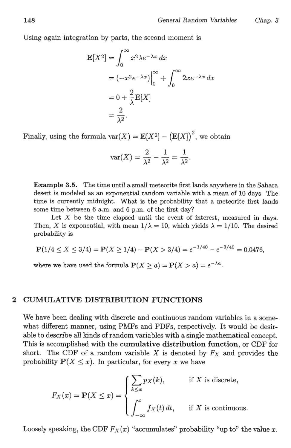
3.3. Normal Random Variables p. 152
3.4. Conditioning on an Event p. 158
3.5. Multiple Continuous Random Variables p. 164
3.6. Derived Distributions p. 179
3.7. Summary and Discussion p. 190
Problems p. 192
ν

vi Contents
4. Further Topics on Random Variables p. 209
4.1. Transforms p. 210
4.2. Sums of Independent Random Variables - Convolution p. 221
4.3. More on Conditional Expectation and Variance p. 225
4.4. Sum of a Random Number of Independent Random Variables . . p. 232
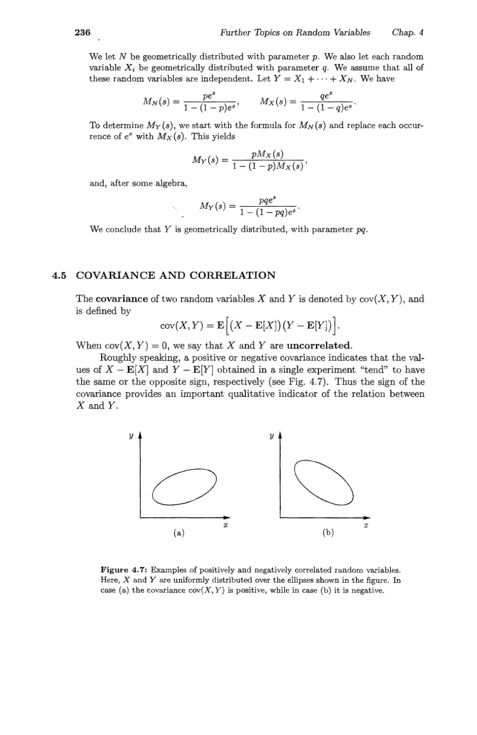
4.5. Covariance and Correlation p. 236
4.6. Least Squares Estimation p. 240
4.7. The Bivariate Normal Distribution p. 247
4.8. Summary and Discussion p. 255
Problems p. 257
5. The Bernoulli and Poisson Processes p. 271
5.1. The Bernoulli Process p. 273
5.2. The Poisson Process p. 285
5.3. Summary and Discussion p. 299
Problems p. 301
6. Markov Chains p. 313
6.1. Discrete-Time Markov Chains p. 314
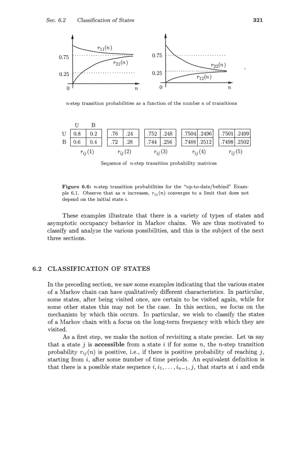
6.2. Classification of States p. 321
6.3. Steady-State Behavior p. 326
6.4. Absorption Probabilities and Expected Time to Absorption ... p. 337
6.5. Continuous-Time Markov Chains p. 344
6.6. Summary and Discussion p. 352
Problems p. 354
7. Limit Theorems p. 379
7.1. Markov and Chebyshev Inequalities p. 381
7.2. The Weak Law of Large Numbers p. 383
7.3. Convergence in Probability p. 386
7.4. The Central Limit Theorem p. 388
7.5. The Strong Law of Large Numbers p. 395
7.6. Summary and Discussion p. 397
Problems p. 399
Index p. 411

Preface
Probability is common sense reduced to calculation
Laplace
This book is an outgrowth of our involvement in teaching an introductory
probability course ("Probabilistic Systems Analysis") at the Massachusetts Institute
of Technology.
The course is attended by a large number of students with diverse
backgrounds, and a broad range of interests. They span the entire spectrum from
freshmen to beginning graduate students, and from the engineering school to the
school of management. Accordingly, we have tried to strike a balance between
simplicity in exposition and sophistication in analytical reasoning. Our key aim
has been to develop the ability to construct and analyze probabilistic models in
a manner that combines intuitive understanding and mathematical precision.
In this spirit, some of the more mathematically rigorous analysis has been
just sketched or intuitively explained in the text, so that complex proofs do not
stand in the way of an otherwise simple exposition. At the same time, some of
this analysis is developed (at the level of advanced calculus) in theoretical
problems, that are included at the end of the corresponding chapter. Furthermore,
some of the subtler mathematical issues are hinted at in footnotes addressed to
the more attentive reader.
The book covers the fundamentals of probability theory (probabilistic
models, discrete and continuous random variables, multiple random variables, and
limit theorems), which are typically part of a first course on the subject. It
also contains, in Chapters 4-6 a number of more advanced topics, from which an
instructor can choose to match the goals of a particular course. In particular, in
Chapter 4, we develop transforms, a more advanced view of conditioning, sums
of random variables, least squares estimation, and the bivariate normal distribu-
vii

viii
Preface
tion. Furthermore, in Chapters 5 and 6, we provide a fairly detailed introduction
to Bernoulli, Poisson, and Markov processes.
Our M.I.T. course covers all seven chapters in a single semester, with the
exception of the material on the bivariate normal (Section 4.7), and on continuous-
time Markov chains (Section 6.5). However, in an alternative course, the material
on stochastic processes could be omitted, thereby allowing additional emphasis
on foundational material, or coverage of other topics of the instructor's choice.
Our most notable omission in coverage is an introduction to statistics.
While we develop all the basic elements of Bayesian statistics, in the form of
Bayes' rule for discrete and continuous models, and least squares estimation, we
do not enter the subjects of parameter estimation, or non-Bayesian hypothesis
testing.
The problems that supplement the main text are divided in three categories:
(a) Theoretical problems: The theoretical problems (marked by *) constitute
an important component of the text, and ensure that the mathematically
oriented reader will find here a smooth development without major gaps.
Their solutions are given in the text, but an ambitious reader may be able
to solve many of them, especially in earlier chapters, before looking at the
solutions.
(b) Problems in the text: Besides theoretical problems, the text contains several
problems, of various levels of difficulty. These are representative of the
problems that are usually covered in recitation and tutorial sessions at
M.I.Т., and are a primary mechanism through which many of our students
learn the material. Our hope is that students elsewhere will attempt to
solve these problems, and then refer to their solutions to calibrate and
enhance their understanding of the material. The solutions are posted on
the book's www site
ht t ρ: / /www. at henasc. com/ probbook.html
(c) Supplementary problems: There is a large (and growing) collection of
additional problems, which is not included in the book, but is made available
at the book's www site. Many of these problems have been assigned as
homework or exam problems at M.I.Т., and we expect that instructors
elsewhere will use them for a similar purpose. While the statements of
these additional problems are publicly accessible, the solutions are made
available from the authors only to course instructors.
We would like to acknowledge our debt to several people who contributed
in various ways to the book. Our writing project began when we assumed
responsibility for a popular probability class at M.I.T. that our colleague Al Drake
had taught for several decades. We were thus fortunate to start with an
organization of the subject that had stood the test of time, a lively presentation of the
various topics in Al's classic textbook, and a rich set of material that had been
used in recitation sessions and for homework. We are thus indebted to Al Drake

Preface
ix
for providing a very favorable set of initial conditions.
We are thankful to the several colleagues who have either taught from the
draft of the book at various universities or have read it, and have provided us
with valuable feedback. In particular, we thank Ibrahim Abou Faycal, Gustavo
de Veciana, Eugene Feinberg, Bob Gray, Muriel Medard, Jason Papastavrou,
Ilya Pollak, David Tse, and Terry Wagner.
The teaching assistants for the M.I.T. class have been very helpful. They
pointed out corrections to various drafts, they developed problems and solutions
suitable for the class, and through their direct interaction with the student body,
they provided a robust mechanism for calibrating the level of the material.
Reaching thousands of bright students at M.I.T. at an early stage in their
studies was a great source of satisfaction for us. We thank them for their
valuable feedback and for being patient while they were taught from a textbook-in-
progress.
Last but not least, we are grateful to our families for their support
throughout the course of this long project.
Dimitri P. Bertsekas, dimitrib@mit.edu
John N. Tsitsiklis, jnt@mit.edu
Cambridge, Mass., May 2002

ATHENA SCIENTIFIC BOOKS
1. Introduction to Probability, by Dimitri R Bertsekas and John N.
Tsitsiklis, 2002, ISBN 1-886529-40-X, 430 pages
2. Dynamic Programming and Optimal Control: Second Edition, Vols. I
and II, by Dimitri P. Bertsekas, 2001, ISBN 1-886529-08-6, 704 pages
3. Nonlinear Programming, Second Edition, by Dimitri P. Bertsekas,
1999, ISBN 1-886529-00-0, 791 pages
4. Network Optimization: Continuous and Discrete Models by Dimitri
P. Bertsekas, 1998, ISBN 1-886529-02-7, 608 pages
5. Network Flows and Mono tropic Optimization by R. Tyrrell Rockafel-
lar, 1998, ISBN 1-886529-06-X, 634 pages
6. Introduction to Linear Optimization by Dimitris Bertsimas and John
N. Tsitsiklis, 1997, ISBN 1-886529-19-1, 608 pages
7. Parallel and Distributed Computation: Numerical Methods by Dimitri
P. Bertsekas and John N. Tsitsiklis, 1997, ISBN 1-886529-01-9, 718
pages
8. Neuro-Dynamic Programming, by Dimitri P. Bertsekas and John N.
Tsitsiklis, 1996, ISBN 1-886529-10-8, 512 pages
9. Constrained Optimization and Lagrange Multiplier Methods, by
Dimitri P. Bertsekas, 1996, ISBN 1-886529-04-3, 410 pages
10. Stochastic Optimal Control: The Discrete-Time Case by Dimitri P.
Bertsekas and Steven E. Shreve, 1996, ISBN 1-886529-03-5, 330 pages

1
Sample Space and
Probability
Contents
1.1. Sets p. 3
1.2. Probabilistic Models p. 6
1.3. Conditional Probability p. 18
1.4. Total Probability Theorem and Bayes' Rule p. 28
1.5. Independence p. 34
1.6. Counting p. 43
1.7. Summary and Discussion p. 50
Problems p. 52
1

2 Sample Space and Probability Chap. 1
"Probability" is a very useful concept, but can be interpreted in a number of
ways. As an illustration, consider the following.
A patient is admitted to the hospital and a potentially life-saving drug is
administered. The following dialog takes place between the nurse and a
concerned relative.
RELATIVE: Nurse, what is the probability that the drug will work?
NURSE: I hope it works, we'll know tomorrow.
RELATIVE: Yes, but what is the probability that it will?
NURSE: Each case is different, we have to wait.
RELATIVE: But let's see, out of a hundred patients that are treated under
similar conditions, how many times would you expect it to work?
NURSE (somewhat annoyed): I told you, every person is different, for some
it works, for some it doesn't.
RELATIVE (insisting): Then tell me, if you had to bet whether it will work
or not, which side of the bet would you take?
NURSE (cheering up for a moment): I'd bet it will work.
RELATIVE (somewhat relieved): OK, now, would you be willing to lose two
dollars if it doesn't work, and gain one dollar if it does?
NURSE (exasperated): What a sick thought! You are wasting my time!
In this conversation, the relative attempts to use the concept of probability
to discuss an uncertain situation. The nurse's initial response indicates that the
meaning of "probability" is not uniformly shared or understood, and the relative
tries to make it more concrete. The first approach is to define probability in
terms of frequency of occurrence, as a percentage of successes in a moderately
large number of similar situations. Such an interpretation is often natural. For
example, when we say that a perfectly manufactured coin lands on heads "with
probability 50%," we typically mean "roughly half of the time." But the nurse
may not be entirely wrong in refusing to discuss in such terms. What if this
was an experimental drug that was administered for the very first time in this
hospital or in the nurse's experience?
While there are many situations involving uncertainty in which the
frequency interpretation is appropriate, there are other situations in which it is
not. Consider, for example, a scholar who asserts that the Iliad and the Odyssey
were composed by the same person, with probability 90%. Such an assertion
conveys some information, but not in terms of frequencies, since the subject is
a one-time event. Rather, it is an expression of the scholar's subjective
belief. One might think that subjective beliefs are not interesting, at least from a
mathematical or scientific point of view. On the other hand, people often have
to make choices in the presence of uncertainty, and a systematic way of making
use of their beliefs is a prerequisite for successful, or at least consistent, decision
making.

Sea 1.1 Sets
3
In fact, the choices and actions of a rational person, can reveal a lot about
the inner-held subjective probabilities, even if the person does not make conscious
use of probabilistic reasoning. Indeed, the last part of the earlier dialog was an
attempt to infer the nurse's beliefs in an indirect manner. Since the nurse was
willing to accept a one-for-one bet that the drug would work, we may infer
that the probability of success was judged to be at least 50%. And had the
nurse accepted the last proposed bet (two-for-one), that would have indicated a
success probability of at least 2/3.
Rather than dwelling further into philosophical issues about the
appropriateness of probabilistic reasoning, we will simply take it as a given that the theory
of probability is useful in a broad variety of contexts, including some where the
assumed probabilities only reflect subjective beliefs. There is a large body of
successful applications in science, engineering, medicine, management, etc., and
on the basis of this empirical evidence, probability theory is an extremely useful
tool.
Our main objective in this book is to develop the art of describing
uncertainty in terms of probabilistic models, as well as the skill of probabilistic
reasoning. The first step, which is the subject of this chapter, is to describe
the generic structure of such models, and their basic properties. The models we
consider assign probabilities to collections (sets) of possible outcomes. For this
reason, we must begin with a short review of set theory.
1.1 SETS
Probability makes extensive use of set operations, so let us introduce at the
outset the relevant notation and terminology.
A set is a collection of objects, which are the elements of the set. If S is
a set and χ is an element of 5, we write χ £ 5. If χ is not an element of 5, we
write χ φ. 5. A set can have no elements, in which case it is called the empty
set, denoted by 0.
Sets can be specified in a variety of ways. If S contains a finite number of
elements, say xi, X2,..., %, we write it as a list of the elements, in braces:
S = {xi,X2,· ..,Xn}·
For example, the set of possible outcomes of a die roll is {1,2,3,4,5,6}, and the
set of possible outcomes of a coin toss is {if, T}, where Η stands for "heads"
and Τ stands for "tails."
If S contains infinitely many elements xi, X2,..., which can be enumerated
in a list (so that there are as many elements as there are positive integers) we
write
S = {xi,X2,·· ·},
and we say that S is count ably infinite. For example, the set of even integers
can be written as {0,2, —2,4, —4,...}, and is count ably infinite.

4
Sample Space and Probability Chap. 1
Alternatively, we can consider the set of all χ that have a certain property
P, and denote it by
{x | χ satisfies P}.
(The symbol "|" is to be read as "such that.") For example, the set of even
integers can be written as {к \ к/2 is integer}. Similarly, the set of all scalars χ
in the interval [0,1] can be written as {x | 0 < χ < 1}. Note that the elements χ
of the latter set take a continuous range of values, and cannot be written down
in a list (a proof is sketched in the end-of-chapter problems); such a set is said
to be uncountable.
If every element of a set S is also an element of a set T, we say that S
is a subset of T, and we write S С Τ or Τ э S. If S С Τ and Τ С 5, the
two sets are equal, and we write S = T. It is also expedient to introduce a
universal set, denoted by Ω, which contains all objects that could conceivably
be of interest in a particular context. Having specified the context in terms of a
universal set Ω, we only consider sets S that are subsets of Ω.
Set Operations
The complement of a set 5, with respect to the universe Ω, is the set {χ Ε
Ω Ι χ φ. S} of all elements of Ω that do not belong to 5, and is denoted by 5C.
Note that Qc = 0.
The union of two sets S and Τ is the set of all elements that belong to S
or Τ (or both), and is denoted by S U T. The intersection of two sets S and Τ
is the set of all elements that belong to both S and T, and is denoted by S Γ\Τ.
Thus,
S υ Τ = {χ Ι χ e S or χ e T},
and
S η Τ = {χ Ι χ e S and χ e T}.
In some cases, we will have to consider the union or the intersection of several,
even infinitely many sets, defined in the obvious way. For example, if for every
positive integer n, we are given a set 5n, then
CO
Μ Sn = Si U 52 U · · · = {χ Ι χ ε Sn for some η},
n=l
and
CO
f) Sn = Si П S2 П · · · = {χ I x e Sn for all n}.
n=l
Two sets are said to be disjoint if their intersection is empty. More generally,
several sets are said to be disjoint if no two of them have a common element. A
collection of sets is said to be a partition of a set S if the sets in the collection
are disjoint and their union is 5.

Sea 1.1 Sets
5
If χ and у are two objects, we use (x, y) to denote the ordered pair of χ
and y. The set of scalars (real numbers) is denoted by Sft; the set of pairs (or
triplets) of scalars, i.e., the two-dimensional plane (or three-dimensional space,
respectively) is denoted by Sft2 (or Sft3, respectively).
Sets and the associated operations are easy to visualize in terms of Venn
diagrams, as illustrated in Fig. 1.1.
, Ω
S J_^
(a)
Figure 1.1: Examples of Venn diagrams, (a) The shaded region is S Π Т. (b)
The shaded region is S U Г. (c) The shaded region is S Π Tc. (d) Here, Τ С S.
The shaded region is the complement of S. (e) The sets 5, T, and U are disjoint,
(f) The sets S, T, and U form a partition of the set Ω.
The Algebra of Sets
Set operations have several properties, which are elementary consequences of the
definitions. Some examples are:
SUT =TUS,
Sn(TuU) = (SnT)U(SnU),
(в*)* = 5,
5υΩ =Ω,
SU(TUU) =(SUT)UU,
SU(TnU) = (SUT) П (SUIT),
SnS* = 0,
5ηΩ = 5.
Two particularly useful properties are given by De Morgan's laws which
state that
(\JSn\ =f)SZ, (f]Snj =\JSZ.
To establish the first law, suppose that χ Ε (Un5n)c. Then, χ φ. Un5n, which
implies that for every n, we have χ φ Sn. Thus, χ belongs to the complement

6
Sample Space and Probability Chap. 1
of every i>nj and xn Ε nnSn. This shows that (UnSn)c С nnSn. The converse
inclusion is established by reversing the above argument, and the first law follows.
The argument for the second law is similar.
1.2 PROBABILISTIC MODELS
A probabilistic model is a mathematical description of an uncertain situation.
It must be in accordance with a fundamental framework that we discuss in this
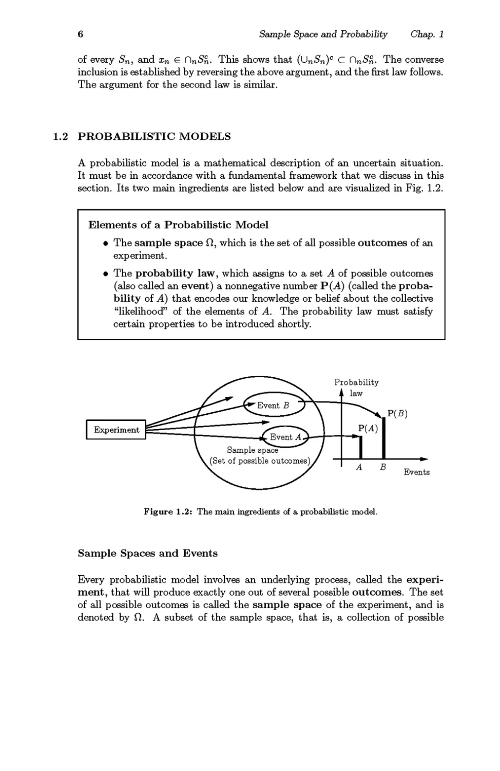
section. Its two main ingredients are listed below and are visualized in Fig. 1.2.
Elements of a Probabilistic Model
• The sample space Ω, which is the set of all possible outcomes of an
experiment.
• The probability law, which assigns to a set A of possible outcomes
(also called an event) a nonnegative number Ρ (A) (called the
probability of A) that encodes our knowledge or belief about the collective
"likelihood" of the elements of A. The probability law must satisfy
certain properties to be introduced shortly.
Probability
1 law
Events
Figure 1.2: The main ingredients of a probabilistic model.
Sample Spaces and Events
Every probabilistic model involves an underlying process, called the
experiment, that will produce exactly one out of several possible outcomes. The set
of all possible outcomes is called the sample space of the experiment, and is
denoted by Ω. A subset of the sample space, that is, a collection of possible

Sea 1.2 Probabilistic Models
7
outcomes, is called an event J There is no restriction on what constitutes an
experiment. For example, it could be a single toss of a coin, or three tosses,
or an infinite sequence of tosses. However, it is important to note that in our
formulation of a probabilistic model, there is only one experiment. So, three
tosses of a coin constitute a single experiment, rather than three experiments.
The sample space of an experiment may consist of a finite or an infinite
number of possible outcomes. Finite sample spaces are conceptually and
mathematically simpler. Still, sample spaces with an infinite number of elements are
quite common. For an example, consider throwing a dart on a square target and
viewing the point of impact as the outcome.
Choosing an Appropriate Sample Space
Regardless of their number, different elements of the sample space should be
distinct and mutually exclusive so that when the experiment is carried out,
there is a unique outcome. For example, the sample space associated with the
roll of a die cannot contain "1 or 3" as a possible outcome and also "1 or 4"
as another possible outcome, because we would not be able to assign a unique
outcome when the roll is a 1.
A given physical situation may be modeled in several different ways,
depending on the kind of questions that we are interested in. Generally, the sample
space chosen for a probabilistic model must be collectively exhaustive, in the
sense that no matter what happens in the experiment, we always obtain an
outcome that has been included in the sample space. In addition, the sample space
should have enough detail to distinguish between all outcomes of interest to the
modeler, while avoiding irrelevant details.
Example 1.1. Consider two alternative games, both involving ten successive coin
tosses:
Game 1: We receive $1 each time a head comes up.
Game 2: We receive $1 for every coin toss, up to and including the first time
a head comes up. Then, we receive $2 for every coin toss, up to the second
time a head comes up. More generally, the dollar amount per toss is doubled
each time a head comes up.
| Any collection of possible outcomes, including the entire sample space Ω and
its complement, the empty set 0, may qualify as an event. Strictly speaking, however,
some sets have to be excluded. In particular, when dealing with probabilistic models
involving an uncountably infinite sample space, there are certain unusual subsets for
which one cannot associate meaningful probabilities. This is an intricate technical issue,
involving the mathematics of measure theory. Fortunately, such pathological subsets
do not arise in the problems considered in this text or in practice, and the issue can be
safely ignored.

8
Sample Space and Probability Chap. 1
In game 1, it is only the total number of heads in the ten-toss sequence that
matters, while in game 2, the order of heads and tails is also imp or t ant. Thus, in
a probabilistic model for game 1, we can work with a sample space consisting of
eleven possible outcomes, namely, 0,1,..., 10. In game 2, a finer grain description
of the experiment is called for, and it is more appropriate to let the sample space
consist of every possible ten-long sequence of heads and tails.
Sequential Models
Many experiments have an inherently sequential character, such as for example
tossing a coin three times, or observing the value of a stock on five successive
days, or receiving eight successive digits at a communication receiver. It is then
often useful to describe the experiment and the associated sample space by means
of a tree-based sequential description, as in Fig. 1.3.
Figure 1.3: Two equivalent descriptions of the sample space of an experiment
involving two rolls of a 4-sided die. The possible outcomes are all the ordered pairs
of the form (i>j)7 where г is the result of the first roll, and j is the result of the
second. These outcomes can be arranged in a 2-dimensional grid as in the figure
on the left, or they can be described by the tree on the right, which reflects the
sequential character of the experiment. Here, each possible outcome corresponds
to a leaf of the tree and is associated with the unique path from the root to
that leaf. The shaded area on the left is the event {(1,4), (2,4), (3,4), (4,4)}
that the result of the second roll is 4. That same event can be described by the
set of leaves highlighted on the right. Note also that every node of the tree can
be identified with an event, namely, the set of all leaves downstream from that
node. For example, the node labeled by a 1 can be identified with the event
{(1,1), (1,2), (1,3), (1,4)} that the result of the first roll is 1.
Probability Laws
Suppose we have settled on the sample space Ω associated with an experiment.
Then, to complete the probabilistic model, we must introduce a probability

Sea 1.2 Probabilistic Models
9
law. Intuitively, this specifies the "likelihood" of any outcome, or of any set of
possible outcomes (an event, as we have called it earlier). More precisely, the
probability law assigns to every event A, a number Ρ (A), called the probability
of A, satisfying the following axioms.
In order to visualize a probability law, consider a unit of mass which is
"spread" over the sample space. Then, Ρ (A) is simply the total mass that was
assigned collectively to the elements of A In terms of this analogy, the additivity
axiom becomes quite intuitive: the total mass in a sequence of disjoint events is
the sum of their individual masses.
A more concrete interpretation of probabilities is in terms of relative
frequencies: a statement such as Ρ (A) = 2/3 often represents a belief that event A
will occur in about two thirds out of a large number of repetitions of the
experiment. Such an interpretation, though not always appropriate, can sometimes
facilitate our intuitive understanding. It will be revisited in Chapter 7, in our
study of limit theorems.
There are many natural properties of a probability law, which have not been
included in the above axioms for the simple reason that they can be derived
from them. For example, note that the normalization and additivity axioms
imply that
1 = Ρ(Ω) = Ρ(Ω U 0) = Ρ(Ω) + Ρ(0) = 1 + Ρ(0),
and this shows that the probability of the empty event is 0:
P(0) = 0.

10 Sample Space and Probability Chap. 1
As another example, consider three disjoint events Αι7 A2, and A3. We can use
the additivity axiom for two disjoint events repeatedly, to obtain
P(Ai U A2 U A3) = P(Ai U (A2UA3))
= P(A1) + P(A2UA3)
= P(Ai) + P(A2) + P(A3).
Proceeding similarly, we obtain that the probability of the union of finitely many
disjoint events is always equal to the sum of the probabilities of these events.
More such properties will be considered shortly.
Discrete Models
Here is an illustration of how to construct a probability law starting from some
common sense assumptions about a model.
Example 1.2. Consider an experiment involving a single coin toss. There are
two possible outcomes, heads (Я) and tails (T). The sample space is Ω = {Η, Τ},
and the events are
{н,т}, {ну, m, 0.
If the coin is fair, i.e., if we believe that heads and tails are "equally likely," we
should assign equal probabilities to the two possible outcomes and specify that
Р({Я}) = Ρ ({Γ}) = 0.5. The additivity axiom implies that
Р({Я,Г})=Р({Я})+Р({Г}) = 1,
which is consistent with the normalization axiom. Thus, the probability law is given
by
Р({Я,Г}) = 1, Р({Я})=0.5, Ρ ({Τ}) =0.5, Ρ(0) = 0,
and satisfies all three axioms.
Consider another experiment involving three coin tosses. The outcome will
now be a 3-long string of heads or tails. The sample space is
Ω = {HHH, ЯЯГ, ЯГЯ, HTT, ГЯЯ, THT, TTH, TTT}.
We assume that each possible outcome has the same probability of 1/8. Let us
construct a probability law that satisfies the three axioms. Consider, as an example,
the event
A = {exactly 2 heads occur} = {ЯЯГ, ЯГЯ, THH}.
Using additivity, the probability of A is the sum of the probabilities of its elements:
Ρ ({ЯЯГ, ЯГЯ, ГЯЯ}) = Ρ ({HHT}) + Ρ ({ΗΤΗ}) + Ρ ({ГЯЯ})
8τ 8τ 8
_ 3
" 8'

Sea 1.2 Probabilistic Models
11
Similarly, the probability of any event is equal to 1/8 times the number of possible
outcomes contained in the event. This defines a probability law that satisfies the
three axioms.
By using the additivity axiom and by generalizing the reasoning in the
preceding example, we reach the following conclusion.
Note that we are using here the simpler notation Ρ(si) to denote the
probability of the event {$$}, instead of the more precise Ρ ({$$}). This convention
will be used throughout the remainder of the book.
In the special case where the probabilities P(si),..., P(sn) are all the same
(by necessity equal to 1/n, in view of the normalization axiom), we obtain the
following.
Let us provide a few more examples of sample spaces and probability laws.
Example 1.3. Consider the experiment of rolling a pair of 4-sided dice (cf. Fig.
1.4). We assume the dice are fair, and we interpret this assumption to mean that
each of the sixteen possible outcomes [pairs (г, j)t with itj = 1, 2, 3, 4], has the same
probability of 1/16. To calculate the probability of an event, we must count the
number of elements of the event and divide by 16 (the total number of possible

12
Sample Space and Probability Chap. 1
outcomes). Here are some event probabilities calculated in this way:
Ρ ({the sum of the rolls is even}) = 8/16 = 1/2,
Ρ ({the sum of the rolls is odd}) = 8/16 = 1/2,
Ρ ({the first roll is equal to the second}) = 4/16 = 1/4,
Ρ ({the first roll is larger than the second}) = 6/16 = 3/8,
Ρ ({at least one roll is equal to 4}) = 7/16.
Figure 1.4: Various events in the experiment of rolling a pair of 4-sided dice,
and their probabilities, calculated according to the discrete uniform law.
Continuous Models
Probabilistic models with continuous sample spaces differ from their discrete
counterparts in that the probabilities of the single-element events may not be
sufficient to characterize the probability law. This is illustrated in the following
examples, which also indicate how to generalize the uniform probability law to
the case of a continuous sample space.
Example 1.4. A wheel of fortune is continuously calibrated from 0 to 1, so the
possible outcomes of an experiment consisting of a single spin are the numbers in
the interval Ω = [0,1]. Assuming a fair wheel, it is appropriate to consider all
outcomes equally likely, but what is the probability of the event consisting of a
single element? It cannot be positive, because then, using the additivity axiom, it
would follow that events with a sufficiently large number of elements would have

Sea 1.2 Probabilistic Models
13
probability larger than 1. Therefore, the probability of any event that consists of a
single element must be (λ
In this example, it makes sense to assign probability b — α to any subinter-
val [atb] of [0,1], and to calculate the probability of a more complicated set by
evaluating its "length." Τ This assignment satisfies the three probability axioms and
qualifies as a legitimate probability law.
Example 1.5. Romeo and Juliet have a date at a given time, and each will arrive
at the meeting place with a delay between 0 and 1 hour, with all pairs of delays
being equally likely. The first to arrive will wait for 15 minutes and will leave if the
other has not yet arrived. What is the probability that they will meet?
Let us use as sample space the unit square, whose elements are the possible
pairs of delays for the two of them. Our interpretation of "equally likely" pairs of
delays is to let the probability of a subset of Ω be equal to its area. This probability
law satisfies the three probability axioms. The event that Romeo and Juliet will
meet is the shaded region in Fig. 1.5, and its probability is calculated to be 7/16.
Figure 1.5: The event Μ that Romeo and Juliet will arrive within 15 minutes
of each other (cf. Example 1.5) is
M={(xyy) | |з-у|<1/4,0<з<1,0<у<1},
and is shaded in the figure. The area of Μ is 1 minus the area of the two unshaded
triangles, or 1 - (3/4) · (3/4) = 7/16. Thus, the probability of meeting is 7/16.
| The "length" of a subset S of [0,1] is the integral J dt, which is defined, for
"nice" sets 5, in the usual calculus sense. For unusual sets, this integral may not be
well defined mathematically, but such issues belong to a more advanced treatment of
the subject. Incidentally, the legitimacy of using length as a probability law hinges on
the fact that the unit interval has an uncountably infinite number of elements. Indeed,
if the unit interval had a countable number of elements, with each element having
zero probability, the additivity axiom would imply that the whole interval has zero
probability, which would contradict the normalization axiom.

14 Sample Space and Probability Chap. 1
Properties of Probability Laws
Probability laws have a number of properties, which can be deduced from the
axioms. Some of them are summarized below.
These properties, and other similar ones, can be visualized and verified
graphically using Venn diagrams, as in Fig. 1.6. Note that property (c) can be
generalized as follows:
η
ρ(Α1υΑ2υ...υΑη)<Σρ(Α*)'
г=1
To see this, we apply property (c) to the sets A\ and A2 U · · · U An7 to obtain
P(Ai U A2 U · · · U An) < P(Ai) + P(A2 U · · · U An).
We also apply property (c) to the sets A2 and As U · · · U An, to obtain
P(A2 U · · · U An) < P(A2) + P(A3 U · · · U An).
We continue similarly, and finally add.
Models and Reality
The framework of probability theory can be used to analyze uncertainty in a
wide variety of physical contexts. Typically, this involves two distinct stages.
(a) In the first stage, we construct a probabilistic model, by specifying a
probability law on a suitably defined sample space. There are no hard rules to
guide this step, other than the requirement that the probability law
conform to the three axioms. Reasonable people may disagree on which model
best represents reality. In many cases, one may even want to use a
somewhat "incorrect" model, if it is simpler than the "correct" one or allows for
tractable calculations. This is consistent with common practice in science

Sea 1.2 Probabilistic Models
15
and engineering, where the choice of a model often involves a tradeoff
between accuracy, simplicity, and tract ability. Sometimes, a model is chosen
on the basis of historical data or past outcomes of similar experiments,
using methods from the field of statistics.
Figure 1.6: Visualization and verification of various properties of probability
laws using Venn diagrams. If А С В, then В is the union of the two disjoint
events A and Ac Π Β; see diagram (a). Therefore, by the additivity axiom, we
have
P(B) = P(A) + P(AC C\B)> P(A),
where the inequality follows from the nonnegativity axiom, and verifies
property (a).
Prom diagram (b), we can express the events A U В and В as unions of
disjoint events:
AUB = AU(AcnB)y B = (AnB)U(Acn B).
Using the additivity axiom, we have
P(A U Β) = Ρ (Α) + P(AC η Б), Р(В) = Ρ (Α Π Β) + Р(АС η Β).
Subtracting the second equality from the first and rearranging terms, we obtain
P(A U В) = Ρ (Α) + Ρ(Β)- Ρ (Α Π Β), verifying property (b). Using also the fact
P(A Π Β) > 0 (the nonnegativity axiom), we obtain P(A U B) < Ρ (A) + P(B),
verifying property (c).
Prom diagram (c), we see that the event A U Б U С сал be expressed as a
union of three disjoint events:
A\JB\JC = A\J(Acr\B)\J(Acr\Bcr\C)y
so property (d) follows as a consequence of the additivity axiom.

16
Sample Space and Probability Chap. 1
(b) In the second stage, we work within a fully specified probabilistic model and
derive the probabilities of certain events, or deduce some interesting
properties. While the first stage entails the often open-ended task of connecting
the real world with mathematics, the second one is tightly regulated by the
rules of ordinary logic and the axioms of probability. Difficulties may arise
in the latter if some required calculations are complex, or if a probability
law is specified in an indirect fashion. Even so, there is no room for
ambiguity: all conceivable questions have precise answers and it is only a matter
of developing the skill to arrive at them.
Probability theory is full of "paradoxes" in which different calculation
methods seem to give different answers to the same question. Invariably though,
these apparent inconsistencies turn out to reflect poorly specified or ambiguous
probabilistic models. An example, Bertrand's paradox, is shown in Fig. 1.7.
Figure 1.7: This example, presented by L. F. Bertrand in 1889, illustrates the
need to specify unambiguously a probabilistic model. Consider a circle and an
equilateral triangle inscribed in the circle. What is the probability that the length
of a randomly chosen chord of the circle is greater than the side of the triangle?
The answer here depends on the precise meaning of "randomly chosen." The two
methods illustrated in parts (a) and (b) of the figure lead to contradictory results.
In (a), we take a radius of the circle, such as AB, and we choose a point
С on that radius, with all points being equally likely. We then draw the chord
through С that is orthogonal to AB. From elementary geometry, AB intersects
the triangle at the midpoint of AB, so the probability that the length of the chord
is greater than the side is 1/2.
In (b), we take a point on the circle, such as the vertex V, we draw the
tangent to the circle through V, and we draw a line through V that forms a random
angle Φ with the tangent, with all angles being equally likely. We consider the
chord obtained by the intersection of this line with the circle. From elementary
geometry, the length of the chord is greater that the side of the triangle if Φ is
between π/З and 2π/3. Since Φ takes values between 0 and π, the probability
that the length of the chord is greater than the side is 1/3.

Sea 1.2 Probabilistic Models 17

18
Sample Space and Probability Chap. 1
1.3 CONDITIONAL PROBABILITY
Conditional probability provides us with a way to reason about the outcome
of an experiment, based on partial information. Here are some examples of
situations we have in mind:
(a) In an experiment involving two successive rolls of a die, you are told that
the sum of the two rolls is 9. How likely is it that the first roll was a 6?
(b) In a word guessing game, the first letter of the word is a "t". What is the
likelihood that the second letter is an "h"?
(c) How likely is it that a person has a disease given that a medical test was
negative?
(d) A spot shows up on a radar screen. How likely is it that it corresponds to
an aircraft?
In more precise terms, given an experiment, a corresponding sample space,
and a probability law, suppose that we know that the outcome is within some
given event Б. We wish to quantify the likelihood that the outcome also belongs
to some other given event A We thus seek to construct a new probability law,
which takes into account the available knowledge and which, for any event A,
gives us the conditional probability of A given Б, denoted by P(A | Б).
We would like the conditional probabilities Ρ (Α \ Β) of different events A to
constitute a legitimate probability law, that satisfies the probability axioms. The
conditional probabilities should also be consistent with our intuition in important
special cases, e.g., when all possible outcomes of the experiment are equally likely.
For example, suppose that all six possible outcomes of a fair die roll are equally
likely. If we are told that the outcome is even, we are left with only three possible
outcomes, namely, 2, 4, and 6. These three outcomes were equally likely to start
with, and so they should remain equally likely given the additional knowledge
that the outcome was even. Thus, it is reasonable to let
1
Ρ (the outcome is б | the outcome is even) = —.
This argument suggests that an appropriate definition of conditional probability
when all outcomes are equally likely, is given by
_, . , ,_>. number of elements of Α Π Β
жг(А\ Jd) = .
number of elements of В
Generalizing the argument, we introduce the following definition of
conditional probability:
Р(А|Б)- Ί>(Β) '

Sea 1.3 Conditional Probability
19
where we assume that P(-B) > 0; the conditional probability is undefined if the
conditioning event has zero probability. In words, out of the total probability of
the elements of Β, Ρ (Α \ B) is the fraction that is assigned to possible outcomes
that also belong to A.
Conditional Probabilities Specify a Probability Law
For a fixed event B, it can be verified that the conditional probabilities Ρ (Α \ Β)
form a legitimate probability law that satisfies the three axioms. Indeed, non-
negativity is clear. Furthermore,
Ρ(Ω|Β)- р(Б) -р(я)-1,
and the normalization axiom is also satisfied. To verify the additivity axiom, we
write for any two disjoint events A\ and A2,
, ч P((A1UA2)r\B)
P(A1UA2\B) = " λν{^ ί
_Р((А1пВ)и(А2пВ))
P(B)
_ Ρ(ΑιΠΒ) + Ρ(Α2ηΒ)
Р(В)
Р(АгпВ) Р(А2пВ)
Р(В) + Р(В)
= Ρ(Αι|Β) + Ρ(Α2|Β),
where for the third equality, we used the fact that A\ Π Β and A2 Π Β are
disjoint sets, and the additivity axiom for the (unconditional) probability law.
The argument for a countable collection of disjoint sets is similar.
Since conditional probabilities constitute a legitimate probability law, all
general properties of probability laws remain valid. For example, a fact such as
Ρ (A U С) < Ρ (Α) + P(C) translates to the new fact
P(A U СΙ Β) < P(A | B) + P(C | B).
Let us also note that since we have P(B | B) = P(B)/P(B) = 1, all of the
conditional probability is concentrated on B. Thus, we might as well discard all
possible outcomes outside В and treat the conditional probabilities as a
probability law defined on the new universe B.
Let us summarize the conclusions reached so far.

20
Sample Space and Probability Chap. 1
Example 1.6. We toss a fair coin three successive times. We wish to find the
conditional probability Έ>(Α\Β) when A and В are the events
A = {more heads than tails come up}, В = {1st toss is a head}.
The sample space consists of eight sequences,
Ω = {HHH, HHT, HTH, HTT, THH, THT, TTH, TTT},
which we assume to be equally likely. The event В consists of the four elements
HHH, HHT, HTH, HTT, so its probability is
P(B)=|.
The event Α Π Β consists of the three elements HHH> HHT> HTH> so its
probability is
Р(ЛПВ)=§.
Thus, the conditional probability ~P{A\B) is
Р(ЛпБ) _ 3/8 _ 3
V(A\B) =
Р(Б) 4/8 4'

Sea 1.3 Conditional Probability
21
Because all possible outcomes are equally likely here, we can also compute P(j4 | B)
using a shortcut. We can bypass the calculation of Р(Б) and Р(ЛПБ), and simply
divide the number of elements shared by A and В (which is 3) with the number of
elements of В (which is 4), to obtain the same result 3/4.
Example 1.7. A fair Φ sided die is rolled twice and we assume that all sixteen
possible outcomes are equally likely. Let X and У be the result of the 1st and the
2nd roll, respectively. We wish to determine the conditional probability ~P{A | Б),
where
A= {max(X, Y) = m}, B= {min(X, Y) = 2},
and m takes each of the values 1, 2, 3, 4.
As in the preceding example, we can first determine the probabilities Р(ЛПБ)
and P(.B) by counting the number of elements of Α Π Β and Б, respectively, and
dividing by 16. Alternatively, we can directly divide the number of elements of
ΑΠ Β with the number of elements of B; see Fig. 1.8.
Figure 1.8: Sample space of an experiment involving two rolls of a 4-sided die.
(cf. Example 1.7). The conditioning event В = {mm(XyY) = 2} consists of the
5-element shaded set. The set A = {max(X, Y) = m} shares with В two elements
if m = 3 or m = 4, one element if m = 2, and no element if m = 1. Thus, we have
{2/5, if m = 3 or m = 4,
1/5, 'dm = 2,
0, if m = 1.
Example 1.8. A conservative design team, call it C, and an innovative design
team, call it N, are asked to separately design a new product within a month. From
past experience we know that:
(a) The probability that team С is successful is 2/3.
(b) The probability that team N is successful is 1/2.

22
Sample Space and Probability Chap. 1
(c) The probability that at least one team is successful is 3/4.
Assuming that exactly one successful design is produced, what is the probability
that it was designed by team N?
There are four possible outcomes here, corresponding to the four combinations
of success and failure of the two teams:
SS: both succeed, FF: both fail,
SF: С succeeds, N fails, FS: С fails, N succeeds.
We are given that the probabilities of these outcomes satisfy
P(55) + P(SF) = |, P(SS) + P(FS) = ±, P(55) + P(SF) + P(FS) = J.
From these relations, together with the normalization equation
P(55) + P(£F) + T>(FS) + T>(FF) = 1,
we can obtain the probabilities of all the outcomes:
P(55) = A, P(SiT) = I, P(FS)=±, V(FF) = ±.
The desired conditional probability is
P(F5 | {SF,FS}) = г 12 г = i
4+12
Using Conditional Probability for Modeling
When constructing probabilistic models for experiments that have a sequential
character, it is often natural and convenient to first specify conditional
probabilities and then use them to determine unconditional probabilities. The rule
Ρ(ΑπΒ) =Έ>(Β)Έ>(Α\Β), which is a restatement of the definition of conditional
probability, is often helpful in this process.
Example 1.9. Radar Detection. If an aircraft is present in a certain area, a
radar correctly registers its presence with probability 0.99. If it is not present, the
radar falsely registers an aircraft presence with probability 0.10. We assume that
an aircraft is present with probability 0.05. What is the probability of false alarm
(a false indication of aircraft presence), and the probability of missed detection
(nothing registers, even though an aircraft is present)?
A sequential representation of the experiment is appropriate here, as shown
in Fig. 1.9. Let A and Б be the events
A = {an aircraft is present},
В = {the radar registers an aircraft presence},

Sea 1.3 Conditional Probability
23
and consider also their complements
Ac = {an aircraft is not present},
Bc = {the radar does not register an aircraft presence}.
The given probabilities are recorded along the corresponding branches of the tree
describing the sample space, as shown in Fig. 1.9. Each possible outcome corresponds
to a leaf of the tree, and its probability is equal to the product of the probabilities
associated with the branches in a path from the root to the corresponding leaf. The
desired probabilities of false alarm and missed detection are
P(false alarm) = Р(ЛС Π Β) = Р(ЛС)Р(Б | Ас) = 0.95 · 0.10 = 0.095,
P(missed detection) = Р(Л Π Вс) = Р(Л)Р(БС | А) = 0.05 · 0.01 = 0.0005.
Figure 1.9: Sequential description of the experiment for the radar detection
problem in Example 1.9.
Extending the preceding example, we have a general rule for calculating
various probabilities in conjunction with a tree-based sequential description of
an experiment. In particular:
(a) We set up the tree so that an event of interest is associated with a leaf.
We view the occurrence of the event as a sequence of steps, namely, the
traversals of the branches along the path from the root to the leaf.
(b) We record the conditional probabilities associated with the branches of the
tree.
(c) We obtain the probability of a leaf by multiplying the probabilities recorded
along the corresponding path of the tree.

24
Sample Space and Probability Chap. 1
In mathematical terms, we are dealing with an event A which occurs if and
only if each one of several events Ai,..., An has occurred, i.e., A = A\ Π Аъ П
• · · Π Αη> The occurrence of A is viewed as an occurrence of Ai, followed by the
occurrence of A2, then of A3, etc., and it is visualized as a path with η branches,
corresponding to the events Ai,..., An. The probability of A is given by the
following rule (see also Fig. 1.10).
Figure 1.10: Visualization of the multiplication rule. The intersection event
A = Αί Π A2 Π · · · Π Αη is associated with a particular path on a tree that
describes the experiment. We associate the branches of this path with the events
Ai,..., An7 and we record next to the branches the corresponding conditional
probabilities.
The final node of the path corresponds to the intersection event A, and
its probability is obtained by multiplying the conditional probabilities recorded
along the branches of the path
P(Ai Π A2 Π · · · Π Аз) = P(Ai)P(A2 | Αι) · · · P(An | Αι Π Α2 Π · · · Π Αη_ι).
Note that any intermediate node along the path also corresponds to some
intersection event and its probability is obtained by multiplying the corresponding
conditional probabilities up to that node. For example, the event Αι Π Α2 Π A3
corresponds to the node shown in the figure, and its probability is
Ρ(Αι Π Α2 Π A3) = P(Ai)P(A2 | Ai)P(Aa | Αι Π Α2).

Sea 1.3 Conditional Probability
25
and by using the definition of conditional probability to rewrite the right-hand
side above as
P(A1)P(A21 Ах)Р(Аз | Аг η A2) ■ ■ ■ P(An | n^1 At).
For the case of just two events, A\ and A2, the multiplication rule is simply the
definition of conditional probability.
Example 1.10. Three cards are drawn from an ordinary 52-card deck without
replacement (drawn cards are not placed back in the deck). We wish to find the
probability that none of the three cards is a heart. We assume that at each step,
each one of the remaining cards is equally likely to be picked. By symmetry, this
implies that every triplet of cards is equally likely to be drawn. A cumbersome
approach, that we will not use, is to count the number of all card triplets that
do not include a heart, and divide it with the number of all possible card triplets.
Instead, we use a sequential description of the experiment in conjunction with the
multiplication rule (cf. Fig. 1.11).
Define the events
Ai = {the ith. card is not a heart}, г = 1,2,3.
We will calculate Ρ(>1ι Π Α2 ПЛз), the probability that none of the three cards is
a heart, using the multiplication rule
P(>h Π Α2 Π As) = Έ>(Αι)Έ>(Α2 \ Ai)-p(As \ Αι Π Л2).
We have
since there are 39 cards that are not hearts in the 52-card deck. Given that the
first card is not a heart, we are left with 51 cards, 38 of which are not hearts, and
Р(А2\А0=Щ.
Finally, given that the first two cards drawn are not hearts, there are 37 cards which
are not hearts in the remaining 50-card deck, and
P(i48|i4irii4a) = |i.
OU
These probabilities are recorded along the corresponding branches of the tree
describing the sample space, as shown in Fig. 1.11. The desired probability is now
obtained by multiplying the probabilities recorded along the corresponding path of
the tree:
«/ . , , ч 39 38 37
Г(А1ПА2ПАг)=ш.^.ш.

26
Sample Space and Probability Chap. 1
Figure 1.11: Sequential description
of the experiment in the 3-card
selection problem of Example 1.10.
Note that once the probabilities are recorded along the tree, the probability
of several other events can be similarly calculated. For example,
39 13
Ρ (1st is not a heart and 2nd is a heart) =— · —,
Ο,ώ Ο i.
39 38 13
Ρ (1st two are not hearts and 3rd is a heart) =— · —- · —τ·.
v ' 52 51 50
Example 1.11. A class consisting of 4 graduate and 12 undergraduate students
is randomly divided into 4 groups of 4. What is the probability that each group
includes a graduate student? We interpret "randomly" to mean that given the
assignment of some students to certain slots, any of the remaining students is equally
likely to be assigned to any of the remaining slots. We then calculate the desired
probability using the multiplication rule, based on the sequential description shown
in Fig. 1Л2. Let us denote the four graduate students by 1, 2, 3, 4, and consider
the events
Ai = {students 1 and 2 are in different groups},
A2 = {students 1, 2, and 3 are in different groups},
A3 = {students 1, 2, 3, and 4 are in different groups}.
We will calculate ~Р(Аз) using the multiplication rule:
P(i43) = P(i4i Π Α2 η A3) = P(i4i)P(i421 Ai)-p(A3 \ Ai η Α2).
We have
since there are 12 student slots in groups other than the one of student 1, and there
are 15 student slots overall, excluding student 1. Similarly,
V(A2\A,)=^

Sea 1.3 Conditional Probability
27
since there are 8 student slots in groups other than those of students 1 and 2, and
there are 14 student slots, excluding students 1 and 2. Also,
Έ>(Α3\Α1ηΑ2)=±,
since there are 4 student slots in groups other than those of students 1, 2, and 3,
and there are 13 student slots, excluding students 1, 2, and 3. Thus, the desired
probability is
Η JL JL
15 " 14 " 13'
and is obtained by multiplying the conditional probabilities along the corresponding
path of the tree of Fig. 1.12.
Figure 1.12: Sequential
description of the experiment in the
student problem of Example 1.11.
Example 1.12. The Monty Hall Problem. This is a much discussed puzzle,
based on an old American game show. You are told that a prize is equally likely to
be found behind any one of three closed doors in front of you. You point to one of
the doors. A friend opens for you one of the remaining two doors, after making sure
that the prize is not behind it. At this point, you can stick to your initial choice,
or switch to the other unopened door. You win the prize if it lies behind your final
choice of a door. Consider the following strategies:
(a) Stick to your initial choice.
(b) Switch to the other unopened door.
(c) You first point to door 1. If door 2 is opened, you do not switch. If door 3 is
opened, you switch.
Which is the best strategy? To answer the question, let us calculate the probability
of winning under each of the three strategies.
Under the strategy of no switching, your initial choice will determine whether
you win or not, and the probability of winning is 1/3. This is because the prize is
equally likely to be behind each door.
Under the strategy of switching, if the prize is behind the initially chosen
door (probability 1/3), you do not win. If it is not (probability 2/3), and given that

28
Sample Space and Probability Chap. 1
another door without a prize has been opened for you, you will get to the winning
door once you switch. Thus, the probability of winning is now 2/3, so (b) is a better
strategy than (a).
Consider now strategy (c). Under this strategy, there is insufficient
information for determining the probability of winning. The answer depends on the way
that your friend chooses which door to open. Let us consider two possibilities.
Suppose that if the prize is behind door 1, your friend always chooses to open
door 2. (If the prize is behind door 2 or 3, your friend has no choice.) If the prize
is behind door 1, your friend opens door 2, you do not switch, and you win. If the
prize is behind door 2, your friend opens door 3, you switch, and you win. If the
prize is behind door 3, your friend opens door 2, you do not switch, and you lose.
Thus, the probability of winning is 2/3, so strategy (c) in this case is as good as
strategy (b).
Suppose now that if the prize is behind door 1, your friend is equally likely to
open either door 2 or 3. If the prize is behind door 1 (probability 1/3), and if your
friend opens door 2 (probability 1/2), you do not switch and you win (probability
1/6). But if your friend opens door 3, you switch and you lose. If the prize is behind
door 2, your friend opens door 3, you switch, and you win (probability 1/3). If the
prize is behind door 3, your friend opens door 2, you do not switch and you lose.
Thus, the probability of winning is 1/6+ 1/3= 1/2, so strategy (c) in this case is
inferior to strategy (b).
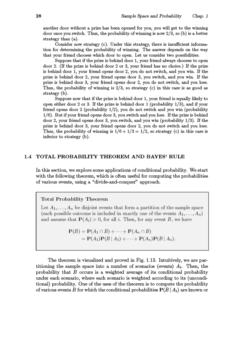
1.4 TOTAL PROBABILITY THEOREM AND BAYES' RULE
In this section, we explore some applications of conditional probability. We start
with the following theorem, which is often useful for computing the probabilities
of various events, using a "divide-and-conquer" approach.
The theorem is visualized and proved in Fig. 1.13. Intuitively, we are
partitioning the sample space into a number of scenarios (events) Ai. Then, the
probability that В occurs is a weighted average of its conditional probability
under each scenario, where each scenario is weighted according to its
(unconditional) probability. One of the uses of the theorem is to compute the probability
of various events В for which the conditional probabilities Р(Б | Ai) are known or

Sea 1.4 Total Probability Theorem and В ayes' Rule
29
Figure 1.13: Visualization and verification of the total probability theorem. The
events A\,..., An form a partition of the sample space, so the event В can be
decomposed into the disjoint union of its intersections Ai Π Β with the sets Ai,
i.e.,
В = (Ai Π Β) U · · · U (Ап Π Б).
Using the additivity axiom, it follows that
P(B) = P(Ai Π Β) + · · · + P(An Π Б).
Since, by the definition of conditional probability, we have
P(AinB) = P(Ai)P(B\Ai)>
the preceding equality yields
P(B) = P(ili)P(B I Ai) + · · · + Р(А„)Р(Б | An).
For an alternative view, consider an equivalent sequential model, as shown
on the right. The probability of the leaf Αι Π Β is the product P(Ai)P(B \Ai) of
the probabilities along the path leading to that leaf. The event В consists of the
three highlighted leaves and P(B) is obtained by adding their probabilities.
easy to derive. The key is to choose appropriately the partition Αχ7..., An, and
this choice is often suggested by the problem structure. Here are some examples.
Example 1.13. You enter a chess tournament where your probability of winning
a game is 0.3 against half the players (call them type 1), 0.4 against a quarter of
the players (call them type 2), and 0.5 against the remaining quarter of the players
(call them type 3). You play a game against a randomly chosen opponent. What
is the probability of winning?
Let Ai be the event of playing with an opponent of type г. We have
P(i4i) = 0.5, P(A2) = 0.25, P(A3) = 0.25.
Let also В be the event of winning. We have
Р(Б | Ai) = 0.3, Р(Б | A2) = 0.4, Р(Б | A3) = 0.5.

30
Sample Space and Probability Chap. 1
Thus, by the total probability theorem, the probability of winning is
Р(Б) = P(i4i)P(5 \A0 + Р(Л2)Р(Б | А2) + Р(Л3)Р(Б | Аъ)
= 0.5 · 0.3 + 0.25 · 0.4 + 0.25 · 0.5
= 0.375.
Example 1.14. You roll a fair four-sided die. If the result is 1 or 2, you roll once
more but otherwise, you stop. What is the probability that the sum total of your
rolls is at least 4?
Let Ai be the event that the result of first roll is г, and note that P(>U) = 1/4
for each г. Let Б be the event that the sum total is at least 4. Given the event Ai,
the sum total will be at least 4 if the second roll results in 3 or 4, which happens
with probability 1/2. Similarly, given the event Л2, the sum total will be at least
4 if the second roll results in 2, 3, or 4, which happens with probability 3/4. Also,
given the event Л3, you stop and the sum total remains below 4. Therefore,
P(B|Ai) = i, Ρ(Β|Λ2)=|, Ρ(Β|Λ3) = 0, Ρ(Β|Λ4)=1.
By the total probability theorem,
P(B)"4 2 + 4 4 + 4 °+4 U16·
The total probability theorem can be applied repeatedly to calculate
probabilities in experiments that have a sequential character, as shown in the following
example.
Example 1.15. Alice is taking a probability class and at the end of each week
she can be either up-to-date or she may have fallen behind. If she is up-to-date in
a given week, the probability that she will be up-to-date (or behind) in the next
week is 0.8 (or 0.2, respectively). If she is behind in a given week, the probability
that she will be up-to-date (or behind) in the next week is 0.4 (or 0.6, respectively).
Alice is (by default) up-to-date when she starts the class. What is the probability
that she is up-to-date after three weeks?
Let Ui and Bi be the events that Alice is up-to-date or behind, respectively,
after г weeks. According to the total probability theorem, the desired probability
Р(С/з) is given by
p(t/3) = р(с/2)Р(г/з I u2) + р(в2)Р(г/з I b2) = p(c/2) · 0.8+p(b2) · 0.4.
The probabilities Ρ(^2) and Р(^г) can also be calculated using the total probability
theorem:
P(U2) = P(tfi)P(tfa I Ci) + P(Bi)P(tfa I Bi) = P(C/i) · 0.8 + P(Bi) · 0.4,

Sea 1.4 Total Probability Theorem and В ayes' Rule
31
Р(Б2) = Ρ(ί/ι)Ρ(β2 Ι Ui) + P(£i)P(& I Bi) = P(C/i) ■ 0.2 + P(£i) · 0.6.
Finally, since Alice starts her class up-to-date, we have
P(l7i) = 0.8, P(£i) = 0.2.
We can now combine the preceding three equations to obtain
P(£/2) = 0.8 · 0.8 + 0.2 · 0.4 = 0.72,
P(£2) = 0.8 · 0.2 + 0.2 · 0.6 = 0.28,
and by using the above probabilities in the formula for Р(С/з):
p(C/3) = 0.72 · 0.8 + 0.28 · 0.4 = 0.688.
Note that we could have calculated the desired probability Р(£/з) by
constructing a tree description of the experiment, by calculating the probability of
every element of Us using the multiplication rule on the tree, and by adding.
However, there are cases where the calculation based on the total probability theorem is
more convenient. For example, suppose we are interested in the probability P(C/2o)
that Alice is up-to-date after 20 weeks. Calculating this probability using the
multiplication rule is very cumbersome, because the tree representing the experiment is
20-stages deep and has 220 leaves. On the other hand, with a computer, a sequential
calculation using the total probability formulas
P(£/*+i) = P(17<) ■ 0.8 + P( Д) ■ 0.4,
P(u+i) = P(W) · 0.2 + P(Д) · 0.6,
and the initial conditions Ρ(ΪΛ) = 0.8, P(-Bi) = 0.2, is very simple.
Inference and Bayes' Rule
The total probability theorem is often used in conjunction with the following
celebrated theorem, which relates conditional probabilities of the form Ρ (Α | Β)
with conditional probabilities of the form P(B | A), in which the order of the
conditioning is reversed.

32
Sample Space and Probability Chap. 1
To verify Bayes' rule, note that Ρ(Α*)Ρ(Β | A») and Ρ(Α*|Β)Ρ(Β) are
equal, because they are both equal to Ρ(Αί Π В). This yields the first equality.
The second equality follows from the first by using the total probability theorem
to rewrite P(B).
Bayes' rule is often used for inference. There are a number of "causes"
that may result in a certain "effect." We observe the effect, and we wish to infer
the cause. The events Ai,..., An are associated with the causes and the event В
represents the effect. The probability P(B | Ai) that the effect will be observed
when the cause Ai is present amounts to a probabilistic model of the cause-effect
relation (cf. Fig. 1.14). Given that the effect В has been observed, we wish to
evaluate the probability P(Ai \ B) that the cause Ai is present.
Figure 1.14: An example of the inference context that is implicit in Bayes'
rule. We observe a shade in a person's X-ray (this is event B, the "effect") and
we want to estimate the likelihood of three mutually exclusive and collectively
exhaustive potential causes: cause 1 (event A\) is that there is a malignant tumor,
cause 2 (event A2) is that there is a nonmalignant tumor, and cause 3 (event
A3) corresponds to reasons other than a tumor. We assume that we know the
probabilities P(Ai) and P(B | Ai), г = 1,2,3. Given that we see a shade (event
В occurs), Bayes' rule gives the conditional probabilities of the various causes as
PiA.im= P(AQP(£|A0
V " ; P(Al)P(Б|A1)+P(A2)P(S|A2)+P(A3)P(Б|Aз),
For an alternative view, consider an equivalent sequential model, as shown
on the right. The probability Ρ (Α ι \ Β) of a malignant tumor is the probability
of the first highlighted leaf, which is Ρ (Α ι Π Б), divided by the total probability
of the highlighted leaves, which is P(B).
Example 1.16. Let us return to the radar detection problem of Example 1.9 and
Fig. 1.9. Let
A = {an aircraft is present},
В = {the radar registers an aircraft presence}.

Sea 1.4 Total Probability Theorem and В ayes' Rule
33
We are given that
P(i4) = 0.05, Р(Б | A) = 0.99, Р(Б | Ac) = 0.1.
Applying Bayes' rule, with Αι = A and A2 = Ac, we obtain
Ρ (aircraft present | radar registers) =Έ>(Α\Β)
_ P(i4)P(£|i4)
P(B)
Έ>(Α)Έ>(Β\Α)
Р(Л)Р(Б I A) + Р(ЛС)Р(Б | Ac)
0.05 · 0.99
0.05· 0.99+0.95· 0.1
π 0.3426.
Example 1.17. Let us return to the chess problem of Example 1.13. Here, Ai is
the event of getting an opponent of type г, and
P(i4i) = 0.5, P(i42) = 0.25, Р(Л3) = 0.25.
Also, В is the event of winning, and
Р(Б | Ai) = 0.3, Р(Б | A2) = 0.4, Р(Б | A3) = 0.5.
Suppose that you win. What is the probability P(>h | B) that you had an opponent
of type 1?
Using Bayes' rule, we have
P(* | B) = VJA^WAj)
P(i4i)P(5 | АО + Р(Л2)Р(Б I A2) + Р(Л3)Р(Б | Аъ)
0.5 · 0.3
0.5· 0.3+0.25· 0.4+0.25· 0.5
0.4.
Example 1.18. The False-Positive Puzzle. A test for a certain rare disease is
assumed to be correct 95% of the time: if a person has the disease, the test results
are positive with probability 0.95, and if the person does not have the disease,
the test results are negative with probability 0.95. A random person drawn from
a certain population has probability 0.001 of having the disease. Given that the
person just tested positive, what is the probability of having the disease?
If A is the event that the person has the disease, and В is the event that the
test results are positive, the desired probability, Р(Л | Б), is
P(i4)P(£|i4)
T>(A\B) =
Р(Л)Р(Б | A) + Р(ЛС)Р(Б | Ac)
0.001 ■ 0.95
0.001 · 0.95 + 0.999 · 0.05
= 0.0187.

34
Sample Space and Probability Chap. 1
Note that even though the test was assumed to be fairly accurate, a person who has
tested positive is still very unlikely (less than 2%) to have the disease. According
to The Economist (February 20th, 1999), 80% of those questioned at a leading
American hospital substantially missed the correct answer to a question of this type.
Most of them said that the probability that the person has the disease is 0.95!
1.5 INDEPENDENCE
We have introduced the conditional probability Ρ (A | B) to capture the partial
information that event В provides about event A An interesting and important
special case arises when the occurrence of В provides no such information and
does not alter the probability that A has occurred, i.e.,
P(A\B)=P(A).
When the above equality holds, we say that A is independent of Б. Note that
by the definition P(A\B) = P(A Π Β)/Ρ(Β), this is equivalent to
P(AnB)=P(A)P(B).
We adopt this latter relation as the definition of independence because it can be
used even if P(-B) = 0, in which case Ρ (Α \ Β) is undefined. The symmetry of
this relation also implies that independence is a symmetric property; that is, if
A is independent of Б, then В is independent of A, and we can unambiguously
say that A and В are independent events.
Independence is often easy to grasp intuitively. For example, if the
occurrence of two events is governed by distinct and noninteracting physical processes,
such events will turn out to be independent. On the other hand, independence
is not easily visualized in terms of the sample space. A common first thought
is that two events are independent if they are disjoint, but in fact the opposite
is true: two disjoint events A and В with Ρ (A) > 0 and P(-B) > 0 are never
independent, since their intersection Α Π Б is empty and has probability 0.
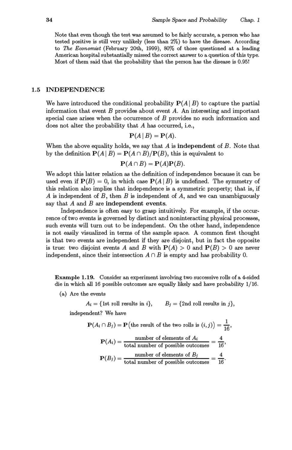
Example 1.19. Consider an experiment involving two successive rolls of a 4-sided
die in which all 16 possible outcomes are equally likely and have probability 1/16.
(a) Are the events
Ai = {1st roll results in г}, Bj = {2nd roll results in j},
independent? We have
1
P(Ai C)Bj) = P (the result of the two rolls is (г, j)) = —,
P(Ai) =
P(Bi) =
16'
number of elements of A% _ 4
total number of possible outcomes 16'
number of elements of Bj _ 4
total number of possible outcomes 16

Sea 1.5 Independence
35
We observe that "P(AiC\Bj) = 'P(Ai)P(Bj)1 and the independence of A% and
Bj is verified. Thus, our choice of the discrete uniform probability law (which
might have seemed arbitrary) models the independence of the two rolls.
(b) Are the events
A = {1st roll is a 1}, В = {sum of the two rolls is a 5},
independent? The answer here is not quite obvious. We have
P(i4 Π Β) = Ρ (the result of the two rolls is (1,4)) = —,
and also
ту/ A\ _ number of elements of A _ 4
total number of possible outcomes 16
The event В consists of the outcomes (1,4), (2,3), (3,2), and (4,1), and
number of elements of Б 4
P(B) =
total number of possible outcomes 16
Thus, we see that Р(ЛПБ) = Р(Л)Р(Б), and the events A and В are
independent.
(c) Are the events
A = {maximum of the two rolls is 2}, В = {minimum of the two rolls is 2},
independent? Intuitively, the answer is "no" because the minimum of the
two rolls conveys some information about the maximum. For example, if the
minimum is 2, the maximum cannot be 1. More precisely, to verify that A
and В are not independent, we calculate
P(i4 Π Β) = Ρ (the result of the two rolls is (2,2)) = -ί
and also
number of elements of A 3
P(A) =
P(B) =
total number of possible outcomes 16'
number of elements of Б _ 5
total number of possible outcomes 16
We have Р(Л)Р(Б) = 15/(16)2, so that Р(Л П В) ф Р(Л)Р(Б), and A and
В are not independent.

36
Sample Space and Probability Chap. 1
Conditional Independence
We noted earlier that the conditional probabilities of events, conditioned on
a particular event, form a legitimate probability law. We can thus talk about
independence of various events with respect to this conditional law. In particular,
given an event C, the events A and В are called conditionally independent
if
P(A Π В I С) = Έ>(Α I С)Р(Б | С).
To derive an alternative characterization of conditional independence, we use the
definition of the conditional probability and the multiplication rule, to write
P(A η Β I C)
We now compare the preceding two expressions, and after eliminating the
common factor P(B | C), assumed nonzero, we see that conditional independence is
the same as the condition
P(A\BnC)=P(A\C).
In words, this relation states that if С is known to have occurred, the additional
knowledge that В also occurred does not change the probability of A.
Interestingly, independence of two events A and В with respect to the
unconditional probability law, does not imply conditional independence, and
vice versa, as illustrated by the next two examples.
Example 1.20. Consider two independent fair coin tosses, in which all four
possible outcomes are equally likely. Let
Hi = {1st toss is a head},
Η2 = {2nd toss is a head},
D = {the two tosses have different results}.
The events Hi and Η2 are (unconditionally) independent. But
Р(Я1|Л)=|, Р(Я2|Я) = |, Р(Я1ПЯ2|Л) = 0,
so that Р(Я1 П Я2 ID) φ P(#i | D)P(H2 \ D), and Hu H2 are not conditionally
independent.
P(A Π Β Π С)
Р(С)
Р(С)Р(В\С)Р(А\ВпС)
Р(С)
= Р(Б I С)Р(А\ВпС).

Sea 1.5 Independence
37
Example 1.21. There are two coins, a blue and a red one. We choose one of
the two at random, each being chosen with probability 1/2, and proceed with two
independent tosses. The coins are biased: with the blue coin, the probability of
heads in any given toss is 0.99, whereas for the red coin it is 0.01.
Let Б be the event that the blue coin was selected. Let also Hi be the event
that the ith. toss resulted in heads. Given the choice of a coin, the events Hi and
Η2 are independent, because of our assumption of independent tosses. Thus,
P(#i Π Я2 | B) = P(iii | Б)Р(Я2 | B) = 0.99 · 0.99.
On the other hand, the events Hi and Η2 are not independent. Intuitively, if we
are told that the first toss resulted in heads, this leads us to suspect that the blue
coin was selected, in which case, we expect the second toss to also result in heads.
Mathematically, we use the total probability theorem to obtain
P(tfi) = P(B)P(tfi I B) + P(Sc)P(#i I &) = I · 0.99+ ± · 0.01 = ±,
as should be expected from symmetry considerations. Similarly, we have Ρ (#2) =
1/2. Now notice that
Έ>(Ηι ПН2) = Р(Б)Р(Я1 Π Я2 Ι В) + Р(БС)Р(Я1 П Я2 | Вс)
= \г · 0.99 · 0.99 + ^ · 0.01 · 0.01 « ^
Thus, Р(Я1 ПН2) ^ Р(Я1)Р(Я2), and the events Hi and Η2 are dependent, even
though they are conditionally independent given Б.
As mentioned earlier, if A and В are independent, the occurrence of В does
not provide any new information on the probability of A occurring. It is then
intuitive that the non-occurrence of В should also provide no information on the
probability of A. Indeed, it can be verified that if A and В are independent, the
same holds true for A and Bc (see the end-of-chapter problems).
We now summarize.

38
Sample Space and Probability Chap. 1
Independence of a Collection of Events
The definition of independence can be extended to multiple events.
For the case of three events, Αι, A2, and A3, independence amounts to
satisfying the four conditions
P(A1nA2)=P(A1)P(A2),
P(A1nA3) = P(A1)P(A3),
P(A2nAs) = P(A2)P(As),
P(Ai ni2n As) = P(Ai)P(A2)P(A3).
The first three conditions simply assert that any two events are independent,
a property known as pairwise independence. But the fourth condition is
also important and does not follow from the first three. Conversely, the fourth
condition does not imply the first three; see the two examples that follow.
Example 1.22. Pairwise Independence does not Imply Independence.
Consider two independent fair coin tosses, and the following events:

Sea 1.5 Independence
39
Hi = {1st toss is a head},
Η2 = {2nd toss is a head},
D = {the two tosses have different results}.
The events Hi and Η2 are independent, by definition. To see that Hi and D are
independent, we note that
P(£>|ffi)- p№) - ϊ/2 - 2 - Р(Г>)-
Similarly, #2 and D are independent. On the other hand, we have
p(ff! nff2nfl) = 0^ \ · 1 · 1 = р(Я1)Р(Я2)Рф),
and these three events are not independent.
Example 1.23. The Equality P(i4i Π Α2 П A3) = P(i4i)P(i42)P(i43) is not
Enough for Independence. Consider two independent rolls of a fair six-sided
die, and the following events:
A = {1st roll is 1, 2, or 3},
В = {1st roll is 3, 4, or 5},
С = {the sum of the two rolls is 9}.
We have
Р(ЛПБ) = |^|.|=Р(Л)Р(В),
ρμηα) = ±4.± = Ρ(Λ)Ρ(α),
Thus the three events А, Б, and С are not independent, and indeed no two of these
events are independent. On the other hand, we have
Р(ЛПБПС7) = ± = 1.1.±=Р(Л)Р(В)Р(С).
The intuition behind the independence of a collection of events is
analogous to the case of two events. Independence means that the occurrence or
non-occurrence of any number of the events from that collection carries no
information on the remaining events or their complements. For example, if the
events Ai, ^2,^3, Ai are independent, one obtains relations such as
Ρ (Αι U A2 I As Π Μ) = Ρ (Αι U A2)
or
P(Ai U Al I A\ η Μ) = P(Ai U A§);
see the end-of-chapter problems.

40
Sample Space and Probability Chap. 1
Reliability
In probabilistic models of complex systems involving several components, it is
often convenient to assume that the behaviors of the components are uncoupled
(independent). This typically simplifies the calculations and the analysis, as
illustrated in the following example.
Example 1.24. Network Connectivity. A computer network connects two
nodes A and В through intermediate nodes C, D, E, F, as shown in Fig. 1.15(a).
For every pair of directly connected nodes, say г and j, there is a given probability
Pij that the link from г to j is up. We assume that link failures are independent
of each other. What is the probability that there is a path connecting A and В in
which all links are up?
Figure 1.15: (a) Network for Example 1.24. The number next to each link
indicates the probability that the link is up. (b) Series and parallel connections
of three components in a reliability problem.
This is a typical problem of assessing the reliability of a system consisting of
components that can fail independently. Such a system can often be divided into
subsystems, where each subsystem consists in turn of several components that are
connected either in series or in parallel; see Fig. 1.15(b).
Let a subsystem consist of components 1, 2,... ,ra, and let pi be the
probability that component г is up ("succeeds"). Then, a series subsystem succeeds
if all of its components are up, so its probability of success is the product of the
probabilities of success of the corresponding components, i.e.,
Ρ (series subsystem succeeds) = P1P2 - 'Pm-
A parallel subsystem succeeds if any one of its components succeeds, so its
probability of failure is the product of the probabilities of failure of the corresponding
components, i.e.,
Ρ (parallel subsystem succeeds) = 1 — Ρ (parallel subsystem fails)
= l-(l-Pl)(l-p2)-..(l-pro).

Sea 1.5 Independence
41
Returning now to the network of Fig. 1.15(a), we can calculate the
probability of success (a path from A to В is available) sequentially, using the preceding
formulas, and starting from the end. Let us use the notation X —*■ Υ to denote the
event that there is a (possibly indirect) connection from node X to node Y. Then,
P(C ->B)=l-(l- P(C -»■ Ε and Ε -»■ Б)) (l - Ρ (С ^FandF^ Б))
= 1 - (1 -рс.Б№в)(1 -pofPfb)
= 1 - (1 - 0.8 ■ 0.9)(1 - 0.95 · 0.85)
= 0.946,
Р(Л -»■ С and С -»■ Б) = Р(Л -»■ С)Р(С -»■ В) = 0.9 · 0.946 = 0.851,
Р(Л -»■ D and D -»■ Б) = Р(Л -»■ D)P(D -»■ Б) = 0.75 · 0.95 = 0.712,
and finally we obtain the desired probability
Έ>(Α -> Б) = 1 - (l - Ρ (A -> С and С -> Б)) (l - Р(Л -> D and D -> Б))
= 1-(1-0.851)(1-0.712)
= 0.957.
Independent Trials and the Binomial Probabilities
If an experiment involves a sequence of independent but identical stages, we say
that we have a sequence of independent trials. In the special case where there
are only two possible results at each stage, we say that we have a sequence of
independent Bernoulli trials. The two possible results can be anything, e.g.,
"it rains" or "it doesn't rain," but we will often think in terms of coin tosses and
refer to the two results as "heads" (H) and "tails" (T).
Consider an experiment that consists of η independent tosses of a coin, in
which the probability of heads is p, where ρ is some number between 0 and 1. In
this context, independence means that the events j4.i,j4.2,. .. ,An are
independent, where Αι = {ith. toss is a head}.
We can visualize independent Bernoulli trials by means of a sequential
description, as shown in Fig. 1.16 for the case where η = 3. The conditional
probability of any toss being a head, conditioned on the results of any
preceding tosses is p, because of independence. Thus, by multiplying the conditional
probabilities along the corresponding path of the tree, we see that any particular
outcome (3-long sequence of heads and tails) that involves к heads and 3 — к
tails has probability pk(l — p)3_/c. This formula extends to the case of a general
number η of tosses. We obtain that the probability of any particular n-long
sequence that contains к heads and η — к tails is pk(l — p)n_/c, for all к from 0
to n.
Let us now consider the probability
p(k) =P(k heads come up in an η-toss sequence),

42
Sample Space and Probability Chap. 1
Figure 1.16: Sequential description of an experiment involving three
independent tosses of a coin. Along the branches of the tree, we record the corresponding
conditional probabilities, and by the multiplication rule, the probability of
obtaining a particular 3-toss sequence is calculated by multiplying the probabilities
recorded along the corresponding path of the tree.
which will play an important role later. We showed above that the probability
of any given sequence that contains к heads is pk(l — p)n_/c, so we have
p(k)= (f\pk(l-p)n-k,
where we use the notation
. . number of distinct η-toss sequences that contain к heads.
kj
The numbers (£) (called "n choose к") are known as the binomial coefficients,
while the probabilities p(k) are known as the binomial probabilities. Using a
counting argument, to be given in Section 1.6, we can show that
n\ n\
к = 0,1,... , η,
KkJ k\(n-k)V
where for any positive integer г we have
г! = 1 · 2 · · · (г - 1) · г,
and, by convention, 0! = 1. An alternative verification is sketched in the end-of-
chapter problems. Note that the binomial probabilities p(k) must add to 1, thus

Sea 1.6 Counting 43
showing the binomial formula
£(?W-p)«-*=i.
k=0 ^ '
Example 1.25. Grade of Service. An internet service provider has installed с
modems to serve the needs of a population of η customers. It is estimated that at a
given time, each customer will need a connection with probability p, independently
of the others. What is the probability that there are more customers needing a
connection than there are modems?
Here we are interested in the probability that more than с customers
simultaneously need a connection. It is equal to
η
Ε **>»
fc=c+l
where
l К t
are the binomial probabilities. For instance, ifra=100, p=0.1, and с = 15, the
desired probability turns out to be 0.0399.
This example is typical of problems of sizing a facility to serve the needs of a
homogeneous population, consisting of independently acting customers. The
problem is to select the facility size to achieve a certain threshold probability (sometimes
called grade of service) that no user is left unserved.
1.6 COUNTING
The calculation of probabilities often involves counting the number of outcomes
in various events. We have already seen two contexts where such counting arises.
(a) When the sample space Ω has a finite number of equally likely outcomes,
so that the discrete uniform probability law applies. Then, the probability
of any event A is given by
_, . ν number of elements of A
number of elements of Ω'
and involves counting the elements of A and of Ω.
(b) When we want to calculate the probability of an event A with a finite
number of equally likely outcomes, each of which has an already known
probability p. Then the probability of A is given by
Ρ (Α) = ρ · (number of elements of A),

44
Sample Space and Probability Chap. 1
and involves counting the number of elements of A An example of this type
is the calculation of the probability of к heads in η coin tosses (the binomial
probabilities). We saw in the preceding section that the probability of each
distinct sequence involving к heads is easily obtained, but the calculation
of the number of all such sequences is somewhat intricate, as will be seen
shortly.
While counting is in principle straightforward, it is frequently challenging;
the art of counting constitutes a large portion of the field of combinatorics. In
this section, we present the basic principle of counting and apply it to a number
of situations that are often encountered in probabilistic models.
The Counting Principle
The counting principle is based on a divide-and-conquer approach, whereby the
counting is broken down into stages through the use of a tree. For example,
consider an experiment that consists of two consecutive stages. The possible
results of the first stage are αι,α2,... ,am; the possible results of the second
stage are 61,62?— · ?&n. Then, the possible results of the two-stage experiment
are all possible ordered pairs (сц, fy), г = 1,... ,m, j = 1,..., n. Note that the
number of such ordered pairs is equal to run. This observation can be generalized
as follows (see also Fig. 1.17).
Figure 1.17: Illustration of the basic counting principle. The counting is carried
out in r stages (r = 4 in the figure). The first stage has n\ possible results. For
every possible result of the first г — 1 stages, there are щ possible results at the
ith stage. The number of leaves is гь\гьч · · -nr. This is the desired count.

Sea 1.6 Counting
45
Example 1.26. The Number of Telephone Numbers. A telephone number
is a 7-digit sequence, but the first digit has to be different from 0 or L How many
distinct telephone numbers are there? We can visualize the choice of a sequence
as a sequential process, where we select one digit at a time. We have a total of 7
stages, and a choice of one out of 10 elements at each stage, except for the first
stage where we only have 8 choices. Therefore, the answer is
8·10·10···10 = 8·106.
6 times
Example 1.27. The Number of Subsets of an n-Element Set. Consider
an гь-element set {si, $2, ♦ ♦ ♦, sn}- How many subsets does it have (including itself
and the empty set)? We can visualize the choice of a subset as a sequential process
where we examine one element at a time and decide whether to include it in the set
or not. We have a total of η stages, and a binary choice at each stage. Therefore
the number of subsets is
η times
It should be noted that the Counting Principle remains valid even if each
first-stage result leads to a different set of potential second-stage results, etc. The
only requirement is that the number of possible second-stage results is constant,
regardless of the first-stage result.
In what follows, we will focus primarily on two types of counting arguments
that involve the selection of к objects out of a collection of η objects. If the order
of selection matters, the selection is called a permutation, and otherwise, it is
called a combination. We will then discuss a more general type of counting,
involving a partition of a collection of η objects into multiple subsets.

46
Sample Space and Probability Chap. 1
fc-per mutations
We start with η distinct objects, and let к be some positive integer, with к < η.
We wish to count the number of different ways that we can pick к out of these
η objects and arrange them in a sequence, i.e., the number of distinct k-object
sequences. We can choose any of the η objects to be the first one. Having chosen
the first, there are only η — 1 possible choices for the second; given the choice of
the first two, there only remain η — 2 available objects for the third stage, etc.
When we are ready to select the last (the fcth) object, we have already chosen
к — 1 objects, which leaves us with η — (к — 1) choices for the last one. By the
Counting Principle, the number of possible sequences, called fc-permutations,
is
n(n - 1) ■ ■ ■ (n - к + 1) (η - fc) ■ ■ ■ 2 ■ 1
n(n - 1) · · · (n - к + 1) =
η!
(n-fc)---2-l
(n-k)V
In the special case where к = η, the number of possible sequences, simply called
permutations, is
η(η-1)(η-2)···2·1 =η!.
(Let fc = η in the formula for the number of fc-permutations, and recall the
convention 0! = 1.)
Example 1.28. Let us count the number of words that consist of four distinct
letters. This is the problem of counting the number of 4-permutations of the 26
letters in the alphabet. The desired number is
ra! 26!
= — = 26 · 25 · 24 · 23 = 358,800.
(n-k)\ 22!
The count for permutations can be combined with the Counting Principle
to solve more complicated counting problems.
Example 1.29. You have щ classical music CDs, гаг rock music CDs, and газ
country music CDs. In how many different ways can you arrange them so that the
CDs of the same type are contiguous?
We break down the problem in two stages, where we first select the order of
the CD types, and then the order of the CDs of each type. There are 3! ordered
sequences of the types of CDs (such as classical/rock/country, rock/country/classical,
etc.), and there are rail (or гаг!, or газ!) permutations of the classical (or rock, or
country, respectively) CDs. Thus for each of the 3! CD type sequences, there are
rail гаг! газ! arrangements of CDs, and the desired total number is 3! rail гаг! газ!.

Sea 1,6 Counting
47
Combinations
There are η people and we are interested in forming a committee of fc. How
many different committees are possible? More abstractly, this is the same as the
problem of counting the number of fc-element subsets of a given n-element set.
Notice that forming a combination is different than forming a k-permutation,
because in a combination there is no ordering of the selected elements.
Thus for example, whereas the 2-permutations of the letters А, В, С, and D are
AB, AC, AD, BA, ВС, BD, CA, CB, CD, DA, DB, DC,
the combinations of two out of these four letters are
AB, AC, AD, ВС, BD, CD.
(Since the elements of a combination are unordered, В A is not viewed as being
distinct from AB.)
To count the number of combinations, we observe that selecting a k-
permutation is the same as first selecting a combination of к items and then
ordering them. Since there are k\ ways of ordering the к selected items, we
see that the number n\/(n — k)\ of k-permutations is equal to the number of
combinations times fc!. Hence, the number of possible combinations, is equal to
fc!(n-fc)!'
Let us now relate the above expression to the binomial coefficient, which
was denoted by (£) and was defined in the preceding section as the number of
η-toss sequences with к heads. We note that specifying an η-toss sequence with
к heads is the same as selecting к elements (those that correspond to heads) out
of the n-element set of tosses, i.e., a combination of к out of η objects. Hence,
the binomial coefficient is also given by the same formula and we have
/n\ n!
\k) = k\(n-k)V
Example 1.30. The number of combinations of two out of the four letters A, B,
C, and D is found by letting η = 4 and к = 2. It is
\2) = 2!2! = 6?
consistently with the listing given earlier.

48
Sample Space and Probability Chap. 1
It is worth observing that counting arguments sometimes lead to formulas
that are rather difficult to derive algebraically. One example is the binomial
formula
£(£)pfc(1-i,)n~*=1'
/c=0
discussed in Section 1.5. In the special case where ρ = 1/2, this formula becomes
/c=0 Ч 7
and admits the following simple interpretation. Since (£) is the number of k-
element subsets of a given n-element subset, the sum over к of (£) counts the
number of subsets of all possible cardinalities. It is therefore equal to the number
of all subsets of an η-element set, which is 2n.
Partitions
Recall that a combination is a choice of к elements out of an η-element set
without regard to order. Thus, a combination can be viewed as a partition of
the set in two: one part contains к elements and the other contains the remaining
η — fc. We now generalize by considering partitions into more than two subsets.
We are given an η-element set and nonnegative integers ηχ,η2,... ,nr,
whose sum is equal to n. We consider partitions of the set into r disjoint subsets,
with the ith subset containing exactly щ elements. Let us count in how many
ways this can be done.
We form the subsets one at a time. We have (^) ways of forming the
first subset. Having formed the first subset, we are left with η — n\ elements.
We need to choose n<2 of them in order to form the second subset, and we have
(n~ni) choices, etc. Using the Counting Principle for this r-stage process, the
total number of choices is
n\ in — П-Л in — П\ — П2\ /η — П1 — · · · — ПГ_;Д
\П\) \ П2 J \ ПЗ J \ Пг У
which is equal to
n! (n —ni)! (n— n\ — · · · — nr-i)\
nil (n — ni)! П2! (n — ni — П2)! (n — ni — · · · — nr_i — nr)\ nr\ *
We note that several terms cancel and we are left with
n!
П\\ П2! · · · Ur\

Sea 1.6 Counting
49
This is called the multinomial coefficient and is usually denoted by
( n )·
Example 1.31. Anagrams. How many different words (letter sequences) can be
obtained by rearranging the letters in the word TATTOO? There are six positions
to be filled by the available letters. Each rearrangement corresponds to a partition
of the set of the six positions into a group of size 3 (the positions that get the letter
T), a group of size 1 (the position that gets the letter A), and a group of size 2 (the
positions that get the letter O). Thus, the desired number is
_g_=l-2-3-4-5-6
1! 2! 3! 1 · 1 · 2 · 1 · 2 · 3
It is instructive to derive this answer using an alternative argument. (This
argument can also be used to rederive the multinomial coefficient formula; see
the end-of-chapter problems.) Let us write TATTOO in the form TiAT2T30i02
pretending for a moment that we are dealing with 6 distinguishable objects. These
6 objects can be rearranged in 6! different ways. However, any of the 3! possible
permutations of Τι, Τι, and Тз, as well as any of the 2! possible permutations of
Oi and O2, lead to the same word. Thus, when the subscripts are removed, there
are only 6!/(3!2!) different words.
Example 1.32. A class consisting of 4 graduate and 12 undergraduate students
is randomly divided into four groups of 4. What is the probability that each group
includes a graduate student? This is the same as Example 1.11 in Section 1.3, but
we will now obtain the answer using a counting argument.
We first determine the nature of the sample space. A typical outcome is a
particular way of partitioning the 16 students into four groups of 4. We take the
term "randomly" to mean that every possible partition is equally likely, so that the
probability question can be reduced to one of counting.
According to our earlier discussion, there are
/ 16 \_ 16!
\4,4,4,4/ " 4!4!4!4!
different partitions, and this is the size of the sample space.
Let us now focus on the event that each group contains a graduate student.
Generating an outcome with this property can be accomplished in two stages:
(a) Take the four graduate students and distribute them to the four groups; there
are four choices for the group of the first graduate student, three choices for
the second, two for the third. Thus, there is a total of 4! choices for this stage.
(b) Take the remaining 12 undergraduate students and distribute them to the
four groups (3 students in each). This can be done in
/ 12 \_ 12!
\3,3,3,3/ " 3!3!3!3!

50 Sample Space and Probability Chap. 1
different ways.
By the Counting Principle, the event of interest can occur in
4! 12!
3!3!3!3!
different ways. The probability of this event is
4! 12!
3!3!3!3!
16!
4! 4! 4! 4!
After some cancellations, we find that this is equal to
12 ■ 8 ■ 4
15· 14· 13'
consistent with the answer obtained in Example 1.11.
Here is a summary of all the counting results we have developed.
1.7 SUMMARY AND DISCUSSION
A probability problem can usually be broken down into a few basic steps:
(a) The description of the sample space, that is, the set of possible outcomes
of a given experiment.
(b) The (possibly indirect) specification of the probability law (the probability
of each event).
(c) The calculation of probabilities and conditional probabilities of various
events of interest.

Sea 1.7 Summary and Discussion
51
The probabilities of events must satisfy the nonnegativity, additivity, and
normalization axioms. In the important special case where the set of possible
outcomes is finite, one can just specify the probability of each outcome and obtain
the probability of any event by adding the probabilities of the elements of the
event.
Given a probability law, we are often interested in conditional probabilities,
which allow us to reason based on partial information about the outcome of
the experiment. We can view conditional probabilities as probability laws of a
special type, under which only outcomes contained in the conditioning event can
have positive conditional probability. Conditional probabilities can be derived
from the (unconditional) probability law using the definition P(A \B) =Ρ(ΑΠ
В)/Р(В). However, the reverse process is often convenient, that is, first specify
some conditional probabilities that are natural for the real situation that we wish
to model, and then use them to derive the (unconditional) probability law.
We have illustrated through examples three methods for calculating
probabilities:
(a) The counting method. This method applies to the case where the
number of possible outcomes is finite, and all outcomes are equally likely. To
calculate the probability of an event, we count the number of elements of
the event and divide by the number of elements of the sample space.
(b) The sequential method. This method applies when the experiment has a
sequential character, and suitable conditional probabilities are specified or
calculated along the branches of the corresponding tree (perhaps using the
counting method). The probabilities of various events are then obtained
by multiplying conditional probabilities along the corresponding paths of
the tree, using the multiplication rule.
(c) The divide-and-conquer method. Here, the probabilities P(-B) of
various events В are obtained from conditional probabilities Р(Б | A*), where
the Αι are suitable events that form a partition of the sample space and
have known probabilities P(A^). The probabilities P(-B) are then obtained
by using the total probability theorem.
Finally, we have focused on a few side topics that reinforce our main themes.
We have discussed the use of Bayes' rule in inference, which is an important
application context. We have also discussed some basic principles of counting
and combinatorics, which are helpful in applying the counting method.

52
Sample Space and Probability Chap. 1
PROBLEMS
SECTION 1.1. Sets
Problem 1. Consider rolling a six-sided die. Let A be the set of outcomes where the
roll is an even number. Let Б be the set of outcomes where the roll is greater than 3.
Calculate and compare the sets on both sides of De Morgan's laws
(A U B)c = АСП Bc, (Α Π Β) ° = Ac U Bc.
Problem 2. Let A and В be two sets.
(a) Show that
Ac = (Ac η В) U (Ac η Бс), Вс = (Α η Вс) U (Ас η Вс).
(b) Show that
(Α Π В)с = (Ас Π Б) U (Ас Π Вс) U (An Bc).
(c) Consider rolling a six-sided die. Let A he the set of outcomes where the roll
is an odd number. Let Б be the set of outcomes where the roll is less than 4.
Calculate the sets on both sides of the equality in part (b), and verify that the
equality holds.
Problem 3.* Prove the identity
Ли(п~=1Бп) =η~=ί(ΑυΒη).
Solution. If χ belongs to the set on the left, there are two possibilities. Either xGi,
in which case χ belongs to all of the sets A U Бп, and therefore belongs to the set on
the right. Alternatively, χ belongs to all of the sets Bn in which case, it belongs to all
of the sets A U Бп, and therefore again belongs to the set on the right.
Conversely, if χ belongs to the set on the right, then it belongs to A U Bn for all
n. If χ belongs to A, then it belongs to the set on the left. Otherwise, χ must belong
to every set Bn and again belongs to the set on the left.
Problem 4.* Cantor's diagonalization argument. Show that the unit interval
[0,1] is uncountable, i.e., its elements cannot be arranged in a sequence.
Solution. Any number ж in [0,1] can be represented in terms of its decimal expansion,
e.g., 1/3 = 0.3333 · · ·. Note that most numbers have a unique decimal expansion,
but there are a few exceptions. For example, 1/2 can be represented as 0.5000 · · · or
as 0.49999 · · ·. It can be shown that this is the only kind of exception, i.e., decimal
expansions that end with an infinite string of zeroes or an infinite string of nines.

Problems
53
Suppose, to obtain a contradiction, that the elements of [0,1] can be arranged
in a sequence Ж1,Ж2,£з,..., so that every element of [0,1] appears in the sequence.
Consider the decimal expansion of xn:
_ n 1 2 3
Xn — V.CLnCLnCLn · · · ,
where each digit агп belongs to {0,1,..., 9}. Consider now a number у constructed as
follows. The nth digit of у can be 1 or 2, and is chosen so that it is different from the
nth digit of Xn- Note that у has a unique decimal expansion since it does not end with
an infinite sequence of zeroes or nines. The number у differs from each xn, since it has
a different nth digit. Therefore, the sequence cci, ж 2,... does not exhaust the elements
of [0,1], contrary to what was assumed. The contradiction establishes that the set [0,1]
is uncountable.
SECTION 1.2. Probabilistic Models
Problem 5. Out of the students in a class, 60% are geniuses, 70% love chocolate,
and 40% fall into both categories. Determine the probability that a randomly selected
student is neither a genius nor a chocolate lover.
Problem 6. A six-sided die is loaded in a way that each even face is twice as likely
as each odd face. All even faces are equally likely, as are all odd faces. Construct a
probabilistic model for a single roll of this die and find the probability that the outcome
is less than 4.
Problem 7. A four-sided die is rolled repeatedly, until the first time (if ever) that an
even number is obtained. What is the sample space for this experiment?
Problem 8.* Bonferroni's inequality.
(a) Prove that for any two events A and Б, we have
P(i4 Π Β) > P(i4) + Р(Б) - 1.
(b) Generalize to the case of η events Αι, Л2,..., An, by showing that
P(i4ini42n---ni4n)>P(i4i) + P(i42)+---+P(i4n)-(n-l).
Solution. We have Р(Л U В) = Р(Л) + Р(Б) - Р(Л Π Β) and Р(Л U В) < 1, which
implies part (a). For part (b), we use De Morgan's law to obtain
1 - P(Ai Π · · · Π An) = Ρ ((Ai Π · · · Π An)c)
= р<л?и-.-и^)
<р(Л5) + ... + р(^)
= (1-Р(Л1))+...+ (1-Р(Лп))
= η-Έ>(Α1) Ρ(Λ,).

54
Sample Space and Probability Chap. 1
Problem 9.* The inclusion-exclusion formula. Show the following generalizes
tions of the formula
P(i4 U Β) = Έ>(Α) + Р(Б) - Έ>(Α Π Б).
(a) Let А, Б, and С be events. Then,
Р(ЛиБиС) = Р(Л)+Р(Б)+Р(С)-Р(ЛПБ)-Р(БПС)-Р(ЛПС)+Р(ЛПБПС).
(b) Let Αι, Аъ,... ,i4n be events. Let 5i = {г 11 < г < тг}, 5г = {(ή,^) 11 < ч <
г2 < η}> and more generally, let Sm be the set of all m-tuples (ii,...,im) of
indices that satisfy 1 < ή < %2 < · · · < im < n. Then,
P (ut=1Ak) = Σ Ρ(Λ4) - £ P(Ah η At2)
+ Σ P(i4ilni4i2ni4l8)---- + (-l)n-1P(n2=1A»).
Solution, (a) We use the formulas P(X U Y) = P(X) + P(Y) - P(X Π У) and
(Л U Б) Π С = (А П С) U (В Π С). We have
Έ>(Α UBUC) = Έ>(Α U В) + Р(С) - Ρ ((Л U Б) Π С)
= Р(Л U Б) + Р(С) - Ρ ((Л Π С) U (Б Π С))
= Р(Л U Б) + Р(С) - Р(Л Π С) - Р(Б Π С) + Р(Л Π Б Π С)
= Р(Л) + Р(Б) - Р(Л Π Б) + Р(С) - Р(Л Π С) - Р(Б Π С)
+ Р(ЛпБпС)
= Р(Л) + Р(Б) + Р(С) - Р(Л Π Б) - Р(Б Π С) - Р(Л Π С)
+ Р(ЛпБпС).
(b) Use induction and verify the main induction step by emulating the derivation of
part (a). For a different approach, see the problems at the end of Chapter 2.
Problem 10.* Continuity property of probabilities.
(a) Let Αι, Α2,... be an infinite sequence of events, which is "monotonically
increasing," meaning that An С -Αη+ι for every n. Let A = и^=1Ап. Show that
Р(Л) = Итп-юоР(>1п)- Hint: Express the event Л as a union of count ably
many disjoint sets.
(b) Suppose now that the events are "monotonically decreasing," i.e., Αη+ι С Ап
for every n. Let A = n%LiAn. Show that ~P{A) = limn_}.00P(>ln). Hint: Apply
the result of part (a) to the complements of the events.
(c) Consider a probabilistic model whose sample space is the real line. Show that
P([0,oo)) = lim P([0,n]) and lim P([n,oo)) = 0.

Problems
55
Solution, (a) Let B\ = A\ and, for η > 2, Bn = An ΠΑ^-ί- The events Bn are
disjoint, and we have U^=1Bk = An, and Ц^Б*. = A, We apply the additivity axiom
to obtain
oo η
Ρ(Λ) = VP(B»)= lim Vp(St)= lim P(u£=1Sfc) = HmP(4„).
' ^ п-юо ' ^ п-юо n—J-oo
(b) Let Сn = A%, and С = Ac. Since Лп+1 С Лп, we obtain Cn С <7η+ι, and the events
С η are increasing. Furthermore, С = Ac = (П^Лп)0 = \J£=1Acn = \J£=1Cn. Using
the result from part (a) for the sequence Cn, we obtain
1 --P(A) = -p(Ac) = -p(C) = lim P(Cn) = lim (1-Р(Лп)),
η—юо п-юо ν '
from which we conclude that Έ>(Α) = limn_}.00P(>ln).
(c) For the first equality, use the result from part (a) with An = [0, n] and A = [0, oo).
For the second, use the result from part (b) with An = [n, oo) and A = Ρ^=1Αη = 0.
SECTION 1.3. Conditional Probability
Problem 11. We roll two fair 6-sided dice. Each one of the 36 possible outcomes is
assumed to be equally likely.
(a) Find the probability that doubles are rolled.
(b) Given that the roll results in a sum of 4 or less, find the conditional probability
that doubles are rolled.
(c) Find the probability that at least one die roll is a 6.
(d) Given that the two dice land on different numbers, find the conditional probability
that at least one die roll is a 6.
Problem 12. A coin is tossed twice. Alice claims that the event of two heads is at
least as likely if we know that the first toss is a head than if we know that at least one
of the tosses is a head. Is she right? Does it make a difference if the coin is fair or
unfair? How can we generalize Alice's reasoning?
Problem 13. We are given three coins: one has heads in both faces, the second has
tails in both faces, and the third has a head in one face and a tail in the other. We
choose a coin at random, toss it, and it comes heads. What is the probability that the
opposite face is tails?
Problem 14. A batch of one hundred items is inspected by testing four randomly
selected items. If one of the four is defective, the batch is rejected. What is the
probability that the batch is accepted if it contains five defectives?
Problem 15. Let Л and В be events. Show that Р(Л (Ί В | В) = Ρ (Л | Б), assuming
that Р(Б) > 0.

56
Sample Space and Probability Chap. 1
SECTION 1.4. Total Probability Theorem and Bayes' Rule
Problem 16. Alice searches for her term paper in her filing cabinet, which has η
drawers. She knows that she left her term paper in drawer j with probability pj > 0.
The drawers are so messy that even if she correctly guesses that the term paper is in
drawer г, the probability that she finds it is only сЦ. Alice searches in a particular
drawer, say drawer г, but the search is unsuccessful. Conditioned on this event, show
that the probability that her paper is in drawer j, is given by
Vi if.-^i Pt(l-dj)
Problem 17. How an inferior player with a superior strategy can gain an
advantage. Boris is about to play a two-game chess match with an opponent, and
wants to find the strategy that maximizes his winning chances. Each game ends with
either a win by one of the players, or a draw. If the score is tied at the end of the two
games, the match goes into sudden-death mode, and the players continue to play until
the first time one of them wins a game (and the match). Boris has two playing styles,
timid and bold, and he can choose one of the two at will in each game, no matter what
style he chose in previous games. With timid play, he draws with probability pd > 0,
and he loses with probability 1 — pd* With bold play, he wins with probability pw, and
he loses with probability 1 — pw. Boris will always play bold during sudden death, but
may switch style between games 1 and 2.
(a) Find the probability that Boris wins the match for each of the following strategies:
(i) Play bold in both games 1 and 2.
(ii) Play timid in both games 1 and 2.
(iii) Play timid whenever he is ahead in the score, and play bold otherwise.
(b) Assume that pw < 1/2, so Boris is the worse player, regardless of the playing
style he adopts. Show that with the strategy in (iii) above, and depending on
the values of pw and pd, Boris may have a better than a 50-50 chance to win the
match. How do you explain this advantage?
Problem 18. Two players take turns removing a ball from a jar that initially contains
m white and η black balls. The first player to remove a white ball wins. Develop a
recursive formula that allows the convenient computation of the probability that the
starting player wins.
Problem 19. Each of к jars contains m white and η black balls. A ball is randomly
chosen from jar 1 and transferred to jar 2, then a ball is randomly chosen from jar 2
and transferred to jar 3, etc. Finally, a ball is randomly chosen from jar /e. Show that
the probability that the last ball is white is the same as the probability that the first
ball is white, i.e., it is m/(m-\- n).
Problem 20. We have two jars each containing initially η balls. We perform four
successive ball exchanges. In each exchange, we pick simultaneously and at random a
ball from each jar and move it to the other jar. What is the probability that at the
end of the four exchanges all the balls will be in the jar where they started?

Problems
57
Problem 21. The prisoner's dilemma. Two out of three prisoners are to be
released. One of the prisoners asks a guard to tell him the identity of a prisoner other
than himself that will be released. The guard refuses with the following rationale: at
your present state of knowledge, your probability of being released is 2/3, but after you
know my answer, your probability of being released will become 1/2, since there will
be two prisoners (including yourself) whose fate is unknown and exactly one of the two
will be released. What is wrong with the guard's reasoning?
Problem 22. A two-envelopes puzzle. You are handed two envelopes, and you
know that each contains a positive integer dollar amount and that the two amounts are
different. The values of these two amounts are modeled as constants that are unknown.
Without knowing what the amounts are, you select at random one of the two envelopes,
and after looking at the amount inside, you may switch envelopes if you wish. A friend
claims that the following strategy will increase above 1/2 your probability of ending
up with the envelope with the larger amount: toss a coin repeatedly, let X be equal to
1/2 plus the number of tosses required to obtain heads for the first time, and switch
if the amount in the envelope you selected is less than the value of X, Is your friend
correct?
Problem 23. The paradox of induction. Consider a statement whose truth is
unknown. If we see many examples that are compatible with it, we are tempted to
view the statement as more probable. Such reasoning is often referred to as
inductive inference (in a philosophical, rather than mathematical sense). Consider now the
statement that "all cows are white." An equivalent statement is that "everything that
is not white is not a cow." We then observe several black crows. Our observations are
clearly compatible with the statement, but do they make the hypothesis "all cows are
white" more likely?
To analyze such a situation, we consider a probabilistic model. Let us assume
that there are two possible states of the world, which we model as complementary
events:
A : all cows are white,
Ac : 50% of all cows are white.
Let ρ be the prior probability Ρ (A) that all cows are white. We make an observation
of a cow or a crow, with probability q and 1 — q, respectively, independently of whether
event A occurs or not. Assume that 0<ρ<1,0<<?<1, and that all crows are black.
(a) Given the event В = {a black crow was observed}, what is Р(Л | Б)?
(b) Given the event С = {a white cow was observed}, what is Р(Л | С)?
Problem 24.* Conditional version of the total probability theorem. Show
the identity
P(i41 B) = P(C | B)P(A | Β η С) + P(CC | B)P(A \ Β η Cc),
assuming all the conditioning events have positive probability.
Solution. Using the conditional probability definition and the additivity axiom on the
disjoint sets Α Π Β (Ί С and Α Π Β (Ί Cc, we obtain

58 Sample Space and Probability Chap. 1
P(C | B)P(A | Б η С) + P(CC I Б)Р(Л | Б П Сс)
Р(БпС) Р(ЛпБпС) Ρ(ΰηα°) Р(ЛпБпСс)
Р(Б) " Р(БпС) + Р(Б) " Р(БпСс)
_ Р(Л П Б П С) + Р(Л П Б П Сс)
Р(Б)
Ρ ((Л Π Б Π С) U (Л Π В η Сс))
= Р(Б)
_ Р(ЛпБ)
Р(Б)
= Р(А|В).
Problem 25.* Let A and Б be events with P(Л) > 0 and Р(Б) > 0. We say that
an event Б suggests an event Л if Ρ (Л | В) > P(>1), and does not suggest event Л if
Р(Л | Б) < Р(Л).
(a) Show that Б suggests A if and only if A suggests B.
(b) Assume that Р(БС) > 0. Show that Б suggests A if and only if Bc does not
suggest A.
(c) We know that a treasure is located in one of two places, with probabilities β and
1 — β, respectively, where 0 < β < 1. We search the first place and if the treasure
is there, we find it with probability p> 0. Show that the event of not finding the
treasure in the first place suggests that the treasure is in the second place.
Solution, (a) We have Р(Л | Б) = Р(Л П Б)/Р(Б), so Б suggests A if and only if
Р(ЛпБ) >Р(Л)Р(Б), which is equivalent to A suggesting Б, by symmetry.
(b) Since Р(Б) + Р(БС) = 1, we have
Р(Б)Р(Л) + Р(БС)Р(Л) = P(A) = Р(Б)Р(Л | Б) + Р(БС)Р(Л | Бс),
which implies that
Р(БС) (P(A) - P(i4 | Bc)) = Р(Б) (Р(А | Б) - P(A)).
Thus, P(i4 | Б) > P(i4) (Б suggests A) if and only if P(A) > Ρ (Л | Бс) (Бс does not
suggest Л).
(c) Let A and Б be the events
A = {the treasure is in the second place},
Б = {we don't find the treasure in the first place}.
Using the total probability theorem, we have
P(B) = Р(ЛС)Р(Я | Ac) + Р(Л)Р(В \Α) = β(1-ρ) + (1-β),

Problems
59
It follows that event Б suggests event A.
SECTION 1.5. Independence
Problem 26. A hunter has two hunting dogs. One day, on the trail of some animal,
the hunter comes to a place where the road diverges into two paths. He knows that
each dog, independently of the other, will choose the correct path with probability p.
The hunter decides to let each dog choose a path, and if they agree, take that one, and
if they disagree, to randomly pick a path. Is his strategy better than just letting one
of the two dogs decide on a path?
Problem 27. Communication through a noisy channel. A binary (0 or 1)
symbol transmitted through a noisy communication channel is received incorrectly
with probability бо and ei, respectively (see Fig. 1.18). Errors in different symbol
transmissions are independent.
Figure 1.18: Error probabilities in a binary communication channel·
(a) Suppose that the channel source transmits a 0 with probability ρ and transmits a
1 with probability 1 — p. What is the probability that a randomly chosen symbol
is received correctly?
(b) Suppose that the string of symbols 1011 is transmitted. What is the probability
that all the symbols in the string are received correctly?
(c) In an effort to improve reliability, each symbol is transmitted three times and
the received symbol is decoded by majority rule. In other words, a 0 (or 1) is
transmitted as 000 (or 111, respectively), and it is decoded at the receiver as a
0 (or 1) if and only if the received three-symbol string contains at least two 0s
(or Is, respectively). What is the probability that a transmitted 0 is correctly
decoded?
(d) Suppose that the channel source transmits a 0 with probability ρ and transmits
a 1 with probability 1 — p, and that the scheme of part (c) is used. What is the
probability that a 0 was transmitted given that the received string is 101?
Problem 28. The king's sibling. The king has only one sibling. What is the
probability that the sibling is male? Assume that every birth results in a boy with probability

60
Sample Space and Probability Chap. 1
1/2, independent of other births. Be careful to state any additional assumptions you
have to make in order to arrive at an answer.
Problem 29. Using a biased coin to make an unbiased decision. Alice and Bob
want to choose between the opera and the movies by tossing a fair coin. Unfortunately,
the only available coin is biased (though the bias is not known exactly). How can they
use the biased coin to make a decision so that either option (opera or the movies) is
equally likely to be chosen?
Problem 30. An electrical system consists of identical components that are
operational with probability p, independently of other components. The components are
connected in three subsystems, as shown in Fig. 1.19. The system is operational if
there is a path that starts at point A, ends at point Б, and consists of operational
components. This is the same as requiring that all three subsystems are operational.
What are the probabilities that the three subsystems, as well as the entire system, are
operational?
Figure 1.19: A system of identical components that consists of the three
subsystems 1, 2, and 3. The system is operational if there is a path that starts at
point A, ends at point B, and consists of operational components.
Problem 31. Reliability of a k-out-of-n system. A system consists of η identical
components that are operational with probability p, independently of other
components. The system is operational if at least к out of the η components are operational.
What is the probability that the system is operational?
Problem 32. A power utility can supply electricity to a city from η different power
plants. Power plant г fails with probability pi, independently of the others.
(a) Suppose that any one plant can produce enough electricity to supply the entire
city. What is the probability that the city will experience a black-out?
(b) Suppose that two power plants are necessary to keep the city from a black-out.
Find the probability that the city will experience a black-out.
Problem 33. A cellular phone system services a population of η ι 'Voice users" (those
that occasionally need a voice connection) and n^ "data users" (those that occasionally
need a data connection). We estimate that at a given time, each user will need to be
connected to the system with probability pi (for voice users) or p2 (for data users),

Problems
61
independently of other users. The data rate for a voice user is η bits/sec and for a data
user is Г2 bits/sec. The cellular system has a total capacity of с bits/sec. What is the
probability that more users want to use the system than the system can accommodate?
Problem 34. The problem of points. Telis and Wendy play a round of golf (18
holes) for a $10 stake, and their probabilities of winning on any one hole are ρ and
1 — p, respectively, independently of their results in other holes. At the end of 10 holes,
with the score 4 to 6 in favor of Wendy, Telis receives an urgent call and has to report
back to work. They decide to split the stake in proportion to their probabilities of
winning had they completed the round, as follows. If ρτ and pw axe the conditional
probabilities that Telis and Wendy, respectively, are ahead in the score after 18 holes
given the 4-6 score after 10 holes, then Telis should get a fraction ρτ/(ρτ ~Vpw) of the
stake, and Wendy should get the remaining pw/{pr + pw)· How much money should
Telis get? Note: This is an example of the, so-called, problem of points, which played
an important historical role in the development of probability theory. The problem
was posed by Chevalier de Mere in the 17th century to Pascal, who introduced the
idea that the stake of an interrupted game should be divided in proportion to the
players' conditional probabilities of winning given the state of the game at the time of
interruption. Pascal worked out some special cases and through a correspondence with
Fermat, stimulated much thinking and several probability-related investigations.
Problem 35. A particular class has had a history of low attendance. The annoyed
professor decides that she will not lecture unless at least к of the η students enrolled
in the class are present. Each student will independently show up with probability
pg if the weather is good, and with probability рь if the weather is bad. Given the
probability of bad weather on a given day, calculate the probability that the professor
will teach her class on that day.
Problem 36. Consider a coin that comes up heads with probability ρ and tails with
probability 1 — p. Let qn be the probability that after η independent tosses, there have
been an even number of heads. Derive a recursion that relates qn to qn-it and solve
this recursion to establish the formula
<Ь=(1 + (1-2рГ)/2.
Problem 37.* Gambler's ruin. A gambler makes a sequence of independent bets.
In each bet, he wins $1 with probability p, and loses $1 with probability 1—p, Initially,
the gambler has $/e, and plays until he either accumulates %n or has no money left.
What is the probability that the gambler will end up with $тг?
Solution. Let us denote by A the event that he ends up with $тг, and by F the event
that he wins the first bet. Denote also by Wk the probability of event A, if he starts
with $/e. We apply the total probability theorem to obtain
wk = Р(Л | F)P(F) + Р(Л I FC)V(FC) = pP(A \ F) + qP(A \ Fc), 0 < к < η,
where q = 1 — p. By the independence of past and future bets, having won the first bet
is the same as if he were just starting now but with $(/e+l), so that ~P(A\F) = lUfc+i
and similarly Р(Л | F°) = Wk-i* Thus, we have Wk = pwk+i + qwk-i, which can be
written as
Wfc+i -Wk = r(wk - Wfc_i), 0 < к < nf

62
Sample Space and Probability Chap. 1
where r = q/p. We will solve for Wk in terms of ρ and q using iteration, and the
boundary values wo = 0 and wn = 1.
We have lUfc+i — Wk = rk(wi — гио), and since гио = 0,
fc fc—1 fc fc
iufc+i = Wk + г г^1 = Wfc_i + г iui + r w\ = w\ + riui + \- r w\.
The sum in the right-hand side can be calculated separately for the two cases where
r = 1 (or ρ = q) and τ φ 1 (or ρ φ q). We have
{1 -rh
kwit if p= q.
Since ад η = 1, we can solve for w\ and therefore for ги&:
1-r
Wi =
so that
wk =
Problem 38.* Let A and Б be independent events. Use the definition of
independence to prove the following:
(a) The events A and Bc are independent.
(b) The events Ac and Bc are independent.
Solution, (a) The event A is the union of the disjoint events АГ\ВС and АГ\В. Using
the additivity axiom and the independence of A and Б, we obtain
P(i4) = P(i4 Π Б) + Р(Л Π Бс) = Р(Л)Р(Б) + Р(Л Π Бс).
It follows that
P(i4 Π Бс) = P(i4) (l - Р(Б)) = Р(Л)Р(БС),
so A and Бс are independent.
(b) Apply the result of part (a) twice: first on A and Б, then on Bc and A.
Problem 39.* Let A, B, and С be independent events, with P(C) > 0. Prove that
A and В are conditionally independent given С
Solution. We have
PMnBio-EU^gpa
P(A)P(B)P(C)
P(C)
= Р(Л)Р(В)
= P(i4|(7)P(B|(7),

Problems
63
so A and В are conditionally independent given C, In the preceding calculation, the
first equality uses the definition of conditional probabilities; the second uses the
assumed independence; the fourth uses the independence of A from C, and of В from C,
Problem 40.* Assume that the events А\,Аъ,Аъ,А± are independent and that
Р(Лз Π Α4) > 0. Show that
P(i4i U A21A3 Π A4) = P(i4i U A2).
Solution. We have
1><А\АПА\ РМ1ПЛ3ПЛ4) Ρ(Λι)Ρ(Λ8)Ρ(Λ4) рм,
Ρ(Χι I Лз Π JU) = г{АзПА4) = р(Лз)Р(Л4) = Р(Л1)'
We similarly obtain Р(Л2 | Лз П Л4) = P(>h) and P(j4i ПЛ2 | Лз ПА4) = P(j4i ПЛ2),
and finally,
P(i4i U Л21А3 η Л4) = P(i4i I As Π Л4) + Р(Л21Л3 Π Л4) - P(Ai Π Л21А3 П Л4)
= P(i4i)+P(i42)-P(i4ini42)
= P(i4iUi42).
Problem 41.* Laplace's rule of succession. Consider m-\- 1 boxes with the /eth
box containing к red balls and m — k white balls, where к ranges from 0 to m. We
choose a box at random (all boxes are equally likely) and then choose a ball at random
from that box, η successive times (the ball drawn is replaced each time, and a new ball
is selected independently). Suppose a red ball was drawn each of the η times. What
is the probability that if we draw a ball one more time it will be red? Estimate this
probability for large m.
Solution. We want to find the conditional probability Έ>(Ε | Rn), where Ε is the event
of a red ball drawn at time n-\-1, and Rn is the event of a red ball drawn each of the η
preceding times. Intuitively, the consistent draw of a red ball indicates that a box with
a high percentage of red balls was chosen, so we expect that Έ>(Ε | Rn) is closer to 1
than to 0. In fact, Laplace used this example to calculate the probability that the sun
will rise tomorrow given that it has risen for the preceding 5,000 years. (It is not clear
how serious Laplace was about this calculation, but the story is part of the folklore of
probability theory.)
We have
and by using the total probability theorem, we obtain
JUL / h\n л ^ / h\n
P(i4) = EP(^h box chosen) (A) = _L_£(±) ,
fc=0 fc=0
m ό-1-1
P(iniil) = P(JW.) = ^IEfc) ·
fc=0

64
Sample Space and Probability Chap. 1
For large m, we can view ~P(Rn) as a piecewise constant approximation to an integral:
k\n 1 Γ «, 1 mn+1 1
v ' m + l^U/ m+lmMn
(m+l)mn n+1 η+Γ
fc=0 ' t/u
Similarly,
Р(£пД„) = Р(^+1)«-1^,
so that
Thus, for large ra, drawing a red ball one more time is almost certain when η is large.
Problem 42.* Binomial coefficient formula and the Pascal triangle.
(a) Use the definition of (£) as the number of distinct ?>toss sequences with к
heads, to derive the recursion suggested by the so called Pascal triangle, given in
Fig. 1.20.
(b) Use the recursion derived in part (a) and induction, to establish the formula
к k\ (n - k)\'
Figure 1.20: Sequential calculation method of the binomial coefficients using the
Pascal triangle. Each term («) in the triangular array on the left is computed
and placed in the triangular array on the right by adding its two neighbors in the
row above it (except for the boundary terms with к = 0 or к = η, which are equal
to 1).
Solution, (a) Note that тг-toss sequences that contain к heads (for 0 < к < η) can be
obtained in two ways:
(1) By starting with an (n— l)-toss sequence that contains к heads and adding a tail
at the end. There are (η^) different sequences of this type.

Problems
65
(2) By starting with an (n — l)-toss sequence that contains к — 1 heads and adding
a head at the end. There are
(lZ{) different sequences of this type.
Thus,
1, if /e = 0, тг.
This is the formula corresponding to the Pascal triangle calculation, given in Fig. 1.20.
(b) We now use the recursion from part (a), to demonstrate the formula
n\ n\
к J k\(n-k)V
by induction on n. Indeed, we have from the definition (I) = (]) = 1, so for тг = 1 the
above formula is seen to hold as long as we use the convention 0! = 1. If the formula
holds for each index up to η — 1, we have for к = 1, 2,..., η — 1,
n\ _ in — l\ in— 1
(k - 1)! (n - 1 - к + 1)! k\ (n - 1 - k)\
к n\ η — к п\
η k\(n-k)\ ' η k\(n-k)\
n\
~ k\(n-k)V
and the induction is complete.
Problem 43.* The Bore 1-CanteHi lemma. Consider an infinite sequence of trials.
The probability of success at the ith trial is some positive number pi. Let N be the
event that there is no success, and let / be the event that there is an infinite number
of successes.
(a) Assume that the trials are independent and that Y^=1P% = oo. Show that
P(N) = 0 and P(J) = 1.
(b) Assume that Σ^ p% < oo. Show that P(/) = 0.
subset of the event th
η
P(JV)<JJ(1-W).
Solution, (a) The event N is a subset of the event that there were no successes in the
first η trials, so that
i=l
Taking logarithms,
togp(jv) < £>g(i - w) < Σί-w).

66
Sample Space and Probability Chap. 1
Taking the limit as η tends to infinity, we obtain log Ρ (TV) = — oo, or P(iV) = 0.
Let now Ln be the event that there is a finite number of successes and that the
last success occurs at the nth. trial. We use the already established result P(iV) = 0,
and apply it to the sequence of trials after trial n, to obtain P(Ln) = 0. The event Iе
(finite number of successes) is the union of the disjoint events Ln, η > 1, and N, so
that
oo
P(Jc) = P(iV) + ^P(L„) = 0,
n=l
and P(J) = 1.
(b) Let S% be the event that the ith. trial is a success. Fix some number η and for every
г > тг, let Fi be the event that the first success after time η occurs at time г. Note
that Fi С Si. Finally, let An be the event that there is at least one success after time
n. Note that J С Ап, because an infinite number of successes implies that there are
successes subsequent to time n. Furthermore, the event An is the union of the disjoint
events Fi, i > n. Therefore,
(oo \ oo oo oo
U Fi = Σ р<ди Σ ρ(5<)= Σ ρ*·
i=n+l / %=n+l %=n+l %=n+l
We take the limit of both sides as η —*■ oo. Because of the assumption Y^=1 Pi < oo,
the right-hand side converges to zero. This implies that P(/) = 0.
SECTION 1.6. Counting
Problem 44. De Mere's puzzle. A six-sided die is rolled three times independently.
Which is more likely: a sum of 11 or a sum of 12? (This question was posed by the
French nobleman de Mere to his friend Pascal in the 17th century.)
Problem 45. The birthday problem. Consider η people who are attending a
party. We assume that every person has an equal probability of being born on any day
during the year, independently of everyone else, and ignore the additional complication
presented by leap years (i.e., nobody is born on February 29). What is the probability
that each person has a distinct birthday?
Problem 46. An urn contains m red and η white balls.
(a) We draw two balls randomly and simultaneously. Describe the sample space and
calculate the probability that the selected balls are of different color, by using
two approaches: a counting approach based on the discrete uniform law, and a
sequential approach based on the multiplication rule.
(b) We roll a fair 3-sided die whose faces are labeled 1,2,3, and if к comes up, we
remove к balls from the urn at random and put them aside. Describe the sample
space and calculate the probability that all of the balls drawn are red, using a
divide-and-conquer approach and the total probability theorem.
Problem 47. We deal from a well-shuffled 52-card deck. Calculate the probability
that the 13th card is the first king to be dealt.

Problems 67
Problem 48. Ninety students, including Joe and Jane, are to be split into three
classes of equal size, and this is to be done at random. What is the probability that
Joe and Jane end up in the same class?
Problem 49. Twenty distinct cars park in the same parking lot every day. Ten of
these cars are US-made, while the other ten are foreign-made. The parking lot has
exactly twenty spaces, all in a row, so the cars park side by side. However, the drivers
have varying schedules, so the position any car might take on a certain day is random.
(a) In how many different ways can the cars line up?
(b) What is the probability that on a given day, the cars will park in such a way
that they alternate (no two US-made are adjacent and no two foreign-made are
adjacent)?
Problem 50. Eight rooks are placed in distinct squares of an 8 X 8 chessboard, with
all possible placements being equally likely. Find the probability that all the rooks are
safe from one another, i.e., that there is no row or column with more than one rook.
Problem 51. An academic department offers 8 lower level courses: {Li, L2,..., Ls}
and 10 higher level courses: {i?i, i?2, ♦ ♦ ♦, i?io}- A valid curriculum consists of 4 lower
level courses, and 3 higher level courses.
(a) How many different curricula are possible?
(b) Suppose that {i?i,..., Η5} have L\ as a prerequisite, and {He,... Ηю} have L2
and L3 as prerequisites, i.e., any curricula which involve, say, one of {i?i,..., Hq}
must also include Li. How many different curricula are there?
Problem 52. How many 6-word sentences can be made using each of the 26 letters
of the alphabet exactly once? A word is defined as a nonempty (possibly jibberish)
sequence of letters.
Problem 53. Consider a group of η persons. A club consists of a special person from
the group (the club leader) and a number (possibly zero) of additional club members.
(a) Explain why the number of possible clubs is n2n_1.
(b) Find an alternative way of counting the number of possible clubs and show the
identity
Problem 54. We draw the top 7 cards from a well-shuffled standard 52-card deck.
Find the probability that:
(a) The 7 cards include exactly 3 aces.
(b) The 7 cards include exactly 2 kings.
(c) The probability that the 7 cards include exactly 3 aces or exactly 2 kings.
Problem 55. A parking lot contains 100 cars, к of which happen to be lemons. We
select m of these cars at random and take them for a testdrive. Find the probability

68
Sample Space and Probability Chap. 1
that η of the cars tested turn out to be lemons.
Problem 56. A well-shuffled 52-card deck is dealt to 4 players. Find the probability
that each of the players gets an ace.
Problem 57.* Hypergeometric probabilities. An urn contains η balls, out of
which ra are red. We select к of the balls at random, without replacement (i.e., selected
balls are not put back into the urn before the next selection). What is the probability
that г of the selected balls are red?
Solution. The sample space consists of the (£ J different ways that we can select к out
of the available balls. For the event of interest to occur, we have to select г out of the
ra red balls, which can be done in (™) ways, and also select к — г out of the n—m blue
balls, which can be done in (^Ί™) ways. Therefore, the desired probability is
(T)(V-T)
G) '
for г > 0 satisfying г < га, г < /с, and к — г <п — т. For all other г, the probability is
zero.
Problem 58.* Correcting the number of permutations for indistinguishable
objects. When permuting η objects, some of which are indistinguishable, different
permutations may lead to indistinguishable object sequences, so the number of
distinguishable object sequences is less than n\. For example, there are six permutations of
the letters A, B, and C:
ABC, ACB, ВАС, BCA, CAB, CBA,
but only three distinguishable sequences that can be formed using the letters A, D,
and D:
ADD, DAD, DDA.
(a) Suppose that к out of the η objects are indistinguishable. Show that the number
of distinguishable object sequences is n\/k\,
(b) Suppose that we have r types of indistinguishable objects, and for each г, ki
objects of type г. Show that the number of distinguishable object sequences is
n\
Solution, (a) Each one of the n\ permutations corresponds to k\ duplicates which are
obtained by permuting the к indistinguishable objects. Thus, the n\ permutations can
be grouped into n\/k\ groups of k\ indistinguishable permutations that result in the
same object sequence. Therefore, the number of distinguishable object sequences is
n\/k\. For example, the three letters A, D, and D give the 3! = 6 permutations
ADD, ADD, DAD, DDA, DAD, DDA,

Problems
69
obtained by replacing В and С by D in the permutations of A, B, and С given earlier.
However, these 6 permutations can be divided into the n\/k\ = 3!/2! = 3 groups
{ADD, ADD}, {DAD, DAD}, {DDA, DDA},
each having k\ = 2! = 2 indistinguishable permutations.
(b) One solution is to extend the argument in (a) above: for each object type г, there are
ki\ indistinguishable permutations of the fe objects. Hence, each permutation belongs
to a group of fci! fe! · · · krl indistinguishable permutations, all of which yield the same
object sequence.
An alternative argument goes as follows. Choosing a distinguishable object
sequence is the same as starting with η slots and for each г, choosing the fe slots to be
occupied by objects of type г. This is the same as partitioning the set {1,..., n} into
groups of size /ci,..., kT, and the number of such partitions is given by the multinomial
coefficient.

2
Discrete Random Variables
Contents
2.1. Basic Concepts p. 72
2.2. Probability Mass Functions p. 74
2.3. Functions of Random Variables p. 80
2.4. Expectation, Mean, and Variance p. 81
2.5. Joint PMFs of Multiple Random Variables p. 92
2.6. Conditioning p. 98
2.7. Independence p. 110
2.8. Summary and Discussion p. 116
Problems p. 119
71

72
Discrete Random Variables Chap 2
2.1 BASIC CONCEPTS
In many probabilistic models, the outcomes are numerical, e.g , when they
correspond to instrument readings or stock prices. In other experiments, the outcomes
are not numerical, but they may be associated with some numerical values of
interest. For example, if the experiment is the selection of students from a given
population, we may wish to consider their grade point average. When dealing
with such numerical values, it is often useful to assign probabilities to them.
This is done through the notion of a random variable, the focus of the present
chapter.
Given an experiment and the corresponding set of possible outcomes (the
sample space), a random variable associates a particular number with each
outcome, see Fig. 2.1 We refer to this number as the numerical value or simply
the value of the random variable. Mathematically, a random variable is a
real-valued function of the experimental outcome.
3 4
Real number line
Sample space
pairs of rolls
(b>
Figure 2.1: (a) Visualization of a random variable It is a function that assigns
a numerical value to each possible outcome of the experiment (b) An example
of a random variable. The experiment consists of two rolls of a 4-sided die, and
the random variable is the maximum of the two rolls. If the outcome of the
experiment is (4,2), the value of this random variable is 4
Here are some examples of random variables*
In an experiment involving a sequence of 5 tosses of a coin, the number of
heads in the sequence is a random variable. However, the 5-long sequence

Sec. 2Λ Basic Concepts
73
of heads and tails is not considered a random variable because it does not
have an explicit numerical value.
(b) In an experiment involving two rolls of a die, the following are examples of
random variables:
(i) The sum of the two rolls.
(ii) The number of sixes in the two rolls.
(iii) The second roll raised to the fifth power.
(c) In an experiment involving the transmission of a message, the time needed
to transmit the message, the number of symbols received in error, and the
delay with which the message is received are all random variables.
There are several basic concepts associated with random variables, which
are summarized below. These concepts will be discussed in detail in the present
chapter.
Main Concepts Related to Random Variables
Starting with a probabilistic model of an experiment:
φ A random variable is a real-valued function of the outcome of the
experiment,
© A function of a random variable defines another random variable.
© We can associate with each random variable certain "averages" of
interest, such as the mean and the variance.
© A random variable can be conditioned on an event or on another |
random variable. I
© There is a notion of independence of a random variable from an |
event or from another random variable. I
A random variable is called discrete if its range (the set of values that
it can take) is finite or at most countably infinite. For example, the random
variables mentioned in (a) and (b) above can take at most a finite number of
numerical values, and are therefore discrete.
A random variable that can take an uncountably infinite number of values
is not discrete. For an example, consider the experiment of choosing a point
α from the interval [—1,1]. The random variable that associates the numerical
value a2 to the outcome a is not discrete. On the other hand, the random variable
that associates with a the numerical value
( 1, if a > 0,
sgn(a) — < 0, if a = 0,
l-l, ifa<0,

74
Discrete Random Variables Chap. 2
is discrete.
In this chapter, we focus exclusively on discrete random variables, even
though we will typically omit the qualifier "discrete."
Concepts Related to Discrete Random Variables
Starting with a probabilistic model of an experiment:..;...
© A discrete random variable is a real-valued function of the outcome
* of the experiment that can take a finite or countably infinite number
of values.
© A discrete random variable has an associated probability mass
function (PMF), which gives the probability of each numerical value that
the random variable can take.
"· A function of a discrete random variable defines another discrete
random variable, whose PMF can be obtained from the PMF of the
original random variable.
We will discuss each of the above concepts and the associated methodology
in the following sections. In addition, we will provide examples of some important
and frequently encountered random variables. In Chapter 3, we will discuss
general (not necessarily discrete) random variables.
Even though this chapter may appear to be covering a lot of new ground,
this is not really the case. The general line of development is to simply take
the concepts from Chapter 1 (probabilities, conditioning, independence, etc.)
and apply them to random variables rather than events, together with some
appropriate new notation. The only genuinely new concepts relate to means and
variances.
2.2 PROBABILITY MASS FUNCTIONS
The most important way to characterize a random variable is through the
probabilities of the values that it can take. For a discrete random variable X, these
are captured by the probability mass function (PMF for short) of X, denoted
ρχ. In particular, if χ is any possible value of X, the probability mass of я,
denoted px(x)) is the probability of the event {X = x} consisting of all outcomes
that give rise to a value of X equal to x:
Px{x) = F{{X = x}).
For example, let the experiment consist of two independent tosses of a fair coin,
and let X be the number of heads obtained. Then the PMF of X is

Sec. 2.2 Probability Mass Functions
75
{1/4, if x = 0 or χ = 2,
1/2, ifs = l,
0, otherwise.
In what follows, we will often omit the braces from the event/set notation,
when no ambiguity can arise. In particular, we will usually write P(X = x)
in place of the more correct notation P({X = x}). We will also adhere to
the following convention throughout: we will use upper case characters
to denote random variables, and lower case characters to denote real
numbers such as the numerical values of a random variable.
Note that
J2px(x) = 1,
X
where in the summation above, χ ranges over all the possible numerical values
of X. This follows from the additivity and normalization axioms, because the
events {X = x) are disjoint and form a partition of the sample space, as χ ranges
over all possible values of X, By a similar argument, for any set S of possible
values of X, we have
P(XeS) = ^Px(x).
xes
For example, if X is the number of heads obtained in two independent tosses of
a fair coin, as above, the probability of at least one head is
2
x—1
Calculating the PMF of X is conceptually straightforward, and is
illustrated in Fig. 2.2.
Calculation of the PMF of a Random Variable X
For each possible value χ of X:
1. Collect all the possible outcomes that give rise to the event {X = x}.
2, Add their probabilities to obtain ρχ(χ). ··.··
The Bernoulli Random Variable
Consider the toss of a coin, which comes up a head with probability p, and a tail
with probability 1 — p. The Bernoulli random variable takes the two values 1
and 0, depending on whether the outcome is a head or a tail:
γ __ / 1» ^ a neadj
""" \ 0, if a tail.

76
Discrete R&ndom Variables Chap. 2
Ρχ(χ)
Event {X= x}
(a)
4 ψ ψ
гк
2'φ;':.. :'ψ
■φ φ
%\
Sample space:
pairs of rolls
Random variable:
X = maximum roll
(b)
J3_
16
JL -
16
Figure 2.2: (a) Illustration of the method to calculate the PMF of a random
variable X. For each possible value x, we collect all the outcomes that give rise
to X — χ and add their probabilities to obtain ρχ(χ). (b) Calculation of the
PMF px of the random variable X = maximum roll in two independent rolls
of a fair 4-sided die. There are four possible values x, namely, 1, 2, 3, 4. To
calculate px(x) for a given x, we add the probabilities of the outcomes that give
rise to x. For example, there are three outcomes that give rise to a: — 2, namely,
(1,2), (2,2), (2,1). Each of these outcomes has probability 1/16, so ρ χ (2) = 3/16,
as indicated in the figure.
Its PMF is
px(x) =
P,
-P,
if χ = 1,
if χ = 0.
For all its simplicity, the Bernoulli random variable is very important. In
practice, it is used to model generic probabilistic situations with just two
outcomes, such as:
(a) The state of a telephone at a given time that can be either free or busy.
(b) A person who can be either healthy or sick with a certain disease.
(c) The preference of a person who can be either for or against a certain
political candidate.

Sec. 2.2 Probability Mass Functions
77
Furthermore, by combining multiple Bernoulli random variables, one can
construct more complicated random variables, such as the binomial random variable,
which is discussed next.
The Binomial Random Variable
A coin is tossed η times. At each toss, the coin comes up a head with probability
p, and a tail with probability 1 — p, independently of prior tosses. Let X be the
number of heads in the η-toss sequence. We refer to X as a binomial random
variable with parameters η and p. The PMF of X consists of the binomial
probabilities that were calculated in Section 1.5:
px(k) = P(X = *:)=( 'J )p*(l - ρ)»"*
к = 0,1,... ,n.
(Note that here and elsewhere, we simplify notation and use fc, instead of x,
to denote the values of integer-valued random variables.) The normalization
property, specialized to the binomial random variable, is written as
£("V(i-p)»-fc = i.
Some special cases of the binomial PMF are sketched in Fig. 2.3.
Px
i
0
L Binomial ]
> ι 1
ι 2 :
\ 4
3MF
f η = 9, ρ = 1/2
1111 .r
5 6 7 8 9 к
PxW
4
Binomial PMF,
η = large, ρ = small
lilL
Figure 2.3: The PMF of a binomial random variable. If ρ = 1/2, the PMF is
symmetric around n/2. Otherwise, the PMF is skewed towards 0 if ρ < 1/2, and
towards η if ρ > 1/2.
The Geometric Random Variable
Suppose that we repeatedly and independently toss a coin with probability of
a head equal to p, where 0 < ρ < 1. The geometric random variable is the
number X of tosses needed for a head to come up for the first time. Its PMF is
given by
Px{k) = (1 ~p)k~lP,
fc = l,2,...,

78
Discrete Random Variables Chap. 2
since (1 - p)k~~1p is the probability of the sequence consisting of к — 1 successive
tails followed by a head; see Fig. 2.4. This is a legitimate PMF because
Σρχ (k) = Σ^1 ™ P)k~lP = Ρ Σ^1 ~P)k=P'Y
fc=l
/c=l
Jfc=0
(i-p)
= 1.
Naturally, the use of coin tosses here is just to provide insight. More
generally, we can interpret the geometric random variable in terms of repeated
independent trials until the first "success." Each trial has probability of success
ρ and the number of trials until (and including) the first success is modeled by
the geometric random variable. The meaning of "success" is context-dependent.
For example, it could mean passing a test in a given try, or finding a missing
item in a given search, or logging into a computer system in a given attempt,
etc.
A
Ρ
PxW
Μ111111 ,
12 3 к
Figure 2.4: The PMF
РХ(*) = (1-Р)*-1Р, А = 1,2,...,
of a geometric random variable. It decreases as a geometric progression with
parameter 1 — p.
The Poisson Random Variable
A Poisson random variable has a PMF given by
px(k) = e-* — , fc = 0,1,2,...,
where λ is a positive parameter characterizing the PMF, see Fig. 2.5. This is a
legitimate PMF because
Σ'
fc=0
Xk . Λ . λ2 A3
'¥ = β-λ 1 + λ+2ί + ¥ +
— e~xex

Sec. 2.2 Probability Mass Functions
79
~λ~0.6
PxW
Poisson, λ = 0.5
1 2 3
i
β-λ~0.05
0
t PxW
I
1 2
Poisson, λ =5 3
2
Ih..
4 5 6 7*
Figure 2.5: The PMF e~xXk/k\ of the Poisson random variable for different
values of λ. Note that if λ < 1, then the PMF is monotonically decreasing, while
if λ > 1, the PMF first increases and then decreases as the value of к increases
(this is shown in the end-of-chapter problems).
To get a feel for the Poisson random variable, think of a binomial random
variable with very small ρ and very large n. For example, consider the number
of typos in a book with a total of η words, when the probability ρ that any one
word is misspelled is very small (associate a word with a coin toss which comes
a head when the word is misspelled), or the number of cars involved in accidents
in a city on a given day (associate a car with a coin toss which comes a head
when the car has an accident). Such random variables can be well-modeled with
a Poisson PMF.
More precisely, the Poisson PMF with parameter Λ is a good approximation
for a binomial PMF with parameters η and p, i.e.,
D-λ
Π!
λ*
k\ k\ (n - k)
■pk{l-p)n~k, fc = 0,l,...,n,
provided λ = np) η is very large, and ρ is very small. In this case, using the
Poisson PMF may result in simpler models and calculations. For example, let
η = 100 and ρ = 0.01. Then the probability of к = 5 successes in η — 100 trials
is calculated using the binomial PMF as
100!
95! 5!
•0.015(1-0.01)95 = 0.00290.
Using the Poisson PMF with λ = np
approximated by
1
100 · 0.01 = 1, this probability is
3-i.
5!
0.00306.
We provide a formal justification of the Poisson approximation property
in the end-of-chapter problems and also in Chapter 5, where we will further
interpret it, extend it, and use it in the context of the Poisson process.

80
Discrete Random Variables Chap. 2
2.3 FUNCTIONS OF RANDOM VARIABLES
Given a random variable X, one may generate other random variables by
applying various transformations on X. As an example, let the random variable
X be today's temperature in degrees Celsius, and consider the transformation
Υ = 1ЯХ 4- 32, which gives the temperature in degrees Fahrenheit. In this
example, Υ is a linear function of X, of the form
Υ = g(X) = аХ + Ъ,
where α and b are sealars. We may also consider nonlinear functions of the
general form
For example, if we wish to display temperatures on a logarithmic scale, we would
want to use the function g(X) = log ΛΓ.
If Υ = g(X) is a function of a random variable X, then Υ is also a random
variable, since it provides a numerical value for each possible outcome. This is
because every outcome in the sample space defines a numerical value χ for X
and hence also the numerical value у = g(x) for Y. If X is discrete with PMF
px, then Υ is also discrete, and its PMF ργ can be calculated using the PMF
of X. In particular, to obtain py(y) for any y, we add the probabilities of all
values of χ such that g(x) = y:
py(y) = Σ ρχ(χ)·
{χ I g(x)=y]
Example 2.1. Let Υ = \X\ and let us apply the preceding formula for the PMF
py to the case where
, κ _ f 1/9, if ж is an integer in the range [-4,4],
[^ 0, otherwise;
see Fig. 2.6 for an illustration. The possible values of Υ are у — 0,1,2,3,4. To
compute py(y) for some given value у from this range, we must add px(x) over
all values χ such that |x| = y. In particular, there is only one value of X that
corresponds to у = 0, namely χ — 0. Thus,
ργ(0)=ρχ(0) = |.
Also, there are two values of X that correspond to each у = 1,2,3,4, so for example,
9
py(l) =Px(-1)+Pjc(1) = ^

Sec. 2.4 Expectation, Mean, and Variance
81
4 Ργ(ν)
Figure 2.6: The PMFs of X and У = \X\ in Example 2.1.
Thus, the PMF of Υ is
f 2/9, ify = 1,2,3,4,
Ру(у)= < 1/9, ify = 0,
^ 0, otherwise.
For another related example, let Ζ = X2. To obtain the PMF of Z, we
can view it either as the square of the random variable X or as the square of the
random variable Υ — \X\. By applying the formula pz(z) = Y^rx>x2=zypx(z) οτ
the formula pz(z) = ]ζ r 112_,\ Pv(2/)i we obtain
2/9, if 3 = 1,4,9,16,
pz(*)= < 1/9, if * = 0,
0, otherwise.
2.4 EXPECTATION, MEAN, AND VARIANCE
The PMF of a random variable X provides us with several numbers, the
probabilities of all the possible values of X. It would be desirable to summarize this
information in a single representative number. This is accomplished by the
expectation of X, which is a weighted (in proportion to probabilities) average of
the possible values of X.
As motivation, suppose you spin a wheel of fortune many times. At each
spin, one of the numbers mi, rri2,..., mn comes up with corresponding
probability pi,p2, · · ♦ ,Pm and this is your monetary reward from that spin. What is
the amount of money that you "expect" to get "per spin"? The terms "expect"
and "per spin" are a little ambiguous, but here is a reasonable interpretation.
Suppose that you spin the wheel к times, and that ki is the number of times
that the outcome is m%. Then, the total amount received is m\k\ -\-m2k2 Η h
mnkn. The amount received per spin is
mifci 4- mote Λ l· mnkn
M:
к

82
Discrete Random Variables Chap. 2
If the number of spins к is very large, and if we are willing to interpret
probabilities as relative frequencies, it is reasonable to anticipate that гщ comes up a
fraction of times that is roughly equal to ρς.
-£-~Pi, г = 1,...,п.
Thus, the amount of money per spin that you "expect" to receive is
miki+m2k2-\ \-mnkn
Μ = « rriipi + ГП2Р2 -I h rrinPn.
Motivated by this example, we introduce the following definition.!
Expectation
We.define the ...expected value (also called the expectation or the mean)
of a random variable Jf, with YMF ρ χ, by .
Έ[Χ]=ΣχΡχ(χ).
Example 2.2. Consider two independent coin tosses, each with a 3/4 probability
of a head, and let X be the number of heads obtained. This is a binomial random
variable with parameters η = 2 and ρ = 3/4. Its PMF is
f(l/4)2, iffc = 0,
px(k)= I 2-(1/4)-(3/4), iffc = l,
( (3/4)2 , if к = 2,
so the mean is
ВД = о.(1)2 + 1.(2.1.|)+2.
a) 16 ~ 2'
f When dealing with random variables that take a countably infinite number
of values, one has to deal with the possibility that the infinite sum Σχ xVx (x) ls
not well-defined. More concretely, we will say that the expectation is well-defined if
Σχ \x\px(x) < 00. In that case, it is known that the infinite sum Σχ xpx{x) converges
to a finite value that is independent of the order in which the various terms are summed.
For an example where the expectation is not well-defined, consider a random
variable X that takes the value 2/c with probability 2~ , for к — 1,2, For a more
subtle example, consider the random variable X that takes the values 2k and — 2k with
probability 2-/\ for к = 2,3, — The expectation is again undefined, even though the
PMF is symmetric around zero and one might be tempted to say that ЩХ] is zero.
Throughout this book, in lack of an indication to the contrary, we implicitly
assume that the expected value of the random variables of interest is well-defined.

Sec. 2.4 Expectation, Mean, and Variance
83
It is useful to view the mean of X as a "representative" value of X) which
lies somewhere in the middle of its range. We can make this statement more
precise, by viewing the mean as the center of gravity of the PMF, in the sense
explained in Fig. 2.7.
Ι ι 1 ι
t
Center of gravity
с = mesm = E[X]
Figure 2.7: Interpretation of the mean as a center of gravity. Given a bar with
a weight ρ χ (χ) placed at each point χ with ρ χ (χ) > 0, the center of gravity с is
the point at which the sum of the torques from the weights to its left is equal to
the sum of the torques from the weights to its right:
Σ<
(x ~ c)px(x) = 0.
Thus, с = ]P χρχ(χ), i.e., the center of gravity is equal to the mean ЩХ].
Variance, Moments, and the Expected Value Rule
Besides the mean, there are several other quantities that we can associate with
a random variable and its PMF. For example, we define the 2nd moment
of the random variable X as the expected value of the random variable X2.
More generally, we define the nth moment as E[Xn], the expected value of the
random variable Xn. With this terminology, the 1st moment of X is just the
mean.
The most important quantity associated with a random variable X, other
than the mean, is its variance, which is denoted by var(X) and is defined as
the expected value of the random variable [X — ЩХ\) , i.e.,
var(X)=Ef(X-E[X])2
, 9
Since (X — ЩХ])" can only take nonnegative values, the variance is always
nonnegative.
The variance provides a measure of dispersion of X around its mean.
Another measure of dispersion is the standard deviation of X, which is defined
as the square root of the variance and is denoted by σχ:

84
Discrete Random Variables Chap 2
The standard deviation is often easier to interpret, because it has the same units
as X For example, if X measures length in meters, the units of variance are
square meters, while the units of the standard deviation are meters.
One way to calculate var(X), is to use the definition of expected value,
after calculating the PMF of the random variable [X — Epf])"* This latter
random variable is a function of X, and its PMF can be obtained in the manner
discussed in the preceding section.
Example 2.3. Consider the random variable X of Example 2 1, which has the
PMF
1/9, if χ is an integer in the range [—4,4],
px(x) =
1 0, otherwise.
The mean Έ[Χ] is equal to 0 This can be seen from the symmetry of the PMF of
X around 0, and can also be verified from the definition
4
9
Let Ζ = (X - ЩХ})2 = X2. As in Example 2 1, we obtain
2/9, if 2 = 1,4,9,16,
pz(z)= { 1/9, if z = 0,
0, otherwise
The variance of X is then obtained by
ν(Χ) = Έ[Ζ] = Υ^ζΡζ(ζ) = 0 i+1 |+4 ?+9 | +16
2 = 60
9 ' ^ 9'" 9'" 9 ' ~ 9 ~ 9
It turns out that there is an easier method to calculate var(Ji), which uses
the PMF of X but does not require the PMF of (X - E[X])2. This method
is based on the following rule.
Expected Value Rule for Functions of Random Variables
Let X be a random variable with PMF ρχ, and let g{X) be a function of
X. Then, the expected value of the random variable g(X) is given by
Έ[9(Χ)}=Σ9(χ)Ρχ(χ).

Sec. 2.4 Expectation, Mean, and Variance 85
To verify this rule, we let Υ = g(X) and use the formula
py(v) = Σ Ρχ№
{x\g(x)=y}
derived in the preceding section. We have
E[s(X)]=E[F]
= Y^ypy(y)
У
у {x\g(x)=y}
у {л|5(х)=у}
= Σ,9{χ)Ρχ(β)·
χ
Using the expected value rule, we can write the variance of X as
var(X) = Ε [(X ~ E[X})2] = J^{x - Έ[Χ])2ρχ(χ).
X
Similarly, the nth moment is given by
Έ[Χ"]=Σχ*ρχ{χ),
χ
and there is no need to calculate the PMF of Xn.
Example 2.3 (continued). For the random variable X with PMF
. _ f 1/9, if χ is an integer in the range [—4,4],
\ 0, otherwise,
we have
γ(Χ)=ε[(Ι-Ε[1])2
= J2(x-B[X})2px(x)
4
= ^τ2 (since ЩХ] = 0)
я=-4
= i(16 + 9 + 4 + 1 + 0 + 1+4 + 9 + 16)
- ™
~ 9'

86
Discrete Random Variables Chap. 2
which is consistent with the result obtained earlier.
As we have noted earlier, the variance is always nonnegative, but could it
be zero? Since every term in the formula Σχ{χ — Έ[Χ])"ρχ(χ) for the variance
is nonnegative, the sum is zero if and only if (x — Έ[Χ])2ρχ(χ) = 0 for every x.
This condition implies that for any χ with px{x) > 0, we must have χ — ЩХ]
and the random variable X is not really "random": its value is equal to the mean
ЩХ], with probability 1.
Variance
The variance vax(X) of a random variable X is denned by
! var(X) = Ε
(X-E[X})2],
and can be calculated as
var(X) = Σ(χ - Ε[Χ})2ρχ(χ).
χ
1 It is always nonnegative. Its square root is denoted by σχ and
standard deviation.
is called the
Properties of Mean and Variance
We will now use the expected value rule in order to derive some important
properties of the mean and the variance. We start with a random variable X
and define a new random variable Y, of the form
Y = aX + 6,
where α and b are given scalars. Let us derive the mean and the variance of the
linear function Y. We have
E[F] = J2(ax + b)px{x) = αγ^χρχ{χ) + Ь^рх(х) = аЩХ] 4- 6.
Χ XX
Furthermore,
var(y) = 53(αχ + b - B{aX + b])2px{x)
χ
= J2(ax + b- αΈ[Χ] - bfpx{x)
χ
= α^(χ-Β[Χ])2ρχ(χ)
Χ
= a2vav{X).

Sec. 2.4 Expectation, Mean, and Variance
87
Mean and Variance of a Linear Function of a
Let X be a random variable and let
Y^aX + b,
where a and b are given scalars. Then,
E[Y] = аЩХ] + 6, var(F) = a2
Random Variable
var(X).
Let us also give a convenient formula for the variance of a random variable
X with given PMF.
Variance in Terms of Moments Expression
var(X)=E[X2]-(E[X])2.
This expression is verified as follows:
νν(Χ)=Σ(χ-Ε[Χ]γρχ{χ)
X
= Σ (χ2 - 2xE[X] + (Έ[Χ})2)ρχ(χ)
Χ
= ХУЫ*) - 2ЩХ) J>px{x) + (E[X])2 5>χ(χ)
= ЩХ*]-2(Е[Х})2 + (ЦХ})2
= Е[Х*}-(Е[Х))2.
We finally illustrate by example a common pitfall: unless g(X) is a linear
function it is not generally true that E[#(X)] is equal to #(ЕрГ]).
Example 2.4. Average Speed Versus Average Time. If the weather is good
(which happens with probability 0.6), Alice walks the 2 miles to class at a speed
of V = 5 miles per hour, and otherwise rides her motorcycle at a speed of V = 30
miles per hour. What is the mean of the time Τ to get to class?
A correct way to solve the problem is to first derive the PMF of T,
f 0.6, if t = 2/5 hours,
PT{t) - < 0 ^ .f t = 2^30 hourg^

88 Discrete Random Variables Chap. 2
and then calculate its mean by
E[T] = 0.6.? + 0.4.| = Ahours.
However, it is wrong to calculate the mean of the speed V,
ЩУ] = 0.6 · 5 + 0.4 · 30 = 15 miles per hour,
and then claim that the mean of the time Τ is
W}=i5h°WS-
To summarize, in this example we have
T=L· and Ε[Γ] = Ε
'2'
У.
^ E[V]
Mean and Variance of Some Common Random Variables
We will now derive formulas for the mean and the variance of a few important
random variables. These formulas will be used repeatedly in a variety of contexts
throughout the text.
Example 2.5. Mean and Variance of the Bernoulli. Consider the
experiment of tossing a coin, which comes up a head with probability ρ and a tail with
probability 1 — p, and the Bernoulli random variable X with PMF
n /ιλ_ J Ρ» if fc = l,
px(*) = (1_Pi ifJb==0.
Its mean, second moment, and variance are given by the following calculations:
Ε[Χ] = 1·ρ+0·(1-ρ)=ρ,
ЕрГ2] = 12.р + 0-(1-р)=р,
var(X) = E[X2] - (E[X])2 = ρ - ρ2 = p(l - ρ).
Example 2.6. Discrete Uniform Random Variable. What is the mean and
variance of the roll of a fair six-sided die? If we view the result of the roll as a
random variable X, its PMF is
„Wirt-/1/6' iik = 1,2,3,4,5,6,
PXW- to, otherwise.

Sec. 2A Expectation, Mean, and Variance
89
Since the PMF is symmetric around 3.5, we conclude that ЩХ] = 3.5. Regarding
the variance, we have
var(X) = ЩХ2} - (ЩХ})2
= i(l2 + 22 + 32 + 42 + 52 + β2) - (3.5)2,
о
which yields var(X) = 35/12.
The above random variable is a special case of a discrete uniformly
distributed random variable (or discrete uniform for short), which by definition,
takes one out of a range of contiguous integer values, with equal probability. More
precisely, this random variable has a PMF of the form
if fc = α,α -h 1,... ,6,
Px(k)= < δ~α + 1
10, otherwise,
where α and 6 are two integers with а < b; see Fig. 2.8.
The mean is
ЩХ] = ^,
as can be seen by inspection, since the PMF is symmetric around (a -f- b)/2. To
calculate the variance of X, we first consider the simpler case where а = 1 and
6 = n. It can be verified by induction on η that
η
η
Ь=1
We leave the verification of this as an exercise for the reader. The variance can now
be obtained in terms of the first and second moments
var(X)=E[*a]-(E[Xl)a
i(n + l)(2n + l)~i(n + l)2
-—{η + 1)(4η + 2--3η-3)
12 *
For the case of general integers α and 6, we note that a random variable which
is uniformly distributed over the interval [a, b] has the same variance as one which
is uniformly distributed over [1,6 — а + 1], since the PMF of the second is just a
shifted version of the PMF of the first. Therefore, the desired variance is given by
the above formula with η = b — а + 1, which yields
,vv (fr-a-rl)2-! (6-q)(fe-a + 2)

90
Discrete Random Variables Chap 2
L· px(k)
1
b -a+l
• j ι
I
9 Ъ &
1 II
a
8
8
111.
b к
Figure 2.8: PMF of the discrete random variable that is uniformly
distributed between two integers a and b Its mean and variance are
Example 2*7. The Mean of the Poisson- The mean of the Poisson PMF
fc = 0,1,2, .,
px(k) = e~x£.
can be calculated is foiJows:
CO
-AE-"J(*-i)
,fc~l
(the fc = 0 term is zero)
\ 171
m!
(let m = &- 1)
= λ.
The last equality is obtained by noting that
is the normalization property for the Poisson PMF,
A similar calculation shows that the variance of a Poisson random variable is
also Λ (see ihe end-of-chapter problems). We will derive this fact in a number of
different ways in later chapters

Sec. 2A Expectation, Mean, and Variance
91
Decision Making Using Expected Values
Expected values often provide a convenient vehicle for formulating optimization
problems where we have to choose between several candidate decisions that result
in random rewards. If we view the expected reward of a decision as its "average
payoff over a large number of trials," it is reasonable to choose a decision with
maximum expected reward. The following is an example.
Example 2.8. The Quiz Problem. This example, when generalized
appropriately, is a prototypical model for optimal scheduling of a collection of tasks that
have uncertain outcomes.
Consider a quiz game where a person is given two questions and must decide
which question to answer first. Question 1 will be answered correctly with
probability 0.8, and the person will then receive as prize $100, while question 2 will be
answered correctly with probability 0.5, and the person will then receive as prize
$200. If the first question attempted is answered incorrectly, the quiz terminates,
i.e., the person is not allowed to attempt the second question. If the first question
is answered correctly, the person is allowed to attempt the second question. Which
question should be answered first to maximize the expected value of the total prize
money received?
The answer is not obvious because there is a tradeoff: attempting first the
more valuable but also more difficult question 2 carries the risk of never getting a
chance to attempt the easier question 1. Let us view the total prize money received
as a random variable X, and calculate the expected value ЩХ] under the two
possible question orders (cf. Fig. 2.9):
0.5 у $0
0.2/ $0
X °'Bj/
0.8\X
0.5s
' $ 100
* $300
Question 1
:; answered first
Question 2
answered first
Figure 2.9: Sequential description of the sample space of the quiz problem
for the two cases where we answer question 1 or question 2 first.
(a) Answer question 1 first: Then the PMF of X is (cf. the left side of Fig. 2.9)
px(0) = 0.2, px(100) = 0.8 · 0.5, px(300) = 0.8 · 0.5,
and we have
ЩХ] = 0.8 · 0.5 · 100 + 0.8 · 0.5 < 300 = $160.

92
Discrete Random Variables Chap. 2
(b) Answer question 2 first: Then the PMF of X is (cf. the right side of Pig. 2.9)
px(0)=0.5, ρχ(200) = 0.5-0.2, Px(300) = 0.5 · 0.8,
and we have
E[X] = 0.5 · 0.2 - 200 + 0.5 · 0.8 · 300 = $140.
Thus, it is preferable to attempt the easier question 1 first.
Let us now generalize the analysis. Denote by pi and pa the probabilities
of correctly answering questions 1 and 2г respectively, and by vi and V2 the
corresponding prizes. If question 1 is answered first, we have
ЩХ] =Pl(l -P2)vi -hPlP2(vi +V2) =piVi + P1JW2,
while if question 2 is answered first, we have
ЩХ] =p2(l -pi)V2 +P2Pl(v2+Vi) -p2V2 +P2PlVl-
It is thus optimal to answer question 1 first if and only if
pwi 4- P1P2V2 > p2i72 + P2P1V1,
or equivalent^, if
P1V1 > P2V2
1 ~ pi ~~ 1 — po'
Therefore, it is optimal to order the questions in decreasing value of the expression
pv/(\ — p), which provides a convenient index of quality for a question with
probability of correct answer ρ and value v. Interestingly, this rule generalizes to the
case of more than two questions (see the end-of-chapter problems).
2,5 JOINT PMFS OF MULTIPLE RANDOM VARIABLES
Probabilistic models often involve several random variables. For example, in
a medical diagnosis context, the results of several tests may be significant, or
in a networking context, the workloads of several gateways may be of interest.
All of these random variables are associated with the same experiment, sample
space, and probability law, and their values may relate in interesting ways. This
motivates us to consider probabilities involving simultaneously the numerical
values of several random variables and to investigate their mutual couplings.
In this section, we will extend the concepts of PMF and expectation developed
so far to multiple random variables. Later on, we will also develop notions
of conditioning and independence that closely parallel the ideas discussed in
Chapter 1.
Consider two discrete random variables X and Υ associated with the same
experiment. The probabilities of the values that X and Υ can take are captured

Sec. 2.5 Joint PMFs of Multiple Random Variables
93
by the joint PMF of X and У, denoted ρχ,γ. In particular, if (x,y) is a pair
of possible values of X and Υ, the probability mass of (x, y) is the probability
of the event {X = χ, Υ — у}:
ρχ,γ{χ, у) = Р(Х = χ, У = у).
Here and elsewhere, we will use the abbreviated notation P(X = x,Y = y)
instead of the more precise notations P({X = x}f){Y = y}) or ¥(X = χ and Υ =
X).
The joint PMF determines the probability of any event that can be specified
in terms of the random variables X and Y. For example if A is the set of all
pairs {Х)У) that have a certain property, then
P{(X,Y)eA)= Σ px,y(x,y).
(x,y)eA
In fact, we can calculate the PMFs of X and Υ by using the formulas
px(s) = Х^рх,И^у)> ру(у) = Σνχν{χ,ν)·
у χ
The formula for ρχ(χ) can be verified using the calculation
ρχ{χ) = Ρ{Χ = χ)
У
= Σρχ,γ{χ,ν),
У
where the second equality follows by noting that the event {X = x} is the union
of the disjoint events {X = ж, Υ = у} as у ranges over all the different values of
Y. The formula for py(y) is verified similarly. We sometimes refer to ρχ and
Py as the marginal PMFs, to distinguish them from the joint PMF.
We can calculate the marginal PMFs from the joint PMF by using the
tabular method. Here, the joint PMF of X and Υ is arranged in a two-
dimensional table, and the marginal PMF of X or Υ at a given value is
obtained by adding the table entries along a corresponding column or
row, respectively. This is illustrated in the following example and in Fig. 2.10.
Example 2.9. Consider two random variables, X and Y, described by the joint
PMF shown in Fig. 2,10, The marginal PMFs are calculated by adding the table
entries along the columns (for the marginal PMF of X) and along the rows (for the
marginal PMF of Y"), as indicated.

94
Discrete Random Variables Chap. 2
у t
4
3
2
1
Joint PMF Ρχ γ(χ&)
in tabular form
1/20
1/20
1/20
1/20
2/20
2/20
1/20
1/20
3/20
3/20
1/20
1/20
1/20
1/20
f f f f
3/20 6/20 8/20 3/20
Column sums:
marginal PMF p^(i)
3/20
—e»^
7/20
Row sums:
7/20 marginal PMF py(y)
3/20
Figure 2.10: Illustration of the tabular method for calculating the marginal
PMFs from the joint PMF in Example 2.9. The joint PMF is represented by the
table, where the number in each square (xty) gives the value of ρχ,γ(£,#)♦ To
calculate the marginal PMF ρχ (χ) for a given value of x, we add the numbers in
the column corresponding to x. For example ρχ (2) = 6/20. Similarly, to calculate
the marginal PMF ργ (у) for a given value of y, we add the numbers in the row
corresponding to y. For example py(2) = 7/20.
Functions of Multiple Random Variables
When there are multiple random variables of interest, it is possible to generate
new random variables by considering functions involving several of these random
variables. In particular, a function Ζ = g(X, Y) of the random variables X and
Υ defines another random variable. Its PMF can be calculated from the joint
PMF ρχ,γ according to
Furthermore, the expected value rule for functions naturally extends and takes
the form
E[g(X.Y)} = ^^9{х,у)рхА*>У)-
x у
The verification of this is very similar to the earlier case of a function of a single
random variable. In the special case where g is linear and of the form aX+bY+c,
where a, 6, and с are given scalars, we have
E[aX + bY + c]= aE[X] + bB[Y] + c.

Sec, 2.5 Joint PMFs of Multiple Random Variables
95
Example 2.9 (continued). Consider again the random variables X and Υ whose
joint PMF is given in Fig. 2,10, and a new random, variable Ζ defined by
Ζ = X 4- 2K
The PMF of Ζ can be calculated using the formula
and we have, using the PMF given in Fig. 2ДО,
P'W-lf, ^) = |. p»(io)- |- ρ.(ΐΐ)-έ" p*(12) = lr
The expected value of Ζ can be obtained from its PMF:
E[Z} = J^Zpz(z)
+ 8-A+9-1 + 10.1 + 11.| + 12.i
= 7.55.
Alternatively, we can obtain E[Z] using the formula
Е[21 = Е[Х] + 2Е[У].
From the marginal PMFs, given in Fig, 2.10, we have
Е^ = 1-| + 2.А+З.А+4.| = |,
Е[У]-1.1 + 2.1+3.1+4.| = |,
Ε^=1+2·1=7·55-

96 Discrete Random Variables Chap. 2
More than Two Random Variables
The joint PMF of three random variables X, F, and Ζ is defined in analogy with
the above as
Pxy,z{x> У> z) = PCX" = #> Υ = У, Ζ = ζ),
for all possible triplets of numerical values (x,y,z). Corresponding marginal
PMFs are analogously obtained by equations such as
Px,y(x,y) = ^PxtYMx,y,z),
ζ
and
у ζ
The expected value rule for functions is given by
E[g(X,Y,Z)] =ΣΣΣ9(χ,ν,ζ)ρχ,γίΖ(χ,ν,ζ),
x у ζ
and if g is linear and has the form αΧ Η- bY -f cZ -f d, then
E[aX + Ы + cZ + d] = aE[X] + ЬБ[У] 4- cE[Z) ~b d.
Furthermore, there are obvious generalizations of the above to more than three
random variables. For example, for any random variables ΛΊ,Χ2> · · · ,Χη and
any scalars αχ, α2,.. ·, αη, we have
Ε[αιΖι 4- α2Χ2 + · · · + αηΧη] = οχΕ[Χι] + α2Ε[Χ2) + ■ · · + αηΕ[Χη].
Example 2.10. Mean of the Binomial. Your probability class has 300 students
and each student has probability 1/3 of getting an A, independently of any other
student. What is the mean of X, the number of students that get an A? Let
_ Γ 1, if the ith student gets an A}
J г ~~ \ 0, otherwise.
Thus Х1Д2).-Дп are Bernoulli random variables with common mean ρ = 1/3.
Their sum
X = Χι + X2 -J- ■ · ■ 4- Xn
is the number of students that get an A. Since X is the number of "successes" in η
independent trials, it is a binomial random variable with parameters η and p.
Using the linearity of X as a function of the X^ we have
300 300
BM = V^EfXi] = Σ i «= 300 ■ I = 100.

Sea 2.5 Joint PMFs of Multiple Random Variables
97
If we repeat this calculation for a general number of students η and probability of
A equal to p, we obtain
η η
Ε[Χ]=^Ε[Χ;] = ^ρ = ηρ
i=l ι=1
Example 2.11. The Hat Problem. Suppose that η people throw their hats
in a box and then each picks one hat at random. (Each hat can be picked by only
one person, and each assignment of hats to persons is equally likely.) What is the
expected value of X, the number of people that get back their own hat?
For the zth person, we introduce a random variable Хг that takes the value
1 if the person selects his/her own hat, and takes the value 0 otherwise Since
P(X£ = l) = i/n and P(Xt = Q) = 1 - 1/n, the mean of Xi is
EpG] = bi+0 (l-I) = I
η \ η/ η
We now have
x = X!+x2+ +Xn,
so that
E[X] - E[Xl] + E[X2] + · + E[Xn] = η · - = 1
Summary of Facts About Joint PMFs
Let X and У be random variables associated with the same experiment.
© The joint PMF ρχ,γ of X and У is defined by
Px,y(x, У) = V(X = ж, У = у).
# The marginal PMFs of X and У can be obtained from the joint
PMF, using the formulas
Px (x) = 53 Px>Y (x' У) ' PY № = Σ Px>Y ^ ^) "
у χ
© A function g(X, Y) of X and У defines another random variable, and
E[g(X,Y)] = £Х>Мрх,И*,2/)-
χ у

98 Discrete Random Variables Chap. 2
If g is linear, of the form aX + bY -f c, we have
ЩаХ + bY + c}= aE[X] + bB[Y] + с
о The above have natural extensions to the ease where more than two
random variables are involved.
2.6 CONDITIONING
Similar to our discussion in Chapter 1, conditional probabilities can be used to
capture the information conveyed by various events about the different possible
values of a random variable We are thus motivated to introduce conditional
PMFs, given the occurrence of a certain event or given the value of another
random variable. We develop this idea in this section and we discuss the properties
of conditional PMFs. In reality though, there is not much that is new, only an
elaboration of concepts that are familiar from Chapter 1, together with some
new notation.
Conditioning a Random Variable on an Event
The conditional PMF of a random variable X, conditioned on a particular
event A with Ρ (A) > 0, is defined by
Note that the events {X = χ} Π A are disjoint for different values of x, their
union is A, and, therefore,
Ρ(Α} = ΣΡ({Χ = χ}ηΑ).
X
Combining the above two formulas, we see that
ΣρλΊα(ζ) = 1,
χ
so Px\a is & legitimate PMF.
The conditional PMF is calculated similar to its unconditional counterpart:
to obtain Px\a(%)i we add the probabilities of the outcomes that give rise to

Sec. 2.6 Conditioning
99
X — χ and belong to the conditioning event A1 and then normalize by dividing
with Ρ (A).
Example 2.12. Let X be the roll of a fair six-sided die and let A be the event that
the roll is an even number. Then, by applying the preceding formula, we obtain
Рх\а(Ь) = P(·^ = & I r°H is even)
P(X = к and X is even)
/1/3,
Ρ (roll is even)
if A; = 2,4,6,
otherwise.
Example 2.13. A student will take a certain test repeatedly, up to a maximum
of η times, each time with a probability ρ of passing, independently of the number
of previous attempts. What is the PMF of the number of attempts, given that the
student passes the test?
Let A be the event that the student passes the test (with at most η attempts).
We introduce the random variable X, which is the number of attempts that would
be needed if an unlimited number of attempts were allowed. Then, X is a geometric
random variable with parameter p, and A = {X < n}. We have
and
ρ(Α) = ^(ι-ρΓ-1ρ,
m=l
(i-p)fc"lP
, if A; = 1,... ,n,
PxiA(k) = \ ΣΖ=1(ι-ρΓ_1ρ
0, otherwise,
as illustrated in Fig. 2.11.
Px(k)
1 g ι
1 2 ··· n-1 η
J
Ρ
P(A)
0
i ?x
|Л(*
1
0
"Ί ι
2 η-1 η
к
Figure 2.11: Visualization and calculation of the conditional PMF Px\aW lTi
Example 2.13. We start with the PMF of X, we set to zero the PMF values for all
к that do not belong to the conditioning event A, and we normalize the remaining
values by dividing with P(A).

100
Discrete Random Variables Chap. 2
1$даФ;
Figure 2.12: Visualization and calculation of the conditional PMF р.х{д(ж)- For
each ж, we add the probabilities of the outcomes in the intersection {X =г}ПД
and normalize by dividing with ΐ*(Α).
Figure 2.12 provides a more abstract visualization of the construction of
the conditional PMF.
Conditioning one Random Variable on Another
Let X and Υ be two random variables associated with the same experiment. If
we know that the value of Υ is some particular у [with py(y) > 0], this provides
partial knowledge about the value of X, This knowledge is captured by the
conditional PMF ρχ\γ of X given Y, which is defined by specializing the
definition of Px\a to events A of the form {Y = y}:
px{Y(x\y) = 1P{X=:x\Y^y)·
Using the definition of conditional probabilities, we have
P(X = x,Y = y) pxxfay)
Px\y{x\y)
Р(У = у)
py{y)
Let us fix some у with py(y) > 0, and consider px\y{x\y) as a function
of x. This function is a valid PMF for X: it assigns nonnegative values to each
possible x} and these values add to 1. Furthermore, this function of я, has the
same shape as pxfy(x,y) except that it is divided by py(y)t which enforces the
normalization property
Σ,Ρχ\γ{χ\ν) = 1·
Figure 2.13 provides a visualization of the conditional PMF.
The conditional PMF is often convenient for the calculation of the joint
PMF, using a sequential approach and the formula
Px>y{x,v) ·=ργ{ν)ρχ\γ(χ\ν),

Sec. 2.6 Conditioning
101
Slice view
of conditional PMF
Ρχ\γ(*\ν)
Joint PMF Ρχγ(χ,ν)
Conditional PMF
Ρχ\γ{χ\Ζ)
Conditional PMF
Ρχ\γ(ζ\ϊ)
Conditional PMF
f Ρχ\γ(χ\ι) ш
Figure 2.13: Visualization of the conditional PMF Ρχ\γ(χ\ν)< For each y, we
view the joint PMF along the slice Υ = у and renormalize so that
or its counterpart
^Рх|у(я|у) = 1.
Px,Y{x,y) =Px{x)PY\x(y\z).
This method is entirely similar to the use of the multiplication rule from
Chapter 1. The following example provides an illustration.
Example 2.14. Professor May B. Right often has her facts wrong, and answers
each of her students' questions incorrectly with probability 1/4, independently of
other questions. In each lecture May is asked 0, 1, or 2 questions with equal
probability 1/3. Let X and Υ be the number of questions May is asked and the
number of questions she answers wrong in a given lecture, respectively To construct
the joint PMF ρχ,γ (x, y), we need to calculate all the probabilities P(X = χ, Υ — у)
for all combinations of values of χ and y. This can be done by using a sequential
description of the experiment and the multiplication rule, as shown in Fig. 2.14.
For example, for the case where one question is asked and is answered wrong, we
have
11 1
px,y(l, 1) = px{x)pY\x(y | x) =
3 4
12'
The joint PMF can be represented by a two-dimensional table, as shown in Fig.
2.14. It can be used to calculate the probability of any event of interest. For

102
Discrete Random Variables Chap. 2
instance, we have
P(at least one wrong answer) = px,y (1,1) -f рлг,у (2, i) Λ-ρχ γ(2,2)
_ _£ _β_ 2.
~~ 48 + 48 + 48*
Piob 2/48
3/44* Prob 12/48
Prob 1G/4S
V -
2
1
0
I
0
0
16/4S
0
4/48
12/48
1/48
6/48
9/48
X Number of Υ Number of
questions asked questions answered
wrong
Joint PMF ρχ у{х,у)
in tabular form
Figure 2.14: Calculation of the joint PMF VX>y{x,v) *-n Example 2 14.
The conditional PMF can also be used to calculate the marginal PMFs. In
particular, we have by using the definitions,
px(x) = Σρχ,γ(χ,ν) = Σνγ{ν)Ρχ\γ{χ\ν)-
У У
This formula provides a divide~and-conquer method for calculating marginal
PMFs It is in essence identical to the total probability theorem given in
Chapter 1, but cast in different notation. The following example provides an
illustration.
Example 2.15. Consider a transmitter that is sending messages over a computer
network Let us define the following two random variables
X : the travel time of a given message, Υ the length of the given message.
We know the PMF of the travel time of a message that has a given length, and we
know the PMF of the message length We want to find the (unconditional) PMF
of the travel time of a message.

Sec. 2.6 Conditioning
103
We assume that the length of a message can take two possible values: у = 102
bytes with probability 5/6, and у = 104 bytes with probability 1/6, so that
5/6, ify = 102,
1/6, ify=104.
Mv) ],„ _.,. чл4
We assume that the travel time X of the message depends on its length Υ and the
congestion in the network at the time of transmission. In particular, the travel time
is 10~4У seconds with probability 1/2, 10~3Y seconds with probability 1/3, and
10~2Y seconds with probability 1/6. Thus, we have
(1/2, if ж = HP2, (1/2, ifa? = l,
1/3, if a; = HP1, px|y(x|104)= | 1/3, if a? = 10,
1/6, ifx = l, (1/6, if я = 100.
To find the PMF of X, we use the total probability formula
ρχ{ν) = Σργ(ν)ρχ\γ(χ I y)·
У
We obtain
PJC(io-») = |.I, Ρ*(ΐο-ι) = §-|, px(i) = |.l + l.I,
ρχ(ΐο) = |-|. w(ioo) = |.l.
Note finally that one can define conditional PMFs involving more than two
random variables, such as Рх,у\г(х,У I z) °r Px\y,z(x 12Λ 2)· The concepts and
methods described above generalize easily.
Summary of Facts About Conditional PMFs
Let X and Υ be random variables associated with the same experiment.
® Conditional PMFs are similar to ordinary PMFs, but refer to a
universe where the conditioning event is known to have occurred.
© The conditional PMF of X given an event A with Ρ (A) > 0, is defined
by
Px\a(x) = *{X = x\A).
and satisfies

104
Discrete Random Variables Chap. 2
® The conditional PMF of X given Υ = у is related to the joint PMF
by ,.. :-■:< v:
Px,y (ж, у) = PV'(y)Pxir О* I У)·
This is analogous to the multiplication rule for calculating probabilities
and can be used to calculate the joint PMF from the conditional PMF.
® The conditional PMF of X given Υ can be used to calculate the
marginal PMF of X with the formula
Px{x) = Y^PY {y)Px\Y (x I У)-
This is analogous to the divide-and-eonquer approach for calculating
probabilities using the total probability theorem.
There are natural extensions to the above involving more than two
random variables.
Conditional Expectation
A conditional PMF can be thought of as an ordinary PMF over a new universe
determined by the conditioning event. In the same spirit, a conditional
expectation is the same as an ordinary expectation, except that it refers to the new
universe, and all probabilities and PMFs are replaced by their conditional
counterparts. (Conditional variances can also be treated similarly.) We list the main
definitions and relevant facts below.
Summary of Facts About Conditional Expectations
Let X and Υ be random variables associated with the same experiment.
® The conditional expectation of X given an event A with Ρ (A) > 0, is
defined by
Ε[Χ|Α] = Σ>ρχ,Α(ζ).
X
For a function g{X), we have
■Ё[д{Х)\А]=^д{х)Рх\А{х).

Sec. 2.6 Conditioning
105
• The conditional expectation of X given a value у of Υ is defined by
E[X\Y = y] = Y^ χρΧ\γ{χ | y).
X
® We have
Ε[Χ]=ΣΡΥ(ν)Ε[Χ\Υ = υ}.
У
This is the total expectation theorem.
© Let Αι,..., An be disjoint events that form a partition of the sample
space, and assume that P(Ai) > 0 for all г. Then,
η
B[X}=J2P(Ai)E[X\Ai].
2=1
® Let Αχ,..., An be disjoint events that form a partition of an event B,
and assume that Р(Аг· П В) > 0 for all i. Then,
П i
ЩХ \Β] = ΣP(Ai | S)E[X \AiCiB].
i=l
Let us verify the total expectation theorem, which basically says that "the
unconditional average can be obtained by averaging the conditional averages."
The theorem is derived using the total probability formula
Px{z) = Σργ(ν)Ρχ\γ(χ\ν),
у
and the calculation
X
= ΣχΣρυ (ν)ρχ\γ{χ I y)
χ у
= Σργ(ν)Σχρχ\γ(χ\ν)
у χ
= ΣΡγ{ν)Έ,[Χ\Υ = ν\.
у
The relation ЩХ] = ΣΓ=ι Р(А{)ЩХ | Αι) can be verified by viewing it as
a special case of the total expectation theorem. Let us introduce the random

106
Discrete Random Variables Chap. 2
variable Υ that takes the value i if and only if the event Ai occurs. Its PMF is
given by
(i)=/P(^). ifi = l,2,...,n,
\ 0, otherwise.
The total expectation theorem yields
Έ[Χ\=ΣΡ(Αί)Έ[Χ\Υ = ί],
and since the event {Y = i} is just Ai, we obtain the desired expression
71
Е[Х] = ^Р(Аг)ЩХ\Аг}.
i=l
Finally, the last relation in the table is essentially the same as the preceding one,
but applied to a universe where event В is known to have occurred.
The total expectation theorem is analogous to the total probability
theorem. It can be used to calculate the unconditional expectation ЩХ] from the
conditional PMF or expectation, using a divide-and-conquer approach.
Example 2.16. Messages transmitted by a computer in Boston through a data
network are destined for New York with probability 0.5, for Chicago with probability
0.3, and for San Francisco with probability 0.2. The transit time X of a message
is random. Its mean is 0.05 seconds if it is destined for New York, 0.1 seconds if it
is destined for Chicago, and 0.3 seconds if it is destined for San Francisco. Then,
ЩХ] is easily calculated using the total expectation theorem as
ЩХ] = 0.5 · 0.05 + 0.3 · 0.1 + 0.2 · 0.3 = 0.115 seconds.
Example 2.17. Mean and Variance of the Geometric. You write a software
program over and over, and each time there is probability ρ that it works correctly,
independently from previous attempts. What is the mean and variance of X, the
number of tries until the program works correctly?
We recognize X as a geometric random variable with PMF
px(k) = (l-p)k-1p, к = 1,2,....
The mean and variance of X are given by
em=£>(i- ?>'~v ««w=Σ<* - вдЛ1 - rf~1'·
Σ'
k=l jfc=l
but evaluating these infinite sums is somewhat tedious. As an alternative, we will
apply the total expectation theorem, with A± = {X = 1} = {first try is a success},

Sec. 2.6 Conditioning
107
A2 = {X > 1} = {first try is a failure}, and end up with a much simpler
calculation.
If the first try is successful, we have X = 1, and
ЩХIX = 1] = 1.
If the first try fails (X > 1), we have wasted one try, and we are back where we
started. So, the expected number of remaining tries is E[X], and
ЩХ\Х> 1] = 1 + Е[Х].
Thus,
E[X] = P(X = 1)E[X I X = 1] + P(X > 1)E[X \X>1]
= Р + (1-р)(1 + Ей),
from which we obtain
вд = -·
With similar reasoning, we also have
E[X2 I X = 1] = 1, ЩХ2 IX > 1] = E[(l + Xf] = 1 + ЩХ] + ЩХ%
so that
E[X2] = ρ ■ I + (1 - p) (1 + 2ЕИ + E[X2}),
from which we obtain
2 = l + 2(l-p)EW
and, using the formula Έ[Χ] = 1/p derived above,
Ρ2 Ρ
We conclude that
S2 2 1 1 l-p
var(X)^E[X2]^(EW)^^-i
Ρ* Ρ Ρ2 Ρ2
Example 2.18. The Two-Envelopes Paradox. This is a much discussed
puzzle that involves a subtle mathematical point regarding conditional expectations.
You are handed two envelopes, and you are told that one of them contains
m times as much money as the other, where m is an integer with m > 1. You
open one of the envelopes and look at the amount inside. You may now keep this
amount, or you may switch envelopes and keep the amount in the other envelope.
What is the best strategy?
Here is a line of reasoning that argues in favor of switching. Let A be the
envelope you open and В be the envelope that you may switch to. Let also χ and

108
Discrete Random Variables Chap. 2
у be the amounts in A and B, respectively. Then, as the argument goes, either
у = χ /τη or у = mx, with equal probability 1/2, so given x, the expected value of
У is
1*1 1/1, \ 1 + m2
l· - · mx = ~ ( h m ) χ = — χ > x.
2 m 2 2 \m / 2m
since 1 4- m2 > 2m for m > 1. Therefore, you should always switch to envelope B!
But then, since you should switch regardless of the amount found in A, you might
as well open В to begin with; but once you do, you should switch again, etc.
There are two assumptions, both flawed to some extent, that underlie this
paradoxical line of reasoning.
(a) You have no a priori knowledge about the amounts in the envelopes, so given
x, the only thing you know about t/, is that it is either 1/m or m times χ,
and there is no reason to assume that one is more likely than the other.
(b) Given two random variables X and Y, representing monetary amounts, if
E[Y | X = x] > x,
for all possible values χ of X, then the strategy that always switches to Υ
yields a higher expected monetary gain.
Let us scrutinize these assumptions. ·
Assumption (a) is flawed because it relies on an incompletely specified
probabilistic model. Indeed, in any correct model, all events, including the possible
values of X and Y, must have well-defined probabilities. With such probabilistic
knowledge about X and Y, the value of X may reveal a great deal of information
about Y. For example, assume the following probabilistic model: someone chooses
an integer dollar amount Ζ from a known range [z, z] according to some
distribution, places this amount in a randomly chosen envelope, and places m times this
amount in the other envelope. You then choose to open one of the two envelopes
(with equal probability), and look at the enclosed amount X. If X turns out to
be larger than the upper range limit z, you know that X is the larger of the two
amounts, and hence you should not switch. On the other hand, for some other
values of X, such as the lower range limit z, you should switch envelopes. Thus, in
this model, the choice to switch or not should depend on the value of X. Roughly
speaking, if you have an idea about the range and likelihood of the values of X, you
can judge whether the amount X found in A is relatively small or relatively large,
and accordingly switch or not switch envelopes.
Mathematically, in a correct probabilistic model, we must have a joint PMF
for the random variables X and Y, the amounts in envelopes A and B, respectively.
This joint PMF is specified by introducing a PMF ρ ζ for the random variable Z,
the minimum of the amounts in the two envelopes. Then, for all z,
ρχ,γ(πιζ,ζ) -ρχ,γ(ζ1τηζ) = -pz(z),
and
px,y(x,y) ==0,
for every (x,y) that is not of the form (mz,z) or (z,mz). With this specification
of рх,у(х, у) j and given that X — x, one can use the rule
switch if and only if E[Y | X = x] > x.

Sec. 2.6 Conditioning
109
According to this decision rule, one may or may not switch envelopes, depending
on the value of X, as indicated earlier.
Is it true that, with the above described probabilistic model and decision
rule, you should be switching for some values χ but not for others? Ordinarily yes,
as illustrated from the earlier example where Ζ takes values in a bounded range.
However, here is a devilish example where because of a subtle mathematical quirk,
you will always switch!
A fair coin is tossed until it comes up heads. Let N be the number of tosses.
Then, mN dollars are placed in one envelope and m^-1 dollars are placed in the
other. Let X be the amount in the envelope you open (envelope A), and let Υ be
the amount in the other envelope (envelope B).
Now, if A contains $1, clearly В contains $m, so you should switch envelopes.
If, on the other hand, A contains mn dollars, where π > 0, then В contains either
mn_1 or m71*1 dollars. Since iV has a geometric PMF, we have
P(F = m^1 \X = mn) _ P(Y = тп+\ X = mn) _ Έ>(Ν = η + 1) _ 1
P(F - m""1 | X = m">) ~~ Έ>(Υ = m«-\ X = mn) " I>(N = n) " 2"
Thus
Р(У = τη71"11X = mn) = \, Р(У = mn+1 | X = mn) = i
and
E[amount in В | X = mn] = \ ■ m71"1 + i · mn+1 = ^4^ · mn.
3 3 3m
We have (2 + m2)/3m > 1 if and only if m2 - 3m + 2 > 0 or (m - l)(m - 2) > 0.
Thus if m > 2, then
E[amount in В | X = mn] > mn,
and to maximize the expected monetary gain you should always switch to B!
What is happening in this example is that you switch for all values of χ
because
E[F \X = x]>x, for all x.
A naive application of the total expectation theorem might seem to indicate that
E[F] > E[X]. However, this cannot be true, since X and Υ have identical PMFs.
Instead, we have
E[Y] = ЩХ] = со,
which is not necessarily inconsistent with the relation E[V| X = x] > χ for all χ.
The conclusion is that the decision rule that switches if and only if E[Y | X =
χ] > χ does not improve the expected monetary gain in the case where E[Y] =
E[X] = oo, and the apparent paradox is resolved.

110
Discrete Random Variables Chap. 2
2.7 INDEPENDENCE
We now discuss concepts of independence related to random variables. These
concepts are analogous to the concepts of independence between events (cf.
Chapter 1). They are developed by simply introducing suitable events involving the
possible values of various random variables, and by considering the independence
of these events.
Independence of a Random Variable from an Event
The independence of a random variable from an event is similar to the
independence of two events. The idea is that knowing the occurrence of the conditioning
event provides no new information on the value of the random variable. More
formally, we say that the random variable X is independent of the event A
if
P{X = χ and A) = P(X = x)P(A) = Px(x)P{A)1 for all χ,
which is the same as requiring that the two events {X = x} and A be
independent, for any choice x. Prom the definition of the conditional PMF, we have
P(X = χ and A) = px]A{x)P(A),
so that as long as Ρ (A) > 0, independence is the same as the condition
Px\a(x) = Px(s), for all x.
Example 2.19. Consider two independent tosses of a fair coin. Let X be the
number of heads and let A be the event that the number of heads is even. The
(unconditional) PMF of X is
( 1/4, if χ = 0,
px(x)= I 1/2, ifx = l,
[l/4, if* = 2,
and Ρ (A) = 1/2. The conditional PMF is obtained from the definition px\a(x) =
P(X = xandA)/P{A):
(1/2, if χ = 0,
0, if χ = 1,
1/2, if χ = 2.
Clearly, X and A are not independent, since the PMFs ρ χ and ρχ\Α are different.
For an example of a random variable that is independent of A, consider the random
variable that takes the value 0 if the first toss is a head, and the value 1 if the first
toss is a tail. This is intuitively clear and can also be verified by using the definition
of independence.

Sec. 2Л Independence 111
Independence of Random Variables
The notion of independence of two random variables is similar to the
independence of a random variable from an event. We say that two random variables
X and Υ are independent if
px,y(x,y) =px{x)py(y), for all x,y.
This is the same as requiring that the two events {X = x) and {Y = y} be
independent for every χ and y. Finally, the formula ρχ,γ{χ, у) = Ρχ\γ{x \ y)pv{y)
shows that independence is equivalent to the condition
Px\y(x I У) — Px(x)t f°r ^ У wfth Ру(у) > 0 and all x.
Intuitively, independence means that the value of Υ provides no information on
the value of X.
There is a similar notion of conditional independence of two random
variables, given an event A with Ρ (A) > 0. The conditioning event A defines a new
universe and all probabilities (or PMFs) have to be replaced by their conditional
counterparts. For example, X and Υ are said to be conditionally
independent, given a positive probability event A, if
P{X = χ, Υ = у I A) = P{X = χ | A)P(Y = y\A), for all χ and y,
or, in this chapter's notation,
Рхгг\л(х,у) = Px\a{x)Py\a{v), for all χ and y.
Once more, this is equivalent to
Ρχ\υ,α(χ Ι У) = Р*|л(з) for ail x and 2/ such that pY\A{y) > 0.
As in the case of events (Section 1.5), conditional independence may not imply
unconditional independence and vice versa. This is illustrated by the example
in Fig. 2.15.
If X and Υ are independent random variables, then
Β[ΧΥ}=Ε[Χ}Έ[Υ},
as shown by the following calculation:
Ε[ΧΥ} = ΣΣ*νΡχ,γ(*,ν)
x у
= V^ У^ хУРх (x)py (у) (by independence)
χ у
= Y^xpx{x)Y^ypY{y)
χ у
= E[X}E[Y].

112
Discrete Random Variables Chap. 2
A
[$20·;
ЩЖ:
0
0
ά'ΐφ::
b/j&l
1/20
1/20
2/20
1/20
3/20
0
0
2/20
1/20
0
е-
12 3 4a:
Figure 2Л5: Example illustrating that conditional independence may not imply
unconditional independence. For the PMF shown, the random variables X and
Υ are not independent. For example, we have
PX|y(l|l) = P(Jf = l|l' = l) = 0?4P(Jf = l)=pje(l).
On the other hand, conditional on the event A = {X < 2, Υ > 3} (the shaded
set in the figure), the random variables X and Υ can be seen to be independent.
In particular, we have
, /1/3, if ж = 1,
рх|у1л(*1у) = (2/3| ϊΐχ = 2}
for both values у = 3 and у = 4.
A very similar calculation also shows that if X and У are independent, then
E[g(X)h(Y)]=B[g(X)]E[h(Y)],
for any functions g and ft. In fact, this follows immediately once we realize that
if X and У are independent, then the same is true for g(X) and h(Y). This is
intuitively clear and its formal verification is left as an end-of-ehapter problem.
Consider now the sum X -f Υ of two independent random variables X and
У, and let us calculate its variance. Since the variance of a random variable is
unchanged when the random variable is shifted by a constant, it is convenient to
work with the zero-mean random variables X = X - ЩХ] and Υ = У — Ε [У].
We have
var(X + У) = vax(X + У)
= E[(* + K)a]
= Ε[χζ + 2ΧΫ±Ϋ2]
= E[X2]-f 2Е[1У]+Е[У2]
= E[X2] + Е[У2]
-var(X)+var(y)
= var(X)+var(y).

Sec 2 7 Independence
113
We have used above the property Έ[Χ Ϋ] — 0, which is justified as follows. The
random variables X = X - ЩХ] and Υ = Υ — Ε [Υ] are independent (because
they are functions of the independent random variables X and Y), and since
they also have zero-mean, we obtain
E[X Y] = E[X\ E[Y] = 0.
In conclusion, the variance of the sum of two independent random variables
is equal to the sum of their variances. As an interesting contrast, note that the
mean of the sum of two random variables is always equal to the sum of their
means, even if they are not independent.
Summary of Facts About Independent Random Variables
Let A be an event, with Ρ (A) > 0, and let X and Υ be random variables
associated with the same experiment.
© X is independent of the event A if
Px\a(x) = Px(x), for all ж,
that is, if for all x, the events {X = x} and A are independent.
@ X and Υ are independent if for all possible pairs (x7y), the events
{X = x} and {Y = y} are independent, or equivalently
pXiY(x, y) = Px(x)pr(y), for all ar, y.
® If X and Υ are independent random variables, then
E[XY]=E[X]E[Y].
Furthermore, for any functions # and &, the random variables g(X)
and /i(Y) are independent, and we have
E[g(X)h(Y)]=E[g(X)]E[h(Y)].
® If X and Υ are independent, then
var(X + Y) = var(X) + var(Y).
Independence of Several Random Variables
The preceding discussion extends naturally to the case of more than two random
variables For example, three random variables X, Y, and Ζ are said to be

114
Discrete Random Variables Chap. 2
independent if
Ρχ,γ,ζ(χ>ν>ζ) ^Px(x)'PY{y)Pz{z), for all x,y,z.
If X, У, and Ζ are independent random variables, then any three random
variables of the form f(X), g{Y)-> and h(Z)) are also independent. Similarly, any
two random variables of the form g{X, Y) and h(Z) are independent. On the
other hand, two random variables of the form g(X, Y) and /г(У, Ζ) are usually
not independent, because they are both affected by У. Properties such as the
above are intuitively clear if we interpret independence in terms of noninter-
acting (sub)experiments. They can be formally verified but this is sometimes
tedious. Fortunately, there is general agreement between intuition and what is
mathematically correct. This is basically a testament that our definitions of
independence adequately reflect the intended interpretation.
Variance of the Sum of Independent Random Variables
Sums of independent random variables are especially important in a variety of
contexts. For example, they arise in statistical applications where we "average"
a number of independent measurements, with the aim of minimizing the effects
of measurement errors. They also arise when dealing with the cumulative effect
of several independent sources of randomness. We provide some illustrations in
the examples that follow and we will also return to this theme in later chapters.
In the examples below, we will make use of the following key property. If
Xi,Xz}...yXn are independent random variables, then
varpii + X2 + · · · + Xn) = varpfi) -f var(X2) + · · · + var(Xn).
This can be verified by repeated use of the formula var(X-f-y) = var(X) -f-var(y)
for two independent random variables X and Y.
Example 2.20. Variance of the Binomial· We consider η independent coin
tosses, with each toss having probability ρ of coming up a head. For each i, we let
Xi be the Bernoulli random variable which is equal to 1 if the ith toss comes up
a head, and is 0 otherwise. Then, X = Xj 4- Χι Λ V Xn is a binomial random
variable. By the independence of the coin tosses, the random variables Χι,..., Xn
are independent, and
η
var(X) = 2~2 var(Xi) = np(l - p).
The formulas for the mean and variance of a weighted sum of random
variables form the basis for many statistical procedures that estimate the mean
of a random variable by averaging many independent samples. A typical case is
illustrated in the following example.

Sec. 2.7 Independence
115
Example 2.21. Mean and Variance of the Sample Mean. We wish to
estimate the approval rating of a president, to be called B, To this end, we ask η
persons drawn at random from the voter population, and we let Χι be a random
variable that encodes the response of the ith person:
y- _ / 1> ^ *ne ^а Person approves B's performance,
г \ 0, if the ith person disapproves B's performance.
We model XXl X2j ♦.., Xn as independent Bernoulli random variables with common
mean ρ and variance p(l — p). Naturally, we view ρ as the true approval rating of
B. We "average" the responses and compute the sample mean 5n, defined as
c _Xi+X* + --- + Xn
On — ♦
71
Thus, the random variable Sn is the approval rating of В within our n-person
sample.
We have, using the linearity of Sn as a function of the Xi,
and making use of the independence of Xi,..., Xn,
The sample mean Sn can be viewed as a "good" estimate of the approval rating.
This is because it has the correct expected value, which is the approval rating p, and
its accuracy, as reflected by its variance, improves as the sample size η increases.
Note that even if the random variables Xi are not Bernoulli, the same
calculation yields
var(X)
var(Sn) = ,
η
as long as the Xi are independent, with common mean ЩХ] and variance var(X).
Thus, again, the sample mean becomes a very good estimate (in terms of variance) of
the true mean E[X], as the sample size η increases. We will revisit the properties
of the sample mean and discuss them in much greater detail in Chapter 7, in
connection with the laws of large numbers.
Example 2.22. Estimating Probabilities by Simulation. In many practical
situations, the analytical calculation of the probability of some event of interest is
very difficult. However, if we have a physical or computer model that can generate
outcomes of a given experiment in accordance with their true probabilities, we
can use simulation to calculate with high accuracy the probability of any given
event A. In particular, we independently generate with our model η outcomes,
we record the number m of outcomes that belong to the event A of interest, and
we approximate Ρ (A) by m/n. For example, to calculate the probability ρ =

116
Discrete Random Variables Chap. 2
Ρ (Heads) of a coin, we toss the coin η times, and we approximate ρ with the ratio
(number of heads recorded)/π.
To see how accurate this process is, consider η independent Bernoulli random
variables Xu ..., Xn, each with PMF
**<<*> = \l-P(A), iffe = 0.
In a simulation context, Xt corresponds to the ith outcome, and takes the value 1
if the zth outcome belongs to the event A. The value of the random variable
γ ~ -^"i ~t~ -^2 + · · · + Xn
η
is the estimate of P(A) provided by the simulation. According to Example 2.21, X
has mean Ρ (A) and variance P(A)(l — P(A))/n, so that for large n, it provides an
accurate estimate of Ρ (A)*
2,8 SUMMARY AND DISCUSSION
Random variables provide the natural tools for dealing with probabilistic models
in which the outcome determines certain numerical values of interest. In this
chapter, we focused on discrete random variables, and developed a conceptual
framework and some relevant tools.
In particular, we introduced concepts such as the PMF, the mean, and the
variance, which describe in various degrees of detail the probabilistic character
of a discrete random variable. We showed how to use the PMF of a random
variable X to calculate the mean and the variance of a related random variable
Υ = g(X) without calculating the PMF of Y. In the special case where g is
a linear function, Υ = αΧ 4- b, the means and the variances of X and Υ are
related by
E[F] = άΕ[Χ\ + 6, var(F) = a2var(X).
We also discussed several special random variables, and derived their PMF,
mean, and variance, as summarized in the table that follows>
Summary of Results for Special Random Variables
Discrete Uniform over [a^b]i
• PHk)^ir=hri' 'nk=a'a+1'-:-'h\
lo, otherwise, ::
ВД = ^, var(X)=(5-a)(^a+;2),.

Sec. 2.8 Summary and Discussion
117
Bernoulli with Parameter p: (Describes the success or failure in a single
trial.)
p, if к = 1,
ЩХ}=р, var(X)=p(l-p).
Binomial with Parameters ρ and n: (Describes the number of successes
in η independent Bernoulli trials.)
Px(k)= uV(l~p)n-fc, fc = 0,l,...,n,
E[X] = np, var(X) = np(l - p).
Geometric with Parameter p: (Describes the number of trials until the
first success, in a sequence of independent Bernoulli trials.)
рх{к) = {1-р)к-гр, Λ = 1,2,...,
ВД = I, var(X) = ^,
Poisson with Parameter Л: (Approximates the binomial PMF when η
is large, ρ is small, and λ = пр.)
Рх(к) = е-^,' Л = 0,1,...,
Е[Х] = λ, var(X) = λ.
We also considered multiple random variables, and introduced their joint
and conditional PMFs, and associated expected values. Conditional PMFs are
often the starting point in probabilistic models and can be used to calculate
other quantities of interest, such as marginal or joint PMFs and expectations,
through a sequential or a divide-and-eonquer approach. In particular, given the
conditional PMF ρχ\γ{χ | y):
(a) The joint PMF can be calculated by
PX,y{x, У) = PY {y)Px\Y (s | y).
This can be extended to the case of three or more random variables, as in
Px,Ytz(x, y, ζ) = ρζ(ζ)ργ\ζ(ν Ι ζ)ρχ\γιΖ{χ | y, z),

118
Discrete Random Variables Chap. 2
and is analogous to the sequential tree-based calculation method using the
multiplication rule, discussed in Chapter 1.
(b) The marginal PMF can be calculated by
Px(s) = Σργ(ν)Ρχ\γ(χ I y)i
у
which generalizes the divide-and-conquer calculation method we discussed
in Chapter 1.
(c) The divide-and-conquer calculation method in (b) above can be extended
to compute expected values using the total expectation theorem:
У
We introduced the notion of independence of random variables, in analogy
with the notion of independence of events. Among other topics, we focused on
random variables X obtained by adding several independent random variables
-Xi,..., Xn'
We argued that the mean and the variance of the sum are equal to the sum of
the means and the sum of the variances, respectively:
E[X] = E[Xi] + · · · + Έ{ΧηΙ var(X) - var(Xx) + .. · + var(Xn).
The formula for the mean does not require independence of the X^ but the
formula for the variance does.
The concepts and methods of this chapter extend appropriately to general
random variables (see the next chapter), and are fundamental for our subject.

Problems
119
PROBLEMS
SECTION 2.2. Probability Mass Functions
Problem 1. The MIT soccer team has 2 games scheduled for one weekend. It has
a 0.4 probability of not losing the first game, and a 0.7 probability of not losing the
second game, independently of the first. If it does not lose a particular game, the team
is equally likely to win or tie, independently of what happens in the other game. The
MIT team will receive 2 points for a win, 1 for a tie, and 0 for a loss. Find the PMF
of the number of points that the team earns over the weekend.
Problem 2. You go to a party with 500 guests. What is the probability that
exactly one other guest has the same birthday as you? Calculate this exactly and
also approximately by using the Poisson PMF. (For simplicity, exclude birthdays on
February 29.)
Problem 3. Fischer and Spassky play a chess match in which the first player to win
a game wins the match. After 10 successive draws, the match is declared drawn. Each
game is won by Fischer with probability 0.4, is won by Spassky with probability 0.3,
and is a draw with probability 0.3, independently of previous games.
(a) What is the probability that Fischer wins the match?
(b) What is the PMF of the duration of the match?
Problem 4. An internet service provider uses 50 modems to serve the needs of 1000
customers. It is estimated that at a given time, each customer will need a connection
with probability 0.01, independently of the other customers.
(a) What is the PMF of the number of modems in use at the given time?
(b) Repeat part (a) by approximating the PMF of the number of customers that
need a connection with a Poisson PMF.
(c) What is the probability that there are more customers needing a connection than
there are modems? Provide an exact, as well as an approximate formula based
on the Poisson approximation of part (b).
Problem 5. A packet communication system consists of a buffer that stores packets
from some source, and a communication line that retrieves packets from the buffer and
transmits them to a receiver. The system operates in time-slot pairs. In the first slot,
the system stores a number of packets that are generated by the source according to
a Poisson PMF with parameter A; however, the maximum number of packets that can
be stored is a given integer 6, and packets arriving to a full buffer are discarded. In the
second slot, the system transmits either all the stored packets or с packets (whichever
is less). Here, с is a given integer with 0 < с < b.

120
Discrete Random Variables Chap. 2
(a) Assuming that at the beginning of the first slot the buffer is empty, find the PMF
of the number of packets stored at the end of the first slot and at the end of the
second slot.
(b) What is the probability that some packets get discarded during the first slot?
Problem 6. The Celtics and the Lakers are set to play a playoff series of η basketball
games, where η is odd. The Celtics have a probability ρ of winning any one game,
independently of other games.
(a) Find the values of ρ for which η = 5 is better for the Celtics than η = 3.
(b) Generalize part (a), i.e., for any к > 0, find the values for ρ for which η = 2k + 1
is better for the Celtics than η = 2k — 1.
Problem 7. You just rented a large house and the realtor gave you 5 keys, one for
each of the 5 doors of the house. Unfortunately, all keys look identical, so to open the
front door, you try them at random.
(a) Find the PMF of the number of trials you will need to open the door, under the
following alternative assumptions: (1) after an unsuccessful trial, you mark the
corresponding key, so that you never try it again, and (2) at each trial you are
equally likely to choose any key. .
(b) Repeat part (a) for the case where the realtor gave you an extra duplicate key
for each of the 5 doors.
Problem 8. Recursive computation of the binomial PMF. Let X be a binomial
random variable with parameters η and p. Show that its PMF can be computed by
starting with px{0) = (1 — p)n, and by using the recursive formula
Px(k + l) = T^--^-Px(k), fc = 0,l n-l.
1 — ρ к -J-1
Problem 9. Form of the binomial PMF. Consider a binomial random variable
X with parameters η and p. Let k* be the largest integer that is less than or equal
to (n -f l)p. Show that the PMF ρχ (к) is monotonically nondecreasing with к in the
range from 0 to &*, and is monotonically decreasing with к for к > к*.
Problem 10. Form of the Poisson PMF. Let X be a Poisson random variable
with parameter λ. Show that the PMF px(k) increases monotonically with к up to
the point where к reaches the largest integer not exceeding λ, and after that point
decreases monotonically with к.
Problem 11.* The matchbox problem - inspired by Banach's smoking
habits. A smoker mathematician carries one matchbox in his right pocket and one in
his left pocket. Each time he wants to light a cigarette, he selects a matchbox from
either pocket with probability ρ — 1/2, independently of earlier selections. The two
matchboxes have initially η matches each. What is the PMF of the number of
remaining matches at the moment when the mathematician reaches for a match and discovers
that the corresponding matchbox is empty? How can we generalize to the case where
the probabilities of a left and a right pocket selection are ρ and 1 — p, respectively?

Problems
121
Solution. Let X be the number of matches that remain when a matchbox is found
empty. For к = 0,1,... , η, let Lk (or Rk) be the event that an empty box is first
discovered in the left (respectively, right) pocket while the number of matches in the
right (respectively, left) pocket is к at that time. The PMF of X is
px(k) = P(Ljfc) + P(ifc), fc = Q, 1,..., n.
Viewing a left and a right pocket selection as a "success" and a "failure," respectively,
P(-Lfc) is the probability that there are η successes in the first 2n — к trials, and trial
2n — & + 1 is a success, or
*:')©'
р^чмаг", *-o.. -
By symmetry, P(Ljk) = Р(#*)> so
In the more general case, where the probabilities of a left and a right pocket
selection are ρ and 1 — p, using a similar reasoning, we obtain
P(Lfc)=p('2n~fc)pn(i-pr-fc, fc = oli,...,n,
and
Р(Щ = (1-?)(2"Я *)р"-*(1-рГ, * = o,i,...,n,
which yields
px(k) = T?(Lk)+P(Rk)
= Г2п~^(р"+1(1-р)п-'! + рп-'!(1-рГ+1), * = o,i,...;n.
Problem 12.* Justification of the Poisson approximation property.
Consider the PMF of a binomial random variable with parameters η and p. Show that
asymptotically, as
η —* oo, ρ —► 0,
while np is fixed at a given value A, this PMF approaches the PMF of a Poisson random
variable with parameter A.
Solution. Using the equation A — np, write the binomial PMF as
_ n(n - 1) - - * (n - к + 1) Afc
■И)

122
Discrete Random Variables Chap. 2
Fix к and let η —> со. We have, for j = 1,..., fc,
η \ nj \ n/
Thus, for each fixed &, as η —* со we obtain
SECTION 2.3. Functions of Random Variables
Problem 13. A family has 5 natural children and has adopted 2 girls. Each natural
child has equal probability of being a girl or a boy, independently of the other children.
Find the PMF of the number of girls out of the 7 children.
Problem 14. Let X be a random variable that takes values from 0 to 9 with equal
probability 1/10.
(a) Find the PMF of the random variable Υ = X mod(3).
(b) Find the PMF of the random variable Υ = 5 mod(X + 1).
Problem 15. Let К be a random variable that takes, with equal probability 1/(2тй-1),
the integer values in the interval [—n,n]. Find the PMF of the random variable Υ =
lnX, where X = q}k*, and α is a positive number.
SECTION 2.4. Expectation, Mean, and Variance
Problem 16. Let X be a random variable with PMF
( \ - f χ2Ι°» if x = ~3> "~2> _1» °' *' 2>3>
\ 0, otherwise.
(a) Find α and E[X].
(b) What is the PMF of the random variable Ζ = (X - E[X])2 ?
(c) Using part (b), compute the variance of X.
(d) Compute the variance of X using the formula var(X) = Σχ (χ - ЩХ}) рх(х).
Problem 17. A city's temperature is modeled as a random variable with mean and
standard deviation both equal to 10 degrees Celsius. A day is described as "normal" if
the temperature during that day ranges within one standard deviation from the mean.
What would be the temperature range for a normal day if temperature were expressed
in degrees Fahrenheit?
Problem 18. Let α and 6 be positive integers with α < b1 and let X be a random
variable that takes as values, with equal probability, the powers of 2 in the interval
[2a, 2b]. Find the expected value and the variance of X.

Problems
123
Problem 19. A prize is randomly placed in one of ten boxes, numbered from 1 to 10.
You search for the prize by asking yes-no questions. Find the expected number of
questions until you are sure about the location of the prize, under each of the following
strategies.
(a) An enumeration strategy: you ask questions of the form "is it in box kV.
(b) A bisection strategy: you eliminate as close to half of the remaining boxes as
possible by asking questions of the form "is it in a box numbered less than or
equal to kV.
Problem 20. As an advertising campaign, a chocolate factory places golden tickets
in some of its candy bars, with the promise that a golden ticket is worth a trip through
the chocolate factory, and all the chocolate you can eat for life. If the probability of
finding a golden ticket is p, find the mean and the variance of the number of candy
bars you need to eat to find a ticket.
Problem 21. St. Petersburg paradox. You toss independently a fair coin and you
count the number of tosses until the first tail appears. If this number is n, you receive
2n dollars. What is the expected amount that you will receive? How much would you
be willing to pay to play this game?
Problem 22. Two coins are simultaneously tossed until one of them comes up a head
and the other a tail. The first coin comes up a head with probability ρ and the second
with probability q. All tosses are assumed independent.
(a) Find the PMF, the expected value, and the variance of the number of tosses.
(b) What is the probability that the last toss of the first coin is a head?
Problem 23.
(a) A fair coin is tossed successively until two consecutive heads or two consecutive
tails appear. Find the PMF, the expected value, and the variance of the number
of tosses.
(b) Assume now that the coin is tossed successively until we obtain a tail .that is
immediately preceded by a head. Find the PMF and the expected value of the
number of tosses.
Problem 24.* Variance of the Poisson. Consider the Poisson random variable
with parameter λ. Compute its second moment and variance.
Solution. As shown in the text, the mean is given by
ЩХ] = Λ.
Also
OO χ fc
=2X22k(k-l)\
fc=l '

124
Discrete Random Variables Chap. 2
00 е^лЛт
^λΥ"(τη+1) —
= λ(Ε[Χ] + ΐ)
= λ(λ + 1),
from which o
var(X) = ЩХ2} - (E[X])~ = λ(λ 4-1) - Λ2 = Λ.
SECTION 2.5. Joint PMFs of Multiple Random Variables
Problem 25. A stock market trader buys 100 shares of stock A and 200 shares of
stock B. Let X and Υ be the price changes of A and B, respectively, over a certain time
period, and assume that the joint PMF of X and Υ is uniform over the set of integers
χ and у satisfying
~2<z<4, -1<г/-а?<1.
(a) Find the marginal PMFs and the means of X and У.
(b) Find the mean of the trader's profit.
Problem 26. A class of η students takes a test consisting of m questions. Suppose
that student i submitted answers to the first rm questions.
(a) The grader randomly picks one answer, call it (/, J), where / is the student ID
number (taking values l,...,n) and J is the question number (taking values
1,..., m). Assume that all answers are equally likely to be picked. Calculate the
joint and the marginal PMFs of I and J.
(b) Assume that an answer to question j, if submitted by student г, is correct with
probability pij. Each answer gets α points if it is correct and gets b points
otherwise. Calculate the expected value of the score of student г.
Problem 27. PMF of the minimum of several random variables. On a
given day, your golf score takes values from the range 101 to 110, with probability 0.1,
independently from other days. Determined to improve your score, you decide to play
on three different days and declare as your score the minimum X of the scores Χι, Χ2,
and Xz on the different days.
(a) Calculate the PMF of X.
(b) By how much has your expected score improved as a result of playing on three
days?
Problem 28.* The quiz problem. Consider a quiz contest where a person is given
a list of η questions and can answer these questions in any order he or she chooses.
Question i will be answered correctly with probability pi, and the person will then
receive a reward v%. At the first incorrect answer, the quiz terminates and the person
is allowed to keep his or her previous rewards. The problem is to choose the ordering
of questions so as to maximize the expected value of the total reward obtained. Show
that it is optimal to answer questions in a nonincreasing order of piVi/(l —pi).

Problems
125
Solution. We will use a so-called interchange argument, which is often useful in
scheduling-like problems. Let г and j be the kth. and (& + l)st questions in an optimally
ordered list
L = (ii,... ,*fc-i,i,,7,^+2,...,in)·
Consider the list
Lf = (ii,... ,^-1,7,^^+2,··. ,*n)
obtained from L by interchanging the order of questions i and j. We compute the
expected values of the rewards of L and L\ and argue that since L is optimally ordered,
we have
E[reward of L] > E[reward of l/].
Define the weight of question i to be
,л PiVi
We will show that any permutation of the questions in a nonincreasing order of weights
maximizes the expected reward.
If L = (iiy..., in) is a permutation of the questions, define L^ to be the
permutation obtained from L by interchanging questions ik and ik+i. Let us first compute
the difference between the expected reward of L and that of L^. We have
E[reward of L] = p^v^ + PixPi2Vi2 Η bPu * * ·Ρΐηυ*π>
and
E[reward of l/fc)] = p^v^ + Pi1Pi2Vi2 Η \~Ргг · -Pih_lvik_1
+ P*i -"Pifc-iPifc+i^fc+i + P*i •■•P<fc-.iPifc+iP<fct;4
+ Pn •••Pifc+1WiA!+1 Η hp^ ••·ρίηυ»η.
Therefore
E[reward of L{k)] - E[reward of L] = ph · · -Pifc.i{Pifc+1Vifc+1 + Pik+1PikVik
~PikVik ~ PikPik+lVik+l)
= Pn ·' -Pifc-i(l - Pifc)(l ~ Pifc+i)(«K*fc+i) - ii/(ifc)).
Now, let us go back to our problem. Consider any permutation L of the questions.
If w(ik) < w(ik+i) for some &, it follows from the above equation that the permutation
L^ has an expected reward larger than that of L. So, an optimal permutation of the
questions must be in a nonincreasing order of weights.
Let us finally show that any two such permutations have equal expected rewards.
Assume that L is such a permutation and say that w(ik) = w(ik+i) for some k. We
know that interchanging ik and ik+i preserves the expected reward. So, the expected
reward of any permutation I/ in a non-increasing order of weights is equal to that of
I/, because Z/ can be obtained from L by repeatedly interchanging adjacent questions
having equal weights.

126
Discrete Random Variables Chap. 2
Problem 29.* The inclusion-exclusion formula. Let Ai,A2,...,An be events.
Let Si = {i 11 < i < n}, S2 = {(ii, го) 11 < h < г2 < π}, and more generally, let Sm
be the set of all m-tuples (ii, ..., im) of indices that satisfy 1 < i\ < %2 < * · · < im < n.
Show that
Ρ(υϊ=1ΛΟ=ΣΡ(Α*)- Χ] P(AtinAi2)
ieSi (U,i2)£s2
+ X P(AiinAi2nAi3)---- + (-l)n-1P(n^=iAfc).
(il'i2>i3)e53
#m£; Let X* be a binary random variable which is equal to 1 when Ai occurs, and
equal to 0 otherwise. Relate the event of interest to the random variable (1 — -X"i)(l —
X2)---(1-Xn)·
Solution. Let us express the event В = U£=1A& in terms of the random variables
Ari,... ,In· The event Bc occurs when all of the random variables X±,..., Xn are
zero, which happens when the random variable Υ = (1 — Xi)(l — Xi) · · · (1 — Xn) is
equal to 1. Note that Υ can only take values in the set {0,1}. Thus,
P(i5c) = P(Y = 1) = B[Y].
Therefore,
P(B) = 1 - E[(l - Xi)(l - X2) - ■ - (1 - Xn)]
= E[Xi 4- · - · + Xn] - Ε
/ Xi\Xi2
(ήΛ2)€52
+ ... + (-l)n-1E[X1..-X„].
We note that
E[Jfi] = P(Ai), E^Xi2] = P(Ah Π Ai2),
E[XtlXi2Xi3] = P(A^ Π Λ2 Π Ai3), В[ХгХ2 ■ ■ · Jtn] - P(n2=1 Afc),
etc., from which the desired formula follows.
Problem 30.* Alvin's database of friends contains η entries, but due to a software
glitch, the addresses correspond to the names in a totally random fashion. Alvin writes
a holiday card to each of his friends and sends it to the (software-corrupted) address.
What is the probability that at least one of his friends will get the correct card? Hint:
Use the inclusion-exclusion formula.
Solution. Let Ak be the event that the fcth card is sent to the correct address. We
have for any &, j} i,
ПАк) = I = (JLzM,
η η!
Р(АкпАЛ=Р(Ак)Р(АЛАк).
П 71—1 71 — Δ
П 71 — 1
. (η-3)1
(η-2)!
η! '

Problems
127
etc., and
n!
Applying the inclusion-exclusion formula,
P (Unk=1Ak) = £ P(Ai) - 53 P(Atl П Ai2)
+ Σ p(A£i nл2n лз) - · ■ · + (-ΐΓ-'Ρ (n2=1Afc),
(п,г2,г3)€5з
we obtain the desired probability
2! 3! l ; n!
When η is large, this probability can be approximated by 1 — e"1,
SECTION 2.6. Conditioning
Problem 31. Consider four independent rolls of a 6-sided die. Let X be the number
of Vs and let Υ be the number of 2}s obtained. What is the joint PMF of X and ΥΊ
Problem 32. D. Bernoulli's problem of joint lives. Consider 2m persons
forming m couples who live together at a given time. Suppose that at some later time,
the probability of each person being alive is p, independently of other persons. At that
later time, let A be the number of persons that are alive and let S be the number of
couples in which both partners are alive. For any survivor number a, find ЩБ \A = a].
Problem 33.* A coin that has probability of heads equal to p, is tossed successively
and independently until a head comes twice in a row or a tail comes twice in a row.
Find the expected value of the number of tosses.
Solution, One possibility here is to calculate the PMF of X, the number of tosses
until the game is over, and use it to compute ЩХ]. However, with an unfair coin, this
turns out to be cumbersome, so we argue by using the total expectation theorem and
a suitable partition of the sample space. Let Hk (or T^) be the event that a head (or a
tail, respectively) comes at the &th toss, and let ρ (respectively, q) be the probability
of Hk (respectively, T&). Since Hi and T\ form a partition of the sample space, and
Ρ(Ηι) = ρ and P(Ti) = g, we have
B[X] = РЩХ | Hi] 4- дЩХ! Τι].
Using again the total expectation theorem, we have
B[X | Hi] = pE[X | tfi Π #2] + q&[X | Hi П Щ = 2p + q(l + ЩХ | Γι]),
where we have used the fact
ЩХ ] Hi Π Η2] = 2

128
Discrete Random Variables Chap, 2
(since the game ends after two successive heads), and
ЩХ | Hi Π T2) = 1 + E[Ar | Ti]
(since if the game is not over, only the last toss matters in determining the number of
additional tosses up to termination). Similarly, we obtain
Е[Х\Т1]^2Я + р(1 + ЩХ\Н1}).
Combining the above two relations, collecting terms, and using the fact ρ -f q = 1, we
obtain after some calculation
and similarly
Thus,
and finally, using
the fact
ЩХ]
p + q-
E[X|Ti}
ЩХ\Нг]
2 +
= 1,
E[X] =
2 + p2
1-й'
= 2+£
1-pg'
pg 1-pg
2+РЧ
In the case of a fair coin (p = g= 1/2), we obtain E[X] = 3. it can also be verified
that 2 < E[X] < 3 for all values of p.
Problem 34.* A spider and a fly move along a straight line. At each second, the fly
moves a unit step to the right or to the left with equal probability p, and stays where
it is with probability 1 — 2p. The spider always takes a unit step in the direction of the
fly. The spider and the ny start D units apart, where D is a random variable taking
positive integer values with a given PMF. If the spider lands on top of the fly, it's the
end. What is the expected value of the time it takes for this to happen?
Solution. Let Τ be the time at which the spider lands on top of the fly. We define
Ad.: the event that initially the spider and the fly are d units apart,
Bd.: the event that after one second the spider and the fly are d units apart.
Our approach will be to first apply the (conditional version of the) total expectation
theorem to compute E[T) A{\} then use the result to compute ЩТ | A2], and similarly
compute sequentially ЩТ J Ad] for all relevant values of d. We will then apply the
(unconditional version of the) total expectation theorem to compute E[T].
We have
Ad = (Ad Π Bd) U (Αά Π Bd-i) U (Αά Π Bd-2), if d > 1.
This is because if the spider and the fly are at a distance d > 1 apart, then one second
later their distance will be d (if the fly moves away from the spider) or d -~ 1 (if the fly

Problems 129
does not move) or d — 2 (if the fly moves towards the spider). We also have, for the
case where the spider and the fly start one unit apart,
Αι = (ΑιΓ)Β1)υ(Α1ηΒ0).
Using the total expectation theorem, we obtain
E[T | Aa] = ¥(Bd | Ad)E[T | Ad Π Bd]
+ P(Bd-1\Ad)B[T\AdnBd-1]
+ P(Sd-2 | Ad)B[T | Ad Π Bd_2], if d > 1,
and
E[T|i4i] = P(Si|i4i)E[T|AinBi]+P(Bo|Ai)B[T|AinBo], if d = 1.
It can be seen based on the problem data that
P(Bi | Ax) = 2p, Р(Б0 | Ai) = 1 - 2p,
E[T | Λι Π Bi] = 1 + E[T | Ai], ЩТ \ Αι Π BQ] = 1,
so by applying the formula for the case d = 1, we obtain
E[T|Al] = 2p(l + E[T|A1])+(l~2p)>
or
By applying the formula with <2 = 2, we obtain
E[T | A2] = pE[T | A2 Π B2] + (1 - 2p)E[T | A2 П B{\ + pE[T \ A2 Π Β0].
We have
Е[Т|А2ПВ0] = 1,
Έ[Τ\Α2ΠΒι} = 1+Ε[Τ|Αι],
Е[Т|А2П£2] = 1+Е(Т|А2],
so by substituting these relations in the expression for E[T | A2], we obtain
E[T|A2]=p(l + E[T|A2])+(l-2p)(l + E[T|A1])+p
= ρ(ΐ + Ε[Γ|Λ2])+(1-2ρ)Γΐ+ϊ-^^+ρ.
This equation yields after some calculation
Е[Т|Л2] = -^-.
1 -ρ

130
Discrete Random Variables Chap. 2
Generalizing, we obtain for d > 2,
E[T|Ad]=p(l + E[T|^) + (l-2p)(l + E[T|AM])+p(l + E[T|^2]).
Thus, E[T | Ad] can be generated recursively for any initial distance d, using as initial
conditions the values of E[T | Αι] and E[T| Аз] obtained earlier.
Finally, the expected value of Τ can be obtained using the given PMF for the
initial distance D and the total expectation theorem:
nT\ = Y^PD(d)nT\Ad].
d
Problem 35.* Verify the expected value rule
E[p(X,Y)] =££$(*,у)рх,у(*.У).
χ у
using the expected value rule for a function of a single random variable. Then, use the
rule for the special case of a linear function, to verify the formula
ЩаХ + bY] = аЩХ] + 6E[F],
where a and b are given scalars.
Solution. We use the total expectation theorem to reduce the problem to the case of
a single random variable. In particular, we have
Ε [g(X, Υ)} =Σρυ (y)E [g{X,Y)\Y=y]
У
= J2pY(y)E[g(X,y)\Y = y]
У
у χ
= 53 53 9(χ> y}vx>Y (χ' уЪ
χ у
as desired. Note that the third equality above used the expected value rule for the
function g(X, y) of a single random variable X.
For the linear special case, the expected value rule gives
ЩаХ + bY] = Y2 ^(ax + by)pXlY (x, y)
χ у
χ у ух
= α)^ρχ(χ) + Ь}^уру(у)
χ у
= оЕ[Х] + ЬЕ[У].

Problems
131
Problem 36.* The multiplication rule for conditional PMFs. Let X, У, and
Ζ be random variables.
(a) Show that
px,Y,z{x> У, ζ) = ρχ(χ)ργ\χ{ν | χ)ρζ\χ,γ(ζ i ж, y).
(b) How can we interpret this formula as a special case of the multiplication rule
given in Section 1.3?
(c) Generalize to the case of more than three random variables.
Solution, (a) We have
px,y,z{x, y, z) = P(X =5 χ, Υ = у, Ζ = ζ)
= Ρ(Χ = χ)Ρ(Υ = y,Z = z\X = x)
= Έ>{Χ = х)Р(У = у | Χ = α?)Ρ(Ζ = ζ | Χ = χ, Κ = у)
= РхОФу[х(з/1 χ)Ρζ\χ,υ(ζ Ι χ, у).
(b) The formula can be written as
P(X = ж, У = у, Ζ = ζ) = Ρ (Χ = χ)Ρ(Υ = у | Χ = α?)Ρ(Ζ = ζ | Χ = ж, У = у),
which is a special case of the multiplication rule.
(c) The generalization is
px1,...1x7l(xi1.^1xn)
— ΡΧι{Χι)Ρχ2\Χι(χι I χι) * -'Pxn\Xi Χη-Χ(χη | a?i, · · мЖпч)·
Problem 37.* Splitting a Poisson random variable. A transmitter sends out
either a 1 with probability p, or a 0 with probability 1 — p, independently of earlier
transmissions. If the number of transmissions within a given time interval has a Poisson
PMF with parameter λ, show that the number of l's transmitted in that same time
interval has a Poisson PMF with parameter pA.
Solution. Let X and У be the numbers of l's and O's transmitted, respectively. Let
Ζ = X -f У be the total number of symbols transmitted. We have
P(X = n,Y = m)^ P(X = n,y = m|Z = n + m)P(Z = n + m)
/n + m\ m e"AAn+m
= β-λ»(Αρ)" e-x^(\(l-p))m
n\ ml

132
Discrete Random. Variables Chap. 2
Thus,
P(X = n) = γ^ P(x ^щ¥ =m)
.е-^(ЛРГ;_Л(1_р)^(А(1-р))т
η! έ—<* rn\
771=0
= е~~Лр(лРГ с-л(1-р)сл(1-Р)
η!
_ е~Лу(Лр)п
η!
so that X is Poisson with parameter Xp.
SECTION 2.7. Independence
Problem 38. Alice passes through four traffic lights on her way to work, and each
light is equally likely to be green or red, independently of the others.
(a) What is the PMF, the mean, and the variance of the number of red lights that
Alice encounters?
(b) Suppose that each red light delays Alice by exactly two minutes. What is the
variance of Alice's commuting time?
Problem 39. Each morning, Hungry Harry eats some eggs. On any given morning,
the number of eggs he eats is equally likely to be 1, 2, 3, 4, 5, or 6, independently of
what he has done in the past. Let X be the number of eggs that Harry eats in 10 days.
Find the mean and variance of X.
Problem 40. A particular professor is known for his arbitrary grading policies. Each
paper receives a grade from the set {A> A—1B+,BJB—,C+}, with equal probability,
independently of other papers. How many papers do you expect to hand in before you
receive each possible grade at least once?
Problem 41. You drive to work 5 days a week for a full year (50 weeks), and with
probability ρ = 0.02 you get a traffic ticket on any given day, independently of other
days. Let X be the total number of tickets you get in the year.
(a) What is the probability that the number of tickets you get is exactly equal to the
expected value of X?
(b) Calculate approximately the probability in (a) using a Poisson approximation.
(c) Any one of the tickets is $10 or $20 or $50 with respective probabilities 0.5, 0.3,
and 0.2, and independently of other tickets. Find the mean and the variance of
the amount of money you pay in traffic tickets during the year.
(d) Suppose you don't know the probability ρ of getting a ticket, but you got 5 tickets
during the year, and you estimate ρ by the sample mean
p=Jo = 002·

Problems
133
What is the range of possible values of ρ assuming that the difference between
ρ and the sample mean p is within 5 times the standard deviation of the sample
mean?
Problem 42. Computational problem.. Here is a probabilistic method for
computing the area of a given subset S of the unit square. The method uses a sequence of
independent random selections of points in the unit square (0,1] x [0,1], according to a
uniform probability law. If the ith point belongs to the subset S the value of a random
variable Xi is set to 1, and otherwise it is set to 0. Let Χι, Χ2, ♦ ♦ - be the sequence of
random variables thus defined, and for any n, let
с — -^ι + %2 + · · · H- Xn
On — ·
η
(a) Show that E[5n] is equal to the area of the subset S, and that var(5n) diminishes
to 0 as η increases.
(b) Show that to calculate Sn, it is sufficient to know 5n-i and Xn, so the past
values of Xk, к = 1,..., η — 1, do not need to be remembered. Give a formula.
(c) Write a computer program to generate Sn for η = 1,2,..., 10000, using the
computer's random number generator, for the case where the subset S is the
circle inscribed within the unit square. How can you use your program to measure
experimentally the value of π?
(d) Use a similar computer program to calculate approximately the area of the set
of all (x,y) that he within the unit square and satisfy 0 < ^8πχ 4- sinny < 1.
Problem 43.* Suppose that X and Υ are independent, identically distributed,
geometric random variables with parameter p. Show that
P(X = i[X + Y = n) = --3—, t = 1,..., η - 1.
η ~ 1
Solution. We can interpret P(X — i\ X + Υ = η) as the probability that a coin will
come up a head for the first time on the ith toss given that it came up a head for the
second time on the nth toss. We can then argue, intuitively, that given that the second
head occurred on the nth toss, the first head is equally likely to have come up at any
toss between 1 and η — 1. To establish this precisely, note that we have
Γ(Ύ ,ly . γ ν P{X = bX + Y~n)_P{X = i)P(Y = n-i)
к>{Х-г\Х + У -η)- p(x + y = n) " Ρ(χ + γ = η) ■
Also
and
It follows that
P(X = i) = p(i - ργ~\ for г > 1,
Р(У = η - г) = р(1 - р)п~'~\ for η - г > 1.
I>{x = i)P{Y = n„i) = h4i-p)n-2, if< = i,...,n-i,
v ' ч l°> otherwise.

134
Discrete Random Variables Chap. 2
Therefore, for any г and j in the range [l,n — 1], we have
Ρ(X = i | X + Υ = η) = P(X = j | X + У - π).
Hence
η — 1
Problem 44.* Let X and Υ be two random variables with given joint PMF, and
let g and h be two functions of X and Y, respectively. Show that if X and Υ are
independent, then the same is true for the random variables g{X) and h{Y).
Solution. Let U = s(X) and V = Л(У). Then, we have
Σ px{x)py{y)
= J] pxW Σ py^
{x { g(x)~u} {x j h(y)—v}
^pu(u)pv(v)%
so {/ and V are independent.
Problem 45.* Variability extremes. Let X1,..., Xn be independent random
variables and let X = X\ -f {- Xn be their sum.
(a) Suppose that each X* is Bernoulli with parameter jp,·, and that pi,...,pn are
chosen so that the mean of X is a given μ > 0. Show that the variance of X is
maximized if the p4 are chosen to be all equal to μ/η.
(b) Suppose that each X* is geometric with parameter p*, and that pi,.., ,pn are
chosen so that the mean of X is a given μ > 0. Show that the variance of X
is minimized if the pi are chosen to be all equal to η/μ. [Note the strikingly
different character of the results of parts (a) and (b).]
Solution, (a) We have
η η η
var(X) = J^ varpQ) = ]TPi(l - Pi) = μ - J^p}.
га=1 г=1 г=1
Thus maximizing the variance is equivalent to minimizing Χ)Γ=ι^?* ^ can ^e seen
(using the constraint ]T)iLi pi — μ) that
Σρ*=Σ(μ/η>2+Σ(ρ* -μ/η)2>
i=l
so X)]Lj ρ? is minimized when p.; — μ/η for all i.

Problems
135
(b) We have
i=l i=l
and
η η
var(X) = ^vax(Xi) = E^£i·
г=1 г=1
Introducing the change of variables jft — l/p* — Ε [Χ*], we see that the constraint
becomes
η
У12fc = Α*ι
t=l
and that we must minimize
η η
i=l г=1
subject to that constraint. This is the same problem as the one of part (a), so the
method of proof given there applies.
Problem 46.* Entropy and uncertainty. Consider a random variable X that can
take η values, Ει,..., жп, with corresponding probabilities pi,... ,pn« The entropy of
X is defined to be
η
H(X) = ~J2PilogPi.
г=1
(All logarithms in this problem are with respect to base two.) The entropy H(X)
provides a measure of the uncertainty about the value of X. To get a sense of this, note
that H(X) > 0 and that H(X) is very close to 0 when X is "nearly deterministic,"
i.e., takes one of its possible values with probability very close to 1 (since we have
ρ log ρ « 0 if either ρ w 0 or ρ « 1).
The notion of entropy is fundamental in information theory, which originated
with C. Shannon's famous work and is described in many specialized textbooks. For
example, it can be shown that H{X) is a lower bound to the average number of yes-no
questions (such as "is X = x\V or "is X < £5?") that must be asked in order to
determine the value of X, Furthermore, if к is the average number of questions required to
determine the value of a string of independent identically distributed random variables
ΛΊ,Χ2ι · · · Дп, then, with a suitable strategy, k/n can be made as close to H(X) as
desired, when η is large.
(a) Show that if gi,..., qn are nonnegative numbers such that ΣΓ=ι φ = 1, then
η
i=l
with equality if and only if pi — q% for all i. As a special case, show that
H(X) < logn, with equality if and only if p* = 1/n for all г. Hint: Use the
inequality In α < a — 1, for a > 0, which holds with equality if and only if α = 1.

136 Discrete Random Variables Chap. 2
(b) Let X and Υ be random variables taking a finite number of values, and having
joint PMF px,y(x,y). Define
χ у v '
Show that I(X, Y) > 0, and that I(Xy Υ) = 0 if and only if X and У are
independent.
(c) Show that
/(X, Y) = Я(Х) + Я(У) - Я(Х, Г),
where
Η(Χ,Υ) = - У^ y^pxfy(g, У) IogPxty (ж, У),
а: у
Н(Х) =: -^px(x)logpx(x), Я(У) = -]PpY(p)logpy(t/).
χ У
(d) Show that
1(Х,У) = Я(Х)-#{Х|Г),
where
Я(Х I У) = - Y^Py (у) Y2px\y(x I У) logpX]Y(x J у).
[Note that И{X \ Υ) may be viewed as the conditional entropy of X given У, that
is, the entropy of the conditional distribution of X, given that Υ — у, averaged
over all possible values #. Thus, the quantity I(X, Y) = Я(Х) — Я(Х | У) is the
reduction in the entropy (uncertainty) on X, when У becomes known. It can be
therefore interpreted as the information about X that is conveyed by У, and is
called the mutual information of X and Y]
Solution, (a) We will use the inequality In а < а— 1. (To see why this inequality is true,
write lna = J"" /Г1 άβ < f* άβ = α - 1 for α > 1, and write Ιηα = - /j /Г1 d/3 <
- /j d/? = а - 1 for 0 < α < 1.)
We have
η η η/\η/\
г=1 «=1 г=1 V ' г=1 Ч '
with equality if and only if pi = Qi for all i. Since In ρ = log ρ In 2, we obtain the desired
relation H(X) < — ^^pilogg*. The inequality Я(Х) < log η is obtained by setting
qi = 1/n for all i.
(b) The numbers px{x)py(y) satisfy ]T] ^ px(x)py(t/) = 1, so by part (a), we have
Y^Y2px1y{x>y)^g(px,y{^^y)) > /^У^Ра:,у(д,у)log(px(g)py(y)),

Problems 237
with equality if and only if
Px,y{x, y) = px(x)py (y), for all χ and y,
which is equivalent to X and Υ being independent.
(c) We have
I(X,Y) ^Y^Y^Px,Y(x,y)logpxlY(x}y) ~Y^Y^Px,v(x,y}log(px(x)pv(y)),
ж У а: у
and
X^X^Px,r(a:Jy)logpx,y(x,t/) = -H(X,Y),
X у
-J2Y^Px,Y{x,y)log(px(x)pY(y)) = -^2Y^pxlY{x}y)logpx(x)
я У х у
χ у
= ~1l,px (χ)iog ρχ № ~~Σργ (у) 1о§ ру (у)
Χ у
= Η(Χ) + Η(Υ).
Combining the above three relations, we obtain I(X, Y) = H(X) + H(Y) - H(X, Y).
(d) From the calculation in part (c), we have
I(X,Y) = Y^Y^Px,Y{x,y)logpx,Y{x,y) -Y^px(x)logpx(x)
я У х
- 22 Σρχ*γ (*»y}log ργ м
χ у
χ у ^ '
= Л (Χ) 4- ^2^2ργ(ν)ρχιν(χ) y) logpx!Y(x Ι у)
χ у
= Η(Χ)-Η(Χ\Υ).

3
General Random Variables
Contents
3.1. Continuous Random Variables and PDFs p. 140
3.2. Cumulative Distribution Functions . p. 148
3.3. Normal Random Variables p. 152
3.4. Conditioning on an Event p. 158
3.5. Multiple Continuous Random Variables p. Ϊ64
3.6. Derived Distributions p. 179
3.7. Summary and Discussion p. 190
Problems . p. 192

140
General Random Variables Chap. 3
Random variables with a continuous range of possible values are quite common;
the velocity of a vehicle traveling along the highway could be one example. If the
velocity is measured by a digital speedometer, we may view the speedometer's
reading as a discrete random variable. But if we wish to model the exact velocity,
a continuous random variable is called for. Models involving continuous random
variables can be useful for several reasons. Besides being finer-grained and
possibly more accurate, they allow the use of powerful tools from calculus and often
admit an insightful analysis that would not be possible under a discrete model.
All of the concepts and methods introduced in Chapter 2, such as
expectation, PMFs, and conditioning, have continuous counterparts. Developing and
interpreting these counterparts is the subject of this chapter.
3.1 CONTINUOUS RANDOM VARIABLES AND PDFS
A random variable X is called continuous if there is a nonnegative function fx,
called the probability density function of X, or PDF for short, such that
P(XeB)= / fx{x)dx,
Jb
for every subset В of the real line J In particular, the probability that the value
of X falls within an interval is
P(a<X <&)= [ fx(x)dx,
J a
and can be interpreted as the area under the graph of the PDF (see Fig. 3.1).
For any single value a, we have P(X = α) = /αα fx(x) dx = 0. For this reason,
including or excluding the endpoints of an interval has no effect on its probability:
P(a < X < b) = P(a < X < b) = Ρ (a < X < b) = Ρ (a < X < b).
Note that to qualify as a PDF, a function fx must be nonnegative, i.e.,
fx{%) > 0 f°r every ж, and must also have the normalization property
/CO
fx(x) dx = P(-oo < X < oo) = 1.
-oo
f The integral JB fx(x)dx is to be interpreted in the usual calculus/Riemann
sense and we implicitly assume that it is well-defined. For highly unusual functions
and sets, this integral can be harder - or even impossible - to define, but such issues
belong to a more advanced treatment of the subject. In any case, it is comforting
to know that mathematical subtleties of this type do not arise if fx is a piecewise
continuous function with a finite or countable number of points of discontinuity, and
В is the union of a finite or countable number of intervals.

Sec. ЗЛ
Continuous Random Variables and PDFs
141
Event"{a<X<6}
Figure 3.1: Illustration of a PDF. The probability that X takes a value in an
interval [a, b] is J fx(x) dx, which is the shaded area in the figure.
Graphically, this means that the entire area under the graph of the PDF must
be equal to 1.
To interpret the PDF, note that for an interval [xy χ + δ] with very small
length 5, we have
Ρ([χ,χ + δ})= Γ fx(t)dt^fx{x)-61
J X
so we can view fx(x) as the "probability mass per unit length" near χ (cf.
Fig. 3.2). It is important to realize that even though a PDF is used to calculate
event probabilities, fx(x) is not the probability of any particular event. In
particular, it is not restricted to be less than or equal to one.
Л:ЩУЕ//Х(х)
Figure 3.2: Interpretation of the
PDF fx (x) as "probability mass per
unit length" around x. If 6 is very
small, the probability that X takes
a value in the interval [χ, χ 4- δ] is
the shaded area in the figure, which
is approximately equal to fx(x) ■ δ.
Example 3.1. Continuous Uniform Random Variable. A gambler spins a
wheel of fortune, continuously calibrated between 0 and 1, and observes the resulting
number. Assuming that any two subintervals of [0,1] of the same length have the
same probability, this experiment can be modeled in terms of a random variable X
with PDF
,,(c, if0<x<l,
jx{*)- γ0^ otherwise)

142
General Random Variables Chap. 3
for some constant с This constant can be determined by using the normalization
property
/oo /»1 pi
fx (x) dx = I cdx = с / dx = c,
-oo JO ν/θ
so that с = 1.
More generally, we can consider a random variable X that takes values in
an interval [a,b]> and again assume that any two subintervals of the same length
have the same probability. We refer to this type of random variable as uniform or
uniformly distributed. Its PDF has the form
if a < χ < 6,
fx{x) = { Ъ-q
0, otherwise,
(cf. Fig. 3.3). The constant value of the PDF within [a, b] is determined from the
normalization property. Indeed, we have
1 =
fx(x)dx =
b — α
dx.
b- a
ι PDF,
; ' '.- ·
J^VSy-y:.
α,ν ';·. -. .."·.· ' -;
Luii_ l__ p_
b. - : χ .
Figure 3.3: The PDF of a
uniform random variable.
Example 3.2. Piecewise Constant PDF. Alvin's driving time to work is
between 15 and 20 minutes if the day is sunny, and between 20 and 25 minutes if
the day is rainy, with all times being equally likely in each case. Assume that a day
is sunny with probability 2/3 and rainy with probability 1/3. What is the PDF of
the driving time, viewed as a random variable X?
We interpret the statement that "all times are equally likely" in the sunny
and the rainy cases, to mean that the PDF of X is constant in each of the intervals
[15,20] and [20,25]. Furthermore, since these two intervals contain all possible
driving times, the PDF should be zero everywhere else:
fx{x) =
if 15 < χ < 20,
if 20 < χ < 25,
otherwise,

Sec. 3.1 Continuous Random Variables and PDFs
143
where c\ and C2 are some constants. We can determine these constants by using
the given probabilities of a sunny and of a rainy day:
- = Ρ (sunny day)
-/,
20 />20
fx (x) dx = / c\ dx = 5ci,
J15
15
25
15
25
- = Ρ (rainy day) = / fx(x) dx — cidx~ 5c2
*■* </20 «/20
so that
Cl=15'
C2 =
15'
Generalizing this example, consider a random variable X whose PDF has the
piecewise constant form
fx(x) =
Cii if сц < x < α*+ι, i = 1,2,... ,n — 1,
0, otherwise,
where ai, аг,. ·., Qn are some scalars with a» < a*+i for all г, and ci, сг,..., cn are
some nonnegative constants (cf. Fig. 3.4). The constants α may be determined
by additional problem data, as in the preceding driving context. Generally, the Ci
must be such that the normalization property holds:
/an JlZ^ rai+i JLI^
fx(x) dx = 22 / Cidx — 2J ci(ai+i - α0·
-1 г=1 ^ai г=1
m&»~
-1-^:'y-' ~-: "■ a2 %>: ^3 ;":?f"ai
Figure 3.4: A piecewise constant PDF involving three intervals.
Example 3.3. A PDF Can Take Arbitrarily Large Values. Consider a
random variable X with PDF
1
, if0<z<l,
fx{x) = { 2φβ
0, otherwise.
Even though fx{x) becomes infinitely large as χ approaches zero, this is still a valid
PDF, because
fx(x)dx =
1
2^/Ξ
dx = yfx

144
General Random Variables Chap. 3
^'Summary of PDF Properties
Let Jbea continuous random variable
®. fx(x) > 0 for all $*
··.::;: /»00 -
."· 1 fa(x)dx = l.
:";;:;.. ■■.-■.;'--'"У~oo.. "' - - - '.
, .ч-:#Щ;£ is very small, then Р([ж5ж + <5
©For any subset В of the real line,
y;;; ■ p(X€B) =
with PDF fa.
])«
i
/xW-δ. |
fa(x)dx.
Expectation
The expected value or mean of a continuous random variable X is defined
byt
/oo
:rfx(a;)ite.
This is similar to the discrete case except that the PMF is replaced by the PDF,
and summation is replaced by integration. As in Chapter 2, E[X] can be
interpreted as the "center of gravity" of the PDF and, also, as the anticipated average
value of X in a large number of independent repetitions of the experiment. Its
mathematical properties are similar to the discrete case - after all, an integral
is just a limiting form of a sum,
If X is a continuous random variable with given PDF, any real-valued
function Υ = g{X) of X is also a random variable. Note that Υ can be a
continuous random variable: for example, consider the trivial case where Υ =
g(X) = X. But У can also turn out to be discrete. For example, suppose that
f One has to deal with the possibility that the integral j°° xfx(x)dx is
infinite or undefined. More concretely, we will say that the expectation is weU-defined if
/По \x\fx(x) ^x < °°* I*1 that case, it is known that the integral J™ xfx(x) dx takes
a finite and unambiguous value.
For an example where the expectation is not well-defined, consider a random
variable X with PDF fx(x) — c/(l + x2), where с is a constant chosen to enforce the
normalization condition. The expression \x\fx(x) can be approximated by c/\x\ when
\x\ is large. Using the fact f™(l/x) dx = oo, one can show that f^° \x\fx(x) dx = oo.
Thus, E[X] is left undefined, despite the symmetry of the PDF around zero.
Throughout this book, in the absence of an indication to the contrary, we
implicitly assume that the expected value of any random variable of interest is well-defined.

Sec. 3.1 Continuous Random Variables and PDFs
145
g(x) = 1 for χ > 0, and g(x) = 0, otherwise. Then Υ = g(X) is a discrete
random variable taking values in the finite set {0,1}. In either case, the mean
of g(X) satisfies the expected value rule
Ε
/CO
g(x)fx(x)dx,
-co
in complete analogy with the discrete case; see the end-of-chapter problems.
The nth moment of a continuous random variable X is defined as E[Xn],
the expected value of the random variable Xn. The variance, denoted by
vai(X), is defined as the expected value of the random variable [X — E[X]) .
We now summarize this discussion and list a number of additional facts
that are practically identical to their discrete counterparts.
Expectation of a Continuous Random Variable and its Properties
Let X be a continuous random variable with PDF /χ.
© The expectation of X is defined by
ΛΟΟ
E[X] = 7 xfx(x)dx.
J—oo
• The expected value rule for a function g{X) has the form
/oo
g(x)fx(x)dx. -ν·;·;'.
-OO
# The variance of X is defined by
/oo
(x-E[X])2fx{x)dx.
-CO " . · - ; '
© We have
0 < var(X) - E[X2] - (E[X])2. ; , .
ш If Υ = αΧ + 6, where α and 6 are given scalars, then
Е[У] = аЩХ] + Ь, var(F) = a2var(X), .
Example 3.4. Mean and Variance of the Uniform Random Variable.
Consider the case of a uniform PDF over an interval [a, 6], as in Example 3.1. We

146
General Random Variables Chap. 3
have
-L
oo
ЩХ}= I xfx{x)dx
-OO
= / χ · - dx
b — а
-x
b-α 2
1 Ъ2-а2
δ-α 2
α + b
as one expects based on the symmetry of the PDF around (a + b)/2.
To obtain the variance, we first calculate the second moment. We have
EpT2
«/ α
b — а
ь
dx
x2 dx
χ
Ъ-а 3
Ь3-а3
3(6 - a)
a2 + ab + b2
Thus, the variance is obtained as
var(X) = ЩХ2} - (E[X3)2 = a2+°b + b2 - ^±K = Q>~«)\
after some calculation.
Exponential Random Variable
An exponential random variable has a PDF of the form
fx(x) =
Xe~Xx, if or > 0,
0,
otherwise,

Sec. 3Λ Continuous Random Variables and PDFs
147
where λ is a positive parameter characterizing the PDF (see Fig. 3.5). This is a
legitimate PDF because
/
χ
Γ
(χ) dx —
Jo
Xe~Xx dx
з-Аж
Note that the probability that X exceeds a certain value decreases exponentially.
Indeed, for any а > 0, we have
P(X
> a) = Г
J a
Xe~Xx dx = — e~~Xx
= e*
-λα
An exponential random variable can, for example, be a good model for the
amount of time until a piece of equipment breaks down, until a light bulb burns
out, or until an accident occurs. It will play a major role in our study of random
processes in Chapter 5, but for the time being we will simply view it as a special
random variable that is fairly tractable analytically.
Ux(x)
small λ
Figure 3.5: The PDF Xe of an exponential random variable.
The mean and the variance can be calculated to be
E[X] = i, varpO = ^.
These formulas can be verified by straightforward calculation, as we now show.
We have, using integration by parts,
ЩХ) = Γ
J0
xXe~Xxdx
= (~xe-~Xx)
a — Xx
+ / e~Xx dx
о Jo
0-
1.
λ*
λ

148
General Random Variables
Chap. 3
Using again integration by parts, the second moment is
лею
E[X2} = / x^Xe-^dx
Jo
= (-x2e~Xx)
+ I 2xe~Xxdx
о ./o
= 0 + -ЩХ]
A
_ 2_
Finally, using the formula var(X) = E[X2] - (E[-X]) , we obtain
var(Z)
λ2 λ2 λ2
Example 3.5. The time until a small meteorite first lands anywhere in the Sahara
desert is modeled as an exponential random variable with a mean of 10 days» The
time is currently midnight. What is the probability that a meteorite first lands
some time between 6 a.m. and 6 p.m. of the first day?
Let X be the time elapsed until the event of interest, measured in days.
Then, X is exponential, with mean l/λ = 10, which yields λ = 1/10. The desired
probability is
P(l/4 < X < 3/4) = P(X > 1/4) - P(X > 3/4) = e
- „-1/40 _ -3/40 _
— e
= 0.0476,
where we have used the formula P(X > a) = P(X > a) = e"
-λα
2 CUMULATIVE DISTRIBUTION FUNCTIONS
We have been dealing with discrete and continuous random variables in a
somewhat different manner, using PMFs and PDFs, respectively. It would be
desirable to describe all kinds of random variables with a single mathematical concept.
This is accomplished with the cumulative distribution function, or CDF for
short. The CDF of a random variable X is denoted by Fx and provides the
probability P(X <x). In particular, for every χ we have
Fx{x) = ¥{X <s) = <
f /-]£^(^)> ^ X is discrete,
k<x
/ fx{t) dt1 if X is continuous.
^ «/-00
Loosely speaking, the CDF Fx(x) "accumulates" probability "up to" the value x.

Sec. 3.2 Cumulative Distribution Functions
149
Any random variable associated with a given probability model has a CDF,
regardless of whether it is discrete, continuous, or other. This is because {X < x}
is always an event and therefore has a well-defined probability. In what follows,
any unambiguous specification of the probabilities of all events of the form {X <
x}, be it through a PMF, PDF, or CDF, will be referred to as the probability
law of the random variable X.
Figures 3.6 and 3.7 illustrate the CDFs of various discrete and continuous
random variables. From these figures, as well as from the definition, some general
properties of the CDF can be observed.
Properties of a CDF
The CDF Fx of a random variable X is defined by
Fx{x)^P{X<x), for all я,
and has the following properties.
. ' · Fx is monotonically nondeereasing:
if χ < y, then Fx(x) < Fx(y).
® Fx(x) tends to 0 as χ —> —oo, and to 1 as χ --» oo.
. ·· If X is discrete, then Fx(x) is a piecewise constant function of x.
\ · If X is continuous, then Fx(x) is a continuous function of x.
'·· If X is discrete and takes integer values, the PMF and the CDF can
be obtained from each other by summing or differencing:
' ' ' ' ' . .· '·*"·. '-'-'■''
Px(k) = P(X < k) - P(X < к -1) = Fx(h) - Fx(k- 1), ,
for all integers fc.
;.· If X is continuous, the PDF and the CDF can be obtained from each
other by integration or differentiation:
Fx{x) = /l/x(i)di' fx{x) = it{x)-
(The second equality is valid for those χ for which the CDF has a
derivative.)

150
General Random Variables Chap. 3
A PMF px(x)
Ρχ(2)
0
12 3 4
A CDF Fx(x)
χ Ο
px№
1.234
A ?MFpx(x)
к coffx(x)
Figure 3.6: CDFs of some discrete random variables. The CDF is related to the
PMF through the formula
Fx(x) ^P(X < x) = ^2px(k)
k<x
and has a staircase form, with jumps occurring at the values of positive probability
mass. Note that at the points where a jump occurs, the value of Ρχ is the larger
of the two corresponding values (i.e., Ρχ is continuous from the right).
FDFfx(x)
CDF Px{x)
Figure 3,7: CDFs of some continuous random variables. The CDF is related to
the PDF through the formula
Fx(x)=P(X<x) = / fx(t)dt.
Thus, the PDF fx can be obtained from the CDF by differentiation:
For a continuous random variable, the CDF has no jumps, i.e., it is continuous.

Sec. 3.2 Cumulative Distribution Functions
151
Sometimes, in order to calculate the PMF or PDF of a discrete or
continuous random variable, respectively, it is more convenient to first calculate the
CDF. The systematic use of this approach for the case of a continuous random
variable will be discussed in Section 3.6. The following is a discrete example.
Example 3.6. The Maximum of Several Random Variables. You are
allowed to take a certain test three times, and your final score will be the maximum
of the test scores. Thus,
Х = тгх{ХиХ2,Хг},
where Xi,X2,^3 are the three test scores and X is the final score. Assume that
your score in each test takes one of the values from 1 to 10 with equal probability
1/10, independently of the scores in other tests. What is the PMF ρχ of the final
score?
We calculate the PMF indirectly. We first compute the CDF Fx and then
obtain the PMF as
px(k) = Fx(k) - Fx(k - 1), к = 1,..., 10.
We have
Fx(k) = ¥(X<k)
= P(Xi < fc, X2 < fc, Хз < к)
= Ρ(Χι < fc)P(X2 < k)P(X3 < k)
where the third equality follows from the independence of the events {Xi < к},
{X2 < k}, {X3 < к}. Thus, the PMF is given by
"<*>-(я)'-(*йг)'· * = 1--10·
The Geometric and Exponential CDFs
Because the CDF is defined for any type of random variable, it provides a
convenient means for exploring the relations between continuous and discrete random
variables. A particularly interesting case in point is the relation between
geometric and exponential random variables.
Let X be a geometric random variable with parameter p; that is, X is the
number of trials until the first success in a sequence of independent Bernoulli
trials, where the probability of success is p. Thus, for к = 1,2,..., we have
P(X = k) = p(l -p)k~l and the CDF is given by
Fgeo(n) = ^p(i^p)k-i=pLzSL·^ = ι _ (l -P)n, for η = 1,2,....
t^ l-(l-p)

152
General Random Variables Chap. 3
Suppose now that X is an exponential random variable with parameter
A > 0. Its CDF is given by
Fexp(x) - P(X < x) = 0, for χ < 0,
and
f Xe~xtdt^_e-xt\ ^1^е~Хх^ forzX).
ο Ό
k Exponential CDF. 1·- e
l-Xx
Geometric CDF:. 1;- (I;7-.jj)?. with:i?^l:^^:
Figure 3.8: Relation of the geometric and the exponential CDFs. We have
Fexp(n6) = Fgeo(n), 71 = 1, 2, ... ,
where the interval 6 is such that е~~Хб = 1 — _p. As δ approaches 0, the exponential
random variable can be interpreted as a "limit" of the geometric.
To compare the two CDFs above, let us define δ = — ln(l - ρ)/λ, so that
e~xs = χ _pe
Then we see that the values of the exponential and the geometric CDFs are equal
for all χ = n<5, where η = 1,2,..., i.e.,
Fexp(nO) = Fgeo(n)5 П = 1, 2, . . . .
For other values of #, the two CDFs are close to each other, as illustrated in
Fig. 3.8. This relation between the geometric and the exponential random
variables will play an important role when we study the Bernoulli and Poisson
processes in Chapter 5.
NORMAL RANDOM VARIABLES
A continuous random variable X is said to be normal or Gaussian if it has a
PDF of the form (see Fig. 3.9)
1
fx(x) =
2ττσ
6~(χ-μ) /2σ-?

Sec. 3.3 Normal Random Variables
153
where μ and σ are two scalar parameters characterizing the PDF, with σ assumed
positive, It can be verified that the normalization property
β-(*-μ)-/2σ- dx-1
/2πσ j~~oq
holds (see the end-o£-chapter problems).
Цс J Λί.Νρΐ^^ 7.,.
Figure 3.9; A normal PDF and CDF, with μ = 1 and σ2 = 1. We observe that
the PDF is symmetric around its mean μ, and has a characteristic bell shape.
As χ gets further from μ, the term е~~(*-~м)"720"~ decreases very rapidly. In this
figure, the PDF is very close to zero outside the interval [—1,3].
The mean and the variance can be calculated to be
B[X\ = μ, var(X) = σ*.
To see this, note that the PDF is symmetric around μ, so the mean can only be
μ, Furthermore, the variance is given by
Var(X) = -p^- / (x - μ)2β-(*-μ)2/2σ2 fa.
у2ж σ J-co
Using the change of variables у = (χ — μ)/σ and integration by parts, we have
9 /»00
var(X) - -= / y2e V/2 dy
V27T J_oo
у^У-
-ye~v~/2
е~У2/2 dy
+
/τ2 Γ00
e-v /2 %
σ2.
The last equality above is obtained by using the fact
-1 /-00
-4= / eV/2dy = l,
у27г J_oo

154
General Random Variables Chap. 3
which is just the normalization property of the normal PDF for the case where
μ = 0 and σ = 1.
The normal random variable has several special properties. The following
one is particularly important and will be justified in Section 3.6.
Normality is Preserved by Linear Transformations
If X is a normal random variable with mean μ and variance σ2, and if α φ О,
Ъ are scalars, then the random variable
У = αΧ + b
is also normal, with mean and variance
Е[У] ^αμ + b, var(Y) = α2σ2.
The Standard Normal Random Variable
A normal random variable У with zero mean and unit variance is said to be a
standard normal. Its CDF is denoted by Φ,
Ф(у) - Р(У < y) - P(F < y) - -j== Г е~*2/2 dt.
у2тг J-oq
It is recorded in a table (given in the next page), and is a very useful tool
for calculating various probabilities involving normal random variables; see also
Fig. 3.10.
Note that the table only provides the values of Ф(у) for у > 0, because the
omitted values can be found using the symmetry of the PDF. For example, if Υ
is a standard normal random variable, we have
φ(-0.5) - Р(У < -0.5) - Р(У > 0.5) - 1 - Ρ (У < 0.5)
- 1 - Φ(0.5) - 1 - .6915 - 0.3085.
More generally, we have
Ф(-у) = 1-Ф(з/), for ally.
Let I" be a normal random variable with mean μ and variance σ2. We
"standardize" X by defining a new random variable У given by
σ

Sec. 3.3 Normal Random Variables
155
0.0
0.1
0.2
0.3
0.4
0.5
0.6
0.7
0.8
0.9
1.0
1.1
1.2
1.3
1.4
1.5
1.6
1.7
1.8
1.9
2.0
2.1
2.2
2.3
2.4
2.5
| 2.6
2.7
2.8
2.9
3.0
3.1
3.2
3.3
3.4
I .00
.5000
.5398
.5793
.6179
.6554
.6915
.7257
.7580
.7881
.8159
.8413
.8643
.8849
.9032
.9192
.9332
.9452
.9554
.9641
.9713
.9772
.9821
.9861
.9893
.9918
.9938
.9953
.9965
.9974
.9981
.9987
.9990
.9993
.9995
.9997
.01
.5040
.5438
.5832
.6217
.6591
.6950
.7291
.7611
.7910
.8186
.8438
.8665
.8869
.9049
.9207
.9345
.9463
.9564
.9649
.9719
.9778
.9826
.9864
.9896
.9920
.9940
.9955
.9966
.9975
.9982
.9987
.9991
.9993
.9995
.9997
.02
.5080
.5478
.5871
.6255
.6628
.6985
.7324
.7642
.7939
.8212
.8461
.8686
.8888
.9066
.9222
.9357
.9474
.9573
.9656
.9726
.9783
.9830
.9868
.9898
.9922
.9941
.9956
.9967
.9976
.9982
.9987
.9991
.9994
.9995
.9997
.03
.5120
.5517
.5910
.6293
.6664
.7019
.7357
.7673
.7967
.8238
.8485
.8708
.8907
.9082
.9236
.9370
.9484
.9582
.9664
.9732
.9788
.9834
.9871
.9901
.9925
.9943
.9957
.9968
.9977
.9983
.9988
.9991
.9994
.9996
.9997
.04
.5160
.5557
.5948
.6331
.6700
.7054
.7389
.7704
.7995
.8264
.8508
.8729
.8925
.9099
.9251
.9382
.9495
.9591
.9671
.9738
.9793
.9838
.9875
.9904
.9927
.9945
.9959
.9969
.9977
.9984
.9988
.9992
.9994
.9996
.9997
.05
.5199
.5596
.5987
.6368
.6736
.7088
.7422
.7734
.8023
.8289
.8531
.8749
.8944
.9115
.9265
.9394
.9505
.9599
.9678
.9744
.9798
.9842
.9878
.9906
.9929
.9946
.9960
.9970
.9978
.9984
.9989
.9992
.9994
.9996
.9997
.06
.5239
.5636
.6026
.6406
.6772
.7123
.7454
.7764
.8051
.8315
.8554
.8770
.8962
.9131
.9279
.9406
.9515
.9608
.9686
.9750
.9803
.9846
.9881
.9909
.9931
.9948
.9961
.9971
.9979
.9985
.9989
.9992
.9994
.9996
.9997
.07
.5279
.5675
.6064
.6443
.6808
.7157
.7486
.7794
.8078
.8340
.8577
.8790
.8980
.9147
.9292
.9418
.9525
.9616
.9693
.9756
.9808
.9850
.9884
.9911
.9932
.9949
.9962
.9972
.9979
.9985
.9989
.9992
.9995
.9996
.9997
.08
.5319
.5714
.6103
.6480
.6844
.7190
.7517
.7823
.8106
.8365
.8599
.8810
.8997
.9162
.9306
.9429
.9535
.9625
.9699
.9761
.9812
.9854
.9887
.9913
.9934
.9951
.9963
.9973
.9980
.9986
.9990
.9993
.9995
.9996
.9997
Ю9
.5359
.5753
.6141
.6517
.6879
.7224
.7549
.7852
.8133
.8389
.8621
.8830
.9015
.9177
.9319
.9441
.9545
.9633
.9706
.9767
.9817 1
.9857
.9890
.9916
.9936
.9952
.9964
.9974
.9981
.9986
.9990
.9993
.9995
.9997
.9998
The standard normal table. The entries in this table provide the numerical values
of Ф(у) = Ρ (У < у), where У is a standard normal random variable, for у between 0
and 3.49. For example, to find Ф(1.71), we look at the row corresponding to 1.7 and
the column corresponding to 0.01, so that Ф(1.71) = .9564. When у is negative, the
value of Ф(у) can be found using the formula Ф(у) = 1 — Ф(—у).

156
General Random Variables Chap. 3
Since У is a linear function of X, it is normal Purthermore5
= 4Χ)-μ = 0} yar(F) = var£) = l
Thus, У* is a standard normal random variable, This fact allows us to calculate
the probability of any event defined in terms of X: we redefine the event in terms
of У, and then use the standard normal table.
Агеа = Ф(0.7)
Mean = 0
Variance = 1
' .-1. .' G 0.7 .2
Standard normal PDF
-1 0 0.7 - 2 .,: У
Standard normal.CDF Ф(у)
Figure 3.10: The PDF
/y(v) =
V2^
o-Vd/2
of the standard normal random variable. The corresponding CDF, which is
denoted by Ф, is recorded in a table.
Example 3.7. Using the Normal Table· The annual snowfall at a particular
geographic location is modeled as a normal random variable with a mean of μ = 60
inches and a standard deviation of σ = 20. What is the probability that this year's
snowfall will be at least 80 inches?
Let X be the snow accumulation, viewed as a normal random variable, and
let
V _ X ~ l·1 - X ~~60
σ ~ 20 '
be the corresponding standard normal random variable. We want to find
Ρ(χ>80) = ρΓί^»>80-Μ
м-
γ > ®LJ®) = p(r > 1} = 1-ад>
20 ~ 20 / V ~ 20
where Φ is the CDF of the standard normal. We read the value Φ(1) from the table:
Φ(1) = 0.8413,
so that
P(X > 80) = 1 - Φ(1) = 0.1587.
Generalizing the approach in the preceding example, we have the following
procedure.

Sec. 3.3 Normal Random Variables
157
CDF Calculation of the Normal Random Variable
The CDF of a normal random variable X with mean μ and variance σ2 is
obtained using the standard normal table as
Ρ(γ<^ζΜ=φ^-μ
σ
where У is a standard normal random variable.
The normal random variable is often used in signal processing and
communications engineering to model noise and unpredictable distortions of signals.
The following is a typical example»
Example 3.8. Signal Detection. A binary message is transmitted as a signal
5, which is either —1 or +1. The communication channel corrupts the transmission
with additive normal noise with mean μ = 0 and variance σ2. The receiver concludes
that the signal —1 (or +1) was transmitted if the value received is < 0 (or > 0,
respectively); see Fig. 3.11. What is the probability of error?
Normal zero-mean
noise N wither
variance cr
+ lifiV+5>0
Transmitter
Signal
S= + l or-I
Noisy Channel
N+S
Receiver
-lifJV+S<0
when -1 is
transmitted
Region of error Region of error
when +1 is
transmitted
Figure 3.11: The signal detection scheme of Example 3.8. The area of the
shaded region gives the probability of error in the two cases where —1 and -f 1
is transmitted.
An error occurs whenever —1 is transmitted and the noise JV is at least 1 so
that N + S = N — 1 > 0, or whenever +1 is transmitted and the noise JV" is smaller

158
General Random Variables Chap. 3
than —1 so that N + S = N + 1<0. In the former case, the probability of error is
'Ν-μ 1-μ"
P(iV > 1) = 1 - P(N < 1) = 1 - Ρ (——£ <
σ
In the latter case, the probability of error is the same, by symmetry. The value
of Φ(1/σ) can be obtained from the normal table. For σ = 1, we have Φ(1/σ) =
Φ(1) = 0.8413, and the probability of error is 0.1587.
The normal random variable plays an important role in a broad range of
probabilistic models. The main reason is that, generally speaking, it models well
the additive effect of many independent factors in a variety of engineering,
physical, and statistical contexts. Mathematically, the key fact is that the sum of а
large number of independent and identically distributed (not necessarily normal)
random variables has an approximately normal CDF} regardless of the CDF of
the individual random variables. This property is captured in the celebrated
central limit theorem, which will be discussed in Chapter 7.
CONDITIONING ON AN EVENT
The conditional PDF of a continuous random variable X, given an event
{X € A} with P(X 6i)>0, is defined by:
f /*(*) iixeA
fx\A(x) = l P(XeA) ' uxeA'
[ 0, otherwise.
It can be used to calculate the conditional probability of events of the form
{X e B} because
P(*eв 1 χe A)- P(V(x"Л)" A) = T(xlT "LΜΊ*·
As in the discrete case, the conditional PDF is zero outside the conditioning
set. Within the conditioning set, the conditional PDF has exactly the same
shape as the unconditional one, except that it is scaled by the constant factor
\jV{X € A). This normalization ensures that fx\A integrates to 1, which makes
it a legitimate PDF; see Fig. 3.12. Thus, the conditional PDF is similar to an
ordinary PDF, except that it refers to a new universe in which the event {X e ^4}
is known to have occurred.
In the more general case where we wish to condition on a positive
probability event A that cannot be described in terms of the random variable X, the

Sec. ЗА Conditioning on an event
159
Figure 3.12: The unconditional PDF fx and the conditional PDF fx\Ay where
A is the interval [a, 6]. Note that within the conditioning event A, fx\A retains
the same shape as fx, except that it is scaled along the vertical axis.
conditional PDF of X given A is defined as a nonnegative function fx\A that
satisfies
>{XeB\A)= f fxlA{x)dx,
Jb
for any subset В of the real line although, in general, there is no simple formula
for fx\A(x) in terms of fx(x).^
Example 3.9. The Exponential Random Variable is Memoryless. The
time Τ until a new light bulb burns out is an exponential random variable with
parameter λ. Ariadne turns the light on, leaves the room, and when she returns, t
time units later, finds that the light bulb is still on, which corresponds to the event
A — {T > t]. Let X be the additional time until the light bulb burns out. What
is the conditional CDF of X, given the event A?
We have, for χ > 0,
Ppi > χ | A) - Ρ(Γ >t + x\T>t)
_ F(T>t + x andT> t)
P(T > t)
P(T > t)
-xt
^—\x
f According to the notation introduced here, when we condition on an event of
the form {X £ A}, we should be using the notation /хцхеАу(х). However, in such
cases, we will be reverting to the simpler notation /х|л(ж), introduced in the beginning
of this section.

160
General Random Variables Chap, 3
where we have used the expression for the CDF of an exponential random variable
derived in Section 3*2.
Thus, the conditional CDF of X is exponential with parameter λ5 regardless
of the time t that elapsed between the lighting of the bulb and Ariadne's arrival.
This is known as the memorylessness property of the exponential. Generally, if we
model the time to complete a certain operation by an exponential random variable
X, this property implies that as long as the operation has not been completed, the
remaining time up to completion has the same exponential CDF, no matter when
the operation started.
For a continuous random variable, we define the conditional expectation
E[X|A] and the conditional variance var(X|j4), given an event Д? similar
to the unconditional case, except that we now need to use the conditional PDF.
We summarize the discussion so far, together with some additional properties in
the table that follows.
Conditional PDF and Expectation Given an Event
·· The conditional PDF fx\A of a continuous random variable X given
.. '· an event A with P(A) > 0, satisfies
V(XeB\A)^f}fxll(x)^
J в ·.
• If A is a subset of the real line with P(X Ε A) > 0? then
and
fx\A{x)=-< ЩХ.еА)
. л 0,; . ν ... otherwise,
P(X € В | X € А) Ш[ fxlm *?,'
for any set B.
■'*. The corresponding conditional expectation is defined by
E[X\A] = 7 xfxiA{x)dx.
·· The expected value rule remains valid::
.'El
. ·· :" · - poo ■■.:■■:.'.: ■ ' ·······

Sec, ЗА Conditioning on an event 161
• If A3
form
, A2,..., An are disjoint events with Ρ (Αχ) > 0 for each i, that
a partition of the sample space, then
η
fx(x) = Y,F(A4)fx]Ai{x)
(a version of the total probability theorem), and
(the
total expectation theorem). Similarly,
To justify the above version of the total probability theorem, we use the
total probability theorem from Chapter 1, to obtain
η
P{X < x) = ]T P(Ai)P{X < χ I Ai).
This formula can be rewritten as
Γ fx{t)dt = J2nAi) Γ fx]Ai(t)dt
J— CO ^1 J—ΌΟ
We take the derivative of both sides, with respect to ж, and obtain the desired
relation
η
fx(x) = J2P(Ai)fxlAi(x).
If we now multiply both sides by χ and then integrate from —00 to 00, we obtain
the total expectation theorem for continuous random variables.
The total expectation theorem can often facilitate the calculation of the
mean, variance, and other moments of a random variable, using a divide-and-
conquer approach.
Example 3 ДО, Mean and Variance of a Piecewise Constant PDF· Suppose
that the random variable X has the piecewise constant PDF
1/3, ifO<x< 1,
/x(s) = { 2/3, if 1<ж<2,
0, otherwise,

162
General Random Variables Chap. 3
(see Fig. 3.13). Consider the events
Αχ = {X lies in the first interval [0,1]},
Ao = {X lies in the second interval (1,2]}.
We have from the given PDF,
Р(Аг)= / fx(x)dx=-, P(A2)
fx{x)dx^ -.
Furthermore, the conditional mean and second moment of X, conditioned on A\
and Ao, are easily calculated since the corresponding conditional PDFs fx\Ax and
fx\Ao are uniform. We recall from Example 3.4 that the mean of a uniform random
variable over an interval [a, 6] is (a + 6)/2 and its second moment is (α2 + α& + 62)/3.
Thus,
ЩХ\А1} = ±, ЕрП42] = §,
E[X2\Ai]=± E[X2\A2] = l.
fx(x) 4
2/3
1/3
Figure 3.13: Piecewise constant
PDF for Example ЗЛО.
We now use the total expectation theorem to obtain
E[X] = Р(Аг)Е[Х | Аг] + Р(А2)ЩХ \А2] = \ \ + \'\ = \,
E[X2] = Р(Аг)ЩХ2 | Аг] + Ρ(Λ2)Ε[Χ2 | Λ2] = | ·| + | ■ | = у.
The variance is given by
var(X) = ЩХ2} - (E[X})
2 _ 15 _ 49 _ 11
9 36 ~ 36'
Note that this approach to the mean and variance calculation is easily generalized
to piecewise constant PDFs with more than two pieces.

Sec. 3.4 Conditioning on an event
163
The next example illustrates a divide-and-conquer approach that uses the
total probability theorem to calculate a PDF.
Example 3.11. The metro train arrives at the station near your home every
quarter hour starting at 6:00 a.m. You walk into the station every morning between
7:10 and 7:30 a.m., with the time in this interval being a uniform random variable.
What is the PDF of the time you have to wait for the first train to arrive?
1/20
/*(*)
1/5
7:10 7:15
7:30 x
(a)
fruiv)
(b)
1/15
ίγ\β(ν)
(с)
15 у
Uyiv)
1/10
1/20
(d)
15
Figure 3.14: The PDPs /χ, /у|л» /y|B» and Sv *n Example 3.11.
The time of your arrival, denoted by X, is a uniform random variable over
the interval from 7:10 to 7:30; see Fig. 3.14(a). Let Υ be the waiting time. We
calculate the PDF fy using a divide-and-eonquer strategy Let A and В be the
events
A = {7:10 <X< 7:15} = {you board the 7:15 train},
В = {7:15 < X < 7:30} - {you board the 7:30 train}.
Conditioned on the event A, your arrival time is uniform over the interval from 7:10
to 7:15. In that case, the waiting time Υ is also uniform and takes values between
0 and 5 minutes; see Fig, 3.14(b), Similarly conditioned on Β, Υ is uniform and
takes values between 0 and 15 minutes; see Fig. 3.14(c). The PDF of Υ is obtained
using the total probability theorem,
fy(y) = T?(A)fYlA(y) +P(B)/y|B(y),
and is shown in Pig. 3.14(d). In particular,
t f \ 11,31
10'
for 0 < у < 5,

164
General Random Variables Chap. 3
and
MULTIPLE CONTINUOUS RANDOM VARIABLES
We will now extend the notion of a PDF to the case of multiple random
variables. In complete analogy with discrete random variables, we introduce joint,
marginal, and conditional PDFs. Their intuitive interpretation as well as their
main properties parallel the discrete case.
We say that two continuous random variables associated with the same
experiment are jointly continuous and can be described in terms of a joint
PDF /x,y, if fx,y is a nonnegative function that satisfies
>((X,Y)e£)= J jfxx(x,y)dxdy,
(х}у)ев
for every subset В of the two-dimensional plane. The notation above means
that the integration is carried over the set B. In the particular case where В is
a rectangle of the form В = {(χ, у) | а < χ < Ь, с < у < d}, we have
P(a<X<b,c<Y<d)= ί ί 1хЯ^У)
J с J a
dxdy.
Furthermore, by letting В be the entire two-dimensional plane, we obtain the
normalization property
/oo /»oo
/ fx,Y(x,y)dxdy=l.
-oo J—oo
To interpret the joint PDF, we let δ be a small positive number and consider
the probability of a small rectangle. We have
c+6 ra+δ
P{a<X<a + S,c<Y<c+5)= / fxiY(x,y)dxdy«fx,Y(a,c)-P,
J с J a
so we can view /χ^γ(α,ο) as the "probability per unit area" in the vicinity of
(a,c).
The joint PDF contains all conceivable probabilistic information on the
random variables X and У, as well as their dependencies. It allows us to calculate
the probability of any event that can be defined in terms of these two random
variables. As a special case, it can be used to calculate the probability of an

Sec. 3.5 Multiple Continuous Random Variables 165
event involving only one of them. For example, let Л be a subset of the real line
and consider the event {X G A}. We have
F(X € A) = P(X e A MidY € (-00,00)) = [ J fXiY{x,y)dydx.
J A J-oo
Comparing with the formula
¥(XeA)= f fx{x)dx,
Ja
we see that the marginal PDF fx of X is given by
/00
fx,Y(x,y)dy.
-OO
Similarly,
/00
fx,Y{x,y)dx.
-OO
Example 3.12. Two-Dimensional Uniform PDF. Romeo and Juliet have a
date at a given time, and each will arrive at the meeting place with a delay between
0 and 1 hour (recall the example given in Section 1.2). Let X and Υ denote the
delays of Romeo and Juliet, respectively Assuming that no pairs (x,y) in the unit
square are more likely than others, a natural model involves a joint PDF of the
form
f / \ __ Γ c> ifO<x<l and 0 < у < 1,
Тх,у{х>У) - \Qi otherwise,
where с is a constant. For this PDF to satisfy the normalization property
/00 poo pi pi
/ fx,Y(x,y)dxdy= / cdxdy^l,
00 «/— 00 Jo Jo
we must have
c = l.
This is an example of a uniform joint PDF. More generally, let us fix some
subset S of the two-dimensional plane. The corresponding uniform joint PDF on 5
is defined to be
, if (z, у) е s,
/x,y(*,y)=< area of 5
0, otherwise.
For any set А С 5, the probability that (X, Y) lies in A is

166
General Random Variables Chap. 3
P((X1Y)eA)= fx,y(x,y)dxdy =
area of S
dxdy
area of А П S
area of 5
(ac,y)€/i
(x,y)€AnS
Example 3.13. We are told that the joint PDF of the random variables X and
Υ is a constant с on the set S shown in Fig. 3.15 and is zero outside. We wish to
determine the value of с and the marginal PDFs of X and Y.
The area of the set S is equal to 4 and, therefore, fx,y{x,y) = с = 1/4, for
(x,y) € 5. To find the marginal PDF fx(x) for some particular x, we integrate
(with respect to y) the joint PDF over the vertical line corresponding to that x.
The resulting PDF is shown in the figure. We can compute fy similarly.
У к
1/2
1/4
fy(y)
У i
4
3
2
1
i
sM?d
•Y.:;>.'i'<£
'.',"', ;-'/.;Jv\:,:
;1!ШЙ-.лч^^
"■,ГчШп:~
:---''/:~ %:!,-'.
йШ:
L
'?::'-V-'v^
2 ;
5 a:
3/4
fX(x)
1/4
Figure 3.15: The joint PDF in Example 3.13 and the resulting marginal PDFs.
Example 3.14. Buffon's Needle.' This is a famous example, which marks
the origin of the subject of geometrical probability, that is, the analysis of the
f This problem was posed and solved in 1777 by the French naturalist Buff on.
A number of variants of the problem have been investigated, including the case where
the surface is ruled with two sets of perpendicular lines (Laplace, 1812); see the end-
of-chapter problems. The problem has long fascinated scientists, and has been used
as a basis for experimental evaluations of π (among others, it has been reported that
a captain named Fox measured тг experimentally using needles, while recovering from
wounds suffered in the American Civil War). The internet contains several graphical
simulation programs for computing π using Buffon's ideas.

Sec. 3.5 Multiple Continuous Random Variables
167
geometrical configuration of randomly placed objects.
A surface is ruled with parallel lines, which are at distance d from each other
(see Fig. 3.16). Suppose that we throw a needle of length I on the surface at random.
What is the probability that the needle will intersect one of the lines?
Figure 3.16: BufFon's needle. The
length of the line segment between the
midpoint of the needle and the point
of intersection of the axis of the needle
with the closest parallel line is x/ sin Θ.
The needle will intersect the closest
parallel line if and only if this length is less
than 1/2.
We assume here that I < d so that the needle cannot intersect two lines
simultaneously. Let X be the vertical distance from the midpoint of the needle to
the nearest of the parallel lines, and let θ be the acute angle formed by the axis
of the needle and the parallel lines (see Fig. 3.16). We model the pair of random
variables (Χ, Θ) with a uniform joint PDF over the rectangular set {(ж, θ) \ 0 < χ <
d/2, О<0<тг/2}, so that
4/(7rd), if χ G [0, d/2] and θ € [0, тг/2],
0, otherwise.
As can be seen from Fig. 3.16, the needle will intersect one of the lines if and
only if
/x.e(M)
X < ^sin©>
so the probability of intersection is
P(X < (Z/2)sin0) = / / /χ,θ(*,0)ώ;
άθ
x<(l/2)sind
4 /.тг/2 г(1/2)зтв
red
о Jo
dxdO
_4_ Г'2 I
•nd
Λ7Ί
Jo
ixd
sinOde
тг/2
0

168
General Random Variables Chap. 3
The probability of intersection can be empirically estimated, by repeating the
experiment a large number of times. Since it is equal to 2l/ird, this provides us with
a method for the experimental evaluation of тт.
Expectation
If X and Υ are jointly continuous random variables and g is some function, then
Ζ = g(X,Y) is also a random variable. We will see in Section 3.6 methods for
computing the PDF of Z, if it has one. For now, let us note that the expected
value rule is still applicable and
/oo poo
/ g(x,y)fx,Y(x,y)dxdy.
-oo J —oo
As an important special case, for any scalars a, 6, we have
E[aX + bY] = aE[X] + bE[Y].
Conditioning One Random Variable on Another
Let X and Υ be continuous random variables with joint PDF /χ,γ. For any
fixed у with fy(y) > 0, the conditional PDF of X given that Υ = у, is defined
by
This definition is analogous to the formula Px\y{x\y) = pxiy(x,y)/py(y) for
the discrete case.
When thinking about the conditional PDF, it is best to view у as a fixed
number and consider fx\y{x\y) as a function of the single variable x. As a
function of ж, the conditional PDF fx\y{x \y) has the same shape as the joint
PDF /x,y(x,y), because the normalizing factor fy(y) does not depend on x\ see
Fig. 3.17. Note that the normalization ensures that
/oo
fx\Y{x\v)dx = 1,
so for any fixed y, fx\y{x | y) is a legitimate PDF.
Example 3.15. Circular Uniform PDF. Ben throws a dart at a circular target
of radius r (see Fig. 3.18). We assume that he always hits the target, and that
all points of impact (#, y) are equally likely, so that the joint PDF of the random

Sec. 3.5 Multiple Continuous Random Variables
169
АУ
:ШЯ:§
1/2,-
/ЛГ|И^13.5)
fX]Y(x\2.b)
fxlY(x\1.5)
Figure 3.17: Visualization of the conditional PDF fx\y(x | y). Let X and Υ
have a joint PDF which is uniform on the set S. For each fixed y, we consider the
joint PDF along the slice Υ — у and normalize it so that it integrates to 1.
variables X and Υ is uniform. Following Example 3.12, and since the area of the
circle is πτ*2, we have
r-rr—:—ϊ—, if (x,y) is in the circle,
fxv(x1y)= { area of the circle > ч jy' '
0, otherwise,
л'
if x2 + y2 <r2,
0, otherwise.
Figure 3.18: Circular target for
Example 3.15.
To calculate the conditional PDF /χ\γ (χ | у), let us first calculate the marginal
PDF /y(y). For |y| > r, it is zero. For \y\ < r, it can be calculated as follows:
poo
fy(v) = / fx,r{x,y)dx
dx
1ΪΤΔ
x2+y2<r2

170
General Random Variables Chap. 3
1 ЛтЪ-у*
yr2~y^
_ dx
2
= —t\/r2 -y2, if |y| < r.
Note that the marginal PDF /y is not uniform.
The conditional PDF is
1
, /14 1Х>У{%1У) 7ГГ2 1 -r 2 , 2 / 2
My) Α.νςτΓ7 2λ/^Ί^
πΓ2
Thus, for a fixed value of y, the conditional PDF fx\y is uniform.
To interpret the conditional PDF, let us fix some small positive numbers
δι and <^2, and condition on the event В = {у <Y < у + (Ь}· We have
P(x<X<a; + «1|»<y<y + i2) = : P(y<y<y + J2)
~ /y(2/)*2
= /x|y(*|y)<5i·
In words, /x|y(x|2/)ii provides us with the probability that X belongs to a
small interval [ж, ж + 5i], given that У belongs to a small interval [y,y + 62].
Since fx\y{x\y)5i does not depend on <5г, we can think of the limiting case
where #2 decreases to zero and write
Р(ж < X < χ + 6г | Υ = у) « /л:|у(ж | у)5ь (& small),
and, more generally,
V{XeA\Y = y)= f fX\Y(x\y)dx.
J A
Conditional probabilities, given the zero probability event {Y = y}, were left
undefined in Chapter 1. But the above formula provides a natural way of defining
such conditional probabilities in the present context. In addition, it allows us to
view the conditional PDF /χ\γ(χ | y) (as a function of x) as a description of the
probability law of X1 given that the event {Y = y} has occurred.
As in the discrete case, the conditional PDF fx\y, together with the
marginal PDF /y are sometimes used to calculate the joint PDF. Furthermore,
this approach can be also used for modeling: instead of directly specifying /x?y,
it is often natural to provide a probability law for Yy in terms of a PDF /y,

Sec. 3,5 Multiple Continuous Random Variables
171
and then provide a conditional PDF fx\y(x\y) for X, given any possible value
ν of Υ.
у of У.
Example 3.16. The speed of a typical vehicle that drives past a police radar is
modeled as an exponentially distributed random variable X with mean 50 miles per
hour. The police radar's measurement Υ of the vehicle's speed has an error which
is modeled as a normal random variable with zero mean and standard deviation
equal to one tenth of the vehicle's speed. What is the joint PDF of X and У?
We have fx{x) = (l/50)e"x/5°, for χ > 0. Also, conditioned on X = ж, the
measurement Υ has a normal PDF with mean χ and variance x2/100. Therefore,
N2/^2,
ν2π(χ/10)
Thus,
л / \ χ / \ ρ ( t \ 1 -x/50 10 -бОГу-а:)2/*2
50 ν 2π ж
for all χ > 0 and all y.
Having defined a conditional probability law, we can also define a
corresponding conditional expectation by letting
/OO
xfx\Y{x\y)dx.
-oo
The properties of unconditional expectations carry through, with the obvious
modifications, to conditional expectations. For example, we have the following
conditional version of the expected value rule:
/oo
g(x)fx]Y(x\y)dx.
-OO
Summary of Facts About Multiple Continuous Random Variables
Let X and Υ be jointly continuous random variables with joint PDF /χ,γ.
• The joint, marginal, and conditional PDFs are related to each other
by the formulas
/х,у(х,у) = /у{у)/х\у{х\у),
лОО - ·Ι
"'".· fx(x)^ fY{y)fX\Y(x\y)dy.
The conditional PDF /χ\γ(χ\ у) is defined only for those у for which 1·;

172 General Random Variables Chap. 3
β These PDFs can be used to calculate probabilities:
Р((Х,У) 6 B) = J Jfx<Y(x,y)dxdy,
(x,v)€B
P(XEA)= ffx(x)dx,
J A
¥(XEA\Y = y)= [fxlY(x\y)dx.
J A
β They can also be used to calculate expectations:
E[g(X)}^Jg(x)fx(x)dx,
Ε [e?(X Y)}= J J g(Xt y)fXtY (X) y) dx dy,
E[g(X) | Υ = у] = jg{x)fX\Y(x | y) dx,
E[g(X,Y)\Y = y]= Jg(x,y)fxlY(x\y)dx.
® For any event A, we have the following version of the total probability
theorem:
P(A)=fp(A\Y = y)Mv)dy.
• We have the following versions of the total expectation theorem:
E{X} = jE[X\Y = y}fY(y)dy,
E[g(X)} = JE[g(X) \ Υ = y\fY{y) dy,
E[g{X,Y)] ~ jE[g(X,Y)\Y=:y}fY(y)dy.
To justify the first version of the total expectation theorem, we observe
that
Je\X\Y = y]fY(y)dy = J \JxfxlY(x\y)dx
fr{y)dy
~ j I xfx\Y{%\y)fY{y)dxdy

Sec. 3.5 Multiple Continuous Random Variables
173
= / / xfx,Y(x,y)dxdy
fx,y(x,y)dy
= X
dx
= / xfx{x)dx
= ЦП
The other two versions are justified similarly. The total probability equation
Ρ (A) = JP(A\Y = y)fy(y) dy is a special ease of the total expectation theorem:
we let X be the random variable that takes the value 1 if Χ G A and the value
0 otherwise, in which case, E[X] = Ρ (A) and E[X \Y = y] = P(A \Y = y).
Independence
In full analogy with the discrete case, we say that two continuous random
variables X and Υ are independent if their joint PDF is the product of the marginal
PDFs:
fx,y{x,y) = fx{x)fy(y)> for all x,y.
Comparing with the formula /x,y(x,y) = fx\y(x \y)fy{y)i we see that
independence is the same as the condition
fx\y(x | y) = fx{x), for all χ and all у with fy(y) > 0,
or, symmetrically,
fy\x{y I x) = fy(y)i for a11 У and all χ with fx(x) > 0.
If X and Υ are independent, then any two events of the form {X G A} and
{Y G B} are independent. Indeed,
P(X G A and Υ G B) = f f fx,y{x,y)dydx
= / / fx{x)fy{y)dydx
JxeA Jy€B
fx{x)dx I fy{y)dy
JyGB
txeA JyeB
= P(X e A)P(Y eB).
A converse statement is also true; see the end-of-ehapter problems.
An argument similar to the discrete case shows that if X and Υ are
independent, then
E[g(X)h(Y)] = Е[5(Х)]Е[Л(Г)]5

174
General Random Variables Chap. 3
for any two functions g and h. Finally, the variance of the sum of independent
random variables is again equal to the sum of the variances.
Independence of Continuous Random Variables
Suppose that X and Υ are independent, that is,
fx,y(x,y) = fx(x)fY(y)> for all x,y.
We then have the following properties.
• The random variables g(X) and h(Y) are independent, for any
functions g and h.
• We have
E[XY] = E[X}E[Yl
and, more generally,
We have
E[g(X)h(Y)]=E[g(X)]E[h(Y)l
var(X + Y) = var(X) + vax(Y).
Joint CDFs
If X and Υ are two random variables associated with the same experiment, we
define their joint CDF by
Fx,Y(x,y) = P(X <x,Y <y).
As in the case of one random variable, the advantage of working with the CDF
is that it applies equally well to discrete and continuous random variables. In
particular, if X and Υ are described by a joint PDF /x\y, then
jdsdt.
-oo J — oo
Fx>Y(x,y) = -p(X<x,Y<y)= I ! fXiY(s,t)<
J —oo J — oo
Conversely, the PDF can be recovered from the CDF by differentiating:
d2FXY
Example 3.17. Let X and Υ be described by a uniform PDF on the unit square.
The joint CDF is given by
Fx,Y(x,y) = P(X <x,Y <y) = xy, for 0 < *,y < 1.

Sec. 3.5 Multiple Continuous Random Variables
175
We then verify that
d2Fx,
дхду ' дхду
for all (x,y) in the unit square.
Y (*>») = *fl. (Х'У) = 1 = /л:1у(ж,2/),
Inference and the Continuous Bayes' Rule
In many situations, we have a model of an underlying but unobserved
phenomenon, represented by a random variable X with PDF /χ, and we make a
noisy measurement У, which is modeled in terms of a conditional PDF /γ\χ.
Once the value of Υ is measured, what information does it provide on the
unknown value of ΧΊ
This setting is similar to the one of Section 1.4, where we introduced Bayes'
rule and used it to solve inference problems; see Fig. 3.19. The only difference
is that we are now dealing with continuous random variables.
X
fxi*)
Measurement
Υ
ίγ\χ(ν\χ)
Inference
fx\Y{x\v)
Figure 3.19: Schematic description of the inference problem. We have an
unobserved random variable X with known PDF and we obtain a measurement
Y, according to a conditional PDF fy\x- Given an observed value у of Y, the
inference problem is to evaluate the conditional PDF ίχ\γ{χ\ν)-
Note that whatever information is provided by the event {Y = y} is
captured by the conditional PDF fx\y{x \ y). It thus suffices to evaluate this PDF.
A calculation analogous to the original derivation of Bayes' rule, based on the
formulas fxfY\x = fx,y = fyfxiy, yields
/*ir(*lv) = Ш
/
fx(x)fy\x{y\x)
fx(t)fy\x(y\t)dt
which is the desired formula.
Example 3.18. A lightbulb produced by the General Illumination Company is
known to have an exponentially distributed lifetime Υ. However, the company has
been experiencing quality control problems. On any given day, the parameter λ of
the PDF of Υ is actually a random variable, uniformly distributed in the interval
[1,3/2]. We test a lightbulb and record its lifetime. What can we say about the
underlying parameter λ?

176
General Random Variables Chap, 3
We model the parameter λ in terms of a uniform random variable Λ with
PDF
Λ(λ) = 2, for 1< A< |.
The available information about Λ is captured by the conditional PDF /Л|У (λ | у),
which using the continuous В ayes' rule, is given by
/л|у(А|у) = — ! = —^ -, for 1 <λ< -.
J fA(t)fYlA(y\t)dt f3/~2te-tydt
In some cases, the unobserved phenomenon is inherently discrete. For some
examples, consider a binary signal which is observed in the presence of normally
distributed noise, or a medical diagnosis that is made on the basis of continuous
measurements such as temperature and blood counts. In such cases, a somewhat
different version of Bayes' rule applies.
We first consider the case where the unobserved phenomenon is described in
terms of an event A whose occurrence is unknown. Let Ρ (A) be the probability of
event A. Let У be a continuous галаот.variable, and assume that the conditional
PDFs /у\л(у) and fv\Ac(y) are known. We are interested in the conditional
probability Ρ (Α | У = у) of the event A, given the value у of У.
Instead of working with the conditioning event {У — $/}, which has zero
probability, let us instead condition on the event {y < Υ < у + δ}, where δ is
a small positive number, and then take the limit as δ tends to zero. We have,
using Bayes' rule,
P( A | У = у) « P(A I у < У < у + δ)
__ P(A)P(y<Y <υ + δ\Α)
Ρ(υ<Υ<υ + δ)
P(A)fY{A(y)S
~ frW
= Р(^)/у|а(у)
Му) '
The denominator can be evaluated using the following version of the total
probability theorem:
fY(y) = P(A)fYlA(y) + P(Ac)fYlAc(y),
so that
V(A\Y = V)= Р(Л)МЛУ)
P(A)fYiA(y) + P(A<)fY{Ac(v)
In a variant of this formula, we consider an event A of the form {N = n},
where N is a discrete random variable that represents the different discrete

Sec, 3.5 Multiple Continuous Random Variables
177
possibilities for the unobserved phenomenon of interest. Let рдг be the PMF
of N. Let also У be a continuous random variable which, for any given value η
of iV, is described by a conditional PDF /у|дг(у | n). The above formula becomes
Ρ (JV = η У = y) = K I , }.
my)
The denominator can be evaluated using the following version of the total
probability theorem:
Mi/) = ^ZPN{i)fy\N{y I i),
г
so that
т>/дг ι ν \ PN(n)fY\N{y\n)
Ρ (Ν = п|У = у) =
X]pN(i)/y|jsr(y|i)
Example 3.19. Signal Detection. A binary signal S is transmitted, and we are
given that Ρ(S = 1) == ρ and Ρ(5 = -1) = 1 -p. The received signal is Υ = N + S,
where JV is normal noise, with zero mean and unit variance, independent of 5. What
is the probability that 5 = 1, as a function of the observed value у of У?
Conditioned on S = 5, the random variable У has a normal distribution with
mean s and unit variance. Applying the formulas given above, we obtain
Р(5 = 1|У = у)
which simplifies to
Ρ c-(l/-l)2/2
Ps(l)fY\s(y 11) _ V2^
fv(y) _P_-e-(*-l)2/2 + Lz£e-(»+l)2/2 '
P(S=l|y = y) =
2π V2tt
pey
pe*> + (l-p)e~y'
Note that the probability P(5 = 1\Y = y) goes to zero as у decreases to -co,
goes to 1 as у increases to oo, and is monotonically increasing in between, which is
consistent with intuition.
Bayes' Rule for Continuous Random Variables
Let У be a continuous random variable.
• If X is a continuous random variable, we have
fx\y{x I y)fy(y) = fx(x)fy\x{y I ж),
and
fx\y{x IУ) = -7 ! ·
М*)/у|х(у.1*)*

178
General Random Variables Chap. 3
If A is an event, we have
P(A\Y = y)fY(y) = P(A)fY{A(y),
and
PWY = y)= ρ<^ω
P(A)fY\A(v)+P(Ac)frtA4y)'
© If N is a discrete random variable, we have
P(JV = η | У = 2/)jy(y) = PN(n)fY\N(y | n),
and
X)pjv(i)/y|iv(2/H)
More than Two Random Variables
The joint PDF of three random variables X, Y, and Ζ is defined in analogy with
the ease of two random variables. For example, we have
P((X,Y,Z)eB) = J J Jfxx,z(x,y,z)dxdydz,
{x,y,z)eB
for any set B. We also have relations such as
fx,y(x,y) = / fx,Y,z(x,y,z)dz,
and
fx(x)= / fXiY,z(x,y,z)dydz.
One can also define conditional PDFs by formulas such as
. /i\ fx,Y,z(x,V,z) . .
/x.yisfoy *) = FT! ' for№)>0,
Jz{z)
, / ι \ fx,Y,z(x,y,z)
fx\Y,z(x \ν^ζ) = —Ί 7 4— · for /V,z(y, 2) > 0.
jY,z{y,z)
There is an analog of the multiplication rule:
fx,Y,z(x,y,z) = fx\Y,z(x\y,z)fY\z(y\z)fz(z).

Sec. 3.6 Derived Distributions
179
Finally, we say that the three random variables X, Y", and Ζ are independent if
fx,Y,z{x*y,z) = fx{x)fy{y)fz{z), for alls,j/,2.
The expected value rule for functions takes the form
B[g(X,Y,Z)]= / / g(x,y,z)fx,Y,z{x,y,z)dxdydz,
and if gf is linear and of the form aX + bY + cZ, then
ЩаХ + bY + cZ] = аЩХ] + ЬЕ[У] + cE[Z\.
Furthermore, there are obvious generalizations of the above to the case of more
than three random variables. For example, for any random variables Χι, X2,.. <,
Xn and any scalars αϊ, α2,.. ·, αη, we have
Ε[αιΧι + α2Χ2 + · · ■ + anXnj = αχΕ[Χι] + α2Ε[Χ2] + · · · + α„Ε[Χη].
3.6 DERIVED DISTRIBUTIONS
In this section, we consider functions Υ = #(X) of a continuous random variable
X. We discuss techniques whereby, given the PDF of X, we calculate the PDF
of Υ (also called a derived distribution). The principal method for doing so is
the following two-step approach.
Calculation of the PDF of a Function Υ = g(X) of a Continuous
Random Variable X
1. Calculate the CDF Fy of У using the formula
. FY{y)=P(g(X)<y)= [ fx(x)dx.
S-2'.S(Dife^
Example 3.20. Let X be uniform on [0,1], and let Υ = yfX. We note that for
every у G [0,1], we have
FY(y) = P(Y <y) = P(VX <y)= P(X < y2) = y2.

180
General Random Variables Chap. 3
We then differentiate and obtain
dFY d(y2)
fr{y) = ~rr(y) = —E~ = 22/>
dy
dy
0<y < 1.
Outside the range [0,1], the CDF Fy(y) is constant, with Fy(y) = 0 for у < 0, and
Fy(y) = 1 for у > 1. By differentiating, we see that /y(y) = 0 for у outside [0,1].
Example 3.21. John Slow is driving from Boston to the New York area, a distance
of 180 miles at a constant speed, whose value is uniformly distributed between 30
and 60 miles per hour. What is the PDF of the duration of the trip?
Let X be the speed and let Υ = g(X) be the trip duration:
9(X) =
180
X '
To find the CDF of Y, we must calculate
Р(У<!/) = р(у<у)=р(
180
<x
We use the given uniform PDF of X, which is
Г 1/30, if 30 < χ < 60,
[ 0, otherwise,
and the corresponding CDF, which is
0, if χ < 30,
Fx(x) = { (x - 30)/30, if 30 < χ < 60,
1, if 60 < x.
Thus,
= 1-F,('^
У
(0,
180
30
if у < 180/60,
1 - -^-~ , if 180/60 < у < 180/30,
Ok)
I 1, if 180/30 < y,
0, if у < 3,
= i 2-(6/y), if3<y<6,
1, if 6 < y,

Sec. 3.6 Derived Distributions
181
(see Fig. 3.20). Differentiating this expression, we obtain the PDF of Y:
0, if у < 3,
/v(l/)= { 6/y2, if3<y<6,
0, if 6 < y.
Example 3.22. Let Υ = g(X) = X2, where X is a random variable with known
PDF. For any у > 0, we have
FY(y)=¥(Y<y)
= P(X2<y)
= P(-Vy<x<Vv)
= Fx(^y)-Fx(-^y),
and therefore, by differentiating and using the chain rule,
fy(y) = ^/*Ш + -j=fx(-y/v), у > о.
kpmjx(x)
1
Ίο
"·' 30
PDF/y(2/).
60 χ
1 CDF-Fx(x)
CDF Fy(y)
Figure 3.20: The calculation of the PDF of У = 180/A" in Example 3.21. The
arrows indicate the flow of the calculation.

182 General Random Variables Chap. 3
•-2'·".'
·.' · .'■ ■·
φ....
'■'-1 '■..-■
■fy
. -2 '
faX
X;
3 ' .. 4;
faX+b
: U
■■" 9'■■'..·
Figure 3.21: The PDF of aX + b in terms of the PDF of X. In this figure, α = 2
and b = Б. As a first step, we obtain the PDF of aX. The range of Υ is wider than
the range of X, by a factor of a. Thus, the PDF fx must be stretched (scaled
horizontally) by this factor. But in order to keep the total area under the PDF
equal to 1, we need to scale down the PDF (vertically) by the same factor a. The
random variable aX -f b is the same as aX except that its values are shifted by
b. Accordingly, we take the PDF of aX and shift it (horizontally) by 6. The end
result of these operations is the PDF of Υ = aX + b and is given mathematically
fr(y) = ±fx (^) ·
\a\ \ a J
If a were negative, the procedure would be the same except that the PDF
of X would first need to be reflected around the vertical axis ("flipped") yielding
f-χ. Then a horizontal and vertical scaling (by a factor of \a\ and l/|a|,
respectively) yields the PDF of — |a|X = aX. Finally, a horizontal shift of b would again
yield the PDF of aX + b.
The Linear Case
We now focus on the important special case where Υ is a linear function of X;
see Fig. 3.21 for a graphical interpretation.
;J? of a Random Variable
;^;iet"X Ъеъ continuous random variable with PDE /χ?.and let
;:-tylxeie ά,άΜδ are^

Sec. 3.6 Derived Distributions
183
To verify this formula, we first calculate the CDF of Υ and then
differentiate. We only show the steps for the case where a > 0; the case a < 0 is similar.
We have
FY(y)=P(Y<y)
= P{aX + b<y)
= р(х<у—±
a
We now differentiate this equality and use the chain rule, to obtain
dFY 1 fy-b
Mv) = -^-(w) = -Jx (—
Example 3.23. A Linear Function of an Exponential Random Variable.
Suppose that X is an exponential random variable with PDF
, , ч Г \е~Хх, ΊϊχΧ),
JX\X) — < ~~
I 0, otherwise,
where A is a positive parameter. Let Υ = aX + b. Then,
-А(»-ь)/^ if (y __ b)/a > 0?
0, otherwise.
Note that if b = 0 and α > 0, then У is an exponential random variable with
parameter λ/α. In general, however, Υ need not be exponential· For example, if
a < 0 and 6 — 0, then the range of Υ is the negative real axis.
Example 3.24. A Linear Function of a Normal Random Variable is
Normal. Suppose that X is a normal random variable with mean μ and variance σ2,
and let Υ = aX + i>, where a and b are scalars with α φ 0. We have
1 -(χ-μ)2/2σ2
\/2ira
Therefore,
1 fy-b
\a\ \ a
\a\ лУЪта
1 е-((у-Ь)/а-М)2/2а2
J; -(y-b-αμ)2 /2α2σ2
2π|α|σ
We recognize this as a normal PDF with mean α μ + b and variance α2σ2. In
particular, У is a normal random variable.

184
General Random Variables Chap. 3
The Monotonic Case
The calculation and the formula for the linear case can be generalized to the
case where g is a monotonic function. Let X be a continuous random variable
and suppose that its range is contained in a certain interval /, in the sense that
fx{%) = 0 f°r x & I· We consider the random variable Υ — g{X)> and assume
that g is strictly monotonic over the interval J, so that either
(a) g(x) < g(x') for all χ,χ' Ε I satisfying χ < xl (monotonically increasing
case), or
(b) g(x) > g{xf) for all ж, xl G / satisfying χ < x! (monotonically decreasing
case).
Furthermore, we assume that the function g is differentiable. Its derivative
will necessarily be nonnegative in the increasing case and nonpositive in the
decreasing case.
An important fact is that a strictly monotonic function can be "inverted"
in the sense that there is some function /ι, called the inverse of #, such that for
all χ G i", we have у — g(x) if and only if χ = h(y). For example, the inverse of
the function g(x) = 180/ж considered in Example 3.21 is h(y) = 180/y, because
we have у = 180/ж if and only if χ = 180/y. Other such examples of pairs of
inverse functions include
g{x) =ax + b, h(y) = ,
a
where a and b are scalars with a^O, and
jW = eflI, %) = —,
a
where α is a nonzero scalar.
For strictly monotonic functions g) the following is a convenient analytical
formula for the PDF of the function Υ — g(X).
PDF Formula for a Strictly Monotonic Function of a Continuous
Random Variable
Suppose that g is strictly monotonic and that for some function h and all χ
in the range of X we have
у = g(x) if and only if χ == h(y).

Sec. 3.6 Derived Distributions
185
Assume that h is differentiable. Then, the PDF of Υ in the region where
fy(y) >0 is given by
fY(y) = fx(h(y))
dh
dy
(У)
For a verification of the above formula, assume first that g is monotonically
increasing. Then, we have
FY(y) = P(g(X) <у)=-Р(Х< h(y)) = Fx{h(y)),
where the second equality can be justified using the monotonically increasing
property of g (see Fig. 3.22). By differentiating this relation, using also the
chain rule, we obtain
л· ω = ^ы
h (Ну)) fy (у).
Because g is monotonically increasing, h is also monotonically increasing, so its
derivative is nonnegative:
dh t N
dh
This justifies the PDF formula for a monotonically increasing function g> The
justification for the case of monotonically decreasing function is similar: we
differentiate instead the relation
Fy(y) = P(g(X) <У)=-Р(Х> h(y)) = 1 - Fx(h(y)),
and use the chain rule.
У=9(х)
у = g{x)
Event {X<h(y}}
Event {X> h(y)}
Figure 3.22: Calculating the probability Ρ [g{X) < y) - When g is monotonically
increasing (left figure), the event {g{X) < y} is the same as the event {X < h(y)}.
When g is monotonically decreasing (right figure), the event {g(X) < y} is the
same as the event {X > h(y)}.

186
General Random Variables Chap. 3
Example 3.21 (continued). To check the PDF formula, let us apply it to
the problem of Example 3.21. In the region of interest, χ € [30,60], we have
h(y) = 180/y, and
fx(Hy}) = on,
30'
dh. ч
180
у2 '
Thus, in the region of interest ye [3,6], the PDF formula yields
fr(y) = fx(h(y))
dh, ν
Ty{y)
l_ 180
30' y2
consistent with the expression obtained earlier.
Example 3.25. Let Υ = g(X) = X2, where X is a continuous uniform random
variable on the interval (0,1]. Within this interval, g is strictly monotonic, and its
inverse is h(y) = ^/y. Thus, for any у € (0,1], we have
fx(Vy) = i,
dh
dy
(У)
2yV
and
fy(y) = { %Vv
0, otherwise.
We finally note that if we interpret PDFs in terms of probabilities of small
intervals, the content of our formulas becomes pretty intuitive; see Fig. 3.23.
Functions of Two Random Variables
The two-step procedure that first calculates the CDF and then differentiates to
obtain the PDF also applies to functions of more than one random variable.
Example 3.26. Two archers shoot at a target. The distance of each shot from
the center of the target is uniformly distributed from 0 to 1, independently of the
other shot. What is the PDF of the distance of the losing shot from the center?
Let X and Υ be the distances from the center of the first and second shots,
respectively Let also Ζ be the distance of the losing shot:
Z = max{X1Y}.
We know that X and Υ are uniformly distributed over [0,1], so that for all ζ £ [0,1],
we have
P(X < z) = P(F < z) = z.

Sec. 3S Derived Distributions
187
Sl0pe Ш{Х)
ШШЫ
[ж, ζ+δ}]
Figure 3*23: Illustration of the PDF formula for a monotonieally increasing
function g. Consider an interval [x,x -f ii], where £χ is a small number. Under
the mapping #, the image of this interval is another interval [t/,t/ + 82]* Since
(dg/dx)(x) is the slope of £, we have
£2 ^ Φ , ν
#i da;
or in terms of the inverse function,
δι dh
#2 «У
We now note that the event {x < X < χ + δι} is the same as the event {y <Y <
y + 62}. Thus,
fY(y)e2^P{y<Y<y + 52)
^P(x<X <x + oj)
We move £1 to the left-hand side and use our earlier formula for the ratio #а/£ъ
to obtain
fY(yAx) = fx(x).
ax
Alternatively, if we move £2 to the right-hand side and use the formula for δι /^2 *
we obtain
/y(y) = /x(fc(v))^(y)-
Thus, using the independence of X and Y, we have for all ζ € [0,1],
Fz{z) = P(maxpf, У} < z)
= Ppf < 2, F < z)
= Ppf < z)P(Y < z)
= z\

188 General Random Variables Chap. 3
slope ζ
jf^Z-'^^'·-\ ^^^^}'Щс\'^\''^"^*
Figure 3.24: The calculation of the CDF of Ζ = Υ/Χ in Example 3.27. The
value P(Y/X < z) is equal to the shaded subarea of the unit square. The figure
on the left deals with the case where 0 < ζ < 1 and the figure on the right refers
to the case where ζ > 1.
Differentiating, we obtain
/*«»{?*
if 0 < ζ < 1,
otherwise.
Example 3.27. Let X and Υ be independent random variables that are uniformly
distributed on the interval [0T1]. What is the PDF of the random variable Ζ =
Y/Xl
We will find the PDF of Ζ by first finding its CDF and then differentiating.
We consider separately the cases 0 < ζ < 1 and ζ > L As shown in Fig. 3,24, we
have
fs/2, ifO<*<l,
Fz{z)=J?(~ <ή = 1 l-l/(2z), if ^> 1,
otherwise.
By differentiating, we obtain
{1/2, ιί0<ζ<1,
l/(2z% ifz>l,
О, otherwise.
Example 3.28. Romeo and Juliet have a date at a given time, and each,
independently, will be late by an amount of time that is exponentially distributed with
parameter λ. What is the PDF of the difference between their times of arrival?
Let us denote by X and Υ the amounts by which Romeo and Juliet are late,
respectively. We want to find the PDF of Ζ s= X — K, assuming that X and Υ are
independent and exponentially distributed with parameter λ. We will first calculate
the CDF Fz{z) by considering separately the cases ζ > 0 and ζ < 0 (see Fig. 3.25).

Sec. 3.6 Derived Distributions
189
line x-y=z
к line χ -y = ζ
Figure 3.25: The calculation of the CDF of Ζ = X - Υ in Example 3.28. To
obtain the value P(X — Υ > ζ) we must integrate the joint PDF fxyy(x,y)
over the shaded area in the above figures, which correspond to ζ > 0 (left
side) and ζ < 0 (right side).
For ζ > 0, we have (see the left side of Fig. 3.25)
Fz(z) = P(X~Y<z)
= 1 - P(X - Υ > ζ)
= 1
fx,y(x,y)dx I dy
Ae
z-\-V
-Ay
Ae ж d# ) dy
z+y
1-
Ae
~Ay -A(z+y)
dy
= 1
-λζ
Ae
-2Ay
dy
0
= 1-1е-Лг.
2
For the case ζ < 0, we can use a similar calculation, but we can also argue
using symmetry. Indeed, the symmetry of the situation implies that the random
variables Ζ = X — Υ and — Ζ = Υ — X have the same distribution. We have
Fz{z) = P(Z <z) = P(-Z > -z) = ¥{Z > -г) = 1 - Fz{-z).
With ζ < 0, we have — 2 > 0 and using the formula derived earlier,
Fz(z) = 1 - Fz(-z) = 1 - (l - \e-X{~z)) =
Combining the two cases ζ > 0 and ζ < 0, we obtain
1
1 λζ
FZ(Z) =
\e~x\ ifz>0,
2 '
if ζ < 0,

190
General Random Variables Chap. 3
or
We now calculate the PDF of Ζ by differentiating its CDF. We have
±e~Xx, ifz>0,
ψ\ if ^ < 0,
λ -λ|2|
fz(z) = -f
This is known as a two-sided exponential PDF, also called the Laplace PDF.
SUMMARY AND DISCUSSION
Continuous random variables are characterized by PDFs, which are used to
calculate event probabilities. This is similar to the use of PMFs for the discrete case,
except that now we need to integrate instead of summing. Joint PDFs are similar
to joint PMFs and are used to determine the probability of events that are
defined in terms of multiple random variables. Furthermore, conditional PDFs are
similar to conditional PMFs and are used to calculate conditional probabilities,
given the value of the conditioning random variable. An important application is
in problems of inference, using various forms of Bayes' rule that were developed
in this chapter.
There are several special continuous random variables which frequently
arise in probabilistic models. We introduced some of them, and derived their
mean and variance. A summary is provided in the table that follows.
Summary of Results for Special Random Variables
Continuous Uniform Over [a, 6]:
, if a < χ < b,
fx(x) = { b-a
0, otherwise,
■τ,γ^ι a + b ,,_4 (b — a)2
ЩХ] = —, var(X) = ^-^
Exponential with Parameter λ:
f ( \=,iXe~Xx> if*^°> ρ ( \ = ίΐ-^-Λ*, ifs>0,
Ix[X) \0, otherwise, x{X) \ 0, otherwise,

Sec. 3.7 Summary and Discussion 191
Normal with Parameters μ and σ2 > 0:
/χ(χ) = -^-β-(*-μ)!,/2σ2)
γ2πσ
Ε[Χ] = μ, var(X) = a2.
We have also introduced CDFs, which can be used to characterize general
random variables that are neither discrete nor continuous. CDFs are related
to PMFs and PDFs, but are more general. In the case of a discrete random
variable, we can obtain the PMF by differencing the CDF, and in the case of a
continuous random variable, we can obtain the PDF by differentiating the CDF.
Calculating the PDF of a function g(X) of a continuous random variable
X can be challenging. The concept of a CDF is useful in this calculation. In
particular, the PDF of g(X) is typically obtained by calculating and
differentiating the corresponding CDF. In some cases, such as when the function g is
strictly monotonic, the calculation is facilitated through the use of some special
formulas.

192 General Random Variables Chap, 3
PROBLEMS
SECTION 3.1. Continuous Random Variables and PDFs
Problem 1. Let X be uniformly distributed in the unit interval [0,1]. Consider the
random variable Υ = g(X), where
9[X)~\2, if χ > 1/3.
Find the expected value of Υ by first deriving its PMR Verify the result using the
expected value rule.
Problem 2. Laplace random variable. Let X have the PDF
where λ is a positive scalar. Verify that fx satisfies the normalization condition, and
evaluate the mean and variance of X.
Problem 3.* Show that the expected value of a continuous random variable X
satisfies
/»oo /»oo
ЩХ] = / P(X > χ) dx - / P(X < -x) dx.
Jo Jo
Solution. We have
poo poo / лсо \
/ P(X>x)dx = I fx(y) dy) dx
-hi
-L
fx(y)dxj dy
dx 1 dy
yfx(v)dy,
where for the second equality we have reversed the order of integration by writing the
set {(x, y)\0 < x < oo, x <y < oo} as {(x, y) | 0 < χ < у, 0 < у < оо}. Similarly, we
can show that
poo /*0
/ P(X < -x) dx = - /
JO J-<x
yfx(y)dy.
Combining the two relations above, we obtain the desired result.

Problems
193
Problem 4.* Establish the validity of the expected value rule
/CO
g(x)fx(x)dx,
-co
where X is a continuous random variable with PDF fx.
Solution. Let us express the function g as the difference of two nonnegative functions,
9{x) =£+(^)-£~(2),
where g+(x) = ma,x{g(x)1 0}, and g~(x) = max{-~g(x)> 0}. In particular, for any t > 0,
we have g(x) > t if and only if g+(x) > t.
We will use the result
ΛΟΟ POO
B[g(X)} = / P(g(X) >t)dt- P(g(X) < -t) dt
Jo Jo
from the preceding exercise. The first term in the right-hand side is equal to
fx(x)dxdt = / / fx(x)dtdx = / g (x)fx(x)dx.
0 J{x\g(x)>t} J-oo J{t\0<t<g(x)} J-oo
By a symmetrical argument, the term in the left-hand side is given by
ΛΟΟ /»CO
/ P(g(X) < -t) dt= g-(x)fx(x) dx.
Jo J -co
Combining the above equalities, we obtain
/CO /»CO /*CO
g+(x)fx(x) dx- g-(x)fx(x) dx = g(x)fx(x) dx.
-co J—oo J—oo
SECTION 3.2. Cumulative Distribution Functions
Problem 5. Consider a triangle and a point chosen within the triangle according to
the uniform probability law. Let X be the distance from the point to the base of the
triangle. Given the height of the triangle, find the CDF and the PDF of X.
Problem 6. Calamity Jane goes to the bank to make a withdrawal, and is equally
likely to find 0 or 1 customers ahead of her. The service time of the customer ahead,
if present, is exponentially distributed with parameter λ. What is the CDF of Jane's
waiting time?
Problem 7. Consider two continuous random variables Υ and Z, and a random
variable X that is equal to Υ with probability ρ and to Ζ with probability 1 — p.
(a) Show that the PDF of X is given by
fx(x) = pfv(x) + (1 - p)fz(x)·

194
General Random Variables Chap. 3
(b) Calculate the CDF of the two-sided exponential random variable that has PDF
given by
JxW |(ι_ρ)λβ-λ*, ifs>0,
where λ > 0 and 0 < ρ < 1.
Problem 8.* Simulating a continuous random variable. A computer has a
subroutine that can generate values of a random variable U that is uniformly distributed
in the interval [0,1]. Such a subroutine can be used to generate values of a continuous
random variable with given CDF F(x) as follows. If U takes a value u, we let the value
of X be a number χ that satisfies F(x) = u. For simplicity, we assume that the given
CDF is strictly increasing over the range S of values of interest, where S = {χ | 0 <
F(x) < 1}. This condition guarantees that for any и € (0,1), there is a unique χ that
satisfies F(x) — гг.
(a) Show that the CDF of the random variable X thus generated is indeed equal to
the given CDF.
(b) Describe how this procedure can be used to simulate an exponential random
variable with parameter λ.
(c) How can this procedure be generalized to simulate a discrete integer-valued
random variable?
Solution, (a) By definition, the random variables X and U satisfy the relation F(X) =
U. Since F is monotonic, we have for every x,
X < χ if and only if F(X) < F(x).
Therefore,
P(* <x)= &{F(X) < F(x)) = T>(U < F(x)) = Fix),
where the last equality follows because U is uniform. Thus, X has the desired CDF.
(b) The exponential CDF has the form F(x) = 1 - e~Xx for χ > 0. Thus, to generate
values of Xy we should generate values и G (0,1) of a uniformly distributed random
variable U, and set X to the value for which 1 — e~Xx = u, or χ = — ln(l — u)/\.
(c) Let again F be the desired CDF. To any и G (0,1), there corresponds a unique
integer xu such that F(xu — I) < и < F(xu). This correspondence defines a random
variable X as a function of the random variable U. We then have, for every integer k,
P(X = k) = P(F(fc - 1) < 17 < F(k)) = F(fc) - F(fc - 1).
Therefore, the CDF of X is equal to F, as desired.
SECTION 3.3. Normal Random Variables
Problem 9. Let X and Υ be normal random variables with means 0 and 1,
respectively, and variances 1 and 4, respectively.
(a) Find P(X < 1.5) and P(X < -1).

Problems
195
(b) Find the PDF of (Y - l)/2.
(c) Find P(-l < Υ < 1).
Problem 10. Let X be a normal random variable with zero mean and standard
deviation σ. Use the normal tables to compute the probabilities of the events {X > ka}
and {\X\ < ka} for fc = 1,2, 3.
Problem 11. A city's temperature is modeled as a normal random variable with mean
and standard deviation both equal to 10 degrees Celsius. What is the probability that
the temperature at a randomly chosen time will be less than or equal to 59 degrees
Fahrenheit?
Problem 12.* Show that the normal PDF satisfies the normalization property. Hint:
The integral J^° e~x^^2 dx is equal to the square root of
/oo /»<
-oo J —
oo
oo «/ —oo
and the latter integral can be evaluated by transforming to polar coordinates.
Solution. We note that
a;
2
dx) =il I e~X~"dx J e~y "dy
1 Г -*2/2
J —oo
- /»oo /»oo
^ /»2π poo
= 1 e~T *~ r dr
Jo
/»oo
= / e~u du
Jo
= -e lo
dx I e-y"/2t
J — oo
-(*2+y*)/2dxdy
r2/2rdrde
= 1,
where for the third equality, we use a transformation into polar coordinates, and for
the fifth equality, we use the change of variables и = r2/2. Thus, we have
/_
1 -я2/2 ι -,
e ' dx = 1,
2π
because the integral is positive. Using the change of variables и = (χ — μ)/σ> it follows
that
fx(x)dx
= Γ 1 e-(-M)W dx = Γ 1 e-*2/adu = l.

196
General Random Variables Chap. 3
SECTION 3.4. Conditioning on an Event
Problem 13. Let X be a random variable with PDF
f jx\ = /x/4i if 1 <я < 3,
10, otherwise,
and let A be the event {X > 2}.
(a) Find E[X], P(A), fx]A(x), and E[X | A].
(b) Let Υ = X2. Find E[Y] and var(Y).
Problem 14. The random variable X has the PDF
/*(*) = if"2' V-1-2,
[ 0, otnerwise.
(a) Determine the value of c.
(b) Let A be the event {X > 1.5}. Calculate Ρ (A) and the conditional PDF of X
given that A has occurred.
(c) Let Υ = X2. Calculate the conditional expectation and the conditional variance
of Υ given A.
Problem 15. An absent-minded professor schedules two student appointments for the
same time. The appointment durations are independent and exponentially distributed
with mean thirty minutes. The first student arrives on time, but the second student
arrives five minutes late. What is the expected value of the time between the arrival
of the first student and the departure of the second student?
Problem 16. Alvin throws darts at a circular target of radius r and is equally likely
to hit any point in the target. Let X be the distance of Alvin's hit from the center.
(a) Find the PDF, the mean, and the variance of X.
(b) The target has an inner circle of radius t. If X < t, Alvin gets a score of S = 1/X.
Otherwise his score is S = 0. Find the CDF of 5. Is S a continuous random
variable?
Problem 17.* Consider the following two-sided exponential PDF
p\e~Xx, if £>0,
(1-р)ХеХх, if s<0,
/*<*)=!,. ...X*
where λ and ρ are scalars with λ > 0 and ρ € [0,1]. Find the mean and the variance
of X in two ways:
(a) By straightforward calculation of the associated expected values.
(b) By using a divide-and-conquer strategy, and the mean and variance of the
(onesided) exponential random variable.

Problems
197
Solution, (a)
— Xx
/oo
xfx(x)dx
-oo
(•О гоо
а;(1-р)АеАа:£Й;4- / a;pAe_Aa:da;
> Jo
ι-ρ , ρ
λ λ
2p-l
λ '
and
E[X2] = / z2/x(z)cte
-oo
0
x2(l-p)AeAxdx + / x2p\e-Xxdx
2(1 -p) 2p
λ2 ~^λ2
_2_
λ2'
var(X)
λ2
2p-l
A
(b) Let Л be the event {X > 0}, and note that Ρ (A) = p. Conditioned on A, the
random variable X has a (one-sided) exponential distribution with parameter A. Also,
conditioned on Ac, the random variable —X has the same one-sided exponential
distribution. Thus,
ЩХ\А] = \, Е[Х\Ас} = -\,
and
It follows that
and
A'
A'
ЕрГ|А] = ЕрГ jAc] = ^.
ЩХ] = Р(А)ЦХ | A] + Р(АСЩХ \ Ac]
- £ _ 1-^
λ λ
_ 2p-l
A
E[X3] - Р(А)ЕрГ | A] + Р(Ас)ЕрГ | Ac]
_ 2p 2(1-p)
A2 A2
_ _2_
" A2'
nr\ 2 ί2Ρ-ΐΥ
var(X) = γ2 - (-j-)

198
General Random Variables Chap. 3
Problem 18.* Mixed random variables. Probabilistic models sometimes involve
random variables that can be viewed as a mixture of a discrete random variable Υ and
a continuous random variable Z. By this we mean that the value of X is obtained
according to the probability law of Υ with a given probability p, and according to the
probability law of Ζ with the complementary probability 1 — p. Then, X is called a
mixed random variable and its CDF is given, using the total probability theorem, by
Fx(x) = P(X<x)
= pP(Y <x) + (l- ρ)Έ>(Ζ < χ)
= pFY{x) + (l-p)Fz(x).
Its expected value is defined in a way that conforms to the total expectation theorem:
Е[Х]=рЕ[У] + (1-р)Е[2].
The taxi stand and the bus stop near APs home are in the same location. Al goes
there at a given time and if a taxi is waiting (this happens with probability 2/3) he
boards it. Otherwise he waits for a taxi or a bus to come, whichever comes first. The
next taxi will arrive in a time that is uniformly distributed between 0 and 10 minutes,
while the next bus will arrive in exactly 5 minutes. Find the CDF and the expected
value of APs waiting time.
Solution. Let A be the event that Al will find a taxi waiting or will be picked up by
the bus after 5 minutes. Note that the probability of boarding the next bus, given that
Al has to wait, is
Ρ (a taxi will take more than 5 minutes to arrive) = -.
APs waiting time, call it X, is a mixed random variable. With probability
P<A> -1+ Η -1·
it is equal to its discrete component Υ (corresponding to either finding a taxi waiting,
or boarding the bus), which has PMP
if У = 0,
f ϊ / 3P(A)'
PYKV) = \ j
ЩАУ ify = 5'
12 -t η
15' lfy = °'
h ify = 5·
[This equation follows from the calculation
P(Y = 0,A)
ργ(0)=¥(Υ = 0\Α) =
Ρ (A) 3P{A)'

Problems
199
The calculation for ργ(5) is similar.] With the complementary probability 1 — P(-A),
the waiting time is equal to its continuous component Ζ (corresponding to boarding a
taxi after having to wait for some time less than 5 minutes), which has PDF
,ы=П/5, if0<z<5,
J K ' 10, otherwise.
The CDF is given by Fx(x) = P(A)FY(x) + (l - P(A))Fz(x), from which
0, if χ < 0,
1, if5<ar.
The expected value of the waiting time is
ЩХ) = Ρ(Α)Έ[Υ] + (1 - Р(Л))Е[Я] ^£.А.5 + |.| = ^.
SECTION 3.5. Multiple Continuous Random Variables
Problem 19. We start with a stick of length L We break it at a point which is chosen
according to a uniform distribution and keep the piece, of length X, that contains the
left end of the stick. We then repeat the same process on the piece that we were left
with, and let Υ be the length of the remaining piece after breaking for the second time.
(a) Find the joint PDF of X and Υ.
(b) Find the marginal PDF of Y.
(c) Use the PDF of Υ to evaluate Е[У].
(d) Evaluate E[Y], by exploiting the relation Υ = X · (Y/X).
Problem 20. We have a stick of unit length, and we consider breaking it in three
pieces using one of the following three methods.
(i) We choose randomly and independently two points on the stick using a uniform
PDF, and we break the stick at these two points.
(ii) We break the stick at a random point chosen by using a uniform PDF, and then
we break the piece that contains the right end of the stick, at a random point
chosen by using a uniform PDF.
(iii) We break the stick at a random point chosen by using a uniform PDF, and then
we break the larger of the two pieces at a random point chosen by using a uniform
PDF.
For each of the methods (i), (ii), and (iii), what is the probability that the three pieces
we are left with can form a triangle?
Problem 21. A point is chosen at random (according to a uniform PDF) within the
semicircle of the form {(x,y) | x2 + у2 < г, у > θ}, for some given r > 0.

200
General Random Variables Chap. 3
(a) Find the joint PDF of the coordinates X and У of the chosen point.
(b) Find the marginal PDF of Υ and use it to find Е[У].
(c) Check your answer in (b) by computing Е[У] directly without using the marginal
PDF of У.
Problem 22. Consider the following variant of the Buffon needle problem (Example
3.14), which was investigated by Laplace. A needle of length I is dropped on a plane
surface that is partitioned in rectangles by horizontal lines that are α apart and vertical
lines that are b apart. Suppose that the needle's length I satisfies I < α and I < b. What
is the expected number of rectangle sides crossed by the needle? What is the probability
that the needle will cross at least one side of some rectangle?
Problem 23. A defective coin minting machine produces coins whose probability of
heads is a random variable Ρ with PDF
™=u:
pep, ρ €[0,1],
otherwise.
A coin produced by this machine is selected and tossed repeatedly, with successive
tosses assumed independent.
(a) Find the probability that a coin toss results in heads.
(b) Given that a coin toss resulted in heads, find the conditional PDF of P.
(c) Given that a first coin toss resulted in heads, find the conditional probability of
heads on the next toss.
Problem 24.* Let X, У, and Ζ be three random variables with joint PDF /χ,γ,ζ-
Show the multiplication rule:
fx,Ytz(x>y, z) = fx\YyZ(x I У, z)fy\z{v I z)fz(z).
Solution. We have, using the definition of conditional density,
fX]Y,z(*\v,*)= fy^z) ·
and
fY,z(y, z) = fY\Z(y | z)fz(z).
Combining these two relations, we obtain the multiplication rule.
Problem 25.* Estimating an expected value by simulation. Let fx(x) be a
PDF such that for some nonnegative scalars a, 6, and c, we have fx(x) = 0 for all χ
outside the interval [a, 6], and xfx(x) < с for all x. Let YJ, i — 1,..., n, be independent
random variables with values generated as follows: a point (V£, W%) is chosen at random
(according to a uniform PDF) within the rectangle whose corners are (a, 0), (6,0), (a, c),
and (6, c), and if Wi < Vifx(Vi)7 the value of Yi is set to 1, and otherwise it is set to 0.
Consider the random variable
z= Υϊ + .-. + Υη
η

Problems
201
Show that
and
E[Z] =
var(Z) <
ЩХ]
c(b — a)
An'
In particular, we have var(i?) —► 0 as η —* сю.
Solution. We have
P(K = l) = P(Wi<K/x(Vi))
rb fvfx(v) ^
pb ръ
J a JO
f
J a
c{b - a)
dwdv
vfx (v) dv
c(b — a)
E[X]
c(b — a)'
The random variable Ζ has mean P(K — 1) and variance
var(Z) = - —.
η
Since 0 < (1 — 2p)2 = 1 — 4p(l — p), we have p(l — p) < 1/4 for any ρ in [0,1], so it
follows that var(^) < l/(4n).
Problem 26.* Estimating an expected value by simulation using samples of
another random variable. Let Yi7*. .}Yn be independent random variables drawn
from a common and known PDF /γ. Let S be the set of all possible values of Y*,
S = {y\ fy(y) > 0}. Let X be a random variable with known PDF /χ, such that
fx(y) = 0, for all у f? 5. Consider the random variable
2 = 1
/χΟϊ)
Show that
Solution, We have
Ε
Vi
fx(Yi)
fr(Yi)
E[Z] = E[X].
= J y^MfY(y)dy = J yfx(y)dy = B{X}.
Thus,
E[Z] = I]T>
И
г=1
МИ)
= ~2^Ε[Χ]=Ε[Χ].
г=1

202
General Random Variables Chap. 3
Problem 27.* Let X and У be independent continuous random variables with PDFs
fx and /y, respectively, and let Ζ = X + У.
(a) Show that fz\x{z ) #) = /y (* — #)· #ΐπί: Write an expression for the conditional
CDF of Ζ given X} and differentiate.
(b) Assume that X and У are exponentially distributed with parameter λ. Find the
conditional PDF of X, given that Ζ = ζ.
Solution, (a) We have
P(Z < ζ | X = ж) = Ppf + Υ < ζ J X = ж)
= Р(* + У <z|X = :r)
= P(a? + У < я)
= Р(У <2-а0,
where the third equality follows from the independence of X and У. By differentiating
both sides with respect to z, the result follows.
(b) We have, for 0 < χ < ζ,
Лфг(г|я)/х(х) _ fY(z-x)fx(x) _ λβ-λ(*-")λβ-λ* _ X2e~Xz
fx\z(x\z)
fz(z) fz(z) fz(z) fz(z)
Since this is the same for all x, it follows that the conditional distribution of X is
uniform on the interval [0,2], with PDF fx\z(x I z) = I/21»
Problem 28.* Consider two continuous random variables with joint PDF fxy.
Suppose that for any subsets A and В of the real line, the events {X 6 Л} and {У € i?}
are independent. Show that the random variables X and У are independent.
Solution. For any two real numbers χ and y, using the independence of the events
{X < x] and {У < y}, we have
ix,r(*,y) = P(X < ж, У < у) - Ρ (Χ < х)Р(У < у) = Fx(x)Fy(y).
Taking derivatives of both sides, we obtain
which establishes that X and У are independent.
Problem 29.* The sum of a random number of random variables. You visit
a random number N of stores and in the ith store, you spend a random amount of
money X%. Let
Τ = Χι + Χ<ι + · · · + Χν
be the total amount of money that you spend. We assume that N is a discrete random
variable with a given PMF, and that the Xi are random variables with the same

Problems
203
mean ЩХ] and variance var(X). Furthermore, we assume that N and all the Xi are
independent. Show that
ЩТ] = ЩХ] · E[N] and var(T) = var(X)E[iV] + (E[X])2var(iV)·
Solution. We have for all i,
E[T\N = i\ = iE[X],
since conditional on N — i, you will visit exactly i stores, and you will spend an
expected amount of money ЩХ] in each.
We now apply the total expectation theorem. We have
E[T] = J2 P(N = *)EtT \N = i]
i=l
oo
= J2nN = i)iE[X]
i=l
oo
= E[X]]TiP(JV = z)
= E[X]-E[iV].
Similarly, using also the independence of the Xi, which implies that E[X%Xj] = (Έ[Χ]Υ
if i φ j, the second moment of Τ is calculated as
oo
E[T2] = ^ P(N = i)E[T2 | iV = i]
i=l
oo
= Y^P(N = i)E[(Xi + · · · + XN)2 \N = i]
i-l
oo
= ]ГР(Я = г)(гЕ[Х2] + г(г - 1)(E[X])2)
г=1
oo oo
= ЩХ2} ]TiP(iV = i) + (Έ[Χ})2 £\(, - 1)Ρ(Ν = t)
г=1 г=1
.2 ,
= Έ[Χ2}Β{Ν] + (ЩХ]) (Έ[Ν2] - Έ[Ν])
= var(X)E[iV] + (Έ[Χ\)2Έ[Ν2].
The variance is then obtained by
var(T) = E[T2]-(E[T])2
= varpT)E[iV] + (E[X])2E[iV2] - (E[X])2(E[iV])S
= var(X)E[iV] + (E[X])2(E[i¥2] - (E[J¥])2),

204
General Random Variables Chap. 3
so finally
var(T) = varpf)E[iV] + (Е[Х])%аг(Я).
Note: The formulas for E[T] and var(T) will also be obtained in Chapter 4, using a
more abstract approach.
SECTION 3.6. Derived Distributions
Problem 30. If X is a random variable that is uniformly distributed between —1
and 1, find the PDF of y/\X\ and the PDF of - In \X\.
Problem 31. Find the PDF of ex in terms of the PDF of X. Specialize the answer
to the case where X is uniformly distributed between 0 and 1.
Problem 32. Find the PDFs of |X|1/3 and |X|1/4 in terms of the PDF of X.
Problem 33. The metro train arrives at the station near your home every quarter
hour starting at 6:00 a.m. You walk into the station every morning between 7:10 and
7:30 a.m., with the time in this interval being a random variable with given PDF (cf.
Example 3.11). Let X be the elapsed time, in minutes, between 7:10 and the time of
your arrival. Let Υ be the time that you have to wait until you board a train. Calculate
the CDF of Υ in terms of the CDF of X and differentiate to obtain a formula for the
PDF of Y.
Problem 34. Let X and Υ be independent random variables, uniformly distributed
in the interval [0,1]. Find the CDF and the PDF of \X - Y\.
Problem 35. Let X and Υ be the Cartesian coordinates of a randomly chosen point
(according to a uniform PDF) in the triangle with vertices at (0,1), (0, —1), and (1,0).
Find the CDF and the PDF of \X - Y\.
Problem 36. Two points are chosen randomly and independently from the interval
[0,1] according to a uniform distribution. Show that the expected distance between
the two points is 1/3.
Problem 37. Consider the same problem as in Example 3.28, but assume that the
random variables X and Υ are independent and exponentially distributed with different
parameters λ and μ, respectively. Find the PDF of X — Y.
Problem 38.* Cauchy random variable.
(a) Let X be a random variable that is uniformly distributed between —1/2 and 1/2.
Show that the PDF of Υ = tan(TrX) is
π(1 + y2)
(Y is called a Cauchy random variable.)
(b) Let Υ be a Cauchy random variable. Find the PDF of the random variable X,
which is equal to the angle between — π/2 and π/2 whose tangent is Y.

Problems
205
Solution, (a) We first note that У is a continuous, strictly monotonically increasing
function of X, which takes values between — oo and oo5 as 1 ranges over the interval
[—1/2,1/2]. Therefore, we have for all scalars y,
FY(y) = P(Y < y) = P(tan(7rX) <у)=Р(тгХ< tan^1 v) = \ tan"1 y+\,
where the last equality follows using the CDF of X, which is uniformly distributed in the
interval [—1/2,1/2]. Therefore, by differentiation, using the formula d/dyitzxC1 y) =
1/(1 + y2), we have for all y,
Mv) = ^~^-y
(b) We first compute the CDF of X and then differentiate to obtain its PDF. We have
for -π/2 < χ < тг/2,
P(X <x) = P(tan_1 Υ < χ)
= Р(У < tana;)
ptan χ -
, . η dy
1 + y2
tan χ
= ι Γ
_ ""У-с
= — tan у
π
-:(■+!)■
For ж < — π/2, we have P(X < ж) = 0, and for π/2 < χ, we have Ρ(ΛΓ < χ) = 1.
Taking the derivative of the CDF P(X < ж), we find that X is uniformly distributed
on the interval [—π/2, π/2].
iVo£e: An interesting property of the Cauchy random variable is that it satisfies
/»oo /»0
/ (л Vl_ 2\ аУ^- (л \ 2\ аУ = °°>
J0 7Г{1+У2) J_oo7T{l+y2)
as can be easily verified. As a result, the Cauchy random variable does not have a
well-defined expected value, despite the symmetry of its PDF around 0.
Problem 39.* Competing exponentials. The lifetimes of two lightbulbs are
modeled as independent and exponential random variables X and У, with parameters λ
and μ, respectively. The time at which a lightbulb first burns out is
Ζ = mm{X,Y}.
Show that Ζ is an exponential random variable with parameter λ + μ.
Solution. For all ζ > 0, we have, using the independence of X and У, and the form of
the exponential CDF,
Fz(z)=P(mm{X,Y}<z)
= 1-Р(тт{Х,У} >z)
= 1 - P(X >z,Y>z)
= 1-P(X> z)P(Y> z)
= 1 - β~Χζβ-μζ
= 1 _ e~(x+^z

206
General Random Variables Chap. 3
This is recognized as the exponential CDF with parameter λ + μ. Thus, the
minimum of two independent exponentials with parameters λ and μ is an exponential with
parameter λ 4- μ.
Problem 40.* Let X and Υ be independent standard normal random variables. The
pair (Xj Y) can be described in polar coordinates in terms of random variables R > 0
and Θ € [0,27г], so that
X = /?cos0, Υ = jRsin©.
(a) Show that θ is uniformly distributed in [0,2π], that R has the PDF
о
fR(r) = re~r /2, r>0,
and that R and Θ are independent. (The random variable R is said to have a
Rayleigh distribution.)
(b) Show that R2 has an exponential distribution, with parameter 1/2.
Note: Using the results in this problem, we see that samples of a normal random
variable can be generated using samples of independent uniform and exponential random
variables.
Solution, (a) The joint PDF of X and Υ is
fx.y{*,v) = fx(*)Mv) - ^~(χ2+ν2)/2-
Consider a subset A of the two-dimensional plane, and let β be a representation of the
same subset in polar coordinates, i.e.,
(ar, y) € A if and only if (r, Θ) € J3,
where (я, у) and (r, 5) are related by
χ = r cos 0, у = r sin 6.
In particular, the events'(X,Y) € Л and (Й,θ) 6 В coincide. Therefore,
Р((Д,в) € В) = Р((*,У) € A) = ^ / fe~{x4y2)/2dxdy = i- /* fe-r2/2rdrd0,
(a?,v)€A (г,в)€В
where the third equality is obtained by transforming to polar coordinates. By
comparing with the formula
p((л,©) € в) = / ffRMr,e)drde7
(r,0)€B

Problems 207
we see that 9
/д.е(г, θ) = ^е~г"/2, r>0j€[0, 2тг].
We then obtain
^-e-r"/2^ = re-r /2, r>0,
and
J 0
Since /я,е(г,0) = /д(г)/е(0), we see that Д and θ are independent,
(b) Let t > 0. We have
P(R2 >t) = P(R >Vt)= re~r /2dr= / e~udu = e~t/2,
Jy/t Jt/2
where we have used the change of variables и = r2/2. By differentiating, we obtain
/*2(ί)=φ-*/2, t>0.

4
Further Topics
on Random Variables
Contents
4.1. Transforms p. 210
4.2. Sums of Independent Random Variables - Convolution .... p. 221
4.3. More on Conditional Expectation and Variance p. 225
4.4. Sum of a Random Number of Independent Random Variables p. 232
4.5. Covariance and Correlation p. 236
4.6. Least Squares Estimation p. 240
4.7. The Bivariate Normal Distribution p. 247
4.8. Summary and Discussion p. 255
Problems p. 257
209

210
Further Topics on Random Variables Chap. 4
In this chapter, we develop a number of more advanced topics. We introduce
methods that are useful in:
(a) dealing with the sum of independent random variables, including the case
where the number of random variables is itself random;
(b) addressing problems of estimation or prediction of an unknown random
variable on the basis of observed values of other random variables.
With these goals in mind, we introduce a number of tools, including transforms
and convolutions, and we refine our understanding of the concept of conditional
expectation. We end the chapter with a discussion of the bivariate normal
distribution.
The material in this chapter may be viewed as optional in a first reading of
the book. It is not used anywhere in the main text of other chapters, although
it is used in the solutions of a few problems. On the other hand, the concepts
and methods discussed here constitute essential background for a more advanced
treatment of probability and stochastic processes, and provide powerful tools in
several disciplines that rely on probabilistic models.
4.1 TRANSFORMS
In this section, we introduce the transform associated with a random variable.
The transform provides us with an alternative representation of a probability
law (PMF or PDF). It is not particularly intuitive, but it is often convenient for
certain types of mathematical manipulations.
The transform associated with a random variable X (also referred to as
the associated moment generating function) is a function Mx{s) of a scalar
parameter s, defined by
Mx(s)=E[e*X].
The simpler notation M(s) can also be used whenever the underlying random
variable X is clear from the context. In more detail, when X is a discrete random
variable, the corresponding transform is given by
M(s) = y^esxpx(x),
X
while in the continuous case, we havet
M(s)= / esxfx(x)dx.
Let us now provide some examples of transforms.

Sec. 4.1 Transforms
211
Example 4.1. Let
Г 1/2, if* = 2,
px(x) = < 1/6, if χ = 3,
[ 1/3, if χ = 5.
Then, the corresponding transform is
Л/Г/ ч 1 2s , 1 3s , 1 5s
M(s) = 2e +ge +зе ·
Example 4.2. The Transform Associated with a Poisson Random
Variable. Let X be a Poisson random variable with parameter A:
px{x)
Xх e
-\
The corresponding transform is given by
~ А е
We let а = esA and obtain
χ!
z=0
Л V-^ α __λ α α_λ A(es-1)
\ — — e e=e = e v '.
x!
ж=0
Example 4.3. The Transform Associated with an Exponential Random
Variable. Let X be an exponential random variable with parameter A:
Then,
fx{x) = Xe~Xx, χ>ΰ.
M(s) = X esxe~Xxdx
Jo
A / e<"
~x)xdx
Jo
(s-X)x
s — Χ
A
0
(if s < A)
λ-s"
f The reader who is familiar with Laplace transforms may recognize that the
transform associated with a continuous random variable is essentially the same as
the Laplace transform of its PDF, the only difference being that Laplace transforms
usually involve e~sx rather than esx. For the discrete case, a variable ζ is sometimes
used in place of es and the resulting transform M(z) = Σχ ζχρχ(χ) is known as the
z-transform. However, we will not be using ^-transforms in this book.

212
Farther Topics on Random Variables Chap. 4
The above calculation and the formula for M(s) is correct only if the integrand
e(s-x)x decays as x increases, which is the case if and only if s < λ; otherwise, the
integral is infinite.
It is important to realize that the transform is not a number but rather a
function of a parameter s. Thus, we are dealing with a transformation that starts
with a function, e.g., a PDF, and results in a new function. Strictly speaking,
Μ(s) is only defined for those values of s for which E[e5X] is finite, as noted in
the preceding example.
Example 4.4. The Transform Associated with a Linear Function of a
Random Variable. Let Mx(s) be the transform associated with a random
variable X. Consider a new random variable Υ = αΧ -f b. We then have
MY{s) = B[es{aX+b)] = esbE[esaX] = esbMx{sa).
For example, if X is exponential with parameter λ = 1, so that Mx(s) = 1/(1 — s),
and if Υ = 2X + 3, then
MY (s) = e3
1-25
Example 4.5. The Transform Associated with a Normal Random
Variable. Let X be a normal random variable with mean μ and variance σ2. To
calculate the corresponding transform, we first consider the special case of the
standard normal random variable У, where μ = 0 and σ2 = 1, and then use the
formula derived in the preceding example. The PDF of the standard normal is
Му) г ~υ2/2
/2π
and the associated transform is
Γ _1_
i-oc V2^
MY(s)= I -^=e-y2/2esydy
'2ll
— Γ
/12 1 / e-(y2/2)+sy-(s*/2)dy
= esV2l I e-(v-^/2dy
es2'\
where the last equality follows by using the normalization property of a normal
PDF with mean s and unit variance.

Sec. 4.1 Transforms
213
A general normal random variable with mean μ and variance σ2 is obtained
from the standard normal via the linear transformation
X - σΥ + μ.
The transform associated with the standard normal is My(s) = es"/2, as verified
above. By applying the formula of Example 4.4, we obtain
Mx(s) = βΒμΜγ{8σ) = e^2s2/2^s.
From Transforms to Moments
The reason behind the alternative name "moment generating function" is that
the moments of a random variable are easily computed once a formula for the
associated transform is available. To see this, let us consider a continuous random
variable X, and let us take the derivative of both sides of the definition
/oo
esxfx(x)dx,
-oo
with respect to s. We obtain
d
rf f°°
_ M(s) = — esxfx(x)dx
ds ds J^^
f°° d
= / --esxfx(x)dx
xesxfx(x) dx.
f.
— oo
■oo
This equality holds for all values of s.t By considering the special case where
s = 0, we obtain
SM<S>
s=0
/oo
xfx(x)dx = E[X].
-oo
f This derivation involves an interchange of differentiation and integration. The
interchange turns out to be justified for all of the applications to be considered in
this book. Furthermore, the derivation remains valid for general random variables,
including discrete ones. In fact, it could be carried out more abstractly, in the form
d „w ч d
-М(в) = -Е[е'л]=Е -с-л =E[X
ds ds
d
ds
leading to the same conclusion.

214
Farther Topics on Random Variables Chap. 4
More generally, if we differentiate η times the function Μ(s) with respect to s,
a similar calculation yields
An
dsn v '
/OO
Xn
,—~ -oo
fx{x)dx = E[Xn].
Example 4.6. We saw earlier (Example 4.1) that the PMF
Г 1/2, if* = 2,
px(x) = < 1/6, if χ = 3,
I 1/3, if ж = 5,
is associated with the transform
Thus,
Also,
M{s) = \e2s + \e*s + \<?s.
E[X]=AM(S)|
s=0
-L о 2s , -L о 3s , -^ r 5s
= _.2e +_.3e +-.5e
= 1.2+1.3+1-5
2 6 3
_ 19
6 *
^ = £Ща)
ls=0
= l-4e2s + i-9e3s + J-25e5s
ZOO
= 1.4+1-9+1.25
- II
6 ■
For an exponential random variable with PDF
fx(x) = Xe
χ > 0,
we found earlier that
M(s) =
Л
Thus,
X-s
ds
2M{s) =
2X
(λ-β)3·

Sec. 4.1 Transforms
215
By setting s — 0, we obtain
ЩХ] = i, E[X2] = A,
which agrees with the formulas derived in Chapter 3.
We close by noting two more useful and generic properties of transforms.
For any random variable X, we have
Mx(0) = E[e°*]=E[l] = l,
and if X takes only nonnegative integer values, then
lim Mx(s) = P(X = u)
S—+ — CO
(see the end-of-chapter problems).
Inversion of Transforms
A very important property of the transform Mx(s) is that it can be inverted,
i.e., it can be used to determine the probability law of the random variable X.
Some appropriate mathematical conditions are required, which are satisfied in
all of our examples that make use of the inversion property. The following is a
more precise statement. Its proof is beyond our scope.
Inversion Property
The transform Μχ (s) associated with a random variable X uniquely
determines the CDF of X, assuming that Mx(s) is finite for all s in an interval
[—a, a], where a is a positive number.
There exist explicit formulas that allow us to recover the PMF or PDF of a
random variable starting from the associated transform, but they are quite
difficult to use. In practice, transforms are usually inverted by "pattern matching,"
based on tables of known distribution-transform pairs. We will see a number of
such examples shortly.
Example 4.7. We are told that the transform associated with a random variable
Xis
Л/ГГ \ — S ι ι 4s , J- 5s
M(S)=46 +2 + 8e +86 ■
Since M(s) is a sum of terms of the form esx, we can compare with the general
formula
M(s)^^esxpx(x),
X

216
Further Topics on Random Variables Chap. 4
and infer that X is a discrete random variable. The different values that X can
take can be read from the corresponding exponents, and are — 1, 0, 4, and 5. The
probability of each value χ is given by the coefficient multiplying the corresponding
esx term. In our case,
P(X = -l) = i, P(X = Q) = i, P(X = 4) = ±, P(X = 5) = |.
Generalizing from the last example, the distribution of a finite-valued
discrete random variable can be always found by inspection of the corresponding
transform. The same procedure also works for discrete random variables with
an infinite range, as in the example that follows.
Example 4.8. The Transform Associated with a Geometric Random
Variable. We are told that the transform associated with a random variable X
is of the form
pes
M{s)
l-(l-p)es'
where ρ is a constant in the range 0 < ρ < 1. We wish to find the distribution of
X. We recall the formula for the geometric series:
= 1 + α + α2 + ■ - -,
1-α
which is valid whenever \ot\ < 1. We use this formula with α = (1 — p)es, and for s
sufficiently close to zero so that (1 — p)es < 1. We obtain
M(s) = pes (1 + (1 - p)es + (1 - p)2e2s + (1 - p)Vs +■■■).
As in the previous example, we infer that this is a discrete random variable that
takes positive integer values. The probability P(X = k) is found by reading the
coefficient of the term eks. In particular, P(X = 1) = p, P(X = 2) = p(l — p), and
P(X = k)=p(l-p)k-\ к = 1,2,...
We recognize this as the geometric distribution with parameter p.
Note that
ds w 1 - (1 - p)es (1 - (1 - p)es)2 '
For s — 0, the right-hand side is equal to 1/p, which agrees with the formula for
Έ[Χ] derived in Chapter 2.
Example 4.9. The Transform Associated with a Mixture of Two
Distributions. The neighborhood bank has three tellers, two of them fast, one slow.
The time to assist a customer is exponentially distributed with parameter λ = 6 at
the fast tellers, and λ = 4 at the slow teller. Jane enters the bank and chooses a

Sec. 4.1 Transforms
217
teller at random, each one with probability 1/3. Find the PDF of the time it takes
to assist Jane and the associated transform.
We have
/x(x) = !-6e-te + i.4e-4*, χ > 0.
Then,
M(s) = ί esx (he-6x + |4е-4:Л dx
9 f°° 1 f°°
= i esx6e~6x dx + i / es4e~4x dx
3 Jo 3 Jo
2 6 14 ,.
= 3-6^ + 3'4^ (fOTS<4)·
More generally, let X\,..., Xn be continuous random variables with PDFs
ίχλ 5 ■ · ·, fxn- The value у of a random variable Υ is generated as follows: an index
i is chosen with a corresponding probability pi, and у is taken to be equal to the
value of Xi. Then,
fr (v) = Pi/xi Ы + · ■ ■ + Pnfxn (y),
and
My (s) = piMXl (s) + ■ · · + pnMXn (s).
The steps in this problem can be reversed. For example, we may be given
that the transform associated with a random variable Υ is of the form
1 1 3 1
2 " 2-s + 4 " 1-5'
We can then rewrite it as
and recognize that Υ is the mixture of two exponential random variables with
parameters 2 and 1, which are selected with probabilities 1/4 and 3/4, respectively.
Sums of Independent Random Variables
Transform methods are particularly convenient when dealing with a sum of
random variables. The reason is that addition of independent random variables
corresponds to multiplication of transforms, as we now show.
Let X and Υ be independent random variables, and let W = X + Y. The
transform associated with W is, by definition,
Mw{s) = ®[esW] = Це^х+у)] = E[e*xe*Y].

218 Further Topics on Random Variables Chap. 4
Since X and Υ are independent, esX and esY are independent random variables,
for any fixed value of s. Hence, the expectation of their product is the product
of the expectations, and
Mw{s) = E[esX]E[esY] = Mx(s)MY(s).
By the same argument, if Xi>... ,Xn is a collection of independent random
variables, and
W = X! + ---+Xn,
then
Mw{s) = MXl(s)---Mxn{s).
Example 4.10. The Transform Associated with the Binomial. Let
X\,..., Xn be independent Bernoulli random variables with a common
parameter p. Then,
MXi(s) = (1 -p)e0s+pels = 1 - ρ + pes, for alH.
The random variable Υ = X\ + ■ ■ · + Xn is binomial with parameters η and p. The
corresponding transform is given by
MY(s) = (l -p + pes)n.
Example 4.11. The Sum of Independent Poisson Random Variables is
Poisson. Let X and Υ be independent Poisson random variables with means Λ
and μ, respectively, and let W = X 4- Y. Then,
Mx{s) = eHeS-1\ My(S) = eii(eS-1),
and
Mw(s) = Mx(s)MY(s) = eMe*-DeM.'-i) = e(vw0<e'-i>.
Thus, the transform associated with W is the same as the transform associated
with a Poisson random variable with mean Λ + μ. By the uniqueness property of
transforms, W is Poisson with mean Λ + μ.
Example 4.12. The Sum of Independent Normal Random Variables is
Normal. Let X and Υ be independent normal random variables with means μχ,
μυ, and variances σ^, σ^, respectively, and let W = X + Y. Then,
Mx{s) = e-2-+^s, MY(s) = β~^-+μν\
and
MW{S) = в 2 + (μ* + μϊ,)β>

Sec. 4.1 Transforms
219
Thus, the transform associated with W is the same as the transform associated
with a normal random variable with mean μχ -f μν and variance σχ -f σ%. By the
uniqueness property of transforms, W is normal with these parameters.
Summary of Transforms and their Properties
® The transform associated with a random variable X is given by
Mx(s)-E[e^] = I
f 7^es:cffx(ff), X discrete,
] χ
/oo
esxfx(x)dx, X continuous.
-co
The distribution of a random variable is completely determined by the
corresponding transform.
Moment generating properties:
Mx(0) = l, 4-Mx(s)
as
5 = 0
= ВД, ^xW
= E[Xn].
s=0
If Υ = αΧ Η- Ь, then My (5) = esbMx(as).
If X and У are independent, then Μχ+γ(β) = Mx(s)My(s).
We have obtained formulas for the transforms associated with a few
common random variables. We can derive such formulas with a moderate amount
of algebra for many other distributions (see the end-of-chapter problems for the
case of the uniform distribution). We summarize the most useful ones in the
tables that follow.
Transforms Associated with Joint Distributions
If two random variables X and Υ are described by some joint distribution (e.g., a
joint PDF), then each one is associated with a transform Μχ (s) or My (5). These
are the transforms of the marginal distributions and do not convey information on
the dependence between the two random variables. Such information is contained
in a multivariate transform, which we now define.
Consider η random variables Χχ,... ,Xn related to the same experiment.
Let 5i,..., sn be scalar free parameters. The associated multivariate
transform is a function of these η parameters and is defined by
Mxlv..,xn(si,..., sn) = E[eei*i+-+S"*"].

220
Further Topics on Random Variables Chap. 4
Transforms for Common Discrete Random Variables
Bernoulli(p) (k = 0,1)
n\ f Pi iffc = l,
PxW = {l-p, if fc = 0,
Binomial(n,p) (k = 0,1,..., n)
Px(k)= (Jjpk(l-p)n-k,
Geometric(p) (k = 1,2,...)
px(*)=p(l-p)fc-1,
Poisson(A) (fc = 0,l,...)
Рх(к) = ——,
Uniform(a, 6) (fc = a,a + l,...
m 1
^W-6_a + i'
,b)
Mx(s) = 1 -p + pes.
Μχ(ί) = (1 -p + pes)n.
Af,-M — Ρ6**
MA(j)-l-(l-p)e··
Mx(e)=eM«e-i).
gas g(b—a+l)s |[
ΛΐΑ^-&-α+1 e«-l '
Transforms for Common Continuous Random Variables
Uniform(a, b) (a < χ <b)
1 1 psb psa
fx(x) = r , Mx{s)
b — a' b — a s '
Exponential(A) (x > 0)
fx(x) = Ae-λ*, Μχ(β) = -A_, (β < λ).
Λ — «s
Normal^, σ2) (—оэ < ж < оо)
fx{x) = —L-e-(x-^2/^\ Mx{s) = е(Л2/2)+м*.
ν2πσ
The inversion property of transforms discussed earlier extends to the
multivariate case. That is, if Y\,..., Yn is another set of random variables and

Sec. 4.2 Sums of Independent Random Variables — Convolution
221
Mxb..„xn(si,..., sn), Myb...,yn(5i,... ,5n) are the same functions of sx, .. .,sn,
then the joint distribution of Xi,..., Xn is the same as the joint distribution of
У1,...,Уп-
4.2 SUMS OF INDEPENDENT RANDOM VARIABLES
— CONVOLUTION
If X and Υ are independent random variables, the distribution of their sum
W = X 4- Υ can be obtained by computing and then inverting the transform
Mw{s) = Mx(s)My(s). But it can also be obtained directly, using the method
developed in this section.
The Discrete Case
Let W = X-\-Y, where X and Υ are independent integer-valued random variables
with PMFs px and ργ, respectively. Then, for any integer w,
pw{w)=P{X + Y = w)
{(x,y) |ж+у=г(;}
= ]Гр(Х = :е,У = ги-я)
a:
= Y^Px{x)py{w - χ).
χ
The resulting PMF pw is called the convolution of the PMFs of X and Υ. See
Fig. 4.1 for an illustration.
Example 4.13. Let X and Υ be independent random variables with PMFs
1/2, ify = 0,
. A/w, if ж = 1,2,3, . . J 1/3, if 3/ = 1,
P*MHn otherwisej ^^ = ji/6, ify = 2>
0, otherwise.
/1/3,
To calculate the PMF of W = X + У by convolution, we first note that the range
of possible values of W are the integers from the range [1,5]. Thus we have
pw(w) = 0, if w φ 1,2,3,4,5.
We calculate pw(w) for each of the values w = 1,2,3,4,5, using the convolution
formula. We have
pw(l) = ]>^pxO)pr(l ~x) =Рх(1)ру(0) =
3 2

222
Further Topics on Random Variables Chap. 4
У
(0,3)
.(1=2)
.(2,1)
(3,0)
Figure 4.1: The probability pw (3) that X+Y = 3 is the sum of the probabilities
of all pairs (ж, у) such that x + y — 3, which are the points indicated in the figure.
The probability of a generic such point is of the form
Px,y{x, 3 - ж) = ρχ{χ)ργ(3 - χ).
where the second equality above is based on the fact that for χ φ 1 either ρ χ (χ) or
ργ(1 — χ) (or both) is zero. Similarly, we obtain
pw(2) =px(l)pY(l) +ρχ(2)ργ(0) = 1.1 + 1. ^ = ~,
pw(3)=px(l)py(2)+px(2)pY(l) +px(3)pY(0) = 1.1 + 1.1 + 1.1 = 1,
pw(4)=px(2)pY(2) +ρχ(3)ργ(1) = 1.1 + 1.1 = 1,
pw(5) =ρχ(3)ργ(2) = -■- = —.
The Continuous Case
Let X and Υ be independent continuous random variables with PDFs fx and
/y, respectively. We wish to find the PDF of W = X + Y. Towards this goal,
we will first find the joint PDF of X and W, and then integrate to find the PDF
of TV.
We first note that
¥(W <w\X = x) = P(X + Υ < w | X = x)
= P(x + Y <w)
= P(Y <w-x),

Sec. 4.2 Sums of Independent Random Variables — Convolution 223
where the second equality follows from the independence of X and Y. By
differentiating both sides with respect to w, we see that fw\x(w \x) = fy{w — x).
Using the multiplication rule, we have
fx,w{x,w) = fx(x)fw\x(w\x) = fx(x)fy(w-x),
from which we finally obtain
/oo /*oo
fxtw{x,w)dx= / fx(x)fy(w ~x)dx.
-oo J—oo
This formula is entirely analogous to the formula for the discrete case, except
that the summation is replaced by an integral and the PMFs are replaced by
PDFs. For an intuitive understanding of this formula, see Fig. 4.2.
x + у = w+ δ
Figure 4.2: Illustration of the convolution formula for the case of continuous
random variables (compare with Fig. 4.1). For small δ, the probability of the
strip indicated in the figure is Р(ги < Χ + Υ < w + δ) ~ /\γ(ν>)δ· Thus,
fw(w)6 = Р(ги <Χ + Υ<νυ + δ)
poo pw — x-\-6
fx(^)fy(y)dydx
oo ·/ w — x
-n
J —oo «/ w
-/
J —с
fx{^)fy{w - χ)δάχ.
The desired formula follows by canceling δ from both sides.
Example 4.14. The random variables X and Υ are independent and uniformly
distributed in the interval [0,1]. The PDF of W = X + Υ is
fw{w)
fx(x)fy{w -x)dx.

224
Further Topics on Random Variables Chap. 4
The integrand fx(x)fy(w — x) is nonzero (and equal to 1) for 0 < χ < 1 and
0 < it? — χ < 1. Combining these two inequalities, the integrand is nonzero for
max{0,it; — 1} < χ < min{l,it;}. Thus,
min{l,it;} — max{0, w — 1}, 0 < w < 2,
otherwise,
which has the triangular shape shown in Fig. 4.3
fw(w) |
1
2-
w
Figure 4.3: The PDF of the sum
of two independent uniform random
variables in [0,1].
The calculation in the last example was based on a literal application of the
convolution formula. The most delicate step was to determine the correct limits
for the integration. This is often tedious and error prone, but can be bypassed
using a graphical method described next.
Graphical Calculation of Convolutions
We use a dummy variable t as the argument of the different functions involved
in this discussion; see also Fig. 4.4. Consider two PDFs fx(t) and /y(£). For a
fixed value of ги, the graphical evaluation of the convolution
/oo
fx(t)fY(w-t)
-oo
dt
consists of the following steps:
(a) We plot fy(w — t) as a function of t. This plot has the same shape as the
plot of /y (t) except that it is first "flipped" and then shifted by an amount
w. If w > 0, this is a shift to the right, if w < 0, this is a shift to the left.
(b) We place the plots of fx(t) and fy(w — t) on top of each other, and form
their product.
(c) We calculate the value of fw{w) by calculating the integral of the product
of these two plots.
By varying the amount w by which we are shifting, we obtain fw(w) for any w.

Sec. 4.3 More on Conditional Expectation and Variance
225
* Jx
/*(*)
A /yW
A fY{™-t)
i/y(-*)
{ fY(w-t)fx(t)
Figure 4.4: Illustration of the convolution calculation. For the value of w under
consideration, f\y (w) is equal to the integral of the function shown in the last
plot.
4.3 MORE ON CONDITIONAL EXPECTATION AND VARIANCE
The value of the conditional expectation Έ[Χ \ Υ = у] of a random variable X,
given another random variable У, depends on the value у of Y. This makes
E[X | Y] a function of У, and therefore a random variable. In this section,
we study the expectation and variance of ЩХ \Y]. In the process, we obtain
some useful formulas (the law of iterated expectations and the law of total
variance) that are often convenient for the calculation of expected values and
variances.
Recall that the conditional expectation Έ[Χ \ Υ = у] is defined by
ЩХ | У = у] = ΣχΡχ\υ(χ 12/)' X discrete>
and
/oo
xfx\y{x I y) dx, X continuous.
-co
Once a value of у is given, the above summation or integration yields a numerical
value for E[X \Y = y].

226
Further Topics on Random Variables Chap. 4
1-2/
(b)
Figure 4.5: (a) The joint PDF in Example 4.15. (b) The conditional density
of X.
Example 4.15. Let the random variables X and Υ have a joint PDF which
is equal to 2 for (x,y) belonging to the triangle indicated in Fig. 4.5(a), and zero
everywhere else. In order to compute Έ[Χ \ Υ = у], we first obtain the conditional
density of X given Υ = у.
We have
My)
/oo pi —у
fx,Y(x,y)dx= I 2dx = 2{\
-oo Jo
■v),
0<y<l,
and
fx\y(x\y) =
fx,y(x,y)
My)
0 < x < 1 -y.
The conditional density is shown in Fig. 4.5(b).
Intuitively, since the joint PDF is constant, the conditional PDF (which is a
"slice" of the joint, at some fixed y) is also constant. Therefore, the conditional
PDF must be a uniform distribution. Given that Υ = у, X ranges from 0 to 1 — y.
Therefore, for the PDF to integrate to 1, its height must be equal to 1/(1 — y), in
agreement with Fig. 4.5(b).
For у > 1 or у < 0, the conditional PDF is undefined, since these values of у
are impossible. For 0 < у < 1, the conditional mean Έ[Χ | Υ = у] is obtained using
the uniform PDF in Fig. 4.5(b), and we have
E[X\Y = y] =
i-y
0 < 2/ < 1.
For у = 1, X must be equal to 0, with certainty, so ЩХ | Υ = 1] = 0. Thus, the
above formula is also valid when у = 1. The conditional expectation is undefined
when у is outside [0,1].
For any number у, ЩХ \Y = y] is also a number.
E[X \ Υ = 2/], and we can therefore view Έ[Χ | Υ = у] as a
я у, ЩХ \Y = y] is also a number. As у varies, so does
i can therefore view Έ[Χ | Υ = у] as a function of y. Since у

Sec. 4.3 More on Conditional Expectation and Variance
227
is the value of the random variable Υ, we are dealing with a function of a random
variable, hence a new random variable. More precisely, we define ЩХ \ Υ] to
be the random variable whose value is ЩХ | Υ — у] when the value of Υ is y.
Example 4.15 (continued). We saw that ЩХ | Υ = у) = (1 — y)/2. Hence,
ЩХ | Y] is the random variable (1 - Y)/2:
ЩХ\У} = 1^-.
Since E[X \Y] is a random variable, it has an expectation E[E[X | Y]] of
its own, which can be calculated using the expected value rule:
Γ Σ E[X | Υ = y]pY (y), Υ discrete,
Е[Е[Х|У]] = | *
/ ЩХ I Y = y]fy(y) dy, Υ continuous.
V «/-co
Both expressions in the right-hand side are familiar from Chapters 2 and 3,
respectively. By the corresponding versions of the total expectation theorem, they
are equal to ЩХ]. This brings us to the following conclusion, which is actually
valid for every type of random variable Υ (discrete, continuous, or mixed), as
long as X has a well-defined and finite expectation E[X].
Law of Iterated Expectations; Έ[Έ[Χ \ Y}] = E[X].
Example 4.15 (continued). In Example 4.15, we found Έ[Χ | Y] = (1 - Y)/2.
Taking expectations of both sides, and using the law of iterated expectations to
evaluate the left-hand side, we obtain ЩХ] = (l — Е[У])/2. Because of symmetry,
we must have Έ[Χ] = Ε [У]. Therefore, ЩХ] = (l -E[X])/2, which yields E[X] =
1/3.
Example 4.16. We start with a stick of length i. We break it at a point which
is chosen randomly and uniformly over its length, and keep the piece that contains
the left end of the stick. We then repeat the same process on the piece that we
were left with. What is the expected length of the piece that we are left with after
breaking twice?
Let У be the length of the piece after we break for the first time. Let X be
the length after we break for the second time. We have ЩХ | У] = У/2, since the
breakpoint is chosen uniformly over a piece of length У. For a similar reason, we
also have Е[У] = ί/2. Thus,
ЩХ] = Ε [Ε[Χ I У]] = Ε
Е[У] _ ί_
2 ~ 4*

228
Further Topics on Random Variables Chap. 4
Example 4.17. Averaging Quiz Scores by Section. A class has η students
and the quiz score of student г is X{. The average quiz score is
η
The students are divided into к disjoint subsets Αι,... ,Ak, and are accordingly
assigned to different sections. We use ns to denote the number of students in
section s. The average score in section s is
ns £-*
The average score over the whole class can be computed by taking the average score
ms of each section, and then forming a weighted average] the weight given to section
s is proportional to the number of students in that section, and is ns/n. We verify
that this gives the correct result:
fc к
Ση8 v—v ns 1 \-^
—ms = \ — \ Xi
η ^—* η ns *—^
s = l s=l i£As
к
= ΙΣ Σ*
s = l гЕА8
η
= - > Xi.
г=1
= т.
How is this related to conditional expectations? Consider an experiment in
which a student is selected at random, each student having probability 1/n of being
selected. Consider the following two random variables:
X = quiz score of a student,
Υ = section of a student, (V Ε {1,.. ., /с}) .
We then have
E[X] = m.
Conditioning on У — s is the same as assuming that the selected student is
in section s. Conditional on that event, every student in that section has the same
probability l/ns of being chosen. Therefore,
Е[Х|У = s] = — V^-m,
i£As
A randomly selected student belongs to section s with probability ns/n, i.e., Р(У =
s) = ns/n. Hence,
к к
m - ЩХ] = E[E[X I Y]] = J24X | Υ = s]P{Y = β) = ]T — ms.
s=l s=l

Sec. 4.3 More on Conditional Expectation and Variance
229
Thus, averaging by section can be viewed as a special case of the law of iterated
expectations.
Example 4.18. Forecast Revisions. Let Υ be the sales of a company in the
first semester of the coming year, and let X be the sales over the entire year. The
company has constructed a statistical model of sales, and so the joint distribution
of X and Υ is assumed to be known. In the beginning of the year, the expected
value Έ[Χ] serves as a forecast of the actual sales X. In the middle of the year,
the first semester sales have been realized and the value of the random variable Υ
is now known. This places us in a new "universe," where everything is conditioned
on the realized value of Y. Based on the knowledge of Y, the company constructs
a revised forecast of yearly sales, which is Έ[Χ | Υ].
We view Έ[Χ \Υ] — ЩХ] as the forecast revision, in light of the mid-year
information. The law of iterated expectations implies that
Β[Έ[Χ I Y] - ЩХ]] = E[E[X I Y]] - E[X] = E[X] ~ ЩХ] = 0.
This means that in the beginning of the year, we do not expect our forecast to
be revised in any specific direction. Of course, the actual revision will usually be
nonzero, but the probabilities are such that it is zero on the average. This is quite
intuitive. Indeed, if a positive revision was expected, the original forecast should
have been higher in the first place.
The Conditional Variance
The conditional variance of X, given that Υ = у, is defined by the same formula
as the unconditional variance, except that everything is conditioned on Υ = у:
νκ{Χ\Υ = y) =e[{X -E[X\Y = y])2 \Y = y
Note that the conditional variance is a function of the value у of the random
variable Y. Hence, it is a function of a random variable, and is itself a random
variable that will be denoted by var(X | Y).
Arguing by analogy to the law of iterated expectations, we may conjecture
that the expectation of the conditional variance var(X [ Y) is related to the
unconditional variance var(X). This is indeed the case, but the relation is more
complex.
Law of Total Variance: var(X) = Ε [var(X | Y)} + var(ЩХ \ Y]).
To verify the law of total variance, we start with the formula
42
var(X)-E[X2]-(E[X])^

230 Further Topics on Random Variables Chap. 4
and use the law of iterated expectations for each of the terms E[X2] and E[X].
We have
var(X) =E[Epf2|y]] _ (e[E[X \¥}\У
= Efvarpf | Y) + (ЦХ | Y})2} - (е[ЩХ | F]])2
- E[var(X | Y)] + var(E[X | Y]).
The last step is justified by defining Ζ = ЩХ \ Υ] and observing that
\(E[X I Y])2] - (ЩЩХ \Y}])2 = Έ[Ζ2) - Ε[Ζγ - var(Z) - var(E[X | F]).
Ε
Example 4.16 (continued). Consider again the problem where we break twice
a stick of length £, at randomly chosen points, with Υ being the length of the
piece left after the first break and X being the length after the second break. We
calculated the mean of X as I/A. We will now use the law of total variance to
calculate var(X).
Since X is uniformly distributed between 0 and Y, we have
var(X|Y) = ^.
Thus, since Υ is uniformly distributed between 0 and £, we have
lo~ 36"
E|var(X[Y)| = ~ / trfdy^^.Lf
П 12 Λ ί
We also have E[X | Y] = Y/2, so
var(E[X | Y]) = var(Y/2) = jvar(Y)
Ιλ η , >i 02
ι e e
4 v y 4 12 48'
Using now the law of total variance, we obtain
p2 p2 jp2
var(X) = E[var(X | Y)] + var(E[X | Y]) = i- + - = ±L.
Example 4.19. Averaging Quiz Scores by Section — Variance. The setting
is the same as in Example 4.17 and we consider again the random variables
X — quiz score of a student,
Υ = section of a student, (Уб{1,..., fc}).
Let ns be the number of students in section 5, and let η be the total number of
students. We interpret the different quantities in the formula
var(X) = Ε [var(X | Y)] + var(E[X \Y}).

Sec. 4.3 Моте,on Conditional Expectation and Variance
231
In this context, var(X | Υ — s) is the variance of the quiz scores within section
s. Thus,
Ε [var(X | У)] = У2 Р(У = s)var(X | У =
s~l
к
8-1
var(X \Y = s)
so that E[var(X | У)] is the weighted average of the section variances, where each
section is weighted in proportion to its size.
Recall that Έ[Χ \ Υ — s] is the average score in section s. Then, var(E[X | Y})
is a measure of the variability of the averages of the different sections. The law of
total variance states that the total quiz score variance can be broken into two parts:
(a) The average score variability Ε [var(X | У)1 within individual sections.
(b) The variability var(E[X | Y]) between sections.
We have seen earlier that the law of iterated expectations (in the form of the
total expectation theorem) can be used to break down complicated expectation
calculations, by considering different cases. A similar method applies to variance
calculations.
Example 4.20. Computing Variances by Conditioning. Consider a
continuous random variable X with the PDF given in Fig. 4.6. We define an auxiliary
random variable У as follows:
У =
{l:
if χ < 1,
if χ > 1.
Here, Έ[Χ | У] takes the values 1/2 and 2, each with probability 1/2. Thus, the
mean of E[X | У] is 5/4. It follows that
„<,™)-ί(ΐ-!)4Η)"-£-
/χ(ζ)
1/2 1
1/4
Figure 4.6: The PDF in Example 4.20.

232 Further Topics on Random Variables Chap. 4
Conditioned on Υ = 1 or Υ = 2, X is uniformly distributed on an interval of
length 1 or 2, respectively. Therefore,
w(X|y = l) = -^, var(X|y = 2) = ^,
and
Putting everything together, we obtain
var(X) = Ε [var(X | Y)] + var(E[X | Y]) = A + A = g.
We summarize the main points in this section.
Properties of the Conditional Expectation and Variance
• Έ[Χ \ Υ = у] is a number whose value depends on y.
• Б [Χ Ι Υ] is a function of the random variable Υ, hence a random
variable. Its value is Έ[Χ | Υ — у] whenever the value of Υ is y.
β E[E[X I Y]] — ЩХ] (law of iterated expectations).
β var(X | Y) is a random variable whose value is var(X | Υ = у) whenever
the value of Υ is y.
• var(X) - E[var(X | Y)] + var(E[X | Y}) (1 aw of total variance).
4.4 SUM OF A RANDOM NUMBER OF INDEPENDENT RANDOM
VARIABLES
In our discussion so far of sums of random variables, we have always assumed
that the number of variables in the sum is known and fixed. In this section, we
will consider the case where the number of random variables being added is itself
random. In particular, we consider the sum
where N is a random variable that takes positive integer values, and Χχ, Χ<ι,...
are identically distributed random variables. We assume that N,Xi,X2, ■ ■ · are
independent, meaning that any finite subcollection of these random variables are
independent.

Sec. 4.4 Sum of a Random Number of Independent Random Variables 233
Let us denote by μ and σ2 the common mean and variance, respectively,
of the Xi. We wish to derive formulas for the mean, variance, and the transform
of Y. The method that we follow is to first condition on the event N = n, which
brings us to the more familiar case of a fixed number of random variables.
Fix some number n. The random variable X\ Η h Xn is independent of
N and, therefore, independent of the event {N = n}. Hence,
E[Y\N = n] = Έ[Χι + -·- + ΧΝ\Ν = η]
= E[Xi + --- + Xn|iV = n]
= E[Xi + · ■ · + Xn]
= ημ.
This is true for every positive integer η and, therefore,
* Έ[Υ\Ν] =Νμ.
Using the law of iterated expectations, we obtain
B[Y] = E[E[F | Ν}} = Έ[μΝ] = μΈ[Ν].
Similarly,
var(F \N = n)= var(Xi + · · - + XN \ N = n)
= var(Xi + · · · + Xn)
= ησ2.
Since this is true for every positive integer n, the random variable var(F | N) is
equal to Νσ2. We now use the law of total variance to obtain
var(F) = E[var(F | Nj\ + var(E[F | N])
= Έ[Νσ2}+νζτ(Νμ)
= Έ[Ν)σ2+μ2νζτ(Ν).
The calculation of the transform proceeds along similar lines. The
transform associated with F, conditional on N = n, is E[esy \N = n). However,
conditioned on Ν = η, Υ is the sum of the independent random variables X\,..., Xn,
and
E[esY | N = n}= Ε [esXi ■ ■ · esXN \N = n]
= E[esXi ...esX™]
= E[es*i]---E[es*-]
- (MxOC,
where Mx(s) is the transform associated with Xi, for each i. Using the law of
iterated expectations, the (unconditional) transform associated with Υ is
oo
MY{s) = Ε[β«η = E[E[e^ | N]] = E[(Mx(s))N] = ]T (Mx(s))npN(n).

234 " Further Topics on Random Variables Chap. 4
Comparing with the formula
oo
MN(s) = E[esN] = Y^(es)npN(n),
n=l
we see that Μγ (s) is essentially the same as M/v(s), except that es is replaced
by Mx(s).
Let us summarize the properties derived so far.
Properties of the Sum of a Random Number of Independent
Random Variables
Let,Xl,.X2,.··. be identically distributed random variables with mean μ
and variance σ2. Let N be a random variable that takes positive integer
values. We. assume that all of these random variables are independent, and
we consider the sum
. ¥=.Хг + -.>+Хх.
Then:
• Ε[Υ] = μΕ[Ν}:
·" · var(y) U σ?Ε[Ν] + μ2var(iV);
• The transform My(s) is found by starting with the transform Mn(s)
and replacing each occurrence of es with Μ χ. (s).
Example 4.21. A remote village has three gas stations. Each gas station is open
on any given day with probability 1/2, independently of the others. The amount of
gas available in each gas station is unknown and is uniformly distributed between 0
and 1000 gallons. We wish to characterize the probability law of the total amount
of gas available at the gas stations that are open.
The number N of open gas stations is a binomial random variable with ρ =
1/2 and the corresponding transform is
MN(s) = (l-p + pes)3 = J(l+e5)3.
о
The transform Mx{s) associated with the amount of gas available in an open gas
station is
Mx(s) =
10005
The transform associated with the total amount Υ available is the same as Mn(s)
except that each occurrence of es is replaced with Mx(s), i.e.,
1 / /eiooos_1\ \ 3

Sec. 4.4 Sum of a Random Number of Independent Random Variables 235
Example 4.22. Sum of a Geometric Number of Independent
Exponential Random Variables. Jane visits a number of bookstores, looking for Great
Expectations. Any given bookstore carries the book with probability p,
independently of the others. In a typical bookstore visited, Jane spends a random amount
of time, exponentially distributed with parameter λ, until she either finds the book
or she determines that the bookstore does not carry it. Assuming that Jane will
keep visiting bookstores until she buys the book and that the time spent in each
is independent of everything else, we wish to find the mean, variance, and PDF of
the total time spent in bookstores.
The total number N of bookstores visited is geometrically distributed with
parameter p. Hence, the total time Υ spent in bookstores is the sum of a geometrically
distributed number N of independent exponential random variables Χι, Χ2, We
have
E[Y] = Ε[Ν]Έ[Χ] = i · i
Using the formulas for the variance of geometric and exponential random variables,
we also obtain
var(F) = E[iV]var(X) + (E[X])2var(iV) = I . -1 + X l ~ p ~~ l
p Χ2 λ2 ρ2 Χ2ρ2'
In order to find the transform My(s), let us recall that
pes
Mx(s) = , Mjv(s)
1 - (1 -p)es"
Then, My(s) is found by starting with Mjv(s) and replacing each occurrence of es
with Mx(s). This yields
p\
My{s)_ pMx{s) __ A^
which simplifies to
l-(l-p)Mx(s) 1 (1 p) X '
λ — s
MY(s)= pX
pX — s
We recognize this as the transform associated with an exponentially distributed
random variable with parameter ρλ, and therefore,
fY(y)=p\e-pXy, y>0.
This result can be surprising because the sum of a fixed number η of
independent exponential random variables is not exponentially distributed. For example,
if η = 2, the transform associated with the sum is (λ/(λ — s)) , which does not
correspond to the exponential distribution.
Example 4.23. Sum of a Geometric Number of Independent Geometric
Random Variables. This example is a discrete counterpart of the preceding one.

236
Further Topics on Random Variables Chap. 4
We let N be geometrically distributed with parameter p. We also let each random
variable Xi be geometrically distributed with parameter q. We assume that all of
these random variables are independent. Let Υ = Χι 4- · · · 4- Χν· We have
MN(s) =
pe*
1 - (1 - p)es'
Mx(s) =
qe°
1- (l-q)es'
To determine My(s)1 we start with the formula for Mn(s) and replace each
occurrence of es with Mx(s). This yields
-. , ν pMx(s)
My(s) = -—»—; /
1- 1-pMxs '
and, after some algebra,
MY(s) =
pqe
1 — (1 — pq)es'
We conclude that Υ is geometrically distributed, with parameter pq.
4.5 COVARIANCE AND CORRELATION
The covariance of two random variables Χ and Υ is denoted by cov(X, F), and
is defined by
cov(X, Υ) = Ε Ux - ЩХ]) (У - E[Y]) I
When cov(X, У) = 0, we say that X and Υ are uncorrelated.
Roughly speaking, a positive or negative covariance indicates that the
values of X — E[X] and Υ — Ε [У] obtained in a single experiment "tend" to have
the same or the opposite sign, respectively (see Fig. 4.7). Thus the sign of the
covariance provides an important qualitative indicator of the relation between
X and Y.
(b)
Figure 4.7: Examples of positively and negatively correlated random variables.
Here, X and У are uniformly distributed over the ellipses shown in the figure. In
case (a) the covariance cov(X, Y) is positive, while in case (b) it is negative.

Sec. 4.5 Covariance and Correlation
237
An alternative formula for the covariance is
cov(X, Y) = E[XY] - E[X] E[Y],
as can be verified by a simple calculation. Note that if X and Υ are independent,
we have ЩХУ] = ЩХ] E[Y], which implies that cov(X, Y) = 0. Thus, if X and
Υ are independent, they are also uncorrected. However, the reverse is not true,
as illustrated by the following example.
Example 4.24. The pair of random variables (X, Y) takes the values (1,0), (0,1),
(—1,0), and (0,-1), each with probability 1/4 (see Fig. 4.8). Thus, the marginal
PMFs of X and Υ are symmetric around 0, and ЩХ] = Е[У] = 0. Furthermore,
for all possible value pairs (x,y), either χ or у is equal to 0, which implies that
XY = 0 and B[XY] = 0. Therefore,
cov(X, Y) = B[XY] - E[X] Е[У] = 0,
and X and Υ are uncorrelated. However, X and Υ are not independent since, for
example, a nonzero value of X fixes the value of Υ to zero.
У ♦
4 №Д)
(-ι,ο)
(1,0)
t (o-i)
Figure 4.8: Joint PMF of X and Υ
for Example 4.24. Each of the four
points shown has probability 1/4. Here
X and Υ are uncorrelated but not
independent.
The correlation coefficient p(X, Y) of two random variables X and Υ
that have nonzero variances is denned as
p(X,y)
cov(X,F)
v/var(X)var(F)"
(The simpler notation ρ will also be used when X and У are clear from the
context.) It may be viewed as a normalized version of the covariance cov(X, F),
and in fact, it can be shown that ρ ranges from —1 to 1 (see the end-of-chapter
problems).
If ρ > 0 (or ρ < 0), then the values of X - E[X] and Υ - E[F] "tend"
to have the same (or opposite, respectively) sign, and the size of \p\ provides a

238
Further Topics on Random Variables Chap. 4
normalized measure of the extent to which this is true. In fact, always assuming
that X and Υ have positive variances, it can be shown that ρ = 1 (or ρ — -Τ)
if and only if there exists a positive (or negative, respectively) constant с such
that
Υ - E[F] = c(X - ЩХ})
(see the end-of-chapter problems). The following example illustrates in part this
property.
Example 4.25. Consider η independent tosses of a coin with probability of a
head equal to p. Let X and Υ be the numbers of heads and of tails, respectively,
and let us look at the correlation coefficient of X and У. Here, we have X -\-Y = n,
and also E[X] + E[Y] = ή: Thus,
Х-ЩХ] = -(У-Е[У]).
We will calculate the correlation coefficient of X and Υ, and verify that it is indeed
equal to —1.
We have
cov(X, Υ) = Ε
(Х-Е[Х])(У-Е[У])
{Х-ЩХ])
-Ε
-var(X).
Hence, the correlation coefficient is
p(x,y) =
cov(X, Y)
-var(X)
v/var(X)var(y) v/var(X)var(X)
- -1.
Covariance and Correlation
• The covariance of X and Υ is given by
cov(X,F) =E
\Χ-Έ\Χ]){Υ-Έ\Υ])_
= ЩХУ]-ЩХ]ЩУ].
• If cov(Ji, Y) = 0, we say that X and Υ are uncorrelated.
• If X and Υ are independent, they are uncorrelated. The converse is
ι not always true.

Sec. 4.5 Covariance and Correlation
239
• We have
var
{X + Y)= var(X) + var(F) + 2cov(X, Y).
• The correlation coefficient p(X, Y) of two random variables X and
Υ with positive variances is defined by
and satisfies
У VW(X)vax(F)
"... -1<P{X,Y)<1.
Variance of the Sum of Random Variables
The covariance can be used to obtain a formula for the variance of the sum
of several (not necessarily independent) random variables. In particular, if
Xl, X%,..., Xn are random variables with finite variance, we have
var(Xi + X2) = var(Xi) + var(X2) + 2cov(Xi, X2),
and, more generally,
(η \ η η—Ι η
Ί2Χί) =ΣνεΐΓ№) + 2Σ Σ c°v№,Xj)-
г=1 / г=1 г=1 j=i+l
This can be seen from the following calculation, where for brevity, we denote
Xi — Xi — E[XiJ:
\ 2Ί
var
Σ* =E
= E
Σ*
i=l j = l
= ΣΣΕ№
i=l j = l
= £е[х,2]+2]Г JT щъха
i—1 i=l j=i-f 1
η η —Ι η
i=l i=l j— г+1

240
Further Topics on Random Variables Chap. 4
The following example illustrates the use of this formula.
Example 4.26. Consider the hat problem discussed in Section 2.5, where η
people throw their hats in a box and then pick a hat at random. Let us find the
variance of X, the number of people who pick their own hat. We have
X = Xi + · · · + Xn,
where Xi is the random variable that takes the value 1 if the ith. person selects
his/her own hat, and takes the value 0 otherwise. Noting that Xi is Bernoulli with
parameter ρ = P(X; = 1) — 1/n, we obtain
var(X,) = - (l--).
η \ n/
For г ф j, we have
cov(Xi,Xj) = Ε
(Хг-Е[Хг])(Х,-Е[Х3Щ
= E[XiXj] - Е[Х{] E[Xj]
= P(Xi = 1 and Xj = 1) - Р(Хг - 1)P№ = 1)
- Р(Хг = 1)Р(Х,· = 11 Хг = 1) - Р(Хг = l)Pffi - 1)
1 1 1
Therefore
η η — 1
1
n2(n-l)
var(X) = var (^^г J
71 71— 1 71
= Σvar№) + 2ΣΣ cov(Xi;X,-
г=1 г=1 j=i + l
= n.I(i-I)+2.=iV1) '
η \ η/ 2
= 1.
n2(n-l)
4.6 LEAST SQUARES ESTIMATION
In many practical contexts, we want to form an estimate of the value of a random
variable X given the value of a related random variable Υ, which may be viewed
as some form of "measurement" of X. For example, X may be the range of

Sec. 4.6 Least Squares Estimation
241
an aircraft and У may be a noise-corrupted measurement of that range. In
this section we discuss a popular formulation of the estimation problem, which
is based on finding the estimate с that minimizes the expected value of the
squared error (X — c)2 (hence the name "least squares").
We start by considering the simpler problem of estimating X before
learning the value of У. The estimation error X~с is random (because X is random),
but the mean squared error E[(X — с)2] is a number that depends on с and can
be minimized over c. With respect to this criterion, it turns out that the best
possible estimate is to set с equal to E[X], as we proceed to verify.
For any estimate c, we have
E[(X - c)2] = var(X - с) + (E[X - c]f = var(X) + (E[X] - c)2,
where the first equality makes use of the formula E[Z2] = var(Z) + (E[Z]) , and
the second holds because when the constant с is subtracted from the random
variable X, the variance is unaffected while the mean is reduced by c. We now
note that the term var(X) does not depend on our choice of c. Therefore, we
should choose с to minimize the term (E[X]
Fig. 4.9).
■ c) , which leads to с — Έ[Χ] (see
Mean squared
estimation error
A E[(X-c)2] = var(X) + (E[X]-c)2
var(X)
E[X]
Figure 4.9: The mean squared error , as a function of the estimate
c, is a quadratic in с and is minimized when с = E[X]. The minimum value of
the mean squared error is var(X).
Suppose now that we observe the value у of some related random variable
У, before forming an estimate of X. How can we exploit this additional
information? Once we know the value у of У, the situation is identical to the one
considered earlier, except that we are now in a new "universe," where
everything is conditioned on У = у. We can therefore adapt our earlier conclusion
and assert that с = E[X | У = у] minimizes the conditional mean squared error
E[(c — X)2 ( У = у]. Note that the resulting estimate с depends on the value у
of У (as it should). Thus, we call E[X | У = у] the least-squares estimate of
X given the value у of У.

242
Farther Topics on Random Variables Chap. 4
Example 4.27. Let X be uniformly distributed in the interval [4,10] and suppose
that we observe X with some random error W, that is, we observe the value of the
random variable
Υ = X + W.
We assume that W is uniformly distributed in the interval [—1,1], and independent
of X. What is the least squares estimate of X given the value у of Yl
We have fx(x) = 1/6 for 4 < χ < 10, and fx(x) = 0, elsewhere. Conditioned
on X being equal to some χ, Υ is the same as χ + W, and is uniform over the
interval [x — 1, χ + 1]. Thus, the joint PDF is given by
ίχΛ^ν) = fx(x)fy\x(y\x) = g · 2 =Ϊ2>
if 4 < χ < 10 and x — l<y<x + l, and is zero for all other values of (x,y).
The slanted rectangle in the right-hand side of Fig. 4.10 is the set of pairs (x,y) for
which fx,y(x,y) is nonzero:
Given a value у of У, the conditional PDF fx\y of X is uniform on the
corresponding vertical section of the slanted rectangle. The optimal estimate Έ[Χ | Υ =
у] is the midpoint of that section. In the special case of the present example, it
happens to be a piecewise linear function of y.
Y=X+W
where Wis a measurement
error that is uniformly distributed
in the interval [-1,1]
A fxfa)
1/6
10 χ
10 i
4
i X
3
5
Least squares estimate
ЩХ\У=у]
9 11 У
Figure 4.10: The PDFs in Example 4.27. The joint PDF of X and Υ is uniform
over the parallelogram shown on the right. The least squares estimate of X, given
the value у of the random variable Υ = X + W, depends on у and is represented
by the piecewise linear function shown on the right.
As Example 4.27 illustrates, the estimate ЩХ \ Υ = у] depends on the
observed value у and should be viewed as a function of y\ see Fig. 4.11. To
amplify this point, we refer to any function g{Y) of the available information Υ
as an estimator. Given a value у of У, such an estimator provides an estimate
g(y) (which is a number). However, if у is left unspecified, then the estimator is
the random variable g(Y). The expected value of the squared estimation error
associated with an estimator g(Y) is
Ε
\x-g{Y))2].

Sec. 4.6 Least Squares Estimation
243
fX(*)
Measurement
Y=y
fY\x(y\*
Least squares
estimator
E[X\Y=y)
Figure 4.11: The least squares estimator.
Out of all possible estimators, it turns out that the mean squared estimation
error is minimized when g(Y) = Έ[Χ \Y]. To see this, note that if с is any
number, we have
Б
[(Χ -Έ[Χ\Υ = у])2 \Y = y]< E[(X - c)2 \Y = y],
since Έ[Χ | Υ = у] is the least squares estimate of X, given the information
Υ = у. Consider now an arbitrary estimator g(Y). For a given value у of У,
g(y) is a number and, therefore,
Ε
(X - E[X | Υ = у})2 I Y = у] < Ε [(Χ - g(y)f | У = у].
This inequality is true for every possible value у of Υ. Thus,
е[(Х-Е[Х|У])2 I y\ <e\(X - g{Y)f | Υ
which is now an inequality between random variables (functions of Y). We take
expectations of both sides, and use the law of iterated expectations, to conclude
that
Ε
for all functions g(Y).
(Χ-Έ[Χ\Υ]Υ
<E
(x-g(Y)Y
Key Facts About Least Squares Estimation
β E[(X — c)2] is minimized when с = Έ[Χ]:
Ε
(Χ - ЩХ})2] <Е[(Х- с)2], for all с.
β Ε [(Χ - с)2 | Υ = y] is minimized when с = E[X \ Υ = у]:
Ε
(Χ-Ε[Χ\Υ = у])2 \Y = y]< E[(X - с)2 \Υ = у], for all с.
• Out of all estimators g(Y) of X based on Y, the mean squared
estimation error ΕUx - g(Y)) is minimized when g(Y) = E[X \ Y]:
e\(X - E[X | Y])2] <e\(X- g(Y)f], for all functions g(Y).

244
Farther Topics on Random Variables Chap. 4
Some Properties of the Estimation Error
Let us use the notation
X = E[X\Y], X = X-X,
for the (optimal) estimator and the associated estimation error, respectively.
The random variables X and X have a number of useful properties, which are
stated below.
Properties of the Estimation Error
• The estimation error
E[i] = o,
• The estimation error
X has zero unconditional and conditional mean:
E[X\Y = y) = 0,
for all y.
X is uncorrelated with the estimate X:
cov(l, X) = 0.
• The variance of X can be decomposed as
var(X) = var(X) + var(X).
To verify the first property, note that
E[X | Y] = E[X -X\Y] = E[X\Y]-E[X\Y] = X-X = 0.
We have used here the fact that X is completely determined by Υ and therefore
E[X | Y] = X. Using the law of iterated expectations, we also have
E[X] =E[E[X|Y]] =0.
For similar reasons, since X — E[X] is completely determined by Y,
Ε
(X - E[X])X \Y\ = (X- E[X])E[11Y] = 0.
Taking expectations and using the law of iterated expectations, we obtain
cov(l,X) =E\(X- E[X])X
= E
Ε
[X-E[X])X
Υ
= 0.
We finally, note that X = X + X. Since X and X are uncorrelated, we obtain
varpf) = var(l) + var(X) + 2cov(X, X) = var(X) + var(l).

Sec. 4.6 Least Squares Estimation
245
Example 4.28. Let us say that the observed random variable Υ is uninformative if
the mean squared estimation error E[X2] = var(X) is the same as the unconditional
variance var(X) of X. When is this the case?
Using the formula
var(X) = var(X) + var(X),
we see that Υ is uninformative if and only if var (X) = 0. The variance of a random
variable is zero if and only if that random variable is a constant, equal to its mean.
We conclude that Υ is uninformative if and only if the estimate X = ЩХ \ Y] is
equal to E[X], for every value of Y.
If X and Υ are independent, we have ЩХ \ Υ = у] — ЩХ] for all ί/, and Υ is
indeed uninformative, which is quite intuitive. The converse, however, is not true:
it is possible for ЩХ \ Y] to be always equal to the constant E[X], without X and
Υ being independent. (Can you construct an example?)
Estimation Based on Several Measurements
So far, we have discussed the estimation of one random variable X on the basis of
another random variable Y. In practice, one often has access to the values of
several random variables У1,..., Yn, that can be used to estimate X, Generalizing
our earlier discussion, and using essentially the same argument, it can be shown
that the mean squared estimation error is minimized if we use ЩХ \ Yi,..., Yn]
as our estimator, i.e.,
Ε
(Х-Е[Х|У1,...,Уп])21 <E\(X-g(Yu...,Yn))
for all functions g(Yi,..., Yn)·
This provides a complete solution to the general problem of least squares
estimation, but is sometimes difficult to implement, for the following reasons.
(a) In order to compute the conditional expectation ЩХ | Yi,..., Yn], we need
a complete probabilistic model, that is, the joint PDF /x,yb...,yu.
(b) Even if this joint PDF is available, Έ[Χ | Yi,..., Yn] can be a very
complicated function of Yi,..., Yn.
As a consequence, practitioners often resort to approximations of the conditional
expectation or focus on estimators that are not optimal but are simple and easy
to implement. The most common approach involves linear estimators, of the
form
αιΥί Η VcLnYn + Ь.
Given a particular choice of αχ,..., αη, 6, the corresponding mean squared error
is
Ε[(Χ-αιϋ апУп-Ь)2],

246
Further Topics on Random Variables Chap. 4
and it is meaningful to choose the coefficients αϊ,... , αη, b in a way that
minimizes the above expression. This problem is relatively easy to solve and only
requires knowledge of the means, variances, and covariances of the different
random variables. We develop the solution for the case where η = 1, and we refer
to the problem section for the case where η > 1.
Linear Least Squares Estimation Based on a Single Measurement
We are interested in finding α and b that minimize the mean squared estimation
error Ε [(X — αΥ — б)2], associated with a linear estimator oY + b of X. Suppose
that α has already been chosen. How should we choose 6? This is the same as
having to choose a constant b to estimate the random variable X — aY and, by
our earlier results, the best choice is to let b = Έ[Χ — αΥ] = Ε [Χ] — аЕ[У].
It now remains to minimize, with respect to a, the expression
Έ\{Χ -~αΥ- Ε[Χ] + αΈ[Υ})2
which is the same as
var(X - oY) = σ\ + ο?σ\ + 2cov(X, -αΥ) = σ\ + ο?σ\ - 2α ■ cov(X, F),
where σχ and σγ are the standard deviations of X and У, respectively, and
cov(X, Y) = Ε \(X - E[X}) (Y - E[Y])1
is the covariance of X and Y. The squared error is a quadratic function of a. It
is minimized at the point where its derivative is zero, which is
cov(X,F) ρσχσγ σχ
а = — к = -s— = ρ—,
Оу ар σγ
where
cov(X, F)
Ρ
σχσγ
is the correlation coefficient. With this choice of a, the mean squared estimation
error is given by
2
σ2χ + α2σ\ — 2α ■ cov(X, У) = σ2^ + ρ2~^-ο~γ — 2ρ—ρσχσγ
σγ σγ
(1 - ρ2)σ2-
χ-

Sec. 4.7 The Bivariate Normal Distribution
247
Linear Least Squares Estimation Formulas
© The linear least squares estimator of X based on Υ is given by
Έ[Χ] + ρ^(Υ-Ε[Υ]),
σγ
where
cov(X,F)
p = -
σχσγ
is the correlation coefficient.
© The resulting mean squared estimation error is equal to
(i-/>>!·
The formula for the linear least squares estimator has an intuitive
interpretation. Suppose, for concreteness, that the correlation coefficient ρ is positive.
The estimator starts with the baseline estimate Έ[Χ] for X, which it then
adjusts by taking into account the value of Υ — Ε [У]. For example, when Υ is
larger than its mean, the positive correlation between X and Υ suggests that X
is expected to be larger than its mean, and the resulting estimate is set to a value
larger than X. The value of ρ also affects the quality of the estimate. When
|p| is close to 1, the two random variables are highly correlated and knowing Υ
allows us to accurately estimate X.
4.7 THE BIVARIATE NORMAL DISTRIBUTION
Let U and У be two independent normal random variables, and consider two
new random variables X and Υ of the form
X = aU + bV,
Y = cU + dV,
where a, b, c, d, are some scalars. Each one of the random variables X and Υ is
normal, since it is a linear function of independent normal random variables (see
Example 4.12).Τ Furthermore, because X and Υ are linear functions of the same
f For the purposes of this section, we adopt the following convention. A random
variable which is always equal to a constant will also be called normal, with zero
variance, even though it does not have a PDF. With this convention, the family of
normal random variables is closed under linear operations. That is, if X is normal,
then aX 4- b is also normal, even if a = 0.

248
Farther Topics on Random Variables Chap. 4
two independent normal random variables, their joint PDF takes a special form,
known as the bivariate normal PDF. The bivariate normal PDF has several
useful and elegant properties and, for this reason, it is a commonly employed
model. In this section, we derive many such properties, both qualitative and
analytical, culminating in a closed-form expression for the joint PDF. To keep
the discussion simple, we restrict ourselves to the case where X and Υ have zero
mean.
Jointly Normal Random Variables
Two random variables X and Υ
be expressed in the form
X
Υ
where U and V are independent
are said to be
= aU + bV,
= cU + dV,
jointly normal if they can
normal random variables.
Note that if X and Υ are jointly normal, then any linear combination
Z = SlX + s2Y
has a normal distribution. The reason is that if we have X = aU + bV and
Υ = cU + dV for some independent normal random variables U and V, then
Ζ = si{aU + bV) + s2(cU + dV) = (osi + cs2)U + (bsi + ds2)V.
Thus, Ζ is the sum of the independent normal random variables {as\ + cs2)U
and (6sι + ds2)V\ and is therefore normal.
A very important property of jointly normal random variables, and which
will be the starting point for our development, is that zero correlation implies
independence.
Zero Correlation Implies Independence
If two random variables X and Υ are jointly normal and are uncorrelated,
then they are independent.
This property can be verified using multivariate transforms, as follows.
Suppose that U and V are independent zero-mean normal random variables,
and that X = aU + bV and Υ = cU + dV, so that X and Υ are jointly normal.
We assume that X and Υ are uncorrelated, and we wish to show that they are
independent. Our first step is to derive a formula for the multivariate transform
Mx^y(si,s2) associated with X and Y. Recall that if Ζ is a zero-mean normal

Sec. 4.7 The Bivariate Normal Distribution
249
random variable with variance σ|, the associated transform is
E[esZ)^Mz{s) =e4*2/2?
which implies that
E[ez] = Mz(l) =βσζ'2.
Let us fix some scalars si, 52, and let Ζ = siX + s%Y. The random variable Ζ
is normal, by our earlier discussion, with variance
<j| ~ s\o2x + s^y·
This leads to the following formula for the multivariate transform associated
with the uncorrected pair X and У:
MXiY(si,s2) =Е[е51х+32У]
= E[ez]
r= β^1σΧ+52σΥ^2·
Let now X and Υ be independent zero-mean normal random variables with
the same variances σ\ and σ\ as X and У, respectively. Since X and У are
independent, they are also uncorrelated, and the preceding argument yields
MYiF(si,s2) = e^^+fli4)/2·.
Thus, the two pairs of random variables (X, Y) and (X, У) are associated with
the same multivariate transform. Since the multivariate transform completely
determines the joint PDF, it follows that the pair (X, У) has the same joint
PDF as the pair (Х,У). Since X and У are independent, X and У must also
be independent, which establishes our claim.
The Conditional Distribution of X Given У
We now turn to the problem of estimating X given the value of У. To avoid
uninteresting degenerate cases, we assume that both X and У ha\^e positive
variance. Let us define!
χ = ρΖ£γ7 x = x-x,
σγ
where
E[XY]
p= -—■—
σχσγ
| Comparing with the formulas in the preceding section, it is seen that X is
defined to be the linear least squares estimator of X, and X is the corresponding
estimation error, although these facts are not needed for the argument that follows.

250
Farther Topics on Random Variables Chap. 4
is the correlation coefficient of X and У. Since X and Υ are linear combinations
of independent normal random variables U and V, it follows that Υ and X are
also linear combinations of U and V. In particular, Υ and X are jointly normal.
Furthermore,
Е[УХ] = E[YX) - Е[УХ] = ρσχσγ - ρ—σ\ = 0.
σγ
Thus, Υ and X are uncorrelated and, therefore, independent. Since X is a scalar
multiple of У, it follows that X and X are independent.
We have so far decomposed X into a sum of two independent normal
random variables, namely,
X = X + X = ρ^γ + χ.
σγ
We take conditional expectations of both sides, given У, to obtain
ЩХ Ι γ] = p^E[Y | Y] + E[X | Y] = p°^-Y = X,
σγ σγ
where we have made use of the independence of Υ and X to set E[X | Y) = 0. We
have therefore reached the important conclusion that the conditional expectation
ЩХ | Y] is a linear function of the random variable Y.
Using the above decomposition, it is now easy to determine the conditional
PDF of X. Given a value of У, the random variable X = ρσχΥ/σγ becomes
a known constant, but the normal distribution of the random variable X is
unaffected, since X is independent of Y. Therefore, the conditional distribution
of X given Υ is the same as the unconditional distribution of X, shifted by X.
Since X is normal with mean zero and some variance σ%, we conclude that the
conditional distribution of X is also normal with mean X and the same variance
σ\. The variance of X can be found with the following calculation:
χ
Ε
Jx
X-p^Y
σγ
2 ρ—ρσχσγ
σγ
= (ΐ-
■ρ2)σ2
χ·>
σγ
where we have made use of the property Е[ХУ] = ρσχσγ.
We summarize our conclusions below. Although our discussion used the
zero-mean assumption, these conclusions also hold for the non-zero mean case
and we state them with this added generality; see the end-of-chapter problems.

Sec, 4.7 The Bivariate Normal Distribution
251
Properties of Jointly Normal Random Variables
Let X and Υ be jointly normal random variables.
• X and Υ are independent if and only if they are uncorrelated.
® The conditional expectation of X given Υ satisfies
E[X | Y] = ЩХ] + ρ— (Υ - E[Y]).
σγ
It is a linear function of Υ and has a normal PDF.
® The estimation error X = X ~ ЩХ \ Y] is zero-mean, normal, and
independent of Y, with variance
•4 σΙ = {1-ρΐ)σ\.
• The conditional distribution of X given Υ is normal with mean Έ[Χ | У]
and variance σ\.
The Form of the Bivariate Normal PDF
Having determined the parameters of the PDF of X and of the conditional PDF
of X, we can give explicit formulas for these PDFs. We keep assuming that
X and Υ have zero means and positive variances. Furthermore, to avoid the
degenerate where X is identically zero, we assume that \p\ < 1. We have
/*(x) = /A|y(*|y) = -7=7=L=?-e-*2/24,
and
where
χ - p—y ) /2σ2
^АхЫ = Ж7^¥^хе σγ
σ% = {1-ρ>)σ%.
2
'9υτ_
Using also the formula for the PDF of Y,
/K(i,) = _i_e-»a/24)
\/2πσγ
and the multiplication rule /х,у(х,у) = /у(у)/х\у(х \ у), we can obtain the
joint PDF of X and Y. This PDF is of the form

252
Further Topics on Random Variables Chap. 4
where the normalizing constant is
2π\Λ _ Ρ2 σχ σΥ
The exponent term q(x,y) is a quadratic function of χ and ?/,
\ 2
σχ
ι~-ρ У
( \ У . V σγ
2σ£ 2(1-ρ2)σ^ '
which after some straightforward algebra simplifies to
x2 xy y2
Τ ~ 2^ h ~~2~
Q(X V) = ^ ^Г ?V
^'^ 2(1-p2)
An important observation here is that the joint PDF is completely
determined by σχ, σγ, and p.
In the special case where X and Υ are uncorrelated (p = 0), the joint PDF
takes the simple form
ζπσχσγ-
which is just the product of two independent normal PDFs. We can get some
insight into the form of this PDF by considering its contours, i.e., sets of points
at which the PDF takes a constant value. These contours are described by an
equation of the form
rp Δ ηιΔ
—κ- Η—s" = constant,
σ
and are ellipses whose two axes are horizontal and vertical.
In the more general case where X and Υ are dependent, a typical contour
is described by
x л ху y2
—2 2 ρ 1—2" = constant,
&x σχσγ <У γ
and is again an ellipse, but its axes are no longer horizontal and vertical. Figure
4.12 illustrates the contours for two cases, one in which ρ is positive and one in
which ρ is negative.
Example 4.29. Suppose that X and Ζ are zero-mean jointly normal random
variables, such that σ2χ = 4, σ| = 17/9, and E[XZ] = 2. We define a new random
variable У = 2X - 3Z. We wish to determine the PDF of У, the conditional PDF
of X given У, and the joint PDF of X and У.

Sec. 4.7 The Bivariate Normal Distribution 253
Figure 4.12г Contours of the bivariate normal PDF. The diagram on the left
(respectively, right) corresponds to a case of positive (respectively, negative)
correlation coefficient p.
As noted earlier, a linear function of two jointly normal random variables is
also normal. Thus, У is normal with variance
σγ = E[(2X - 3Z)2] = ЩХ2) + 9E[Z2} - 12B[XZ] = 4-4 + 9—- 12 · 2 = 9.
Hence, Υ has the normal PDF
We next note that X and Υ are jointly normal. The reason is that X and Ζ are
linear functions of two independent normal random variables (by the definition of
joint normality), so that X and У are also linear functions of the same independent
normal random variables. The covariance of X and Υ is equal to
ЩХУ] = Έ[Χ(2Χ - 3Z)]
= 2E[X2] - 3E[XZ]
= 2-4-3-2
= 2.
Hence, the correlation coefficient of X and У, denoted by ρ, is equal to
_ ЩХУ] _ 2 _ 1
P~ σχσγ ~ 2-3 ~ 3'
The conditional expectation of X given Υ is

254
Further Topics on Random Variables Chap. 4
The conditional variance of X given У (which is the same as the variance of X
X-E[X\Y]) is
4 = (i-,V, = (i-|)4 = f,
so that σχ = \/32/3. Hence, the conditional PDF of X given Υ is
(x-(2y/9))2
'*'<■"> = vsb'~ 232/9 ·
Finally, the joint PDF of X and Υ is obtained using either the multiplication
rule fx,y(x,y) = fx(x)fx\Y(x\y), °r by using the earlier developed formula for
the exponent q(x,y), and is equal to
У1 _l £L· - - JUL·
fx,y{x,v) = -l=e"9 2(l4-(l/9))2'3.
ζπγοζ
We end with a cautionary note. If X and Υ are jointly normal, then each
random variable X and Υ is normal. However, the converse is not true. Namely,
if each of the random variables X and Υ is normal, it does not follow that
they are jointly normal, even if they are uncorrelated. This is illustrated in the
following example.
Example 4.30. Let X have a normal distribution with zero mean and unit
variance. Let Ζ be independent of X, with P(Z = 1) = P(Z = —1) = 1/2. Let
Υ = ZX, which is also normal with zero mean. The reason is that conditioned
on either value of Z, У has the same normal distribution, hence its unconditional
distribution is also normal. Furthermore,
Έ[ΧΥ] = E[ZX2] = E[Z] ЩХ2] =0-1=0,
so X and У are uncorrelated. On the other hand X and У are clearly dependent.
(For example, if X = 1, then У must be either —1 or 1.) If X and У were jointly
normal, we would have a contradiction to our earlier conclusion that zero correlation
implies independence. It follows that X and У are not jointly normal, even though
both marginal distributions are normal.
The Multivariate Normal PDF
The development in this section generalizes to the case of more than two random
variables. For example, we can say that the random variables Xi,... , Xn are
jointly normal if all of them are linear functions of a set Ε/χ,..., Un of independent

Sec. 4.8 Summary and Discussion
255
normal random variables. We can then establish the natural extensions of the
results derived in this section. For example, it is still true that zero correlation
implies independence, that the conditional expectation of one random variable
given some of the others is a linear function of the conditioning random variables,
and that the conditional PDF of X\,..., Xk given Xfc+i,..., Xn is multivariate
normal. Finally, there is a closed-form expression for the joint PDF. Assuming
that none of the random variables is a deterministic function of the others, we
have
ίχι,.,.,Χη =се-9(*ь-,яп)?
where с is a normalizing constant and where q{xi,. ■., xn) is a quadratic function
of χι,..., xn that increases to infinity as the magnitude of the vector (χι,..., xn)
tends to infinity.
Multivariate normal models are very common in statistics, econometrics,
signal processing, feedback control, and many other fields. However, a full
development falls outside the scope of this text.
4.8 SUMMARY AND DISCUSSION
In this chapter, we have studied a number of advanced topics. We discuss here
some of the highlights.
In Section 4.1, we introduced the transform associated with a random
variable, and saw how such a transform can be computed. Conversely, we indicated
that given a transform, the distribution of an associated random variable is
uniquely determined and can be found, for example, using tables of commonly
occurring transforms. We have found transforms useful for a variety of purposes,
such as the following.
(a) Knowledge of the transform associated with a random variable provides a
shortcut for calculating the moments of the random variable.
(b) The transform associated with the sum of two independent random
variables is equal to the product of the transforms associated with each one of
them. This property was used to show that the sum of two independent
normal (respectively, Poisson) random variables is normal (respectively,
Poisson).
(c) Transforms can be used to characterize the distribution of the sum of a
random number of random variables (Section 4.4), something which is often
impossible by any other means.
(d) The inversion property of multivariate transforms was used in Section 4.7
to establish that two uncorrelated jointly normal random variables are
independent.
Sums of independent random variables can also be handled without using
transforms. In Section 4.2, we gave the convolution formula for the PMF or

256
Further Topics on Random Variables Chap. 4
PDF of the sum of two independent random variables, in terms of the individual
PMFs or PDFs. Furthermore, in Section 4.4, we derived formulas for the mean
and variance of the sum of a random number of random variables, using a divide-
and-conquer strategy.
One of the most useful divide-and-conquer strategies relies on conditioning
and the use of conditional expectations. In Section 4.3, we took a closer look
at the conditional expectation and indicated that it can be viewed as a random
variable, with an expectation and variance of its own. We derived some
related properties, including the law of iterated expectations, and the law of total
variance.
In Section 4.6 we discussed problems of estimation and prediction of one
random variable X, based on knowledge of another random variable Y. These
problems are related to the problems of inference that we discussed in Section
3.5 using В ayes' rule. In this chapter, we discussed the least squares approach.
The highlights of this approach are:
(a) The conditional expectation ЩХ | Y] is the optimal estimator under the
least squares criterion.
(b) When the conditional expectation is hard to compute, one may be
interested in an optimal estimator within a restricted class of estimators that
depend linearly on the available information Y. The formula for the best
linear estimator involves the correlation coefficient between X and У, which
was introduced in Section 4.5, and which provides a numerical indicator of
the relation between X and Y.
Finally, in Section 4.7, we introduced the concept of jointly normal random
variables. Such random variables have several remarkable properties. For
example, the sum of jointly normal random variables is normal. Furthermore, the
conditional expectation Έ[Χ \ Y] is a linear function of Υ and is therefore
normal. These properties imply that one can keep on forming linear combinations
of jointly normal random variables, and taking conditional expectations, while
remaining within the analytically tractable class of normal random variables.
Furthermore, the somewhat cumbersome formula for the bivariate normal PDF
is completely determined in terms of a few parameters: the means, variances,
and the correlation coefficient of the random variables of interest. Thus, in
order to determine the particular form of a bivariate normal PDF, one only needs
to calculate the values of these parameters. For all these reasons, jointly
normal models have found a tremendous range of applications, in statistics, signal
processing, communication theory, and many other contexts.

Problems
257
PROBLEMS
SECTION 4.1. Transforms
Problem 1. Let X be a random variable that takes the values 1, 2, and 3, with the
following probabilities:
P(X = 1) = |, P(X = 2) = i, Р(Х = 3)=Л.
Find the transform associated with X and use it to obtain the first three moments,
E[X], E[X2], E[X3].
Problem 2. A nonnegative integer-valued random variable X has one of the following
two expressions as its transform:
1. M{s) = e2^S'1-1\
2. M{s)=e2^S-1\
(a) Explain why one of the two cannot possibly be the transform.
(b) Use the true transform to find P(X = 0).
Problem 3. Find the PDF of the continuous random variable X associated with the
transform
„„ ч 1 2 2 3
M{s) = - ■ —— +
3 2-s 3 3-5
Problem 4. Let X be a random variable that takes nonnegative integer values, and
is associated with a transform of the form
Mx(s) =c·
3 + 4e2s + 2e3s
3-е5
where с is some scalar. Find E[X], px(l), and E[X | Χ φ 0].
Problem 5. Let X, У, and Ζ be independent random variables, where X is Bernoulli
with parameter 1/3, Υ is exponential with parameter 2, and Ζ is Poisson with
parameter 3.
(a) Consider the new random variable U = XY -b (1 — X)Z. Find the transform
associated with U.
(b) Find the transform associated with 2Z -f 3.
(c) Find the transform associated with Υ + Z.
Problem 6.* Let X be a discrete random variable taking nonnegative integer values.
Let M(s) be the transform associated with X.

258
Further Topics on Random Variables Chap. 4
(a) Show that
P(X = 0) = Hm M(s).
s—► — oo
(b) Use part (a) to verify that if X is a binomial random variable with parameters
η and p, we have P(X = 0) = (1 — p)n. Furthermore, if X is a Poisson random
variable with parameter λ, we have P(X = 0) = e~A.
(c) Suppose that X is instead known to take only integer values that are greater
than or equal to a given integer k. How can we calculate P(X = k) using the
transform associated with X?
Solution, (a) We have
oo
M(s) = ^P(X = k)eks.
k=o
As s ~> -co, all the terms ehs with к > 0 tend to 0, so we obtain lims—-oo M(s) =
P(X = 0).
(b) In the case of the binomial, we have from the transform tables
M(s) = (l-p + peV,
so that lims_+_oo M(s) = (1 — p)n. In the case of the Poisson, we have
M(s) = eHe"-1\
so that Нт5-+-сю M(s) = e~x.
(c) The random variable Υ = X — к takes only nonnegative integer values and the
associated transform is MY(s) = e~skM(s) (cf. Example 4.4). Since P(Y = 0) =
P(X = k), we have from part (a),
P(X = k) = lim e~sIM(s).
s—► — oo
Problem 7.* Transforms associated with uniform random variables.
(a) Find the transform associated with an integer-valued random variable X that is
uniformly distributed in the range {α,α + 1,...,6}.
(b) Find the transform associated with a continuous random variable X that is
uniformly distributed in the range [a, b].
Solution, (a) The PMF of X is
Г 1
px(k) = i b-a + 1
I 0, otherwise.
if к = a, a + 1,..., 6,

Problems
259
The transform is
M(s)= Y2 eskP(X = k)
k = — oo
b ,
= Υ - esk
l-^b-a + l
k—a
b~a
„sa
e v^ sk
fc=0
esa ι _ es(b~a+1)
6-a + l 1-е5
(b) We have
f" sx sb sa
M(s)=B[esX]= 1^dx =
J a
b — a s(b — a)
Problem 8,* Find the third, fourth, and fifth moments of an exponential random
variable with parameter λ.
Solution. The transform is
M(s) = Λ
X-s
Thus,
d **/ \ λ d ъл., ч 2λ d ъ/г/ ч 6λ
M(s) = 7Γ--Τ3, ^M(s) = 7Γ--Τ3, ^M(s) =
(λ-s)2' ds2 w (A-5)3' ds3 w (λ-s)4'
d4 ,,, ч 24λ d5 я„ ч 120λ
M(s) = ^_^? —M(s) =
ds4 w (λ-5)5' ds5 w (λ-s)6"
By setting s = 0, we obtain
E[X3] = A, E[X4] = g, E[X5] = ^.
Problem 9.* Suppose that the transform associated with a discrete random variable
X has the form
A(e')
M(s) =
S(e·)'
where A(t) and B(t) are polynomials of the generic variable t. Assume that A(t) and
B(t) have no common roots and that the degree of A(t) is smaller than the degree of
B(t). Assume also that B(t) has distinct, real, and nonzero roots that have absolute
value greater than 1. Then it can be seen that M(s) can be written in the form
1 — nes 1 — rmes

260
Farther Topics on Random Variables Chap. 4
where 1/ri,..., l/rm are the roots of B(t) and the <ц are constants that are equal to
lim s jl(1 - ries)M(s), i = 1,.. .,m.
(a) Show that the PMF of X has the form
P(X = k) = {
У,агГг, if fc = 0,1, . . .,
г=1
[ 0, otherwise.
Note: For large k, the PMF of X can be approximated by α^, where г is the
index corresponding to the largest \ri\ (assuming г is unique).
(b) Extend the result of part (a) to the case where M(s) = ebsA(t)/B(t) and b is an
integer.
Solution, (a) We have for all s such that \ri\es < 1
1 ii s , 2 2s .
= 1 + тче + 7\ e + «■ ■.
1 — nes
Therefore,
m / m \ / m \
M(s)=Σαΐ + ΣαΐΓι e"+ Σα<Γι?ί e2s+■
and by inverting this transform, we see that
m
for к > 0, and P(X = fc) = 0 for к < 0. Note that this PMF is a mixture of geometric
PMFs.
(b) In this case, M(s) corresponds to the translation by b of a random variable whose
transform is A(t)/B(t) (cf. Example 4.4), so we have
( rn
VaiT-f-6', if fc = 6,b+l,...,
0, otherwise.
SECTION 4.2. Sums of Independent Random Variables -
Convolutions
Problem 10. A soccer team has three designated players who take turns striking
penalty shots. The ith player has probability of success pi, independently of the
successes of the other players. Let X be the number of successful penalty shots after each
player has had one turn. Use convolution to calculate the PMF of X. Confirm your

Problems
261
answer by first calculating the transform associated with X and then obtaining the
PMF from the transform.
Problem 11. The random variables X, Y", and Ζ are independent and uniformly
distributed between zero and one. Find the PDF of X 4- Υ + Ζ.
Problem 12. Consider a PDF that is positive only within an interval [a, b] and is
symmetric around the mean (a 4- b)/2. Let X and Υ be independent random variables
that both have this PDF. Suppose that you have calculated the PDF and the transform
associated with X+Y. How can you easily obtain the PDF and the transform associated
with X - У?
SECTION 4.3. More on Conditional Expectation and Variance
Problem 13. Pat and Nat are dating, and all of their dates are scheduled to start at
9 p.m. Nat always arrives promptly at 9 p.m. Pat is highly disorganized and arrives at
a time that is uniformly distributed between 8 p.m. and 10 p.m. Let X be the time in
hours between 8 p.m. and the time when Pat arrives. If Pat arrives before 9 p.m., their
date will last exactly 3 hours. If Pat arrives after 9 p.m., their date will last for a time
that is uniformly distributed between 0 and 3-Х hours. The date starts at the time
they meet. Nat gets irritated when Pat is late and will end the relationship after the
second date on which Pat is late by more than 45 minutes. All dates are independent
of any other dates.
(a) What is the expected number of hours Nat waits for Pat to arrive?
(b) What is the expected duration of any particular date?
(c) What is the expected number of dates they will have before breaking up?
Problem 14. A retired professor comes to the office at a time which is uniformly
distributed between 9 a.m. and 1 p.m., performs a single task, and leaves when the task
is completed. The duration of the task is exponentially distributed with parameter
X(y) — 1/(5 — ?/), where у is the length of the time interval between 9 a.m. and the
time of his arrival.
(a) What is the expected amount of time that the professor devotes to the task?
(b) What is the expected time at which the task is completed?
(c) The professor has a Ph.D. student who on a given day comes to see him at a
time that is uniformly distributed between 9 a.m. and 5 p.m. If the student does
not find the professor, he leaves and does not return. If he finds the professor, he
spends an amount of time that is uniformly distributed between 0 and 1 hour.
The professor will spend the same total amount of time on his task regardless of
whether he is interrupted by the student. What is the expected amount of time
that the professor will spend with the student and what is the expected time at
which he will leave his office?
Problem 15. Consider a gambler who at each gamble either wins or loses his bet
with probabilities ρ and 1 — p, independently of earlier gambles. When ρ > 1/2, a
popular gambling system, known as the Kelly strategy, is to always bet the fraction

262 Further Topics on Random Variables Chap. 4
2p — 1 of the current fortune. Assuming ρ > 1/2, compute the expected fortune after
η gambles, starting with χ units and employing the Kelly strategy.
Problem 16. Let X and Υ be two random variables that are uniformly distributed
over the triangle formed by the points (0,0), (1,0), and (0,2) (this is an asymmetric
version of the PDF of Example 4.15). Calculate Έ[Χ] and Е[У] using the law of iterated
expectations and a method similar to the one of Example 4.15.
Problem 17.* Let X and Υ be independent random variables. Use the law of total
variance to show that
var(XY) = (E[X])2var(Y) + (E[Y])2var(X) + var(X)var(Y).
Solution. Let Ζ — XY. The law of total variance yields
var(Z) - var(E[Z | X]) + E[var(Z | X)].
We have
E[Z | X) - E[XY | X) = XE[Y],
so that
var(E[Z|X]) =var(XE[Y]) = (Е[У])\аг(Х).
Furthermore,
var(Z | X) = var(XY | X) - X2var(Y | X) = X2var(Y),
so that
E[var(Z|X)] - E[X2]var(Y) - (Е[Х])\аг(У) + var(X)var(Y).
Combining the preceding relations, we obtain
var(XY) = (E[X])2var(Y) + (Е[У])%аг(Х) + var(X)var(Y).
SECTION 4.4. Sum of a Random Number of Independent Random
Variables
Problem 18. At a certain time, the number of people that enter an elevator is a
Poisson random variable with parameter λ. The weight of each person is independent
of every other person's weight, and is uniformly distributed between 100 and 200 lbs.
Let Xi be the fraction of 100 by which the ith person exceeds 100 lbs, e.g., if the 7th
person weighs 175 lbs., then Χγ = 0.75. Let Υ be the sum of the Xi.
(a) Find the transform associated with Y.
(b) Use the transform to compute the expected value of Y.
(c) Verify your answer to part (b) by using the law of iterated expectations.

Problems
263
Problem 19. Construct an example to show that the sum of a random number of
independent normal random variables is not normal (even though a fixed sum is).
Problem 20. A motorist goes through 4 lights, each of which is found to be red with
probability 1/2. The waiting times at each light are modeled as independent normal
random variables with mean 1 minute and standard deviation 1/2 minute. Let X be
the total waiting time at the red lights.
(a) Use the total probability theorem to find the PDF and the transform associated
with X, and the probability that X exceeds 4 minutes. Is X normal?
(b) Find the transform associated with X by viewing X as a sum of a random number
of random variables.
Problem 21.* Use transforms to show that the sum of a Poisson-distributed number
of independent, identically distributed Bernoulli random variables is Poisson.
Solution. Let N be a Poisson-distributed random variable with parameter λ. Let X*,
г = 1,... ,iV, be independent Bernoulli random variables with success probability p,
and let
L = Χι + ■ · · + Xn
be the corresponding sum. The transform associated with L is found by starting with
the transform associated with iV, which is
MN(s)=eA(eS-1),
and replacing each occurrence of es by the transform associated with Хг, which is
Mx(s) = 1 -p + pes.
We obtain
ML(S)=eA(1-p+peS-1)=eAp(eS-1).
This is the transform associated with a Poisson random variable with parameter λρ.
SECTION 4.5» Covariance and Correlation
Problem 22. Consider four random variables, W, Χ, Υ, Ζ, with
E[W] = E[X] = Έ[Υ] = Ε [Ζ] = 0,
var(W) = var(X) = var(F) = var(Z) = 1,
and assume that W, X, У, Ζ are pairwise uncorrected. Find the correlation coefficients
p(A, B) and p(A, C), where A = W + Χ, Β = X + У, and С = Υ + Ζ.
Problem 23. Suppose that X is a standard normal random variable.
(a) Calculate E[X3] and E[X4].
(b) Define a new random variable Υ such that
Υ ^а + ЪХ + сХ2.

264
Further Topics on Random Variables Chap. 4
Find the correlation coefficient p(X,Y).
Problem 24.* Schwarz inequality. Show that if X and У are random variables,
we have
k2 „ _γ,λ2ι-ε,γλ^2Ί
(Е[ХУ]) <Е[Х2]Е[У2].
Solution. We may assume that E[Y2] φ 0; otherwise, we have Υ — 0 with probability
1, and hence Е[ХУ] = О, so the inequality holds. We have
0 <E
= E
X1
ЩХУ] '
yE[XY]
ПУ2] (E[y^])2
= Е[1^2ИЕ[1т^Е[у2]
= E[X2
Е[У2
(Е[ХУ])2
Ε [У2]
(Е[У»])'
i.e., (Е[ХУ])2<Е[Х2]Е[У2].
Problem 25.* Correlation coefficient. Consider the correlation coefficient
Р(*,У) =
cov(X, У)
v/var(X)var(y)
of two random variables X and У that have positive variances. Show that:
(a) |p(X, У)| < 1. Hint: Use the Schwarz inequality from the preceding problem.
(b) If У - Ε [У] is a positive (or negative) multiple of X - E[X], then p(X, У) = 1
[or p(X,Y) — — 1, respectively].
(c) If p(X, У) = 1 [or p(X, Y) = -1], then, with probability 1, У -Е[У] is a positive
(or negative, respectively) multiple of X — E[X].
Solution, (a) Let X = X - E[X] and У = У - Ε [У]. Using the Schwarz inequality,
we get
(Ρ(Χ,Υ)γ= &Щ <l,
V У Е[Х2]Е[У2] "
and hence \p(X,Y)\ < 1.
(b) If У = αΧ, then
РЙП
ЩХаХ]
у/щх>]Щ(аХ)*] H

Problems
265
(с) If (ρ(Χ,Υ))2 = 1, then
Ε
k ηχγ]γ
ЧУ2]
Б
Ε[Υ2] ' -
.η»
2
(Е[У'])
= Е[Х2]-2ЕШЕ[ХУ]+(Е^)22Е[у2]
Е[У2] (Е[У2])2
=Ε[χ2]_№^!
L J Е[У2]
= Е[Х2](1-(Р(Х,У))2)
= 0.
Thus, with probability 1, the random variable
Е[У2]
is equal to zero. It follows that, with probability 1,
i=B[x?]Y_
Е[У2]
/E[X2
Е[У2
-р(Х,У)У,
i.e., the sign of the constant ratio of X and У is determined by the sign of p(X, Y).
SECTION 4.6. Least Squares Estimation
Problem 26. A police radar always overestimates the speed of incoming cars by an
amount that is uniformly distributed between 0 and 5 miles/hour. Assume that car
speeds are uniformly distributed from 55 to 75 miles/hour. What is the least squares
estimate of the car speed based on the radar's measurement?
Problem 27» Consider the random variables X and У of Example 4.27. Find the
linear least squares estimator of X given У.
Problem 28.* Linear least squares estimate based on several measurements.
Let X be a random variable with mean μ and variance v, and let ΥΊ,..., Yn be
measurements of the form
Yi = X + Wu
where the W% are random variables with mean 0 and variance v%, which represent
measurement errors. We assume that the random variables X, W\,..., Wn are independent.
Show that the linear least squares estimator of X based on Y\,..., Yn is
(ΐ/«) + ΣΓ=ι(ΐ/«0'

266
Further Topics on Random Variables Chap. 4
Note: If either ν is very large, or if the number of measurements is very large so that
1/v is negligible relative to ^^==1(1/^), this estimator can be well approximated by
ΣΓ=1(ΐ/»ν
which does not require knowledge of μ and v. If in addition all the Vi are equal (all
the measurements are of equal "quality"), the estimator can be well approximated by
ΣΓ=ι ^Vn' the sample mean of the measurements.
Solution. We want to show that the choices of αϊ,.. ., αη, b that minimize the function
/(αϊ,..., αη, ЪУ= -Б [(X -01У1 αηΥη - b)2],
are
μ/ν
6* =
(i/M + EIUUM)'
ΐ/4·
j = Ι,.,.,η.
To this end, it is sufficient to show that the partial derivatives of /, with respect to
αϊ,..., αη, Ь, are all equal to 0 when evaluated at a\,. .. , α^, b*.
By differentiating /, we have
db
Ε
^2at - 1 J X + J2a^m + b*
дсц
Ε
а*,Ъ*
уч Σα**~4χ+Σα^+6*
Prom the expressions for 6* and α*, we see that
η
Using this equation and the facts
ЩХ] = μ, Е[ИУ = О,
it follows that
db\
Ε
(-£)*+i>w+b*
-0.

Problems
267
Using, in addition, the equations
E[Yifa-X)] =E[(X - μ + Wi^ μ)(μ~ X)] =-ν,
E[YiWi] = E[(X + Wi)Wi] = vu for all i,
E[YjWi] = E[(X + Wj)Wi] = 0, for all i and j with г ф j,
we obtain
= E
Ε
Ή
(-7)Χ+Σα*^+6*
УЛ (μ-Χ)^+^α*^
= — ν \~ a*Vi
where the last equality holds in view of the definitions of a* and 6*.
Problem 29. * Let X and У be two random variables with positive variances.
(a) Let Xl be the linear least squares estimator of X based on У. Show that
E[(X-XL)Y]=G
and that the estimation error X — Xl is uncorrelated with У.
(b) Let X = E[X | У] be the least squares estimator of X given У. Show that
ЩХ-Х)Н(У)]=0,
for any function h.
(c) Is it true that the estimation error X — E[X \ Y] is independent of У?
Solution, (a) We have
XL = E[X] + p(X, Y)^-(Y- E[Y}) = E[X] + C°v(f,F) (Y - E[Y]),
so
E[(X-Xl)Y] = E|XY- (E[X] + C°v(f'У) (У - E[Y]) ) y]
:E
ХГ - E[X] У - COv(f'F) (У2 - УЕ[У])
= Е[ХУ] - E[X]Е[У] - £21№Ш1!1 + соу(Х^)(Е[У])2
^(-^ + ^)
cov(X,y)fl-^|
0.

268
Further Topics on Random Variables Chap. 4
To show that cov(X — Xl, Y) = 0, we write
cov(X - XL,Y) = Ε [{X - XL)Y] - ЩХ - XL] Е[У] = -ЩХ - XL] Е[У],
and
ЩХ - XL] - Ε \x - ЩХ] - C°v(f? У) (У - Е[У]) J
= ЩХ) - ЩХ] - CW{X2'Y)E[Y - E[Y]\
σγ
= 0,
as desired.
(b) We have
Ε [(X - X)h(Y)] = Ε [(X - ЩХ | Y]) h(Y)]
= E[Xh(Y)] -Έ[Έ,[Χ\Υ]Η(Υ)]
= Ε [Xh(Y)] - Ε [ЩХЦУ) I Υ]]
= E[Xh(Y)] ~Έ[ΧΗ(Υ)]
= 0.
(c) The answer is no. For a counterexample, let X and Υ be discrete random variables
with the joint PMF
rfay) = {
_ /1/4, for (x,y) = (1,0), (0,1), (-1,0), (0,-1)
' v"'yy 10, otherwise
Note that ЩХ | Υ = у] = 0 for all possible values y, so E[X | У] = 0. Thus, we have
Χ -Έ[Χ\Υ]=Χ. Since X and У are not independent, X - ЩХ | У] and У are also
not independent.
SECTION 4.7. The Bivariate Normal Distribution
Problem 30. Let X\ and X2 be independent standard normal random variables.
Define the random variables Y\ and У2 by
Yi = 2Xi + X2i Y2 = X1- X2.
Find Е[У1], Е[У2], cov(yl5y2), and the joint PDF fYlfy2.
Problem 31. The random variables X and У are described by a joint PDF of the
form
fx,y(x,y) = ce-8*2-6*y-18y2.
Find the means, variances, and the correlation coefficient of X and У. Also, find the
value of the constant c.
Problem 32. Suppose that X and У are independent normal random variables with
the same variance. Show that X — Υ and X -\-Y are independent.

Problems
269
Problem 33. The coordinates X and У of a point are independent zero-mean normal
random variables with common variance σ2. Given that the point is at a distance of
at least с from the origin, find the conditional joint PDF of X and Y.
Problem 34.* Suppose that X and Υ are jointly normal random variables. Show
that
E[X|Y]=E[X]+p^(Y-E[Y]).
Hint: Consider the random variables X — ЩХ] and Υ — Ε [Υ] and use the result
established in the text for the zero-mean case.
Solution. Let X = X - E[X] and Υ = Υ - E[Y]. The random variables X and Ϋ
are jointly normal. This is because if X and Υ are linear functions of two independent
normal random variables U and V, then X and Υ are also linear functions of U and
V. Therefore, as established in the text,
Ε[Χ\Ϋ] -ρ(Χ,Ϋ)^Ϋ.
σΫ
Note that conditioning on Υ is the same as conditioning on Y. Therefore,
E[X | Y] = E[X | Y] = E[X | Y] - ЩХ].
Since X and X only differ by a constant, we have σ^ = σχ and, similarly, σγ — σγ.
Finally,
cov(X, Ϋ) - ЩХУ] = Ε[{X - ЩХ]) (Y - E[Y])] = cov(X, Y),
from which it follows that p(X, Y) = p(X, Y). The desired formula follows by
substituting the above relations in the formula for Έ[Χ | Y].
Problem 35.*
(a) Let Χι, Хъ,..., Xn be independent identically distributed random variables and
let Υ = Хг -f X2 + ■ ■ · + Xn. Show that
Έ[Χι\Υ] = Ζ.
η
(b) Let X and W be independent zero-mean normal random variables, with
positive integer variances к and ra, respectively. Use the result of part (a) to find
Έ[Χ | X -f- W], and verify that this agrees with the conditional expectation
formula for jointly normal random variables given in the text. Hint: Think of X
and W as sums of independent random variables.
Solution, (a) By symmetry, we see that ЩХг \ Y] is the same for all i. Furthermore,
E[Xi + · · · + Xn | Y] = E[Y | Υ] = Υ
Therefore, E[X2 | Υ] = Υ/η.
(b) We can think of X and W as sums of independent standard normal random
variables:
X = Хг + ... + xki W = W1 + '-- + Wm.

270 L Further Topics on Random Variables Chap. 4
We identify Υ with X + W and use the result from part (a), to obtain
X + W
цχг\χ + w] = ή-^-.
k + m
Thus,
ЩХ I X + W] = E[Xi + · · ■ + Xk | X + W] = —^— (X + И0-
/c Η- τη
This formula agrees with the formula derived in the text because
σχ _ cov(X, X + W) _ /c
p(X,X + W)-
CTx+14/ σχ+π/ & + m
We have used here the property
cov(X, X + W) = Ε [X(X + W)] - E[X2] = fc.

5
Stochastic Processes
Contents
5.1. The Bernoulli Process p. 273
5.2. The Poisson Process p. 285
5.3. Summary and Discussion p. 299
Problems p. 301
271

272
Stochastic Processes Chap. 5
A stochastic process is a mathematical model of a probabilistic experiment that
evolves in time and generates a sequence of numerical values. For example, a
stochastic process can be used to model:
(a) the sequence of daily prices of a stock;
(b) the sequence of scores in a football game;
(c) the sequence of failure times of a machine;
(d) the sequence of hourly traffic loads at a node of a communication network;
(e) the sequence of radar measurements of the position of an airplane.
Each numerical value in the sequence is modeled by a random variable, so a
stochastic process is simply a (finite or infinite) sequence of random variables
and does not represent a major conceptual departure from our basic framework.
We are still dealing with a single basic experiment that involves outcomes
governed by a probability law, and random variables that inherit their probabilistic
properties from that law.Τ
However, stochastic processes involve some change in emphasis over our
earlier models. In particular:
(a) We tend to focus on the dependencies in the sequence of values generated
by the process. For example, how do future prices of a stock depend on
past values?
(b) We are often interested in long-term averages, involving the entire
sequence of generated values. For example, what is the fraction of time that
a machine is idle?
(c) We sometimes wish to characterize the likelihood or frequency of certain
boundary events. For example, what is the probability that within a
given hour all circuits of some telephone system become simultaneously
busy, or what is the frequency with which some buffer in a computer
network overflows with data?
There is a wide variety of stochastic processes, but in this book, we will
only discuss two major categories.
(i) Arrival-Type Processes: Here, we are interested in occurrences that have
the character of an "arrival," such as message receptions at a receiver, job
completions in a manufacturing cell, customer purchases at a store, etc.
We will focus on models in which the interarrival times (the times between
successive arrivals) are independent random variables. In Section 5.1, we
consider the case where arrivals occur in discrete time and the interarrival
f Let us emphasize that all of the random variables arising in a stochastic process
refer to a single and common experiment, and are therefore defined on a common sample
space. The corresponding probability law can be specified explicitly or implicitly (in
terms of its properties), provided that it determines unambiguously the joint CDF of
any subset of the random variables involved.

Sec. 5.1 The Bernoulli Process
273
times are geometrically distributed - this is the Bernoulli process. In
Section 5.2, we consider the case where arrivals occur in continuous time and
the interarrival times are exponentially distributed - this is the Poisson
process.
(ii) Markov Processes: Here, we are looking at experiments that evolve in time
and in which the future evolution exhibits a probabilistic dependence on
the past. As an example, the future daily prices of a stock are typically
dependent on past prices. However, in a Markov process, we assume a very
special type of dependence: the next value depends on past values only
through the current value. There is a rich methodology that applies to
such processes, and is the subject of Chapter 6.
5.1 THE BERNOULLI PROCESS
The Bernoulli process can be visualized as a sequence of independent coin tosses,
where the probability of heads in each toss is a fixed number ρ in the range
0 < ρ < 1. In general, the Bernoulli process consists of a sequence of Bernoulli
trials, where each trial produces a 1 (a success) with probability p, and a 0 (a
failure) with probability 1 — p, independently of what happens in other trials.
Of course, coin tossing is just a paradigm for a broad range of contexts
involving a sequence of independent binary outcomes. For example, a Bernoulli
process is often used to model systems involving arrivals of customers or jobs at
service centers. Here, time is discretized into periods, and a "success" at the kth
trial is associated with the arrival of at least one customer at the service center
during the kth period. We will often use the term "arrival" in place of "success"
when this is justified by the context.
In a more formal description, we define the Bernoulli process as a sequence
Xl, X2, · · · of independent Bernoulli random variables Xi with
P(Xi = 1) = Ρ (success at the ith trial) = p,
p(Xi = 0) = Ρ (failure at the ith trial) = 1 - p,
for each г.Τ
Given an arrival process, one is often interested in random variables such
as the number of arrivals within a certain time period, or the time until the first
f Generalizing from the case of a finite number of random variables, the
independence of an infinite sequence of random variables Xi is defined by the requirement
that the random variables X\,..., Xn be independent for any finite n. Intuitively,
knowing the values of any finite subset of the random variables does not provide any
new probabilistic information on the remaining random variables, and the conditional
distribution of the latter is the same as the unconditional one.

274
Stochastic Processes Chap. 5
arrival. For the case of a Bernoulli process, some answers are already available
from earlier chapters. Here is a summary of the main facts.
Some Random Variables Associated with the Bernoulli Process
and their Properties
• The binomial with parameters ρ and n. This is the number S of
successes in η independent trials. Its PMF, mean, and variance are
к = 0,1,... , η,
np{l-p).
® The geometric with parameter p. This is the number Г of trials
up to (and including) the first success. Its PMF, mean, and variance
are
рг(*) = (1-р)*-1Р, t = l,2,...,
Independence and Memorylessness
The independence assumption underlying the Bernoulli process has important
implications, including a memorylessness property (whatever has happened in
past trials provides no information on the outcomes of future trials). An
appreciation and intuitive understanding of such properties is very useful, and allows
the quick solution of many problems that would be difficult with a more formal
approach. In this subsection, we aim at developing the necessary intuition.
Let us start by considering random variables that are defined in terms of
what happened in a certain set of trials. For example, the random variable
Ζ = (Χι + Χ^)ΧβΧγ is defined in terms of the first, third, sixth, and seventh
trial. If we have two random variables of this type and if the two sets of trials
that define them have no common element, then these random variables are
independent. This is a generalization of a fact first seen in Chapter 2: if two
random variables U and V are independent, then any two functions of them,
g(U) and h(V), are also independent.
Example 5.1.
(a) Let U be the number of successes in trials 1 to 5. Let V be the number of
successes in trials 6 to 10. Then, U and V are independent. This is because
Ps{k)= ['k)pk{l-p)n-k,
E[S] = np, var(S) =

Sec. 5.1 The Bernoulli Process
275
U — X\ Л hXs, V = Xq-\ hXio, and the two collections {Χι,..., X5},
{X6,..., Χ10} have no common elements.
(b) Let U (respectively, V) be the first odd (respectively, even) time i in which we
have a success. Then, U is determined by the odd-time sequence Χι, X$,...,
whereas V is determined by the even-time sequence X2, Xa,. · ■· Since these
two sequences have no common elements, U and V are independent.
Suppose now that a Bernoulli process has been running for η time steps,
and that we have observed the values of Χχ,Χ2, · · * , Xn· We notice that the
sequence of future trials Xn+i,Xn+2,. ■. are independent Bernoulli trials and
therefore form a Bernoulli process. In addition, these future trials are
independent from the past ones. We conclude that starting from any given point in time,
the future is also modeled by a Bernoulli process, which is independent of the
past. We refer to this as the fresh-start property of the Bernoulli process.
Let us now recall that the time Τ until the first success is a geometric
random variable. Suppose that we have been watching the process for η time
steps and no success has been recorded. What can we say about the number T—n
of remaining trials until the first success? Since the future of the process (after
time n) is independent of the past and constitutes a fresh-starting Bernoulli
process, the number of future trials until the first success is described by the
same geometric PMF. Mathematically, we have
P(T -n = t\T>n) = {l- p)*-ip = P(T = £), t = 1,2,....
This memorylessness property can also be derived algebraically, using the
definition of conditional probabilities, but the argument given here is certainly
more intuitive.
Memorylessness and the Fresh-Start Property of the Bernoulli
Process
• For any given time n, the sequence of random variables Xn+i, Xn+2, ■ · ■
(the future of the process) is also a Bernoulli process, and is
independent from Xi,..., Xn (the past of the process).
• Let η be a given time and let Τ be the time of the first success after
time n. Then, T — n has a geometric distribution with parameter p,
and is independent of the random variables Χχ,..., Xn.
According to the fresh-start property, if we start watching a Bernoulli
process at a certain time n, what we see is indistinguishable from a Bernoulli process
that has just started. It turns out that the same is true if we start watching
the process at some random time N, as long as N is determined only by the
past history of the process and does not convey any information on the future.
As an example, consider a roulette wheel with each occurrence of red viewed

276
Stochastic Processes Chap. 5
as a success. The sequence generated starting at some fixed spin (say, the 25th
spin) is probabilistically indistinguishable from the sequence generated starting
immediately after red occurs in five consecutive spins. In either case, the process
starts fresh (although one can certainly find gamblers with alternative theories).
The example that follows makes a similar argument, but more mathematically.
Example 5.2. Fresh-Start at a Random Time. Let N be the first time in
which we have a success immediately following a previous success. (That is, TV is the
first г for which Хг-ι = X% = 1.) What is the probability Y(Xn+i = Xn+2 = 0)
that there are no successes in the two trials that follow?
Intuitively, once the condition Xn-i = Xn = 1 is satisfied, and from then
on, the future of the process consists of independent Bernoulli trials. Therefore, the
probability of an event that refers to the future of the process is the same as in a
fresh-starting Bernoulli process, so that ~P(Xn+i = Xn+2 = 0) = (1 — p)2.
To provide a rigorous justification of the above argument, we note that the
time TV is a random variable, and by conditioning on the possible values of TV, we
have
oo
PpGv+i = XN+2 = 0) = ]T P(7V = η)Έ>(ΧΝ+1 = XN+2 = 0\N = n)
n=l
oo
= ]Γ Ρ(ΛΓ = η)Ρ(Χη+1 = Xn+2 = 0\N = n).
n=l
Because of the way that N was defined, the event {N = n} occurs if and only if
the values of X\,..., Xn satisfy a certain condition. But these random variables
are independent of Xn+i and Xn+2- Therefore,
P(Xn+i = Xn+2 = 0\N = n) = P(Xn+i = Xn+2 = 0) = (1 - p)\
which leads to
oo
P(Xn+i = Xn+2 = 0) = J2r(-N = ™)(1 " p)2 = (1 " p)2·
n = l
The next example illustrates the use of the fresh-start property to derive
the distribution of certain random variables.
Example 5.3. A computer executes two types of tasks, priority and nonpriority,
and operates in discrete time units (slots). A priority task arrives with probability
ρ at the beginning of each slot, independently of other slots, and requires one full
slot to complete. A nonpriority task is always available and is executed at a given
slot if no priority task is available. In this context, it may be important to know
the probabilistic properties of the time intervals available for nonpriority tasks.
With this in mind, let us call a slot busy if within this slot, the computer
executes a priority task, and otherwise let us call it idle. We call a string of idle

Sec. 5.1 The Bernoulli Process
277
(or busy) slots, flanked by busy (or idle, respectively) slots, an idle period (or busy
period, respectively). Let us derive the PMF, mean, and variance of the following
random variables (cf. Fig. 5.1):
(a) T = the time index of the first idle slot;
(b) В = the length (number of slots) of the first busy period;
(c) i" = the length of the first idle period.
(d) Ζ = the number of slots after the first slot of the first busy period up to and
including the first subsequent idle slot.
В ^ ^ I
|B|B|B|I|I|B|B|B|B|I|I|I|I|B|
time
Τ Busy Idle
-и*
period period
I В
► ^
|i|i|i|iji|b|b|b|b|i|i|i|i|b| ^
^^. ^ ► time
Τ Ζ
Figure 5.1: Illustration of random variables, and busy and idle periods in
Example 5.3. In the top diagram, Τ = 4, В = 3, / = 2, and Ζ = 3. In the
bottom diagram, T = l,/ = 5, J3 = 4, and Ζ = 4.
We recognize Τ as a geometrically distributed random variable with
parameter 1 - p. Its PMF is
Pr(fc)=pfc"1(l-p), fc = l,2,....
Its mean and variance are
E[T] = -J-, var(T) - P
1-p' ч ' (1-p)2'
Let us now consider the first busy period. It starts with the first busy slot,
call it slot L. (In the top diagram in Fig. 5.1, L = 1; in the bottom diagram, L = 6.)
The number Ζ of subsequent slots until (and including) the first subsequent idle
slot has the same distribution as T, because the Bernoulli process starts fresh at
time L + 1. We then notice that Ζ = В and conclude that В has the same PMF
asT.

278
Stochastic Processes Chap. 5
If we reverse the roles of idle and busy slots, and interchange ρ with 1 — p, we
see that the length i" of the first idle period has the same PMF as the time index
of the first busy slot, so that
pI(k) = (l-p)k-1p, к = 1,2,..., E[/] = i, var(/) = i^.
We finally note that the argument given here also works for the second, third,
etc. busy (or idle) period. Thus, the PMFs calculated above apply to the ith busy
and idle period, for any i.
Interarrival Times
An important random variable associated with the Bernoulli process is the time
of the kth success (or arrival), which we denote by Y&. A related random variable
is the kth interarrival time, denoted by T&. It is defined by
Γι = Yi, Tk = Yk- Yfc_i, к = 2,3,...,
and represents the number of trials following the (k — l)st success until the next
success. See Fig. 5.2 for an illustration, and also note that
|o|o|iJojo|o|o|i|o|iMo|o|^
тг т2 r3 r4 tir
Figure 5.2: Illustration of interarrival times, where a 1 represents an arrival. In
this example, Ti = 3, T2 = 5, T3 = 2, T4 = 1. Furthermore, ΥΊ = 3, Y2 = 8,
y3 = 10, У4 = 11.
We have already seen that the time T\ until the first success is a geometric
random variable with parameter p. Having had a success at time T\, the future
is a fresh-starting Bernoulli process. Thus, the number of trials T2 until the
next success has the same geometric PMF. Furthermore, past trials (up to and
including time T\) are independent of future trials (from time T\ H- 1 onward).
Since T2 is determined exclusively by what happens in these future trials, we
see that T2 is independent of T\. Continuing similarly, we conclude that the
random variables T\, T2, Τ3,... are independent and all have the same geometric
distribution.
This important observation leads to an alternative, but equivalent way of
describing the Bernoulli process, which is sometimes more convenient to work
with.

Sec. 5.1 The Bernoulli Process
279
Alternative Description of the Bernoulli Process
1. Start with a sequence of independent geometric random variables Ti,
T2,..., with common parameter p, and let these stand for the inter
arrival times.
2. Record a success (or arrival) at times Γι, Γι + ГЬ, Γι -f Γ2 Η- Γ3, etc.
Example 5.4. It has been observed that after a rainy day, the number of days
until it rains again is geometrically distributed with parameter p, independently of
the past. Find the probability that it rains on both the 5th and the 8th day of the
month.
If we attempt to approach this problem by manipulating the geometric PMFs
in the problem statement, the solution is quite tedious. However, if we view rainy
days as "arrivals," we notice that the description of the weather conforms to the
alternative description of the Bernoulli process given above. Therefore, any given day
is rainy with probability p, independent of other days. In particular, the probability
that days 5 and 8 are rainy is equal to p2.
The kth Arrival Time
The time Yk of the kth success (or arrival) is equal to the sum Y& = Τι Η- Τ2 H-
• · · -+- Tfc of к independent identically distributed geometric random variables.
This allows us to derive formulas for the mean, variance, and PMF of Yk, which
are given in the table that follows.
Properties of the kth Arrival Time
• The fcth arrival time is equal to the sum of the first к interarrival times
yfc=Ti+r2 + .--+Tfc,
and the latter are independent geometric random variables with
common parameter p.
• The mean and variance of Yk are given by
E[yfe]=E[Ti] + -..+E[Tfc] = -,
Ρ
var(Ffc) = var(Ti) + · · · + var(Tfc) = к^~р\

280 Stochastic Processes Chap, 5
• The PMF of Yfc
PYk(t)--
and is known as
is given by
o-
-p)i-fc, t =
the Pascal PMF of order k.
/c, /c + i,...,
To verify the formula for the PMF of Y^, we first note that Yk cannot be
smaller than к. For t > /с, we observe that the event {Yk = t} (the kth success
comes at time t) will occur if and only if both of the following two events A and
В occur:
(a) event A: trial t is a success;
(b) event B: exactly к — 1 successes occur in the first t — 1 trials.
The probabilities of these two events are
P(A)=p,
and
p(s) = (fel11)^-1(i-p)t-fc,
respectively. In addition, these two events are independent (whether trial t is a
success or not is independent of what happened in the first t—1 trials). Therefore,
PYk(t) = P(Yk = t) = Ρ(ΑΓιΒ) = P(A)P(B) = ([~_X\fc(l -p)*-*,
as claimed.
Example 5.5» In each minute of basketball play, Alicia commits a single foul with
probability ρ and no foul with probability 1 — p. The number of fouls in different
minutes are assumed to be independent. Alicia will foul out of the game once she
commits her sixth foul, and will play 30 minutes if she does not foul out. What is
the PMF of Alicia's playing time?
We model fouls as a Bernoulli process with parameter p. Alicia's playing time
Ζ is equal to Ye, the time until the sixth foul, except if Yq is larger than 30, in which
case, her playing time is 30; that is, Ζ = тт{Уе, 30}. The random variable Yq has
a Pascal PMF of order 6, which is given by
pye(t)=(*-1\e(l-p)t-e, t = 6,7,...'
To determine the PMF pz (z) of Z, we first consider the case where ζ is between б
and 29. For ζ in this range, we have
pz{z) = P(z = z) = P(F6 = z) = l· ~ Лрб(1 - ρ)-6,

Sec. 5.1 The Bernoulli Process
281
The probability that Ζ — 30 is then determined from
29
pz(30) = l-^pz(z).
2=6
Splitting and Merging of Bernoulli Processes
Starting with a Bernoulli process in which there is a probability ρ of an arrival
at each time, consider splitting it as follows. Whenever there is an arrival, we
choose to either keep it (with probability g), or to discard it (with probability
1 — q)\ see Fig. 5.3. Assume that the decisions to keep or discard are independent
for different arrivals. If we focus on the process of arrivals that are kept, we see
that it is a Bernoulli process: in each time slot, there is a probability pq of a
kept arrival, independently of what happens in other slots. For the same reason,
the process of discarded arrivals is also a Bernoulli process, with a probability
of a discarded arrival at each time slot equal to p(l — q).
I 1-1 I I I I 1-1 I I I I I I ^
I f f time
I HI |Q| I I \o\©\ Ι Ι Η I ^
I I time
I I I I I I 1 I I 1 I 1 1Q| I ^
time
Figure 5.3: Splitting of a Bernoulli process.
In a reverse situation, we start with two independent Bernoulli processes
(with parameters ρ and q, respectively) and merge them into a single process,
as follows. An arrival is recorded in the merged process if and only if there
is an arrival in at least one of the two original processes, which happens with
probability p + q — pq [one minus the probability (1 — p)(l — q) of no arrival in
either process]. Since different time slots in either of the original processes are
independent, different slots in the merged process are also independent. Thus,
the merged process is Bernoulli, with success probability ρ + q — pq at each time
step; see Fig. 5.4.
Splitting and merging of Bernoulli (or other) arrival processes arises in
many contexts. For example, a two-machine work center may see a stream of
arriving parts to be processed and split them by sending each part to a randomly

282
Stochastic Processes Chap. 5
Bernoulli ад 1 lol 1 I I I lolol I I I I I „
I I I time
Merged process: | |Q| |Q| | | lolol | | |0| | „
Bernoulli (p+q-pq) * a a .·
Bernoulli ω I I I Ю1 I I Ю1 I I I lol I ^
time
Figure 5.4: Merging of independent Bernoulli processes.
chosen machine. Conversely, a machine may be faced with arrivals of different
types that can be merged into a single arrival stream.
The Poisson Approximation to the Binomial
The number of successes in η independent Bernoulli trials is a binomial random
variable with parameters η and p, and its mean is np. In this subsection, we
concentrate on the special case where η is large but ρ is small, so that the mean
np has a moderate value. A situation of this type arises when one passes from
discrete to continuous time, a theme to be picked up in the next section. For
some examples, think of the number of airplane accidents on any given day:
there is a large number η of trials (airplane flights), but each one has a very
small probability ρ of being involved in an accident. Or think of counting the
number of typos in a book: there is a large number of words, but a very small
probability of misspelling any single one.
Mathematically, we can address situations of this kind, by letting η grow
while simultaneously decreasing p, in a manner that keeps the product np at a
constant value λ. In the limit, it turns out that the formula for the binomial PMF
simplifies to the Poisson PMF. A precise statement is provided next, together
with a reminder of some of the properties of the Poisson PMF that were derived
in earlier chapters.
Poisson Approximation to the Binomial
• A Poisson random variable Ζ with parameter λ takes nonnegative
integer values and is described by the PMF
\k
Μ*) = β-λ —, к = 0,1,2,....

Sec. 5Λ The Bernoulli Process
283
Its mean and variance are given by
E[Z] = λ, var(Z) = λ.
• For any fixed nonnegative integer fc, the binomial probability
converges to pz(&), when we take the limit as η —> oo and ρ = λ/η,
while keeping λ constant.
• In general, the Poisson PMF is a good approximation to the binomial
as long as λ = np, η is very large, and ρ is very small.
To verify the validity of the Poisson approximation, we let ρ = \/n and
note that
n\
vs{k) = j^Wk\-pk{l-v)n~k
n{n— 1) · ■ · (n — к -' iN w" / ч ч п
■-(n-fc+1) A** / _ λ V
k\ nk \ n)
_n (n-1) (n-fc + 1) λ^ (1_±Y~k
η η η k\ \ η)
Let us focus on a fixed к and let η —» oo. Each one of the ratios (n — l)/n,
(n — 2)/n,..., (n — к + l)/n converges to 1. Furthermore,!
η J \ η
We conclude that for each fixed k, and as η —» со, we have
Xk
Ps(k) -> e~XJf-
Example 5.6. As a rule of thumb, the Poisson/binomial approximation
-α λ* _ η!
e
fc! (n-k)\k\
■p (l-p)n , fc = 0,l,...,n,
f We are using here, the well known formula Птж^оо(1 — ^)x = e *. Letting
x = η/λ, we have limn—oo(l - £)η/λ = е-1, from which limn-oo(l - £)n = e~x.

284
Stochastic Processes Chap. 5
is valid to several decimal places if η > 100, ρ < 0.01, and λ = пр. То check this,
consider the following.
Gary Kasparov, a world chess champion, plays against 100 amateurs in a large
simultaneous exhibition. It has been estimated from past experience that Kasparov
wins in such exhibitions 99% of his games on the average (in precise probabilistic
terms, we assume that he wins each game with probability 0.99, independently of
other games). What are the probabilities that he will win 100 games, 98 games, 95
games, and 90 games?
We model the number of games X that Kasparov does not win as a binomial
random variable with parameters η = 100 and ρ = 0.01. Thus the probabilities
that he will win 100 games, 98, 95 games, and 90 games are
px(0) = (l-0.01)100 = 0.366,
Px(2) = S,0-0l2(1"°-01)9
0.185,
px(b) = ^ · 0.015(1 - 0.01)95 = 0.00290,
px(10) = ^^y · 0.0110(1 - 0.01)90 = 7.006 ■ 10"8,
respectively. Now let us check the corresponding Poisson approximations with λ =
100 · 0.01 = 1. They are:
pz(0) = e-1^ = 0.368,
pz(2) = e-1i = 0.184,
pz(b) = e-1l = 0.00306,
5!
pz(10) = e"1^ = 1.001 ·10"8.
By comparing the binomial PMF values px(k) with their Poisson approximations
pz(k), we see that there is close agreement.
Suppose now that Kasparov plays simultaneously against just 5 opponents,
who are, however, stronger so that his probability of a win per game is 0.9. Here
are the binomial probabilities px(k) for η = 5 and ρ = 0.1, and the corresponding
Poisson approximations pz(k) for λ = np = 0.5:
fc |
px(k)
Pz(k)
0
0.590
0.605
1
0.328
0.303
2
0.0729
0.0758
3
0.0081
0.0126
4
0.00045
0.0016
5
0.00001
0.00016
We see that the approximation, while not poor, is considerably less accurate than
in the case where η = 100 and ρ = 0.01.

Sec. 5.2 The Poisson Process
285
Example 5.7. A packet consisting of a string of η symbols is transmitted over
a noisy channel. Each symbol has probability ρ = 0.0001 of being transmitted in
error, independently of errors in the other symbols. How small should η be in order
for the probability of incorrect transmission (at least one symbol in error) to be less
than 0.001?
Each symbol transmission is viewed as an independent Bernoulli trial. Thus,
the probability of a positive number S of errors in the packet is
l-P(S = 0) = l-(l-p)n.
For this probability to be less than 0.001, we must have 1 - (1 - 0.0001)n < 0.001
or
In 0.999 1ЛЛЛ/1С
П < Ь09999 = 10·0045·
We can also use the Poisson approximation for Ρ(S = 0), which is e~x with λ =
np = 0.0001 · n, and obtain the condition 1 - e"00001n < 0.001, which leads to
-In 0.999 1ЛЛЛГ
n < rt,w4- = Ю.005.
0.0001
Given that η must be integer, both methods lead to the same conclusion that η
can be at most 10.
5.2 THE POISSON PROCESS
The Poisson process is a continuous-time analog of the Bernoulli process and
applies to situations where there is no natural way of dividing time into discrete
periods.
To see the need for a continuous-time version of the Bernoulli process, let
us consider a possible model of traffic accidents within a city. We can start by
discretizing time into one-minute periods and record a "success" during every
minute in which there is at least one traffic accident. Assuming the traffic
intensity to be constant over time, the probability of an accident should be the
same during each period. Under the additional (and quite plausible) assumption
that different time periods are independent, the sequence of successes becomes a
Bernoulli process. Note that in real life, two or more accidents during the same
one-minute interval are certainly possible, but the Bernoulli process model does
not keep track of the exact number of accidents. In particular, it does not allow
us to calculate the expected number of accidents within a given period.
One way around this difficulty is to choose the length of a time period to be
very small, so that the probability of two or more accidents becomes negligible.
But how small should it be? A second? A millisecond? Instead of answering
this question, it is preferable to consider a limiting situation where the length of
the time period becomes zero, and work with a continuous-time model.

286
Stochastic Processes Chap. 5
We consider an arrival process that evolves in continuous time, in the sense
that any real number t is a possible arrival time. We define
P(k,r) = Ρ (there are exactly к arrivals during an interval of length τ),
and assume that this probability is the same for all intervals of the same length r.
We also introduce a positive parameter λ, called the arrival rate or intensity
of the process, for reasons that will soon become apparent.
Definition of the Poisson Process
An arrival process is called a Poisson process with rate λ if it has the
following properties:
(a) (Time-homogeneity) The probability Р(к,т) of к arrivals is the
same for all intervals of the same length r.
(b) (Independence) The number of arrivals during a particular interval
is independent of the history of arrivals outside this interval.
(c) (Small interval probabilities) The probabilities P(k,r) satisfy
Ρ(0,τ) = 1-λτ + ο(τ),
Ρ(1,τ) = λτ + θι(τ),
Р(к,т) = Ok{r), for к = 2,3,...
Here, ο(τ) and ο&(τ) are functions of r that satisfy
τ—+0 Г τ—+0 Г
The first property states that arrivals are "equally likely" at all times. The
arrivals during any time interval of length r are statistically the same, i.e., they
obey the same probability law. This is a counterpart to the assumption that the
success probability ρ in a Bernoulli process is the same for all trials.
To interpret the second property, consider a particular interval [£,£'], of
length V — t. The unconditional probability of к arrivals during that interval
is P{k,t' — t). Suppose now that we are given complete or partial information
on the arrivals outside this interval. Property (b) states that this information
is irrelevant: the conditional probability of к arrivals during [£, t'\ remains equal
to the unconditional probability P(k,t' — t). This property is analogous to the
independence of trials in a Bernoulli process.
The third property is critical. The o(r) and Ok{r) terms are meant to be
negligible in comparison to r, when the interval length r is very small. They can
be thought of as the 0(т2) terms in a Taylor series expansion of P(k,r). Thus,

Sec. 5.2 The Poisson Process
287
for small τ, the probability of a single arrival is roughly λτ, plus a negligible
term. Similarly, for small τ, the probability of zero arrivals is roughly 1 — λτ.
Finally, the probability of two or more arrivals is negligible in comparison to
P(1,t), as τ becomes smaller.
Number
of periods:
η=τ/δ
Probability of success
per period:
ρ =λδ
Expected number
of arrivals:
ηρ=λ%
time
Arrivals
Figure 5.5: Bernoulli approximation of the Poisson process over an interval of
length r.
Number of Arrivals in an Interval
We will now derive some probability distributions associated with the arrivals
in a Poisson process. We first use the connection with the Bernoulli process to
obtain the PMF of the number of arrivals in a given time interval.
Let us consider a fixed time interval of length r, and partition it into τ/δ
periods of length 5, where δ is a very small number; see Fig. 5.5. The probability
of more than two arrivals during any period can be neglected, because of property
(c) and the preceding discussion. Different periods are independent, by property
(b). Furthermore, each period has one arrival with probability approximately
equal to λ£, or zero arrivals with probability approximately equal to 1 — \δ.
Therefore, the process being studied can be approximated by a Bernoulli process,
with the approximation becoming more and more accurate as δ becomes smaller.
The probability P(k,r) oik arrivals in time τ is approximately the same as
the (binomial) probability of к successes inn = τ/δ. independent Bernoulli trials
with success probability ρ = \δ at each trial. While keeping the length τ of the
interval fixed, we let the period length δ decrease to zero. We then note that the
number η of periods goes to infinity, while the product np remains constant and
equal to λτ. Under these circumstances, we saw in the previous section that the
binomial PMF converges to a Poisson PMF with parameter λτ. We are then led
to the important conclusion that
P(fc,r) = e-
XrML
k\ ''
к = 0,1,

288 Stochastic Processes Chap. 5
Note that a Taylor series expansion of e~Xr yields
P(0, r) = e-Xr = 1 - λτ + o(r),
P(l, r) = λτβ-λτ = At - A2r2 + 0(r3) = λτ + Oi (r),
consistently with property (c).
Using our earlier formulas for the mean and variance of the Poisson PMF,
as presented in Chapter 2, we obtain
E[NT] = At, var(iVT) = Ar,
where Nr denotes the number of arrivals during a time interval of length r.
These formulas are hardly surprising, since we are dealing with the limit of a
binomial PMF with parameters η = τ/δ, ρ = \δ, mean np = Ar, and variance
np(l — p) w np = Ar.
Let us now derive the probability law for the time Τ of the first arrival,
assuming that the process starts at time zero. Note that we have Τ > t if and
only if there are no arrivals during the interval [0,t]. Therefore,
FT(t) = P(T < t) = 1 - P(T > t) = 1 - P(0, t) = 1 - e~xt, t > 0.
We then differentiate the CDF FT{t) of Γ, and obtain the PDF formula
fT(t) = \e~x\ t>0,
which shows that the time until the first arrival is exponentially distributed with
parameter A. We summarize this discussion in the table that follows. See also
Fig. 5.6.
Random Variables Associated with the Poisson Process and their
Properties
• The Poisson with parameter Ar. This is the number NT of arrivals
in a Poisson process with rate A, over an interval of length r. Its PMF,
mean, and variance are
(\r)k
pNT{k) = P{k,r) = e-x^_L·^ fc = 0,l,...,
Έ[ΝΤ] = Ar, var(iVT) = Ar.
• The exponential with parameter A. This is the time Γ until the
first arrival. Its PDF, mean, and variance are
/r(i)=Ae-*t, t>0, E[T] = i, var(T) = i.

Sec. 5.2 The Poisson Process
289
δ
δ
■X-
δ
δ
δ δ
-κ-
δ
δ
■X-
ρ=λδ
m~
time
Arrivals
Times of Arrival
PMF of # of Arrivals
Interarrival Time CDF
Arrival Rate
POISSON
Continuous
Poisson
Exponential
λ/unit time
BERNOULLI
Discrete
Binomial
Geometric
p/рег trial
Figure 5.6: View of the Bernoulli process as the discrete-time version of the
Poisson process. We discretize time in small intervals δ and associate each interval
with a Bernoulli trial whose parameter is ρ = λδ. The table summarizes some of
the basic correspondences.
Example 5.8. You get email according to a Poisson process at a rate of λ = 0.2
messages per hour. You check your email every hour. What is the probability of
finding 0 and 1 new messages?
These probabilities can be found using the Poisson PMF е~Хт(\т)к/k\, with
τ = 1, and к = 0 or к = 1:
Ρ(θ,1)
: 0.819,
P(l,l) = 0.2-e~
0.164.
Suppose that you have not checked your email for a whole day. What is the
probability of finding no new messages? We use again the Poisson PMF and obtain
P(0,24) = e~0·2"24 = 0.0083.
Alternatively, we can argue that the event of no messages in a 24-hour period is the
intersection of the events of no messages during each of 24 hours. The latter events
are independent and the probability of each is P(0,1) = e-0'2, so
P(0,24) = (P(0,1))24 = (e"0·2)24 = 0.0083,
which is consistent with the preceding calculation method.
Example 5.9. The Sum of Independent Poisson Random Variables is
Poisson. Arrivals of customers at the local supermarket are modeled by a Poisson

290
Stochastic Processes Chap. 5
process with a rate of λ = 10 customers per minute. Let Μ be the number of
customers arriving between 9:00 and 9:10. Also, let N be the number of customers
arriving between 9:30 and 9:35. What is the distribution of Μ -f TV?
We notice that Μ is Poisson with parameter μ = 10-10 = 100 and N is Poisson
with parameter ν = 10-5 = 50. Furthermore, Μ and N are independent. As shown
in Section 4.1, using transforms, Μ-f N is Poisson with parameter μ-\-ν = 150. We
will now proceed to derive the same result in a more direct and intuitive manner.
Let N be the number of customers that arrive between 9:10 and 9:15. Note
that N has the same distribution as N (Poisson with parameter 50). Furthermore,
N is also independent of M. Thus, the distribution of Μ + TV is the same as the
distribution of Μ + N. But Μ + N is the number of arrivals during an interval of
length 15, and has therefore a Poisson distribution with parameter 10 · 15 = 150.
This example makes a point that is valid in general. The probability of к
arrivals during a set of times of total length τ is always given by Р(к,т), even if
that set is not an interval. (In this example, we dealt with the set [9:00,9:10]U
[9:30,9:35], of total length 15.)
Independence and Memorylessness
The Poisson process has several properties that parallel those of the Bernoulli
process, including the independence of nonoverlapping time sets, a fresh-start
property, and the memorylessness of the inter arrival time distribution. Given
that the Poisson process can be viewed as a limiting case of a Bernoulli process,
the fact that it inherits the qualitative properties of the latter should be hardly
surprising.
Memorylessness and the Presh-Start Property of the Poisson
Process
• For any given time t > 0, the history of the process after time t is also
a Poisson process, and is independent from the history of the process
until time t.
• Let t be a given time and let Τ be the time of the first arrival after
time t. Then, Τ — t has an exponential distribution with parameter λ,
and is independent of the history of the process until time t.
The fresh-start property is established by observing that the portion of the
process that starts at time t satisfies the properties required by the definition of
the Poisson process. The independence of the future from the past is a direct
consequence of the independence assumption in the definition of the Poisson
process. Finally, the fact that Τ — t has the same exponential distribution can
be verified by noting that
P(T - t > s) = P(0 arrivals during [t, t + s])= P(0, s) = e~Xs.
The following is an example of reasoning based on the memoryless property.

Sec. 5.2 The Poisson Process
291
Example 5.10. You and your partner go to a tennis court, and have to wait until
the players occupying the court finish playing. Assume (somewhat unrealistically)
that their playing time has an exponential PDF. Then the PDF of your waiting
time (equivalently, their remaining playing time) also has the same exponential
PDF, regardless of when they started playing.
Example 5.11. When you enter the bank, you find that all three tellers are busy
serving other customers, and there are no other customers in queue. Assume that
the service times for you and for each of the customers being served are independent
identically distributed exponential random variables. What is the probability that
you will be the last to leave?
The answer is 1/3. To see this, focus at the moment when you start service
with one of the tellers. Then, the remaining time of each of the other two customers
being served, as well as your own remaining time, have the same PDF. Therefore,
you and the other two customers have equal probability 1/3 of being the last to
leave.
Interarrival Times
An important random variable associated with a Poisson process that starts at
time 0, is the time of the kth arrival, which we denote by Y^. A related random
variable is the kth interarrival time, denoted by Γ&. It is defined by
Г1=Уь Tfc = yfe-rfc_i, к = 2,3,...
and represents the amount of time between the (k — l)st and the kth arrival.
Note that
Yfc = ri+r2 + --- + rfe.
We have already seen that the time T\ until the first arrival is an
exponential random variable with parameter λ. Starting from the time T\ of the first
arrival, the future is a fresh-starting Poisson process.! Thus, the time until the
next arrival has the same exponential PDF. Furthermore, the past of the process
(up to time Γι) is independent of the future (after time Γι). Since Γ2 is
determined exclusively by what happens in the future, we see that Γ2 is independent
of Γι. Continuing similarly, we conclude that the random variables T\, Γ2, Γ3,...
are independent and all have the same exponential distribution.
t We are stating here that the Poisson process starts afresh at the random time
T\. This statement is a bit stronger than what was claimed earlier (fresh-start at
deterministic times), but is quite intuitive, and can be formally justified using an
argument analogous to the one used in Example 5.2, by conditioning on all possible
values of the random variable T\.

292 Stochastic Processes Chap. 5
This important observation leads to an alternative, but equivalent, way of
describing the Poisson process.!
Alternative Description of the Poisson Process
1. Start with a sequence of independent exponential random variables
Ti,T2,..., with common parameter λ, and let these represent the
inter arrival times.
2. Record an arrival at times Γι, Τι + Γ2, Γι + Τ2 + Τ3, etc.
The fcth Arrival Time
The time Yk of the fcth arrival is equal to the sum Yk = T\ + T2 + · · · + T& of
fc independent identically distributed exponential random variables. This allows
us to derive formulas for the mean, variance, and PDF of Y&, which are given in
the table that follows.
Properties of the fcth Arrival Time
• The fcth arrival time is equal to the sum of the first fc interarrival times
Yk = T1+T2 + --- + Tk,
and the latter are independent exponential random variables with
common parameter λ.
• The mean and variance of Yk are given by
В[П]=В[Г1] + -.. + В[Т*Н~,
vax(Yfc) = var(T\) + · · - + var(Tfc) - A.
• The PDF of Yk is given by
f In our original definition, a process was called Poisson if it possessed certain
properties. The reader may have noticed that we did not establish that a process with
the required properties exists. In an alternative line of development, we can use the
constructive description given here: we start with a sequence of independent, exponentially
distributed interarrival times, from which the arrival times are completely determined.
With this definition, it is then possible to establish that the process satisfies all of the
properties that were postulated in our original Poisson process definition.

Sec. 5.2 The Poisson Process
293
and is known as the Erlang PDF of order fc.
To evaluate the PDF fyk of Yfc, we can argue that for a small 5, the product
δ· fyk(y) is the probability that the fcth arrival occurs between times у and y + 5J
When 5 is very small, the probability of more than one arrival during the interval
[у, у + <S] is negligible. Thus, the fcth arrival occurs between у and у + δ if and
only if the following two events A and В occur:
(a) event A: there is an arrival during the interval [у, у -f δ};
(b) event £: there are exactly fc — 1 arrivals before time y.
The probabilities of these two events are
P{A)f*\5, and P(B) = P(fe-l,y)= У
(fc-l)i
(*-l)!
Since Л and В are independent, we have
5fYk(y) и P(y < Ffc < у + 5) и Р(Л П В) = Р(Л)Р(В) и λ«5
from which we obtain
\kyk-le-Xy
Example 5.12. You call the IRS hotline and you are told that you are the
56th person in line, excluding the person currently being served. Callers depart
f For an alternative derivation that does not rely on approximation arguments,
note that for a given у > 0, the event {Υ& < у} is the same as the event
{number of arrivals in the interval [0,y] is at least fc}.
Thus the CDF of Yk is given by
oo k — l fc—1 _Xy
Fyk(y) = P(Yk < y) = VJp(n,y) = 1 - Y>(nI?/) = 1 - ]T WJ ■
n=fc n=0 n=0
The PDF of Yt can be obtained by differentiating the above expression, which by
straightforward calculation yields the Erlang PDF formula
d Xkvk~1e~Xy
fn(y)=TyFrk(v)=-^r-

294
Stochastic Processes Chap. 5
according to a Poisson process with a rate of λ = 2 per minute. How long will you
have to wait on the average until your service starts, and what is the probability
you will have to wait for more than an hour?
By the memoryless property, the remaining service time of the person
currently being served is exponentially distributed with parameter 2. The service times
of the 55 persons ahead of you are also exponential with the same parameter, and
all of these random variables are independent. Thus, your waiting time in minutes,
call it У, is Erlang of order 56, and
Е[У] = ^ = 28.
Λ
The probability that you have to wait for more than an hour is given by the formula
roo λ56 55 xy
Р{Г>-Щ = 1 -"5Й-*
Computing this probability is quite tedious. In Chapter 7, we will discuss a much
easier way to compute approximately this probability. This is done using the central
limit theorem, which allows us to approximate the CDF of the sum of a large number
of independent random variables with a normal CDF, and then to calculate various
probabilities of interest by using the normal tables.
Splitting and Merging of Poisson Processes
Similar to the case of a Bernoulli process, we can start with a Poisson process
with rate λ and split it, as follows: each arrival is kept with probability ρ and
discarded with probability 1—_p, independently of what happens to other arrivals.
In the Bernoulli case, we saw that the result of the splitting was also a Bernoulli
process. In the present context, the result of the splitting turns out to be a
Poisson process with rate Xp.
Alternatively, we can start with two independent Poisson processes, with
rates λι and λ2, and merge them by recording an arrival whenever an arrival
occurs in either process. It turns out that the merged process is also Poisson
with rate λι + λ2· Furthermore, any particular arrival of the merged process has
probability X\/(X\ + X2) of originating from the first process, and probability
λ2/(λι + Аг) of originating from the second, independently of all other arrivals
and their origins.
We discuss these properties in the context of some examples, and at the
same time provide the arguments that establish their validity.
Example 5.13. Splitting of Poisson Processes. A packet that arrives at a
node of a data network is either a local packet that is destined for that node (this
happens with probability p), or else it is a transit packet that must be relayed to
another node (this happens with probability 1—p). Packets arrive according to a
Poisson process with rate A, and each one is a local or transit packet independently

Sec. 5.2 The Poisson Process
295
of other packets and of the arrival times. As stated above, the process of local
packet arrivals is Poisson with rate λρ. Let us see why.
We verify that the process of local packet arrivals satisfies the defining
properties of a Poisson process. Since λ and ρ are constant (do not change with time),
the first property (time homogeneity) clearly holds. Furthermore, there is no
dependence between what happens in disjoint time intervals, verifying the second
property. Finally, if we focus on a small interval of length δ, the probability of a
local arrival is approximately the probability that there is a packet arrival, and that
this turns out to be a local one, i.e., \6-p. In addition, the probability of two or more
local arrivals is negligible in comparison to 5, and this verifies the third property.
We conclude that local packet arrivals form a Poisson process and, in particular,
the number of such arrivals during an interval of length τ has a Poisson PMF with
parameter ρ\τ. By a symmetrical argument, the process of transit packet arrivals
is also Poisson, with rate λ(1 — ρ). A somewhat surprising fact in this context is
that the two Poisson processes obtained by splitting an original Poisson process are
independent, see the end-of-chapter problems.
Example 5.14. Merging of Poisson Processes. People with letters to mail
arrive at the post office according to a Poisson process with rate λχ, while people
with packages to mail arrive according to an independent Poisson process with rate
λ2· As stated earlier the merged process, which includes arrivals of both types, is
Poisson with rate λι + λ2. Let us see why.
First, it should be clear that the merged process satisfies the time-homogeneity
property. Furthermore, since different intervals in each of the two arrival processes
are independent, the same property holds for the merged process. Let us now focus
on a small interval of length δ. Ignoring terms that are negligible compared to 5,
we have
P(0 arrivals in the merged process) « (1 — λι<5)(1 — λ2#) « 1 — (λι + \2)δ,
P(l arrival in the merged process) « λι5(1 — Χ2δ) -Ь (1 — λι5)λ2# « (λι + λ2)£,
and the third property has been verified.
Given that an arrival has just been recorded, what is the probability that it
is an arrival of a person with a letter to mail? We focus again on a small interval
of length δ around the current time, and we seek the probability
P(l arrival of person with a letter 11 arrival).
Using the definition of conditional probabilities, and ignoring the negligible
probability of more than one arrival, this is
P(l arrival of person with a letter) ^ λι<5 _ λι
P(l arrival) ~ (λι + λ2)δ ~ λι + λ2 *
Generalizing this calculation, we let Lk be the event that the fcth arrival corresponds
to an arrival of a person with a letter to mail, and we have
p<^aTTV

296
Stochastic Processes Chap. 5
Furthermore, since distinct arrivals happen at different times, and since, for Poisson
processes, events at different times are independent, it follows that the random
variables Li, L2,... are independent.
Example 5.15. Competing Exponentials. Two light bulbs have independent
and exponentially distributed lifetimes Ta and Тъ, with parameters λα and Ль,
respectively. What is the distribution of Ζ = min{Ta,Tb}, the first time when а
bulb burns out?
We can treat this as an exercise in derived distributions. For all ζ > 0, we
have,
Fz(z) = P(mm{TaiTb} < z)
= l-P(min{Ta, Tb}> z)
= 1 - P(Ta > z,Tb> z)
= 1 - P(Ta > z)P(Tb > z)
= 1 _ e-Xaze-Xbz
= ι - е-(х*+хъ)\
This is recognized as the exponential CDF with parameter \а + \ь- Thus, the
minimum of two independent exponentials with parameters λα and λ& is an exponential
with parameter λα + Ль.
For a more intuitive explanation of this fact, let us think of Ta and Тъ as
the times of the first arrival in two independent Poisson processes with rates λα
and Ль, respectively. If we merge these two processes, the first arrival time will be
min{Ta,Tb}. But we already know that the merged process is Poisson with rate
λα -h Аь, and it follows that the first arrival time, min{Ta,Tb}, is exponential with
parameter λα + \ь-
The preceding discussion can be generalized to the case of more than two
processes. Thus, the total arrival process obtained by merging the arrivals of
η independent Poisson processes with arrival rates λι,..., λη is Poisson with
arrival rate equal to the sum λι + ■ · · + λη.
Example 5.16. More on Competing Exponentials. Three light bulbs have
independent exponentially distributed lifetimes with a common parameter λ. What
is the expected value of the time until the last bulb burns out?
We think of the times when each bulb burns out as the first arrival times
in independent Poisson processes. In the beginning, we have three bulbs, and the
merged process has rate 3λ. Thus, the time T\ of the first burnout is exponential
with parameter 3λ, and mean 1/3Λ. Once a bulb burns out, and because of the
memorylessness property of the exponential distribution, the remaining lifetimes
of the other two lightbulbs are again independent exponential random variables
with parameter λ. We thus have two Poisson processes running in parallel, and
the remaining time T2 until the first arrival in one of these two processes is now

Sec. 5.2 The Poisson Process
297
exponential with parameter 2λ and mean 1/2Λ. Finally, once a second bulb burns
out, we are left with a single one. Using memorylessness once more, the remaining
time T3 until the last bulb burns out is exponential with parameter λ and mean
l/λ. Thus, the expected value of the total time is
Е[Г1+Г2+Гз] =4 + ^ + 1.
Note that the random variables ΤΊ, T2, T3 are independent, because of
memorylessness. This allows us to also compute the variance of the total time:
var(Ti + T2 + Гз) = vaj(Ti) + var(T2) + var(T3) - ^ + ^ + -^.
We close by noting a related and quite deep fact, namely that the sum
of a large number of (not necessarily Poisson) independent arrival processes,
can be approximated by a Poisson process with arrival rate equal to the sum of
the individual arrival rates. The component processes must have a small rate
relative to the total (so that none of them imposes its probabilistic character on
the total arrival process) and they must also satisfy some technical mathematical
assumptions. Further discussion of this fact is beyond our scope, but we note
that it is in large measure responsible for the abundance of Poisson-like processes
in practice. For example, the telephone traffic originating in a city consists of
many component processes, each of which characterizes the phone calls placed by
individual residents. The component processes need not be Poisson; some people
for example tend to make calls in batches, and (usually) while in the process of
talking, cannot initiate or receive a second call. However, the total telephone
traffic is well-modeled by a Poisson process. For the same reasons, the process
of auto accidents in a city, customer arrivals at a store, particle emissions from
radioactive material, etc., tend to have the character of the Poisson process.
The Random Incidence Paradox
The arrivals of a Poisson process partition the time axis into a sequence of
interarrival intervals; each interarrival interval starts with an arrival and ends at
the time of the next arrival. We have seen that the lengths of these interarrival
intervals are independent exponential random variables with parameter λ, where
λ is the rate of the process. More precisely, for every fc, the length of the fcth
interarrival interval has this exponential distribution. In this subsection, we look
at these interarrival intervals from a different perspective.
Let us fix a time instant t* and consider the length L of the interarrival
interval that contains t*. For a concrete context, think of a person who shows
up at the bus station at some arbitrary time t* and records the time from the
previous bus arrival until the next bus arrival. The arrival of this person is often
referred to as a "random incidence," but the reader should be aware that the
term is misleading: t* is just a particular time instance, not a random variable.

298
Stochastic Processes Chap. 5
We assume that t* is much larger than the starting time of the Poisson
process so that we can be fairly certain that there has been an arrival prior to
time t*. To avoid the issue of how large t* should be, we assume that the Poisson
process has been running forever, so that we can be certain that there has been
a prior arrival, and that L is well-defined. One might superficially argue that L
is the length of a "typical" interarrival interval, and is exponentially distributed,
but this turns out to be false. Instead, we will establish that L has an Erlang
PDF of order two.
This is known as the random incidence phenomenon or paradox, and it can
be explained with the help of Fig. 5.7. Let [£/, V] be the interarrival interval that
contains £*, so that L = V — U. In particular, U is the time of the first arrival
prior to t* and V is the time of the first arrival after t*. We split L into two
parts,
L= {t*-U) + {V-t*)>
where t* — U is the elapsed time since the last arrival, and V — t* is the remaining
time until the next arrival. Note that t* — U is determined by the past history of
the process (before £*), while V — t* is determined by the future of the process
(after time £*). By the independence properties of the Poisson process, the
random variables t* — U and V — t* are independent. By the memorylessness
property, the Poisson process starts fresh at time £*, and therefore V — t* is
exponential with parameter λ. The random variable t* — U is also exponential
with parameter λ. The easiest way to see this is to realize that if we run a
Poisson process backwards in time it remains Poisson; this is because the defining
properties of a Poisson process make no reference to whether time moves forward
or backward. A more formal argument is obtained by noting that
P(t* - U > χ) = Ρ (no arrivals during [t* - x, £*]) = P(0, x)
p — \x
>0.
We have therefore established that L is the sum of two independent exponential
random variables with parameter λ, i.e., Erlang of order two, with mean 2/λ.
U
V
Elapsed
time t - U
Chosen
time instant
time
■ Remaining
time V- t
Figure 5.7: Illustration of the random incidence phenomenon. For a fixed time
instant t*, the corresponding interarrival interval [U, V] consists of the elapsed
time i* — U and the remaining time V — t*. These two times are independent
and are exponentially distributed with parameter λ, so the PDF of their sum is
Erlang of order two.

Sec. 5.3 Summary and Discussion
299
Random incidence phenomena are often the source of misconceptions and
errors, but these can be avoided with careful probabilistic modeling. The key
issue is that even though interarrival intervals have length l/λ on the average, an
observer who arrives at an arbitrary time is more likely to fall in a large rather
than a small interarrival interval. As a consequence the expected length seen by
the observer is higher, 2/λ in this case. A similar situation arises in the example
that follows.
Example 5.17. Random Incidence in a Non-Poisson Arrival Process.
Buses arrive at a station deterministically, on the hour, and five minutes after the
hour. Thus, the interarrival times alternate between 5 and 55 minutes. The average
interarrival time is 30 minutes. A person shows up at the bus station at a "random"
time. We interpret "random" to mean a time that is uniformly distributed within
a particular hour. Such a person falls into an interarrival interval of length 5 with
probability 1/12, and an interarrival interval of length 55 with probability 11/12.
The expected length of the chosen interarrival interval is
5-T2+55"lb50'83·
which is considerably larger than 30, the average interarrival time.
As the preceding example indicates, random incidence is a subtle
phenomenon that introduces a bias in favor of larger interarrival intervals, and can
manifest itself in contexts other than the Poisson process. In general, whenever
different calculations give contradictory results, the reason is that they refer to
different probabilistic mechanisms. For instance, considering a fixed nonran-
dom к and the associated random value of the kth interarrival interval is a
different experiment from fixing a time t and considering the random К such
that the Kth interarrival interval contains t.
For a last example with the same flavor, consider a survey of the utilization
of town buses. One approach is to select a few buses at random and calculate
the average number of riders in the selected buses. An alternative approach is to
select a few bus riders at random, look at the buses that they rode and calculate
the average number of riders in the latter set of buses. The estimates produced
by the two methods have very different statistics, with the second method being
biased upwards. The reason is that with the second method, it is much more
likely to select a bus with a large number of riders than a bus that is near-empty.
5.3 SUMMARY AND DISCUSSION
In this chapter, we introduced and analyzed two memoryless arrival processes.
The Bernoulli process evolves in discrete time, and during each discrete time
step, there is a constant probability ρ of an arrival. The Poisson process evolves

300
Stochastic Processes Chap. 5
in continuous time, and during each small interval of length δ > 0, there is a
probability of an arrival approximately equal to Χδ. In both cases, the numbers
of arrivals in disjoint time intervals are assumed independent. Thus the Poisson
process can be viewed as a limiting case of the Bernoulli process, in which the
duration of each discrete time slot is taken to be a very small number <S. This fact
can be used to draw parallels between the major properties of the two processes,
and to transfer insights gained from one process to the other.
Using the memorylessness property of the Bernoulli and the Poisson, we
derived the following.
(a) The PMF of the number of arrivals during a time interval of given length
is binomial and Poisson, respectively.
(b) The distribution of the time between successive arrivals is geometric and
exponential, respectively.
(c) The distribution of the time until the kth arrival, is Pascal of order к and
Erlang of order fc, respectively.
Furthermore, we saw that one can start with two independent Bernoulli
(respectively, Poisson) processes and "merge" them to form a new Bernoulli
(respectively, Poisson) process. Conversely, if one "accepts" each arrival by flipping
a coin with success probability ρ ("splitting"), the process of accepted arrivals is
a Bernoulli or Poisson process whose arrival rate is ρ times the original arrival
rate.
We finally considered the "random incidence" phenomenon where an
external observer arrives at some given time and measures the inter arrival interval
within which he arrives. The statistics of the measured interval are different from
those of a "typical" interarrival interval, because the arriving observer is more
likely to fall in a larger interarrival interval. This phenomenon indicates that
when talking about a "typical" interval, one must carefully describe the
mechanism by which the interval is selected. Different mechanisms will in general
result in different statistical properties.

Problems
301
PROBLEMS
SECTION 5.1. The Bernoulli Process
Problem 1. Each of η packages is loaded independently onto either a red truck (with
probability p) or onto a green truck (with probability 1—p). Let R be the total number
of items selected for the red truck and let G be the total number of items selected for
the green truck.
(a) Determine the PMF, expected value, and variance of the random variable R.
(b) Evaluate the probability that the first item to be loaded ends up being the only
one on its truck.
(c) Evaluate the probability that at least one truck ends up with a total of exactly
one package.
(d) Evaluate the expected value and the variance of the difference R — G.
(e) Assume that η > 2. Given that both of the first two packages to be loaded go
onto the red truck, find the conditional expectation, variance, and PMF of the
random variable R.
Problem 2. Dave fails quizzes with probability 1/4, independently of other quizzes.
(a) What is the probability that Dave fails exactly two of the next six quizzes?
(b) What is the expected number of quizzes that Dave will pass before he has failed
three times?
(c) What is the probability that the second and third time Dave fails a quiz will
occur when he takes his eighth and ninth quizzes, respectively?
(d) What is the probability that Dave fails two quizzes in a row before he passes two
quizzes in a row?
Problem 3. A computer system carries out tasks submitted by two users. Time
is divided into slots. A slot can be idle, with probability pi = 1/6, and busy with
probability рв = 5/6. During a busy slot, there is probability р\\в = 2/5 (respectively,
Ρί\β — 3/5) that a task from user 1 (respectively, 2) is executed. We assume that
events related to different slots are independent.
(a) Find the probability that a task from user 1 is executed for the first time during
the 4th slot.
(b) Given that exactly 5 out of the first 10 slots were idle, find the probability that
the 6th idle slot is slot 12.
(c) Find the expected number of slots up to and including the 5th task from user 1.

302
Stochastic Processes Chap. 5
(d) Find the expected number of busy slots up to and including the 5th task from
user 1.
(e) Find the PMF, mean, and variance of the number of tasks from user 2 until the
time of the 5th task from user 1.
Problem 4.* Consider a Bernoulli process with probability of success in each trial
equal to p.
(a) Relate the number of failures before the rth success (sometimes called a negative
binomial random variable) to a Pascal random variable and derive its PMF.
(b) Find the expected value and variance of the number of failures before the rth
success.
(c) Obtain an expression for the probability that the ith failure occurs before the
rth success.
Solution, (a) Let Υ be the number of trials until the rth success, which is a Pascal
random variable of order r. Let X be the number of failures before the rth success, so
that X = Y — r. Therefore, ρχ (к) = ру(к-\-г), and
рх(к)=(к + Г_~Лрг(1-р)к, к = 0,1,....
(b) Using the notation of part (a), we have
В[Х]=ЩУ]-г=Г--г = ^^.
ρ ρ
Furthermore,
var(X) = var(Y) = (1~p)r.
(c) Let again X be the number of failures before the rth success. The ith failure occurs
before the rth success if and only if X > i. Therefore, the desired probability is equal
to
k-i k=i ^ '
An alternative formula is derived as follows. Consider the first r + i — 1 trials. The
number of failures in these trials is at least i if and only if the number of successes is
less than r. But this is equivalent to the ith failure occurring before the rth success.
Hence, the desired probability is the probability that the number of successes in r-N— 1
trials is less than r, which is
Problem 5.* Random incidence in the Bernoulli process. Your cousin has
been playing the same video game from time immemorial. Assume that he wins each

Problems
303
game with probability p, independently of the outcomes of other games. At midnight,
you enter his room and witness his losing the current game. What is the PMF of the
number of lost games between his most recent win and his first future win?
Solution. Let t be the number of the game when you enter the room. Let Μ be the
number of the most recent past game that he won, and let N be the number of the first
game to be won in the future. The random variable X — N — t is geometrically
distributed with parameter p. By symmetry and independence of the games, the random
variable Υ = t — Μ is also geometrically distributed with parameter p. The games he
lost between his most recent win and his first future win are all the games between Μ
and TV. Their number L is given by
L = N-M-1 = X + Y-1.
Thus, L -f 1 has a Pascal PMF of order two, and
P(L +1 = *)=(* 7 ^(l-p)*"2·
Hence,
pL(i)=P(L+l = i + l)=(jV(l-pr\ i = l,2,....
Problem 6.* Sum of a geometric number of independent geometric random
variables. Let Υ = X\ + · · · Н-Хдг, where the random variables Xi are geometric with
parameter p, and N is geometric with parameter q. Assume that the random variables
N,Xi,X2j... are independent. Show, without using transforms, that Υ is geometric
with parameter pq. Hint: Interpret the various random variables in terms of a split
Bernoulli process.
Solution. We derived this result in Chapter 4, using transforms, but we develop a
more intuitive derivation here. We interpret the random variables Xi and N as follows.
We view the times Χι, X\ + X2, etc. as the arrival times in a Bernoulli process with
parameter p. Each arrival is rejected with probability 1 — q and is accepted with
probability q. We interpret N as the number of arrivals until the first acceptance. The
process of accepted arrivals is obtained by splitting a Bernoulli process and is therefore
itself Bernoulli with parameter pq. The random variable Υ = Χι + · · ■ + Χ ν is the
time of the first accepted arrival and is therefore geometric, with parameter pq.
Problem 7.* The bits in a uniform random variable form a Bernoulli
process. Let Χι, X2, · ■ · be a sequence of binary random variables taking values in the set
{0,1}. Let У be a continuous random variable that takes values in the set [0,1]. We
relate X and Υ by assuming that Υ is the real number whose binary representation is
O.XiX2-^3 · ■· More concretely, we have
00
y = J22~kXk-
fc = l
(a) Suppose that the Xi form a Bernoulli process with parameter ρ = 1/2. Show
that Υ is uniformly distributed. Hint: Consider the probability of the event
(г — l)/2fc < Υ < i/2k, where г and к are positive integers.

304
Stochastic Processes Chap. 5
(b) Suppose that Υ is uniformly distributed. Show that the Xi form a Bernoulli
process with parameter ρ = 1/2.
Solution, (a) We have
Р(У € [0,1/2]) = P(Xj = 0) = i = Ρ (У € [1/2,1]).
Furthermore,
P(У e [0,1/4]) = Р(Хг = 0, Х2 = 0) = 1.
Arguing similarly, we consider an interval of the form Г(г — l)/2fc, г/2*Ч, where г and к
are positive integers and г < 2k. For У to fall in the interior of this interval, we need
Χι,..., Xk to take on a particular set of values (namely, the binary expansion of г — 1).
Hence,
Р((г-1)/2к<¥<г/2к) = ^.
Note also that for any у G [0,1], we have P(Y = y) =0, because the event {Y = y} can
only occur if infinitely many XiS take on particular values, a zero probability event.
Therefore, the CDF of Υ is continuous and satisfies
P(Y <г/2к) = г/2к.
Since every number у in [0,1] can be closely approximated by a number of the form
z/2fc, we have P(Y < у) = у, for every у 6 [0,1], which establishes that Υ is uniform.
(b) As in part (a), we observe that every possible zero-one pattern for Χι,... ,Xk
is associated to one particular interval of the form [(г — l)/2fc,i/2fc] for Y. These
intervals have equal length, and therefore have the same probability 1/2 , since Υ
is uniform. This particular joint PMF for X\,..., Xk, corresponds to independent
Bernoulli random variables with parameter ρ = 1/2.
SECTION 5.2. The Poisson Process
Problem 8. During rush hour, from 8 a.m. to 9 a.m., traffic accidents occur according
to a Poisson process with a rate of 5 accidents per hour. Between 9 a.m. and 11 a.m.,
they occur as an independent Poisson process with a rate of 3 accidents per hour. What
is the PMF of the total number of accidents between 8 a.m. and 11 a.m.?
Problem 9. A fisherman catches fish according to a Poisson process with rate λ = 0.6
per hour. The fisherman will keep fishing for two hours. If he has caught at least one
fish, he quits. Otherwise, he continues until he catches at least one fish.
(a) Find the probability that he stays for more than two hours.
(b) Find the probability that the total time he spends fishing is between two and five
hours.
(c) Find the probability that he catches at least two fish.
(d) Find the expected number of fish that he catches.
(e) Find the expected total fishing time, given that he has been fishing for four hours.

Problems
305
Problem 10. Customers depart from a bookstore according to a Poisson process
with rate λ per hour. Each customer buys a book with probability p, independent of
everything else.
(a) Find the distribution of the time until the first sale of a book.
(b) Find the probability that no books are sold during a particular hour.
(c) Find the expected number of customers who buy a book during a particular hour.
Problem 11. Transmitters A and В independently send messages to a single receiver
in a Poisson manner, with rates of Xa and Лв, respectively. All messages are so brief
that we may assume that they occupy single points in time. The number of words in
a message, regardless of the source that is transmitting it, is a random variable with
PMF
(2/6, if w = 1,
3/6, if™ = 2,
1/6, if«, = 3,
0, otherwise,
and is independent of everything else.
(a) What is the probability that during an interval of duration t, a total of exactly
nine messages will be received?
(b) Let N be the total number of words received during an interval of duration t.
Determine the expected value of N.
(c) Determine the PDF of the time from t = 0 until the receiver has received exactly
eight three-word messages from transmitter A.
(d) What is the probability that exactly eight of the next twelve messages received
will be from transmitter A?
Problem 12. Beginning at time t = 0, we start using bulbs, one at a time, to
illuminate a room. Bulbs are replaced immediately upon failure. Each new bulb is
selected independently by an equally likely choice between a type-Α bulb and a type-B
bulb. The lifetime, X, of any particular bulb of a particular type is a random variable,
independent of everything else, with the following PDF:
for type-A Bulbs: fx(x) = { *"*' if * - °'
10, otherwise;
for type-B Bulbs: /*<*) = { ^ j£^
■{;
(a) Find the expected time until the first failure.
(b) Find the probability that there are no bulb failures before time t.
(c) Given that there are no failures until time £, determine the conditional probability
that the first bulb used is a type-A bulb.
(d) Find the variance of the time until the first bulb failure.
(e) Find the probability that the 12th bulb failure is also the 4th type-A bulb failure.

306
Stochastic Processes Chap. 5
(f) Up to and including the 12th bulb failure, what is the probability that a total of
exactly 4 type-Α bulbs have failed?
(g) Determine either the PDF or the transform associated with the time until the
12th bulb failure.
(h) Determine the probability that the total period of illumination provided by the
first two type-B bulbs is longer than that provided by the first type-Α bulb.
(i) Suppose the process terminates as soon as a total of exactly 12 bulb failures
have occurred. Determine the expected value and variance of the total period of
illumination provided by type-B bulbs while the process is in operation.
(j) Given that there are no failures until time t, find the expected value of the time
until the first failure.
Problem 13. A service station handles jobs of two types, A and B. (Multiple jobs can
be processed simultaneously.) Arrivals of the two job types are independent Poisson
processes with parameters Ад = 3 and λβ = 4 per minute, respectively. Type A jobs
stay in the service station for exactly one minute. Each type В job stays in the service
station for a random but integer amount of time which is geometrically distributed,
with mean equal to 2, and independent of everything else. The service station started
operating at some time in the remote past.
(a) What is the mean, variance, and PMF of the total number of jobs that arrive
within a given three-minute interval?
(b) We are told that during a 10-minute interval, exactly 10 new jobs arrived. What
is the probability that exactly 3 of them are of type A?
(c) At time 0, no job is present in the service station. What is the PMF of the number
of type В jobs that arrive in the future, but before the first type A arrival?
(d) At time t = 0, there were exactly two type A jobs in the service station. What
is the PDF of the time of the last (before time 0) type A arrival?
(e) At time 1, there was exactly one type В job in the service station. Find the
distribution of the time until this type В job departs.
Problem 14. Each morning, as you pull out of your driveway, you would like to make
a U-turn rather than drive around the block. Unfortunately, U-turns are illegal in your
neighborhood, and police cars drive by according to a Poisson process with rate λ. You
decide to make a U-turn once you see that the road has been clear of police cars for τ
time units. Let N be the number of police cars you see before you make the U-turn.
(a) Find E[N].
(b) Find the conditional expectation of the time elapsed between police cars η — 1
and n, given that N > n.
(c) Find the expected time that you wait until you make the U-turn. Hint: Condition
on N.
Problem 15. A wombat in the San Diego zoo spends the day walking from a burrow
to a food tray, eating, walking back to the burrow, resting, and repeating the cycle.
The amount of time to walk from the burrow to the tray (and also from the tray to the

Problems
307
burrow) is 20 sees. The amounts of time spent at the tray and resting are exponentially
distributed with mean 30 sees. The wombat, with probability 1/3, will momentarily
stand still (for a negligibly small time) during a walk to or from the tray, with all times
being equally likely (and independently of what happened in the past). A photographer
arrives at a random time and will take a picture at the first time the wombat will stand
still. What is the expected value of the length of time the photographer has to wait to
snap the wombat's picture?
Problem 16.* Consider a Poisson process. Given that a single arrival occurred in a
given interval [Ο,ή, show that the PDF of the arrival time is uniform over [0,t].
Solution. Consider an interval [a, b] С [0, t] of length I = b — a. Let Τ be the time of
the first arrival, and let A be the event that a single arrival occurred during [0,£]. We
have
P(Te [a, b] and A)
Р(Г€[а>Ь]|А)= l ^ 1
The numerator is equal to the probability P(l, I) that the Poisson process has exactly
one arrival during the length I interval [a, 6], times the probability P(0,t — l) that the
process has zero arrivals during the set [0, a) U (6, t], of total length t — I. Hence
P(T6M|A) = ^^y-')=i^f
P(l,t) (\t)e~xt V
which establishes that Τ is uniformly distributed.
Problem 17.*
(a) Let X\ and X2 be independent and exponentially distributed, with parameters
λι and Аг, respectively. Find the expected value of max{Xi,X2}·
(b) Let Υ be exponentially distributed with parameter λι. Let Ζ be Erlang of order
2 with parameter λ2· Assume that Υ and Ζ are independent. Find the expected
value of max{Y, Z}.
Solution. A direct but tedious approach would be to find the PDF of the random
variable of interest and then evaluate an integral to find its expectation. A much
simpler solution is obtained by interpreting the random variables of interest in terms
of underlying Poisson processes.
(a) Consider two independent Poisson processes with rates λι and λ2, respectively. We
interpret X\ as the first arrival time in the first process, and X2 as the first arrival
time in the second process. Let Τ = min{Xi,X2} be the first time when one of the
processes registers an arrival. Let S = max{Xi, Χ2} — Τ be the additional time until
both have registered an arrival. Since the merged process is Poisson with rate λι + λ2,
we have
EP1 = ra·
Concerning 5, there are two cases to consider.
(i) The first arrival comes from the first process; this happens with probability
λι/(λι Η- λ2). We then have to wait for an arrival from the second process,
which takes 1/λ2 time on the average.

308
Stochastic Processes Chap. 5
(ii) The first arrival comes from the second process; this happens with probability
λ2/(λι + Аг). We then have to wait for an arrival from the first process, which
takes 1/Ai time on the average.
Putting everything together, we obtain
E[max{Xi,X2}]
1 Ai 1 Aa
Ai + A2 Ai + A2 A2 Ai + A2
1 / A: A2\
Ai+A2 V A2 Aj'
1
'λ~ι
(b) Consider two independent Poisson processes with rates Ai and A2, respectively.
We interpret Υ as the first arrival time in the first process, and Ζ as the second
arrival time in the second process. Let Τ be the first time when one of the processes
registers an arrival. Since the merged process is Poisson with rate Ai + A2, we have
E[T] = l/(Ai + A2). There are two cases to consider.
(i) The arrival at time Τ comes from the first process; this happens with probability
λι/(λι + A2). In this case, we have to wait an additional time until the second
process registers two arrivals. This additional time is Erlang of order 2, with
parameter A2, and its expected value is 2/A2.
(ii) The arrival at time Τ comes from the second process; this happens with
probability Аг/(А1 + A2). In this case, the additional time S we have to wait is the
time until each of the two processes registers an arrival. This is the maximum
of two independent exponential random variables and, according to the result of
part (a), we have
Putting everything together, we have
where Ε [S] is given by the previous formula.
Problem 18.* Let Yk be the time of the kth arrival in a Poisson process with rate
A. Show that for all у > 0,
oo
fc=l
Solution.
We have
00
fc=l
fc—1
fc = l
~ \k-l k-1 -\y
00 \ mn,m„ — Xy
= \УХ y f

Problems
309
The last equality holds because the Xrnyrne~Xy/m\ terms are the values of a Poisson
PMF with parameter Xy and must therefore sum to 1.
For a more intuitive derivation, let δ be a small positive number and consider the
following events:
A]z\ the kth arrival occurs between у and y-\-5\ the probability of this event is P(Afc) «
A\ an arrival occurs between у and у -\- δ\ the probability of this event is Ρ (A) «
Suppose that δ is taken small enough so that the possibility of two or more arrivals
during an interval of length δ can be ignored. With this approximation, the events
Αι, Α2,.. . become disjoint, and their union is A. Therefore,
£>fc(v)-i*£>(^)
fc=l fc=l
«P(A)
and the desired result follows by canceling δ from both sides.
Problem 19.* Consider an experiment involving two independent Poisson processes
with rates λι and A2. Let Xi(k) and X2(k) be the times of the /cth arrival in the 1st
and the 2nd process, respectively. Show that
P(„(„,<xl(m,)^X;,("+r-I)(^)'(^)
п-\-т — 1 — к
Solution. Consider the merged Poisson process, which has rate Ai + A2. Each time
there is an arrival in the merged process, this arrival comes from the first process
("success") with probability λι/(λι + A2), and from the second process ("failure") with
probability Аг/(А1 + Аг). Consider the situation after n-\- m — 1 arrivals. The number
of arrivals from the first process is at least η if and only if the number of arrivals from
the second process is less than m, which happens if and only if the nth success occurs
before the mth failure. Thus, the event {Xi(n) < X2(m)} is the same as the event of
having at least η successes in the first η + m — 1 trials. Therefore, using the binomial
PMF for the number of successes in a given number of trials, we have
n+m-l / л\ . fc . n+m_i_fc
'(*<«><*<«))= Σ С Τ' лгтл: (ιγτλ;) ■
Problem 20.* Sum of a geometric number of independent exponential
random variables. Let Υ = Χι -Ь · · ■ + Хдг, where the random variables Xi are
exponential with parameter A, and N is geometric with parameter p. Assume that the random
variables TV, Χι, Χ2,... are independent. Show, without using transforms, that Υ is
exponential with parameter Xp. Hint: Interpret the various random variables in terms
of a split Poisson process.

310
Stochastic Processes Chap. 5
Solution. We derived this result in Chapter 4, using transforms, but we develop a
more intuitive derivation here. We interpret the random variables Xi and N as follows.
We view the times Xi, X\ + X2, etc. as the arrival times in a Poisson process with
parameter λ. Each arrival is rejected with probability 1 — ρ and is accepted with
probability p. We interpret N as the number of arrivals until the first acceptance. The
process of accepted arrivals is obtained by splitting a Poisson process and is therefore
itself Poisson with parameter p\. Note that Υ = Χι + ■ · · + Χ ν is the time of the first
accepted arrival and is therefore exponential with parameter p\.
Problem 21.* The number of Poisson arrivals during an exponentially
distributed interval. Consider a Poisson process with parameter λ, and an independent
random variable T, which is exponential with parameter v. Find the PMF of the
number of Poisson arrivals during the time interval [О, Г].
Solution. Let us view Τ as the first arrival time in a new, independent, Poisson process
with parameter z/, and merge this process with the original Poisson process. Each
arrival in the merged process comes from the original Poisson process with probability
λ/(λ Η- и), independently from other arrivals. If we view each arrival in the merged
process as a trial, and an arrival from the new process as a success, we note that the
number К of trials/arrivals until the first success has a geometric PMF, of the form
^МхЬИаЬГ· fc=i·2--
Now the number L of arrivals from the original Poisson process until the first "success"
is equal to К — 1 and its PMF is
Pl(I)=pic(i + i)=(i^)(xA_)Ii 1 = 0,1
Problem 22.* An infinite server queue. We consider a queueing system with an
infinite number of servers, in which customers arrive according to a Poisson process with
rate λ. The ith customer stays in the system for a random amount of time, denoted by
Xi. We assume that the random variables Xi are independent identically distributed,
and also independent from the arrival process. We also assume, for simplicity, that the
Xi take integer values in the range 1, 2,..., n, with given probabilities. Find the PMF
of Nt, the number of customers in the system at time t.
Solution. Let us refer to those customers г whose service time Xi is equal to к as
"type-A;" customers. We view the overall arrival process as the merging of η Poisson
subprocesses; the kth subprocess corresponds to arrivals of type-k customers, is
independent of the other arrival subprocesses, and has rate λρ/c, where pk = Ρ (.Χι = к).
Let Nt be the number of type-k customers in the system at time t. Thus,
η
Μ = £>,*,
fc=l
and the random variables Nt are independent.
We now determine the PMF of Nt- A type-k customer is in the system at time t
if and only if that customer arrived between times t — к and t. Thus, iVtfc has a Poisson

Problems
311
PMF with mean Xkpk* Since the sum of independent Poisson random variables is
Poisson, it follows that Nt has a Poisson PMF with parameter
η
B[Nt] = X^2kpk = XEi[Xi].
fc=l
Problem 23.* Independence of Poisson processes obtained by splitting.
Consider a Poisson process whose arrivals are split, with each arrival assigned to one
of two subprocesses by flipping an independent coin with success probability p. In
Example 5.13, it was established that each of the subprocesses is a Poisson process.
Show that the two subprocesses are independent.
Solution. Let us start with two independent Poisson processes V\ and V2, with rates pX
anc[ (1 — ρ)λ, respectively. We merge the two processes and obtain a Poisson process
V with rate λ. We now split the process V into two new subprocesses V[ and V2,
according to the following rule: an arrival is assigned to subprocess V[ (respectively,
V2) if and only if that arrival corresponds to an arrival from subprocess V\ (respectively,
V2). Clearly, the two new subprocesses V[ and V'i are independent, since they are
identical to the original subprocesses V\ and V2· However, V[ and V2 were generated
by a splitting mechanism that looks different than the one in the problem statement.
We will now verify that the new splitting mechanism considered here is statistically
identical to the one in the problem statement. It will then follow that the subprocesses
constructed in the problem statement have the same statistical properties as V[ and
V2, and are also independent.
So, let us consider the above described splitting mechanism. Given that V had
an arrival at time t, this was due to either an arrival in V\ (with probability p), or to
an arrival in V2 (probability 1 — p). Therefore, the arrival to V is assigned to V[ or
V2 with probabilities ρ and 1 — p, respectively, exactly as in the splitting procedure
described in the problem statement. Consider now the kth. arrival in V and let Lk
be the event that this arrival originated from subprocess V\\ this is the same as the
event that the kth arrival is assigned to subprocess V[. As explained in the context
of Example 5.14, the events Lk are independent. Thus, the assignments of arrivals to
the subprocesses V[ and Vf2 are independent for different arrivals, which is the other
requirement of the splitting mechanism described in the problem statement.
Problem 24.* Random incidence in an Erlang arrival process. Consider an
arrival process in which the interarrival times are independent Erlang random variables
of order 2, with mean 2/λ. Assume that the arrival process has been ongoing for a very
long time. An external observer arrives at a given time t. Find the PDF of the length
of the interarrival interval that contains t.
Solution. We view the Erlang arrival process in the problem statement as part of a
Poisson process with rate λ. In particular, the Erlang arrival process registers an arrival
once every two arrivals of the Poisson process. For concreteness, let us say that the
Erlang process arrivals correspond to even-numbered arrivals in the Poisson process.
Let Yk be the time of the kth. arrival in the Poisson process.
Let К be such that Yk < t < Υκ+ι· By the discussion of random incidence
in Poisson processes in the text, we have that Υκ+ι — Υκ is Erlang of order 2. The
interarrival interval for the Erlang process considered in this problem is of the form
[Yk, Ук+2] or [Ук-ι, У/с+ι], depending on whether К is even or odd, respectively. In

312
Stochastic Processes Chap. 5
the first case, the interarrival interval in the Erlang process is of the form (Υκ+ι ~
Υκ) + (Yk+2 ~~ Υκ+ι)· We claim that Υκ+2 ~~ Υκ+ι is exponential with parameter λ
and independent of Υκ+ι ~ Υκ· Indeed, an observer who arrives at time t and notices
that К is even, must first wait until the time Υκ+ι of the next Poisson arrival. At
that time, the Poisson process starts afresh, and the time Υκ+2 ~ Υκ+ι until the next
Poisson arrival is independent of the past (hence, independent of Υκ+ι — Υκ) and
has an exponential distribution with parameter λ, as claimed. This establishes that,
conditioned on К being even, the interarrival interval length Υκ+2 — Υκ of the Erlang
process is Erlang of order 3 (since it is the sum of an exponential random variable
and a random variable which is Erlang of order 2). By a symmetrical argument, if
we condition on К being odd, the conditional PDF of the interarrival interval length
Υκ+ι — Yk-i of the Erlang process is again the same. Since the conditional PDF of
the length of the interarrival interval that contains t is Erlang of order 3, for every
conditioning event, it follows that the unconditional PDF is also Erlang of order 3.

6
Markov Chains
Contents
6.1. Discrete-Time Markov Chains p. 314
6.2. Classification of States p. 321
6.3. Steady-State Behavior p. 326
6.4. Absorption Probabilities and Expected Time to Absorption . p. 337
6.5. Continuous-Time Markov Chains p. 344
6.6. Summary and Discussion p. 352
Problems p. 354
313

314
Markov Chains Chap. 6
The Bernoulli and Poisson processes studied in the preceding chapter are memo-
ryless, in the sense that the future does not depend on the past: the occurrences
of new "successes" or "arrivals" do not depend on the past history of the process.
In this chapter, we consider processes where the future depends on and can be
predicted to some extent by what has happened in the past.
We emphasize models where the effect of the past on the future is sum-,
marized by a state, which changes over time according to given probabilities.
We restrict ourselves to models in which the state can only take a finite number
values and can change according to probabilities that do not depend on the time
of the change. We want to analyze the probabilistic properties of the sequence
of state values.
The range of applications of the type of models described in this chapter
is truly vast. It includes just about any dynamical system whose evolution over
time involves uncertainty, provided the state of the system is suitably defined.
Such systems arise in a broad variety of fields, such as, for example,
communications, automatic control, signal processing, manufacturing, economics, and
operations research.
6.1 DISCRETE-TIME MARKOV CHAINS
We will first consider discrete-time Markov chains, in which the state changes
at certain discrete time instants, indexed by an integer variable n. At each time
step n, the state of the chain is denoted by Xn, and belongs to a finite set S of
possible states, called the state space. Without loss of generality, and unless
there is a statement to the contrary, we will assume that S = {1,..., ra}, for some
positive integer m. The Markov chain is described in terms of its transition
probabilities pif whenever the state happens to be г, there is probability рц
that the next state is equal to j. Mathematically,
Pij = P(Xn+i = j\Xn = г)» г, j e S.
The key assumption underlying Markov chains is that the transition probabilities
Pij apply whenever state i is visited, no matter what happened in the past, and
no matter how state i was reached. Mathematically, we assume the Markov
property, which requires that
P(Xn+i = j \Xn = г, Xn-i = in-i, ...,Xo = io) = P(Xn+i = j \Xn = i)
for all times n, all states г, j G <S, and all possible sequences го,..., in-i of earlier
states. Thus, the probability law of the next state Xn+i depends on the past
only through the value of the present state Xn.

Sec. 6.1 Discrete-Time Markov Chains
315
The transition probabilities p^ must be of course nonnegative, and sum to
one:
m
2_\pij = 15 for all i.
J = l
We will generally allow the probabilities pu to be positive, in which case it is
possible for the next state to be the same as the current one. Even though the
state does not change, we still view this as a state transition of a special type (a
"self-transition").
Specification of Markov Models
© A Markov chain model is specified by identifying:
(a) the set of states S = {1,..., m},
(b) the set of possible transitions, namely, those pairs (г, j) for which
Pij > 0, and,
(c) the numerical values of those рц that are positive.
© The Markov chain specified by this model is a sequence of random
variables Xo^b^G, ·. ·, that take values in <S, and which satisfy
P(Xn+i = j\Xn = i,Xn-i = in-ι,. ·. ,-Χό = *o) =Pij,
for all times n, all states г, j £ S, and all possible sequences го,..., in-i
of earlier states.
All of the elements of a Markov chain model can be encoded in a transition
probability matrix, which is simply a two-dimensional array whose element
at the zth row and jth column is pij:
ГРИ Р12 ··■ Plrnl
P21 P22 ·'· Vim
LPml Pm2 ' ' " Pmm J
It is also helpful to lay out the model in the so-called transition probability
graph, whose nodes are the states and whose arcs are the possible transitions.
By recording the numerical values of pij near the corresponding arcs, one can
visualize the entire model in a way that can make some of its major properties
readily apparent.
Example 6.1. Alice is taking a probability class and in each week, she can be
either up-to-date or she may have fallen behind. If she is up-to-date in a given

316
Markov Chains Chap. 6
week, the probability that she will be up-to-date (or behind) in the next week is
0.8 (or 0.2, respectively). If she is behind in the given week, the probability that
she will be up-to-date (or behind) in the next week is 0.6 (or 0.4, respectively). We
assume that these probabilities do not depend on whether she was up-to-date or
behind in previous weeks, so the problem has the typical Markov chain character
(the future depends on the past only through the present).
Let us introduce states 1 and 2, and identify them with being up-to-date^and
behind, respectively. Then, the transition probabilities are
pu = 0.8, pi2 = 0.2, pal = 0.6, p22 = 0.4,
and the transition probability matrix is
0.8 0.2
0.6 0.4
The transition probability graph is shown in Fig. 6.1.
0.2
-огстлЕо
0.4
up-to-date 0.6 behind
Figure 6.1: The transition probability graph in Example 6.1.
Example 6.2. Spiders and Fly. A fly moves along a straight line in unit
increments. At each time period, it moves one unit to the left with probability
0.3, one unit to the right with probability 0.3, and stays in place with probability
0.4, independently of the past history of movements. Two spiders are lurking at
positions 1 and m: if the fly lands there, it is captured by a spider, and the process
terminates. We want to construct a Markov chain model, assuming that the fly
starts in a position between 1 and m.
Let us introduce states 1, 2,..., m, and identify them with the corresponding
positions of the fly. The nonzero transition probabilities are
Pll = 1, Pmm = 1,
Г 0.3, if j = i- 1 or j = г-Н, , . _
The transition probability graph and matrix are shown in Fig. 6.2.
Example 6.3. Machine Failure, Repair, and Replacement. A machine can
be either working or broken down on a given day. If it is working, it will break
down in the next day with probability 6, and will continue working with probability

Sec. 6.1 Discrete-Time Markov Chains
317
CO
^f^
1
2
3
4
1
1.0
0.3
0
0
2
0
0.4
0.3
0
3
0
0.3
0.4
0
4
0
0
0.3
1.0
Pij
Figure 6.2: The transition probability graph and the transition probability
matrix in Example 6.2, for the case where m = 4.
1-6. If it breaks down on a given day, it will be repaired and be working in the
next day with probability r, and will continue to be broken down with probability
1 -r.
We model the machine by a Markov chain with the following two states:
State 1: Machine is working, State 2: Machine is broken down.
The transition probability graph of the chain is given in Fig. 6.3. The transition
probability matrix is
"l-Ь b
r 1 — r
1-6 < [J.
working
2 Ϊ \l~r
broken
Figure 6.3: Transition probability graph for Example 6.3.
The situation considered here evidently has the Markov property: the state of
the machine at the next day depends explicitly only on its state at the present day.
However, it is possible to use a Markov chain model even if there is a dependence
on the states at several past days. The general idea is to introduce some additional
states which encode relevant information from preceding periods, as in the variation
that we consider next.
Suppose that whenever the machine remains broken for a given number of
t days, despite the repair efforts, it is replaced by a new working machine. To
model this as a Markov chain, we replace the single state 2, corresponding to a
broken down machine, with several states that indicate the number of days that
the machine is broken. These states are
State (2, г): The machine has been broken for г days, г = 1, 2,..., L
The transition probability graph is given in Fig. 6.4 for the case where i = 4.

318
Markov Chains Chap. 6
working broken
Figure 6.4: Transition probability graph for the second part of Example 6.3. A
machine that has remained broken for I — 4 days is replaced by a new, working
machine.
The second half of the preceding example illustrates that in order to
construct a Markov model, there is often a need to introduce new states that capture
the dependence of the future on the model's past history. We note that there
is some freedom in selecting these additional states, but their number should be
generally kept small, for reasons of analytical or computational tractability.
The Probability of a Path
Given a Markov chain model, we can compute the probability of any particular
sequence of future states. This is analogous to the use of the multiplication rule
in sequential (tree) probability models. In particular, we have
P(X0 = i^X\ = 4,. · · Дп = in) = P(^0 = ΐθ)ρΐ0ϊιΡΐιΐ2 ' ' -Pin-iin·
To verify this property, note that
P(Xo = io,Xi =ίι,····>Χη = in)
= P(Xn = ίη\Χο = ίο,····> Xn-i = zn_i)P(X0 = г'о,..., Xn-i = in-i)
= Ргп_1гпР(^0 = ΐο, · · · , Xn-1 = *τι-ΐ),
where the last equality made use of the Markov property. We then apply the
same argument to the term P(Xo = г'о,..., Xn-i — in-i) and continue similarly,
until we eventually obtain the desired expression. If the initial state Xq is given
and is known to be equal to some г"о, a similar argument yields
Ρ(Χι =ΐι,...,Χη = ΐη\Χο = го) =Pi0i1Pi1i2 · ■ -p^^in-
Graphically, a state sequence can be identified with a sequence of arcs in the
transition probability graph, and the probability of such a path (given the
initial state) is given by the product of the probabilities associated with the arcs
traversed by the path.
Example 6.4. For the spider and fly example (Example 6.2), we have
P№ = 2, X2 = 2, X3 = 3, X4 = 4 | Xo = 2) = P22P22P23P34 = (0.4)2 (0.3)2.

Sec. 6.1 Discrete-Time Markov Chains
319
We also have
P(Xo = 2, XY = 2, X2 = 2, X3 = 3, X4 = 4) = P(X0 = 2)p22p22p23p34
= P(Xo = 2)(0.4)2(0.3)2.
Note that in order to calculate a probability of this form, in which there is no
conditioning on a fixed initial state, we need to specify a probability law ίοτ the
initial state Xq.
η-Step Transition Probabilities
Many Markov chain problems require the calculation of the probability law of
the state at some future time, conditioned on the current state. This probability
law is captured by the n»step transition probabilities, defined by
Πά(ή)=Ρ(Χη=ί\Χο = ί).
In words, rij(n) is the probability that the state after η time periods will be j,
given that the current state is г. It can be calculated using the following basic
recursion, known as the Chapman-Kolmogorov equation.
Chapman-Kolmogorov
Probabilities
Equation
The η-step transition probabilities can
rij{n) --
starting with
m
/c=l
(n-l)pkj,
n3{l)
for the
η-Step Transition
be generated by the recursive
for η
= Pij.
> 1, and all г, j,
formula
To verify the formula, we apply the total probability theorem as follows:
m
P(Xn =j\X0 = i) = J2 P(*«-i =k\X0 = i) P(Xn = j \ Xn-i = К Хо = i)
/c = l
m
= ^yife(n- l)vkj\
fe = l
see Fig. 6.5 for an illustration. We have used here the Markov property: once
we condition on Xn-i = &, the conditioning on Xo = i does not affect the
probability pkj of reaching j at the next step.

320
Markov Chains Chap. 6
time 0 time n— 1 time η
Figure 6.5: Derivation of the Chapman-Kolmogorov equation. The probability
of being at state j at time η is the sum of the probabilities г^{п — l)pkj of the
different ways of reaching j.
We can view тц {n) as the element at the zth row and jth column of a two-
dimensional array, called the n»step transition probability matrix.Τ
Figures 6.6 and 6.7 give the η-step transition probabilities тц(п) for the cases of
Examples 6.1 and 6.2, respectively. There are some interesting observations
about the limiting behavior of гц(п) in these two examples. In Fig. 6.6, we see
that each гц(п) converges to a limit, as η —»· oo, and this limit does not depend
on the initial state i. Thus, each state has a positive "steady-state"
probability of being occupied at times far into the future. Furthermore, the probability
тц (η) depends on the initial state % when η is small, but over time this
dependence diminishes. Many (but by no means all) probabilistic models that evolve
over time have such a character: after a sufficiently long time, the effect of their
initial condition becomes negligible.
In Fig. 6.7, we see a qualitatively different behavior: гц(п) again converges,
but the limit depends on the initial state, and can be zero for selected states.
Here, we have two states that are "absorbing," in the sense that they are infinitely
repeated, once reached. These are the states 1 and 4 that correspond to the
capture of the fly by one of the two spiders. Given enough time, it is certain that
some absorbing state will be reached. Accordingly, the probability of being at the
non-absorbing states 2 and 3 diminishes to zero as time increases. Furthermore,
the probability that a particular absorbing state will be reached depends on how
"close" we start to that state.
f Those readers familiar with matrix multiplication, may recognize that the
Chapman-Kolmogorov equation can be expressed as follows: the matrix of η-step
transition probabilities r%j(n) is obtained by multiplying the matrix of (n — l)-step
transition probabilities r%k(n — 1), with the one-step transition probability matrix. Thus,
the η-step transition probability matrix is the nth power of the transition probability
matrix.

Sec. 6.2 Classification of States
321
A
U.V5
0.25
0
"^--^_^^>)
^^^Ы[η)
/
η
к
0.75
0.25
0
\
^^-^_J22^
^^^ п^И
η
η-step transition probabilities as a function of the number η of transitions
и
в
и
0.8
0.6
В
0.2
0.4
.76
.72
.24
.28
.752
.744
.248
.256
.7504
.7488
.2496
.2512
.7501
.7498
.2499
.2502
4jW
гц (2)
г«(3)
V
(4)
rij (5)
Sequence of η-step transition probability matrices
Figure 6.6: η-step transition probabilities for the "up-to-date/behind"
Example 6.1. Observe that as η increases, Ti3(n) converges to a limit that does not
depend on the initial state i.
These examples illustrate that there is a variety of types of states and
asymptotic occupancy behavior in Markov chains. We are thus motivated to
classify and analyze the various possibilities, and this is the subject of the next
three sections.
6.2 CLASSIFICATION OF STATES
In the preceding section, we saw some examples indicating that the various states
of a Markov chain can have qualitatively different characteristics. In particular,
some states, after being visited once, are certain to be visited again, while for
some other states this may not be the case. In this section, we focus on the
mechanism by which this occurs. In particular, we wish to classify the states
of a Markov chain with a focus on the long-term frequency with which they are
visited.
As a first step, we make the notion of revisiting a state precise. Let us say
that a state j is accessible from a state г if for some n, the η-step transition
probability rij(n) is positive, i.e., if there is positive probability of reaching j,
starting from г, after some number of time periods. An equivalent definition is
that there is a possible state sequence г, ζχ,..., гп-ъ.7\ that starts at i and ends

322
Markov Chains Chap. 6
0 ' η
η-step transition probabilities into state 1
1
2
3
4
1
1.0
0.3
0
0
2
0
0.4
0.3
0
3
0
0.3
0.4
0
4
0
0
0.3
1.0
nfi)
1.0
.42
.09
0
0
.25
.24
0
0
.24
.25
0
0
.09
.42
1.0
1.0
.50
.16
0
0
.17
.17
0
0
.17
.17
0
0
.16
.50
1.0
1.0
.55
.21
0
0
.12
.12
0
0
.12
.12
0
0
.21
.55
1.0
4j{2)
up)
гф)
Sequence of transition probability matrices
1.0
2/3
1/3
0
0
0
0
0
0
0
0
0
0
1/3
2/3
1.0
ГуН
Figure 6.7: The top part of the figure shows the η-step transition probabilities
гц(п) for the "spiders-and-fly" Example 6.2. These are the probabilities of
reaching state 1 by time n, starting from state i. We observe that these probabilities
converge to a limit, but the limit depends on the starting state. In this example,
note that the probabilities 7*12(71) and 743 (n) of being at the non-absorbing states
2 or 3, go to zero, as η increases.
at j, in which the transitions (г, ή), (ή, г'г), · · ·, (in-2, V1-1), {in-i,j) all have
positive probability. Let A(i) be the set of states that are accessible from i. We
say that г is recurrent if for every j that is accessible from г, г is also accessible
from j; that is, for all j that belong to A(i) we have that i belongs to A(j).
When we start at a recurrent state г, we can only visit states j G A(i)
from which г is accessible. Thus, from any future state, there is always some
probability of returning to i and, given enough time, this is certain to happen.
By repeating this argument, if a recurrent state is visited once, it is certain to
be revisited an infinite number of times. (See the end-of-chapter problems for a
more rigorous version of this argument.)
A state is called transient if it is not recurrent. Thus, a state i is transient
if there is a state j G A{i) such that i is not accessible from j. After each visit to
state г, there is positive probability that the state enters such a j. Given enough
time, this will happen, and state i cannot be visited after that. Thus, a transient
state will only be visited a finite number of times; see again the end-of-chapter
problems.
Note that transience or recurrence is determined by the arcs of the tran-

Sec. 6.2 Classification of States
323
sition probability graph [those pairs (i,j) for which pij > 0] and not by the
numerical values of the pij. Figure 6.8 provides an example of a transition
probability graph, and the corresponding recurrent and transient states.
Recurrent Transient Recurrent Recurrent
Figure 6.8: Classification of states given the transition probability graph.
Starting from state 1, the only accessible state is itself, and so 1 is a recurrent state.
States 1, 3, and 4 are accessible from 2, but 2 is not accessible from any of them,
so state 2 is transient. States 3 and 4 are accessible from each other, and they are
both recurrent.
If г is a recurrent state, the set of states A(i) that are accessible from i
form a recurrent class (or simply class), meaning that states in A(i) are all
accessible from each other, and no state outside A{i) is accessible from them.
Mathematically, for a recurrent state г, we have A(i) = A(j) for all j that belong
to A(i), as can be seen from the definition of recurrence. For example, in the
graph of Fig. 6.8, states 3 and 4 form a class, and state 1 by itself also forms a
class.
It can be seen that at least one recurrent state must be accessible from any
given transient state. This is intuitively evident and is left as an end-of-chapter
problem. It follows that there must exist at least one recurrent state, and hence
at least one class. Thus, we reach the following conclusion.
Markov Chain Decomposition
© A Markov chain can be decomposed into one or more recurrent classes,
plus possibly some transient states.
• A recurrent state is accessible from all states in its class, but is not
accessible from, recurrent states in other classes.
• A transient state is not accessible from any recurrent state.
• At least one, possibly more, recurrent states are accessible from a given
transient state.
Figure 6.9 provides examples of Markov chain decompositions.
Decomposition provides a powerful conceptual tool for reasoning about Markov chains
and visualizing the evolution of their state. In particular, we see that:
(a) once the state enters (or starts in) a class of recurrent states, it stays within

324
Markov Chains Chap. 6
Single class of recurrent states
Single class of recurrent states (1 and 2)
and one transient state (3)
Two classes of recurrent states
(class of state 1 and class of states 4 and 5)
and two transient states (2 and 3)
Figure 6.9: Examples of Markov chain decompositions into recurrent classes and
transient states.
that class; since all states in the class are accessible from each other, all
states in the class will be visited an infinite number of times;
(b) if the initial state is transient, then the state trajectory contains an
initial portion consisting of transient states and a final portion consisting of
recurrent states from the same class.
For the purpose of understanding long-term behavior of Markov chains, it is
important to analyze chains that consist of a single recurrent class. For the purpose
of understanding short-term behavior, it is also important to analyze the
mechanism by which any particular class of recurrent states is entered starting from a
given transient state. These two issues, long-term and short-term behavior, are
the focus of Sections 6.3 and 6.4, respectively.

Sec. 6.2 Classincation of States 325
Periodicity
There is another important characterization of a recurrent class, which relates
to the presence or absence of a certain periodic pattern in the times that a state
can be visited. In particular, a recurrent class is said to be periodic if its states
can be grouped in d > 1 disjoint subsets Si,..., Sd so that all transitions, from
one subset lead to the next subset; see Fig. 6.10. More precisely,
if г G Sfc and Pii > 0, thenjj^fc+1' ^* = V ■■><*-1,
J [j G oi, if к = а.
A recurrent class that is not periodic, is said to be aperiodic.
Figure 6.10: Structure of a periodic recurrent class. In this example, d = 3.
Thus, in a periodic recurrent class, we move through the sequence of subsets
in order, and after d steps, we end up in the same subset. As an example, the
recurrent class in the second chain of Fig. 6.9 (states 1 and 2) is periodic, and
the same is true of the class consisting of states 4 and 5 in the third chain of Fig.
6.9. All other recurrent classes in the chains of this figure are aperiodic.
Note that given a periodic recurrent class, a positive time n, and a state
i in the class, there must exist one or more states j for which rij(n) = 0. The
reason is that starting from г, only one of the sets Sk is possible at time n. Thus,
a way to verify aperiodicity of a given recurrent class Я, is to check whether
there is a special time η > 1 and a special state i G R from which all states in R
can be reached in η steps, i.e., rij(n) > 0 for all j G R. As an example, consider
the first chain in Fig. 6.9. Starting from state 1, every state is possible at time
η = 3, so the unique recurrent class of that chain is aperiodic.
A converse statement, which we do not prove, also turns out to be true: if
a recurrent class R is aperiodic, then there exists a time η such that rij(n) > 0
for every i and j in R\ see the end-of-chapter problems.

326
Markov Chains Chap. 6
Periodicity
Consider a recurrent class R.
• The class is called periodic if its states can be grouped in d > 1
disjoint subsets 5Ί,..., Sd, so that all transitions from Sk lead to Sk+i
(or to Si if к = d).
• The class is aperiodic (not periodic) if and only if there exists a time
η such that rij(n) > 0, for all i,j G R.
6.3 STEADY-STATE BEHAVIOR
In Markov chain models, we are often interested in long-term state occupancy
behavior, that is, in the η-step transition probabilities rij(n) when η is very
large. We have seen in the example of Fig. 6.6 that the rij(n) may converge
to steady-state values that are independent of the initial state. We wish to
understand the extent to which this behavior is typical.
If there are two or more classes of recurrent states, it is clear that the
limiting values of the гц (п) must depend on the initial state (the possibility of
visiting j far into the future depends on whether j is in the same class as the
initial state i). We will, therefore, restrict attention to chains involving a single
recurrent class, plus possibly some transient states. This is not as restrictive
as it may seem, since we know that once the state enters a particular recurrent
class, it will stay within that class. Thus, the asymptotic behavior of a multiclass
chain can be understood in terms of the asymptotic behavior of a single-class
chain.
Even for chains with a single recurrent class, the τγ? (n) may fail to converge.
To see this, consider a recurrent class with two states, 1 and 2, such that from
state 1 we can only go to 2, and from 2 we can only go to 1 (pu = P21 = 1)- Then,
starting at some state, we will be in that same state after any even number of
transitions, and in the other state after any odd number of transitions. Formally,
, ν Γ 1, η even,
rii(n) = \0, η odd.
What is happening here is that the recurrent class is periodic, and for such a
class, it can be seen that the rij(n) gerierically oscillate.
We now assert that for every state j, the probability rij(n) of being at state
j approaches a limiting value that is independent of the initial state г, provided
we exclude the two situations discussed above (multiple recurrent classes and/or
a periodic class). This limiting value, denoted by 7Tj, has the interpretation
7Tj « Р(Х7г = j), when η is large,

Sec. 6.3 Steady-State Behavior
327
and is called the steady-state probability of j. The following is an important
theorem. Its proof is quite complicated and is outlined together with several
other proofs in the end-of-chapter problems.
Steady-State Convergence Theorem
Consider a Markov chain with a single recurrent class, which is aperiodic.
Then, the states j are associated with steady-state probabilities ttj that
have the following properties.
(a) For each j, we have
lim rij(n) = 7Tj, for all i.
n-*oo
(b) The 7Tj are the unique solution to the system of equations below:
m
π·? = ^J^kPkj, j = 1,..., m,
m
(c) We have
7Tj = 0, for all transient states j,
7Tj > 0, for all recurrent states j.
The steady-state probabilities 7Tj sum to 1 and form a probability
distribution on the state space, called the stationary distribution of the chain.
The reason for the qualification "stationary" is that if the initial state is chosen
according to this distribution, i.e., if
P(Xo =j) =7Tj, j = l,...,m,
then, using the total probability theorem, we have
m m
P(Xi = j) = J2F^Xo = к}ркэ = Σπ*ρν = π^
fc=l fc=l
where the last equality follows from part (b) of the steady-state convergence
theorem. Similarly, we obtain P(Xn = j) = ttj, for all η and j. Thus, if the
initial state is chosen according to the stationary distribution, the state at any
future time will have the same distribution.

328 Markov Chains Chap. 6
The equations
m
πό = Σ ^Pkj, j = 1,..., m,
are called the balance equations. They are a simple consequence of part (a)
of the theorem and the Chapman-Kolmogorov equation. Indeed, once the
convergence of rij(n) to some 7Tj is taken for granted, we can consider the equation,
m
ΓίΛη) = ^2/Пк{п- l)pkj,
take the limit of both sides as η —> oo, and recover the balance equations.!
Together with the normalization equation
m
Σ71"*= 1'
the balance equations can be solved to obtain the 7Tj. The following examples
illustrate the solution process.
Example 6.5. Consider a two-state Markov chain with transition probabilities
pii = 0.8, pi2 = 0.2,
P21 = 0.6, P22 = 0.4.
(This is the same as the chain of Example 6.1 and Fig. 6.1.) The balance equations
take the form
7Π = TTipu + 7T2P21, 7T2 = 7TiPi2 + 7Y2P22,
or
πι = 0.8 · πι + 0.6 · π2, π2 = 0.2 · щ + 0.4 · π2.
Note that the above two equations are dependent, since they are both equivalent
to
πι = 3π2.
f According to a famous and important theorem from linear algebra (called the
Perron-Frobenius theorem), the balance equations always have a nonnegative solution,
for any Markov chain. What is special about a chain that has a single recurrent class,
which is aperiodic, is that given also the normalization equation, the solution is unique
and is equal to the limit of the η-step transition probabilities nj (ή).

Sec. 6.3 Steady-State Behavior
329
This is a generic property, and in fact it can be shown that any one of the balance
equations can always be derived from the remaining equations. However, we also
know that the π? satisfy the normalization equation
πι + π2 = 1,
which supplements the balance equations and suffices to determine the π3· uniquely.
Indeed, by substituting the equation πι = 3π2 into the equation πι + π2 = 1, we
obtain 3π2 + π2 = 1, or
π2 = 0.25,
which using the equation πι + π2 = 1, yields
πι = 0.75.
This is consistent with what we found earlier by iterating the Chapman-Kolmogorov
equation (cf. Fig. 6.6).
Example 6.6. An absent-minded professor has two umbrellas that she uses when
commuting from home to office and back. If it rains and an umbrella is available in
her location, she takes it. If it is not raining, she always forgets to take an umbrella.
Suppose that it rains with probability ρ each time she commutes, independently
of other times. What is the steady-state probability that she gets wet during a
commute?
We model this problem using a Markov chain with the following states:
State г: г umbrellas are available in her current location, г = 0,1, 2.
The transition probability graph is given in Fig. 6.11, and the transition probability
matrix is
Г 0 0 1]
0 1 — ρ ρ \ .
[_1 — ρ ρ 0 J
No umbrellas Two umbrellas One umbrella
Figure 6.11: Transition probability graph for Example 6.6.
The chain has a single recurrent class that is aperiodic (assuming 0 < ρ < 1),
so the steady-state convergence theorem applies. The balance equations are
π0 = (1-ρ)π2, πι = (1 — ρ)πι +ρπ2, π2 = π0+ρπι.

330
Markov Chains Chap. 6
Prom the second equation, we obtain πι = π2, which together with the first equation
7Го = (1 — р)тг2 and the normalization equation πο + πι + π2 = 1, yields
1
π0 ■
πι
π2
3-ρ
According to the steady-state convergence theorem, the steady-state probability
that the professor finds herself in a place without an umbrella is πο· The steady-
state probability that she gets wet is πο times the probability of rain p.
Example 6.7. A superstitious professor works in a circular building with m
doors, where m is odd, and never uses the same door twice in a row. Instead
he uses with probability ρ (or probability 1 — p) the door that is adjacent in the
clockwise direction (or the counterclockwise direction, respectively) to the door he
used last. What is the probability that a given door will be used on some particular
day far into the future?
Door 1
Door 2
Door 5
Door 3
Door 4
Figure 6.12: Transition probability graph in Example 6.7, for the case of
m = 5 doors. Assuming that 0 < ρ < 1, it is not hard to see that given an
initial state, every state j can be reached in exactly 5 steps, and therefore the
chain is aperiodic.
We introduce a Markov chain with the following m states:
State i: last door used is door г, i = 1,..., m.
The transition probability graph of the chain is given in Fig. 6.12, for the case
m = 5. The transition probability matrix is
0 ρ
1-p 0
0
ΙΟ 0
ρ Ο
ρ 0 ρ
О О
О
О
О
1-р
1-р
О
О

Sec. 6.3 Steady-State Behavior
331
Assuming that 0 < ρ < 1, the chain has a single recurrent class that is aperiodic.
(To verify aperiodicity, we leave it to the reader to verify that given an initial state,
every state j can be reached in exactly m steps, and the criterion for aperiodicity
given at the end of the preceding section is satisfied.) The balance equations are
πι = (1 - ρ)π2 +p7rm,
7Гг = pKi-i + (1 - ρ)7Γΐ + 1, Ζ = 2, ... , 771 — 1,
7Гт = (1 - ρ)πι +ρπτη-ι·
These equations are easily solved once we observe that by symmetry, all doors
should have the same steady-state probability. This suggests the solution
7Tj = —, j = l,...,m.
m
Indeed, we see that these ttj satisfy the balance equations as well as the
normalization equation, so they must be the desired steady-state probabilities (by the
uniqueness part of the steady-state convergence theorem).
Note that if either ρ = 0 or ρ = 1, the chain still has a single recurrent
class but is periodic. In this case, the η-step transition probabilities rij(n) do not
converge to a limit, because the doors are used in a cyclic order. Similarly, if m is
even, the recurrent class of the chain is periodic, since the states can be grouped
into two subsets, the even and the odd numbered states, such that from each subset
one can only go to the other subset.
Long-Term Frequency Interpretations
Probabilities are often interpreted as relative frequencies in an infinitely long
string of independent trials. The steady-state probabilities of a Markov chain
admit a similar interpretation, despite the absence of independence.
Consider, for example, a Markov chain involving a machine, which at the
end of any day can be in one of two states, working or broken down. Each time
it breaks down, it is immediately repaired at a cost of $1. How are we to model
the long-term expected cost of repair per day? One possibility is to view it as the
expected value of the repair cost on a randomly chosen day far into the future;
this is just the steady-state probability of the broken down state. Alternatively,
we can calculate the total expected repair cost in η days, where η is very large,
and divide it by n. Intuition suggests that these two methods of calculation
should give the same result. Theory supports this intuition, and in general we
have the following interpretation of steady-state probabilities (a justification is
given in the end-of-chapter problems).

332
Markov Chains Chap. 6
Steady-State Probabilities as Expected State Frequencies
For a Markov chain with a single class which is aperiodic, the steady-state
probabilities π? satisfy
7Tj = lim
Vij{n)
where Vij (n) is the expected value of the number of visits to state j within
the first η transitions, starting from state i.
Based on this interpretation, nj is the long-term expected fraction of time
that the state is equal to j. Each time that state j is visited, there is probability
Pjk that the next transition takes us to state к. We conclude that KjPjk can
be viewed as the long-term expected fraction of transitions that move the state
from j to к J
Expected Frequency of a Particular Transition
Consider η transitions of a Markov chain with a single class which is
aperiodic, starting from a given initial state. Let qjkip) be the expected number
of such transitions that take the state from j to к. Then, regardless of the
initial state, we have
lim -^-i— = -KjPjk.
The frequency interpretation of 7Tj and KjPjk allows for a simple
interpretation of the balance equations. The state is equal to j if and only if there is a
transition that brings the state to j. Thus, the expected frequency ttj of visits to
j is equal to the sum of the expected frequencies тг kPkj of transitions that lead
to j, and
πο = ^2^kPkjm,
k=l
see Fig. 6.13.
f In fact, some stronger statements are also true, such as the following. Whenever
we carry out a probabilistic experiment and generate a trajectory of the Markov chain
over an infinite time horizon, the observed long-term frequency with which state j is
visited will be exactly equal to π?, and the observed long-term frequency of transitions
from j to к will be exactly equal to i^jPjk- Even though the trajectory is random, these
equalities hold with essential certainty, that is, with probability 1. The exact meaning
of such a statement will become more apparent in the next chapter, when we discuss
concepts related to the limiting behavior of random processes.

Sec. 6.3 Steady-State Behavior
333
Figure 6.13: Interpretation of the balance equations in terms of frequencies. In
a very large number of transitions, we expect a fraction n^p^j that bring the state
from к to j. (This also applies to transitions from j to itself, which occur with
frequency kjPjj.) The sum of the expected frequencies of such transitions is the
expected frequency ttj of being at state j.
Birth-Death Processes
A birth-death process is a Markov chain in which the states are linearly
arranged and transitions can only occur to a neighboring state, or else leave the
state unchanged. They arise in many contexts, especially in queueing theory.
Figure 6.14 shows the general structure of a birth-death process and also
introduces some generic notation for the transition probabilities. In particular,
bt = P(Jtn+i =i + l\Xn=i)>
dt = P(X„+i=i-l|Xn = i),
("birth" probability at state г),
("death" probability at state г)
1-6
l-b1-d1
Figure 6.14: Transition probability graph for a birth-death process.
For a birth-death process, the balance equations can be substantially
simplified. Let us focus on two neighboring states, say, i and г +1. In any trajectory
of the Markov chain, a transition from г to г +1 has to be followed by a transition
from i + 1 to г, before another transition from г to г + 1 can occur. Therefore,
the expected frequency of transitions from г to г +1, which is π^, must be equal

334
Markov Chains Chap. 6
to the expected frequency of transitions from г + 1 to г, which is ^+idi+i- This
leads to the local balance equations!
щЬг — πϊ+idi+i, г = 0,1,..., m - 1.
Using the local balance equations, we obtain
№ ■ · · bi-ι .
πί = π°~η j~' г = ^
ά\α2· · -di
• ·>,,v·)
from which, using also the normalization equation ]>~V щ = 1, the steady-state
probabilities щ are easily computed.
Example 6.8. Random Walk with Reflecting Barriers. A person walks
along a straight line and, at each time period, takes a step to the right with
probability 6, and a step to the left with probability 1 — 6. The person starts in one of
the positions 1, 2,..., m, but if he reaches position 0 (or position m + 1), his step is
instantly reflected back to position 1 (or position m, respectively). Equivalently, we
may assume that when the person is in positions 1 or m, he will stay in that position
with corresponding probability 1 — 6 and 6, respectively. We introduce a Markov
chain model whose states are the positions l,...,m. The transition probability
graph of the chain is given in Fig. 6.15.
1-6
1-6 1-6
Figure 6.15: Transition probability graph for the random walk Example 6.8.
The local balance equations are
7Гг6 =; 7Γΐ+ι(1 — 6), г — 1,..., т — 1.
Thus, 7Γΐ+ι — ρττί, where
6
1-6'
f A more formal derivation that does not rely on the frequency interpretation
proceeds as follows. The balance equation at state 0 is πο(1 — 6o) + ττιάι — πο, which
yields the first local balance equation πο6ο = nidi.
The balance equation at state 1 is πο6ο + πι(1 — 6ι — d{) -\- тх^ч — πι. Using
the local balance equation πο6ο — nidi at the previous state, this is rewritten as
nidi + 7Γι(1 — 6i — di) + π26?2 — πι, which simplifies to mbi — π2^2· We can then
continue similarly to obtain the local balance equations at all other states.

Sec. 6.3 Steady-State Behavior
335
and we can express all the π? in terms of πι, as
7Γΐ — pl~ 7Γΐ, ί = 1, ... , 7Π.
Using the normalization equation 1 = πι + · · · + тгт, we obtain
Ι-π^Ι + ρ+.-.+ρ™-1)
which leads to
г — 1,... , т.
1 + Ρ+··· + Ρ™-ι;
Note that if ρ — 1 (left and right steps are equally likely), then π; — 1/m for all :
Example 6.9. Queueing. Packets arrive at a node of a communication network,
where they are stored in a buffer and then transmitted. The storage capacity of
the buffer is m: if m packets are already present, any newly arriving packets are
discarded. We discretize time in very small periods, and we assume that in each
period, at most one event can happen that can change the number of packets stored
in the node (an arrival of a new packet or a completion of the transmission of an
existing packet). In particular, we assume that at each period, exactly one of the
following occurs:
(a) one new packet arrives; this happens with a given probability b > 0;
(b) one existing packet completes transmission; this happens with a given
probability d > 0 if there is at least one packet in the node, and with probability
0 otherwise;
(c) no new packet arrives and no existing packet completes transmission; this
happens with probability 1 — b — d if there is at least one packet in the node,
and with probability 1 — 6 otherwise.
We introduce a Markov chain with states 0,1,. .., m, corresponding to the
number of packets in the buffer. The transition probability graph is given in
Fig. 6.16.
1-b-d
"QcbSi
\-d
Figure 6.16: Transition probability graph in Example 6.9.
The local balance equations are
πφ — 7Ti+id, г — 0,1,..., m — 1.

336
Markov Chains Chap. 6
We define
b
P^d'
and obtain 714+1 — p^i, which leads to
TVi = pVo, ΐ = 0, 1, ... ,771.
By using the normalization equation 1 — πο + πι + · · ■ + 7rm, we obtain
1„7Го(1+р+...+рт),
and
1
π0 =
1-/
1
if p= 1.
Ш + Г
Using the equation щ — ριπο, the steady-state probabilities are
7Ti — <
1-p
-p\ ifp^l,
1 _pm + l'
r г = 0,1,...,т.
ifp = l,
771+1'
It is interesting to consider what happens when the buffer size m is so large
that it can be considered as practically infinite. We distinguish two cases.
(a) Suppose that b < d, or ρ < 1. In this case, arrivals of new packets are
less likely than departures of existing packets. This prevents the number
of packets in the buffer from growing, and the steady-state probabilities 714
decrease with г, as in a (truncated) geometric PMF. We observe that as
τη —► 00, we have 1 — pm+1 —► 1, and
π* —» рг(1 — p), for all г.
We can view these as the steady-state probabilities in a system with an infinite
buffer. [As a check, note that we have ]ζ°^0 рг{1 — ρ) — 1.]
(b) Suppose that b > d, or ρ > 1. In this case, arrivals of new packets are more
likely than departures of existing packets. The number of packets in the buffer
tends to increase, and the steady-state probabilities щ increase with i. As we
consider larger and larger buffer sizes ттг, the steady-state probability of any
fixed state г decreases to zero:
π* —> 0, for all i.
Were we to consider a system with an infinite buffer, we would have a Markov
chain with a countably infinite number of states. Although we do not have
the machinery to study such chains, the preceding calculation suggests that
every state will have zero steady-state probability and will be "transient." The
number of packets in queue will generally grow to infinity, and any particular
state will be visited only a finite number of times.
The preceding analysis provides a glimpse into the character of Markov chains
with an infinite number of states. In such chains, even if there is a single and
aperiodic recurrent class, the chain may never reach steady-state and a steady-
state distribution may not exist.

Sec. 6.4 Absorption Probabilities and Expected Time to Absorption 337
6.4 ABSORPTION PROBABILITIES AND EXPECTED TIME
TO ABSORPTION
In this section, we study the short-term behavior of Markov chains. We first
consider the case where the Markov chain starts at a transient state., We are
interested in the first recurrent state to be entered, as well as in the time until
this happens.
When addressing such questions, the subsequent behavior of the Markov
chain (after a recurrent state is encountered) is immaterial. We can therefore
focus on the case where every recurrent state fc is absorbing, i.e.,
Pkk = 1, Pkj = 0 for all j φ к.
If there is a unique absorbing state fc, its steady-state probability is 1 (because
all other states are transient and have zero steady-state probability), and will be
reached with probability 1, starting from any initial state. If there are multiple
absorbing states, the probability that one of them will be eventually reached is
still 1, but the identity of the absorbing state to be entered is random and the
associated probabilities may depend on the starting state. In the sequel, we fix a
particular absorbing state, denoted by s, and consider the absorption probability
di that s is eventually reached, starting from i:
αϊ = P(Xn eventually becomes equal to the absorbing state s \ Xo =i).
Absorption probabilities can be obtained by solving a system of linear equations,
as indicated below.
Absorption Probability Equations
Consider a Markov chain where each state is either transient or
absorbing, and fix a particular absorbing state s. Then, the probabilities сц of
eventually reaching state s, starting from г, are the unique solution to the
equations
as = 1,
di — 0, for all absorbing i φ s,
m
ai = 2.Pijaj, for all transient i.
3 = 1
The equations as = 1, and ai = 0, for all absorbing г ф 5, are evident
from the definitions. To verify the remaining equations, we argue as follows. Let
us consider a transient state г and let A be the event that state s is eventually

338
Markov Chains Chap. 6
reached. We have
en = P(A\X0 = i)
m
= Y^ Ρ (A \X0 = i,X±= j)P(Xi =j\X0 = i) (total probability thm.)
m
= \J P(A\X\ = j)pij (Markov property)
j = l
m
i=i
The uniqueness property of the solution to the absorption probability equations
requires a separate argument, which is given in the end-of-chapter problems.
The next example illustrates how we can use the preceding method to
calculate the probability of entering a given recurrent class (rather than a given
absorbing state).
Example 6.10. Consider the Markov chain shown in Fig. 6.17(a). Note that
there are two recurrent classes, namely {1} and {4,5}. We would like to calculate
the probability that the state eventually enters the recurrent class {4, 5} starting
from one of the transient states. For the purposes of this problem, the possible
transitions within the recurrent class {4, 5} are immaterial. We can therefore lump
the states in this recurrent class and treat them as a single absorbing state (call it
state 6), as in Fig. 6.17(b). It then suffices to compute the probability of eventually
entering state 6 in this new chain.
The probabilities of eventually reaching state 6, starting from the transient
states 2 and 3, satisfy the following equations:
a2 = 0.2αι + 0.3a2 + 0.4a3 + 0.1a6,
a3 = 0.2a2 + 0.8a6.
Using the facts a\ — 0 and α§ = 1, we obtain
a2 = 0.3α2 + 0.4α3 + 0.1,
' α3 - 0.2а2 + 0.8.
This is a system of two equations in the two unknowns a2 and аз, which can be
readily solved to yield a2 — 21/31 and аз — 29/31.
Example 6.11. Gambler's Ruin. A gambler wins $1 at each round, with
probability p, and loses $1, with probability 1 — p. Different rounds are assumed
independent. The gambler plays continuously until he either accumulates a
target amount of $m, or loses all his money What is the probability of eventually
accumulating the target amount (winning) or of losing his fortune?

Sec. 6.4 Absorption Probabilities and Expected Time to Absorption 339
Figure 6.17: (a) Transition probability graph in Example 6.10. (b) A new
graph in which states 4 and 5 have been lumped into the absorbing state 6.
We introduce the Markov chain shown in Fig. 6.18 whose state г represents
the gambler's wealth at the beginning of a round. The states i — 0 and г — m
correspond to losing and winning, respectively.
All states are transient, except for the winning and losing states which are
absorbing. Thus, the problem amounts to finding the probabilities of absorption
at each one of these two absorbing states. Of course, these absorption probabilities
depend on the initial state i.
lose 1~P 1~P win
Figure 6.18: Transition probability graph for the gambler's ruin problem
(Example 6.11). Here m = 4.
Let us set s — m in which case the absorption probability a* is the probability
of winning, starting from state i. These probabilities satisfy
a0 — 0,
di — (1 — p)di-i -hpai+i, г — 1,..., m — 1,
am — 1.

340
Markov Chains Chap. 6
These equations can be solved in a variety of ways. It turns out there is an elegant
method that leads to a nice closed form solution.
Let us write the equations for the щ as
(1 -p)(di - di-i) = p(ai+i - а*), г = 1,..., га - 1.
Then, by denoting
6i — ai+i — а*, г — 0,... , га — 1,
and
Ρ
the equations are written as
Si = p6i-\, i = 1,... ,ra - 1,
from which we obtain
Si = рг(50, г — 1,...,га-1.
This, together with the equation So + <5i + · · · + Sm-i — am — ao — 1, implies that
(l + p+.-' + p771-1)^-!,
and
δ 1
0 l + p + '-' + p^-1'
Since ao — 0 and α*+ι — α^ + <5г, the probability αϊ of winning starting from a
fortune г is equal to
CLi
which simplifies to
CLi
The solution reveals that if ρ > 1, which corresponds to ρ < 1/2 and
unfavorable odds for the gambler, the probability of winning approaches 0 as m —► oo,
for any fixed initial fortune. This suggests that if you aim for a large profit under
unfavorable odds, financial ruin is almost certain.
<5o + δι Η + δί-ι
(1 + P +
1 + ρ + · · · + ρ
1 + ρ + · · · + ρΊ
(ΐ+ρ+...+ρ*-*)$0
|7тг — 1 '
Г ι
1ТГ
-ρ
г
у га'
α ρ φ ι,
if p= 1.

Sec. 6.4 Absorption Probabilities and Expected Time to Absorption 341
Expected Time to Absorption
We now turn our attention to the expected number of steps until a recurrent
state is entered (an event that we refer to as "absorption"), starting from a
particular transient state. For any state г, we denote
μ% = В [number of transitions until absorption, starting from г]
= E[min{n > 0 | Xn is recurrent} | Xo = г].
Note that if г is recurrent, then μι = 0 according to this definition.
We can derive equations for the μι by using the total expectation theorem.
We argue that the time to absorption starting from a transient state г is equal to
1 plus the expected time to absorption starting from the next state, which is j
with probability pij. We then obtain a system of linear equations, stated below,
which has a unique solution (see the end-of-chapter problems).
Equations for the Expected Time to Absorption
The expected times to absorption,
the equations
Мг
βί
= 0,
m
= l + ^pij/xj-,
μι,...,μ™, are the unique
for all recurrent states г,
for all transient states i.
solution to
Example 6.12. Spiders and Fly. Consider the spiders-and-fly model of
Example 6.2. This corresponds to the Markov chain shown in Fig. 6.19. The states
correspond to possible fly positions, and the absorbing states 1 and m correspond
to capture by a spider.
Let us calculate the expected number of steps until the fly is captured. We
have
μι = Mm = 0,
and
μι = 1 + 0.3μΐ-ι + 0.4μ; + 0.3μΐ+ι, for г = 2,..., τη — 1.
We can solve these equations in a variety of ways, such as for example by
successive substitution. As an illustration, let m = 4, in which case, the equations
reduce to
μ2 = 1 + 0.4μ2 + 0.3μ3, Мз = 1 + 0.3μ2 + 0.4μ3·

342
Markov Chains Chap. 6
0.4 0.4 0.4 0.4
0.3 f~\ 0.3 0.3 ΛΛ 0.3
-* t^-V 0.3
\m~2) (ra-li——**·
■ή=^
Figure 6.19·. Transition probability graph in Example 6.12.
The first equation yields μ<ι — (1/0.6) + (1/2)дз, which we can substitute in the
second equation and solve for дз. We obtain дз = 10/3 and by substitution again,
μ2 = Ю/3.
Mean First Passage and Recurrence Times
The idea used to calculate the expected time to absorption can also be used
to calculate the expected time to reach a particular recurrent state, starting
from any other state. For simplicity, we consider a Markov chain with a single
recurrent class. We focus on a special recurrent state s, and we denote by U the
mean first passage time from state г to state s, defined by
U = Ε [number of transitions to reach s for the first time, starting from г]
= E[min{n> 0\Xn = s} \ X0 = i].
The transitions out of state s are irrelevant to the calculation of the mean
first passage times. We may thus consider a new Markov chain which is identical
to the original, except that the special state s is converted into an absorbing
state (by setting pss = 1, and pSj = 0 for all j φ s). With this transformation,
all states other than s become transient. We then compute U as the expected
number of steps to absorption starting from г, using the formulas given earlier
in this section. We have
ts = 0.
This system of linear equations can be solved for the unknowns U, and has a
unique solution (see the end-of-chapter problems).
The above equations give the expected time to reach the special state s
starting from any other state. We may also want to calculate the mean
recurrence time of the special state s, which is defined as
tt = Ε [number of transitions up to the first return to s, starting from s]
= Ε [ min{n > 11 Xn = s} | Xq = s].

Sec. 6.4 Absorption Probabilities and Expected Time to Absorption 343
We can obtain £J, once we have the first passage times U, by using the equation
m
To justify this equation, we argue that the time to return to s, starting, from s,
is equal to 1 plus the expected time to reach s from the next state, which is j
with probability pSj. We then apply the total expectation theorem.
Example 6.13. Consider the "up-to-date"-"behind" model of Example 6.1.
States 1 and 2 correspond to being up-to-date and being behind, respectively, and
the transition probabilities are
pn=0.8, pi2 = 0.2,
P21 = 0.6, P22 = 0.4.
Let us focus on state s = 1 and calculate the mean first passage time to state 1,
starting from state 2. We have t\ = 0 and
t2 = 1 + P2ltl + P22*2 = 1+ 0.4*2,
from which
0.6 3
The mean recurrence time to state 1 is given by
t\ = 1 + ριι*ι+ρΐ2*2 = 1 + 0 + 0.2-^ = |.
Equations for Mean First Passage and Recurrence Times
Consider a Markov chain with a single recurrent class, and let s be a
particular recurrent state.
® The mean first passage times U to reach state s starting from г, are
the unique solution to the system of equations
ts = 0, U = 1 + ^^Pijtj, for all г ф s.
• The mean recurrence time tt of state s is given by
m
tJ = ϊ + Σ,ΡεΛ'·

344
Markov Chains Chap. 6
6.5 CONTINUOUS-TIME MARKOV CHAINS
In the Markov chain models that we have considered so far, we have assumed
that the transitions between states take unit time. In this section, we consider a
related class of models that evolve in continuous time and can be used tp study
systems involving continuous-time arrival processes. Examples are distribution
centers or nodes in communication networks where some events of interest (e.g.,
arrivals of orders or of new calls) are described in terms of Poisson processes.
As before, we will consider a process that involves transitions from one
state to the next, according to given transition probabilities, but we will model
the times spent between transitions as continuous random variables. We will
still assume that the number of states is finite and, in the absence of a statement
to the contrary, we will let the state space be the set S = {1,..., m}.
To describe the process, we introduce certain random variables of interest:
Xn : the state right after the nth transition;
Yn : the time of the nth transition;
Tn : the time elapsed between the (n — l)st and the nth transition.
For completeness, we denote by Xq the initial state, and we let Yq = 0. We also
introduce some assumptions.
Continuous»Time Markov Chain Assumptions
• If the current state is г, the time until the next transition is
exponentially distributed with a given parameter щ, independently of the past
history of the process and of the next state.
• If the current state is г, the next state will be j with a given probability
Pij, independently of the past history of the process and of the time
until the next transition.
The above assumptions are a complete description of the process and
provide an unambiguous method for simulating it: given that we just entered state
г, we remain at state i for a time that is exponentially distributed with
parameter щ, and then move to a next state j according to the transition probabilities
Pij. As an immediate consequence, the sequence of states Xn obtained after
successive transitions is a discrete-time Markov chain, with transition probabilities
Pij, called the embedded Markov chain.
In mathematical terms, our assumptions can be formulated as follows. Let
A = {T\ = ti,... ,Tn = tn, Xq = го, · ·.,-ΧΉ-1 = in-i, Xn = i}

Sec. 6.5 Continuous-Time Markov Chains
345
be an event that captures the history of the process until the nth transition. We
then have
P(Xn+i = j, Tn+1 >t\A)= P(Xn+i = j, Tn+i >t\Xn = i)
= P(Xn+i = J I *n = г) Р(Гя+1 >t\Xn = i)
= Pije-^\ for alH> 0.
The expected time to the next transition is
f°° 1
Ε[Γη+ι | Xn = г] = / тще-чт dr = —
Jo v%
so we can interpret ^ as the average number of transitions out of state г, per unit
time spent at state i. Consequently, the parameter щ is called the transition
rate out of state i. Since only a fraction pij of the transitions out of state i
will lead to state j, we may also view
as the average number of transitions from г to j, per unit time spent at i.
Accordingly, we call qij the transition rate from г to j. Note that given the
transition rates qij, one can obtain the transition rates щ using the formula
m
J = l
and the transition probabilities using the formula
Щ
Note that the model allows for self-transitions, from a state back to itself,
which can indeed happen if a self-transition probability рц is nonzero. However,
such self-transitions have no observable effects: because of the memorylessness
of the exponential distribution, the remaining time until the next transition is
the same, irrespective of whether a self-transition just occurred or not. For this
reason, we can ignore self-transitions and we will henceforth assume that
Pa = qu = 0, for all i.
Example 6.14. A machine, once in production mode, operates continuously until
an alarm signal is generated. The time up to the alarm signal is an exponential
random variable with parameter 1. Subsequent to the alarm signal, the machine is
tested for an exponentially distributed amount of time with parameter 5. The test
results are positive, with probability 1/2, in which case the machine returns to
production mode, or negative, with probability 1/2, in which case the machine is taken

346
Markov Chains Chap. 6
for repair. The duration of the repair is exponentially distributed with parameter
3. We assume that the above mentioned random variables are all independent and
also independent of the test results.
Let states 1, 2, and 3, correspond to production mode, testing, and repair,
respectively. The transition rates are v\ — 1, V2 = 5, and v% = 3. The transition
probabilities and the transition rates are given by the following two matrices:
0 1 0
1/2 0 1/2
1 0 0
See Fig. 6.20 for an illustration.
Q =
0 1 0
5/2 0 5/2
3 0 0
Figure 6.20: Illustration of the Markov chain in Example 6.14. The quantities
indicated next to each arc are the transition rates qij.
We finally note that the continuous-time process we have described has a
Markov property similar to its discrete-time counterpart: the future is
independent of the past, given the present. To see this, denote by X(t) the state of a
continuous-time Markov chain at time t > 0, and note that it stays constant
between transitions.! Let us recall the memorylessness property of the
exponential distribution, which in our context implies that for any time t between the
nth and (n + l)st transition times Yn and Yn+i, the additional time Yn+i — t
until the next transition is independent of the time t — Yn that the system has
been in the current state. It follows that for any time t, and given the present
state X(t), the future of the process [the random variables X(r) for r > £], is
independent of the past [the random variables X(r) for τ < t].
Approximation by a Discrete-Time Markov Chain
We now elaborate on the relation between a continuous-time Markov chain and
a corresponding discrete-time version. This relation will lead to an alternative
f If a transition takes place at time t, the notation X(t) is ambiguous. A common
convention is to let X(i) refer to the state right after the transition, so that X(Yn) is
the same as Xn.

Sec. 6.5 Continuous-Time Markov Chains
347
description of a continuous-time Markov chain, and to a set of balance equations
characterizing the steady-state behavior.
Let us fix a small positive number δ and consider the discrete-time Markov
chain Zn that is obtained by observing X(t) every δ time units:
Ζη = Χ(ηδ), η = 0,1,....
The fact that Zn is a Markov chain (the future is independent from the past,
given the present) follows from the Markov property of X{t). We will use the
notation p^ to describe the transition probabilities of Zn.
Given that Zn = i, there is a probability approximately equal to ν^δ that
there is a transition between times ηδ and (n + 1)5, and in that case there is a
further probability рц that the next state is j. Therefore,
pi:j = P(Zn+i =j\Zn=i) = ViPijS + o{S) = qijS + o(i), if j φ г,
where ο(δ) is a term that is negligible compared to 5, as δ gets smaller. The
probability of remaining at г [i.e., no transition occurs between times ηδ and
(ra + l)i] is
Pu = P(^n+i = i \ Zn = i) = 1 - Y^Piy
This gives rise to the following alternative description.Τ
Alternative Description of a Continuous-Time Markov Chain
Given the current state г of a continuous-time Markov chain, and for any
j φ г, the state δ time units later is equal to j with probability
qijS + o{S),
independent of the past history of the process.
Example 6.14 (continued). Neglecting ο(δ) terms, the transition probability
matrix for the corresponding discrete-time Markov chain Zn is
П-δ δ 0 1
5δ/2 1 - 5δ 5δ/2 .
Ι 3δ 0 1-35 J
t Our argument so far shows that a continuous-time Markov chain satisfies this
alternative description. Conversely, it can be shown that if we start with this
alternative description, the time until a transition out of state г is an exponential random
variable with parameter щ = ^2-qij- Furthermore, given that such a transition has
just occurred, the next state is j with probability qij/щ = Pij. This establishes that
the alternative description is equivalent to the original one.

348
Markov Chains Chap. 6
Example 6.15. Queueing. Packets arrive at a node of a communication network
according to a Poisson process with rate λ. The packets are stored at a buffer with
room for up to m packets, and are then transmitted one at a time. However, if a
packet finds a full buffer upon arrival, it is discarded. The time required to transmit
a packet is exponentially distributed with parameter μ. The transmission times of
different packets are independent and are also independent from all the interarrival
times.
We will model this system using a continuous-time Markov chain with state
X(t) equal to the number of packets in the system at time t [if X(t) > 0, then
X(t) — 1 packets are waiting in the queue and one packet is under transmission].
The state increases by one when a new packet arrives and decreases by one when
an existing packet departs. To show that X(t) is indeed a Markov chain, we verify
that we have the property specified in the above alternative description, and at the
same time identify the transition rates qij.
Consider first the case where the system is empty, i.e., the state X(t) is equal
to 0. A transition out of state 0 can only occur if there is a new arrival, in which
case the state becomes equal to 1. Since arrivals are Poisson, we have
Ρ(Χ(ί + δ) = 1 | X{t) = θ) = Χδ + ο(δ),
and
-{
λ, if i = 1,
λ 0, otherwise.
Consider next the case where the system is full, i.e., the state X(t) is equal
to τη. A transition out of state m will occur upon the completion of the current
packet transmission, at which point the state will become m — 1. Since the duration
of a transmission is exponential (and in particular, memoryless), we have
Έ>(Χ(ί + δ) = m - 11 X(t) = m) = μδ + ο(δ),
and
. = /Mi if 3 =m- 1,
3 \ 0, otherwise.
Consider finally the case where X(t) is equal to some intermediate state г,
with 0 < г < т. During the next δ time units, there is a probability Χδ + ο(δ) of a
new packet arrival, which will bring the state to г + 1, and a probability μδ + ο(δ)
that a packet transmission is completed, which will bring the state to г — 1. [The
probability of both an arrival and a departure within an interval of length δ is of
the order of δ2 and can be neglected, as is the case with other ο(δ) terms.] Hence,
P(X(t + δ) = i - 1 | X(t) = i) = μδ + ο(δ),
P(X(* + t)=i + l\ X(t) = г) = Χδ + ο(δ),
Г λ, if j = i + l,
Qij — { βι if j = г — 1, for i = 1, 2,..., m — 1;
10 otherwise,
see Fig. 6.21.
and

Sec. 6.5 Continuous-Time Markov Chains
349
μ μ μ μ
Figure 6.21: Transition graph in Example 6.15.
Steady-State Behavior
We now turn our attention to the long-term behavior of a continuous-time
Markov chain and focus on the state occupancy probabilities P(X(t) = г), in
the limit as t gets large. We approach this problem by studying the steady-state
probabilities of the corresponding discrete-time chain Zn.
Since Zn = Χ(ηδ), it is clear that the limit 7Tj of P(Zn = j \ Zq = г),
if it exists, is the same as the limit of P(X(t) = j\X(0) = г). It therefore
suffices to consider the steady-state probabilities associated with Zn. Reasoning
as in the discrete-time case, we see that for the steady-state probabilities to be
independent of the initial state, we need the chain Zn to have a single recurrent
class, which we will henceforth assume. We also note that the Markov chain Zn
is automatically aperiodic. This is because the self-transition probabilities are
of the form
which is positive when δ is small, and because chains with nonzero self-transition
probabilities are always aperiodic.
The balance equations for the chain Zn are of the form
m
πο =Σπ}*Ρ^ for alli,
or
кфз
We cancel out the term ttj that appears on both sides of the equation, divide by
(5, and take the limit as δ decreases to zero, to obtain the balance equations
кфз кфз
We can now invoke the Steady-State Convergence Theorem for the chain Zn to
obtain the following.

350
Markov Chains Chap. 6
Steady-State Convergence Theorem
Consider a continuous-time Markov chain with a single recurrent (
Then, the states j are associated with steady-state probabilities ttj
have the following properties.
(a)
\ (b)
(c)
For each j, we have
limP(X(i) =
t—>oo
= j | X(0) = i) = kj, for alH.
The ttj are the unique solution to the system of equations below
Kj ]P qjk
кфз
1
We have
7Г, = 0,
щ > 0,
= ^^kqkj, j = l,...,m,
кфз
m
= Σπ*·
fe=l
for all transient states j,
for all recurrent states j.
:lass.
that
To interpret the balance equations, we view ttj as the expected long-term
fraction of time the process spends in state j. It follows that 7rkqkj can be
viewed as the expected frequency of transitions from к to j (expected number
of transitions from к to j per unit time). It is seen therefore that the balance
equations express the intuitive fact that the frequency of transitions out of state
j (the left-hand side term ttj J2k^j qjk) is equal to the frequency of transitions
into state j (the right-hand side term Σ^α ^kqkj)·
Example 6.14 (continued). The balance and normalization equations for this
example are
5 5
7Γι = -π2+3π3, 5π2 = πι, 3π3 = -π2,
1 = πι + π2 + ΤΤ3·
As in the discrete-time case, one of these equations is redundant, e.g., the third
equation can be obtained from the first two. Still, there is a unique solution:
30 6 5
Thus, for example, if we let the process run for a long time, X(t) will be at state 1
with probability 30/41, independent of the initial state.

Sec. 6.5 Continuous-Time Markov Chains
351
The steady-state probabilities π? are to be distinguished from the steady-
state probabilities Wj of the embedded Markov chain Xn. Indeed, the balance and
normalization equations for the embedded Markov chain are
1_ _ _ 1_
7Γΐ = -π2+7Γ3, 7Γ2=7Γι, 7Гз = -7Г2,
1 = 7Γ ι + π 2 + тгз,
yielding the solution
2 2 1
πι = g, π2 = -, π3 = -.
To interpret the probabilities tFj, we can say, for example, that if we let the process
run for a long time, the expected fraction of transitions that lead to state 1 is equal
to 2/5.
Note that even though π ι = тг2 (that is, there are about as many transitions
into state 1 as there are transitions into state 2), we have πι > тг2. The reason is
that the process tends to spend more time during a typical visit to state 1 than
during a typical visit to state 2. Hence, at a given time i, the process X(t) is
more likely to be found at state 1. This situation is typical, and the two sets of
steady-state probabilities (π? and ttj) are generically different. The main exception
arises in the special case where the transition rates щ are the same for all г; see the
end-of-chapter problems.
Birth-Death Processes
As in the discrete-time case, the states in a birth-death process are linearly
arranged and transitions can only occur to a neighboring state, or else leave the
state unchanged; formally, we have
qij = 0, for \i - j\ > 1.
In a birth-death process, the long-term expected frequencies of transitions from
i to j and of transitions from j to г must be the same, leading to the local
balance equations
KjQji = ^гЧгз, for all г J.
The local balance equations have the same structure as in the discrete-time case,
leading to closed-form formulas for the steady-state probabilities.
Example 6.15 (continued). The local balance equations take the form
7гД = 7Гг+1^, г = 0,1,... ,?n - 1,
and we obtain 714+1 = р7т^, where ρ = λ/μ. Thus, we have 714 = ргтго for all i. The
normalization equation 1 = J^^0 714 yields
ι = π°Σρί'
and the steady-state probabilities are
, г = 0,1,... ,?n.

352
Markov Chains Chap. 6
6.6 SUMMARY AND DISCUSSION
In this chapter, we have introduced Markov chain models with a finite number
of states. In a discrete-time Markov chain, transitions occur at integer times
according to given transition probabilities pij. The crucial property that
distinguishes Markov chains from general random processes is that the transition
probabilities pij apply each time that the state is equal to г, independently of the
previous values of the state. Thus, given the present, the future of the process
is independent of the past.
Coming up with a suitable Markov chain model of a given physical
situation is to some extent an art. In general, we need to introduce a rich enough
set of states so that the current state summarizes whatever information from
the history of the process is relevant to its future evolution. Subject to this
requirement, we usually aim at a model that does not involve more states than
necessary.
Given a Markov chain model, there are several questions of interest.
(a) Questions referring to the statistics of the process over a finite time horizon.
We have seen that we can calculate the probability that the process follows a
particular path by multiplying the transition probabilities along the path.
The probability of a more general event can be obtained by adding the
probabilities of the various paths that lead to the occurrence of the event.
In some cases, we can exploit the Markov property to avoid listing each and
every path that corresponds to a particular event. A prominent example
is the recursive calculation of the η-step transition probabilities, using the
Chapman-Kolmogorov equations.
(b) Questions referring to the steady-state behavior of the Markov chain. To
address such questions, we classified the states of a Markov chain as
transient and recurrent. We discussed how the recurrent states can be divided
into disjoint recurrent classes, so that each state in a recurrent class is
accessible from every other state in the same class. We also distinguished
between periodic and aperiodic recurrent classes. The central result of
Markov chain theory is that if a chain consists of a single aperiodic
recurrent class, plus possibly some transient states, the probability rij(n) that
the state is equal to some j converges, as time goes to infinity, to a steady-
state probability 7Tj, which does not depend on the initial state г. In other
words, the identity of the initial state has no bearing on the statistics of
Xn when η is very large. The steady-state probabilities can be found by
solving a system of linear equations, consisting of the balance equations
and the normalization equation Σϊπ3 = 1·
(c) Questions referring to the transient behavior of a Markov chain. We
discussed the absorption probabilities (the probability that the state
eventually enters a given recurrent class, given that it starts at a given transient
state), and the mean first passage times (the expected time until a
particular recurrent state is entered, assuming that the chain has a single recurrent

Sec. 6.6 Summary and Discussion
353
class). In both cases, we showed that the quantities of interest can be found
by considering the unique solution to a system of linear equations.
We finally considered continuous-time Markov chains. In such models,
given the current state, the next state is determined by the same mechanism as
in discrete-time Markov chains. However, the time until the next transition is an
exponentially distributed random variable, whose parameter depends only the
current state. Continuous-time Markov chains are in many ways similar to their
discrete-time counterparts. They have the same Markov property (the future
is independent from the past, given the present). In fact, we can visualize a
continuous-time Markov chain in terms of a related discrete-time Markov chain
obtained by a fine discretization of the time axis. Because of this
correspondence, the steady-state behaviors of continuous-time and discrete-time Markov
chains are similar: assuming that there is a single recurrent class, the occupancy
probability of any particular state converges to a steady-state probability that
does not depend on the initial state. These steady-state probabilities can be
found by solving a suitable set of balance and normalization equations.

354
Markov Chains Chap. 6
PROBLEMS
SECTION б» 1 о Discrete-Time Markov Chains
Problem 1. The times between successive customer arrivals at a facility are
independent and identically distributed random variables with the following PMF:
p(k) = {
( 0.2, fc=l,
0.3, fc=3,
0.5, fc=4,
0, otherwise.
Construct a four-state Markov chain model that describes the arrival process. In this
model, one of the states should correspond to the times when an arrival occurs.
Problem 2. Consider the Markov chain in Example 6.2, for the case where m = 4,
as in Fig. 6.2, and assume that the process starts at any of the four states, with equal
probability. Let Yn = 1 whenever the Markov chain is at state 1 or 2, and Yn = 2
whenever the Markov chain is at state 3 or 4. Is the process Yn a Markov chain?
SECTION 6.2. Classification of States
Problem 3. A spider and a fly move along a straight line in unit increments. The
spider always moves towards the fly by one unit. The fly moves towards the spider by
one unit with probability 0.3, moves away from the spider by one unit with probability
0.3, and stays in place with probability 0.4. The initial distance between the spider
and the fly is integer. When the spider and the fly land in the same position, the spider
captures the fly.
(a) Construct a Markov chain that describes the relative location of the spider and
fly·
(b) Identify the transient and recurrent states.
Problem 4.* Existence of a recurrent state. Show that in a Markov chain at
least one recurrent state must be accessible from any given state, i.e., for any г, there
is at least one recurrent j in the set A(i) of accessible states from i.
Solution. Fix a state i. If г is recurrent, then every j £ A(i) is also recurrent so we
are done. Assume that г is transient. Then, there exists a state i\ £ A(i) such that
i £ A(ii). If i\ is recurrent, then we have found a recurrent state that is accessible from
г, and we are done. Suppose now that i\ is transient. Then, i\ Φ i because otherwise
the assumptions i\ £ A(i) and г £ A(i\) would yield i £ A(i) and г ф А(г), which is
a contradiction. Since i\ is transient, there exists some г 2 such that г 2 £ A(i\) and
i\ ^ A(i2). In particular, %2 £ A(i). If гг is recurrent, we are done. So, suppose that гг
is transient. The same argument as before shows that г2 Ф i\. Furthermore, we must

Problems
355
also have г 2 φ г. This is because if we had %2 = г, we would have i\ G A(i) = А(гг),
contradicting the assumption ii ^ А(гг). Continuing this process, at the fcth step, we
will either obtain a recurrent state г к which is accessible from г, or else we will obtain
a transient state ik which is different than all the preceding states г, ii,..., ik-i- Since
there is only a finite number of states, a recurrent state must ultimately be obtained.
Problem 5.* Consider a Markov chain with some transient and some recurrent states.
(a) Show that for some numbers с and 7, with с > 0 and 0 < 7 < 1, we have
P(Xn is transient | Xo = i) < C7n, for all г and η > 1.
(b) Let Τ be the first time η at which Xn is recurrent. Show that such a time is
certain to exist (i.e., the probability of the event that there exists a time η at
which Xn is recurrent is equal to 1) and that E[T] < 00.
Solution, (a) For notational convenience, let
q%(n) = P(Xn transient \Xq = i).
A recurrent state that is accessible from state г can be reached in at most m steps,
where m is the number of states. Therefore, qi(m) < 1. Let
β = max qi(m)
i—l,...,m
and note that for all г, we have qi(m) < β < 1. If a recurrent state has not been reached
by time m, which happens with probability at most β, the conditional probability that
a recurrent state is not reached in the next m steps is at most β as well, which suggests
that с/г(2m) < β2. Indeed, conditioning on the possible values of Xm, we obtain
qi(2m) = P(X2m transient \ X0 = i)
= 22 P№m transient I Xrn = j, Xo = i) P(Xm = j\Xo=l)
j transient
= 2_2 P№m transient | Xm = j) P(Xm = j \ Xo = i)
j transient
= ]P P(Xm transient | X0 = j) P(Xm =j\X0=i)
j transient
< β Σ P(Xm =J\Xo=i)
j transient
= βΈ*(Χτη transient \Xo = i)
<β2.
Continuing similarly, we obtain
qi(km) < β , for all г and к > 1.

356
Markov Chains Chap. 6
Let η be any positive integer, and let к be the integer such that km < η <
(к + l)m. Then, we have
*(») < g<(fcm) < /3* = /Г1 (,?Л»)<к+1>т < β-ι ^ι/η)» .
Thus, the desired relation holds with c = β~λ and 7 = /31/m.
(b) Let A be the event that the state never enters the set of recurrent states. Using
the result from part (a), we have
Ρ (A) < P(Xn transient) < cjn.
Since this is true for every η and since 7 < 1, we must have Ρ (A) = 0. This establishes
that there is certainty (probability equal to 1) that there is a finite time Τ that a
recurrent state is first entered. We then have
00
E[T] = \ ηΡ(Χη-ι transient, Xn recurrent)
n=l
00
< \ nP(Xn-i transient)
n=l
00
n=l
00
= Τ3^Ση(1-Ύ)7η~1
n=l
С
(1-7)2'
where the last relation is obtained using the expression for the mean of the geometric
distribution.
Problem 6.* Recurrent states. Show that if a recurrent state is visited once, the
probability that it will be visited again in the future is equal to 1 (and, therefore, the
probability that it will be visited an infinite number of times is equal to 1). Hint:
Modify the chain to make the recurrent state of interest the only recurrent state, and
use the result from Problem 5(b).
Solution. Let s be a recurrent state, and suppose that s has been visited once. Prom
then on, the only possible states are those in the same recurrence class as s. Therefore,
without loss of generality, we can assume that there is a single recurrent class. Suppose
that the current state is some г ф s. We want to show that s is guaranteed to be visited
some time in the future.
Consider a new Markov chain in which the transitions out of state s are disabled,
so that pss = 1. The transitions out of states г, for г ф s are unaffected. Clearly, s
is recurrent in the new chain. Furthermore, for any state г ф s, there is a positive
probability path from г to s in the original chain (since s is recurrent in the original
chain), and the same holds true in the new chain. Since i is not accessible from s in
the new chain, it follows that every г ф s in the new chain is transient. By the result

Problems
357
of Problem 5(b), state s will be eventually visited by the new chain (with probability
1). But the original chain is identical to the new one until the time that s is first
visited. Hence, state s is guaranteed to be eventually visited by the original chain s.
By repeating this argument, we see that s is guaranteed to be visited an infinite number
of times (with probability 1).
Problem 7.* Periodic classes. Consider a recurrent class R. Show that exactly
one of the following two alternatives must hold:
(i) The states in R can be grouped in d > 1 disjoint subsets 6Ί,..., Sd, so that all
transitions from Sk lead to Sk+ι, or to Si if к = d. (In this case, R is periodic.)
(ii) There exists a time η such that rij(n) > 0 for all i,j G R. (In this case R is
aperiodic.)
Hint: Fix a state г and let d be the greatest common divisor of the elements of the set
Q = {n | гц(п) > 0}. If d = 1, use the following fact from elementary number theory: if
the positive integers 0:1,0:2,··· have no common divisor other than 1, then every positive
integer η outside a finite set can be expressed in the form η = fciOi + /C2O2 + · · · + ktat
for some nonnegative integers fci,..., fo, and some t > 1.
Solution. Fix a state г and consider the set Q = {п\т(п) > 0}. Let d be the
greatest common divisor of the elements of Q. Consider first the case where d φ 1.
For к = 1,..., d, let Sk be the set of all states that are reachable from i in Id + к
steps for some nonnegative integer I. Suppose that s G Sk and pssi > 0. Since s £ Sk,
we can reach s from г in Id + к steps for some Z, which implies that we can reach s'
from г in Id + к + 1 steps. This shows that sf G Sk+i Ίΐ к < d, and that s' G Si if
к = d. It only remains to show that the sets 6Ί,..., Sd are disjoint. Suppose, to derive
a contradiction, that s G Sk and s G Skf for some к φ к''. Let q be the length of some
positive probability path from s to i. Starting from г, we can get to s in Id + к steps,
and then return to г in q steps. Hence Id + к + q belongs to Q, which implies that d
divides к + q. By the same argument, d must also divide k' + q. Hence d divides к —к',
which is a contradiction because 1 < \k — k'\ < d — 1.
Consider next the case where d = 1. Let Q = {oi,o;2,·..}. Since these are the
possible lengths of positive probability paths that start and end at г, it follows that
any integer η of the form η = /ciOi + ^202 + · ■ · + ktctt is also in Q. (To see this, use
fci times a path of length 01, followed by using fe times a path of length 02, etc.) By
the number-theoretic fact given in the hint, the set Q contains all but finitely many
positive integers. Let щ be such that
тц(п) > 0, for all η > ты.
Fix some j φ г and let q be the length of a shortest positive probability path from г
to j, so that g < ттг, where m is the number of states. Consider some η that satisfies
η > rii + ттг, and note that η — q > n* + m — q > n*. Thus, we can go from г to itself in
η — q steps, and then from г to j in q steps. Therefore, there is a positive probability
path from г to j, of length n, so that rij{n) > 0.
We have so far established that at least one of the alternatives given in the
problem statement must hold. To establish that they cannot hold simultaneously, note
that the first alternative implies that гц(п) = 0 whenever η is not an integer multiple
of d, which is incompatible with the second alternative.
For completeness, we now provide a proof of the number-theoretic fact that was
used in this problem. We start with the set of positive integers 01, o2,..., and assume

358
Markov Chains Chap. 6
that they have no common divisor other than 1. We define Μ as the set of all positive
integers the form Σί=1 кгШ, where the ki are nonnegative integers. Note that this set
is closed under addition (the sum of two elements of Μ is of the same form and must
also belong to M). Let g be the smallest difference between two distinct elements of
M. Then, g > 1 and g < щ for all г, since оц and 2щ both belong to M.
Suppose that g > 1. Since the greatest common divisor of the щ is 1, there exists
some oti* which is not divisible by g. We then have
&i* = £g + r,
for some positive integer £, where the remainder r satisfies 0 < r < g. Furthermore, in
view of the definition of g, there exist nonnegative integers fci, k[,..., fct, k't such that
t t
/] kiOLi = 22, kiai + 9-
г=1 г=1
Multiplying this equation by £ and using the equation c^* = £g + r, we obtain
t t t
^2(£ki)ai = ,^2(£ki)ai + £g = /2^k^ai + αί* ~ r'
i—l г=1 г = 1
This shows that there exist two numbers in the set M, whose difference is equal to r.
Since 0 < r < g, this contradicts our definition of g as the smallest possible difference.
This contradiction establishes that g must be equal to 1.
Since g = 1, there exists some positive integer χ such that χ £ Μ and χ + 1 £ Μ.
We will now show that every integer η larger than a\x belongs to M. Indeed, by
dividing η by αϊ, we obtain η = ka\ + r, where к > χ and where the remainder r
satisfies 0 < r < a\. We rewrite η in the form
η = x(a.\ — r) + (x + l)r + (fc — x)q!i.
Since χ, χ + 1, and cki all belong to M, this shows that η is the sum of elements of Μ
and must also belong to M, as desired.
SECTION 6.3. Steady-State Behavior
Problem 8. Consider the two models of machine failure and repair in Example 6.3.
Find conditions on b and' r for the chain to have a single recurrent class which is
aperiodic and, under those conditions, find closed form expressions for the steady-state
probabilities.
Problem 9. A professor gives tests that are hard, medium, or easy. If she gives a
hard test, her next test will be either medium or easy, with equal probability. However,
if she gives a medium or easy test, there is a 0.5 probability that her next test will be of
the same difficulty, and a 0.25 probability for each of the other two levels of difficulty.
Construct an appropriate Markov chain and find the steady-state probabilities.
Problem 10. Alvin likes to sail each Saturday to his cottage on a nearby island off
the coast. Alvin is an avid fisherman, and enjoys fishing off his boat on the way to and

Problems
359
from the island, as long as the weather is good. Unfortunately, the weather is good on
the way to or from the island with probability p, independently of what the weather
was on any past trip (so the weather could be nice on the way to the island, but poor
on the way back). Now, if the weather is nice, Alvin will take one of his η fishing rods
for the trip, but if the weather is bad, he will not bring a fishing rod with him. We
want to find the probability that on a given leg of the trip to or from the island the
weather will be nice, but Alvin will not fish because all his fishing rods are at his other
home.
(a) Formulate an appropriate Markov chain model with η + 1 states and find the
steady-state probabilities.
(b) What is the steady-state probability that on a given trip, Alvin sails with nice
weather but without a fishing rod?
Problem 11. Consider the Markov chain in Fig. 6.22. Let us refer to a transition
that results in a state with a higher (respectively, lower) index as a birth (respectively,
death). Calculate the following quantities, assuming that when we start observing the
chain, it is already in steady-state.
0.3 0.2
Figure 6.22: Transition probability graph for Problem 11.
(a) For each state г, the probability that the current state is г.
(b) The probability that the first transition we observe is a birth.
(c) The probability that the first change of state we observe is a birth.
(d) The conditional probability that the process was in state 2 before the first
transition that we observe, given that this transition was a birth.
(e) The conditional probability that the process was in state 2 before the first change
of state that we observe, given that this change of state was a birth.
(f) The conditional probability that the first observed transition is a birth given that
it resulted in a change of state.
(g) The conditional probability that the first observed transition leads to state 2,
given that it resulted in a change of state.
Problem 12. Consider a Markov chain with given transition probabilities and with a
single recurrent class that is aperiodic. Assume that for η > 500, the η-step transition
probabilities are very close to the steady-state probabilities.

360
Markov Chains Chap. 6
(a) Find an approximate formula for Р(Хюоо = j, -ΧΊ001 — &, -^2000 = 11 Xo = i)·
(b) Find an approximate formula for Р(Хюоо = г | Х1001 = j)·
Problem 13. Ehrenfest model of diffusion. We have a total of η balls, some of
them black, some white. At each time step, we either do nothing, which happens with
probability e, where 0 < e < 1, or we select a ball at random, so that each ball has
probability (1 — e)/n > 0 of being selected. In the latter case, we change the color of
the selected ball (if white it becomes black, and vice versa), and the process is repeated
indefinitely. What is the steady-state distribution of the number of white balls?
Problem 14. Bernoulli-Laplace model of diffusion. Each of two urns contains
m balls. Out of the total of the 2m balls, m are white and m are black. A ball is
simultaneously selected from each urn and moved to the other urn, and the process
is indefinitely repeated. What is the steady-state distribution of the number of white
balls in each urn?
Problem 15. Consider a Markov chain with two states denoted 1 and 2, and transition
probabilities
pn = 1 - α, Ρ12 = a,
P21 =β, Ρ22 = 1 - β,
where α and β are such that 0 < а < 1 and 0 < β < 1.
(a) Show that the two states of the chain form a recurrent and aperiodic class.
(b) Use induction to show that for all n, we have
β α(1 - а - β)η , ч α α(1 - а - β)η
β β(1-α-β)η . . α β(1-α-β)η
Г21(П) = ΪΤβ ~ α + β > Г22(П) = ^Γβ + α + β ■
(c) What are the steady-state probabilities πι and π2?
Problem 16. The parking garage at MIT has installed a card-operated gate, which,
unfortunately, is vulnerable to absent-minded faculty and staff. In particular, in each
day, a car crashes the gate with probability p, in which case a new gate must be
installed. Also a gate that has survived for m days must be replaced as a matter of
periodic maintenance. What is the long-term expected frequency of gate replacements?
Problem 17.* Steady-state convergence. Consider a Markov chain with a single
recurrent class, and assume that there exists a time η such that
rij(n) > 0,
for all г and all recurrent j. (This is equivalent to assuming that the class is aperiodic.)
We wish to show that for any г and j, the limit
lim rij(n)

Problems
361
exists and does not depend on i. To derive this result, we need to show that the choice of
the initial state has no long-term effect. To quantify this effect, we consider two different
initial states г and /c, and consider two independent Markov chains, Xn and Yn, with
the same transition probabilities and with Xo = г, Уо = к. Let Τ = min{n | Xn = Yn}
be the first time that the two chains enter the same state.
(a) Show that there exist positive constants с and 7 < 1 such that
P(T>n) <c7n.
(b) Show that if the states of the two chains became equal by time n, their occupancy
probabilities at time η are the same, that is,
P(Xn = j Ι Γ < η) = P(Yn = j Ι Γ < η).
(c) Show that \rij(n) — rkj(n)\ < c7n, for all г, j, /c, and n. Hint: Condition on the
two events {T > n} and {T <n).
(d) Let qj~(n) = max; rij(n) and q~ (n) = min; rij(n). Show that
q~(n) < qj{n + 1) < <?/(n + 1) < g/(n), for all n.
(e) Show that the sequence rijin) converges to a limit that does not depend on i.
Hint: Combine the results of parts (c) and (d) to show that the two sequences
q~ (n) and q^' (n) converge and have the same limit.
Solution, (a) The argument is similar to the one used to bound the PMF of the time
until a recurrent state is entered (Problem 5). Let I be some recurrent state and let
β = т1щгц(п) > 0. No matter what is the current state of Xn and Yn, there is
probability of at least β2 that both chains are at state I after η time steps. Thus,
Ρ(Γ>η) < Ι-β2.
Similarly,
Ρ(Γ>2ή) = Ρ(Γ>ή)Ρ(Γ>2ή|Γ>ή) < (1-/32)2,
and
Р(Г>/стг) < {\-β2γ.
This implies that
P(T > n) < c7n,
where 7 = (1 - /32)1Λ\ and с = 1/(1 - β2ψ.
(b) We condition on the possible values of Τ and on the common state I of the two
chains at time T, and use the total probability theorem. We have
η m
P(Xn=j|T<n) = ^^P(Xn=j|r = i,Xt = Z)P(r = i,Xt = Z|T<n)
t=o 1=1
η m
t=0 1=1
η m
= ^^ч(п-Ь)-Р(Т = 1,Ъ = 1\Т<п).
t=0 1=1

362
Markov Chains Chap. 6
Similarly,
η m
Ρ (Yn = j Ι Τ < η) = 2^ 2^ гц (η - t) Ρ (Γ = t, Yt = 11 Γ < η).
t=o ι=ι
But the events {Τ = t,Xt = 1} and {T = t, Yt = 1} are identical, and therefore Have
the same probability, which implies that P(Xn = j \T < ή) = Ρ(Υη = j \T < n).
(c) We have
Гц (n) = P(Xn = j) = P(Xn = j Ι Τ < η) Ρ (Γ < η) + Ρ(Χη = Я Γ > η) Ρ (Γ > η)
and
rkj(n)=F(YrL=j)=F(Yri=j\T<n)I>(T<ri)+P(Yrl=j\T>n)I>(T>ri).
By subtracting these two equations, using the result of part (b) to eliminate the first
terms in their right-hand sides, and by taking the absolute value of both sides, we
obtain
Vij(n) - rkj(n)\ < \P(Xn =j | Γ > η)Ρ(Γ > η) - P(Yn = j I Г > η) Ρ (Γ > η)\
< Ρ (Γ > η)
^ η
< CJ .
(d) By conditioning on the state after the first transition, and using the total probability
theorem, we have the following variant of the Chapman-Kolmogorov equation:
m
nj(n + 1) = y]pikrkj(n)·
fc=l
Using this equation, we obtain
m m
qf(n-\-1) = maxrij(n+ 1) = max }Pikrkj(n) < max } pikq* (n) = <?/(η)-
fc=l fc=l
The inequality q~ (n) < q~ (n -\- 1) is established by a symmetrical argument. The
inequality q~ (n + 1) < q^~(n + 1) is a consequence of the definitions.
(e) The sequences qj(n) and q^{n) converge because they are monotonic. The
inequality \rij(n) — rkj(n)\ < eyn, for all i and fc, implies that qf (n) — qj(n) < oyn. Taking
the limit as η —> сю, we obtain that the limits of q* (ri) and qj (ri) are the same. Let
ttj denote this common limit. Since q~(n) < rij(n) < q^(n), it follows that гц(п) also
converges to π?, and the limit is independent of i.
Problem 18.* Uniqueness of solutions to the balance equations. Consider a
Markov chain with a single recurrent class, plus possibly some transient states.
(a) Assuming that the recurrent class is aperiodic, show that the balance equations
together with the normalization equation have a unique nonnegative solution.

Problems
363
Hint: Given a solution different from the steady-state probabilities, let it be the
PMF of Xq and consider what happens as time goes to infinity.
(b) Show that the uniqueness result of part (a) is also true when the recurrent class is
periodic. Hint: Introduce self-transitions in the Markov chain, in a manner that
results in an equivalent set of balance equations, and use the result of part (a).
Solution, (a) Let πι,..., 7rm be the steady-state probabilities, that is, the limits of the
Tij(n). These satisfy the balance and normalization equations. Suppose that there is
another nonnegative solution π ι,..., тгт. Let us initialize the Markov chain according
to these probabilities, so that P(Xo = j) = ttj for all j. Using the argument given in
the text, we obtain P(Xn = j) = tTj, for all times. Thus,
Wj = Hm P(Xn = j)
η—юо
m
= lim y^7Tkrkj(n)
fc=l
m
= уyuwRi
fc=l
(b) Consider a new Markov chain, whose transition probabilities pij are given by
Pa = (1 - a)Pa + a, Pij = (1 - <*)Pij, J Φ i-
Here, a is a number satisfying 0 < a < 1. The balance equations for the new Markov
chain take the form
*э = π3 (ί1 - a)Pn + a) + Y^ π^λ ~ °^Vij'
or
m
(1 - a)nj = (1 - a) }]niPij·
i=l
These equations are equivalent to the balance equations for the original chain. Notice
that the new chain is aperiodic, because self-transitions have positive probability. This
establishes uniqueness of solutions for the new chain, and implies the same for the
original chain.
Problem 19o* Expected long-term frequency interpretation. Consider a Markov
chain with a single recurrent class which is aperiodic. Show that
Τ Vij(n) г 11 · · -,
7Tj = lim , for all г, j = 1,..., τη,
η—юо 71
where the π? are the steady-state probabilities, and Vij (n) is the expected value of the
number of visits to state j within the first η transitions, starting from state i. Hint:
Use the following fact from analysis. If a sequence an converges to a number a, the
sequence bn defined by bn = (1/n) X^=1 a>k also converges to a.

364
Markov Chains Chap. 6
Solution. We first assert that for all n, г, and j, we have
fc = l
To see this, note that
Vij (η) = Ε
Σ'*
.fc = l
Xo =i
where Ik is the random variable that takes the value 1 if Xk = j, and the value 0
otherwise, so that
E[lk\X0=i] =ri3(k).
Since
^ = -][>«,
fc = l
and rij(k) converges to π?, it follows that Vij(n)/n also converges to π?, which is the
desired result.
For completeness, we also provide the proof of the fact given in the hint, and
which was used in the last step of the above argument. Consider a sequence an that
converges to some a, and let bn = (l/n) X^=1 o»k- Fix some e > 0. Since an converges
to a, there exists some no such that ak < a+(e/2), for all к > no- Let also с = max/- ak.
We then have
n0 ri
. 1 \—^ 1 \-^ ^ no η — no / б \
6n = - > ak + - > ak < —с Η α + - .
η ^—> η ^—' η η \ 2/
fc = l fc=nQ + l
The limit of the right-hand side, as η tends to infinity, is a + (e/2). Therefore, there
exists some щ such that 6n < a + б, for every η > ni. By a symmetrical argument,
there exists some n<i such that bn > α — б, for every η > П2. We have shown that for
every б > 0, there exists some П3 (namely, пз = max{ni,ri2}) such that |6n — a\ < б,
for all η > пз. This means that 6n converges to a.
Problem 2(h* Doubly stochastic matrices о Consider a Markov chain with a
single recurrent class which is aperiodic, and whose transition probability matrix is
doubly stochastic, i.e., it has the property that the entries in any column (as well as
in any row) add to unity, so that
Y^Pij = h .7 = 1,
(a) Show that the transition probability matrix of the chain in Example 6.7 is doubly
stochastic.
(b) Show that the steady-state probabilities are
π, = —, j = l,...,m.
m

Problems
365
(с) Suppose that the recurrent class of the chain is instead periodic. Show that
πι = ■ · ■ = Tim = 1/m is the unique solution to the balance and normalization
equations. Discuss your answer in the context of Example 6.7 for the case where
m is even.
Solution, (a) Indeed the rows and the columns of the transition probability matrix in
this example all add to 1.
(b) We have
m
\^ 1 1
— Pij = —
m m
i=l
Thus, the given probabilities π? = 1/m satisfy the balance equations and must therefore
be the steady-state probabilities.
(c) Let 7Tj be a solution to the balance and normalization equations. Consider a
particular j such that ivj > щ for all г, and let q = π?. The balance equation for state j
yields
q = nj = Σ niPij ~ qY2Pij = q'
where the last step follows because the transition probability matrix is doubly
stochastic. It follows that the above inequality is actually an equality and
У~] Kjpij = y~]qpij.
Since 7Гг < q for all г, we must have mpij = qpij for every г, Thus, τη = q for every
state г from which a transition to j is possible. By repeating this argument, we see that
щ = q for every state г such that there is a positive probability path from г to j. Since
all states are recurrent and belong to the same class, all states г have this property,
and therefore щ is the same for all i. Since the щ add to 1, we obtain m = 1/m for
all i.
If m is even in Example 6.7, the chain is periodic with period 2. Despite this
fact, the result we have just established shows that π? = 1/m is the unique solution to
the balance and normalization equations.
Problem 21.* Queueingo Consider the queueing Example 6.9, but assume that the
probabilities of a packet arrival and a packet transmission depend on the state of the
queue. In particular, in each period where there are i packets in the node, one of the
following occurs:
(i) one new packet arrives; this happens with a given probability b{. We assume that
hi > 0 for i < ra, and 6m = 0.
(ii) one existing packet completes transmission; this happens with a given probability
di > 0 if i > 1, and with probability 0 otherwise;
(iii) no new packet arrives and no existing packet completes transmission; this
happens with probability 1 — bi — di if г > 1, and with probability 1 — bi if г = 0.
Calculate the steady-state probabilities of the corresponding Markov chain.

366
Markov Chains Chap. 6
Figure 6.23: Transition probability graph for Problem 21.
Solution. We introduce a Markov chain where the states are 0,1,..., ra, and correspond
to the number of packets currently stored at the node. The transition probability graph
is given in Fig. 6.23.
Similar to Example 6.9, we write down the local balance equations, which take
the form
TTibi = πί+idi+i, г = 0,1,... , ra — 1.
Thus we have щ+ι = РгЯ"*, where
bi
pi = ι—·
Hence π i = (po · ■ ■ ρ;-ι)πο for г = l,...,ra. By using the normalization equation
1 = 7Γο + πι + ■ · · + 7rm, we obtain
1 = πο(1 + po + popi Η hpo •••Pm-i),
from which
1
7Γ0
1 + pO + POpl + · · ■ + PO ■ ■ · Pm-l
The remaining steady-state probabilities are
_ po ' · ■ pi-i
1 + PO + P0Pl Η + PO · · · pm-l
= l,...,m.
Problem 22.* Dependence of the balance equations. Show that if we add the
first ?n—l balance equations π? = Σ™=ι nkPkji for j = 1,..., ra — 1, we obtain the
last equation 7rm = ]Cfcli ^кРкт-
Solution. By adding the first ra — 1 balance equations, we obtain
771—1· 771 — 1 771
j = l j = l fc = i
771 771— 1
= Σ ^ ΣPfc j
fc=l j=l
771
fc=l
771—1 771
= Пгп ~^ z^ Пк ~ /Lj 7TkPkrn-
fc=l fc=l

Problems
367
This equation is equivalent to the last balance equation 7rm = X^^ ^kPkrn-
Problem 23.* Local balance equations. We are given a Markov chain that has
a single recurrent class which is aperiodic. Suppose that we have found a solution
πι,..., 7rm to the following system of local balance and normalization equations:
TTiPij = TTjPji, г, j = 1, . . . , 771,
m
j> π* = 1, г = 1,... ,m.
ί = 1
(a) Show that the π? are the steady-state probabilities.
(b) What is the interpretation of the equations mpij = KjPji in terms of expected
long-term frequencies of transitions between г and jl
(c) Construct an example where the local balance equations are not satisfied by the
steady-state probabilities.
Solution, (a) By adding the local balance equations KiPij = ^jPji over г, we obtain
m m
/] KiPij = 2Z^jVji = nji
i=l i=l
so the 7Tj also satisfy the balance equations. Therefore, they are equal to the steady-
state probabilities.
(b) We know that niPij can be interpreted as the expected long-term frequency of
transitions from г to j, so the local balance equations imply that the expected long-
term frequency of any transition is equal to the expected long-term frequency of the
reverse transition. (This property is also known as time reversibility of the chain.)
(c) We need a minimum of three states for such an example. Let the states be 1,2, 3,
and let p12 > О, P13 > 0, p2i > 0, рзг > О, with all other transition probabilities being
0. The chain has a single recurrent aperiodic class. The local balance equations do
not hold because the expected frequency of transitions from 1 to 3 is positive, but the
expected frequency of reverse transitions is 0.
Problem 24.* Sampled Markov chains. Consider a Markov chain Xn with
transition probabilities pij, and let гц (п) be the η-step transition probabilities.
(a) Show that for all η > 1 and I > 1, we have
m
rij(n + l) = /]rik(n)rkj(l).
fc=l
(b) Suppose that there is a single recurrent class, which is aperiodic. We sample the
Markov chain every I transitions, thus generating a process Yn, where Yn = Xin-
Show that the sampled process can be modeled by a Markov chain with a single
aperiodic recurrent class and transition probabilities rij(l).
(c) Show that the Markov chain of part (b) has the same steady-state probabilities
as the original process.

368
Markov Chains Chap. 6
Solution, (a) We condition on Xn and use the total probability theorem. We have
rij(n + l) = P(Xn+z =j\Xo=i)
m
= Σ**(Χη = 1ζ\Χο=ί) Ρ(Χη+ζ =j\Xn = k,X0= i)
fc = l
m
= Σρ(Χη = fc|Xo = *)ρ(χ-+<=i \xn = *o
fc = l
m
= X^nfc(n)rfcj(Z),
fc = l
where in the third equality we used the Markov property.
(b) Since Xn is Markov, once we condition on Xin, the past of the process (the states Xk
for к < In) becomes independent of the future (the states Xk for к > In). This implies
that given Yn, the past (the states Yk for к < η) is independent of the future (the states
Yfc for к > n). Thus, Yn has the Markov property. Because of our assumptions on Xn,
there is a time η such that
P(Xn=j\Xo = i)>0,
for every η > η, every state г, and every state j in the single recurrent class R of the
process Xn. This implies that
P(Yn=j\Yo=i)>0,
for every η > η, every г, and every j G R. Therefore, the process Yn has a single
recurrent class, which is aperiodic.
(c) The η-step transition probabilities гц (η) of the process Xn converge to the steady-
state probabilities π?. The η-step transition probabilities of the process Yn are of the
form rij(ln)j and therefore also converge to the same limits nj. This establishes that
the 7Tj are the steady-state probabilities of the process Yn.
Problem 25.* Given a Markov chain Xn with a single recurrent class which is
aperiodic, consider the Markov chain whose state at time η is (Xn-i,Xn)· Thus, the state
in the new chain can be associated with the last transition in the original chain.
(a) Show that the steady-state probabilities of the new chain are
T)ij = TTiPij,
where the m are the steady-state probabilities of the original chain.
(b) Generalize part (a) to the case of the Markov chain (Xn-kjXn-k+i,· · · ,Χη),
whose state can be associated with the last к transitions of the original chain.
Solution, (a) For every state (г, j) of the new Markov chain, we have
P((Xn-uXn) = (i,j)) =P(X„_i =i)P(Xn = j\Xn-i =i) =P(Xn-i =i)Pij.

Problems
369
Since the Markov chain Xn has a single recurrent class which is aperiodic, P(Xn_i = г)
converges to the steady-state probability щ, for every i. It follows that Ρ ((Χη-ι, Χ η) =
(i,j)) converges to KiPij, which is therefore the steady-state probability of (i,j).
(b) Using the multiplication rule, we have
P((Xn_fc,. . . ,Xn) = (io,. · · ,lk)) = P(Xn-fc = го)рг0г! ■ ■ •Vik_1ik-
Therefore, by an argument similar to the one in part (a), the steady-state probability
of state (г0,. ..,ik) is equal to πίορίοίι ■••pik_1ik-
SECTION 6.4. Absorption Probabilities and Expected Time to
Absorption
Problem 26. There are m classes offered by a particular department, and each year,
the students rank each class from 1 to m, in order of difficulty, with rank m being the
highest. Unfortunately, the ranking is completely arbitrary. In fact, any given class is
equally likely to receive any given rank on a given year (two classes may not receive
the same rank). A certain professor chooses to remember only the highest ranking his
class has ever gotten.
(a) Find the transition probabilities of the Markov chain that models the ranking
that the professor remembers.
(b) Find the recurrent and the transient states.
(c) Find the expected number of years for the professor to achieve the highest ranking
given that in the first year he achieved the zth ranking.
Problem 27. Consider the Markov chain specified in Fig. 6.24. The steady-state
probabilities are known to be:
6 9 6 10
πι = 3Ϊ' π2 = 3Ϊ' π3=3Ϊ' π4 = 3Ϊ·
Assume that the process is in state 1 just before the first transition.
ι
3/5
1/3
2/3
ЪЭ-^D
Figure 6.24: Transition probability graph for Problem 27.
(a) What is the probability that the process will be in state 1 just after the sixth
transition?

370
Markov Chains Chap. 6
(b) Determine the expected value and variance of the number of transitions up to
and including the next transition during which the process returns to state 1.
(c) What is (approximately) the probability that the state of the system resulting
from transition 1000 is neither the same as the state resulting from transition
999 nor the same as the state resulting from transition 1001?
Problem 28. Consider the Markov chain specified in Fig. 6.25.
0.5 0.4 0.4 0.4
0.2 0.3
Figure 6.25: Transition probability graph for Problem 28.
(a) Identify the transient and recurrent states. Also, determine the recurrent classes
and indicate which ones, if any are periodic.
(b) Do there exist steady-state probabilities given that the process starts in state 1?
If so, what are they?
(c) Do there exist steady-state probabilities given that the process starts in state 6?
If so, what are they?
(d) Assume that the process starts in state 1 but we begin observing it after it reaches
steady-state.
(i) Find the probability that the state increases by one during the first
transition we observe.
(ii) Find the conditional probability that the process was in state 2 when we
started observing it, given that the state increased by one during the first
transition that we observed.
(iii) Find the probability that the state increased by one during the first change
of state that we observed.
(e) Assume that the process starts in state 4.
(i) For each recurrent class, determine the probability that we eventually reach
that class.
(ii) What is the expected number of transitions up to and including the
transition at which we reach a recurrent state for the first time?
Problem 29.* Absorption probabilities. Consider a Markov chain where each
state is either transient or absorbing. Fix an absorbing state s. Show that the
probabilities en of eventually reaching s starting from a state г are the unique solution to

Problems
371
the equations
as = 1,
ai = 0,
αί = /;PiJai'
J = l
for all absorbing г ф s,
for all transient i.
~ У J P^1 / j PolJ2 ' '
i^i - Σ №ι Σpjij2'
У j Pjm-lJm ' Vjm
3m(£A
' ' У j PJm-lJm ' \vj-n
Hint: If there are two solutions, find a system of equations that is satisfied by their
difference, and look for its solutions.
Solution. The fact that the ai satisfy these equations was established in the text, using
the total probability theorem. To show uniqueness, let a~i be another solution, and let
5i = ~a~i — ai. Denoting by A the set of absorbing states and using the fact 5j = 0 for
all j 6 A, we have
m
&i — / Pijuj = / Vijbji f°r aH transient i.
j = l j(£A
Applying this relation m successive times, we obtain
Hence
Jl£A j2£A jm£A
= Р(Х1$А,...,Хт<£А\Хо = 1)-\5,т\
<P(Xi £A,...,Xm ^-А|Х0 = г)-тах|^|.
The above relation holds for all transient г, so we obtain
max \Sj\ < β ■ max \Sj\,
j(£A j(£A
where
β = 'Ρ(Χ1<£Α,...,ΧΤηϊΑ\Χ0 = ΐ).
Note that β < 1, because there is positive probability that Xm is absorbing, regardless
of the initial state. It follows that maxJ(£,4 \Sj\ = 0, or ai = ~a~i for all i that are not
absorbing. We also have clj = aj for all absorbing j, so ai = a~i for all i.
Problem 30.* Multiple recurrent classes. Consider a Markov chain that has
more that one recurrent class, as well as some transient states. Assume that all the
recurrent classes are aperiodic.
(a) For any transient state г, let ai(k) be the probability that starting from г we
will reach a state in the kth recurrent class. Derive a system of equations whose
solution are the ai(k).
(b) Show that each of the η-step transition probabilities rij(n) converges to a limit,
and discuss how these limits can be calculated.

372
Markov Chains Chap. 6
Solution, (a) We introduce a new Markov chain that has only transient and absorbing
states. The transient states correspond to the transient states of the original, while
the absorbing states correspond to the recurrent classes of the original. The transition
probabilities pij of the new chain are as follows: if г and j are transient, pij = pij\ if г is
a transient state and к corresponds to a recurrent class, pik is the sum of the transition
probabilities from г to states in the recurrent class in the original Markov chain.
The desired probabilities di(k) are the absorption probabilities in the new Markov
chain and are given by the corresponding formulas:
a,i(k) = pik -f / PijQ>j(k)i f°r aH transient i.
j: transient
(b) If г and j are recurrent but belong to different classes, rij(n) is always 0. If г
and j are recurrent but belong to the same class, rij(n) converges to the steady-state
probability of j in a chain consisting of only this particular recurrent class. If j is
transient, rij(n) converges to 0. Finally, if г is transient and j is recurrent, then rij(n)
converges to the product of two probabilities: (1) the probability that starting from г
we will reach a state in the recurrent class of j, and (2) the steady-state probability of
j conditioned on the initial state being in the class of j.
Problem 31.* Mean first passage times and expected times to absorption.
Consider a Markov chain with a single recurrent class, and let s be a fixed recurrent
state. Show that the system of equations
m
ts = 0, U = 1 -f Vpijij, for all г φ s,
3 = 1
satisfied by the mean first passage times, has a unique solution. Show a similar result
for the system of equations satisfied by the expected times to absorption μι. Hint: If
there are two solutions, find a system of equations that is satisfied by their difference,
and look for its solutions.
Solution. Let U be the mean first passage times. These satisfy the given system of
equations. To show uniqueness, let U be another solution. Then we have for all г φ s
U = 1 + z2Pijtj' ΐΐ = 1 + /]pijtj,
and by subtraction, we obtain
5i = / \,Pijuj,
where Si =U —U. By applying m successive times this relation, if follows that
= / j Pijl / j PJ132 ' ' ' 2^J PJm-l3m ' °3m·
3\φζ 32^s ЗтФ$
Hence, we have for all г ф s
I5*' - Σ №'l Σ Pjlj2 ' " ' Σ Pjm-lim ' Ш8Х 15j |
= P(Xl φ s,. . .,Xm φ s\X0 = i) · max|5j|.
3

Problems
373
On the other hand, we have P(Xl φ s,..., Xm φ s\X0 = i) < 1. This is because
starting from any state there is positive probability that s is reached in m steps. It
follows that all the δι must be equal to zero. The proof for the case of the system of
equations satisfied by the expected times to absorption is nearly identical.
Problem 32.* Balance equations and mean recurrence times. Consider a
Markov chain with a single recurrent class, and let s be a fixed recurrent state. For
any state г, let
Pi = Ε Γ Number of visits to г between two successive visits to si,
where by convention, ps = 1.
(a) Show that for all г, we have
(b) Show that the numbers
714 = ^, г = 1,...,т,
sum to 1 and satisfy the balance equations, where t* is the mean recurrence time
of s (the expected number of transitions up to the first return to s, starting
from s).
(c) Show that if πι,..., 7rm are nonnegative, satisfy the balance equations, and sum
to 1, then
fi, if Hs recurrent,
\ 0, if г is transient,
where t* is the mean recurrence time of i.
(d) Show that the distribution of part (b) is the unique probability distribution that
satisfies the balance equations.
Note: This problem not only provides an alternative proof of the existence and
uniqueness of probability distributions that satisfy the balance equations, but also makes
an intuitive connection between steady-state probabilities and mean recurrence times.
The main idea is to break the process into "cycles," with a new cycle starting each
time that the recurrent state s is visited. The steady-state probability of state s can be
interpreted as the long-term expected frequency of visits to state s, which is inversely
proportional to the average time between consecutive visits (the mean recurrence time);
cf. part (c). Furthermore, if a state г is expected to be visited, say, twice as often as
some other state j during a typical cycle, it is plausible that the long-term expected
frequency π; of state г will be twice as large as 7Tj. Thus, the steady-state probabilities
π; should be proportional to the expected number of visits pi during a cycle; cf. part
(b).
Solution, (a) Let us consider the Markov chain Xn, initialized with Xq = s. We first
assert that for all г,
oo
pi = Σ p(Xi ^s' ■ · ■'Xn-λ ^8ιχ™ =i)-
n=l
Pi = 2^ PkPki
k=l

374
Markov Chains Chap. 6
To see this, we first consider the case г φ s, and let In be the random variable that takes
the value 1 if X\ φ s,..., Χη-ι φ s, and Xn = г, and the value 0 otherwise. Then, the
number of visits to state i before the next visit to state s is equal to Σ^=ι ^n' Thus,'
P; = E
Σ'-
= ΣΕ[/"ΐ
n=l
oo
= /_^P№ Φ s'· ·■ 5-^n-i φ s,Xn = i).
When г = s, the events {Χι φ s,... ,Χη-ι φ s,Xn = s}, for the different values
of n, form a partition of the sample space, because they correspond to the different
possibilities for the time of the next visit to state s. Thus,
oo
2^P(Xl φ s,.. . ,Χη-ι φ s,Xn = s) = 1 = ps,
n=l
which completes the verification of our assertion.
We next use the total probability theorem to write for η > 2,
P(Xl φ S, . . . , Χη-ι φ S,Xn=i) = 2_2 P№ Φ S' ■ ■ ■ ' Xn-2 φ S, Xn-l = fc)pfci-
t The interchange of the infinite summation and the expectation in the subsequent
calculation can be justified by the following argument. We have for any к > 0,
Ε
со
Σ'~
_η=1
= Ε
к
Σ^
_η=1
+ Ε
со
Σ'«
_n=fc + l
= ^Ε[/η]+Ε
Σ1-
Ln=fc+i
Let T be the first positive time that state s is visited. Then,
Ε
Σ'»
£)'Ρ(Γ = ί)Ε
t=k+2
Σ1-
n=k+l
T = t
< J^ tP(T = t).
t=k+2
Since the mean recurrence time Y^=1t'P(T = t) is finite, the limit, as к —► oo of
^^fc , 2 £P(T = £) is equal to zero. We take the limit of both sides of the earlier
equation, as к —► oo, to obtain the desired relation
Ε
Σ>
= ]Ге[/п].

Problems
375
We thus obtain
oo
Ρ* = ΣΡ(Χι ^....Дп-i фз,Хп=г)
n=l
oo
= Psi + JJP(^i t^ s' · ■ ч-^n-i ^ 5,Xn = г)
n=2
oo
= Psi + X^X^P№ 7^ 5,...,Xn_2 ^ S,In_i = k)pki
oo
= Psi + Σ№ ΣΡ^ ^ 5, ...,Xn_2 φ s,Xn-i = k)
кфБ TL = 2
= psPsi + / \pkipk
кфв
m
= /\ркРЫ.
fc=l
(b) Dividing both sides of the relation established in part (a) by £*, we obtain
7Гг = У ^КкРкг,
fc=l
where π; = p%/t*s. Thus, the π* solve the balance equations. Furthermore, the щ are
nonnegative, and we clearly have Σ™^ Рг = ^ or Σ)Ιϋι π* = 1- Hence, (πι,..., π™) is
a probability distribution.
(c) Consider a probability distribution (πι,..., nm) that satisfies the balance equations.
Fix a recurrent state s, let t* be the mean recurrence time of s, and let U be the mean
first passage time from a state г φ s to state s. We will show that nst* = 1. Indeed,
we have
Ь*8 = 1 +ΣΡί^''
ti = 1 -Ь У pijtj, for all г ф s.
зфз
Multiplying these equations with π5 and π*, respectively, and adding, we obtain
m
ίφε г = 1 зФБ
By using the balance equations, the right-hand side is equal to
m m
1+Σπί ^2pijtj = 1+Σij' Σπΐ№ = 1+Σij-7rj''
г = 1 j^s j^s г=1 j^s

376
Markov Chains Chap. 6
By combining the last two equations, we obtain nst* = 1.
Since the probability distribution (πι,..., 7rm) satisfies the balance equations, if
the initial state Xq is chosen according to this distribution, all subsequent states Xn
have the same distribution. If we start at a transient state г, the probability of being
at that state at time η diminishes to 0 as η —► oo. It follows that we must have щ = 0.
(d) Part (b) shows that there exists at least one probability distribution that satisfies
the balance equations. Part (c) shows that there can be only one such probability
distribution.
SECTION 6.5. Continuous-Time Markov Chains
Problem 33. A facility of m identical machines is sharing a single repairperson. The
time to repair a failed machine is exponentially distributed with mean l/λ. A machine
once operational, fails after a time that is exponentially distributed with mean 1/μ.
All failure and repair times are independent.
(a) Find the steady-state probability that there is no operational machine.
(b) Find the expected number of operational machines, in steady-state.
Problem 34. An athletic facility has 5 tennis courts. Pairs of players arrive at the
courts according to a Poisson process with rate of one pair per 10 minutes, and use a
court for an exponentially distributed time with mean 40 minutes. Suppose a pair of
players arrives and finds all courts busy and к other pairs waiting in queue. What is
the expected waiting time to get a court?
Problem 35. Empty taxis pass by a street corner at a Poisson rate of two per minute
and pick up a passenger if one is waiting there. Passengers arrive at the street corner
at a Poisson rate of one per minute and wait for a taxi only if there are less than four
persons waiting; otherwise they leave and never return. Penelope arrives at the street
corner at a given time. Find her expected waiting time, given that she joins the queue.
Assume that the process is in steady-state.
Problem 36. There are m users who share a computer system. Each user
alternates between "thinking" intervals whose durations are independent exponentially
distributed with parameter λ, and an "active" mode that starts by submitting a
service request. The server can only serve one request at a time, and will serve a request
completely before serving other requests. The service times of different requests are
independent exponentially distributed random variables with parameter μ, and also
independent of the thinking times of the users. Construct a Markov chain model and
derive the steady-state distribution of the number of pending requests, including the
one presently served, if any.
Problem 37.* Consider a continuous-time Markov chain in which the transition rates
V{ are the same for all i. Assume that the process has a single recurrent class.
(a) Explain why the sequence Yn of transition times form a Poisson process.
(b) Show that the steady-state probabilities of the Markov chain X(t) are the same
as the steady-state probabilities of the embedded Markov chain Xn.

Problems
377
Solution, (a) Denote by ν the common value of the transition rates щ. The sequence
{Yn} is a sequence of independent exponentially distributed time intervals with
parameter v. Therefore they can be associated with the arrival times of a Poisson process
with rate v.
(b) The balance and normalization equations for the continuous-time chain are
nj Σ qjk = L^kqkj' i = *'''''ш'
кфз кфз
m
ι = Σπ*-
fc=l
By using the relation qjk = vpjk, and by canceling the common factor z/, these equations
are written as
fc = l
We have ^2k, · Pjfc = 1 — Pjj ? so the first of these two equations is written as
M1 -Pjj) = /^kPkj,
кфз
Kj = 2_^ nkpkj, j = 1, · · ·, m.
These are the balance equations for the embedded Markov chain, which have a unique
solution since the embedded Markov chain has a single recurrent class, which is
aperiodic. Hence the π3· are the steady-state probabilities for the embedded Markov chain.

7
Limit Theorems
Contents
7.1. Markov and Chebyshev Inequalities
7.2. The Weak Law of Large Numbers .
7.3. Convergence in Probability ....
7.4. The Central Limit Theorem . . .
7.5. The Strong Law of Large Numbers
7.6. Summary and Discussion ....
Problems
p. 381
p. 383 |
p. 386
p. 388
p. 395 1
p. 397
p. 399
379

380
Limit Theorems Chap. 7
In this chapter, we discuss some fundamental issues related to the asymptotic
behavior of sequences of random variables. Our principal context involves a
sequence Χι, Χ2, ■ · · of independent identically distributed random variables with
mean μ and variance σ2. Let
Sn = X\ + ■ · · + Xn
be the sum of the first η of them. Limit theorems are mostly concerned with the
properties of Sn and related random variables as η becomes very large.
Because of independence, we have
var(£n) = var(Xi) Η h var(Xn) = ησ2.
Thus, the distribution of Sn spreads out as η increases, and cannot have a
meaningful limit. The situation is different if we consider the sample mean
λ/Γ _ ^ "t" " ' ' + X™ _ Sn
lVln — — .
η η
A quick calculation yields
σ2
E[Mn] =μ, var(Mn) - —.
η
In particular, the variance of Mn decreases to zero as η increases, and the bulk
of the distribution of Mn must be very close to the mean μ. This phenomenon
is the subject of certain laws of large numbers, which generally assert that the
sample mean Mn (a random variable) converges to the true mean μ (a
number), in a precise sense. These laws provide a mathematical basis for the loose
interpretation of an expectation ЩХ] = μ as the average of a large number of
independent samples drawn from the distribution of X.
We will also consider a quantity which is intermediate between Sn and Mn.
We first subtract ημ from 5n, to obtain the zero-mean random variable Sn — ημ
and then divide by σ^η, to form the random variable
rr __ Sn - ημ
σνη
It can be seen that
E[Zn] - 0, var(Zn) - 1.
Since the mean and the variance of Zn remain unchanged as η increases, its
distribution neither spreads, nor shrinks to a point. The central limit theorem
is concerned with the asymptotic shape of the distribution of Zn and asserts that
it becomes the standard normal distribution.
Limit theorems are useful for several reasons:
(a) Conceptually, they provide an interpretation of expectations (as well as
probabilities) in terms of a long sequence of identical independent
experiments.
(b) They allow for an approximate analysis of the properties of random
variables such as Sn- This is to be contrasted with an exact analysis which
would require a formula for the PMF or PDF of Sn, a complicated and
tedious task when η is large.

Sec. 7.1 Markov and Chebyshev Inequalities
381
7.1 MARKOV AND CHEBYSHEV INEQUALITIES
In this section, we derive some important inequalities. These inequalities use the
mean, and possibly the variance, of a random variable to draw conclusions on
the probabilities of certain events, They are primarily useful in situations where
the mean and variance of a random variable X are easily computable, but the
distribution of X is either unavailable or hard to calculate.
We first present the Markov inequality. Loosely speaking, it asserts that
if a nonnegative random variable has a small mean, then the probability that it
takes a large value must also be small.
Markov Inequality
If a random variable X can only
P(X>
a) <
take
E[X]
a
nonnegative
for all
values,
a> 0.
then
To justify the Markov inequality, let us fix a positive number a and consider
the random variable Ya defined by
У _ f 0, if X < a,
[a, if X > a.
It is seen that the relation
Ya<X
always holds and therefore,
Έ[Υα]<Έ[Χ].
On the other hand,
Е[Уа] = aP{Ya = a) = aP{X > a),
from which we obtain
aP{X>a) <E[X];
see Fig. 7.1 for an illustration.
Example 7.1. Let X be uniformly distributed in the interval [0,4] and note that
ЩХ] — 2. Then, the Markov inequality asserts that
P(X > 2) < | = 1, P(X > 3) < | - 0.67, P(X > 4) < | - 0.5.

382
Limit Theorems Chap. 7
/l(i) 4
(a)
Ρ(Κα = 0)
(b)
Figure 7.1: Illustration of the derivation of the Markov inequality. Part (a) of
the figure shows the PDF of a nonnegative random variable X. Part (b) shows
the PMF of a related random variable Υα, which is constructed as follows. All of
the probability mass in the PDF of X that lies between 0 and α is assigned to 0,
and all of the mass that lies above α is assigned to a. Since mass is shifted to the
left, the expectation can only decrease and, therefore,
E[X] > Е[У0] = α¥(Υα = α) = α¥(Χ > α).
By comparing with the exact probabilities
P(X > 2) = 0.5, P(X > 3) = 0.25, P(X > 4) = 0,
we see that the bounds provided by the Markov inequality can be quite loose.
We continue with the Chebyshev inequality. Loosely speaking, it asserts
that if the variance of a random variable is small, then the probability that it
takes a value far from its mean is also small. Note that the Chebyshev inequality
does not require the random variable to be nonnegative.
Chebyshev Inequality
If X is a random variable with mean μ and variance σ2, then
t2
Ρ{\Χ~μ\>ο)<
for all c> 0.

Sec. 7.2 The Weak Law of Large Numbers
383
To justify the Chebyshev inequality, we consider the nonnegative random
variable (X — μ)2 and apply the Markov inequality with а = с2. We obtain
We complete the derivation by observing that the event (Χ — μ)2 > с2 is identical
to the event \X — μ\ > с, so that
P(|* ~ μ| > ή = P((X - μ)2 > с2) < ^.
An alternative form of the Chebyshev inequality is obtained by letting
с = &σ, where /с is positive, which yields
Ρ(|Χ-μ| > ко) <
к2а2 к2
Thus, the probability that a random variable takes a value more than к standard
deviations away from its mean is at most 1/k2.
The Chebyshev inequality tends to be more powerful than the Markov
inequality (the bounds that it provides are more accurate), because it also uses
information on the variance of X. Still, the mean and the variance of a random
variable are only a rough summary of its properties, and we cannot expect the
bounds to be close approximations of the exact probabilities.
Example 7.2. As in Example 7.1, let X be uniformly distributed in [0,4]. Let us
use the Chebyshev inequality to bound the probability that \X — 2| > 1. We have
σ2 - 16/12 - 4/3, and
P(|X-2|>1)<|,
which is uninformative.
For another example, let X be exponentially distributed with parameter λ —
1, so that ЩХ] — var(X) — 1. For с > 1, using the Chebyshev inequality, we
obtain
P(X > c) = P(X - 1 > c- 1) < P(|X - 1| > c- 1) < ^4ϊ)ϊ·
This is again conservative compared to the exact answer P(X > c) — e~c.
7.2 THE WEAK LAW OF LARGE NUMBERS
The weak law of large numbers asserts that the sample mean of a large number
of independent identically distributed random variables is very close to the true
mean, with high probability.

384
Limit Theorems Chap. 7
As in the introduction to this chapter, we consider a sequence Xl, -X2, · · ■ of
independent identically distributed random variables with mean μ and variance
σ2, and define the sample mean by
We have
M„ =
E[Xi]
Xi +
■■+Xn
η
+ ■■■ + E[Xn]
E[M„] = ^^ '-^^ = ^ = μ,
η
and, using independence,
var(Xi Λ h Xn) var(Xi) ~\ + var(Xn) ησ2 _ σ2
η2 η
var(Mn) =
We apply the Chebyshev inequality and obtain
σ2
P(|Mn - μ| > e) < —, for any e > 0.
We observe that for any fixed e > 0, the right-hand side of this inequality goes to
zero as η increases. As a consequence, we obtain the weak law of large numbers,
which is stated below. It turns out that this law remains true even if the Xi
have infinite variance, but a much more elaborate argument is needed, which we
omit. The only assumption needed is that E[X$] is finite.
The Weak Law of Large Numbers
Let Χι, Χ2, · · · be independent identically distributed random variables with
mean μ. For every e > 0, we have
P(|Mn - μ| > e) = Ρ MXl + '" + Xn - μ > λ -> 0, as n -> сю.
The weak law of large numbers states that for large n, the bulk of the
distribution of Mn is concentrated near μ. That is, if we consider a positive
length interval [μ — e, μ + e) around μ, then there is high probability that Mn
will fall in that interval; as η —> сю, this probability converges to 1. Of course, if
€ is very small, we may have to wait longer (i.e., need a larger value of n) before
we can assert that Mn is highly likely to fall in that interval.
Example 7.3. Probabilities and Frequencies. Consider an event A defined
in the context of some probabilistic experiment. Let ρ = Ρ (A) be the probability

Sec. 7.2 The Weak Law of Large Numbers
385
of that event. We consider η independent repetitions of the experiment, and let
Mn be the fraction of time that event A occurs; in this context, Mn is often called
the empirical frequency of A. Note that
Mn=Xl + ... + Xn
η
where Xi is 1 whenever A occurs, and 0 otherwise; in particular, EpQ] = p. The
weak law applies and shows that when η is large, the empirical frequency is most
likely to be within e of p. Loosely speaking, this allows us to say that empirical
frequencies are faithful estimates of p. Alternatively, this is a step towards interpreting
the probability ρ as the frequency of occurrence of A.
Example 7.4. Polling. Let ρ be the fraction of voters who support a particular
candidate for office. We interview η "randomly selected" voters and record Mn,
the fraction of them that support the candidate. We view Mn as our estimate of ρ
and would like to investigate its properties.
We interpret "randomly selected" to mean that the η voters are chosen
independently and uniformly from the given population. Thus, the reply of each person
interviewed can be viewed as an independent Bernoulli random variable Xi with
success probability ρ and variance σ2 = p(l — p). The Chebyshev inequality yields
P(|M„-P|>e)<^.
The true value of the parameter ρ is assumed to be unknown. On the other hand,
it is easily verified that p(l — p) < 1/4, which yields
P(|M„-p|>£)< J-
4ne2'
For example, if e = 0.1 and η = 100, we obtain
P(|M100 - P|> 0.1) <4 ,^(0^=0.25.
In words, with a sample size of η = 100, the probability that our estimate is
incorrect by more than 0.1 is no larger than 0.25.
Suppose now that we impose some tight specifications on our poll. We would
like to have high confidence (probability at least 95%) that our estimate will be
very accurate (within .01 of p). How many voters should be sampled?
The only guarantee that we have at this point is the inequality
Р(|М„-Р|>0.01)<МШ^.
We will be sure to satisfy the above specifications if we choose η large enough so
that
, * ^ < 1 - 0-95 = 0.05,
4n(0.01)2 ~
which yields η > 50, 000. This choice of η satisfies our specifications, but turns
out to be fairly conservative, because it is based on the rather loose Chebyshev
inequality A refinement will be considered in Section 7.4.

386
Limit Theorems Chap. 7
7.3 CONVERGENCE IN PROBABILITY
We can interpret the weak law of large numbers as stating that "Mn converges to
μ." However, since Μι, Μ2,... is a sequence of random variables, not a sequence
of numbers, the meaning of convergence has to be made precise. A particular
definition is provided below. To facilitate the comparison with the ordinary
notion of convergence, we also include the definition of the latter.
Convergence of a Deterministic Sequence
Let αι,α2,... be a sequence of real numbers, and let α be another real
number. We say that the sequence an converges to a, or lim
η—ί-οο &n — G^ 11
for every e > 0 there exists some no such that
\θ"π ~ a\ < e, for all η > no-
Intuitively, if Нтп_юо an = a, then for any given accuracy level e, an must
be within e of a, when η is large enough.
Convergence in Probability
LetFi,Y2,...
dent), and let
be a sequence of random variables (not necessarily indepen-
a be a real number.
to a in probability, if for every
We say that the sequence
б > 0, we have
lim P(\Yn-a\>e) = 0.
Yn
converges
Given this definition, the weak law of large numbers simply says that the
sample mean converges in probability to the true mean μ.
If the random variables Yi, Y~2, · ■ · have a PMF or a PDF and converge in
probability to a, then according to the above definition, "almost all" of the PMF
or PDF of Yn is concentrated in an e-interval around a for large values of n. It
is also instructive to rephrase the above definition as follows: for every e > 0,
and for every δ > 0, there exists some no such that
P(|Yn - a| > e) < i, for all η > n0.
If we refer to e as the accuracy level, and δ as the confidence level, the definition
takes the following intuitive form: for any given level of accuracy and confidence,
Yn will be equal to a, within these levels of accuracy and confidence, provided
that η is large enough.

Sec. 7.3 Convergence in Probability
387
Example 7.5. Consider a sequence of independent random variables Xn that are
uniformly distributed in the interval [0,1], and let
Yn = min{Xi,...,Xn}.
The sequence of values of Yn cannot increase as η increases, and it will occasionally
decrease (when a value of Xn that is smaller than the preceding values is obtained).
Thus, we intuitively expect that Yn converges to zero. Indeed, for e > 0, we have
using the independence of the Xn,
Ρ (\Yn - 0| > e) = P(Xi >€,..., Xn > e)
= P(X1>e)---P(Xn>e)
= (l-€)".
In particular,
lim Ρ (\Yn - 0| > e) = lim (1 - e)n = 0.
п-юо n—voo
Since this is true for every e > 0, we conclude that Yn converges to zero, in
probability.
Example 7.6. Let Υ be an exponentially distributed random variable with
parameter λ = 1. For any positive integer n, let Yn = Y/n. (Note that these
random variables are dependent.) We wish to investigate whether the sequence Yn
converges to zero.
For б > 0, we have
P(|^n - 0| > e) = P(Yn > e) = Р(У > ne) = e~n\
In particular,
lim P(\Yn - 0| > б) = lim e~ne = 0.
n—voo ' n—voo
Since this is the case for every e > 0, Yn converges to zero, in probability.
One might be tempted to believe that if a sequence Yn converges to a
number a, then Έ[Υη] must also converge to a. The following example shows
that this need not be the case, and illustrates some of the limitations of the
notion of convergence in probability.
Example 7.7. Consider a sequence of discrete random variables Yn with the
following distribution:
f 1
1 , for у = 0,
η' y
1 f 2
-, for у = η ,
η
К 0, elsewhere;
P(Yn = y)={

388
Limit Theorems Chap. 7
see Fig. 7.2 for an illustration. For every e > 0, we have
lim Р(|УП| > e) = lim - = 0,
n—voo n—voo 71
and Уп converges to zero in probability. On the other hand, E[Y^]
which goes to infinity as η increases.
n2 /n = n,
1-1/n
PMF of У
1/n
Figure 7.2: The PMF of the random variable Yn in Example 7.7.
7.4 THE CENTRAL LIMIT THEOREM
According to the weak law of large numbers, the distribution of the sample
mean Mn is increasingly concentrated in the near vicinity of the true mean μ.
In particular, its variance tends to zero. On the other hand, the variance of the
sum
Sn = Χι + ■ ■ · + Xn = nMn
increases to infinity, and the distribution of Sn cannot be said to converge to
anything meaningful. An intermediate view is obtained by considering the
deviation Sn — η μ of Sn from its mean ημ, and scaling it by a factor proportional to
1/y/n. What is special about this particular scaling is that it keeps the variance
at a constant level. The central limit theorem asserts that the distribution of
this scaled random variable approaches a normal distribution.
More specifically, let X\,X2,... be a sequence of independent identically
distributed random variables with mean μ and variance σ2. We define
„ _ Sn - ημ Χι Η h Xn - ημ
An easy calculation yields
E[Zn]
Έ[Χι + · · · + Xn] ~ ημ
= 0,
o~\/n

Sec. 7.4 The Central Limit Theorem 389
and
fry s _ var(Xi Η h Xn) _ var(Xi) Η h var(Xn) _ ησ2 _
var(ZnJ - — — — — —-p - 1.
The Central Limit Theorem
Let Xl, X2, · · · be a sequence of independent identically distributed random
variables with common mean μ and variance σ2, and define
Ύ _ ^H l· Χη-ημ
•/jn — ш
Then, the CDF of Zn converges to the standard normal CDF
«*>-££
e-:c /2 dx,
in the sense that
lim V{Zn < ζ) = Φ(ζ), for every z.
The central limit theorem is surprisingly general. Besides independence,
and the implicit assumption that the mean and variance are finite, it places
no other requirement on the distribution of the X$, which could be discrete,
continuous, or mixed; see the end-of-chapter problems for an outline of its proof.
The theorem is of tremendous importance for several reasons, both
conceptual and practical. On the conceptual side, it indicates that the sum of a large
number of independent random variables is approximately normal. As such, it
applies to many situations in which a random effect is the sum of a large number
of small but independent random factors. Noise in many natural or engineered
systems has this property. In a wide array of contexts, it has been found
empirically that the statistics of noise are well-described by normal distributions, and
the central limit theorem provides a convincing explanation for this phenomenon.
On the practical side, the central limit theorem eliminates the need for
detailed probabilistic models, and for tedious manipulations of PMFs and PDFs.
Rather, it allows the calculation of certain probabilities by simply referring to the
normal CDF table. Furthermore, these calculations only require the knowledge
of means and variances.
Approximations Based on the Central Limit Theorem
The central limit theorem allows us to calculate probabilities related to Zn as

390
Limit Theorems Chap. 7
if Zn were normal. Since normality is preserved under linear transformations,
this is equivalent to treating Sn as a normal random variable with mean ημ and
variance ησ2.
Normal Approximation Based on the Central Limit Theorem
Let Sn = Xl + · · · + Xn-> where the Xi are independent identically
distributed random variables with mean μ and variance σ2. If η is large, the
probability P(Sn < c) can be approximated by treating Sn as if it were
normal, according to the following procedure.
1. Calculate the mean ημ and the variance ησ2 of Sn-
2. Calculate the normalized value ζ = (с — ημ)/σ^/η.
3. Use the approximation
Р(5п<с)«Ф(г),
where Φ(ζ) is available from standard normal CDF tables.
Example 7.8. We load on a plane 100 packages whose weights are independent
random variables that are uniformly distributed between 5 and 50 pounds. What is
the probability that the total weight will exceed 3000 pounds? It is not easy to
calculate the CDF of the total weight and the desired probability, but an approximate
answer can be quickly obtained using the central limit theorem.
We want to calculate Р(5юо > 3000), where 5ioo is the sum of the weights
of 100 packages. The mean and the variance of the weight of a single package are
μ = ^ = 27.5> σ2 = ί^ = 168.75>
based on the formulas for the mean and variance of the uniform PDF. We thus
calculate the normalized value
_ 3000 - 100 · 27.5 _ 250 _
V168.75 · 100 ~ 129.9 ~ ' '
and use the standard normal tables to obtain the approximation
Ρ(5Ίοο < 3000) « Φ(1.92) = 0.9726.
Thus the desired probability is
Р(5юо > 3000) = 1 - Р(5юо < 3000) « 1 - 0.9726 = 0.0274.
Example 7.9. A machine processes parts, one at a time. The processing times
of different parts are independent random variables, uniformly distributed in [1, 5].

Sec. 7.4 The Central Limit Theorem
391
We wish to approximate the probability that the number of parts processed within
320 time units, denoted by N320, is at least 100.
There is no obvious way of expressing the random variable N320 as a sum
of independent random variables, but we can proceed differently. Let Xi be the
processing time of the ith part, and let 5ioo = Χι -l·· · --fXioo be the total processing
time of the first 100 parts. The event {N320 > 100} is the same as the event
{5Ίοο < 320}, and we can now use a normal approximation to the distribution of
S100. Note that μ = E[XJ = 3 and σ2 = var(X;) = 16/12 = 4/3. We calculate the
normalized value
_ 320 - ημ _ 320 - 300
= 1.73,
°Vn 000 ■ 4/3
and use the approximation
Ρ(5Ίοο < 320) « Φ(1.73) = 0.9582.
If the variance of the Xi is unknown, but an upper bound is available,
the normal approximation can be used to obtain bounds on the probabilities of
interest.
Example 7.10. Polling. Let us revisit the polling problem in Example 7.4.
We poll η voters and record the fraction Mn of those polled who are in favor of a
particular candidate. If ρ is the fraction of the entire voter population that supports
this candidate, then
Μη = χ1+...+χη
η
where the Xi are independent Bernoulli random variables with parameter p. In
particular, Mn has mean ρ and variance p(l —p)/n. By the normal approximation,
Xi + · ■ · + Xn is approximately normal, and therefore Mn is also approximately
normal.
We are interested in the probability P(|Mn —p\ > e) that the polling error is
larger than some desired accuracy e. Because of the symmetry of the normal PDF
around the mean, we have
P(|M„ -p\ > e) « 2P(Mn -p > e).
The variance p{\ —p)/n of Mn —p depends on ρ and is therefore unknown. We note
that the probability of a large deviation from the mean increases with the variance.
Thus, we can obtain an upper bound on P(Mn — ρ > e) by assuming that Mn — ρ
has the largest possible variance, namely, l/(4n) which corresponds to ρ = 1/2. To
calculate this upper bound, we evaluate the standardized value
1/(2»'
and use the normal approximation
P(Mn-p> e) < 1-Φ(ζ) = 1-ф(2бУ/п).

392
Limit Theorems Chap. 7
For instance, consider the case where η = 100 and e = 0.1. Assuming the
worst-case variance, and treating Mn as if it were normal, we obtain
Р(|Мюо-р| >0.l) ^2P(Mn-p>0.1)
< 2 - 2Φ(2 ■ 0.1 · VTOO) = 2 - 2Φ(2) = 2 - 2 · 0.977 = 0.046.
This is much smaller (and more accurate) than the estimate of 0.25 that was
obtained in Example 7.4 using the Chebyshev inequality.
We now consider a reverse problem. How large a sample size η is needed
if we wish our estimate Mn to be within 0.01 of ρ with probability at least 0.95?
Assuming again the worst possible variance, we are led to the condition
2-2Φ(2·0.01· Vn) <0.05,
or
Φ(2·0.01· Vn) > 0.975.
Prom the normal tables, we see that Φ(1.96) = 0.975, which leads to
2-0.01 -y/n> 1.96,
or
This is significantly better than the sample size of 50,000 that we found using
Chebyshev's inequality.
The normal approximation is increasingly accurate as η tends to infinity,
but in practice we are generally faced with specific and finite values of n. It
would be useful to know how large η should be before the approximation can
be trusted, but there are no simple and general guidelines. Much depends on
whether the distribution of the X{ is close to normal and, in particular, whether
it is symmetric. For example, if the Χι are uniform, then Ss is already very close
to normal. But if the Xi are, say, exponential, a significantly larger η will be
needed before the distribution of Sn is close to a normal one. Furthermore, the
normal approximation to P(5n < c) tends to be more faithful when с is in the
vicinity of the mean of Sn ·
De Moivre — Laplace Approximation to the Binomial
A binomial random variable Sn with parameters η and ρ can be viewed as the
sum of η independent Bernoulli random variables Xi,...,Xn, with common
parameter p:
Ьп — X\ + · · · + X-n ■
Recall that
μ = ЩХг] - ρ, σ - y/var(Xi) = <Jp(l-p),

Sec. 7.4 The Central Limit Theorem
393
We will now use the approximation suggested by the central limit theorem to
provide an approximation for the probability of the event {k < Sn < £}, where
к and I are given integers. We express the event of interest in terms of a
standardized random variable, using the equivalence
k<Sn<l
np
Sn -np <
I — np
y/np(l-p) \/np(l - p) y/np(l-p)
By the central limit theorem, (Sn — np)/ynp{\ — p) has approximately a
standard normal distribution, and we obtain
P(k < Sn < i) = Ρ
-pL·
np
Sn -np
I — np
\\/np(l-p) y/np(l-p) y/np(l-p)t
к — np \
\ \/np{l - p) ) \ y/np(l - p)
An approximation of this form is equivalent to treating Sn as a normal
random variable with mean np and variance np(l — p). Figure 7.3 provides an
illustration and indicates that a more accurate approximation may be possible if
we replace к and l Ъу к — ^ and I + -|, respectively. The corresponding formula
is given below.
(a)
(b)
Figure 7.3: The central limit approximation treats a binomial random variable
Sn as if it were normal with mean np and variance np(l — p). This figure shows
a binomial PMF together with the approximating normal PDF. (a) A first
approximation of a binomial probability P(fc < Sn < I) is obtained by integrating
the area under the normal PDF from к to I, which is the shaded area in the
figure. With this approach, if we have к = I, the probability P(5n = k) would
be approximated by zero, (b) A possible remedy is to use the normal probability
between к — ^ and к + ^ to approximate P(5n = k). By extending this idea,
P(fc < Sn < I) can be approximated by using the area under the normal PDF
from к — ^ to I + i, which corresponds to the shaded area.

394
Limit Theorems Chap. 7
De Moivre — Laplace Approximation to the Binomial
If Sn is a binomial random variable with parameters η and ρ, η is large, and
k, I are nonnegative integers, then
p(* < sn < i)« φ (ι + ϊ-ηΑ _ φ Ik - ί- .5ρΛ
y/np(l -ρ) I \y/np(l-p)
When p is close to 1/2, in which case the PMF of the Xi is symmetric, the
above formula yields a very good approximation for η as low as 40 or 50. When
ρ is near 1 or near 0, the quality of the approximation drops, and a larger value
of η is needed to maintain the same accuracy.
Example 7.11. Let Sn be a binomial random variable with parameters η = 36
and ρ = 0.5. An exact calculation yields
P(Sn < 21) = ]Г П6 J (0.5)36 = 0.8785.
The central limit theorem approximation, without the above discussed refinement,
yields
0.8413.
Using the proposed refinement, we have
P(S„ < 21) « Φ ( Ά-"-ηρ ) = Φ Г21·5"18) = Φ(1.17) = 0.879,
\y/np(l-p)J V 3 У
which is much closer to the exact value.
The de Moivre - Laplace formula also allows us to approximate the probability
of a single value. For example,
P(Sn = 19) « Φ (19-5з~18) - Φ (185з~18) = 0.6915 - 05675 = 0.124.
This is very close to the exact value which is
J) (0.5)3e = 0.1251.

Sec. 7.5 The Strong Law of Large Numbers
395
7.5 THE STRONG LAW OF LARGE NUMBERS
The strong law of large numbers is similar to the weak law in that it also deals
with the convergence of the sample mean to the true mean. It is different,
however, because it refers to another type of convergence.
The following is a general statement of the strong law of large numbers.
A proof of the strong law, under the mildly restrictive assumption that the Χι
have finite fourth moments is developed in the end-of-chapter problems.
The Strong Law of Large Numbers
Let Χι, Χ2, · · · be a sequence of independent identically distributed random
variables with mean μ. Then, the sequence of sample means Mn = (X\ +
• ■ · H- Xn)/n converges to μ, with probabiiity 1, in the sense that
In order to interpret the strong law of large numbers, we need to go back to
our original description of probabilistic models in terms of sample spaces. The
contemplated experiment is infinitely long and generates a sequence of values, one
value for each one of the random variables in the sequence Χι, Χ2, · · ·· Thus, it
is best to think of the sample space as a set of infinite sequences ω = (χι, ^2, ·..)
of real numbers: any such sequence is a possible outcome of the experiment.
Let us now consider the set A consisting of those sequences {x\,X2, · · ·) whose
long-term average is μ, i.e.,
(χι,Χ2,·..)€Α <==> lim = μ.
η—юо 77,
The strong law of large numbers states that all of the probability is concentrated
on this particular subset of the sample space. Equivalently, the collection of
outcomes that do not belong to A (infinite sequences whose long-term average
is not μ) has probability zero.
The difference between the weak and the strong law is subtle and deserves
close scrutiny. The weak law states that the probability P(|Mn — μ| > e) of a
significant deviation of Mn from μ goes to zero as η —» oo. Still, for any finite
n, this probability can be positive and it is conceivable that once in a while,
even if infrequently, Mn deviates significantly from μ. The weak law provides
no conclusive information on the number of such deviations, but the strong law
does. According to the strong law, and with probability 1, Mn converges to μ.
This implies that for any given e > 0, the difference \Mn — μ| will exceed e only
a finite number of times.
= 1.

396
Limit Theorems Chap. 7
Example 7.12. Probabilities and Frequencies. As in Example 7.3,
consider an event A defined in terms of some probabilistic experiment. We consider
a sequence of independent repetitions of the same experiment, and let Mn be the
fraction of the first η trials in which A occurs. The strong law of large numbers
asserts that Mn converges to Ρ (A), with probability 1. In contrast, the weak law of
large numbers asserts that Mn converges to P(A) in probability (cf. Example 7.3).
We have often talked intuitively about the probability of an event A as the
frequency with which it occurs in an infinitely long sequence of independent trials.
The strong law backs this intuition and establishes that the long-term frequency of
occurrence of A is indeed equal to Ρ (A), with essential certainty (the probability
of this happening is 1).
Convergence with Probability 1
The convergence concept behind the strong law is different than the notion
employed in the weak law. We provide here a definition and some discussion of this
new convergence concept.
Convergence with Probability 1
Let Yi,>25 ·.. be a sequence of random variables (not necessarily
independent) associated with the same probabilistic model. Let с be a real number.
We say that Yn converges to с with probability 1 (or almost surely) if
P( lim Yn = c) = 1.
\n—*-oo /
Similar to our earlier discussion, a proper interpretation of this type of
convergence involves a sample space consisting of infinite sequences: all of the
probability is concentrated on those sequences that converge to c. This does not
mean that other sequences are impossible, only that they are extremely unlikely,
in the sense that their total probability is zero.
Example 7.13. Let Xi, X2,... be a sequence of independent random variables
that are uniformly distributed in [0,1], and let Yn = min{Xi,..., Xn}. We wish to
show that Yn converges to 0, with probability 1.
In any execution of the experiment, the sequence Yn is nonincreasing, i.e.,
Yn+i < Yn for all n. Since this sequence is bounded below by zero, it must have a
limit, which we denote by Y. Let us fix some e > 0. If Υ > e, then Xi > e for all г,
which implies that
P(Y > e) < P(Xi >€,..., Xn > e) = (1 - e)n.

Sec. 7.6 Summary and Discussion
397
Since this is true for all n, we must have
P(^ > e) < lim (1 - e)n = 0.
n—мэо
This shows that P(Y > e) = 0, for any positive e. We conclude that P(Y > 0) = 0,
which implies that P(Y = 0) = 1. Since Υ is the limit of Yn, we see that Yn
converges to zero with probability 1.
Convergence with probability 1 implies convergence in probability (see the
end-of-chapter problems), but the converse is not necessarily true. Our last
example illustrates the difference between convergence in probability and
convergence with probability 1.
Example 7.14. Consider a discrete-time arrival process. The set of times is
partitioned into consecutive intervals of the form Ik = {2fc,2fc + 1,..., 2fc+1 — 1}.
Note that the length of Ik is 2fc, which increases with k. During each interval Ik,
there is exactly one arrival, and all times within an interval are equally likely. The
arrival times within different intervals are assumed to be independent. Let us define
Yn = 1 if there is an arrival at time n, and Yn = 0 if there is no arrival.
We have P(Yn φ 0) = l/2fc, if η £ Д. Note that as η increases, it belongs to
intervals Ik with increasingly large indices k. Consequently,
lim P(Yn φ 0) = lim i = 0,
n—>oo fc—>oo Δ
and we conclude that Yn converges to 0 in probability. However, when we carry out
the experiment, the total number of arrivals is infinite (one arrival during each
interval Д). Therefore, Yn is unity for infinitely many values of n, the event
{Птп_+оо Yn = 0} has zero probability, and we do not have convergence with
probability 1.
Intuitively, the following is happening. At any given time, there is only a
small, and diminishing with n, probability of a substantial deviation from 0, which
implies convergence in probability. On the other hand, given enough time, a
substantial deviation from 0 is certain to occur and for this reason, we do not have
convergence with probability 1.
7.6 SUMMARY AND DISCUSSION
In this chapter, we explored some fundamental aspects of probability theory that
have major conceptual and practical implications. On the conceptual side, they
put on a firm ground the interpretation of probability as relative frequency in
a large number of independent trials. On the practical side, they allow the
approximate calculation of probabilities in models that involve sums of independent
random variables and that would be too hard to compute with other means.

398
Limit Theorems Chap. 7
We discussed three major laws that take the form of limit theorems.
(a) The first one, the weak law of large numbers, indicates that the sample
mean is very likely to be close to the true mean, as the sample size
increases. It is based on the Chebyshev inequality, which is of independent
interest and is representative of a large collection of useful inequalities that
permeate probability theory.
(b) The second one, the central limit theorem, is one of the most remarkable
results of probability theory, and asserts that the sum of a large number
of independent random variables is approximately normal. The central
limit theorem finds many applications: it is one of the principal tools of
statistical analysis and also justifies the use of normal random variables in
modeling a wide array of situations.
(c) The third one, the strong law of large numbers, makes a more emphatic
connection of probabilities and relative frequencies, and is often an
important tool in theoretical studies.
While developing the various limit theorems, we introduced a number of
convergence concepts (convergence in probability and convergence with
probability 1), which provide a precise language for discussing convergence in
probabilistic models. The limit theorems and the convergence concepts discussed in
this chapter underlie several more advanced topics in the study of probabilistic
models and random processes.

Problems
399
PROBLEMS
SECTION 7.1. Some Useful Inequalities
Problem 1.* The Chernoff bound. The Chernoff bound is a powerful tool that
relies on the transform associated with a random variable, and provides bounds on the
probabilities of certain tail events.
(a) Show that the inequality
P(X > a) < e-saM(s)
holds for every a and every s > 0, where M(s) = E[es ] is the transform
associated with the random variable X.
(b) Show that the inequality
P(X < a) < e~saM(s)
holds for every a and every s < 0.
(c) Show that the inequality
P(X > a) < е~ф{а)
holds for every a, where
ф(а) = max (sa — InM(s)J.
(d) Show that if a > E[X], then ф(а) > О.
(e) Apply the result of part (c) to obtain a bound for P(X > a), for the case where
X is a standard normal random variable and a > 0.
(f) Let Xi,X2,... be independent random variables with the same distribution as
X. Show that for any a > E[X], we have
Ρ [ -]ГХг>а) <е~пф{а\
η
г=1
so that the probability that the sample mean exceeds the mean by a certain
amount decreases exponentially with n.
Solution, (a) Given some a and s > 0, consider the random variable Ya defined by
a~lesa, if
У ι -, if X < a,
Ia S чп if X > a.

400 Limit Theorems Chap. 7
It is seen that the relation
Ya < esX
always holds and therefore,
Е[Уа] <E[esX] = M(s).
On the other hand,
Е[Уа] = е5аР(Уа = esa) = esaP(X > a),
from which we obtain
P(X > a) < e~saM(s).
(b) The argument is similar to the one for part (a). We define Ya by
_ /esa, if X <a,
a ~ I 0, if X > a.
Since s < 0, the relation
Ya < esX
always holds and therefore,
Е[Уа] < E[esX] = M(s).
On the other hand,
Е[Уа] = е5аР(Уа = esa) = esaP(X < a),
from which we obtain
P(X < a) < e-saM(s).
(c) Since the inequality from part (a) is valid for every s > 0, we obtain
P(X>a) < min (e_saM(s))
■isa-lnM(s))
iso-lnM(s))
= е~ф{а).
(d) For s = 0, we have
sa- InM(s) =0-lnl = 0,
where we have used the generic property Μ(0) = 1 of transforms. Furthermore,
1 d
= mine
s>0
fs(sa-lnM(s))
s=o M(s) ds v J
= a - 1 · E[X] > 0.
s=0

Problems
401
Since the function sa — In M(s) is zero and has a positive derivative at s = 0, it must be
positive when s is positive and small. It follows that the maximum φ(α) of the function
sa — lnM(s) over all s > 0 is also positive.
(e) For a standard normal random variable X, we have M(s) = es ^2. Therefore,
sa — In M(s) = sa — s2/2. To maximize this expression over all s > 0, we form the
derivative, which is a — s, and set it to zero, resulting in s = a. Thus, φ(α) = α2/2,
which leads to the bound
P(X >a)< e~a2/2.
Note: In the case where a < 0, the maximizing value of s turns out to be s =0,
resulting in φ(α) = 0 and in the uninteresting bound
P(X > a) < 1.
(f) Let Υ = Χι + · · · + Xn · Using the result of part (c), we have
- У^Хг > a ) = P(Y > па) < е~фУ(па\
η ^—^
ч г=1
where
and
r(na) = max (nsa — lnMy(s)),
My(s) = (M(s))n
is the transform associated with Y. We have lnMy(s) = η In M(s), from which we
obtain
φγ(ηα) = η · max (sa — In M(s)) = ηφ(α),
and
ι η
77, Z_^
α <е~пф(а).
η
ч г=1
Note that when а > Ε[X], part (d) asserts that φ(α) > 0, so the probability of interest
decreases exponentially with n.
Problem 2.* Jensen inequality. A twice differentiable real-valued function / of a
single variable is called convex if its second derivative (d2f/dx2)(x) is nonnegative for
all χ in its domain of definition.
(a) Show that the functions f(x) = eax, f(x) = — lnx, and f(x) = x4 are all convex.
(b) Show that if / is twice differentiable and convex, then the first order Taylor
approximation of / is an underestimate of the function, that is,
/(а)+ (*-а)£(а) </(*),
for every a and x.

402
Limit Theorems Chap. 7
(c) Show that if / has the property in part (b), and if X is a random variable, then
/(E[X])<E[/(X)].
Solution, (a) We have
έβ" = Λ">°· έ(-1η*> = ά>0' έ*4 = 4·3·^0·
(b) Since the second derivative of / is nonnegative, its first derivative must be nonde-
creasing. Using the fundamental theorem of calculus, we obtain
f(x) = f(a) + J ft(t)dt>f(a) + j ft(a)dt = f(a
(с) Since the inequality from part (b) is assumed valid for every possible value a; of the
random variable X, we obtain
/(α) + (Χ-α)£(α)</(Χ).
We now choose a = Έ[Χ] and take expectations, to obtain
/(EM) + (E[X] -E[X])£(E[X]) < E[/(X)],
or
/(Ε[;η)< ε [/(*)].
SECTION 7.2. The Weak Law of Large Numbers
Problem 3. In order to estimate /, the true fraction of smokers in a large population,
Alvin selects η people at random. His estimator Mn is obtained by dividing 5n, the
number of smokers in his sample, by n, i.e., Mn = Sn/n. Alvin chooses the sample
size η to be the smallest possible number for which the Chebyshev inequality yields a
guarantee that
P(|Mn-/|>e) <<5,
where e and δ are some prespecified tolerances. Determine how the value of η
recommended by the Chebyshev inequality changes in the following cases.
(a) The value of e is reduced to half its original value.
(b) The probability δ is reduced to δ/2.
SECTION 7.3. Convergence in Probability
Problem 4.* Consider two sequences of random variables Xl, X2,... and ΥΊ, У2,...,
associated with the same experiment. Suppose that Xn converges to a and Yn converges
to 6, in probability. Show that Xn + Yn converges to a -\- 6, in probability.

Problems
403
Solution. We need to show that P(|Xn -\-Yn — a — b\ > e) converges to zero, for any
б > 0. To bound this probability, we note that for \Xn -\-Yn — a — b\ to be as large as
e, we need either \Xn — a\ or \Yn — b\ (or both) to exceed e/2. Therefore, in terms of
events, we have
{\Xn + Yn - a - b| > e} С {\Xn - a\ > e/2} U {\Yn - b| > e/2}.
This implies that
P(|Xn + Yn - a - b| > e) < P(|Xn - a| > e/2) + Р(|УП - 6| > e/2),
and
lim Р(|Хп + Уп-а-6| > e) < lim P(|Xn-a| > e/2) + lim Р(|УП-Ь| > e/2) = 0,
η—мэо тг—юо тг—>·οο
where the last equality follows because of the assumption that the sequences Xn and
Yn converge, in probability, to a and 6, respectively.
Problem 5.* A sequence Xn of random variables is said to converge to a number с
in the mean square, if
lim E[(Xn-c)2l =0.
П-ЮО
(a) Show that convergence in the mean square implies convergence in probability.
(b) Give an example that shows that convergence in probability does not imply
convergence in the mean square.
Solution, (a) Suppose that Xn converges to с in the mean square. Using the Markov
inequality, we have
P(|Xn - c| > e) = P(|Xn - c|2 > e2) < E^2~ ^ .
Taking the limit as η —► oo, we obtain
lim P(|Xn-c| >e) =0,
n-voo
which establishes convergence in probability.
(b) In Example 7.7, we have convergence in probability to 0 but E[Y^] = n3, which
diverges to infinity.
SECTION 7.4. The Central Limit Theorem
Problem 6. Before starting to play the roulette in a casino, you want to look for
biases that you can exploit. You therefore watch 100 rounds that result in a number
between 1 and 36, and count the number of rounds for which the result is odd. If the
count exceeds 55, you decide that the roulette is not fair. Assuming that the roulette is
fair, find an approximation for the probability that you will make the wrong decision.

404
Limit Theorems Chap. 7
Problem 7. During each day, the probability that your computer's operating system
crashes at least once is 5%, independent of every other day. You are interested in the
probability of at least 45 crash-free days out of the next 50 days.
(a) Find the probability of interest by using the normal approximation to the
binomial.
(b) Repeat part (a), this time using the Poisson approximation to the binomial.
Problem 8. A factory produces Xn gadgets on day n, where the Xn are independent
and identically distributed random variables, with mean 5 and variance 9.
(a) Find an approximation to the probability that the total number of gadgets
produced in 100 days is less than 440.
(b) Find (approximately) the largest value of η such that
P(Xi + · · ■ + Xn > 200 + 5rc) < 0.05.
(c) Let N be the first day on which the total number of gadgets produced exceeds
1000. Calculate an approximation to the probability that N > 220.
Problem 9. Let Xi, Yi, X2, У2, · · ■ be independent random variables, uniformly
distributed in the unit interval [0,1]. Let
w = (Xi + · · · + Xie) - (У1 + ■ ■ ■ + У16)
16
Find a numerical approximation to the quantity
P(\W-B[W}\ < 0.001)
Problem 10.* Proof of the central limit theorem. Let Χι, Χ2,... be a sequence
of independent identically distributed zero-mean random variables with common
variance σ2, and associated transform Mx(s). We assume that Mx(s) is finite when
—d < s < d, where d is some positive number. Let
„ _ Xi + · ■ · + Xn
An — — .
(a) Show that the transform associated with Zn satisfies
(b) Suppose that the transform Mx(s) has a second order Taylor series expansion
around s = 0, of the form
Mx(s) = а + bs + cs2 + o(s2),

Problems
405
where o(s2) is a function that satisfies lims-+o o(s2)/s2 = 0. Find a, 6, and с in
terms of σ2.
(с) Combine the results of parts (a) and (b) to show that the transform Mzn(s)
converges to the transform associated with a standard normal random variable,
that is,
lim MZn(s) = es2/2, for all 5.
n-voo
Note: The central limit theorem follows from the result of part (c), together with the
fact (whose proof lies beyond the scope of this text) that if the transforms Mzn (s)
converge to the transform Mz(s) of a random variable Ζ whose CDF is continuous,
then the CDFs Fzn converge to the CDF of Z. In our case, this implies that the CDF
of Zn converges to the CDF of a standard normal.
Solution, (a) We have, using the independence of the Хг,
Mzn(S) = E[esZ"]
= E
I exp < -A= У2 Хг
i = l
= (M.
σφι
(b) Using the moment generating properties of the transform, we have
α = Μχ(0) = 1,
b=—Mx(s)
as
: E[X] = 0,
and
C=2'ds^Mx{s)
ЩХ2
is=o 2 2
(c) We combine the results of parts (a) and (b). We have
MZn(s)= [Mx
bs cs ( s~
= a+ - + -T-+0 f
and using the formulas for a, 6, and с from part (b), it follows that
Mz„(*)=(l + |U0(^
We now take the limit as η —» oo, and use the identity
lim 1 +
ι)

406
Limit Theorems Chap. 7
to obtain
lim MZrL(s) = es /2.
SECTION 7.5. The Strong Law of Large Numbers
Problem 11.* Consider two sequences of random variables Χι, Χ2,... and Yi, Y2, —
Suppose that Xn converges to α and Yn converges to 6, with probability 1. Show that
Xn+Yn converges to α+б, with probability 1. Also, assuming that the random variables
Yn cannot be equal to zero, show that Xn/Yn converges to a/6, with probability 1.
Solution. Let A (respectively, B) be the event that the sequence of values of the
random variables Xn (respectively, Yn) does not converge to α (respectively, b). Let С
be the event that the sequence of values of Xn + Yn does not converge to а + b and
notice that С С AU B.
Since Xn and Yn converge to α and 6, respectively, with probability 1, we have
P(A) = 0 and P(B) = 0. Hence,
P(C) < P(A U В) < Ρ (A) + P(B) = 0.
Therefore, P(CC) = 1, or equivalently, Xn + Yn converges to а + b with probability 1.
For the convergence of Xn/yn, the argument is similar.
Problem 12.* Let Xi,X2,... be a sequence of independent identically distributed
random variables. Let Yi, Y2, · ·. be another sequence of independent identically
distributed random variables. We assume that the Xi and Y% have finite mean, and that
Yi + · · · + Yn cannot be equal to zero. Does the sequence
converge with probability 1, and if so, what is the limit?
Solution. We have
(X1 + ... + Xn)/n
n (Yi + · · · + Yn)/n ■
By the strong law of large numbers, the numerator and denominator converge with
probability 1 to ЩХ] and E[Y], respectively. It follows that Zn converges to E[X]/E[Y],
with probability 1 (cf. the preceding problem).
Problem 13.* Suppose that a sequence Yi, Y2,... of random variables converges to
a real number c, with probability 1. Show that the sequence also converges to с in
probability.
Solution. Let С be the event that the sequence of values of the random variables Yn
converges to c. By assumption, we have P(C) = 1. Fix some e > 0, and let Ak be
the event that \Yn — c\ < e for every η > к. If the sequence of values of the random
variables Yn converges to c, then there must exist some к such that for every η > к,
this sequence of values is within less than e from c. Therefore, every element of С
belongs to Ak for some fc, or
00
Cc[JAk.
k = l

Problems
407
Note also that the sequence of events Ak is monotonically increasing, in the sense
that Ak С Afc+i for all k. Finally, note that the event Ak is a subset of the event
{\Yk — c\ < e}. Therefore,
lim Р(|П - c\ < e) > lim P(Afc) = Ρ(υΓ=ι^) > P(C) = 1,
where the first equality uses the continuity property of probabilities (Problem 10 in
Chapter 1). It follows that
lim Р(Щ-с| > e) =0,
к—>оо ч
which establishes convergence in probability.
Problem 14.* Consider a sequence Yn of nonnegative random variables and suppose
that
Ε
Ey«
< oo.
Show that Υη converges to 0, with probability 1.
Note: This result provides a commonly used method for establishing convergence with
probability 1. To evaluate the expectation of Ση°=ι ^~n' one typically uses the formula
Ε
Σ^
X>[y"
The fact that the expectation and the infinite summation can be interchanged, for
the case of nonnegative random variables, is known as the monotone convergence
theorem, a fundamental result of probability theory, whose proof lies beyond the scope
of this text.
Solution. We note that the infinite sum Ση°=ι -^ must be finite, with probability
1. Indeed, if it had a positive probability of being infinite, then its expectation would
also be infinite. But if the sum of the values of the random variables Yn is finite, the
sequence of these values must converge to zero. Since the probability of this event is
equal to 1, it follows that the sequence Yn converges to zero, with probability 1.
Problem 15.* Consider a sequence of Bernoulli random variables Xn, and let pn =
P(Xn = 1) be the probability of success in the nth trial. Assuming that Σ^=ι Pn < oo,
show that the number of successes is finite, with probability 1. [Compare with Exercise
1.43(b).]
Solution. Using the monotone convergence theorem (see above note), we have
Ε
Σ*«
= ΣΕίΧη^= Σρη < °°·
This implies that
X>n
< oo,

408
Limit Theorems Chap. 7
with probability 1. We then note that the event { Y^=1 Xn < oo} is the same as the
event that there is a finite number of successes.
Problem 16.* The strong law of large numbers. Let Xl,X2, ... be a sequence
of independent identically distributed random variables and assume that E[X4] < oo.
Prove the strong law of large numbers.
Solution. We note that the assumption E[X4] < oo implies that the expected value of
the Xi is finite. Indeed, using the inequality \x\ < 1 + x4, we have
E[\Xi\] < 1 + E[X4] <oo.
Let us assume first that Е[Хг] = 0. We will show that
I v^ (Xi + ·. · + Xn)4
Ε
n=l
< OO.
We have
Ε
№ + - + xn)
τι η η η
έΣΣΣΣΕ^νΛ·
г1=1 i2 = l гз = 1 4 = 1
Let us consider the various terms in this sum. If one of the indices is different from
all of the other indices, the corresponding term is equal to zero. For example, if i\ is
different from гг, гз, or 24, the assumption E[X^] = 0 yields
'Ei[Xi1Xi2Xi3Xi4} = Έι[Χί1]Έι[Χι2Χί3Χί4:] = 0.
Therefore, the nonzero terms in the above sum are either of the form Е[Хг4] (there are
η such terms), or of the form E[X2X2], with г φ j. Let us count how many terms
there are of this form. Such terms are obtained in three different ways: by setting
i\ = ii φ гз = ΰ, or by setting i\ = 23 φ г 2 = ΰ, or by setting ίλ = ίΑ φ i2 = 13. For
each one of these three ways, we have η choices for the first pair of indices, and η — 1
choices for the second pair. We conclude that there are 3n(n — 1) terms of this type.
Thus,
Ε
(*! + ... +Xn)
nE[X4] + 3n(n - 1)E[X2X22]
Using the inequality xy < (x2 + y2)/2, we obtain Ε[Χ2Χ|] < E[X4], and
"(X! + ... + Xn)4
Ε
It follows that
I ^ (*! + . . . + Xnf
(n + 3n(n-l))E[X4] ^ 3n2E[X4] = 3E[X4]
Ε
n=l
oo 00
= Σ έΕ C(Xi+■ · ■+x^4] ^ Σ |да4] < ~.

Problems
409
where the last step uses the well known property J^0^-, n~2 < oo. This implies that
(Χι + · · --\-Χη)Α/nA converges to zero with probability 1 (cf. Problem 14), and therefore,
(Χι + · · · + Xn)/n also converges to zero with probability 1, which is the strong law of
large numbers.
For the more general case where the mean of the random variables Xi is nonzero,
the preceding argument establishes that (X\ -\ hXn — ηΈ[Χι])/n converges to zero,
which is the same as (X\ + ■ · · + Xn)/n converging to E[Xl], with probability 1.
Problem 17»* The strong law of large numbers for Markov chains. Consider
a finite-state Markov chain in which all states belong to a single recurrent class which
is aperiodic. For a fixed state s, let Yk be the time of the kth visit to state s. Let also
Vn be the number of visits to state s during the first η transitions.
(a) Show that Yk/k converges with probability 1 to the mean recurrence time t* of
state s.
(b) Show that Vn/n converges with probability 1 to 1/t*.
(c) Can you relate the limit of Vn/n to the steady-state probability of state s?
Solution, (a) Let us fix an initial state г, not necessarily the same as s. Thus, the
random variables Yk+i — Yfc, for fc > 1, correspond to the time between successive visits
to state s. Because of the Markov property (the past is independent of the future,
given the present), the process "starts fresh" at each revisit to state s and, therefore,
the random variables Yk+i —Yk are independent and identically distributed, with mean
equal to the mean recurrence time t*. Using the strong law of large numbers, we obtain
(Y2-Yi) + --- + (Yk-Yk-i) _n .
к—юо К fc-+oo К
with probability 1.
(b) Let us fix an element of the sample space (a trajectory of the Markov chain). Let
у к and vn be the values of the random variables Yk and Vn, respectively. Furthermore,
let us assume that the sequence yk/k converges to £*; according to the result of part
(a), the set of trajectories with this property has probability 1. Let us consider some
η between the time of the kth visit to state s and the time just before the next visit to
that state:
yk <n< yk+i.
For every η in this range, we have vn = k, and also
1 1^1
< - < —,
Yk
lim —
fc-+oo к
= lim -—h Hm
к—юо К к—>·οο
from which we obtain
yk+i η yk
< — < —
Ук+ι η ук
Note that
к ,. fc-fl к к 1
lim = lim · lim = lim — = —.
fc-+oo Ук + l fc-+oo Ук + 1 к->оо к + 1 fc-+oo yk t%
If we now let η go to infinity, the corresponding values of &, chosen to satisfy у к < η <
Ук+ι also go to infinity. Therefore, the sequence vn/n is between two sequences both

410
Limit Theorems Chap. 7
of which converge to 1/t*, which implies that the sequence vn/n converges to 1/t* as
well. Since this happens for every trajectory in a set of trajectories that has probability
equal to 1, we conclude that Vn/n converges to 1/t*, with probability 1.
(c) It turns out that 1/t* = π5, as established in Problem 32 of Chapter 6. This implies
the intuitive result that Vn/n converges to π5, with probability 1.
It is tempting to try to establish the convergence of Vn/n to ns by combining the
facts that Vn/n converges [part (b)] together with the fact that Ε[νη]/η converges to
ns (cf. the long-term expected frequency interpretation of steady-state probabilities in
Section 6.3). However, this line of reasoning is not valid. This is because it is generally
possible for a sequence Yn of random variables to converge with probability 1 to a
constant, while the expected values converge to a different constant. An example is the
following. Let X be uniformly distributed in the unit interval [0,1]. let
Y = f 0, if X > 1/n,
n \ n, if X < 1/n.
As long as X is nonzero (which happens with probability 1), the sequence Yn converges
to zero. On the other hand, it can be seen that
η

INDEX
A
Absorbing state, 320, 337
Absorption probabilities, 337, 370
Accessible state, 321
Additivity axiom, 9
Almost surely, 396
Aperiodic recurrent class, 325
Axioms, 9, 17
В
Balance equations, 328, 349, 373
dependence, 366
local, 334, 351, 367
uniqueness of solutions, 327, 362
Bayes, 17
Bayes' rule, 28, 31
continuous, 175
Bernoulli, Daniel, 17
problem of joint lives, 127
Bernoulli-Laplace model of diffusion, 360
Bernoulli, Jacob, 17
Bernoulli process, 273
alternative description, 279
definition, 273
fresh-start at random time, 275
fresh-start property, 275
independence, 274
interarrival times, 278
memorylessness, 274
merging, 281
number of successes, 274
Poisson approximation, 282
random incidence in, 302
relation to uniform, 303
splitting, 281
time until first success, 274
time until kth success, 279
Bernoulli r.v., 75, 117
mean, 88
sum of, 96, 263
transform, 218
variance, 88
Bernoulli trial, 41
Bertrand's paradox, 16
Binomial
coefficient, 42, 47, 64
formula, 43, 48
probabilities, 42, 44
Binomial r.v., 77, 117
de Moivre-Laplace approximation, 392
mean, 96
Poisson approximation, 79, 121
recursive calculation of PMF, 120
transform, 218
variance, 114
Birth-death process, 333, 351
Birthday problem, 66
Bivariate normal, 247
conditional expectation, 250, 269
conditional PDF, 249
conditional variance, 250
PDF, 251
properties, 251
Bonferroni's inequality, 53
Borel-Cantelli lemma, 65
Buffon's needle, 166, 200
С
Cantor's diagonalization, 52
Cardano, 17
Cauchy r.v., 204
CDF, 148
joint, 174
properties, 149
Central limit theorem, 158, 380, 388
history, 17
proof, 404
Chain, see Markov chain
Chapman-Kolmogorov equation, 319, 328
Chebyshev, 17
Chebyshev inequality, 382
Chernoff bound, 399
Classification of states, 321
Collectively exhaustive, 7
Combination, 45, 47
Competing exponentials, 205
Conditional
expectation, see expectation, conditional
independence, 111
PDF, see conditional PDF
PMF, see conditional PMF
probability, 18
variance, see variance, conditional
411

412
Index
Conditioning
continuous r.v. on an event, 158
continuous r.v. on another, 168, 170
discrete r.v. on an event, 98
discrete r.v. on another, 100
Continuity property of probabilities, 54
Continuous random variable, see random
variable
Convergence
in probability, 386, 397
in the mean square, 403
of a deterministic sequence, 386
with probability one, 396
Convolution, 221
graphical calculation, 224
Correlation coefficient, 237, 264
Covariance, 236
Countably infinite, 3, 82
Counting, 44
principle, 45
Cumulative distribution function, see CDF
D
De Mere, 61, 66
De Moivre-Laplace approximation, 17, 392
De Morgan's laws, 5, 52
Decomposition, 323
Density, see PDF
Derived distributions, 179
of function of two r.v.'s, 186
Detection, 22, 32, 157, 177
Diffusion
Bernoulli-Laplace model, 360
Ehrenfest model, 360
Discrete probability law, 11
Discrete uniform probability law, 11
Discrete random variable, see random variable
Discrete uniform random variable, see
uniform
Doubly stochastic, 364
Ε
Ehrenfest model of diffusion, 360
Empirical frequency, 385
Entropy, 135
Erlang process, 311
Erlang r.v., 293
Estimation
error, 244-267
least squares, 240
linear least squares, 245
w. several measurements, 245, 265
Estimator, 242
linear, 245
Event, 6, 7
independent, 34
Expectation
as center of gravity, 83
conditional, 104, 160, 225
linearity, 87, 94, 96, 98, 130, 145, 168, 179
of continuous r.v., 144, 192
of discrete r.v., 81, 82
of function of r.v., see expected value rule
well-defined, 82, 144
Expected time to absorption, 341
Expected value, see expectation
Expected value rule
for continuous r.v.'s, 145, 160, 168, 172,
179, 193
for discrete r.v.'s, 84, 94, 96, 97, 130
Experiment, 6
Exponential random variable, 146, 190
CDF, 151
in Markov chain, 344
in Poisson process, 288
linear function of, 183
maximum of, 307
mean, 147
memorylessness, 159
minimum of, 205, 296
moments, 259
relation to geometric, 152
sum of geometric number, 235, 309
transform, 211
two-sided, 190, 196
variance, 147
F
False-positive puzzle, 33
Fermat, 17, 61
First passage time, 342, 372
Frequency interpretation of probabilities, 2, 9,
17, 385, 396
Function of a r.v., 74, 80, see also derived
distributions
mean, see expected value rule
Function of multiple r.v.'s
continuous case, 179
discrete case, 94
G
Gambler's ruin, 61, 338
Gauss, 17
Gaussian r.v., see normal r.v.
Geometric r.v., 77, 117, 133
CDF, 151

Index
413
mean, 106
relation to exponential, 152
sum of a geometric number, 235, 303
transform, 216
variance, 106
Grade of service, 43
Η
Hat problem, 97, 240
History of probability, 17
Hypergeometric probabilities, 68
I
Inclusion-exclusion formula, 54, 126
Independence
conditional, 36, 111
of continuous r.v.'s, 173, 179
of discrete r.v.'s, 111
of events, 34
of functions of r.v.'s, 112, 134, 174
of r.v. from an event, 110
of several events, 38
pairwise, 38
Independent trials, 41
Indistinguishable objects, 68
Inequality
Chebyshev, 382
Chernov bound, 399
Jensen, 401
Markov, 381
Schwarz, 264
Inference, 31, 175
Inversion property, 215
Iterated expectations, law of, 227
J
Jensen inequality, 401
Joint PDF, 164
Joint PMF, 92
Jointly normal, see bivariate normal
К
Kelly strategy, 261
King's sibling, 59
L
Lagrange, 17
Laplace, 17, 166, 192, 200
Laplace r.v., 190
Laplace transform, 211
Laplace's rule of succession, 63
Law of iterated expectations, 227
Law of large numbers
weak, see weak law of large numbers
strong, see strong law of large numbers
Law of total variance, 229
Least squares estimate, 241
Least squares estimation, 17, 240
with several measurements, 245
Limit, see convergence
Linear least squares estimation, 245
with several measurements, 265
Legendre, 17
Leibnitz, 17
Linear function of r.v.'s
mean, 87, see also expectation, linearity
normal, 154
PDF, 182
transform, 212
variance, 87, 145
Local balance equations, 334, 351, 367
Lyapunov, 17
Μ
Marginal
PDF, 165
PMF, 93
Markov, 17
Markov chain in continuous time, 344
alternative description, 347
assumptions, 344
balance equations, 349
birth-death, 351
definition, 344
discrete-time approximation, 346
embedded chain, 344
local balance equations, 351
normalization equation, 350
steady-state, 349
steady-state convergence theorem, 350
transition rate, 345
Markov chain in discrete time, 314
absorption probabilities, 337, 370
balance equations, 328, 362, 373
birth-death, 333
Chapman-Kolmogorov equation, 319, 328
classification, 321
decomposition, 323
definition, 314
expected state frequencies, 332, 363
expected time to absorption, 341
expected transition frequencies, 332
first passage time, 342, 372
local balance equations, 334, 367

414
Index
multiple recurrent classes, 371
η-step transition probability, 319
normalization equation, 328
periodicity, 326, 357
probability of a path, 318
recurrence time, 342, 373
sampled, 367
stationary distribution, 327
steady-state, 326
steady-state convergence theorem, 327,
strong law of large numbers, 409
transition graph, 315
transition matrix, 315, 320
transition probability, 314
Markov inequality, 381
Markov model, 315
Markov property, 314, 346
Matchbox problem, 120
Matrix
doubly stochastic, 364
transition, 315, 320
Mean, see expectation
Mean first passage time, 342, 372
Mean recurrence time, 342, 373
Merging
Bernoulli processes, 281
Poisson processes, 294
Minimum of r.v.'s, 124
Mixed r.v., 198
Mixture of distributions, 216
Moment, 83, 145
calculation using transforms, 213
Moment generating function, 213
see also transform
Monotone convergence theorem, 407
Monotonic function of a r.v., 184
Monty Hall problem, 27
Multinomial coefficient, 49
Multiplication rule
for PDFs, 178, 200
for PMFs, 104, 131
for probabilities, 24
Multivariate normal, 254
Multivariate transform, 219, 249
Mutual information, 136
Mutually exclusive, 7
N
Negative binomial r.v., 302
Nonnegativity axiom, 9
Normal approximation, 390
Normal r.v.
CDF, 156
central limit theorem, 388
jointly, 248
linear function of, 154, 183
mean, 153
multivariate, 254
normalization property, 153, 195
standard, 154
sum of, 218
table, 155
360 transform, 212, 249
uncorrelated, 248
variance, 153
see also bivariate normal
Normalization axiom, 9
Normalization equation, in Markov chains, 328
О
Ordered pair, 5
Outcome, 6
mutually exclusive, 7
Ρ
Pairwise independence, 38
Paradox
Bertrand's, 16
of induction, 57
random incidence, 298
St. Petersburg, 123
two-envelopes, 107
Parallel connection, 40
Partition, 48
Pascal, 17, 61, 66
Pascal r.v., 280, 302
Pascal triangle, 64
PDF, 140
conditional, 159, 168, 170
joint, 164
marginal, 165
of function of r.v.'s, see derived
distributions
of linear function of r.v.'s, 182
of monotonic function of r.v.'s, 184
Periodic class, 325, 357
Permutation, 45, 68
fc-permutation, 46
Perron-Frobenius theorem, 328
Piecewise constant PDF, 142
mean, 161
variance, 161
PMF, 74
calculation of, 75
conditional, 98, 100
summary, 103

Index
415
joint, 92
marginal, 93
Poisson, 17
Poisson process, 285
alternative description, 292
arrival rate, 286
definition, 286
fresh-start at random time, 291
fresh-start property, 290
independence, 286, 290
intensity, 286
interarrival times, 291
memorylessness, 290
merging, 294
number of arrivals, 287, 310
random incidence, 297
small interval probabilities, 286
splitting, 294, 311
time-homogeneity, 286
time until first arrival, 288
time until kth arrival, 292
Poisson random variable, 78, 117, 288
approximation of binomial, 79, 121
mean, 90
splitting, 131
sum of, 218, 263
transform, 211
variance, 123
Polling, 385, 391
Prisoner's dilemma, 57
Probabilistic model, 6
Probability
conditional, 18
history, 17
steady-state, see steady-state probability
subjective, 3
Probability density function, see PDF
Probability mass function, see PMF
Probability law, 6, 8
of random variable, 149
properties, 14
Problem of joint lives, 127
Problem of points, 61
Process
arrival, 272
Bernoulli, 273
birth-death, 333, 351
Erlang, 311
Markov, 273
Poisson, 273, 285
Queueing, 310, 335, 348, 365
Quiz problem, 91, 124
R
Random incidence
in Bernoulli process, 302
in Erlang process, 311
in Poisson process, 297
in non-Poisson process, 299
Random variable
continuous, 140
definition, 73
discrete, 74
function of, 74, 80, 94
independent, 111, 173, 179
mixed, 198
Random walk, 334
Rayleigh r.v., 206
Recurrence time, 342, 373
Recurrent
class, 323
aperiodic, 325
multiple, 371
periodic, 325
state, 322, 356
existence, 354
Relative frequency, 9, 17, see also frequency
interpretation
Reliability, 40, 60
Reversibility, 367
Sample mean, 115, 380
mean, 115
variance, 115
Sample space, 6
uncountable, 7
Schwarz inequality, 264
Sequential model, 8, 22
Sequential method, 51
Series connection, 40
Set, 3
complement, 4
count ably infinite, 3
disjoint, 4
element of, 3
empty, 3
intersection, 4
partition, 4
uncountable, 4
union, 4
universal, 4
Shannon, 135
Simulation, 115, 194, 200, 201

416
Splitting
Bernoulli process, 281
Poisson r.v., 131
Poisson process, 294, 311
St. Petersburg paradox, 123
Standard deviation, 83
Standard normal random variable, 154
Standard normal table, 155
use for calculating normal CDF, 156
State
absorbing, 320, 337
accessible, 321
classification, 321
of Markov chain, 314
recurrent, 322, 354, 356
transient, 322, 355
State space, 314
Stationary distribution, 327
Statistics, 15
Steady-state, in Markov chains, 326, 349
Steady-state convergence theorem, 327, 350,
360
Steady-state probability, 327, 350
Strong law of large numbers, 395
for Markov chains, 409
proof, 408
Subset, 4
Sum of random number of r.v.'s, 232
geometric number of exponential r.v.'s, 235,
309
geometric number of geometric r.v.'s, 235,
303
mean, 203, 233
variance, 203, 233
transform, 233
Sum of random variables
of Bernoulli, 96
convolution, 221
expectation, see expectation, linearity
of normal, 218
of Poisson, 218
transform, 217
variability extremes, 134
variance, 112, 114, 174, 239
Τ
Tabular method, 93, 94
Total expectation theorem
for continuous r.v.'s, 161, 172
for discrete r.v.'s, 105
Total probability theorem, 28
conditional version, 57
for PDFs, 161, 172
index
for PMFs, 104
Transient state, 322, 355
Transition
graph, 315
matrix, 315, 320
probability, 314
rate, 345
Transform, 210
inversion property, 215
multivariate, 219
of linear function, 212
of mixture, 216
of sum of r.v.'s 217
of sum of random number of r.v.'s, 233
table, 220
Trial
Bernoulli, 41
independent, 41
Two-envelopes paradox, 107
Two-envelopes puzzle, 57
U
Uncorrected r.v.'s, 236, 248
Uniform r.v.
continuous, 141, 190
mean, 145
relation to Bernoulli process, 303
transform, 258
variance, 145
discrete, 116
mean, 88
transform, 258
variance, 88
two-dimensional continuous, 165
Uncountable, 4, 7, 13, 52
V
Value of a r.v., 72
Variability extremes, 134
Variance, 83, 86, 145
conditional, 104, 160, 229
law of total, 229
of product of r.v.'s, 262
of sum of r.v.'s, 113, 114, 174, 239
in terms of moments, 87, 145
Venn diagram, 5, 15
W
weak law of large numbers, 384
Ζ
^-transform, 211

ATHENA SCIENTIFIC BOOKS
1. Introduction to Probability, by Dimitri P. Bertsekas and John N. Tsit-
siklis, 2002, ISBN 1-886529-40-X, 430 pages
2. Dynamic Programming and Optimal Control: Second Edition, Vols. I
and II, by Dimitri P. Bertsekas, 2001, ISBN 1-886529-08-6, 848 pages
3. Nonlinear Programming, Second Edition, by Dimitri P. Bertsekas,
1999, ISBN 1-886529-00-0, 791 pages
4. Network Optimization: Continuous and Discrete Models, by Dimitri
P. Bertsekas, 1998, ISBN 1-886529-02-7, 606 pages
5. Network Flows and Monotropic Optimization, by R. Tyrrell Rockafel-
lar, 1998, ISBN 1-886529-06-X, 634 pages
6. Introduction to Linear Optimization, by Dimitris Bertsimas and John
N. Tsitsiklis, 1997, ISBN 1-886529-19-1, 602 pages
7. Parallel and Distributed Computation: Numerical Methods, by
Dimitri P. Bertsekas and John N. Tsitsiklis, 1997, ISBN 1-886529-01-9, 718
pages
8. Neuro-Dynamic Programming, by Dimitri P. Bertsekas and John N.
Tsitsiklis, 1996, ISBN 1-886529-10-8, 512 pages
9. Constrained Optimization and Lagrange Multiplier Methods, by
Dimitri P. Bertsekas, 1996, ISBN 1-886529-04-3, 410 pages
10. Stochastic Optimal Control: The Discrete-Time Case, by Dimitri P.
Bertsekas and Steven E. Shreve, 1996, ISBN 1-886529-03-5, 330 pages