/


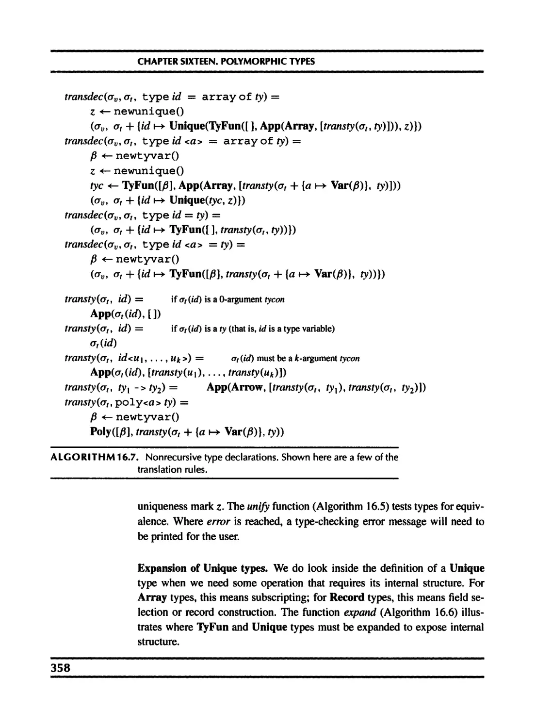


Текст
modern
compiler
piementation
in C
andrew w. appel
Modem Compiler Implementation in C
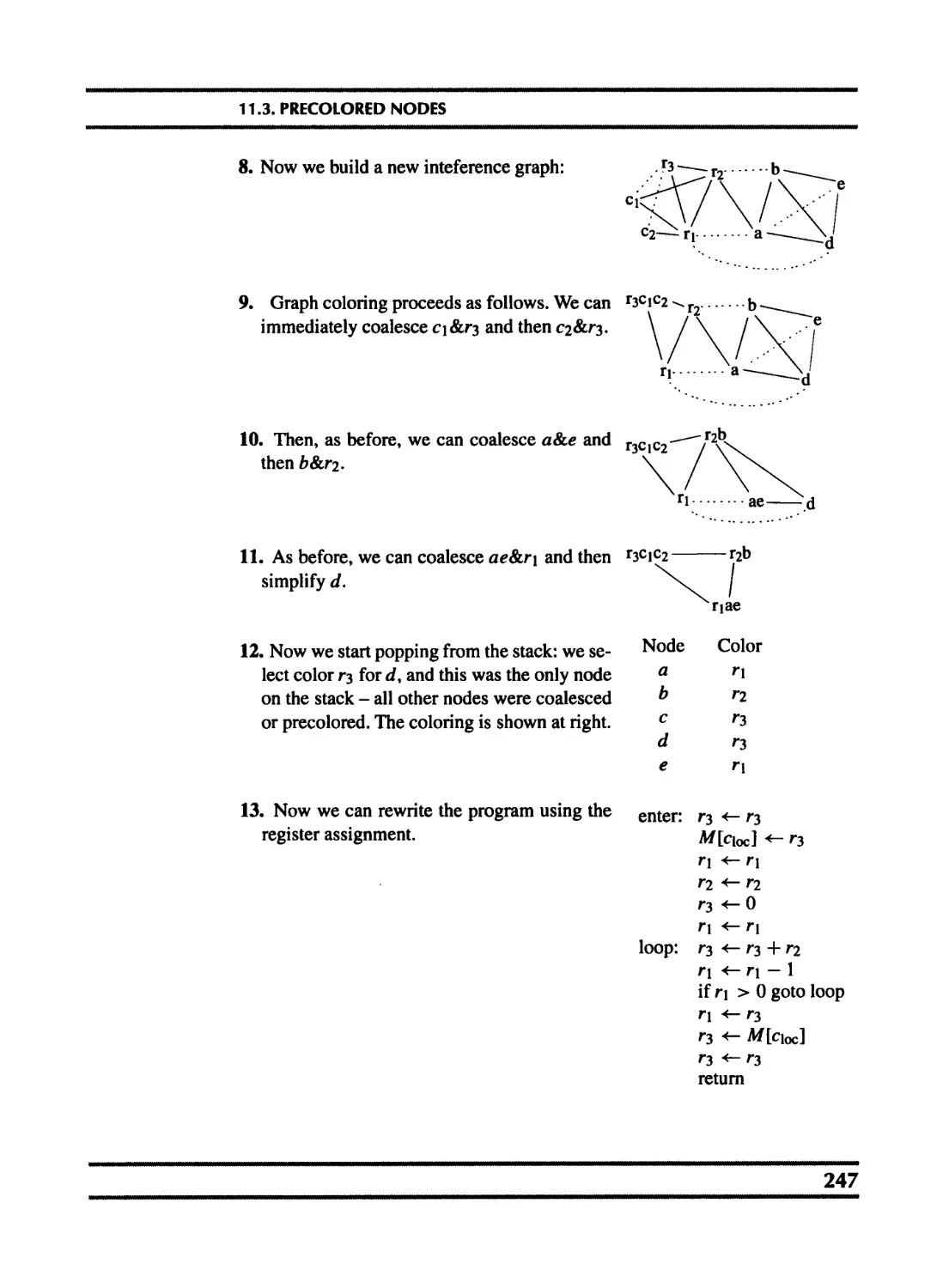
Modem Compiler
Implementation
in C
ANDREW W. APPEL
Princeton University
with MAIA GINSBURG
Cambridge
UNIVERSITY PRESS
PUBLISHED BY THE PRESS SYNDICATE OF THE UNIVERSITY OF CAMBRIDGE
The Pitt Building, Trumpington Street, Cambridge, United Kingdom
CAMBRIDGE UNIVERSITY PRESS
The Edinburgh Building, Cambridge CB2 2RU, UK
40 West 20th Street, New York NY 10011-4211, USA
477 Williamstown Road, Port Melbourne, VIC 3207, Australia
Ruiz de Alarcdn 13, 28014 Madrid, Spain
Dock House, The Waterfront, Cape Town 8001, South Africa
http://www.cambridge.org
©Andrew W. Appel and Maia Ginsburg 1998
This book is in copyright. Subject to statutory exception
and to the provisions of relevant collective licensing agreements,
no reproduction of any part may take place without
the written permission of Cambridge University Press.
First published 1998
Revised and expanded edition of Modern Compiler Implementation in C: Basic Techniques
Reprinted with corrections, 1999
First paperback edition 2004
Typeset in Times, Courier, and Optima
A catalogue record for this book is available from the British Library
Library of Congress Cataloguing-in-Publication data
Appel, Andrew W., 1960-
Modern compiler implementation in C / Andrew W. Appel with Maia Ginsburg. - Rev.
and expanded ed.
x, 544 p. : ill. ; 24 cm.
Includes bibliographical references (p. 528-536) and index.
ISBN 0 521 58390 X (hardback)
1. C (Computer program language) 2. Compilers (Computer programs)
I. Ginsburg, Maia. II. Title.
QA76.73.C15A63 1998
005.4'53—dc21 97-031089
CIP
ISBN 0 521 58390 X hardback
ISBN 0 521 60765 5 paperback
Contents
Preface ix
Part I Fundamentals of Compilation
1 Introduction 3
1.1 Modules and interfaces 4
1.2 Tools and software 5
1.3 Data structures for tree languages 7
2 Lexical Analysis 16
2.1 Lexical tokens 17
2.2 Regular expressions 18
2.3 Finite automata 21
2.4 Nondeterministic finite automata 24
2.5 Lex: a lexical analyzer generator 30
3 Parsing 39
3.1 Context-free grammars 41
3.2 Predictive parsing 46
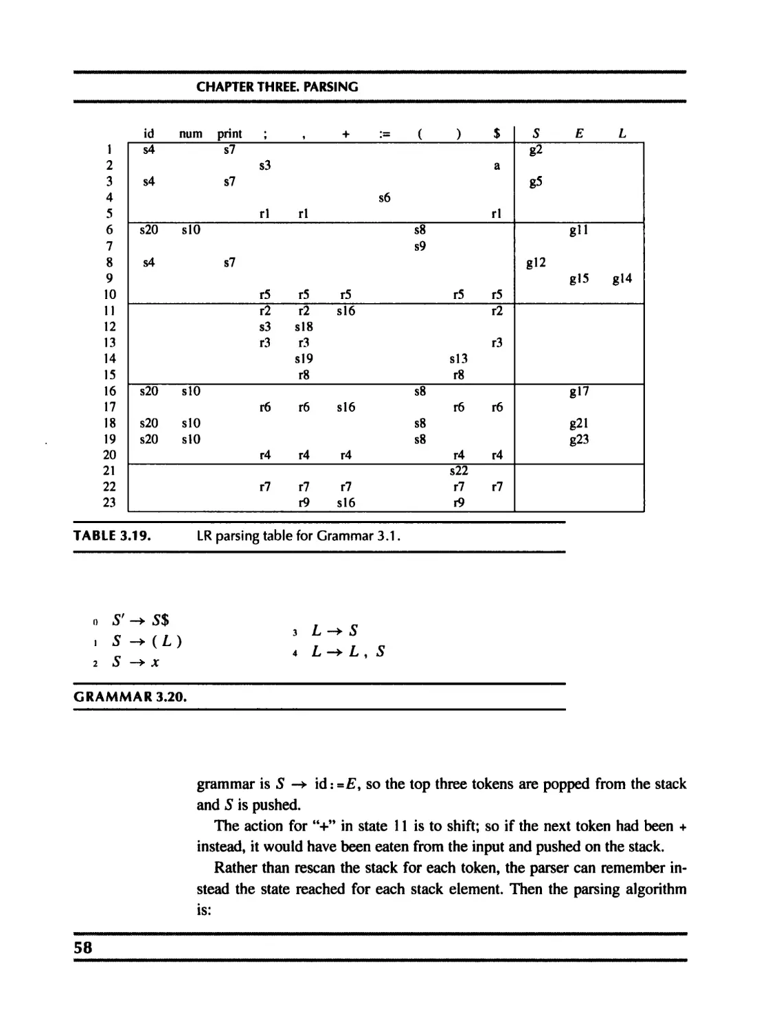
3.3 LR parsing 56
3.4 Using parser generators 69
3.5 Error recovery 76
4 Abstract Syntax 88
4.1 Semantic actions 88
4.2 Abstract parse trees 92
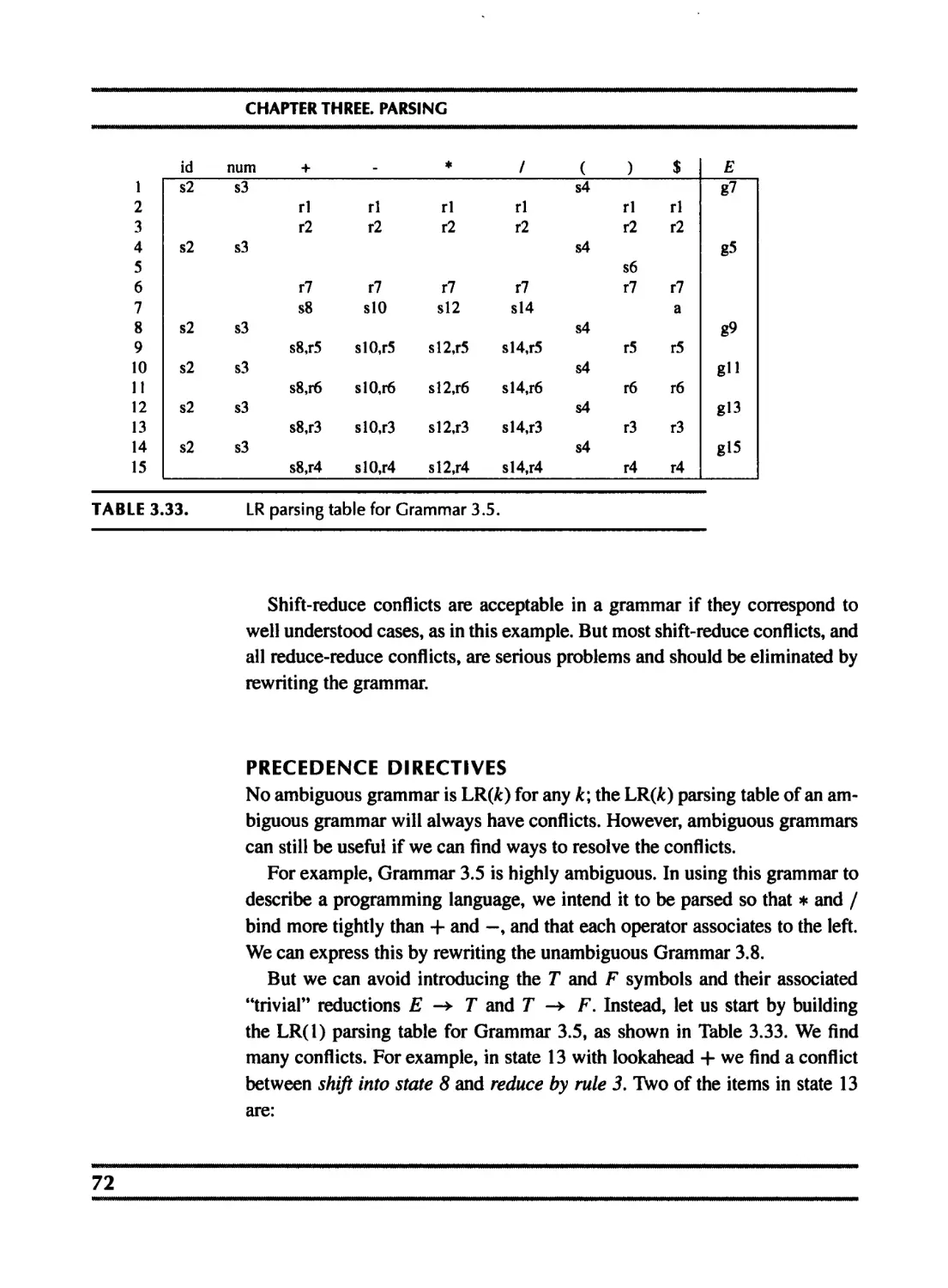
5 Semantic Analysis 103
5.1 Symbol tables 103
5.2 Bindings for the Tiger compiler 112
v
CONTENTS
5.3 Type-checking expressions 5.4 Type-checking declarations 115 118
6 Activation Records 125
6.1 Stack frames 127
6.2 Frames in the Tiger compiler 135
7 Translation to Intermediate Code 150
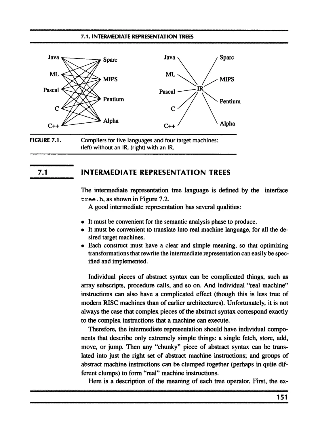
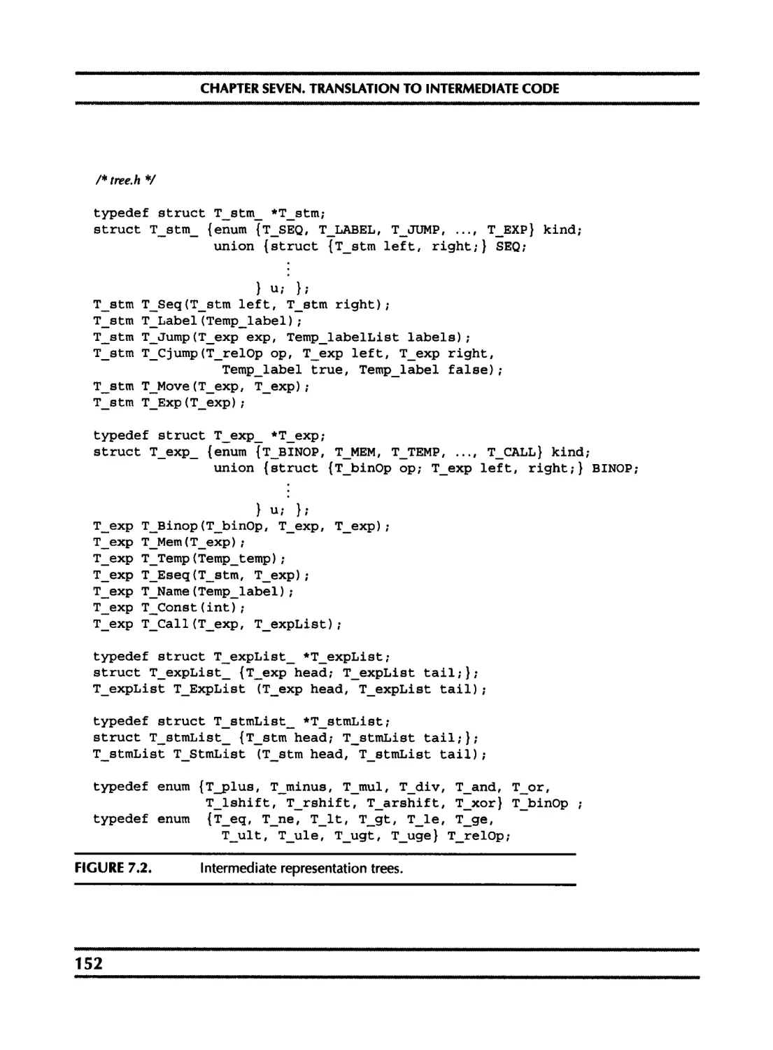
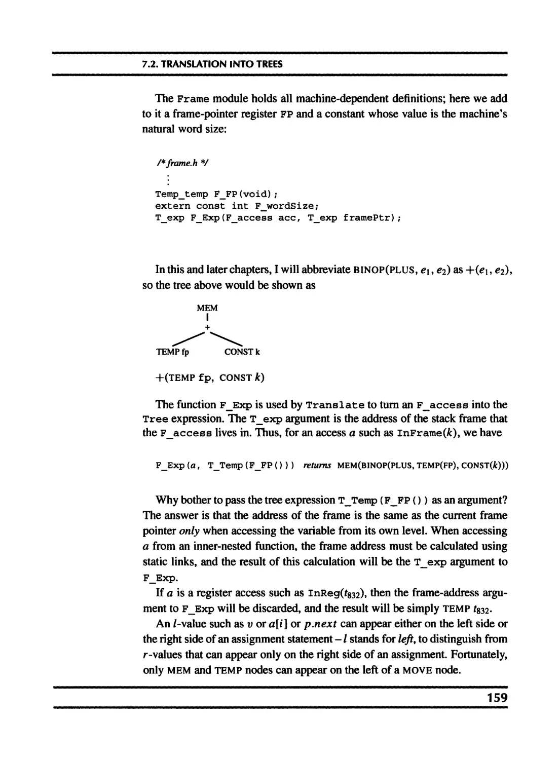
7.1 Intermediate representation trees 151
7.2 Translation into trees 154
7.3 Declarations 170
8 Basic Blocks and Traces 176
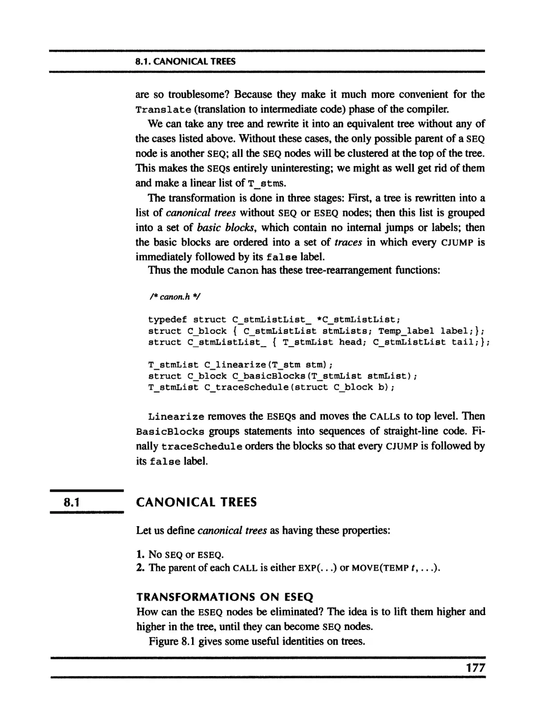
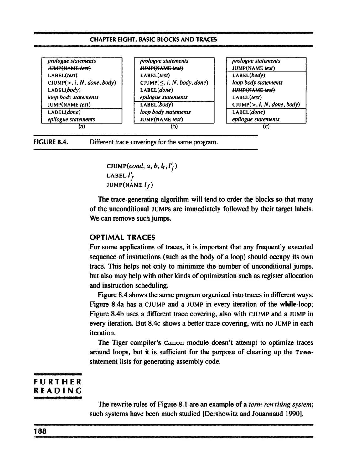
8.1 Canonical trees 177
8.2 Taming conditional branches 185
9 Instruction Selection 191
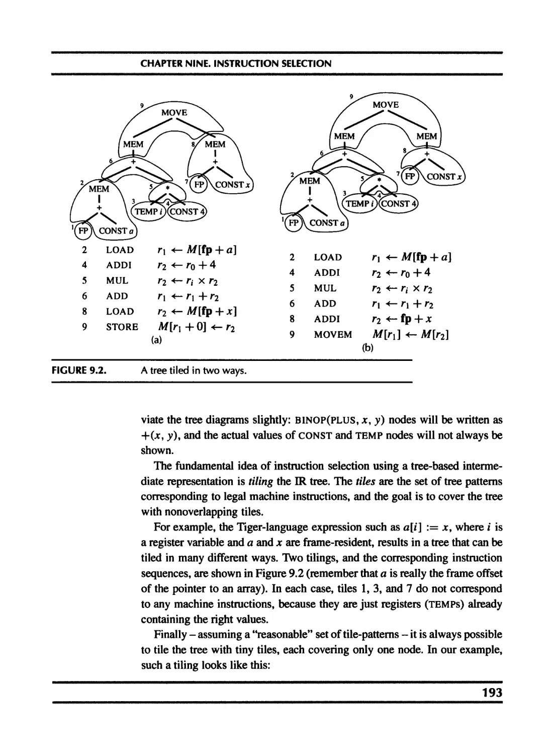
9.1 Algorithms for instruction selection 194
9.2 CISC machines 202
9.3 Instruction selection for the Tiger compiler 205
10 Liveness Analysis 218
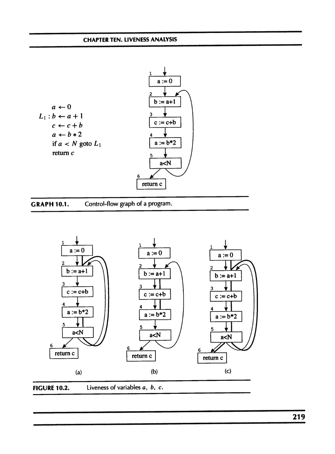
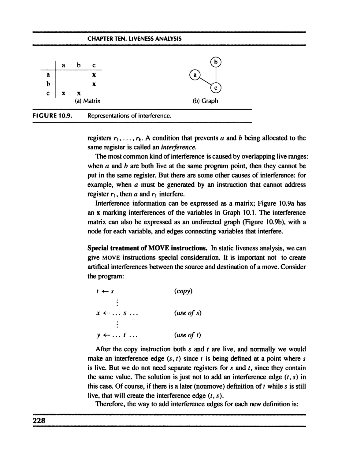
10.1 Solution of dataflow equations 220
10.2 Liveness in the Tiger compiler 229
11 Register Allocation 235
11.1 Coloring by simplification 236
11.2 Coalescing 239
11.3 Precolored nodes 243
11.4 Graph coloring implementation 248
11.5 Register allocation for trees 257
12 Putting It All Together 265
Part II Advanced Topics
13 Garbage Collection
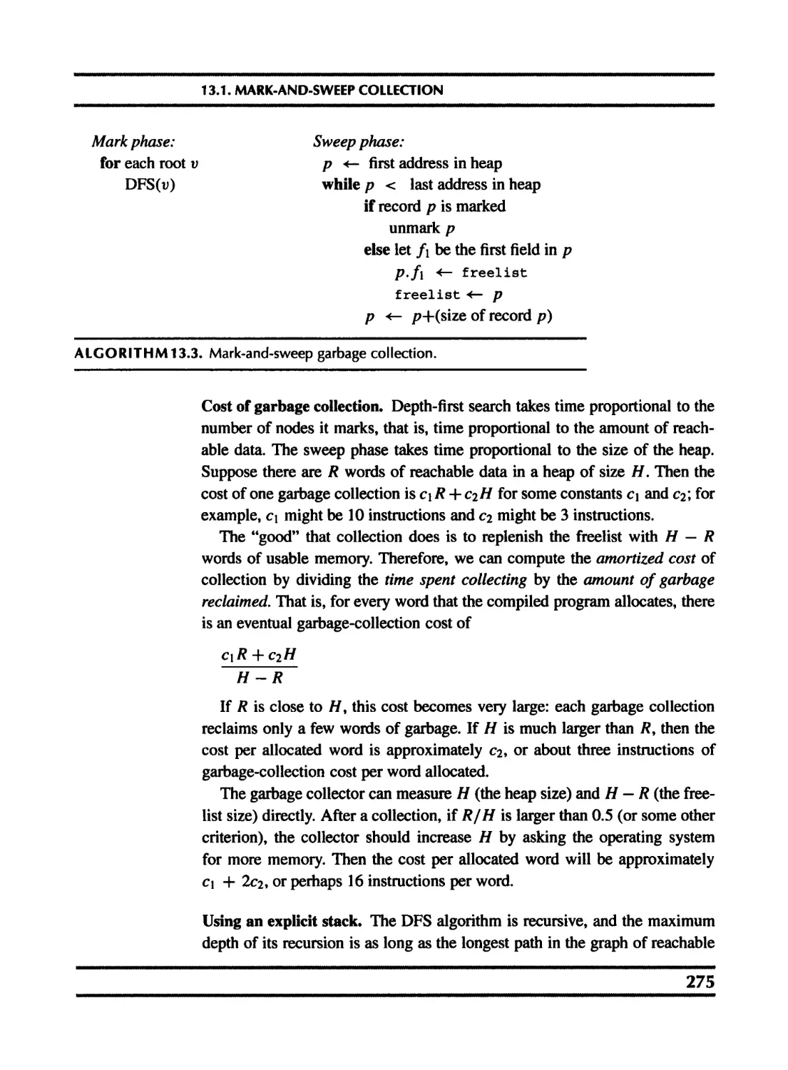
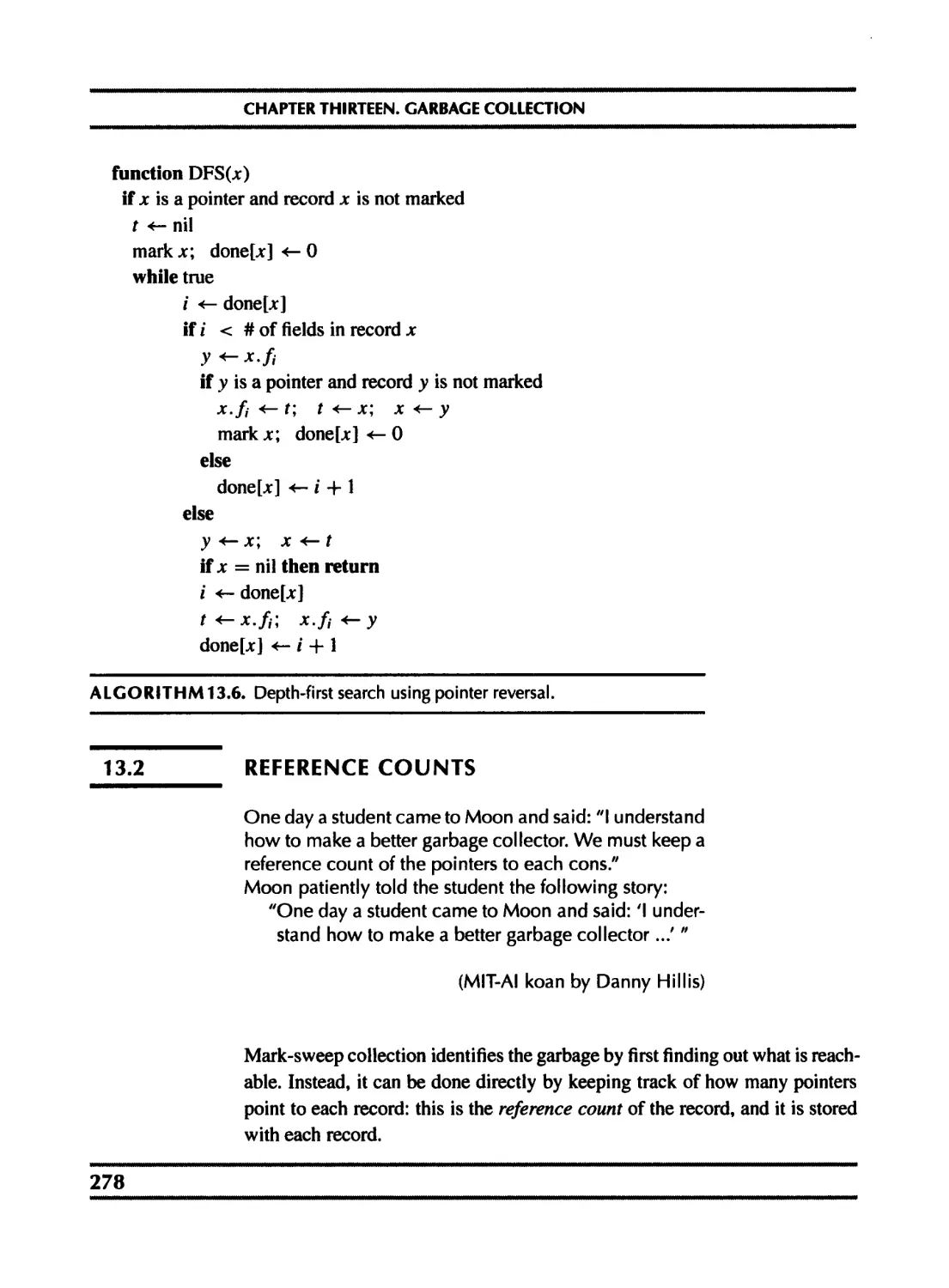
13.1 Mark-and-sweep collection
13.2 Reference counts
273
273
278
vi
CONTENTS
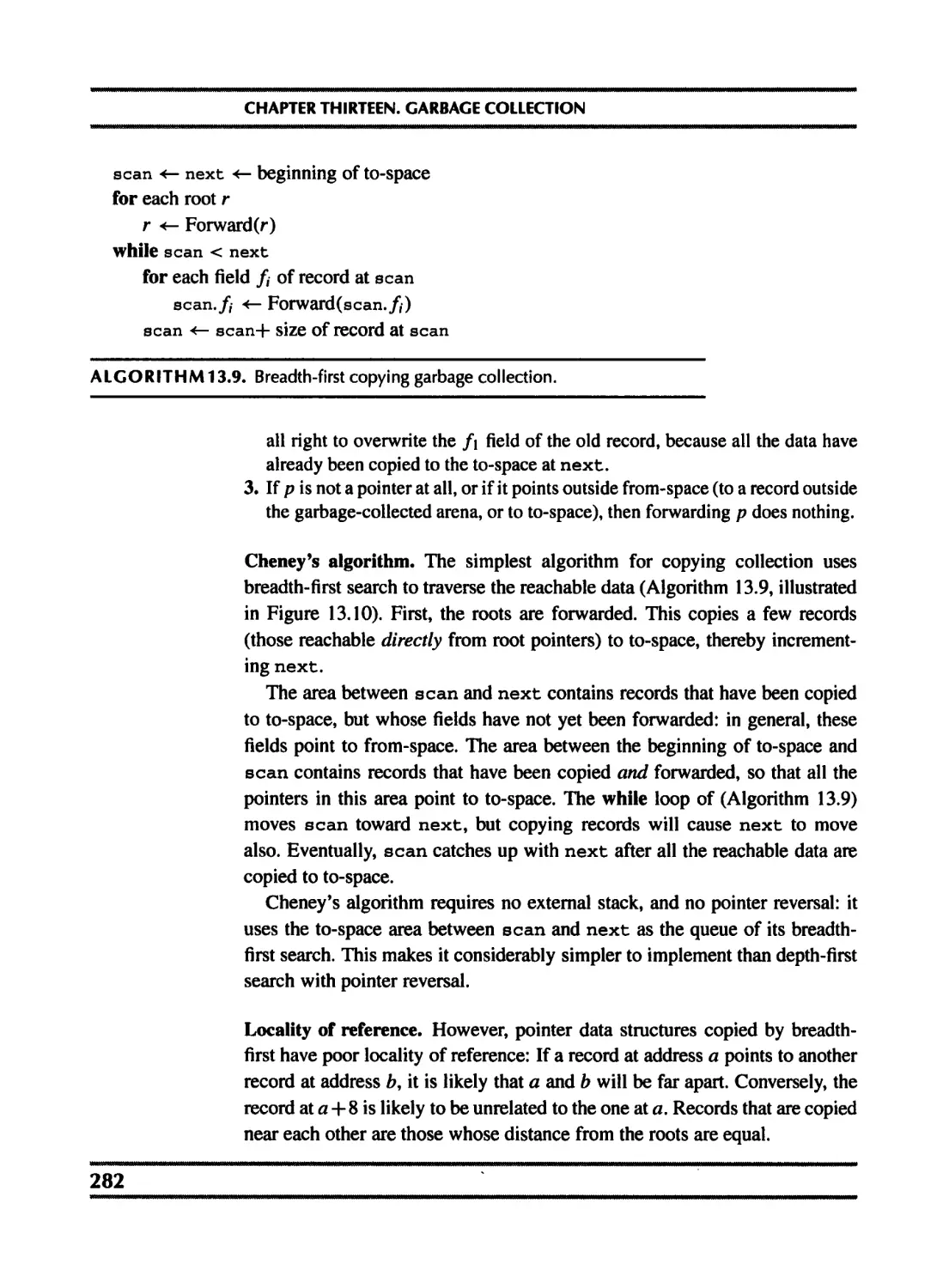
13.3 Copying collection 280
13.4 Generational collection 285
13.5 Incremental collection 287
13.6 Baker’s algorithm 290
13.7 Interface to the compiler 291
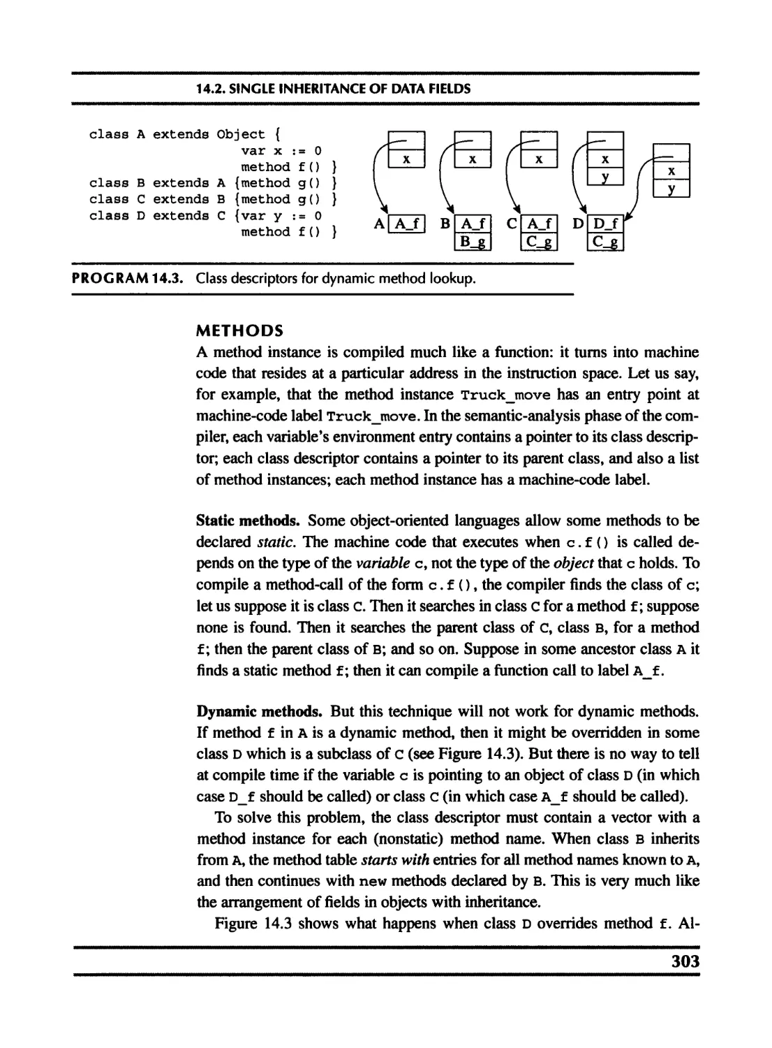
14 Object-Oriented Languages 299
14.1 Classes 299
14.2 Single inheritance of data fields 302
14.3 Multiple inheritance 304
14.4 Testing class membership 306
14.5 Private fields and methods 310
14.6 Classless languages 310
14.7 Optimizing object-oriented programs 311
15 Functional Programming Languages 315
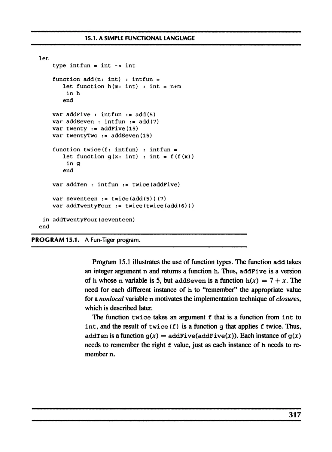
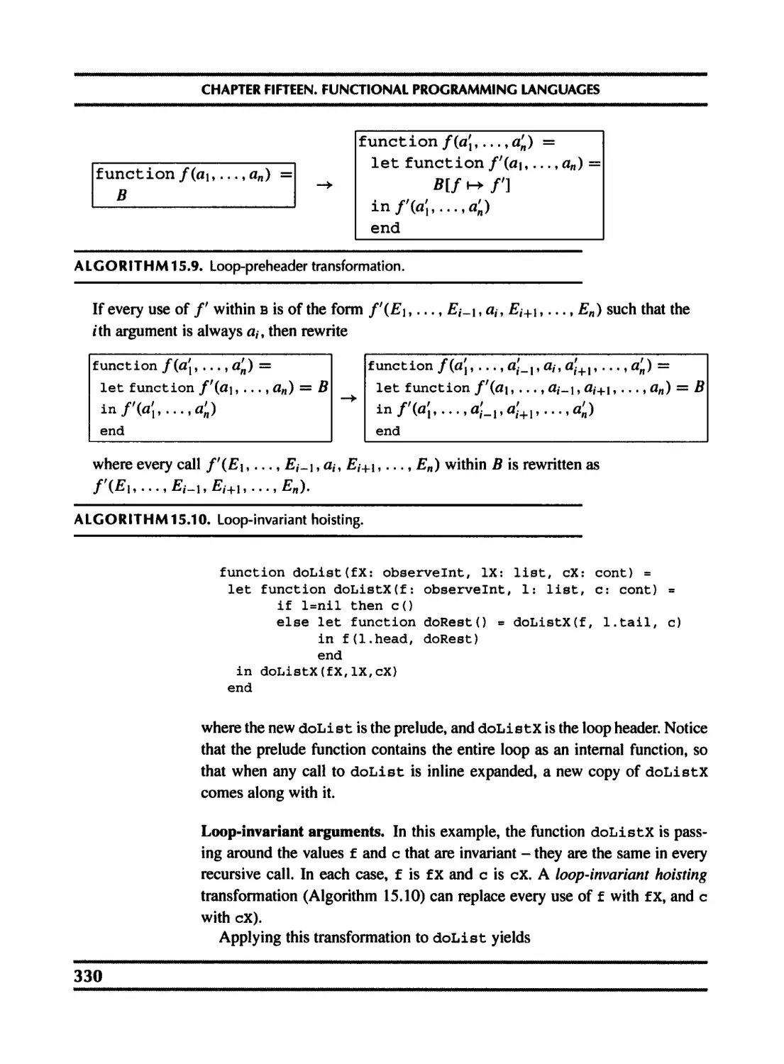
15.1 A simple functional language 316
15.2 Closures 318
15.3 Immutable variables 319
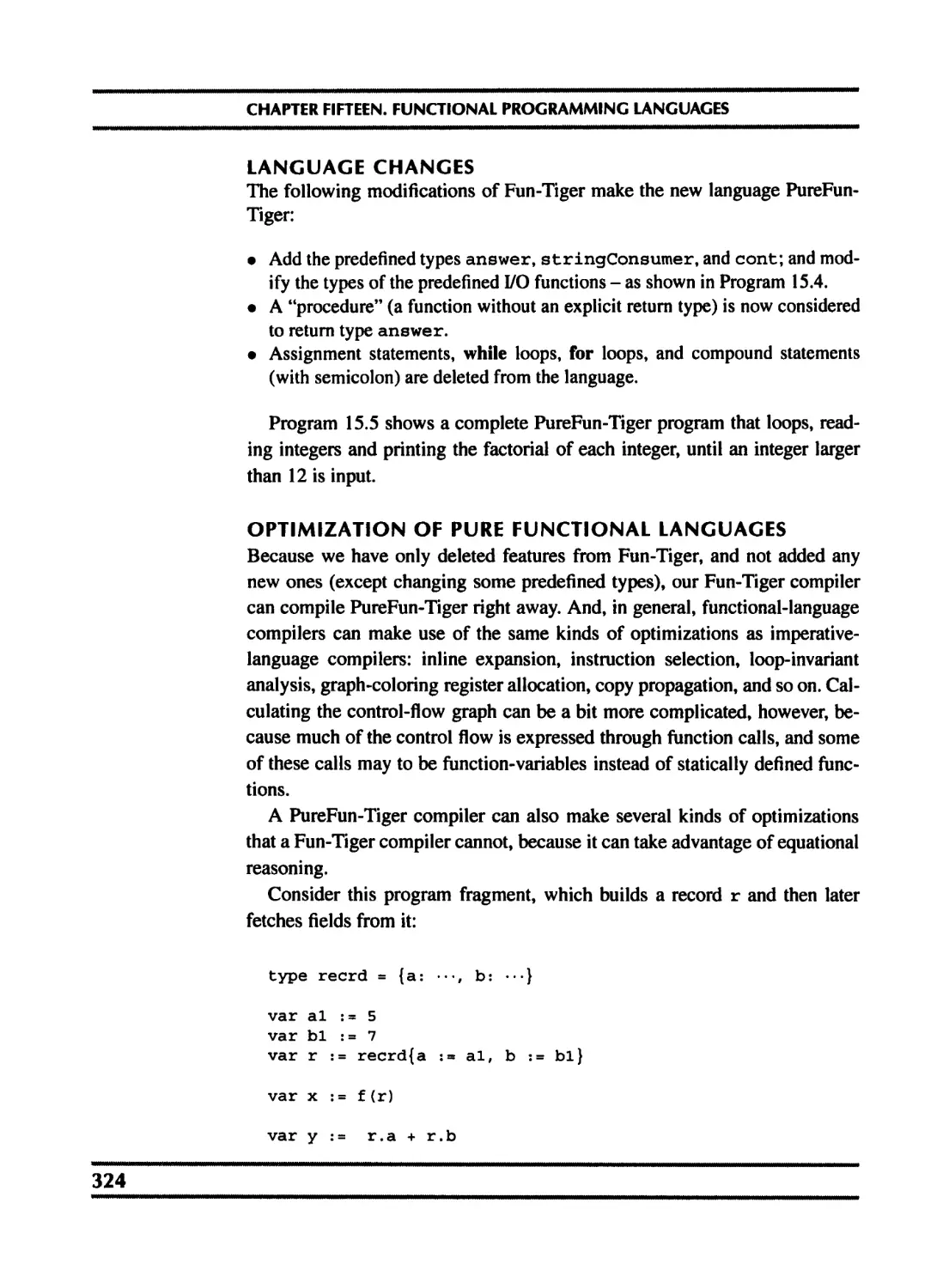
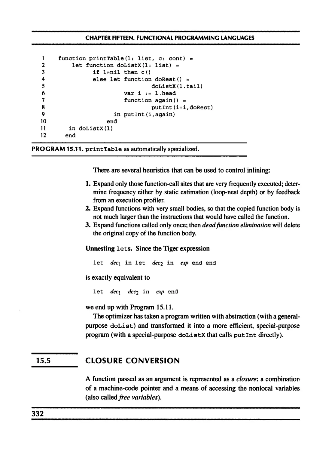
15.4 Inline expansion 326
15.5 Closure conversion 332
15.6 Efficient tail recursion 335
15.7 Lazy evaluation 337
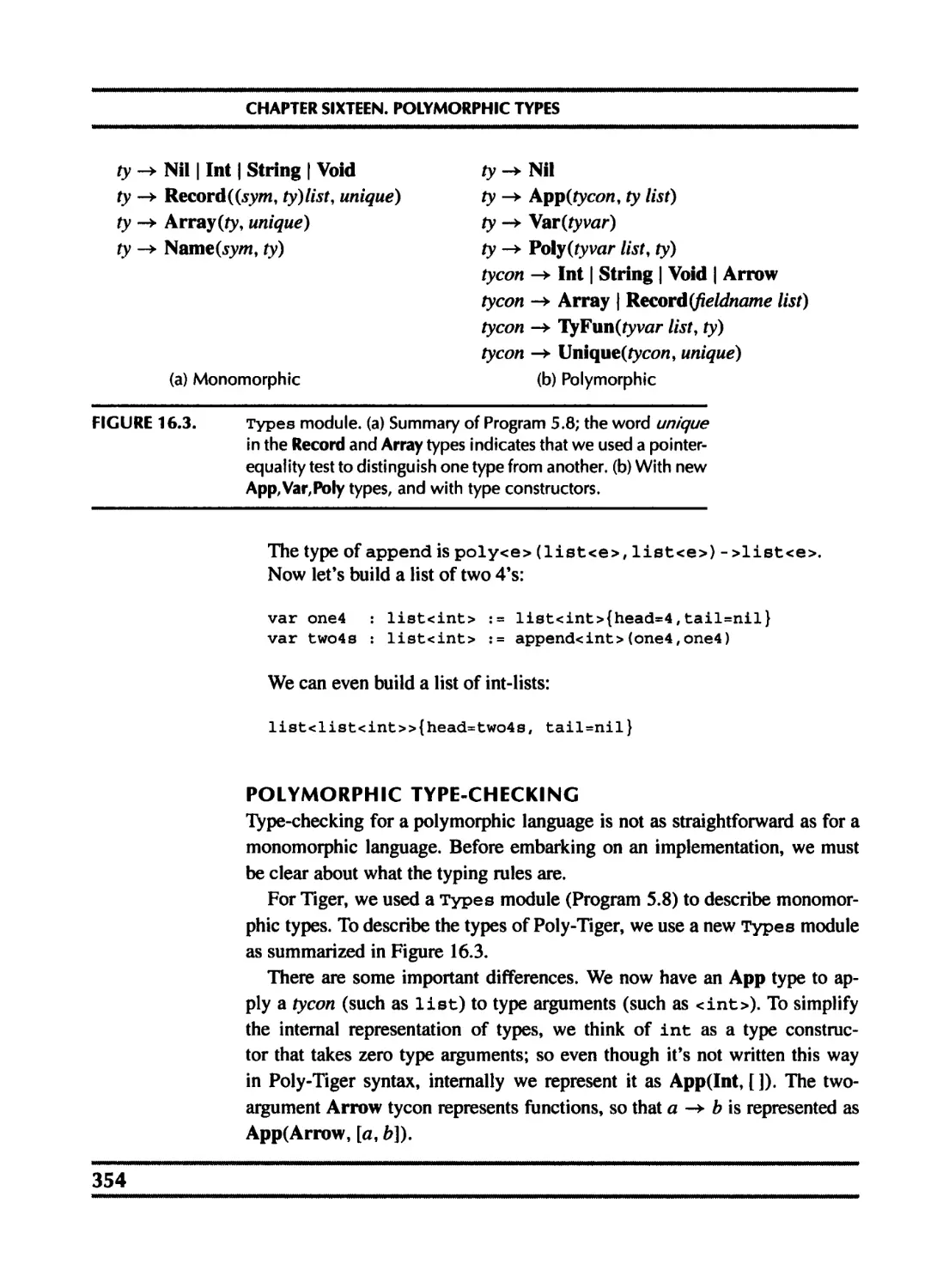
16 Polymorphic Types 350
16.1 Parametric polymorphism 351
16.2 Type inference 359
16.3 Representation of polymorphic variables 369
16.4 Resolution of static overloading 378
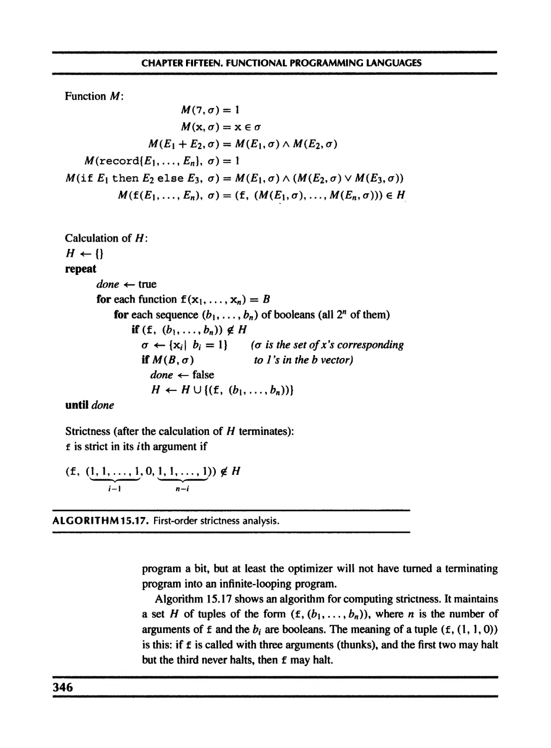
17 Dataflow Analysis 383
17.1 Intermediate representation for flow analysis 384
17.2 Various dataflow analyses 387
17.3 Transformations using dataflow analysis 392
17.4 Speeding up dataflow analysis 393
17.5 Alias analysis 402
18 Loop Optimizations 410
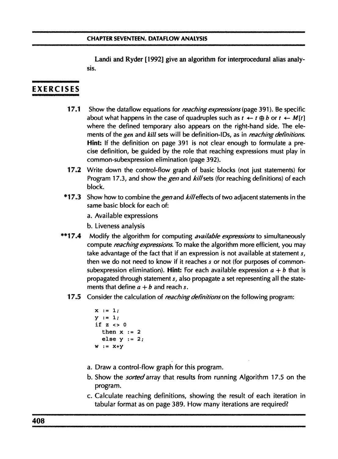
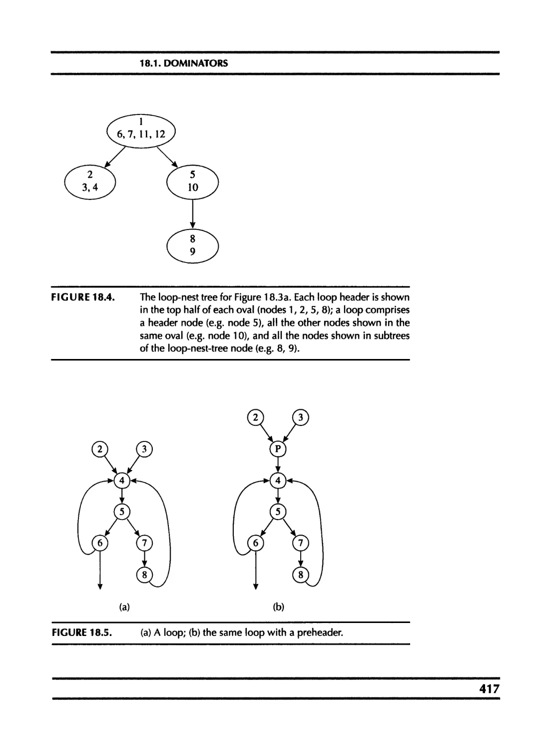
18.1 Dominators 413
vii
CONTENTS
18. 2 Loop-invariant computations 418
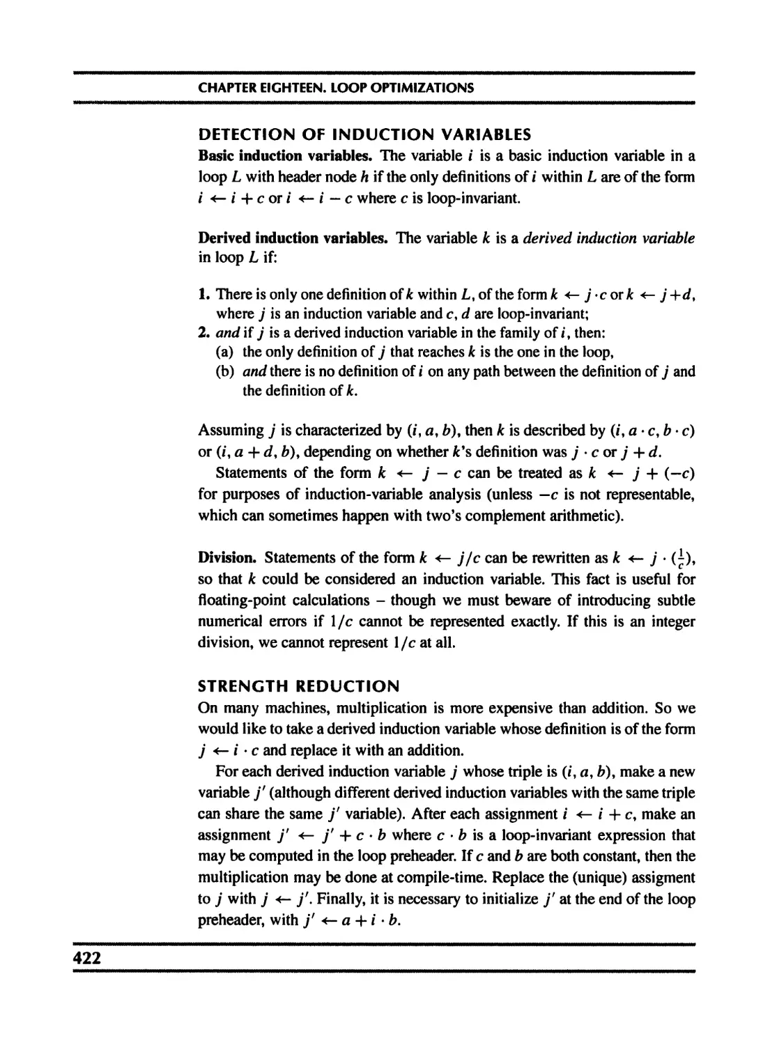
18. 3 Induction variables 419
18. 4 Array-bounds checks 425
18. 5 Loop unrolling 429
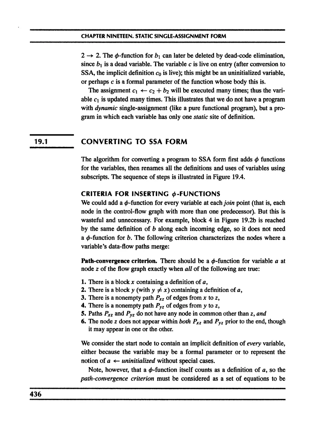
19 Static Single-Assignment Form 433
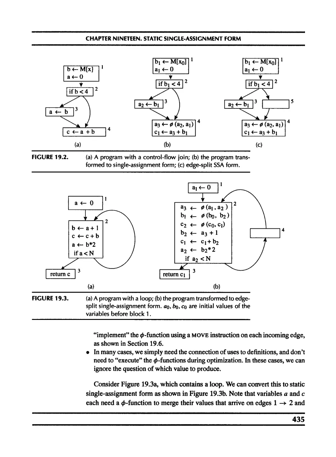
19.1 Converting to SSA form 436
19.2 Efficient computation of the dominator tree 444
19.3 Optimization algorithms using SSA 451
19.4 Arrays, pointers, and memory 457
19.5 The control-dependence graph 459
19.6 Converting back from SSA form 462
19.7 A functional intermediate form 464
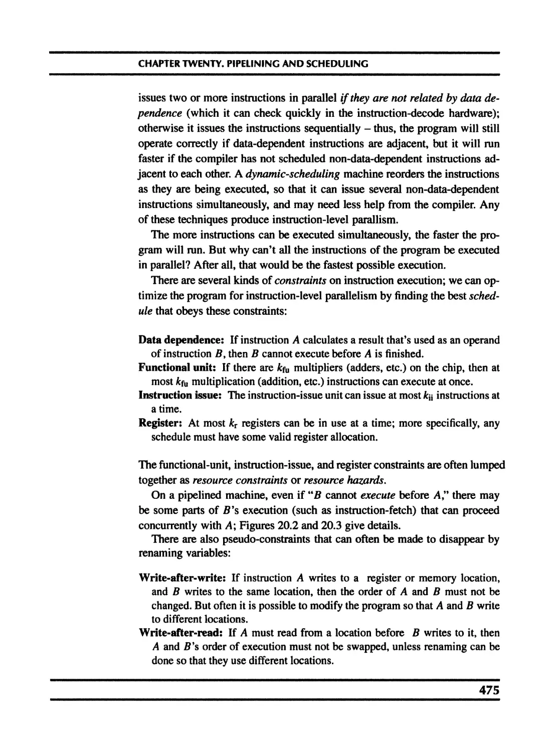
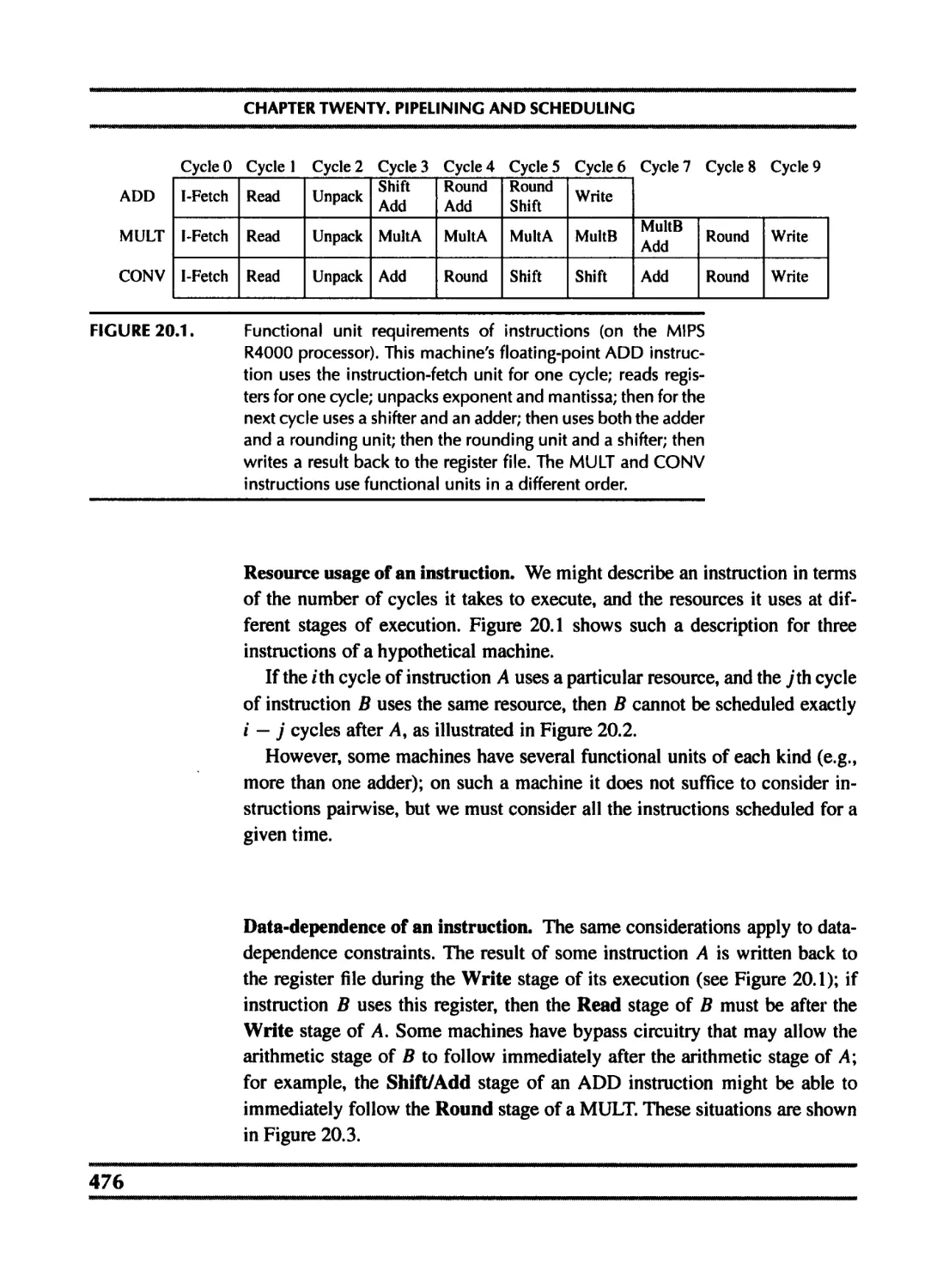
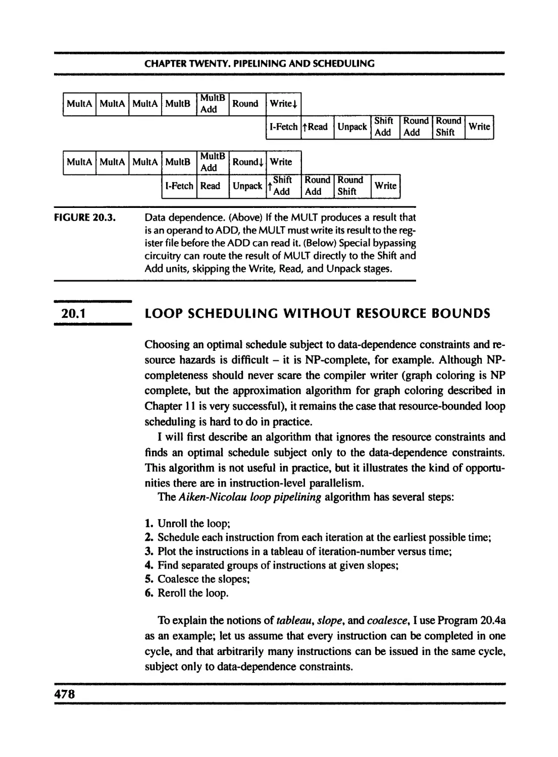
20 Pipelining and Scheduling 474
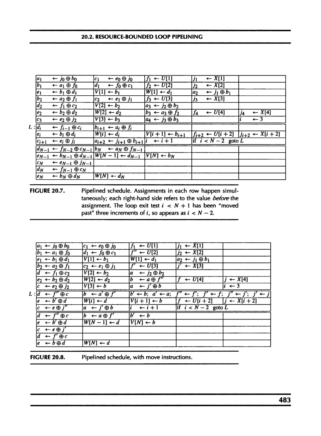
20.1 Loop scheduling without resource bounds 478
20.2 Resource-bounded loop pipelining 482
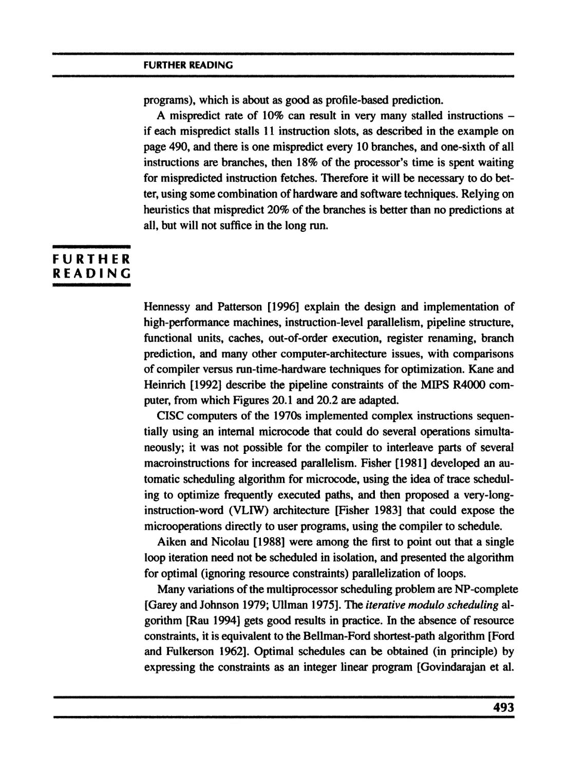
20.3 Branch prediction 490
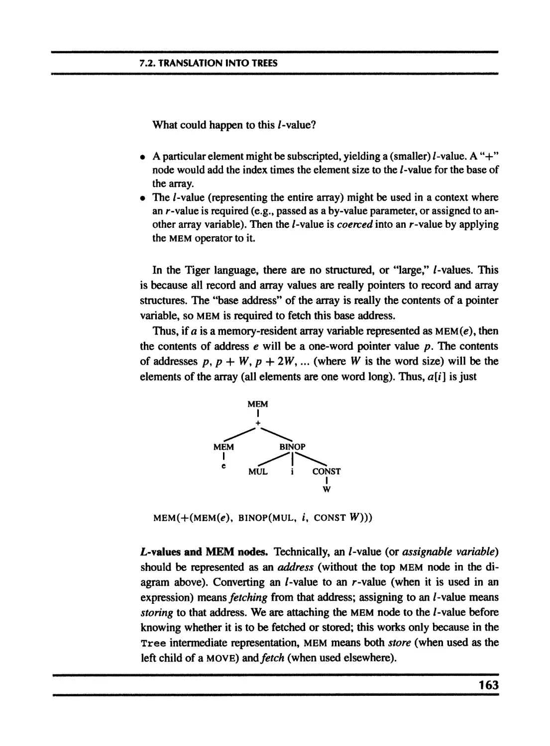
21 The Memory Hierarchy 498
21.1 Cache organization 499
21.2 Cache-block alignment 502
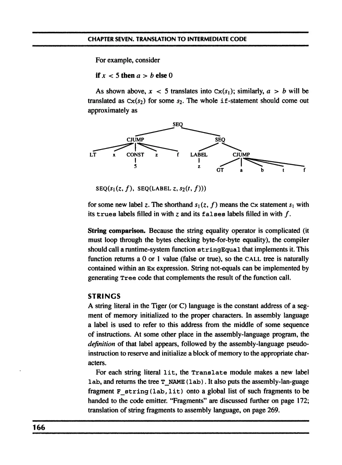
21.3 Prefetching 504
21.4 Loop interchange 510
21.5 Blocking 511
21.6 Garbage collection and the memory hierarchy 514
Appendix: Tiger Language Reference Manual 518
A.l Lexical issues 518
A.2 Declarations 518
A.3 Variables and expressions 521
A.4 Standard library 525
A.5 Sample Tiger programs 526
Bibliography 528
Index 537
viii
Preface
Over the past decade, there have been several shifts in the way compilers are
built. New kinds of programming languages are being used: object-oriented
languages with dynamic methods, functional languages with nested scope
and first-class function closures; and many of these languages require garbage
collection. New machines have large register sets and a high penalty for mem-
ory access, and can often run much faster with compiler assistance in schedul-
ing instructions and managing instructions and data for cache locality.
This book is intended as a textbook for a one- or two-semester course
in compilers. Students will see the theory behind different components of a
compiler, the programming techniques used to put the theory into practice,
and the interfaces used to modularize the compiler. To make the interfaces
and programming examples clear and concrete, I have written them in the C
programming language. Other editions of this book are available that use the
Java and ML languages.
Implementation project The “student project compiler” that I have outlined
is reasonably simple, but is organized to demonstrate some important tech-
niques that are now in common use: abstract syntax trees to avoid tangling
syntax and semantics, separation of instruction selection from register alloca-
tion, copy propagation to give flexibility to earlier phases of the compiler, and
containment of target-machine dependencies. Unlike many “student compil-
ers” found in textbooks, this one has a simple but sophisticated back end,
allowing good register allocation to be done after instruction selection.
Each chapter in Part I has a programming exercise corresponding to one
module of a compiler. Software useful for the exercises can be found at
http://www.cs.princeton.edu/~appel/modern/c
PREFACE
Exercises. Each chapter has pencil-and-paper exercises; those marked with
a star are more challenging, two-star problems are difficult but solvable, and
the occasional three-star exercises are not known to have a solution.
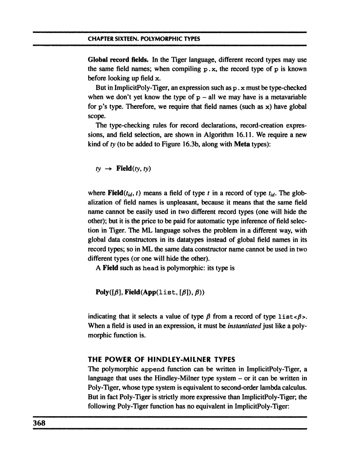
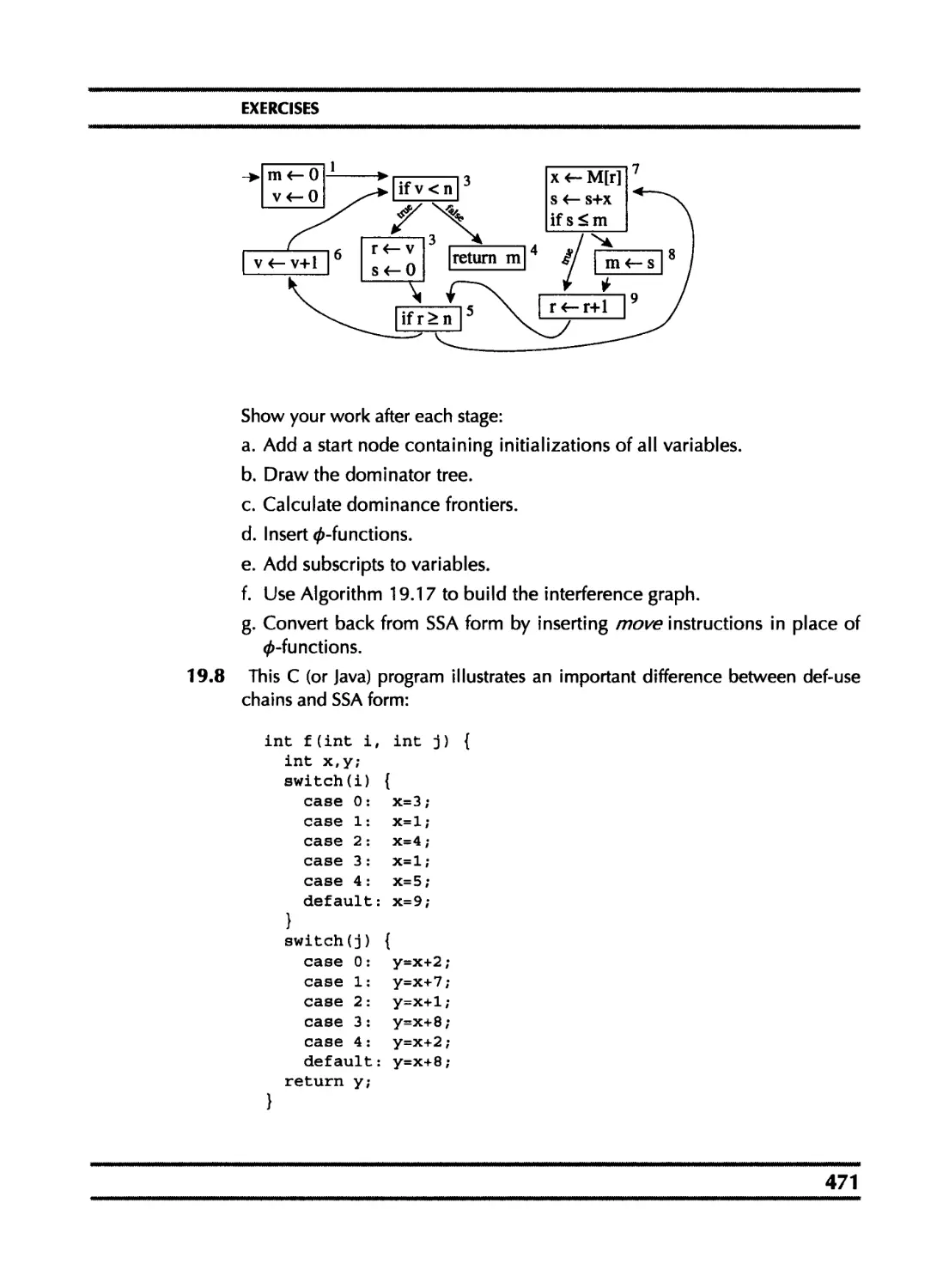
Course sequence. The figure shows how the chapters depend on each other.
Activation
Records
- Lexical л „ . л Abstract - Semantic
1 Analysis------3> Parsing----4 Syntax ------5‘ Analysis X
? Translation to ________g Basic Blocks
Intermediate Code * and Traces
1. Introduction — 9. ^nJtr“ctlon
\ Selection
10.
Liveness
Analysis
n Register
* Allocation
17 Putting it
All Together
15.
13.
<U
u
<D
co
6
<U
С/Э
Dataflow___w Loop
1 ' Analysis * Optimizations
Functional -, Polymorphic
Languages * Types
Garbage
Collection
14 Object-Oriented
* Languages
Static Slngle-
----19. Assignment
Form
Pipelining,
Scheduling
01 Memory
Hierarchies
V
u
Л
5
О
Q
CO
£
V
С/Э
• A one-semester course could cover all of Part I (Chapters 1-12), with students
implementing the project compiler (perhaps working in groups); in addition,
lectures could cover selected topics from Part II.
• An advanced or graduate course could cover Part II, as well as additional
topics from the current literature. Many of the Part II chapters can stand inde-
pendently from Part I, so that an advanced course could be taught to students
who have used a different book for their first course.
• In a two-quarter sequence, the first quarter could cover Chapters 1-8, and the
second quarter could cover Chapters 9-12 and some chapters from Part II.
Acknowledgments. Many people have provided constructive criticism or
helped me in other ways on this book. I would like to thank Leonor Abraido-
Fandino, Scott Ananian, Stephen Bailey, Max Hailperin, David Hanson, Jef-
frey Hsu, David MacQueen, Torben Mogensen, Doug Morgan, Robert Netzer,
Elma Lee Noah, Mikael Petterson, Todd Proebsting, Anne Rogers, Barbara
Ryder, Amr Sabry, Mooly Sagiv, Zhong Shao, Maty Lou Soffa, Andrew Tol-
mach, Kwangkeun Yi, and Kenneth Zadeck.
PART ONE
Fundamentals of
Compilation
1------------------------
Introduction
A compiler was originally a program that "compiled"
subroutines [a link-loader]. When in 1954 the combina-
tion "algebraic compiler" came into use, or rather into
misuse, the meaning of the term had already shifted into
the present one.
Bauer and Eickel [1975]
This book describes techniques, data structures, and algorithms for translating
programming languages into executable code. A modem compiler is often or-
ganized into many phases, each operating on a different abstract “language.”
The chapters of this book follow the organization of a compiler, each covering
a successive phase.
To illustrate the issues in compiling real programming languages, I show
how to compile Tiger, a simple but nontrivial language of the Algol family,
with nested scope and heap-allocated records. Programming exercises in each
chapter call for the implementation of the corresponding phase; a student
who implements all the phases described in Part I of the book will have a
working compiler. Tiger is easily modified to be functional or object-oriented
(or both), and exercises in Part II show how to do this. Other chapters in Part
II cover advanced techniques in program optimization. Appendix A describes
the Tiger language.
The interfaces between modules of the compiler are almost as important
as the algorithms inside the modules. To describe the interfaces concretely, it
is useful to write them down in a real programming language. This book uses
the C programming language.
3
CHAPTER ONE. INTRODUCTION
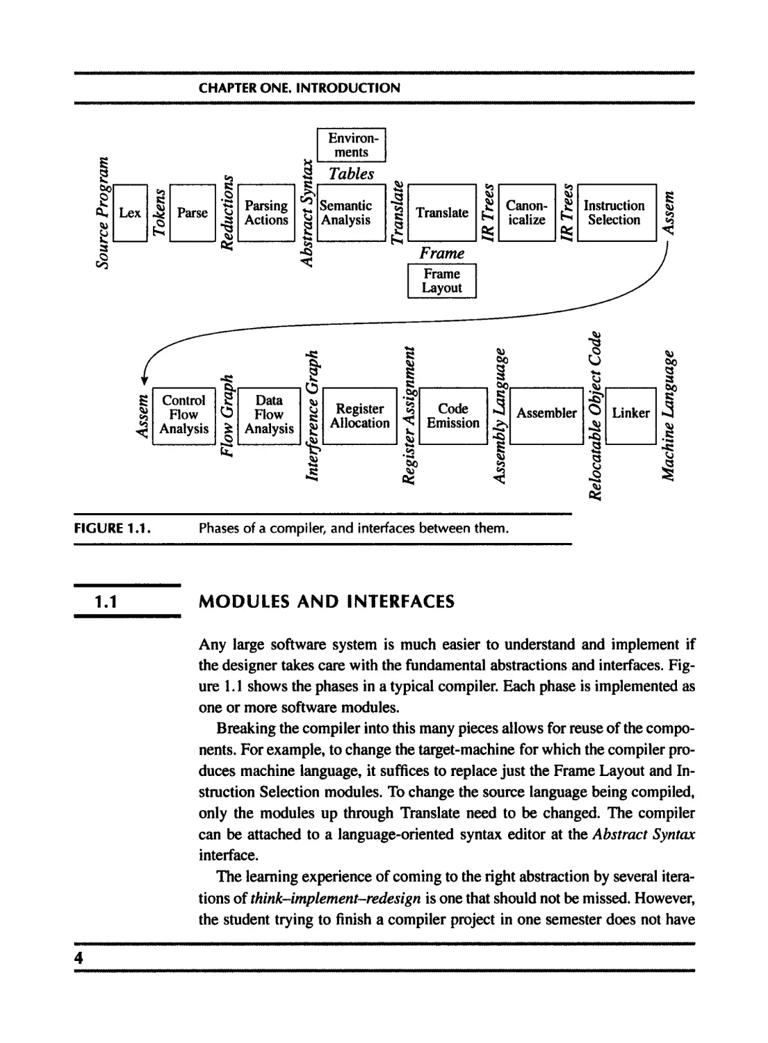
FIGURE 1.1.
Phases of a compiler, and interfaces between them.
1.1 MODULES AND INTERFACES
Any large software system is much easier to understand and implement if
the designer takes care with the fundamental abstractions and interfaces. Fig-
ure 1.1 shows the phases in a typical compiler. Each phase is implemented as
one or more software modules.
Breaking the compiler into this many pieces allows for reuse of the compo-
nents. For example, to change the target-machine for which the compiler pro-
duces machine language, it suffices to replace just the Frame Layout and In-
struction Selection modules. To change the source language being compiled,
only the modules up through Translate need to be changed. The compiler
can be attached to a language-oriented syntax editor at the Abstract Syntax
interface.
The learning experience of coming to the right abstraction by several itera-
tions of think-implement-redesign is one that should not be missed. However,
the student trying to finish a compiler project in one semester does not have
4
1.2. TOOLS AND SOFTWARE
this luxury. Therefore, I present in this book the outline of a project where the
abstractions and interfaces are carefully thought out, and are as elegant and
general as I am able to make them.
Some of the interfaces, such as Abstract Syntax, IR Trees, and Assem, take
the form of data structures: for example, the Parsing Actions phase builds an
Abstract Syntax data structure and passes it to the Semantic Analysis phase.
Other interfaces are abstract data types; the Translate interface is a set of
functions that the Semantic Analysis phase can call, and the Tokens interface
takes the form of a function that the Parser calls to get the next token of the
input program.
DESCRIPTION OF THE PHASES
Each chapter of Part I of this book describes one compiler phase, as shown in
Table 1.2
This modularization is typical of many real compilers. But some compil-
ers combine Parse, Semantic Analysis, Translate, and Canonicalize into one
phase; others put Instruction Selection much later than I have done, and com-
bine it with Code Emission. Simple compilers omit the Control Flow Analy-
sis, Data Flow Analysis, and Register Allocation phases.
I have designed the compiler in this book to be as simple as possible, but
no simpler. In particular, in those places where comers are cut to simplify the
implementation, the structure of the compiler allows for the addition of more
optimization or fancier semantics without violence to the existing interfaces.
1.2 TOOLS AND SOFTWARE
Two of the most useful abstractions used in modem compilers are context-
free grammars, for parsing, and regular expressions, for lexical analysis. To
make best use of these abstractions it is helpful to have special tools, such
as Yacc (which converts a grammar into a parsing program) and Lex (which
converts a declarative specification into a lexical analysis program).
The programming projects in this book can be compiled using any ANSI-
standard C compiler, along with Lex (or the more modem Flex) and Yacc
(or the more modem Bison). Some of these tools are freely available on the
Internet; for information see the World Wide Web page
http://www.cs.princeton.edu/~appel/modern/c
5
CHAPTER ONE. INTRODUCTION
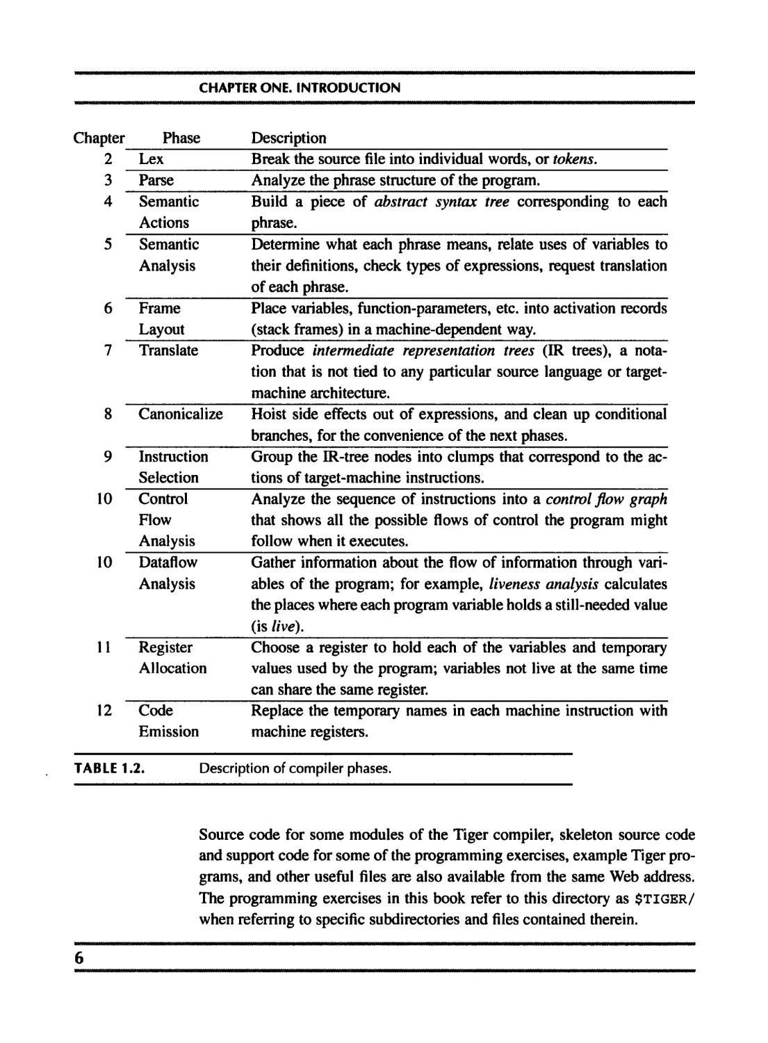
Chapter Phase Description
2 Lex Break the source file into individual words, or tokens.
3 Parse Analyze the phrase structure of the program.
4 Semantic Actions Build a piece of abstract syntax tree corresponding to each phrase.
5 Semantic Analysis Determine what each phrase means, relate uses of variables to their definitions, check types of expressions, request translation of each phrase.
6 Frame Layout Place variables, function-parameters, etc. into activation records (stack frames) in a machine-dependent way.
7 Translate Produce intermediate representation trees (IR trees), a nota- tion that is not tied to any particular source language or target- machine architecture.
8 Canonicalize Hoist side effects out of expressions, and clean up conditional branches, for the convenience of the next phases.
9 Instruction Selection Group the IR-tree nodes into clumps that correspond to the ac- tions of target-machine instructions.
10 Control Flow Analysis Analyze the sequence of instructions into a control flow graph that shows all the possible flows of control the program might follow when it executes.
10 Dataflow Analysis Gather information about the flow of information through vari- ables of the program; for example, liveness analysis calculates the places where each program variable holds a still-needed value (is live).
11 Register Allocation Choose a register to hold each of the variables and temporary values used by the program; variables not live at the same time can share the same register.
12 Code Emission Replace the temporary names in each machine instruction with machine registers.
TABLE 1.2. Description of compiler phases.
Source code for some modules of the Tiger compiler, skeleton source code
and support code for some of the programming exercises, example Tiger pro-
grams, and other useful files are also available from the same Web address.
The programming exercises in this book refer to this directory as $tiger/
when referring to specific subdirectories and files contained therein.
6.............. ...........................................................................
1.3. DATA STRUCTURES FOR TREE LANGUAGES
Stm -> Stm; Stm (CompoundStm)
Stm id : = Exp (AssignStm)
Stm —> print ( ExpList) (PrintStm)
Exp -> id (IdExp)
Exp —> num (NumExp)
Exp —> Exp Binop Exp (OpExp)
Exp -> (Stm , Exp) (EseqExp)
ExpList - * Exp , ExpList (PairExpList)
ExpList - > Exp (LastExpList)
Binop - * + (Plus)
Binop - > — (Minus)
Binop - > X (Times)
Binop - >/ (Div)
GRAMMAR 1.3. A straight-line programming language.
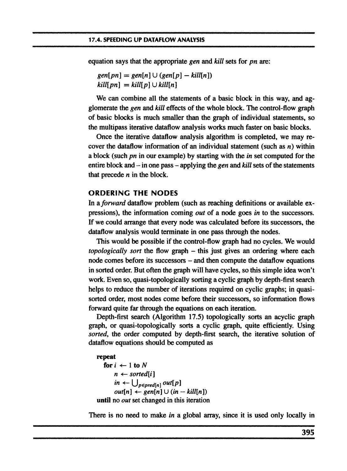
1.3 DATA STRUCTURES FOR TREE LANGUAGES
Many of the important data structures used in a compiler are intermediate
representations of the program being compiled. Often these representations
take the form of trees, with several node types, each of which has different
attributes. Such trees can occur at many of the phase-interfaces shown in
Figure 1.1.
Tree representations can be described with grammars, just like program-
ming languages. To introduce the concepts, I will show a simple program-
ming language with statements and expressions, but no loops or if-statements
(this is called a language of straight-line programs).
The syntax for this language is given in Grammar 1.3.
The informal semantics of the language is as follows. Each Stm is a state-
ment, each Exp is an expression, $i; S2 executes statement si, then statement
S2. i --=e evaluates the expression e, then “stores” the result in variable i.
print(«i, e2,..., en) displays the values of all the expressions, evaluated
left to right, separated by spaces, terminated by a newline.
An identifier expression, such as i, yields the current contents of the vari-
able i. A number evaluates to the named integer. An operator expression
e\ op e2 evaluates then ег, then applies the given binary operator. And
an expression sequence (s, e) behaves like the C-language “comma” opera-
tor, evaluating the statement 5 for side effects before evaluating (and returning
the result of) the expression e.
-
CHAPTER ONE. INTRODUCTION
CompoundStm
AssignStm CompoundStm
PrintStm
I
LastExpList
I
IdExp
I
b
I I
a OpExp
IdExp Minus NumExp
I I
a 1
a
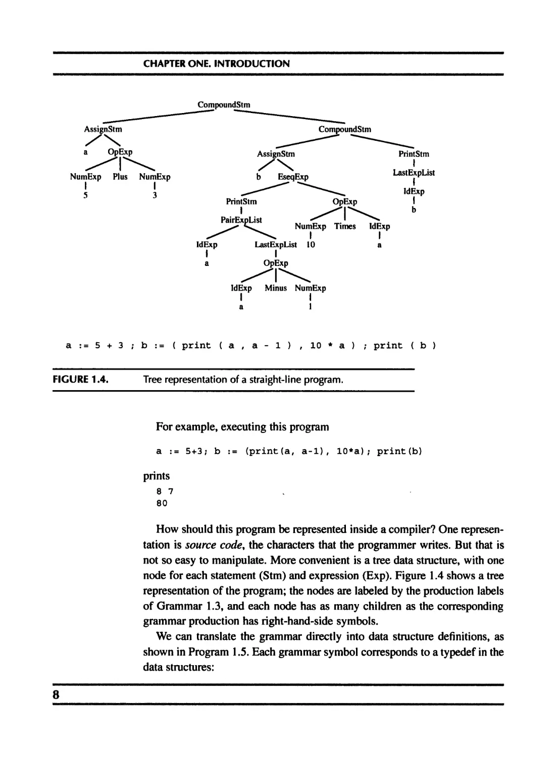
5 + 3 ; b := ( print ( a , a - 1 ) , 10 * a ) ; print ( b )
FIGURE 1.4. Tree representation of a straight-line program.
For example, executing this program
a := 5+3; b := (print(a, a-1), 10*a); print(b)
prints
8 7
80
How should this program be represented inside a compiler? One represen-
tation is source code, the characters that the programmer writes. But that is
not so easy to manipulate. More convenient is a tree data structure, with one
node for each statement (Stm) and expression (Exp). Figure 1.4 shows a tree
representation of the program; the nodes are labeled by the production labels
of Grammar 1.3, and each node has as many children as the corresponding
grammar production has right-hand-side symbols.
We can translate the grammar directly into data structure definitions, as
shown in Program 1.5. Each grammar symbol corresponds to a typedef in the
data structures:
8
1.3. DATA STRUCTURES FOR TREE LANGUAGES
Grammar typedef
Stm A_stm
Exp A_exp
ExpList A_expList
id string
num int
For each grammar rule, there is one constructor that belongs to the union
for its left-hand-side symbol. The constructor names are indicated on the
right-hand side of Grammar 1.3.
Each grammar rule has right-hand-side components that must be repre-
sented in the data structures. The CompoundStm has two Stm’s on the right-
hand side; the AssignStm has an identifier and an expression; and so on. Each
grammar symbol’s struct contains a union to carry these values, and a
kind field to indicate which variant of the union is valid.
For each variant (CompoundStm, AssignStm, etc.) we make a constructor
function to malloc and initialize the data structure. In Program 1.5 only the
prototypes of these functions are given; the definition of A_CompoundStm
would look like this:
A_sttn A_CompoundStm(A_stm strnl, A_stm stm2) {
A_stm s = checked_malloc(sizeof(*s));
s->kind = A_compoundStm;
s->u.compound.strnl=stml; s->u.compound.stm2=stm2;
return s;
}
For Binop we do something simpler. Although we could make a Binop
struct - with union variants for Plus, Minus, Times, Div - this is overkill
because none of the variants would carry any data. Instead we make an enum
type A_binop.
Programming style. We will follow several conventions for representing tree
data structures in C:
1. Trees are described by a grammar.
2. A tree is described by one or more typedef s, corresponding to a symbol in
the grammar.
3. Each typedef defines a pointer to a corresponding struct. The struct
name, which ends in an underscore, is never used anywhere except in the
declaration of the typedef and the definition of the struct itself.
4. Each struct contains a kind field, which is an enum showing different
variants, one for each grammar rule; and a u field, which is a union.
-
CHAPTER ONE. INTRODUCTION
typedef char *string;
typedef struct A_stm_ *A_stm;
typedef struct A_exp_ *A__exp;
typedef struct A_expList_ *A_expList;
typedef enum {Ajplus, A_minus,A_times,A_div} A_binop;
struct A_stm_ {enum {A__compoundStm, A__assignStm, AjprintStm} kind;
union {struct {A_stm stml, stm2;} compound;
struct {string id? A_exp exp;} assign;
struct {A_expList exps;} print;
} u;
};
A_stm A__CompoundStm(A_stm stml, A_stm stm2) ;
A__stm A_AssignStm(string id, A_exp exp) ;
A_stm A_PrintStm(A_expList exps);
struct A_exp_ {enum {A_idExp, A_numExp, A_opExp, A_eseqExp} kind;
union {string id;
int num;
struct {A_exp left; A_binop oper; A_exp right;} op;
struct {A_stm stm; A_exp exp;} eseq;
} u;
};
A_exp A_IdExp(string id);
A_exp A_NumExp(int num);
A_exp A_OpExp(A_exp left, A_binop oper, A_exp right);
A_exp A_EseqExp(A_stm stm, A_exp exp);
struct A_expList_ {enum {A_pairExpList, A_lastExpList} kind;
union {struct {A_exp head; A_expList tail;} pair;
A_exp last;
} u?
};
PROGRAM 1.5. Representation of straight-line programs.
5. If there is more than one nontrivial (value-carrying) symbol in the right-hand
side of a rule (example: the rule CompoundStm), the union will have a com-
ponent that is itself a struct comprising these values (example: the compound
element of the A_stm_ union).
6. If there is only one nontrivial symbol in the right-hand side of a rule, the
union will have a component that is the value (example: the num field of the
A_exp union).
7. Every class will have a constructor function that initializes all the fields. The
malloc function shall never be called directly, except in these constructor
functions.
10
1.3. DATA STRUCTURES FOR TREE LANGUAGES
8. Each module (header file) shall have a prefix unique to that module (example,
A_ in Program 1.5).
9. Typedef names (after the prefix) shall start with lowercase letters; constructor
functions (after the prefix) with uppercase; enumeration atoms (after the pre-
fix) with lowercase; and union variants (which have no prefix) with lowercase.
Modularity principles for C programs. A compiler can be a big program;
careful attention to modules and interfaces prevents chaos. We will use these
principles in writing a compiler in C:
1. Each phase or module of the compiler belongs in its own “.c” file, which will
have a corresponding “.h” file.
2. Each module shall have a prefix unique to that module. All global names
(structure and union fields are not global names) exported by the module shall
start with the prefix. Then the human reader of a file will not have to look
outside that file to determine where a name comes from.
3. All functions shall have prototypes, and the C compiler shall be told to warn
about uses of functions without prototypes.
4. We will #include "util. h" in each file:
/*util.h */
ttinclude <assert.h>
typedef char *string;
string String(char *);
typedef char bool;
ttdefine TRUE 1
#define FALSE 0
void *checked_malloc(int);
The inclusion of assert. h encourages the liberal use of assertions by the C
programmer.
5. The string type means a heap-allocated string that will not be modified af-
ter its initial creation. The String function builds a heap-allocated string
from a C-style character pointer (just like the standard C library function
strdup). Functions that take strings as arguments assume that the con-
tents will never change.
6. C’s malloc function returns NULL if there is no memory left. The Tiger
compiler will not have sophisticated memory management to deal with this
problem. Instead, it will never call malloc directly, but call only our own
function, checked_malloc, which guarantees never to return NULL:
11
CHAPTER ONE. INTRODUCTION
void *checked__malloc (int len) {
void *p = malloc(len);
assert(p);
return p;
}
7. We will never call free. Of course, a production-quality compiler must free
its unused data in order to avoid wasting memory. The best way to do this is
to use an automatic garbage collector, as described in Chapter 13 (see partic-
ularly conservative collection on page 296). Without a garbage collector, the
programmer must carefully f ree (p) when the structure p is about to become
inaccessible - not too late, or the pointer p will be lost, but not too soon, or
else still-useful data may be freed (and then overwritten). In order to be able
to concentrate more on compiling techniques than on memory deallocation
techniques, we can simply neglect to do any freeing.
PROGRAM
STRAIGHT-LINE PROGRAM INTERPRETER
Implement a simple program analyzer and interpreter for the straight-line
programming language. This exercise serves as an introduction to environ-
ments (symbol tables mapping variable-names to information about the vari-
ables); to abstract syntax (data structures representing the phrase structure of
programs); to recursion over tree data structures, useful in many parts of a
compiler; and to a functional style of programming without assignment state-
ments.
It also serves as a “warm-up” exercise in C programming. Programmers
experienced in other languages but new to C should be able to do this exercise,
but will need supplementary material (such as textbooks) on C.
Programs to be interpreted are already parsed into abstract syntax, as de-
scribed by the data types in Program 1.5.
However, we do not wish to worry about parsing the language, so we write
this program by applying data constructors:
A_stm prog =
A_CompoundStTn (A_AssignStm ("a",
A_OpExp (AJJumExp (5) , A_plus, A_NumExp (3) ) ) ,
A_CompoundStm(A_AssignStm("b",
A_EseqExp(AJPrintStm(A_PairExpList(A_IdExp("a") ,
A_LastExpList (A_OpExp (A__I dExp (" a ”), A_minus t
A_NumExp(1))))),
A_OpExp(A_NumExp(10), A_times, A_IdExp("a")))),
AJPrintStm(A_LastExpList(A_IdExp("b”)))));
12
PROGRAMMING EXERCISE
Files with the data type declarations for the trees, and this sample program,
are available in the directory $TlGER/chapl.
Writing interpreters without side effects (that is, assignment statements
that update variables and data structures) is a good introduction to denota-
tional semantics and attribute grammars, which are methods for describing
what programming languages do. It’s often a useful technique in writing com-
pilers, too; compilers are also in the business of saying what programming
languages do.
Therefore, in implementing these programs, never assign a new value to
any variable or structure-field except when it is initialized. For local variables,
use the initializing form of declaration (for example, int i=j+3;) and for
each kind of struct, make a “constructor” function that allocates it and
initializes all the fields, similar to the A_CompoundStm example on page 9.
1. Write a function int maxargs (A_stm) that tells the maximum number
of arguments of any print statement within any subexpression of a given
statement. For example, maxargs (prog) is 2.
2. Write a function void interp (A_stm) that “interprets” a program in this
language. To write in a “functional programming” style - in which you never
use an assignment statement - initialize each local variable as you declare it.
For part 1, remember that print statements can contain expressions that
contain other print statements.
For part 2, make two mutually recursive functions interpStm and
interpExp. Represent a “table,” mapping identifiers to the integer values
assigned to them, as a list of id x int pairs.
typedef struct table *Tab1ob-
struct table {string id; int value; Table_ tail};
Table_ Table(string id, int value, struct table *tail) {
Table_ t = malloc(sizeof (*t));
t->id=id; t->value=value; t->tail=tail;
return t;
}
The empty table is represented as NULL. Then interpStm is declared as
Table_ interpStm(A_stm s, Table_ t)
taking a table ti as argument and producing the new table h that’s just like
?j except that some identifiers map to different integers as a result of the
statement.
CHAPTER ONE INTRODUCTION
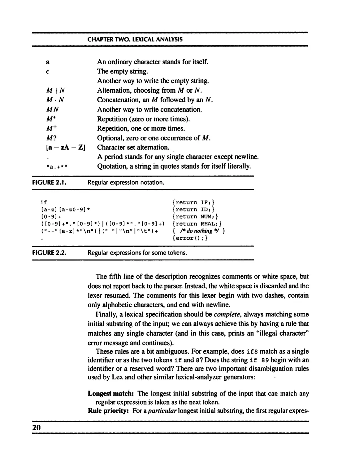
For example, the table that maps a to 3 and maps c to 4, which we write
{а 3, с 4} in mathematical notation, could be represented as the linked
list | a | 3 | -4—4~c 14 И •
Now, let the table t2 be just like ti, except that it maps c to 7 instead of 4.
Mathematically, we could write,
= update^, c, 7)
where the update function returns a new table {a 3, c i-> 7).
On the computer, we could implement ti by putting a new cell at the head
of the linked list: | c 17 | -|—>| a | 3 | H c 14 И as l°ng 38 we assume
that the first occurrence of c in the list takes precedence over any later occur-
rence.
Therefore, the update function is easy to implement; and the correspond-
ing lookup function
int lookup(Table_ t, string key)
just searches down the linked list.
Interpreting expressions is .more complicated than interpreting statements,
because expressions return integer values and have side effects. We wish
to simulate the straight-line programming language’s assignment statements
without doing any side effects in the interpreter itself. (The print statements
will be accomplished by interpreter side effects, however.) The solution is to
declare interpExp as
struct IntAndTable {int i; Table_ t;};
struct IntAndTable interpExp(A_exp e, Table_ t)
The result of interpreting an expression ei with table ti is an integer value i
and a new table ?2- When interpreting an expression with two subexpressions
(such as an OpExp), the table t2 resulting from the first subexpression can be
used in processing the second subexpression.
FURTHER
READING
Hanson [1997] describes principles for writing modular software in C.
14
EXERCISES
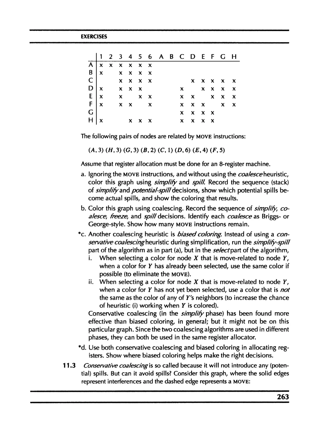
EXERCISES
1.1 This simple program implements persistent functional binary search trees, so
that if tree2=insert (x, treel), then treel is still available for lookups
even while tree2 can be used.
typedef struct tree *T_tree;
struct tree {T_tree left; String key; T_tree right;};
T_tree Tree(T_tree 1, String k, T_tree r) {
T_tree t = checked_malloc(sizeof(*t));
t->left=l; t->key=k; t->right=r;
return t;
}
T_tree insert (String key, T__tree t) {
if (t==NULL) return Tree(NULL, key, NULL)
else if (strcmp(key,t->key) < 0)
return Tree(insert(key,t->left),t->key,t->right);
else if (strcmp(key,t->key) > 0)
return Tree(t->left,t->key,insert(key,t->right));
else return Tree(t->left,key,t->right);
}
a. Implement a member function that returns true if the item is found, else
FALSE.
b. Extend the program to include not just membership, but the mapping of
keys to bindings:
T_tree insert(string key, void ‘binding, T_tree t);
void * lookup(string key, T_tree t);
c. These trees are not balanced; demonstrate the behavior on the following
two sequences of insertions:
(a) t s p i p f b s t
(b) abcdefghi
*d. Research balanced search trees in Sedgewick [1997] and recommend
a balanced-tree data structure for functional symbol tables. Hint: To
preserve a functional style, the algorithm should be one that rebalances
on insertion but not on lookup, so a data structure such as splay trees 'v-,
not appropriate.
15
2-------------
Lexical Analysis
lex-i-cal: of or relating to words or the vocabulary of
a language as distinguished from its grammar and con-
struction
Webster's Dictionary
To translate a program from one language into another, a compiler must first
pull it apart and understand its structure and meaning, then put it together in a
different way. The front end of the compiler performs analysis; the back end
does synthesis.
The analysis is usually broken up into
Lexical analysis: breaking the input into individual words or “tokens”;
Syntax analysis: parsing the phrase structure of the program; and
Semantic analysis: calculating the program’s meaning.
The lexical analyzer takes a stream of characters and produces a stream of
names, keywords, and punctuation marks; it discards white space and com-
ments between the tokens. It would unduly complicate the parser to have to
account for possible white space and comments at every possible point; this
is the main reason for separating lexical analysis from parsing.
Lexical analysis is not very complicated, but we will attack it with high-
powered formalisms and tools, because similar formalisms will be useful in
the study of parsing and similar tools have many applications in areas other
than compilation.
16
2.1. LEXICAL TOKENS
2.1 LEXICAL TOKENS
A lexical token is a sequence of characters that can be treated as a unit in the
grammar of a programming language. A programming language classifies
lexical tokens into a finite set of token types. For example, some of the token
types of a typical programming language are:
Type Examples
ID foo nl4 last
NUM 73 0 00 515 082
REAL 66.1 .5 10. le67 5.5e-10
IF if
COMMA /
NOTEQ ! =
LPAREN (
RPAREN )
Punctuation tokens such as IF, void, return constructed from alphabetic
characters are called reserved words and, in most languages, cannot be used
as identifiers.
Examples of nontokens are
comment
preprocessor directive
preprocessor directive
macro
blanks, tabs, and newlines
/* try again */
#include<stdio.h>
#define NUNS 5 , 6
NUNS
In languages weak enough to require a macro preprocessor, the prepro-
cessor operates on the source character stream, producing another character
stream that is then fed to the lexical analyzer. It is also possible to integrate
macro processing with lexical analysis.
Given a program such as
float matchO(char *s) /* find a zero */
{if (!strncmp(s, "0.0", 3))
return 0.;
}
the lexical analyzer will return the stream
FLOAT ID(matchO) LPAREN CHAR STAR ID(s) RPAREN
LBRACE IF LPAREN BANG ID(strncmp) LPAREN ID(s)
—
CHAPTER TWO. LEXICAL ANALYSIS
COMMA STRING(O.O) COMMA NUM(3) RPAREN RPAREN
RETURN REAL(O.O) SEMI RBRACE EOF
where the token-type of each token is reported; some of the tokens, such as
identifiers and literals, have semantic values attached to them, giving auxil-
iary information in addition to the token type.
How should the lexical rules of a programming language be described? In
what language should a lexical analyzer be written?
We can describe the lexical tokens of a language in English; here is a de-
scription of identifiers in C or Java:
An identifier is a sequence of letters and digits; the first character must be a
letter. The underscore _ counts as a letter. Upper- and lowercase letters are .
different. If the input stream has been parsed into tokens up to a given char-
acter, the next token is taken to include the longest string of characters that
could possibly constitute a token. Blanks, tabs, newlines, and comments are
ignored except as they serve to separate tokens. Some white space is required
to separate otherwise adjacent identifiers, keywords, and constants.
And any reasonable programming language serves to implement an ad hoc
lexer. But we will specify lexical tokens using the formal language of regular
expressions, implement lexers using deterministic finite automata, and use
mathematics to connect the two. This will lead to simpler and more readable
lexical analyzers.
2.2 REGULAR EXPRESSIONS
Let us say that a language is a set of strings', a string is a finite sequence of
symbols. The symbols themselves are taken from a finite alphabet.
The Pascal language is the set of all strings that constitute legal Pascal
programs; the language of primes is the set of all decimal-digit strings that
represent prime numbers; and the language of C reserved words is the set of
all alphabetic strings that cannot be used as identifiers in the C programming
language. The first two of these languages are infinite sets; the last is a finite
set. In all of these cases, the alphabet is the ASCII character set.
When we speak of languages in this way, we will not assign any meaning
to the strings; we will just be attempting to classify each string as in the
language or not.
To specify some of these (possibly infinite) languages with finite descrip-
18
2.2. REGULAR EXPRESSIONS
tions, we will use the notation of regular expressions. Each regular expression
stands for a set of strings.
Symbol: For each symbol a in the alphabet of the language, the regular expres-
sion a denotes the language containing just the string a.
Alternation: Given two regular expressions M and TV, the alternation operator
written as a vertical bar | makes a new regular expression M | N. A string is
in the language of Af | TV if it is in the language of M or in the language of
N. Thus, the language of a | b contains the two strings a and b.
Concatenation: Given two regular expressions M and N, the concatenation
operator • makes a new regular expression M • N. A string is in the language
of M • N if it is the concatenation of any two strings a and 0 such that a is in
the language of M and 0 is in the language of N. Thus, the regular expression
(a | b) • a defines the language containing the two strings aa and ba.
Epsilon: The regular expression € represents a language whose only string is
the empty string. Thus, {a • b) | e represents the language {" ",''ab"}.
Repetition: Given a regular expression M, its Kleene closure is M*. A string
is in M* if it is the concatenation of zero or more strings, all of which are in
M. Thus, ((a | b) -a)* represents the infinite set { " " , "aa", "ba", "aaaa",
"baaa", "aaba", "baba", "aaaaaa",...}.
Using symbols, alternation, concatenation, epsilon, and Kleene closure we
can specify the set of ASCII characters corresponding to the lexical tokens of
a programming language. First, consider some examples:
(0 | 1)* • 0 Binary numbers that are multiples of two.
b*(abb*)*(a|e) Strings of a’s and b’s with no consecutive a’s.
(a|b)*aa(a|b)* Strings of a’s and b’s containing consecutive a’s.
In writing regular expressions, we will sometimes omit the concatenation
symbol or the epsilon, and we will assume that Kleene closure “binds tighter”
than concatenation, and concatenation binds tighter than alternation; so that
ab | c means (a • b) | c, and (a |) means (a | e).
Let us introduce some more abbreviations: [abed] means (a | b | c |
d), [b-g] means [bedefg], [b-gM-Qkr] means [bcdefgMNOPQkr], ТИ?
means (M | e), and M+ means (M-M*). These extensions are convenient, but
none extend the descriptive power of regular expressions: Any set of strings
that can be described with these abbreviations could also be described by just
the basic set of operators. All the operators are summarized in Figure 2.1.
Using this language, we can specify the lexical tokens of a programming
language (Figure 2.2). For each token, we supply a fragment of C code that
reports which token type has been recognized.
—
CHAPTER TWO. LEXICAL ANALYSIS
a € An ordinary character stands for itself. The empty string. Another way to write the empty string.
M 1 W M-N MN M* M+ M? Alternation, choosing from M or N. Concatenation, an M followed by an N. Another way to write concatenation. Repetition (zero or more times). Repetition, one or more times. Optional, zero or one occurrence of M.
[a — zA — Z] Character set alternation.
"a.+*" A period stands for any single character except newline. Quotation, a string in quotes stands for itself literally.
FIGURE 2.1. Regular expression notation.
if
[a-z][a-zO-9]*
[0-9] +
( [0-9]+" . " [0-9]*) | ([0-9]"[0-9]+)
[a-z] *"\n") | (" "| "\n" | "\t") +
{return IF;}
{return ID;}
{return NUM;}
{return REAL;}
{ /♦ do nothing */ }
{error();}
FIGURE 2.2.
Regular expressions for some tokens.
The fifth line of the description recognizes comments or white space, but
does not report back to the parser. Instead, the white space is discarded and the
lexer resumed. The comments for this lexer begin with two dashes, contain
only alphabetic characters, and end with newline.
Finally, a lexical specification should be complete, always matching some
initial substring of the input; we can always achieve this by having a rule that
matches any single character (and in this case, prints an “illegal character”
error message and continues).
These rules are a bit ambiguous. For example, does if 8 match as a single
identifier or as the two tokens if and 8? Does the string if 89 begin with an
identifier or a reserved word? There are two important disambiguation rules
used by Lex and other similar lexical-analyzer generators:
Longest match: The longest initial substring of the input that can match any
regular expression is taken as the next token.
Rule priority: For a particular longest initial substring, the first regular expres-
20
2.3. FINITE AUTOMATA
any but \n
error
FIGURE 2.3. Finite automata for lexical tokens. The states are indicated by
circles; final states are indicated by double circles. The start
state has an arrow coming in from nowhere. An edge labeled
with several characters is shorthand for many parallel edges.
sion that can match determines its token type. This means that the order of
writing down the regular-expression rules has significance.
Thus, if 8 matches as an identifier by the longest-match rule, and if matches
as a reserved word by rule-priority.
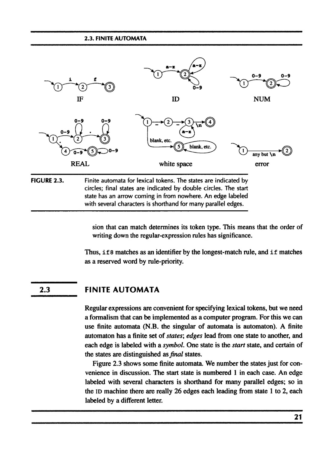
2.3 FINITE AUTOMATA
Regular expressions are convenient for specifying lexical tokens, but we need
a formalism that can be implemented as a computer program. For this we can
use finite automata (N.B. the singular of automata is automaton). A finite
automaton has a finite set of states', edges lead from one state to another, and
each edge is labeled with a symbol. One state is the start state, and certain of
the states are distinguished as final states.
Figure 2.3 shows some finite automata. We number the states just for con-
venience in discussion. The start state is numbered 1 in each case. An edge
labeled with several characters is shorthand for many parallel edges; so in
the ID machine there are really 26 edges each leading from state 1 to 2, each
labeled by a different letter.
CHAPTER TWO. LEXICAL ANALYSIS
FIGURE 2.4.
Combined finite automaton.
In a deterministic finite automaton (DFA), no two edges leaving from the
same state are labeled with the same symbol. A DFA accepts or rejects a
string as follows. Starting in the start state, for each character in the input
string the automaton follows exactly one edge to get to the next state. The
edge must be labeled with the input character. After making n transitions for
an n -character string, if the automaton is in a final state, then it accepts the
string. If it is not in a final state, or if at some point there was no appropriately
labeled edge to follow, it rejects. The language recognized by an automaton
is the set of strings that it accepts.
For example, it is clear that any string in the language recognized by au-
tomaton ID must begin with a letter. Any single letter leads to state 2, which
is final; so a single-letter string is accepted. From state 2, any letter or digit
leads back to state 2, so a letter followed by any number of letters and digits
is also accepted.
In fact, the machines shown in Figure 2.3 accept the same languages as the
regular expressions of Figure 2.2.
These are six separate automata; how can they be combined into a single
machine that can serve as a lexical analyzer? We will study formal ways of
doing this in the next section, but here we will just do it ad hoc: Figure 2.4
shows such a machine. Each final state must be labeled with the token-type
22
2.3. FINITE AUTOMATA
that it accepts. State 2 in this machine has aspects of state 2 of the IF machine
and state 2 of the ID machine; since the latter is final, then the combined state
must be final. State 3 is like state 3 of the IF machine and state 2 of the ID
machine; because these are both final we use rule priority to disambiguate
- we label state 3 with IF because we want this token to be recognized as a
reserved word, not an identifier.
We can encode this machine as a transition matrix: a two-dimensional ar-
ray (a vector of vectors), subscripted by state number and input character.
There will be a “dead” state (state 0) that loops to itself on all characters; we
use this to encode the absence of an edge.
int edges [] [256] ={ /* •• •0 1 2- -0,0,0-- e f g h i j -0---0,0,0,0,0,0
/* state 0 */ {0,0,--
/* state 1 */ I[ 0,0, • • -7,7,7-- -9- -4,4,4,4,2,4
/* state 2 */ {0,0,-- •4,4,4” -0 --4,3,4,4,4,4
/* state 3 */ {0, о,-- •4,4,4-- •0”-4,4,4,4,4,4
/* state 4 {0,0,-- •4,4,4” •0” -4,4,4,4,4,4
/* state 5 */ {0,0,-- -6,6,6- -0---0,0,0,0,0,0
/* state 6 */ {0,0,-- -6,6,6” •0”-0,0,0,0,0,0
/* state 7 */ {0,0,-- •7,7,7-- -0---0,0,0,0,0,0
/* state 8 */ et cetera {0,0,-- •8,8,8” -0---0,0,0,0,0,0
}
There must also be a “finality” array, mapping state numbers to actions - final
state 2 maps to action ID, and so on.
RECOGNIZING THE LONGEST MATCH
It is easy to see how to use this table to recognize whether to accept or reject
a string, but the job of a lexical analyzer is to find the longest match, the
longest initial substring of the input that is a valid token. While interpreting
transitions, the lexer must keep track of the longest match seen so far, and the
position of that match.
Keeping track of the longest match just means remembering the last time
the automaton was in a final state with two variables, Last-Final (the state
number of the most recent final state encountered) and input-Position-
at-Last-Final. Every time a final state is entered, the lexer updates these
variables; when a dead state (a nonfinal state with no output transitions) is
reached, the variables tell what token was matched, and where it ended.
Figure 2.5 shows the operation of a lexical analyzer that recognizes longest
matches; note that the current input position may be far beyond the most
recent position at which the recognizer was in a final state.
—
CHAPTER TWO. LEXICAL ANALYSIS
Last Final Current State Current Input Accept Action
0 1 ]lf --not-a-com
2 2 |i]f --not-a-com
3 3 |if[ - -not-a-com
3 0 |i ffj- -not - a - com return IF
0 1 if[--not-a-com
12 12 if| J--not-a-com
12 0 i f| tj- not - a - com found white space; resume
0 1 if J--not-a-com
9 9 if l-J-not-a-com
9 10 if l-^pot-a-com
9 10 if |^npt-a-com
9 10 if R^-ngt-a-com
9 10 if l-^-notta-com
9 0 if not-ja-com error, illegal token resume
0 1 if -J-not-a-com
9 9 if -l-Jiot-a-com
9 0 if -Rnpt-a-com error, illegal token resume
FIGURE 2.5. The automaton of Figure 2.4 recognizes several tokens. The
symbol | indicates the input position at each successive call
to the lexical analyzer, the symbol ± indicates the current
position of the automaton, and T indicates the most recent
position in which the recognizer was in a final state.
2.4 NONDETERMINISTIC FINITE AUTOMATA
A nondeterministic finite automaton (NFA) is one that has a choice of edges
- labeled with the same symbol - to follow out of a state. Or it may have
special edges labeled with e (the Greek letter epsilon), that can be followed
without eating any symbol from the input.
Here is an example of an NFA:
24
2.4. NONDETERMINISTIC FINITE AUTOMATA
In the start state, on input character a, the automaton can move either right or
left. If left is chosen, then strings of a’s whose length is a multiple of three
will be accepted. If right is chosen, then even-length strings will be accepted.
Thus, the language recognized by this NFA is the set of all strings of a’s
whose length is a multiple of two or three.
On the first transition, this machine must choose which way to go. It is
required to accept the string if there is any choice of paths that will lead to
acceptance. Thus, it must “guess,” and must always guess correctly.
Edges labeled with € may be taken without using up a symbol from the
input. Here is another NFA that accepts the same language:
Again, the machine must choose which 6-edge to take. If there is a state
with some c-edges and some edges labeled by symbols, the machine can
choose to eat an input symbol (and follow the corresponding symbol-labeled
edge), or to follow an 6-edge instead.
CONVERTING A REGULAR EXPRESSION TO AN NFA
Nondeterministic automata are a useful notion because it is easy to convert
a (static, declarative) regular expression to a (simulatable, quasi-executable)
NFA.
The conversion algorithm turns each regular expression into an NFA with
a tail (start edge) and a head (ending state). For example, the single-symbol
regular expression a converts to the NFA
The regular expression ab, made by combining a with b using concatena-
tion is made by combining the two NFAs, hooking the head of a to the tail of
b. The resulting machine has a tail labeled by a and a head into which the b
edge flows.
25
CHAPTER TWO. LEXICAL ANALYSIS
Л/+
[abc]
constructed as M • M *
constructed as M | €
"abcn constructed as a • b • c
FIGURE 2.6.
Translation of regular expressions to NFAs.
In general, any regular expression M will have some NFA with a tail and
head:
We can define the translation of regular expressions to NFAs by induc-
tion. Either an expression is primitive (a single symbol or 6) or it is made
from smaller expressions. Similarly, the NFA will be primitive or made from
smaller NFAs.
Figure 2.6 shows the rules for translating regular expressions to nonde-
terministic automata. We illustrate the algorithm on some of the expressions
in Figure 2.2 - for the tokens IF, ID, num, and error. Each expression is
translated to an NFA, the “head” state of each NFA is marked final with a dif-
ferent token type, and the tails of all the expressions are joined to a new start
node. The result - after some merging of equivalent NFA states - is shown in
Figure 2.7.
26
FIGURE 2.7.
Four regular expressions translated to an NFA.
CONVERTING AN NFA TO A DFA
As we saw in Section 2.3, implementing deterministic finite automata (DFAs)
as computer programs is easy. But implementing NFAs is a bit harder, since
most computers don’t have good “guessing” hardware.
We can avoid the need to guess by trying every possibility at once. Let
us simulate the NFA of Figure 2.7 on the string in. We start in state 1. Now,
instead of guessing which e-transition to take, we just say that at this point the
NFA might take any of them, so it is in one of the states {1,4,9,14}; that is,
we compute the e-closure of {1}. Clearly, there are no other states reachable
without eating the first character of the input.
Now, we make the transition on the character i. From state 1 we can reach
2, from 4 we reach 5, from 9 we go nowhere, and from 14 we reach 15. So we
have the set {2,5,15}. But again we must compute e-closure: from 5 there is
an 6-transition to 8, and from 8 to 6. So the NFA must be in one of the states
{2,5,6, 8,15}.
On the character n, we get from state 6 to 7, from 2 to nowhere, from 5 to
nowhere, from 8 to nowhere, and from 15 to nowhere. So we have the set {7};
its e-closure is {6,7, 8}.
Now we are at the end of the string in; is the NFA in a final state? One
of the states in our possible-states set is 8, which is final. Thus, in is an ID
token.
We formally define e-closure as follows. Let edge(5, c) be the set of all
NFA states reachable by following a single edge with label c from state s.
—
CHAPTER TWO. LEXICAL ANALYSIS
For a set of states 5, closure(S) is the set of states that can be reached from a
state in S without consuming any of the input, that is, by going only through
e edges. Mathematically, we can express the idea of going through € edges
by saying that closure(S) is smallest set T such that
T = 5 U | {J edgefv, t) I.
Ver /
We can calculate T by iteration:
T <- S
repeat T' +-T
T ^ru(U5eredge(5,C))
until T = Г
Why does this algorithm work? T can only grow in each iteration, so the
final T must include 5. If T = T' after an iteration step, then T must also in-
clude User edge(s, б). Finally, the algorithm must terminate, because there
are only a finite number of distinct states in the NFA.
Now, when simulating an NFA as described above, suppose we are in a set
d = $*,$/} of NFA states s,-, s*, s/. By starting in d and eating the input
symbol c, we reach a new set of NFA states; we’ll call this set DFAedge(d, c):
DFAedge(J, c) = closure([_Jedge(s, c))
sed
Using DFAedge, we can write the NFA simulation algorithm more formally.
If the start state of the NFA is $i, and the input string is cj,..., q, then the
algorithm is:
d «- closure({si})
for i <- 1 to к
d «— DFAedge(d, q)
Manipulating sets of states is expensive - too costly to want to do on every
character in the source program that is being lexically analyzed. But it is
possible to do all the sets-of-states calculations in advance. We make a DFA
from the NFA, such that each set of NFA states corresponds to one DFA state.
Since the NFA has a finite number n of states, the DFA will also have a finite
number (at most 2") of states.
DFA construction is easy once we have closure and DFAedge algorithms.
The DFA start state d\ is just closure^), as in the NFA simulation algo-
28
2.4. NONDETERMINISTIC FINITE AUTOMATA
FIGURE 2.8. NFA converted to DFA.
rithm. Abstractly, there is an edge from d, to dj labeled with c if dj =
DFAedge(J( , c). We let S be the alphabet.
states[0] «- {}; states[l] <— closure({si})
p i; j
while j < p
foreach c e E
e DFAedge(states[J], c)
if e = states[i] for some i < p
then trans[j, c] i
else p p + 1
states[p] <— e
transfj, c] p
j <- ./ +1
The algorithm does not visit unreachable states of the DFA. This is ex-
tremely important, because in principle the DFA has 2" states, but in practice
we usually find that only about n of them are reachable from the start state.
It is important to avoid an exponential blowup in the size of the DFA inter-
preter’s transition tables, which will form part of the working compiler.
A state d is final in the DFA if any NFA-state in states [d] is final in the
NFA. Labeling a state final is not enough; we must also say what token is
recognized; and perhaps several members of states[J] are final in the NFA.
In this case we label d with the token-type that occurred first in the list of
—
CHAPTER TWO. LEXICAL ANALYSIS
regular expressions that constitute the lexical specification. This is how rule
priority is implemented.
After the DFA is constructed, the “states” array may be discarded, and the
“trans” array is used for lexical analysis.
Applying the DFA construction algorithm to the NFA of Figure 2.7 gives
the automaton in Figure 2.8.
This automaton is suboptimal. That is, it is not the smallest one that recog-
nizes the same language. In general, we say that two states 5| and S2 are equiv-
alent when the machine starting in si accepts a string a if and only if starting
in 52 it accepts a. This is certainly true of the states labeled 5,6,8,15 and
6,7,8 in Figure 2.8; and of the states labeled 10,11,13,15 and 11,12,13.
In an automaton with two equivalent states 5| and 52, we can make all of 52’s
incoming edges point to 5] instead and delete 52.
How can we find equivalent states? Certainly, 51 and 52 are equivalent if
they are both final or both non-final and for any symbol c, transit, c] =
trans[52, c]; 110,11,13,L5~ and 11,12,13 satisfy this criterion. But this con-
dition is not sufficiently general; consider the automaton
Here, states 2 and 4 are equivalent, but trans[2, a] / trans[4, a].
After constructing a DFA it is useful to apply an algorithm to minimize it
by finding equivalent states; see Exercise 2.6.
2.5 Lex: A LEXICAL ANALYZER GENERATOR
DFA construction is a mechanical task easily performed by computer, so it
makes sense to have an automatic lexical analyzer generator to translate reg-
ular expressions into a DFA.
Lex is a lexical analyzer generator that produces a C program from a lexi-
cal specification. For each token type in the programming language to be lex-
ically analyzed, the specification contains a regular expression and an action.
30
2.5. LEX: A LEXICAL ANALYZER GENERATOR
*{
/* C Declarations: */
ttinclude " tokens. h" /* definitions of IF, ID, NUM,... */
ttinclude "errormsg.h"
union {int ival; string sval; double fval;} yylval;
int charPos=l;
#define ADJ (EM_tokPos=charPos, charPos+=yyleng)
%}
/* Lex Definitions: */
digits [0-9] +
%%
/* Regular Expressions and Actions: */
if {ADJ; return IF;}
[a-z] [a-zO-9] * {ADJ; yylval.sval=String(yytext);
return ID;}
{digits} {ADJ; yylval.ival=atoi(yytext);
return NUM;}
({digits}"."[0-9]*)|([0-9]*"."{digits}) {ADJ;
yylval.fval=atof(yytext);
return REAL;}
("--"[a-z]*"\n")|(" "|"\n"|"\t")+ {ADJ;}
{ADJ; EM_error("illegal character");}
PROGRAM 2.9. Lex specification of the tokens from Figure 2.2.
The action communicates the token type (perhaps along with other informa-
tion) to the next phase of the compiler.
The output of Lex is a program in C - a lexical analyzer that interprets
a DFA using the algorithm described in Section 2.3 and executes the action
fragments on each match. The action fragments are just C statements that
return token values.
The tokens described in Figure 2.2 are specified in Lex as shown in Pro-
gram 2.9.
The first part of the specification, between the %{• • •%} braces, contains
includes and declarations that may be used by the C code in the remainder
of the file.
The second part of the specification contains regular-expression abbrevi-
ations and state declarations. For example, the declaration digits [0 - 9] +
in this section allows the name {digits} to stand for a nonempty sequence
of digits within regular expressions.
The third part contains regular expressions and actions. The actions are
fragments of ordinary C code. Each action must return a value of type int,
denoting which kind of token has been found.
—
CHAPTER TWO. LEXICAL ANALYSIS
In the action fragments, several special variables are available. The string
matched by the regular expression is yytext. The length of the matched
string is yyleng.
In this particular example, we keep track of the position of each token,
measured in characters since the beginning of the file, in the variable char-
Pos. The EM_tokPos variable of the error message module errormsg. h is
continually told this position by calls to the macro adj. The parser will be
able to use this information in printing informative syntax error messages.
The include file tokens .h in this example defines integer constants IF,
ID, NUM, and so on; these values are returned by the action fragments to tell
what token-type is matched.
Some tokens have semantic values associated with them. For example, ID’s
semantic value is the character string constituting the identifier; num’s se-
mantic value is an integer; and IF has no semantic value (any IF is indistin-
guishable from any other). The values are communicated to the parser through
the global variable yylval, which is a union of the different types of seman-
tic values. The token-type returned by the lexer tells the parser which variant
of the union is valid.
START STATES
Regular expressions are static and declarative-, automata are dynamic and
imperative. That is, you can see the components and structure of a regular
expression without having to simulate an algorithm, but to understand an
automaton it is often necessary to “execute” it in your mind. Thus, regular
expressions are usually more convenient to specify the lexical structure of
programming-language tokens.
But sometimes the step-by-step, state-transition model of automata is ap-
propriate. Lex has a mechanism to mix states with regular expressions. One
can declare a set of start states-, each regular expression can be prefixed by
the set of start states in which it is valid. The action fragments can explic-
itly change the start state. In effect, we have a finite automaton whose edges
are labeled, not by single symbols, but by regular expressions. This example
shows a language with simple identifiers, if tokens, and comments delimited
by (* and *) brackets:
32
PROGRAMMING EXERCISE
Though it is possible to write a single regular expression that matches an en-
tire comment, as comments get more complicated it becomes more difficult,
or even impossible if nested comments are allowed.
The Lex specification corresponding to this machine is
: the usual preamble...
%Start INITIAL COMMENT
%%
<INITIAL>if {ADJ; return IF;}
<INITIAL>[a-z]+ {ADJ; yylval.sval=String(yytext); return ID;}
<INITIAL>"(* *" {ADJ; BEGIN COMMENT;}
<INITIAL>. {ADJ; EM_error("illegal character");}
«COMMENTS."*)" {ADJ; BEGIN INITIAL;}
<COMMENT>. {ADJ;}
{BEGIN INITIAL; yyless(l);}
PROGRAM
where initial is the “outside of any comment” state. The last rule is a hack
to get Lex into this state. Any regular expression not prefixed by a < state >
operates in all states; this feature is rarely useful.
This example can be easily augmented to handle nested comments, via a
global variable that is incremented and decremented in the semantic actions.
LEXICAL ANALYSIS
Use Lex to implement a lexical analyzer for the Tiger language. Appendix A
describes, among other things, the lexical tokens of Tiger.
This chapter has left out some of the specifics of how the lexical analyzer
should be initialized and how it should communicate with the rest of the com-
piler. You can learn this from the Lex manual, but the “skeleton” files in the
$TiGER/chap2 directory will also help get you started.
Along with the tiger. lex file you should turn in documentation for the
following points:
• how you handle comments;
• how you handle strings;
• error handling;
• end-of-file handling;
• other interesting features of your lexer.
33
CHAPTER TWO. LEXICAL ANALYSIS
Supporting files are available in $TlGER/chap2 as follows:
tokens .h Definition of lexical-token constants, and yylval.
errormsg.h, errormsg.c The error message module, useful for produc-
ing error messages with file names and line numbers.
driver. c A test scaffold to run your lexer on an input file,
tiger. lex The beginnings of a real tiger. lex file.
makefile A “makefile” to compile everything.
When reading the Tiger Language Reference Manual (Appendix A), pay
particular attention to the paragraphs with the headings Identifiers, Com-
ments, Integer literal, and String literal.
The reserved words of the language are: while, for, to, break, let, in,
end, function, var, type, array, if, then, else, do, of, nil.
The punctuation symbols used in the language are:
, : ; ( ) [ 1 { } .+-*/=<><<=>>=& | :=
The string value that you return for a string literal should have all the es-
cape sequences translated into their meanings.
There are no negative integer literals; return two separate tokens for -32.
Detect unclosed comments (at end of file) and unclosed strings.
The directory $TIGER/testcases contains a few sample Tiger programs.
To get started: Make a directory and copy the contents of $TlGER/chap2
into it. Make a file test .tig containing a short program in the Tiger lan-
guage. Then type make; Lex will run on tiger. lex, producing lex. yy. c,
and then the appropriate C files will be compiled.
Finally, lextest test. tig will lexically analyze the file using a test
scaffold.
FURTHER
READING
Lex was the first lexical-analyzer generator based on regular expressions
[Lesk 1975]; it is still widely used.
Computing €-closure can be done more efficiently by keeping a queue or
stack of states whose edges have not yet been checked for e-transitions [Aho
et al. 1986]. Regular expressions can be converted directly to DFAs without
going through NFAs [McNaughton and Yamada 1960; Aho et al. 1986].
DFA transition tables can be very laige and sparse. If represented as a sim-
ple two-dimensional matrix (states x symbols) they take far too much mem-
34
EXERCISES
ory. In practice, tables are compressed; this reduces the amount of memory
required, but increases the time required to look up the next state [Aho et al.
1986].
Lexical analyzers, whether automatically generated or handwritten, must
manage their input efficiently. Of course, input is buffered, so that a large
batch of characters is obtained at once; then the lexer can process one charac-
ter at a time in the buffer. The lexer must check, for each character, whether
the end of the buffer is reached. By putting a sentinel - a character that can-
not be part of any token - at the end of the buffer, it is possible for the lexer
to check for end-of-buffer only once per token, instead of once per character
[Aho et al. 1986]. Gray [1988] uses a scheme that requires only one check
per line, rather than one per token, but cannot cope with tokens that contain
end-of-line characters. Bumbulis and Cowan [1993] check only once around
each cycle in the DFA; this reduces the number of checks (from once per
character) when there are long paths in the DFA.
Automatically generated lexical analyzers are often criticized for being
slow. In principle, the operation of a finite automaton is very simple and
should be efficient, but interpreting from transition tables adds overhead.
Gray [1988] shows that DFAs translated directly into executable code (imple-
menting states as case statements) can run as fast as hand-coded lexers. The
Flex “fast lexical analyzer generator” [Paxson 1995] is significantly faster
than Lex.
EXERCISES
2.1 Write regular expressions for each of the following.
a. Strings over the alphabet (a, b, c] where the first a precedes the first b.
b. Strings over the alphabet [a, b, c} with an even number of a's.
c. Binary numbers that are multiples of four.
d. Binary numbers that are greater than 101001.
e. Strings over the alphabet {a, b, c] that don't contain the contiguous sub-
string baa.
f. The language of nonnegative integer constants in C, where numbers
—
CHAPTER TWO. LEXICAL ANALYSIS
beginning with 0 are octal constants and other numbers are decimal
constants.
g. Binary numbersn such that there exists an integer solution ofan+b" = cn.
2.2 For each of the following, explain why you're not surprised that there is no
regular expression defining it.
a. Strings of a's and b's where there are more a's than b’s.
b. Strings of a's and b's that are palindromes (the same forward as backward).
c. Syntactically correct C programs.
2.3 Explain in informal English what each of these finite state automata recognizes.
2.4 Convert these regular expressions to nondeterministic finite automata.
a. (if|then|else)
b. a((b|a*c)x)*|x*a
2.5 Convert these NFAs to deterministic finite automata.
36
EXERCISES
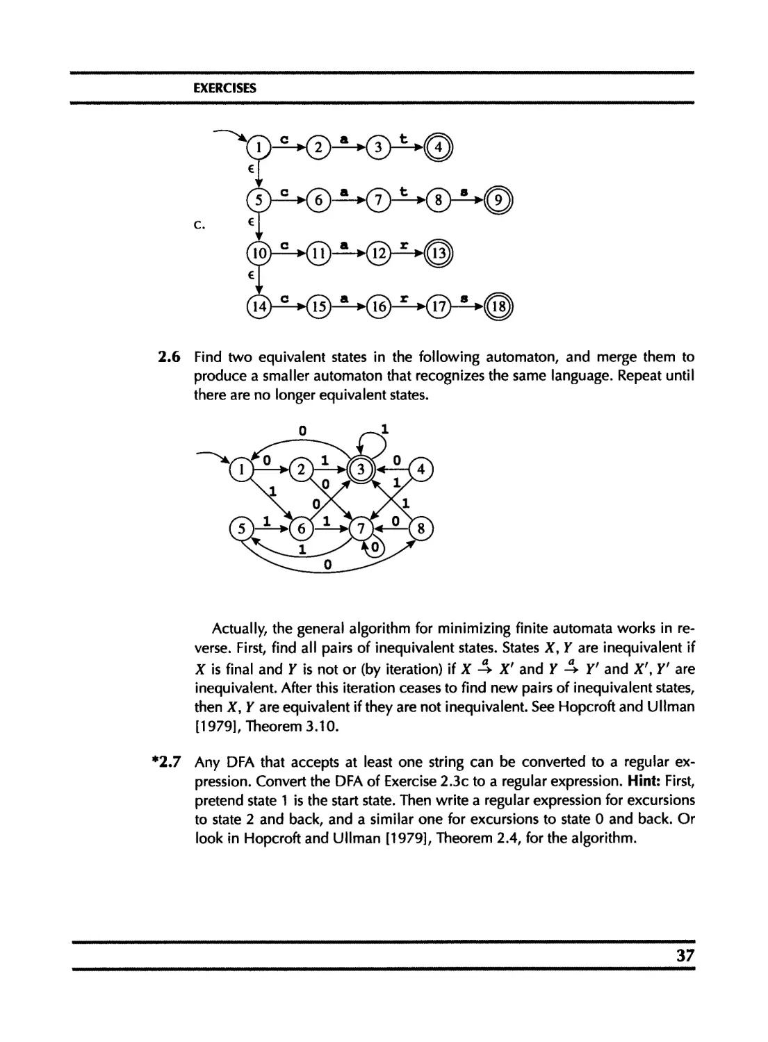
2.6 Find two equivalent states in the following automaton, and merge them to
produce a smaller automaton that recognizes the same language. Repeat until
there are no longer equivalent states.
Actually, the general algorithm for minimizing finite automata works in re-
verse. First, find all pairs of inequivalent states. States X, Y are inequivalent if
X is final and Y is not or (by iteration) if X Л X' and Y Д Y' and X', Y' are
inequivalent. After this iteration ceases to find new pairs of inequivalent states,
then X, Y are equivalent if they are not inequivalent. See Hopcroft and Ullman
[1979], Theorem 3.10.
*2.7 Any DFA that accepts at least one string can be converted to a regular ex-
pression. Convert the DFA of Exercise 2.3c to a regular expression. Hint: First,
pretend state 1 is the start state. Then write a regular expression for excursions
to state 2 and back, and a similar one for excursions to state 0 and back. Or
look in Hopcroft and Ullman [1979], Theorem 2.4, for the algorithm.
37
CHAPTER TWO. LEXICAL ANALYSIS
*2.8 Suppose this DFA were used by Lex to find tokens in an input file.
a. How many characters past the end of a token might Lex have to examine
before matching the token?
b. Given your answer k to part (a), show an input file containing at least
two tokens such that the first call to Lex will examine к characters past
the end of the first token before returning the first token. If the answer to
part (a) is zero, then show an input file containing at least two tokens,
and indicate the endpoint of each token.
2.9 An interpreted DFA-based lexical analyzer uses two tables,
edges indexed by state and input symbol, yielding a state number, and
final indexed by state, returning 0 or an action-number.
Starting with this lexical specification,
(aba)+ (action 1);
(a(b*)a) (action 2);
(a|b) (action 3);
generate the edges and final tables for a lexical analyzer.
Then show each step of the lexer on the string abaabbaba. Be sure to show
the values of the important internal variables of the recognizer. There will be
repeated calls to the lexer to get successive tokens.
**2.10 Lex has a iookaheadxypzxbXQX / so that the regular expression abc/def matches
abc only when followed by def (but def is not part of the matched string,
and will be part of the next token(s)). Aho et al. [1986] describe, and Lex
[Lesk 1975] uses, an incorrect algorithm for implementing lookahead (it fails
on (a | ab) /ba with input aba, matching ab where it should match a). Flex
[Raxson 1995] uses a better mechanism that works correctly for (a | ab) /ba
but fails (with a warning message) on zx*/xy*.
Design a better lookahead mechanism.
38
3 —
Parsing
syn-tax: the way in which words are put together to form
phrases, clauses, or sentences.
Webster's Dictionary
The abbreviation mechanism in Lex, whereby a symbol stands for some regu-
lar expression, is convenient enough that it is tempting to use it in interesting
ways:
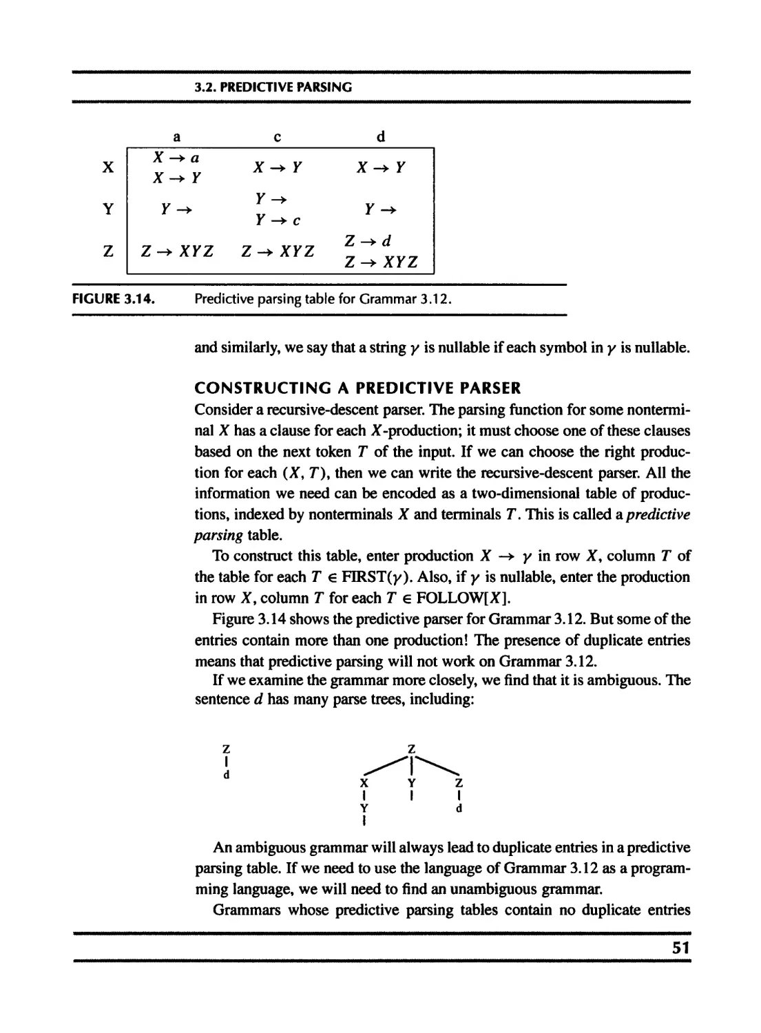
digits = [0 — 9]+
sum = (digits “+”)* digits
These regular expressions define sums of the form 28+301+9.
But now consider
digits = [0 — 9]+
sum = expr “+” expr
expr = “ (” sum “) ” I digits
This is meant to define expressions of the form:
(109+23)
61
(l+(250+3))
in which all the parentheses are balanced. But it is impossible for a finite au-
tomaton to recognize balanced parentheses (because a machine with N states
cannot remember a parenthesis-nesting depth greater than 2V), so clearly sum
and expr cannot be regular expressions.
So how does Lex manage to implement regular-expression abbreviations
such as digits? The answer is that the right-hand-side ( [0- 9] +) is simply
—
CHAPTER THREE. PARSING
substituted for digits wherever it appears in regular expressions, before
translation to a finite automaton.
This is not possible for the sum-and-expr language; we can first substitute
sum into expr, yielding
expr = “ (” expr “+” expr “) ” I digits
but now an attempt to substitute expr into itself leads to
expr = “(”(“(” expr “+” expr “) ” | digits ) “+” expr “) ” | digits
and the right-hand side now has just as many occurrences of expr as it did
before - in fact, it has more!
Thus, the notion of abbreviation does not add expressive power to the lan-
guage of regular expressions - there are no additional languages that can be
defined - unless the abbreviations are recursive (or mutually recursive, as are
sum and expr).
The additional expressive power gained by recursion is just what we need
for parsing. Also, once we have abbreviations with recursion, we do not need
alternation except at the top level of expressions, because the definition
expr = ab(c | d)e
can always be rewritten using an auxiliary definition as
aux = c | d
expr = a b aux e
In fact, instead of using the alternation mark at all, we can just write several
allowable expansions for the same symbol:
aux = c
aux = d
expr = a b aux e
The Kleene closure is not necessary, since we can rewrite it so that
expr = (abc)*
becomes
expr = (a b c) expr
expr = 6
40
3.1. CONTEXT-FREE GRAMMARS
i S-> 5; S
2 S-* id-.= E
з 5 -> print ( L )
< E —> id
s E —> num
6 E —> E + E
7 E -> (S , E )
8 L -> E
9 L —> L , E
GRAMMAR 3.1. A syntax for straight-line programs.
What we have left is a very simple notation, called context-free grammars.
Just as regular expressions can be used to define lexical structure in a static,
declarative way, grammars define syntactic structure declaratively. But we
will need something more powerful than finite automata to parse languages
described by grammars.
In fact, grammars can also be used to describe the structure of lexical to-
kens, although regular expressions are adequate - and more concise - for that
purpose.
3.1 CONTEXT-FREE GRAMMARS
As before, we say that a language is a set of strings; each string is a finite
sequence of symbols taken from a finite alphabet. For parsing, the strings are
source programs, the symbols are lexical tokens, and the alphabet is the set
of token types returned by the lexical analyzer.
A context-free grammar describes a language. A grammar has a set of
productions of the form
symbol —> symbol symbol • • symbol
where there are zero or more symbols on the right-hand side. Each symbol
is either terminal, meaning that it is a token from the alphabet of strings in
the language, or nonterminal, meaning that it appears on the left-hand side of
some production. No token can ever appear on the left-hand side of a produc-
tion. Finally, one of the nonterminals is distinguished as the start symbol of
the grammar.
Grammar 3.1 is an example of a grammar for straight-line programs. The
start symbol is S (when the start symbol is not written explicitly it is conven-
tional to assume that the left-hand nonterminal in the first production is the
start symbol). The terminal symbols are
id print num , + ( ) := ;
—
CHAPTER THREE. PARSING
5
S; 5
S ; id : = E
id : = E ; id : = E
id : = num ; id : = E
id : = num ; id : = E + E
id : = num ; id : = E + (5 , E )
id : = num ; id : = id + (S, E )
id : = num ; id : = id + (id : = E , E )
id : = num ; id : = id + (id : = E + E , E )
id : = num ; id : = id + (id : = E + E , id)
id : = num ; id : = id + (id : = num + E , id)
id : = num ; id : = id + (id : = num 4- num , id )
DERIVATION 3.2.
and the nonterminals are 5, E, and L. One sentence in the language of this
grammar is
id := num; id := id + (id := num + num, id)
where the source text (before lexical analysis) might have been
a := 7;
b := C + (d := 5 + 6, d)
The token-types (terminal symbols) are id, num, : =, and so on; the names
(a, b, c, d) and numbers (7, 5, 6) are semantic values associated with some
of the tokens.
DERIVATIONS
To show that this sentence is in the language of the grammar, we can per-
form a derivation: start with the start symbol, then repeatedly replace any
nonterminal by one of its right-hand sides, as shown in Derivation 3.2.
There are many different derivations of the same sentence. A leftmost
derivation is one in which the leftmost nonterminal symbol is always the one
expanded; in a rightmost derivation, the rightmost nonterminal is always next
to be expanded.
42
3.1. CONTEXT-FREE GRAMMARS
FIGURE 3.3. Parse tree.
Derivation 3.2 is neither leftmost nor rightmost; a leftmost derivation for
this sentence would begin,
S
S; S
id : = E ; 5
id : = num ; S
id : = num ; id : = E_
id : = num ; id : = E_ + E
PARSE TREES
A parse tree is made by connecting each symbol in a derivation to the one
from which it was derived, as shown in Figure 3.3. Two different derivations
can have the same parse tree.
AMBIGUOUS GRAMMARS
A grammar is ambiguous if it can derive a sentence with two different parse
trees. Grammar 3.1 is ambiguous, since the sentence id : = id+id+id has
two parse trees (Figure 3.4).
Grammar 3.5 is also ambiguous; Figure 3.6 shows two parse trees for the
sentence i-2-з, and Figure 3.7 shows two trees for 1+2*3. Clearly, if we use
—
CHAPTER THREE. PARSING
FIGURE 3.4. Two parse trees for the same sentence using Grammar 3.1.
E —► id
E —> num
E —> E * E
EE / E
E-+ E + E
E-* E - E
E^{E)
GRAMMAR 3.5.
FIGURE 3.6. Two parse trees for the sentence 1-2-3 in Grammar 3.5.
FIGURE 3.7. Two parse trees for the sentence 1+2*3 in Grammar 3.5.
44
3.1. CONTEXT-FREE GRAMMARS
E E + T
E^> E - T
E^T
T -+T * F
T^T/F
T -> F
F -> id
F —> num
F-> (E)
GRAMMAR 3.8.
FIGURE 3.9. Parse trees that Grammar 3.8 will never produce.
parse trees to interpret the meaning of the expressions, the two parse trees for
1-2-3 mean different things: (1 — 2) — 3 = —4 versus 1 — (2 — 3) = 2.
Similarly, (1 + 2) x 3 is not the same as 1 + (2 x 3). And indeed, compilers
do use parse trees to derive meaning.
Therefore, ambiguous grammars are problematic for compiling: in general
we would prefer to have unambiguous grammars. Fortunately, we can often
transform ambiguous grammars to unambiguous grammars.
Let us find an unambigous grammar that accepts the same language as
Grammar 3.5. First, we would like to say that * binds tighter than +, or has
higher precedence. Second, we want to say that each operator associates to
the left, so that we get (1 — 2) — 3 instead of 1 — (2 — 3). We do this by
introducing new nonterminal symbols to get Grammar 3.8.
The symbols E,T, and F stand for expression, term, and factor, conven-
tionally, factors are things you multiply and terms are things you add.
This grammar accepts the same set of sentences as the ambiguous gram-
mar, but now each sentence has exactly one parse tree. Grammar 3.8 can never
produce parse trees of the form shown in Figure 3.9 (see Exercise 3.17).
Had we wanted to make * associate to the right, we could have written its
production as T -> F * T.
We can usually eliminate ambiguity by transforming the grammar. Though
there are some languages (sets of strings) that have ambiguous grammars
but no unambiguous grammar, such languages may be problematic as pro-
gramming languages because the syntactic ambiguity may lead to problems
in writing and understanding programs.
—
CHAPTER THREE. PARSING
S -> E$ T ->T * F F —► id
E -> E + T T -+T / F F -> num
E -> E - T T -> F (E)
E T
GRAMMAR 3.10.
5 —> if E then S else S L - J * end * ; SL
S -> begin S L Lt “
S -> print E E - -> num = num
GRAMMAR 3.11.
END-OF-FILE MARKER
Parsers must read not only terminal symbols such as num, and so on, but
also the end-of-file marker. We will use $ to represent end of file.
Suppose S is the start symbol of a grammar. To indicate that $ must come
after a complete 5-phrase, we augment the grammar with a new start symbol
S' and a new production S' -> S$.
In Grammar 3.8, E is the start symbol, so an augmented grammar is Gram-
mar 3.10.
3.2 PREDICTIVE PARSING
Some grammars are easy to parse using a simple algorithm known as recur-
sive descent. In essence, each grammar production turns into one clause of a
recursive function. We illustrate this by writing a recursive-descent parser for
Grammar 3.11.
A recursive-descent parser for this language has one function for each non-
terminal and one clause for each production.
46
3.2. PREDICTIVE PARSING
enum token {IF, THEN, ELSE, BEGIN, END, PRINT, SEMI, NUM, EQ};
extern enum token getToken(void);
enum token tok;
void advance() {tok=getToken();}
void eat(enum token t) {if (tok==t) advance0; else error();}
void S(void) {switch(tok) {
case IF: eat (IF); E(); eat (THEN); SO;
eat (ELSE); SO; break;
case BEGIN: eat (BEGIN) ; SO; L(); break;
case PRINT: eat (PRINT); E(); break;
default: error();
}}
void L(void) {switch(tok) {
case END: eat(END); break;
case SEMI: eat (SEMI); SO; L(); break;
default: error();
}}
void E(void) { eat(NUM); eat(EQ); eat(NUM); }
With suitable definitions of error and getToken, this program will parse
very nicely.
Emboldened by success with this simple method, let us try it with Gram-
mar 3.10:
void S (void) { E() ; eat (EOF); }
void E(void) {switch (tok) {
case ?: E(); eat(PLUS); T(); break;
case ?: E(); eat(MINUS); T(); break;
case ?: TO; break;
default: error();
}}
void T(void) {switch (tok) {
case ?: TO; eat (TIMES) ; F () ; break;
case ?: T(); eat (DIV) ; F(); break;
case ?: F(); break;
default: error();
}}
There is a conflict here: the E function has no way to know which clause to
use. Consider the strings (1*2-3) +4 and (1*2-3). In the former case, the
initial call to E should use the E —> E + T production, but the latter case
should use E -► T.
Recursive-descent, or predictive, parsing works only on grammars where
the first terminal symbol of each subexpression provides enough information
—
CHAPTER THREE. PARSING
Z -> d
Z-tXYZ
X -► Y
Xa
GRAMMAR 3.12.
to choose which production to use. To understand this better, we will formal-
ize the notion of FIRST sets, and then derive conflict-free recursive-descent
parsers using a simple algorithm.
Just as lexical analyzers can be constructed from regular expressions, there
are parser-generator tools that build predictive parsers. But if we are going to
use a tool, then we might as well use one based on the more powerful LR(1)
parsing algorithm, which will be described in Section 3.3.
Sometimes it’s inconvenient or impossible to use a parser-generator tool.
The advantage of predictive parsing is that the algorithm is simple enough
that we can use it to construct parsers by hand - we don’t need automatic
tools.
FIRST AND FOLLOW SETS
Given a string у of terminal and nonterminal symbols, FIRST(y) is the set of
all terminal symbols that can begin any string derived from y. For example,
let у = T * F. Any string of terminal symbols derived from у must start with
id, num, or (. Thus,
FIRST(T * F) = {id, num, (}.
If two different productions X -► yi and X -> yi have the same left-
hand-side symbol (X) and their right-hand sides have overlapping FIRST
sets, then the grammar cannot be parsed using predictive parsing. If some
terminal symbol / is in FIRST(yi) and also in FIRSTS), then the X func-
tion in a recursive-descent parser will not know what to do if the input token
is I.
The computation of FIRST sets looks very simple: if у = X YZ, it seems
as if Y and Z can be ignored, and FIRST(X) is the only thing that matters.
But consider Grammar 3.12. Because Y can produce the empty string - and
therefore X can produce the empty string - we find that FIRST(X YZ) must
include FIRST(Z). Therefore, in computing FIRST sets, we must keep track
of which symbols can produce the empty string; we say such symbols are
nullable. And we must keep track of what might follow a nullable symbol.
With respect to a particular grammar, given a string у of terminals and
nonterminals,
48
3.2. PREDICTIVE PARSING
• nullable(X) is true if X can derive the empty string.
• FIRST(y) is the set of terminals that can begin strings derived from y.
• FOLLOW(X) is the set of terminals that can immediately follow X. That is,
t e FOLLOW(X) if there is any derivation containing Xt. This can occur if
the derivation contains X YZt where Y and Z both derive e.
A precise definition of FIRST, FOLLOW, and nullable is that they are the
smallest sets for which these properties hold:
For each terminal symbol Z, FIRST[Z] = {Z}.
for each production X -> Fi Y2 • • • Y*
for each i from 1 to k, each j from i + 1 to k,
if all the Y, are nullable
then nullable[X] = true
if Yi • • • F, _i are all nullable
then FIRST[X] = FIRST[X] U FZRST[F,]
if y,+i • • • Yk are all nullable
then FOLLOW!/,] = FOLLOW!/,] U FOLLOW[X]
if F|+i • • • Yj-i are all nullable
then FOLLOW[У,] = FOLLOW!//] U FIRST!/J
Algorithm 3.13 for computing FIRST, FOLLOW, and nullable just follows
from these facts; we simply replace each equation with an assignment state-
ment, and iterate.
Of course, to make this algorithm efficient it helps to examine the produc-
tions in the right order; see Section 17.4. Also, the three relations need not be
computed simultaneously; nullable can be computed by itself, then FIRST,
then FOLLOW.
This is not the first time that a group of equations on sets has become
the algorithm for calculating those sets; recall the algorithm on page 28 for
computing c-closure. Nor will it be the last time; the technique of iteration to
a fixed point is applicable in dataflow analysis for optimization, in the back
end of a compiler.
We can apply this algorithm to Grammar 3.12. Initially, we have:
nullable FIRST FOLLOW
X no
Y no
Z no
In the first iteration, we find that a € FIRST! X], Y is nullable,
c e FIRST!/], d e FIRST[Z], d e FOLLOW[X], c e FOLLOW[X],
—
CHAPTER THREE. PARSING
Algorithm to compute FIRST, FOLLOW, and nullable.
Initialize FIRST and FOLLOW to all empty sets, and nullable to all false.
for each terminal symbol Z
FIRST[Z] <- {Z}
repeat
for each production X -> Yi Y2 • • • F*
for each i from 1 to k, each j from i + 1 to k,
if all the F, are nullable
then nullablef X] <— true
if Fi • • • T,_i are all nullable
then FIRST[XJ *- FIRST[X] U FIRST! F(J
if T(+| • • • Yk are all nullable
then FOLLOW!У,] *- FOLLOW! F,] U FOLLOW[X]
if K+i • • • y?_i are all nullable
then FOLLOW!У,] ч-FOLLOW!F,] UFIRST!FJ
until FIRST, FOLLOW, and nullable did not change in this iteration.
ALGORITHM 3.13. Iterative computation of FIRST, FOLLOW, and nullable.
d € FOLLOW^]. Thus:
nullable FIRST FOLLOW
X no a c d
Y yes c d
Z no d
In the second iteration, we find that X is nullable, c e FIRST[X], {a, с) c
FIRSTIZ], {a, c, d] c FOLLOW[X], {a, c, d] C FOLLOW^]. Thus:
nullable FIRST FOLLOW
X yes ac ac d
Y yes c a c d
Z no ac d
The third iteration finds no new information, and the algorithm terminates.
It is useful to generalize the FIRST relation to strings of symbols:
FIRST(Xy) = FIRSTfX] if not nullable[X]
FIRST(Xy) = FIRSTIX] U FIRST(y) if nullable[X]
50
3.2. PREDICTIVE PARSING
and similarly, we say that a string у is nullable if each symbol in у is nullable.
CONSTRUCTING A PREDICTIVE PARSER
Consider a recursive-descent parser. The parsing function for some nontermi-
nal X has a clause for each X-production; it must choose one of these clauses
based on the next token T of the input. If we can choose the right produc-
tion for each (X, T), then we can write the recursive-descent parser. All the
information we need can be encoded as a two-dimensional table of produc-
tions, indexed by nonterminals X and terminals T. This is called a predictive
parsing table.
To construct this table, enter production X -> у in row X, column T of
the table for each T € FIRST(y). Also, if у is nullable, enter the production
in row X, column T for each T e FOLLOWfX].
Figure 3.14 shows the predictive parser for Grammar 3.12. But some of the
entries contain more than one production! The presence of duplicate entries
means that predictive parsing will not work on Grammar 3.12.
If we examine the grammar more closely, we find that it is ambiguous. The
sentence d has many parse trees, including:
An ambiguous grammar will always lead to duplicate entries in a predictive
parsing table. If we need to use the language of Grammar 3.12 as a program-
ming language, we will need to find an unambiguous grammar.
Grammars whose predictive parsing tables contain no duplicate entries
51
CHAPTER THREE. PARSING
are called LL(1). This stands for Left-to-right parse, Leftmost-derivation,
1-symbol lookahead. Clearly a recursive-descent (predictive) parser exam-
ines the input left-to-right in one pass (some parsing algorithms do not, but
these are generally not useful for compilers). The order in which a predic-
tive parser expands nonterminals into right-hand sides (that is, the recursive-
descent parser calls functions corresponding to nonterminals) is just the order
in which a leftmost derivation expands nonterminals. And a recursive-descent
parser does its job just by looking at the next token of the input, never looking
more than one token ahead.
We can generalize the notion of FIRST sets to describe the first k tokens of
a string, and to make an LL(k) parsing table whose rows are the nonterminals
and columns are every sequence of к terminals. This is rarely done (because
the tables are so large), but sometimes when you write a recursive-descent
parser by hand you a need to look more than one token ahead.
Grammars parsable with LL(2) parsing tables are called LL(2) grammars,
and similarly for LL(3), etc. Every LL(1) grammar is an LL(2) grammar, and
so on. No ambiguous grammar is LL(k) for any k.
ELIMINATING LEFT RECURSION
Suppose we want to build a predictive parser for Grammar 3.10. The two
productions
E -> E + T
E-+T
are certain to cause duplicate entries in the LL(1) parsing table, since any
token in FIRST(T) will also be in FIRST(E + T). The problem is that E
appears as the first right-hand-side symbol in an E-production; this is called
left recursion. Grammars with left recursion cannot be LL(1).
To eliminate left recursion, we will rewrite using right recursion. We intro-
duce a new nonterminal E', and write
E -> T E'
E' -» + T E'
E' -►
This derives the same set of strings (on T and +) as the original two produc-
tions, but now there is no left recursion.
52
3.2. PREDICTIVE PARSING
s E$
T FT'
E T E' F - > id
Г -> * FT' F - * num
E' -> + T E' T' -+ / FT' F - > (E)
E' -ТЕ' T' ->
E' ->
GRAMMAR 3.15.
nullable FIRST FOLLOW
5 no (id num
E no (id num )$
E' yes + - )$
T no (id num ) + -$
Г yes */ ) + -$
F no (id num )*/+-$
TABLE 3.16.
Nullable, FIRST, and FOLLOW for Grammar 3.8.
In general, whenever we have productions X -> Xy and X —► a, where a
does not start with X, we know that this derives strings of the form ay*, an a
followed by zero or more y. So we can rewrite the regular expression using
right recursion:
< X -► X yi >
X -> X y2
X -> ai
X a2 >
(X —> ai X'\
X —> a2 X'
X' yt X'
X' -> y2 X'
Applying this transformation to Grammar 3.10, we obtain Grammar 3.15.
To build a predictive parser, first we compute nullable, FIRST, and FOL-
LOW (Table 3.16). The predictive parser for Grammar 3.15 is shown in Ta-
ble 3.17.
LEFT FACTORING
We have seen that left recursion interferes with predictive parsing, and that
it can be eliminated. A similar problem occurs when two productions for the
—
CHAPTER THREE. PARSING
Predictive parsing table for Grammar 3.15. We omit the
columns for num, /, and as they are similar to others in
the table.
TABLE 3.17.
same nonterminal start with the same symbols. For example:
S —> if E then S else S
S —> if E then S
In such a case, we can left factor the grammar - that is, take the allowable
endings (“else S” and c) and make a new nonterminal X to stand for them:
S if E then S X
X -►
X -> else S
The resulting productions will not pose a problem for a predictive parser.
ERROR RECOVERY
Armed with a predictive parsing table, it is easy to write a recursive-descent
parser. Here is a representative fragment of a parser for Grammar 3.15:
void T(void) {switch (tok) {
case ID:
case NUM:
case LPAREN: F(); TprimeO; break;
default: error!
}}
void Tprime(void) {switch (tok) {
case PLUS: break;
case TIMES: eat(TIMES); F(); TprimeO; break;
case EOF: break;
case RPAREN: break;
default: error!
}}
54
3.2. PREDICTIVE PARSING
A blank entry in row T, column x of the LL(1) parsing table indicates that
the parsing function т () does not expect to see token x - this will be a syntax
error. How should error be handled? It is safe just to raise an exception and
quit parsing, but this is not very friendly to the user. It is better to print an
error message and recover from the error, so that other syntax errors can be
found in the same compilation.
A syntax error occurs when the string of input tokens is not a sentence in
the language. Error recovery is a way of finding some sentence similar to that
string of tokens. This can proceed by deleting, replacing, or inserting tokens.
For example, error recovery for T could proceed by inserting a num token.
It’s not necessary to adjust the actual input; it suffices to pretend that the num
was there, print a message, and return normally.
void T(void) {switch (tok) {
case ID:
case NUM:
case LPAREN: P () ; TprimeO; break;
default: printf("expected id, num, or left-paren");
}}
It’s a bit dangerous to do error recovery by insertion, because if the error
cascades to produce another error, the process might loop infinitely. Error re-
covery by deletion is safer, because the loop must eventually terminate when
end-of-file is reached.
Simple recovery by deletion works by skipping tokens until a token in the
FOLLOW set is reached. For example, error recovery for T' could work like
this:
int Tprime_follow [] = {PLUS, TIMES, RPAREN, EOF, -1};
void Tprime(void) { switch (tok) {
case PLUS: break;
case TIMES: eat (TIMES); F(); TprimeO; break;
case RPAREN: break;
case EOF: break;
default: printf("expected +, *, right-paren,
or end-of-file");
skipto(Tprime_follow);
}}
A recursive-descent parser’s error-recovery mechanisms must be adjusted
(sometimes by trial and error) to avoid a long cascade of error-repair mes-
sages resulting from a single token out of place.
—
CHAPTER THREE. PARSING
3.3 LR PARSING
The weakness of LL(k) parsing techniques is that they must predict which
production to use, having seen only the first к tokens of the right-hand side.
A more powerful technique, LR(k) parsing, is able to postpone the decision
until it has seen input tokens corresponding to the entire right-hand side of
the production in question (and к more input tokens beyond).
LR(k) stands for Left-to-right parse, Rightmost-derivation, к-token looka-
head. The use of a rightmost derivation seems odd; how is that compatible
with a left-to-right parse? Figure 3.18 illustrates an LR parse of the program
a := 7;
Ь := C + (d := 5 + 6, d)
using Grammar 3.1, augmented with a new start production S' —> S$.
The parser has a stack and an input. The first к tokens of the input are the
lookahead. Based on the contents of the stack and the lookahead, the parser
performs two kinds of actions:
Shift: move the first input token to the top of the stack.
Reduce: Choose a grammar rule X -> А В C; pop С, B, A from the top of the
stack; push X onto the stack.
Initially, the stack is empty and the parser is at the beginning of the input.
The action of shifting the end-of-file marker $ is called accepting and causes
the parser to stop successfully.
In Figure 3.18, the stack and input are shown after every step, along with
an indication of which action has just been performed. The concatenation
of stack and input is always one line of a rightmost derivation; in fact, Fig-
ure 3.18 shows the rightmost derivation of the input string, upside-down.
LR PARSING ENGINE
How does the LR parser know when to shift and when to reduce? By us-
ing a deterministic finite automaton! The DFA is not applied to the input
- finite automata are too weak to parse context-free grammars - but to the
stack. The edges of the DFA are labeled by the symbols (terminals and non-
terminals) that can appear on the stack. Table 3.19 is the transition table for
Grammar 3.1.
The elements in the transition table are labeled with four kinds of actions:
56
3.3. LR PARSING
Stack Input + ( d : = 5 + 6 , d ) $ Action shift
1 a : = 7 ; b := C
1 'd4 • = 7 ; b : = C + ( d : = 5 + 6 , d ) $ shift
1 id4 : =6 7 ; b : = C + ( d : = 5 + 6 , d ) $ shift
1 id4 : =6 numio ; b := C + ( d : = 5 + 6 , d ) $ reduce E -> num
1 id4 : =6 E11 ; b := C + ( d : = 5 + 6 , d ) $ reduce S —► id: =E
1 S2 ; b : = c + ( d : = 5 + 6 , d ) $ shift
1 S2 :з b := C + ( d : = 5 + 6 , d ) $ shift
1 $2 13 id4 := C + ( d : = 5 + 6 , d ) $ shift
1 S2 !3 id4 :=6 C + ( d : = 5 + 6 , d ) $ shift
1 S2 !3 id4 :=6 *d20 + ( d : = 5 + 6 , d ) $ reduce E —> id
1 S2 ;з iclt :=б ЙЦ + ( d : = 5 + 6 , d ) $ shift
1 S2 ;з id4 :=6 Ell +16 ( d : = 5 + 6 , d ) $ shift
1 S2 ;з id4 : =6 Eh +16 <8 d : = 5 + 6 , d ) $ shift
1 S2 ;з icLj : =6 Ен +16 (8 id4 : = 5 + 6 , d ) $ shift
1 S2 ;3 id4 : =6 Ец +16 (8 id4 : =6 5 + 6 , d ) $ shift
1 s2 !3 id4 :=6 En +16 (8 id4 : =6 ПШПЮ + 6 , d ) $ reduce E -► num
1 S2 ;з id* : =6 En +16 (8 1<Ц :=6 Ец + 6 , d ) $ shift
1 S2 ;3 id4 : =6 En +16 (8 id4 :=6 Ец +16 6 , d ) $ shift
1 S2 ;з itU :=6 En +16 (8 id4 :=бЕц +16 numio , d ) $ reduce E —> num
1 S2 ;з itU :=6 En +16 (8 id4 :=6 Ец +16 En , d ) $ reduce E E + E
1 S2 ;з id4 : =6 En +16 (8 id4 :=6 Ец , d ) $ reduce S —> id:-E
1 5г ;з id4 : =6 En +16 <8 512 , d ) $ shift
1 5г ;з id4 : =6 Ец +16 (8 S12 .18 d ) $ shift
1 S2 ;з *d4 :=6 Ец +16 (8 512 .18 id20 ) $ reduce E -► id
1 s2 13 id4 : =6 Ец +16 (8 ^12.18 E21 ) $ shift
1 s2 ;з iclt :=6 En +16 (8 512 .18 E21 )22 $ reduce E —> (5, E)
1 S2 ;3 id4 : =6 Ец +16 E17 $ reduce E E + E
1 S2 ;з id4 : =6 Ец $ reduce S —► id:=E
i s2 ;з $ reduce S -► S; S
1 S2 $ accept
FIGURE 3.18.
Shift-reduce parse of a sentence. Numeric subscripts in the
Stack are DFA state numbers; see Table 3.19.
sn Shift into state n;
gn Goto state n*
rk Reduce by rule k\
a Accept;
Error (denoted by a blank entry in the table).
To use this table in parsing, treat the shift and goto actions as edges of a
DFA, and scan the stack. For example, if the stack is id : == E, then the DFA
goes from state 1 to 4 to 6 to 11. If the next input token is a semicolon, then
the column in state 11 says to reduce by rule 2. The second rule of the
—
CHAPTER THREE. PARSING
id num print ; , + ( ) $ S Е L
1 s4 s7 g2
2 s3 а
3 s4 s7 g5
4 s6
5 rl rl rl
6 s20 slO s8 gll
7 s9
8 s4 s7 gl2
9 g!5 g!4
10 r5 r5 r5 r5 г5
11 r2 r2 sl6 г2
12 s3 si 8
13 r3 r3 гЗ
14 sl9 sl3
15 r8 r8
16 s20 slO s8 gl7
17 r6 r6 S16 гб гб
18 s20 slO s8 g21
19 s20 slO s8 g23
20 r4 r4 r4 r4 г4
21 s22
22 r7 r7 r7 r7 г7
23 r9 S16 г9
TABLE 3.19. LR parsing table for Grammar 3.1.
о S' -> S$
I S -> (L)
2 S —> x
з L S
4 L -> L , S
GRAMMAR 3.20.
grammar is 5 -> id: =E, so the top three tokens are popped from the stack
and 5 is pushed.
The action for “+” in state 11 is to shift; so if the next token had been +
instead, it would have been eaten from the input and pushed on the stack.
Rather than rescan the stack for each token, the parser can remember in-
stead the state reached for each stack element. Then the parsing algorithm
is:
58
3.3. LR PARSING
Look up top stack state, and input symbol, to get action;
If action is
Shift(n): Advance input one token; push n on stack.
Reduce(fc): Pop stack as many times as the number of
symbols on the right-hand side of rule k;
Let X be the left-hand-side symbol of rule fc;
In the state now on top of stack, look up X to get “goto n”;
Push n on top of stack.
Accept: Stop parsing, report success.
Error: Stop parsing, report failure.
LR(O) PARSER GENERATION
An LR(k) parser uses the contents of its stack and the next к tokens of the
input to decide which action to take. Table 3.19 shows the use of one sym-
bol of lookahead. For к = 2, the table has columns for every two-token se-
quence and so on; in practice, к > 1 is not used for compilation. This is
partly because the tables would be huge, but more because most reasonable
programming languages can be described by LR(V) grammars.
LR(0) grammars are those that can be parsed looking only at the stack,
making shift/reduce decisions without any lookahead. Though this class of
grammars is too weak to be very useful, the algorithm for constructing LR(0)
parsing tables is a good introduction to the LR(1) parser construction algo-
rithm.
We will use Grammar 3.20 to illustrate LR(0) parser generation. Consider
what the parser for this grammar will be doing. Initially, it will have an empty
stack, and the input will be a complete S-sentence followed by $; that is,
the right-hand side of the S' rule will be on the input. We indicate this as
S' -> .S$ where the dot indicates the current position of the parser.
In this state, where the input begins with S, that means that it begins with
any possible right-hand side of an S-production; we indicate that by
S' .S$
S -> .x
S .(£)
Call this state 1. A grammar rule, combined with the dot that indicates a
position in its right-hand side, is called an item (specifically, an LR(0) item).
A state is just a set of items.
—
CHAPTER THREE. PARSING
Shift actions. In state 1, consider what happens if we shift an x. We then
know that the end of the stack has an x; we indicate that by shifting the dot
past the x in the S -> x production. The rules S' -> .S$ and S -> .(L) are
irrelevant to this action, so we ignore them; we end up in state 2:
2
S -> x.
Or in state 1 consider shifting a left parenthesis. Moving the dot past the
parenthesis in the third item yields S -► (.L), where we know that there
must be a left parenthesis on top of the stack, and the input begins with some
string derived by L, followed by a right parenthesis. What tokens can begin
the input now? We find out by including all L-productions in the set of items.
But now, in one of those L-items, the dot is just before an S, so we need to
include all the S-productions:
Goto actions. In state 1, consider the effect of parsing past some string of to-
kens derived by the S nonterminal. This will happen when an x or left paren-
thesis is shifted, followed (eventually) by a reduction of an 5-production. All
the right-hand-side symbols of that production will be popped, and the parser
will execute the goto action for 5 in state 1. The effect of this can be simulated
by moving the dot past the S in the first item of state 1, yielding state 4:
-----------14
S' -> 5.$
Reduce actions. In state 2 we find the dot at the end of an item. This means
that on top of the stack there must be a complete right-hand side of the cor-
responding production (S -> x), ready to reduce. In such a state the parser
could perform a reduce action.
The basic operations we have been performing on states are closure(/),
and goto(7, X), where / is a set of items and X is a grammar symbol (terminal
or nonterminal). Closure adds more items to a set of items when there is a
dot to the left of a nonterminal; goto moves the dot past the symbol X in all
items.
60
3.3. LR PARSING
Closure(Z) =
repeat
for any item A -> a.X/1 in I
for any production X -> у
I 4- /U {X^ .y}
until Z does not change,
return I
Goto(Z, X) =
set J to the empty set
for any item A —> a.Xf} in I
add A -> aX.fl to J
return Closure( J)
Now here is the algorithm for LR(O) parser construction. First, augment
the grammar with an auxiliary start production S' -> 5$. Let T be the set of
states seen so far, and E the set of (shift or goto) edges found so far.
Initialize T to {Closure({S' -> .£$})}
Initialize E to empty.
repeat
for each state I in T
for each item A -> a.Xfi in I
let J be Goto(Z, X)
T 4- TU{J}
E 4- EU{/ 4 J}
until E and T did not change in this iteration
However, for the symbol $ we do not compute Goto(Z, $); instead we will
make an accept action.
For Grammar 3.20 this is illustrated in Figure 3.21.
Now we can compute set R of LR(0) reduce actions:
/?<-{}
for each state I in T
for each item A -> a. in I
R 4- Я U {(Z, A -> a)}
We can now construct a parsing table for this grammar (Table 3.22). For
x
each edge / —> J where X is a terminal, we put the action shift J at position
(Z, X) of the table; if X is a nonterminal we put goto J at position (Z, X). For
each state Z containing an item S' -> S.$ we put an accept action at (Z, $).
Finally, for a state containing an item A -► y. (production n with the dot at
the end), we put a reduce n action at (Z, K) for every token Y.
In principle, since LR(0) needs no lookahead, we just need a single action
for each state: a state will shift or reduce, but not both. In practice, since we
—
CHAPTER THREE. PARSING
FIGURE 3.21.
LR(O) states for Grammar 3.20.
<> S —► E $ 2 E —> T
। E T + E з T -> x
GRAMMAR 3.23.
need to know what state to shift into, we have rows headed by state numbers
and columns headed by grammar symbols.
SLR PARSER GENERATION
Let us attempt to build an LR(0) parsing table for Grammar 3.23. The LR(0)
states and parsing table are shown in Figure 3.24.
In state 3, on symbol +, there is a duplicate entry: the parser must shift into
state 4 and also reduce by production 2. This is a conflict and indicates that
62
3.3. LR PARSING
x + $ E T
FIGURE 3.24. LR(O) states and parsing table for Grammar 3.23.
the grammar is not LR(0) - it cannot be parsed by an LR(0) parser. We will
need a more powerful parsing algorithm.
A simple way of constructing better-than-LR(O) parsers is called SLR,
which stands for Simple LR. Parser construction for SLR is almost identi-
cal to that for LR(O), except that we put reduce actions into the table only
where indicated by the FOLLOW set.
Here is the algorithm for putting reduce actions into an SLR table:
Я
for each state I in T
for each item A -> a. in I
for each token X in FOLLOW(A)
R <—7? U {(/, X, A-*a)}
The action (7, X, A -> a) indicates that in state I, on lookahead symbol X,
the parser will reduce by rule A —> a.
Thus, for Grammar 3.23 we use the same LR(0) state diagram (Figure 3.24),
but we put fewer reduce actions into the SLR table, as shown in Figure 3.25.
The SLR class of grammars is precisely those grammars whose SLR pars-
ing table contains no conflicts (duplicate entries). Grammar 3.23 belongs to
this class, as do many useful programming-language grammars.
—
CHAPTER THREE. PARSING
FIGURE 3.25. SLR parsing table for Grammar 3.23.
LR(1) ITEMS; LR(1) PARSING TABLE
Even more powerful than SLR is the LR(1) parsing algorithm. Most program-
ming languages whose syntax is describable by a context-free grammar have
an LR(1) grammar.
The algorithm for constructing an LR(1) parsing table is similar to that for
LR(0), but the notion of an item is more sophisticated. An LR(1) item consists
of a grammar production, a right-hand-side position (represented by the dot),
and a lookahead symbol. The idea is that an item (A -* а.Д x) indicates that
the sequence a is on top of the stack, and at the head of the input is a string
derivable from j8x.
An LR(1) state is a set of LR(1) items, and there are Closure and Goto
operations for LR(1) that incorporate the lookahead:
Closure(/) =
repeat
for any item (A -> a.Xfi, z) in /
for any production X -► у
for any w e FIRST(jSz)
Z <-/U{(X-> ./, w)}
Goto(Z, X) =
J ^{}
for any item (A —> a.Xfi, z) in /
add (A -► aX.fl, z) to J
return Closure(J).
until I does not change
return /
The start state is the closure of the item (S' -> .5 $, ?), where the looka-
head symbol ? will not matter, because the end-of-file marker will never be
shifted.
The reduce actions are chosen by this algorithm:
for each state I in T
for each item (A -> a., z) in /
R Z?U{(Z, z, A -> a)}
64
3.3. LR PARSING
The action (/, z, A —► a) indicates that in state 1, on lookahead symbol z,
the parser will reduce by rule A a.
Grammar 3.26 is not SLR (see Exercise 3.9), but it is in the class of LR(1)
grammars. Figure 3.27 shows the LR(1) states for this grammar; in the figure,
where there are several items with the same production but different looka-
head, as at left below, I have abbreviated as at right:
S' -> .S& •)
s .V = E $
5 -> . E $
E -> . V $
V -► . X $
V -> . * E $
V -> . X =
V -> . * E =
S' -> .S& e>
s . V = E $
s -> . E $
E -> . V $
V -> . X $,=
V -> . * E $,=
The LR(1) parsing table derived from this state graph is Table 3.28a. Wher-
ever the dot is at the end of a production (as in state 3 of Figure 3.27, where
it is at the end of production E -> V), then there is a reduce action for that
production in the LR(1) table, in the row corresponding to the state number
and the column corresponding to the lookahead of the item (in this case, the
lookahead is $). Whenever the dot is to the left of a terminal symbol or non-
terminal, there is a corresponding shift or goto action in the LR(1) parsing
table, just as there would be in an LR(0) table.
LALR(1) PARSING TABLES
LR(1) parsing tables can be very large, with many states. A smaller table
can be made by merging any two states whose items are identical except for
lookahead sets. The result parser is called an LALR( 1) parser, for Look-Ahead
LR(1).
For example, the items in states 6 and 13 of the LR(1) parser for Gram-
mar 3.26 (Figure 3.27) are identical if the lookahead sets are ignored. Also,
states 7 and 12 are identical except for lookahead, as are states 8 and 11 and
states 10 and 14. Merging these pairs of states gives the LALR(l) parsing
table shown in Figure 3.28b.
For some grammars, the LALR(l) table contains reduce-reduce conflicts
where the LR(1) table has none, but in practice the difference matters little.
—
CHAPTER THREE. PARSING
о £'-►$$
i s -> V = E
2 S E
3 EV
4 V X
5 V -> * E
GRAMMAR 3.26. A grammar capturing the essence of expressions, variables, and
po inter-dereference (by the *) operator in the C language.
FIGURE 3.27.
LR(1) states for Grammar 3.26.
x * = $ 5 E V
1
2
3
4
5
6
7
8
9
10
11
12
13
14
s8
sll
s8
sll
s6
a
s4 r3
sl3
r2
s6
r3
r4 r4
rl
r5 r5
r4
r3 r3
sl3
r5
(a) LR(1)
TABLE 3.28.
g2 g5 g3
g9 g7
glO g!2
x * = $ 5 E V
1
2
3
4
5
6
7
8
9
10
s8
s6
s4
a
r3
s8
s8
s6
s6
r3
r4
r5
r2
r3
r4
rl
r5
g2
g5
g3
g!4 g7
(b) LALR(1)
LR(1) and LALR(1) parsing tables for Grammar 3.26.
g9
g7
glO
g7
66
3.3. LR PARSING
FIGURE 3.29. A hierarchy of grammar classes.
What does matter is that the LALR(l) parsing table requires less memory to
represent than the LR(1) table, since there can be many fewer states.
HIERARCHY OF GRAMMAR CLASSES
A grammar is said to be LALR(l) if its LALR(l) parsing table contains no
conflicts. All SLR grammars are LALR(l), but not vice versa. Figure 3.29
shows the relationship between several classes of grammars.
Any reasonable programming language has a LALR(l) grammar, and there
are many parser-generator tools available for LALR(l) grammars. For this
reason, LALR(l) has become a standard for programming languages and for
automatic parser generators.
__
CHAPTER THREE. PARSING
LR PARSING OF AMBIGUOUS GRAMMARS
Many programming languages have grammar rules such as
S -> if E then S else 5
5 -* if E then S
S -* other
which allow programs such as
if a then if b then si else s2
Such a program could be understood in two ways:
(1) if a then { if b then si else s2 }
(2) if a then { if b then si } else s2
In most programming languages, an else must match the most recent pos-
sible then, so interpretation (1) is correct. In the LR parsing table there will
be a shift-reduce conflict:
s- * if £ then S . else
s- * if E then S . else 5 (any)
Shifting corresponds to interpretation (1) and reducing to interpretation (2).
The ambiguity can be eliminated by introducing auxiliary nonterminals M
(for matched statement) and U (for unmatched statement):
S -> M
S U
M -► if E then M else M
M -> other
U -> if E then S
U -> if E then M else U
But instead of rewriting the grammar, we can leave the grammar unchanged
and tolerate the shift-reduce conflict. In constructing the parsing table this
conflict should be resolved by shifting, since we prefer interpretation (1).
It is often possible to use ambiguous grammars by resolving shift-reduce
conflicts in favor of shifting or reducing, as appropriate. But it is best to use
this technique sparingly, and only in cases (such as the dangling-else de-
scribed here, and operator-precedence to be described on page 73) that are
68
3.4. USING PARSER GENERATORS
. P -* L
2 S -> id : = id
j S —> while id do S
4 S -* begin L end
s S —> if id then S
7 L -> S
8 L -> L ; S
6 S -> if id then S else S
GRAMMAR 3.30.
well understood. Most shift-reduce conflicts, and probably all reduce-reduce
conflicts, should not be resolved by fiddling with the parsing table. They are
symptoms of an ill-specified grammar, and they should be resolved by elimi-
nating ambiguities.
3.4 USING PARSER GENERATORS
The task of constructing LR(1) or LALR(l) parsing tables is simple enough
to be automated. And it is so tedious to do by hand that LR parsing for real-
istic grammars is rarely done except using parser-generator tools. Yacc (“Yet
another compiler-compiler”) is a classic and widely used parser generator;
Bison and occs are more recent implementations.
A Yacc specification is divided into three sections, separated by % % marks:
parser declarations
%%
grammar rules
%%
programs
The parser declarations include a list of the terminal symbols, nonterminals,
and so on. The programs are ordinary C code usable from the semantic ac-
tions embedded in the earlier sections.
The grammar rules are productions of the form
exp : exp PLUS exp { semantic action }
where exp is a nonterminal producing a right-hand side of exp+exp, and
PLUS is a terminal symbol (token). The semantic action is written in ordinary
C and will be executed whenever the parser reduces using this rule.
69
CHAPTER THREE. PARSING
*{
int yylex(void);
void yyerror(char *s) { EM_error(EM_tokPos, "%s", s); }
%}
%token ID WHILE BEGIN END DO IF THEN ELSE SEMI ASSIGN
%start prog
%%
prog: stmlist
stm : ID ASSIGN ID
| WHILE ID DO stm
| BEGIN stmlist END
| IF ID THEN stm
| IF ID THEN Stm ELSE stm
stmlist : stm
| stmlist SEMI stm
GRAMMAR 3.31. Yacc version of Grammar 3.30. Semantic actions are omitted
and will be discussed in Chapter 4.
Consider Grammar 3.30. It can be encoded in Yacc as shown in Gram-
mar 3.31. The Yacc manual gives a complete explanation of the directives
in a grammar specification; in this grammar, the terminal symbols are ID,
WHILE, etc.; the nonterminals are prog, stm, stmlist; and the grammar’s
start symbol is prog.
CONFLICTS
Yacc reports shift-reduce and reduce-reduce conflicts. A shift-reduce conflict
is a choice between shifting and reducing; a reduce-reduce conflict is a choice
of reducing by two different rules. By default, Yacc resolves shift-reduce con-
flicts by shifting, and reduce-reduce conflicts by using the rule that appears
earlier in the grammar.
Yacc will report that this Grammar 3.30 has a shift-reduce conflict. Any
conflict is cause for concern, because it may indicate that the parse will not be
as the grammar-designer expected. The conflict can be examined by reading
the verbose description file that Yacc produces. Figure 3.32 shows this file.
A brief examination of state 17 reveals that the conflict is caused by the
familiar dangling else. Since Yacc’s default resolution of shift-reduce con-
flicts is to shift, and shifting gives the desired result of binding an else to the
nearest then, this conflict is not harmful.
70
3.4. USING PARSER GENERATORS
state 0:
prog :. stmlist state 7: state 14:
ID shift 6 stmlist: stmlist SEMI. stm stm : BEGIN stmlist END.
WHILE shift 5 ID shift 6 reduce by rule 3
BEGIN shift 4 WHILE shift 5 state 15:
IF shift 3 goto 21 BEGIN shift 4
prog IF shift 3 stm : WHILE ID DO. stm
stm goto 2 stm goto 12 ID shift 6
stmlist goto 1 error WHILE shift 5
error state 8: BEGIN shift 4
state 1: prog : sti stm : IF ID . THEN stm IF shift 3
mlist. stm : IF ID. THEN stm ELSE stm stm goto 18 error
stmlist: stmlist. SEMI stm THEN shift 13 state 16:
SEMI shift 7 error stm : ID ASSIGN ID.
reduce by rule 0 state 9:
state 2: stm : BEGIN stmlist. END reduce by rule 1
stmlist: stm. stmlist: stmlist. SEMI stm state 17: shift/reduce conflict
reduce by rule 6 END shift 14 SEMI shift 7 (shift ELSE, reduce 4) stm : IF ID THEN stm .
state 3: error stm : IF ID THEN stm. ELSE stm
stm: IF . ID THEN stm state 10: stm: WHILE ID. DO stm ELSE shift 19
stm : IF . ID THEN stm ELSE stm reduce by rule 4
ID shift 8 DO shift 15 state 18:
error error stm : WHILE ID DO stm.
state 4: state 11: reduce by rale 2
stm : BEGIN . stmlist END
stm : ID ASSIGN . ID state 19:
ID WHILE shift 6 shift 5 ID shift 16 stm : IF ID THEN stm ELSE. stm
BEGIN shift 4 error ID shift 6
IF shift 3 state 12: WHILE shift 5
stm goto 2 stmlist: stmlist SEMI stm . BEGIN shift 4
stmlist goto 9 reduce by rule 7 IF shift 3
error stm goto 20
state 13: error
state 5: stm : IF ID THEN . stm state 20:
stm : WHILE. ID DO stm stm : IF ID THEN . stm ELSE stm
stm : IF ID THEN stm ELSE stm.
ID shift 10 ID shift 6
error WHILE shift 5 reduce by rale 5
state 6: BEGIN shift 4 state 21:
stm: ID . ASSIGN ID IF shift 3 stm goto 17 EOF accept
ASSIGN shift 11 error error
error
FIGURE 3.32. LR states for Grammar 3.30.
71
CHAPTER THREE. PARSING
id num + - * / ( ) $ E
1 s2 s3 s4 g7
2 rl rl rl rl rl rl
3 r2 r2 r2 r2 r2 r2
4 s2 s3 s4 g5
5 s6
6 r7 r7 r7 rl rl rl
7 s8 slO sl2 sl4 a
8 s2 s3 s4 g9
9 s8,r5 slO,r5 sl2,r5 sl4,r5 r5 r5
10 s2 s3 s4 gll
11 s8,r6 sl0,r6 sl2,r6 sl4,r6 r6 r6
12 s2 s3 s4 gl3
13 s8,r3 slO,r3 sl2,r3 sl4,r3 r3 r3
14 s2 s3 s4 g!5
15 s8,r4 s!0,r4 s!2,r4 sl4,r4 r4 r4
TABLE 3.33. LR parsing table for Grammar 3.5.
Shift-reduce conflicts are acceptable in a grammar if they correspond to
well understood cases, as in this example. But most shift-reduce conflicts, and
all reduce-reduce conflicts, are serious problems and should be eliminated by
rewriting the grammar.
PRECEDENCE DIRECTIVES
No ambiguous grammar is LR(&) for any k‘, the LR(fc) parsing table of an am-
biguous grammar will always have conflicts. However, ambiguous grammars
can still be useful if we can find ways to resolve the conflicts.
For example, Grammar 3.5 is highly ambiguous. In using this grammar to
describe a programming language, we intend it to be parsed so that * and /
bind more tightly than + and —, and that each operator associates to the left.
We can express this by rewriting the unambiguous Grammar 3.8.
But we can avoid introducing the T and F symbols and their associated
“trivial” reductions E -> T and T -* F. Instead, let us start by building
the LR(1) parsing table for Grammar 3.5, as shown in Table 3.33. We find
many conflicts. For example, in state 13 with lookahead + we find a conflict
between shift into state 8 and reduce by rule 3. Two of the items in state 13
are:
72
3.4. USING PARSER GENERATORS
E -> E * E . +
E —> E . + E (any)
In this state the top of the stack is • • • E * E. Shifting will lead to a stack
• • • E * E+ and eventually ••£*£ + £ with a reduction of E + E to E.
Reducing now will lead to the stack • • • E and then the + will be shifted. The
parse trees obtained by shifting and reducing are:
E E
Shift
Reduce
If we wish * to bind tighter than +, we should reduce instead of shift. So
we fill the (13, +) entry in the table with r3 and discard the s8 action.
Conversely, in state 9 on lookahead *, we should shift instead of reduce,
so we resolve the conflict by filling the (9, *) entry with si2.
The case for state 9, lookahead + is
E-+ E + E . +
E -> E . + E (any)
Shifting will make the operator right-associative; reducing will make it left-
associative. Since we want left associativity, we fill (9, +) with r5.
Consider the expression a — b — c. In most programming languages, this
associates to the left, as if written (a — b) — c. But suppose we believe that
this expression is inherently confusing, and we want to force the programmer
to put in explicit parentheses, either (a — b) — c or a — (b — c). Then we say
that the minus operator is nonassociative, and we would fill the (11, —) entry
with an error entry.
The result of all these decisions is a parsing table with all conflicts resolved
(Table 3.34).
Yacc has precedence directives to indicate the resolution of this class of
shift-reduce conflicts. A series of declarations such as
%nonassoc EQ NEQ
%left PLUS MINUS
%left TIMES DIV
%right EXP
73
CHAPTER THREE. PARSING
9
11
13
15
+ * /
r5 r5 sl2 sl4
s!2 s!4
r3 гЗ гЗ гЗ
r4 г4
TABLE 3.34.
Conflicts of Table 3.33 resolved.
indicates that + and - are left-associative and bind equally tightly; that * and
I are left-associative and bind more tightly than +; that " is right-associative
and binds most tightly; and that = and are nonassociative, and bind more
weakly than +.
In examining a shift-reduce conflict such as
E - * E * E . +
E - > E . + E (any)
there is the choice of shifting a token and reducing by a rule. Should the rule
or the token be given higher priority? The precedence declarations (%lef t,
etc.) give priorities to the tokens; the priority of a rule is given by the last
token occurring on the right-hand side of that rule. Thus the choice here is
between a rule with priority * and a token with priority +; the rule has higher
priority, so the conflict is resolved in favor of reducing.
When the rule and token have equal priority, then a % left precedence
favors reducing, %right favors shifting, and %nonassoc yields an error ac-
tion.
Instead of using the default “rule has precedence of its last token,” we
can assign a specific precedence to a rule using the %prec directive. This is
commonly used to solve the “unary minus” problem. In most programming
languages a unary minus binds tighter than any binary operator, so —6 * 8 is
parsed as (—6) * 8, not —(6 * 8). Grammar 3.35 shows an example.
The token UMINUS is never returned by the lexer; it is merely a place-
holder in the chain of precedence (%lef t) declarations. The directive %prec
uminus gives the rule exp: minus exp the highest precedence, so reduc-
ing by this rule takes precedence over shifting any operator, even a minus
sign.
74
3.4. USING PARSER GENERATORS
% { declarations of yyl ex and yyerror %}
%token INT PLUS MINUS TIMES UMINUS
%start exp
%left PLUS MINUS
%left TIMES
%left UMINUS
%%
exp : INT
| exp PLUS exp
| exp MINUS exp
| exp TIMES exp
| MINUS exp %prec UMINUS
GRAMMAR 3.35.
Precedence rules are helpful in resolving conflicts, but they should not be
abused. If you have trouble explaining the effect of a clever use of precedence
rules, perhaps instead you should rewrite the grammar to be unambiguous.
SYNTAX VERSUS SEMANTICS
Consider a programming language with arithmetic expressions such as x + у
and boolean expressons such as x + у = z or a&fb = c). Arithmetic opera-
tors bind tighter than the boolean operators; there are arithmetic variables and
boolean variables; and a boolean expression cannot be added to an arithmetic
expression. Grammar 3.36 gives a syntax for this language.
The grammar has a reduce-reduce conflict, as shown in Figure 3.37. How
should we rewrite the grammar to eliminate this conflict?
Here the problem is that when the parser sees an identifier such as a, it has
no way of knowing whether this is an arithmetic variable or a boolean variable
- syntactically they look identical. The solution is to defer this analysis until
the “semantic” phase of the compiler; it’s not a problem that can be handled
naturally with context-free grammars. A more appropriate grammar is:
S -> id :=E
E -> id
E -> E & E
E^E = E
E E + E
Now the expression a 4- 5&b is syntactically legal, and a later phase of the
compiler will have to reject it and print a semantic error message.
—
CHAPTER THREE. PARSING
% { declarations of yyl ex and yyerror %}
%token ID ASSIGN PLUS MINUS AND EQUAL
%start stm
%left OR
%left AND
%left PLUS
%%
stm : ID ASSIGN ae
| ID ASSIGN be
be : be OR be
| be AND be
| ae EQUAL ae
I ID
ae : ae PLUS ae
I ID
GRAMMAR 3.36.
3.5 ERROR RECOVERY
LR(k) parsing tables contain shift, reduce, accept, and error actions. On page
59 I claimed that when an LR parser encounters an error action it stops pars-
ing and reports failure. This behavior would be unkind to the programmer,
who would like to have all the errors in her program reported, not just the
first error.
RECOVERY USING THE ERROR SYMBOL
Local error recovery mechanisms work by adjusting the parse stack and the
input at the point where the error was detected in a way that will allow parsing
to resume. One local recovery mechanism - found in many versions of the
Yacc parser generator - uses a special error symbol to control the recovery
process. Wherever the special error symbol appears in a grammar rule, а
sequence of erroneous input tokens can be matched.
For example, in a Yacc grammar for Tiger, we might have productions
such as
76
3.5. ERROR RECOVERY
state 0: state 5: reduce/reduce conflict state 9:
stm :. ID ASSIGN ae between rule 6 and be : ae EQUAL ae .
stm ID ASSIGN be rule 4 on EOF ae: ae . PLUS ae
ID shift 1 be: ID. PLUS shift 7
stm goto 14 ae : ID. reduce by rule 3
error PLUS reduce by rule 6 state 10’
state 1: AND reduce by rule 4 ae: ID.
stm : ID . ASSIGN ae EQUAL reduce by rule 6
stm : ID. ASSIGN be EOF reduce by rule 4 reduce by rule 6
error state 11:
ASSIGN shift 2
error state 6: be : ae EQUAL. ae ae : ae . PLUS ae ae : ae PLUS ae .
state 2: stm : ID ASSIGN . ae ID shift 10 reduce by rule 5
stm : ID ASSIGN . be ae goto 9 state 12:
ID shift 5 error be: ae . EQUAL ae
be goto 4 state 7: ae : ae . PLUS ae
ae goto 3 ae : ae PLUS . ae PLUS shift 7
error ID shift 10 EQUAL shift 6
state 3: ae goto 11 error
stm : ID ASSIGN ae . error state 13:
be : ae . EQUAL ae state 8: be: be. AND be
ae : ae . PLUS ae be : be AND. be be : be AND be .
PLUS shift 7 ID shift 5 reduce by rule 2
EQUAL shift 6 be goto 13 state 14:
reduce by rule 0 ae goto 12 EOF accept
state 4: error error
stm : ID ASSIGN be .
be : be. AND be
AND shift 8
reduce by rule 1
FIGURE 3.37. LR states for Grammar 3.36.
exp —> ID
exp —> exp + exp
exp —> ( exps )
exps -> exp
exps —> exps ; exp
Informally, we can specify that if a syntax error is encountered in the mid-
dle of an expression, the parser should skip to the next semicolon or right
parenthesis (these are called syncronizing tokens) and resume parsing. We do
—
CHAPTER THREE. PARSING
this by adding error-recovery productions such as
exp —> ( error )
exps -> error ; exp
What does the parser-generator do with the error symbol? In parser gener-
ation, error is considered a terminal symbol, and shift actions are entered in
the parsing table for it as if it were an ordinary token.
When the LR parser reaches an error state, it takes the following actions:
1. Pop the stack (if necessary) until a state is reached in which the action for the
error token is shift.
2. Shift the error token.
3. Discard input symbols (if necessary) until a state is reached that has a non-
error action on the current lookahead token.
4. Resume normal parsing.
In the two error productions illustrated above, we have taken care to follow
the error symbol with an appropriate synchronizing token - in this case, right
parenthesis or semicolon. Thus, the “non-error action” taken in step 3 will
always shift. If instead we used the production exp -> error, the “non-error
action” would be reduce, and (in an SLR or LALR parser) it is possible that
the original (erroneous) lookahead symbol would cause another error after
the reduce action, without having advanced the input. Therefore, grammar
rules that contain error not followed by a token should be used only when
there is no good alternative.
Caution. One can attach semantic actions to Yacc grammar rules; whenever
a rule is reduced, its semantic action is executed. Chapter 4 explains the use
of semantic actions. Popping states from the stack can lead to seemingly “im-
possible” semantic actions, especially if the actions contain side effects. Con-
sider this grammar fragment:
statements: statements exp SEMICOLON
| statements error SEMICOLON
| /* empty */
exp : increment exp decrement
I ID
increment: LPAREN {nest=nest+l;}
decrement: RPAREN {nest=nest-l;}
78
3.5. ERROR RECOVERY
“Obviously” it is true that whenever a semicolon is reached, the value of
nest is zero, because it is incremented and decremented in a balanced way
according to the grammar of expressions. But if a syntax error is found after
some left parentheses have been parsed, then states will be popped from the
stack without “completing” them, leading to a nonzero value of nest. The
best solution to this problem is to have side-effect-free semantic actions that
build abstract syntax trees, as described in Chapter 4.
GLOBAL ERROR REPAIR
What if the best way to recover from the error is to insert or delete tokens from
the input stream at a point before where the error was detected? Consider the
following Tiger program:
let type a := intArray [ 10 ] of 0 in ...
A local technique will discover a syntax error with : = as lookahead sym-
bol. Error recovery based on error productions would likely delete the phrase
from type to 0, resynchronizing on the in token. Some local repair tech-
niques can insert tokens as well as delete them; but even a local repair that
replaces the : = by = is not very good, and will encounter another syntax er-
ror at the [ token. Really, the programmer’s mistake here is in using type
instead of var, but the error is detected two tokens too late.
Global error repair finds the smallest set of insertions and deletions that
would turn the source string into a syntactically correct string, even if the
insertions and deletions are not at a point where an LL or LR parser would
first report an error. In this case, global error repair would do a single-token
substitution, replacing type by var.
Burke-Fisher error repair. I will describe a limited but useful form of global
error repair, which tries every possible single-token insertion, deletion, or
replacement at every point that occurs no earlier than К tokens before the
point where the parser reported the error. Thus, with К = 15, if the parsing
engine gets stuck at the 100th token of the input, then it will try every possible
repair between the 85th and 100th token.
The correction that allows the parser to parse furthest past the original
reported error is taken as the best error repair. Thus, if a single-token substi-
tution of var for type at the 98th token allows the parsing engine to proceed
past the 104th token without getting stuck, this repair is a successful one.
CHAPTER THREE. PARSING
Old numio
Stack :=6
icU
4
:= 7 ;
a
Current (8
Stack +16
E\\
:=6
id4
Si
4
b := c + ( d
6-token queue
d ) $
:= 5 + 6
FIGURE 3.38.
Burke-Fisher parsing, with an error-repair queue. Figure 3.18
shows the complete parse of this string according to Table 3.19.
Generally, if a repair carries the parser R = 4 tokens beyond where it origi-
nally got stuck, this is “good enough.”
The advantage of this technique is that the LL(£) or LR(/c) (or LALR, etc.)
grammar is not modified at all (no error productions), nor are the parsing
tables modified. Only the parsing engine, which interprets the parsing tables,
is modified.
The parsing engine must be able to back up К tokens and reparse. To do
this, it needs to remember what the parse stack looked like К tokens ago.
Therefore, the algorithm maintains two parse stacks: the current stack and
the old stack. A queue of К tokens is kept; as each new token is shifted, it
is pushed on the current stack and also put onto the tail of the queue; simul-
taneously, the head of the queue is removed and shifted onto the old stack.
With each shift onto the old or current stack, the appropriate reduce actions
are also performed. Figure 3.38 illustrates the two stacks and queue.
Now suppose a syntax error is detected at the current token. For each possi-
ble insertion, deletion, or substitution of a token at any position of the queue,
the Burke-Fisher error repairer makes that change to within (a copy of) the
queue, then attempts to reparse from the old stack. The success of a modifi-
cation is in how many tokens past the current token can be parsed; generally,
if three or four new tokens can be parsed, this is considered a completely
successful repair.
In a language with N kinds of tokens, there are К + К -N + К -N possible
deletions, insertions, and substitutions within the A"-token window. Trying
80
3.5. ERROR RECOVERY
this many repairs is not very costly, especially considering that it happens
only when a syntax error is discovered, not during ordinary parsing.
Semantic actions. Shift and reduce actions are tried repeatly and discarded
during the search for the best error repair. Parser generators usually perform
programmer-specified semantic actions along with each reduce action, but the
programmer does not expect that these actions will be performed repeatedly
and discarded - they may have side effects. Therefore, a Burke-Fisher parser
does not execute any of the semantic actions as reductions are performed on
the current stack, but waits until the same reductions are performed (perma-
nently) on the old stack.
This means that the lexical analyzer may be up to К + R tokens ahead of
the point to which semantic actions have been performed. If semantic actions
affect lexical analysis - as they do in C, compiling the typedef feature -
this can be a problem with the Burke-Fisher approach. For languages with a
pure context-free grammar approach to syntax, the delay of semantic actions
poses no problem.
Semantic values for insertions. In repairing an error by insertion, the parser
needs to provide a semantic value for each token it inserts, so that semantic
actions can be performed as if the token had come from the lexical analyzer.
For punctuation tokens no value is necessary, but when tokens such as num-
bers or identifiers must be inserted, where can the value come from? The
ML-Yacc parser generator, which uses Burke-Fischer error correction, has a
%value directive, allowing the programmer to specify what value should be
used when inserting each kind of token:
%value ID ("bogus")
%value INT (1)
%value STRING ("")
Programmer-specified substitutions. Some common kinds of errors cannot
be repaired by the insertion or deletion of a single token, and sometimes a
particular single-token insertion or substitution is very commonly required
and should be tried first. Therefore, in an ML-Yacc grammar specification the
programmer can use the % change directive to suggest error corrections to be
tried first, before the default “delete or insert each possible token” repairs.
%change EQ -> ASSIGN | ASSIGN -> EQ
| SEMICOLON ELSE -> ELSE | -> IN INT END
81
CHAPTER THREE. PARSING
Here the programmer is suggesting that users often write else” where
they mean “else” and so on.
The insertion of in о end is a particularly important kind of correction,
known as a scope closer. Programs commonly have extra left parentheses or
right parentheses, or extra left or right brackets, and so on. In Tiger, another
kind of nesting construct is let • • • in • • • end. If the programmer forgets to
close a scope that was opened by left parenthesis, then the automatic single-
token insertion heuristic can close this scope where necessary. But to close
a let scope requires the insertion of three tokens, which will not be done
automatically unless the compiler-writer has suggested “change nothing to
in 0 end” as illustrated in the %change command above.
PROGRAM PARSING
.........— Use Yacc to implement a parser for the Tiger language. Appendix A de-
scribes, among other things, the syntax of Tiger.
You should turn in the file tiger. grm and a readme.
Supporting files available in $TlGER/chap3 include:
makefile The “makefile.”
errormsg. [ch] The Error Message structure, useful for producing error mes-
sages with file names and line numbers.
lex.yy.c The lexical analyzer. I haven’t provided the source file tiger. lex,
but I’ve provided the output of Lex that you can use if your lexer isn’t working,
parsetest. c A driver to run your parser on an input file.
tiger. grm The skeleton of a file you must fill in.
You won’t need tokens. h anymore; instead, the header file for tokens is
у. tab. h, which is produced automatically by Yacc from the token specifi-
cation of your grammar.
Your grammar should have as few shift-reduce conflicts as possible, and
no reduce-reduce conflicts. Furthermore, your accompanying documentation
should list each shift-reduce conflict (if any) and explain why it is not harmful.
My grammar has a shift-reduce conflict that’s related to the confusion be-
tween
variable [ expression ]
type-id [ expression ] of expression
In fact, I had to add a seemingly redundant grammar rule to handle this con-
fusion. Is there a way to do this without a shift-reduce conflict?
82
FURTHER READING
Use the precedence directives (%lef t, %nonassoc, %right) when it is
straightforward to do so.
Do not attach any semantic actions to your grammar rules for this exercise.
Optional: Add error productions to your grammar and demonstrate that your
parser can sometimes recover from syntax errors.
FURTHER
READING
Conway [1963] describes a predictive (recursive-descent) parser, with a no-
tion of FIRST sets and left-factoring. LL(fc) parsing theory was formalized
by Lewis and Steams [1968].
LR(k) parsing was developed by Knuth [1965]; the SLR and LALR tech-
niques by DeRemer [1971]; LALR(l) parsing was popularized by the de-
velopment and distribution of Yacc [Johnson 1975] (which was not the first
parser-generator, or “compiler-compiler,” as can be seen from the title of the
cited paper).
Figure 3.29 summarizes many theorems on subset relations between gram-
mar classes. Heilbrunner [1981] shows proofs of several of these theorems,
including LL(fc) c LR(k) and LL(1) £ LALR(l) (see Exercise 3.14). Back-
house [1979] is a good introduction to theoretical aspects of LL and LR pars-
ing.
Aho et al. [1975] showed how deterministic LL or LR parsing engines
can handle ambiguous grammars, with ambiguities resolved by precedence
directives (as described in Section 3.4).
Burke and Fisher [1987] invented the error-repair tactic that keeps a K-
token queue and two parse stacks.
EXERCISES
3.1 Translate each of these regular expressions into a context-free grammar.
a. ((xy*x)|(yx*y))?
b. ((0|l)+". "(0|l)*)|((0|l)*". "(0|l)+)
*3.2 Write a grammar for English sentences using the words
time, arrow, banana, flies, like, a, an, the, fruit
—
CHAPTER THREE. PARSING
and the semicolon. Be sure to include all the senses (noun, verb, etc.) of each
word. Then show that this grammar is ambiguous by exhibiting more than one
parse tree for "time flies like an arrow; fruit flies like a banana."
3.3 Write an unambigous grammar for each of the following languages. Hint: One
way of verifying that a grammar is unambiguous is to run it through Yacc and
get no conflicts.
a. Palindromes over the alphabet {a, b} (strings that are the same backward
and forward).
b. Strings that match the regular expression a*b* and have more a's than
b’s.
c. Balanced parentheses and square brackets. Example: ([ [] (() [ () ] []) ])
*d. Balanced parentheses and brackets, where a closing bracket also closes
any outstanding open parentheses (up to the previous open bracket).
Example: [ ([] (() [ (] []) ]. Hint: First, make the language of balanced
parentheses and brackets, where extra open parentheses are allowed;
then make sure this nonterminal must appear within brackets.
e. All subsets and permutations (without repetition) of the keywords public
final static synchronized transient. (Then comment on how
best to handle this situation in a real compiler.)
f. Statement blocks in Pascal or ML where the semicolons separate the
statements:
( statement ; ( statement ; statement ) ; statement )
g. Statement blocks in C where the semicolons terminatefoz statements:
{ expression; { expression; expression; } expression; }
3.4 Write a grammar that accepts the same language as Grammar 3.1, but that is
suitable for LL(1) parsing. That is, eliminate the ambiguity, eliminate the left
recursion, and (if necessary) left-factor.
3.5 Find nullable, FIRST, and FOLLOW sets for this grammar; then construct the
LL(1) parsing table.
0 S' -> S $
i S ->
2 S -► X s
з В -> \ begin { WORD }
4 E -> \ end { WORD }
5 X -> В S E
6 X -> { s }
7 X -> WORD
в X -> begin
9 X -> end
io X -+ \ WORD
84
EXERCISES
3.6 a. Calculate nullable, FIRST, and FOLLOW for this grammar:
S -> и В D z
В -+ Bv
В -> w
D-+ E F
E-* у
E
F —> x
F -»
b. Construct the LL(1) parsing table.
c. Give evidence that this grammar is not LL( 1).
d. Modify the grammar as little as possible to make an LL(1) grammar that
accepts the same language.
*3.7 a. Left-factor this grammar.
о 5 —> G $ з P —> id : R
i G P 4 R ->
2 G —> PG s R —> id R
b. Show that the resulting grammar is LL(2). You can do this by construct-
ing FIRST sets (etc.) containing two-symbol strings; but it is simpler to
construct an LL(1) parsing table and then argue convincingly that any
conflicts can be resolved by looking ahead one more symbol.
c. Show how the tok variable and advance function should be altered for
recursive-descent parsing with two-symbol lookahead.
d. Use the grammar class hierarchy (Figure 3.29) to show that the (left-
factored) grammar is LR(2).
e. Prove that no string has two parse trees according to this (left-factored)
grammar.
3.8 Make up a tiny grammar containing left recursion, and use it to demonstrate
that left recursion is not a problem for LR parsing. Then show a small example
comparing growth of the LR parse stack with left recursion versus right recursion.
3.9 Diagram the LR(O) states for Grammar 3.26, build the SLR parsing table, and
identify the conflicts.
3.10 Diagram the LR(1) states for the grammar of Exercise 3.7 (without left-factoring),
and construct the LR(1) parsing table. Indicate clearly any conflicts.
3.11 Construct the LR(O) states for this grammar, and then determine whether it is an
CHAPTER THREE. PARSING
SLR grammar.
n S —> В $
1 В -> id P
2 В id ( E ]
з P
4 £->(£)
5 E -> В
6 E->B.E
3.12 a. Build the LR(O) DFA for this grammar:
о 5 -> £ $
i E -> id
2 E -> id ( E )
з E -> E + id
b. Is this an LR(O) grammar? Give evidence.
c. Is this an SLR grammar? Give evidence.
d. Is this an LR(1) grammar? Give evidence.
3.13 Show that this grammar is LALR(1) but not SLR:
о S -> X $
i X -► Ma
2 Xb M c
3 X -+dc
4 X -► bda
s Md
3.14 Show that this grammar is LL( 1) but not LALR(1):
i S ( X
2 S -+ E]
з S F)
4 X -► E)
5 X -► F ]
6 £ -> A
7 F -+ A
8 A —>
*3.15 Feed this grammar to Yacc; from the output description file, construct the
LALR(1) parsing table for this grammar, with duplicate entries where there are
conflicts. For each conflict, show whether shifting or reducing should be chosen
so that the different kinds of expressions have "conventional" precedence. Then
show the Yacc-style precedence directives that resolve the conflicts this way.
n S —> £ $
i £ -> while £ do £
2 £ -> id := £
3 £->£ + £
4 £ -» id
86
EXERCISES
*3.16 Explain how to resolve the conflicts in this grammar, using precedence direc-
tives, or grammar transformations, or both. Use Yacc as a tool in your investi-
gations, if you like.
i E -> id
2 E^EBE
з B-> +
4 В -> -
5 В -> X
6 В I
*3.17 Prove that Grammar 3.8 cannot generate parse trees of the form shown in
Figure 3.9. Hint: What nonterminals could possibly be where the ?X is shown?
What does that tell us about what could be where the ?У is shown?
87
4-------------
Abstract Syntax
4.1
ab-stract: disassociated from any specific instance
Webster's Dictionary
A compiler must do more than recognize whether a sentence belongs to the
language of a grammar - it must do something useful with that sentence. The
semantic actions of a parser can do useful things with the phrases that are
parsed.
In a recursive-descent parser, semantic action code is interspersed with the
control flow of the parsing actions. In a parser specified in Yacc, semantic
actions are fragments of C program code attached to grammar productions.
SEMANTIC ACTIONS
Each terminal and nonterminal may be associated with its own type of se-
mantic value. For example, in a simple calculator using Grammar 3.35, the
type associated with exp and-int might be int; the other tokens would not
need to carry a value. The type associated with a token must, of course, match
the type that the lexer returns with that token.
For a rule A -> В C D, the semantic action must return a value whose type
is the one associated with the nonterminal A. But it can build this value from
the values associated with the matched terminals and nonterminals В, C, D.
RECURSIVE DESCENT
In a recursive-descent parser, the semantic actions are the values returned by
parsing functions, or the side effects of those functions, or both. For each ter-
minal and nonterminal symbol, we associate a type (from the implementation
88
4.1. SEMANTIC ACTIONS
enum token {EOF, ID, NUM, PLUS, MINUS, ••• };
union tokenval {string id; int num; ••• };
enum token tok;
union tokenval tokval;
int lookup(String id) { }
int F_f ollow [] = { PLUS, TIMES, RPAREN, EOF, -1 };
int F(void) {switch (tok) {
case ID: {int i=lookup(tokval.id); advanceO; return i;}
case NUM: {int i=tokval .num; advanceO; return i;}
case LPAREN: eat(LPAREN); { int i = E();
eatOrSkipTo(RPAREN, F_follow);
return i; }
case EOF:
default: printf("expected ID, NUM, or left-paren”);
skipto(F_follow);
return 0;
}}
int T_follow[] = { PLUS, RPAREN, EOF, -1 };
int T(void) {switch (tok) {
case ID: case NUM: case LPAREN: return Tprime(FO);
default: printf("expected ID, NUM, or left-paren”);
skipto(T_follow);
return 0;
}}
int Tprime(int a) {switch (tok) {
case TIMES: eat(TIMES); return Tprime(a*F());
case PLUS: case RPAREN: case EOF: return a;
default:
}}
void eatOrSkipTo(int expected, int *stop) {
if (tok==expected) eat(expected);
else {printf (•••) ; skipto (stop) ;}
}_____________________________________________________________
PROGRAM 4.1. Recursive-descent interpreter for part of Grammar 3.15.
89
CHAPTER FOUR. ABSTRACT SYNTAX
%{ declarations of yylex and yyerror %}
%union {int num; string id;}
%token <num> INT
%token <id> ID
%type <num> exp
%start exp
%left PLUS MINUS
%left TIMES
%left UMINUS
%%
exp : INT {$$ = $1;}
| exp PLUS exp {$$ = $1 + $3;}
j exp MINUS exp {$$ = $1 - $3;}
j exp TIMES exp {$$ = $1 * $3;}
| MINUS exp %prec UMINUS {$$ = - $2;}
PROG RAM 4.2. Yacc version of Grammar 3.35.
language of the compiler) of semantic values representing phrases derived
from that symbol.
Program 4.1 is a recursive-descent interpreter for Grammar 3.15. The to-
kens ID and NUM must now carry values of type string and int, respec-
tively. We will assume there is a lookup table mapping identifiers to integers.
The type associated with E,T,F, etc. is int, and the semantic actions are
easy to implement.
The semantic action for an artificial symbol such as T' (introduced in the
elimination of left recursion) is a bit tricky. Had the production been T ->
T*F then the semantic action would have been
{int a,b; a = T(); eat(TIMES); int b=F(); return a*b;}
With the rearrangement of the grammar, the production T' -> *FT' is
missing the left operand of the *. One solution is for T to pass the left operand
as an argument to T', as shown in Program 4.1.
Yacc-GENERATED PARSERS
A parser specification for Yacc consists of a set of grammar rules, each an-
notated with a semantic action that is a C statement. Whenever the generated
parser reduces by a rule, it will execute the corresponding semantic action
fragment.
90
4.1. SEMANTIC ACTIONS
Stack Input Action
1 + 2*3$ shift
1 I- 2 * 3 $ reduce
INT
1 + 2 * 3 $ shift
exp
1 2 * 3 $ shift
exp +
1 2 * 3 $ reduce
exp + INT
1 2 * 3 $ shift
exp + exp
1 2 3 $ shift
exp + exp ★
1 2 3 $ reduce
exp + exp * INT
1 2 3 $ reduce
exp + exp * exp
1 6 $ reduce
exp + exp
7 $ accept
exp
FIGURE 4.3.
Parsing with a semantic stack.
Program 4.2 shows how this works for Grammar 3.35. The semantic action
can refer to the semantic values of the ith right-hand-side symbol as $i. It can
produce a value for the left-hand-side nonterminal symbol by assigning to $$.
The %union declaration declares different possible types for semantic values
to carry; each terminal or nonterminal symbol declares which variant of the
union it uses by means of the <variant> notation.
In a more realistic example, there might be several nonterminals each car-
rying a different type.
A Yacc-generated parser implements semantic values by keeping a stack
of them parallel to the state stack. Where each symbol would be on a sim-
ple parsing stack, now there is a semantic value. When the parser performs
a reduction, it must execute a C-language semantic action; it satisfies each
reference to a right-hand-side semantic value by a reference to one of the top
к elements of the stack (for a rule with к right-hand-side symbols). When the
—
CHAPTER FOUR. ABSTRACT SYNTAX
parser pops the top к elements from the symbol stack and pushes a nontermi-
nal symbol, it also pops к from the semantic value stack and pushes the value
obtained by executing the C semantic action code.
Figure 4.3 shows an LR parse of a string using Program 4.2. The stack
holds states and semantic values (in this case, the semantic values are all
integers). When a rule such as E -► E + E is reduced (with a semantic
action such as expl+exp2), the top three elements of the semantic stack are
expl, empty (a place-holder for the trivial semantic value carried by +), and
exp2, respectively.
AN INTERPRETER IN SEMANTIC ACTIONS
Program 4.2 shows how semantic values for nonterminals can be calculated
from the semantic values of the right-hand side of the productions. The se-
mantic actions in this example do not have side effects that change any global
state, so the order of evaluation of the right-hand-side symbols does not mat-
ter.
However, an LR parser does perform reductions, and associated semantic
actions, in a deterministic and predictable order: a bottom-up, left-to-right
traversal of the parse tree. In other words, the (virtual) parse tree is traversed
in postorder. Thus, one can write semantic actions with global side effects,
and be able to predict the order of their occurrence.
Program 4.4 shows an interpreter for the straight-line program language.
It uses a global variable for the symbol table (a production-quality interpreter
would use a better data structure than a linked list; see Section 5.1).
4.2 ABSTRACT PARSE TREES
It is possible to write an entire compiler that fits within the semantic action
phrases of a Yacc parser. However, such a compiler is difficult to read and
maintain. And this approach constrains the compiler to analyze the program
in exactly the order it is parsed.
To improve modularity, it is better to separate issues of syntax (parsing)
from issues of semantics (type-checking and translation to machine code).
One way to do this is for the parser to produce a parse tree - a data structure
that later phases of the compiler can traverse. Technically, a parse tree has
exactly one leaf for each token of the input and one internal node for each
grammar rule reduced during the parse.
92
4.2. ABSTRACT PARSE TREES
%{
typedef struct table *Table_;
Table_ {string id; int value; Table_ tail};
Table__ Table (string id, int value, struct table *tail); (seepage 13)
Table_ table=NULL;
int lookup(Table_ table, string id) {
assert(table!=NULL);
if (id==table.id) return table.value;
else return lookup(table.tail, id);
}
void update(Table_ *tabptr, string id, int value) {
*tabptr = Table(id, value, *tabptr);
%}
%union {int num; string id;}
%token <num> INT
%token <id> ID
%token ASSIGN PRINT LPAREN RPAREN
%type <num> exp
%right SEMICOLON
%left PLUS MINUS
%left TIMES DIV
%start prog
%%
prog: stm
stm : stm SEMICOLON stm
stm : ID ASSIGN exp {update(&table,ID,$3);}
Stm : PRINT LPAREN exps RPAREN {printf("\n");}
exps: exp {printf(”%d ”, $D ;}
exps: exps COMMA exp {printf("%d ”, $3) ;}
exp : INT {$$=$1;}
exp : ID {$$=lookup(table,$1);}
exp : exp PLUS exp {$$=$l+$3;}
exp : exp MINUS exp {$$=$l-$3;}
exp : exp TIMES exp {$$=$1*$3;}
exp : exp DIV exp {$$=$l/$3;}
exp : stm COMMA exp {$$=$3;}
exp : LPAREN exp RPAREN {$$=$2;}
PROGRAM4.4. An interpreter in imperative style.
93
CHAPTER FOUR. ABSTRACT SYNTAX
S -> 5; S
S —> id : = E
S —► print L
E —> id
E —► num
E^EBE
E-+ S , E
L
L -+ L E
B-+ +
B-+ -
В -> x
5->/
GRAMMAR 4.5. Abstract syntax of straight-line programs.
Such a parse tree, which we will call a concrete parse tree representing the
concrete syntax of the source language, is inconvenient to use directly. Many
of the punctuation tokens are redundant and convey no information - they are
useful in the input string, but once the parse tree is built, the structure of the
tree conveys the structuring information more conveniently.
Furthermore, the structure of the parse tree depends too much on the gram-
mar! The grammar transformations shown in Chapter 3 - factoring, elimina-
tion of left recursion, elimination of ambiguity - involve the introduction of
extra nonterminal symbols and extra grammar productions for technical pur-
poses. These details should be confined to the parsing phase and should not
clutter the semantic analysis.
An abstract syntax makes a clean interface between the parser and the
later phases of a compiler (or, in fact, for the later phases of other kinds of
program-analysis tools such as dependency analyzers). The abstract syntax
tree conveys the phrase structure of the source program, with all parsing is-
sues resolved but without any semantic interpretation.
Many early compilers did not use an abstract syntax data structure because
early computers did not have enough memory to represent an entire compi-
lation unit’s syntax tree. Modem computers rarely have this problem. And
many modem programming languages (ML, Modula-3, Java) allow forward
reference to identifiers defined later in the same module; using an abstract
syntax tree makes compilation easier for these languages. It may be that Pas-
cal and C require clumsy forward declarations because their designers wanted
to avoid an extra compiler pass on the machines of the 1970s.
Grammar 4.5 shows the abstract syntax of a straight-line-program lan-
guage. This grammar is completely impractical for parsing: the grammar is
94
4.2. ABSTRACT PARSE TREES
quite ambiguous, since precedence of the operators is not specified, and many
of the punctuation keywords are missing.
However, Grammar 4.5 is not meant for parsing. The parser uses the con-
crete syntax (Program 4.6) to build a parse tree for the abstract syntax. The
semantic analysis phase takes this abstract syntax tree', it is not bothered by
the ambiguity of the grammar, since it already has the parse tree!
The compiler will need to represent and manipulate abstract syntax trees
as data structures. In C, these data structures are organized according to the
principles outlined in Section 1.3: a typedef for each nonterminal, a union-
variant for each production, and so on. Program 1.5 shows the data structure
declarations for Grammar 4.5.
The Yacc (or recursive-descent) parser, parsing the concrete syntax, con-
structs the abstract syntax tree. This is shown in Program 4.6.
POSITIONS
In a one-pass compiler, lexical analysis, parsing, and semantic analysis (type-
checking) are all done simultaneously. If there is a type error that must be
reported to the user, the current position of the lexical analyzer is a reason-
able approximation of the source position of the error. In such a compiler,
the lexical analyzer keeps a “current position” global variable, and the error-
message routine just prints the value of that variable with each message.
A compiler that uses abstract-syntax-tree data structures need not do all
the parsing and semantic analysis in one pass. This makes life easier in many
ways, but slightly complicates the production of semantic error messages.
The lexer reaches the end of file before semantic analysis even begins; so if
a semantic error is detected in traversing the abstract syntax tree, the current
position of the lexer (at end of file) will not be useful in generating a line-
number for the error message. Thus, the source-file position of each node of
the abstract syntax tree must be remembered, in case that node turns out to
contain a semantic error.
To remember positions accurately, the abstract-syntax data structures must
be sprinkled with pos fields. These indicate the position, within the original
source file, of the characters from which these abstract syntax structures were
derived. Then the type-checker can produce useful error messages.
The lexer must pass the source-file positions of the beginning and end of
each token to the parser. Ideally, the automatically generated parser should
maintain a position stack along with the semantic value stack, so that the
beginning and end positions of each token and phrase are available for the
—
CHAPTER FOUR. ABSTRACT SYNTAX
%{
#include "absyn.h"
%}
%union {int num; string id; A_stm stm; A_exp exp; A_expList expList;
%token <num> INT
%token <id> ID
%token ASSIGN PRINT LPAREN RPAREN
%type <stm> stm prog
%type <exp> exp
%type <expList> exps
%left SEMICOLON
%left PLUS MINUS
%left TIMES DIV
%start prog
%% prog: stm {$$=$1;}
stm : stm SEMICOLON stm stm : ID ASSIGN exp Stm : PRINT LPAREN exps RPAREN {$ $ =A_CompoundS tm($1,$ 3);} {$$=A_AssignStm($l,$3);} {$$=A_PrintStm($3);}
exps: exp exps: exp COMMA exps {$$=A_ExpList($1,NULL);} {$$=A_ExpList($1,$3);}
exp : INT exp : ID exp : exp PLUS exp . exp : exp MINUS exp exp : exp TIMES exp exp : exp DIV exp exp : stm COMMA exp exp : LPAREN exp RPAREN {$$=A_NumExp($D;} {$$=A_IdExp($1);} {$$=A_OpExp($1,A_plus,$3);} {$$=A_OpExp($1,A_minus,$3);} {$$=A_OpExp($l,A_times,$3);} {$$=A_OpExp($1,A_div,$3);} {$$=A_EseqExp($1,$3);} {$$=$2;}
PROGRAM 4.6. Abstract-syntax builder for straight-line programs.
semantic actions to use in reporting error messages. The Bison parser gener-
ator can do this; Yacc does not. When using Yacc, one solution is to define
a nonterminal symbol pos whose semantic value is a source location (line
number, or line number and position within line). Then, if one wants to ac-
cess the position of the plus from the semantic action after exp plus exp,
the following works:
96
4.2. ABSTRACT PARSE TREES
%{ extern A_OpExp(A_exp, A_binop, A_exp, position); %}
%union{int num; string id; position pos; ••• };
%type <pos> pos
pos : { $$ « EM_tOkPOS; }
exp : exp PLUS pos exp { $$ = A_OpExp($1,A_plusr$4,$3); }
But this trick can be dangerous. With pos after PLUS, it works; but with
pos too early in the production, it does not:
exp : pos exp PLUS exp { $$ = A_OpExp ($2, Ajplus, $4, $1) ; }
This is because the LR(1) parser must reduce pos -> € before seeing the
plus. A shift-reduce or reduce-reduce conflict will result.
ABSTRACT SYNTAX FOR Tiger
Figure 4.7 shows for the abstract syntax of Tiger. The meaning of each con-
structor in the abstract syntax should be clear after a careful study of Ap-
pendix A, but there are a few points that merit explanation.
Figure 4.7 shows only the constructor functions, not the typedefs and
structs. The definition of A_var would actually be written as
/*absyn.h */
typedef struct A_var_ *A_yar;
struct A_var_
{enum {A_simpleVar, A_fieldVar, A_subscriptVar} kind;
A_pos pos;
union {S_symbol simple;
struct {A_var var;
S_symbol sym;} field;
struct {A_var var;
A_exp exp;} subscript;
} u;
};
This follows the principles outlined on page 9.
The Tiger program
(a := 5; a+1)
translates into abstract syntax as
97
CHAPTER FOUR. ABSTRACT SYNTAX
/*absyn.h У
A_var ASimpleVar (A_pos pos, S_symbol sym);
A_var A_FieldVar(A_jpos pos, A__var var, S_symbol sym);
A__var AjSubscriptVar(Ajdos pos, A_var var, A_exp exp) ;
A_exp A_VarExp (A_pos pos, A_var var) ;
A_exp A_NilExp(A_jpos pos);
A_exp AlntExp(A_pos pos, int i);
A_exp A StringExp(A_pos pos, string s) ;
A_exp A—CallExp(A__pos pos, S_symbol func, A_expList args) ;
A_exp AOpExp(A_pos pos, A_oper oper, A_exp left, A_exp right);
A_exp A RecordExp(A_pos pos, S__symbol typ, A__ef ieldList fields);
A_exp A_SeqExp(A_pos pos, A_expList seq) ;
A_exp A AssignExp(A_pos pos, A_var var, A_exp exp);
A_exp AlfExp(A_jpos pos, A_exp test, A_exp then, A_exp elsee);
A_exp A WhileExp(A_pos pos, A_exp test, A_exp body);
A_exp A BreakExp(A_pos pos);
A_exp A ForExp(A_pos pos, S_symbol var, A__exp lo, A_exp hi, A_exp body) ;
A_exp A LetExp(A_pos pos, A_decList decs, A_exp body);
A__exp A_ArrayExp(A_pos pos, S_symbol typ, A_exp size, A_exp init) ;
A_dec A_FunctionDec(A_pos pos, A_fundecList function);
A_dec A_VarDec(A_pos pos, S_symbol var, S_symbol typ, A_exp init) ;
A_dec A TypeDec(A_pos pos, A_nametyList type);
A_ty A_NameTy(A_jdos pos, S_symbol name);
A_ty ARecordTy (Apos pos, A_fieldList record);
A_ty А АггауТу(A_pos pos, S_symbol array);
A_field A_Field (A_pos pos, S_symbol name, S_symbol typ);
A_fieldList A FieldList(Anfield head, A_fieldList tail) ;
A_expList A__ExpList(A_exp head, A_expList tail) ;
A_fundec A__Fundec(A_jpos pos, S_symbol name, A_fieldList params,
S_symbol result, A_exp body);
A_fundecList A_FundecList(A_fundec head, A_fundecList tail) ;
A_decList A DecList(A_dec head, A_decList tail) ;
A_namety A_Namety (S_symbol name, A_ty ty) ;
A_nametyList A_NametyList(A_namety head, A_nametyList tail) ;
A_e field A__Efield (S_symbo 1 name, A_exp exp) ;
A_efieldList A_E field List (A_ef ield head, A_efieldList tail) ;
typedef enum {A_plusOp, A_minusOp, A_timesOp, A_divideOp,
A_eqOp, A_neqOp, A_ltOp, A_leOp, A__gtOp, A_geOp} A_oper;
FIGURE 4.7. Abstract syntax for the Tiger language. Only the constructor
functions are shown; the structure fields correspond exactly to
the names of the constructor arguments.
98
4.2. ABSTRACT PARSE TREES
A_SeqExp(2,
A_ExpList(A_AssignExp(4,A_SimpleVar(2,S_Symbol(“a”)),AJntExp(7,5)),
A_ExpList((A_OpExp( 11 ,A4>lusOp,A_VarExp(A_SimpleVar( 10,
S_Symbol(“a”))), A JntExp( 12,1))),
NULL)))
This is a sequence expression containing two expressions separated by
a semicolon: an assignment expression and an operator expression. Within
these are a variable expression and two integer constant expressions.
The positions sprinkled throughout are source-code character count. The
position I have chosen to associate with an AssignExp is that of the : =
operator, for an OpExp that of the + operator, and so on. These decisions are
a matter of taste; they represent my guesses about how they will look when
included in semantic error messages.
Now consider
let var a := 5
function f() : int = g(a)
function g(i: int) = f()
in f ()
end
The Tiger language treats adjacent function declarations as (possibly) mu-
tually recursive. The FunctionDec constructor of the abstract syntax takes
a list of function declarations, not just a single function. The intent is that
this list is a maximal consecutive sequence of function declarations. Thus,
functions declared by the same FunctionDec can be mutually recursive.
Therefore, this program translates into the abstract syntax,
A_LetExp(
A_DecList(A_VarDec(S_Symbol(“a”),NULL,AJntExp(5)),
A_DecList(A_FunctionDec(
A_FundecList(A_Fundec(
S_Symbol(“f”),NULL,SJJymbol(“int”),
A_CallExp(S_Symbol(“g”), • • •)),
A_FundecList(A_Fundec(
S_Symbol(“g”),
A_FieldList(S_Symbol(“i”),S_Symbol(“int”),NULL),
NULL,
A_CallExp(S_Symbol(“f ”), • • •)),
NULL))),
NULL)),
A_CallExp(S_Symbol(“f ”), NULL))
99
CHAPTER FOUR. ABSTRACT SYNTAX
where the positions are omitted for clarity.
The TypeDec constructor also takes a list of type declarations, for the
same reason; consider the declarations
type tree = {key: int, children: treelist}
type treelist = {head: tree, tail: treelist}
which translate to one type declaration, not two:
A_TypeDec(
A_NametyList(A_Namety(S_Symbol(“tree”),
A_Recordl\(
A_FieldList(A_Field(S_Symbol(“key”),S_Symbol(“int”)),
A_FieldList(A_Field(S_Symbol(“children”),
S_Symbol(“t гее 1 i st”)),
NULL)))),
A_NametyList(A-Nameiy(S_Sy mbol(“t гее 1 i st”),
A_Recordiy(
A_FieldList(A_Field(S_Symbol(“head”),S_Symbol(“tree”)),
A_FieldList(A_Field(S_Symbol(“t ai l”),S_Sy mbol(“t гее 1 i st”)),
NULL)))),
NULL)))
There is no abstract syntax for and “ | ” expressions; instead, в| &e2 is
translated as if ei then <?2 else 0, and \ e2 is translated as though it had
been written if e\ then 1 else в2-
Similarly, unary negation (—/) should be represented as subtraction (0 —
i) in the abstract syntax.1 Also, where the body of a LetExp has multiple
statements, we must use a seqExp. An empty statement is represented by
A_seqExp(NULL).
By using these representations for &, |, and unary negation, we keep the
abstract syntax data type smaller and make fewer cases for the semantic anal-
ysis phase to process. On the other hand, it becomes harder for the type-
checker to give meaningful error messages that relate to the source code.
The lexer returns ID tokens with string values. The abstract syntax re-
quires identifiers to have symbol values. The function S_symbol (from
symbol. h) converts strings to symbols, and the function S_name converts
back. The representation of symbols is discussed in Chapter 5.
'This might not be adequate in an industrial-strength compiler. The most negative two’s complement
integer of a given size cannot be represented as 0 — i for any i of the same size. In floating point numbers,
0 — x is not the same as — x if x = 0. We will neglect these issues in the Tiger compiler.
100
PROGRAMMING EXERCISE
The semantic analysis phase of the compiler will need to keep track of which local variables are used from within nested functions. The escape component of a varDec or field is used to keep track of this. This escape field is not mentioned in the parameters of the constructor function, but is al- ways initialized to true, which is a conservative approximation. The field type is used for both formal parameters and record fields; escape has mean- ing for formal parameters, but for record fields it can be ignored. Having the escape fields in the abstract syntax is a “hack,” since escap- ing is a global, nonsyntactic property. But leaving escape out of the Absyn would require another data structure for describing escapes.
PROGRAM ABSTRACT SYNTAX
Add semantic actions to your parser to produce abstract syntax for the Tiger
language. You should turn in the file tiger. grm. Supporting files available in $TiGER/chap4 include: absyn. h The abstract syntax declarations for Tiger. absyn. c Implementation of the constructor functions. prabsyn. [ch] A pretty-printer for abstract syntax trees, so you can see your results. errormsg. [ch] As before. lex.yy.c Use this only if your own lexical analyzer still isn’t working. symbol. [ch] A module to turn strings into symbols. make file As usual. parse. [ch] A driver to run your parser on an input file. tiger. grm The skeleton of a grammar specification.
FURTHER READING Many compilers mix recursive-descent parsing code with semantic-action code, as shown in Program 4.1; Gries [1971] and Fraser and Hanson [1995] are ancient and modem examples. Machine-generated parsers with seman- tic actions (in special-purpose “semantic-action mini-languages”) attached to the grammar productions were tried out in 1960s [Feldman and Gries 1968]; Yacc [Johnson 1975] was one of the first to permit semantic action fragments to be written in a conventional, general-purpose programming language. 101
CHAPTER FOUR. ABSTRACT SYNTAX
The notion of abstract syntax is due to McCarthy [1963], who designed
the abstract syntax for Lisp [McCarthy et al. 1962]. The abstract syntax was
intended to be used writing programs until designers could get around to cre-
ating a concrete syntax with human-readable punctuation (instead of Lots of
Irritating Silly Parentheses), but programmers soon got used to programming
directly in abstract syntax.
The search for a theory of programming-language semantics, and a no-
tation for expressing semantics in a compiler-compiler, led to ideas such as
denotational semantics [Stoy 1977]. The denotational semanticists also ad-
vocated the separation of concrete syntax from semantics - using abstract
syntax as a clean interface - because in a full-sized programming language
the syntactic clutter gets in the way of understanding the semantic analysis.
EXERCISES
4.1 Write type declarations and constructor functions to express the abstract syntax
of regular expressions.
4.2 Implement Program 4.4 as a recursive-descent parser, with the semantic actions
embedded in the parsing functions.
102
5--------------
Semantic Analysis
se-man-tic: of or relating to meaning in language
Webster's Dictionary
The semantic analysis phase of a compiler connects variable definitions to
their uses, checks that each expression has a correct type, and translates the
abstract syntax into a simpler representation suitable for generating machine
code.
5,1 SYMBOL TABLES
This phase is characterized by the maintenance of symbol tables (also called
environments') mapping identifiers to their types and locations. As the decla-
rations of types, variables, and functions are processed, these identifiers are
bound to “meanings” in the symbol tables. When uses (nondefining occur-
rences) of identifiers are found, they are looked up in the symbol tables.
Each local variable in a program has a scope in which it is visible. For
example, in a Tiger expression let D in E end all the variables, types, and
functions declared in D are visible only until the end of E. As the semantic
analysis reaches the end of each scope, the identifier bindings local to that
scope are discarded.
An environment is a set of bindings denoted by the »-> arrow. For ex-
ample, we could say that the environment сто contains the bindings {g i->
string, a int}; meaning that the identifier a is an integer variable and
g is a string variable.
Consider a simple example in the Tiger language:
—
CHAPTER FIVE. SEMANTIC ANALYSIS
1 function f(a:int, b:int, c:int) =
2 (print_int(a+c);
3 let var j := a+b
4 var a := "hello"
5 in print(a); print_int(j)
6 end;
7 print_int(b)
8 )
Suppose we compile this program in the environment сто. The formal pa-
rameter declarations on line 1 give us the table cti equal to ct0 4- {a
int, b i-> int, c i-> int}, that is, ct0 extended with new bindings for a,
b, and c. The identifiers in line 2 can be looked up in ctj. At line 3, the table
стг = + {j i-> int} is created; and at line 4, стз = стг 4- {а н»- string} is
created.
How does the 4- operator for tables work when the two environments being
“added” contain different bindings for the same symbol? When стг and {a
string} map a to int and string, respectively? To make the scoping rules
work the way we expect them to in real programming languages, we want
{a i-> string) to take precedence. So we say that X 4- Y for tables is not the
same as Y 4- X; bindings in the right-hand table override those in the left.
Finally, in line 6 we discard стз and go back to crt for looking up the iden-
tifier b in line 7. And at line 8, we discard cti and go back to ctq.
How should this be implemented? There are really two choices. In a Junc-
tional style, we make sure to keep ctj in pristine condition while we create стг
and стз. Then when we need Ст] again, it’s rested and ready.
In an imperative style, we modify ctj until it becomes стг. This destruc-
tive update “destroys” cti ; while стг exists, we cannot look things up in ctj .
But when we are done with стг, we can undo the modification to get ctj
back again. Thus, there is a single global environment ст which becomes
ст0, сть ст2, ct3, <71, сто at different times and an “undo stack” with enough in-
formation to remove the destructive updates. When a symbol is added to the
environment, it is also added to the undo stack; at the end of scope (e.g., at
line 6 or 8), symbols popped from the undo stack have their latest binding
removed from ст (and their previous binding restored).
Either the functional or imperative style of environment management can
be used regardless of whether the language being compiled, or the implemen-
tation language of the compiler, is a “functional” or “imperative” or “object-
oriented” language.
104
5.1. SYMBOL TABLES
structure M = struct package M;
structure E = struct class E {
val a = 5; static int a = 5;
end }
structure N = struct class N {
val b - 10 static int b = 10;
val a = E.a + b static int a = E.a + b;
end }
structure D = struct class D {
val d = E.a + N.a static int d = E.a + N.a
end }
end
(a) An example in ML (b) An example in Java
FIGURE 5.1. Several active environments at once.
MULTIPLE SYMBOL TABLES
In some languages there can be several active environments at once: each
module, or class, or record, in the program has a symbol table a of its own.
In analyzing Figure 5.1, let сто be the base environment containing pre-
defined functions, and let
Ст| = (a int}
CT2 = [E CTi}
ct3 = [b h> int, a h> int}
CT4 = {JV i—> стз}
Ст5 — {d h> int}
a6 = [DH- ct5}
CT7 = CT2 + CT4 + CTo
In ML, the N is compiled using environment сто + 02 to look up identifiers;
D is compiled using сть + стг + 04, and the result of the analysis is {M i-> aj}.
In Java, forward reference is allowed (so inside N the expression D.d
would be legal), so E, N, and D are all compiled in the environment ст?;
for this program the result is still {M ct7}.
EFFICIENT IMPERATIVE SYMBOL TABLES
Because a large program may contain thousands of distinct identifiers, symbol
tables must permit efficient lookup.
105
CHAPTER FIVE. SEMANTIC ANALYSIS
struct bucket {string key; void *binding; struct bucket *next;};
ttdefine SIZE 109
struct bucket *table[SIZE];
unsigned int hash(char *s0)
{unsigned int h=0; char *s;
for(s=sO; *s; s++)
h = h*65599 + *S;
return h;
}
struct bucket *Bucket(string key, void *binding, struct bucket *next) {
struct bucket *b » checked_malloc(sizeof(*b));
b->key=key; b->binding=binding; b->next=next;
return b;
void insert(string key, void *binding) {
int index = hash(key) % SIZE;
table[index] = Bucket(key, binding, table[index]);
}
void *lookup(string key) {
int index = hash(key) % SIZE;
struct bucket *b;
for(b=table[index]; b; b=b->next)
if (0==strcmp(b->key,key)) return b->binding;
return NULL;
}
void pop(string key) {
int index = hash(key) % SIZE;
table[index] = table[index]->next;
}
PROGRAM 5.2. Hash table with external chaining.
Imperative-style environments are usually implemented using hash tables,
which are very efficient. The operation a' = a + {a f-> r} is implemented
by inserting r in the hash table with key a. A simple hash table with exter-
nal chaining works well and supports deletion easily (we will need to delete
(в н r} to recover a at the end of the scope of a).
Program 5.2 implements a simple hash table. The / th bucket is a linked list
of all the elements whose keys hash to i mod SIZE.
106
5.1. SYMBOL TABLES
Consider ст + {a >->• T2} when a contains a »-> ri already. The insert
function leaves a ti in the bucket and puts a >->• T2 earlier in the list.
Then, when pop(a) is done at the end of a’s scope, ст is restored. Of course,
pop works only if bindings are inserted and popped in a stacklike fashion.
An industrial-strength implementation would improve on this in several
ways; see Exercise 5.1.
EFFICIENT FUNCTIONAL SYMBOL TABLES
In the functional style, we wish to compute ст' = ст + {a i-> r} in such a way
that we still have ст available to look up identifiers. Thus, instead of “altering”
a table by adding a binding to it we create a new table by computing the
“sum” of an existing table and a new binding. Similarly, when we add 7 + 8
we don’t alter the 7 by adding 8 to it; we create a new value 15 - and the 7 is
still available for other computations.
However, nondestructive update is not efficient for hash tables. Figure 5.3a
shows a hash table implementing mapping mi. It is fast and efficient to add
mouse to the fifth slot; just make the mouse record point at the (old) head
of the fifth linked list, and make the fifth slot point to the mouse record. But
then we no longer have the mapping mi: we have destroyed it to make mt.
The other alternative is to copy the array, but still share all the old buckets, as
shown in Figure 5.3b. But this is not efficient: the array in a hash table should
be quite laige, proportional in size to the number of elements, and we cannot
afford to copy it for each new entry in the table.
By using binary search trees we can perform such “functional” additions
to search trees efficiently. Consider, for example, the search tree in Figure 5.4,
107
CHAPTER FIVE. SEMANTIC ANALYSIS
(a) (b)
FIGURE 5.4. Binary search trees.
which represents the mapping
mi = {bat 1, camel i-> 2, dog 3}.
We can add the binding mouse н> 4, creating the mapping m2 without de-
stroying the mapping m\, as shown in Figure 5.4b. If we add a new node at
depth d of the tree, we must create d new nodes - but we don’t need to copy
the whole tree. So creating a new tree (that shares some structure with the old
one) can be done as efficiently as looking up an element: in log(n) time for a
balanced tree of n nodes. This is an example of a persistent data structure; a
persistent red-black, tree can be kept balanced to guarantee log(n) access time
(see Exercise 1.1c, and also page 292).
SYMBOLS IN THE Tiger COMPILER
The hash table of Program 5.2 must examine every character of the string
s for the hash operation, and then again each time it compares 5 against a
string in the /th bucket. To avoid unnecessary string comparisons, we can
convert each string to a symbol, so that all the different occurrences of any
given string convert to the same symbol object.
The Symbol module implements symbols and has these important proper-
ties:
• Comparing two symbols for equality is very fast (just pointer or integer com-
parison).
108
5.1. SYMBOL TABLES
/* * symbol, h */
typedef struct S_symbol_ *S_symbol;
S_symbol S_Symbol(string);
string S_name(S_symbol);
typedef struct TAB_table_ *S_table;
S_table S_empty(void);
void S_enter(S_table t, S_symbol sym, void *value);
void *S_look(S_table t, S_symbol sym);
void SJbeginScope(S_table t);
void S_endScope(S_table t);
PROGRAM 5.5. symbol .h, the interface for symbols and symbol tables.
• Extracting an integer hash-key is very fast (in case we want to make hash table
mapping symbols to something else). We will use the Symbol-pointer itself
as the integer hash-key.
• Comparing two symbols for “greater-than” (in some arbitrary ordering) is
very fast (in case we want to make binary search trees).
Even if we intend to make functional-style environments mapping sym-
bols to bindings, we can use a destructive-update hash table to map strings to
symbols: we need this to make sure the second occurrence of “abc” maps to
the same symbol as the first occurrence. Program 5.5 shows the interface of
the Symbol module.
Environments are implemented in symbol. c as S_Tables mapping
S_Symbols to bindings. We want different notions of binding for differ-
ent purposes in the compiler - type bindings for types, value bindings for
variables and functions - so we let the bindings be void*, though in any
given table every binding should be a type binding, or every binding should
be a value binding, and so on.
To implement S_Symbol (Program 5.6), we use hashing much as in Pro-
gram 5.2.
For the Tiger compiler in C we choose to use destructive-update envi-
ronments. The S_empty () function of the symbol module makes a new
S_Table.
To handle the “undo” requirements of destructive update, the interface
function S_beginScope remembers the current state of the table, and
S_endScope restores the table to where it was at the most recent beginScope
that has not already been ended.
An imperative table is implemented using a hash table. When the binding
—
CHAPTER FIVE. SEMANTIC ANALYSIS
tfinclude <stdio.h>
flinclude <string.h>
tfinclude "util.h"
#include "symbol.h"
struct S_symbol_ {string name; S_symbol next;};
static S_symbol mksymbol(string name, S_symbol next) {
S_symbol s=checked—malloc(sizeof(*s));
s->name=name; s->next=next;
return s;
}
tfdefine SIZE 109
static S_symbol hashtable[SIZE];
static unsigned int hash (char *s0) {... as in Program 5.2}
S—symbol S_Symbol(string name) {
int index= hash(name) % SIZE;
S_symbol syms ® hashtable[index], sym;
for(sym=syms; sym; sym=sym->next)
if (0==strcmp(sym->name,name)) return sym;
sym = mksymbol(name,syms);
hashtable[index]=sym;
return sym;
}
string S_name(S_symbol sym) {
return sym->name;
}
S_table S_empty(void) { return TAB_empty(); }
void S_enter(S_table t, S_symbol sym, void *value){TAB_enter(t,sym,value);}
void *S—look(S_table t, S_symbol sym) {return TAB_look(t,sym);}
static struct S_symbol_ marksym = {"<mark>",0};
void S_beginScope(S-table t) { S_enter(t,&marksym,NULL); }
void S—endScope(S_table t) {
S—symbol s;
do s=TAB_pop(t); while (s != fcmarksym);
}
PROGRAM 5.6. Symbol table (symbol .c) implementation.
110
5.1. SYMBOL TABLES
/* table, h - generic hash table */
typedef struct TAB_table_ *TAB_table;
TAB_table TAB_empty(void); /* Make a new table */
void TAB_enter(TAB_table t, void *key, void *value);
/* Enter key—> value into table t, shadowing any previous binding for key. */
void *TAB_look (TAB_table t, void *key) ; /* Look up key in t */
void *TAB_pop(TAB_table t) ;
/* Pop the most recent binding and return its key. This may expose another binding for the same key. *7
PROGRAM5.7. The table .h interface.
x h-> b is entered (S_enter (table, x, b)), x is hashed into an index i, and
a Binder object x b is placed at the head of the linked list for the /th
bucket. If the table had already contained a binding x »-> b', that would still
be in the bucket, hidden by x i-> b. This is important because it will support
the implementation of undo (beginScope and endScope).
The key x is not a character string, but is the S_sytnbol pointer itself.
Module table implements generic pointer hash tables (TAB_table), map-
ping a key type (void*) to a binding type (also void*). Program 5.7 shows
the table.h interface. Since using so many void*’s can easily lead to
programming mistakes, the symbol module will encapsulate these opera-
tions with functions s_empty, S_enter, and so on, where the key type is
S_symbol instead of void*.
There must also be an auxiliary stack, showing in what order the symbols
were “pushed” into the symbol table. When x b is entered, then x is
pushed onto this stack. A beginScope operation pushes a special marker
onto the stack. Then, to implement endscope, symbols are popped off the
stack down to and including the topmost marker. As each symbol is popped,
the head binding in its bucket is removed.
The auxiliary stack can be integrated into the Binder by having a global
variable top showing the most recent Symbol bound in the table. Then “push-
ing” is accomplished by copying top into the prevtop field of the Binder.
Thus, the “stack” is threaded through the binders.
—
CHAPTER FIVE. SEMANTIC ANALYSIS
FUNCTIONAL-STYLE SYMBOL TABLES
If we wanted to use functional-style symbol tables in the Tiger compiler, the
S_table interface might look like this:
typedef struct TAB_table_ *S__table;
S_table S_empty(void);
S_table S_enter(S_table t, S_symbol sym, void *value);
void *S__look(S_table t, S__symbol sym);
The Sweater function would return a new table without modifying the old
one. We wouldn’t need beginScope and endscope, because we could keep
an old version of the table even as we use the new version.
5.2 BINDINGS FOR THE Tiger COMPILER
With what should a symbol table be filled - that is, what is a binding?
Tiger has two separate name spaces, one for types and the other for functions
and variables. A type identifier will be associated with a Ty_ty. The Types
module describes the structure of types, as shown in Program 5.8.
The primitive types in Tiger are int and string; all types are either
primitive types or constructed using records and arrays from other (primitive,
record, or array) types.
Record types carry additional information: the names and types of the
fields.
Arrays work just like records: the Ty_array constructor carries the type
of the array elements.
For array and record types, there is another implicit piece of information
carried by the Ty_array or Ty_record object: the address of the object
itself. That is, every Tiger-language “record type expression” creates a new
(and different) record type, even if the fields are similar. We can encode this
in our compiler by using == to compare record types to see if they are the
same.
If we were compiling some other language, we might have the following
as a legal program:
let type a = {x: int, y: int}
type b = {x: int, y: int}
var i : a := • • •
var j : b := • • •
in i := j
end
112
5.2. BINDINGS FOR THE TIGER COMPILER
/* types, h */
typedef struct Ty_ty_ *Ty_ty;
typedef struct Ty_tyList_ *Ty_tyList;
typedef struct Ty_field_ *Ty_field;
typedef struct Ty_fieldList_ *Ty_fieldList;
struct Ty_ty_ {enum {Ty_record, Ty_nil, Ty_int, Ty_string,
Ty_array, Ty_name, Ty_void} kind;
union {Ty_fieldList record;
Ty_ty array;
struct {S_symbol sym; Ty_ty ty;} name;
} } u;
Ty_ty Ty_Nil(void);
Ty_ty Ty_Int(void);
Ty_ty Ty_String(void);
Ty_ty Ty_Void(void);
Ty_ty Ty_Record(Ty_fieldList fields);
Ty_ty Ty_Array(Ty_ty ty);
Ty_ty Ty_Name(S_symbol sym, Ty_ty ty);
struct Ty_tyList_ {Ty__ty head; Ty_tyList tail;};
Ty_tyList Ty_TyList(Ty_ty head, Ty_tyList tail);
struct Ty_field_ {S_symbol name; Ty_ty ty;};
Ty_field Ty_Field(S_symbol name, Ty__ty ty) ;
struct Ty_fieldList_ {Ty_field head; Ty__f ieldList tail;};
Ty_fieldList Ty_FieldList(Ty_field head, Ty__fieldList tail);
PROGRAM 5.8. Module Types.
This is illegal in Tiger, but would be legal in a language where structurally
equivalent types are interchangeable. To test type equality in a compiler for
such a language, we would need to examine record types field by field, recur-
sively.
However, the following Tiger program is legal, since type c is the same as
type a:
113
CHAPTER FIVE. SEMANTIC ANALYSIS
let type a = {x: int, y: int}
type c = a
var i : a := •••
var j : c := • • •
in i := j
end
It is not the type declaration that causes a new and distinct type to be made,
but the type expression {x: int, у: int}.
In Tiger, the expression nil belongs to any record type. We handle this
exceptional case by inventing a special “nil” type. There are also expressions
that return “no value,” so we invent a type Ty_void.
When processing mutually recursive types, we will need a place-holder for
types whose name we know but whose definition we have not yet seen. We
can create a Ty_Name (sym, null) as a place-holder for the type-name sym
and later on fill in the ty field of the Ty_Name object with the type that sym
is supposed to stand for.
ENVIRONMENTS
The table type of the Symbol module provides mappings from symbols to
bindings. Thus, we will have a type environment and a value environment. The
following Tiger program demonstrates that one environment will not suffice:
let type a = int
var a : a := 5
var b : a := a
in b+a
end
The symbol a denotes the type “a” in syntactic contexts where type identifiers
are expected, and the variable “a” in syntactic contexts where variables are
expected.
For a type identifier, we need to remember only the type that it stands
for. Thus a type environment is a mapping from symbol to Ty_ty - that
is, a S_table whose S_lookup function always returns Ty_ty pointers.
As shown in Figure 5.9, the Env module will contain a base_tenv value -
the “base” or “predefined” type environment. This maps the symbol int to
Ty_Int and string to Ty_String.
We need to know, for each value identifier, whether it is a variable or a
function; if a variable, what is its type; if a function, what are its parameter
and result types, and so on. The type enventry holds all this information, as
114
5.3. TYPE-CHECKING EXPRESSIONS
typedef struct E_enventry_ *E_enventry;
struct E_enventry_ {enum {E_yarEntry, E_funEntry} kind;
union {struct {Ty_ty ty;} var;
struct {Ty_tyList formals; Ty_ty result;} fun;
} u;
};
E_enventry E_VarEntry(Ty_ty ty) ;
E_enventry E_FunEntry(Ty__tyList formals, Ty_ty result);
S_table E_base_tenv (void) ; /*Ty_ty environment */
S_table E_base_venv (void) ; /* E_ enventry environment V
FIGURE 5.9. env.h: Environments for type-checking.
shown in Figure 5.9; and a value environment is a mapping from symbol to
environment-entry.
A variable will map to a VarEntry telling its type. When we look up a
function we will obtain a FunEntry containing:
formals The types of the formal parameters.
result The type of result returned by the function (or UNIT).
For type-checking, only formals and result are needed; we will add other
fields later for translation into intermediate representation.
The base_venv environment contains bindings for predefined functions
flush, ord, chr, size, and so on, described in Appendix A.
Environments are used during the type-checking phase.
As types, variables, and functions are declared, the type-checker augments
the environments; they are consulted for each identifier that is found during
processing of expressions (type-checking, intermediate code generation).
5.3 TYPE-CHECKING EXPRESSIONS
The Semant module (semant. h, semant. c) performs semantic analysis -
including type-checking - of abstract syntax. It contains four functions that
recur over syntax trees:
struct expty transVar(S_table venv,
struct expty transExp(S_table venv,
void transDec(S_table venv,
struct Ty_ty transTy (
S_table tenv, A_var v)
S_table tenv, Aexp a)
S_table tenv, A_dec d)
S_table tenv, A_ty a) ;
115
CHAPTER FIVE. SEMANTIC ANALYSIS
The type-checker is a recursive function of the abstract syntax tree. I will
call it transExp because we will later augment this function not only to
type-check but also to translate the expressions into intermediate code. The
arguments of transExp are a value environment venv, a type environment
tenv, and an expression. The result will be an expty, containing a translated
expression and its Tiger-language type:
struct expty {Tr_exp exp; Ty_ty ty;};
struct expty expTy(Tr_exp exp, Ty_ty ty) {
struct expty e; e.exp=exp; e.ty=ty; return e;
}
where Tr_exp is the translation of the expression into intermediate code, and
ty is the type of the expression.
To avoid a discussion of intermediate code at this point, let us define a
dummy Translate module:
typedef void *Tr_exp;
and use null for every value. We will flesh out the Tr_exp type in Chap-
ter 7.
Let’s take a very simple case: an addition expression e\ + ez. In Tiger, both
operands must be integers (the type-checker must check this) and the result
will be an integer (the type-checker will return this type).
In most languages, addition is overloaded: the + operator stands for either
integer addition or real addition. If the operands are both integers, the result is
integer; if the operands are both real, the result is real. And in many languages
if one operand is an integer and the other is real, the integer is implicitly
converted into a real, and the result is real. Of course, the compiler will have
to make this conversion explicit in the machine code it generates.
Tiger’s nonoverloaded type-checking is easy to implement:
—
5.3. TYPE-CHECKING EXPRESSIONS
struct expty transExp(S_table venv, S_table tenv, A_exp a) {
switch(a->kind) {
case A_opExp: {
A_oper oper = a->u.op.oper;
struct expty left =transExp(venv,tenv,a->u.op.left);
struct expty right=transExp(venv,tenv,a->u.op.right);
if (oper==A__plusOp) {
if (left.ty->kind!=Ty_int)
EM__error(a->u.op.left->pos, "integer required");
if (right.ty->kindI=Ty_int)
EM_error(a->u.op.right->pos,"integer required");
return expTy(NULL,Ty_Int());
}
} }
assert (0) ; /* should have returned from some clause of the switch */
}
This works well enough, although we have not yet written the cases for other
kinds of expressions (and operators other than +), so when the recursive calls
on left and right are executed, an assertion will fail. You can fill in the
other cases yourself (see page 122).
TYPE-CHECKING VARIABLES, SUBSCRIPTS, AND FIELDS
The function transVar recurs over A_yar expressions just as transExp
recurs over A_exp.
struct expty transVar(S_table venv, S_table tenv, A_yar v ) {
switch(v->kind) {
case A_simpleVar: {
E__enventry x = S_look(venv,v->u.simple) ;
if (x && x->kind==E_varEntry)
return expTy(NULL, actuality(x->u.var.ty));
else {EM_error(v->pos,"undefined variable %s",
S_name(v->u.simple));
return expTy(NULL,Ty_Int());}
}
case A_fieldVar:
The clause of transVar that type-checks a SimpleVar illustrates the use
of environments to look up a variable binding. If the identifer is present in the
—
CHAPTER FIVE. SEMANTIC ANALYSIS
environment and is bound to a VarEntry (not a FunEntry), then its type is
the one given in the VarEntry (Figure 5.9).
The type in the VarEntry will sometimes be a “Name type” (Program 5.8),
and all the types returned from transExp should be “actual” types (with the
names traced through to their underlying definitions). It is therefore useful to
have a function, perhaps called actual_ty, to skip past all the Names. The
result will be a Ty_ty that is not a Name, though if it is a record or array type
it might contain Name types to describe its components.
For function calls, it is necessary to look up the function identifier in the en-
vironment, yielding a FunEntry containing a list of parameter types. These
types must then be matched against the arguments in the function-call expres-
sion. The FunEntry also gives the result type of the function, which becomes
the type of the function call as a whole.
Every kind of expression has its own type-checking rules, but in all the
cases I have not already described the rules can be derived by reference to the
Tiger Language Reference Manual (Appendix A).
5.4 TYPE-CHECKING DECLARATIONS
Environments are constructed and augmented by declarations. In Tiger, decla-
rations appear only in a let expression. Type-checking a let is easy enough,
using transDec to translate declarations:
struct expty transExp(s_table venv, S_table tenv, A_exp a) {
switch(a->kind) {
case A_letExp: {
struct expty exp;
A_decList d;
S_beginScope(venv);
S_beginScope(tenv);
for (d = a->u.let.decs; d; d=d->tail)
transDec(venv,tenv,d->head);
exp = transExp(venv,tenv,a->u.let.body);
S_endScope(tenv);
S_endScope(venv);
return exp;
}
118
5.4. TYPE-CHECKING DECLARATIONS
Here transExp marks the current “state” of the environments by call-
ing beginScope (); calls transDec to augment the environments (venv,
tenv) with new declarations; translates the body expression; then reverts to
the original state of the environments using endscope ().
VARIABLE DECLARATIONS
In principle, processing a declaration is quite simple: a declaration augments
an environment by a new binding, and the augmented environment is used in
the processing of subsequent declarations and expressions.
The only problem is with (mutually) recursive type and function declara-
tions. So we will begin with the special case of nonrecursive declarations.
For example, it is quite simple to process a variable declaration without a
type constraint, such as var x : = exp.
void transDec(S_table venv, S_table tenv, A_dec d) {
switch(d->kind) {
case A_varDec: {
struct expty e = transExp(venv,tenv,d->u.var.init);
S_enter(venv, d->u.var.var, E_VarEntry(e.ty));
}
What could be simpler? In practice, if d- >typ is present, as in
var x : type-id : = exp
it will be necessary to check that the constraint and the initializing expres-
sion are compatible. Also, initializing expressions of type Ty_Nil must be
constrained by a Ty_Record type.
TYPE DECLARATIONS
Nonrecursive type declarations are not too hard:
void transDec(S_table venv, S_table tenv, A_dec d) {
case A_typeDec: {
S_enter(tenv, d->u.type->head->name,
transTy(d->u.type->head->ty));
}
—
CHAPTER FIVE. SEMANTIC ANALYSIS
The transTy function translates type expressions as found in the abstract
syntax (A_ty) to the digested type descriptions that we will put into envi-
ronments (Ty_ty). This translation is done by recurring over the structure
of an A_ty, turning A_recordTy into Ty_Record, etc. While translating,
transTy just looks up any symbols it finds in the type environment tenv.
The program fragment shown is not very general, since it handles only a
type-declaration list of length 1, that is, a singleton list of mutually recursive
type declarations. The reader is invited to generalize this to lists of arbitrary
length.
FUNCTION DECLARATIONS
Function declarations are a bit more tedious:
void transDec (S_table venv, S_table tenv, A_dec d) {
switch(d->kind) {
case A_functionDec: {
A_fundee f = d->u.function->head;
Ty_ty resultTy = S_look(tenv,f->result);
Ty_tyList formalTys = makeFormalTyList(tenv,f->params);
S_enter(venv,f->name,E_FunEntry(formalTys,resultTy));
S__beginScope (venv) ;
{A_fieldList 1; Ty_tyList t;
for(l=f->paratns, t=formalTys; 1; l=l->tail, t=t->tail)
S__enter (venv, 1 ->head->name, E_VarEntry (t->head)) ;
}
transExp(venv, tenv, d->u.function->body);
Spendscope(venv);
break;
}
This is a very stripped-down implementation: it handles only the case of
a single function; it does not handle recursive functions; it handles only a
function with a result (a function, not a procedure); it doesn’t handle program
errors such as undeclared type identifiers, etc; and it doesn’t check that the
type of the body expression matches the declared result type.
So what does it do? Consider the Tiger declaration
function f(a: ta, b: tb) : rt = body.
First, transDec looks up the result-type identifier rt in the type environ-
ment. Then it calls the local function makeFormalTyList, which traverses
120
5.4. TYPE-CHECKING DECLARATIONS
the list of formal parameters and returns a list of their types (by looking each
parameter type-id in the tenv). Now transDec has enough information to
construct the FunEntry for this function and enter it in the value environ-
ment.
Next, the formal parameters are entered (as VarEntrys) into the value en-
vironment; this environment is used to process the body (with the transExp
function). Finally, endscope () discards the formal-parameters (but not the
FunEntry) from the environment; the resulting environment is used for pro-
cessing expressions that are allowed to call the function f.
RECURSIVE DECLARATIONS
The implementations above will not work on recursive type or function dec-
larations, because they will encounter undefined type or function identifiers
(in transTy for recursive record types or transExp (body) for recursive
functions).
The solution for a set of mutually recursive things (types or functions)
t\,..., tn is to put all the “headers” in the environment first, resulting in an
environment gj. Then process all the “bodies” in the environment et. During
processing of the bodies it will be necessary to look up some of the newly
defined names, but they will in fact be there - though some of them may be
empty headers without bodies.
What is a header? For a type declaration such as
type list = {first: int, rest: list}
the header is approximately type list =.
To enter this header into an environment tenv we can use a Ty_Name type
with an empty binding :
S_enter(tenv, name, Ty_Name(name,NULL));
Now, we can call transTy on the “body” of the type declaration, that is, on
the record expression {first: int, rest: list}.
It’s important that transTy stop as soon as it gets to any Ty_Name type. If,
for example, transTy behaved like actual_ty and tried to look “through”
the Ty_Name type bound to the identifier list, all it would find (in this case)
would be null - which it is certainly not prepared for. This null can be
replaced only by a valid type after the entire {first: int, rest: list} is
translated.
121
CHAPTER FIVE. SEMANTIC ANALYSIS
The type that transTy returns can then be assigned into the ty field within
the Ty_Name struct. Now we have a fully complete type environment, on
which actual_ty will not have a problem.
Every cycle in a set of mutually recursive type declarations must pass
through a record or array declaration; the declaration
type a = b
type b = d
type c = a
type d = a
contains an illegal cycle a —> b —> d —> a. Illegal cycles should be detected
by the type-checker.
Mutually recursive functions are handled similarly. The first pass gathers
information about the header of each function (function name, formal pa-
rameter list, return type) but leaves the bodies of the functions untouched. In
this pass, the types of the formal parameters are needed, but not their names
(which cannot be seen from outside the function).
The second pass processes the bodies of all functions in the mutually recur-
sive declaration, taking advantage of the environment augmented with all the
function headers. For each body, the formal parameter list is processed again,
this time entering the parameters as VarEntrys in the value environment.
PROGRAM TYPE-CHECKING
Write a type-checking phase for your compiler, a module semant. c match-
ing the following header file:
/* semant.h */
void SEM_transProg(A_exp exp);
that type-checks an abstract syntax tree and produces any appropriate error
messages about mismatching types or undeclared identifiers.
Also provide the implementation of the Env module described in this chap-
ter. Make a module Main that calls the parser, yielding an A_exp, and then
calls SEM_transProg on this expression.
You must use precisely the Absyn interface described in Figure 4.7, but
you are free to follow or ignore any advice given in this chapter about the
internal organization of the Semant module.
You’ll need your parser that produces abstract syntax trees. In addition,
supporting files available in $TlGER/chap5 include:
122
EXERCISES
type s. h, type s. c Describes data types of the Tiger language.
and other files as before. Modify the makefile from the previous exercise as
necessary.
Part a. Implement a simple type-checker and declaration processor that does
not handle recursive functions or recursive data types (forward references to
functions or types need not be handled). Also don’t bother to check that each
break statement is within a for or while statement.
Part b. Augment your simple type-checker to handle recursive (and mutu-
ally recursive) functions; (mutually) recursive type declarations; and correct
nesting of break statements.
EXERCISES
5.1 Improve the hash table implementation of Program 5.2:
a. Double the size of the array when the average bucket length grows larger
than 2 (so table is now a pointer to a dynamically allocated array). To
double an array, allocate a bigger one and rehash the contents of the old
array; then discard the old array.
b. Allow for more than one table to be in use by making the table a param-
eter to insert and lookup.
c. Hide the representation of the table type inside an abstraction module,
so that clients are not tempted to manipulate the data structure directly
(only through the insert, lookup, and pop operations).
***5.2 In many applications, we want a + operator for environments that does more
than add one new binding; instead oftr' = ст + {a i-> r}, we want cr' = cti Ч-стг,
where cti and стг are arbitrary environments (perhaps overlapping, in which
case bindings in стг take precedence).
We want an efficient algorithm and data structure for environment "adding."
Balanced trees can implement ст + (a и r) efficiently (in log(AZ) time, where
N is the size of ст), but take O(N) to compute cti + стг, if cti and стг are both
about size N.
To abstract the problem, solve the general nondisjoint integer-set union prob-
CHAPTER FIVE. SEMANTIC ANALYSIS
lem. The input is a set of commands of the form,
54 — {4} (define singleton set)
S2 = {7}
$3 = $1 Us*! (nondestructive union)
?
6 e 53 (membership test)
54 = 51 U53
*5 = {9}
56 = 54 U 55
?
7 e 52
An efficient algorithm is one that can process an input of N commands,
answering all membership queries, in less than o(№) time.
* a. Implement an algorithm that is efficient when a typical set union a <- b\Jc
has b much smaller than c [Brown and Tarjan 1979].
* **b. Design an algorithm that is efficient even in the worst case, or prove
that this can't be done (see Lipton et al. [1997] for a lower bound in a
restricted model).
* 5.3 The Tiger language definition states that every cycle of type definitions must
go through a record or array. But if the compiler forgets to check for this error,
nothing terrible will happen. Explain why.
124
6----------------
Activation Records
stack: an orderly pile or heap
Webster's Dictionary
In almost any modem programming language, a function may have local vari-
ables that are created upon entry to the function. Several invocations of the
function may exist at the same time, and each invocation has its own instan-
tiations of local variables.
In the Tiger function,
function f(x: int) : int =
let var у := x+x
in if у < 10
then f(y)
else y-1
end
a new instantiation of x is created (and initialized by f’s caller) each time
that f is called. Because there are recursive calls, many of these x’s exist
simultaneously. Similarly, a new instantiation of у is created each time the
body of f is entered.
In many languages (including C, Pascal, and Tiger), local variables are
destroyed when a function returns. Since a function returns only after all the
functions it has called have returned, we say that function calls behave in last-
in-first-out (LIFO) fashion. If local variables are created on function entry and
destroyed on function exit, then we can use a LIFO data structure - a stack -
to hold them.
125
CHAPTER SIX. ACTIVATION RECORDS
fun f(x) = let fun g(y) = x+y in g end int (*) 0 f (int x) { int g(int y) {return x+y;} return g; }
val h = f(3) val j = f(4) int (*h)() = f(3); int (*j) () = f (4) ;
val z = h(5) val w = j (7) int z = h(5); int w « j(7);
(a) Written in ML (b) Written in pseudo-C
PROGRAM 6.1. An example of higher-order functions.
HIGHER-ORDER FUNCTIONS
But in languages supporting both nested functions and function-valued vari-
ables, it may be necessary to keep local variables after a function has returned!
Consider Program 6.1: This is legal in ML, but of course in C one cannot re-
ally nest the function g inside the function f.
When f (3) is executed, a new local variable x is created for the activation
of function f. Then g is returned as the result of /(x); but g has not yet been
called, so у is not yet created.
At this point f has returned, but it is too early to destroy x, because when
/i(5) is eventually executed it will need the value x = 3. Meanwhile, /(4) is
entered, creating a different instance of x, and it returns a different instance
of g in which x = 4.
It is the combination of nested functions (where inner functions may use
variables defined in the outer functions) and functions returned as results (or
stored into variables) that causes local variables to need lifetimes longer than
their enclosing function invocations.
Pascal (and Tiger) have nested functions, but they do not have functions as
returnable values. C has functions as returnable values, but not nested func-
tions. So these languages can use stacks to hold local variables.
ML, Scheme, and several other languages have both nested functions and
functions as returnable values (this combination is called higher-order func-
tions). So they cannot use stacks to hold all local variables. This complicates
the implementation of ML and Scheme - but the added expressive power of
higher-order functions justifies the extra implementation effort.
For the remainder of this chapter we will consider languages with stackable
126
6.1. STACK FRAMES
local variables and postpone discussion of higher-order functions to Chap-
ter 15.
6.1 STACK FRAMES
The simplest notion of a stack is a data structure that supports two opera-
tions, push and pop. However, it turns out that local variables are pushed in
large batches (on entry to functions) and popped in large batches (on exit).
Furthermore, when local variables are created they are not always initialized
right away. Finally, after many variables have been pushed, we want to con-
tinue accessing variables deep within the stack. So the abstract push and pop
model is just not suitable.
Instead, we treat the stack as a big array, with a special register - the stack
pointer - that points at some location. All locations beyond the stack pointer
are considered to be garbage, and all locations before the stack pointer are
considered to be allocated. The stack usually grows only at the entry to a
function, by an increment large enough to hold all the local variables for
that function, and, just before the exit from the function, shrinks by the same
amount. The area on the stack devoted to the local variables, parameters, re-
turn address, and other temporaries for a function is called the function’s ac-
tivation record or stack frame. For historical reasons, run-time stacks usually
start at a high memory address and grow toward smaller addresses. This can
be rather confusing: stacks grow downward and shrink upward, like icicles.
The design of a frame layout takes into account the particular features of
an instruction set architecture and the programming language being compiled.
However, the manufacturer of a computer often prescribes a “standard” frame
layout to be used on that architecture, where possible, by all compilers for all
programming languages. Sometimes this layout is not the most convenient
one for a particular programming language or compiler. But by using the
“standard” layout, we gain the considerable benefit that functions written in
one language can call functions written in another language.
Figure 6.2 shows a typical stack frame layout. The frame has a set of in-
coming arguments (technically these are part of the previous frame but they
are at a known offset from the frame pointer) passed by the caller. The re-
turn address is created by the CALL instruction and tells where (within the
calling function) control should return upon completion of the current func-
tion. Some local variables are in this frame; other local variables are kept in
127
CHAPTER SIX. ACTIVATION RECORDS
f higher addresses
argument n
incoming arguments frame pointer -> argument 2 argument 1 static link previous frame
local variables
return address
temporaries saved registers current frame
argument m
outgoing arguments stack pointer —> argument 2 argument 1 static link
next frame
| lower addresses
FIGURE 6.2. A stack frame.
128
6.1. STACK FRAMES
machine registers. Sometimes a local variable kept in a register needs to be
saved into the frame to make room for other uses of the register; there is an
area in the frame for this purpose. Finally, when the current function calls
other functions, it can use the outgoing argument space to pass parameters.
THE FRAME POINTER
Suppose a function g(...) calls the function f(ai,..., an). We say g is the
caller and f is the callee. On entry to f, the stack pointer points to the first
argument that g passes to f. On entry, f allocates a frame by simply sub-
tracting the frame size from the stack pointer SP.
The old SP becomes the current frame pointer FP. In some frame layouts,
FP is a separate register; the old value of FP is saved in memory (in the frame)
and the new FP becomes the old SP. When f exits, it just copies FP back to
SP and fetches back the saved FP. This arrangement is useful if /’s frame size
can vary, or if frames are not always contiguous on the stack. But if the frame
size is fixed, then for each function f the FP will always differ from SP by a
known constant, and it is not necessary to use a register for FP at all - FP is a
“fictional” register whose value is always SP+framesize.
Why talk about a frame pointer at all? Why not just refer to all variables,
parameters, etc. by their offset from SP, if the frame size is constant? The
frame size is not known until quite late in the compilation process, when the
number of memory-resident temporaries and saved registers is determined.
But it is useful to know the offsets of formal parameters and local variables
much earlier. So, for convenience, we still talk about a frame pointer. And
we put the formals and locals right near the frame pointer at offsets that are
known early, the temporaries and saved registers go farther away, at offsets
that are known later.
REGISTERS
A modem machine has a large set of registers (typically 32 of them). To make
compiled programs run fast, it’s useful to keep local variables, intermediate
results of expressions, and other values in registers instead of in the stack
frame. Registers can be directly accessed by arithmetic instructions; on most
machines, accessing memory requires separate load and store instructions.
Even on machines whose arithmetic instructions can access memory, it is
faster to access registers.
A machine (usually) has only one set of registers, but many different pro-
cedures and functions need to use registers. Suppose a function f is using
129
CHAPTER SIX. ACTIVATION RECORDS
register r to hold a local variable and calls procedure g, which also uses r for
its own calculations. Then r must be saved (stored into a stack frame) before
g uses it and restored (fetched back from the frame) after g is finished using
it. But is it /’s responsibility to save and restore the register, or g’s? We say
that r is a caller-save register if the caller (in this case, /) must save and re-
store the register, and r is callee-save if it is the responsibility of the callee
(in this case, g).
On most machine architectures, the notion of caller-save or callee-save reg-
ister is not something built into the hardware, but is a convention described
in the machine’s reference manual. On the MIPS computer, for example, reg-
isters 16-23 are preserved across procedure calls (callee-save), and all other
registers are not preserved across procedure calls (caller-save).
Sometimes the saves and restores are unnecessary. If f knows that the
value of some variable x will not be needed after the call, it may put x in a
caller-save register and not save it when calling g. Conversely, if f has a local
variable i that is needed before and after several function calls, it may put i
in some callee-save register r,- and, save r, just once (upon entry to /) and
fetch it back just once (before returning from /). Thus, the wise selection of
a caller-save or callee-save register for each local variable and temporary can
reduce the number of stores and fetches a program executes. We will rely on
our register allocator to choose the appropriate kind of register for each local
variable and temporary value.
PARAMETER PASSING
On most machines whose calling conventions were designed in the 1970s,
function arguments were passed on the stack.1 But this causes needless mem-
ory traffic. Studies of actual programs have shown that very few functions
have more than four arguments, and almost none have more than six. There-
fore, parameter-passing conventions for modem machines specify that the
first к arguments (for к = 4 or к = 6, typically) of a function are passed in
registers rp,..., rp+*_i, and the rest of the arguments are passed in memory.
Now, suppose f(a\,... ,a„) (which received its parameters in n,..., rn,
for example) calls h(z). It must pass the argument z in n; so f saves the
old contents of (the value a,) in its stack frame before calling h. But there
is the memory traffic that was supposedly avoided by passing arguments in
registers! How has the use of registers saved any time?
1 Before about 1960, they were passed not on the stack but in statically allocated blocks of memory,
which precluded the use of recursive functions.
130
6.1. STACK FRAMES
There are four answers, any or all of which can be used at the same time:
1. Some procedures don’t call other procedures - these are called leaf proce-
dures. What proportion of procedures are leaves? Well, if we make the (opti-
mistic) assumption that the average procedure calls either no other procedures
or calls at least two others, then we can describe a “tree” of procedure calls in
which there are more leaves than internal nodes. This means that most proce-
dures called are leaf procedures.
Leaf procedures need not write their incoming arguments to memory. In
fact, often they don’t need to allocate a stack frame at all. This is an important
savings.
2. Some optimizing compilers use interprocedural register allocation, analyz-
ing all the functions in an entire program at once. Then they assign different
procedures different registers in which to receive parameters and hold local
variables. Thus f(x) might receive x in n, but call h(z) with z in rq.
3. Even if f is not a leaf procedure, it might be finished with all its use of the
argument x by the time it calls h (technically, x is a dead variable at the point
where h is called). Then f can overwrite ri without saving it.
4. Some architectures have register windows, so that each function invocation
can allocate a fresh set of registers without memory traffic.
If f needs to write an incoming parameter into the frame, where in the
frame should it go? Ideally, /’s frame layout should matter only in the imple-
mentation of f. A straightforward approach would be for the caller to pass
arguments ai,..., ak in registers and ajt+i, •••, an at the end of its own frame
- the place marked outgoing arguments in Figure 6.2 - which become the
incoming arguments of the callee. If the callee needed to write any of these
arguments to memory, it would write them to the area marked local variables.
The C programming language actually allows you to take the address of
a formal parameter and guarantees that all the formal parameters of a func-
tion are at consecutive addresses! This is the varargs feature that printf
uses. Allowing programmers to take the address of a parameter can lead to
a dangling reference if the address outlives the frame - as the address of x
will in int *f (int x) {return &x;} - and even when it does not lead to
bugs, the consecutive-address rule for parameters constrains the compiler and
makes stack-frame layout more complicated. To resolve the contradiction that
parameters are passed in registers, but have addresses too, the first к param-
eters are passed in registers; but any parameter whose address is taken must
be written to a memory location on entry to the function. To satisfy printf,
the memory locations into which register arguments are written must all be
—
CHAPTER SIX. ACTIVATION RECORDS
consecutive with the memory locations in which arguments к + 1, к 4- 2, etc.
are written. Therefore, C programs can’t have some of the arguments saved
in one place and some saved in another - they must all be saved contiguously.
So in the standard calling convention of many modem machines the calling
function reserves space for the register arguments in its own frame, next to
the place where it writes argument к + 1. But the calling function does not
actually write anything there; that space is written into by the called Junction,
and only if the called function needs to write arguments into memory for any
reason.
A more dignified way to take the address of a local variable is to use call-
by-reference. With call-by-reference, the programmer does not explicitly ma-
nipulate the address of a variable x. Instead, if x is passed as the argument to
У(у) where у is a “by-reference” parameter, the compiler generates code to
pass the address of x instead of the contents of x. At any use of у within the
function, the compiler generates an extra pointer dereference. With call-by-
reference, there can be no “dangling reference,” since у must disappear when
f returns, and f returns before x’s scope ends.
RETURN ADDRESSES
When function g calls function f, eventually f must return. It needs to know
where to go back to. If the call instruction within g is at address a, then
(usually) the right place to return to is a + 1, the next instruction in g. This is
called the return address.
On 1970s machines, the return address was pushed on the stack by the
call instruction. Modem science has shown that it is faster and more flexi-
ble to pass the return address in a register, avoiding memory traffic and also
avoiding the need to build any particular stack discipline into the hardware.
On modem machines, the call instruction merely puts the return address
(the address of the instruction after the call) in a designated register. A non-
leaf procedure will then have to write it to the stack (unless interprocedural
register allocation is used), but a leaf procedure will not.
FRAME-RESIDENT VARIABLES
So a modem procedure-call convention will pass function parameters in reg-
isters, pass the return address in a register, and return the function result in a
register. Many of the local variables will be allocated to registers, as will the
intermediate results of expression evaluation. Values are written to memory
(in the stack frame) only when necessary for one of these reasons:
132
6.1. STACK FRAMES
• the variable will be passed by reference, so it must have a memory address
(or, in the C language the & operator is anywhere applied to the variable);
• the variable is accessed by a procedure nested inside the current one;2
• the value is too big to fit into a single register;3
• the variable is an array, for which address arithmetic is necessary to extract
components;
• the register holding the variable is needed for a specific purpose, such as pa-
rameter passing (as described above), though a compiler may move such val-
ues to other registers instead of storing them in memory;
• or there are so many local variables and temporary values that they won’t all
fit in registers, in which case some of them are “spilled” into the frame.
We will say that a variable escapes if it is passed by reference, its address
is taken (using C’s & operator), or it is accessed from a nested function.
When a formal parameter or local variable is declared, it’s convenient to
assign it a location - either in registers or in the stack frame - right at that
point in processing the program. Then, when occurrences of that variable are
found in expressions, they can be translated into machine code that refers
to the right location. Unfortunately, the conditions in our list don’t manifest
themselves early enough. When the compiler first encounters the declaration
of a variable, it doesn’t yet know whether the variable will ever be passed
by reference, accessed in a nested procedure, or have its address taken; and
doesn’t know how many registers the calculation of expressions will require
(it might be desirable to put some local variables in the frame instead of in
registers). An industrial-strength compiler must assign provisional locations
to all formals and locals, and decide later which of them should really go in
registers.
STATIC LINKS
In languages that allow nested function declarations (such as Pascal, ML, and
Tiger), the inner functions may use variables declared in outer functions. This
language feature is called block structure.
For example, in Program 6.3, write refers to the outer variable output,
and indent refers to outer variables n and output. To make this work, the
function indent must have access not only to its own frame (for variables i
and s) but also to the frames of show (for variable n) and prettyprint (for
variable output).
2 However, with register allocation across function boundaries, local variables accessed by inner func-
tions can sometimes go in registers, as long as the inner function knows where to look.
3 However, some compilers spread out a large value into several registers for efficiency.
133
CHAPTER SIX. ACTIVATION RECORDS
1
2
3
4
5
6
7
8
9
10
11
12
13
14
15
16
17
18
19
20
21
22
type tree = {key: string, left: tree, right: tree}
function prettyprint(tree: tree) : string =
let
var output ;= ""
function write(s: string) ®
output := concat(output,s)
function show(n:int, t: tree) =
let function indent(s: string) =
(for i := 1 to n
do write(” ");
output := concat(output,s); write("\n"))
in if t=nil then indent(".")
else (indent(t.key);
show(n+1,t.left);
show(n+1,t.right))
end
in show(0,tree); output
end
PROGRAM 6.3. Nested functions.
There are several methods to accomplish this:
• Whenever a function f is called, it can be passed a pointer to the frame of the
function statically enclosing /; this pointer is the static link.
• A global array can be maintained, containing - in position i - a pointer to the
frame of the most recently entered procedure whose static nesting depth is i.
This array is called a display.
• When g calls /, each variable of g that is actually accessed by f (or by any
function nested inside /) is passed to f as an extra argument. This is called
lambda lifting.
I will describe in detail only the method of static links. Which method
should be used in practice? See Exercise 6.7.
Whenever a function f is called, it is passed a pointer to the stack frame
of the “current” (most recently entered) activation of the function g that im-
mediately encloses f in the text of the program.
For example, in Program 6.3:
Line #
21 prettyprint calls show, passing prettyprint' s own frame pointer as
show’s static link.
134
6.2. FRAMES IN THE TIGER COMPILER
10 show stores its static link (the address of prettyprint' s frame) into its
own frame.
15 show calls indent, passing its own frame pointer as indent’s static link.
17 show calls show, passing its own static link (not its own frame pointer) as
the static link.
12 indent uses the value n from show’s frame. To do so, it fetches at an appro-
priate offset from indent’s static link (which points at the frame of show).
13 indent calls write. It must pass the frame pointer of prettyprint as
the static link. To obtain this, it first fetches at an offset from its own static
link (from show’s frame), the static link that had been passed to show.
14 indent uses the variable output from prettyprint’s frame. To do so it
starts with its own static link, then fetches show’s, then fetches output.4
So on each procedure call or variable access, a chain of zero or more
fetches is required; the length of the chain is just the difference in static nest-
ing depth between the two functions involved.
6.2 FRAMES IN THE Tiger COMPILER
What sort of stack frames should the Tiger compiler use? Here we face the
fact that every target machine architecture will have a different standard stack
frame layout. If we want Tiger functions to be able to call C functions, we
should use the standard layout. But we don’t want the specifics of any particu-
lar machine intruding on the implementation of the semantic analysis module
of the Tiger compiler.
Thus we must use abstraction. Just as the Symbol module provides a clean
interface, and hides the internal representation of s_table from its clients,
we must use an abstract representation for frames.
The frame interface will look something like this:
4This program would be cleaner if show called write here instead of manipulating output
directly, but it would not be as instructive.
—
CHAPTER SIX. ACTIVATION RECORDS
/* frame.h */
typedef struct F_frame_ *F_frame;
typedef struct F_access_ *F_access;
typedef struct F_accessList__ *F__accessList ;
struct F_accessList_ {F_access head; F_accessList tail;};
F_frame F_newFrame(Temp_label name, U_boolList formals);
Temp_label F__name (F_f rame f) ;
F_accessList F_formals(F_frame f);
F_access F_allocLocal(F_frame f, bool escape);
The abstract interface frame.h is implemented by a module specific to
the target machine. For example, if compiling to the MIPS architecture, there
would be a file mipsf rame. c containing
#include "frame.h”
In general, we may assume that the machine-independent parts of the com-
piler have access to this implementation of frame. h; for example,
/* in translates */
# inc1ude "frame.h”
F_frame frame = F_newFrame (• • •) ;
In this way the rest of the compiler may access the Frame module without
knowing the identity of the target machine.
The type F_frame holds information about formal parameters and local
variables allocated in this frame. To make a new frame for a function f with
к formal parameters, call F_newFrame (/,/), where / is a list of к booleans:
true for each parameter that escapes and false for each parameter that
does not. The result will be a F_frame object. For example, consider a three-
argument function named g whose first argument escapes (needs to be kept
in memory). Then
F_newFrame (g,U_BoolList (TRUE,
UJBoolList (FALSE,
U_BoolList(FALSE, NULL))))
136
6.2. FRAMES IN THE TIGER COMPILER
returns a new frame object.
The F_access type describes formats and locals that may be in the frame
or in registers. This is an abstract data type, so the contents of struct
F_access_ are visible only inside the Frame module:
/* mipsframe.c V
ttinclude "frame.h"
struct F_access_
{enum {inFrame, inReg} kind;
union {
int offset; /* InFrame */
Temp_temp reg; /*InReg */
} u;
};
static F_access InFrame(int offset);
static F_access InReg(Temp_temp reg);
inFrame (X) indicates a memory location at offset X from the frame pointer;
InReg(tg4) indicates that it will be held in “register” fa. F_access is an
abstract data type, so outside of the module the InFrame and InReg con-
structors are not visible. Other modules manipulate accesses using interface
functions to be described in the next chapter.
The F_f ormals interface function extracts a list of к “accesses” denoting
the locations where the formal parameters will be kept at run time, as seen
from inside the callee. Parameters may be seen differently by the caller and
the callee. For example, if parameters are passed on the stack, the caller may
put a parameter at offset 4 from the stack pointer, but the callee sees it at offset
4 from the frame pointer. Or the caller may put a parameter into register 6,
but the callee may want to move it out of the way and always access it from
register 13. On the Sparc architecture, with register windows, the caller puts
a parameter into register oi, but the save instruction shifts register windows
so the callee sees this parameter in register il.
Because this “shift of view” depends on the calling conventions of the
target machine, it must be handled by the Frame module, starting with new-
Frame. For each formal parameter, newFrame must calculate two things:
• How the parameter will be seen from inside the function (in a register, or in a
frame location);
• What instructions must be produced to implement the “view shift.”
For example, a frame-resident parameter will be seen as “memory at offset
—
CHAPTER SIX. ACTIVATION RECORDS
Pentium MIPS Sparc
1 Formals 2 3 lnFrame(8) InFrame(12) InFrame(16) InFrame(O) InReg(ti57) InReg(ti58) InFrame(68) InReg(t|57) InReg(ri58)
View Shift M [sp + 0] 4- fp fp 4—sp sp 4- sp — К sp 4- sp — К M[sp + К 4- 0] 4- Г2 *157 <- Г4 *158 4- r5 save %sp,-K,%sp A/[fp + 68] 4- io *157 4- il *158 i2
TABLE 6.4.
Formal parameters for g(xi, X2, *з) where xi escapes.
X from the frame pointer,” and the view shift will be implemented by copying
the stack pointer to the frame pointer on entry to the procedure.
REPRESENTATION OF FRAME DESCRIPTIONS
The implementation module Frame is supposed to keep the representation of
the F_frame type secret from any clients of the Frame module. But really
it’s a data structure holding:
• the locations of all the formals,
• instructions required to implement the “view shift,”
• the number of locals allocated so far,
• and the label at which the function’s machine code is to begin (see page 141).
Table 6.4 shows the formals of the three-argument function g (see page 136)
as newFrame would allocate them on three different architectures: the Pen-
tium, MIPS, and Sparc. The first parameter escapes, so it needs to be InFrame
on all three machines. The remaining parameters are InFrame on the Pen-
tium, but inReg on the other machines.
The freshly created temporaries 1157 and ?i58, and the move instructions that
copy r4 and r5 into them (or on the Sparc, il and i2) may seem superflu-
ous. Why shouldn’t the body of g just access these formals directly from the
registers in which they arrive? To see why not, consider
function m(x:int, y:int) = (h(y,y); h(x,x))
If x stays in “parameter register 1” throughout m, and у is passed to h in
parameter register 1, then there is a problem.
The register allocator will eventually choose which machine register should
hold * *157. If there is no interference of the type shown in function m, then (on
138
6.2. FRAMES IN THE TIGER COMPILER
the MIPS) the allocator will take care to choose register r4 to hold Г157 and
r5 to hold t|58. Then the move instructions will be unnecessary and will be
deleted at that time.
See also pages 172 and 267 for more discussion of the view shift.
LOCAL VARIABLES
Some local variables are kept in the frame; others are kept in registers. To
allocate a new local variable in a frame f, the semantic analysis phase calls
F_allocLocal(/.TRUE)
This returns an InFrame access with an offset from the frame pointer. For
example, to allocate two local variables on the Sparc, allocLocal would
be called twice, returning successively InFrame (-4) and InFrame (-8),
which are standard Sparc frame-pointer offsets for local variables.
The boolean argument to allocLocal specifies whether the new vari-
able escapes and needs to go in the frame; if it is false, then the variable can
be allocated in a register. Thus, F_allocLocal (/, false) might create
InReg(r48i).
The calls to allocLocal need not come immediately after the frame is
created. In a language such as Tiger or C, there may be variable-declaration
blocks nested inside the body of a function. For example,
function f() =
let var v := 6
in print(v);
let var v := 7
in print (v)
end;
print(v);
let var v := 8
in print (v)
end;
print(v)
end
void f()
{int v=6;
print(v);
{int v=7;
print(v);
}
print(v);
{int v=8;
print(v);
}
print(v);
}
In each of these cases, there are three different variables v. Either program
will print the sequence 6 7 6 8 6. As each variable declaration is encountered
in processing the Tiger program, allocLocal will be called to allocate a
temporary or new space in the frame, associated with the name v. As each
end (or closing brace) is encountered, the association with v will be forgotten
139
CHAPTER SIX. ACTIVATION RECORDS
- but the space is still reserved in the frame. Thus, there will be a distinct
temporary or frame slot for every variable declared within the entire function.
The register allocator will use as few registers as possible to represent the
temporaries. In this example, the second and third v variables (initialized to
7 and 8) could be held in the same temporary. A clever compiler might also
optimize the size of the frame by noticing when two frame-resident variables
could be allocated to the same slot.
CALCULATING ESCAPES
Local variables that do not escape can be allocated in a register; escaping
variables must be allocated in the frame. A FindEscape function can look
for escaping variables and record this information in the escape fields of the
abstract syntax. The simplest way is to traverse the entire abstract syntax tree,
looking for escaping uses of every variable. This phase must occur before
semantic analysis begins, since Semant needs to know whether a variable
escapes immediately upon seeing that variable for the first time.
The traversal function for FindEscape will be a mutual recursion on ab-
stract syntax exp’s and var’s, just like the type-checker. And, just like the
type-checker, it will use environments that map variables to bindings. But in
this case the binding will be very simple: it will be the boolean flag that is to
be set if the particular variable escapes:
/* escape.h */
void Esc_findEscape(A_exp exp);
/* escape, c */
static void traverseExp(S_table env,
static void traverseDec(S_table env,
static void traverseVar(S_table env,
int depth,
int depth,
int depth,
A_exp e);
A_dec d);
A_var v);
Whenever a variable or formal-parameter declaration is found at static
function-nesting depth d, such as
A_VarDec{name=symbol(“a”), escape=r,...}
then EscapeEntry (d, & (x->escape)) is entered into the environment,
and x- >escape is set to FALSE.
This new environment is used in processing expressions within the scope
of the variable; whenever a is used at depth > d, then the escape field of x
is set to TRUE.
140
6.2. FRAMES IN THE TIGER COMPILER
For a language where addresses of variables can be taken explicitly by
the programmer, or where there are call-by-reference parameters, a similar
FindEscape can find variables that escape in those ways.
TEMPORARIES AND LABELS
The compiler’s semantic analysis phase will want to choose registers for pa-
rameters and local variables, and choose machine-code addresses for proce-
dure bodies. But it is too early to determine exactly which registers are avail-
able, or exactly where a procedure body will be located. We use the word
temporary to mean a value that is temporarily held in a register, and the word
label to mean some machine-language location whose exact address is yet to
be determined - just like a label in assembly language.
Temps are abstract names for local variables; labels are abstract names
for static memory addresses. The Temp module manages these two distinct
sets of names.
/* temp.h */
typedef struct Temp_temp_ *Temp_temp;
Temp_temp Temp_newtemp(void);
typedef S_symbol Tetnp_label ;
Temp_label Tetnp_newlabel (void) ;
Temp_label Temp_namedlabel(string name);
string Temp_labelstring(Temp_label s);
typedef struct Temp_tempList_ *Temp_tempList;
struct Temp_tempList_ {Temp_temp head; Temp_tempList tail;}
Temp_tempList Temp_TempList(Temp_temp head,
Temp_tempList tail);
typedef struct Temp_labelList_ *Temp_labelList;
struct Temp_labelList_{Temp_label head; Temp_labelList tail;}
Temp_labelList Temp_LabelList(Temp_label head,
Temp_labelList tail);
/♦ Temp map type, and operations on it, described on page 207 */
Temp_newtemp () returns a new temporary from an infinite set of temps.
Temp_newlabel () returns a new label from an infinite set of labels. And
Temp_namedlabel (string} returns a new label whose assembly-language
name is string.
When processing the declaration function f (• • •), a label for the ad-
dress of f’s machine code can be produced by Temp_newlabel (). It’s tempt-
—
CHAPTER SIX. ACTIVATION RECORDS
ingtocall Temp_namedlabel ("f") instead - the assembly-language pro-
gram will be easier to debug if it uses the label f instead of L213 - but unfor-
tunately there could be two different functions named f in different scopes.
TWO LAYERS OF ABSTRACTION
Our Tiger compiler will have two layers of abstraction between semantic
analysis and frame-layout details:
semant.c
translate.h
| translatec
frame.h temp.h
jzframe.c temp.c
The frame. h and temp. h interfaces provide machine-independent views
of memory-resident and register-resident variables. The Translate module
augments this by handling the notion of nested scopes (via static links), pro-
viding the interface translate. h to the Semant module.
It is essential to have an abstraction layer at frame.h, to separate the
source-language semantics from the machine-dependent frame layout (g stands
for a target machine such as mips, spare, pentium). Separating Semant
from Translate at the translate. h interface is not absolutely necessary:
we do it to avoid a huge, unwieldy module that does both type-checking and
semantic translation.
In Chapter 7, we will see how Translate provides C functions that are
useful in producing intermediate representation from abstract syntax. Here,
we need to know how Translate manages local variables and static function
nesting for Semant.
/* translate, h
typedef struct Tr_access_ *Tr_access;
typedef ••• Tr_accessList •••
Tr_accessList Tr_AccessList(Tr_access head,
Tr_accessList tail);
Tr_level Tr_outermost(void);
Tr_level Tr_newLevel(Tr_level parent, Temp_label name,
U_boolList formals);
Tr_accessList Tr__formals (Tr_level level) ;
Tr_access Tr_allocLocal(Tr_level level, bool escape);
142
6.2. FRAMES IN THE TIGER COMPILER
In the semantic analysis phase of the Tiger compiler, transDec creates a
new “nesting level” for each function by calling Tr_newLevel. That func-
tion in turn calls F_newFrame to make a new frame. Semant keeps this
level in its FunEntry data structure for the function, so that when it comes
across a function call it can pass the called function’s level back to Trans -
late. The FunEntry also needs the label of the function’s machine-code
entry point:
/* new versions of VarEntry and FunEntry */
struct E_enventry_ {
enum {E_varEntry, E_funEntry} kind;
union {struct {Tr_access access; Ty_ty ty;} var;
struct {Tr_level level; Temp_label label;
Ty_tyList formals; Ty_ty result;} fun;
} u;
};
E_enventry E_VarEntry(Tr_access access, Ty_ty ty) ;
E_enventry E_FunEntry(Tr_level level, Temp_label label,
Ty_tyList formals, Ty_ty result);
When Semant processes a local variable declaration at level lev, it calls
Tr_allocLocal (lev, esc) to create the variable in this level; the argu-
ment esc specifies whether the variable escapes. The result is a Tr_access,
which is an abstract data type (not the same as F_access, since it must know
about static links). Later, when the variable is used in an expression, Semant
can hand this access back to Translate in order to generate the machine
code to access the variable. Meanwhile, Semant records the access in each
VarEntry in the value-environment.
The abstract data type Tr_access can be implemented as a pair consisting
of the variable’s level and its F_access:
/* inside trans late, c */
struct Tr_access_ {Tr_level level; F_access access;};
so that Tr_allocLocal calls F_allocLocal, and also remembers what
level the variable lives in. The level information will be necessary later for
calculating static links, when the variable is accessed from a (possibly) dif-
ferent level.
MANAGING STATIC LINKS
The Frame module should be independent of the specific source language
being compiled. Many source languages do not have nested function declara-
—
CHAPTER SIX. ACTIVATION RECORDS
tions; thus, Frame should not know anything about static links. Instead, this
is the responsibility of Translate.
Translate knows that each frame contains a static link. The static link
is passed to a function in a register and stored into the frame. Since the static
link behaves so much like a formal parameter, we will treat it as one (as much
as possible). For a function with к “ordinary” parameters, let I be the list of
booleans signifying whether the parameters escape. Then
/' = U_BoolList(TRUE, /)
is a new list; the extra true at the front signifies that the static link “extra
parameter” does escape. Then newFrame(/abe/, /') makes the frame whose
formal parameter list includes the “extra” parameter.
Suppose, for example, function f(x, y) is nested inside function g, and the
level (previously created) for g is called level,,. Then transDec (inside
semant. c) can call
Tr_newLeve1(1evelg, f,
U_BoolList(FALSE, U_BoolList(FALSE, NULL)))
assuming that neither x nor у escapes. Then Tr_newLevel (label, fmls)
adds an extra element to the formal-parameter list (for the static link), and
calls
F_newFrame(label,U_BoolList(TRUE, fmls))
What comes back is a F_f rame. In this frame are three frame-offset values,
accessible by calling F_formals(frame). The first of these is the static-
link offset; the other two are the offsets for x and y. When Semant calls
Tr_formals(level), it will get these two offsets, suitably converted into
access values.
KEEPING TRACK OF LEVELS
With every call to Tr_newLevel, Semant must pass the enclosing level
value. When creating the level for the “main” Tiger program (one not within
any Tiger function), Semant should pass a special level value, obtained by
calling Tr_outermost (). This is not the level of the Tiger main program,
it is the level within which that program is nested. All “library” functions are
declared (as described at the end of Section 5.2) at this outermost level, which
does not contain a frame or formal parameter list. Tr_outermost () returns
144
PROGRAMMING EXERCISE
the same level every time it is called; it is a function just because initializing
global variables to heap-allocated values is difficult in C.
The function transDec will make a new level for each Tiger function
declaration. But Tr_newLevel must be told the enclosing function’s level.
This means that transDec must know, while processing each declaration,
the current static nesting level.
This is easy: transDec will now get an additional argument (in addition
to the type and value environments) that is the current level as given by
the appropriate call to newLevel. And transExp will also require this ar-
gument, so that transDec can pass a level to transExp, which passes it
in turn to transDec to process declarations of nested functions. For similar
reasons, transvar will also need a level argument.
PROGRAM FRAMES
........... Augment semant. c to allocate locations for local variables, and to keep
track of the nesting level. To keep things simple, assume every variable es-
capes.
Implement the Translate module as translate. c.
If you are compiling for the Sparc, implement the SparcFrame module
(matching frame. h) as spareframe. c. If compiling for the MIPS, imple-
ment MipsFrame, and so on.
Try to keep all the machine-specific details in your machine-dependent
Frame module, not in Semant or Translate.
To keep things simple, handle only escaping parameters. That is, when
implementing newFrame, handle only the case where all “escape” indicators
are true.
If you are working on a RISC machine (such as MIPS or Sparc) that passes
the first к parameters in registers and the rest in memory, keep things simple
by handling only the case where there аге к or fewer parameters.
Optional: Implement FindEscape, the module that sets the escape field
of every variable in the abstract syntax. Modify your transDec function to
allocate nonescaping variables and formal parameters in registers.
Optional: Handle functions with more than к formal parameters.
Supporting files available in $TlGER/chap6 include:
temp. h, temp. c The module supporting temporaries and labels.
145
CHAPTER SIX. ACTIVATION RECORDS
FURTHER
READING
The use of a single contiguous stack to hold variables and return addresses
dates from Lisp [McCarthy 1960] and Algol [Naur et al. 1963]. Block struc-
ture (the nesting of functions) and the use of static links are also from Algol.
Computers and compilers of the 1960s and ’70s kept most program vari-
ables in memory, so that there was less need to worry about which variables
escaped (needed addresses). The VAX, built in 1978, had a procedure-call
instruction that assumed all arguments were pushed on the stack, and itself
pushed program counter, frame pointer, argument pointer, argument count,
and callee-save register mask on the stack [Leonard 1987].
With the RISC revolution [Patterson 1985] came the idea that procedure
calling can be done with much less memory traffic. Local variables should be
kept in registers by default; storing and fetching should be done as needed,
driven by “spilling” in the register allocator [Chaitin 1982].
Most procedures don’t have more than five arguments and five local vari-
ables [Tanenbaum 1978]. To take advantage of this, Chow et al. [1986] and
Hopkins [1986] designed calling conventions optimized for the common case:
the first four arguments are passed in registers, with the (rare) extra arguments
passed in memory; compilers use both caller- and callee-save registers for lo-
cal variables; leaf procedures don’t even stack frames of their own if they can
operate within the caller-save registers; and even the return address need not
always be pushed on the stack.
EXERCISES
6.1 Using the C compiler of your choice (or a compiler for another language),
compile some small test functions into assembly language. On Unix this is
usually done by cc -S. Turn on all possible compiler optimizations. Then
evaluate the compiled programs by these criteria:
a. Are local variables kept in registers?
b. If local variable b is live across more than one procedure call, is it kept
in a callee-save register? Explain how doing this would speed up the
following program:
int f(int a) {int b; b=a+l; g(); h(b); return b+2;}
146
EXERCISES
c. If local variable x is never live across a procedure call, is it properly
kept in a caller-save register? Explain how doing this would speed up the
following program:
void Mint y) {int x; x=y+l; f (y) ; f (2) ; }
6.2 If you have a C compiler that passes parameters in registers, make it generate
assembly language for this function:
extern void h(int, int);
void m(int x, int y) {h(y,y); h(x,x);}
Clearly, if arguments to m(x, y) arrive in registers rargi and rarg2, and arguments
to h must be passed in and rarg2, then x cannot stay in rargi during the
marshalling of arguments to й(у, у). Explain when and how your C compiler
moves x out of the rargi register so as to call Л(у, у).
6.3 For each of the variables a, b, c, J, e in this C program, say whether the variable
should be kept in memory or a register, and why.
int f(int a, int b)
{ int c (3], d, e;
d=a+l;
e=g(c, &b);
return e+c[l]+b;
}
*6.4 How much memory should this program use?
int f(int i) {int j,k; j=i*i; k=i?f (i-1):0; return k+j ;}
void main() {f (100000);}
a. Imagine a compiler that passes parameters in registers, wastes no space
providing "backup storage" for parameters passed in registers, does not
use static links, and in general makes stack frames as small as possible.
How big should each stack frame for f be, in words?
b. What is the maximum memory use of this program, with such a compiler?
c. Using your favorite C compiler, compile this program to assembly lan-
guage and report the size of f's stack frame.
d. Calculate the total memory use of this program with the real C compiler.
e. Quantitatively and comprehensively explain the discrepancy between (a)
and (c).
f. Comment on the likelihood that the designers of this C compiler consid-
ered deeply recursive functions important in real programs.
CHAPTER SIX. ACTIVATION RECORDS
*6.5 Some Tiger functions do not need static links, because they do not make use of
a particular feature of the Tiger language.
a. Characterize precisely those functions that do not need a static link
passed to them.
b. Give an algorithm (perhaps similar to FindEscape) that marks all such
functions.
*6.6 Instead of (or in addition to) using static links, there are other ways of getting
access to nonlocal variables. One way is just to leave the variable in a register!
function f() : int «
let var a := 5
function g() : int =
(a+1)
in g()+g()
end
If a is left in register rj (for example) while g is called, then g can just access it
from there.
What properties must a local variable, the function in which it is defined,
and the functions in which it is used, have for this trick to work?
*6.7 A displays a data structure that may be used as an alternative to static links
for maintaining access to nonlocal variables. It is an array of frame pointers,
indexed by static nesting depth. Element D, of the display always points to the
most recently called function whose static nesting depth is i.
The bookkeeping performed by a function /, whose static nesting depth is
if looks like:
Copy Di to save location in stack frame
Copy frame pointer to D,
• • • body of f • • •
Copy save location back to £>,
In Program 6.3, function prettyprint is at depth 1, write and show are at
depth 2, and so on.
a. Show the sequence of machine instructions required to fetch the variable
output into a register at line 14 of Program 6.3, using static links.
b. Show the machine instructions required if a display were used instead.
c. When variable x is declared at depth d\ and accessed at depth di, how
many instructions does the static-link method require to fetch x?
d. How many does the display method require?
148
EXERCISES
e. How many instructions does static-link maintenance require for a proce-
dure entry and exit (combined)?
f. How many instructions does display maintenance require for procedure
entry and exit?
Should we use displays instead of static links? Perhaps; but the issue is more
complicated. For languages such as Rascal and Tiger with block structure but
no function variables, displays work well.
But the full expressive power of block structure is obtained when functions
can be returned as results of other functions, as in Scheme and ML. For such
languages, there are more issues to consider than just variable-access time and
procedure entry-exit cost: there is closure-building cost, and the problem of
avoiding useless data kept live in closures. Chapter 15 explains some of the
issues.
149
7----------------
Translation to
Intermediate Code
trans-late: to turn into one's own or another language
Webster's Dictionary
The semantic analysis phase of a compiler must translate abstract syntax into
abstract machine code. It can do this after type-checking, or at the same time.
Though it is possible to translate directly to real machine code, this hin-
ders portability and modularity. Suppose we want compilers for N different
source languages, targeted to M different machines. In principle this is N • M
compilers (Figure 7.1a), a large implementation task.
An intermediate representation (IR) is a kind of abstract machine language
that can express the target-machine operations without committing to too
much machine-specific detail. But it is also independent of the details of the
source language. The front end of the compiler does lexical analysis, parsing,
semantic analysis, and translation to intermediate representation. The back
end does optimization of the intermediate representation and translation to
machine language.
A portable compiler translates the source language into IR and then trans-
lates the IR into machine language, as illustrated in Figure 7.1b. Now only
N front ends and M back ends are required. Such an implementation task is
more reasonable.
Even when only one front end and one back end are being built, a good
IR can modularize the task, so that the front end is not complicated with
machine-specific details, and the back end is not bothered with information
specific to one source language. Many different kinds of IR are used in com-
pilers; for this compiler I have chosen simple expression trees.
150
7.1. INTERMEDIATE REPRESENTATION TREES
Sparc
MIPS
Pentium
Alpha
Sparc
MIPS
Pentium
Alpha
FIGURE 7.1 . Compilers for five languages and four target machines:
(left) without an IR, (right) with an IR.
7Л INTERMEDIATE REPRESENTATION TREES
The intermediate representation tree language is defined by the interface
tree. h, as shown in Figure 7.2.
A good intermediate representation has several qualities:
• It must be convenient for the semantic analysis phase to produce.
• It must be convenient to translate into real machine language, for all the de-
sired target machines.
• Each construct must have a clear and simple meaning, so that optimizing
transformations that rewrite the intermediate representation can easily be spec-
ified and implemented.
Individual pieces of abstract syntax can be complicated things, such as
array subscripts, procedure calls, and so on. And individual “real machine”
instructions can also have a complicated effect (though this is less true of
modem RISC machines than of earlier architectures). Unfortunately, it is not
always the case that complex pieces of the abstract syntax correspond exactly
to the complex instructions that a machine can execute.
Therefore, the intermediate representation should have individual compo-
nents that describe only extremely simple things: a single fetch, store, add,
move, or jump. Then any “chunky” piece of abstract syntax can be trans-
lated into just the right set of abstract machine instructions; and groups of
abstract machine instructions can be clumped together (perhaps in quite dif-
ferent clumps) to form “real” machine instructions.
Here is a description of the meaning of each tree operator. First, the ex-
151
CHAPTER SEVEN. TRANSLATION TO INTERMEDIATE CODE
/* tree.h */
typedef struct T_stm_ *T_stm;
struct T_stm_ {enum {T_SEQ, T_LABEL, T_JUMP, ..., T_EXP} kind;
union {struct {T_stm left, right;} SEQ;
} u; };
T_stm T_Seq(T_stm left, T_stm right);
T_stm T_Label(Temp_label);
T_stm T_Jump(T_exp exp, Temp_labelList labels);
T_stm T_Cjump(T_relOp op, T_exp left, T_exp right,
Temp_label true, Temp_label false);
T_stm T_Move(T_exp, T_exp);
T_stm T_Exp(T_exp);
typedef struct T_exp_ *T_exp;
struct T_exp_ {enum {T_BINOP, T_MEM, T_TEMP, ..., T_CALL} kind;
union {struct {T_binOp op; T_exp left, right;} BINOP;
} u; };
T__exp T_Binop (T_binOp, T_exp, T_exp) ;
T_exp T_Mem(T_exp);
T_exp T_Temp(Temp_temp);
T_exp T_Eseq(T_stm, T_exp);
T_exp T_Name(Temp_label);
T_exp T_Const(int);
T_exp T_Call (T_exp, T_expList) ;
typedef struct T__expList_ *T_expList;
struct T_expList_ {T_exp head; T_expList tail;};
T_expList T_ExpList (T_exp head, T_expList tail);
typedef struct T_stmList_ *T_stmLiab-
stract T_stmList_ {T_stm head; T_stmList tail;};
T_stmList T_StmList (T_stm head, T_stmList tail);
typedef enum {T_plus, Tjninus, T_mul, T_div, T_and, T__or,
T__lshift, T_rshift, T_arshift, T_xor} T_binOp ;
typedef enum {T_eq, T_ne, T_lt, T_gt, T_le, T_ge,
T__ult, T_ule, T_ugt, T_uge} T_relOp;
FIGURE 7.2 . Intermediate representation trees.
152
7.1. INTERMEDIATE REPRESENTATION TREES
pressions (T_exp), which stand for the computation of some value (possibly
with side effects):
CONST(i) The integer constant i. Written in C as T_Const (i).
NAME(n) The symbolic constant n (corresponding to an assembly language la-
bel). Written in C as T_Name (n).
TEMP(t) Temporary L A temporary in the abstract machine is similar to a reg-
ister in a real machine. However, the abstract machine has an infinite number
of temporaries.
binop(o, ei, e2) The application of binary operator о to operands ei, ^2- Subex-
pression ei is evaluated before €2- The integer arithmetic operators are PLUS,
MINUS, MUL, Div; the integer bitwise logical operators are and, OR, XOR;
the integer logical shift operators are LSHIFT, RSHIFT; the integer arithmetic
right-shift is ARSHIFT. The Tiger language has no logical operators, but the
intermediate language is meant to be independent of any source language;
also, the logical operators might be used in implementing other features of
Tiger.
MEM(e) The contents of wordSize bytes of memory starting at address e (where
wordSize is defined in the Frame module). Note that when MEM is used as
the left child of a move, it means “store,” but anywhere else it means “fetch.”
CALL(/, /) A procedure call: the application of function f to argument list /.
The subexpression f is evaluated before the arguments which are evaluated
left to right.
eseq(s, e) The statement s is evaluated for side effects, then e is evaluated for
a result.
The statements (T_stm) of the tree language perform side effects and con-
trol flow:
MOVE(TEMP r, e) Evaluate e and move it into temporary r.
MOVE(MEM(ei), ei) Evaluate ei, yielding address a. Then evaluate в2, and
store the result into wordSize bytes of memory starting at a.
EXP(e) Evaluate e and discard the result.
JUMP(e, labs) Transfer control (jump) to address e. The destination e may be a
literal label, as in NAME(laZ>), or it may be an address calculated by any other
kind of expression. For example, a C-language switch (i) statement may
be implemented by doing arithmetic on i. The list of labels labs specifies all
the possible locations that the expression e can evaluate to; this is necessary
for dataflow analysis later. The common case of jumping to a known label I is
written as
T_Jump (/, Temp_Label Li st (Z, NULL)) ;
cjump(o, ei, €2, t, f) Evaluate ei, e2 in that order, yielding values a, b. Then
compare a, b using the relational operator o. If the result is true, jump to
—
CHAPTER SEVEN. TRANSLATION TO INTERMEDIATE CODE
t; otherwise jump to f. The relational operators are EQ and NE for integer
equality and nonequality (signed or unsigned); signed integer inequalities lt,
GT, LE, GE; and unsigned integer inequalities ULT, ule, UGT, UGE.
seq(si,52) The statement si followed by S2-
label(zi) Define the constant value of name n to be the current machine code
address. This is like a label definition in assembly language. The value
NAME(n) may be the target of jumps, calls, etc.
It is almost possible to give a formal semantics to the Tree language.
However, there is no provision in this language for procedure and function
definitions - we can specify only the body of each function. The procedure
entry and exit sequences will be added later as special “glue” that is different
for each target machine.
7.2 TRANSLATION INTO TREES
Translation of abstract syntax expressions into intermediate trees is reason-
ably straightforward; but there are many cases to handle.
KINDS OF EXPRESSIONS
What should the representation of an abstract syntax expression A_exp be in
the Tree language? At first it seems obvious that it should be T_exp. How-
ever, this is true only for certain kinds of expressions, the ones that compute
a value. Expressions that return no value (such as some procedure calls, or
while expressions in the Tiger language) are more naturally represented by
T_stm. And expressions with Boolean values, such as a > b, might best be
represented as a conditional jump - a combination of T_stm and a pair of
destinations represented by Temp_labels.
Therefore, we will make a union type (with kind tag, as usual) in the
Translate module, to model these three kinds of expressions:
/* in translate.h */
typedef struct Tr_exp_ *Tr_exp;
154
7.2. TRANSLATION INTO TREES
/* in translates */
struct Cx {patchList trues; patchList falses; T_stm stm;};
struct Tr_exp__
{enum {Tr_ex, Trjix, Tr_cx} kind;
union {T__exp ex; T_stm nx; struct Cx cx; } u;
};
static Tr_exp Tr_Ex(T_exp ex);
static Tr_exp Tr_Nx(T_stm nx);
static Tr_exp Tr_Cx(patchList trues, patchList falses,
T_stm stm);
Ex stands for an “expression,” represented as a Tr_exp.
Nx stands for “no result,” represented as a Tree statement.
Cx stands for “conditional,” represented as a statement that may jump to a true-
label or false-label, but these labels have yet to be filled in. If you fill in
a true-destination and a false-destination, the resulting statement evaluates
some conditionals and then jumps to one of the destinations (the statement
will never “fall through”).
For example, the Tiger expression a>b | c<d might translate to the con-
ditional:
Temp-label z = Temp_newlabel();
T_stm si « T_Seq(T_Cjump (T_gt,a,b,|NULL [, z) ,
T_Seq(T_Label(z),
T_C j ump (T_1 t,cfdt [NULL |, [nULL^ ) ) ) ;
The problem here is that t and f are not known yet, so the statement is full of
nulls. We won’t know the true-destination and false-destination until much
later. We need to make a list of where all the nulls are that need to be filled
in with t when it is known, and another list of all the places that need to be
filled in with f.
To represent “a list of places where a label must be filled in” we use a
patchList:
typedef struct patchList_ *patchList;
struct patchList_ {Temp_label *head; patchList tail;};
static patchList PatchList(Temp_label *head, patchList tail);
Therefore, we can complete the translation of a>b | c<d into a Tr_exp as
follows:
155
CHAPTER SEVEN. TRANSLATION TO INTERMEDIATE CODE
patchList trues = PatchList(&sl->u.SEQ.left->u.CJUMP.true, PatchList(&sl->u.SEQ.right->u.SEQ.right-> u.CJUMP.true, NULL));
patchList falses= PatchList(&sl->u.SEQ.right->u.SEQ.right-> u.CJUMP.false, NULL);
Tr_exp el = Tr_Cx(trues, falses, si);
Sometimes we will have an expression of one kind and we will need to
convert it to an equivalent expression of another kind. For example, the Tiger
statement
flag := (a>b | c<d)
requires the conversion of a Cx into an Ex so that a 1 (for true) or 0 (for false)
can be stored into flag.
It is helpful to have three conversion functions:
static T_exp unEx(Tr_exp e);
static T_stm unNx(Tr_exp e);
static struct Cx unCx(Tr_exp e);
Each of these behaves as if it were simply stripping off the corresponding
constructor (Ex, Nx, or Cx), but the catch is that each conversion function
must work no matter what constructor has been used!
Suppose e is the representation of a>b | c<d, so
e = Tr_Cx(trues,falses, stm)
Then the assignment statement can be implemented as
MOVE(TEMPjfag, unEx(e)).
We have “stripped off the Ex constructor” even though Cx was really there
instead.
Program 7.3 is the implementation of unEx. To convert a “conditional”
into a “value expression,” we invent a new temporary r and new labels t and
f. Then we make a T_stm that moves the value 1 into r, and follow it with
the statement e- >u. cs. stm; it will jump to t if true, and f if false. If the
condition is false, then 0 is moved into r; if true, then execution proceeds at
t and the second move is skipped. The result of the whole thing is just the
temporary r containing zero or one.
156
7.2. TRANSLATION INTO TREES
static T_exp unEx(Tr_exp e) {
switch (e->kind) {
case Tr_ex:
return e->u.ex;
case Tr_cx: {
Temp_temp r = Temp_newtemp();
Temp_label t = Temp_newlabel(), f = Temp_newlabel();
doPatch(e->u.cx.trues, t) ;
doPatch(e->u.cx.falses, f) ;
return T_Eseq(T_Move(T_Temp(r), T_Const(l)),
T_Eseq(e->u.cx.stm,
T_Eseq(T_Label(f),
T_Es eq (T_Move(T_Temp(r), T_Const(0)),
T_Eseq(T_Label(t) ,
T_Temp(r)))) )) ;
case Tr_nx:
return T__Eseq(e->u.nx, T_Const(0));
}
assert (0) ; /* can't get here */
PROGRAM 7.3, The conversion function unEx.
By calling doPatch(e->u.cx. trues, t) we fill in all the label-holes in
the trues patch list with the label t, and similarly for the falses list with
doPatch (e->u. cx. trues, f) .The doPat ch function is one of two useful
utility functions on patch lists:
void doPatch(patchList tList, Temp_label label) {
for (; tList; tList=tList->tail)
*(tList->head) = label;
}
patchList joinpatch(patchList first,patchList second) {
if (Ifirst) return second;
for (; first->tail; first=first->tail) ; /* go to end of list */
first->tail = second;
return first;
}
The functions unCx and unNx are left as an exercise. It’s helpful to have
unCx treat the cases of const 0 and CONST 1 specially, since they have
particularly simple and efficient translations. Also, unCx should never expect
to see a Tr_exp with a kind of Tr_nx - such a case should never occur in
compiling a well typed Tiger program.
—
CHAPTER SEVEN. TRANSLATION TO INTERMEDIATE CODE
SIMPLE VARIABLES
The semantic analysis phase has a function that type-checks a variable in
the context of a type environment tenv and a value environment venv. This
function transVar returns a struct expty containing a Tr_exp and a
Ty_ty. In Chapter 5 the exp was merely a place-holder, but now Semant
must be modified so that each exp holds the intermediate-representation trans-
lation of each Tiger expression.
For a simple variable v declared in the current procedure’s stack frame, we
translate it as
MEM
I
BINOP
PLUS TEMPfp CONST к
MEM(BINOP(PLUS, TEMP fp, CONST k))
where к is the offset of v within the frame and temp fp is the frame pointer
register. For the Tiger compiler we make the simplifying assumption that all
variables are the same size - the natural word size of the machine.
Interface between Translate and Semant. The type Tr_exp is an abstract
data type, whose Ex and Nx constructors are visible only within Translate.
The manipulation of MEM nodes should all be done in the Translate
module, not in Semant. Doing it in Semant would clutter up the readability
of that module and would make Semant dependent on the Tree representa-
tion.
We add a function
Tr_Exp Tr_simpleVar(Tr_Access, Tr_Level);
to the Translate interface. Now Semant can pass the access of x (ob-
tained from Tr_allocLocal) and the level of the function in which x is
used and get back a Tr_exp.
With this interface, Semant never gets its hands dirty with a т_ехр at
all. In fact, this is a good rule of thumb in determining the interface between
Semant and Translate: the Semant module should not contain any direct
reference to the Tree or Frame module. Any manipulation of IR trees should
be done by Translate.
158
7.2. TRANSLATION INTO TREES
The Frame module holds all machine-dependent definitions; here we add
to it a frame-pointer register FP and a constant whose value is the machine’s
natural word size:
/*frame.h */
Temp-temp F_FP(void);
extern const int F__wordSize;
T_exp F_Exp(F_access acc, T_exp framePtr);
In this and later chapters, I will abbreviate binop(plus, e\, «2) as +(ei, 62),
so the tree above would be shown as
MEM
I
+
TEMP fp CONST к
+(TEMP fp, CONST k)
The function F_Exp is used by Translate to turn an F_access into the
Tree expression. The T_exp argument is the address of the stack frame that
the F_access lives in. Thus, for an access a such as InFrame(fc), we have
F_Exp (a, T_Temp (F_FP () ) ) returns MEM(BINOP(PLUS, TEMP(FP), CONST(fc)))
Why bother to pass the tree expression T_Temp ( f_f₽ ()) as an argument?
The answer is that the address of the frame is the same as the current frame
pointer only when accessing the variable from its own level. When accessing
a from an inner-nested function, the frame address must be calculated using
static links, and the result of this calculation will be the T_exp argument to
F_Exp.
If a is a register access such as inRegfr^), then the frame-address argu-
ment to F_Exp will be discarded, and the result will be simply temp fs32-
An /-value such as v or a[i] or p.next can appear either on the left side or
the right side of an assignment statement - / stands for left, to distinguish from
r-values that can appear only on the right side of an assignment. Fortunately,
only mem and temp nodes can appear on the left of a move node.
—
CHAPTER SEVEN. TRANSLATION TO INTERMEDIATE CODE
FOLLOWING STATIC LINKS
When a variable x is declared at an outer level of static scope, static links
must be used. The general form is
MEM(+(CONST kn, MEM(+(CONST kn_\, ...
MEM(+(CONST&i, TEMP FP)) . ..))))
where the k]...fcn_i are the various static link offsets in nested functions,
and kn is the offset of x in its own frame.
To construct this expression, we need the level If of the function f in
which x is used, and the level lg of the function g in which x is declared.
As we strip levels from If, we use the static link offsets ki, кг,... from these
levels to construct the tree. Eventually we reach lg, and we can stop.
Tr_simpleVar must produce a chain of MEM and + nodes to fetch static
links for all frames between the level of use (the level passed to simplevar)
and the level of definition (the level within the variable’s access).
ARRAY VARIABLES
For the rest of this chapter I will not specify all the interface functions of
Translate, as I have done for simpleVar. But the rule of thumb just given
applies to all of them; there should be a Translate function to handle array
subscripts, one for record fields, one for each kind of expression, and so on.
Different programming languages treat array-valued variables differently.
In Pascal, an array variable stands for the contents of the array - in this
case all 12 integers. The Pascal program
var a,b : array[1..12] of integer
begin
a := b
end;
copies the contents of array a into array b.
In C, there is no such thing as an array variable. There are pointer variables;
arrays are like “pointer constants.” Thus, this is illegal:
{int a [12], b[12] ;
a = b;
but this is quite legal:
160
7.2. TRANSLATION INTO TREES
{int a [12], *b;
b = a;
}
The statement b = a does not copy the elements of a; instead, it means that b
now points to the beginning of the array a.
In Tiger (as in Java and ML), array variables behave like pointers. Tiger
has no named array constants as in C, however. Instead, new array values are
created (and initialized) by the construct ta[n] of /, where ta is the name of
an array type, n is the number of elements, and i is the initial value of each
element. In the program
let
type intArray = array of int
var a := intArray[12] of 0
var b := intArray[12] of 7
in a := b
end
the array variable a ends up pointing to the same 12 sevens as the variable ft;
the original 12 zeros allocated for a are discarded.
Tiger record values are also pointers. Record assigment, like array assign-
ment, is pointer assigment and does not copy all the fields. This is also true
of modem object-oriented and functional programming languages, which try
to blur the syntactic distinction between pointers and objects. In C or Pascal,
however, a record value is “big,” and record assigment means copying all the
fields.
STRUCTURED L-VALUES
An /-value is the result of an expression that can occur on the left of an as-
signment statement, such as x or p .y or a [i+2]. An r-value is one that can
only appear on the right of an assignment, such as a+з or f (x). That is, an
/-value denotes a location that can be assigned to, and an r-value does not.
Of course, an /-value can occur on the right of an assignment statement; in
this case the contents of the location are implicitly taken.
We say that an integer or pointer value is a “scalar,” since it has only one
component. Such a value occupies just one word of memory and can fit in a
register. All the variables and /-values in Tiger are scalar. Even a Tiger array
or record variable is really a pointer (a kind of scalar); the Tiger Language
Reference Manual does not say so explicitly, because it is talking about Tiger
semantics instead of Tiger implementation.
—
CHAPTER SEVEN. TRANSLATION TO INTERMEDIATE CODE
In C or Pascal there are structured /-values - streets in C, arrays and records
in Pascal - that are not scalar. To implement a language with “large” variables
such as the arrays and records in C or Pascal requires a bit of extra work. In a
C compiler, the access type would require information about the size of the
variable. Then, the MEM operator of the tree intermediate language would
need to be extended with a notion of size:
T_exp T_Metn (T_exp, int size) ;
The translation of a local variable into an IR tree would look like
MEM(+(TEMP fp, CONST kn), S)
where the S indicates the size of the object to be fetched or stored (depending
on whether this tree appears on the left or right of a move).
Leaving out the size on MEM nodes makes the Tiger compiler easier to
implement, but limits the generality of its intermediate representation.
SUBSCRIPTING AND FIELD SELECTION
To subscript an array in Pascal or C (to compute a[i]), just calculate the ad-
dress of the z th element of a: (/ — I) x s + a, where I is the lower bound of the
index range, s is the size (in bytes) of each array element, and a is the base
address of the array elements. If a is global, with a compile-time constant
address, then the subtraction a — s x I can be done at compile time.
Similarly, to select field f of a record /-value a (to calculate a.f), simply
add the constant field offset of f to the address a.
An array variable a is an /-value; so is an array subscript expression a[i],
even if i is not an /-value. To calculate the /-value a[i] from a, we do arith-
metic on the address of a. Thus, in a Pascal compiler, the translation of an
/-value (particularly a structured /-value) should not be something like
MEM
TEMP fp
CONST к
but should instead be the Tree expression representing the base address of
the array:
TEMP fp
CONST к
162
7.2. TRANSLATION INTO TREES
What could happen to this /-value?
• A particular element might be subscripted, yielding a (smaller) /-value. A “+”
node would add the index times the element size to the /-value for the base of
the array.
• The /-value (representing the entire array) might be used in a context where
an r-value is required (e.g., passed as a by-value parameter, or assigned to an-
other array variable). Then the /-value is coerced into an r-value by applying
the mem operator to it.
In the Tiger language, there are no structured, or “large,” /-values. This
is because all record and array values are really pointers to record and array
structures. The “base address” of the array is really the contents of a pointer
variable, so MEM is required to fetch this base address.
Thus, if a is a memory-resident array variable represented as MEM(e), then
the contents of address e will be a one-word pointer value p. The contents
of addresses p, p + W, p + 2W,... (where W is the word size) will be the
elements of the array (all elements are one word long). Thus, a[i] is just
MEM
I
MEM(4-(MEM(e), BINOP(MUL, /, CONST W)))
L-values and MEM nodes. Technically, an /-value (or assignable variable)
should be represented as an address (without the top MEM node in the di-
agram above). Converting an /-value to an r-value (when it is used in an
expression) means fetching from that address; assigning to an /-value means
storing to that address. We are attaching the MEM node to the /-value before
knowing whether it is to be fetched or stored; this works only because in the
Tree intermediate representation, MEM means both store (when used as the
left child of a MOVE) and fetch (when used elsewhere).
—
CHAPTER SEVEN. TRANSLATION TO INTERMEDIATE CODE
A SERMON ON SAFETY
Life is too short to spend time chasing down irreproducible bugs, and money
is too valuable to waste on the purchase of flaky software. When a program
has a bug, it should detect that fact as soon as possible and announce that fact
(or take corrective action) before the bug causes any harm.
Some bugs are very subtle. But it should not take a genius to detect an out-
of-bounds array subscript: if the array bounds are L..H, and the subscript is
i, then i < L or i > H is an array bounds error. Furthermore, computers are
well-equipped with hardware able to compute the condition i > H. For sev-
eral decades now, we have known that compilers can automatically emit the
code to test this condition. There is no excuse for a compiler that is unable to
emit code for checking array bounds. Optimizing compilers can often safely
remove the checks by compile-time analysis; see Section 18.4.
One might say, by way of excuse, “but the language in which I program has
the kind of address arithmetic that makes it impossible to know the bounds
of an array.” Yes, and the man who shot his mother and father threw himself
upon the mercy of the court because he was an orphan.
In some rare circumstances, a portion of a program demands blinding
speed, and the timing budget does not allow for bounds checking. In such
a case, it would be best if the optimizing compiler could analyze the sub-
script expressions and prove that the index will always be within bounds, so
that an explicit bounds check is not necessary. If that is not possible, perhaps
it is reasonable in these rare cases to allow the programmer to explicitly spec-
ify an unchecked subscript operation. But this does not excuse the compiler
from checking all the other subscript expressions in the program.
Needless to say, the compiler should check pointers for nil before deref-
erencing them, too.1
ARITHMETIC
Integer arithmetic is easy to translate: each Absyn arithmetic operator corre-
sponds to a Tree operator.
The Tree language has no unary arithmetic operators. Unary negation of
integers can be implemented as subtraction from zero; unary complement can
be implemented as xor with all ones.
Unary floating-point negation cannot be implemented as subtraction from
zero, because many floating-point representations allow a negative zero. The
1A different way of checking for nil is to unmap page 0 in the virtual-memory page tables, so that
attempting to fetch/stoie fields of a nil record results in a page fault.
164
7.2. TRANSLATION INTO TREES
negation of negative zero is positive zero, and vice versa. Some numerical
programs rely on identities such as —0 < 0. Thus, the Tree language does
not support unary negation very well.
Fortunately, the Tiger language doesn’t support floating-point numbers;
but in a real compiler, a new operator would have to be added for floating
negation.
CONDITIONALS
The result of a comparison operator will be a Cx expression: a statement s
that will jump to any true-destination and false-destination you specify.
Making “simple” Cx expressions from Absyn comparison operators is
easy with the cjump operator. However, the whole point of the Cx represen-
tation is that conditional expressions can be combined easily with the Tiger
operators & and |. Therefore, an expression such as x<5 will be translated as
a Cx with
trues = {t}
falses = {/}
stm = CJUMP(LT, X, CONST(5), , □/)•
The & and | operators of the Tiger language, which combine conditionals
with short-circuit conjunction and disjunction (and and or) respectively, have
already been translated into if-expressions in the abstract syntax.
The most straightforward thing to do with an if-expression
if ei then ei else ез
is to treat e, as a Cx expression, and e^ and ез as Ex expressions. That is,
apply unCx to ei and unEx to and ез. Make two labels t and f to which
the conditional will branch. Allocate a temporary r, and after label t, move ег
to r; after label f, move ез tor. Both branches should finish by jumping to a
newly created “join” label.
This will produce perfectly correct results. However, the translated code
may not be very efficient at all. If «2 and ез are both “statements” (expres-
sions that return no value), then their representation is likely to be Nx, not Ex.
Applying unEx to them will work - a coercion will automatically be applied
- but it might be better to recognize this case specially.
Even worse, if в2 or ез is a Cx expression, then applying the unEx coercion
to it will yield a horrible tangle of jumps and labels. It is much better to
recognize this case specially.
CHAPTER SEVEN. TRANSLATION TO INTERMEDIATE CODE
For example, consider
if x < 5 then a > b else 0
As shown above, x < 5 translates into Cx(si); similarly, a > b will be
translated as Сх($г) for some sz. The whole if-statement should come out
approximately as
SEQ(si(z, /), SEQ(LABEL Z, Sz{t, /)))
for some new label z. The shorthand (z, /) means the Cx statement $i with
its trues labels filled in with z and its falses labels filled in with f.
String comparison. Because the string equality operator is complicated (it
must loop through the bytes checking byte-for-byte equality), the compiler
should call a runtime-system function stringEqual that implements it. This
function returns a 0 or 1 value (false or true), so the call tree is naturally
contained within an Ex expression. String not-equals can be implemented by
generating Tree code that complements the result of the function call.
STRINGS
A string literal in the Tiger (or C) language is the constant address of a seg-
ment of memory initialized to the proper characters. In assembly language
a label is used to refer to this address from the middle of some sequence
of instructions. At some other place in the assembly-language program, the
definition of that label appears, followed by the assembly-language pseudo-
instruction to reserve and initialize a block of memory to the appropriate char-
acters.
For each string literal lit, the Translate module makes a new label
lab, and returns the tree t_name (lab). It also puts the assembly-lan-guage
fragment F_string(lab, lit) onto a global list of such fragments to be
handed to the code emitter. “Fragments” are discussed further on page 172;
translation of string fragments to assembly language, on page 269.
166
7.2. TRANSLATION INTO TREES
All string operations are performed in functions provided by the runtime
system; these functions heap-allocate space for their results, and return point-
ers. Thus, the compiler (almost) doesn’t need to know what the representation
is, as long as it knows that each string pointer is exactly one word long. I say
“almost” because string literals must be represented.
But how are strings represented in Tiger? In Pascal, they are fixed-length
arrays of characters; literals are padded with blanks to make them fit. This is
not very useful. In C, strings are pointers to variable-length, zero-terminated
sequences. This is much more useful, though a string containing a zero byte
cannot be represented.
Tiger strings should be able to contain arbitrary 8-bit codes (including
zero). A simple representation that serves well is to have a string pointer point
to a one-word integer containing the length (number of characters), followed
immediately by the characters themselves. Then the string function in the
machine-specific Frame module (mipsframe.c, spareframe.c, pen-
tiumf rame. c, etc.) can make a string with a label definition, an assembly-
language pseudo-instruction to make a word containing the integer length,
and a pseudo-instruction to emit character data.
RECORD AND ARRAY CREATION
The Tiger language construct a{f\ = ei, /2 = ^2, •••, fn = en} creates an n-
element record initialized to the values of expressions et. Such a record may
outlive the procedure activation that creates it, so it cannot be allocated on
the stack. Instead, it must be allocated on the heap. There is no provision for
freeing records (or strings); industrial-strength Tiger systems should have a
garbage collector to reclaim unreachable records (see Chapter 13).
The simplest way to create a record is to call an external memory-allocation
function that returns a pointer to an и-word area into a new temporary r. Then
a series of move trees can initialize offsets 0, IVY, 2VY,..., (n — 1) W from r
with the translations of expressions e,-. Finally the result of the whole expres-
sion is TEMP(r), as shown in Figure 7.4.
In an industrial compiler, calling malloc (or its equivalent) on every record
creation might be too slow; see Section 13.7.
Array creation is very much like record creation, except that all the fields
are initialized to the same value. The external ini t Ar ray function can take
the array length and the initializing value as arguments.
167
CHAPTER SEVEN. TRANSLATION TO INTERMEDIATE CODE
ESEQ
PLUS TEMP CONST BINOP
I I
r 0*W
PLUS TEMP CONST
I
BINOP
r (n-l)*W
FIGURE 7.4. Record allocation.
Calling runtime-system functions. To call an external function named init-
Array with arguments a, b, simply generate a CALL such as
CALL(NAME(Temp_namedlabel ("initArray")),
T_ExpList(a, T_ExpList(fc, NULL)))
This refers to an external function initArray which is written in a language
such as C or assembly language - it cannot be written in Tiger because Tiger
has no mechanism for manipulating raw memory.
But on some operating systems, the C compiler puts an underscore at the
beginning of each label; and the calling conventions for C functions may
differ from those of Tiger functions; and C functions don’t expect to receive
a static link, and so on. All these target-machine-specific details should be
encapsulated into a function provided by the Frame structure:
/* frame, h */
T_exp F_externalCall(string s,T_expList args);
where F_externalCall takes the name of the external procedure and the
arguments to be passed.
168
7.2. TRANSLATION INTO TREES
The implementation of external Call depends on the relationship be-
tween Tiger’s procedure-call convention and that of the external function.
The simplest possible implementation looks like
T_exp F_externa1Call(string s, T_expList args) {
return T_Call(T_Name(Temp_namedlabel(s)), args);
}
but may have to be adjusted for static links, or underscores in labels, and so
on.
WHILE LOOPS
The general layout of a while loop is
test:
if not(conditiori) goto done
body
goto test
done:
If a break statement occurs within the body (and not nested within any
interior while statements), the translation is simply a jump to done.
So that transExp can translate break statements, it will have a new for-
mal parameter break that is the done label of the nearest enclosing loop. In
translating a while loop, transExp is called upon body with the done label
passed as the break parameter. When transExp is recursively calling itself
in nonloop contexts, it can simply pass down the same break parameter that
was passed to it.
The break argument must also be added to the transDec function.
FOR LOOPS
A for statement can be expressed using other kinds of statements:
for i : = lo to hi
do body
let var i : = lo
var limit : = hi
in while i <= limit
do (body; i := i+7)
end
A very straightforward approach to the translation of for statements is to
rewrite the abstract syntax into the abstract syntax of the let/while expression
shown, and then call trans Exp on the result.
—
CHAPTER SEVEN. TRANSLATION TO INTERMEDIATE CODE
This is almost right, but consider the case where limit=maxint. Then i + 1 will overflow; either a hardware exception will be raised, or i < limit will always be true! The solution is to put the test at the bottom of the loop, where i < limit can be tested before the increment. Then an extra test will be needed before entering the loop to check lo < hi.
FUNCTION CALL Translating a function call f(a\, is simple, except that the static link must be added as an implicit extra argument:
CALL(NAME//, [si, et,e2 en])
Here If is the label for f, and si is the static link, computed as described in Chapter 6. To do this computation, both the level of f and the level of the function calling f are required. A chain of (zero or more) offsets found in successive level descriptors is fetched, starting with the frame pointer TEMP(FP) defined by the Frame module.
7.3 DECLARATIONS
The clause to type-check let expressions was shown on page 118. It is not hard to augment this clause to translate into Tree expressions. TransExp and transDec now take more arguments than before (as described elsewhere in this chapter), and transDec must now return an extra result - the Tr_exp resulting from the evaluation of the declaration (this will be explained below). The call to transDec will now side-effect the frame data structure: for each variable declaration within the declaration, additional space will be re- served in the current level’s frame. Also, for each function declaration, anew “fragment” of Tree code will be kept for the function’s body.
VARIABLE DEFINITION The transDec function, described in Chapter 5, updates the value environ- ment and type environment that are used in processing the body of a let expression. However, the initialization of a variable translates into a Tree expres- sion that must be put just before the body of the let. Therefore, transDec must also return a Tr_exp containing assignment expressions that accom- plish these initializations.
170
7.3. DECLARATIONS
If transDec is applied to function and type declarations, the result will
be a “no-op” expression such as Ex (const (о)) .
FUNCTION DEFINITION
Each Tiger function is translated into a segment of assembly language with a
prologue, a body, and an epilogue. The body of a Tiger function is an expres-
sion, and the body of the translation is simply the translation of that expres-
sion.
The prologue, which precedes the body in the assembly-language version
of the function, contains
1. pseudo-instructions, as needed in the particular assembly language, to an-
nounce the beginning of a function;
2. a label definition for the function name;
3. an instruction to adjust the stack pointer (to allocate a new frame);
4. instructions to save “escaping” arguments - including the static link - into the
frame, and to move nonescaping arguments into fresh temporary registers;
5. store instructions to save any callee-save registers - including the return ad-
dress register - used within the function.
Then comes
6. the function body.
The epilogue comes after the body and contains
7. an instruction to move the return value (result of the function) to the register
reserved for that purpose;
8. load instructions to restore the callee-save registers;
9. an instruction to reset the stack pointer (to deallocate the frame);
10. a return instruction (jump to the return address);
11. pseudo-instructions, as needed, to announce the end of a function.
Some of these items (1, 3, 9, and 11) depend on exact knowledge of the
frame size, which will not be known until after the register allocator deter-
mines how many local variables need to be kept in the frame because they
don’t fit in registers. So these instructions should be generated very late, in
a FRAME function called procEntryExit3 (see also page 269). Item 2 (and
10), nestled between 1 and 3 (and 9 and 11, respectively) are also handled at
that time.
To implement 7, the Translate phase should generate a move instruction
MOVE(RV, body)
171
CHAPTER SEVEN. TRANSLATION TO INTERMEDIATE CODE
that puts the result of evaluating the body in the return value (RV) location
specified by the machine-specific frame structure:
/* frame, h */
Temp_temp F_RV(void);
Item 4 (moving incoming formal parameters), and 5 and 8 (the saving
and restoring of callee-save registers), are part of the view shift described
page 137. They should be done by a function in the Frame module:
/* frame, h */
T_stm F_procEntryExitl(F_frarne frame, T_stm stm);
The implementation of this function will be discussed on page 267. Trans-
late should apply it to each procedure body (items 5-7) as it is translated.
FRAGMENTS
Given a Tiger function definition comprising a level and an already-trans-
lated body expression, the Translate phase should produce a descriptor for
the function containing this necessary information:
frame: The frame descriptor containing machine-specific information about lo-
cal variables and parameters;
body: The result returned from procEntryExitl.
Call this pair a fragment to be translated to assembly language. It is the
second kind of fragment we have seen; the other was the assembly-language
pseudo-instruction sequence for a string literal. Thus, it is useful to define (in
the Translate interface) a frag datatype:
/*frame.h */
typedef struct F_frag_ *F_frag;
struct F_frag_ { enum {F_stringFrag, F_procFrag} kind;
union {
s t rue t {Temp_labe1 1abe1;
string str;} stringg;
struct {T_stm body; F_frame frame;} proc;
} u;
};
F__frag F_StringFrag (Temp_label label, string str);
172
PROGRAMMING EXERCISE
F_frag F_ProcFrag(T_stm body, F_frame frame);
typedef struct F_fragList_ *F_fragList;
struct F_fragList_ {F_frag head; F_fragList tail;};
F_fragList F_FragList(F_frag head, F_fragList tail);
/* translate.h */
void Tr_procEntryExit(Tr_level level, Tr_exp body,
Tr_accessList formals);
F_fragList Tr_getResult(void);
The semantic analysis phase calls upon Tr_newLevel in processing a
function header. Later it calls other interface functions of Translate to
translate the body of the Tiger function; this has the side effect of remember-
ing DataFrag fragments for any string literals encountered (see pages 166
and 269). Finally the semantic analyzer calls procEntryExit, which has
the side effect of remembering a ProcFrag.
All the remembered fragments go into a private fragment list within
Translate; then getResult can be used to extract the fragment list.
PROGRAM TRANSLATION TO TREES
'1ШШЯЯЯШЯЯЯШЯЯШЯШ‘ Design translate.h, implement translate.c, and rewrite the Semant
structure to call upon Translate appropriately. The result of calling
SEM_transProg should be a F_f ragList.
To keep things simpler (for now), keep all local variables in the frame; do
not bother with FindEscape, and assume that every variable escapes.
In the Frame module, a “dummy” implementation
T_stm F_procEntryExitl(F_frame frame, T_stm stm) {
return stm;
}
is suitable for preliminary testing of Translate.
Supporting files in $TlGER/chap7 include:
tree. h, tree. c Data types for the Tree language,
printtree. c Functions to display trees for debugging.
and other files as before.
—-
CHAPTER SEVEN. TRANSLATION TO INTERMEDIATE CODE
A simpler Translate. To simplify the implementation of Translate, you
may do without the Ex, Nx, Cx constructors. The entire Translate module
can be done with ordinary value-expressions. This makes Tr_exp identi-
cal to T_exp. That is, instead of Ex(e), just use e. Instead of Nx(s), use the
expression ESEQ(s, const 0). For conditionals, instead of a Cx, use an ex-
pression that just evaluates to 1 or 0.
The intermediate representation trees produced from this kind of naive
translation will be bulkier and slower than a “fancy” translation. But they will
work correctly, and in principle a fancy back-end optimizer might be able
to clean up the clumsiness. In any case, a clumsy but correct Translate
module is better than a fancy one that doesn’t work.
EXERCISES
7.1 Suppose a certain compiler translates all expressions and subexpressions into
T_exp trees, and does not use the Nx and Cx constructors to represent expres-
sions in different ways. Draw a picture of the IR tree that results from each of the
following expressions. Assume all variables are nonescaping unless specified
otherwise.
3. a+5
b. b[i+i]
c. p. z .x, where p is a Tiger variable whose type is
type m = {x:int,у:int,z:m}
d. write (" "), as it appears on line 13 of Program 6.3.
e. a<b, which should be implemented by making an eseq whose left-hand
side moves a 1 or 0 into some newly defined temporary, and whose
right-hand side is the temporary.
f. if a then b else c, where a is an integer variable (true if £ 0); this
should also be translated using an eseq.
g. a : = x+y, which should be translated with an exp node at the top.
h. if a<b then c:=a else c: =b, translated using the a<b tree from part
(e) above; the whole statement will therefore be rather clumsy and inef-
ficient.
i. if a<b then c:=a else c: =b, translated in a less clumsy way.
7.2 Translate each of these expressions into IR trees, but using the Ex, Nx, and Cx
constructors as appropriate. In each case, just draw pictures of the trees; an Ex
174
EXERCISES
tree will be a Tree exp, an Nx tree will be a Tree stm, and a Cx tree will be a
stm with holes labeled to/eand false into which labels can later be placed.
a. a+5
b. output : = concat (output, s), as it appears on line 8 of Program 6.3.
The concat function is part of the standard library (see page 525), and
for purposes of computing its static link, assume it is at the same level of
nesting as the prettyprint function.
C. b[i+l] :=0
d. (c:=a+l; C*c)
e. while a>0 do a := a-1
f. a<b moves a 1 or 0 into some newly defined temporary, and whose
right-hand side is the temporary.
g. if a then b else c, where a is an integer variable (true if £ 0).
h. a := x+y
i. if a<b then a else b
j. if a<b then c:=a else c:=b
7.3 Using the C compiler of your choice (or a compiler for another language),
translate some functions to assembly language. On Unix this is done with the
-S option to the C compiler.
Then identify all the components of the calling sequence (items 1-11), and
explain what each line of assembly language does (especially the pseudo-
instructions that comprise items 1 and 11). Try one small function that returns
without much computation (a /еа/function), and one that calls another function
before eventually returning.
7.4 The Tree intermediate language has no operators for floating-point variables.
Show how the language would look with new binops for floating-point arith-
metic, and new relops for floating-point comparisons. You may find it useful to
introduce a variant of mem nodes to describe fetching and storing floating-point
values.
*7.5 The Tree intermediate language has no provision for data values that are not
exactly one word long. The C programming language has signed and unsigned
integers of several sizes, with conversion operators among the different sizes.
Augment the intermediate language to accommodate several sizes of integers,
with conversions among them.
Hint: Do not distinguish signed values from unsigned values in the intermedi-
ate trees, but do distinguish between signed operators and unsigned operators.
See also Fraser and Hanson [1995), sections 5.5 and 9.1.
175
8------------------
Basic Blocks and Traces
ca-non-i-cal: reduced to the simplest or clearest schema
possible
Webster's Dictionary
The trees generated by the semantic analysis phase must be translated into as-
sembly or machine language. The operators of the Tree language are chosen
carefully to match the capabilities of most machines. However, there are cer-
tain aspects of the tree language that do not correspond exactly with machine
languages, and some aspects of the Tree language interfere with compile-
time optimization analyses.
For example, it’s useful to be able to evaluate the subexpressions of an ex-
pression in any order. But the subexpressions of Tree. exp can contain side
effects - eseq and call nodes that contain assignment statements and per-
form input/output. If tree expressions did not contain eseq and CALL nodes,
then the order of evaluation would not matter.
Some of the mismatches between Trees and machine-language programs
are:
• The CJUMP instruction can jump to either of two labels, but real machines’
conditional jump instructions fall through to the next instruction if the condi-
tion is false.
• eseq nodes within expressions are inconvenient, because they make different
orders of evaluating subtrees yield different results.
• call nodes within expressions cause the same problem.
• call nodes within the argument-expressions of other call nodes will cause
problems when trying to put arguments into a fixed set of formal-parameter
registers.
Why does the Tree language allow eseq and two-way CJUMP, if they
176
8.1. CANONICAL TREES
are so troublesome? Because they make it much more convenient for the
Translate (translation to intermediate code) phase of the compiler.
We can take any tree and rewrite it into an equivalent tree without any of
the cases listed above. Without these cases, the only possible parent of a seq
node is another seq; all the seq nodes will be clustered at the top of the tree.
This makes the seqs entirely uninteresting; we might as well get rid of them
and make a linear list of T_stms.
The transformation is done in three stages: First, a tree is rewritten into a
list of canonical trees without SEQ or ESEQ nodes; then this list is grouped
into a set of basic blocks, which contain no internal jumps or labels; then
the basic blocks are ordered into a set of traces in which every CJUMP is
immediately followed by its false label.
Thus the module Canon has these tree-rearrangement functions:
/* canon, h */
typedef struct C_stmListList_ *C_stmListList;
struct C_block { C_stmListList stmLists; Temp_label label;};
struct C_stmListList__ { T_stmList head; C_stmListList tail;};
T_stmList C_linearize(T_stm stm);
struct C_block C_basicBlocks(T_stmList stmList);
T_stmList C_traceSchedule(struct C_block b);
Linearize removes the eseqs and moves the calls to top level. Then
BasicBlocks groups statements into sequences of straight-line code. Fi-
nally traceschedule orders the blocks so that every CJUMP is followed by
its false label.
8.1 CANONICAL TREES
Let us define canonical trees as having these properties:
1. No SEQ or ESEQ.
2. The parent of each call is either EXP(...) or move(temp t,...).
TRANSFORMATIONS ON ESEQ
How can the ESEQ nodes be eliminated? The idea is to lift them higher and
higher in the tree, until they can become SEQ nodes.
Figure 8.1 gives some useful identities on trees.
—
CHAPTER EIGHT. BASIC BLOCKS AND TRACES
ESEQ
ESEQ(S1, eseq(j2, 6»
ESEQ (SEQ (Sj, S2), e)
BlNOP(op, ESEQ(s, ei), e2) =
MEM(ESEQ(s, 6») =
JUMP(ESEQ(s, 6])) =
CJUMP(op, ESEQ(s, e\),e2,l\,l2) =
ESEQ(s, BINOP(op, 61,62))
ESEQ(s, MEM(60)
SEQ(s, JUMP(ei))
SEQ(s, CJUMP(op, 6|, 62, /1, /2))
BINOP(op, 6i, ESEQ(s, 62))
CJUMP(op, ei, ESEQ(s, 62), /1, /2)
= ESEQ(MOVE(TEMP t, 6]),
ESEQ(s, BINOP(op, TEMP t, e2)))
SEQ(MOVE(TEMP t, 6»,
SEQ(s, CJUMP(op, TEMP t, e2, /1, /2)))
if s, 61 commute
=>
if s, 61 commute
BINOP(op, ei, ESEQ(s, 62)) = ESEQ(s, BINOP(op, et, e2))
CJUMP(op, 6i,ESEQ(s,e2),/l,/2) = SEQ(s, CJUMP(op, 61,62,/1,/г))
FIGURE 8.1.
Identities on trees (see also Exercise 8.1).
178
8.1. CANONICAL TREES
Identity (1) is obvious. So is identity (2): Statement s is to be evaluated;
then e\; then then the sum of the expressions is returned. If s has side
effects that affect e\ or e2, then either the left-hand side or the right-hand side
of the first equation will execute those side effects before the expressions are
evaluated.
Identity (3) is more complicated, because of the need not to interchange
the evaluations of s and e\. For example, if s is MOVE(MEM(x), y) and ei is
binop(plus, mem(x), z), then the program will compute a different result if
s is evaluated before e\ instead of after. Our goal is simply to pull s out of the
binop expression; but now (to preserve the order of evaluation) we must pull
ei out of the BINOP with it. To do so, we assign e\ into a new temporary t,
and put t inside the binop.
It may happen that .v causes no side effects that can alter the result produced
by This will happen if the temporaries and memory locations assigned by
5 are not referenced by e\ (and s and e\ don’t both perform external I/O). In
this case, identity (4) can be used.
We cannot always tell if two expressions commute. For example, whether
move(mem(x), y) commutes with mem(z) depends on whether x = z,
which we cannot always determine at compile time. So we conservatively
approximate whether statements commute, saying either “they definitely do
commute” or “perhaps they don’t commute.” For example, we know that any
statement “definitely commutes” with the expression CONST(n), so we can
use identity (4) to justify special cases like
BINOP(op, CONST(n), ESEQ(5, e)) = ESEQ(s, BINOP(qp, CONST(n), <?)).
The commute function estimates (very naively) whether two expressions
commute:
static bool isNop(T_stm x) {
return x->kind == T_EXP && x->u.EXP->kind == T_CONST;
}
static bool commute(T_stm x, T_exp y) {
return isNop(x) || y->kind==T_NAME || y->kind==T_CONST;
}
A constant commutes with any statement, and the empty statement com-
mutes with any expression. Anything else is assumed not to commute.
179
CHAPTER EIGHT. BASIC BLOCKS AND TRACES
GENERAL REWRITING RULES
In general, for each kind of Tree statement or expression we can identify
the subexpressions. Then we can make rewriting rules, similar to the ones in
Figure 8.1, to pull the eseqs out of the statement or expression.
For example, in [e,, ez, eseq(5, e3)], the statement s must be pulled left-
ward past e2 and et. If they commute, we have (s; [et, ez, e3]). But suppose
ez does not commute with s; then we must have
(SEQ(MOVE(h, (?1), SEQ(MOVE(r2, *?2), s)); [ТЕМР(Г]), TEMP(t2), 4?3])
Or if ez commutes with 5 but et does not, we have
(SEQ(MOVE(n,ei),s); [темр(л), e2, e3])
The reorder function takes a list of expressions and returns a pair of
(statement, expression-list). The statement contains all the things that must be
executed before the expression-list. As shown in these examples, this includes
all the statement-parts of the eseqs, as well as any expressions to their left
with which they did not commute. When there are no eseqs at all we will
use exp(const 0), which does nothing, as the statement.
Algorithm. Step one is to make a “subexpression-extraction” method for
each kind. Step two is to make a “subexpression-insertion” method: given
an ESEQ-clean version of each subexpression, this builds a new version of the
expression or statement.
typedef struct expRefList_ *expRefList;
struct expRefList_ {T_exp *head; expRefList tail;};
struct stmExp {T_stm s; T_exp e;};
static T_stm reorder(expRefList rlist);
static T_stm do_stm(T_stm stm);
static struct stmExp do_exp(T_exp exp);
The reorder function is supposed to pull all the eseqs out of a list of ex-
pressions and combine the statement-parts of these ESEQ into one big T_stm.
The argument to reorder is a list of references to the immediate subexpres-
sions of that statement. Figure 8.2 illustrates the use of a pointer to a pointer.
If we call reorder(/2), we are saying, “please pull any ESEQS out of the
children and grandchildren of this binop node e2. For your convenience, the
180
8.1. CANONICAL TREES
places where it points to its children are at the locations pointed to by the list
/2. For each child that is an ESEQ (5*, e*)» you should update the child-pointer
to point to ek instead and put Sk on the big sequence of statements that you
will return as a result.”
Reorder^) calls upon an auxiliary function do_exp on each expression
in the list /2» that is, the expressions e\ and e$. Do_exp(ei) returns a statement
5i and an expression where contains no eseqs, such that eseq(5, ej)
would be equivalent to the original expression ep In this case, since e\ is
so trivial, 5i will be a no-op statement exp(const(0)) and e\ = e\. But if
expression ea’s MEM node pointed to ESEQ(5X,TEMP a), then do_exp(es)
will yield 53 = sx and e'3 = MEM(TEMP a).
The implementation of do_exp is rather simple. For any kind of expres-
sion except ESEQ, do_exp just makes a list of the subexpression references
and calls reorder:
static struct stmExp do_exp(T_exp exp) {
switch(exp->kind) {
case T_BINOP:
return StmExp(reorder(ExpRefList(&exp->u.BINOP.left,
ExpRefList(&exp->u.BINOP.right,NULL))), exp);
case T—MEM:
return StmExp(reorder(ExpRefList(&exp->u.MEM,NULL)), exp) ;
case T_ESEQ: {
struct stmExp x « do__exp(exp->u.ESEQ.exp) ;
return StmExp(seq(do_stm(exp->u.ESEQ.stm) , x.s), x.e);
}
case T_CALL:
return StmExp(reorder(get_call_rlist(exp)), exp);
default:
return StmExp(reorder(NULL), exp);
}}
The function seq($i, S2) just returns a statement equivalent to SEQ($i ,52),
but in the very common case that or $2 is a no-op, we can so something
simpler:
static T_stm seq(T_stm x, T_stm y) {
if (isNop(x)) return y;
if (isNop(y)) return x;
return T_Seq(x,y);
}
181
CHAPTER EIGHT. BASIC BLOCKS AND TRACES
FIGURE 8.2. List-of-refs argument passed to reorder.
The ESEQ case of do_exp must call do_stm, which pulls all the ESEQs out of a statement. It also works by making a list of all the subexpression references and calling reorder: static T_stm do_stm(T_stm stm) { switch (stm->kind) { case T-SEQ: return seq(do_stm(stm->u.SEQ.left), do__stm(stm->u.SEQ.right)) ; case T_JUMP: return seq (reorder (ExpRefList (&stm->u. JUMP. exp,NULL)) , stm) ; case T_CJUMP: return seq(reorder(ExpRefList(&stm->u.CJUMP.left, ExpRefList(&stm->u.CJUMP.right,NULL))), stm) ? case T_MOVE: : see below case T_EXP: if (stm->u.EXP->kind == T_CALL) return seq(reorder(get_call_rlist(stm->u.EXP)), stm) ; else return seq(reorder(ExpRefList(&stm->u.EXP, NULL)), stm) ; default: return stm; }} The left-hand operand of the MOVE statement is not considered a subex- pression, because it is the destination of the statement - its value is not used
182
8.1. CANONICAL TREES
by the statement. However, if the destination is a memory location, then the
address acts like a source. Thus we have,
static T_stm do_stm(T_stm stm) {
case T_MOVE:
if (stm->u.MOVE.dst->kind == TJTEMP &&
stm->u.MOVE.src->kind == T_CALL)
return seq(reorder(get_call_rlist(stm->u.MOVE.src)),
stm) ;
else if (stm->u.MOVE.dst->kind == T_TEMP)
return seq(reorder(ExpRefList(&stm->u.MOVE.src, NULL)),
stm) ;
else if (stm->u.MOVE.dst->kind == T_MEM)
return seq(reorder(ExpRefList(&stm->u.MOVE.dst->u.MEM,
ExpRefList(&Stm->u.MOVE.src, NULL))),
stm) ;
else if (stm->u.MOVE.dst->kind == T_ESEQ) {
T_stm s = stm->u.MOVE.dst->u.ESEQ.stm;
stm->u.MOVE.dst = stm->u.MOVE.dst->u.ESEQ.exp;
return do_stm(T_Seq(s, stm));
}
With the assistance of do_exp and do_stm, the reorder function can
pull the statement s, out of each expression e, on its list of references, going
from right to left.
MOVING CALLS TO TOP LEVEL
The Tree language permits call nodes to be used as subexpressions. How-
ever, the actual implementation of call will be that each function returns its
result in the same dedicated return-value register temp(rv). Thus, if we have
BINOP(PLUS, CALL(...), CALL(...))
the second call will overwrite the RV register before the plus can be executed.
We can solve this problem with a rewriting rule. The idea is to assign each
return value immediately into a fresh temporary register, that is
CALL(/wn, args) -► ESEQ(MOVE(TEMP t, CMAjfim, args)), TEMP t)
Now the ESEQ-eliminator will percolate the move up outside of its contain-
ing binop (etc.) expressions.
183
CHAPTER EIGHT. BASIC BLOCKS AND TRACES
This technique will generate a few extra move instructions, which the
register allocator (Chapter 11) can clean up.
The rewriting rule is implemented as follows: reorder replaces any oc-
currence of CALL(/, args) by
ESEQ(MOVE(TEMP tnew, CALL(/, args)), TEMP tnew)
and calls itself again on the ESEQ. But do_stm recognizes the pattern
MOVE(TEMP rnew, CALL(/, args)),
and does not call reorder on the call node in that case, but treats the f
and args as the children of the move node. Thus, reorder never “sees”
any call that is already the immediate child of a move. Occurrences of the
pattern EXP(CALL(/, args)) are treated similarly.
A LINEAR LIST OF STATEMENTS
Once an entire function body so is processed with do_stm, the result is a tree
Sp where all the SEQ nodes are near the top (never underneath any other kind
of node). The linearize function repeatedly applies the rule
SEQ(SEQ(a, b), c) = SEQ(a,seq(b,c))
The result is that s'o is linearized into an expression of the form
SEQ($], SEQ($2, • • •, SEQ(sn_i, Sn) ...))
Here the seq nodes provide no structuring information at all, and we can just
consider this to be a simple list of statements,
S|, S2, . . • , Sn—1, Sn
where none of the s, contain seq or eseq nodes.
These rewrite rules are implemented by linearize, with an auxiliary
function linear:
static T_stmList linear(T_stm stm, T_stmList right) {
if (stm->kind == T_SEQ)
return linear(stm->u.SEQ.left,
1inear(stm->u.SEQ.right,
right));
else return T_StmList(stm, right);
}
T—StmList C_1 inearize (T__stm stm) {
return linear (do__stm (stm) , NULL);
}
184
8.2. TAMING CONDITIONAL BRANCHES
8.2 TAMING CONDITIONAL BRANCHES
Another aspect of the Tree language that has no direct equivalent in most
machine instruction sets is the two-way branch of the CJUMP instruction. The
Tree language CJUMP is designed with two target labels for convenience in
translating into trees and analyzing trees. On a real machine, the conditional
jump either transfers control (on a true condition) or “falls through” to the
next instruction.
To make the trees easy to translate into machine instructions, we will re-
arrange them so that every CJUMP(cond, lt, I f) is immediately followed by
label(/ f), its “false branch.” Each such CJUMP can be directly implemented
on a real machine as a conditional branch to label lt.
We will make this transformation in two stages: first, we take the list of
canonical trees and form them into basic blocks', then we order the basic
blocks into a trace. The next sections will define these terms.
BASIC BLOCKS
In determining where the jumps go in a program, we are analyzing the pro-
gram’s control flow. Control flow is the sequencing of instructions in a pro-
gram, ignoring the data values in registers and memory, and ignoring the
arithmetic calculations. Of course, not knowing the data values means we
cannot know whether the conditional jumps will go to their true or false la-
bels; so we simply say that such jumps can go either way.
In analyzing the control flow of a program, any instruction that is not a
jump has an entirely uninteresting behavior. We can lump together any se-
quence of non-branch instructions into a basic block and analyze the control
flow between basic blocks.
A basic block is a sequence of statements that is always entered at the
beginning and exited at the end, that is:
• The first statement is a LABEL.
• The last statement is a JUMP or CJUMP.
• There are no other labels, jumps, or cjumps.
The algorithm for dividing a long sequence of statements into basic blocks
is quite simple. The sequence is scanned from beginning to end; whenever
a label is found, a new block is started (and the previous block is ended);
whenever a JUMP or CJUMP is found, a block is ended (and the next block
is started). If this leaves any block not ending with a jump or cjump, then
—
CHAPTER EIGHT. BASIC BLOCKS AND TRACES
a jump to the next block’s label is appended to the block. If any block has
been left without a label at the beginning, a new label is invented and stuck
there.
We will apply this algorithm to each function-body in turn. The procedure
“epilogue” (which pops the stack and returns to the caller) will not be part of
this body, but is intended to follow the last statement. When the flow of pro-
gram execution reaches the end of the last block, the epilogue should follow.
But it is inconvenient to have a “special” block that must come last and that
has no jump at the end. Thus, we will invent a new label done - intended
to mean the beginning of the epilogue - and put a JUMP(NAME done) at the
end of the last block.
In the Tiger compiler, the function C_basicBlocks implements this sim-
ple algorithm.
TRACES
Now the basic blocks can be arranged in any order, and the result of executing
the program will be the same - every block ends with a jump to the appropri-
ate place. We can take advantage of this to choose an ordering of the blocks
satisfying the condition that each CJUMP is followed by its false label.
At the same time, we can also arrange that many of the unconditional
jumps are immediately followed by their target label. This will allow the
deletion of these jumps, which will make the compiled program run a bit
faster.
A trace is a sequence of statements that could be consecutively executed
during the execution of the program. It can include conditional branches. A
program has many different, overlapping traces. For our purposes in arrang-
ing c JU MPs and false-labels, we want to make a set of traces that exactly
covers the program: each block must be in exactly one trace. To minimize the
number of jumps from one trace to another, we would like to have as few
traces as possible in our covering set.
A very simple algorithm will suffice to find a covering set of traces. The
idea is to start with some block - the beginning of a trace - and follow a
possible execution path - the rest of the trace. Suppose block b\ ends with а
jump to Z>4, and Z>4 has a jump to b^. Then we can make the trace b\,b^, bf>-
But suppose Ьь ends with a conditional jump CJUMP(conJ, by, by). We
cannot know at compile time whether by or 63 will be next. But we can assume
that some execution will follow by, so let us imagine it is that execution that
we are simulating. Thus, we append by to our trace and continue with the rest
186
8.2. TAMING CONDITIONAL BRANCHES
Put all the blocks of the program into a list Q.
while Q is not empty
Start a new (empty) trace, call it T.
Remove the head element b from Q.
while b is not marked
Mark b\ append b to the end of the current trace T.
Examine the successors of b (the blocks to which b branches);
if there is any unmarked successor c
b <— c
(All the successors of b are marked.)
End the current trace T.
ALGORITHM 8.3. Generation of traces.
of the trace after b-$. The block bj will be in some other trace.
Algorithm 8.3 (which is similar to C_traceSchedule) orders the blocks
into traces as follows: It starts with some block and follows a chain of jumps,
marking each block and appending it to the current trace. Eventually it comes
to a block whose successors are all marked, so it ends the trace and picks an
unmarked block to start the next trace.
FINISHING UP
An efficient compiler will keep the statements grouped into basic blocks, be-
cause many kinds of analysis and optimization algorithms run faster on (rel-
atively few) basic blocks than on (relatively many) individual statements. For
the Tiger compiler, however, we seek simplicity in the implementation of later
phases. So we will flatten the ordered list of traces back into one long list of
statements.
At this point, most (but not all) CJUMPs will be followed by their true or
false label. We perform some minor adjustments:
• Any CJUMP immediately followed by its false label we let alone (there will
be many of these).
• For any CJUMP followed by its true label, we switch the true and false labels
and negate the condition.
• For any CJUMP(cond, a, b, lt, I f) followed by neither label, we invent a new
false label I'f and rewrite the single cjump statement as three statements, just
to achieve the condition that the CJUMP is followed by its false label:
187
CHAPTER EIGHT. BASIC BLOCKS AND TRACES
prologue statements
JUMP(NAME test)
LABEL(teSf)
CJUMP(>, i, N, done, body)
LABEL(tody)
loop body statements
JUMP(NAME test)_________
LABEL(done)
epilogue statements
(a)
prologue statements
JUMP(NAME test)
LABEL(tesr)
CJUMP(<, Л N, body, done)
LABEL(done)
epilogue statements_____
LABEL(fcody)
loop body statements
JUMP(NAME test)
(Б)
prologue statements
JUMP(NAME test)_________
LABEL(Wy)
loop body statements
JUMP(NAMEfert)
LABEL(te$0
CJUMP(>, i, N, done, body)
LABEL(done)
epilogue statements
is
FIGURE 8.4.
Different trace coverings for the same program.
CJUMP(cond, a, b, lt, l'f)
LABEL /у
JUMP(NAMEfy)
The trace-generating algorithm will tend to order the blocks so that many
of the unconditional jumps are immediately followed by their taiget labels.
We can remove such jumps.
OPTIMAL TRACES
For some applications of traces, it is important that any frequently executed
sequence of instructions (such as the body of a loop) should occupy its own
trace. This helps not only to minimize the number of unconditional jumps,
but also may help with other kinds of optimization such as register allocation
and instruction scheduling.
Figure 8.4 shows the same program organized into traces in different ways.
Figure 8.4a has a cjump and a jump in every iteration of the while-loop;
Figure 8.4b uses a different trace covering, also with CJUMP and a JUMP in
every iteration. But 8.4c shows a better trace covering, with no jump in each
iteration.
The Tiger compiler’s Canon module doesn’t attempt to optimize traces
around loops, but it is sufficient for the purpose of cleaning up the Tree-
statement lists for generating assembly code.
FURTHER
READING
The rewrite rules of Figure 8.1 are an example of a term rewriting system-,
such systems have been much studied [Dershowitz and Jouannaud 1990].
188
EXERCISES
Fisher [1981] shows how to cover a program with traces so that frequently
executing paths tend to stay within the same trace. Such traces are useful for
program optimization and scheduling.
EXERCISES
*8.1 The rewriting rules in Figure 8.1 are a subset of the rules necessary to eliminate
all eseqs from expressions. Show the right-hand side for each of the following
incomplete rules:
a. MOVE(TEMP t, ESEQ(s, e)) =>
b. MOVE(MEM(ESEQ(s, ei)), «2) =>
С. MOVE(MEM(ei), ESEQ(5, 4?г)) =>
d. exp(eseq(s, e)) =>
e. EXP(CALL(ESEQ(s, e),args)) =>
f. MOVEfTEMP t, CALL(ESEQ(5, e), args)) =>
g. EXP(CALL(ei, [e2, ESEQ (5, 63), 64])) =>
In some cases, you may need two different right-hand sides depending on
whether something commutes (just as parts (3) and (4) of Figure 8.1 have differ-
ent right-hand sides for the same left-hand sides).
8.2 Draw each of the following expressions as a tree diagram, and then apply the
rewriting rules of Figure 8.1 and Exercise 8.1, as well as the call rule on
page 183.
a. MOVE(MEM(ESEQ(SEQ(CJUMP(LT, TEMP,, CONSTo, Lout, Lok), LABELO*),
TEMP,)), CONSTi)
b. MOVE(MEM(MEM(NAMEa)), MEM(CALL(TEMPy, [])))
C. BINOP(PLUS, CALL(NAME/, [ТЕМРЛ]),
CALL(NAMEg, [ESEQ(MOVE(TEMPX, CONSTo), TEMPjc)]))
*8.3 The directory $TIGER/chap8 contains an implementation of every algorithm
described in this chapter. Read and understand it.
8.4 A primitive form of the commute test is shown on page 179. This function is
conservative: if interchanging the order of evaluation of the expressions will
change the result of executing the program, this function will definitely return
false; but if an interchange is harmless, commute might return true or false.
Write a more powerful version of commute that returns true in more cases,
but is still conservative. Document your program by drawing pictures of (pairs
of) expression trees on which it will return true.
—
CHAPTER EIGHT. BASIC BLOCKS AND TRACES
*8.5 The left-hand side of a move node really represents a destination, not an ex-
pression. Consequently, the following rewrite rule is not a good idea:
MOVE(ei, eseq(s, 22)) SEQ(s, MOVEfei,^)) if s, e\ commute
Write an statement matching the left side of this rewrite rule that produces a
different result when rewritten.
Hint: It is very reasonable to say that the statement M0VE(TEMPa, temp/,)
commutes with expression temp/, (if a and b are not the same), since temp/,
yields the same value whether executed before or after the move.
Conclusion: The only subexpression of MOVE(TEMPa, e) is e, and the subex-
pressions of MOVE(MEM(ei), ei) are [ei, ег]; we should not say that a is a subex-
pression of MOVE(a, b).
8.6 Break this program into basic blocks.
i m 0
2 v 4- 0
з if v > n goto 15
4 r <— v
5 5 <— 0
6 if r < n goto 9
7 V <- V + 1
8 gOtO 3
9 X 4- М[Г]
10 S <- 5 + X
и if 5 < m goto 13
12 m s
13 r <- r + 1
14 gOtO 6
is return m
8.7 Express the basic blocks of Exercise 8.6 as statements in the Tree intermediate
form, and use Algorithm 8.3 to generate a set of traces.
190
Instruction Selection
in-struc-tion: a code that tells a computer to perform a
particular operation
Webster's Dictionary
The intermediate representation (Tree) language expresses only one opera-
tion in each tree node: memory fetch or store, addition or subtraction, condi-
tional jump, and so on. A real machine instruction can often perform several
of these primitive operations. For example, almost any machine can perform
an add and a fetch in the same instruction, corresponding to the tree
MEM
BINOP
PLUS e CONST
Finding the appropriate machine instructions to implement a given interme-
diate representation tree is the job of the instruction selection phase of a com-
piler.
TREE PATTERNS
We can express a machine instruction as a fragment of an IR tree, called a tree
pattern. Then instruction selection becomes the task of tiling the tree with a
minimal set of tree patterns.
For purposes of illustration, we invent an instruction set: the Jouette ar-
chitecture. The arithmetic and memory instructions of Jouette are shown in
Figure 9.1. On this machine, register ro always contains zero.
191
CHAPTER NINE. INSTRUCTION SELECTION
Name Effect Trees
— Г, TEMP
ADD r, rj + rk +
MUL r, <- rj X rk ♦
SUB П <- rj - rk
DIV ri rj/rk /
ADDI П ^-rj+c CONST CONST CONST
SUBI r; ^rj-c CONST
MEM MEM 1 I MEM MEM | |
LOAD r, <- M [г, + c] I I + + CONST
CONST CONST
MOVE MOVE MOVE MOVE
STORE M\rj + <?]<- r,- MEM MEM 1 1 + + MEM MEM 1 1 CONST
CONST CONST
MOVE
MOVEM W/l M[rt} MEM MEM 1 1
FIGURE 9.1.
Arithmetic and memory instructions. The notation Л/[х] de-
notes the memory word at address x.
Each instruction above the double line in Figure 9.1 produces a result in a
register. The very first entry is not really an instruction, but expresses the idea
that a temp node is implemented as a register, so it can “produce a result in a
register” without executing any instructions at all. The instructions below the
double line do not produce results in registers, but are executed only for side
effects on memory.
For each instruction, the tree-patterns it implements are shown. Some in-
structions correspond to more than one tree pattern; the alternate patterns are
obtained for commutative operators (+ and *), and in some cases where a
register or constant can be zero (load and store). In this chapter we abbre-
192
CHAPTER NINE. INSTRUCTION SELECTION
5 MUL r2 < - П X r2
6 ADD r\ < - П + r2
8 LOAD r2 * -M[fp + x]
9 STORE M[f \ +0] *— Г2
(a)
2 LOAD r\ <-JW[fp + a]
4 ADDI Г2 <- r0 + 4
5 MUL Г2 <“ fj x r2
6 ADD r\ <-ri+r2
8 ADDI Г2 <-fp + x
9 MOVEM M[n] <- M\r2\ (b)
FIGURE 9.2.
A tree tiled in two ways.
viate the tree diagrams slightly: binop(plus, x, y) nodes will be written as
+(x, y), and the actual values of const and temp nodes will not always be
shown.
The fundamental idea of instruction selection using a tree-based interme-
diate representation is tiling the IR tree. The tiles are the set of tree patterns
corresponding to legal machine instructions, and the goal is to cover the tree
with nonoverlapping tiles.
For example, the Tiger-language expression such as a[i] := x, where i is
a register variable and a and x are frame-resident, results in a tree that can be
tiled in many different ways. Two tilings, and the corresponding instruction
sequences, are shown in Figure 9.2 (remember that a is really the frame offset
of the pointer to an array). In each case, tiles 1, 3, and 7 do not correspond
to any machine instructions, because they are just registers (temps) already
containing the right values.
Finally - assuming a “reasonable” set of tile-patterns - it is always possible
to tile the tree with tiny tiles, each covering only one node. In our example,
such a tiling looks like this:
—
CHAPTER NINE. INSTRUCTION SELECTION
ADDI ri «- ro + a
ADD П «- fp + П
LOAD r\ M [r, + 0]
ADDI r2 <- fo + 4
MUL Г2 <- П x r2
ADD n <- П + r2
ADDI Г2 «- ro +x
ADD Г2 *- fp + Г2
LOAD Г2 «- M[r2 + 0]
STORE M [z-| 4- 0] <- Г2
For a reasonable set of patterns, it is sufficient that each individual Tree
node correspond to some tile. It is usually possible to arrange for this; for
example, the load instruction can be made to cover just a single MEM node
by using a constant of 0, and so on.
OPTIMAL AND OPTIMUM TILINGS
The best tiling of a tree corresponds to an instruction sequence of least cost:
the shortest sequence of instructions. Or if the instructions take different
amounts of time to execute, the least-cost sequence has the lowest total time.
Suppose we could give each kind of instruction a cost. Then we could
define an optimum tiling as the one whose tiles sum to the lowest possible
value. An optimal tiling is one where no two adjacent tiles can be combined
into a single tile of lower cost. If there is some tree pattern that can be split
into several tiles of lower combined cost, then we should remove that pattern
from our catalog of tiles before we begin.
Every optimum tiling is also optimal, but not vice versa. For example, sup-
pose every instruction costs one unit, except for movem which costs m units.
Then either Figure 9.2a is optimum (if m > 1) or Figure 9.2b is optimum (if
m < 1) or both (if m = 1); but both trees are optimal.
Optimum tiling is based on an idealized cost model. In reality, instructions
are not self-contained with individually attributable costs; nearby instructions
interact in many ways, as discussed in Chapter 20.
9.1 ALGORITHMS FOR INSTRUCTION SELECTION
There are good algorithms for finding optimum and optimal tilings, but the
algorithms for optimal tilings are simpler, as you might expect.
194
9.1. ALGORITHMS FOR INSTRUCTION SELECTION
Complex Instruction Set Computers (CISC) have instructions that accom-
plish several operations each. The tiles for these instructions are quite large,
and the difference between optimum and optimal tilings - while never veiy
large - is at least sometimes noticeable.
Most architectures of modem design are Reduced Instruction Set Com-
puters (RISC). Each RISC instruction accomplishes just a small number of
operations (all the Jouette instructions except MOVEM are typical RISC in-
structions). Since the tiles are small and of uniform cost, there is usually no
difference at all between optimum and optimal tilings. Thus, the simpler tiling
algorithms suffice.
MAXIMAL MUNCH
The algorithm for optimal tiling is called Maximal Munch. It is quite simple.
Starting at the root of the tree, find the laigest tile that fits. Cover the root
node - and perhaps several other nodes near the root - with this tile, leaving
several subtrees. Now repeat the same algorithm for each subtree.
As each tile is placed, the instruction corresponding to that tile is gen-
erated. The Maximal Munch algorithm generates the instructions in reverse
order - after all, the instruction at the root is the first to be generated, but it
can only execute after the other instructions have produced operand values in
registers.
The “laigest tile” is the one with the most nodes. For example, the tile for
add has one node, the tile for subi has two nodes, and the tiles for store
and MOVEM have three nodes each.
If two tiles of equal size match at the root, then the choice between them
is arbitrary. Thus, in the tree of Figure 9.2, store and movem both match,
and either can be chosen.
Maximal Munch is quite straightforward to implement in C. Simply write
two recursive functions, munchStm for statements and munchExp for expres-
sions. Each clause of munchExp will match one tile. The clauses are ordered
in order of tile preference (biggest tiles first).
Programs 9.3 and 9.4 sketch a partial example of a Jouette code-generator
based on the Maximal Munch algorithm. Executing this program on the tree
of Figure 9.2 will match the first clause of munchStm; this will call munchExp
to emit all the instructions for the operands of the store, followed by the
STORE itself. Program 9.3 does not show how the registers are chosen and
operand syntax is specified for the instructions; we are concerned here only
with the pattern-matching of tiles.
195
CHAPTER NINE. INSTRUCTION SELECTION
static void munchStm (T_stm s) {
switch(s->kind) {
case T-MOVE: {
T_exp dst = s->u.MOVE.dst, src = s->u.MOVE.src;
if (dst->kind==T_MEM) {
if (dst->u.MEM->kind==T_BINOP
&& dst->u.MEM->u.BINOP.op-=T_plus
&& dst->u.MEM->u.BINOP.right->kind==T__CONST) {
T_exp el = dst->u.MEM->u.BINOP.left, e2=src;
/* MOVE(MEM(BINOP(PLUS, el, CONST(t))), e2) */
munchExp(el); munchExp(e2); emit("STORE”);
else if (dst->u.MEM->kind==T_BINOP
&& dst->u.MEM->u.BINOP.op==T_plus
&& dst->u.MEM->u.BINOP.left->kind==T_CONST) {
T_exp el = dst->u.MEM->u.BINOP.right, e2=src;
/* MOVE(MEM(BINOP(PLUS, CONST(l), el)), e2) */
munchExp(el); munchExp(e2); emit("STORE");
}
else if (src->kind==T_MEM) {
T_exp el = dst->u.MEM, e2=src->u.MEM;
/* MOVE(MEM(el), MEM(e2)) */
munchExp(el); munchExp(e2); emit("MOVEM");
}
else (
T__exp el = dst->u.MEM, e2=src;
/* MOVE(MEM(el), e2) */
munchExp(el); munchExp(e2); emit("STORE");
} }
else if (dst->kind==T_TEMP) {
T_exp e2=:src;
/* MOVE(TEMP~l, e2) ★/
munchExp(e2); emit("ADD");
}
else assert (0) ; /* destination of MOVE must be MEM or TEMP */
break;
case T-JUMP: • • •
case T-CUMP: • • •
case T NAME: •••
PROGRAM 9.3. Maximal Munch in C.
If, for each node-type in the Tree language, there exists a single-node tile
pattern, then Maximal Munch cannot get “stuck” with no tile to match some
subtree.
196
9.1. ALGORITHMS FOR INSTRUCTION SELECTION
static void munchStm(T_sttn s)
MEM(BINOP(PLUS,el, CONST(i))) => munchExp (el); emit("LOAD");
mem(binop(plus, CONST(i), el)) =» munchExp (el) ; emit ("LOAD") ;
MEM(CONST(i)) => emit("LOAD");
MEM(el) => munchExp(el) ; emit ("LOAD") ;
BINOP(PLUS, el, CONST(0) => munchExp (el) ; emit ("ADDI") ;
binop(plus,const(i’),el) => munchExp(el); emit ("ADDI") ;
const(i’) => munchExp(el); emit ("ADDI") ;
BINOP(PLUS, el, CONST(i)) =» munchExp (el) ; emit ("ADD") ;
ТЕМР(Г) => { }
PROGRAM 9.4. Summary of the C function munchStm.
DYNAMIC PROGRAMMING
Maximal Munch always finds an optimal tiling, but not necessarily an opti-
mum. A dynamic-programming algorithm can find the optimum. In general,
dynamic programming is a technique for finding optimum solutions for a
whole problem based on the optimum solution of each subproblem; here the
subproblems are the tilings of the subtrees.
The dynamic-programming algorithm assigns a cost to every node in the
tree. The cost is the sum of the instruction-costs of the best instruction se-
quence that can tile the subtree rooted at that node.
This algorithm works bottom-up, in contrast to Maximal Munch, which
works top-down. First, the costs of all the children (and grandchildren, etc.)
of node n are found recursively. Then, each tree-pattern (tile kind) is matched
against node n.
Each tile has zero or more leaves. In Figure 9.1 the leaves are represented
as edges whose bottom ends exit the tile. The leaves of a tile are places where
subtrees can be attached.
For each tile t of cost c that matches at node n, there will be zero or more
subtrees s,- corresponding to the leaves of the tile. The cost c, of each subtree
has already been computed (because the algorithm works bottom-up). So the
cost of matching tile t is just c + $2 Q-
Of all the tiles tj that match at node n, the one with the minimum-cost
match is chosen, and the (minimum) cost of node n is thus computed. For
example, consider this tree:
MEM
I
+
CONST 1 CONST 2
197
CHAPTER NINE. INSTRUCTION SELECTION
The only tile that matches const 1 is an addi instruction with cost 1. Simi-
larly, const 2 has cost 1. Several tiles match the + node:
Tile Instruction Tile Cost Leaves Cost Total Cost
1 1+1 3
1 1 2
1 1 2
CONST
ADD
\ ADDI
CONST
ADDI
The add tile has two leaves, but the addi tile has only one leaf. In match-
ing the first addi pattern, we are saying “though we computed the cost of
tiling const 2, we are not going to use that information.” If we choose to
use the first addi pattern, then const 2 will not be the root of any tile, and
its cost will be ignored. In this case, either of the two ADDI tiles leads to the
minimum cost for the + node, and the choice is arbitrary. The + node gets a
cost of 2.
Now, several tiles match the MEM node:
Tile Instruction Tile Cost Leaves Cost Total Cost
MEM I LOAD 1 2 3
MEM 1
1 + LOAD 1 1 2
CONST MEM
const
Either of the last two matches will be optimum.
Once the cost of the root node (and thus the entire tree) is found, the in-
struction emission phase begins. The algorithm is as follows:
Emission(node n): for each leaf I, of the tile selected at node n, per-
form Emission(lj). Then emit the instruction matched at node n.
Emission(n) does not recur on the children of node n, but on the leaves
of the tile that matched at n. For example, after the dynamic programming
198
9.1. ALGORITHMS FOR INSTRUCTION SELECTION
algorithm finds the optimum cost of the simple tree above, the Emission phase
emits
ADDI П *- ro + 1
LOAD П <- M[r\ + 2]
but no instruction is emitted for any tile rooted at the + node, because this
was not a leaf of the tile matched at the root.
TREE GRAMMARS
For machines with complex instruction sets and several classes of registers
and addressing modes, there is a useful generalization of the dynamic pro-
gramming algorithm. Suppose we make a brain-damaged version of Jouette
with two classes of registers: a registers for addressing, and d registers for
“data.” The instruction set of the Schizo-Jouette machine (loosely based on
the Motorola 68000) is shown in Figure 9.5.
The root and leaves of each tile must be marked with a or J to indicate
which kind of register is implied. Now, the dynamic programming algorithm
must keep track, for each node, of the min-cost match as an a register, and
also the min-cost match as a J register.
At this point it is useful to use a context-free grammar to describe the tiles;
the grammar will have nonterminals s (for statements), a (for expressions cal-
culated into an a register), and d (for expressions calculated into a d register).
Section 3.1 describes the use of context-free grammars for source-language
syntax; here we use them for quite a different purpose.
The grammar rules for the load, movea, and moved instructions might
look like this:
d -> MEM(+(a, CONST))
d -> mem(4-(const, a))
d -> MEM (CONST)
d -> MEM(a)
d —> a
a —> d
Such a grammar is highly ambiguous: there are many different parses
of the same tree (since there are many different instruction sequences im-
plementing the same expression). For this reason, the parsing techniques
described in Chapter 3 are not very useful in this application. However, a
generalization of the dynamic programming algorithm works quite well: the
—
CHAPTER NINE. INSTRUCTION SELECTION
Name Effect Trees
— r. TEMP
ADD dj 4— dj 4~ dk MUL dj 4- dj x dk d + d d d* d d
SUB dj 4- dj - dk DIV di +-dj/dk d- d d d/ d d
ADDI di <-dj+c d + d + d CONST d CONST CONST d
SUB I di 4— dj — c d- d CONST
MOVEA dj 4—a,- d a
MOVED dj <-di ad
LOAD di 4- M[dj 4- c] dMEM dMEM dMEM d MEM 1 III + + CONST a a CONST CONST a
STORE M[dj 4- c] 4- di MOVE MOVE MOVE MOVE MEM d MEM d MEM d MEM d 1 III + + CONST a a CONST CONST a
MOVEM M[dj] 4- Mfa] MOVE MEM MEM 1 1 a a
FIGURE 9.5.
The Schizo-Jouette architecture.
200
9.1. ALGORITHMS FOR INSTRUCTION SELECTION
minimum-cost match at each node for each nonterminal of the grammar is
computed.
Though the dynamic programming algorithm is conceptually simple, it
becomes messy to write down directly in a general-purpose programming
language such as C. Thus, several tools have been developed. These code-
generator generators process grammars that specify machine instruction sets;
for each rule of the grammar, a cost and an action are specified. The costs are
used to find the optimum tiling, and then the actions of the matched rules are
used in the emission phase.
Like Yacc and Lex, the output of a code-generator generator is usually a
program in C that operates a table-driven matching engine with the action
fragments (written in C) inserted at the appropriate points.
Such tools are quite convenient. Grammars can specify addressing modes
of treelike CISC instructions quite well. A typical grammar for the VAX has
112 rules and 20 nonterminal symbols; and one for the Motorola 68020 has
141 rules and 35 nonterminal symbols. However, instructions that produce
more than one result - such as autoincrement instructions on the VAX - are
difficult to express using tree patterns.
Code-generator generators are probably overkill for RISC machines. The
tiles are quite small, there aren’t very many of them, and there is little need
for a grammar with many nonterminal symbols.
FAST MATCHING
Maximal Munch and the dynamic programming algorithm must examine, for
each node, all the tiles that match at that node. A tile matches if each nonleaf
node of the tile is labeled with the same operator (MEM, CONST, etc.) as the
corresponding node of the tree.
The naive algorithm for matching would be to examine each tile in turn,
checking each node of the tile against the corresponding part of the tree. How-
ever, there are better approaches. To match a tile at node n of the tree, the label
at n can be used in a case statement:
match(n) {
switch (label(n)) {
case MEM: • • •
case binop: • • •
case const: • • •
}
Once the clause for one label (such as MEM) is selected, only those patterns
—-
CHAPTER NINE. INSTRUCTION SELECTION
rooted in that label remain in consideration. Another case statement can use
the label of the child of n to begin distinguishing among those patterns.
The organization and optimization of decision trees for pattern matching
is beyond the scope of this book. However, for better performance the naive
sequence of clauses in function munchExp should be rewritten as a sequence
of comparisons that never looks twice at the same tree node.
EFFICIENCY OF TILING ALGORITHMS
How expensive are Maximal Munch and dynamic programming?
Let us suppose that there are T different tiles, and that the average match-
ing tile contains К nonleaf (labeled) nodes. Let K' be the largest number of
nodes that ever need to be examined to see which tiles match at a given sub-
tree; this is approximately the same as the size of the largest tile. And suppose
that, on the average, T' different patterns (tiles) match at each tree node. For
a typical RISC machine we might expect T = 50, К = 2, К' = 4, T' = 5.
Suppose there are N nodes in the input tree. Then Maximal Munch will
have to consider matches at only N/K nodes because, once a “munch” is
made at the root, no pattern-matching needs to take place at the nonleaf nodes
of the tile.
To find all the tiles that match at one node, at most K' tree nodes must be
examined; but (with a sophisticated decision tree) each of these nodes will be
examined only once. Then each of the successful matches must be compared
to see if its cost is minimal. Thus, the matching at each node costs К' 4- T',
for a total cost proportional to (K' 4- T')N/К.
The dynamic programming algorithm must find all the matches at every
node, so its cost is proportional to (K7 4- T')N. However, the constant of
proportionality is higher than that of Maximal Munch, since dynamic pro-
gramming requires two tree-walks instead of one.
Since К, K', and T' are constant, the running time of all of these algo-
rithms is linear. In practice, measurements show that these instruction selec-
tion algorithms run very quickly compared to the other work performed by a
real compiler - even lexical analysis is likely to take more time than instruc-
tion selection.
9.2 CISC MACHINES
A typical modem RISC machine has
202
9.2. CISC MACHINES
1. 32 registers,
2. only one class of integer/pointer registers,
3. arithmetic operations only between registers,
4. “three-address” instructions of the form r\ «- гг ® ГЗ,
5. load and store instructions with only the M[reg+const] addressing mode,
6. every instruction exactly 32 bits long,
7. one result or effect per instruction.
Many machines designed between 1970 and 1985 are Complex Instruction
Set Computers (CISC). Such computers have more complicated addressing
modes that encode instructions in fewer bits, which was important when com-
puter memories were smaller and more expensive. Typical features found on
CISC machines include
1. few registers (16, or 8, or 6),
2. registers divided into different classes, with some operations available only
on certain registers,
3. arithmetic operations can access registers or memory through “addressing
modes,”
4. “two-address” instructions of the form и «— и ф и,
5. several different addressing modes,
6. variable-length instructions, formed from variable-length opcode plus variable-
length addressing modes,
7. instructions with side effects such as “auto-increment” addressing modes.
Most computer architectures designed since 1990 are RISC machines, but
most general-purpose computers installed since 1990 are CISC machines: the
Intel 80386 and its descendants (486, Pentium).
The Pentium, in 32-bit mode, has six general-purpose registers, a stack
pointer, and a frame pointer. Most instructions can operate on all six registers,
but the multiply and divide instructions operate only on the eax register. In
contrast to the “3-address” instructions found on RISC machines, Pentium
arithmetic instructions are generally “2-address,” meaning that the destination
register must be the same as the first source register. Most instructions can
have either two register operands (и «— и ф гг). or one register and one
memory operand, for example M[ri 4- c] «— M[r\ 4- с] ф r2 or и «— и ®
M[r2 + с], but not M[r\ + cd M[ri 4- ci] ф M[r2 4- сг]
We will cut through these Gordian knots as follows:
1. Few registers: we continue to generate temp nodes freely, and assume that
the register allocator will do a good job.
203
CHAPTER NINE. INSTRUCTION SELECTION
2. Classes of registers: The multiply instruction on the Pentium requires that its
left operand (and therefore destination) must be the eax register. The high-
order bits of the result (useless to a Tiger program) are put into register edx.
The solution is to move the operands and result explicitly; to implement q <-
ti x t3:
mov eax, t2 eax <- t2
mul t3 eax <— eax x ty, edx garbage
mov h, eax fi <— eax
This looks very clumsy; but one job that the register allocator performs is to
eliminate as many move instructions as possible. If the allocator can assign
Г1 or t3 (or both) to register eax, then it can delete one or both of the move
instructions.
3. Two-address instructions: We solve this problem in the same way as we
solve the previous one: by adding extra move instructions. To implement f] «-
f2 + t3 we produce
mov и, t2 t\ +- t2
add h, t3 f i И + *3
Then we hope that the register allocator will be able to allocate fi and t2 to the
same register, so that the move instruction will be deleted.
4. Arithmetic operations can address memory: The instruction selection phase
turns every temp node into a “register” reference. Many of these “registers”
will actually turn out to be memory locations. The spill phase of the register
allocator must be made to handle this case efficiently; see Chapter 11.
The alternative to using memory-mode operands is simply to fetch all the
operands into registers before operating and store them back to memory after-
wards. For example, these two sequences compute the same thing:
mov eax, [ebp — 8]
add eax, ecx add [ebp — 8], ecx
mov [ebp — 8], eax
The sequence on the right is more concise (and takes less machine-code space),
but the two sequences are equally fast. The load, register-register add, and
store take 1 cycle each, and the memory-register add takes 3 cycles. On a
highly pipelined machine such as the Pentium Pro, simple cycle counts are
not the whole story, but the result will be the same: the processor has to per-
form the load, add, and store, no matter how the instructions specify them.
The sequence on the left has one significant disadvantage: it trashes the
value in register eax. Therefore, we should try to use the sequence on the
right when possible. But the issue here turns into one of register allocation,
not of instruction speed; so we defer its solution to the register allocator.
204
9.3. INSTRUCTION SELECTION FOR THE TIGER COMPILER
5. Several addressing modes: An addressing mode that accomplishes six things
typically takes six steps to execute. Thus, these instructions are often no faster
than the multi-instruction sequences they replace. They have only two advan-
tages: they “trash” fewer registers (such as the register eax in the previous
example), and they have a shorter instruction encoding. With some work, tree-
matching instruction selection can be made to select CISC addressing modes,
but programs can be just as fast using the simple RISC-like instructions.
6. Variable-length instructions: This is not really a problem for the compiler;
once the instructions are selected, it is a trivial (though tedious) matter for the
assembler to emit the encodings.
7. Instructions with side effects: Some machines have an “autoincrement”
memory fetch instruction whose effect is
Г2 M[nJ; n п +4
This instruction is difficult to model using tree patterns, since it produces two
results. There are three solutions to this problem:
(a) Ignore the autoincrement instructions, and hope they go away. This is an
increasingly successful solution, as few modem machines have multiple-
side-effect instructions.
(b) Try to match special idioms in an ad hoc way, within the context of a tree
pattern-matching code generator.
(c) Use a different instruction algorithm entirely, one based on DAG-pattems
instead of tree-patterns.
Several of these solutions depend critically on the register allocator to elim-
inate move instructions and to be smart about spilling; see Chapter 11.
9.3 INSTRUCTION SELECTION FOR THE Tiger COMPILER
Pattern-matching of “tiles” is simple (if tedious) in C, as shown in Program
9.3. But this figure does not show what to do with each pattern match. It is
all very well to print the name of the instruction, but which registers should
these instructions use?
In a tree tiled by instruction patterns, the root of each tile will correspond
to some intermediate result held in a register. Register allocation is the act of
assigning register-numbers to each such node.
The instruction selection phase can simultaneously do register allocation.
However, many aspects of register allocation are independent of the particu-
lar target-machine instruction set, and it is a shame to duplicate the register-
—
CHAPTER NINE. INSTRUCTION SELECTION
allocation algorithm for each target machine. Thus, register allocation should
come either before or after instruction selection.
Before instruction selection, it is not even known which tree nodes will
need registers to hold their results, since only the roots of tiles (and not other
labeled nodes within tiles) require explicit registers. Thus, register allocation
before instruction selection cannot be very accurate. But some compilers do
it anyway, to avoid the need to describe machine instructions without the real
registers filled in.
We will do register allocation after instruction selection. The instruction
selection phase will generate instructions without quite knowing which reg-
isters the instructions use.
ABSTRACT ASSEMBLY-LANGUAGE INSTRUCTIONS
We will invent a data type for “assembly language instruction without register
assignments,” called AS_instr:
/* assem. h */
typedef struct {Temp_labelList labels;} *AS_targets;
AS_targets AS_Targets(Temp_labelList labels);
typedef struct {
enum {l_0PER, I_LABEL, I_M0VE} kind;
union {struct {string assem; Temp_tempList dst, src;
AS_targets jumps;} OPER;
struct {string assem; Temp_label label;} LABEL;
struct {string assem;
Temp_tempList dst, src;} MOVE;
} u;
} *AS_instr;
AS_instr AS_0per(string a, Temp__tempList d,
Temp__tempList s, AS_targets j);
AS_instr AS_Label(string a, Temp_label label);
AS_instr AS_Move(string a, Temp_tempList d, Temp_tempList s);
void AS_print(FILE *out, AS_instr i, Temp_map m);
An OPER holds an assembly-language instruction assem, a list of operand
registers src, and a list of result registers dst. Either of these lists may
be empty. Operations that always fall through to the next instruction have
206
9.3. INSTRUCTION SELECTION FOR THE TIGER COMPILER
jump=NULL; other operations have a list of “target” labels to which they
may jump (this list must explicitly include the next instruction if it is possible
to fall through to it).
A label is a point in a program to which jumps may go. It has an assem
component showing how the label will look in the assembly-language pro-
gram, and a label component identifying which label-symbol was used.
A move is like an oper, but must perform only data transfer. Then, if the
dst and src temporaries are assigned to the same register, the move can
later be deleted.
Calling AS_print(/, /, m) formats an assembly instruction as a string and
prints it to the file /); m is a temp mapping that tells the register assignment
(or perhaps just the name) of every temp.
The temp.h interface describes functions for operating on temp map-
pings:
/* temp.h */
typedef struct Temp_map_ *Temp_map;
Temp_map Temp_empty (void) ; /* create a new, empty map */
Temp_map Tetnp_layerMap(Temp_map over, Temp_map under);
void Temp_enter(Temp_map m, Temp_temp t, string s);
string Temp_look(Temp_map tn, Temp_temp t);
Tetnp_map Temp_name (void) ;
A Temp_map is just a table whose keys are Temp_temps and whose bind-
ings are strings. However, one mapping can be layered over another; if <73 =
1ауег(сть <т2), this means that 1оок(стз, t) will first try 1оок(сть t). and if
that fails it will try 1оок(стг, 0- Also, enter^, t, a) will have the effect of
entering t »-> a into n2.
The primary users of these Temp_map operations will be the register al-
locator, which will decide which register name to use for each temporary.
But the Frame module makes a Temp_map to describe the names of all the
preallocated registers (such as the frame-pointer, stack-pointer, etc.); and for
debugging purposes it’s useful to have a special Temp_name mapping that
just maps each temporary (such as fisa) to its “name” (such as "ti82").
Machine-independence. The AS_instr type is independent of the chosen
target-machine assembly language (though it is tuned for machines with only
one class of register). If the taiget machine is a Sparc, then the assem strings
—
CHAPTER NINE. INSTRUCTION SELECTION
will be Sparc assembly language. I will use Jouette assembly language for
illustration.
For example, the tree
MEM
I
TEMP fp
CONST 8
could be translated into Jouette assembly language as
AS_Oper("LOAD 'dO <- M['s0+8]",
Temp_TempList(Temp_newtemp(), NULL),
Temp_TempList(T_Temp(F_FP()), NULL),
NULL)
This instruction needs some explanation. The actual assembly language of
Jouette, after register allocation, might be
LOAD rl <- M[r27+8]
assuming that register Г27 is the frame pointer fp and that the register allocator
decided to assign the new temp to register п. But the Assem instruction does
not know about register assignments; instead, it just talks of the sources and
destination of each instruction. This load instruction has one source register,
which is referred to as ' sO; and one destination register, referred to as 'do.
Another example will be useful. The tree
could be translated as
assem dst src
ADDI 'dO <- 'sO+3 t908 t87
LOAD 'dO <- M['s0+0] t909 t92
MUL 'dO <- 'SO*'sl t910 t908,t909
where t908, t909, and t910 are temporaries newly chosen by the instruction
selector.
After register allocation the assembly language might look like:
208
9.3. INSTRUCTION SELECTION FOR THE TIGER COMPILER
ADDI rl <- Г12+3
LOAD r2 <- M[rl3+0]
MUL rl <- rl * r2
The string of an instr may refer to source registers 'sO, 'si, ...
's(k — 1), and destination registers 'do, 'dl, etc. Jumps are OPER instruc-
tions that refer to labels 'jo, ' j 1, etc. Conditional jumps, which may branch
away or fall through, typically have two labels in the jump list but refer to
only one of them in the assem string.
Two-address instructions. Some machines have arithmetic instructions with
two operands, where one of the operands is both a source and a destination.
The instruction add tl, t2, which has the effect of *— t\ + t^, can be
described as
assem dst src
add 'dO,'si tl tl,t2
where ' so is implicitly, but not explicitly, mentioned in the assem string.
PRODUCING ASSEMBLY INSTRUCTIONS
Now it is a simple matter to write the right-hand sides of the pattern-matching
clauses that “munch” Tree expressions into Assem instructions. I will show
some examples from the Jouette code generator, but the same ideas apply to
code generators for real machines.
The functions munchStmand munchExp will produce Assem instructions,
bottom-up, as side effects. MunchExp returns the temporary in which the
result is held.
static Temp_terap munchExp(T_exp e);
static void munchStm(T_stm s);
The “actions” of the munchExp clauses of Program 9.3 can be written as
shown in Programs 9.7 and 9.6.
The emit function just accumulates a list of instructions to be returned
later, as shown in Program 9.8. The assem.h interface contains data struc-
tures and functions for lists of instructions, AS_instrList:
209
CHAPTER NINE INSTRUCTION SELECTION
static Temp__temp munchExp (T_exp e) {
switch( e )
case MEM (BINOP(PLUS, el,CONST (i))) : {
Temp_temp r = Temp_newtemp();
emit (AS_Oper ("LOAD 'dO <- M['sO+" + i + "]\n",
L(r,NULL), L(munchExp(el),NULL), NULL));
return r; }
case MEM (BINOP(PLUS, CONST (i) ,el)) : {
Temp—temp r = Temp_newtemp();
emit(AS_Oper("LOAD 'dO <- M['sO+" + i + "]\n",
L(r,NULL), L(munchExp(el),NULL), NULL));
return r; }
case MEM (CONST (i) ) : {
Temp_temp r = Temp_newtemp();
emit(AS_Oper("LOAD 'dO <- M[rO+" + i + "]\n",
L(r,NULL), NULL, NULL));
return r; }
case MEM (el) : {
Temp_temp r = Temp_newtemp();
emit(AS_Oper("LOAD 'dO <- M['s0+0]\n",
L(r,NULL), L(munchExp(el),NULL), NULL));
return r; }
case BINOP (PLUS, el, CONST (i)) : {
Temp_temp r = Tempjnewtemp();
emit(AS_Oper("ADDI 'dO <- 's0+" + i + "\n",
L(r,NULL), L(munchExp(el),NULL), NULL));
return r; }
case BINOP (PLUS, CONST (i) ,el) : {
Temp__temp r = Tempjnewtemp () ;
emit (AS__Oper ("ADDI 'dO <- 's0 + " + i + "\n",
L(r,NULL), L(munchExp(el),NULL), NULL));
return r; }
case const(i): {
Temp_temp r = Tempjnewtemp();
emit(AS_Oper("ADDI 'do <- r0+" + i + "\n",
NULL, L(munchExp(el),NULL), NULL));
return r; }
case binop (plus, el, e2) : {
Temp_temp r = Temp_newtemp();
emit(AS_Oper("ADD 'dO <- 'sO+'sl\n",
L(r,NULL), L(munchExp(el),L(munchExp(e2),NULL)), NULL));
return r; }
case TEMP(t):
return t;
PROGRAM 9.6. Assem-instructions for munchExp.
210
9.3. INSTRUCTION SELECTION FOR THE TIGER COMPILER
Temp_tempList L(Temp_temp h, Temp_tempList t) {return Temp_TempList(h,t);}
static void munchStm(T_stm s) {
switch ( s )
case move (mem (BINOP (PLUS, el, CONST (i))),e2):
emit(AS_Oper("STORE M['sO+" + i + "] <- 'sl\n",
NULL, L(munchExp(el), L(munchExp(e2), NULL)), NULL));
case MOVE (MEM (BINOP (PLUS, CONST (i) , el) ) ,e2) :
emit(AS_Oper("STORE M['sO+" + i + "] <- 'sl\n",
NULL, L(munchExp(el), L(munchExp(e2), NULL)), NULL));
case move (mem (el) ,MEM(e2)) :
emit (AS_Oper( "MOVE M['sO] <- M['sl]\n",
NULL, L(munchExp(el), L(munchExp(e2), NULL)), NULL));
case move (mem (const (i)) ,e2) :
emit(AS_Oper("STORE M[rO+" + i + "] <- 'sO\n",
NULL, L(munchExp(e2), NULL), NULL));
case MOVE (mem (el) ,e2) :
emit(AS_Oper("STORE M['sO] <- 'sl\n",
NULL, L(munchExp(el), L(munchExp(e2), NULL)), NULL));
case MOVE(TEMP(i) , e2) :
emit(AS_Move("ADD 'dO <- 'sO + rO\n",
i, munchExp(e2)));
case LABEL(lab):
emit(AS_Label(Temp_labelstring(lab) + ":\n", lab));
}
PROGRAM 9.7. Assem-instructions for munchStm.
/* more of assem. h */
typedef struct AS_instrList__ *AS_instrList?
struct AS__instrList_ { AS_instr head; AS_instrList tail;};
AS_instrList AS_InstrList(AS_instr head, AS_instrList tail);
AS_instrList AS_splice(AS_instrList a, AS_instrList b);
void AS_printInstrList (FILE *out, AS_instrList iList,
Temp_map m);
typedef struct {
string prolog; AS_instrList body; string epilog;
} *AS_proc;
211
CHAPTER NINE. INSTRUCTION SELECTION
/* codegen. c */
static AS_instrList iList^NULL, last=NULL;
static void emit(AS_instr inst) {
if (last!=NULL)
last - last->tail = AS_InstrList(inst,NULL);
else last = iList = AS_InstrList(inst,NULL);
AS_instrList F_codegen(F_frame f, T_stmList stmList) {
AS_instrList list; T_stmList si;
: /* miscellaneous initializations as necessary */
for (sl=stmList; si; sl=sl->tail) munchStm(sl->head);
list=iList; iList=last=NULL; return list;
}
PROGRAM 9.8. The codegen function.
PROCEDURE CALLS
Procedure calls are represented by exp(call(/, args)), and function calls by
MOVE(TEMP t, call(/, args)). These trees can be matched by tiles such as
case EXP(call(e,args)): {
Temp_temp r = munchExp(e);
Temp_tempList 1 = munchArgs(0,args);
emit(AS_Oper("CALL ’sO\n", calldefs, L(r,l), NULL));}
In this example, munchArgs generates code to move all the arguments to
their correct positions, in outgoing parameter registers and/or in memory. The
integer parameter to munchArgs is i for the /th argument; munchArgs will
recur with i + 1 for the next argument, and so on.
What munchArgs returns is a list of all the temporaries that are to be
passed to the machine’s call instruction. Even though these temps are never
written explicitly in assembly language, they should be listed as “sources” of
the instruction, so that liveness analysis (Chapter 10) can see that their values
need to be kept up to the point of call.
A CALL is expected to “trash” certain registers - the caller-save regis-
ters, the return-address register, and the return-value register. This list of
calldefs should be listed as “destinations” of the call, so that the later
phases of the compiler know that something happens to them here.
In general, any instruction that has the side effect of writing to another reg-
ister requires this treatment. For example, the Pentium’s multiply instruction
212
9.3. INSTRUCTION SELECTION FOR THE TIGER COMPILER
writes to register edx with useless high-order result bits, so edx and eax are
both listed as destinations of this instruction. (The high-order bits can be very
useful for programs written in assembly language to do multiprecision arith-
metic, but most programming languages do not support any way to access
them.)
IF THERE'S NO FRAME POINTER
In a stack frame layout such as the one shown in Figure 6.2, the frame pointer
points at one end of the frame and the stack pointer points at the other. At
each procedure call, the stack pointer register is copied to the frame pointer
register, and then the stack pointer is incremented by the size of the new
frame.
Many machines’ calling conventions do not use a frame pointer. Instead,
the “virtual frame pointer” is always equal to stack pointer plus frame size.
This saves time (no copy instruction) and space (one more register usable for
other purposes). But our Translate phase has generated trees that refer to
this fictitious frame pointer. The codegen function must replace any refer-
ence to FP+Л with sp + к +fs, where fs is the frame size. It can recognize
these patterns as it munches the trees.
However, to replace them it must know the value of fs, which cannot
yet be known because register allocation is not known. Assuming the func-
tion f is to be emitted at label L14 (for example), codegen can just put
sp+L14_f ramesize in its assembly instructions and hope that the prologue
for f (generated by F_jprocEntryExit3) will include a definition of the
assembly-language constant L14_f ramesize. Codegen is passed the frame
argument (Program 9.8) so that it can learn the name L14.
Implementations that have a “real” frame pointer won’t need this hack and
can ignore the frame argument to codegen. But why would an implemen-
tation use a real frame pointer when it wastes time and space to do so? The
answer is that this permits the frame size to grow and shrink even after it
is first created; some languages have permitted dynamic allocation of arrays
within the stack frame (e.g., using alloca in C). Calling-convention design-
ers now tend to avoid dynamically adjustable frame sizes, however.
213
CHAPTER NINE. INSTRUCTION SELECTION
PROGRAM INSTRUCTION SELECTION
/* codegen. h */
AS_instrList F_codegen(F_frame f, T_stmList stmList);
Implement the translation to Assem-instructions for your favorite instruc-
tion set (let д stand for Sparc, Mips, Alpha, Pentium, etc.) using Maximal
Munch. If you would like to generate code for a RISC machine, but you have
no RISC computer on which to test it, you may wish to use SPIM (a MIPS
simulator implemented by James Larus), described on the Web page for this
book.
First write the module jucodegen. c that implements the codegen. h in-
terface using the “Maximal Munch” translation algorithm from IR trees to the
Assem data structure.
Use the Canon module (described in Chapter 8) to simplify the trees be-
fore applying your Codegen module to them. Use the AS_printInstrList
function to translate the resulting Assem trees to p. assembly language. Since
you won’t have done register assignment, just pass Temp_name to AS_print
as the translation function from temporaries to strings.
This will produce “assembly” language that does not use register names at
all: the instructions will use names such as t3, t283, and so on. But some of
these temps are the “built-in” ones created by the Frame module to stand for
particular machine registers (see page 159), such as Frame. FP. The assembly
language will be easier to read if these registers appear with their natural
names (e.g., fp instead of ti).
The Frame module must provide a mapping from the special temps to their
names, and nonspecial temps to null:
/* frame.h */
Temp_map F_tempMap;
Then, for the purposes of displaying your assembly language prior to reg-
ister allocation, use Temp_layerMap to make a new function that first tries
F_tempMap, and if that returns NULL, resorts to Temp_name.
REGISTER LISTS
Make the following lists of registers; for each register, you will need a string
for its assembly-language representation and a Temp_temp for referring to it
in Tree and Assem data structures.
214
PROGRAMMING EXERCISE
specialregs a list of /x registers used to implement “special” registers such
as rv and FP and also the stack pointer sp, the return-address register RA, and
(on some machines) the zero register zero. Some machines may have other
special registers;
argregs a list of ijl registers in which to pass outgoing arguments (including
the static link);
calleesaves a list of /x registers that the called procedure (callee) must pre-
serve unchanged (or save and restore);
callersaves a list of /x registers that the callee may trash.
The four lists of registers must not overlap, and must include any regis-
ter that might show up in Assem instructions. These lists are not exported
through the frame. h interface, but they are useful internally for both Frame
and Codegen - for example, to implement munchArgs and to construct the
calldefs list.
Implement the FjprocEntryExit2 function of the frame. h interface.
/* frame, h */
AS_instrList F_procEntryExit2(AS_instrList body);
This function appends a “sink” instruction to the function body to tell the
register allocator that certain registers are live at procedure exit. In the case
of the Jouette machine, this is simply:
static Temp_tempList returnsink = NULL;
AS_instrList F_procEntryExit2(AS__instrList body) {
if (!returnsink) returnsink =
Temp_TempList(ZERO, Temp_TempList(RA,
Temp_TempList(SP, calleeSaves)));
return AS_splice(body, AS_InstrList(
AS_Oper("", NULL, returnsink, NULL), NULL));
}
meaning that the temporaries zero, return-address, stack-pointer, and all the
callee-saves registers are still live at the end of the function. Having zero live
at the end means that it is live throughout, which will prevent the register
allocator from trying to use it for some other purpose. The same trick works
for any other special registers the machine might have.
Files available in $TlGER/chap9 include:
canon. c Canonicalization and trace-generation.
215
CHAPTER NINE. INSTRUCTION SELECTION
assem.c TheAssem module.
main. c A Main module that you may wish to adapt.
Your code generator will handle only the body of each procedure or func-
tion, but not the procedure entry/exit sequences. Use a “scaffold” version of
F_procEntryExit3 function:
AS__proc F_procEntryExit3(F_frame frame, AS_instrList body) {
char buf[100];
sprint f(buf,"PROCEDURE % s\n", S_name(f rame->name));
return AS_Proc(String(buf), body, *'END\n");
}
FURTHER
READING
Cattell [1980] expressed machine instructions as tree patterns, invented the
Maximal Munch algorithm for instruction selection, and built a code gen-
erator generator to produce an instruction-selection function from a tree-
pattern description of an instruction set. Glanville and Graham [1978] ex-
pressed the tree patterns as productions in LR(1) grammars, which allows the
Maximal Munch algorithm to use multiple nonterminal symbols to represent
different classes of registers and addressing modes. But grammars describ-
ing instruction sets are inherently ambiguous, leading to problems with the
LR(1) approach; Aho et al. [1989] use dynamic programming to parse the tree
grammars, which solves the ambiguity problem, and describe the Twig auto-
matic code-generator generator. The dynamic programming can be done at
compiler-construction time instead of code-generation time [Pelegri-Llopart
and Graham 1988]; using this technique, the BURG tool [Fraser et al. 1992]
has an interface similar to Twig’s but generates code much faster.
216
EXERCISES
EXERCISES
9.1 For each of the following expressions, draw the tree and generate Jouette- machine instructions using Maximal Munch. Circle the tiles (as in Figure 9.2), but number them in the order that they are munched, and show the sequence of Jouette instructions that results. a. MOVE(MEM(+(+(CONSTiooo, MEM(TEMPx)), TEMPjj,)), CONSTo) b. BINOP(MUL, CONST5, MEM(CONSTioo))
*9.2 Consider a machine with the following instruction: mult constl(srcl), const2(src2), dst3 Г3 4- M[ri + const]] * М[г2 + consta] On this machine, ro is always 0, and M[1] always contains 1. a. Draw all the tree patterns corresponding to this instruction (and its special cases). b. Pick one of the bigger patterns and show how to write a C if-statement to match it, with the Tree representation used for the Tiger compiler.
9.3 The Jouette machine has control-flow instructions as follows: BRANCHGE if Г,- > 0 goto L BRANCHLT if r, < 0 goto L BRANCHEQ if П = 0 gOtO L BRANCHNE if r, 0 0 goto L jump goto Г, where the jump instruction goes to an address contained in a register. Use these instructions to implement the following tree patterns: CJUMP JUMP jump NAME GT NAME NAME
Assume that a cjump is always followed by its false label. Show the best
way to implement each pattern; in some cases you may need to use more
than one instruction or make up a new temporary. How do you implement
cjump(gt, ...) without a branchgt instruction?
217
10------------
Liveness Analysis
live: of continuing or current interest
Webster's Dictionary
The front end of the compiler translates programs into an intermediate lan-
guage with an unbounded number of temporaries. This program must run
on a machine with a bounded number of registers. Two temporaries a and b
can fit into the same register, if a and b are never “in use” at the same time.
Thus, many temporaries can fit in few registers; if they don’t all fit, the excess
temporaries can be kept in memory.
Therefore, the compiler needs to analyze the intermediate-representation
program to determine which temporaries are in use at the same time. We say
a variable is live if it holds a value that may be needed in the future, so this
analysis is called liveness analysis.
To perform analyses on a program, it is often useful to make a control-flow
graph. Each statement in the program is a node in the flow graph; if statement
x can be followed by statement y, there is an edge from x to y. Graph 10.1
shows the flow graph for a simple loop.
Let us consider the liveness of each variable (Figure 10.2). A variable is
live if its current value will be used in the future, so we analyze liveness by
working from the future to the past. Variable b is used in statement 4, so b is
live on the 3 -> 4 edge. Since statement 3 does not assign into b, then b is
also live on the 2 —> 3 edge. Statement 2 assigns into b. That means that the
contents of b on the 1 -> 2 edge are not needed by anyone; b is dead on this
edge. So the live range of b is {2 —> 3, 3 -> 4}.
The variable a is an interesting case. It’s live from 1 -> 2, and again
from 4 -> 5 -> 2, but not from 2 —> 3 —> 4. Although a has a perfectly
218
CHAPTER TEN. LIVENESS ANALYSIS
a «— 0
L\ : b «- a 4-1
c <- c + b
a *— b *2
if a < N goto L\
return c
GRAPH 10.1.
Control-flow graph of a program.
(c)
(a) (b)
FIGURE 10.2. Liveness of variables a, b, c.
219
CHAPTER TEN. LIVENESS ANALYSIS
well defined value at node 3, that value will not be needed again before a is
assigned a new value.
The variable c is live on entry to this program. Perhaps it is a formal param-
eter. If it is a local variable, then liveness analysis has detected an uninitialized
variable; the compiler could print a warning message for the programmer.
Once all the live ranges are computed, we can see that only two registers
are needed to hold a, b, and c, since a and b are never live at the same time.
Register 1 can hold both a and b, and register 2 can hold c.
10.1 SOLUTION OF DATAFLOW EQUATIONS
Liveness of variables “flows” around the edges of the control-flow graph; de-
termining the live range of each variable is an example of a dataflow problem.
Chapter 17 will discuss several other kinds of dataflow problems.
Flow graph terminology. A flow-graph node has out-edges that lead to suc-
cessor nodes, and in-edges that come from predecessor nodes. The set pred[n]
is all the predecessors of node n, and swcc[n] is the set of successors.
In Graph 10.1 the out-edges of node 5 are 5 —► 6 and 5 -> 2, and
smcc[5] = {2,6}. The in-edges of 2 are 5 -> 2 and 1 -> 2, and pred[2] =
{1,5}.
Uses and defs. An assignment to a variable or temporary defines that variable.
An occurrence of a variable on the right-hand side of an assignment (or in
other expressions) uses the variable. We can speak of the def of a variable as
the set of graph nodes that define it; or the def of a graph node as the set of
variables that it defines; and similarly for the use of a variable or graph node.
In Graph 10.1, def(3) = {c}, use(3) = {b, c}.
Liveness. A variable is live on an edge if there is a directed path from that
edge to a use of the variable that does not go through any def. A variable is
live-in at a node if it is live on any of the in-edges of that node; it is live-out
at a node if it is live on any of the out-edges of the node.
CALCULATION OF LIVENESS
Liveness information (live-in and live-out) can be calculated from use and def
as follows:
220
10.1. SOLUTION OF DATAFLOW EQUATIONS
in[n] = wse[n] U (our[n] — def[n])
out[n] = U
sesuccfn]
EQUATIONS 10.3. Dataflow equations for liveness analysis.
for each n
zn[n] •<—{}; outfn] <— { }
repeat
for each n
in'fn] «— in[n]; out'fn] «— outfn]
in[n] usefn] U (out[n] — deffn])
outfn] <- UJejucc(n] ад
until in'fn] = infn] and out'fn] = outfn] for all n
ALGORITHM 10.4. Computation of liveness by iteration.
1. If a variable is in ure[n], then it is live-in at node n. That is, if a statement uses
a variable, the variable is live on entry to that statement.
2. If a variable is live-in at a node n, then it is live-out at all nodes m in predfn].
3. If a variable is live-out at node n, and not in deffn], then the variable is also
live-in at n. That is, if someone needs the value of a at the end of statement n,
and n does not provide that value, then a’s value is needed even on entry to n.
These three statements can be written as Equations 10.3 on sets of vari-
ables. The live-in sets are an array in[n] indexed by node, and the live-out
sets are an array outfn]. That is, in[n] is all the variables in иде[п], plus all the
variables in outfn] and not in deffn]. And outfn] is the union of the live-in
sets of all successors of n.
Algorithm 10.4 finds a solution to these equations by iteration. As usual,
we initialize in[n] and outfn] to the the empty set {}, for all n, then repeatedly
treat the equations as assignment statements until a fixed point is reached.
Table 10.5 shows the results of running the algorithm on Graph 10.1. The
columns 1st, 2nd, etc. are the values of in and out on successive iterations of
the repeat loop. Since the 7th column is the same as the 6th, the algorithm
terminates.
We can speed the convergence of this algorithm significantly by ordering
the nodes properly. Suppose there is an edge 3 -> 4 in the graph. Since in[4]
221
CHAPTER TEN. LIVENESS ANALYSIS
1st 2nd 3rd 4th 5th 6th 7th
use def in out in out in out in out in out in out in out
1 a a a ac c ac c ac c ac
2 a b a a be ac be ac be ac be ac be ac be
3 be c be be b be b be c be b be be be be
4 b a b b a b a b ac be ac be ac be ac
5 a a a a ac ac ac ac ac ac ac ac ac ac ac
6 c c c c c c c c
TABLE 10.5.
Liveness calculation following forward control-flow edges.
use def 1st 2nd 3rd
out in out in out in
6 c c c c
5 a c ac ac ac ac ac
4 b a ac be ac be ac be
3 be c be be be be be be
2 a b be ac be ac be ac
1 a ac c ac c ac c
TABLE 10.6. Liveness calculation following reverse control-flow edges.
is computed from оиг[4], and ouf[3] is computed from in[4], and so on, we
should compute the in and out sets in the order out[4] —> fn[4] -> оиЦЗ] -►
in[3]. But in Table 10.5, just the opposite order is used in each iteration! We
have waited as long as possible (in each iteration) to make use of information
gained from the previous iteration.
Table 10.6 shows the computation, in which each for loop iterates from 6 to
1 (approximately following the reversed direction of the flow-graph arrows),
and in each iteration the out sets are computed before the in sets. By the end
of the second iteration, the fixed point has been found; the third iteration just
confirms this.
When solving dataflow equations by iteration, the order of computation
should follow the “flow.” Since liveness flows backward along control-flow
arrows, and from “out” to “in,” so should the computation.
Ordering the nodes can be done easily by depth-first search, as shown in
Section 17.4.
222
10.1. SOLUTION OF DATAFLOW EQUATIONS
Basic blocks. Flow-graph nodes that have only one predecessor and one suc-
cessor are not very interesting. Such nodes can be merged with their pre-
decessors and successors; what results is a graph with many fewer nodes,
where each node represents a basic block. The algorithms that operate on
flow graphs, such as liveness analysis, go much faster on the smaller graphs.
Chapter 17 explains how to adjust the dataflow equations to use basic blocks.
In this chapter we keep things simple.
One variable at a time. Instead of doing dataflow “in parallel” using set
equations, it can be just as practical to compute dataflow for one variable at
a time as information about that variable is needed. For liveness, this would
mean repeating the dataflow traversal once for each temporary. Starting from
each use site of a temporary t, and tracing backward (following predecessor
edges of the flow graph) using depth-first search, we note the liveness of t
at each flow-graph node. The search stops at any definition of the temporary.
Although this might seem expensive, many temporaries have very short live
ranges, so the searches terminate quickly and do not traverse the entire flow
graph for most variables.
REPRESENTATION OF SETS
There are at least two good ways to represent sets for dataflow equations: as
arrays of bits or as sorted lists of variables.
If there are N variables in the program, the bit-array representation uses
N bits for each set. Calculating the union of two sets is done by or-ing the
corresponding bits at each position. Since computers can represent К bits per
word (with К = 32 typical), one set-union operation takes N/K operations.
A set can also be represented as a linked list of its members, sorted by any
totally ordered key (such as variable name). Calculating the union is done by
merging the lists (discarding duplicates). This takes time proportional to the
size of the sets being unioned.
Clearly, when the sets are sparse (fewer than N/K elements, on the aver-
age), the sorted-list representation is asymptotically faster; when the sets are
dense, the bit-array representation is better.
TIME COMPLEXITY
How fast is iterative dataflow analysis?
A program of size N has at most N nodes in the flow graph, and at most
N variables. Thus, each live-in set (or live-out set) has at most N elements;
223
CHAPTER TEN. LIVENESS ANALYSIS
use X Y Z
in out in out in out
1 a c ac cd acd c ac
2 a b ac be acd bed ac b
3 be c be be bed bed b b
4 b a be ac bed acd b ac
5 a ac ac acd acd ac ac
6 c c c c
TABLE 10.7.
X and Y are solutions to the liveness equations; Z is not a
solution.
each set-union operation to compute live-in (or live-out) takes O(N) time.
The for loop computes a constant number of set operations per flow-graph
node; there are O(N) nodes; thus, the for loop takes O(N2) time.
Each iteration of the repeat loop can only make each in or out set larger,
never smaller. This is because the in and out sets are monotonic with respect to
each other. That is, in the equation infn] = usefn] U (outfn]—deffn]), a larger
outfn] can only make infn] larger. Similarly, in outfn] = Use«/cdn] /ИЫ. a
larger infs] can only make outfn] larger.
Each iteration must add something to the sets; but the sets cannot keep
growing infinitely; at most every set can contain every variable. Thus, the
sum of the sizes of all in and out sets is 2/V2, which is the most that the repeat
loop can iterate.
Thus, the worst-case run time of this algorithm is O(/V4). Ordering the
nodes using depth-first search (Algorithm 17.5, page 396) usually brings the
number of repeat-loop iterations to two or three, and the live-sets are often
sparse, so the algorithm runs between O(N) and O(/V2) in practice.
Section 17.4 discusses more sophisticated ways of solving dataflow equa-
tions quickly.
LEAST FIXED POINTS
Table 10.7 illustrates two solutions (and a nonsolution!) to the Equations 10.3;
assume there is another program variable d not used in this fragment of the
program.
In solution Y, the variable d is carried uselessly around the loop. But in
fact, Y satisfies Equations 10.3 just as X does. What does this mean? Is d live
or not?
224
10.1. SOLUTION OF DATAFLOW EQUATIONS
The answer is that any solution to the dataflow equations is a conservative
approximation. If the value of variable a will truly be needed in some execu-
tion of the program when execution reaches node n of the flow graph, then
we can be assured that a is live-out at node n in any solution of the equations.
But the converse is not true; we might calculate that d is live-out, but that
doesn’t mean that its value will really be used.
Is this acceptable? We can answer that question by asking what use will be
made of the dataflow information. In the case of liveness analysis, if a variable
is thought to be live then we will make sure to have its value in a register. A
conservative approximation of liveness is one that may erroneously believe a
variable is live, but will never erroneously believe it is dead. The consequence
of a conservative approximation is that the compiled code might use more
registers than it really needs; but it will compute the right answer.
Consider instead the live-in sets Z, which fail to satisfy the dataflow equa-
tions. Using this Z we think that b and c are never live at the same time, and
we would assign them to the same register. The resulting program would use
an optimal number of registers but compute the wrong answer.
A dataflow equation used for compiler optimization should be set up so
that any solution to it provides conservative information to the optimizer;
imprecise information may lead to suboptimal but never incorrect programs.
Theorem. Equations 10.3 have more than one solution.
Proof. X and Y are both solutions.
Theorem. All solutions to Equations 10.3 contain solution X. That is, if
iny[n] and iny[n] are the live-in sets for some node n in solutions X and
Y, then inx[n] C iny[n].
Proof. See Exercise 10.2.
We say that X is the least solution to Equations 10.3. Clearly, since a bigger
solution will lead to using more registers (producing suboptimal code), we
want to use the least solution. Fortunately, Algorithm 10.4 always computes
the least fixed point.
STATIC VS. DYNAMIC LIVENESS
A variable is live “if its value will be used in the future.” In Graph 10.8, we
know that b x b must be nonnegative, so that the test c > b will be true. Thus,
—-
CHAPTER TEN. LIVENESS ANALYSIS
G R APH 10.8. Standard static dataflow analysis will not take advantage of the
fact that node 4 can never be reached.
node 4 will never be reached, and a’s value will not be used after node 2; a is
not live-out of node 2.
But Equations 10.3 say that a is live-in to node 4, and therefore live-out
of nodes 3 and 2. The equations are ignorant of which way the conditional
branch will go. “Smarter” equations would permit a and c to be assigned the
same register.
Although we can prove here that b*b > 0, and we could have the compiler
look for arithmetic identities, no compiler can ever fully understand how all
the control flow in every program will work. This is a fundamental mathe-
matical theorem, derivable from the halting problem.
Theorem. There is no program H that takes as input any program P and
input X and (without infinite-looping) returns true if P(X) halts and false if
P(X) infinite-loops.
Proof. Suppose that there were such a program H; then we could arrive at a
contradiction as follows. From the program H, construct the function F,
F(F) = if У) then (while true do ()) else true
By the definition of H, if F(F) halts, then H(F, F) is true; so the then
clause is taken; so the while loop executes forever; so F(F) does not halt.
But if F(F) loops forever, then H(F, F) is false; so the else clause is taken;
so F(F) halts. The program F(F) halts if it doesn’t halt, and doesn’t halt if
226
10.1. SOLUTION OF DATAFLOW EQUATIONS
it halts: a contradiction. Thus there can be no program H that tests whether
another program halts (and always halts itself).
Corollary. No program H'(X, L) can tell, for any program X and label L
within X, whether the label L is ever reached on an execution of X.
Proof. From H' we could construct H. In some program that we want to test
for halting, just let L be the end of the program, and replace all instances of
the halt command with goto L.
Conservative approximation. This theorem does not mean that we can never
tell if a given label is reached or not, just that there is not a general algo-
rithm that can always tell. We could improve our liveness analysis with some
special-case algorithms that, in some cases, calculate more information about
run-time control flow. But any such algorithm will come up against many
cases where it simply cannot tell exactly what will happen at run time.
Because of this inherent limitation of program analysis, no compiler can
really tell if a variable’s value is truly needed - whether the variable is truly
live. Instead, we have to make do with a conservative approximation. We
assume that any conditional branch goes both ways. Thus, we have a dynamic
condition and its static approximation:
Dynamic liveness A variable a is dynamically live at node n if some execution
of the program goes from n to a use of a without going through any definition
of a.
Static liveness A variable a is statically live at node n if there is some path
of control-flow edges from n to some use of a that does not go through a
definition of a.
Clearly, if a is dynamically live it is also statically live. An optimizing
compiler must allocate registers, and do other optimizations, on the basis of
static liveness, because (in general) dynamic liveness cannot be computed.
INTERFERENCE GRAPHS
Liveness information is used for several kinds of optimization in a compiler.
For some optimizations, we need to know exactly which variables are live at
each node in the flow graph.
One of the most important applications of liveness analysis is for register
allocation: we have a set of temporaries a, b, c,... that must be allocated to
—
CHAPTER TEN. LIVENESS ANALYSIS
a b c
a
b
c
X
X
X X
(a) Matrix
(b) Graph
FIGURE 10.9. Representations of interference.
registers n,..., r*. A condition that prevents a and b being allocated to the
same register is called an interference.
The most common kind of interference is caused by overlapping live ranges:
when a and b are both live at the same program point, then they cannot be
put in the same register. But there are some other causes of interference: for
example, when a must be generated by an instruction that cannot address
register rb then a and и interfere.
Interference information can be expressed as a matrix; Figure 10.9a has
an x marking interferences of the variables in Graph 10.1. The interference
matrix can also be expressed as an undirected graph (Figure 10.9b), with a
node for each variable, and edges connecting variables that interfere.
Special treatment of MOVE instructions. In static liveness analysis, we can
give move instructions special consideration. It is important not to create
artifical interferences between the source and destination of a move. Consider
the program:
t <r- s (copy)
x <- ... s ... (use of s)
У <r- ... t ...
(use of t)
After the copy instruction both s and t are live, and normally we would
make an interference edge (s, t) since t is being defined at a point where s
is live. But we do not need separate registers for s and t, since they contain
the same value. The solution is just not to add an interference edge (t, s) in
this case. Of course, if there is a later (nonmove) definition of t whileis still
live, that will create the interference edge (t, s).
Therefore, the way to add interference edges for each new definition is:
228
10.2. LIVENESS IN THE TIGER COMPILER
1. At any nonmove instruction that defines a variable a, where the live-out vari-
ables are bi,..., bj, add interference edges (a, bi), bj).
2. At a move instruction a «- c, where variables bi,.. .,bj are live-out, add
interference edges (a, bi),(a, bj) for any bi that is not the same as c.
10.2 LIVENESS IN THE liger COMPILER
The flow analysis for the Tiger compiler is done in two stages: first, the con-
trol flow of the Assem program is analyzed, producing a control-flow graph;
then, the liveness of variables in the control-flow graph is analyzed, producing
an interference graph.
GRAPHS
To represent both kinds of graphs, let’s make a Graph abstract data type
(Program 10.10).
The function G_Graph () creates an empty directed graph; G_Node (g, x)
makes a new node within a graph g, where x is any extra information that the
caller wants to keep “attached” to the new node. A directed edge from n
to m is created by G_addEdge (n,m); after that, m will be found in the list
g_succ (n) and n will be in G_pred(m). When working with undirected
graphs, the function adj is useful: G_adj (m) = G_succ(m) U G_pred(»i).
To delete an edge, use G_rmEdge. To test whether m and n are the same
node, use m==n.
When using a graph in an algorithm, we want each node to represent some-
thing (an instruction in a program, for example). To make mappings from
nodes to the things they are supposed to represent, we use a G_table. The
following idiom associates information x with node n in a mapping mytable.
G_enter(mytable,ntx);
Instead of keeping a separate table mapping n i-> x, we can put x directly
inside n. Executing n=G_Node (g,x) creates a new node n with “associated
information” x. Calling G_nodelnfo (n) retrieves x.
CONTROL-FLOW GRAPHS
The Flowgraph module manages control-flow graphs. Each instruction (or
basic block) is represented by a node in the flow graph. If instruction m can
be followed by instruction n (either by a jump or by falling through), then
there will be an edge (m, n) in the graph.
—
CHAPTER TEN. LIVENESS ANALYSIS
/*graph.h */
typedef struct G_graph_ *G_graph; The graph type
typedef struct G_node_ *G_node; The node type
typedef struct G_nodeList_ *G_nodeList; List of nodes
struct G_nodeList_ { G_node head; G_nodeList tail;};
G_graph G_Graph(void);
G_node G_Node(G_graph g, void *info);
Make a new graph
Make new node in g
G_nodeList G_NodeList(G_node head, G_nodeList tail);
G_nodeLi st G_nodes (G_graph g) ; Get the list of g's nodes
bool G_inNodeList (G__node a, G_nodeList 1); Is л in 1?
void G_addEdge (G_node from, G__node to); Make a new edge
void G_rmEdge (G_node from, G_node to); Delete an edge
void G show(FILE *out, G nodeList p, void showinfo(void *));
G_nodeList G_succ (G__node n) ;
G__nodeList G_pred (G_node n) ;
G_nodeList G_adj(G_node n);
bool G_goesTo(G_node a, G_node b);
int G_degree(G_node n);
void *G nodeinfo(G node n);
typedef struct TAB_table_ *G_table;
G_table G_empty(void);
void G_enter(G_table t, G_node n, void *v);
void *G_look(G_table t, G_node n);
Get n’s successors
Get n 's predecessors
G_ succf n) U G_ pred(n)
Is there an edge from л to b?
How many edges to/from n?
Get n’j info
Mapping nodes to whatever
Make a new table
Make пн* v in t
Find n н v, report v
PROGRAM 10.10. The Graph abstract data type.
/* flowgraph, h */
Temp_tempList FG_def(G_node n);
Temp_tempList FG_use(G_node n);
bool FG_isMove(G_node n);
G__graph FG_AssemFlowGraph(AS_instrList il) ;
A flow graph is just a G_graph with some extra (hidden) information in each
node. From this information it is possible to learn three things about each
node n:
FG_def (n) a list of the temporaries defined at node n (destination registers of
the instruction);
FG_use(n) a list of the temporaries used at n (source registers of the instruc-
tion);
FG_isMove(n) tells whether n represents a move instruction, that could be
deleted if the def and use are identical.
230
10.2. LIVENESS IN THE TIGER COMPILER
The Flowgraph module is an abstract data type; clients cannot see the in-
formation inside the nodes. The implementation - flowgraph. h - contains
a function FG_AssemFlowGraph that takes a list of instructions and returns
a flow graph in which the info of each G_node is actually a pointer to an
AS_instr. In making the flow graph, the jump fields of the instrs are used
in creating control-flow edges, and the use and def information is obtained
from the src and dst fields of the instructions. Clients of Flowgraph should
never call G_nodelnf о directly, but go through the operations provided in
flowgraph.h.
Information associated with the nodes. For a flow graph, we want to as-
sociate some use and def information with each node in the graph. Then
the liveness-analysis algorithm will also want to remember live-in and live-
out information at each node. We have made room in the G_node struct to
store all of this information - this is the “associated information” accessed
by G_nodelnfo (). This works well and is quite efficient. However, it may
not be very modular. Eventually we may want to do other analyses on flow
graphs, which remember other kinds of information about each node. We may
not want to modify the data structure (which is a widely used interface) for
each new analysis.
Instead of storing the information in the nodes, a more modular approach is
to say that a graph is a graph, and that a flow graph is a graph along with sep-
arately packaged auxiliary information (tables, or functions mapping nodes
to whatever). Similarly, a dataflow algorithm on a graph does not need to
modify dataflow information in the nodes, but modifies its own privately held
mappings.
There may be a trade-off here between efficiency and modularity, since it
may be faster to keep the information in the nodes, accessibly by a simple
pointer-traversal instead of a hash-table or search-tree lookup.
We will compromise by putting the “permanent” information about a node
- that is, the Assem instruction it represents - into the info, and making up a
G_table for each dataflow analysis that needs to keep additional information
about the nodes.
LIVENESS ANALYSIS
The Liveness module takes a flow graph and produces two things: an inter-
ference graph, and a list of node-pairs (representing move instructions) that
should be assigned the same register if possible (so that the move can be
deleted).
—
CHAPTER TEN. LIVENESS ANALYSIS
/* liveness, h V
typedef struct Live_moveList_ *Live_moveList;
struct Live_moveList_ {G_node src, dst;
Live_moveList tail;};
Live_moveList Live_MoveList(G_node src, G_node dst,
Live_moveList tail);
struct Live_graph { G_graph graph; Live_moveList moves; };
Temp_temp Live_gtemp(G_node n);
struct Live_graph Live__liveness (G_graph flow);
For an interference-graph node n, Live_gtemp tells what temporary variable
is represented by n. It is implemented, of course, by making the info field
of each graph node point to a Temp_temp.
In the implementation of the Liveness module, it is useful to maintain a
data structure that remembers what is live at the exit of each flow-graph node:
static void enterLiveMap(G_table t, G_node flowNode,
Temp_tempList temps) {
G_enter(t, flowNode, temps);
}
static Temp_tempList lookupLiveMap(G_table t,
G_node flownode) {
return (Temp_tempList)G_look(t, flownode);
}
Given a flow-graph node n, the set of live temporaries at that node can be
looked up in a global liveMap.
Having calculated a complete liveMap, we can now construct an interfer-
ence graph. At each flow node n where there is a newly defined temporary
d G def(n), and where temporaries {t।, t2,...} are in the liveMap, we just
add interference edges (d, о), (d, ?г).For moves, these edges will be
safe but suboptimal; pages 228-229 describe a better treatment.
What if a newly defined temporary is not live just after its definition? This
would be the case if a variable is defined but never used. It would seem that
there’s no need to put it in a register at all; thus it would not interfere with any
other temporaries. But if the defining instruction is going to execute (perhaps
232
PROGRAMMING EXERCISE
it is necessary for some other side effect of the instruction), then it will write to some register, and that register had better not contain any other live variable. Thus, zero-length live ranges do interfere with any live ranges that overlap them.
PROGRAM CONSTRUCTING FLOW GRAPHS Implement flowgraph, c that turns a list of Assem instructions into a flow graph. Use the interfaces graph. h and flowgraph. h, and the implementa- tion of graph, c, provided in $TIGER/chapl0.
PROGRAM LIVENESS Implement the Liveness module. Use either the set-equation algorithm with the array-of-boolean or sorted-list-of-temporaries representation of sets, or the one-variable-at-a-time method.
EXERCISES
10.1 Perform flow analysis on the program of Exercise 8.6:
a. Draw the control-flow graph.
b. Calculate live-in and live-out at each statement.
c. Construct the register interference graph.
* *10.2 Prove that Equations 10.3 have a least fixed point and that Algorithm 10.4
always computes it.
Hint: We know the algorithm refuses to terminate until it has a fixed point.
The questions are whether (a) it must eventually terminate, and (b) the fixed
point it computes is smaller than all other fixed points. For (a) show that the sets
can only get bigger. For (b) show by induction that at any time, the in and out
sets are subsets of those in any possible fixed point. This is clearly true initially,
when in and ottfare both empty; show that each step of the algorithm preserves
the invariant.
* 10.3 Analyze the asymptotic complexity of the one-variable-at-a-time method of
computing dataflow information.
* 10.4 Analyze the worst-case asymptotic complexity of making an interference graph,
for a program of size N (with at most N variables and at most N control-flow
nodes). Assume the dataflow analysis is already done and that use, def, and
live-out information for each node can be queried in constant time. What
representation of graph adjacency matrices should be used for efficiency?
—
CHAPTER TEN. LIVENESS ANALYSIS
10.5 The DEC Alpha architecture places the following restrictions on floating-point
instructions, for programs that wish to recover from arithmetic exceptions:
1. Within a basic block (actually, in any sequence of instructions not sep-
arated by a trap-barrier instruction), no two instructions should write to
the same destination register.
2. A source register of an instruction cannot be the same as the destination
register of that instruction or any later instruction in the basic block.
И + Г5 -> Г4
ГЗ x Г2 -> Г4
violates rule 1.
П + r5 -> r4
Г4 X Г2 -> Л
violates rule 2.
Л + Г5 -> гз
Г4 X Г2 -> Г4
violates rule 2.
П + r5 -> r4
Г4 X Г2 -> Г6
OK
Show how to express these restrictions in the register interference graph.
234
11---------------
Register Allocation
reg-is-ter: a device for storing small amounts of data
al-lo-cate: to apportion for a specific purpose
Webster's Dictionary
The Translate, Canon, and Codegen phases of the compiler assume that
there are an infinite number of registers to hold temporary values and that
move instructions cost nothing. The job of the register allocator is to assign
the many temporaries to a small number of machine registers, and, where
possible, to assign the source and destination of a move to the same register
so that the move can be deleted.
From an examination of the control and dataflow graph, we derive an in-
terference graph. Each node in the inteference graph represents a temporary
value; each edge (li, tf) indicates a pair of temporaries that cannot be assigned
to the same register. The most common reason for an interference edge is that
Ц and tz are live at the same time. Interference edges can also express other
constraints; for example, if a certain instruction a «- b ф c cannot produce
results in register on our machine, we can make a interfere with пг-
Next we color the interference graph. We want to use as few colors as
possible, but no pair of nodes connected by an edge may be assigned the
same color. Graph coloring problems derive from the old mapmakers’ rule
that adjacent countries on a map should be colored with different colors. Our
“colors” correspond to registers: if our target machine has К registers, and we
can К -color the graph (color the graph with К colors), then the coloring is a
valid register assignment for the inteference graph. If there is no A'-coloring,
we will have to keep some of our variables and temporaries in memory instead
of registers; this is called spilling.
235
CHAPTER ELEVEN. REGISTER ALLOCATION
11.1 COLORING BY SIMPLIFICATION
Register allocation is an NP -complete problem (except in special cases, such
as expression trees); graph coloring is also WP-complete. Fortunately there
is a linear-time approximation algorithm that gives good results; its principal
phases are Build, Simplify, Spill, and Select.
Build: Construct the interference graph. We use dataflow analysis to com-
pute the set of temporaries that are simultaneously live at each program point,
and we add an edge to the graph for each pair of temporaries in the set. We
repeat this for all program points.
Simplify: We color the graph using a simple heuristic. Suppose the graph G
contains a node m with fewer than К neighbors, where К is the number of
registers on the machine. Let G' be the graph G — {m} obtained by removing
m. If G' can be colored, then so can G, for when m is added to the colored
graph G', the neighbors of m have at most К — 1 colors among them so a
free color can always be found for m. This leads naturally to a stack-based
(or recursive) algorithm for coloring: we repeatedly remove (and push on a
stack) nodes of degree less than К. Each such simplification will decrease the
degrees of other nodes, leading to more opportunity for simplification.
Spill: Suppose at some point during simplification the graph G has nodes
only of significant degree, that is, nodes of degree > К. Then the simplify
heuristic fails, and we mark some node for spilling. That is, we choose some
node in the graph (standing for a temporary variable in the program) and de-
cide to represent it in memory, not registers, during program execution. An
optimistic approximation to the effect of spilling is that the spilled node does
not interfere with any of the other nodes remaining in the graph. It can there-
fore be removed and pushed on the stack, and the simplify process continued.
Select: We assign colors to nodes in the graph. Starting with the empty graph,
we rebuild the original graph by repeatedly adding a node from the top of the
stack. When we add a node to the graph, there must be a color for it, as the
premise for removing it in the simplify phase was that it could always be
assigned a color provided the remaining nodes in the graph could be success-
fully colored.
When potential spill node n that was pushed using the Spill heuristic is
236
11.1. COLORING BY SIMPLIFICATION
live-in: к j
g := mem[j+12]
h := к - 1
f := g * h
e := mem[j + 8]
m := mem[j+16]
b := mem[f]
c := e + 8
d := c
к := m + 4
j := b
live-out: d к j
GRAPH 11.1. Interference graph for a program. Dotted lines are not interfer-
ence edges but indicate move instructions.
popped, there is no guarantee that it will be colorable: its neighbors in the
graph may be colored with К different colors already. In this case, we have
an actual spill. We do not assign any color, but we continue the Select phase
to identify other actual spills.
But perhaps some of the neighbors are the same color, so that among them
there are fewer than К colors. Then we can color n, and it does not become
an actual spill. This technique is known as optimistic coloring.
Start over: If the Select phase is unable to find a color for some node(s),
then the program must be rewritten to fetch them from memory just before
each use, and store them back after each definition. Thus, a spilled tempo-
rary will turn into several new temporaries with tiny live ranges. These will
interfere with other temporaries in the graph. So the algorithm is repeated on
this rewritten program. This process iterates until simplify succeeds with no
spills; in practice, one or two iterations almost always suffice.
EXAMPLE
Graph 11.1 shows the interferences for a simple program. The nodes are la-
beled with the temporaries they represent, and there is an edge between two
nodes if they are simultaneously live. For example, nodes d, k, and j are all
connected since they are live simultaneously at the end of the block. Assum-
ing that there are four registers available on the machine, then the simplify
phase can start with the nodes g, h, c, and f in its working set, since they
—
CHAPTER ELEVEN. REGISTER ALLOCATION
GRAPH 11.2. After removal of h, g, k.
tn
c
b
f
e
j
d
к
h
g
(a) stack
1
3
2
2
4
3
4
1
2
4
(b) assignment
FIGURE 11.3. Simplification stack, and a possible coloring.
have less than four neighbors each. A color can always be found for them if
the remaining graph can be successfully colored. If the algorithm starts by
removing h and g and all their edges, then node к becomes a candidate for
removal and can be added to the work-list. Graph 11.2 remains after nodes
g, h, and к have been removed. Continuing in this fashion a possible order in
which nodes are removed is represented by the stack shown in Figure 11.3a,
where the stack grows upward.
The nodes are now popped off the stack and the original graph recon-
structed and colored simultaneously. Starting with m, a color is chosen ar-
bitrarily since the graph at this point consists of a singleton node. The next
node to be put into the graph is c. The only constraint is that it be given a color
different from m, since there is an edge from m to c. A possible assignment of
colors for the reconstructed original graph is shown in Figure 11.3b.
238
11.2. COALESCING
11.2 COALESCING
It is easy to eliminate redundant move instructions with an interference graph.
If there is no edge in the interference graph between the source and destina-
tion of a move instruction, then the move can be eliminated. The source and
destination nodes are coalesced into a new node whose edges are the union
of those of the nodes being replaced.
In principle, any pair of nodes not connected by an interference edge could
be coalesced. This aggressive form of copy propagation is very successful at
eliminating move instructions. Unfortunately, the node being introduced is
more constrained than those being removed, as it contains a union of edges.
Thus, it is quite possible that a graph, colorable with К colors before coa-
lescing, may no longer be K-colorable after reckless coalescing. We wish to
coalesce only where it is safe to do so, that is, where the coalescing will not
render the graph uncolorable. Both of the following strategies are safe:
Briggs: Nodes a and b can be coalesced if the resulting node ab will have fewer
than К neighbors of significant degree (i.e., having > К edges). The coa-
lescing is guaranteed not to turn a К -colorable graph into a non-ЛГ -colorable
graph, because after the simplify phase has removed all the insignificant-
degree nodes from the graph, the coalesced node will be adjacent only to
those neighbors that were of significant degree. Since there are fewer than К
of these, simplify can then remove the coalesced node from the graph. Thus
if the original graph was colorable, the conservative coalescing strategy does
not alter the colorability of the graph.
George: Nodes a and b can be coalesced if, for every neighbor t of a, either t
already interferes with b or t is of insignificant degree. This coalescing is safe,
by the following reasoning. Let 5 be the set of insignificant-degree neighbors
of a in the original graph. If the coalescing were not done, simplify could
remove all the nodes in S, leaving a reduced graph Gi. If the coalescing is
done, then simplify can remove all the nodes in S, leaving a graph G2. But G2
is a subgraph of Gi (the node ab in G2 corresponds to the node b in Gi), and
thus must be at least as easy to color.
These strategies are conservative, because there are still safe situations in
which they will fail to coalesce. This means that the program may perform
some unnecessary move instructions - but this is better than spilling!
Interleaving simplification steps with conservative coalescing eliminates
most move instructions, while still guaranteeing not to introduce spills. The
coalesce, simplify, and spill procedures should be alternated until the graph
is empty, as shown in Figure 11.4.
—
These are the phases of a register allocator with coalescing:
Build: Construct the interference graph, and categorize each node as either
move-related or non-move-related. A move-related node is one that is either
the source or destination of a move instruction.
Simplify: One at a time, remove non-move-related nodes of low (< K) de-
gree from the graph.
Coalesce: Perform conservative coalescing on the reduced graph obtained in
the simplification phase. Since the degrees of many nodes have been reduced
by simplify, the conservative strategy is likely to find many more moves to
coalesce than it would have in the initial interference graph. After two nodes
have been coalesced (and the move instruction deleted), if the resulting node
is no longer move-related it will be available for the next round of simpli-
fication. Simplify and coalesce are repeated until only significant-degree or
move-related nodes remain.
Freeze: If neither simplify nor coalesce applies, we look for a move-related
node of low degree. We freeze the moves in which this node is involved: that
is, we give up hope of coalescing those moves. This causes the node (and
perhaps other nodes related to the frozen moves) to be considered non-move-
related, which should enable more simplification. Now, simplify and coalesce
are resumed.
Spill: If there are no low-degree nodes, we select a significant-degree node
for potential spilling and push it on the stack.
Select: Pop the entire stack, assigning colors.
Consider Graph 11.1; nodes b, c, d, and j are the only move-related nodes.
The initial work-list used in the simplify phase must contain only non-move-
240
11.2. COALESCING
GRAPH 11.5. (a) after coalescing c and d; (b) after coalescing b and j.
e 1
m 2
f 3
j&b 4
c&d 1
к 2
h 2
g 1
stack coloring
FIGURE 11.6. A coloring, with coalescing, for Graph 11.1.
related nodes and consists of nodes g, h, and f. Once again, after removal of
g, h, and к we obtain Graph 11.2.
We could continue the simplification phase further; however, if we invoke
a round of coalescing at this point, we discover that c and d are indeed coa-
lesceable as the coalesced node has only two neighbors of significant degree:
m and b. The resulting graph is shown in Graph 11.5a, with the coalesced
node labeled as c&d.
From Graph 11.5a we see that it is possible to coalesce b and j as well.
Nodes b and j are adjacent to two neighbors of significant degree, namely m
and e. The result of coalescing b and j is shown in Graph 11.5b.
After coalescing these two moves, there are no more move-related nodes,
and therefore no more coalescing is possible. The simplify phase can be in-
voked one more time to remove all the remaining nodes. A possible assign-
ment of colors is shown in Figure 11.6.
Some moves are neither coalesced nor frozen. Instead, they are constrained.
Consider the graph x, y, z, where (x, z) is the only interference edge and there
are two moves x «— у and у «— z. Either move is a candidate for coalesc-
ing. But after x and у are coalesced, the remaining move xy •<- z cannot
—
CHAPTER ELEVEN. REGISTER ALLOCATION
be coalesced because of the interference edge (xy, г). We say this move is
constrained, and we remove it from further consideration: it no longer causes
nodes to be treated as move-related.
SPILLING
If spilling is necessary, build and simplify must be repeated on the whole
program. The simplest version of the algorithm discards any coalescences
found if build must be repeated. Then it is easy to see that coalescing does
not increase the number of spills in any future round of build. A more efficient
algorithm preserves any coalescences done before the first potential spill was
discovered, but discards (uncoalesces) any coalescences done after that point.
Coalescing of spills. On a machine with many registers (> 20), there will
usually be few spilled nodes. But on a six-register machine (such as the Intel
Pentium), there will be many spills. The front end may have generated many
temporaries, and transformations such as SSA (described in Chapter 19) may
split them into many more temporaries. If each spilled temporary lives in its
own stack-frame location, then the frame may be quite large.
Even worse, there may be many move instructions involving pairs of spilled
nodes. But to implement a <- b when a and b are both spilled temporaries re-
quires a fetch-store sequence, t «- M[fcioJ «- t. This is expensive,
and also defines a temporary t that itself may cause other nodes to spill.
But many of the spill pairs are never live simultaneously. Thus, they may
be graph-colored, with coalescing! In fact, because there is no fixed limit to
the number of stack-frame locations, we can coalesce aggressively, without
worrying about how many high-degree neighbors the spill-nodes have. The
algorithm is thus:
1. Use liveness information to construct the interference graph for spilled nodes.
2. While there is any pair of non-interfering spilled nodes connected by a move
instruction, coalesce them.
3. Use simplify and select to color the graph. There is no (further) spilling in
this coloring; instead, simplify just picks the lowest-degree node, and select
picks the first available color, without any predetermined limit on the number
of colors.
4. The colors correspond to activation-record locations for the spilled variables.
This should be done before generating the spill instructions and regenerating
the register-temporary interference graph, so as to avoid creating fetch-store
sequences for coalesced moves of spilled nodes.
242
11.3. PRECOLORED NODES
11.3 PRECOLORED NODES
Some temporaries are precolored - they represent machine registers. The
front end generates these when interfacing to standard calling conventions
across module boundaries, for example. For each actual register that is used
for some specific purpose, such as the frame pointer, standard-argument-
1-register, standard-argument-2-register, and so on, the Codegen or Frame
module should use the particular temporary that is permanently bound to that
register (see also page 267). For any given color (that is, for any given ma-
chine register) there should be only one precolored node of that color.
The select and coalesce operations can give an ordinary temporary the
same color as a precolored register, as long as they don’t interfere, and in
fact this is quite common. Thus, a standard calling-convention register can be
reused inside a procedure as a temporary variable. Precolored nodes may be
coalesced with other (non-precolored) nodes using conservative coalescing.
For a -register machine, there will be К precolored nodes that all inter-
fere with each other. Those of the precolored nodes that are not used explicitly
(in a parameter-passing convention, for example) will not interfere with any
ordinary (non-precolored) nodes; but a machine register used explicitly will
have a live range that interferes with any other variables that happen to be live
at the same time.
We cannot simplify a precolored node - this would mean pulling it from
the graph in the hope that we can assign it a color later, but in fact we have
no freedom about what color to assign it. And we should not spill precolored
nodes to memory, because the machine registers are by definition registers.
Thus, we should treat them as having “infinite” degree.
TEMPORARY COPIES OF MACHINE REGISTERS
The coloring algorithm works by calling simplify, coalesce, and spill until
only the precolored nodes remain, and then the select phase can start adding
the other nodes (and coloring them).
Because precolored nodes do not spill, the front end must be careful to
keep their live ranges short. It can do this by generating move instructions
to move values to and from precolored nodes. For example, suppose r7 is a
callee-save register; it is “defined” at procedure entry and “used” at procedure
exit. Instead of being kept in a precolored register throughout the procedure
(Figure 11.7a), it can be moved into a fresh temporary and then moved back
243
CHAPTER ELEVEN. REGISTER ALLOCATION
enter: def(r7) enter: def(r7)
*231 *7
*7 *231
exit: use(r7) exit: use(r7)
FIGURE 11.7. Moving a callee-save register to a fresh temporary.
(Figure 11.7b). If there is register pressure (a high demand for registers) in
this function, ^231 will spill; otherwise Г231 will be coalesced with r7 and the
move instructions will be eliminated.
CALLER-SAVE AND CALLEE-SAVE REGISTERS
The most basic of spill heuristics can achieve the effect of allocating variables
live across calls to callee-save registers. A local variable or compiler tempo-
rary that is not live across any procedure call should usually be allocated to a
caller-save register, because in this case no saving and restoring of the register
will be necessary at all. On the other hand, any variable that is live across sev-
eral procedure calls should be kept in a callee-save register, since then only
one save/restore will be necessary (on entry/exit from the calling procedure).
The register allocator should allocate variables to registers using this cri-
terion. Fortunately, a graph-coloring allocator with spilling can do this very
easily. The CALL instructions in the Assem language have been annotated
to define (interfere with) all the caller-save registers. If a variable is not live
across a procedure call, it will tend to be allocated to a caller-save register.
If a variable x is live across a procedure call, then it interferes with all
the caller-save (precolored) registers, and it interferes with all the new tem-
poraries (such as ?23i in Figure 11.7) created for callee-save registers. Thus,
a spill will occur. Using the common spill-cost heuristic that spills a node
with high degree but few uses, the node chosen for spilling will not be x but
f23i - Since ?23i is spilled, r7 will be available for coloring x (or some other
variable).
EXAMPLE WITH PRECOLORED NODES
A worked example will illustrate the issues of register allocation with precol-
ored nodes, callee-save registers, and spilling.
A C compiler is compiling Program 11.8a for a target machine with three
244
11.3. PRECOLORED NODES
int f(int a, int b) {
int d=0;
int e=a;
do {d = d+b;
e = e-1;
} while (e>0);
return d;
(a)
enter: с гз
a <— и
b <— Г2
d +-0
e <— a
loop: d +- d + b
e <— e — 1
if e > 0 goto loop
П d
Гз <~c
return (и, гз live out)
(b)
PROGRAM 11.8. A C function and its translation into instructions
registers; rj and n are caller-save, and гз is callee-save. The code generator
has therefore made arrangements to preserve the value of гз explicitly, by
The register allocation proceeds as follows (with К = 3):
1. In this graph, there is no opportunity for simplify or freeze (because all the
non-precolored nodes have degree > K). Any attempt to coalesce would pro-
duce a coalesced node adjacent to К or more significant-degree nodes. There-
fore we must spill some node. We calculate spill priorities as follows:
Node Uses+Defs outside loop Uses+Defs within loop Degree Spill priority
a ( 2 + 10 X 0 ) / 4 0.50
b ( 1 + 10 X 1 ) / 4 2.75
c ( 2 + 10 X 0 ) / 6 0.33
d ( 2 + 10 X 2 ) / 4 5.50
e ( 1 + 10 X 3 ) / 3 10.33
245
CHAPTER ELEVEN. REGISTER ALLOCATION
Node c has the lowest priority - it interferes
with many other temporaries but is rarely
used ~ so it should be spilled first. Spilling
c, we obtain the graph at right.
2. We can now coalesce a and e, since the
resulting node will be adjacent to fewer than
К significant-degree nodes (after coalescing,
node d will be low-degree, though it is
significant-degree right now). No other
simplify or coalesce is possible now.
3. Now we could coalesce ae&r\ or coalesce
Ь&ъ- Let us do the latter.
4. We can now coalesce either ae&r\ or coa-
lesce d&r\. Let us do the former.
5. We cannot now coalesce r\ae&d because the
move is constrained: the nodes r\ae and d
interfere. We must simplify d.
r3-----r2b
qae
6. Now we have reached a graph with only precolored nodes, so we pop nodes
from the stack and assign colors to them. First we pick d, which can be as-
signed color r3. Nodes a, b, e have already been assigned colors by coalesc-
ing. But node c, which was a potential spill, turns into an actual spill when it
is popped from the stack, since no color can be found for it.
7. Since there was spilling in this round, we
must rewrite the program to include spill in-
structions. For each use (or definition) of c,
we make up a new temporary, and fetch (or
store) it immediately afterward (or before-
hand).
enter:
loop:
ci <-r3
M[ciocJ +- ci
a
b <— Г2
d <-0
e <— a
d +-d + b
e <— e — 1
if e > 0 goto loop
r\ d
C2 Mfcloc]
r3 <~C2
return
246
11.3. PRECOLORED NODES
8. Now we build a new inteference graph:
9. Graph coloring proceeds as follows. We can
immediately coalesce ci&n and then С2&Г3.
10. Then, as before, we can coalesce a&e and
then b&r2-
11. As before, we can coalesce ae&r\ and then r3cic2------ггЬ
simplify d. x. I
xrjae
12. Now we start popping from the stack: we se- Node Cole
lect color гз for J, and this was the only node a ri
on the stack - all other nodes were coalesced r2
or precolored. The coloring is shown at right. c r3
d гз
e п
13. Now we can rewrite the program using the
register assignment.
enter:
loop:
r3 <- r3
Af [cloc] n
ri П
Г2 <- Г2
ГЗ 0
И <- П
гз <- ГЗ + Г2
И П - 1
if ri >0 goto loop
и +- ГЗ
ГЗ <- Mfaoc]
ГЗ +- ГЗ
return
247
CHAPTER ELEVEN. REGISTER ALLOCATION
14. Finally, we can delete any move instruction enter:
whose source and destination are the same;
these are the result of coalescing. loop.
M[floc! ГЗ
гз <- 0
r3 П + Г2
n <- п - 1
if r 1 >0 goto loop
n *- П
r3 4- Af[cioc]
return
The final program has only one uncoalesced move instruction.
11.4 GRAPH COLORING IMPLEMENTATION
The graph coloring algorithm needs to query the inteference-graph data struc-
ture frequently. There are two kinds of queries:
1. Get all the nodes adjacent to node X; and
2. Tell if X and Y are adjacent.
An adjacency list (per node) can answer query 1 quickly, but not query 2
if the lists are long. A two-dimensional bit matrix indexed by node numbers
can answer query 2 quickly, but not query 1. Therefore, we need both data
structures to (redundantly) represent the interference graph. If the graph is
very sparse, a hash table of integer pairs may be better than a bit matrix.
The adjacency lists of machine registers (precolored nodes) can be very
large; because they’re used in standard calling conventions they interfere with
any temporaries that happen to be live near any of the procedure-calls in the
program. But we don’t need to represent the adjacency list for a precolored
node, because adjacency lists are used only in the select phase (which does
not apply to precolored nodes) and in the Briggs coalescing test. To save space
and time, we do not explicitly represent the adjacency lists of the machine
registers. We coalesce an ordinary node a with a machine register r using the
George coalescing test, which needs the adjacency list of a but not of r.
To test whether two ordinary (non-precolored) nodes can be coalesced, the
algorithm shown here uses the Briggs coalescing test.
Associated with each move-related node is a count of the moves it is in-
volved in. This count is easy to maintain and is used to test if a node is no
longer move-related. Associated with all nodes is a count of the number of
neighbors currently in the graph. This is used to determine whether a node is
248
11.4. GRAPH COLORING IMPLEMENTATION
of significant degree during coalescing, and whether a node can be removed
from the graph during simplification.
It is important to be able to quickly perform each simplify step (removing a
low-degree non-move-related node), each coalesce step, and each freeze step.
To do this, we maintain four work-lists:
• Low-degree non-move-related nodes (simplifyWorklist)*,
• Move instructions that might be coalesceable (worklistMoves);
• Low-degree move-related nodes (freezeWorklist);
• High-degree nodes (spillWorklist).
Using these work-lists, we avoid quadratic time blowup in finding coalesce-
able nodes.
MOVE-WORK-LIST MANAGEMENT
When a node x changes from significant to low degree, the moves associ-
ated with its neighbors must be added to the move work-list. Moves that were
blocked with too many significant neighbors might now be enabled for coa-
lescing. Moves are added to the move work-list in only a few places:
• During simplify the degree of a node x might make the transition as a result
of removing another node. Moves associated with neighbors of x are added to
the worklistMoves.
• When и and v are coalesced, there may be a node x that interferes with both
и and v. The degree of x is decremented as it now interferes with the single
coalesced node. Moves associated with neighbors of x are added. If x is move-
related, then moves associated with x itself are also added as both и and v may
have been significant degree nodes.
• When и is coalesced into v, moves associated with и are added to the move
work-list. This will catch other moves from и to v.
DATA STRUCTURES
The algorithm maintains these data structures to keep track of graph nodes
and move edges:
Node work-lists, sets, and stacks. The following lists and sets are always
mutually disjoint and every node is always in exactly one of the sets or lists.
precolored: machine registers, preassigned a color.
initial: temporary registers, not precolored and not yet processed.
simpIifyWorklist: list of low-degree non-move-related nodes.
freeze Worklist: low-degree move-related nodes.
—
CHAPTER ELEVEN. REGISTER ALLOCATION
spiHWorklist: high-degree nodes.
spilledNodes: nodes marked for spilling during this round; initially empty.
coalescedNodes: registers that have been coalesced; when u<—v is coalesced, v
is added to this set and и put back on some work-list (or vice versa).
coloredNodes: nodes successfully colored.
selectStack: stack containing temporaries removed from the graph.
Since membership in these sets is often tested, the representation of each
node should contain an enumeration value telling which set it is in. Since
nodes must frequently be added to and removed from these sets, each set
can be represented by a doubly linked list of nodes. Initially (on entry to
Main), and on exiting RewriteProgram, only the sets precolored and initial
are nonempty.
Move sets. There are five sets of move instructions, and every move is in
exactly one of these sets (after Build through the end of Main).
coalescedMoves: moves that have been coalesced.
constrainedMoves: moves whose source and target interfere.
frozenMoves: moves that will no longer be considered for coalescing.
worklistMoves: moves enabled for possible coalescing.
activeMoves: moves not yet ready for coalescing.
Like the node work-lists, the move sets should be implemented as dou-
bly linked lists, with each move containing an enumeration value identifying
which set it belongs to.
Other data structures.
adjSet: the set of interference edges (m, v) in the graph. If (u, v) e adjSet then
(v, m) g adjSet.
adjList: adjacency list representation of the graph; for each non-precolored
temporary и, adjListfu ] is the set of nodes that interfere with u.
degree: an array containing the current degree of each node.
moveList: a mapping from a node to the list of moves it is associated with,
alias: when a move (к, v) has been coalesced, and v put in coalescedNodes,
then alias(v) = к.
color: the color chosen by the algorithm for a node; for precolored nodes this is
initialized to the given color.
250
11.4. GRAPH COLORING IMPLEMENTATION
Invariants. After Build, the following invariants always hold:
Degree invariant.
(и e simplifyWorklist U freeze Worklist U spillWorklist) =>
degree(w) = |adjList(«)n (precolored U simplifyWorklist
U freeze Worklist U spillWorklist) |
Simplify worklist invariant
(u e simplifyWorklist) =>
degree(n) < К л moveList[M] П (activeMoves U worklistMoves) = {}
Freeze worklist invariant
(и e freezeWorklist) =>
degree(w) < К л moveListfw] Г) (activeMoves U worklistMoves) / {}
Spill worklist invariant.
(и e spillWorklist) => degree(w) > К
PROGRAM CODE
The algorithm is invoked using the procedure Main, which loops (via tail
recursion) until no spills are generated.
procedure Main()
LivenessAnalysis()
Build()
MakeWorklistO
repeat
if simplifyWorklist / {} then SimplifyO
else if worklistMoves 7^ {} then CoalesceQ
else if freezeWorklist /= {} then FreezeQ
else if spillWorklist / {} then SelectSpill()
until simplifyWorklist = {} л worklistMoves = {}
л freezeWorklist = {} л spillWorklist = {}
AssignColorsO
if spilledNodes Ф {} then
RewriteProgram(spilledNodes)
Main()
If Assigncolors spills, then RewriteProgram allocates memory loca-
tions for the spilled temporaries and inserts store and fetch instructions to
access them. These stores and fetches are to newly created temporaries (with
tiny live ranges), so the main loop must be performed on the altered graph.
251
CHAPTER ELEVEN. REGISTER ALLOCATION
procedure Build ()
forall b € blocks in program
let live = liveOut(fe)
forall / e instructions(fe) in reverse order
if isMovelnstruction(Z) then
live <— live\use(/)
forall n c def(Z) U use(/)
moveList[n] ч— moveList[n] U {/}
worklistMoves worklistMoves U {/}
live <- live U def(/)
forall d e def(/)
forall I e live
AddEdge(/, d)
live use(/) U (live\def(/))
Procedure Build constructs the interference graph (and bit matrix) using
the results of static liveness analysis, and also initializes the worklistMoves
to contain all the moves in the program.
procedure AddEdge(u, v)
if ((u, v) £ adjSet) л (u / v) then
adjSet «- adjSet U {(u, v), (v, u)}
if и £ precolored then
adjList[«] adjList[«] U {v}
degree[«] ч— degree[u] + 1
if v £ precolored then
adjList[v] ч- adjList[v] U {u}
degree[v] ч- degree[v] + 1
procedure MakeWorklist()
forall n e initial
initial ч- initial \ {n}
if degree[n] > К then
spillWorklist ч- spillWorklist U {n}
else if MoveRelated(n) then
freezeWorklist ч— freezeWorklist U {n}
else
simplifyWorklist <— simplifyWorklist U {n}
function Adjacent(n)
adjList[n] \ (selectStack U coalescedNodes)
252
11.4. GRAPH COLORING IMPLEMENTATION
function NodeMoves (n)
moveList[n] П (activeMoves U worklistMoves)
function MoveRelated(n)
NodeMoves(n) {}
procedure SimplifyO
let n 6 simplifyWorklist
simplifyWorklist •<- simplifyWorklist \ {n}
push(n, selectStack)
forall m € Adjacent(n)
DecrementDegree(m)
Removing a node from the graph involves decrementing the degree of its
current neighbors. If the degree of a neighbor is already less than К — 1 then
the neighbor must be move-related, and is not added to the simplifyWork-
list. When the degree of a neighbor transitions from К to К — 1, moves
associated with its neighbors may be enabled.
procedure DecrementDegree(zn)
let d = degreefm]
degree[m] «- d-1
if d = К then
EnableMoves({m} U Adjacent(m))
spillWorklist <— spillWorklist \ {zn}
if MoveRelated(m) then
freeze Worklist <- freezeWorklist U pn}
else
simplifyWorklist ч— simplifyWorklist U {m}
procedure EnableMoves(nodes)
forall n e nodes
forall m e NodeMoves(n)
if m e activeMoves then
activeMoves <- activeMoves \ {m}
worklistMoves ч- worklistMoves U {m}
Only moves in the worklistMoves are considered in the coalesce phase.
When a move is coalesced, it may no longer be move-related and can be
added to the simplify work-list by the procedure AddWorkList. OK imple-
ments the heuristic used for coalescing a precolored register. Conservative
implements the conservative coalescing heuristic.
—
CHAPTER ELEVEN. REGISTER ALLOCATION
procedure Coalesce()
letm(=cr)j,y(X,y)) c worklistMoves
x GetAlias(x)
у <- GetAlias(y)
if у c precolored then
let (и, v) = (y,x)
else
let (u, v) = (x, y)
worklistMoves <— worklistMoves \ {m}
if (u = v) then
coalescedMoves <— coalescedMoves U {m}
AddWorkList(u)
else if v e precolored v (u, v) € adjSet then
constrainedMoves <— constrainedMoves U {m}
AddWorkList(u)
AddWorkList(v)
else if и c precolored л (Vr e Adjacent(v), OK(r, u))
v и & precolored л
Conservative(Adjacent(«) U Adjacent(v)) then
coalescedMoves coalescedMoves U {m}
Combine(u,v)
AddWorkList(u)
else
activeMoves activeMoves U {mJ
procedure AddWorkList(u)
if (u & precolored л not(MoveRelated(w)) л degree[u] < K) then
freezeWorklist «- freezeWorklist \ {u}
simplifyWorklist <— simplifyWorklist U {и}
function OK(f ,r)
degree[r] < К v t g precolored v (r, r) g adjSet
function Conservative(nodes)
let к = 0
forall n e nodes
if degree[n] > К then к к + 1
return (к < К)
function GetAlias (n)
if n c coalescedNodes then
GetAlias(alias[n])
elsen
254
11.4. GRAPH COLORING IMPLEMENTATION
procedure Combine(u,v)
if v e freezeWorklist then
freezeWorklist ч- freezeWorklist \ {v}
else
spillWorklist ч- spillWorklist \ {v}
coalescedNodes ч- coalescedNodes U {v}
alias[v] ч- и
nodeMoves[u] ч- nodeMovesfu] U nodeMoves[v]
forall t e Adjacent(v)
AddEdge(r,u)
DecrementDegree(r)
if degree [и] > К л и e freezeWorkList
freezeWbrkList ч- freezeWorkList \ {и}
spillWorkList ч- spillWorkList U {u}
procedure Freeze()
let и e freezeWorklist
freezeWorklist ч-~ freezeWorklist \ {и}
simplifyWorklist ч— simplifyWorklist U {к}
FreezeMoves(u)
procedure FreezeMoves(w)
forall m(=copy(X^) e NodeMoves(u)
if GetAlias(y)=GetAlias(u) then
v <— GetAlias(x)
else
v ч— GetAlias(y)
activeMoves ч— activeMoves \ {mJ
frozenMoves ч— frozenMoves U {m}
if NodeMoves(v) = {} л degreefv] < К then
freezeWorklist ч— freezeWorklist \ {v)
simplifyWorklist ч— simplifyWorklist U {v)
procedure SelectSpill()
let m € spillWorklist selected using favorite heuristic
Note: avoid choosing nodes that are the tiny live ranges
resulting from the fetches of previously spilled registers
spillWorklist ч- spillWorklist \ {m}
simplifyWorklist ч— simplifyWorklist U {m}
FreezeMoves(m)
255
CHAPTER ELEVEN. REGISTER ALLOCATION
procedure AssignColors()
while SelectStack not empty
let n = pop(SelectStack)
okColors {0........K-l)
forall w e adjListfn]
if GetAlias(w) c (coloredNodes U precolored) then
okColors okColors \ {color[GetAlias(w)]}
if okColors = {} then
spilledNodes spilledNodes U {n}
else
coloredNodes <— coloredNodes U {n}
let c e okColors
color[n] c
forall n e coalescedNodes
color[n] color[GetAlias(n)]
procedure RewriteProgram()
Allocate memory locations for each v g spilledNodes,
Create a new temporary v, for each definition and each use,
In the program (instructions), insert a store after each
definition of а V/, a fetch before each use of a v,.
Put all the Vj into a set newTemps.
spilledNodes <— {}
initial «- coloredNodes U coalescedNodes U newTemps
coloredNodes <- {}
coalescedNodes <— {}
I show a variant of the algorithm in which all coalesces are discarded if
the program must be rewritten to incorporate spill fetches and stores. For a
faster algorithm, keep all the coalesces found before the first call to Select -
Spill and rewrite the program to eliminate the coalesced move instructions
and temporaries.
In principle, a heuristic could be used to select the freeze node; the Freeze
shown above picks an arbitrary node from the freeze work-list. But freezes
are not common, and a selection heuristic is unlikely to make a significant
difference.
256
11.5. REGISTER ALLOCATION FOR TREES
function SimpleAlloc(Z)
for each nontrivial tile и that is a child of t
SimpleAlloc(w)
for each nontrivial tile и that is a child of t
n <— n — 1
n 4- n + 1
assign rn to hold the value at the root of t
ALGORITHM 11.9. Simple register allocation on trees.
11.5 REGISTER ALLOCATION FOR TREES
Register allocation for expression trees is much simpler than for arbitrary flow
graphs. We do not need global dataflow analysis or interference graphs. Sup-
pose we have a tiled tree such as in Figure 9.2a. This tree has two trivial tiles,
the temp nodes fp and i, which we assume are already in registers гд> and r,.
We wish to label the roots of the nontrivial tiles (the ones corresponding to
instructions, i.e., 2,4, 5,6, 8) with registers from the list и, r2,..., rk.
Algorithm 11.9 traverses the tree in postorder, assigning a register to the
root of each tile. With n initialized to zero, this algorithm applied to the root
(tile 9) produces the allocation {tile2 i-> n, tile4 h-> r2, tile5 i-> r2, tile6 i->
ri, tile8 i-> r2, tile9 i-> rj. The algorithm can be combined with Maximal
Munch, since both algorithms are doing the same bottom-up traversal.
But this algorithm will not always lead to an optimal allocation. Consider
the following tree, where each tile is shown as a single node:
MEM(NAMEa)
MEMfNAME b)
MEM(NAME c)
The SimpleAlloc function will use three registers for this expression (as shown
at left below), but by reordering the instructions we can do the computation
—
CHAPTER ELEVEN. REGISTER ALLOCATION
function Label(r)
for each tile и that is a child of t
Label(w)
if t is trivial
then need[t] <- 0
else if t has two children, «iCft and «right
then iff need[uieft] = neeJ[Unght]
then need[t] 4- 1 4- needfu^]
else need[t] <— max(l,neeJ[«ieft]. nm/[«right])
else if t has one child, и
then need[t] 4- max( 1, need [и])
else if t has no children
then need[t] «- 1
ALGORITHM 11.10. Sethi-Ullman labeling algorithm.
using only two registers (as shown at right):
П <- M[a\
r2 «- M[b]
r3 4- M [c]
I'2 *- Г2 x Г3
И <- П + Г2
ri 4- M[b]
r2 <- Af[c]
И <- П x r2
Г2 4- M[d\
Г\ 4- r2 4- Г|
Using dynamic programming, we can find the optimal ordering for the in-
structions. The idea is to label each tile with the number of registers it needs
during its evaluation. Suppose a tile t has two nontrivial children «left and
ИпЯы that require n and m registers, respectively, for their evaluation. If we
evaluate «ieft first, and hold its result in one register while we evaluate «right,
then we have needed max(n, 1 4-m) registers for the whole expression rooted
at t. Conversely, if we evaluate «right first, then we need max(l 4- n, tri) regis-
ters. Clearly, if n > m we should evaluate M|eft first, and if n < m we should
evaluate «right first. If n = m we will need n 4- 1 registers no matter which
subexpression is evaluated first.
Algorithm 11.10 labels each tile t with needft], the number of registers
needed to evaluate the subtree rooted at t. It can be generalized to handle tiles
with more than two children. Maximal Munch should identify - but not emit
258
11.5. REGISTER ALLOCATION FOR TREES
function SethiUllman(t)
if t has two children, uieft and Unght
if needfuiett] > К A need[Uright] > К
SethiUllman^right)
n *— n — 1
spill: emit instruction to store reg[rright]
SethiUllman(tieft)
unspill: regRright] *- emit instruction to fetch reg[tright]
else if need[uieft] > neeJ[Unght]
SethiUllman(tieft)
SethiUllman(tnght)
n 4- n — 1
else need[u\eft] < needfunghtl
SethiUllman(rright)
SethiUllman(7|eft)
n •<— n — 1
reg[t] 4- “r„”
emit <JPER(instruction[t], reg[t], [ regfoeft], regRright]])
else if t has one child, и
SethiUllman(w)
reg[t] 4- “rn”
emit OPER(instrMcft‘on[t], reg[t], [reg[u]])
else if t is nontrivial but has no children
n 4- n + 1
reg[t] 4- “r„”
emit OPER(instruction[t], reg[f], [ ])
else if t is a trivial node TEMP(r()
reg[t] 4— “r,”
ALGORITHM 11.11. Sethi-Ullman register allocation for trees.
- the tiles, simultaneously with the labeling of Algorithm 11.10. The next
pass emits Assem instructions for the tiles; wherever a tile has more than one
child, the subtrees must be emitted in decreasing order of register need.
Algorithm 11.10 can profitably be used in a compiler that uses graph-
coloring register allocation. Emitting the subtrees in decreasing order of need
259
CHAPTER ELEVEN. REGISTER ALLOCATION
will minimize the number of simultaneously live temporaries and reduce the
number of spills.
In a compiler without graph-coloring register allocation, Algorithm 11.10
is used as a pre-pass to Algorithm 11.11, which assigns registers as the trees
are emitted and also handles spilling cleanly. This takes care of register allo-
cation for the internal nodes of expression trees; allocating registers for ex-
plicit temps of the Tree language would have to be done in some other way.
In general, such a compiler would keep almost all program variables in the
stack frame, so there would not be many of these explicit temps to allocate.
PROGRAM GRAPH COLORING
implement graph coloring register allocation as two modules: Color, which
does just the graph coloring itself, and RegAlloc, which manages spilling
and calls upon Color as a subroutine. To keep things simple, do not imple-
ment spilling or coalescing; this simplifies the algorithm considerably.
/*color.h */
struct C0L_result{Temp_map coloring; Temp_tempList spills;};
struct COL_result C0L_color(G_graph ig,
Temp_map initial,
Temp_tempList registers);
/* regalloc.h */
struct RA_result {Temp_map coloring; AS_instrList il;};
struct RA_result RA_regAlloc(F_fratne f, AS_instrList il);
Given an interference graph, an initial allocation (precoloring) of some
temporaries imposed by calling conventions, and a list of colors (registers),
color produces an extension of the initial allocation. The resulting allo-
cation assigns all temps used in the flow graph, making use of registers from
the registers list.
The initial allocation is the F_tempMap provided by the Frame struc-
ture; the registers argument is just the list of all machine registers,
F_registers () (see page 267). The registers in the initial allocation
can also appear in the registers argument to C0L_color (), since it’s OK
to use them to color other nodes as well.
The result of COL_color is a Temp_map describing the register allocation,
along with a list of spills. The result of RegAlloc - if there were no spills -
is an identical Temp_map, which can be used in final assembly-code emission
as an argument to AS_print.
260
FURTHER READING
A better COL_color interface would have a spillCost argument that
specifies the spilling cost of each temporary. This can be just the number of
uses and defs, or better yet, uses and defs weighted by occurrence in loops
and nested loops. A naive spillCost that just returns 1 for every temporary
will also work.
A simple implementation of the coloring algorithm without coalescing
requires only one work-list: the simplifyWorklist, which contains all
non-precolored, nonsimplified nodes of degree less than K. Obviously, no
freezeWorklist is necessary. No spillWorklist is necessary either, if
we are willing to look through all the nodes in the original graph for a spill
candidate every time the simplifyWorklist becomes empty.
With only a simplifyWorklist, the doubly linked representation is not
necessary: this work-list can be implemented as a singly linked list or a stack,
since it is never accessed “in the middle.”
ADVANCED PROJECT: SPILLING
Implement spilling, so that no matter how many parameters and locals a Tiger
program has, you can still compile it.
ADVANCED PROJECT: COALESCING
Implement coalescing, to eliminate practically all the move instructions from
the program.
FURTHER
READING
Kempe [1879] invented the simplification algorithm that colors graphs by
removing vertices of degree < K. Chaitin [1982] formulated register allo-
cation as a graph-coloring problem - using Kempe’s algorithm to color the
graph - and performed copy propagation by (nonconservatively) coalescing
non-interfering move-related nodes before coloring the graph. Briggs et al.
[1994] improved the algorithm with the idea of optimistic spilling, and also
avoided introducing spills by using the conservative coalescing heuristic be-
fore coloring the graph. Geoige and Appel [1996] found that there are more
opportunities for coalescing if conservative coalescing is done during sim-
plification instead of beforehand, and developed the work-list algorithm pre-
sented in this chapter.
—
CHAPTER ELEVEN. REGISTER ALLOCATION
Ershov [1958] developed the algorithm for optimal register allocation on
expression trees; Sethi and Ullman [1970] generalized this algorithm and
showed how it should handle spills.
EXERCISES
11.1 The following program has been compiled for a machine with three registers
г’|,г‘2,гз; n and rt are (caller-save) argument registers and гз is a callee-save
register. Construct the interference graph and show the steps of the register
allocation process in detail, as on pages 244-248. When you coalesce two
nodes, say whether you are using the Briggs or George criterion.
Hint: When two nodes are connected by an interference edge anda move
edge, you may delete the move edge; this is called constrain and is accom-
plished by the first else if clause of procedure Coalesce.
f с <-гз
P
if p = 0 goto L\
П «- M[p]
call f (uses r\, defines r\, rt)
s <- И
r\ <- M[p + 4]
call f (uses r।, defines ri,rt)
t 4-П
U 4- s + t
goto Lt
L\ : и «- 1
Lt ‘. и «- и
Гз *- с
return (uses ri, n)
11.2 The table below represents a register-interference graph. Nodes 1-6 are pre-
colored (with colors 1-6), and nodes A-H are ordinary (non-precolored). Every
pair of precolored nodes interferes, and each ordinary node interferes with
nodes where there is an x in the table.
262
EXERCISES
12 3 4
A x x x x В x xx C xx D x xx Ex x F x xx G H x x
X X
XX X
X X
X
XX X
5 6 А В С
x x
X X
X X
D E F G H
X X X X X
X X X X
X XXX
XX XX
XXX
XXX
The following pairs of nodes are related by move instructions:
(A, 3) (//, 3) (G, 3) (B, 2) (C, 1) (£>, 6) (£, 4) (F, 5)
Assume that register allocation must be done for an 8-register machine.
a. Ignoring the move instructions, and without using the coalesce heuristic,
color this graph using simplify and spill. Record the sequence (stack)
of simplify and potential-spill decisions, show which potential spills be-
come actual spills, and show the coloring that results.
b. Color this graph using coalescing. Record the sequence of simplify, co-
alesce, freeze, and spill decisions. Identify each coalesce as Briggs- or
George-style. Show how many move instructions remain.
*c. Another coalescing heuristic is biased coloring. Instead of using a con-
servative coalescing\\&ax'\^\c. during simplification, run the simplify-spill
part of the algorithm as in part (a), but in the selectman. of the algorithm,
i. When selecting a color for node X that is move-related to node Y,
when a color for Y has already been selected, use the same color if
possible (to eliminate the move).
ii. When selecting a color for node X that is move-related to node Y,
when a color for Y has not yet been selected, use a color that is not
the same as the color of any of K's neighbors (to increase the chance
of heuristic (i) working when Y is colored).
Conservative coalescing (in the simplify phase) has been found more
effective than biased coloring, in general; but it might not be on this
particular graph. Since the two coalescing algorithms are used in different
phases, they can both be used in the same register allocator.
*d. Use both conservative coalescing and biased coloring in allocating reg-
isters. Show where biased coloring helps make the right decisions.
11.3 Conservative coalescing'^ so called because it will not introduce any (poten-
tial) spills. But can it avoid spills? Consider this graph, where the solid edges
represent interferences and the dashed edge represents a move:
CHAPTER ELEVEN. REGISTER ALLOCATION
a. 4-color the graph without coalescing. Show the 5e/<?cAstack, indicating
the order in which you removed nodes. Is there a potential spill? Is there
an actual spill?
b. 4-color the graph with conservative coalescing. Did you use the Briggs
or George criterion? Is there a potential spill? Is there an actual spill?
11.4 It has been proposed that the conservative coalescing heuristic could be simpli-
fied. In testing whether MOVE(a, b) can be coalesced, instead of asking whether
the combined node ab is adjacent to < К nodes of significant degree, we could
simply test whether ab is adjacent to < К nodes of any degree. The theory
is that if ab is adjacent to many low-degree nodes, they will be removed by
simplification anyway.
a. Show that this kind of coalescing cannot create any new potential spills,
b. Demonstrate the algorithm on this graph (with К = 3):
*c. Show that this test is less effective than standard conservative coalescing.
Hint: Use the graph of Exercise 11.3, with К = 4.
264
12---------------
Putting It All Together
de-bug: to eliminate errors in or malfunctions of
Webster's Dictionary
Chapters 2-11 have described the fundamental components of a good com-
piler: a front end, which does lexical analysis, parsing, construction of ab-
stract syntax, type-checking, and translation to intermediate code; and a back
end, which does instruction selection, dataflow analysis, and register alloca-
tion.
What lessons have we learned? I hope that the reader has learned about
the algorithms used in different components of a compiler and the interfaces
used to connect the components. But the author has also learned quite a bit
from the exercise.
My goal was to describe a good compiler that is, to use Einstein’s phrase,
“as simple as possible - but no simpler.” I will now discuss the thorny issues
that arose in designing Tiger and its compiler.
Nested functions. Tiger has nested functions, requiring some mechanism (such
as static links) for implementing access to nonlocal variables. But many pro-
gramming languages in widespread use - C, C++, Java - do not have nested
functions or static links. The Tiger compiler would become simpler without
nested functions, for then variables would not escape, and the FindEscape
phase would be unnecessary. But there are two reasons for explaining how
to compile nonlocal variables. First, there are programming languages where
nested functions are extremely useful - these are the Junctional languages de-
scribed in Chapter 15. And second, escaping variables and the mechanisms
necessary to handle them are also found in languages where addresses can be
taken (such as C) or with call-by-reference (such as C++).
265
CHAPTER TWELVE. PUTTING IT ALL TOGETHER
Structured 1-values. Tiger has no record or array variables, as C, C++, and
Pascal do. Instead, all record and array values are really just pointers to heap-
allocated data. This omission is really just to keep the compiler simple; imple-
menting structured 1-values requires some care but not too many new insights.
Tree intermediate representation. The Tree language has a fundamental
flaw: it does not describe procedure entry and exit. These are handled by
opaque procedures inside the Frame module that generate Tree code. This
means that a program translated to Trees using, for example, the Pent ium-
Frame version of Frame will be different from the same program translated
using SparcFrame - the Tree representation is not completely machine in-
dependent.
Also, there is not enough information in the trees themselves to simu-
late the execution of an entire program, since the view shift (page 137) is
partly done implicitly by procedure prologues and epilogues that are not
represented as Trees. Consequently, there is not enough information to do
whole-program optimization (across function boundaries).
The Tree representation is useful as a low-level intermediate represen-
tation, useful for instruction selection and intraprocedural optimization. A
high-level intermediate representation would preserve more of the source-
program semantics, including the notions of nested functions, nonlocal vari-
ables, record creation (as distinguished from an opaque external function
call), and so on. Such a representation would be more tied to a particular
family of source languages than the general-purpose Tree language is.
Register allocation. Graph-coloring register allocation is widely used in real
compilers, but does it belong in a compiler that is supposed to be “as simple as
possible”? After all, it requires the use of global dataflow (liveness) analysis,
construction of interference graphs, and so on. This makes the back end of
the compiler significantly bigger.
It is instructive to consider what the Tiger compiler would be like without
it. We could keep all local variables in the stack frame (as we do now for vari-
ables that escape), fetching them into temporaries only when they are used
as operands of instructions. The redundant loads within a single basic block
can be eliminated by a simple intrablock liveness analysis. Internal nodes of
Tree expressions could be assigned registers using Algorithms 11.10 and
11.9. But other parts of the compiler would become much uglier: The temps
introduced in canonicalizing the trees (eliminating ESEQs) would have to be
266
PROGRAMMING EXERCISE
PROGRAM
dealt with in an ad hoc way, by augmenting the Tree language with an opera-
tor that provides explicit scope for temporary variables; the Frame interface,
which mentions registers in many places, would now have to deal with them
in more complicated ways. To be able to create arbitrarily many temps and
moves, and rely on the register allocator to clean them up, greatly simplifies
procedure calling sequences and code generation.
PROCEDURE ENTRY/EXIT
Implement the rest of the Frame module, which contains all the machine-
dependent parts of the compiler: register sets, calling sequences, activation
record (frame) layout.
Program 12.1 shows frame.h. Most of this interface has been described
elsewhere. What remains is:
registers A list of all the register names on the machine, which can be used as
“colors” for register allocation.
tempMap For each machine register, the Frame module maintains a particu-
lar Temp_temp that serves as the “precolored temporary” that stands for the
register. These temps appear in the Assem instructions generated from CALL
nodes, in procedure entry sequences generated by procEntryExitl, and so
on. The tempMap tells the “color” of each of these precolored temps.
procEntryExitl For each incoming register parameter, move it to the place
from which it is seen from within the function. This could be a frame location
(for escaping parameters) or a fresh temporary. One good way to handle this
is for newFrame to create a sequence of T_MOVE statements as it creates all
the formal parameter “accesses.” newFrame can put this into the frame data
structure, and procEntryExitl can just concatenate it onto the procedure
body.
Also concatenated to the body are statements for saving and restoring of
callee-save registers (including the return-address register). If your register
allocator does not implement spilling, all the callee-save (and return-address)
registers should be written to the frame at the beginning of the procedure
body and fetched back afterward. Therefore, procEntryExitl should call
allocLocal for each register to be saved, and generate T_MOVE instructions
to save and restore the registers. With luck, saving and restoring the callee-
save registers will give the register allocator enough headroom to work with,
so that some nontrivial programs can be compiled. Of course, some programs
just cannot be compiled without spilling.
If your register allocator implements spilling, then the callee-save registers
should not always be written to the frame. Instead, if the register allocator
needs the space, it may choose to spill only some of the callee-save registers.
—
CHAPTER TWELVE. PUTTING IT ALL TOGETHER
/* frame, h */
typedef struct F_frame_ *F_frame;
typedef struct F_access_ *F_access;
typedef struct F_accessList_ *F_accessList;
struct F_accessList_ {F—access head; F_accessList tail;};
F_accessList F_AccessList(F_access head, F_accessList tail);
typedef struct F—frag_ *F_frag;
struct F_frag_ {
enum {F_stringFrag, F_procFrag} kind;
union {struct {Temp_label label; string str;} stringg;
struct {T_stm body; F_frame frame;} proc;
} u;
};
F_frag F_StringFrag(Temp—label label, string str);
F_frag F_ProcFrag(T_stm body, F_frame frame);
typedef struct F_fragList_ *F_fragList;
struct F_fragList_ {F_frag head; F_fragList tail;};
F_fragList F_FragList(F_frag head, F_fragList tail);
Temp_map F_tempMap;
Temp_tempList F_registers(void);
string F_getlabel(F_frame frame);
T_exp F_Exp(F_access acc, T_exp framePtr);
F_access F_allocLocal (F_f rame f, bool escape); (seep. 139)
F_accessList F_f ormals (F_f rame f) ; (p. 137)
Temp_label F_name (F_f rame f) ; (p. 136)
extern const int F_wordsize; (p. 159)
Temp-temp F_FP (void) ; (p. 159)
Temp_temp F_SP(void);
Temp_temp F_ZERO(void);
Temp_temp F_RA(void);
Temp-temp F-RV(void); (p. 172)
F—frame F_ newFrame (Temp_ label name, U__boolList formals); (p. 136)
T—exp F—externalcall (string s, T_expList args); (p. 168)
F_frag F-String (Temp_label lab, string str) ; (p. 269)
F—frag F—newProcFrag(T—stm body, F—frame frame) ;
Т-Stm F_procEntryExitl (F_frame frame, T_ stm stm); (p.267)
AS—instrList F—procEntryExit2 (AS—instrList body) ; (p. 215)
AS_proc F_procEntryExit3 (F_frame frame, AS_instrList body) ;
/* codegen. h V
AS_instrList F_codegen(F_frame f, T_stmList stmList); (p.212)
PROGRAM 12.1. Interface frame.h.
268
PROGRAMMING EXERCISE
But “precolored” temporaries are never spilled; so procEntryExitl should
make up new temporaries for each callee-save (and return-address) register.
On entry, it should move all these registers to their new temporary locations,
and on exit, it should move them back. Of course, these moves (for nonspilled
registers) will be eliminated by register coalescing, so they cost nothing.
procEntryExit3 Creates the procedure prologue and epilogue assembly lan-
guage. First (for some machines) it calculates the size of the outgoing param-
eter space in the frame. This is equal to the maximum number of outgoing
parameters of any call instruction in the procedure body. Unfortunately, af-
ter conversion to Assem trees the procedure calls have been separated from
their arguments, so the outgoing parameters are not obvious. Either proc-
EntryExit2 should scan the body and record this information in some new
component of the frame type, or procEntryExit3 should use the maxi-
mum legal value.
Once this is known, the assembly language for procedure entry, stack-
pointer adjustment, and procedure exit can be put together; these are the
prologue and epilogue.
string A string literal in Tiger, translated into a FjStringFrag fragment, must
eventually be translated into machine-dependent assembly language that re-
serves and initializes a block of memory. The F_string function returns a
string containing the assembly-language instructions required to define and
initialize a string literal. For example,
F_string (Temp_namedlabel ("L3 ’*) , "hello")
would yield “L3 : .ascii "hello"\n” in a typical assembly language.
The Translate module might make a F_StringFrag(L3,hello)
(page 172); the Main module (see below) would process this fragment by
calling F_string.
PROGRAM
MAKING IT WORK
Make your compiler generate working code that runs.
The file $TlGER/chapl2/runtime.c is a C-language file containing
several external functions useful to your Tiger program. These are generally
reached by externalcall from code generated by your compiler. You may
modify this as necessary.
Write a module main.c that calls on all the other modules to produce
an assembly language file prog. s for each input program prog. tig. This
assembly language program should be assembled (producing prog. o) and
linked with runtime. о to produce an executable file.
—
CHAPTER TWELVE PUTTING IT ALL TOGETHER
Programming projects
After your Tiger compiler is done, here are some ideas for further work:
12.1 Write a garbage collector (in C) for your Tiger compiler. You will need to make
some modifications to the compiler itself to add descriptors to records and stack
frames (see Chapter 13).
12.2 Implement first-class function values in Tiger, so that functions can be passed
as arguments and returned as results (see Chapter 15).
12.3 Make the Tiger language object-oriented, so that instead of records there are
objects with methods. Make a compiler for this object-oriented Tiger (see Chap-
ter 14).
12.4 Implement dataflow analyses such as reaching definitions and available ex-
pressions and use them to implement some of the optimizations discussed in
Chapter 17.
12.5 Figure out other approaches to improving the assembly-language generated by
your compiler. Discuss; perhaps implement.
12.6 Implement instruction scheduling to fill branch-delay and load-delay slots in
the assembly language. Or discuss how such a module could be integrated into
the existing compiler; what interfaces would have to change, and in what ways?
12.7 Implement "software pipelining" (instruction scheduling around loop iterations)
in your compiler.
12.8 Analyze how adequate the Tiger language itself would be for writing a compiler.
What are the smallest possible additions/changes that would make it a much
more useful language?
12.9 In the Tiger language, some record types are recursive and must\& implemented
as pointers; others are not recursive and could be implemented without point-
ers. Modify your compiler to take advantage of this by keeping nonrecursive,
nonescaping records in the stack frame instead of on the heap.
12.10 Similarly, some arrays have bounds known at compile time, are not recursive,
and are not assigned to other array variables. Modify your compiler so that these
arrays are implemented right in the stack frame.
12.11 Implement inline expansion of functions (see Section 15.4).
12.12 Suppose an ordinary Tiger program were to run on a parallel machine (a mul-
tiprocessor)? How could the compiler automatically make a parallel program
out of the original sequential one? Research the approaches.
270
PART TWO
Advanced Topics
13--------------------
Garbage Collection
13.1
gar-bage: unwanted or useless material
Webster's Dictionary
Heap-allocated records that are not reachable by any chain of pointers from
program variables are garbage. The memory occupied by garbage should be
reclaimed for use in allocating new records. This process is called garbage
collection, and is performed not by the compiler but by the runtime system
(the support programs linked with the compiled code).
Ideally, we would say that any record that is not dynamically live (will
not be used in the future of the computation) is garbage. But, as Section 10.1
explains, it is not always possible to know whether a variable is live. So we
will use a conservative approximation: we will require the compiler to guar-
antee that any live record is reachable-, we will ask the compiler to minimize
the number of reachable records that are not live; and we will preserve all
reachable records, even if some of them might not be live.
Figure 13.1 shows a liger program ready to undergo garbage collection (at
the point marked garbage-collect here). There are only three program vari-
ables in scope: p, q, and r.
MARK-AND-SWEEP COLLECTION
Program variables and heap-allocated records form a directed graph. The
variables are roots of this graph. A node n is reachable if there is a path
of directed edges r ->•••-> n starting at some root r. A graph-search algo-
rithm such as depth-first search (Algorithm 13.2) can mark all the reachable
nodes.
273
CHAPTER THIRTEEN. GARBAGE COLLECTION
let
type list = {link: list,
key: int)
type tree = {key: int,
left: tree,
right: tree}
function maketree 0 = •••
function showtree(t: tree) = •••
in
let var x := list{link=nil,key=7}
var у := list{link=x,key=9}
in x.link := у
end;
let var p := maketree()
var r := p.right
var q := r.key
in garbage-collect here
showtree(r)
end
end
Program Heap
FIGURE 13.1. A heap to be garbage collected.
function DFS(x)
if x is a pointer into the heap
iff record x is not marked
mark*
for each field /, of record x
DFS(x.Z)
ALGORITHM 13.2. Depth-first search.
Any node not marked must be garbage, and should be reclaimed. This can
be done by a sweep of the entire heap, from its first address to its last, looking
for nodes that are not marked (Algorithm 13.3). These are garbage and can
be linked together in a linked list (the freelist). The sweep phase should also
unmark all the marked nodes, in preparation for the next garbage collection.
After the garbage collection, the compiled program resumes execution.
Whenever it wants to heap-allocate a new record, it gets a record from the
freelist. When the freelist becomes empty, that is a good time to do another
garbage collection to replenish the freelist.
274
13.1. MARK-AND-SWEEP COLLECTION
Mark phase:
for each root v
DFS(v)
Sweep phase:
p *- first address in heap
while p < last address in heap
if record p is marked
unmark p
else let /1 be the first field in p
p.fl <— freelist
freelist •<— p
p p+(size of record p)
ALGORITHM 13.3. Mark-and-sweep garbage collection.
Cost of garbage collection. Depth-first search takes time proportional to the
number of nodes it marks, that is, time proportional to the amount of reach-
able data. The sweep phase takes time proportional to the size of the heap.
Suppose there are R words of reachable data in a heap of size H. Then the
cost of one garbage collection is ci R + ciH for some constants ci and C2; for
example, might be 10 instructions and ci might be 3 instructions.
The “good” that collection does is to replenish the freelist with H — R
words of usable memory. Therefore, we can compute the amortized cost of
collection by dividing the time spent collecting by the amount of garbage
reclaimed. That is, for every word that the compiled program allocates, there
is an eventual garbage-collection cost of
Ci R + C2H
H — R
If R is close to H, this cost becomes very large: each garbage collection
reclaims only a few words of garbage. If H is much larger than R, then the
cost per allocated word is approximately C2, or about three instructions of
garbage-collection cost per word allocated.
The garbage collector can measure H (the heap size) and H — R (the free-
list size) directly. After a collection, if R/H is larger than 0.5 (or some other
criterion), the collector should increase H by asking the operating system
for more memory. Then the cost per allocated word will be approximately
ci + 2c2, or perhaps 16 instructions per word.
Using an explicit stack. The DFS algorithm is recursive, and the maximum
depth of its recursion is as long as the longest path in the graph of reachable
—
CHAPTER THIRTEEN. GARBAGE COLLECTION
FIGURE 13.4. Mark-and-sweep collection.
data. There could be a path of length H in the worst case, meaning that the
stack of activation records would be larger than the entire heap!
To attack this problem, we use an explicit stack (instead of recursion), as
in Algorithm 13.5. Now the stack could still grow to size H, but at least this
is H words and not H activation records. Still, it is unacceptable to require
auxiliary stack memory as large as the heap being collected.
Pointer reversal. After the contents of field x.ft has been pushed on the
stack, Algorithm 13.5 will never again look the original location x.fi. This
means we can use x.f, to store one element of the stack itself! This all-too-
clever idea is called pointer reversal, because x.fj will be made to point back
to the record from which x was reached. Then, as the stack is popped, the
field x.fi will be restored to its original value.
Algorithm 13.6 requires a field in each record called done, which indicates
how many fields in that record have been processed. This takes only a few
276
13.1. MARK-AND-SWEEP COLLECTION
function DFS(x)
if x is a pointer and record x is not marked
t «- 1
stackft] «- x
while t > 0
x «— stack ft]; t <— t — 1
for each field f of record x
ifx.fi is a pointer and record x.f is not marked
mark x.f
t «— t 4-1; stackft] x.f
ALGORITHM 13.5. Depth-first search using an explicit stack.
bits per record (and it can also serve as the mark field).
The variable t serves as the top of the stack; every record x on the stack is
already marked, and if i = donefx] then x.f is the “stack link” to the next
node down. When popping the stack, x.f is restored to its original value.
An array of freelists. The sweep phase is the same no matter which marking
algorithm is used: it just puts the unmarked records on the freelist, and un-
marks the marked records. But if records are of many different sizes, a simple
linked list will not be very efficient for the allocator. When allocating a record
of size n, it may have to search a long way down the list for a free block of
that size.
A good solution is to have an array of several freelists, so that freelistfi] is
a linked list of all records of size i. The program can allocate a node of size i
just by taking the head of freelistfi]; the sweep phase of the collector can put
each node of size j at the head of freelistfj].
If the program attempts to allocate from an empty freelistfi], it can try
to grab a larger record from freelistfj] (for j > i) and split it (putting the
unused portion back on freelistf j — i ]). If this fails, it is time to call the
garbage collector to replenish the freelists.
Fragmentation. It can happen that the program wants to allocate a record of
size n, and there are many free records smaller than n but none of the right
size. This is called external fragmentation. On the other hand, internal frag-
mentation occurs when the program uses a too-large record without splitting
it, so that the unused memory is inside the record instead of outside.
—
CHAPTER THIRTEEN. GARBAGE COLLECTION
function DFS(x)
if x is a pointer and record x is not marked
t 4- nil
mark x; done[x] 4- 0
while true
i 4- done[x]
if i < # of fields in record x
У x.fi
if у is a pointer and record у is not marked
X.fi 4— f, t 4— x; X 4— у
mark x; donefx] 4- 0
else
done[x] 4- i + 1
else
у 4- x; x 4- t
if x = nil then return
i 4- done[x]
t<-x.f; x.f 4- у
done[x] 4— i + 1
ALGORITHM 13.6. Depth-first search using pointer reversal.
13.2 REFERENCE COUNTS
One day a student came to Moon and said: "I understand
how to make a better garbage collector. We must keep a
reference count of the pointers to each cons."
Moon patiently told the student the following story:
"One day a student came to Moon and said: 'I under-
stand how to make a better garbage collector...' "
(MIT-AI koan by Danny Hillis)
Mark-sweep collection identifies the garbage by first finding out what is reach-
able. Instead, it can be done directly by keeping track of how many pointers
point to each record: this is the reference count of the record, and it is stored
with each record.
278
13.2. REFERENCE COUNTS
The compiler emits extra instructions so that whenever p is stored into
x.fi, the reference count of p is incremented, and the reference count of what
x.fi previously pointed to is decremented. If the decremented reference count
of some record r reaches zero, then r is put on the freelist and all the other
records that r points to have their reference counts decremented.
Instead of decrementing the counts of r.fi when r is put on the freelist,
it is better to do this “recursive” decrementing when r is removed from the
freelist, for two reasons:
1. It breaks up the “recursive decrementing” work into shorter pieces, so that
the program can run more smoothly (this is important only for interactive or
real-time programs).
2. The compiler must emit code (at each decrement) to check whether the count
has reached zero and put the record on the freelist, but the recursive decre-
menting will be done only in one place, in the allocator.
Reference counting seems simple and attractive. But there are two major
problems:
1. Cycles of garbage cannot be reclaimed. In Figure 13.1, for example, there is a
loop of list cells (whose keys are 7 and 9) that are not reachable from program
variables; but each has a reference count of 1.
2. Incrementing the reference counts is very expensive indeed. In place of the
single machine instruction x.fi p, the program must execute
z +-X.fi
c <- z.count
c <— c — 1
z.count c
if c = 0 call putOnFreelist
x.fi *- p
c <- p.count
c <— c + 1
p.count <— c
A naive reference counter will increment and decrement the counts on ev-
ery assignment to a program variable. Because this would be extremely ex-
pensive, many of the increments and decrements are eliminated using dataflow
analysis: As a pointer value is fetched and then propagated through local vari-
ables, the compiler can aggregate the many changes in the count to a single
increment, or (if the net change is zero) no extra instructions at all. However,
even with this technique there are many ref-count increments and decrements
that remain, and their cost is very high.
—
CHAPTER THIRTEEN. GARBAGE COLLECTION
There are two possible solutions to the “cycles” problem. The first is sim-
ply to require the programmer to explicitly break all cycles when she is done
with a data structure. This is less annoying than putting explicit free calls (as
would be necessary without any garbage collection at all), but it is hardly
elegant. The other solution is to combine reference counting (for eager and
nondisruptive reclamation of garbage) with an occasional mark-sweep col-
lection (to reclaim the cycles).
On the whole, the problems with reference counting outweigh its advan-
tages, and it is rarely used for automatic storage management in programming
language environments.
13.3 COPYING COLLECTION
The reachable part of the heap is a directed graph, with records as nodes, and
pointers as edges, and program variables as roots. Copying garbage collection
traverses this graph (in a part of the heap called from-space), building an
isomorphic copy in a fresh area of the heap (called to-space). The to-space
copy is compact, occupying contiguous memory without fragmentation (that
is, without free records interspersed with the reachable data). The roots are
made to point at the to-space copy; then the entire from-space (garbage, plus
the previously reachable graph) is unreachable.
Figure 13.7 illustrates the situation before and after a copying collection.
Before the collection, from-space is full of reachable nodes and garbage;
there is no place left to allocate, since next has reached limit. After the
collection, the area of to-space between next and limit is available for the
compiled program to allocate new records. Because the new-allocation area
is contiguous, allocating a new record of size n into pointer p is very easy:
just copy next to p, and increment next by n. Copying collection does not
have a fragmentation problem.
Eventually, the program will allocate enough that next reaches limit;
then another garbage collection is needed. The roles of from-space and to-
space are swapped, and the reachable data are again copied.
Initiating a collection. To start a new collection, the pointer next is initial-
ized to point at the beginning of to-space; as each reachable record in from-
space is found, it is copied to to-space at position next, and next incre-
mented by the size of the record.
280
13.3. COPYING COLLECTION
FIGURE 13.7. Copying collection.
function Forward(p)
if p points to from-space
then if p.f\ points to to-space
then return p.f\
else for each field f of p
next.fi P-fi
P-fi next
next «- next+ size of record p
return p.fi
else return p
ALGORITHM13.8. Forwarding a pointer.
Forwarding. The basic operation of copying collection is forwarding a
pointer; that is, given a pointer p that points to from-space, make p point
to to-space (Algorithm 13.8).
There are three cases:
1. If p points to a from-space record that has already been copied, then p.f\ is
a special forwarding pointer that indicates where the copy is. The forwarding
pointer can be identified just by the fact that it points within the to-space, as
no ordinary from-space field could point there.
2. If p points to a from-space record that has not yet been copied, then it is
copied to location next; and the forwarding pointer is installed into p.f\. It’s
281
CHAPTER THIRTEEN. GARBAGE COLLECTION
scan «— next «- beginning of to-space
for each root r
r *— Forward(r)
while scan < next
for each field fa of record at scan
Bcan.fi ч— Forward(scan./)
scan <— scan+ size of record at scan
ALGORITHM 13.9. Breadth-first copying garbage collection.
all right to overwrite the /1 field of the old record, because all the data have
already been copied to the to-space at next.
3. If p is not a pointer at all, or if it points outside from-space (to a record outside
the garbage-collected arena, or to to-space), then forwarding p does nothing.
Cheney’s algorithm. The simplest algorithm for copying collection uses
breadth-first search to traverse the reachable data (Algorithm 13.9, illustrated
in Figure 13.10). First, the roots are forwarded. This copies a few records
(those reachable directly from root pointers) to to-space, thereby increment-
ing next.
The area between scan and next contains records that have been copied
to to-space, but whose fields have not yet been forwarded: in general, these
fields point to from-space. The area between the beginning of to-space and
scan contains records that have been copied and forwarded, so that all the
pointers in this area point to to-space. The while loop of (Algorithm 13.9)
moves scan toward next, but copying records will cause next to move
also. Eventually, scan catches up with next after all the reachable data are
copied to to-space.
Cheney’s algorithm requires no external stack, and no pointer reversal: it
uses the to-space area between scan and next as the queue of its breadth-
first search. This makes it considerably simpler to implement than depth-first
search with pointer reversal.
Locality of reference. However, pointer data structures copied by breadth-
first have poor locality of reference: If a record at address a points to another
record at address b, it is likely that a and b will be far apart. Conversely, the
record at a+8 is likely to be unrelated to the one at a. Records that are copied
near each other are those whose distance from the roots are equal.
282
13.3. COPYING COLLECTION
(a) Before collection
(b) Roots forwarded
FIGURE 13.10. Breadth-first copying collection.
In a computer system with virtual memory, or with a memory cache, good
locality of reference is important. After the program fetches address a, then
the memory subsystem expects addresses near a to be fetched soon. So it
ensures that the entire page or cache line containing a and nearby addresses
can be quickly accessed.
Suppose the program is fetching down a chain of n pointers in a linked
list. If the records in the list are scattered around memory, each on a page (or
cache line) containing completely unrelated data, then we expect n difference
pages or cache lines to be active. But if successive records in the chain are
at adjacent addresses, then only n/k pages (cache lines) need to be active,
where к records fit on each page (cache line).
Depth-first copying gives better locality, since each object a will tend to be
adjacent to its first child b\ unless b is adjacent to another “parent” a'. Other
children of a may not be adjacent to a, but if the subtree b is small, then they
should be nearby.
But depth-first copy requires pointer-reversal, which is inconvenient and
—
CHAPTER THIRTEEN. GARBAGE COLLECTION
function Forward(p)
if p points to from-space
then if p.f\ points to to-space
then return p.f\
else Chase(p); return p.f\
else return p
function Chase(p)
repeat
q «— next
next «- next+ size of record p
r «- nil
for each field f of record p
Q-f, «- P-fi
if q.fi points to from-space and q. fi.fi does not point to to-space
then г 4- q.f
P-f\ Q
p <-r
until p = nil
ALGORITHM 13.11. Semi-depth-first forwarding.
slow. A hybrid, partly depth-first and partly breadth-first algorithm can pro-
vide acceptable locality. The basic idea is to use breadth-first copying, but
whenever an object is copied, see if some child can be copied near it (Algo-
rithm 13.11).
Cost of garbage collection. Breadth-first search (or the semi-depth-first vari-
ant) takes time proportional to the number of nodes it marks; that is, c^R for
some constant C3 (perhaps equal to 10 instructions). There is no sweep phase,
so c^R is the total cost of collection. The heap is divided into two semi-spaces,
so each collection reclaims H/2 — R words that can be allocated before the
next collection. The amortized cost of collection is thus
C3/?
instructions per word allocated.
284
13.4. GENERATIONAL COLLECTION
(b) After collection
FIGURE 13.12. Generational collection. The bold arrow is one of the rare
pointers from an older generation to a newer one.
As H grows much larger than R, this cost approaches zero. That is, there is
no inherent lower bound to the cost of garbage collection. In a more realistic
setting, where H = 4R, the cost would be about 10 instructions per word al-
located. This is rather costly in space and time: it requires four times as much
memory as reachable data, and requires 40 instructions of overhead for every
4-word object allocated. To reduce both space and time costs significantly,
we use generational collection.
13.4 GENERATIONAL COLLECTION
In many programs, newly created objects are likely to die soon; but an object
that is still reachable after many collections will probably survive for many
collections more. Therefore the collector should concentrate its effort on the
“young” data, where there is a higher proportion of garbage.
We divide the heap into generations, with the youngest objects in gen-
eration Go; every object in generation G\ is older than any object in Go;
everything in G2 is older than anything in G\ and so on.
To collect (by mark-and-sweep or by copying) just Go, just start from
the roots and do either depth-first marking or breadth-first copying (or semi-
depth-first copying). But now the roots are not just program variables: they
285
CHAPTER THIRTEEN. GARBAGE COLLECTION
include any pointer within Gi, G2,... that points into Go. If there are too
many of these, then processing the roots will take longer than the traversal of
reachable objects within Go!
Fortunately, it is rare for an older object to point to a much younger object.
In many common programming styles, when an object a is created its fields
are immediately initialized; for example, they might be made to point to b and
c. But b and c already exist; they are older than a. So we have a newer object
pointing to an older object. The only way that an older object b could point
to a newer object a is if some field of b is updated long after b is created; this
turns out to be rare.
To avoid searching all of Gi, G2,... for roots of Go, we make the com-
piled program remember where there are pointers from old objects to new
ones. There are several ways of remembering:
Remembered list: The compiler generates code, after each update store of the
form b.fi <— a, to put b into a vector of updated objects. Then, at each
garbage collection, the collector scans the remembered list looking for old
objects b that point into Go.
Remembered set: Like the remembered list, but uses a bit within object b to
record that b is already in the vector. Then the code generated by the compiler
can check this bit to avoid duplicate references to b in the vector.
Card marking: Divide memory into logical “cards” of size 2k bytes. An object
can occupy part of a card or can start in the middle of one card and continue
onto the next. Whenever address b is updated, the card containing that address
is marked. There is an array of bytes that serve as marks; the byte index can
be found by shifting address b right by к bits.
Page marking: This is like card marking, but if 2k is the page size, then the
computer’s virtual memory system can be used instead of extra instructions
generated by the compiler. Updating an old generation sets a dirty bit for
that page. If the operating system does not make dirty bits available to user
programs, then the user program can implement this by write-protecting the
page and asking the operating system to refer protection violations to a user-
mode fault handler that records the dirtiness and unprotects the page.
When a garbage collection begins, the remembered set tells which objects (or
cards, or pages) of the old generation can possibly contain pointers into Go;
these are scanned for roots.
Algorithm 13.3 or 13.9 can be used to collect Go: “heap” or “from-space”
means Go, “to-space” means a new area big enough to hold the reachable
objects in Go, and “roots” include program variables and the remembered
set. Pointers to older generations are left unchanged: the marking algorithm
286
13.5. INCREMENTAL COLLECTION
does not mark old-generation records, and the copying algorithm copies them
verbatim without forwarding them.
After several collections of Go, generation Gi may have accumulated a
significant amount of garbage that should be collected. Since Go may contain
many pointers into Gi, it is best to collect Go and G\ together. As before, the
remembered set must be scanned for roots contained in G2, G3,.... Even
more rarely, G2 will be collected, and so on.
Each older generation should be exponentially bigger than the previous
one. If Go is half a megabyte, then Gi should be two megabytes, G2 should
be eight megabytes, and so on. An object should be promoted from G, to
G,+i when it survives two or three collections of G,-.
Cost of generational collection. Without detailed empirical information about
the distribution of object lifetimes, we cannot analyze the behavior of gener-
ational collection. In practice, however, it is common for the youngest gener-
ation to be less than 10% live data. With a copying collector, this means that
H/R is 10 in this generation, so that the amortized cost per word reclaimed
is сз/?/(10/? — R), or about 1 instruction. If the amount of reachable data in
Go is about 50 to 100 kilobytes, then the amount of space “wasted” by having
H = 10/? in the youngest generation is about a megabyte. In a 50-megabyte
multigeneration system, this is a small space cost.
Collecting the older generations can be more expensive. To avoid using
too much space, a smaller H/R ratio can be used for older generations. This
increases the time cost of an older-generation collection, but these are suffi-
ciently rare that the overall amortized time cost is still good.
Maintaining the remembered set also takes time, approximately 10 instruc-
tions per pointer update to enter an object into the remembered set and then
process that entry in the remembered set. If the program does many more
updates than fresh allocations, then generational collection may be more ex-
pensive than nongenerational collection.
13.5 INCREMENTAL COLLECTION
Even if the overall garbage collection time is only a few percent of the com-
putation time, the collector will occasionally interrupt the program for long
periods. For interactive or real-time programs this is undesirable. Incremen-
tal or concurrent algorithms interleave garbage collection work with program
execution to avoid long interruptions.
—
CHAPTER THIRTEEN. GARBAGE COLLECTION
while there are any grey objects
select a grey record p
for each field f of p
if record p.fj is white
color record p.f grey
color record p black
ALGORITHM13.13. Basic tricolor marking.
Terminology. The collector tries to collect the garbage; meanwhile, the com-
piled program keeps changing (mutating) the graph of reachable data, so it is
called the mutator. An incremental algorithm is one in which the collector
operates only when the mutator requests it; in a concurrent algorithm the col-
lector can operate between or during any instructions executed by the mutator.
Tricolor marking. In a mark-sweep or copying garbage collection, there are
three classes of records:
White objects are not yet visited by the depth-first or breadth-first search.
Grey objects have been visited (marked or copied), but their children have not
yet been examined. In mark-sweep collection, these objects are on the stack;
in Cheney’s copying collection, they are between scan and next.
Black objects have been marked, and their children also marked. In mark-sweep
collection, they have already been popped off the stack; in Cheney’s algo-
rithm, have already been scanned.
The collection starts with all objects white; the collector executes Algo-
rithm 13.13, blackening grey objects and greying their white children. Im-
plicit in changing an object from grey to black is removing it from the stack
or queue', implicit in greying an object is putting it into the stack or queue.
When there are no grey objects, then all white objects must be garbage.
Algorithm 13.13 generalizes all of the mark-sweep and copying algorithms
shown so far: Algorithms 13.2, 13.3,13.5,13.6, and 13.9.
All these algorithms preserve two natural invariants:
1. No black object points to a white object.
2. Every grey object is on the collector’s (stack or queue) data structure (which
we will call the grey-set).
While the collector operates, the mutator creates new objects (of what color?)
and updates pointer fields of existing objects. If the mutator breaks one of the
288
13.5. INCREMENTAL COLLECTION
invariants, then the collection algorithm will not work.
Most incremental and concurrent collection algorithms are based on tech-
niques to allow the mutator to get work done while preserving the invariants.
For example:
Dijkstra, Lamport, et al. Whenever the mutator stores a white pointer a into a
black object b, it colors a grey. (The compiler generates extra instructions at
each store to check for this.)
Steele. Whenever the mutator stores a white pointer a into a black object b, it
colors b grey (using extra instructions generated by the compiler).
Boehm, Demers, Shenker. All-black pages are marked read-only in the virtual
memory system. Whenever the mutator stores any value into an all-black
page, a page fault marks all objects on that page grey (and makes the page
writable).
Baker. Whenever the mutator fetches a pointer b to a white object, it colors b
grey. The mutator never possesses a pointer to a white object, so it cannot
violate invariant 1. The instructions to check the color of b are generated by
the compiler after every fetch.
Appel, Ellis, Li. Whenever the mutator fetches a pointer b from any virtual-
memory page containing any nonblack object, a page-fault handler colors ev-
ery object on the page black (making children of these objects grey). Thus the
mutator never possesses a pointer to a white object.
The first three of these are write-barrier algorithms, meaning that each
write (store) by the mutator must be checked to make sure an invariant is pre-
served. The last two are read-barrier algorithms, meaning that read (fetch)
instructions are the ones that must be checked. We have seen write barriers
before, for generational collection: remembered lists, remembered sets, card
marking, and page marking are all different implementations of the write bar-
rier. Similarly, the read barrier can be implemented in software (as in Baker’s
algorithm) or using the virtual-memory hardware.
Any implementation of a write or read barrier must synchronize with the
collector. For example, a Dijkstra-style collector might try to change a white
node to grey (and put it into the grey-set) at the same time the mutator is also
greying the node (and putting it into the grey-set). Thus, software implemen-
tations of the read or write barrier will need to use explicit synchronization
instructions, which can be expensive.
But implementations using virtual-memory hardware can take advantage
of the synchronization implicit in a page fault: if the mutator faults on a page,
the operating system will ensure that no other process has access to that page
before processing the fault.
289
CHAPTER THIRTEEN. GARBAGE COLLECTION
13.6 BAKER'S ALGORITHM
Baker’s algorithm illustrates the details of incremental collection. It is based
on Cheney’s copying collection algorithm, so it forwards reachable objects
from from-space to to-space. Baker’s algorithm is compatible with genera-
tional collection, so that the from-space and to-space might be for generation
Go, or might be Go 4-----1- G*..
To initiate a garbage collection (which happens when an allocate request
fails for lack of unused memory), the roles of the (previous) from-space and
to-space are swapped, and all the roots are forwarded; this is called the flip.
Then the mutator is resumed; but each time the mutator calls the allocator to
get a new record, a few pointers at scan are scanned, so that scan advances
toward next. Then a new record is allocated at the end of the to-space by
decrementing limit by the appropriate amount.
The invariant is that the mutator has pointers only to to-space (never to
from-space). Thus, when the mutator allocates and initializes a new record,
that record need not be scanned; when the mutator stores a pointer into an old
record, it is only storing a to-space pointer.
If the mutator fetches a field of a record, it might break the invariant. So
each fetch is followed by two or three instructions that check whether the
fetched pointer points to from-space. If so, that pointer must be forwarded
immediately, using the standard forward algorithm.
For every word allocated, the allocator must advance scan by at least one
word. When scan=next, the collection terminates until the next time the
allocator runs out of space. If the heap is divided into two semi-spaces of
size Я/2, and R < H/4, then scan will catch up with next before next
reaches halfway through the to-space; also by this time, no more than half the
to-space will be occupied by newly allocated records.
Baker’s algorithm copies no more data than is live at the flip. Records al-
located during collection are not scanned, so they do not add to the cost of
collection. The collection cost is thus ct,R. But there is also a cost to check
(at every allocation) whether incremental scanning is necessary; this is pro-
portional to H/2 — R.
But the largest cost of Baker’s algorithm is the extra instructions after ev-
ery fetch, required to maintain the invariant. If one in every 10 instructions
fetches from a heap record, and each of these fetches requires two extra in-
structions to test whether it is a from-space pointer, then there is at least a
290
13.7. INTERFACE TO THE COMPILER
20% overhead cost just to maintain the invariant. All of the incremental or
concurrent algorithms that use a software write or read barrier will have a
significant cost in overhead of ordinary mutator operations.
13.7 INTERFACE TO THE COMPILER
The compiler for a garbage-collected language interacts with the garbage
collector by generating code that allocates records, by describing locations
of roots for each garbage-collection cycle, and by describing the layout of
data records on the heap. For some versions of incremental collection, the
compiler must also generate instructions to implement a read barrier or write
barrier.
FAST ALLOCATION
Some programming languages, and some programs, allocate heap data (and
generate garbage) very rapidly. This is especially true of programs in func-
tional languages, where updating old data is discouraged.
The most allocation (and garbage) one could imagine a reasonable pro-
gram generating is one word of allocation per store instruction; this is be-
cause each word of a heap-allocated record is usually initialized. Empirical
measurements show that about one in every seven instructions executed is a
store, almost regardless of programming language or program. Thus, we have
(at most) | word of allocation per instruction executed.
Supposing that the cost of garbage collection can be made small by proper
tuning of a generational collector, there may still be a considerable cost to
create the heap records. To minimize this cost, copying collection should be
used so that the allocation space is a contiguous free region; the next free
location is next and the end of the region is limit. To allocate one record
of size N, the steps are:
1. Call the allocate function.
2. Test next -I- N < limit ? (If the test fails, call the garbage collector.)
3. Move next into result
4. Clear M[next], M[next + 1],..., M[next 4- N — 1]
5. next <- next 4- N
6. Return from the allocate function.
A. Move result into some computationally useful place.
B. Store useful values into the record.
—
CHAPTER THIRTEEN. GARBAGE COLLECTION
Steps 1 and 6 should be eliminated by inline expanding the allocate function
at each place where a record is allocated. Step 3 can often be eliminated by
combining it with step A, and step 4 can be eliminated in favor of step В (steps
A and В are not numbered because they are part of the useful computation;
they are not allocation overhead).
Steps 2 and 5 cannot be eliminated, but if there is more than one allocation
in the same basic block (or in the same trace, see Section 8.2) the compar-
ison and increment can be shared among multiple allocations. By keeping
next and limit in registers, steps 2 and 5 can be done in a total of three
instructions.
By this combination of techniques, the cost of allocating a record - and
then eventually garbage collecting it - can be brought down to about four
instructions. This means that programming techniques such as the persistent
binary search tree (page 108) can be efficient enough for everyday use.
DESCRIBING DATA LAYOUTS
The collector must be able to operate on records of all types: list, tree, or
whatever the program has declared. It must be able to determine the number
of fields in each record, and whether each field is a pointer.
For statically typed languages such as Tiger or Pascal, or for object-oriented
languages such as Java or Modula-3, the simplest way to identify heap objects
is to have the first word of every object point to a special type- or class-
descriptor record. This record tells the total size of the object and the location
of each pointer field.
For statically typed languages this is an overhead of one word per record to
serve the garbage collector. But object-oriented languages need this descriptor-
pointer in every object just to implement dynamic method lookup, so that
there is no additional per-object overhead attributable to garbage collection.
The type- or class-descriptor must be generated by the compiler from the
static type information calculated by the semantic analysis phase of the com-
piler. The descriptor-pointer will be the argument to the runtime system’s
alloc function.
In addition to describing every heap record, the compiler must identify to
the collector every pointer-containing temporary and local variable, whether
it is in a register or in an activation record. Because the set of live temporaries
can change at every instruction, the pointer map is different at every point
in the program. Therefore, it is simpler to describe the pointer map only at
points where a new garbage collection can begin. These are at calls to the
292
13.7. INTERFACE TO THE COMPILER
alloc function; and also, since any function-call might be calling a function
which in turn calls alloc, the pointer map must be described at each function
call.
The pointer map is best keyed by return addresses: a function call at lo-
cation a is best described by its return address immediately after a, because
the return address is what the collector will see in the very next activation
record. The data structure maps return addresses to live-pointer sets; for each
pointer that is live immediately after the call, the pointer map tells its register
or frame location.
To find all the roots, the collector starts at the top of the stack and scans
downward, frame by frame. Each return address keys the pointer-map entry
that describes the next frame. In each frame, the collector marks (or forwards,
if copying collection) from the pointers in that frame.
Callee-save registers need special handling. Suppose function f calls g,
which calls h. Function h knows that it saved some of the callee-save registers
in its frame and mentions this fact in its pointer map; but h does not know
which of these registers are pointers. Therefore the pointer map for g must
describe which of its callee-save registers contain pointers at the call to h and
which are “inherited” from f.
DERIVED POINTERS
Sometimes a compiled program has a pointer that points into the middle of
a heap record, or that points before or after the record. For example, the ex-
pression a [i-2000] can be calculated internally as M [а-2000+i]:
ti <-a- 2000
ti ti + i
t3 <- Mfe]
If the expression a [ i - 2 о о о ] occurs inside a loop, the compiler might choose
to hoist ti «— a — 2000 outside the loop to avoid recalculating it in each
iteration. If the loop also contains an alloc, and a garbage collection occurs
while ti is live, will the collector be confused by a pointer t\ that does not
point to the beginning of an object, or (worse yet) points to an unrelated
object?
We say that the t\ is derived from the base pointer a. The pointer map
must identify each derived pointer and tell the base pointer from which it is
derived. Then, when the collector relocates a to address a', it must adjust ?i
to point to address ti +a’ — a.
—
CHAPTER THIRTEEN. GARBAGE COLLECTION
Of course, this means that a must remain live as long as t\ is live. Consider
the loop at left, implemented as shown at right:
let П <- 100
var a := intarray[100] of 0 in Г2 <— 0 call alloc a ri q <- a - 2000
for i := 1930 to 1990 i <- 1930
do f(a[i-2000]) end Ll : r] «- M[t\ + «'] call f L2 : if i < 1990 goto L
If there are no other uses of a, then the temporary a appears dead after the
assignment to f i. But then the pointer map associated with the return address
Lz would not be able to “explain” fi adequately. Therefore, for purposes of
the compiler’s liveness analysis, a derived pointer implicitly keeps its base
pointer live.
PROGRAM DESCRIPTORS
Implement record descriptors and pointer maps for the Tiger compiler.
For each record-type declaration, make a string literal to serve as the record
descriptor. The length of the string should be equal to the number of fields in
the record. The Zth byte of the string should be p if the ith field of the record
is a pointer (string, record, or array); or n if the /th field is a nonpointer.
The allocRecord function should now take the record descriptor string
(pointer) instead of a length; the allocator can obtain the length from the string
literal. Then allocRecord should store this descriptor pointer at field zero
of the record. Modify the runtime system appropriately.
The user-visible fields of the record will now be at offsets 1, 2, 3,... in-
stead of 0,1, 2,...; adjust the compiler appropriately.
Design a descriptor format for arrays, and implement it in the compiler and
runtime system.
Implement a temp-map with a boolean for each temporary: is it a pointer or
not? Also make a similar map for the offsets in each stack frame, for frame-
resident pointer variables. You will not need to handle derived pointers, as
your Tiger compiler probably does not keep derived pointers live across func-
tion calls.
For each procedure call, put a new return-address label Lret immediately
after the call instruction. For each one, make a data fragment of the form
294.....................
PROGRAMMING EXERCISE
£ptrmap327 : word Lptnnap326 link to previous ptr-map entry .word Lret327 key for this entry .word ... pointer map for this return address and then the runtime system can traverse this linked list of pointer-map en- tries, and perhaps build it into a data structure of its own choosing for fast lookup of return addresses. The data-layout pseudo-instructions (. word, etc.) are, of course, machine dependent.
PROGRAM GARBAGE COLLECTION
Implement a mark-sweep or copying garbage collector in the C language, and
link it into the runtime system. Invoke the collector from allocRecord or ini tArray when the free space is exhausted.
FURTHER READING Reference counting [Collins 1960] and mark-sweep collection [McCarthy 1960] are almost as old as languages with pointers. The pointer-reversal idea is attributed by Knuth [1967] to Peter Deutsch and to Herbert Schorr and W. M. Waite. Fenichel and Yochelson [1969] designed the first two-space copying col- lector, using depth-first search; Cheney [1970] designed the algorithm that uses the unscanned nodes in to-space as the queue of a breadth-first search, and also the semi-depth-first copying that improves the locality of a linked list. Steele [1975] designed the first concurrent mark-and-sweep algorithm. Di- jkstra et al. [1978] formalized the notion of tricolor marking, and designed a concurrent algorithm that they could prove correct, trying to keep the syn- chronization requirements as weak as possible. Baker [1978] invented the incremental copying algorithm in which the mutator sees only to-space point- ers. Generational garbage collection, taking advantage of the fact that newer objects die quickly and that there are few old-to-new pointers, was invented by Lieberman and Hewitt [1983]; Ungar [1986] developed a simpler and more efficient remembered set mechanism.
295
CHAPTER THIRTEEN. GARBAGE COLLECTION
The Symbolics Lisp Machine [Moon 1984] had special hardware to as-
sist with incremental and generational garbage collection. The microcoded
memory-fetch instructions enforced the invariant of Baker’s algorithm; the
microcoded memory-store instructions maintained the remembered set for
generational collection. This collector was the first to explicitly improve lo-
cality of reference by keeping related objects on the same virtual-memory
page.
As modem computers rarely use microcode, and a modem general-purpose
processor embedded in a general-purpose memory hierarchy tends to be an
order of magnitude faster and cheaper than a computer with special-purpose
instructions and memory tags, attention turned in the late 1980s to algo-
rithms that could be implemented with standard RISC instractions and stan-
dard virtual-memory hardware. Appel et al. [1988] use virtual memory to
implement a read barrier in a truly concurrent variant of Baker’s algorithm.
Shaw [1988] uses virtual memory dirty bits to implement a write barrier for
generational collection, and Boehm et al. [1991] make the same simple write
barrier serve for concurrent generational mark-and-sweep. Write barriers are
cheaper to implement than read barriers, because stores to old pages are rarer
than fetches from to-space, and a write barrier merely needs to set a dirty
bit and continue with minimal interruption of the mutator. Sobalvarro [1988]
invented the card marking technique, which uses ordinary RISC instructions
without requiring interaction with the virtual-memory system.
Appel and Shao [1996] describe techniques for fast allocation of heap
records and discuss several other efficiency issues related to garbage-collected
systems.
Branquart and Lewi [1971] describe pointer maps communicated from a
compiler to its garbage collector; Diwan et al. [1992] tie pointer maps to re-
turn addresses, show how to handle derived pointers, and compress the maps
to save space.
Appel [1992, Chapter 12] shows that compilers for functional languages
must be careful about closure representations; using simple static links (for
example) can keep enormous amounts of data reachable, preventing the col-
lector from reclaiming it.
Boehm and Weiser [1988] describe conservative collection, where the com-
piler does not inform the collector which variables and record-fields contain
pointers, so the collector must “guess.” Any bit-pattem pointing into the al-
located heap is assumed to be a possible pointer and keeps the pointed-to
record live. However, since the bit-pattem might really be meant as an inte-
296
EXERCISES
ger, the object cannot be moved (which would change the possible integer),
and some garbage objects may not be reclaimed. Wentworth [1990] points out
that such an integer may (coincidentally) point to the root of a huge garbage
data structure, which therefore will not be reclaimed; so conservative col-
lection will occasionally suffer from a disastrous space leak. Boehm [1993]
describes several techniques for making these disasters unlikely: for exam-
ple, if the collector ever finds an integer pointing to address X that is not a
currently allocated object, it should blacklist that address so that the alloca-
tor will never allocate an object there. Boehm [1996] points out that even a
conservative collector needs some amount of compiler assistance: if a derived
pointer can point outside the bounds of an object, then its base pointer must
be kept live as long as the derived pointer exists.
Page 515 discusses some of the literature on improving the cache perfor-
mance of garbage-collected systems.
Cohen [1981] comprehensively surveys the first two decades of garbage-
collection research; Wilson [1997] describes and discusses more recent work.
Jones and Lins [1996] offer a comprehensive textbook on garbage collection.
EXERCISES
*13.1 Analyze the cost of mark-sweep versus copying collection. Assume that every
record is exactly two words long, and every field is a pointer. Some pointers
may point outside the collectible heap, and these are to be left unchanged.
a. Analyze Algorithm 13.6 to estimate ci, the cost (in instructions per reach-
able word) of depth-first marking.
b. Analyze Algorithm 13.3 to estimate сг, the cost (in instructions per word
in the heap) of sweeping.
c. Analyze Algorithm 13.9 to estimate сз, the cost per reachable word of
copying collection.
d. There is some ratio у so that with H = yR the cost of copying collection
equals the cost of mark-sweep collection. Find y.
e. For H > yR, which is cheaper, mark-sweep or copying collection?
13.2 Run Algorithm 13.6 (pointer reversal) on the heap of Figure 13.1. Show the
state of the heap, the done flags, and variables t, x, and у at the time the node
containing 59 is first marked.
*13.3 Assume main calls f with callee-save registers all containing 0. Then f saves
the callee-save registers it is going to use; puts pointers into some callee-save
—
CHAPTER THIRTEEN. GARBAGE COLLECTION
registers, integers into others, and leaves the rest untouched; then calls g. Now
g saves some of the callee-save registers, puts some pointers and integers into
them, and calls alloc, which starts a garbage collection.
a. Write functions f and g matching this description.
b. Illustrate the pointer maps of functions f and g.
c. Show the steps that the collector takes to recover the exact locations of
all the pointers.
**13.4 Every object in the Java language supports a hashcode () method that returns
a "hash code" for that object. Hash codes need not be unique - different objects
can return the same hash code - but each object must return the same hash
code every time it is called, and two objects selected at random should have
only a small chance of having the same hash code.
The Java language specification says that "This is typically implemented by
converting the address of the object to an integer, but this implementation
technique is not required by the Java language."
Explain the problem in implementing hashCode () this way in a Java system
with copying garbage collection, and propose a solution.
298
14------------
Object-Oriented
Languages
ob-ject: to feel distaste for something
Webster's Dictionary
A useful software-engineering principle is information hiding or encapsula-
tion. A module may provide values of a given type, but the representation of
that type is known only to the module. Clients of the module may manipulate
the values only through operations provided by the module. In this way, the
module can assure that the values always meet consistency requirements of
its own choosing.
Object-oriented programming languages are designed to support informa-
tion hiding. Because the “values” may have internal state that the operations
will modify, it makes sense to call them objects. Because a typical “module”
manipulates only one type of object, we can eliminate the notion of module
and (syntactically) treat the operations as fields of the objects, where they are
called methods.
Another important characteristic of object-oriented languages is the no-
tion of extension or inheritance. If some program context (such as the formal
parameter of a function or method) expects an object that supports methods
mi, m2, m3, then it will also accept an object that supports mi, m2, m3, m^.
14.1 CLASSES
To illustrate the techniques of compiling object-oriented languages I will use
a simple class-based object-oriented language called Object-Tiger.
299
CHAPTER FOURTEEN. OBJECT-ORIENTED LANGUAGES
We extend the Tiger language with new declaration syntax to create classes:
dec -> classdec
classdec class class-id extends class-id { {classfield} )
classfield -* vardec
classfield method
method -> method id(tyfields) = exp
method —> method id(tyfields) : type-id = exp
The declaration class В extends A { • • } declares a new class В
that extends the class A. This declaration must be in the scope of the let-
expression that declares A. All the fields and methods of A implicitly belong
to B. Some of the A methods may be overridden (have new declarations) in
B, but the fields may not be overridden. The parameter and result types of an
overriding method must be identical to those of the overridden method.
There is a predefined class identifier Object with no fields or methods.
Methods are much like functions, with formal parameters and bodies. How-
ever, each method within в has an implicit formal parameter self of type B.
But self is not a reserved word, it is just an identifier automatically bound
in each method.
The responsibility for initializing object data fields rests with the class,
not with the client. Thus, object-field declarations look more like variable
declarations than like record-field declarations.
We make new expression syntax to create objects and invoke methods:
exp new class-id
-> lvalue . id()
-> lvalue . id(exp{, exp})
The expression new в makes a new object of type в; the data fields are
initialized by evaluating their respective initialization expressions from the
class declaration of B.
The /-value b.x, where b is an /-value of type B, denotes the field x of
object b; this is similar to record-field selection and requires no new syntax.
The expression b. f(x, у), where b is an /-value of type B, denotes a call
to the f method of object b with explicit actual parameters x and y, and the
value b for the implicit self parameter of f.
Program 14.1 illustrates the use of the Object-Tiger language. Every Ve-
hicle is an Object; every Car is a Vehicle; thus every Car is also an
300
14.1. CLASSES
let start := 10
class Vehicle extends Object {
var position : = start
method move(int x) = (position := position + x)
}
class Car extends Vehicle {
var passengers := 0
method await(v: Vehicle) =
if (v.position < position)
then v.move(position - v.position)
else self.move(10)
}
class Truck extends Vehicle {
method move(int x) =
if x <= 55 then position : = position + x
}
var t := new Truck
var c := new Car
var v : Vehicle := c
in
c.passengers : = 2;
c.move(60);
v.move(70);
c.await(t)
end
PROGRAM 14.1. An object-oriented program.
Object. Every Vehicle (and thus every Car and Truck) has an integer
position field and a move method.
In addition, a Car has an integer passengers field and an await method.
The variables in scope on entry to await are
start By normal Tiger language scoping rules,
passengers Because it is a field of Car.
position Because it is (implicitly) a field of Car.
v Because it is a formal parameter of await.
self Because it is (implicitly) a formal parameter of await.
In the main program, the expression new Truck has type Truck, so the
type of t is Truck (in the normal manner of variable declarations in Tiger).
Variable c has type Car, and variable v is explicitly declared to have type
Vehicle. It is legal to use c (of type Car) in a context where type Vehicle is
required (the initialization of v), because class Car is a subclass of Vehicle.
301
CHAPTER FOURTEEN. OBJECT-ORIENTED LANGUAGES
class A extends Object { a := 0}
var
class В extends A {var b := 0
var c := 0}
class C extends A {var d := 0}
class D extends В {var e := 0}
D
a
Jb^
c
e
FIGURE 14.2. Single inheritance of data fields.
Class Truck overrides the move method of vehicle, so that any attempt
to move a truck “faster” than 55 has no effect.
At the call to c. await (t), the truck t is bound to the formal parame-
ter v of the await method. Then when v.move is called, this activates the
Truck_move method body, not Vehicle_move.
We use the notation A_m to indicate a method instance m declared within
a class A. This is not part of the Object-Tiger syntax, it is just for use in dis-
cussing the semantics of Object-Tiger programs. Each different declaration
of a method is a different method instance. Two different method instances
could have the same method name if, for example, one overrides the other.
14.2 SINGLE INHERITANCE OF DATA FIELDS
To evaluate the expression v. position, where v belongs to class Vehicle,
the compiler must generate code to fetch the field position from the object
(record) that v points to.
This seems simple enough: the environment entry for variable v contains
(among other things) a pointer to the type (class) description of Vehicle;
this has a list of fields and their offsets. But at run time the variable v could
also contain a pointer to a Car or Truck; where will the position field be
in a Car or Truck object?
Single inheritance. For single-inheritance languages, in which each class ex-
tends just one parent class, the simple technique of prefixing works well.
Where в extends A, those fields of в that are inherited from A are laid out in а
В record at the beginning, in the same order they appear in A records. Fields
of в not inherited from A are placed afterward, as shown in Figure 14.2.
302
14.2. SINGLE INHERITANCE OF DATA FIELDS
class A extends Object {
var x := 0
method f() }
class В extends A {method g() }
class C extends В {method g() }
class D extends C {var у := 0
method f() }
PROGRAM 14.3. Class descriptors for dynamic method lookup.
METHODS
A method instance is compiled much like a function: it turns into machine
code that resides at a particular address in the instruction space. Let us say,
for example, that the method instance Truck_move has an entry point at
machine-code label Truck_move. In the semantic-analysis phase of the com-
piler, each variable’s environment entry contains a pointer to its class descrip-
tor; each class descriptor contains a pointer to its parent class, and also a list
of method instances; each method instance has a machine-code label.
Static methods. Some object-oriented languages allow some methods to be
declared static. The machine code that executes when c. f () is called de-
pends on the type of the variable c, not the type of the object that c holds. To
compile a method-call of the form c. f (), the compiler finds the class of c;
let us suppose it is class c. Then it searches in class C for a method f; suppose
none is found. Then it searches the parent class of C, class B, for a method
f; then the parent class of в; and so on. Suppose in some ancestor class A it
finds a static method f; then it can compile a function call to label A_f.
Dynamic methods. But this technique will not work for dynamic methods.
If method f in A is a dynamic method, then it might be overridden in some
class D which is a subclass of C (see Figure 14.3). But there is no way to tell
at compile time if the variable c is pointing to an object of class D (in which
case D_f should be called) or class C (in which case A_f should be called).
To solve this problem, the class descriptor must contain a vector with a
method instance for each (nonstatic) method name. When class В inherits
from A, the method table starts with entries for all method names known to A,
and then continues with new methods declared by B. This is very much like
the arrangement of fields in objects with inheritance.
Figure 14.3 shows what happens when class D overrides method f. Al-
—-
CHAPTER FOURTEEN. OBJECT-ORIENTED LANGUAGES
class A extends Object {var a := 0}
class В extends Object {var b := 0
var c := 0}
class C extends A {var d := 0}
class D extends A,B,C {var e := 0}
FIGURE 14. 4. Multiple inheritance of data fields.
though the entry for f is at the beginning of D’s method table, as it is also at
the beginning of the ancestor class A’s method table, it points to a different
method-instance label because f has been overridden.
To execute c. f (), where f is a dynamic method, the compiled code must
execute these instructions:
1. Fetch the class descriptor d at offset 0 from object c.
2. Fetch the method-instance pointer p from the (constant) f offset of d.
3. Jump to address p, saving return address (that is, call p).
14,3 MULTIPLE INHERITANCE
In languages that permit a class D to extend several parent classes A,B,c
(that is, where A is not a subclass of в or vice versa), finding field offsets and
method instances is more difficult. It is impossible to put all the A fields at the
beginning of D and to put all the в fields at the beginning of D.
Global graph coloring. One solution to this problem is to statically analyze
all classes at once, finding some offset for each field name that can be used
in every record containing that field. We can model this as a graph-coloring
problem: there is a node for each distinct field name, and an edge for any two
fields which coexist (perhaps by inheritance) in the same class.1 The offsets
0,1, 2,... are the colors. Figure 14.4 shows an example.
The problem with this approach is that it leaves empty slots in the middle
of objects, since it cannot always color the N fields of each class with colors
with the first N colors. To eliminate the empty slots in objects, we pack the
fields of each object and have the class descriptor tell where each field is.
Figure 14.5 shows an example. We have done graph coloring on all the field
1 Distinct field name does not mean simple equivalence of strings. Each fresh declaration of field or
method x (where it is not overriding the x of a parent class) is really a distinct name.
304
14.3. MULTIPLE INHERITANCE
FIGURE 14. 5. Field offsets in descriptors for multiple inheritance.
names, as before, but now the “colors” are not the offsets of those fields within
the objects but within the descriptors. To fetch a field a of object x, we fetch
the а-word from x’s descriptor; this word contains a small integer telling the
position of the actual a data within x.
In this scheme, class descriptors have empty slots, but the objects do not;
this is acceptable because a system with millions of objects is likely to have
only dozens of class descriptors. But each data fetch (or store) requires three
instructions instead of one:
1. Fetch the descriptor-pointer from the object.
2. Fetch the field-offset value from the descriptor.
3. Fetch (or store) the data at the appropriate offset in the object.
In practice, it is likely that other operations on the object will have fetched
the descriptor-pointer already, and multiple operations on the same field (e.g.,
fetch then store) won’t need to re-fetch the offset from the descriptor; common-
subexpression elimination can remove much of this redundant overhead.
Method lookup. Finding method instances in a language with multiple inher-
itance is just as complicated as finding held offsets. The global graph-coloring
approach works well: the method names can be mixed with the field names to
form nodes of a large interference graph. Descriptor entries for fields give lo-
cations within the objects; descriptor entries for methods give machine-code
addresses of method instances.
305
CHAPTER FOURTEEN. OBJECT-ORIENTED LANGUAGES
Problems with dynamic linking. Any global approach suffers from the prob-
lem that the coloring (and layout of class descriptors) can be done only at
link-time; the job is certainly within the capability of a special-purpose linker.
However, many object-oriented systems have the capability to load new
classes into a running system; these classes may be extensions (subclasses)
of classes already in use. Link-time graph coloring poses many problems for
a system that allows dynamic.incremental linking.
Hashing. Instead of global graph coloring, we can put a hash table in each
class descriptor, mapping field names to offsets and method names to method
instances. This works well with separate compilation and dynamic linking.
The characters of the field names are not hashed at run time. Instead, each
field name a is hashed at compile time to an integer hasha in the range [0, N —
1]. Also, for each field name a unique run-time record (pointer) ptra is made
for each field.
Each class descriptor has a field-offset table Ftab of size N containing
field-offsets and method instances, and (for purposes of collision detection)
a parallel key table Ktab containing field-name pointers. If the class has a
field x, then field-offset-table slot number hashx contains the offset for x, and
key-table slot number hashx contains the pointer ptrx.
To fetch a field x of object c, the compiler generates code to
1. Fetch the class descriptor d at offset 0 from object c.
2. Fetch the field-name f from the address offset d + Ktab + hashx.
3. Test whether f = ptrx; if so
4. Fetch the field offset к from d + Ftab + hashx.
5. Fetch the contents of the field from с + к.
This algorithm has four instructions of overhead, which may still be tolerable.
A similar algorithm works for dynamic method-instance lookup.
The algorithm as described does not say what to do if the test at line 3 fails.
Any hash-table collision-resolution technique can be used.
14.4 TESTING CLASS MEMBERSHIP
Some object-oriented languages allow the program to test membership of an
object in a class at run time, as summarized in Table 14.6.
Since each object points to its class descriptor, the address of the class de-
scriptor can serve as a “type-tag.” However, if x is an instance of D, and D
306
14.4. TESTING CLASS MEMBERSHIP
Modula-3 Java
Test whether object x belongs class C, or to any sub- ISTYPE(x,C) x instanceof C
class of C.
Given a variable x of class C, where x actually points NARROW (x, D) (D) x
to an object of class D that extends C, yield an ex-
pression whose compile-time type is class D.
TABLE 14.6. Facilities for type testing and safe casting.
extends c, then x is also an instance of c. Assuming there is no multiple in-
heritance, a simple way to implement x instanceof C is to generate code
that performs the following loop at run time:
t\ x. descriptor
L\ : if ti = C goto true
h <— n.super
if fi = nil goto false
goto L i
where t\ .super is the superclass (parent class) of class tj.
However, there is a faster approach using a display of parent classes. As-
sume that the class nesting depth is limited to some constant, such as 20.
Reserve a 20-word block in each class descriptor. In the descriptor for a class
D whose nesting depth is j, put a pointer to descriptor D in the jth slot, a
pointer to D. super in the (j — 1 )th slot, a pointer to D. super. super in
slot j — 2, and so on up to Object in slot 0. In all slots numbered greater
than j, put nil.
Now, if x is an instance of D, or of any subclass of D, then the jth slot of
x’s class descriptor will point to the class descriptor D. Otherwise it will not.
So x instanceof D requires
1. Fetch the class descriptor d at offset 0 from object c.
2. Fetch the j th class-pointer slot from d.
3. Compare with the class descriptor D.
This works because the class-nesting depth of D is known at compile time.
Type coercions. Given a variable c of type C, it is always legal to treat c as
any supertype of C - if C extends B, and variable b has type B, then the
assignment b <- c is legal and safe.
But the reverse is not true. The assignment c «— b is safe only if b is
really (at run time) an instance of C, which is not always the case. If we have
—-
CHAPTER FOURTEEN. OBJECT-ORIENTED LANGUAGES
b 4- new B,c 4— b, followed by fetching some field of c that is part of class
C but not class B, then this fetch will lead to unpredictable behavior.
Thus, safe object-oriented languages (such as Modula-3 and Java) accom-
pany any coercion from a superclass to a subclass with a run-time type-check
that raises an exception unless the run-time value is really an instance of the
subclass (e.g. unless b instanceof C).
It is a common idiom to write
Modula-3: Java:
IF ISTYPE(b,C) if (b instanceof C)
THEN f(NARROW(b,C)) f((C)b)
ELSE ... else ...
Now there are two consecutive, identical type tests: one explicit (istype or
instanceof) and one implicit (in NARROW or the cast). A good compiler
will do enough flow analysis to notice that the then-clause is reached only if
b is in fact an instance of C, so that the type-check in the narrowing operation
can be eliminated.
C++ is an unsafe object-oriented language. It has a static cast mechanism
without run-time checking; careless use of this mechanism can make the pro-
gram “go wrong” in unpredictable ways. C++ also has dynamic_cast with
run-time checking, which is like the mechanisms in Modula-3 and Java.
Typecase. Explicit instanceof testing, followed by a narrowing cast to a
subclass, is not a wholesome “object-oriented” style. Instead of using this
idiom, programmers are expected to use dynamic methods that accomplish
the right thing in each subclass. Nevertheless, the test-then-narrow idiom is
fairly common.
Modula-3 has a typecase facility that makes the idiom more beautiful and
efficient (but not any more “object-oriented”):
typecase expr
OF C] (Vi) => S]
I C2(V2)=>52
I Cn (Vn) => $n
ELSE So
END
If the expr evaluates to an instance of class C,, then a new variable v,- of
type С, points to the result of the expr, and statement S, is executed. The
308
14.4. TESTING CLASS MEMBERSHIP
declaration of v, is implicit in the TYPECASE, and its scope covers only Sj.
If more than one of the C, match (which can happen if, for example, one is
a superclass of another), then only the first matching clause is taken. If none
of the С, match, then the else clause is taken (statement So is executed).
Typecase can be converted straightforwardly to a chain of else-ifs, with
each if doing an instance test, a narrowing, and a local variable declaration.
However, if there are very many clauses, then it can take a long time to go
through all the else-ifs. Therefore it is attractive to treat it like a case (switch)
statement on integers, using an indexed jump (computed goto).
That is, an ordinary case statement on integers:
ML: C,Java:
case i switch (i) {
of 0 => «0 case 0: sq; break
1 1 => «1 case 1: 5]; break
1 2 => S2 case 2: S2; break
1 3 => s3 case 3: $3; break
1 4 => $4 case 4: 54; break
I _ => 5</ default: sj;
is compiled as follows: first a range-check comparison is made to ensure that
i is within the range of case labels (0-4, in this case); then the address of the
i th statement is fetched from the i th slot of a table, and control jumps to s,.
This approach will not work for typecase, because of subclassing. That is,
even if we could make class descriptors be small integers instead of point-
ers, we cannot do an indexed jump based on the class of the object, because
we will miss clauses that match superclasses of that class. Thus, Modula-3
typecase is implemented as a chain of else-ifs.
Assigning integers to classes is not trivial, because separately compiled
modules can each define their own classes, and we do not want the integers
to clash. But a sophisticated linker might be able to assign the integers at link
time.
If all the classes in the typecase were final classes (in the sense used
by Java, that they cannot be extended), then this problem would not apply.
Modula-3 does not have final classes; and Java does not have typecase. But
a clever Java system might be able to recognize a chain of else-ifs that do
instanceof tests for a set of final classes, and generate a indexed jump.
—
CHAPTER FOURTEEN. OBJECT-ORIENTED LANGUAGES
14.5 PRIVATE FIELDS AND METHODS
True object-oriented languages can protect fields of objects from direct ma-
nipulation by other objects’ methods. A private field is one that cannot be
fetched or updated from any function or method declared outside the object;
a private method is one that cannot be called from outside the object.
Privacy is enforced by the type-checking phase of the compiler. In the sym-
bol table of c, along with each field offset and method offset, is a boolean flag
indicating whether the field is private. When compiling the expression c. f ()
or c. x, it is a simple matter to check that field and reject accesses to private
fields from any method outside the object declaration.
There are many varieties of privacy and protection. Different languages
allow
• Fields and methods which are accessible only to the class that declares them.
• Fields and methods accessible to the declaring class, and to any subclasses of
that class.
• Fields and methods accessible only within the same module (package, name-
space) as the declaring class.
• Fields that are read-only from outside the declaring class, but writable by
methods of the class.
In general, these varieties of protection can be statically enforced by compile
time type-checking, for class-based languages.
14.6 CLASSLESS LANGUAGES
Some object-oriented languages do not use the notion of class at all. In such
a language, each object implements whatever methods and has whatever data
fields it wants. Type-checking for such languages is usually dynamic (done at
run time) instead of static (done at compile time).
Many objects are created by cloning: copying an existing object (or tem-
plate object) and then modifying some of the fields. Thus, even in a classless
language there will be groups (“pseudo-classes”) of similar objects that can
share descriptors. When b is created by cloning a, it can share a descriptor
with a. Only if a new field is added or a method field is updated (overridden)
does b require a new descriptor.
The techniques used in compiling classless languages are similar to those
310
14.7. OPTIMIZING OBJECT-ORIENTED PROGRAMS
for class-based languages with multiple inheritance and dynamic linking:
pseudo-class descriptors contain hash tables that yield field offsets and method
instances.
The same kinds of global program analysis and optimization that are used
for class-based languages - finding which method instance will be called
from a (dynamic) method call site - are just as usefill for classless languages.
14.7 OPTIMIZING OBJECT-ORIENTED PROGRAMS
An optimization of particular importance to object-oriented languages (which
also benefit from most optimizations that apply to programming languages
in general) is conversion of dynamic method calls to static method-instance
calls.
Compared with an ordinary function call, at each method call site there
is a dynamic method lookup to determine the method instance. For single-
inheritance languages, method lookup takes only two instructions. This seems
like a small cost, but:
• Modem machines can jump to constant addresses more efficiently than to ad-
dresses fetched from tables. When the address is manifest in the instruction
stream, the processor is able to pre-fetch the instruction cache at the destina-
tion and direct the instruction-issue mechanism to fetch at the target of the
jump. Unpredictable jumps stall the instruction-issue and -execution pipeline
for several cycles.
• An optimizing compiler that does inline expansion or interprocedural analysis
will have trouble analyzing the consequences of a call if it doesn’t even know
which method instance is called at a given site.
For multiple-inheritance and classless languages, the dynamic method-lookup
cost is even higher.
Thus, optimizing compilers for object-oriented languages do global pro-
gram analysis to determine those places where a method call is always calling
the same method instance; then the dynamic method call can be replaced by
a static function call.
For a method call c. f (), where c is of class C, type hierarchy analysis is
used to determine which subclasses of C contain methods f that may override
C_f. If there is no such method, then the method instance must be C_f.
This idea is combined with type propagation, a form of static dataflow
analysis similar to reaching definitions (see Section 17.2). After an assign-
—
CHAPTER FOURTEEN. OBJECT-ORIENTED LANGUAGES
ment c new C, the exact class of c is known. This information can be
propagated through the assignment d •<— c, and so on. When d. f () is en-
countered, the type-propagation information limits the range of the type hier-
archy that might contribute method instances to d.
Suppose a method f defined in class C calls method g on self. But g is
a dynamic method and may be overridden, so this call requires a dynamic
method lookup. An optimizing compiler may make a different copy of a
method instance c_f for each subclass (e.g. D, E) that extends C. Then when
the (new copy) D_f calls g, the compiler knows to call the instance D_g with-
out a dynamic method lookup.
PROGRAM OBJECT-Tiger
.................. Implement the Object-Tiger object-oriented extensions to your Tiger com-
piler.
This chapter’s description of the Object-Tiger language leaves many things
unspecified: if method f is declared before method g, can f call g? Can a
method access all the class variables, or just the ones declared above it? Can
the initializer of a class variable (field) call a method of the class (and can
the method therefore see an unitialized field)? You will need to refine and
document the definition of the Object-Tiger language.
FURTHER
READING
Dahl and Nygaard’s Simula-67 language [Birtwistle et al. 1973] introduced
the notion of classes, objects, single inheritance, static methods, instance test-
ing, typecase, and the prefix technique to implement static single inheritance.
In addition it had coroutines and garbage collection.
Cohen [1991] suggested the display for constant-time testing of class mem-
bership.
Dynamic methods and multiple inheritance appeared in Smalltalk [Gold-
berg et al. 1983], but the first implementations used slow searches of par-
ent classes to find method instances. Rose [1988] and Connor et al. [1989]
discuss fast hash-based field- and method-access algorithms for multiple in-
heritance. The use of graph coloring in implementing multiple inheritance is
due to Dixon et al. [1989]. Lippman [1996] shows how C++-style multiple
inheritance is implemented.
312
EXERCISES
Chambers et al. [1991] describe several techniques to make classless, dy-
namically typed languages perform efficiently: pseudo-class descriptors, mul-
tiple versions of method instances, and other optimizations. Diwan et al.
[1996] describe optimizations for statically typed languages that can replace
dynamic method calls by static function calls.
Conventional object-oriented languages choose a method instance for a
call a. f (x, y) based only on the class of the method receiver (a) and not
other arguments (x,y). Languages with multimethods [Bobrow et al. 1989]
allow dynamic method lookup based on the types of all arguments. Chambers
and Leavens [1995] show how to do static type-checking for multimethods;
Amiel et al. [1994] and Chen and Turau [1994] show how to do efficient
dynamic multimethod lookup.
Nelson [1991] describes Modula-3, Stroustrup [1997] describes C++, and
Arnold and Gosling [1996] describe Java.
EXERCISES
*14.1 A problem with the display technique (as explained on page 307) for testing
class membership is that the maximum class nesting depth W must be fixed
in advance, and every class descriptor needs N words of space even if most
classes are not deeply nested. Design a variant of the display technique that
does not suffer from these problems; it will be a couple of instructions more
costly than the one described on page 307.
14.2 The hash-table technique for finding field offsets and method instances in the
presence of multiple inheritance is shown incompletely on page 306 - the case
of f / ptrx is not resolved. Choose a collision-resolution technique, explain
how it works, and analyze the extra cost (in instructions) in the case that f = ptrx
(no collision) and f / ptr^ (collision).
*14.3 Consider the following class hierarchy, which contains five method-call sites.
The task is to show which of the method-call sites call known method instances,
and (in each case) show which method instance. For example, you might say
that "method-instance X_g always calls Y_f; method Z_g may call more than
one instance of f."
313
CHAPTER FOURTEEN. OBJECT-ORIENTED LANGUAGES
class A extends Object { method f 0 = print("1") }
class В extends A { method 9 <) = (f () ; print("2")) }
class C extends В { method f () = (g(); print("3”)) }
class D extends C { method 9<) = (f(); print("4")) }
class E extends A { method 9() = (f () ; print("5")) }
class F extends E { method g() = (f () ; print("6")) }
Do this analysis for each of the following assumptions:
a. This is the entire program, and there are no other subclasses of these
modules.
b. This is part of a large program, and any of these classes may be extended
elsewhere.
c. Classes c and e are local to this module, and cannot be extended else-
where; the other classes may be extended.
*14.4 Use method replication to improve your analysis of the program in Exer-
cise 14.3. That is, make every class override f and g. For example, in class
в (which does not already override f), put a copy of method A_f, and in D put
a copy of C_F:
class В extends A { method f() = (print("1")) }
class D extends C { ... method f() = (g(); print("3")) }
Similarly, add new instances E_f, F_f, and C_g. Now, for each set of assump-
tions (a), (b), and (c), show which method calls go to known static instances.
**14.5 Devise an efficient implementation mechanism for any typecase that only men-
tions final classes. A final class is one that cannot be extended. (In Java,
there is a final keyword; but even in other object-oriented languages, a
class that is not exported from a module is effectively final, and a link-
time whole-program analysis can discover which classes are never extended,
whether declared final or not.)
You may make any of the fol lowing assumptions, but state which assumptions
you need to use:
a. The linker has control over the placement of class-descriptor records.
b. Class descriptors are integers managed by the linker that index into a
table of descriptor records.
c. The compiler explicitly marks final classes (in their descriptors).
d. Code for typecase can be generated at link time.
e. After the program is running, no other classes and subclasses are dynam-
ically linked into the program.
314
15----------------
Functional Programming
Languages
func-tion: a mathematical correspondence that assigns
exactly one element of one set to each element of the
same or another set
Webster's Dictionary
The mathematical notion of function is that if /(л) = a “this time,” then
/(x) = a “next time”; there is no other value equal to /(x). This allows
the use of equational reasoning familiar from algebra: that if a = f(x)
then g(f(x), /(x)) is equivalent to g(a, a). Pure Junctional programming
languages encourage a kind of programming in which equational reasoning
works, as it does in mathematics.
Imperative programming languages have similar syntax: a «— f(x). But if
we follow this by b <- f (x) there is no guarantee that a = b\ the function f
can have side effects on global variables that make it return a different value
each time. Furthermore, a program might assign into variable x between calls
to /(x), so /(x) really means a different thing each time.
Higher-order functions. Functional programming languages also allow func-
tions to be passed as arguments to other functions, or returned as results.
Functions that take functional arguments are called higher-order functions.
Higher-order functions become particularly interesting if the language also
supports nested Junctions with lexical scope (also called block structure). As
in Tiger, lexical scope means that each function can refer to variables and
parameters of any function in which it is nested. A higher-order Junctional
language is one with nested scope and higher-order functions.
What is the essence of functional programming: is it equational reasoning
or is it higher-order functions? There is no clear agreement about the answer
315
CHAPTER FIFTEEN. FUNCTIONAL PROGRAMMING LANGUAGES
to this question. In this chapter I will discuss three different flavors of “func-
tional” language:
Fun-Tiger The Tiger language with higher-order functions. Because side ef-
fects are still permitted (and thus, equational reasoning won’t work), this is an
impure, higher-order Junctional language; other such languages are Scheme,
ML, and Smalltalk.
PureFun-Tiger A language with higher-order functions and no side effects,
capturing the essence of strict, pure functional languages (like the pure func-
tional subset of ML).
Lazy-Tiger A поп-strict, pure functional language that uses lazy evaluation like
the language Haskell. Non-strict pure functional languages support equational
reasoning very well (see Section 15.7).
A first-order, pure functional language such as SISAL supports equational
reasoning but not higher-order functions.
15.1 A SIMPLE FUNCTIONAL LANGUAGE
To make the new language Fun-Tiger, we add function types to Tiger:
ty -> ty -> ty
((y{, O’}) ->ty
-> ()->(y
The type int->string is the type of functions that take a single integer
argument and return a string result. The type (int, string) ->intarray
describes functions that take two arguments (one integer, one string) and re-
turn an intarray result. The getchar function has type () - >string.
Any variable can have a functional type; functions can be passed as ar-
guments and returned as results. Thus, the type (int->int) ->int->int
is perfectly legal; the - > operator is right-associative, so this is the type of
functions that take an int - >int argument and return an int - >int result.
We also modify the format of a CALL expression, so that the function being
called is an arbitrary expression, not just an identifier:
exp -> exp ( exp { , exp })
exp -> exp ()
316
15.1. A SIMPLE FUNCTIONAL LANGUAGE
let
type intfun = int -> int
function add(n: int) : intfun =
let function h(m: int) : int = n+m
in h
end
var addFive : intfun := add(5)
var addSeven : intfun := add(7)
var twenty := addFive(15)
var twentyTwo := addSeven(15)
function twice(f: intfun) : intfun =
let function g(x: int) : int = f(f(x))
in g
end
var addTen : intfun := twice(addFive)
var seventeen := twice(add(5))(7)
var addTwentyFour :== twice (twice (add (6)))
in addTwentyFour(seventeen)
end
PROGRAM 15.1. A Fun-Tiger program.
Program 15.1 illustrates the use of function types. The function add takes
an integer argument n and returns a function h. Thus, addFive is a version
of h whose n variable is 5, but addSeven is a function h(x) = 7 + x. The
need for each different instance of h to “remember” the appropriate value
for a nonlocal variable n motivates the implementation technique of closures,
which is described later.
The function twice takes an argument f that is a function from int to
int, and the result of twice (f) is a function g that applies f twice. Thus,
addTen is a function g(x) = addFive(addFive(x)). Each instance of g(x)
needs to remember the right f value, just as each instance of h needs to re-
member n.
317
CHAPTER FIFTEEN. FUNCTIONAL PROGRAMMING LANGUAGES
15.2 CLOSURES
In languages (such as C) without nested functions, the run-time representation
of a function value can be the address of the machine code for that function.
This address can be passed as an argument, stored in a variable, and so on;
when it is time to call the function, the address is loaded into a machine
register, and the “call to address contained in register” instruction is used.
In the Tree intermediate representation, this is easy to express. Suppose the
function starts at label L123; we assign the address into a variable Г57 using
MOVE(TEMP(r57), NAME(Li23))
and then call the function with something like
CALL(TEMP(ts7),.. .parameters...).
But this will not work for nested functions; if we represent the h function
by an address, in what outer frame can it access the variable n? Similarly,
how does the g function access the variable f ?
The solution is to represent a function-variable as closure: a record that
contains the machine-code pointer and a way to access the necessary nonlocal
variables. One simple kind of closure is just a pair of code pointer and static
link; the nonlocal variables can be accessed by following the static link. The
portion of the closure giving access to values of variables is often called the
environment.
Closures need not be based on static links; any other data structure that
gives access to nonlocal variables will do. Using static links has some seri-
ous disadvantages: it takes a chain of pointer dereferences to get to the outer-
most variables, and the garbage collector cannot collect the intermediate links
along this chain even if the program is going to use only the outermost vari-
ables. However, in this chapter I will use static-link closures for simplicity.
HEAP-ALLOCATED ACTIVATION RECORDS
Using static links in closures means that the activation record for add must
not be destroyed when add returns, because it still serves as the environment
for h. To solve this problem, we could create activation records on the heap
instead of on the stack. Instead of explicitly destroying add’s frame when add
returns, we would wait until the garbage collector determines that it is safe to
reclaim the frame; this would happen when all the pointers to h disappear.
318
15.3. IMMUTABLE VARIABLES
A refinement of this technique is to save on the heap only those variables
that escape (that are used by inner-nested functions). The stack frame will
hold spilled registers, return address, and so on, and also a pointer to the
escaping-variable reconi. The escaping-variable record holds (1) any local
variables that an inner-nested procedure might need and (2) a static link to the
environment (escaping-variable record) provided by the enclosing function;
see Figure 15.2.
Modifications to the Tiger compiler. In each Fun-Tiger function we make a
temporary called the escaping-variables pointer or EP that will point to the
record of escaping variables. All static link computations, whether to access
nonlocal variables or to compute a static link to pass to some other func-
tion, will be based on the EP, not the FP. The EP itself is a nonescaping local
temporary that will be spilled as needed, just like any other temporary. The
static-link formal parameter passed to this function escapes (as does the static
link of an ordinary Tiger function) since inner nested functions need to access
it; thus, the static link is stored into the escaping-variables record.
In the Frame module of the compiler, the interface functions that cre-
ate formats and locals (newFrame and allocLocal) must be modified to
make accesses (for escaping variables) that are offsets from EP instead of FP.
The escaping-variables record must be allocated by instructions produced in
procEntryExitl.
15.3 IMMUTABLE VARIABLES
The Fun-Tiger language has higher-order functions with nested scope, but it
is still not really possible to use equational reasoning about Fun-Tiger pro-
grams. That is, /(3) may return a different value each time. To remedy this
situation, we prohibit side effects of functions: when a function is called, it
must return a result without changing the “world” in any observable way.
Thus, we make a new pure Junctional programming language PureFun-
Tiger, in which the following are prohibited:
0 Assignments to variables (except as initializations in var declarations);
0 Assignments to fields of heap-allocated records;
0 Calls to external functions that have visible effects: print, flush, getchar,
exit.
This seems rather Draconian: how is the program to get any work done?
—
CHAPTER FIFTEEN. FUNCTIONAL PROGRAMMING LANGUAGES
a. Inside add
b. Back in main
frame
for
main
frame
for
add
frame
for
main
main's
escaping
variables
add's
escaping
variables
main's
escaping
variables
add's
escaping
variables
machine
code
for h
c. Inside twice
frame
for
twice
frame
for
main
machine
code
for h
FIGURE 15.2. Closures for execution of twice (add(5) ). SL=static
link; RV=return value; EP=escaping-variables-pointer or
environment-pointer.
320
15.3. IMMUTABLE VARIABLES
type key = string
type binding = int
type tree = {key: key,
binding: binding,
left: tree,
right: tree}
function look(t: tree, k: key)
: binding -
if к < t.key
then look(t.left,k)
else if к > t.key
then look(t.right,k)
else t.binding
function enter(t: tree, k: key,
b: binding) =
if к < t.key
then if t.left=nil
then t.left :=
tree{key=k,
binding=b,
left=nil,
right=nil}
else enter(t.left,k,b)
else if к > t.key
then if t.right=nil
then t.right :=
tree{key=k,
binding=b,
left=nil,
right=nil}
else enter(t.right,k,b)
else t.binding := b
(a) Imperative
type key = string
type binding = int
type tree = {key: key,
binding: binding,
left: tree,
right: tree}
function look(t: tree, k: key)
: binding =
if к < t.key
then look(t.left,k)
else if к > t.key
then look(t.right,k)
else t.binding
function enter(t: tree, k: key,
b: binding) : tree =
if к < t.key
then
t гее{key= t.key,
bindingst.binding,
left=enter(t.left,k,b),
right=t.right}
else if к > t.key
then
tree{key=t.key,
bindingst.binding,
left=t.left,
right=enter(t.right,k,b)}
else tree{key=t.key,
binding=b,
left=t.left,
right^t.right}
(b) Functional
PROGRAM 15.3. Binary search trees implemented in two ways.
321
CHAPTER FIFTEEN. FUNCTIONAL PROGRAMMING LANGUAGES
type answer
type stringconsumer = string -> answer
type cont » () -> answer
function getchar(c: stringconsumer) : answer
function print(s: string, c: cont) : answer
function flush(c: cont) : answer
function exit() : answer
PROGRAM 15.4. Built-in types and functions for PureFun-Tiger.
To program without assignments, in a functional style, you produce new val-
ues instead of updating old ones. For example, Program 15.3 shows the im-
plementation of binary search trees in imperative and functional styles. As
explained in Section 5.1 (page 108), the imperative program updates a tree-
node, but the functional program returns a new tree much like the old one,
though the path from the root to a “new” leaf has been copied. If we let 11 be
the tree in Figure 5.4a on page 108, we can say
var t2 := enter(tl,"mouse”,4)
and now tl and t2 are both available for the program to use. On the other
hand, if the program returns t2 as the result of a function and discards tl,
then the root node of tl will be reclaimed by the garbage collector (the other
nodes of tl will not be reclaimed, because they are still in use by tree t2).
Similar techniques can allow functional programs to express the same wide
variety of algorithms that imperative programs can, and often more clearly,
expressively and concisely.
CONTINUATION-BASED I/O
Producing new data structures instead of updating old ones makes it possi-
ble to obey the “no assignments” rules, but how is the program to do in-
put/output? The technique of continuation-based I/O expresses input/output
in a functional framework. As shown in Program 15.4, the predefined types
and functions in PureFun-Tiger rely on the notion of an answer: this is the
“result” returned by the entire program.
The built-in getchar function does not return a string (as in Tiger); in-
stead, getchar takes an argument that is a stringconsumer and passes
the newly read character to that consumer. Whatever answer the consumer
produces will also be the answer of the getchar.
322
15.3. IMMUTABLE VARIABLES
let
type intConsumer = int -> answer
function isDigit(s : string) : int =
ord(s)>=ord("0") & ord(s)<=ord("9")
function getlnt(done: intConsumer) =
let function nextDigit(accum: int) =
let function eatChar(dig: string) =
if isDigit(dig)
then nextDigit(accum*10+ord(dig))
else done(accum)
in getchar(eatChar)
end
in nextDigit(0)
end
function putlntd: int, c: cont) «
if i=0 then c()
else let var rest := i/10
var dig := i - rest * 10
function doDigitO = print (chr (dig) , c)
in putlnt(rest, doDigit)
end
function factorial(i: int) : int =
if i=0 then 1 else i * factorial (i-1)
function loop(i) =
if i > 12 then exit()
else let function next() = getlnt(loop)
in putlnt(factorial(i), next)
end
in
getlnt(loop)
end
PROGRAM 15.5. PureFun-Tiger program to read i, print il.
Similarly, print takes a string to print as well as a continuation (cont);
print outputs a string and then calls the cont to produce an answer.
The point of these arrangements is to allow input/output while preserving
equational reasoning. Interestingly, input/output is now “visible” to the type-
checker: any function which does I/O will have answer in its result type.
—
CHAPTER FIFTEEN. FUNCTIONAL PROGRAMMING LANGUAGES
LANGUAGE CHANGES
The following modifications of Fun-Tiger make the new language PureFun-
Tiger:
• Add the predefined types answer, stringconsumer, and cont; and mod-
ify the types of the predefined I/O functions - as shown in Program 15.4.
• A “procedure” (a function without an explicit return type) is now considered
to return type answer.
• Assignment statements, while loops, for loops, and compound statements
(with semicolon) are deleted from the language.
Program 15.5 shows a complete PureFun-Tiger program that loops, read-
ing integers and printing the factorial of each integer, until an integer larger
than 12 is input.
OPTIMIZATION OF PURE FUNCTIONAL LANGUAGES
Because we have only deleted features from Fun-Tiger, and not added any
new ones (except changing some predefined types), our Fun-Tiger compiler
can compile PureFun-Tiger right away. And, in general, functional-language
compilers can make use of the same kinds of optimizations as imperative-
language compilers: inline expansion, instruction selection, loop-invariant
analysis, graph-coloring register allocation, copy propagation, and so on. Cal-
culating the control-flow graph can be a bit more complicated, however, be-
cause much of the control flow is expressed through function calls, and some
of these calls may to be function-variables instead of statically defined func-
tions.
A PureFun-Tiger compiler can also make several kinds of optimizations
that a Fun-Tiger compiler cannot, because it can take advantage of equational
reasoning.
Consider this program fragment, which builds a record r and then later
fetches fields from it:
type recrd = {a: •••, b: •••}
var al := 5
var Ы := 7
var r := recrd{a := al, b := bl}
var x := f(r)
var у ;= r.a + r.b
324
15.3. IMMUTABLE VARIABLES
let
type list = {head: int, tail: list}
type observelnt = (int,cont) -> answer
function doList(f: observelnt, 1: list, c: cont) »
if l=nil then c()
else let function doRestO = doList(f, l.tail, c)
in f(l.head, doRest)
end
function double(j: int) : int = j+j
function printDouble(i: int, c: cont) =
let function again() = putlnt(double(i),c)
in putlnt(i, again)
end
function printTable(1: list, c: cont) =
doList(printDouble, 1, c)
var mylist := •••
in printTable(mylist, exit)
end
PROGRAM 15.6. printTable in PureFun-Tiger.
In a pure functional language, the compiler knows that when the computation
of у refers to r. a and r. b, it is going to get the values al and bl. In an im-
perative (or impure functional) language, the computation f (r) might assign
new values to the fields of r, but not in PureFun-Tiger.
Thus, within the scope of r every occurrence of r. a can be replaced with
al, and similarly bl can be substituted for r. b. Also, since no other part of
the program can assign any new value to al, it will contain the same value (5)
for all time. Thus, 5 can be substituted for al everywhere, and 7 for bl. Thus,
we end up with var у := 5+7 which can be turned into var у := 12;
thus, 12 can be substituted for у throughout its scope.
The same kind of substitution works for imperative languages too; it’s just
that a compiler for an imperative language is often not sure whether a field or
variable is updated between the point of definition and the point of use. Thus,
it must conservatively approximate - assuming that the variable may have
been modified - and thus, in most cases, the substitution cannot be performed.
See also alias analysis (Section 17.5).
—
CHAPTER FIFTEEN. FUNCTIONAL PROGRAMMING LANGUAGES
let
type list = {head: int,
tail: list}
function double(j: int): int = j+j function printDouble(i: int) = (putlnt(i); putlnt(double(i))) function printTable(1: list) = while 1 <> nil do (printDouble(1.head); 1 := l.tail) let type list = {head: int, tail:list} function printTable(1: list) = while 1 <> nil do let var i : = l.head in putlnt(i); putlnt(i+i); 1 := l.tail end
var mylist := • • • var mylist := • • •
in printTable(mylist) end (a) As written in printTable(mylist) end (b) Optimized
PROGRAM 15.7. Regular Tiger printTable.
The ML language has pure-functional records, which cannot be updated
and on which this substitution transformation is always valid, and also has
updatable reference cells, which can be assigned to and which behave like
records in a conventional imperative language.
15.4 INLINE EXPANSION
Because functional programs tend to use many small functions, and espe-
cially because they pass functions from one place to another, an important
optimization technique is inline expansion of function calls: replacing a func-
tion call with a copy of the function body.
For example, in Program 15.6, an observeint is any function (like the
putint of Program 15.5) that “observes” an integer and then continues.
doList is a function that applies tm observer f to a list 1, and then con-
tinues. In this case, the observer is not putlnt but printDouble, which
prints i followed by 2i. Thus, printTable prints a table of integers, each
followed by its double.
For comparison, Program 15.7a is a regular Tiger program that does the
same thing.
326
15.4. INLINE EXPANSION
Program 15.6 uses a generic list-traverser, doList, for which any func-
tion can be plugged in. Although in this case printDouble is used, the
same program could reuse doList for other purposes that print or “observe”
all the integers in the list. But Program 15.7a lacks this flexibility - it calls
printDouble directly, because the ordinary Tiger language lacks the ability
to pass functions as arguments.
If compiled naively, the pure-functional program - which passed print -
Double as an argument - will do many more function calls than the impera-
tive program. By using inline expansion and tail-call optimizations (described
in Section 15.6), Program 15.6 can be optimized into machine instructions
equivalent to the efficient loop of Program 15.7b.
Avoiding variable capture. We must be careful about variable names when
doing inlining in Tiger (or C) where a local declaration creates a “hole” in the
scope of an outer variable:
1 let var x := 5
2 function g(y: int): int =
3 y+x
4 function f(x: int): int =
5 g(l)+x
6 in f(2)+x
7 end
The formal parameter x on line 4 creates a hole in the scope of the variable
x declared on line 1, so that the x on line 5 refers to the formal parameter,
not the variable. If we were to inline-expand the call to g (1) on line 5 by
substituting the body of g for the call, we could not simply write 1+x, for
then we’d have
4 function f(x: int) : int =
5 (l+x)+x
but the first x on line 5 is now incorrectly referring to f’s parameter instead
of the variable declared on line 1.
To solve this problem, we could first rename, or a-convert, the formal pa-
rameter of f, then perform the substitution:
1 let var x := 5 let var x := 5
2 function g (y: int) : int= function g(y:int):int=
3 y+x y+x
4 function f(a:int):int= function f(a:int):int=
5 g(i)+a (1+x)+a
6 in f (2)+x in f (2)+x
7 end end
327
CHAPTER FIFTEEN. FUNCTIONAL PROGRAMMING LANGUAGES
(a) When the actual parameters are simple variables i\,..., in. Within the scope of: (b) When the actual parameters are non- trivial expressions, not just variables. Within the scope of:
function f(a\,..., an) = В function f(a\,... ,a„) = В
the expression the expression
/(<!»•••»<») f{Ex En)
rewrites to rewrites to let var i’i := E\
5[oi »-► й i-> fn] var in := En in B[aj i—► i] an /„] end where i\,... ,in are previously unused names.
ALGORITHM 15.8. Inline expansion of function bodies. We assume that no two
declarations declare the same name.
Alternately, we can rename the actual parameters instead of the formal pa-
rameters, and define the substitution function to avoid substituting for x inside
the scope of a new definition of x.
But the best solution of all for avoiding variable capture is to have an earlier
pass of the compiler rename all variables so that the same variable-name is
never declared twice. This simplifies reasoning about, and optimizing, the
program.
Rules for inlining. Algorithm 15.8 gives the rules for inline expansion, which
can apply to imperative or functional programs. The function body В is used
in place of the function call /(...), but within this copy of B, each actual
parameter is substituted for the corresponding formal parameter. When the
actual parameter is just a variable or a constant, the substitution is very simple
(Algorithm 15.8a). But when the actual parameter is a nontrivial expression,
we must first assign it to a new variable (Algorithm 15.8b).
For example, in Program 15.6 the function-call doubled) can be re-
placed by a copy of j+j in which each j is replaced by the actual parameter
328
15.4. INLINE EXPANSION
i. Here we have used Algorithm 15.8a, since i is a variable, not a more com-
plicated expression.
Suppose we wish to inline expand double (g (x)); if we improperly use
Algorithm 15.8a, we obtain g (x) +g (x), which computes g (x) twice. Even
though the principle of equational reasoning assures that we will compute
the same result each time, we do not wish to slow down the computation
by repeating the (potentially expensive) computation g (x). Instead, Algo-
rithm 15.8b yields
let i := g(x) in i+i end
which computes g (x) only once.
In an imperative program, not only is g (x) +g (x) slower than
let i := g(x) in i+i end
but - because g may have side effects - it may compute a different result!
Again, Algorithm 15.8b does the right thing.
Dead function elimination. If all the calls to a function (such as double)
have been inline expanded, and if the function is not passed as an argument
or referenced in any other way, the function itself can be deleted.
Inlining recursive functions. Inlining doList into printTable yields this
new version of printTable:
function printTable(1: list, c: cont) =
if l=nil then c()
else let function doRestO =
doList(printDouble, l.tail, c)
in printDouble(1.head, doRest)
end
This is not so good: printTable calls printDouble on 1 .head, but to
process 1. tail it calls doList as before. Thus, we have inline expanded
only the first iteration of the loop. We would rather have a fully customized
version of doRest; therefore, we do not inline expand in this way.
For recursive functions we use a loop-preheader transformation (Algo-
rithm 15.9). The idea is to split f into two functions: a prelude called from
outside, and a loop header called from inside. Every call to the loop header
will be a recursive call from within itself, except for a single call from the
prelude. Applying this transformation to doList yields
—-
CHAPTER FIFTEEN. FUNCTIONAL PROGRAMMING LANGUAGES
function f(ai,.. • ,an) =
В
function f(a\,a'n) =
let function ...,an) =
B[f » f]
in ...,a'n)
end
ALGORITHM15.9. Loop-preheader transformation.
If every use of /' within в is of the form f'(E],, a,, Ei+\,En) such that the
i th argument is always a,, then rewrite
function f(a\,..., a'n) =
let function , a„) = В
in /'(nj....a'n)
end
function f(a\,a'j_l, a,, a-+l ,...,a'n) =
let function ff(a\,..., at-j, ,..., an) = В
in /Ча'р..., a,'-1,0,a')
end
where every call f'(E\,..., Ej-\, a,, E/+i,..., En) within В is rewritten as
f (Ei,..., Ei—i, Ej+\,..., En).
ALGORITHM 15.10. Loop-invariant hoisting.
function doList(fX: observelnt, IX: list, cX: cont) =
let function doListX(f: observelnt, 1: list, c: cont) =
if l=nil then c()
else let function doRestO = doListX(f, l.tail, c)
in f(l.head, doRest)
end
in doListX(fX,IX,cX)
end
where the new doList is the prelude, and doListX is the loop header. Notice
that the prelude function contains the entire loop as an internal function, so
that when any call to doList is inline expanded, a new copy of doListX
comes along with it.
Loop-invariant arguments. In this example, the function doListX is pass-
ing around the values f and c that are invariant - they are the same in every
recursive call. In each case, f is fX and c is cx. A loop-invariant hoisting
transformation (Algorithm 15.10) can replace every use of f with fX, and c
with cx).
Applying this transformation to doList yields
330
15.4. INLINE EXPANSION
function doList(f: observelnt, IX: list, c: cont) =
let function doListX(1: list) = if l=nil then c() else let function doRestO = doListXd .tail) in f(l.head, doRest) end
in end doListX(IX)
Finally, in printTable when the call doList (printDouble, 1, c) is
inlined, we obtain:
function printTable(1: list, c: cont) =
let function doListX(1: list) =
if ls=nil then c ()
else let function doRest0 = doListX(1.tail)
in printDouble(1.head, doRest)
end
in doListX(1)
end
Cascading inlining. In this version of printTable, we have printDouble
applied to arguments (instead of just passed to doList), so we can inline
expand that call, yielding
function printTable(1: list, c: cont) «
let function doListX(1: list) =
if l=nil then c()
else let function doRestO = doListX(1.tail)
in let var i := l.head
in let function again() = putInt(i+i,doRest)
in putInt(i,again)
end
end
end
in doListX(1)
end
Avoiding code explosion. Inline expansion copies function bodies. This gen-
erally makes the program bigger. If done indiscriminantly, the size of the
program explodes; in fact, it is easy to construct cases where expanding one
function call creates new instances that can also be expanded, ad infinitum.
—
CHAPTER FIFTEEN. FUNCTIONAL PROGRAMMING LANGUAGES
1
2
3
4
5
6
7
8
9
10
11
12
function printTable(1: list, c: cont) «
let function doListX(1: list) =
then c()
function doRestO =
doListX(1.tail)
var i := 1.head
function again() =
putlnt(i+i,doRest)
putlnt(i,again)
if l=nil
else let
in
end
in doListX(l)
end
PROGRAM 15.11. printTable as automatically specialized.
There are several heuristics that can be used to control inlining:
1. Expand only those function-call sites that are very frequently executed; deter-
mine frequency either by static estimation (loop-nest depth) or by feedback
from an execution profiler.
2. Expand functions with very small bodies, so that the copied function body is
not much larger than the instructions that would have called the function.
3. Expand functions called only once; then dead function elimination will delete
the original copy of the function body.
Unnesting lets. Since the Tiger expression
let dec\ in let dec2 in exp end end
is exactly equivalent to
let dec\ dec2 in exp end
we end up with Program 15.11.
The optimizer has taken a program written with abstraction (with a general-
purpose doList) and transformed it into a more efficient, special-purpose
program (with a special-purpose doListX that calls putlnt directly).
15.5 CLOSURE CONVERSION
A function passed as an argument is represented as a closure: a combination
of a machine-code pointer and a means of accessing the nonlocal variables
(also called free variables).
332~...... I...................
15.5. CLOSURE CONVERSION
Chapter 6 explained the method of static links for accessing free variables,
where the static links point directly to the enclosing functions’ stack frames.
Figure 15.2 shows that the free variables can be kept in a heap-allocated
record, separate from the stack frame. Now, for the convenience of the back
end of the compiler, we would like to make the creation and access of those
free-variable records explicit in the program.
The closure conversion phase of a functional-language compiler trans-
forms the program so that none of the functions appears to access free (nonlo-
cal) variables. This is done by turning each free-variable access into a formal-
parameter access.
Given a function f(ai,... ,an) = В at nesting depth d with escaping local
variables (and formal parameters) x\,X2, ...,xn and nonescaping variables
yi,..., yn\ rewrite into
/(«o, a\,... ,an) = let var r := {oq, xi,X2, .... xn} in B' end
The new parameter oq is the static link, now made into an explicit argument.
The variable r is a record containing all the escaping variables and the enclos-
ing static link. This r becomes the static-link argument when calling functions
of depth d + 1.
Any use of a nonlocal variable (one that comes from nesting depth < d)
within В must be transformed into an access of some offset within the record
ao (in the rewritten function body B').
Function values. Function values are represented as closures, comprising a
code pointer and environment. Instead of heap allocating a two-word record
to hold these two, when the programmer passes a function as an argument,
the compiler should pass the code pointer and environment as two adjacent
arguments.
Program 15.12 is the result of closure-converting Program 15.11. We can
see that each function creates an explicit record to hold escaping variables. In
fact, the function doListX creates two different records r2 and r3, because
the variables 1 and doRestc are not available at the time r2 must be created.
Functions in closure-converted programs access only local variables, so that
later phases of the compiler need not worry about nonlocal-variable access or
static links.
Unknown types of static links in closures. The types of all escaping-variable
records are given by record declarations at the top of Program 15.12. But
—
CHAPTER FIFTEEN. FUNCTIONAL PROGRAMMING LANGUAGES
type mainLink = { • • • }
type printTableLink= {SL: mainLink, cFunc: cont, cSL: ?}
type cont = ? -> answer
type doListXLinkl = {SL: printTableLink, 1: list}
type doListXLink2 = {SL: doListXLinkl, i: int,
doRestFunc: cont, doRestSL: doListXLinkl}
function printTable(SL: mainLink, 1: list, cFunc: cont, cSL: ?) =
let var rl := printTableLink{SL=SL,cFunc=cFunc,cSL=cSL}
function doListX(SL: printTableLink, 1: list) «
let var r2 := doListXLinkl{SL: printTableLink, 1=1}
in if r2.1=nil then SL.cFunc(SL.cSL)
else let function doRest(SL: doListXLinkl) =
doListX(SL.SL, SL.l.tail)
var i := r2.1.head
var r3 := doListXLink2{SL=r2, i=i,
doRestFunc=doRest, doRestSL=r2}
function again(SL: doListXLink2) =
putlnt(SL.SL.SL, SL.i+SL.i,
SL.doRest.func, SL.doRestSL)
in putlnt(SL.SL,i, again,r3)
end
in doListX(rl,1)
end
PROGRAM 15.12. printTable after closure conversion.
what is the type of cont’s static link argument? It must be the type of the
escaping-variable record of the function that encloses the cont function.
But there are several different functions of type cont:
• the c argument of printTable, which comes from main (examination of
Program 15.6 shows that this will in fact be the exit function);
• doRest;
• and again.
Each of these functions has a different kind of static link record. Thus, the
type of the SL field of contClosure varies, and cannot always be known by
the caller. The type of the static-link argument of the cont type is shown as a
question-mark. That is, although we can write closure-converted Fun-Tiger or
PureFun-Tiger programs in Tiger syntax, these programs do not type-check
in a conventional sense.
334
15.6. EFFICIENT TAIL RECURSION
15.6 EFFICIENT TAIL RECURSION
Functional programs express loops and other control flow by function calls.
Where Program 15.7b has a while loop, Program 15.12 has a function call to
doListX. Where Program 15.7b’s putlnt simply returns to its two points
of call within printTable, Program 15.11 has continuation functions. The
Fun-Tiger compiler must compile the calls to doListX, doRest, and again
as efficently as the Tiger compiler compiles loops and function returns.
Many of the function calls in Program 15.11 are in tail position. A function
call f (x) within the body of another function g(y) is in tail position if “calling
f is the last thing that g will do before returning.” More formally, in each of
the following expressions, the B, are in tail contexts, but the C, are not:
1. let var x := Ci in Bi end
2. Ci (C2)
3. if Ci then B\ else B2
4. Ci + C2
For example, C2 in expression 4 is not in a tail context, even though it seems
to be “last,” because after C2 completes there will still need to be an add
instruction. But B\ in expression 3 is in a tail context, even though it is not
“last” syntactically.
If a function call f (x) is in a tail context with respect to its enclosing
expression, and that expression is in a tail context, and so on all the way to
the body of the enclosing function definition function g(y) = B, then /(x)
is a tail call.
Tail calls can be implemented more efficiently than ordinary calls. Given
д(у) ж let var x := h(y) in f(x) end
Then h (y) is not a tail call, but f (x) is. When f (x) returns some result z,
then z will also be the result returned from g. Instead of pushing a new return
address for f to return to, g could just give f the return address given to g,
and have f return there directly.
That is, a tail call can be implemented more like a jump than a call. The
steps for a tail call are:
1. Move actual parameters into argument registers.
2. Restore callee-save registers.
3. Pop the stack frame of the calling function, if it has one.
4. Jump to the callee.
—
CHAPTER FIFTEEN. FUNCTIONAL PROGRAMMING LANGUAGES
printTable: allocate record ri jump to doListX printTable: allocate stack frame jump to whileL
doListX: allocate record r2 whileL:
if l=nil goto doneL if l=nil goto doneL
i := r2.1.head i : = 1.head
allocate record гз
jump to put int call putlnt
again: add SL.i+SL.i add i+i
jump to put int call putlnt
doRest: jump to doListX jump to whileL
doneL: jump to SL . CFunc doneL: return
(a) Functional program (b) Imperative program
FIGURE 15.13. printTable as compiled.
In many cases, item 1 (moving parameters) is eliminated by the copy-propa-
gation (coalescing) phase of the compiler. Often, items 2 and 3 are eliminated
because the calling function has no stack frame - any function that can do all
its computation in caller-save registers needs no frame. Thus, a tail call can
be as cheap as a jump instruction.
In Program 15.12, every call is a tail call! Also, none of the functions in
this program needs a stack frame. This need not have been true; for example,
the call to double in Program 15.6 is not in tail position, and this nontail call
only disappeared because the inline expander did away with it.
Tail calls implemented as jumps. The compilation of Programs 15.12 and
15.7b is instructive. Figure 15.13 shows that the pure-functional program and
the imperative program are executing almost exactly the same instructions!
The figure does not show the functional program’s fetching from static-link
records; and it does not show the imperative program’s saving and restoring
callee-save registers.
The remaining inefficiency in the functional program is that it creates
three heap-allocated records, rl, r2, r3, while the imperative program cre-
ates only one stack frame. However, more advanced closure-conversion algo-
rithms can succeed in creating only one record (at the beginning of print-
Table). So the difference between the two programs would be little more
than a heap-record creation versus a stack-frame creation.
Allocating a record on the garbage-collected heap may be more expensive
336
15.7. LAZY EVALUATION
than pushing and popping a stack frame. Optimizing compilers for functional
languages solve this problem in different ways:
• Compile-time escape analysis can identify which closure records do not out-
live the function that creates them. These records can be stack-allocated. In the
case of printTable, this would make the “functional” code almost identical
to the “imperative” code.
• Or heap allocation and garbage collection can be made extremely cheap. Then
creating (and garbage-collecting) a heap-allocated record takes only four or
five instructions, making the functional printTable almost as fast as the
imperative one (see Section 13.7).
15.7 LAZY EVALUATION
Equational reasoning aids in understanding functional programs. One impor-
tant principle of equational reasoning is /3-substitution: if f(x) = В with
some function body В then any application f (E) to an expression E is equiv-
alent to В with every occurrence of x replaced with E:
f(x) = В implies that f(E) = 5[x E]
But consider the PureFun-Tiger program fragments,
let let
function loop(z:int):int= function loop(z:int):int
if z>0 then z if z>0 then z
else loop(z) else loop(z)
function f(x:int):int= function f(x:int):int=
if y>8 then x if y>8 then x
else -y else -y
in in if y>8 then loop(y)
f(loop(y)) else -y
end end
If the expression В is if y>8 then x else -y, and expression E is
loop (y), then clearly the program on the left contains f(E) and the pro-
gram on the right contains 5[x i—> Е]. So these programs are equivalent,
using equational reasoning.
However, the programs do not always behave the same! If у = 0, then the
program on the right will return 0, but the program on the left will first get
stuck in a call to /oop(0), which infinite-loops.
—
CHAPTER FIFTEEN. FUNCTIONAL PROGRAMMING LANGUAGES
Clearly, if we want to claim that two programs are equivalent then they
must behave the same. In PureFun-Tiger, if we obtain program A by doing
substition on program B, then A and В will never give different results if they
both half, but A or В might not halt on the same set of inputs.
To remedy this (partial) failure of equational reasoning, we can introduce
lazy evaluation into the programming language. Haskell and Miranda are the
most widely used lazy languages. A program compiled with lazy evaluation
will not evaluate any expression unless its value is demanded by some other
part of the computation. In contrast, strict languages such as Tiger, PureFun-
Tiger, ML, C, and Java evaluate each expression as the control flow of the
program reaches it.
To explore the compilation of lazy functional languages, we will use the
Lazy-Tiger language. Its syntax is identical to PureFun-Tiger, and its seman-
tics are almost identical, except that lazy evaluation is used in compiling it.
CALL-BY-NAME EVALUATION
Most programming languages (Pascal, C, ML, Java, Tiger, PureFun-Tiger)
use call-by-value to pass function arguments: to compute /(g(x)), first g(x)
is computed, and this value is passed to f. But if f did not actually need to
use its argument, then computing g(x) will have been unnecessary.
To avoid computing expressions before their results are needed, we can
use call-by-name evaluation. Essentially, each variable is not a simple value,
but is a thunk: a function that computes the value on demand. The compiler
replaces each expression of type int with a function value of type () - >int,
and similarly for all other types.
At each place where a variable is created, the compiler creates a function
value; and everywhere a variable is used, the compiler puts a function appli-
cation.
Thus the Lazy-Tiger program
let var a := 5+7 in a + 10 end
is automatically transformed to
let function a() = 5+7 in a() + 10 end
Where are variables created? At var declarations and at function-parameter
bindings. Thus, each var turns into a function, and at each function-call
site, we need a little function declaration for each actual-parameter expres-
sion.
338
15.7. LAZY EVALUATION
type tree = {key: ()->key,
binding: ()->binding,
left: ()->tree,
right: ()->tree}
function look(t: ()->tree, k: ()->key) : ()->binding =
if k() < t().key() then look(t0.left,k)
else if k() > tO.keyO then look(t () .right, k)
else t ().binding
PROGRAM 15.14. Call-by-name transformation applied to Program 15.3a.
Program 15.14 illustrates this transformation applied to the look function
of Program 15.3a.
The problem with call-by-name is that each thunk may be executed many
times, each time (redundantly) yielding the same value. For example, suppose
there is a tree represented by a thunk tl. Each time look (tl, k) is called,
tl () is evaluated, which rebuilds the (identical) tree every time!
CALL-BY-NEED
Lazy evaluation, also called call-by-need, is a modification of call-by-name
that never evaluates the same thunk twice. Each thunk is equipped with a
memo slot to store the value. When the thunk is first created, the memo slot is
empty. Each evaluation of the thunk checks the memo slot: if full, it returns
the memo-ized value; if empty, it calls the thunk function.
To streamline this process, we will represent a lazy thunk as a two-element
record containing a thunk Junction and a memo slot. An unevaluated thunk
contains an arbitrary thunk function, and the memo slot is a static link to
be used in calling the thunk function. An evaluated thunk has the previ-
ously computed value in its memo slot, and its thunk function just returns
the memo-slot value.
For example, the Lazy-Tiger declaration var twenty:=addFive (15)
(in Program 15.1) is compiled in a context where the environment pointer EP
will point to a record containing the addFive function. The representation
of addFive (15) is not a function call that will go and compute the answer
now, but a thunk that will remember how to compute it on demand, later.
We might translate this fragment of the Lazy-Tiger program into Fun-Tiger
as follows:
/ * EP already points to a record containing addFive * I
var twenty := intThunk{func=twentyFunc, tnemo=E₽}
—
CHAPTER FIFTEEN. FUNCTIONAL PROGRAMMING LANGUAGES
which is supported by the auxiliary declarations
type intThunk = {func: ?->int, memo: ?}
type intfunc = {func: (?,intThunk)->int, SL: ?}
type intfuncThunk = {func: ?->intfunc, memo: ?}
function evaluatedFunc(th: intThunk) : int =
th.memo
function twentyFunc(mythunk: intThunk) : int =
let var EP := mythunk.memo
var addSthunk : intfuncThunk := EP.addFive
var adds : intfunc := addSthunk.func(addSthunk)
var fifteenThunk:=intThunk{func=evaluatedFunc,memo=15}
var result : int := add5.func(add5.SL, fifteenThunk)
in mythunk.memo := result;
mythunk.func := evaluatedFunc;
result
end
To touch a lazy thunk t, we just compute t. func (t). For t=twenty, the
first time t is touched, twentyFunc(twenty) will execute, making
twenty.memo point at the integer result computed by addFive(\5) and
making twenty. func point to the special function evaluatedFunc. Any
subsequent time that twenty is touched, evaluatedFunc will simply return
the twenty. memo field, which will contain the integer 20.
EVALUATION OF A LAZY PROGRAM
Here is a program that uses the enter function of Program 15.3b to build a
tree mapping {three 3!, minusOne (—1)!}:
let function fact(i: int) : int =
if i=0 then 1 else i * fact(i-l)
var tl := enter(nil, "minusOne”, fact(-l))
var t2 ;= enter(tl, "three", fact(3))
in putlnt(look(t2,"three"), exit)
end
A curious thing about this program is that fact (-1) is undefined. Thus, if
this program is compiled by a (strict) PureFun-Tiger compiler, it will infinite-
loop (or will eventually overflow the machine’s arithmetic as it keeps sub-
tracting 1 from a negative number).
But if compiled by a Lazy-Tiger compiler, the program will succeed, re-
turning three factorial! First, variable tl is defined; but this does not actually
340
15.7. LAZY EVALUATION
call enter - it merely makes a thunk which will do so on demand. Then, t2
is defined, which also does nothing but make a thunk. Then a thunk is created
for look (t2, "three") (but look is not actually called).
Finally, a thunk for the expression putlnt (. .., exit) is created. This is
the result of the program. But the runtime system then “demands” an answer
from this program, which can be computed only by calling the outermost
thunk. So the body of putlnt executes, which immediately demands the
integer value of its first argument; this causes the look (t2," three") thunk
to evaluate.
The body of look needs to compare к with t. key. Since к and t are each
thunks, we can compute an integer by evaluating к () and a tree by evaluating
t(). From the tree we can extract the key field, but each field is a thunk, so
we must actually do (t О . key) () to get the integer.
The t.key value will turn out to be —1, so look(t() .right,k) is
called. The program never evaluates the binding thunk in the minusOne
node, so fact (-1) is never given a chance to infinite-loop.
OPTIMIZATION OF LAZY FUNCTIONAL PROGRAMS
Lazy functional programs are subject to many of the same kinds of optimiza-
tions as strict functional programs, or even imperative programs. Loops can
be identified (these are simply tail-recursive functions), induction variables
can be identified, common subexpressions can be eliminated, and so on.
In addition, lazy compilers can do some kinds of optimizations that strict-
functional or imperative compilers cannot, using equational reasoning.
Invariant hoisting. For example, given a loop
type intfun = int->int
function f(i: int) : intfun =
let function g(j: int) = h(i) * j
in g
end
an optimizer might like to hoist the invariant computation h (i) out of the
function g. After all, g may be called thousands of times, and it would be
better not to recompute h (i) each time. Thus we obtain
—-
CHAPTER FIFTEEN. FUNCTIONAL PROGRAMMING LANGUAGES
type intfun = int->int
function f(i: int) : intfun =
let var hi := h(i)
function g(j: int) = hi * j
in g
end
and now each time g is called, it runs faster.
This is valid in a lazy language. But in a strict language, this transformation
is invalid! Suppose after var a := f (8) the function a is never called at
all; and suppose h(8) infinite-loops; before the “optimization” the program
would have terminated successfully, but afterward we get a nonterminating
program. Of course, the transformation is also invalid in an impure functional
language, because h (8) might have side effects, and we are changing the
number of times h (8) is executed.
Dead-code removal. Another subtle problem with strict programming lan-
guages is the removal of dead code. Suppose we have
function f(i: int) : int =
let var d := g(x)
in i+2
end
The variable d is never used; it is dead at its definition. Therefore, the call
to g (x) should be removed. In a conventional programming language, such
as Tiger or Fun-Tiger, we cannot remove g (x) because it might have side
effects that are necessary to the operation of the program.
In a strict, purely functional language such as PureFun-Tiger, removing
the computation g(x) could optimize a nonterminating computation into a
terminating one! Though this seems benign, it can be very confusing to the
programmer. We do not want programs to change their input/output behavior
when compiled with different levels of optimization.
In a lazy language, it is perfectly safe to remove dead computations such
asg(x).
Deforestation. In any language, it is common to break a program into one
module that produces a data structure and another module that consumes it.
Program 15.15 is a simple example; range (i, j ) generates a list of the in-
tegers from i to j, squares (1) returns the square of each number, and
sum (1) adds up all the numbers.
342
15.7. LAZY EVALUATION
type intList = {head: int, tail: intList}
type intfun = int->int
type int2fun = (int,int) -> int
function sumSq(inc: intfun, mul: int2fun, add: int2fun) : int =
let
function range(i: int, j: int) : intList =
if i>j then nil else intList{head=i, tail=range(inc(i),j)}
function squares(1: intList) : intList =
if l=nil then nil
else intList{head=mul(1.head,1.head), tail=squares(1.tail)}
function sum(accum: int, 1: intList) : int =
if l=nil then accum else sum(add(accum,1.head), l.tail)
in sum(0,squares(range(1,100)))
end
PROGRAM 15.15. Summing the squares.
First range builds a list of 100 integers; then squares builds another list
of 100 integers; finally sum traverses this list.
It is wasteful to build these lists. A transformation called deforestation
removes intermediate lists and trees (hence the name) and does everything in
one pass. The deforested sumSq program looks like this:
function sumSq(inc:intfun, mul:int2fun, add:int2fun):int =
let function f(accum: int, i: int, j: int) : int =
if i>j then accum else f(add(accum,mul(i,i)),inc(i))
in f (0,1,100)
end
In impure functional languages (where functions can have side effects) de-
forestation is not usually valid. Suppose, for example, that the functions inc,
mul, and add alter global variables, or print on an output file. The defor-
estation transformation has rearranged the order of calling these functions;
instead of
inc(l), inc(2), ... inc(100),
mul(l, 1), mul(2, 2), ... mul(100, 100),
add(0, 1), add(l, 4), ... add(32835O, 10000)
343
CHAPTER FIFTEEN. FUNCTIONAL PROGRAMMING LANGUAGES
the functions are called in the order
mul(l, 1), add(0, 1), inc(l),
mul(2,2), add(l,4), inc(2),
mul(100, 100), add(328350, 10000), inc(100)
Only in a pure functional language is it always legal to make this transforma-
tion.
STRICTNESS ANALYSIS
Although laziness allows certain new optimizations, the overhead of thunk
creation and thunk evaluation is very high. If no attention is paid to this prob-
lem, then the lazy program will run slowly no matter what other optimizations
are enabled.
The solution is to put thunks only where they are needed. If a function f (x)
is certain to evaluate its argument x, then there is no need to pass a thunk for
x; we can just pass an evaluated x instead. We are trading an evaluation now
for a certain eventual evaluation.
Definition of strictness. We say a function f(x) is strict in x if, whenever
some actual parameter a would fail to terminate, then /(a) would also fail to
terminate. A multi-argument function f(xi,... ,xn) is strict in x, if, when-
ever a would fail to terminate, then f(bi, ...,bt-i,a, Ь,+\, ...,bn) also fails
to terminate, regardless of whether the bj terminate.
Let us take an example:
function f(x: int, y: int) : int = x + x + у
function g(x: int, y: int) : int = if x>0 then у else x
function h(x: string, y: int) : tree =
tree{key=x,binding=y,left=nil,right=nil)
function j(x: int) : int = j(0)
The function f is strict in its argument x, since if the result f (x,y) is de-
manded then f will certainly touch (demand the value of) x. Similarly, f is
strict in argument y, and g is strict in argument x. But g is not strict in its sec-
ond argument, because g can sometimes compute its result without touching
У-
344
15.7. LAZY EVALUATION
function look(t: tree, k: key) : ()->binding =
if к < t.key() then look(t.left(),k)
else if к > t.keyO then look (t. right (), k)
else t.binding
PROGRAM 15.16. Partial call-by-name using the results of strictness analysis;
compare with Program 15.14.
The function h is not strict in either argument. Even though it appears to
“use” both x and y, it does not demand (string or integer) values from them;
instead it just puts them into a data structure, and it could be that no other part
of the program will ever demand values from the key or binding fields of
that particular tree.
Curiously, by our definition of strictness, the function j is strict in x even
though it never uses x. But the purpose of strictness analysis is to determine
whether it is safe to evaluate x before passing it to the function j: will this
cause a terminating program to become nonterminating? In this case, if j
is going to be called, it will infinite-loop anyway, so it doesn’t matter if we
perform a (possibly nonterminating) evaluation of x beforehand.
Using the result of strictness analysis. Program 15.16 shows the result of
transforming the look function (of Program 15.3a) using strictness infor-
mation. A call-by-name transformation has been applied here, as in Pro-
gram 15.14, but the result would be similar using call-by-need. Function
look is strict in both its arguments t and key. Thus, when comparing
k<t .key, it does not have to touch к and t. However, the t .key field still
points to a thunk, so it must be touched.
Since look is strict, callers of look are expected to pass evaluated values,
not thunks. This is illustrated by the recursive calls, which must explicitly
touch t. lef t and t. right to turn them from thunks to values.
Approximate strictness analysis. In some cases, such as the functions f, g, h
above, the strictness or nonstrictness of a function is obvious - and easily de-
termined by an optimizing compiler. But in general, exact strictness analysis
is not computable - like exact dynamic liveness analysis (see page 225) and
many other dataflow problems.
Thus, compilers must use a conservative approximation; where the exact
strictness of a function aigument cannot be determined, the argument must
be assumed nonstrict. Then a thunk will be created for it; this slows down the
—
CHAPTER FIFTEEN. FUNCTIONAL PROGRAMMING LANGUAGES
Function M:
Л/(7,ст) = 1
M(x, ст) = x e ст
M(Ei + £2, ст) = Л/(£], ст) л M(E2, ct)
M(record{£i, ...,£„}, ст) = 1
A/(if £] then £2 else £3, ст) = M(E\, ст) л (M(E2, ст) v Л/(£з, ст))
Af(f (£],..., £„), ст) = (f, (Л/(£ьст),...,Л/(£п,ст)))е Я
Calculation of H:
Я^{}
repeat
done *— true
for each function f (xi,..., x„) = В
for each sequence (&i,... ,bn) of booleans (all 2" of them)
if(f, (Ьъ...,ЬпУ) *H
a {x, | bj = 1} (ст is the set of x’s corresponding
if M(B, ст) to 1 ’s in the b vector)
done «— false
H ....&„))}
until done
Strictness (after the calculation of H terminates):
f is strict in its /th argument if
(f, (1,1....1,0,1,1,..., 1)) $ H
i—l n—i
ALGORITHM 15.17. First-order strictness analysis.
program a bit, but at least the optimizer will not have turned a terminating
program into an infinite-looping program.
Algorithm 15.17 shows an algorithm for computing strictness. It maintains
a set H of tuples of the form (f, (b\,..., bn)), where n is the number of
arguments of f and the b, are booleans. The meaning of a tuple (f, (1,1,0))
is this: if f is called with three arguments (thunks), and the first two may halt
but the third never halts, then f may halt.
346
FURTHER READING
If (f, (1,1,0)) is in the set H, then f might not be strict in its third ar-
gument. If (f, (1,1,0)) is never put into H, then f must be strict in its third
argument.
We also need an auxiliary function to calculate whether an expression
may terminate. Given an expression E and a set of variables ст, we say that
M(E, ст) means “E may terminate if all the variables in ст may terminate.”
If E\ is i+j, and there is some possibility that the thunks i and j may halt,
then it is also possible that E\ will halt too: Af(i + j, {i, j}) is true. But if
Ei is if к then i else j, where i and j could conceivably halt but к
never does, then certainly E2 will not halt, so M(E2, {i, j}) is false.
Algorithm 15.17 will not work on the full Lazy-Tiger language, because it
does not handle functions passed as arguments or returned as results. But for
first-order programs (without higher-order functions), it does a good job of
computing (static) strictness. More powerful algorithms for strictness analy-
sis handle higher-order functions.
FURTHER
READING
Church [1941] developed the Л-calculus, a “programming language” of nested
functions that can be passed as arguments and returned as results. He was
hampered by having no machines to compile for.
Closures. Landin [1964] showed how to interpret Л-calculus on an abstract
machine, using closures allocated on a heap. Steele [1978] used closure repre-
sentations specialized to different patterns of function usage, so that in many
cases nonlocal variables are passed as extra arguments to an inner function
to avoid heap allocating a record. Cousineau et al. [1985] showed how clo-
sure conversion can be expressed as a transformation back into the source
language, so that closure analysis can be cleanly separated from other phases
of code generation.
Static links are actually not the best basis for doing closure conversion; for
many reasons it is better to consider each nonlocal variable separately, instead
of always grouping together all the variables at the same nesting level. Kranz
et al. [1986] performed escape analysis to determine which closures can be
stack-allocated because they do not outlive their creating function and also in-
tegrated closure analysis with register allocation to make a high-performance
optimizing compiler. Shao and Appel [1994] integrate closures with the use
of callee-save registers to minimize the load/store traffic caused by accessing
—
CHAPTER FIFTEEN. FUNCTIONAL PROGRAMMING LANGUAGES
local and nonlocal variables. Appel [1992, Chapters 10 and 12] has a good
overview of closure conversion.
Continuations. Tail calls are particularly efficient and easy to analyze. Stra-
chey and Wadsworth [1974] showed that the control flow of any program
(even an imperative one) can be expressed as function calls, using the no-
tion of continuations. Steele [1978] transformed programs into continuation-
passing style early in compilation, turning all function calls into tail calls, to
simplify all the analysis and optimization phases of the compiler. Kranz et al.
[1986] built an optimizing compiler for Scheme using continuation-passing
style; Appel [1992] describes a continuation-based optimizing compiler for
ML.
Inline expansion. Cocke and Schwartz [1970] describe inline expansion of
function bodies; Scheifler [1977] shows that it is particularly useful for lan-
guages supporting data abstraction, where there tend to be many tiny func-
tions implementing operations on an abstract data type. Appel [1992] de-
scribes practical heuristics for controlling code explosion.
Continuation-based I/O. Wadler [1995] describes the use of monads to gen-
eralize the notion of continuation-based interaction.
Lazy evaluation. Algol-60 [Naur et al. 1963] used call-by-name evaluation
for function arguments, implemented using thunks - but also permitted side
effects, so programmers needed to know what they were doing! Most of its
successors use call-by-value. Henderson and Morris [1976] and Friedman and
Wise [1976] independently invented lazy evaluation (call-by-need). Hughes
[1989] argues that lazy functional languages permit clearer and more modular
programming than imperative languages.
Several lazy pure-functional languages were developed in the 1980s; the
community of researchers in this area designed and adopted the language
Haskell [Hudak et al. 1992] as a standard. Peyton Jones [1987; 1992] de-
scribes many implementation and optimization techniques for lazy functional
languages; Peyton Jones and Partain [1993] describe a practical algorithm for
higher-order strictness analysis. Wadler [1990] describes deforestation.
PROGRAM COMPILING FUNCTIONAL LANGUAGES
a. Implement Fun-Tiger. A function value can be allocated as a heap-allocated
348
EXERCISES
two-element record, containing function-address and static-link fields.
b. Implement PureFun-Tiger. This is just like Fun-Tiger, except that several “im-
pure” features are removed and the predefined functions have different inter-
faces.
c. Implement optimizations on PureFun-Tiger. This requires changing the Tree
intermediate language so that it can represent an entire program, including
function entry and exit, in a machine-independent way. After inline expansion
(and other) optimizations, the program can be converted into the standard
Tree intermediate representation of Chapter 7.
d. Implement Lazy-Tiger.
EXERCISES
15.1 Draw a picture of the closure data structures representing add24 and a in
Program 15.1 just at the point where add24 (a) is about to be called. Label all
the components.
*15.2 Figure 15.13 summarizes the instructions necessary to implement printTable
in a functional or an imperative style. But it leaves out the move instructions
that pass parameters to the calls. Flesh out both the functional and imperative
versions with all omitted instructions, writing pseudo-assembly language in the
style of the program accompanying Graph 11.1 on page 237. Show which
move instructions you expect to be deleted by copy propagation.
*15.3 Explain why there are no cycles in the graph of closures and records of
a PureFun-Tiger program. Comment on the applicability of reference-count
garbage collection to such a program. Hint: Under what circumstances are
records or closures updated after they are initialized?
a. Perform Algorithm 15.9 (loop-preheader transformation) on the look
function of Program 15.3a.
b. Perform Algorithm 15.10 (loop-invariant hoisting) on the result.
c. Perform Algorithm 15.8 (inline expansion) on the following call to look
(assuming the previous two transformations have already been applied):
lookfmytree, a+1)
15.5 Perform Algorithm 15.17 (strictness analysis) on the following program, showing
the set H on each pass through the repeat loop.
function f{w: int, x: int, y: int, z: int) =
if z=0 then w+y else f(x,0,0,z-l) + f(y,y,0,z-l)
In which arguments is f strict?
349
16------------
Polymorphic Types
poly-mor-phic: able to assume different forms
Webster's Dictionary
Some functions execute in a way that’s independent of the data type on which
they operate. Some data structures are structured in the same way regardless
of the types of their elements.
As an example, consider a function to concatenate linked lists in Tiger. We
first define a linked-list data type, and then an append function:
type elern = int
type intlist = {head: elem, tail: intlist}
function append(a: intlist, b: intlist) : intlist =
if a=nil
then b
else intlist{head= a.head, tail» append(a.tail,b)}
There’s nothing about the code for the intlist data type or the append
function that would be any different if the elem type were string or tree
instead. We might like append to be able to work on any kind of list.
A function is polymorphic (from the Greek тапу+shape) if it can operate
on arguments of different types. There are two main kinds of polymorphism:
Parametric polymorphism. A function is parametrically polymorphic if it fol-
lows the same algorithm regardless of the type of its argument. The Ada or
Modula-3 generic mechanism, C++ templates, or ML type schemes are exam-
ples of parametric polymorphism.
Overloading. A function identifier is overloaded if it stands for different algo-
rithms depending on the type of its argument. For example, in most languages
350
16.1. PARAMETRIC POLYMORPHISM
Explicitly Typed
Source Language
(Poly-Tiger)
Implicitly Typed
Source Language
(ImplicitPoly-Tiger)
FIGURE 16.1. Compiler phases for polymorphic languages.
+ is overloaded, meaning integer addition on integer arguments and floating-
point addition (which is quite a different algorithm) on floating-point argu-
ments. In many languages, including Ada, C++, and Java, programmers can
make overloaded functions of their own.
These two kinds of polymorphism are quite different - almost unrelated - and
require different implementation techniques.
16.1 PARAMETRIC POLYMORPHISM
A polymorphic function f(x : f) takes some parameter x of type t, where
t can be instantiated at different actual types. In an explicit style of para-
metric polymorphism, we pass the type as an argument to the function, so
we write something like f<t>(x : t), and a function call might look like
/<int>(3) or /<string>(”three”) In a language with implicit paramet-
ric polymorphism, we simply write the definition as /(x), and the call as /(3)
or у (’’three”) - the type-parameter t is unstated. Reasonable programming
languages can be designed either way.
Even when compiling an implicitly typed language, it makes sense to use
an explicitly typed language as the intermediate representation, as shown in
Figure 16.1. One of the biggest advantages of an explicitly typed intermedi-
ate language is that the intermediate representation is type-checkable, unlike
the Tree language described in Chapter 7. This means that after each opti-
mization phase the type-checker can be run again - not to debug the program
being compiled, but to debug the compiler!
Trust, but verify. A typed intermediate form allows the recipient of a par-
tially compiled (and optimized) program to check it for safety and security;
this is an important principle of Web applets. A Java program, for example,
351
CHAPTER SIXTEEN. POLYMORPHIC TYPES
can be compiled into an intermediate form called Java virtual machine byte
codes; the semi-compiled program is transmitted to a user’s machine, where it
can still be type-checked by a byte-code verifier. Then the byte-code program
is either interpreted or translated to native machine code. Type-checking of
byte codes (or other transmitted intermediate representation) means that the
user of an applet does not have to take it on faith that the applet will not sub-
vert security by violating the type system. But Java does not have parametric
polymorphism; in this chapter we will show a typed intermediate form for a
polymorphic programming language.
To investigate polymorphism, let us make an explicitly polymorphic lan-
guage Poly-Tiger, and an implicitly polymorphic language ImplicitPoly-Tiger,
both based on the functional language Fun-Tiger described in Chapter 15. The
explicitly typed abstract syntax for both languages will be similar to Poly-
Tiger.
AN EXPLICITLY TYPED POLYMORPHIC LANGUAGE
Poly-Tiger is the Tiger language described in Appendix A, but with differ-
ent syntax for declarations and types, and two new kinds of expressions,
as shown in Grammar 16.2. Like Fun-Tiger, Poly-Tiger has function types
ty->ty (as shown in the function type, multi-argument function type, and no-
argument function type rules of Grammar 16.2), and function-calling syntax
expf(expx,..., expn) that allows expj to be an expression, not just an identi-
fier.
For Poly-Tiger we add several new kinds of types ty. A polymorphic type
poly<a>T can behave like type T for any a. For example, poly<a>a- >a
is the type of a function that, for any a, can take a parameter of type a and
return a result of type a.
We also need a way to build polymorphic data structures. Therefore we add
new rules for parametric type constructor and type construction: the declara-
tion type id tyvars = ty declares a parameterized type id’, any type variables
occurring in the right-hand-side ty must be from the explicit type parameters
tyvars.
With this, we can make the “list of anything:”
type list<e> = {head: e, tail: list<e>}
Note that list is not a type - it is a type constructor (tycon for short), de-
clared by the programmer as shown here. But for any type T, list<7’> is a
type-
352
16.1. PARAMETRIC POLYMORPHISM
ty id Type identifier
ty ty->ty Function type
ty (ty {, ty }) ->ty Multi-argument function type
ty () ~>ty No-argument function type
ty poly tyvars ty Polymorphic type
ty -» ty tyargs T\pe construction
tyvars -> < id {, id] > Formal type parameters
tyvars € No type parameters
tyargs —> <ty{, ty}> Type arguments
tyargs -> € No type arguments
vardec —> var id : ty := exp Variable declaration with type
tydec —> type id tyvars = ty Parametric type constructor
tydec —> type id tyvars = array of ty Array type expression
tydec —> type id tyvars = { tyfields } (these braces stand for themselves)
tyfields -> 6 Empty record type
tyfields -> id : ty {, id : ty } Record type fields
fundee —> function id tyvars ( tyfields) = exp Polymorphic procedure declaration
fundee —> function id tyvars ( tyfields) : id = exp Polymorphic function declaration
Restriction: tydec must not be nested inside the body of a fundee.
exp —> all the Tiger expressions, plus...
exp —> exp tyargs (exp {, exp}) Function call with instantiation
exp -+ type-id tyargs (id=exp{, id=exp}} Record creation with type instantiation
GRAMMAR 16.2. Syntax rules for Poly-Tiger.
To construct a record from a polymorphic record-type constructor, the
record creation with type instantiation rule requires a type argument before
the record-field initializers. Thus, for example, we can make a list<int>
record by
list<int>{head==4, tail=nil}
The Junction call with instantiation allows us to call a polymorphic func-
tion. Now we are prepared to write a polymorphic append function:
type list<e> = {head: e, tail: list<e>}
function append<e>(a: list<e>, b: list<e>) : list<e> =
if a=nil
then b
else list<e>{head= a.head, tail= append<e>(a.tail,b)}
353
CHAPTER SIXTEEN. POLYMORPHIC TYPES
ty Nil | Int | String | Void
ty —> Record((sy»i, ty)list, unique)
ty -> Array(ty, unique)
ty —> Name(sy/n, ty)
(a) Monomorphic
ty-+ Nil
ty —> App(tycon, ty list)
ty -> Var(tyvar)
ty Poly(fyrar list, ty)
tycon -► Int | String | Void | Arrow
tycon —> Array | Record (fieldname list)
tycon —> TyFun((yrar list, ty)
tycon —> Unique(tycon, unique)
(b) Polymorphic
FIGURE 16.3. Types module, (a) Summary of Program 5.8; the word unique
in the Record and Array types indicates that we used a pointer-
equality test to distinguish one type from another, (b) With new
App, Var,Poly types, and with type constructors.
The type of append is poly<e> (list<e>, list<e>) ->list<e>.
Now let’s build a list of two 4’s:
var one4 : list<int> := list<int>{head=4,tail=nil}
var two4s : list<int> := append<int>(one4,one4)
We can even build a list of int-lists:
list<list<int>>{head=two4s, tail=nil}
POLYMORPHIC TYPE-CHECKING
Type-checking for a polymorphic language is not as straightforward as for a
monomorphic language. Before embarking on an implementation, we must
be clear about what the typing rules are.
For Tiger, we used a Types module (Program 5.8) to describe monomor-
phic types. To describe the types of Poly-Tiger, we use a new Types module
as summarized in Figure 16.3.
There are some important differences. We now have an App type to ap-
ply a tycon (such as list) to type arguments (such as <int>). To simplify
the internal representation of types, we think of int as a type construc-
tor that takes zero type arguments; so even though it’s not written this way
in Poly-Tiger syntax, internally we represent it as App(Int, [ ]). The two-
argument Arrow tycon represents functions, so that a -> b is represented as
App(Arrow, [a, £]).
354
16.1. PARAMETRIC POLYMORPHISM
subst(Var(a), {/3, i-> tj..Дн>4})=(^ lf “
I Var (a) otherwise
sMhst(Nil, ст) = Nil
sK&5t(App(iyFun([ai,... ,a„], t), [i<i...ил]), ст) =
subst(subst(t, {«1 н-> И|,..., an i-> ил}), ст)
subst(App(tycon, [к j,..., ил]), ст) = where tycon is not a TyFun
App(/ycon, [subst(ui, a),.subst(un, ст)])
5wZut(Poly([ai,..., стл], и), ст) = Poly([yi.ул], subst(u', ст))
where yi,..., yn are new variables not occurring in ст or in и
and u' = subst(u, {aj н> Var(yi), Var(y„)})
ALGORITHM 16.4. Rules for substitution of type variables. The third clause shows
that when we encounter a TyFun, we expand it out before
continuing the substitution; it would also have been possible
to carry the substitution into the body of the TyFun if we took
care about scopes as shown in the Roly clause. We could avoid
applying SCT^ftwice in the Poly clause by composing the two
substitutions; see Exercise 16.4.
Substitution. The type-constructor TyFun([Q!i,..., a„], t) represents a type
function. Type t may mention ai.. .a„, and the meaning of any App type
using this tycon is found by expanding t, substituting actual type arguments
for the formal parameters a,-. The rules for this substitution are given in Al-
gorithm 16.4.
The basic idea of substitution is that substituting ti for in a type ex-
pression t replaces all the occurrences of /3, within t by tj. But this must
be done subject to scope rules to avoid variable capture. If the type t is
Poly([^i], list</J]>), then the formal parameter [/Ji] of the Poly is a new
variable whose scope is the body of the Poly (e.g. listc^i >), and no sub-
stitution for Д1 should occur within that scope.
The problem of variable capture for expressions is described in Section 15.4
(page 327). Type substitution requires а-conversion in the same way as term
(i.e., expression) substitution. To avoid capture, we introduce the new vari-
ables [ yi,..., ул] in the Poly rule of Algorithm 16.4.
Equivalence of types. Given the declarations
type number = int
type transformer<e> = e -> e
355
CHAPTER SIXTEEN. POLYMORPHIC TYPES
then number means just the same as int, and transformer<int> means
the same as int - >int; we can freely substitute the definitions of these types
for their uses. This is called structural equivalence of types.
The internal representation of these type constructors is
number Int
transformer h-> TyFunQe], App(Arrow, [Var(e), Var(e)]))
In Poly-Tiger we wish to preserve the “record distinction” rule of the Tiger
language (page 519), that each record-type declaration creates a “new” type.
This is called occurrence equivalence of types) That is, given the declarations
type pair<a> = {first: a, second: a}
type twosome<a> = {first: a, second: a}
the types pair< int > and twosome<int> are not the same. Structural ver-
sus occurrence equivalence is a decision that each language designer must
make; record types in ML, for example, use structural equivalence.
In ordinary Tiger, Record types are distinguished by the pointer values of
the Ty_record structures that represent them internally. But in a polymor-
phic language, we may need to copy record descriptions when we apply them
to arguments. In the following program,
let type pair<z> = {first: z, second: z}
function f(a: pair<int>) : pair<int> = a
in f
end
the first line creates a new type constructor pair, not a new type. We want
pair<int> (the parameter type) to be the same type as pair<int> (the
result type); but pair<string> must be recognized as a different type.
To express the internal structure of the pair type-constructor, we could
write,
tyconp = TyFun([z], App(Record([/zrvt, second]), [Var(z), Var(z)]))
but this would not distinguish pair from twosome. Therefore, we wrap a
Unique tycon around it:
fyco«pair = Unique(tyconp, ^323)
^«twosome = Unique(ryconp, <7324)
1 Sometimes this has been called name equivalence, but in fact it is the occurrence of a definition that
“generates” the new type» not the name to which it is bound.
356
16.1. PARAMETRIC POLYMORPHISM
unify(App(tycotii, [Г1,..., 1„]), App(.tyconl, [ыi,..., и„])) = if tyconi isInt, String, Void,
unify(t\, Ki); ... unify(tn,un) Arrow, Array, or Record ([id].idn])
Mniyy(App(TyFun([ai.......ал], и), Ri..t„]), t) =
unify(subst(u, {«i ti,..., ал t„}), t)
unify(t, App(TyFun([a,....a„], и), fo,..., t„])) =
unify(t, subst(u, {ai h> ti,, an i-> t„}))
uni/y(App(Unique(u, z), [h,..., tn]), App(Unique(i<', z'), [t{,..., t^])) =
if z /= z' then error,
unify(ti, t{); • • • unify(t„, tj,)
unify (Poly ([a i.a„], и), Poly([ap ..., a'], и')) =
unify(u, subst(u', {aj i-> Var(ai).a'n h> Var(a„)}))
unify(Nw(P), Уаг(Д)) = OK
un#y(Nil, App(Record(..)) = OK
wiz/y(App(Record(...),...), Nil) = OK
unify(t, u) = error in all other cases
ALGORITHM 16.5. Testing for equivalence of types. This function may print
an error message but has no other side effect on the global
state. It is called unify because - when we extend it to do
type inference in an implicitly typed language - it will not only
check that two types are the same but will /ra^ethem the same
if possible, modifying global state.
expanJ(App(iyFun([ai......ал], и), [h,..., t„])) =
expand(subst(u, {«i i-> ti,..., an t„}))
expanJ(App(Unique(tycon, z), fri,..., fn])) = expand(App(tycon, [ti,..., t„]))
expand(u) = и in all other cases
ALGORITHM 16.6. Expanding a type to see its internal structure.
The tags <7323 and <7324 distinguish pair types from twosome types (in prac-
tice we might use the pointer-address of the Ty_unique structure to identify
occurrences).
Testing type equivalence. In type-checking, we often need to test whether
one type is equivalent to another. To test equivalence of types containing
AppCtyFun.........) we may need to expand the TyFun, substituting actual
parameters for formal parameters. But to compare types containing
App(Unique(/ycon, z),. .) we should not expand tycon, but instead test the
—-
CHAPTER SIXTEEN. POLYMORPHIC TYPES
transdec(crv,crt, type id == array of/у) =
z •*— newuniqueO
(ct„, at + [id i-> Unique(iyFun([], App(Array, [transty(at, ry)D), z)})
transdec(av,at, type id <a> = array of ty) =
<— newtyvar()
z <— newuniqueO
tyc «- TyFun([j8], App(Array, \transty(at + [a i-> Var(0)}, /у)]))
(ct„, at 4- [id h-> Unique((yc, z)})
transdec(av, at, type id = ty) =
(ct„, ct, + [id i-> TyFun([], transty(at, ty))})
transdec(av, crt, type id <a> = ty) =
fr 4- newtyvar()
(or„, ст, + [id iyFun([)8], transty(at + [a Var(/8)}, /у))})
transty (at< id) = if <т,(й/) is a О-argument tycon
App(cr,(W), [])
transty(crt, id) = if at (id) is a ty (that is, id is a type variable)
CT,(fd)
transty (a,, id<u।, ..., u* >) = at(id) must be a ^-argument tycon
App(CT,(tJ), [transty(u\),..., transty(uk)])
transty (ar, ty, ->ty2)= App(Arrow, [transty(<rt, tyt), transty(ay, ty2)])
transty (at, poly<a> ty) =
Д <- newtyvar()
Poly([0], transty((rt + {a h> Var(j8)h ty))
ALGORITHM 16.7. Nonrecursive type declarations. Shown here are a few of the
translation rules.
uniqueness mark z. The unify function (Algorithm 16.5) tests types for equiv-
alence. Where error is reached, a type-checking error message will need to
be printed for the user.
Expansion of Unique types. We do look inside the definition of a Unique
type when we need some operation that requires its internal structure. For
Array types, this means subscripting; for Record types, this means field se-
lection or record construction. The function expand (Algorithm 16.6) illus-
trates where TyFun and Unique types must be expanded to expose internal
structure.
358
16.2. TYPE INFERENCE
Translation of types. Algorithm 16.7 shows how the syntax of Poly-Tiger
type declarations is translated into the internal representation of the new
Types module. The type environments at map identifiers to tycons, except
that a type-variable identifier is mapped to a ty, type variables are introduced
into the environment for explicit type parameters of polymorphic functions,
poly types, and parameterized type constructors.
Like the C code on page 119, Algorithm 16.7 does not handle recursive
types. The way to handle recursive type declarations is just as described on
pages 121-122: process the headers first, then the bodies. For ordinary Tiger,
the first pass of processing a recursive declaration creates name types whose
right-hand sides were not filled in until the second pass. For Poly-Tiger, the
“hole” that gets filled in on the second pass must be in the Unique type-
constructor, not in the TyFun.
Type-checking. Algorithm 16.8 shows some of the rules for type-checking
declarations and expressions. To type-check function f<z> (xttj) :t2=«i,
we create a new type variable fi and insert the binding z i-> /1 into the type
environment for the processing of the function parameters and body, so that
uses of z will be correctly recognized. Then we create a Poly type whose
formal parameter is ft.
To type-check a function-call f<int> (ез), we look up f in the variable-
environment av to get PoIy([/3], App(Arrow, [ti, r?])). and substitute int for
in ц and tz. Then we check that ет, has type ti, and return type tz as the type
of the entire function-call.
To type-check a record-creation list<int>{ head=x, tai 1 =y}, we look
up list in the type-environment at to get a tycon, translate int in ot to get
ti, and then make the type of the new record, tr = Appftycon, ti). Then we
can get the type of the head field from tr and make sure that it unifies with
the type of x (and similarly for tail).
16.2 TYPE INFERENCE
In order to make polymorphic programming easier, some polymorphic lan-
guages - notably ML and Haskell - don’t require the programmer to write
down all the types. Instead, the type-checker infers the types. For exam-
ple, consider the append function from page 353, written without all the
<types> - except that polymorphic record-type declarations must still be
written with all type parameters spelled out in full:
—
CHAPTER SIXTEEN. POLYMORPHIC TYPES
CT,o = {int i—► Appflnt, []),...}
Initial type environment
transdec(av, at9 function f<z>(x : Ji) : = ^1) = Function declaration
P 4- newtyvar()
ст/ 4- CTf + {z Var(j8)}
t[ «— transty(a{, t|); t2 <— transtyia^, /2)
ст/ «- ст„ + {/ Ро1у([Д], Арр (Arrow, [t{, 4]))}
< + t{}
t( «— transexp (a", ст/, в|)
unify(t2, ф
(o-nO
transdec(av, at, var id : ty = exp) = Variable declaration
t <— transty(at, ty)
unify(t, transexp(at,av,exp))
(at, av + {id i-> t})
transexp(av, ati id) = <rv(id)
transexp(av, at,e\ 4- ei) =
unify(transexp{av, at, ej, App(Int, []));
unify(transexp(av, at, ei), App(Int, []));
App(Int, [ ])
transexp(av, at, e\ <Гу>(ег)) =
t <- transty(at, ty)
tf 4- transexp (ст at,e\)
te <— transexp(av, at, 62)
check that expand(tf) = Poly([j6], App(Arrow, [Ti, Тг]))
unify(te, subst(t\, {fl (-► f}))
subst(t2, {fl и* r})
transexp(av, at, rcrd<ty>{fld\ = ei}) =
tr <- Арр(ст, (rcrd), [transty(at, ty)])
check that expand(tr) = App(Record([^/]]), [ty])
unify(tf, transexp(crv, a,, e,))
tr
Identifier expression
Integer addition
Function call with instantiation
Record creation
ALGORITHM 16.8. Type-checking expressions of Poly-Tiger. Shown here are a
few of the type-checking rules; not shown are the cases for re-
cursive or multi-argument functions, multiple type arguments,
or multiple record fields.
360
16.2. TYPE INFERENCE
type list<e> = {head: e, tail: list<e>}
function append(a, b) =
if a=nil
then b
else list{head= a.head, tail= appendfa.tail,b)}
This style is more concise to write and perhaps easier to read, but how
does a compiler infer the types? First, it inserts place-holders а, Д у, 8 where
types will be required:
function append(a: at b: ft) : у =
if a=nil
then b
else list<3>{head= a.head, tail= append(a.tail,b)}
Now, because of the expressions a. head and a. tail it knows that a must
be a list,2 so a = list<r/> for some rj. Because b can be returned as the
result of append, it knows that (5 = y. The else clause returns list«5>,
so у = list<3>. Finally, because of head=a.head, 8 = rj. Applying these
equations to the append code, the compiler has:
function append(a: list<6>, b: list<£>) : list<6> =
if a=nil
then b
else list<3>{head= a.head, tail= append(a.tail,b)}
It has not relied on any particular property of <5, so this append function
should work for any type 8. We express this by generalizing over 3, making
it an explicit type parameter of the append function:
function append<d>(a: list<d>, b: list<d>) : list<d> =
if a=nil
then b
else list<d>{head= a.head, tail= append<d>(a.tail,b)}
and now we have a function identical (modulo renaming of d) to the one
shown on page 353. The next few pages will explain this type inference and
generalization algorithm in detail.
2This follows only if there are no other record types with head or tail fields; the issue will be
discussed later in this section.
361
CHAPTER SIXTEEN. POLYMORPHIC TYPES
AN IMPLICITLY TYPED POLYMORPHIC LANGUAGE
The Hindley-Milner type inference algorithm takes a polymorphic program
written without explicit type annotations, and converts it to an explicitly typed
program. To explain the algorithm we can use a language ImplicitPoly-Tiger,
which is like Poly-Tiger but without explicit type annotations on function
parameters (Grammar 16.9). This language is meant to model some of the
important concepts of the ML programming language.
Unlike Poly-Tiger, function declarations in ImplicitPoly-Tiger don’t list
the types of their arguments and are not written with a tyargs list. Also, users
cannot write explicit poly types in ImplicitPoly-Tiger, although these can be
inferred internally by the type inferencing algorithm. Finally, function calls
and record creations are written without any type-argument list.
However, type declarations (such as the declaration of list<e>) are writ-
ten with explicit type parameters and explicitly typed record fields.
Translation of ImplicitPoly-Tiger. Algorithm 16.7 fortranslating Poly-Tiger
types and type declarations also applies to ImplicitPoly-Tiger, although we do
not need the last rule (for poly types). But type-checking function declara-
tions and expressions is rather different, so we cannot use Algorithm 16.8 but
use Algorithm 16.10 instead.
ALGORITHM FOR TYPE INFERENCE
Type inference uses an internal representation of types similar to the one
shown in Figure 16.3b, but with two additional kinds of tys, the first of which
is the type metavariable:
ty -> Meta(metavar)
A metavariable is not like an ordinary Var type variable that is bound by a
Poly; it is just a placeholder for an unknown type that we expect to infer. In the
append program on page 361, the Greek letters a, /3, y, 8 are metavariables;
we solve for the values of a, fl, y, but 8 is left undetermined. That means we
can convert 3 to an ordinary variable d that is bound by a Poly in the type of
append.
As Algorithm 16.10 shows, when type-checking function f(x) = e\
we make up new metavariables tx (to stand for the type of x) and t2 (to stand
for the return-type of /). Then we use unify to derive the relationship between
the metavariables, in the following way.
362
16.2. TYPE INFERENCE
ty, tyvars, tyargs, tydec Allas in Poly-Tiger (Grammar 16.2), but no polytypes
vardec —> var id := exp Variable declaration without type
fundee —> function id (formats) = exp Function declaration
Restriction: tydec must not be nested inside the body of a Jundec.
formats —> id { , id } Formal parameter list without types
formats —> Empty parameter list
exp —> ... all the Tiger expressions, plus...
exp —> exp ( exp {, exp}) Function call with implicit type instantiation
exp —> type-id {id=exp{, id=exp}} Record creation with implicit type instantiation
GRAMMAR 16.9. Syntax rules for ImplicitPoly-Tiger.
The type-checker maintains a global environment am mapping metavari-
ables to their instantiations. On page 361 when we learn that a = list<^>,
we add the binding a i-> App(list, [Meta(rj)]) into am.
Most implementations do not implement am as a lookup table; instead,
each Meta(a) has an additional field that starts out empty; when an instanti-
ation is done, instead of adding the binding a i-> r to a table, a pointer to t is
stored into the Meta record.
The unify function of Algorithm 16.5 needs new clauses to handle Meta
types; these clauses access and update the global environment sigma_m:
unify(fAet&(a), t) =
if a G domain(crOT)
then unify(om(a), t)
else if t = App(TyFun...)
then nni^(Meta(a), expand TyFun type as usual)
else if t = Meta(y) and у G domain(crm)
then wnt/y(Meta(a), <rm(y))
else if t = Meta(a)
then OK
else if Meta(a) occurs in t
then error
else am «- am + {a i-> t}; OK
unify(t, Meta(a)) = where t is not a Meta
Mni^(Meta(a), t)
If the metavariable a has already been instantiated to some type u, then
we just unify и with t. Otherwise, we instantiate a to t, except that we never
instantiate a to a.
363
CHAPTER SIXTEEN. POLYMORPHIC TYPES
The clause “if Meta(a) occurs in t" is called the occurs check, and it avoids
creating circular types: we do not want to instantiate a = list<a>, because
this is not permitted in ImplicitPoly-Tiger’s type system.
Other functions that deal with types - such as subst and expand - need to
“see through” instantiated metavariables:
su/wr(Meta(a), ст) =
if a e domain (стт)
then subst{om(a), ст)
else Meta(a)
expanJ(Meta(a)) =
if a e domain(o-m)
then expand(am(ay)
else Meta(a)
Generalization and instantiation. In the translation of function f(x) =
е\, we may end up with a type with free metavariables. That is, the type
tf may be something like App(Arrow, [Meta(a), Meta(a)]) where a is not
instantiated in am. In such a case, we would like to generalize this type to
Poly([a], App(Arrow, [Var(a), Var(a)]))
so that f can be applied to any type of argument. But we must be careful.
Consider the program
function randomzap (x) =
let function f(y) = if random() then у else x
in f
end
While type-checking randomzap, we recursively call transexp on the let
expression, which type-checks the declaration of f. At this point, the type of
x in ct„ is Meta(a), and the type of f turns out to be App(Arrow, [Meta(a),
Meta(a)]). But we cannot generalize - f cannot take arguments of arbitrary
type, only arguments whose type is the same as that of x. The point is that a
appears in the current environment ct„, in the description of x’s type.
Therefore the algorithm for generalize is:
generalize(av, t) =
let a ....a* be the metavariables that appear in t
but do not appear anywhere in av
(when searching av we must interpret metavariables
by looking them up in om and searching the result)
for i <— 1 to к
let a, newtyvarQ
<rm am + {«/ <-> Var(a,)}
return Poly([ai,..., a*], t)
364
16.2. TYPE INFERENCE
ст,о = {int I—> App(Int, []),...} Initial type environment
transdec(av, at, function f(x) = e\) = Function declaration
tx Meta(newmetavar())
t2 *- Meta(newmetavar())
tf <- App(Arrow, [rx, r2])
Гз «- transexp(av + {f Гу, x rx}, at, e\)
unify(t2, r3)
Гу «— generalize(av, tf)
(^v + {/•-► ty}, ст»)
transdec(av, at, var id'.=exp) = Variable declaration with implicit type
Г •<— transexp(crt, av, exp)
check that г is not Nil
if id is assigned to anywhere in its scope
t' <- Poly([],r)
else t' <— generalize^)
(at, av + {id i-> Г})
transexp(av, at, id) —
instantiate (av (id))
transexp(av, ст,, g] + e2) =
unify(transexp(av, at, ei), Appflnt, []))
unify(transexp(av, at, e2), App(Int, []))
App(Int, [])
transexp(av, at, f(e)) =
Гу <- transexp(av, at, f)
te transexp(av, at, e)
t2 «— Meta(newmetavar())
unify(tf, App(Arrow, [re, r2]))
Occurrence of a variable
same as for Poly-Tiger
Function call
ALGORITHM 16.10. Hindley-Milner algorithm for type-checking expressions in
ImplicitPoly-Tiger.
Note that all functions will be given Poly types - but a monomorphic function
will have type Poly([ ],...) which is polymorphic only in a trivial sense.
The converse of generalization is instantiation. Where a polymorphic vari-
able is used, we replace the bound type variables with metavariables:
365
CHAPTER SIXTEEN. POLYMORPHIC TYPES
instantiate(Po\y([a\,a*], t)) =
for i <— 1 to k
let a, <— newmetavar()
returnsubst(t, {ai i-> Meta(ai), н Meta(at)})
We perform instantiation at each use of a polymorphic function. At one
call site, the bound variable a\ may be replaced with a metavariable a that
unifies with int; at another call site, the same a\ may be replaced with a
metavariable ff that unifies with string. But at a particular call site, all the
uses of a must be consistent with each other.
For example, the randomzap function has type poly<a> a- > (a- >a). It
can be used in the following way:
let var iO := randomzap(0)
var sO := randomzap("zero")
in iO(3)+size(sO("three"))
end
which might return any of the following: 3+5, 0+5, 3+4, or 0-1-4. The first
occurrence of randomzap is instantiated with the type a —> (a -+ a),
where a is a metavariable. But all the a’s must unify: when type-checking
randomzap (0) we unify a with int, which instantiates a; when type-check-
ing io (3) we unify a with int, but since a is already instantiated to int
this is just a check that a is used consistently; then when type-checking
io (3) +... we again unify a with int. Similarly, the second occurrence of
randomzap is instantiated to fi -+ (ft -+• /3), and the £’s are all unified with
string ("zero", "three", and the argument of size).
Updatable variables. Given a variable declaration var a : = exp, we gen-
eralize the type of exp in determining the type of a. This is sound as long as
there are no assignments to a other than this initialization. But polymorphic
references (i.e., assignable variables of polymorphic type) are a problem. The
following program should not be allowed to type-check:
let function identity(x) = x
function increment(i) = i+1
var a identity
in a := increment; a ("oops'’)
end
and one way of assuring this is to avoid generalizing the types of updatable
variables; this restriction on polymorphic references is implemented in the
Variable declaration with implicit type clause of Algorithm 16.10.
366
16.2. TYPE INFERENCE
transdec(av, at, type id <a> = {fid : fy} ) = Parametric record declaration
Z newuniqueO
P 4- newtyvarO
CT,' <- CT, + {a h> Var(/3)}
t «— transty(cr', ty)
tid 4- Unique(TyFun([je], App (Record ((fid]), [?])), z)
tf 4- Poly([/3], Fields, t))
(ct„, ct, + {id i-> tid, fid */})
transexp(ov, at, rcrd{fld} = ej) = Record creation
check that at(rcrd) — Unique(TyFun([ai,..., at], tr), z) (perhaps к = 0)
for i 4- 1 to к let X, 4- Meta(newmetavar())
t'r 4- subst(tr, {«1 i—> ДГ1.ak i-> Xft})
check that expand(t'r) = AppfRecorddyZt/J), [ty])
unify(t'f, transexp(av, at, ei))
tr
transexp(av, at, e.id) = Field selection
te 4- transexp(av, at, e)
t2 «— Meta(newmetavar())
tf 4- instantiate (av(id))
unify(tf, Field(te, t2))
h
ALGORITHM16.11.Type-checking records and fields in ImplicitPoly-Tiger.
RECURSIVE DATA TYPES
In Tiger and its variants, record types may be recursive; a language must have
some form of recursive types in order to build lists and trees. Recursive types
pose their own challenges for type inference: we might ask, for example,
whether the following parameterized types are equivalent:
type list<a> = {head: a, tail: list<a>}
type sequence<a> = {head: a, tail: sequence<a>}
We have sidestepped this question by the record distinction rule, saying that
record types declared at different places are different - a simple and neat
solution, overall. The Unique tycons are used to make this distinction, as
explained earlier in the chapter.
—-
CHAPTER SIXTEEN. POLYMORPHIC TYPES
Global record fields. In the Tiger language, different record types may use
the same field names; when compiling p. x, the record type of p is known
before looking up field x.
But in ImplicitPoly-Tiger, an expression such as p. x must be type-checked
when we don’t yet know the type of p - all we may have is a metavariable
for p’s type. Therefore, we require that field names (such as x) have global
scope.
The type-checking rules for record declarations, record-creation expres-
sions, and field selection, are shown in Algorithm 16.11. We require a new
kind of ty (to be added to Figure 16.3b, along with Meta types):
ty -> Field(fy, ty)
where Field(t,j, t) means a field of type t in a record of type The glob-
alization of field names is unpleasant, because it means that the same field
name cannot be easily used in two different record types (one will hide the
other); but it is the price to be paid for automatic type inference of field selec-
tion in Tiger. The ML language solves the problem in a different way, with
global data constructors in its datatypes instead of global field names in its
record types; so in ML the same data constructor name cannot be used in two
different types (or one will hide the other).
A Field such as head is polymorphic: its type is
Poly([^], Field(App(list, [j9]), Д))
indicating that it selects a value of type /J from a record of type list</?>.
When a field is used in an expression, it must be instantiated just like a poly-
morphic function is.
THE POWER OF HINDLEY-MILNER TYPES
The polymorphic append function can be written in ImplicitPoly-Tiger, a
language that uses the Hindley-Milner type system - or it can be written in
Poly-Tiger, whose type system is equivalent to second-order lambda calculus.
But in fact Poly-Tiger is strictly more expressive than ImplicitPoly-Tiger; the
following Poly-Tiger function has no equivalent in ImplicitPoly-Tiger:
368
16.3. REPRESENTATION OF POLYMORPHIC VARIABLES
function mult(m: poly<a>((a->a)->(a->a)),
n: poly<b>((b->b)->(b->b)))
: poly<c>(c->c)->(c->c) =
let function g<d>(f: d->d) : d->d =
m<d->d>(n<d>(f))
in g
end
The reason is that the function mult has formal parameters m and n that
are explicitly polymorphic. But the only place that the Algorithm 16.10 in-
troduces a poly type is in generalization, which only occurs at function dec-
larations, never at formal parameters.
On the other hand, any ImplicitPoly-Tiger program can be translated di-
rectly into Poly-Tiger.3 Algorithm 16.10 can be augmented to perform this
translation as it does type-checking; it would then fit in the “Type Inference”
box of Figure 16.1.
No Hindley-Milner-style type inference algorithm exists - or can exist
- for a Poly-Tiger-like type system (one that can handle functions such as
mult). If we wish to use the full power of second-order lambda calculus
we will have to write our types out in full. It is not clear whether the extra
expressive power of Poly-Tiger is necessary, or whether it outweighs the con-
venience of type inference available in implicitly typable languages. ML and
Haskell, which use implicit polymorphic types, have been quite successful
as general-purpose functional programming languages in the research com-
munity; no explicitly typed polymorphic language has caught on in the same
way. But explicitly typed languages are becoming the state of the art in inter-
mediate representations for polymorphic languages.
16.3 REPRESENTATION OF POLYMORPHIC VARIABLES
After type-checking, the program can be translated into an explicitly typed
intermediate language similar in structure to Poly-Tiger. Canonicalization
(translation into functional intermediate form, as described in Section 19.7)
and optimization (as in Chapters 17-19) can be performed on this typed IR.
Finally, we must prepare for instruction selection. The basic problem that
must be solved for polymorphic languages is that the compiler cannot know
the type - and size - of the data held in a polymorphic variable.
3Well, almost any; see Exercise 16.7.
—-
CHAPTER SIXTEEN. POLYMORPHIC TYPES
Consider the append function, rewritten with variables x and у to model
compiler-generated temporaries:
function append<e>(a: list<e>, b: list<e>) : list<e> =
if a=nil
then b
else let var x : e := a.head
var у : list<e> := a.tail
in list<e>{head=x, tail=append<e>(y,b)}
end
What is the type of x? If it is a pointer (i.e., a record or array type), then it
should serve as a root for garbage collection; if is an integer, then it should
not. If it is a double-precision floating-point number (in a Poly-Tiger en-
hanced with floating-point types) then it is eight bytes long; if it is a pointer,
it is (typically) four bytes.
It is obvious why the compiler needs to know the size of a value such
as a. he ad: it must copy the data from the a record to the newly created
list record, and it needs to know how many bits to copy. But the garbage-
collection issue is also important: if the allocation call that creates the new
list finds that a garbage collection is necessary, then all the local variables
and compiler temporaries of append are roots of garbage collection (see Sec-
tion 13.7). If a. head is an integer i, then attempting to trace reachable data
from heap-address i will lead to disaster.4
But the compile-time type of a. head is simply e, which is a type variable
that will be instantiated differently at different call sites of append. How can
the machine code deal with different types and sizes of data for a. head?
There are several solutions to this problem:
Expansion: Don't generate code for the general-purpose append<e> function;
instead, for each different type at which e is instantiated, generate an append
function specific to that type.
Boxing, tagging: Make sure that every value is the same size (typically one
word) and can serve as a root of garbage collection.
Coercions: Allow differently typed values to be different sizes, but coerce them
into a uniform-size representation when they are passed to polymorphic func-
tions.
"type-passing: Allow differently typed values to be different sizes, and pass type
information to polymorphic functions along with the values so that the poly-
morphic functions know how to handle them.
4Only a conservative collector (see page 296) doesn’t need to be told which fields are pointers.
370
16.3. REPRESENTATION OF POLYMORPHIC VARIABLES
Each of these is a complete solution that can handle every case - some
compilers use only expansion, others use only boxing/tagging, and so on.
But a compiler can best optimize programs by using tagging for some types,
coercions for other types, type-passing to handle other cases, and expansion
where convenient.
The next few sections describe these techniques in more detail.
EXPANSION OF POLYMORPHIC FUNCTIONS
A simple approach to polymorphism is to inline-expand all polymorphic func-
tions until everything is monomorphic. This is the way that Ada generics and
C++ templates work. The advantage of this approach is a simple and efficient
compilation model; the disadvantage is that functions are replicated, which
can cause code bloat.
Section 15.4 describes the inline expansion of functions: the body of a
function is copied, but with the actual parameters of the call substituted for
the formal parameters of the definition. This technique works just as well
when the parameters are types instead of values.
Given a function definition
function f<z\.......Zk>{x\ :tn):tr = e
and a function call f<u\,..., Uk>(a\,..., an), we can replace the call by
let function f(x\ : ..., xn : t'n) : t’r = e' in y(ab..., an) end
where t- = subst(t,, {zi i-> ui,..., Zk и*]) and e' is formed by replacing
any occurrence of a z, within e by и,-.
This works very straightforwardly for nonrecursive functions: we just do it
bottom-up, so that in the case of function f the expression e would have been
processed already, so that it contains no polymorphic function definitions or
calls to polymorphic functions. But if e contains a recursive call to f, then
we have two cases to consider:
1. The call to f within e is of the form f <zi,..., Zk>(- • •)> where the actual
type parameters of the call match the formal type parameters of f’s defini-
tion. In this case, we can just delete the parameters as we rewrite e to use
the monomorphic function f introduced by the let described above. This is,
in fact, a very common case; all recursive function-calls introduced by Algo-
rithm 16.10 follow this pattern.
2. The recursive call to f has different actual type parameters.
371
CHAPTER SIXTEEN. POLYMORPHIC TYPES
The latter situation is called polymorphic recursion, and is illustrated by the
following program:
let function blowup<e>(i:int, x:e) : e =
if i=0 then x
else blowup<list<e>>(i-1,list<e>{head=x,tail=nil}).head
in blowup<int>(N, 0)
end
The blowup function will be called at N different types: int, list<int>,
list<list<int>>, and so on. No finite amount of inline expansion of
blowup can cover all possible values of N.
Because ImplicitPoly-Tiger (and languages like ML and Haskell) do not
permit polymorphic recursion, this kind of blowup cannot occur, so complete
expansion into monomorphic code is possible. But total inline-expansion will
not work for Poly-Tiger; and in languages where it does work, there’s still a
difficulty with separate compilation: often we’d like to compile a function
where it is declared, not recompile it at every place where it’s called.
FULLY BOXED TRANSLATIONS
Another way to solve the polymorphic-variable problem is to use fully boxed
representations, in which all values are the same size, and each value de-
scribes itself to the garbage collector. Usually we put each value in one word;
when its natural representation is too laige to fit, we allocate a record, and use
the pointer as the word. This technique is called boxing, and the pointer is a
boxed value. As described in Section 13.7, the record representing the boxed
value usually starts with a descriptor indicating how large the record is and
whether it contains pointers.
The basic Tiger compiler described in Chapters 2-12 represents everything
in one word, but the data objects do not describe themselves to the garbage
collector. The garbage-collection descriptor format described at the end of
Chapter 13 does better, but still cannot not support polymorphism.
Boxing and tagging. An integer value fits into a word but doesn’t describe
itself to the garbage collector, so it must also be boxed. In this case, we create
a one-word record (preceded by a descriptor, as usual) to hold the integer, and
the boxed value is the pointer to this record.
To compile arithmetic such as c +- a + b on boxed values requires that a
be fetched from its box (unboxed), b be fetched, the addition performed, then
a new record be allocated to hold the boxed value c. This is quite expensive.
372
16.3. REPRESENTATION OF POLYMORPHIC VARIABLES
For values (such as characters) whose natural representation is smaller than
one word, there is an alternative to boxing called tagging. Suppose, for ex-
ample, that all record pointers on a byte-addressed machine are aligned at
multiple-of-4 boundaries; then any word ending with a 1 bit will be recogniz-
ably not a pointer. So we can represent character values by shifting them left
and adding 1:
c 1
To compile c «— a+b on tagged values requires that a be shifted right (un-
tagged), b be shifted right, the addition performed, then c be shifted left and
incremented (tagged). This is much cheaper than allocating a new (garbage-
collectable) record. In fact, many of the shifts cancel out (see Exercise 16.8).
Tagging is so much cheaper than boxing that many implementations of
polymorphic languages use tagging for their ordinary integer variables, with
the disadvantage that integers cannot use the full word size of the machine
because one bit must be reserved for the tag.
COERCION-BASED REPRESENTATION ANALYSIS
The problem with full boxing is that the entire program uses (expensive)
boxed representations, even in places where the programmer has not used any
polymorphic functions. The idea of coercion-based representation analysis is
to use unboxed (and untagged) representations for values held in monomor-
phic variables, and boxed (or tagged) representations for values held in poly-
morphic variables. That way the monomorphic parts of the program can be
very efficient, with a price paid only when polymorphic functions are called.
In Poly-Tiger, or in an ImplicitPoly-Tiger program that the type-checker
has converted into Poly-Tiger, the conversion from unboxed to boxed values
must occur at the call to a polymorphic function. Consider the definition of f
as
function f<a>(x : a) : a = .. .x .. .x ...
with some call-site that calls /<int>(y), where у is an integer variable. The
type of у is int, and the type of x is a, which is a polymorphic type variable.
In this case we can convert from int to “polymorphic” by boxing y.
The type of the formal parameter will always be at least as general as
the type of the actual parameter; that is, the actual type can be derived from
the formal type by substitution. Based on this substitution, the compiler will
always be able to construct a sort of boxing function appropriate for the task.
373
CHAPTER SIXTEEN. POLYMORPHIC TYPES
Type Representation How to wrap and unwrap
int 32-bit word wrapim unwrapint allocate 1-word record fetch 1 word
char 8 bits wraPchar unwrapchar shift left and add 1 shift right
float 64 bits wrapfloat unwrapfloat allocate 8-byte record fetch 8 bytes
(h, tf) fi (n words) catenated with ti (m words) wraptupie unwraptuple allocate (n 4- /n)-word record fetch n + tn words
a -> b 2-word closure: code pointer and env. pointer wrapclosure unwrapclosure allocate 2-word record fetch 2 words
{a : f(,b : t2} pointer to record wraprecord unwraprecord leave it as is leave it as is
string pointer to characters wrapstring unwrapstrinK leave it as is leave it as is
TABLE 16.12. Wrapping and unwrapping of primitive types.
Table 16.12 shows how to wrap values of primitive types (int, char, string)
by boxing or tagging.
Records by value or by reference? A Tiger-language record, like a Java ob-
ject or a C pointer-to-struct, allows several kinds of operations:
1. Is a value there or is it nil?
2. Is it the same record (by pointer-equality) as that one?
3. What are the field values?
4. Let me update one of the fields!
But a C struct or ML record value has no pointer and cannot be “nil.” There-
fore, only operation (3) applies. The essential difference is between a refer-
ence and a pure value. The importance of this for representation analysis is
that we can take advantage of concept (3) especially when (1), (2), and (4)
don’t get in the way: we can copy the record into a different format - we can
keep a two-word C struct or ML record in two registers if we want to, and
pass the record as a function-parameter in registers. That is, representation
analysis can do more on pure values than it can on references.
374
16.3. REPRESENTATION OF POLYMORPHIC VARIABLES
To give an example of a record-style language construct that is a pure
value, I have introduced tuple types into Table 16.12. The type (tj, for
example, is the type of two-element tuples whose first element has type ti and
whose second has type h- Tuples are just like records without field names.
However, I have given these tuples a pure-value semantics: one cannot test
a tuple for nil, update a field of a tuple value, or test pointer-equality on
tuples. This is a design choice; the fact that records have field names and
tuples do not is actually irrelevant to the distinction between references and
pure values.
Recursive wrapping. For structured types such as (int, char) or (int —>
char), primitive wrapping (as shown in Table 16.12) can convert the value
into a single boxed word. But this is not enough, as shown by this example:
let function get(l) = l.head.l
function dup(x) = list{head=x,tail=list{head=x,tail=nil}}
var tuple = (3,'a')
in extract(dup(tuple))
end
If we primitive-wrap tuple by making a boxed tuple containing an un-
boxed integer and an untagged character, then the polymorphic function get
will be directly handling the unboxed integer - which is not allowed.
To solve this problem we recursively wrap: we first wrap the components
(bottom-up), then build a tuple of wrapped types. When a function is to be
wrapped, we must recursively wrap its argument and result. Recursive wrap-
ping is summarized in Table 16.13. Note that to recursively wrap a function
f of type (int —► char), we make a new function f that takes a boxed
argument, unwraps the argument, applies f, and wraps the result. Thus, the
recursive definition of wrap relies on unwrap for function-parameters, and
vice versa.
These primitive wrapping functions will suffice when the actual parame-
ter is a polymorphic variable. But when the type of the formal parameter is
something like a -► int or (int, a) where a is a polymorphic type variable,
then we cannot simply box the entire actual parameter. Instead, we must make
an unboxed function (or tuple, respectively) whose argument (or component,
respectively) is boxed.
Let us use • as the symbol for a type variable holding a boxed value. We
can do this because coercion-based analysis doesn’t care which type variable
has been used: they all have the same, boxed, representation.
—
CHAPTER SIXTEEN. POLYMORPHIC TYPES
Type How to wrap and unwrap
(tl, h) unwrap (t, .,2)(x) wraPtuple(wraPn (•*•1), wrap,, (x.2)) у = unwraptuple(x); (unwrap,, (y. 1), unwrap,, (y.2))
tl —>• t2 wrap„^,2(/) unwrap,r>,2(/) wrapc|osure(let function fw(a)= wrap,2 (f (unwrapri (a))) in fw end) let function fu(a) = unwrap/2 (unwrapciosure(f) (wrapZj (a))) in fu end
{a : tbb : t2} wrap(a:,bb:,2)(r) unwrapfa^.b:,,)!'-) WraPrecordt'') unwraprecord(r)
TABLE 16.13. Recursive wrapping and unwrapping of structured types.
Type of actual Type of formal Transformation
У : • • У
у : int • wrapint(y)
у :char • wraPchar (У)
У : (ti. t2) • wraP(ru2)(y)
У : (ti,t2) (tl,«) (y.l, wrap,2(y.2))
У : (ti,t2) (•, •) (wrap,, (y.l), wrap,2(y.2))
f ' ti -> t2 • wrap„_>,2(/)
f : t| -> t2 • t2 let function fw(a) = f (unwrapZ1 (a)) in fw end
f : tt -> t2 • —» • let function fw(a)=wrap,2 (f (unwrap^ (a))) in fw end
TABLE 16.14. Wrapping for partially polymorphic formal parameters.
To convert variable у from type (int, char) to (int, •) we must create a
new record whose first component is copied from the first component of y,
and whose second component is wrapchar applied to the second component of
У-
To wrap a function f : h -> ti into a boxed •, we recursively wrap f
into a single pointer as shown in Table 16.13. But when the formal parameter
is x : • —> t2, then that won’t do: the called function expects a function-
closure, not a box, and the return-value must be t2, not a box. The compiler
must construct a new function as shown in Table 16.14.
When a polymorphic function returns a result into a monomorphic con-
376
16.3. REPRESENTATION OF POLYMORPHIC VARIABLES
text, the return value must be unwrapped. If the result is completely polymor-
phic, then we can use an unwrapper from Table 16.12 or 16.13. But if it is
something like (ti, Гг —► •), then we must pick it apart, unwrap some of the
components, and rebuild it; the process is complementary to the one shown
in Table 16.14.
Performance advantage. Coercion-based representation analysis relies on
the fact that in typical programs, instantiation of polymorphic variables
(which is where the coercions must be inserted) is rarer than ordinary execu-
tion. Representation analysis is particularly useful for programs that heavily
use floating point numbers (which need lots of boxing/unboxing in the fully
boxed translation scheme) or other data types for which tagging or boxing is
expensive.
PASSING TYPES AS RUN-TIME ARGUMENTS
Another approach to the implementation of polymorphism is to keep data
always in its natural representation. A function f with a polymorphic formal
parameter x will tolerate different representations of x depending on the type
of the actual parameter. To do this, f must be told the actual type of each
instance.
Descriptions of the types of actual parameters can be passed exactly in
those places where Poly-Tiger (or, equivalently, second-order lambda calcu-
lus) passes a type parameter. Consider the randomzap function as an exam-
ple; its representation in Poly-Tiger is
function randomzap<a>(x:a) : a =
let function f (y:a) : a = if randomO then у else x
in f
end
and a sample use of it is
let var io := randomzap<int>(0)
var sO := randomzap<string>("zero")
in io(3)+size(sO("three"))
end
So far we have seen three ways to deal with the parameter <a>: substitute for
it (expansion of polymorphic functions), ignore it (fully boxed translations),
or treat it as a black box (coercion-based representation analysis). But the
most explicit thing we could do is to take it at face value: that is, to pass at
run time a description of the type a.
—
CHAPTER SIXTEEN. POLYMORPHIC TYPES
The compiler can build run-time descriptions of types, not so different
from the data structures summarized in Figure 16.3b. The primitive types
can be statically bound to specific labels (such as L_int_type). Then the
function randomzap<a> (x: a) can actually be translated as something like,
function randomzap(a:type,x:a) : a =
let function f(y:a) : a =
let var s = sizeof(a)
in if random()
then copy s bytes from у to result
else copy s bytes from x to result
end
in f
end
The type-description a is a free variable of the inner function f, and must be
handled using closures as described in Section 15.2. The code in the then-
clause inside f that moves a value of type a from its argument у to the return-
value register must examine a to see how many words to move, and from
what kind of register.
An interesting aspect of type passing is that the descriptions of types can
also be used in the garbage-collector interface. The data does not need to
describe itself using boxing, because each function knows the type of all its
variables - and the polymorphic functions know which variables describe
the types of other variables, "type passing also enables the introduction of a
typecase facility (see Table 14.6 on page 307).
Type passing has certain implementation challenges. Descriptions of types
must be constructed at run time, as in the append function (page 353), which
receives a type-description e and must construct the description list<e>.
One must take care that constructing these descriptions does not become too
costly. Also, a polymorphic function must treat its variables differently de-
pending on what the type parameters say, and this can become costly.
16.4 RESOLUTION OF STATIC OVERLOADING
Some languages permit overloading: different functions of the same name but
different argument types. The compiler must choose between function-bodies
based on the types of the actual parameters. This is sometimes known as ad
hoc polymorphism, as opposed to the parametric polymorphism described in
the previous sections.
378
FURTHER READING
Static overloading is not difficult to implement. When processing the dec-
laration of an overloaded function f, the new binding bn must not hide the old
definitions b\,..., bn_\. Instead, the new binding maps f to a list of different
implementations, f t-> [&i,..., bn]. Depending on the language semantics,
it may be necessary to give an error message if bn has identical parameter
types to one of the b,.
Then, when looking up f in a place where it is called with actual parame-
ters, the types of the actual parameters will determine which of the bindings
bj should be used.
Some languages allow functions of identical argument types (but differ-
ent result type) to be overloaded; some languages allow forms of dynamic
overloading; see the Further Reading section.
FURTHER
READING
One of the first “polymorphic” languages was Lisp [McCarthy 1960], which
has no static (i.e., compile-time checkable) type system at all. Consequently,
the fully boxed implementation of data was used, so that the data could de-
scribe itself to the run-time type-checker as well as to the garbage collector.
The Hindley-Milner type system was invented for combinatory logic by
Hindley [1969] and for the ML programming language by Milner [1978].
Similarly, second-order lambda calculus was invented for logic by Girard
[1971] and for programming by Reynolds [1974]. Harper and Mitchell [1993]
show how programs using Hindley-Milner types can be translated into second-
order lambda calculus (e.g., how ImplicitPoly-Tiger can be automatically
translated into Poly-Tiger). Mitchell [1990] explains the theoretical aspects
of polymorphic type systems.
The first programming language to use implicit parametric polymorphism
was ML, which was originally the MetaLanguage of the Edinburgh theorem
prover [Gordon et al. 1978] but was later developed into a general-purpose
programming language [Milner et al. 1990]. Cardelli [1984] describes a fully
boxed implementation of ML. Leroy [1992] describes coercion-based repre-
sentation analysis, Shao and Appel [1995] describe a variant that does re-
cursive wrapping only when necessary, and Shao [1997] shows a more gen-
eral scheme that combines coercion-based and type-passing styles, and also
works on explicitly typed languages such as Poly-Tiger. Harper and Morrisett
[1995] and Tolmach [1994] describe type-passing style.
379
CHAPTER SIXTEEN. POLYMORPHIC TYPES
Type inference for ML takes exponential time in the worst case [Mair-
son 1990], but in practice it runs quickly: the particular arrow-type structures
that cause the worst-case behavior have not been observed in real programs.
When polymorphic recursion is permitted, then type inference is no longer a
computable problem [Henglein 1993; Kfoury et al. 1993].
In the Ada programming language [Ada 1980], the generic mechanism
allows a function (in fact, an entire package) to be parameterized over types;
but full type-checking is done at each call site after the generic is applied to
actual parameters, and the expansion technique of implementation must be
used.
Overloading. Ada allows different functions with the same parameter types
to be overloaded, as long as the result types are different. When the output
of such a function is an argument to another overloaded identifier, then there
may be zero, one, or many possible interpretations of the expression; the Ada
semantics say that the expression is legal only if there is exactly one interpre-
tation. Aho et al. [1986, section 6.5] discuss this issue and give a resolution
algorithm. But Ada-style overloading has not been widely imitated in recent
language designs, perhaps because it can confuse the programmer.
Dynamic overloading allows different implementations of a function to be
chosen based on the run-time type of an actual parameter; another name for
this is overriding, and it is a fundamental concept of object-oriented program-
ming (see Chapter 14). Type classes in the Haskell language allow overload-
ing and parametric polymorphism to interact in a useful and expressive way
[Hall et al. 1996].
EXERCISES
16.1 Show the steps in type-checking the declaration of append on page 353 using
Algorithm 16.8.
*16.2 Algorithm 16.8 shows how to type-check the declarations and calls of single-
argument functions and records. Write a version (in the same notational style)
that covers the cases where there are multiple type arguments, multiple value
arguments, and multiple record fields; that is, complete these clauses:
transdec(uv,at, function f<z\...zt>(xi : t\,... ,xn : tn): tr = ebody) =
transexp(av, at, ef<t\,tk>(e\,..., en)) =
transexp(ov, at, rcrd<t\,tk>{fldl = e\.fldn = en}) =
380
EXERCISES
16.3 Show the results of calling ал/'/уоп the following pairs of arguments: Is the
result OK or error* What bindings are added to аш? The symbols а, Д ... stand
for Meta types, and in each case om is initially empty.
a. (a, int y) and (int -> y, /}).
b. a a and a.
c. (list<0>, a —> string) and (list<a>, -> string).
d. a —> a and int -> string.
e. (a, a, a, Д, fi) and (5, int, y, y, 3).
*16.4 Show an algorithm for composing two substitutions. That is, given ai and аг,
construct an such that subst(t, u\i) = subst(subst(t, ai), аг) for any type t. Then
show how Algorithm 16.4 can be written more efficiently.
*16.5 Show the steps in type-inferencing the declaration of randomzap (page 364)
followed by the expression randomzap (0), using Algorithm 16.10.
16.6 Translate the following declarations from ImplicitPoly-Tiger to Poly-Tiger.
a. type list<e> = {head: e, tail: list<e>}
function map(f,l) =
if l=nil then nil
else list{head=f(1.head),tail=map(f,1.tail)}
b. type list<e> « {head: e, tail: list<e>}
function fold(f,z) =
let function helper(1) =
if l=nil then z else f(1.head,helper(1.tail))
in helper
end
function add(i,j) = i+j
var x := fold(add,0)(list{head=3,tail=
list{head=5,tail=nil}})
*16.7 There is a difficulty in translating the following program from ImplicitPoly-Tiger
to Poly-Tiger:
let function f(s) = let function g(y) = у
in print(s) ; g
end
var fl := f("beep")
in size(fl("three"))+fl(3)
end
a. What integer does this expression return, and what gets printed during
the evaluation of the expression?
—-
CHAPTER SIXTEEN. POLYMORPHIC TYPES
b. Apply Algorithm 16.10 to this program to demonstrate that it is well typed
in ImplicitPoly-Tiger. (Remember that print takes a string argument; it
is not polymorphic.) Hint: The type of f is Poly([z], App(String, []) ->
(Var(z) -> Var(z))).
c. Show how the declaration function f (s) =... is translated to Poly-Tiger.
Hint: Because the type of f is Poly([z],...), the explicitly typed function
should begin function f<z>(s:string) = ...
d. Translate var fl := f ("beep"). Hint: Somewhere in that process you'll
have f <t> ("beep"); but where does t come from? The usual solution is
to make up a new function
var fl: ? = let function h<t>(): ? = f<t>("beep") in h end
but I'll let you fill the omitted types. The function h has a type parameter
but no value parameter!
e. Translate the expression size (fl ("three")) +fi (3).
f. What gets printed during the evaluation of the translated expression?
Hint: It's not the same as what's printed in part (a).
One way to avoid this problem [Wright 1995] is to restrict the implicitly poly-
morphic language (such as ML or ImplicitPoly-Tiger) such that expressions
containing top-level effects (such the function call f ("beep")) must not be
polymorphic.
16.8 On a 32-bit machine, let us represent pointers with the last two bits 00 (be-
cause they point to word-aligned data), and integers with the last bit 1. The
31-bit integer value x will be represented as x' = 2x -I- 1. Show the best se-
quence of ordinary machine instructions to implement each of the following
expressions on tagged values. In each case, compare the length of this instruc-
tion sequence with the instructions needed to implement the same expression
on 32-bit untagged values.
a. c' <- a' + b'
b. c' <— a' + 3
c. c' a' x b'.
d. A conditional branch on a' < b'.
e. The basic block c' a' x b'\ $'«-$' + c' with c' dead afterwards.
f. Now suppose you wish to have the computer's overflow flags set if any
computation computes a value that cannot fit in a 31-bit signed integer.
But your computer only calculates this for its 32-bit calculations. Analyze
each of the instruction sequences above to see whether it sets the overflow
appropriately in all cases.
382
17------------
Dataflow Analysis
anal-y-sis: an examination of a complex, its elements,
and their relations
Webster's Dictionary
An optimizing compiler transforms programs to improve their efficiency with-
out changing their output. There are many transformations that improve effi-
ciency:
Register allocation: Keep two nonoverlapping temporaries in the same register.
Common-subexpression elimimination: If an expression is computed more
than once, eliminate one of the computations.
Dead-code elimination: Delete a computation whose result will never be used.
Constant folding: If the operands of an expression are constants, do the com-
putation at compile time.
This is not a complete list of optimizations. In fact, there can never be a
complete list.
NO MAGIC BULLET
Computability theory shows that it will always be possible to invent new op-
timizing transformations.
Let us say that a fully optimizing compiler is one that transforms each pro-
gram P to a program Opt(P) that is the smallest program with the same
input/output behavior as P. We could also imagine optimizing for speed in-
stead of program size, but let us choose size to simplify the discussion.
For any program Q that produces no output and never halts, Opt(Q) is
short and easily recognizable:
Li : goto Li
—-
CHAPTER SEVENTEEN. DATAFLOW ANALYSIS
Therefore, if we had a fully optimizing compiler we could use it to solve the
halting problem; to see if there exists an input on which P halts, just see if
Opt(P) is the one-line infinite loop. But we know that no computable algo-
rithm can always tell whether programs halt, so a fully optimizing compiler
cannot be written either.
Since we can’t make a fully optimizing compiler, we must build optimizing
compilers instead. An optimizing compiler transforms P into a program P'
that always has the same input/output behavior as P, and might be smaller or
faster. We hope that P' runs faster than the optimized programs produced by
our competitors’ compilers.
No matter what optimizing compiler we consider, there must always ex-
ist another (usually bigger) optimizing compiler that does a better job. For
example, suppose we have an optimizing compiler A. There must be some
program Px which does not halt, such that A(PX) / Opt(7\). If this were
not the case, then A would be a fully optimizing compiler, which we could
not possibly have. Therefore, there exists a better compiler B:
B(P) = if P = Px then [L : goto L] else A(P)
Although we don’t know what Px is, it is certainly just a string of source code,
and given that string we could trivially construct B.
The optimizing compiler В isn’t very useful - it’s not worth handling spe-
cial cases like Px one at a time. In real life, we improve A by finding some
reasonably general program transformation (such as the ones listed at the be-
ginning of the chapter) that improves the performance of many programs. We
add this transformation to the optimizer’s “bag of tricks” and we get a more
competent compiler. When our compiler knows enough tricks, we deem it
mature.
This theorem, that for any optimizing compiler there exists a better one, is
known as the fill employment theorem for compiler writers.
17.1 INTERMEDIATE REPRESENTATION FOR FLOW ANALYSIS
In this chapter we will consider intraprocedural global optimization. Intrapro-
cedural means the analysis stays within a single procedure or function (of a
language like Tiger); global means that the analysis spans all the statements
or basic blocks within that procedure. Interprocedural optimization is more
global, operating on several procedures and functions at once.
384
17.1. INTERMEDIATE REPRESENTATION FOR FLOW ANALYSIS
Each of the optimizing transformations listed at the beginning of the chap-
ter can be applied using the following generic recipe:
Dataflow analysis: Traverse the flow graph, gathering information about what
may happen at run time (this will necessarily be a conservative approxima-
tion).
Transformation: Modify the program to make it faster in some way; the in-
formation gathered by analysis will guarantee that the program’s result is un-
changed.
There are many dataflow analyses that can provide useful information for
optimizing transformations. Like the liveness analysis described in Chap-
ter 10, most can be described by dataflow equations, a set of simultaneous
equations derived from nodes in the flow graph.
QUADRUPLES
Chapter 10’s liveness analysis operates on Assem instructions, which clearly
indicate uses and defs but whose actual operations are machine-dependent
assembly-language strings. Liveness analysis, and register allocation based
on it, do not need to know what operations the instructions are performing,
just their uses and deflnitions. But for the analyses and optimizations in this
chapter, we need to understand the operations as well. Therefore, instead of
Assem instructions we will use Tree-language terms (Section 7.2), simpli-
fied even further by ensuring that each Exp has only a single MEM or binop
node.
We can easily turn ordinary Tree expressions into simplified ones. Wher-
ever there is a nested expression of one binop or mem inside another, or a
binop or mem inside a jump or cjump, we introduce a new temporary using
ESEQ:
binop
el BINOP
and then apply the Canon module to remove all the ESEQ nodes.
We also introduce new temporaries to ensure that any store statement (that
385
CHAPTER SEVENTEEN. DATAFLOW ANALYSIS
a <- b binop c
JUMP
I
L
goto L
LABEL
I
L
L :
MOVE
a <— b
MOVE
MEM b
M[a] 4- b
b
a <- M[b]
CJUMP
f(ai,...,an) b 4- f(ax.......an)
relop a b LI L2
if a relop b goto L\ else goto Li
TABLE 17.1.
Quadruples expressed in the Tree language. Occurrences of
a, b, c, f, L denote TEMP, const, or label nodes only.
is, a move whose left-hand side is a mem node) has only a temp or a const
on its right-hand side, and only a temp or const under the MEM.
The statements that remain are all quite simple; they take one of the forms
shown in Table 17.1.
Because the “typical” statement is a <— b ф c with four components
(a, b, с, Ф), these simple statements are often called quadruples. We use Ф
to stand for an arbitrary binop.
A more efficient compiler would represent quadruples with their own data
type (instead of using Tree data structures), and would translate from trees
to quadruples all in one pass.
Intraprocedural optimizations take these quadruples that come out of the
Canon phase of the compiler, and transform them into a new set of quadru-
ples. The optimizer may move, insert, delete, and modify the quadruples. The
resulting procedure-body must then be fed into the instruction-selection phase
386
17.2. VARIOUS DATAFLOW ANALYSES
of the compiler. However, the tree matching will not be very effective on the
“atomized” trees where each expression contains only one binop or move.
After the optimizations are completed, there will be many move statements
that define temporaries that are used only once. It will be necessary to find
these and turn them back into nested expressions.
We make a control flow graph of the quadruples, with a directed edge from
each node (statement) n to its successors - that is, the nodes that can execute
immediately after n.
17.2 VARIOUS DATAFLOW ANALYSES
A dataflow analysis of a control flow graph of quadruples collects information
about the execution of the program. One dataflow analysis determines how
definitions and uses are related to each other, another estimates what values a
variable might have at a given point, and so on. The results of these analyses
can be used to make optimizing transformations of the program.
REACHING DEFINITIONS
For many optimizations we need to see if a particular assignment to a tem-
porary t can directly affect the value of t at another point in the program. We
say that an unambiguous definition of t is a particular statement (quadruple)
in the program of the form t +-a®bort *— M[a]. Given such a definition
d, we say that d reaches a statement и in the program if there is some path
of control flow edges from d to и that does not contain any unambiguous
definition of t.
An ambiguous definition is a statement that might or might not assign a
value to t. For example, if t is a global variable, and the statement 5 is a
CALL to a function that sometimes modifies t but sometimes does not, then
5 is an ambiguous definition. But our Tiger compiler treats escaping vari-
ables as memory locations, not as temporaries subject to dataflow analysis.
This means that we never have ambiguous definitions; unfortunately, we also
lose the opportunity to perform optimizations on escaping variables. For the
remainder of this chapter, we will assume all definitions are unambiguous.
We can express the calculation of reaching definitions as the solution of
dataflow equations. We label every move statement with a definition-ID, and
we manipulate sets of definition-IDs. We say that the statement d\ : t «— x ф
у generates the definition d\, because no matter what other definitions reach
—
CHAPTER SEVENTEEN. DATAFLOW ANALYSIS
Statement s gen[s] killfs]
d : t b ф c {</} defsft) - {J}
d : t <r- Mfb] {</} defsft) - fd]
Mfa] 4- b {} {}
if a relop b goto L\ else goto L2 {} {}
goto L {} {}
L : {} 0
f(a\ an) {} {}
d: t<- f(ai a„) {<0 defsft) - {J}
TABLE 17.2. Gen and £/7/for reaching definitions.
the beginning of this statement, we know that d\ reaches the end of it. And
we say that this statement kills any other definition of t, because no matter
what other definitions of t reach the beginning of the statement, they do not
reach the end (they cannot directly affect the value of t after this statement).
Let us define defsft) as the set of all definitions (or definition-IDs) of the
temporary t. Table 17.2 summarizes the generate and kill effects of the dif-
ferent kinds of quadruples.
Using gen and kill, we can compute in[n] (and outfn]) the set of definitions
that reach the beginning (and end) of each node n:
infn] = outfp]
pepred[n]
outfn] = genfn] U (infn] — killfn])
These equations can be solved by iteration: first infn] and outfn] are initial-
ized to the empty set, for all n; then the equations are treated as assignment
statements and repeatedly executed until there are no changes.
We will take Program 17.3 as an example; it is annotated with statement
numbers that will also serve as definition-IDs. In each iteration, we recalcu-
late in and out for each statement in turn:
388
17.2. VARIOUS DATAFLOW ANALYSES
1 : a 4-5
2 : c <- 1
3 : L i : if c > a goto L2
4 : с <— с + c
5 : goto L\
6 : L2 : a 4- c — a
7 : c 4-0
PROGRAM 17.3.
Iter. 1 Iter. 2 Iter. 3
n gen[n] kill[n] in[n] outfn] ш[и] out[n] m[n] out[n]
1 1 6 1 1 1
2 2 4,7 1 1,2 1 1,2 1 1,2
3 1,2 1,2 1,2,4 1,2,4 1,2,4 1,2,4
4 4 2,7 1,2 1,4 1,2,4 1,4 1,2,4 1,4
5 1,4 1,4 1,4 1,4 1,4 1,4
6 6 1 1,2 2,6 1,2,4 2,4,6 1,2,4 2,4,6
7 7 2,4 2,6 6,7 2,4,6 6,7 2,4,6 6,7
Iteration 3 serves merely to discover that nothing has changed since iteration
2.
Having computed reaching definitions, what can we do with the informa-
tion? The analysis is useful in several kinds of optimization. As a simple
example, we can do constant propagation: only one definition of a reaches
statement 3, so we can replace the test c > a with c > 5.
AVAILABLE EXPRESSIONS
Suppose we want to do common-subexpression elimination', that is, given a
program that computes x фу more than once, can we eliminate one of the du-
plicate computations? To find places where such optimizations are possible,
the notion of available expressions is helpful.
An expression x ф у is available at a node n in the flow graph if, on every
path from the entry node of the graph to node n, x ф у is computed at least
once and there are no definitions of x or у since the most recent occurrence
of x ф у on that path.
We can express this in dataflow equations using gen and kill sets, where
the sets are now sets of expressions.
—
CHAPTER SEVENTEEN. DATAFLOW ANALYSIS
Statement 5
t «— b ф c
t <- M\b\
M{a\ b
if a > b goto L\ else goto L2
goto L
L :
f(ai.....a„)
t <- /(«i.....an)
gen[s]_____________
{b © c) — kill[s]
{Af[fe]} - kill[s]
{}
{}
{}
{}
{}
{}
kill[s]___________________________
expressions containing t
expressions containing t
expressions of the form Л/[х]
0
{}
{}
expressions of the form A/[x]
expressions containing t,
and expressions of the form M [x]
TABLE 17.4.
Gen and kill for available expressions.
Any node that computes x ф у generates {x ф у}, and any definition of x
or у kills {x ® y); see Table 17.4.
Basically, t «— b + c generates the expression b + c. But b b + c does
not generate b + c, because after b + c there is a subsequent definition of b.
The statement gen[s] = {&©<?} — killfs] takes care of this subtlety.
A store instruction (M [a] <- b) might modify any memory location, so it
kills any fetch expression (Af[x J). If we were sure that a x, we could be
less conservative, and say that M[a] 4- b does not kill M [x]. This is called
alias analysis’, see Section 17.5.
Given gen and kill, we compute in and out almost as for reaching defini-
tions, except that we compute the intersection of the out sets of the predeces-
sors instead of a union. This reflects the fact that an expression is available
only if it is computed on every path into the node.
in[n] = Q out[p]
pepred[n]
outfn] = gen[n] U (in[n] — kill[n])
if n is not the start node
To compute this by iteration, we define the in set of the start node as empty,
and initialize all other sets to full (the set of all expressions), not empty. This is
because the intersection operator makes sets smaller, not bigger as the union
operator does in the computation of reaching definitions. This algorithm then
finds the greatest fixed point of the equations.
390
17.2. VARIOUS DATAFLOW ANALYSES
REACHING EXPRESSIONS
We say that an expression t *— x ф у (in node s of the flow graph) reaches
node n if there is a path from s to n that does not go through any assignment
to x or y, or through any computation of x ф у. As usual, we can express gen
and kill-, see Exercise 17.1.
In practice, the reaching expressions analysis is needed by the common-
subexpression elimination optimization only for a small subset of all the ex-
pressions in a program. Thus, reaching expressions are usually computed ad
hoc, by searching backward from node n and stopping whenever a compu-
tation x ф у is found. Or reaching expressions can be computed during the
calculation of available expressions; see Exercise 17.4.
LIVENESS ANALYSIS
Chapter 10 has already covered liveness analysis, but it is useful to note that
liveness can also be expressed in terms of gen and kill. Any use of a variable
generates liveness, and any definition kills liveness:
Statement 5 gen[s] kill[s]
t <— b ф c {*,c} w
t <- Mfb] {b}
Mfa] <- b {b} {}
if a > b goto L\ else goto La {a,b} {}
goto L {} {}
L : {} {}
f(a\,...,an) {ai,... ,an} {}
t <- f(a\,...,an) {ai,... , an] {t}
The equations for in and out are similar to the ones for reaching defini-
tions and available expressions, but backward because liveness is a backward
dataflow analysis:
in[n] = genfn] U (outfn] — killfn])
outfn] = in[s]
—
CHAPTER SEVENTEEN. DATAFLOW ANALYSIS
17.3 TRANSFORMATIONS USING DATAFLOW ANALYSIS
Using the results of dataflow analysis, the optimizing compiler can improve
the program in several ways.
COMMON-SUBEXPRESSION ELIMINATION
Given a flow-graph statement s : t 4— x ф у, where the expression x ф у is
available at s, the computation within .v can be eliminated.
Algorithm. Compute reaching expressions, that is, find statements of the
form n : v 4- x ф у, such that the path from n to s does not compute
x ф у or define x or y.
Choose a new temporary w, and for such n, rewrite as
n : w *- x ф у
n': v 4- w
Finally, modify statement 5 to be
5 : t 4— w
We will rely on copy propagation to remove some or all of the extra as-
signment quadruples.
CONSTANT PROPAGATION
Suppose we have a statement d : t 4— c where c is a constant, and another
statement n that uses t, such as n : у 4— t ф x.
We know that t is constant in л if J reaches n, and no other definitions of
t reach n.
In this case, we can rewrite n as у 4— с ф x.
COPY PROPAGATION
This is like constant propagation, but instead of a constant c we have a vari-
able z.
Suppose we have a statement d : t 4- z. and another statement n that uses
t, such as n : у 4- t ф x.
If d reaches n, and no other definition of t reaches n, and there is no defi-
nition of z on any path from d to n (including a path that goes through n one
or more times), then we can rewrite n as n : у 4- z Ф x.
392
17.4. SPEEDING UP DATAFLOW ANALYSIS
A good graph-coloring register allocator will do coalescing (see Chap-
ter 11), which is a form of copy propagation. It detects any intervening defi-
nitions of z in constructing the interference graph - an assignment to z while
d is live makes an interference edge (z, d), rendering d and z uncoalesceable.
If we do copy propagation before register allocation, then we may increase
the number of spills. Thus, if our only reason to do copy propagation were to
delete redundant move instructions, we should wait until register allocation.
However, copy propagation at the quadruple stage may enable the recogni-
tion of other optimizations such as common-subexpression elimination. For
example, in the program
a 4- y + z
и
C 4-U+Z
the two +-expressions are not recognized as common subexpressions until
after the copy propagation of и 4- у is performed.
DEAD-CODE ELIMINATION
If there is a quadruple s : a 4- b ф c or s : a 4- A/[x], such that a is not
live-out of s, then the quadruple can be deleted.
Some instructions have implicit side effects. For example, if the computer
is configured to raise an exception on an arithmetic overflow or divide by
zero, then deletion of an exception-causing instruction will change the result
of the computation.
The optimizer should never make a change that changes program behavior,
even if the change seems benign (such as the removal of a run-time “error”)-
The problem with such optimizations is that the programmer cannot predict
the behavior of the program - and a program debugged with the optimizer
enabled may fail with the optimizer disabled.
17.4 SPEEDING UP DATAFLOW ANALYSIS
Many dataflow analyses - including the ones described in this chapter - can
be expressed using simultaneous equations on finite sets. So also can many
of the algorithms used in constructing finite automata (Chapter 2) and parsers
(Chapter 3). The equations can usually be set up so that they can be solved by
iteration: by treating the equations as assignment statements and repeatedly
—-
CHAPTER SEVENTEEN. DATAFLOW ANALYSIS
executing all the assignments until none of the sets changes any more.
There are several ways to speed up the evaluation of dataflow equations.
BIT VECTORS
A set S over a finite domain (that is, where the elements are integers in the
range 1 - N or can be put in an array indexed by 1 - N) can be represented by
a bit vector. The ith bit in the vector is a 1 if the element i is in the set S.
In the bit-vector representation, unioning two sets S and T is done by a
bitwise-or of the bit vectors. If the word size of the computer is W, and the
vectors are N bits long, then a sequence of N/ W or instructions can union
two sets. Of course, 2N/ W fetches and N/W stores will also be necessary,
as well as indexing and loop overhead.
Intersection can be done by bitwise-nnJ, set complement can be done by
bitwise complement, and so on.
Thus, the bit-vector representation is commonly used for dataflow analysis.
It would be inadvisable to use bit vectors for dataflow problems where the sets
are expected to be very sparse (so the bit vectors would be almost all zeros),
in which case a different implementation of sets would be faster.
BASIC BLOCKS
Suppose we have a node n in the flow graph that has only one predecessor,
p, and p has only one successor, n. Then we can combine the gen and kill
effects of p and n and replace nodes n and p with a single node. We will take
reaching definitions as an example, but almost any dataflow analysis permits
a similar kind of combining.
Consider what definitions reach out of the node n:
outfn] = genfn] U (in[«] — killfn])
We know tn[n] is just outfp]; therefore
оиГ[и] = genfn] U ((gen[p] U (infp] - killfp])) - killfn])
By using the identity (AUB)-C = (A—C)U(B—C) and then (A — B)—C =
A — (B U C), we have
outfn] = genfn] U (gen[p] — killfn]) U (in[p] — (killfp] U killfn]))
If we want to say that node pn combines the effects of p and n, then this last
394
17.4. SPEEDING UP DATAFLOW ANALYSIS
equation says that the appropriate gen and kill sets for pn are:
gen[pn] = gen[n] U (gen[p] - kill[n])
kill[pn] = kill[p] L) kill[n]
We can combine all the statements of a basic block in this way, and ag-
glomerate the gen and kill effects of the whole block. The control-flow graph
of basic blocks is much smaller than the graph of individual statements, so
the multipass iterative dataflow analysis works much faster on basic blocks.
Once the iterative dataflow analysis algorithm is completed, we may re-
cover the dataflow information of an individual statement (such as n) within
a block (such pn in our example) by starting with the in set computed for the
entire block and - in one pass - applying the gen and kill sets of the statements
that precede n in the block.
ORDERING THE NODES
In a forward dataflow problem (such as reaching definitions or available ex-
pressions), the information coming out of a node goes in to the successors.
If we could arrange that every node was calculated before its successors, the
dataflow analysis would terminate in one pass through the nodes.
This would be possible if the control-flow graph had no cycles. We would
topologically sort the flow graph - this just gives an ordering where each
node comes before its successors - and then compute the dataflow equations
in sorted order. But often the graph will have cycles, so this simple idea won’t
work. Even so, quasi-topologically sorting acyclic graph by depth-first search
helps to reduce the number of iterations required on cyclic graphs; in quasi-
sorted order, most nodes come before their successors, so information flows
forward quite far through the equations on each iteration.
Depth-first search (Algorithm 17.5) topologically sorts an acyclic graph
graph, or quasi-topologically sorts a cyclic graph, quite efficiently. Using
sorted, the order computed by depth-first search, the iterative solution of
dataflow equations should be computed as
repeat
for i «— 1 to N
n «- sorted[i]
in Upepr«Z[n] out[p]
out[n] «— genfn] U (in — kiltfn])
until no out set changed in this iteration
There is no need to make in a global array, since it is used only locally in
—-
CHAPTER SEVENTEEN. DATAFLOW ANALYSIS
Topological-sort:
N <— number of nodes
for all nodes i
mark[i] *— false
DFS(start-node)
function DFS(i)
if markfi] = false
mark[i] <- true
for each successor s of node i
DFS(s)
sorted[N] i
N <- N - 1
ALGORITHM 17.5. Topological sort by depth-first search.
computing out.
For backward dataflow problems such as liveness analysis, we use a ver-
sion of Algorithm 17.5 starting from exit-node instead of start-node, and
traversing predecessor instead of successor edges.
USE-DEF AND DEF-USE CHAINS
Information about reaching definitions can be kept as use-def chains, that
is, for each use of a variable x, a list of the definitions of x reaching that
use. Use-def chains do not allow faster dataflow analysis per se, but allow
efficient implementation of the optimization algorithms that use the results of
the analysis.
A generalization of use-def chains is static single-assignment form, de-
scribed in Chapter 19. SSA form not only provides more information than
use-def chains, but the dataflow analysis that computes it is very efficient.
One way to represent the results of liveness analysis is via def-use chains:
a list, for each definition, of all possible uses of that definition. SSA form also
contains def-use information.
WORK-LIST ALGORITHMS
If any out set changes during an iteration of the repeat-until loop of an iter-
ative solver, then all the equations are recalculated. This seems a pity, since
most of the equations may not be affected by the change.
A work-list algorithm keeps track of just which out sets must be recalcu-
lated. Whenever node n is recalculated and its out set is found to change, all
the successors of n are put onto the work-list (if they’re not on it already).
This is illustrated in Algorithm 17.6.
The algorithm will converge faster if, whenever a node is removed from
396
17.4. SPEEDING UP DATAFLOW ANALYSIS
W «- the set of all nodes
while W is not empty
remove a node n from W
old <— outfn]
in Upepredln] outfp]
outfn] 1- genfn] U (in — killfn])
if old outfn]
for each successor 5 of n
if s t W
put 5 into W
ALGORITHM 17.6. A work-list algorithm for reaching definitions.
W for processing, we choose the node in W that occurs earliest in the sorted
array produced by Algorithm 17.5.
The coalescing, graph-coloring register allocator described in Chapter 11
is an example of a work-list algorithm with many different work-lists. Sec-
tion 19.3 describes a work-list algorithm for constant propagation.
INCREMENTAL DATAFLOW ANALYSIS
Using the results of dataflow analysis, the optimizer can perform program
transformations: moving, modifying, or deleting instructions. But optimiza-
tions can cascade:
• Removal of the dead code a <- b ф c might cause b to become dead in a
previous instruction b <- x ф у.
• One common-subexpression elimination begets another. In the program
x «— b + c
у 4-a + x
U 4- b + c
v <— a + и
after u <— b + c is replaced by и <— x, copy propagation changes a + и to
a + x, which is a common subexpression and can be eliminated.
A simple way to organize a dataflow-based optimizer is to perform a global
flow analysis, then make all possible dataflow-based optimizations, then re-
peat the global flow analysis, then perform optimizations, and so on until no
397
CHAPTER SEVENTEEN. DATAFLOW ANALYSIS
more optimizations can be found. At best this iterates two or three times, so
that on the third round there are no more transformations to perform.
But the worst case is very bad indeed. Consider a program in which the
statement z 4- «1 4-«2 + «з 4----t-an occurs where z is dead. This translates
into the quadruples
X] 4- ai + a-i
X2 4- X| + a3
Хи—2 4 Хи—3 + On—1
z 4- x„_2 + a„
Liveness analysis determines that z is dead; then dead-code elimination re-
moves the definition of z. Then another round of liveness analysis determines
that x„_2 is dead, and then dead-code elimination removes xn-2, and so on. It
takes n rounds of analysis and optimization to remove X] and then determine
that there is no more work to do.
A similar situation occurs with common-subexpression elimination, when
there are two occurrences of an expression such as ai 4- az 4- аз 4--F an in
the program.
To avoid the need for repeated, global calculations of dataflow information,
there are several strategies:
Cutoff: Perform no more than к rounds of analysis and optimization, for к = 3
or so. Later rounds of optimization may not be finding many transformations
to do anyway. This is a rather unsophisticated approach, but at least the com-
pilation will terminate in a reasonable time.
Cascading analysis: Design new dataflow analyses that can predict the cascade
effects of the optimizations that will be done.
Incremental dataflow analysis: When the optimizer makes a program trans-
formation - which renders the dataflow information invalid - instead of dis-
carding the dataflow information, the optimizer should “patch” it.
Value numbering. The value numbering analysis is an example of a cascad-
ing analysis that, in one pass, finds all the (cascaded) common subexpressions
within a basic block.
The algorithm maintains a table T, mapping variables to value numbers,
and also mapping triples of the form (value number, operator, value number)
to value numbers. For efficiency, T should be represented as a hash table.
There is also a global number N counting how many distinct values have
been seen so far.
398
17.4. SPEEDING UP DATAFLOW ANALYSIS
T «— empty
N <-0
for each quadruple a b ф c in the block
if (/? i—► &) g T for some к
nb <-к
else
N <- N + I
nb *- N
put b i-> nb into T
if (c i-> k) g T for some к
nc «— к
else
N 4- W + 1
nc +- N
put с н» nc into T
if ((nb, Ф, nc) i-> tn) G T for some m
put a i-> m into T
mark this quadruple a *— b ф c as a common subexpression
else
N <r-N + \
put (nb, ф, nc) N into T
put a i-> N into T
ALGORITHM17.7. Value numbering.
Using T and N, the value-numbering algorithm (Algorithm 17.7) scans the
quadruples of a block from beginning to end. Whenever it sees an expression
b + c, it looks up the value number of b and the value number of c. It then
looks up hash(nt, nc, +) in T; if found, it means that b + c repeats the work
of an earlier computation; we mark b + c for deletion, and use the previously
computed result. If not found, we leave b + c in the program and also enter it
in the hash table.
Figure 17.8 illustrates value numbering on a basic block: (a) is the list of
quadruples, and (b) is the table (after the algorithm is finished). We can view
the table as a directed acyclic graph (DAG), if we view an entry (m, ф, n) i->
q as a node q with edges to nodes m and n, as shown in Figure 17.8c.
—
CHAPTER SEVENTEEN. DATAFLOW ANALYSIS
g ^x+y
h *— и — v
i <-x + y
x <- и — v
и <—g + h
v <- i + x
w «— и + v
(a)
FIGURE 17.8.
An illustration of value numbering, (a) A basic block; (b) the
table created by the value-numbering algorithm, with hidden
bindings shown crossed out; (c) a view of the table as a DAG.
Value numbering is an example of a single dataflow analysis that calcu-
lates the effect of cascaded optimizations: in this case, cascaded common-
subexpression elimination. But the optimizer would like to perform a wide
variety of transformations - especially when the loop optimizations described
in the next chapter are included. It is very hard to design a single dataflow
analysis capable of predicting the results of many different optimizations in
combination.
Instead, we use a general-purpose dataflow analyzer and a general-purpose
optimizer; but when the optimizer changes the program, it must tell the ana-
lyzer what information is no longer valid.
Incremental liveness analysis. For example, an incremental algorithm for
liveness analysis must keep enough information so that if a statement is in-
serted or deleted, the liveness information can be efficiently updated.
Suppose we delete this statement s : a *- b ф c from a flow graph on
which we have live-in and live-out information for every node. The changes
to the dataflow information are as follows:
1. a is no longer defined here. Therefore, if a is live-out of this node, it will now
be live-in where it was not before.
400
17.4. SPEEDING UP DATAFLOW ANALYSIS
2. b is no longer used here. Therefore, if b is not live-out of this node, it will no
longer be live-in. We must propagate this change backwards, and do the same
for c.
A work-list algorithm will be useful here, since we can just add the predeces-
sor of 5 to the work-list and run until the work-list is empty; this will often
terminate quickly.
Propagating change (1) does the same kind of thing that the original (non-
incremental) work-list algorithm for liveness does: it makes the live-sets big-
ger. Thus, our proof (Exercise 10.2) that the algorithm finds a least fixed point
of the liveness equations also applies to the propagation of additional liveness
caused by the deletion of the definition of a. Even the proof that the liveness
analysis terminates was based on the idea that any change makes things big-
ger, and there was an a priori limit to how big the sets could get.
But change (2) makes live-sets smaller, not bigger, so naively running our
original algorithm starting from the previously computed in and out sets may
find a fixed point that is not a least fixed point. For example, suppose we have
the following program:
о d 4— 4
i a 4-0
2 L\ : b 4— ci + 1
3 c 4— c + b
3a a 4— d
4 a 4— b • 2
5 if a < N goto L\
6 return c
Liveness analysis shows that d is live-in at statements 1,2,3,3a, 4,5. But a is
not live-out of statement 3a, so this statement is dead code, and we can delete
it. If we then start with the previously computed dataflow information and use
Algorithm 10.4 (page 221) until it reaches a fixed point, we will end up with
the column Y of Table 10.7, which is not the best possible approximation of
the actual liveness information.
A more refined liveness analysis. Therefore, we must use a better algorithm.
The solution is that at each point where a variable d is defined, we must keep
track of exactly what uses it might have. Our liveness calculation will be
very much like Algorithm 10.4, but it will operate on sets of uses instead of
sets of variables. In fact, it is just like the reaching definitions algorithm in
—
CHAPTER SEVENTEEN. DATAFLOW ANALYSIS
reverse. Let uses(v) be the set of all uses of variable v in the program. Given
a statement 5 : a +- b ф c, the set
live-out[s] Г) uses (a)
contains all the uses of a that could possibly be reached by this definition.
Now, when we delete a quadruple that uses some variable b, we can delete
that use of b from all the live-in and live-out sets. This gives the least fixed
point, as we desire.
Cascades of dead code After deleting statement 3a from the program above,
the incremental liveness analysis will find that statement 0 is dead code and
can be deleted. Thus, incremental liveness analysis cooperates well with dead-
code elimination. Other kinds of dataflow analysis can similarly be made in-
cremental; sometimes, as in the case of liveness analysis, we must first refine
the analysis.
17.5 ALIAS ANALYSIS
The analyses we have described in this chapter consider only the values of
Tree-language temporaries. Variables that escape are represented (by the
front end of the compiler) in memory locations with explicit fetches and
stores, and we have not tried to analyze the definitions, uses, and liveness of
these variables. The problem is that a variable or memory location may have
several different names, or aliases, so that it is hard to tell which statements
affect which variables.
Variables that can be aliases include:
• variables passed as call-by-reference parameters (in Pascal, C++, Fortran);
• variables whose address is taken (in C, C++);
• /-value expressions that dereference pointers, such as p. x in Tiger or *p in
C;
• /-value expressions that explicitly subscript arrays, such as a [ i ];
• and variables used in inner-nested procedures (in Pascal, Tiger, ML).
A good optimizer should optimize these variables. For example, in the
program fragment
p.x := 5; q.x := 7; a := p.X
402
17.5. ALIAS ANALYSIS
we might want our reaching definitions analysis to show that only one defi-
nition of p. x (namely, 5) reaches the definition of a. But the problem is that
we cannot tell if one name is an alias for another. Could q point to the same
record as p? If so, there are two definitions (5 and 7) that could reach a.
Similarly, with call-by-reference parameters, in the program
function f (ref i: int, ref j: int) =
(i := 5; j := 7; return i)
a naive computation of reaching definitions would miss the fact that i might
be the same variable as j, if f is called with f (x, x).
The may-alias relation We use alias analysis, a kind of dataflow analysis, to
learn about different names that may point to the same memory locations. The
result of alias analysis is a may-alias relation: p may-alias q if, in some run
of the program, p and q might point to the same data. As with most dataflow
analyses, static (compile-time) information cannot be completely accurate, so
the may-alias relation is conservative: we say that p may-alias q if we cannot
prove that p is never an alias for q.
ALIAS ANALYSIS BASED ON TYPES
For languages with strong typing (such as Pascal, Java, ML, liger) where if
two variables have incompatible types they cannot possibly be names for the
same memory location, we can use the type information to provide a useful
may-alias relation. Also in these languages the programmer cannot explicitly
make a pointer point to a local variable, and we will use that fact as well.
We divide all the memory locations used by the program into disjoint sets,
called alias classes. For Tiger, here are the classes we will use:
• For every frame location created by F_al locLocal (true), we have a new
class;
• For every record field of every record type, a new class;
• For every array type a, a new class.
The semantic analysis phase of the compiler must compute these classes, as
they involve the concept of type, of which the later phases are ignorant. Each
class can be represented by a different integer.
The Translate functions must label every fetch and store (that is, every
mem node in the Tree language) with its class. We will need to modify the
Tree data structure, putting an aliasclass field into the MEM node.
403
CHAPTER SEVENTEEN. DATAFLOW ANALYSIS
type list = {head: int, {int *p, *q
tail: list} int h,i;
var p : list := nil p = &h;
var q : list := nil q = &i;
q := list(head=0, tail=nil}; *p = 0;
p := list{head=0, tail=q); *q = 5;
q.head := 5; a := p.head a = *p; }
(a) Tiger program
(b) C program
PROGRAM 17.9. p and q are not aliases.
Given two MEM nodes M, [x] and Mj [y], where i and j are the alias classes
of the mem nodes, we can say that M, [x] may-alias Mj[y] if i = j.
This works for Tiger and Java. But it fails in the presence of call-by-
reference or type casting.
ALIAS ANALYSIS BASED ON FLOW
Instead of, or in addition to, alias classes based on types, we can also make
alias classes based on point of creation.
In Program 17.9a, even though p and q are the same type, we know they
point to different records. Therefore we know that a must be assigned 0; the
definition q. head: =5 cannot affect a. Similarly, in Program 17.9b we know
p and q cannot be aliases, so a must be 0.
To catch these distinctions automatically, we will make an alias class for
each point of creation. That is, for every different statement where a record is
allocated (that is, for each call to malloc in C or new in Pascal or Java) we
make a new alias class. Also, each different local or global variable whose
address is taken is an alias class.
A pointer (or call-by-reference parameter) can point to variables of more
than one alias class. In the program
1 p := list {head=0, tail=nil);
2 q := list {head=6, tail=p};
3 if a=0
4 then p:=q;
5 p.head := 4;
at line 5, q can point only to alias class 2, but p might point to alias class 1 or
2, depending on the value of a.
404
17.5. ALIAS ANALYSIS
Statement s
t <- b
t *— b + к (к is a constant)
t <- b ф c
t <- M[b]
M[a] <- b
if a > b goto L\ else
goto L
L :
/(«1, ...,an)
d : t 4- allocRecord(a)
t f{a{.......an)
transs (A)
(A - S,) U {(r, d, it)| (b, d, к) e A}
(A - Sr) U {(t, d, i)| {b, d, i — к) e A}
(A - Sf) U {(t, d, i)| (b, d, j) e Av (c, d, к) e A}
AUS,
A
A
A
A
A
(A-E,)U{(r,d,O)}
AUE(
TABLE 17.10. Transfer function for alias flow analysis.
So we must associate with each MEM node a set of alias classes, not just a
single class. After line 2 we have the information p h-> {1}, q t-> {2}; out of
line 4 we have p i-> {2}, q t-> {2}. But when two branches of control flow
merge (in the example, we have the control edges 3 -> 5 and 4 -> 5) we must
merge the alias class information; at line 5 we have p i-> {1, 2}, q h> {2}.
Algorithm. The dataflow algorithm manipulates sets of tuples of the form
(t, d, к) where t is a variable and d, к is the alias class of all instances of the
Zcth field of a record allocated at location d. The set infs] contains (r, d, к) if
t — к might point to a record of alias class d at the beginning of statement s.
This is an example of a dataflow problem where bit vectors will not work as
well as a tree or hash table representation better suited to sparse problems.
Instead of using gen and kill sets, we use a transfer function: we say that
if A is the alias information (set of tuples) on entry to a statement s, then
transs(A) is the alias information on exit. The transfer function is defined by
Table 17.10 for the different kinds of quadruples.
The initial set Ao includes the binding (FP, framefi) where frame is the
special alias class of all frame-allocated variables of the current function.
We use the abbreviation S, to mean the set of all tuples (t, d, k), where d, к
is the alias class of any record field whose type is compatible with variable t.
Cooperation from the front end in providing a “small” for each t makes
the analysis more accurate. Of course, in a typeless language, or one with
type-casts, might have to be the set of all alias classes.
405
CHAPTER SEVENTEEN. DATAFLOW ANALYSIS
The set equations for alias flow analysis are:
in[s0] = Ao where so is the start node
ш[и] =Up6p,MniOM'[p]
outfn] = transn(infn])
and we can compute a solution by iteration in the usual way.
Producing may-alias information. Finally, we say that
p may-alias q at statement 5
if there exists d, k such that (p, d, к) e in[s] and (q, d, к) € ш[$].
USING MAY-ALIAS INFORMATION
Given the may-alias relation, we can treat each alias class as a “variable” in
dataflow analyses such as reaching definitions and available expressions.
To take available expressions as an example, we modify one line of Ta-
ble 17.4, the gen and kill sets:
Statement s gen[s] killfs]
Mfa] +- b {} fM[x]I a may alias x at 5}
Now we can analyze the following program fragment:
1 : и <r- A/[t]
2 : Л/[х] <- r
3 : w <r- A/[r]
4 : b 4- и + w
Without alias analysis, the store instruction in line 2 would kill the avail-
ability of M[t], since we would not know whether t and x were related. But
suppose alias analysis has determined that t may alias x at 2 is false', then
M[t] is still available at line 3, and we can eliminate the common subexpres-
sion; after copy propagation, we obtain:
1 :
2 :
4 :
z Mft]
Af[x] «- r
b *- z + z
406
FURTHER READING
What I have shown here is intraprocedural alias analysis. But an interpro-
cedural analysis would help to analyze the effect of CALL instructions. For
example, in the program
1 : t <-Jp+12
2 : и <-W]
3 : f(t)
4 : w <- M[f]
5 : b «— и + w
does the function f modify M[t]7 If so, then M\t] is not available at line 4.
However, interprocedural alias analysis is beyond the scope of this book.
ALIAS ANALYSIS IN STRICT PURE-FUNCTIONAL LANGUAGES
Some languages have immutable variables that cannot change after their ini-
tialization. For example, const variables in the C language, most variables
in the ML language, and all variables in PureFun-Tiger (see Chapter 15) are
immutable.
Alias analysis is not needed for these variables. The purpose of alias anal-
ysis is to determine whether different statements in the program interfere,
or whether one definition kills another. Though it is true that there could be
many pointers to the same value, none of the pointers can cause the value to
change, i.e. no immutable variable can be killed.
This is a good thing for the optimizer, and also for the the programmer.
The optimizer can do constant propagation and loop-invariant detection (see
Chapter 18) without being bothered by aliases; and the programmer can un-
derstand what a segment of the program is doing also without the confusion
and complexity introduced by stores through aliased pointers.
FURTHER
READING
Godel [1931] proved the full employment theorem for mathematicians. Tur-
ing [1937] proved that the halting problem is undecidable, and Rice [1953]
proved the full employment theorem for compiler writers, even before there
were any compiler writers.
Ershov [1958] developed value numbering. Allen [1969] codified many
program optimizations; Allen [1970] and Cocke [1970] designed the first
global dataflow analysis algorithms. Kildall [1973] first presented the fixed-
point iteration method for dataflow analysis.
—
CHAPTER SEVENTEEN. DATAFLOW ANALYSIS
Landi and Ryder [1992] give an algorithm for interprocedural alias analy-
sis.
EXERCISES
17.1 Show the dataflow equations for reaching expressions (page 391). Be specific
about what happens in the case of quadruples such as t <- t © b or t M[r]
where the defined temporary also appears on the right-hand side. The ele-
ments of the gen and kill sets will be definition-IDs, as in reaching definitions.
Hint: If the definition on page 391 is not clear enough to formulate a pre-
cise definition, be guided by the role that reaching expressions must play in
common-subexpression elimination (page 392).
17.2 Write down the control-flow graph of basic blocks (not just statements) for
Program 17.3, and show the gen and X7//sets (for reaching definitions) of each
block.
*17.3 Show how to combine the ^e/zand Xr/7/effects of two adjacent statements in the
same basic block for each of:
a. Available expressions
b. Liveness analysis
**17.4 Modify the algorithm for computing available expressions to simultaneously
compute reaching expressions. To make the algorithm more efficient, you may
take advantage of the fact that if an expression is not available at statement s,
then we do not need to know if it reaches 5 or not (for purposes of common-
subexpression elimination). Hint: For each available expression а 4- b that is
propagated through statement s, also propagate a set representing all the state-
ments that define а 4- b and reach 5.
17.5 Consider the calculation of reaching definitions on the following program:
x : = 1;
у := 1;
if z <> 0
then x := 2
else У := 2;
W := Х+У
a. Draw a control-flow graph for this program.
b. Show the sorted array that results from running Algorithm 17.5 on the
program.
c. Calculate reaching definitions, showing the result of each iteration in
tabular format as on page 389. How many iterations are required?
408
EXERCISES
*d. Prove that when reaching definitions is computed by iteration on an
acyclic graph, taking the nodes in the order given by Algorithm 17.5,
only one iteration is necessary (the second iteration merely verifies that
nothing has changed).
Hint: Prove, and make use of, the lemma that each node is visited after
all of its predecessors.
e. Suppose we order the nodes according to the order they are first visited
by depth-first search. Calculate reaching definitions using that order,
showing the results in tabular format; how many iterations are required?
*17.6 Write down a work-list algorithm for liveness analysis, in a form similar to that
of Algorithm 17.6.
409
18--------------
Loop Optimizations
loop: a series of instructions that is repeated until a ter-
minating condition is reached
Webster's Dictionary
Loops are pervasive in computer programs, and a great proportion of the ex-
ecution time of a typical program is spent in one loop or another. Hence it is
worthwhile devising optimizations to make loops go faster. Intuitively, a loop
is a sequence of instructions that ends by jumping back to the beginning. But
to be able to optimize loops effectively we will use a more precise definition.
A loop in a control-flow graph is a set of nodes S including a header node
h with the following properties:
• From any node in S there is a path of directed edges leading to h.
• There is a path of directed edges from h to any node in S.
• There is no edge from any node outside S to any node in S other than h.
Thus, the dictionary definition (from Webster’s) is not the same as the techni-
cal definition.
Figure 18.1 shows some loops. A loop entry node is one with some prede-
cessor outside the loop; a loop exit node is one with a successor outside the
loop. Figures 18.1c, 18.Id, and 18.1e illustrate that a loop may have multiple
exits, but may have only one entry. Figures 18.1e and 18.If contain nested
loops.
REDUCIBLE FLOW GRAPHS
A reducible flow graph is one in which the dictionary definition of loop cor-
responds more closely to the technical definition; but let us develop a more
precise definition.
410
CHAPTER EIGHTEEN. LOOP OPTIMIZATIONS
Figure 18.2a does not contain a loop; either node in the strongly connected
component (2, 3) can be reached without going through the other.
Figure 18.2c contains the same pattern of nodes 1, 2, 3; this becomes more
clear if we repeatedly delete edges and collapse together pairs of nodes (x, y),
where x is the only predecessor of y. That is: delete 6 —> 9, 5 —> 4, collapse
(7,9), (3,7), (7, 8), (5,6), (1,5), (1,4); and we obtain Figure 18.2a.
An irreducible flow graph is one in which - after collapsing nodes and
deleting edges - we can find a subgraph like Figure 18.2a. A reducible flow
graph is one that cannot be collapsed to contain such a subgraph. Without
such subgraphs, then any cycle of nodes does have a unique header node.
Common control-flow constructs such as if-then, if-then-else, while-do,
repeat-until, for, and break (even multilevel break) can only generate re-
ducible flow graphs. Thus, the control-flow graph for a liger or Java function,
or a C function without goto, will always be reducible.
The following program corresponds to flow graph 18.1e, assuming Tiger
were augmented with repeat-until loops:
411
CHAPTER EIGHTEEN. LOOP OPTIMIZATIONS
FIGURE 18.2.
None of these contains a loop. Dotted lines indicate reduction
of graph (c) by deleting edges and collapsing nodes.
function isPrime(n: int) : int =
(i := 2;
repeat j := 2;
repeat if i* j=n
then return 0
else j := j + 1
until j=n;
i := i+1
until i=n;
return 1)
In a functional language, loops are generally expressed using tail-recursive
function calls. The isPrime program might be written as:
function isPrime(n: int) : int »
0 tryl(n,2)
function tryl(n: int, i: int) : int =
1 tryj(n,i,2)
function tryJ(n: int, i: int, j: int) : int =
2 if i*j=n
3 then 0
4 else nextJ(n,i,j+1)
function nextJfn: int, i: int, j: int) : int =
5 if j=n
then nextl(n,i+l)
else tryJ(n,i,j)
function nextl(n: int, i: int) : int =
6 if i=n
then 1
else tryl(n,i)
412
18.1. DOMINATORS
where the numbers 1-6 show the correspondence with the flow-graph nodes of Figure 18. If. Because the programmer can arrange these functions in arbitrary ways, flow graphs produced by the tail-call structure of functional programs are sometimes irreducible.
Advantages of reducible flow graphs. Many dataflow analyses (presented in Chapter 17) can be done very efficiently on reducible flow graphs. Instead of using fixed-point iteration (“keep executing assignments until there are no changes”), we can determine an order for computing the assignments, and calculate in advance how many assignments will be necessary - that is, there will never be a need to check to see if anything changed. However, for the remainder of this chapter we will assume that our control- flow graphs may be reducible or irreducible.
18.1 DOMINATORS
Before we optimize the loops, we must find them in the flow graph. The notion of dominators is useful for that purpose. Each control-flow graph must have a start node $o with no predecessors, where program (or procedure) execution is assumed to begin. A node d dominates a node n if every path of directed edges from $o to n must go through d. Every node dominates itself.
ALGORITHM FOR FINDING DOMINATORS Consider a node n with predecessors pi,..., Pk, and a node d (with d / n). If d dominates each one of the p,-, then it must dominate n, because every path from 5o to n must go through one of the p,, but every path from 5o to a p, must go through d. Conversely, if d dominates n, it must dominate all the pp, otherwise there would be a path from $o to n going through the predecessor not dominated by d. Let D[n] be the set of nodes that dominate n. Then
£>[s0] = Uo) !>[«] = {n}U| P| £>[p] j forn^so \p€pred[rt] / The simultaneous equations can be solved, as usual, by iteration, treating each equation as an assignment statement. However, in this case each set £)[n] (for
413
CHAPTER EIGHTEEN. LOOP OPTIMIZATIONS
n so) must be initialized to hold all the nodes in the graph, because each
assignment D[n] <- {n}U... makes D[n] smaller (or unchanged), not larger.
This algorithm can be made more efficient by ordering the set assignments
in quasi-topological order, that is, according to a depth-first search of the
graph (Algorithm 17.5). Section 19.2 describes a faster algorithm for com-
puting dominators.
Technically, an unreachable node is dominated by every node in the graph;
we will avoid the pathologies this can cause by deleting unreachable nodes
from the graph before calculating dominators and doing loop optimizations.
See also Exercise 18.4.
IMMEDIATE DOMINATORS
Theorem: In a connected graph, suppose d dominates n, and e dominates n.
Then it must be that either d dominates e, or e dominates d.
Proof: (By contradiction.) Suppose neither d nor e dominates the other.
Then there is some path from $o to e that does not go through d. Therefore
any path from e to n must go through d\ otherwise d would not dominate n.
Conversely, any path from d to n must go through e. But this means that
to get from e to n the path must infinitely loop from d to e to d ... and never
get to n.
This theorem tells us that every node n has no more than one immediate
dominator, idom(n), such that
1. idom(n) is not the same node as n,
2. idom(n) dominates n, and
3. idom(n) does not dominate any other dominator of n.
Every node except so is dominated by at least one node other than itself (since
so dominates every node), so every node except so has exactly one immediate
dominator.
Dominator tree. Let us draw a graph containing every node of the flow graph,
and for every node n an edge from idom(n) to n. The resulting graph will be а
tree, because each node has exactly one immediate dominator. This is called
the dominator tree.
Figure 18.3 shows a flow graph and its dominator tree. Some edges in
the dominator tree correspond single flow-graph edges (such as 4 —► 6), but
others do not (such as 4 —> 7). That is, the immediate dominator of a node is
not necessarily its predecessor in the flow graph.
414
18.1. DOMINATORS
A flow-graph edge from a node n to a node h that dominates n is called a
back edge. For every back edge there is a corresponding subgraph of the flow
graph that is a loop. The back edges in Figure 18.3a are 3 -> 2,4 -> 2,10 ->
5, 9 -> 8.
LOOPS
The natural loop of a back edge n -+ h, where h dominates n, is the set of
nodes x such that h dominates x and there is a path from x to n not containing
h. The header of this loop will be h.
The natural loop of the back edge 10 —> 5 from Figure 18.3a includes
nodes 5, 8,9,10 and has the loop 8,9 nested within it.
A node h can be the header of more than one natural loop, if there is more
than one back edge into h. In Figure 18.3a, the natural loop of 3 —> 2 consists
of the nodes 3,2 and the natural loop of 4 —> 2 consists of 4,2.
The loop optimizations described in this chapter can cope with any loop,
whether it is a natural loop or not, and whether or not that loop shares its
header with some other loop. However, we usually want to optimize an inner
loop first, because most of the program’s execution time is expected to be in
415
CHAPTER EIGHTEEN. LOOP OPTIMIZATIONS
the inner loop. If two loops share a header, then it is hard to determine which
should be considered the inner loop. A common way of solving this problem
is to merge all the natural loops with the same header. The result will not
necessarily be a natural loop.
If we merge all the loops with header 2 in Figure 18.3a, we obtain the loop
2, 3,4 - which is not a natural loop.
Nested loops If A and В are loops with headers a and b respectively, such
that a b and b is in A, then the nodes of Я are a proper subset of the nodes
of A. We say that loop В is nested within A, or that В is the inner loop.
We can construct a loop-nest tree of loops in a program. The procedure is,
for a flow graph G:
1. Compute dominators of G.
2. Construct the dominator tree.
3. Find all the natural loops, and thus all the loop-header nodes.
4. For each loop header h, merge all the natural loops of h into a single loop,
loop[h].
5. Construct the tree of loop headers (and implicitly loops), such that h । is above
Й2 in the tree if /12 is in loop[hi].
The leaves of the loop-nest tree are the innermost loops.
Just to have a place to put nodes not in any loop, we could say that the
entire procedure body is a pseudo-loop that sits at the root of the loop-nest
tree. The loop-nest tree of Figure 18.3 is shown in Figure 18.4.
LOOP PREHEADER
Many loop optimizations will insert statements immediately before the loop
executes. For example, loop-invariant hoisting moves a statement from inside
the loop to immediately before the loop. Where should such statements be
put? Figure 18.5a illustrates a problem: if we want to insert statement 5 into a
basic block immediately before the loop, we need to put s at the end of blocks
2 and 3. In order to have one place to put such statements, we insert a new,
initially empty, preheader node p outside the loop, with an edge p -> h. All
edges x -> h from nodes x inside the loop are left unchanged, but all existing
edges у -> h from nodes у outside the loop are redirected to point to p.
416
18.1. DOMINATORS
FIGURE 18.4. The loop-nest tree for Figure 18.3a. Each loop header is shown
in the top half of each oval (nodes 1,2, 5, 8); a loop comprises
a header node (e.g. node 5), all the other nodes shown in the
same oval (e.g. node 10), and all the nodes shown in subtrees
of the loop-nest-tree node (e.g. 8, 9).
FIGURE 18.5. (a) A loop; (b) the same loop with a preheader.
417
CHAPTER EIGHTEEN. LOOP OPTIMIZATIONS
18.2 LOOP-INVARIANT COMPUTATIONS
If a loop contains a statement t «- а ф b such that a has the same value each
time around the loop, and b has the same value each time, then t will also
have the same value each time. We would like to hoist the computation out of
the loop, so it is computed just once instead of every time.
We cannot always tell if a will have the same value every time, so as usual
we will conservatively approximate. The definition d : t «- at ф is loop-
invariant within loop L if, for each operand a,-
1. a, is a constant,
2. or all the definitions of a, that reach d are outside the loop,
3. or only one definition of a, reaches d, and that definition is loop-invariant.
This leads naturally to an iterative algorithm for finding loop-invariant defini-
tions: first find all the definitions whose operands are constant or from outside
the loop, then repeatedly find definitions whose operands are loop-invariant.
HOISTING
Suppose t 4- а ф b is loop-invariant. Can we hoist it out of the loop? In
Figure 18.6a, hoisting makes the program compute the same result faster.
But in Figure 18.6b, hoisting makes the program faster but incorrect - the
original program does not always execute t «- а ф b, but the transformed
program does, producing an incorrect value for x if i > N initially. Hoisting
in Figure 18.6c is also incorrect, because the original loop had more than one
definition of t, and the transformed program interleaves the assignments to
t in a different way. And hoisting in Figure 18.6d is wrong because there is
a use of t before the loop-invariant definition, so after hoisting, this use will
have the wrong value on the first iteration of the loop.
With these pitfalls in mind, we can set the criteria for hoisting d : t «-
а Ф b to the end of the loop preheader:
1. d dominates all loop exits at which t is live-out;
2. and there is only one definition of t in the loop,
3. and t is not live-out of the loop preheader.
Implicit side effects. These rules need modification if t <- a® b could raise
some sort of arithmetic exception or have other side effects; see Exercise 18.7.
Turning while loops into repeat-until loops. Condition (1) tends to prevent
many computations from being hoisted from while loops; from Figure 18.7a
418
18.3. INDUCTION VARIABLES
L0 t 4-0 Li i 4- i + 1 t 4— a®b M[i] 4- t if i < N goto L i L2 X 4- t Lq t 4-0 Li if i > N goto L2 / 4- i + 1 t 4— a®b M[i] 4- t goto Li L2 X 4- t Lq t 4-0 Li i 4- i + 1 t 4— af&b M [1] 4- t t 4-0 M[j] 4- t if i < N goto Li l2 Lq t 4-0 Li M[j] <- t i 4- i + 1 t 4- a®b M [i ] 4- t if i < N goto L1 L2 X 4— t
(a) Hoist (b) Don't (c) Don't (d) Don't
FIGURE 18.6. Some good and bad candidates for hoisting t 4- а ф b.
it is clear that none of the statements in the loop body dominates the loop
exit node (which is the same as the header node). To solve this problem, we
can transform the while loop into a repeat loop preceded by an if statement.
This requires duplication of the statements in the header node, as shown in
Figure 18.7b. Of course, all the statements in the body of a repeat loop dom-
inate the loop exit (if there are no break or explicit loop-exit statements), so
condition (1) will be satisfied.
18.3 INDUCTION VARIABLES
Some loops have a variable i that is incremented or decremented, and a vari-
able j that is set (in the loop) to i-c+d where c and d are loop-invariant. Then
we can calculate j’s value without reference to i; whenever i is incremented
by a we can increment j by c • a.
Consider, for example, Program 18.8a, which sums the elements of an ar-
ray. Using induction-variable analysis to find that i and j are related induc-
tion variables, strength reduction to replace a multiplication by 4 with an
addition, then induction-variable elimination to replace i > n by к > 4n + a,
followed by miscellaneous copy propagation, we get Program 18.8b. The
transformed loop has fewer quadruples; it might even run faster. Let us now
take the series of transformations one step at a time.
We say that a variable such as i is a basic induction variable, and j and к
419
CHAPTER EIGHTEEN. LOOP OPTIMIZATIONS
FIGURE 18.7.
A while loop (a), transformed into a repeat loop (b).
s <-0
i <-0
L\ : if i >n goto L2
j <-i-4
к 4- j + a
x 4- M[k]
S 4- S + X
i 4-1 + I
gotoLi
L2
(a) Before
5 4-0
k' 4- a
b 4— n -4
c 4- a + b
Li : if к' > c goto L2
x <—M[k']
S 4- S + X
k' 4- k' + 4
goto Li
L2
(b) After
PROGRAM 18.8. A loop before and after induction-variable optimizations.
420
18.3. INDUCTION VARIABLES
5 4-0
L\ : if s > 0 goto Li
i 4— i +b
j -4
x <- M[j]
s <— s — X
goto LI
L2 i 4—1 + I
s <-s + j
if i < n goto L1
(a) Before
s 4- 0
j' <- i - 4
У 4-6-4
n' 4- n • 4
L\ : if s > 0 goto L2
j'+-j' + y
j *- j'
x <-M[j]
S 4— S — X
goto Li
L2:j' ^f + 4
s +-s + j
if j' < n' goto Li
(b) After
FIGURE 18.9.
The basic induction variable i is incremented by different
amounts in different iterations; the derived induction variable
j is not changed in every iteration.
are derived induction variables in the family ofi. Right after j is defined (in
the original loop), we have j = aj + i • bj, where aj = 0 and bj = 4. We can
completely characterize the value of j at its definition by (i, a, b), where i is
a basic induction variable and a and b are loop-invariant expressions.
If there is another derived induction variable with definition к 4- j + q
(where q is loop-invariant), then к is also in the family of i. We can charac-
terize к by the triple (i, q, bj), that is, к — Ck + i • bj.
We can characterize the basic induction variable i by a triple in the same
way, that is O', 0,1), meaning that i = 0+i • 1. Thus every induction variable
can be characterized by such a triple.
If an induction variable changes by the same (constant or loop-invariant)
amount in every iteration of the loop, we say it is a linear induction vari-
able. In Figure 18.9a, the induction variable i is not linear: incremented by
b in some iterations and by 1 in other iterations. Furthermore, in some iter-
ations j = i • 4 and in other iterations the derived induction variable j gets
(temporarily) left behind as i is incremented.
—-
CHAPTER EIGHTEEN. LOOP OPTIMIZATIONS
DETECTION OF INDUCTION VARIABLES
Basic induction variables. The variable i is a basic induction variable in a
loop L with header node h if the only definitions of i within L are of the form
i 4— i 4- c or i 4- i — c where c is loop-invariant.
Derived induction variables. The variable к is a derived induction variable
in loop L if:
1. There is only one definition of к within L, of the form к <- j-c or к 4- j +d,
where j is an induction variable and c, d are loop-invariant;
2. and if j is a derived induction variable in the family of i, then:
(a) the only definition of j that reaches к is the one in the loop,
(b) and there is no definition of i on any path between the definition of j and
the definition of k.
Assuming j is characterized by (i, a, b), then к is described by (i, a • c, b • c)
or (i, a + d, b), depending on whether k's definition was j • c or j 4- d.
Statements of the form к <— j — c can be treated as к 4- j 4- (—c)
for purposes of induction-variable analysis (unless — c is not representable,
which can sometimes happen with two’s complement arithmetic).
Division. Statements of the form к 4- j/c can be rewritten as к 4- j • (j),
so that к could be considered an induction variable. This fact is useful for
floating-point calculations - though we must beware of introducing subtle
numerical errors if 1/c cannot be represented exactly. If this is an integer
division, we cannot represent 1/c at all.
STRENGTH REDUCTION
On many machines, multiplication is more expensive than addition. So we
would like to take a derived induction variable whose definition is of the form
j 4- i -c and replace it with an addition.
For each derived induction variable j whose triple is (t, a, b), make a new
variable j' (although different derived induction variables with the same triple
can share the same j' variable). After each assignment i 4- i 4- c, make an
assignment j' 4— j' 4- c • b where c • b is a loop-invariant expression that
may be computed in the loop preheader. If c and b are both constant, then the
multiplication may be done at compile-time. Replace the (unique) assigment
to j with j 4- j'. Finally, it is necessary to initialize j' at the end of the loop
preheader, with j' 4— a 4- i • b.
422
18.3. INDUCTION VARIABLES
We say two induction variables x, у in the family of i are coordinated if
(x — ax)/bx = (y — a?)/by at every time during the execution of the loop, ex-
cept during a sequence of statements zt *- z, + q, where q is loop-invariant.
Clearly, all the new variables in the family of i introduced by strength reduc-
tion are coordinated with each other, and with i.
When the definition of an induction variable j «— • • • is replaced by j «-
j', we know that j' is coordinated but j might not be. However, the standard
copy propagation algorithm can help here, replacing uses of j by uses of j'
where there is no intervening definition of j'.
Thus, instead of using some sort of flow analysis to learn whether j is
coordinated, we just use j' instead, where copy propagation says it is legal to
do so.
After strength reduction there is still a multiplication, but it is outside the
loop. If the loop executes more than one iteration, then the program should
run faster with additions instead of multiplication, on many machines. The
results of strength reduction may be disappointing on processors that can
schedule multiplications to hide their latency.
Example. Let us perform strength reduction on Program 18.8a. We find that
j is a derived induction variable with triple (i, 0,4), and к has triple (i, a, 4).
After strength reduction on both j and к, we have
5 4-0
i ^-0
j' ^0
к' *— a
Li : if i > n goto L2
j j'
к <- к'
x <-Л/[Л]
s <— s + X
i «- 1 + 1
Г^Г + 4
к' <- к' + 4
goto Li
We can perform dead-code elimination to remove the statement j +- j'.
We would also like to remove all the definitions of the useless variable j', but
423
CHAPTER EIGHTEEN. LOOP OPTIMIZATIONS
technically it is not dead, since it is used in every iteration of the loop.
ELIMINATION
After strength reduction, some of the induction variables are not used at all
in the loop, and others are used only in comparisons with loop-invariant vari-
ables. These induction variables can be deleted.
A variable is useless in a loop L if it is dead at all exits from L, and its
only use is in a definition of itself. All definitions of a useless variable may
be deleted.
In our example, after the removal of j, the variable j' is useless. We can
delete j' «- j' + 4. This leaves a definition of j' in the preheader that can
now be removed by dead-code elimination.
REWRITING COMPARISONS
A variable к is almost useless if it is used only in comparisons against loop-
invariant values and in definitions of itself, and there is some other induction
variable in the same family that is not useless. An almost-useless variable may
be made useless by modifying the comparison to use the related induction
variable.
If we have к < n, where j and к are coordinated induction variables in
the family of i, and n is loop-invariant; then we know that (j — a j)/bj =
(k — ak)/bk, so therefore the comparison к < n can be written as
bk
ak + -r<J-aj} < n
bj
Now, we can subtract ak from both sides and multiply both sides by bj/bk- If
bj/bk is positive, the resulting comparison is:
bj
J ~aJ < 77(« ~akl
bk
but if bj/bk is negative, then the comparison becomes
bj
j~ai > -^(n-ak)
bk
instead. Finally, we add aj to both sides (here we show the positive case):
bj
j < -r-(n-ak)+aj
bk
The entire right-hand side of this comparison is loop-invariant, so it can be
computed just once in the loop preheader.
424
18.4. ARRAY-BOUNDS CHECKS
Restrictions:
1. If bj(n — at) is not evenly divisible by bk, then this transformation cannot be
used, because we cannot hold a fractional value in an integer variable.
2. If bj or bk is not constant, but is a loop-invariant value whose sign is not
known, then the transformation cannot be used since we won’t know which
comparison (less-than or greater-than) to use.
Example. In our example, the comparison i < n can be replaced by k' <
a + 4 • n. Of course, a + 4 • n is loop-invariant and should be hoisted. Then i
will be useless and may be deleted. The transformed program is:
s 0
k' a
b *— n -4
c <— a + b
Li : if к' < c goto L2
к 4- k'
x 4-M[k]
S 4- s +x
k' 4r- k' + 4
goto Li
Finally, copy propagation can eliminate к «- к', and we obtain Program 18.8b.
18.4 ARRAY-BOUNDS CHECKS
Safe programming languages automatically insert array-bounds checks on ev-
ery subscript operation (see the sermon on page 164). Of course, in well writ-
ten programs all of these checks are redundant, since well written programs
don’t access arrays out of bounds. We would like safe languages to achieve
the fast performance of unsafe languages. Instead of turning off the bounds
checks (which would not be safe) we ask the compiler to remove any checks
that it can prove are redundant.
We cannot hope to remove all the redundant bounds checks, because this
problem is not computable (it is as hard as the halting problem). But many
array subscripts are of the form a[i], where i is an induction variable. These
the compiler can often understand well enough to optimize.
—
CHAPTER EIGHTEEN. LOOP OPTIMIZATIONS
The bounds for an array are generally of the form 0 < i л i < N. When
W is nonnegative, as it always is for array sizes, this can be implemented as
i <u N, where <„ is the unsigned comparison operator.
Conditions for eliminating array-bounds checking. Although it seems nat-
ural and intuitive that an induction variable must stay within a certain range,
and we should be able to tell whether that range does not exceed the bounds
of the array, the criteria for eliminating a bounds check from a loop L are
actually quite complicated:
1. There is an induction variable j and a loop-invariant и used in a statement ,
taking one of the following forms:
if j < и goto L\ else goto L2
if j' > и goto L2 else goto L1
if и > j goto Li else goto L2
if и < j goto L2 else goto L\
where L2 is out of the loop.
2. There is a statement S2 of the form
if к <u n goto L3 else goto L4
where к is an induction variable coordinated with j, n is loop-invariant, and
si dominates S2.
3. There is no loop nested within L containing a definition of k.
4. к increases when j does, that is, bj/bk > 0.
Often, n will be an array length. In a language with static arrays an array
length n is a constant. In many languages with dynamic arrays, array lengths
are loop-invariant. In Tiger, Java, and ML the length of an array cannot be
dynamically modified once the array has been allocated. The array-length n
will typically be calculated by fetching the length field of some array-pointer
v. For the sake of illustration, assume the length field is at offset 0 in the array
object. To avoid the need for complicated alias analysis, the semantic anal-
ysis phase of the compiler should mark the expression M[v\ as immutable,
meaning that no other store instruction can possibly update the contents of
the length field of the array v. If v is loop-invariant, then n will also be loop-
invariant. Even if n is not an array length but is some other loop invariant, we
can still optimize the comparison к <u n.
We want to put a test in the loop preheader that expresses the idea that in
every iteration, к > 0 л к < n. Let ко be the value of к at the end of the
426
18.4. ARRAY-BOUNDS CHECKS
preheader, and let ДЛь Дкг, • • •, Д&т be all the loop-invariant values that
are added to к inside the loop. Then we can ensure к > 0 by testing
к > О Л ДЛ1 > 0 A • • • А Дкот > 0
at the end of the preheader.
Let ДЛЬ ДЛг. • • •, Дкр be the set of loop-invariant values that are added
to к on any path between si and si that does not go through si (again). Then,
to ensure к < n at S2, it is sufficient to ensure that к < n — (Д&1 -I-1- Дкр)
at si. Since we know (k — a^j/bk = (j — aj)/bj, this test becomes
bi
J < ~ (дл1 -i-----Ь ДМ “ «*) + aj
bk
This will always be true if
и < -^(n - (Дк1 -I-----1- Дк„) - Ok) + aj
bk
since the test j < и dominates the test к < n.
Since everything in this comparison is loop-invariant, we can move it to
the preheader as follows. First, ensure that definitions of loop-invariants are
hoisted out of the loop. Then, rewrite the loop L as follows: copy all the
statements of L to make a new loop L' with header L'h. Inside L', replace the
statement
if к < n goto Lj else goto
by goto L'3. At the end of the preheader of L, put statements equivalent to
ifI>OAl|>OA ••• A km > 0
л и < - (Д&1 -I-----1- ДЛр) - ak) + aj
goto L'h
else goto Lk
The conditional goto tests whether к will always be between 0 and n.
Sometimes we will have enough information to evaluate this complicated
condition at compile time. This will be true in at least two situations:
1. all the loop-invariants mentioned in it are constants, or
2. n and и are the same temporary variable, ak = aj, bk = bj, and there are no
Ak’s added to к between si and 52- In a language like Tiger or Java or ML,
this could happen if the programmer writes,
—
CHAPTER EIGHTEEN. LOOP OPTIMIZATIONS
let var u := length(A)
var i := 0
in while i<u
do (sum := sum + A[i];
i i+1)
end
The quadruples for length (A) will include и «- M[A], assuming that the
length of an array is fetched from offset zero from the array pointer; and the
quadruples for A [i] will include n <— M[A], to fetch n for doing the bounds
check. Now the expressions defining и and n are common subexpressions,
assuming the expression Af [ A ] is marked so that we know that no other store
instruction is modifying the contents of memory location M[А].
If we can evaluate the big comparison at compile time, then we can uncondi-
tionally use loop L or loop L', and delete the loop that we are not using.
Cleaning up. After this optimization, the program may have several loose
ends. Statements after the label L\ may be unreachable; there may be several
useless computations of n and к within Lf, The former can be cleaned up by
unreachable-code elimination, and the latter by dead-code elimination.
Generalizations. To be practically useful, the algorithm needs to be general-
ized in several ways:
1. The loop-exit comparison might take one of the forms
if j < w' goto L\ else goto Li
if j > m' goto L2 else goto L\
if u' > j goto L\ else goto L2
if u' < j goto L2 else goto L\
which compares j < u' instead of j < u.
2. The loop-exit test might occur at the bottom of the loop body, instead of before
the array-bounds test. We can describe this situation as follows: There is a test
S2 : if j < и goto L\ else goto L2
where L2 is out of the loop and S2 dominates all the loop back edges. Then
the Afc, of interest are the ones between S2 and any back edge, and between
the loop header and si.
3. We should handle the case where bj/bk < 0.
4. We should handle the case where j counts downward instead of up, and the
loop-exit test is something like j > I, for I a loop-invariant lower bound.
5. The induction-variable increments might be “undisciplined”; for example,
428
18.5. LOOP UNROLLING
Li : x 4- M[i]
S 4— S -J-X
i 4- i + 4
if i < n goto L\ else Li
Li
(a) Before
Li :x
S 4— S + X
i 4— i + 4
if i < n goto Lj else Li
L\:x ч- M[i]
5 4— 5 + X
i 4— i + 4
iff < n goto L] else Li
Li
(b) After
PROGRAM 18.10. Useless loop unrolling.
while i<n-l
do (if sum<0
then (i:=i+l; sum:= sum+i; i:=i+l)
else i := i+2;
sum := sum + a[i])
Here there are three Ai, (of 1,1, and 2 respectively). Our analysis will assume
that any, all, or none of these increments may be applied; but clearly the effect
is i 4- i + 2 on either path. In such cases, an analysis that hoists (and merges)
the increments above the if will be useful.
18.5 LOOP UNROLLING
Some loops have such a small body that most of the time is spent incre-
menting the loop-counter variable and testing the loop-exit condition. We can
make these loops more efficient by unrolling them, putting two or more copies
of the loop body in a row.
Given a loop L with header node h and back edges s, -► h, we can unroll
the loop as follows:
1. Copy the nodes to make a loop L' with header h' and back edges s- -> h'.
2. Change all the back edges in L from s, -* h to 5,- -> h'.
3. Change all the back edges in L' from s'- -> h' to s- -> h.
For example, Program 18.10a unrolls into Program 18.10b. But nothing
useful has been accomplished; each “original” iteration still has an increment
and a conditional branch.
—
CHAPTER EIGHTEEN. LOOP OPTIMIZATIONS
L\ : x 4- M[i]
S 4- S +x
x 4- M[i + 4]
if i < n goto L । else L2
L2
if i < n — 8 goto L] else L2
Lr.x <- M[i]
s +- s +x
X 4- M[i + 4]
s 4— s + X
i 4- i + 8
if i < n — 8 goto L1 else L2
L2 x 4- M[i]
S 4- s + X
i 4- i + 4
if i < n goto L2 else L3
s <— s + X
i 4— i -J- 8
(a) Fragile
L3
(b) Robust
PROGRAM 18.11. Useful loop unrolling; (a) works correctly only for an even
number of iterations of the original loop; (b) works for any
number of iterations of the original loop.
By using information about induction variables, we can do better. We need
an induction variable i such that every increment i 4— i + A dominates
every back edge of the loop. Then we know that each iteration increments i
by exactly the sum of all the A, so we can agglomerate the increments and
loop-exit tests to get Program 18.1 la. But this unrolled loop works correctly
only if the original loop iterated an even number of times. We execute “odd”
iterations in an epilogue, as shown in Program 18.1 lb.
Here we have shown only the case of unrolling by a factor of two. When a
loop is unrolled by a factor of K, then the epilogue is a loop (much like the
original one) that iterates up to К — 1 times.
FURTHER
READING
Lowry and Medlock [1969] characterized loops using dominators and per-
formed induction-variable optimizations. Allen [1970] introduced the notion
of reducible flow graphs. Ahoetal. [1986] describe many optimizations, anal-
yses, and transformations on loops.
Splitting control-flow nodes or edges gives a place into which statements
430
EXERCISES
can be moved. The loop preheader transformation described on page 416 is
an example of such splitting. Other examples are landing pads [Cytron et al.
1986] - nodes inserted in each loop-exit edge; postbody nodes [Wolfe 1996]
- nodes inserted at the end of a loop body (see Exercise 18.6); and edge
splitting to ensure a unique successor or predecessor property [Rosen et al.
1988] (see Section 19.1).
Chapter 19 describes other loop optimizations and a faster algorithm for
computing dominators.
EXERCISES
18.1
a. Calculate the dominators of each node of this flowgraph:
b. Show the immediate dominator tree.
c. Identify the set of nodes in each natural loop.
18.2 Calculate the immediate-dominator tree of each of the following graphs:
a. The graph of Figure 2.8.
b. The graph of Exercise 2.3a.
c. The graph of Exercise 2.5a.
d. The graph of Figure 3.27.
*18.3 Let G be a control-flow graph, h be a node in G, A be the set of nodes in a
loop with header h, and В be the set of nodes in a different loop with header
h. Prove that the subgraph whose nodes are A U В is also a loop.
*18.4 The immediate dominator theorem (page 414) is false for graphs that contain
unreachable nodes.
—
CHAPTER EIGHTEEN. LOOP OPTIMIZATIONS
a. Show a graph with nodes d, e, and n such that J dominates n, e dominates
n, but neither d dominates e nor e dominates d.
b. Identify which step of the proof is invalid for graphs containing unreach-
able nodes.
c. In approximately three words, name an algorithm useful in finding un-
reachable nodes.
*18.5 Show that in a connected flow graph (one without unreachable nodes), a natural
loop as defined on page 415 satisfies the definition of loop given on page 410.
18.6 For some purposes it is desirable that each loop header node should have
exactly two predecessors, one outside the loop and one inside. We can ensure
that there is only one outside predecessor by inserting a preheader node, as
described in Section 18.1. Explain how to insert a postbody node to ensure
that the loop header has only one predecessor inside the loop.
*18.7 Suppose any arithmetic overflow or divide-by-zero will raise an exception at
run time. If we hoist t а Ф b out of a loop, and the loop might not have
executed the statement at all, then the transformed program may raise the
exception where the original program did not. Revise the criteria for loop-
invariant hoistingto take account of this. Instead of writing something informal
like "might not execute the statement," use the terminology of dataflow analysis
and dominators.
18.8 On pages 418-419 the transformation of a while loop to a repeat loop is
described. Show how a while loop may be characterized in the control-flow
graph of basic blocks (using dominators) so that the optimizer can recognize it.
The body of the loop may have explicit break statements that exit the loop.
*18.9 For bounds-check elimination, we required (on page 426) that the loop-exit
test dominate the bounds-check comparison. If it is the other way around, then
(effectively) we have one extra array subscript at the end of the loop, so the
criterion
ak + i • bk > 0 л (n - ak) • bj < (и - dj) • bk
is "off by one." Rewrite this criterion for the case where the bounds-check
comparison occurs before the loop-exit test.
*18.10 Write down the rules for unrolling a loop, such that the induction-variable
increments are agglomerated and the unrolled loop has only one loop-exit test
per iteration, as was shown informally for Program 18.10.
432
19------------------
Static Single-Assignment
Form
dom-i-nate: to exert the supreme determining or guiding
influence on
Webster's Dictionary
YAassj dataflow analyses need to find the use-sites of each defined variable or
the definition-sites of each variable used in an expression. The def-use chain
is a data structure that makes this efficient: for each statement in the flow
graph, the compiler can keep a list of pointers to all the use sites of variables
defined there, and a list of pointers to all definition sites of the variables used
there. In this way the compiler can hop quickly from use to definition to use
to definition.
An improvement on the idea of def-use chains is static single-assignment
form, or SSA form, an intermediate representation in which each variable has
only one definition in the program text. The one (static) definition-site may be
in a loop that is executed many (dynamic) times, thus the name static single-
assignment form instead of single-assignment form (in which variables are
never redefined at all).
The SSA form is useful for several reasons:
1. Dataflow analysis and optimization algorithms can be made simpler when
each variable has only one definition.
2. If a variable has N uses and M definitions (which occupy about N + M in-
structions in a program), it takes space (and time) proportional to N • M to
represent def-use chains - a quadratic blowup (see Exercise 19.8). For almost
all realistic programs, the size of the SSA form is linear in the size of the
original program (but see Exercise 19.9).
3. Uses and defs of variables in SSA form relate in a useful way to the domi-
nator structure of the control-flow graph, which simplifies algorithms such as
interference-graph construction.
433
CHAPTER NINETEEN. STATIC SINGLE-ASSIGNMENT FORM
a +-x +y ai < -x + y
b <— a — 1 bi < — aj — 1
a у + b a2 < -y+ bi
b <— x 4 b2 « — x • 4
a <— a 4- b a3 < — a2 + b2
(a) (b)
FIGURE 19.1.
(a) A straight-line program, (b) The program in single-
assignment form.
4. Unrelated uses of the same variable in the source program become different
variables in SSA form, eliminating needless relationships. An example is the
program,
for i «- 1 to N do A [i ] «- 0
for i «- 1 to M do s «- s + В [i ]
where there is no reason that both loops need to use the same machine reg-
ister or intermediate-code temporary variable to hold their respective loop
counters, even though both are named i.
In straight-line code, such as within a basic block, it is easy to see that
each instruction can define a fresh new variable instead of redefining an old
one, as shown in Figure 19.1. Each new definition of a variable (such as a)
is modified to define a fresh new variable (ai, аг, • • •)> and each use of the
variable is modified to use the most recently defined version. This is a form
of value numbering (see page 398).
But when two control-flow paths merge together, it is not obvious how to
have only one assignment for each variable. In Figure 19.2a, if we were to
define a new version of a in block 1 and in block 2, which version should be
used in block 4? Where a statement has more than one predecessor, there is
no notion of “most recent.”
To solve this problem we introduce a notational fiction, called a ф-function.
Figure 19.2b shows that we can combine ai (defined in block 1) and аг (de-
fined in block 3) using the function аз «- ф(аьаг). But unlike ordinary
mathematical functions, ф(а\, аг) yields a\ if control reaches block 4 along
the edge 2 —> 4, and yields аг if control comes in on edge 3 —> 4.
How does the «^-function know which edge was taken? That question has
two answers:
• If we must execute the program, or translate it to executable form, we can
434
CHAPTER NINETEEN. STATIC SINGLE-ASSIGNMENT FORM
(b)
FIGURE 19.2.
(a) A program with a control-flow join; (b) the program trans-
formed to single-assignment form; (c) edge-split SSA form.
(a)
(b)
FIGURE 19.3.
(a) A program with a loop; (b) the program transformed to edge-
split single-assignment form, ao, bo, co are initial values of the
variables before block 1.
“implement” the ф-function using a move instruction on each incoming edge,
as shown in Section 19.6.
• In many cases, we simply need the connection of uses to definitions, and don’t
need to “execute” the 0-functions during optimization. In these cases, we can
ignore the question of which value to produce.
Consider Figure 19.3a, which contains a loop. We can convert this to static
single-assignment form as shown in Figure 19.3b. Note that variables a and c
each need a ^-function to merge their values that arrive on edges 1 -> 2 and
—
CHAPTER NINETEEN. STATIC SINGLE-ASSIGNMENT FORM
2 —► 2. The «^-function for bi can later be deleted by dead-code elimination,
since bi is a dead variable. The variable c is live on entry (after conversion to
SSA, the implicit definition co is live); this might be an uninitialized variable,
or perhaps c is a formal parameter of the function whose body this is.
The assignment ci «- C2 + &2 will be executed many times; thus the vari-
able ci is updated many times. This illustrates that we do not have a program
with dynamic single-assignment (like a pure functional program), but a pro-
gram in which each variable has only one static site of definition.
19.1 CONVERTING TO SSA FORM
The algorithm for converting a program to SSA form first adds ф functions
for the variables, then renames all the definitions and uses of variables using
subscripts. The sequence of steps is illustrated in Figure 19.4.
CRITERIA FOR INSERTING ф-FUNCTIONS
We could add a ф-function for every variable at each join point (that is, each
node in the control-flow graph with more than one predecessor). But this is
wasteful and unnecessary. For example, block 4 in Figure 19.2b is reached
by the same definition of b along each incoming edge, so it does not need
a ф-function for b. The following criterion characterizes the nodes where a
variable’s data-flow paths merge:
Path-convergence criterion. There should be a ф-function for variable a at
node z of the flow graph exactly when all of the following are true:
1. There is a block x containing a definition of a,
2. There is a block у (with у x) containing a definition of a,
3. There is a nonempty path Pxz of edges from x to z,
4. There is a nonempty path Pyz of edges from у to z,
S. Paths Pxz and Pyz do not have any node in common other than z, and
6. The node z does not appear within both Pxz and Pyz prior to the end, though
it may appear in one or the other.
We consider the start node to contain an implicit definition of every variable,
either because the variable may be a formal parameter or to represent the
notion of a <— uninitialized without special cases.
Note, however, that a ф-function itself counts as a definition of a, so the
path-convergence criterion must be considered as a set of equations to be
436
19.1. CONVERTING TO SSA FORM
i <— 1
j ^1
к <-0
whiled < 100
if j < 20
j
else
j
k+-k + 2
return j
(a) Program
(b) CFG
n DF(n)
1 {}
2 {2}
3 {2}
4 {}
5 {7}
6 {7}
7 {2}
(c) Dominator
(d) Dominance
tree
frontiers
Variable j defined in node 1,
but DF(1) is empty. Variable
j defined in node 5, DF(5)
contains 7, so node 7 needs
</>(;, j). Now j is defined in 7
(by a 0-function), DF(7) con-
tains 2, so node 2 needs ф(у, j).
DF(6) contains 7, so node 7
needs j) (but already has
it). DF(2) contains 2, so node
2 needs ф(у j) (but already
has it). Similar calculation for
k. Variable i defined in node
1, DF(1) is empty, so no ф-
functions necessary for i.
(e) Insertion criteria for ф-
functions
(f) ^-functions inserted
(g) Variables renamed
FIGURE 19.4.
Conversion of a program to static single-assignment form.
Node 7 is a postbody node, inserted to make sure there is
only one loop edge (see Exercise 18.6); such nodes are not
strictly necessary but are sometimes helpful.
437
CHAPTER NINETEEN. STATIC SINGLE-ASSIGNMENT FORM
satisfied. As usual, we can solve them by iteration.
Iterated path-convergence criterion:
while there are nodes x, у, z satisfying conditions 1-5
and z does not contain a ф-function for a
do insert a <- ф(а, a,..., a) at node Z
where the «/«-function has as many a arguments as there are predecessors of
node z.
Dominance property of SSA form. An essential property of static single-
assignment form is that definitions dominate uses; more specifically,
1. If x is the ith argument of a ф-function in block n, then the definition of x
dominates the i th predecessor of n.
2. If x is used in a non-ф statement in block n, then the definition of x dominates
n.
Section 18.1 defines the dominance relation: d dominates n if every path from
the start node to n goes through d.
THE DOMINANCE FRONTIER
The iterated path-conveigence algorithm for placing «/(-functions is not prac-
tical, since it would be very costly to examine every triple of nodes x,y,z
and every path leading from x and y. A much more efficient algorithm uses
the dominator tree of the flow graph.
Definitions, x strictly dominates w if x dominates w and x / w. In this
chapter I use successor and predecessor to refer to graph edges, and parent
and child to refer to tree edges. Node x is an ancestor of у if there is a path
x —> у of tree edges, and is a proper ancestor if that path is nonempty.
The dominance frontier of a node x is the set of all nodes w such that x
dominates a predecessor of w, but does not strictly dominate w.
Figure 19.5a illustrates the dominance frontier of a node; in essence, it is
the “border” between dominated and undominated nodes.
Dominance frontier criterion. Whenever node x contains a definition of some
variable a, then any node z in the dominance frontier of x needs a «/(-function
fora.
438
19.1. CONVERTING TO SSA FORM
Node 5 dominates all the nodes in the grey area, (a) Dominance
frontier of node 5 includes the nodes (4, 5, 12, 13) that are
targets of edges crossing from the region dominated by 5 (grey
area including node 5) to the region not strictly dominated by 5
(white area including node 5). (b) Any node in the dominance
frontier of n is also a point of convergence of non intersect! ng
paths, one from n and one from the root node, (c) Another
example of converging paths Pi.s and Ps,5.
FIGURE 19.5.
Iterated dominance frontier. Since a ф-function itself is a kind of definition,
we must iterate the dominance-frontier criterion until there are no nodes that
need ф-functions.
Theorem. The iterated dominance frontier criterion and the iterated path-
convergence criterion specify exactly the same set of nodes at which to put
ф-functions.
The end-of-chapter bibliographic notes refer to a proof of this theorem.
I will sketch one half of the proof, showing that if w is in the dominance
frontier of a definition, then it must be a point of convergence. Suppose there
is a definition of variable a at some node n (such as node 5 in Figure 19.5b),
and node w (such as node 12 in Figure 19.5b) is in the dominance frontier of
n. The root node implicitly contains a definition of every variable, including
a. There is a path Prw from the root node (node 1 in Figure 19.5) to w that
does not go through n or through any node that n dominates; and there is a
path Pnw from n to w that goes only through dominated nodes. These paths
have w as their first point of convergence.
Computing the dominance frontier. To insert all the necessary ф-functions,
for every node n in the flow graph we need DF[n], its dominance frontier.
Given the dominator tree, we can efficiently compute the dominance frontiers
of all the nodes of the flow graph in one pass. We define two auxiliary sets
—
CHAPTER NINETEEN. STATIC SINGLE-ASSIGNMENT FORM
DFiocat[n]: The successors of n that are not strictly dominated by n;
OF\ip[w]! Nodes in the dominance frontier of n that are not dominated by
n’s immediate dominator.
The dominance frontier of n can be computed from DFiocai and £>Fup:
DF[n] =DFloca)[n] U (J DFup[c]
cechildreri[n]
where children[n] are the nodes whose immediate dominator (idom) is n.
To compute DFiocaifn] more easily (using immediate dominators instead
of dominators), we use the following theorem: DF|ocai[n] = the set of those
successors of n whose immediate dominator is not n.
The following computeDF function should be called on the root of the
dominator tree (the start node of the flow graph). It walks the tree computing
£>F[n] for every node n: it computes DFjocaiM by examining the successors
of n, then combines DFiocaifn] and (for each child c) DFup[c].
computeDFpi] =
5 <-{}
for each node у in succ[n ] This loop computes DFiocai InI
if idom(y) n
S <-SU{y)
for each child c of n in the dominator tree
computeDF[c]
for each element w of Z>F[c] This loop computes £>Fup[c]
if n does not dominate w
S <-SU {w}
DF[n] <- S
This algorithm is quite efficient. It does work proportional to the size (num-
ber of edges) of the original graph, plus the size of the dominance frontiers it
computes. Although there are pathological graphs in which most of the nodes
have very large dominance frontiers, in most cases the total size of all the
DFs is approximately linear in the size of the graph, so this algorithm runs in
“practically” linear time.
INSERTING ^-FUNCTIONS
Starting with a program not in SSA form, we need to insert just enough
^-functions to satisfy the iterated dominance frontier criterion. To avoid re-
440
19.1. CONVERTING TO SSA FORM
Placet-Functions =
for each node n
for each variable a in Aorjg[n]
defsites[a] «— defsites[a] U {«}
for each variable a
W <— defsites[a]
while W not empty
remove some node n from W
for each У in DF[n]
if У ^Аф[п]
insert the statement a «- ф(а, a,..., a) at the top
of block У, where the «/(-function has as many
arguments as У has predecessors
АДи] <- АДл] U {У}
if У Aorjg[n]
W <- W U {У}
ALGORITHM 19.6. Inserting ^-fun«^ions.
examining nodes where no «^-function has been inserted, we use a work-list
algorithm.
Algorithm 19.6 starts with a set V of variables, a graph G of control-flow
nodes - each node is a basic block of statements - and for each node n a set
AOrigl«] of variables defined in node n. The algorithm computes АДи], the
set of variables that must have ф-functions at node n. Note that a variable
may be in both Aorig[n] and A^[n]; for example, in Figure 19.3b, a is in both
Aong [2] and Лф [2].
The outer loop is performed once for each variable a. There is a work-list
W of nodes that might violate the dominance-frontier criterion.
The representation for W must allow quick testing of membership and
quick extraction of an element. Work-list algorithms (in general) do not care
which element of the list they remove, so an array or linked list of nodes
suffices. To quickly test membership in W, we can use a mark bit in the
representation of every node n which is set to true when n is put into the
list, and false when n is removed. If it is undesirable to modify the node
representation, a list plus a hash table will also work efficiently.
441
CHAPTER NINETEEN. STATIC SINGLE-ASSIGNMENT FORM
This algorithm does a constant amount of work (a) for each node and
edge in the control-flow graph, (b) for each statement in the program, (c)
for each element of every dominance frontier, and (d) for each inserted ф-
function. For a program of size N, the amounts a and b are proportional to N,
c is usually approximately linear in N. The number of inserted ^-functions
(d) could be N2 in the worst case, but empirical measurement has shown
that it is usually proportional to N. So in practice, Algorithm 19.6 runs in
approximately linear time.
RENAMING THE VARIABLES
After the «^-functions are placed, we can walk the dominator tree, renaming
the different definitions (including ^-functions) of variable a to at, a2, «з and
so on.
In a straight-line program, we would rename all the definitions of a, and
then each use of a is renamed to use the most recent definition of a. For
a program with control-flow branches and joins whose graph satisfies the
dominance-frontier criterion, we rename each use of a to use the closest def-
inition d of a that is above a in the dominator tree.
Algorithm 19.7 renames all uses and definitions of variables, after the ф-
functions have been inserted by Algorithm 19.6. In traversing the dominator
tree, the algorithm “remembers” for each variable the most recently defined
version of each variable, on a separate stack for each variable.
Although the algorithm follows the structure of the dominator tree - not
the flow graph - at each node in the tree it examines all outgoing flow edges,
to see if there are any ^-functions whose operands need to be properly num-
bered.
This algorithm takes time proportional to the size of the program (after ф-
functions are inserted), so in practice it should be approximately linear in the
size of the original program.
EDGE SPLITTING
Some analyses and transformations are simpler if there is never a control-flow
edge that leads from a node with multiple successors to a node with multiple
predecessors. To give the graph this unique successor or predecessor prop-
erty, we perform the following transformation: For each control-flow edge
a —> b such that a has more than one successor and b has more than one pre-
decessor, we create a new, empty control-flow node z, and replace the a -> b
edge with an a -> z edge and a z -> b edge.
442
19.1. CONVERTING TO SSA FORM
Initialization:
for each variable a
Count [a] «— 0
Stackfa] <- empty
push 0 onto Stack[a]
Rename(n) =
for each statement S in block n
if S is not a ф-function
for each use of some variable x in S
i <— top(Stac&[x])
replace the use of x with x, in S
for each definition of some variable a in S
Count[a] <— Countfa] + 1
i «— Countfa]
push i onto Stacfc[a]
replace definition of a with definition of a,- in S
for each successor Y of block n,
Suppose n is the / th predecessor of У
for each «^-function in Y
suppose the j th operand of the ^-function is a
i top(Stadr[a])
replace the jth operand with a,
for each child X of n
Rename (A-)
for each definition of some variable a in the original S
pop Stack[a]
ALGORITHM 19.7. Renaming variables.
An SSA graph with this property is in edge-split SSA form. Figure 19.2
illustrates edge splitting. Edge splitting may be done before or after insertion
of ф-functions.
443
CHAPTER NINETEEN. STATIC SINGLE-ASSIGNMENT FORM
19.2 EFFICIENT COMPUTATION OF THE DOMINATOR TREE
A major reason for using SSA form is that it makes the optimizing compiler
faster. Instead of using costly iterative bit-vector algorithms to link uses to
definitions (to compute reaching definitions, for example), the compiler can
just look up the (unique) definition, or the list of uses, of each variable.
For SSA to help make a compiler faster, we must be able to compute
the SSA form quickly. The algorithms for computing SSA from the domi-
nator tree are quite efficient. But the iterative set-based algorithm for com-
puting dominators, given in Section 18.1, may be slow in the worst case. An
industrial-strength compiler that uses dominators should use a more efficient
algorithm for computing the dominator tree.
The near-linear-time algorithm of Lengauer and Taijan relies on properties
of the depth-first spanning tree of the control-flow graph. This is just the
recursion tree implicitly traversed by the depth-first search (DFS) algorithm,
which numbers each node of the graph with a depth-first number (dfnum) as
it is first encountered.
The algorithm is rather technical; those readers who feel content just know-
ing that the dominator tree can be calculated quickly can skip to Section 19.3.
DEPTH-FIRST SPANNING TREES
We can use depth-first search to calculate a depth-first spanning tree of the
control-flow graph. Figure 19.8 shows a CFG and a depth-first spanning tree,
along with the dfhum of each node.
A given CFG may have many different depth-first spanning trees. From
now on I will assume that we have arbitrarily picked one of them - by depth-
first search. When I say “a is an ancestor of b” I mean that there is some path
from a to b following only spanning-tree edges, or that a = b; “a is a proper
ancestor of b” means that a is an ancestor of b and a /= b.
Properties of depth-first spanning trees. The start node r of the CFG is the
root of the depth-first spanning tree.
If a is a proper ancestor of b, then dfnum(a) < dfhum(b).
Suppose there is a CFG path from a to b but a is not an ancestor of b.
The depth-first recursion (along spanning-tree paths) that found b must have
returned all the way up to a and b’s common ancestor before going back down
to find b. This means that dfnum(a) > dfhum(b), and that the path from a to
b must include some non-spanning-tree edges.
444
19.2. EFFICIENT COMPUTATION OF THE DOMINATOR TREE
Ai
(a) Graph
‘B2
l\i l\
Da \\_E12 '
F< G’ H13
/\Л»/
M7
(b) Depth-first
spanning tree
В M
D G I
(c) Semidominator
tree
(d) Dominator
tree
FIGURE 19.8.
A control-flow graph and trees derived from it. The numeric
labels in part (b) are the dfnurrn of the nodes.
Therefore, if we know that there is a path from a to b, we can test whether
a is an ancestor of b just by comparing the dfnum's of a and b.
When drawing depth-first spanning trees, we order the children of a node
in the order that they are visited by the depth-first search, so that nodes to the
right have a higher dfhum. This means that if a is an ancestor of b, and there
is a CFG path from a to b that departs from the spanning tree, it must branch
off to the right of the tree path, never to the left.
Dominators and spanning-tree paths. Consider a non-root node n in the
CFG, and its immediate dominator d. The node d must be an ancestor of
n in the spanning tree - because any path (including the spanning-tree path)
from r to n must include d. Therefore dfnum(d) < dfhum (n).
Now we know that n’s immediate dominator must be on the spanning-tree
path between r and n; all that’s left is to see how high up it is.
If some ancestor x does not dominate
n, then there must be a path that departs
from the spanning-tree path above x and
rejoins it below x. The nodes on the by-
passing path are not ancestors of л, so
their djhum’s are higher than n’s. The
path might rejoin the spanning-tree path
to n either at n or above n.
445
CHAPTER NINETEEN. STATIC SINGLE-ASSIGNMENT FORM
SEMIDOMINATORS
Paths that bypass ancestors of n are useful for proving that those ancestors
do not dominate n. Let us consider, for now, only those bypassing paths that
rejoin the spanning tree at n (not above n). Let’s find the path that departs
from the tree at the highest possible ancestor s, and rejoins the tree at n. We
will call s the semidominator of n.
Another way of saying this is that s is the node of smallest dfnum having a
path to n whose nodes (not counting s and n) are not ancestors of n. This de-
scription of semidominators does not explicitly say that s must be an ancestor
of n, but of course any non-ancestor with a path to n would have a higher
dfnum than n’s own parent in the spanning tree, which itself has a path to n
with no non-ancestor internal nodes (actually, no internal nodes at all).
Very often, a node’s semidominator is also its
immediate dominator. But as the figure at right
shows, to find the dominator of n it’s not enough
just to consider bypassing paths that rejoin the
tree at n. Here, a path from r to n bypasses n’s
semidominator s, but rejoins the tree at node y,
above n. However, finding the semidominator s is
still a useful step toward finding the dominator d.
Semidominator Theorem. To find the semidominator of a node n, consider
all predecessors v of n in the CFG.
• If v is a proper ancestor of n in the spanning tree (so dfnum(v) < dfnum(n)),
then v is a candidate for semi(n).
• If v is a non-ancestor of n (so dfnum(v) > dfnum(n)) then for each u that is
an ancestor of v (or и = v), let semi(u) be a candidate for semi(n).
Of all these candidates, the one with lowest dfnum is the semidominator of n.
Proof. See the Further Reading section.
Calculating dominators from semidominators. Let s be the semidominator
of n. If there is a path that departs from the spanning tree above s, bypasses
5, and rejoins the spanning tree at some node between s and n, then s does
not dominate n.
However, if we find the node у between s and n with the smallest-numbered
semidominator, and semi(y) is a proper ancestor of s, then y’s immediate
dominator also immediately dominates n.
446
19.2. EFFICIENT COMPUTATION OF THE DOMINATOR TREE
Dominator Theorem. On the spanning-tree path below semi(n) and above
or including n, let у be the node with the smallest-numbered semidominator
(minimum dfhum(semi(y))). Then,
{semitn) if semify) = semi(ri)
idom(y) if semi(y) semt(n)
Proof. See the Further Reading section.
THE LENGAUER-TARJAN ALGORITHM
Using these two theorems, Algorithm 19.9 uses depth-first search (DFS) to
compute dfnum’s for every node.
Then it visits the nodes in order, from highest dfhum to lowest, computing
semidominators and dominators. As it visits each node, it puts the node into
a spanning forest for the graph. It’s called a forest because there may be mul-
tiple disconnected fragments; only at the very end will it be a single spanning
tree of all the CFG nodes.
Calculating semidominators requires that, given some edge v —> n, we
look at all ancestors of v in the spanning tree that have higher dfnum than n.
When Algorithm 19.9 processes node n, only nodes with higher dfnum than
n will be in the forest. Thus, the algorithm can simply examine all ancestors
of v that are already in the forest.
We use the Dominator Theorem to compute the immediate dominator of
n, by finding node у with lowest semidominator on the path from semi[n] to
n. When s = semifn] is being computed, it’s not yet possible to determine
y; but we will be able to do so later, when s is being added to the spanning
forest. Therefore with each semidominator s we keep a bucket of all the nodes
that s semidominates; when s is linked into the spanning forest, we can then
calculate the idom of each node in [s].
The forest is represented by an ancestor array: for each node v in the forest,
ancestorfv] points to v’s parent. This makes searching upward from v easy.
Algorithm 19.10a shows a too-slow version of the AncestorWithLowest-
Semi and Link functions that manage the spanning forest. Link sets the ances-
tor relation, and AncestorWithLowestSemi searches upward for the ancestor
whose semidominator has the smallest dfnum.
But each call to AncestorWithLowestSemi could take linear time (in N,
the number of nodes in the graph) if the spanning tree is very deep; and
AncestorWithLowestSemi is called once for each node and edge. Thus Al-
gorithm 19.9+19.10a has quadratic worst-case time complexity.
—
CHAPTER NINETEEN. STATIC SINGLE-ASSIGNMENT FORM
DFS(node p, node n) =
if dfiiumfn] = 0
djhumfn] <- N; vertexfN] n; parentfn] <- p
N 4-tf + l
for each successor w of n
DFS(/i, w)
Link(node p, node n) = add edge p —> n to spanning forest implied by ancestor array
AncestorWithLowestSemi(node n) = in the forest, find the nonroot ancestor ofn that
has the lowest-numbered semidominator
Dominators() =
N 4- 0; Vn. bucketfn] 4- {}
Vn. dfnumfn] 4— 0, semifn] 4— ancestorfn] 4- idomfn] <— samedomfn] none
DFS(none, r)
for i <— N — 1 downto 1 Skip over node 0, the root node.
n vertex[l]; P parentfn]; s +- p
for each predecessor v of n
if dfnumfv] < dfnumfn]
s' V
else s' 4- se/m[AncestorWithLowestSemi(v)]
if dfnumfs'] < dfnumfs]
s 4- s'
These lines calcu-
late the semidom-
inator of n9 based
on the Semidom-
inator Theorem.
semifn] 4— s
bucketfs] bucketfs] U {n}
Link(p, ri)
for each v in bucketfp]
у 4-AncestorWithLowestSemi(v)
if semify] = semi[v]
idomfv] 4- p
else samedomfv] у
bucketfp] 4- {}
for i 4— 1 to N — 1
n 4— vertexfi]
if samedomfn] ф none
idomfn] <— idomfsamedomfn]]
Calculation of n’s dominator is deferred
until the path from s to n has been linked
into the forest.
Now that the path from p to v has been linked into
the spanning forest, these lines calculate the dom-
inator of v, based on the first clause the Domina-
tor Theorem, or else defer the calculation until y’s
dominator is known.
Now all the deferred dominator calcula-
tions, based on the second clause of the
Dominator Theorem, are performed.
ALGORITHM 19.9. Lengauer-Tarjan algorithm for computing dominators.
448
19.2. EFFICIENT COMPUTATION OF THE DOMINATOR TREE
AncestorWithLowestSemi(node v) =
и <— v
while ancestor[v] 0 none
if dftiumfsemifv]] < dfhum[semi[u]]
и <— v
return и
Link(node p, node n) =
ancestor[n] <— p
(a) Naive version,
O(N) per operation.
AncestorWithLowestSemi(node v) =
a <— ancestorfv]
if ancestor[a] none
b <- AncestorWithLowestSemi(a)
ancestorfv] ancestor[a]
if dfnum[semi[b]] <
dfnum[semi[best[v]]]
betf[v] <— b
return hest[v]
Link(node p, node n) =
ancestor[n] p; n
(b) With path-compression,
О (log#) per operation.
ALGORITHM19.10. Two versions of AncestorWithLowestSemi and Linkfunctions
for operations on spanning forest. The naive version (a) takes
O(N) per operation (so the algorithm runs in time O(N2))
and the efficient version (b) takes О (log#) amortized time per
operation, for an O(N log#) algorithm.
Path compression. The algorithm may call AncestorWithLowestSemi(v) sev-
eral times for the same node v. The first time, AncestorWithLowestSemi tra-
verses the nodes from v to ai, some ancestor of v, as shown in Figure 19.11a.
Then perhaps some new links аз —> a2 —► are added to the forest above ai,
so the second AncestorWithLowestSemi(v) searches up to аз. But we would
like to avoid the duplicate traversal of the path from v to ai. Furthermore, sup-
pose we later call AncestorWithLowestSemi(w) on some child of v. During
that search we would like to be able to skip from v to ai.
The technique of path compression makes AncestorWithLowestSemi faster.
For each node v in the spanning forest, we allow ancestor[v] to point to some
ancestor of v that may be far above v’s parent. But then we must remember -
in bestf[v] - the best node in the skipped-over path between ancestor[v] and
v.
ancestor[v] — Any node above v in the spanning forest.
bertfv] — The node whose semidominator has lowest dfnum, in the skipped-
over path from ancestor[v] down to v (including v but not nncestorfv]).
Now, when AncestorWithLowestSemi searches upwards, it can compress
—
CHAPTER NINETEEN. STATIC SINGLE-ASSIGNMENT FORM
(0 (d)
FIGURE 19.11.
Rath compression, (a) Ancestor links in a spanning
tree; AncestorWithLowestSemi(u) traverses three links, (b)
New nodes аг, аз are linked into the tree. Now
AncestorWithLowestSemi(w) would traverse 6 links, (c)
AncestorWithLowestSemi(v) with path compression redirects
ancestor links, but fee$r[v] remembers the best intervening node
on the compressed path between v and ay. (d) Now, after аг
and аз are linked, AncestorWithLowestSemi(w) traverses only
4 links.
paths by setting ancestor[v] ancestor [а л ceytor[v]], as long as it updates
6esf[v] at the same time. This is shown in Algorithm 19.10b.
In a graph of К nodes and E edges, there will be К — 1 calls to Link and
E + К ~ 1 calls to AncestorWithLowestSemi. With path compression it can
be shown that this takes O(E log K) time. In terms of the “size” N = E + К
of the control-flow graph, Algorithm 19.9+19.10b takes O(N log#) time.
Balanced path compression. The most sophisticated version of the Lengauer-
Taijan algorithm is Algorithm 19.9 with Link and AncestorWithLowestSemi
functions that rebalance the spanning trees, so that the work of path compres-
sion is undertaken only when it will do the most good. This algorithm has
time complexity O(N • a(#)), where a(N) is the slowly growing inverse-
Ackermann function that is for all practical purposes constant. In practice it
appears that this sophisticated algorithm is about 35% faster than the N log#
algorithm (when measured on graphs of up to 1000 nodes). See also the Fur-
ther Reading section of this chapter.
450
19.3. OPTIMIZATION ALGORITHMS USING SSA
19.3 OPTIMIZATION ALGORITHMS USING SSA
Since we are primarily interested in SSA form because it provides quick ac-
cess to important dataflow information, we should pay some attention to data-
structure representations of the SSA graph.
The objects of interest are statements, basic blocks, and variables:
Statement Fields of interest are containing block, previous statement in block,
next statement in block, variables defined, variables used. Each statement may
be an ordinary assignment, ф-function, fetch, store, or branch.
Variable Has a definition site (statement) and a list of use sites.
Block Has a list of statements, an ordered list of predecessors, a successor (for
blocks ending with a conditional branch, more than one successor). The order
of predecessors is important for determining the meaning , V2, из) inside
the block.
DEAD-CODE ELIMINATION
The SSA data structure makes dead-code analysis particularly quick and easy.
A variable is live at its site of definition if and only if its list of uses is not
empty. This is true because there can be no other definition of the same vari-
able (it’s single-assignment form!) and the definition of a variable dominates
every use - so there must be a path from definition to use.1
This leads to the following iterative algorithm for deleting dead code:
while there is some variable v with no uses
and the statement that defines v has no other side-effects
do delete the statement that defines и
In deleting a statement v «- x ф у or the statement v <— ф(х, у), we
take care to remove the statement from the list of uses of x and of y. This
may cause x or у to become dead, if it was the last use. To keep track of this
efficiently, Algorithm 19.12 uses a work-list W of variables that need to be
reconsidered. This takes time proportional to the size of the program plus the
number of variables deleted (which itself cannot be larger than the size of the
program) - or linear time overall. The only question is how long it takes to
delete S from a (potentially long) list of uses of x,. By keeping x,’s list of
uses as a doubly linked list, and having each use of x, point back to its own
entry in this list, the deletion can be done in constant time.
'As usual, we are considering only connected graphs.
451
CHAPTER NINETEEN. STATIC SINGLE-ASSIGNMENT FORM
W *— a list of all variables in the SSA program
while W is not empty
remove some variable v from W
if v’s list of uses is empty
let S be v’s statement of definition
if 5 has no side effects other than the assignment to v
delete S from the program
for each variable x, used by S
delete S from the list of uses of x,
W <- WU{x(}
ALGORITHM 19.12. Dead-code elimination in SSA form.
If run on the program of Figure 19.3b, this algorithm would delete the
statement bj 4- ф(Ьо, Ьг).
A more aggressive dead-code-elimation algorithm, which uses a different
definition of dead, is shown on page 461.
SIMPLE CONSTANT PROPAGATION
Whenever there is a statement of the form v 4- c for some constant c, then
any use of v can be replaced by a use of c.
Any ^-function of the form v 4- ф(с\, ci,..., ся), where all the c, are
equal, can be replaced by v 4- c.
Each of these conditions is easy to detect and implement using the SSA
data structure, and we can use a simple work-list algorithm to propagate con-
stants:
W 4— a list of all statements in the SSA program
while W is not empty
remove some statement S from W
if S is v 4- ф(с, c,..., c) for some constant c
replace S by v 4- c
if S is v 4- c for some constant c
delete S from the program
for each statement T that uses v
substitute c for v in T
W 4- J¥U{T}
452
19.3. OPTIMIZATION ALGORITHMS USING SSA
If we run this algorithm on the SSA program of Figure 19.4g, then the
assignment j3 i will be replaced with j3 1, and the assignment ii 1
will be deleted. Uses of variables ji and k\ will also be replaced by constants.
The following transformations can all be incorporated into this work-list
algorithm, so that in linear time all these optimizations can be done at once:
Copy propagation A single-argument ф-function x <— ф(у) or a copy assign-
ment x <— у can be deleted, and у substituted for every use of x.
Constant folding If we have a statement x <— a ®b, where a and b are constant,
we can evaluate с а Ф b at compile time and replace the statement with
x <— c.
Constant conditions In block L, a conditional branch if a < b goto L i else L 2,
where a and b are constant, can be replaced by either goto L\ or goto £2,
depending on the (compile-time) value of a < b. The control-flow edge from
L to £2 (or £1, respectively) must be deleted; this reduces the number of
predecessors of £2 (or £ 1), and the ф-functions in that block must be adjusted
accordingly (by removing an argument).
Unreachable code Deleting a predecessor may cause block £2 to become un-
reachable. In this case, all the statements in £2 can be deleted; use-lists of all
the variables that are used in these statements must be adjusted accordingly.
Then the block itself should be deleted, reducing the number of predecessors
of its successor blocks.
CONDITIONAL CONSTANT PROPAGATION
In the program of Figure 19.4b, is j always equal to 1?
• If j = 1 always, then block 6 will never execute, so the only assigment to j
is j <— 1, so j — 1 always.
• If sometimes j > 20, then block 6 will eventually execute, which assigns
j k9 so that eventually j > 20.
Each of these statements is self-consistent; but which is true in practice? In
fact, when this program executes, j is never set to any value other than 1. This
is a kind of least fixed point (analogous to what is described in Section 10.1
on page 224).
The “simple” constant-propagation algorithm has the problem of assuming
the block 6 might be executed, and therefore that j might not be constant, and
therefore that perhaps j > 20, and therefore that block 6 might be executed.
Simple constant propagation finds a fixed point that is not the least fixed point.
j—
CHAPTER NINETEEN. STATIC SINGLE-ASSIGNMENT FORM
Why would programmers put never-executed statements in their programs?
Many programs have statements of the form if debug then . .. where
debug is a constant false value; we would not like to let the statements in the
debug-clauses get in the way of useful optimizations.
The SSA conditional constant propagation finds the least fixed point: it
does not assume a block can be executed until there is evidence that it can be,
and does not assume a variable is non-constant until there is evidence, and
so on.
The algorithm tracks the run-time value of each variable as follows:
V[v] = ± We have seen no evidence that any assignment to v is ever executed.
V[v] = 4 We have seen evidence that an assignment v <- 4 is executed, but no
evidence that v is ever assigned any other value.
V[v] = T We have seen evidence that v will have, at various times, at least
two different values, or some value (perhaps read from an input file or from
memory) that is not predictable at compile time.
Thus we have a lattice of values, with ± meaning never defined, 4 meaning
defined as 4, and T meaning overdefined:
New information can only move a variable up in the lattice.2
We also track the executability of each block, as follows:
£[B] = false We have seen no evidence that block В can ever be executed.
£[B] = true We have seen evidence that block В can be executed.
Initially we start with V[ ] = ± for all variables, and £[ ] = false for all
blocks. Then we observe the following:
1. Any variable v with no definition, which is therefore an input to the program,
a formal parameter to the procedure, or (horrors!) an uninitialized variable,
must have V[v] «- T.
2. The start block Bi is executable: £[Bi] ч— true.
3. For any executable block В with only one successor C, set £[C] «- true.
^Authors in the subfield of dataflow analysis use ± to mean overdefined and T to mean never defined;
authors in semantics and abstract interpretation use X for undefined and T for overdefined; I am following
the latter practice.
454
19.3. OPTIMIZATION ALGORITHMS USING SSA
4. For any executable assignment v «- x ф у where V[x] = ci and V[y] = C2,
set V[v] <— ci ф C2.
5. For any executable assignment v <- x ф у where V[x] = T or V[y] = T, set
V[v] T.
6. For any executable assignment v <- ф(х\,..., xn), where У[х(] = ci, V[x;] =
C2, ci C2, the ith predecessor is executable, and the jth predecessor is exe-
cutable, set V[v] <- T.
7. For any executable assignment v «- mem() or v «- call(), set V[v] <- T.
8. For any executable assignment v «- 0(xi,..., xn) where V[x(] = T and the
г th predecessor is executable, set V[v] T.
9. For any assignment v ф(х\........x„) whose ith predecessor is executable
and V[x(] = ci; and for every j either the у th predecessor is not executable,
or y[xj] = ±, or V[x7] = ci, set V[v] <- ci.
10. For any executable branch if x < у goto L\ else L2, where V[x] = T or
У[у] = T, set £[L 1] «- true and £[L2] «- true.
11. For any executable branch if x < у goto L\ else £2, where V[x] = ci and
V[y] = C2, set £[L 1] «— true or £ [Li] <- true depending on ci < C2.
An executable assignment is an assignment statement in a block В with
= true. These conditions “ignore” any expression or statement in an
unexecutable block, and the ^-functions “ignore” any operand that comes
from an unexecutable predecessor.
The algorithm can be made quite efficient using work-lists: there will be
one work-list Wy for variables and and another work-list Wb for blocks. The
algorithm proceeds by picking x from Wv and considering conditions 4—9 for
any statement in x’s list of uses; or by picking an block В from Wb and con-
sidering condition 3, and conditions 4-9 for any statement within B. When-
ever a block is newly marked executable, it and its executable successors are
added to We. Whenever V[x] is “raised” from ± to c or from c to T, then x is
added to Wv. When both Wv and Wb are empty, the algorithm is finished. The
algorithm runs quickly, because for any x it raises V[x] at most twice, and for
any В it changes £[B] at most once.
We use this information to optimize the program as follows. After the anal-
ysis terminates, wherever £[J9] = false, delete block B. Wherever V[x] = c,
substitute c for x and delete the assignment to x.
Figure 19.13 shows the conditional constant propagation algorithm exe-
cuted on the program of Figure 19.4. The algorithm finds that all the j vari-
ables are constant (with value 1), k\ is constant (with value 0), and block 6
is not executed. Deleting unreachable blocks, and replacing uses of constant
variables with the constant value - deleting their definitions - leads to some
—
CHAPTER NINETEEN. STATIC SINGLE-ASSIGNMENT FORM
ji«-i
k|<-0
BE[B] x V[x]
return j;
1 true
2 true
3 true
4 true
5 true
6 false
7 true
«1 1
/1 1
h 1
J3 1
л» i
/5 -L
0
k2 T
кз T
k4 T
k5 -L
к2 «— 0 (кд, 0)
if k2 < 100
(a) SSA program
(same as 19.4g)
(b) E and V
(c) After constant
propagation
(d) Empty blocks and
single-argument
^-functions deleted
FIGURE 19.13. Conditional constant propagation.
empty blocks and a ^-function that has only one argument; these can be sim-
plified, leaving the program of Figure 19.13d.
The unique successor or predecessor property is important for the proper
operation of this algorithm. Suppose we were to do conditional constant prop-
agation on the graph of Figure 19.2b, in a case where M[x] is known to be
10. Then blocks 1, 2, 3, and 4 will be marked executable, but it will not be
clear that edge 2 —> 4 cannot be taken. In Figure 19.2c, block 5 would not be
executable, making the situation clear. By using the edge-split SSA form, we
avoid the need to mark edges (not just blocks) executable.
PRESERVING THE DOMINANCE PROPERTY
Almost every reasonable optimizing transformation - including the ones de-
scribed above - preserves the dominance property of the SSA program: the
definition of a variable dominates each use (or, when the use is in a ^-function,
the predecessor of the use).
It is important to preserve this property, since some optimization algo-
rithms (such as Algorithm 19.17) depend on it. Also, the very definition of
SSA form - that there is a ф-function at the convergence point of any two
dataflow paths - implicitly requires it.
But there is one kind of optimization that does not preserve the dominance
property. In the program of Figure 19.14a, we can prove that - because the
condition z > 0 evaluates the same way in blocks 1 and 4 - the use of x2 in
456
19.4. ARRAYS, POINTERS, AND MEMORY
(a) Before
(b) After
FIGURE 19.14. This transformation does not preserve the dominance property
of SSA form, and should be avoided.
block 5 always gets the value xi, never xo- Thus it is tempting to substitute
xi for xz in block 5. But the resulting graph does not have the dominance
property: block 5 is not dominated by the definition of xj in block 2.
Therefore this kind of transformation - based on the knowledge that two
conditional branches test the same condition - is not valid for SSA form.
19.4 ARRAYS, POINTERS, AND MEMORY
For many purposes in optimization, parallelization, and scheduling, the com-
piler needs to know, “how does statement В depend on statement A?” The
transformations of constant propagation and dead-code removal have relied
on this dependence information.
There are several kinds of dependence relations:
Read-after-write A defines variable v, then В uses v.
Write-after-write A defines v, then В defines v.
Write-after-read A uses v, then В defines v.
Control A controls whether В executes.
Read-after-write dependences are evident in the SSA graph: A defines v,
v’s list of uses points to B; or B’s use list contains v, and v’s def-site is A.
Control dependences will be discussed in Section 19.5.
—
CHAPTER NINETEEN. STATIC SINGLE-ASSIGNMENT FORM
In SSA form, there are no write-after-write or write-after-read dependences.
Statements A and В can never write to the same variable, and any use must
be “after” (that is, dominated by) the variable’s definition.
MEMORY DEPENDENCE
The discussion thus far of assignments and ^-function has been only for scalar
non-escaping variables. Real programs must also load and store memory
words.
One way to get a single-assignment property for memory is to ensure that
each memory word is written only once. Although this seems severe, it is just
what a pure functional programming language does (see Chapter 15) - with a
garbage collector behind the scenes to allow actual reuse of physical memory
locations.
However, in an imperative language we must do something else. Consider
a sequence of stores and fetches such as this one:
1 M[i] <- 4
2 x M[j}
3 M\k\ +- j
We cannot treat each individual memory location as a separate variable for
static-single-assigment purposes, because we don’t know whether i, j, and к
are the same address.
We could perhaps treat memory as a “variable,” where the store instruction
creates a new value (of the entire memory):
1 M\ 4— store(Mo, i, 4)
2 x *- load(M\, j)
3 М2 <— store(M\ ,k, j)
This creates the def-use edges 1^2 and 1^3. These def-use edges are
like any SSA def-use relationship, and we make ^-functions for them at join
points in the same way.
But there is no edge from 2 -> 3, so what prevents the compiler from
reordering the statements as follows?
1 M\ 4— store(Mv, i, 4)
3 М2 4— store(Mi,k, j)
4 x <—load(Mj,j)
458
19.5. THE CONTROL-DEPENDENCE GRAPH
The functional dependences are still correct - if Mi is viewed as a snapshot
of memory after statement 1, then statement 4 is still correct in loading from
address j in that snapshot. But it is inefficient - to say the least! - for the
computer to keep more than one copy of the machine’s memory.
We would like to say that there is a write-after-read dependence 2 —> 3
to prevent the compiler from creating М2 before all uses of have been
computed. But calculation of accurate dependence information for memory
locations is beyond the scope of this chapter.
A naive but practical solution. In the absence of write-after-read and write-
after-write dependence information, we will just say that a store instruction is
always presumed live - we will not do dead-code elimination on stores - and
we will not transform the program in such a way as to interchange a load and
a store, or two stores. Store instructions can be unreachable, however, and
unreachable stores can be deleted.
The optimization algorithms presented in this chapter do not reorder in-
structions, and do not attempt to propagate dataflow information through
memory, so they implicitly use this naive model of loads and stores.
19.5 THE CONTROL-DEPENDENCE GRAPH
Can node x directly control whether node у is executed? The answer to this
question can help us with program transformations and optimizations.
Any flow graph must have an exit node. If a control-flow graph represents
a single function, then this is the return statement of the function; if there
are several return statements, we assume that each one of them is really a
control-flow edge to some unique canonical exit node of the CFG.
We say that a node у is control-dependent on x if from x we can branch to
и or v; from и there is a path to exit that avoids y, and from v every path to
exit hits y:
459
CHAPTER NINETEEN. STATIC SINGLE-ASSIGNMENT FORM
4 r
\/
exit
n DFg'Ih)
г П
1 И
2 (2,r|
3 (2|
4 (г)
5 {3}
6 (3)
7 {2}
(a) CFG (from (b) Reverse
(c) Post- (d) Postdominance
(e) CDG
Fig. 19.4b) CFG
dominators frontiers
FIGURE 19.15. Construction of the control-dependence graph.
The control-dependence graph (CDG) has an edge from x to у whenever у is
control-dependent onx,
We say that у postdominates v when у is on every path from v to exit -
that is, у dominates v in the reverse control-flow graph.
Construction of the control-dependence graph. To construct the CDG of a
control-flow graph G,
1. Add a new entry-node r to G, with an edge r —> s to the start node s of G
(indicating that the surrounding program might enter G) and an edge r ->
exit to the exit node of G (indicating that the surrounding program might not
execute G at all).
2. Let G' be the reverse control-flowgraph that has an edge у -> x whenever G
has an edge x -> y, the start node of G' corresponds to the exit node of G.
3. Construct the dominator tree of G' (its root corresponds to the exit node of
G).
4. Calculate the dominance frontiers DFg> of the nodes of G'.
5. The CDG has edge* -> у wheneverx e DFc'ty]-
That is, x directly controls whether у executes, if and only if x is in the
dominance frontier of у in the reverse control-flow graph.
Figure 19.15 shows the CDG for the program of Figure 19.4.
With the SSA graph and the control-dependence graph, we can now answer
questions of the form, “must A be executed before B?” If there is any path
A —> В composed of SSA use-def edges and CDG edges, then there is a trail
of data- and control-dependence requiring A to be performed before В.
460
19.5. THE CONTROL-DEPENDENCE GRAPH
AGGRESSIVE DEAD-CODE ELIMINATION
One interesting use of the control-dependence graph is in dead-code elimi-
nation. Suppose we have a situation such as the one in Figure 19.13d, where
conventional dead-code analysis (as described in Section 17.3 or Algorithm
19.12) determines:
• k2 is live because it’s used in the definition of кз,
• кз is live because it’s used in the definition of k2,
but neither variable contributes anything toward the eventual result of the
calculation.
Just as conditional constant propagation assumes a block is unreachable
unless there is evidence that execution can be reach it, aggressive dead-code
elimination assumes a statement is dead unless it has evidence that it con-
tributes to the eventual result of the program.
Algorithm. Mark live any statement that:
1. Performs input/output, stores into memory, returns from the function, or calls
another function that might have side effects;
2. Defines some variable v that is used by another live statement; or
3. Is a conditional branch, upon which some other live statement is control-
dependent.
Then delete all unmarked statements.
This can be solved by iteration (or by a work-list algorithm). Figure 19.16
shows the amusing result of running the this algorithm on the program of
Figure 19.13d: the entire loop is deleted, leaving a very efficient program!
Caveat. The aggressive dead-code elimination algorithm will remove output-
free infinite loops, which does change the meaning of the program. Instead
of producing nothing, the program will execute the statements after the loop,
which may produce output. In many environments this is regarded as unac-
ceptable.
But on the other hand, the control-dependence graph is often used in par-
allelizing compilers: any two statements that are not control-dependent or
data-dependent can be executed in parallel. Even if such a compiler did not
delete a useless infinite loop, it might choose to execute the loop in parallel
with successor statements (that are not control-dependent on it); this would
have approximately the same effect as deleting the infinite loop.
461
CHAPTER NINETEEN. STATIC SINGLE-ASSIGNMENT FORM
(a) SSA program
(b) Postdominators
n DFG'(n)
1 {}
2 {2}
4 {}
5 {2}
(c) Postdominance
frontiers
enter
4\
5
(d) Control-dependence
graph
Block 4 returns, so it is live; no
live block is control-dependent on
2, and no live assignment is data-
dependent on or £3, so nothing
else is live.
(e) Finding live
statements
I return 1 ]4
(f) After deletion of
dead statements
FIGURE 19.16. Aggressive dead-code elimination
19.6 CONVERTING BACK FROM SSA FORM
After program transformations and optimization, a program in static single-
assignment form must be translated into some executable representation with-
out ф-functions. The definition у 4- ф(х\, хг, X3) can be translated as “move
у 4- xi if arriving along predecessor edge 1, move у <- X2 if arriving along
predecessor edge 2, and move у <— X3 if arriving along predecessor edge 3.”
To “implement” this definition in an edge-split SSA form, for each i we insert
the move у <- x, at the end of the i th predecessor of the block containing the
ф-function.
The unique successor or predecessor property prevents redundant moves
from being inserted; in Figure 19.2b (without the property), block 2 would
need a move аз 4- aj that is redundant if the then branch is taken; but in
Figure 19.2c, the move аз 4- a\ would be in block 5, and never executed
redundantly.
Now we can do register allocation on this program, as described in Chap-
ter 11. Although it is tempting simply to assign xi and X2 the same register if
they were derived from the same variable x in the original program, it could
be that program transformations on the SSA form have made their live ranges
interfere (see Exercise 19.11). Thus, we ignore the original derivation of the
462
19.6. CONVERTING BACK FROM SSA FORM
LivenessAnalysis() =
for each variable v
M
for each site-of-use s of v
if s is a 0-function with
v as its i th argument
let p be the z th predecessor of
the block containing s
LiveOutAtBlock(p, v)
else LiveInAtStatement(s, v)
LiveOutAtBlock(n, v) =
v is live-out at n
if n M
M 4- MU {n}
let s be the last statement in n
LiveOutAtStatement(s, v)
LiveInAtStatement(s, v) =
v is live-in at s
if s is the first statement of some block n
v is live-in at n
for each predecessor p of n
LiveOutAtBlockfp, v)
else
let s' be the statement preceding s
LiveOutAtStatement(s', v)
LiveOutAtStatement(s, v) =
v is live-out at s
let W be the set of variables that s defines
for each variable w G (W — {v})
add (f, w) to interference graph
ifv £ W
LiveInAtStatement(s, v)
ALGORITHM 19.17. Calculation of live ranges in SSA form, and building the inter-
ference graph. The graph-walking algorithm is expressed as a
mutual recursion between LiveOutAtB/ock, LivelnAtStatement,
and LiveOutAtStatement. The recursion is bounded whenever
LiveOutAtBlock finds an already walked block, or whenever
LiveOutAtStatement reaches the definition of u.
different SSA variables, and we rely on coalescing (copy propagation) in the
register allocator to eliminate almost all of the move instructions.
LIVENESS ANALYSIS FOR SSA
We can efficiently construct the interference graph of an SSA program, just
prior to converting the ^-functions to move instructions. For each variable v,
Algorithm 19.17 walks backward from each use, stopping when it reaches v’s
definition. The dominance property of SSA form ensures that the algorithm
will always stay in the region dominated by the definition of v. For many
variables this region is small; contrast this with the situation in Figure 19.14
(a non-SSA program), where the algorithm applied to variable Xi would walk
upwards through the 1 —> 3 edge and traverse the entire program. Because
this algorithm processes only the blocks where v is live, its running time
—
CHAPTER NINETEEN. STATIC SINGLE-ASSIGNMENT FORM
is proportional to the size of the interference graph that it constructs (see
Exercise 19.12).
Algorithm 19.17 as shown uses recursion (when LivelnAtStatement calls
LiveOutAtBlock), and also tail recursion (when LivelnAtStatement calls Live-
OutAtStatement, when LiveOutAtStatement calls LivelnAtStatement, and when
LiveOutAtBlock calls LiveOutAtStatement). Some programming languages or
compilers can compile tail recursion very efficiently as a goto - see Sec-
tion 15.6. But when implementing this algorithm in compilers that do not
support efficient tail calls, then instead of tail recursion it might be best to use
explicit goto’s, or use work-lists for LiveOutAtStatement and LivelnAtState-
ment.
19.7 A FUNCTIONAL INTERMEDIATE FORM
A Junctional programming language is one in which (as discussed in Chap-
ter 15) execution proceeds by binding variables to values, and never modify-
ing a variable once it is initialized. This permits equational reasoning, which
is useful to the programmer.
But equational reasoning is even more useful to the compiler - many com-
piler optimizations involve the rewriting of a slow program into an equivalent
faster program. When the compiler doesn’t have to worry about x’s value now
versus x’s value later, then these transformations are easier to express.
This single-assignment property is at the heart of both functional program-
ming and SSA form. There is a close relationship between the functional
intermediate representations used by functional-language compilers and the
SSA form used by imperative-language compilers.
Figure 19.18 shows the abstract syntax of the kind of intermediate repre-
sentation used in modem functional-language compilers. It aspires to the best
qualities of quadruples, SSA form, and lambda-calculus. As in quadruple no-
tation, expressions are broken down into primitive operations whose order of
evaluation is specified, every intermediate result is an explicitly named tem-
porary, and every argument of an operator or function is an atom (variable or
constant). As in SSA form and lambda-calculus, every variable has a single
assignment (or binding), and every use of the variable is within the scope of
the binding. As in lambda-calculus, scope is a simple syntactic notion, not
requiring calculation of dominators.
464
19.7. A FUNCTIONAL INTERMEDIATE FORM
atom —> c
atom —> 5
atom —> v
exp —> let fundefs in exp
exp —► let v = atom in exp
exp —> let v = binop(atom, atom) in exp
exp —> let v = M[atom] in exp
exp —> M[atom]:=atom; exp
exp -» if atom relop atom then exp else exp
exp —> atom(args)
exp -> let v = atom(args) in exp
exp —> return atom
Constant integer
Constant string pointer
Variable
Function declaration
Copy
Arithmetic operator
Fetch from memory
Store to memory
Conditional branch
Tail call
Non-tail call
Return
args ->
args —> atom args
fundefs —>
fundefs fundefs function v (formats) = exp
formats —>
formats —> v formats
binop -> plus | minus | mul | ...
relop —> eq | ne | It | ...
FIGURE 19.18. Functional intermediate representation. Binding occurrences
of variables are underlined.
Scope. No variable name can be used in more than one binding. Every bind-
ing of a variable has a scope within which all the uses of that variable must
occur. For a variable bound by let v = ... in exp, the scope of v is just the
exp. The scope of a function-variable bound in
let function /i(...) = ехр^
function fat...) = expk
in exp
includes all the expj (to allow for mutually recursive functions) as well as the
exp. For a variable bound as the formal parameter of a function, the scope is
the body of that function.
465
CHAPTER NINETEEN. STATIC SINGLE-ASSIGNMENT FORM
let i’i = 1 in
let ji = 1 in
let ki = 0 in
let function /2(7'2, &г)=
if кг < 100 then
let function /7(7'4, Л4) =
/2(7'4, ^4)
in if jz < 20 then
let j3 = ii in
let k3 = ki + 1 in
/7(7'3, *3)
else
let js = k2 in
let = ki + 2 in
/7(75, M
else return j2
in fi(jt, kt)
PROGRAM 19.19. SSA program of Figure 19.4g converted to functional interme-
diate form.
These scope rules make many optimizations easy to reason about; we
will take inline expansion of functions as an example. As discussed in Sec-
tion 15.4, when we have a definition f(x) = E and a use f (z) we can replace
the use by a copy of E but with all the x’s replaced by z’s. In the Tree lan-
guage of Chapter 7 this is difficult to express because there are no functions;
in the functional notation of Chapter 15 the substitution can get complicated
if z is a non-atomic expression (as shown in Algorithm 15.8b). But in the
functional intermediate form of Figure 19.18, where all actual parameters are
atomic, inline-expansion becomes very simple, as shown in Algorithm 15.8a.
Translating SSA into functional form. Any SSA program can be translated
into this functional form, as shown in Algorithm 19.20. Each control-flow
node with more than one predecessor becomes a function. The arguments
of that function are precisely the variables for which there are ф-functions
at the node. If node f dominates node g, then the function for g will be
nested inside the body of the function for f. Instead of jumping to a node, a
control-flow edge into a ф-containing node is represented by a function call.
Program 19.19 shows how a translated program looks.
466
19.7. A FUNCTIONAL INTERMEDIATE FORM
Translate(node) =
let C be the children of node in the dominator tree
let pi,..., pn be the nodes of C that have more than one predecessor
for i «- 1 to n
let a\,..., a/c be the targets of ф functions in p, (possibly к = 0)
let Si = Translate(pi)
let Fj = “function ..., ak) = S”
let F = Fi 7*2 • • • F„
return Statements(node, 1, F)
Statements(node, j, F) =
if there are < j statements in node
then let s be the successor of node
if s has only one predecessor
then return Statements(s, 1, F)
else s has m predecessors
suppose node is the i th predecessor of s
suppose the ^-functions in s are си «— ф(а\i,..., a\m), ...
Ok Ф(&к1» • • • » Ofan)
return “let F in fs(a\i,..ан)”
else if the j th statement of node is a «^-function
then return Statements(node, j + 1, F)
else if the jth statement of node is “return a”
then return “let F in return a”
else if the j th statement of node is a «- b®c „
The cases for a «- b,
then let 5 = Statements (node, j 4-1, F) a M[bl M[a] <_ b
return “let a = b ф C in 5” are similar.
else if the jth statement of node is “if a < b goto $i else $2”
then (in edge-split SSA form) si has only one predecessor, as does si
let 5i = Translate (.Vi)
let S2 = Translate^)
return “let F in if a < b then 5i else 5г”
ALGORITHM 19.20. Translating SSA to functional intermediate form.
467
CHAPTER NINETEEN. STATIC SINGLE-ASSIGNMENT FORM
Translating functional programs into functional intermediate form. A func-
tional program in a language such as PureFun-Tiger starts in a form that obeys
all the scope rules, but arguments are not atomic and variables are not unique.
It is a simple matter to introduce well-scoped intermediate temporaries by a
recursive walk of expression trees; dominator and SSA calculations are un-
necessary.
All of the SSA-based optimization algorithms work equally well on a func-
tional intermediate form; so will the optimizations and transformations on
functional program described in Chapter 15. Functional intermediate forms
can also be made explicitly typed, type-checkable, and polymorphic as de-
scribed in Chapter 16. All in all, this kind of intermediate representation has
much to recommend it.
FURTHER
READING
The IBM Fortran H compiler used dominators to identify loops in control-
flow graphs of basic blocks of machine instructions [Lowry and Medlock
1969]. Lengauer and Tarjan [1979] developed the near-linear-time algorithm
for finding dominators in a directed graph, and prove the related theorems
mentioned in this chapter. It is common to use this algorithm while mention-
ing the existence [Harel 1985] of a more complicated linear-time algorithm.
Finding the “best” node above a given spanning-forest node is an example of
a union-find problem; analyses of balanced path-compression algorithms for
union-find (such as the “sophisticated” version of the Lengauer-Tarjan algo-
rithm) can be found in many algorithms textbooks (e.g. Sections 22.3-22.4
of Cormen et al. [1990]).
Static single-assignment form was developed by Wegman, Zadeck, Alpem,
and Rosen [Alpem et al. 1988; Rosen et al. 1988] for efficient computation
of dataflow problems such as global value numbering, congruence of vari-
ables, aggressive dead-code removal, and constant propagation with condi-
tional branches [Wegman and Zadeck 1991]. Control-dependence was for-
malized by Ferrante et al. [1987] for use in an optimizing compiler for vec-
tor parallel machines. Cytron et al. [1991] describe the efficient computation
of SSA and control-dependence graphs using dominance frontiers and prove
several of the theorems mentioned in this chapter.
Wolfe [1996] describes several optimization algorithms on SSA (which he
468
FURTHER READING
calls factored use-def chains), including induction-variable analysis.
It is useful to perform several transformations on the flow graph before
conversion to SSA form. These include the conversion of while-loops to
repeat-loops (Section 18.2); and the insertion of loop preheader nodes (see
page 416), postbody nodes [Wolfe 1996] (Exercise 18.6), and landing pads
for loop-exit edges [Rosen et al. 1988] (edge splitting effectively accom-
plishes the insertion of landing pads). Such transformations provide loca-
tions into which statements (such as loop-invariant computations or common
subexpressions) may be placed.
Varieties of functional intermediate representations. Functional intermedi-
ate forms are all based on lambda-calculus, more or less, but they differ in
three important respects:
1. Some are strict and some are lazy (see Chapter 15).
2. Some have arbitrary nesting of subexpressions; some have atomic arguments;
and some have atomic arguments +Л meaning that all arguments except anony-
mous functions are atomic.
3. Some permit non-tail calls (direct style) and some support only tail calls
(continuation-passing style).
Distinction (1) ceases to matter in continuation-passing style.
The design-space of these options has been well explored, as this table
shows:
Direct style Continuation-
Strict Lazy passing
Arbitrarily nested sub- expressions Cardelli [1984], Cousineau et al. [1985] Augustsson [1984]
Atomic arguments + к Flanagan et al. [1993] Steele [1978], Kranz et al. [1986]
Atomic arguments Tarditi [1997] Peyton Jones [1992] Appel [1992]
The Junctional intermediate form shown in Figure 19.18 fits in the lower left-
hand comer, along with Tarditi [1997]. Kelsey [1995] shows how to convert
between SSA and continuation-passing style.
469
CHAPTER NINETEEN. STATIC SINGLE-ASSIGNMENT FORM
EXERCISES
19.1 Write an algorithm, using depth-first search, to number the nodes of a tree in
depth-first order and to annotate each node with the number of its highest-
numbered descendent. Show how these annotations can be used - once your
preprocessing algorithm has been run on a dominator tree - to answer a query
of the form "does node i dominate node j?" in constant time.
19.2 Use Algorithm 19.9 to calculate the dominators of the flow graph of Exer-
cise 18.1, showing the semidominators and spanning forest at various stages.
19.3 For each of the graphs of Figure 18.1 and Figure 18.2, calculate the immediate
dominator tree (using either Algorithm 19.9 or the algorithm in Section 18.1),
and for each node n calculate £>F|0Cai[n], OFup[«], and DF.
*19.4 Prove that, for any node v, Algorithm 19.9+19.1 Ob always initializes f>esr[v] <-
v (in the Link function) before calling AncestorWithLowestSemi v).
19.5 Calculate the dominance frontier of each node in each of these graphs:
a. The graph of Figure 2.8.
b. The graph of Exercise 2.3a.
c. The graph of Exercise 2.5a.
d. The graph of Figure 3.27.
**19.6 Prove that
DF[n} = DFiocailn] U J DFup[Z]
Zechildrerfyi]
as follows:
a. Show that DFiocalH] c DF[n];
b. Show that for each child Z of n, DFup[Z] c £)F[n];
c. If there is a node Y in DF[n], then therefore there is an edge U -> Y such
that n dominates U but does not strictly dominate Y. Show that if Y = n
then Y e £>Fiocai[n], and if Y n then Y e £>Fup[Z] for some child Z of
N.
d. Combine these lemmas into a proof of the theorem.
19.7 Convert this program to SSA form:
470
EXERCISES
Show your work after each stage:
a. Add a start node containing initializations of all variables.
b. Draw the dominator tree.
c. Calculate dominance frontiers.
d. Insert ф-functions.
e. Add subscripts to variables.
f. Use Algorithm 19.17 to build the interference graph.
g. Convert back from SSA form by inserting move instructions in place of
ф-functions.
19.8 This C (or Java) program illustrates an important difference between def-use
chains and SSA form:
int f(int i, int j) {
int x,y;
switch(i) {
case 0: x=3;
case 1: x=l;
case 2: X=4;
case 3: x=l;
case 4: x=5;
default: x=9;
}
switch(j) {
case 0: y=x+2;
case 1: y=x+7;
case 2: y=x+l;
case 3: y=x+8;
case 4: y=x+2;
default: y=x+8;
return y;
}
471
CHAPTER NINETEEN. STATIC SINGLE-ASSIGNMENT FORM
a. Draw the control-flow graph of this program.
b. Draw the use-def and def-use data structures of the program: for each
definition site, draw a linked-list data structure pointing to each use-site,
and vice versa.
c. Starting from the CFG of part (a), convert the program to SSA form. Draw
data structures representing the uses, defs, and ф-functions, as described
at the beginning of Section 19.3.
d. Count the total number of data-structure nodes in the use-def data, and
the total number in the SSA data structure. Compare.
e. Approximate the total sizes of the use-def data structures, and the SSA
data structures, if there were N cases in each switch instead of 6.
*19.9 Suppose the graph of Exercise 2.3a is the control-flow graph of a program, and
in block 1 there is an assigment to a variable v.
a. Convert the graph to SSA form (insert ^-functions for v).
b. Show that for any N, there is a "ladder" CFG with O(N) blocks, O(N)
edges, and O(N) assignment statements (all in the first block!), such that
the number of «^-functions in the SSA form is /V2.
c. Write a program whose CFG looks like this.
d. Show that a program containing deeply nested repeat-until loops can
have the same N2 blowup of ф-functions.
*19.10 Algorithm 19.7 uses a stack for each variable, to remember the current active
definition of the variable. This is equivalent to using environments to process
nested scopes, as Chapter 5 explained for type-checking.
a. Rewrite Algorithm 19.7, calling upon the imperative environments of the
Table module (whose interface is given in Program 5.5) instead of using
explicit stacks.
b. Rewrite Algorithm 19.7, using the functional-style symbol tables whose
TAB.table interface is described on page 112.
19.11 Show that optimization on an SSA program can cause two SSA variables a\
and аг, derived from the same variable a in the original program, to have
overlapping live ranges as described on page 462. Hint: Convert this program
to SSA, and then do exactly one constant-propagation optimization.
while C<0 do (b := a; a := M[x]; C := a+b);
return a;
*19.12 Let Vc and Ec be the nodes and edges of the CFG, and V, and E, be the
nodes and edges of the interference graph produced by Algorithm 19.17. Let
/V = |Vf| + |£c| + |V,| + |E,|.
472
EXERCISES
a. Show that the run time of Algorithm 19.17 on the following (weird)
program is asymptotically proportional to Ni 5:
vi 0
V2 <- 0
Lt :
L2 :
vm <— 0
goto Lt
goto L2
goto L3
Lmi :
Wl <r- Vl
W2 <— V2
Vm
*b. Show that if every block defines at least one variable, and has no more
than c statements and no more than c out-edges (for some constant c),
then the time complexity of Algorithm 19.17 is O(N). Hint: Whenever
LiveOutAtBlock is called, there will be at most c calls to LiveOutAtState-
ment, and at least one will add an edge to the interference graph.
473
20----------
Pipelining and
Scheduling
sched-ule: a procedural plan that indicates the time and
sequence of each operation
Webster's Dictionary
A simple computer can process one instruction at a time. First it fetches the
instruction, then decodes it into opcode and operand specifiers, then reads the
operands from the register bank (or memory), then performs the arithmetic
denoted by the opcode, then writes the result back to the register back (or
memory); and then fetches the next instruction.
Modem computers can execute parts of many different instructions at the
same time. At the same time the processor is writing results of two instruc-
tions back to registers, it may be doing arithmetic for three other instruc-
tions, reading operands for two more instructions, decoding four others, and
fetching yet another four. Meanwhile, there may be five instructions delayed,
awaiting the results of memory-fetches.
Such a processor usually fetches instructions from a single flow of control;
it’s not that several programs are running in parallel, but the adjacent instruc-
tions of a single program are decoded and executed simultaneously. This is
called instruction-level parallelism (ILP), and is the basis for much of the
astounding advance in processor speed in the last decade of the twentieth
century.
A pipelined machine performs the write-back of one instruction in the
same cycle as the arithmetic “execute” of the next instruction and the operand-
read of the previous one, and so on. A very-long-instruction-word (VLIW)
issues several instructions in the same processor cycle; the compiler must en-
sure that they are not data-dependent on each other. A superscalar machine
474
CHAPTER TWENTY. PIPELINING AND SCHEDULING
issues two or more instructions in parallel if they are not related by data de-
pendence (which it can check quickly in the instruction-decode hardware);
otherwise it issues the instructions sequentially - thus, the program will still
operate correctly if data-dependent instructions are adjacent, but it will run
faster if the compiler has not scheduled non-data-dependent instructions ad-
jacent to each other. A dynamic-scheduling machine reorders the instructions
as they are being executed, so that it can issue several non-data-dependent
instructions simultaneously, and may need less help from the compiler. Any
of these techniques produce instruction-level parallism.
The more instructions can be executed simultaneously, the faster the pro-
gram will run. But why can’t all the instructions of the program be executed
in parallel? After all, that would be the fastest possible execution.
There are several kinds of constraints on instruction execution; we can op-
timize the program for instruction-level parallelism by finding the best sched-
ule that obeys these constraints:
Data dependence: If instruction A calculates a result that’s used as an operand
of instruction B, then В cannot execute before A is finished.
Functional unit: If there are &fu multipliers (adders, etc.) on the chip, then at
most fcfU multiplication (addition, etc.) instructions can execute at once.
Instruction issue: The instruction-issue unit can issue at most кц instructions at
a time.
Register: At most kr registers can be in use at a time; more specifically, any
schedule must have some valid register allocation.
The functional-unit, instruction-issue, and register constraints are often lumped
together as resource constraints or resource hazards.
On a pipelined machine, even if “B cannot execute before A,” there may
be some parts of B’s execution (such as instruction-fetch) that can proceed
concurrently with A; Figures 20.2 and 20.3 give details.
There are also pseudo-constraints that can often be made to disappear by
renaming variables:
Write-after-write: If instruction A writes to a register or memory location,
and В writes to the same location, then the order of A and В must not be
changed. But often it is possible to modify the program so that A and В write
to different locations.
Write-after-read: If A must read from a location before В writes to it, then
A and B’s order of execution must not be swapped, unless renaming can be
done so that they use different locations.
475
CHAPTER TWENTY. PIPELINING AND SCHEDULING
ADD
MULT
CONV
Cycle 0 Cycle 1 Cycle 2 Cycle 3 Cycle 4 Cycle 5 Cycle 6 Cycle 7 Cycle 8 Cycle 9
I-Fetch Read Unpack Shift Add Round Add Round Shift Write
I-Fetch Read Unpack MultA MultA MultA MultB MultB Add Round Write
I-Fetch Read Unpack Add Round Shift Shift Add Round Write
Functional unit requirements of instructions (on the MIPS
R4000 processor). This machine's floating-point ADD instruc-
tion uses the instruction-fetch unit for one cycle; reads regis-
ters for one cycle; unpacks exponent and mantissa; then for the
next cycle uses a shifter and an adder; then uses both the adder
and a rounding unit; then the rounding unit and a shifter; then
writes a result back to the register file. The MULT and CONV
instructions use functional units in a different order.
FIGURE 20.1.
Resource usage of an instruction. We might describe an instruction in terms
of the number of cycles it takes to execute, and the resources it uses at dif-
ferent stages of execution. Figure 20.1 shows such a description for three
instructions of a hypothetical machine.
If the i th cycle of instruction A uses a particular resource, and the j th cycle
of instruction В uses the same resource, then В cannot be scheduled exactly
i — j cycles after A, as illustrated in Figure 20.2.
However, some machines have several functional units of each kind (e.g.,
more than one adder); on such a machine it does not suffice to consider in-
structions pairwise, but we must consider all the instructions scheduled for a
given time.
Data-dependence of an instruction. The same considerations apply to data-
dependence constraints. The result of some instruction A is written back to
the register file during the Write stage of its execution (see Figure 20.1); if
instruction В uses this register, then the Read stage of В must be after the
Write stage of A. Some machines have bypass circuitry that may allow the
arithmetic stage of В to follow immediately after the arithmetic stage of A;
for example, the Shift/Add stage of an ADD instruction might be able to
immediately follow the Round stage of a MULT. These situations are shown
in Figure 20.3.
476
CHAPTER TWENTY. PIPELINING AND SCHEDULING
ADD MULT I-Fetch Read Unpack Shift Add Round Add Round Shift Write v-
I-Fetch Read Unpack MultA MultA MultA MultB MultB Add Round Write X
ADD OK
I-Fetch Read Unpack Shift Add Round Add Round Shift Write
MULT I-Fetch Read Unpack MultA MultA MultA MultB MultB Add Round Write
ADD OK
I-Fetch Read Unpack Shift Add Round Add Round Shift Write
MULT I-Fetch Read Unpack MultA MultA MultA MultB MultB Add Round Write
ADD I-Fetch Read Unpack Shift Add Round Add Round Shift Write
MULT I-Fetch Read Unpack MultA MultA MultA MultB MultB Add Round Write
ADD I-Fetch Read Unpack Shift Add Round Add Round Shift Write
MULT Read Unpack MultA MultA MultA MultB MultB Add Round Write
I-Fetch Read Unpack Shift Add Round Add Round Shift Write
Unpack MultA MultA MultA MultB MultB Add Round Write
FIGURE 20.2. If there is only one functional unit of each kind, then an ADD
cannot be started at the same time as a MULT (because of nu-
merous resource hazards shown in boldface); nor three cycles
after the MULT (because of Add, Round, and Write hazards);
nor four cycles later (because of a Round hazard). But if there
were two rounding units, then an ADD cou/dbe started four
cycles after a MULT. Or with dual fetch units, multiple-access
register file, and dual unpackers, the MULT and ADD could be
started simultaneously.
477
CHAPTER TWENTY. PIPELINING AND SCHEDULING
MultA MultA MultA MultB MultB Add Round Writej
I-Fetch fRead Unpack Shift Add Round Add Round Shift Write
MultA MultA MultA MultB MultB Add Round! Write
I-Fetch Read Unpack .Shift fAdd Round Add Round Shift Write
FIGURE 20.3.
Data dependence. (Above) If the MULT produces a result that
is an operand to ADD, the MULT must write its result to the reg-
ister file before the ADD can read it. (Below) Special bypassing
circuitry can route the result of MULT directly to the Shift and
Add units, skipping the Write, Read, and Unpack stages.
20.1 LOOP SCHEDULING WITHOUT RESOURCE BOUNDS
Choosing an optimal schedule subject to data-dependence constraints and re-
source hazards is difficult - it is NP-complete, for example. Although NP-
completeness should never scare the compiler writer (graph coloring is NP
complete, but the approximation algorithm for graph coloring described in
Chapter 11 is very successful), it remains the case that resource-bounded loop
scheduling is hard to do in practice.
I will first describe an algorithm that ignores the resource constraints and
finds an optimal schedule subject only to the data-dependence constraints.
This algorithm is not useful in practice, but it illustrates the kind of opportu-
nities there are in instruction-level parallelism.
The Aiken-Nicolau loop pipelining algorithm has several steps:
1. Unroll the loop;
2. Schedule each instruction from each iteration at the earliest possible time;
3. Plot the instructions in a tableau of iteration-number versus time;
4. Find separated groups of instructions at given slopes;
5. Coalesce the slopes;
6. Reroll the loop.
To explain the notions of tableau, slope, and coalesce, I use Program 20.4a
as an example; let us assume that every instruction can be completed in one
cycle, and that arbitrarily many instructions can be issued in the same cycle,
subject only to data-dependence constraints.
478
20.1. LOOP SCHEDULING WITHOUT RESOURCE BOUNDS
for i «- 1 to N
a ^j®V[i-l]
b «- а ф f
c <— e Ф J
d *- f ®c
e d
f ^U[i]
g : V[i] ч- b
h : W[t] d
J <-X[i]
(a)
for i ч- 1 to N
a,
bi
c,
di
Ci
fi
g : V[i]
*“ Л-i Ф bi-i
4- а{ ф Л-1
•*— e(-i Ф ji-i
<- fi-l © Cj
ч— bi ф di
<- UU]
h : W[i] ч- di
ji <-*[<]
(b)
PROGRAM 20.4. (a) A for-loop to be software-pipelined, (b) After a scalar-
replacement optimization (in the definition of a); and scalar
variables labeled with their iteration-number.
Data dependence through memory. For optimal scheduling of stores and
fetches, we need to trace data dependence as a value is stored into mem-
ory and then fetched back. As discussed on page 458, dependence analysis
of memory references is not trivial! In order to illustrate loop scheduling for
Program 20.4a without full-fledged dependence analysis, we can use scalar
replacement to replace the reference to V[i — 1] with the (equivalent) b; now
we can see that in the resulting Program 20.4b all memory references are in-
dependent of each other, assuming that the arrays U, V, W, X do not overlap.
Next we mark each variable in the loop body to indicate whether this it-
eration’s value is used, or the previous iteration’s value, as shown in Pro-
gram 20.4b. We can construct a data-dependence graph as a visual aid in
scheduling; solid edges are data dependences within an iteration, and dotted
edges are loop-carried dependences, as shown in Graph 20.5a.
Now suppose we unroll the loop; the data-dependence graph is a DAG, as
shown in Graph 20.5b. Scheduling DAGs is easy if there are no resource con-
straints; starting from operations with no predecessors, each operation goes
—
CHAPTER TWENTY. PIPELINING AND SCHEDULING
as soon as its predecessors have all completed:
Cycle Instructions
1 axcxfijifijifoh...
2 bxd{
3 eigiAia2
4 bzci
5 d2g2O3
It is convenient to write this schedule in a tableau where the rows are
successive cycles and the columns are successive iterations of the original
loop, as shown in Table 20.6a.
After a few iterations are scheduled, we notice a pattern in the tableau:
there is a group of instructions cdeh racing down to the lower-right comer
with a slope of three cycles per iteration, another group abg with a more
moderate slope of two cycles per iteration, and a third group fj with zero
slope. The key observation is that there are gaps in the schedule, separating
identical groups, that grow larger at a constant rate. In this case the groups of
instructions at iteration i > 4 are identical to the groups at iteration i + 1. In
general the groups at iteration i will be identical to the groups at i + c, where
sometimes c > 1; see Exercise 20.1.
Theorems:
• If there are К instructions in the loop, the pattern of identical groups separated
by gaps will always appear within tf 2 iterations (and usually much sooner).
• We can increase the slopes of the less steeply sloped groups, either closing
the gaps or at least making them small and nonincreasing, without violating
data-dependence constraints.
• The resulting tableau has a repeating set of m identical cycles, which can
constitute the body of a pipelined loop.
• The resulting loop is optimally scheduled (it runs in the least possible time).
See the Further Reading section for reference to proofs. But to see why the
loop is optimal, consider that the data-dependence DAG of the unrolled loop
has some path of length P to the last instruction to execute, and the scheduled
loop executes that instruction at time P.
The result, for our example, is shown in Table 20.6b. Now we can find
a repeating pattern of three cycles (since three is the slope of the steepest
480
20.1. LOOP SCHEDULING WITHOUT RESOURCE BOUNDS
(b)
GRAPH 20.5.
Data-dependence graph for Program 20.4b: (a) original graph,
in which solid edges are same-iteration dependences and dot-
ted edges are loop-carried dependences; (b) acyclic depen-
dences of the unrolled loop.
Iterations
1 2 3 4 5
acfj
bd fj
Pro- egh a
logue be fj
dg a
eh b fj
eg a
d~b----------------------
eh g fj
c a
------T'b'
eh g
c
d
eh
(b)
Loop
body
Epilogue
TABLE 20.6. (a) Tableau of software-pipelined loop schedule; there is a
group of instructions fj with slope 0, another group abg with
slope 2, and a third group cdeh with slope 3. (b) The smaller-
slope groups are pushed down to slope 3, and a pattern is
found (boxed) that constitutes the pipelined loop.
481
CHAPTER TWENTY. PIPELINING AND SCHEDULING
group). In this case, the pattern does not begin until cycle 8; it is shown in a
box. This will constitute the body of the scheduled loop. Irregularly scheduled
instructions before the loop body constitute a prologue, and instructions after
it constitute the epilogue.
Now we can generate the multiple-instruction-issue program for this loop,
as shown in Figure 20.7. However, the variables still have subscripts in this
“program”: the variable j/+i is live at the same time as j,. To encode this
program in instructions, we need to put in move instructions between the
different variables, as shown in Figure 20.8.
This loop is optimally scheduled - assuming the machine can execute 8
instructions at a time, including four simultaneous loads and stores.
Multicycle instructions. Although I have illustrated an example where each
instruction takes exactly one cycle, the algorithm is easily extensible to the
situation where some instructions take multiple cycles.
20.2 RESOURCE-BOUNDED LOOP PIPELINING
A real machine can issue only a limited number of instructions at a time,
and has only a limited number of load/store units, adders, and multipliers. To
be practically useful, a scheduling algorithm must take account of resource
constraints.
The input to the scheduling algorithm must be in three parts:
1. A program to be scheduled;
2. A description of what resources each instruction uses in each of its pipeline
stages (similar to Figure 20.1);
3. A description of the resources available on the machine (how many of each
kind of functional unit, how many instructions may be issued at once, restric-
tions on what kinds of instructions may be issued simultaneously, and so on).
Resource-bounded scheduling is NP-complete, meaning that there is un-
likely to be an efficient optimal algorithm. As usual in this situation, we use
an approximation algorithm that does reasonably well in “typical” cases.
MODULO SCHEDULING
Iterative modulo scheduling is a practical, though not optimal, algorithm for
resource-bounded loop scheduling. The idea is to use iterative backtracking
482
20.2. RESOURCE-BOUNDED LOOP PIPELINING
*- JO ® &0 ci «—eo®JO fl l/[l] Jl *- X[U
bl *- <4 © fo dl *- fo © ci fi *" С/R] ji *-X[2]
el b\^d\ V[1] <-bi MU *- di a2 4- Jl ф bl
bi ai © /1 C2 «- «1 © ji f3 *- ЩЗ] 73 4-X[3]
di /1 © c2 V[2] 4- b2 «3 *- 72 © b2
e2 4- b2 Ф d2 W[2] <- d2 4- аз © fi /4 4- t/[4] J4 «- X[4]
сз «- «2 ©72 V[3] <- b3 «4 *- h © b3 i <- 3
di •<- fi-l ®C| ^i+l ai Ф fi
*- bj © di W[i] 4- di V[i + 1] 4- bi+l fi+2 4- U[i +2] 7i+2 4- X[i + 2]
Cl+1 *- «i © ji ai+2 ji+l © bi+l i 4- i + 1 if i < N — 2 goto L
dN-i •*- fN-2 ®cN-l bN <- aN® fN_i
«N-l •*- bN-1 ©dyv-l W[N-l]^dN~i V[M <- bN
CN •*- ещ-i © Jn-i
dN •*- fN-l ®CN
eN MM 4- dN
FIGURE 20.7.
Pipelined schedule. Assignments in each row happen simul-
taneously; each right-hand side refers to the value before the
assignment. The loop exit test i < N + 1 has been "moved
past" three increments of i, so appears as i < N — 2.
al *- 70 © bo Cl 4- e0 © JO fi jl *- X[1]
bl 4- ai © fo dl 4- fy © ci f" t/[2] 72 <- ^12]
ej <- b{ V[l] ^-bi W[l] <- dx a2 4- ji ф bi
b2 4- a2 © fl C2 *- «1 © 71 f t/[3] j' X[3]
d /1 Ф C2 V[2] 4- b2 a 4- j2 ф b2
e2 ^2 ® ^2 W[2] <- d2 b 4- а ф f" f j +- X[4]
С <- C2 ф J2 V[3] 4- b a 4- j'^b i 4^3
d f"®c b 4— af ® /' b' 4- b; a' 4- a; f" 4- f' 4- /; f 4- /; j1 4- j
e 4- br ®d ИЧЛ 4г- d V[i + 1] 4-b f ^U[i + 2] \j^X[i + 2]
c 4- e ф jh a «- jf i 4- i + 1 if i < N — 2 goto L
d <- f”®c b <^a®f b' t-b
e 4r- bf ф J W[N- 1] 4^d V[7V] 4r- b
c 4- e © j'
d 4- f ф c
e 4- b^d WIN] <- d
Pipelined schedule, with move instructions.
FIGURE 20.8.
483
CHAPTER TWENTY. PIPELINING AND SCHEDULING
to find a good schedule that obeys the functional-unit and data-dependence
constraints, and then perform register allocation.
The algorithm tries to place all the instructions of the loop body in a sched-
ule of A cycles, assuming that there will also be a prologue and epilogue of
the kind used by the Aiken-Nicolau algorithm. The algorithm tries increasing
values of A until it reaches a value for which it can make a schedule.
A key idea of modulo scheduling is that if an instruction violates functional-
unit constraints at time t, then it will not fit at time t + A, or at any time t'
where t = t' modulo A.
Suppose, for example, we are trying to schedule Program 20.4b with A =
3 on a machine that can perform only one load instruction at a time. The
following loop-body schedule is illegal, with two different loads at cycle 1:
Either one avoids the resource conflict. We could move f, even earlier, to
cycle —1, where (in effect) we are computing fi+\ \ or even later, to cycle 3,
where we are computing
ji *- XU!
Л+1 *- U[i + П
Л-1 4- £/[* - 1]
ji *- X[i]
But with A = 3 we can never solve the resource conflict by moving ft
from cycle 1 to cycle 4 (or to cycle -2), because 1 = 4 modulo 3; the calcula-
tion of f would still conflict with the calculation of j:
Л-1 <- U[i - 1] ji *- X[i]
Effects on register allocation. Consider the calculation of J f ф c, which
occurs at cycle 0 of the schedule in Figure 20.7. If we place the calculation
of J in a later cycle, then the data-dependence edges from the definitions of
f and c to this instruction would lengthen, and the data-dependence edges
484
20.2. RESOURCE-BOUNDED LOOP PIPELINING
from this instruction to the use of d in W[t] <— d would shrink. If a data-
dependence edge shrinks to less than zero cycles, then a data-dependence
constraint has been violated; this can be solved by also moving the calcula-
tions that use J to a later cycle.
Conversely, if a data-dependence edge grows many cycles long, then we
must carry several “versions” of a value around the loop (as we carry f, f, f"
around the loop of Figure 20.8), and this means that we are using more tempo-
raries, so that register allocation may fail. In fact, an optimal loop-scheduling
algorithm should consider register allocation simultaneously with scheduling;
but it is not clear whether optimal algorithms are practical, and the iterated
modulo scheduling algorithm described in this section first schedules, then
does register allocation and hopes for the best.
FINDING THE MINIMUM INITIATION INTERVAL
Modulo scheduling begins by finding a lower bound for the number of cycles
in the pipelined loop body:
Resource estimator: For any kind of functional unit, such as a multiplier or a
memory-fetch unit, we can see how many cycles such units will be used by
the corresponding instructions (e.g. multiply or load, respectively) in the loop
body. This, divided by the number of that kind of functional unit provided by
the hardware, gives a lower bound for A. For example, if there are 6 mul-
tiply instructions that each use a multiplier for 3 cycles, and there are two
multipliers, then A > 6 • 3/2.
Data-dependence estimator: For any data-dependence cycle in the data-depen-
dence graph, where some value x, depends on a chain of other calculations
that depends on x, _], the total latency of the chain gives a lower bound for A.
Let Amin be the maximum of these estimators.
Let us calculate Amin for Program 20.4b. For simplicity, we assume that
one ©-arithmetic instruction and one load/store can be issued at a time, and
every instruction finishes in one cycle; and we will not consider the schedul-
ing off «— i + 1 or the conditional branch.
Then the arithmetic resource estimator is 5 ©-instructions in the loop
body divided by 1 issuable arithmetic instructions per cycle, or A > 5. The
load/store resource estimator is 4 load/store instructions in the loop body
divided by 1 issuable memory operations per cycle, or A > 4. The data-
dependence estimator comes from the cycle c, -► dj -> e, —► c,+i in
Graph 20.5a, whose length gives A > 3.
—-
CHAPTER TWENTY. PIPELINING AND SCHEDULING
Next, we prioritize the instructions of the loop body by some heuristic that
decides which instructions to consider first. For example, instructions that
are in critical data-dependence cycles, or instructions that use a lot of scarce
resources, should be placed in the schedule first, and then other instructions
can be filled in around them. Let H\,..., Hn be the instructions of the loop
body, in (heuristic) priority order.
In our example, we could use H = [c, d, e, a, b, f, j, g, h], putting early
the instructions that are in the critical recurrence cycle or that use the arith-
metic functional unit (since the resource estimators for this loop tell us that
arithmetic is in more demand than load/stores).
The scheduling algorithm maintains a set 5 of scheduled instructions, each
scheduled for a particular time t. The value of SchedTime[h] = none if h £ S,
otherwise Sched77me[h] is the currently scheduled time for h. The members
of S obey all resource and data-dependence constraints.
Each iteration of Algorithm 20.9 places the highest-priority unscheduled
instruction h into 5, as follows:
1. In the earliest time slot (if there is one) that obeys all dependence constraints
with respect to already-placed predecessors of h, and respects all resource
constraints.
2. But if there is no slot in Д consecutive cycles that obeys resource constraints,
then there can never be such a slot, because the functional units available at
time t are the same as those at t + c • A. In this case, h is placed without
regard to resource constraints, in the earliest time slot that obeys dependence
constraints (with respect to already-placed predecessors), and is later than any
previous attempt to place h.
Once h is placed, other instructions are removed to make the subset sched-
ule 5 legal again: any successors of h that now don’t obey data-dependence
constraints, or any instructions that have resource conflicts with h.
This placement-and-removal could iterate forever, but most of the time
either it finds a solution quickly or there is no solution, for a given A. To cut
the algorithm off if it does not find a quick solution, a Budget of c-n schedule
placements is allowed (for c = 3 or some similar number), after which this
value of A is abandoned and the next one is tried.
When a def-use edge associated with variable J becomes longer than A
cycles, it becomes necessary to have more than one copy of j, with move
instructions copying the different-iteration versions in bucket-brigade style.
This is illustrated in Figure 20.8 for variables a, b, f, j, but I will not show
an explicit algorithm for inserting the moves.
486
20.2. RESOURCE-BOUNDED LOOP PIPELINING
for A <— Amin to OO
Budget <— n • 3
for i +- 1 to n
LastTime[i] 0
Sched7ime[i] <— none
while Budget > 0 and there are any unscheduled instructions
Budget <— Budget — 1
let h be the highest-priority unscheduled instruction
Anin 0
for each predecessor p of h
if SchedTime{p} none
Anin max(rmjn, SchedTime[p] +Delay(p, h))
for t <- rmin to tmin + A - 1
if SchedTime[h] = none
if h can be scheduled without resource conflicts
SchedTune\h\ 1
if SchedTime\h\ — none
SchedTime\h\ «—maximin, 1 + LastTime[h\)
LastTime[h] <— SchedTime[h]
for each successor s of h
if SchedTime[s] none
if SchedTime[h] + Delay(h, s) > SchedTime[s]
SchedTime\s] <— none
while the current schedule has resource conflicts
let 5 be some instruction (other than Л) involved in a resource conflict
SchedTime\s} <— none
if all instructions are scheduled
RegisterAllocateO
if register allocation succeeded without spilling
return and report a successfully scheduled loop.
Delay (Л, s) =
Given a dependence edge ht -► so that h uses the value of s from the Jlth previous iteration
(where k = 0 means that h uses the current iteration’s value of s);
Given that the latency of the instruction that computes 5 is I cycles;
return I — к A
ALGORITHM20.9. Iterative modulo scheduling.
487
CHAPTER TWENTY. PIPELINING AND SCHEDULING
d -> e; remove e.
FIGURE 20.10. Iterative modulo scheduling applied to Program 20.4b.
Graph 20.5a is the data-dependence graph; Amjn = 5 (see
page 485); H = [c, d, e, a, b, f, j, g, h].
Checking for resource conflicts is done with a resource reservation table,
an array of length Д. The resources used by an instruction at time t can be
entered in the array at position t mod A; adding and removing resource-usage
from the table, and checking for conflicts, can be done in constant time.
This algorithm is not guaranteed to And an optimal schedule in any sense.
There may be an optimal, register-allocable schedule with initiation-interval
A, and the algorithm may fail to And any schedule with time A, or it may And
a schedule for which register-allocation fails. The only consolation is that it
is reported to work very well in practice.
The operation of the algorithm on our example is shown in Figure 20.10.
OTHER CONTROL FLOW
I have shown scheduling algorithms for simple straight-line loop bodies. What
if the loop contains internal control flow, such as a tree of if-then-else state-
ments? One approach is to compute both branches of the loop, and then use a
conditional move instruction (provided on many high-performance machines)
to produce the right result.
For example, the loop at left can be rewritten into the loop at right, using a
conditional move:
488
20.2. RESOURCE-BOUNDED LOOP PIPELINING
for i 4- 1 to N
x «- M[i]
if x > 0
и «— z * x
else и «- A[i]
s «— 5 + и
for i «— 1 to N
x <- M[i]
u' «— Z * X
и «— A[i]
if x > 0 move и <- и
The resulting loop body is now straight-line code that can be scheduled easily.
But if the two sides of the if differ greatly in size, and the frequently exe-
cuted branch is the small one, then executing both sides in every iteration will
be slower than optimal. Or if one branch of the if has a side effect, it must not
be executed unless the condition is true.
To solve this problem we use trace scheduling: we pick some frequently
executed straight-line path through the branches of control flow, schedule this
path efficiently, and suffer some amount of ineffiency at those times where
we must jump into or out of the trace. See Section 8.2 and also the Further
Reading section of this chapter.
SHOULD THE COMPILER SCHEDULE INSTRUCTIONS?
Many machines have hardware that does dynamic instruction rescheduling
at run time. These machines do out-of-order execution, meaning that there
may be several decoded instructions in a buffer, and whichever instruction’s
operands are available can execute next, even if other instructions that ap-
peared earlier in the program code are still awaiting operands or resources.
Such machines first appeared in 1967 (the IBM 360/91), but did not be-
come common until the mid-1990s. Now it appears that most high-perfor-
mance processors are being designed with dynamic (run-time) scheduling.
These machines have several advantages and disadvantages, and it is not yet
clear whether static (compile-time) scheduling or out-of-order execution will
become standard.
Advantages of static scheduling. Out-of-order execution uses expensive hard-
ware resources and tends to increase the chip’s cycle time and wattage. The
static scheduler can schedule earlier the instructions whose future data-depen-
dence path is longest; a real-time scheduler cannot know the length of the
data-dependence path leading from an instruction (see Exercise 20.3). The
scheduling problem is NP-complete, so compilers - which have no real-time
constraint on their scheduling algorithms - should in principle be able to find
better schedules.
489
CHAPTER TWENTY. PIPELINING AND SCHEDULING
COMPARE | I-Fetch Read Arith | Write
BRANCH I-Fetch Read t Arith |
ADD wait wait t I-Fetch | Read | Arith | Write |
FIGURE 20.11. Dependence of ADD's instruction-fetch on result of BRANCH.
Advantages of dynamic scheduling. Some aspects of the schedule are unpre-
dictable at compile time, such as cache misses, and can be better scheduled
when their actual latency is known (see Figure 21.5). Highly pipelined sched-
ules tend to use many registers; typical machines have only 32 register names
in a five-bit instruction-field, but out-of-order execution with run-time regis-
ter renaming can use hundreds of actual registers with a few static names (see
the Further Reading section). Optimal static scheduling depends on knowing
the precise pipeline state that will be reached by the hardware, which is some-
times difficult to determine in practice. Finally, dynamic scheduling does not
require that the program be recompiled (i.e. rescheduled) for each different
implementation of the same instruction set.
20.3 BRANCH PREDICTION
In many floating-point programs, such as Program 20.4a, the basic blocks
are long, the instructions are long-latency floating-point operations, and the
branches are very predictable for-loop exit conditions. In such programs the
problem, as described in the previous sections, is to schedule the long-latency
instructions.
But in many programs - such as compilers, operating systems, window
systems, word processors - the basic blocks are short, the instructions are
quick integer operations, and the branches are harder to predict. Here the
main problem is fetching the instructions fast enough to be able to decode
and execute them.
Figure 20.11 illustrates the pipeline stages of a COMPARE, BRANCH,
and ADD instruction. Until the BRANCH has executed, the instruction-fetch
of the successor instruction cannot be performed because the address to fetch
is unknown.
Suppose a superscalar machine can issue four instructions at once. Then,
in waiting three cycles after the BRANCH is fetched before the ADD can be
fetched, 11 instruction-issue slots are wasted (3x4 minus the slot that the
BRANCH occupies).
490
20.3. BRANCH PREDICTION
Some machines solve this problem by fetching the instructions immedi-
ately following the branch; then if the branch is not taken, these fetched-and-
decoded instructions can be used immediately. Only if the branch is taken
are there stalled instruction slots. Other machines assume the branch will be
taken, and begin fetching the instructions at the target address; then if the
branch falls through, there is a stall. Some machines even fetch from both
addresses simultaneously, though this requires a very complex interface be-
tween processor and instruction-cache.
Modem machines rely on branch prediction to make the right guess about
which instructions to fetch. The branch prediction can be static - the compiler
predicts which way the branch is likely to go and places its prediction in
the branch instruction itself; or dynamic - the hardware remembers, for each
recently executed branch, which way it went last time, and predicts that it will
go the same way.
STATIC BRANCH PREDICTION
The compiler can communicate predictions to the hardware by a 1-bit field of
the branch instruction that encodes the predicted direction.
To save this bit, or for compatibility with old instruction sets, some ma-
chines use a rule such as “backward branches are assumed to be taken, for-
ward branches are assumed to be not-taken.” The rationale for the first part
of this rule is that backward branches are (often) loop branches, and a loop
is more likely to continue than to exit. The rationale for the second part of
the rule is that it’s often useful to have predicted-not-taken branches for ex-
ceptional conditions; if all branches are predicted taken, we could reverse the
sense of the condition to make the exceptional case “fall through” and the
normal case take the branch, but this leads to worse instruction-cache per-
formance, as discussed in Section 21.2. When generating code for machines
that use forward/backward branch direction as the prediction mechanism, the
compiler can order the basic blocks of the program in so that the predicted-
taken branches go to lower addresses.
Several simple heuristics help predict the direction of a branch. Some of
these heuristics make intuitive sense, but all have been validated empirically:
Pointer: If a loop performs an equality comparison on pointers (p=null or
p=q) then predict the condition as false.
Call: A branch is less likely to the successor that dominates a procedure call
(many conditional calls are to handle exceptional situations).
491
CHAPTER TWENTY. PIPELINING AND SCHEDULING
Return: A branch is less likely to a successor that dominates a retum-from-
procedure.
Loop: A branch is more likely to the successor (if any) that is the header of the
loop containing the branch.
Loop: A branch is more likely to the successor (if any) that is a loop preheader,
if it does not postdominate the branch. This catches the results of the opti-
mization described in Figure 18.7, where the iteration count is more likely to
be > 0 than = 0. (B postdominates A if any path from A to program-exit
must go through B\ see Section 19.5.)
Guard: If some value r is used as an operand of the branch (as part of the
conditional test), then a branch is more likely to a successor in which r is live
and which does not postdominate the branch.
There are some branches to which more than one of the heuristics apply.
A simple approach in such cases is to give the heuristics a priority order and
use the first heuristic in order that applies (the order in which they are listed
above is a reasonable prioritization, based on empirical measurements).
Another approach is to index a table by every possible subset of conditions
that might apply, and decide (based on empirical measurements) what to do
for each subset.
SHOULD THE COMPILER PREDICT BRANCHES?
Perfect static prediction results in a dynamic mispredict rate of about 9% (for
C programs) or 6% (for Fortran programs). The “perfect” mispredict rate is
not zero because any given branch does not go in the same direction more
than 91 % of the time, on average. If a branch did go the same direction 100%
of the time, there would be little need for it! Fortran programs tend to have
more predictable branches because more of the branches are loop branches,
and the loops have longer iteration counts.
Profile-based prediction, in which a program is compiled with extra in-
structions to count the number of times each branch is taken, executed on
sample data, and recompiled with prediction based on the counts, approaches
the accuracy of perfect static prediction.
Prediction based the heuristics described above results in a dynamic mis-
predict rate of about 20% (for C programs), or about half as good as perfect
(or profile-based) static prediction.
A typical hardware-based branch-prediction scheme uses two bits for ev-
ery branch in the instruction cache, recording how the branch went the last
two times it executed. This leads to misprediction rates of about 11 % (for C
492
FURTHER READING
programs), which is about as good as profile-based prediction.
A mispredict rate of 10% can result in very many stalled instructions -
if each mispredict stalls 11 instruction slots, as described in the example on
page 490, and there is one mispredict every 10 branches, and one-sixth of all
instructions are branches, then 18% of the processor’s time is spent waiting
for mispredicted instruction fetches. Therefore it will be necessary to do bet-
ter, using some combination of hardware and software techniques. Relying on
heuristics that mispredict 20% of the branches is better than no predictions at
all, but will not suffice in the long run.
FURTHER
READING
Hennessy and Patterson [1996] explain the design and implementation of
high-performance machines, instruction-level parallelism, pipeline structure,
functional units, caches, out-of-order execution, register renaming, branch
prediction, and many other computer-architecture issues, with comparisons
of compiler versus run-time-hardware techniques for optimization. Kane and
Heinrich [1992] describe the pipeline constraints of the MIPS R4000 com-
puter, from which Figures 20.1 and 20.2 are adapted.
CISC computers of the 1970s implemented complex instructions sequen-
tially using an internal microcode that could do several operations simulta-
neously; it was not possible for the compiler to interleave parts of several
macroinstructions for increased parallelism. Fisher [1981] developed an au-
tomatic scheduling algorithm for microcode, using the idea of trace schedul-
ing to optimize frequently executed paths, and then proposed a very-long-
instruction-word (VLIW) architecture [Fisher 1983] that could expose the
microoperations directly to user programs, using the compiler to schedule.
Aiken and Nicolau [1988] were among the first to point out that a single
loop iteration need not be scheduled in isolation, and presented the algorithm
for optimal (ignoring resource constraints) parallelization of loops.
Many variations of the multiprocessor scheduling problem are NP-complete
[Garey and Johnson 1979; Ullman 1975]. The iterative modulo scheduling al-
gorithm [Rau 1994] gets good results in practice. In the absence of resource
constraints, it is equivalent to the Bellman-Ford shortest-path algorithm [Ford
and Fulkerson 1962]. Optimal schedules can be obtained (in principle) by
expressing the constraints as an integer linear program [Govindarajan et al.
493
CHAPTER TWENTY. PIPELINING AND SCHEDULING
1996], but integer-linear-program solvers can take exponential time (the prob-
lem is NP-complete), and the register-allocation constraint is still difficult to
express in linear inequalities.
Ball and Larus [1993] describe and measure the static branch-prediction
heuristics shown in Section 20.3. Young and Smith [1994] show a profile-
based static branch-prediction algorithm that does better than optimal static
predition; the apparent contradiction in this statement is explained by the fact
that their algorithm replicates some basic blocks, so that a branch that’s 80%
taken (with a 20% misprediction rate) might become two different branches,
one almost-always taken and one almost-always not taken.
EXERCISES
20.1 Schedule the following loop using the Aiken-Nicolau algorithm:
for i «- 1 to N
a <- X[i - 2]
b
c «— a x b
d +-(/[/]
e «- X[i - 1]
f <- d + e
g «— d x c
h : X[i] «- g
j : ПЛ *- f
a. Label all the scalar variables with subscripts i and i — 1. Hint: In this
loop there are no loop-carried scalar-variable dependences, so none of
the subscripts will be i — 1.
b. Perform scalar replacement on uses of X[] and K[ ]. Hint: Now you will
have subscripts of i — 1 and i — 2.
c. Perform copy propagation to eliminate variables a, b, e.
d. Draw a data-dependence graph of statements c, d, f, g, h, j; label intra-
iteration edges with 0 and loop-carried edges with 1 or 2, depending on
the number of iterations difference there is in the subscript.
e. Show the Aiken-Nicolau tableau (as in Table 20.6a).
f. Find the identical groups separated by increasing gaps. Hint: The iden-
tical groups will be c cycles apart, where in this case c is greater than
one!
g. Show the steepest-slope group. Hint: The slope is not an integer.
494
EXERCISES
h. Unroll the loop k times, where k is the denominator of the slope.
i. Draw the data-dependence graph of the unrolled loop.
j. Draw the tableau for the schedule of the unrolled loop.
k. Find the slope of the steepest-slope group. Hint: Now it should be an
integer.
I. Move the shallow-slope group(s) down to close the gap.
m. Identify the loop body, the prologue, and the epilogue.
n. Write a schedule showing placement of the prologue, loop body, and
epilogue in specific cycles, like Figure 20.7.
o. Eliminate the subscripts on variables in the loop body, inserting move
instructions where necessary, as in Figure 20.8.
20.2 Do parts а-d of Exercise 20.1. Then use iterated modulo scheduling to schedule
the loop for a machine that can issue three instructions at a time, of which at
most one can be a memory instruction and at most one can be a multiply
instruction. Every instruction completes in one cycle.
e. Explicitly represent the increment instruction il+i <- i, + 1 and the loop
branch k : if il+i < N goto loop in the data-dependence graph, with an
edge from i to itself (labeled by 1), from i to к (labeled by 0), and from к
to every node in the loop body (labeled by 1).
f. Calculate Amin based on data-dependence cycles, the 2-instruction per
cycle limit, the 1-load/store-per-cycle limit, and the 1-multiply-per-cycle
limit. Remark: the A required for a data-dependence cycle is the length
of the cycle divided by the sum of the edge-labels (where edge labels
show iteration distance, as described in Exercise 20.1 d).
g. Run Algorithm itermod, showing the SchedTime and Resource tables
each time a variable has to be removed from the schedule, as in Fig-
ure 20.10. Use the priority order H = [i, к, c, d, g, f, h, j],
h. Eliminate the subscripts on variables in the loop body, inserting move
instructions where necessary, as in Figure 20.8. If the move instructions
don't fit into the 3-instruction-issue limit, then it's time to increase A and
try again.
495
CHAPTER TWENTY. PIPELINING AND SCHEDULING
20.3 Consider the following program:
L :
a : a «- t/[i]
b : b 4- a x a
с : V [i ] 4- b
i : i <- i + 1
d : d 4- d x a
e : if d < 1.0 goto L
(I) Unscheduled
L :
a : a <- U[i]
d : d 4— d x a
b : b 4- a x a
c : V[i] <r-b
i : i 4— i + 1
e : if d < 1.0 goto L
(II) Scheduled
Suppose these loops are to be run on an out-of-order execution machine with
these characteristics: Each instruction takes exactly one cycle, and may be exe-
cuted as soon as its operands are ready anda\\ preceding conditional branches
have been executed. Several instructions may be executed at once, except that
there is only one multiply unit. If two multiply instructions are ready, the in-
struction from an earlier iteration, or occurring first in the same iteration, is
executed.
The program was originally written as shown in loop (I); the compiler has
rescheduled it as loop (II). For each of the two loops:
a. Draw the data-dependence graph, showing loop-carried dependences
with a dashed line.
b. Add the control dependence as a loop-carried edge from e to each of the
other nodes.
c. To simulate how the machine will execute the loop, show the Aiken-
Nicolau tableau, with the restriction that b and d must never be put in
the same cycle. In a cycle where b and d's predecessors are both ready,
prefer the instruction from the earlier iteration, or from earlier in the same
iteration.
d. Compute the steepest slope in the tableau; how many cycles per iteration
does the loop take?
e. Can compiler scheduling be useful for dynamically rescheduling (out-of-
order execution) machines?
20.4 On many machines, instructions after a conditional branch can be executed
even before the branch condition is known (the instructions do not commit
until after the branch condition is verified).
Suppose we have an out-of-order execution machine with these characteris-
tics: An add or branch takes one cycle; a multiply takes 4 cycles; each instruction
may be executed as soon as its operands are ready. Several instructions may be
executed at once, except that there is only one multiply unit. If two multiply
496
EXERCISES
instructions are ready, the instruction from an earlier iteration, or occurring first
in the same iteration, is executed.
For a machine with this behavior, do parts a-e of Exercise 20.3 for the
following programs:
L :
a : a «- e x и
b : b <- e x v
с : c <- a + w
d : d 4- c + x
e : e <- d + у
f : if e > 0.0 goto L
(I) Unscheduled
L :
b : b «- e x v
a : a <— e x и
с : c <- a + w
d \ d 4- c + x
e: e <- d + y
f : if e > 0.0 goto L
(II) Scheduled
20.5 Write a short program that contains an instance of each of the branch-prediction
heuristics (pointer, call, return, loop header, loop preheader, guard) described
on pages 491-492. Label each instance.
20.6 Use branch-prediction heuristics to predict the direction of each of the condi-
tional branches in the programs of Exercise 8.6 (page 190) and Figure 18.7b
(page 420); explain which heuristic applies to each prediction.
497
21----------------
The Memory Hierarchy
mem-o-ry: a device in which information can be inserted
and stored and from which it may be extracted when
wanted
hi-er-ar-chy: a graded or ranked series
Webster's Dictionary
An idealized random access memory (RAM) has N words indexed by inte-
gers such that any word can be fetched or stored - using its integer address
- equally quickly. Hardware designers can make a big slow memory, or a
small fast memory, but a big fast memory is prohibitively expensive. Also,
one thing that speeds up access to memory is its nearness to the processor,
and a big memory must have some parts far from the processor no matter
how much money might be thrown at the problem.
Almost as good as a big fast memory is the combination of a small fast
cache memory and a big slow main memory; the program keeps its frequently
used data in cache and the rarely used data in main memory, and when it
enters a phase in which datum x will be frequently used it may move x from
the slow memory to the fast memory.
It’s inconvenient for the programmer to manage multiple memories, so the
hardware does it automatically. Whenever the processor wants the datum at
address x, it looks first in the cache, and - we hope - usually finds it there.
If there is a cache miss - x is not in the cache - then the processor fetches
x from main memory and places a copy of x in the cache so that the next
reference to x will be a cache hit. Placing x in the cache may mean removing
some other datum у from the cache to make room for it, so that some future
access to у will be a cache miss.
498
21.1. CACHE ORGANIZATION
tag$key\ matches the tag field of the address then the data is
valid (cache hit). Word index is used to select a word from the
cache block.
21.1 CACHE ORGANIZATION
A direct-mapped cache is organized in the following way to do this quickly.
There are 2m blocks, each holding 2l words of 2W bytes; thus, the cache holds
2“’+/+ш bytes in all, arranged in an array Data\block\[word]\byte]. Each block
is a copy of some main-memory data, and there is a tag array indicating where
in memory the current contents come from. Typically, the word size 2W might
be 4 bytes, the block size 2w+l might be 32 bytes, and the cache size 2w+l+m
might be as small as 8 kilobytes or as large as 2 megabytes.
tag key word byte
(n — (m + I + w)) bits m bits I w
Given an address x, the cache unit must be able to find whether x is in
the cache. The address x is composed of n bits, xn-\xn_2 • • .хг*1*о (see Fig-
ure 21.1). In a direct-mapped cache organization, we take the middle bits as
the key = xw+i+m_\xw+i+m_2 • • • *w+b and hold the data for x in Data[key].
—
CHAPTER TWENTY-ONE. THE MEMORY HIERARCHY
The high bits xn_|Xn_2 . ..xu,+i+in form the tag, and if 7ags[fcey] Ф tag then
there is a cache miss — the word we require is not in cache. In this case con-
tents of data[key] are sent back to main memory, and the contents of memory
at address xn_i ... хш+/, are fetched into the &th cache block (and also sent
to the CPU). Access time for main memory is much longer than the cache
access time, so frequent misses are undesirable.
The next time address x is fetched, if no intervening instruction has fetched
another address with the same key but different tag, there will be a cache
hit: Tags[key] = tag, and bits xM)+/_| .. .xw will address a word within the
iteyth block: the contents of data[key][xw+i-y • • .x,„] are transferred to the
processor. This is much faster than going all the way to main memory for the
data. If the fetching instruction is a byte-fetch (instead of a word-fetch), then
(typically) the processor takes care of selecting the byte x,_i... x0 from the
word.
Another common organization is the set-associative cache, which is quite
similar but can hold more than one block with the same key value. The com-
piler optimization strategies presented in this chapter are valid for both direct-
mapped caches and set-associative caches, but they are a bit more straightfor-
ward to analyze for direct-mapped caches.
Write-hit policy. The paragraphs above explain what happens on a read,
when the CPU asks for data at address x. But what happens when the CPU
writes data at address x? If x is in the cache, this is a write hit, which is easy
and efficient to process. On a write hit, main memory may be updated now
(write-through), or only when the cache block is about to be flushed from the
cache (write-back), but choice of write-hit policy does not much affect the
compilation and optimization of sequential programs.
Write-miss policy. If the CPU writes data at an address not in the cache, this
is a write miss. Different machines have different write-miss policies:
Fetch-on-write. Word x is written to the cache. But now the other data words in
the same cache block belonged to some other address (that had the same key
as x), so to make a valid cache block the other words are fetched from main
memory. Meanwhile, the processor is stalled.
Write-validate. Word x is written to the cache. The other words in the same
cache block are marked invalid: nothing is fetched from main memory, so the
processor is not stalled.
Write-around. Word x is written directly to main memory, and not to the cache.
The processor is not stalled, as no response is required from the memory sys-
500
21.1. CACHE ORGANIZATION
64k-2M
8-64k
д-1 cycle I 7-10 cycles
70-100 cycles
2M-2G
Main Memory
l(f- 1(J cycles
1G-?
Disk
Registers Primary Secondary
Cache Cache
FIGURE 21. 2. The memory hierarchy.
tem. Unfortunately, the next time x is fetched there will be a read miss, which
will delay the processor.
The write-miss policy can affect how programs should be optimized (see
pages 509 and 514).
Several layers of cache. A modem machine has a memory hierarchy of sev-
eral layers, as shown in Figure 21.2: inside the processor are registers, which
can typically hold about 200 bytes in all and can be accessed in 1 processor
cycle; a bit farther away is the primary cache, which can typically hold 8-
64 kilobytes and be accessed in about 2-3 cycles; then the secondary cache
can hold about a megabyte and be accessed in 7-10 cycles; main memory
can hold 100 megabytes and be accessed in 100 cycles. The primary cache
is usually split into an instruction cache - from which the processor fetches
instructions to execute, and a data cache, from which the processor fetches
and stores operands of instractions. The secondary cache usually holds both
instructions and data.
Many processors can issue several instructions per cycle; the number of
usefill instructions in a cycle varies, depending on data-dependence and re-
source constraints (see page 475), but let us suppose that two usefill instruc-
tions can be completed in each cycle, on the average. Then a primary-cache
miss is a 15-instraction delay (7-10 cycles, times 2), and a secondary-cache
miss is a 200-instraction delay.
This cache organization has several consequences of interest to the pro-
grammer (and often to the compiler):
Byte fetch: Fetching a single byte is often more expensive than fetching a whole
word, because the memory interface delivers a whole word at a time, so the
processor must do extra shifting.
Byte store: Storing a single byte is usually more expensive than storing a whole
word, because the other bytes of that word must be fetched from the cache and
stored back into it.
501
CHAPTER TWENTY-ONE. THE MEMORY HIERARCHY
Temporal locality: Accessing (fetching or storing) a word that has been re-
cently accessed will usually be a cache hit.
Spatial locality: Accessing a word in the same cache-block as one that has been
accessed recently will usually be a cache hit.
Cache conflict: If address a and address a + i • 2w+b+m are both frequently
accessed, there will be many cache misses because accessing one will throw
the other out of the cache.
The compiler can do optimizing transformations that do not decrease the
number of instructions executed, but that decrease the number of cache misses
(or other memory stalls) that the program encounters.
21.2 CACHE-BLOCK ALIGNMENT
The typical cache-block size (B = about 8 words, more or less) is similar to
the typical data-object size. We may expect that an algorithm that fetches one
field of an object will probably fetch other fields as well.
If x straddles a multiple-of-B boundary, then it occupies portions of two
different cache blocks, both of which are likely to be active at the same time.
On the other hand, if x does not cross a multiple-of-B boundary, then access-
ing all the fields of x uses up only one cache block.
To improve performance by using the cache effectively, the compiler should
arrange that data objects are not unnecessarily split across blocks.
There are simple ways to accomplish this:
1. Allocate objects sequentially; if the next object does not fit in the remaining
portion of the current block, skip to the beginning of the next block.
2. Allocate size-2 objects in one area of memory, all aligned on multiple-of-2
boundaries; size-4 objects in another area, aligned on multiple-of-4 bound-
aries, and so on. This eliminates block-crossing for many common-sized ob-
jects, without wasted space between the objects.
Block alignment can waste some space, leaving unused words at the end of
some blocks, as shown in Figure 21.3. However, the execution speed may im-
prove; for a given phase of the program, there is a set S of frequently accessed
objects, and alignment may reduce the number of cache blocks occupied by
S from a number greater than the cache size to a number that fits in the cache.
Alignment can be applied both to global, static data and to heap-allocated
data. For global data, the compiler can use assembly-language alignment di-
rectives to instruct the linker. For heap-allocated records and objects, it is not
502
21.2. CACHE-BLOCK ALIGNMENT
FIGURE 21. 3. Alignment of data objects (or basic blocks) to avoid crossing
cache-block boundaries is often worthwhile, even at the cost
of empty space between objects.
the compiler but the memory allocator within the runtime system that must
place objects on cache-block boundaries, or otherwise minimize the number
of cache-block crossings.
ALIGNMENT IN THE INSTRUCTION CACHE
Instruction “objects” (basic blocks) occupy cache blocks just as do data
records, and the same considerations of block-crossing and alignment apply
to instructions. Aligning the beginning of frequently executed basic blocks
on multiple-of-5 boundaries increases the number of basic blocks that fit si-
multaneously in the instruction cache.
Infrequently executed instructions should not be placed on the same cache
blocks as frequently executed instructions. Consider the program
P;
if x then Q;
R;
where x is rarely true. We could generate code for it in either of the ways
shown in Figure 21.4; but placing Q out-of-line means that this series of state-
ments (usually) occupies two cache blocks, but placing Q straddling cache
blocks between P and R will mean that even in the common case, where Q
—
CHAPTER TWENTY-ONE. THE MEMORY HIERARCHY
Q
goto 13
(a) (b)
FIGURE 21. 4. If x is rarely true, basic-block placement (a) will occupy three
in-cache blocks, while (b) will usually occupy only two.
is not executed, this part of the program will occupy three blocks in the cache.
On some machines it is particularly important to align the target of a branch
instruction on a power-of-2 boundary. A modem processor fetches an aligned
block of £ (2 or 4 or more) words. If the program branches to some address
that is not on a multiple-of-^ boundary, then the instruction-fetch is not fetch-
ing к useful instructions.
An optimizing compiler should have a basic-block-ordering phase, after
instruction selection and register allocation. Trace scheduling (as described
in Section 8.2) can then be used to order a frequently executed path through a
contiguous set of cache blocks; in constructing a trace through a conditional
branch, it is important to follow the most-likely-taken out-edge, as determined
by branch prediction (as described in Section 20.3).
21.3 PREFETCHING
If a load instruction misses the primary (or secondary) cache, there will be a
7-10 cycle delay (or a 70-100 cycle delay, respectively) while the datum is
fetched from the next level of the memory hierarchy. In some cases, the need
for that datum is predictable many cycles earlier, and the compiler can insert
prefetch instructions to start the fetching earlier.
A prefetch instruction is a hint to the hardware to start bringing data at
address x from main memory into the cache. A prefetch never stalls the pro-
cessor - but on the other hand, if the hardware finds that some exceptional
condition (such as a page fault) would occur, the prefetch can be ignored.
When prefetch(x) is successful, it means that the next load from x will hit the
504
21.3. PREFETCHING
cache; an unsuccessful prefetch might cause the next load to miss the cache,
but the program will still execute correctly. Many machines now have some
form of prefetch instruction.
Of course, one reasonable alternative is - instead of starting the fetch ear-
lier - to just delay the instruction that uses the result of the fetch until later,
using the software-pipelining techniques described in Chapter 20. In fact,
processors that dynamically reorder instructions (to account for operands not
ready) achieve this effect without any special work by the compiler.
The problem with using software pipelining or dynamic rescheduling to
hide secondary-cache misses is that it increases the number of live tempo-
raries. Consider the following dot-product loop as an example:
Li :x +-M[i]
У M[j]
z X X у
s 4-s + z
i <- » + 4
j *- j + 4
if i < N goto L\
If the data for the i and j arrays are not in the primary cache, or if N is
large (> 8 kilobytes or so) so that the arrays cannot possibly fit in the cache,
then each time i or j crosses to a new multiple-of-B boundary (into a new
cache block), there will be a cache miss. In effect, the miss rate will be exactly
W/B, where W is the word size and В is the block size. Typical values for
W/В are | or |, and this is a rather high miss rate.
The penalty for a primary cache miss is perhaps 7 cycles, or (on a dual-
instruction-issue-per-cycle machine) 14 instructions. This would stall the pro-
cessor of an early-’90s machine for 14 instructions, but a good late-’90s ma-
chine with out-of-order execution will find some other instruction to execute
that is not data-dependent on the load.
The effective order of execution, on a dynamic-instruction-reordering ma-
chine, is shown in Figure 21.5a. When x, «— A/[i’ol is fetched there is a cache
miss, so instructions data-dependent on xi cannot be issued for 11 cycles. In
the meantime, /] and and even i2 and j'2 can be computed; and the fetch
X2 *- M [11 ] can be issued.
As the number of uncompleted loop-iterations increases, the number of
live or reserved registers increases proportionately. The cache-misses for
X2, X3, X4 are the same miss as for xi because they are all in the same cache
—
CHAPTER TWENTY-ONE. THE MEMORY HIERARCHY
Cache Instruction
Delay issued
X] — A/[i0]
У1 M[jo)
«1 — «o + 4
Jl *~7o + 4
if «1 <N ...
x2 - Af[iU
У2 — ML/l]
«2 — «1 + 4
72 *- 71 + 4
if i2 < N ...
x3 - M[i2]
У1 - M[j2]
>3 — «2+4
Z1 *“ -<1 + У1
5| *- s0 + zi
22 — X2 + У2
52 <- 5| + Z2
гз *-*з + уз
S3 — 52 + Z3
73 — 72 + 4
if/3 <N ...
X4 — Af[/3]
У4 4- M[jy]
24 — X4 + y4
54 4- 52 + Z3
«4 +- «3 + 4
74 4- 73 + 4
if i4 < N ...
x5 4- iW[i4]
У5 — M[74]
«4 4-i 3+4
Live or reserved
registers
50'070*1
SQioJQX}y\
SQl\jQX\y\
W\j\X\y\
*0'171*171
*0'171*171*2
*0'171*171*272
Щ2Л*\У\Х2У2
SQi2J2X\y\x2y2
SQi2j2X\y\x2y2
W2hx\y\X2y2X3
W2j2X\y\x2y2x3yi
*0'372*171*272*373
W3j2ZiX2y2x$ys
*1'372*272*373
s\hj2Z2X3y3
*2'372*373
*2'37223
*3'372
*3'37*3
*3'37*3
*3'37*3*4
*3'37*3*474
•53'37324
*4'37*3
*4'47*3
54'474
*4'47*4
*4'47*4*5
54'474*5 75
*4'574*575
(a) Without prefetching
Cache Instruction Live or reserved
Delay issued registers fetch Af[io+16] . . x{ - M[io] So'oyo у - M[7b] i0'070X1 , , 1 „ WOJO-qyi . . , . . SO'OJOZ 51 <— 5Л + Zl i -iO+ 4 S|'°'0 ; j.4 *1*1.70 71 —70+ 4 • ifi,<N... ,1‘.1У.1 х2-М[(1] у -Л/[7' ] 51'171X2 i^x2+y2 5i,iyiX2y2 c c ,, *1«171Z2 52— 5|+Z2 • /2^i1+4 52‘.iy.' ifi2<iV... S2'.27.2 fetch Л/[72 + 16] ®2'.272 ~ mn: 1 л2’272 X3 <— Mill J . . УЗ-Л/17] 52,272X3 ™^X2 + y2 i2<2^ 4_,22 + z2 ^2J2Z3 4^f22 + 42 ^72 л-72+4 ;^2 x4 - M[i3] 53'.373 у - л/[Д] 53,373X4 24-Х4+’у4 53,373X43,4 54 - 53 + 24 J3'.37324 i4^i, + 4 54,373 7^;,+4 54,473 \ti4< N ... S414J* fetch Af[i4 + 16] ^'.V4 । 4 54Ц74 (b) With prefetching
FIGURE 21. 5. Execution of a dot-product loop, with 4-word cache blocks.
(a) Without prefetching, on a machine with dynamic instruc-
tion reordering, the number of outstanding instructions (re-
served registers) grows proportionally to the cache-miss la-
tency.
(b) With prefetching, the hardware reservation table never
grows large. (Steady-state behavior is shown here, not the ini-
tial transient.)
506
21.3. PREFETCHING
block, so x\, X2, X3, X4 all become available at about the same time. Iterations
5-8 (which use the next cache block) would be dynamically scheduled like
iterations 1-4, and so on.
The primary-cache latency, illustrated here, is usually small enough to han-
dle without prefetching techniques. But with a secondary cache miss latency
of 200 instructions (i.e. 29 loop iterations), there will be about 116 outstand-
ing instructions (computations of x, y, z, s waiting for the cache miss), which
may exceed the capacity of the machine’s instruction-issue hardware.
Prefetch instructions. Suppose the compiler inserts a prefetch instruction for
address a, in advance of the time a will be fetched. This is a hint to the
computer that it should start transferring a from main memory into the cache.
Then, when a is fetched a few cycles later by an ordinary load instruction, it
will hit the cache and there will be no delay.
Many machines don’t have a prefetch instruction as such, but many ma-
chines do have a non-blocking load instruction. That is, when n M[rj] is
performed, the processor does not stall even on a cache miss, until r-} is used
as an operand of some other instruction. If we want to prefetch address a,
we can just do rt 4— M [a], and then never use the value ofrt. This will start
the load, bringing the value into cache if necessary, but not delay any other
instruction. Later, when we fetch M [a] again, it will hit the cache. Of course,
if the computation was already memory-bound - fully utilizing the load/store
unit while the arithmetic units are often idle - then prefetching using ordinary
load instructions may not help.
If the computation accesses every word of an array sequentially, it uses
several words from each cache block. Then we don’t need to prefetch every
word - just one word per cache block is enough. Assuming a 4-byte word and
16-byte cache block, the dot-product loop with prefetching looks something
like this:
L\ : if i mod 16 = 0 then prefetch M[i 4- K"]
if j mod 16 = 0 then prefetch M[j + K]
x 4- M[i]
уM[j]
Z 4- X X у
S 4- S + Z
i <— i + 4
j J + 4
if i < N goto Li
507
CHAPTER TWENTY-ONE. THE MEMORY HIERARCHY
L\ : prefetch M[i 4- K]
prefetch M[j 4- K]
x <- M[i]
У M[j]
z x xy
s <— s + z
i 4- i 4- 4
j *- j + 4
if i > N goto Lj
X 4- M [1 ]
У <- M[j]
Z <- X X у
S 4- S +z
i 4- i 4- 4
j *- j + 4
if i‘ > N goto L2
x 4- Лф]
У <- M[j]
Z 4- X X у
s 4- s 4-z
i 4- i 4- 4
j *- >+4
if i > N goto L2
x 4- M[i]
У M[j]
z 4- X xy
S 4- 54-Z
i 4- i 4- 4
j *- j + 4
if i < N goto L1
:
L\ : n 4- i 4-16
if n 4- К > N goto L3
prefetch M[i 4- AT]
prefetch M[j 4- KJ
L2 : x 4- M[i]
У M[j]
Z 4- X X у
s 4— s 4-z
i 4- i 4- 4
j«- j + 4
if i < n goto L2
goto Li
L3 : x 4- Af[i]
У M[j]
z 4- X X у
S 4- s 4-z
i 4-14-4
j *- j + 4
if i < N goto L3
PROGRAM 21.6. Inserting prefetches using loop unrolling or nested loops.
The value К is chosen to match the expected cache-miss latency. For a sec-
ondary-cache-miss latency of 200 instructions, when each loop iteration exe-
cutes 7 instructions and advances i by 4, we would use К = 200-4/7 rounded
up to the nearest multiple of the block size; that is, about 128. Figure 21.5b
uses prefetching to “hide” a cache latency of 11 instructions, so К = 16,
the block size. An additional improvement that may be helpful on some ma-
chines, when К is small, is to avoid overlapping the prefetch latencies so the
memory hardware needn’t process two misses simultaneously.
In practice, we don’t want to test i mod 16 = 0 in each iteration, so we
unroll the loop, or nest a loop within a loop, as shown in Program 21.6. The
loop-unrolled version on the left could be further improved - in ways unre-
508
21.3. PREFETCHING
lated to prefetching - by removing some of the intermediate if statements, as
described in Section 18.5.
Prefetching for stores. Sometimes we can predict at compile time that a store
instruction will miss the cache. Consider the following loop:
for i «- 0 to N — 1
A[i] <- i
If the array A is larger than the cache, or if A has not recently been accessed,
then each time i crosses into a new cache block there will be a write miss.
If the write-miss policy is write-validate, then this is no problem, as the pro-
cessor will not be stalled and all the marked-invalid words will be quickly
overwritten with valid data. If the policy is fetch-on-write, then the stalls at
each new cache block will significantly slow down the program. But prefetch-
ing can be used here:
for i 4- 0 to N — 1
if i mod blocksize = 0 then prefetch A[i + /С]
A[i] +- i
As usual, unrolling the loop will remove the if-test. The A[z + K} value that’s
prefetched will contain garbage - dead data that we know will be overwritten.
We perform the prefetch only to avoid the write-miss stall.
If the write-miss policy is write-around, then we should prefetch only if
we expect the A[i] values to be fetched soon after they are stored.
Summary. Prefetching is applicable when
• The machine has a prefetch instruction, or a non-blocking load instruction that
can be used as a prefetch;
• The machine does not dynamically reorder instructions, or the dynamic re-
order buffer is smaller than the particular cache latency that we desire to hide;
and
• The data in question is larger than the cache, or not expected to be already in
cache.
I will not describe the algorithm for inserting prefetch instructions in loops,
but see the Further Reading section.
—
CHAPTER TWENTY-ONE. THE MEMORY HIERARCHY
21.4 LOOP INTERCHANGE
The most fundamental way of using cache effectively is the reuse of cached
data. When nested loops access memory, successive iterations of a loop often
reuse the same word, or use adjacent words that occupy the same cache block.
If it is the innermost loop whose iterations reuse the same values, then there
will be many cache hits. But if one of the outer loops reuses a cache block, it
may be that execution of the inner loop stomps through the cache so heavily
that by the time the next outer-loop iteration executes, the cache block will
have been flushed.
Consider the following nested loops, for example.
for i <- 0 to N — 1
for j <- 0 to M — 1
for к 0 to P — 1
A[i, j, k] <- (B[i, j-l,k] + B[i, j, *] + B[i, j + 1, k])/3
The value B[i, j + 1, k] is reused in the next iteration of the j loop (where
its “name” is B[i, j, &]), and then is reused again in the iteration after that.
But in the meantime, the к loop brings 3P elements of the В array, and P
elements of the A array, through the cache. Some of these words may very
well conflict with B[i, j + 1, k], causing a cache miss the next time it is
fetched.
The solution in this case is to interchange the j and к loops, putting the j
loop innermost:
for i <— 0 to N — 1
for к «- 0 to P — 1
for j <- 0 to M — 1
A[i, j, k] <- (B[i, j - 1, k] + B[i, j, £] + B[i, j + 1, *])/3
Now B[i, j, Л] will always be a cache hit, and so will B[i, j — 1, Л].
To see whether interchange is legal for a given pair of loops, we must
examine the data-dependence graph of the calculation. We say that iteration
(/, k) depends on iteration (j', k') if (/, k') computes values that are used by
(j, k) (read-after-write), or stores values that are overwritten by (j, k) (write-
after-write), or reads values that are overwritten (write-after-read). If the in-
terchanged loops execute (/, k') before (J, k), and there is a dependence,
then the computation may yield a different result, and the interchange is
illegal.
510
21.5. BLOCKING
In the example shown above, there is no dependence between any iterations
of the nested loops, so interchange is legal.
See the Further Reading section for a discussion of the analysis of depen-
dence relations for array accesses in nested loops.
21.5 BLOCKING
The technique of blocking reorders a computation so that all the computa-
tions that use one portion of the data are completed before moving on to the
next portion. The following nested loop for matrix multiplication, C = AB,
illustrates the need for blocking:
for i «- 0 to N — 1
for j <- 0 to N — 1
for к 4- 0 to N — 1
С[«,л <-С[»,л + А[«,*]-ЖЛ
If both A and В fit into the cache simultaneously, then the к loop will run
without cache misses, and there may be only one cache miss for C[i, j] on
each iteration of the j loop.
But suppose the cache is large enough to hold only 2 • c • N matrix elements
(floating-point numbers), where 1 < c < N. For example, multiplying 50 x
50 matrices of 8-byte floats on a machine with an 8-kilobyte cache, c = 10.
Then every reference to B[k, j] in the inner loop will be a cache miss, because
- since the last time that particular cell of В was accessed - the entire В
matrix will have been marched through the cache, dumping out the “old”
values. Thus, each iteration of the inner loop will have a cache miss.
Loop interchange cannot help here, because if the j loop is outermost, then
A will suffer cache misses, and if the к loop is outermost, then C will suffer
misses.
The solution is to reuse rows of the A matrix and columns of the В matrix
while they are still in cache. A с x c block of the matrix C can be calculated
from c rows of A and c columns of B, as follows (see also Figure 21.7):
for i <- io to io + c — 1
for j 4- jo to jo + c - 1
for к <— 0 to N — 1
—
CHAPTER TWENTY-ONE. THE MEMORY HIERARCHY
FIGURE 21.7. Matrix multiplication. Each element of C is computed from a
row of A and a column of B. With blocking, a с x c block of
the C matrix is computed from a c x N block of A and a N xc
block of B.
Only c • N elements of A and c • N elements of В are used in this loop, and
each element is used c times. Thus, at a cost of 2 • c • N cache misses to bring
this portion of A and В into cache, we are able to compute с - c • N iterations
of the inner loop, for a miss rate of 2/c misses per iteration.
All that remains is to nest this set of loops inside outer loops that compute
each с x c block of C:
for io 4- 0 to N — 1 by c
for jo 4- 0 to N — 1 by c
for i 4- i0 to min(i0 + c — 1, N — 1)
for j 4- j0 to min(jo + c - 1, N - 1)
for к *— 0 to N — 1
C[i,j]+-C[i,j] + A[i,k]B[k,j]
This optimization is called blocking because it computes one block of the
iteration space at a time. There are many nested-loop programs on which an
optimizing compiler can automatically perform the blocking transformation.
Crucial to the situation are loops whose iterations are not data-dependent on
each other; in matrix multiplication, the calculation of C[f, j] does not de-
pend on С[Г, j'], for example.
Scalar replacement Even though the access to C[i, j] in the matrix-multiply
program will almost always hit the cache (since the same word is being used
repeatedly in the к loop), we can still bring it up one level in the memory
hierarchy - from primary cache into registers! - by the scalar replacement
optimization. That is, when a particular array element is used as a scalar for
repeated computations, we can “cache” it in a register:
512
21.5. BLOCKING
for i <- io to io + c — 1
for j <- j0 to j0 + c - 1
<- C[f, Л
for к «- 0 to N — 1
5 <— s + A[i, Л] • B[k, j]
C[i, j] <- s
This reduces the number of fetches and stores in the innermost loop by a
factor of 2.
Blocking at every level of the memory hierarchy. To do blocking optimiza-
tions, the compiler must know how big the cache is - this determines the best
value of c, the block size. If there are several levels of the memory hierarchy,
then blocking can be done at each level. Even the machine’s registers should
be considered as a level of the memory hierarchy.
Taking again the example of matrix multiply, we suppose there are 32
floating-point registers, and we want to use d of them as a kind of cache.
We can rewrite the с x c loop (of the blocked matrix multiply) as follows:
for i <— io to io + c — 1
for ко *- 0 to N — 1 by d
for к ко toko + d — I
T[k - Jtol *- A[i, Л]
for j <- jo to jo + c - 1
s <- C[i, j]
for к «- ко to ко + d — 1
s ^s + T[k-ko]-B[k, j]
C[i, j] 4- 5
Unroll and jam. Loop unrolling must be used for register-level blocking,
since registers cannot be indexed by subscripts. So we unroll the Л-loops d
times and keep each Т[Л] in a separate scalar temporary variable (for illustra-
tion, I will use d = 3, though d = 25 would be more realistic):
for i «- io to io + c — 1
for ко «- 0 to N — 1 by 3
to *“ j4.[i, Ло]; ii *- ^[i> Ло + 1]; Лг *- Ло + 2]
for j <- jo to jo + c - 1
C[i, j] <— C[i, j] + to • B[ko, j] + ti • B[ko + 1, j] + ?2 • B[ko + 2, j]
—
CHAPTER TWENTY-ONE. THE MEMORY HIERARCHY
The register allocator will ensure, of course, that the 4 are kept in registers.
Every value of A[i, Л] fetched from the cache is used c times; the В values
still need to be fetched, so the number of memory accesses in the inner loop
goes down by almost a factor of two.
A high-tech compiler would perform - on the same loop! - blocking trans-
formations for the primary cache and for the secondary cache, and scalar re-
placement and unroll-and-jam for the register level of the memory hierarchy.
21,6 GARBAGE COLLECTION AND THE MEMORY HIERARCHY
Garbage-collected systems have had the reputation as cache-thrashers with
bad cache locality: after all, it would appear that a garbage collection touches
all of memory in random-access fashion.
But a garbage-collector is really a kind of memory manager, and we can
organize it to manage memory for improved locality of reference.
Generations: When generational copying garbage collection is used, the young-
est generation (allocation space) should be made to fit inside the secondary
cache. Then each memory allocation will be a cache hit, and each youngest-
generation garbage collection will operate almost entirely within the cache as
well - only the objects promoted to another generation may cause cache-write
misses. (Keeping the youngest generation inside the primary cache is imprac-
tical, since that cache is usually so small that too-frequent garbage collections
would be required.)
Sequential allocation: With copying collection, new objects are allocated from
a large contiguous free space, sequentially in order of address. The sequential
pattern of stores to initialize these objects is easy for most modem write-
buffers to handle.
Few conflicts: The most frequently referenced objects tend to be the newer
ones. With sequential allocation of objects in the youngest generations, the
keys of these newer objects (in a direct-mapped cache) will be all different.
Consequently, garbage-collected programs have significantly lower conflict-
miss rates than programs that use explicit freeing.
Prefetching for allocation: The sequential initializing stores cause cache-write
misses (in the primary cache, which is much smaller than the allocation space)
at the rate of one miss per В/ W stores, where В is the cache block size and W
is the word size. On most modem machines (those with write-validate cache
policies) these misses are not costly, because a write miss does not cause
the processor to wait for any data. But on some machines (those with fetch-
—
FURTHER READING
on-write or write-around policies) a write miss is costly. One solution is to
prefetch the block well in advance of storing into it. This does not require anal-
ysis of any loops in the program (like the technique shown in Section 21.3) -
instead as the allocator creates a new object at address a, it prefetches word
a + К. The value К is related to the cache-miss latency and also the frequency
of allocation versus other computation, but a value of К = 100 should work
well in almost all circumstances.
Grouping related objects: If object x points to object y, an algorithm that ac-
cesses x will likely access у soon, so it is profitable to put the two objects in
the same block. A copying collector using depth-first search to traverse the
live data will automatically tend to put related objects together; a collector us-
ing breadth-first search will not. Copying in depth-first order improves cache
performance - but only if the cache blocks are larger than the objects.
These cache-locality improvement techniques are all applicable to copying
collection. Mark-and-sweep collectors, which cannot move the live objects,
are less amenable to cache management; but see the Further Reading section.
FURTHER
READING
Sites [1992] discusses several kinds of instruction- and data-cache alignment
optimizations. Efficient approximation algorithms for the traveling
salesman problem (TSP) can be applied to basic-block ordering, to minimize
the instruction-fetch penalties for branches [Young et al. 1997].
Mowry et al. [1992] describe an algorithm for inserting prefetch instruc-
tions in for-loops, taking care not to insert prefetches (which do, after all,
have an instruction-issue cost) where the data in question is likely to be in
cache already.
The Lisp Machine’s garbage collector used depth-first search to group re-
lated objects on the same page to minimize page faults [Moon 1984]. Koop-
man et al. [1992] describe prefetching for a garbage-collected system. Diwan
et al. [1994], Reinhold [1994], and Goncalves and Appel [1995] analyze the
cache locality of programs that use copying garbage collection. For mark-
sweep collectors, Boehm et al. [1991] suggest that (to improve page-level
locality) new objects should not be allocated into mostly full pages contain-
ing old objects, and that the sweep phase should be done incrementally so
that pages and cache-blocks are “touched” by the sweep just before they’ll be
allocated by the program.
—
CHAPTER TWENTY-ONE. THE MEMORY HIERARCHY
The techniques for optimizing the memory locality of programs with nested
loops have much in common with techniques for parallelizing loops. For ex-
ample, in a parallel implementation of matrix multiplication, having each pro-
cessor compute one row of the C matrix requires that processor to have /V2
elements of A and N elements of B, or O(N2) words of interprocessor com-
munication. Instead, each processor should compute one block of C (where
the block size is x у/N)', then each processor requires W • \fN words
of A and of B, which is only O(№ 5) words of communication. Many of the
compilers that use blocking and loop-nest optimizations to generate the most
memory-efficient code for uniprocessors are parallelizing compilers - with
the parallelization turned off!
To generate good parallel code - or to perform many of the loop opti-
mizations described in this chapter, such as blocking and interchange - it’s
necessary to analyze how array accesses are data-dependent on each other.
Array dependence analysis is beyond the scope of this book, but is covered
well by Wolfe [1996].
Callahan et al. [1990] show how to do scalar replacement; Carr and Kennedy
[1994] show how to calculate the right amount of unroll-and-jam for a loop
based on the characteristics of the target machine.
Wolf and Lam [1991] describe a compiler optimization algorithm that uses
blocking, tiling (like blocking but where the tiles can be skewed instead of
rectangular), and loop interchange to achieve locality improvements on many
kinds of nested loops.
The textbook by Wolfe [1996] covers almost all the techniques described
in this chapter, with particular emphasis on automatic parallelization but also
with some treatment of improving memory locality.
EXERCISES
*21.1 Write a program in C for multiplying lOOOxlOOOdouble-precision floating-point
matrices. Run it on your machine and measure the time it takes.
a. Find out the number of floating-point registers on your machine, the size
of the primary cache, and the size of the secondary cache.
b. Write a matrix-multiply program that uses blocking transformations at
the secondary cache level only. Measure its run time.
516
EXERCISES
c. Modify your program to optimize on both levels of cache; measure its
run time.
d. Modify the program again to optimize over both levels of cache and
use registers via unroll-and-jam; view the output of the C compiler to
verify that the register allocator is keeping your temporary variables in
floating-point registers. Measure the run time.
*21.2 Write a program in C for multiplying lOOOx 1000 double-precision floating-point
matrices. Use the C compiler to print out assembly language for your loop. If
your machine has a prefetch instruction, or a non-stalling load instruction that
can serve as a prefetch, insert prefetch instructions to hide secondary-cache
misses. Show what calculations you made to take account of the cache-miss
latency. How much faster is your program with prefetching?
517
Appendix —
Tiger Language
Reference Manual
The Tiger language is a small language with nested functions, record values
with implicit pointers, arrays, integer and string variables, and a few simple
structured control constructs.
A.1 LEXICAL ISSUES
Identifiers: An identifier is a sequence of letters, digits, and underscores, start-
ing with a letter. Uppercase letters are distinguished from lowercase. In this
appendix the symbol id stands for an identifier.
Comments: A comment may appear between any two tokens. Comments start
with / * and end with * / and may be nested.
A.2 DECLARATIONS
A declaration-sequence is a sequence of type, value, and function declara-
tions; no punctuation separates or terminates individual declarations.
decs —> {dec}
dec - -> tydec •> vardec -> fundee
In the syntactic notation used here, € stands for the empty string and {x}
stands for a possibly empty sequence of x’s.
518
А.2. DECLARATIONS
DATA TYPES
The syntax of types and type declarations in Tiger is
tydec —> type type-id = ty
ty —> type-id
- > { tyfields } (these braces stand for themselves)
— > array of type-id
tyfields -> e
— > id: type-id {, id : type-id}
Built-in types: Two named types int and string are predefined. Additional
named types may be defined or redefined (including the predefined ones) by
type declarations.
Records: Record types are defined by a listing of their fields enclosed in braces,
with each field described by fieldname : type-id, where type-id is an identifier
defined by a type declaration.
Arrays: An array of any named type may be made by array of type-id. The
length of the array is not specified as part of its type; each array of that type
can have a different length, and the length will be decided upon array creation,
at run time.
Record distinction: Each declaration of a record or array type creates a new
type, incompatible with all other record or array types (even if all the fields
are similar).
Mutually recursive types: A collection of types may be recursive or mutually
recursive. Mutually recursive types are declared by a consecutive sequence
of type declarations without intervening value or function declarations. Each
recursion cycle must pass through a record or array type.
Thus, the type of lists of integers:
type intlist = {hd: int, tl: intlist}
type tree « {key: int, children: treelist}
type treelist = {hd: tree, tl: treelist}
But the following declaration sequence is illegal:
type b = c
type c = b
Field name reusability: Different record types may use the same field names
(such as the hd field of intlist and treelist in the example above).
519
APPENDIX. TIGER LANGUAGE REFERENCE MANUAL
VARIABLES
vardec —> var id := exp
- > var id: type-id := exp
In the short form of variable declaration, the name of the variable is given,
followed by an expression representing the initial value of the variable. In this
case, the type of the variable is determined from the type of the expression.
In the long form, the type of the variable is also given. The expression must
have the same type.
If the initializing expression is nil, then the long form must be used.
Each variable declaration creates a new variable, which lasts as long as the
scope of the declaration.
FUNCTIONS
fundee -> function id ( tyfields) = exp
- > function id ( tyfields) : type-id = exp
The first of these is a procedure declaration; the second is a function decla-
ration. Procedures do not return result values; functions do, and the type is
specified after the colon. The exp is the body of the procedure or function,
and the tyfields specify the names and type of the parameters. All parameters
are passed by value.
Functions may be recursive. Mutually recursive functions and procedures
are declared by a sequence of consecutive function declarations (with no in-
tervening type or variable declarations):
function treeLeaves(t : tree) : int =
if t=nil then 1
else treelistLeaves(t.children)
function treelistLeaves(L : treelist) : int =
if L=nil then 0
else treeLeaves(L.hd) + treelistLeaves(L.tl)
SCOPE RULES
Local variables: In the expression let - - vardec - in exp end, the scope of
the declared variable starts just after its vardec and lasts until the end.
Parameters: In function id ( id\: idi ••• ) = exp the scope of the param-
eter id\ lasts throughout the function body exp.
520
А.З. VARIABLES AND EXPRESSIONS
Nested scopes: The scope of a variable or parameter includes the bodies of any
function definitions in that scope. That is, access to variables in outer scopes
is permitted, as in Pascal and Algol.
Types: In the expression let • • • tydecs • • • in exps end the scope of a type iden-
tifier starts at the beginning of the consecutive sequence of type declarations
defining it and lasts until the end. This includes the headers and bodies of any
functions within the scope.
Functions: In the expression let - • fundees -in exps end the scope of a func-
tion identifier starts at the beginning of the consecutive sequence of function
declarations defining it and lasts until the end. This includes the headers and
bodies of any functions within the scope.
Name spaces: There are two different name spaces: one for types, and one for
functions and variables. A type a can be “in scope” at the same time as a
variable a or a function a, but variables and functions of the same name cannot
both be in scope simultaneously (one will hide the other).
Local redeclarations: A variable or function declaration may be hidden by the
redeclaration of the same name (as a variable or function) in a smaller scope;
for example, this function prints “6768 6” when applied to 5:
function f(v: int) =
let var v := 6
in print(v);
let var v := 7 in print (v) end;
print(v);
let var v := 8 in print (v) end;
print(v)
end
Functions hide variables of the same name, and vice versa. Similarly, a type
declaration may be hidden by the redeclaration of the same name (as a type)
in a smaller scope. However, no two functions in a sequence of mutually re-
cursive functions may have the same name; and no two types in a sequence of
mutually recursive types may have the same name.
A.3 VARIABLES AND EXPRESSIONS
L-VALUES
An l-value is a location whose value may be read or assigned. Variables, pro-
cedure parameters, fields of records, and elements of arrays are all /-values.
lvalue —> id
lvalue . id
lvalue [ exp ]
521
APPENDIX. TIGER LANGUAGE REFERENCE MANUAL
Variable: The form id refers to a variable or parameter accessible by scope
rules.
Record field: The dot notation allows the selection of the correspondingly named
field of a record value.
Array subscript: The bracket notation allows the selection of the correspond-
ingly numbered slot of an array. Arrays are indexed by consecutive integers
starting at zero (up to the size of the array minus one).
EXPRESSIONS
/-value: An /-value, when used as an expression, evaluates to the contents of the
corresponding location.
Valueless expressions: Certain expressions produce no value: procedure calls,
assignment, if-then, while, break, and sometimes if-then-else. Therefore the
expression (a: =b) +c is syntactically correct but fails to type-check.
Nil: The expression nil (a reserved word) denotes a value nil belonging to every
record type. If a record variable v contains the value nil, it is a checked run-
time error to select a field from v. Nil must be used in a context where its type
can be determined, that is:
var a : my .record := nil OK
a := nil OK
if a <> nil then ... OK
if nil <> a then ... OK
if a = nil then ... OK
function f(p: my .record) = . .. f(nil) OK
var a := nil Illegal
if nil = nil then ... Illegal
Sequencing: A sequence of two or more expressions, surrounded by parenthe-
ses and separated by semicolons (exp; exp; ...exp) evaluates all the expres-
sions in order. The result of a sequence is the result (if any) yielded by the last
of the expressions.
No value: An open parenthesis followed by a close parenthesis (two separate
tokens) is an expression that yields no value. Similarly, a let expression with
nothing between the in and end yields no value.
Integer literal: A sequence of decimal digits is an integer constant that denotes
the corresponding integer value.
String literal: A string constant is a sequence, between quotes ("), of zero or
more printable characters, spaces, or escape sequences. Each escape sequence
is introduced by the escape character \, and stands for a character sequence.
The allowed escape sequences are as follows (all other uses of \ being illegal):
522
А.З. VARIABLES AND EXPRESSIONS
\n A character interpreted by the system as end-of-line.
\t Tab.
V c The control character c, for any appropriate c.
\ddd The single character with ASCII code ddd (3 decimal dig-
its).
\ " The double-quote character (").
\\ The backslash character (\).
\f___f\ This sequence is ignored, where f________f stands for a se-
quence of one or more formatting characters (a subset of
the non-printable characters including at least space, tab,
newline, formfeed). This allows one to write long strings
on more than one line, by writing \ at the end of one line
and at the start of the next.
Negation: An integer-valued expression may be prefixed by a minus sign.
Function call: A function application id() or id(exp{, exp}) indicates the appli-
cation of function id to a list of actual parameter values obtained by evaluating
the expressions left to right. The actual parameters are bound to the corre-
sponding formal parameters of the function definition and the function body
is bound using conventional static scoping rules to obtain a result. If id actu-
ally stands for a procedure (a function returning no result), then the function
body must produce no value, and the function application also produces no
value.
Arithmetic: Expressions of the form exp op exp, where op is require
integer arguments and produce an integer result.
Comparison: Expressions of the form exp op exp, where op is =,<>,>,<,>=,<=,
compare their operands for equality or inequality and produce the integer 1 for
true, 0 for false. All these operators can be applied to integer operands. The
equals and not-equals operators can also be applied to two record or array
operands of the same type, and compare for “reference” or “pointer” equality
(they test whether two records are the same instance, not whether they have
the same contents).
String comparison: The comparison operators may also be applied to strings.
Two strings are equal if their contents are equal; there is no way to distinguish
strings whose component characters are the same. Inequality is according to
lexicographic order.
Boolean operators: Expressions of the form exp op exp, where op is & or |,
are short-circuit boolean conjunctions and disjunctions: they do not evaluate
the right-hand operand if the result is detemined by the left-hand one. Any
nonzero integer value is considered true, and an integer value of zero is false.
Precedence of operators: Unary minus (negation) has the highest precedence.
Then operators *,/ have the next highest (tightest binding) precedence, fol-
523
APPENDIX. TIGER LANGUAGE REFERENCE MANUAL
lowed by +,-, then by =,<>,>,<»>=,<=, then by &, then by |.
Associativity of operators: The operators *,/, +, - are all left-associative. The
comparison operators do not associate, so a=b=c is not a legal expression,
although a= (b=c) is legal.
Record creation: The expression type-id {id=exp{, id=exp]} or (for an empty
record type) type-id { } creates a new record instance of type type-id. The
field names and types of the record expression must match those of the named
type, in the order given. The braces { } stand for themselves.
Array creation: The expression type-id [expj ] of exp2 evaluates expi and exp2
(in that order) to find n, the number of elements, and v the initial value. The
type type-id must be declared as an array type. The result of the expression
is a new array of type type-id, indexed from 0 to n — 1, in which each slot is
initialized to the value v.
Array and record assignment: When an array or record variable a is assigned
a value b, then a references the same array or record as b. Future updates of
elements of a will affect b, and vice versa, until a is reassigned. Parameter
passing of arrays and records is similarly by reference, not by copying.
Extent: Records and arrays have infinite extent: each record or array value lasts
forever, even after control exits from the scope in which it was created.
Assignment: The assignment statement lvalue : = exp evaluates the lvalue, then
evaluates the exp, then sets the contents of the lvalue to the result of the ex-
pression. Syntactically, : = binds weaker than the boolean operators & and |.
The assignment expression produces no value, so that (a: =b) +c is illegal.
If-then-else: The if-expression if exp^ then exp2 else exp3 evaluates the integer
expression exp}. If the result is nonzero it yields the result of evaluating exp2,
otherwise it yields the result of exp$. The expressions exp2 and exp$ must
have the same type, which is also the type of the entire if-expression (or both
expressions must produce no value).
If-then: The if-expression if exp{ then exp2 evaluates the integer expression
exp\. If the result is nonzero, then exp2 (which must produce no value) is
evaluated. The entire if-expression produces no value.
While: The expression while exp^ do exp2 evaluates the integer expression
exp\. If the result is nonzero, then exp2 (which must produce no value) is
executed, and then the entire while-expression is reevaluated.
For: The expression for id expx to exp2 do exp$ iterates exp$ over each
integer value of id between exp\ and exp2. The variable id is a new variable
implicitly declared by the for statement, whose scope covers only exp$, and
may not be assigned to. The body exp^ must produce no value. The upper and
lower bounds are evaluated only once, prior to entering the body of the loop.
If the upper bound is less than the lower, the body is not executed.
524
А.4. STANDARD LIBRARY
Break: The break expression terminates evaluation of the nearest enclosing
while-expression or for-expression. A break in procedure p cannot termi-
nate a loop in procedure q, even if p is nested within q. A break that is not
within a while or for is illegal.
Let: The expression let decs in expseq end evaluates the declarations decs, bind-
ing types, variables, and procedures whose scope then extends over the exp-
seq. The expseq is a sequence of zero or more expressions, separated by semi-
colons. The result (if any) of the last exp in the sequence is then the result of
the entire let-expression.
Parentheses: Parentheses around any expression enforce syntactic grouping, as
in most programming languages.
PROGRAMS
Tiger programs do not have arguments: a program is just an expression exp.
A.4 STANDARD LIBRARY
Several functions are predefined:
function print(s : string)
Print s on standard output.
function flush()
Flush the standard output buffer.
function getcharO : string
Read a character from standard input; return empty string on end of file.
function ord(s: string) : int
Give ASCH value of first character of s; yields -1 if s is empty string.
function chr(i: int) : string
Single-character string from ASCII value i; halt program if i out of range.
function size(s: string) : int
Number of characters in s.
function substring(s:string, first:int, n:int) : string
Substring of string s, starting with character first, n characters long. Char-
acters are numbered starting at 0.
function concat (si: string, s2: string) : string
Concatenation of el and s2.
function not(i : integer) : integer
Return (i=0).
function exit(i: int)
Terminate execution with code i.
525
APPENDIX. TIGER LANGUAGE REFERENCE MANUAL
A.5 SAMPLE Tiger PROGRAMS
On this page and the next are two complete Tiger programs; Program 6.3
(page 134) is a fragment (one function) of a Tiger program.
QUEENS.TIG
/* A program to solve the 8-queens problem */
let
var N := 8
type intArray = array of int
var row := intArray [ N ] of 0
var col : intArray [ N ] of 0
var diagl := intArray [N+N-l] of 0
var diag2 := intArray [N+N-l] of 0
function printboard 0 =
(for i := 0 to N-l
do (for j := 0 to N-l
do print(if col[i]=j then " 0" else "
print("\nn));
print("\n"))
function try(c:int) =
if c=N
then printboard()
else for r := 0 to N-l
do if row[r]=0 & diagl[r+c]=0 & diag2[r+7-c]=0
then (row[r]:=1; diagl[r+c]:=1; diag2[r+7-c]:=1;
COl [c] :=r;
try(c+D ;
row[r]:=0; diagl[r+c]:=0; diag2[r+7-c]:=0)
in try(0)
end
This program prints out all the ways to put eight queens on a chessboard so
that no two are in the same row, column, or diagonal. It illustrates arrays and
recursion. Suppose we have successfully placed queens on columns 0 to c— 1.
Then row [r] will be 1 if the rth row is occupied, diagl [d] will be 1 if the
Jth lower-left-to-upper-right diagonal is occupied, and diag2 [d] will be 1 if
the Jth upper-left-to-lower-right diagonal is occupied. Now, try(c) attempts
to place the queens in rows c to N — 1.
526
А.5. SAMPLE TIGER PROGRAMS
MERGE.TIG
This program
reads two lists of
integers from the
standard input; the
numbers in each list
should be sorted in
increasing order,
separated by blanks
or newlines; each list
should be terminated
by a semicolon.
The output is the
merge of the two
lists: a single list of
integers in increas-
ing order.
The any record
is used to simulate
call by reference
in Tiger. Although
readint cannot
update its argument
(to signify whether
any more numbers
remain on the input),
it can update a field
of its argument.
The assignment
any: =any{any=0}
illustrates that a
name can mean a
variable, a type, and
a field, depending on
context.
let type any = {any : int}
var buffer := getcharO
function readint(any: any) : int =
let var i := 0
function isdigit(s : string) : int =
ord(buffer)>=ord("0") & ord(buffer)<=ord("9")
in while buffer=" ” | buffer="\n” do buffer := getcharO
any.any := isdigit(buffer);
while isdigit(buffer)
do (i := i*10+ord(buffer)-ord("0");
buffer := getcharO);
i
end
type list = {first: int, rest: list}
function readlist() : list =
let var any := any{any=0}
var i := readint(any)
in if any.any
then list{first=i,rest=readlist()}
else (buffer := getcharO; nil)
end
function merge(a: list, b: list) : list =
if a=nil then b
else if b=nil then a
else if a.first < b.first
then list{first=a.first,rest=merge(a.rest,b)}
else list{first=b.first,rest=merge(a,b.rest)}
function printint(i: int) =
let function f(i:int) = if i>0
then (f (i/10) ; print (chr (i-i/10*10+ord(’,0'’))))
in if i<0 then (print(”-"); f(-i))
else if i>0 then f(i)
else print("0")
end
function printlist (1: list) =
if l=nil then print("\nn)
else (printint (1. first) ; print (*' ") ; printlist (1. rest))
/* BODY OF MAIN PROGRAM */
in printlist (merge (readlist 0 , readlistO))
end
527
Bibliography
Ada 1980. Military standard: Ada programming language. Tech. Rep. MIL-STD-1815,
Department of Defense, Naval Publications and Forms Center, Philadelphia, PA.
Ано, A. V., Ganapathi, M., and Tjiang, S. W. K. 1989. Code generation using tree
matching and dynamic programming. ACM Trans, on Programming Languages and
Systems 11(4), 491-516.
Ано, A. V., Johnson, S. C., and Ullman, J. D. 1975. Deterministic parsing of
ambiguous grammars. Commun. ACM 18(8), 441-452.
Ано, A. V., SETHI, R., and Ullman, J. D. 1986. Compilers: Principles, Techniques, and
Tools. Addison-Wesley, Reading, MA.
Aiken, A. and Nicolau, A. 1988. Optimal loop parallelization. In Proc. SIGPLAN ’88
Conf, on Prog. Lang. Design and Implementation. SIGPLAN Notices 23(7), 308-17.
Allen, F. E. 1969. Program optimization. Annual Review of Automatic Programming 5,
239-307.
Allen, F. E. 1970. Control flow analysis. SIGPLAN Notices 5(7), 1-19.
Alpern, B., Wegman, M. N., and Zadeck, F. K. 1988. Detecting equality of variables
in programs. In Proc. 15th ACM Symp. on Principles of Programming Languages. ACM
Press, New York, 1-11.
Amiel, E., Gruber, O., and Simon, E. 1994. Optimizing multi-method dispatch using
compressed dispatch tables. In OOPSLA ’94: 9th Annual Conference on
Object-Oriented Programming Systems, Languages, and Applications. SIGPLAN
Notices 29(10), 244-258.
Appel, A. W. 1992. Compiling with Continuations. Cambridge University Press,
Cambridge, England.
Appel, A. W., Ellis, J. R., and Li, K. 1988. Real-time concurrent collection on stock
multiprocessors. In Proc. SIGPLAN *88 Conf, on Prog. Lang. Design and
Implementation. SIGPLAN Notices 23(7), 11-20.
Appel, A. W. and Shao, Z. 1996. Empirical and analytic study of stack versus heap cost
for languages with closures. J. Functional Programming 6( 1), 47-74.
Arnold, K. and Gosling, J. 1996. The Java Programming Language. Addison Wesley,
Reading, MA.
AUGUSTS SON, L. 1984. A compiler for lazy ML. In Proc. 1984 ACM Conf, on LISP and
Functional Programming. ACM Press, New York, 218-27.
BACKHOUSE, R. C. 1979. Syntax of Programming Languages: Theory and Practice.
Prentice-Hall International, Englewood Cliffs, NJ.
Baker, H. G. 1978. List processing in real time on a serial computer. Commun.
528
BIBLIOGRAPHY
ACM 21(4), 280-294.
Ball, T. and Larus, J. R. 1993. Branch prediction for free. In Proc. ACM SIGPLAN ’93
Conf, on Prog. Lang. Design and Implementation. SIGPLAN Notices 28(6), 300-313.
Bauer, F. L. and Eickel, J. 1975. Compiler Construction: An Advanced Course.
Springer-Verlag, New York.
Birtwistle, G. M., Dahl, O.-L, Myhrhaug, B., and Nygaard, K. 1973. Simula
Begin. Petrocelli/Charter, New York.
Bobrow, D. G., DeMichiel, L. G., Gabriel, R. P., Keene, S. E., Kiczales, G., and
Moon, D. A. 1989. Common Lisp Object System specification. Lisp and Symbolic
Computation 1(3), 245-293.
Boehm, H.-J. 1993. Space efficient conservative garbage collection. In Proc. ACM
SIGPLAN ’93 Conf, on Prog. Lang. Design and Implementation. SIGPLAN
Notices 28(6), 197-206.
Boehm, H.-J. 1996. Simple garbage-collector-safety. In Proc. ACM SIGPLAN ’96 Conf,
on Prog. Lang. Design and Implementation. SIGPLAN Notices 31(5), 89-98.
Boehm, H.-J., Demers, A. J., and Shenker, S. 1991. Mostly parallel garbage
collection. In Proc. ACM SIGPLAN *91 Conf, on Prog. Lang. Design and
Implementation. SIGPLAN Notices 26(6), 157-164.
Boehm, H.-J. and Weiser, M. 1988. Garbage collection in an uncooperative
environment. Software—Practice and Experience 18(9), 807-820.
Branquart, P. and Lewi, J. 1971. A scheme for storage allocation and garbage collection
in Algol-68. In Algol 68 Implementation, J. E. L. Peck, Ed. North-Holland, Amsterdam.
Briggs, P., Cooper, K. D„ and Torczon, L. 1994. Improvements to graph coloring
register allocation. ACM Trans, on Programming Languages and Systems 16(3),
428-455.
Brown, M. R. and Tarjan, R. E. 1979. A fast merging algorithm. Journal of the
Association for Computing Machinery 26(2), 211-226.
Bumbulis, P. and Cowan, D. D. 1993. RE2C: A more versatile scanner generator. ACM
Letters on Programming Languages and Systems 2(1-4), 70-84.
Burke, M. G. and Fisher, G. A. 1987. A practical method for LR and LL syntactic error
diagnosis and recovery. ACM Trans, on Programming Languages and Systems 9(2),
164—167.
Callahan, D., Carr, S., and Kennedy, K. 1990. Improving register allocation for
subscripted variables. In Proc. ACM SIGPLAN *90 Conf, on Prog. Lang. Design and
Implementation. SIG PLAN Notices 25(6), 53-65.
Cardelli, L. 1984. Compiling a functional language. In 1984 Symp. on LISP and
Functional Programming. ACM Press, New York, 208-17.
Carr, S. and Kennedy, K. 1994. Improving the ratio of memory operations to
floating-point operations in loops. ACM Trans, on Programming Languages and
Systems 16(6), 1768-1810.
Cattell, R. G. G. 1980. Automatic derivation of code generators from machine
descriptions. ACM Trans, on Programming Languages and Systems 2(2), 173-190.
Chaitin, G. J. 1982. Register allocation and spilling via graph coloring. SIGPLAN
Notices 17(6), 98-105. Proceeding of the ACM SIGPLAN ’82 Symposium on Compiler
Construction.
Chambers, C. and Leavens, G. T. 1995. Typechecking and modules for multimethods.
ACM Trans, on Programming Languages and Systems 17(6), 805-843.
Chambers, C., Ungar, D., and Lee, E. 1991. An efficient implementation of SELF, a
dynamically-typed object-oriented language based on prototypes. Lisp and Symbolic
529
BIBLIOGRAPHY
Computation 4(3), 243-281.
Chen, W. and Turau, B. 1994. Efficient dynamic look-up strategy for multi-methods. In
European Conference on Object-Oriented Programming (ECOOP ’94).
Cheney, C. J. 1970. A nonrecursive list compacting algorithm. Commun. ACM 13(11),
677-678.
Chow, F., Himelstein, M., Killian, E„ and Weber, L. 1986. Engineering a RISC
compiler system. In Proc. COMPCON Spring 86. IEEE, 132-137.
Church, A. 1941. The Calculi of Lambda Conversion. Princeton University Press,
Princeton, NJ.
Cocke, J. 1970. Global common subexpression elimination. SIGPLAN Notices 5(7), 20-24.
Cocke, J. and Schwartz, J. T. 1970. Programming languages and their compilers:
Preliminary notes. Tech, rep., Courant Institute, New York University.
Cohen, J. 1981. Garbage collection of linked data structures. Computing Surveys 13(3),
341-367.
Cohen, N. H. 1991. Type-extension type tests can be performed in constant time. ACM
Trans, on Programming Languages and Systems 13(4), 626-629.
Collins, G. E. 1960. A method for overlapping and erasure of lists. Commun. ACM 3(12),
655-657.
Connor, R. С. H., Dearle, A., Morrison, R., and Brown, A. L. 1989. An object
addressing mechanism for statically typed languages with multiple inheritance.
SIGPLAN Notices 24(10), 279-285.
Conway, M. E. 1963. Design of a separable transition-diagram compiler. Commun.
ACM 6(7), 396-408.
Cormen, T. H., LEISERSON, С. E., and Rivest, R. L. 1990. Introduction to Algorithms.
MIT Press, Cambridge, MA.
Cousineau, G., Curien, P. L„ AND Mauny, M. 1985. The categorical abstract machine.
In Functional Programming Languages and Computer Architecture, LNCS Vol. 201,
J. P. Jouannaud, Ed. Springer-Verlag, New York, 50-64.
Cytron, R., Ferrante,}., Rosen, В. K., Wegman, M. N., and Zadeck, F. K. 1991.
Efficiently computing static single assignment form and the control dependence graph.
ACM Trans, on Programming Languages and Systems 13(4), 451-490.
Cytron, R., Lowry, A., and Zadeck, K. 1986. Code motion of control structures in
high-level languages. In Proc. 13th ACM Symp. on Principles of Programming
Languages. ACM Press, New York, 70-85.
DeRemer, F. L. 1971. Simple LR(fc) grammars. Commun. ACM 14,453-460.
Dershowitz, N. and Jouannaud, J.-P. 1990. Rewrite systems. In Handbook of
Theoretical Computer Science, J. van Leeuwen, Ed. Vol. B. Elsevier, Amsterdam,
243-320.
Dijkstra, E. W., Lamport, L„ Martin, A. J., Scholten, C. S., and Steffens, E.
F. M. 1978. On-the-fly garbage collection: An exercise in cooperation. Commun.
ACM 21(11), 966-975.
Diwan, A., Moss, E., and Hudson, R. 1992. Compiler support for garbage collection in
a statically typed language. In Proc. ACM SIGPLAN ’92 Conf, on Prog. Lang. Design
and Implementation. SIGPLAN Notices 27(7), 273-282.
Diwan, A., Moss, J. E. B., and McKinley, K. S. 1996. Simple and effective analysis of
statically typed object-oriented programs. In OOPSLA ’96: 11th Annual Conference on
Object-Oriented Programming Systems, Languages, and Applications. SIGPLAN
Notices 31, 292-305.
Diwan, A., Tarditi, D., and Moss, E. 1994. Memory subsystem performance of
530
BIBLIOGRAPHY
programs using copying garbage collection. In Proc. 21st Annual ACM
SIGPLAN-SIGACT Symp. on Principles of Programming Languages. ACM Press, New
York, 1-14.
Dixon, R., McKee, T., Schweizer, P., and Vaughan, M. 1989. A fast method
dispatcher for compiled languages with multiple inheritance. In OOPSLA ’89:
Object-Oriented Programming: Systems, Languages, and Applications. SIGPLAN
Notices 24(10), 211-214.
Ershov, A. P. 1958. On programming of arithmetic operations. Commun. ACM 1(8), 3-6.
Feldman, J. and Gries, D. 1968. Translator writing systems. Commun. ACM 11(2),
77-113.
Fenichel, R. R. and Yochelson, J. C. 1969. A LISP garbage-collector for
virtual-memory computer systems. Commun. ACM 12(11), 611-612.
Ferrante, J., Ottenstein, K. J., and Warren, J. D. 1987. The program dependence
graph and its use in optimization. ACM Trans, on Programming Languages and
Systems 9(3), 319-349.
Fisher, J. A. 1981. Trace scheduling: A technique for global microcode compaction. IEEE
Transactions on Computers C-30(7), 478-490.
Fisher, J. A. 1983. Very long instruction word architectures and the ELI-512. In Proc. 10th
Symposium on Computer Architecture. 140-150.
Flanagan, C., Sabry, A., Duba, В. E, and Felleisen, M. 1993. The essence of
compiling with continuations. In Proceedings of the ACM SIGPLAN *93 Conference on
Programming Language Design and Implementation. ACM Press, New York, 237-247.
FORD, L. R. AND Fulkerson, D. R. 1962. Flows in Networks. Princeton University
Press, Princeton, NJ.
Fraser, C. W. and Hanson, D. R. 1995. A Retargetable C Compiler: Design and
Implementation. Benjamin Cummings, Redwood City, CA.
Fraser, C. W., Henry, R. R., and Proebsting, T. 1992. BURG—fast optimal
instruction selection and tree parsing. SIGPLAN Notices 24(4), 68-76.
Friedman, D. P. and Wise, D. S. 1976. Cons should not evaluate its arguments. In
Automata, Languages and Programming, S. Michaelson and R. Milner, Eds. Edinburgh
University Press, 257-284.
Garey, M. R. AND Johnson, D. S. 1979. Computers and Intractability: A Guide to the
Theory of NP-completeness. W. H. Freeman, New York.
George, L. and Appel, A. W. 1996. Iterated register coalescing. ACM Trans, on
Programming Languages and Systems 18(3), 300-324.
Girard, J.-Y. 1971. Une extension de I’interprEtation de Godel £ I’analyse, et son
application й [’Elimination des coupures dans I’analyse et la thEorie des types. In Proc.
2nd Scandinavian Logic Symposium, J. E. Fenstad, Ed. North-Holland, Amsterdam,
63-92.
Glanville, R. S. and Graham, S. L. 1978. A new method for compiler code
generation. In Fifth ACM Symposium on Principles of Programming Languages.
231-40.
Godel, K. 1931. Uber formal unentscheidbare Satze der Principia Mathematica and
verwandter Systeme I. Monatshefte fur Mathematik und Physik 38, 173-198.
Goldberg, A., Robson, D., and Ingalls, D. H. H. 1983. Smalltalk-80: The Language
and Its Implementation. Addison-Wesley, Reading, MA.
Goncalves, M. J. R. and Appel, A. W. 1995. Cache performance of fast-allocating
programs. In Proc. Seventh Int*I Conf, on Functional Programming and Computer
Architecture. ACM Press, New York, 293-305.
531
BIBLIOGRAPHY
Gordon, M. J. C„ Milner, A. J. R. G., Morris, L., Newey, M. C., and
Wadsworth, С. P. 1978. A metalanguage for interactive proof in LCF. In Fifth ACM
Symp. on Principles of Programming Languages. ACM Press, New York.
Govindarajan, R., Altman, E. R., and Gao, G. R. 1996. A framework for
resource-constrained rate-optimal software pipelining. IEEE Transactions on Parallel
and Distributed Systems 7(11), 1133-1149.
Gray, R. W. 1988. y-GLA—a generator for lexical analyzers that programmers can use. In
USENIX Conference Proceedings. USENIX Association, Berkeley, CA, 147-160.
Gries, D. 1971. Compiler Construction for Digital Computers. John Wiley & Sons, New
York.
Hall, С. V., Hammond, K., Peyton Jones, S. L., and Wadler, P. L. 1996. Type
classes in Haskell. ACM Trans, on Programming Languages and Systems 18(2),
109-138.
HANSON, D. R. 1997. C Interfaces and Implementations: Techniques for Creating Reusable
Software. Addison-Wesley, Reading, Mass.
Harel, D. 1985. A linear time algorithm for finding dominators in flow graphs and related
problems. In Proc. 7th Annual ACM Symp. on Theory of Computing. ACM Press, New
York, 185-194.
Harper, R. and Mitchell, J. C. 1993. On the type structure of Standard ML. ACM
Trans, on Programming Languages and Systems 15(2), 211-252.
Harper, R. and Morrisett, G. 1995. Compiling polymorphism using intensional type
analysis. In Twenty-second Annual ACM Symp. on Principles of Prog. Languages. ACM
Press, New York, 130-141.
Heilbrunner,S. 1981. A parsing automata approach to LR theory. Theoretical Computer
Science 15, 117-157.
Henderson, P. and Morris, J. H. 1976. A lazy evaluator. In Third ACM Symp. on
Principles of Prog. Languages. ACM Press, New York, 123-142.
Henglein, F. 1993. T\pe inference with polymorphic recursion. ACM Trans, on
Programming Languages and Systems 15(2), 253-289.
Hennessy, J. L. and Patterson, D. A. 1996. Computer Architecture: A Quantitative
Approach, Second ed. Morgan Kaufmann, San Mateo, CA.
Hindley, J. R. 1969. The principal type-scheme of an object in combinatory logic. Trans.
AMS 146, 29-60.
Hopcroft, J. E. AND Ullman, J. D. 1979. Introduction to Automata Theory, Languages,
and Computation. Addison-Wesley, Reading, MA.
HOPKINS, M. E. 1986. Compiling for the RT PC ROMP. In Tutorial, Reduced Instruction
Set Computers, W. Stallings, Ed. IEEE Computer Society, Los Angeles, 196-203.
Hudak, P., Peyton Jones, S., and Wadler, P. 1992. Report on the programming
language Haskell, a non-strict, purely functional language, version 1.2. SIG PLAN
Notices 27(5).
Hughes, J. 1989. Why functional programming matters. Computer Journal 32(2), 98-107.
Johnson, S. C. 1975. Yacc - yet another compiler compiler. Tech. Rep. CSTR-32, AT&T
Bell Laboratories, Murray Hill, NJ.
JONES, R. AND LINS, R. 1996. Garbage Collection: Algorithms for Automatic Dynamic
Memory Management. John Wiley & Sons, Chichester, England.
Kane, G. AND Heinrich, J. 1992. MIPS RISC Architecture. Prentice-Hall, Englewood
Cliffs, NJ.
Kelsey, R. A. 1995. A correspondence between continuation passing style and static single
assignment form. In Proceedings ACM SIGPLAN Workshop on Intermediate
532
BIBLIOGRAPHY
Representations. SIGPLAN Notices 30(3), 13—22.
Kempe, A. B. 1879. On the geographical problem of the four colors. American Journal of
Mathematics 2, 193-200.
Kfoury, A. J., Tiuryn, J., and Urzyczyn, P. 1993. Type reconstruction in the presence
of polymorphic recursion. ACM Trans, on Programming Languages and Systems 15(2),
290-311.
Kildall, G. A. 1973. A unified approach to global program optimization. In Proc. ACM
Symp. on Principles of Programming Languages. ACM Press, New York, 194-206.
Knuth, D. E. 1965. On the translation of languages from left to right. Information and
Control 8,607-639.
KNUTH, D. E. 1967. The Art of Computer Programming, Vol. I: Fundamental Algorithms.
Addison Wesley, Reading, MA.
Koopman, P. J., Lee, P., and Siewiorek, D. P. 1992. Cache behavior of combinator
graph reduction. ACM Trans, on Programming Languages and Systems 14(2), 265-297.
Kranz, D., Kelsey, R., Rees, J., Hudak, P., Philbin, J., and Adams, N. 1986.
ORBIT: An optimizing compiler for Scheme. SIGPLAN Notices (Proc. Sigplan '86
Symp. on Compiler Construction) 21(7), 219-33.
Lan di, W. and Ryder, B. G. 1992. A safe approximation algorithm for interprocedural
pointer aliasing. In Proc. ACM SIGPLAN ’92 Conf, on Prog. Lang. Design and
Implementation. SIGPLAN Notices 26(6), 235-248.
Landin, P. J. 1964. The mechanical evaluation of expressions. Computer J. 6(4), 308-320.
Lengauer, T. and Tarjan, R. E. 1979. A fast algorithm for finding dominators in a
flowgraph. ACM Trans, on Programming Languages and Systems 1(1), 121-141.
LEONARD, T. E., Ed. 1987. VAX Architecture Reference Manual. Digital Press, Bedford,
MA.
LEROY, X. 1992. Unboxed objects and polymorphic typing. In 19th Annual ACM Symp. on
Principles of Prog. Languages. ACM Press, New York, 177-188.
Lesk, M. E. 1975. Lex—a lexical analyzer generator. Tech. Rep. Computing Science
Technical Report 39, Bell Laboratories, Murray Hill, NJ.
Lewis, P. M. I. and Stearns, R. E. 1968. Syntax-directed translation. Journal of the
ACM 15,464—488.
Lieberman, H. and Hewitt, C. 1983. A real-time garbage collector based on the
lifetimes of objects. Commun. ACM 26(6), 419-429.
Lippman, S. B. 1996. Inside the C++ Object Model. Addison Wesley, Reading, MA.
Lipton, R. J., Martino, P. J., and Neitzke, A. 1997. On the complexity of a set-union
problem. In Proc. 38th Annual Symposium on Foundations of Computer Science. IEEE
Computer Society Press, Los Alamitos, CA, 110-115.
Lowry, E. S. and Medlock, C. W. 1969. Object code optimization. Commun.
ACM 12(1), 13-22.
Mairson, H. G. 1990. Deciding ML typability is complete for deterministic exponential
time. In 17th Annual ACM Symp. on Principles of Prog. Languages. ACM Press, New
York, 382-401.
McCarthy, J. 1960. Recursive functions of symbolic expressions and their computation by
machine -1. Commun. ACM 3(1), 184-195.
McCarthy, J. 1963. Towards a mathematical science of computation. In Information
Processing (1962). North-Holland, Amsterdam, 21-28.
McCarthy, J., Abrahams, P. W., Edwards, D. J., Hart, T. P., and Levin, M. I.
1962. LISP 1.5 Programmer's Manual. M.I.T., RLE and МГГ Computation Center,
Cambridge, MA.
533
BIBLIOGRAPHY
McNaughton, R. and Yamada, H. 1960. Regular expressions and state graphs for
automata. IEEE Trans, on Electronic Computers 9(1), 39-47.
Milner, R. 1978. A theory of type polymorphism in programming. J. Comput. Syst.
Sci. 17, 348-75.
Milner, R., Tofte, M., and Harper, R. 1990. The Definition of Standard ML. MIT
Press, Cambridge, MA.
MITCHELL, J. C. 1990. Type systems for programming languages. In Handbook of
Theoretical Computer Science, J. van Leeuwen, Ed. Vol. B. Elsevier, Amsterdam,
365-458.
Moon, D. A. 1984. Garbage collection in a large LISP system. In ACM Symposium on
LISP and Functional Programming. ACM Press, New York, 235-246.
Mowry, T. C., Lam, M. S., and Gupta, A. 1992. Design and evaluation of a compiler
algorithm for prefetching. In Proc. 5rd Int’l Conf, on Architectural Support for
Programming Languages and Operating Systems. SIGPLAN Notices 27(9), 62-73.
Naur, P., Backus, J. W., Bauer, F. L., Green, J., Katz, C., McCarthy, J., Perlis,
A. J., Rutishauser, H., Samelson, K., Vauquois, B., Wegstein, J. H., van
Wungaarden, A., AND WOODGER, M. 1963. Revised report on the algorithmic
language ALGOL 60. Commun. ACM 6(1), 1-17.
Nelson, G., Ed. 1991. Systems Programming with Modula-3. Prentice-Hall, Englewood
Cliffs, NJ.
Patterson, D. A. 1985. Reduced instruction set computers. Commun. ACM 28(1), 8-21.
Paxson, V. 1995. Flex—Fast lexical analyzer generator. Lawrence Berkeley Laboratory,
Berkeley, CA, ftp://ftp.ee.lbl.gOv/flex-2.5.3.tar.gz.
Pelegri-Llopart, E. and Graham, S. L. 1988. Optimal code generation for expression
trees: An application of BURS theory. In 15th ACM Symp. on Principles of
Programming Languages. ACM Press, New York, 294-308.
Peyton Jones, S. and Partain, W. 1993. Measuring the effectiveness of a simple
strictness analyser. In Functional Programming: Glasgow 1993, K. Hammond and
M. O’Donnell, Eds. Springer Workshops in Computer Science. Springer, New York,
201-220.
Peyton Jones, S. L. 1987. The Implementation of Functional Programming Languages.
Prentice-Hall, Englewood Cliffs, NJ.
Peyton Jones, S. L. 1992. Implementing lazy functional languages on stock hardware:
The Spineless Tagless G-machine. Journal of Functional Programming 2(2), 127-202.
Rau, B. R. 1994. Iterative modulo scheduling: An algorithm for software pipelining loops.
In Proc. 27th Annual International Symposium on Microarchitecture. ACM Press, New
York, 63-74.
Reinhold, M. В. 1994. Cache performance of garbage-collected programs. In Proc.
SIGPLAN ’94 Symp. on Prog. Language Design and Implementation. SIGPLAN
Notices 29(6), 206-217.
Reynolds, J. C. 1974. Towards a theory of type structure. In Proc. Paris Symp. on
Programming. Lecture Notes in Computer Science, vol. 19. Springer, Berlin, 408-425.
Rice, H. G. 1953. Classes of recursively enumerable sets and their decision problems.
Transactions of the American Mathematical Society 89, 25-59.
Rose, J. R. 1988. Fast dispatch mechanisms for stock hardware. In OOPSLA ’88: 3rd
Annual Conference on Object-Oriented Programming Systems, Languages, and
Applications. SIGPLAN Notices 23(11), 27-35.
Rosen, В. K., Wegman, M. N., and Zadeck, F. K. 1988. Global value numbers and
redundant computations. In Proc. 15th ACM Symp. on Principles of Programming
534
BIBLIOGRAPHY
Languages, ACM Press, New York, 12-27.
Scheifler, R. W. 1977. An analysis of inline substitution for a structured programming
language. Commun. ACM 20(9), 647-654.
Sedgewick, R. 1997. Algorithms in C, Third ed. Addison Wesley, Reading, MA.
Sethi, R. and Ullman, J. D. 1970. The generation of optimal code for arithmetic
expressions. J. Assoc. Computing Machinery 17(4), 715-28.
Shao, Z. 1997. Flexible representation analysis. In Proc. 1997 ACM SIGPLAN
International Conference on Functional Programming (ICFP *97). ACM Press, New
York, 85-98.
Shao, Z. and Appel, A. W. 1994. Space-efficient closure representations. In Proc. 1994
ACM Conf, on Lisp and Functional Programming. ACM Press, New York, 150-161.
Shao, Z. and Appel, A. W. 1995. A type-based compiler for Standard ML. In Proc 1995
ACM Conf, on Programming Language Design and Implementation. SIGPLAN
Notices 30(6), 116-129.
Shaw, R. A. 1988. Empirical analysis of a Lisp system. Ph.D. thesis, Stanford University,
Palo Alto, CA.
Sites, R. L., Ed. 1992. Appendix A: Software Considerations. Digital Press, Boston.
Sobalvarro, P. G. 1988. A lifetime-based garbage collector for LISP systems on
general-purpose computers. Tech. Rep. 1417, МГГ Artificial Intelligence Laboratory.
Steele, G. L. 1975. Multiprocessing compactifying garbage collection. Commun.
ACM 18(9), 495-508.
Steele, G. L. 1978. Rabbit: a compiler for Scheme. Tech. Rep. AI-TR-474, MIT,
Cambridge, MA.
Stoy, J. E. 1977. Denotational Semantics: The Scott-Strachey Approach to Programming
Language Theory. MIT Press, Cambridge, MA.
Str ache Y, C. and Wadsworth, C. 1974. Continuations: A mathematical semantics
which can deal with full jumps. Technical Monograph PRG-11, Programming Research
Group, Oxford University.
Stroustrup, B. 1997. The C++ Programming Language, Third ed. Addison-Wesley,
Reading, MA.
Tanenbaum, A. S. 1978. Implications of structured programming for machine
architecture. Commun. ACM 21(3), 237-246.
Tarditi, D. 1997. Design and implementation of code optimizations for a type-directed
compiler for Standard ML. Ph.D. thesis, Carnegie Mellon University, Pittsburgh, PA.
Tolmach, A. 1994. Tag-free garbage collection using explicit type parameters. In Proc.
1994 ACM Conf, on Lisp and Functional Programming. ACM Press, New York, 1-11.
Turing, A. M. 1937. On computable numbers, with an application to the
Entscheidungsproblem. Proceedings of the London Mathematical Society 42, 230-265.
Ullman, J. D. 1975. NP-complete scheduling problems. Journal of Computerand System
Sciences 10, 384-393.
Ungar, D. M. 1986. The Design and Evaluation of a High Performance Smalltalk System.
MIT Press, Cambridge, MA.
Wadler, P. 1990. Deforestation: Transforming programs to eliminate trees. Theoretical
Computer Science 73, 231-248.
Wadler, P. 1995. How to declare an imperative. In International Logic Programming
Symposium, J. Lloyd, Ed. МГГ Press, Cambridge, MA.
Wegman, M. N. and Zadeck, F. K. 1991. Constant propagation with conditional
branches. ACM Trans, on Programming Languages and Systems 13(2), 181-210.
Wentworth, E. P. 1990. Pitfalls of conservative collection. Software—Practice and
535
BIBLIOGRAPHY
Experience 20(7), 719-727.
Wilson, P. R. 1997. Uniprocessor garbage collection techniques. ACM Computing
Surveys, (to appear).
Wolf, M. E. AND Lam, M. S. 1991. A data locality optimizing algorithm. In Proc ACM
SIGPLAN ’91 Conf, on Prog. Lang. Design and Implementation. SIGPLAN
Notices 26(6), 30-44.
WOLFE, M. 1996. High Performance Compilers for Parallel Computing. Addison Wesley,
Redwood City, CA.
Wright, A. K. 1995. Simple imperative polymorphism. Lisp and Symbolic
Computation 8(4), 343-355.
Young, C., Johnson, D. S., Karger, D. R., and Smith, M. D. 1997. Near-optimal
intraprocedural branch alignment. In Proc. ACM SIGPLAN *97 Conf, on Prog. Lang.
Design and Implementation. SIGPLAN Notices 32(5), 183-193.
Young, C. and Smith, M. D. 1994. Improving the accuracy of static branch prediction
using branch correlation. In ASPLOS VI: Sixth International Conference on
Architectural Support for Programming Languages and Operating Systems. SIGPLAN
Notices 29(11), 232-241.
536
Index
abstract data type, 5
abstract syntax, see syntax, abstract
access link, see static link
activation record, 6,125—134
Ada, 350, 351,371,380
addressing mode, 199, 203
ADT, see abstract data type
Aiken-Nicolau algorithm, 478-482, 493
alias
analysis, 390,402-407,426
in coalescing register allocation, 250
alignment, see cache alignment
alloca, 213
allocation
of activation records, 125, 127,171
of arrays and records, 167
of heap data, 291
register, see register allocation
alphabet, 18
ambiguous grammar, see grammar
analysis
dataflow, see dataflow analysis
liveness, see liveness
antidependence, see dependence, write-after-
read
approximation
dataflow analysis, 224, 227, 385
in garbage collection, 273
of spill effect, 236
of strictness, 345
argument, see parameter
array, 160,162, 167
bounds check, 164,425-429
Assem module, 206
associativity, see right-associative, left-
associative, nonassociative
attribute grammar, 13
available expressions, 389
Baker’s algorithm, 290
basic block, 185, 187, 394, 398,416
beta reduction, see inline expansion
binding, 103-111, see also precedence
in FindEscape module, 140
in type environment, 112
in value environment, 115
Bison, 5,69, 96
blacklist, 297
block structure, see function, nested
blocking, 511-514, 516
boxing, 372-377
branch prediction, 490-493
buffered input, 35
bypass datapaths, 476,478
C programming language, 95
linking to, 168
writing compiler for, 18,94,125,126,
131,139,153,160-162,166,167,
213, 265, 338,402,404,407,411
writing compiler in, 5,9-11,145
C++, 265, 308, 350, 351, 371,402
cache, 498-501
alignment, 502-504
and garbage collection, 283,514-515
cache alignment, 515
CALL, 176,177,183
call
by name, 338
by need, 339
537
INDEX
by reference, 132,133
callee-save, see register, callee-save
caller-save, see register, caller-save
Canon module, 177
canonical tree, see intermediate represen-
tation, canonical
card marking, 286
CISC, 195, 203-205,493
class
descriptor, 303-306, 309-314
classless language, 310
cloning, 310
closure
conversion, 332-334, 336
e, 27, 28, 34
function, 318, 320, 347
Kleene, 19,40
of LR state, 60, 64
coalescing, 239-256, 261, 336, 393
conservative, 239
of SSA variables, 463
code generation, see instruction selection
code-generator generator, 201
Codegen module, 212
coercion, 307, 373
coloring, see graph coloring
comma operator, see expression sequence
common-subexpression elimination, 389,
392
commute, 179-189
complex instruction set, see CISC
computer, see CISC and RISC
conditional jump, 154,165, 176, 185
conditional move, 488
conflict
in predictive parser, 47
reduce-reduce, 69, 70, 72, 75,97
resolution of, 72-75
shift-reduce, 62,68-70, 72,74,97
conservative approximation, see approxi-
mation
constant folding, 453
constant propagation, 389, 452-453
conditional, 453-456
constraint
functional-unit, 475,477
constructor, 9
continuation, 323, 348
continuation-passing style, 469
control dependence, 459-460
graph, 460
control flow, 185, see also flow graph
control-flow graph, see flow graph
coordinated induction variable, 423-426
copy propagation, 392,453, see also coa-
lescing
dangling else, 68
dangling reference, 131
data type, abstract, see abstract data type
dataflow, see also liveness, reaching defi-
nitions, available expressions, etc.
analysis, 6
bit vector, 394
equations, 220-225,385,387,389,401,
406,413
iteration, see iteration algorithms
work-list algorithms, 396
dead
state, 23
dead code, 329, 342, 393, 397, 398, 401,
402,423,428,451,461
def (of variable), 220
def-use chain, 433,472
deforestation, 342-344
dependence
control, see control dependence
data, 457,476, 510
loop-carried, 479
memory and array, 457-459,479
read-after-write, see dependence, data
write-after-read, 457,475, 510
write-after-write, 457,475, 510
depth-first search
for dataflow analysis, 222, 224, 395,
396
garbage collection, 273, 283, 295
spanning tree, 444-445
derivation, 42
descriptor
class, 292, 303-306, 309-314
level, 170
record, 292, 294
DFA, see finite automaton
display, 148
class hierarchy, 307, 312, 313
dominance frontier, 438,470
538
INDEX
dominance property, see static single-assignment
form
dominator, 413-416, 418, 426-428, 430,
470
efficient calculation of, 444-150, 468
dynamic programming
for instruction selection, 197-201
for register allocation, 257-260
dynamic scheduling, see out-of-order ex-
ecution
edge splitting, 442
edge-split SSA, see static single-assignment
form
else, dangling, 68
emission
in instruction selection phase, 198,201
of assembly code, 5,6,214,260
encapsulation, 299
end-of-file marker, 46
Env module, 115
environment, 12,103-112, 114,115,123,
140, 302,318, 333
functional, 107
imperative, 105
multiple, 105
equational reasoning, 315-319, 324, 337,
464
error message, 95,99
error recovery, 54
escape, 101,133,140-141, 265, 319,337,
347, see also FindEscape
Escape module, 140
ESEQ, 176-184
expression sequence, 99, see also ESEQ
FindEscape module, 140
finite automaton, 18,21-30
deterministic, 22
minimization, 37
nondeterministic, 24
converting to DFA, 27-32
FIRST set, 48-53,64
fixed point, 49, 221, 390,407
least, 224, 233,401,453
Flex, 5,35
flow graph, 218
reducible, 411
flow, data, see dataflow
FlowGraph module, 231
FOLLOW set, 49-51, 53,55, 63
forward reference, see recursion, mutual
forwarding, 281-284
fragmentation, 277
frame, see activation record
Frame module, 136, 268
frame pointer, 127-129,148,158,159,170,
213, 215
on Pentium, 203
freeze, 240, 249, 255
function
dead, 329
declaration, 122
header, 122
higher-order, 126, 315
integration, see inline expansion
leaf, 131
nested, 101, 126-127, 133-135, 143,
144,148,159,265,315,318-319,
402, 521
functional intermediate form, 369, 464-
469
functional programming, 13,104,315-349,
see also side effect
impure, 316-317
pure, 319-325
symbol tables, 107-108
functional unit, 475,476
multiple, 476
garbage collection, 12,167,273-298, 318,
337, 349
and cache, 283,514-515
Baker’s algorithm, 290
compiler interface, 291-294,370,372,
378
concurrent, 288
conservative, 296
copying, 280-285
cost, 275,279,284,287,290
flip, 290
generational, 285-287, 514
incremental, 287-291
mark-sweep, 273-277
reference counts, 278-280
generic, 350, 380
grammar, 5,41-46, see also syntax
ambiguous, 43,51,52,68-69,94,199
attribute, 13
539
INDEX
factoring, 54
for intermediate representation, 7,9
for parser generator, 90-92
hierarchy of classes, 67
LALR, 65,67, 69
LL(1), 52
of straight-line programs, 7
to specify instruction set, 199-201
transformations, 52, 90,94
unambiguous, 51
graph
coloring, 235-239, 266, 304, 393
optimistic, 237
with coalescing, 239-256, 261, 336
work-list algorithm, 248-256
interference, see interference graph
Graph module, 230
graph, flow, see flow graph
halting problem, 384,407
hash table, 106, 123
hazard, 475, see also constraint, functional-
unit
Hindley-Milner type system, 362,368,379
IBM 360/91,489
ImplicilPoly-Tiger, 362
induction variable, 419-425
coordinated, 423,424,426
linear, 421
inheritance, 299, 302
multiple, 304
single, 302,311,312
inline expansion, 292, 326-332, 348, 466
of polymorphic functions, 371
instantiation of variable, 125
instruction
fetch, 490, 504
instr representation of, 206
pipeline, see pipeline
resource usage of, 476
selection of, 6,191-217
side effect of, 203,213
three-address, 203
two-address, 203, 209
variable-length, 203
instruction set, see CISC and RISC
instruction-level parallelism, 474
Intel, see Pentium
interfaces, 5
interference graph, 227-248, 260
construction of, 228, 231-233, 252
for SSA form, 463
from SSA form, 463,472
intermediate representation, 6, 151-154,
see also Tree
canonical, 176-184
functional, 369,464-469
interpreter, 92,93
invariant, see loop invariant
IR, see intermediate representation
item
LR(0), 59
LR(1), 64
iteration algorithms
alias analysis, 406
dominators, 413
e-closure, 28
efficient, 393-397
first and follow sets, 49
invention of, 407
liveness analysis, 221-222
LR parser construction, 61
minimization of finite automata, 37
reaching definitions, 388
iterative modulo scheduling, see modulo
scheduling
Java, 351
writing compiler for, 18,94,105,161,
265,292,298,307-309,314,338,
403,404,426,427
Jouette, 191-195, 208-210
Schizo, 199
Kleene closure, 19,40
label, 141
lambda calculus, 347,464
second-order, 368,369,377, 379
landing pad, 469
lattice, 454
lazy evaluation, 337-342, 469
leaf function, 131
left factoring, 53
left recursion, 52
left-associative operator, 73, 74, 524
Lengauer-Taijan algorithm, 444-450,468,
see also dominator
level, static nesting, 143, 144
540
INDEX
Lex, 5, 30, 34
lexical analyzer, 6,16-38, 95
generator, 30
lexical scope, see function, nested
Lisp, 379
live range, 218, 228
live-in, 220
live-out, 220
liveness, 6, 218-234, 252, 391, 393, 396,
398,400, 401
in SSA form, 463
of heap data, 273
Liveness module, 231
LL(Ar), see parser, LL(A)
local variable, 125
locality of reference, see cache
lookahead, 38
loop, 410
header, 410,415-416
inner, 415
interchange, 510-511
invariant, 330,341,416,418-424,432
natural, 415-416
nested, 416
postbody, see postbody node
scheduling, 478-490
unrolling, 429-430, 478, 508
LR(Ar), see parser, LR(fc)
/-value, 161-163
macro preprocessor, 17
Maximal Munch, 195
memory
allocation, see allocation and garbage
collection
method, 299
instance, 302
lookup, 303, 311-313
multi-, 313
private, 310
replication, 314
static, 303
MIPS, 476,493
MIPS computer, 138,145
ML, 94, 350, 379
writing compiler for, 105, 126, 133,
149,161,316,338,348,402,403,
407,426, 427
Modula-3, 94,292, 350
modularity, 11, 299
modulo scheduling, 482-490
Motorola 68000, 199
move, 182
multimethod, 313
negation, 100,164
NFA, see finite automaton
nonassociative operator, 73,524
nonterminal symbol, 41
nullable symbol, 48-51, 53
object-oriented
classless language, 310
language, 161, 292, 299-314, 380
occs parser generator, 69
occurs check, 364
out-of-order execution, 489, 505
output dependence, see dependence, write-
after-write
overloaded operator, 116
overloading, 350, 378-380
parallel processing
instruction-level, 474
parameter, see also view shift
actual, 212, 328, 335
address of, 131
allocating location of, 133
by-reference, 132, 141,402,404
declaration, 120,122
formal, 115,138, 176
inframe, 131,136,137
in Tiger, 520, 521,523
lazy, 338
nesting level of, 140
of method, 300
outgoing, 129, 212, 269
register, 130,138,145
self, 300, 301
static link, 144,319,333
substitution, 328
type-checking, 118
variable number of, 131
parse tree, 43,92
abstract, 96
parser, 6,95
dynamic programming, 199
error recovery, 54
generator, 69
541
INDEX
LL(1), 47-55
LL(«, 52, 56
LR, 92
LR(O), 59-63
LR(I), 56-59
LR(£), 56-59
predictive, 47-55
construction, 51
recursive-descent, 46-48, 51-55, 88
SLR, 62-64
Pascal, 94, 125, 126, 133, 149, 160-162,
167, 292, 338,402, 403
pattern, see tile
Pentium, 138, 203, 204, 213
persistent data structure, 15,108
phases
of a compiler, 4, 351
order of, 5
0-function, 434
pipeline, 476
software, see scheduling
pointer
derived, 293
reversal, 276
Poly-Tiger, 352
polymorphism, 350
pos, 95
position
in source code, 95
postbody node, 431,432,437,469
postdominance, 460
precedence, 45
precedence directive, 72-75
predicated execution, 488
prediction, see branch prediction
predictive parser, see parser
prefetching, 504-509, 514, 515
preheader, 329-330, 416, 422, 426, 431,
432,469,492
preprocessor, 17
procedure, see function
profile-based optimization, 492,494
pure functional language, see functional
programming, pure
quadruple, 386,464
RAW, see dependence, data
reachable data, 273
reaching definitions, 311,387,403
reaching expressions, 391
recursion
mutual, 94,99
tail, see tail recursion
recursive descent, see parser
red-black tree, 108
reduce-reduce conflict, see conflict
reduced instruction set, see RISC
reducible flow graph, 411
reference counts, 278-280
reference parameter, see call by reference
register
allocation, 6, 204, 393
for trees, 257-260
Sethi-Ullman algorithm, 258
callee-save, 129-130, 171, 172, 215,
243-244, 267,293, 335, 347
caller-save, 129-130, 147, 212, 244,
336
classes of, 199, 203, 204
windows, 131, 137, 138
zero, 215
register allocation
for SSA form, 462
regular expression, 18-21, 34
converting to NFA, 25-26
remembered set, 286, 295
representation analysis, 373-377, 379
reservation table, 488, 506
reserved word, 17
return
address, 215
right-associative operator, 73, 74, 316
RISC, 145, 195
roots of garbage-collected heap, 273,280,
282, 286, 297
rule priority, 20, 30
runtime system, 167
scalar replacement, 512, 516
scanner, see lexical analyzer
scheduling, 478-490, 505
modulo, see modulo scheduling
Scheme, 126, 149, 316, 348
Schizo-Jouette, 199
scope, 103-108, 132, 142,464, 520-525
lexical, see function, nested
nested, 160
search tree, 15
542
INDEX
balanced, 15
semantic
action, 31, 88-97, 101-102
analysis, 6,103
stack, 91, 92,95
value, 18,42,90, 91
semantics, 13, 92
semidominator, 446
sentinel, 35
Sethi-Ullman algorithm, 258
shift of view, see view shift
shift-reduce conflict, see conflict
side effect, 13,92,315
in semantic action, 92
of instruction, 203, 213
significant degree, 236,239-249, 264
Simula, 312
Sparc, 137-139, 145
sparse conditional constant, see constant
propagation
spill, 204, 235-237, 239, 242, 260, 267
cost, 261
potential, 236, 240, 242, 263, 264
work-list, 249-251
splitting, see edge splitting
SSA, see static single-assignment form
stack
frame, see activation record
illustration of, 128
of activation records, 127-129
pointer, 127-129, 171, 213, 215
on Pentium, 203
semantic, 91, 92,95
start state, 32
state
LR(0), 61,62
LR(1), 64
static link, 134, 142, 143, 148, 159, 160,
170,171,215,318,319, 332, 333
static single-assignment form, 433-436
converting from, 462-463
converting to, 436-442
data structures for, 451
dominance property, 438,456,463
edge-split, 443, 456
optimizations using, 451-457
size of, 471,472
unique successor or predecessor prop-
erty, 442,456
straight-line program, 7-9,94
interpreter, 12
strength reduction, 419,422-424
strictness analysis, 344-347
string literal, 166
substitution, 337, see type substitution
superscalar, 475
Symbol, 100
symbol
in Tiger compiler, 108
Symbol module, 109,110
symbol table, see environment
symbol, grammar, 41
syntax, 39, see also grammar
abstract, 5,6,92-95
of straight-line programs, 8-9
of Tiger, 97-101
tree, 95
concrete, 94,95
vs. semantics, 75
table compression, 34
tableau, 480
tagging values, 373
tail recursion, 335-336
Temp module, 141
template, 350
temporary variable, 141
terminal symbol, 41
thunk, 338-341, 344, 348
Tiger
abstract syntax, 97-101
instruction selection, 205-214
language, 518-525
tile, 191-206, 212, 257-259
cost, 197
optimum vs. optimal, 194
tools, compiler generation, 5, 201
trace, 186-188
trace scheduling, 489,493
Translate module, 142,154
tree
canonical, see intermediate represen-
tation, canonical
data structures, 7
intermediate representation, 6
parse, see parse tree
pattern, see tile
pattern matching, 201
543
INDEX
red-black, 108
register allocation for, 257-260
search, see search tree
Tree intermediate represention, 151-154,
266
Tree module, 152
type
checking, 115-122, 354-359
constructor, 352
equivalence, 114, 355, 357
generalization, 364
hierarchy analysis, 311
Hindley-Milner, 362, 368, 379
inference, 359-369
instantiation, 365
metavariable, 362
passing, 377, 379
polymorphic, 352
propagation, 311
recursive, 114, 359
substitution, 355, 373
unification, 357, 362-364
Types module, 113
unification, see type unification
union-find, 468
unique successor or predecessor property,
462
unreachable code, 428,453
unroll and jam, 513, 516
unrolling, see loop unrolling
use (of variable), 220
use-def chain, 472
factored, 469
useless variable, 424
value numbering, 398,407,434, 468
varargs, 131
variable
escaping, see escape
free, 332
in frame, 132
live, see liveness
local, 125
useless, 424
view shift, 137, 139, 266
VLIW, 493
WAR, see dependence, write-after-read
WAW, see dependence, write-after-write
work-list algorithms, 249, 396, 441, 452,
455
Yacc, 5, 69-90, 92, 96
544
Printed in the United Kingdom
by Lightning Source UK Ltd.
101191UKS00001B/29-36
9 780521 "6076501
Paperback Re-issue
Г his textbook describes all phases of a modern compiler: lexical
analysis, parsing, abstract syntax, semantic actions, intermediate
representations, instruction selection via tree matching, dataflow
analysis, graph-coloring register allocation, and runtime systems. It
includes good coverage of current techniques in code generation and
register allocation, as well as functional and object-oriented languages,
that is missing from most books. The most accepted and successful
techniques are described in a concise way, rather than as an exhaustive
catalog of every possible variant. Detailed descriptions of the interfaces
between modules of a compiler are illustrated with actual C header files.
The first part of the book, Fundamentals of Compilation, is suitable for a
one-semester first course in compiler design. The second part, Advanced
Topics, which includes the compilation of object-oriented and functional
languages, garbage collection, loop optimizations, SSA form, loop
scheduling, and optimization for cache-memory hierarchies, can be
used as the basis for a second semester or graduate course.
A unique feature of the book is a well designed compiler
implementation project in C, including front-end and
“high-tech” back-end phases, so that students can
build a complete working compiler in one semester.
Accompanying support software is available from
http: //www.es.princeton . edu / ~appe!/ modern /
http://www.cup.cam.ac.uk/pubgroups/STM/appel/appei.html
Cover design by Adventure House, NYC
CAMBRIDGE
I NIVERSITY PRESS